Self-organization and pattern formationin soft matter

Candidate: Giulia Bevilacqua

Advisor:Prof. Pasquale Ciarletta

Chair of The Doctoral Program:Prof.ssa Irene Sabadini

Doctoral programme inMathematical Models

and Methods in Engineering

2020 - Cycle XXXIII

Abstract

This thesis deals with the formulation and analysis of mathematical models for soft bio-logical matter. More precisely, it focuses on two main aspects: self-organization and pat-tern formation.

Self-organization is a well-studied phenomenon in different forms. In this thesis, wecharacterize this aspect studying the equilibrium configurations of an agglomerate of soapbubbles to mimic the phenomenon of the cell mitosis in the embryo as well as extendingrecent results of so-called Kirchhoff-Plateau problem, in which the fixed boundary is re-placed by an elastic rod and it represents a prototype of a membrane problem.

Pattern formation characterizes many aspects in nature: in this thesis we focus on de-scribing growth and remodeling in living matter. First, we study the gyrification process,i.e. the formation of folded structures in brain organoids equipping a nonlinear elastic modelwith tissue surface tension and thanks to the competition between the elastic energy andthe surface one, we correctly capture the experimental behavior of brain organoids.

Second, we deal with the c-looping process in the heart tube, which is the first-symmetrybreaking in cardiac embryogenesis and we show that a torsional internal remodeling alonecan drive the spontaneous onset and the fully nonlinear development of the c-looping withinits physiological range of geometrical parameters. Third, we characterize the onset of Fara-day waves in soft elastic solids proving that standing waves at the free surface can appearalso in soft matter. Remarkably, we find that Faraday instability in soft slabs is chara-cterized by a harmonic resonance in the physical range of the material parameters, and,thanks to a collaboration with the Mechanical Department at the Clemson University,we are able to develop an experimental procedure to distinguish solid-like from fluid-likeresponses of soft matter. Finally, we propose a mathematical description of cancer de-velopment involving the growth process of fluid-like tumor cells surrounded by a porousmedium. We include an additional source term to the classical porous-media equationto model the cell division rate. In order to introduce a free-boundary model, which givesmore realistic description of tumor growth, we extend the Aronson-Bénilan estimate onsecond order derivatives for the solution of the porous media equation for different fields ofpressure and in all Lebesgue spaces.

iii

Riassunto

Questa tesi si occupa della formulazione e dell’analisi di modelli matematici per la mate-ria biologica. Più precisamente, si concentra su due suoi aspetti principali: auto-organizzazionee formazione di pattern.

L’auto-organizzazione è un fenomeno ben studiato in diverse sue forme. In questa tesi,caratterizziamo questo aspetto studiando le configurazioni di equilibrio di un agglome-rato di bolle di sapone per imitare il fenomeno della mitosi cellulare nell’embrione nonchèestendendo recenti risultati del cosiddetto problema di Kirchhoff-Plateau, in cui il bordofisso è sostituito da una trave elastica e rappresenta un prototipo per la rappresentazionedi membrane.

La formazione di pattern caratterizza molti aspetti della natura: in questa tesi ci con-centriamo sulla descrizione dei fenomeni di crescita e di rimodellamento nella materia vivente.Per prima cosa studiamo il processo di girificazione, cioè la formazione delle cosiddetterughe cerebrali negli organoidi aggiungendo ad un modello elastico non lineare la compo-nente della tensione superficiale, e in questo modo, grazie alla competizione tra l’energiaelastica e quella di superficie, rappresentiamo in maniera corretta il comportamento speri-mentale degli organoidi. In secondo luogo, ci occupiamo del processo di c-looping nel tubocardiaco, che rappresenta la prima rottura di simmetria nell’embriogenesi cardiaca e mo-striamo che un rimodellamento interno da solo può guidare l’insorgenza spontanea e losviluppo non lineare del c-looping nell’intervallo fisiologico dei parametri geometrici. Interzo luogo, caratterizziamo lo sviluppo delle onde di Faraday nei solidi elastici soffici di-mostrando che le onde stazionarie sulla superficie libera possono presentarsi anche in talimateriali. In più, troviamo che l’instabilità di Faraday nei solidi soffici è caratterizzata dauna risonanza di tipo armonico e, grazie alla collaborazione con il Dipartimento di Mec-canica della Clemson University, siamo in grado di sviluppare una robusta procedura spe-rimentiale per distinguere una risposta di un solido da quella di un fluido viscoso. Infine,proponiamo una descrizione matematica dello sviluppo del cancro che coinvolge il processodi crescita di cellule tumorali modellizzate come fluidi che evolvono in un mezzo poroso edincludiamo un termine sorgente aggiuntivo alla classica equazione dei mezzi porosi per de-scrivere il tasso di divisione cellulare. Al fine di introdurre un modello che caratterizza ilmoto del bordo del tumore e che è di fatto una descrizione più realistica della crescita tu-morale, estendiamo la stima di Aronson-Bénilan sulle derivate parziali del secondo ordineper la soluzione dell’equazione dei mezzi porosi, ottenendola per diversi campi di pressionee in tutti gli spazi di Lebesgue.

iv

Contents

1 Introduction 11.1 Technical preliminaries for self-organization . . . . . . . . . . . . . . . . . . . . . 4

1.1.1 Brief notions of Calculus of Variations . . . . . . . . . . . . . . . . . . . . 41.1.1.1 The Direct Methods of Calculus of Variations . . . . . . . . . 61.1.1.2 Other strategies . . . . . . . . . . . . . . . . . . . . . . . . . . . 11

1.2 Technical preliminaries for pattern formation . . . . . . . . . . . . . . . . . . . . 121.2.1 Brief notions of nonlinear elasticity . . . . . . . . . . . . . . . . . . . . . . 12

1.2.1.1 Hyperelasticity . . . . . . . . . . . . . . . . . . . . . . . . . . . . 131.2.2 Active processes . . . . . . . . . . . . . . . . . . . . . . . . . . . . . . . . . 15

1.2.2.1 Morphoelasticity . . . . . . . . . . . . . . . . . . . . . . . . . . . 161.2.2.2 Porous-Media Equation (PME) . . . . . . . . . . . . . . . . . . 19

2 Self-organization of soft matter 252.1 Symmetry break in the eight bubble compaction . . . . . . . . . . . . . . . . . . 28

2.1.1 Geometrical principle . . . . . . . . . . . . . . . . . . . . . . . . . . . . . . 302.1.1.1 Spatial arrangement . . . . . . . . . . . . . . . . . . . . . . . . . 302.1.1.2 Coordinates . . . . . . . . . . . . . . . . . . . . . . . . . . . . . . 332.1.1.3 “bubble compaction”: tiling the central sphere . . . . . . . . . 342.1.1.4 Geometrical optimality . . . . . . . . . . . . . . . . . . . . . . . 362.1.1.5 Surfaces, edges and vertices . . . . . . . . . . . . . . . . . . . . 38

2.1.2 Mechanical balance . . . . . . . . . . . . . . . . . . . . . . . . . . . . . . . 402.1.2.1 Tensional balance . . . . . . . . . . . . . . . . . . . . . . . . . . 402.1.2.2 Volume conservation . . . . . . . . . . . . . . . . . . . . . . . . . 422.1.2.3 Results . . . . . . . . . . . . . . . . . . . . . . . . . . . . . . . . . 43

2.1.3 Final remarks . . . . . . . . . . . . . . . . . . . . . . . . . . . . . . . . . . 442.2 The Kirchhoff-Plateau problem . . . . . . . . . . . . . . . . . . . . . . . . . . . . 46

2.2.1 Historical view on the Kirchhoff-Plateau Problem . . . . . . . . . . . . . 462.2.2 Soap film spanning an elastic link . . . . . . . . . . . . . . . . . . . . . . 49

2.2.2.1 Formulation of the problem . . . . . . . . . . . . . . . . . . . . 522.2.2.2 Main results . . . . . . . . . . . . . . . . . . . . . . . . . . . . . . 642.2.2.3 Some simple experiments . . . . . . . . . . . . . . . . . . . . . . 72

2.2.3 Soap film spanning electrically repulsive elastic protein links . . . . . . 732.2.3.1 Formulation of the problem and main result . . . . . . . . . . 75

v

2.2.4 Dimensional reduction of the Kirchhoff-Plateau Problem . . . . . . . . . 772.2.4.1 Physical motivation . . . . . . . . . . . . . . . . . . . . . . . . . 792.2.4.2 Mathematical preliminaries . . . . . . . . . . . . . . . . . . . . . 832.2.4.3 Setting of the problem and main result . . . . . . . . . . . . . 852.2.4.4 Proof of the convergence result . . . . . . . . . . . . . . . . . . 91

A Appendix to Chapter 2 96A.1 Dual tessellation of the central bubble . . . . . . . . . . . . . . . . . . . . . . . . 96A.2 Polyedra with seven faces . . . . . . . . . . . . . . . . . . . . . . . . . . . . . . . . 97A.3 Calculation of volumes . . . . . . . . . . . . . . . . . . . . . . . . . . . . . . . . . 98A.4 Equations of balance of tensions . . . . . . . . . . . . . . . . . . . . . . . . . . . . 104

3 Pattern formation in soft matter 1093.1 Surface tension controls the onset of gyrification in brain organoids . . . . . . . 113

3.1.1 Intercellular adhesion generates surface tension in cellular aggregates . 1163.1.1.1 Estimation of the surface tension . . . . . . . . . . . . . . . . . 117

3.1.2 Elastic model of brain organoids . . . . . . . . . . . . . . . . . . . . . . . 1193.1.2.1 Kinematics . . . . . . . . . . . . . . . . . . . . . . . . . . . . . . 1193.1.2.2 Mechanical constitutive assumptions and force balance equa-

tions . . . . . . . . . . . . . . . . . . . . . . . . . . . . . . . . . . 1213.1.2.3 Equilibrium radially-symmetric solution . . . . . . . . . . . . . 123

3.1.3 Linear stability analysis . . . . . . . . . . . . . . . . . . . . . . . . . . . . 1273.1.3.1 Incremental equations . . . . . . . . . . . . . . . . . . . . . . . . 1273.1.3.2 Stroh formulation . . . . . . . . . . . . . . . . . . . . . . . . . . 1283.1.3.3 Incremental solution for the lumen . . . . . . . . . . . . . . . . 1303.1.3.4 Numerical procedure for the solution in the cortex . . . . . . . 1313.1.3.5 Discussion of the results . . . . . . . . . . . . . . . . . . . . . . 134

3.1.4 Post-buckling analysis . . . . . . . . . . . . . . . . . . . . . . . . . . . . . 1393.1.4.1 Description of the numerical method . . . . . . . . . . . . . . . 1393.1.4.2 Results of the finite element simulations . . . . . . . . . . . . . 142

3.1.5 Discussion and concluding remarks . . . . . . . . . . . . . . . . . . . . . . 1463.2 Morphomechanical model of the torsional c-looping in the embryonic heart . . 149

3.2.1 Mathematical model . . . . . . . . . . . . . . . . . . . . . . . . . . . . . . 1523.2.1.1 Kinematics . . . . . . . . . . . . . . . . . . . . . . . . . . . . . . 1523.2.1.2 Boundary-Value Problem (BVP) . . . . . . . . . . . . . . . . . 1543.2.1.3 Radially-symmetric solution . . . . . . . . . . . . . . . . . . . . 155

3.2.2 Linear stability analysis . . . . . . . . . . . . . . . . . . . . . . . . . . . . 1583.2.2.1 Incremental BVP . . . . . . . . . . . . . . . . . . . . . . . . . . . 1593.2.2.2 Stroh formulation . . . . . . . . . . . . . . . . . . . . . . . . . . 1603.2.2.3 Impedence matrix method . . . . . . . . . . . . . . . . . . . . . 1633.2.2.4 Marginal stability thresholds . . . . . . . . . . . . . . . . . . . . 165

3.2.3 Numerical simulations . . . . . . . . . . . . . . . . . . . . . . . . . . . . . 169

vi

3.2.3.1 Simulation results . . . . . . . . . . . . . . . . . . . . . . . . . . 1713.2.4 Conclusions . . . . . . . . . . . . . . . . . . . . . . . . . . . . . . . . . . . . 179

3.3 Faraday waves in soft elastic solids . . . . . . . . . . . . . . . . . . . . . . . . . . 1813.3.1 Experimental investigation of Faraday waves in soft materials . . . . . 1833.3.2 The nonlinear elastic problem and its ground state . . . . . . . . . . . . 1853.3.3 Incremental equations . . . . . . . . . . . . . . . . . . . . . . . . . . . . . 188

3.3.3.1 Subharmonic resonance . . . . . . . . . . . . . . . . . . . . . . . 1913.3.3.2 Harmonic resonance . . . . . . . . . . . . . . . . . . . . . . . . . 195

3.3.4 Marginal stability analysis . . . . . . . . . . . . . . . . . . . . . . . . . . . 1993.3.4.1 Dimensionless parameters . . . . . . . . . . . . . . . . . . . . . 1993.3.4.2 Marginal stability thresholds . . . . . . . . . . . . . . . . . . . . 2003.3.4.3 Asymptotic limit of Rayleigh-Taylor instability . . . . . . . . . 206

3.3.5 Conclusions . . . . . . . . . . . . . . . . . . . . . . . . . . . . . . . . . . . . 2073.4 Porous Media model of tissue growth: analytical estimates in the free bound-

ary limit . . . . . . . . . . . . . . . . . . . . . . . . . . . . . . . . . . . . . . . . . . 2093.4.1 The Aronson-Bénilan estimate and regularity theory of the PME . . . 2103.4.2 Population-based description of tissue growth . . . . . . . . . . . . . . . 211

3.4.2.1 Free Boundary-based Description of Tissue Growth . . . . . . 2133.4.3 Extension to two species . . . . . . . . . . . . . . . . . . . . . . . . . . . . 2143.4.4 L1-type estimate . . . . . . . . . . . . . . . . . . . . . . . . . . . . . . . . . 216

3.4.4.1 L1-Estimates when G ≡ 0 . . . . . . . . . . . . . . . . . . . . . . 2163.4.4.2 L1-estimates with G ≠ 0 . . . . . . . . . . . . . . . . . . . . . . . 219

3.4.5 L∞-type Estimate . . . . . . . . . . . . . . . . . . . . . . . . . . . . . . . . 2223.4.5.1 L∞-estimates when G ≡ 0 . . . . . . . . . . . . . . . . . . . . . . 2233.4.5.2 L∞-estimates when G ≠ 0 . . . . . . . . . . . . . . . . . . . . . . 229

3.4.6 L2-type estimate . . . . . . . . . . . . . . . . . . . . . . . . . . . . . . . . . 2303.4.6.1 L2-estimates when G ≡ 0. No weight. . . . . . . . . . . . . . . . 2313.4.6.2 L2-estimates when G ≡ 0. With weights. . . . . . . . . . . . . . 2323.4.6.3 L2-estimates when G ≠ 0. With weights . . . . . . . . . . . . . 235

3.4.7 Conclusions . . . . . . . . . . . . . . . . . . . . . . . . . . . . . . . . . . . . 238

B Appendix to Chapter 3 240B.1 Computation of the incremental curvature . . . . . . . . . . . . . . . . . . . . . . 240B.2 Role of the Matrigel embedment . . . . . . . . . . . . . . . . . . . . . . . . . . . . 241B.3 Expressions of ζn, τn, σn . . . . . . . . . . . . . . . . . . . . . . . . . . . . . . . . . 243B.4 Expressions of Zn, Tn,Σn . . . . . . . . . . . . . . . . . . . . . . . . . . . . . . . . 243

4 Conclusion and perspectives 245

References 276

vii

Listing of figures

1.1 Scheme of the basic and perturbed variables. In the reference state, X is thereference position vector, the tensor G takes into account growth/remodeling,while Fe describes the elastic distorsion. In the actual configuration, x is the basesolution and F the deformation gradient. Finally, in the perturbed setting, x isthe perturbed position vector and F the perturbed deformation gradient. . . . 17

2.1 (a) Top and (b) side view of the position and connections of the seven pointson the spherical surface of the central bubble. The blue connections are the arcsof length a defined by Tammes’ construction. . . . . . . . . . . . . . . . . . . . . 31

2.2 Stereographic (a) and spherical (b) projections of the Tammes’ points on thespherical surface and their connecting arcs. Grey and thin lines, correspondingto arcs of length 1.34 a, make the tessellation fully triangular. . . . . . . . . . . 32

2.3 Geometrical sketch of the latitude of the points A, B and C: the central angleβ, the radius r of the sphere and the radius rϕ of the circumference laying in theplane defined by the triplet of points. . . . . . . . . . . . . . . . . . . . . . . . . . 32

2.4 (a) Initial arrangement of the bubbles before compaction. Tangent points aredenoted by a blue dot, red dots denote the center of each sphere. (b) Sketch ofthe “compaction process” between two bubbles driven by the parameter δ. . . 34

2.5 (a) Bottom view of the construction of the tessellation. (b) Top view of the con-struction of the tessellation. . . . . . . . . . . . . . . . . . . . . . . . . . . . . . . 35

2.6 (a) Sketch of four independent nodes V1, V2, V3 and V4 on the tessellation, high-lighting the corresponding symmetry group. (b) Stereographic projection of thedual tassellation. . . . . . . . . . . . . . . . . . . . . . . . . . . . . . . . . . . . . . 36

2.7 (a) Balance of tensions on an edge. (b) The bubble volume is the sum of a pyra-midal frustum (with pink side boundaries) plus the polygonal–basis vault stand-ing on it (light pink). . . . . . . . . . . . . . . . . . . . . . . . . . . . . . . . . . . 41

2.8 Compactification of peripheral bubbles around (a) the triangle, (b) a quadri-lateral and (c) a pentagon. The corresponding peripheral bubble is removed forthe sake of graphical representation. The yellow segment represents the radialheight h of the intersection surface among three adjacent bubbles . . . . . . . . 42

2.9 Geometry of the problem. . . . . . . . . . . . . . . . . . . . . . . . . . . . . . . . . 502.10 γi (i = 1,2) are simple links for Hi while γ3 ∈ F (Λ[w]). Even if K is not D-

spanning for the whole system, notice how γ1 ∩K ≠ ∅. . . . . . . . . . . . . . . 62

viii

2.11 Results obtained by our configuration with two fixed linked rigid metallic wires. 732.12 Results obtained by our configuration with the mobile component. . . . . . . . 742.13 A schematic representation of a knotted protein linked to another one. . . . . 742.14 Geometry of the problem. . . . . . . . . . . . . . . . . . . . . . . . . . . . . . . . . 752.15 A possible choice of h . . . . . . . . . . . . . . . . . . . . . . . . . . . . . . . . . . 76

A.1 Bottom view of the dual tessellation. The dashed lines represent the chord ℓ ofthe Tammes’ construction. The centroid of the triangle A,B,C is the South Pole,called V1 in the dual tessellation. . . . . . . . . . . . . . . . . . . . . . . . . . . . 97

A.2 Different views of the tessellation: (a) top, (b) bottom and (c) side view. Blackdots indicate the Tammes’ points. Irrespective of the graphic illusion, the cor-ners of the inscribed polyhedron are on the spherical surface; after restoring ofthe initial volume, they will be external. Yellow lines underline the sides of thedifferent obtained polygons: (a) a triangle, (b) three quadrilaterals and (c) threepentagons. . . . . . . . . . . . . . . . . . . . . . . . . . . . . . . . . . . . . . . . . . 97

A.3 Graphical representation, obtained through the software Plantri, of the five con-vex polygons among the 34 inscribed into a sphere which satisfy the first op-timal criterium Eq. (2.7). The Tammes’ dual tessellation is one of them, i.e. thelast one. . . . . . . . . . . . . . . . . . . . . . . . . . . . . . . . . . . . . . . . . . . 98

A.4 In the plane passing through the projected Tammes points D, E and the ori-gin O, the points CD and CE are the centres of the spheres of radius RP , thateventually define the free surface of the bubble. The side of the pyramidal frus-tum is h2. . . . . . . . . . . . . . . . . . . . . . . . . . . . . . . . . . . . . . . . . . 100

A.5 Geometrical representation of the lateral cut of the spherical cap. . . . . . . . . 103A.6 Geometrical sketch of the rotation around the axis x by the angle ϕpqr. The co-

ordinates ρ, θ and ϕ are the spherical ones set into a Cartesian frame of refer-ence (x, y, z). . . . . . . . . . . . . . . . . . . . . . . . . . . . . . . . . . . . . . . . 104

3.1 Cells in the bulk (left) and on the free surface (right) of a cellular lattice. Ad-hesion forces generated by the surrounding cells are denoted by the red arrows.The sum of all these forces on an internal cell is zero, while it is non-zero andperpendicular to the boundary for a cell on the free surface. . . . . . . . . . . . 115

3.2 Plot of the marginal stability threshold gcr and of the critical mode mcr versusαγ for (a) αR = 0.9 and (b) αR = 0.95. . . . . . . . . . . . . . . . . . . . . . . . . . 135

3.3 Plot of the critical value αtrγ at which the instability moves from the external

surface to the interface versus αR. . . . . . . . . . . . . . . . . . . . . . . . . . . . 1363.4 Plot of the marginal stability threshold gcr and of the critical mode mcr versus

αR for (a) αγ = 0, (b) αγ = 0.5, (c) αγ = 1, (d) αγ = 1.5. . . . . . . . . . . . . . . 1383.5 Representation of the conformal mapping g that maps the computational do-

main Ωn to the reference configuration Ω0 . . . . . . . . . . . . . . . . . . . . . . 1403.6 Mesh generated through GMSH for αR = 0.9. The maximum diameter of this

mesh elements is 0.2488 while the minimum diameter is 0.0017. . . . . . . . . . 141

ix

3.7 Buckled configuration for (a) αγ = 0 and g = 1.7556 and (b) αγ = 0.5 and g =2.1646. . . . . . . . . . . . . . . . . . . . . . . . . . . . . . . . . . . . . . . . . . . . 143

3.8 Bifurcation diagrams for (a) αγ = 0 and (b) αγ = 0.5. The orange square de-notes the theoretical marginal stability threshold computed as exposed in Sec-tion 3.1.3. The good agreement between the linear stability analysis and the fi-nite element code outcomes validates the numerical algorithm. . . . . . . . . . 143

3.9 Plot of the ratio Enum/Eth for (a) αγ = 0 and (b) αγ = 0.5. The orange squaredenotes the theoretical marginal stability threshold computed as exposed in Sec-tion 3.1.3. . . . . . . . . . . . . . . . . . . . . . . . . . . . . . . . . . . . . . . . . . 144

3.10 Thickness of the cortex of ridges (blue) and furrows (green) for (a) αγ = 0 and(b) αγ = 0.5. The latter situation, in which the the thickness of ridges is higherthat the one of furrows, corresponds to the “antiwrinkling” behavior describedin [131]. . . . . . . . . . . . . . . . . . . . . . . . . . . . . . . . . . . . . . . . . . . 145

3.11 Ventral views showing the positional and morphological changes of the embry-onic heart tube between its first morphological appearance at Hamburger Hamil-ton (HH)-stage 10 [171] (A), the beginning of the c-looping, HH-stage 12/13 [171](C), the end of the phase of dextral-looping at HH-stage 13 [171] and the trans-formation from the c-shaped loop into the s-shaped one (D)-(F). [c], primitiveconus; [v], primitive ventricular bend; [a], primitive atria. Scale bar 100µm. Fig-ures adapted from [221]. . . . . . . . . . . . . . . . . . . . . . . . . . . . . . . . . 151

3.12 Plot of (a) the axial force Fz and (b) the torque M versus the torsion rate γ fix-ing the external radius Ro = 1, the shear modulus µ = 1, computing ri throughEq. (3.64) and varying the ratio between the external and the internal radii withinthe range Ro

Ri∈ (1,10). . . . . . . . . . . . . . . . . . . . . . . . . . . . . . . . . . . 158

3.13 Plot of the critical values versus αR, varying the initial thickness ratio αR ∈ (1,10].(a) Plot of the circumferential critical wavenumber mcr versus αR. Varying αR ∈(1,2) and αL = +∞, (b) plot of the critical axial wavenumber kcr and (c) of themarginal stability threshold γcr versus αR. Varying αR ∈ (2,10), (d) plot of thecritical circumferential wavenumber mcr and (e) of the critical axial wavenum-ber kcr versus αR having chosen different values of αL = 4,4.5,5,6,7,15,30. . 167

3.14 Plot of the marginal stability threshold γcr versus αR for thick cylinders, αR ∈(2,10), varying αL = 14,14.5,15,15.5,16. The inset shows a zoom of the curvewith αL = 14. . . . . . . . . . . . . . . . . . . . . . . . . . . . . . . . . . . . . . . . 168

3.15 Plot of critical wavenumbers and the marginal stability threshold versus αL, fix-ing the initial thickness ratio αR = 2.85. (a) The critical circumferential wavenum-ber is mcr = 1. (b) The critical axial wavenumber kcr and (c) of the marginalstability threshold γcr decrease as αL increases. . . . . . . . . . . . . . . . . . . . 168

3.16 Mesh generated through MSHR for αR = 2.85 with local refinement. . . . . . . 1693.17 Actual configuration of the buckled tube when αR = 2.85, αL = 7 and Eq. (3.91)

is taken as the boundary condition at z = 0, αL. For such values, the linear sta-bility analysis gives γcr ≃ 0.881748. . . . . . . . . . . . . . . . . . . . . . . . . . . 172

x

3.18 (a) Plot of the different shapes of the mid-section z = αL/2 = 3.5 at differentvalues of the torsion control parameter γ. The black dot is O = (0,0, αL/2), i.e.the centroid of the initial midsection of the original HT, while the red one is thecentroid of the midsection in the current configuration. The shape of the sec-tion changes and the lumen is getting smaller causing the stop of the numer-ical simulation. (b) Bifurcation diagram where we show the dimensionless pa-rameter ∆r/Ro defined in Eq. 3.93 versus the torsion control parameter γ whenαR = 2.85 and αL = 7. The numerical simulation is validated against the marginalstability threshold computed with the linear stability analysis (orange square,γcr ≃ 0.881748). . . . . . . . . . . . . . . . . . . . . . . . . . . . . . . . . . . . . . . 173

3.19 Plot of the bifurcation diagram varying the numbers of faces 30,35,40,45,50,60,70,80on the side of the cylinder [212]. In the inset, we highlight the behavior near themarginal stability threshold. . . . . . . . . . . . . . . . . . . . . . . . . . . . . . . 173

3.20 Actual configuration of the looped tube when αR = 2.85, αL = 7 and Eq. (3.92)is taken as boundary condition at z = 0, αL. In such conditions γcr ≃ 0.881748. 174

3.21 Plot of the ratio Enum/Eth for (a) αR = 2.85 and Eq. (3.91) as boundary con-dition and (b) αR = 2.85 and (3.92) on the two bases versus the torsion con-trol parameter γ. The orange square denotes the theoretical marginal stabilitythreshold computed in Section 3.2.2. . . . . . . . . . . . . . . . . . . . . . . . . . 175

3.22 Actual configuration of the buckled tube for when αR = 2.85 and αL = 12 andEq. (3.91) is taken as BC. In such conditions mcr = 1, kcr = 2π/αL and γcr =0.521594. . . . . . . . . . . . . . . . . . . . . . . . . . . . . . . . . . . . . . . . . . . 176

3.23 (a) Plot of the ratio Enum/Eth for αR = 2.85, αL = 12 and Eq. (3.91) is takenas boundary condition versus the torsion control parameter γ. (b) Bifurcationdiagram where we show the dimensionless parameter ∆r/Ro versus the torsioncontrol parameter γ when αR = 2.85, αL = 12 and z = αL/2 = 6. The orangesquare denotes the theoretical marginal stability threshold computed in Section3.2.2, i.e. mcr = 1, kcr = 2π/αL and γcr = 0.521594. . . . . . . . . . . . . . . . . . 177

3.24 Actual configuration of the buckled tube when αR = 1.35, αL = 7 and Eq. (3.91)is taken as BC. In such conditions mcr = 2, kcr = 2π/αL and γcr ≃ 0.177001. . . 177

3.25 Actual configuration of the buckled tube for when αR → ∞, αL = 12 and Eq.(3.91) is taken as BC. We choose mcr = 1 and kcr = 2π/αL. . . . . . . . . . . . . 178

3.26 (a) Mesh generated through MSHR for αR →∞ with local refinements. (b) Bi-furcation diagram showing the dimensionless parameter ∆r/Ro versus the tor-sion control parameter γ when αR → ∞, αL = 12 and z = αL/2 = 6. The or-ange square denotes the marginal stability threshold γcr ≃ 0.8 [164], with mcr =1 and kcr = 2π/αL. . . . . . . . . . . . . . . . . . . . . . . . . . . . . . . . . . . . . 179

3.27 Faraday waves in soft gels: (a) schematic of experimental setup, (b) typical wave pat-tern for a gel with shear modulus µ = 19Pa in a square container, as it depends upondriving frequency f , and (c) typical instability tongue plotting critical acceleration a

against frequency f for a given mode in a circular container. . . . . . . . . . . . . . 183

xi

3.28 Sketch of the reference configuration of the model: L is the reference length ofthe elastic slab and H is its reference height. It is clamped to a rigid substrateand it is subjected to its own weight and to a vertical sinusoidal oscillation withamplitude a and frequency ω. . . . . . . . . . . . . . . . . . . . . . . . . . . . . . 186

3.29 Marginal stability curves showing the order parameter a versus the horizontalwavenumber k where we fix λx = 1, αγ = 0 and αg = 0.1. (a) α = 1/2 and αω =0.5,1,2,2.5,3,3.1, π; (b) α = 0 and αω = 0.3,0.6,0.9,1.3,1.5,1.56, π/2. (c)Critical threshold acr versus αω fixing λx = 1, αγ = 0 and αg = 0.1: the blueline is the subharmonic case α = 1/2 (SH), while the yellow one is the harmonicresonant mode α = 0 (H). . . . . . . . . . . . . . . . . . . . . . . . . . . . . . . . . 201

3.30 Plot of the critical value acr and the critical wavenumber kcr versus αω fixing λx =1 and varying the physical quantities. (a) - (b) αγ = 0 and αg = 0.001, (c) α =0, αγ = 0 and αg ∈ [1,5] step 0.5 for graphical reasons, (d) α = 0, αγ = 0 andαg ∈ [0,6.22] step 0.2, (e) - (f) α = 0, αg = 0.001 and αγ ∈ [0,0.2] step 0.05.In (a) - (b), the yellow line is the harmonic solution while the blue one is thesubharmonic one. . . . . . . . . . . . . . . . . . . . . . . . . . . . . . . . . . . . . . 203

3.31 Plot of the critical values acr and the critical wavenumber kcr versus αω fixingthe first unstable resonant mode, i.e.α = 0 and varyng λx ∈ [0.7,1.4] step 0.1.(a) - (b) αg = 0.001, αγ = 0, (c) - (d) αg = 0.1, αγ = 0, (e) - (f) αg = 0.001,αγ = 0.05 . . . . . . . . . . . . . . . . . . . . . . . . . . . . . . . . . . . . . . . . . . 204

3.32 Plot of the (a) critical values (αg)min and (b) (kcr)min versus λx in the limit ofαω ≪ 1 fixing a = 0 and αγ = 0. . . . . . . . . . . . . . . . . . . . . . . . . . . . . . 207

B.1 Marginal stability threshold gcr (top) and critical wavenumber mcr (bottom) ver-sus αγ for αR = 0.9 and αk = 0, 0.5. . . . . . . . . . . . . . . . . . . . . . . . . . . 241

xii

"Penso che la matematica sia una delle manifestazioni più significativedell’amore per la sapienza e come tale la matematica è caratterizzata daun lato da una grande libertà e dall’altro da una intuizione che il mondodiciamo è grandissimo, è fatto di cose visibili e invisibili, e la matematicaha forse una capacità unica tra tutte le scienze di passare dalla osser-vazione delle cose visibili all’immaginazione delle cose invisibili. Questoforse è il segreto della forza della matematica."

Ennio De Giorgi

xiii

Acknowledgments

In the first place, I would like to express my gratitude to my advisor Pasquale Ciarletta,for being a guide and a great font of mathematical inspiration. He taught me how mathe-matics can be extremely concrete and how it can be used to describe the surrounding re-ality, always supporting me and helping to overcome any difficulties encountered.

I wish to thank Davide Ambrosi for his contagious optimism, his endless patience andfor giving me the opportunity to work together.

I would like to thank Benoît Perthame who kindly hosted me at Laboratoire J.-Louis Li-ons in Paris for six months and always encouraged my independence as a mathematician.

I also wish to thank Luca Lussardi and Alfredo Marzocchi, with whom I not only starteda fruitful scientific collaboration but also an excellent human relationship, they were thefirst to believe in me and to introduce me into the fascinating world of research.

My deep gratitude goes to my coauthors, who have substantially contributed to the re-alization of part of this thesis: a big thanks to Davide Riccobelli and Markus Schmidtchen,who contributed to my mathematical growth with many stimulating discussions.

xiv

Chi non conosce la matematica difficilmente

riesce a cogliere la bellezza, la più intima

bellezza, della natura.

R.P. Feynman

1Introduction

This thesis deals with the formulation and analysis of mathematical models for soft mat-

ter. More precisely, we focus on two main phenomena: self-organization and pattern for-

mation.

The first one is a spontaneous process which gives a specific order to a disordered sys-

tem thanks to the multiple interactions of particles or parts of the system and due to the

presence of an external energy which drives the entire process. Examples can be found in

different subjects, like in Physics [14], Chemistry [32] and Biology [76], but also in Econ-

omy [197], Sociology [311] and Technology [326]. For instance, we mention the protein

1

folding [2], which drives the system to equilibrium configuration, or the different shapes

of liquid crystals [330], which strongly depend on the amount of available energy.

Pattern formation refers to the generation of complex configurations organized in space

and time, for instance the pigmentation of seashells or the skin of animals. In this thesis,

we mainly focus on modeling growth and remodeling in living matter and studying pos-

sible consequences due to the presence of these active phenomena. For instance, in soft

elastic solids, the mentioned active processes change the internal microstructure and cause

geometrical incompatibilities, which, in combination with physical nonlinearities of the

material itself, may induce a topological transition. Indeed, residual mechanical stresses,

which are present even in the absence of external loads, can arise and once they exceed a

critical threshold, an elastic instability can occur driving to a morphological change. Ex-

amples in this setting are the windy development of tumor growth in the healthy tissue

[157] or the formation of biological organs, like arteries [324, 146] and the intestine [26].

Moving to a fluid-like description, the phenomenon of growth characterizes cancer devel-

opment. Indeed, considering the tumor cell density evolving in the healthy tissue, modeled

as a porous medium, to take into account its cell division rate, an additional source term is

included to the model. Hence, classical results have to be modified since this new term can

lead to different analytical solutions [250] or, from a numerical point of view, the emer-

gence of finger-like patterns [127, 214].

The results of this thesis are collected int two chapters. In Chapter 2, we focus on two

different problems to characterize the self-organization phenomenon in soft matter. First,

we propose a theoretical explanation for the symmetry break in the arrangement of eight

cells undergoing optimal compaction driven by anisotropies in the mechanical cues, mimic

the mitotic process in the embryo passing from the eight-cell stage to the sixteen one. Sec-

ond, we present recent extensions of the so-called Kirchhoff-Plateau problem, in which the

fixed boundary of the classical Plateau problem is replaced by an elastic rod and it can be

2

used as a prototype to study the process of absorption of a protein by a biological mem-

brane.

In Chapter 3, we deal with different models to study growth and remodeling in living

matter. First, we address the phenomenon of the gyrification, i.e. the formation of the

folded structures in brain organoids by proposing an elastic model coupled with surface

tension to correctly describe their experimental behavior. Second, we study the c-looping

process in the heart tube, which is the first-symmetry breaking process in cardiac embryo-

genesis, by introducing an internal remodeling cell flow, and we show that this active pro-

cess alone can drive the spontaneous onset and the fully nonlinear development of the c-

looping. Third, we propose a new model to characterize the onset of Faraday instability in

soft tissues showing that standing waves at the free surface can appear also in soft elastic

solids. By studying the linear problem through the Floquet theory, we obtain that Faraday

instability in soft solids is characterized by a harmonic resonance, which will also intro-

duce a new experimental procedure to distinguish a fluid-like from a solid-like response.

Finally, we characterize growth process in a fluid-like system by studying cancer invasion.

We consider the evolution of a tumor cell density through the healthy tissue, modeled as a

porous-medium and, to take into account the cell division rate, we introduce an additional

source function. Since it is known that models of this type are equivalent, in the incom-

pressible limit, to more realistic tumor growth ones formulated as free boundary problems,

we extend the Aronson-Bénilan estimate on the second derivatives for porous media in dif-

ferent Lebesgue spaces and for all fields of pressure.

All the aforementioned problems are solved within Mathematical Physics framework,

dealing with the definition of a suitable model to characterize the real and observable phys-

ical phenomenon. Then, this model can be studied using different mathematical tools: we

exploit variational formulations to look for an absolute minimum, perturbative techniques

to describe the behavior in a neighborhood of an equilibrium point, energy estimates to

3

control the evolution of a specif quantity or numerical methods to characterize the post-

buckling behavior.

For sake of clarity, we collect in the following some preliminary notions for the benefit of

the reader which will be used in the next chapters.

1.1 Technical preliminaries for self-organization

Self-organization is a process where some forms of overall order arise from local interac-

tions between parts of an initially disordered system. In the following we study this phe-

nomenon by introducing a powerful mathematical strategy to characterize all the equilib-

rium configurations of a system.

1.1.1 Brief notions of Calculus of Variations

Almost every phenomena in nature can be modeled using partial differential equations

(PDE). However solving and studying a PDE could be hard and sometimes impossible.

Hence, mathematicians prefer to use its variational form, to determine and characterize

all the equilibrium solutions. Indeed, these solutions are minima of a specific and given

functional related to, for instance, elasticity, solid and fluid mechanics, electromagnetism,

gravitation, quantum mechanics, string theory, and many other examples. To perform this

minimization process an old and famous method has been introduced: the Direct Method

of Calculus of Variations [106]. For our specific purpose, this method can be formulated as

follows.

Definition 1.1.1. Let

F[φ] ∶= ∫Ω0

W (X,φ(X),Gradφ(X)) dX (1.1)

where

4

• Ω0 ⊂ RN is a bounded set and X ∈ Ω0;

• φ ∶ Ω0 → RN is a function whose regularity will be specified later and Gradφ is the

Jacobian matrix of φ;

• W ∶ Ω0 ×RN ×RN×n, W =W (X,φ, z) is a given function which will be characterized

better later.

The minimization process can be formulated in the following way:

1. Computing the Euler-Lagrange equations. Let A be a function space. If ∀ψ ∈ A the

functiongφ ∶ R ×A→ R

(t,ψ)↦ gφ ∶= F[φ + tψ]

satisfies the condition

g′φ(0,ψ) = 0, (1.2)

we call Eq. (1.2) an Euler-Lagrange equation for the functional F .

2. Computing the minimum of the functional. We wish to find φ ∈ A such that

m = F[φ] ≤ F[ψ] ∀ψ ∈ A,

where

m ∶= infF[ψ],ψ ∈ A. (1.3)

The minumum m of Eq. (1.3) is a stationary point, i.e. it is a solution of Eq. (1.2) and we

call φ ∈ A a minimal point of F .

There are several examples in the use of this variational form, especially in 1D. For ex-

ample, the brachistochrone problem or the minimal revolution surface [106].

5

In the aforementioned examples, the minimum exists and it can be computed explicitly

by assuming that the solution φ is regular enough, φ ∈ C2 is for instance sufficient. How-

ever, there are many physical examples, particularly those dealing with partial derivatives

(i.e.n > 1), in which considering the class of admissible functions (i.e. the space A) too

small (i.e. the elements of A are too regular), is too strict and the minimum φ cannot be

found. The essence of the Direct Methods of the Calculus of Variations is to split the min-

imization problem into two parts. First to enlarge the space of admissible functions, for

example by considering spaces such as the Sobolev spaces W 1,p so as to get a general exis-

tence theorem and then to prove some regularity results that should satisfy any minimizer

of the considered problem. In the following, we do not address in studying any regularity

results, but we are essentially concerned only with the first problem.

1.1.1.1 The Direct Methods of Calculus of Variations

The Direct Methods of Calculus of Variations is a very powerful strategy which consists in

proving some steps. Since we want to provide a method to model physical problems, in the

following we assume N = n = 3.

Let F be a functional as in Eq. (1.1). We want to compute

minφ∈AF ,

where A is a Banach space. To do so, we have to check the following requests:

1. F is bounded from below and F ≠ +∞∀φ ∈ A

2. considering a minimizing sequence, i.e.

limhF[φh] = inf

φ∈AF[φ]

6

3. finding a subsequence (φhk)k∈N ∈ A which “converges" to φ ∈ A

4. proving that F is lower semicontinuous with respect to the topology introduced above,

i.e.

F[φ] ≤ lim infjF[φj].

Hence

F[φ] ≤ lim infkF[φhk

] = limhF[φh] = inf

φ∈AF[φ], (1.4)

which ensures that F is bounded from below and it admits a minimum.

Immediately, we notice that the first two points are necessary but the last ones “fight"

each other. Indeed, to be sure that a sequence converges, one can choose the weakest topol-

ogy on which, unfortunately, proving the lower semicontinuity becomes harder. Hence, we

are forced to consider reflexive spaces, like W 1,p, p > 1, to move to the weak topology, to

use the weakly lower semiconinuity (WLSC) property of the functional F and to require

the coercivity condition on F to prove the following theorem [106]

Theorem 1.1.2. Let A be a reflexive Banach space and F ∶ A → R ∪ +∞ a proper

function. If F is WLSC and coercive on A, then the minimum exists.

This theorem alone is not enough because we need to characterize the form of a weakly

lower semicontinuous functional F . Let L+(R3) be the group (with respect to the opera-

tion of function composition) of all the linear applications with positive determinant be-

longing to the set of all the automorphisms of R3, by requiring that W is a Carathéodory

function, i.e. for all φ ∈ R3 and ∀z ∈ L+(R3), W (⋅,φ, z) is a measurable function in Ω0 and

for almost every X ∈ Ω0, W (X, ⋅, ⋅) is continuous, the following result holds true [106]

Theorem 1.1.3. Let Ω0 be an open bounded set of R3 and W ∶ Ω0 ×R3 ×L+(R3)→ [0,+∞)

be a Carathéodory function such that a. e. X ∈ Ω0 and ∀φ ∈ R3, W (X,φ, ⋅) is a convex

7

function. Then, the functional F in Eq. (1.1) is weakly lower semicontinuous with respect

the weak topology induced by W 1,p with p > 1.

Precisely, if N = n = 1, F is WLSC ⇐⇒ z↦W (X,φ, z) is convex.

Thanks to Theorem 1.1.3, both the existence [137] and the uniqueness [195] of the solu-

tion of the mixed boundary value problem in linear elasticity can be proved.

Moving to nonlinear elasticity, proving the existence of a minimum becomes more com-

plicated for two main reasons: first the convexity is incompatible with the constitutive as-

sumption of continuum mechanics, such as frame-indifference and non-degeneracy of the

strain energy density W [98, 88] and then we expect many equilibrium configurations, in

contrast with the strict convexity of F which guarantees the existence and the uniqueness

of a minimum. Thus, different conditions, weaker than convexity, should be considered to

exploit the Direct Method of Calculus of Variations for proving the existence of energy

minimizers. The replaced necessary condition is the quasiconvexity

Definition 1.1.4. Let Ω0 be an open set and W ∶ L+(R3) → R a continuous function. The

strain energy density W is quasicovex if, ∀A ∈ L+(R3) and ∀φ ∈ C10(Ω0,RN) the following

inequality holds

∫Ω0

W (A +Gradφ)dX ≥ ∣Ω0∣W (A),

where C10 denotes the set of all functions g ∶ Ω0 → R3 with compact support that are differ-

entiable with a continuous first derivative and ∣ ⋅ ∣ is the Lebesgue measure of Ω0.

The definitions of convexity and quasiconvexity are not disjoint, since it is possible to

prove that all convex function W are also quasiconvex. Moreover, if an energy functional

is weakly lower semicontinuous, then the strain energy density is quasiconvex. However

we need the converse implication which has been proved by Acerbi-Fusco [1], assuming

suitable growth conditions, i.e.

8

Theorem 1.1.5. Let Ω0 be an open bounded set and W ∶ Ω0 × R3 × L+(R3) → [0,+∞) be

a Carathéodory function which, given two constants L ≥ 0 and p > 1, satisfies the following

inequality

0 ≤W (X,φ, z) ≤ L (1 + ∣φ∣p + ∣z∣p) .

Moreover, the function W (X,φ, ⋅) is assumed to be quasiconvex a.e. X ∈ Ω0 and ∀φ ∈ R3,

then F in Eq. (1.1) is weakly lower semicontinuous with respect to the weak convergence in

W 1,p(Ω0,R3).

However, quasiconvexity condition is hard to use since it is a non-local condition, hence

it rarely provides an operative rule for constitutive modeling. A more restrictive property

(but easier to prove) is the following one

Definition 1.1.6. A function W ∶ L+(R3)→ R ∪ +∞ of the form

W (A) = h(A,Cof A,detA) ∀A ∈ L+(R3)

with g ∶ R19 → R ∪ +∞ a convex function, is said polyconvex.

It can be proved that a polyconvex function is quasincovex, while the viceversa is not

necessarily true [310]. Precisely if n = N = 1 all the previous definitions are equivalent.

This definition is fundamental to prove [30] the existence of minimizer for nonlinear elas-

tic problems with polyconvex strain energy densities satisfying some conditions

Theorem 1.1.7. Let Ω0 ⊂ R3 be an open, connected, bounded subset with regular boundary

and W ∶ Ω0 ×L+(R3) be a strain energy density such that

• (Polyconvexity) There exists a Carathéodory function g ∶ Ω0 × L+(R3) × L+(R3) ×

(0,+∞)→ R such that g(X, ⋅, ⋅, ⋅) is convex and such that

∀A ∈ L+(R3) W (X,A) = g(X,A,Cof A,detA)

9

• (Continuity at infinity) if Ah → A, Ch → C and δh → 0+, then

limhg(X,Ah,Ch, δh) = +∞

• (Coercivity) there exist α > 0, β ∈ R, p ≥ 2, q ≥ p/(p−1), r > 1 such that ∀A,C ∈ L+(R3)

and δ > 0

g(X,A,C, δ) ≥ α (∣A∣p + ∣C∣q + δr) + β.

We assume that there exist two disjoint subsets Γ0 and Γ1 such that ∂Ω0 = Γ0 ∪ Γ1 and such

that ∣Γ0∣ > 0. Let b ∶ Ω0 → R3 and s0 ∶ Γ1 → R3 be measurable such that the functional

L[φ] ∶= ∫Ω0

b ⋅φdX + ∫Γ1

s0 ⋅φdS

is continuous on W 1,p(Ω0,R3). Finally, let φ0 ∶ Γ0 → R3 be a measurable function and such

that the set

U ∶= φ ∈W 1,p(Ω0,R3) ∶ Cof Gradφ ∈ Lq,detGradφ ∈ Lr,

detGradφ > 0 a. e. in Ω0,φ = φ0 on Γ0(1.5)

is not empty. Then, defining F ∶ U → R ∪ +∞ as

F[φ] ∶= ∫Ω0

W (X,Gradφ) −L[φ]

and assuming inf F[φ] < +∞, then there exists

minF[φ].

Hence, in a nonlinear elastic problem, just by replacing the convexity condition with

10

polyconvexity on the strain energy density, we can prove the existence of the solution.

1.1.1.2 Other strategies

In the previous section, we specify the Direct Method of the Calculus of Variations just in

a particular framework, i.e.when the functional F has a specific form. However, the steps

mentioned at the beginning of Section 1.1.1.1 are true for all types of problem, proving

the compactness and lower-semicontinuity of the functional. Indeed, in the Plateau prob-

lem, which in its simplest form studies the existence of a surface spanning a given bound-

ary, the shape of F strongly depends on the chosen regularity. For instance, the Plateau

problem can be defined in terms of finite perimeter sets [217] or in terms of currents [135].

In both cases, adding some additional hypothesis like imposing suitable regularity of the

involved boundaries in the finite perimeter set approach or requiring finite mass for the

current and its boundary in the currents description, the same steps presented in Section

1.1.1.1 are valid and the existence of a minimizer for the associated functional is obtained

[237].

However, even if this method is very powerful, there are some problems in which the

minimum cannot be explicitly computed and numerical computations are too expensive.

Indeed, describing multiple interactions among different components in 3D should be hard

since as the number of the involved parts grows, these links increase exponentially. Hence,

using a typical technique of Rational Mechanics [313], we adopt another approach: giv-

ing a mechanical system, it reaches the equilibrium if the distribution of forces is suitable.

Then, since any equilibrium configuration is not the minimal one, some physical crite-

ria, which mimic nature’s attitude to save energy and to choose the most favorable rear-

rangement, have to be introduced. If these criteria are satisfied, we might expect that the

obtained configuration is the minimal one. We use this strategy to study the symmetry

break in the eight bubbles configuration (see Section 2.1) since this method allows to face

11

immediately with the needed rearrangement, and then we can perform a quantitative anal-

ysis on this configuration computing the active tensions on the different surfaces.

1.2 Technical preliminaries for pattern formation

Pattern formation refers to the generation of complex configurations in space and time.

In the following, we focus on modeling active phenomena, like growth and remodeling, in

living matter, on characterizing their mathematical formulation in soft solids or a in fluid-

like system and on describing possible consequences due to their presence.

1.2.1 Brief notions of nonlinear elasticity

Nonlinear elasticity has been introduced to describe deformed materials like rubbers and

hydrogels since linear elasticity is not appropriate, especially in large deformations regimes

[243, 180]. The most famous class, and the only one considered throughout the thesis, of

nonlinear elastic materials is the hyperelastic one. Before describing this class of materials,

we introduce the general form of the mixed Boundary Value Problem (BVP) in nonlinear

elasticity.

Denoting by E3 the three-dimensional Euclidean space, we call reference configuration of

the body a regular subset Ω0 of E3. Let X ∈ Ω0 be the Lagrangian or Material coordinate

of a point. The motion is described by the vector field φ ∶ Ω0 × (0,+∞) → R3, called de-

formation. We indicate with Ω ∶= φ(Ω0, t) the deformed configuration of the body at time

t. Let x(t) = φ(X, t) be the Eulerian or spatial coordinate of the point X at time t. We

indicate with F = Gradφ(X, t) the deformation gradient and we assume that J = detF > 0.

The vector u(X, t) = φ(X, t) −X is called the displacement of a point X ∈ Ω0 at a time t,

hence F = I +Gradu(X, t).

By imposing the conservation of mass and the linear momentum [168], the general form

12

of mixed BVP in elasticity is given by

⎧⎪⎪⎪⎪⎪⎪⎪⎪⎪⎨⎪⎪⎪⎪⎪⎪⎪⎪⎪⎩

DivP + ρ0B = ρ0d2u

dt2in Ω0

u = u0 on Γ0

PTN = s0 on Γ1,

where P is the first Piola-Kirchhoff stress tensor, B is the force density in the reference

configuration, N is the outer normal to the portion of the boundary Γ1 and we choose to

apply Dirichlet boundary conditions on a portion Γ0 with ∣Γ0∣ > 0 and Neumann boundary

conditions on Γ1 with Γ0 ∩ Γ1 = ∅ and Γ0 ∪ Γ1 = ∂Ω0 [243].

1.2.1.1 Hyperelasticity

To model nonlinear elastic materials, a constitutive equation has to be imposed to link the

first Piola-Kirchhoff stress tenson P with the deformation gradient F. A material is said to

be hyperelastic if there exists a free energy density W ∶ Ω0 × L+(R3), also known as strain

energy density, depending only on the deformation gradient and satisfying the following

relation

P = ∂W (X,F)∂F

.

Moreover, W is an elastic potential if it satisfies the following axioms

• Frame indifference The strain energy density W has to be independent on the se-

lected reference system, i.e.

W (X,F) =W (X,QF) ∀X ∈ Ω0, ∀F ∈ L+(R3) and ∀Q ∈ O+(R3), (1.6)

where O+(R3) is the set of rigid rotations. Using the polar decomposition theorem

13

[168], Eq. (1.6) is true if and only if

W (X,F) = W (X,C),

where C ∶= FTF is the right Cauchy-Green tensor. Precisely, for an isotropic mate-

rial, i.e.W (X,F) = W (X,FQ)∀Q ∈ O+(R3), this frame-indifference condition im-

plies that the strain energy function W is a function of the principal invariants of the

right Cauchy-Green tensor C [275], namely W =W (I1, I2, I3), where

I1 = trC, I2 =(trC)2 − trC2

2, I3 = detC.

• Non-degeneracy To avoid energetic paradoxes, we require

W (X,F)→ +∞ if J → 0+

W (X,F)→ +∞ if ∣F∣→ +∞,(1.7)

where ∣F∣ =√trC.

There are many examples of hyperelastic strain energy densities [232, 220]. In the follow-

ing, we only consider the simplest one: our elastic materials behave as neo-Hookean ones

and the strain energy density is given by

W (F) = µ2(trC − 3) ,

where µ is the shear modulus.

14

1.2.2 Active processes

One of the possible outcomes of an active process, where active refers to an open thermo-

dynamical system working in out of equilibrium conditions, is the change of the macro-

scopic shape thanks to the microscopic rearrangement of matter [10]. This rearrangement

is called remodeling where there is no generation of mass and growth otherwise [293, 69,

10, 250, 161].

The mathematical description of these phenomena strongly depends on which material

we are considering: for solid matter these active phenomena generate residual stresses, de-

fined as the remained stress field present even in the absence of external loading or ther-

mal gradients [178] and the most famous approach is the multiplicative decomposition of

the deformation gradient. Moving to a liquid-type description, one of the most important

examples is the tumor cells proliferation and their motion in tissue environment. In this

context, where usually an Eulerian form is adopted, one of the most used approach is the

evolution of a tumor cell density through a porous-medium with an additional and spec-

ified source term. The obtained PDE is not the classical porous-media equation (PME),

implying the modulation of classical known analytical estimates [250, 110] or a morpholog-

ical change of the interfaces, leading for instance to the emergence of finger-like patterns

[214, 215].

In the following sections, first we characterize the presence of active processes in soft-

elastic solids, which can cause several topological transitions and the appearance of an in-

stability pattern [10, 26, 161, 273]. Then, moving to the mathematical description of can-

cer development, we study the “modified" porous-media equation in which a source addi-

tional term is taken into account to model the cell division rate [250, 214, 65, 110].

15

1.2.2.1 Morphoelasticity

In solid soft matter, the presence of active processes can lead to a local inelastic distortion,

hence inducing geometrical incompatibilities, like for instance change of shapes, variations

of mass or direction of fibers. To restore the geometrical compatibility lost and to balance

external and internal forces, an elastic distortion is necessary [293]. The introduction of

the elastic contribution generates residual stresses, which are very common in biological

soft materials: they have been found in blood vessels [209, 324, 146], heart [245], intestine

[26] and many others [161].

The most famous approach to model the response of residually stressed materials has

been first introduced in elasto-plasticity by Kröner [196] and Lee [204] and, then widely

employed in continuum mechanics models [276]. It is based on a multiplicative decomposi-

tion of the deformation gradient into two contributions

F = FeG,

where G takes into account purely the growth/remodeling process, i.e. it describes the in-

elastic change of shape induced by the microstructural rearrangement of the matter, while

Fe restores the geometrical compatibility by inducing an elastic deformation. The main

advantage of this approach is that it describes the effect growth and remodeling without

specifying the inner mechanisms involved [10].

From a physical point of view, the presence of residual stresses and the non-uniqueness

of the solution in nonlinear elasticity lead to several morphological transitions, governed

by geometrical and constitutive parameters. Morphoelasticity investigates the emergence of

complex patterns in soft tissue which occur for an elastic instability.

The oldest problem is the buckling of a column subjected by a load: a critical load τcr

16

Figure 1.1: Scheme of the basic and perturbed variables. In the reference state, X is the reference positionvector, the tensor G takes into account growth/remodeling, while Fe describes the elastic distorsion. In theactual configuration, x is the base solution and F the deformation gradient. Finally, in the perturbed setting, xis the perturbed position vector and F the perturbed deformation gradient.

can be computed which implies that, if the column is subjected to a higher force than τcr,

then it will buckle, i.e. it will deviate from its straight configuration. Not only an exter-

nal load can drive the onset of an elastic bifurcation but, as we mentioned before, also the

excessive accumulation, i.e. beyond a critical threshold, of residual stresses can lead to a

pattern formation in the material, due to the introduced geometrical incompatibility in the

micro-structure.

Methods of perturbation theory can be applied to study the stability of solutions in fi-

nite elasticity [54, 56]. The one adopted in this thesis is the method of incremental defor-

mations superposed on finite deformations, first introduced by Ogden [243], see Fig. 1.1.

Similar to the stability study of a nonlinear ODE, the main idea of this method, which will

be detailed in Sections 3.1 - 3.3 - 3.2 for different problems and geometries, is to introduce

a small perturbation δx and to sum it to the base solution x, i.e.

x = x + δx,

17

where we assume that δx is small with respect to the W 1,∞(Ω,R3) of the base solution x.

We are characterizing the initial shape of the material, given by x and its morphology af-

ter a possible bifurcation, expressed by δx. Hence, a linearization process of the nonlinear

problem about the actual configuration can be performed, and the results is the construc-

tion of a incremental BVP where the unknown is the increment δx.

The BVP is hard to numerically solve, hence the Stroh formalism [297] is introduced: it

allows to transform the system of BVP into an hamiltonian system of first order ordinary

differential equations with initial conditions [144]. Then, since the problem is still numer-

ically stiff, the surface impedence matrix is introduced [59, 242] to transform the vectorial

ODE into a Riccati equation which can be efficiently numerically solved by using standard

iterative methods.

This vibrant research field has rapidly developed in the last decade, pushed on a hand

by the technological availability of experimental devices controlling the extreme deforma-

tions of soft incompressible materials, like hydrogels [307], and on the other one by the

development of even more efficient computational resources, fundamental to run sophisti-

cated numerical algorithms without losing too much time [273].

Studying mechanical instabilities and topological transitions in soft elastic solids has

highlighted some similarities, yet several relevant differences, with the instability charac-

teristics of hydrodynamic systems, even if their BVP are completely different. For exam-

ple, if the surface tension in fluid drives the formation of droplets, which spontaneously

break down [265], such a dynamics can be also seen due to elastic effects in soft solid cylin-

ders [234], thus driving the emergence of stable beads-on-a-string patterns [303]. Another

interesting example is the effect of gravity on one or more elastic layers attached to a rigid

substrate [235, 272]. The interplay between elastic and gravity waves has a regularizing ef-

fect: it changes and in particular reduces the typical velocity of propagation of the Rayleigh

waves, always computed in a fluid-like system [213, 308]. In Section 3.3, we prove that a

18

well-known phenomenon in fluid dynamics can display a completely different behavior if

elastic effects are taken into account opening the path for using Faraday waves for a pre-

cise and robust experimental method that is able to distinguish solid-like from fluid-like

responses of soft matter.

1.2.2.2 Porous-Media Equation (PME)

In the last decades the study of cancer development increases thanks to the introduction

of new mathematical models [69, 250] and efficient numerical algorithms [4] to describe the

last and the worst part of tumor growth, i.e. its invasion though the healthy tissue and the

formation of metastases.

The main mechanical model is based on considering the evolution of the tumor density,

called in the following n(t, x) through a porous medium, i.e. the healthy tissue, with an

additional source term G to characterize the cell division rate. Hence, its mathematical

formulation is given by∂n

∂t+ div(n∇p) = nG(p), (1.8)

where p denotes the pressure. Since the equation, in its current form, is not closed, a con-

stitutive pressure law, also referred to as equation of state, is chosen to close the equa-

tion. Such a law relates the pressure directly to the quantity, n, affected by the pressure,

i.e. p = p(n). Precisely, Eq. (1.8), both with and without G, can be used in many practi-

cal applications, reaching from problems related to ground water flow [107], nonlinear heat

transfer [329], and population dynamics, [167, 187, 238], to name just a few of them. For

an extensive and elaborate treatise of the porous medium equation, we refer the reader to

the homonymous book by Vázquez [316], and references therein.

One of the most fascinating properties of nonlinear diffusion phenomena is the finite

speed of propagation. While solutions of the linear diffusion equation have an instanta-

19

neous regularizing effect, i.e. solutions become positive and smooth after an arbitrarily

short time, solutions of the porous medium equation exhibit a behavior quite different

from that of the linear case – solutions remain with limited regularity and compactly sup-

ported if they were compactly supported initially, a phenomenon often referred to as finite

speed of propagation. In [244], the Authors introduce a notion of weak solutions and give

an existence and uniqueness result of weak solutions to the filtration equation,

∂n

∂t= ∂2

∂x2ϕ(n), (1.9)

for a certain class of functions ϕ. Moreover, they show that the equation is satisfied in the

classical sense in neighborhoods of points, (t, x), where n(t, x) > 0, and, that solutions,

emerging from compactly supported initial data, have compact support for all times.

In a later paper, [192], more properties of the porous medium equation were shown. In

particular, invaded regions will remain covered with the density, n, cf. [192, Lemma 2] for

all times, every point in space will be invaded by the density after a sufficiently long time,

[192, Lemma 3] and regions of vacuum do not fill up spontaneously, cf. [192, Lemma 3].

Intrigued by the fact that the support of any solution emanating from compactly sup-

ported initial data is bounded by two free boundaries, or interfaces, cf. [192], Aronson

proved a characterization of the free boundary speed which is directly related to the pres-

sure gradient which acts as the formal velocity in Eq. (1.8) with G ≡ 0, see [18]. In this pa-

per, it is assumed that some initial data supported on an interval I = (a1, a2) are given. In

order to establish the aforementioned characterization of the speed of the moving bound-

ary, Aronson remarks that some control of the quantity “pxx” is required for the analysis.

However, the author was able to construct a counterexample explaining that this type of

regularity cannot, in general, be expected, which was already known in the case of the ex-

plicit Barenblatt-Pattle solution, discovered in 1952, cf. [31, 247]. In fact, in [17], he pro-

20

vides smooth initial data (of C∞-regularity) that exhibit blow-up of “pxx” in finite time.

Assuming a Power-law for the pressure, i.e.

p = nγ, (1.10)

Aronson investigates the behavior of the following one-dimension Cauchy problem

⎧⎪⎪⎪⎪⎨⎪⎪⎪⎪⎩

∂p

∂t= γppxx + p2x

p(x,0) = cos2(x)(1.11)

and he proves that, in general, it is not possible to estimate the second derivatives of the

solution of Eq. (1.11) in terms of the bounds for the derivatives of the initial data. Indeed,

he obtains that the second derivative of the pressure behaves like

pxx =2T

T − t, where T = m − 1

2m(m − 1), (1.12)

which implies that it exceeds any bound in finite time; for more details one can refer to

[17, Theorem 1]. Moreover, a similar result can be obtained when the initial data has com-

pact support, cf. [17, p. 301], Example 2.

Thus a different type of control is necessary. In [18, Lemma 2], Aronson proves that if

ess infI∂2p

∂x2(0, x) ≥ −α, (1.13)

for some α ≥ 0, then

∂2p

∂x2(t, x) ≥ −α, (1.14)

for all (t, x) such that n(t, x) > 0. To the best of our knowledge, this is the first time this

21

type of lower bound on the Laplacian∗ of the pressure is obtained. At the same time, this

observation acts as the foundation of the more refined version with less restrictions on the

initial data, obtained in [19], in 1979.

The lower bound on the Laplacian of the pressure is achieved by regularizing the initial

data in the following way:

pn0(x) = (kn ⋆ p0)(x) + 22−nK, (1.15)

where K is the Lipschitz constant of p0 and kn is a sequence of smoothing kernels converg-

ing to a Dirac delta. For the smoothened and strictly positive initial data classical solu-

tions exist, cf. [244], and an equation for the second derivative of the pressure, pxx, can be

found. Aronson observes that the resulting equation for pxx can be cast into a form whose

parabolic operator satisfies the maximum principle presented in [184, Theorem 8]. Ulti-

mately, this allows to deduce the uniform bound from below on the second derivative of

the pressure.

Later, Aronson and Bénilan show that a similar estimate (known as Aronson-Bénilan

estimate, i.e.AB-estimate) can be obtained in the multi-dimensional case, cf. [19]. Under

no additional assumptions† they show that

∆p ≥ −ct, (1.16)

for some constant c > 0. Let us note that the same result is already mentioned in [18] as a

note, since the regularizing effect was not the main focus in the derivation of the boundary

speed characterization in one dimension.

In 1982, Crandall and Pierre generalize the Aronson-Bénilan estimate for the initial-∗At this time, the results by Oleinik, Kalashnikov, and Aronson only concern the one-dimensional case.†only exponents “large enough", cf. their paper

22

value problem associated to the filtration equation, cf. Eq. (1.9), given by

⎧⎪⎪⎪⎪⎨⎪⎪⎪⎪⎩

∂tn =∆ϕ(n),

n(0, x) = n0(x),(1.17)

for t > 0, and x ∈ RN , where ϕ is a non-negative, non-decreasing, continuous function with

ϕ(0) = 0, cf. [102]. They prove that if ϕ satisfies an inequality, cf. [102, Eq. (3)] which

formally controls the growth of ϕ, the solution n of Eq. (1.17) satisfies

∂tϕ (n) ≥K

t(ϕ(n) + a) , (1.18)

for some constants K > 0 and a ≥ 0. In the Power-law case, ϕ(n) = nγ, with a = 0 and

K ≥ γ

γ − 1 + 2/N,

obtained from the aforementioned inequality, cf. [102, Eq. (3)], the solution n underlies the

same regularizing effect as that of [19]. With this approach, they are able to extend the

AB-type estimate to cover a larger class of problems, including, for instance, the Stefan

problem (see [71]) which holds for a = 1, K = N/2.

The first proposed macroscopic model, i.e.Eq. (1.8), is widely studied with many nu-

merical and analytical tools but it does not capture correctly the biological vision of tumor

growth. Hence, tissue growth can be described by devising a free boundary model, where

tissue growth is due to the motion of its boundary. It is a more geometrical approach and

it allows to better study the motion and the dynamics of cancer. Moreover, they are not

independent, since there is a well-developed technique to establish a link between these

two approaches, the so-called incompressible limit, which implies that the pressure be-

comes stiff.

23

Free Boundary-based description of tissue growth Besides its huge impact

on the regularity theory of solutions to the porous medium equation and the free bound-

aries thereof, the AB-estimate proves to be a crucial tool for building a bridge between a

density-based description and a geometric description of tissue growth. The link between

the two models is established through a rigorous study of the incompressible limit of the

porous medium pressure equation, i.e. for a general pressure law

∂tp = ∣∇p∣2 + qw, (1.19)

where

q(p) ∶= np′(n) and w ∶=∆p +G(p),

and the limit is obtained as the pressure law becomes stiffer and stiffer. For instance, in

Power-Law case, where p = nγ, the incompressible limit holds when i.e. γ → ∞. An incom-

pressible model has to satisfy two relations. The first, p(n − 1) = 0, implies the absence of

any pressure in zones that are not saturated (n < 1), while the second one, also referred

to as complementarity relation, yields an equation satisfied by the pressure on p > 0,

which is of the form

p(∆p +G(p)) = 0.

It is immediately apparent that strong regularity is needed to obtain such an expression,

which is provided by (adaptations) of the AB-estimate — bounds on the Laplacian of the

pressure are enough to infer strong compactness of the pressure gradient. This was first

observed in [250] to be equivalent to being able to pass to the limit in the porous medium

pressure equation and obtain the incompressible limit.

24

Una cosa è matematicamente ovvia dopo che la

si è capita.

R. D. Carmichael

2Self-organization of soft matter

The main focus of this chapter is to study the ordered rearrangement of different physical

structures in the space.

In this chapter, first we aim to study the symmetry break of an equilibrium multi-bubbles

configuration proving that Geometry and Mechanics have both a relevant role in determin-

ing the three-dimensional packing of 8 bubbles. In Section 2.1.1.1, we define the spatial

arrangement of bubbles assuming that it obeys a geometrical principle maximizing the

minimum mutual distance between the bubble centroids. Then, in Section 2.1.1.3, we con-

struct the compacted structure by radially packing the bubbles under constraint of volume

25

conservation. We generate a polygonal tiling on the central sphere and peripheral bubbles

with both flat and curved interfaces. Since this configuration is not obtained through a

minimization process, in Section 2.1.1.4, we verify that the obtained polyhedron is optimal

under suitable physical criteria. In Section 2.1.2, we enforce the mechanical balance impos-

ing the constraint of conservation of volume and we find an anisotropy in the distribution

of the field of forces: surface tensions of bubble-bubble interfaces with normal oriented in

the circumferential direction of bubbles aggregate are larger than the ones with normal

unit vector pointing radially out of the aggregate. We suggest that this mechanical cue is

key for the symmetry break of this bubbles configuration. Finally, in Section 2.1.3, we add

few concluding remarks.

Then, we generalize the so called Kirchhoff-Plateau problem. The first existence result,

in its general form, appears in 2017, thanks to Giusteri et al. [156]. The rest of the chap-

ter is devoted to present our investigations on this famous problem.

First, in Section 2.2.2, we consider a more complex configuration of the bounding loop:

we study the equilibrium problem of a system consisting by several Kirchhoff rods linked

in an arbitrary way and tied by a soap film. Precisely, for the sake of simplicity we will

consider throughout the section just two thin elastic three-dimensional closed rods. In Sec-

tion 2.2.2.1, we formulate the problem similar to [156], but while the first loop has a pre-

scribed frame at a point, the second one does not have a fixed position in space. Then,

in Section 2.2.2.2, we prove the existence of a solution with minimum energy. Finally, in

Section 2.2.2.3, we perform experiments confirming the kind of surface predicted by the

model, showing its irregularity in some points.

Second, in Section 2.2.3, we study the equilibrium problem of a mechanical system con-

sisting of two Kirchhoff rods linked in an arbitrary way and also forming knots, constrained

not to touch themselves by means of electrical repulsion and tied by a soap film. This is

not only a simple model to describe the interaction between an electrically charged pro-

26

tein and a biomembrane but, from a mathematical point of view, it is a generalization of

the Kirchhoff-Plateau problem with a single component, studied by Fried et al. in [156],

and with several Kirchhoff rods, studied by Bevilacqua et al. in [47]. Since the mathemat-

ical model is exactly the same as the on in Section 2.2.2, in Section 2.2.3, we underline the

major differences. Precisely, to give a more realistic, physical and biological background

to take into account processes like the adsorption of a protein by a biomembrane [181], we

introduce an additional repulsional energy between the two rods. Finally, the same con-

clusion can be achieved: we prove the existence of a solution with minimum total energy,

which may be quite irregular, as expected from the physical problem.

Finally, in Section 2.2.4, we obtain the minimal energy solution of the Plateau prob-

lem with elastic boundary as a variational limit of the minima of the Kirchhoff-Plateau

problems with a rod boundary when the cross-section of the rod vanishes. First, in section

2.2.4.1 we sketch the physical motivations that support the fact that the limit curve can

sustain also a twisting energy, proving that a “memory" of the twist is preserved. Then, in

sections 2.2.4.2 and 2.2.4.3 we define the rigorous setting of the problem and we state the

Γ-convergence result and its most important consequence. Precisely, we obtain (Theorems

2.2.20 and 2.2.21) that the approximating problems have minima which converge weakly

to the minimum energy solution of the limit problem, as well as the corresponding value

of the energy. This also shows that the Plateau solution with elastic boundary may be ap-

proximated by solutions of the problems with a rod border. Indeed, the limit boundary is

a framed curve that can sustain bending and twisting. Finally, section 2.2.4.4 contains the

proof of the main theorem.

The results of this Chapter lead to the following publications:

• G. Bevilacqua; Symmetry break in the eight bubble compaction; preprint

https://arxiv.org/pdf/2007.15399.pdf, [45].

27

• G. Bevilacqua, L. Lussardi, A. Marzocchi; Soap film spanning electrically repulsive

elastic protein links; Atti Accad. Peloritana Pericolanti Cl. Sci. Fis. Mat. Natur. 96

(2018), suppl. 3, A1, 13 pp, [48].

• G. Bevilacqua, L. Lussardi, A. Marzocchi; Soap film spanning an elastic loop; Quart.

Appl. Math. (2019) 77:3, 507-523, doi:10.1090/qam/1510 (2019), [47].

• G. Bevilacqua, L. Lussardi, A. Marzocchi; Dimensional reduction of the Kirchhoff-

Plateau problem; J. Elasticity 140, no. 1, 135-148, doi:10.1007/s10659-020-09763-y

(2020), [49].

2.1 Symmetry break in the eight bubble compaction

Often used for children’s enjoyment, soap bubbles are the simplest physical example of a

lot of mathematical problems: they are the solution of the minimal surface problem [253],

they solve a stability problem since their longevity is limited [284] and when two or more

bubbles cluster together, their configuration obeys a shape optimality problem [53]. As-

sembling several bubbles traps pockets of gas in a liquid and results in foam: the surfac-

tants added to the liquid stabilize the bubbles by reducing the surface tension and by ar-

ranging themselves at the liquid/gas interfaces [322].

Regarding the behavior of a single soap bubble, everything is known. What is not com-

pletely understood is the geometrical and mechanical properties of a cluster of many bub-

bles, known as a foam. For instance, its optimal rearrangement in space is still matter of

debate.

28

In 2D there are more results: Hales proved the honeycomb conjecture, which states that

the partition of the plane into regular hexagons of equal area has least perimeter, i.e. it

minimizes the perimeter fixing the area [170]. In this context, some years later, Morgan

proved that the optimal (i.e.minimal) configuration exists for N clusters [237] and Cox et

al. obtained their numerical visualizations up to N = 200 [100]. Due to the non linearity

of the problem, in a lot of physical situations, the equilibrium solution is only stable with

respect to small displacements, i.e. it is not a global minimum of the system. This aspect

leads to mechanical instabilities which break the symmetry of the system [62, 101, 321,

139].

If we move to 3D, the problem is minimizing the area functional and few exact result

exist. The only rigorous one is the proof of the Double Bubble Conjecture [183], which

states that the standard double bubble provides the least-area enclose and separates two

regions of prescribed volume in R3. As regarding the numerical results, Kelvin [312] pro-

posed an optimal candidate structure with identical cells, which has been numerically re-

futed in [320]: by numerical calculations, an agglomerate of two different types of bubbles

has less perimeter, for fixed area.

The aim of this section is to study the symmetry break of a eight bubble compaction in

3D, i.e.we want to investigate the mechanical cues driving the three-dimensional packing

of 8 bubbles displayed in a recalling foam structure. To circumvent the difficulty of a vari-

ational approach, i.e. the minimization of an area functional satisfying some geometrical

constraints, we follow a different strategy. First of all, we fix the geometrical arrangement

of the eight bubbles as the solution of the Tammes’ problem [306]: we exploit a geometri-

cal principle of maximal mutual distance between neighbor points on a spherical surface

obtaining seven symmetrical peripheral spheres tangent to the central one [228]. Then,

compaction is produced by packing the outer bubbles along the radial direction of the ag-

gregate. The obtained agglomerate recalls the foam structure [77]: the central sphere is

29

completely covered, while the peripheral ones have a free-curved surface. While our con-

struction does not ensure that the obtained final configuration is the minimal one, we will

prove that the our tessellation on the central sphere is the optimal one among all the pos-

sible [64] according to physical assumptions: the liquid/liquid interface is favored versus

the liquid/gas one and it maximizes the volume [322].

2.1.1 Geometrical principle

2.1.1.1 Spatial arrangement

In this section, we introduce a geometrical principle that we exploit to describe the spatial

arrangement of the 8-bubbles configuration, to determine the position of the seven bub-

bles surrounding the central one. The coordinates of the peripheral bubbles centroids are

given as solution of the classical Tammes’s Problem [306]: determine the arrangement of

n points on the surface of a sphere maximizing the minimum distance between nearest

points (maxmin principle). This is equivalent to determine (up to rigid rotations) the n

unit vectors ri such that

limm→+∞

1

∣ri − rj ∣m∶ 1 ≤ i < j ≤ n , (2.1)

is maximum, where the limit m→ +∞ selects the distance among closest points only.

In our case n = 7; we want to find the position of seven points on a sphere with mini-

mum distance from their nearest neighbors.

Here, we exploit the graph theory [323] to find this maximizing configuration. A set of n

points on a sphere forms a graph G of n points connected by arcs of great circles of length

a [287]. The maximal spatial arrangement of seven points can be obtained by the projec-

tive argument presented in [287]. Consider a frame of reference centered in O = (0,0,0)

and the coordinates on the spherical surface (r, θ, ϕ), where θ ∈ [0,2π) (longitude) and

30

(a) Top view (b) Side view

Figure 2.1: (a) Top and (b) side view of the position and connections of the seven points on the sphericalsurface of the central bubble. The blue connections are the arcs of length a defined by Tammes’ construction.

ϕ ∈ [0, π] (latitude) on S2, namely

S2 = r,0 ≤ θ < 2π,0 ≤ ϕ ≤ π,

where r is the radius of the sphere N and S the North and South Pole, respectively. Three

points A,B,C are placed at the same latitude on the surface of the central sphere, such

that they are connected by arcs of length a and they form an equilateral triangle cen-

tered in S. Three more identical triangles are then created, adjacent to the former ones,

with vertices D,E and F : they share the same latitude too. The final step is then to con-

nect D,E and F with N and vary the radius r (for fixed a) until also the latter arcs have

length a, ∗ (see Fig. 2.1). The associated extremal graph defines four triangles and three

quadrangles on the spherical surface, as illustrated in Fig. 2.2.∗In a fully equivalent way, one can fix the radius r and vary the chord length a.

31

(a) Stereographic projection (b) Spherical projection

Figure 2.2: Stereographic (a) and spherical (b) projections of the Tammes’ points on the spherical surface andtheir connecting arcs. Grey and thin lines, corresponding to arcs of length 1.34 a, make the tessellation fullytriangular.

Fundamental relations of spherical trigonometry tell us that the internal angle of an

equilateral spherical triangle is α = 4π9 , while the arc angle β with respect to the centre

of the sphere β is given by [42]

cosβ =cos 4π

9

1 − cos 4π9

, (2.2)

as illustrated in Fig. 2.3.

Figure 2.3: Geometrical sketch of the latitude of the points A, B and C: the central angle β, the radius r ofthe sphere and the radius rϕ of the circumference laying in the plane defined by the triplet of points.

This allows to find explicitly the linear relation between arc length and radius, i.e. a =

32

βr.

The length ℓ of the chord between closest points is

ℓ = 2r sin(β2) .

2.1.1.2 Coordinates

By construction, the spherical distance on S2 of the points D,E and F from N is equal to

a, so their latitude is the angle ϕpqr = β. For the triplet of points A,B,C, the calcula-

tions are a little bit more elaborated. Let rϕ be the radius of the circumference defined by

the intersection of the sphere and the plane where A,B and C are. The following relation

holds

rϕ = r sin (ϕabc) , (2.3)

where ϕabc is the latitude of the points A, B and C.

Since the chord length is the same for the spherical arc and for the in–plane circle, we

findℓ

2= rϕ sin(1

2

2π

3) = r sin(β

2) . (2.4)

By combining Eqs. (2.3) and (2.4) we get

sinϕabc =2√3sin(β

2) . (2.5)

Summarizing, the coordinates of the seven Tammes points depicted in Fig. 2.1 are

A = (r,0, ϕabc) B = (r, 2π3, ϕabc) C = (r, 4π

3, ϕabc) ,

D = (r, π3, ϕpqr) E = (r, π, ϕpqr) F = (r, 5π

3, ϕpqr) N = (r,0,0).

(2.6)

33

(a) Before compaction(b) Compaction process

Figure 2.4: (a) Initial arrangement of the bubbles before compaction. Tangent points are denoted by a bluedot, red dots denote the center of each sphere. (b) Sketch of the “compaction process” between two bubblesdriven by the parameter δ.

This configuration, given by the maxmin principle (2.1), is here adopted as the ideal ref-

erence bubble arrangement: seven spheres are tangent to the former one in the Tammes’

points, as illustrated in Fig. 2.4a.

2.1.1.3 “bubble compaction”: tiling the central sphere

The tessellation of the spherical surface illustrated in the previous sections, is composed by

four equilateral triangles and three quadrilaterals, see Fig. 2.2a. However it can be made

of triangles only by connecting points D,E,F, see Fig. 2.2b. The triangle D,E,N

is not equilateral, since the distance between D and E is equal to 1.34a. On the basis of

such a triangular tessellation we can produce a dual tessellation connecting the circumcen-

ters of the triangles: the locus where the axis of the edges cross each other (Fig. 2.5).

The Tammes’ points are the centroids of the polygons that define the dual tessellation

(see Fig. 2.5 and for more mathematical details Appendix A.1).

The bubble packing is obtained ideally moving each peripheral bubble, initially tangent

34

(a) Bottom view (b) Top view

Figure 2.5: (a) Bottom view of the construction of the tessellation. (b) Top view of the construction of thetessellation.

to the central one in the Tammes’ points, towards the origin O along the radial direction,

as illustrated in Fig. 2.4b, while enforcing the volume conservation. In other words, to

pack the bubbles aggregate we generate a collection of flat surfaces of contact among bub-

bles starting from the maxmin distribution of the tangent points: each peripheral bubble

adheres to the central one moving centripetally, see Fig. 2.4b. At the same time we shuf-

fle the peripheral and the central spheres to preserve the initial volume V . The contact

surfaces between central and peripheral bubbles obtained by such a dive and shuffle proce-

dure are nothing but the polygons obtained connecting the points of the dual tessellation

defined above.

The final configuration is a tiling of the spherical surface of the central bubble with

seven polygons, as illustrated in Fig. 2.6:

• an equilateral triangle centered in N (area ≃ 0.66a2),

• three quadrilaterals centered in A,B,C (area ≃ 0.7a2),

• three pentagons centered in D,E,F (area ≃ 0.74a2).

35

(a) Independente nodes(b) Stereographic projection

Figure 2.6: (a) Sketch of four independent nodes V1, V2, V3 and V4 on the tessellation, highlighting the corre-sponding symmetry group. (b) Stereographic projection of the dual tassellation.

2.1.1.4 Geometrical optimality

While the produced polygonal surface covers the central sphere, it naturally arises the

question if such a tiling is optimal according to some suitable criterion. The problem to

cover a spherical surface with polygons is old, rigorous results dating back to Cauchy [82].

In the present context, all the bubbles are identical and it is therefore tempting the idea

to cover the central bubble with identical polygons. Unfortunately, this is not allowed by

Euler’s Polyhedron Formula†.

There is no regular heptahedron. In order to prove if our tiling is optimal, we can con-†Euler’s Polyhedron Formula has been proved by Cauchy [82] and it gives a relation among the number

of faces, edges and vertices of a polyhedron, such as

F + V −E = 2.

The number of vertices and edges are related with the number of faces faces F as follows

E = Fn

2V = 2E

m= Fn

m,

where n is the number of edges of the polygon at hand, while m is the number of faces which insist on thesame vertex. We are interested in the case F = 7. By elementary calculations one can easily see that thereis no n for which a suitable integer m exists.

36

struct all the convex polyhedra with 7 faces which can be inscribed into a sphere of fixed

radius r. By the software Plantri [64], we find 34 convex polytopes with seven faces. They

can be classified in terms of number of edges and number of vertices, see Table 2.1.

Number of vertices Number of polyhedra Number of edges6 2 117 8 128 11 139 8 1410 5 15

Table 2.1: Classification of the 34 convex polytopes with respect to the number of vertices (from left to right)or in terms of edges (from right to left).

The packing rearrangement of soap bubbles is dictated by both geometrical and me-

chanical motivations. Moreover, the optimal configuration is the one which minimizes the

energy maximizing the volume. From the physics of the problem, we know that creating

an interface liquid/liquid energetically costs less than one liquid/air [322]. Hence, we can

assume that the final shape of the central bubble has the maximum numbers of edges, i.e.

P = 15maxE=11

EPii = 1, ...,34. (2.7)

where EPiis the number of edges the i-polyhedron. In this way, we can reduce the num-

ber of polyhedra: we pass from 34 convex polytopes with 7 faces to just 5 in which our

tiling is included. In Appendix A.2, we show these 5 polyhedra obtained and drawn by the

software Plantri. So, we need another condition to select just one configuration. From the

isoperimetric inequality, we know that the sphere is the solid that, fixing the area, it max-

imizes the volume and viceversa. For this reason, the shape of a single bubble is spherical.

When two bubbles enter in contact, the surface of the agglomerate is lower than the sur-

face of the two bubbles. Therefore, we search among the favorable energetically configura-

37

tions, the one that has the maximum volume, such as

P = 5maxi=1(L3(Pi)) , (2.8)

where L3 is the volume measure. By numerically computing the five volumes, we find that

the tiling obtained as the dual of the Tammes’ one is the one with the maximum volume,

i.e. the optimal one according to our criteria.

Remark 2.1.1. Since each polyhedron is not regular, we do not have an explicit formula

to compute the volume. However, each polyhedron can be divided into 7 pyramids, where

the basis is a face. Using this geometrical argument, the total volume can be computed as

the sum of the volumes of the pyramids.

2.1.1.5 Surfaces, edges and vertices

The dual tessellation defines ten nodes and it belongs to C3z(1,3,3,3). ‡ We denote the

nodes of the dual tessellation on the basis of the vertices of the Tammes’ triangles they

belong to, such as

V1 = (A,B,C),

V2 = (A,F,B), V3 = (E,F,N), V4 = (A,E,F ),

V5 = (A,E,C), V6 = (B,D,C), V7 = (D,E,N),

V8 = (B,D,E), V9 = (D,F,N), V10 = (B,D,F ).

Because of the symmetry of the problem, there are only four independent nodes, as de-

picted in Fig. 2.6a.‡Cnz is the group of a cyclic symmetry after a rotation 2π/n with respect to the axis z [96, 283]: the

configuration is invariant for rotations of an angle 2π/3 around the z axis. The notation (1,3,3,3) denoteshow many nodes of the tessellation share the same longitude.

38

The dual tessellation is formed by 15 edges, only 4 of them being independent. Each

edge is identified by the polygons it belongs to on the tiled surface and the boldface de-

notes the unit vector parallel to the edge. Therefore, c1 = V1V2 denotes the edge between

two quadrilaterals, c2 = V2V3 separates a quadrilateral and a pentagon, c3 = V3V4 separates

a pentagon and a pentagon and c4 = V2V3 is between a pentagon and the triangle.

We generate a three dimensional structure projecting radially the dual tessellation, by

an height to be fixed later on the basis of volume conservation arguments. Each vertex of

the tessellation on the central bubble has therefore a corresponding outer one that we de-

note by V hi , i = 1,2,3,4. The connection between inner, outer and side surfaces is defined

by two classes of edges:

• c5 = V1V h1 , c6 = V2V h

2 , c7 = V3V h3 , c8 = V4V h

4 point radially,

• c9 = V h1 V

h2 , c10 = V h

2 Vh3 , c11 = V h

3 Vh4 , c12 = V h

2 Vh3 , are parallel to the ones on the

tessellation of the central bubble.

At this stage the geometrical characterization of the 8-bubbles configuration derived on

the basis of a maximum-minimum distance of the centroids of the peripheral bubbles is

completed. The inner bubble has no free surface: it is surrounded by contact interfaces

with other bubbles only. The external ones have the shape of a pyramidal frustum covered

by a laterally cut spherical cap: the lower basis is the polygon generated by the adhesion

with the central bubble, lateral sides are flat too, their edges being radially oriented, the

upper basis of the frustum is a radial projection of the lower one. The upper geometrical

structure is a spherical vault on a polygonal frustum, intriguingly known since the Mid-

dle Age in Sicilian architecture [147]. The radius of the spherical cap and the height of the

frustum are to specified on the basis of balance and conservation arguments discussed be-

low.

39

2.1.2 Mechanical balance

In this section, we compute the surface tensions that make the geometrical packing me-

chanically equilibrated. We remark that the central sphere has only bubble–bubble con-

tact interfaces, while the peripheral ones also possess a traction–free surface. Each bubble–

bubble interface and each free surface is characterized by a tension τi, defined as the en-

ergy density per unit area of the liquid/liquid or liquid/air interfaces [279]. Thus, we have

ten unknown independent tensions τi: three on the central bubble, four on lateral bubble-

bubble interfaces and three at the free surface denoted by

τQ, τP , τT , τQQ, τPQ, τPP , τPT , τsQ, τ

sP , τ

sT , (2.9)

where the subscript identifies the surface of the polygon it applies to and the superscript s

specifies the tensions at the free surfaces.

2.1.2.1 Tensional balance

First, we enforce the mechanical equilibrium imposing that the surface tensions are bal-

anced on each independent edge ci, where i = 1, ...,12 (see Fig. 2.7a). Three (flat or curved)

surfaces are attached to each edge, their local orientation being denoted by the normal

unit vectors nij, j = 1,2,3. The balance of tensions on each edge is defined by the sum of

the tensions, oriented orthogonally to the edge and in-plane with the corresponding inter-

face (see Fig. 2.7a). Therefore it must hold

3

∑j=1

tjτj =3

∑j=1

ci × nijτj = ci ×

3

∑j=1

nijτj = 0 ⇒

3

∑j=1

nijτj = 0 i = 1, ....,12 (2.10)

Eq. (2.10) defines 36 scalar equations, 12 of them being trivially null because all the summed

vectors are in the plane orthogonal to the edge under consideration. With the help of a

40

(a) Balance on a edge

(b) Volume of a peripheral sphere

Figure 2.7: (a) Balance of tensions on an edge. (b) The bubble volume is the sum of a pyramidal frustum(with pink side boundaries) plus the polygonal–basis vault standing on it (light pink).

symbolic software §, we eventually find that, given the unit vectors nij only 10 of them are

independent.¶ The equations are detailed in Appendix A.4 in Tables A.1 - A.2 - A.3.

The linear system Eq. (2.10) is however not closed because, while the direction orthog-

onal to the flat surfaces is uniquely defined, the edge contribution of the tension defined

on the free surface depends on the curvature of the surface itself. Curvature, tension and

pressure gap on the free surface of the peripheral bubbles obey the Young-Laplace equa-

tion [33] in the following way

∆p =4τ siRi

i = P,Q,T, (2.11)

where Ri is the radius of curvature of the free surface of the i-th bubble and ∆p is the dif-

ference between the outer and the inner of pressure and there is an extra factor 2 since the§We used Mathematica (Wolfram Inc., Version 12).¶The orientation of the normal unit vectors is not defined according any specific rule because it is ex-

pected to affect only the sign of tension, that we know to be positive.

41

(a) Triangle(b) Quadrilateral (c) Pentagon

Figure 2.8: Compactification of peripheral bubbles around (a) the triangle, (b) a quadrilateral and (c) a pen-tagon. The corresponding peripheral bubble is removed for the sake of graphical representation. The yellowsegment represents the radial height h of the intersection surface among three adjacent bubbles

surface of the bubble is composed by two leaflets. Since we have only three independent

types of polygons on the tessellation, Eq. (2.11) gives three independent equations.

2.1.2.2 Volume conservation

Finally, we have to impose the conservation of bubble volume under compaction. While

the central (packed) bubble is bounded by flat interfaces, the peripheral ones have the

shape of a pyramidal frustum covered with a spherical vault (see Fig. 2.7b). The basis of

the pyramidal frustum are

• the interface with the central bubble;

• its radially directed homothetic projection, by a factor r+hr , where h is the radial

height of the intersection surface among three adjacent cells (see the yellow segment

in Fig. 2.8).

The value of h has to be fixed on the basis of volume conservation arguments: the sum of

the pyramidal and apsal volumes must be equal to the common volume of all bubbles.

42

Details about the calculation of these volumes are given in Appendix A.3. As the area

of each polygonal basis and the curvature radius of the apse are different, the radial height

h of the cells is not actually the same; however differences are below 1%.

2.1.2.3 Results

We can solve the system of 16 equations given by Eqs. (2.10)-(2.11), constrained to vol-

ume conservation, with respect the 16 unknowns: 10 tensions, 3 curvature radii and 3

heights. Using some experimental data coming from the foam literature, [77], we can fix

the pressure difference ∆p = 50Pa and the radius of the round bubble as r = 1mm, before

the compaction process. Numerical solution of the nonlinear system of equations predicts

the following surface tensions

⎧⎪⎪⎪⎪⎪⎪⎪⎪⎪⎪⎨⎪⎪⎪⎪⎪⎪⎪⎪⎪⎪⎩

τP = 51mN

mτT = 45

mN

mτQ = 47

mN

m

τPP = 69mN

mτQQ = 58

mN

mτPT = 63

mN

mτPQ = 65

mN

m

τ sP = 41mN

mτ sT = 35

mN

mτ sQ = 39

mN

m.

(2.12)

The computed radii of curvature are

RP = 3.5mm, RT = 2.5mm, RQ = 3.1mm. (2.13)

The obtained surface tensions are consistent with experimental results [77]: to create a

soap bubble, the surface tension has to be less than the one of water, which is τwater ≃

73mN/m, otherwise the bubble cannot exist. The obtained field of forces Eq. (2.12) is the

one at the equilibrium. We immediately notice that there is an anisotropy in the distri-

bution of the field of forces: surface tensions of bubble-bubble interfaces with normal ori-

ented in the circumferential direction of bubbles aggregate (second line of Eq. (2.12)) are

43

larger than the ones with normal unit vector pointing radially out of the aggregate (first

and third line of Eq. (2.12)).

This result supports our conjecture: the anisotropy in the mechanical cues may be the

cause of the symmetry break, i.e. there might be a preferential direction of the next topo-

logical instability [101]. Indeed, from experiments and numerical results, it is known that

a similar aggregate, due to some physical involved parameters, can develop an asymmetry

or a topological transition [321]. The study of the stability of this configuration is out of

this section. This result wants just to show that the distribution of forces in the equilib-

rium configuration itself is not symmetric, hence we can state that any small perturbations

can change the rearrangement of forces inside the system and can develop a topological

transition which breaks the starting symmetrical structure.

2.1.3 Final remarks

In this section, we studied the symmetry break of a particular configuration of 8 spheres,

showing the anisotropy in the distribution of the field of forces of the equilibrium position,

that might possible originate a topological transition and break the symmetric structure

of the starting agglomerate [101, 321]. This result can be applied to a physical situation,

i.e. the study of foam, since the selected rearrangement of spheres remembers the one of

soap bubbles in a single module of the foam structure [77].

We considered 7 identical spheres symmetrically surrounding a central one: their initial

position is dictated by the solution of the Tammes’ problem [306]. Neglecting any dynam-

ical process, the final configuration is obtained by a compaction process which results into

a full tiling of the central sphere. By introducing physical criteria of optimality dictated

by the energy minimality, Eq. (2.7), and by the volume maximality, Eq. (2.8), we proved

that our polyhedra is the optimal one among all the 34 convex polytopes inscribed into a

sphere with radius r [64], since due to Euler Polyhedra Formula no regular heptahedrons

44

exist [82].

Fixing this geometrical arrangement, we looked for the force balance that realizes such

a configuration: we computed balance of forces on every edge, we forced the conservation

of volume (by experimental evidences soap bubbles can be assumed to be incompressible

[133]) and we imposed the Laplace law on the possibly curved free surface. We obtained

a force field, Eq. (2.12), which fulfills an acceptable physical range [77], but it shows an

anisotropy in its orientation, see second line in Eq. (2.12). This result suggests that a dif-

ference in tension, generated by a purely mechanical principle, might be crucial for next

topological transitions and for the development of anisotropies [321]. In this respect, we

conjecture that the expulsion if a single bubble, dictated by any small perturbations, in

the flower cluster in 2D [101] can be replicated in higher dimensions, breaking the sym-

metrical structure.

The main drawback of this work is that we expect that the obtained configuration is the

minimal one due to the geometrical intuitions in Section 2.1.1.4 but we cannot state that

it is the minimal one since it has not be formulates as a minimization problem. Indeed, we

decided not to follow such a research line due to the high difficulty in writing down the en-

ergy functional, which has to take into account many interactions among all the bubbles.

Hence, future efforts will be to devoted to numerically study the dynamical evolution of

this agglomerate and then to reproduce this system in a laboratory.

The main novelty is the application mathematical method, to a particular context, i.e. the

symmetry break of a 8-bubble compaction. In general. the study of the geometrical rear-

rangement and the change of shape of a configuration by mechanical and geometrical con-

siderations might introduce a new non-destructive approach to better understand differ-

ent physical phenomena. For instance, it can be used to design new meta-materials, where

it is fundamental to know a priori the balance of forces, or to study the mitosis of cells.

Indeed, just by knowing their geometrical rearrangement at a fixed stage, we can deter-

45

mine if the distribution of forces has an anisotropy which can favor the duplication process

along a particular direction. This means that our method can give an insight on a more

detail comprehension on the mechanics of morphogenesis of a variety of tissues.

2.2 The Kirchhoff-Plateau problem

In this Section, we will extend recent results of the Plateau problem, a milestone in Calcu-

lus of Variations which in its simplest form studies the existence of a surface spanning a

given boundary. Precisely, We solve the so called Kirchhoff-Plateau problem, in which the

fixed boundary is replaced by an elastic rod adding another un- known to the problem.

2.2.1 Historical view on the Kirchhoff-Plateau Problem

Liquid films spanning rigid frames have been of longstanding interest to physicists and

mathematicians, thanks to the sheer beauty of the countless observable shapes. After the

experimental investigations of Plateau [254], the first satisfactory proofs of the existence

of a surface of least area bounded by a fixed contour were provided only in the twenti-

eth century by Douglas [126] and Radó [260]. This first result, formally, establishes that

in the equilibrium any liquid surface is a minimizer of the potential energy caused by the

molecular forces. Since for soap films such a energy is proportional to the area, they can

be viewed as physical models for stable minimal surfaces. Thanks to Douglas and Radó,

who won the first Fields medal for this original contribution, the Plateau problem becomes

a milestone in the field of Calculus of Variations giving rise to a great variety of beautiful

generalizations in Mathematics.

For instance, in contrast with Plateau problem, in which a soap film spans a fixed frame,

the Kirchhoff-Plateau problem concerns the equilibrium shapes of a system in which a flex-

ible filament has the form of a closed loop spanned by a liquid film. The filament form-

46

ing the loop is assumed to be thin enough to be modeled faithfully by a Kirchhoff rod, an

unshearable inextensible rod which can sustain bending of its midline and twisting of its

cross sections, see [15, Ch. 8]. In this way the problem becomes “elasto-variational”.

Furthermore, the physical presence of the bounding loop requires a proper treatment

of the constraint of noninterpenetration of matter, which is clearly at play in real exper-

iments and even becomes essential, since the bounding loop can sustain large deflections

but remains constrained when self-contact occurs. If, in particular, the relative strength

of surface tension with respect to the elastic response of the filament becomes large, then

the compliance of the mathematical solution with physical requirements can only be guar-

anteed by including the noninterpenetration constraint. Thanks to the description of the

elastic rod provided in [286], all these properties can be included in a variational frame-

work.

The first existence results of the Kirchhoff-Plateau problem were given by Bernatzky

[43] and Bernatzky and Ye [44] who employed the theory of currents, but their elastic en-

ergy fails to satisfy the physical requirement of invariance under superposed rigid transfor-

mations. Furthermore, a strong hypothesis is used to avoid self-contact. Giomi and Ma-

hadevan in [154] investigated the bifurcation from the flat state and provide also numerical

examples. The Kirchhoff-Plateau problem, where a 3-dimensional elastic rod plays the role

of the boundary of the soap film, was first formulated by Giusteri et al. [155] where the au-

thors derive general equilibrium and linear stability conditions by considering the first and

second variations of the energy functional. Stability properties of flat circular solutions un-

der various conditions regarding the material properties of the rod have been investigated

also by Chen and Fried [84], Biria and Fried [57, 58], and Hoang and Fried [177].

However, in all of these studies the boundary of the spanning surface is assumed to coin-

cide with the rod midline and not to lie on the surface of the rod. Moreover, the surface is

viewed as diffeomorphic to a disk, except in [44].

47

The most delicate point in the description of the elasto-variational problem is a good

definition of spanning surface, since it is not prescribed a priori the region where the soap

film touches the surface of the spanning loop.

To overcome this problem, different approaches have been proposed: the theories of

integral currents and of varifolds were applied to the Plateau problem by Federer and

Fleming[136] and Almgren [5], respectively. However, their approaches also fail either to

cover all the physical soap film solutions to the Plateau problem or to furnish a sufficiently

general existence result. An alternate route was initiated by Reifenberg [268], who treated

the surface as a point set that minimizes the two-dimensional Hausdorff measure. This

purely spatial point of view, adopted also by De Pauw [248] and David [109], deals nicely

with the topology of solutions, but makes it difficult to handle a generic boundary condi-

tion.

A more complete treatment is the definition of spanning surface introduced by Harrison

[173] based on the concept of linking number, which is a numerical invariant well-known in

topology. Even if this approach describes all soap-film solutions [173, 172], it needs much

strong regularity, which can be achieved though a recent and powerful reformulation by De

Lellis et al. [112], who formulate the Plateau problem in a particular notion of spanning.

Precisely, this result [112] has been generalized in every codimension, for general energies

and allowing multiplicities respectively in [113, 252, 281]. In [112], the authors make use

of the weak∗ topology of measures for the convergence for surfaces. Precisely, in the ex-

tension [252] to any codimension and general energies, a convergence in Hausdorff topol-

ogy is provided in homological classes. In this way the minimum of the problem is defined

as the support of a Radon measure, [109, 248, 268]. Hence, this approach has the advan-

tage of considering also non-rectifiable or not fixed boundaries but it is not easy to apply

since the minimization of Hausdorff measures on classes of compact sets could cause lack

of lower semicontinuity (it depends on the notion of convergence adopted), which is fun-

48

damental, as we mentioned before, for the direct method of the Calculus of Variations. To

avoid these difficulties they combine Preiss rectifiability theorem [255] for Radon measure

in combination with some variational arguments, such as the introduction of cone and cup

competitors. However, an important simplification is that, following the proof in [206], the

use of the deep Preiss Theorem can be avoided, using instead a soft argument with Cac-

cioppoli sets (see [206, Section 3.2]).

Using these recent works, the first existence result for the Kirchhoff-Plateau problem has

been given by Giusteri et al. [156] where the functional to be minimized is composed by

the elastic energy of the rod, the weight of the rod and the area of the soap film spanned

by the rod. Even if the gravity is relatively easy to treat from the mathematical point of

view since it is a continuous perturbation of the rest of the energy, it cannot be neglected

since there is a significant separation of scales between the typical thickness of the liquid

film and the cross-sectional thickness of the filaments, at least two orders of magnitude.

Hence, in their work which is the pioneer in this sector, they model the liquid film as a

two-dimensional set, while the bounding loop is a three-dimensional object.

The main novelty of this work, which was our starting point in developing different

prospective of the Kirchhof-Plateau problem (see Sections 2.2.2 - 2.2.3 - 2.2.4), is the strong

link with the experimental observations justified also by the dimensional reduction per-

formed by expressing the total energy of the system (bounding loop plus spanning surface)

as a functional of the geometric descriptors of the bounding loop only. Indeed, this step

is motivated by the existence of a solution to the problem of finding an area-minimizing

surface spanning a three-dimensional bounding loop.

2.2.2 Soap film spanning an elastic link

This kind of problem has been investigated in [156] by Giusteri et al. where they consider

only a filament, while our aim is to study more complex configurations of the bounding

49

loop, like a finite number of them linked in an arbitrary way. For the sake of simplicity we

will consider throughout the section two thin elastic three-dimensional closed rods, i.e. two

loops, linked in a simple but nontrivial way: we impose that the midline of each rod has

to have linking number equal to one with the other one: this implies that they form what

is called a link (see Fig. 2.9), but the case of a number of N loops possibly non isotopic

to a torus and arbitrarily linked can be easily treated with the same technique and minor

changes. In this way, the major difference with respect to [156] is the fact that the sec-

ond loop doesn’t have a fixed position in space, while the first has a prescribed frame at a

point. To take into account all of these requests we have to impose some physically moti-

Figure 2.9: Geometry of the problem.

vated constraints, such as local and global non-interpenetration of matter (though allowing

for points on the surface of the bounding loop to come into contact), and other already in-

troduced by Schuricht [286], adding the necessary specifications in considering a link and

not a single loop.

As for the energy functional of the system, we consider three contributions: the elastic

and the potential energy for the link and the surface tension energy of the film. Precisely,

50

we do not take into account the energy associated with the liquid/solid interface since it

is less then the one between the liquid/air interface. However, for the future it could be a

parameter to add to the problem in order to give a more physical description also for the

spanning surface.

The most delicate point in our elasto-variational problem is a good definition of span-

ning surface, since we do not prescribe a priori the region where the soap film touches the

surface of the spanning loop.

To overcome this problem we use the definition of spanning surface introduced by Har-

rison [173] based on the concept of linking number, which is a numerical invariant well-

known in topology. Even if this approach describes all soap-film solutions [173, 172], it

needs much strong regularity. Therefore, like in [156], we use a recent and powerful re-

formulation by De Lellis et al. [112], who formulate the Plateau problem in a particular

notion of spanning. We quote that the result [112] has been generalized in every codimen-

sion, for general energies and allowing multiplicities respectively in [113, 252, 281]. In [112]

the authors make use of the weak∗ topology of measures for the convergence for surfaces.

We also mention that in the extension [252] to any codimension and general energies, a

convergence in Hausdorff topology is provided in homological classes. In this way the min-

imum of the problem is defined as the support of a Radon measure, [109, 248, 268]. Hence,

this approach has the advantage of considering also non-rectifiable or not fixed boundaries

but it is not easy to apply since the minimization of Hausdorff measures on classes of com-

pact sets could cause lack of lower semicontinuity (it depends on the notion of convergence

adopted), which is fundamental for the direct method of the Calculus of Variations. To

avoid these difficulties they combine Preiss rectifiability theorem [255] for Radon measure

in combination with some variational arguments, such as the introduction of cone and cup

competitors. However, we point out that, following the proof in [206] we could avoid the

use of the deep Preiss Theorem, using instead a soft argument with Caccioppoli sets (see

51

[206, Section 3.2]).

2.2.2.1 Formulation of the problem

We consider two continuous bodies whose reference, or material, configurations are two

right cylinders of lengths L1, L2. The arc-length parameter s of the axis of each cylinder

identifies a material (cross) section A(s), which consists of all points on a plane perpen-

dicular to the axis at s belonging to a simply connected and compact subset of the plane.

Like in [15, Ch. 8] we describe each rod by three vector-valued functions [0, Li] → R3 given

by s↦ (ri(s),ui(s),vi(s)) (i = 1,2).

Now we fix a point O in the euclidean space E3 and describe the position in space of

each point of the ith rod. Setting Gi(s) − O = ri(s) (the so-called midline), where Gi(s)

is the center of mass of the cross-sections and considering ui and vi as applied vectors in

Gi(s), a generic point Pi of the rod in space is given by the knowledge of the vector

pi(s, ζ1, ζ2) = Pi −O = ri(s) + ζ1ui(s) + ζ1vi(s), (2.14)

where (s, ζ1, ζ2) ∈ Ωi ∶= (s, ζ1, ζ2)∣ s ∈ [0, Li], (ζ1, ζ2) ∈ Ai(s). Hence, Ωi is the closure of

an open set in R3. Moreover, ζ1 and ζ2 are not completely free: we require that our body

is “longer than broad”, so there exists an R > 0, the maximum thickness, which has to be

small compared to the length Li, such that ∣ζ1∣ < R and ∣ζ2∣ < R for any (s, ζ1, ζ2).

Moreover, we also assume that the rod is unshearable, i.e. the cross section at any point

of the midline remains in the plane orthogonal to the midline at that point, so that u and

v are orthogonal to the midline, and that this line is inextensible. Hence, by these assump-

tions, we can choose the Kirchhoff rod as a model for the first rod, which is a special case

of a Cosserat rod.

Given the function Ai(s), the position of the midline of each rod is then completely de-

52

termined by three scalar parameters with a physical meaning: k′i and k′′i are the flexural

densities and ω the twist density. The vectors ri,ui,vi satisfy the system of Ordinary Dif-

ferential Equations⎧⎪⎪⎪⎪⎪⎪⎪⎪⎪⎨⎪⎪⎪⎪⎪⎪⎪⎪⎪⎩

ri(s) =wi(s),

ui(s) = −ω(s)wi(s) − k′i(s)vi,

vi(s) = k′i(s)ui(s) + k′′i (s)wi(s);

(2.15)

where i = 1,2 and w = u × v is tangent to the midline.

Up to now, the two rods are defined in the same way. We now suppose that the first one

is “clamped” by assigning an initial value to its system, i.e.

(r1(0),u1(0),v1(0)) = (r1, u1, v1). (2.16)

Since clearly

w1(s) = −ω1(s)u1(s) − k′′1 (s)v1(s)

the triple (u1,v1,w1) satisfies a non-autonomous linear system and therefore, then by

classical results [174], if the densities k′1, k′′1 and ω belong to Lp([0, L1];R) for some p ∈

(1,∞), then the initial-value problem has a unique solution, with r1 ∈ W 2,p([0, L1];R3)

and u1,v1 ∈ W 1,p([0, L1];R3). It is easy to verify that if (u1, v1, w1) is orthonormal, so is

(u1(s),v1(s),w1(s)) for every s ∈ [0, L1]. For every (u1, v1, w1) ∈ (R3)3 we then set

z1 = (k′1, k′′1 , ω1) ∈ V1 ∶= Lp([0, L1];R3).

As for the second rod, since we do not know a priori its position in space, we need some

information also on the orientation of one of its orthonormal frames. Therefore we seek a

53

solution of the form

z2 = (k′2, k′′2 , ω2, r2, u2, v2, w2) ∈ V2 ∶= Lp([0, L2];R3) ×R3 ×R3 ×R3 ×R3

where u2, v2, w2 are orthonormal and r2 gives their application point.

Now the system (2.15)2,3 and (2.16), together with the knowledge of r2, fully fixes the

position in space of the second midline.

Since we want to deal with closed loops, we have to restrict to a suitable subclass of de-

scriptors by imposing topological constraints. Obviously we impose the closure of the mid-

lines, i.e.

ri(0) = ri(Li) (i = 1,2) (2.17)

and, since we do not want interpenetration, we need to have also continuity of the tangent

vectors, so that for i = 1,2

wi(0) =wi(Li). (2.18)

The simple determination of the midline, however, does not completely fix the shape of

the loops if they are three-dimensional. Indeed, the same midline may correspond to dif-

ferent bodies if the cross-sections Ai(s) are rotated around the midline before being glued,

and the final rotation angle depends on the shape of the cross-section. On the other hand,

since they are undeformable, the information to be encoded reduces to fixing a point in

every section. First of all we recall the notion of isotopy, which will be useful also later on.

Definition 2.2.1. Let ηi ∶ [a, b] → R3, with i = 1,2, be two continuous curves with

ηi(a) = ηi(b). η1 and η2 are said to be isotopic, η1 ≃ η2, if there are open neighborhoods

N1 of η1([a, b]), N2 of η2([a, b]) and a continuous mapping Φ ∶ N1 × [0,1] ↦ R3 such that

Φ(N1, τ) is homeomorphic to N1 for all τ ∈ [0,1], Φ(⋅,0) is the identity, Φ(N1,1) = N2 and

Φ(η1([a, b]),1) = η2([a, b]).

54

The isotopy class is then stable with respect to diffeomorphism and define also the knot

type. Another very useful notion is the linking number.

Definition 2.2.2. Let η1, η2 be two absolutely continuous disjoint closed curves in E3.

The number

L(η1, η2) =1

4π ∫b

a∫

b

a

η1(s) − η2(t)∣η1(s) − η2(t)∣3

⋅ (η′1(s) × η′2(t))dsdt

is called the linking number between η1 and η2.

It is well-known [241] that L is always an integer and that is invariant in the isotopy

class of the two curves.

To encode a possible rotation of the cross-sections, we then proceed as follows for each

of the two rods. Since the thickness is nonzero, we can consider a curve “near” the mid-

line ri, which could be not a closed one since the endpoints may be different. Joining them

without intersecting the midline, we obtain a closed curve which has a certain linking num-

ber with the midline. Of course, every possible midline has to preserve this number, so

we will impose this constraint on the midline. At this point, once we know the midline,

the position of the nearby curve is fixed and so is its every cross-section, thus completely

defining‖ the shape of the loops, which we will indicate by Λ[z], see Fig. 2.10.

Finally, we want to impose that the two loops form a link. We then come back to the

two midlines, and we suppose that they are linked with a given linking number L12 ∈ Z.

As they are closed sets, they admit disjoint neighborhoods, which we can suppose tubular

without loss of generality ([239] pp. 199-223). By a further shrinking to the diameter of

A(s) we have that both rods are disjoint and linked one each other with the given linking

number.

At this point, the shape of the two solids is assigned once we know z1,z2, but we still

have to avoid local and global interpenetration, which is clearly unphysical. To this end,‖Up to a set of L 1-zero measure which is irrelevant.

55

we first introduce the elastic and potential energy stored in the loops.

In the following, since the elastic energy density depends only on a single scalar variable

and to introduce a more comprehensible notation to treat this problem, we refer to is us-

ing the classical notation f . The elastic energy is supposed to be of the classical form (see

for instance [106, Ch. 2])

Eeli[zi] ∶= ∫Li

0fi(zi(s), s)ds (2.19)

where fi(⋅, s) are continuous and convex for any s ∈ [0, Li] and fi(a, ⋅) is measurable for

any a ∈ R3. Since we are going to apply the Direct Method of the Calculus of Variations,

we suppose that there exist positive constants Ci,Di such that In view of this, the total

elastic energy

Eel[z] = Eel1[z1] +Eel2[z2] ∶= ∫If(z(ξ), ξ)dξ,

where I = [0, L1]×[0, L2], z = (z1,z2) and ξ is a vector variable, is easily seen to be coercive

on V ∶= V1 × V2.

fi(a, s) ≥ Ci∣a∣p +Di ∀(a, s) ∈ R3 × [0, Li]. (2.20)

As for the potential energy of the weight, it is given for each loop by

Egi[zi] = −∫Li

0ρi(s)g ⋅ (Gi(s) −O)ds

where ρi > 0 stand for the mass of each section of the rod and g denotes the acceleration of

gravity.

It is worth insisting on the fact that the weight plays a different role in the two rods: in

the first it acts essentially deforming only the midline, while in the second it influences the

global positioning of the rod, and could draw it away without appropriate conditions of

non intersection, that we will introduce below.

56

We also set

Eloop[z] = Eel1[z1] +Eg1[z1] +Eel2[z2] +Eg2[z2].

We now need to set sufficient conditions for the local and global non-interpenetration of

our configuration.

As for the first, it is well known ([15, Thm. 6.2]) that for Kirchhoff rods the condition

is equivalent to the existence of two convex, homogeneous functions gi(ξ1, ξ2, s) such that

g(0,0, s) = 0 and

gi(k′i(s), k′′i (s), s) < 1 for a.e. s ∈ [0, Li], (i = 1,2). (2.21)

However, this will not define a weakly closed set in the space of solutions, due to the

strict inequality. Therefore, we will require the weaker condition

gi(k′i(s), k′′i (s), s) ≤ 1 for a.e. s ∈ [0, Li], (i = 1,2). (2.22)

even if this could let some point to infinite compression, and to prevent this we impose the

natural growth condition on the elastic energy as

fi(zi(s), s)→ +∞ as gi(k′i(s), k′′i (s), s)→ 1, (i = 1,2) (2.23)

i.e. the elastic energy approaches infinity under complete compression (remember thay fi

may depend on gi). By this assumption we have that the equality in (2.21) can occur only

on a set of measure zero for configurations with finite energy.

At this point it is not difficult to prove the next theorem.

Theorem 2.2.3. Let z = (z1,z2) ∈ V = V1×V2 satisfies (2.22), fi with i = 1,2 satisfies (2.23)

and Eel(z) < +∞. Then the mapping (s, ζ1, ζ2) ↦ p[z](s, ζ1, ζ2) = (p1,p2)[z1,z2](s, ζ1, ζ2) is

57

locally injective on intΩ. Moreover, this mapping is open on intΩ.

Proof. The proof can be made easily by following the proof presented in [156] taking into

account the fact that we can study the two rods separately since it is sufficient to reduce

the proof in an open neighborhood well-contained in each rod.

As for the global injectivity, we must distinguish each loop and their union. First of all,

Ciarlet and Nečas [89] proved that if this condition holds (2.24)

∫Ωi

det∂pi(s, ζ1, ζ2)∂(s, ζ1, ζ2)

d(s, ζ1, ζ2) ≤L 3(pi[zi](Ωi)), (2.24)

the global injectivity is true. Moreover, in our case it can be rewritten as

∫Ωi

(1 − ζ1k′i(s) − ζ2k′′i (s))d(s, ζ1, ζ2) ≤L 3(pi[zi](Ωi)). (2.25)

Hence, assuming (2.25) true, one has the global injectivity of the functions pi on each rod.

Roughly speaking, this condition guarantees that parts of the rod which are far away from

each other in the reference configuration, cannot penetrate each other after large deforma-

tions.

We will then suppose (2.25) for the non-interpenetration of each rod. At this point, for

the union of the two, we notice that the midlines (which are closed sets) have to be dis-

joint and therefore there exist R > 0 such that the maximum diameter of the sections is

less than R it holds

∀z ∈ V p1[z1](Ω1) ∩ p2[z2](Ω2) = ∅. (2.26)

We will then suppose the sections so small that (2.26) is verified.

Now we can prove the following result.

Theorem 2.2.4. Let z be an element of V = V1 × V2 such that Eloop[w] < +∞ and fi with

58

i = 1,2 satisfy (2.23). Suppose that p1[z](Ω1) ∩ p2[z](Ω2) = ∅ and zi satisfies (2.22) and

(2.25). Then the mapping (s, ζ1, ζ2)↦ p[z](s, ζ1, ζ2) is globally injective on intΩ.

Proof. By (2.26) it suffices to show the global injectivity of p1 and repeat the arguments

for p2. Let us fix a configuration z1 ∈ V1, by Theorem 2.2.3 there is a set I0 of measure

zero such that

lim sup(s,ζ1,ζ2)→(s,ζ1,ζ2)

∥p1(s, ζ1, ζ2) − p1(s, ζ1, ζ2)∥∥(s, ζ1, ζ2) − (s, ζ1, ζ2)∥

<∞ ∀(s, ζ1, ζ2) ∈ Ω′1,

where Ω′1 is defined as Ω1 ∖Ω1(I0) and

Ω1(I0) = (s, ζ1, ζ2) ∈ Ω1 ∶ s ∈ I0.

Obviously∗∗ L 3(p1[z1](Ω1(I0))) is equal to zero. By the coarea formula†† ([135], pp. 243-

244), we have

∫Ω′1

(1 − ζ1k′1 − ζ2k′′1 )d(s, ζ1, ζ2) = ∫p1(Ω′1)

cardp−11 (q)dq, (2.27)

∗∗The complete proof of this statement is in [286]. However, we can give a simple and empirical idea ofthe proof: since I0 has measure zero, the cross-sections such that their arc-length parameter s belongs toI0 are the elements of the set Ω1(I0). Hence, L 3(Ω1(I0)) = 0. But now, since p1 is a regular function, wecan think that sets of measure zero are mapped into sets of measure zero.

††Let consider two locally Lipschitz continuous functions f ∶ Rn → R and g ∶ Rn → Rm with m ≤ n. Then

∫Rn

f(x)√det [dg(x)(dg(x))T ]dL n(x) = ∫

Rm(∫

g−1(y)f(x)dH n−m(x))dL m(y).

If m = n, the quantity H 0 = card, i.e. the function which counts the elements of a set [135].

59

where p−11 is the inverse of the mapping p1. Therefore, using (2.25) and (2.27), it yields

L 3(p1[z1](Ω1)) = ∫p1[z1](Ω1)

dq = ∫p1[z1](Ω1(I0))

dq ≤

∫p1[z1](Ω1(I0))

cardp−11 (q)dq = ∫Ω′1

(1 − ζ1k′1 − ζ2k′′1 )d(s, ζ1, ζ2) =

∫Ω1

(1 − ζ1k′1 − ζ2k′′1 )d(s, ζ1, ζ2) ≤L 3(p1[z1](Ω1)).

Hence,

cardp−11 (q) = 1 for almost all q ∈ p1[z1](Ω1), (2.28)

which combined with Theorem 2.2.3 ensure the injectivity of p1 on intΩ1 and then the

global injectivity of p on intΩ.

Finally, the energy stored in a film that will deform the link is defined as

Efilm(S) = 2σH 2(S), (2.29)

where H d represents the d-dimensional Hausdorff measure. When a soap film is in stable

equilibrium, as in eq. (2.29), any small change in its area, S, will produce a correspond-

ing change in its energy E, providing σ remains constant. As Efilm is minimized when the

film is in stable equilibrium, S will be minimized. Precisely, in (2.29), we do not consider

what happens between the film and the bounding loop, i.e. the energy associated with the

liquid/solid interface.

Anyway, we still cannot provide the final expression for the energy since we have not

yet specified how the film is attached to each loop. Since in our case we have a boundary

with non vanishing thickness, to formulate the idea of a solution we have to give a good

definition of the terms surface, area and contact, which we will call span. We need also a

precise mathematical formulation of the conditions which explain how the liquid film spans

60

the bounding loop without detaching from it, after which we will end up with the final

expression of the functional to be minimized. We begin with some recalls of topology.

Definition 2.2.5. Let H = ⋃j∈J Hj be a closed compact 3-dimensional submanifold of E3

consisting of connected components Hj. We say that a circle γ embedded in E3 ∖ H is a

simple link of H if there exists i ∈ J such that the linking numbers L(γ,Hj) verify

∣L(γ,Hi)∣ = 1, L(γ,Hj) = 0 j ≠ i.

Clearly, a simple link “winds around” only one component of H (see figure 2.10). Pre-

cisely, the definition of the linking number between a closed subset and a curve is exactly

the one given before (Definition 2.2.2) by considering compactification of the E3 (for more

details see [278], pp.132-136).

Definition 2.2.6. We say that a compact subset K ⊆ E3 spans H if every simple link of H

intersects K.

This idea is crucial: we need spanning sets (in simple cases, surfaces) crossing every

simple link: in this way it is impossible for K to be “detached” from H, or having “holes”

which are not occupied by other components of H (see figure 2.10).

However, in our case we need a still more general definition, because in our problem H

is not given a priori since H = Λ[z], i.e. it depends on the considered configuration.

Now let H be an arbitrary closed subset of E3 and consider the family

CH = γ ∶ S1 → E3 ∖H ∶ γ is a smooth embedding of S1 into E3.

A set C ⊆ CH is said to be closed by homotopy (with respect to H) if it contains all ele-

ments belonging to the same homotopy class.

Definition 2.2.7. Given C ⊆ CH closed by homotopy, we say that a relatively closed sub-

61

set K ⊂ E3 ∖H is a C-spanning set of H if

K ∩ γ ≠ ∅ ∀γ ∈ C.

We denote by F (H,C) the family of all C-spanning sets of H.

Notice that the set spanned by the surface, can be any closed set in E3, so we can con-

sider H = Λ[z] with finite cross-section, as in our case and not only a line as in the Plateau’s

problem. Nevertheless, the spanning surface depends only on the choice of the homotopy

class and not to the configuration z. Hence, we can give the following definition.

Definition 2.2.8. We call a set DΛ[z] ⊆ CΛ[z] a DΛ[z]-spanning set of Λ[z] if it contains all

the smooth embeddings γ which are not homotopic to a constant and which have linking

number one with both rods. For the sake of brevity, we will write D in place of DΛ[z].

Finally, we denote F (Λ[z],D) the family of D-spanning sets of Λ[z] with linking num-

ber one with both components (see Fig 2.10).

HK

H

1

1

3

2

2

°

°

°

¤[ ]z

Figure 2.10: γi (i = 1,2) are simple links for Hi while γ3 ∈ F (Λ[w]). Even if K is not D-spanning for thewhole system, notice how γ1 ∩K ≠ ∅.

62

We are now in position to set the energy functional for our problem. We set

EKP[z] ∶= Eloop[z] + infEfilm(S) ∶ S is a D-spanning set of Λ[z], (2.30)

where z ∈ V and verifies all the above-mentioned constraints. Precisely, the inf in the equa-

tion (2.30) is necessary since we want to eliminate the dependence on the spanning surface

S and writing everything in the terms of the configuration z only.

At this point a first important result holds.

Theorem 2.2.9. Let two circumferences ηi ∶ [0, Li] → E3 and M ∈ R and n1, n2 ∈ Z three

constants be given. Then, the set

UM,ni,ηi ∶= z = (z1,z2, r2, u2, v2) ∈ V = V1 × V2 ∶ Eloop[z] <M ;

(2.17), (2.18), (2.25) and (2.26) hold; L(zi) = ni;

L12 = 1 and (r1[z1],r2[z2]) ≃ (η1, η2)

(2.31)

is weakly closed in V .

Proof. If UM,ni,ηi = ∅ the thesis is obviously true.

If UM,ni,ηi ≠ ∅, it is an extension to Schuricht’s theorems 3.9, 4.5 and 4.6 [286], by re-

membering that

p = (p1,p2) z = (z1,z2).

Moreover, since pi are two open maps and Ωi are the closure of two open sets in E3, con-

dition (2.26) yields the intersection of two closed sets, which is obviously a closed set and

concludes the proof.

63

2.2.2.2 Main results

Now we want to prove the existence of a solution to the Kirchhoff-Plateau problem, i.e. the

existence of a minimizer of EKP given by (2.30) in the class UM,ni,ηi . As a first step we find

a minimizer of each its two terms. Obviously, we cannot say that the solution of our prob-

lem will be the sum of them, but this will be useful to prove the main result.

Energy minimizer for the bounding loop For the first term in the right-hand side

of (2.30) we use a quite straightforward application of the direct method of the Calculus of

variations. Recall that its expression is

Eloop[z] ∶ V → R ∪ +∞

z↦ Eloop[z] = Eel[z] +Eg[z] = ∫If(z(ξ), ξ)dξ +Eg[z].

In order to verify if we can apply this method to Eloop, we follow the following steps.

First, we need to show that Eloop is bounded from below and proper, i.e.Eloop ≠ +∞. Eel

is proper by definition. As for the boundedness, we can focus only on Eel, because Eg is

always bounded from below, since the midline is bounded. Therefore, by (2.20) we imme-

diately obtain

Eeli[z] ≥ Ci∫Li

0∣zi∣p ds +DiLi ≥DiLi > −∞. (2.32)

Hence, Eloop is bounded from below and moreover Eloop[z] = +∞ only under complete com-

pression.

Next, consider a sequence zkk∈N such that

limk

Eloop[zk] = infz∈V

Eloop[z] =m.

64

Obviously, it exists k such that ∀k ≥ k

Eloop[zk] ≤m + 1.

Now, we notice that this sequence is bounded: this follows easily from the boudedness of

the clamping parameters and by coercitivity, since

∫Li

0∣zik ∣p dx ≤

1

Ci∫

Li

0fi(zik(s), s)ds −

DiLi

Ci

≤ 1

Ci

(m + 1) − DiLi

Ci

≤ A,

where A > 0 is a constant. Since V is a reflexive space, zk admits a weakly convergent

subsequence, i.e. up to subsequences one has

∃z ∈ V ∶ zk z.

Now we show that Eloop[z] is weakly-lower semicontinuous (wlsc) in V . Remember that

Eloop = Eel + Eg and all linear functionals are wlsc, so we can focus on the total stored

energy Eel. By assumptions made on Eeli ,i.e. the hypotheses made on fi, we obtain first

that Eel is wlsc and then the total energy associated to the bounding loop.

To introduce and to prove the following theorem, we have to remember that we are

looking for the solution of our problem not in a generic Banach space but in UM,n,ηi , i.e. it

has to satisfy the physical and the topological constraints imposed to the problem. There-

fore:

Theorem 2.2.10. If there is at least one admissible

z = (z1,z2) ∈ UM,ni,ηi

with M ∈ R, ni ∈ N and ηi ∶ [0, Li] → E3, then the variational problem described above has a

65

minimizer, i.e. there exists a minimizer z ∈ UM,ni,ηi for the loop energy functional.

Proof. Since z ∈ UM,ni,ηi , i.e. it is a competitor, UM,ni,ηi ≠ ∅. So, let zkk∈N ∈ UM,ni,ηi a

minimizing sequence such that Eloop[zk] <M for some M ∈ R be given.

By the coercitivity of fi with i = 1,2, we obtain that UM,ni,ηi is a bounded subset in

V . So, we can extract a weakly converging subsequence zkh z. Moreover, as UM,ni,ηi is

weakly closed in V (Theorem 2.2.9), so z ∈ UM,ni,ηi .

Finally, the weak lower semicontinuity of Eloop[z] yields

Eloop[z] ≤ lim infh

Eloop[zkh] = limk

Eloop[zk] = infz∈UM,ni,ηi

Eloop[z],

where zkh is a subsequence of the chosen minimizing sequence zk. Therefore, the weak

limit z is a global minimizer.

Area-minimizing spanning surface Up to now, we only proved the existence of an

energy-minimizing configuration for the bounding loop in the absence of the liquid film.

Now we want to show the existence of an area-minimizing spanning surface for the link. If

Λ[z] is rigid, De Lellis et al. [112] proved an important result:

Theorem 2.2.11. Fix z ∈ V . If

m0 ∶= infEfilm(S) ∶ S ∈ F (Λ[z],D) < +∞,

then

1. F (Λ[z],D) is a good class;

2. there exists K[z] a relatively closed subset of R3 ∖ Λ[z] such that K[z] ∈ F (Λ[z],D)

and K[z] is a minimizer, i.e.Efilm(K[z]) =m0;

66

3. K[z] is a countably H 2-rectifiable set and it is an (M ,0,∞)-minimal set in R3 ∖

Λ[z] in the sense of Almgren.

For a precise definition of good class and (M ,0,∞)-minimal set in the sense of Almgren,

see respectively [112] and [5]. In our case the first one is just a family of subsets in which

we can control their measures. Namely, it exists a selected and well-defined competitor L

with finite 2-dimensional Hausdorff measure which control the measure of each element of

the good class. The second one, instead, is a property of regularity on the subset K[z].

The theorem is just a combination of Theorem 2 and 3 in [112].

Main result Now we come to our main result. Since we are dealing with approximat-

ing surfaces, we need to specify the notion of convergence of surfaces. We do this following

Giusteri et al. [156].

Definition 2.2.12. Let A,B be two non empty subsets of a metric space (M,dM). The

Hausdorff distance between A and B is defined by

dH(A,B) ∶=maxsupa∈A

infb∈B

dM(a, b), supb∈B

infa∈A

dM(a, b).

If we consider all non-empty subsets of M , then dH is a pseudo-metric, i.e.we can al-

ways find two subsets A,B with A ≠ B such that dH(A,B) = 0. However, the set K(M)

of non empty compact subsets of M is a metric space. Moreover, the topology induced by

dH on all closed non empty subsets of M does not depend on dM and it is said Hausdorff

topology.

The problem we have to solve is connected to the fact that Λ[zk], the closed subset in

R3 occupied by the whole link, changes along the minimizing sequence. So we have to con-

sider sequences of nonempty closed sets, possibly converging to a closed set, which might

be our minimal link.

67

Theorem 2.2.13. Let Λk a sequence of closed non empty subsets of E3 converging in the

Hausdorff topology to a closed set Λ ≠ ∅. Assume that

i) ∀k ∈ N, Sk ∈ F (Λk[z],D), where F (Λk[z],D) is a good class;

ii) Sk is a countably H 2-rectifiable set;

iii) H 2(Sk) = infH 2(S) ∶ S ∈ F (Λk[z],D) < +∞.

Then the sequence of measures µk ∶= H 2 Sk is a bounded sequence, µk∗Ð µ, up to subse-

quences, and

µ ≥H 2 S∞, where S∞ = (suptµ) ∖Λ and it is a H 2-rectifiable set.

Proof. Let µk = H 2 Sk and Sk ∈ F (Λk[z],D). Since F (Λk[z],D) is a good class, for all

J ∈ F (Λk[z],D) one has

µk(J) =H 2 Sk(J) =H 2(Sk ∩ J) ≤H 2(J) ≤H 2(L) < +∞,

where L is the generic competitor in the good class. Hence, µk is a bounded Radon mea-

sure, therefore ([132], pp. 54-59), up to a subsequence (not relabeled), µk∗Ð µ.

Now let f ∈ C∞c (Rn) with 0 ≤ f ≤ χB(x,r); by the weak* convergence of µk we have

∫B(x,r)

fdµ = limk∫B(x,r)

fdµk ≤ lim infk

µk(B(x, r))

so that µ(B(x, r)) ≤ lim infk µk(B(x, r)).

Since ΛkHÐ→ Λ, for any x ∈ S∞ = (suptµ) ∖Λ we can find a radius r such that

0 < r < d(x,Λ) ⇐⇒ d(x,Λk) >1

2d(x,Λ).

68

Moreover, if we assume that µ(Rn) = limk µk(Rn), combining De Lellis’ result with this

additional specification, we have that

µ = θH 2 S∞ with S∞ = (suptµ) ∖Λ.

Indeed

µ(Rn) = limkµk(Rn) ≥ lim inf

kµk(Rn) =

lim infk

µk(B(x, r)) + lim infk

µk(Rn ∖B(x, r))

≥ µ(B(x, r)) + µ(Rn ∖B(x, r)) = µ(Rn), (2.33)

where the last equivalence is true because if a set r > 0 ∶ µ(∂B(x, r)) ≠ 0 is countable,

then its Lebesgue measure is zero. Finally, µ(Rn) = limk µk(Rn) is obviously true because

of the definition of µk and the convergence in the Hausdorff topology.

Let’s see that S∞ is a H 2-rectifiable set. If we fix x ∈ S∞, i.e. d(x,Λ) > 0, the function

r ↦ µ(B(x, r))/rn is increasing on (0, d(x,Λk)) (see, for instance, the Step two of the proof

of [112, Thm.2]). By using Preiss’ results [255], we can find immediately that

µ = θH 2 K

where K is a H 2-rectifiable set. By the definition of the support of a measure K = S∞.

However, this is still not enough. Up to now, we proved in a separate way that the two

functionals, the one associated with the elastic link and the other with the film, admit

global minimizers.

Now, first we have to rewrite the second result in terms of the configurations of our sys-

69

tem since we only prove the existence of the minimal surface in the presence of a changing

boundary, and then we have to write the solution to our problem, i.e.making a balance of

the two contributions.

Theorem 2.2.14. Let us suppose that

i) zkk∈N ⊆ UM,ni,ηi a sequence such that zk z with z ∈ UM,ni,ηi;

ii) Sk ∈ F (Λ[zk],D);

iii) γ is a smooth embedding like the one defined in Definition 2.2.8.

Then there exist two constants ε > 0 and M = M(ε) > 0 such that U2ε(γ) ⊆ E3 ∖ Λ[z] and

∀k ≥ k0

H 2(Sk ∩Uε(γ)) ≥M,

where Ur(γ) denotes the tubular neighborhood of radius r > 0 around γ, namely the union

of all balls of radius r centered at the points of γ.

Moreover, Theorem 2.2.14 says that the intersection between the sequence of the sur-

face Sk, for large k, and a neighborhood of the smooth embedding γ is not a point but

a set with positive measure. Since the tubular neighborhood Uε(γ) depends only on the

embedding γ, we can state that the surface S∞ which realizes the area minimal set (The-

orem 2.2.13) belongs to F (Λ[z],D). This theorem is fundamental in order to rewrite ev-

erything in terms of the configuration z only, i.e.we solve the first gap mentioned before.

Indeed, suppose true Theorem 2.2.13 and 2.2.14; if we assume by contradiction that S∞ ∉

F (Λ[z],D), this would mean that

∃γ ∈DΛ[z] ∶

⎧⎪⎪⎪⎪⎪⎪⎪⎪⎪⎨⎪⎪⎪⎪⎪⎪⎪⎪⎪⎩

γ ∩ S∞ = ∅

L(γ,r1) ≠ 1

L(γ,r2) ≠ 1.

70

If γ ∩ S∞ = ∅, we have µ(Uε(γ)) = 0, with ε defined in Theorem 2.2.14. Hence

0 = µ(Uε(γ)) ≥H 2 S∞(Uε(γ)) =H 2(S∞ ∩Uε(γ)) = limk

H 2(Sk ∩Uε(γ))

which implies

limk

H 2(Sk ∩Uε(γ)) = 0,

which contradicts the thesis of Theorem 2.2.14. Precisely, both L(γ,r1) ≠ 1 and Ln(γ,r2) ≠

1 cannot be achieved because the sequence of Λk converges in the Hausdorff topology,

i.e. it implies a uniform convergence. Hence, we can state that F (Λ[z],D) is a weakly

closed subset with respect to the weak* convergence.

Now, for the proof of Theorem 2.2.14, we can say that it is similar to the one presented

by Giusteri et al. [156] with some modifications. Remember that we are considering a link

so, for example, the constant ε is the same for the whole system and we have to consider

the embedding which has the linking number equal to one with both the filaments.

We are now ready to prove our final and main result.

Theorem 2.2.15. Let M ∈ R, ni ∈ N and ηi ∶ [0, Li] → E3 two circumferences be given. If

there exists z = (z1,z2) ∈ UM,ni,ηi, then there exists a solution z ∈ UM,ni,ηi to the Kirchhoff-

Plateau problem, i.e. there exists a minimizer z for the energy functional EKP .

Proof. Let zk be a minimizing sequence for EKP . First of all, by coercivity, we have

Eloop[zk] ≤ C1 H 2(Sk) ≤ C2,

where C1,C2 > 0 and Sk ∈ F (Λ[z],D). Precisely, if zk ∈ UM,ni,ηi , by weak closure we can

extract a subsequence zki such that

zki z,

71

where z ∈ UM,ni,ηi . Now EKP is wlsc on V . Indeed, by Theorem 2.2.10, Eloop is wlsc, so we

only need to show that the functional

z↦ infH 2(S) ∶ S ∈ F (Λ[z],D) is WLSC. (2.34)

To this end, consider Sk ∈ F (Λ[zk],D) such that

H 2(Sk) = infH 2(S) ∶ S ∈ F (Λ[zk],D) <∞.

Notice that since zk z in V we can say that the sequence of corresponding midlines con-

verges uniformly. Hence, Λ[zk] converges in the Hausdorff topology to Λ[z]. By Theorem

2.2.13, we find immediately that

µ ≥H 2 S∞,

where S∞ = suptµ ∖ Λ[z] and it belongs to F (Λ[z],D), by the previous remarks. Hence,

we obtain the chain of inequalities

lim infk

infH 2(S) ∶ S ∈ F (Λ[zk],D)

≥ lim infk(H 2(Sk)) = lim inf

kµk(R3) = µ(R3)

≥H 2(S∞) ≥ infH 2(S) ∶ S ∈ F (Λ[z],D), (2.35)

which establishes the lower semicontinuity of the functional (2.34) and so the existence of

the solution.

2.2.2.3 Some simple experiments

Finally, we tried to get some hint and confirmation reproducing our problem in the labo-

ratory. The film was a solution of 81% water, 16% glycerine, 3% of common dish soap and

72

(a) Top view (b) Side view

Figure 2.11: Results obtained by our configuration with two fixed linked rigid metallic wires.

we added a spoon of baking powder to make it more resistant.

In the first example we took two fixed linked rigid metallic wires in the configuration of

fig. 2.14, and we observed first a locally minimal configuration consisting of a plane surface

and a D-spanning set in the sense of our definition. Once the extra surface was removed,

the remaining surface seemed to be the minimum surface (fig. 2.11).

In the second experiment, for practical reasons, we took a fixed rigid metallic wire as

first rod, while the second was a 0.5 mm thick slender fishing line, twisted of 4 turns and

then glued together. The pictures (fig. 2.12) show the existence of a configuration balanc-

ing the weight of the line with the energy coming from the film.

2.2.3 Soap film spanning electrically repulsive elastic protein links

The existence of knotted proteins is widely known (see for instance [226]). In addition,

they may also form links with other proteins or molecules. Such proteins are in general

extremely complicated and made up by repeated subunits, so that a sort of “macroscopic

modeling” as a filament is reasonable. Of course, since everything is immersed in a biologi-

cal fluid, it is natural to take into account the action of a liquid film spanning the filament.

73

(a) Top view (b) Side view

Figure 2.12: Results obtained by our configuration with the mobile component.

Figure 2.13: A schematic representation of a knotted protein linked to another one.

Therefore, we use the same mathematical description as the one presented in Section

2.2.2: we consider flexible filaments of the form of a closed loop spanned by a liquid film

and we model our filament as a Kirchhoff rod (see for instance Antman [15] Ch. 8). More-

over, in order to consider somewhat more complicated shapes, as the ones exhibited by

proteins, we consider two thin elastic three-dimensional closed rods linked in a simple but

nontrivial way: we impose that the midline of each rod has to have linking number equal

74

to one with the other one: this implies that they form what is called a link (see Fig. 2.14).

Figure 2.14: Geometry of the problem.

The major achievement with respect to [47] is the introduction of a contribution into

the energy functional of the system: we take into account the elastic and the potential en-

ergy for the link, the repulsion between the two loops and the surface tension energy of the

film. Then, by using the Direct Method of the Calculus of Variations, we are able to prove

the existence of the minimum, i.e. the solution of our problem.

2.2.3.1 Formulation of the problem and main result

As we have already mentioned, the problem is exactly the same presented in Section 2.2.2.1

with two main novelties:

1. since we want to avoid the possibility for the two loops to touch themselves, we need

to modify the energy of the loop, and it is given by

Eloop[z] = Eel1[z1] +Eg1[z1] +Eel2[z2] +Eg2[z2] +Erep[r],

75

where Erep[r] is a kind of electrical potential energy which, physically, encodes the

repulsion between the two rods. This idea is linked to the fact that the amino acids

can link together by peptide bonds, but some of them, because of their chemical

structure, can repel (see for instance Alberts [2] Ch. 3). Its mathematical form is

given by

Erep[r] ∶= ∫L1

0∫

L2

0

c

h(∥r1(s1) − r2(s2)∥)ds1 ds2, (2.36)

where r = (r1,r2), s1 ∈ [0, L1], s2 ∈ [0, L2], c is a constant and h is an increasing non-

negative and continuous function. A possible choice for h is represented in Fig. 2.15.

ε

2 4 6 8 10r1 - r2

2

4

6

8

h

Figure 2.15: A possible choice of h

Notice that with this choice we are introducing a positively unbounded energy, which

may be infinite if the midlines are sufficiently close (this happens if the set where

∥r1 − r2∥ < ε is large enough). However, notice also that we cannot take ε too large

otherwise we do not get any linked rods with finite repulsion energy. Since we are

only assuming that h is increasing, nonnegative and continuous for r > ε we will also

assume that ε is small enough so that the rods have finite repulsion energy. More-

over, by the introduction of this repulsive component in the loop energy, with an

appropriate choice of ε, we ensure not only the possibility of non-interpenetration

76

between the two rods but also we avoid the contact.

2. the proof of the WLSC of the energy of the loop has to take into account an addi-

tional term which can be easily considered using the Fatou’s lemma, i.e.

Erep[r] = ∫L1

0∫

L2

0lim inf

j

c

h(∥rj1(s1) − rj2(s2)∥)

ds1 ds2

≤ lim infj∫

L1

0∫

L2

0

c

h(∥rj1(s1) − rj2(s2)∥)

ds1 ds2

= lim infj

Erep[rj] = limk

Erep[rk] ≤m.

As in Sec. 2.2.2.1, we are able to prove the existence of a solution to the Kirchhoff-

Plateau problem, i.e. the existence of a minimizer of EKP given by (2.30) in the class UM,ni,ηi ,

defined in Theorem 2.2.9.

2.2.4 Dimensional reduction of the Kirchhoff-Plateau Problem

The Plateau problem with elastic boundary curve, a precursor of the Kirchhoff-Plateau

problem, has been investigated only in recent years. The first existence results were given

by Bernatzky [43] and Bernatzky and Ye [44] who employed the theory of currents, but

their elastic energy fails to satisfy the physical requirement of invariance under superposed

rigid transformations. Furthermore, a strong hypothesis is used to avoid self-contact. Giomi

and Mahadevan in [154] investigated the bifurcation from the flat state and provide also

numerical examples. The Kirchhoff-Plateau problem, where a 3-dimensional elastic rod

plays the role of the boundary of the soap film, was first formulated by Giusteri et al. [155]

where the authors derive general equilibrium and linear stability conditions by considering

the first and second variations of the energy functional. Stability properties of flat circu-

lar solutions under various conditions regarding the material properties of the rod have

been investigated also by Chen and Fried [84], Biria and Fried [57, 58], and Hoang and

77

Fried [177]. The first existence result for the Kirchhoff-Plateau problem has been given by

Giusteri et al. [156] where the functional to be minimized is composed by the elastic en-

ergy of the rod, the weight of the rod and the area of the soap film spanned by the rod.

The presence of the gravity here is relatively easy to treat from the mathematical point of

view since it is a continuous perturbation of the rest of the energy, but at the same time

it is interesting from the physical point of view. For instance, the weight of the rod could

be a non-negligible contribution when considering two or more linked rods and only one of

them is clamped: in this situation (see Bevilacqua et al. [48] and [47]) there is a competi-

tion between the weight of the non-clamped rods and the surface tension of the soap films

created by the structure of linked rods. In order to treat successfully the soap film part

in Giusteri et al. [156] the authors employed the recent approach by De Lellis et al. [112]

which used a concept of contact between film and rod, called spanning, introduced by Har-

rison and Pugh [173]. This can be also generalized to complicated topologies of the rod,

like knots, and even to links as said before (see Bevilacqua et al. [48] and [47]).

In the Kirchhoff-Plateau problem a sufficiently thin rod is considered, in order to avoid

self-intersection which is unphysical. As a consequence, a natural question arises: what

happens when the thickness of the rod vanishes, that is the rod shrinks to a line? The

limit should give a more physical way to state the Plateau problem with elastic bound-

ary curve. The first attempt is clearly to look for simple cases and the first one, the lin-

ear twisted case sketched below, already shows that in the linear case the elastic energy

tends to zero as a certain power of the radius of the cross-section of the rod. The same

happens in nonlinear elasticity, showing that the elastic contribution to the total energy,

duly rescaled, may be expressed in the limit with a density that depends only on the mid-

line parameters. Therefore we assume such an expression be generally true (as in all the

above mentioned problems) and we perform the passage to the limit. Moreover, it turns

out that the limiting curve may retain some “memory” of the twisting, showing that some-

78

thing more than the simple image of the curve must be given in order to model the asso-

ciated elastic energy. The same conclusion comes also from another experiment: suppose

to force a regular elastic curve to belong to a plane. Then every deformed curve will have

zero torsion, but some energy associated to it will be present and will be compensated by

the reaction of the plane, so that an energy associated to twist is perfectly conceivable.

2.2.4.1 Physical motivation

An example in linear elasticity Let us consider a rod in space, which can sustain

bending and torsion within the linear theory of elasticity. If we split the total stored en-

ergy of the rod into the corresponding contributions Eb and Et, we may find their densities

expressions in the literature (see, for example [202]) as

Eb =π

8Eε4k2 and Et =

π

4Gε4ω2, (2.37)

where E is the Young’s modulus and G is the shear modulus, both carry the physical di-

mensions of pressure, ε is the radius of the section of the rod which can be thought, for

simplicity, as a circular section, k is the curvature of the rod, the inverse of a length, and

ω = θ/L, where θ is the angle of twist and ω is the twist density, also the inverse of a

length, and finally L is the length of the rod. Therefore the quantities in (2.37) are energy

densities per unit length and in order to get the total stored energy we have to integrate

along the rod, getting

Erod = ∫L

0(Eb +Et)ds =

π

8LEε4k2 + π

4LGε4ω2. (2.38)

79

Then, given Eb and Et in a more general way, the expression (2.38) suggests that if we

wish to obtain something not trivial as Γ-limit we should consider

Eεrod = ∫

L

0

1

ε4(Eb +Et)ds.

Notice that the rescaled density energy, in the linear case, given by

1

ε4(Eb +Et) =

π

8Ek2 + π

4Gω2,

does not depend on ε.

Nonlinear elasticity Let us now model our rod as a cylinder made of an isotropic,

hyperelastic, incompressible material assuming for simplicity a neo-Hookean strain energy

function ψ

ψ(F) = µ2(trC − 3) ,

where F is the deformation gradient and C = FFT and µ is the shear modulus. The ma-

terial can sustain both bending and torsion but for simplicity we take into account only

torsion. Always looking for the correct rescaling of the energy to use in the abstract set

of Γ-convergence, we want also justify the geometrical setting of the framed curves we are

going to introduce. The cylinder has axial length L and external radius ε in the fixed ref-

erence configuration Ω0 described by the cylindrical coordinates (R,Θ, Z). The deforma-

tion mapping χ ∶ Ω0 → R3 brings the material point represented by X = X(R,Θ, Z) to

the point represented by x = x(r, θ, z) = χ(X), where (r, θ, z) are the coordinates in the

deformed configuration. Hence, following Truesdell and Noll [314], the deformation of a

80

cylinder subjected to a finite torsion rate γ is given by

r = R, θ = Θ + γZ, z = Z,

where its gradient can be easily computed as

F =

⎛⎜⎜⎜⎜⎜⎜⎝

1 0 0

0 1 γR

0 0 1

⎞⎟⎟⎟⎟⎟⎟⎠

.

Taking into account the constraint of incompressibility (detF = 1), the Piola stress tensor

and the Cauchy stress tensor are given by

S = µF − pF−T and T = SFT = µFFT − pI, (2.39)

where p is the Langrangian multiplier which enforces the incompressibility. The balance

equation is given by

divT = 0, in Ω = χ(Ω0),

where Ω0 = 0 < R < ε,0 < Θ < 2π,0 < Z < L. It turns out that p is only radial, so

by assuming zero stress on the lateral surface it is not difficult to see that the total stored

energy in the cylinder is given by

Ecyl =µLπγ2

4ε4 .

As before, the area contribution is proportional to ε4. So, the nonlinear case is in agree-

ment with the linear one, so we obtain that, for a more general stored energy ψ(F) the

81

simplest rescaling of the functional is

Eεcyl =

1

ε4 ∫Ω0

ψ(F)R dRdΘdZ. (2.40)

Moreover, when the cylinder has a finite radius, every reference system with e3 as an axis

in the original configuration is rotated by a fixed angle proportional to the value of the Z

coordinate. The interesting fact is that, in the limit case, i.e.when the radius vanishes,

this geometrical feature remains unaltered. This is in accordance with the notion of framed

curve and the well-known fact that the torsion is not continuous with respect to uniform

convergence. For example, helices on the finite cylinders have finite and strictly positive

torsion independent of the radius of the cylinder, while their limit is a straight line and

therefore has zero torsion. Notice that we can rewrite (2.40) as

Eεcyl = ∫

L

0( 1ε4 ∫

2π

0∫

ε

0ψ(F)RdRdΘ) dZ, (2.41)

and, as in the linear case, we notice that the rescaled density, given by

f(γ) = 1

ε4 ∫2π

0∫

ε

0ψ(F)RdRdΘ = µ

4πγ2,

does not depend on ε, so that we have

Eεcyl = ∫

L

0f(γ(s))ds.

Both examples show that there exists a rescaled energy density which is a function of

some variables of the limiting midline only, and which may retain some terms related to

the original three-dimensional configuration. Therefore we may think, as an assumption,

that there exists an elastic energy density f which is a function of the line variables only.

82

Notice that this is not equivalent to say that the elastic energy is the same irrespective of

the section of the rod attached to the midline, since all constraints that we will introduce

(e.g. the non-interpenetration or the knot type) depend on the shape of the section and

therefore they may affect the minimizers during the limiting process, as well as the exten-

sion of the film, which exerts a tension. So, our problem differs from the very interesting

one in which the full 3D elastic energy is rescaled to the midline, which seems on the other

part very difficult in view of our constraints.

We will also introduce the weight of the rod in the total energy expression, but this

may be treated in several ways: if one wants to see a heavy curve in the limit, then an ap-

propriate rescaling of the density is necessary; if on the contrary the rescaling is not per-

formed, the weight in the limit vanishes and one sees only the condition of passing through

the curve—which by the way exerts an elastic traction, which is physically strange. Any-

way, from the mathematical point of view, these terms are relatively easy to treat and

their presence do not affect deeply our main result.

2.2.4.2 Mathematical preliminaries

Geometry of closed curves In this paragraph we recall some classical notions of the

theory of curves and knots. Let L > 0 and x1,x2∶ [0, L] → R3 be two continuous and closed

curves. We define their linking number as

Link(x1,x2) =1

4π ∫L

0∫

L

0

x1(s) −x2(t)∣x1(s) −x2(t)∣3

⋅x′1(s) ×x′2(t)dsdt.

It turns out that the linking number is always integer. We say that x1 and x2 are isotopic,

and we use the notation x1 ≃ x2, if there exists an open neighborhood N1 of x1([0, L]), an

open neighborhood N2 of x2([0, L]) and a continuous map Φ∶N1 × [0,1] → R3 such that

83

Φ(N1, τ) is homeomorphic to N1 for all τ in [0,1] and

Φ(⋅,0) = Identity , Φ(N1,1) = N2 , Φ(x1([0, L]),1) = x2([0, L]) .

Roughly speaking, two closed curves are isotopic if and only if they have the same knot

type. Following Gonzalez et al. [160], we define the minimal global radius of curvature of a

closed curve x ∈W 1,p([0, L];R3), with p > 1, by

∆(x) = infs∈[0,L]

infσ,τ∈[0,L]∖s

R(x(s),x(σ),x(τ)),

where R(x, y, z) denotes the radius of the smallest circle containing x, y, z, with the con-

vention R(x, y, z) = +∞ if x, y, z are collinear. The global radius of curvature has been in-

troduced to see if a tubular neighborhood of a curve has self-intersections. More precisely,

if r > 0 we define the r-tubular neighborhood of x by

Ur(x) = ⋃s∈[0,L]

Br(x(s)).

Accordingly to Ciarlet and Nečas [89] we say that Ur(x) is not self-intersecting if for any

p ∈ ∂Ur(x) there exists a unique s ∈ [0, L] such that ∥p − x(s)∥ = r. The following result

holds true (see Gonzalez et al. [160]).

Lemma 2.2.16. Let x ∈W 1,p([0, L];R3) be a closed curve and let r > 0. Then ∆(x) ≥ r if

and only if Ur(x) is not self-intersecting. In particular, if ∆(x) > 0 then x is simple, that

is x∶ [0, L)→ R3 is injective.

Plateau problem Now we recall how to solve the Plateau problem using one of the

most recent result based on a new notion of spanning condition which dates back to Har-

rison and Pugh [173] and has been also developed by De Lellis et al. [112]. In particular,

84

we will follow the notation of De Lellis et al. [112] choosing a suitable class of loops, par-

ticularly appropriate for the Kirchhoff-Plateau problem (see Giusteri et al. [156]). Let H

be a closed set in R3. We denote by CH the set of all smooth embeddings γ∶S1 → R3 ∖H

which are not homotopic to a constant in R3 ∖H. Given K ⊂ R3 we say that K spans H if

K ⊂ R3 ∖H is relatively closed in R3 ∖H and K ∩ γ(S1) ≠ ∅ for every γ in CH . Then, in De

Lellis et al. [112] the following theorem is proved.

Theorem 2.2.17. Assume that there exists S ⊂ R3 such that H2(S) < +∞ and that spans

R3 ∖H. Then the problem minH2(S) ∶ S spans R3 ∖H has a solution‡‡.

2.2.4.3 Setting of the problem and main result

The rod Let L > 0, let p ∈ (1,+∞) and let κ1, κ2, ω ∈ Lp([0, L]). We let w = (κ1, κ2, ω) ∈

Lp([0, L];R3). Let x0, t0,d0 ∈ R3 with t0 ⊥ d0 and ∣t0∣ = ∣d0∣ = 1. Denote by x[w] ∈

W 2,p([0, L];R3) and t[w],d[w] ∈ W 1,p([0, L];R3) the unique solution of the Cauchy prob-

lem⎧⎪⎪⎪⎪⎪⎪⎪⎪⎪⎪⎪⎪⎪⎨⎪⎪⎪⎪⎪⎪⎪⎪⎪⎪⎪⎪⎪⎩

x[w]′(s) = t[w](s) ,

t[w]′(s) = κ1(s)d[w](s) + κ2(s)t[w](s) × d[w](s) ,

d[w]′(s) = ω(s)t[w](s) × d[w](s) − κ1(s)t[w](s),

x[w](0) = x0, t[w](0) = t0, d[w](0) = d0.

It is easy to prove that t[w](s) ⊥ d[w](s) and ∣t[w](s)∣ = ∣d[w](s)∣ = 1 for any s ∈ [0, L]

which means that the frame (t[w](s),d[w](s), t[w](s) × d[w](s)) is an orthonormal frame

in R3 for any s ∈ [0, L]. For any s ∈ [0, L] let A(s) ⊂ R2 be compact and simply connected‡‡It is possible to prove that the solution belongs also to the class of Almgren minimal sets. We do not

enter in details since we will not make use of them. We refer to Almgren [6] for a precise definition. Herewe just stress that they seem to be the best model for soap films because they have, thanks to a celebratedtheorem by Taylor [309], the singularities of Plateau type.

85

such that Bη(0) ⊂ A(s) ⊂ Bν(0) for any s ∈ [0, L] and for some η, ν > 0. For any ε > 0 let

Ωε = (s, ζ1, ζ2) ∶ s ∈ [0, L] and (ζ1, ζ2) ∈ εA(s).

For any w ∈ Lp([0, L];R3) let then

pε[w]∶Ωε → R3, pε[w](s, ζ1, ζ2) = x[w](s) + ζ1d[w](s) + ζ2t[w](s) × d[w](s) . (2.42)

Moreover, we set Λε[w] = pε[w](Ωε).

The constraints Before defining the energy it is convenient to fix the constraints. The

fact that the midline is a closed curve can be readily expressed by

(C1) x[w](L) = x[w](0) = x0.

The closure of the midline is supplemented with the closure of the tangent vectors

(C2) t[w](L) = t[w](0) = t0,

and the assignment of the other clamping condition

(C3) d[w](0) = d0.

To prescribe how many times the ends of the rod are twisted before being glued together

we close up the curve x[w] + τd[w], for τ > 0 fixed and small enough, defining, as in

Schuricht [286],

xτ [w](s) =

⎧⎪⎪⎪⎪⎪⎪⎪⎪⎪⎪⎪⎪⎨⎪⎪⎪⎪⎪⎪⎪⎪⎪⎪⎪⎪⎩

x[w](s) + τd[w](s),

if s ∈ [0, L],

x[w](L) + τ(cos(φw(s −L))d[w](L) + sin(φw(s −L))t[w](L) × d[w](L)),

if s ∈ [L,L + 1],

86

where φw ∈ [0,2π) is the unique angle between d0 and d[w](L) such that φw − π has the

same sign as d0×d[w](L) ⋅t0. We trivially identify x[w] with its extension x[w](s) = x(L)

for any s ∈ [L,L + 1] and therefore we require that

(C4) Link(x[w], xτ [w]) = L0, for some fixed L0 ∈ Z.

To encode the knot type of the midline we fix a continuous mapping ℓ∶ [0, L] → R3 such

that ℓ(L) = ℓ(0) and require that

(C5) x[w] ≃ ℓ.

Finally, in order to prevent self-intersections also in the limit we require that

(C6) ∆(x[w]) ≥∆0, for some prescribed ∆0 > 0.

We denote by V the set of all constraints, namely

V = w ∈ Lp([0, L];R3) ∶ (C1)–(C6) hold true.

It turns out that V is weakly closed in Lp([0, L];R3) (see Gonzalez et al. [160] and Schuricht

[286]).

Remark 2.2.18. Following Ciarlet and Nečas [89] the non-interpenetration of matter can

be enforced through the global injectivity condition

∫Ωε

detDpε[w]dsdζ1dζ2 ≤ L3(pε[w](Ωε)),

which follows from (C6) and Lemma 2.2.16 if ε is small enough.

The energy contributions and the convergence result In what follows, with-

out loss of generality ε ∈ (0,1). First, let f ∶R3 × [0, L] → R ∪ +∞ be bounded from below

such that:

87

(a) f(⋅, s) is continuous and convex for any s in [0, L],

(b) f(a, ⋅) is measurable for any a ∈ R3,

(c) f(a, s) ≥ c1∣a∣p + c2 for some c1 > 0 and c2 in R.

Taking into account the discussion in Section 2.2.4.1 we define the elastic energy of the

bounding rod Eel∶V → R ∪ +∞ as

Eel(w) = ∫L

0f(w(s), s)ds. (2.43)

The second energy contribution we want to take into account is the weight of the rod. Let

Ω = Ω1 and let ρ ∈ L∞(Ω) with ρ ≥ 0 be the mass density function and g be the gravita-

tional acceleration. Let us define Egε ∶V → R ∪ +∞ as

Egε (w) =

1

ε2 ∫Ωε

ρ(s, ζ1, ζ2)g ⋅ pε[w](s, ζ1, ζ2)dsdζ1dζ2,

where pε is defined as in (2.42). The last contribution is the soap film energy. We define

Esfε ∶V → R ∪ +∞ as

Esfε (w) = 2σ inf H2(S) ∶ S ⊂ R3 and S spans Λε[w],

where σ > 0 is a constant called surface tension.

Remark 2.2.19. Assume that

infVEε < +∞.

Then (see Giusteri et al. [156]) there exists wε ∈ V be such that

Eε(wε) =minVEε.

88

Let now introduce the limit energy functional. Let ρ0∶ [0, L]→ R be given by

ρ0(s) = lim(ξ1,ξ2)→(0,0)

ρ(s, ξ1, ξ2).

For any w ∈ V we let

E0(w) = ∫L

0f(w(s), s)ds + ∫

L

0∣A(s)∣ρ0(s)g ⋅x[w](s)ds

+ 2σ inf H2(S) ∶ S ⊂ R3 spans x[w]([0, L]).

The functional E0 is an energy on framed curves: when dealing with minimization of E0

we are finding a soap film spanning an elastic and heavy boundary curve. Existence and

approximation of such a solutions follow in a standard way (using the theory of Γ-convergence,

see Theorem 2.2.21) from the next theorem.

Theorem 2.2.20. For any ε > 0 let Eε∶V → R ∪ +∞ be given by

Eε(w) = Eel(w) +Egε (w) +Esf

ε (w).

Let (εh) be a sequence with εh → 0 as h → +∞ and let (wh) be a sequence in V with

Eεh(wh) ≤ c for some c > 0. Then, up to a subsequence, wh w in Lp([0, L];R3) and

w ∈ V . Moreover, the family Eεε>0 Γ-converges to E0 as ε → 0+ with respect to the weak

topology of Lp([0, L];R3), namely:

(a) for any sequence (εh) with εh → 0, for any w ∈ V and for any sequence (wh) in V

with wh w in Lp([0, L];R3) we have

E0(w) ≤ lim infh→+∞

Eεh(wh); (2.44)

(b) for any w ∈ V there is a sequence (εh) with εh → 0 and a sequence (wh) in V with

89

wh w in Lp([0, L];R3) such that

E0(w) ≥ lim suph→+∞

Eεh(wh). (2.45)

Proof. The compactness statement is Proposition 2.2.22 below. Inequality (2.44) follows

combining (2.49), (2.50) and (2.51) with the subadditivity of the liminf operator. Next, for

any w ∈ V let wh = w. Of course wh w in Lp([0, L];R3). Inequality (2.45) follows easily

combining (2.50) and (2.53) with the superadditivity of the limsup operator.

Theorem 2.2.21. Let (εh) be such that εh → 0 as h→ +∞. Assume that

infVEεh < +∞, ∀h ∈ N,

and for any h ∈ N let wh ∈ V be such that

Eεh(wh) =minVEεh .

Then, up to a subsequence wh w0 in Lp([0, L];R3),

E0(w0) =minVE0, (2.46)

and

limh→+∞

minVEεh =min

VE0. (2.47)

Proof. The proof is standard in the theory of Γ-convergence but for the sake of complete-

ness we add the details. Since f(a, s) ≥ c1∣a∣p + c2 we deduce that ∥wh∥p is bounded, which

says that, up to a subsequence, wh w0 in Lp([0, L];R3). Let w ∈ V . Accordingly with

90

(2.45) let wh w in Lp([0, L];R3) such that

E0(w) ≥ lim suph→+∞

Eεh(wh).

By (2.44) we obtain

E0(w0) ≤ lim infh→+∞

Eεh(wh) = lim infh→+∞

minVEεh ≤ lim sup

h→+∞minVEεh ≤ lim sup

h→+∞Eεh(wh) ≤ E0(w),

(2.48)

that is

E0(w0) =minVE0.

Finally, putting w = w0 in (2.48) we deduce that

limh→+∞

minVEεh =min

VE0,

and this ends the proof.

2.2.4.4 Proof of the convergence result

Fix a sequence εh → 0 as h→ +∞.

Proposition 2.2.22. (compactness) Let (wh) be a sequence in V with Eεh(wh) ≤ c for

some c > 0. Then, up to a subsequence, wh w in Lp([0, L];R3) and w ∈W .

Proof. Since f(a, s) ≥ c1∣a∣p + c2 we can say that ∥wh∥p is bounded. Then, up to a subse-

quence, wh w in Lp([0, L];R3). Moreover, w ∈ V since V is weakly closed in Lp([0, L];R3)

and this yields the conclusion.

91

Proposition 2.2.23. (lower semicontinuity of the elastic energy) Let w ∈ W . Then

for any sequence (wh) in V with wh w in Lp([0, L];R3) we have

∫L

0f(w(s), s)ds ≤ lim inf

h→+∞Eel(wh). (2.49)

Proof. Inequality (2.49) follows easily by the fact that V is weakly closed in Lp([0, L];R3)

and the functional

u↦ ∫L

0f(u(s), s)ds

is weakly lower semicontinuous in Lp([0, L];R3) because f(⋅, s) is convex.

The study of the weight term is easy since the weak convergence wh w implies the

uniform convergence of the midlines.

Proposition 2.2.24. (convergence of the weight) For any w ∈ W and for any se-

quence (wh) in V with wh w in Lp([0, L];R3) we have

limh→+∞

Egεh(wh) = ∫

L

0∣A(s)∣ρ0(s)g ⋅x[w](s)ds. (2.50)

Proof. By the change of variables ζi = εhηi, i = 1,2, we obtain

1

ε2h∫Ωεh

ρ(s, ζ1, ζ2)g ⋅ pεh[wh](s, ζ1, ζ2)dsdζ1dζ2

= 1

ε2h∫Ωεh

ρ(s, ζ1, ζ2)g ⋅ (x[wh](s) + ζ1d[wh](s) + ζ2t[wh](s) × d[wh](s))dsdζ1dζ2

= ∫Ωρ(s, εhη1, εhη2)g ⋅ (x[wh](s) + εhη1d[wh](s) + εhη2t[wh](s) × d[wh](s))dsdη1dη2.

Passing to the limit as h → +∞, using the fact that x[wh] → x[w] uniformly on [0, L] and

applying the Dominated Convergence Theorem we conclude.

The main difficulty is to pass to the limit in the soap film part of the energy. First of

92

all we need the following Lemma whose proof requires minor modifications of the proof of

Theorem 2 in De Lellis et al. [112] (see also Lemma 3.4 in Giusteri et al. [156]).

Lemma 2.2.25. Let (Λh) be a sequence of closed subsets of R3 converging in the Haus-

dorff topology to a closed set Λ ≠ ∅. For any h ∈ N let Sh ⊂ R3 be such that

H2(Sh) =minH2(S) ∶ S spans Λh.

Let µh = H2 Sh. Then, up to a subsequence, µh∗ µ and

µ ≥ H2 S∞,

where S∞ = spt(µ) ∖Λ is a countably H2-rectifiable set.

Proposition 2.2.26. (lower estimate for the soap film energy) For any w ∈ W and

for any sequence (wh) in V with wh w in Lp([0, L];R3) we have

2σ infH2(S) ∶ S spans x[w]([0, L]) ≤ lim infh→+∞

Esfεh(wh). (2.51)

Proof. Let Sh ⊂ R3 be such that

H2(Sh) =minH2(S) ∶ S spans Λεh[wh].

Since x[wh] → x[w] uniformly on [0, L] we easily deduce that Λεh[wh] → x[w]([0, L]) in

the Hausdorff topology. Let µh = H2 Sh. Then, using Lemma 2.2.25 we can say that, up

to a subsequence, µh∗ µ and

µ ≥ H2 S∞,

where S∞ = spt(µ) ∖ x[w]([0, L]) is a countably H2-rectifiable set. We now prove that S∞

93

spans x[w]([0, L]). Let γ ∈ Cx[w]([0,L]). The key point is to show that for any r > 0 such

that U2r(γ) ⊂ R3 ∖x[w]([0, L]), there exists M =M(r) > 0 such that, for h large enough,

H2(Sh ∩Ur(γ)) ≥M. (2.52)

The proof of (2.52) can be done as in the proof of Lemma 3.5 in Giusteri et al. [156]: in-

deed the proof uses essentially the fact that Λεh[wh] → x[w]([0, L]) in the Hausdorff

topology. Using (2.52) we can show that S∞ spans x[w]([0, L]). Assume by contradiction

that there exists γ ∈ Cx[w]([0,L]) with γ(S1) ∩ S∞ = ∅ and take r > 0 as before. We then find

that µ(Ur(γ)) = 0 and, therefore, that

limhH2(Sh ∩Ur(γ)) = 0,

which contradicts (2.52). Finally, we obtain

lim infh

2σ infH2(S) ∶ S spans Λεh[wh]

= 2σ lim infhH2(Sh)

≥ 2σH2(S∞)

≥ 2σ infH2(S) ∶ S spans x[w]([0, L]),

and this yields the conclusion.

Now we prove the upper estimate.

Proposition 2.2.27. (upper estimate for the soap film energy) For any w ∈ V we

have

2σ infH2(S) ∶ S spans x[w]([0, L]) ≥ lim suph→+∞

Esfεh(w). (2.53)

94

Proof. Without loss of generality, we can assume that

infH2(S) ∶ S spans x[w]([0, L]) < +∞.

otherwise (2.53) becomes trivial. Let S∞ ⊂ R3 be such that

H2(S∞) =minH2(S) ∶ S spans x[w]([0, L]).

We have to construct Sh ⊂ R3 which spans Λεh[w] and such that H2(Sh) ≤ H2(S∞). The

idea is to look S∞ outside Λεh[w]. Let Sh = S∞ ∖ Λεh[w]. We claim that Sh spans Λεh[w].

This is straightforward since for any γ ∈ CΛεh[w] we have γ(S1) ∩ (S∞ ∖ Λεh[w]) ≠ ∅. Of

course we have H2(Sh) ≤ H2(S∞). As a consequence,

lim suph→+∞

Esfεh(w) ≤ 2σ lim sup

h→+∞H2(Sh)

≤ 2σH2(S∞)

= 2σ infH2(S) ∶ S spans x[w]([0, L]),

and this ends the proof.

Remark 2.2.28. It is likely that the condition

S spans x[w]([0, L]), x[w] ∈W 2,p([0, L];R3),

carries some more informations on its boundary. For instance, is it true that S assumes

x[w]([0, L]) as a boundary in a more classical sense? We do not know the answer, and

this seems to be challenging since very few results are known about boundary regularity

for Plateau problem.

95

AAppendix to Chapter 2

A.1 Dual tessellation of the central bubble

A visual three-dimensional representation of the dual tessellation produced on the central

sphere by the bubble packing is depicted in Figs. A.1 and A.2. The polygons representing

the flat bubble–bubble interfaces are here plotted inside the original spherical bubble of

radius r before reshuffling the polyhedron to recover the original bubble volume.

As we can see from Figs. A.1-A.2, the projection of Tammes’ points along the radial

direction represents the centroid of each polygon on the dual tessellation. Viceversa, the

96

Figure A.1: Bottom view of the dual tessellation. The dashed lines represent the chord ℓ of the Tammes’ con-struction. The centroid of the triangle A,B,C is the South Pole, called V1 in the dual tessellation.

(a) Top view (b) Bottom view(c) Side view

Figure A.2: Different views of the tessellation: (a) top, (b) bottom and (c) side view. Black dots indicate theTammes’ points. Irrespective of the graphic illusion, the corners of the inscribed polyhedron are on the spher-ical surface; after restoring of the initial volume, they will be external. Yellow lines underline the sides of thedifferent obtained polygons: (a) a triangle, (b) three quadrilaterals and (c) three pentagons.

vertices Vi with i = 1, . . . ,10 are the centroids of the triangles of the modified Tammes’

tessellation, see Fig. 2.2b.

A.2 Polyedra with seven faces

In this appendix, we want to show the five polyhedra among all the 34 convex polytopes

with seven faces inscribed into a sphere of a fixed radius r, which satisfies the first optimal

97

criterium, i.e. Eq. (2.7). By the software Plantri, we can draw them and their graphical

representation is presented n Fig. A.3.

Figure A.3: Graphical representation, obtained through the software Plantri, of the five convex polygonsamong the 34 inscribed into a sphere which satisfy the first optimal criterium Eq. (2.7). The Tammes’ dualtessellation is one of them, i.e. the last one.

A.3 Calculation of volumes

In order to compute the volume of the peripheral bubbles, we have to mathematical de-

scribe the shape of a pyramidal frustum covered by a vault. The vault is obtained radially

cutting slices of a spherical cap drawn on the vertices of the external basis of the frustum,

by prolongation of the lateral surfaces of the frustum itself (see Figs. 2.7b and A.5). From

a mathematical point of view, this calculation is a bit technical since the final solid is not

a known or a common one.

98

First of all, we have to better clarify which are the involved unknowns. As it concerns

the packing parameter, which is used to define the position of the vertices on the free sur-

face and it is obtained though the interaction among three surfaces, we a priori have four

different values of packing parameter, i.e.

h1 = h(Q,Q,Q) h2 = h(P,P,T ) h3 = h(Q,P,Q) h4 = h(Q,P,P ), (A.1)

where the letters into brackets denote the interaction between three polygons, i.e. P for

pentagons, Q for quadrilaterals and T for the triangle.

We denote with the symbol ˜ the centroids of the dual tessellation polygon: A, B, C, . . . ,

the center of the sphere passing through the vertices of the homotetically projected poly-

gons is Ci, with i = A,B,C,D,E,F,N . Since we have three type of polygons, we make the

calculations only on a representative of each class, such as on the quadrilateral A, on the

pentagon D and on the triangle N .

We define hP = D − CD, hQ = A − CA and hT = N − CN (see Fig. A.4) the distance

between the centre of the sphere associated with the vault curvature and the centroid of

the polygonal inner basis of the frustum (the projection of the Tammes’ points on the cen-

tral bubble interfaces). These distances are to be fixed in order to enforce conservation of

volumes of the peripheral bubbles.

Depending on the type of adjacent polygons (pentagon-pentagon, pentagon-triangle,....),

a different packing parameter hi with i = 1,2,3,4 is expected (see Eq. (A.1)). For illustra-

tive purposes, here below we only show how the radial height h2, obtained by the intersec-

tion among the sphere constructed on the triangle and on the two adjacent pentagons. We

are going to show that it can be rewritten as a function of hP (Fig. A.4).

99

Figure A.4: In the plane passing through the projected Tammes points D, E and the origin O, the points CD

and CE are the centres of the spheres of radius RP , that eventually define the free surface of the bubble. Theside of the pyramidal frustum is h2.

The sphere of radius RP , centered in CD is defined by the equation

(x − xCD)2 + (y − yCD

)2 + (z − zCD)2 = R2

P , (A.2)

where the coordinates of CD are

CD = (dxD, d yD, d zD) with d = 1 − hPr.

Analogously, we construct the sphere on the adjacent pentagon E, so that

(x − xCE)2 + (y − yCE

)2 + (z − zCE)2 = R2

P . (A.3)

The same compation parameter d scales the coordinates (xCE, yCE

, zCE) because both D

and E are pentagons.

The intersection between the two spheres is a circumference, and the edge c3 = V3V4

100

lies on it. In the same way, we can also consider another circumference obtained by the

intersection of, for instance, the sphere centered in CD and the adjacent constructed on

the triangle, i.e. centered in CN . The length of the side of the frustum h2 is the distance

between the node V4 of the dual tessellation and the outer intersection point of the two

circumferences defined above. The parametric representation of the radial line passing

through V4 = (xV4 , yV4 , zV4) is given by

⎧⎪⎪⎪⎪⎪⎪⎪⎪⎪⎨⎪⎪⎪⎪⎪⎪⎪⎪⎪⎩

x = txV4 ,

y = tyV4 ,

z = tzV4 ,

(A.4)

where t is a positive real parameter. The intersection between the two spherical surfaces

Eqs. (A.2) and (A.3) with the line Eq. (A.4) is the point x0 on the free surface with the

following coordinates (where zV4 ≠ 0 by construction)

x0 ∶

⎧⎪⎪⎪⎪⎪⎪⎪⎪⎪⎪⎪⎪⎨⎪⎪⎪⎪⎪⎪⎪⎪⎪⎪⎪⎪⎩

x = xV4

zV4

z

y = yV4

zV4

z

z =(−x2CP

+ x2CQ− y2CP

+ y2CQ− z2CP

+ z2CQ)zV4

−2(xCP+ xCQ

)xV4 − 2(yCP+ yCQ

)yV4 − 2(zCP+ zCQ

)zV4

.

(A.5)

Hence, we define

h2 = ∣x0 − V4∣. (A.6)

This procedure can be repeated on all the lateral interfaces in order to calculate all the hi

with i = 1,2,3,4.

The second and final step is to write down the volume of the solid (pyramidal frustum

plus spherical vault) as a function of hP , hT and hQ calculated as in Eq. (A.5). The vol-

101

ume of the pyramidal frustum is

V ipy =(Ai

bottom +Aitop +

√Ai

bottomAitop)H i

py

3i = P,Q,T, (A.7)

where Aibottom is the area of the i-th polygon on the dual tessellation, Ai

top = r+hr A

ibottom is

the area of the upper basis, and H ipy is the height of the pyramidal frustum.

The volume of the spherical vault is nothing but the volume of the laterally cut spher-

ical cap. For the sake of simplicity, we consider here the spherical vault based on the tri-

angle N . We use local coordinates with origin in CN , the centroid of the triangle is in

N = (0,0, hT ).

In terms of the local coordinates (x′, y′, z′), the volume of the spherical cap is

Ω′ = (x′, y′, z′) ∈ R3 ∶ (x′)2 + (y′)2 + (z′)2 ≤ R2T , z

′ ≥ h + hT.

and its measure is obtained by standard volume integration. We have to subtract to the

measure of Ω′ the volume of the slices obtained by prolongation of the flat interface de-

fined by the vertices V3V7 (and so on). It is worth to remark that the plane attached to

V3V7 is not perpendicular to basis of the spherical cap. So, first of all, the expression of the

area of a circular segment of radius ρ and chord b is

Acir = ρ2 (arcsin(b

2ρ) − b

2ρ) . (A.8)

Here ρ and b are functions of the quote z′ ∈ [h + hT , hmax] and hmax has to be determined,

see Fig. A.5. The value of hmax is fixed at the z′-level such that the homothetic projection

of the inner triangle is circumscribed into the circumference. Namely, a plane at given z′

crosses the plane defined by V3V7 along a line, that we represent by its equation ax′ + by′ +

102

Figure A.5: Geometrical representation of the lateral cut of the spherical cap.

c = 0. To obtain the upper integration bounds in z′ we impose

∣ax′ + by′ + c∣√a2 + b2

=√R2

T − (z′)2, (A.9)

where x′ = 0, y′ = 0 and the left-hand-side of Eq. (A.9) is exactly the radius ρ of the cir-

cumference at fixed z′.

By solving (A.9), we get

z′1,2 =−cd ±

√c2d2 − (a2 + b2 + c2) (d2 −R2

Ta2 −R2

T b2)

c2 + a2 + b2,

where a = 2.48 − 2.96hT , b = 0, c = 1 and d = 0.42 − hT and hmax is the positive value, since it

belongs to Ω′.

Finally, the volume of the bubble constructed on the triangle is given by

VT = ∣Ω′∣ − 3∫hmax

h+hT

Acir dα,

103

Figure A.6: Geometrical sketch of the rotation around the axis x by the angle ϕpqr. The coordinates ρ, θ andϕ are the spherical ones set into a Cartesian frame of reference (x, y, z).

where ∣ ⋅ ∣ denotes the measure of the volume of Ω′. All the calculations are computed nu-

merically by using the Newton’s method with the software Mathematica 11.3 (Wolfram

Research,Champaign,IL, USA). For the other polygons, the computation is similar up to a

rotation which has to be done before computing the translation of the centre of the frame

of reference, see Fig. A.6.

A.4 Equations of balance of tensions

The detailed expressions of Eqs. (2.10) and their geometrical representation are listed in

Tables A.1-A.3. We introduce different superscripts to distinguish the different directions.

The unit vectors denoting the direction of the force on the side edge is denoted by the

symbol t, tr for the ones oriented in the radial direction, ts on the free surface.

In the following tables, the unit vector normal to the free surface applied in the homo-

thetical vertex of the dual Tammes’ tessellation are not reported due to absence of space.

104

We collect them below, i.e.

nsD = (−0.18 + 0.39h2 + 0.62hP ,0.53 + 0.68h2,−0.4 − 0.64h2 − 0.13hP )

nsE = (0.55 + 0.39h2 − 0.3hP ,0.11 + 0.67h2 + 0.58hP ,−0.4 − 0.64h2 − 0.13hP )

nsA = (0.48 + 0.83h4 + 0.23hQ,−0.31 + 0.3hQ,0.11 + 0.56h4 + 0.43hQ)

nsB = (0.35 − 0.44hQ,0,0.46 + h4 + 0.43hQ)

nsN = (0.31 + 0.39h3,−0.53 − 0.67h3,−0.09 − 0.64h3 − 0.53hT ),

where hP , hQ and hT are the distance between the center of the sphere associated with

the vault curvature and the centroid of the polygonal inner basis of the frustum, for more

details see Appendix A.3.

105

Adjacent polygons Edges Vectors Equation

pentagon–pentagon V3 = (−0.3,−0.53,0.51)V4 = (−0.38,−0.66,0.2)nD = (0.78,0,−0.16)nE = (−0.38,0.67,−0.16)nDE = (−0.3,0.13,0)c3 = (0.078,0.14,0.3)

τP tD

+τP tE+τPP tDE

= 0

quadrilateral–pentagon V2 = (−0.66,0,−0.45)

V4 = (−0.38,−0.66,0.2)nE = (0.78,0,−0.16)nA = (0.28,0.5,0.55)nAE = (−0.3,0.3,0.44)c2 = (−0.27,0.66,−0.65)

τQ tA

+τP tE+τPQ tAE

= 0

quadrilateral–quadrilateral

V1 = (0,0,−0.79)V5 = (−0.65,0,−0.45)nA = (0.28,0.5,0.55)nB = (−0.57,0,0.55)nAB = (0,0.52,0)c1 = (−0.66,0,0.35)

τQ tA

+τQ tB+τQQ tAB

= 0

triangle–pentagon V3 = (−0.31,−0.53,0.51)V7 = (−0.31,0.53,0.51)nD = (0.78,0,−0.16)nN = (0,0,0.79)nDN = (0.54,0,0.33)c4 = (0,1.06,0)

τP tD

+τT tN+τPT tDN

= 0

Table A.1: Edges on the tesselation

106

Interaction Edges Angles Equation

quadrilateral–quadrilateral–quadrilateral V h

1 = (0,0,−0.79 − h4)nAB = (0,0.52,0)nBC = (0.45,−0.26,0)nCA = (−0.45,−0.26,0)c5 = (0,0, h4)

τQQ trAB

+τQQ trBC

+τQQ trCA

= 0

pentagon–pentagon–triangle

V h3 = (− 0.31 − 0.39h3,

− 0.53 − 0.67h3,

0.51 + 0.64h3)nDE = (−0.3,0.13,0)nDN = (−0.27,0.47,0.33)nEN = (−0.54,0,0.33)c7 = (0.39h3,0.67h3,−0.64h3)

τPT trDN

+τPT trEN

+τPP trDE

= 0

quadrilateral–quadrilateral–

pentagon

V h2 = (− 0.66 − 0.83h1,

0,

− 0.45 − 0.56h1)nAB = (0,0.52,0)nAE = (−0.3,0.31,0.44)nBE = (0.3,0.31,−0.44)c6 = (0.83h1,0,0.56h1)

τQQ trAB

+τPQ trAE

+τPQ trBE

= 0

pentagon–pentagon–

quadrilateral

V h4 = (− 0.38 − 0.48h1,

− 0.67 − 0.84h1,

0.20 + 0.25h1)nDE = (−0.23,0.13,0)nCD = (−0.3,0.31,0.44)nCE = (0.41,−0.17,0.44)c8 = (0.48h1,0.84h1,−0.25h1)

τPP trDE

+τPQ trCD

+τPQ trCE

= 0

Table A.2: Radial edges

107

Interaction Edges Angles Equation

pentagon–pentagon

nDE = (−0.23,0.13,0)c11 = ( 0.078 + 0.1h3,

0.14 + 0.17h3,

0.3 + 0.38h3)

τ sP tsD

+τ sP tsE+τPP t

sDE

= 0

quadrilateral–pentagon

nAE = (0.41,−0.17,0.44)c10 = ( −0.27 − 0.34h1,

0.67 + 0.84h1,

− 0.65 − 0.82h1)

τ sP tsE

+τ sQ tsA+τPQ t

sAE

= 0

quadrilateral–quadrilateral

nAB = (0,0.52,0)c9 = ( −0.66 − 0.82h4,

0,

0.35 + 0.44h4)

τ sQ tsA

+τ sQ tsB+τQQ t

sAB

= 0

pentagon–triangle

nDN = (−0.54,0,0.33)c12 = (0,−1.06 − 1.34h3,0)

τ sP tsD

+τ sT tsN+τPT t

sDN

= 0

Table A.3: Edges on the free surface. The expressions of nsi are reported at the beginning of this Appendix.

108

Tutti gli effetti della Natura sono soltanto con-

seguenze matematiche di un piccolo numero di

leggi immutabili.

P. S. Laplace

3Pattern formation in soft matter

The main focus of this Chapter is to propose new models to characterize active processes,

such as growth and remodeling, in living matter.

First, we study the morphogenetic process behind the formation of folded structure

in human brains. in Section 3.1.1, we justify the assumption of a solid model for brain

organoids and we compute an estimation of the surface tension acting on a solid cellular

aggregate. In Section 3.1.2 we develop a nonlinear elastic model of brain organoids based

on the theory of morphoelasticity and we revisit the model proposed by [25] to overcome

the limitations remarked by [131]. We describe organoids as nonlinear elastic bodies, com-

109

posed of a disk surrounded by a growing layer called cortex. The external boundary is

subjected to a tissue surface tension due the intercellular adhesion forces. In Section 3.1.3,

we perform a linear stability analysis of the radially symmetric configuration and in Sec-

tion 3.1.4 we implement a finite element code to study the post-buckling behavior. We find

that the process of gyrification is triggered by the cortex growth and modulated by the

competition between two length scales: the radius of the organoid and the capillary length

generated by surface tension. This competition causes a reduction of the cell stiffness and

drives lissencephaly: the softening of the organoid strengthens the role of surface tension,

delaying or even inhibiting the onset of a mechanical instability at the free boundary. Fi-

nally, in Section 3.1.5 we discuss the outcomes of our model together with some concluding

remarks.

Secondly, in Section 3.2, we study the c-looping process in the heart tube, that is the

first-symmetry breaking process in cardiac embryogeneis. Before septation processes shape

its four chambers, the embryonic heart is a straight tube that spontaneously bends and

twists breaking the left-right symmetry. First in Section 3.2.1, we propose a morphome-

chanical model for the torsion of the heart tube describing the heart tube (HT) as a non-

linear incompressible isotropic hollow cylinder. We hypothesize that this spontaneous loop-

ing can be modeled as a mechanical instability due to accumulation of residual stresses

induced by the geometrical frustration of tissue remodeling, which mimics the cellular re-

arrangement within the heart tube. Second, in Section 3.2.2, we perform a linear stability

analysis of the resulting nonlinear elastic boundary value problem to determine the onset

of c-looping as a function of the aspect ratios of the tube and of the internal remodeling

rate. Then, in Section 3.2.3, we perform numerical simulations to study the fully nonlin-

ear morphological transition, showing that the soft tube develops a realistic self-contacting

looped shape in the physiological range of geometrical parameters. Finally, in Section 3.2.4

we discuss the outcomes of our model together with some concluding remarks.

110

Then, in Section 3.3, we characterize Faraday waves in soft incompressible slabs. This

phenomenon, known as Faraday instability, is now well understood for viscous fluids but

surprisingly eluded any theoretical explanation for soft solids. Here, we characterize Fara-

day waves in soft incompressible slabs using the Floquet theory to study the onset of har-

monic and subharmonic resonance eigenmodes. First, in Section 3.3.1, we show some re-

cent experimental results highlighting the emergence of standing waves at the free surface

of soft elastic bodies attached to a rigid oscillating substrate and subjected to critical val-

ues of forcing frequency and amplitude. Second, in Section 3.3.2, we define the nonlinear

elastic problem and we identify its homogeneous solution as the ground state. Then, in

Section 3.3.3, we derive the incremental boundary value problem that is solved using the

Floquet theory, considering both harmonic and subharmonic resonance modes. In Section

3.3.4.1 we define the dimensionless parameters governing the onset of Faraday instability

in soft solids, which characterize the interaction of elastic, gravity and capillary waves. In

Section 3.3.4.2 we collect the numerical outcomes of the linear stability analysis and in

Section 3.3.4.3 we discuss some analytical results of the linear stability analysis. Remark-

ably, we found that Faraday instability in soft solids is characterized by a harmonic reso-

nance in the physical range of the material parameters, completely different to the subhar-

monic resonance that is known to characterize viscous fluids. Finally, in Section 3.3.5, we

add few concluding remarks.

Finally, in Section 3.4, we derive the famous Aronson-Bénilan estimate in different Lp

spaces, fundamental to provide analytical and numerical models for tissue growth. First,

in Section 3.4.2, we introduce the typical single equation model of tissue growth, which is

a “modified” porous-media equation, since an additional source term is take into account,

and it will be closed by considering, as equations of state, different pressure fields. Second,

in Section 3.4.2.1, we briefly describe the mathematical setting to pass to the incompress-

ible limit in a population-based model and then we carefully describe which kind of regu-

111

larity the Aronson-Bénilan estimate (AB-estimate) provides in a porous-media setting. In

Section 3.4.4, we derive the L1-estimate without and with a reaction term G and we show

the advantages and limitations of adding a weight h, in particular classical results hold

just in 1D, since dissipative terms are missing. Then, in Section 3.4.5, we conduct similar

computations in the L∞ space proving that the additional weight helps in generalizing the

AB-type estimate for all pressure laws. We use a similar technique as [102], where they

studied the evolution of the Laplacian of the pressure, ∆p, which satisfies an appropriate

parabolic inequality. Upon introducing a suitable function h(p) characterized a posteriori,

they deduced the time estimate on the solution n. Different from [102], here, first we do

not need any additional regularity on the quantities involved and then, we do not have to

specify the shape of the weight: it solves an inequality, different from [102] where they im-

pose the equality, and we just need to prove that the weight is bounded from above and

below. Finally, thanks to Theorem 3.4.4, we are able to pass to the incompressible limit

for all fields of pressure. In Section 3.4.6, we perform an L2-estimate showing that it can

be obtained just for the a particular class of pressure laws. Finally, in Section 3.4.7, we

add few concluding remarks.

The results of this Section lead to the following publications:

• D. Riccobelli, and G. Bevilacqua; Surface tension controls the onset of gyrification in

brain organoids; J. Mech. Phys. Solids (2020) 134: 103745,

doi:10.1016/j.jmps.2019.103745, [271].

• G. Bevilacqua, P. Ciarletta, A. Quarteroni; Morphomechanical model of the torsional

c-looping in the embryonic heart; arxiv.org/pdf/2010.01006.pdf, under review, [46].

• G. Bevilacqua, X. Shao, J. R. Saylor, J. B. Bostwick and P. Ciarletta; Faraday waves

in soft elastic solids; Proc. Royal Soc. A (2020) 476 no. 2241: 20200129,

doi.org/10.1098/rspa.2020.0129, [51].

112

• X. Shao, G. Bevilacqua, P. Ciarletta, J. R. Saylor, and J. B. Bostwick; Experimental

observation of Faraday waves in soft gels; under review, [288].

• G. Bevilacqua, B. Perthame, and M. Schmidtchen; The Aronoson-Bénilan estimate

in Lebesgue spaces; preprint arxiv.org/pdf/2007.15267.pdf, under review, [50].

3.1 Surface tension controls the onset of gyrification in brain organoids

The formation of folded structures in human and animal brains makes it possible to in-

crease the extension of the cerebral cortex, packing a larger number of neurons in a limited

space. The creation of these furrows and ridges called sulci and gyri, respectively, is funda-

mental for a healthy development of the brain in embryogenesis. The mechanics underly-

ing this morphogenetic phenomenon is not still completely understood.

Recent experiments performed on human brain organoids [193], i.e. cell agglomerates

cultured in vitro that reproduce the morphogenesis of organs, apparently confirm the hy-

pothesis that sulci are generated by brain cortex buckling triggered by growth [280, 68,

34]. In [193], the authors observed an increased growth of the cortex with respect to the

underlying lumen. In some pathological situations such as lissencephaly, a genetic muta-

tion, the physiological generation of brain sulci is inhibited or even suppressed. This dis-

ease, caused by the LIS1 heterozygous (+/−) mutation, is correlated to nutritional disor-

ders, alterations in muscle tone, severe psychomotor and mental retardation [122]. The

mathematical description of brain sulci embryogenesis can provide new insights to under-

stand the mechanisms underlying this disease.

113

A well developed framework to model mechanical instabilities induced by growth is the

theory of morphoelasticity [161], where living tissues are treated as growing elastic ma-

terials. A spatially inhomogeneous growth generates microstructural misfits, leading to a

geometrically incompatible relaxed configuration. The restoration of the compatibility re-

quires elastically distorting the body and generating residual stresses [178, 276].

Differential growth and residual stresses are involved in the morphogenesis of tissues

such as intestinal villi [23, 39, 92] and they enhance the mechanical strength of several bio-

logical structures, such as arteries [87].

A first model of the experiments on brain organoids [193] has been developed by [25].

The authors model the organoid as a nonlinear elastic material, where gyrification is trig-

gered by a remodeling of the cortex and the contraction of the lumen. In their model, the

selection of the critical wavelength is dictated by different mechanical properties of the lu-

men and the cortex. Despite the good agreement with experimental results, [131] noticed

that brain organoids exhibit an unconventional behavior: the cortex is thinner in corre-

spondence of sulci and thicker in correspondence of gyri, in contrast with the morphology

predicted by elastic models.

In cellular aggregates, cohesion among cells is due to adhesion forces induced by adhe-

sion molecules [315, 218]. Internal cells are surrounded by other cells, so that the sum of

all these forces is zero and each cell is in mechanical equilibrium. Conversely, cells at the

boundary of the agglomerate possess a portion of their membrane which is not in contact

with other cells: the total adhesion force acting on such cells is non null and it is perpen-

dicular to the free surface of the cellular agglomerate (see Fig. 3.1 for a graphical represen-

tation). These forces generate deformation and the appearance of a boundary layer at the

periphery that can be treated as a surface effect called tissue surface tension [296].

This phenomenon is reminiscent of the mechanics of surface tension in fluids and soft

gels [299]. Since organoids and embryos are characterized by small length scales, surface

114

Figure 3.1: Cells in the bulk (left) and on the free surface (right) of a cellular lattice. Adhesion forces gener-ated by the surrounding cells are denoted by the red arrows. The sum of all these forces on an internal cell iszero, while it is non-zero and perpendicular to the boundary for a cell on the free surface.

effects arising from cohesion forces cannot be neglected. The presence of tissue surface ten-

sion has been used in fluid models of cellular agglomerates [141, 111, 138] but it is usually

overlooked in solid models.

Surface tension has been used within the framework of the theory of nonlinear elasticity

to regularize the [55] instability, i.e. the buckling instability of an elastic half-space under

compression. Without taking into account surface tension, all the wrinkling modes become

unstable at the same compression rate [38]. Non-linear elasticity and particularly models

based on elastic bilayers [207, 78, 189, 191] have been widely employed to model growth

phenomena in living tissues, such as the morphogenesis of intestinal villi [39, 92] and of

brain sulci [305, 179]. The majority of the literature (see for instance [190, 27] for solid

cylindrical bi-layers) focuses their attention on growth induced instability without consid-

ering surface tension. A remarkable exception is provided by the work of [119], where sur-

face tension is introduced in a cylindrical bi-layer as a regularization of the Biot instabil-

ity: when the substrate is much more rigid than the coating, the critical wavelength goes

to zero. A possible method to regularize this instability is to introduce a small surface ten-

sion that introduces a new length scale (the capillary length), leading to a finite critical

115

wavelength (see [38]). At small length scales, elasto-capillary forces can deform soft gel

beams [234, 233] even inducing mechanical instabilities [304, 325]. Surface tension can also

enhance the resistance to fracture in soft solids [210, 182].

3.1.1 Intercellular adhesion generates surface tension in cellular aggre-

gates

At the micro-scale, cellular aggregates are composed by several constituents that, in bulk,

have a solid or a fluid-like mechanical nature, like cells, the extracellular matrix, the in-

terstitial fluid. From a macroscopic point of view, these agglomerates can be treated as

continuum media but their rheology is still a matter of debate. In fact, cellular aggregates

are frequently modeled as fluids [140, 225] that can bear external loading thanks to the

tissue surface tension. Another point of view is that cellular aggregates behave as active

viscoelastic solids [201, 11, 193].

Some important features of biological tissues mechanics cannot be reproduced by fluid-

like models. First, there are experimental evidences that cell mitosis and apoptosis (i.e. the

cell division and death respectively) are regulated by mechanical stress [231, 230]. In par-

ticular, in [85], the authors report an increased cell duplication in the regions where the

compressive stress exerted by the surrounding material on the tumor spheroid is minimum.

This spatially inhomogeneous growth can be explained only by using a solid description of

the cellular agglomerate: the stress tensor of a fluid at rest corresponds to an hydrostatic

pressure which is independent on the spatial position [11].

Furthermore, contrarily to fluids, solids can store mechanical stress even in the absence

of external loads. These stresses are called residual [178] and they are created when dif-

ferential growth in solid matter develops microstructural misfits. These geometrical in-

compatibilities are restored by elastic distortions of the body, generating mechanical stress

[276, 161, 270].

116

Contrary to the fluid approach, the tissue surface tension of cellular aggregates is fre-

quently neglected in solid models. Nonetheless, solids possess surface tension too [299]: it

can play an important role, when the aggregate is very soft or has a small size. In fact,

surface tension introduces a new length scale in the problem: let µ be the shear modulus

of the cellular agglomerate and γ the surface tension, then the capillary length ℓ is defined

as [233, 299]

ℓ = γµ.

Whenever this length scale is of the same order as the characteristic length of the body

(e.g. the radius of a spheroid) surface tension cannot be neglected: it can produce a non-

negligible deformation [233, 298, 236] and it can even induce mechanical instabilities [234,

304, 325]. Cellular aggregates are very soft and the effect of the surface tension can be

highly relevant, as we show in the following.

3.1.1.1 Estimation of the surface tension

There are experimental evidences that a tensile skin, having the thickness of a couple of

cells, generates an isotropic compression inside multicellular aggregates [205]. This phe-

nomenon can be explained as a manifestation of tissue surface tension induced by intercel-

lular adhesion: the tensile skin is indeed very thin and such boundary layer can be treated

as a surface tension.

Modeling the unloaded multicellular spheroid as a ball occupying the domain

Ωs = X ∈ R3 ∣ ∣X ∣ < Ro ,

we assume that the spheroid is composed of an incompressible elastic material. Let T be

117

the Cauchy stress tensor, the balance of the linear and angular momentum reads

divT = 0. (3.1)

If the spheroid is subjected to a tissue surface tension γ, the boundary condition reads

[299]

Tn = γKn, at R = Ro (3.2)

where R denotes the radial position, K is twice the mean curvature, and n is the external

normal.

We now show that the undeformed reference configuration is in mechanical equilibrium.

Experimental observations [205] lead us to state that residual stresses are absent. The

Cauchy stress is then given by [243]

T = −pI

where I is the identity and p is the pressure field that enforces the incompressibility con-

straint. A constant pressure field p satisfies the equilibrium equation (3.1). By imposing

Eq. (3.2), we get

p = 2γ

Ro

which is nothing but the Young-Laplace equation. We invert the previous equation with

respect to γ, obtaining

γ = pRo

2. (3.3)

From the work of [205], we get that the typical radius of a spheroid is ∼ 400µm and the

internal pressure p is about 500Pa (Fig. 5d in [205]). From these data and from Eq. (3.3),

we estimate that the surface tension acting on the spheroid is γ ≃ 0.1N/m.

Remark 3.1.1. In this Section, we have estimated the tissue surface tension acting on

118

a spheroid. Unfortunately, up to our knowledge, there are not similar experimental data

that can be used to perform the same computation for brain organoids. There are some

measurements of the surface tension acting on different embryonic tissues when they are

treated as fluids [285]. In their work, all the measured values have the same order of mag-

nitude. From these data, we can assume that γ ≃ 0.1N/m is a qualitative estimate of tissue

surface tension acting on a brain organoid.

3.1.2 Elastic model of brain organoids

In this Section, we illustrate a model of brain organoids, described as growing hyperelastic

bodies subjected to surface tension.

3.1.2.1 Kinematics

We denote by X the material position coordinate. Since brain organoids are cell aggre-

gates confined in a narrow space by a coverslip and a membrane [193], we model them as

two dimensional objects. Let

Ω0 = X = [R cosΘ, R sinΘ] ∈ R2 ∣ 0 ≤ R < Ro and 0 ≤ Θ < 2π

be the reference configuration of the organoid. We indicate with φ ∶ Ω0 → R2 the de-

formation field, so that the actual configuration of the body Ω is given by φ(Ω0). Let

x = φ(X) be the actual position of the point X and the displacement vector is defined

as u(X) = φ(X) −X. Let F be the deformation gradient, i.e.F = Gradφ. We exploit a

multiplicative decomposition of the deformation gradient (known as Kröner-Lee decompo-

sition [196, 204]) to model the growth of the organoid, so that

F = FeG

119

where the growth tensor G accounts for the local inelastic distortion due to the body growth,

while Fe describes the elastic distortion necessary to maintain the geometrical compatibil-

ity of the body and to balance the external and internal forces [276]. As commonly done

for biological tissues, it is reasonable to model organoids as incompressible media, namely

we enforce that

detFe = 1. (3.4)

In [193], the authors identified two distinct regions in brain organoids: an internal lu-

men and an external ring, called cortex, the latter being characterized by a faster growth.

Indicating with Ri the radius of the lumen, we denote these two regions by Ω0L and Ω0R:

Ω0L = X ∈ Ω ∣ R < Ri, Ω0C = X ∈ Ω ∣ Ri < R < Ro,

and their images through φ are denoted by ΩL and ΩR respectively.

We assume that the growth tensor G takes diagonal form

G =

⎧⎪⎪⎪⎪⎨⎪⎪⎪⎪⎩

I if R < Ri,

gI if Ri < R < Ro,

(3.5)

where the scalar quantity g is the growth rate of the cortex with respect to the lumen.

Tissue surface tension acts at both the interfaces organoid-coverslip and organoid-membrane.

Let us call γmembrane and γcoverslip the tension acting on the organoid at the interface with

these two surfaces. Their contribution to the total energy is given by

Einterface = ∫Ω[γmembrane + γcoverslip]dv = (γmembrane + γcoverslip)∣Ω0∣detF.

Since the deformation is isochoric, detF = detG. The contribution of the surface tension

acting on both the membrane and the coverslip, given by Einterface, does not change when

120

the organoid undergoes an elastic deformation and it does not influence either the stability

or the morphology of the organoid. This agrees with the observations of [193]: the authors

tried different coverslips and membranes, each one characterized by a different adhesion to

the organoid and they did not notice remarkable differences (see Fig. S9 of the supplemen-

tary material of [193]). From now on, since Einterface does not influence the deformation of

the body, it is not explicitly included in the total energy.

We now introduce some mechanical constitutive assumptions.

3.1.2.2 Mechanical constitutive assumptions and force balance equations

We assume that the organoids are composed of a homogenous hyperelastic material, hav-

ing strain energy density W . The first Piola–Kirchhoff stress P and the Cauchy stress ten-

sors T are then given by

P = (detG)G−1∂W0(Fe)∂Fe

− pF−1 T = 1

detFFP

where p is the Lagrange multiplier enforcing the incompressibility constraint (3.4). The

balance of the linear and angular momentum reads

DivP = 0 in Ω0L, Ω0C, or divT = 0 in ΩL, ΩC (3.6)

in the material and actual reference frame, respectively.

We assume that the center of the organoid is fixed, i.e.

u(0) = 0 (3.7)

while a constant surface tension γ acts at the external boundary of the organoid, so that

121

[299]

Tn = γKn (3.8)

where n is the outer normal in spatial coordinates and K is the oriented curvature of the

boundary curve L parametrized clockwise, i.e.

L(Θ) = φ ([Ro cos(Θ), Ro sin(−Θ)]) . (3.9)

The Lagrangian form of the boundary condition (3.8) is obtained performing a pull-back

PTN = (detF)γKF−TN . (3.10)

Finally, we enforce the continuity of the stress at the interface R = Ri, so that

limR→R−i

PTN = limR→R+i

PTN . (3.11)

We can assume that brain organoids behave as isotropic media, since they are composed of

neural progenitors and not fully developed neurons [193]. Moreover, in the fully developed

brain, both the gray and the white matter are essentially isotropic [66, 67]. As it concerns

the internal structure, brain organoids are complex cell agglomerates composed of different

biological materials, such as the extra-cellular matrix, cells, interstitial fluid. According to

the observations reported in [193], the extra cellular matrix and the cellular cytoskeleton

account for the elasticity of the organoid. We have assumed that the two elastic phases

in the organoids generate a homogeneous hyperelastic material. There are several works

which show a very good fit of the experimental data by assuming a Mooney–Rivlin model

(especially when the stretches are moderate [120, 27]). Such an energy reduces to the neo-

Hookean one whenever the deformation is planar. Hence, the strain energy density is given

122

by

W (F) = det(G)W0(Fe) = (detG)µ

2(tr(FT

e Fe) − 2) . (3.12)

The first Piola–Kirchhoff and Cauchy stress tensors read, respectively,

⎧⎪⎪⎪⎪⎨⎪⎪⎪⎪⎩

P = µ(detG)G−1G−TF−T − pF−1,

T = µFG−1G−TFT − pI.(3.13)

Summing up, Eqs. (3.4) and (3.6), together with the kinematic constraint Eq. (3.7) and

the boundary condition Eq. (3.10) define the nonlinear elastic problem. In the next Sec-

tion we look for a radially symmetric solution.

3.1.2.3 Equilibrium radially-symmetric solution

Let (r, θ) be the actual radial and polar coordinates of a point. Let (ER, EΘ) and (er, eθ)

be the local vector basis in polar coordinates in the Lagrangian and Eulerian reference

frame, respectively. We look for a radially-symmetric solution of the form

φ(X) = r(R)er.

The deformation gradient expressed in polar coordinates reads

F = diag (r′, rR) . (3.14)

It is immediate to notice that

r(R) = R for R < Ri,

123

where ri = r(Ri) = Ri. In the cortex, from the incompressibility constraint given by Eq. (3.4),

we get

r′r = g2R.

Performing an integration and imposing that Ri = ri, we get

r(R) = g√R2 + ( 1

g2− 1)R2

i . (3.15)

It remains to determine the pressure field p. First, we notice that, inverting and differ-

entiating (3.15), we obtain

⎧⎪⎪⎪⎪⎪⎪⎨⎪⎪⎪⎪⎪⎪⎩

R = 1

g

√r2 + (g2 − 1)R2

i ,

r′ = g√r2 + (g2 − 1)R2

i

r,

in Ri < R < Ro (3.16)

respectively. The curvature of the boundary line is −r−1o , where

ro = r(Ro) = g√R2

o + (1

g2− 1)R2

i .

The boundary condition Eq. (3.8) reads

Ter = −γ

roer.

Since the deformation depends only on the radial position r, the balance of the linear and

angular momentum in polar coordinates reads

dTrrdr+ Trr − Tθθ

r= 0 (3.17)

where Tij are the components of the Cauchy stress tensor T in polar coordinates. From

124

Eqs. (3.13), (3.14) and (3.16), the Cauchy stress in the cortex reads

T = diag(µ (R2

i (g2 − 1) + r2)r2

− p, µr2

R2i (g2 − 1) + r2

− p) . (3.18)

We can integrate Eq. (3.17) from r to ro, obtaining

Trr(r) = −γ

ro+ ∫

ro

r

⎡⎢⎢⎢⎢⎢⎣

µ (− ρ4

R2i (g2−1)+ρ2

+R2i (g2 − 1) + ρ2)

ρ3

⎤⎥⎥⎥⎥⎥⎦dρ. (3.19)

We can find the pressure field in the cortex (i.e. for ri < r < ro) by plugging Eq. (3.18) into

Eq. (3.19), obtaining

p = fp(r) ∶=1

2(µ(

R2i (g2 − 1)r2

+ 2)+

+ µ(− log (R2i (g2 − 1) + r2) + log (R2

i (g2 − 1) + r2o) + 2 log (r

ro))+

+µR2

i (g2 − 1) + 2γror2o

) .

(3.20)

Finally, we impose the continuity of the stress Eq. (3.11) at r = ri = Ri to get the pressure

for r < ri. Since the lumen remains undeformed, the Cauchy stress reads

T = −pLI.

125

Using Eq. (3.18) and Eq. (3.20), we can write the solution

⎧⎪⎪⎪⎪⎨⎪⎪⎪⎪⎩

r = R

p = pL ∶= fp(ri) + µ − g2µfor r < ri, (3.21)

⎧⎪⎪⎪⎪⎪⎪⎨⎪⎪⎪⎪⎪⎪⎩

r = g√R2 + ( 1

g2− 1)R2

i

p = pC ∶= fp(r)for ri < r < ro. (3.22)

In the next section a linear stability analysis of the solution given by Eqs. (3.21)-(3.22) is

performed, but first we remark some important aspects regarding the boundary conditions.

Remark 3.1.2. In this model, we have assumed that the only force acting on the bound-

ary of the organoid is due to tissue surface tension. We remark that, in the experiments

reported in [193], organoids are embedded in Matrigel. Karzbrun and co-authors tried dif-

ferent concentration of the gel, without registering remarkable changes to the morphology

of the wrinkling (see Fig. S9 [193]), so that we are lead to conjecture that Matrigel has a

negligible effect on the onset of the instability.

Matrigel is characterized by an elastic modulus of the same order as the organoid one

(500 Pa [294]). In each experiment, eleven organoids are placed in a dish having a diam-

eter of 6 cm, so that the distance among organoids is of the order of centimeters. The

distance among organoids is much larger than the displacement induced by the organoid

growth, so that the response of the Matrigel is linear and can be modeled as the action of

linear springs acting at the boundary, as done for similar motivations in [273]. We have

verified through this approach that the role of Matrigel is negligible. For the readers inter-

ested in the modeling of the Matrigel embedment, we expose in Appendix B.2 some details

on the linear stability analysis in the presence of linear springs at the boundary.

126

3.1.3 Linear stability analysis

3.1.3.1 Incremental equations

We apply the theory of incremental deformations superposed on finite strains [243] to in-

vestigate the stability of the radially symmetric solution. Let δu be the incremental dis-

placement field and let Γ = grad δu. We introduce the push-forward of the incremental

Piola-Kirchhoff stress in the axisymmetric deformed configuration, given by

δP = A0 ∶ Γ + pΓ − δpI (3.23)

where A0 is the fourth order tensor of instantaneous elastic moduli, δp is the increment

of the Lagrangian multiplier that imposes the incompressibility constraint. The two dots

operator (∶) denotes the double contraction of the indices

(A0 ∶ Γ)ij = (A0)ijhkΓkh,

where the convention of summation over repeated indices is used. The components of the

tensor A0 for a neo-Hookean material are given by

(A0)ijhk = µδik(Be)ih

where Be = FeFTe and δik is the Kronecker Delta. The incremental equilibrium equation and

the linearized form of the incompressibility constraint read respectively

⎧⎪⎪⎪⎪⎨⎪⎪⎪⎪⎩

Div δP = 0 in Ω0L, Ω0C,

tr Γ = 0 in Ω0L, Ω0C.

(3.24)

127

The linearized form of the kinematic constraint (3.7) and of the boundary condition (3.8)

complement the incremental equations

δu(0) = 0, (3.25)

δPer = γδKer − γKΓT er, (3.26)

where δK is the increment of the curvature. Finally, we enforce the continuity of the incre-

mental displacement of the stress at the interface

⎧⎪⎪⎪⎪⎪⎪⎨⎪⎪⎪⎪⎪⎪⎩

limr→R−i

δu = limr→R+i

δu,

limr→R−i

δPTer = limr→R+i

δPTer.

(3.27)

In the following, we rewrite the incremental problem given by the Eqs. (3.24)-(3.26) into

a more convenient form using the [297] formulation.

3.1.3.2 Stroh formulation

We rewrite the incremental problem in non-dimensional form adopting as the characteris-

tic length scale and shear modulus Ro and µ respectively. The behavior of the problem is

governed by the non-dimensional parameters

αγ =ℓ

Ro= γ

µRo, αR =

Ri

Ro, (3.28)

in addition to the growth parameter g.

For the sake of brevity, we introduce the multi-index W = L,C. The quantities with

subscript L are computed in the lumen, while the ones in the cortex have the subscript C.

We denote with uW and vW the components of δuW while δPWrr and δPW

rθ are the com-

128

ponents of the incremental stress along the radial direction er. We can reduce the system

of partial differential equations (3.24) into a system of ordinary differential equations by

assuming the following ansatz for the incremental displacement, pressure and stress:

uW(r, θ) = UW(r) cos(mθ), (3.29)

vW(r, θ) = VW(r) sin(mθ), (3.30)

δPWrr (r, θ) = sW

rr(r) cos(mθ), (3.31)

δPWrθ (r, θ) = sW

rθ(r) sin(mθ), (3.32)

δpWrθ(r, θ) = QW(r) cos(mθ), (3.33)

where m ∈ n ∈ N ∣ n ≥ 2 is the circumferential wavenumber. By substituting Eq. (3.31)

into Eq. (3.24), we obtain the following expression for QL and QC

QL(r) = −sLrr(r) + pLU

′L(r),

QC(r) = U ′C(r)(α2R (g2 − 1)r2

+ pC + 1) − sCrθ(r),

where pL, pC are defined in Eq. (3.22).

By the choices (3.29)-(3.32) and using a well established procedure, the incremental

problem can be rewritten in the [297] form

dηW

dr= 1

rNWηW with W = L, C, (3.34)

where ηW is the displacement-traction vector defined as

ηW = [UW, rΣW] where

⎧⎪⎪⎪⎪⎨⎪⎪⎪⎪⎩

UW = [UW, VW],

ΣW = [sWrr , s

Wrθ].

129

The matrix NW ∈ R4×4 is the Stroh matrix and it has the following sub-block form

NL =

⎡⎢⎢⎢⎢⎢⎢⎣

NW1 NW

2

NW3 NW

4

⎤⎥⎥⎥⎥⎥⎥⎦

.

For the lumen (r < ri), the sub-blocks read:

NL1 =

⎡⎢⎢⎢⎢⎢⎢⎣

−1 −m

mpL pL

⎤⎥⎥⎥⎥⎥⎥⎦

, NL3 =

⎡⎢⎢⎢⎢⎢⎢⎣

−p2Lm2 +m2 + 2pL + 2 m (−p2L + 2pL + 3)

1 −mpL

⎤⎥⎥⎥⎥⎥⎥⎦

,

NL2 =

⎡⎢⎢⎢⎢⎢⎢⎣

0 0

0 1

⎤⎥⎥⎥⎥⎥⎥⎦

, NL4 =

⎡⎢⎢⎢⎢⎢⎢⎣

m (−p2L + 2pL + 3) (2m2 − pL + 1) (pL + 1)

m −pL

⎤⎥⎥⎥⎥⎥⎥⎦

.

(3.35)

In the cortex (ri < r < ro), the sub-blocks are given by

NC1 =

⎡⎢⎢⎢⎢⎢⎢⎣

−1 −m

mpCβC pCβC

⎤⎥⎥⎥⎥⎥⎥⎦

, NC2 =

⎡⎢⎢⎢⎢⎢⎢⎣

0 0

0 βC

⎤⎥⎥⎥⎥⎥⎥⎦

, NC4 =

⎡⎢⎢⎢⎢⎢⎢⎣

1 −mpCβC

m −pCβC

⎤⎥⎥⎥⎥⎥⎥⎦

,

NC3 =

⎡⎢⎢⎢⎢⎢⎢⎣

1/βC + (1 +m2)βC + pC(2 −mpCβC) mβC (2 + 1/β2C + 2pC/βC − p2C)

mβC (2 + 1/β2C + 2pC/βC − p2C) m2/βC + (1 +m2)βC + 2m2pC − p2CβC

⎤⎥⎥⎥⎥⎥⎥⎦

;

(3.36)

where

βC =r2

r2 + (g2 − 1)α2R

.

We remark that the coefficient of the Stroh matrix are constant in the lumen (see Eq. (3.35)).

This allows us to solve analytically the incremental problem for r < ri.

3.1.3.3 Incremental solution for the lumen

We follow the procedure proposed in [119] and in [25]. Since Eq. (3.34) with W = L is a

system of ODEs with constant coefficients, its solution can be rewritten in terms of eigen-

130

values and eigenvectors of NL. The eigenvalues of NL are λ1 =m− 1, λ2 =m+ 1, λ3 = −m+ 1

and λ4 = −m − 1. The general integral of Eq. (3.34) is given by

ηL = c1w1rm−1 + c2w2r

m+1 + c3w3r−m+1 + c4w2r

−m−1, (3.37)

where wi are the eigenvectors of NL associated with the eigenvalues λi, i = 1, . . . , 4. Since

the incremental solution must satisfy the kinematic constraint Eq. (3.25), we immediately

get that c3 = c4 = 0 while

w1 = [−1,1,−(m − 1)(1 + pL), (m − 1)(1 + pL)]

w2 = [−m,m + 2,−(m + 1)(m(1 + pL) − 4), (m + 1)((m + 2) + (m − 2)pL)] .(3.38)

The two constants c1 and c2 will be fixed by imposing the continuity of the displacement

and of the stress at r = ri (i.e. by enforcing Eq. (3.27)).

3.1.3.4 Numerical procedure for the solution in the cortex

The incremental problem in the cortex cannot be solved analytically since the coefficient of

the Stroh matrix NC given by Eq. (3.36) are not constant. To overcome this difficulty, we

implement a numerical code based on the impedance matrix method [59, 60].

We first introduce the conditional impedance matrix, defined as

rΣC(r) = ZC(r, ro)UC(r). (3.39)

Such a matrix is called conditional since its expression depends on an auxiliary condition

at r = ro, in this case the boundary condition Eq. (3.26). In the following paragraphs we

expose a procedure to construct the matrix ZC(r, ro). The incremental boundary condition

131

Eq. (3.26) reads

δPTer = αγδKer +αγ

roΓT er, at r = ro. (3.40)

where the incremental curvature δK is given by (see the Appendix B.1 for the details of

the computation):

δK = 1

r2o(∂u∂θ+ ∂

2u

∂θ2) , at r = ro.

From the ansatz of variable separation in Eqs.(3.29)-(3.30) and using the incremental form

of the incompressibility constraint Eq. (3.24), the boundary condition Eq. (3.40) is equiva-

lent to

δPTer = −αγ

r2o[(m2UC +mVC) cos(mθ), (mUC + VC) sin(mθ)] at r = ro. (3.41)

We can now define the auxiliary impedance matrix [242] as

ZCo = −

αγ

ro

⎡⎢⎢⎢⎢⎢⎢⎣

m2 m

m 1

⎤⎥⎥⎥⎥⎥⎥⎦

, (3.42)

so that the boundary condition Eq. (3.41) is equivalent to the equation

roΣC(ro) = ZCoU(ro). (3.43)

We introduce the matricant

MC(r, ro) =

⎡⎢⎢⎢⎢⎢⎢⎣

MC1 (r, ro) MC

2 (r, ro)

MC3 (r, ro) MC

4 (r, ro)

⎤⎥⎥⎥⎥⎥⎥⎦

, MC(r, ro) ∈ R4×4

132

called conditional matrix, defined as the solution of the problem

⎧⎪⎪⎪⎪⎪⎨⎪⎪⎪⎪⎪⎩

dMC

dr= 1

rNCM

C(r, ro)

MC(ro, ro) = I.(3.44)

From Eq. (3.44), the Stroh form of the incremental problem given by Eq. (3.34) and Eq. (3.43),

we get⎧⎪⎪⎪⎪⎨⎪⎪⎪⎪⎩

UC(r) = (MC1 (r, ro) + roMC

2 (r, ro)Zo)UC(ro),

rΣC(r) = (MC3 (r, ro) + roMC

4 (r, ro)Zo)UC(ro),

so that

rΣC(r) = (MC3 (r, ro) + roMC

4 (r, ro)Zo)(MC1 (r, ro) + roMC

2 (r, ro)Zo)−1UC(r). (3.45)

From Eq. (3.45), the conditional impedance matrix is given by

ZC(r, ro) = (MC3 (r, ro) + roMC

4 (r, ro)Zo)(MC1 (r, ro) + roMC

2 (r, ro)Zo)−1.

From now on, we omit the dependence of ZC wherever convenient for sake of simplicity.

By using Eq. (3.39), we can rewrite the Stroh problem given by Eq. (3.34) into a differen-

tial Riccati equation. Indeed, from Eq. (3.34), we get

dUC

dr= 1

r(NC

1UC +NC2 ZCUC) , (3.46)

dZC

drUC + ZC

dUC

dr= 1

r(NC

3UC +NC4 ZCUC) . (3.47)

Substituting Eq. (3.46) into Eq. (3.47) we get the following differential Riccati equation

dZC

dr= 1

r(ZCN

C1 − ZCN

C2 ZC +NC

3 +NC4 ZC) . (3.48)

133

We integrate Eq. (3.48) from ro to ri, using as initial condition the auxiliary impedance

matrix defined in Eq. (3.42), i.e.

ZC(ro, ro) = ZCo .

To construct a bifurcation criterion, we follow [25]: from the continuity of the displacement-

traction vector ηC(ri) = ηL(ri) Eq. (3.27) we get

riΣL(ri) = riΣC(ri) = ZC(ri, ro)UC(ri) = ZC(ri, ro)UL(ri),

so that non-null solutions of the incremental problem exist if and only if

det [A − ZC(ri, ro)B] = 0, (3.49)

where

Aij = (wi)j+2 Bij = (wi)j, i, j = 1,2,

with wi defined in Eq. (3.38). For a fixed value of the control parameter g we integrate the

Riccati Eq. (3.48) from r = ro up to r = ri making use of the the software Mathematica

11.3 (Wolfram Research, Champaign, IL, USA). We iteratively increase the control param-

eter g until the bifurcation criterion Eq. (3.49) is satisfied.

3.1.3.5 Discussion of the results

First, we need to identify an interval of interest for the dimensionless parameter αγ. We

have estimated the surface tension of cellular aggregates in Section 3.1.1.1. From the stress

profiles reported by [205], we obtain a surface tension of the order of 10−1N/m. According

to [193], the shear modulus of the wild-type brain organoid is µ ≃ 900Pa (Young modulus

E ≃ 2.7kPa) while µ ≃ 333Pa (Young modulus E ≃ 1kPa) for the unhealthy ones, afflicted

134

by lissencephaly (i.e.when the mutation LIS1 +/− is present). Provided that the typical

radius of the organoid is about Ro = 400µm [193], αγ ranges between 0.25 for the wild-type

organoids and 0.75 for the ones affected by lissencephaly.

Let us now discuss the results of the linear stability analysis. For fixed values of the di-

mensionless parameters αR and αγ, we denote by gm the first value of g such that the bi-

furcation criterion (3.49) is satisfied for the wavenumber m. We define the critical thresh-

old gcr as the minimum gm for m ≥ 2 and the critical mode mcr as the wavenumber corre-

sponding to gcr.

In Fig. 3.2, we plot the critical values gcr and mcr versus αγ for two different values of

αR, i.e. in the first one αR = 0.9, while in the other one αR = 0.95. We observe that, for

relatively small values of αγ, the marginal stability threshold gcr increases monotonously

as αγ increases, while the critical wavenumber mcr decreases. There is a change in the be-

havior of the instability when the parameter αγ is sufficiently large: the critical wavenum-

ber mcr increases suddenly and the marginal stability threshold gcr remains nearly con-

stant about gcr ≃ 2.5.

The threshold at which this transition occurs strongly depends on αR, as shown in Fig. 3.2.

0.0 0.5 1.0 1.5 2.0

1.8

2.0

2.2

2.4

αγ

gcr

surface instability

interfacial

instability

4

6

8

10

12

14

16

18

20

22

mcr

(a) αR = 0.9

0.0 0.5 1.0 1.5 2.0

1.8

2.0

2.2

2.4

αγ

gcr

surface

instability

interfacial intstability

7

13

19

25

31

37

43

49

55

mcr

(b) αR = 0.95

Figure 3.2: Plot of the marginal stability threshold gcr and of the critical mode mcr versus αγ for (a) αR = 0.9and (b) αR = 0.95.

135

0.86 0.88 0.90 0.92 0.94

0.8

1.0

1.2

1.4

1.6

αR

αγtr

Figure 3.3: Plot of the critical value αtrγ at which the instability moves from the external surface to the inter-

face versus αR.

Indeed, when αR = 0.9, gcr increases from 1.745 to 2.481 with αγ ∈ (0,1.34), while when

αR = 0.95, gcr increases in approximately the same range as for αR = 0.9, i.e. (1.671,2.510),

but αγ varies in a smaller interval, i.e.αγ ∈ (0,0.86).

To study the morphology of the critical mode, we have integrated Eq. (3.46) to compute

the incremental displacement field, as described in [121]. We depict in Tab. 3.1 a morpho-

logical diagram where we show the solution of the incremental problem for different val-

ues of αγ and αR. For small values of αγ, we observe that the instability mainly releases

elastic energy at the free boundary, displaying a wrinkling pattern: as we increase αγ the

wavenumber decreases and the critical mode displays a more rounded boundary. Further-

more, for larger values of αγ there is a drastic change in the features of the instability: the

morphological transition localizes at the interface between the cortex and the lumen with

a high critical wavenumber. Let us call αtrγ the smallest value at which, fixing αR, the in-

stability localizes at the interface between the cortex and the lumen. We plot in Figure 3.3

αtrγ versus αR. Interestingly, the transition from a surface to an interfacial instability can

take place only if surface tension is relatively large. It is to be remarked that, whenever a

surface instability takes place, the stretch induced by growth is quite large at the bound-

ary between cortex and lumen. It is possible that, instead of wrinkles with short wave-

136

length, interfacial creases appear. However, the nucleation of sharp creases is the result of

a nonlinear instability, not detectable by a linear analysis [94].

αγ = 0 αγ = 0.5 αγ = 1 αγ = 2

αR = 0.9

αR = 0.95

Table 3.1: Solutions of the linearized incremental problem at different αR and different αγ . The amplitude ofthe incremental radial displacement has been set equal to 0.05Ro for the sake of graphical clarity.

We also investigate the influence of αR on the instability by fixing αγ (see Fig. 3.4). In

the absence of surface tension (i.e.αγ = 0), we observe that gcr decreases monotonously as

αR increases (see Fig. 3.4a). The behavior is the opposite in the presence of surface ten-

sion, where the marginal stability threshold gcr monotonously increases with αR. For the

range of parameters in which the critical mode displays an interfacial instability, we ob-

serve that gcr increases linearly with αR.

As regards the critical wavenumber mcr, we can see that it increases in all the cases,

both in the presence and in the absence of surface tension.

We observe that our model captures the main features of organoid development. First,

for small values of αγ, a morphological transition takes place at the free boundary, giving

rise to a wrinkling pattern: as αγ increases, we observe a decrease of the critical wavenum-

ber and a higher marginal stability threshold. This is in agreement with the experiments

137

0.80 0.82 0.84 0.86 0.88 0.90 0.92 0.94

1.70

1.75

1.80

1.85

αR

gcr

3

4

5

6

7

8

9

10

11

12

13

14

15

mcr

(a) αγ = 0

0.80 0.82 0.84 0.86 0.88 0.90 0.92 0.94

2.15

2.20

2.25

2.30

αR

gcr

3

4

5

6

7

mcr

(b) αγ = 0.5

0.80 0.82 0.84 0.86 0.88 0.90 0.92 0.94

2.30

2.35

2.40

2.45

2.50

αR

gcr

surface instability

inte

rfa

cia

l in

sta

bili

ty

3

9

15

21

27

33

39

45

51

mcr

(c) αγ = 1

0.80 0.82 0.84 0.86 0.88 0.90 0.92 0.94

2.38

2.40

2.42

2.44

2.46

2.48

2.50

αR

gcr

surface instability

interfacial instability

3

9

15

21

27

33

39

45

51

mcr

(d) αγ = 1.5

Figure 3.4: Plot of the marginal stability threshold gcr and of the critical mode mcr versus αR for (a) αγ = 0,(b) αγ = 0.5, (c) αγ = 1, (d) αγ = 1.5.

of [193]: if the cells have the LIS1 +/− mutation, the authors measured that the elastic

modulus of the cells is 2.7 times lower than the one of healthy cells. In our model this re-

duction of the stiffness is equivalent to an increase of αγ. They have also reported a re-

duction of the number of folds in organoids affected by lissencephaly. As one can observe

from the plots of Figs. 3.2-3.4 and from the morphological diagram of Table 3.1, as we in-

crease αγ the number of wrinkles decreases and the critical threshold increases, in accor-

dance with [193]’s experiments (these results are shown in [193], Figure 5). Furthermore,

for large values of αγ, wrinkles at the free surface are completely absent, as happens in the

most serious case of lissencephaly.

Compared to the model proposed by [25], in which the authors do not take into account

138

the tissue surface tension, our theoretical description presents some advantages. In fact,

we do not introduce different shear moduli for the cortex and the lumen to modulate the

critical wavenumber and the critical growth threshold. This choice is motivated by the ex-

perimental results of [193]: the authors reported a unique value of elastic modulus for the

organoid and they did not experimentally measure a change in the shear moduli between

the cortex and the lumen.

In our model the selection of the critical wavenumber is controlled by the competition

between surface capillary energy and bulk elasticity. Furthermore, we are able to justify

the complete absence of surface wrinkles in the most severe cases of lissencephaly, which

corresponds to the case of large αγ: large values of αγ corresponds to both a high value of

surface tension and a very soft material, the shear modulus is decreasing.

Notwithstanding the good agreement with the experimental results of our model, it

is to be reported that models based on solid mechanics of brain organoids have been re-

cently criticized by [131]. The authors observe that the folds of the cortex display an “anti-

wrinkling” behavior: the cortex is thicker in correspondence of furrows and thinner at the

ridges of wrinkles. The authors claim that solid models do not show this feature and, thus,

they are inadequate to model multicellular aggregates. In the next section we implement

a numerical code to approximate the fully non-linear problem and we show that the “anti-

wrinkling” phenomenon is provoked by tissue surface tension.

3.1.4 Post-buckling analysis

3.1.4.1 Description of the numerical method

In this section we show the results of the numerical approximation of the non-linear prob-

lem given by Eqs. (3.6)-(3.7)-(3.10) to investigate the post-buckling behavior of the organoid.

We use as computational domain the rectangle obtained through the conformal mapping

139

corresponding to the polar coordinate transformation, as done in [274]: let

Ωn = (0, 1) × (0, π).

Given Xn ∈ Ωn, the components represent the referential radial coordinate normalized with

respect to the external radius, and the referential polar angle, respectively:

⎧⎪⎪⎪⎪⎪⎨⎪⎪⎪⎪⎪⎩

Xn1 =

R

Ro,

Xn2 = Θ,

as represented in Fig. 3.5. The function

g(Xn) = [RoXn1 cos(Xn

2 ),RoXn1 sin(Xn

2 )]

maps the computational domain to a half circle, which represent half of the reference con-

figuration. The full domain can be obtained thanks to the axial symmetry of the problem.

We discretise the computational domain through the software GMSH [151]. We use a

triangular grid, with a progressive refinement of the elements from Xn1 = 0 up to Xn

1 = αR.

Figure 3.5: Representation of the conformal mapping g that maps the computational domain Ωn to the refer-ence configuration Ω0

140

Figure 3.6: Mesh generated through GMSH for αR = 0.9. The maximum diameter of this mesh elements is0.2488 while the minimum diameter is 0.0017.

In the cortex we instead use a structured mesh (i.e. for αR <Xn1 < 1), see Fig. 3.6.

We implement a numerical code based on the mixed finite element method to enforce

the incompressibility constraint (3.4). We discretise the displacement field u using contin-

uous, piecewise quadratic functions, while we approximate the pressure through piecewise

constant functions. The corresponding mixed finite element is the P2 − P0 element, which

is numerically stable for the incompressible hyperelastic problem [61]. We use an index

h when we refer to the discretised counterpart of the mathematical quantities. We adi-

mensionalise the system of equation with respect to µ and Ro as we did at the continuum

level. We set the following discrete boundary conditions

⎧⎪⎪⎪⎪⎪⎪⎪⎪⎪⎪⎪⎪⎪⎨⎪⎪⎪⎪⎪⎪⎪⎪⎪⎪⎪⎪⎪⎩

uh = 0 if Xn1 = 0,

uh ⋅ e2 = 0 if Xn2 = 0 or Xn

2 = π,

PThe2 ⋅ e1 = 0 if Xn

2 = 0 or Xn2 = π,

PThe1 = detFhαγKhF

−Th e1 if Xn

1 = 1,

141

where (e1, e2) represents the canonical vector basis.

We solve the discretised form of the equilibrium equation (3.6) in the Lagrangian form

using a Newton method. The control parameter g is incremented of δg when the Newton

method converges, the numerical solution is used as initial guess for the following Newton

cycle. The increment δg is automatically reduced near the theoretical marginal stability

threshold and when the Newton method does not converge. The numerical simulation is

stopped when δg < 10−6. To trigger the mechanical instability, a small perturbation of

an amplitude of ∼ 10−5, having the shape of the critical mode computed in Section 3.1.3,

is applied at the free boundary of the mesh. We have numerically verified that the wave-

length of the buckled pattern is not sensitive to the applied imperfection and the only ef-

fect is a slight anticipation of the instability threshold.

The numerical algorithm is implemented in Python through the open-source comput-

ing platform FEniCS (version 2018.1) [211]. The computation of the weak form and of the

Jacobian necessary to solve each step of the Newton method are computed from the total

energy through the library UFL [7]. Surface tension is introduced in the numerical algo-

rithm following the implementation proposed in [233]. We use PETSc [22] as linear algebra

back-end and MUMPS [12] as linear solver.

3.1.4.2 Results of the finite element simulations

In this section, we discuss the results of the numerical simulations for αR = 0.9. In Fig. 3.7,

we plot the buckled configuration of the organoid. As predicted by the critical modes of

the linear stability analysis plotted in Table 3.1, in presence of surface tension (Fig. 3.7b)

the free boundary is smoother and rounded.

We define ∆r as the amplitude of the pattern at the free surface

∆r = maxΘ∈[0,π]

r(Ro, Θ) − minΘ∈[0,π]

r(Ro, Θ)

142

(a) αγ = 0 (b) αγ = 0.5

Figure 3.7: Buckled configuration for (a) αγ = 0 and g = 1.7556 and (b) αγ = 0.5 and g = 2.1646.

1.66 1.68 1.70 1.72 1.74g

0.02

0.04

0.06

0.08

Δr/Ro

(a) αγ = 0

2.11 2.12 2.13 2.14 2.15 2.16g

0.01

0.02

0.03

0.04

0.05

0.06

Δr/Ro

(b) αγ = 0.5

Figure 3.8: Bifurcation diagrams for (a) αγ = 0 and (b) αγ = 0.5. The orange square denotes the theoreticalmarginal stability threshold computed as exposed in Section 3.1.3. The good agreement between the linearstability analysis and the finite element code outcomes validates the numerical algorithm.

where r denotes the actual radial position of the point with polar coordinates (R, Θ).

In Fig. 3.8, we show how the amplitude of the pattern ∆r evolves with respect to the

growth rate g. We observe that there is an excellent agreement with the marginal stability

thresholds computed in the previous section, proving the consistence of the numerical code

with respect to the theoretical predictions. Both the bifurcation diagrams exhibit a con-

143

1.66 1.68 1.70 1.72 1.74g

0.9997

0.9998

0.9999

1.0000

Enum/Eth

(a) αγ = 0

2.11 2.12 2.13 2.14 2.15 2.16g

0.999985

0.999990

0.999995

1.000000

Enum/Eth

(b) αγ = 0.5

Figure 3.9: Plot of the ratio Enum/Eth for (a) αγ = 0 and (b) αγ = 0.5. The orange square denotes the theo-retical marginal stability threshold computed as exposed in Section 3.1.3.

tinuous transition from the unbuckled to the buckled configuration, displaying the typical

behavior of a supercritical pitchfork bifurcation. Let

E = ∫ΩW (F)dV + γ ∫

∂Ω∣F−TN ∣dS

be the total mechanical energy of the organoid. We compute the ratio of the energy Eth of

the base solution given by Eqs. (3.21)-(3.22) and the energy Enum arising from the numeri-

cal simulations.

In Fig. 3.9 we plot the ratio Enum/Eth versus the control parameter g for both αγ = 0

and αγ = 0.5. In both cases, the buckled configuration exhibits a total lower mechanical en-

ergy with respect to the unbuckled state. Furthermore we observe that the energy lowers

continuously, confirming that the bifurcation is supercritical.

Finally, we compute the thickness of the cortex at the ridges and at the furrows of the

buckled configuration (which correspond to the gyri and the sulci of the fully developed

brain respectively). We observe that the thickness of the ridges is higher than the one of

the furrows for αγ = 0 (see Fig. 3.10a), while the behavior is the opposite in the case of

αγ = 0.5 (see Fig. 3.10b). The latter case is typical of brain organoids, as observed in [131].

144

1.70 1.71 1.72 1.73 1.74 1.75g

0.266

0.268

0.270

0.272

0.274

0.276

0.278

h

(a) αγ = 0

2.130 2.135 2.140 2.145 2.150 2.155 2.160 2.165g

0.395

0.400

0.405

h

(b) αγ = 0.5

Figure 3.10: Thickness of the cortex of ridges (blue) and furrows (green) for (a) αγ = 0 and (b) αγ = 0.5.The latter situation, in which the the thickness of ridges is higher that the one of furrows, corresponds to the“antiwrinkling” behavior described in [131].

These numerical results suggest that the “antiwrinkling” behavior, as named by [131], is

due to the presence of surface tension, which is highly relevant due to the small radius of a

brain organoid. If we consider a fully developed brain, its typical size is of order of decime-

ters. In this case, keeping γ and µ fixed, αγ is reduced by five order of magnitudes with

respect to the case of the organoid and the contribution of surface tension to the total en-

ergy becomes negligible. Experimental results show that gyri are thicker than sulci [179],

differently from what happens at the small length scales of the brain organoid. This is in

agreement with the outcomes of our model in the case αγ = 0, confirming that the “an-

tiwrinkling” behavior is caused by the competition of bulk elastic energy and the surface

tension.

However, our numerical algorithm has some limitations. The Newton method does not

converge anymore slightly past the marginal stability threshold. In fact, the bifurcation di-

agrams of Fig. 3.8 show that the amplitude of the pattern increases very rapidly beyond

the marginal stability threshold. As one can observe in Fig. 3.7a, the deformation tends

to localize near the furrows, highlighting a possible subcritical transition to a folded state,

which would be in agreement with the experimental observations of [193]. The numeri-

145

cal approximation of a layer growing on a substrate with similar mechanical properties is

particularly tricky, even numerically [145]. Future efforts will be devoted to the improve-

ment of the numerical scheme, implementing an arclength continuation method to study

the wrinkle-to-fold transition in brain organoids.

3.1.5 Discussion and concluding remarks

In this work, we have developed a model of brain organoids to describe the formation of

cerebral sulci and to investigate the influence of surface tension on such a morphogenetic

process. In Section 3.1.1 we have computed that the tissue surface tension acting on a

solid multicellular spheroid is γ = 10−1N/m, using the data reported in [205]. We exploit

this measure as a qualitative estimate of tissue surface tension of a generic cellular aggre-

gate. In fact, measures performed on different embryonic tissues modeled as fluids all have

the same order of magnitude [285]. Thus, we do not expect that the tissue surface ten-

sion acting on brain organoids dramatically differs from the one acting on multicellular

spheroids.

Then, we have built in Section 3.1.2 an elastic model of brain organoids. They are de-

scribed as disks surrounded by a growing rim and subjected to a surface tension generated

by intercellular adhesion forces [225]. We have assumed that the two regions (disk and

outer rim) are composed of the same incompressible neo-Hookean material. The system is

governed by the dimensionless parameters g, i.e. the growth rate of the cortex with respect

to the lumen, αR and αγ, which are the lumen radius and the capillary length, normalized

with respect to the initial radius of the organoid, respectively.

We have computed a radially symmetric solution and we have studied its linear stability

in Section 3.1.3 using the theory of incremental deformations. We have rewritten the linear

stability analysis into an optimal Hamiltonian system using the Stroh formulation [144].

The impedance matrix method is adapted to take into account the boundary contribution

146

of surface tension.

The outcomes are discussed in Section 3.1.3.5. The introduction of a tissue surface ten-

sion of the same order as the estimate computed in Section 3.1.1.1 strongly influence the

stability of the base solution and alters the critical wavelength. This result suggests that

the interplay between elasticity and tissue surface tension plays a crucial role in controlling

pattern selection in embryo morphogenesis. The predicted critical wavelength is always fi-

nite (see Fig. 3.4a). In our model the softening of cells, due to lissencephaly, corresponds

to an increase of the parameter αγ, strengthening the role of tissue surface tension and

leading to a lower critical wavenumber. Experimental observations of [193] report a similar

behavior: when the LIS1 +/− mutation is present, the shear modulus of the organoid is re-

duced and the wavenumber decreases compared with the healthy organoids. This suggest

that the reduction of brain sulci due to lissencephaly is due to the competition between

elastic and surface energies in early embryogenesis. Moreover, we have observed that, for

larger αγ, a transition from a surface to an interfacial instability occurs: buckling localizes

at the interface between the cortex and the lumen. In this case the cortex remains smooth

as one can observe in the most severe cases of lissencephaly. The results are reported in

Figs. 3.2-3.3-3.4 and in Tab. 3.1.

Finally, in Section 3.1.4, we have implemented a finite element code to approximate the

fully non-linear problem. The algorithm is based on a mixed variational formulation and

the Newton method. The outcomes of the numerical simulations are reported in Fig. 3.7-

3.10. These results show that tissue surface tension rounds the external boundary. Both

in the presence and in the absence of surface energy, the bifurcation is supercritical, dis-

playing a continuous transition from the unbuckled to the buckled state. Contrarily to the

bilayer model without surface tension, our model reproduces “antiwrinkling” behavior of

the cortex (namely the thickness of the outer layer is larger in the furrows). This suggests

that this unconventional variation of cortex thickness is due to tissue surface energy. This

147

strengthens the importance of considering surface tension in the modelling of cellular ag-

gregates.

Summing up, our model suggests a possible purely mechanical explanation of a number

of open questions:

• brain sulci in organoids are generated by a mechanical instability triggered by cortex

growth;

• the “anti-wrinkling” behavior is induced by the presence of surface tension which

tends to reduce the perimeter of the organoid as proved by the numerical simula-

tions;

• the reduction of stiffness of the cell decreases the role of elasticity and enhances the

effect of surface tension (leading to an increased αγ while keeping γ constant). A

reduction of stiffness of the organoid has different consequences: the onset of bifur-

cation is delayed, the critical wavelength increases, the cortex is thicker and, in the

most severe cases, the surface instability is absent.

This work opens the path to other studies, such as the analysis of the effect of surface

tension on the growth of embryos and tumor spheroid. It proposes a theoretical explana-

tion of purely mechanical nature of known experiments; of course further investigations

will be needed to validate it. What emerges from our model is that tissue surface tension

cannot be disregarded whenever a living tissue is characterized by relatively small length

scales or by small elastic moduli. Future efforts will include the improvement of the nu-

merical scheme in order to capture possible secondary bifurcations. Possible extensions

include the implementation of an arclength continuation method to improve the numerical

convergence in presence of turning points. From an experimental point of view, it would

be important to quantitatively measure the surface tension acting on the organoid cor-

148

tex. Another possible line of research is the study of the influence of surface tension on the

growth of cellular aggregates.

3.2 Morphomechanical model of the torsional c-looping in the embryonic heart

In human embryos, the heart is the first functioning organ. Around 17 days post-conception,

the heart is essentially a single, relatively straight, muscle-wrapped tube [301]. In the next

stage, the heart tube (HT) bends and twists developing a curved shape towards the right

side of the embryo. Cardiac looping represents the first visible sign of left-right asymmetry

in vertebrate embryos. Its inception received much attention in clinics, since spontaneous

abortions (miscarriage) during the first trimester may occur for cardiac malformations

caused by serious structural defects and abnormalities induced by minor looping pertur-

bations [295]. After that looping is complete, the heart reaches the required configuration

for further development into a four-chambered pump.

Collecting well-defined images of the human embryo in its first days of formation is a

challenging procedure due to the necessity to avoid invasive procedures on the mother’s

body and to its very small size [318]. In order to circumvent these difficulties, researchers

used chick embryos for studying cardiac morphogenesis, since the development of the chick

heart has the same characteristic duration as the human one. The chick development takes

approximately 21 days and it has been well-studied by Hamilton and Hamburger, who di-

vided this morphological development into 46 chronological stages, starting from laying of

the egg and ending with a newly hatched chick [171]. Moreover, the chick embryo can be

cultured both in-vivo and in-vitro to better understand the underlying biological and phys-

ical mechanisms [117, 318, 302].

In the first stages (1 − 8), the primitive shapes of the cranial and caudal parts of the

chick embryo develop, together with the beginning of the construction of the neural sys-

149

tem [171, 222]. Looping of the HT begins at stage 10 and consists of two main phases: c-

looping and s-looping [246, 221]. During normal c-looping (stages 9 − 12), the heart tube

transforms from a straight tube Fig. 3.11 (A), into a c-shaped one, see Fig. 3.11 (C), via

two main deformations: a ventral bending Fig. 3.11 (B), and a dextral (rightward) torsion

Fig. 3.11 (C) [301, 221, 291]. Hence, the looped HT looks like a helix [223] since the origi-

nal ventral surface of the straight heart tube becomes the outer curvature (convex surface)

of the looped heart, while the original dorsal side becomes the inner curvature (concave

surface). During s-looping (stages 12 − 16), the primitive ventricle from its post c–loop

cranial position moves to its definitive caudal position Fig. 3.11 (D), and induces a short-

ening of the distance between the conotruncus (outflow tract) and the atrium Fig. 3.11

(E) [262, 261]. At the end of the looping process, the obtained configuration is not yet a

four-chambered pump, see Fig. 3.11 (F). Finally, during stages 18 − 26, septation processes

divide the tube into four chambers. In the later stages (20 − 46), the embryonic length in-

creases until the morphology of the limbs and of the face is well defined [171, 222].

In the following, we primarily focus on the c-looping of the HT. Since previous works

mostly focused on biological and genetic aspects [219, 186, 318, 317], the looping remain

poorly understood from the mechanical point of view. Indeed, it has been highlighted that

internal and external physical forces direct bending and torsion in the embryo [300, 292].

Concerning the HT bending, the main idea is that it is driven by differential growth: cells

on the dorsal side growth primarily by hypertrophy (bigger cells) than by hyperplasia

(more cells), in contrast to what happens on the ventral surface. Hence, on the ventral

surface the size of the cells is smaller than the ones on the dorsal one [291]. The physi-

cal origin of dextral torsion is openly debated. The HT is covered by a membrane, called

splanchnopleure (SPL), which exerts a pressure on the heart. At the end of the tube there

are two veins called omphalomesenteric vein (OVs), one on the right side and the other on

the left. Before the onset of c-looping, the stress in the OVs is different in its caudal and

150

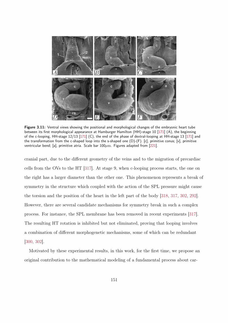
Figure 3.11: Ventral views showing the positional and morphological changes of the embryonic heart tubebetween its first morphological appearance at Hamburger Hamilton (HH)-stage 10 [171] (A), the beginningof the c-looping, HH-stage 12/13 [171] (C), the end of the phase of dextral-looping at HH-stage 13 [171] andthe transformation from the c-shaped loop into the s-shaped one (D)-(F). [c], primitive conus; [v], primitiveventricular bend; [a], primitive atria. Scale bar 100µm. Figures adapted from [221].

cranial part, due to the different geometry of the veins and to the migration of precardiac

cells from the OVs to the HT [317]. At stage 9, when c-looping process starts, the one on

the right has a larger diameter than the other one. This phenomenon represents a break of

symmetry in the structure which coupled with the action of the SPL pressure might cause

the torsion and the position of the heart in the left part of the body [318, 317, 302, 292].

However, there are several candidate mechanisms for symmetry break in such a complex

process. For instance, the SPL membrane has been removed in recent experiments [317].

The resulting HT rotation is inhibited but not eliminated, proving that looping involves

a combination of different morphogenetic mechanisms, some of which can be redundant

[300, 302].

Motivated by these experimental results, in this work, for the first time, we propose an

original contribution to the mathematical modeling of a fundamental process about car-

151

diac shaping: we introduce a morphomechanical model for the torsion of the HT. We hy-

pothesize that this spontaneous morphological transition can be modeled as a mechanical

instability due to accumulation of residual stresses because of the geometrical frustration

imposed by tissue remodelling. Precisely, we assume that the HT is a nonlinear elastic, ho-

mogeneous, incompressible body that is subjected to a torsional remodelling, which mimics

the cells flux in the HT [291]. We assume that the tube undergoes a finite torsion by accu-

mulating such a geometrical frustration, and we perform a linear stability analysis of the

nonlinear elastic boundary value problem to determine the onset of c-looping as a function

of the geometrical parameters of the HT. Then, we perform numerical simulations to study

the post-buckling behaviour in the fully nonlinear morphological transition.

3.2.1 Mathematical model

n this Section, we define the morphomechanical model of the HT, described as a hypere-

lastic body subjected to torsional remodeling.

3.2.1.1 Kinematics

Let

Ω0 = X = [R cosΘ, R sinΘ, Z] ∈ R3 ∣ Ri ≤ R < Ro and 0 ≤ Θ < 2π and 0 < Z < L ,

be the reference configuration of the HT, where Ri and Ro are respectively the internal

and the external radius of the cylinder, L is the height of the hollow cylinder and X is the

material position coordinate. Although the HT is composed by different layers, for sake of

simplicity, we assume that the HT is a homogeneous one-layered tissue. By experimental

evidences, the HT can be modeled as a hollow cylinder since there is a small lumen in the

middle. We indicate with φ ∶ Ω0 → R3 the deformation field, so that the actual config-

152

uration of the body Ω is given by φ(Ω0). Let x = φ(X) be the actual position and the

displacement vector is defined as u(X) = φ(X) −X. Let F be the deformation gradient,

i.e. F = Gradφ.

In order to describe the finite torsion induced by tissue remodelling, we consider the

multiplicative decomposition of the deformation gradient [196, 203, 277], such as

F = FeG, (3.50)

where G describes the metric distortion induced by the applied torsion and Fe is the elastic

deformation of the material restoring the geometrical compatibility of the current config-

uration. Defining γ as the finite torsion rate resulting from the remodelling processes, we

choose G as

G =

⎛⎜⎜⎜⎜⎜⎜⎝

1 0 0

0 1 −γR

0 0 1

⎞⎟⎟⎟⎟⎟⎟⎠

. (3.51)

We further assume that the cylinder cannot elongate along the z-direction, i.e.

z(Z = 0) = 0, z(Z = L) = L. (3.52)

Since no relevant growth processes occur in the stages of interest of c-looping (detG = 1)

and the tissue is mainly composed by water, we model the HT as incompressible media,

namely we enforce that

detFe = 1. (3.53)

We now introduce the mechanical constitutive assumptions.

153

3.2.1.2 Boundary-Value Problem (BVP)

Since we are describing the first stage of development and fibers are not yet present [171],

it is reasonable to model the HT as an isotropic body. We assume that the HT is com-

posed of a homogeneous hyperelastic material, having strain energy density W . The first

Piola-Kirchhoff stress tensor P and the Cauchy stress tensors T are then given by

P = detG∂W (FG−1)

∂F− pF−1 T = 1

detFFP

where p is the Lagrange multiplier enforcing the incompressibility constraint, i.e. physi-

cally p is the necessary hydro-static pressure to enforce the incompressibility constraint

detFe = 1. Assuming quasi-static conditions in absence of external body forces, the balance

of the linear momentum reads

DivP = 0 in Ω0, or divT = 0 in Ω (3.54)

where Div and div denote the divergence operator in material and current frame, respec-

tively. The nonlinear system of equations (3.54) is complemented by the following Neu-

mann condition on the inner and outer boundaries

⎧⎪⎪⎪⎪⎨⎪⎪⎪⎪⎩

T ⋅n = 0 on r = ri

T ⋅n = 0 on r = ro, (3.55)

where n is the outer normal in spatial coordinates, and ri, ro are the spatial inner and

outer radius, respectively. By performing a pull-back of Eq. (3.55), the Lagrangian form

154

of the boundary condition is given by

⎧⎪⎪⎪⎪⎨⎪⎪⎪⎪⎩

PT ⋅N = 0 on R = Ri

PT ⋅N = 0 on R = Ro

(3.56)

where N is the material outer normal. To keep the model as simple as possible, we as-

sume that the tube behaves as a neo-Hookean material with the strain energy density

given by

W (F) = det(G)W0(Fe) = (detG)µ

2(tr(FT

e Fe) − 3) . (3.57)

The first Piola–Kirchhoff and Cauchy stress tensors read respectively

⎧⎪⎪⎪⎪⎨⎪⎪⎪⎪⎩

P = µ(detG)G−1G−TFT − pF−1,

T = µFG−1G−TFT − pI,(3.58)

where I is the identity tensor. Eqs. (3.53), (3.54) and (3.56) define the nonlinear elastic

BVP.

We now compute a solution of the BVP using the symmetry of the problem.

3.2.1.3 Radially-symmetric solution

Let (ER, EΘ, EZ) and (er, eθ, ez) be the unit vectors in material and spatial polar coor-

dinates, respectively. Denoting (r, θ, z) the polar coordinates of a point, we search for a

radially-symmetric solution

φ(X) = r(R)er +Zez.

155

so that the geometrical and the elastic deformation gradient read

F = diag (∂r(R)∂R

,r

R, 1) , Fe = FG−1 =

⎛⎜⎜⎜⎜⎜⎜⎝

∂r(R)∂R 0 0

0 rR γr

0 0 1

⎞⎟⎟⎟⎟⎟⎟⎠

. (3.59)

From Eq. (3.59) and the incompressibility constraint Eq. (3.53), we get r′r = R, where ′

denotes differentiation. By integrating, we obtain

r(R) =√R2 + r2i −R2

i . (3.60)

The balance of the linear momentum in polar coordinates imposes

dTrrdr+ Trr − Tθθ

r= 0 (3.61)

where Thk, with h, k spanning over (r, θ, z), are the components of the Cauchy stress ten-

sor T in polar coordinates. Using Eqs. (3.59) and (3.58), the Cauchy stress tensor is given

by

T =

⎛⎜⎜⎜⎜⎜⎜⎝

µ(r2−r2i +R2i )

r2 − p 0 0

0 µr2 (γ2 + 1r2−r2i +R

2i) − p γµr

0 γµr µ − p

⎞⎟⎟⎟⎟⎟⎟⎠

. (3.62)

As regarding the current radii, by using Eq. (3.60), the expression of the external radius ro

is given by

ro =√R2

o + r2i −R2i , (3.63)

while for the internal one, we have to integrate Eq. (3.61) from ro to ri, use the boundary

156

conditions Eq. (3.55) to get

1

2µ⎛⎝(R2

i −R2o)⎛⎝γ2 + r2i −R2

i

r2i (r2i −R2i +R2

o)⎞⎠+ log(r

2i −R2

i +R2o

R2o

) + log(R2i

r2i)⎞⎠= 0 (3.64)

which is an implicit relation to derive first ri and then ro from Eq. (3.63). Fixing the tor-

sion rate γ and the initial geometry of the hollow tube, Eq. (3.64) is solved using the New-

ton method.

Finally, for the Lagrange multiplier p, we can integrate Eq. (3.61) from r to ro, obtain-

ing

Trr(r) = ∫ro

r[µ (ρ2 − r2i +R2

i )ρ3

− µρ(γ2 + 1

ρ2 − r2i +R2i

)] dρ. (3.65)

Hence, solving Eq. (3.65) with respect to p, we obtain

p(r) = 1

2µ(γ2 (−r2 + r2i −R2

i +R2o) +

R2i − r2ir2

+ R2i − r2i

r2i −R2i +R2

o

+ log( r2

r2 − r2i +R2i

) + log( R2o

r2i −R2i +R2

o

) + 2) .(3.66)

Eqs. (3.60) and (3.66) represent the radially symmetric solution of the BVP.

Remark 3.2.1. It is useful to recall that a finite torsion on an hollow cylinder can be sus-

tained by surface tractions alone, namely it is sufficient to apply an axial force Fz and a

torque M on the end surfaces S, given by

Fz = ∫STzz dS =

1

2πµR2

i log(r2i R

2o

R2i (r2i −R2

i +R2o))

+ πµ

4

(R2i −R2

o) [γ2(R2o −R2

i ) (r2i +R2o −R2

i ) + 2 (R2i − r2i )]

(r2i −R2i +R2

o),

(3.67)

while the torque M

M = ∫STzθr dS =

1

2πγµ (R2

o −R2i ) (2r2i −R2

i +R2o) . (3.68)

157

Both surface tractions depend nonlinearly on the geometric parameters, namely Ro and

Ri, while only M is linearly dependent on γ. In Fig. 3.12, we plot the two quantities de-

fined in Eqs. (3.67) - (3.68) versus the torsion rate γ varying the ratio Ro

Ri. In Fig. 3.12a,

(a) Ro

Ri∈ (1,10) (b) Ro

Ri∈ (1,10)

Figure 3.12: Plot of (a) the axial force Fz and (b) the torque M versus the torsion rate γ fixing the externalradius Ro = 1, the shear modulus µ = 1, computing ri through Eq. (3.64) and varying the ratio between theexternal and the internal radii within the range Ro

Ri∈ (1,10).

we notice that the axial force is compressive, showing the characteristic Poynting effect

that favors buckling as the torsion rate increases [164, 148, 162].

In the following section, we study the linear stability analysis of the radially symmetric

solution given by Eqs. (3.60) and (3.66).

3.2.2 Linear stability analysis

In this section we study the linear stability of the finitely deformed tube by using the method

of incremental deformations superposed on a finite strain [243]. We rewrite the resulting

incremental BVP into the Stroh formulation that is solved using the impedance matrix

method.

158

3.2.2.1 Incremental BVP

We apply the theory of incremental deformations superposed on finite strains to investi-

gate the stability of the radially symmetric solution. Let δu be the incremental displace-

ment field and let Γ = grad δu. We introduce the push-forward of the incremental Piola-

Kirchhoff stress tensor δP0 in the axis-symmetric deformed configuration, given by

δP = A0 ∶ Γ + pΓ − δpI, (3.69)

where A0 is the fourth order tensor of instantaneous elastic moduli, δp is the increment

of the Lagrangian multiplier that imposes the incompressibility constraint. The two dots

operator (∶) denotes the double contraction of the indices

(A0 ∶ Γ)rs = (A0)rshkΓkh,

where the convention of summation over repeated indices is used. The components of the

tensor A0 for a neo-Hookean material are given by

(A0)rshk = µδrk(Be)sh

where Be = FeFTe and δrk is the Kronecker delta. The incremental equilibrium equation and

the linearised form of the incompressibility constraint read respectively

⎧⎪⎪⎪⎪⎨⎪⎪⎪⎪⎩

Div δP = 0 in Ω,

tr Γ = 0 in Ω.

(3.70)

159

This system of partial differential equations is complemented by the following boundary

conditions⎧⎪⎪⎪⎪⎨⎪⎪⎪⎪⎩

δPT er = 0 on r = ri,

δPT er = 0 on r = ro.(3.71)

Now, we reformulate the BVP given by Eqs. (3.70) - (3.71) using the Stroh formulation

to implement a robust numerical procedure.

3.2.2.2 Stroh formulation

We denote with u, v and w the components of δu in cylindrical coordinates and with δPrr,

δPrϑ and δPrz the components of the incremental stress tensor. Following [297], we rewrite

the system of partial differential equations Eq. (3.70) into a system of ordinary differential

equations, by assuming the following variable separation ansatz for the incremental fields

[92, 24, 327]

u(r, ϑ, z) = U(r) cos(kz −mϑ), (3.72)

v(r, ϑ, z) = V (r) sin(kz −mϑ) (3.73)

w(r, ϑ, z) =W (r) sin(kz −mϑ), (3.74)

δPrr(r, ϑ, z) = srr(r) cos(kz −mϑ) (3.75)

δPrϑ(r, ϑ, z) = srϑ(r) sin(kz −mϑ), (3.76)

δPrz(r, ϑ, z) = srz(r) sin(kz −mϑ), (3.77)

δp(r, ϑ, z) = Q(r) cos(kz −mϑ), (3.78)

160

where m and k = (2nπ)/L are respectively the circumferential and axial wavenumbers,

with m,n ∈ N. By substituting Eq. (3.75) into Eq. (3.69), we get

Q(r) =U ′(r) (r2p(r) + r2 − r2i +R2

i )r2

− srr(r),

where p(r) is defined in Eq. (3.66). Following a similar and well established procedure [24],

the incremental problem can be rewritten into the Stroh form [297], such as

dη

dr= 1

rNη, (3.79)

where η is the displacement-traction vector defined as

η = [U , rΣ] where

⎧⎪⎪⎪⎪⎨⎪⎪⎪⎪⎩

U = [U,V,W ],

Σ = [srr, srϑ, srz].

The matrix N ∈ R6×6 is the Stroh matrix and it has the following sub-block form

N =

⎡⎢⎢⎢⎢⎢⎢⎣

N1 N2

N3 N4

⎤⎥⎥⎥⎥⎥⎥⎦

,

such that Ni ∈ R3 ×R3, N1 = −NT4 , N2 = NT

2 and N3 = NT3 , which means that the Stroh matrix

has an Hamiltonian structure [144]. The expression of the four blocks is given by

N1 =

⎡⎢⎢⎢⎢⎢⎢⎢⎢⎢⎣

−1 m −kr

−mσp σp 0

krpσ 0 0

⎤⎥⎥⎥⎥⎥⎥⎥⎥⎥⎦

, N2 =

⎡⎢⎢⎢⎢⎢⎢⎢⎢⎢⎣

0 0 0

0 σ 0

0 0 σ

⎤⎥⎥⎥⎥⎥⎥⎥⎥⎥⎦

, N3 =

⎡⎢⎢⎢⎢⎢⎢⎢⎢⎢⎣

κ11 κ12 κ13

κ12 κ22 κ23

κ13 κ23 κ33

⎤⎥⎥⎥⎥⎥⎥⎥⎥⎥⎦

, (3.80)

161

where

κ11 = 1/σ + r2δ1 + 2p + δ3σ κ12 = σm(1/σ2 − 2 + p2) + δ2

κ13 = k/r(σ + rp) κ22 = r2(k + γ2 − 2mγk) + σ(1 − p2) +m2(2 + σδ5 + σγR)

κ23 = −km(σ/r + 2pr) κ33 =m2(σ + rγ2) + r2kδ4

and

σ = r2

Rδ1 = γ2 + k2 − 2γkm + γ2m2 δ2 = −p2 (k2r2 +m2) +m2 + 1

δ3 = 2r2γ(k −mγ) − 2mp δ4 = k(1 + 1/σ − 2p) + 2mγ δ5 = (R2i − r2i )2/r4,

with r and p defined in Eq. (3.60) and Eq. (3.66), respectively. Eq. (3.79) with the bound-

ary condition Σ = 0 at r = ri and r = ro define the incremental BVP.

Eqs. (3.72) - (3.78) do not fulfill the boundary condition Eq. (3.52) at the bases, impos-

ing w = 0 at Z = 0, L [123, 130]. This difference in boundary conditions will likely appear

as an end effect in proximity of the two bases at Z = 0 and Z = L, that becomes increas-

ingly relevant as the tube is short with respect to its length.

The incremental BVP is hard to solve, hence, different numerical techniques have been

introduced in literature to overcome the problem, e.g the compound matrix method [175],

the determinantal method [9] or the Adams-Moulton method [331]. We employ the impe-

dence matrix method to transform the differential problem into a Riccati equation, that is

easier to solve numerically [59, 60].

162

3.2.2.3 Impedence matrix method

Following a similar procedure used in [24], we introduce the matricant

M(r, ro) =

⎡⎢⎢⎢⎢⎢⎢⎣

M1(r, ro) M2(r, ro)

M3(r, ro) M4(r, ro)

⎤⎥⎥⎥⎥⎥⎥⎦

, M(r, ro) ∈ R6×6,

defined as the solution of the problem

dM

dr= 1

rNM(r, ro), M(ro, ro) = I. (3.81)

Since the solution of the Stroh problem Eq. (3.79) can be expressed as

η(r) =M(r, ro)η(ri)

and no traction loads are applied on the external surface, i.e. Σ(ro) = 0, we can define the

conditional impedence matrix Z(r, ro) [242] as

Z(r, ro) =M3(r, ro)M−13 (r, ro), (3.82)

where the term conditional refers to the dependence on the boundary condition at ro.

Omitting the explicit dependence of Z on r and ro, such a matrix satisfy the following re-

lation

rΣ = ZU ∀r ∈ (ri, ro) (3.83)

163

By using Eq. (3.83), we can rewrite the Stroh problem given by Eq. (3.79) into a differen-

tial Riccati equation, such as

dU

dr= 1

r(N1 +N2Z)U , (3.84)

dZ

drU + ZdU

dr= 1

r(N3 +N4Z)U . (3.85)

Substituting Eq. (3.84) into Eq. (3.85) we get the following differential Riccati equation

dZ

dr= 1

r(N3 +N4Z − ZN1 − ZN2Z) . (3.86)

We integrate Eq. (3.86) from ro to ri, using as starting condition the fact that there are no

applied loads at r = ro, i.e.

Z(ro, ro) = 0.

To construct a bifurcation criterion, we use the fact that there are no applied loads in r =

ri: non-null solutions of the incremental problem exist if and only if

detZ(ri) = 0. (3.87)

Fixing the initial geometry of the HT, making outer iterations on the wavenumbers m and

k, for a fixed value of the torsion control parameter γ we integrate the Riccati Eq. (3.86)

from r = ro up to r = ri making use of the the software Mathematica 11.3 (Wolfram

Research, Champaign, IL, USA). We iteratively increase the torsion control parameter γ

following its stable solution [92] until the bifurcation criterion Eq. (3.87) is satisfied.

164

3.2.2.4 Marginal stability thresholds

In this section we collect and discuss the results of the linear stability analysis. First of all,

we introduce the dimensionless parameters which govern the boundary value problem, i.e.

γ = γRo k = kRo αR =Ro

Ri

αL =L

Ro

, (3.88)

where γ represents the dimensionless torsion rate, k the dimensionless axial wavenumber,

αR and αL are geometrical parameters, representing the thickness and the slenderness ra-

tios, respectively. Given a material length L, the admissible axial wavenumber k is given

by

k = 2πn

αL

n ∈ N. (3.89)

In the following, first we aim at characterizing the torsion deformation during the c-looping

by considering suitable biological values of the two parameters involved, i.e. the initial

thickness ratio αR of the HT and its slenderness ratio αL.

In human embryo, looping begins approximately around 23 − 28 days after the fertiliza-

tion, when the length is about 1 − 2mm [163]. A lot of experiments have been performed

on animals whose cardiovascular system is similar to humans, for instance the chick em-

bryo [317, 328, 263, 223, 291], whose size is comparable with the human one; being about

3−4mm. From these experimental results, a physiologically relevant range for both αR and

αL is

αR = [1.35,2.85] αL = [7,10]. (3.90)

Second, we use a wider range of dimensionless parameters to investigate to a further ex-

165

tent the effect of geometry on pattern selection and nonlinear development.

In the following, we vary the thickness ratio αR ∈ (1,+∞), since neither αR = 1 nor

αR → +∞ represent a hollow cylinder. In Figs. 3.13 - 3.14, we plot the marginal stability

threshold γcr, the circumferential mcr and the axial kcr critical wavenumbers versus the

thickness ratio αR.

Considering the infinite cylinder, i.e. k ∈ R, in Fig. 3.13a, we plot the critical circum-

ferential number mcr versus αR and we notice that there is a cut-off thickness at which

the morphological transition of the HT completely changes: for thin cylinder, i.e. αR < 2,

the critical circumferential wavenumber mcr = 2, while for αR > 2, i.e. considering thicker

cylinders, the critical circumferential number is mcr = 1. From a biological standpoint, this

result implies that c-looping is controlled by the geometry of the embryonic tube. More-

over, from a mathematical point of view, geometrical nonlinearity dominates the post-

bifurcation behavior [162, 159, 290].

Considering an infinite cylinder, i.e. k ∈ R, we plot the critical axial wavenumber kcr

and the marginal stability threshold γcr, see respectively Figs. 3.13b - 3.13c, versus the

thickness parameter αR in the range of thin cylinders, i.e. αR ∈ (1,2). Both the marginal

stability threshold γcr and the critical axial wavenumber kcr increase as αR increases as

already pointed out in [24], compare their Figs. 7a - 8a with our Figs. 3.13c - 3.13b.

Since thicker cylinders, i.e. αR ≫ 1, immediately buckle for a very small value of the

torsion control parameter γ, we study finite hollow thick tubes varying αR ∈ (2,10) and

αL = 4,4.5,5,6,7,15,30. From Fig. 3.13d and Fig. 3.13e, we notice that both the cir-

cumferential mcr and the axial kcr critical wavenumbers are affected by the slenderness ra-

tio αL. For small values of αL and αR, the critical circumferential wavenumber mcr = 2 and

there is a doubling period for the critical axial wavenumber, i.e. kcr = 4π/αL. Fixing the

slenderness ratio and increasing αR, we find that mcr = 1 and kcr = 2π/αL, in accordance to

what happens for an infinite cylinder.

166

In Fig. 3.14, we plot the marginal stability threshold γcr versus αR for different values of

αL. For graphical scaling of the parameters, we change the range of αL = 14,14.5,15,15.5,16:

similar to what happens for thin cylinder, i.e. αR < 2, γcr increases as αR increases, see the

inset in Fig. 3.14.

1 2 3 4 5 6 7 8 9 10αR0.5

1

1.5

2

2.5mcr

(a) αR ∈ (1,10)1 1.2 1.4 1.6 1.8 2

αR0

0.2

0.4

0.6

0.8

1

1.2

1.4

1.6k˜cr

(b) αR ∈ (1,2)

1 1.2 1.4 1.6 1.8 2αR0

0.1

0.2

0.3

0.4

0.5

0.6

0.7

γ˜cr

(c) αR ∈ (1,2)

(d) αR ∈ (2,10) (e) αR ∈ (2,10)

Figure 3.13: Plot of the critical values versus αR, varying the initial thickness ratio αR ∈ (1,10]. (a) Plot ofthe circumferential critical wavenumber mcr versus αR. Varying αR ∈ (1,2) and αL = +∞, (b) plot of thecritical axial wavenumber kcr and (c) of the marginal stability threshold γcr versus αR. Varying αR ∈ (2,10),(d) plot of the critical circumferential wavenumber mcr and (e) of the critical axial wavenumber kcr versus αR

having chosen different values of αL = 4,4.5,5,6,7,15,30.

The parameter αL also affects the marginal stability thresholds of the HT. In Fig. 3.15,

fixing the thickness ratio αR = 2.85, first we notice that the critical circumferential wavenum-

167

Figure 3.14: Plot of the marginal stability threshold γcr versus αR for thick cylinders, αR ∈ (2,10), varyingαL = 14,14.5,15,15.5,16. The inset shows a zoom of the curve with αL = 14.

ber mcr is always mcr = 1 for all αL (see Fig. 3.15a). Then, in Figs. 3.15b - 3.15c, we plot

the marginal stability threshold γcr and the critical axial wavenumber kcr versus αL. Both

the curves are coherent with the typical mechanical behavior of a twisted Euler rod: as we

increase the slenderness ratio as the cylinder buckles earlier and the emerging pattern is an

helix of pitch 1/k [164, 148].

7 11 15 19 23 27 31αL0.5

1

1.5mcr

(a) αR = 2.857 11 15 19 23 27 31

αL0.1

0.3

0.5

0.7

0.9k˜cr

(b) αR = 2.857 11 15 19 23 27 31

αL0.1

0.3

0.5

0.7

0.9

γ˜cr

(c) αR = 2.85

Figure 3.15: Plot of critical wavenumbers and the marginal stability threshold versus αL, fixing the initialthickness ratio αR = 2.85. (a) The critical circumferential wavenumber is mcr = 1. (b) The critical axialwavenumber kcr and (c) of the marginal stability threshold γcr decrease as αL increases.

168

Figs. 3.13-3.15 characterize the loss of marginal stability as a function of the thickness

ratio αR and the slenderness ratio αL. By using these characteristic values, in the next

section we study the development of the looped configuration far beyond the marginal sta-

bility threshold: we implement a finite element code to discretize and numerically solve the

fully nonlinear BVP given by Eqs. (3.54)-(3.56).

3.2.3 Numerical simulations

The boundary value problem is implemented by using FEniCS, an open source tool for

solving partial differential equations [212]. We generate as a computational domain a hol-

low cylinder with a non-structured tetrahedral mesh created through the module MSHR

[212], see Fig. 3.16, where we refine the mesh around the two bases z = 0 and z = αL,

see Fig. 3.16b. Since the cylinder is finite, to solve the non linear elastic BVP Eqs. (3.53),

(a) Mesh (b) Top view

Figure 3.16: Mesh generated through MSHR for αR = 2.85 with local refinement.

(3.54) and (3.56), we need to impose suitable boundary conditions on the top and bottom

bases. First, we assume a stronger form of (3.52), imposing

u = 0 on z = 0, z = αL. (3.91)

169

We discretize the computational domain by using a mesh composed by 78338 elements and

to solve the problem, we use the Taylor-Hood P2 − P1 element, i.e. the displacement field

is given by a continuous, piecewise quadratic function while the pressure field by a contin-

uous, piecewise linear function. The choice of this particular element is motivated by its

stability for non-linear elastic problems [21]. We introduce an additional term to stabilize

the numerical scheme which penalizes the volumetric deformations, since at the discrete

level the use of P2-elements can result in unphysical values for the determinant of Fe [21].

Second, in order to evaluate the effect of the boundary conditions on the top and the bot-

tom surfaces, we perform further simulations imposing a weaker form of (3.52), precisely

⎧⎪⎪⎪⎪⎪⎪⎪⎪⎪⎨⎪⎪⎪⎪⎪⎪⎪⎪⎪⎩

u ⋅ er = 0 on z = 0, z = αL,

u ⋅ eϑ = 0 on z = 0, z = αL,

∫z=iu ⋅ ez = 0 where i = 0, αL.

(3.92)

In this case, the mesh is composed by 78426 elements. We solve the discretised form of

the equilibrium equation Eq. (3.54) in the Lagrangian form using a Newton method. The

torsion control parameter γ is incremented of δγ when the Newton method converges, the

numerical solution is used as initial guess for the following Newton cycle. The increment

δγ is automatically reduced near the theoretical marginal stability threshold and when the

Newton method does not converge. The numerical simulation is stopped when δγ < 10−6.

To trigger the mechanical instability, a small perturbation of an amplitude of 10−5Ro, hav-

ing the shape of the critical mode computed in Section 3.2.2, is applied at the free bound-

ary of the mesh. The numerical algorithm is implemented in Python through the open-

source computing platform FEniCS (version 2018.1) [212]. We use PETSc [22] as linear

algebra back-end and MUMPS [12] as linear solver.

170

3.2.3.1 Simulation results

In this section, we discuss the results of the numerical simulations varying the two physical

parameters αR and αL firstly within the biological range given by the experimental papers,

and secondly outside this range to further understand the role of geometrical parameters

in pattern selection, validating the results against some known features in the limiting case

of solid cylinder.

Torsional c-looping numerical results In this section, we discuss the nonlinear

pattern formation fixing the geometry of the cylinder within the range of dimensionless

parameters given by the experimental results.

In Fig. 3.17, we plot the looping development of the HT for a hollow cylinder with αR =

2.85, αL = 7, imposing Eq. (3.91) on the top and bottom bases. We show the actual config-

uration for several values of the torsion control parameter γ. As γ increases, the cylinder

displays an helical pattern and the simulation stops around γ ≃ 1.4 because the lumen

closes with an incipient self-contact, see Fig. 3.18a. This phenomenon is consistent with

the chronological development of the HT: in later stages 13 − 18 the blood starts flowing

in the tube and the open and the close of the lumen represents the primitive valve in the

heart [224, 158, 229].

In order to study the amplitude of the helical pattern, we cut the cylinder with a plane

z = c, where c is a constant. To respect the symmetry of the system, we select the central

section c = αL/2 = 3.5. Hence, we define

∆r = dist(Cc −O), (3.93)

where Cc is the centroid of the considered section, the red dot in Fig. 3.18a and O = (0,0, c)

the centroid of the original HT, the black dot in Fig. 3.18a. In Fig. 3.18b, we plot ∆r/Ro

171

Figure 3.17: Actual configuration of the buckled tube when αR = 2.85, αL = 7 and Eq. (3.91) is taken as theboundary condition at z = 0, αL. For such values, the linear stability analysis gives γcr ≃ 0.881748.

versus γ to measure the distance of the centroid of the section from the z-axis. We observe

that there is an excellent agreement with the marginal stability thresholds computed in

the previous section, verifying the results obtained by the numerical code against the the-

oretical predictions. Both bifurcation diagrams exhibit a continuous transition from the

axis-symmetric to the buckled configuration, displaying the typical behaviour of a super-

critical pitchfork bifurcation.

Finally, in Fig. 3.19, we perform the convergence analysis on our numerical simulations.

We run several simulations at fixed geometry whilst increasing the number of the tetrahe-

dra in the mesh, precisely we vary the numbers of faces on the side of the cylinder [212].

As the mesh gets finer and finer, as all the curves collapse on the same curve, and the nu-

merical instability threshold is delayed for a coarser mesh, as expected due to the lower

accuracy of the numerical approximation.

In Fig. 3.20, we fix the same geometry, i.e. αR = 2.85 and αL = 7, we solve again the

fully nonlinear BVP Eqs. (3.53), (3.54) and (3.56), but we change the boundary condi-

tion on the two bases, substituting Eq. (3.91) with Eq. (3.92). As in the previous case, the

172

(a) z = 3.5 (b) z = 3.5

Figure 3.18: (a) Plot of the different shapes of the mid-section z = αL/2 = 3.5 at different values of the torsioncontrol parameter γ. The black dot is O = (0,0, αL/2), i.e. the centroid of the initial midsection of the originalHT, while the red one is the centroid of the midsection in the current configuration. The shape of the sectionchanges and the lumen is getting smaller causing the stop of the numerical simulation. (b) Bifurcation diagramwhere we show the dimensionless parameter ∆r/Ro defined in Eq. 3.93 versus the torsion control parameterγ when αR = 2.85 and αL = 7. The numerical simulation is validated against the marginal stability thresholdcomputed with the linear stability analysis (orange square, γcr ≃ 0.881748).

Figure 3.19: Plot of the bifurcation diagram varying the numbers of faces 30,35,40,45,50,60,70,80 on theside of the cylinder [212]. In the inset, we highlight the behavior near the marginal stability threshold.

173

simulation stops because the lumen closes and the internal surfaces enters in self-contact

approximately at the same value of the torsion control parameter γ ≃ 1.4 as in the previous

case. Thus, the two different choices of the boundary conditions for the top and bottom

Figure 3.20: Actual configuration of the looped tube when αR = 2.85, αL = 7 and Eq. (3.92) is taken asboundary condition at z = 0, αL. In such conditions γcr ≃ 0.881748.

ends of the HT result in a small deviation of the onset of the bifurcation.

Let

E = ∫Ω0

W (F)dV (3.94)

be the total elastic energy of the hollow cylinder. We compute the ratio of the energy Eth

of the axis-symmetric solution given by Eqs. (3.60) and (3.66) and the energy Enum com-

puted through the finite elements computation. In Fig. 3.21, we plot the ratio Enum/Eth

versus the control parameter γ fixing αR = 2.85 and αL = 7 for the two different bound-

ary conditions on the two bases, respectively Eq. (3.91) - (3.92). As expected, the buckled

configuration exhibits in both cases a total mechanical energy lower than the one in the

unbuckled state. In Fig. 3.21a, we fixed the whole displacement field u = 0, and the in-

stability is a bit delayed with respect to the theoretical marginal stability threshold γcr.

174

In Fig. 3.21b we require that the displacement along z is zero in a weaker way, and the

threshold is closer to the theoretical prediction. Furthermore we observe that the energy

decays continuously as γ grows beyond thresholds, confirming that the bifurcation is in

both cases supercritical, see Figs. 3.18 and 3.19.

(a) Eq. (3.91) as BC (b) Eq. (3.92) as BC

Figure 3.21: Plot of the ratio Enum/Eth for (a) αR = 2.85 and Eq. (3.91) as boundary condition and (b)αR = 2.85 and (3.92) on the two bases versus the torsion control parameter γ. The orange square denotes thetheoretical marginal stability threshold computed in Section 3.2.2.

Numerical results for a wider range of geometrical parameters We now

investigate how the geometry, i.e. varying αR and αL, influences the buckled configuration

in a wider range of dimensionaless parameters, extending the linear stability analysis for

some cases illustrated in Section 3.2.2.

First, let us consider the same thickness ratio αR = 2.85 as in the torsion c-looping case

and increase the slenderness ratio setting αL = 12. From the linear stability analysis, we

obtain that the marginal stability threshold decreases, i.e. γcr = 0.52159, and the critical

circumferential and axial wavenumbers are mcr = 1 and kcr = 2π/αL, respectively. In Fig.

3.22, we plot the buckled configuration of the cylinder having imposed Eq. (3.91) on the

two bases. We show the actual configuration for several values of the torsion control pa-

rameter γ. As γ increases, the cylinder displays the expected helical pattern with a higher

amplitude with respect to the one obtained fixing αL = 7, see the scale-bar of Fig. 3.22.

175

Figure 3.22: Actual configuration of the buckled tube for when αR = 2.85 and αL = 12 and Eq. (3.91) is takenas BC. In such conditions mcr = 1, kcr = 2π/αL and γcr = 0.521594.

To quantify the amplitude of the helical pattern, in Fig. 3.23b, we plot the quantity

∆r/R0 defined in Eq. (3.93) versus the torsion control parameter γ, where in this case

O = (0,0,6). Comparing this picture with Fig. 3.18b, we notice a higher amplitude of

the emerging helical loop, see Fig. 3.23b. In Fig. 3.23a, we plot the ratio of the energy Eth

of the axis-symmetric solution given by Eqs. (3.60) and (3.66) and the energy Enum com-

puted through the finite elements computation. We observe, first, the typical continuous

transition from the unbuckled to the buckled configuration, confirming the supercritical

pitchfork bifurcation and then a little delay on the onset of the instability due to the im-

posed boundary conditions Eq. (3.91).

Second, let us consider the same slenderness ratio αL as in the torsional c-looping case,

i.e. αL = 7, and consider a different initial thickness ratio αR = 1.35. With this choice we

want to visualize the effect of the geometrical parameters on the nonlinear development of

the looped patterns.

Imposing the boundary condition Eq. (3.91) on the two bases, we plot in Fig. 3.24 the

resulting buckled configuration. As expected from the linear stability analysis, the critical

176

(a) αL = 12, Eq. (3.91) as BC

(b) αL = 12, z = αL/2

Figure 3.23: (a) Plot of the ratio Enum/Eth for αR = 2.85, αL = 12 and Eq. (3.91) is taken as boundarycondition versus the torsion control parameter γ. (b) Bifurcation diagram where we show the dimensionlessparameter ∆r/Ro versus the torsion control parameter γ when αR = 2.85, αL = 12 and z = αL/2 = 6. Theorange square denotes the theoretical marginal stability threshold computed in Section 3.2.2, i.e. mcr = 1,kcr = 2π/αL and γcr = 0.521594.

circumferential number is mcr = 2, while the critical axial wavenumber is 2π/αL.

Figure 3.24: Actual configuration of the buckled tube when αR = 1.35, αL = 7 and Eq. (3.91) is taken as BC.In such conditions mcr = 2, kcr = 2π/αL and γcr ≃ 0.177001.

Finally, if we consider a solid cylinder, that is characterized by mcr = 1, we validate our

numerical results against the classical problem of a twisted Euler rod, forming an helix of

pitch 1/k. For a Neo-Hookean material, this solution has been first presented by Green

177

and Spencer in [164]. Then, Gent and Hua [148] investigated the evolution of this instabil-

ity: it can evolve with the sudden onset of a sharply bent ring, or knot. Up to our knowl-

edge, this section is the first one which aims at reproducing the 3D numerical simulation

of a finite torsion rate on a soft solid cylinder.

Let us fix the geometry of the solid cylinder, αL = 12 and impose the boundary condi-

tion Eq. (3.91) on the two bases, we plot in Fig. 3.25 the buckled configuration of the full

cylinder. We show the actual configuration for several values of the torsion control param-

eter γ. As γ increases, as the cylinder displays an helical pattern with a higher amplitude

compared to the one of hollow cylinders, we can compare Fig: 3.17 and Fig. 3.23 with

Fig. 3.25. The simulation stops around γ ≃ 2.45 probably due to the excessive distortion

of the elements. Unfortunately, our simulation does not display the expected knot, since

we should consider a longer cylinder which, however, requires a fine mesh, hence a bigger

computational effort. Future efforts will be devoted in improving the performance of the

numerical simulations, taking also into account for the self-contact.

Figure 3.25: Actual configuration of the buckled tube for when αR → ∞, αL = 12 and Eq. (3.91) is taken asBC. We choose mcr = 1 and kcr = 2π/αL.

In order to reduce the distortion of the tetrahedra, we refine the mesh near the two

178

bases and around z = αL/2, where we noticed the greatest concentration of elongated el-

ements. The used mesh is presented in Fig. 3.26a. The linear stability analysis performed

(a) αR →∞ (b) αR →∞ and z = αL/2 = 6

Figure 3.26: (a) Mesh generated through MSHR for αR → ∞ with local refinements. (b) Bifurcation diagramshowing the dimensionless parameter ∆r/Ro versus the torsion control parameter γ when αR → ∞, αL = 12and z = αL/2 = 6. The orange square denotes the marginal stability threshold γcr ≃ 0.8 [164], with mcr = 1 andkcr = 2π/αL.

in Section 3.2.2 is no longer valid for a solid cylinder since the structure of the Stroh for-

mulation changes in the absence of the lumen [92]. In order to assess our numerical re-

sults, we compare the marginal stability threshold obtained from our numerical simula-

tions with the theoretical one computed by Green and Spencer [164]. In particular, we

found that the critical torsion is around γcr = 0.8 for k = 2π/αL. In Fig. 3.26b, we plot the

dimensionless quantity ∆r/R0 defined in eq. (3.93) versus the control parameter γ where

in this case O = (0,0,6).

3.2.4 Conclusions

In this work, we have developed a simple morphomechanical model to describe the dextral

torsion during the c-looping of the HT, which represents the first asymmetry during the

179

embryogenesis of the human heart. In Section 3.2.1, we have proposed a nonlinear elas-

tic model of the HT undergoing torsional remodelling. The HT is described as a hollow

cylinder whose thickness and slenderness ratios are obtained by experimental observations

[302]. The elastic BVP is governed by the dimensionless parameters γ, i.e. the finite tor-

sion rate induced by the remodelling cell flow, αR, the ratio between outer and inner ra-

dius, and αL, the ratio between the length and the outer radius of the HT. We have com-

puted a radially symmetric solution and we have studied its linear stability in Section 3.2.2

using the theory of incremental deformations [243]. We have rewritten the linear stabil-

ity analysis into an optimal Hamiltonian system using the Stroh formulation, following a

procedure similar to that proposed in [24].

The marginal stability thresholds are discussed in Section 3.2.2.4. Both the critical cir-

cumferential and axial modes strongly depend on the geometrical parameters αR and αL.

In particular, we recover some known results in the limit of thin tubes, as shown in Fig.

3.13a, showing a cut-off thickness at which the circumferential critical mode of the HT

completely changes [162, 159, 290]. We also highlight that increasing αL lowers the insta-

bility threshold [164, 148], as shown in Fig. 3.15.

Finally, we have implemented in Section 3.2.3 a finite element code to approximate the

fully non-linear BVP. We use a mixed variational formulation whose linearization is based

on the Newton method. The outcomes of our numerical simulations are reported in Figs.

3.17 - 3.26. We have considered both a physiological range of the geometrical parame-

ters with experimental data, see Figs. 3.17 - 3.21, different geometrical data to validate

our code, see Figs. 3.22 - 3.24 and the solid cylinder limit, see Figs. 3.25 - 3.26. These re-

sults show how the geometry of the cylinder, both the thickness and the slenderness ratio,

strongly affect the looping onset and its nonlinear development. In all the cases, the bi-

furcation is supercritical, displaying a continuous transition from the axis-symmetric to

the looped configurations, see Figs. 3.18, 3.21, 3.23 and 3.26b. We finally performed a grid

180

convergence analysis showing that our numerical results do not change any longer if a fur-

ther mesh refinement is operated, as shown in Fig. 3.19.

In conclusion, our simple morphomechanical model suggests that a torsional internal

remodelling alone can drive the spontaneous onset and the fully nonlinear development

of the c-looping of the HT within its physiological range of geometrical parameters. This

works aims to prove that mechanical features are as important as biological and chemical

processes during this stage of heart embryogenesis. Further developments will be directed

to investigate if the symmetry break results from the cell flow remodelling or may be di-

rected from external constraints. We also aim to perform numerical simulations using a

more realistic geometry extracted from bioimaging data.

3.3 Faraday waves in soft elastic solids

In 1831 Faraday first observed standing capillary waves at the free surface of several flu-

ids on a thin plate subjected to a periodic vertical oscillation [134]. Notably, he remarked

that the characteristic frequency of the emerging patterns was half that of the driving

frequency of the imposed vibration. This seminal observation of subharmonic resonance,

later, inspired Lord Rayleigh in 1883 to propose a theoretical explanation based on a para-

metric oscillator governed by the Mathieu equation [266]. The analytic solution of the lin-

ear stability analysis for an ideal fluid was given after several decades by Benjamin and

Ursell, showing a marginal stability diagram alternating loci of subharmonic and harmonic

(i.e. isochronous) resonance [41].

The later analysis for a viscous fluid has shown that the dominance of a resonance mode

over the other is mainly controlled by the ratio between the basin height and the typi-

cal length-scale of the viscous fluid at the free surface [199, 52]. Subharmonic resonance

dominates in the nearly inviscid case, whilst bicritical points where both modes emerge si-

181

multaneously are encountered in shallow basins since the viscous effects are enhanced by

the presence of the bottom rigid substrate [198]. The emergence of Faraday waves having

a critical wavenumber is observed when the acceleration of the vertical oscillation reaches

a critical threshold. Cubic terms are the weakest nonlinearities allowed to resonate with

subharmonic linear eigenmodes in the associated amplitude equations, thus controlling the

morphological transition to a large variety of ordered patterns [125]. Similar to other su-

percritical fluid instabilities [104], in the subharmonic regime the selection and the weakly

nonlinear development of such patterns is mainly driven by the shape of the edge con-

straints of the basin [124, 108]. In the case where subharmonic and harmonic eigenmodes

compete near the instability threshold, the patterns can arrange to a superlattice, local-

ize in space and display chaotic motion on a slow timescale [95]. In experimental condi-

tions with flexible boundaries, Faraday waves enable a localized wave particle interaction

reminiscent of quantum mechanics, resulting into complex dynamics of self-propagation

[99, 259].

The elastic behavior of the medium has been recently found to have a dramatic regular-

izing effect on some well-known dynamic phenomena in fluid mechanics, such as Rayleigh-

Plateau [234, 303] or Rayleigh-Taylor instabilities [235, 83, 272] . Despite the recent exper-

imental interest in this subject, very little is known about the elastic effects on the propa-

gation of Faraday waves. For Non-Newtonian solutions of polymers, it has been observed

that the instability threshold increases with respect to the Newtonian case as the driving

frequency increases, suggesting that viscosity of the solution conversely decreases [267].

For linear viscoelastic fluids, the resonant mode becomes harmonic in the range where

elastic forces are of the same order as the surface tension at the free boundary[319, 240].

Moreover, the corresponding instability diagram is strongly affected by variations of the

liquid relaxation time [200]. For soft solids, recent experiments reported the dispersion

relations of standing waves in soft agarose gels [289], paving the way for a positive use

182

of Faraday instability to measure the rheological properties of complex matter at scales

where capillary-gravity and Rayleigh waves interact.

3.3.1 Experimental investigation of Faraday waves in soft materials

~~~~~~~~~~~~~~~~ ~~~~

Electromagnetic

Shaker

Gel AccelerometerVibration

PSD

(a)

(b)

(c)

f [Hz]

a [

m/

s2]

f = 90 Hz 50 Hz 30 Hz

μ =

19

Pa

Figure 3.27: Faraday waves in soft gels: (a) schematic of experimental setup, (b) typical wave patternfor a gel with shear modulus µ = 19Pa in a square container, as it depends upon driving frequency f ,and (c) typical instability tongue plotting critical acceleration a against frequency f for a given modein a circular container.

We have observed Faraday waves on agarose gels using the experimental setup shown

in Fig. 3.27(a). Here a square plexiglass container with edge length 9 cm is affixed to a

183

mechanical shaker which vertically drives the container over a range of frequencies fd =

30 − 90Hz to give the images presented in Fig. 3.27(b). The amplified signal of a func-

tion generator is used to drive the shaker, and the container acceleration is measured using

an accelerometer mounted to the tank support. The soft materials used in these exper-

iments are agarose gels made by dissolving agarose powder (Sigma Aldrich Type VI-A)

in warm deionized water. The liquid is then allowed to gel in a container having a height

h = 24mm. The rheology of the gels are measured using an Anton Paar MCR-302 rheome-

ter which admits a complex modulus G′ + iG′′. The storage modulus is typically many

orders of magnitude larger than the loss modulus G′ ≫ G′′ implying that these gels behave

as an elastic solid with shear modulus in the range µ = 1−300Pa. Because our gels are soft,

they are also subject to surface tension effects and the observed properties of the Faraday

waves depend upon the resistance to motion caused by both shear modulus µ and surface

tension γ with the relative importance quantified by the elastocapillary length ℓ = γ/µ. An

advantage of exploring these soft agarose hydrogels is that these materials are often used

in cell-printing applications for tissue engineering because they are capable of sustaining

biological function. Studying Faraday wave formation in these gels may facilitate methods

for patterning cells in a hydrogel matrix.

Above a critical acceleration threshold, waves appear on the gel surface as shown in

Fig. 3.27(b), which tend to exhibit square-wave symmetry and align with the container

geometry. For low driving frequency the surface wave exhibits a discrete mode number and

finite bandwidth over which that mode can be excited [125, 124]. The bandwidth is illus-

trated in the typical instability tongue shown in Fig. 3.27(c). Here the resonance frequency

≈ 11Hz coincides with the minimum value of the threshold acceleration. In general, for

high driving frequency, the instability tongues become clustered closer together, there is

no longer a finite bandwidth, the spatial wavenumber k is continuous, and the container

geometry does not affect the wave pattern, as shown by [129] using irregular container ge-

184

ometries. The wavenumber k increases with the driving frequency and for accelerations

much above threshold the waves lose their symmetry and become chaotic in nature. In our

theoretical development, we assume the wavenumber is continuous and this corresponds to

the high-frequency limit. We have also measured the critical acceleration for Faraday wave

onset using essentially the same setup shown in Fig. 3.27, except using a circular tank.

The HeNe laser beam (632.8nm) shown in the figure is directed at the gel surface, and

the reflected beam is captured by a position sensitive detector (PSD). The PSD output

gives the location of the centroid of the light striking the detector which, in these experi-

ments, is essentially the location of the laser spot on the detector. The vertically oscillat-

ing gel surface results in an oscillating signal from the PSD whose frequency is obtained

via an FFT to yield the surface wave frequency fo. In our experiments, we observe that

fo = 0.5fd, a subharmonic response which is a signature of Faraday waves. We have ob-

tained Faraday wave tongues by fixing fd, performing an amplitude sweep and locating the

threshold acceleration ac. By repeating this for a range of fd, Faraday wave tongues are

traced out in a − fd space. An example of such a tongue is presented in Fig. 3.27(c) for the

case of an agarose gel having an elasticity of µ = 3.5Pa.

Recently [288], apart of this seminal result, some experiments have been conducted to

study the appearance of Faraday waves on the surface of an agarose gel which is mechanically-

vibrated in a cylindrical container. We characterize the shape of the instability tongue and

show the complex dependence upon material properties can be understood as an elasto-

capillary effect highlighting the role of solid surface tension in soft gels.

3.3.2 The nonlinear elastic problem and its ground state

We consider a soft hyperelastic body with a reference domain Ω0 ∈ R3 in its undeformed

state. The body is infinitely long along the Z direction, so that a plane strain assumption

185

can be made, hence

Ω0 = X = [X,Y,Z] ∈ R3 ∶X ∈ (0, L), Y ∈ (0,H), Z ∈ R,

where H is the reference height, L is the reference length, and X is the material position

vector. The body is attached to a rigid substrate at Y = 0 and free to slide at the lateral

walls X = 0, X = L, being subjected to its own weight and to a vertical sinusoidal oscilla-

tion of amplitude a and frequency ω, as sketched in Fig. 3.28. We consider in the follow-

ing a Cartesian coordinate system that is fixed with the rigid substrate, with unit material

vectors Ei, with i =X,Y,Z.

Figure 3.28: Sketch of the reference configuration of the model: L is the reference length of the elastic slaband H is its reference height. It is clamped to a rigid substrate and it is subjected to its own weight and to avertical sinusoidal oscillation with amplitude a and frequency ω.

The actual position vector is given by x = φ(X, t), where φ ∶ Ω0 → Ω ∈ E3 is a one-

to-one mapping at time t, so that the kinematics of motion is described by the geometrical

deformation tensor F = Gradx = ∂x∂X . We also assume that the body is made of an incom-

pressible neo–Hookean material with strain energy density given by

W (F) = µ2(trC − 2) − p (detF − 1) , (3.95)

where µ is the shear modulus, C = FTF is the right Cauchy–Green tensor and p is the La-

186

grangian multiplier enforcing the internal constraint of incompressibility. Using the consti-

tutive assumption in Eq. (3.95), the nominal stress tensor P and the Cauchy stress tensors

T are given respectively by [243]

P = ∂W (F)∂F

− pF−1 = µFT − pF−1, T = FP. (3.96)

Thus, the balance of linear momentum for the elastic body reads

DivP + ρG(t)Ey = ρ∂2u

∂t2in Ω0, (3.97)

where Div is the material divergence operator, ρ is the material density, u(X) = φ(X) −

X is the displacement vector, G(t) = g − a cos(ω t) is the time-dependent gravitational

acceleration in the moving framework.

The nonlinear elastic problem is complemented by the following boundary conditions:

⎧⎪⎪⎪⎪⎪⎪⎪⎪⎪⎪⎪⎪⎪⎪⎪⎪⎪⎪⎨⎪⎪⎪⎪⎪⎪⎪⎪⎪⎪⎪⎪⎪⎪⎪⎪⎪⎪⎩

u ⋅EX = (λx − 1)X, u ⋅EY = 0 for Y = 0

PTEY = γKF−TEY for Y =H

EY ⋅ PTEX = 0 for X = 0,X = L

u ⋅EX = 0 for X = 0

u ⋅EX = (λx − 1)L for X = L,

(3.98)

where λx is the applied horizontal stretch at the side boundaries X = 0 and X = L, γ is

the surface tension at the free boundary Y = H and K is the oriented curvature of the free

surface due to the Young-Laplace law [33]. The homogeneous deformation field u0 solving

187

the boundary value problem Eqs. (3.97) - (3.98) is given by

u0 = φ0(X) −X =

⎧⎪⎪⎪⎪⎪⎨⎪⎪⎪⎪⎪⎩

ux = (λx − 1)X

uy = (1

λx− 1)Y

. (3.99)

This basic solution maps the ground state with the geometrical deformation tensor F0

given by

F0 =

⎡⎢⎢⎢⎢⎢⎢⎣

λx 0

0 1λx

⎤⎥⎥⎥⎥⎥⎥⎦

. (3.100)

From Eq. (3.97) and the second boundary condition in Eq. (3.98), with K0 = 0 due to

the imposed deformation field F0 in Eq. (3.100), the expression of the Lagrange multiplier

p0 in the ground state is given by

p0 (X,Y, t) =µ

λ2x+ ρ

λx(a cos(ωt) + g) (Y −H) , (3.101)

so that the body is subjected to a hydrostatic pressure linearly dependent on Y and peri-

odically oscillating over the time t.

3.3.3 Incremental equations

In order to investigate the stability of such a homogeneous deformation, the theory of in-

cremental deformations superposed on finite strains will be used [243]. Let us superpose an

infinitesimal displacement δu over the finite strain mapping the homogeneous ground state

x = φ0(X), as follows

x = x + δu = φ0(X) +φ1(x), (3.102)

where x is the perturbed position vector and φ1(x) ∶ Ω → Ω′ is the incremental mapping

that takes the finitely deformed position vector x into the perturbed configuration Ω′. Let

188

Γ = gradφ1(x) = ∂φ1(x)∂x be the spatial displacement gradient associated to the incremental

deformation. Hence, we can define the perturbed deformation gradient

F = F0 + δF = F0 + ΓF0, (3.103)

where δF is the increment of the basic deformation gradient F. The perturbed Nominal

stress tensor is given by

P = P0 + δP0, (3.104)

where P0 = P(F0, p0) is the stress tensor in the ground state given in Eq. (3.96) and δP0 is

its increment. In particular, we can compute the push-forward of the increment δP0, such

as

δP = F0 δP0 = A0 ∶ Γ + p0 δF0 − δp I,

where, using [91],

(A0)jikl = µBjkδil

is the forth–order tensor of the instantaneous elastic moduli, B = F0FT0 the left Cauchy-

Green tensor, δil is the Kronecher-delta, the operator (∶) denotes the double contraction of

the indices, i.e. (A0 ∶ Γ)ij = (A0)ijhk Γkh, I is the identity tensor and δp is the increment of

the Lagrangian multiplier.

With respect with the finitely deformed coordinates x = λxX and y = Y /λx, the in-

cremental equilibrium equations and the incremental incompressibility constraint read,

respectively,⎧⎪⎪⎪⎪⎨⎪⎪⎪⎪⎩

div δP = ρ ∂2δu

∂t2in Ω

trΓ = 0 in Ω.

(3.105)

(3.106)

189

Using K0 = 0, the incremental boundary conditions read

⎧⎪⎪⎪⎪⎪⎪⎪⎪⎪⎪⎪⎪⎨⎪⎪⎪⎪⎪⎪⎪⎪⎪⎪⎪⎪⎩

δu = 0 for y = 0

δPT EY = γδKEY for y =H/λx

Ey ⋅ δPTEx = 0 for x = 0, x = λxL

δu ⋅Ex = 0 for x = 0, , x = λxL,

(3.107)

(3.108)

(3.109)

(3.110)

where the expression of the incremental curvature can be obtained by a standard varia-

tional argument following [8] and it is given by

δK = 1

λ3x

∂2uy∂x2

Since the effective gravitational acceleration is a periodic function, the solutions to the

boundary value problem given by Eqs. (3.105) - (3.108) are assumed to be of the Floquet

form. By imposing the incompressibility constraint, i.e. trΓ = 0, we can introduce a stream

function ψ(x, y, t) [80, 90] such that the incremental displacement δu is given by

δu = ∂ψ(x, y, t)∂y

ex −∂ψ(x, y, t)

∂xey. (3.111)

In particular, we make the following ansatz of the Floquet type:

ψ(x, y, t) = eηt(eikx + e−ikx)+∞∑

n=−∞ψ1,n(y)einωt, (3.112)

where k is the horizontal spatial wavenumber, ω is the frequency of the external oscillation

imposed and η is the Floquet exponent equal to

η = s + iαω, (3.113)

190

with s = s(k) and α = α(k) being real and having finite values. Such a functional de-

pendence along the x direction suitably describes both the infinite geometry, where k is

assumed to be a continuous variable, and a finite length L, so that k = 2πm/(λxL), with

any integer mode m. The mathematical formulation of ψ implies that we are considering

a linear superposition of waves with different amplitudes along the y directions, multiple

frequencies of ω and the same wavelength along the x-direction.

Since we are interested in the onset of Faraday instability in this system model, we set

s = 0 and we consider both the subharmonic and the harmonic resonance modes in the

following.

3.3.3.1 Subharmonic resonance

In the subharmonic case (SH), i.e. setting α = 1/2, the stream function and the incremen-

tal Lagrange multiplier read:

ψ(x, y, t) = e iωt2 (eikx + e−ikx)

+∞∑

n=−∞Ψ1,n(y)einωt , (3.114)

δp(x, y, t) = e iωt2 (eikx + e−ikx)

+∞∑

n=−∞pSH1,n (y)einωt , (3.115)

where the eigenmodes satisfy the reality conditions

Ψ1,−n = Ψ∗1,n−1; pSH1,−n = (pSH1,n−1)∗

SUBHARMONIC (SH), (3.116)

and the superscript ∗ denotes the complex conjugate. The unknowns of the incremental

problem are pSH1,n and the amplitude of the n-wave, i.e.Ψ1,n. From the first component of

191

Eq. (3.105), we obtain the expression for pSH1,n , such as

pSH1,n (y) = −i

4k3λ2x(4ak2λ2xρΨ1,n−1(y) + 4ak2λ2xρΨ1,n+1(y) + 4gk2λ2xρΨ1,n(y)

−4k2λ4xµ(Ψ1,n(y))′ + 4λ2xn2ρω2(Ψ1,n(y))′ + 4λ2xnρω2(Ψ1,n(y))′

+λ2xρω2(Ψ1,n(y))′ + 4µ(Ψ1,n(y))′′′) .

(3.117)

Then, by substituting Eq. (3.117) into the second component of Eq. (3.105), we obtain a

fourth-order differential equation given by

ASH (Ψ1,n)′′′′(y) +BSH (Ψ1,n)′′(y) +CSH Ψ1,n(y) = 0, (3.118)

where

ASH =µ

k3λ2x; BSH =

ρ(2nω + ω)24k3

− (λ4x + 1)µkλ2x

; CSH =(4k2λ2xµ − ρ(2nω + ω)2)

4k.

The general solutions of Eq. (3.118) is

Ψ1,n(y) = S1,n cosh(Qny) + S2,n sinh(Qny) + S3,n cosh(ky) + S4,n sinh(ky), (3.119)

where

Qn =λxH

¿ÁÁÀk2H2λ2x −

(1 + 2n)24

ω2H2

µ/ρ. (3.120)

To find the expressions for the constant Si,n with i = 1,2,3,4, we have to impose Eq.

(3.107) and Eq. (3.108). Accordingly, Si,n with i = 1,2,3 can be rewritten as a function of

192

S4,n, such as

S1,n = −S3,n; S2,n = −k S4,n

Qn

; S3,n = S4,nGn, (3.121)

where

Gn = −k (k2 sinh (HQn

λx) − 2kQn sinh (Hk

λx) +Q2

n sinh (HQn

λx))

k2Qn (cosh (HQn

λx) − 2 cosh (Hk

λx)) +Q3

n cosh (HQn

λx). (3.122)

Finally, from the second component of Eq. (3.108), we get the following recursion relation

ζnS4,n = a (τnS4,n−1 + σnS4,n+1), (3.123)

where the complete form of ζn, τn, σn are reported in Appendix B.3.

Following the linear analysis for viscous fluids [198], we can rewrite the recursion rela-

193

tion Eq. (3.123) into a matrix form, such as

⎡⎢⎢⎢⎢⎢⎢⎢⎢⎢⎢⎢⎢⎢⎢⎢⎢⎢⎢⎢⎢⎢⎣

⋮ ⋮ ⋮ ⋮ ⋮ ⋮

⋯ ζ−2 0 0 0 ⋯

⋯ 0 ζ−1 0 0 ⋯

⋯ 0 0 ζ0 0 ⋯

⋯ 0 0 0 ζ1 ⋯

⋮ ⋮ ⋮ ⋮ ⋮ ⋮

⎤⎥⎥⎥⎥⎥⎥⎥⎥⎥⎥⎥⎥⎥⎥⎥⎥⎥⎥⎥⎥⎥⎦´¹¹¹¹¹¹¹¹¹¹¹¹¹¹¹¹¹¹¹¹¹¹¹¹¹¹¹¹¹¹¹¹¹¹¹¹¹¹¹¹¹¹¹¹¹¹¹¹¹¹¹¹¹¹¹¹¹¹¹¹¹¹¹¹¹¹¹¹¹¹¹¹¹¹¹¹¹¹¹¹¹¹¹¹¹¹¹¹¸¹¹¹¹¹¹¹¹¹¹¹¹¹¹¹¹¹¹¹¹¹¹¹¹¹¹¹¹¹¹¹¹¹¹¹¹¹¹¹¹¹¹¹¹¹¹¹¹¹¹¹¹¹¹¹¹¹¹¹¹¹¹¹¹¹¹¹¹¹¹¹¹¹¹¹¹¹¹¹¹¹¹¹¹¹¹¹¹¶

B

⎡⎢⎢⎢⎢⎢⎢⎢⎢⎢⎢⎢⎢⎢⎢⎢⎢⎢⎢⎢⎢⎢⎣

⋮

S4,−2

S4,−1

S4,0

S4,1

⋮

⎤⎥⎥⎥⎥⎥⎥⎥⎥⎥⎥⎥⎥⎥⎥⎥⎥⎥⎥⎥⎥⎥⎦

(3.124)

= a

⎡⎢⎢⎢⎢⎢⎢⎢⎢⎢⎢⎢⎢⎢⎢⎢⎢⎢⎢⎢⎢⎢⎣

⋮ ⋮ ⋮ ⋮ ⋮ ⋮

⋯ 0 σ−1 0 0 ⋯

⋯ τ−2 0 σ0 0 ⋯

⋯ 0 τ−1 0 σ1 ⋯

⋯ 0 0 τ0 0 ⋯

⋮ ⋮ ⋮ ⋮ ⋮ ⋮

⎤⎥⎥⎥⎥⎥⎥⎥⎥⎥⎥⎥⎥⎥⎥⎥⎥⎥⎥⎥⎥⎥⎦´¹¹¹¹¹¹¹¹¹¹¹¹¹¹¹¹¹¹¹¹¹¹¹¹¹¹¹¹¹¹¹¹¹¹¹¹¹¹¹¹¹¹¹¹¹¹¹¹¹¹¹¹¹¹¹¹¹¹¹¹¹¹¹¹¹¹¹¹¹¹¹¹¹¹¹¹¹¹¹¹¹¹¹¹¹¹¹¹¹¹¹¸¹¹¹¹¹¹¹¹¹¹¹¹¹¹¹¹¹¹¹¹¹¹¹¹¹¹¹¹¹¹¹¹¹¹¹¹¹¹¹¹¹¹¹¹¹¹¹¹¹¹¹¹¹¹¹¹¹¹¹¹¹¹¹¹¹¹¹¹¹¹¹¹¹¹¹¹¹¹¹¹¹¹¹¹¹¹¹¹¹¹¹¶

C

⎡⎢⎢⎢⎢⎢⎢⎢⎢⎢⎢⎢⎢⎢⎢⎢⎢⎢⎢⎢⎢⎢⎣

⋮

S4,−2

S4,−1

S4,0

S4,1

⋮

⎤⎥⎥⎥⎥⎥⎥⎥⎥⎥⎥⎥⎥⎥⎥⎥⎥⎥⎥⎥⎥⎥⎦

,

or in a compact way as

BS4,n = aCS4,n. (3.125)

An ordinary eigenvalue problem can be easily constructed from Eq. (3.125) by inverting B,

such as

MSHS4,n =1

aS4,n, (3.126)

whereMSH = B−1C. Thus, the subharmonic resonance condition imposes that an eigen-

value ofMSH be equal the inverse of the forcing amplitude a.

194

3.3.3.2 Harmonic resonance

In the harmonic case (H), i.e. setting α = 0, the stream function and the incremental La-

grange multiplier read:

ψ(x, y, t) = (eikx + e−ikx)+∞∑

n=−∞Φ1,n(y)einωt , (3.127)

δp(x, y, t) = (eikx + e−ikx)+∞∑

n=−∞pH1,n(y)einωt , (3.128)

where the eigenmodes satisfy the harmonic reality conditions

Φ1,−n = Φ∗1,n pH1,−n = (pH1,n)∗

HARMONIC (H). (3.129)

We get a vectorial equation depending on n, which has to be solved at each n with respect

to the unknowns pH1,n and Φ1,n. The expression of pH1,n is obtained from the first component

of Eq. (3.105), i.e.

pH1,n(y) = −i

k3λ2x(ak2λ2xρΦ1,n−1(y) + ak2λ2xρΦ1,n+1(y) + gk2λ2xρΦ1,n(y)

−k2λ4xµ(Φ1,n(y))′ + λ2xn2ρω2(Φ1,n(y))′ + µ(Φ1,n(y))′′′) .(3.130)

By substituting Eq. (3.130) into the second component of Eq. (3.105), we obtain a fourth-

order differential equation

AH (Φ1,n)′′′′(y) +BH (Φ1,n)′′(y) +CH Φ1,n(y) = 0, (3.131)

where

AH =µ

k3λ2x; BH =

n2ρω2

k3− λ

2xµ

k− µ

kλ2x; CH = kλ2xµ −

n2ρω2

k.

195

The general integral of Eq. (3.131) is given by

Φ1,n(y) = A1,n cosh(Pny) +A2,n sinh(Pny) +A3,n cosh(ky) +A4,n sinh(ky), (3.132)

where

Pn =λxH

√k2H2λ2x − n2

ω2H2

µ/ρ. (3.133)

If λx = 1, in Eq. (3.133) the case n = 0 simplifies as

P0 = k. (3.134)

This means that, for λx = 1 and n = 0, k is a root of double multiplicity equal of the char-

acteristic polynomial associated to the differential equation Eq. (3.131). Hence, for λx = 1,

the general solution has to be correct and the right one is given by

Φ1,n∣λx=1(y) =

⎧⎪⎪⎪⎪⎪⎨⎪⎪⎪⎪⎪⎩

A1,0 cosh(ky) +A2,0 sinh(ky) +A3,0 y cosh(ky) +A4,0 y sinh(ky) if n = 0

A1,n cosh(Pny) +A2,n sinh(Pny) +A3,n cosh(ky) +A4,n sinh(ky) if n ≠ 0.

(3.135)

By imposing the boundary conditions Eq. (3.107) and the first component of Eq. (3.108),

for λx ≠ 1, we can express Ai,n with i = 1,2,3 as a function of A4,n, such as

A1,n = −A3,n; A2,n = −kA4,n

Pn

; A3,n = A4,nJn; (3.136)

196

where

Jn = −k (k2 sinh (HPn

λx) − 2kPn sinh (Hk

λx ) + P 2n sinh (HPn

λx))

k2Pn (cosh (HPn

λx) − 2 cosh (Hk

λx)) + P 3

n cosh (HPn

λx). (3.137)

In the other case, such as λx = 1, the constants Ai,n with i = 1,2,3 are given by

A1,n =

⎧⎪⎪⎪⎪⎪⎨⎪⎪⎪⎪⎪⎩

0 if n = 0

−A3,n if n ≠ 0; A2,n =

⎧⎪⎪⎪⎪⎪⎨⎪⎪⎪⎪⎪⎩

−A3,0

P0if n = 0

−kA4,n

Pnif n ≠ 0

; A3,n =

⎧⎪⎪⎪⎪⎪⎨⎪⎪⎪⎪⎪⎩

J0A4,0 if n = 0

JnA4,n if n ≠ 0;

where

Jn∣λx=1=

⎧⎪⎪⎪⎪⎪⎪⎪⎪⎨⎪⎪⎪⎪⎪⎪⎪⎪⎩

k(−2HkP0 sinh(Hk) − 2P0 cosh(Hk))−k2 sinh(HP0) + 2Hk2P0 cosh(Hk) + 2kP0 sinh(Hk) − P 2

0 sinh(HP0)if n = 0

k (k2 sinh(HPn) − 2kPn sinh(Hk) + P 2n sinh(HPn))

2k2Pn cosh(Hk) − k2Pn cosh(HPn) + P 3n(− cosh(HPn))

if n ≠ 0

.

(3.138)

Finally, by imposing the second component of Eq. (3.108), we obtain the recursion rela-

tion in the harmonic case, such as

ZnA4,n = a (TnA4,n−1 +ΣnA4,n+1) (3.139)

where the complete expressions of Zn, Tn, Σn are reported in Appendix B.4. We can rewrite

Eq. (3.139) in a compact form, such as

DA4,n = aEA4,n , (3.140)

197

where

⎡⎢⎢⎢⎢⎢⎢⎢⎢⎢⎢⎢⎢⎢⎢⎢⎢⎢⎢⎢⎢⎢⎢⎢⎢⎢⎣

⋮ ⋮ ⋮ ⋮ ⋮ ⋮ ⋮

⋯ Z−2 0 0 0 0 ⋯

⋯ 0 Z−1 0 0 0 ⋯

⋯ 0 0 Z0 0 0 ⋯

⋯ 0 0 0 Z1 0 ⋯

⋯ 0 0 0 0 Z2 ⋯

⋮ ⋮ ⋮ ⋮ ⋮ ⋮ ⋮

⎤⎥⎥⎥⎥⎥⎥⎥⎥⎥⎥⎥⎥⎥⎥⎥⎥⎥⎥⎥⎥⎥⎥⎥⎥⎥⎦´¹¹¹¹¹¹¹¹¹¹¹¹¹¹¹¹¹¹¹¹¹¹¹¹¹¹¹¹¹¹¹¹¹¹¹¹¹¹¹¹¹¹¹¹¹¹¹¹¹¹¹¹¹¹¹¹¹¹¹¹¹¹¹¹¹¹¹¹¹¹¹¹¹¹¹¹¹¹¹¹¹¹¹¹¹¹¹¹¹¹¹¹¹¹¹¹¹¹¹¹¹¹¹¹¹¹¹¹¹¹¹¹¹¹¸¹¹¹¹¹¹¹¹¹¹¹¹¹¹¹¹¹¹¹¹¹¹¹¹¹¹¹¹¹¹¹¹¹¹¹¹¹¹¹¹¹¹¹¹¹¹¹¹¹¹¹¹¹¹¹¹¹¹¹¹¹¹¹¹¹¹¹¹¹¹¹¹¹¹¹¹¹¹¹¹¹¹¹¹¹¹¹¹¹¹¹¹¹¹¹¹¹¹¹¹¹¹¹¹¹¹¹¹¹¹¹¹¹¹¶

D

⎡⎢⎢⎢⎢⎢⎢⎢⎢⎢⎢⎢⎢⎢⎢⎢⎢⎢⎢⎢⎢⎢⎢⎢⎢⎢⎣

⋮

A4,−2

A4,−1

A4,0

A4,1

A4,2

⋮

⎤⎥⎥⎥⎥⎥⎥⎥⎥⎥⎥⎥⎥⎥⎥⎥⎥⎥⎥⎥⎥⎥⎥⎥⎥⎥⎦

(3.141)

= a

⎡⎢⎢⎢⎢⎢⎢⎢⎢⎢⎢⎢⎢⎢⎢⎢⎢⎢⎢⎢⎢⎢⎢⎢⎢⎢⎣

⋮ ⋮ ⋮ ⋮ ⋮ ⋮ ⋮

⋯ 0 Σ−1 0 0 0 ⋯

⋯ T−2 0 Σ0 0 0 ⋯

⋯ 0 T−1 0 Σ1 0 ⋯

⋯ 0 0 T0 0 Σ2 ⋯

⋯ 0 0 0 T1 0 ⋯

⋮ ⋮ ⋮ ⋮ ⋮ ⋮ ⋮

⎤⎥⎥⎥⎥⎥⎥⎥⎥⎥⎥⎥⎥⎥⎥⎥⎥⎥⎥⎥⎥⎥⎥⎥⎥⎥⎦´¹¹¹¹¹¹¹¹¹¹¹¹¹¹¹¹¹¹¹¹¹¹¹¹¹¹¹¹¹¹¹¹¹¹¹¹¹¹¹¹¹¹¹¹¹¹¹¹¹¹¹¹¹¹¹¹¹¹¹¹¹¹¹¹¹¹¹¹¹¹¹¹¹¹¹¹¹¹¹¹¹¹¹¹¹¹¹¹¹¹¹¹¹¹¹¹¹¹¹¹¹¹¹¹¹¹¹¹¹¹¹¹¹¹¹¸¹¹¹¹¹¹¹¹¹¹¹¹¹¹¹¹¹¹¹¹¹¹¹¹¹¹¹¹¹¹¹¹¹¹¹¹¹¹¹¹¹¹¹¹¹¹¹¹¹¹¹¹¹¹¹¹¹¹¹¹¹¹¹¹¹¹¹¹¹¹¹¹¹¹¹¹¹¹¹¹¹¹¹¹¹¹¹¹¹¹¹¹¹¹¹¹¹¹¹¹¹¹¹¹¹¹¹¹¹¹¹¹¹¹¹¶

E

⎡⎢⎢⎢⎢⎢⎢⎢⎢⎢⎢⎢⎢⎢⎢⎢⎢⎢⎢⎢⎢⎢⎢⎢⎢⎢⎣

⋮

A4,−2

A4,−1

A4,0

A4,1

A4,2

⋮

⎤⎥⎥⎥⎥⎥⎥⎥⎥⎥⎥⎥⎥⎥⎥⎥⎥⎥⎥⎥⎥⎥⎥⎥⎥⎥⎦

.

The ordinary eigenvalue problem can be constructed from Eq. (3.140) by inverting D, to

get

MHA4,n =1

aA4,n , (3.142)

whereMH = D−1E . Thus, the harmonic resonance condition imposes that an eigenvalue of

MH be equal the inverse of the forcing amplitude a.

The results of the marginal stability analysis are collected in the next section.

198

3.3.4 Marginal stability analysis

In this Section, we first identify the dimensionless parameters governing the nonlinear elas-

tic problem. We later present a numerical procedure to solve robustly the eigenvalue prob-

lems in Eqs. (3.126) and (3.142) determining the influence of such parameters on the onset

of Faraday instability. We finally perform some asymptotic limits to retrieve some known

results for Rayleigh-Taylor instability.

3.3.4.1 Dimensionless parameters

Before solving the eigenvalue problems, we have rewritten the nonlinear elastic problem in

a dimensionless form. The order parameter of the Faraday instability is the dimensionless

quantity a = ag , determining the relative intensity of the imposed gravitational acceleration.

Moreover, we set the characteristic length of the system to be the height H of the elastic

slab, so that k = kH is taken to be the dimensionless wavenumber of the standing wave.

The onset of the instability is characterized by the emergence of a marginally unstable

wave with critical mode ( ωH√µ/ρ)cr

when the forcing amplitude reaches a critical threshold

acr. These critical values are controlled by the following dimensionless parameters:

αω =ω

ωcar

= ωH√µ/ρ

; αg =ρgH

µ; αγ =

γ

µH. (3.143)

The parameter αω represents the ratio between the forcing frequency ω and the charac-

teristic frequency ωcar =√µ/ρH of shear waves inside the elastic material. It can be rewritten

as αω = k(c/cs), where c = ω/k is the velocity of the standing wave and cs =√µ/ρ is the

velocity of the shear elastic wave. Since αω/k is the ratio of the velocities of the standing

and shear waves, we expect a physical range of admissible solutions in the subsonic range,

i.e.αω/k < 1.

199

The parameter αg is the ratio between the characteristic value of the gravitational po-

tential energy ρgH and of the elastic energy µ. Thus, if αg ≪ 1 gravity waves are negligi-

ble with respect to shear waves, whilst if αg = O(1) we expect the gravitation effects to be

of the same order as the elastic ones.

Finally, αγ is the ratio between the capillary length ℓ = γ/µ and the characteristic height

of the slab H. Thus, if αγ ≪ 1 capillary waves are negligible with respect to shear waves,

whilst if αγ = O(1) we expect the surface tension effects to be of the same order as the

elastic ones. Accordingly, αg/αγ represents the ratio between gravity and capillarity.

In the next section, we discuss the results of the linear stability analysis varying the

physical parameters defined in Eq. (3.143) and the pre-stretch parameter λx.

3.3.4.2 Marginal stability thresholds

In Eqs. (3.126) and (3.142), the two matricesMi with i = SH,H possess infinite en-

trances. Following [198], we propose a robust numerical procedure for solving these eigen-

value problems considering truncated matrices involving only the first resonant mode, i.e a

2 × 2 matrix for the SH mode and a 3 × 3 one for the H mode.

In particular, we implemented an iterative algorithm using the software Mathemat-

ica (Wolfram Inc., version 12), varying the physical parameters αg, αγ, αω defined in Eq.

(3.143), the pre-stretch λx, and the wavenumber k. We compute numerically using Arnoldi’s

method the largest eigenvalue ofMSH in Eq. (3.126) and ofMH in Eq. (3.142), and we

obtain the smallest value of the marginal stability threshold a(k). The critical value kcr is

selected as the wavenumber corresponding to the smallest value acr = min(a(k)) computed

for all subsonic modes k at fixed physical parameters.

The subsonic regime can be explicitly identified in the limit αg ≪ 1 and αγ ≪ 1, i.e.when

gravity and capillary effects become negligible with respect to elastic ones. By simple Tay-

lor expansion of the eigenvalues of the truncated matricesMi with i = SH,H we find that

200

the subsonic range is αω ∈ [0, π2λx) for the H resonant mode, and αω ∈ [0, π

λx) for the SH

resonant mode.

(a) α = 1/2, αω ∈ [0.5, π] (b) α = 0, αω ∈ [0.3, π/2] (c) αg = 0.1, αγ = 0

Figure 3.29: Marginal stability curves showing the order parameter a versus the horizontal wavenumber kwhere we fix λx = 1, αγ = 0 and αg = 0.1. (a) α = 1/2 and αω = 0.5,1,2,2.5,3,3.1, π; (b) α = 0 andαω = 0.3,0.6,0.9,1.3,1.5,1.56, π/2. (c) Critical threshold acr versus αω fixing λx = 1, αγ = 0 and αg = 0.1:the blue line is the subharmonic case α = 1/2 (SH), while the yellow one is the harmonic resonant mode α = 0(H).

In Fig. 3.29a and in Fig. 3.29b, we plot the inverse of the largest eigenvalue a versus the

wavenumber k setting λx = 1, αγ = 0 and αg = 0.1 at different values of αω in the subsonic

regime for subharmonic and harmonic resonance modes, respectively. We notice that the

dispersion curves are smooth and admit a minimum value representing the marginal stabil-

ity threshold acr at the critical wavenumber kcr. In Fig. 3.29c, fixing λx = 1, we depict the

harmonic and subharmonic thresholds when αg = 0.1 and αγ = 0 to illustrate that harmonic

resonance occurs before the subharmonic one. By these considerations, at fixed values of

λx, αg and αγ, the eigenvalue problem has to be solved until the marginal stability thresh-

old acr goes to zero.

We found that the first marginally stable eigenmode is the harmonic one for all physical

ranges of the dimensionless parameters. This is completely different with respect to what

happens in viscous fluids, see [198], where the subharmonic resonance dominates. This is

201

illustrated in Fig. 3.30a - 3.30b, for λx = 1, αγ = 0 and αg = 0.001, showing the critical

values acr and kcr versus the subsonic range of αω.

We further notice that both the harmonic and the subharmonic curves collapse on the

same one in the limit αω ≪ 1, suggesting the onset of a different kind of elastic bifurcation,

i.e. an elastic Rayleigh-Taylor instability [233, 272].

In Figs. 3.30c - 3.30d, we plot the marginal stability threshold acr and the corresponding

critical wavenumber kcr versus αω in the critical H case varying αg at fixed λx = 1 and

αγ = 0. For graphic clarity, in Fig. 3.30c, we vary αg ∈ [1,5] step 0.5 and we notice that

as we increase αg, as the critical threshold acr decreased at fixed αω, and the physically

admissible range of αω decreases. As depicted in Fig. 3.30d, the critical wavenumber does

not depend on αg even if the range of αω does, so that all the curves collapse on the same

one.

Finally, the influence of surface tension is illustrated by the marginal stability curves in

Figs. 3.30e - 3.30f. As expected the presence of a surface tension has a regularized effect

on the onset of a Faraday instability, since it penalizes any morphological transition creat-

ing a non-flat free surface [234, 303]. The physical range of interest for the dimensionless

parameter αγ for soft solids with shear modulus in the range µ ∈ [10,100]Pa made by hy-

drogels with γ ∈ [0,0.05]N/m [289] is about αγ ∈ [0,0.2]. In Figs. 3.30e - 3.30f, we plot the

marginal stability threshold acr and the corresponding critical wavenumber kcr versus αω

fixing λx = 1, αg = 0.001 and varying αγ ∈ [0,0.2] step 0.05. We only depict the first unsta-

ble resonant eigenmode that is always the harmonic case. We notice that by increasing αγ,

the critical wavenumber decreases, while the marginal stability threshold for the relative

acceleration increases.

In Fig. 3.31, we show the effects of the pre-stretch λx on both the critical acceleration

acr and the critical wavenumber kcr as a function of αω. We find that the marginally sta-

ble Faraday wave is always given by the harmonic eigenmode in the physical range of αω ∈

202

(a) αg = 0.001, αγ = 0 (b) αg = 0.001, αγ = 0

(c) αγ = 0, αg ∈ [1,5] (d) αγ = 0, αg ∈ [0,6.22]

(e) αg = 0.001, αγ ∈ [0,0.2] (f) αg = 0.001, αγ ∈ [0,0.2]

Figure 3.30: Plot of the critical value acr and the critical wavenumber kcr versus αω fixing λx = 1 and varyingthe physical quantities. (a) - (b) αγ = 0 and αg = 0.001, (c) α = 0, αγ = 0 and αg ∈ [1,5] step 0.5 for graphicalreasons, (d) α = 0, αγ = 0 and αg ∈ [0,6.22] step 0.2, (e) - (f) α = 0, αg = 0.001 and αγ ∈ [0,0.2] step 0.05. In(a) - (b), the yellow line is the harmonic solution while the blue one is the subharmonic one.

203

(a) αg = 0.001, αγ = 0 (b) αg = 0.001, αγ = 0

(c) αg = 0.1, αγ = 0 (d) αg = 0.1, αγ = 0

(e) αg = 0.001, αγ = 0.05 (f) αg = 0.001, αγ = 0.05

Figure 3.31: Plot of the critical values acr and the critical wavenumber kcr versus αω fixing the first unstableresonant mode, i.e.α = 0 and varyng λx ∈ [0.7,1.4] step 0.1. (a) - (b) αg = 0.001, αγ = 0, (c) - (d) αg = 0.1,αγ = 0, (e) - (f) αg = 0.001, αγ = 0.05

204

λx = 0.8 λx = 1 λx = 1.2

αω = 0.1 0.01 0.02 0.03 0.04 0.05 0.06

0

0.005

0.01

0.015

0.02

0.025

0.03

0.02 0.03 0.04 0.05 0.06 0.07 0.08 0.09

0

0.005

0.01

0.015

0.02

0.025

0.07 0.08 0.09 0.1 0.11 0.12 0.13 0.14 0.15 0.16

0

0.005

0.01

0.015

0.02

αω = 32λx

0.01 0.02 0.03 0.04 0.05 0.06

0

0.005

0.01

0.015

0.02

0.025

0.03

0.035

0.02 0.03 0.04 0.05 0.06 0.07 0.08 0.09 0.1 0.11 0.12

0

0.005

0.01

0.015

0.02

0.025

0.03

0.14 0.16 0.18 0.2 0.22 0.24 0.26 0.28 0.3 0.32

0

0.005

0.01

0.015

0.02

0.025

Table 3.2: Solutions of the linearised incremental problem at αγ = 0 and different λx where we fix αg = 1 andαω = 0.1 (top) and αω = 3/(2λx) (bottom). The amplitude of the incremental displacement A4,n has been setequal to 0.05H for the sake of graphical clarity.

[0, π/(2λx)]. We consider a range of λx ∈ [0.6,1.5] that excludes the possibility of a surface

(or Biot) instability in compression [55]. Comparing with Fig. 3.30a, where λx = 1, from

Fig. 3.31a, we immediately notice that a compressive pre-stretch favours the onset of a

Faraday instability, whilst a tensile pre-stretch has a stabilising effect. We further remark,

by comparing Fig. 3.30b with Fig. 3.31b, that the critical wavenumber increases in com-

pression and decreases in traction. Comparing Fig. 3.31a with Fig. 3.31e and Fig. 3.31b

with Fig. 3.31f, we remark that an increase of the surface tension results into a decrease of

the critical wavenumber while the marginal stability threshold acr increases.

Moreover, we consider αg = 0.1 and αγ = 0 in Figs. 3.31c - 3.31d. Compared to the

results in Fig. 3.31a, we confirm that increasing αg favours the onset of a Faraday instabil-

ity.

Finally, we study the morphology of the emerging Faraday wave by computing the in-

cremental displacement δux and δuy defined in Eq. (3.111), where we substitute the ex-

pressions of Φ1,n defined in Eq. (3.132) if λx ≠ 1 and Eq. (3.135) if λx = 1 superposing the

harmonic modes n = 0,−1,1,2,−2,3,−3. We collect in Table 3.2 the resulting displacement

fields over one critical wavelength of the eigenmode within the elastic slab. We depict the

critical morphology for three different values of the pre-stretch parameter λx: one in com-

205

pression at λx = 0.8, one without pre-stretch at λx = 1 and one in extension at λx = 1.2. We

fix αg = 1 and αγ = 0 and we consider two different values of αω.

3.3.4.3 Asymptotic limit of Rayleigh-Taylor instability

In this section we give a few analytic results of the asymptotic behavior of the marginal

stability curves for αω ≪ 1, i.e. in the limit when the driving frequency of the oscillation is

small and the imposed acceleration can induce a Rayleigh-Taylor instability.

(A1) If λx = 1 and a = 0, an elastic bifurcation occurs for αg ≃ 6.22 and kcr ≃ 2.11.

Setting λx = 1 and a = 0, the undeformed elastic slab does not oscillate. Hence, the right-

hand side terms in Eqs. (3.125) and (3.140) vanish. Thus, the dispersion relations simplify

as the vanishing of the determinant of the matrix B and the matrix D. Performing a series

expansion around αω = 0, both expression read at the leading order:

αg =2k (2k2 + cosh(2k) + 1)

sinh(2k) − 2k, (3.144)

which is the same expression reported in [233]. Eq. (3.144) has a minimum for (αg)min ≃

6.22 and the corresponding minimum wavenumber is (k)min ≃ 2.11, which is the known

threshold for an elastic Rayleigh-Taylor instability.

If λx ≠ 1, the dispersion relation reads

αg =k (− (λ8x + 6λ4x + 1) sinh ( k

λx) sinh(kλx) + (λ8x + 2λ4x + 5)λ2x cosh ( k

λx) cosh(kλx) − 4 (λ6x + λ2x))

λ2x (λ4x − 1) (λ2x sinh ( kλx) cosh(kλx) − sinh(kλx) cosh ( k

λx))

. (3.145)

In Fig. 3.32, we plot the marginal stability threshold (αg)min and (kcr)min from Eq. (3.145)

versus the applied pre-stretch λx.

206

(a) a = 0, αω ≪ 1 (b) a = 0, αω ≪ 1

Figure 3.32: Plot of the (a) critical values (αg)min and (b) (kcr)min versus λx in the limit of αω ≪ 1 fixinga = 0 and αγ = 0.

(A2) If λx = 1 and a ≠ 0, an elastic bifurcation occurs if the following relation holds

acr =6.22

αg

− 1. (3.146)

This asymptotic limit corresponds to a Rayleigh-Taylor instability corresponding to a

maximum effective acceleration given by G = (g + a). We obtain Eq. (3.146) by performing

a series expansion of the matricesMi with i = SH,H around αω = 0 and by computing the

corresponding eigenvalues. The critical value acr given by Eq. (3.146) is physically relevant

only if αg < 6.22. By imposing that, this threshold is an extremal point with respect to

variations of the wavenumber. We also find that the expression of the critical wavenumber

kcr is independent on αg.

3.3.5 Conclusions

This section has investigated the onset of Faraday instability in a pre-stretched elastic slab

whose lateral sides are free to slide, that is attached at the bottom to a rigid substrate and

subjected to a vertical oscillation with a forcing frequency ω and amplitude a. The soft

207

solid is assumed to behave as an incompressible hyperelastic material of the neo-Hookean

type. We have used the Floquet theory to study the onset of harmonic and subharmonic

resonance eigenmodes from the ground state corresponding to a finite homogeneous de-

formation of the elastic slab. The incremental boundary value problem is characterized

by the three dimensionless parameters defined in Eq. (3.143), that characterize the inter-

play of gravity, capillary and elastic waves. Remarkably, we found that Faraday instability

in soft solids is characterized by a harmonic resonance in the physical range of the ma-

terial parameters, in contrast to the subharmonic resonance that is known to character-

ize viscous fluids and shearing motions in nonlinear elastodynamics [81, 258]. The domi-

nance of harmonic modes was earlier observed in viscoelastic fluids [319, 240], but it first

proved here for nonlinear elastic solids. Moreover, the critical threshold for the relative

acceleration decreases by increasing the parameter αg, demonstrating that gravity waves

can favour the instability when their potential energy is of the same order as the elastic

strain energy. On the contrary, the presence of surface tension has a stabilizing effect by

introducing an energy penalty to the emergence of standing waves at the free boundary.

Interestingly, both harmonic and subharmonic eigenmodes become simultaneously unsta-

ble in the limit of small driving frequency, highlighting the transition towards an elastic

bifurcation of the Rayleigh-Taylor type. Precisely, this phenomenon, together with the sta-

bilizing effect of the surface tension have been recovered by some experiments on agarose

gel [288]. Since the material is very soft, it can be excited just by using lower frequency,

i.e.ω ∈ (0,30)Hz, causing that the visualized resonant eigenmode is the subharmonic one.

Moreover, the typical effect of the surface tension, i.e. it penalizes any morphological tran-

sition creating a non-flat free surface, is also obtained from the experimental results. In-

deed, the critical acceleration acr decreases with decreasing αγ, see Fig. 3.30e and Fig. 5

of [288]. Noteworthy, we found that the application of a finite pre-stretch can alter signif-

icantly the marginal stability curves and the morphology of the emerging standing waves.

208

In particular, a compressive pre-stretch favors the onset of Faraday instability with shorter

critical wavelength. This novel result suggests a new path for the experimental characteri-

zation of soft materials using Faraday waves. The application of a wide range of controlled

pre-stretch indeed allows to measure the corresponding dispersion relations of the standing

waves, thus inferring the mechanical parameters of the soft matter. Since Faraday waves

are found to be controlled by radically different resonance modes for viscous liquids and

elastic matter, this precise and robust experimental method may be suitable to distinguish

solid-like from fluid-like responses of soft matter at different scales.

Further analysis will be focused on extending the proposed analysis to study pattern

formation in a 3D experimental setting, considering the weakly nonlinear interactions of

linear eigenmodes traveling in different directions.

3.4 Porous Media model of tissue growth: analytical estimates in the free

boundary limit

In the last few decades, the study of cancer development improve due to new analytical

tools and due to the introduction of new numerical methods [36, 142, 37, 216, 118, 35].

The main difficulty in studying these phenomena is the vast biological complexity related

to the presence of different kinds of inter-specifically and intra-specifically interacting cells.

Describing the tumor at the macroscopic level, we can distinguish two categories. On the

one hand, we can devise partial differential equations (PDEs) of type , used primarily to

model tumor growth [166, 70, 269, 256, 63, 93], in which cells are represented by den-

sities. On the other hand, tissue growth can be described by devising a free boundary

model [165, 105, 143], where tissue growth is due to the motion of its boundary. Each of

these approaches have their advantages: the first approach, also called mechanical mod-

els, is widely studied with many numerical and analytical tools. Regarding the second

209

approach, it is closer to the biological vision of the tissue and allows to study its motion

and dynamics. There is a well-developed technique to establish a link between the two ap-

proaches, the so-called incompressible limit, which implies that the pressure becomes stiff

[250, 251, 176, 227, 65, 86, 208, 194].

3.4.1 The Aronson-Bénilan estimate and regularity theory of the PME

The Aronson-Bénilan estimate is fundamental in proving and obtaining much more regu-

larity in the PME. Indeed, in [72], the authors prove that the unique generalised solution

to the porous medium equation in two (or more) dimension, a result due to [282], is con-

tinuous. Moreover, they give an explicit expression for the modulus of continuity in space

and time, cf. [72, Theorem 1.1], thus extending the known one-dimensional result on the

Hölder-regularity in space by Aronson, cf. [16, Theorem, p.465]. It is important to stress

that the regularity theory of Caffarelli and Friedman heavily relies on the AB-estimate.

On the one hand, it allows them, in some sense, to quantify how the density at the cen-

tre of small balls changes in small time instance, cf. [72, Lemmas 2.2 & 2.3], and derive an

explicit modulus of continuity for the multi-dimensional porous medium equation. On the

other hand, it allows them to study the regularity of the free boundary in any dimension,

cf. [74], generalising the one-dimensional results of [18, 73]. In doing so, they need to quan-

tify how fast the density begins to intrude a previously unoccupied domain, cf. [74, Lemma

2.1], which uses the multi-dimensional AB-estimate. One of the key findings in their pa-

per is the Hölder-regularity of the free boundary, t = f(x), which allows them to improve

the modulus of continuity solutions which are established to be Hölder-continuous, too,

[72, Section 4]. Eight years later, in [75], the authors prove that the free boundary is in

fact Lipschitz continuous for all times larger than the first time that the solution contains

a ball which includes the initial data. For smaller time instance, however, Hölder regular-

ity is optimal due to so-called focusing phenomena, [20, 13, 75]. The focusing problem is

210

dedicated to understanding how areas of vacuum in the initial data are filled by the evolu-

tion of the porous medium equation. While solutions are Hölder continuous, the pressure

gradient can blow up in time, cf. [20].

A hard problem is to perform a linear limit of the PME, to recover the heat equation.

Indeed, the mentioned Hölder regularity for the solution of the PME cannot be obtained.

Only in recent works [149, 150], the authors prove that given an initial data with low regu-

larity, the solution is Lp in time and belongs to a fractional Sobolev space in Rd with d > 1.

Moreover, using the Barenblatt solution, the authors prove that this result is the optimal

one.

3.4.2 Population-based description of tissue growth

The simplest way to model tumor growth is introducing a single equation describing the

evolution of the abnormal cell density, n(x, t), where x ∈ Rd and t ∈ R+ which evolves under

pressure forces and cell multiplication according to the equation [69, 250]

∂n

∂t− div(n∇p) = nG(p), (3.147)

where p = p(n) is the pressure field and G ∶= G(p) models the proliferation of cells and it is

called growth function. Suitable assumptions have to be imposed on G, for instance

G′(p) < 0, and G(pM) = 0, (3.148)

which imply that the increasing number of the cells is limited by the pressure p and pM >

0 is called the homeostatic pressure [69]. Concerning the pressure, in many papers [250,

251, 176, 65, 208, 194], there is an explicit and assigned relation between p and n. In the

211

following, to be as general as possible, we only assume that

p = p(n), p(0) = 0, p′(n) > 0, (3.149)

for n > 0. We have two examples in mind, the classical Power-law case, where

p(n) = nγ, (3.150)

see [249, 65, 110] and the pressure used in [116] (called DHV throughout) where

p(n) = ε n

1 − n, (3.151)

cf. [116]. For a general pressure law, the quantity p satisfies the evolution equation given

by

∂tp = ∣∇p∣2 + qw, (3.152)

where

q(p) ∶= np′(n), and w ∶=∆p +G(p). (3.153)

The aforementioned examples give

q(p) = γp (polytropic law), and q(p) = p(1 + pε) (DHV law).

They differ deeply near p = 0 in their behaviors as ε → 0 and γ →∞ and this is a major is-

sue if one wants to study these limits and establish the Hele-Shaw free boundary problem.

For G ≡ 0, Aronson and Bénilan build their estimate on the observation that one can

212

obtain an equation for w [19]. Their argument can be extended to include G and leads to

the equation

∂tw = 2N

∑i,j=1(∂2ijp)2 + 2∇p ⋅ ∇w −G′(p)∣∇p∣2 +∆(qw) +G′(p)qw.

Because

2N

∑i,j=1(∂2ijp)2 ≥

2

N(∆p)2 = 2

N(w −G)2,

and since we assume G′ ≤ 0, i.e.Eq. (3.148), we may also write

∂tw ≥2

Nw2 + 2∇p ⋅ ∇w +∆(qw) + [G′(p)q − 4

NG]w. (3.154)

This inequality, which is self-contained when G ≡ 0, is the very basis of estimates on ∣w∣− =

max(0,−w) which we analyze in different Lp spaces.

3.4.2.1 Free Boundary-based Description of Tissue Growth

Besides its huge impact on the regularity theory of solutions to the porous medium equa-

tion and the free boundaries thereof, the AB-estimate proves to be a crucial tool for build-

ing a bridge between a density-based description and a geometric description of tissue

growth. The link between the two models is established through a rigorous study of the

incompressible limit of the porous medium pressure equation, cf. Eq. (3.152), as the pres-

sure law becomes stiffer and stiffer, i.e. , γ → ∞ or ε → 0, in the respective pressure law

(Eqs. (3.150), (3.151)). As a result an incompressible model is obtained, satisfying two re-

lations. The first, p(n − 1) = 0, implies the absence of any pressure in zones that are not

saturated (n < 1), while the second one, also referred to as complementarity relation,

213

yields an equation satisfied by the pressure on p > 0, which is of the form

p(∆p +G(p)) = 0.

It is immediately apparent that strong regularity is needed to obtain such an expression,

which is provided by (adaptations) of the AB-estimate — bounds on the Laplacian of the

pressure are enough to infer strong compactness of the pressure gradient. This was first

observed in [250] to be equivalent to being able to pass to the limit in the porous medium

pressure equation and obtain the incompressible limit.

3.4.3 Extension to two species

Let us highlight that the mathematical theory of the limit for equations like Eq. (3.147) is

well studied both with G ≠ 0, cf. [250, 116, 194], and without G, cf. [40, 152, 153], as well

as in the case where nutrients and viscosity are included, cf. [251, 115, 114, 110]. The limit

model turns out to be a free boundary model of Hele-Shaw type. The model of a single

evolution equation, which describes the tumor cell distribution, can be complemented by

another species consisting of healthy tissue, and it is given by

∂n(i)

∂t− div(n(i)∇p) = n(1)F (i)(p) + n(2)G(i)(p), (3.155)

where i = 1,2, n(1), n(2) denote the population densities and G(i), F (i) model the reaction

or growth phenomena, which are assumed to depend exclusively on the pressure according

to experimental observations [69, 264]. The system structure of Eq. (3.155) causes serious

analytical difficulties, cf. [79, 169, 65, 257, 128], due to its hyperbolic flavour. The careful

study of the pressure equation helps in proving the existence of solutions and obtaining

uniform estimates with respect to the stiffness parameter, i.e. γ in the classical Power-law

214

case, p = nγ [249, 227, 169]. Due to the insufficient regularity of the pressure, the incom-

pressible limit can be achieved just in 1D using Sobolev embedding. For the DHV pressure

law, i.e. assuming that the pressure blows up at a finite threshold, cf. [176, 86, 116], similar

mathematical difficulties arise: in order to pass to the limit, strong restrictions have to be

imposed.

While the incompressible limit for multiple species remains an interesting open problem

for the Darcy law, including viscosity of cells in the model changes the analytical proper-

ties of the model drastically and recently. In case of the so-called Brinkmans law [3], the

model reads ⎧⎪⎪⎪⎪⎪⎨⎪⎪⎪⎪⎪⎩

∂n(i)

∂t− div(n(i)∇W ) = n(1)F (i)(p) + n(2)G(i)(p)

− ν∆W +W = p,(3.156)

where i = 1,2 and ν is the viscosity parameter. On the one hand, the idea to couple the

two equations for the individual species through Brinkmans law changes the behavior dra-

matically as mentioned before, i.e. classical techniques used in the one-specie model fail

[251], but on the other hand the pressure field gains regularity and some mathematical

difficulties can be overcome. Recently, two results have been obtained in this direction:

in [115], the authors are able to establish the incompressible limit in the one dimensional

case by establishing uniform BV-bounds for the two species; then in [114], since the BV-

strategy fails in higher dimensions, by employing a non-local compactness criterion [188],

the passage to the incompressible limit can be accomplished.

215

3.4.4 L1-type estimate

The form of Eq. (3.154) is well adapted to perform L1-estimates of the second-order quan-

tity w because it generates, thanks to the Kato inequality, the following inequality

∂t∣w∣− ≤ −2

N∣w∣2− + 2∇p ⋅ ∇∣w∣− +∆(q∣w∣−) + [G′(p)q −

4

NG] ∣w∣−. (3.157)

It turns out that further manipulations lead to restrictions which are more demanding

than expected. To explain that, we first treat the case G ≡ 0. The extension to the case

G ≥ 0 is stated in the second corresponding subsection.

3.4.4.1 L1-Estimates when G ≡ 0

When G ≡ 0, w =∆p and a simple integration of Eq. (3.154) yields,

d

dt ∫RN∣w∣− dx ≤ 2

N − 1N ∫

RN∣w∣2− dx.

Because of the quadratic growth of the right-hand side, this inequality provides us with

an L1 control only in dimension N = 1. We thus adopt a different strategy. By adding a

positive weight function, h = h(p), we aim to study whether or not it helps improve the

above result. We shall establish the

Theorem 3.4.1 (Case G ≡ 0, L1-theory). Assume the pressure law is such that for p > 0

α1(p) ∶= ∫p

0[q(⋅)h′(⋅) + 1

Nh(⋅)]dρ > 0, with h(p) ∶= ∫

p

0e∫

ρ⋅

1q dρ. (3.158)

Then, the following a priori estimates hold true

∫RNh(p)∣∆p(t)∣− dx + 2∫

t

0∫RNα1(p(s))∣∆p(s)∣2− dxds ≤ ∫

RNh(p)∣∆p(0)∣− dx, (3.159)

216

and for all t ≤ T

∫RNh(p)∣∆p(t)∣− dx ≤

A(T )t

with A = 1

2sup0≤t≤T

∫RN

h(p)2α1(p)

dx. (3.160)

Estimate (3.159) also holds when N = 1 with h ≡ 1 and α1 ≡ 0.

Notice that, because q′(p)p′(n) = p′(n) + np′′(n), the condition α1 > 0 is satisfied when,

for instance, p(n) is a convex function.

However, it turns out that the result of this theorem is rather weak compared of L∞-

type estimate. Indeed, the calculation forces us to choose h(0) = 0, therefore the estimate

is weak near the free boundary p = 0. However, for the pressure laws we have introduced

before, when γ is large or ε is small, the decay rate scales correctly with γ or ε, and al-

lows for a uniform control of ∂tp. To see this we may give the corresponding expressions of

α1, h, A, explicitly:

For the Power-law, we have q(p) = γp and

h(p) = γ

γ + 1p

γ+1γ , α1(p) = γ [1 −

N − 1N

1

γ + 1]p

γ+1γ > 0, and A = O(γ−1).

For the DHV law, the situation is similar and we find

h(p) = εp − ε2 ln(1 + pε) , α1(p) = p2 + ε

N − 1N[ε ln(1 + p

ε) − p] > 0, and A = O(ε2).

217

Proof. Hence, integrating over RN , we get

d

dt ∫RNh(p)∣w∣− dx = ∫RN

(h′(p) ∣w∣−(∂p

∂t) + h(p)(

∂∣w∣−∂t))dx

≤ ∫RNh′(p) ∣∇p∣2∣w∣− dx − ∫RN

h′(p) q(p) ∣w∣2− dx − ∫RN

2h

N∣w∣2− dx

+ ∫RNh(p)∆(q(p) ∣w∣−)dx

´¹¹¹¹¹¹¹¹¹¹¹¹¹¹¹¹¹¹¹¹¹¹¹¹¹¹¹¹¹¹¹¹¹¹¹¹¹¹¹¹¹¹¹¹¹¹¹¹¹¹¹¹¹¹¹¹¹¹¹¹¹¹¹¹¹¹¹¹¹¹¹¹¹¹¹¹¹¸¹¹¹¹¹¹¹¹¹¹¹¹¹¹¹¹¹¹¹¹¹¹¹¹¹¹¹¹¹¹¹¹¹¹¹¹¹¹¹¹¹¹¹¹¹¹¹¹¹¹¹¹¹¹¹¹¹¹¹¹¹¹¹¹¹¹¹¹¹¹¹¹¹¹¹¹¹¶I1

+2∫RNh(p)∇p ⋅ ∇∣w∣− dx

´¹¹¹¹¹¹¹¹¹¹¹¹¹¹¹¹¹¹¹¹¹¹¹¹¹¹¹¹¹¹¹¹¹¹¹¹¹¹¹¹¹¹¹¹¹¹¹¹¹¹¹¹¹¹¹¹¹¹¹¹¹¹¹¹¹¹¹¹¹¹¹¹¸¹¹¹¹¹¹¹¹¹¹¹¹¹¹¹¹¹¹¹¹¹¹¹¹¹¹¹¹¹¹¹¹¹¹¹¹¹¹¹¹¹¹¹¹¹¹¹¹¹¹¹¹¹¹¹¹¹¹¹¹¹¹¹¹¹¹¹¹¹¹¹¹¹¶I2

.

(3.161)

We next estimate separately the integral terms I1 and I2. Beginning with I1, integrating

by parts twice, we obtain

I1 = ∫RNq(p) ∣w∣−∆h(p)dx

= ∫RNq(p)h′′(p) ∣∇p∣2∣w∣− dx − ∫RN

h′(p) q(p) ∣w∣2− dx.

As for the second term, I2, we integrate by parts once, which yields

I2 = −2∫RNh′(p)∣∇p∣2∣w∣− dx − 2∫RN

h(p) ∣w∣2− dx.

Substituting the expressions for the two integral terms I1 and I2 into Eq. (3.161), we ob-

tain

d

dt ∫RNh(p) ∣w∣− dx ≤ −2∫RN

α1 ∣w∣2− dx + ∫RNβ1 ∣w∣−∣∇p∣

2dx, (3.162)

where

α1 ∶= h′q − h(1 −1

N), and β1 ∶= qh′′ − h′. (3.163)

In dimension N = 1 we can choose h = 1, α1 = β1 = 0 which provides us with and L1-

218

estimate of ∣∆p∣− and proves the last statement of Theorem 3.4.1.

In higher dimension, we are unable to do that and we solve β1(p) = 0 instead, which

gives the expression of h and α1 in (3.158). Then, integrating Eq. (3.162) in t gives the

announced estimate (3.159).

To obtain estimate (3.160), we use the Cauchy-Schwarz inequality to write

(∫RNh∣w∣−)

2

dx ≤ A ∫RNα1 ∣w∣2− dx, A ∶= 1

2 ∫RN

h2

α1

dx.

Substituting this information into Eq. (3.162), we get

d

dt ∫RNh(p) ∣w∣− dx ≤ −A−1 (∫RN

h∣w∣− dx)2

.

Since U(t) = At is a solution, we conclude that

∫RNh(p) ∣w∣− dx ≤ A/t,

which proves the statement (3.160) and concludes the proof of Theorem 3.4.1.

3.4.4.2 L1-estimates with G ≠ 0

With the notations of Theorem 3.4.1, we define

δ1 = max0≤p≤pM

G [2N − 2N− h

′q

h] +G′q .

Theorem 3.4.2 (Case G′ ≤ 0, L1-theory). With the notations and assumptions of Theo-

rem 3.4.1, G′ ≤ 0 and δ1 as above, the following a priori estimates hold true

∫RNh(p)∣w(t)∣− dx + ∫

t

0eδ1(t−s)∫

RNα1(p)∣w∣2− dxds ≤ eδ1t∫

RNh(p)∣w(0)∣− dx, (3.164)

219

and

∫RNh(p)∣w(t)∣− dx ≤ A

δ1eδ1t

eδ1t − 1. (3.165)

with A as in Eq. (3.160). Estimate (3.164) also holds when N = 1 with h ≡ 1 and α1 ≡ 0.

Notice that the sign of δ1 does not play a role here.

Proof. Still building on the inequality (3.154) and using a positive weight, h = h(p), the

evolution in time of the quantity hw is given by

∂t (h∣w∣−) = h′∣w∣−∂tp + h∂t∣w∣−

≤ h′∣w∣− (∣∇p∣2 + qw)

+ h− 2

N∣w∣2− + 2∇p ⋅ ∇∣w∣− +∆(q∣w∣−) + [G′(p)q −

4

NG] ∣w∣−

Integrating, we get

d

dt ∫RNh∣w∣− dx ≤ ∫RN

h′∣∇p∣2∣w∣− dx − ∫RNh′q∣w∣2− dx − ∫RN

2h

N∣w∣2− dx

+ ∫RNh∆(q∣w∣−) dx + 2∫RN

h∇p ⋅ ∇∣w∣− dx − ∫RN[ 4NG −G′q]h ∣w∣− dx

≤ ∫RNh′∣∇p∣2∣w∣− dx − ∫RN

[2hN+ h′q] ∣w∣2− dx − ∫RN

[ 4NG −G′q]h ∣w∣− dx

+ ∫RNq∣w∣− ∆h dx

´¹¹¹¹¹¹¹¹¹¹¹¹¹¹¹¹¹¹¹¹¹¹¹¹¹¹¹¹¹¹¹¹¹¹¹¹¹¹¹¹¹¹¹¹¹¸¹¹¹¹¹¹¹¹¹¹¹¹¹¹¹¹¹¹¹¹¹¹¹¹¹¹¹¹¹¹¹¹¹¹¹¹¹¹¹¹¹¹¹¹¹¶I1

−2 ∫RN[∇h ⋅ ∇p + h∆p] ∣w∣− dx

´¹¹¹¹¹¹¹¹¹¹¹¹¹¹¹¹¹¹¹¹¹¹¹¹¹¹¹¹¹¹¹¹¹¹¹¹¹¹¹¹¹¹¹¹¹¹¹¹¹¹¹¹¹¹¹¹¹¹¹¹¹¹¹¹¹¹¹¹¹¹¹¹¹¹¹¹¹¹¹¹¹¹¹¹¹¹¹¹¹¸¹¹¹¹¹¹¹¹¹¹¹¹¹¹¹¹¹¹¹¹¹¹¹¹¹¹¹¹¹¹¹¹¹¹¹¹¹¹¹¹¹¹¹¹¹¹¹¹¹¹¹¹¹¹¹¹¹¹¹¹¹¹¹¹¹¹¹¹¹¹¹¹¹¹¹¹¹¹¹¹¹¹¹¹¹¹¹¹¹¶I2

.

Integrating by parts twice, the term I1 can be rewritten as

I1 = ∫RN[h′′∣∇p∣2 + h′∆p] q∣w∣− dx

= ∫RNh′′q∣∇p∣2∣w∣− dx − ∫RN

h′q∣w∣2− dx − ∫RNh′qG∣w∣− dx.

220

Next we simplify the term I2. Integrating by parts and using the chain rule we obtain

I2 = ∫RNh′∣∇p∣2∣w∣− dx − ∫RN

h∣w∣2− dx − ∫RNhG∣w∣− dx.

Substituting I1 and I2 back into our main inequality, we get

d

dt ∫RNh∣w∣− dx ≤ −2∫RN

αh1 ∣w∣

2− dx + ∫RN

βh1 ∣w∣−∣∇p∣

2dx + ∫

RNδh1h∣w∣− dx,

where

αh1 = h′q − h

N − 1N

, βh1 = h′′q − h′, and δh1 = G [2

N − 2N− h

′q

h] +G′q ≤ δ1.

To control the terms on the right-hand side, we argue as in the case G ≡ 0. In dimension

N = 1, we can choose h = 1, αh1 = βh

1 = 0. Otherwise, it is sufficient to impose that

αh1(p) > 0, and βh

1 (p) = 0,

as chosen in Theorem 3.4.1.

We rewrite the inequality, after using the Cauchy-Schwarz inequality, as

d

dt ∫RNh∣w∣− dx ≤ −A−1 (∫RN

h∣w∣−)2

dx + δ1∫RNh∣w∣− dx.

It remains to observe that A δ1eδ1t

eδ1t−1is a solution and we obtain the statements of Theorem

3.4.2.

221

3.4.5 L∞-type Estimate

The other extreme Lp-space is that used in the original paper, and establishes a bound

in L∞ of ∣w∣−. To show the AB in this space, we use a similar technique first proposed in

[102]. They study the evolution of the Laplacian of the pressure, ∆p, which satisfies an ap-

propriate parabolic inequality. Upon introducing a suitable function h(p) characterized a

posteriori, they deduce the time estimate on the solution n. Here, we are able to weaken

the condition on the the function ϕ, i.e.we do not need to impose their Eq. (3). Precisely,

our needed condition to get the AB-type estimate are the same as the ones in [102]. There

are two main differences: first they are not addressing the incompressible limit and then,

to assume their Eq. (3), they are forced to select a specific form of the weight which also

ensures that a specific power of ϕ is convex. In the following, first we do not need any ad-

ditional regularity on the quantities involved and we do not have to specify the shape of

the weight: it solves an inequality, different from [102] where they impose the equality, and

we just need to prove that the weight is bounded from above and below. Finally, thanks to

Theorem 3.4.4, we are able to pass to the incompressible limit for all fields of pressure.

It uses the strong form of the equation satisfied by w. Namely, starting from Eq. (3.154),

we can write

∂tw ≥2

Nw2 + 2∇(p + q) ⋅ ∇w + q∆w +w∆q + [G′(p)q − 4

NG]w.

Using that

∆q = q′′(p)∣∇p∣2 + q′(p)∆p = q′′(p)∣∇p∣2 + q′(p)(w −G),

we find

∂tw ≥ [q′ +2

N]w2 + 2∇(p + q) ⋅ ∇w + q′′∣∇p∣2w + q∆w + [G′ q − ( 4

N+ q′)G]w. (3.166)

222

A first result that can be deduced directly from this calculation is

Theorem 3.4.3 (Lower bound on ∆p, special case). Assume that q′′ ≥ 0 and assume there

are constants δ ∈ R, α0 > 0 such that G′ q − ( 4N + q′)G ≤ δ and q′ + 2

N ≥ α0, then we have

∆p +G ≥ − 1

α0

δeδt

eδt − 1.

This result applies to homogeneous pressure laws q(p) = γp and α0 = O(γ) and matches

that of [250], see [250, Eqs. (2.14)]. It also applies to DHV law, q = p + ε−1p2, q′ = 1 + 2ε−1p

and q′′ = 2ε−1, but then α0 = O(1) (when p ≈ 0) does not give a uniform decay as 1ε) as

needed to study the Hele-Shaw limit.

To treat more general pressure laws we can refine the argument and as in the L1-case,

we begin with the porous-medium equation and then we include the growth term.

3.4.5.1 L∞-estimates when G ≡ 0

We begin with estimating the Laplacian of the pressure, w = ∆p, when G ≡ 0. We are

going to prove the following theorem

Theorem 3.4.4 (Lower bound on ∆p, G ≡ 0). 1. Assume that

(qp)′≥ 0, and α0 ∶= min

0≤p≤pM

p q′(p)q(p)

> 0,

thenq(p)p

∆p ≥ − 1

α0 t.

2. Assume that q′(p) > −1 for p ∈ [0, pM], and

α0 =min0≤p≤pM q′(p)

1 +max0≤p≤pM q′(p)+ 2

N

1 + q′(0)(1 +max0≤p≤pM q′(p))2

> 0.

223

Then, we have

(1 + min0≤p≤pM

q′(r))∆p ≥ − 1

α0 t.

With the first set of assumptions, the estimate is compatible with the Hele-Shaw asymp-

totics in the two examples of Power-Law (then α0 = 1 and qp = γ) and DHV law (then

α0 = 1 and qp =

p+εε ). The second set of assumption is an explicit example motivated by

[102].

To understand if there is some slack in the estimate, we compute the evolution of the

quantity hw, where h = h(p) is assumed to be a positive weight function. We obtain

∂(hw)∂t

= wh′∂p∂t+ h∂w

∂t

≥ wh′(∣∇p∣2 + qw)

+ h([q′ + 2

N]w2 + q′′∣∇p∣2w + 2∇(p + q) ⋅ ∇w + q∆w) ,

where we used the equation satisfied by the pressure, Eq. (3.152), and Eq. (3.166) for w.

Upon rearranging the terms, we get

∂(hw)∂t

≥ w2[hq′ + qh′ + 2

N] +w∣∇p∣2(h′ + q′′h) + q h∆w

²I1

+2h(1 + q′)∇p ⋅ ∇w´¹¹¹¹¹¹¹¹¹¹¹¹¹¹¹¹¹¹¹¹¹¹¹¹¹¹¹¹¹¹¹¹¹¹¹¹¹¹¹¹¹¹¹¹¹¹¹¹¸¹¹¹¹¹¹¹¹¹¹¹¹¹¹¹¹¹¹¹¹¹¹¹¹¹¹¹¹¹¹¹¹¹¹¹¹¹¹¹¹¹¹¹¹¹¹¹¹¶

I2

. (3.167)

The terms involving the linear operators have to be rewritten in terms of the new quantity

224

hw rather than w. Therefore, from the first term we get

I1 =∆(hw) −w∆h − 2∇h ⋅ ∇w

=∆(hw) −w(h′′∣∇p∣2 + h′w) − 2h′∇p ⋅ ∇w

=∆(hw) −w(h′′∣∇p∣2 + h′w) − 2h′

h∇p ⋅ (∇(hw) −w∇h)

=∆(hw) − 2h′

h∇p ⋅ ∇(hw) −w(h′′∣∇p∣2 + h′w) + 2(hw)(h

′)2

h2∣∇p∣2

=∆(hw) − 2h′

h∇p ⋅ ∇(hw) +w∣∇p∣2(2(h

′)2

h− h′′) − h′w2.

For the second one we have

I2 = 2∇(p + q) ⋅ h∇w

= 2∇(p + q) ⋅ (∇(hw) − h′w∇p)

= 2∇(p + q) ⋅ ∇(hw) − 2(1 + q′)h′w∣∇p∣2.

Substituting the simplified expressions of I1 and I2 into Eq. (3.167), we have

∂(hw)∂t

≥ αh∞(hw)

2 + βh∞(hw)∣∇p∣

2 +Lh∞(hw), (3.168)

where

αh∞ =

q′

h+ 2

Nh2, and βh

∞ = q′′ −qh′′

h+ 2q(h

′)2

h2− 2q

′h′

h− h

′

h,

as well as

Lh∞(hw) = q∆(hw) + 2(1 + q′ −qh′

h)∇p ⋅ ∇(hw).

225

In order to find a sub-solution and to close the estimate, it is enough to ensure that

αh∞ =

q′

h+ 2

Nh2≥ α0 > 0,

βh∞h= ( q

h)′′+ (1

h)′≤ 0, (3.169)

where α0 is a constant. We propose two strategies to fulfill these requirements.

1. Assume ( qp)′≥ 0. With this assumption, we can simply choose

h = q

q′(0)p, ( q

h)′= q′(0),

because 1h is non-increasing. Then we compute,

α0 ∶= q′(0) ≃ min0≤p≤pM

[p q′(p)

q(p)+ 2

N

q′(0)p2q(p)2

] ,

and this gives our first statement in Theorem 3.4.4 after simplifying a coefficient q′(0).

2. Assume q′(p) > −1. Then we impose, from Eq. (3.169)

( qh)′+ 1

h= 1 + q′(0), and h(0) = 1. (3.170)

Because of the degeneracy at p = 0, the condition h(0) = 1 is imposed since we can com-

pute

1 + q′(0) = q′(0)h(0)

+ q(0)(h−1)′(0) + 1

h(0)= q

′(0) + 1h(0)

.

We can analyze the differential equation (3.170).

Lemma 3.4.5. Assume that q′(p) > −1 for p ∈ [0, pM]. Then, the solution of (3.170)

226

satisfies,

1 +min0≤r≤p q′(r)1 + q′(0)

≤ h(p) ≤1 +max0≤r≤p q′(r)

1 + q′(0), ∀p ∈ (0, pM).

Remark 3.4.6 (Power-law, DHV Pressure, General Pressure Laws). Notice that if q is

smooth as in DHV, q′(0) = 1 but for the Power-law, q′(0) = γ. As a matter of fact, for the

Power-law pressure and the singular pressure we are able to provide explicit expressions

for h, i.e.

hγ(p) = 1, and hε(p) = 1 + p − ε log(p + ε) + ε log ε. (3.171)

However, we also emphasize that the bounds established in the preceding theorem allow

to prove an Aronson-Bénilan type estimate for more general pressure-laws p = p(n), under

rather week assumptions on q, thus extending the known cases.

Proof. First, we change variables and set, in Eq. (3.170),

u(p) ∶= 1

h(p),

In the new variable, it becomes

qu′ + (q′ + 1)u = 1 + q′(0), (3.172)

with u(0) = 1. The rest of the argument, i.e. the proof of the upper and lower bound on h,

is by contradiction. To this end, we define

U(p) = a 1 + q′(0)1 +max0≤r≤p q′(r)

.

227

By construction, it is a non-increasing function and it satisfies u(0) = 1 > U(0) = a. Assume

there exists a point p∗ ∈ (0, pM), that we can choose to be minimal, such that

u(p∗) = U(p∗). (3.173)

Therefore, at this point we have to have u′(p∗) ≤ 0, as well as (1 + q′(p∗))u(p∗) = (1 +

q′(p∗)) U(p∗). Revisiting Eq. (3.172), we see that

1 + q′(0) = (qu)′(p∗) + u(p∗)

= q(p∗)u′(p∗) + (q(p∗) + 1)u(p∗)

≤ (1 + q(p∗))U(p∗)

≤ a(1 + q′(0)),

having used the fact that qu′(p∗) ≤ 0 and the definition of U . It is clear that this is a con-

tradiction, since 0 < a < 1 and proves that u > aU . Finally, taking a → 1, we obtain the

upper bound. The lower bound is obtained in the same way.

The derivation of Theorem 3.4.4 is now as usual because − 1α0t

is a sub-solution of Eq. (3.168)

and, using Lemma 3.4.5, we can choose

α0 = min0≤p≤pM

q′(p) 1 + q′(0)1 +max0≤p≤pM q′(p)

+ 2

N( 1 + q′(0)1 +max0≤p≤pM q′(p)

)2

.

Then, using Lemma 3.4.5 a second time,

1 +min0≤r≤p q′(r)1 + q′(0)

w ≥minph(p) w ≥ − 1

α0t,

which gives the result of Theorem 3.4.4.

228

3.4.5.2 L∞-estimates when G ≠ 0

Next, we proceed by incorporating reaction terms, cf. Eq. (3.147) and prove the

Theorem 3.4.7 (Lower bound on ∆p, general G). With the assumptions and notations of

Theorem 3.4.4, we have, with the constant δh∞ defined below

(1 + min0≤p≤pM

q′(r)) (∆p +G) ≥ − 1

α0

δh∞eδh∞t

eδh∞t − 1.

Still using (3.166), we compute the evolution of the quantity hw, i.e.

∂(hw)∂t

≥ h′∣∇p∣2w + (h′q

h2)(hw)2 + hq′′∣∇p∣2w + (q

′

h)(hw)2

+ 2h∇(p + q) ⋅ ∇w´¹¹¹¹¹¹¹¹¹¹¹¹¹¹¹¹¹¹¹¹¹¹¹¹¹¹¹¹¹¹¹¹¹¹¹¹¹¹¹¹¹¹¸¹¹¹¹¹¹¹¹¹¹¹¹¹¹¹¹¹¹¹¹¹¹¹¹¹¹¹¹¹¹¹¹¹¹¹¹¹¹¹¹¹¹¶

I1

+q h∆w²

I2

+(hw)(G′q − ( 4N+ q′)G).

(3.174)

Next, we rewrite the terms I1 and I2 using the new variable, hw. The first term, I1, be-

comes

I1 = 2∇(p + q) ⋅ ∇(hw) − 2w∣∇p∣2(1 + q′)h′.

Regarding the second one, we obtain

I2 =∆(hw) −w∆h − 2∇h ⋅ ∇w

=∆(hw) −w(h′′∣∇p∣2 + h′∆p) − 2h′∇p ⋅ ∇w

=∆(hw) −w(h′′∣∇p∣2 + h′w − h′G) − 2h′

h∇p ⋅ (∇(hw) −wh′∇p)

=∆(hw) − 2h′

h∇p ⋅ ∇(hw) +w∣∇p∣2(2h

′2

h− h′′) − (hw)2(h

′

h2) + (hw)(h

′G

h).

229

Substituting the terms I1 and I2 back into Eq. (3.174), we get

∂(hw)∂t

≥ αh∞(hw)

2 + βh∞∣∇p∣

2w +Lh∞(hw) + δh∞(hw), (3.175)

where αh∞, βh

∞ and Lh∞(hw) are as in inequality (3.168), and

δh∞(p) ∶= G′q − (4

N+ q′)G + qh

′G

h≤ δ∞ <∞. (3.176)

In order to close the L∞-type bound, it suffices to apply a slight variation of the proof

of Theorem 3.4.4 incorporating additional terms related to the growth. Again, we have to

require that

αh∞ ≥ α0 > 0, and βh

∞ = 0, (3.177)

which are identical to the conditions given by Eq. (3.169), (3.170).

Therefore Theorem 3.4.7 follows as in Section 3.4.4.2 because − 1α0

δh∞eδh∞t

eδh∞t−1

is a sub-solution

of the corresponding equation.

3.4.6 L2-type estimate

We now investigate the L2 space which has been used in situations where the L∞ estimate

cannot be applied because the growth term depends on other quantities and cannot be

differentiated with uniform control. As we shall see, the advantage of working in L2 is to

provide additional dissipation terms which do not appear in L1 or L∞ while keeping an

estimate compatible with the free boundary in opposition to L1.

We proceed again by departing from Eq. (3.154) which we write as

∂t∣w∣2−2≤ − 2

N∣w∣3− +∇p ⋅ ∇∣w∣

2− + ∣w∣−∆(q∣w∣−) + [G′q −

4

NG] ∣w∣2−. (3.178)

230

And we distinguish the two cases G ≡ 0 or not.

3.4.6.1 L2-estimates when G ≡ 0. No weight.

We are going to prove the following theorem

Theorem 3.4.8. Assume inf0≤p≤pM ( 2N − 1 +

q′

2) =∶ α0 ≥ 0 and q′′ ≤ 0, then

∫RN∣w(t)∣2− dx + 2∫

t

0∫RN( 2N− 1 + q

′

2)∣w(s)∣3− dxds ≤ ∫RN

∣w(t = 0)∣2− dx.

When, for t ∈ [0, T ], we have α0 > 0, for solutions with compact support in x , it holds

∫RN∣w(t)∣2− dx ≤

C(T )t2

∀t ∈ [0, T ].

For the Power-law, q′ = γ, we recover the condition obtained in [169], that is

γ ≥ 2 − 4

N.

In the case of the DHV pressure, cf. Eq. (3.151), the assumption q′′ ≤ 0 is not met.

Notice also that the argument can be localized, see [110], and this allows to remove the

compact support assumption.

Proof. Integrating Eq. (3.178), and using two integration by parts, we obtain

d

dt ∫RN

∣w∣2−2

dx ≤ − 2

N ∫RN∣w∣3− dx + ∫RN

∣w∣3− dx−∫RN∇∣w∣−∇(q∣w∣−) dx

´¹¹¹¹¹¹¹¹¹¹¹¹¹¹¹¹¹¹¹¹¹¹¹¹¹¹¹¹¹¹¹¹¹¹¹¹¹¹¹¹¹¹¹¹¹¹¹¹¹¹¹¹¹¹¹¹¹¹¹¹¹¹¹¹¹¹¹¹¹¹¹¹¹¸¹¹¹¹¹¹¹¹¹¹¹¹¹¹¹¹¹¹¹¹¹¹¹¹¹¹¹¹¹¹¹¹¹¹¹¹¹¹¹¹¹¹¹¹¹¹¹¹¹¹¹¹¹¹¹¹¹¹¹¹¹¹¹¹¹¹¹¹¹¹¹¹¹¶I

. (3.179)

231

Integrating by parts, the first term, I, can be rewritten, i.e.

I = −∫RN∣w∣−∇q ⋅ ∇∣w∣− dx − ∫RN

q∣∇∣w∣−∣2dx

= 1

2 ∫RN∆q ∣w∣2− dx − ∫RN

q∣∇∣w∣−∣2dx

= 1

2 ∫RNq′′∣∇p∣2∣w∣2− dx −

1

2 ∫RNq′∣w∣3− dx − ∫RN

q∣∇∣w∣−∣2dx,

where we used the chain rule ∆q = q′′∣∇p∣2 + q′w.

Substituting the simplified expressions for I into Eq. (3.179), we obtain

d

dt ∫RN

∣w∣2−2

dx ≤ −∫RN( 2N− 1 + q

′

2)∣w∣3− dx +

1

2 ∫RNq′′∣∇p∣2∣w∣2− dx − ∫RN

q∣∇∣w∣−∣2dx.

Since q ≥ 0, this ensures that the estimate can be closed if q′ > 2 − 4N , for all p ∈ (0, pM) and

q′′ ≤ 0. Indeed, we deduce the inequality

∫RN∣w(t)∣2− dx ≤ −∫RN

α0∣w(t)∣3−. (3.180)

The conclusions of the theorem follow by time integration (first estimate) or using a sub-

solution C(T )t2 (second estimate with regularizing effect).

It is interesting to investigate if adding a weight can help us to include more general

pressure laws.

3.4.6.2 L2-estimates when G ≡ 0. With weights.

In order to be as general as possible, we add a weight h = h(p).

Theorem 3.4.9. Assume there exists a positive weight, 0 < c ≤ h(p) ≤ c−1 such that the two

232

differential inequalities

αh2 ∶=

4

N+ 2h′q

h− 2 + q′ ≥ 0, and βh

2 ∶=h′′q + q′′h − h′

h≤ 0.

are met. Then

∫RNh∣w∣2−(t) dx + ∫

t

0∫RNαh2h∣w∣

3− dxdt ≤ ∫RN

h∣w∣2−(0) dx.

Note that the same regularization effect as in Theorem 3.4.8 can be obtained if αh2 > α0,

for some constant α0 > 0.

Proof. Using the equation satisfied by the pressure, Eq. (3.152), and Eq. (3.178) for ∣w∣2−,

we compute the evolution in time of h∣w∣2−

∂

∂t(h∣w∣2−) = h′∣w∣2−(∣∇p∣

2 + qw) + h∂t∣w∣2−

≤ h′∣∇p∣2∣w∣2− − h′q∣w∣3−

+ 2h(− 2

N∣w∣3− + 2∣w∣−∇p ⋅ ∇∣w∣− + ∣w∣−∆(q∣w∣−)).

(3.181)

Integrating over RN and with an integration by parts for the last two terms, we get

d

dt ∫RN(h∣w∣2−) dx ≤ ∫

RNh′∣∇p∣2∣w∣2− dx − ∫RN

( 4N+ h

′q

h)h∣w∣3− dx

+ 4∫RNh∣w∣−∇p ⋅ ∇∣w∣− dx − 2∫RN

∇(h∣w∣−)∇(q∣w∣−) dx

≤ −∫RNh′∣∇p∣2∣w∣2− dx − ∫RN

( 4N− 2 + h

′q

h)h∣w∣3− dx

− 2∫RN∇(h∣w∣−)∇(q∣w∣−) dx

´¹¹¹¹¹¹¹¹¹¹¹¹¹¹¹¹¹¹¹¹¹¹¹¹¹¹¹¹¹¹¹¹¹¹¹¹¹¹¹¹¹¹¹¹¹¹¹¹¹¹¹¹¹¹¹¹¹¹¹¹¹¹¹¹¹¹¹¹¹¹¹¹¹¹¹¹¹¹¹¸¹¹¹¹¹¹¹¹¹¹¹¹¹¹¹¹¹¹¹¹¹¹¹¹¹¹¹¹¹¹¹¹¹¹¹¹¹¹¹¹¹¹¹¹¹¹¹¹¹¹¹¹¹¹¹¹¹¹¹¹¹¹¹¹¹¹¹¹¹¹¹¹¹¹¹¹¹¹¹¶I

.

(3.182)

233

Next, we need to address the term I. We compute

I = ∫RN[h′∇p ∣w∣− + h∇∣w∣−] ⋅ [q′∇p ∣w∣− + q∇∣w∣−]dx

= ∫RN[h′q′∣∇p∣2 ∣w∣2− +

h′q + hq′2

∇p ⋅ ∇∣w∣2− + hq∣∇∣w∣−∣2]dx (3.183)

= ∫RN[h′q′∣∇p∣2 ∣w∣2− +

h′q + hq′2

∣w∣3− − [h′q + hq′

2]′∣∇p∣2∣w∣2− + hq∣∇∣w∣−∣2]dx.

Reorganizing the terms, we get

I = ∫RN[h′q + hq′2

∣w∣3− −h′′q + hq′′

2∣∇p∣2∣w∣2− + hq∣∇∣w∣−∣2]dx

Finally, substituting I into Eq. (3.182), we obtain

d

dt ∫RN(h∣w∣2−) dx ≤ −∫

RNαh2h∣w∣

3− dx + ∫RN

βh2 ∣∇p∣

2h∣w∣2− dx − 2∫RN

hq∣∇∣w∣−∣2 dx,

where

αh2 =

4

N+ 2h′q

h− 2 + q′, and βh

2 =h′′q + q′′h − h′

h.

By assumption

αh2 ≥ 0, and βh

2 ≤ 0. (3.184)

the statement holds true.

Remark 3.4.10. For the condition αh2 ≥ 0, the weight h does not help when it is positive

because the term generated by the weight, 2h′qh3 vanishes for p = 0. However, loosing on the

estimate near the free boundary, for instance we may choose h = p, then we improve the

234

range of possible parameters. For Power-law, we reach the conditions

αh2 =

4

p2N+ 3γ

p2− 2

p2≥ 0,

which is less restrictive than when h = 1, while the condition βh2 ≤ 0 is fulfilled.

It is unclear to us how to choose the weight h for DHV law in L2.

Adding the reaction term G, we do not gain anything. Precisely, without the weight

h, we obtain the same conditions on q′ and q′′ as the ones in Theorem 3.4.8. Since G is

bounded and decreasing, cf. Eq. (3.148), the term which involves G can always be con-

trolled. We decide not to report all the calculations because they can be derived easily

from the ones in Section 3.4.6.1.

To conclude the section, we decide to add the reaction term G > 0 and we can derive the

L2-estimate for h∣w∣−.

3.4.6.3 L2-estimates when G ≠ 0. With weights

This section is dedicated to proving the following theorem.

Theorem 3.4.11. Assume there exists a positive weight, 0 < c ≤ h(p) ≤ c−1 such that

the two differential inequalities αh2 ≥ 0, βh

2 ≤ 0, are satisfied, with αh2 and βh

2 defined as in

Theorem 3.4.9.

Then there holds

∫RNh∣w∣2−(t) dx + ∫

t

0∫RNαh2h∣w∣

3− dxdt ≤ ∫RN

h∣w∣2−(0) dx + ∫t

0∫RNδh2h∣w∣

2− dxdt,

235

where

δh2 = sup0≤p≤pM

2G′q +G(2(1 − 4

N) − h

′q + q′hh

) .

As before, the same regularization effect as in Theorem 3.4.8 is obtained if we can guar-

antee that αh2 > α0, for a positive constant α0 > 0. Theorem 3.4.11 proves that adding the

reaction, the estimate does not gain anything.

Proof. Starting from Eq. (3.181) and including the additional growth terms G, the evolu-

tion of h∣w∣2− becomes

∂

∂t(h∣w∣2−) ≤ h′∣∇p∣

2∣w∣2− − h′q∣w∣3−

+ 2h(− 2

N∣w∣3− +∇p ⋅ ∇∣w∣

2− + ∣w∣−∆(q∣w∣−))

+ 2h(G′q − 4

NG) ∣w∣2−.

(3.185)

Integrating in space and by an integration by parts, we get

d

dt ∫RNh∣w∣2− dx ≤ −∫RN

( 4N+ qh

′

h− 2)h∣w∣3− dx − ∫RN

h′∣w∣2−∣∇p∣2dx

− 2∫RN∇ (h∣w∣−) ⋅ ∇ (q∣w∣−) dx

´¹¹¹¹¹¹¹¹¹¹¹¹¹¹¹¹¹¹¹¹¹¹¹¹¹¹¹¹¹¹¹¹¹¹¹¹¹¹¹¹¹¹¹¹¹¹¹¹¹¹¹¹¹¹¹¹¹¹¹¹¹¹¹¹¹¹¹¹¹¹¹¹¹¹¹¹¹¹¹¹¹¹¹¹¹¹¹¹¸¹¹¹¹¹¹¹¹¹¹¹¹¹¹¹¹¹¹¹¹¹¹¹¹¹¹¹¹¹¹¹¹¹¹¹¹¹¹¹¹¹¹¹¹¹¹¹¹¹¹¹¹¹¹¹¹¹¹¹¹¹¹¹¹¹¹¹¹¹¹¹¹¹¹¹¹¹¹¹¹¹¹¹¹¹¹¹¹¶I

+2∫RNh∣w∣2− (G′q +G(1 −

4

N))dx.

(3.186)

Using Eq. (3.183) and the definition of w, cf. Eq. (3.153), the term I simplifies to

I = 1

2 ∫RN(h′q + hq′) ∣w∣3− dx −

1

2 ∫RN(h′′q + hq′′) ∣∇p∣2∣w∣2− dx

+ 1

2 ∫RN(h′q + hq′)G∣w∣2− dx + ∫RN

hq∣∇∣w∣−∣2dx

(3.187)

236

Substituting everything into Eq. (3.186), we obtain

d

dt ∫RN

h∣w∣2−2

dx ≤ −∫RNαh2h∣w∣

3− dx + ∫RN

∣∇p∣2βh2h∣w∣

2− dx + ∫RN

δh2h∣w∣2− dx,

where

αh2 =

4

N+ 2qh′

h− 2 + q′, and βh

2 =h′′q + q′′h − h′

h,

as well as

δh2 = 2G′q +G(2(1 −4

N) − h

′q + q′hh

) ≤ δ2 <∞,

where δ2 is as in the statement. By assumption

αh2 ≥ 0 and βh

2 ≤ 0, (3.188)

and the statement holds true.

Remark 3.4.12. Different techniques have been used to perform an L2-bound. For in-

stance, in [110], the authors compute exactly the square of the expression (w − G) and

then they apply the Young’s inequality to the term

2(1 − 2

N)G∣w∣2−.

This choice allows them to get an additional small constant µ > 0 in the expression of αh2

which can help in getting a weaken condition to close the estimate. However, there is an

237

additional term which involves the growth term, i.e.

C ∫RNG2∣w∣− dx,

with C > 0 a constant. Now the estimate can only be closed by assuming the standard

conditions on G, cf. Eq. (3.148), plus an additional condition on the domain. Finally, the

expression of δh2 change a bit, i.e.

(δh2)Y =2G′q

h−G(h

′q + q′hh2

) ≤ δ2 <∞,

which can be bounded by controlling h′.

Remark 3.4.13. In the Power-law case, regarding the conditions on αh2 and βh

2 , we can

refer to Remark 3.4.10. The last one, substituting q = pγ and h(p) = c1 + p, δh2 becomes

δh2 = γp(2G′ − c1G) − (p + c1)(Gγ + 2G) <∞. (3.189)

Note that this expression is always non-positive for non-negative and decreasing growth

terms, cf. Eq. (3.148).

3.4.7 Conclusions

The Aronson-Bénilan estimate has proven to be a fundamental tool in order to study reg-

ularity and asymptotic in several problems related to the porous media equations. Even if

it has been used mainly to control the Laplacian of the pressure from below by a term as

∆p(t) ≥ −Ct , one may use it in other Lebesgue spaces. We have systematically studied the

restrictions on the parameters and the conclusions that one can draw in L1, L2 and L∞

(original work of Aronson and Bénilan). In particular we considered two specific forms of

the pressure law, the Power-law and DHV law.

238

Our conclusions are that the L∞ setting provides the widest range of parameters, gener-

ating the strongest estimate. For instance, it can be applied to both pressure laws. On the

other hand, the L2 estimate requires restrictions on the parameters (which exclude DHV

law) but is enough to estimate the Laplacian of the pressure for the Power-law. Because

of integration by parts, and because a dissipation term occurs explicitly, it is however use-

ful for some strongly coupled problem where L∞ bounds are not possible. The L1 estimate

turns out to be the simplest but is only useful in space dimension N = 1.

When weights are included in order to treat more general equations of state, we improve

the results in [102] and we obtain estimates correctly scaled with respect to the Hele-Shaw

limit, which, with our notations, is expressed as ∣w∣− ≈ 0 for γ ≫ 1 or ε≪ 1.

If one wishes to estimate the quantity p∆p(t), loosing regularity near the free boundary,

then one can drastically extend the range of possible pressure laws.

239

BAppendix to Chapter 3

B.1 Computation of the incremental curvature

The external boundary in the actual incremental configuration is given by

α(θ) = (ro + u(ro, θ)) [cos(θ + v(ro, θ)), sin (−θ − v(ro, θ)] , (B.1)

240

since the parametrization of α is counter-clockwise (3.9). By differential geometry, the ori-

ented curvature of α is given by

K =α′x(θ)α′′y (θ) − α′y(θ)α′′x(θ)

∣α′(θ)∣3, (B.2)

where with ′ we denote the derivative with respect to θ. By combining Eq. (B.1) and Eq. (B.2)

we obtain

K =(v′ + 1) ((u + ro) (u′′ − (u + ro) (v′ + 1)2) − 2u′2) − (u + ro)u′v′′

(u′2 + (u + ro)2 (v′ + 1)2)3/2 . (B.3)

We can linearize the relation (B.3) with respect to u, v, and their derivatives to get the

following expression of the incremental curvature

δK = u′′ + ur2o

.

B.2 Role of the Matrigel embedment

0.5 1.0 1.5 2.0

1.8

2.0

2.2

2.4

αk = 0

αk = 0.05

0.5 1.0 1.5 2.0

5

10

15

20

αk = 0

αk = 0.05

Figure B.1: Marginal stability threshold gcr (top) and critical wavenumber mcr (bottom) versus αγ for αR =0.9 and αk = 0, 0.5.

241

Let ks be the elastic constant of the springs per unit length. Let µM ≃ µ be the shear mod-

ulus of the Matrigel. The boundary condition Eq. (3.10) modifies into

PTN = (detF)γKF−TN − ksu.

The radially symmetric solution given by Eqs. (3.21)-(3.22) is still a solution of the mod-

ified problem, the only difference is that the pressure increases of a constant ksRo(1 −

Ro/ro). Denoting by RM the characteristic distance among the organoids, from a dimen-

sional evaluation we obtain

ks ≃µ

RM

.

We adimensionalize ks with respect to µ and Ro, obtaining

αk =ksRo

µ≃ Ro

RM

≃ 500µm

1cm= 0.05.

From this computation it is likely that the force exerted by the Matrigel on the organoid is

negligible. To verify it, we have modified the linear stability of exposed in Section 3.1.3 to

account for the Matrigel embedment.

Following the procedure exposed in [273], we can compute the marginal stability thresh-

old using the same algorithm exposed in the manuscript by just modifying Eq. (3.43) into

Zo = −αγ

ro

⎡⎢⎢⎢⎢⎢⎢⎣

m2 m

m 1

⎤⎥⎥⎥⎥⎥⎥⎦

− αkI.

The marginal stability threshold are only slightly influenced by the presence of the lin-

ear springs at the boundary, as shown by Fig. B.1. From these results, it is clear that the

presence of Matrigel has very little influence on the behavior of the organoid, as observed

in [193].

242

B.3 Expressions of ζn, τn, σn

We report the functions ζn, τn and σn we introduced in Eq. (3.123), such as

ζn =1

4k3λ3xQn

(kQn (Gn ((4gkλ3xρ − 4γk3) cosh(HQn

λx) + 4k cosh(Hk

λx)(γk2 − gλ3xρ)

+λx sinh(Hk

λx)(4k2 (λ4x + 1)µ − λ2x(2n + 1)2ρω2)) − 4gkλ3xρ sinh(

Hk

λx) + 4γk3 sinh(Hk

λx)

+4k2λ5xµ cosh(Hk

λx) + 4k2λxµ cosh(

Hk

λx) − 4k2λ5xµ cosh(

HQn

λx) − 8k2λxµ cosh(

HQn

λx)

−λ3xρω2 cosh(Hkλx) − 4λ3xn2ρω2 cosh(Hk

λx) − 4λ3xnρω2 cosh(Hk

λx) + 4λ3xn2ρω2 cosh(HQn

λx)

+4λ3xnρω2 cosh(HQn

λx) + λ3xρω2 cosh(HQn

λx)) + 4k3 (gλ3xρ − γk2) sinh(

HQn

λx)

−λxGnQ2n sinh(

HQn

λx)(4k2 (λ4x + 2)µ − λ2x(2n + 1)2ρω2) + 4λxµGnQ

4n sinh(

HQn

λx)

+4kλxµQ3n cosh(

HQn

λx))

τn =ρGn+1 cosh (Hk

λx)

k−ρGn+1 cosh (HQn+1

λx)

k+ρ sinh (Hk

λx)

k−ρ sinh (HQn+1

λx)

Qn+1

σn =ρGn−1 cosh (Hk

λx)

k−ρGn−1 cosh (HQn−1

λx)

k+ρ sinh (Hk

λx)

k−ρ sinh (HQn−1

λx )Qn−1

where Qn and Gn are respectively defined in Eqs. (3.120) and (3.122)

B.4 Expressions of Zn, Tn,Σn

We report the functions Zn, Tn and Σn we introduced in Eq. (3.139), such as

Zn =1

k3λ3xPn

(kPn (Jn ((gkλ3xρ − γk3) cosh(HPn

λx) + k cosh(Hk

λx)(γk2 − gλ3xρ) + λx sinh(

Hk

λx)

(k2 (λ4x + 1)µ − λ2xn2ρω2)) − gkλ3xρ sinh(Hk

λx) + γk3 sinh(Hk

λx) + k2λ5xµ cosh(

Hk

λx)

+k2λxµ cosh(Hk

λx) − k2λ5xµ cosh(

HPn

λx) − 2k2λxµ cosh(

HPn

λx) − λ3xn2ρω2 cosh(Hk

λx)

+λ3xn2ρω2 cosh(HPn

λx)) + k3 (gλ3xρ − γk2) sinh(

HPn

λx) − λxJnP 2

n sinh(HPn

λx)

(k2 (λ4x + 2)µ − λ2xn2ρω2) + λxµJnP 4n sinh(

HPn

λx) + kλxµP 3

n cosh(HPn

λx))

Tn =ρJn+1 cosh (Hk

λx)

k−ρJn+1 cosh (HPn+1

λx)

k+ρ sinh (Hk

λx)

k−ρ sinh (HPn+1

λx)

Pn+1

Σn =ρJn−1 cosh (Hk

λx)

k−ρJn−1 cosh (HPn−1

λx)

k+ρ sinh (Hk

λx)

k−ρ sinh (HPn−1

λx)

Pn−1

243

where Pn and Jn are respectively defined in Eqs. (3.133) and (3.137).

In the case λx = 1, Zn∣λx=1

, Tn∣λx=1

and Σn∣λx=1

are given by

Zn∣λx=1=

⎧⎪⎪⎪⎪⎪⎪⎪⎪⎪⎪⎪⎪⎪⎪⎪⎪⎪⎪⎪⎪⎪⎪⎪⎪⎪⎪⎪⎪⎪⎪⎪⎪⎪⎪⎪⎪⎨⎪⎪⎪⎪⎪⎪⎪⎪⎪⎪⎪⎪⎪⎪⎪⎪⎪⎪⎪⎪⎪⎪⎪⎪⎪⎪⎪⎪⎪⎪⎪⎪⎪⎪⎪⎪⎩

− 1

k3P0

(J0 (k2 sinh(HP0) (γk2 − gρ) +HkP0 (cosh(Hk) (gkρ − γk3)

−2k2µ sinh(Hk)) + 3k2µP0 cosh(HP0) − µP 30 cosh(HP0))

+HkP0 (k sinh(Hk) (gρ − γk2) − 2k2µ cosh(Hk))) if n = 0

− 1

k3Pn

(kPn cosh(HPn) (−gJnkρ + γJnk3 + 3k2µ − ρω2)

+JnkPn (cosh(Hk) (gkρ − γk3) + sinh(Hk) (ρω2 − 2k2µ))

+kPn (k sinh(Hk) (gρ − γk2) + cosh(Hk) (ρω2 − 2k2µ))

+k3 sinh(HPn) (γk2 − gρ) + JnP 2n sinh(HPn) (3k2µ − ρω2)

+Jn(−µ)P 4n sinh(HPn) − kµP 3

n cosh(HPn)) if n ≠ 0

Tn∣λx=1=

⎧⎪⎪⎪⎪⎪⎪⎪⎪⎪⎪⎪⎪⎨⎪⎪⎪⎪⎪⎪⎪⎪⎪⎪⎪⎪⎩

− ρ

kP0

(J0(sinh(HP0) −HP0 cosh(Hk)) −HP0 sinh(Hk)) if n = 0

− ρ

kPn

(Jn(Pn cosh(HPn) − Pn cosh(Hk))

−Pn sinh(Hk) + k sinh(HPn)) if n ≠ 0

Σn∣λx=1=

⎧⎪⎪⎪⎪⎪⎪⎪⎪⎪⎪⎪⎨⎪⎪⎪⎪⎪⎪⎪⎪⎪⎪⎪⎩

− ρ

kP0

(J0(sinh(HP0) −HP0 cosh(Hk)) −HP0 sinh(Hk)) if n = 0

− ρ

kPn

(Jn(Pn cosh(HPn) − Pn cosh(Hk))

−Pn sinh(Hk) + k sinh(HPn)) if n ≠ 0

with Jn is defined in Eq. (3.138).

244

È assai più bello sapere un po’ di tutto che

saper tutto di una cosa.

B. Pascal

4Conclusion and perspectives

This thesis has dealt with several physical problems concerning soft and active matter. We

performed several investigations by proposing ad hoc models that have been solved using

Mathematical and Physical methods and techniques.

More precisely, we focused on two main phenomena: self-organization and pattern for-

mation in soft matter. The first one is a spontaneous process which gives to a disordered

system a specific order, whereas pattern formation refers to the generation of complex con-

figurations organized in space and time.

The main results are briefly summarized in the following.

245

self-organization in soft matter In Chapter 2, we characterized the phenomenon

of self-organization in soft matter.

First, we studied how Geometry and Mechanics have both a relevant role in determin-

ing the three-dimensional packing of eight soap bubbles, to mimic the mitotic process in

the embryo and precisely the transition from eight-cells stage to sixteen-cells stage. We

focused on a particular configuration of 8 bubbles and we investigated the mechanical dis-

tribution of forces. The toy model is composed by 7 identical spheres symmetrically sur-

rounding a central one: their initial position is dictated by the solution of the Tammes

problem [306], while the final one is obtained by a compaction process which results into

a full tiling of the central sphere. The obtained rearrangement is an equilibrium one and

by proving suitable physical criteria of optimality we might ensure that our polyhedron

is the optimal one among all the possible convex polytopes inscribed into a sphere [64].

Fixing this geometrical arrangement, we looked for the force balance that realizes such a

configuration. The obtained force field showed an anisotropy in its orientation, suggest-

ing that difference in tensions might be crucial for next topological transitions. The power

of this method is its non-destructive technique which will be perfect to design new meta-

materials, where it is fundamental to know a priori the distribution of forces.

Secondly, we extended recent results of the Plateau problem, which in its simplest form

studies the existence of a surface spanning a given boundary. Precisely, we solved the so-

called Kirchhoff-Plateau problem, in which the fixed boundary is replaced by an elastic

rod adding another unknown to the problem.

We started studying the equilibrium configuration of a system consisting by two Kirch-

hoff rods linked in an arbitrary way and tied by a soap film. The major difference with re-

spect to [156] is the fact that the second loop did not have a fixed position in space, while

the first had a prescribed frame at a point. For the energy functional of the system, we

considered three contributions: the elastic and the potential energy for the link, since the

246

thickness is not zero, and the surface tension energy of the film. The main difficulty con-

sisted in looking for a suitable definition of spanning surface, since we did not want to pre-

scribe a priori the region of the boundary touched by the film. We used a proper defini-

tion introduced by Harrison [172] based on the concept of linking number and the reformu-

lation of the concept spanning proposed by De Lellis [112], fundamental to gain the neces-

sary regularity. Then, we proved the existence of a solution with minimum energy and we

performed some experiments to confirm the kind of surface predicted by the model.

Second, we modified the previous model by introducing an additional contribution into

the energy functional to describe the process of the absorption of a protein by a biologi-

cal membrane. After constructing a system consisting of two Kirchhoff rods linked in an

arbitrary way and also forming knots, constrained not to touch themselves by means of

an electrical repulsion and tied by a soap film, we proved the existence of a solution with

minimum total energy.

Finally, we studied what happens to the Kirchhoff-Plateau problem when the thickness

of the rod vanishes, i.e.when the rod shrinks to a line, to try to recover the Plateau prob-

lem with an elastic boundary curve. After studying simple examples using the liner and

the nonlinear elasticity to show that the limiting curve may retain some “memory" of the

twisting, we conjectured that something more than the simple image of the curve must be

given in order to model the associated elastic energy. Indeed, by using the Γ-convergence

technique, we performed a dimensional reduction of the classical Kirchhoff-Plateau prob-

lem, obtaining that the limiting curve is the midline of the rod itself, i.e. it is a framed

curve that can sustain bending and twisting. Hence, the approximating problems have

minima which converge weakly to the minimum energy solution of the limit problem, as

well as the corresponding value of the energy, showing that the Plateau solution with elas-

tic boundary may be approximated by solutions of the problems with a rod boundary.

247

Pattern formation in soft matter In Chapter 3, we modeled active processes and

their consequences in living matter. In soft solids, the coupling between physical and geo-

metrical nonlinearities leads to non-convex energies that admit multiple local minimizers.

Thus, a morphological transition may occur as the result of the accumulation in the elastic

body of mechanical residual stress. In porous media, the presence of an additional source

term, introduced to mimic the cell proliferation in tissue growth, implied the introduction

of an exhaustive regularity theory to correctly describe the evolution of tumor density cell

over time.

First, to study the gyrification phenomenon, i.e. the formation of folded structures in

brain organoids, we proposed a morphoelastic model in which brain organoids are de-

scribed as disks surrounded by a growing rim and subjected to a surface tension generated

by intercellular adhesion forces. We assumed that the two regions (disk and outer grow-

ing rim) are composed of the same incompressible neo-Hookean material, whose growth is

modeled using the multiplicative decomposition of the deformation gradient. Computing a

radially symmetric solution, we performed its linear stability analysis using the method of

incremental deformation superposed on a finite stress. The introduction of a tissue surface

tension strongly influences the stability of the base solution and alters the critical wave-

length. The post-buckling morphology is studied using a mixed finite element formulation

in the fully nonlinear regime. The obtained result suggests that the interplay between elas-

ticity and tissue surface tension plays a crucial role in controlling pattern selection in em-

bryo morphogenesis and it strengthens the importance of considering surface tension in

modeling cellular aggregates.

Second, we developed a simple morphomechanical model to describe the dextral torsion

during the c-looping of the heart tube (HT), which represents the first asymmetry dur-

ing the embryogenesis of the human heart. We proposed a nonlinear elastic model of the

HT undergoing torsional remodeling, describing it as a hollow cylinder whose aspect ratio

248

and length are obtained by experimental observations. We computed a radially symmet-

ric solution, we studied its linear stability using the theory of incremental deformations

and we solved the corresponding incremental problem using the Stroh formulation and the

impedance matrix method. The geometry of the cylinder controls the onset of a bifurca-

tion: both the critical circumferential and axial modes strongly depend on the aspect ra-

tio and on the length of the cylinder itself. We implemented a finite element code using

a mixed variational formulation whose linearization is based on the Newton method. Our

morphomechanical model suggests that a torsional internal remodeling alone can drive the

spontaneous onset and the fully nonlinear development of the c-looping of the heart tube.

Third, we investigated the onset of Faraday instability in a pre-stretched elastic slab, as-

sumed to behave as a neo-Hookean material, attached at the bottom to a rigid substrate

and subjected to a vertical oscillation. We used the Floquet theory to study the onset of

harmonic and subharmonic resonance eigenmodes from a finite homogeneous deformation

of the elastic slab. We found that Faraday instability in soft solids is characterized by a

harmonic resonance in the physical range of the material parameters, in contrast to the

subharmonic resonance that is known to characterize viscous fluids [81]. Noteworthy, we

found that the application of a finite pre-stretch can alter significantly the marginal stabil-

ity curves and the morphology of the emerging standing waves. This novel result suggests

a new path for the experimental characterization of soft materials using Faraday waves to

distinguish solid-like from fluid-like responses of soft matter at different scales.

Finally, to characterize cancer invasion we studied the evolution of a tumor cell den-

sity through a porous-media and we include an additional source term to model the cell

division rate. Hence, we needed to extend the Aronson-Bénilan estimate on second order

derivatives for the solution of the porous-media equation. Precisely, thanks to this con-

trol, two different approaches of tissue growth, i.e. the partial differential equations (PDEs)

types, where tumor cells are represented by densities, and the free boundary approach, in

249

which tissue growth is due to the motion of its boundary, are linked using the so-called in-

compressible limit. We systematically studied the restrictions on the parameters and the

conclusions that one can draw in L1, L2 and L∞ (original work of Aronson and Bénilan):

the L∞ setting provides the widest range of parameters, generating the strongest estimate

since it can be applied to all the pressure laws; the L2 estimate requires restrictions on the

parameters and the L1 estimate turns out to be the simplest but it is only useful in space

dimension N = 1. When weights are included to treat more general equations of state, we

improve the results of [102] but we pay in regularity near the free boundary.

Future developments The research field concerning the formulation and analysis of

mathematical models for soft biological matter is rapidly expanding and several open chal-

lenges have to be tackled. Beyond the few achievements provided in this thesis, there are

several improvements that will be addressed in future works. Without pretending to give

a full overview of the many open problems in the field, in the following I summarize some

questions that are more directly related to the main object of this thesis.

For what concerns the formulation of the Plateau problem, in this thesis we mainly fo-

cus on looking for the minimum of the associated energy functional which can be phys-

ically visualized by putting a wire in a film solution, since it realizes a stable configura-

tion. Future developments will be devoted in getting a complete characterization of the

mechanical structure of the Plateau problem by classifying and computing all the critical

points, i.e. all the equilibrium configurations. Recently, a new mathematical tool has been

introduced to find first simple closed geodesics on spheres [103] and then to characterize

minimal surfaces in the manifold environment [97]. Hence, a possible line of research that

I am interesting in developing is using the Min-max theory to recover the already known

minima, then to prove the existence and the stability of non-trivial critical points and fi-

nally, to visualize the obtained shapes using efficient numerical tools. Indeed, numerical

250

aspects of the Kirchhoff-Plateau problem are quite difficult due to its mathematical formu-

lation, namely the intersection set between the boundary of the rod and the soap film is

not known a priori. A big challenge that it will be interesting to study is finding a suitable

mathematical characterization of this set which will open new paths in numerical investi-

gations [57, 155].

Moreover, there is the necessity of further developing perturbative theories in a weakly

non-linear regime in solid mechanics for a deeper theoretical understanding of pattern for-

mations. Indeed, another interesting research line that I would like to develop is to try to

extend theories coming from dynamical systems to nonlinear elasticity. These techniques

have been recently developed to analyze the existence of periodic and quasi-periodic solu-

tions (KAM Theory) of some equations arising from fluid dynamics [185, 28, 29]. In this

thesis, we exploited only the linear behavior of Faraday waves in soft elastic solids and it

will be interesting to analyze the nonlinear regime by using normal form procedure, in the

spirit of KAM theory.

Finally, all the studied problems were motivated primarily by biological phenomena.

The main drawback of studying a real phenomenon is the huge complexity in its descrip-

tion. For instance, we considered a simplified geometry or we reduced the dimension of the

problem setting. It will be not only interesting but I think more useful to introduce more

realistic models, to really help the medical community in understanding the biological pro-

cess and overcoming possible related pathologies. It is my personal belief that future de-

velopments in this research field will be driven by interactions among different disciplines,

including new analytical tools to investigate strong nonlinearities, more refined models to

capture a wider physical complexity of modeled systems and efficient numerical methods

to approximate accurately their solutions.

251

References

[1] Acerbi, E. & Fusco, N. (1984). Semicontinuity problems in the calculus of variations.Archive for Rational Mechanics and Analysis, 86(2), 125–145.

[2] Alberts, B., Johnson, A., Lewis, J., Walter, P., Raff, M., & Roberts, K. (2002).Molecular biology of the cell 4th edition: International student edition.

[3] Allaire, G. (1991). Homogenization of the navier-stokes equations and derivationof brinkmans law. Mathématiques appliquées aux sciences de lingénieur (Santiago,1989), (pp. 7–20).

[4] Almeida, L., Bubba, F., Perthame, B., & Pouchol, C. (2019). Energy and implicitdiscretization of the fokker-planck and keller-segel type equations. Networks andHeterogeneous Media, 14(1).

[5] Almgren, F. J. (1968). Existence and regularity almost everywhere of solutions to el-liptic variational problems among surfaces of varying topological type and singularitystructure. The Annals of Mathematics, 87(2), 321.

[6] Almgren, F. J. (1976). Existence and regularity almost everywhere of solutions to el-liptic variational problems with constraints. Memoirs of the American MathematicalSociety, 4(165), 0–0.

[7] Alnæs, M. S., Logg, A., Ølgaard, K. B., Rognes, M. E., & Wells, G. N. (2014). Uni-fied form language. ACM Transactions on Mathematical Software, 40(2), 1–37.

[8] Amar, M. B. & Ciarletta, P. (2010). Swelling instability of surface-attached gels asa model of soft tissue growth under geometric constraints. Journal of the Mechanicsand Physics of Solids, 58(7), 935–954.

[9] Amar, M. B. & Goriely, A. (2005). Growth and instability in elastic tissues. Journalof the Mechanics and Physics of Solids, 53(10), 2284–2319.

[10] Ambrosi, D., Ateshian, G. A., Arruda, E. M., Cowin, S., Dumais, J., Goriely, A.,Holzapfel, G. A., Humphrey, J. D., Kemkemer, R., Kuhl, E., et al. (2011). Perspec-tives on biological growth and remodeling. Journal of the Mechanics and Physics ofSolids, 59(4), 863–883.

252

[11] Ambrosi, D., Pezzuto, S., Riccobelli, D., Stylianopoulos, T., & Ciarletta, P. (2017).Solid tumors are poroelastic solids with a chemo-mechanical feedback on growth.Journal of Elasticity, 129(1-2), 107–124.

[12] Amestoy, P., Duff, I., & L’Excellent, J.-Y. (2000). Multifrontal parallel distributedsymmetric and unsymmetric solvers. Computer Methods in Applied Mechanics andEngineering, 184(2-4), 501–520.

[13] Angenent, S. & Aronson, D. (1995). The focusing problem for the radially symmetricporous medium equation. Communications in Partial Differential Equations, 20(7-8),1217–1240.

[14] Ansari, M. H. & Smolin, L. (2008). Self-organized criticality in quantum gravity.Classical and Quantum Gravity, 25(9), 095016.

[15] Antman, S. S. (1995). Nonlinear Problems of Elasticity. Springer New York.

[16] Aronson, D. G. (1969). Regularity propeties of flows through porous media. SIAMJournal on Applied Mathematics, 17(2), 461–467.

[17] Aronson, D. G. (1970a). Regularity properties of flows through porous media: Acounterexample. SIAM Journal on Applied Mathematics, 19(2), 299–307.

[18] Aronson, D. G. (1970b). Regularity properties of flows through porous media: Theinterface. Archive for Rational Mechanics and Analysis, 37(1), 1–10.

[19] Aronson, D. G. & Bénilan, P. (1979). Régularité des solutions de l’équation des mi-lieux poreux dans Rn. CR Acad. Sci. Paris Sér. AB, 288(2), A103–A105.

[20] Aronson, D. G. & Graveleau, J. (1993). A selfsimilar solution to the focusing prob-lem for the porous medium equation. European Journal of Applied Mathematics,4(1), 65–81.

[21] Auricchio, F., Da Veiga, L. B., Lovadina, C., Reali, A., Taylor, R. L., & Wriggers, P.(2013). Approximation of incompressible large deformation elastic problems: someunresolved issues. Computational Mechanics, 52(5), 1153–1167.

[22] Balay, S., Abhyankar, S., Adams, M., Brown, J., Brune, P., Buschelman, K., Dal-cin, L., Dener, A., Eijkhout, V., Gropp, W., Kaushik, D., Knepley, M., May, D.,McInnes, L. C., Munson, T., Rupp, K., Sanan, P., Smith, B., Zampini, S., Zhang,H., & Zhang, H. (2018). PETSc Users Manual: Revision 3.10. Technical report,Argonne National Lab.(ANL), Argonne, IL (United States).

[23] Balbi, V. & Ciarletta, P. (2013). Morpho-elasticity of intestinal villi. Journal of TheRoyal Society Interface, 10(82), 20130109–20130109.

253

[24] Balbi, V. & Ciarletta, P. (2015). Helical buckling of thick-walled, pre-stressed, cylin-drical tubes under a finite torsion. Mathematics and Mechanics of Solids, 20(6), 625–642.

[25] Balbi, V., Destrade, M., & Goriely, A. (2020). Mechanics of human brain organoids.Physical Review E, 101(2).

[26] Balbi, V., Kuhl, E., & Ciarletta, P. (2015). Morphoelastic control of gastro-intestinalorganogenesis: theoretical predictions and numerical insights. Journal of the Me-chanics and Physics of Solids, 78, 493–510.

[27] Balbi, V., Trotta, A., Destrade, M., & Annaidh, A. N. (2019). Poynting effect ofbrain matter in torsion. Soft Matter, 15(25), 5147–5153.

[28] Baldi, P., Berti, M., Haus, E., & Montalto, R. (2018). Time quasi-periodic gravitywater waves in finite depth. Inventiones mathematicae, 214(2), 739–911.

[29] Baldi, P. & Montalto, R. (2020). Quasi-periodic incompressible euler flows in 3d.arXiv preprint arXiv:2003.14313.

[30] Ball, J. M. (1976). Convexity conditions and existence theorems in nonlinear elastic-ity. Archive for rational mechanics and Analysis, 63(4), 337–403.

[31] Barenblatt, G. I. (1952). On some unsteady motions of a liquid and gas in a porousmedium. Akad. Nauk SSSR. Prikl. Mat. Meh., 16, 67–78.

[32] Barlow, S. M. & Raval, R. (2003). Complex organic molecules at metal surfaces:bonding, organisation and chirality. Surface Science Reports, 50(6-8), 201–341.

[33] Batchelor, G. K. (2000). An introduction to fluid dynamics. Cambridge universitypress.

[34] Bayly, P., Taber, L., & Kroenke, C. (2014). Mechanical forces in cerebral corticalfolding: A review of measurements and models. Journal of the Mechanical Behaviorof Biomedical Materials, 29, 568–581.

[35] Bellomo, N., Bianca, C., & Delitala, M. (2009). Complexity analysis and mathe-matical tools towards the modelling of living systems. Physics of Life Reviews, 6(3),144–175.

[36] Bellomo, N. & De Agelis, E. (2003). Modeling and simulation of tumor development,treatment, and control. Mathematical and computer modelling, 37(11).

[37] Bellomo, N., Li, N., & Maini, P. K. (2008). On the foundations of cancer modelling:selected topics, speculations, and perspectives. Mathematical Models and Methods inApplied Sciences, 18(04), 593–646.

254

[38] Ben Amar, M. & Ciarletta, P. (2010). Swelling instability of surface-attached gels asa model of soft tissue growth under geometric constraints. Journal of the Mechanicsand Physics of Solids, 58(7), 935–954.

[39] Ben Amar, M. & Jia, F. (2013). Anisotropic growth shapes intestinal tissues duringembryogenesis. Proceedings of the National Academy of Sciences, 110(26), 10525–10530.

[40] Bénilan, P., Boccardo, L., & Herrero, M. A. (1989). On the limit of solutions of ut =δum as m→∞.

[41] Benjamin, T. B. & Ursell, F. J. (1954). The stability of the plane free surface of aliquid in vertical periodic motion. Proceedings of the Royal Society of London. SeriesA. Mathematical and Physical Sciences, 225(1163), 505–515.

[42] Berger, M. (2010). Geometry revealed: a Jacob’s ladder to modern higher geometry.Springer Science & Business Media.

[43] Bernatzki, F. (1997). On the existence and regularity of mass-minimizing currentswith an elastic boundary. Annals of Global Analysis and Geometry, 15(5), 379–399.

[44] Bernatzki, F. & Ye, R. (2001). Minimal surfaces with an elastic boundary. Annals ofGlobal Analysis and Geometry, 19(1), 1–9.

[45] Bevilacqua, G. (2020). Symmetry break in the eight bubble compaction. arXivpreprint arXiv:2007.15399.

[46] Bevilacqua, G., Ciarletta, P., & Quarteroni, A. (2020a). Morphomechanical model ofthe torsional c-looping in the embryonic heart. arXiv preprint arXiv:2010.01006.

[47] Bevilacqua, G., Lussardi, L., & Marzocchi, A. (2018a). Soap film spanning an elasticlink. Quarterly of Applied Mathematics, 77(3), 507–523.

[48] Bevilacqua, G., Lussardi, L., & Marzocchi, A. (2018b). Soap film spanning electri-cally repulsive elastic protein links. Atti della Accademia Peloritana dei Pericolanti-Classe di Scienze Fisiche, Matematiche e Naturali, 96(S3), 1.

[49] Bevilacqua, G., Lussardi, L., & Marzocchi, A. (2020b). Dimensional reduction of thekirchhoff-plateau problem. Journal of Elasticity, (pp. 1–14).

[50] Bevilacqua, G., Perthame, B., & Schmidtchen, M. (2020c). The aronson-b/’enilanestimate in lebesgue spaces. arXiv preprint arXiv:2007.15267.

[51] Bevilacqua, G., Shao, X., Saylor, J. R., Bostwick, J. B., & Ciarletta, P. (2020d).Faraday waves in soft elastic solids. Proceedings of the Royal Society A, 476(2241),20200129.

255

[52] Beyer, J. & Friedrich, R. (1995). Faraday instability: linear analysis for viscous flu-ids. Physical Review E, 51(2), 1162.

[53] Bikerman, J. (1973). Formation and structure. In Foams (pp. 33–64). Springer.

[54] Biot, M. A. (1938). Theory of elasticity with large displacements and rotations.

[55] Biot, M. A. (1963). Surface instability of rubber in compression. Applied ScientificResearch, Section A, 12(2), 168–182.

[56] Biot, M. A. (1965). Mechanics of incremental deformations.

[57] Biria, A. & Fried, E. (2014). Buckling of a soap film spanning a flexible loop resis-tant to bending and twisting. Proceedings of the Royal Society A: Mathematical,Physical and Engineering Sciences, 470(2172), 20140368.

[58] Biria, A. & Fried, E. (2015). Theoretical and experimental study of the stability of asoap film spanning a flexible loop. International Journal of Engineering Science, 94,86–102.

[59] Biryukov, S. (1985). Impedance method in the theory of elastic surface waves. SovietPhysics. Acoustic.

[60] Biryukov, S. V., Gulyaev, Y. V., Krylov, V. V., & Plessky, V. P. (1995). SurfaceAcoustic Waves in Inhomogeneous Media. Springer Berlin Heidelberg.

[61] Boffi, D., Brezzi, F., & Fortin, M. (2013). Mixed Finite Element Methods and Appli-cations. Springer Berlin Heidelberg.

[62] Brakke, K. & Morgan, F. (2002). Instabilities of cylindrical bubble clusters. TheEuropean Physical Journal E, 9(1), 453–460.

[63] Bresch, D., Colin, T., Grenier, E., Ribba, B., & Saut, O. (2010). Computationalmodeling of solid tumor growth: the avascular stage. SIAM Journal on ScientificComputing, 32(4), 2321–2344.

[64] Brinkmann, G., McKay, B. D., et al. (2007). Fast generation of planar graphs.MATCH Commun. Math. Comput. Chem, 58(2), 323–357.

[65] Bubba, F., Perthame, B., Pouchol, C., & Schmidtchen, M. (2020). Hele–shaw limitfor a system of two reaction-(cross-) diffusion equations for living tissues. Archive forRational Mechanics and Analysis, 236(2), 735–766.

[66] Budday, S., Sommer, G., Birkl, C., Langkammer, C., Haybaeck, J., Kohnert, J.,Bauer, M., Paulsen, F., Steinmann, P., Kuhl, E., & Holzapfel, G. (2017a). Mechani-cal characterization of human brain tissue. Acta Biomaterialia, 48, 319–340.

256

[67] Budday, S., Sommer, G., Haybaeck, J., Steinmann, P., Holzapfel, G., & Kuhl, E.(2017b). Rheological characterization of human brain tissue. Acta Biomaterialia,60, 315–329.

[68] Budday, S., Steinmann, P., & Kuhl, E. (2014). The role of mechanics during braindevelopment. Journal of the Mechanics and Physics of Solids, 72, 75–92.

[69] Byrne, H. & Drasdo, D. (2009). Individual-based and continuum models of growingcell populations: a comparison. Journal of mathematical biology, 58(4-5), 657.

[70] Byrne, H. M. & Chaplain, M. A. J. (1996). Modelling the role of cell-cell adhesion inthe growth and development of carcinomas. Mathematical and Computer Modelling,24(12), 1–17.

[71] Caffarelli, L. & Evans, L. (1983). Continuity of the temperature in the two-phasestefan problem. Archive for Rational Mechanics and Analysis, 81(3), 199–220.

[72] Caffarelli, L. & Friedman, A. (1979a). Continuity of the Density of a Gas Flow in aPorous Medium. Transactions of the American Mathematical Society, 252, 99.

[73] Caffarelli, L. & Friedman, A. (1979b). Regularity of the free boundary for the one-dimensional flow of gas in a porous medium. American Journal of Mathematics,101(6), 1193–1218.

[74] Caffarelli, L. & Friedman, A. (1980). Regularity of the Free Boundary of a Gas Flowin an n-dimensional Porous Medium. Indiana University Mathematics Journal, 29,361–391.

[75] Caffarelli, L., Vázquez, J.-L., & Wolanski, N. (1987). Lipschitz continuity of solu-tions and interfaces of the n–dimensional porous medium equation. Indiana Univer-sity mathematics journal, 36(2), 373–401.

[76] Camazine, S., Deneubourg, J.-L., Franks, N. R., Sneyd, J., Bonabeau, E., & Ther-aula, G. (2003). Self-organization in biological systems. Princeton university press.

[77] Cantat, I., Cohen-Addad, S., Elias, F., Graner, F., Höhler, R., Pitois, O., Rouyer, F.,& Saint-Jalmes, A. (2013). Foams: structure and dynamics. OUP Oxford.

[78] Cao, Y.-P., Li, B., & Feng, X.-Q. (2012). Surface wrinkling and folding of core–shellsoft cylinders. Soft Matter, 8(2), 556–562.

[79] Carrillo, J. A., Fagioli, S., Santambrogio, F., & Schmidtchen, M. (2018). Splittingschemes and segregation in reaction cross-diffusion systems. SIAM Journal on Math-ematical Analysis, 50(5), 5695–5718.

[80] Carroll, M. (2004). A representation theorem for volume-preserving transformations.International journal of non-linear mechanics, 39(2), 219–224.

257

[81] Carroll, M. M. (1967). Some results on finite amplitude elastic waves. Acta Mechan-ica, 3(2), 167–181.

[82] Cauchy, A.-L. (1813). Recherches sur les polyedres. J. Ecole Polytechnique, 9(16),68–86.

[83] Chakrabarti, A., Mora, S., Richard, F., Phou, T., Fromental, J.-M., Pomeau, Y., &Audoly, B. (2018). Selection of hexagonal buckling patterns by the elastic rayleigh-taylor instability. Journal of the Mechanics and Physics of Solids, 121, 234–257.

[84] Chen, Y. C. & Fried, E. (2013). Stability and bifurcation of a soap film spanning aflexible loop. Journal of Elasticity, 116(1), 75–100.

[85] Cheng, G., Tse, J., Jain, R. K., & Munn, L. L. (2009). Micro-environmental mechan-ical stress controls tumor spheroid size and morphology by suppressing proliferationand inducing apoptosis in cancer cells. PLoS ONE, 4(2), e4632.

[86] Chertock, A., Degond, P., Hecht, S., & Vincent, J. (2019). Incompressible limit of acontinuum model of tissue growth with segregation for two cell populations. Mathe-matical biosciences and engineering: MBE, 16(5), 5804.

[87] Chuong, C. J. & Fung, Y. C. (1986). Residual stress in arteries. In Frontiers inBiomechanics (pp. 117–129). Springer New York.

[88] Ciarlet, P. G. (1988). Mathematical Elasticity: Volume I: three-dimensional elastic-ity. North-Holland.

[89] Ciarlet, P. G. & Nečas, J. (1987). Injectivity and self-contact in nonlinear elasticity.Archive for Rational Mechanics and Analysis, 97(3).

[90] Ciarletta, P. (2011). Generating functions for volume-preserving transformations.International Journal of Non-Linear Mechanics, 46(9), 1275–1279.

[91] Ciarletta, P. (2014). Wrinkle-to-fold transition in soft layers under equi-biaxialstrain: A weakly nonlinear analysis. Journal of the Mechanics and Physics of Solids,73, 118–133.

[92] Ciarletta, P., Balbi, V., & Kuhl, E. (2014). Pattern selection in growing tubular tis-sues. Physical Review Letters, 113(24).

[93] Ciarletta, P., Foret, L., & Ben Amar, M. (2011). The radial growth phase of malig-nant melanoma: multi-phase modelling, numerical simulations and linear stabilityanalysis. Journal of the Royal Society Interface, 8(56), 345–368.

[94] Ciarletta, P. & Truskinovsky, L. (2019). Soft nucleation of an elastic crease. PhysicalReview Letters, 122(24).

258

[95] Ciliberto, S. & Gollub, J. (1985). Chaotic mode competition in parametrically forcedsurface waves. Journal of Fluid Mechanics, 158, 381–398.

[96] Clare, B. & Kepert, D. (1986). The closest packing of equal circles on a sphere. Proc.R. Soc. Lond. A, 405(1829), 329–344.

[97] Colding, T. & Lellis, C. d. (2003). The min-max construction of minimal surfaces.Surveys in Differential Geometry, 8(1), 75–107.

[98] Coleman, B. D. & Noll, W. (1959). On the thermostatics of continuous media.Archive for rational mechanics and analysis, 4(1), 97–128.

[99] Couder, Y., Protiere, S., Fort, E., & Boudaoud, A. (2005). Dynamical phenomena:Walking and orbiting droplets. Nature, 437(7056), 208.

[100] Cox, S., Graner, F., Vaz, F., Monnereau-Pittet, C., & Pittet, N. (2003a). Minimalperimeter for n identical bubbles in two dimensions: calculations and simulations.Philosophical Magazine, 83(11), 1393–1406.

[101] Cox, S., Vaz, M., & Weaire, D. (2003b). Topological changes in a two-dimensionalfoam cluster. The European Physical Journal E, 11(1), 29–35.

[102] Crandall, M. G. & Pierre, M. (1982). Regularizing effects for ut = ∆φ(u). Trans.Amer. Math. Soc., 274(1), 159–168.

[103] Croke, C. B. et al. (1988). Area and the length of the shortest closed geodesic. Jour-nal of Differential Geometry, 27(1), 1–21.

[104] Cross, M. C. & Hohenberg, P. C. (1993). Pattern formation outside of equilibrium.Reviews of modern physics, 65(3), 851.

[105] Cui, S. & Escher, J. (2008). Asymptotic behaviour of solutions of a multidimensionalmoving boundary problem modeling tumor growth. Communications in Partial Dif-ferential Equations, 33(4), 636–655.

[106] Dacorogna, B. (1989). Direct Methods in the Calculus of Variations. Springer BerlinHeidelberg.

[107] Darcy, H. P. G. (1856). Les Fontaines publiques de la ville de Dijon. Exposition etapplication des principes à suivre et des formules à employer dans les questions dedistribution d’eau, etc. V. Dalamont.

[108] Daudet, L., Ego, V., Manneville, S., & Bechhoefer, J. (1995). Secondary instabili-ties of surface waves on viscous fluids in the faraday instability. EPL (EurophysicsLetters), 32(4), 313.

259

[109] David, G. (2017). Should We Solve Plateau’s Problem Again? Princeton UniversityPress.

[110] David, N. & Perthame, B. (2020). Free boundary limit of tumor growth model withnutrient. arXiv preprint arXiv:2003.10731.

[111] Davis, G. S., Phillips, H. M., & Steinberg, M. S. (1997). Germ-layer surface tensionsand “tissue affinities” in Rana pipiens Gastrulae: Quantitative measurements. Devel-opmental Biology, 192(2), 630–644.

[112] De Lellis, C., Ghiraldin, F., & Maggi, F. (2017). A direct approach to plateau’sproblem. Journal of the European Mathematical Society, 19(8).

[113] De Philippis, G., De Rosa, A., & Ghiraldin, F. (2016). A direct approach toplateau’s problem in any codimension. Advances in Mathematics, 288, 59–80.

[114] Debiec, T., Perthame, B., Schmidtchen, M., & Vauchelet, N. (2020). Incompressiblelimit for a two-species model with coupling through brinkman’s law in any dimen-sion. ArXiv.

[115] Debiec, T. & Schmidtchen, M. (2020). Incompressible limit for a two-species tumourmodel with coupling through brinkmans law in one dimension. Acta ApplicandaeMathematicae, (pp. 1–19).

[116] Degond, P., Hecht, S., Vauchelet, N., & and (2020). Incompressible limit of a con-tinuum model of tissue growth for two cell populations. Networks & HeterogeneousMedia, 15(1), 57–85.

[117] DeHaan, R. L. (1967). Development of form in the embryonic heart an experimentalapproach. Circulation, 35(5), 821–833.

[118] Deroulers, C., Aubert, M., Badoual, M., & Grammaticos, B. (2009). Modeling tumorcell migration: from microscopic to macroscopic models. Physical Review E, 79(3),031917.

[119] Dervaux, J. & Ben Amar, M. (2011). Buckling condensation in constrained growth.Journal of the Mechanics and Physics of Solids, 59(3), 538–560.

[120] Destrade, M., Gilchrist, M., Murphy, J., Rashid, B., & Saccomandi, G. (2015). Ex-treme softness of brain matter in simple shear. International Journal of Non-LinearMechanics, 75, 54–58.

[121] Destrade, M., Ní Annaidh, A., & Coman, C. D. (2009). Bending instabilities of softbiological tissues. International Journal of Solids and Structures, 46(25-26), 4322–4330.

260

[122] Dobyns, W. B. (1993). Lissencephaly. a human brain malformation associated withdeletion of the LIS1 gene located at chromosome 17p13. JAMA: The Journal of theAmerican Medical Association, 270(23), 2838–2842.

[123] Donnell, L. H. (1935). Stability of thin-walled tubes under torsion.

[124] Douady, S. (1990). Experimental study of the faraday instability. Journal of fluidmechanics, 221, 383–409.

[125] Douady, S. & Fauve, S. (1988). Pattern selection in faraday instability. EPL (Euro-physics Letters), 6(3), 221.

[126] Douglas, J. (1931). Solution of the problem of plateau. Transactions of the AmericanMathematical Society, 33(1), 263–321.

[127] Drasdo, D. & Hoehme, S. (2012). Modeling the impact of granular embedding me-dia, and pulling versus pushing cells on growing cell clones. New Journal of Physics,14(5), 055025.

[128] Druet, P.-E. & Jüngel, A. (2020). Analysis of cross-diffusion systems for fluid mix-tures driven by a pressure gradient. SIAM Journal on Mathematical Analysis, 52(2),2179–2197.

[129] Edwards, W. S. & Fauve, S. (1994). Patterns and quasi-patterns in the faraday ex-periment. Journal of Fluid Mechanics, 278, 123–148.

[130] Emuna, N. & Durban, D. (2020). Stability analysis of arteries under torsion. Journalof biomechanical engineering, 142(6).

[131] Engstrom, T., Zhang, T., Lawton, A., Joyner, A., & Schwarz, J. (2018). Bucklingwithout bending: A new paradigm in morphogenesis. Physical Review X, 8(4).

[132] Evans, L. C. (2015). Measure Theory and Fine Properties of Functions, Revised Edi-tion. Chapman and Hall/CRC.

[133] Exerowa, D. & Kruglyakov, P. M. (1997). Foam and foam films: theory, experiment,application. Elsevier.

[134] Faraday, M. (1831). Xvii. on a peculiar class of acoustical figures; and on certainforms assumed by groups of particles upon vibrating elastic surfaces. Philosophicaltransactions of the Royal Society of London, 121, 299–340.

[135] Federer, H. (2014). Geometric measure theory. Springer.

[136] Federer, H. & Fleming, W. H. (1960). Normal and integral currents. Annals of Math-ematics, (pp. 458–520).

261

[137] Fichera, G. (1973). Existence theorems in elasticity. In Linear theories of elasticityand thermoelasticity (pp. 347–389). Springer.

[138] Forgacs, G., Foty, R. A., Shafrir, Y., & Steinberg, M. S. (1998). Viscoelastic prop-erties of living embryonic tissues: a quantitative study. Biophysical Journal, 74(5),2227–2234.

[139] Fortes, M., Vaz, M. F., Cox, S., & Teixeira, P. (2007). Instabilities in two-dimensional flower and chain clusters of bubbles. Colloids and Surfaces A: Physic-ochemical and Engineering Aspects, 309(1-3), 64–70.

[140] Foty, R. A., Forgacs, G., Pfleger, C. M., & Steinberg, M. S. (1994). Liquid propertiesof embryonic tissues: Measurement of interfacial tensions. Physical Review Letters,72(14), 2298–2301.

[141] Foty, R. A., Pfleger, C. M., Forgacs, G., & Steinberg, M. S. (1996). Surface ten-sions of embryonic tissues predict their mutual envelopment behavior. Development,122(5), 1611–1620.

[142] Friedman, A. (2004). A hierarchy of cancer models and their mathematical chal-lenges. Discrete & Continuous Dynamical Systems-B, 4(1), 147.

[143] Friedman, A. & Hu, B. (2008). Stability and instability of Liapunov-Schmidt andHopf bifurcation for a free boundary problem arising in a tumor model. Transactionsof the American Mathematical Society, 360(10), 5291–5342.

[144] Fu, Y. (2007). Hamiltonian interpretation of the stroh formalism in anisotropic elas-ticity. Proceedings of the Royal Society A: Mathematical, Physical and EngineeringSciences, 463(2088), 3073–3087.

[145] Fu, Y. B. & Ciarletta, P. (2015). Buckling of a coated elastic half-space when thecoating and substrate have similar material properties. Proceedings of the RoyalSociety A: Mathematical, Physical and Engineering Sciences, 471(2178), 20140979–20140979.

[146] Fung, Y. C. & Liu, S. Q. (1992). Strain distribution in small blood vessels with zero-stress state taken into consideration. American Journal of Physiology-Heart andCirculatory Physiology, 262(2), H544–H552.

[147] Garofalo, E. (2015). Absidi poligonali e impianti basilicali della sicilia tardome-dievale. TRACCIATI. STORIA E COSTRUZIONE NEL MEDITERRANEO, (pp.169–185).

[148] Gent, A. & Hua, K.-C. (2004). Torsional instability of stretched rubber cylinders.International Journal of Non-Linear Mechanics, 39(3), 483–489.

262

[149] Gess, B. (2017). Optimal regularity for the porous medium equation. arXiv preprintarXiv:1708.04408.

[150] Gess, B., Sauer, J., & Tadmor, E. (2019). Optimal regularity in time and space forthe porous medium equation. arXiv preprint arXiv:1902.08632.

[151] Geuzaine, C. & Remacle, J.-F. (2009). Gmsh: A 3-D finite element mesh generatorwith built-in pre- and post-processing facilities. International Journal for NumericalMethods in Engineering, 79(11), 1309–1331.

[152] Gil, O. & Quirós, F. (2001). Convergence of the porous media equation to Hele-Shaw. Nonlinear Analysis: Theory, Methods & Applications, 44(8), 1111–1131.

[153] Gil, O. & Quirós, F. (2003). Boundary layer formation in the transition from theporous media equation to a hele–shaw flow. Annales de l'Institut Henri Poincare (C)Non Linear Analysis, 20(1), 13–36.

[154] Giomi, L. & Mahadevan, L. (2012). Minimal surfaces bounded by elastic lines. Pro-ceedings of the Royal Society A: Mathematical, Physical and Engineering Sciences,468(2143), 1851–1864.

[155] Giusteri, G. G., Franceschini, P., & Fried, E. (2016). Instability paths in the kirch-hoff–plateau problem. Journal of Nonlinear Science, 26(4), 1097–1132.

[156] Giusteri, G. G., Lussardi, L., & Fried, E. (2017). Solution of the kirchhoff–plateauproblem. Journal of Nonlinear Science, 27(3).

[157] Giverso, C. & Ciarletta, P. (2016). Tumour angiogenesis as a chemo-mechanical sur-face instability. Scientific reports, 6, 22610.

[158] Goenezen, S., Rennie, M. Y., & Rugonyi, S. (2012). Biomechanics of early cardiacdevelopment. Biomechanics and modeling in mechanobiology, 11(8), 1187–1204.

[159] Goktas, S., Yalcin, O., Ermek, E., Piskin, S., Capraz, C. T., Cakmak, Y. O., &Pekkan, K. (2017). Haemodynamic recovery properties of the torsioned testicularartery lumen. Scientific reports, 7(1), 1–9.

[160] Gonzalez, O., Maddocks, J., Schuricht, F., & von der Mosel, H. (2002). Global cur-vature and self-contact of nonlinearly elastic curves and rods. Calculus of Variationsand Partial Differential Equations, 14(1), 29–68.

[161] Goriely, A. (2017). The Mathematics and Mechanics of Biological Growth. SpringerNew York.

[162] Goriely, A., Vandiver, R., & Destrade, M. (2008). Nonlinear euler buckling. Pro-ceedings of the Royal Society A: Mathematical, Physical and Engineering Sciences,464(2099), 3003–3019.

263

[163] Gray, H. (2009). Gray’s anatomy. Arcturus Publishing.

[164] Green, A. E. & Spencer, A. (1958). The stability of a circular cylinder under finiteextension and torsion. Journal of Mathematics and Physics, 37(1-4), 316–338.

[165] Greenspan, H. P. (1972). Models for the growth of a solid tumor by diffusion. Stud-ies in Applied Mathematics, 51(4), 317–340.

[166] Greenspan, H. P. (1976). On the growth and stability of cell cultures and solid tu-mors. Journal of theoretical biology, 56(1), 229–242.

[167] Gurney, W. S. C. & Nisbet, R. M. (1975). The regulation of inhomogeneous popula-tions. Journal of Theoretical Biology, 52(2), 441–457.

[168] Gurtin, M. E. (1982). An introduction to continuum mechanics, volume 158. Aca-demic press.

[169] Gwiazda, P., Perthame, B., & Świerczewska-Gwiazda, A. (2019). A two-specieshyperbolic–parabolic model of tissue growth. Communications in Partial Differen-tial Equations, 44(12), 1605–1618.

[170] Hales, T. C. (2001). The honeycomb conjecture. Discrete & Computational Geome-try, 25(1), 1–22.

[171] Hamburger, V. & Hamilton, H. L. (1951). A series of normal stages in the develop-ment of the chick embryo. Journal of morphology, 88(1), 49–92.

[172] Harrison, J. (2012). Soap film solutions to plateau’s problem. Journal of GeometricAnalysis, 24(1), 271–297.

[173] Harrison, J. & Pugh, H. (2016). Existence and soap film regularity of solutions toplateau’s problem. Advances in Calculus of Variations, 9(4).

[174] Hartman, P. (2002). Ordinary Differential Equations. Society for Industrial andApplied Mathematics.

[175] Haughton, D. & Orr, A. (1997). On the eversion of compressible elastic cylinders.International journal of solids and structures, 34(15), 1893–1914.

[176] Hecht, S. & Vauchelet, N. (2017). Incompressible limit of a mechanical model fortissue growth with non-overlapping constraint. Communications in MathematicalSciences, 15(7), 1913–1932.

[177] Hoang, T. & Fried, E. (2016). Influence of a spanning liquid film on the stability andbuckling of a circular loop with intrinsic curvature or intrinsic twist density. Mathe-matics and Mechanics of Solids, 23(1), 43–66.

264

[178] Hoger, A. (1985). On the residual stress possible in an elastic body with materialsymmetry. Archive for Rational Mechanics and Analysis, 88(3), 271–289.

[179] Holland, M., Budday, S., Goriely, A., & Kuhl, E. (2018). Symmetry breaking inwrinkling patterns: Gyri are universally thicker than sulci. Physical Review Letters,121(22).

[180] Holzapfel, A. G. (2000). Nonlinear solid mechanics ii.

[181] Huang, H. (1986). Deformation free energy of bilayer membrane and its effect ongramicidin channel lifetime. Biophysical Journal, 50(6).

[182] Hui, C.-Y., Liu, T., & Schwaab, M.-E. (2016). How does surface tension affect en-ergy release rate of cracks loaded in Mode I? Extreme Mechanics Letters, 6, 31–36.

[183] Hutchings, M., Morgan, F., Ritoré, M., & Ros, A. (2002). Proof of the double bubbleconjecture. Annals of Mathematics, (pp. 459–489).

[184] Ilin, A. M., Kalashnikov, A. S., & Oleinik, O. A. (1962). Linear equations of thesecond order of parabolic type. Russian Mathematical Surveys, 17(3), 1143.

[185] Iooss, G., Plotnikov, P. I., & Toland, J. F. (2005). Standing waves on an infinitelydeep perfect fluid under gravity. Archive for rational mechanics and analysis, 177(3),367–478.

[186] Itasaki, N., Nakamura, H., Sumida, H., & Yasuda, M. (1991). Actin bundles on theright side in the caudal part of the heart tube play a role in dextro-looping in theembryonic chick heart. Anatomy and embryology, 183(1), 29–39.

[187] Itô, Y. (1952). The growth form of populations in some aphids, with special refer-ence to the relation between population density and the movements. Researches onPopulation Ecology, 1(1), 36–48.

[188] Jabin, P. E. (2010). Differential equations with singular fields. Journal de mathéma-tiques pures et appliquées, 94(6), 597–621.

[189] Jia, F., Li, B., Cao, Y.-P., Xie, W.-H., & Feng, X.-Q. (2015). Wrinkling pattern evo-lution of cylindrical biological tissues with differential growth. Physical Review E,91(1).

[190] Jia, F., Pearce, S. P., & Goriely, A. (2018). Curvature delays growth-induced wrin-kling. Physical Review E, 98(3), 033003.

[191] Jin, L., Liu, Y., & Cai, Z. (2019). Post-buckling analysis on growing tubular tissues:A semi-analytical approach and imperfection sensitivity. International Journal ofSolids and Structures, 162, 121–134.

265

[192] Kalashnikov, A. S. (1967). The occurrence of singularities in solutions of the non-steady seepage equation. USSR Computational Mathematics and MathematicalPhysics, 7(2), 269–275.

[193] Karzbrun, E., Kshirsagar, A., Cohen, S. R., Hanna, J. H., & Reiner, O. (2018). Hu-man brain organoids on a chip reveal the physics of folding. Nature Physics, 14(5),515–522.

[194] Kim, I. & Požár, N. (2017). Porous medium equation to hele-shaw flow with generalinitial density. Transactions of the American Mathematical Society, 370(2), 873–909.

[195] Knops, R. J. & Payne, L. E. (2012). Uniqueness theorems in linear elasticity, vol-ume 19. Springer Science & Business Media.

[196] Kröner, E. (1959). Allgemeine kontinuumstheorie der versetzungen und eigenspan-nungen. Archive for Rational Mechanics and Analysis, 4(1), 273.

[197] Krugman, P. (1996). The self-organizing economy. Number 338.9 KRU 1996. CIM-MYT.

[198] Kumar, K. (1996). Linear theory of faraday instability in viscous liquids. Proceedingsof the Royal Society of London. Series A: Mathematical, Physical and EngineeringSciences, 452(1948), 1113–1126.

[199] Kumar, K. & Tuckerman, L. S. (1994). Parametric instability of the interface be-tween two fluids. Journal of Fluid Mechanics, 279, 49–68.

[200] Kumar, S. (1999). Parametrically driven surface waves in viscoelastic liquids. Physicsof Fluids, 11(8), 1970–1981.

[201] Kuznetsova, T. G., Starodubtseva, M. N., Yegorenkov, N. I., Chizhik, S. A., & Zh-danov, R. I. (2007). Atomic force microscopy probing of cell elasticity. Micron, 38(8),824–833.

[202] Landau, L. (1986). Em lifshitz theory of elasticity. Course of theoretical physics, 7.

[203] Lee, E. H. (1968). Elastic-Plastic deformation at finite strains. Technical report.

[204] Lee, E. H. (1969). Elastic-plastic deformation at finite strains. Journal of AppliedMechanics, 36(1), 1.

[205] Lee, W., Kalashnikov, N., Mok, S., Halaoui, R., Kuzmin, E., Putnam, A. J.,Takayama, S., Park, M., McCaffrey, L., Zhao, R., Leask, R. L., & Moraes, C. (2019).Dispersible hydrogel force sensors reveal patterns of solid mechanical stress in multi-cellular spheroid cultures. Nature Communications, 10(1).

266

[206] Lellis, C. D., Rosa, A. D., & Ghiraldin, F. (2019). A direct approach to theanisotropic plateau problem. Advances in Calculus of Variations, 12(2), 211–223.

[207] Li, B., Cao, Y.-P., Feng, X.-Q., & Gao, H. (2012). Mechanics of morphological insta-bilities and surface wrinkling in soft materials: a review. Soft Matter, 8(21), 5728.

[208] Liu, J.-G., Tang, M., Wang, L., & Zhou, Z. (2019). Towards understandingthe boundary propagation speeds in tumor growth models. arXiv preprintarXiv:1910.11502.

[209] Liu, S. & Fung, Y. (1988). Zero-stress states of arteries. Journal of biomechanicalengineering, 110(1), 82–84.

[210] Liu, T., Long, R., & Hui, C.-Y. (2014). The energy release rate of a pressurizedcrack in soft elastic materials: effects of surface tension and large deformation. SoftMatter, 10(39), 7723–7729.

[211] Logg, A., Mardal, K.-A., & Wells, G., Eds. (2012a). Automated Solution of Differen-tial Equations by the Finite Element Method. Springer Berlin Heidelberg.

[212] Logg, A., Mardal, K.-A., & Wells, G. (2012b). Automated solution of differentialequations by the finite element method: The FEniCS book, volume 84. Springer Sci-ence & Business Media.

[213] Lord, R. (1900). Investigation of the character of the equilibrium of an incompress-ible heavy fluid of variable density. Scientific papers, (pp. 200–207).

[214] LORENZI, T., LORZ, A., & PERTHAME, B. (2017). On interfaces between cellpopulations with different mobilities. Kinetic & Related Models, 10(1).

[215] Lorenzi, T., Perthame, B., & Ruan, X. (2020). Invasion fronts and adaptive dynam-ics in a model for the growth of cell populations with heterogeneous mobility. arXivpreprint arXiv:2007.13084.

[216] Lowengrub, J. S., Frieboes, H. B., Jin, F., Chuang, Y.-L., Li, X., Macklin, P., Wise,S. M., & Cristini, V. (2009). Nonlinear modelling of cancer: bridging the gap be-tween cells and tumours. Nonlinearity, 23(1), R1.

[217] Maggi, F. (2012). Sets of finite perimeter and geometric variational problems: an in-troduction to Geometric Measure Theory. Number 135. Cambridge University Press.

[218] Maître, J.-L., Niwayama, R., Turlier, H., Nédélec, F., & Hiiragi, T. (2015). Pulsatilecell-autonomous contractility drives compaction in the mouse embryo. Nature CellBiology, 17(7), 849–855.

[219] Manasek, F. (1976). Heart development: interactions involved in cardiac morphogen-esis. Cell surface reviews.

267

[220] Mangan, R., Destrade, M., & Saccomandi, G. (2016). Strain energy function forisotropic non-linear elastic incompressible solids with linear finite strain response inshear and torsion. Extreme Mechanics Letters, 9, 204–206.

[221] Männer, J. (2000). Cardiac looping in the chick embryo: a morphological reviewwith special reference to terminological and biomechanical aspects of the loopingprocess. The Anatomical Record, 259(3), 248–262.

[222] Männer, J. (2009). The anatomy of cardiac looping: a step towards the under-standing of the morphogenesis of several forms of congenital cardiac malformations.Clinical Anatomy: The Official Journal of the American Association of ClinicalAnatomists and the British Association of Clinical Anatomists, 22(1), 21–35.

[223] Männer, J. & Bayraktar, M. (2014). Cardiac looping may be driven by compressiveloads resulting from unequal growth of the heart and pericardial cavity. observationson a physical simulation model. Frontiers in physiology, 5, 112.

[224] Männer, J., Thrane, L., Norozi, K., & Yelbuz, T. M. (2008). High-resolution in vivoimaging of the cross-sectional deformations of contracting embryonic heart loops us-ing optical coherence tomography. Developmental Dynamics, 237(4), 953–961.

[225] Manning, M. L., Foty, R. A., Steinberg, M. S., & Schoetz, E.-M. (2010). Coaction ofintercellular adhesion and cortical tension specifies tissue surface tension. Proceedingsof the National Academy of Sciences, 107(28), 12517–12522.

[226] Mansfield, M. L. (1994). Are there knots in proteins? Nature Structural & MolecularBiology, 1(4).

[227] Mellet, A., Perthame, B., & Quirós, F. (2017). A Hele-Shaw problem for tumorgrowth. J. Funct. Anal., 273(10), 3061–3093.

[228] Melnyk, T. W., Knop, O., & Smith, W. R. (1977). Extremal arrangements of pointsand unit charges on a sphere: equilibrium configurations revisited. Canadian Journalof Chemistry, 55(10), 1745–1761.

[229] Midgett, M., Chivukula, V. K., Dorn, C., Wallace, S., & Rugonyi, S. (2015). Bloodflow through the embryonic heart outflow tract during cardiac looping in hh13–hh18chicken embryos. Journal of The Royal Society Interface, 12(111), 20150652.

[230] Montel, F., Delarue, M., Elgeti, J., Vignjevic, D., Cappello, G., & Prost, J. (2012a).Isotropic stress reduces cell proliferation in tumor spheroids. New Journal of Physics,14(5), 055008.

[231] Montel, F., Delarue, M., Elgeti, J., Vignjevic, D., Cappello, G., Prost, J., & Joanny,J.-F. (2012b). Stress clamp experiments on multicellular tumor spheroids. Biophysi-cal Journal, 102(3), 220a.

268

[232] Mooney, M. (1940). A theory of large elastic deformation. Journal of applied physics,11(9), 582–592.

[233] Mora, S., Maurini, C., Phou, T., Fromental, J.-M., Audoly, B., & Pomeau, Y.(2013). Solid drops: large capillary deformations of immersed elastic rods. Physi-cal review letters, 111(11), 114301.

[234] Mora, S., Phou, T., Fromental, J.-M., Pismen, L. M., & Pomeau, Y. (2010). Capil-larity driven instability of a soft solid. Physical review letters, 105(21), 214301.

[235] Mora, S., Phou, T., Fromental, J.-M., & Pomeau, Y. (2014). Gravity driven instabil-ity in elastic solid layers. Physical review letters, 113(17), 178301.

[236] Mora, S. & Pomeau, Y. (2015). Softening of edges of solids by surface tension. Jour-nal of Physics: Condensed Matter, 27(19), 194112.

[237] Morgan, F. (2016). Geometric measure theory: a beginner’s guide. Academic press.

[238] Morisita, M. (1950). Population density and dispersal of a water strider. gerris la-custris: Observations and considerations on animal aggregations. Contributions onPhysiology and Ecology, Kyoto University, 65, 1–149.

[239] Mukherjee, A. (2015). Differential Topology. Springer International Publishing.

[240] Müller, H. & Zimmermann, W. (1999). Faraday instability in a linear viscoelasticfluid. EPL (Europhysics Letters), 45(2), 169.

[241] Munkres, J. R. (1963). Elementary Differential Topology. (AM-54). Princeton Uni-versity Press.

[242] Norris, A. N. & Shuvalov, A. L. (2010). Wave impedance matrices for cylindricallyanisotropic radially inhomogeneous elastic solids. The Quarterly Journal of Mechan-ics and Applied Mathematics, 63(4), 401–435.

[243] Ogden, R. W. (1997). Non-linear elastic deformations. Courier Corporation.

[244] Oleinik, O. A., Kalasinkov, A. S., & Czou, Y. (1958). The Cauchy problem andboundary problems for equations of the type of non-stationary filtration. Izv. Akad.Nauk SSSR. Ser. Mat., 22, 667–704.

[245] Omens, J. H. & Fung, Y. C. (1990). Residual strain in rat left ventricle. CirculationResearch, 66(1), 37–45.

[246] Patten, B. M. (2008). Early embryology of the chick. Wildside Press LLC.

[247] Pattle, R. E. (1959). Diffusion from an instantaneous point source with aconcentration-dependent coefficient. The Quarterly Journal of Mechanics and Ap-plied Mathematics, 12(4), 407–409.

269

[248] Pauw, T. D. (2009). Size minimizing surfaces. Annales scientifiques de l'École nor-male supérieure, 42(1).

[249] Perthame, B., Quirós, F., Tang, M., & Vauchelet, N. (2014a). Derivation of a hele-shaw type system from a cell model with active motion. Interfaces and Free Bound-aries, 16, 489–508.

[250] Perthame, B., Quirós, F., & Vázquez, J.-L. (2014b). The Hele-Shaw asymptotics formechanical models of tumor growth. Archive for Rational Mechanics and Analysis,212(1), 93–127.

[251] Perthame, B. & Vauchelet, N. (2015). Incompressible limit of a mechanical model oftumour growth with viscosity. Phil. Trans. R. Soc. A, 373(2050), 20140283.

[252] Philippis, G. D., Rosa, A. D., & Ghiraldin, F. (2019). Existence results for mini-mizers of parametric elliptic functionals. The Journal of Geometric Analysis, 30(2),1450–1465.

[253] Plateau, J. (1869). Recherches expérimentales et théoriques sur les figures d’équilibred’une masse liquide sans pesanteur, volume 391. sn.

[254] Plateau, J. (1873). Experimental and theoretical statics of liquids subject to molecu-lar forces only. Gauthier-Villars, Paris.

[255] Preiss, D. (1987). Geometry of measures in r n : Distribution, rectifiability, and den-sities. The Annals of Mathematics, 125(3).

[256] Preziosi, L. & Tosin, A. (2009). Multiphase modelling of tumour growth and extra-cellular matrix interaction: mathematical tools and applications. Journal of mathe-matical biology, 58(4-5), 625.

[257] Price, B. & Xu, X. (2020). Global existence theorem for a model governing the mo-tion of two cell populations. arXiv preprint arXiv:2004.05939.

[258] Pucci, E. & Saccomandi, G. (2009). Parametric resonance in non-linear elastody-namics. International Journal of Non-Linear Mechanics, 44(5), 560–569.

[259] Pucci, G., Fort, E., Amar, M. B., & Couder, Y. (2011). Mutual adaptation of a fara-day instability pattern with its flexible boundaries in floating fluid drops. Physicalreview letters, 106(2), 024503.

[260] Radó, T. (1930). The problem of the least area and the problem of plateau. Mathe-matische Zeitschrift, 32(1), 763–796.

[261] Ramasubramanian, A., Capaldi, X., Bradner, S. A., & Gangi, L. (2019). On thebiomechanics of cardiac s-looping in the chick: Insights from modeling and perturba-tion studies. Journal of Biomechanical Engineering, 141(5).

270

[262] Ramasubramanian, A., Chu-Lagraff, Q. B., Buma, T., Chico, K. T., Carnes, M. E.,Burnett, K. R., Bradner, S. A., & Gordon, S. S. (2013). On the role of intrinsic andextrinsic forces in early cardiac s-looping. Developmental Dynamics, 242(7), 801–816.

[263] Ramasubramanian, A., Latacha, K. S., Benjamin, J. M., Voronov, D. A., Ravi, A.,& Taber, L. A. (2006). Computational model for early cardiac looping. Annals ofbiomedical engineering, 34(8), 1355–1369.

[264] Ranft, J., Basana, M., Elgeti, J., Joanny, J., Prost, J., & Jülicher, F. (2010). Flu-idization of tissues by cell division and apoptosis. Natl. Acad. Sci. USA, 49, 657–687.

[265] Rayleigh, L. (1879). On the capillary phenomena of jets. Proc. R. Soc. London,29(196-199), 71–97.

[266] Rayleigh, L. (1883). Vii. on the crispations of fluid resting upon a vibrating support.The London, Edinburgh, and Dublin Philosophical Magazine and Journal of Science,16(97), 50–58.

[267] Raynal, F., Kumar, S., & Fauve, S. (1999). Faraday instability with a polymer so-lution. The European Physical Journal B-Condensed Matter and Complex Systems,9(2), 175–178.

[268] Reifenberg, E. R. (1960). Solution of the plateau problem for $m$-dimensional sur-faces of varying topological type. Bulletin of the American Mathematical Society,66(4).

[269] Ribba, B., Saut, O., Colin, T., Bresch, D., Grenier, E., & Boissel, J.-P. (2006). Amultiscale mathematical model of avascular tumor growth to investigate the thera-peutic benefit of anti-invasive agents. Journal of theoretical biology, 243(4), 532–541.

[270] Riccobelli, D., Agosti, A., & Ciarletta, P. (2019). On the existence of elastic mini-mizers for initially stressed materials. Philosophical Transactions of the Royal SocietyA: Mathematical, Physical and Engineering Sciences, 377(2144), 20180074.

[271] Riccobelli, D. & Bevilacqua, G. (2020). Surface tension controls the onset of gyrifica-tion in brain organoids. Journal of the Mechanics and Physics of Solids, 134, 103745.

[272] Riccobelli, D. & Ciarletta, P. (2017). Rayleigh–taylor instability in soft elastic lay-ers. Philosophical Transactions of the Royal Society A: Mathematical, Physical andEngineering Sciences, 375(2093), 20160421.

[273] Riccobelli, D. & Ciarletta, P. (2018a). Morpho-elastic model of the tortuous tumourvessels. International Journal of Non-Linear Mechanics, 107, 1–9.

[274] Riccobelli, D. & Ciarletta, P. (2018b). Shape transitions in a soft incompressiblesphere with residual stresses. Mathematics and Mechanics of Solids, 23(12), 1507–1524.

271

[275] Rivlin, R. (1948). Large elastic deformations of isotropic materials iv. further de-velopments of the general theory. Philosophical Transactions of the Royal Society ofLondon. Series A, Mathematical and Physical Sciences, 241(835), 379–397.

[276] Rodriguez, E. K., Hoger, A., & McCulloch, A. D. (1994a). Stress-dependent finitegrowth in soft elastic tissues. Journal of Biomechanics, 27(4), 455–467.

[277] Rodriguez, E. K., Hoger, A., & McCulloch, A. D. (1994b). Stress-dependent finitegrowth in soft elastic tissues. Journal of biomechanics, 27(4), 455–467.

[278] Rolfsen, D. (2003). Knots and Links. American Mathematical Society.

[279] Roman, B. & Bico, J. (2010). Elasto-capillarity: deforming an elastic structure witha liquid droplet. Journal of Physics: Condensed Matter, 22(49), 493101.

[280] Ronan, L., Voets, N., Rua, C., Alexander-Bloch, A., Hough, M., Mackay, C., Crow,T. J., James, A., Giedd, J. N., & Fletcher, P. C. (2013). Differential tangential ex-pansion as a mechanism for cortical gyrification. Cerebral Cortex, 24(8), 2219–2228.

[281] Rosa, A. D. (2018). Minimization of anisotropic energies in classes of rectifiable vari-folds. SIAM Journal on Mathematical Analysis, 50(1), 162–181.

[282] Sabinina, E. S. (1961). On the cauchy problem for the equation of nonstationary gasfiltration in several space variables. volume 136 (pp. 1034–1037).: Russian Academyof Sciences.

[283] Sands, D. E. (1993). Introduction to crystallography. Courier Corporation.

[284] Saye, R. I. & Sethian, J. A. (2013). Multiscale modeling of membrane rearrange-ment, drainage, and rupture in evolving foams. Science, 340(6133), 720–724.

[285] Schötz, E.-M., Burdine, R. D., Jülicher, F., Steinberg, M. S., Heisenberg, C.-P., &Foty, R. A. (2008). Quantitative differences in tissue surface tension influence ze-brafish germ layer positioning. HFSP journal, 2(1), 42–56.

[286] Schuricht (2002). Global injectivity and topological constraints for spatial nonlin-early elastic rods. Journal of Nonlinear Science, 12(5).

[287] Schütte, K. & Van der Waerden, B. (1951). Auf welcher kugel haben 5, 6, 7, 8 oder9 punkte mit mindestabstand eins platz? Mathematische Annalen, 123(1), 96–124.

[288] Shao, X., Bevilacqua, G., Ciarletta, P., Saylor, J., & Bostwick, J. (2020). Experimen-tal observation of faraday waves in soft gels. Physical Review E, 102(6), 060602.

[289] Shao, X., Saylor, J., & Bostwick, J. (2018). Extracting the surface tension of softgels from elastocapillary wave behavior. Soft matter, 14(36), 7347–7353.

272

[290] Sharzehee, M., Fatemifar, F., & Han, H.-C. (2019). Computational simulations ofthe helical buckling behavior of blood vessels. International Journal for NumericalMethods in Biomedical Engineering, 35(12), e3277.

[291] Shi, Y., Yao, J., Xu, G., & Taber, L. A. (2014a). Bending of the looping heart: dif-ferential growth revisited. Journal of biomechanical engineering, 136(8), 081002.

[292] Shi, Y., Yao, J., Young, J. M., Fee, J. A., Perucchio, R., & Taber, L. A. (2014b).Bending and twisting the embryonic heart: a computational model for c-loopingbased on realistic geometry. Frontiers in physiology, 5, 297.

[293] Skalak, R., Dasgupta, G., Moss, M., Otten, E., Dullemeijer, P., & Vilmann, H.(1982). Analytical description of growth. Journal of theoretical biology, 94(3), 555–577.

[294] Soofi, S. S., Last, J. A., Liliensiek, S. J., Nealey, P. F., & Murphy, C. J. (2009). Theelastic modulus of matrigel™ as determined by atomic force microscopy. Journal ofStructural Biology, 167(3), 216–219.

[295] Srivastava, D. & Olson, E. N. (1997). Knowing in your heart what’s right. Trends inCell Biology, 7(11), 447–453.

[296] Steinberg, M. S. (1963). Reconstruction of tissues by dissociated cells. Science,141(3579), 401–408.

[297] Stroh, A. N. (1962). Steady state problems in anisotropic elasticity. Journal of Math-ematics and Physics, 41(1-4), 77–103.

[298] Style, R. W., Hyland, C., Boltyanskiy, R., Wettlaufer, J. S., & Dufresne, E. R.(2013). Surface tension and contact with soft elastic solids. Nature Communications,4(1).

[299] Style, R. W., Jagota, A., Hui, C.-Y., & Dufresne, E. R. (2017). Elastocapillarity:Surface tension and the mechanics of soft solids. Annual Review of Condensed Mat-ter Physics, 8(1), 99–118.

[300] Taber, L. A. (2003). Biophysical mechanisms of cardiac looping. International Jour-nal of Developmental Biology, 50(2-3), 323–332.

[301] Taber, L. A., Lin, I.-E., & Clark, E. B. (1995). Mechanics of cardiac looping. Devel-opmental Dynamics, 203(1), 42–50.

[302] Taber, L. A., Voronov, D. A., & Ramasubramanian, A. (2010). The role of mechan-ical forces in the torsional component of cardiac looping. Annals of the New YorkAcademy of Sciences, 1188, 103.

273

[303] Taffetani, M. & Ciarletta, P. (2015a). Beading instability in soft cylindrical gels withcapillary energy: weakly non-linear analysis and numerical simulations. Journal ofthe Mechanics and Physics of Solids, 81, 91–120.

[304] Taffetani, M. & Ciarletta, P. (2015b). Elastocapillarity can control the formationand the morphology of beads-on-string structures in solid fibers. Physical Review E,91(3).

[305] Tallinen, T., Chung, J. Y., Biggins, J. S., & Mahadevan, L. (2014). Gyrification fromconstrained cortical expansion. Proceedings of the National Academy of Sciences,111(35), 12667–12672.

[306] Tammes, P. M. L. (1930). On the origin of number and arrangement of the placesof exit on the surface of pollen-grains. Recueil des travaux botaniques néerlandais,27(1), 1–84.

[307] Tanaka, T., Sun, S.-T., Hirokawa, Y., Katayama, S., Kucera, J., Hirose, Y., &Amiya, T. (1987). Mechanical instability of gels at the phase transition. Nature,325(6107), 796–798.

[308] Taylor, G. I. (1950). The instability of liquid surfaces when accelerated in a directionperpendicular to their planes. i. Proceedings of the Royal Society of London. SeriesA. Mathematical and Physical Sciences, 201(1065), 192–196.

[309] Taylor, J. E. (1976). The structure of singularities in soap-bubble-like and soap-film-like minimal surfaces. Annals of Mathematics, (pp. 489–539).

[310] Terpstra, F. J. (1939). Die darstellung biquadratischer formen als summen vonquadraten mit anwendung auf die variationsrechnung. Mathematische Annalen,116(1), 166–180.

[311] Thomas, L. F. & Harri-Augstein, E. S. (1985). Self-organised learning: Foundationsof a conversational science for psychology. Routledge Kegan & Paul.

[312] Thomson, W. (1887). On the division of space with minimum partitional area.The London, Edinburgh, and Dublin Philosophical Magazine and Journal of Science,24(151), 503–514.

[313] Truesdell, C. (1966). Rational mechanics of materials. In Six Lectures on ModernNatural Philosophy (pp. 1–22). Springer.

[314] Truesdell, C. & Noll, W. (2004). The non-linear field theories of mechanics. In Thenon-linear field theories of mechanics (pp. 1–579). Springer.

[315] Turlier, H. & Maître, J.-L. (2015). Mechanics of tissue compaction. Seminars in Cell& Developmental Biology, 47-48, 110–117.

274

[316] Vázquez, J.-L. (2007). The porous medium equation: mathematical theory. OxfordUniversity Press.

[317] Voronov, D. A., Alford, P. W., Xu, G., & Taber, L. A. (2004). The role of mechan-ical forces in dextral rotation during cardiac looping in the chick embryo. Develop-mental biology, 272(2), 339–350.

[318] Voronov, D. A. & Taber, L. A. (2002). Cardiac looping in experimental conditions:effects of extraembryonic forces. Developmental dynamics: an official publication ofthe American Association of Anatomists, 224(4), 413–421.

[319] Wagner, C., Müller, H., & Knorr, K. (1999). Faraday waves on a viscoelastic liquid.Physical review letters, 83(2), 308.

[320] Weaire, D. & Phelan, R. (1994). A counter-example to Kelvin’s conjecture on mini-mal surfaces. Philosophical Magazine Letters, 69(2), 107–110.

[321] Weaire, D., Vaz, M., Teixeira, P., & Fortes, M. (2007). Instabilities in liquid foams.Soft Matter, 3(1), 47–57.

[322] Weaire, D. L. & Hutzler, S. (2001). The physics of foams. Oxford University Press.

[323] West, D. B. et al. (2001). Introduction to graph theory, volume 2. Prentice hall Up-per Saddle River.

[324] Xie, J. P., Liu, S. Q., Yang, R. F., & Fung, Y. C. (1991). The zero-stress state of ratveins and vena cava. Journal of Biomechanical Engineering, 113(1), 36–41.

[325] Xuan, C. & Biggins, J. (2016). Finite-wavelength surface-tension-driven instabilitiesin soft solids, including instability in a cylindrical channel through an elastic solid.Physical Review E, 94(2).

[326] Yang, X.-S., Deb, S., Loomes, M., & Karamanoglu, M. (2013). A framework for self-tuning optimization algorithm. Neural Computing and Applications, 23(7-8), 2051–2057.

[327] Ye, S., Yin, S.-F., Li, B., & Feng, X.-Q. (2019). Torsion instability of anisotropiccylindrical tissues with growth. Acta Mechanica Solida Sinica, 32(5), 621–632.

[328] Zamir, E. A. & Taber, L. A. (2004). Material properties and residual stress in thestage 12 chick heart during cardiac looping. Journal of Biomechanical Engineering,126(6), 823–830.

[329] Ze1’dovich, I. B. & Raizer, I. P. (1966). Physics of shock waves and high-temperature phenomena.

275

[330] Zhang, B., Lee, F. K., Tsui, O. K., & Sheng, P. (2003). Liquid crystal orientationtransition on microtextured substrates. Physical review letters, 91(21), 215501.

[331] Zhu, Y., Luo, X., & Ogden, R. W. (2008). Asymmetric bifurcations of thick-walledcircular cylindrical elastic tubes under axial loading and external pressure. Interna-tional Journal of Solids and Structures, 45(11-12), 3410–3429.

276