The ICES North Sea Benthos Project 2000: aims, outcomes and recommendations
Upload
khangminh22Category
view
4download
0
#332 NOVEMBER 2018
ICES COOPERATIVE RESEARCH REPORT
RAPPORT DES RECHERCHESCOLLECTIVES
ICES INTERNATIONAL COUNCIL FOR THE EXPLORATION OF THE SEA CIEM CONSEIL INTERNATIONAL POUR L’EXPLORATION DE LA MER
Pelagic survey series for sardine and anchovy in ICES subareas 8 and 9 —Towards an ecosystem approach
ICES COOPERATIVE RESEARCH REPORT RAPPORT DES RECHERCHES COLLECTIVES
NO. 332
NOVEMBER 2018
Pelagic survey series for sardine and anchovy in ICES subareas 8 and 9 –
Towards an ecosystem approach
Prepared by the Working Group on Acoustic and Egg Surveys for Sardine and Anchovy in ICES Subareas 8 and 9
Editors Jacques Massé • Andrés Uriarte • Maria Manuel Angélico • Pablo Carrera

International Council for the Exploration of the Sea
Conseil International pour l’Exploration de la Mer
H. C. Andersens Boulevard 44–46DK‐1553 Copenhagen V
Denmark
Telephone (+45) 33 38 67 00
Telefax (+45) 33 93 42 15
www.ices.dk
Recommended format for purposes of citation:
Massé, J., Uriarte, A., Angélico, M. M., and Carrera, P. (Eds.) 2018. Pelagic survey series for sardine and anchovy in ICES subareas 8 and 9 – Towards an ecosystem approach. ICES Cooperative Research Report No. 332. 268 pp. https://doi.org/10.17895/ices.pub.4599
Series Editor: Emory D. Anderson
The material in this report may be reused for non‐commercial purposes using the
recommended citation. ICES may only grant usage rights of information, data, images,
graphs, etc. of which it has ownership. For other third‐party material cited in this
report, you must contact the original copyright holder for permission. For citation of
datasets or use of data to be included in other databases, please refer to the latest ICES
data policy on the ICES website. All extracts must be acknowledged. For other
reproduction requests please contact the General Secretary.
This document is the product of an Expert Group under the auspices of the International
Council for the Exploration of the Sea and does not necessarily represent the view of the Council.
https://doi.org/10.17895/ices.pub.4599ISBN 978‐87‐7482‐195‐3
ISSN 2707-7144
© 2018 International Council for the Exploration of the Sea

Contents
1 Introduction .................................................................................................................... 1
1.1 Historical background on the coordination of acoustic and egg
surveys in the southwestern waters of Europe ............................................... 1
1.2 Overview of the surveys carried out on small pelagic species in
southwestern European waters ......................................................................... 5
1.3 Objectives and structure of the report .............................................................. 7
2 Description of surveys on pelagic species in ICES subareas 8 and 9 ................... 9
2.1 Sardine DEPM surveys in Atlantic Iberian waters ......................................... 9
2.1.1 Introduction .............................................................................................. 9
2.1.2 Methodology: past and present .............................................................. 9
2.1.3 Results ...................................................................................................... 21
2.1.4 Present and future challenges ............................................................... 38
2.1.5 Acknowledgements................................................................................ 38
2.2 Spring acoustic surveys (PELAGO, PELACUS, PELGAS) .......................... 40
2.2.1 Introduction ............................................................................................ 40
2.2.2 PELGAS surveys ..................................................................................... 43
2.2.3 PELACUS surveys .................................................................................. 51
2.2.4 PELAGO surveys ................................................................................... 70
2.2.5 Seabirds and marine mammals ............................................................ 84
2.3 Anchovy DEPM surveys 2003–2012 in the Bay of Biscay (Subarea 8):
BIOMAN survey series ..................................................................................... 85
2.3.1 DEPM BIOMAN survey series ............................................................. 85
2.3.2 Material and methods ............................................................................ 86
2.3.3 Results and discussion ........................................................................... 92
2.3.4 Concluding remarks ............................................................................. 101
2.3.5 Acknowledgements.............................................................................. 102
2.4 Summer acoustic surveys in the Gulf of Cádiz: ECOCADIZ survey
series (2004–2010)............................................................................................. 103
2.4.1 Introduction of the survey .................................................................. 103
2.4.2 Material and methods .......................................................................... 104
2.4.3 Results and discussion ......................................................................... 110
2.4.4 Acknowledgements.............................................................................. 123
2.5 Anchovy DEPM surveys in Cádiz (Division 9.a South) BOCADEVA
2005/2008/2011 .................................................................................................. 124
2.5.1 Introduction: DEPM BOCADEVA survey series ............................. 124
2.5.2 Material and methods .......................................................................... 125
2.5.3 Results and discussion ......................................................................... 129
2.5.4 Acknowledgments ............................................................................... 141
2.6 Autumn acoustic surveys on juvenile anchovy in Subarea 8: JUVENA
2003–2012 .......................................................................................................... 142
2.6.1 Introduction .......................................................................................... 142
2.6.2 Material and methods .......................................................................... 142
2.6.3 Results and discussion ......................................................................... 144
2.6.4 Acknowledgements.............................................................................. 150
2.7 Autumn acoustic surveys off the Portuguese continental shelf and
Gulf of Cádiz (ICES Division 9.a) .................................................................. 151
2.7.1 Introduction .......................................................................................... 151
2.7.2 Material and methods .......................................................................... 151
2.7.3 Results .................................................................................................... 152
2.7.4 Acknowledgements.............................................................................. 163
3 Spatial distributions of small pelagics and environmental indicators
from surveys ............................................................................................................... 164
3.1 Method of common database and gridding ................................................. 164
3.2 Grid database ................................................................................................... 164
3.3 Grid maps ......................................................................................................... 165
4 Variability and habitats in spring ........................................................................... 168
4.1 Interannual variability .................................................................................... 168
4.2 Surface temperature and salinity................................................................... 168
4.3 Anchovy and sardine adults .......................................................................... 169
4.4 Anchovy and sardine eggs ............................................................................. 171
4.5 Common dolphins ........................................................................................... 172
4.6 Birds ................................................................................................................... 173
4.7 Habitats ............................................................................................................. 174
4.8 Anchovy and sardine eggs ............................................................................. 174
4.9 Anchovy and sardine adults .......................................................................... 175
4.10 Spatial overlaps and differences .................................................................... 175
4.10.1 Differences between spawning adults and egg distributions ........ 176
4.10.2 Overlap between top predators and anchovy and sardine ............ 176
5 Discussion: towards pelagic ecosystem monitoring ............................................ 179
5.1 Ecosystem indicators from regular surveying ............................................. 179
5.1.1 Indicator categories, spatial/temporal and taxonomic scales ......... 179
5.1.2 WGACEGG MFSD indicators list ...................................................... 179
5.2 Forward look: expansion of survey coverage north of the Bay of
Biscay ................................................................................................................. 182
5.2.1 Introduction .......................................................................................... 182
5.2.2 Celtic Sea herring survey ..................................................................... 182
5.2.3 Pelagic ecosystem survey in the English Channel and eastern
Celtic Sea: PELTIC ................................................................................ 184
5.2.4 Contributions of northern surveys to understanding pelagic
fish in the Iberian–Biscay–Celtic Atlantic ecoregion ....................... 184
5.3 Conclusion ........................................................................................................ 186
6 References ................................................................................................................. 188

Annex 1: DEPM protocols for surveying and data processing ................................... 202
A1.1 Introduction ...................................................................................................... 202
A1.2 Surveying .......................................................................................................... 202
A1.2.1 Area sampled and timing of the survey ......................................... 202
A1.3 Sampling ........................................................................................................... 203
A1.3.1 Eggs ..................................................................................................... 203
A1.3.2 Hydrology data collection ................................................................ 204
A1.4 Adults ................................................................................................................ 205
A1.4.1 Fishing ................................................................................................. 205
A1.5 Fish sample processing ................................................................................... 206
A1.5.1 General procedure ............................................................................. 206
A1.5.2 Sardine or anchovy ............................................................................ 206
A1.6 Census on seabirds and marine mammals ................................................... 208
A1.7 Laboratory processing..................................................................................... 208
A1.7.1 Eggs ..................................................................................................... 208
A1.7.2 Egg development stages ................................................................... 208
A1.7.3 Adults .................................................................................................. 214
A1.7.4 Analysis ............................................................................................... 214
A1.7.5 Estimation of total daily egg production ........................................ 214
A1.7.6 Estimation of adult parameters ....................................................... 216
A1.7.7 Spawning‐stock biomass estimation ............................................... 219
Annex 2: Acoustic survey protocols and data processing ........................................... 221
A2.1 Introduction ...................................................................................................... 221
A2.1.1 Acoustic surveying ............................................................................ 221
A2.1.2 Identification fishing hauls ............................................................... 221
A2.1.3 Echotyping .......................................................................................... 221
A2.1.4 Target strength (TS) ........................................................................... 221
A2.1.5 Biomass calculation ........................................................................... 222
A2.2 PELGAS survey protocols (IFREMER – France) ......................................... 223
A2.2.1 Sampling strategy .............................................................................. 223
A2.2.2 Hydrobiological data collection ....................................................... 225
A2.2.3 Pelagic trawling ................................................................................. 227
A2.2.4 Pelagic fish biomass assessment by acoustic method ................... 230
A2.3 PELACUS survey protocol (IEO – Spain) ..................................................... 237
A2.3.1 Data acquisition ................................................................................. 237
A2.3.2 Data processing .................................................................................. 238
A2.4 PELAGO surveys (IPMA – Portugal) ........................................................... 241
A2.4.1 Equipment .......................................................................................... 241
A2.4.2 Sample design .................................................................................... 241
A2.4.3 Abundance estimates ........................................................................ 241
A2.4.4 Energy splitting between species and between length
classes .................................................................................................. 242
A2.4.5 Target strength b20 used (20logL − b20) ......................................... 242

A2.4.6 Sampling and biology ....................................................................... 244
A2.4.7 Sardine otolith preparation procedures and age‐reading
criteria ................................................................................................. 245
A2.4.8 Sardine and anchovy eggs and environmental conditions .......... 245
A2.4.9 Seabird and marine mammal census .............................................. 245
A2.5 JUVENA survey protocol (AZTI – Basque country, Spain) ....................... 246
A2.5.1 Sampling strategy .............................................................................. 246
A2.5.2 Data acquisition ................................................................................. 247
A2.5.3 Intercalibration of acoustic data between vessels ......................... 251
A2.5.4 Acoustic abundance estimation ....................................................... 251
A2.5.5 Near‐field correction ......................................................................... 253
A2.5.6 Recruitment predictive capability ................................................... 254
A2.6 Top predator sighting protocol (UMS PELAGIS) ....................................... 256
7 Abbreviations and acronyms ................................................................................... 258
8 FAO 3‐Alpha Species Codes (ASFIS) (for the most frequent species in
this report) ................................................................................................................... 262
9 Author contact information ...................................................................................... 263

Pelagic survey series for sardine and anchovy in ICES subareas 8 and 9 | 1
1 Introduction
Jacques Massé, Andrés Uriarte, Maria Manuel Angélico, and Pablo Carrera
1.1 Historical background on the coordination of acoustic and egg surveys in the southwestern waters of Europe
The history of active hydroacoustics for marine target detection began almost at the
end of World War I when Paul Langevin, a French physicist, patented the first
piezoelectric submarine detector. This device was soon improved, and in 1934, after
some trials on board the MS “Glen Kidston”, the first fish shoal was recorded on
echogram paper. Since then, the fish‐finder or echosounder became popular among the
different fishing fleets and, for scientific applications, technological improvements
made during the 1960s allowed the estimation of pelagic fish abundance using the
echo‐intregration method (Dragesund and Olsen, 1965; Fernandes et al., 2002). In the
Bay of Biscay, the first scientific explorations targeting coastal pelagic fish (sardine
[Sardina pilchardus], anchovy [Engraulis encrasicolus], and sprat [Sprattus sprattus]) were
conducted in 1975 (Diner et al., 1976) whilst in the Iberian Peninsula, Portugal started
acoustic survey trials in the late 1970s (Moura and dos Santos, 1982). Acoustic methods
for fish detection and abundance estimation were first introduced by a cooperative
development project coordinated by FAO and Norway (Marchal, 1982) and then in a
series of working groups supported by the General Fisheries Council for the
Mediterranean (FAO, 1980, 1983) in which France was also involved. As a result of the
cooperation between Norway, Portugal, and Spain, the first intership calibration
between RV “Fridtjof Nansen”, RV “Noruega”, and RV “Cornide de Saavedra” was
done before the first joint acoustic survey on sardine in ICES divisions 8.c and 9.a took
place in 1982 (Dias et al., 1983). Acoustic surveys have been regularly reported at
meetings of the ICES Working Group on Fisheries Acoustics Science and Technology
(WGFAST) since the 1980s where various questions or issues are discussed. Protocols
consequently take into account all advice stemming from this working group.
On the other hand, and almost at the same time as the acoustic development in the
Iberian Peninsula, the Intergovernmental Oceanographic Commission (IOC) launched
an ambitious programme called the International Recruitment Experiment (IREX),
aimed at assessing the present understanding of the mechanisms through which
variability in the physical–chemical marine environment affects biological
productivity of the ocean and the abundance and distribution of living marine
resources. Through this programme, several projects were carried out, such as the
Sardine and Anchovy Recruitment Process (SARP) project, focusing, among other
things, on biological variables such as fecundity, egg production, and egg survival
(Barber et al., 1982). At the same time, daily egg production, which had been developed
and applied in California for northern anchovy (Engraulis mordax) (Hunter and
Goldberg, 1980; Parker, 1980; Lasker, 1985), was being disseminated all over the world
as a powerful, direct‐estimation method for indeterminate spawning fish with pelagic
eggs, characteristic of most small pelagic fish species. In this way, research in these
fields in both Spain and Portugal during the 1980s allowed the application of the daily
egg production method (DEPM), in 1987 for anchovy (Anon., 1987a; Santiago and
Sanz, 1992a, 1992b) and in 1988 for sardine stocks (Anon., 1987b; Cunha et al., 1992;
García et al., 1992).
2 | ICES Cooperative Research Report No. 332
While biological and catch information was routinely provided to the ICES assessment
working groups1, coordination between countries within the framework of ICES began
in 1986 for acoustics (ICES, 1986a), first between Portugal and Spain and then, since
1998, including France. At that time, taking into account the preliminary results of the
CLUSTER project (aggregation patterns of commercial fish species under different
stock situations and their impact on exploitation and assessment; FAIR‐CT‐96.1799)
and previous behaviour observations, the working group recommended that the
acoustic track should be conducted only during daylight. The Working Group on the
Assessment of Pelagic Stocks in Divisions VIIIc and IXa and Horse Mackerel also made
a series of recommendations in order to (i) improve the hydrological characterization
of the surveyed area; (ii) store the echograms on a digital basis for further post‐
processing analysis; (iii) increase the number of fishing stations, when possible, to
characterize the whole pelagic community; and (iv) propose a common list of target
strength/length relationships for the main fish species (ICES, 1987).
Regarding the egg surveys, after the first applications in the late 1980s, the surveys
during the 1990s were implemented on an ad hoc coordinated basis between IEO and
IPIMAR (presently IPMA) for sardines around the Iberian Peninsula and by AZTI for
anchovies in the Bay of Biscay (ICES, 2004). Actual formal coordination within ICES
between institutes was first framed at a workshop held in 2000 for the estimation of
sardine spawning‐stock biomass through the DEPM (ICES, 2000a). It demonstrated the
convenience of having a common and more permanent forum for planning and
discussing the implementation of the daily egg production method on both anchovy
and sardine. As such, the ICES Study Group on the Estimation of Spawning Biomass
for Sardine and Anchovy (SGSBSA) was launched in 2001 (ICES, 2002a) to design
sardine and anchovy DEPM surveys in the following years, standardizing all
methodologies of the DEPM, and generally discussing and evaluating improvements
to the methodologies required for implementation of the DEPM on both adult and egg
production parameters. It was also considered to analyze the feasibility of using the
continuous underway fish egg sampler (CUFES) to improve DEPM estimates.
The ICES SGSBSA existed for five years, until 2005 (ICES, 2005a), and was a major step
forward through standardization and modernization of the DEPM surveys,
incorporating many improvements to the methods involved in the DEPM applications,
particularly in the estimation of egg production parameters as well as adult
parameters. The study group was supported by Portuguese and Spanish scientists
from IPIMAR (presently IPMA), IEO, and AZTI; though the main focus was the
application of the DEPM in southwestern European waters, connections with its
application in other areas (e.g. the Mediterranean) were also achieved. Two major
products of the group were the ICES CRR report on the surveys and methods applied
for the applications on sardine and anchovies around the Iberian Peninsula (ICES,
2004) and a review paper on the applications and challenges of the DEPM around the
world (Stratoudakis et al., 2006).
1Groupe de Travail pour lʹEvaluation des Stocks de Reproducteurs de Sardines et Clupéidés au Sud des Îles
Britaniques first met in 1979 (ICES, 1979). In 1980, the group changed its name to Working Group on the
Assessment of Sardine Stocks in Divisions VIIIc and IXa (ICES, 1980, 1981). In subsequent years (1982–1886)
the official name was Working Group on the Appraisal of Sardine Stocks in Divisions VIIIc and IXa (ICES,
1982a, 1986b); in 1987–1991, it was renamed the Working Group on the Assessment of Pelagic Stocks in
Divisions VIIIc and IXa and Horse Mackerel (ICES, 1987); and in 1992–2008, it was the Working Group on
the Assessment of Mackerel, Horse Mackerel, Sardine and Anchovy (ICES, 1992).

Pelagic survey series for sardine and anchovy in ICES subareas 8 and 9 | 3
In parallel, at the beginning of the 21st century (2000–2002), the EU project PELASSES
(Direct abundance estimation and distribution of pelagic fish species in Northeast
Atlantic waters) was developed to improve acoustic and daily egg production methods
for sardine and anchovy (DGXIV no. 99.010). The project was carried out by IEO,
IFREMER, AZTI, IPIMAR, RUWPA (Mathematical Institute, University of St.
Andrews), and MBA (Marine Biological Association, Plymouth) in order to update
knowledge, standardize methods, and combine results from acoustic and egg surveys.
The objectives of this project were to:
(i) standardize methods, including age reading, acoustic post‐processing
analysis, and egg stage allocation from CUFES samples;
(ii) evaluate the use of CUFES as a quantitative estimator of anchovy and
sardine egg production;
(iii) carry out synoptic coverage from the Gulf of Cádiz to the Celtic Sea to
assess the abundance of sardine and anchovy and other pelagic fish
species through the use of the echo‐integration method;
(iv) map the distribution of the main pelagic fish species at spawning time;
(v) map egg distribution at 5 m depth with CUFES;
(vi) study the feasibility of using a single research vessel to obtain abundance
and biomass estimates by echo‐integration acoustic and daily egg
production methods;
(vii) collect biological information obtained at fishing stations; and
(viii) map climatic, hydrographic, and planktonic parameters that potentially
influence the spatial distribution of pelagic fish species.
Following the PELASSES project, and with SGSBSA having achieved most of its
objectives, the expediency of creating a common working group for acoustic and
DEPM surveys on sardine and anchovy in southwestern European waters was
recognized in order to facilitate the planning of coordinated surveys and the discussion
of methods and improvements. This suggestion resulted in the ICES Working Group
on Acoustic and Egg Surveys for Sardine and Anchovy in ICES Subareas 8 and 9
(WGACEGG), which first met 24–28 October 2005 in Vigo, Spain (ICES, 2006a).
The scope of the working group was formulated through the definition of the following
terms of reference (ICES, 2009a):
1) plan, coordinate, and review acoustic and egg surveys in ICES subareas 8 and
9 and standardize analysis procedures;
2) update innovations on sampling and estimation methods for DEPM and
acoustics;
3) develop a framework to cross‐validate and integrate egg production and
acoustic methods for the estimation of spawning‐stock biomass and its
distribution;
4) produce an annual synoptic overview of distribution, abundance, and
population structure of sardine and anchovy in relation to the pelagic
ecosystem for ICES Subarea 8 and Division 9.a;
5) integrate biological/environmental information from surveys and additional
sources to improve the understanding of the spatial distribution and dynamics
of sardine and anchovy in relation to the pelagic ecosystem in ICES Subarea 8
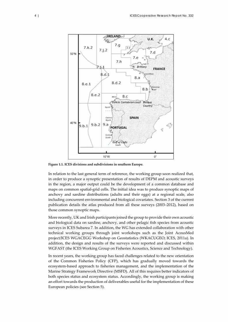
and Division 9.a (Figure 1.1).
4 | ICES Cooperative Research Report No. 332
Figure 1.1. ICES divisions and subdivisions in southern Europe.
In relation to the last general term of reference, the working group soon realized that,
in order to produce a synoptic presentation of results of DEPM and acoustic surveys
in the region, a major output could be the development of a common database and
maps on common spatial‐grid cells. The initial idea was to produce synoptic maps of
anchovy and sardine distributions (adults and their eggs) at a regional scale, also
including concurrent environmental and biological covariates. Section 3 of the current
publication details the atlas produced from all these surveys (2003–2012), based on
those common synoptic maps.
More recently, UK and Irish participants joined the group to provide their own acoustic
and biological data on sardine, anchovy, and other pelagic fish species from acoustic
surveys in ICES Subarea 7. In addition, the WG has extended collaboration with other
technical working groups through joint workshops such as the Joint AcousMed
project/ICES WGACEGG Workshop on Geostatistics (WKACUGEO; ICES, 2011a). In
addition, the design and results of the surveys were reported and discussed within
WGFAST (the ICES Working Group on Fisheries Acoustics, Science and Technology).
In recent years, the working group has faced challenges related to the new orientation
of the Common Fisheries Policy (CFP), which has gradually moved towards the
ecosystem‐based approach to fisheries management, and the implementation of the
Marine Strategy Framework Directive (MSFD). All of this requires better indicators of
both species status and ecosystem status. Accordingly, the working group is making
an effort towards the production of deliverables useful for the implementation of these
European policies (see Section 5).

Pelagic survey series for sardine and anchovy in ICES subareas 8 and 9 | 5
1.2 Overview of the surveys carried out on small pelagic species in southwestern European waters
Continuous field research studies targeting the two main species, sardine and anchovy,
based on surveys at sea have been carried for more than 30 years (Table 1.1) by France,
Spain, and Portugal. At the same time, ancillary variables were gradually added in
order to promote a better understanding of the complexity of the pelagic ecosystem
related to those species.
France, Spain, and Portugal have traditionally participated through four institutions
(IFREMER, AZTI, IEO, and IPIMAR [presently IPMA]) in carrying out the surveys, in
several cases cosponsored through different EU projects and eventually (since 2002)
within the Community framework for the collection and management of data needed
to conduct the Common Fisheries Policy. Recently (2011), the UK and Ireland launched
their own new surveys north of the Bay of Biscay (Celtic Sea, western English Channel,
Irish Sea) and began to participate in WGACEGG.
Table 1.1. Seasonal survey effort on pelagic fish stocks made by IEO, IPMA, AZTI, and IFREMER
institutes since the 1980s by regions in southwestern European Atlantic waters between Gibraltar
and the Celtic Sea.
In order to allow for joint analyses of maps and data in this publication, the surveys
operating exclusively in ICES divisions 8.a–c and 9.a since 2003–2012 are reported.
Furthermore, these surveys occurred rather regularly in a coordinated and
standardized form. Since the method used for Atlanto‐Iberian sardine DEPM surveys
is applied on a triennial basis, a decision was made to include the entire series (1988–
2011). The surveys reviewed and coordinated by WGACEGG (or previous working
groups) since 2003 are presented in Table 1.2. A summary of the surveys reported in
Year Season IPMA IEO AZTI IFREMER Year IPMA AZTI IFREMER Year IPMA AZTI IFREMER
PortugalGalice Biscay
Biscay Biscay PortugalGalice Biscay
Gulf of Cadiz
Biscay Biscay PortugalGalice Biscay
Gulf of Cadiz
Biscay Biscay
winter spring summer autumn winter spring summer autumn winter spring summer autumn winter spring summer autumn winter spring summer autumn winter spring summer autumn winter spring summer autumn winter spring summer autumn winter spring summer autumn winter spring summerautumn
2010
2011
2012
1999
2000
2001
2002
2009
2008
1994
1995
1996
1997
1998
2004
2005
2006
2007
1988
1989
1990
1991
1992
IEO IEO
1987
1983 1993
1984
1985
1986
2003

6 | ICES Cooperative Research Report No. 332
this document (acronyms, summary description, and usual period of implementation)
is provided in Table 1.3.
Table 1.2. Surveys taken into account for the establishment of the common database and maps in
this report. Orange refers to acoustic surveys and blue indicates DEPM surveys; sardine DEPM
surveys in 1988, 1990, 1997, 1999, and 2002 are also reported.

Pelagic survey series for sardine and anchovy in ICES subareas 8 and 9 | 7
Table 1.3. Acronyms, objectives, and the usual period of implementation of each survey series
reported in this report.
Surveys Country Acronym Month Target
species
ICES divisions and
subareas
Spring DEPM
surveys
Portugal PT‐DEPM‐
PIL
2 Sardine 9.a Central N., 9.a
Central S., 9.a South
Spain SAREVA 4 Sardine 9.a North, 8.c, 8.b
Spring
acoustic
surveys
France PELGAS 5 Sardine and
anchovy
8.a , 8.b, 8.c (East)
Spain PELACUS 4 Sardine and
anchovy
9.a North, 8.c
Portugal PELAGO 4 Sardine and
anchovy
9.a Central N., 9.a
Central S., 9.a South
Spring DEPM
surveys
Spain BIOMAN 5 Anchovy 8.a, 8.b, 8.c (East)
Summer
acoustic
survey in
Division 9.a
South
Spain ECOCADIZ 6–7 Anchovy 9.a South
Summer
DEPM survey
in Division 9.a
South
Spain BOCADEVA 6–7 Anchovy 9.a South
Autumn
acoustic
surveys
Spain JUVENA 9 Anchovy
recruits
Subarea 8
Autumn
acoustic
surveys
Portugal SAR 10–11 Sardine
recruits
Subarea 8
1.3 Objectives and structure of the report
The purpose of this report is to present the results of the systematic surveys for
monitoring the coastal pelagic fish species (mainly sardine and anchovy) in the
southwestern Atlantic European waters, carried out between 2003 and 2012 by France,
Spain, and Portugal and coordinated within ICES working groups. This is basically
achieved as described below.
A description of the monitoring system used in the acoustic and DEPM surveys carried
out in these years is given in Section 2 on a survey‐by‐survey time‐series basis (Tables
1.2 and 1.3). This includes a synopsis of the background of each survey and its
objectives, the global approach for the method applied (e.g. calendar, parameters
collected, sampling procedures, standardization of methods throughout the series). In
addition, a summary of the main results (overall maps of species distributions, series
of biomass, and other indicators) is followed by a summary discussion.
The more technical procedures of each survey are further shown in annexes at the end
of this report.

8 | ICES Cooperative Research Report No. 332
A synoptic series of spatial distributions of small pelagics and the environmental
indicators obtained from the different surveys is presented in a standard format in
Section 3. This is a novel contribution of WGACEGG to the scientific community in the
form of an atlas of sardine and anchovy distribution in the region along with different
covariates and indicators provided by these surveys, based on common spatial‐grid
cells. Individual maps are available for download from the ICES website
(http://ices.dk/community/groups/Documents/Forms/AllItems.aspx?RootFolder=%2F
community%2Fgroups%2FDocuments%2FWGACEGG%2FCRR%20332%20Supplem
entary%20online%20material&View=%7B49A2EFDE‐3932‐4900‐A03D‐
70258239F39E%7D). Among the several indicators included are those on
backscattering energy by species (Nautical area scattering coefficient [NASC],
m2 nautical mile−2; MacLennan et al., 2002), sardine and anchovy egg abundance from
vertical tows at fixed stations (PairoVET/CalVET) or continuous subsurface samples
(continuous underway fish egg sampler, CUFES), sea surface temperature and salinity,
cetaceans, or birds. These are provided on common scales and produced for each
survey through the years, together with the mean distribution and its spatial variance
across each survey time‐series.
This contribution responds to terms of reference 4) and 5) of WGACEGG (Section 1.1).
The final product is a joint common database and an atlas summarizing the trends and
the mean situation of pelagic fish and its environment for over a decade. Section 4 aims
at analyzing the interannual variability and spatial patterns of the indicators presented
in Section 3, as well as the relationships among the parameters collected concomitantly
during these surveys, making use of the common database assembled from these
surveys. Section 4 presents a first essay for such crossed analysis, e.g. making use of
the spring coordinated acoustic series (PELAGO, PELACUS, PELGAS) where
parameters on environment, ichthyoplankton, fish, and top predators are collected
simultaneously and cover the entire area from Cádiz to Brest. Characterizations of
habitats and the spatial covariation of the indicators are also provided.
Section 5 briefly presents the challenges faced by the monitoring surveys on small
pelagics, in addition to reporting on the abundance of the target species, and also
contributing to the ecosystem monitoring required by the new CFP and MSFD.
Clearly, this report constitutes a major deliverable by the ICES WGACEGG and the
surveys implemented for the monitoring of the small pelagics in the southwestern
European Atlantic waters to the marine scientific community in Europe. It is expected
that the description of the surveys used in the monitoring programmes, as well as the
provision of the synoptic overview of the status and distribution of the small pelagic
fish resources in this region during the first decade of this century will serve as a
benchmark reference point on the small pelagics and/or ecosystem overviews of this
region in any future studies.

Pelagic survey series for sardine and anchovy in ICES subareas 8 and 9 | 9
2 Description of surveys on pelagic species in ICES subareas 8 and 9
2.1 Sardine DEPM surveys in Atlantic Iberian waters
Maria Manuel Angélico, Miguel Bernal, Paz Díaz, Ana Lago de Lanzós, Cristina
Nunes, José Ramón Pérez, and Alexandra Silva
2.1.1 Introduction
The DEPM methodology was first applied for spawning‐stock biomass (SSB)
estimation in 1988 for the Atlanto‐Iberian sardine (Sardina pilchardus) by Portugal
(presently IPMA [used hereafter in the text], but previously under other designations:
INIP, IPIMAR, INIAP, and INRB) and by IEO in Spain (Miranda et al., 1990; Cunha et
al., 1992; García et al., 1992). During the 1990s, through informal contacts, both
countries organized surveys in 1997 and 1999; in 1990, only Spain carried out a survey
that covered part of the area (García et al., 1991, 1993; Cunha et al., 1997; Lago de Lanzós
et al., 1998; Bernal et al., 2000; ICES, 2000a; Stratoudakis et al., 2000).
Since 2000, the surveys have been planned and conducted within the framework of
ICES, with cofinancing from the national states and the EU, on a triennial basis.
Coordinated surveys between IPMA and IEO were conducted in 2002, 2005, 2008, and
2011 (ICES, 2004, 2009a, 2010a, 2011a, 2012a; Stratoudakis et al., 2006). Improvements
in methods and standardization were possible due to methodological developments
and effective coordination undertaken first within ICES SGSBSA (2002–2004) and later
within WGACEGG.
The DEPM surveys targeting the Atlanto‐Iberian sardine cover the area from the inner
Gulf of Cádiz to the inner part of the Bay of Biscay (Atlanto‐Iberian sardine stock). The
region from the Gulf of Cádiz to the northern Portugal/Spain border (River Minho) is
surveyed by IPMA in January–February, while IEO covers the northwestern and
northern Iberian Peninsula and part of the Bay of Biscay (to 45°N) in March–April.
To obtain SSB estimation, the DEPM surveys are directed at egg abundance and
spawning area definition for daily egg production determination and at adult
sampling for daily fecundity calculation. Ichthyoplankton samples, simultaneous
conductivity, temperature, depth and Fluorescence (CTDF) casts, and fishing hauls are
undertaken over the entire spawning region. In recent years, data collection has been
enhanced and diversified to not only promote improvement in the method (e.g.
otoliths for population age structure), but also to take advantage of the comprehensive
coverage of the pelagic environment and further the understanding of the ecosystem
(hydrodynamics, zooplankton assemblages, fish diets, bird and marine mammal
census, etc.).
2.1.2 Methodology: past and present
Since the DEPM was first applied in the late 1980s, it has evolved due to several
methodological developments related to survey coverage, intensity of sampling,
laboratory processing of samples, data analysis, and estimation of parameters.
Moreover, there has been a systematic effort over the years in coordinating the surveys
and standardizing methodologies for surveying, laboratory work, and data analysis.
This was first due to the joint work between IEO and IPMA within the framework of
national/international projects, and then under the auspices of ICES working groups,
especially since 2002.

10 | ICES Cooperative Research Report No. 332
2.1.2.1 Surveying and sampling
Traditional DEPM is a survey‐based estimation, requiring the entire potential
spawning area to be covered with an adequate sampling effort, i.e. samples
representative of the population – adults and eggs – and a sufficient number of
observations for the required precision (Smith and Hewitt, 1985). On the other hand,
Stratoudakis and Fryer (2000) suggested adopting a stratified random design in Iberian
waters with an allocation proportional to local fish densities. This was done to obtain
reliable estimates of spawning biomass when there are spatial differences in
abundance and in the DEPM adult parameters. External information on fish
abundance (acoustic density) and abundance of eggs observed during DEPM surveys
are used as indicators of fish density, but there is no guarantee that the regional
allocation of sampling effort carried out during the surveys has accurately reflected the
relative abundance of the sampled population. Accordingly, the surveyed areas were
divided into three geographical strata: Division 9.a South (Algarve and the Gulf of
Cádiz); Division 9.a West (from Cape San Vicente to the Minho River at the northern
Portuguese/Spanish border); and divisions 9.a North and 8.c (northern Spanish
waters).
Regarding the Atlanto‐Iberian sardine stock, the Gulf of Cádiz was not sampled in the
first DEPM survey undertaken in 1988, and in 1990, only the north stratum was covered
(there was no survey in Portugal). The survey carried out in 1997 was the first to
include the entire distribution area of the sardine stock; since then, this same area has
been surveyed jointly by IEO and IPMA.
The number of samples collected during the surveys also varied throughout the time‐
series. In 2002, there was a substantial improvement in terms of sampling effort for
both eggs and adults, resulting in sufficiently intense sampling that guaranteed good
spatial coverage. This allowed, for the first time, an accurate spatial analysis of the data
(see ICES, 2004 and below), and potentially increased the precision of the biomass
estimates. Since then, this effort has been sustained (see Tables 2.1.1 and 2.1.2).
The grid of transects along which the fixed stations of ichthyoplankton (PairoVET)
sampling are located has suffered some minor changes over the years (see Table 2.1.2).
Since 2002, the fixed grid has remained unchanged, and an adaptive design has also
been applied with the aid of the auxiliary CUFES, the use of which helps in delimiting
sardine spawning areas and adapting the sampling intensity and the offshore limit of
PairoVET sampling (as described in detail in the annexed protocol, Annex 1).
In DEPM, the most appropriate timing for surveying is the peak spawning period of
the targeted species. Accordingly, for Atlanto‐Iberian sardines, surveys are carried out
in January/February in Portuguese waters (with the exception of the 1988 and 1997
surveys which took place simultaneously with the March acoustic survey) and in
March/April in northern Spanish waters and the southern Bay of Biscay (up to 45°N).
Furthermore, IEO surveys are carried out closely in time to the acoustic surveys, which
also provides biological samples. On the contrary, since 1999, IPMA acoustic and
DEPM surveys have become separated in time, and biological samples collected during
the acoustic survey are no longer available. Since then, adult samples collected during
the IPMA DEPM survey have been complemented by additional samples provided by
the commercial fleet.

Pelagic survey series for sardine and anchovy in ICES subareas 8 and 9 | 11
Table 2.1.1. Summary of plankton sampling for sardine DEPM surveys (Division 9.a South and West surveyed by IPMA, and divisions 9.a North and 8.c surveyed
by IEO). In 1990, only areas in divisions 9.a North and 8.c were sampled. Division 8.b was covered by IEO from 1997 to 2011.
Year
Strata
(ICES
divisions)
Dates Research
vessel
Transects
and grid
nautical
miles
(transects
× stations)
PairoVET
stations
(% with
eggs)
Eggs
PairoVET
Max. eggs
m–2
PairoVET
Temp.
(°C)
Min–
max
Survey
area
(km2)
Positive
area
(km2)
CUFES
stations
Eggs
CUFES
Max.
eggs m–3
CUFES
1988 9.a South 28/03–
30/03
RV “Noruega” 15 (7×7) 55(25.5) 344 1 680 14.5–
17.2
9 037 2 144
9.a West 01/03–
08/03
and
21/03–
28/03
42 (7×7) 249(35.7) 944 1 360 12.8–
16.1
39 073 14 889
9.a North +
8.c
31/03–
05/05
RV “Cornide
de Saavedra”
68 (6×6–3) 516(51.7) 3 922 2 758.3 10.6–
15.5
55 492 26 644
Iberian
Peninsula
125 820(45.1) 5 210 2 758.3 10.6–
17.2
103 602 43 676
1990 9.a South
9.a West
9.a North +
8.c
18/04–
10/05
RV
“Investigador”
475(36.6) 1 494 2 063.4 12.8–
18.5
64 185 30 555
Iberian
Peninsula
1997 9.a South 18/03–
25/03
RV “Noruega” 29 (7×7) 135(43.0) 868 5 593.8 16–19.3 19 951 8 745
9.a West 01/03–
16/03
39 (7x7) 238(16.0) 586 2 012.3 14–16.9 37 757 6 696

12 | ICES Cooperative Research Report No. 332
Year
Strata
(ICES
divisions)
Dates Research
vessel
Transects
and grid
nautical
miles
(transects
× stations)
PairoVET
stations
(% with
eggs)
Eggs
PairoVET
Max. eggs
m–2
PairoVET
Temp.
(°C)
Min–
max
Survey
area
(km2)
Positive
area
(km2)
CUFES
stations
Eggs
CUFES
Max.
eggs m–3
CUFES
9.a North +
8.c
05/03–
29/03
RV “Cornide
de Saavedra”
44 (15
GAL,7.5
CANT ×3)
515(16.7) 1 465 5 381 13.2–
15.9
55 870 10 275
Iberian
Peninsula
112 888(20.5) 2 919 5 593.8 13.2–
19.3
113 577 25 716
8.b 27/03–
02/04
12 89(63.6) 1 123 1 669.6 12.8–
15.3
20 149 12 755
1999 9.a South 10/01–
19/01
RV “Noruega” 77 (6×6) 147(36.7) 3 184 13 431 14–17.1 20 633 7 451
9.a West 19/01–
03/02
(6×6) 272(23.2) 1 926 6 060 12.6–
16.3
36 919 9 829
9.a North +
8.c
17/03–
03/04
RV “Cornide
de Saavedra”
50 (15
GAL,7.5
CANT ×3)
290(25.9) 900 1 196.6 12.2–
13.8
30 316 7 174
Iberian
Peninsula
707(27.2) 6 010 13 431 12.2–
17.1
87 868 24 454
8.b 03/04–
05/04
11 37(77.1) 586 1 185.4 12.5–
13.3
6 793 5 724
2002 9.a South 27/01–
02/02
RV “Noruega” 53 (8x3–6) 152(32.2) 530 1 733.4 14.5–
16.9
16 504 7 702 168 2 955 29.4
9.a West 08/01–
27/01
(8x3–6) 332(41.9) 2 077 8 328.2 12.1–
16.8
34 442 18 711 375 8 774 131.0

Pelagic survey series for sardine and anchovy in ICES subareas 8 and 9 | 13
Year
Strata
(ICES
divisions)
Dates Research
vessel
Transects
and grid
nautical
miles
(transects
× stations)
PairoVET
stations
(% with
eggs)
Eggs
PairoVET
Max. eggs
m–2
PairoVET
Temp.
(°C)
Min–
max
Survey
area
(km2)
Positive
area
(km2)
CUFES
stations
Eggs
CUFES
Max.
eggs m–3
CUFES
9.a Nort +
8.c
20/03–
16/04
RV “Cornide
de Saavedra”
36 (8×3–6) 220(58.6) 1 939 1 896.1 10.9–
17.5
25 476 15 202 441 9 669 40.6
Iberian
Peninsula
704(45) 4 546 8 328.2 10.9–
17.5
76 422 41 615 984 21 398 131.0
8.b 06/04–
12/04
RV “Cornide
de Saavedra”
10 55(73.3) 1 090 1 220.1 12.1–
13.9
11 888 9 154 103 5 096 98.3
2005 9.a South 13/02–
22/02
RV
“Capricornio”
(8×3–6) 159(41.5) 1 733 4 825.6 13.1–
15.4
17 321 7 201 186 4 991 30.4
9.a West 29/01–
12/02
(8×3–6) 249(32.9) 1 942 8 020 11.6–
14.8
26 808 10 723 312 4 278 55.6
9.a North +
8.c
13/04–
01/05
RV “Cornide
de Saavedra”
56 (8×3) 371(32.3) 3 216 3 231 12.4–16 38 476 12 307 323 9 748 85.0
Iberian
Peninsula
779(34.4) 6 891 8 020 11.6–16 82 605 30 231 821 19 017 85.0
2008 9.a South 20/01–
27/01
RV “Noruega” 22 (8×3) 174(56.3) 5 727 9 842.5 14.8–
17.1
18 164 9 692 181 10 710 124.9
9.a West 28/01–
15/02
36 (8×3) 288(51.7) 7 895 8 142.4 13.3–
16.7
30 318 19 296 315 19 632 140.0
9.a North +
8.c
02/04–
27/04
RV “Cornide
de Saavedra”
56 (8×3) 426(54.2) 3 788 8 354.2 11.9–
15.2
42 381 242 64 416 17 225 162.7
Iberian
Peninsula
114 888(53.8) 17 410 9 842.5 11.9–
17.1
90 863 53 252 912 47 567 162.7

14 | ICES Cooperative Research Report No. 332
Year
Strata
(ICES
divisions)
Dates Research
vessel
Transects
and grid
nautical
miles
(transects
× stations)
PairoVET
stations
(% with
eggs)
Eggs
PairoVET
Max. eggs
m–2
PairoVET
Temp.
(°C)
Min–
max
Survey
area
(km2)
Positive
area
(km2)
CUFES
stations
Eggs
CUFES
Max.
eggs m–3
CUFES
8.b 20/04–
24/04
RV “Cornide
de Saavedra”
8 74(76.3) 1 104 2 332.1 12.6–
13.9
10 187 8 167 93 13 733 215.5
2011 9.a South 10/02–
20/02
RV “Noruega” 21 (8×3) 170(31.8) 2 208 4 950 14.6–
16.9
17 578 6 523 184 4 607 81.7
9.a West 20/02–
08/03
36 (8×3) 309(12.9) 833 2 970 13.5–
16.1
32 098 4 817 308 479 6.0
9.a North +
8.c
25/03–
10/04
RV “Cornide
de Saavedra”
56 (8×3) 337(38.6) 1 794 1 537 12.5–
14.6
33 832 12 405 291 19 828 97.3
Iberian
Peninsula
113 816(27.5) 4 835 4 950 12.5–
16.9
83 508 23 745 783 24 914 97.3
8.b 09–
15/04
(IEO)
RV “Cornide
de Saavedra”
10 (8×3
IEO)
114(85.1) 2 764 2 322 13–14.7 14 091 12 400 129 36 978 92.1

Pelagic survey series for sardine and anchovy in ICES subareas 8 and 9 | 15
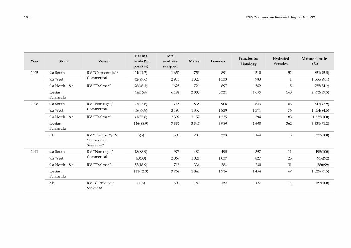
Table 2.1.2. Summary of adult sampling in the Iberian Peninsula (Division 9.a South, Division 9.a West, and divisions 9.a North + 8.c) and French coast (Division 8.b) sardine DEPM
surveys. In 2005, Division 8.b was not sampled due to bad weather.
Year Strata Vessel
Fishing
hauls (%
positive)
Total
sardines
sampled
Males Females Females for
histology
Hydrated
females
Mature females
(%)
1997 9.a South RV “Noruega” 12(83.3) 537 232 305 131 24 304(99.7)
9.a West 28(57.1) 804 298 506 142 6 506(100)
9.a North + 8.c RV “Thalassa” 9(77.8) 402 142 260 255 113 259(99.6)
Iberian
Peninsula
49(67.3) 1 743 672 1 071 528 143 1 069(99.8)
8.b RV “Thalassa” 4(4) 239 104 135 68 42 135(100)
1999 9.a South RV “Noruega”/
Commercial
12(100) 1 208 536 672 151 19 624(92.9)
9.a West 28(100) 2 732 1 125 1 580 283 86 1 479(93.6)
9.a North + 8.c RV “Thalassa” 19(57.9) 997 532 463 100 19 422(91.1)
Iberian
Peninsula
59(86.4) 4 937 2 193 2 715 534 124 2 525(93)
8.b RV “Thalassa” 6(6) 516 241 271 50 12 266(98)
2002 9.a South RV “Noruega”/
Commercial
31(96.8) 2 416 934 1 478 499 47 1 462(98.9)
9.a West 43(93.0) 2 811 1 104 1 472 576 66 1 217(82.7)
9.a North + 8.c RV “Thalassa” 28(100) 2 058 1 019 1 039 470 69 1 038(99.9)
Iberian
Peninsula
102(96.1) 7 285 3 057 3 989 1 545 182 3 717(93.2)
8.b RV “Thalassa” 4(4) 199 106 93 20 93(100)
16 | ICES Cooperative Research Report No. 332
Year Strata Vessel
Fishing
hauls (%
positive)
Total
sardines
sampled
Males Females Females for
histology
Hydrated
females
Mature females
(%)
2005 9.a South RV “Capricornio”/
Commercial
24(91.7) 1 652 759 891 510 52 851(95.5)
9.a West 42(97.6) 2 915 1 323 1 533 983 1 1 366(89.1)
9.a North + 8.c RV “Thalassa” 76(46.1) 1 625 721 897 562 115 755(84.2)
Iberian
Peninsula
142(69) 6 192 2 803 3 321 2 055 168 2 972(89.5)
2008 9.a South RV “Noruega”/
Commercial
27(92.6) 1 745 838 906 643 103 842(92.9)
9.a West 58(87.9) 3 195 1 352 1 839 1 371 76 1 554(84.5)
9.a North + 8.c RV “Thalassa” 41(87.8) 2 392 1 157 1 235 594 183 1 235(100)
Iberian
Peninsula
126(88.9) 7 332 3 347 3 980 2 608 362 3 631(91.2)
8.b RV “Thalassa”/RV
”Cornide de
Saavedra”
5(5) 503 280 223 164 3 223(100)
2011 9.a South RV “Noruega”/
Commercial
18(88.9) 975 480 495 397 11 495(100)
9.a West 40(80) 2 069 1 028 1 037 827 25 954(92)
9.a North + 8.c RV “Thalassa” 53(18.9) 718 334 384 230 31 380(99)
Iberian
Peninsula
111(52.3) 3 762 1 842 1 916 1 454 67 1 829(95.5)
8.b RV ”Cornide de
Saavedra”
11(3) 302 150 152 127 14 152(100)

Pelagic survey series for sardine and anchovy in ICES subareas 8 and 9 | 17
2.1.2.2 Additional information collected
Hydrological information has been collected over the years. In early surveys,
temperature data were obtained with probes (e.g. Minilogs) attached to the CalVET
frame. Since 2005, the incorporation of the CTD to the CalVET structure allowed the
regular collection of conductivity (salinity)/temperature/depth profiles simultaneously
with each ichthyoplankton haul (IPMA and IEO). Additionally, at alternate stations
and at the end of each transect, a second, more precise CTD was used during IEO
surveys.
Catches from fishing hauls provide opportunistic information on the distribution of
organisms composing the pelagic (and sometimes demersal) community as well as
some demographical data (length distribution) mostly for the pelagic fish species, even
though fishing hauls are directed at sardine.
DEPM surveys (since 2005 for IPMA) also include seabird and marine mammal
observers who record all sightings of these animals along transects, contributing to the
monitoring of their populations in Iberian waters.
2.1.2.3 Sampling and processing issues
Regarding egg sampling, the nets of the ichthyoplankton sampler (CalVET/PairoVET)
have remained the same for all surveys (150‐μm mesh), whereas the overall structure
has suffered some modifications over time, although it has remained unchanged since
2005 when the CTD became coupled to the net structure. As for the CUFES (the
auxiliary system), it was equipped with a 500‐μm mesh net until 2005 when the mesh
size was changed to 335 μm, following a working group decision after initial stages of
anchovy eggs were suggested to be potentially lost with the previous net.
Classification of eggs by development stages (11‐stage scale) follows the general
descriptions presented by Gamulin and Hure (1955). However, over the years, small
adaptations have been introduced during discussions undertaken at workshops or
working group meetings (e.g. ICES, 2002a; SGSBSA).
In DEPM, all adult estimates refer to mature fish (including those that are inactive
during the spawning season) defined as those sardines containing gonads classified
macroscopically as stage 2 and above. Until 2002, only stage 2 ovaries were sampled
for histology. However, indication that misclassifications between stages 1
(immature/resting) and 2 (mature/developing) occurred (Afonso‐Dias et al., 2008), it
was decided in 2005 to collect all ovaries irrespective of their maturity stage, the latter
being confirmed microscopically for all fish sampled for histology.
Since 2005, histological slides have been analysed following a standardized procedure.
For revision of the historical series, histological material prior to 2005 was reanalyzed
following this same standardized procedure; oocytes are classified according to an 8‐
stage scale agreed within the working group for sardine and anchovy (adapted from
Ganias et al., 2003; Alday et al., 2004). Regarding postovulatory follicles (POFs), these
are assigned to daily cohorts using histological information according to both
morphological and metric criteria (Ganias et al., 2007). However, these daily cohorts
are still delimited in time differently by IEO and IPIMAR/IPMA; each POF daily cohort
begins at midnight (GMT) for the former and at sardine daily peak spawning time
(21:00 GMT) for the latter.
Estimation of mean batch fecundity has always been limited by the number of
hydrated female samples available in the fishing hauls (see Table 2.1.2). As in Atlantic
sardine ovaries, separation in size of the spawning batch occurs much earlier than the

18 | ICES Cooperative Research Report No. 332
onset of hydration (at the transition between the primary and the secondary yolk stage;
Ganias et al., 2010). It is possible to use non‐hydrated females having ovaries with
oocytes at the above (or later) stages to obtain individual batch fecundity when
hydrated females are scarce or even absent. Moreover, Ganias et al. (2010) developed
an automated procedure (using Image J) by means of images of ovarian whole mounts
to count the oocytes of the spawning batch.
2.1.2.4 Data analysis
The general common methodology currently used in the data analysis for the
estimation of areas (surveyed and spawning areas), egg parameters (Z, P0, and Ptot),
and adult parameters (sex ratio, mean female weight, spawning fraction, and bath
fecundity) is explained in detail in the annexed common protocol (Annex 1).
All analyses are carried out using packages and routines developed in R software
(www.r‐project.org), which have already been updated since the initial versions.
Several internal workshops took place, which helped standardize the use of these
analytical tools between institutes.
2.1.2.5 Egg data
All calculations for area delimitation, egg ageing, and model fitting for egg production
(P0) estimation are based on the DEPM general theory and common methodology
detailed in the annexed protocol (Annex 1). They are carried out using the R packages
available within the open source project ichthyoanalysis
(http://sourceforge.net/projects/ichthyoanalysis).
To avoid overestimation of areas at the borders of the survey limits, the value of the
area represented by each station was forced to the minimum and maximum of 25 and
175 km2, respectively. The range 25–175 was selected as a mean interval suitable for all
surveys according to the distance between transect and stations. Distance varied in the
initial years, but since 2002, it became fixed at 8 nautical miles between transects and 3
or 6 nautical miles between stations along transects.
The positive area (area with eggs) was obtained over the years using different
calculation methods, but from 2008 onwards, the estimation of this parameter became
automatic, and the 2012 revision considered this automatic procedure to recalculate
estimates of all past surveys. Both the limits of the survey area (sampled) and the
positive area (offshore and coastal) are estimated using the geofun library software,
which mainly uses the spatial analysis functionality provided by the R‐package
spatstat. Both the survey and total areas are later corrected to avoid extrapolation to
the coast by computing the intercept between the areas estimated, as above, and the
area delimited by the coastline.
The model of egg development with temperature was derived from the incubation
experiment data available within the egg R library (sardine incubation data from the
Gulf of Cádiz, described in Bernal et al., 2008).
Egg ageing was achieved by a multinomial Bayesian approach described by Bernal et
al. (2008) and using in situ sea surface temperature (SST) data. Distribution of the daily
spawning cycle was assumed to be a normal (Gaussian) distribution, with a peak at
21:00 GMT and a standard deviation of 3 h (spawning period from 21:00–6 h to
21:00+6 h). The upper age cutting limit was determined using a maximum age for the
stratum considered, and it is not dependent on the individual stations (upper age = F).
Older cohorts are dropped if their mean age plus 2 s.d. h is over the critical age at which
5% or more of the eggs are expected to have already hatched (how.complete = 95%).

Pelagic survey series for sardine and anchovy in ICES subareas 8 and 9 | 19
The lower age cutting limit excluded the first cohort of stations in which sampling time
is included within the daily spawning period (lower.age = T).
The approach to fitting egg data to estimate mortality (Z) and egg production (P0)
varied over the years (ICES, 2004; Stratoudakis and Bernal, 2006). Egg mortality
estimates were revised by Bernal et al. (2011a), with results showing that single surveys
are often unreliable, and that mean estimates obtained after aggregating data from
various years are statistically more robust. Bernal et al. (2011b) also presented a revision
of the estimation methods which included both generalized linear modelling (GLM)
and generalized additive models (GAM)‐based spatial analysis. For the 2012 revision,
several GLM models were considered to test different stratification combinations for
P0 and Z (see detailed discussion in ICES, 2011a, 2012a), applying a standardized
procedure. The exponential mortality model is fitted as a GLM with binomial negative
distribution and with log link and weights proportional to the relative area represented
by each station. The results presented here were stratified for P0, based on a single
mortality estimate for the whole area.
2.1.2.6 Adult data
In DEPM, four parameters are estimated based on information collected from adult
fish samples: (i) mean female weight (W), (ii) sex ratio (R), (iii) mean female batch
fecundity (F), and (iv) daily spawning fraction (S).
Depending on the years, W was obtained either excluding the hydrated females from
the calculations or by adjusting all sampled female weights to correct for the temporary
bias due to ovary hydration. For the 2012 revision, only hydrated females had their
weight corrected, whereas the observed weights were considered for all other females.
The sex ratio in weight per haul is obtained as the quotient between the weight of
females and the combined weight of males and females. Ephemeral spawning
aggregations around the daily spawning peak in sardine (Ganias and Nunes, 2011)
may introduce bias and less precision in the estimation of R, unless samples around
this time are avoided.
Batch fecundity is estimated based on the method described in Hunter et al. (1985) of
modelling the individual batch fecundity observed in the sampled hydrated females
and their gonad‐free weight, and subsequently applying this model to all mature
females. Depending on the year, the number of hydrated females collected varied (see
Table 2.1.2). In 1988, hydrated females did not cover the entire range of female weights
sampled off the Portuguese coast, and a unique model was fitted for all areas surveyed
(three strata; see Cunha et al., 1992). In 1997, the same regression model was used to
estimate mean batch fecundity (Cunha et al., 1997). In 1999, a weighted linear model
(using weighted least squares, with weights equal to the inverse of Wnov) was fitted to
the hydrated females samples (Stratoudakis et al., 2000). In 2002, several models were
fitted to the Portuguese and Spanish data, and F was finally obtained by applying
GLMs to the former, whereas estimation followed the standard weighted linear
regression model (batch fecundity as a function of gonad‐free weight [W*], weighted
by the inverse of W*) for the latter. Since 2005, batch fecundity has been modeled for
the three strata with GLMs; several models are tested for each survey, the most
appropriate being selected based on both biological and statistical significance.
Spawning fraction is the adult parameter estimated with less precision and more
potential bias because it is a sample‐based estimate and thus is considerably dependent
on sampling design and number of samples. For sardine, the estimator of spawning
fraction has always been the average proportion of female fish with day 1 and day 2

20 | ICES Cooperative Research Report No. 332
POFs in the sample of mature females collected per haul and examined by histology.
Until 2005, POFs were classified based on descriptions by Hunter and Macewicz (1985)
and Pérez et al. (1992a) on the time of capture and a peak spawning time of 19:00
(GMT). From 2005 onwards, POFs have been assigned to daily cohorts using both
histomorphological and metrical (POF cross‐sectional area) criteria (Ganias et al., 2007)
and peak spawning time at 21:00 (GMT). In the first surveys carried out in Iberian
waters, uncertainties in POF determination and ageing (limited experience in
histological preparation and analysis) prevented the provision of reliable estimates.
For the 2012 revision, all histological material was reanalysed following the same
methodology, and the spawning fraction estimates revised. With the exception of 2011,
the estimated S for the Portuguese survey in 2002 was the lowest of the series (and
probably the lowest ever reported for a sardine species during peak spawning, see
Table 2.1.3). Precision of the S estimate consequently remained low despite the
considerable increase in the number of samples collected that year compared to
previous years. In 1999, no S estimates could be provided in the north and along the
French coasts, and in 2011, estimates obtained were considered unrealistic for the
western and southern strata; a non‐parametric bootstrap approach was applied to
estimate S for those years and strata (see Section 2.1.3 – Results, and the protocol in
Annex 1). Despite the improvements, several potential sources of bias still remain in S
estimation: (i) impact of sampling gear and time of sampling (biased estimates of S can
be obtained due to behaviour of sardines around spawning time), (ii) spatial
heterogeneity (if there is spatial structure in S due to different population demography
and environmental conditions), and (iii) correct assignment of POFs to daily cohorts
depending on temperature.
2.1.2.7 Post-stratification and spatial analysis
A major assumption in DEPM estimation is that all parameters are constant over the
duration and the area covered by the survey. When this assumption is violated,
Picquelle and Stauffer (1985) recommend post‐stratification. Results from several
studies on the spawning areas (Bernal et al., 2007), spawning seasonality (Stratoudakis
et al., 2007), sardine first maturation (Silva et al., 2006), and population dynamics (Silva
et al., 2009) indicate geographical heterogeneity in spawning activity as well as life
history traits among the northern, western, and southern Iberian coasts, suggesting
DEPM analysis should consider the decision to post‐stratify in these three areas.
Post‐stratification was not used for adults in the western and southern areas until 2002
because there was insufficient information (number of fish samples) to stratify in 1988
and 1997, and post‐stratification was not used in 1999 for comparability with the
previous two surveys. Following recommendations by SGSBSA, post‐stratified
estimates for western and southern areas were provided later for these years, which
led to an overall improvement in precision of the estimates (ICES, 2004; Stratoudakis
and Bernal, 2006).
Additionally, spatial analysis was also carried out applying generalized additive
models (GAM) fitted to egg and adult parameters for the first time in the 1999 and 2002
surveys (ICES, 2004). The results were in agreement with the post‐stratification
method, and GAM‐based estimations reduced CVs for sardine (ICES, 2004).
During the 2012 revision, estimations were always obtained with post‐stratification
(for the southern, western, and northern strata) for adult parameters and P0. For
mortality, different options were tested and discussed; the results presented here
consider a single mortality for the whole area. As for GAM‐based estimations, no
further work has been carried out in recent years for adult parameters. For P0, spatially

Pelagic survey series for sardine and anchovy in ICES subareas 8 and 9 | 21
explicit estimates were published by Bernal et al. (2011b), providing a flexible estimator
of egg production and increasing the precision of the time‐series estimates.
2.1.3 Results
This section describes the results obtained after the revision of the complete dataseries
undertaken in 2012 for the ICES benchmark assessment of the Atlanto‐Iberian stock,
using the standardized analytical procedures and options described in detail in ICES
(2012a). For this revision, the data used were revised, recompiled, and standardized by
IPIMAR/IPMA and IEO (ICES, 2011a, 2012a). The revision of estimations included all
data available for eggs (1988–2011); however, for adults, it was not yet possible to
guarantee the correct interpretation of the raw data for the 1988 survey; therefore, these
data were not included. This section also includes estimations from egg and adult data,
collected by IEO in Division 8.b since 1997.
2.1.3.1 Environmental setting
Sea surface temperature (SST) and sea surface salinity (SSS) distributions observed
during the DEPM survey series are presented in Figure 2.1.1. Water temperature is the
only variable applied in the method for egg ageing. Therefore, at the beginning of the
survey series, only temperature probes were used; regular CTD casts were
implemented at a later point.
The SST and SSS maps show the general distribution features for the Atlanto‐Iberian
coastal region, with temperature and salinity decreasing from south to north. When
the DEPM surveys take place in winter or early spring, the water column is usually
still thermally mixed. However, haline stratification may occur outside the major river
mouths (Guadalquivir and Guadiana on the southern coast; Tejo, Douro, and the
Galician Rias in the west). In the inner corner of the Bay of Biscay, water stratification
begins during spring. Shelf hydrology is subject to the influence of water originating
from the Azores Current and the Gulf of Cádiz, mainly in the south and southern
region and from the North Atlantic Current in the north. The geographic orientation
of the shore of the Iberian Peninsula confers different oceanographic characteristics to
the southern and northern zonal coasts and to the meridionally orientated west coast.
The west coast, aligned with prevailing winds, is subject to upwelling events during
summer (occasionally even off season) and, hence, has more productive colder waters.
A poleward flow runs off the shelf edge, being more evident from Nazaré Canyon
northward during winter. Off the southern and northern shores, local winds drive
highly variable transient coastal currents. All year‐round, the coastal Atlanto‐Iberian
waters are populated with mesoscale oceanographic features that promote patchy
distributions of plankton and other components of the system (Mason et al., 2006).
Throughout the series, coastal temperature and primary production have fluctuated
considerably (information not shown here). At the beginning of the series, typical
average water temperatures were observed during the surveys. Winter 2005 was cold,
particularly along the southern and western coasts and was preceded by a rather warm
summer–autumn period in all regions. The winters of 2008 and 2011 were quite mild
everywhere, and these years also had high primary production.
2.1.3.2 Spawning area
A summary of the plankton sampling for the sardine DEPM surveys is presented in
Table 2.1.1. Modifications in the survey design were introduced during the first years
of the DEPM application; from 2002 onwards, the surveys undertaken by IPMA and

22 | ICES Cooperative Research Report No. 332
IEO have followed a regular grid of transects, perpendicular to the coast and spaced
eight nautical miles apart.
Figure 2.1.1. Sea surface temperature (SST) (top two rows of panels) and sea surface salinity (SSS)
(bottom panels) distributions observed during the DEPM surveys for the Atlanto‐Iberian sardine
stock. SSS data is only available since 2002. In 2011, SSS data were not reliable and hence are not
included. Discontinuity in the distributions indicates that surveying was not sequential.
Sardine egg distributions obtained from the PairoVET (1988–2011) and CUFES systems
(since 2002), for the whole area are presented in Figures 2.1.2a and 2.1.2b. The egg
distribution pattern derived from the observations from the two samplers is similar.
Sardine spawning grounds occupied all of the surveyed shelf, and in some years, eggs

Pelagic survey series for sardine and anchovy in ICES subareas 8 and 9 | 23
were observed offshore (likely due to advection); however, egg distribution (hot spots
or egg voids) varied over years. It is also important to note that the timing of the
surveys also varied over years (due to logistic constraints), particularly in the southern
and western regions where the DEPM survey was conducted simultaneously with the
acoustics survey during March at the beginning of the series, when the spawning
season is already advanced for the southern and western populations. During 1997 and
1999, a discontinuity in egg distribution was observed between the northern and
western areas. The gap in egg presence was evident in Galician waters and at the
northern part of the western area, although sardine eggs have been found in these areas
since 2002. Recurrent areas of high egg abundance are found in the inner Gulf of Cádiz,
over the northwestern shelf, and in the corner of the Bay of Biscay. In some years, either
because of survey timing, environmental conditions, or population structure, egg
distribution was very patchy. 2005, for example, was the coldest winter of the series
where the percentage of young sardines (first‐year spawners) in the northwestern
region was very high, while egg abundance was low and very patchy. In 2008, when
weather conditions were quite good and the population included a high percentage of
middle–older age individuals, egg abundance (and egg production) was the highest of
the series (over 50% of the samples contained eggs). Regarding egg distribution along
the French coast, eggs were always observed to encompass the shelf extension to the
200‐m isobaths.

24 | ICES Cooperative Research Report No. 332
Figure 2.1.2a. Egg distribution during the DEPM surveys for the Atlanto‐Iberian sardine stock
derived from PairoVET (eggs m–2). In 1990, only the northern Spanish coast was sampled.
-10º -9º -8º -7º -6º -5º -4º -3º -2º36º
37º
38º
39º
40º
41º
42º
43º
44º
45º
-10º -9º -8º -7º -6º -5º -4º -3º -2º36º
37º
38º
39º
40º
41º
42º
43º
44º
45º
1988
-10º -9º -8º -7º -6º -5º -4º -3º -2º36º
37º
38º
39º
40º
41º
42º
43º
44º
45º
1990
-10º -9º -8º -7º -6º -5º -4º -3º -2º36º
37º
38º
39º
40º
41º
42º
43º
44º
45º
1997
-10º -9º -8º -7º -6º -5º -4º -3º -2º36º
37º
38º
39º
40º
41º
42º
43º
44º
45º
1999
-10º -9º -8º -7º -6º -5º -4º -3º -2º36º
37º
38º
39º
40º
41º
42º
43º
44º
45º
2002
-10º -9º -8º -7º -6º -5º -4º -3º -2º36º
37º
38º
39º
40º
41º
42º
43º
44º
45º
2005
2008
-10º -9º -8º -7º -6º -5º -4º -3º -2º36º
37º
38º
39º
40º
41º
42º
43º
44º
45º
2011 Sardine eggs/m2
0.01 to 50 50 to 100 100 to 500 500 to 1000 1000 to 5000 5000 to 10000 10000 to 13432

Pelagic survey series for sardine and anchovy in ICES subareas 8 and 9 | 25
Figure 2.1.2b. Egg distribution (eggs m–3) during the DEPM surveys for the Atlanto‐Iberian sardine
stock derived from CUFES sampling.
Figure 2.1.3 shows egg densities (sum of all stations) derived from PairoVET and
CUFES sampling (see number of stations and maximum values by area and year in
Table 2.1.1). An increase in the number of eggs was observed from 2002 to 2008 when
high egg densities were obtained for all areas. After 2008, a generalized drop in
abundance was observed, particularly in the south and west. Some very high values
were observed in the north (1988) and in the south (1999).
-10º -9º -8º -7º -6º -5º -4º -3º -2º36º
37º
38º
39º
40º
41º
42º
43º
44º
45º
-10º -9º -8º -7º -6º -5º -4º -3º -2º36º
37º
38º
39º
40º
41º
42º
43º
44º
45º
-10º -9º -8º -7º -6º -5º -4º -3º -2º36º
37º
38º
39º
40º
41º
42º
43º
44º
45º
-10º -9º -8º -7º -6º -5º -4º -3º -2º36º
37º
38º
39º
40º
41º
42º
43º
44º
45º
2008
20052002
2011
0.01 to 1 1 to 5 5 to 10 10 to 25 25 to 50 50 to 75 75 to 100 100 to 225
Sardine eggs/m3
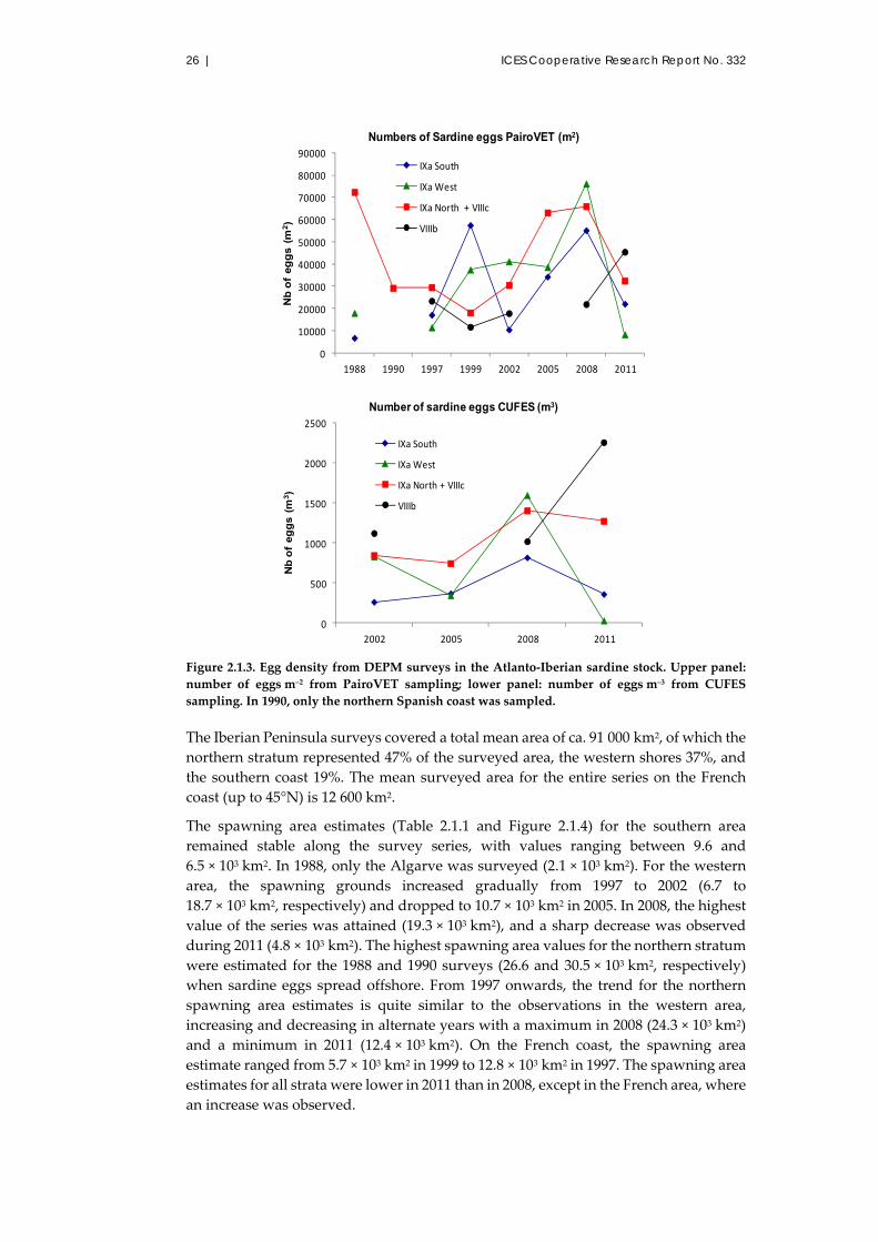
26 | ICES Cooperative Research Report No. 332
Figure 2.1.3. Egg density from DEPM surveys in the Atlanto‐Iberian sardine stock. Upper panel:
number of eggs m–2 from PairoVET sampling; lower panel: number of eggs m–3 from CUFES
sampling. In 1990, only the northern Spanish coast was sampled.
The Iberian Peninsula surveys covered a total mean area of ca. 91 000 km2, of which the
northern stratum represented 47% of the surveyed area, the western shores 37%, and
the southern coast 19%. The mean surveyed area for the entire series on the French
coast (up to 45°N) is 12 600 km2.
The spawning area estimates (Table 2.1.1 and Figure 2.1.4) for the southern area
remained stable along the survey series, with values ranging between 9.6 and
6.5 × 10³ km2. In 1988, only the Algarve was surveyed (2.1 × 10³ km2). For the western
area, the spawning grounds increased gradually from 1997 to 2002 (6.7 to
18.7 × 10³ km2, respectively) and dropped to 10.7 × 10³ km2 in 2005. In 2008, the highest
value of the series was attained (19.3 × 10³ km2), and a sharp decrease was observed
during 2011 (4.8 × 10³ km2). The highest spawning area values for the northern stratum
were estimated for the 1988 and 1990 surveys (26.6 and 30.5 × 10³ km2, respectively)
when sardine eggs spread offshore. From 1997 onwards, the trend for the northern
spawning area estimates is quite similar to the observations in the western area,
increasing and decreasing in alternate years with a maximum in 2008 (24.3 × 10³ km2)
and a minimum in 2011 (12.4 × 10³ km2). On the French coast, the spawning area
estimate ranged from 5.7 × 10³ km2 in 1999 to 12.8 × 10³ km2 in 1997. The spawning area
estimates for all strata were lower in 2011 than in 2008, except in the French area, where
an increase was observed.
0
10000
20000
30000
40000
50000
60000
70000
80000
90000
1988 1990 1997 1999 2002 2005 2008 2011
Nb
of
eg
gs (
m2)
Numbers of Sardine eggs PairoVET (m2)
IXa South
IXa West
IXa North + VIIIc
VIIIb
0
500
1000
1500
2000
2500
2002 2005 2008 2011
Nb
of
eg
gs (
m3)
Number of sardine eggs CUFES (m3)
IXa South
IXa West
IXa North + VIIIc
VIIIb
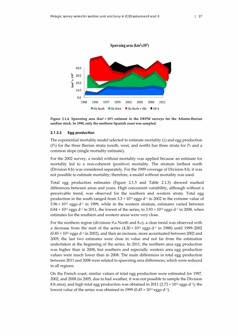
Pelagic survey series for sardine and anchovy in ICES subareas 8 and 9 | 27
Figure 2.1.4. Spawning area (km2 × 103) estimate in the DEPM surveys for the Atlanto‐Iberian
sardine stock. In 1990, only the northern Spanish coast was sampled.
2.1.3.3 Egg production
The exponential mortality model selected to estimate mortality (z) and egg production
(P0) for the three Iberian strata (south, west, and north) has three strata for P0 and a
common slope (single mortality estimate).
For the 2002 survey, a model without mortality was applied because an estimate for
mortality led to a non‐coherent (positive) mortality. The stratum farthest north
(Division 8.b) was considered separately. For the 1999 coverage of Division 8.b, it was
not possible to estimate mortality; therefore, a model without mortality was used.
Total egg production estimates (Figure 2.1.5 and Table 2.1.3) showed marked
differences between areas and years. High concurrent variability, although without a
perceivable trend, was observed for the southern and western strata. Total egg
production in the south ranged from 3.3 × 10¹² eggs d–1 in 2002 to the extreme value of
5.96 × 10¹² eggs d–1 in 1999, while in the western stratum, estimates varied between
0.84 × 10¹² eggs d–1 in 2011, the lowest of the series, to 3.93 × 10¹² eggs d–1 in 2008, when
estimates for the southern and western areas were very close.
For the northern region (divisions 9.a North and 8.c), a clear trend was observed with
a decrease from the start of the series (4.30 × 10¹² eggs d–1 in 1988) until 1999–2002
(0.85 × 10¹² eggs d–1 in 2002), and then an increase, more accentuated between 2002 and
2005; the last two estimates were close in value and not far from the estimation
undertaken at the beginning of the series. In 2011, the northern area egg production
was higher than in 2008, but southern and especially western area egg production
values were much lower than in 2008. The main differences in total egg production
between 2011 and 2008 were related to spawning area differences, which were reduced
in all regions.
On the French coast, similar values of total egg production were estimated for 1997,
2002, and 2008 (in 2005, due to bad weather, it was not possible to sample the Division
8.b area), and high total egg production was obtained in 2011 (2.72 × 10¹² eggs d–1); the
lowest value of the series was obtained in 1999 (0.45 × 10¹² eggs d–1).

28 | ICES Cooperative Research Report No. 332
Figure 2.1.5. Egg production for the three spatial strata for all surveys off the Iberian Peninsula.
Dots and lines indicate the estimates of egg production and their confidence intervals. The y‐scale
is the same for all strata.
0
2
4
6
8
10
88 90 97 99 02 05 08 11
IXa South
0
2
4
6
8
10
88 90 97 99 02 05 08 11
IXa West
0
2
4
6
8
10
88 90 97 99 02 05 08 11
IXa North + VIIIc
0
2
4
6
8
10
88 90 97 99 02 05 08 11
VIII b
Pto
t [eggs
10
12 d
ay1
]
Survey

Pelagic survey series for sardine and anchovy in ICES subareas 8 and 9 | 29
Table 2.1.3. DEPM surveys for the Atlanto‐Iberian sardine stock. Summary of the results for eggs, adults, and SSB estimates. Final egg production model for the Iberian Peninsula
includes individual egg production estimates for each stratum (divisions 9.a South, 9.a West, and 9.a North–8.c) and a common mortality for the whole area. Egg production estimates
and mortality values are also shown for the Division 8.b area. Significant mortality values (h-1) are shown. * Significance at p < 0.05, ** significance at p < 0.01, and *** significance at p < 0.001. Mean females weight (W) (in g), Batch fecundity (F) (number eggs female–1), sex ratio (R), spawning fraction (S), and spawning‐stock biomass (SSB) (in t). CV corresponds to the coefficient of variation for each parameter estimated.
Year Strata
(divisions)
Mortality Ptot W R F S SSB
Estimate CV Estimate CV Estimate CV Estimate CV Estimate CV Estimate CV Estimate CV
1988 9.a South 0.85 0.31
9.a West –0.019*** 0.20 1.84 0.17
9.a North
+ 8.c
4.3 0.15
Total
Iberian
Peninsula
6.99 0.11
1990 9.a North
+ 8.c
–0.034*** 0.24 3.56 0.26
1997 9.a South –0.032*** 0.23 1.55 0.27 43.1 0.07 0.557 0.05 19 062 0.12 0.104 0.13 60 556 0.33
9.a West 2.09 0.29 48.5 0.07 0.637 0.04 22 569 0.13 0.049 0.18 144 012 0.37
9.a North
+ 8.c
2.91 0.27 72.2 0.05 0.493 0.14 28 544 0.07 0.144 0.10 103 611 0.33
Total
Iberian
Peninsula
6.55 0.16 308 178 0.22
8.b –0.012* 0.41 1.74 0.20 74.5 0.12 0.508 0.08 32 269 0.17 0.131 0.10 60 332 0.310
1999 9.a South –0.023** 0.34 5.96 0.33 42.1 0.05 0.531 0.03 22 436 0.11 0.074 0.22 284 749 0.42
9.a West 3.59 0.30 44.9 0.06 0.639 0.05 24 086 0.09 0.142 0.05 73 672 0.33
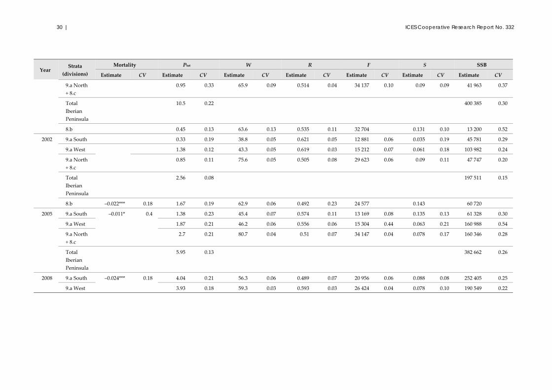
30 | ICES Cooperative Research Report No. 332
Year Strata
(divisions)
Mortality Ptot W R F S SSB
Estimate CV Estimate CV Estimate CV Estimate CV Estimate CV Estimate CV Estimate CV
9.a North
+ 8.c
0.95 0.33 65.9 0.09 0.514 0.04 34 137 0.10 0.09 0.09 41 963 0.37
Total
Iberian
Peninsula
10.5 0.22 400 385 0.30
8.b 0.45 0.13 63.6 0.13 0.535 0.11 32 704 0.131 0.10 13 200 0.52
2002 9.a South 0.33 0.19 38.8 0.05 0.621 0.05 12 881 0.06 0.035 0.19 45 781 0.29
9.a West 1.38 0.12 43.3 0.05 0.619 0.03 15 212 0.07 0.061 0.18 103 982 0.24
9.a North
+ 8.c
0.85 0.11 75.6 0.05 0.505 0.08 29 623 0.06 0.09 0.11 47 747 0.20
Total
Iberian
Peninsula
2.56 0.08 197 511 0.15
8.b –0.022*** 0.18 1.67 0.19 62.9 0.06 0.492 0.23 24 577 0.143 60 720
2005 9.a South –0.011* 0.4 1.38 0.23 45.4 0.07 0.574 0.11 13 169 0.08 0.135 0.13 61 328 0.30
9.a West 1.87 0.21 46.2 0.06 0.556 0.06 15 304 0.44 0.063 0.21 160 988 0.54
9.a North
+ 8.c
2.7 0.21 80.7 0.04 0.51 0.07 34 147 0.04 0.078 0.17 160 346 0.28
Total
Iberian
Peninsula
5.95 0.13 382 662 0.26
2008 9.a South –0.024*** 0.18 4.04 0.21 56.3 0.06 0.489 0.07 20 956 0.06 0.088 0.08 252 405 0.25
9.a West 3.93 0.18 59.3 0.03 0.593 0.03 26 424 0.04 0.078 0.10 190 549 0.22
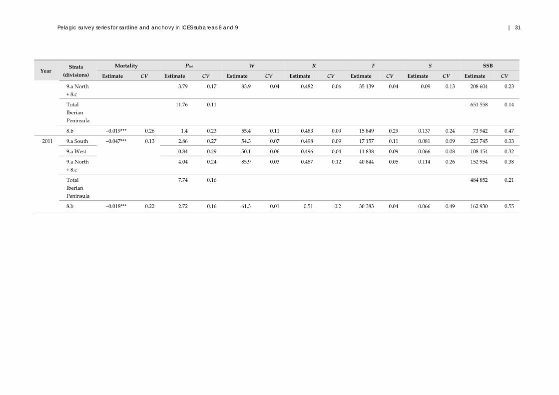
Pelagic survey series for sardine and anchovy in ICES subareas 8 and 9 | 31
Year Strata
(divisions)
Mortality Ptot W R F S SSB
Estimate CV Estimate CV Estimate CV Estimate CV Estimate CV Estimate CV Estimate CV
9.a North
+ 8.c
3.79 0.17 83.9 0.04 0.482 0.06 35 139 0.04 0.09 0.13 208 604 0.23
Total
Iberian
Peninsula
11.76 0.11 651 558 0.14
8.b –0.019*** 0.26 1.4 0.23 55.4 0.11 0.483 0.09 15 849 0.29 0.137 0.24 73 942 0.47
2011 9.a South –0.047*** 0.13 2.86 0.27 54.3 0.07 0.498 0.09 17 157 0.11 0.081 0.09 223 745 0.33
9.a West 0.84 0.29 50.1 0.06 0.496 0.04 11 838 0.09 0.066 0.08 108 154 0.32
9.a North
+ 8.c
4.04 0.24 85.9 0.03 0.487 0.12 40 844 0.05 0.114 0.26 152 954 0.38
Total
Iberian
Peninsula
7.74 0.16 484 852 0.21
8.b –0.018*** 0.22 2.72 0.16 61.3 0.01 0.51 0.2 30 383 0.04 0.066 0.49 162 930 0.55

32 | ICES Cooperative Research Report No. 332
2.1.3.4 Mean female weight
The percentage of larger (older) individuals is greater for the population occupying the
northern region than for populations in the other regions (Figure 2.1.6 and Section 2.2).
As a consequence, mean female weight (W) is always higher in the northern stratum,
where it has shown an increasing trend since 1999 (Figure 2.1.7). Conversely, the
western (NW) and southern (SE) regions are loci for sardine recruitment, which is
reflected in the structure of the population sampled during the DEPM series. Mean
weights obtained for Division 8.b varied greatly, depending on the number of hauls
considered and their locations. During the more recent surveys, the population
observed in this region appears closer in weight composition to the more southern
regions (proximity to the Bay of Biscay recruitment locus).
Minimum mean weight values were observed off northern Portugal and in the Gulf of
Cádiz (Figure 2.1.7). Mean female weight was similar for the entire Portuguese and
Cádiz coasts, and considerably higher for the northern Spanish coast. On the French
coast, mean female weight was lower than in the northern stratum, particularly evident
in the last two years (2008 and 2011). During the last survey in 2011, mean female
weights obtained for all strata were similar to the ones estimated in 2008, the values
calculated for the northern stratum being quite a lot higher than for the western and
southern strata.

Pelagic survey series for sardine and anchovy in ICES subareas 8 and 9 | 33
Figure 2.1.6. Sardine length (mm; top panel) and age distributions (bottom panel) per stratum for
DEPM sardine surveys. Only values from females sampled randomly (absolute values), obtained
according to the DEPM sardine sampling protocol (see Annex 1), are shown. No otoliths for age
reading were available in 1997 in the divisions 9.a South/West and 8.b.
Length (mm)
Num
ber o
f ind
ivid
uals
0
100
200
300
400
100 150 200250
IXa South
2011
IXa West
2011
100150 200 250
IXa North + VIIIc
2011
VIIIb
2011
IXa South
2008
IXa West
2008
IXa North + VIIIc
2008
0
100
200
300
400VIIIb
2008
0
100
200
300
400 IXa South
2005
IXa West
2005
IXa North + VIIIc
2005
VIIIb
2005
IXa South
2002
IXa West
2002
IXa North + VIIIc
2002
0
100
200
300
400VIIIb
2002
0
100
200
300
400 IXa South
1999
IXa West
1999
IXa North + VIIIc
1999
VIIIb
1999
IXa South
1997
IXa West
1997
IXa North + VIIIc
1997
0
100
200
300
400VIIIb
1997
Age
Num
ber of i
ndiv
iduals
0
200
400
600
2 4 6 8 10
IXa South
2011
IXa West
2011
2 4 6 8 10
IXa North + VIIIc
2011
VIIIb
2011
IXa South
2008
IXa West
2008
IXa North + VIIIc
2008
0
200
400
600VIIIb
2008
0
200
400
600IXa South
2005
IXa West
2005
IXa North + VIIIc
2005
VIIIb
2005
IXa South
2002
IXa West
2002
IXa North + VIIIc
2002
0
200
400
600VIIIb
2002
0
200
400
600IXa South
1999
IXa West
1999
IXa North + VIIIc
1999
VIIIb
1999
IXa South
1997
IXa West
1997
IXa North + VIIIc
1997
0
200
400
600VIIIb
1997

34 | ICES Cooperative Research Report No. 332
Figure 2.1.7. Mean female weight (W; in g), batch fecundity (F; number of eggs female–1), sex ratio
(R), and spawning fraction (S) estimates for the four strata (Division 9.a South in blue, Division 9.a
West in green, divisions 9.a North and 8.c in blue, and Division 8.b in black). Vertical lines indicate
the approximate 95% confidence intervals (i.e. ±2 s.d.).
30
40
50
60
70
80
90
100
1996 1999 2002 2005 2008 2011
Mea
n fe
mal
e w
eigh
t (g)
Mean females weight (W)
1000
6000
11000
16000
21000
26000
31000
36000
41000
46000
1996 1999 2002 2005 2008 2011
Mea
n ba
tch
fecu
ndity
(nb.
egg
s/fe
mal
e)
Batch fecundity (F)
0.25
0.35
0.45
0.55
0.65
0.75
1996 1999 2002 2005 2008 2011
Mea
n se
x ra
tio
Sex ratio (R)
0
0.02
0.04
0.06
0.08
0.1
0.12
0.14
0.16
0.18
1996 1999 2002 2005 2008 2011
Mea
n sp
awni
ng f
ract
ion
Spawning fraction (S)
0
100000
200000
300000
400000
500000
600000
1996 1999 2002 2005 2008 2011
SS
B (T
ons)
Spawning Stock Biomass (SSB)
IXa South
IXa West
IXa North + VIIIc
VIII b

Pelagic survey series for sardine and anchovy in ICES subareas 8 and 9 | 35
2.1.3.5 Batch fecundity
To estimate mean batch fecundity (F), several models were tested for each survey in
the historical series. The model finally selected for all years was the one considering
the same intercept, but different slopes (although in 2008 and 2011, the option was to
consider the models with null intercept). In 1997 and 2005, very few hydrated females
were collected off the west coast (n = 6 and 1, respectively, which means 1.2% and 0.1%
of the total females sampled). For those years, the model considered the western and
southern strata together, but F estimates were, nevertheless, calculated for the three
strata separately. Percentages of hydrated females from the total females sampled by
stratum ranged between 2.2% and 11.4% (southern), 0.1% and 5.4% (western), and 4.1%
and 43.5% (northern). For the French coast, considering that few hydrated females (n =
3) were collected in 2008 and no hydrated females were available in 1999 and 2002, the
adult data from those three years were pooled with data from the northern Atlantic
Spanish coast for modelling the batch fecundity.
Results showed that F usually follows a similar trend to that of mean female weight,
the exceptions being the 1999 estimate in the north (which is one of the highest, while
mean female weight is the lowest of the series) and the 2011 estimates in the south and
west (Figure 2.1.7). In the former case, data from hydrated females used to model batch
fecundity were obtained only in Galician waters (one haul), although the model was
then applied to all samples from Galician and Cantabrian waters (11 hauls). Spatially
related differences in relative fecundity (the slope of the regression curve) between the
two areas may have resulted in diverging weight and fecundity estimates. In the latter
case, relative fecundity was apparently lower for those strata in 2011.
Mean batch fecundity estimates in 2011 were considerably lower (one‐third) off the
Portuguese and Cádiz coasts than off the northern Spanish coast. The latter presented
the highest estimate of the historical series, although similar to the ones obtained for
the 2005 and 2008 surveys. On the contrary, mean batch fecundity estimates from the
Portuguese and Cádiz areas were among the lowest of the time‐series, only comparable
to the batch fecundities obtained for the 2002 survey from the western stratum and for
the 1997 survey from the southern stratum. In particular, for the western stratum,
although mean female weight was similar to that obtained during the 2008 survey, the
batch fecundity estimate in 2011 was reduced to less than one‐half when compared to
the value obtained in 2008.
2.1.3.6 Spawning fraction
Spawning fraction (S) estimates show noticeable geographical and temporal
differences (Figure 2.1.7). Spawning fraction is usually higher in the north and much
higher on the French coast than in the remaining areas, except for the 2005 southern
and 1999 western estimates. In the north, the highest spawning fraction value was
observed in 1997, but it remained relatively stable in the 2000s at lower values, closer
to the estimates of the western stratum. On the contrary, spawning fraction fluctuates
more in the south.
The 2011 estimate for the northern Spanish coast was higher than that obtained during
the 2005 and 2008 surveys (0.114 vs. 0.078 and 0.090, respectively). For the southern
and western strata, the spawning fraction estimates obtained in 2011 were very low
(0.015 and 0.019, respectively) and likely unrealistic taking into account female mean
weight and egg production in those two strata. Those two spawning fraction values
were not included in the estimation of the SSB, and a non‐parametric bootstrap
approach was applied (using mean S values per haul for the whole series, between

36 | ICES Cooperative Research Report No. 332
1997 and 2008, as described in the annexed protocol) to obtain alternative estimates of
S for the southern and western strata (0.081 and 0.066, respectively). In 1999, no
histology samples were available to estimate the spawning fraction in the north and
along the French coast, and the bootstrap approach was also performed using mean
spawning fraction by each haul obtained during the entire series in these areas (S =
0.09).
Despite the fact that the revised histological data are now more reliable, spawning
fraction is still one of the most difficult and less precise estimates of the method.
Interannual and geographical variability of this parameter needs to be studied in more
detail in relation to population demography (spawning fraction is reported to be size‐
dependent in other clupeids, e.g. Claramunt et al., 2007), seasonal dynamics of
reproductive activity, and environmental conditions. Discussions are underway in
order to define the validity of the estimator used to obtain this parameter for each
survey separately (e.g. in case of over/under sampling of recent – day 0 POFs –
spawners).
2.1.3.7 Sex ratio
In the north, the sex ratio is more or less constant (ca. 0.5) and similar to values obtained
on the French coast, whereas the sex ratio in the west and south is usually higher and
shows variations with no apparent explanation (Figure 2.1.7). This issue should be
further explored in relation to sampling (time, depth, and fishing gear) and sardine
behaviour (e.g. actively spawning sardines are known to separate from the main
schools and form ephemeral spawning aggregations; Ganias and Nunes, 2011).
2.1.3.8 Spawning-stock biomass
Table 2.1.3 provides the DEPM parameter estimates, including spawning‐stock
biomass (SSB), for the three strata (south, west, and north) and the estimate for the
entire Iberian Peninsula stock. SSB estimates for the French coast (Division 8.b area)
are also shown.
The spawning‐stock biomass for the Iberian Peninsula stock was estimated, taking into
consideration the options discussed and provided in ICES (2012a). For assessment
purposes, the following were selected:
1. The model for mortality and egg production, considering three strata for egg
production and a common mortality for the whole area, was selected for all years,
except 2002. For the 2002 survey, a model without mortality was applied because
an estimate for mortality resulted in non‐coherent (positive) mortality.
2. Spawning fraction estimates were obtained using a non‐parametric bootstrap for
the southern and western coasts in 2011 and for the north in 1999.
3. Batch fecundity for the south and west in 2011 was attained using the original
dataset of hydrated females from that year.
For the French coast, spawning‐stock biomass was estimated applying:
1. a non‐parametric bootstrap in 1999 for the spawning fraction;
2. models of batch fecundity in 1999, 2002, and 2008 with data from the northern
Atlantic Spanish coast;
3. a model without mortality in 1999, since an estimate for mortality led to non‐
coherent (positive) mortality.
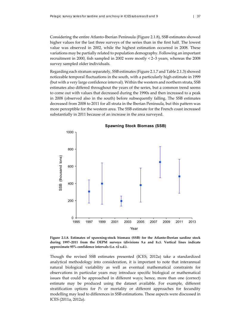
Pelagic survey series for sardine and anchovy in ICES subareas 8 and 9 | 37
Considering the entire Atlanto‐Iberian Peninsula (Figure 2.1.8), SSB estimates showed
higher values for the last three surveys of the series than in the first half. The lowest
value was observed in 2002, while the highest estimation occurred in 2008. These
variations may be partially related to population demography. Following an important
recruitment in 2000, fish sampled in 2002 were mostly < 2–3 years, whereas the 2008
survey sampled older individuals.
Regarding each stratum separately, SSB estimates (Figure 2.1.7 and Table 2.1.3) showed
noticeable temporal fluctuations in the south, with a particularly high estimate in 1999
(but with a very large confidence interval). Within the western and northern strata, SSB
estimates also differed throughout the years of the series, but a common trend seems
to come out with values that decreased during the 1990s and then increased to a peak
in 2008 (observed also in the south) before subsequently falling. The SSB estimates
decreased from 2008 to 2011 for all strata in the Iberian Peninsula, but this pattern was
more perceptible for the western area. The SSB estimate for the French coast increased
substantially in 2011 because of an increase in the area surveyed.
Figure 2.1.8. Estimates of spawning‐stock biomass (SSB) for the Atlanto‐Iberian sardine stock
during 1997–2011 from the DEPM surveys (divisions 9.a and 8.c). Vertical lines indicate
approximate 95% confidence intervals (i.e. ±2 s.d.).
Though the revised SSB estimates presented (ICES, 2012a) take a standardized
analytical methodology into consideration, it is important to note that interannual
natural biological variability as well as eventual mathematical constraints for
observations in particular years may introduce specific biological or mathematical
issues that could be approached in different ways; hence, more than one (correct)
estimate may be produced using the dataset available. For example, different
stratification options for P0 or mortality or different approaches for fecundity
modelling may lead to differences in SSB estimations. These aspects were discussed in
ICES (2011a, 2012a).
0
200
400
600
800
1000
1995 1997 1999 2001 2003 2005 2007 2009 2011 2013
SS
B (
tho
usa
nd
to
ns)
Year
Spawning Stock Biomass (SSB)

38 | ICES Cooperative Research Report No. 332
2.1.4 Present and future challenges
Egg production methods (EPMs) are used worldwide to evaluate the spawning‐stock
biomass of a variety of fish species (Stratoudakis et al., 2006), especially small pelagic
species, but also demersal fish (Armstrong et al., 2001; Jackson and Cheng, 2001). For
small pelagic fish, EPMs together with acoustic estimates of biomass (Simmonds and
MacLennan, 2005) are the fishery‐independent methods most commonly used for
biomass evaluation (Hampton, 1996; Barange et al., 2009). EPMs assist in management
by providing information that can be integrated into or used to inform the stock
assessment process. The DEPM was adopted for Atlanto‐Iberian sardines in the late
1980s (Miranda et al., 1990; Cunha et al., 1992; García et al., 1992) and has been used for
assessment ever since (ICES, 2012b). Methodological and analytical developments
have reduced bias and improved the precision of the estimates (which are now being
used in assessment modelling). The CVs for SSB calculated for the dataseries presented
(revised in 2012) were mainly below or around 30%, within the error range for EPMs
(Jacobson et al., 1994; Armstrong et al., 2001).
The Atlanto‐Iberian sardine DEPM series is still short and because it is conducted
triennially, it is more difficult to fully understand intersurvey fluctuations that could
eventually have an effect during assessment model fitting. Moreover, when
discrepancies between biomass estimation from acoustics surveying and DEPM are
apparent, the stability of the assessment model may be affected. Non‐concurrent
estimation by both methods has precluded thorough discussion on the potential causes
behind the differences in the estimates.
Future developments for the Atlanto‐Iberian sardine DEPM will consider
improvements in the estimations of mortality, e.g. external modelling (Bernal et al.,
2011b) and spawning fraction (stageing/ageing POFs, alternative estimators),
assessment of the validity of single‐survey estimations for S, R, and F vs. mean values
or modeled estimates, calculation of SSB estimates at age, spatially explicit P0
modelling, and the introduction of models with Bayesian approach and data
assimilation to include yearly observations. Furthermore, interannual and between‐
strata variability of the DEPM parameters will be addressed in an integrated approach
encompassing detailed environmental fluctuations, seasonal dynamics of reproductive
activity, and population demography.
The monospecific nature of each EPM application has been criticized in the context of
an ecosystem approach. However, EPM surveys are already providing, or have the
potential to deliver, a range of products (e.g. biological indices, oceanographic data,
foodweb indicators) to marine environment managers, particularly because of the
obligation to comply with the Marine Strategy Framework Directive (MSFD), and a
wealth of information for several scientific subjects (e.g. realized habitats, mortality,
connectivity, reproductive potential, population fluctuations, and ecosystem
modelling). There are good examples of the importance of egg production time‐series
in providing basic scientific data; the CalCOFI programme, for example, established in
1949, has promoted some of the most cited works in various aspects of marine pelagic
ecosystems.
2.1.5 Acknowledgements
We acknowledge the work carried out at the research institutes IEO and IPMA as well
as the crews of the research vessels used to collect the data. We are grateful to those
who contributed to Atlantic sardine biological sampling in the laboratory, egg staging,
histological processing of gonads tissues, otolith preparation, and age determination.

Pelagic survey series for sardine and anchovy in ICES subareas 8 and 9 | 39
Early surveys reported in this section were funded by each institute and national
research funding bodies, but most of the recent surveys were funded through the EU
Data Collection Framework (national programmes). Data collection coordination was
carried out under the auspices of the ICES study and working groups SGSBSA and
WGACEGG and the PELASSES research projects. The EU project SARDYN also
introduced considerable developments to DEPM estimation results. We also thank the
observers from SPEA who joined IPMA´s surveys since 2005, adding value with the
monitoring of birds and marine mammals. A special thanks to Miguel Bernal from IEO
and Yorgos Stratoudakis from IPMA for their long contribution to the development of
the sardine DEPM.

40 | ICES Cooperative Research Report No. 332
2.2 Spring acoustic surveys (PELAGO, PELACUS, PELGAS)
2.2.1 Introduction
Three acoustic surveys (PELGAS, PELACUS, and PELAGO) have been carried out
from Brest to Gibraltar in the northern East Atlantic since the 1980s. Coordinated by
WGACEGG since 2002, a great effort has been made to standardize the surveys so as
to allow the merging of their results. As such, global maps of species distributions are
provided for each year. In addition, from a specific assessment objective, despite the
different target species by surveys (sardine for Portugal and Spain or anchovy for
France), the institutes moved rapidly towards a pelagic community objective by fishing
to identify echoes (whatever the species was suspected to be) instead of fishing only to
obtain biological parameters when the target species was evident.
Three countries have been involved in the spring acoustic surveys:
France (IFREMER): PELGAS surveys
Spain (IEO): PELACUS surveys
Portugal (IPMA): PELAGO surveys
The global transect network can be seen in Figure 2.2.1 based on the 2010 surveys.
Transects are perpendicular to the coast and cover the entire shelf, which is wider in
the Bay of Biscay than along the Portuguese and Spanish coasts. Protocols of these
surveys are found in Annex 2.
The pelagic trawl fishing operations carried out during the three surveys (Figure 2.2.2)
show, from one year to another, the heterogeneity of species along the shelf, from
Brittany to Gibraltar.
The particularities or evolution of these acoustic spring surveys are described in the
following sections.

Pelagic survey series for sardine and anchovy in ICES subareas 8 and 9 | 41
0
Figure 2.2.1. Global transect network of PELGAS, PELACUS, and PELAGO acoustic surveys (2010
surveys shown as an example).

42 | ICES Cooperative Research Report No. 332
Figure 2.2.2. Species compositions by pelagic trawling during PELGAS, PELACUS, and PELAGO surveys from 2003 to 2012. Colour coding: light purple = boarfish;
green = anchovy; dark purple = blue whiting; blue = sardine; red = mackerel; black = sprat; yellow = horse mackerel; grey = herring.
2007 2003 2004 2005 2006
2008 2010 2011 2012 2009

Pelagic survey series for sardine and anchovy in ICES subareas 8 and 9 | 43
2.2.2 PELGAS surveys
Jacques Massé, Erwan Duhamel, Pierre Petitgas, Mathieu Doray, and Martin Huret
2.2.2.1 Introduction
IFREMER has conducted acoustic surveys in the Bay of Biscay since the early 1980s.
The intent was to develop the method and also describe the distribution of pelagic
species.
Acoustic surveys are carried out every spring in the Bay of Biscay on board the RV
“Thalassa”. Te objective of the PELGAS surveys has been to study the abundance and
distribution of pelagic fish in the Bay of Biscay. The main target species are anchovy
and sardine, but they are considered in a multispecies context and within an ecosystem
approach as these species are located in the centre of a pelagic ecosystem.
These surveys are connected with IFREMER programmes on data collection for
monitoring and management of fisheries and the ecosystem approach for fisheries.
This task is formally included in the first priorities defined by Council Regulation (EC)
No. 199/2008 of 6 November 2008 (EC, 2008), establishing the minimum and extended
Community programmes for the collection of data in the fisheries sector and laying
down detailed rules for the application of Council Regulation (EC) No. 1543/2000 (EC,
2000). These surveys must be considered in the framework of the IFREMER fisheries
ecology action” resources variability“, which is the French contribution to the
international GLOBEC programme.
Historically, IFREMER has been involved in acoustic surveys since the 1970s and
developed a numerical interface and software (INES‐MOVIES) in 1988 in order to save
echotraces and energies from a SIMRAD EK400 echosounder. A series of surveys was
then developed in the southern Bay of Biscay (1989–1994), mainly in order to produce
anchovy abundance indices for stock management considerations. In 1996, a new
research vessel (also called RV “Thalassa”) was available with considerable
possibilities for the collection of data on a large group of parameters: acoustics, biology,
behaviour, environmental factors. Therefore, aiming to discover the factors influencing
anchovy recruitment, two surveys were carried out (1997 and 1998) in different seasons
to analyse both the possibilities of this new research platform and factors of interest.
2.2.2.2 Survey methodology
In 2000, the first PELGAS survey was carried out, assembling IFREMER scientists as
well as national and international collaborations in an acoustic survey designed to
obtain abundance indices for the main pelagic species from the Spanish coast to the
western point of Brittany, and also to collect relevant oceanographic data aimed at
deriving ecosystem descriptors. Because of the common vertical migration and
scattering behaviour of fish (mainly anchovy) close to the surface at night, it is difficult
to separate fish from plankton inside a dense layer of plankton. Furthermore, being
located in the surface acoustic blind zone, an unknown quantity of fish became
inaccessible to the acoustic equipment.Therefore, priority was given to acoustic
exploration and fishing operations by day. All parameters collected along transects
during surveying were acceptable, and night‐time was free for other operations even
at stations (mainly physical, chemical, and plankton observations). Therefore, in order
to produce an optimum horizontal and vertical description of the area, surveys have
been carried out following the same transects and station network since 2000 (Figure

44 | ICES Cooperative Research Report No. 332
2.2.3) in order to characterize the pelagic ecosystem at each trophic level. This was
achieved through two types of action:
1. Daylight: continuous acquisition along transects of acoustic data, seawater
characteristics, and number of fish eggs by pumping under the surface using a
CUFES system (continuous underway fish egg sampler). Concurrently, visual
counting and identification of cetaceans (from the vessel) and birds (by plane) is
carried out in order to characterize the higher‐level predators of the pelagic
ecosystem.
2. Night‐time: discrete sampling at stations (by trawls, plankton nets, CTD) of the
whole water column.
Figure 2.2.3. Acoustics, surface hydrology, and CUFES are operated along transects (in red), and
vertical profiles are implemented at stations (blue stars) during PELGAS surveys on board RV
“Thalassa”.
Satellite imagery (sea surface temperature and chlorophyll concentration derived from
MODIS sea colour) and modelling are also used before and during the cruise to
recognize the main physical and biological structures and to improve the sampling
strategy.
As specified previously, acoustic data are only collected during daylight in systematic
parallel transects perpendicular to the French coast at ten knots. The length of the
ESDU (elementary sampling distance unit) is one mile, while the transects are
uniformly spaced by twelve nautical miles and cover the continental shelf from 20 m
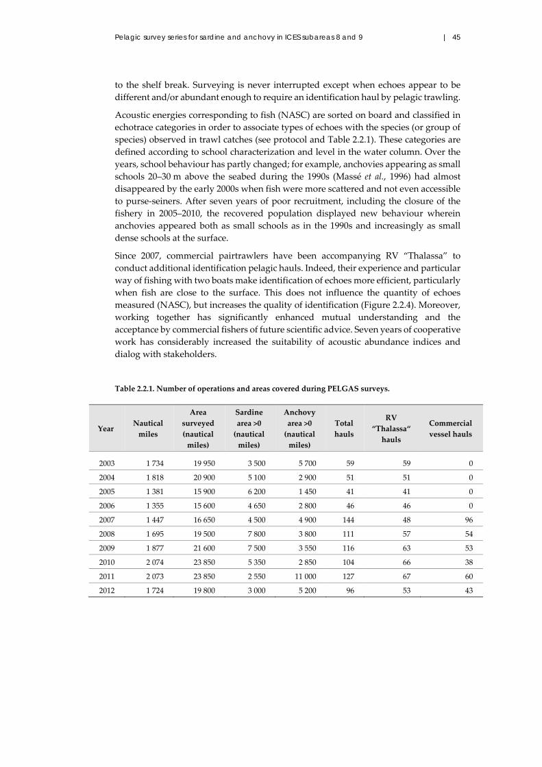
Pelagic survey series for sardine and anchovy in ICES subareas 8 and 9 | 45
to the shelf break. Surveying is never interrupted except when echoes appear to be
different and/or abundant enough to require an identification haul by pelagic trawling.
Acoustic energies corresponding to fish (NASC) are sorted on board and classified in
echotrace categories in order to associate types of echoes with the species (or group of
species) observed in trawl catches (see protocol and Table 2.2.1). These categories are
defined according to school characterization and level in the water column. Over the
years, school behaviour has partly changed; for example, anchovies appearing as small
schools 20–30 m above the seabed during the 1990s (Massé et al., 1996) had almost
disappeared by the early 2000s when fish were more scattered and not even accessible
to purse‐seiners. After seven years of poor recruitment, including the closure of the
fishery in 2005–2010, the recovered population displayed new behaviour wherein
anchovies appeared both as small schools as in the 1990s and increasingly as small
dense schools at the surface.
Since 2007, commercial pairtrawlers have been accompanying RV “Thalassa” to
conduct additional identification pelagic hauls. Indeed, their experience and particular
way of fishing with two boats make identification of echoes more efficient, particularly
when fish are close to the surface. This does not influence the quantity of echoes
measured (NASC), but increases the quality of identification (Figure 2.2.4). Moreover,
working together has significantly enhanced mutual understanding and the
acceptance by commercial fishers of future scientific advice. Seven years of cooperative
work has considerably increased the suitability of acoustic abundance indices and
dialog with stakeholders.
Table 2.2.1. Number of operations and areas covered during PELGAS surveys.
Year Nautical
miles
Area
surveyed
(nautical
miles)
Sardine
area >0
(nautical
miles)
Anchovy
area >0
(nautical
miles)
Total
hauls
RV
“Thalassa“
hauls
Commercial
vessel hauls
2003 1 734 19 950 3 500 5 700 59 59 0
2004 1 818 20 900 5 100 2 900 51 51 0
2005 1 381 15 900 6 200 1 450 41 41 0
2006 1 355 15 600 4 650 2 800 46 46 0
2007 1 447 16 650 4 500 4 900 144 48 96
2008 1 695 19 500 7 800 3 800 111 57 54
2009 1 877 21 600 7 500 3 550 116 63 53
2010 2 074 23 850 5 350 2 850 104 66 38
2011 2 073 23 850 2 550 11 000 127 67 60
2012 1 724 19 800 3 000 5 200 96 53 43

46 | ICES Cooperative Research Report No. 332
Three modes of acoustic observations are stored during PELGAS surveys:
six split‐beam vertical echosounders (EK60) with frequencies of 18, 38, 70,
120, and 200 kHz (adding 333 kHz since 2009);
one horizontal echosounder on the starboard side for surface echotraces
(120 kHz);
one SIMRAD ME70 multibeam echosounder (32 × 2°beams, 70–120 kHz),
used essentially for visualization to observe the behaviour and aggregation
pattern of fish schools during the survey; only echoes stored from the
vertical echosounder (38 kHz) were used for abundance index calculation.
Figure 2.2.4. Fishing operations and catch composition during PELGAS12 by RV “Thalassa” alone
(left) and with pairtrawlers (right).
Energies and samples provided by all sounders are simultaneously visualized and
stored using the MOVIES+ and MOVIES3D software packages and stored at the same
standard hydroacoustic data format (HAC). Sea surface temperature, as well as surface
salinity and fluorometry are also stored simultaneously.
NASC are allocated by species according to echotype classification and catches,
applying TS–length relationships from the literature (see Table A2.1).
The calibration method was the same every year and performed at anchorage, usually
in the Concarneau bay, in the South of Brittany, in optimum meteorological conditions
at the end of the survey.
Since 2003, top predators have also been observed because of the collaboration of
PELAGIS (La Rochelle University, previously called CRMM), during both PELGAS
and PELACUS surveys. Therefore, marine mammals, birds, and litters are
simultaneously located, identified, and counted (see Section 2.2.5).
During night‐time stations (Figure 2.2.3), vertical profiles are carried out with
associated CTD and laser optical plankton counter (LOPC) followed by vertical fishing
with a 315‐μ WP2 plankton net. Samples are filtered and preserved for further
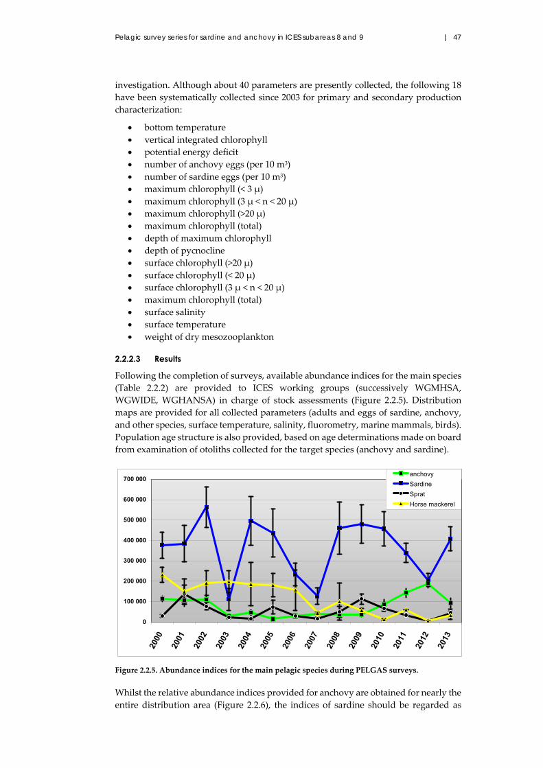
Pelagic survey series for sardine and anchovy in ICES subareas 8 and 9 | 47
investigation. Although about 40 parameters are presently collected, the following 18
have been systematically collected since 2003 for primary and secondary production
characterization:
bottom temperature
vertical integrated chlorophyll
potential energy deficit
number of anchovy eggs (per 10 m3)
number of sardine eggs (per 10 m3)
maximum chlorophyll (< 3 μ)
maximum chlorophyll (3 μ < n < 20 μ)
maximum chlorophyll (>20 μ)
maximum chlorophyll (total)
depth of maximum chlorophyll
depth of pycnocline
surface chlorophyll (>20 μ)
surface chlorophyll (< 20 μ)
surface chlorophyll (3 μ < n < 20 μ)
maximum chlorophyll (total)
surface salinity
surface temperature
weight of dry mesozooplankton
2.2.2.3 Results
Following the completion of surveys, available abundance indices for the main species
(Table 2.2.2) are provided to ICES working groups (successively WGMHSA,
WGWIDE, WGHANSA) in charge of stock assessments (Figure 2.2.5). Distribution
maps are provided for all collected parameters (adults and eggs of sardine, anchovy,
and other species, surface temperature, salinity, fluorometry, marine mammals, birds).
Population age structure is also provided, based on age determinations made on board
from examination of otoliths collected for the target species (anchovy and sardine).
Figure 2.2.5. Abundance indices for the main pelagic species during PELGAS surveys.
Whilst the relative abundance indices provided for anchovy are obtained for nearly the
entire distribution area (Figure 2.2.6), the indices of sardine should be regarded as
0
100 000
200 000
300 000
400 000
500 000
600 000
700 000
2000
2001
2002
2003
2004
2005
2006
2007
2008
2009
2010
2011
2012
2013
anchovy
Sardine
Sprat
Horse mackerel

48 | ICES Cooperative Research Report No. 332
partial since the potential sardine distribution area at the time of the surveys can extend
to more northern areas (Figure 2.2.7). Sardine distribution would, therefore, be
representative of only that part of the stock present in the area covered at the time of
the survey.
Table 2.2.2. Acoustic biomass indices (t) and coefficients of variation provided for the main pelagic
fish species during the PELGAS surveys.
Species 2003 2004 2005 2006 2007 2008 2009 2010 2011 2012
Anchovy 30 632 45 965 14 643 30 877 40 876 37 574 34 855 86 354 142 601 186 865
CV 0.13 0.17 0.17 0.14 0.10 0.16 0.11 0.15 0.08 0.05
Sardine 111 234 496 371 435 287 234 128 126 237 460 727 479 684 457 081 338 468 205 627
CV 0.24 0.12 0.14 0.12 0.16 0.14 0.10 0.09 0.07 0.08
Sprat 23 994 15 807 72 684 30 009 17 312 50 092 112 497 67 046 34 726 6 417
CV 0.20 0.18 0.23 0.16 0.13 0.27 0.11 0.11 NA NA
Horse
mackerel 198 528 186 046 181 448 156 300 45 098 100 406 56 593 11 662 61 237 7 435
CV 0.14 0.29 0.16 0.32 0.07 0.46 0.09 0.19 NA NA
Blue
whiting 1 953 12 267 26 099 1 766 3 545 576 4 333 48 141 11 823 68 533
CV 0.13 0.20 0.59 0.21 0.15 0.25 0.22 0.07 NA NA
Nevertheless, for both species (anchovy and sardine), cohorts can be followed over the
years as shown in Figure 2.2.8. For sardine, cohorts can be traced for up to five years,
even if the abundance index is not accurate. This means that, despite the partial
coverage of the spatial distribution by PELGAS, the index provides relevant
information on the sardine stock dynamics, particularly with respect to the level and
contribution of the recruitment to the total stock over years.

Pelagic survey series for sardine and anchovy in ICES subareas 8 and 9 | 49
Figure 2.2.6. Distribution of anchovy (NASC) during PELGAS acoustic surveys.

50 | ICES Cooperative Research Report No. 332
Figure 2.2.7. Distribution of sardine (NASC) during PELGAS acoustic surveys.

Pelagic survey series for sardine and anchovy in ICES subareas 8 and 9 | 51
Figure 2.2.8. Age distribution of anchovy (left) and sardine (right) as observed during PELGAS
surveys.
Since the beginning of the series (2000), anchovy and sardine eggs were counted during
daylight (Figure 2.2.9) using a continuous underway fish egg sampler (CUFES)
(Checkley et al., 1997). This system was acquired as a result of special funding in the
framework of the PELASSES European project. It was first attached with a stick at
3.5 m depth along the hull and, since 2003, has been attached directly to the hull by an
internal adaptation at 5 m depth. The mesh in the CUFES collector was initially 500 μ,
but, following a suggestion by AZTI, two parallel CUFES were used (500 and 315 μ)
from 2003 until 2006, when a 315‐μ collector was finally adopted. Samples were
collected every 3 nautical miles along transects and preserved in 4% formaldehyde for
further processing.
Figure 2.2.9. Cumulative number of eggs 10 m–3 counted during PELGAS surveys for anchovy
(green on the right) and for sardine (blue on the left). The sampling unit was 3 nautical miles.
2.2.2.4 Acknowledgements
PELGAS surveys were funded partially by the EU programme DCF. We thank all
scientists and students who participated in the PELGAS surveys and the crew of RV
“Thalassa”.
2.2.3 PELACUS surveys
Magdalena Iglesias, Isabel Riveiro, María Begoña Santos, Miguel Bernal, Pablo
Carrera, Joan Miquel, Dolores Oñate, Nuria Díaz, and Ana Ventero
2.2.3.1 From SARACUS to PELACUS: Spanish acoustic surveys
Although echosounders for fish detection have been used by the Spanish commercial
fleets since the 1950s, their use for scientific purposes only began in the 1980s. At the
beginning of this decade, the Instituto Español de Oceanografía (IEO), together with
its Portuguese counterpart Instituto Nacional de Investigaçao das Pescas (INIP, then
IPIMAR, and now IPMA) started a series of projects targeting sardine, with the main

52 | ICES Cooperative Research Report No. 332
goal of improving biological knowledge and providing a fishery‐independent index
for its assessment (ICES, 1980).
In this context and, given the behaviour of the sardine shoals, scientific echosounders
coupled with digital echointegrators were used following the methodology proposed
by Dragesund and Olsen (1965) to achieve an assessment based on echointegration
estimates (Midttun and Nakken, 1968; Nakken and Dommasnes, 1977).
The first challenge was to determine the relationship between target strength (TS) and
length for sardine. In situ TS measurements and cage trials were carried out, although
given both the physiological and biological proximity between sardine and herring
(Clupea harengus) and also the similarity in results, the TS–length relationship estimated
by Degnbol et al. (1985) for herring was finally adopted (ICES, 1988).
The first joint acoustic survey took place in August 1982 (Table 2.2.3) on RV “Noruega”
(Portugal) and RV “Cornide de Saavedra” (Spain). This first survey covered only the
Atlantic waters of the Iberian Peninsula, i.e. Galician (northwestern Spain) and
Portuguese waters, targeting mainly juvenile sardines to achieve an estimate of
recruitment strength. Both vessels were equipped with Simrad EK‐400 scientific
echosounders working at 38 kHz (in addition, RV “Cornide de Saavedra” had a second
echosounder working at 120 kHz) coupled with a Simrad QD+QX digital echo
integrator.
In order to standardize methods and analyse data, the Planning Group for Acoustic
Surveys in ICES Subareas VIII and IX met for the first time in 1986 (ICES, 1986a). The
group adopted a value of b20 = –72.6 dB for sardine and, in addition, biomass estimates
were established at fixed strata (this methodology had already been in use in previous
years). The surveyed area was divided into sectors of ca. 10–30 nautical miles width,
depending on geographical and oceanographic characteristics. Each sector was
divided into depth strata (20–50, 50–100, 100–200, and 200–500 m). Within each sector,
at least one track perpendicular to the coast (i.e. crossing all depth strata) was included.
For practical reasons, rather than random allocation, a systematic survey design, either
in zigzag or parallel, was adopted. Biomass was then estimated for each sector and
depth stratum according to Nakken and Dommasnes (1977), using the mean (either
arithmetic or geometric) integrated value, the area expressed in square nautical miles,
and the length distribution provided from the neighbouring fishing stations. In cases
when fishing stations were not available, length distributions from commercial purse‐
seine fleets were used.
The first acoustic survey covering the waters off the northern and northwestern
Spanish coast (Atlantic and Cantabrian waters) was carried out in August 1983. This
survey targeted young of the year sardine and was the starting point of the SARACUS
(SARdine ACoUStic in Spanish waters) survey series. From 1983 to 1985, the surveys
were conducted in August. In 1986, a new strategy was adopted to increase survey
effort. Two SARACUS surveys took place: the first one in spring to obtain an estimate
of sardine spawning biomass and the second in November to obtain an estimate of
recruitment strength. While Portugal performed both surveys for several years, IEO
focused its efforts only in spring after 1987. All surveys from 1983 to 1990 were carried
out on RV “Cornide de Saavedra”, except in 1990 when RV “Ignat Pavliuchenvok” was
used due to the refitting of the Spanish vessel. For the same reason, there was no survey
in 1989.
In 1991, IEO purchased the new Simrad EK‐500, a fully compact digital echosounder‐
echo integrator. This equipment, with better dynamic range and control settings,

Pelagic survey series for sardine and anchovy in ICES subareas 8 and 9 | 53
allowed the surveyed area to be extended to a depth of 1000 m. Although this
improvement gave access to the main distribution area of new commercial target
species such as horse mackerel (Trachurus trachurus), Atlantic mackerel (Scomber
scombrus), blue whiting (Micromesistius poutassou), and anchovy, only anchovy and
blue whiting, together with sardine, were routinely assessed. Accordingly, the time‐
series changed its name to PELACUS (PELagic ACoUStic in northwestern Spanish
waters). Survey durations increased to deal with these new objectives. The number of
fishing stations increased as well, with new pelagic gear being used, CTD being
deployed, and, as in previous years, acoustic data were collected both during day and
night. In 1993, the assessment methodology was changed and, instead of estimates
been calculated for fixed strata, estimates were based on the true distribution area.
However, for comparison purposes, results were given by ICES division (divisions 9.a
North, 8.c West, 8.c East [western part], and 8.c East [eastern part]). During 1994–1996,
the survey design and objectives were again changed and, although SEFOS (Shelf Edge
Fisheries and Oceanography Studies) in 1994 and 1996 took place in spring, both
surveys focused on blue whiting distribution. This objective meant that the area
surveyed covered mainly the shelf‐break area from the Spanish–Portuguese border to
Brittany. The acoustic estimate of sardine abundance and biomass was again the
objective of the survey carried out in 1995 (IBERSAR 95) that took place on RV
“Noruega”.
From 1997 to 2012, PELACUS was carried out on RV “Thalassa”, a new French–
Spanish vessel. This modern ship presented advantages over the older vessels (silent
diesel‐electric engine and fixed‐blade propeller) together with improved fishing
facilities that resulted in a notable increase in the number of survey objectives. This
vessel was also used for the French acoustic survey (PELGAS). Since 1998, the Planning
Group for Pelagic Acoustic Surveys in ICES Subareas VIII and IX, attended until then
only by Spanish and Portuguese scientists, incorporated French scientists (ICES, 1999).
As a first joint recommendation, the Planning Group agreed that acoustic data would
only be recorded during daylight, leaving the night‐time available for physical,
chemical, and plankton characterization of the water column. This recommendation
was implemented in 1998. In 2000, under the framework of the DG FISH PELASSES
project, the spring acoustic surveys incorporated the CUFES together with the routine
collection of other systematic measurements (e.g. SSS, SST, fluorometry, CTD rosette
casts, plankton hauls to determine primary production, or dry weight at different sizes
among other biological descriptors of the water column). In addition, 120‐kHz
frequency began to be used to help discriminate between different fish species. During
this period, acoustic estimates were also provided for non‐commercial species.
In 2005, RV “Thalassa” was equipped with the new EK60 together with a series of new
transducers (18, 70, and 200 kHz).
In 2007, a new team used the survey as a platform to obtain data on presence,
abundance, and behaviour of top predators (marine mammals and seabirds). Since
2007, data have also been routinely collected on floating litter (type, number, and
position) and on other human pressures such as fishing (e.g. number of boats, type,
activity).

54 | ICES Cooperative Research Report No. 332
Table 2.2.3. Acoustic surveys undertaken before 2003 in northwestern Spanish waters.
Survey Year Month RV Target
species Equipment
Survey
design
Depth
(m)
PILCHARD 1982 August CS PIL EK‐400 Parallel 30–500
SARACUS 1983 August CS PIL EK‐400 Parallel 30–500
SARACUS 1984 August CS PIL EK‐400 Parallel 30–500
SARACUS 1985 August CS PIL EK‐400 Parallel 30–500
SARACUS 1986 March CS PIL EK‐400 Parallel 30–500
SARACUS 1986 September CS PIL EK‐400 Parallel 30–500
SARACUS 1987 February CS PIL EK‐400 Parallel 30–500
SARACUS 1988 April CS PIL EK‐400 Parallel 30–500
IBERSAR1 1989 November N PIL EK‐400 Parallel 30–500
SARACUS 1990 April–May IP PIL EK‐400 Parallel 30–500
PELACUS 1991 March CS PIL,
WHB EK‐500 Zigzag 30–1 000
IBERSAR2 1991 November N PIL EK‐400 Parallel 30–500
PELACUS 1992 April–May CS PIL,
WHB EK‐500 Zigzag 30–1 000
PELACUS 1993 April–May CS PIL,
WHB EK‐500 Zigzag 30–1 000
SEFOS 1994 March–April CS WHB EK‐500 Zigzag 150–1 000
IBERSAR 1995 May N PIL EK‐500 Parallel 30–500
SEFOS 1996 March–April CS PIL,
WHB EK‐500 Parallel 30–1 000
PELACUS 1997 March T All EK‐500 Parallel 30–1 000
PELACUS 1998 March T All EK‐500 Parallel 30–1 000
PELACUS 1999 March T All EK‐500 Parallel 30–1 000
PELACUS 2000 March T All EK‐500 Parallel 30–1 000
PELACUS 2001 April T All EK‐500 Parallel 30–1 000
PELACUS 2002 March T All EK‐500 Parallel 30–1 000
1Suspended due to bad weather conditions. 2Only divisions 8.c West and 9.a North. Research vessels: “Cornide de Saavedra” (CS), “Noruega” (N), “Ignat Pavliuchenkov”(IP), “Miguel Oliver” (MO). Pelagic species: Sardina pilchardus (PIL), Micromesistius poutassou (WHB), pelagic community (All).
Since the beginning of the time‐series (1982), biological data (length, weight, sex,
maturity, etc.) and samples obtained from individual fish caught in hauls have been
used to construct length–weight and age–length relationships needed for the
assessment of sardines and all other target species. Fish stomachs have also been
routinely examined to quantify the trophic relationships between species, and isotope
analysis of sardine and anchovy muscle have been also carried out to study their
trophic position.
The evolution of the survey design and objectives has transformed this survey series
into an essential platform for integrated data collection following the requirements
posed by the ecosystem approach to fisheries management, the Marine Strategy
Framework Directive (2008/56/CE), and the revised CFP.

Pelagic survey series for sardine and anchovy in ICES subareas 8 and 9 | 55
Acoustic data presented in this report include estimates of abundance, distribution,
and mean size for the eleven main pelagic species found in northern and northwestern
Spanish waters.
2.2.3.2 Methods
The survey design consists of a grid of parallel transects, eight nautical miles apart and
perpendicular to the coastline, and covering the continental shelf up to a depth of
200 m. The starting point of each transect is located close to the coast (1–1.5 nautical
miles from the shoreline), although the exact location can be modified due to adverse
weather conditions or the presence of shallows. The end point of each transect can be
also extended if shoals are detected in deeper waters. Table 2.2.4 and Figure 2.2.10
show the main features of the survey series.
Table 2.2.4. Acoustic surveys undertaken during 2003–2012 in northwestern Spanish waters.
Survey Year Month RV Target
species Equipment
Survey
design
Depth
(m)
PELACUS 2003 March–
April T All EK‐500 Parallel 30–200
PELACUS 2004 April T All EK‐500 Parallel 30–200
PELACUS 2005 April T All EK‐60 Parallel 30–200
PELACUS 2006 April T All EK‐60 Parallel 30–200
PELACUS 2007 April T All EK‐60 Parallel 30–200
PELACUS 2008 April T All EK‐60 Parallel 30–200
PELACUS 2009 April T All EK‐60 Parallel 30–200
PELACUS 2010 April T All EK‐60 Parallel 30–200
PELACUS 2011 April T All EK‐60 Parallel 30–200
PELACUS 2012 April T All EK‐60 Parallel 30–200
Figure 2.2.10. Spanish acoustic transects (in black) and ICES divisions (9.a N; 8.c W; 8.c EW [western
part]; 8.c EE [eastern part]) considered for abundance estimation (in red).

56 | ICES Cooperative Research Report No. 332
Acoustic records were obtained during daylight together with egg samples from a
CUFES, with an internal water intake located at 5 m depth. In addition, pelagic trawl
hauls were performed opportunistically to verify the acoustic data.
2.2.3.2.1 Acoustic equipment
Acoustic equipment consisted initially of a Simrad EK‐500 and then a EK‐60 scientific
echosounder, first operating at 38 and 120 kHz, and then increasing the number of
frequencies used since 2005 (including 18, 70, and 200 kHz). All frequencies were
calibrated according to standard procedures. The elementary sampling distance unit
(ESDU) was fixed at 1 nautical mile. Acoustic data were obtained only during daylight
at a survey speed of 8–10 knots. Data were stored in raw format and post‐processed
using Sonar Data Echoview software (Myriax Ltd.). Fish abundance was calculated
with the 38 kHz frequency as recommended by the Planning Group on Aerial and
00Acoustic Surveys for Mackerel (ICES, 2002b), although echograms from 18, 120, and
200 kHz frequencies were used to visually discriminate between fish and other scatter‐
producing objects such as plankton or bubbles, and to distinguish different fish
according to the strength of their echo at each frequency. The 38, 70, and 120 kHz
frequencies were also used to create a mask, allowing better discrimination among fish
species and plankton. The threshold used to scrutinize the echograms was –70 dB. The
integration values were expressed as nautical area scattering coefficient (NASC) units
or acoustic area backscattering coefficient (sA) values (m2 nautical mile–2) (MacLennan
et al., 2002).
2.2.3.2.2 NASC allocation
Several pelagic gears were used during the survey series, both to identify species and
size classes responsible for the acoustic energy detected and to provide samples. The
choice of net was also dependent on the availability of rather unobstructed ground
over which the net could be deployed and recovered, allowing for effective fishing.
Haul duration was variable and ultimately depended on the number of fish entering
the net and the conditions under which the fishing took place, with attempts being
made to always achieve a minimum of 20 min. fishing. The quality of the hauls for
verifying acoustic data was classified according to catch composition in numbers and
length distribution of the fish caught.
Hauls considered to best represent the fish community for a specific area were used to
allocate NASC of each ESDU within this area. This process involved the method of
Nakken and Dommasnes (1977) for multiple species, but instead of using the mean
backscattering cross section, the full length class distribution (0.5 cm length classes)
were used as follows:
⋅
∑ ⋅ (2.2.1)
where wli is the proportion in number of the length class l and species i in the hauls,
and σbs is the corresponding proportion of backscattering cross section. This is related
to the target strength (TS) as follows:
10 ⁄ (in dB) (2.2.2)
This is computed from the formula TS = 20 logLT + b20 (Simmonds and MacLennan,
2005), where LT is the length class (0.5 cm). The b20 values for the most important
species present in the area are shown in Table A2.2.

Pelagic survey series for sardine and anchovy in ICES subareas 8 and 9 | 57
2.2.3.2.3 Echo integration estimates
With the backscattering energy allocated to fish species, the spatial distribution for
each species was analysed, taking into account both the NASC values and the length
frequency distributions (LFD) to provide homogeneous assessment polygons. These
were calculated as follows: an empty track determines the along‐coast limit of the
polygon, whilst three consecutive empty ESDUs determine a gap or the across‐coast
limit. Within each polygon, LFD is analysed.
LFD were obtained for all positive hauls for a particular species (either from the total
catch or from a representative random sample of 100–200 fish). For the purpose of
acoustic assessment, only those LFD which were based on a minimum of 30
individuals and/or a normal distribution were considered. Differences in probability
density functions (PDF) were tested using the Kolmogorov–Smirnoff (K–S) test. PDF
distributions without significant differences were joined, providing homogeneous PDF
strata. Spatial distribution was then analysed within each stratum and, finally, the
mean sA value and the surface (nautical miles2) were calculated using the GIS system‐
based ArcGis 9.3. These values, together with the length distributions, were used to
calculate fish abundance in numbers, as described in Nakken and Dommasnes (1977).
Numbers were converted into biomass using the length–weight relationship. Biomass
estimation was carried out for each stratum (polygon) using the arithmetic mean of the
backscattering energy (NASC, sA) attributed to each fish species and the surface
expressed in nautical miles2. For purposes of comparison, results are given by ICES
divisions (9.a North, 8.c West, 8.c East [western part], 8.c East [eastern part], and 8.b;
see Figure 2.2.10).
Otoliths were taken from anchovy, sardine, horse mackerel, blue whiting, hake
(Merluccius merluccius), and Atlantic mackerel in order to determine age and to obtain
the age–length key for each species and area.
Other biological variables such as maturity, stomach repletion, content and colour, and
fat content are routinely registered for sardine, Atlantic mackerel, horse mackerel,
hake, blue whiting, and other pelagic species.
2.2.3.2.4 CUFES counts
Samples from CUFES were collected every three nautical miles during acoustic surveys
of the transects. After the sample was taken, it was fixed in a buffered 4% formaldehyde
solution. Anchovy and sardine eggs were sorted, counted, and preserved in the same
solution. The remaining ichthyoplankton (other eggs and larvae) were also preserved
in the same way.
2.2.3.2.5 Plankton and hydrological characterization
Continuous records of SSS, SST, and fluorometry were taken using a SeaBird
Thermosalinograph coupled with a Turner fluorometer. Plankton and CTD + bottle
rosette for water sample casts were performed at night. Five stations of the acoustic
survey were placed over the transects, but were extended onto open waters until the
1000–2000 m isobaths. The stations were evenly distributed over the surveyed area at
a distance of 16–24 nautical miles.
Plankton was sampled using several nets (Bongo, WP2, and CalVet). Fractionated
dried biomass was calculated at 53–200, 200–500, 500–1000, and >2000 μm fractions,
together with species composition and taxonomic groups at fixed strata from samples
collected at the CTD + bottle rosette carrousel (pico and nanoplankton, microplankton,

58 | ICES Cooperative Research Report No. 332
and mesozooplankton). For this purpose, FlowCAM, LOPC, and Zoo‐Image
techniques were used.
Water samples were stored at −20°C for further analysis of dissolved nutrients (NO3,
NO2, P, NH4+, SiO4).
Top predator observations: three observers, working in turns of two, are placed above
the bridge of the vessel at a height of 16 m above sea level, surveying an area of 180°
(each observer covers a field of 90°). Observations are carried out by sight, although
binoculars are used (7 × 50) to confirm species identification and determine predator
behaviour. Observations are carried out during daylight while the vessel surveys the
transects and covers the distance between transects at an average speed of 10 knots.
Observers record species, number of individuals, behaviour, distance to the vessel,
angle to the trackline, and observation conditions (windspeed and direction, sea state,
visibility, etc.). Observers also record presence, number, and type of boats and type,
size, and number of floating litter. The same methodology is used on the PELGAS
surveys, and both observer teams shared a common database.
2.2.3.3 Results and discussion
The pelagic fish community in northwestern Spanish waters, as derived from
PELACUS (2003–2012), is mainly characterized by sardine, Atlantic mackerel, and
horse mackerel, together with bogue, blue whiting, and boarfish (Capros aper), whilst
anchovy, Mediterranean horse mackerel, chub mackerel, and blue jack mackerel have
only appeared occasionally. Besides, since the 1990s, the number of direct echotrace
allocations to species from the echogram scrutiny has decreased, mainly due to a
change in the aggregation pattern. This change, together with the change in survey
objectives to assess the main pelagic fish species, has led to an increase in the number
of fishing stations for echotrace identification (shown in Table 2.2.5 and Figures 2.2.11
and 2.2.12), aimed at increasing precision in the echotrace analysis.
Sardine abundance estimated in PELACUS in ICES divisions 9.a N and 8.c is used as a
relative fishery‐independent index for assessment purposes. This index shows a
decreasing trend during the time‐series in both abundance and distribution area
(Figures 2.2.13–2.2.17). The increase in 2008 was mainly due to the strength of the 2004
year class (Figure 2.2.18).
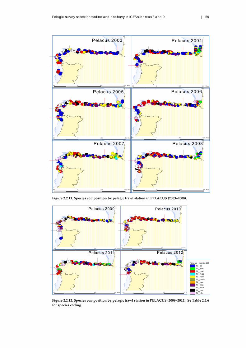
Pelagic survey series for sardine and anchovy in ICES subareas 8 and 9 | 59
Figure 2.2.11. Species composition by pelagic trawl station in PELACUS (2003–2008).
Figure 2.2.12. Species composition by pelagic trawl station in PELACUS (2009–2012). Se Table 2.2.6
for species coding.
# ### #
##
#
#
#
#
#
#
# ##
##
#
##
#
##
###
#
#
#
#
#
#
#
#
##
###
# ##
###
#
# #
# #
# ##
# # ##
#
#
##
#
#
#
#
##
##
#
##
## #
###
##
# ### ## #
###
##
#
#
200 0 200 400 Mi les
Pelacus 2003
# ### #
##
#
#
#
#
#
#
# ##
##
#
##
#
##
###
#
#
#
#
#
#
#
#
##
###
###
# #
###
#
#
###
####
#
#
# #
#
## # #
#
# ##
##
#
##
#
# # #
#
###
# # ## # # #
# ##
#
# ##
#
###
## #
#
##
200 0 200 400 Miles
Pelacus 2004
# ### #
##
#
#
#
#
#
#
# ##
##
#
##
#
##
###
#
#
#
#
#
#
#
#
## #
# ##
## ##
#
##
#####
#
##
##
####
##
##
###
#
#
#
# #### #
#### # ## #
# #
#
# ### # ## # #
##
#
#
# # ##
##
#
# #
200 0 200 400 Miles
Pelacus 2005
# ### #
##
#
#
#
#
#
#
# ##
##
#
##
#
##
###
#
#
#
#
#
#
#
#
##
#
###
## #
# #
# # #
##
#
##
#
#
##
##
##
#
##
#
##
# ##
# ##
#
##
#
# ##
###
# # ## #
# # #
####
200 0 200 400 Mi les
Pelacus 2006
# ### #
##
#
#
#
#
#
#
# ##
##
#
##
#
##
###
#
#
#
#
#
#
#
#
#
##
#
## ##
##
##
###
# # #
# #
#
##
#
#
#
#
#
##
##
#
#
# # #
##
##
## #
## # ##
#
# #
###
##
200 0 200 400 Miles
Pelacus 2007
# ### #
##
#
#
#
#
#
#
# ##
##
#
##
#
##
###
#
#
#
#
#
#
#
#
##
##
##
#
#
###
#
##
## #
#
#
#
#
## #
#
##
##
##
#
#
#
# #
##
##
##
#
#
# ##
# # ## # ### #
# ## #
##
#
200 0 200 400 Mi les
Pelacus 2008
# ### #
##
#
#
#
#
#
#
# ##
##
#
##
#
##
###
#
#
#
#
#
#
#
#
#
# ###
# ##
###
#
#
##
##
##
#
##
#
## #
## #
#
#
## #
###
#
##
###
#
###
# ## # # # # #
# ##
## #
#
200 0 200 400 Mi les
Pelacus 2009
# ### #
##
#
#
#
#
#
#
# ##
##
#
##
#
##
###
#
#
#
#
#
#
#
#
##
#
#
#
#
####
#
##
## #
##
##
# ##
##
#
#
#
# #
#
## #
##
#
## #
## #
## ###
#### # ## #
## #
## #
#
200 0 200 400 Mi les
Pelacus 2010
# ### #
##
#
#
#
#
#
#
# ##
##
#
##
#
##
###
#
#
#
#
#
#
#
#
#
#
##
##
#
#
#
# #
#
#
#
# ### #
# ##
##
#
#
##
# #
##
#
# ##
## #
# # ###
## # # # #
#
200 0 200 400 Mi les
Pelacus 2011
# ### #
##
#
#
#
#
#
#
# ##
##
#
##
#
##
###
#
#
#
#
#
#
#
#
#
# #
#
##
##
##
##
##
# #
###
#
# ##
#
#
## # #
##
##
##
### #
# # #
## ## #
# ## #
#
###
200 0 200 400 M
Pelacus 2012
Pescas ︳totales.dbfN ︳p ilN ︳aneN ︳macN ︳masN ︳homN ︳hmmN ︳jaaN ︳bogN ︳whbN ︳bocN ︳hke

60 | ICES Cooperative Research Report No. 332
Table 2.2.5. Number of fishing hauls carried out in PELACUS (2003–2012).
Year Survey
start
Survey
end
Target
species Echosounder
Fishing
operations
Sardine‐
positive fishing
operations
2003 20 March 10 April Pelagic
community
EK‐500 30 13
2004 30 March 23 April Pelagic
community
EK‐500 31 21
2005 6 April 28 April Pelagic
community
EK‐60 45 20
2005 3 April 26 April Pelagic
community
EK‐60 52 22
2007 29 March 22 April Pelagic
community
EK‐60 49 16
2008 27 March 22 April Pelagic
community
EK‐60 56 35
2009 28 March 20 April Pelagic
community
EK‐60 59 25
2010 27 March 20 April Pelagic
community
EK‐60 62 25
2011 27 March 20 April Pelagic
community
EK‐60 51 10
2012 29 March 20 April Pelagic
community
EK‐60 54 6
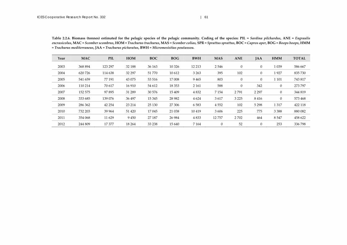
ICES Cooperative Research Report No. 332 | 61
Table 2.2.6. Biomass (tonnes) estimated for the pelagic species of the pelagic community. Coding of the species: PIL = Sardina pilchardus, ANE = Engraulis encrasicolus, MAC = Scomber scombrus, HOM = Trachurus trachurus, MAS = Scomber colias, SPR = Sprattus sprattus, BOC = Capros aper, BOG = Boops boops, HMM = Trachurus mediterraneus, JAA = Trachurus picturatus, BWH = Micromesistius poutassou.
Year MAC PIL HOM BOC BOG BWH MAS ANE JAA HMM TOTAL
2003 368 894 123 297 32 188 36 163 10 326 12 213 2 546 0 0 1 039 586 667
2004 620 726 114 638 32 297 51 770 10 612 3 263 395 102 0 1 927 835 730
2005 541 659 77 191 43 075 53 516 17 008 9 465 803 0 0 1 101 743 817
2006 110 214 70 617 16 910 54 612 18 353 2 161 588 0 342 0 273 797
2007 152 575 97 895 31 289 30 576 15 409 4 832 7 154 2 791 2 297 0 344 819
2008 333 685 139 076 36 497 15 345 28 982 4 624 3 617 3 225 8 416 0 573 468
2009 286 362 42 254 23 214 25 130 27 306 6 583 4 552 102 5 298 1 317 422 118
2010 732 203 39 964 51 420 17 045 21 038 10 419 3 606 225 775 3 388 880 082
2011 354 068 11 629 9 450 27 187 26 984 4 833 12 757 2 702 464 8 547 458 622
2012 244 809 17 377 18 264 33 238 15 640 7 164 0 52 0 253 336 798
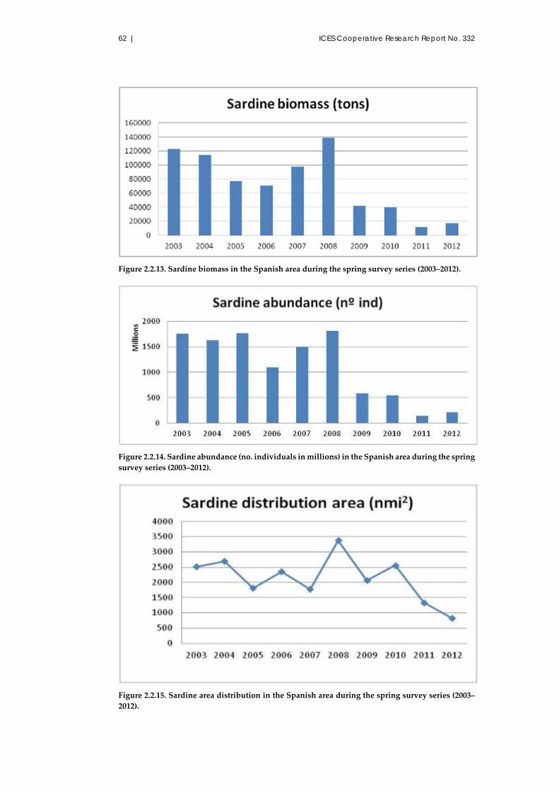
62 | ICES Cooperative Research Report No. 332
Figure 2.2.13. Sardine biomass in the Spanish area during the spring survey series (2003–2012).
Figure 2.2.14. Sardine abundance (no. individuals in millions) in the Spanish area during the spring
survey series (2003–2012).
Figure 2.2.15. Sardine area distribution in the Spanish area during the spring survey series (2003–
2012).
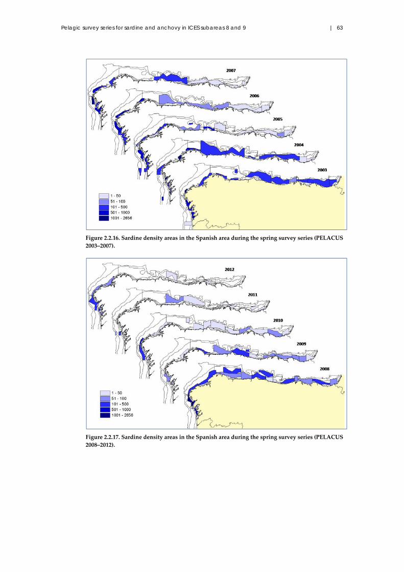
Pelagic survey series for sardine and anchovy in ICES subareas 8 and 9 | 63
Figure 2.2.16. Sardine density areas in the Spanish area during the spring survey series (PELACUS
2003–2007).
Figure 2.2.17. Sardine density areas in the Spanish area during the spring survey series (PELACUS
2008–2012).

64 | ICES Cooperative Research Report No. 332
Figure 2.2.18. Sardine age distribution during the PELACUS survey series (2003–2012).
Abundance by age for sardine is reflected in Figure 2.2.18, where abundance of the
2004 cohort can be clearly followed year after year until 2008, when high abundance of
sardines at age 4 produced high biomass for this species (Figure 2.2.13).
Younger sardines (ages 1 and 2) are mainly located in Atlantic waters (Division
9.a North), whereas the older ages used to be found in the inner part of the Bay of
Biscay, as shown in Figure 2.2.19. Nevertheless, and contrary to what was observed in
the 1990s, the proportion of younger sardines found in some years in the inner part of
the Bay of Biscay was also noticeable. Whether these sardines came from ICES Division
8.b (French waters) or were hatched in Division 8.c is still unknown.
Atlantic mackerel, representing about 69% of the total biomass, is generally the most
abundant fish species estimated in PELACUS surveys (Table 2.9 and Figures 2.2.20 and
2.2.21). As in the case of sardine, younger mackerel are mainly located in Division
9.a North.

Pelagic survey series for sardine and anchovy in ICES subareas 8 and 9 | 65
Figure 2.2.19. Sardine age distribution by ICES subdivision during the PELACUS survey series
(2003–2012).
Figure 2.2.20. Biomass (tonnes) estimated for Atlantic mackerel (MAC) and for the rest of the
pelagic fish community (Other Pelagic fish) during the 2003–2012 pelagic surveys.
2003 2004 2005 2006 2007 2008 2009 2010 2011 20120
100000
200000
300000
400000
500000
600000
700000
800000
MAC
Other Pelagic f ish
Year
Biomass (m
t)

66 | ICES Cooperative Research Report No. 332
Figure 2.2.21. Mackerel spatial distribution during PELACUS (top, 2008–2012 cruises; bottom, 2003–
2007 cruises). Polygon colours indicate the mean backscattering energy range (sA values, m2 nmi−2,
1–10; 11–30; 31–50; 51–100; and >100).
Since 2007, there has been some increase in perciforms, such as bogue, Mediterranean
horse mackerel, and others (Table 2.2.6; Figure 2.2.22), although this was not sustained
in 2012.
Anchovy distribution in the Bay of Biscay is mainly outside the PELACUS coverage in
Division 8.c. Only in the years when the southern part of ICES Division 8.b was
surveyed was anchovy found in relative high densities, as shown in Figure 2.2.23. The
PELACUS survey demonstrates that the presence of anchovy is scarce and in low
relative density off the northern Spanish coast.

Pelagic survey series for sardine and anchovy in ICES subareas 8 and 9 | 67
Figure 2.2.22. Biomass (tonnes) estimated for nine pelagic species during the 2003–2012 pelagic
surveys.
Figure 2.2.23. Anchovy distribution area and relative density (NASC) during PELACUS (2004–
2012).
0
20000
40000
60000
80000
100000
120000
140000
160000
2003 2004 2005 2006 2007 2008 2009 2010 2011 2012
Biomass (tons)
PIL
HOM
BOC
BOG
WHB
MAS
JAA
HMM
ANE

68 | ICES Cooperative Research Report No. 332
Concerning the rest of the pelagic species detected during the PELACUS surveys, a
potential bias exists for horse mackerel, which is a bentho‐pelagic species. Parts of the
schools are potentially undetected because some horse mackerel may be present within
the bottom acoustic blind zone. However, in general, most of the schools are expected
to be accessible to the echosounders. Younger fish are found in shallower waters,
whilst the adults are mainly located close to the slope extending over the shelf. No clear
distribution pattern along the surveyed area is found, as shown in Figure 2.2.24.
Blue whiting is mainly located around the shelf break, but contrary to the spatial
pattern shown in northern European areas, rather than forming pelagic layers from the
slope towards more oceanic waters at depths of 200–500 m, the fish extends its
distribution area in Spanish waters towards the continental shelf (Carrera et al., 2001).
Therefore, although PELACUS only surveys the continental shelf (from 30 to 200–
250 m), it covers part of its potential distribution area. In addition, mean size estimated
during PELACUS is ca. 18–20 cm, which is similar to that found in the surveys which
target this species (Carrera et al., 2001), and 8–10 cm less than the size of adult fish. As
shown in Figure 2.2.25, the main distribution area is located in the northwestern corner
(ICES Division 7.c West).
Figure 2.2.24. Horse mackerel distribution area and relative density (NASC) during PELACUS
(2008–2012).

Pelagic survey series for sardine and anchovy in ICES subareas 8 and 9 | 69
Figure 2.2.25. Blue whiting distribution area and relative density (NASC) during PELACUS (2003–
2012).
Although acoustic surveys in northwestern Spain were primarily targeted on sardine,
improvements in survey strategies, equipment (including new research vessels such as
RV “Thalassa”), and post‐processing analysis made PELACUS an ideal platform for
collecting multiple types of oceanographic data, both at fixed stations and through
continuous recordings. These data were used in the beginning to improve the precision
of fish abundance estimates by echo integration, but also allowed detailed integrated
monitoring of pelagic communities and ecosystems. Data on abundance, distribution,
and behaviour of pelagic species can be collected systematically and geo‐referenced at
the same temporal and spatial scales as environmental data. Future work, which will
deal with the Marine Strategy Framework Directive (MSFD) challenges, will include
the comparison between pelagic communities of different areas and their evolution

70 | ICES Cooperative Research Report No. 332
over time as well as the development of indices and coupled models to analyse the
state of the pelagic ecosystem.
2.2.3.4 Acknowledgements
We thank all the scientists who took part in the PELACUS surveys as well as the crew
of RV “Thalassa”.
2.2.4 PELAGO surveys
Vitor Marques, Maria Manuel Angélico, Eduardo Soares, Alexandra Silva, and
Cristina Nunes
2.2.4.1 Historical perspective and objectives of the Portuguese acoustic surveys
The Portuguese acoustic surveys began in August 1982. The first survey was a joint
exploratory survey, together with IEO, covering the Iberian sardine stock and carried
out with RV “Noruega” and RV “Cornide Saavedra”. During 1984–1988, the
Portuguese surveys were systematically performed in spring and autumn/winter each
year. After no surveys in 1989–1991, two sporadic surveys were carried out in 1992 and
1995, the latter, with a Portuguese and Spanish scientific team, covering all Iberian
Atlantic waters. The acoustic surveys resumed with a systematic periodicity effective
in 1996. The Portuguese spring acoustic surveys have always been funded by the
Portuguese Ministry of Fisheries; between 2000 and 2002, they also benefited from an
EU Project (PELASSES). Since 2002, they have been cofunded by the EU Data
Collection Framework (DCF).
Surveys were carried out mainly on RV “Noruega”, except in July 1996, August 1999,
and June 2004 when they were performed with RV “Capricórnio”.
The survey area has been extended to the Spanish part of the Gulf of Cádiz since 1992,
but was not covered in 2004.
The main objective of the Portuguese spring acoustic surveys has been the abundance
estimate for the part of the Atlanto‐Iberian sardine stock inhabiting the Portuguese
shelf. Additionally, the biological data collected provides information on the
population demography (numbers and biomass per length and age).
Since 1999, anchovy abundance has also been obtained from these surveys. This species
is mainly distributed off the southern coast from Cape Santa Maria to Gibraltar
(Division 9.a South).
2.2.4.2 Material and methods
2.2.4.2.1 Changes in methodology and equipment during the time-series
The acoustic equipment used before 1995 was a Simrad EK38S echosounder with 38‐
and 120‐kHz frequencies and a Simrad QM analogic echo‐integrator. Since 1995, a
Simrad EK 500 has been used. Since 2000, the IFREMER MOVIES+ (Weill et al., 1993)
software has been used to acquire and process the acoustic data. Previously, the
echograms were registered on paper, and the acoustic energies were extracted visually,
for each nautical mile. The integration deflection line on the echogram was read with
a ruler.
Before 1996, a large pelagic trawl net (20‐m vertical opening) was used. This net was
replaced by a smaller net (10‐m vertical opening) to allow fishing operations in shallow
waters.

Pelagic survey series for sardine and anchovy in ICES subareas 8 and 9 | 71
Acoustic coverage became systematic only after 1997, following a parallel grid
perpendicular to the coastline with a separation of eight nautical miles between
transects, where a “zig‐zag” grid had previously been applied. In addition, before 1997,
the acoustic coverage was done continuously during daylight and night‐time, whereas
it has subsequently been done only by day to allow distinguishing between pelagic
schools in the echograms. In all the surveys, fishing trawl hauls have been done during
daylight, whereas night‐time has often been used to perform hydrology and plankton
stations.
Since 2000, a CUFES system (Checkley et al., 1997) has been used in the acoustic surveys
for underway surface (ca. 3 m) plankton sampling (every three nautical miles) with the
main objective to describe sardine and anchovy spawning grounds. A SeaBird thermo‐
salinographer and a SeaPoint fluorometer are coupled to the CUFES system allowing
continuous recording of SST, SSS, and SSF (fluorescence, ~chlorophyll). Information
from the TCF probes is compiled, together with GPS data, by dedicated software
(EDAS). High‐resolution data acquisition on egg abundance, temperature, salinity, and
fluorescence allow the production of detailed distribution maps that assist in
environmental characterization and spawning area definition.
Regarding the TS for sardine, the relationship TS = 21.7 logL – 75.5 dB (Haldorsson and
Reynisson, 1983) was used until 1986; later, the relationship TS = 20 logL – 72.6 dB
(Degnbol et al., 1985) was used for sardine, following the recommendations of the
Planning Group for Acoustic Surveys in ICES Subareas 8 and 9 (ICES, 1986a). The TS
relationships for the other main pelagic species were also recommended by this
Planning Group. The TS relationship for anchovy has changed from TS = 20 logL –
71.2 dB to TS = 20 logL – 72.6 dB, becoming similar to that for sardine, in the 2007 and
subsequent surveys. After discussing TS values at the WGACEGG 2007 meeting, it was
decided that the anchovy TS could not be higher than the sardine TS. The relationship
used before for anchovy (TS = 20 logL – 71.2 dB) was the same as used for North Sea
herring and was an average of several TS measurements. As such, the reported series
for anchovy make use of two different TS.
The following target strength b20 (20 logL – b20) relationships are currently used in the
Portuguese acoustic surveys:
Sardina pilchardus (PIL): 72.6 dB
Scomber colias (MAS): 68.7 dB
Scomber scombrus (MAC): 82 dB
Trachurus trachurus (HOM): 68.7 dB
Trachurus picturatus (JAA): 68.7 dB
Boops boops (BOG): 67.0 dB
Engraulis encrasicholus (ANE): 72.6 dB
Micromesistius poutassou (WHB): 80 dB
Macroramphosus spp. (SNS): 80 dB
The spring surveys referred to in this section (covering the period 2003–2012, though
the Portuguese spring survey did not take place in 2012 due to technical problems)
were performed in the consolidated phase, when the methodology was already well
established. Although the main objective of these spring surveys is to estimate the
abundance of sardine and anchovy, there has been an increasing concern in light of the
ecosystem approach, and fishing trawls aim at catching different fish school
aggregations, not just sardine and anchovy. As a result, the abundance and distribution
of other pelagic species have been estimated whenever possible. Since 2005, the
observation and monitoring of marine birds and mammals has also been carried out

72 | ICES Cooperative Research Report No. 332
during the acoustic surveys (within the framework of projects in collaboration with
SPEA and SPVS). The night‐time (when acoustic surveying ceases) is used for
hydrology and zooplankton surveying.
2.2.4.2.2 Equipment used in the PELAGO series
A Simrad EK 500 – 38 kHz echosounder, with a split‐beam transducer 8°× 7°
(equivalent beam angle: 10 log = –20.2 dB; pulse duration = 1 ms) calibrated prior to
the survey, is used. For data storage and post‐processing, the software Movies+ (©
IFREMER) is used.
Calibration of the acoustic instruments, using standard procedures, is performed
before each acoustic survey (Foote et al., 1987).
A pelagic trawlnet (10‐m vertical opening) and a bottom trawlnet are used in the
fishing stations to collect information on species distribution and biological data. The
trawl data are used to help identify the echoes and to split the acoustic energy NASC
into species and length classes. A Scanmar Netsounder (trawl‐eye and depth sensor) is
used in the fishing operations.
2.2.4.2.3 Sample design in the PELAGO series
The total surveyed area is divided into four zones to allow between‐year comparison
(Figure 2.2.26): Occidental North – OCN (Caminha to Nazaré), Occidental South – OCS
(Nazaré to Cape St. Vicente), Algarve – ALG (St. Vicente to Vila Real Santo António),
and Cádiz – CAD (Vila Real Santo António to Cape Trafalgar).
The surveyed area is covered using a parallel systematic grid, with transect separation
of eight nautical miles on the west coast and six nautical miles in Algarve; in Cádiz, the
transects are perpendicular to the coastline, making them not perfectly parallel, and
divided by around eight nautical miles in the middle of the radials (Figure 2.2.26). The
acoustic survey is done only during daylight. The ESDU used for NASC collection is
one nautical mile. The survey vessel speed is 9–10 knots.
2.2.4.2.4 Abundance estimates
The RV ”Noruega“ has a draft of four metres. The echo integration is made using a
surface blind depth (from transducer) of 3 m, but depending on weather conditions, it
can increase up to 10 m. The bottom blind zone height is fixed at 0.2 m. When needed,
the bottom contour in the echograms is manually corrected to avoid bottom
integration.
The acoustic energy (NASC) is split into species according to the proportion of species
(in numbers) in the fishing trawls, taking into account the species TS when direct
energy allocation is not possible (for details, see the acoustics protocol in Annex 2).

Pelagic survey series for sardine and anchovy in ICES subareas 8 and 9 | 73
Figure 2.2.26. Portuguese acoustic transects and subareas used for abundance estimation.
There is post‐stratification in coherent areas (i.e. areas with similar species length
composition). Area density is calculated using the arithmetic mean.
Abundance estimate is calculated in numbers of individuals by length class in each
coherent area. Hauls are combined in this area, usually without weighting each haul
differently.
Biomass estimation is calculated using weight–length relationships obtained from
fishing samples.
Estimated abundance by age groups is calculated using age–length (total length) keys
produced from the species otoliths obtained from the biological sampling on board.
2.2.4.3 Results and discussion
Until 2007, sardine was the predominant species on the Portuguese continental shelf
north of Lisbon and the other pelagic species were distributed more southerly, mainly
in the Algarve and Cádiz areas. Since 2007, the diversity and mixture of species
extended to the entire Portuguese coast (Figure 2.2.27). At the same time, the decrease
in sardine abundance has been noticeable (Table 2.2.7 and Figure 2.2.28) in recent years.
The sardine distribution area has also decreased during this time (Figure 2.2.29). Figure
2.2.30 shows the change in sardine acoustic density and geographic distribution.
Caminha
Viana do Castelo
Porto
Aveiro
Figueira da Foz
Nazaré
Peniche
Lisboa
Setubal
Sines
Arrifana
Portimão Faro
V. Real Sto. António
Cádiz
100
0 m
200
m
Trajecto das campanhas acústicas
OCN
OCS
ALG
CAD

74 | ICES Cooperative Research Report No. 332
Figure 2.2.27. Species trawl composition in the PELAGO survey series (2007–2011). Species FAO
key code.
-11º -10º -9º -8º -7º -6º -5º35º
36º
37º
38º
39º
40º
41º
42ºCaminha
Porto
Nazaré
Lisboa
V. Real Sto. António
Cádiz
200 m
AF1AP2
AP3AP4
AP5
AF7AP8
AP9AP10
AP11AF12AF13
AP14AP15
AP16
AF17
AP18
AP19
AP20
AP21
AP22
AP24
AP25
AP26 AP27AP28
AP29AP30
AP32
AP33
AP34AP35
AP36
AF37
AP38
AP39
AP40
AF41
AP42
AP43
AP44AP45
AF46
AP47AP49
AP50
AP48
PIL
ANE
HOM
BOG
MAC
MAS
JAA
WHB
SNS + BOC
PELAGO08
-11º -10º -9º -8º -7º -6º -5º35º
36º
37º
38º
39º
40º
41º
42º200 m
AP20AP45
AF46 AP44
AP43
AF41
AF22
AP40
AF39
AP38
AP37
AP36
AP34
AP35
AP33
AF32
AP31 AF30
AP29
AF28
AF27
AF25
AP26
AP23
AF2
AP4
AF6
AP7AP8
AP9AP10AF11
AP12
AP14
AP15AP17
AP16AP18
AF1
AF19
AP48
AP42
PELAGO 07
PIL
ANE
HOM
BOG
MAC
MAS
JAA
WHB
SNS + BOC
AP24
AP3
AP5
-11º -10º -9º -8º -7º -6º -5º35º
36º
37º
38º
39º
40º
41º
42ºCaminha
Viana do Castelo
Porto
Aveiro
Figueira da Foz
Nazaré
Peniche
Lisboa
Setubal
Sines
Arri fanaPortimão
Faro
V. Rea l Sto. António
Cádiz
PELAGO10
PESCAS
PIL
ANE
HOM
BOG
MAC
MAS
JAA
WHB
SNS + BOC
HMM
AF1
AP2
AF3
AP4
AP5AP6
AF7AP8
AP9
AP10
AP11
AP13
AF14
AP15
AP16
AP17
AP18
AP19AP20
AP23
AP24
AP25
AP26
AP21- AP22
-11º -10º -9º -8º -7º -6º -5º35º
36º
37º
38º
39º
40º
41º
42ºCaminha
Viana do Castelo
Porto
Aveiro
Figueira da Foz
Nazaré
Peniche
Lisboa
Setubal
Sines
ArrifanaPortimão
Faro
V. Real Sto. António
Cádiz
200 m
PIL
ANE
HOM
BOG
MAC
MAS
JAA
WHB
SNS + BOC
PELAGO09
Fishing trawls
AP14AF16
AP15
AP1
AF13AP12
AP11AP4AF9
AP3
AP2
AP8AP7
AF6
AP5
AP17
AF18
AP19
AF35 AF34
AF33
AF32
AF31
AF30
AF29AF28
AF27
AP26 AP25
AP24
AF23
AP22
AP21
AF20

Pelagic survey series for sardine and anchovy in ICES subareas 8 and 9 | 75
Figure 2.2.28. Sardine biomass (thousand tonnes) in the surveyed area during the spring survey
series. Cádiz area was not covered in the 2004 survey.
Figure 2.2.29. Sardine distribution area (nautical miles2) during the spring survey series. Cádiz area
was not covered in the 2004 survey.
0
500
1000
1500
2000
2500
3000
2003 2004 2005 2006 2007 2008 2009 2010 2011
Sardine distribution area(nm^2)

76 | ICES Cooperative Research Report No. 332
Figure 2.2.30. Sardine NASC distribution (2003–2011). Circle sizes are proportional to the acoustic
energy.
-11º -10º -9º -8º -7º -6º -5º35º
36º
37º
38º
39º
40º
41º
42º
W
N
Caminha
Porto
Aveiro
Nazaré
Lisboa
Faro
V. Real Sto. António
Cádiz
10
00
m
200 m
PIL 2003
-11º -10º -9º -8º -7º -6º -5º35º
36º
37º
38º
39º
40º
41º
42º
W
N
Caminha
Porto
Aveiro
Nazaré
Lisboa
Faro
V. Real Sto. António
Cádiz
10
00
m
200 m
PIL 2004
-11º -10º -9º -8º -7º -6º -5º35º
36º
37º
38º
39º
40º
41º
42º
W
N
Caminha
Porto
Aveiro
Nazaré
Lisboa
Faro
V. Real Sto. António
Cádiz
10
00
m
200 m
PIL 2005
-11º -10º -9º -8º -7º -6º -5º35º
36º
37º
38º
39º
40º
41º
42º
W
N
Caminha
Porto
Aveiro
Nazaré
Lisboa
Faro
V. Real Sto. António
Cádiz
10
00
m
200 m
PIL 2006

Pelagic survey series for sardine and anchovy in ICES subareas 8 and 9 | 77
Figure 2.2.30 (continued). Sardine NASC distribution (2003–2011). Circle sizes are proportional to
the acoustic energy.
-11º -10º -9º -8º -7º -6º -5º35º
36º
37º
38º
39º
40º
41º
42º
W
N
Caminha
Porto
Aveiro
Nazaré
Lisboa
Faro
V. Real Sto. António
Cádiz
10
00
m
200 m
PIL 2007
-11º -10º -9º -8º -7º -6º -5º35º
36º
37º
38º
39º
40º
41º
42º
W
N
Caminha
Porto
Aveiro
Nazaré
Lisboa
Faro
V. Real Sto. António
Cádiz
10
00
m
200 m
PIL 2008
-11º -10º -9º -8º -7º -6º -5º35º
36º
37º
38º
39º
40º
41º
42º
W
N
Caminha
Porto
Aveiro
Nazaré
Lisboa
Faro
V. Real Sto. António
Cádiz
10
00
m
200 m
PIL 2009
-11º -10º -9º -8º -7º -6º -5º35º
36º
37º
38º
39º
40º
41º
42º
W
N
Caminha
Porto
Aveiro
Nazaré
Lisboa
Faro
V. Real Sto. António
Cádiz
10
00
m
200 m
PIL 2010

78 | ICES Cooperative Research Report No. 332
Figure 2.2.30 (continued). Sardine NASC distribution (2003–2011). Circle sizes are proportional to
the acoustic energy.
The sardine stock biomass is mainly sustained by recruitment strength (Figure 2.2.31).
During 2003–2011, the strongest recruitment took place in 2004, which resulted in a
biomass increase in 2005 and 2006 (Table 2.2.7 and Figure 2.2.32).
Figure 2.2.31. Sardine age distribution during the PELAGO survey series.
-11º -10º -9º -8º -7º -6º -5º35º
36º
37º
38º
39º
40º
41º
42º
W
N
Caminha
Porto
Aveiro
Nazaré
Lisboa
Faro
V. Real Sto. António
Cádiz
10
00
m
200 m
PIL 2011
PELAGO sardine age series

Pelagic survey series for sardine and anchovy in ICES subareas 8 and 9 | 79
Table 2.2.7. Sardine biomass (thousand tonnes) in each zone, Portugal, and total surveyed area
during the spring acoustic surveys in 2003–2011.
Survey OCN OCS Algarve Cádiz Portugal Total
area
SAR03FEV 153 145 60 73 359 432
SAR04JUN 240 60 39 ‐ 339 ‐
SAR05ABR 286 199 62 40 547 587
SAR06ABR 370 138 40 89 548 637
PELAGO07 215 89 40 107 344 452
PELAGO08 170 13 26 35 209 244
PELAGO09 112 84 14 84 210 294
PELAGO10 125 43 11 26 179 205
PELAGO11 90 15 20 2 125 127
The main anchovy distribution area was in the Gulf of Cádiz from Cape Santa Maria
to Cape Trafalgar, with some spots off the west coast near Figueira da Foz and Lisbon.
In 2011, there was exceptional recruitment of anchovy in the north, and the traditional
distribution pattern changed for this species as a result of very few anchovies found in
the south (Table 2.2.8).
Table 2.2.8. Anchovy estimated biomass (tonnes) for the West coast (Division 9.a OCN and Division
9.a OCS), South coast (Division 9.a South), and total surveyed area.
Survey West South Total
February 2003 112 24 677 24 789
April 2005 1 062 14 041 15 103
April 2006 0 24 082 24 082
April 2007 1 945 38 020 39 965
April 2008 5 500 34 200 39 700
April 2009 2 000 24 800 26 800
April 2010 1 188 7 395 8 583
April 2011 27 050 0 27 050
2.2.4.3.1 Sardine and anchovy egg distributions
Sardine and anchovy egg density spatial distributions and total abundance by area
(from CUFES sampling) during 2003–2011 are presented in Figures 2.2.32–2.2.34.
Sardine eggs, in agreement with fish biomass distribution, are usually more abundant
on the west coast (larger area with higher number of samples), with hot spots
appearing on the northwestern shelf and off Promontório da Estremadura (just north
of Lisbon); in the south, higher numbers generally occur in the inner Bay of Cádiz. On
the contrary, anchovy eggs are more common on the southern coast, particularly
towards the east, where a regular population is maintained. The peak spawning period
for sardine is centred in winter, whereas southern anchovy is a summer spawner,
which is reflected in the low abundance of anchovy eggs observed during the

80 | ICES Cooperative Research Report No. 332
Portuguese acoustic survey that usually takes place in early to mid‐spring. The 2003
survey was conducted earlier in the season, starting in February, while the 2004
campaign, due to logistic constraints, was conducted in June after the normal acoustics
season.
Sardine total egg abundance followed a similar pattern for the western and southern
areas, except for 2005–2006. During this period, high adult (predominantly young
adults) biomass was observed, particularly in the west. The trends in adult biomass
and egg densities over time are not in close agreement. High adult sardine biomass
was observed until 2007. High egg densities were observed in 2003, but then decreased
in 2005–2006, before a very pronounced increase in 2008. The peak in high egg
abundance in 2008 over the entire surveyed area was not observed in adult acoustic
abundance, but was highlighted in the DEPM egg production (and fecundity) of that
year and was also observed off the Cantabrian shores (Section 2.1). 2008 had a
particularly mild winter–spring season, with high primary productivity (data not
shown). After 2008, the trend in egg abundance and adult fish is more comparable.
However, egg abundance during the last reported survey showed a small increase that
was not observed in adult sardines, but egg occurrence was very localized (particularly
in the northern region).
During the reported period, sardine egg spatial distribution varied substantially, with
years of very patchy distribution, particularly on the west coast. Egg abundance
fluctuations are very likely related not only to the abundance of adult fish, but also to
the demography of the population, its reproductive dynamics, and environmental
conditions. Sea surface temperature is higher in the south (ca. 14–19°C) than on the
west coast (ca. 13–16°C; see maps in sections 3 and 4) and suffers less fluctuations.
During the period reported, the more recent years were slightly warmer, particularly
in the south (also with high winter/spring river runoff); in 2003 and 2009, sea surface
temperatures were lower than during the remaining years.
During IPMA acoustic surveys in spring, egg densities for anchovy are lower than for
sardine, not only because the sardine and anchovy populations have very distinct
levels of abundance, but also because the survey generally occurs early in the anchovy
spawning season. Despite this fact, in 2010 and 2011, egg abundance was higher for
anchovy than for sardine. Furthermore, egg observations have shown that
echosounding detection of anchovy in the Bay of Cádiz was not consistent with egg
densities every year because the highest egg abundance was found in 2010 and 2011
when the acoustic anchovy estimates were minimal. In addition, it has been shown that
egg production estimates in the region from the DEPM increased in recent surveys
(Section 2.5). During the years of high anchovy biomass, egg densities (generally
higher in the south) are also noticeable on the west coast in areas other than the regular
patch off Lisbon.

Pelagic survey series for sardine and anchovy in ICES subareas 8 and 9 | 81
Figure 2.2.32. Sardine egg density (eggs m–3) distribution during the acoustic surveys (2003–2011)
derived from the CUFES sampler (equipped with a 500‐μm mesh net in 2003–2004 and a 335‐μm
mesh net in 2005–present).
36
37
38
39
40
41
42
43
Latit
ude
(ºN
)
Eggs/m3
2003Sardine eggs
36
37
38
39
40
41
42
43
Latit
ude
(ºN
)
-10 -9 -8 -7 -6
Longitude (ºW)
36
37
38
39
40
41
42
43
Latit
ude
(ºN
)
0.01 to 1 1 to 5 5 to 10 10 to 25 25 to 50 50 to 100 100 to 250 250 to 1000
2004Sardine eggs
2005Sardine eggs
2006Sardine eggs
2007Sardine eggs
2009Sardine eggs
2008Sardine eggs
-10 -9 -8 -7 -6
Longitude (ºW)
-10 -9 -8 -7 -6
Longitude (ºW)
2010Sardine eggs
2011Sardine eggs

82 | ICES Cooperative Research Report No. 332
Figure 2.2.33. Anchovy egg density (eggs m–3) distribution during the acoustic surveys (2003–2011)
derived from the CUFES sampler (equipped with a 500‐μm mesh net in 2003–2004 and a 335‐μm
mesh net in 2005–present).
36
37
38
39
40
41
42
43
Latit
ude
(ºN
)
Eggs/m3
2003Anchovy eggs
36
37
38
39
40
41
42
43
Latit
ude
(ºN
)
-10 -9 -8 -7 -6
Longitude (ºW)
36
37
38
39
40
41
42
43
Latit
ude
(ºN
)
0.01 to 1 1 to 5 5 to 10 10 to 25 25 to 50 50 to 75 75 to 100 100 to 350
2004Anchovy eggs
2005Anchovy eggs
2006Anchovy eggs
2007Anchovy eggs
2009Anchovy eggs
2008Anchovy eggs
-10 -9 -8 -7 -6
Longitude (ºW)
-10 -9 -8 -7 -6
Longitude (ºW)
2010Anchovy eggs
2011Anchovy eggs

Pelagic survey series for sardine and anchovy in ICES subareas 8 and 9 | 83
Figure 2.2.34. Sardine (top panel) and anchovy (bottom panel) egg densities (sum of egg m–3) per
stratum (West, green; South, blue) from CUFES sampling along the acoustics transects during 2003–
2011 and number of samples (unit: 3 nautical miles) collected per survey and area. The 2004 survey
was not conducted in the usual season (in June, and only covered the Portuguese shores). CUFES
was equipped with a 500‐μm mesh net in 2003–2004 and a 335‐μm mesh net in 2005–present).
2.2.4.4 Acknowledgements
We acknowledge all of the IPIMAR/IPMA staff who contributed to the work presented
here, as well as the crew of the research vessels used to collect data. Early surveys were
funded by the national research budget and since 2002 were cosponsored by the EU
Data Collection Framework. Special thanks to Carlos Afonso Dias, the real pioneer of
the fisheries acoustic surveys in Portugal.
Sardine eggs CUFES (m3)
0
500
1000
1500
2000
2500
3000
3500
4000
4500
5000
2003 2004 2005 2006 2007 2008 2009 2010 2011
Year
Nb
of
egg
s (m
3 )
Sar ‐ West
Sar ‐ South
Anchovy eggs CUFES (m3)
0
200
400
600
800
1000
1200
1400
1600
2003 2004 2005 2006 2007 2008 2009 2010 2011
Year
Nb
of
egg
s (m
3)
Engr ‐ West
Engr ‐ South
Area/Year 2003 2004 2005 2006 2007 2008 2009 2010 2011West 269 272 321 331 313 349 324 330 315
South 159 108 150 146 159 151 167 160 159
Number of CUFES stations

84 | ICES Cooperative Research Report No. 332
2.2.5 Seabirds and marine mammals
Authier Matthieu, Ghislain Dorémus, Olivier Van Canneyt, Hélene Falchetto, Maite
Louzao, Maria Begoña Santos, Joana Andrade, Ana Meirinho, and Vincent Ridoux
Seabirds and marine mammals are upper trophic level predators. As such, they are
thought to be reliable indicators of ecosystem health and functioning, assuming
bottom–up forcing. Any impact of lower trophic levels may reverberate up the
foodweb and affect top predators. These charismatic species can be monitored at sea
(cetaceans and seabirds) or on land during the breeding season (seabirds and
pinnipeds). However, the highly mobile species are difficult to monitor across large,
but ecologically meaningful, areas. This report illustrates a rare case of fruitful
collaboration across several countries to map the distribution and relative abundance
of marine mammals and seabirds over several successive years.
Marine mammals and seabirds were recorded along transects performed during the
three spring surveys PELAGO, PELACUS, and PELGAS. However, monitoring
protocols were slightly different between PELAGO and the two other surveys.
For PELAGO, the methodology is that of the European Seabirds at Sea (ESAS), with
more emphasis put on monitoring seabirds. Two observers carried out a visual search
for cetaceans and seabirds within an angle of 180° ahead of the ship’s bow. Upon
detection, species identification is made with the aid of binoculars. Snapshot censuses
of seabirds and marine mammal presence and activities are made every 5 min within
a 300‐m transect parallel to the ship’s direction.
For PELGAS and PELACUS, the methodology used is that of continuous recording of
seabirds and marine mammals from a single platform line transect survey.Two
observers searched with the naked eye for cetaceans and seabirds within an angle of
180° ahead of the ship’s bow. Upon detection, species identification is made with the
aid of binoculars. For birds and cetaceans, distance and angle from the ship’s main
route are recorded based on distance sampling methodologies. Any seabird detected
within a 1000‐m transect (or less depending on observation conditions) parallel to the
ship’s direction and spanning an angle of 180° ahead of the ship’s bow is recorded.
To account for the slightly different methodology between PELAGO and
PELACUS/PELGAS, the numbers of detected marine mammals and seabirds are
standardized by transect length (in nautical miles). Data are a linear density of seabirds
and marine mammals.
Additionally, crude taxonomic groupings were made (see top predators protocol in
Annex), except for two easily identified and abundant species (northern gannets
[Morus bassanus] and common dolphins [Delphinus spp.], labelled ”Bird_Gannet” and
”Mam_CommonDolphin”, respectively). These crude groupings are all seabirds
(including rare and vagrant species labelled ”Birds”) and all marine mammal species
(excluding sperm whales [Physeter macrocephalus], labelled ”Mam”). Within seabirds, a
further functional distinction was made between diving (labelled ”Bird_Div”) and
surface‐feeding (labelled ”Bird_Surf”) species. Within these two groups, rare and
vagrant species were excluded. Within marine mammals, balenopterids (labelled
”Mam_BaleenWhales”) and delphinids (labelled ”Mam_Dolphins”) were further
distinguished. Compared to the larger marine mammal grouping, these two
subgroups exclude beaked whales. The pooled observations from the three surveys
were gridded and are presented in sections 3 and 4.

Pelagic survey series for sardine and anchovy in ICES subareas 8 and 9 | 85
2.3 Anchovy DEPM surveys 2003–2012 in the Bay of Biscay (Subarea 8): BIOMAN survey series
María Santos, Andrés Uriarte, Guillermo Boyra, and Leire Ibaibarriaga
2.3.1 DEPM BIOMAN survey series
The BIOMAN survey series began in 1987, aiming to improve the direct monitoring
and assessment of the Bay of Biscay anchovy population, for which no internationally
agreed assessment had been made until then (Santiago and Sanz, 1992a; Motos, 1994;
Uriarte et al., 1996). The main objective was the estimation of the spawning‐stock
biomass of the Bay of Biscay anchovy by applying the daily egg production method
(DEPM; Lasker, 1985). In addition, the survey aimed to improve the knowledge on the
spawning environment (Motos et al., 1996) and reproductive biology of anchovy (Sanz
and Uriarte, 1989; Sanz et al., 1992; Motos, 1996; Alday et al., 2008, 2010). The survey
soon collaborated with other ichthyoplankton national and international surveys for
the estimation of spawning stocks of other pelagic species such as sardine (García et al.,
1992), Atlantic mackerel, and horse mackerel (Ibaibarriaga et al., 2007a). Today,
BIOMAN collaborates with the triennial egg surveys for these species concerning
coverage of the Bay of Biscay (ICES, 2011a). Currently, the principal objective of the
survey is the same, but other objectives have been added to try to revalue the survey
within the European Marine Strategy Framework Directive as hydrographic
characterization, acoustic estimates, stomach content of fish species, zooplankton
distribution, genetics of fish, microchemistry of otoliths.
The survey has always been funded by the Department of Fisheries of the Basque
Government within Spain. Moreover, since 1989, most of the surveys have been
directly supported by EU projects funded by the European Commission. In 2002, the
survey was included in the list of EC‐funded research surveys at sea within the
Community framework for the collection and management of data needed to support
the Common Fisheries Policy and has since been carried out in that context [Council
Regulations (EC) No. 1543/2000 and No. 199/2008]. The survey is also being supported
by the Spanish General Secretariat of Sea providing the RV “Emma Bardán” since 2003.
The first two surveys in 1987 and 1988 were made autonomously by AZTI (Santiago
and Sanz, 1992a; Sanz et al., 1992; Motos and Uriarte, 1992); since then, most of the
surveys have been in the context of international projects and in collaboration with
other institutes, particularly IFREMER and IEO. The annual spawning‐stock biomass
(SSB) estimates obtained applying the DEPM have been referred to the successive ICES
working groups through working documents (ICES, 2004, 2006a, 2006b, 2007, 2008;
Santos et al., 2009, 2010, 2011a, 2012, 2013a) and were summarized in contributions to
conferences (Ibaibarriaga et al., 2005; Motos et al., 2005), publications (Santos et al.,
2011b), or collective publications on the application of the method to anchovies in
European areas (Somarakis et al., 2004).
In this section of the report, we discuss the application of the DEPM to the Bay of Biscay
anchovy during 2003–2012, which is only part of the entire historical series (1987–2014).
In this period, the anchovy population passed from a period of very low biomass
(2005–2009), associated with a fishery closure for five years, to a recovery up to its
historical maximum in 2011 (Santos et al., 2013a).

86 | ICES Cooperative Research Report No. 332
2.3.2 Material and methods
2.3.2.1 DEPM and application to the Bay of Biscay anchovy
For the DEPM, the anchovy spawning‐stock biomass estimate is derived according to
Parker (1980) and Picquelle and Stauffer (1985) from the ratio between daily
production of eggs in the sea and the daily specific fecundity of the adult population:
f
tot
WSFRk
APDF
PSSB
0
(2.3.1)
where SSB is spawning‐stock biomass in tonnes, Ptot is the total daily egg production
in the sampled area, P0 is the daily egg production per surface unit in the sampled area,
A+ is the spawning area in sampling units, and DF is the daily specific fecundity:
fWSFRk
DF
(2.3.2)
Where Wf is the average weight of mature females in grams, R is the sex ratio by
weight, F is the batch fecundity or numbers of eggs spawned per mature females per
batch, S is the fraction of mature females spawning per day, and k is the conversion
factor from grammes to tonnes (106).
An estimate of an approximate variance and bias for this biomass estimator is derived
by the delta method (Seber, 1982; Picquelle and Stauffer, 1985).
For the Bay of Biscay, the method is extended to produce spawning population (in
numbers) at age estimates (SSPa), as follows (Uriarte, 2001):
ataa PWSSBPSSPSSP (2.3.3)
where SSP is the total spawning‐stock estimate in numbers (= SSB/Wt), Wt is the mean
weight of anchovies in the population, and Pa is the relative frequency (proportion in
numbers) of age a in the population.
Variance estimate of the anchovy stock in numbers‐at‐age and total is derived applying
the delta method (Uriarte, 2001).
Obtaining the estimate of the different parameters is achieved first through egg and
adult sampling at spawning time in May and second through laboratory analysis of
those samples and analysis of the results of samples to produce joint estimates of the
parameters and final SSB. For this population, as all anchovies are fully mature at the
spawning peak (May), SSB equals total population biomass.
2.3.2.2 Surveys 2003–2012
All surveys were carried out in May, covering the anchovy spawning area in the Bay
of Biscay. This area extends over the southeastern area of the Bay, with typical limits
at 5°W along the Iberian coast and at 48°N along the French coast (Figure 2.3.1). In
order to get the estimates of the daily egg production and daily specific fecundity, egg
and adult sampling took place simultaneously on board different vessels. In addition,
the cooperation of the commercial fishing fleet provided opportunistic adult samples
in several years (Table 2.3.1).

Pelagic survey series for sardine and anchovy in ICES subareas 8 and 9 | 87
Figure 2.3.1. Predetermined stations of the vertical hauls (PairoVET) that could be performed
during the surveys.
28
29
30
27
31
32
33
34
35
37
39
41
42
43
44
45
46
47
49
51
53
2523211917151311Bi
Bordeaux
SS
Arcachon
Santander
Nantes
47°
46°
45°
44°
6° 5° 4° 3° 2° 1°
48°
La Rochelle
0907
55
57
59
61
Predetermined vertical hauls (PairoVET)

88 | ICES Cooperative Research Report No. 332
Table 2.3.1. Some characteristics of DEPM surveys BIOMAN during 2003–2012. More details in references ICES WGACEGG. OPT (oceanographic pelagic trawler),
CPS (commercial purse‐seiner).
Year Name Dates Egg vessel
PV
no.
CUFES
no.
Total
area
(km2)
Positive
area (km2)
Adult
vessel
Fishing
hauls
Selected
no. Reference
2003
BIOMAN
2003
22 May–
9 June
RV
“Investigator” 503 1 122 70 041 42 915
OPT,
CPS 36 36
Santos et al.
(2004)
2004
BIOMAN
2004
2–17
May
RV “Vizconde
de Eza” 352 656 53 285 20 365
OPT,
CPS 47 30
Santos et al.
(2004)
2005
BIOMAN
2005
8–28
May
RV “Vizconde
de Eza” 414 900 61 619 27 863 OPT 30 20
Santos et al.
(2005)
2006
BIOMAN
2006
4–24
May
RV “Vizconde
de Eza” 404 798 53 110 24 614 OPT 43 37
Santos et al.
(2006)
2007
BIOMAN
2007
3–23
May
RV
“Investigator” 420 775 56 079 34 449 OPT 44 34
Santos et al.
(2007)
2008
BIOMAN
2008
6–26
May
RV
“Investigator” 544 1 175 69 150 33 502 OPT 39 29
Santos et al.
(2008)
2009
BIOMAN
2009
5–25
May
RV
“Investigator” 409 949 60 733 28 214 OPT 38 31
Santos et al.
(2009)
2010
BIOMAN
2010
5–20
May
RV
“Investigator” 484 1 035 61 940 37 633
OPT,
CPS 34 30
Santos et al.
(2010)
2011
BIOMAN
2011
6–28
May
RV
“Investigator” 699 1 200 98 405 69 094
OPT,
CPS 52 40
Santos et al.
(2011a)
2012
BIOMAN
2012
10–29
May
RV “Ramón
Margalef” 529 1 156 80 381 38 974 OPY 42 24
Santos et al.
(2012)
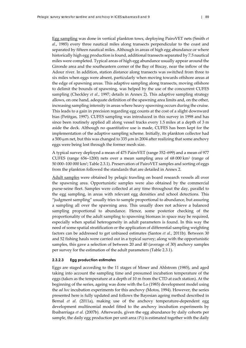
Pelagic survey series for sardine and anchovy in ICES subareas 8 and 9 | 89
Egg sampling was done in vertical plankton tows, deploying PairoVET nets (Smith et
al., 1985) every three nautical miles along transects perpendicular to the coast and
separated by fifteen nautical miles. Although in areas of high egg abundance or where
historically high egg production is found, additional transects separated by 7.5 nautical
miles were completed. Typical areas of high egg abundance usually appear around the
Gironde area and the southeastern corner of the Bay of Biscay, near the inflow of the
Adour river. In addition, station distance along transects was switched from three to
six miles when eggs were absent, particularly when moving towards offshore areas at
the edge of spawning areas. This adaptive sampling along transects, moving offshore
to delimit the bounds of spawning, was helped by the use of the concurrent CUFES
sampling (Checkley et al., 1997; details in Annex 2). This adaptive sampling strategy
allows, on one hand, adequate definition of the spawning area limits and, on the other,
increasing sampling intensity in areas where heavy spawning occurs during the cruise.
This leads to a gain in precision regarding egg counts at the cost of a slight downward
bias (Petitgas, 1997). CUFES sampling was introduced in this survey in 1998 and has
since been routinely applied all along vessel tracks every 1.5 miles at a depth of 3 m
aside the deck. Although no quantitative use is made, CUFES has been kept for the
implementation of the adaptive sampling scheme. Initially, its plankton collector had
a 500‐m net, but this was changed to 335 m in 2004 after realizing that some anchovy
eggs were being lost through the former mesh size.
A typical survey deployed a mean of 475 PairoVET (range 352–699) and a mean of 977
CUFES (range 656–1200) nets over a mean sampling area of 68 000 km2 (range of
50 000–100 000 km2; Table 2.3.1). Preservation of PairoVET samples and sorting of eggs
from the plankton followed the standards that are detailed in Annex 2.
Adult samples were obtained by pelagic trawling on board research vessels all over
the spawning area. Opportunistic samples were also obtained by the commercial
purse‐seine fleet. Samples were collected at any time throughout the day, parallel to
the egg sampling, in areas with relevant egg densities and school detections. This
“judgment sampling” usually tries to sample proportional to abundance, but assuring
a sampling all over the spawning area. This usually does not achieve a balanced
sampling proportional to abundance. Hence, some posterior checking of the
proportionality of the adult sampling to spawning biomass in space may be required,
especially when spatial heterogeneity in adult parameters is found. In this way the
need of some spatial stratification or the application of differential sampling weighting
factors can be addressed to get unbiased estimates (Santos et al., 2011b). Between 30
and 52 fishing hauls were carried out in a typical survey; along with the opportunistic
samples, this gave a selection of between 20 and 40 (average of 30) anchovy samples
per survey for the estimation of the adult parameters (Table 2.3.1).
2.3.2.3 Egg production estimates
Eggs are staged according to the 11 stages of Moser and Ahlstrom (1985), and aged
taking into account the sampling time and presumed incubation temperature of the
eggs (taken as the temperature at a depth of 10 m from the CTD at each station). At the
beginning of the series, ageing was done with the Lo (1985) development model using
the ad hoc incubation experiments for this anchovy (Motos, 1994). However, the series
presented here is fully updated and follows the Bayesian ageing method described in
Bernal et al. (2011a), making use of the anchovy temperature‐dependent egg
development multinomial model fitted to the anchovy incubation experiments by
Ibaibarriaga et al. (2007b). Afterwards, given the egg abundance by daily cohorts per
sample, the daily egg production per unit area (P0) is estimated together with the daily

90 | ICES Cooperative Research Report No. 332
egg mortality rate (Z) from the general exponential decay mortality model. This model
is fitted using a generalized linear model with negative binomial distribution and
logarithmic link (Stratoudakis et al., 2006) and following the iterative procedure
described in Bernal et al. (2011a). The P0 estimates have been jointly produced for the
entire positive spawning area without any post‐stratification of the area.
When the bulk of spawning for the day is not over at the time of sampling, or when
the cohort is so old that its constituent eggs had started to hatch in substantial numbers,
these incomplete cohorts are removed from the model fit in order to avoid any possible
bias. At each station, the youngest cohorts are dropped if they are sampled before twice
the spawning peak width; after the spawning peak, the oldest cohorts are dropped if
their mean age plus twice the spawning peak width is over the critical age at which
< 99% of the eggs are expected to be still unhatched. In addition, the oldest cohorts at
survey level are excluded; for that, the upper limit is set at the age in which 99% of the
eggs are unhatched, having developed at the 50th quantile of the survey incubation
temperature (weighted by egg abundance at each station; Santos et al., 2013b).
After the final model estimates are obtained, the coefficient of variation of P0 is given
by the standard error of the model intercept (log(P0); Seber, 1982) and the coefficient of
variation of Z is obtained directly from the model estimates. The analysis is conducted
in R (www.r‐project.org). The two libraries are used for different purposes, the
”MASS” library for fitting the GLM with negative binomial distribution and the ”egg”
library (http://sourceforge.net/projects/ichthyoanalysis/) for the ageing and the
iterative algorithm.
A typical fitted model corresponding to the 2012 survey is presented in Figure 2.3.2.
Figure 2.3.2. Exponential mortality model adjusted in 2012, applying a GLM to data obtained in the
age estimation process following the Bayesian method (spawning peak 23:00 GMT). The red line
is the adjusted line. Data in log scale.
2.3.2.4 Adult parameters and daily fecundity estimates
Mean weight of mature females (Wf) and sex ratio (R) per sample were obtained
following standard procedures. As R in numbers is assumed to be 0.5, R in weight per
sample is estimated as the ratio between the average female weight and the sum of the
0 20 40 60 80
01
23
45
6
Age (hours)
Lo
g(N
o.
of
eg
gs
in c
oh
ort
s)

Pelagic survey series for sardine and anchovy in ICES subareas 8 and 9 | 91
average female and male weights of the anchovies in each of the samples. This is
because, in the past, it was found that R in numbers was not significantly different from
50%.
For the batch fecundity (F), the hydrated oocyte method has always been followed
(Hunter et al., 1985). A model between the number of hydrated oocytes and the female
gonad free weight is fitted to the available collection of hydrated females, using a
generalized linear model with Gamma distribution and “identity” link. The model is
subsequently applied to the mean female gonad‐free weight of each sample to get the
sample estimate of batch fecundity. Routine checking of potential spatial differences in
the batch fecundity is made for all surveys, with particular attention to differences
between the major nursery area, the Gironde area, where 1‐year‐old anchovies
predominate, and the remaining areas. However, during 2003–2012, no spatial
significant differences in the batch fecundity relationship was found, so a single
relationship was obtained for the whole sampled area in each year. A typical fitting is
shown in Figure 2.3.3, for the year 2009.
Figure 2.3.3. Generalized linear model between weight gonad‐free and hydrated oocytes fitted to
hydrated females in year 2009.
The estimation process of the spawning frequency (S) has been recently revised
(Uriarte et al., 2012), and the current work reports on the estimates resulting from this
revision. The revision was based on the validation of post‐ovulatory follicles (POF)
degeneration stages with time, made for this population by Alday et al. (2008, 2010). It
indicates a faster degeneration process of POFs than previously thought (Motos, 1996).
Application of this knowledge to age estimate oocytes and POFs led to selection of an
estimator of S per sample, based on the joint occurrence of Day 0 and Day 1 daily
spawning cohorts of females (Uriarte et al., 2012). The current estimates of S have an
average of 0.4, which is about 60% higher than previous estimates reported for this
population (Motos, 1996; Somarakis et al., 2004; ICES, 2006b, 2007). This led to a
downscaling by 38% of the series of SSB produced by this survey. For 2006, the analysis
of the histological slides has not yet been done; hence, the long‐term average spawning
fraction was taken as the value of reference for S in this year.
Routine checking of potential spatial differences of the S estimates is made in all
surveys, with particular attention to differences between the major nursery areas vs.
the remaining areas. In several years, some differences were observed between the
estimates of S in the Gironde area, where 1‐year‐old anchovies predominated over the
remaining areas with lower S values in the former area, although the difference was
0 10 20 30 40 50
010000
20000
30000
Gonad free WEIGHT(g)
Hyd
rate
d o
ocy
tes

92 | ICES Cooperative Research Report No. 332
not statistically significant. Nevertheless, such spatial differences were taken into
account, not to stratify the estimates, but to give differential individual weighting
factors to the samples from each of the different areas in order to get unbiased estimates
of the adult parameters. This happened in 2004, 2005, and 2009–2012.
In order to get individual weighting factors for the adult samples, egg abundance over
large regions was taken as a proxy of spawning biomass, together with the number of
samples by region (Santos et al., 2011b). For the purposes of producing population‐at‐
age estimates, a collection of about 60 otoliths per sample was obtained from most of
the samples. If any sample did not have such a collection, the age–length key
constructed from the rest of samples was applied to its length distribution to infer the
age composition of the sample. Estimates of anchovy mean weights‐ and proportions‐
at‐age in the population were the average of proportions‐at‐age in the samples,
weighted by values proportional to the population each sample represents (Uriarte,
2001; Santos et al., 2011b).
2.3.3 Results and discussion
On average, the surveys covered an area of around 67 000 km2 (range of 50 000–
100 000 km2), of which about 50% (range 40–70%) corresponded with the actual
spawning area of anchovy, as evidenced by the occurrence of anchovy eggs. Thanks to
the adaptive sampling scheme, the density of egg samples across the spawning area of
anchovy was about one sample per 35 nautical miles2, instead of the a priori standard
density of one sample per 45 nautical miles2.
The survey showed some regular areas with relevant spawning activities (a) around
the coastal areas in front of the Gironde (all years) and Adour river mouths and the
surrounding French coastal areas, as clearly seen in 2004, 2006–2008, and 2012, and (b)
along the shelf, particularly in the southernmost part of the Bay, as seen in 2006, 2009,
2010, and 2012. The latter areas often excede the shelf edge, which, in some years, is
separated from the more coastal areas, as in 2007, 2008, and 2011. These are the typical
spawning areas, as previously described (Motos et al., 1996, 2005), situated mainly in
coastal regions and around the river mouths, that correspond to nursery areas with 1‐
year‐old fish. Older fish, on the other hand, are more frequently found over the shelf
and shelf‐edge regions.

Pelagic survey series for sardine and anchovy in ICES subareas 8 and 9 | 93
Figure 2.3.4. Series of biomass estimates (tonnes) obtained since 1987 with DEPM for anchovy in
the Bay of Biscay. The 2013 value is taken from ICES (2013).
Anchovy egg abundance in 2003–2012 was low in comparison with historical series
and reflected the poor levels of biomass of this species during the past decade (Figure
2.3.4). Maximum egg abundance occurred in 2011 when the spawning area also
expanded offshore and north, making it the maximum positive area of the series
(Figures 2.3.5 and 2.3.6).
Sardine spawning occurred typically all along the coastal continental shelf from the
south to north of the Bay, in some years concentrating more at the northern areas, as
in 2005, 2007, and 2011, and in others showing higher concentrations to the south, as
in 2006 and 2009 (Figure 2.3.7). The overall tendencies of the sardine egg abundance
series are parallel to the acoustic estimates of biomass from the PELGAS survey.
Accordingly, the sardine egg abundance series has been considered an auxiliary source
of information for the assessment of the tendencies of this population in the Bay of
Biscay (ICES, 2013).
Egg spatial distributions obtained with CUFES at a depth of 3 m were similar to those
produced by the vertical plankton sampler PairoVET (Figure 2.3.8).
Analyzing the whole historical series (1987–2013), it was found that the spawning area
increased linearly with the spawning biomass estimates obtained through the DEPM
(Figure 2.3.9). The model explains 69% of the total variability (p = 0). As mentioned by
Somarakis et al. (2004), this is partly due to the area being part of the DEPM
formulation, but the condition for it to be true is P0 (daily egg production per surface
unit) and daily fecundity (DF) being rather invariant parameters (Figure 2.3.5, Table
2.3.2).
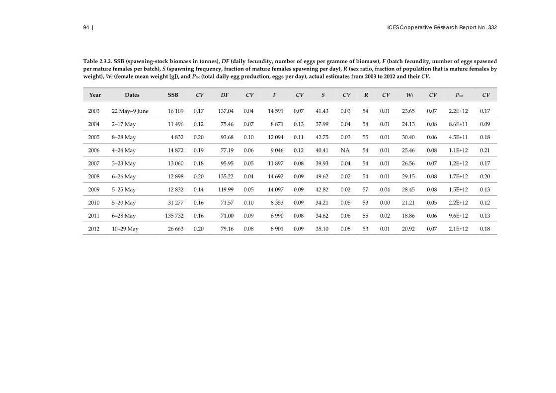
94 | ICES Cooperative Research Report No. 332
Table 2.3.2. SSB (spawning‐stock biomass in tonnes), DF (daily fecundity, number of eggs per gramme of biomass), F (batch fecundity, number of eggs spawned
per mature females per batch), S (spawning frequency, fraction of mature females spawning per day), R (sex ratio, fraction of population that is mature females by
weight), Wf (female mean weight [g]), and Ptot (total daily egg production, eggs per day), actual estimates from 2003 to 2012 and their CV.
Year Dates SSB CV DF CV F CV S CV R CV Wf CV Ptot CV
2003 22 May–9 June 16 109 0.17 137.04 0.04 14 591 0.07 41.43 0.03 54 0.01 23.65 0.07 2.2E+12 0.17
2004 2–17 May 11 496 0.12 75.46 0.07 8 871 0.13 37.99 0.04 54 0.01 24.13 0.08 8.6E+11 0.09
2005 8–28 May 4 832 0.20 93.68 0.10 12 094 0.11 42.75 0.03 55 0.01 30.40 0.06 4.5E+11 0.18
2006 4–24 May 14 872 0.19 77.19 0.06 9 046 0.12 40.41 NA 54 0.01 25.46 0.08 1.1E+12 0.21
2007 3–23 May 13 060 0.18 95.95 0.05 11 897 0.08 39.93 0.04 54 0.01 26.56 0.07 1.2E+12 0.17
2008 6–26 May 12 898 0.20 135.22 0.04 14 692 0.09 49.62 0.02 54 0.01 29.15 0.08 1.7E+12 0.20
2009 5–25 May 12 832 0.14 119.99 0.05 14 097 0.09 42.82 0.02 57 0.04 28.45 0.08 1.5E+12 0.13
2010 5–20 May 31 277 0.16 71.57 0.10 8 353 0.09 34.21 0.05 53 0.00 21.21 0.05 2.2E+12 0.12
2011 6–28 May 135 732 0.16 71.00 0.09 6 990 0.08 34.62 0.06 55 0.02 18.86 0.06 9.6E+12 0.13
2012 10–29 May 26 663 0.20 79.16 0.08 8 901 0.09 35.10 0.08 53 0.01 20.92 0.07 2.1E+12 0.18
Pelagic survey series for sardine and anchovy in ICES subareas 8 and 9 | 95
Regarding the adult reproductive parameters (Figure 2.3.5, Table 2.3.2), the sex ratio
(R) in mass is basically a constant around its long‐term mean of ca. 0.54, given our own
assumption of an invariant sex ratio 1:1 in numbers. Female mean weight (Wf) peaks
in years with poor levels of 1‐year‐old anchovies when the proportion of the 2+ age
group becomes relevant, as in 2005, 2008, and 2009. An exception happened in 2012
when, despite the high occurrence of 2‐year‐old anchovies (50%), the mean weight did
not increase markedly. This was due to abnormal low mean weights‐at‐ages (Figure
2.3.10).

96 | ICES Cooperative Research Report No. 332
Figure 2.3.5. Series of parameters needed to apply the DEPM from anchovy surveys in the Bay of
Biscay: spawning area (km²), daily egg production (eggs m–²), total daily egg production (eggs d–1),
batch fecundity (number of eggs spawned per mature females per batch), sex ratio (fraction of
population that are mature females by weight), females mean weight (g), spawning frequency
(fraction of mature females spawning per day), total mean weight (g), daily fecundity (number of
egg per gramme of biomass), and biomass in tonnes.

Pelagic survey series for sardine and anchovy in ICES subareas 8 and 9 | 97
Figure 2.3.6. Anchovy egg abundance (egg m–²) distribution obtained with PairoVET during DEPM
surveys in 2003–2012 in the Bay of Biscay.

98 | ICES Cooperative Research Report No. 332
Figure 2.3.7. Sardine egg abundance (egg m–²) distribution obtained with PairoVET during DEPM.
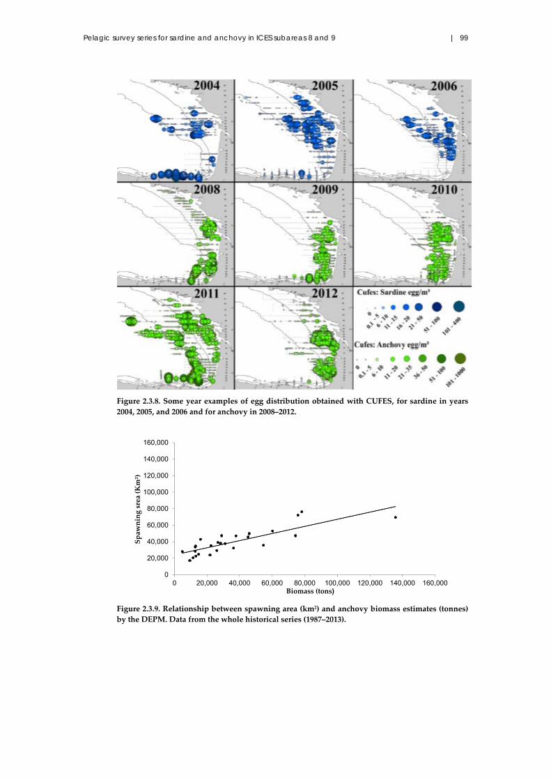
Pelagic survey series for sardine and anchovy in ICES subareas 8 and 9 | 99
Figure 2.3.8. Some year examples of egg distribution obtained with CUFES, for sardine in years
2004, 2005, and 2006 and for anchovy in 2008–2012.
Figure 2.3.9. Relationship between spawning area (km2) and anchovy biomass estimates (tonnes)
by the DEPM. Data from the whole historical series (1987–2013).
0
20,000
40,000
60,000
80,000
100,000
120,000
140,000
160,000
0 20,000 40,000 60,000 80,000 100,000 120,000 140,000 160,000
Spawning srea (Km²)
Biomass (tons)

100 | ICES Cooperative Research Report No. 332
Figure 2.3.10. Series of (top) percentage‐at‐age and (bottom) weight‐at‐age (g) for anchovy in the
Bay of Biscay from DEPM surveys BIOMAN.
As expected, batch fecundity (F) was closely related to the mean weight of females.
Spawning frequency (S) tended to be around the historical mean of about 0.4, except
in 2005 and for the last three years. In 2005, S peaked at 0.5, coinciding with a high
mean weight of females as a result of the relevant occurrence of 2‐year‐old anchovies
in the population. However, for the last three years, S stayed at about 0.34, below
average, coincidingwith the lower mean weights of the females during 2003–2012.
The relationship between S and Wf was perceived to be significant, but of little intensity
(Uriarte et al., 2012). However, for these last years, the intensity of this relationship
seems to be greater than perceived in the past series. According to all these results,
daily specific fecundity (DF) has varied during 2003–2012 between 70 and 140 in a
parallel trend to the mean weight of females (correlation coefficient of 0.56 and p of
0.073 due to being random), peaking in 2003, 2008, and 2009 and being at minima for
the last three years (2010–2012).
The DF in the Gironde area, where the smallest anchovies are found, has been slightly
below that in the remaining areas in several years (2004, 2005, and 2009–2012).
0
5
10
15
20
25
30
35
40
45
2003 2004 2005 2006 2007 2008 2009 2010 2011 2012
W AGE 1
W AGE 2
W AGE 3

Pelagic survey series for sardine and anchovy in ICES subareas 8 and 9 | 101
Accordingly, in these years, the weighting factors per adult sample were differentiated
according to the egg abundance in the area where they were obtained and to the
number of adult samples by area. Even though the results of the DF did not vary much,
depending or not on the applications of those weighting factors, they were prefered to
avoid potential bias in the results. These results suggest that at the time of the survey,
smaller anchovies around the Gironde area tended to have slightly smaller DF than the
remaining bigger anchovies.
Mean weight and mean lengths by age showed no clear trend, although in 2012, the
weights of the 1‐ and 2‐year‐old anchovies were the lowest in this series. At this stage,
no study on potential ecological reasons for this shift in mean weights and DF in recent
years has been done.
Biomass series, weight‐at‐age, and population in numbers‐at‐age are presented in
Figures 2.3.5 and 2.3.10. Between 2003 and 2010, DEPM SSB estimates were below
20 000 t. During this period, the fishery had difficulties obtaining normal levels of
catch. In 2003, the Spanish fishery was in deep crisis (STECF, 2003) and later, in 2005
and 2006, it collapsed completely and was unable to get any significant catch. This led
to the repeated closure of the fishery, first in June 2005 and another closure in June 2006
that lasted until January 2010. The DEPM estimated a recovery of the population in
2010 (up to ca. 31 300 t, CV = 16%) and peaked in 2011, with about 135 000 t (CV = 16%).
In these two years, the recovery was due to strong recruitment, as reflected in the high
percentage of 1‐year‐old anchovies in the population (>85%). In 2012, however, a sharp
drop in total egg production was recorded, which led to an estimate of ca. 27 000 t (CV =
20%) by the DEPM. The latter estimate contrasted with the results of the acoustic
survey which pointed to a further increase in population size to ca. 186 000 t. The
percentage‐at‐age 1 fish in the DEPM dropped to ca. 50%, which indirectly supported,
for an assumed level of natural mortality, some decrease in the population in 2012
relative to the high peak of 2011.
The consistency between the acoustic and DEPM estimates has been proven for a long
period of parallel surveys in May in the Bay of Biscay. However, in some years, there
are disagreements, as in 2012. The latest assessment of anchovy made by ICES in 2013
suggests that both surveys provided noisy results in 2012 in terms of biomass, with
opposite signs of their errors. ICES (2013) concluded that an intermediate biomass
estimate for that year was the one best accommodating all different information
collected up to 2013.
2.3.4 Concluding remarks
Overall, the DEPM has proven to be a very helpful monitoring system of the biomass
of anchovy in the Bay of Biscay, providing inputs for the assessment both in terms of
biomass and population (percentages) at age. The general consistency of the DEPM
estimates with those of the acoustic surveys are high, even though ICES assessments
reveal that there are overall catchability phenomena associated with both methods;
therefore, the series are not compatible in absolute, but in relative terms.
In this survey, CUFES is essentially used for the implementation of the adaptive
sampling scheme. There have been several studies trying to convert egg sampling at
the surface to the integrated water column egg abundance (Boyra et al., 2003; Petitgas
et al., 2006), but the method is still not sufficiently developed to be used.
The utility of the DEPM survey on anchovy also applies to sardine in the region,
because by the time of the survey, sardine spawning still takes place in an intense
manner, even though peak spawning is known to take place earlier in this area (Carrera

102 | ICES Cooperative Research Report No. 332
and Porteiro, 2003). The overall tendencies of PairoVET sardine egg abundance is
parallel to the acoustic estimates of biomass and these egg abundance estimates have
been considered an auxiliary source of information for the assessment of this sardine
population in the Bay of Biscay (ICES, 2013).
Beyond its use as input for assessment, the DEPM has contributed largely to a better
understanding of the reproductive biology of anchovy and of its spawning dynamics.
The first studies were undertaken in the past century on batch fecundity (Sanz and
Uriarte, 1989) and on spawning frequency and the dynamics of spawning females
(Sanz et al., 1992; Motos, 1994, 1996). Afterward, the study of adult parameters,
especially spawning frequency, was revisited, leading to a review of the classification
of POFs and oocytes (Alday et al., 2008, 2010) and, subsequently, the estimation
procedures of the spawning fraction (Uriarte et al., 2012). Moreover, a review of the
model to age anchovy eggs was realized (Ibaibarriaga et al., 2007b) and a review on the
procedures for estimating egg production (Bernal et al., 2001; Ibaibarriaga et al., 2007b)
and studies on egg mortality rates (Peña et al., 2010) were conducted. The review of the
whole series with these improvements on spawning frequency and egg production
was presented in ICES WKPELA (Santos et al., 2013b). Other studies were performed
related to the spatial distribution of anchovy eggs and their interaction with the
environment (Motos et al., 1996; Irigoien et al., 2007), sampling errors (Uriarte and
Motos, 1998), vertical distribution and modeling of anchovy eggs (Motos and Coombs,
2000; Boyra et al., 2003; Coombs et al., 2004), or in relation to recruitment (Irigoien et al.,
2008, 2009). During these surveys, zooplankton samples, phytoplankton samples, other
fish species, gut content of fish, fish larvae, and hydrographic parameters have also
been collected. These data have led to several PhD theses that have provided ecosystem
information of the Bay of Biscay (Albaina, 2007; Zarauz, 2007; Díaz, 2008; Aldanondo,
2010; Bachiller, 2012).
2.3.5 Acknowledgements
The BIOMAN survey series have been sponsored since 2003 by the Department of
Fisheries of the autonomous Basque Government within Spain and by the European
Union within the Community framework for the Data Collection Regulation (EC, 2000,
2008). The survey has also been supported by the Spanish General Secretariat of the
Sea, providing the RV “Emma Bardán” since 2003. Special thanks are due to the crews
of RV “Investigador”, RV “Emma Bardán”, RV “Vizconde de Eza”, and RV “Ramón
Margalef”, and to all the AZTI staff that have participated in the BIOMAN surveys
since 1987 for their excellent job and collaborative support. Thanks are given to
IFREMER (Institute français de recherche pour lʹexploitation de la mer) and IEO
(Instituto Español de Oceanografía) Santander for their support in the collection of
adult samples in 2003–2005.
Pelagic survey series for sardine and anchovy in ICES subareas 8 and 9 | 103
2.4 Summer acoustic surveys in the Gulf of Cádiz: ECOCADIZ survey series (2004–2010)
Fernando Ramos, Magdalena Iglesias, Joan Miquel, Dolors Oñate, and Jorge
Tornero
2.4.1 Introduction of the survey
A purse‐seine fishery on anchovy and sardine operates traditionally in the Spanish
waters of the Gulf of Cádiz (ICES Division 9.a South). Other species like chub mackerel
and, to a lesser extent, horse mackerel stand out as secondary species (Millán, 1992;
Ramos and Millán, 2004). The IEO started the studies on both this fishery and anchovy
biology in the late 1980s, with such studies being successively subordinated to different
IEO structural research projects.
The series of Spanish acoustic surveys in ICES Division 9.a South started in its current
form in 2004, although the IEO had already conducted two previous surveys in 1993
and 2002 with the RV “Cornide de Saavedra”, surveying only the Spanish waters of
the Gulf of Cádiz. The ECOCADIZ 0693 survey, carried out in June 1993, was aimed at
the acoustic assessment of anchovy (Baro et al., 1993). In February 2002, the SIGNOISE
survey was carried out, which was an acoustic intercalibration exercise between the
RV “Cornide de Saavedra” and the RV “Vizconde de Eza”. This survey also obtained
the noise signature of both vessels (Carrera, 2003).
The IEO accepted the formal commitment to initiate regular assessments of the Gulf of
Cádiz anchovy by direct methods in 2004, proposing to conduct the BOCADEVA 0604
survey series. This survey was one of the research activities comprised within the IEO
research project PELCOSAT, a project mainly focused on the study of the Gulf of Cádiz
anchovy fisheries, biology, and population dynamics. BOCADEVA 0604 was
considered the starting point of two newly proposed survey series that IEO expected
to develop structurally in the study area: the triennial Gulf of Cádiz anchovy DEPM
survey (the BOCADEVA series, see Section 2.5) and the annual acoustic survey from
the ECOCADIZ series. The season for both survey series (late spring–early summer)
was initially chosen to obtain either an acoustic or a DEPM‐based estimate of the
anchovy SSB in the study area. Furthermore, the geographical coverage of these survey
series was extended to both Spanish and Portuguese waters of the Gulf of Cádiz in
order to obtain synoptic coverage of the distribution of pelagic resources all over ICES
Division 9.a South.
BOCADEVA 0604 was planned as a pilot combined acoustic–DEPM survey. There
were several reasons why this survey was considered exploratory. First, as noted
above, the only preceding acoustic survey conducted during the same season as the
present one in the study area dated back to June 1993 (ECOCADIZ 0693). Second, the
same sampling area surveyed in BOCADEVA 0604 was also acoustically assessed in a
routine way by the Portuguese IPMA (former IPIMAR) since 1996 (SAR survey series
in those years), but the timing (February–March and November) was not very suitable
for assessing the anchovy SSB. Third, the distribution pattern of abundance of the main
pelagic species in early summer in the study area was unknown from direct surveying.
Hence, those problems related to both the acoustic sampling and coverage, and the
fishing hauls used for echotrace identification during the survey season had to be
evaluated in order to adequately plan and design the next acoustic surveys.
Additionally, the survey also included a series of exploratory activities
(ichthyoplankton and adult DEPM‐based sampling) aimed at elucidating certain
aspects of the Gulf of Cádiz anchovy spawning ecology and reproductive strategy.

104 | ICES Cooperative Research Report No. 332
Results from this survey provided the clues for the subsequent design and planning of
the next DEPM surveys, the first one in 2005.
Regarding the acoustic surveying, the ECOCADIZ series actually started in 2004 with
the BOCADEVA 0604 survey, with the next surveys in the series already termed as
ECOCADIZ surveys since 2006.
The main objective of the ECOCADIZ surveys since 2004 was the acoustic assessment
(by echo integration) and mapping of the abundance and biomass of the populations
of the main neritic pelagic fish species in the Gulf of Cádiz over the continental shelf
(depths of 20–200 m), including both Portuguese and Spanish waters (i.e. the entire
ICES Division 9.a South).
The Gulf of Cádiz is a mixed‐species ecosystem where gregarious pelagic fish species
form numerous small schools. Main pelagic species assessed in the ECOCADIZ
surveys include: anchovy, sardine, round sardinella (Sardinella aurita), Atlantic
mackerel, chub mackerel, Atlantic horse mackerel, Mediterranean horse mackerel, blue
jack mackerel, and bogue. However, round sardinella and Atlantic mackerel usually
show an incidental occurrence in the surveyed area. Under the sampling scheme of a
”pelagic ecosystem survey”, the above overall objective is routinely complemented
with the following ones:
biological characterization of the assessed species in relation to their main
habitats (i.e. feeding, spawning, nursery, or recruitment habitat, according
to the case), especially from their size composition and/or age structure,
maturity, repletion, and condition status;
characterization and (rough) delimitation of the anchovy spawning habitat
in the surveyed area from the spatial distribution of both the adults (by
acoustics and pelagic hauls sampling) and eggs (by CUFES sampling);
distribution and abundance of the top predators of the pelagic community
(cetaceans, sea turtles, and seabirds);
oceanographic and environmental characterization of the surveyed area,
namely the thermo‐haline properties of the shelf waters through continuous
(subsuperficial layer) and discrete (vertical profiles) sampling, as well as the
recording of climatic variables.
Throughout the recent series, ECOCADIZ surveys have included other objectives such
as the realization of the first trials of in situ measurements of anchovy target strength
in the study area (2006 and 2007), the collection of biological material for anchovy
DEPM‐based studies (2004, 2006, 2007, and 2009), studies of the summer feeding
behavior of the main pelagic species in the surveyed area (2009), and direct studies of
the importance and use of discards by scavenger seabirds (2009 and 2010).
2.4.2 Material and methods
The surveys in this new series were planned to be routinely performed on a yearly
basis. However, the series had some gaps in those years (2005, 2008, and 2011)
coinciding with the conduct of the anchovy DEPM survey (the true BOCADEVA series;
see Section 2.5 below) because of available ship time (Table 2.4.1). Given the above
constraints, the ECOCADIZ series was conducted in 2004, 2006, 2007, 2009, 2010, and
2013 (this last survey is not analysed in the present report).
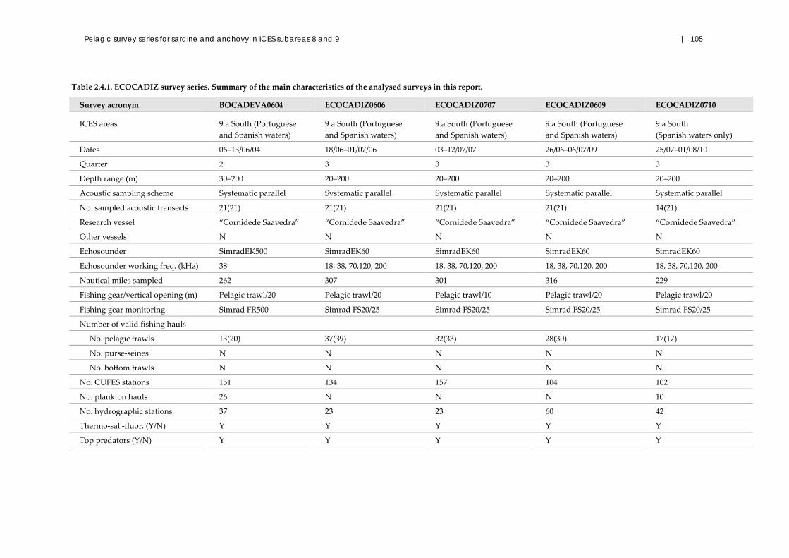
Pelagic survey series for sardine and anchovy in ICES subareas 8 and 9 | 105
Table 2.4.1. ECOCADIZ survey series. Summary of the main characteristics of the analysed surveys in this report.
Survey acronym BOCADEVA0604 ECOCADIZ0606 ECOCADIZ0707 ECOCADIZ0609 ECOCADIZ0710
ICES areas 9.a South (Portuguese
and Spanish waters)
9.a South (Portuguese
and Spanish waters)
9.a South (Portuguese
and Spanish waters)
9.a South (Portuguese
and Spanish waters)
9.a South
(Spanish waters only)
Dates 06–13/06/04 18/06–01/07/06 03–12/07/07 26/06–06/07/09 25/07–01/08/10
Quarter 2 3 3 3 3
Depth range (m) 30–200 20–200 20–200 20–200 20–200
Acoustic sampling scheme Systematic parallel Systematic parallel Systematic parallel Systematic parallel Systematic parallel
No. sampled acoustic transects 21(21) 21(21) 21(21) 21(21) 14(21)
Research vessel “Cornidede Saavedra” “Cornidede Saavedra” “Cornidede Saavedra” “Cornidede Saavedra” “Cornidede Saavedra”
Other vessels N N N N N
Echosounder SimradEK500 SimradEK60 SimradEK60 SimradEK60 SimradEK60
Echosounder working freq. (kHz) 38 18, 38, 70,120, 200 18, 38, 70,120, 200 18, 38, 70,120, 200 18, 38, 70,120, 200
Nautical miles sampled 262 307 301 316 229
Fishing gear/vertical opening (m) Pelagic trawl/20 Pelagic trawl/20 Pelagic trawl/10 Pelagic trawl/20 Pelagic trawl/20
Fishing gear monitoring Simrad FR500 Simrad FS20/25 Simrad FS20/25 Simrad FS20/25 Simrad FS20/25
Number of valid fishing hauls
No. pelagic trawls 13(20) 37(39) 32(33) 28(30) 17(17)
No. purse‐seines N N N N N
No. bottom trawls N N N N N
No. CUFES stations 151 134 157 104 102
No. plankton hauls 26 N N N 10
No. hydrographic stations 37 23 23 60 42
Thermo‐sal.‐fluor. (Y/N) Y Y Y Y Y
Top predators (Y/N) Y Y Y Y Y

106 | ICES Cooperative Research Report No. 332
Unfortunately, the current economic crisis also affected the original planning and
degree of accomplishment of the objectives of the last ECOCADIZ surveys, a series that
is so far financed with IEO’s own funds (and with no Data Collection Resolution [DCR]
partial funding). Thus, recent surveys experienced a gradual reduction in the number
of survey days in relation to the 14 days originally requested (e.g. 10 days in 2009 and
7 days in 2010). The drastic reduction in ship time available for the 2010 survey resulted
in the surveying of only those waters located east of Cape Santa Maria. Because of these
budgetary problems, no standard summer ECOCADIZ survey was carried out in 2012.
As noted above, late spring (i.e. early‐mid June) was initially considered the most
suitable time for conducting the ECOCADIZ surveys as this coincides with the peak
spawning of anchovy in the Gulf of Cádiz (Millán, 1992) and is, therefore, the best
season to acoustically sample and estimate the anchovy SSB in the area. However, the
start of these surveys was also progressively delayed to mid‐summer as a consequence
of both a reduction in ship time and the priority given to other DCR‐funded IEO
surveys within the IEO research vessels’ timetables.
All the surveys in the series have been carried out with the IEO’s RV “Cornide de
Saavedra”, a 66.7‐m stern trawler (Table 2.4.2). Research vessels of smaller dimensions
and lower draughts, such as the IEO’s RV “Francisco de Paula Navarro” and the
General Secretariat of Maritime Fisheries’ (SGPM) RV “Emma Bardán”, were
occasionally used in some experiments of acoustic surveying in the shallowest waters
of the Gulf of Cádiz (see below). The RV “Cornide de Saavedra” went out of service
after the ECOCADIZ 0813 survey conducted in August 2013. The SGPM’s RV “Miguel
Oliver” will be the new candidate to conduct the next ECOCADIZ surveys beginning
in 2014.
Table 2.4.2. ECOCADIZ surveys series. Technical characteristics of the research vessels used in the
IEO standard surveys and pilot experiments (in the shallowest waters) of acoustic surveying of the
Gulf of Cádiz.
Research vessel Length
(m)
Width
(m)
Draught
(m) GRT HP
“Cornide de Saavedra” 66.7 11.3 4.65 1 113 2 250
“Francisco de Paula
Navarro”
30.5 7.4 4.26 178 750
“Emma Bardán” 29.0 7.5 3.90 200 900
As mentioned in Section 2.2, the IEO acoustic surveys, including the ECOCADIZ
series, experienced a continuous and very dynamic standardization process during the
second half of the past decade. This involved not only improvement of the design and
objectives of the surveys (trying to satisfy the implementation of the ecosystem
approach), but also the development of techniques of data post‐processing and
analysis (use of specific software, algorithms, masks, and virtual echograms) as a
logical consequence of the incorporation of multifrequency acoustic instrumentation
(see ICES, 2006a,b and Annex 2 for details). These and other related research activities
in fisheries bioacoustics were then and still are currently developed by IEO within the
framework of the consecutive proposals of its structural research project DETAC. Both
research project and standardization process benifitted from the progress and expertise
achieved in previous EU projects (e.g. PELASSES, CLUSTER, SIMFAMI) as well as
from recommendations from different ICES expert groups on fisheries acoustics
(Working Group on Fisheries Acoustics Science and Technology [WGFAST]; former
Planning Group for Acoustic Surveys in ICES Subareas 8 and 9 [PGPAS]; Working

Pelagic survey series for sardine and anchovy in ICES subareas 8 and 9 | 107
Group on Acoustic and Egg Surveys for Sardine and Anchovy in ICES Subareas 8 and
9 [WGACEGG]), assessment of pelagic stocks (former working groups on the
Assessment of Mackerel, Horse Mackerel, Sardine and Anchovy [WGMHSA]; on
Anchovy and Sardine [WGANSA]; and on Anchovy [WGANC], currently merged as
working groups on Widely Distributed Stocks [WGWIDE] and on Southern Horse
Mackerel, Anchovy and Sardine [WGHANSA]), and small pelagic fish ecology (former
Study Group on Regional Scale Ecology of Small Pelagic Fish [SGRESP];
ICES/GLOBEC Working Group on Life Cycle and Ecology of Small Pelagic Fish
[WGLESP]).
In parallel, the RV “Cornide de Saavedra”, as the observational platform of the Gulf of
Cádiz pelagic ecosystem during the ECOCADIZ surveys, was equipped during a short
time‐period with the required scientific–technical equipment for accomplishing the
above‐mentioned recommendations (Table 2.4.1). Thus, since the beginning of the
ECOCADIZ series, the research vessel was equipped with samplers of the biological
and hydrological environment, namely a continuous underway fish egg sampler
(CUFES; Checkley et al., 1997), a thermo‐salinometer and fluorometer, a meteorological
station (since 2009), and the discrete sampling of vertical profiles of physical variables
in the water column with a CTD. Regarding acoustic sampling, the replacement in 2006
of the old SimradTM EK500 echosounder, working at 38 kHz, by the SimradTM EK60
scientific echosounder, working in a multifrequency fashion, satisfied the ICES
recommendations on the use, as a minimum, of two working frequencies, 38 and
120 kHz. Following this line of improvements, the RV “Cornide de Saavedra” also
incorporated a new system of pelagic trawl gear monitoring consisting of a SimradTM
Mesotech FS20/25 net sonar, allowing the net geometry and vertical positioning of the
fishing gears as samplers of pelagic fish assemblages to be monitored.
Notwithstanding the above, there are still steps to be taken to obtain a better and more
complete characterization of the Gulf of Cádiz pelagic ecosystem (e.g. the routine
sampling of the mesozooplankton species composition and biomass and the collection
of direct measures of primary production and nutrients in the water column are not
yet available). However, it is expected that, in the medium term, ECOCADIZ surveys
may achieve the same level as other pelagic ecosystem surveys that are conducted on
board more modern research vessels and considered as references, such as the
PELACUS and PELGAS surveys on board RV “Thalassa”.
On the other hand, the acoustic sampling scheme adopted in the ECOCADIZ surveys
has also experienced some changes and attempts to improve the spatial coverage
through its relatively short history. The standard surveyed area comprises the Gulf of
Cádiz waters, both Portuguese (Algarve) and Spanish waters, with an acoustic
sampling grid consisting of a systematic parallel grid of 21 transects, equally spaced by
8 nautical miles and perpendicular to the shoreline (Figure 2.4.1). This scheme allows
the entire study area to be sampled in about 12–14 days.
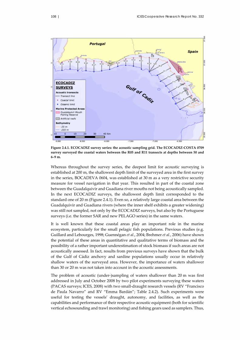
108 | ICES Cooperative Research Report No. 332
Figure 2.4.1. ECOCADIZ survey series: the acoustic sampling grid. The ECOCADIZ‐COSTA 0709
survey surveyed the coastal waters between the R05 and R11 transects at depths between 50 and
6–9 m.
Whereas throughout the survey series, the deepest limit for acoustic surveying is
established at 200 m, the shallowest depth limit of the surveyed area in the first survey
in the series, BOCADEVA 0604, was established at 30 m as a very restrictive security
measure for vessel navigation in that year. This resulted in part of the coastal zone
between the Guadalquivir and Guadiana river mouths not being acoustically sampled.
In the next ECOCADIZ surveys, the shallowest depth limit corresponded to the
standard one of 20 m (Figure 2.4.1). Even so, a relatively large coastal area between the
Guadalquivir and Guadiana rivers (where the inner shelf exhibits a greater widening)
was still not sampled, not only by the ECOCADIZ surveys, but also by the Portuguese
surveys (i.e. the former SAR and new PELAGO series) in the same waters.
It is well known that these coastal areas play an important role in the marine
ecosystem, particularly for the small pelagic fish populations. Previous studies (e.g.
Guillard and Lebourges, 1998; Guennégan et al., 2004; Brehmer et al., 2006) have shown
the potential of these areas in quantitative and qualitative terms of biomass and the
possibility of a rather important underestimation of stock biomass if such areas are not
acoustically assessed. In fact, results from previous surveys have shown that the bulk
of the Gulf of Cádiz anchovy and sardine populations usually occur in relatively
shallow waters of the surveyed area. However, the importance of waters shallower
than 30 or 20 m was not taken into account in the acoustic assessments.
The problem of acoustic (under‐)sampling of waters shallower than 20 m was first
addressed in July and October 2008 by two pilot experiments surveying these waters
(PACAS surveys; ICES, 2008) with two small‐draught research vessels (RV “Francisco
de Paula Navarro” and RV “Emma Bardán”; Table 2.4.2). Such experiments were
useful for testing the vessels’ draught, autonomy, and facilities, as well as the
capabilities and performance of their respective acoustic equipment (both for scientific
vertical echosounding and trawl monitoring) and fishing gears used as samplers. Thus,

Pelagic survey series for sardine and anchovy in ICES subareas 8 and 9 | 109
in 2009, the standard ECOCADIZ 0609 survey was complemented with the
ECOCADIZ‐COSTA 0709 survey. This last survey was conducted with the IEO’s RV
“Francisco de Paula Navarro”, almost synchronously to the conventional one, in
waters shallower than 20 m off the central part of the study area. However, because
the acoustic equipment used in the coastal survey was not properly calibrated, the
resulting estimates were considered only indicative, although they demonstrated that
coastal shallow waters not covered by conventional surveys (either Spanish or
Portuguese) may hold a relatively important biomass (Ramos et al., 2010). Tentative
estimates for the combination of standard and coastal surveys indicated that these
central shallow waters yielded about 14% and 12% of the acoustically assessed overall
fish abundance and biomass,. Obviously, the relative importance of these coastal
waters was greater for coastal species; anchovy abundance and biomass accounted for
18% and 14% of the total estimates, respectively, whereas the corresponding
abundance and biomass estimates for sardine were 16% and 17%. Coastal relative
contributions for bogue and Mediterranean horse mackerel were even higher (ca. 36%
for both variables in the former species and ca. 50% for the latter). Unfortunately,
sampling of the shallowest coastal waters by a survey complementary to the standard
one did not continue in subsequent years.
Species identification, size classes, and other biological characteristics comprising fish
echotraces heavily depend on identification via trawl hauls. Fishing stations are
opportunistic, according to the echogram information, and are performed in daylight
as often as possible according to the echogram information. In any case, trawl catches
do not allow for the identification of single schools, but rather for an ensemble of
schools over several nautical miles, resulting in identifying groups of schools to species
assemblages. These ground‐truth trawl hauls have been carried out throughout the
ECOCADIZ series using the different pelagic trawl gears of the RV “Cornide de
Saavedra”, depending on their availability during the survey. The usual research
vessel’s set of pelagic trawl gears comprises three different gears with vertical openings
of ca. 12–13 m (Pedreira), 16–18 m (Tuneado), and 20–22 m (Gran Hermano), with the
last one being the preferred option because of its greater sampling coverage, but
mainly used in waters deeper than 30–40 m. Acoustic transects are adaptively
interrupted to perform the trawl hauls and subsequently resumed. Trawls are carried
out at a mean speed of four knots. In the ECOCADIZ surveys, duration of the fishing
hauls will depend on the success in capturing the situation to be identified, although
the effective fishing time (as monitored by netsonde or sonar) usually lasts between 30
and 45 min.
Ground‐truth fishing in the shallowest waters (usually between the 20‐ and 40‐m
isobaths) in the central and western parts of the sampled area is not always possible
because of the presence of artisanal fixed fishing gears. Coastal fishing in Spanish
waters is additionally complicated by the presence of artificial reefs and of a fishing
reserve in the coastal waters close to the mouth of the Guadalquivir River (Figure 2.4.1).
Some locations in this coastal area, unfortunately, have recorded high backscattering
values, indicating relevant fish abundance. As an alternative to this serious drawback,
fishing hauls in these situations are usually attempted by fishing over an isobath as
close as possible to the depths where the fishing situation of interest is detected over
the acoustic track. It was also found that fishing over an isobath, instead of along the
acoustic track, was preferable in various other situations to avoid mixing different size
compositions (i.e. bi‐ or multimodality of length frequency distributions). This mixing
is more apt to occur close to nursery or recruitment areas and in regions with a very
narrow continental shelf. Given that all of these situations are quite common in the

110 | ICES Cooperative Research Report No. 332
sampled area, these kinds of fishing hauls usually represent a relatively high
percentage of the total in each survey. In any case, because the echotraces occur close
to the seabed during daylight (especially those echotraces attributed to anchovy), most
of the pelagic hauls are carried out very close to the seabed.
As for the acoustic assessment, a detailed description of the adopted species‐specific
TS values and methods for NASC allocation to species and computation of echo
integration estimates (including the definition of coherent post‐strata) are given in
Section 2.2.2.2.
The sampling of oceanographic variables also experienced some improvement in
recent years regarding coverage with CTD casts. Thus, the CTD sampling grid has been
progressively intensified to include a greater number of stations than those initially
planned in the first surveys in the series (Table 2.4.1, Figure 2.4.2).
A census of top predators (seabirds, sea turtles, and cetaceans) along all of the acoustic
transects and intertransects has also been carried out since the beginning of the series
by a bow observer, using standardized strip‐transect techniques (Tasker et al., 1984)
adapted to match the specific conditions of the surveyed area. A 600‐m strip‐width (i.e.
180°) transect band is normally used, with the observer surveying both sides of the
vessel. The width of the band is checked periodically using a range‐finder (Heinemann,
1981). Snapshot counts are used to carry out a census of flying birds (Tasker et al., 1984).
Only those observations recorded between the depths of 20 and 200 m are considered.
Figure 2.4.2. ECOCADIZ surveys series. Recent CTD sampling grid.
2.4.3 Results and discussion
The number of valid groundtruth trawl hauls from those surveys that sampled the
whole study area oscillated between 13 and 37 hauls. This range even increases up to
28–37 trawl hauls if the 2004 survey is not considered because of its experimental
nature (Table 2.4.1, Figure 2.4.3). Although they were performed in an opportunistic
way, it is assumed that, with the above coverage, such pelagic hauls provide a
relatively realistic picture of the pelagic fish species assemblage in the study area in

Pelagic survey series for sardine and anchovy in ICES subareas 8 and 9 | 111
summer. Thus, the percentages of occurrence of fish species in the surveys’ valid hauls
indicate that chub mackerel, anchovy, and sardine, in that order, are the most frequent
species, with average presence indices at ca. or >70% (Table 2.4.3). These species are
followed by Atlantic mackerel, hake, and bogue, with mean presence indices at ca.
60%, and Atlantic and Mediterranean horse mackerel and blue jack mackerel, with
average indices for the surveys series < 50%.
Some inferences on species distribution may also be made from the results from the
pelagic trawls (Figure 2.4.3 shows species composition in the catches by haul and
survey in terms of percentages in weight) and from the acoustic energy attributed to
species (as a proxy for species density in the surveyed area; Figures 2.4.4 and 2.4.5).
Visual inspection of all these figures suggests that anchovy exhibits some preference
for the central and eastern waters of the Gulf, mainly where the shelf widens, a zone
that corresponds to the Guadalquivir River estuary. Sardine shows a more variable
pattern depending on the year, but generally with a more coastal distribution than
anchovy, and sardine also seems to avoid, to some extent, the preferred waters of
anchovy. Chub mackerel, although widely distributed, seems to show some preference
for the westernmost mid‐ and outer shelf waters of the Gulf, with a secondary nucleus
of occurrence in the easternmost extreme of the surveyed area. Conversely, Atlantic
mackerel seems to be restricted to the central‐eastern waters of the Gulf. Regarding
representatives of the genus Trachurus, Atlantic horse mackerel is widely distributed
throughout the surveyed area, whereas blue jack mackerel prefers the mid‐ and outer
shelf waters of the western sector, while Mediterranean horse mackerel is mainly
distributed in the coastal waters of the easternmost sector, closer to the vicinity of the
Strait of Gibraltar.
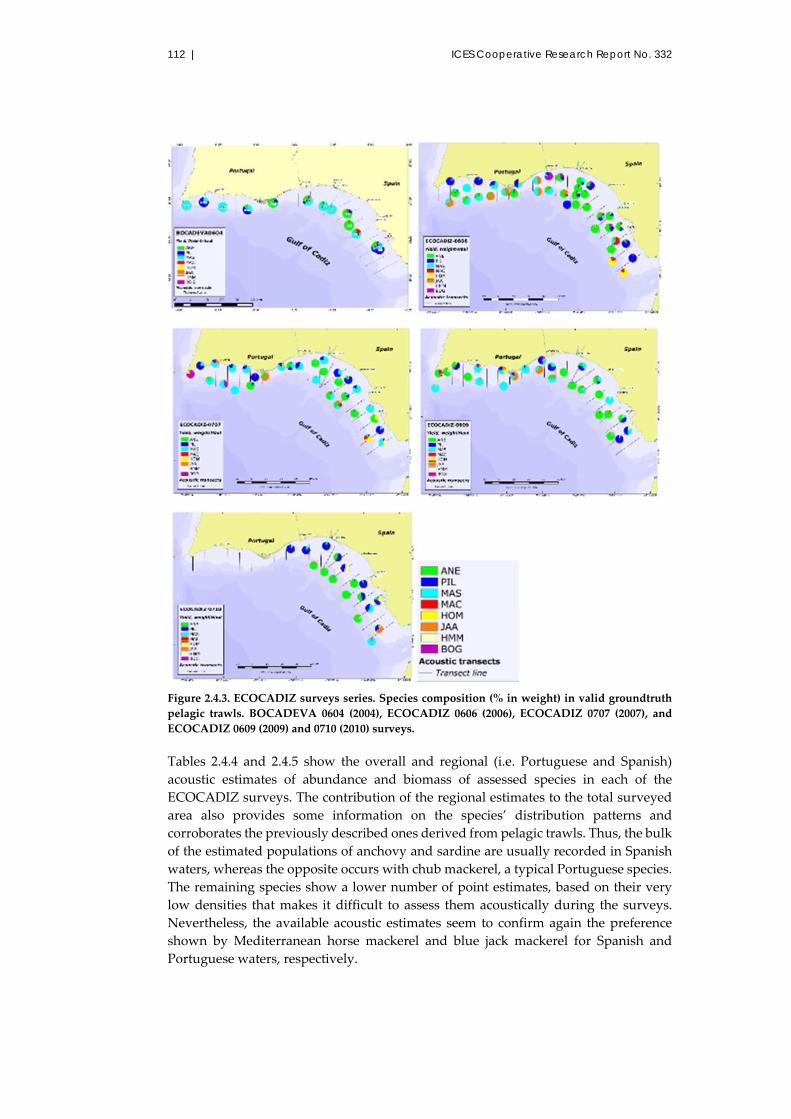
112 | ICES Cooperative Research Report No. 332
Figure 2.4.3. ECOCADIZ surveys series. Species composition (% in weight) in valid groundtruth
pelagic trawls. BOCADEVA 0604 (2004), ECOCADIZ 0606 (2006), ECOCADIZ 0707 (2007), and
ECOCADIZ 0609 (2009) and 0710 (2010) surveys.
Tables 2.4.4 and 2.4.5 show the overall and regional (i.e. Portuguese and Spanish)
acoustic estimates of abundance and biomass of assessed species in each of the
ECOCADIZ surveys. The contribution of the regional estimates to the total surveyed
area also provides some information on the species’ distribution patterns and
corroborates the previously described ones derived from pelagic trawls. Thus, the bulk
of the estimated populations of anchovy and sardine are usually recorded in Spanish
waters, whereas the opposite occurs with chub mackerel, a typical Portuguese species.
The remaining species show a lower number of point estimates, based on their very
low densities that makes it difficult to assess them acoustically during the surveys.
Nevertheless, the available acoustic estimates seem to confirm again the preference
shown by Mediterranean horse mackerel and blue jack mackerel for Spanish and
Portuguese waters, respectively.

Pelagic survey series for sardine and anchovy in ICES subareas 8 and 9 | 113
Figure 2.4.4. ECOCADIZ survey series. Distribution of the backscattering energy (nautical area
scattering coefficient, NASC, in m2 nautical mile–2) attributed to anchovy (Engraulis encrasicolus). BOCADEVA 0604 (2004), ECOCADIZ 0606 (2006), ECOCADIZ 0707 (2007), and ECOCADIZ 0609 (2009) and 0710 (2010) surveys.
Regarding the target species in the present report, Figure 2.4.6 shows the trends in the
estimated biomass of Gulf of Cádiz anchovy and sardine populations through the
ECOCADIZ series. In order to achieve better visualization of the trend, anchovy
biomass estimates by acoustics are complemented with the DEPM‐based estimates
obtained during the BOCADEVA surveys (see Section 2.5). The Gulf of Cádiz anchovy
biomass estimated by acoustics for the period under study is about 26 kt on average (a
value computed for the whole series, except for the 2010 partial estimate).
Nevertheless, the period starts with relatively low biomass levels in 2004–2005, well
below the mean in 2006, which shows a remarkable increase to 36 kt. Since 2007, the
biomass shows a slight decreasing trend, but with point estimates relatively close to
the average. During the period under analysis, the size composition of the estimated
population ranged between the 7‐ and 18.5‐cm size classes, with modal classes mainly
located at 13 or 14 cm (Figure 2.4.7). Larger (older) anchovies are usually recorded in
Portuguese waters. A smaller mode at 9.5 cm (and composed of age 0 anchovies) was
also recorded in 2010 as a probable consequence of the delay in the start of the survey
to early August, a time that is usually coincident with the first main events of anchovy
recruitment in the Gulf. In any case, age‐structured estimates of anchovy abundance

114 | ICES Cooperative Research Report No. 332
show that the population is supported mainly by age 1 anchovies, with their annual
fluctuations being responsible for the fluctuations observed for the whole population
(Figure 2.4.7).
Figure 2.4.5. ECOCADIZ survey series. Distribution of the backscattering energy (nautical area
scattering coefficient, NASC, in m2 nautical mile–2) attributed to sardine (Sardina pilchardus). BOCADEVA 0604 (2004), ECOCADIZ 0606 (2006), ECOCADIZ 0707 (2007), and ECOCADIZ 0609
(2009) and 0710 (2010) surveys.
The sardine biomass estimated for the period under analysis averaged ca. 69 kt. The
interannual evolution of the sardine biomass estimates seems to run parallel to that
described above for anchovy, with a very low estimate in 2004, a peak in 2006, and a
decreasing trend since 2007, somewhat more pronounced than observed in anchovy,
although suggesting a certain recovery up to average levels in 2010 (Figure 2.4.6).
Unfortunately, there are no sardine age‐structured estimates available. The size
composition of the estimated population is rather constant throughout the series and
is characterized by a size range usually oscillating between 9 and 21.5–22.5 cm and
with two clear modes. The smallest mode is composed of recruits (and occurs more
frequently in coastal Spanish waters) at ca. 10.5–11.5 cm, and the second mode
encompasses the major part of the population at ca. 18–18.5 cm (Figure 2.4.8).

Pelagic survey series for sardine and anchovy in ICES subareas 8 and 9 | 115
Regarding the assessment of the sardine and anchovy stocks in ICES divisions 8.c and
9.a (sardine), or in Division 9.a only (anchovy), indices provided by the ECOCADIZ
survey series have become a relevant data source to verify the actual trends in at least
the southern components of these stocks, although more specifically in the case of the
Gulf of Cádiz anchovy because of the survey dates (ICES, 2013).
For the time being, no analytical assessment model has been successfully applied to
anchovy in Division 9.a. The provision of advice on anchovy in Division 9.a currently
relies almost exclusively on a qualitative analysis of survey trends (those
corresponding to the PELAGO, ECOCADIZ, and BOCADEVA surveys; see sections
2.2, 2.4, and 2.5). Recent results on genetics and independent trends observed in the
fisheries and in the population abundance estimates have confirmed an independent
stock of anchovy in the northwestern part of Division 9.a (western Iberian waters)
separate from the anchovy in Division 9.a South. In this context, ICES has considered
each of the above survey series (including the PELACUS results for the northernmost
area in Division 9.a) as an essential tool for the direct assessment of the population in
their respective survey areas (subdivisions) and has recommended their continuity,
mainly in those series that have suffered interruptions in their recent history, as in the
case of ECOCADIZ. Regarding this last series, ICES has emphasized that this survey
could trigger the revision in autumn of the advice for anchovy in Division 9.a South
provided in June, particularly in case of contradicting tendencies observed by the
(spring) PELAGO surveys in this area. ICES also recognizes that these sources of
information might become the knowledge base for the implementation of future
alternative management regimes based on survey information and analytic
assessments.
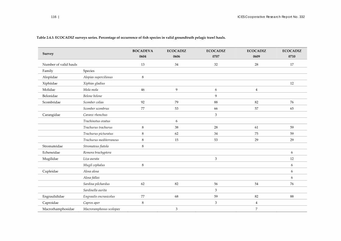
116 | ICES Cooperative Research Report No. 332
Table 2.4.3. ECOCADIZ surveys series. Percentage of occurrence of fish species in valid groundtruth pelagic trawl hauls.
Survey BOCADEVA
0604
ECOCADIZ
0606
ECOCADIZ
0707
ECOCADIZ
0609
ECOCADIZ
0710
Number of valid hauls 13 34 32 28 17
Family Species
Alopiidae Alopias superciliosus 8
Xiphiidae Xiphias gladius 12
Molidae Mola mola 46 9 6 4
Belonidae Belone belone 9
Scombridae Scomber colias 92 79 88 82 76
Scomber scombrus 77 53 66 57 65
Carangidae Caranx rhonchus 3
Trachinotus ovatus 6
Trachurus trachurus 8 38 28 61 59
Trachurus picturatus 8 62 34 75 59
Trachurus mediterraneus 8 15 53 29 29
Stromateidae Stromateus fiatola 8
Echeneidae Remora brachyptera 6
Mugilidae Liza aurata 3 12
Mugil cephalus 8 6
Cupleidae Alosa alosa 6
Alosa fallax 6
Sardina pilchardus 62 82 56 54 76
Sardinella aurita 3
Engraulididae Engraulis encrasicolus 77 68 59 82 88
Caproidae Capros aper 8 3 4
Macrorhamphosidae Macroramphosus scolopax 3 7
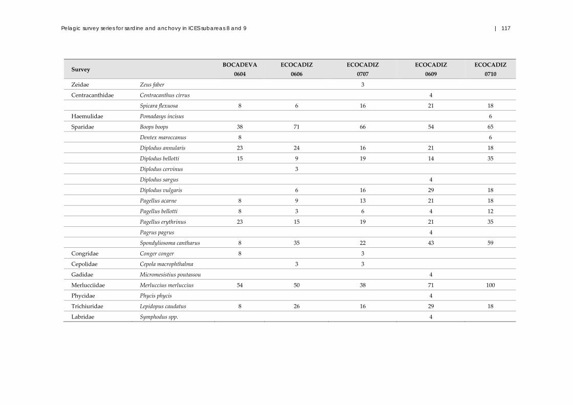
Pelagic survey series for sardine and anchovy in ICES subareas 8 and 9 | 117
Survey BOCADEVA
0604
ECOCADIZ
0606
ECOCADIZ
0707
ECOCADIZ
0609
ECOCADIZ
0710
Zeidae Zeus faber 3
Centracanthidae Centracanthus cirrus 4
Spicara flexuosa 8 6 16 21 18
Haemulidae Pomadasys incisus 6
Sparidae Boops boops 38 71 66 54 65
Dentex maroccanus 8 6
Diplodus annularis 23 24 16 21 18
Diplodus bellotti 15 9 19 14 35
Diplodus cervinus 3
Diplodus sargus 4
Diplodus vulgaris 6 16 29 18
Pagellus acarne 8 9 13 21 18
Pagellus bellotti 8 3 6 4 12
Pagellus erythrinus 23 15 19 21 35
Pagrus pagrus 4
Spondyliosoma cantharus 8 35 22 43 59
Congridae Conger conger 8 3
Cepolidae Cepola macrophthalma 3 3
Gadidae Micromesistius poutassou 4
Merlucciidae Merluccius merluccius 54 50 38 71 100
Phycidae Phycis phycis 4
Trichiuridae Lepidopus caudatus 8 26 16 29 18
Labridae Symphodus spp. 4

118 | ICES Cooperative Research Report No. 332
Survey BOCADEVA
0604
ECOCADIZ
0606
ECOCADIZ
0707
ECOCADIZ
0609
ECOCADIZ
0710
Serranidae Anthias anthias 7
Callantias ruber 4
Serranus cabrilla 3
Serranus hepatus 3 6 11
Scorpaenidae Scorpaena notata 3 3 4
Triglidae Aspitrigla cuculus 3
Chelidonichthys lastoviza 4
Chelidonichthys lucerna 7 18
Chelidonichthys obscurus 6
Lepidotrigla cavillone 8 7
Lepidotrigla dieuzeidei 3 7
Trigla lucerna 8
Trachinidae Trachinus draco 8 3 3 11 29
Mullidae Mullus barbatus 3 3 14
Mullus surmuletus 4
Gobiidae Aphia minuta 31 4 18
Lesueurigobius sanzoi 3
Batrachoididae Halobatrachus didactylus 3
Tetraodontidae Sphoeroides pachygaster 7
Citharidae Citharus linguatula 8 6
Soleidae Microchirus boscanion 4

Pelagic survey series for sardine and anchovy in ICES subareas 8 and 9 | 119
Table 2.4.4. ECOCADIZ survey series. Overall and regional acoustic estimates of abundance (million fish) of the assessed species. The 2010 estimates are only available for the waters located
east of Cape Santa Maria that, for simplicity, are considered Spanish waters.
Abundance (millions)/species/
geographical stratum/year 2004 2006 2007 2009 2010
Engraulis encrasicolus Portugal 125 363 558 35 ?
Spain 1 109 2 801 1 232 1 102 954
Total 1 235 3 163 1 790 1 137 ?
Sardina pilchardus Portugal 56 1 446 483 62 ?
Spain 881 1 428 1 216 588 2 068
Total 937 2 874 1 699 649 ?
Sardinella aurita Portugal ‐ ‐ ‐ ‐ ?
Spain ‐ ‐ 0,2 ‐ ‐
Total ‐ ‐ 0,2 ‐ ?
Scomber colias Portugal 332 476 542 365 ?
Spain 39 48 247 264 43
Total 371 524 788 629 ?
Scomber scombrus Portugal ‐ ‐ 0,9 ‐ ?
Spain ‐ ‐ 3 ‐ ‐
Total ‐ ‐ 3 ‐ ?
Trachurus trachurus Portugal ‐ ‐ 11 52 ?
Spain ‐ ‐ 36 13 13
Total ‐ ‐ 47 66 ?
Trachurus
mediterraneus
Portugal ‐ ‐ 4 0 ?
Spain ‐ ‐ 19 28 28
Total ‐ ‐ 24 28 ?
Trachurus picturatus Portugal ‐ ‐ 104 92 ?
Spain ‐ ‐ 9 13 65
Total ‐ ‐ 113 104 ?
Boops boops Portugal ‐ ‐ 28 16 ?
Spain ‐ ‐ 12 27 6
Total ‐ ‐ 41 42 ?

120 | ICES Cooperative Research Report No. 332
Table 2.4.5. ECOCADIZ survey series. Overall and regional acoustic estimates of biomass (t) of the
assessed species. The 2010 estimates are only available for the waters located east of Cape Santa
Maria that, for simplicity, are considered Spanish waters.
Biomass (t)/species/
geographical stratum/year 2004 2006 2007 2009 2010
Engraulis encrasicolus Portugal 2 474 6 477 11 639 1 075 ?
Spain 15 703 30 043 17 243 20 506 12 339
Total 18 177 36 521 28 882 21 580 ?
Sardina pilchardus Portugal 2 310 64 187 31 525 3 880 ?
Spain 24 258 59 662 55 252 33 140 66 964
Total 26 568 123 849 86 777 37 020 ?
Sardinella aurita Portugal ‐ ‐ ‐ ‐ ?
Spain ‐ ‐ 49 ‐ ‐
Total ‐ ‐ 49 ‐ ?
Scomber colias Portugal 30 077 29 995 39 206 28 935 ?
Spain 3 181 5 585 22 324 27 341 2 861
Total 33 258 35 580 61 530 56 276 ?
Scomber scombrus Portugal ‐ ‐ 218 ‐ ?
Spain ‐ ‐ 272 ‐ ‐
Total ‐ ‐ 381 ‐ ?
Trachurus trachurus Portugal ‐ ‐ 578 4 330 ?
Spain ‐ ‐ 1 847 790 739
Total ‐ ‐ 2 425 5 121 ?
Trachurus
mediterraneus
Portugal ‐ ‐ 314 0 ?
Spain ‐ ‐ 1 548 2 705 3 732
Total ‐ ‐ 1 862 2 705 ?
Trachurus picturatus Portugal ‐ ‐ 3 429 6 904 ?
Spain ‐ ‐ 424 344 4 126
Total ‐ ‐ 3 853 7 248 ?
Boops boops Portugal ‐ ‐ 1 932 1 088 ?
Spain ‐ ‐ 903 2 324 551
Total ‐ ‐ 2 836 3 412 ?

Pelagic survey series for sardine and anchovy in ICES subareas 8 and 9 | 121
Figure 2.4.6. ECOCADIZ survey series. Recent trends in biomass estimates (in tonnes) for anchovy
(top) and sardine (bottom). Gaps for the 2005 and 2008 anchovy acoustic estimates are filled with
the BOCADEVA DEPM survey estimates (see Section 2.5.1). Note that the 2010 survey only
partially covered the study area.
2004 2005 2006 2007 2008 2009 2010
Engraulis encrasicolus 18177 14637 36521 28882 31527 21580 12339
0
5000
10000
15000
20000
25000
30000
35000
40000Biomass (t)
Year
Engraulis encrasicolus
Egg surveys
Acoustic surveys
2010 Acoust. Surv.
2004 2005 2006 2007 2008 2009 2010
Sardina pilchardus 26568 123849 86777 37020 66964
0
20000
40000
60000
80000
100000
120000
140000
Biomass (t)
Year
Sardina pilchardus

122 | ICES Cooperative Research Report No. 332
Figure 2.4.7. ECOCADIZ survey series. Anchovy size‐ (top) and age‐structured (bottom) abundance
estimates. Note that the 2010 survey only partially covered the study area.

Pelagic survey series for sardine and anchovy in ICES subareas 8 and 9 | 123
Figure 2.4.8. ECOCADIZ survey series. Sardine length frequency distributions of the estimated
populations. Note that the 2010 survey only partially covered the study area.
2.4.4 Acknowledgements
The authors express their sincere gratitude to the different captains and crews of the
RV “Cornide de Saavedra” during the ECOCADIZ surveys for their help,
collaboration, and professionalism. They are also very grateful to the IEO scientific and
technical teams involved in these surveys. Of special mention is Milagros Millán (now
retired) who provided continuous support from the beginning. Finally, the authors
express their thanks to the IEO scientific directorate for promoting the financial
support given to the ECOCADIZ series with IEO funds.

124 | ICES Cooperative Research Report No. 332
2.5 Anchovy DEPM surveys in Cádiz (Division 9.a South) BOCADEVA 2005/2008/2011
Maria Paz Jiménez, Carmen González, Jorge Tornero, and Fernando Ramos
2.5.1 Introduction: DEPM BOCADEVA survey series
The BOCADEVA series was launched by IEO in 2004 in order to provide absolute
estimates of the anchovy in Division 9.a (Algarve + Gulf of Cádiz anchovy) by means
of the daily egg production method. This was decided after several attempts of various
ICES assessment working groups (the former Working Group on the Assessment of
Mackerel, Horse Mackerel, Sardine, and Anchovy [WGMHSA] and the Working
Group on Anchovy and Sardine [WGANC]) to produce analytical assessments of this
anchovy stock between 2001 and 2008 (Ramos et al., 2001; ICES, 2009b). However, all
of those attempts were considered by ICES as mere data exploratory analyses since it
was impossible to reliably assess the stock without having information provided by
direct methods, particularly without the scaling role of direct absolute estimates (i.e.
SSB estimates from DEPM surveys). This is why ICES in those years repeatedly
recommended initiation of a historical series of anchovy biomass indices in the study
area (especially by DEPM, but also by acoustics).
The first BOCADEVA survey (BOCADEVA 0604) was experimental in nature and
included the following DEPM‐based objectives: (1) delimitation of the extension of the
anchovy spawning area in ICES Division 9.a South; (2) non‐intensive collection of
anchovy adult samples for a preliminary (exploratory) analysis of DEPM adult
parameters; and (3) evaluation of CUFES sampling as a quantitative method to
estimate anchovy egg abundance in the study area.
Since 2005, the IEO has conducted a DEPM survey every three years to estimate the
Gulf of Cádiz anchovy SSB. The BOCADEVA 0605 survey was the first standard
anchovy DEPM survey in the series and aimed to be the beginning of a historical series
carried out by IEO in this area. BOCADEVA 0608 and BOCADEVA 0711 were the
second and third surveys in this series, respectively. All the surveys are included as
research activities developed within the framework of the IEO project ICTIOEVA for
the different years.
In order to collect the required parameters for the estimation of the Gulf of Cádiz
anchovy SSB by the DEPM (main objective), the surveys undertake:
ichthyoplankton sampling along a grid of parallel transects perpendicular
to the coast in order to obtain the spatial distribution of anchovy eggs, the
delimitation and calculation of the extension of the anchovy spawning area,
and the estimation of the Gulf of Cádiz anchovy daily egg production (P0)
and total egg production (Ptot);
fishing hauls to obtain the spatial distribution of adults as well as samples
for the estimation of DEPM‐based adult parameters: sex ratio (R), mean
female weight (W), batch fecundity (F), and spawning fraction (S) within the
mature component of the population.
The survey objectives also include estimating the size composition and biological
characterization of other important commercial pelagic fish species in the area as well
as characterizing oceanographic and meteorological conditions in the study area
during the survey.

Pelagic survey series for sardine and anchovy in ICES subareas 8 and 9 | 125
2.5.2 Material and methods
The Gulf of Cádiz anchovy DEPM surveys (BOCADEVA series) have been carried out
on board RV “Cornide de Saavedra” (IEO), the same vessel used for the ECOCADIZ
surveys (see Section 2.4). The surveyed area extends from the Strait of Gibraltar (Spain)
to Cape San Vicente (Portugal), from 36°18’N to 36°75’N and 6°22’W to 8°92’W. This
area includes the continental shelf waters between the 20‐ and 200‐m isobaths,
comprising both Spanish and Portuguese waters of the Gulf of Cádiz. The survey dates
are determined by the reproductive cycle of the species in the study area and should
coincide with peak spawning (Table 2.5.1).
Table 2.5.1. Dates of the BOCADEVA survey series.
Survey acronym Year Dates
BOCADEVA 0605 2005 10–23 June
BOCADEVA 0608 2008 21 June–3 July
BOCADEVA 0711 2011 22 July–2 August
The sampling scheme was established following the standards set by the Study Group
on Spawning Biomass of Sardine and Anchovy (ICES, 2003). Also, several workshops
have been developed to standardize and improve the methodologies:
Anchovy and Sardine Egg Staging Workshop. AZTI, Pasajes (Spain),
January 2002. Standardization of anchovy and sardine eggs staging criteria.
Anchovy and Sardine DEPM workshop. IEO Cádiz (Spain), June 2006.
Standardization of methodologies and estimation of anchovy and sardine
SSB by DEPM.
Workshop on Anchovy and Sardine DEPM using R. IEO, Cádiz (Spain),
October 2007. Standardization of methodologies and estimation of anchovy
and sardine SSB by DEPM using R. Gulf of Cádiz anchovy eggs
development modelling. A summary of the process (incubation experiment
and modelling) is shown below.
Workshop on Anchovy and Sardine DEPM using R (WKRESTIM). IEO,
Madrid (Spain), June 2009. Standardization of methodologies and
estimation of anchovy and sardine SSB by DEPM using R.
2.5.2.1 Incubation model summary
Assigning ages to eggs sorted from plankton samples represents some degree of
uncertainty related to variability at spawning time, development temperature, stage
duration, and ontogenetic variability, allowing possible systematic errors in the
laboratory identification of stages in multiple spawning pelagic species (Ahlstrom,
1943 in Motos, 1994). Therefore, the development of incubation experiments where
eggs are reared from fertilization to hatching under controlled conditions improved a
more precise estimation for assigned ages, validating the daily egg production method
(DEPM) (Miranda et al., 1990; Motos, 1994; Stratoudakis et al., 2006).
A temperature‐dependent embryonic development model for Engraulis encrasicolus in
the Gulf of Cádiz was obtained (Duarte et al., 2007). The data used came from an
incubation experiment carried out during July 2007. The samples of adults were
obtained on board a commercial purse‐seine vessel. Forty‐four (44) hydrated females
and 15 ripe males were used, and the fertilization of eggs was carried out on board.

126 | ICES Cooperative Research Report No. 332
Fertilized eggs were removed to the laboratory and reared in an incubator composed
of five aquariums which were maintained at five different controlled temperatures (10,
14, 18, 22, and 26°C). The incubation experiment occurred inside a controlled
temperature room at 18°C. Routine sampling took place about once every hour
throughout the experiment, and the assignment of stages was based on Moser and
Ahlstrom (1985) morphological keys.
The number of eggs in each stage follows a multinomial distribution, which has a
certain probability of being at any given stage. Ibaibarriaga et al. (2007b) proposed a
multinomial model that can be used to analyze data from an incubation experiment by
modelling the probability of being at a certain stage as a function of age and other
variables that may affect egg development (like temperature):
(n1,n2,…,nk) ~ [Multi(n, π1, π2,..., πk)]
where πi = P(stage = i) represents the individual probability of being at a certain stage
i. The age referred to above is defined as the elapsed time from the beginning of the
incubation experiment until the sampling event. The final model included stage, age,
and temperature as covariates and was fitted with age and temperature interaction.
The transition from one stage to the next is well defined at all temperatures and shows
a certain increasing degree of overlap between stages when temperature increases
(Figure 2.5.1). The model shows there is highest probability of finding eggs at stage 2,
followed by stage 6 at all temperatures. Apparently also these stages had the largest
stage duration, visualized as the width of the curves. Stages 10 and 11 have a very low
probability of being found for a given age and temperature, and especially the
transition to stage 11 is not clearly marked. Stage 11 has the lowest probability of being
found for a given age and temperature, and this is also the stage with the lowest
number of sampling observations for all temperatures. The fact that this stage could be
characterized by a very fast development and also energetic movements of the tail as
the moment of hatching approaches (Miranda et al., 1990), may make the counting and
stage identification difficult. A comparison with development rates in the Bay of Biscay
has been done in Bernal et al. (2011c).

Pelagic survey series for sardine and anchovy in ICES subareas 8 and 9 | 127
Figure 2.5.1. Multinomial model fitted to the anchovy incubation experiment data. Each panel
represents one of the three temperature incubations taken into account for the analysis. The
numbers within each plot represent the stage number (stages 1–11) at each sampling time. Each line
represents the evolution of the modeled probability of eggs being at a given stage over age and
temperature (Bernal et al., 2011c).
The sampling methodologies and the data analysis for estimation of areas (surveyed
and spawning areas); egg parameters (Z, P0, and Ptot) and adult parameters (sex ratio,
mean female weight, spawning fraction, and bath fecundity) are explained in Annex 1
(DEPM surveys protocol). Table 2.5.2 summarizes a brief description of the
methodology used to obtain samples of eggs and adults during the surveys. Only
particular considerations about the BOCADEVA series are explained in this section.
2.5.2.2 Egg sampling and processing
The sampling grid is established over the continental shelf following a systematic
sampling scheme, with transects perpendicular to the coast and equally spaced eight
nautical miles apart, in the same way as in the ECOCADIZ acoustic surveys (Figure
2.4.1). A total of 21 transects are established, 11 in Spanish waters and 10 in Portuguese
waters. The surveys are carried out from east to west, starting in transect 1 located close
to the Strait of Gibraltar. The egg sampling strategy is identical in all surveys. Adaptive
sampling is carried out using the PairoVET net at discrete stations as the main sampler
and a continuous record with CUFES as secondary sampler (Annex 1).

128 | ICES Cooperative Research Report No. 332
Table 2.5.2. BOCADEVA survey series. General sampling.
Parameter Anchovy DEPM survey BOCADEVA0711
Surveyed area 36–37°N 6–8°5’W
Research vessel ”Cornide de Saavedra” (IEO)
Eggs
Transects
(Sampling grid) 21 (8 × 3)
Sampler PairoVET net (150 m)
Sampling
maximum depth 100 m
Hydrographical
sensor CTD SBE25 and SBE37
Flowmeter Yes
Continuous
sampler CUFES (335 m)
Environmental
data Temperature and salinity
Adults
Gear Pelagic trawl
Trawling time Ca. 07:00–20:00 GMT
Biological
sampling On fresh material, on board the RV
Sample size
Individual samples of at least 60 and up to 120 randomly picked
individuals, adding batches of 10 randomly picked anchovies until a
minimum of 30 mature females is found for spawning fraction estimation.
At survey level a minimum of 150 hydrated females is required for batch
fecundity estimation.
Fixation 4% phosphate‐buffered formaldehyde
Preservation 4% phosphate‐buffered formaldehyde
Egg samples by PairoVET are taken every 3 nautical miles in the inner shelf up to a
maximum depth of 100 m, or 5 m above the seabed at shallower depths, at a speed of
ca. 1 m s–1 (ICES, 2003). The inshore limit of transects is determined by the bottom
depth (as close to the shore as possible), while the offshore extension is decided
adaptively depending on the results of the CUFES samples. Vertical hauls of plankton
are carried out with a PairoVET sampler equipped with nets of 150‐μm mesh size.
Sampling depth and temperature of the water column are recorded initially with a
minilog sensor. Since 2008, a CTD SBE 37 (or SBE 19) fitted onto the tow wire has been
used. Flowmeters are used to calculate the volume of water filtered during each haul.
To estimate P0, only samples from one codend were used in 2005 and 2008, while
samples from both codends were used in 2011. However, an analysis to test differences
of using one or two samples was carried out. From this, it was concluded that no
differences exist (Jiménez and González, 2009).
Pelagic survey series for sardine and anchovy in ICES subareas 8 and 9 | 129
During the CUFES sampling (Checkley et al., 1997), the volume of filtered water (ca.
600 l min–1) is also integrated every 3 nautical miles at a fixed depth of 5 m. The CUFES
collector was fixed with a 335‐μm net.
Samples from both PairoVET and CUFES are preserved in a 4% buffered formaldehyde
solution. Samples are preliminarily sorted on board, and a preliminary analysis is
conducted in order to obtain results of anchovy egg abundance in real‐time. Later in
the laboratory, anchovy eggs from the PairoVET samples are resorted and classified
into 11 developmental stages (Moser and Ahlstrom, 1985), while the CUFES samples
are resorted and classified into three categories (no embryo, early embryo, and late
embryo; ICES, 2003).
2.5.2.3 Adult sampling and processing
Adult anchovy samples for DEPM purposes are obtained from pelagic trawl hauls.
Two types of pelagic trawl were used throughout the period: the Pedreira (vertical
opening of 12–13 m, 20‐mm codend mesh) and the Tuneado (vertical opening of 17–
18 m). The performance and geometry of both trawls as well as the entrance of fish into
the net were monitored by a Simrad® Mesotech FS20/25 net sonar (120–200 kHz). The
location of the fishing hauls was opportunistic, according to echogram information on
expected anchovy presence (by visual scrutiny based on expertise). Acoustic data were
first recorded (in 2005) with a Simrad® EK 500 echosounder working at 38 kHz and
subsequently with a Simrad® EK60 echosounder working in a multifrequency fashion
(18, 38, 70, 120, and 200 kHz).
Except when searching for anchovy females with hydrated gonads, fishing hauls were
mostly conducted during daylight (ranges for fishing stations were 06:08–20:23 GMT)
and were carried out over the isobaths after echo traces presumably belonging to
anchovy were detected by the echosounder. Additionally, in 2005, adult anchovy
samples were also collected with a commercial purse‐seiner at night between 21:55 and
05:30 GMT.
Maturity in anchovy females was established by a 6‐stage macroscopic maturity scale
(Pinto and Andreu, 1957): virgin or resting (stage I), developing (stage II), prespawning
(stage III), spawning (stage IV), partial post‐spawning (stage V), and ultimate post‐
spawning (stage VI).
Spawning fraction (S) was determined in 2005 and 2008 by histological analysis of the
post‐ovulatory follicles (POFs) (Hunter and Macewicz, 1985). Ovaries were initially
classified according to oocyte type (i.e. developmental stage) following the
classification key proposed by Alday et al. (2004) (see also Millán et al., 2005; Jiménez
et al., 2009). In 2011, POFs were assigned to stages according to Alday et al. ( 2010), and
the correspondence in days according to Hunter and Macewicz (1985): Day 0 POFs
(stages 1 and 2, new post‐ovulatory follicles [0–6 h]); Day 1 POFs (stages 3 and 4, 7–
30 h post‐ovulatory follicles); Day 2 POFs (stages 5 and 6, 31–54 h post‐ovulatory
follicles); Day 3+ POFs (stage 7, >54 h post‐ovulatory follicles; Solla, 2012), considering
the specific peak spawning for the species in the study area (22:00 GMT).
2.5.3 Results and discussion
This section shows the main results obtained from Gulf of Cádiz anchovy DEPM
surveys (BOCADEVA series): surveyed and positive areas, eggs, adult parameters, and
anchovy spawning‐stock biomass estimates. There are no results for sardine because
of the very low, practically negligible, presence of sardine eggs in the samples in
summer when the surveys are conducted.

130 | ICES Cooperative Research Report No. 332
Some results in the study area suggest a persistently increasing gradient in the anchovy
mean weight from east to west. Heavier fish usually occur in the western limit of their
distribution, whereas a recruitment area featuring the presence of smaller anchovies is
detected in the shallower waters close to the mouth of the Guadalquivir River. The
distribution of the daily egg production estimated in the 2005 and 2008 surveys also
shows a spatial structure. So, the anchovy spawning (= positive) area is separated into
two regions by a spatial discontinuity placed just west of the mouth of the Guadiana
River (Jiménez et al., 2005, 2009). Taking into account all evidence, post‐stratification
was adopted to derive stratified estimates of both egg and adult parameters in 2005
and only of egg production in 2008, establishing the meridian corresponding to 7°30’W
(Figure 2.5.2) as the geographic limit of the two strata.
2.5.3.1 Anchovy egg distribution surveyed and positive area
In order to show both the spatial distribution of anchovy egg abundance and the
surveyed and positive areas, data collected by CUFES are also presented because they
form a longer dataseries. Such data come from acoustic (2004, 2006, 2007, 2009, and
2010) and DEPM surveys (2005, 2008, and 2011), all of which were carried out by the
same vessel, with the same equipment, and during a similar survey season (summer).
2.5.3.2 CUFES
The number of CUFES stations ranged between 104 in 2009 and 157 in 2007 (only 11
radials were sampled in 2010, see Section 2.4). Positive stations for anchovy eggs
averaged 66.5% of the total. A total of 122 102 anchovy eggs were collected throughout
the sampled period (mean = 15 263). The maximum number of anchovy eggs captured
by CUFES occurred in 2011 (Table 2.5.3). The highest densities (no. m–3) were obtained
in 2004, 2007, and 2011. Until 2009, the spatial distribution of anchovy egg abundance,
as sampled by CUFES, shows a clear zone of maximum abundance in the coastal area
between Huelva and Cádiz (Figure 2.5.2), where the areas with maximum egg
concentrations have been oscillating depending on the year. During this period (2004–
2009) most eggs were captured in Spanish waters (86.1% on average). However, since
2010, higher abundance has been observed in the Portuguese part (63.5% in the most
recent year).
Table 2.5.3. Number of stations and anchovy eggs collected (number and maximum egg density)
by CUFES in the Gulf of Cádiz.
Survey 20041 20052 20061 20071 20082 20091 20101* 20112
No. stations 151 107 134 157 121 104 102 114
No. positive
stations 82 48 93 114 85 85 74 76
No. anchovy eggs 21 109 2 955 5 723 26 770 8 213 9 885 9 615 37 832
Maximum egg
density (no. m−3) 265.1 38.5 49.3 244.0 42.7 94.8 226.1 274.1
1 Acoustic surveys. 2 DEPM surveys.
*Surveyed from Strait of Gibraltar to Cape Santa Maria only.

Pelagic survey series for sardine and anchovy in ICES subareas 8 and 9 | 131
-9 -8 -7 -635.5
36.5
37.5
100
200
500
0 - 0.001 0.001 - 1 1 - 10 10 - 50 50 - 100 100 - 150 150 - 200 200 - 275
CÁDIZ
Guadalquivir River
HUELVAGuadiana River
SPAIN
MOROCCO
PORTUGAL
2004Anchovy eggs/m3
-9 -8 -7 -635.5
36.5
37.5
100
200
500
0 - 0.001 0.001 - 1 1 - 10 10 - 50 50 - 100 100 - 150 150 - 200 200 - 275
CÁDIZ
Guadalquivir River
HUELVAGuadiana River
SPAIN
MOROCCO
PORTUGAL
2005Anchovy eggs/m3
-9 -8 -7 -635.5
36.5
37.5
100
200
500
0 - 0.001 0.001 - 1 1 - 10 10 - 50 50 - 100 100 - 150 150 - 200 200 - 275
CÁDIZ
Guadalquivir River
HUELVAGuadiana River
SPAIN
MOROCCO
PORTUGAL
2006Anchovy eggs/m3

132 | ICES Cooperative Research Report No. 332
-9 -8 -7 -635.5
36.5
37.5
100
200
500
0 - 0.001 0.001 - 1 1 - 10 10 - 50 50 - 100 100 - 150 150 - 200 200 - 275
CÁDIZ
Guadalquivir River
HUELVAGuadiana River
SPAIN
MOROCCO
PORTUGAL
2007Anchovy eggs/m3
-9 -8 -7 -635.5
36.5
37.5
100
200
500
0 - 0.001 0.001 - 1 1 - 10 10 - 50 50 - 100 100 - 150 150 - 200 200 - 275
CÁDIZ
Guadalquivir River
HUELVAGuadiana River
SPAIN
MOROCCO
PORTUGAL
2008Anchovy eggs/m3
-9 -8 -7 -635.5
36.5
37.5
100
200
500
0 - 0.001 0.001 - 1 1 - 10 10 - 50 50 - 100 100 - 150 150 - 200 200 - 275
CÁDIZ
Guadalquivir River
HUELVAGuadiana River
SPAIN
MOROCCO
PORTUGAL
2009Anchovy eggs/m3

Pelagic survey series for sardine and anchovy in ICES subareas 8 and 9 | 133
Figure 2.5.2. Spatial distribution of the anchovy egg abundance (no. m–3) by CUFES in the Gulf of
Cádiz (2004–2011).
2.5.3.3 PairoVET
The number of PairoVET stations was similar in all DEPM surveys, and the positive
stations were the same in 2008 and 2011, but lower in 2005 (Table 2.5.4). Regarding egg
densities, the highest maximum density, ca. 4500 eggs m–2, was recorded in 2005. This
value was largely attributed to a single station which accounted for 35% of all anchovy
eggs collected at all stations that year (a total of 204 anchovy eggs were caught at this
station located at the mouth of the Guadalquivir River).
-9 -8 -7 -635.5
36.5
37.5
100
200
500
0 - 0.001 0.001 - 1 1 - 10 10 - 50 50 - 100 100 - 150 150 - 200 200 - 275
CÁDIZ
Guadalquivir River
HUELVAGuadiana River
SPAIN
MOROCCO
PORTUGAL
2010Anchovy eggs/m3
-9 -8 -7 -635.5
36.5
37.5
100
200
500
0 - 0.001 0.001 - 1 1 - 10 10 - 50 50 - 100 100 - 150 150 - 200 200 - 275
CÁDIZ
Guadalquivir River
HUELVAGuadiana River
SPAIN
MOROCCO
PORTUGAL
2011Anchovy eggs/m3
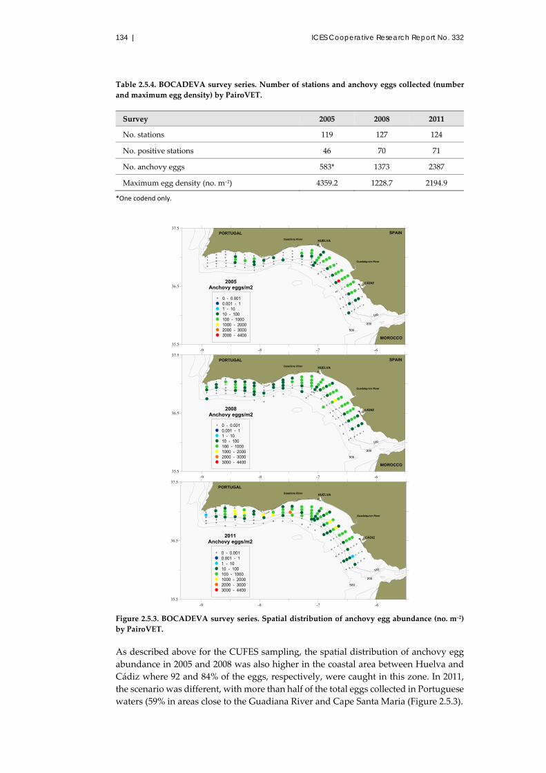
134 | ICES Cooperative Research Report No. 332
Table 2.5.4. BOCADEVA survey series. Number of stations and anchovy eggs collected (number
and maximum egg density) by PairoVET.
Survey 2005 2008 2011
No. stations 119 127 124
No. positive stations 46 70 71
No. anchovy eggs 583* 1373 2387
Maximum egg density (no. m–2) 4359.2 1228.7 2194.9
*One codend only.
Figure 2.5.3. BOCADEVA survey series. Spatial distribution of anchovy egg abundance (no. m–2)
by PairoVET.
As described above for the CUFES sampling, the spatial distribution of anchovy egg
abundance in 2005 and 2008 was also higher in the coastal area between Huelva and
Cádiz where 92 and 84% of the eggs, respectively, were caught in this zone. In 2011,
the scenario was different, with more than half of the total eggs collected in Portuguese
waters (59% in areas close to the Guadiana River and Cape Santa Maria (Figure 2.5.3).
-9 -8 -7 -635.5
36.5
37.5
100
200
500
0 - 0.001 0.001 - 1 1 - 10 10 - 100 100 - 1000 1000 - 2000 2000 - 3000 3000 - 4400
CÁDIZ
Guadalquivir River
HUELVAGuadiana River
SPAIN
MOROCCO
PORTUGAL
2005Anchovy eggs/m2
-9 -8 -7 -635.5
36.5
37.5
100
200
500
0 - 0.001 0.001 - 1 1 - 10 10 - 100 100 - 1000 1000 - 2000 2000 - 3000 3000 - 4400
CÁDIZ
Guadalquivir River
HUELVAGuadiana River
SPAIN
MOROCCO
PORTUGAL
2008Anchovy eggs/m2
-9 -8 -7 -635.5
36.5
37.5
100
200
500
0 - 0.001 0.001 - 1 1 - 10 10 - 100 100 - 1000 1000 - 2000 2000 - 3000 3000 - 4400
CÁDIZ
Guadalquivir River
HUELVAGuadiana River
PORTUGAL
2011Anchovy eggs/m2

Pelagic survey series for sardine and anchovy in ICES subareas 8 and 9 | 135
2.5.3.4 Surveyed and positive area
The series of surveyed areas by CUFES ranged between 14 150 km2 in 2007 and
10 846 km2 in 2005 (only Spanish waters were surveyed in 2010). The largest positive
area was estimated in 2009 and the smallest in the two first years in the series (Figure
2.5.4). Except for some interannual variations, no trend is detected throughout the
series. Regarding PairoVET data and taking into account post‐stratification, the
Portuguese positive area comprised 23–25% of the total in both 2005 and 2008 (Table
2.5.5). The total surveyed and spawning areas for the Gulf of Cádiz estimated in the
three DEPM surveys (BOCADEVA) were very similar.
Figure 2.5.4. Surveyed and positive areas by CUFES: acoustic (2004, 2006, 2007, 2009, and 2010) and
DEPM (2005, 2008, and 2011) surveys. In 2010, the survey was only from Strait of Gibraltar to Cape
Santa Maria.
Table 2.5.5 BOCADEVA survey series. Surveyed and positive areas sampled by PairoVET.
Area Stratum 2005 2008 2011
Surveyed area Total Gulf of Cádiz 11 982 13 029 13 107
Positive area
Portuguese waters 1 409 1 690 ‐
Spanish waters 4 729 5 172 ‐
Total Gulf of Cádiz 6 138 6 862 6 770
2.5.3.5 Egg parameters
2.5.3.5.1 Daily and total egg production (P0 and Ptot)
As described above, both daily egg production (P0) and total egg production (Ptot) in
2005 and 2008 were calculated for two strata: Portuguese and Spanish waters. Figure
2.5.5 shows the results obtained for these parameters in each stratum. In both cases, the
regional estimates obtained from the Portuguese area in 2005 and 2008 were lower than
those obtained in the Spanish area: 18 and 35% for daily egg production per surface
unit, 6 and 14% for total production, respectively. In general, we can observe an
increasing soft trend in Ptot, with the highest value in the middle of the series
(1.87 × 10¹² eggs d–1).

136 | ICES Cooperative Research Report No. 332
Figure 2.5.5. Daily egg production per surface unit (left) and total egg production (right) for anchovy
in the Gulf of Cádiz, estimated by the DEPM (BOCADEVA surveys) (CV in bars).
2.5.3.6 Adult parameters
2.5.3.6.1 Sampling data
The number of hauls was similar in the three surveys, ranging between 24 in 2011 and
27 in 2005. The percentage of occurrence for anchovy was very high, >85% in all cases.
Other frequent species were mackerel, chub mackerel, sardine, or hake (Table 2.5.6
shows the species with catches of >10 kg in each survey). The abundance of anchovy,
both in numbers and weight, was highest in 2011, with a clear increasing trend in the
yield of this species during the period: 46 kg h–1 in 2005, 70 kg h–1 in 2008, and
311 kg h–1 in 2011.
Figure 2.5.6 shows the species composition in the catches by haul and survey in terms
of percentages in weight. In 2005, anchovy was widely distributed, mainly in front of
the Guadiana and Guadalquivir rivers and along the Portuguese coastal area. In 2008,
the species showed some preference for the central and eastern waters of the study
area, mainly where the shelf widens, a zone that corresponds to the environment of the
Guadalquivir River estuary. In 2011, anchovy distribution was more reduced, mainly
occurring in the area between Huelva and the Guadiana River, and in the mouth of the
Guadalquivir River. Sardine exhibited a more variable spatial pattern, depending on
the year. In general, the species had a more coastal distribution than anchovy. In 2011,
sardine was the most important species in some hauls, especially in Spanish coastal
waters. Chub mackerel was more abundant in the Spanish part in 2005, but was mainly
distributed in the western part of the Gulf in 2008 and 2001.
Table 2.5.6. BOCADEVA survey series. List of the main species caught (only for species with
catches >10 kg).
Year Species Weight (kg) Number Occurrence (%)
2005
Engraulis encrasicolus 1 153.1 75 459 94
Scomber colias 717.5 5 011 71
Lepidopus caudatus 285.6 8 076 29
Sardina pilchardus 197.0 5 174 61
Mola mola 72.0 6 16
Scomber scombrus 34.0 177 74
Boops boops 26.0 296 52
Merluccius merluccius 23.3 219 81
0
100
200
300
400
500
2005 2008 2011
Daily egg production (P0)
eggs
/m2 /d
ay (
x103 )
Portuguese waters Spanish waters Total GoC
0,0
0,5
1,0
1,5
2,0
2,5
3,0
3,5
4,0
2005 2008 2011
Total egg production (Ptotal)
eggs
/day
(x10
12)
Portuguese waters Spanish waters Total GoC

Pelagic survey series for sardine and anchovy in ICES subareas 8 and 9 | 137
Year Species Weight (kg) Number Occurrence (%)
Trachurus trachurus 22.2 1 586 87
Diplodus bellottii 19.8 338 35
Spondyliosoma cantharus 18.9 104 32
Pagellus acarne 15.0 73 13
Pagellus erythrinus 13.0 68 16
Serranus hepatus 10.5 308 39
Trachinotus ovatus 10.1 30 16
2008
Scomber colias 1 687.9 16 726 100
Engraulis encrasicolus 839.8 45 966 88
Trachurus picturatus 449.5 7 194 62
Sardina pilchardus 236.9 5 707 50
Scomber scombrus 107.0 939 96
Trachurus mediterraneus 44.0 405 42
Trachurus trachurus 34.8 459 50
Boops boops 33.6 408 65
Merluccius merluccius 32.7 220 81
Pagellus erythrinus 20.1 121 31
Mola mola 19.8 5 12
2011
Scomber colias 3 957.8 82 041 91
Sardina pilchardus 3 018.3 111 702 68
Engraulis encrasicolus 2 760.3 234 958 95
Scomber scombrus 1 444.4 11 245 86
Trachurus mediterraneus 347.8 2 155 23
Boops boops 77.7 840 77
Pagellus acarne 61.2 333 18
Merluccius merluccius 53.5 575 100
Pagellus erythrinus 46.2 309 32
Diplodus bellottii 35.2 751 55
Mola mola 19.3 1 5
Alopias vulpinus 18.8 2 9
Spondyliosoma cantharus 18.5 150 36

138 | ICES Cooperative Research Report No. 332
Figure 2.5.6. BOCADEVA survey series for the years 2005, 2008, and 2011. Species composition (%
in weight) in valid fishing hauls.
The number of samples from both size and biological sampling are shown in Table
2.5.7. The results from 2005 showed some spatial structure, clearly evidenced by visual
inspection of the mature female mean weight and batch fecundity. In agreement with
the spatial distribution of daily egg production in that year, data post‐stratification in
two geographic strata was also considered and tested for all adult parameters. The
limit of separation of these two different strata was established at 7°30’W, which, to
some extent, splits the whole study area in Spanish and Portuguese waters.
Table 2.5.7. BOCADEVA survey series. Number of anchovies sampled.
Year 2005 2008 2011
Size sampling 3 328 2 538 2 528
Non‐hydrated 643 565 707
Hydrated 317 208 303
The values obtained for the sex‐ratio have been very similar in the three years
analyzed, very close to the 1:1 ratio (Figure 2.5.7). The female mean weight estimated
in the Portuguese area in 2005 was higher than in Spanish waters (8.5 g less). In 2008,
female mean weight was 23.7 g, whereas it decreased significantly in 2011 (15.2 g).
Relative to batch fecundity, the results follow a very similar trend to that observed for
female mean weight, recording the lowest value in 2011 (ca. 8000 eggs per female). The
values obtained for the spawning fraction have been similar, ranging from 0.22 in 2005
to 0.28 in 2011. The value obtained for the Spanish area was slightly higher than in

Pelagic survey series for sardine and anchovy in ICES subareas 8 and 9 | 139
Portuguese waters in 2005, with a difference of 0.05% (Figure 2.5.7). In all cases, the
estimated CVs have been low.
Figure 2.5.7. Sex ratio (in weight) of the mature population (R), mean female weight (W), batch
fecundity (F), and spawning fraction (S) estimated for anchovy in the Gulf of Cádiz (BOCADEVA
survey series).
2.5.3.7 Anchovy spawning-stock biomass
Gulf of Cádiz anchovy spawning‐stock biomass estimated by DEPM for 2005, 2008,
and 2011 averaged ca. 26 kt. In the first year, a relatively low biomass level (14 kt) was
estimated. In 2008, a remarkable increase up to 31.5 kt was estimated (Figure 2.5.8,
Table 2.5.8). This value is very similar to that obtained in 2011. The size composition of
the estimated population ranged between the 7.5‐ and 19.0‐cm size classes, with modal
classes mainly located at 11.5–13.5 cm (Figure 2.5.9). In 2011, a high number of
anchovies measuring 11–11.5 cm was registered.
Figure 2.5.8. Gulf of Cádiz anchovy spawning‐stock biomass estimates by the DEPM (BOCADEVA
series). The bars indicate the CV (not available for 2005).
0,0
0,5
1,0
2005 2008 2011
Sex ratio (R)
Portuguese waters Spanish waters Total GoC
0
5
10
15
20
25
30
2005 2008 2011
Mean females weight (W)
Portuguese waters Spanish waters Total GoC
gra
mm
e
0
4000
8000
12000
16000
20000
2005 2008 2011
Batch fecundity (F)
nb
. e
gg
s/f
em
ale
Portuguese waters Spanish waters Total GoC
0,00
0,10
0,20
0,30
0,40
2005 2008 2011
Spawning fraction (S)
Sp
aw
nin
g f
rac
tio
n
Portuguese waters Spanish waters Total GoC
0
20000
40000
60000
80000
2005 2008 2011
Spawning stock biomass (SSB)
ton
s

140 | ICES Cooperative Research Report No. 332
Figure 2.5.9. BOCADEVA survey series. Anchovy length frequency distributions of the estimated
population.
Table 2.5.8. BOCADEVA survey series. Summary table of the parameters obtained during the
series.
Parameter 2005 2008 2011
Area Portuguese
waters
Spanish
waters
Portuguese
waters
Spanish
waters
Total Gulf of
Cádiz
Surveyed area
(km2) 11 982 13 020 13 107
Positive area
(km2) 1 409.4 4 729.1 1 690.4 5 172.2 6 770
Eggs
P0 (eggs m–2 d–1)
(CV) 51 (0.80) 225 (0.69) 184 (0.44) 348 (0.35) 276 (0.32)
Ptot (eggs d–1 ×
1012) (CV) 0.07 (0.76) 1.06 (0.65) 0.31 (0.44) 1.80 (0.35) –0.29 (1.14)
Z d–1 (CV) –0.039 (0.75) –1.43 (0.29) 1.87 (0.36)

Pelagic survey series for sardine and anchovy in ICES subareas 8 and 9 | 141
Parameter 2005 2008 2011
Area Portuguese
waters
Spanish
waters
Portuguese
waters
Spanish
waters
Total Gulf of
Cádiz
Adults
Female weight
(g) (CV) 25.2 (0.03) 16.7 (0.04) 23.67 (0.06) 15.2 (0.11)
Batch fecundity
(CV) 13 820 (0.05) 11 160 (0.05) 13 778 (0.07) 7 486 (0.12)
Sex ratio (CV) 0.53 (0.01) 0.54 (0.01) 0.53 (0.005) 0.53 (0.007)
Spawning
fraction (CV) 0.26 (0.07) 0.21 (0.07) 0.22 (0.065) 0.27 (0.036)
Spawning
biomass (t) (CV) 14 673 31 527 (0.32) 32 757 (0.40)
2.5.4 Acknowledgments
We express gratitude to all the colleagues who made possible the goals achieved
in this survey, to the crew of the RV “Cornide de Saavedra” for their
professionalism and collaboration at all times, and to the entire scientific staff who
contributed to the successful results of the survey. Special thanks to Miguel Bernal
for his support in estimating the different parameters and his input to the R project,
and to Antonio Solla for his collaboration in the classification of POFs in 2011.

142 | ICES Cooperative Research Report No. 332
2.6 Autumn acoustic surveys on juvenile anchovy in Subarea 8: JUVENA 2003–2012
Guillermo Boyra and Udane Martínez
2.6.1 Introduction
In the Bay of Biscay, the management of the anchovy fishery relies on an annual
estimate of abundance, based on the information provided by the spring acoustic and
DEPM surveys plus the annual catches of the fishing fleet (ICES, 2011a). This approach
has been applied since the late 1980s and has produced a well‐established and robust
time‐series. However, this annual estimate of abundance is provided at the end of the
spawning season when a significant part of the annual anchovy fishery has already
ended, thus limiting the potential effectiveness of the management measures resulting
from the scientific advice.
A succession of low recruitments since 2001 that eventually caused the closure of the
fishery in 2005–2009, highlighted the need for an early index of recruitment strength in
order to improve management (Barange et al., 2009). With this purpose in mind, an
acoustic survey (JUVENA) for estimating the abundance of juvenile anchovy in early
autumn was set up (Boyra et al., 2013), following methodologies derived from the
European project JUVESU (Uriarte, 2002; Carrera et al., 2006). The objective of the
survey was to use the juvenile abundance estimate as an indicator of the abundance of
recruits that would enter the adult stock in the following year.
2.6.2 Material and methods
The JUVENA surveys were carried out annually during 2003–2012 between September
and October in the Bay of Biscay (Table 2.6.1) following an acoustic methodology
specifically designed to sample juvenile anchovy (Boyra et al., 2013). An adaptive
sampling strategy was chosen, using a combination of two small vessels (instead of the
more commonly used single larger vessel) to allow more flexible coverage of the
potentially variable and near‐surface sampling area (see Annex 2 [Section A2.5] and
Boyra et al., 2013 for details). Also, the biological sampling and fish species
identification was based on commercial purse‐seining (highly efficient for the surficial
distribution of juvenile anchovy, but of limited capacity for deeper detections) in the
first years of the survey, and incorporated pelagic trawling since year 2006 (see Table
A2.4 for vessel characteristics and equipment employed in each survey).
Since the addition of the second vessel, intercalibration exercises were carried out each
year. The intercalibration process consists of comparing the echo‐integrated acoustic
backscattering of the water column and the bottom echo in areas with a smoothly
variable seabed. A minimum distance of 30 nautical miles was covered simultaneously
by the two vessels for these exercises. The NASC values (MacLennan et al., 2002)
obtained by the layer echo integration of both the water column and bottom echoes
obtained by the two vessels were compared to detect recording biases or other
potential problems.

Pelagic survey series for sardine and anchovy in ICES subareas 8 and 9 | 143
Table 2.6.1. Summary of sampling effort in the JUVENA surveys in 2003–2012.
Year
Start
of
survey
End of
survey
No.
vessels
Effective
survey
time (d)
Fishing
operations
Anchovy‐
positive
fishing
operations
Inter‐
transect
distance
(nautical
miles)
Sampled
area
(nautical
miles2)
Positive
area
(nautical
miles2)
2003 18/09 14/10 1 20 47 36 17.5 16 829 3 476
2004 19/09 19/10 1 18 21 9 17.5 12 736 1 907
2005 12/09 07/10 2 20 47 45 17.5 25 176 7 790
2006 13/09 14/10 2 42 80 52 15 27 125 7 063
2007 04/09 30/09 2 37 70 40 15 23 116 5 677
2008 26/08 25/09 2 33 85 46 15 23 325 6 895
2009 26/08 25/09 2 39 67 42 15 34 585 12 984
2010 1/09 30/09 2 40 79 60 15 40 500 21 110
2011 1/09 5/10 2 40 77 64 15 37 500 21 025
2012 2/09 5/10 2 40 67 51 15 31 500 14 271
In general terms only, the 38‐kHz data were echo integrated using the TS–length
relationships agreed in ICES WGACEGG for the main species (ICES, 2006b). Acoustic
data were converted to biomass using information from the hauls and following
standard procedures (see Annex 2 and Boyra et al., 2013 for details). Each fishing haul
was classified by species. A random sample of each species was measured to determine
the length frequency distribution of the different species. Complete biological
sampling of anchovy was performed to analyze age, size, and the size–weight
relationship. The hauls were grouped by strata of homogeneous species and size
composition. The species and size composition of each homogeneous stratum were
obtained by averaging the composition (in numbers) of the individual hauls contained
in the stratum, weighted to the acoustic density in the vicinity (±2 nautical miles
around the fishing haul). This species and size composition of each stratum was used
to obtain the mixed species echo integrator conversion factor (Simmonds and
MacLennan, 2005) for converting the NASC values of each ESDU into numbers of each
species. However, although the methodology involved estimating multiple species, the
survey strategy was focused strongly on juvenile anchovy, and only the positive areas
for anchovy were processed. Therefore, estimates were produced only for this species.
Anchovy juveniles (age 0) and adults (age ≥1) were separated and treated as different
species. To separate juveniles from adults, the length frequency distribution of
anchovy by haul was multiplied by a corresponding age–length key. The key was
determined every year for three broad areas: the pure juvenile area, the mixed juvenile
area (a mixture of juveniles and adults), and the Garonne River area (located at the
coastal area around 45°40’N; also a mixed area, but here, adult anchovy were usually
smaller than in the other areas). Finally, the abundance in numbers of juveniles and
adults was multiplied by the mean weight to obtain the biomass per age and length
class for each ESDU.
Juvenile anchovy showed a near‐surface distribution during the JUVENA survey
period (Uriarte et al., 2001). In order to achieve the best possible coverage of the vertical
distribution of this species in the JUVENA surveys, the echo integration was started at

144 | ICES Cooperative Research Report No. 332
a range of 5 m from the transducer face (i.e. at a depth of 7.5 m from the surface) rather
than the 10.5 m (13‐m depth) recommended to avoid integrating the near‐field of the
38‐kHz transducer (Simmonds and MacLennan, 2005). Instead of ignoring these first
layers, the bias produced by the near‐field in the 7.5–15 m echo integration channel
was estimated and corrected for in the biomass estimates. The details of this analysis
are explained in Boyra et al. (2003).
Yearly maps of anchovy NASC values by ESDU along the survey transects were
produced, including SST based on the CTD casts. Also, in order to estimate the
recruitment predictive capability, the annual biomass estimates for anchovy juveniles
were compared with the estimates of anchovy recruitment the following year. The
recruitment is the biomass of age 1 anchovy in January of the following year, which is
estimated using a Bayesian‐based assessment model (ICES, 2013). This model takes
information from spring acoustic and DEPM surveys into account, but not the juvenile
index from JUVENA (hence being independent from the JUVENA estimates). The
biomass estimates were fitted by linear, log‐linear, and rank regressions between
variables using the R software version 2.14.0 (R Development Core Team, 2011).
2.6.3 Results and discussion
The sampling coverage over the surveys (Figure 2.6.1) reflects the adaptive sampling
scheme followed and shows the methodological changes made to improve the
coverage, particularly since 2005. For example, the northern coverage along the French
coast was considerably enlarged. The northern limit changed from 46°N in the first two
years to beyond 47°N in subsequent years. The number of fishing operations increased
from 40 in 2003 to >60 in the years since 2005. The incorporation of the pelagic trawler
in 2006 improved fishing flexibility, making it possible to fish near the seabed. This is
shown in the fishing maps (Figure 2.6.1) by the increase in species diversity (due to the
addition of the near‐bottom species).
Every year, the juvenile anchovy population could be divided into two clearly
distinguishable groups. One part of the population consisted of nearly 100% juvenile
anchovy (not mixed with adults), and the other part was mixed with, or in close
proximity to, adults. The predominantly juvenile group was located in the
southwestern part of the Bay of Biscay, normally off the shelf or in the outer part
(Figure 2.6.2), and the mixed group was located to the northeast in shelf waters at
depths < 130 m. In each group, juveniles were found in a different species composition
context and bathymetrical distribution pattern. In the largely juvenile region, anchovy
was generally the only or the predominant species (the percentage of anchovy
individuals in these strata was always >90%), mixed sometimes with smaller
proportions of salp, jellyfish, and juvenile horse mackerel (Figure 2.6.1). In the mixed
group, juvenile anchovy was found mixed in variable proportions with adult anchovy
(the adult proportion increasing towards the northeast, Figure 2.6.2) and other pelagic
species, mainly sardine, horse mackerel, mackerel, and sprat (Figure 2.6.1).
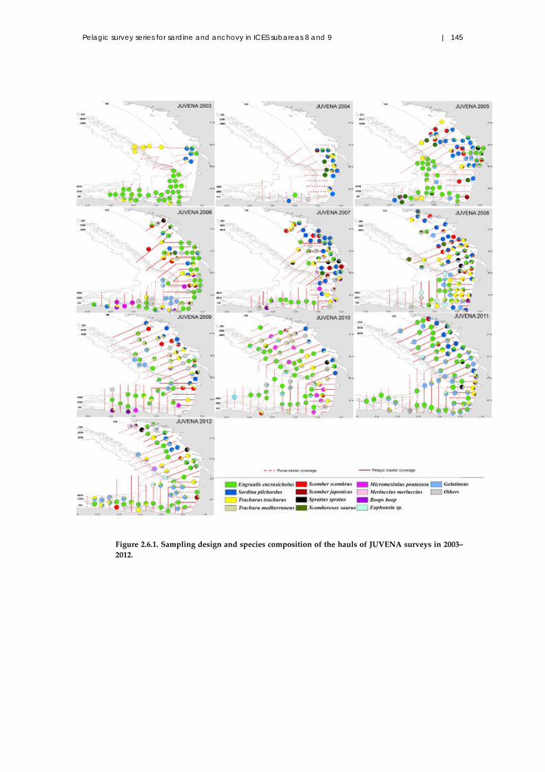
Pelagic survey series for sardine and anchovy in ICES subareas 8 and 9 | 145
Figure 2.6.1. Sampling design and species composition of the hauls of JUVENA surveys in 2003–
2012.

146 | ICES Cooperative Research Report No. 332
Figure 2.6.2. Age composition of anchovy for the ten years of the survey. The pie charts represent
the mean percentage of juveniles (white) and adults (black) in the fishing hauls at each fishing site.
For the years that had the highest juvenile biomass estimates, the largest biomass
contributions were invariably observed in the largely juvenile areas (Figure 2.6.3). This
region contained, on average throughout the series, ca. 58% of the total biomass. This
average increased to 75%, when the least abundant years (2004, 2007, and 2008) were
excluded, and reached 95% of the total biomass in 2010, when the strongest recruitment
in the JUVENA series was recorded. The contribution of the mixed‐juvenile region to
the biomass was quite constant across the series, and in the years with the highest total
juvenile abundance, the contribution was relatively weak. The occupation of the off‐
shelf waters by predominantly juvenile anchovy is consistent throughout the series
and agrees with previous work on juvenile anchovy in the Bay of Biscay (Uriarte et al.,
1996, 2001; Carrera et al., 2006; Lezama‐Ochoa et al., 2010). Uriarte et al. (2001) described
a large juvenile abundance in the French outer‐shelf waters (as in 2009 and 2010) in the
1999 JUVESU survey, which was followed by strong recruitment in 2000 (ICES, 2010a).

Pelagic survey series for sardine and anchovy in ICES subareas 8 and 9 147 |
Figure 2.6.3. Positive area of presence of anchovy and total acoustic energy echo integrated (from all the species) for JUVENA 2003–2012. The area delimited by the
dashed line is the minimum or standard area used for interannual comparison.

148 | ICES Cooperative Research Report No. 332
A wide range of acoustic estimates of juvenile anchovy biomass was assessed over the
JUVENA series (Table 2.6.2, Figure 2.6.4). The estimates showed differences of more
than two orders of magnitude between the lowest value in 2004 and the highest in 2010.
The series of juvenile anchovy biomass estimates showed good parallelism to the
independent estimates of anchovy biomass at age 1 recruitment at the beginning of the
following year (Figure 2.6.4). Both quantitative linear (Pearson) and non‐parametric
rank (Spearman) correlations showed highly significant values (the coefficients of
determination were 0.93 and 0.86, respectively, with probabilities of being random
< 0.0001 and 0.01, respectively). These significant relationships were not dependent on
the extreme values of the series; both correlations continued to be significant (at an
alpha of 1%) even when the highest or lowest juvenile index from the JUVENA series
was excluded from the analysis. Several quantitative linear or log‐linear models can be
fitted to series of recruitment based on the juvenile abundance indexes from JUVENA.
The best fitting was achieved by the log‐linear model, i.e. a potential model in linear
scale, with coefficient of determination of 0.95 and p‐value = 5 × 10⁻⁵ (Figure 2.6.4).
Concerning the main observed groups, the biomass of the purely juvenile group was
significantly correlated with recruitment, explaining 87% of the recruitment variability,
while the biomass of the mixed juvenile and adult group showed no significant
relationship and explained less than 20% of the recruitment variability.
Table 2.6.2. Synthesis of the abundance estimation (acoustic index of biomass) for the ten years of
JUVENA surveys.
Year
Sampled area
(nautical
miles2)
Positive area
(nautical
miles2)
Juvenile
length (cm)
Juvenile
biomass
(year y)
Recruits age
1 (year y+1)
2003 16 829 3 476 7.9 98 601 46 500
2004 12 736 1 907 10.6 2 406 6 648
2005 25 176 7 790 6.7 134 131 29 530
2006 27 125 7 063 8.1 78 298 36 350
2007 23 116 5 677 5.4 13 121 12 960
2008 23 325 6 895 7.5 20 879 13 010
2009 34 585 12 984 9.1 178 028 61 755
2010 40 500 21 110 8.3 599 990 128 400
2011 37 500 21 063 6.0 207 625 37 650
2012 31 724 14 271 6.4 142 083 32 860

Pelagic survey series for sardine and anchovy in ICES subareas 8 and 9 149 |
Figure 2.6.4. Temporal series of juvenile (J) against recruitment (R) indices and fitting of different
regression models between them: linear, log‐linear, and and by order of rank (Spearman).
The main aim of these surveys was to test whether the abundance of juveniles in
autumn constitutes a reliable indicator of the strength of recruitment to the adult stock
each year in the Bay of Biscay. The hypothesis has been confirmed by the significant
positive correlations between the biomass estimates of juveniles and the age 1 recruits
in the following year (Figure 2.6.4). Boyra et al. (2013) showed that a significant
correlation exists between juvenile and recruitment indices, thus supporting the
reliability of the JUVENA index to anticipate abundance trends in the Bay of Biscay
anchovy. In the present work, after the addition of two more survey estimates
corresponding to medium and high recruitment levels, the correlations between
juvenile and recruitment are still highly significant, further supporting the validity of
the JUVENA index. The study period has shown a broad range of recruitment levels,
from an extremely low level in 2004, which caused the collapse of the fishery, to one of
the highest recruitment levels of the entire time‐series in 2011. The relationship
between the juvenile and recruitment indices is not too dependent on any particular
point of the series, neither the maximum nor the minimum. The relationship was also
independent of the model chosen. Although linear and log‐linear models were shown
to be good candidates, the definition of the best quantitative model for prediction is
left to the ICES assessment working group to decide.
The results of the JUVENA acoustic series reveal the spatial pattern of anchovy
recruitment in the Bay of Biscay, in which the southwestern drift of larvae towards
southern and offshore areas, surpassing the shelf and occupying oceanic waters within
the bay until becoming juveniles, is not detrimental to the success of recruitment, but
constitutes a natural phase before juveniles reach a sufficient size to migrate back
towards more coastal areas during autumn. This was already postulated by Uriarte et
al. (2001) and Irigoien et al. (2008) and finally supported by the finding of JUVENA that
the biomass of the purely juvenile group, which mostly occupies the southwestern
waters in the Bay, is significantly correlated with the next recruitment at age 1,
explaining 87% of its variability (already pointed out in Boyra et al., 2013).

150 | ICES Cooperative Research Report No. 332
2.6.4 Acknowledgements
This project was funded by the Basque Government “Viceconsejería de Agricultura,
Pesca y Politicas Alimentarias – Departamento de Desarrollo Económico y
Competitividad” – Gobierno Vasco” and the Spanish Government ”Secretaría General
de Pesca, Ministerio de Agricultura, Alimentación y Medio Ambiente – Gobierno
Español”. We acknowledge the skippers and crew of the vessels that participated in
the survey: FV “Divino Jesús de Praga”, FV “Nuevo Erreinezubi”, FV “Mater Bi”, FV
“Gure Aita Joxe”, FV “Itsas Lagunak”, RV “Emma Bardán”, and RV “Ramón
Margalef”.

Pelagic survey series for sardine and anchovy in ICES subareas 8 and 9 151 |
2.7 Autumn acoustic surveys off the Portuguese continental shelf and Gulf of Cádiz (ICES Division 9.a)
Vitor Marques, Maria Manuel Angélico, Eduardo Soares, Alexandra Silva, and
Cristina Nunes
2.7.1 Introduction
The Portuguese autumn acoustic surveys were mainly designed to estimate the
abundance of young sardines recruiting to the fishery as age group 0. Sardine peak
spawning is in winter, and young‐of‐the‐year sardines are more visible to the fisheries
in autumn. In 1984–1987, the Portuguese surveys were systematically performed each
year in autumn/winter. Only a sporadic attempt took place in 1992, after which the
surveys resumed with a systematic periodicity in 1997–2008. During the last decade,
four acoustic autumn surveys were performed with RV “Noruega”, identified with the
acronym SAR: SAR05NOV, SAR06NOV, SAR07NOV, and SAR08OUT. The surveys
presented in this report were carried out during the last decade, using a standardized
methodology and covering the majority of the area.
2.7.2 Material and methods
The acoustic methodology was the echo integration of the acoustic targets and fish
schools, surveyed along 60 transects perpendicular to the coast line and spaced ca.
8 nautical miles apart. For acoustic data collection, a Simrad EK500 echosounder with
38‐kHz frequency was used. The acoustic data were stored and processed using the
IFREMER software MOVIES+ (Weill at al., 1993). For species identification and
biological sampling, trawl hauls were performed (for details, see the Portuguese
acoustic survey protocols in Annex 2).

152 | ICES Cooperative Research Report No. 332
2.7.3 Results
2.7.3.1 Abundance estimates
The main results of these surveys are presented in the tables and figures below (Table
2.7.1 and Figures 2.7.1–3). The results of each survey are then described separately.
Table 2.7.1. Autumn survey main information: trawl hauls, sardine biomass (thousand tonnes), and
juvenile percentage for each zone.
Survey SAR05NOV SAR06NOV SAR07NOV SAR08OUT
Number of trawl hauls 29 27 33 31
Number of hauls with sardine 21 16 24 20
OCN biomass 458 257 258 121
OCS biomass 34 69 114 35
Algarve biomass 12 27 11 0.6
Cádiz biomass ‐ 57 133 149
Total biomass 504 410 516 306
% juv_OCN 75 7 41 76
% juv_OCS 43 29 32 10
% juv_Alg 63 41 17 11
% juv_Cádiz ‐ 3 34 46

Pelagic survey series for sardine and anchovy in ICES subareas 8 and 9 153 |
Figure 2.7.1. Trawl haul geographic location and proportion of the main pelagic species in the trawl
catches. Species FAO key code.
-11º -10º -9º -8º -7º -6º -5º35º
36º
37º
38º
39º
40º
41º
42ºCaminha
Viana do Castelo
Porto
Aveiro
Figueira da Foz
Nazaré
Peniche
Lisboa
Setubal
Sines
ArrifanaPortimão
Faro
V. Real Sto. António
Cádiz
200 m
SAR08OUT
estações de pesca:
- com sardinha
- sem sardinha
PIL
ANE
HOM
BOG
MAC
MAS
JAA
WHB
SNS + BOC
AP18AP17
AP1
AP3
AP4AP5
AP6
AP7
AP9
AP10
AP8
AP11
AP12
AP14
AP16
AP15
AP13
AP19
AP20
AP21
AP24
AP23
AP25
AP28AP27
AP29
AP30
AP31
-11º -10º -9º -8º -7º -6º -5º35º
36º
37º
38º
39º
40º
41º
42ºCaminha
Viana do Castelo
Porto
Aveiro
Figueira da Foz
Nazaré
Peniche
Lisboa
Setubal
Sines
ArrifanaPortimão
Faro
V. Real Sto. António
Cádiz
200 m
SAR08OUT
estações de pesca:
- com sardinha
- sem sardinha
PIL
ANE
HOM
BOG
MAC
MAS
JAA
WHB
SNS + BOC
PIL
ANE
HOM
BOG
MAC
MAS
JAA
WHB
SNS + BOC
AP18AP17
AP1
AP3
AP4AP5
AP6
AP7
AP9
AP10
AP8
AP11
AP12
AP14
AP16
AP15
AP13
AP19
AP20
AP21
AP24
AP23
AP25
AP28AP27
AP29
AP30
AP31
-11º -10º -9º -8º -7º -6º -5º35º
36º
37º
38º
39º
40º
41º
42ºCaminha
Porto
Aveiro
Figueira da Foz
Nazaré
Lisboa
Faro
V. Real Sto. António
Cádiz
200 m
SAR07NOV
- fishing trawl stations
AP1
AP2
AP3
AP5AP6
AF7
AF8AF9
AP10AP13
AP11
AP12
AP14
AF15
AP16AP17
AF18
AP19AF20
AP21
AP23
AP22AP24
AF27
AP25
AP26AP28
AF29
AP30
AP32
AP33
PIL
ANE
HOM
BOG
MAC
MAS
JAA
WHB
SNS + BOC
-11º -10º -9º -8º -7º -6º -5º35º
36º
37º
38º
39º
40º
41º
42º
Nazaré
Lisboa
200 m
SAR06NOV
- estações de pesca
AP - arrasto pelágicoAF - arrasto fundo
=<16.0 cm16.5-19.5 cm> 20.0 cm
AP27
AP26
AP25
AP24
AP23
AP21
AP20
AP19
AP17
AP15
AP14
AP12
AP11
AF9;AF10
AP6
AP3AF4;AP5
AP7
AP13
AP18
AP22
PIL
ANE
HOM
BOG
MAC
MAS
JAA
WHB
SNS + BOC
-11º -10º -9º -8º -7º -6º -5º35º
36º
37º
38º
39º
40º
41º
42º
Porto
Figueira da Foz
Nazaré
Lisboa
Sines
Faro
V. Real Sto. António
Cádiz
200 m
AP5 AP7AP8
AP29AP28
AP27AP26
AP24AP25
AF22AP23
AF19AP21
AP17AP18
AP15AP16
AF14
AP11
AP12
AP4
AP10
PIL
ANE
HOM
BOG
MAC
MAS
JAA
WHB
SNS + BOC
SAR05NOV

154 | ICES Cooperative Research Report No. 332
Figure 2.7.2. Acoustic energy (NASC) attributed to sardine along the transects. Sardine abundance
and length composition in each zone. The Portuguese southwestern coast and the western Algarve
coast were not covered during the 2007 survey.
Porto
Nazaré
Lisboa
Faro
Cádiz
200 m
SAR05NOV
- 10000
SA mn2(m-2
)
- 100
- 500
- 1000
- 5000
- 15000
ALGARVE
0
10
20
5 7 9 11 13 15 17 19 21 23 25
Classes de comprimento (cm)
%
OCN
0
10
20
5 7 9 11 13 15 17 19 21 23 25
Classes de comprimento (cm)
%
B=458 mil ton.N=16623 x 10^6
OCS
0
10
20
5 7 9 11 13 15 17 19 21 23 25
Classes de comprimento (cm)
%
B=34 mil ton.N=863 x 10^6
B=12 mil ton.N=333 x 10^6
PORTUGAL
0
10
20
5 7 9 11 13 15 17 19 21 23 25
Classes de comprimento (cm)
%
B=504 mil ton.N=17818 x 10^6
OCN
OCS
ALGARVE
-11º -10º -9º -8º -7º -6º -5º35º
36º
37º
38º
39º
40º
41º
42ºCaminha
Viana do Castelo
Porto
Aveiro
Figueira da Foz
Nazaré
Peniche
Lisboa
Setubal
Sines
ArrifanaPortimão
Faro
V. Real Sto. António
Cádiz
200 m
Energia acústica (SA) sardinha
= 15000
= 5000
= 1000
SAR06NOVOCN
0
10
20
30
5 7 9 11 13 15 17 19 21 23 25
Classes de comprimento (cm)
%
OCS
0
10
20
30
5 7 9 11 13 15 17 19 21 23 25
Classes de comprimento (cm)
%
ALGARVE
0
10
20
5 7 9 11 13 15 17 19 21 23 25
Classes de comprimento (cm)
% CÁDIZ
0
10
20
30
5 7 9 11 13 15 17 19 21 23 25
Classes de comprimento (cm)
%
PORTUGAL
0
10
20
30
5 7 9 11 13 15 17 19 21 23 25
Classes de comprimento (cm)
%
TOTAL
0
10
20
30
5 7 9 11 13 15 17 19 21 23 25
Classes de comprimento (cm)
%
B=257 mil ton.
N=4577x 10^6
B=69 mil ton.
N=1602x 10^6
B=27 mil ton.
N=635x 10^6B=58 mil ton.
N=1317x 10^6
B=353 mil ton.
N=6814x 10^6
B=411 mil ton.
N=8131x 10^6
-11º -10º -9º -8º -7º -6º -5º35º
36º
37º
38º
39º
40º
41º
42ºCaminha
Viana do Castelo
Porto
Aveiro
Figueira da Foz
Nazaré
Peniche
Lisboa
Setubal
Sines
ArrifanaPortimão
Faro
V. Real Sto. António
Cádiz
200 m
Energia acústica (SA) sardinha
= 15000
= 5000
= 1000
SAR06NOVOCN
0
10
20
30
5 7 9 11 13 15 17 19 21 23 25
Classes de comprimento (cm)
%
OCS
0
10
20
30
5 7 9 11 13 15 17 19 21 23 25
Classes de comprimento (cm)
%
ALGARVE
0
10
20
5 7 9 11 13 15 17 19 21 23 25
Classes de comprimento (cm)
% CÁDIZ
0
10
20
30
5 7 9 11 13 15 17 19 21 23 25
Classes de comprimento (cm)
%
PORTUGAL
0
10
20
30
5 7 9 11 13 15 17 19 21 23 25
Classes de comprimento (cm)
%
TOTAL
0
10
20
30
5 7 9 11 13 15 17 19 21 23 25
Classes de comprimento (cm)
%
B=257 mil ton.
N=4577x 10^6
B=69 mil ton.
N=1602x 10^6
B=27 mil ton.
N=635x 10^6B=58 mil ton.
N=1317x 10^6
B=353 mil ton.
N=6814x 10^6
B=411 mil ton.
N=8131x 10^6
-11º -10º -9º -8º -7º -6º -5º35º
36º
37º
38º
39º
40º
41º
42ºCaminha
Viana do Castelo
Porto
Aveiro
Figueira da Foz
Nazaré
Peniche
Lisboa
Setubal
Sines
ArrifanaPortimão
Faro
V. Real Sto. António
Cádiz
200 m
SAR07NOV
Energia acústica (SA) sardinha
= 15000
= 5000
= 1000
OCN
0
10
20
30
5 7 9 11 13 15 17 19 21 23 25
Classes de comprimento (cm)
%
OCS
0
10
20
30
5 7 9 11 13 15 17 19 21 23 25
Classes de comprimento (cm)
%
ALGARVE
0
10
20
30
5 7 9 11 13 15 17 19 21 23 25
Classes de comprimento (cm)
%CÁDIZ
0
10
20
30
5 7 9 11 13 15 17 19 21 23 25
Classes de comprimento (cm)
%
N=4,6x10^9
B=258 mil ton.
B=114 mil ton.
N=2,1x10^9
B=11 mil ton. B=133 mil ton.
N=0,18x10^9 N=2,7x10^9
-11º -10º -9º -8º -7º -6º -5º35º
36º
37º
38º
39º
40º
41º
42ºCaminha
Porto
Nazaré
Lisboa
V. Real Sto. António
Cádiz
200 m
SAR08OUT
Energia acústica (SA) sardinha
= 15000
= 5000
= 1000
OCN
0
10
20
30
5 7 9 11 13 15 17 19 21 23 25
Classes de comprimento (cm)
%
OCS
0
10
20
30
5 7 9 11 13 15 17 19 21 23 25
Classes de comprimento (cm)
%
ALG
0
10
20
30
5 7 9 11 13 15 17 19 21 23 25
Classes de comprimento (cm)
%
CAD
0
10
20
30
5 7 9 11 13 15 17 19 21 23 25
Classes de comprimento (cm)
%
N=3962x10^6
B=121 mil ton
N=555x10^6
B=36 mil ton
N=9x10^6
B=0.6 mil tonN=3530x10^6
B=149 mil ton

Pelagic survey series for sardine and anchovy in ICES subareas 8 and 9 155 |
Figure 2.7.3. SAR05NOV and SAR06NOV surveys: proportion of sardine juveniles (white colour)
in each trawl. AP – pelagic trawl, AF – bottom trawl, AD – purse‐seine (during the 2005 survey, one
sample collected from the commercial fleet was also used).
2.7.3.2 SAR05NOV
2.7.3.2.1 Sardine distribution and abundance
Sardine was the dominant species in the Occidental North area (OCN; Figure 2.7.2).
Off the remaining Portuguese shelf, other pelagic species were observed (horse
mackerel, chub mackerel, and bogue), usually more abundant than sardine in this
survey. In the Occidental South (OCS) and Algarve areas, the acoustic energy
attributed to sardine represented only 7 and 11%, respectively, of the total fish acoustic
energy.
2.7.3.2.2 Recruitment strength and sardine length structure
The sardine population presented significant differences between areas (Figures 2.7.2
and 2.7.3). In the OCN area, the population was clearly dominated by sardine juveniles
(total length < 16 cm), with a modal length distribution of 15.5 cm. In numbers,
juveniles represented 75% of the total estimated number for this area.
In the OCS area, the sardine length distribution was bimodal, with one mode at 10.5 cm
and another at 20.5 cm. In this area, the juveniles were mainly distributed off Lisbon,
near Cabo da Roca, and represented 43% of the abundance for this area.
In Algarve, the length structure was also mixed, with juveniles dominating the eastern
part of the area, representing 63% of the individuals.
Porto
Nazaré
Lisboa
Faro
200 m
SAR05NOV
AP - Arrasto PelágicoAF - Arrasto Fundo
- Estações de Pesca
> 20.0 cm
16.5 - 19.5 cm
< 16.0 cm
AP28 AP29
AP27 AP26
AP24AP25
AP23AF22
AP20
AP21AF19
AP18AP17
AP16AP15
AF14
AP13
AP12
AP11
AP10
AF1
AF2
AP9
AP8AP7
AF6
AP5
AP4
AP3
AD30
AD - Cerco
-11º -10º -9º -8º -7º -6º -5º35º
36º
37º
38º
39º
40º
41º
42º
Nazaré
Lisboa
200 m
SAR06NOV
- estações de pesca
AP - arrasto pelágicoAF - arrasto fundo
=<16.0 cm16.5-19.5 cm> 20.0 cm
AP27
AP26
AP25
AP24
AP23
AP21
AP20
AP19
AP17
AP15
AP14
AP12
AP11
AF10
AP6
AP3

156 | ICES Cooperative Research Report No. 332
2.7.3.3 SAR06NOV
2.7.3.3.1 Sardine distribution and abundance
Sardines were mainly distributed off the western shelf, north of Lisbon (Figure 2.7.2).
There was an increase in other pelagic species in all areas (Figure 2.7.1). Anchovy was
mainly distributed in the Bay of Cádiz, as usual.
Off the southwestern part of the coast, south of Lisbon, sardine was almost absent.
2.7.3.3.2 Sardine recruitment
The sardine length structure was clearly dominated by adults in the whole area, which
suggested low recruitment in 2006 (Figures 2.7.2 and 2.7.3). Only 7% of the sardine in
the OCN zone were juveniles. The OCS zone showed a bimodal distribution, with 9‐
and 19‐cm modes. The juveniles, corresponding to 29% of the abundance in this area,
were located near Lisbon. Algarve had also a mixed length structure, with juveniles
representing 41% of the abundance for this area. Cádiz was dominated by adults, with
only 3% juveniles. For all areas surveyed, juveniles represented only 13% of the
estimated sardine abundance.
2.7.3.4 SAR07NOV
The area was not completely covered in autumn 2007 due to lack of time (the southern
coast and the Algarve west coast were not covered), but the main juvenile distribution
area was surveyed, fulfilling the main objective of these surveys.
In the eastern part of Algarve and Cádiz, an increased fishing effort during the survey
was aimed at collecting more information on the pelagic community. As a result, it
became possible to estimate the abundance and distribution of anchovy and chub
mackerel, in addition to sardine (Figures 2.7.4 and 2.7.5).

Pelagic survey series for sardine and anchovy in ICES subareas 8 and 9 157 |
Figure 2.7.4. SAR07NOV: acoustic energy (NASC) attributed to anchovy (Engraulis encrasicholus) along the transects, with anchovy abundance and length composition shown for each zone. The
Portuguese southwestern and western Algarve coasts were not covered.
-11º -10º -9º -8º -7º -6º -5º35º
36º
37º
38º
39º
40º
41º
42º
W
N
Caminha
Nazaré
V. Real Sto. António
Cádiz
1000
m
200
m
0.5 cm<>2000 SA
BIQ07NOV
B=1,1 mil ton.
N=58,6 x10^6
B=7,6 mil ton.
B=16 mil ton.N=475 x10^6
N=1,4 x10^9
OCS
0
10
20
30
5 7 9 11 13 15 17 19 21 23 25
Classes de comprimento (cm)
%
ALGARVE
0
10
20
30
5 7 9 11 13 15 17 19 21 23 25
Classes de comprimento (cm)
% CÁDIZ
0
10
20
30
5 7 9 11 13 15 17 19 21 23 25
Classes de comprimento (cm)
%

158 | ICES Cooperative Research Report No. 332
Figure 2.7.5. SAR07NOV and SAR08OUT: acoustic energy (NASC) attributed to chub mackerel
(Scomber colias) along the transects, with chub mackerel abundance and length composition shown for each zone. The Portuguese southwestern and western Algarve coasts were not covered in the
2007 survey.
2.7.3.4.1 Sardine distribution and abundance
Sardine was distributed along the continental shelf, but was abundant on the west
coast between Figueira da Foz and Peniche (Figure 2.7.2). Sardine abundance for the
OCN and OCS areas was 258 and 114 thousand tonnes, respectively. These amounts
are average within the historical series. In Algarve, only the east part was covered, and
the estimated abundance was 11 000 tonnes. In the Cádiz area, sardine was abundant,
with the biomass being estimated at 133 000 tonnes.
2.7.3.4.2 Sardine recruitment and length structure
The sardine length distribution was bimodal in all areas (Figure 2.7.2), the small mode
corresponding to juveniles. This confirms the existence of sardine recruitment in the
whole distribution area. In the OCN area, 41% of the individuals were juveniles. In the
OCS zone, 32% were juveniles and were found off Lisbon, as is usually the case. In
Algarve, only 17% were juveniles, while in Cádiz, juveniles constituted 34% of the
abundance in this area. These numbers suggest that the average level of recruitment
for sardine corresponded to that in 2007.
2.7.3.4.3 Anchovy distribution and abundance
As usual, anchovy was caught mainly in the Gulf of Cádiz and in minor quantities off
Lisbon (Figure 2.7.3). In the Cádiz area, anchovy was relatively abundant, the biomass
estimated at 16 000 tonnes. Anchovy was also found in the eastern part of Algarve,
with the biomass for this area estimated at 7600 tonnes. The anchovy “spot” found off
Lisbon represented only 1100 tonnes (Figure 2.7.4).
-11º -10º -9º -8º -7º -6º -5º35º
36º
37º
38º
39º
40º
41º
42ºCaminha
Viana do Castelo
Porto
Aveiro
Figueira da Foz
Nazaré
Peniche
Lisboa
Setubal
Sines
Arri fanaPor timão
Faro
V. Real Sto. António
Cádiz
200 m
cavalaenergia acústica
<>SA=15000 m^2
SAR08OUT
OCS
0
10
20
30
5 7 9 11 13 15 17 19 21 23 25 27 29 31 33
Classes de comprimento (cm)
%
ALG
0
10
20
30
5 7 9 11 13 15 17 19 21 23 25 27 29 31 33
Classes de comprimento (cm)
% CAD
0
10
20
30
5 7 9 11 13 15 17 19 21 23 25 27 29 31 33
Classes de comprimento (cm)
%
N=1286x10^6
B=141 mil ton
N=457x10^6
B=26 mil ton
N=319x10^6
B=36 mil ton
-11º -10º -9º -8º -7º -6º -5º35º
36º
37º
38º
39º
40º
41º
42º
W
N
Caminha
Nazaré
V. Real Sto. António
Cádiz
1000
m
200
m
0.5 cm<>10000 SA
CAV07NOVOcidental
0
10
20
30
5 8 11 14 17 20 23 26 29 32 35 38 41 44
Classes de comprimento (cm)
%
ALGARVE
0
10
20
30
5 8 11 14 17 20 23 26 29 32 35 38 41 44
Classes de comprimento (cm)
% CÁDIZ
0
10
20
30
5 8 11 14 17 20 23 26 29 32 35 38 41 44
Classes de comprimento (cm)
%
B=159 mil ton.
N=1,2 x10^9
B=18,2 mil ton.
N=0,1x10^9 B=61 mil ton.
N=0,6 x10^9

Pelagic survey series for sardine and anchovy in ICES subareas 8 and 9 159 |
2.7.3.4.4 Chub mackerel distribution and abundance
It was the first time that an attempt was made to estimate the distribution and
abundance of chub mackerel off the Portuguese continental shelf (Figure 2.7.5). In the
surveyed west coast (southwestern coast not covered), a biomass of 159 000 tonnes was
estimated. In the east part of Algarve, 18 500 tonnes were estimated, with 61 000 tonnes
of chub mackerel estimated at Cádiz. The mode of the length distribution for the whole
area covered was ca. 22 cm.
2.7.3.5 SAR08OUT
2.7.3.5.1 Sardine abundance and distribution
Sardine was mainly distributed off the west coast, north of Peniche (Figure 2.7.2). In
the OCN zone, the sardine biomass was estimated at 121 000 tonnes. On the west coast,
south of Lisbon, and in Algarve, sardine was not abundant. In these areas, chub
mackerel was the dominant species. The estimated sardine biomass in the OCS zone
was only 35 000 tonnes, and sardine were almost absent (601 tonnes) in Algarve. The
abundance estimate for Cádiz (149 000 tonnes) was within the average for this area.
2.7.3.5.2 Sardine length structure
The sardine length structure was bimodal for the OCS and Cádiz areas and trimodal
for the OCN area.
2.7.3.5.3 Chub mackerel abundance and distribution
Chub mackerel was abundant in the OCS and Algarve areas and less so in the Cádiz
zone (Figure 2.7.5). The length structure was bimodal in all areas.
2.7.3.6 Environmental setting and sardine egg distribution
During the first half of the decade, weather conditions in the region in late autumn
were very unsettled, and the survey results were incomplete and discontinuous. For
that reason, it was decided to include only the surveying period from 2005 to 2008 in
this report.
During the October–November period in southern and western Iberian waters, the
structure of the water column is typically still stratified and water temperatures fairly
warm. Normally, it is only later in the season that wind events and the continuous drop
in atmospheric temperature lead to the breakdown of thermal stratification and the
onset of winter conditions. Once rainfall episodes become frequent, river plumes
become evident in the surface temperature and/or salinity data and haline stratification
may occur in some inshore areas; often associated with these conditions, river runoff
promotes local plankton bursts.
The oceanographic setting during the Portuguese autumn surveys in 2005–2008 was
diverse (Figures 2.7.6–2.7.9). Water temperatures were lower during the 2005 and 2008
surveys, milder across the entire region in 2006, and in‐between in 2007. While water
temperatures were still mild in November 2006, the occurrence of rainfall promoted
the onset of extended river plumes off Lisbon and over the northwestern shelf.
Sardine egg distributions shown in Figure 2.7.9 indicate that the spawning season was
underway at the time of all the surveys, but also highlight the differences encountered
between years. During the 2006 survey, egg abundance was higher than in the other
years. In 2005, the low number of eggs and their distribution was quite likely associated
with the population structure dominated by young individuals less fecund and with a

160 | ICES Cooperative Research Report No. 332
shorter (often delayed) spawning season. For the region, surveying in October–
November generally coincides with the beginning of the spawning season, which
reaches its peak in winter, but egg abundance is usually still quite high during the
spring survey (Section 2.2).
Figure 2.7.6. Sea surface temperature distribution contour derived from the CUFES CT sensor.
-10 -9 -8 -7 -6
Longitude (ºW)
36
37
38
39
40
41
42
Lat
itud
e (º
N)
temperature
Oct 2008
13.313.714.114.514.915.315.716.116.516.917.317.718.118.518.919.319.720.120.520.921.321.7
-10 -9 -8 -7 -6
Longitude (ºW)
36
37
38
39
40
41
42
Latit
ude
(ºN
)
temperature
Nov 2005
13.313.714.114.514.915.315.716.116.516.917.317.718.118.518.919.319.720.120.520.921.321.7
-10 -9 -8 -7 -6
Longitude (ºW)
36
37
38
39
40
41
42
Latit
ude
(ºN
)
temperature
Oct 2006
13.313.714.114.514.915.315.716.116.516.917.317.718.118.518.919.319.720.120.520.921.321.7
-10 -9 -8 -7 -6
Longitude (ºW)
36
37
38
39
40
41
42
Latit
ude
(ºN
)
temperature
Oct 2007
13.313.714.114.514.915.315.716.116.516.917.317.718.118.518.919.319.720.120.520.921.321.7

Pelagic survey series for sardine and anchovy in ICES subareas 8 and 9 161 |
Figure 2.7.7. Sea surface salinity distribution contour derived from the CUFES CT sensor.
-10 -9 -8 -7 -6
Longitude (ºW)
36
37
38
39
40
41
42
Latit
ude
(ºN
)
3030.330.630.931.231.531.832.132.432.73333.333.633.934.234.534.835.135.435.73636.336.6
salinity
Nov 2005
-10 -9 -8 -7 -6
Longitude (ºW)
36
37
38
39
40
41
42
Latit
ude
(ºN
)
-10 -9 -8 -7 -6
Longitude (ºW)
36
37
38
39
40
41
42Lat
itude
(ºN
)
3030.330.630.931.231.531.832.132.432.73333.333.633.934.234.534.835.135.435.73636.336.6
salinity
Oct 2008
-10 -9 -8 -7 -6
Longitude (ºW)
36
37
38
39
40
41
42
Lat
itude
(ºN
)
salinity
Oct 2007
3030.330.630.931.231.531.832.132.432.73333.333.633.934.234.534.835.135.435.73636.336.6
3030.330.630.931.231.531.832.132.432.73333.333.633.934.234.534.835.135.435.73636.336.6Oct 2006
salinity

162 | ICES Cooperative Research Report No. 332
Figure 2.7.8. Sea surface fluorescence distribution contour derived from the CUFES system.
-10 -9 -8 -7 -6
Longitude (ºW)
36
37
38
39
40
41
42L
atitu
de (
ºN)
fluorescence
Oct 2008
0.050.090.130.170.210.250.290.330.370.410.450.490.530.570.610.650.690.730.770.810.850.890.930.971.011.051.09
-10 -9 -8 -7 -6
Longitude (ºW)
36
37
38
39
40
41
42
Latit
ude
(ºN
)
fluorescence
Nov 2005
0.050.090.130.170.210.250.290.330.370.410.450.490.530.570.610.650.690.730.770.810.850.890.930.971.011.051.09
-10 -9 -8 -7 -6
Longitude (ºW)
36
37
38
39
40
41
42
Latit
ude
(ºN
)
fluorescence
Oct 2006
-10 -9 -8 -7 -6
Longitude (ºW)
36
37
38
39
40
41
42
Latit
ude
(ºN
)
fluorescence
Oct 2007
0.050.090.130.170.210.250.290.330.370.410.450.490.530.570.610.650.690.730.770.810.850.890.930.971.011.051.09
0.050.090.130.170.210.250.290.330.370.410.450.490.530.570.610.650.690.730.770.810.850.890.930.971.011.051.09

Pelagic survey series for sardine and anchovy in ICES subareas 8 and 9 163 |
Figure 2.7.9. Sardine egg abundance distribution during the acoustic survey, derived from the
CUFES sampler.
2.7.4 Acknowledgements
We acknowledge all the IPIMAR/IPMA staff who contributed to the work presented
here, as well as the crews of the research vessels that were used to collect data. Early
surveys were funded by the national research budget and, since 2002, were
cosponsored by the EU Data Collection Framework. Special thanks to Carlos Afonso
Dias, the real pioneer of the fisheries acoustic surveys in Portugal.
-10 -9 -8 -7 -6
Longitude (ºW)
36
37
38
39
40
41
42
Lat
itude
(ºN
)
Sardine egg / m3
0.01 to 1 1 to 5 5 to 10 10 to 25 25 to 50 50 to 100 100 to 200 200 to 500 500 to 1600
CUFESNov05
-10 -9 -8 -7 -6
Longitude (ºW)
36
37
38
39
40
41
42
Latit
ude
(ºN
)
Sardine egg / m3
0.01 to 1 1 to 5 5 to 10 10 to 25 25 to 50 50 to 100 100 to 200 200 to 500 500 to 1600
CUFESNov06
-10 -9 -8 -7 -6
Longitude (ºW)
36
37
38
39
40
41
42
Latit
ude
(ºN
)
Sardine egg / m3
0.01 to 1 1 to 5 5 to 10 10 to 25 25 to 50 50 to 100 100 to 200 200 to 500 500 to 1600
CUFESNov07
-10 -9 -8 -7 -6
Longitude (ºW)
36
37
38
39
40
41
42L
atitu
de
(ºN
)
Sardine egg / m3
0.01 to 1 1 to 5 5 to 10 10 to 25 25 to 50 50 to 100 100 to 200 200 to 500 500 to 1600
CUFESNov08

164 | ICES Cooperative Research Report No. 332
3 Spatial distributions of small pelagics and environmental indicators from surveys
3.1 Method of common database and gridding
Pierre Petitgas and Matthieu Authier
To achieve the combination at a regional scale of the data from the DEPM and acoustic
surveys, the data for each period were block‐averaged on a common spatial grid. On
this grid it is possible to represent all variables (environmental parameters, egg and
fish concentrations, top predators, plankton, etc.) and to structure a common database.
The spatial resolution of the grid (i.e. mesh size) depends on the spatial configuration
of the surveyed areas and sample locations. Data averaging over tiny blocks has the
disadvantage that either there are no data in the blocks or the average depends on a
single high value. Also, the position of the origin of the grid influences the block
averaging. To mitigate these effects, the origin of the grid is randomized in a larger
block that comprises four smaller blocks, as shown in Figure 3.1.1. This will have the
effect of local smoothing and deconditioning the averaging from the origin of the grid.
The procedure applied is the following: (i) 200 grids are generated, each with a
different origin; (ii) block averaging is performed for each; (iii) all grids are then
superposed; and (iv) the mean in each cell is calculated by averaging the cell means of
all grids. The grid mesh is 0.25 × 0.25°, and the lower left corner of the grid is positioned
at 10.2°W 35.8°N.
Figure 3.1.1. Schematic of the standard grid (black: 0.25 × 0.25°), the large block (dashed red line) in
which the grid origin is randomized. The cross (blue) shows the position where the origin of the
grid is positioned to present the final results.
The above blocking procedure was applied to the reported surveys in this report for
CalVET hauls, CUFES samples, and acoustic area backscatterinog cefficient (sA) data.
For CalVET or CUFES data, the cells containing less than three samples were not
retained because of insufficient observations. For acoustic data, the cells containing less
than five samples were not retained. The number of observations per cell is 3–18 for
CUFES, 3–12 for CALVET, and 5–32 for acoustic data (using 2008 as an example).
3.2 Grid database
A series of gridded data files was created by blocking the raw data from each survey,
institution, and available parameter (Table 3.3.1). Parameters considered were
concentration of eggs, juveniles and adults of anchovy and sardine, physical
parameters, and top predators, all collected simultaneously and continuously along
the ship’s track.
As a whole, 73 surveys were taken into consideration, and 39 blocked data files were
created. Some of the surveys were annual, some were triennial, and some were
irregular over the years and seasons. Nevertheless, each survey was carried out
between 2003 and 2012; the methods were acoustics, CUFES, or DEPM; and the main
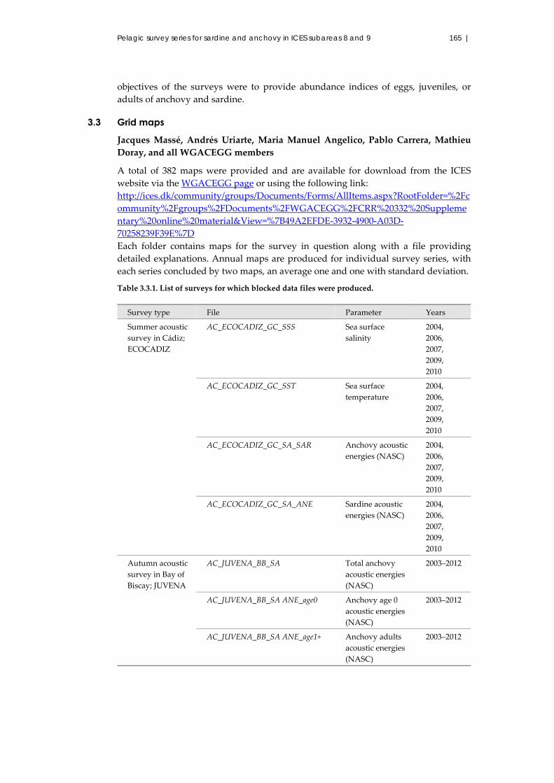
Pelagic survey series for sardine and anchovy in ICES subareas 8 and 9 165 |
objectives of the surveys were to provide abundance indices of eggs, juveniles, or
adults of anchovy and sardine.
3.3 Grid maps
Jacques Massé, Andrés Uriarte, Maria Manuel Angelico, Pablo Carrera, Mathieu
Doray, and all WGACEGG members
A total of 382 maps were provided and are available for download from the ICES
website via the WGACEGG page or using the following link:
http://ices.dk/community/groups/Documents/Forms/AllItems.aspx?RootFolder=%2Fc
ommunity%2Fgroups%2FDocuments%2FWGACEGG%2FCRR%20332%20Suppleme
ntary%20online%20material&View=%7B49A2EFDE‐3932‐4900‐A03D‐
70258239F39E%7D
Each folder contains maps for the survey in question along with a file providing
detailed explanations. Annual maps are produced for individual survey series, with
each series concluded by two maps, an average one and one with standard deviation.
Table 3.3.1. List of surveys for which blocked data files were produced.
Survey type File Parameter Years
Summer acoustic
survey in Cádiz;
ECOCADIZ
AC_ECOCADIZ_GC_SSS Sea surface
salinity
2004,
2006,
2007,
2009,
2010
AC_ECOCADIZ_GC_SST Sea surface
temperature
2004,
2006,
2007,
2009,
2010
AC_ECOCADIZ_GC_SA_SAR Anchovy acoustic
energies (NASC)
2004,
2006,
2007,
2009,
2010
AC_ECOCADIZ_GC_SA_ANE Sardine acoustic
energies (NASC)
2004,
2006,
2007,
2009,
2010
Autumn acoustic
survey in Bay of
Biscay; JUVENA
AC_JUVENA_BB_SA Total anchovy
acoustic energies
(NASC)
2003–2012
AC_JUVENA_BB_SA ANE_age0 Anchovy age 0
acoustic energies
(NASC)
2003–2012
AC_JUVENA_BB_SA ANE_age1+ Anchovy adults
acoustic energies
(NASC)
2003–2012
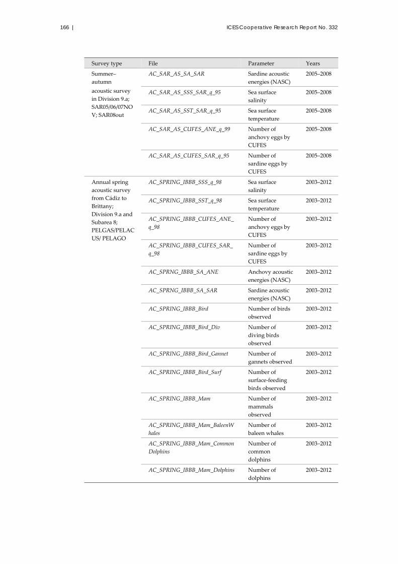
166 | ICES Cooperative Research Report No. 332
Survey type File Parameter Years
Summer–
autumn
acoustic survey
in Division 9.a;
SAR05/06/07NO
V; SAR08out
AC_SAR_AS_SA_SAR Sardine acoustic
energies (NASC)
2005–2008
AC_SAR_AS_SSS_SAR_q_95 Sea surface
salinity
2005–2008
AC_SAR_AS_SST_SAR_q_95 Sea surface
temperature
2005–2008
AC_SAR_AS_CUFES_ANE_q_99 Number of
anchovy eggs by
CUFES
2005–2008
AC_SAR_AS_CUFES_SAR_q_95 Number of
sardine eggs by
CUFES
2005–2008
Annual spring
acoustic survey
from Cádiz to
Brittany;
Division 9.a and
Subarea 8;
PELGAS/PELAC
US/ PELAGO
AC_SPRING_IBBB_SSS_q_98 Sea surface
salinity
2003–2012
AC_SPRING_IBBB_SST_q_98 Sea surface
temperature
2003–2012
AC_SPRING_IBBB_CUFES_ANE_
q_98
Number of
anchovy eggs by
CUFES
2003–2012
AC_SPRING_IBBB_CUFES_SAR_
q_98
Number of
sardine eggs by
CUFES
2003–2012
AC_SPRNG_IBBB_SA_ANE Anchovy acoustic
energies (NASC)
2003–2012
AC_SPRNG_IBBB_SA_SAR Sardine acoustic
energies (NASC)
2003–2012
AC_SPRING_IBBB_Bird Number of birds
observed
2003–2012
AC_SPRING_IBBB_Bird_Div Number of
diving birds
observed
2003–2012
AC_SPRING_IBBB_Bird_Gannet Number of
gannets observed
2003–2012
AC_SPRING_IBBB_Bird_Surf Number of
surface‐feeding
birds observed
2003–2012
AC_SPRING_IBBB_Mam Number of
mammals
observed
2003–2012
AC_SPRING_IBBB_Mam_BaleenW
hales
Number of
baleen whales
2003–2012
AC_SPRING_IBBB_Mam_Common
Dolphins
Number of
common
dolphins
2003–2012
AC_SPRING_IBBB_Mam_Dolphins Number of
dolphins
2003–2012

Pelagic survey series for sardine and anchovy in ICES subareas 8 and 9 167 |
Survey type File Parameter Years
Spring–summer
egg survey;
DEPM survey on
anchovy;
BIOMAN/
BOCADEVA;
Subarea 8 and
Division 9.a
South
DEPM_ANE_BBGC_CUFES_ANE
_q_98
Number of
anchovy eggs by
CUFES
2003–2012
DEPM_ANE_BBGC_CUFES_SAR
_q_98
Number of
sardine eggs by
CUFES
2003–2012
DEPM_ANE_BBGC_PV_SAR_q_9
5
Number of
anchovy eggs by
PairoVET
2003–2012
DEPM_ANE_BBGC_PV_ANE_q_9
8
Number of
sardine eggs by
PairoVET
2003–2012
DEPM_ANE_BBGC_SSS_q_98 Sea surface
salinity
2003–2012
DEPM_ANE_BBGC_SST_q_98 Sea surface
temperature
2003–2012
Triennial spring
egg survey;
DEPM survey on
sardine; PT‐
DEPM‐PIL/
SAREVA; Iberian
coasts; divisions
9.a and 8.b–c
DEPM_SAR_IBBB_SSS_q_98 Sea surface
salinity
2002–2011
DEPM_SAR_IBBB_SST_q_98 Sea surface
temperature
2002–2011
DEPM_SAR_IBBB_CUFES_ANE_
q_98
Number of
anchovy eggs by
CUFES
2002–2011
DEPM_SAR_IBBB_CUFES_SAR_q
_98
Number of
sardine eggs by
CUFES
2002–2011
DEPM_SAR_IBBB_PV_ANE_q_98 Number of
anchovy eggs by
PairoVET
2002–2011
DEPM_SAR_IBBB_PV_SAR_q_98 Number of
sardine eggs by
PairoVET
1988–2011

168 | ICES Cooperative Research Report No. 332
4 Variability and habitats in spring
Pierre Petitgas, Martin Huret, Mathieu Doray, Jacques Massé, Matthieu Autier,
Maria Manuel Angélico, Vitor Marques, Joana Andrade, Isabel Riveiro, Begoña
Santos, Pablo Carrera, and Maria Santos, in collaboration with all WGACEGG
members
All parameters averaged at the same spatial resolution on a common grid (Section 3)
are used to analyze the interannual spatial variability as well as the relationships
among parameters. The procedures were applied to the spring acoustic surveys
(PELAGO, PELACUS, and PELGAS) during which environmental information as well
as data on ichthyoplankton, fish, and top predators are collected, covering the entire
area from Cádiz to Brest.
4.1 Interannual variability
Interannual variability was first characterized globally by computing a coefficient of
variation for each cell as follows : CV(x) = sd(x)/m(x), where m(x) is the arithmetic mean
and sd is the standard deviation over time for each cell (x). Further, to characterize
differences between years more precisely and visually, spatial patches (Woillez et al.,
2009) were estimated, with an R script provided as supplementary material to Woillez
et al. (2009). The R script identifies patches by aggregating to a large value the closest
values in its surroundings. The procedure starts with the highest value and the next
patch is formed around the next highest value that is not included in the previously
formed patch. The patches retained were those that each contained at least 10% of the
total abundance over the entire area.
4.2 Surface temperature and salinity
The coldest surface waters are observed around Galicia and on the northern coast of
Spain; these areas show the lowest variability (Figure 4.2.1). The coastal waters north
of 46°N are also generally cold and show high variability. The warmest waters are
located south of 40°N, with intermediate variability. The French shelf is where the
greatest variability is observed across years in spring, depending on the seasonal
evolution of temperature stratification.
Figure 4.2.1. Spring sea surface temperature: time average (left) and CV (right).
The waters with highest salinity are located south of 40°N (Figure 4.2.2). River plumes
are easily recognized in the Bay of Cádiz, off the rias (estuaries) in Galicia, off northern

Pelagic survey series for sardine and anchovy in ICES subareas 8 and 9 169 |
Portugal, and off Gironde and Loire on the French shelf. The areas of river plume extent
also show the highest interannual variability. The northern Portugal shelf and French
mid‐shelf are also areas of high interannual variability in sea surface salinity.
Figure 4.2.2. Spring sea surface salinity: time average (left) and CV (right).
4.3 Anchovy and sardine adults
For anchovy, the areas of highest concentration are located on the French shelf south
of 47°N, close to the Gironde estuary (45°N) and in the Bay of Cádiz (Figure 4.3.1).
These are recurrent high concentration areas (“core habitats”) as revealed by their low
CVs. In two coastal areas, north of Biscay (47°N) and north of Portugal (41°N), the CV
is high, with mean abundance at medium–low values, meaning that anchovy in these
areas do not always occur (“secondary habitats”). Northern Spain and northwestern
Biscay are areas of very low mean abundance and high interannual variability.
Occasional patches, only for particular years, occur in the secondary habitats (defined
by medium–low mean and high CV), while gravity centres of patches are recurrent in
all years in the core habitats (defined by high mean and low CV) as shown in Figure
4.3.2. Particularly in the Bay of Biscay, two patches (one farther north than the other)
are observed in almost all years. The locations of gravity centres of spatial patches are
more variable in this area than in Cádiz (Figure 4.3.2).
Figure 4.3.1. Spring distribution of anchovy (sA): time average (left) and CV (right); gravity centres
of spatial patches in each year (bottom right).

170 | ICES Cooperative Research Report No. 332
Figure 4.3.2. Spring distribution of anchovy (sA): gravity centres of spatial patches in each year.
For sardine, core and secondary habitats are also observed (Figure 4.3.3). Four core
areas show high mean abundance and low CV: coastal waters in northern Biscay
(47°N); southern shelf Biscay (44°N off Landes); central Portuguese shelf (37–41°N),
where mean abundance is highest; and the Gulf of Cádiz. The two major core areas are
the central Portuguese area and the coastal waters of northern Biscay. It is noteworthy
that these sardine core areas show very little overlap with the anchovy core areas. The
coastal waters off the Galician rias (42–43°N) show medium values for the mean
abundance and CV and could thus be considered as a secondary habitat. In contrast,
the northern coast of Spain and northwestern Biscay are areas of very low abundance
and high variability. The gravity centres of spatial patches complement this picture
with interannual variability (Figure 4.3.4). In the Bay of Biscay, two patches are
observed each year corresponding to the two major core areas, with little variation in
location (good spatial recurrence), which is also observed in the core central
Portuguese area (39–41°N). Patches are observed for particular years in the secondary
habitats in the western part of the Bay of Cádiz and west of Galicia.

Pelagic survey series for sardine and anchovy in ICES subareas 8 and 9 171 |
Figure 4.3.3. Spring distribution of sardine (sA): time average (left) and CV (right).
Figure 4.3.4. Spring distribution of sardine (sA): gravity centres of spatial patches in each year.
4.4 Anchovy and sardine eggs
The distributions of anchovy and sardine eggs show overall distribution patterns
similar to those observed for spawning adults, with similar regions of core and
secondary habitats (Figures 4.4.1 and 4.4.2), although the egg distribution seems to be
shifted from that of spawning adults (see Section 4.3).
Also for sardine, eggs are observed with medium abundance levels and medium CV in
areas where adults were recorded in very low abundance. These areas are located in
the shelfedge north of 45°N in Biscay, the northern coast of Spain, and the northern
coast of Portugal. It is possible that the adults in these areas are less accessible to the
acoustic surveys than the eggs (e.g. very coastal adult distribution, schools too close to
surface).
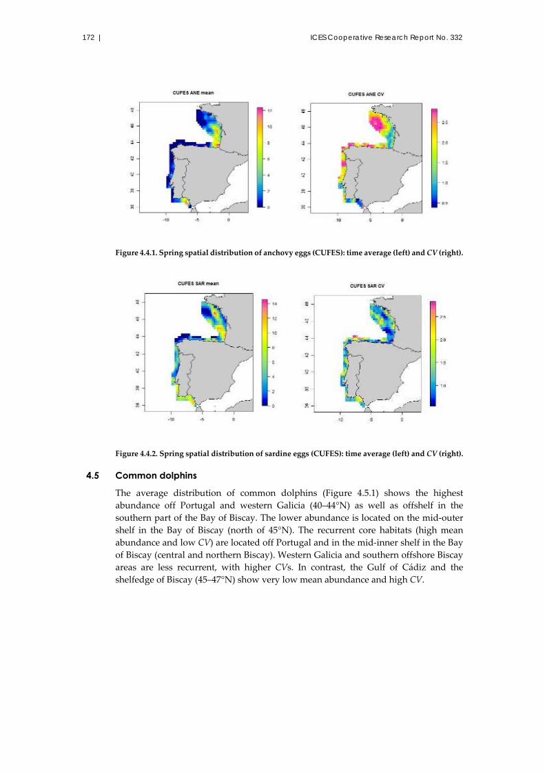
172 | ICES Cooperative Research Report No. 332
Figure 4.4.1. Spring spatial distribution of anchovy eggs (CUFES): time average (left) and CV (right).
Figure 4.4.2. Spring spatial distribution of sardine eggs (CUFES): time average (left) and CV (right).
4.5 Common dolphins
The average distribution of common dolphins (Figure 4.5.1) shows the highest
abundance off Portugal and western Galicia (40–44°N) as well as offshelf in the
southern part of the Bay of Biscay. The lower abundance is located on the mid‐outer
shelf in the Bay of Biscay (north of 45°N). The recurrent core habitats (high mean
abundance and low CV) are located off Portugal and in the mid‐inner shelf in the Bay
of Biscay (central and northern Biscay). Western Galicia and southern offshore Biscay
areas are less recurrent, with higher CVs. In contrast, the Gulf of Cádiz and the
shelfedge of Biscay (45–47°N) show very low mean abundance and high CV.
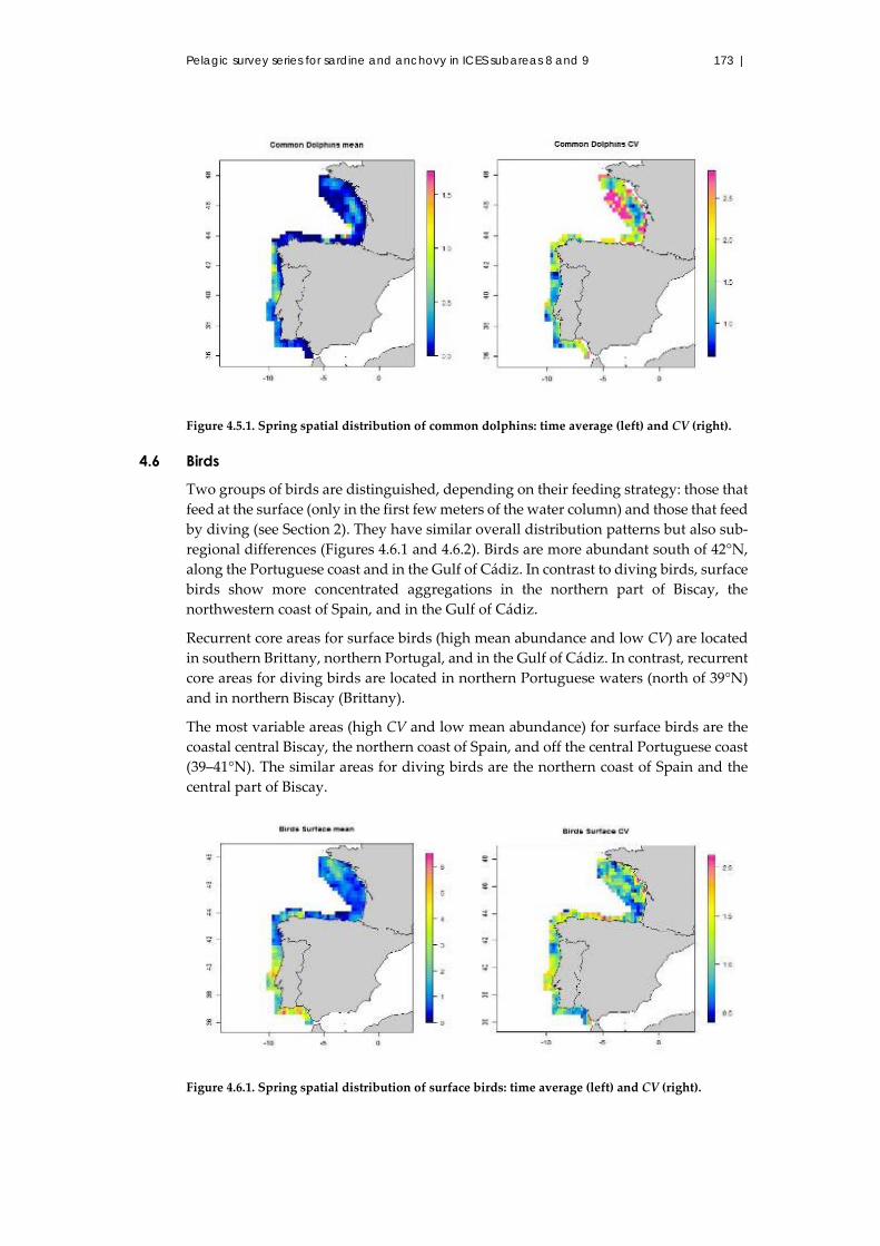
Pelagic survey series for sardine and anchovy in ICES subareas 8 and 9 173 |
Figure 4.5.1. Spring spatial distribution of common dolphins: time average (left) and CV (right).
4.6 Birds
Two groups of birds are distinguished, depending on their feeding strategy: those that
feed at the surface (only in the first few meters of the water column) and those that feed
by diving (see Section 2). They have similar overall distribution patterns but also sub‐
regional differences (Figures 4.6.1 and 4.6.2). Birds are more abundant south of 42°N,
along the Portuguese coast and in the Gulf of Cádiz. In contrast to diving birds, surface
birds show more concentrated aggregations in the northern part of Biscay, the
northwestern coast of Spain, and in the Gulf of Cádiz.
Recurrent core areas for surface birds (high mean abundance and low CV) are located
in southern Brittany, northern Portugal, and in the Gulf of Cádiz. In contrast, recurrent
core areas for diving birds are located in northern Portuguese waters (north of 39°N)
and in northern Biscay (Brittany).
The most variable areas (high CV and low mean abundance) for surface birds are the
coastal central Biscay, the northern coast of Spain, and off the central Portuguese coast
(39–41°N). The similar areas for diving birds are the northern coast of Spain and the
central part of Biscay.
Figure 4.6.1. Spring spatial distribution of surface birds: time average (left) and CV (right).

174 | ICES Cooperative Research Report No. 332
Figure 4.6.2. Spring spatial distribution of diving birds: time average (left) and CV (right).
4.7 Habitats
Perry and Smith (1994) used cumulative distribution functions (CDF) to identify how
fish concentration depend on environmental parameters. Röckmann et al. (2011)
proposed a method to estimate the observed fish distribution in classes of an ancillary
parameter, where the estimated frequencies do not depend on the number of
observations in the different classes. With this method, it was possible to estimate the
CDF of anchovy and sardine eggs and adult concentrations as a function of surface
temperature and salinity. The departure from a straight line characterizes the affinity
or repulsion of the fish for particular classes of temperature or salinity. All grid values
from all years were pooled in the analysis.
4.8 Anchovy and sardine eggs
The distribution of anchovy eggs is limited to warm waters only (>14°C), while sardine
eggs do not seem to be affected by surface temperature >12°C (Figure 4.8.1).
Temperatures between 12 and 14°C are encountered in coastal waters on the French
shelf and in upwelling areas along the Iberian coast and thus may represent key areas.
There is no influence of salinity on the distribution of anchovy and sardine eggs (Figure
4.8.1) above 31 psu. Below that value, hardly any eggs are observed. Similar results are
obtained using DEPM survey data, but with more erratic curves (not shown) because
the survey series contains less samples.

Pelagic survey series for sardine and anchovy in ICES subareas 8 and 9 175 |
Figure 4.8.1. Cumulative distribution of anchovy (plain line) and sardine (dashed line) eggs
(CUFES) in spring as a function of sea surface temperature (left) and salinity (right).
4.9 Anchovy and sardine adults
The distributions of anchovy and sardine do not seem to be influenced by surface
temperature >12°C or by surface salinity >30 psu (Figure 4.9.1). Therefore, these
parameters cannot be used as proxies to describe their habitats.
Figure 4.9.1. Cumulative distribution of anchovy and sardine (sA) in spring as a function of sea
surface temperature (left) and salinity (right).
4.10 Spatial overlaps and differences
To characterize differences in the spatial distribution of spawning adults, as observed
by acoustics and that of their eggs as observed by CUFES, spatial patches (Woillez et
al., 2009) were estimated on the average maps and their gravity centres plotted. Only
those patches that totalled at least 10% of the global mean were considered as the main
patches.
Spatial overlaps between high concentrations in predators and fish were mapped to
identify the main interactions of top predators with anchovy and sardine. There were
grid cells where predator and fish concentrations were both higher than their overall
mean in each year. By counting the number of years when such overlap occurred
throughout the series it was possible to map the occurrence frequency of such overlaps.
Distinction was made between diving and surface birds, and the most abundant

176 | ICES Cooperative Research Report No. 332
marine mammal, the common dolphin (Delphinus sp.), was also taken into
consideration. Distribution maps of demersal predatory fish (e.g. hake) were
unavailable during the spring surveys. Core habitats explained largely the spatial
pattern observed over the years in the frequency of overlaps.
4.10.1 Differences between spawning adults and egg distributions
The egg distributions observed with CUFES are not exactly centred on the observed
distribution of the spawning adults (Figure 4.10.1), although the egg phase duration is
< 4 d (5 d at 13°C). This is observed for anchovy and sardine in the Bay of Biscay where
eggs are shifted westward in comparison to the adults, whereas sardine eggs in the
Gulf of Cádiz are shifted eastwards. For sardine along the Portuguese coast, the dense
patches of spawning adults were not associated with those of eggs.
Figure 4.10.1. Spatial patches of eggs (CUFES) and spawning adults (sA) in spring: anchovy (left)
and sardine (right). Spatial patches are estimated on the time average distributions.
4.10.2 Overlap between top predators and anchovy and sardine
At first is discussed how each predator overlaps with prey, and then how each prey
overlaps with the predators. Common dolphin and anchovy distributions overlapped
(Figure 4.10.2) with high frequency on the mid‐shelf in the Bay of Biscay (45–46°N),
corresponding to a portion of the core habitat of the anchovy. Similarly, common
dolphin and sardine overlapped with high frequency in one of the core areas of sardine
off central Portugal (39–41°N). Overlaps also occurred in the Bay of Biscay and the Gulf
of Cádiz, but with lower frequency in sardine habitats less frequently occupied.
Surface and diving birds overlap with anchovy with highest frequency in similar areas
(Figures 4.10.3 and 4.10.4) such as core anchovy habitat in the Gulf of Cádiz, Bay of
Biscay, and also along the Portuguese coast. A similar pattern is seen for sardine where
the highest overlap frequencies are along the Brittany coast, Portugal, and the Gulf of
Cádiz, corresponding to portions of core sardine habitats.
The anchovy core habitat in the Bay of Biscay overlapped mainly with common
dolphins, while its core habitat in the Gulf of Cádiz overlapped mostly with birds. The

Pelagic survey series for sardine and anchovy in ICES subareas 8 and 9 177 |
core habitats of sardine off central Portugal overlapped with common dolphins as well
as with the birds. On the French shelf in the Bay of Biscay, sardine overlapped with
common dolphins over a large area, while the overlap with birds was more located at
hot spots.
Figure 4.10.2. Occurrence frequency in the yearly overlap between common dolphins and anchovy
(left) and sardine (right).
Figure 4.10.3. Occurrence frequency in the yearly overlap between surface feeding birds and
anchovy (left) and sardine (right).
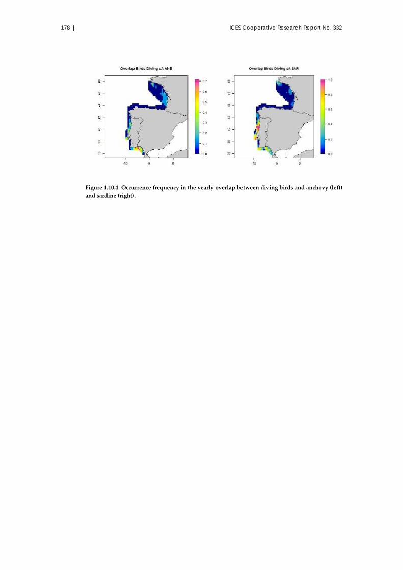
178 | ICES Cooperative Research Report No. 332
Figure 4.10.4. Occurrence frequency in the yearly overlap between diving birds and anchovy (left)
and sardine (right).
Pelagic survey series for sardine and anchovy in ICES subareas 8 and 9 179 |
5 Discussion: towards pelagic ecosystem monitoring
5.1 Ecosystem indicators from regular surveying
Mathieu Doray, Pierre Petitgas, Martin Huret, Jacques Massé, Maria Manuel
Angélico, Vitor Marques, Magdalena Iglesias, Pablo Carrera, Andres Uriarte,
Guillermo Boyra, and Matthieu Autier, in collaboration with all WGACEGG
members
5.1.1 Indicator categories, spatial/temporal and taxonomic scales
WGACEGG participants explored a list of potential indicators of the (good)
environmental status of the pelagic ecosystem in ICES divisions 7.e–h and in subareas
8 and 9 that could be provided by the group in the mid‐term (ICES, 2011a), within the
framework of the Marine Strategy Framework Directive (MSFD). These indicators
could be provided, at both the survey and regional scale, for time‐periods including
spring, summer, autumn, and winter/spring, depending on surveys. The regional scale
was defined as the area encompassing divisions 7.e–h and subareas 8 and 9. The survey
scale was defined as the areas covered by each survey.
The WGACEGG list of potential indicators describes changes in both the biodiversity
and commercial species of the regional pelagic ecosystem. Indicators also describe
marine litter.
Biodiversity indicators are defined at the species and community of species taxonomic
levels. Species for which indicators are available at the regional scale are European
anchovy and sardine at the adult and egg stages, as well as adult marine mammals and
seabirds. Indicators of anchovy and sardine larvae are available for certain surveys.
Indicators of juvenile anchovy are also available in the Bay of Biscay in autumn
(JUVENA survey). Species community indicators describe the pelagic fish community
at the adult and egg stages, as well as the zooplankton community. Commercial fish
indicators describe variations in anchovy and sardine stocks.
5.1.2 WGACEGG MFSD indicators list
The WGACEGG MSFD indicators are summarized in Table 5.1.1.
Table 5.1.1. List of WGACEGG Marine Strategy Framework Directive indicators. The indicators
describing the species distributional patterns are described in Woillez et al. (2007). Indicators in bold are already provided by WGACEGG. Indicators not in bold could be provided every year in
the near future.
Descriptor Attribute Criteria Indicators
Bio‐
diversity
Species Population size DEPM and
acoustic total
biomass and
abundance
estimates,
along with
estimation
error
Population condition Acoustic
biomass and
abundance
estimates per
size/age

180 | ICES Cooperative Research Report No. 332
Descriptor Attribute Criteria Indicators
DEPM
biomass and
abundance
estimate per
size/age
(Biscay
anchovy)
Species distribution Distribu‐
tional
range
Area of
potential
distribution
Distribu‐
tional
pattern
(survey
scale)
Centre of
gravity
Spatial
patches
Inertia
Isotropy
Positive area
Spreading
area
Equivalent
area
Gini index
Coefficient of
variation of
strictly
positive
densities
Microstructure
Global index
of collocation
Mean biomass
Percentage of
total area
occupied
Distribu‐
tional
pattern
(region‐
al scale)
Regional
synthesis of
spatial
indicators at
the survey
scale
Community Community condition Total pelagic
fish NASC
LOPC
zooplankton
abundance at
length
(PELGAS,
PELACUS)
Species
composition

Pelagic survey series for sardine and anchovy in ICES subareas 8 and 9 181 |
Descriptor Attribute Criteria Indicators
Relative
population
abundance
Habitats Habitat
condi‐
tion
Surface
temperature
Surface
salinity
Nutrient
(PELGAS,
PELTIC)
Commercial
fish
Reproduc‐
tive
capacity
DEPM
spawning‐
stock biomass
(SSB) estimate
Acoustic SSB
estimate
DEPM
fecundity
DEPM
spawning
frequency
Age and
size
distribution
95th percentile
of the
population
length
distribution
Proportion of
fish >L50 (only
relevant for
sardine, as all
age 1
anchovies are
mature)
Litter in the
marine
environ‐
ment
Amount, composition, and source of litter floating at sea, in
the water column, and on the seabed
Floating litter
(PELGAS,
PELACUS)
Litter in trawl
catches
(PELGAS,
PELTIC)
Microlitter in
zooplankton
samples
(PELTIC)

182 | ICES Cooperative Research Report No. 332
5.2 Forward look: expansion of survey coverage north of the Bay of Biscay
Jeroen van der Kooij and Ciaran O’Donnell
5.2.1 Introduction
It has long been known that the northern limit of anchovy and sardine distribution
expands beyond the Bay of Biscay. Plankton surveys in the Celtic Sea have reported
large numbers of sardine eggs (Wallace and Pleasants, 1972) comparable to those in the
Bay of Biscay, demonstrating the importance of these northern regions for spawning.
Locally important ringnet fisheries operate in the region and specifically target sardine.
In the case of anchovy, landings in the English Channel and Dutch estuaries were
reported in the late 19th century, but anecdotal information goes back much farther.
Both anchovy and sardine abundance in the north has fluctuated, with periods of high
abundance following periods of near absence (Aurich, 1953). There is some evidence
that the boreal herring dominates this transition region during colder periods, and
sardine during warmer periods (Southward et al., 1988). Since the mid‐1990s, both
anchovy and sardine have apparently increased in the north, a feature that has been
linked to climate variability (Beare et al., 2004; Alheit et al., 2012; Petitgas et al., 2012). In
the case of anchovy, evidence has emerged that the northern anchovy is, in fact, a
separate population from that in the Bay of Biscay (Zarraonaindia et al., 2009, 2012;
Petitgas et al., 2012), yet little is known about it.
Most of the above studies have been based on anecdotal information and indirect data
because of the absence of suitable survey data targeting these species in this area.
Recently, however, concerted efforts have been made to improve on this. Endorsed by
the WGACEGG forum, the UK conducted a one‐off, 23‐day multidisciplinary pelagic
survey in summer 2011 which covered the western English Channel and the Celtic Sea,
extending pelagic coverage in summer beyond 48°N. In 2012, a new five‐year pelagic
survey programme commenced that sampled the pelagic component of the coastal
ecosystem around the southwestern part of the UK in autumn. Additionally, the
Marine Institute (Ireland) has conducted an autumn pelagic survey in the northern
Celtic Sea and southwestern Ireland since 1989, targeting autumn‐ and winter‐
spawning components of the herring stock in both coastal and offshore waters. In
summer 2011, a new survey programme was initiated, targeting spawning
aggregations of boarfish along the shelf edge and shelf seas from north of Scotland to
northern Biscay. This survey offers many opportunities as a newly established large‐
scale summer survey in western waters.
5.2.2 Celtic Sea herring survey
The Celtic Sea herring acoustic survey is carried out annually in October over 21 days
on board the RV “Celtic Explorer”. The survey is carried out to acoustically assess the
size of the autumn‐ and winter‐spawning components of the herring stock in the Celtic
Sea and southwest of Ireland (ICES divisions 7.a, g, and j; Figure 5.2.1). This survey
was first established in 1989 and has been carried out in its current form since 2004.
Area coverage is broken into broad‐scale (offshore) and spawning (inshore) strata.
Broad‐scale strata are important transit routes for herring migrating to inshore
spawning areas from offshore summer feeding grounds. A parallel transect design is
used with transects running perpendicular to the coastline following standard survey
methods. Transect resolution is set at 2–4 nautical miles for the broad‐scale strata,
increased to 1 nautical mile for the spawning strata. Bay and inlets are surveyed using
zigzag transects. Transect starting points within strata are randomized each year

Pelagic survey series for sardine and anchovy in ICES subareas 8 and 9 183 |
within established baseline strata bounds. Further details of survey methods are
provided in the annual cruise report (O’Donnell et al., 2013).
Calibrated acoustic data are collected at four frequencies (18, 38, 120, and 200 kHz)
from transducers mounted within a drop‐keel system. Biological sampling is carried
out using a single pelagic midwater trawl, and biological data are collected from all
species encountered.
Figure 5.2.1. Pelagic survey coverage north of 48°N in ICES Subarea 7 during autumn (top) by the
Celtic Sea herring survey (CSH, red transects) and PELTIC survey (blue transects), and during
summer (bottom) during the boarfish survey.
In addition to herring, other small pelagic fish species are routinely encountered and
sampled, including sprat, mackerel, horse mackerel, anchovy, and sardine. Acoustic

184 | ICES Cooperative Research Report No. 332
abundance estimates are produced for herring and sprat from survey data. At present,
no abundance estimates are calculated for the other species.
In addition to the acoustic component of the survey, comprehensive hydrographic
sampling is undertaken as well as coordinated sighting surveys for marine mammals,
seabirds, and marine litter. Marine mammal and seabird sighting surveys now form
an increasingly important component of this multidisciplinary survey.
5.2.3 Pelagic ecosystem survey in the English Channel and eastern Celtic Sea: PELTIC
In 2011, a one‐off, 23‐day pelagic survey was conducted in the Celtic Sea and western
English Channel in early summer (May–June). The primary aim was to study the
distribution and abundance of the small pelagic fish community in the area, with
particular focus on anchovy and sardine. Other than information on the small pelagic
fish species, this survey collected data across the foodweb, from physical
oceanography to top predators such as birds and marine mammals.
The findings of the above‐mentioned summer survey led to the design and
implementation of a new five‐year pelagic autumn survey series which commenced in
2012 on the RV “Cefas Endeavour”. The survey covers the coastal waters of the western
English Channel, Isles of Scilly, and Bristol Channel, following a series of parallel
transects spaced 10 nautical miles apart and perpendicular to the coast (Figure 5.2.1).
Along these transects, calibrated acoustic data are collected at 38, 120, and 200 kHz
from drop‐keel mounted transducers, which, combined with pelagic trawl operations,
provide information on the small pelagic fish community.
However, during this survey, other components of the pelagic ecosystem are also
sampled: (i) continuous data on surface oceanography and apex predators in
conjunction with the fisheries acoustics; (ii) two ringnets are deployed at 70 fixed
stations with a mini CTD, collecting zooplankton and ichthyoplankton data; and (iii) a
Rosette with CTD is deployed at ca. half of the fixed stations to provide high‐resolution
information on physical oceanography, nutrients, and production in the water column.
5.2.4 Contributions of northern surveys to understanding pelagic fish in the Iberian–Biscay–Celtic Atlantic ecoregion
The above‐mentioned surveys have contributed towards an improved understanding
of the pelagic component of the western shelf seas ecosystems of the Northeast
Atlantic. The established Celtic Sea herring survey has collected a valuable time‐series
on the target species and now also provides information on other pelagic fish species,
such as anchovy and sardine, as well as other levels of the foodweb. For example, fin
(Balaenoptera physalus) and humpback (Megaptera novaeangliae) whales arrive in the
northern Celtic Sea to feed on sprat and herring aggregations in coastal waters, and
peak abundance has been shown to be aligned with the timing of the herring survey
(Ryan et al., 2013). Although not yet a significant time‐series, the PELTIC survey series
has started to contribute important spatial and quantitative data which is further
improving understanding on the small pelagic community and its ecosystem. For
example, it appears that in autumn, sardine spawning is widespread in the western
English Channel, and according to other fixed‐station time‐series data, is increasing
(Coombs et al., 2010). Sprat is the most abundant small pelagic species in coastal waters
of the southern Celtic Sea and western English Channel, and in some years, good
numbers of the “northern” anchovy (Petitgas et al., 2012) are found in the English
Channel, boosting incomes of local fishers. Herring is generally found in low numbers
(< 1% of the pelagic fish biomass) in the southern Celtic Sea, but it is the most important
clupeoid in the northern Celtic Sea. Both Celtic Sea autumn surveys also encounter

Pelagic survey series for sardine and anchovy in ICES subareas 8 and 9 185 |
large quantities of mackerel, some years into the thousands of tonnes. Mackerel is
abundant in the Celtic Sea throughout the year, occurring both as immature and
mature fish. Part of the area has been closed for mackerel trawling to protect what is
thought to be an important nursery area for the juvenile fish which have traditionally
moved there after hatching at the shelf edge. As mentioned above, the southern Celtic
Sea and western English Channel areas mark the southern and northern boundaries of
boreal and Lusitanian species, respectively. One example of a warm‐water species
which has extended further north in recent years in greater abundance is the boarfish.
Since the early 1970s, its abundance in the Northeast Atlantic has increased
dramatically after successive years of good recruitment, attributed to an increase in
water temperature during the spawning season (Blanchard and Vandermeirsch, 2005).
Knowledge on this species has developed quickly since the first dedicated summer
acoustic survey was carried out in 2011 (O’Donnell et al., 2012), particularly in areas
such as spawning conditions (Farrell et al., 2012), boarfish specific TS–length
relationship (Fässler et al., 2013), and age determination (Hüssy et al., 2012a, b).
As stand‐alone units, these surveys have already provided valuable contributions to
fisheries management, as well as to an improved understanding of some of the
ecological mechanisms in the area. However, their scientific contribution will be more
significant when combined with other existing surveys in the area. Coordinated
temporal and geographical coverage of core and peripheral species distribution areas
will help to increase the precision of, and reduce uncertainty in, acoustically derived
abundance indices for transboundary species. Other than the primary target species of
the WGACEGG, sardine and anchovy, it also includes other widely dispersed stocks
such as mackerel. The need for a coordinated acoustic survey approach is becoming
increasingly important to further complement existing survey methods. The ability of
multidisciplinary research cruises to fill gaps in knowledge, not only for traditional
target fish species, but also for wider‐scale research purposes, is not just extremely
beneficial, but also increasingly an EU data requirement.

186 | ICES Cooperative Research Report No. 332
5.3 Conclusion
Jacques Massé, Andrés Uriarte, Maria Manuel Angelico, and Pablo Carrera
This report culminates more than 30 years of collaboration among Portugal, Spain, and
France. From unofficial collaboration to the annual meetings of the WGACEGG, each
country and institution made progress and efforts to move toward better monitoring
of the pelagic species and their ecosystems. Each partner progressed in methodology
and enlarged the range of parameters collected. Through European projects, work on
standardization of methods and sampling strategies was done in parallel with several
intercalibration exercises among vessels. Despite some disagreements and open
debates on methods or results, these three countries succeeded in working together in
a constructive way to assemble information into a common database to allow
combining or cross‐analysing several parameters. The results today appear in this
report as a synthesis of the last ten years of pelagic surveys (2003–2012) across
southwestern European waters.
In the framework of WGACEGG, it is planned to supply, year after year, the agreed
parameters in an agreed format whatever the season or area covered by the survey in
order to achieve together a better understanding of the pelagic ecosystem in
southwestern European Atlantic waters. In this objective, northern countries are now
joining this group with complementary surveys, and the geographical coverage will
certainly result in a better delimitation of the northern limits of sardine and anchovy,
as well as a better comprehension of the southern distribution of more northern pelagic
resources like herring or sprat.
Nevertheless, the members of WGACEGG still have to work further to solve some of
their original challenges, such as achieving a combined estimate from acoustics and
egg surveying, or including egg production estimates from (or with the aid of) CUFES,
improving species recognition from multifrequency analysis of echograms, and so on.
Although some progress has been made along these lines (Petitgas et al., 2009; Lezama‐
Ochoa et al., 2011), there is still much room for improvement. In addition, there might
be new ways of approaching old challenges, such as making use of modelling of
parameters to improve survey estimates. For instance, survey observations of DEPM
parameters could be modelled in space (potentially including environmental or
biological covariates) to lead to improved estimates of either adult or egg abundance
estimates (see Bernal et al. [2011b] for such an approach to estimating sardine egg
mortality). A parallel study could be devised to apply acoustic TS corrected by the
vertical location of schools. This can be used also to infer combined acoustic and egg
biomass estimates. Bayesian inference could certainly be a suitable framework in which
to address these challenges.
Furthermore, the surveys should gradually evolve to provide more suitable outputs
for the integrated monitoring of pelagic habitats and ecosystems where the target
populations develop and interact as forage species. The main challenge addressed by
the Intergovernmental Oceanographic Commission (IOC) during the 1970s (i.e. to
assess the present understanding of the mechanisms through which variability in the
physical–chemical marine environment affects the biological productivity of the ocean
and the abundance and distribution of living marine resources) was the most
important trigger to implement monitoring programmes aiming to assess the pelagic
coastal stocks along the Iberian Peninsula and in the Bay of Biscay. From the
exploratory phase in the 1980s and 1990s, for both acoustics and egg production
surveys, to the consolidated phase of the surveys included in this report, in terms of
technology, survey design, and data analysis, there has been great improvement in

Pelagic survey series for sardine and anchovy in ICES subareas 8 and 9 187 |
knowledge about this pelagic ecosystem. While sampling design and the main
assessment objectives of these surveys will remain nearly unchanged for the next few
years, new vessel‐borne tools and techniques, together with an improvement in the
precision of the estimates, will offer an opportunity for monitoring biotic and abiotic
parameters so as to contribute to the monitoring of the ecosystem and environmental
status related to the Marine Strategy Framework Directive and the Common Fisheries
Policy. This will of necessity mean a close relationship among the different teams
involved in the surveys (planktologists, acousticians, biologists, physical and chemical
oceanographers, and others, including fishers) in order to integrate the results of each
discipline. This integration should certainly lead to an improved series of ecosystem
indicators.

188 | ICES Cooperative Research Report No. 332
6 References
Afonso‐Dias, I., Amorim, P., and Silva, A. 2008. Problems with assigning the ovaries of sardine
(Sardina pilchardus) to the appropriate macroscopic maturity stage. Marine Biodiversity
Records, 1: e20, http://dx.doi.org/10.1017/S175526720700190X.
Agresti, A. 1990. Categorical Data Analysis. Wiley, New York. 576 pp.
Ahlstrom, E. H. 1943. Studies on the Pacific pilchard or sardine (Sardinops caerulea). 4: Influence
of temperature on the rate of development of pilchard eggs in nature. U.S. Fish and Wildlife
Service Special Scientific Report, 15: 132–167.
Albaina, A. 2007. Relationships between mesoscale oceanographic structures and zooplankton
communities in the Bay of Biscay. PhD thesis, Basque Country University, Department of
Plant Biology and Ecology, Bilbao, Spain.
Aldanondo, N. 2010. Young‐of‐the‐year European anchovy in the Bay of Biscay: Study of
recruitment determining processes based on otoliths microstructure analysis. PhD thesis,
Basque Country University, Department of Plant Biology and Ecology, Bilbao, Spain.
Alday, A., Martin, I., Martinez, U., and Santos, M. 2004. Codes and criteria for the identification
of anchovy ovaries: traditional and newly proposed classification key. Working Document,
11 pp. In Report of the Study Group on the Estimation of Spawning Stock Biomass of
Sardine and Anchovy (SGSBSA), 11–13 November 2004, San Sebastian, Spain. ICES
Document CM 2005/G:02. 80 pp.
Alday, A., Uriarte, A., Santos, M., Martín, I., Martínez, U., and Motos, L. 2008. Degeneration of
postovulatory follicles of the Bay of Biscay anchovy (Engraulis encrasicolus L.). Scientia
Marina, 72(3): 565–575.
Alday, A., Santos, M., Uriarte, A., Martín, I., Martínez, U., and Motos, L. 2010. Revision of criteria
for the classification of postovulatory follicles degeneration, for the Bay of Biscay anchovy
(Engraulis encrasicolus, L.). Revista de Investigación Marina, 17(8): 165–171.
Alheit, J., Pohlmann, T., Casini, M., Greve, W., Hinrichs, R., Mathis, M., OʹDriscoll, K., et al. 2012.
Climate variability drives anchovies and sardines into the North and Baltic Seas. Progress
in Oceanography, 96(1): 128–139.
Anonymous. 1987a. Arrantzuarrekiko Zientzia eta Teknologia Iraskundea. Memoria anaul de
actividades científicas 1987. Mimeo. 21 pp.
Anonymous. 1987b. Reuniao Luso‐Espanhola para planeamento das campanhas do “Método de
Produçao de Ovos” para a sardinha, Sardina pilchardus, Walbaum. Mimeo. 147 pp.
Armstrong, M. J. P., Connolly, P., Nash, R. D. M., Pawson, M. G., Alesworth, E., Coulahan, P. J.,
Dickey–Collas, M., et al. 2001. An application of the annual egg production method to
estimate the spawning biomass of cod (Gadus morhua L.), plaice (Pleuronectes platessa L.) and
sole (Solea solea L.) in the Irish Sea. ICES Journal of Marine Science, 58: 183–203.
Aurich, H. J. 1953. Verbreitung und Laichverhältnisse von Sardelle und Sardine in der
südöstlichen Nordsee und ihre Veränderungen als Folge der Klimaänderung. Helgoländer
wissenschaftliche Meeresuntersuchungen, 4(3): 175–204.
Bachiller, E. 2012. Trophic ecology of small pelagic fish in the Bay of Biscay, ecological effects of
trophic interactions. PhD thesis, Basque Country University, Department of Plant Biology
and Ecology, Bilbao, Spain.
Barange, M., Bernal, M., Cercole, M. C., Cubillos, L. A., Daskalov, G. M., de Moor (formerly
Cunningham), C. L., De Oliveira, J. A. A., et al. 2009. Current trends in the assessment and
management of stocks. In Climate Change and Small Pelagic Fish, Section 9, pp. 191–255.
Ed. by D. Checkley, J. Alheit, Y. Oozeki, and C. Roy. Cambridge University Press,
Cambridge. 372 pp.

Pelagic survey series for sardine and anchovy in ICES subareas 8 and 9 189 |
Barber, R. T., Csirke, J., Jones, R., Lasker, R., Parrish, R., and Tomczak, M. 1982. Oceanography
marine ecology and living resources. Scientific Committee on Ocean Research (SCOR)
Proceedings, 18: 56–57.
Baro, J., Sobrino, I., Millán, M., Ramos, F., Jiménez, M. P., and Herrera, M.A. 1993. Fisheries of
the Spanish South Atlantic Region (1st Part). Final Report. Cooperative project IEO/EC–DG
XIV/C/1/1992/8. 59 pp.
Beare, D. J., Burns, F., Greig, A., Jones, E. G., Peach, K., Kienzle, E., McKenzie, D. G., et al. 2004.
Long–term increases in prevalence of North Sea fishes having southern biogeographic
affinities. Marine Ecology Progress Series, 284: 269−278.
Bernal, M. 2007. Modelling the abundance, distribution and production of sardine (Sardina
pilchardus, Walb.) eggs in the Iberian Peninsula. PhD thesis. University of Cádiz, Spain.
240 pp.
Bernal, M., Franco, C., Pérez, J. R., and Lago de Lanzós, A. 2000. DEPM estimates of sardine
(Sardina pilchardus) SSB off the Spanish coast in 1999. Working document presented at the
Workshop on Sardine SSB Estimation, Vigo, Spain, 13–16 June 2000.
Bernal, M., Borchers, D. L., Valdés, L., Lago de Lanzós, A., and Buckland, S. T. 2001. A new
ageing method for eggs of fish species with daily spawning synchronicity. Canadian Journal
of Fisheries and Aquatic Sciences, 58: 2330–2340.
Bernal, M., Stratoudakis, Y., Coombs, S., Angélico, M. M., Lago de Lanzós, A., Porteiro, C.,
Sagarminaga, Y., et al. 2007. Sardine spawning off the European Atlantic coast:
Characterization of and spatio–temporal variability in spawning habitat. Progress in
Oceanography, 74: 210–227.
Bernal, M., Ibaibarriaga, L., Lago de Lanzós, A., Lonergan, M., Hernández, C., Franco, C.,
Rasines, I., et al. 2008. Using multinomial models to analyze data from sardine egg
incubation experiments; a review of advances in fish egg incubation analysis techniques.
ICES Journal of Marine Science, 65: 51–59.
Bernal, M., Stratoudakis, Y., Wood, S., Ibaibarriaga, L., Uriarte, A., Valdés, L., and Borchers, D.
2011a. A revision of daily egg production estimation methods, with application to Atlanto–
Iberian sardine. 1. Daily spawning synchronicity and estimates of egg mortality. ICES
Journal of Marine Science, 68: 519–527.
Bernal, M., Stratoudakis, Y., Wood, S., Ibaibarriaga, L., Valdés, L., and Borchers, D. 2011b. A
revision of daily egg production estimation methods, with application to Atlanto–Iberian
sardine. 2. Spatially and environmentally explicit estimates of egg production. ICES Journal
of Marine Science, 68: 528–536.
Bernal, M., Jiménez, M. P., and Duarte, J. 2011c. Anchovy egg development in the Gulf of Cádiz
and its comparison with development rates in the Bay of Biscay. Fisheries Research, 117–
118: 112–120.
Blanchard, F., and Vandermeirsch, F. 2005. Warming and exponential abundance increase of the
subtropical fish Capros aper in the Bay of Biscay (1973–2002). Comptes Rendus Biologies, 328:
505–509.
Bourriau, P. 1991. The ʺCarré Netʺ. ICES Document CM 1991/L:53. Poster.
Boyra, G., Rueda, L. D., Coombs, S. H., Sundby, S., Ådlandsvik, B., Santos, M., and Uriarte, A.
2003. Modelling the vertical distribution of eggs of anchovy (Engraulis encrasicolus) and
sardine (Sardina pilchardus). Fisheries Oceanography, 12(3/4): 381–395.
Boyra, G., Martinez, U., Cotano, U., Santos, M., Irigoien, X., and Uriarte, A. 2013. Acoustic
surveys for juvenile anchovy in the Bay of Biscay: abundance estimate as an indicator of the
next year’s recruitment and spatial distribution patterns. ICES Journal of Marine Science,
70(7): 1354–1358; http://dx.doi.org/10.1093/icesjms/fst096.

190 | ICES Cooperative Research Report No. 332
Brehmer, P., Guillard, J., Guennégan, Y., Bigot, J. L., and Liorzou, B. 2006. Evidence of a variable
‘‘unsampled’’ pelagic fish biomass in shallow water (< 20 m): the case of the Gulf of Lion.
ICES Journal of Marine Science, 63(3): 444–451.
Camphuysen, K., and Garthe, S. 2004. Recording foraging seabirds at sea – standardised
recording and coding of foraging behaviour and multi‐species foraging associations.
IMPRESS report #2001–001, EC Quality of Life and Management of Living Resources. 21 pp.
Carrera, P. 2003. Preliminary results of the inter‐ship acoustic calibration in the Gulf of Cádiz
signoise report. Working Document 02/03. In Report of the Working Group on the
Assessment of Mackerel, Horse Mackerel, Sardine and Anchovy, 9–18 September 2003,
ICES, Copenhagen. ICES Document CM 2004/ACFM:08. 487 pp.
Carrera, P., and Porteiro, C. 2003. Stock dynamic of the Iberian sardine (Sardina pilchardus, W.)
and its implication on the fishery off Galicia. Scientia Marina, 67(Suppl. 1): 245–258.
Carrera, P., Meixide, M., Porteiro, C., and Miquel, J. 2001. Study of the blue whiting movements
around the Bay of Biscay using acoustic methods. Fisheries Research, 50: 151–161.
Carrera, P., Churnside, J. H., Boyra, G., Marques, V., Scalabrin, C., and Uriarte, A. 2006.
Comparison of airborne lidar with echosounders: a case study in the coastal Atlantic waters
of southern Europe. ICES Journal of Marine Science, 63: 1736–1750.
Checkley, D. M., Ortner, P. B., Settle, L. R., and Cummings, S. R. 1997. A continuous, underway
fish egg sampler. Fisheries Oceanography, 6: 58–73.
Claramunt, G., Serra, R., Castro, L. R., and Cubillos, L. 2007. Is the spawning frequency
dependent on female size? Empirical evidence in Sardinops sagax and Engraulis ringens off
northern Chile. Fisheries Research, 85: 248–257.
Clay, A., and Castonguay, M. 1996. In situ target strengths of Atlantic cod (Gadus morhua) and
Atlantic mackerel (Scomber scombrus) in the Northwest Atlantic. Canadian Journal of
Fisheries and Aquatic Sciences, 53: 87–98.
Coombs, S., Boyra, G., Rueda, L., Uriatre, A., Santos, M., Conway, D. V. P., and Halliday, N. C.
2004. Buoyancy measurements and vertical distribution of eggs of sardine (Sardina
pilchardus) and anchovy (Engraulis encrasicolus). Marine Biology, 145: 959–970.
Coombs, S. H., Halliday, N. C., Conway, D. V. P., and Smyth, T. J. 2010. Sardine (Sardina
pilchardus) egg abundance at station L4, western English Channel, 1988–2008. Journal of
Plankton Research, 32: 693–697.
Cort, J. L., Cendrero, O., and Iribar, X. 1976. La anchoa, Engraulis encrasicholus (L.) del Cantábrico.
Resultados de las campañas de 1974, 1975 y 1976. Boletín del Instituto Español de
Oceanografía, 220: 3–34.
Cunha, M. E., Figueiredo, I., Farinha, A., and Santos, M. 1992. Estimation of sardine spawning
biomass off Portugal, by the daily egg production method. Boletín del Instituto Español de
Oceanografía, 8: 139–153.
Cunha, M. E., Farinha, A., and Soares, E. 1997. Preliminary estimation of sardine spawning
biomass in ICES Division IXa (Lat. 41°50´N 36°00´N) by the daily egg production method.
Working Document. In Report of the Working Group on the Assessment of Mackerel, Horse
Mackerel, Sardine and Anchovy, ICES Headquarters, 9–18 September 1997. ICES Document
CM 1998/Assess:06. 383 pp.
Degnbol, P., Lassen, H., and Stæhr, K‐J. 1985. In‐situ determinations of target strength of herring
and sprat at 38 and 120 kHz. Dana, 5: 45–54.
Dias, C. A., Pastor, X., Pestana, G., Porteiro, C., Soares, E., and Alvarez, F. 1983. Results of the
Spanish–Portuguese joint acoustic survey for pilchard (ICES Divisions VIIIc and IXa),
August–September 1982. ICES Document CM 1983/H:42. 42 pp.

Pelagic survey series for sardine and anchovy in ICES subareas 8 and 9 191 |
Diaz, E. 2008. Condition and biochemical composition of three pelagic larvae in the Bay of Biscay:
Engraulis encrasicolus, Sardina pilchardus, and Trachurus trachurus. PhD thesis, Basque
Country University, Department of Plant Biology and Ecology, Bilbao, Spain.
Diner, N., and Le Men, R. 1983. Evaluation acoustique des stocks de poissons pélagiques dans la
partie Sud du golfe de Gascogne en avril–mai 1983. Résultats préliminaires. ICES Document
CM 1983/H:44. 19 pp.
Diner, N., Avrilla, J. L., Guerault, P., Porche, P., and Vincent, A. 1976. La prospection acoustique
des espèces pélagiques côtières du golfe de Gascogne en 1975. ICES Document CM 1976/J:9.
13 pp.
Doray, M. 2013. EchoR package tutorial. Rapport interne Ifremer, PDG/RBE/EMH 13–01.
Availiable at: http://archimer.ifremer.fr/doc/00128/23879/21814.pdf.
Dragesund, O., and Olsen, S. 1965. On the possibility of estimating year‐class strength by
measuring echo‐abundance of 0‐group fish. Fiskeridirektoratets Skrifter Serie
Havundersøkelser, 13: 47–75.
Duarte, J., Bernal, M., Jiménez, M. P., Canoura, J., García, E., Juárez, A., and Muñoz, I. 2007. Egg
development model for anchovy (Engraulis encrasicolus) in the Gulf of Cádiz. Working
document. In Report of the Working Group on Acoustic and Egg Surveys for Sardine and
Anchovy in ICES areas VIII and IX (WGACEGG), 26–30 November 2007, Palma de Mallorca,
Spain. ICES Document CM 2007/LRC:16. 63 pp.
EC. 2000. COUNCIL REGULATION (EC) No 1543/2000 of 29 June 2000 establishing a
Community framework for the collection and management of the data needed to conduct
the common fisheries policy. Official Journal of the European Communities, L 176: 1–16.
https://publications.europa.eu/en/publication‐detail/‐/publication/4c838762‐b19a‐4212‐
a732‐57ba5bf60223/language‐en.
EC. 2008. COUNCIL REGULATION (EC) No 199/2008 of 25 February 2008 concerning the
establishment of a Community framework for the collection, management and use of data
in the fisheries sector and support for scientific advice regarding the Common Fisheries
Policy. Official Journal of the European Communities, L 60: 1–12.
https://publications.europa.eu/en/publication‐detail/‐/publication/e67dbad9‐5ce7‐4ec8‐
bbb0‐51f52edab45d.
FAO. 1980. Report of the first Session of the Working Party on Acoustic Methods for Fish
Detection and Abundance Estimation, Ancona, Italy, 12–16 November 1979. FAO Fisheries
Report No. 231. 33 pp.
FAO. 1983. Report of the Technical Consultation on Acoustic Methods for Fish Detection and
Abundance Estimation, Palma de Mallorca, Spain, 8–12 November 1982. FAO Fisheries
Report No. 277. 94 pp.
Farrell, E. D., Hüssy, K., Coad, J. O., Clausen, L. W., and Clarke, M. W. 2012. Oocyte development
and maturity classification of boarfish (Capros aper) in the Northeast Atlantic. ICES Journal
of Marine Science, 69: 498–507.
Fässler, S. M. M., OʹDonnell, C., and Jech, J. M. 2013. Boarfish (Capros aper) target strength
modelled from magnetic resonance imaging (MRI) scans of its swimbladder. ICES Journal
of Marine Science, 70: 1451–1459.
Fernandes, P. G., Gerlotto, F., Holliday, D. V., Nakken, O., and Simmonds, E. J. 2002. Acoustic
applications in fisheries science: the ICES contribution. ICES Marine Science Symposia, 215:
483–492.
Foote, K. G. 1987. Fish target strengths for use in echo integrator surveys. The Journal of the
Acoustical Society of America, 82: 981–987.
Foote, K. G., Knudsen, H. P., Vestnes, G., MacLennan, D. N., and Simmonds, E. J. 1987.
Calibration of acoustic instruments for fish‐density estimation: a practical guide. ICES
Cooperative Research Report No. 144. 57 pp.

192 | ICES Cooperative Research Report No. 332
Gamulin, T., and Hure, T. 1955. Contribution a la connaissance de l´ecologie de la ponte de la
sardine, Sardina pilchardus (Walb.) dans l´Adriatique. Acta Adriatica, 7(8): 1–22.
Ganias, K., and Nunes, C. 2011. Bathymetric segregation of spawning stages in the Atlantic
sardine Sardina pilchardus. Marine Ecology Progress Series, 428: 235–244.
Ganias, K., Somarakis, S., Machias, A., and Theodorou, A. J. 2003. Evaluation of spawning
frequency in a Mediterranean sardine population (Sardina pilchardus sardina). Marine
Biology, 142: 1169–1179.
Ganias, K., Somarakis, S., Machias, A., and Theodorou, A. J. 2004. Pattern of oocyte development
and batch fecundity in the Mediterranean sardine. Fisheries Research, 67: 13–23.
Ganias, K., Nunes, C., and Stratoudakis, Y. 2007. Degeneration of postovulatory follicles in the
Iberian sardine, Sardina pilchardus: structural changes and factors affecting resorption.
Fishery Bulletin US, 105(1): 131–139.
Ganias, K., Rakka, M., Vavalidis, T., and Nunes, C. 2010. Measuring batch fecundity using
automated particle counting. Fisheries Research, 106: 570–574.
García, A., Pérez, N., Porteiro, C., and Carrera, P. 1991. Estimates of the sardine spawning stock
biomass off the Galician and Cantabrian coasts. ICES Document CM 1991/H:35.
García, A., Pérez, N., Lo, N. C. H., Lago de Lanzos, A., and Sola, A. 1992. The egg production
method applied to the spawning biomass estimation of sardine, Sardina pilchardus (Walb.)
on the North Atlantic Spanish coast. Boletín del Instituto Español de Oceanografía, 8: 123–
138.
García, A., Franco, C., Solá, A., and Lago de Lanzós, A. 1993. Producción diaria de huevos de
sardina, Sardina pilchardus (Walb.), en las costas de Galicia, Cantabrico y golfo de Vizcaya,
en Abril–Mayo, 1990. Boletín del Instituto Español de Oceanografía, 9: 237–250.
Guennégan, Y., Guillard, J., Bigot, J‐L., Brehmer, P., Colon, M., Cheret, Y., and Liorzou, B. 2004.
Importance de la zone côtière dans les évaluations des stocks de petits poissons pélagiques:
Analyse d’une série de campagnes acoustiques et d’une expérimentation en zone côtière.
Working Document to the Working Group on Small Pelagics, Scientific Advisory
Committee–GFCM, Sub‐Committee of Stock Assessment, Málaga, Spain, 6–7 May 2004.
17 pp.
Guillard, J., and Lebourges, A. 1998. Preliminary results of fish populations’ distribution in a
Senegalese coastal area with depths less than 15 m, using acoustic methods. Aquatic Living
Resources, 11: 13–20.
Guttierez, M., and MacLennan, D. 1998. Preliminary results of determination of in situ target
strength of main pelagic species: Cruise of RV Humboldt 9803–05 from Tumbes to Tacna.
Informe Instituto del Mar del Peru, 135: 16–19.
Haldorsson, O., and Reynisson, P. 1983. Target strength measurements of herring and capelin
in‐situ at Iceland. FAO Fisheries Report No. 300: 78–84.
Hampton, I. 1996. Acoustic and egg production estimates of South African anchovy biomass
over a decade: comparisons, accuracy and utility. ICES Journal of Marine Science, 53: 493–
500.
Heinemann, D. 1981. A range finder for pelagic bird censusing. The Journal of Wildlife
Management, 45: 489–493.
Hoaglin, D. C., Mosteller, F., and Tukey, J. W. 1983. Understanding Robust and Exploratory Data
Analysis. John Wiley & Sons. 447 pp.
Hunter, J. R., and Goldberg, S. R. 1980. Spawning incidence and batch fecundity in northern
anchovy, Engraulis mordax. Fishery Bulletin US, 77: 641–652.
Hunter, J. R., and Macewicz, B. J. 1985. Measurement of spawning frequency in multiple
spawning fishes. In An egg production method for estimating spawning biomass of pelagic

Pelagic survey series for sardine and anchovy in ICES subareas 8 and 9 193 |
fish: application to the northern anchovy, Engraulis mordax, pp. 66–77. Ed. by R. Lasker.
NOAA Technical Report NMFS, 36. 99 pp.
Hunter, J. R., Lo, N. C. H., and Leong, R. J. H. 1985. Batch fecundity in multiple spawning fishes.
In An egg production method for estimating spawning biomass of pelagic fish: application
to the northern anchovy, Engraulis mordax, pp. 79–93. Ed. by R. Lasker. NOAA Technical
Report NMFS, 36. 99 pp.
Hüssy, K., Coad, J. O., Farrell, E. D., Clausen, L. A. W., and Clarke, M. W. 2012a. Age verification
of boarfish (Capros aper) in the Northeast Atlantic Ocean. ICES Journal of Marine Science,
69: 34–40.
Hüssy, K., Coad, J. O., Farrell, E. D., Clausen, L. W., and Clarke, M. W. 2012b. Sexual dimorphism
in size, age, maturation, and growth characteristics of boarfish (Capros aper) in the Northeast
Atlantic. ICES Journal of Marine Science, 69: 1729–1735.
Ibaibarriaga, L., Santos, M., Uriarte, A., Borchers, D. L., Dixon, C. E., Lonergan, M. E., and Wood,
S. N. 2005. Application of generalized additive models to the daily egg production method
for the Bay of Biscay anchovy (Engraulis encrasicolus L.). In Report of SPACC Meeting on
Small Pelagic Fish Spawning Habitat Dynamics and the Daily Egg Production Method
(DEPM), 14–16 January 2004, Concepción, Chile, pp. 91–93. Ed. by L. R. Castro, P. Fréon, C.
D. van der Lingen, and A. Uriarte. GLOBEC Report No. 22. 107 pp.
Ibaibarriaga, L., Irigoien, X., Santos, M., Motos, L., Fives, J., Franco, C., Lago de Lanzos, A., et al.
2007a. Egg and larval distributions of seven fish species in north‐east Atlantic waters.
Fisheries Oceanography, 16(3): 284–293.
Ibaibarriaga, L., Bernal, M., Motos, L., Uriarte, A., Borchers, D. L., Lonergan, M. E., and Wood,
S. N. 2007b. Characterization of stage‐classified biological processes using multinomial
models: a case study of anchovy (Engraulis encrasicolus) eggs in the Bay of Biscay. Canadian
Journal of Fisheries and Aquatic Sciences, 64: 539–553.
ICES. 1979. Rapport du Groupe de Travail pour lʹEvaluation des Stocks de Reproducteurs de
Sardines et Clupéidés au Sud des Îles Britaniques. ICES Document CM 1979/H:5.
ICES. 1980. Rapport du Groupe pour lʹEvaluation des Stocks de Sardines dans les Divisions VIIIc
et IXa. ICES Document CM 1980/H:53. 39 pp.
ICES. 1981. Rapport du Groupe pour lʹEvaluation des Stocks de Sardines dans les Divisions VIIIc
et IXa. ICES Document CM 1981/H:72. 59 pp.
ICES. 1982a. Report of the Working Group for the Appraisal of Sardine Stocks in Divisions VIIIc
and IXa. ICES Document CM 1982/Assess:10. 49 pp.
ICES. 1982b. Report of the 1982 Planning Group on ICES‐Coordinated Herring and Sprat
Acoustic Surveys. ICES Document CM 1982/H:04. 18 pp.
ICES. 1986a. Report of the Planning Group for Acoustic Surveys in ICES Sub‐Areas VIII and IX.
Lisbon, 1–4 April 1986. ICES Document CM 1986/H:27. 7 pp.
ICES. 1986b. Report of the Working Group for the Appraisal of Sardine Stocks in Divisions VIIIc
and IXa, Copenhagen, 23–29 April 1986. ICES Document CM 1986/Assess:23. 65 pp.
ICES. 1987. Report of the Working Group on the Assessment of Pelagic Stocks in Divisions VIIIc
and IXa and Horse Mackerel, Copenhagen, 22–28 April 1987. ICES Document CM
1987/Assess:23. 92 pp.
ICES. 1988. Report of the Working Group on the Assessment of Pelagic Stocks in Divisions VIIIc
and IXa and Horse Mackerel, Copenhagen, 4–11 May 1988. ICES Document CM
1988/Assess:22. 156 pp.
ICES. 1992. Report of the Working Group on the Assessment of Mackerel, Horse Mackerel,
Sardine and Anchovy, Copenhagen, 22‐30 June 1992. ICES Document CM 1992/Assess:17.
207 pp.

194 | ICES Cooperative Research Report No. 332
ICES. 1999. Report of the Planning Group for Pelagic Acoustic Surveys in ICES Sub‐areas VIII
and IX, 2–4 February 1999, Nantes, France. ICES CM 1999/G:8. 12 pp.
ICES. 2000a. Report of the Workshop on the Estimation of Spawning Stock Biomass of Sardine,
Vigo, Spain, 13–16 June 2000. ICES Document CM 2000/G:07. 28 pp.
ICES. 2000b. Report of Echotrace Classification. ICES Cooperative Research Report No. 238.
107 pp.
ICES. 2002a. Report of the Study Group on the Estimation of Spawning Stock Biomass of Sardine
and Anchovy, Lisbon, Portugal, 22–25 October 2001. ICES Document CM 2002/G:01. 62 pp.
ICES. 2002b. Report of the Planning Group on Aerial and Acoustic Surveys for Mackerel, Spain,
18–21 February 2002. ICES Document CM 2002/G:03. 21 pp.
ICES. 2003. Report of the Study Group on the Estimation of Spawning Stock Biomass of Sardine
and Anchovy, Malaga, Spain, 23–27 June 2003. ICES Document CM 2003/G:12. 107 pp.
ICES. 2004. The DEPM estimation of spawning‐stock biomass for sardine and anchovy. ICES
Cooperative Research Report No. 268. 91 pp.
ICES. 2005a. Report of the Study Group on the Estimation of Spawning Stock Biomass of Sardine
and Anchovy (SGSBSA), 11–13 November 2004, San Sebastian, Spain. ICES Document CM
2005/G:02. 80 pp.
ICES. 2005b. Description of the ICES HAC standard data exchange format, version 1.60. ICES
Cooperative Research Report No. 278. 86 pp.
ICES. 2006a. Report of the Working Group on Acoustic and Egg Surveys for Sardine and
Anchovy in ICES Areas VIII and IX (WGACEGG), 24–28 October 2005, Vigo, Spain. ICES
Document CM 2006/LRC:01. 126 pp.
ICES. 2006b. Report of the Working Group on Acoustic and Egg Surveys for Sardine and
Anchovy in ICES Areas VIII and IX (WGACEGG), 27 November–1 December 2006, Lisbon,
Portugal. ICES Document CM 2006/LRC:18. 169 pp.
ICES. 2007. Report of the Working Group on Acoustic and Egg Surveys for Sardine and Anchovy
in ICES Areas VIII and IX (WGACEGG), 26–30 November 2007, Palma de Mallorca, Spain.
ICES Document CM 2007/LRC:16. 167 pp.
ICES. 2008. Report of the Working Group on Acoustic and Egg Surveys for Sardine and Anchovy
in ICES Areas VIII and IX (WGACEGG), 24–28 November 2008, Nantes, France. ICES
Document CM 2008/LRC:17. 183 pp.
ICES. 2009.a. Report of the Working Group on Acoustic and Egg Surveys for Sardine and
Anchovy in ICES Areas VIII and IX (WGACEGG), 16–20 November 2009, Lisbon, Portugal.
ICES Document CM 2009/LRC:20. 181 pp.
ICES. 2009b. Report of the Working Group on Anchovy and Sardine (WGANSA), 15–20 June
2009, ICES Headquarters, Copenhagen. ICES Document CM 2009/ACOM:13. 354 pp.
ICES. 2010a. Report of the Working Group on Acoustic and Egg Surveys for Sardine and
Anchovy in ICES Areas VIII and IX (WGACEGG), 22–26 November 2010. ICES Document
CM 2010/SSGESST:24. 210 pp.
ICES. 2011a. Report of the Working Group on Acoustic and Egg Surveys for Sardine and
Anchovy in ICES Areas VIII and IX (WGACEGG), 21–25 November 2011, Barcelona, Spain.
ICES Document CM 2011/SSGESST:20. 164 pp.
ICES. 2011b. Report of the Workshop on Age Reading of European Atlantic Sardine (WKARAS),
14–18 February 2011 Lisbon, Portugal. ICES Document CM 2011/ACOM:42. 87 pp.
ICES. 2012a. Report of the Working Group on Acoustic and Egg Surveys for Sardine and
Anchovy in ICES Areas VIII and IX (WGACEGG), 26–30 November 2012, Fuenguirola,
Spain. ICES Document CM 2012/SSGESST:16. 227 pp.
Pelagic survey series for sardine and anchovy in ICES subareas 8 and 9 195 |
ICES. 2012b. Report of the Working Group on Southern Horse Mackerel, Anchovy and Sardine
(WGHANSA), 23–28 June 2012, Azores (Horta), Portugal. ICES Document CM
2012/ACOM:16. 544 pp.
ICES. 2013. Report of the Working Group on Southern Horse Mackerel, Anchovy and Sardine
(WGHANSA), 21–26 June 2013, Bilbao, Spain. ICES Document CM 2013/ACOM:16. 685 pp.
Irigoien, X., Fiksen, Ø., Cotano, U., Uriarte, A., Alvarez, P., Arrizabalaga, H., Boyra, G., et al.
2007. Could Biscay Bay anchovy recruit through a spatial loophole? Progress in
Oceanography, 74: 132–148.
Irigoien, X., Cotano, U., Boyra, G., Santos, M., Alvarez, P., Otheguy, P., Etxebeste, E., et al. 2008.
From egg to juvenile in the Bay of Biscay: spatial patterns of anchovy (Engraulis encrasicolus)
recruitment in a non‐upwelling region. Fisheries Oceanography, 17: 446–462.
Irigoien, X., Fernandes, J. A., Grosjean, P., Denis, K., Albaina, A., and Santos, M. 2009. Spring
zooplankton distribution in the Bay of Biscay from 1998 to 2006 in relation with anchovy
recruitment. Journal of Plankton Research, 31: 1–17.
Jackson, G., and Cheng, Y. W. 2001. Parameter estimation with egg production surveys to
estimate snapper, Pagrus auratus, biomass in Shark Bay, Western Australia. Journal of
Agricultural, Biological, and Environmental Statistics, 6: 243–257.
Jacobson, L. D., Lo, N. C. H., and Barnes, J. T. 1994. A biomass–based assessment model for
northern anchovy, Engraulis mordax. Fishery Bulletin US, 92: 711–724.
Jiménez, M. P., and González, C. 2009. The 2008 Gulf of Cádiz anchovy DEPM‐based Spawning
Stock Biomass estimate: a comparative analysis of the results by using one or both PairoVET
cod‐end samples. Working Document. In Report of the Working Group on Acoustic and
Egg Surveys for Sardine and Anchovy in ICES Areas VIII and IX (WGACEGG), 16–20
November 2009, Lisbon, Portugal. ICES Document CM 2009/LRC:20. 181 pp.
Jiménez, M. P., Millán, M., Bernal, M., and Costas, G. 2005. Estimación de la biomasa de
reproductores del stock de Engraulis encrasicolus del Golfo de Cádiz por el Método de
Producción Diaria de Huevos (MPDH). Informe de incidencias y resultados preliminares.
Documento interno IEO. 62 pp.
Jiménez, M. P., Millán, M., and Bernal, M. 2009. South‐Atlantic Iberian (Gulf of Cádiz) Anchovy
Spawning Stock Biomass through the application of DEPM in 2008. Annex 4. In Report of
the Working Group on Anchovy and Sardine (WGANSA), 15–20 June 2009, ICES
Headquarters, Copenhagen, pp. 241–249. ICES Document CM 2009/ACOM:13. 354 pp.
Lago de Lanzós, A., Quintanilla, L., and Franco, C. 1998. The daily egg production method
applied to the spawning biomass estimation of sardine, Sardina pilchardus off the North
Atlantic Spanish coast. ICES Document CM 1998/BB:17. 20 pp.
Lasker, R. (Ed). 1985. An egg production method for estimating spawning biomass of pelagic
fish: application to the northern anchovy, Engraulis mordax. NOAA Technical Report NMFS,
36. 99 pp.
Lezama‐Ochoa, A., Boyra, G., Goñi, N., Arrizabalaga, H., and Bertrand, A. 2010. Investigating
relationships between albacore tuna (Thunnus alalunga) CPUE and prey distribution in the
Bay of Biscay. Progress in Oceanography, 86: 105–114.
Lezama‐Ochoa, A., Ballon, M., Woillez, M., Grados, D., Irigoien, X., and Bertrand, A. 2011.
Spatial patterns and scale‐dependent relationships between macrozooplankton and fish in
the Bay of Biscay: an acoustic study. Marine Ecology Progress Series, 439: 151–168.
Lillo, S., Cordova, J., and Paillaman, A. 1996. Target–strength measurements of hake and jack
mackerel. ICES Journal of Marine Research, 53: 267–272.
Lo, N. C. H. 1985. A model for temperature‐dependent northern anchovy egg development and
an automated procedure for the assignment of age to staged eggs. In An egg production
method for estimating spawning biomass of pelagic fish: application to the northern

196 | ICES Cooperative Research Report No. 332
anchovy, Engraulis mordax, pp. 43–50. Ed. by R. Lasker. NOAA Technical Report NMFS, 36.
99 pp.
MacLennan, D., Fernandes, P., and Dalen, J. 2002. A consistent approach to definitions and
symbols in fisheries acoustics. ICES Journal of Marine Science, 59: 365–369.
Marchal, E. 1982. Use of acoustic methods in West Africa. In Report of the Training Course on
Acoustic Methods for Detecting and Estimating Fish Abundance, Casablanca, Morocco, 3–
21 July 1978. FAO, Rome, pp. 15–18. Report No. FAO‐FI‐TF/RAF 106 (NOR). 52 pp.
Martín, I. 1989. Catch of small pelagic species by the life bait boats of the Basque Country in 1987
and 1988. ICES Document C.M. 1989/H:34. 9 pp.
Mason, E., Coombs, S., and Oliveira, P. B. 2006. An overview of the literature concerning the
oceanography of the eastern North Atlantic region. Relatórios Científicos e Técnicos do
IPIMAR, Série digital (http://ipimar–iniap.ipimar.pt) no. 33. 57 pp.
Massé, J., and Retière, N. 1995. Effect of number of transects and identification hauls on acoustic
biomass estimates under mixed species conditions. Aquatic Living Resources, 8: 195–199.
Massé, J., Koutsikopoulos, C., and Patty, W. 1996. The structure and spatial distribution of
pelagic fish schools in multispecies clusters: an acoustic study. ICES Journal of Marine
Science, 53: 155–160.
McCullagh, P., and Nelder, J. A. 1989. Generalized Linear Models. Chapman & Hall, London.
532 pp.
Midttun, L., and Nakken, O. 1968. Counting of fish with an echo integrator. ICES Document CM
1968/B:17. 8 pp.
Millán, M. 1992. Descripción de la pesquería de cerco en la Región Suratlántica Española y
Atlántico‐Norte Marroquí. Informes Técnicos. Instituto Español de Oceanografía Inf, 136.
70 pp.
Millán, M., Ramos, F., and Tornero, J. 2005. Gulf of Cádiz anchovy adult parameters in Spanish
DEPM surveys in 2004 and 2005. Working document. In Report of the Working Group on
Acoustic and Egg Surveys for Sardine and Anchovy in ICES Areas VIII and IX
(WGACEGGS), 24–28 October 2005, Vigo, Spain. ICES Document CM 2006/LRC:01. 126 pp.
Miranda, A., Cal, R. M., and Iglesias, J. 1990. Effect of temperature on the development of eggs
and larvae of sardine Sardina pilchardus (Walbaum) in captivity. Journal of Experimental
Marine Biology and Ecology, 14: 69–77.
Misund, O. A., and Betelstad, A. K. 1996. Target strength estimates of schooling herring and
mackerel using the comparison method. ICES Journal of Marine Science, 53: 281–284.
Moser, H. G., and Ahlström, E. H. 1985. Staging anchovy eggs. In An egg production method for
estimating spawning biomass of pelagic fish: application to the northern anchovy, Engraulis
mordax, pp. 37–41. Ed. by R. Lasker. NOAA Technical Report NMFS, 36. 99 pp.
Motos, L. 1994. Estimación de la biomasa desovante de la población de anchoa del golfo de
Vizcaya, Engraulis encrasicolus, a partir de su producción de huevos. Bases metodológicas y
aplicación. PhD thesis, Universidad del Pais Vasco/Euskal Herriko Unibertsitatea, Leioa,
Spain.
Motos, L. 1996. Reproductive biology and fecundity of the Bay of Biscay anchovy population
(Engraulis encrasicolus L.). Scientia Marina, 60 (Suppl. 2): 195–207.
Motos, L., and Coombs, S. 2000. Vertical distribution of anchovy eggs and field observations of
incubation temperature. Ozeanografika, 3: 253–272.
Motos, L., and Uriarte, A. 1992. Biomass assessment of the Bay of Biscay anchovy (Engraulis
encrasicolus L.) using the DEPM in 1991. ICES Document CM 1992/H:25.
Motos, L., Uriarte, A., and Valencia, V. 1996. The spawning environment of the Bay of Biscay
anchovy (Engraulis encrasicolus, L.). Scientia Marina, 60 (Suppl. 2): 117–140.
Pelagic survey series for sardine and anchovy in ICES subareas 8 and 9 197 |
Motos, L., Uriarte, A., Prouzet, P., Santos, M., Alvarez, P., and Sagarminaga, Y. 2005. Assessing
the Bay of Biscay anchovy population by DEPM: a review 1989–2001. In Report of the
SPACC Meeting on Small Pelagic Fish Spawning Habitat Dynamics and the Daily Egg
Production Method (DEPM), pp. 88–90. Ed. by L. R. Castro, P. Freón, C. D. van der Lingen,
and A. Uriarte. GLOBEC Report 22. 175 pp.
Moura, O., and Afonso dos Santos, G. 1982. Prospection acoustique de la sardine dans les côtes
portugaises en 1981. CIEM–FAO Symposium sur les Techniques Acoustiques Appliqués à
la Pêche, 21–24 juin 1982. Doc. 61. 15 pp.
Nakken, O., and Dommasnes, A. 1977. Acoustic estimates of the Barents Sea capelin stock 1971–
1976. ICES Document CM 1977/H:35. 10 pp.
O’Donnell, C., Farrell, E., Saunders, R., and Campbell, A. 2012. The abundance of boarfish
(Capros aper) along the western shelf estimated using hydro‐acoustics. Irish Fisheries
Investigations No. 23, Marine Institute. 38 pp.
O’Donnell, C., Nolan, C., Mullins, E., Lyons, K., Volkenandt, M., Keogh, N., McAvoy, S., et al.
2013. Celtic Sea Herring Acoustic Survey. Cruise Report 2013, 07–27 October, 2013. Marine
Institute. FSS Survey Series: 2013/04. 51 pp.
Parker, K. 1980. A direct method for estimating northern anchovy, Engraulis mordax, spawning
biomass. Fishery Bulletin US, 78: 541–544.
Parker, K. 1985. Biomass Model for the Egg Production Method. In An egg production method
for estimating spawning biomass of pelagic fish: application to the northern anchovy,
Engraulis mordax, pp. 5–6. Ed. by R. Lasker. NOAA Technical Report NMFS, 36. 99 pp.
Peña, M., Uriarte, A., Santos, M., and Ibaibarriaga, L. 2010. A maximum likelihood method for
obtaining incubation temperature of eggs of synchronous spawning fishes. Fisheries
Research, 103: 9–17.
Pérez, N., Figueiredo, I., and Macewicz, B. J. 1992a. The spawning frequency of sardine, Sardina
pilchardus (Walb.) off the Atlantic Iberian coast. Boletín Instituto Español de Oceanografía,
8: 175−189.
Pérez, N., Figueiredo, I., and Lo, N. C. H. 1992b. Batch fecundity of sardine, Sardina pilchardus
(Walb.) off the Atlantic Iberian coast. Boletín Instituto Español de Oceanografía, 8: 155–162.
Perry, R., and Smith, S. 1994. Identifying habitat associations of marine fishes using survey data:
an application to the Northwest Atlantic. Canadian Journal of Fisheries and Aquatic
Sciences, 51: 589–602.
Petitgas, P. 1997. Use of disjunctive kriging to analyse an adaptative survey design for anchovy
eggs in Biscay Bay. Ozeanografika, 2: 121–132.
Petitgas, P. 2003. A method for the identification and characterization of clusters of schools along
the transect lines of fisheries–acoustic surveys. ICES Journal of Marine Research, 60: 872–
884.
Petitgas, P., Diner, N., Georgakarakos, S., Reid, D., Auckland, R., Masse, J., Scalabrini, C., et al.
1998. Sensitivity analysis of school parameters to compare schools from different surveys: a
review of the standardization task of the EC–FAIR programme CLUSTER. ICES Document
CM 1998/J:23. 18 pp.
Petitgas, P., Magri, S., and Lazure, P. 2006. One‐dimensional bio‐physical modelling of fish egg
vertical distributions in shelf seas. Fisheries Oceanography, 15: 413–428.
Petitgas, P., Goarant, A., Massé, J., and Bourriau, P. 2009. Combining acoustic and CUFES data
for the quality control of fish‐stock survey estimates. ICES Journal of Marine Science, 66:
1384–1390.
Petitgas, P., Alheit, J., Peck, M. A., Raab, K., Irigoien, X., Huret, M., van der Kooij, J., et al. 2012.
Anchovy population expansion in the North Sea. Marine Ecology Progress Series, 444: 1–13.

198 | ICES Cooperative Research Report No. 332
Picquelle, S., and Stauffer, G. 1985. Parameter estimation for an egg production method of
anchovy biomass assessment. In An egg production method for estimating spawning
biomass of pelagic fish: application to the northern anchovy, Engraulis mordax, pp. 7–16. Ed.
by R. Lasker. NOAA Technical Report NMFS, 36. 99 pp.
Pinto, J. S., and Andreu, B. 1957. Echelle pour la caractérisation des phases evolutives de l’ovaire
de sardine (Sardina pilchardus, Walb.) en rapport avec l’histophisiologie de la gonade.
Proceedings and Technical Papers of the General Fisheries Council for the Mediterranean,
4: 393–411.
R Development Core Team. 2011. R: A language and environment for statistical computing. R
Foundation for Statistical Computing, Vienna, Austria. ISBN 3–900051–07–0, URL
http://www.R–project.org/.
Ramos, F., and Millán, M. 2004. Biología y pesca de los principales recursos pelágic oscosteros
del Golfo de Cádiz. In Acuicultura, pesca y marisqueo en el Golfo de Cádiz a comienzos del
siglo XXI, pp. 100–170. Ed. by J. Morales, A. J. Mata, A. Rodríguez, and C. Revilla. Juntade
Andalucía, Consejería de Agricultura y Pesca. Dirección General de Pesca, Seville, Spain.
Ramos, F., Millán, M., Uriarte, A., and Villamor, B. 2001. Trial analytical assessment for anchovy
(Engraulis encrasicolus L.) in ICES Sub‐division IXa‐South. Working Document. In Report of
the Working Group on the Assessment of Mackerel, Horse Mackerel, Sardine and Anchovy,
ICES Headquarters, 4–13 September 2001. ICES Document CM 2002/ACFM:06. 654 pp.
Ramos, F., Iglesias, M., Miquel, J., Oñate, D., and Millán, M. 2010. A first attempt of acoustically
assessing the shallow waters (< 20 m depth) off the Gulf of Cádiz (ICES Subdivision IXa
South): results from the ECOCADIZ–COSTA 0709 Spanish survey (July 2009). Working
Document. In Report of the Working Group on Acoustic and Egg Surveys for Sardine and
Anchovy in ICES Areas VIII and IX (WGACEGG), 24–28 June 2010, Lisbon, Portugal. ICES
Document CM 2010/SSGESST:24. 28 pp.
Röckmann, C., Dickey‐Collas, M., Payne, M., and Van Hal, R. 2011. Realized habitats of early‐
stage North Sea herring: looking for signals of environmental change. ICES Journal of
Marine Science, 68: 537–546.
Ryan, C., Berrow, S. D., McHugh, B., OʹDonnell, C., Trueman, C. N., and OʹConnor, I. 2013. Prey
preferences of sympatric fin (Balaenoptera physalus) and humpback (Megaptera novaeangliae)
whales revealed by stable isotope mixing models. Marine Mammal Science.
http://dx.doi.org/10.1111/mms.12034.
Santiago, J., and Sanz, A. 1992a. Egg production estimates of the Bay of Biscay anchovy, Engraulis
encrasicolus (L.), spawning stock in 1987 and 1988 (Estimaciones de la producción de hevos
del stock reproductor de anchoa, Engraulis encrasicolus (L.), del golfo de Vizcaya en 1987 y
1988). Boletín Instituto Español de Oceanografía, 8: 225–230.
Santiago, J., and Sanz, A. 1992b. Daily fecundity of the Bay of Biscay anchovy, Engraulis
encrasicolus (L.), population in 1988 (Fecundidad diaria de la población de anchoa, Engraulis
encrasicolus (L.), del golfo de Vizcaya en 1988). Boletín Instituto Español de Oceanografía, 8:
215–224.
Santos, M., Uriarte, A., and Ibaibarriaga, L. 2004. Estimates of the Spawning Stock Biomass of
the Bay of Biscay anchovy (Engraulis encrasicolus, L.) in 2003. Working Document 18/04. In
Report of the Working Group on the Assessment of Mackerel, Horse Mackerel, Sardine, and
Anchovy (WGMHSA), 7–16 September 2004, ICES, Copenhagen. ICES Document CM
2005/ACFM:08. 487 pp.
Santos, M., Ibaibarriaga, L., Alvarez, P., and Uriarte, A. 2005. Anchovy DEPM estimates 2005 in
the Bay of Biscay. Working Document. In Report of the Working Group on Acoustic and
Egg Surveys for Sardine and Anchovy in ICES areas VIII and IX, 24–28 October 2005, Vigo,
Spain. ICES Document CM 2006/LRC:01. 126 pp.
Santos, M., Ibaibarriaga, L., and Uriarte, A. 2006. Estimates of the Spawning Stock Biomass of
the Bay of Biscay anchovy (Engraulis encrasicolus, L.) applying the DEPM. Working

Pelagic survey series for sardine and anchovy in ICES subareas 8 and 9 199 |
Document. In Report of the Working Group on Acoustic and Egg Surveys for Sardine and
Anchovy in ICES Areas VIII and IX (WGACEGG), 27 November–1 December 2006, Lisbon,
Portugal. ICES Document CM 2006/LRC:18. 169 pp.
Santos, M., Ibaibarriaga, L., and Uriarte, A. 2007. Preliminary estimates of the Spawning Stock
Biomass of the Bay of Biscay anchovy in 2007 (Engraulis encrasicolus, L.) applying the DEPM.
Working Document. In Report of the Working Group on Acoustic and Egg Surveys for
Sardine and Anchovy in ICES Areas VIII and IX (WGACEGG), 26–30 November 2007,
Palma de Mallorca, Spain. ICES Document CM 2007/LRC:16. 167 pp.
Santos, M., Uriarte, A., and Ibaibarriaga, L. 2008. Preliminary estimates of the Spawning Stock
Biomass of the Bay of Biscay anchovy (Engraulis encrasicolus, L.) applying the DEPM.
Working Document. In Report of the Working Group on Anchovy, 13–16 June 2008, ICES
Headquarters, Copenhagen, pp. 167–189. ICES Document CM 2008/ACOM:04. 266 pp.
Santos, M., Ibaibarriaga, L., and Uriarte, A. 2009. Preliminary Spawning Stock Biomass estimates
for the Bay of Biscay anchovy (Engraulis encrasicolus, L.) applying the DEPM. Working
Document. In Report of the Working Group on Anchovy and Sardine (WGANSA), 15–20
June 2009, ICES Headquarters, Copenhagen. ICES Document CM 2009/ACOM:13. 354 pp.
Santos, M., Ibaibarriaga, L., and Uriarte, A. 2010. Preliminary Spawning Stock Biomass estimates
for the Bay of Biscay anchovy (Engraulis encrasicolus, L.) applying the DEPM. Working
Document. In Report of the Working Group on Anchovy and Sardine (WGANSA), 24–28
June 2010, Vigo, Spain. ICES Document CM 2010/ACOM:16. 290 pp.
Santos, M., Ibaibarriaga, L., and Uriarte, A. 2011a. Preliminary Spawning Stock Biomass
estimates for the Bay of Biscay anchovy (Engraulis encrasicolus, L.) applying the DEPM.
Working Document. In Report of the Working Group on Anchovy and Sardine (WGANSA),
24–28 June 2011, Vigo, Spain. ICES Document CM 2011/ACOM:16. 462 pp.
Santos, M., Uriarte, A., and Ibaibarriaga, L. 2011b. Spawning Stock Biomass estimates of the Bay
of Biscay anchovy (Engraulis encrasicolus, L.) in 2010 applying the Daily Egg Production
Method. Revista de Investigación Marina, 18(5): 76–91.
Santos, M., Ibaibarriaga, L., and Uriarte, A. 2012. Preliminary Spawning Stock Biomass estimates
for the Bay of Biscay anchovy (Engraulis encrasicolus, L.) applying the DEPM. Working
Document. In Report of the Working Group on Southern Horse Mackerel, Anchovy and
Sardine (WGHANSA), 23–28 June 2012, Azores (Horta), Portugal. ICES Document CM
2012/ACOM:16. 544 pp.
Santos, M., Ibaibarriaga, L., and Uriarte, A. 2013a. Preliminary index of biomass of Bay of Biscay
anchovy (Engraulis encrasicolus, L.) in 2013 applying the DEPM and sardine total egg
abundance. Working Document. In Report of the Working Group on Southern Horse
Mackerel, Anchovy and Sardine (WGHANSA), 21–26 June 2013, Bilbao, Spain. ICES
Document CM 2013/ACOM:16. 752 pp.
Santos, M., Ibaibarriaga, L., and Uriarte, A. 2013b. DEPM revision and implications in the current
assessment. Working Document. In Report of the Benchmark Workshop on Pelagic Stocks
(WKPELA 2013), 4–8 February 2013, Copenhagen, Denmark. ICES Document CM
2013/ACOM:46. 486 pp.
Sanz, A., and Uriarte, A. 1989. Reproductive cycle and batch fecundity of the Bay of Biscay
anchovy (Engraulis encrasicholus) in 1987. CalCOFI Report, 30: 127–135.
Sanz, A., Motos, L., and Uriarte, A. 1992. Daily fecundity of the Bay of Biscay anchovy, Engraulis
encrasicolus (L.), population in 1987. Boletín Instituto Español de Oceanografía, 8: 203–214.
Seber, G. A. F. 1982. The Estimation of Animal Abundance and Related Parameters, 2nd edn.
Charles Griffin and Co., London. 672 pp.
Silva, A., Santos, M. B., Caneco, B., Pestana, G., Porteiro, C., Carrera, P., and Stratoudakis, Y.
2006. Temporal and geographic variability of sardine maturity at length in the northeastern
Atlantic and the western Mediterranean. ICES Journal of Marine Science, 63: 663–676.
200 | ICES Cooperative Research Report No. 332
Silva, A., Skagen, D. W., Uriarte, A., Massé, J., Santos, M. B., Marques, V., Carrera, P., et al. 2009.
Geographic variability of sardine dynamics in the Iberian Biscay region. ICES Journal of
Marine Science, 66: 495–508.
Simmonds, E. J., and MacLennan, D. N. 2005. Fisheries Acoustics.Theory and Practice. Blackwell
Publishing, Oxford.
Smith, P. E., and Hewitt, R. 1985. Sea survey design and analysis for an egg production method
of anchovy biomass assessment. In An egg production method for estimating spawning
biomass of pelagic fish: application to the northern anchovy, Engraulis mordax, pp. 17–26.
Ed. by R. Lasker. NOAA Technical Report NMFS, 36. 99 pp.
Smith, P. E., Flerx, W., and Hewitt, R. H. 1985. The CalCOFI vertical egg tow (CalVET) net. In
An egg production method for estimating spawning biomass of pelagic fish: application to
the northern anchovy, Engraulis mordax, pp. 27–32. Ed. by R. Lasker. NOAA Technical
Report NMFS, 36. 99 pp.
Solla, A. 2012. Descripción de los criterios de clasificación de los folículos postovulatorios (POFs)
seguidos en el análisis de las muestras de ovario de anchoa (Engraulis encrasicolus Linnaeus
1758) del Golfo de Cádiz en 2011. Working Document. In Report of the Working Group on
Acoustic and Egg Surveys for Sardine and Anchovy in ICES Areas VIII and IX
(WGACEGG), 26–30 November 2012, Fuengirola, Spain. ICES Document CM
2012/SSGESST:16. 221 pp.
Somarakis, S., Palomera, I., García, A., Quintanilla, L., Koutsikopoulos, C., Uriarte, A., and
Motos, L. 2004. Daily egg production of anchovy in European waters. ICES Journal Marine
Science, 61: 944–958.
Southward, A. J., Boalch, G. T., and Maddock, L. 1988. Fluctuations in the herring and pilchard
fisheries of Devon and Cornwall linked to change in climate since the 16th century. Journal
of the Marine Biological Association of the United Kingdom, 68: 423–445.
STECF. 2003. Ad hoc working group on “In season assessment of anchovy in the Bay of Biscay”
held at AZTI, Pasaia, Spain, 7–11 July 2003. Commission Staff Working Paper, SEC (2004)–
180. 111 pp.
Stratoudakis, Y., and Bernal, M. 2006. Sardine spawning biomass estimates from Iberian DEPM
surveys, 1997–2005. Working Document 16/06. In Report of the Working Group on the
Assessment of Mackerel, Horse Mackerel, Sardine and Anchovy (WGMHSA), 5–14
September 2006, Galway, Ireland. ICES Document CM 2006/ACFM:36. 601 pp.
Stratoudakis, Y., and Fryer, R. J. 2000. Adult survey design and implications for sardine (Sardina
pilchardus) DEPM estimation off Portugal. Working Document. In Report of the Working
Group on the Assessment of Mackerel, Horse Mackerel, Sardine and Anchovy, ICES
Headquarters, 14–23 September 2000. ICES Document CM 2001/ACFM:06. 456 pp.
Stratoudakis, Y., Soares, E., Garção, M., Mota, F., Albuquerque, J., Godinho, S., Morais, D., et al.
2000. DEPM estimate of sardine spawning biomass in the area 36°–41°50´N during January
1999. Working Document. In Report of the Workshop on the Estimation of Spawning Stock
Biomass of Sardine, Vigo, Spain, 13–16 June 2000. ICES Document CM 2000/G:07. 26 pp.
Stratoudakis, Y., Bernal, M., Ganias, K., and Uriarte, A. 2006. The daily egg production methods:
recent advances, current applications and future challenges. Fish and Fisheries, 7: 35–57.
Stratoudakis, S., Coombs, S., Lago de Lanzós, A., Halliday, N., Costas, G., Caneco, B., Franco, C.,
et al. 2007. Sardine (Sardina pilchardus) spawning seasonality in European waters of the
northeast Atlantic. Marine Biology, 152: 201–212.
Tasker, M. L., Jones, P. H., Dixon, T., and Blake, A. F. 1984. Counting seabirds at sea from ships:
a review of methods employed and a suggestion for a standardized approach. The Auk, 101:
567–577.

Pelagic survey series for sardine and anchovy in ICES subareas 8 and 9 201 |
Trenkel, V., Mazauric, V., and Berger, L. 2008. The new fisheries multibeam echosounder ME70:
description and expected contribution to fisheries research. ICES Journal of Marine Science,
65: 645–655.
Uriarte, A. 2001. Anchovy population‐at‐age estimates and variances from the application of the
Daily Egg Production Method. ICES Document CM 2001/P:25. 19 pp.
Uriarte, A. (Ed.) 2002. Experimental surveys for the assessment of juveniles. Final Report to the
European Commission of FAIR Project CT97–3374 (JUVESU).
Uriarte, A., and Motos, L. 1998. Sampling errors in anchovy egg abundance estimates using the
PAIROVET net. Journal of Plankton Research, 20: 1861–1888.
Uriarte, A., Prouzet, P., and Villamor, B. 1996. Bay of Biscay and Ibero–Atlantic anchovy
populations and their fisheries. Scientia Marina, 60(Suppl. 2): 237–255.
Uriarte, A., Sagarminaga, Y., Scalabrin, C., Valencia, V., Miguel, E. D., Sanchez, J. A. G., and
Jimenez, M. 2001. Ecology of anchovy juveniles in the Bay of Biscay 4 months after peak
spawning: Do they form part of the plankton? ICES Document CM 2001/W:20.
Uriarte, A., Alday, A., Santos, M., and Motos, L. 2012. A re‐evaluation of the spawning fraction
estimation procedures for Bay of Biscay anchovy, a species with short interspawning
intervals. Fisheries Research, 117–118: 96–111.
Wallace, P. D., and Pleasants, C. A. 1972. The distribution of eggs and larvae of some pelagic fish
species in the English Channel and adjacent waters in 1967 and 1968. ICES Document CM
1972/J:8. 17 pp.
Weill, A., Scalabrin, C., and Diner, N. 1993. MOVIES–B: An acoustic detection description
software. Application to shoal speciesʹ classification. Aquatic Living Resources, 6: 255–267.
Woillez, M., Poulard, J. C., Rivoirard, J., Petitgas, P., and Bez, N. 2007. Indices for capturing
spatial patterns and their evolution in time, with application to European hake (Merluccius
merluccius) in the Bay of Biscay. ICES Journal of Marine Science, 64: 537–550.
Woillez, M., Rivoirard, J., and Petitgas, P. 2009. Notes on survey–based spatial indicators for
monitoring fish populations. Aquatic Living Resources, 22: 155–164.
Zarauz, L. 2007. Description and modeling of plankton biomass distribution in the Bay of Biscay
by means of image analysis based methods. PhD thesis, Basque Country University,
Department of Plant Biology and Ecology, Bilbao, Spain.
Zarraonaindia, I., Pardo, M. A., Iriondo, M., Manzano, C., and Estonba, A. 2009. Microsatellite
variability in European anchovy (Engraulis encrasicolus) calls for further investigation of its
genetic structure and biogeography. ICES Journal of Marine Science, 66: 2176−2182.
Zarraonaindia, I., Iriondo, M., Albaina, A., Pardo, M. A., Manzano, C., Grant, W. S., Irigoien, X.,
et al. 2012. Multiple SNP markers reveal fine‐scale population and deep phylogeographic
structure in European anchovy (Engraulis encrasicolus L.). PLoS ONE, 7(7): e42201.
http://dx.doi.org/10.1371/journal.pone.0042201.

202 | ICES Cooperative Research Report No. 332
Annex 1: DEPM protocols for surveying and data processing
A1.1 Introduction
The daily egg production method (DEPM) was developed in the late 1970s (Parker,
1980) as a direct method for the assessment of northern anchovy (Engraulis mordax).
DEPM only applies to indeterminate fecundity spawners with pelagic eggs. It requires
a single survey during peak spawning period (when the proportion of fish that are
reproductively active is highest; Stratoudakis et al., 2006) to obtain an instantaneous
estimate of the total number of eggs produced daily over the spawning area and of the
adults’ daily fecundity. Spawning biomass is then estimated directly by the quotient of
daily egg production over daily fecundity, based on the following equation (Parker,
1985):
FSR
WPASSB
f
(A1.1)
where P is the daily egg production (number of eggs produced per day per unit area),
A is the spawning surveyed area, W is the average body mass of mature females, R is
the fraction of the mature population that is female (by mass), F is the batch fecundity
(number of eggs spawned per mature female per batch), and S is the spawning fraction
(fraction of mature females spawning per day).
The daily egg production method is being used to estimate the population spawning
biomass of both Atlantic sardine (Sardina pilchardus) and European anchovy (Engraulis
encrasicolus) by the Spanish (IEO, AZTI) and the Portuguese (IPIMAR/IPMA) fisheries
institutions. The sardine DEPM was started in 1988 by IEO and IPIMAR (Cunha et al.,
1992; García et al., 1992), was repeated in 1990 only by IEO (García et al., 1993), and
jointly again in 1997 and subsequently triennially since 1999 by IEO and IPIMAR,
covering the Atlantic waters of the Iberian Peninsula. The northern limit of the sardine
DEPM survey was extended to the inner part of the Bay of Biscay (up to 45°N) since
1997 by IEO. Since 2011, AZTI has also collaborated in collecting data and samples for
sardine from 45°N to 48°N in the Bay of Biscay, done within the framework of the
survey dedicated to the application of the DEPM to anchovy in the Bay of Biscay. The
current Bay of Biscay anchovy DEPM surveys have been carried out annually since
1987 by AZTI (Santiago and Sanz 1992; Motos 1992), while the Gulf of Cádiz anchovy
DEPM surveys have been carried out triennially since 2005.
Lasker’s manual (1985) contains a very thorough description of the mathematical
principles of the method, the parameters, the field sampling and data collection,
laboratory methodology, and data analysis developed for the northern anchovy in
southwestern America. The sampling design and methodology of the DEPM surveys
targeting European anchovy and Atlantic sardine, carried out from Cape Trafalgar to
the Atlantic French coast, have been standardized since 2002 by the ICES SGSBSA and
WGACEGG to coordinate both surveying and common analyses of the data collected.
The present protocol aims at compiling the methodology applied currently for these
two species in the southwestern Atlantic area.
A1.2 Surveying
A1.2.1 Area sampled and timing of the survey
The DEPM survey targeting the Atlantic Iberian sardine covers the area from the Gulf
of Cádiz to the inner part of the Bay of Biscay (sardine Atlanto‐Iberian stock). The
region in the Gulf of Cádiz to the northern Portugal/Spain border (River Minho) is

Pelagic survey series for sardine and anchovy in ICES subareas 8 and 9 203 |
surveyed by IPMA (previously IPIMAR) in January–February, while IEO covers the
northwestern and northern Iberian Peninsula and part of the Bay of Biscay (up to 45°N)
in April (Figure A1.1). For 2008, extra sampling was considered by inclusion of
information for sardine eggs collected during AZTI´s anchovy DEPM survey in the
northern part of Subarea 8. Since 2011, the triennial sardine DEPM survey of the entire
Subarea 8 has been carried out in collaboration between IEO (up to 45°N) and AZTI
(up to 48°N, within the annual anchovy survey).
The DEPM surveys targeting anchovy in the Bay of Biscay (ICES divisions 8.a–d) and
the Gulf of Cádiz (ICES Division 9.a South) are performed by AZTI in May, covering
the Spanish eastern Cantabrian Sea and the Atlantic French coast (43–48°N, and from
the French coast to 5°W; Figure A1.1), and by IEO in July–August, covering the Gulf of
Cádiz continental shelf (from Cape Trafalgar to Cape São Vicente). These surveys cover
the main spawning grounds of the Bay of Biscay and Gulf of Cádiz anchovy stocks.
Figure A1.1. Area covered by the DEPM sardine surveys (left) and DEPM anchovy surveys (right).
A1.3 Sampling
A1.3.1 Eggs
The main ichthyoplankton sampler is the PairoVET (double CalVET – Smith et al., 1985)
net, with the auxiliary use of the continuous underway fish egg sampler (CUFES;
Checkley et al., 1997) for adaptive decisions in order to delimit the spawning area and
to modify adaptively the intensity of the PairoVET sampling. The DEPM surveys
perform ichthyoplankton sampling on fixed stations with a PairoVET, using nets with
150‐μm mesh and fitted with flowmeters, operating vertically (1 m s–1) to the surface
from 5 m above the seabed, with a maximum sampling depth of 100 m (or 150 m in the
IPMA survey). The CUFES, equipped with a 335‐μm mesh net, operates underway
(between PairoVET stations) filtering water pumped 3–5 m from the surface. Both
samplers are used on a survey grid consisting of fixed transects perpendicular to the
coast and spaced 8 nautical miles apart (in the case of the AZTI transects, they are
spaced 15 or 7.5 nautical miles apart in areas of high egg abundance). The inshore limit
of the transects is determined by bottom depth (as close to the shore as possible), while
-10º -9º -8º -7º -6º -5º -4º -3º -2º -1º
36º
37º
38º
39º
40º
41º
42º
43º
44º
45º
46º
47º
48º
IPM
A
IEO
AZTI (2011)
Sardine DEPM
-10º -9º -8º -7º -6º -5º -4º -3º -2º -1º
36º
37º
38º
39º
40º
41º
42º
43º
44º
45º
46º
47º
48º
Anchovy DEPM
IEO
AZTI

204 | ICES Cooperative Research Report No. 332
the offshore extension is decided adaptively (based on presence/absence of eggs), but
always covering the extension of the platform to the 200‐m isobath. The sampling
protocol agreed by the ICES Working Group on Acoustic and Eggs (WGACEGG) can
be summarized as follows:
CUFES samples (ongoing) are taken every 3 nautical miles throughout the
transects (AZTI, every 1.5 nautical miles).
PairoVET samples are always taken every 3 nautical miles on the inner shelf
(down to a towing depth of 100 m for IEO and AZTI, or 150 m for IPMA).
PairoVET samples are taken every 3 nautical miles or 6 nautical miles beyond
the inner shelf, depending on the results of the most recent CUFES sample,
collected every 3 nautical miles (1.5 nautical miles in the case of the AZTI
survey). When an ongoing CUFES is negative for sardine or anchovy egg
presence, the following PairoVET, at 3 nautical miles, is skipped.
The outer limit of a transect is reached when two consecutive CUFES samples,
spaced 3 nautical miles apart (for AZTI this is six consecutive samples spaced
at 1.5 nautical miles) are negative beyond the 200‐m isobath.
When finishing a transect offshore, the vessel should proceed to the next
transect and carry out CUFES sampling on the intertransect distance to check
for egg presence. When eggs are found, sampling should be extended offshore
in the next transect. If no eggs are found, sampling starts (always) with a
PairoVET at a point at the same latitude or longitude or equal distance from
the isobath, depending on transect orientation, and then continues from there
towards shore using the sampling criteria defined above.
Whenever a towing angle deviates from the vertical more than 30°, the sample
should be discarded and the haul repeated.
After hauling, nets are washed from the outside with seawater under pressure, and
plankton samples are preserved in buffered formaldehyde at 4% (sodium tetraborate
or sodium acetate) in appropriately labelled containers. After 6 h in the preservation
solution, IEO and AZTI sort the samples and count sardine and anchovy eggs at sea.
Some of the samples are rechecked on land to assess the quality of the sorting made at
sea. IPMA processes all the samples in the laboratory on land.
Date, time, position (GPS), sampling and bottom depth data, cable released and its
angle, and flowmeter readings are registered.
A1.3.2 Hydrology data collection
Concurrently with the plankton sampling, profiles of temperature and salinity (and
fluorescence) are recorded at each PairoVET station. The institutes use specific ways
for coupling the CTD(F) probes to the plankton nets. Surface temperature, salinity, and
fluorescence are also registered underway by probes associated with the surface water
pumped by the CUFES system or dedicated pumps. Other environmental variables
such as wind and current may be recorded and used for general environmental
characterization.
Table A1.1 summarizes the main characteristics of the ichtyoplankton and hydrology
surveying carried out during the sardine and anchovy DEPM surveys.

Pelagic survey series for sardine and anchovy in ICES subareas 8 and 9 205 |
Table A1.1. Common general sampling for icthyoplankton and hydrology.
DEPM
Sardine Anchovy
Portugal
(IPMA)
Spain (IEO) Spain (AZTI) Spain (IEO)
Survey area Portugal and
Gulf of Cádiz
(36–42°N to
6–10°W)
NW and N
Spain
and Bay of
Biscay
(42–45°N to
1–10°W)
Eastern
Cantabrian Sea
and Bay of
Biscay
(43–48°N to
5–1°W)
Gulf of Cádiz
(36–37.2°N to
6–9°W)
Sampling grid
(nautical
miles)
8 × 3 8 × 3 15 × 3 (7.5 × 3) 8 × 3
PairoVET nets 2 1 2 2
Sampling
maximum
depth (m)
150 100 100 100
Hydrographic
sensor
CTDF (RBR) CTD (SBE25)
CTD (SBE37)
CTD (RBR) CTD (SBE25)
CTD (SBE37)
Flowmeter Y Y Y Y
Clinometers Y Y N N
CUFES,
335‐m mesh 3 nautical miles
(sample unit)
3 nautical miles
(sample unit)
1.5 nautical
miles
(sample unit)
3 nautical
miles
(sample unit)
Environmental
data
Temperature,
salinity,
fluorescence
Temperature,
salinity,
fluorescence
(surface only)
Temperature,
salinity,
fluorescence
Temperature,
salinity,
fluorescence
(surface only)
A1.4 Adults
A1.4.1 Fishing
Fishing hauls are undertaken for the estimation of adult parameters (sex ratio, female
weight, batch fecundity, and spawning fraction) within the mature component of the
sardine or anchovy population. Surveying for adults takes place simultaneously with
ichthyoplankton sampling. Fishing hauls should be distributed over the surveyed
region according to fish abundance distribution. The number of samples and their
spatial distribution is thus organized to ensure good and homogeneous coverage of the
survey area and an adequate representation of population demography and
distribution. Fishing hauls are conducted by pelagic or bottom trawling, following the
detection of species schools by echosounder.
In order to increase sample size, samples collected by the RV can be complemented by
samples obtained from the commercial purse‐seine fleet at the main landing harbours,
ideally within a week of the surveying by the RV in each area. This practice makes the
adult sampling both opportunistic and directed.

206 | ICES Cooperative Research Report No. 332
A1.5 Fish sample processing
A1.5.1 General procedure
On board the RV, species caught by the trawl are identified and specimens are sorted
by species. During IEO surveys, length frequency distributions are obtained for all fish
species in the trawl (either from the total catch or from a representative random sample
of 100–200 fish). For the main pelagic species, random samples (consisting of up to 100
fish from each haul) are collected, and the fish are measured and weighed to obtain a
length–weight relationship. Moreover, biological information (sex, macroscopic
maturity stage, gutted weight, stomach contents) is obtained for anchovy, sardine,
horse mackerel, blue whiting, and mackerel, and otoliths are also extracted in order to
estimate age and to obtain the age–length key (ALK) for each species. During AZTI
surveys, 100 individuals of each species caught are taken at random from the haul and
measured. During IPMA surveys, and for the pelagic species (sardine or anchovy,
Trachurus spp., mackerel, chub mackerel, bogue, boarfish), a random sample of 100
specimens of each species is taken. In both AZTI and IPMA surveys, the sample weight
is then determined and noted, and length frequency and weight per length class are
determined (except for the DEPM survey targeted species – sardine or anchovy – that
will follow the next procedure).
A1.5.2 Sardine or anchovy
For each haul and immediately after fishing, a minimum of 60 sardine or anchovy are
randomly selected (this sample is not separated by length classes) and biologically
sampled (length, total weight, gutted weight, sex, macroscopic maturity stage; Table
A1.2). The objective is to preserve the gonads of 25–30 females (25–30 mature but non‐
hydrated females for AZTI; 30 females at all macroscopic maturity stages for IEO and
IPMA). If the target of those 25–30 females for histology is not completed, ten more
sardine or anchovy are taken at random from the same haul and processed in the same
manner. Sampling is stopped when 120 (100 for IPMA and IEO) sardine or anchovy in
the haul have been sampled or when the target of those 25–30 females for histology
was achieved. Otoliths are extracted on board and analysed in the laboratory to obtain
the age composition per sample. From the same haul, extra hydrated females for
fecundity estimations can also be obtained.
The gonads of the 25–30 females are immediately collected and preserved in
formaldehyde solution (4% in distilled or tap water, buffered with sodium phosphate)
in individual containers properly tagged for identification (survey code, trawl station
and observation numbers, FAO species code, and sexual maturation stage) for
posterior weighing and histological processing at the laboratory.
The DEPM requires that samples contain a minimum of mature individuals for the
estimation of its parameters. Therefore, in a given haul, if sardine are sized < 11 cm, i.e.
most individuals likely are still immature, the fish from this haul will not be sampled
and the ovaries not preserved. For anchovy, this does not occur because all the
population is mature when the survey is taking place.
Biological sampling and ovary fixation are always carried out with fresh material,
except for some of the commercial samples obtained from the Portuguese purse‐seines
if biological sampling is impractical to perform on fresh material immediately or within
a few hours after fishing. In this case, immediately after the fish are landed, the
abdomen of each fish sampled is slightly opened, the two lobes of the gonad are
removed, and they are immediately preserved in formaldehyde solution for histology.
The remaining body of the fish is frozen for posterior complete biological sampling in

Pelagic survey series for sardine and anchovy in ICES subareas 8 and 9 207 |
the laboratory, with the correct total body weight of the fish recorded taking into
account the weight of the removed lobes of the gonad. For AZTI, if some of the adult
samples are from purse‐seiners, a 2‐kg sample is selected from the trawl and preserved
in 4% formaldehyde. Afterwards, the samples are processed in the laboratory in the same
manner as explained above. For sardines sampled during AZTI’s anchovy surveys, the
procedure is the same as for anchovy.
Table A1.2. Common general sampling for adults.
DEPM
Sardine Anchovy
Portugal
(IPMA)
Spain (IEO) Spain (AZTI) Spain (AZTI) Spain (IEO)
Survey area Portugal &
Gulf of
Cádiz (ca.
36–42°N)
NW and N
Spain and
Bay of Biscay
(9.5°W to 42–
45°N)
Bay of Biscay
(45–48°N)
Eastern
Cantabrian
Sea and Bay
of Biscay
(5°W to 43–
48°N)
Gulf of
Cádiz
(36‐37°N to
6–9°W)
Gear Pelagic and
bottom
trawl,
purse‐
seiner
Pelagic trawl Pelagic trawl Pelagic trawl
and purse‐
seiner
Pelagic trawl
Trawl time During the
whole day
During the
whole day
During the
whole day
During the
whole day
During the
daylight
hours
Biological
sampling
Fresh
material
used on
board the
RV, and
frozen for
commer‐
cials;
gonads
fresh
Fresh
material used
on board the
RV
Fresh
material used
on board the
RV
Fresh
material used
on board the
RV, and in
formalin for
commercials
Fresh
material used
on board the
RV
Sample size 60 fish
randomly
selected
(minimum
30 female);
extra if
needed and
when
hydrated
60 fish
randomly
selected
(minimum 30
mature
female); extra
if needed and
when
hydrated
60 fish
randomly
selected
(minimum 30
mature
female); extra
if needed and
when
hydrated
60 fish
randomly
selected
(minimum 25
non‐hydrated
mature
females);
extra if
needed and
when
hydrated
60 fish
randomly
selected
(minimum 30
mature
female); extra
if needed and
when
hydrated
Fixation Buffered
formalde‐
hyde 4%
(distilled
water)
Buffered
formalde‐
hyde 4%
(distilled
water)
Buffered
formalde‐
hyde 4%
(distilled
water)
Buffered
formalde‐
hyde 4%
(filtered tap
water)
Buffered
formalde‐
hyde 4%
(filtered tap
water)
Preservation Formalin Formalin Formalin Formalin Formalin

208 | ICES Cooperative Research Report No. 332
A1.6 Census on seabirds and marine mammals
Data on seabirds and marine mammals are also collected during IPMA sardine surveys
and IEO anchovy surveys in the Gulf of Cádiz, according to a modified version of the
Tasker et al. (1984) methodology, as recommended by the European Seabirds At Sea
(ESAS) group (Camphuysen and Garthe, 2004). Sightings are recorded as densities
(number of individuals km–2) along the transects of the survey during observations
each lasting 5 min. All birds in contact with the water or with marine mammals
observed within the transect are counted. All birds in flight are recorded once (as
regular snapshots) in order not to overestimate their density.
A1.7 Laboratory processing
A1.7.1 Eggs
At the laboratory, samples are sorted, and sardine and anchovy eggs are identified and
counted (if not already done during the survey). Anchovy eggs are staged following
an adapted version of the 11‐stage development scale of Moser and Ahlstrom (1985),
while sardine eggs are staged following an adapted version of the 11‐stage scale of
Ahlstrom (1943) and Gamulin and Hure (1955). For sardine IEO surveys, only samples
from one codend are sorted; samples from the second codend are used for plankton
biomass quantification. Table A1.3 summarizes the methodology used in egg analyses.
A1.7.2 Egg development stages
The following are the descriptions agreed during the Workshop on Anchovy and
Sardine Egg Staging, undertaken at AZTI in 2002, and the Workshop of EU PELASSES
project, Study Contract DG XIV 99/010.
Table A1.3. Anchovy egg staging.
Stage I Cell division has not begun. The cytoplasm of the single cell appears as
a clear hemisphere at one pole; the cytoplasm may be displaced to other
locations around the periphery of the yolk mass. The unfertilized eggs
are included in this stage.
Stage II Start: Cell division starts (initially small bubble‐like structures are often
visible). The cytoplasm divides into 2, 4, 8, 16, 32... cells. After the
cytoplasm has divided into 32 cells, it is very difficult to count the cells;
the blastodisc has a mulberry‐like appearance.
End: Blastula: cells are very small, but it is still possible to distinguish
them individually.
Stage III Start: The egg now has the appearance of tissue rather than of a
collection of individual cells. The segmentation cavity is visible.
End: The blastodermal cap is ≤ ⅓ down the yolk mass, and the bilateral
nature of the primordial embryo is apparent.
Stage IV Start: The blastodermal cap is >⅓ of the yolk mass.
End: The blastodermal cap is ≤ ⅔ of the yolk mass.

Pelagic survey series for sardine and anchovy in ICES subareas 8 and 9 209 |
Stage V Start: The blastodermal cap is >⅔ of the yolk mass and grows until it
completely encloses the yolk.
End: Closure of the blastopore; the tail lies flat against the polar region
of the yolk and continues the line of the yolk mass.
There is a rapid differentiation at this stage, resulting in the formation
of several myomeres in the mid‐region of the embryonic axis.
Stage VI Start: The blastopore is always closed, and the tail thickness is apparent.
End: The tail remains against the yolk mass.
The angle formed between the tail and the yolk is ≥90.
During this stage, the myomeres are apparent along the entire body axis
(except at the caudal portion).
Stage VII Start: The tip of the tail is free from the yolk and mostly rounded.
End: The length of the free tail is ≤ ½ the length of the head.
The angle formed between the tail and the yolk is < 90.
Stage VIII Start: The length of the free tail is >½ of the head length.
End: The tail length is ≤ ¼ of the yolk‐sac length.
During this stage, the tail becomes pointed and begins to bend away
from the axis of the body.
Stage IX Start: The tail length is >¼ of the yolk‐sac length.
End: The tail length is ≤ ½ of the yolk‐sac length.
The curvature of the tail is evident at this stage.
The gut is now apparent along the ventral surface of the tail, and the
fin‐fold is considerably wider than in the previous stage.
From this stage onwards, the free portion of the tail is considered to extend from the body
and not from the fin‐fold. Furthermore, the end of the embryo is considered to be the end
of the fin‐fold.
Stage X Start: The tail length is >½ of the yolk‐sac length.
End: The tail length is ≤ ¾ of the yolk‐sac length.
Stage XI Stage XI:
Start: The tail length is >¾ of the yolk‐sac length.
End: Hatching.
DIS: Damaged eggs, for which it is impossible to identify morphological features, are
assigned to the DIS (disintegrated) category.
No Embryo (NE) stage: Includes stages I–III.
Early Embryo (EE) stage: Includes stages IV–VI.
Late Embryo (LE) stage: Includes stages VII–XI.
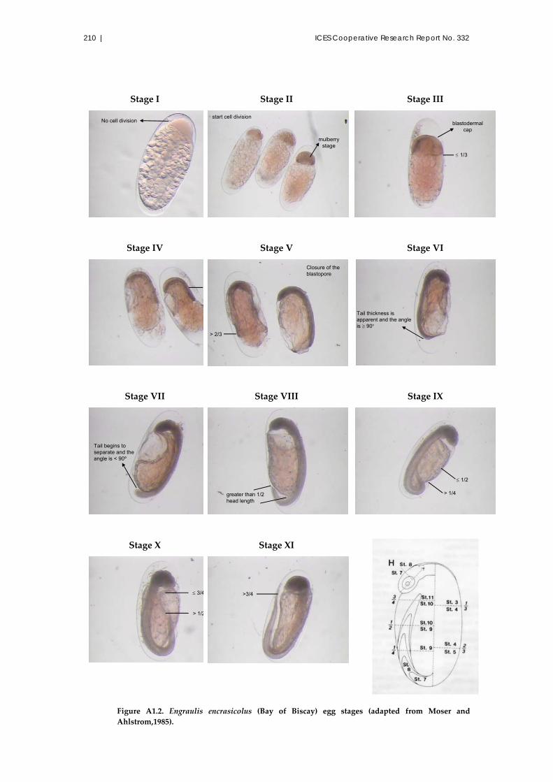
210 | ICES Cooperative Research Report No. 332
Stage I
Stage II
Stage III
Stage IV
Stage V Stage VI
Stage VII
Stage VIII
Stage IX
Stage X
Stage XI
Figure A1.2. Engraulis encrasicolus (Bay of Biscay) egg stages (adapted from Moser and Ahlstrom,1985).
No cell divisionstart cell division
mulberrystage
blastodermalcap
1/3
> 2/3
Closure of theblastopore
Tail thickness isapparent and the angleis 90
Tail begins toseparate and theangle is < 90º
greater than 1/2head length
> 1/4
1/2
> 1/2
3/4 >3/4

Pelagic survey series for sardine and anchovy in ICES subareas 8 and 9 211 |
Table A1.4. Sardine egg staging.
Stage I Eggs are smaller than later stages because of the very small width of
the perivitelline space. The yolk is the same size as the eggs undergoing
development, but cleavage has not yet begun.
Stage II The cleavage begins. After several divisions, the blastodermal cap is
shaped like a berry. This stage persists until the segmentation cavity is
formed.
Stage III Start: The germinal ring with a little pick (formation of the embryonic
shield) can be seen from the top. However, the outline of the embryo is
not clearly defined.
End: The germinal ring begins the development of the yolk with a
cellular sheath until it encloses ⅓ of the yolk mass. The germinal ring
takes on a waist‐like form (≤ ⅓ of the yolk mass).
Stage IV Start: The germinal ring is >⅓ of the yolk mass. The outline of the
embryo can be discerned in the median line of the embryonic shield.
End: The germinal ring encloses ≤ ⅘ of the yolk mass.
Stage V Start: The outline of the embryo is seen around the yolk, covering >⅘ of
the yolk mass. The cephalic region is more apparent than the caudal
one, which is a narrow line, joined to the yolk.
End: The germinal ring completes its evolvement around the yolk until
total closure of the blastopore.
Stage VI Start: The optic vesicles are visible. The myomers are discerned in the
medial region of the embryo, but not in the caudal region or in the
cephalic region.
End: The tail is swollen, but never separates from the yolk. The angle
formed between the tail and the yolk is ≥90. If in doubt, the oil globule is a little behind the tail.
Stage VII Start: The principal characteristic is that the tail begins to separate from
the yolk. The angle formed between the tail and the yolk is < 90. If in doubt, and if the fin‐fold is visible, these characteristics are conclusive.
End: The free portion of the tail is the same length as the head. The tail
reaches the oil globule, but not beyond. If in doubt, for this stage, the
myomeres can only be visible at the beginning of the free portion of the
tail.
From this stage onwards, the free portion of the tail is considered to extend from the body
and not from the fin‐fold. Furthermore, the end of the embryo is considered as the end of
the fin‐fold.

212 | ICES Cooperative Research Report No. 332
Stage VIII Start: The free portion of the tail is bigger than the size of the head, and
at this stage, the tail extends beyond the position of the oil globule.
End: The fin‐fold is becoming very apparent and is half as wide as the
embryo width (≤ ½). ⅓ of the body at the tail end is separated from the
yolk (≤ ⅓). If in doubt, myomeres are visible in the free portion of the
tail until the anus.
Stage IX Start: >⅓ of the body is free. The width of the fin‐folder is >½ the width
of the body. It is wider in the ventral part of the body than in the dorsal
part. The tail is often curved to one side.
End: Generally, the tail is curved to one side of the embryo. The free
tail is ≤ ⅖ of the total body length. The body is straightened and fits less
the shape of the yolk.
Stage X Start: >⅖ of the body is free.
End: The fin‐fold of the free portion of the body does not exceed the
base of the head. From the dorsal view, the tail is very twisted to one
side of the yolk and appears as a U‐shape. The dorsal fin‐fold is as wide
as the body and the ventral is wider.
Stage XI Start: The free portion of the body extends beyond the base of the head.
End: The hatching of the egg. The fin‐fold is wide, 1.5–twofold as wide
as the body. In case there are doubts between two adjacent stages, a
consensus of all the characteristics is taken.
DIS: Damaged eggs, for which it is impossible to identify morphological features, are
assigned to the DIS (disintegrated) category.
No Embryo (NE) stage: Includes stages I–III.
Early Embryo (EE) stage: Includes stages IV–VI.
Late Embryo (LE) stage: Includes stages VII–XI.
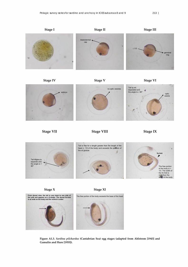
Pelagic survey series for sardine and anchovy in ICES subareas 8 and 9 213 |
Stage I
Stage II
Stage III
Stage IV
Stage V Stage VI
Stage VII
Stage VIII
Stage IX
Stage X
Stage XI
Figure A1.3. Sardina pilchardus (Cantabrian Sea) egg stages (adapted from Ahlstrom [1943] and Gamulin and Hure [1955]).
blastodermalcap
germinalring
1/3
embryo
no optic vesicles
opticvesicls
Tail is notseparated andthe angle is 90º
Tail begins toseparate andthe angle is <90º
Tail is free for a length greater than the length of thehead ( 1/3 of the body) and exceeds the position ofthe oil globule
The free portionof the body is >1/3. The width ofthe fin-fold is>1/2 than thewidth of the body
fin-fold
From dorsal view, the tail is very twist to one side ofthe yolk and appears as a U-shape. The dorsal fin-foldis as wide as the body and the ventral is wider.
The free portion of the body exceeds the base of the head

214 | ICES Cooperative Research Report No. 332
A1.7.3 Adults
The preserved ovaries are weighed in the laboratory (before eventual transfer to
ethanol 70°), and the obtained weights are corrected by a conversion factor (between
fresh and formaldehyde‐fixed material) established previously.
These ovaries are then processed for histology. They are embedded in either resin (IEO,
AZTI) or paraffin (IPMA), the histological sections (3–5 m) are stained with
haematoxylin and eosin, and the slides are examined and scored for their maturity
stage (based on the most advanced batch of oocytes and atresia intensity; Hunter and
Macewicz, 1985; Ganias et al., 2004; Alday et al., 2010), and for POF presence and POF
age assignment to daily cohorts (Hunter and Macewicz, 1985; Pérez et al., 1992a; Ganias
et al., 2007; Alday et al., 2008; Uriarte et al., 2012).
Prior to fecundity estimation, one lobe of each hydrated ovary is processed
histologically in order to check for POF presence and thus avoid underestimating
fecundity (Hunter et al., 1985; Pérez et al., 1992b). The individual batch fecundity is then
measured by means of the gravimetric method applied to the hydrated oocytes on 1–3
whole mounted subsamples per ovary, with an average weight of 50–150 mg (0.1 mg;
Hunter et al., 1985). For sardine, if very few hydrated females are collected during a
given survey or for a given stratum, an additional set of samples can be obtained
following the methodology developed by Ganias et al. (2010), i.e. the gravimetric
method is instead applied to non‐hydrated females (at the oocyte migratory nucleus
stage, MN).
A1.7.4 Analysis
Different geographical strata are considered for the sardine data in the analysis: south
– from Gibraltar to Cabo de S.Vicente (Division 9.a South); west – Santa Vicente to the
northern Portuguese–Spanish border (Division 9.a West); and north – Spanish waters
from Galicia to the French border (divisions 9.a North and 8.b) and the French coast
(Division 8.b). For assessment purposes, the Iberian Peninsula sardine stock databases
for Division 9.a (South and West) and divisions 9.a North–8.c (IPIMAR/IPMA and IEO,
respectively) are merged in a common standardized dataset. Data from Division 8.b is
analysed using the same methodology as for the Iberian Peninsula dataset, but not
merged together with data from divisions 9.a and 8.c.
For the analysis of the anchovy data in the Bay of Biscay and in the Gulf of Cádiz, there
is no a priori stratification of the area covered by the survey, unless the spatial
distribution of the estimates obtained justify it (see Section 2).
A1.7.5 Estimation of total daily egg production
Total daily egg production (Ptot) is calculated as the product of the daily egg production
per area unit (P0) and the spawning area (A):
APPtot 0 (A1.2)
The spawning area is the fraction of the total area surveyed where spawning is
perceived to take place, as revealed by the occurrence of eggs of the target species
(positive stations). The spawning area (A) is delimited by stations with no eggs, but it
may contain some embedded negative stations (no eggs). A continuous single
spawning area can usually be obtained, but occasionally several separate spawning
zones could be defined if several spawning nuclei are clearly distinguishable. The size
of the spawning area is computed as the sum of the areas represented by the stations
within the spawning area. In the case of sardine in the Iberian Peninsula and anchovy

Pelagic survey series for sardine and anchovy in ICES subareas 8 and 9 215 |
in the Gulf of Cádiz, the geographical limits of sampled areas are defined by an
automated routine using neighbourhood distance (in km) between stations (minimum
distance in ratio represented by each station). The area represented by each station
within the survey limits is estimated by a Dirichlet tessellation of the survey stations
(geofun, in the R library). For anchovy in the Bay of Biscay, both the survey limit and
the area represented by each station are calculated with Arcview.
The daily egg production per area unit (P0) is estimated together with the daily
mortality rate (Z) from a general exponential decay mortality model, fitted over the
spawning area, in the formula:
jiji aZPP ,0, exp , (A1.3)
where Pi,j denotes the number of eggs per unit area in cohort j of station i and ai,j denotes
the corresponding mean age and density of eggs in cohort j of station i. Pi,j is computed
as the ratio between the number of eggs Ni,j and the effective sea area sampled Ri (i.e.
Pi,j = Ni,j/Ri). The model was written as a generalized linear model (GLM; McCullagh
and Nelder, 1989; ICES, 2004) with a logarithmic link function:
jiiji aZPRNE ,0, log)log(][log , (A1.4)
where the daily number of eggs in cohort j of station i (Nij) was assumed to follow a
negative binomial distribution. The logarithm of the effective sea surface area sampled
[log(Ri)] is an offset accounting for differences in the sea surface area sampled, while
the logarithm of the daily egg production log(P0) and the daily mortality Z rates are the
parameters to be estimated.
In order to fit the model above, the eggs collected at sea and sorted by morphological
stages have to be transformed into daily cohort frequencies and their mean age
calculated. For that purpose, the Bayesian ageing method described in ICES (2004),
Stratoudakis et al. (2006), and Bernal et al. (2011a) is used. This ageing method is based
on the probability density function (pdf) of the age of an egg f(age|stage, temp), which
is constructed as:
)(),|(),|( ageftempagestageftempstageagef (A1.5)
The first term f(stage|age, temp) is the pdf of stages with given age and temperature. It
represents the temperature‐dependent egg development, which is obtained by fitting
a multinomial model, such as extended continuation ratio models (Agresti, 1990), to
data from temperature‐dependent incubation experiments carried out for these
populations of sardine and anchovy (see Bernal et al., 2001, 2008, 2011a; Ibaibarriaga et
al., 2007b). The second term is the prior distribution of age, a priori the probability of an
egg that was sampled at time τ of having a certain age is the product of the probability
of an egg being spawned at time τ – age and the probability of that egg surviving since
then [exp( –Z age)]:
) exp( )()( ageZagespawnfagef (A1.6)
The probability density function of spawning time f(spawn = τ – age) allows refining the
ageing process for species with spawning synchronicity that spawn at (approximately)
defined times of the day (Lo, 1985; Bernal et al., 2001). Spawning time is assumed to be
normally distributed, with a mean at 21:00 GMT and a standard deviation of 3 h
(spawning period: 15–3 h) for the Iberian Peninsula sardine. For the Gulf of Cádiz
anchovy, peak spawning is assumed to occur at 22:00 GMT, with a standard deviation

216 | ICES Cooperative Research Report No. 332
of 2 h. For the Bay of Biscay anchovy, the pdf function representing spawning has a
mean at 23:00 GMT and a standard deviation of 1.25 h (ICES, 2004). Peak spawning
time is also used to define the age limits for each daily cohort (peak spawning time
±12 h). Details on how the number of eggs in each cohort and the corresponding mean
age are computed from the PDF of age are given in Bernal et al. (2011a). The incubation
temperature considered is obtained from CTD profiling; the strata used for mean
temperature calculation may vary according to surveys and oceanographic conditions.
Given that this ageing process depends on the daily mortality rate, which is initially
unknown, an iterative algorithm (ICES, 2004; Stratoudakis et al., 2006; Bernal et al.,
2011a; R MASS Library) is used in which the ageing and the model fitting are repeated
until convergence of the Z estimates. The procedure is as follows:
Step 1. Assume an initial mortality rate value.
Step 2. Using the current estimates of mortality, calculate the daily cohort
frequencies and their mean age.
Step 3. Fit the GLM and estimate the daily egg production and mortality rates.
Update the mortality rate estimate.
Step 4. Repeat steps 1–3 until the estimate of mortality converge (i.e. the
difference between the old and updated mortality estimates is smaller than
0.0001).
Incomplete cohorts, either because the bulk of the day’s spawning was not complete at
the time of sampling, or because the cohort was so old that its constituent eggs had
started to hatch in substantial numbers, are removed in order to avoid possible bias
(the level of cutting is defined by the user).
Once the final model estimates are obtained, the coefficient of variation of P0 is
calculated from the standard error of the model intercept [log(P0)] (Seber, 1982), and
the coefficient of variation of Z is obtained directly from the model estimates.
The analysis is conducted in R (www.r‐project.org), using packages and routines
available free at ichthyoanalysis (http://sourceforge.net/projects/ichthyoanalysis).
Table A1.3 summarizes the methodology adopted for the sardine and anchovy egg
data.
A1.7.6 Estimation of adult parameters
The adult parameters estimated for each fishing haul consider only the mature fraction
of the population (determined by the fish macroscopic maturity data). Estimation of
the sex ratio, the mean female weight, and the mean female expected batch fecundity
is based on the biological data collected from both survey and commercial samples,
whereas the preserved gonads are used to measure individual batch fecundity, assess
the mature/immature condition of females, and estimate the daily spawning fraction.
Before the estimation of the mean female weight per haul (W), the individual total
weight of the hydrated females is corrected by a linear regression between the total
weight of non‐hydrated females and their corresponding gonad‐free weight (Wnov).
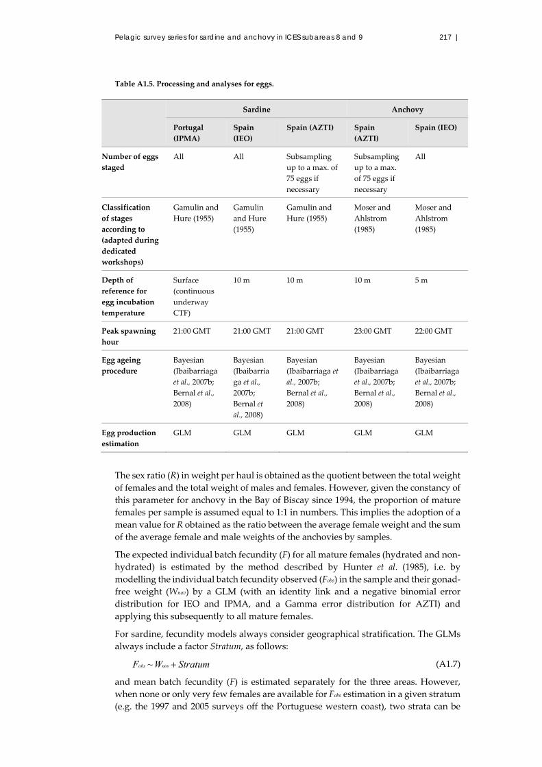
Pelagic survey series for sardine and anchovy in ICES subareas 8 and 9 217 |
Table A1.5. Processing and analyses for eggs.
Sardine Anchovy
Portugal
(IPMA)
Spain
(IEO)
Spain (AZTI) Spain
(AZTI)
Spain (IEO)
Number of eggs
staged
All All Subsampling
up to a max. of
75 eggs if
necessary
Subsampling
up to a max.
of 75 eggs if
necessary
All
Classification
of stages
according to
(adapted during
dedicated
workshops)
Gamulin and
Hure (1955)
Gamulin
and Hure
(1955)
Gamulin and
Hure (1955)
Moser and
Ahlstrom
(1985)
Moser and
Ahlstrom
(1985)
Depth of
reference for
egg incubation
temperature
Surface
(continuous
underway
CTF)
10 m 10 m 10 m 5 m
Peak spawning
hour
21:00 GMT 21:00 GMT 21:00 GMT 23:00 GMT 22:00 GMT
Egg ageing
procedure
Bayesian
(Ibaibarriaga
et al., 2007b;
Bernal et al.,
2008)
Bayesian
(Ibaibarria
ga et al.,
2007b;
Bernal et
al., 2008)
Bayesian
(Ibaibarriaga et
al., 2007b;
Bernal et al.,
2008)
Bayesian
(Ibaibarriaga
et al., 2007b;
Bernal et al.,
2008)
Bayesian
(Ibaibarriaga
et al., 2007b;
Bernal et al.,
2008)
Egg production
estimation
GLM GLM GLM GLM GLM
The sex ratio (R) in weight per haul is obtained as the quotient between the total weight
of females and the total weight of males and females. However, given the constancy of
this parameter for anchovy in the Bay of Biscay since 1994, the proportion of mature
females per sample is assumed equal to 1:1 in numbers. This implies the adoption of a
mean value for R obtained as the ratio between the average female weight and the sum
of the average female and male weights of the anchovies by samples.
The expected individual batch fecundity (F) for all mature females (hydrated and non‐
hydrated) is estimated by the method described by Hunter et al. (1985), i.e. by
modelling the individual batch fecundity observed (Fobs) in the sample and their gonad‐
free weight (Wnov) by a GLM (with an identity link and a negative binomial error
distribution for IEO and IPMA, and a Gamma error distribution for AZTI) and
applying this subsequently to all mature females.
For sardine, fecundity models always consider geographical stratification. The GLMs
always include a factor Stratum, as follows:
StratumWF novobs ~ (A1.7)
and mean batch fecundity (F) is estimated separately for the three areas. However,
when none or only very few females are available for Fobs estimation in a given stratum
(e.g. the 1997 and 2005 surveys off the Portuguese western coast), two strata can be

218 |
ICES Cooperative Research Report No. 332
considered together in the model (e.g. West and South pooled), although F estimates
are still calculated separately for each stratum. Several model options are tested for
each year/survey (same or different intercepts and/or slopes, intercepts through the
origin or not). The model considered as the most adequate is selected, taking into
account both statistical (residual plots, lower AIC value, graphical representation of
the regression curve) and biological significance (models with significant positive
intercepts not accepted).
For anchovy in the Bay of Biscay, an analysis is conducted to verify if there are
differences in batch fecundity between different strata. Similarly, for anchovy in the
Gulf of Cádiz, post‐stratification is undertaken when F estimates obtained are
statistically different (see Section 2).
For sardine (as for anchovy in the past), the spawning fraction (S), the fraction of
females spawning per day, is determined for each haul as the average number of
females with day 1 or day 2 post‐ovulatory follicles (POFs) divided by the total number
of mature females. Hydrated females are not included due to possible over‐sampling
of active spawning females close to peak spawning time (Santiago and Sanz, 1992b;
Bernal, 2007). In this case, the number of females with day 0 POF (of the mature
females) is corrected by the average number of females with day 1 or day 2 POF
(Picquelle and Stauffer, 1985; Pérez et al., 1992a; Motos, 1994; Ganias et al., 2007). For
sardine, POFs are assigned to daily cohorts using both histomorphological and
metrical (POF cross‐sectional area) criteria (Pérez et al., 1992a; Ganias et al., 2007).
If no S estimation is possible for sardine or estimates are considered unrealistic, taking
into account the dataseries and the other parameters (particular situation), a non‐
parametric bootstrap approach is performed using mean spawning fraction by each
haul obtained during the series and considering a single haul as the basic sampling
unit. Hauls are resampled, with replacement from the original dataset, leading to a
new, artificial sample that is then used to estimate the spawning fraction. By repeating
this procedure an adequate number of times (1000 in this application), an empirical
probability distribution is obtained for the S parameter.
For anchovy in the Bay of Biscay, spawning frequency estimates are obtained by
applying the new classification for oocyte and POF stages by Alday et al. (2008) and
the procedures described in Uriarte et al. (2012).
The degeneration of POFs over time at different temperatures was studied for the Bay
of Biscay anchovy by Alday et al. (2008) based on captivity experiments and field
samples. For this purpose, a key of seven POF stages, solely defined on the basis of
their histological degeneration characteristics, was applied (Alday et al., 2008, 2010).
The novelty of this procedure is that it separates staging of POFs from their ageing
process. There was close agreement in the succession of POF stages after spawning
between the experiment and the field samples, and, for the range of temperatures
examined (13–19°C), little effect of temperature on the degeneration of POF was
noticed.
The procedure to assign mature females to spawning classes is then improved by
incorporating all the knowledge on oocyte maturation and degeneration of POFs in a
matrix system which defines the probabilities of females with those histological
indicators belonging to pre‐ or post‐spawning cohort according to the time of capture
(Uriarte et al., 2012). The selected estimator for anchovy is the mean of S for day 0 and
S for day 1.
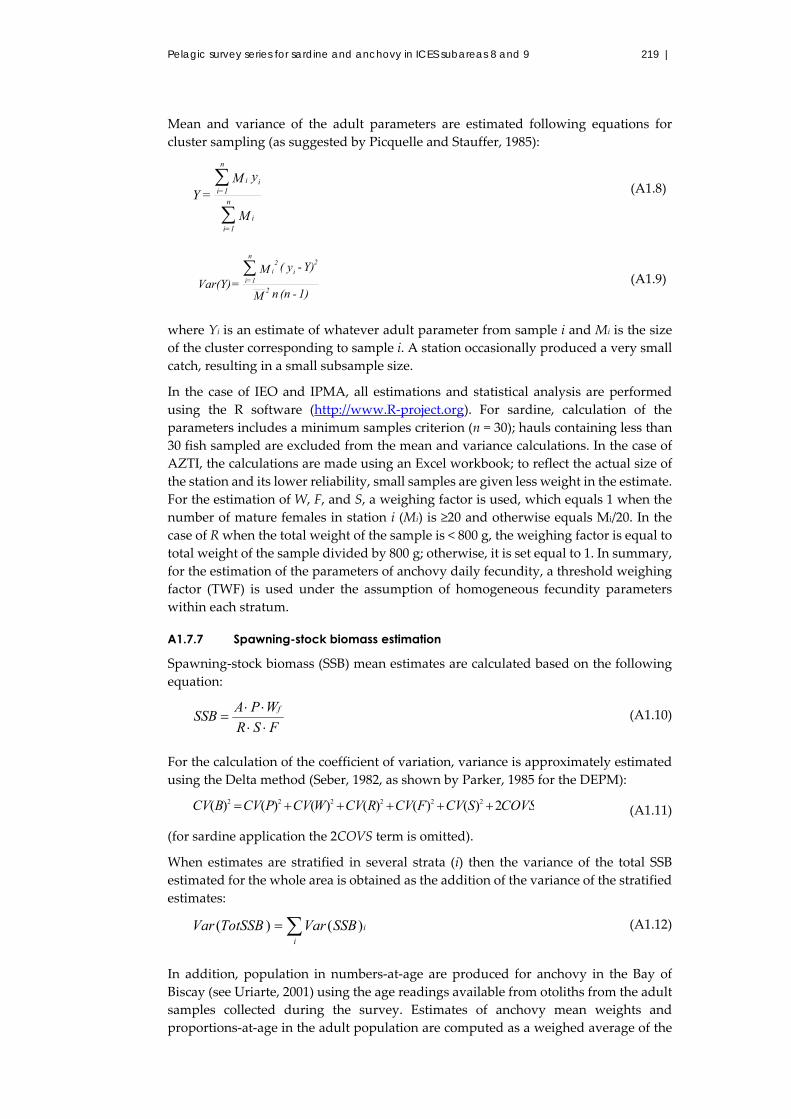
Pelagic survey series for sardine and anchovy in ICES subareas 8 and 9 219 |
Mean and variance of the adult parameters are estimated following equations for
cluster sampling (as suggested by Picquelle and Stauffer, 1985):
M
y M
= Y
i
n
1=i
ii
n
1=i
(A1.8)
1) - (n n M
Y) - y( M
= Var(Y)2
i
2i2
n
1=i
(A1.9)
where Yi is an estimate of whatever adult parameter from sample i and Mi is the size
of the cluster corresponding to sample i. A station occasionally produced a very small
catch, resulting in a small subsample size.
In the case of IEO and IPMA, all estimations and statistical analysis are performed
using the R software (http://www.R‐project.org). For sardine, calculation of the
parameters includes a minimum samples criterion (n = 30); hauls containing less than
30 fish sampled are excluded from the mean and variance calculations. In the case of
AZTI, the calculations are made using an Excel workbook; to reflect the actual size of
the station and its lower reliability, small samples are given less weight in the estimate.
For the estimation of W, F, and S, a weighing factor is used, which equals 1 when the
number of mature females in station i (Mi) is ≥20 and otherwise equals Mi/20. In the
case of R when the total weight of the sample is < 800 g, the weighing factor is equal to
total weight of the sample divided by 800 g; otherwise, it is set equal to 1. In summary,
for the estimation of the parameters of anchovy daily fecundity, a threshold weighing
factor (TWF) is used under the assumption of homogeneous fecundity parameters
within each stratum.
A1.7.7 Spawning-stock biomass estimation
Spawning‐stock biomass (SSB) mean estimates are calculated based on the following
equation:
FSR
WPASSB
f
(A1.10)
For the calculation of the coefficient of variation, variance is approximately estimated
using the Delta method (Seber, 1982, as shown by Parker, 1985 for the DEPM):
COVSSCVFCVRCVWCVPCVBCV 2)()()()()()( 222222 (A1.11)
(for sardine application the 2COVS term is omitted).
When estimates are stratified in several strata (i) then the variance of the total SSB
estimated for the whole area is obtained as the addition of the variance of the stratified
estimates:
i
iSSBVarTotSSBVar )()( (A1.12)
In addition, population in numbers‐at‐age are produced for anchovy in the Bay of
Biscay (see Uriarte, 2001) using the age readings available from otoliths from the adult
samples collected during the survey. Estimates of anchovy mean weights and
proportions‐at‐age in the adult population are computed as a weighed average of the

220 |
ICES Cooperative Research Report No. 332
mean weight and age composition per samples, where the weighing factors are
proportional to the population (in numbers) in different substrata. These weighing
factors are calculated according to the relative egg abundance and the amount of
samples in the substrata defined with the purpose of estimating the numbers‐at‐age.
These strata are defined each year depending on the distribution of the adult samples,
i.e. size, weight, age, and the distribution of the anchovy eggs.
The mean and variance of the adult parameters for the population in numbers‐at‐age
and the population length distribution (total weight, proportion by ages, and length
distribution) are estimated following equations for cluster sampling from Picquelle
and Stauffer (1985) (see Section 2).
Table A1.4 summarizes the methodology used in the processing and data analyses of
sardine and anchovy adult samples.
Table A1.4. Processing and analyses for adults.
DEPM
Sardine Anchovy
Portugal (IPMA) Spain (IEO &
AZTI)
Spain (AZTI) Spain (IEO)
Histology:
Embedding
material
and
staining
Paraffin
Haematoxilin
Eosin
Resin
Haematoxilin
Eosin
Resin
Haematoxilin
Eosin
Resin
Haematoxilin
Eosin
Analyses:
W
estimation
Weight of
hydrated females
corrected
previous to
estimation
Weight of
hydrated
females
corrected
previous to
estimation
Weight of
hydrated
females
corrected
previous to
estimation
Weight of
hydrated
females
corrected
previous to
estimation
R
estimation
The observed
weight fraction
of the females
The observed
weight fraction
of the females
Theoretical
expected values
assumed to be
equal to 1:1 in
numbers
checked with
observed
The observed
weight fraction
of the females
S
estimation
Day 1 and day 2
POFs (according
to Pérez et al.,
1992a and
Ganias et al.,
2007)
Day 1 and day 2
POFs (according
to Pérez et al.,
1992a and
Ganias et al.,
2007)
The mean
incidence of day
0 and day 1
spawners
(Uriarte et al.,
2012)
Day 1 and day
2 POFs
F estimation
On hydrated
females (without
POFs), according
to Pérez et al.
(1992b) and
Ganias et al.
(2010)
On hydrated
females
(without POFs),
according to
Pérez et al.
(1992b)
On hydrated
females (without
POFs), according
to Hunter et al.
(1985)
On hydrated
females
(without POFs),
according to
Hunter et al.
(1985)

Pelagic survey series for sardine and anchovy in ICES subareas 8 and 9 221 |
Annex 2: Acoustic survey protocols and data processing
A2.1 Introduction
After more than 30 years of acoustic surveys carried out in southeastern European
waters, and more than 20 years of meetings and working groups, the institutes
involved in this endeavour have achieved considerable progress in survey strategy and
methodology in order to standardize, to the extent possible, their actions and to ensure
data compatibility. Nevertheless, several types of pecularities have made it impossible
to establish a formal single protocol for surveying that would be applicable to all areas,
seasons, and institutes. This can be attributed to the following:
different geographic characteristics – the continental shelf is very narrow along
the Spanish coast, variable along the Portuguese coast and in the Cádiz area,
and very large in the French waters of the Bay of Biscay;
research vessels from the institutes have different size, performance (e.g.
speed, scattered rays, noise level, fishing possibility), and implementation of
systems;
different fish behaviour and distribution (schooling characteristics, avoidance,
distribution relative to the coast, to the surface, in rias, etc.);
distinct relative occurrence of species, mixing of populations, biological stages,
etc.
Because of these pecularities, it has been generally accepted that each team did its best
to collect clean and compatible data, despite the possible constraints, and always
keeping in mind the strict application of the basic principle of following a common
work plan and general requirements.
A2.1.1 Acoustic surveying
Each survey must be carried out following the same transects year after year
and according to a network of preferable parallel transects.
Vessel speed must be as constant as possible and up to 10 knots.
Acoustic surveying for adult fish must be done only during the day to avoid
missing echoes at night when fish are close to the surface and scattered in
plankton layers.
A2.1.2 Identification fishing hauls
Fishing hauls must be made each time notable echotraces are observed,
whatever the echotraces look like, and as soon as possible after observation.
This is to avoid over‐ or undersampling of particular species, considering that
first, we are never sure of intuitive identification (possible change in behaviour
by season or year) and secondly, because surveys must address all pelagic
species, not just the targeted species.
A2.1.3 Echotyping
Echoes must be sorted by echotypes, taking into account their location, shape,
and density, according to expert knowledge, identification hauls made nearby,
and/or similarity with known echotraces.
A2.1.4 Target strength (TS)
No agreement was obtained, and each institute applies its usual TS
relationships to save the validity of relative index series. Nevertheless, each

222 |
ICES Cooperative Research Report No. 332
institute operates particular experiments in order to solve this problem. Recent
experiments proved that variations could be important relative to the depth of
individuals, their biological conditions, and different behavioural events.
A2.1.5 Biomass calculation
Biomass calculations are done with standard methods using different
software.
Protocols for each acoustic survey series are described in the following sections.

Pelagic survey series for sardine and anchovy in ICES subareas 8 and 9 223 |
A2.2 PELGAS survey protocols (IFREMER – France)
A2.2.1 Sampling strategy
A2.2.1.1 Survey design
Acoustic data are collected along systematic parallel transects perpendicular to the
French coast (Figure A2.1), from the north coast of France to Spain, over a total distance
of ca. 6500 nautical miles (1 nautical mile = 1852 m). Transects are uniformly spaced
every 12 nautical miles (22 km). The mean size of clusters of pelagic fish schools in the
Bay of Biscay has been estimated to be 8 km (Petitgas, 2003). The intertransect distance
results from a compromise between ship time and cluster mean size.
Figure A2.1. Bay of Biscay map and PELGAS survey design. Blue lines: acoustic transects; red dots:
trawl haul locations; colored areas: post‐stratification regions.
The survey design allows for the coverage of the entire Biscay continental shelf (ca.
23 000 nautical miles²) from a depth of 25 m to the shelf break (200 m). The nominal
sailing speed is 10 knots (1 knot = 1852 m s–1), the speed being reduced to an average
of 2 knots during fishing operations. This speed permits sampling of the entire Biscay
shelf in ca. 30 d.
A2.2.1.2 Hydrobiological environment sampling
During daylight, the hydrobiology team operates a continuous underway fish egg
sampler (CUFES) fitted with a 315‐μm mesh size collector. A CUFES sample is
collected every 3 nautical miles along survey transects during acoustic sampling.

224 |
ICES Cooperative Research Report No. 332
During night‐time, 3–4 hydrobiological stations are performed on alternate transects.
Hydrostations are ideally performed on a transect that was surveyed during the
previous daylight period to synoptically characterize the bio‐physical environment of
the fish and to allow for the adjustment of station locations, according to the hull‐
mounted thermo‐salinometer measurements, as well as to egg counts.
Supplementary hydrostations are generally performed in an adaptative manner
during the last week of the PELGAS cruise close to the Gironde estuary. The PELGAS
hydrobiological environment sampling scheme is summarized in Figure A2.2.
Figure A2.2. PELGAS hydrobiological environment sampling scheme. Blue lines: daylight CUFES
transects; crosses: night‐time CTD station locations; colored area: higher frequency sampling area.
A2.2.1.3 Acoustic sampling
The pulse length is set to 1.024 ms for all frequencies and echosounders. In situ on‐axis
calibration of the echosounders is performed before each cruise using standard
methodology (Foote, 1987; Trenkel et al., 2008).
Acoustic data are acquired with the Movies+ (Weill et al., 1993) and Hermes software
and archived in the international hydroacoustic data format (HAC; ICES, 2005b) at a
100 dB threshold.
A2.2.1.4 Species identification by trawling
The identification of species and size classes comprising fish echotraces (ICES, 2000b)
depends heavily on identification via trawl hauls performed by RV “Thalassa” using a
2‐door, 57‐m headline, and 52‐m footrope pelagic trawl. Echograms are scrutinized in
real‐time, and trawl hauls are performed as often as possible. The rationale for
performing an identification haul includes:
observation of numerous fish echotraces over several elementary sampling
distance units (ESDUs) or of very dense fish echotraces in one ESDU;

Pelagic survey series for sardine and anchovy in ICES subareas 8 and 9 225 |
changes in echotrace characteristics (morphology, density, or position in the
water column);
observation of an echotrace type fished on previous transects, but never fished
on the current transect.
Acoustic transects are adaptively interrupted to perform the trawl hauls and then
subsequently resumed. During PELGAS, the trawl stations are conditioned on the
positions of particular acoustic images that are considered to be representative of
communities of echotraces during the survey (Petitgas, 2003).
Trawl catches do not allow for the identification of single schools, but rather to an
ensemble of schools over several nautical miles, resulting in identifying groups of
schools to species assemblages.
At least one commercial pair trawler has accompanied the RV “Thalassa” during the
PELGAS cruise since 2007 to increase the effort devoted to echotrace identification.
A2.2.1.5 Marine mammals and birds sampling
Marine mammals, birds, macrolitter, and ship activity are spotted during daylight
during PELGAS transects. Detailed protocols can be found in the dedicated annex in
this volume.
A2.2.2 Hydrobiological data collection
A2.2.2.1 Workspace and equipment
Located on deck C of the research vessel, the hydrobiology workspace comprises three
laboratories:
Hydrobiology lab: sample handling, filtrations, and binocular observations.
Control room: one computer connected to the conductivity–temperature–
depth probe (CTD) and to the vessel GPS (NMEA through local network since
2012) for real‐time monitoring of CTD profiles, one computer for laser optical
plankton counter (LOPC) data upload, and one computer to define net closing
depths and retrieve MultiNet data.
Chemistry lab: density column experiments.
The hydrobiological equipment routinely used during PELGAS surveys includes:
three computers to operate the CTD, the MultiNet, and the LOPC;
two binoculars;
a filtering system;
pillboxes, formalin for CUFES and MultiNet sample preservation, 90° alcohol
for larvae and otolith preservation;
a CUFES;
a CTD probe fitted with conductivity–temperature–depth, fluorimeter, and
turbidimeter sensors, a LOPC (with datalogger), and nine Niskin bottles;
three WP2 nets (200‐ and 50‐µ mesh);
a 315‐µ mesh “filet Carré” (Bourriau, 1991) for egg and larvae sampling;
a 500‐µ mesh MultiNet (Hydrobios) fitted with five nets for mesozooplankton
sampling.

226 |
ICES Cooperative Research Report No. 332
A2.2.2.2 Staff
The hydrobiology team consists of 6–7 people working 24 h, with 8‐h shifts (two people
per shift).
Although the geographic positions of the night‐time hydrostations are predefined, the
responsible hydrobiology lab person may have to adapt them according to
hydrological conditions. This person needs to have a strong background in ichthyology
as well as in biological and physical oceanography to adapt to the station positions.
The other hydrobiology team members need the following specific skills:
anchovy and sardine egg and larvae taxonomic identification;
Niskin bottle content filtering to extract phytoplankton, zooplankton, and
suspended matter;
sample preservation (nutrients, phytoplankton, zooplankton, and
ichthyoplankton).
A2.2.2.3 Protocols
Daylight operations. During daylight, the hydrobiology team operates the
CUFES, fitted with a 315‐μ mesh size collector. A CUFES sample is collected
every 3 nautical miles along survey transects during acoustic sampling.
Sardine and anchovy eggs are sorted, counted, and preserved with 4%
formalin. Night‐time operations. The CTD profiles are first performed from the surface
to 1–2 m above the seabed at 2 m s–1. Groups of three bottles are subsequently
fired near the seabed, well below the pycnocline, in the chlorophyl maximum
(generally near the pycnocline), and at the surface.
A vertical WP2 net tow is then performed at each station. The WP2 is shot to a
maximum depth of 100 m, or at 5 m above the seabed if the depth is < 100 m. The first
WP2 sample is preserved as a CUFES sample for further mesozooplankton taxonomic
analysis. The second WP2 sample is filtered into four size classes (2000, 1000, 500, and
200 μ) and dried for dry biomass analysis. The third WP2 sample is devoted to other
analyses, depending on the year.
In cases of special hydrographic or meteorological features, or if eggs and/or larvae are
present in the CUFES samples, supplementary Filet carré and/or MultiNet tows are
adaptively performed.
The Filet carré is shot to a maximum depth of 100 m, or at 5 m above the seabed if the
depth is < 100 m. The net is then towed at 1.5–2 knots for 10 min (for eggs) to 15 min
(for larvae), following an oblique tow profile, from the maximum depth to the surface.
The eggs are transferred into the density column to measure their density and calibrate
an egg vertical distribution model (Petitgas et al., 2006).
The MultiNet is shot to a maximum depth of 100 m, or at 5 m above the seabed if the
depth is < 100 m. The MultiNet is then towed at 1.5–2 knots for 15 minutes, following
an oblique tow profile, from the maximum depth to the surface. The five nets are
automatically closed, using the OceanLab software, when reaching the minimum
depth limits that were scheduled.
Data preprocessing and storage. The raw CTD data are smoothed, outliers are
removed, and preprocessed data are stored in Ocean Data View format (one
file per year).
Plankton net tow metadata are recorded in a spreadsheet.

Pelagic survey series for sardine and anchovy in ICES subareas 8 and 9 227 |
A2.2.3 Pelagic trawling
A2.2.3.1 Basic equipment
Located on deck B, the sorting room (130 m2) is, by default, equipped with:
a trunk where the catch is stored;
an automated sorting system fitted with a conveyor belt and a balance, which
allows weighing and delivering the fish to the fish sorters, recording the catch
composition (PUPITRI software interfaced with the balance), and cleaning the
plastic boxes where the sorted fish were stored;
three tables to process fish subsamples (length measurements, stomach
extraction, etc.);
two balances (50 kg and 5 kg maximum weights);
a biology laboratory equipped with a computer fitted with RAPTRI software
to record catch data, a printer, and a small freezer.
A2.2.3.2 Staff
The person in charge of the sorting room (or deckmaster) is an experienced technician
with good knowledge of the following:
PELGAS survey protocol;
sorting room functioning;
PUPITRI and RAPTRI software;
pelagic species taxonomy.
In addition to this person, the fish sorter team consists of 4–5 extra people, including
preferably at least one technician with good experience in small pelagic fish otolith
extraction and catch data checking.
In cases of large catches of mixed species, scientists from other teams are called to assist
in sorting the fish.
A2.2.3.3 Setting up the sorting room
Additional equipment installed at the beginning of the PELGAS includes:
binoculars;
fume cupboard;
poster with catch processing protocols affixed to the wall (including maturity
scales);
an additional light;
5‐kg balance weight;
dissection and otolith extraction tools;
taxonomic reference books.
At the beginning of the cruise, the “RAPTRI” software and biological files are
initialized. The species list is checked, as well as the availibility of all fish processing
protocols (genetic, stomacal content, energy).
A2.2.3.4 Protocols
The actions performed in the sorting room are summarized below.
Catch visual inspection, rescue of live robust species. The deckmaster
evaluates the volume and degree of mixing of the catch and eventually asks
for extra manpower.

228 |
ICES Cooperative Research Report No. 332
A check is made for live ʺrobust” species (sunfish, marine mammals, pelagic sharks)
that might survive if returned to the sea. If any such species are present, they are
quickly identified, measured, weighed, photographed, and returned to the sea.
Choice of sampling scheme and conveyor start‐up. The deckmaster
determines the sampling scheme, based on the catch amount and
composition. Decision is made on (i) whether to sort the entire catch or only
a subset, (ii) whether to use 40‐kg subsamples or less if fish are very small,
and (iii) which are the main and secondary species in the catch.
The deckmaster starts the PUPITRI software operating the conveyor.
Split, weigh, and deliver the catch. The deckmaster operates the conveyor
system. The catch is automatically split into subsamples which are weighed.
Each subsample is then either sent to the sorting belt or thrown overboard.
Catch sorting. (a) Presorting of large species. To precisely assess the
contribution of large species (mackerel, hake, etc.) to the catch, the
deckmaster, aided by a fish sorter if necessary, visually detects and sorts out
large fish before they pass through the PUPITRI system. (b) Catch sorting on
conveyor belts. A minimum of four people sort the catch around the conveyor
belts. Fish of the main species are left on the conveyor, whereas secondary
species are sorted into plastic boxes. If some species display a clear bimodal
length distribution, they are sorted by size category to improve the precision
of length distributions.
The deckmaster operates the PUPITRI workstation which records the amount of catch
sorted and/or discarded.
If the sorting process is long, a second line of belts is opened.
Macroscopic litter and severely damaged fish are sorted into the same box.
Sorted catch data input. The fish sorters around the conveyor belts send the
boxes containing sorted species onto the weighing belt.
The deckmaster inputs the following in the PUPITRI software: (i) the scientific name
of the species in each box passing on the weighing belt, and (ii) the type of box to enable
removing the box weight from the subsample weight. The actual species weight is
automatically recorded by PUPITRI.
Boxes with sorted species are then sent to the biological measurements area.
Biological measurements on subsamples. The following biological measure‐
ments are conducted by 2–3 fish sorters on each species (and eventually size
class). One or two fish sorters perform the measurements, while another
records the size or weight distributions on a sheet of paper.
If the catch of one species is too abundant, measurements are conducted on a
subsample. Either way, all fish are measured.
About 100 fish are usually measured to assess the length distributions of species with
short size distribution ranges (Capros aper and Sprattus sprattus), and ca. 150–200 fish
for other species.
(a) Size measurements. Size data are recorded in a table with one row per size class on a
measurement sheet. Fish lengths are rounded to the nearest lower 0.5 cm for clupeids,
or to the nearest lower centimeter for all other species.

Pelagic survey series for sardine and anchovy in ICES subareas 8 and 9 229 |
Each time a fish length is recorded, a tick is drawn in the table row corresponding to
its size class on the measurement sheet. This permits real‐time visual control of the
length distribution aspect.
Fish are sized until sample exhaustion or until the fish sorter decides that a robust
length distribution appears graphically on the sheet.
(b) Mean weight measurements. The total weight of subsamples used for defining size
distributions is measured and used to derive a global mean weight for the subsample.
Length–weight keys. Based on the level of completion of the fish sampling
scheme, the deckmaster determines when a length–weight key must be
defined for Engraulis encrasicolus, Sardina pilchardus, Scomber scombrus,
Scomber colias, Trachurus trachurus, Capros aper, and Sprattus sprattus.
A total of 1–3 length–weight equations are derived at each trawl station. Anchovy and
sardine length–weight equations are derived each time the catch is sufficient. Length–
weight equations of other species are adaptatively derived, time permitting, to ensure
good spatial coverage.
To define a length–weight key, individual fish used to derive the length distribution
are split by size class into small boxes. The box weight and the number of fish in each
box are recorded on a sheet.
Biometric measurements and otolith extraction. (a) Fish selection. Based on
the level of completion of the fish sampling scheme, the deckmaster
determines when specific biometrics and otolith extraction are to be
conducted for anchovy and sardine only.
For biometric and otolith reading purposes, a total of ca. 40 (sardine) or 50 (anchovy)
individuals are selected over the length classes of the subsample used to derive the
length distribution and stored in small boxes in the laboratory.
(b) Biometric measurements. The following individual biological data are
written on biometric cards by two fish sorters (one trained reader and one
possibly novice writer) for each individual in every sardine and anchovy
subsample: (i) weight (in g), (ii) sex (male/female/undetermined), and (iii)
maturity stage.
The following extra data are recorded for sardine: (i) level of fatness, and (ii) level of
infestation by Anisakis spp. parasite.
(c) Otolith extraction. Different types of trays, each containing 10 pairs of
otoliths, are used for anchovy and sardine.
A trained fish sorter extracts pairs of otoliths from fish whose biometrical parameters
have been previously recorded. Otoliths are cleaned with a wet sponge and dried for
24 h on a tray. Pictures are taken of the completed trays.
After 24 h of drying, the otoliths are placed on the right side, with the concave face
looking downwards, and the point to the top of the tray. Eukitt resin is put into each
of the tray holes with a plastic pipette in a fume cupboard. The resin dries for 1–2 d.
Otolith seasonal growth rings are read using a binocular by a technician certified for
anchovy and sardine otolith reading.

230 |
ICES Cooperative Research Report No. 332
Age of the fish is determined based on the number of growth rings and is expressed in
years, assuming that the birthday is 1 January. The age and nature of the otolith edge
are added to the fish biometric card and input to a standard spreadsheet.
On average, a total of 1200 anchovy and 1400 sardine otoliths are collected during a
cruise.
Anchovy otolith readings are a posteriori double‐checked by another certified
technician, who also measures the growth ring patterns.
Subsamples and biometry data input. The deckmaster and a fish sorter input
subsamples and biometric data to the RAPTRI database and a spreadsheet,
respectively.
Catch data check. Subsamples and biometric data input are checked against
the original values on paper sheets by two fish sorters familiar with the
RAPTRI software. Eventual input errors are corrected in the databases.
A2.2.4 Pelagic fish biomass assessment by acoustic method
Biscay fish population biomass is assessed during a PELGAS cruise using
“expert”methodology to combine acoustic and fishing data.
A2.2.4.1 Acoustic data preprocessing
Only 38‐kHz backscatters are used for biomass assessment. However, echograms
recorded at the 120‐kHz frequency are also scrutinized to assist in isolating fish
echotraces from sound scattering layers (SSLs).
Pelagic fish are frequently scattered close to the sea surface and within the surface
acoustic blind zone (0–10 m depth) at night. SSLs are also denser during night‐time
than during daylight, making fish echotrace partitioning less reliable. Only daylight
acoustic data are then used for stock assessment purposes.
At first echograms are corrected manually for bottom detection errors. Daylight 38‐
kHz volume backscattering coefficients (Sv) higher than –60 dB (Petitgas et al., 1998)
and recorded from depths of 10–150 m along acoustic transects are then echo
integrated in each beam over a standard depth channel of 10‐m thickness and averaged
over 1 nautical mile ESDUs. The resulting values of nautical area backscattering
coefficients (NASC) are used in subsequent analysis.
A2.2.4.2 Classification of echo integrals
The rectified echogram is then used by experts to allocate the echo integrals (SA)
thought to correspond to fish targets for several echotrace categories in each ESDU,
based on echotrace shape, density, and position. Echotrace categories correspond to
species or group of species found in midwater identification trawls. At least four
categories are generally considered during a survey:
D1: diffuse shoals or layers close to the seabed or small “drops” extending up
to 10 m above the seabed – allocated to horse mackerel and gadoids;
D2: schools displaying sharp edges and often high density, generally
distributed up to 50 m above the seabed in coastal areas and sometimes
offshore – allocated to anchovy, sprat, sardine, and mackerel;
D3: diffuse echotraces often observed offshore all along the shelf break –
allocated to a mixture of blue whiting and myctophids;
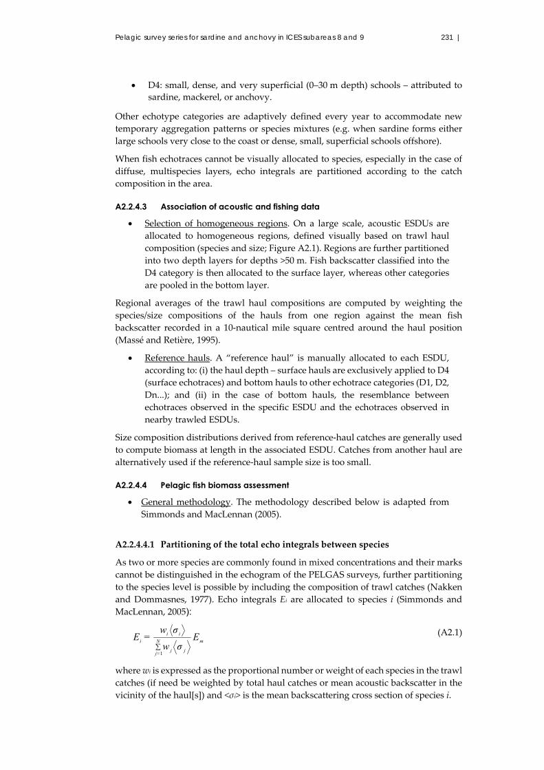
Pelagic survey series for sardine and anchovy in ICES subareas 8 and 9 231 |
D4: small, dense, and very superficial (0–30 m depth) schools – attributed to
sardine, mackerel, or anchovy.
Other echotype categories are adaptively defined every year to accommodate new
temporary aggregation patterns or species mixtures (e.g. when sardine forms either
large schools very close to the coast or dense, small, superficial schools offshore).
When fish echotraces cannot be visually allocated to species, especially in the case of
diffuse, multispecies layers, echo integrals are partitioned according to the catch
composition in the area.
A2.2.4.3 Association of acoustic and fishing data
Selection of homogeneous regions. On a large scale, acoustic ESDUs are
allocated to homogeneous regions, defined visually based on trawl haul
composition (species and size; Figure A2.1). Regions are further partitioned
into two depth layers for depths >50 m. Fish backscatter classified into the
D4 category is then allocated to the surface layer, whereas other categories
are pooled in the bottom layer.
Regional averages of the trawl haul compositions are computed by weighting the
species/size compositions of the hauls from one region against the mean fish
backscatter recorded in a 10‐nautical mile square centred around the haul position
(Massé and Retière, 1995).
Reference hauls. A “reference haul” is manually allocated to each ESDU,
according to: (i) the haul depth – surface hauls are exclusively applied to D4
(surface echotraces) and bottom hauls to other echotrace categories (D1, D2,
Dn...); and (ii) in the case of bottom hauls, the resemblance between
echotraces observed in the specific ESDU and the echotraces observed in
nearby trawled ESDUs.
Size composition distributions derived from reference‐haul catches are generally used
to compute biomass at length in the associated ESDU. Catches from another haul are
alternatively used if the reference‐haul sample size is too small.
A2.2.4.4 Pelagic fish biomass assessment
General methodology. The methodology described below is adapted from
Simmonds and MacLennan (2005).
A2.2.4.4.1 Partitioning of the total echo integrals between species
As two or more species are commonly found in mixed concentrations and their marks
cannot be distinguished in the echogram of the PELGAS surveys, further partitioning
to the species level is possible by including the composition of trawl catches (Nakken
and Dommasnes, 1977). Echo integrals Ei are allocated to species i (Simmonds and
MacLennan, 2005):
m
j
N
=jj
ii
i Eσw
σw=E
1
(A2.1)
where wi is expressed as the proportional number or weight of each species in the trawl
catches (if need be weighted by total haul catches or mean acoustic backscatter in the
vicinity of the haul[s]) and <σi> is the mean backscattering cross section of species i.

232 |
ICES Cooperative Research Report No. 332
The mean backscattering cross section is derived from the mean target strength of one
fish TS1 as a function of its length L (usually expressed in cm):
TS1 =bi +mi log (L ) (A2.2)
where bi and mi are species‐specific coefficients assumed to be known from
experimental evidence. A formula for the mean backscattering cross section (expressed
in m² of backscattering surface) is:
10/10
10/10/log10 ibimii
ibs L=Lm+b
=σ (A2.3)
where <L> is species i mean length while bi and mi are coefficients used for PELGAS
surveys (Table A2.1).
Table A2.1. TS coefficients used at IFREMER for acoustic fish biomass assessment.
Species Frequency
(kHz)
b20 in use
at
IFREMER
Closest b20
value in
literature
Reference Literature
species
Engraulis
encrasicolus 38 71.2 71.2 ICES (1982b)
Clupea harengus
and Sprattus
sprattus
Sardina
pilchardus 38 71.2 71.2 ICES (1982b)
Clupea harengus
and Sprattus
sprattus
Scomber
colias 38 70 70.9
Guttierez and
MacLennan
(1998)
Scomber
japonicus
Scomber
scombrus 38 86 86.4
Misund and
Betelstad (1996)
Scomber
scombrus
Sprattus
sprattus 38 71.2 71.2 ICES (1982b) Clupea harengus
Trachurus
mediteranneus 38 68.7 68.9 Lillo et al. (1996)
Trachurus
symmetricus
Trachurus
trachurus 38 68.7 68.9 Lillo et al. (1996)
Trachurus
symmetricus
Micromesistius
poutassou 38 67 67.4 Foote (1987)
Physoclystii
(gadoids)
Gadoids 38 67 67.4 Foote (1987)
Physoclystii
(gadoids)
If echo integrals Ei are expressed as nautical area‐scattering coeffcients, SA (in
m² nautical mile–2), backscattering cross sections must be expressed in Equation (A2.1)
as spherical backscattering cross sections: σsp−i = 4πσbs−i, to obtain fish density estimates
(MacLennan et al., 2002).
A2.2.4.4.2 Estimation of the density of targets of species i
The density of targets of species i can be estimated using the generic formula
(Simmonds and MacLennan, 2005):
i
i
Ei E
σ
C=F (A2.4)

Pelagic survey series for sardine and anchovy in ICES subareas 8 and 9 233 |
where Fi is the areal density of target of species i, Ei is the mean acoustic backscatter of
species i, CE is the equipment calibration factor which is the same for all species, and
<σi> is the mean backscattering cross section of species i.
A2.2.4.4.3 Number–weight relationships
Fi can be expressed in weight of fish per surface unit by multiplying Fi by an estimate
of the overall mean weight of species i.
Alternatively, one can use a weight‐based TS function, i.e. the target strength of 1 kg
of fish to compute Fi. The mean relationship between the length L of a fish and its
weight W is expressed as:
fb
f La=W (A2.5)
Since the number of individuals of mean weight <W> per unit weight of fish is 1/<W>,
the weight‐based TS function (Simmonds and MacLennan, 2005) is:
Lm+b=TS www log (A2.6)
where:
fiw ab=b 10log and fiw bm=m 10log (A2.7)
From Equation (A2.3), and assuming that mi = 20, the weight‐based spherical scattering
cross section hence is:
10/10
4π 21 ibsp
wsp LW
=W
σ=σ
(A2.8)
A2.2.4.4.4 Abundance estimation
Areal densities of target species i per ESDU must then be raised to the total surface of
the surveyed area. This implies making some assumptions on the density of fish in
areas that have not been sampled. Abundance is calculated independently for each
species or category of target defined during echo partitioning.
In the case of PELGAS surveys, total abundance estimates in previously defined
homogeneous regions are computed by multiplying the mean fish density per ESDU
by the total surface of the region.
From equations (A2.1) and (A2.4), the total abundance in number Qi of species i in a
homogeneous region of surface A then is:
Qi =Fi× A=CE
σ i
ziσ i
∑j
z jσ j
Em× A=C E
zi
∑j
z jσ j
Em× A=Zi× Em× A
(A2.9)
Zi is a region‐specific weighting factor depending only on trawl catches and TS
equations (Diner and Le Men, 1983).
In the same way, the total abundance in weight Qw−i of species i in a homogeneous
region of surface A is then:
∑⁄ (A2.10)

234 |
ICES Cooperative Research Report No. 332
where <Wi> is the mean weight of species i in the region (kg) and Xi is a region‐specific
weighting factor depending only on trawl catches and TS equations (Diner and Le
Men, 1983), expressed in kg m–2.
Using the weight‐based spherical scattering cross section, Equation (A2.8), Xi−k is
expressed as:
jwj
jiEki σzzC=X / (A2.11)
where jwσ is the weight‐based mean spherical scattering cross section of species j in
the region. To express the abundance in numbers of fish, the weighting factor Xi−1 must
be used:
WX=X kii 1 (A2.12)
Abundance and biomass‐at‐size per species and ESDU. Fish densities per
species and size class are computed for each echotype category and ESDU
based on: (i) fish backscatters allocated to the echotype category in ESDU x;
and (ii) the species composition and size distribution in the reference haul
associated with the ESDU.
Acoustic backscatter Eild(x) of species i of mean length l in echotype category d and
ESDU x, associated with reference haul r is (Diner and Le Men, 1983):
xErσrq
rσrq=xE d
jl
N
=jjld
ilildild
1
(A2.13)
where qild(r) is the ratio of the catches of species i of size l over the total catches of the N species of echotype d in reference haul r, Ed(x) is the average fish backscatter allocated to echotype category d in ESDU x, expressed as a nautical area backscattering coefficient (NASC), and rσ il
is the backscattering cross section of species i of size l in
reference haul r.
Replacing Eild(x) in Equation (A2.4) by its expression in Equation (A2.13), the density of fish of size l and species i in echotype category d and ESDU x associated with
reference haul r is:
xErσrq
rqC=xE
rσrq
rσrq
rσ
C=xF d
jlj
jld
ildEd
jlj
jld
ilild
il
Eild
(A2.14)
Further, replacing qild(r) by cild(r)/cd(r), where cild(r) is the catch of species i of size l in
reference haul r, and cd(r) the total catch of N species of echotype d found in haul r, one
gets:
xErX=xE
rσrc
rcC=xE
rσrc
rcrc
rc
C=xF dildEd
jjljld
ildEd
jjl
d
jld
d
ild
Eild
(A2.15)
where XE‐ild(r) is a scaling factor depending only on trawl catches, echotype species
composition, and TS equations.
The total density of targets of species i and size l for each ESDU is then computed as
the sum of the fish densities at size l over all echotype categories comprising species i:

Pelagic survey series for sardine and anchovy in ICES subareas 8 and 9 235 |
xF=xFd
ildil (A2.16)
Total abundance in number and weight of fish of species i and class size l per square
nautical mile are actually computed for each ESDU using equations (A2.7) and (A2.8),
with A equal to 1:
xF=xQ ilil and rWxF=xQ ilililw
(A2.17)
where <Wil>(r) is the mean weight of species i of size l in haul r.
Abundance and biomass‐at‐age per species and ESDU. Size–age keys are
derived from biological samples by otolith reading.
The density of fish of age a and species i in echotype category d and ESDU x associated
with reference haul r is then:
xFq=xF ililaila (A2.18)
where qila is the proportion of fish of species i and age a in size class l, according to the
size–age key, and Fil(x) is the density of fish of species i and size l in ESDU x.
The total density of fish of age a and species i in ESDU x is computed as the sum of
xFilaover l.
Total abundance and biomass estimates per square nautical mile are actually
computed in each ESDU for each species and age class using equations (A2.7) and
(A2.8), with A equal to 1.
Biomass estimates per species and region. Echo integrals allocated to each
echotype category in each ESDU are averaged over each homogeneous
region. Mean echo integrals are then partitioned to species level, relative to
the species composition in the regionʹs mean haul.
In each region, the estimated areal fish density Fi,d of species i in echotype category d
and comprising N species is computed as (Diner and Le Men, 1983):
d
jsp
N
=jjd
idEid E
σw
wC=F
1
(A2.19)
where CE is an equipment calibration factor, Ed is the mean nautical area fish scattering
coefficient (NASC) per ESDU for echotype category d in the region, wid is the weight of
species i in the computation of the mean species composition of echotype category d in
the region (Diner and Le Men, 1983):
M
=kkd
dkik
M
=kkd
idE
qqE=w
1
1/
, (A2.20)
and 10/log4ππ1 iiib
isp
Lm+=σ
is the mean backscattering cross section of species i,
derived from the species mean length iL in the region’s mean haul and from coefficients
bi and mi (Table A2.1), where qik is the catches of species i recorded in the M hauls k
performed in the region, qdk is the total catches of the species in echotype category d in

236 |
ICES Cooperative Research Report No. 332
haul k, and Ekd is the average fish backscatter allocated to echotype d recorded in a 6‐
nautical mile square centred around the position of haul k (Massé et al., 1996).
For each region, abundance Qid and biomass Qw−id of species i in echotype category d
are computed as:
AF=Q idid and iididw wQ=Q (A2.21)
where A is the region area and iw is the mean weight of species i, derived from
biological samples.
Total density estimates for species i in the region are actually computed as the average
of density estimates of species i in all echotype categories. In the same way, total
abundance and biomass estimates for species i are computed as the sum of
abundance/biomass estimates of species i in all echotype categories in the region.
Estimation error
An estimation variance σ²E−i, taking into account the catches and acoustic backscatter
variability, is computed for each species i in echotype d and region j, based on the
product variance:
22
AeeAeA sXvar+Xsvar=XsVar (A2.22)
Assuming that sAAesduAA wsvar=Nsvar=svar / , with
jd,sA
sA N=w
1 , and
2/ kAkAeXeee neisneisXvar=wXvar=Xvar , the estimation variance hence
is:
d j
sAjd,Aji,d,EEji,d,Ejd,AAj
2
iE wSvarX+wXvarswA=σ222 (A2.23)
where A is the surface of the estimation zone, jd,As and jd,Asvar are the average and
variance of acoustic backscatters allocated to echotype d in region j, respectively, ji,d,EX
and ji,d,EXvar are the average and variance of the XE scaling factors of species i in
region j and echotype d,
j
j
j
Aj A
A=w
is the weighting factor of region j of area Aj, and
k
kid,k,neigh,A
id,k,neigh,A
EX s
s=
ji,d,w
2
is the weight of the XE factor of species i in region j and
deviation d, computed over trawl haul k, as the mean fish SA value id,k,neigh,As around the
hauls.
Software. The fish biomass acoustic computations described above are
performed at IFREMER, using the EchoR package (Doray, 2013).

Pelagic survey series for sardine and anchovy in ICES subareas 8 and 9 237 |
A2.3 PELACUS survey protocol (IEO – Spain)
The IEO systematically undertakes acoustic surveys off the Spanish Atlantic coasts. In
the northern area, from the Spanish–Portuguese border to the French–Spanish border,
the PELACUS time‐series takes place annually in spring (March–April). In the
southern area (i.e. Gulf of Cádiz), the ECOCADIZ time‐series covers the area between
the Strait of Gibraltar and the Cape of San Vicente in Portugal.
The survey design consists of a grid with systematic parallel transects equally
separated by 8 nautical miles and perpendicular to the coastline covering the
continental shelf between the 20–30‐m (or 1 nautical mile from the coast or shallower
banks) and 200‐m isobaths. The outer limit has been extended to 1000 m since 2013.
A2.3.1 Data acquisition
A2.3.1.1 Acoustic
Acoustic equipment consists of a Simrad EK‐500/EK‐60 scientific echosounder, first
working at 38 and 120 kHz, and then increasing to 18, 70, and 200 kHz. All frequencies
were calibrated according to standard procedures (Foote et al., 1987). The elementary
sampling distance unit (ESDU) was fixed at 1 nautical mile. Acoustic data were
obtained only during daylight at a survey speed of 8–10 knots. Data were stored in a
raw format and post‐processed using SonarData & Myriax Echoview software (Myriax
Ltd.).
A2.3.1.2 Egg sampling
Coupling with the acoustic track, samples from CUFES were gathered each 3 nautical
miles with the intake located at a depth of 5 m on the starboard side. The collector mesh
size was 350 μm, samples were sorted on board, and sardine and anchovy eggs were
counted before preserving them in a 4% buffered fomaldehyde solution.
A2.3.1.3 Fishing stations
Pelagic trawl hauls were performed in an opportunistic way to provide ground‐
truthing for acoustic data and for sampling purposes. Several pelagic gears were used
throughout the different time‐series: 12‐, 16‐, and 24‐m vertical opening and 20‐mm
codend on RV “Cornide de Saavedra”; and a 76/70 pelagic trawl with 20‐m vertical
opening and 10‐mm mesh codend or a 57/52 pelagic trawl with 10‐m vertical opening
and the same mesh size in the codend on RV “Thalassa”. Effective towing duration is
ca. 15–30 min, depending on fish abundance. All catch is weighed and sorted up to the
species level.
A2.3.1.4 Length and biological sampling
Both length and biological samples (weight, age, sex, and maturity stage) are collected
at fishing stations. All pelagic fish are measured (total length) by 0.5‐ or 1‐cm classes.
Subsampling is done when the catch has >100 specimens. This is used for raising the
length structure to the entire catch.
Biological sampling consisting of individual weight, length, sex, gonad stage (from
immature to resting stage), and otolith removal for further age group allocation is done
for each target species (hake, mackerel, horse mackerel, anchovy, sardine, chub
mackerel). For boar fish and bogue, only individual weight and length is collected.
Additional samples are collected for analysis of stomach contents and trophic position
through stable isotopes, determination of batch fecundity and spawning fraction from

238 |
ICES Cooperative Research Report No. 332
gonads (to apply the daily egg production method for spawning–stock biomass
estimation), or genetic studies.
A2.3.1.5 Top predators
Monitoring of top predators was also done during daylight according to the general
methodology described in Tasker et al. (1984). Three observers, placed above the bridge
of the vessel at a height of 16 m above sea level, work in turns of two, searching an area
of 180° (each observer covers a field of 90°). Observations are carried out with the
naked eye, although binoculars are used (7 × 50) to confirm species identification and
determine predator behaviour. Observations are carried out during daylight while the
vessel surveys the transects and while it covers the distance between transects at an
average speed of 10 knots. Observers record species, number of individuals,
behaviour, distance to the vessel, angle to the trackline, and observation conditions
(wind speed and direction, sea state, visibility, etc.). Observers also record presence,
number, and type of boats, as well as type, size, and number of floating litter.
A2.3.1.6 Continuous meteorological hydrological characterization
Oceanographic data from surface (thermo‐salinograph and flourimeter) and
meteorological data (wind strength and direction, air temperature, humidity,
radiation, atmospheric pressure) are automatically recorded and stored every minute
together with position (GMT and latitude/longitude from a differential GPS).
In PELACUS, CTD casts and plankton and water samples are taken during night‐time
over the same grid steamed for acoustic purposes. Stations are located every 3–4
transects (i.e. 16–24 nautical miles apart), with five stations in each from the coast to
the slope and with the last station located outside the continental shelf. Plankton is
sampled using several nets (Bongo, WP2, and CalVet). Plankton samples are sorted
using four size classes (20–200, 200–500, 500–1000, and >1000 μm). Samples < 200 μm
are further sorted through an array of sieves of 20, 40, and 80 μm and filtered on
preweighed glass fibre filters (Millipore Type A). Plankton biomass is then expressed
as dry weight. Zooplankton is classified up to species composition and taxonomic
groups at fixed strata from samples collected at the CTD + bottle rosette carousel (pico‐
and nanoplankton, microplankton, and mesozooplankton). For this purpose,
FlowCAM, LOPC, and ZooImage techniques are used.
Dissolved nutrients are collected using Niskin water bottle samples which are stored
at –20°C for further dissolved nutrients analysis (NO3, NO2, P, NH4+, SiO4).
A2.3.2 Data processing
A2.3.2.1 Acoustic assessment
Fish abundance is calculated at the 38‐kHz frequency recommended by the ICES
Planning Group on Arial and Acoustic Surveys for Mackerel (PGAAM; ICES, 2002b),
although echograms at frequencies from 18, 70, 120, and 200 kHz are used to visually
discriminate not only between fish and other scatter targets such as plankton or
bubbles, but also among different fish according to the strength of their echo at each
frequency (i.e. frequency response, or more generally fish with or without
swimbladder). Also, frequencies of 38, 70, and 120 kHz have been used to create a mask
(virtual echogram), allowing better discrimination.

Pelagic survey series for sardine and anchovy in ICES subareas 8 and 9 239 |
A2.3.2.2 NASC allocation
Hauls considered to be the best representation of the fish community are used to
allocate the backscattering energy in the surrounding area and with echotraces similar
to those already fished. These hauls are chosen according to fishing performance,
accounting for results in terms of species and length compositions. This criterion is
used as a proxy for ground‐truthing.
This is done by applying the Nakken and Dommasnes (1977) method for multiple
species, but instead of using the mean backscattering cross section, the full length class
distribution (0.5‐ or 1‐cm length classes) are used, as follows:
s s⋅
∑ ⋅ (A2.24)
where wli is the proportion in number of length class l and species i in the catches, and
σbs is its corresponding proportion of backscattering cross section. This is related to the
target strength (TS) as follows:
10 ⁄ (in dB) (A2.25)
This is computed from the formula TS = 20 logLT + b20 (Simmonds and MacLennan,
2005), where LT is the length class (0.5 cm). The b20 values for the most important
species present in the area are shown in Table A2.2.
Table A2.2. Target strength values for the pelagic species assessed in the PELACUS survey.
Species* WHB MAC HOM PIL JAA ANE BOG MAS BOC HMM
b20 –67.5 –84.9 –68.7 –72.6 –68.7 –72.6 –67.0 –68.7 –72.6 –68.7
* WHB = blue whiting; MAC = mackerel; HOM = horse mackerel; PIL = sardine; JAA = blue jack
mackerel; BOG = bogue; MAS = chub mackerel; BOC = boar fish; HMM = Mediterranean horse
mackerel; and ANE = anchovy.
When possible, direct allocation is also done. For this purpose school descriptors are
used, either morphometric (such as length, perimeter, height, or area), energetic (scaled
volume backscattering coefficient [sV] and acoustic area backscattering coefficient [sA]
at 38 kHz), or positional (position in the water column, distance to the coast,
geographical area).
A2.3.2.3 Post-stratification
Once backscattering energy is allocated to fish species, the spatial distribution for each
species is analysed, taking into account both the NASC values and the length frequency
distributions (LFD) to provide homogeneous assessment polygons. These are
calculated as follows: an empty track determines the along‐coast limit of the polygon,
whilst three consecutive empty ESDUs determine a gap or the across‐coast limit.
Within each polygon, LFD is analysed.
LFD are obtained for all positive hauls for a particular species (either from the total
catch or from a representative random sample of 100–200 fish). For the purpose of
acoustic assessment, only those LFD based on a minimum of 30 individuals and/or a
normal distribution are considered. Differences in probability density functions (PDF)
are tested using the Kolmogorov–Smirnoff (K–S) test. PDF distributions without
significant differences are joined, providing homogeneous PDF strata. Spatial
distribution is then analysed within each stratum and finally the mean sA value and
surface (nautical miles2) are calculated using system‐based GIS (ArcGis 9.3 or QGIS).
These values, together with the length distributions, are used to calculate fish

240 |
ICES Cooperative Research Report No. 332
abundance in number, as described in Nakken and Dommasnes (1977). Numbers are
converted into biomass using the length–weight relationship. Biomass estimation is
carried out on each stratum (polygon) using the arithmetic mean of the backscattering
energy (NASC, sA) attributed to each fish species and with the surface expressed in
nautical miles2. For purposes of comparison, results are given by ICES divisions
(9.a North, 8.c West, 8.c East [western part], 8.c East [eastern part], and 8.b). Numbers
are converted into biomass through a length–weight relationship.
Pelagic survey series for sardine and anchovy in ICES subareas 8 and 9 241 |
A2.4 PELAGO surveys (IPMA – Portugal)
A2.4.1 Equipment
Simrad EK 500 – 38 kHz, split‐beam transducer 8 × 7° (equivalent beam angle:
10log = –20.2 dB; pulse duration = 1 ms) calibrated prior to the survey. Data
storage and post‐processing software: Movies+.
Netsounder: Scanmar trawl‐eye and depth sensor.
Pelagic trawl (10‐m vertical opening) and bottom trawl (NTC) to identify
echoes, split acoustic energy, and gather biological data. Opportunistic fishing
hauls.
A2.4.2 Sample design
Parallel systematic grid, 8 nautical miles apart (west coast), 6 nautical miles
apart in Algarve; in Cádiz, not parallel, ca. 8 nautical miles apart in the middle
of the radials (Figure A2.3). The acoustic survey is done only during daylight.
ESDU: 1 nautical mile.
Vessel speed: 9–10 knots.
Vessel draft: 4 m.
A2.4.3 Abundance estimates
Integration ESDU: 1 nautical mile.
Surface threshold (from transducer): 3–10 m, according to the weather.
Bottom threshold: 0.2 m.
Survey area is divided in four zones: (i) OCN (Caminha to Nazaré), (ii) OCS
(Nazaré to Cape Santa Vicente), (iii) ALG (Cape Santa Vicente to Vila Real de
Sto António), and (iv) CAD (Vila Real de Sto António to Cape Trafalgar).
The acoustic energy is split by trawl proportion (in number), taking into
account the species TSs, if direct energy extraction is not possible.
There is post‐stratification in coherent (length composition, density) areas for
each species.
Area density is calculated by arithmetic mean.
Abundance estimation is calculated in number of individuals by length class
in each coherent area. The hauls are combined in this area, usually without
weighting.
Biomass estimation is calculated using the length–weight relationship.
Estimated abundance by age groups is calculated using age–length keys
extracted from the otholith readings.
The number of fish (N) is obtained by dividing the total acoustic fish energy in
the area by the scattering energy of a single fish, which is a function of the
length (L) for each species:
ASN
with <σ> being the mean backscattered
acoustic energy of a fish with length (L).
The conversion constant (C) between acoustic energy sA and the number of
fish is:
1
C
<σ> is obtained by back transforming the TS of the species:
4
10 10TS
The number of fish of length class (L) in each sector is NL = Ci CL < SA > A, where
Ci is the calibration constant (unity for the calibrated EK500), CL is the
conversion constant from acoustic energy to number of fish of length (L), <sA>

242 |
ICES Cooperative Research Report No. 332
is the acoustic density in the sector (total acoustic integration divided by the
number of miles surveyed in the sector), and A is the area of the sector.
For sardine, the conversion constant is CL = 1 448 072L–2 m–2 nautical mile–2.
A2.4.4 Energy splitting between species and between length classes
If SA is the total energy of the species mixture and Ni is the proportion in number of
species i in the fishing sample, then the acoustic energy of species i (SAi) is:
i
ii
iiAAi
N
NSS
(A2.26)
where <σi> is the mean acoustic section (TS in linear units) of species i in the sample.
For the split of acoustic energy between length classes, the methodology is similar:
jjj
jj
AAj
P
PSS
(A2.27)
where SAj is the acoustic energy attributed to class j, Pj is the proportion of length class
j in the sample, and σj is the backscattering acoustic equivalent section (TS in linear
units) for a fish of class j.
A2.4.5 Target strength b20 used (20logL − b20)
Sardina pilchardus (PIL): 72.6 dB
Scomber colias (MAS): 68.7 dB
Scomber scombrus (MAC): 82 dB
Trachurus trachurus (HOM): 68.7 dB
Trachurus picturatus (JAA): 68.7 dB
Boops boops (BOG): 67.0 dB
Engraulis encrasicholus (ANE): 72.6 dB
Micromesistius poutassou (WHB): 80 dB
Macroramphosus spp. (SNS): 80 dB
Capros aper (BOC): 80 dB
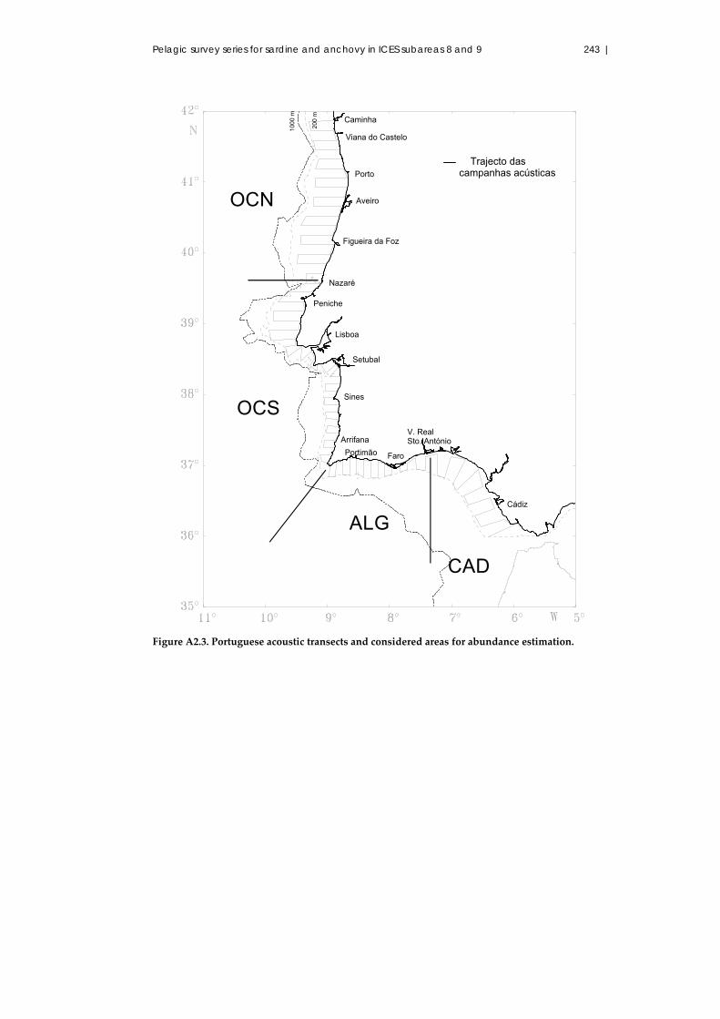
Pelagic survey series for sardine and anchovy in ICES subareas 8 and 9 243 |
Figure A2.3. Portuguese acoustic transects and considered areas for abundance estimation.
Caminha
Viana do Castelo
Porto
Aveiro
Figueira da Foz
Nazaré
Peniche
Lisboa
Setubal
Sines
Arrifana
Portimão Faro
V. Real Sto. António
Cádiz
1000
m
200
m
Trajecto das campanhas acústicas
OCN
OCS
ALG
CAD

244 |
ICES Cooperative Research Report No. 332
A2.4.6 Sampling and biology
A2.4.6.1 Pelagic fish species sampling
General sampling procedure
Five (5) sampling boxes (ca. 30 l) randomly filled from the capture in each trawl station.
Species identification.
Total weight of specimens and number of each species.
Random samples of 100 individuals of each species.
Total weight of sample and individual total lengths.
Distribution of individuals of each species by length classes:
0.5‐cm length classes in fast growing species: sardine, anchovy, sardinellas, shad, twaite shad,
boarfish, snipefish, thickback sole, flounders, gurnards, argentines, weevers, octopus, squids,
cuttlefish;
1.0‐cm length classes: horse mackerel, chub mackerel, bogue, and blue whiting.
Total number and weight by length class.
Individual total length of the remaining sampled species of each haul and no distribution by length classes.
Biological sampling procedure
Primary species:
Sardine, horse mackerel, anchovy, mackerel, and chub mackerel.
Procedure:
Ten (10) individuals by length class (sardine and anchovy: 0.5 cm; chub mackerel, mackerel, and horse
mackerel: 1.0 cm). Extreme length classes completed with specimens taken from the sample box.
Individual total length, total and gutted weights, gonad weight (whenever possible!), sex and sexual
maturation stage, visceral fat stage, stomach filling stage, and colour.
Stomach collection:
Primary species (stomachs always collected) – sardine, anchovy, chub mackerel, and horse mackerel.
Secondary species (stomachs collected if there is spare time and when >30 specimens are caught) –
mackerel, blue jack mackerel, Mediterranean horse mackerel, bogue, European squid, squid (Alloteuthis),
crab (Polybius henslowi), boarfish, snipefish, and blue whiting; for squid (Alloteuthis) and crab (Polybius
henslowi), 20 individuals are randomly taken from the sample and frozen.
For the remaining species, 10 stomachs with contents:
4 stomachs from the modal length class (most abundant class);
2 stomachs from the length class below and 2 from the one above the modal class;
1 stomach from the length class below and 1 from the one above the previous ones;
if the length distribution has 2 modes, the above procedures must be followed for each one (this will
result in a total of 20 collected stomachs for that haul/species);
the individual total length of fish from which stomachs were extracted is measured and recorded as
well as the total and gutted weights. Otoliths are not collected;
evaginated or torn stomachs are not collected;
stomachs individually collected to a plastic bag and identified with the observation number on a
baking paper tag inside the bag. Bags with stomachs of each trawl haul/species are gathered into a
large plastic bag properly identified (survey code, sampling station number, and species) and
immediately frozen.
Otolith collection:
A maximum number of otoliths by length class at the beginning of each area survey for a reasonable
sampling in case of scarce sampling trawl stations. A homogeneous area coverage and an indicative
number of otoliths in each of the following sampling stations must be reached and controlled in order
to achieve the objectives for each area:
Sardine – 10 otolith pairs by length class (total length up to 13 cm); 16 pairs (between 13.5 and 17.5 cm);
20 pairs (18 cm and above);
Anchovy – 10 otolith pairs by length class; Mackerel, chub mackerel, and horse mackerel – 15 otolith pairs by length class. For chub mackerel, if
individuals with total length >27–28 cm (does not frequently occur) are caught in a significant amount
at a sampling station, opportunity must be taken to collect 15 otoliths by length class.
Surveyed areas
OCN – “Occidental Norte” (West Northern coast) – ICES Division 9.a‐Central North
OCS – “Occidental Sul” (West Southern coast) – ICES Division 9.a‐Central South
ALG – “Algarve” – ICES Division 9.a‐South
CAD – “Cádiz” (Gulf of Cádiz) – ICES Division 9.a‐South

Pelagic survey series for sardine and anchovy in ICES subareas 8 and 9 245 |
A2.4.7 Sardine otolith preparation procedures and age-reading criteria
The Iberian–Atlantic sardine stock is commonly surveyed by Portugal and Spain;
therefore, its assessment is also jointly undertaken by both countries. Consequently,
standardized age‐reading methodologies and criteria had to be adopted. Otolith
exchange and age‐reading workshops have been regularly undertaken by the fisheries
research institutes of both countries for this purpose. Based on the experience of age‐
reading experts of both countries and on the results of these events, protocols with
recommendations and age‐reading criteria have been produced in order to improve
data quality and, consequently, the precision of the stock assessments.
The otolith preparation procedures and age‐reading criteria commonly applied by
readers of both countries are those agreed during the last Workshop on Age Reading
of European Atlantic Sardine (WKARAS) held in Lisbon, Portugal, 14–18 February
2011 (ICES, 2011b).
A2.4.8 Sardine and anchovy eggs and environmental conditions
Since 2000, a CUFES system (Checkley et al., 1997) has been used in the acoustic surveys
for underway surface (ca. 3 m) plankton sampling (every 3 nautical miles) with the
main objective to describe sardine and anchovy spawning grounds. A SeaBird thermo‐
salinographer and a SeaPoint fluorometer are coupled to the CUFES system allowing
continuous recording of SST, SSS, and SSF (fluorescence, ~chlorophyll). The
information from the TCF probes is compiled, together with GPS data, by dedicated
software (EDAS). High‐resolution data acquisition on egg abundance, temperature,
salinity, and fluorescence allow the production of detailed distribution maps that assist
in environmental characterization and definition of spawning areas.
A2.4.9 Seabird and marine mammal census
Data on seabirds and marine mammals are collected during IPMA surveys according
to a modified version of the methodology of Tasker et al. (1984), as recommended by
the European Seabirds At Sea (ESAS) group (Camphuysen and Garthe, 2004). Sightings
are recorded as densities (number of individuals km–2) along the transects of the survey
during observation periods each lasting 5 min. All birds in contact with the water or
with marine mammals observed within the transect are counted. All birds in flight are
recorded once (as regular snapshots) in order not to overestimate their density.

246 |
ICES Cooperative Research Report No. 332
A2.5 JUVENA survey protocol (AZTI – Basque country, Spain)
A2.5.1 Sampling strategy
The JUVENA surveys are carried out annually between September and October in the
Bay of Biscay (Table A2.3). In these months, the juveniles have grown to a size that
makes them visible to the echosounders (allowing the tuna fishing fleet to target them
as live bait) and normally occupy large outer‐ and off‐shelf areas off the northern
Spanish and western French coasts (Cort et al., 1976; Martín, 1989; Uriarte et al., 2001).
Acoustic sampling is performed in daylight because, at this time of year, juveniles
usually aggregate in schools in the upper layers of the water column during the day
where they can be distinguished from plankton structures (Cort et al., 1976; Uriarte et
al., 2001). Sampling is carried out following a regular grid formed by transects arranged
perpendicular to the coast (Figure A2.4), spaced at 17.5 nautical miles (2003–2005) or
15 nautical miles (2006 onwards) to ensure their independence (Carrera et al., 2006).
Sampling starts at the northern Spanish coast, going from west to east, and then moves
to the north to cover the waters off the French coast of the Bay of Biscay. It is considered
important to conduct the survey in the precise temporal window that extends from
mid‐August to mid‐October, which is not too early for the juveniles to be detected and
caught, and not so late that they have abandoned the offshore grounds.
Table A2.3. Summary of sampling effort.
Year
Start
of
survey
End of
survey
No. of
vessels
Effective
survey
time (d)
Fishing
operations
Anchovy‐
positive
fishing
operations
Inter‐
transect
distance
(nautical
miles)
Sampled
area
(nautical
miles2)
Positive
area
(nautical
miles2)
2003 18/09 14/10 1 20 47 36 17.5 16 829 3 476
2004 19/09 19/10 1 18 21 9 17.5 12 736 1 907
2005 12/09 07/10 2 20 47 45 17.5 25 176 7 790
2006 13/09 14/10 2 42 80 52 15 27 125 7 063
2007 04/09 30/09 2 37 70 40 15 23 116 5 677
2008 26/08 25/09 2 33 85 46 15 23 325 6 895
2009 26/08 25/09 2 39 67 42 15 34 585 12 984
2010 01/09 30/09 2 40 79 60 15 40 500 21 110
2011 01/09 05/10 2 40 77 64 15 37 500 21 025
2012 02/09 05/10 2 40 67 51 15 31 500 14 271
The survey is intended to cover the entire expected spatial distribution of juvenile
anchovy in these months of the year in the Bay of Biscay (Figure A2.4), from offshore
areas well beyond the continental shelf to very coastal waters, because the spatial
process of anchovy juvenile recruitment occurs from offshore areas towards the coast
during autumn (Uriarte et al., 2001). This survey area can vary from year to year and is
potentially large. Consequently, considerable effort is made to achieve the broadest
possible coverage of the area by using an adaptive sampling strategy. In this strategy,
the boundaries of the sampling area are defined according to the findings of each
survey and to the parallel information obtained from the commercial fishing fleet,

Pelagic survey series for sardine and anchovy in ICES subareas 8 and 9 247 |
which uses juvenile anchovy as live bait for tuna fishing. Along the Spanish and French
coastlines, the minimum limits of the sampling area are set at 5°W and 46°N,
respectively. According to previous information on juvenile distribution, this area is
expected to contain the vast majority of the juvenile anchovy stock (Cort et al., 1976;
Uriarte et al., 2001; Carrera et al., 2006). This area is expanded according to the adaptive
sampling strategy, but, for practical reasons, a maximum surveying area is set within
the limits of 7°30’W and 48°N. Between these limits, the actual along‐coastline
boundaries were set each year at the points where there was a clear decrease in
abundance or, if possible, a transect in which juvenile anchovy was not detected. The
length of the transects extends from about the 20‐m to at least the 1000‐m isobaths, and,
according to the adaptive scheme of the survey, if the detections continued, they were
expanded offshore to 4 nautical miles beyond the last detection of an anchovy school.
In addition, information from the commercial live‐bait tuna fishery collected before
and during each survey is taken into account in making decisions about survey
sampling strategy. As a result of this sampling scheme, the years with higher
abundance of anchovy typically require larger sampling coverage.
Figure A2.4. The current JUVENA default sampling design. The length of the transects and the
actual western and northern boundaries of the sampling area change every year according to the
adaptive sampling strategy.
In the period 2003–2004, the area was sampled with a single commercial purse‐seiner
subcontracted for the survey and equipped with scientific echosounders. In 2005, a
second purse‐seiner was added to the survey to provide extra fishing operations, and
in 2006, a pelagic trawler with complete acoustic equipment, the RV “Emma Bardán”,
replaced the second purse‐seiner (Table A2.4).
A2.5.2 Data acquisition
The acoustic equipment included Simrad EK60 split‐beam echosounders (Kongsberg
Simrad AS, Kongsberg, Norway) of 38 and 120 kHz from 2003 to 2006, plus a 200‐kHz
transducer from 2007 (Table A2.4). The transducers are installed looking vertically
downwards, at a depth of ca. 2.5 m, at the end of a tube attached to the side of the
248 |
ICES Cooperative Research Report No. 332
commercial fishing vessels and on the vessel hull of the research vessel. The
transducers are calibrated using standard procedures (Foote, 1987).
The water column is sampled acoustically to a depth of 200 m. Catches from the fishing
hauls and echotrace characteristics are used to identify fish species and determine the
population size structure. The fishing stations are decided based on the typology on
the detected echoes, trying to identify each change in the detected typologies. Purse‐
seining was used to collect samples until 2005 and was then combined with pelagic
trawls from 2006 onwards. To improve species identification in the first three surveys
when only purse‐seiners were available, additional night fishing operations were
performed by focusing bright light on the water to attract fish from surrounding
waters. In 2006, pelagic trawling was included in the surveys, which made it possible
to fish at greater depths than the purse‐seine range (50 m maximum). The purse‐seiners
generally cover the coastal areas and the waters off the shelf where juveniles occupy
the surface waters and are accessible to the purse‐seine fishing range. The pelagic
trawler covers the intermediate shelf regions where it may be necessary to sample at
all depths. In addition, when deep, anchovy‐like aggregations are detected by the
purse‐seiners, the pelagic trawler may temporally leave its coverage area to carry out
additional fishing operations in these areas.

Pelagic survey series for sardine and anchovy in ICES subareas 8 and 9 249 |
Table A2.4. Vessels and equipment.
Vessel 1 Vessel 2
Vessel Name Variable vessel* ”Emma Bardán”
Length (m) 30–35 27
Side (m) 8 7
Draft (m) 3.5–4 3.5
Acoustic installation Side perch Hull
Acoustic equipment Transducer frequencies (kHz) 38, 120, (200)** 38, 120, 200
Power (for 38, 120, 200 kHz) (W) 1 200, 250, (210)** 1200, 250, 210
Pulse duration (10–6 s) 1 024 1 024 (except in 2006: 256)
Ping interval (s) 0.25–0.5
Target strength (b20)*** Engraulis encrasicolus
Sardina pilchardus
Sprattus sprattus
–72.6 dB Degnbol et al. (1985)
Trachurus trachurus
Trachurus mediterraneus
Scomber colias
–68.7 dB ICES (2006b)
Scomber scombrus –88 dB Clay and Castonguay (1996)
Jellyfish (mean TS) –81.7 dB Average TS for jellyfish species in Simmonds and MacLennan (2005)
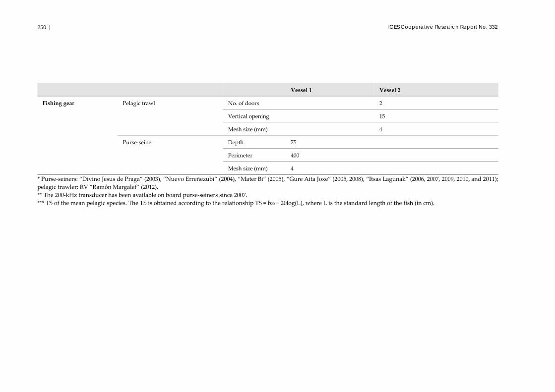
250 |
ICES Cooperative Research Report No. 332
Vessel 1 Vessel 2
Fishing gear Pelagic trawl No. of doors 2
Vertical opening 15
Mesh size (mm) 4
Purse‐seine Depth 75
Perimeter 400
Mesh size (mm) 4
* Purse‐seiners: “Divino Jesus de Praga” (2003), “Nuevo Erreñezubi” (2004), “Mater Bi” (2005), “Gure Aita Joxe” (2005, 2008), “Itsas Lagunak” (2006, 2007, 2009, 2010, and 2011);
pelagic trawler: RV “Ramón Margalef” (2012).
** The 200‐kHz transducer has been available on board purse‐seiners since 2007.
*** TS of the mean pelagic species. The TS is obtained according to the relationship TS = b20 − 20log(L), where L is the standard length of the fish (in cm).

Pelagic survey series for sardine and anchovy in ICES subareas 8 and 9 251 |
A2.5.3 Intercalibration of acoustic data between vessels
Since the 2006 survey, when the acoustic sampling was split between two vessels,
intercalibration exercises between the two vessels have been carried out routinely each
year, based on the intercalibration methodology described by Simmonds and
MacLennan (2005). The data are collected by two vessels advancing side by side ca.
100 m apart. The intercalibration process consists of comparing the echo integration of
the bottom echo in areas of a smoothly variable seabed.
A minimum distance of 30 nautical miles is covered simultaneously by the two vessels
for these exercises. The ratio of NASC (MacLennan et al., 2002) values per ESDU
between vessels is calculated. Initially, layer echo integration of both water column and
bottom echo obtained by the two vessels were compared, but preliminary results
indicated that, while both target types provided similar ratios, the bottom echo
provided much less variability than the water column. Therefore, the bottom echo was
chosen as the reference target and the rest of the analysis is based on bottom echo
NASC values. The intercalibration factor Fint was estimated as the median of the NASC
ratios Ri.
Fint = Median(Ri) (A2.28)
The median was chosen as a robust alternative to the average, given the high number
of outliers of the data (because the transducers did not point to the exact same targets).
As a robust standard deviation, the median absolute deviation (MAD; Hoaglin et al.,
1983) was calculated, based on the deviation of individual data points from the median
of the population:
MADint = [Median(|Ri –Fint|)] × 1.4826 (A2.29)
The value 1.4826 is a constant factor that adjusts the resulting robust value to the
equivalent of a normal population distribution. Thus, for a normally distributed
population, the s.d. and the MAD should be equal. In accordance to this, a robust CV
was calculated as:
CVint = MADint/ Fint (A2.30)
A2.5.4 Acoustic abundance estimation
Echograms are examined visually with the aid of the species composition of catches to
identify positive anchovy layers. Noise from bubbles, double echoes, and, when
necessary, plankton are removed from the echograms. Acoustic data are processed in
the positive strata by layer echo integration, using an ESDU of 0.1 nautical mile with
the Movies+ software (IFREMER, France). Echoes are thresholded to –60 dB and
integrated into six depth channels: 7.5–15, 15–25, 25–35, 35–45, 45–70, and 70–120 m (no
anchovies have been found below 120 m).
Generally, only the 38‐kHz data are echo integrated using the TS–length relationships
agreed in the ICES WGACEGG for the main species (ICES, 2006b; Table A2.4). Each
fishing haul is classified by species. A random sample of each species is measured to
determine the length frequency distribution of the different species, in 0.5‐cm classes
for the smaller species (anchovy and sardine) and 1‐cm classes for the rest. Complete
biological sampling of anchovy is performed to analyse age, size, and the size–weight
ratio. The hauls are grouped by strata of homogeneous species and size composition.

252 |
ICES Cooperative Research Report No. 332
The species and size composition of each homogeneous stratum are obtained by
averaging the composition (in numbers) of the individual hauls contained in the
stratum weighted by the acoustic density in the vicinity (2‐nautical‐mile diameter).
This species and size composition of each stratum is used to obtain the mixed species
echo integrator conversion factor (Simmonds and MacLennan, 2005) for converting the
NASC values of each ESDU into numbers of each species. However, although the
methodology involves estimating multiple species, the survey strategy is strongly
focused on juvenile anchovy, and only the positive areas for anchovy are processed.
Therefore, only estimates of this species are considered reliable and thus produced.
Each fish species has a different acoustic response, defined by its scattering cross
section that measures the amount of the acoustic energy incident to the target that is
scattered backwards. This scattering cross section depends on species i and the size of
the target j, according to:
10/log10/ 1010 jiiij LbaTS
ij
(A2.31)
Here, TS stands for “target strength”, Lj represents the size class, and the constants ai
and bi are determined empirically for each species. For anchovy, we have used the
following TS–length relationship:
jj LTS log206.72 (A2.32)
The composition by size and species of each homogeneous stratum is obtained by
averaging the composition of the individual hauls contained in the stratum, with the
contribution of each haul weighted to the acoustic energy found in its vicinity (2‐
nautical‐mile diameter). Thus, given a homogeneous stratum with M hauls, if Ek is the
mean echo‐integrated acoustic backscattering in the vicinity of the haul k, wi, the
proportion of species i in the total capture of the stratum, is calculated as follows:
jM
kk
M
k k
kijk
jiji
E
QEq
ww
1
1 (A2.33)
where qijk is the quantity of species i and length j in haul k, and Qk is the total quantity
of any species and size in haul k.
In order to distinguish their own contribution, anchovy juveniles and adults are
separated and treated as different species. To this end, the proportion of anchovy in
the hauls of each stratum wij is multiplied by an age–length key to separate the
proportion of adults and juveniles. Thus, individual wi are obtained for each.
Inside each homogeneous stratum, a mean scattering cross section was calculated for
each species by means of the size distribution of such species obtained in the hauls of
the stratum:
i
jijij
i w
w
. (A2.34)
Let SA be the calibration‐corrected, echo‐integrated energy by ESDU (0.1 nautical mile).
The mean echo‐integrated acoustic backscattering in each homogeneous stratum,
Am sE , is divided in terms of the size‐species composition of the haul of the

Pelagic survey series for sardine and anchovy in ICES subareas 8 and 9 253 |
stratum. Thus, the echo‐integrated backscattering attributed to each species i, Ei, is
calculated as:
iii
mii
i w
EwE
(A2.35)
Here, the term inside the parenthesis sums over all the species in the stratum. Finally,
the number of individuals Fi of each species is calculated as:
i
ii
ElHF
(A2.36)
where l is the length of the transect or semi‐transect under the influence of the stratum
and H is the distance between transects (ca. 15 nautical miles). To convert the number
of juveniles to biomass, the size–length ratio obtained in each stratum is applied to
obtain the average weight of the juveniles in the stratum:
b
ii LaW (A2.37)
Thus, the biomass is obtained by multiplying Fi by iW .
Anchovy juveniles (age 0) and adults (age ≥1) are separated and treated as different
species. To separate juveniles from adults, the anchovy length frequency distribution
by haul is multiplied by a corresponding age–length key. The key is determined every
year for three broad areas: pure juvenile area, mixed juvenile area (with a mix of
juveniles and adults), and Garonne River area (located at the coastal area around
45°40’N; also a mixed area, but adult anchovy here are usually smaller than in the other
areas). Finally, the abundance in numbers of juveniles and adults is multiplied by the
mean weight to obtain the biomass per age and length class for each ESDU.
A2.5.5 Near-field correction
Juvenile anchovies exhibit a near‐surface distribution during the JUVENA survey
period (Uriarte et al., 2001; Boyra et al., 2013). In order to achieve the best possible
coverage of the vertical distribution of this species, and after comparing two different
methods (Boyra et al., 2013), a methodology was proposed to deal with the presence of
juvenile anchovy aggregations inside the near‐field range of the Simrad EK60 38‐kHz
transducers (10.5 m; Simmonds and MacLennan, 2005). The method consisted of
measuring and correcting the bias produced when echo integrating fish schools inside
the near‐field (5–11 m range from the transducer face, i.e. ca. 7.5–13 m below the
surface), instead of deleting the entire layer. The reason for occasionally integrating the
7.5–
13‐m depth layer (and thus not following the standard procedure) is that it is
considered important to retrieve as much information as possible about abundance of
juvenile anchovy, a species that largely occupies the top metres of the water column.
To estimate the near‐field bias, we selected a set of the cleanest possible 38‐kHz
echograms, i.e. with the least presence of plankton in the uppermost layers (7.5–13‐m
depth). From these areas relatively free of plankton, five acoustic records of ca. 5 min
duration each were selected for each year and vessel (Figure A2.5). The idea was to try
to characterize the “rainbow” pattern visible in the first layers of these echograms
(visible because the echograms are displayed with a threshold of –80 dB), but not
accounting for the noise produced by the plankton. For this purpose, the backscatter
was echo integrated at –100 dB threshold by a single ping in the 7.5–13‐m layer. As the
records were not completely free of plankton, a filtering procedure was applied to

254 |
ICES Cooperative Research Report No. 332
clean it as much as possible. The echo‐integrated pings of each file were divided into
four groups per minute (about 50 pings per group). Inside each group, the 25th
percentile was computed for each depth layer to characterize the purest possible near‐
field reverberation, free from plankton backscattering, for each group. The resulting
echo‐integration values per layer were further averaged using the mean value for all
records. This estimation of “clean water” backscatter at 7.5–13 m was used as a proxy
for the near‐field and was subtracted from the fish NASC values of the uppermost echo
integration channel (7.5–15 m). As the filtering procedure could not completely remove
the plankton backscatter, some quantity was included in the near‐field estimates and
thus subtracted from the fish backscatter of the first layers. Thus, this correction
procedure of the near‐field is considered to be slightly conservative.
A2.5.6 Recruitment predictive capability
In order to estimate the recruitment predictive capability, the annual biomass estimates
for anchovy juveniles are compared with the estimates of anchovy recruitment the
following year. The recruitment is the biomass of age 1 anchovy in January of the
following year, estimated according to the ICES assessment using a Bayesian model
with inputs from catches and biomass estimates of two spring surveys: an acoustic one
(PELGAS) conducted by IFREMER, and a survey based on DEPM (BIOMAN),
conducted by AZTI (ICES, 2011a). The biomass estimates are fitted by linear, log‐linear,
and rank regressions between variables using the R software version 2.14.0 (R
Development Core Team, 2011).

Pelagic survey series for sardine and anchovy in ICES subareas 8 and 9 255 |
Figure A2.5. Sample echograms of the chosen low plankton areas for the near‐field characterization.
The threshold is set at –80 dB, the same as used during the visual inspection for the selection of
these areas. The process tries to characterize the “rainbow” pattern at the top part of each echogram
by filtering the overlapping “noise” produced by marine organisms, wave‐induced bubbles, etc.

256 |
ICES Cooperative Research Report No. 332
A2.6 Top predator sighting protocol (UMS PELAGIS)
A2.6.1 General method
Data on top predators (seabirds and cetaceans) are collected along transects over the
continental shelf of the Bay of Biscay by ship‐based surveys conducted between 2003
and 2012. These ship‐based surveys involved the use of the RV “Thalassa” during the
PELGAS, PELACUS, and EVHOE surveys. The general method used is a single‐
platform, line‐transect survey.
A2.6.2 Method of data acquisition
Top predator sightings are recorded all day during the observation leg. An observation
leg is a segment with the same sighting conditions, observers, bearing, and speed. If
any one of these parameters changes, the observation leg changes. All sightings
collected are linked to the observation leg concerned. During the observation leg, data
on weather and sighting conditions are recorded, including sea state, windspeed and
‐direction, swell, glare severity, cloud cover, and an index of the subjective conditions
(good, moderate, or poor) estimated to detect a small cetacean.
Two observers are placed 16 m above sea level (upper bridge of the ship, see Figure
A2.6). Ship speed is maintained at 10–12 knots during the observation leg. Two
observers search for cetaceans and seabirds within an angle of 180° ahead of the bow
and are replaced every two hours.
They search with naked eye close to the ship (out to 1000 m and less if sighting
conditions are moderate or poor). For each sighting, number, species, and time (UTC)
are recorded, and the distance and angle are estimated by eye and with a stick and
angleboard. Additional data collected from each detected group of cetaceans or birds
include age for birds (adult, juvenile, immature), behaviour (attracting, flying, sitting,
feeding – for birds; swimming, logging, attracting, feeding – for cetaceans). Data on
litter (macro size more than 30 cm), large pelagic fishes (shark, sunfish, swordfish,
tuna,…), turtles, and boats (fishing, sailing, and commercial) are collected during the
observation leg.
The GPS positions are provided by CASINO and the link with the data location is
performed each day at UTC time.
For every change in the observation leg or activity of the research vessel (trawling), the
birds (scavengers) following the vessel are recorded (number and species
composition).

Pelagic survey series for sardine and anchovy in ICES subareas 8 and 9 257 |
Figure A2.6. Diagram showing the placement of two observers on the upper bridge of the vessel
and their fields of vision while searching for seabirds and cetaceans on board the RV “Thalassa”
during the PELGAS, PELACUS, and EVHOE surveys.
258 |
ICES Cooperative Research Report No. 332
7 Abbreviations and acronyms
AcousMed European project – Harmonization of the acoustic data in the
Mediterranean 2002–2006
AIC Akaike’s Information Criterion, used to compare statistical models
ALK Age–length key
AZTI Food and Fisheries Technological Institute / Instituto Tecnológico
Pesquero y Alimentario
CalCOFI California Cooperative Oceanic Fisheries Investigation
CalVET The CalCOFI vertical egg tow net
CDF Cumulative distribution functions
CFP EU’s Common Fisheries Policy
CLUSTER Aggregation patterns of commercial fish species under different stock
situations and their impact on exploitation and assessment; FAIR‐CT‐
96.1799
CRMM Centre de Recherche sur les Mammifères Marins (now PELAGIS)
CTD An oceanographic instrument of conductivity, temperature, and depth
recording in vertical water tows
CTDF a CTD that includes a fluorescence recording device
TF An oceanographic instrument of conductivity, temperature, and
fluorescence recording, usually coupled to CUFES
CUFES Continuous underway fish egg sampler
CV Coefficient of variation
DCF EU Data Collection Format
DCR EU Data Collection Resolution
DEPM Daily egg production method, applied in surveys to assess the SSB of
pelagic fishes
DETAC A project on the development of acoustic techniques, run by the IEO
DF Daily fecundity
EAFM Ecosystem approach to fisheries management
ECOCADIZ Spanish acoustic survey series
EDAS EGNOS Data Access Service, a terrestrial data service that can provide
raw GPS data collected by the EGNOS monitoring reference network
EPM Egg production method
ESAS European Seabirds at Sea
ESDU Elementary samling distance unit
FlowCAM Brand of Fluid Imaging Technologies, Inc. for dynamic imaging
particle analysis
GAM Generalized additive model

Pelagic survey series for sardine and anchovy in ICES subareas 8 and 9 259 |
GLM Generalized linear model
GLOBEC Global Ocean Ecosystem Dynamics Project
HAC Hydroacoustic data format
ICTIOEVA Egg Production Method Project
IEO Instituto Español de Oceanografía (Spanish Institute of
Oceanography)
IFREMER Institut français de recherche pour lʹexploitation de la mer
INIAP,
INIP, INRP,
IPIMAR These are old acronyms for the Portuguese national research institute
that is now called IPMA
IPMA Instituto Português do Mar e da Atmosfera
IOC Intergovernmental Oceanographic Commission
IREX International Recruitment Experiment
JUVENA A series of autumn acoustic surveys in the Bay of Biscay
LFD Length frequency distributions
LOPC Laser Optical Plankton Counter
MAD Median absolute derivation
MBA Marine Biological Association, Plymouth, UK
MODIS Moderate resolution imaging spectroradiometer
MSFD EU’s Marine Strategy Framework Directive
NASC Nautical area scattering coefficient
OCN Occidental North
OCS Occidental South
P0 Daily egg production (number of eggs produced daily per sea surface
unit)
PACAS Autumn acoustic survey (Spain)
PairoVET Paired (two‐ring) vertical egg nets launched jointly (in parallel, usually
twin CalVETs)
PDF Probability density functions
PELACUS Spring acoustic survey (Spain)
PELAGAS Spring acoustic survey (France)
PELAGIS Observatory systems for the conservation of marine mammals and
birds (La Rochelle, France)
PELAGO Spring acoustic survey (Portugal)
PELASSES EU project: Direct abundance estimation and distribution of pelagic
fish species in Northeast Atlantic waters. Improving acoustic and daily
egg production

260 |
ICES Cooperative Research Report No. 332
PELCOSAT Biology and fishing eco‐ethology of pelagic fish species in the Gulf of
Cádiz
PELTIC Pelagic ecosystem survey in the western English Channel and eastern
Celtic Sea
PGAAM ICES Planning Group on Aerial and Acoustic Surveys for Mackerel
PGPAS ICES Planning Group for Acoustic Surveys
POF Post‐ovulatory follicle
Ptot Total daily egg production (the integral of P0 over the sampling area)
RUWPA Mathematical Institute, University of St. Andrews, UK
sA Acoustic area backscattering coefficient
SAR Synthetic aperture radar
SARACUS Spanish sardine acoustic survey
SARDYN EU project: Sardine Dynamics and Stock Structure in the Northeastern
Atlantic
SARP Sardine and Anchovy Recruitment Process
SGPM General Secretariat for Maritime Fisheries
SGRESP ICES Study Group on Regional Scale Ecology of Small Pelagic Fish
SGSBSA ICES Study Group on the Estimation of Sardine and Anchovy
Spawning Biomass
SPEA Sociedade Portuguesa para o Estudo das Aves
SPVS Sociedade de Pesquisa em Vida Selvagem e Educação Ambiental
SSB Spawning‐stock biomass
SSF Sea surface fluorescence
SSL Sound scattering layer
SSS Sea surface salinity
SST Sea surface temperature
sV Volume backscattering coefficient
TCF Temperature‐corrected fluorescence provided from CTDs
TOR Terms of reference
TS Target strength
WGFAST ICES Working Group on Fisheries Acoustics Science and Technology
WGACEGG ICES Working Group on Acoustic and Egg Surveys for Sardine and
Anchovy in ICES Subareas 7, 8, and 9
WGANC ICES Working Group on the Anchovy, existing in 2008
WGANSA ICES Working Group on Anchovy and Sardine, existing in 2009–2011
WGHANSA ICES Working Group on Southern Horse Mackerel, Anchovy and
Sardine, existing since 2012

Pelagic survey series for sardine and anchovy in ICES subareas 8 and 9 261 |
WGMHSA ICES/GLOBEC Working Group on the Assessment of Mackerel, Horse
Mackerel, Sardine and Anchovy, existing until 2007
WGLESP ICES Working Group on Life Cycle and Ecology of Small Pelagic Fish
WGWIDE ICES Working Group on Widely Distributed Species
WKACUGEO ICES Workshop on Geostatistics
WKPELA ICES Benchmark Workshop on Pelagic Stocks
WKRESTIM ICES Workshop on the Estimation of DEPM‐based Spawning Stock
Biomass of Sardine and Anchovy using R (established in 2009)

262 |
ICES Cooperative Research Report No. 332
8 FAO 3-Alpha Species Codes (ASFIS) (for the most frequent species in this report)
The colour coding used in figures for the six most common species is shown.
Species scientific
name Common name ASFIS code
Colour used in
figures
Engraulis encrasicolus anchovy ANE
Boops boops bogue BOG
Capros aper boar fish BOC
Trachurus picturatus blue jack mackerel JAA
Trachurus trachurus horse mackerel HOM
Trachurus
mediterraneus
Mediterranean horse
mackerel HMM
Scomber scombrus mackerel MAC
Scomber colias chub mackerel MAS*
Sardina pilchardus sardine PIL
Macroramphosus spp. snipefishes SNS
Sprattus sprattus sprat SPR
Micromesistius
poutassou blue whiting WHB
Merluccius merluccius hake HKE
Scomberesox saurus Atlantic saury SAU
* MAS actually corresponds to Scomber japonicus, not to Scomber colias. After 2010, S. colias and S.
japonicus were accepted as being two different species, with VMA being the official FAO code of
Scomber colias. However, in this report the old code name MAS has been retained because prior to 2010
S. japonicus and S. colias were considered to be the same species (and both species were thus labelled
MAS).

Pelagic survey series for sardine and anchovy in ICES subareas 8 and 9 263 |
9 Author contact information
Editors
Jacques Massé
IFREMER – Institut Français de Recherche et dʹExploitation de la Mer
Centre de Nantes, BP 21105
Rue de l’ile d’Yeu
44311 Nantes cedex 03
France
Andrés Uriarte
AZTI – Tecnalia, Marine Research Unit
Herrera Kaia Portualdea z/g
20110 Pasaia (Gipuzkoa) – Basque Country
Spain
Maria Manuel Angélico
IPMA – Instituto Português do Mar e da Atmosfera
Avenida de Brasilia
1449‐006 Lisbon
Portugal
Pablo Carrera
IEO – Instituto Español de Oceanografia
Centro Oceanográfico de Vigo
Av. da Beiramar, 37
36202 Vigo, Pontevedra
Spain
Additional authors
Joana Andrade
SPEA – Sociedade Portuguesa para o Estudo das Aves
Avenida João Crisóstomo, n.º 18–4.º Dto.
1000‐179 Lisbon
Portugal
Miguel Bernal
IEO – Instituto Español de Oceanografia
Centro Oceanográfico de Vigo
Av. da Beiramar, 37
36202 Vigo, Pontevedra
Spain
miguel.bernal@ ieo.es

264 |
ICES Cooperative Research Report No. 332
Guillermo Boyra
AZTI – Tecnalia, Marine Research Unit
Herrera Kaia Portualdea z/g,
20110 Pasaia (Gipuzkoa) – Basque Country
Spain
Olivier Van Canneyt
Observatoire PELAGIS
Université de La Rochelle – CNRS
5 allée de lʹocéan, 17000 La Rochelle
France
olivier.van‐canneyt@univ‐lr.fr
Núria Díaz
IEO – Instituto Español de Oceanografía
Centro Oceanográfico de Baleares
Muelle de Poniente, s/n., 07015 Palma
Spain
Paz Díaz
IEO – Instituto Español de Oceanografía
Centro Oceanográfico de Vigo
Av. da Beiramar, 37
36202 Vigo, Pontevedra
Spain
Mathieu Doray
IFREMER – Institut Français de Recherche et dʹExploitation de la Mer
Centre de Nantes, BP 21105
Rue de l’ile d’Yeu
44311 Nantes cedex 03
France
Ghislain Dorémus
Observatoire PELAGIS
Université de La Rochelle – CNRS
5 allée de lʹocéan, 17000 La Rochelle
France
ghislain.doremus@univ‐lr.fr
Erwan Duhamel
IFREMER – Institut Français de Recherche et dʹExploitation de la Mer
Station de Lorient
8, rue François Toullec , 56100 Lorient
France

Pelagic survey series for sardine and anchovy in ICES subareas 8 and 9 265 |
Hélene Falchetto
Observatoire PELAGIS
Université de La Rochelle – CNRS
5 allée de lʹocéan, 17000 La Rochelle
France
helene.falchetto@univ‐lr.fr
Carmen González
IEO – Instituto Español de Oceanografía
Centro Oceanográfico de Cádiz
Puerto Pesquero, Muelle de Levante, s/n., 11006 Cádiz
Spain
Martin Huret
IFREMER – Institut Français de Recherche et dʹExploitation de la Mer
Centre de Brest
ZI Pointe du Diable, CS 10070
29280 Plouzané
France
Leire Ibaibarriaga
AZTI – Tecnalia, Marine Research Unit
Txatxarramendi ugartea z/g,
48395 Sukarrieta (Bizkaia) – Basque Country
Spain
Magdalena Iglesias
IEO – Instituto Español de Oceanografía
Centro Oceanográfico de Baleares
Muelle de Poniente, s/n., 07015 Palma
Spain
Maria Paz Jiménez
IEO – Instituto Español de Oceanografía
Centro Oceanográfico de Cádiz
Puerto Pesquero, Muelle de Levante, s/n., 11006 Cádiz
Spain
Jeroen van der Kooij
CEFAS – Centre for Environment, Fisheries and Aquaculture Science
Pakefield Road, Lowestoft
Suffolk NR33 0HT
United Kingdom

266 |
ICES Cooperative Research Report No. 332
Ana Lago de Lanzós
IEO – Instituto Español de Oceanografía
Centro Oceanográfico de Vigo
Av. da Beiramar, 37
36202 Vigo, Pontevedra
Spain
Maite Louzao
IEO – Instituto Español de Oceanografía
Centro Oceanográfico de Gijón – Avda
Príncipe de Asturias
70 bis – 33212 Gijón/Xixón
Spain
Vitor Marques
IPMA – Instituto Português do Mar e da Atmosfera
Divisão de Modelação e Gestão de Recursos da Pesca
Avenida de Brasilia
1449‐006 Lisbon
Portugal
Udane Martínez
AZTI – Tecnalia, Marine Research Unit
Herrera Kaia Portualdea z/g,
20110 Pasaia (Gipuzkoa) – Basque Country
Spain
Authier Matthieu
Observatoire PELAGIS
Université de La Rochelle – CNRS
5 allée de lʹocéan, 17000 La Rochelle
France
matthieu.authier@univ‐lr.fr
Ana Meirinho
SPEA – Sociedade Portuguesa para o Estudo das Aves
Avenida João Crisóstomo, n.º 18–4.º Dto.
1000‐179 Lisbon
Portugal
Joan Miquel
IEO – Instituto Español de Oceanografía
Centro Oceanográfico de Baleares
Muelle de Poniente, s/n., 07015 Palma
Spain

Pelagic survey series for sardine and anchovy in ICES subareas 8 and 9 267 |
Cristina Nunes
IPMA – Instituto Português do Mar e da Atmosfera
Avenida de Brasilia
1449‐006 Lisbon
Portugal
Ciaran O’Donnell
Marine Institute
Rinville, Oranmore
Co. Galway
Ireland
[email protected] Dolores Oñate
IEO – Instituto Español de Oceanografia
Centro Oceanográfico de Baleares
Muelle de Poniente, s/n., 07015 Palma
Spain
José Ramón Pérez
IEO – Instituto Español de Oceanografia
Centro Oceanográfico de Vigo
Av. da Beiramar, 37
36202 Vigo, Pontevedra
Spain
Pierre Petitgas
IFREMER – Institut Français de Recherche et dʹExploitation de la Mer
Centre de Nantes, BP 21105
Rue de l’ile d’Yeu
44311 Nantes cedex 03
France
Fernando Ramos
IEO – Instituto Español de Oceanografía
Centro Oceanográfico de Cádiz
Puerto Pesquero, Muelle de Levante, s/n., 11006 Cádiz
Spain
Vincent Ridoux
Observatoire PELAGIS
Université de La Rochelle – CNRS
5 allée de lʹocéan, 17000 La Rochelle
France
vridoux@univ‐lr.fr
268 |
ICES Cooperative Research Report No. 332
Isabel Riveiro
IEO – Instituto Español de Oceanografía
Subida a Radio Faro 50, Cabo Estai – Canido
36390 Vigo
Spain
María Santos
AZTI – Tecnalia, Marine Research Unit
Herrera Kaia Portualdea z/g,
20110 Pasaia (Gipuzkoa) – Basque Country
Spain
Maria Begoña Santos
IEO – Instituto Español de Oceanografia
Centro Oceanográfico de Vigo
PO Box 1552, 36200 Vigo
Spain
Alexandra Silva
IPMA – Instituto Português do Mar e da Atmosfera
Avenida de Brasilia
1449‐006 Lisbon
Portugal
Eduardo Soares
IPMA – Instituto Português do Mar e da Atmosfera
Avenida de Brasilia
1449‐006 Lisbon
Portugal
Jorge Tornero
IEO – Instituto Español de Oceanografía
Centro Oceanográfico de Cádiz
Puerto Pesquero, Muelle de Levante, s/n., 11006 Cádiz
Spain
Ana Ventero
IEO – Instituto Español de Oceanografia
Centro Oceanográfico de Baleares
Muelle de Poniente, s/n., 07015 Palma
Spain
Copyright © 2022 FDOKUMEN