Resource Management Committee ICES CM 2004/D:03 Ref. G, ACFM

Report of the Working Group on Methods of Fish Stock Assessments

11–18 February 2004 Lisbon, Portugal

This report is not to be quoted without prior consultation with the General Secretary. The document is a report of an Expert Group under the auspices of the International Council for the Exploration of the Sea and does not necessarily represent the views of the Council.

International Council for the Exploration of the Sea

Conseil International pour l’Exploration de la Mer

Palægade 2–4 DK–1261 Copenhagen K Denmark Telephone + 45 33 15 42 25 · Telefax +45 33 93 42 15

www.ices.dk · info@ices.dk

TABLE OF CONTENTS Section Page

1 INTRODUCTION...................................................................................................................................................... 1 1.1 Participants...................................................................................................................................................... 1 1.2 Terms of reference .......................................................................................................................................... 1 1.3 Scientific justification for this meeting and relation to ICES Action Plan...................................................... 2 1.4 Structure of the report ..................................................................................................................................... 3

2 ROBUST METHODS FOR THE INVESTIGATION OF MANAGEMENT PROCEDURES ................................ 3 2.1 Conceptual evaluation framework .................................................................................................................. 4

2.1.1 Operating model .................................................................................................................................. 5 2.1.1.1 Biological model.................................................................................................................... 5 2.1.1.2 Fishery model ........................................................................................................................ 6

2.1.2 Management procedure........................................................................................................................ 6 2.1.2.1 Observation model (data collection)...................................................................................... 7 2.1.2.2 Assessment model ................................................................................................................. 7 2.1.2.3 Harvest advice model ............................................................................................................ 8 2.1.2.4 Decision-making model......................................................................................................... 9 2.1.2.5 Complexity versus simplicity ................................................................................................ 9

2.1.3 Implementation error model ................................................................................................................ 9 2.1.4 Performance statistics ........................................................................................................................ 10 2.1.5 Stochasticity....................................................................................................................................... 10

2.2 Guidelines for framework development........................................................................................................ 10 2.3 Inventory of existing tools ............................................................................................................................ 11 2.4 Time frame and priorities for ICES .............................................................................................................. 12

2.4.1 Routine medium- and long-term stochastic projections..................................................................... 12 2.4.2 Evaluation of present or upcoming harvest control rules................................................................... 13 2.4.3 Multi-fleet multi-species considerations related to mixed fisheries................................................... 13 2.4.4 Evaluation of sampling and surveys - more rational use of existing resources.................................. 13 2.4.5 Evaluation of harvest rules and the tools to implement them in a socio-economic context............... 14 2.4.6 Comprehensive simulations of management procedures ................................................................... 14 2.4.7 Comment ........................................................................................................................................... 14

2.5 Alternative approaches to management ........................................................................................................ 14 2.6 Quality Control ............................................................................................................................................. 16

2.6.1 Outputs and summary statistics ......................................................................................................... 16 2.7 Related projects............................................................................................................................................. 17 2.8 Proposed road map for 2004 ......................................................................................................................... 18

3 ASPECTS OF MANAGEMENT PROCEDURES .................................................................................................. 19 3.1 Current advice framework ............................................................................................................................ 19 3.2 Objectives (from MoU)................................................................................................................................. 19 3.3 Elements of management procedures............................................................................................................ 20

3.3.1 Limit/target biomass and F reference points...................................................................................... 20 3.3.2 Variability in biological reference points and ecosystem effects....................................................... 24 3.3.3 HCRs ............................................................................................................................................. 25

3.4 Hypothesis testing......................................................................................................................................... 26 3.5 Recommendations......................................................................................................................................... 28

4 DIAGNOSTICS, UNCERTAINTY AND EVALUATION IN ASSESSMENT METHODS................................. 30 4.1 Introduction................................................................................................................................................... 30 4.2 Diagnostic analysis ....................................................................................................................................... 30

4.2.1 General data screening and diagnostics ............................................................................................. 30 4.2.2 Diagnostics for Bayesian methods..................................................................................................... 36

4.2.2.1 Some generic diagnostics for Bayesian data analysis .......................................................... 36 4.2.2.2 Some diagnostics for MCMC applications in WinBUGS.................................................... 38 4.2.2.3 Diagnostics for Importance Sampling ................................................................................. 41

4.3 Analyses........................................................................................................................................................ 42 4.3.1 Data generation.................................................................................................................................. 42 4.3.2 Results of application of methods...................................................................................................... 42

4.3.2.1 Bayesian VPA...................................................................................................................... 43 4.3.2.2 CADAPT (including CAMERA)......................................................................................... 52 4.3.2.3 CAMERA ............................................................................................................................ 55 4.3.2.4 CSA ............................................................................................................................ 55

WGMG Report 2004 1

TABLE OF CONTENTS Section Page

4.3.2.5 ICA ............................................................................................................................ 59 4.3.2.6 KSA ............................................................................................................................ 68 4.3.2.7 QLSPA ............................................................................................................................ 79 4.3.2.8 SURBA ............................................................................................................................ 88 4.3.2.9 XSA+ ............................................................................................................................ 92

4.4 Conclusions and guidelines........................................................................................................................... 98 4.4.1 Conclusions ....................................................................................................................................... 98 4.4.2 General guidelines for stock assessment Working Groups related to ToR d).................................... 99 4.4.3 Comments related to ToR e): investigate and implement statistical approaches that identify and

quantify uncertainty due to conditioning choices in fish stock assessment ..................................... 100 4.4.4 Reporting of data input, parameter settings and output tables for Bayesian analyses –

provision of basic guidelines .......................................................................................................... 100 4.4.4.1 Guidelines for reporting of data inputs .............................................................................. 100 4.4.4.2 Guidelines for reporting of parameter settings .................................................................. 101 4.4.4.3 Guidelines for reporting of outputs from Bayesian analyses ............................................. 101

5 DEVELOPMENT OF SOFTWARE WITHIN ICES’ FISHERIES SCIENCE ..................................................... 102 5.1 Introduction................................................................................................................................................. 102 5.2 Initial acceptance ........................................................................................................................................ 103 5.3 Web site ...................................................................................................................................................... 104 5.4 Artificial data sets ....................................................................................................................................... 104 5.5 Data simulator............................................................................................................................................. 105 5.6 Technical notes on open source .................................................................................................................. 105

5.6.1 What is OpenSource software?........................................................................................................ 105 5.6.2 Technical notes ................................................................................................................................ 106 5.6.3 Possible examples in fisheries science............................................................................................. 106

5.7 Conclusions................................................................................................................................................. 107 5.8 Minimum requirements to implement an OpenSource initiative within ICES............................................ 107

6 RECOMMENDATIONS AND FURTHER WORK ............................................................................................. 108 6.1 Suggestions and recommendations ............................................................................................................. 108 6.2 Future terms of reference ............................................................................................................................ 108

7 WORKING DOCUMENTS AND BACKGROUND MATERIAL PRESENTED TO THE WORKING GROUP............................................................................................................................................. 109 7.1 Working papers and documents (W)........................................................................................................... 109 7.2 Background material (B)............................................................................................................................. 110

8 REFERENCES....................................................................................................................................................... 111 8.1 Cited in Section 1........................................................................................................................................ 111 8.2 Cited in Section 2........................................................................................................................................ 111 8.3 Cited in Section 3........................................................................................................................................ 113 8.4 Cited in Section 4........................................................................................................................................ 114 8.5 Cited in Section 5........................................................................................................................................ 115

APPENDIX A: WORKING DOCUMENT WD2 .......................................................................................................... 116 APPENDIX B: WORKING DOCUMENT WF2 ........................................................................................................... 128 APPENDIX C: WORKING DOCUMENT WE1........................................................................................................... 151 APPENDIX D: PROGRAMS PRESENTED TO THE WORKING GROUP................................................................ 180 APPENDIX E: WGMG'S DEFINITION OF TERMS USED TO DESCRIBE THE EVALUATION

FRAMEWORK..................................................................................................................................................... 188 APPENDIX F: ICCAT ASSESSMENT PROGRAM DOCUMENTATION (APPENDIX 1) ...................................... 189 APPENDIX G: THE OPEN SOURCE INITIATIVE (WWW.OPENSOURCE.ORG) ................................................. 191 APPENDIX H: PERFORMANCE STATISTICS AS USED BY THE IWC WHEN DEVELOPING THE

ABORIGINAL SUBSISTENCE WHALING MANAGEMENT PROCEDURE.................................................. 193 APPENDIX I: A SUMMARY OF AVAILABLE SOFTWARE TOOLS FOR STOCK ASSESSMENT AND

ASSOCIATED SIMULATION TASKS................................................................................................................ 194

WGMG Report 2004 2

TABLE OF CONTENTS Section Page APPENDIX J: DESCRIPTION OF THE FEMS/FLR PROTOTYPE............................................................................ 196 APPENDIX K: WORKING DOCUMENT WG4 .......................................................................................................... 203

WGMG Report 2004 3

1 INTRODUCTION

1.1 Participants

Manuela Azevedo Portugal Jose Ma Bellido Spain Non-member Noel Cadigan Canada Fátima Cardador Portugal Liz Clarke UK Non-member Chris Darby UK José De Oliveira UK David Die (part-time) USA Non-member Rafael Duarte Portugal Non-member Yuri Efimov Russia Daniel Howell Norway Leire Ibaibarriaga Spain Ernesto Jardim Portugal Non-member Sigurður Þór Jónsson Iceland Laurence Kell UK Ciaràn Kelly Ireland Non-member Knut Korsbrekke Norway Sarah Kraak Netherlands Peter Lewy Denmark Murdoch McAllister (part-time) UK Benoit Mesnil France Iago Mosqueira Spain Alberto Murta Portugal Coby Needle UK Carl O’Brien (Chair) UK Martin Pastoors Netherlands Kenneth Patterson EC Non-member Joaõ Pereira (part-time) ICCAT Non-member Stuart Reeves Denmark Victor Restrepo (part-time) ICCAT Non-member Dankert Skagen Norway Henrik Sparholt ICES Per Johan Sparre Denmark Dmitri Vasilyev Russia

1.2 Terms of reference

The Working Group on Methods on Fish Stock Assessments [WGMG] (Chair: C.M. O’Brien, UK) will meet in Lisbon, Portugal, from 11–18 February 2004 to:

a) develop robust methods and software for the investigation of management procedures for stock recovery and the evaluation of harvest control rules;

b) identify appropriate estimators of stock conservation limits and reference points relating to longer-term potential yield; together with a characterisation of their statistical properties for the range of stocks currently assessed by ICES for its client customers and related management agencies (EU, IBSFC, NAFO, NASCO, NEAFC, ICCAT);

c) examine software capable of generating simulated data, and agree on an initial suite of data sets for use in model-testing and evaluation that will be made generally available from the ICES website;

d) investigate appropriate diagnostics that detect model mis-specification in fish stock assessment; e) investigate and implement statistical approaches that identify and quantify uncertainty due to conditioning

choices in fish stock assessment; f) develop fishery-independent assessment methods, measures of uncertainty, and appropriate diagnostics, with

particular attention to data-poor situations and the estimation of relative catchability; and g) review, revise and adopt guidelines on the formal procedures to be adopted by the Working Group for the

testing, evaluation and validation of software for use by ICES stock assessment Working Groups.

WGMG Report 2004 1

WGMG will report by 29 February 2004 for the attention of the Resource Management and the Living Resources Committees, as well as ACFM.

1.3 Scientific justification for this meeting and relation to ICES Action Plan

WGMG has made a number of suggestions and recommendations on issues of data quality, modelling and stock assessment practice throughout its last two reports (ICES 2002, 2003). The group has focused on the urgent issue of the retrospective problem in stock assessments but it could be anticipated, in advance of the meetings, that the problems of ICES’ assessments would not be fixed at short notice. The group has, however, proposed a way to proceed in the development of a solution to this problem (ICES 2003a) and this year’s terms of reference (ToRs) c), d) and e) are intended to contribute to this. In addition, the ICES Advisory Committee on Fishery Management (ACFM) has given WGMG the two ToRs a) and b) which are of immediate concern to ICES, its client customers and management agencies such as EU, IBSFC, NAFO, NASCO, NEAFC and ICCAT.

Each ToR is further elaborated below:

ToR a) – ICES is in need of computer-based software tools that will allow it to both propose and evaluate management procedures for stock recovery and the evaluation of harvest control rules. In recent years, a number of management agencies have funded a range of studies to investigate longer-term management strategies and there is now an urgent requirement to build upon this accumulated expertise and provide generic tools for use within the advisory process of ICES. It is envisaged that this ToR will need to be addressed not only during this meeting of WGMG, but at least during the next meeting in 2005, and will require inter-sessional work.

[ICES Action Plan numbers 3.2 and 4.15]

ToR b) – Following on from the recent ICES re-evaluation of Precautionary Approach (PA) reference points in 2003, there is a need for a wider methodological review of the basis under which conservation limits and longer-term fishery management targets are identified. Objective approaches need to be investigated and the properties of estimators need to be evaluated.

[ICES Action Plan numbers 3.2 and 4.15]

ToR c) – Simulated data provide a useful means by which to investigate both the choice of model structure and estimation procedure within the development of robust stock assessment procedures. At its last meeting, WGMG discussed the need to have access to a series of data sets designed for specific purposes against which new methods can be tested.

[ICES Action Plan number 3.6]

ToR d) and e) – In response to an EU request to encourage ICES to explore the use of less strongly-conditioned methods and to provide advice taking into account the possibility that different assessment model formulations may be equally valid. In addition, under these two ToRs, the potential benefits from using a Bayesian approach to inference can be evaluated. At the May 2003 meeting of ACFM, the reviewers of the Baltic Salmon and Trout Assessment Working Group [WGBAST] requested that WGMG provide guidelines for the reporting of data input, parameter settings and output tables for Bayesian analyses that would be comparable to standard practice with the current analytical approaches commonly used within ICES (e.g., XSA, ICA and ADAPT). This request will be considered as part of these ToRs d) and e).

[ICES Action Plan number 3.6]

ToR f) – The reliability of commercial catch statistics is continually being called into question. The need for fishery-independent assessment methods is obvious and urgent.

[ICES Action Plan number 3.6]

ToR g) – Necessary as part of the ICES quality assurance.

[ICES Action Plan number 6.5.3]

WGMG Report 2004 2

In general, the remit of this group addresses ICES Action Plan number 4.10; namely, to promote the development and better application of methods for resource enumeration, status evaluations and forecasts.

1.4 Structure of the report

The ToRs are addressed within the four main sections of the report. Specifically, ToR a) is addressed within Section 2 of the report, ToR b) is addressed within Section 3, ToRs d)-f) are addressed within Section 4, and ToRs c) and g) are addressed in Section 5. Various working documents and background material were presented to the meeting. These are listed in Section 7; together with their assigned code for ease of reference within the various sections of this report.

Briefly, the need for computer-based software to allow ICES to propose and evaluate management procedures for stock recovery, and the evaluation of harvest control rules (HCRs) is discussed in Section 2. General concepts underlying harvest control rules with some candidate stocks are presented in Section 3. The need within ICES to explore the use of less strongly-conditioned stock assessment methods and to provide advice taking into account the possibility that different assessment model formulations may be equally valid is discussed in Section 4; together with illustrative analyses using a suite of programs (Bayesian VPA, CADAPT, CAMERA, CSA, ICA, KSA, QLSPA, SURBA and XSA+). Section 5 discusses open computing software that is proposed for further future development within ICES’ fisheries science; with Section 6 detailing further work that needs to be undertaken in the short-term. The Working Papers by Azevedo (WD2), Needle (WF2), Patterson (WE1) and Kraak (WG4) are reproduced in Appendices A, B, C and K, respectively, for completeness.

All the working papers and background documents listed in Section 7 are distributed on the ICES CD for the report of this meeting of WGMG.

2 ROBUST METHODS FOR THE INVESTIGATION OF MANAGEMENT PROCEDURES

Currently within ICES there is a need for computer-based software tools that will allow ICES to both propose and evaluate management procedures for stock recovery, and the evaluation of harvest control rules (HCRs). In recent years, a number of management agencies have funded a range of studies to investigate longer-term management strategies and there is now an urgent requirement to build upon this accumulated expertise and provide generic tools for use within the advisory process of ICES.

This forms the basis of the ToR a) which is addressed in this Section 2 of the report, namely,

- to develop robust methods and software for the investigation of management procedures for stock recovery and the evaluation of harvest control rules,

However, this is by no means an easy task and it is envisaged that this ToR will need to be addressed not only during this meeting of WGMG, but at least during the next meeting in 2005, and will require inter-sessional work. Much work related to this ToR has been carried out by various scientists since the early 1990s. Whilst the framework used by these scientists is similar, WGMG recognizes the fact that no standard terminology exists, which makes it difficult to coordinate the work of ICES.

In view of this problem, it is clearly desirable that ICES adopts a consistent terminology in order that the structure of any simulation models and framework used within the ICES context can be described clearly and unambiguously. WGMG devoted substantial discussion to this issue during this meeting, and its proposed standard terminology is presented in Appendix E. WGMG recommends that ICES adopts the same terminology, and would encourage other groups to do the same. The terminology reflects usage established by the ICES Working Group on Long-Term Management Measures (ICES 1994), which in turn followed usage by the IWC. Despite such attempts at standardisation, any set of terminology will suffer from limitations given that in practice all aspects of the system interact with each other, and this is difficult to represent in a fixed conceptual diagram such as that displayed in Figure 2.1. This complexity is reflected in the more conceptual description developed by the ICES Working Group on Fisheries Systems [WGFS] (ICES 2001).

It is not possible for WGMG to develop robust methods and software within the time frame of this meeting but it is possible to identify candidate stocks for which initial evaluations of HCRs might be developed (see below). Therefore, WGMG provide guidance for the development of such methods and software, and review on-going work in this Section 2.

WGMG Report 2004 3

Harvest control rules could be considered already in 2004/2005 with existing software (perhaps with minor extensions) for some stocks (see Section 2.3, Appendix I and Section 3.5). These are stocks with a relatively stable productivity (variation in recruitment, growth and maturity with stationary distributions), a long time series of data, low levels of technical interactions and exploited in a single species context and with insignificant (i.e., low) levels of discarding. Some candidates stocks are:

• NEA mackerel: candidate for multi-annual TAC (c.f. ICES 1999a); • herring in VIa (North), Irish Sea, North Sea and Celtic Sea; • saithe in the North Sea and North East Arctic saithe; and • North-East Arctic cod. In this context, the recently agreed single species recovery plans for cod stocks (Irish Sea, North Sea and West of Scotland) and northern hake might also be evaluated.

Although ToR a) refers to the evaluation of harvest control rules and management intended to aid stock recovery, such methods and software have a much wider application, and could also be used to evaluate other aspects affecting the successful management of a stock, such as stock assessment tools, sampling methods, discarding and mis-reporting. Hence, WGMG also discuss methods and software that have the potential to address this wider context before addressing ToR a).

WGMG identifies the evaluation framework approach based on simulation as the appropriate method to use. Section 2.1 describes the conceptual framework for such simulation methods. Section 2.2 describes the requirements for the simulation software based on this framework in more detail, prioritising the development of modules in this software according to ToR a). Section 2.3 provides an inventory of existing tools. Section 2.4 discusses the practical design of the software, which would enable it to meet the requirements discussed in Sections 2.1 and 2.2, as well as make use of existing tools discussed in Section 2.3 (a prototype for such software is described in Appendix J). Section 2.5 presents a brief introduction to alternative approaches to management. Section 2.6 discusses guidance to software users and quality control, and Section 2.7 describes projects related to the evaluation framework.

2.1 Conceptual evaluation framework

Simulation tools can be used to conduct experiments that evaluate the response of the fishery system to the strategy. The evaluation framework includes mathematical representations of both the true and the observed systems (data collected, assessment model used and reference points used to guide HCRs and their implementation) and so attempts to investigate the robustness of management strategies to both the intrinsic properties of the natural system and to our ability to understand, monitor and control them. Examples of factors that can be investigated are long-term fluctuations in productivity (Ravier and Fromentin 2001), errors in estimating fishing effort, choices of assessment models, biological reference points and data collection strategies. Importantly, such a framework has the advantage of considering the interactions between all these components and provides an integrated way to evaluate the relative importance of system components for the overall success of management (Wilimovsky 1985, De la Mare 1998, Holt 1998, Kell et al. 2003).

Figure 2.1 is a useful way to represent the conceptual evaluation framework. The framework comprises everything that is needed for conducting the simulations.

WGMG Report 2004 4

OPERATING MODEL

Biological model

Fishery Model

MANAGEMENT PROCEDUREIMPLEMENTATION

ERROR MODEL

Harvest advice model

Decision-making model

Performance Statistics

Performance Statistics

Observation model

Assessment model

Figure 2.1. Conceptual framework for the evaluation of management procedures, recovery plans and harvest control rules.

The operating model in most cases needs to be at least as complex as the simulation of the management procedure. For example, the evaluation of management schemes involving closed areas cannot be carried out without spatial structure in the biological and fishery models. However, even if the initial model is relatively simple, the software should be structured so that further levels of complexity can easily be incorporated at a later date.

This section expands on Figure 2.1, giving more details of models and sub-models that could be incorporated in the software. Whilst it is intended to cover most options, it is not intended to be exhaustive and, in part, reflects the interests of the participants in WGMG. Stochasticity could be incorporated in most models, and is discussed in Section 2.1.5.

2.1.1 Operating model

The operating model is an attempt to reflect reality. However, no model reflects reality exactly, but the operating model creates a virtual world, which represents the true system in the evaluation framework. The applicability of the results to the real world depends on how well the operating model conforms to reality.

The evaluation framework will be used to perform experiments, the outcomes of which rely critically on the underlying hypotheses about this true system contained within the operating model. These hypotheses should therefore be considered carefully, and should either be conditioned on available data or have a strong theoretical basis or justification. In addition, the choice of assumptions underlying the state of the system that is created by the operating model will usually pre-determine many of the results of the simulation. Therefore, as in any experimental set-up, the set of assumptions (implicit or explicit) employed needs to be kept in mind when drawing any conclusions.

The two major components of the operating model are a biological model and a fishery model. A relatively simple operating model could be for a single fishery acting on a single-species, in a single area; the biology of the species could be described by a standard age-structured population dynamics model with a Beverton-Holt stock-recruitment relationship and a von Bertalanffy growth function. More complex operating models could introduce concepts such as spatial structure, length structure, or mixed-species fisheries.

The choice of the level of operating model complexity is a crucial one. On one hand, potential users of the evaluation framework will want an operating model that offers as much realism as possible. On the other hand, a simpler operating model will be easier to define and implement. Therefore, the costs of complexity need to be considered carefully. In general, operating models should capture the characteristics of the underlying dynamics but need not necessarily model the full complexity of them.

WGMG Report 2004 5

2.1.1.1 Biological model

This model represents the development of the stock, which is then acted upon by the fishery, with removals in the form of numbers or fishing mortality output from the fishery model described in Section 2.1.1.2.

Complexity can be included at various stages, however the simplest form is likely to be a single-species age-structured population. This is likely to be generated from a model of the biological development of the stock, which incorporates the main biological processes as separate sub-models:

- natural mortality, - growth, - maturity, and - recruitment.

Further levels of complexity that may be incorporated include:

- several species; - multi-species interactions; - spatial aspects; - seasonal/temporal aspects; - density dependence; - introduce length; - covariance between variables; and - auto-correlation in, for example, recruitment.

2.1.1.2 Fishery model

This model takes output from the decision-making model, as modified by the implementation error model. It quantifies the removal (in terms of fishing mortality or numbers) from the stock, which is input into the biological model. At the simplest level, there would be a single fleet, although this could be extended to a multi-fleet model, with a model for each fleet.

Within this model, the following processes may need to be incorporated:

- selectivity-at-age (by fleet/mesh-size); - relation between effort/TAC and removal (either fishing mortality or numbers); and - spatial structure.

Furthermore, complexity may be incorporated by having feedback from the biological model. For example, implementation error (see Section 2.1.3) may also be included in this model by increasing discards as the removals approach the TAC.

2.1.2 Management procedure

The management procedure represents the human intervention that attempts to understand and control the system that is described by the operating model. The management procedure can be viewed as the entire package comprised of:

i) data collection (observation); ii) assessment; iii) advice; and iv) decision-making.

Many of the simulation studies conducted to date have focused on the evaluation of harvest control rules. These are decision rules that pre-specify what management advice will be given as a function of the perceived status of the stock(s) (item iii) in the above paragraph). However, other factors may also be of interest to some studies. For example, different levels of data collection, or different types of data in (1) will affect the perceived stock status and its precision. Also, the ability to implement technical measures can be an important consideration (see Section 2.1.3).

WGMG Report 2004 6

In order to be amenable to a simulation approach, the various elements of the management procedure should be stable, or at least carefully specified. For example, simulation results of a study in which the assessment model changes every year may be difficult to interpret.

The evaluation of management options is best performed in the context of entire management procedures; that is, the combination of a particular stock assessment technique with particular control rules and their implementation (ICES 1994). For example discarding is a function of management strategy. Discarding in the fishery will causes bias in the assessment that will in turn inform management advice. Alternative management procedures that reduce the reliance on fisheries data will have different biases and even if they give less precise estimates of stock status may perform better. Such alternative management procedures could be based upon surveys alone or tagging data (WF3 McAllister et al.). Below, however, WGMG expands on current ICES management approaches.

2.1.2.1 Observation model (data collection)

The observation model represents the way in which the operating model is sampled. It simulates the collection of data for the assessment model. This will usually involve some type of fishery-dependent statistics, and may also include fishery-independent data or other auxiliary statistics (e.g., tagging).

Each element of the observation model can be defined to varying degrees of complexity. For instance, with a complex operating model, the total catch can be estimated from aggregating samples derived from different fleet components in different areas. Misreporting could also be modelled. Similarly, catch-at-age data or survey data can be modelled with more or less sophistication, largely in a manner that is consistent with the level of complexity in the underlying operating model.

For each element of the observation model, the analyst should carefully consider precision and accuracy.

In the context of the current ICES management approach, increasing degrees of complexity could be as follows:

• Perfect data collection - catch-at-age data (and/or other data required for the assessment) is exactly as generated by the operating model

• Random variation and/or bias is added to the catch-at-age data (and/or other data required for the assessment) from the operating model using simple rules.

• The collection of catch data is simulated in more detail using sub-models for processes such as:

• recording landings • estimation of discards • market sampling for age-structure

• The collection of data from surveys such as acoustic, trawl and egg survey for:

• aggregated/disaggregated estimates of population abundance • estimates of spatial structure

a) Models dealing with sampling issues can include further sub-models for:

• survey design

• sample size • stratification

• measurement error • length/weight measurement error • ageing errors • sexing errors • maturity errors

WGMG Report 2004 7

2.1.2.2 Assessment model

The assessment model uses the information from the observation model in order to provide estimates of the status of the stock(s) and fishery. The maximum possible level of complexity of the assessment model will be limited by the level of complexity of the observation model (which is, in turn, largely limited by the complexity of the operating model).

Some simulation studies are said to have assessment feedback. This means that a piece of assessment software is actually embedded as part of the simulations. A simulation without assessment feedback is one in which the results of the assessment simply follow some prescribed formula, without all of the computer-intensive iterative computations of a typical assessment. There are trade-offs between these two choices. Simulations without assessment feedback are much easier to implement and run much faster. On the other hand, it is not a simple task to find algebraic formulations to predict the biases and precision of assessment results in relation to the choice of assumptions and data.

The framework design should also take into consideration the frequency of assessments. Generally, the framework should allow flexibility so as to match the timing of assessments with the time scale of decision-making.

In ICES terms, this model simulates the current role of the stock assessment working groups. However, this does not necessarily mean actually implementing one of the current stock assessment methods, as explained below. Increasing degrees of complexity could be as follows:

- The assessment estimates the current state of the stock exactly. This model also requires perfect data collection (no assessment feedback).

- The data is not passed to a stock assessment package, but some random variation, and/or bias is added to the (probably perfect) data to simulate the assessment process (no assessment feedback).

- The data is passed to a stock assessment package, but with pre-set input parameters such as age at constant selectivity or shrinkage (assessment feedback).

- An attempt is made to deal with all the problems and ad hoc solutions that Working Groups face, such as choosing shrinkage or including survey data (assessment feedback). This would be very difficult to simulate fully.

2.1.2.3 Harvest advice model

This component uses the assessment results to compare the perceived status of the stock and fishery against a pre-determined set of benchmarks in order to formulate advice. On many occasions, a harvest control rule will be used (a recovery plan is regarded as being a special case of a harvest control rule). These rules represent pre-agreed actions taken conditionally on quantitative comparisons between indicators of the status of the stock and some sustainability or optimality indicators. For example, a very simple rule may be to fish at F=Fpa. In this case, this model component will require all of the assessment results that are needed to compute Fpa and an algorithm (recipe) for computing Fpa. A more complex harvest control rule may prescribe, for example, that F should vary as a non-linear function of SSB.

The advice needs to be expressed into the units that will be used to affect the stock(s). For example, in order to achieve FPA there can be catch controls (advice TACs), effort controls, or other technical measures.

Potentially, harvest control rules may address more than one species at once, e.g., if mixed species advice is implemented according to set rules. Alternatively, taking mixed species fisheries into account could be part of the decision making process (see below).

This model takes the output of the assessment model, and applies a harvest control rule, which is then output as advice to form the input to the decision-making model. For example, current ICES harvest control rules generally fall into the following categories:

- F-regimes: direct effort regulation, TACs derived from F, TAC = fraction of measured biomass - Catch regimes: permanent quotas plus protection rule - Escapement regimes: leave enough for spawning but take the rest - Hybrids: F-regime with catch ceiling, F-regime with constraint on catch variation, F-regime with quotas

derived from predicted catch several years ahead, additional constraints on variation in SSB

WGMG Report 2004 8

The output from this model could include recommendations for:

- TAC - Allowable effort - Closed areas - Mesh size regulations

If the operating model is multi-species, at this point the recommendations may be further revised to account for mixed fisheries, for example by implementing the MTAC software according to pre-specified settings. Alternatively, this may be part of the decision-making process (see the next Section 2.1.2.4).

2.1.2.4 Decision-making model

The decision-making model is able to alter the advice given by the advice model. In most applications, the decision-making model will have no effect on the output of the advice model (following the example above, setting the advice TAC as that that results in Fpa, which may then be adopted as the agreed TAC). However, it is more flexible to design this as a separate model component. This would allow for the examination of control rules in which the management decision is not solely based on assessment results (for example, one that takes inputs from a socio-economic model as well).

Separating harvest advice from the final decision also allows for the making of management decisions for multiple species at once, if accounting for mixed species fisheries is not part of the harvest control rule in the advice.

Increasing degrees of complexity could be as follows:

• advice is unchanged • advice is altered with a simple rule (e.g., TAC increased by 10%) • advice is altered due to taking technical interactions into account, for example by the MTAC software, if this is

not part of the advice itself. • more complex models could be included to take account of other factors which affect management decisions,

such as social or economic factors

2.1.2.5 Complexity versus simplicity

Often the most appropriate management procedures tend to be ones that are fairly simple relative to the actual high degree of complexity in real world situation. The evaluation procedure will therefore be used to identify strategies for use by submitting them to a rigorous testing framework in which the performance of several alternative “simple” models that could be applied achieve the desired objectives. These models are also thoroughly tested against underlying operating models that represent the best available understanding of the actual system dynamics. Thus, operating models will be used to test the performance of management procedures and in general the operating models will be far more complex than the management procedures. Such an approach has been applied in the IWC (1993) to test the potential future performance of alterative proposals for new whaling management procedures and in many other instances also (Kell et al. 1999, McAllister et al. 1999).

2.1.3 Implementation error model

This model provides the interface between the regulations and the fishery. For multiple potential reasons it may be that management decisions are not always implemented exactly. This may include either random noise, or also systematic departures from the intended actions. The implementation error model allows flexibility in the evaluation framework for considering these types of effects.

In a way, this part of the framework can be viewed as an interface between the management procedure and the operating model. It takes the output of the decision-making model and provides input to the fishery model in the form of altered regulations. It is thus the implementation of the regulations rather than the implementation of the fishery, which is dealt with in the fishery model.

In many applications, the implementation error model will maintain the same decisions arising from the decision-making model and the advice model (following the examples above, obtaining a catch equal to the TAC that results in Fpa).

WGMG Report 2004 9

Increasing levels of complexity could be as follows:

• regulations are enforced perfectly • implementation is modelled with a simple rule (e.g., 90% compliance) • extent of compliance of the TAC for one stock depends on uptake of the TAC for other stocks because of

technical interactions • discarding • reduced mesh size are included as separate models • models containing complex models of fishers’ reactions taking social and/or economic factors into account.

Implementation error may also need to be included in the fishery model if feedback from the biological model is required (see Section 2.1.1).

2.1.4 Performance statistics

Performance statistics are summary indicators for the various components of the framework. Summary performance statistics are needed to facilitate the analysis of the simulation results because it is simply not feasible to examine all of the results that can be generated with this type of framework. In addition, performance statistics are the benchmarks that are needed for evaluation of the simulation results.

Examples of performance statistics for single stock trajectories include average variation in annual yield, minimum stock size, time to recovery, average yield. Examples of performance statistics for runs (i.e., many trajectories) include average time to recovery, number of trajectories for which stock size passes below some threshold (i.e., management fails), average discrepancy between assessment output and true stock size.

2.1.5 Stochasticity

All simulations will assume that at least some elements are stochastic, to account for the variability or uncertainty in these elements and to evaluate the probability of events occurring. For example, in a simple operating model, this may include variability in initial numbers, weights, mortalities, maturities and selection at age. Likewise, the observations going into an assessment may, and usually should, be stochastic, and if there is no assessment feedback, the simulated assessment output may also be stochastic. The decision-making and implementation error models could also be regarded as stochastic. However, as with other aspects of the models, stochasticity should be introduced with increasing complexity.

Both the operating model and the observation model can, in principle, be very complex. However, adding complexity to the model structure also raises questions as to where stochasticity should be introduced, and whether the probability structure of the various elements has been adequately represented. The output of such models should be validated against available data wherever possible.

In all cases, there are several ways of introducing stochasticity. Three options are to draw from theoretical statistical distributions, to use bootstrapped model output, or to draw randomly from historical values. Obtaining random numbers at the various stages is by no means trivial. Important points to consider include the quality of the random number generator, correlations between variables and trends or cyclical variations, for example in recruitment.

Incorporating random variation, in itself is also not enough, sometimes it may be important to test the robustness of a model fitting method to incorrect assumptions about the distribution of the data. Experience with simple stochastic forecasts with several types of ICES standard prediction software (WGMTERM, ICP and STPR) have shown that the uncertainty in stock abundance, fishing mortality and recommended catches can be under-estimated (Patterson et al. 2000). This underlines both that care needs to be taken to ensure that all relevant sources of uncertainty are adequately covered, and the need for validation of methods, for example to confirm that confidence intervals have the correct probability coverage.

2.2 Guidelines for framework development

The various models for assessment of fisheries dynamics and evaluation of management strategies are currently implemented in separate software programs and their respective input and output formats are often incompatible although many are performing similar tasks. Most of these packages provide basic analysis tools (model estimation, graphing, result reporting) that are already available in various software platforms. Comparing the results of such models is difficult and requires exporting them to an environment that has more efficient analytical tools. Moreover, as

WGMG Report 2004 10

they stand, such packages are not suitable for incorporation into a single simulation environment that allows evaluation of the whole fishery system.

If the guidelines given in this section are followed, different simulation/evaluation packages may be developed in parallel, and the implementation of particular methods need not be replicated. Modularisation allows code that has already been developed and tested to be easily incorporated into other programs. The method and algorithms should be documented to the extent that it should be possible to recreate the code from the documentation alone, and input and output data formats should be particularly well defined. However, the source code itself should also be available.

Therefore, WGMG favours the development of well-documented, platform independent, modular, open source software, to aid implementation, development and testing by other scientists. This particularly applies to assessment and projection software currently used by ICES stock assessment Working Groups, which should be modularised into input, output and analysis routines, so that the analysis routines can be easily incorporated as modules in the simulation software.

The approach outlined here provides for the possibility of developing extremely complex models, able to accommodate multiple degrees of knowledge about the system. But careful thought should be given to the level of complexity required at each step. Extra complexity imposes further burdens in terms of computation and interpretation, and should be justified by what is actually needed from the exercise. A review of the possible levels of complexity within each of the framework modules can be found in Section 2.1.

A development process along the lines followed by many other Open Source projects should be established. This would be based around a co-ordinating team in charge of managing and co-ordinating the development effort, which would accept or reject changes and additions to the official packages. A central repository for all the source code and documentation would need to be established, under the control of co-ordinating team. Any interested party should have access to this repository, including the freedom to use, change and re-distribute the code. But only approved versions would be then incorporated to the reference repository (see also Section 5). WGMG notes that there may be considerable resource implications in the establishment and maintenance of such a committee. This committee would benefit from collaboration amongst various marine advisory and management bodies (such as EU, ICES, ICCAT, IOTC, NMFS and IWC), and could be started as a designated project.

Development and application of modules inside this evaluation framework would require certain skills on the part of the user. Complex analyses such as those advocated here cannot be simplified to the level of a single procedure. Diagnostics and checks must be carried out at different stages. These would be helped by the adoption of an audit chain approach, where the output at every step carries with it the information necessary to replicate the process that generated it. For example, log files should include a copy of the original program call and reference to the output files included.

The modularity of the framework can only be ensured if the calculation and user interface levels are kept separate. Approaches such as the one outlined in Section J.4.3 of Appendix J, where a GUI is specified as a visual interface to a whole range of methods, can serve as guideline.

A possible approach could be the one being developed under the EU-funded project FEMS (Framework for Evaluation of Management Strategies), currently in its second year. R, a common, feature-rich implementation of the S language, is being used to both run fishery models and analyse their output. The latest object-oriented features of R (named S4 objects, or classes) allow for the definition of complex and flexible objects with a structure and arithmetic that is appropriate to fishery models. R also allows integration of present implementations and models already written in C/C++ or FORTRAN. More details are given in Appendix J.

2.3 Inventory of existing tools

Previous ICES groups have reviewed software available to stock assessment Working Groups (e.g., the Workshop on Standard Assessment Tools for Working Groups, ICES 1999b). However, the remit of the current group [WGMG] is wider and the Working Group as well as considering routine assessment software, also considered simulation and evaluation tools which would allow the performance management procedures and Harvest Control Rules to be evaluated as well as more complex models which allow alternative hypothesis about the dynamics of the resources to be generated. For each tool, in addition to the criteria listed above, WGMG also noted what language the tool was coded in, whether the source code was available from the developers, and where the program is available from.

The tools of most immediate concern to the current ICES stock assessment Working Groups are those, which facilitate the evaluation of management procedures and not just the standard assessment tools. These range from simulation frameworks which allow the whole assessment and management process to be modelled, to relatively simple stochastic

WGMG Report 2004 11

forecast programs (Skagen et al. 2000). Ideally simulation frameworks for the evaluation of management procedures should include the standard working group tools within them and also allow alternative plausible hypotheses about fishery and stock dynamics to be implemented.

Most software that has been developed to perform evaluation is by nature case specific (e.g., that used by the IWC to develop the Revised Management Procedure for Baleen whales or the Aboriginal Subsistence Whaling Procedure, IWC 2003). Therefore whilst the methodology is well developed implementation is within the hands of a few experts and there is no generic software. The FishLab software based upon Excel is a modular and flexible system that can be used to undertake evaluation of management procedures (Kell et al. 1999). However, even this software requires a high degree of user input. The FEMS project recognising these limitations is developing a framework based upon R by applying it to a range of contrasting case studies. The case studies range from temperate demersal and tuna stocks to tropical tunas, partners include ICES, ICCAT and NMFS. It is hoped that in this way a flexible system that can be used for a variety of purposes can be developed.

Tools are also required to explore hypotheses about stock and fleet dynamics to generate plausible hypotheses about stock dynamics that are not solely based upon VPA based assumptions used by most stock assessment software. For example, GADGET (a length based multi-species model) and MSVPA.

Frameworks that allow exploration of data and model assumptions such as R (a general statistical modelling framework) and WinBUGS (a Bayesian modelling package) respectively are also required.

A summary of existing assessment and evaluation tools the WG drew on a previous such exercise conducted at the Workshop on Standard Assessment Tools for Working Groups (ICES 1999b). That group identified the major tasks of what then constituted a standard ICES stock assessment then summarised programs available to address each of those tasks. As part of the intention of that group was to improve standards of quality control and documentation in relation to assessment software, the programs were also summarised in relation to a number of criteria. These were as follows:

• Whether the method implemented had been published in a peer-reviewed publication • Whether user documentation (i.e., documentation of how to use the program) is available • Whether technical documentation (i.e., documentation of the specific methods and algorithms used) is available • Whether the program is currently used by Assessment Working Groups • Whether assessments using the program have been used as the basis of ACFM advice The tools identified are listed Appendix I. This list is incomplete and unchecked. Inclusion of any tool in the Table should not be taken as meaning that the tool has been formally approved in any way, and similarly exclusion should not be taken to mean that a program has not been approved.

2.4 Time frame and priorities for ICES

In this Section 2.4, WGMG list the most likely needs of ICES in the short- to medium-term. For each of these, the kind of software that is relevant is suggested, together with an outline of what it would take to have such software operative for use within the advisory process of ICES.

2.4.1 Routine medium- and long-term stochastic projections

The obligation by ICES to evaluate the medium- to long-term consequences of recommended management measures. This comes from the requirement to advise on the level of catch (and where appropriate the corresponding level of effort in appropriate units) consistent with the long-term sustainable exploitation of the stock and that advise according to adopted harvest rules for setting TACs or levels of effort, shall be evaluated for consistency with precautionary criteria and alternatives proposed if needed (MoU App. II, 2.1 and 2.2), as well as other requests that are likely to appear.

Priority: Needed immediately

Software available: Some tools exist, ICP, WGTERM, STPR. These are of variable quality and with varying degrees of documentation. There is a need to review existing methods, bring them up to the current standards, including compatibility with the requirements of an open source environment, supplement with diagnostics, ensure clear documentation of assumptions, limitations, what is modelled and what is assumed.

WGMG Report 2004 12

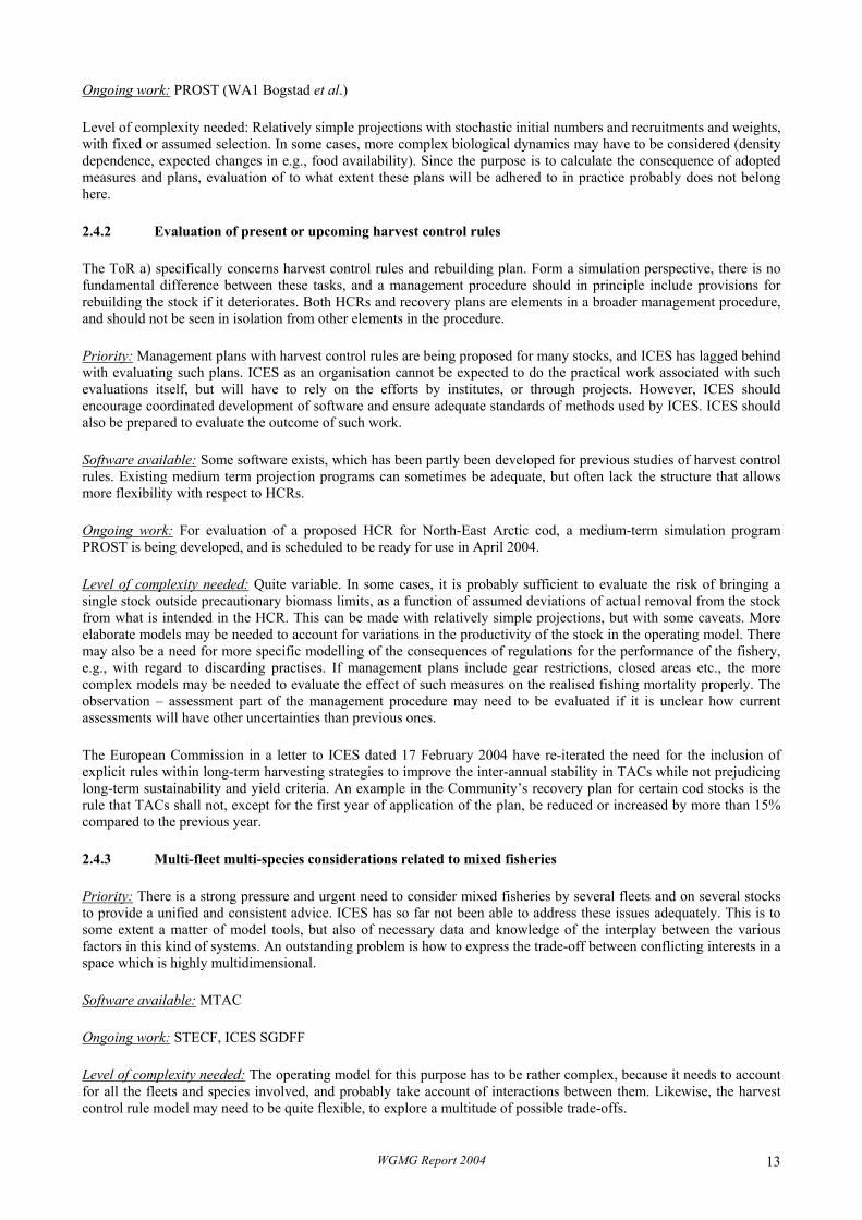
Ongoing work: PROST (WA1 Bogstad et al.)

Level of complexity needed: Relatively simple projections with stochastic initial numbers and recruitments and weights, with fixed or assumed selection. In some cases, more complex biological dynamics may have to be considered (density dependence, expected changes in e.g., food availability). Since the purpose is to calculate the consequence of adopted measures and plans, evaluation of to what extent these plans will be adhered to in practice probably does not belong here.

2.4.2 Evaluation of present or upcoming harvest control rules

The ToR a) specifically concerns harvest control rules and rebuilding plan. Form a simulation perspective, there is no fundamental difference between these tasks, and a management procedure should in principle include provisions for rebuilding the stock if it deteriorates. Both HCRs and recovery plans are elements in a broader management procedure, and should not be seen in isolation from other elements in the procedure.

Priority: Management plans with harvest control rules are being proposed for many stocks, and ICES has lagged behind with evaluating such plans. ICES as an organisation cannot be expected to do the practical work associated with such evaluations itself, but will have to rely on the efforts by institutes, or through projects. However, ICES should encourage coordinated development of software and ensure adequate standards of methods used by ICES. ICES should also be prepared to evaluate the outcome of such work.

Software available: Some software exists, which has been partly been developed for previous studies of harvest control rules. Existing medium term projection programs can sometimes be adequate, but often lack the structure that allows more flexibility with respect to HCRs.

Ongoing work: For evaluation of a proposed HCR for North-East Arctic cod, a medium-term simulation program PROST is being developed, and is scheduled to be ready for use in April 2004.

Level of complexity needed: Quite variable. In some cases, it is probably sufficient to evaluate the risk of bringing a single stock outside precautionary biomass limits, as a function of assumed deviations of actual removal from the stock from what is intended in the HCR. This can be made with relatively simple projections, but with some caveats. More elaborate models may be needed to account for variations in the productivity of the stock in the operating model. There may also be a need for more specific modelling of the consequences of regulations for the performance of the fishery, e.g., with regard to discarding practises. If management plans include gear restrictions, closed areas etc., the more complex models may be needed to evaluate the effect of such measures on the realised fishing mortality properly. The observation – assessment part of the management procedure may need to be evaluated if it is unclear how current assessments will have other uncertainties than previous ones.

The European Commission in a letter to ICES dated 17 February 2004 have re-iterated the need for the inclusion of explicit rules within long-term harvesting strategies to improve the inter-annual stability in TACs while not prejudicing long-term sustainability and yield criteria. An example in the Community’s recovery plan for certain cod stocks is the rule that TACs shall not, except for the first year of application of the plan, be reduced or increased by more than 15% compared to the previous year.

2.4.3 Multi-fleet multi-species considerations related to mixed fisheries

Priority: There is a strong pressure and urgent need to consider mixed fisheries by several fleets and on several stocks to provide a unified and consistent advice. ICES has so far not been able to address these issues adequately. This is to some extent a matter of model tools, but also of necessary data and knowledge of the interplay between the various factors in this kind of systems. An outstanding problem is how to express the trade-off between conflicting interests in a space which is highly multidimensional.

Software available: MTAC

Ongoing work: STECF, ICES SGDFF

Level of complexity needed: The operating model for this purpose has to be rather complex, because it needs to account for all the fleets and species involved, and probably take account of interactions between them. Likewise, the harvest control rule model may need to be quite flexible, to explore a multitude of possible trade-offs.

WGMG Report 2004 13

2.4.4 Evaluation of sampling and surveys - more rational use of existing resources

This may be a task in its own right, where managers address questions on cost –benefit of such activities. It may also be necessary in the evaluation of a management procedure, to investigate what is needed to have a performance of the procedure that is sufficient for compatibility with the precautionary approach.

Priority: Some projects have already addressed this question (e.g., EMAS, EVARES).

Level of complexity needed: A simulating framework for this purpose would have to address in detail the observation and assessment models of the management regime, and would need a correspondingly complex operating model. The complexity of the harvest rule, decision and implementation models depends on the purpose. If only the assessment quality is under scrutiny, they can probably be made rather simple.

2.4.5 Evaluation of harvest rules and the tools to implement them in a socio-economic context

These are studies of how management procedures may be expected to work in a more complex world, taking into consideration the possibility of deviations from agreed guidelines, future developments in fleet structure and economical conditions etc.

Priority: Some studies along this line have been undertaken, and ICES has been asked to evaluate them (e.g., BACOMA) Such studies will require competence outside the remits of ICES itself, and both for this reason and because of the workload, such work will need designated projects.

Software available: There may be software developed in previous projects that may be applicable in other projects, but in general, such projects must be expected to require a good deal of specific software development. The general framework and standards outlined in this report should serve as guidance.

Level of complexity needed: The high level of complexity will primarily be at the management decision and implementation models, as well as on the interaction between the fishery and the stock, in particular if gear restrictions, closed areas and other means of indirectly influencing the removal from the stock are included. This will probably also require a quite complex operating model. The complexity needed in the harvest control rule, the assessment and the observation models of the model framework will depend on the actual situation, but should not be made more complex than necessary.

2.4.6 Comprehensive simulations of management procedures

Evaluation of a complete system, including all aspects of monitoring, assessment, decisions implementations and effects of both the management and external factors, e.g., environmental conditions on the state and productivity of the stock is in principle desirable for any management procedure.

In a scientific perspective this will be a natural challenge. However, this will be a very large task, and it should be recognised that sensible advise most often can be provided by simpler means, provided that the features that matter most in practise are properly accounted for. Necessary managers actions should not be postponed by the scientific desire to make models that cover everything, even when a more comprehensive evaluation is foreseen later on.

2.4.7 Comment

The preceding Sections clearly demonstrate that software has been developed but that there is clearly a problem with inter-sessional work and co-ordination. WGMG suggests that there is an urgent need to identify candidate stocks for HCR evaluation and that this should be undertaken in consultation with ACFM at the earliest opportunity. Furthermore, work should commence on those stocks identified during 2004/2005.

2.5 Alternative approaches to management

Although the current implicit management procedure, as employed by ICES, is largely VPA-based the benefits of alternative assessment methods, data collection regimes, biological reference points and harvest control rules should also be investigated. For example, fishery-independent assessment methods based upon tagging data or research vessel surveys could be used as part of management procedures. WGMG recognized that new research into the use of tagging data within ICES stock assessments is desirable to address the current need within ICES for stock

WGMG Report 2004 14

assessment methods robust to uncertainty about the true dynamics of the fishery and biases in the data. In particular there is a need to develop alternative estimators of stock status and fishing mortality rates which are less affected by the type of biases found in traditional fishery-dependent data-sets (e.g., commercial landings data).

The use of tagging data to estimate mortality rates and abundance have been with us for over a hundred years and these methods have been applied in fisheries stock assessment for at least the last 40 years, for example, in Peterson estimation of salmon population abundance. While good examples of mark-recapture applications exist in many different regions, instances of application remain relatively uncommon within European fisheries. Some current applications include the following. Tagging data are used in CSIRO stock assessments of species including school shark and toothfish. In Canada there are several applications including near shore cod stock assessment off of Newfoundland, and sablefish and Chinook salmon stock assessment in British Columbia.

Mark-recapture experiments involving both conventional and data storage tags have been implemented over the last several decades for numerous European commercial fish stocks but the data from these yet remain largely unused in most European fish stock assessments (ICES 1992; Bolle et al. 2001; Hunter et al. 2001; Arnold et al. 2002). For example, mark-recapture data have been incorporated in stock assessments of Norwegian spring spawning herring for about twenty years, as simple mortality rate estimators in Atlantic mackerel stock assessments for about the last 10 years, and as harvest rate and abundance estimators in Baltic salmon stock assessment since 2002.

A large variety of tagging data-based estimators have been developed to provide estimates of a variety of population parameters (Hilborn 1990; Dorazio and Rago 1991; Rijnsdorp and Pastoors 1995; Brookes et al. 1998; Schwartz and Taylor 1998). These include abundance, natural and fishing mortality rates, migration rates and seasonal migration patterns at age, growth rates, diurnal migrations, stock-structure and catchability (Xioa 2000; Reynolds et al. 2001). Some tagging based estimators do not depend on commercial catch data. For example, a variety of multiple fleet, harvest rate estimators have recently been developed that incorporate fishing effort for multiple fleets (Brooks et al. 1998; Hoenig et al. 1998; ICES 2002, 2003b). Harvest rate estimators that also incorporate fishery independent survey data have also been recently developed (Martell and Walters 2001, Michielsens 2003; ICES 2003b). To some extent, the estimation properties of these latter estimators have been tested using simulated data and in some cases have been simulation tested in combination with harvest control rules (Martell and Walters 2001). However, relatively little effort has yet been devoted to simulation-evaluating the potential merits of tagging based estimators and harvest control rules within European fisheries contexts.

Before the tagging data can be incorporated into stock assessments, and harvest rules, a variety of issues need to be addressed and include the following.

• Can we devise a reliable sampling protocol taking into account the spatial and seasonal distributions of animals to tag a random sample of animals from the harvestable population (Arnold et al. 2002)?

• How many animals should be tagged per year to provide sufficiently precise estimates of harvest rates and abundance and what age or size classes of animals should be tagged?

• Can we devise a reliable protocol to recover sufficient numbers of tags? This may require efforts to inform fishermen of the tagging program and to offer various types of rewards to give fishermen incentive to return the tags and provide accurate information on the location, time and size of the fish upon recapture.

• Can we obtain adequate estimates of tag induced mortality rates, tag shedding rates, and tag reporting rates? • Which tagging-based estimators are best and how should tagging data be combined with other data; e.g., fishing

effort and fishery independent survey data, to provide improved estimates of harvest rates, abundance and migration rates?

• How should harvest control rules that incorporate tagging data be devised and simulation tested? Compile and develop a variety of tag-based estimators of harvest rates and stock biomass. Develop designs for mark recapture experiments. Develop harvest control rules based on mark-recapture methods. Use a management procedure evaluation framework to evaluate the potential performance of tag-based harvest

control rules through simulation. Based on available data and existing scientific knowledge, formulate plausible alternative hypotheses about

stock and fleet dynamics and use these to construct operating models for the simulation evaluations. Include among the harvest control rules evaluated fishing effort control measures. Compare the potential performance of mark-recapture based management procedures to current monitoring,

assessment and management procedures.

WGMG Report 2004 15

Apply statistical power analysis and existing data and expertise to help identify information experimental designs for tagging and sampling programmes.

Consider including in the investigation existing tagging, trawl and acoustic, fishing effort and other datasets and expertise for Norwegian spring spawning herring, Baltic salmon and North Sea flatfish and roundfish.

Previous studies on North Sea flatfish and roundfish stocks have used either conventional or data storage tags and these studies are proposed for a new focal case study to develop spatial and temporal operating models of stock dynamics. In addition, collation and analysis of historic data sets will also be conducted to help develop assessment models and assumptions for use in the study. The operating model will be used to evaluate management procedures based on conventional and/or hit tags (machine counts).

The study will also consider the effect of tag induced mortality rates, reporting rate, level of misreporting and discarding. Alternative strategies that encourage positive feedback such as TAC allocation based upon return rates will also be investigated.

2.6 Quality Control

Gentle (2003) pointed out that a simulation that incorporates a random component is an experiment and that the principles of statistical design and analysis apply just as they do to any other scientific experiment. Such studies should therefore adhere to the same high standards as any scientific experimentation. The reporting of a simulation experiment should receive the same care and consideration accorded to the reporting of any scientific study and Hoaglin and Andrews (1975) outlined the items that should be included in a report of a simulation study. For example, the journal Computational Statistics & Data Analysis, the official journal of the International Association for Statistical Computing includes relevant reporting standards in their guide-lines for authors. Therefore, descriptions of simulation studies must:

• clearly state the hypothesis under study; • be thorough with regard to the choice of parameter settings; • do not over-generalise the conclusions; • carefully describe the limitations of the simulations studies; • be easily reproducible; • guide the user regarding when the recommended methods are appropriate; • indicate why comparisons cannot be made theoretically and why therefore simulations are necessary; • provide enough information so that the quality of the results ca be evaluated; and • give descriptions or references of pseudo-random-number generators, numerical algorithms, computer(s),

programming language(s), and major software components that were used. 2.6.1 Outputs and summary statistics

The large amount of output that simulation models can generate means that careful thought has to be given to the question of how to present all this material. Outputs can be considered to fall in to one of three types:

- Diagnostics needed when conditioning the simulation model - Summaries and results for communication between scientists - Summaries for communication of results to managers and lay-persons

Decision tables (Hilborn et al. 1994) and influence diagrams (Kuikka et al. 1999) have proved to have much merit in synthesizing the results from such simulation studies and should thus be encouraged. Another example is provided by the range of summary statistics developed by IWC (Appendix H).

A discussion on ways to present results from simulation studies is contained in Peterman (2004) who describes methods from the social sciences such as Decision-choice experiments (Louviere and Woodworth, 1983) which efficiently describe the tradeoffs among performance statistics. Graphical presentations such as isopleths (Beverton and Holt, 1957) that show the trade-offs between different choices can be used. Especially if a simulation model is iteratively re-run to produce values for all indicators at each level of management action (Kell et al. 2003b, c). Argue et al. (1983) also illustrated how for a given situation, more than one indicator can be shown on separate isopleth graphs; as long as they have identical horizontal (X-) and vertical (Y-) axes, crosshairs placed at identical X-Y coordinates on the graphs

WGMG Report 2004 16

indicate values of those indicators. Movement of the crosshairs to a new location, representing a new set of management regulations, shows the tradeoffs among indicators that can be expected.

The need for reproducibility and revision of the results of this kind of analysis, especially given their potential complexity, could be ensured by the adoption of a audit chain approach (Section 2.2), where information regarding how exactly a model run or particular simulation is carried out gets incorporated into the results.

2.7 Related projects

Two studies commissioned by the EU have previously evaluated management strategies through simulation for seven major flatfish (MATACS - Kell et al. 2003c) and eight major roundfish stocks (MATES - Kell et al. 2003b) in the ICES area. These studies have been reviewed by both ACFM and STECF and in addition to the Study Group on Precautionary Reference Points for Advice on Fishery Management (ICES 2003a) recommended that in the future the choice of management strategies and biological reference points should be underpinned by the operational model/management plan framework as illustrated within the MATACS/MATES work.

In addition, there are several EU projects that are building tools for the evaluation of management strategies. Three STREPs (Specific Targeted Research Or Innovation Project) funded initiatives - COMMIT, EFIMAS and FISBOAT - are due to start in 2004 which will develop tools to evaluate management strategies. In addition there are three projects within an informal cluster comprising EASE, FEMS and PKFM which together are reviewing the current European advisory framework and developing tools to evaluate management strategies. These six projects are briefly described below.

COMMIT will develop multi-annual management strategies using a simulation framework that includes a bioeconomic model. Strategies will be implementation via scientifically based harvest rules that reduce annual fluctuations in exploitation strategy by setting appropriate technical measures, catch and effort limits and/or targets.

EFIMAS (Operational Evaluation Tools for Fisheries Management Options) will develop an operational management evaluation framework to allow evaluation of the trade-offs between different management objectives when choosing between different management options.

FISBOAT (Fisheries Independent Survey Based Operational Assessment Tools) will develop fish stock assessment tools based on survey data and independent of fisheries data

EASE (Evaluation of the European Advisory Framework) is reviewing the costs and benefits of the advisory process.

FEMS (Framework for the Evaluation of Management Strategies) is developing a prototype evaluation framework.

PKFM (Process Knowledge in Fisheries Management) is studying the flow of knowledge through the advisory process via a North Sea cod case study.

Other projects are currently being funded but these are those of principal note for WGMG and ICES.

Also of note is a working group set up by the Icelandic Ministry of Fisheries in 2001 with the aim of analysing the experience of using the HCR for Icelandic cod and trying out alternative approaches. The working group will deliver a final report in early 2004.

The Netherlands Institute for Fisheries Research is carrying out a national research project (bestek 6c-4) for their Ministry of Agriculture, Nature Management and Food Safety (LNV) on the evaluation of harvest control rules for North Sea flatfish. It is a simulation with an operating model (true system) and a management procedure (perceived system) implemented in FishLab in an Excel Visual Basic framework (Kell et al. 1999; Kell et al. 2001; Kell et al. 2002). The system includes two fleets and two species (plaice and sole) between which technical interactions exist. Economical factors are also considered. Several management scenarios are evaluated:

• Single species TACs. Here two scenarios are simulated: o The TACs are implemented without error

WGMG Report 2004 17

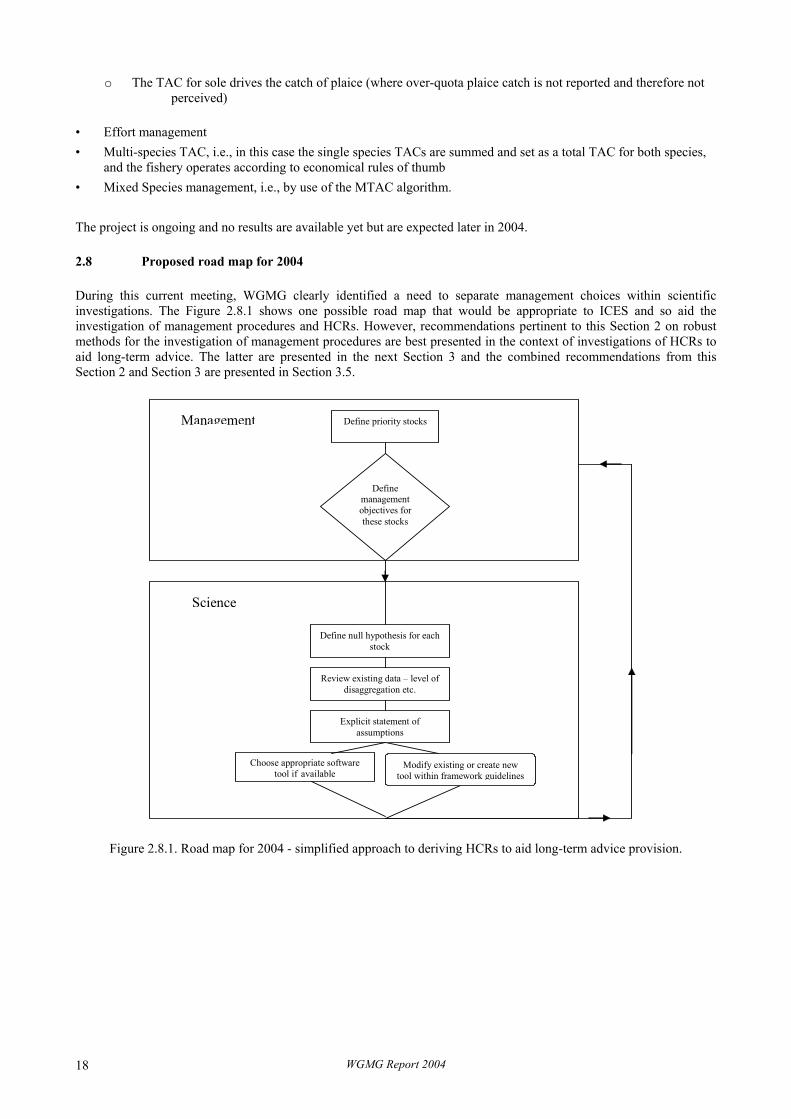
o The TAC for sole drives the catch of plaice (where over-quota plaice catch is not reported and therefore not perceived)

• Effort management • Multi-species TAC, i.e., in this case the single species TACs are summed and set as a total TAC for both species,

and the fishery operates according to economical rules of thumb • Mixed Species management, i.e., by use of the MTAC algorithm. The project is ongoing and no results are available yet but are expected later in 2004.

2.8 Proposed road map for 2004

During this current meeting, WGMG clearly identified a need to separate management choices within scientinvestigations. The Figure 2.8.1 shows one possible road map that would be appropriate to ICES and so aid investigation of management procedures and HCRs. However, recommendations pertinent to this Section 2 on robmethods for the investigation of management procedures are best presented in the context of investigations of HCRsaid long-term advice. The latter are presented in the next Section 3 and the combined recommendations from tSection 2 and Section 3 are presented in Section 3.5.

Define priority stocks

Define management objectives for these stocks

Define null hypothesis for eachstock

Review existing data – level ofdisaggregation etc.

Explicit statement of assumptions

Choose appropriate software tool if available

Modify existing or create new tool within framework guidelines

Management

Science

Figure 2.8.1. Road map for 2004 - simplified approach to deriving HCRs to aid long-term advice provision.

WGMG Report 2004 18

ific the ust to his

3 ASPECTS OF MANAGEMENT PROCEDURES

3.1 Current advice framework

The process of revising the precautionary reference points in ICES has been protracted for several reasons. One is that developing objective and consistent methods for calculating the reference points according to ICES’ definitions has proven difficult. For the limit points the problem has been addressed by the use of segmented regression (BB1 O’Brien et al. 2003). In general (ICES 2002), change-point estimates were judged to be more justifiable when there is an unambiguous stock and recruitment signal in data sets with a wide dynamic range. However, even when there is a good statistical fit to the data the change-point was less acceptable in cases where the stock-recruitment signal appears to be confounded by known biological, fishery or environmental factors, or when there is no clear stock and recruitment signal, or when the data set is restricted.

It is recognised that as a general rule, there is a need for limits representing danger zones that need to be avoided to be in accordance with the Precautionary Approach (PA). For the PA points, a procedure was suggested based on retrospective errors in assessments. This procedure was adopted for NEA cod (ICES 2003a), but proved both to require a substantial amount of work and to be conditional on the method for making catch projections. Software for streamlining this process has been requested, but has not yet been developed.

So far, reference points have focussed on protecting against recruitment failure. The Fpa is intended as a value of the assessed fishing mortality that, taking assessment uncertainty into account, carries a low risk that the real exploitation will lead to impaired recruitment. Therefore, the Fpa has in effect become the de facto target.

There is a growing appreciation that the PA points are not sufficient, in themselves, for the provision of long-term advice on rational management. The issue was raised most recently by the ICES SGPA (ICES 2002). In particular, there is a strong need to establish targets, in addition to these conservation reference points. It is also recognised that targets cannot be seen in isolation from the management framework and objectives. In order to serve management objectives, more elaborate harvest rules than single target reference points may be needed. Hence, targets should not be regarded as single values of fishing mortality or biomass, for example, but rather as parameters in harvest rules. Harvest rules at various levels of sophistication, and with various legal status have already been established for several stocks. Such harvest rules need to be evaluated with respect to the Precautionary Approach, as well as for their performance in relation to management objectives.

3.2 Objectives (from MoU)

Starting in 2004, ICES advice will be changed in several aspects, as outlined in the new MoU between the European Community and ICES. The objectives are:

• changing the advice from mainly short-term to long-term; • transformation of the traditional stock based advice to fisheries based advice; and • fisheries advice be revised to include long-term considerations of management targets relating to inter alia yield by

developing concepts for management targets; identifying targets for individual stocks; developing methods to evaluate Harvest Control Rules (HCR) and recovery plans; and developing an advisory framework based upon long-term advice with short-term implications.

Within the draft MoU, which is expected to be signed this spring 2004, it states:

2.1. Where management plans including a harvest rule for setting TACs or levels of effort have been adopted in the context of management plans, ICES shall advise on the levels of either or both catch and effort consistent with such rules. ICES shall also advise on the consistency of such plans with precautionary criteria.

2.2. ICES shall advise on the level of catch (and where appropriate the corresponding level of effort in appropriate units) consistent with the long-term sustainable exploitation of the stock1 if different from advice provided under 2.1 above. ICES shall make available detailed explanations and the supporting analyses on which the advice is based.

1 Application of the method shall ensure that the spawning biomass shall, with high probability, recover to or remain above the threshold below which recruitment is impaired or the stock dynamics are unknown.

WGMG Report 2004 19

2.3. ICES shall advise on the level of catch consistent with taking high long-term yields and achieving a low risk of depleting the productive potential of the stock, if this is significantly different from advice provided under Paragraph 2.1 after taking into account ecosystem considerations.

In addition, to the MoU between the European Community and ICES, ICES has to develop within the UN agreements and guidelines, a consistent and credible framework for long-term targets in fisheries management. When this has been achieved, ICES will then need to work on the corresponding short-term implications.

3.3 Elements of management procedures

Accounting for assessment uncertainty and error in the implementation of management procedures must be an integral part of choosing biological reference points for use in harvest control rules. WGMG suggests that reference points are better developed within the context of a management procedure and can be regarded as parameters in the harvest control rules, which are tuned (c.f. IWC 1993) to achieve management objectives. It is recognised that there is wide range of possible rules, which will require different kinds of parameters.

Our knowledge of stock and fishery dynamics will always be incomplete making it difficult to choose between alternative hypotheses about the dynamics. There is also confounding between changes in the dynamics and the response to management so that it is not always possible to distinguish between real effects and biases in the data. However, the provision of advice, in respect of management objectives, cannot be postponed until we have full knowledge of the relevant processes. It is therefore important, that any advice is robust to our uncertainty in the dynamic processes and our ability to monitor and control them and variability in key population parameters.

3.3.1 Limit/target biomass and F reference points

Biological reference points are an integral part of single species management advice frameworks and are used to provide advice on safe biological limits and targets. Fishing mortality reference points such as FMSY (or in practice, proxies such F0.1, Fmax) are used to define targets and Fcrash (or proxies Floss and F*) to define limits. Limits and targets can also be defined for biomass; for example, the SSB that would support the maximum yield (BMSY), can be used as a target and the point at which recruitment declines (e.g., S* as defined in BB1 O’Brien et al. 2003) as a limit.

Due to uncertainty in estimates of stock status and reference points once a reference point has been chosen it is necessary to derive confidence or probability distributions so that the reference point can be avoided (in the case of a limit reference point) or achieved (in the case of a target reference point). Where management objectives are to achieve high sustainable yields then an appropriate target might be a lower percentile of the probability distribution of a proxy of FMSY. Likewise if the management objective is to prevent stock collapse then an appropriate target might be a lower percentile of a proxy of Fcrash. A simple approach initially adopted by ICES when a limit reference point was defined was to set a lower limit for fishing mortality reference points as θF*exp(-1.645*σ), or an upper limit for biomass as θB*exp(1.645*σ), where typically σ = 0.2 or 0.3 (and where θF or B represents the fishing mortality/biomass reference points). Advice is then derived for a fishing mortality equal or less than the Fpa level.

However, this approach ignores the fact that reference points only make sense within a management framework and the probability of achieving a target or avoiding a limit is dependent upon our ability to monitor and assess the stock and to regulate fishing activity. A more objective approach therefore is to compare the performance of reference points (i.e., the proxies) within a management procedure to the actual quantities using simulation. The choice between candidate reference points can then be made on the basis of their ability to correctly predict whether the stock is above or below a given limit or target reference point and thereby initiate management action. It should be recognised that reference points are linked, i.e., the choice of an F-limit or F-target will determine the probability of exceeding a limit biomass reference and vice versa. Therefore, management procedures should be constructed that explicitly recognise this linkage. For example, if it is hard to estimate biomass reference points then the stock should be managed so that the outcome of the management procedure is not highly dependent upon a biomass reference point.

A scenario approach was used by O’Brien et al. (2003) (BB1) to investigate the robustness of the change-point method for estimating S* (the point at which recruitment is impaired). The fishing mortality, that if maintained indefinitely, would drive the stock to extinction, can then be determined by the slope of the stock–recruitment curve at the origin. It appeared from the simulations that systematic departures in the data tend to increase the bias in the estimate of S* to a greater extent than F* (the fishing mortality corresponding to the slope at the origin from a segment regression fit to stock-recruitment data).

WGMG Report 2004 20

The choice of a parametric function for stock-recruitment modelling is always problematic and hence, the estimation of reference points. Parametric models are often successful in describing the pattern of expected recruitment within the observed range of stock sizes. The question arises of which model(s) to use. There is seldom any overwhelming biological reason to select one model over another a priori, so the choice is usually based on goodness-of-fit. Nonparametric methods for fitting stock-recruit relationships that avoid the arbitrary restrictions of parametric forms represent one potential solution to this problem.

Bravington et al. (2000) (BB5) proposed a nonparametric method CONCave Recruitment (CONCR) to estimate the slope at the origin and its lower confidence limit. This confidence limit can then be used to derive lower bounds on Flim. F-based reference points using the 75th, 90th and 95th percentiles of the slope at the origin derived from CONCR are contrasted with current values of Fpa and Flim, F0.1, Fmax, and F30%SPR in Table 3.1.

WGMG Report 2004 21

Table 3.1 Fishing mortality reference points for the main ICES stocks. Stocks for which the estimated limit reference point based on the 75% confidence limit estimated using CONCR (denoted CONCR 75%) was greater than 2 have been removed.

Stock F0.1 Fmax spr.30 Fpa Flim CONCR 75% CONCR 90% CONCR 95% anb-78ab 0.10 0.15 0.13 0.23 0.00 0.35 0.32 0.31 anp-78ab 0.06 0.09 0.09 0.24 0.33 0.32 0.30 0.30 cod-2224 0.16 0.26 0.23 0.00 0.00 1.63 1.46 1.37 cod-2532 0.16 0.27 0.26 0.60 0.96 0.92 0.86 0.82 cod-347d 0.18 0.29 0.21 0.70 0.90 0.83 0.81 0.80 cod-7e-k 0.17 0.29 0.24 0.68 0.90 0.75 0.72 0.70 cod-arct 0.14 0.29 0.18 0.40 0.74 1.90 1.71 1.62 cod-coas 0.27 0.52 0.22 - - 0.33 0.31 0.30 cod-farp 0.17 0.37 0.27 0.35 0.68 0.61 0.56 0.54 cod-iceg 0.16 0.33 0.21 - - 1.21 1.07 1.02 cod-iris 0.16 0.30 0.25 0.72 1.00 1.44 1.37 1.32 cod-kat 0.13 0.21 0.21 0.60 1.00 0.83 0.80 0.79 cod-scow 0.16 0.26 0.24 0.60 0.80 1.00 0.95 0.93 ghl-arct 0.07 0.14 0.09 - - 0.42 0.39 0.38 had-7b-k 0.34 0.59 0.39 - - 0.82 0.74 0.70 had-arct 0.19 1.09 0.18 0.35 0.49 0.78 0.68 0.63 had-faro 0.18 0.51 0.29 0.25 0.40 0.53 0.44 0.40 had-iris 0.19 0.35 0.28 0.50 0.00 1.45 1.20 1.08 her-2532 0.26 1.26 0.41 0.17 0.33 0.40 0.36 0.34 her-2532-gor 0.26 1.26 0.41 - - 0.47 0.42 0.40 her-30 0.16 0.49 0.32 0.21 0.30 0.17 0.16 0.15 her-31 0.15 0.31 0.21 - - 0.43 0.36 0.33 her-3a22 0.20 0.37 0.24 - - 0.65 0.60 0.58 her-irls 0.17 - 0.34 0.00 0.00 0.67 0.61 0.57 her-riga 0.27 1.03 0.40 0.40 0.00 0.37 0.34 0.33 her-vian 0.17 - 0.25 - - 1.13 0.96 0.88 hke-nrtn 0.10 0.17 0.16 0.25 0.35 0.35 0.33 0.32 hke-soth 0.15 0.24 0.20 0.00 0.00 0.48 0.46 0.45 mac-nea 0.19 0.66 0.33 0.17 0.26 0.34 0.30 0.29 mgb-8c9a 0.14 0.41 0.33 - - 0.30 0.26 0.25 mgw-78 0.11 0.20 0.18 0.30 0.44 0.41 0.38 0.36 mgw-8c9a 0.12 0.32 0.27 - - 0.30 0.27 0.26 nop-nsea 3.00 - 1.31 0.00 0.00 0.53 0.45 0.40 ple-celt 0.11 0.28 0.16 0.00 0.00 0.64 0.58 0.55 ple-eche 0.10 0.19 0.13 0.45 0.54 0.58 0.57 0.56 ple-echw 0.10 0.22 0.15 0.45 0.00 0.57 0.54 0.53 ple-iris 0.13 0.31 0.17 0.45 0.00 0.57 0.54 0.52 ple-kask 0.10 0.20 0.16 0.73 0.00 1.47 1.13 1.00 ple-nsea 0.11 0.23 0.14 0.30 0.60 0.51 0.46 0.43 sai-3a46 0.12 0.23 0.16 0.40 0.60 0.57 0.54 0.52 sai-arct 0.11 0.24 0.15 0.26 0.45 0.69 0.61 0.58 sai-faro 0.16 0.42 0.21 0.28 0.40 0.36 0.34 0.33 san-nsea 0.73 - 0.54 0.00 0.00 0.79 0.69 0.63 sol-bisc 0.10 0.20 0.14 0.36 0.50 0.49 0.48 0.47 sol-celt 0.10 0.24 0.15 0.37 0.52 0.92 0.78 0.72 sol-eche 0.13 0.31 0.17 0.40 0.55 0.44 0.42 0.41 sol-echw 0.12 0.38 0.15 0.20 0.28 0.26 0.25 0.25 sol-iris 0.16 0.39 0.19 0.30 0.40 0.34 0.31 0.30 sol-kask 0.20 0.65 0.27 0.30 0.47 0.74 0.60 0.54 sol-nsea 0.13 0.34 0.15 0.40 0.00 0.61 0.53 0.49 spr-2232 0.52 - 0.87 0.40 0.00 1.12 0.89 0.78

WGMG Report 2004 22

Table 3.1 and Figure 3.1 show that reference points based upon CONCR are very similar to, and highly correlated with, current Flim values, which in general are based upon Floss (Cook 1998; O’Brien 1999). Since the CONCR reference points are similar to the Flim points, there is no compelling reason to replace the current Flim values adopted by ICES.

The candidate target fishing mortalities (F0.1, Fmax, F30%SPR) are essentially proxies for FMSY. Figure 3.2 shows that whilst the candidate target fishing mortalities (F0.1, Fmax, F30%SPR), with each other, they appear not to be correlated with Fpa, which is used as a de facto target. This implies that changing from Fpa to one of these candidate targets has strong implications for management but the effect will be stock specific.

Rebuilding plans are a special case of HCRs. However, procedures used to rebuild a stock to an agreed target level may need to have different properties from those used to maintain a stock at that target level. For example, in the short-term technical interactions will be of more importance that biological interactions.

Figure 3.1. Fishing mortality limit points for the main ICES stocks given in Table 3.1. Stocks for which Flim is not defined or the estimated limit reference point based on the 75% confidence limit estimated using CONCR (CONCR 75%) was greater than 2 have been removed. Note that the points relating the Flim and CONCR values lie roughly along one of two lines – this is possibly due to different methods of estimating Flim.

WGMG Report 2004 23

Figure 3.2. Candidate target fishing mortalities and Fpa points for the main ICES stocks given in Table 3.1. Stocks for which Fpa or Fmax is not defined have been removed.

3.3.2 Variability in biological reference points and ecosystem effects

ICES has so far hesitated to apply MSY as a target. The justification for this has been that MSY often is ill-defined and influenced by density dependence and multi-species effects (ICES 2001). Any consideration of reference points concerned with long-term yield needs also to consider the wider ecosystem context of the stock. Gislason (1999) considered multi-species reference points for Baltic cod, herring and sprat, taking into account the interactions between them. This analysis also included density dependent growth of cod. It turned out that in terms of maximising yield the optimal harvesting in this ecosystem would be to fish out the cod stock. Even if economics is taken into account by assuming the price per kg of cod is 10 times the price on herring and sprat, this conclusion still holds. Gislasson notes that such a result stresses the need for incorporating socio-economic considerations in the definition of target reference points. He also concludes that reference limits for forage fish cannot be defined without considering changes in the biomass of their natural predators, and likewise, reference limits for predators cannot be defined without considering changes in the biomass of their prey.

The work of Gislason (1999) was based on the Baltic Sea, which has relatively few stocks, with a simple predator-prey interactions. Similarly simple interactions have been noted e.g., in the Barents Sea (Cod/Capelin/Herring) and off Iceland and Newfoundland, where shrimp stocks have increased following depletion of cod stocks. However, even in these relatively simple cases it would not be appropriate to set reference points for one stock without also accounting for the consequences these would have for the other stocks in the ecosystem. In more complex ecosystems it is much less straightforward to predict the effect of managing the size of a give predator or prey population. However, based on their

WGMG Report 2004 24

analysis of the sensitivity of biological reference points to species interactions, Collie and Gislason (2001) note “The demographic parameters that underlie biological reference points change on the time scale of fish generations (5–10 years). For medium-term advice it may suffice to consider only one-way trophic interactions between harvested species and to categorize each species as a predator or prey. Prey reference levels then can be conditioned on the prevailing predator abundance and vice versa.”. With regard to the North Sea, ICES (2003) concluded that: … The validity of the Flim values derived from Blim in a single-species framework depends on how well the assumed natural mortalities represent the actual state of the system.

For fisheries where some or all of the target stocks are over-fished, then biological interactions may be of secondary importance. This situation will change as stocks recover and increase. Under these circumstances, it becomes more important to consider both management targets and species interactions.

Fish stocks can fluctuate extensively over a large range of spatial and temporal scales independently of human exploitation (e.g., Hjort 1914; Cushing 1976). Such fluctuations are often ascribed to stochastic variations in key processes, such as recruitment, growth, survival or migration, in relation to environmental changes (see e.g., Hjort 1926; Ottersen 2000; Bailey 1989; Bjørnstad 1999; Fortier 1996; Dickson 1993; Lehodey et al. 1997). The result of environmental influences on fish biology is that the productivity of the stock may change, and with this the safe biological limits to exploitation (Basson 1999). For example, the environment can affect the survival of eggs/larvae/juveniles either through the food supply or habitat. Two hypotheses can be put forward. The first, and perhaps most commonly proposed scenario, is that temperature affects juvenile survival; i.e., the alpha parameter of the ricker stock-recruitment relationship (Stocker et al. 1985), e.g., Planque and Fredou (1999) and Clark et al (2003). Alternatively temperature may affect carrying capacity (i.e., the beta parameter) so that temperature acts to limit survival of individuals Fromentin et al. (2001). The consequences for biological reference points will be different depending upon the true relationship. Kell and Bromley (2004) also showed that expected recruitment and growth of North Sea plaice can change within a decadal time scale. Whilst it can be difficult to detect changes in population abundance, it is more difficult to detect changes in biological reference points and therefore to develop appropriate management strategies.

In the wider context of the ecosystem implications of fishing, managers may want to address wider considerations than just individual stock target levels. This again indicates that consultation with managers and other stakeholders would be an important component of any attempt to establish long-term reference points.

3.3.3 HCRs

Within the draft MoU between the European Community and ICES (discussed in Section 3.2), there is a requirement for ICES to evaluate harvest rules in the context of management plans. Limit and target reference points can both be used in HCRs. The actual form of the HCR will depend upon the type of data and estimators of stock status used. For example, the requirements for management procedures based on tagging data may be quite different from those based upon Virtual Population Analysis (VPA). To illustrate the diversity of possible limits and targets, one may consider the three following examples of types of HCRs (Skagen et al. 2003): • F-based rules where the primary decision is on the fishing mortality to be applied. This includes, for example,

effort regulation and technical measures. • Fixed catch rules, where a certain amount to be caught is the primary element, independent of the current

perception of the stock abundance, but with some rule to reduce the catch if the stock appears to become dangerously small (WB1 Skagen)

• Escapement strategies, where a certain spawning biomass is set aside and the rest of the spawning stock can be caught. This is the current management regime for capelin.

In addition, there can be combinations of these, typically fixed F regimes with additional constraints on variation in the annual TAC, which has been proposed recently for several stocks.

Each of these requires parameters like the standard F, the fixed catch or the escapement biomass to be applied. Furthermore, there also needs to be limits representing the outer bounds compatible with the precautionary approach, as well as trigger points where remedial action is taken to avoid the limit points.

The choice of harvest rule should be according to managers’ objectives, the dynamics of the stock and the availability of reliable data and assessments. In particular, if the assessment is uncertain or data do not allow a reliable assessment, other harvest rules than those where a catch is advised based on the current perceived state of the stock and a target fishing mortality, may be advisable. The choice and detailed formulations should also be adapted to the time frame for

WGMG Report 2004 25

which the rule is supposed to cover, in particular in recovery situations. This relates to the trade-off between safe and rapid recovery and the need to reduce the problems for the industry.

For species that experience strong interactions with other species, apparently relevant targets set for each species may not be achievable in a multi-species system. MSY for each of the species will depend on the state of the others, and reflect that there will be a trade-off between species that to some extent is a manager’s decision problem. Likewise, harvest rules for groups of stocks in mixed fisheries need to account for the trade-off between fleets and species, as outlined in Section 2.4.3.

Excluding interactions (e.g., multi-species multi-fleet), simplifies the simulation of harvest control rules. Given the nature of pelagic fisheries generally, many of the pelagic stocks lend themselves to single species (and in some cases single fleets) simulations, which could be used to evaluate simple harvest control rules. Indeed there are already a number of pelagic stocks for which single species harvest control rules currently exist, such as North Sea herring, and Norwegian spring spawning herring. Harvest control rules have been evaluated (and adopted) for the Icelandic cod stock. Although harvest control rules are in place for Iceland-Jan Mayen-Greenland capelin and Icelandic summer-spawning herring, they have not been formally evaluated. Empirical track records indicate that they have been successful.

As already proposed in Section 2 of this report, harvest control rules could be considered in the short-term with existing software (perhaps with minor extensions) for some stocks (see Section 2.3, Appendix I and Section 3.5). These are stocks with a relatively stable productivity (variation in recruitment, growth and maturity with stationary distributions), a long time series of data, low levels of technical interactions and exploited in a single species context and with insignificant (i.e., low) levels of discarding. Some candidates stocks are:

• NEA mackerel: candidate for multi-annual TAC (c.f. ICES 1999); • herring in VIa (North), Irish Sea, North Sea and Celtic Sea; • saithe in the North Sea and North East Arctic saithe; and • North-East Arctic cod. In this context, the recently agreed single species recovery plans for cod stocks (such as Irish Sea, North Sea and West of Scotland) and northern hake might also be evaluated.

3.4 Hypothesis testing

As the framework of advice changes towards the long-term evaluation of harvest control rules, the simulation process to evaluate a given harvest control rule should be designed in a way to control the most important type of errors for stock management. In the classic hypothesis testing terminology the Type I error corresponds to rejecting the null hypothesis, whereas the null hypothesis is actually true. The probability of a Type I error occurring is referred to as α. The Type II error corresponds to not rejecting the null hypothesis (and therefore accepting it)2, whereas there actually does exist a deviation from the null hypothesis. The probability of a Type II error occurring is referred to as β, and 1-β is the statistical power of the test: the probability of detecting an existing deviation from the null hypothesis. It is therefore very important to be explicit about the null hypothesis being tested, so that it is clear what the Type I and Type II errors are.

Certain authors (Hoenig and Heisey 2001) believe that experiments planned to test a given hypothesis (H0) should not be used to make inference on the alternative hypothesis through power analysis. Moreover, in many situations power calculations are difficult to carry out. Therefore, it is good practice when planning an experiment to define clearly the error of interest and therefore the hypothesis of interest – to be defined as H0.

In a fisheries context, one could state the null hypothesis in two ways:

1) H0: SSB is at or above the limit biomass level Blim 2) H0: SSB is below the limit biomass level Blim and carry out experiments controlling the Type I error, which would have a different meaning in the two hypotheses above. In the first case, a Type I error occurs when the fishery is regulated needlessly, whereas in the second case a

2 Technically, not rejecting an H0 does not imply that H0 is true.

WGMG Report 2004 26

Type I error occurs if the fishery is not regulated when it should be. The choice of which null hypothesis to test is to be made by the managers, however to be in agreement with the precautionary approach the 2nd null hypothesis should be chosen. Testing that hypothesis would put the burden of proof on those willing to exploit the resource, who would have to prove that the stock is at or above Blim by being able to reject the null hypothesis. The Type I error in this case would be that one concludes that SSB is not below Blim, when SSB is actually below Blim. The probability of this Type I error occurring can be controlled by setting α at a low level such as 0.05 or 0.01.

The current ICES advisory framework may be considered in this way for the relationships between current stock status, and biomass and fishing mortality limits:

Biomass limits

H0: SSB is below the limit biomass level Blim

Type I error: the stock is below Blim but the assessment procedure predicts that the stock is at or above Blim.

true SSB <Blim

estimated SSB >Blim

Type II error: the stock is at or above Blim but the assessment procedure predicts that the stock is below Blim.

true SSB >Blim

estimated SSB <Blim

Fishing mortality limits

H0: fishing mortality is above Flim

Type I error: the stock is overfished (F above Flim) but this is not detected by the assessment procedure.

true F >Flim

estimated F <Flim

Type II error: the stock is not overfished (F is below Flim) but the assessment procedure predicts that overfishing is occurring.

true F <Flim

estimated F >Flim

Managers should provide guidance on the balance between tolerating Type I or Type II errors, with regard to risk, because the cost of committing a Type I or II error differs depending upon the circumstances. For example Peterman (1989) – taking H0 to be that the stock is not declining! – pointed out that if a stock is rapidly declining in abundance but is being managed as if it were relatively constant because of low-power data, Type II error could lead to collapse of the stock and loss of all future revenue. Type I error under this H0, on the other hand, would arise if data incorrectly led to the conclusion that the stock was declining and harvesting was reduced. The cost of reduction in fishing in the latter case would be smaller than that caused by the total collapse of the fishery unless discount rates and present value concepts (Clark, 1976) altered their relative values. Trade-off analysis may help reveal the preferences upon which policies are based and may also suggest priorities (Nicholas, 2002).

By using a simulation framework, the probability of occurrence of Type I and II errors and hence the performance of biological reference points can be evaluated.

WGMG Report 2004 27

A well-planned hypothesis testing procedure has to be part of a carefully designed experimental plan. This means that some steps have to be taken before starting any computer simulation. These are well described in any good experimental design book (e.g., Montgomery, 2000), and involve for example:

• to state clearly the hypothesis to be tested • which is the control treatment • which factors are to be included in the experiment • use an appropriate design to change factors (e.g., a factorial design) • the range of variation of each factor • what is the response variable to be measured (one or more) • if any randomisation restrictions should be applied (e.g., blocking) • how many replicates will be necessary The analysis of the results of a well-designed experiment may suggest alternative data collection, monitoring, assessment and regulatory regimes as well as a choice of biological reference points to be tested against a range of plausible hypotheses about stock dynamics. This is important since the correct identification of changes in abundance of fish stocks is made difficult by large variability in mortality, growth and reproduction rates, as well as errors inherent in stock assessment and sampling methods (Peterman 1989) and the possibility of non-stationarity in biological reference points (Fromentin et al. 2001).

Alternative management procedures and exploration of their costs and benefits with respect to current practice could also be evaluated.

3.5 Recommendations

In the earlier Section 2.8, WGMG recognized the need to separate management choices within scientific investigations. One possible road map was identified that would be appropriate to ICES and so aid in the investigation of management procedures and HCRs in the short- to medium-term (see Figure 2.8.1).

Combined recommendations for the previous Section 2 and this Section 3 of the report are presented next in this Section 3.5. These are pertinent to the identification of robust methods for the investigation of management procedures and to the investigations of HCRs to aid in the long-term provision of advice.

1) It is recommended that in the future, management procedures be submitted to a rigorous testing procedure in which their performance, with respect to pre-agreed objectives, can be compared. This will require them to be thoroughly tested against underlying operating models that represent the best available understanding of the actual system dynamics. Thus, operating models will be used to test the performance of the models that are to be considered for application and in general the operating models will be far more complex than the ones considered for actual application. The operating models should capture the characteristics of the underlying dynamics but will not necessarily model the full complexity of them.

2) In the short-term, technical interactions will be more important than ecosystem considerations. However, ecosystem considerations will become more important in the longer-term once there is a concerted move towards lower fishing mortalities.

3) Recognise that reference points are proxies for biological processes that show time dependent variation.

4) HCRs must be developed as a high priority within ICES using available tools and methods, in the first instance.

5) HCRs are only one part of the management process and in the future there will be a need to move to a more rigorous approach based upon simulation testing of management procedures against plausible hypotheses concerning system dynamics.

6) There is an urgent need for a common software framework to allow the building of simulation models.

7) Whilst general tools and principles can be developed, implementation must occur on a case-by-case basis.

WGMG Report 2004 28

8) Although both biomass and F based reference points are required by international agreements it appears from simulation studies that F-based reference points may exhibit better properties than biomass based ones. In such cases management procedures that minimise the reliance on biomass reference points should be developed.

9) The necessary methodology is well developed but currently there appears to be a lack of any mechanism by which the necessary work can be performed within ICES. WGMG suggests that this needs to be rectified as soon as possible and will be raised by the WGMG Chair at the ICES Study Group for Long-Term Advice [SGLTA] which meets at ICES Headquarters, Copenhagen, Denmark from 23–28 February 2004.

10) Current Flim reference points appear to be consistently defined.

11) If proxies for FMSY (e.g., F0.1) are to be used as the basis for providing advice then these will have to be reviewed on a case by case basis.

12) Guidance must be solicited from managers on the balance between tolerating Type I and/or Type II errors, since the cost of committing a Type I and/or Type II error differs depending upon the circumstances. For example, if a stock is rapidly declining in abundance, a type II error could lead to collapse of the stock and loss of all future revenue; whilst a Type I error would only result in a reduction of yield in the short-term.

13) Simulation models must be regarded as a means to test hypotheses and have to be part of a carefully designed experimental plan.

14) An initial list of candidate stocks for which to evaluate harvest control rules has been proposed in Sections 2 and 3.3.3. Amongst these are included the recently agreed single species recovery plans for cod stocks and northern hake.

The following is a list of some software tools that can help to address to varying degrees the tasks detailed above.

Revising existing simulation software (e.g., WGMTERM, ICP, STPR, CS4):

Standard medium-term prediction software, which to a variable extent can be used for simple evaluations of simple harvest control rules. These programs need to be revised to allow a variety of ways of incorporating uncertainty (variables that are stochastic, assumed probabilistic distributions), outputs to allow the inspection of simulated distributions to compare them with historical data, and documentation of algorithms and assumptions. The framework outlined in Section 2.1 should be followed as far as possible, and the documentation should be structured in accordance with this framework. This will require work primarily by the authors of these programs, but should not be a major job. The STPR program will probably be substituted to a large extent by the PROST software that is scheduled to be ready for use in April 2004.

Software for evaluating mixed fisheries:

The forecast parts of the multi-species programs 4M (formerly, MSVPA-MSFOR) included simulations of harvest rules that can be used for evaluation of some such rules in a multi-species/multi-fleet context. Such an evaluation was made for the North Sea recovery plan (ICES 2003b: Report of the Study Group on Multi-species Assessment in the North Sea. ICES CM 2003/D:09) It is run in a SAS environment and requires some skill to use. In addition, the MTAC software is also available for simulating mixed fisheries harvest rules (WD4 Kraak; Vinther et al. 2003). The WGNSSK used this software, but it was not accepted by ACFM. At present there are no plans to revise the software, as the SGDFF considered that the implementation of the HCR was not compatible with the requirement for relative stability. Thus, developing software for the evaluation of mixed fisheries is still a major task that cannot be expected to be completed within 2004.

Software for comprehensive simulations of management regimes:

This includes all software that requires a level of complexity beyond that considered above. Such software was used for the MATACS/MATES projects. This software is modular and requires considerable input from the user to build a simulation model. The FEMS computational framework (Section 2 and Appendix J) aims at making the methodology available to a wide range of users. The time frame for this development is two (2) years.

WGMG Report 2004 29

4 DIAGNOSTICS, UNCERTAINTY AND EVALUATION IN ASSESSMENT METHODS

4.1 Introduction

Currently within ICES there is a need to explore the use of less strongly-conditioned methods and to provide advice taking into account the possibility that different assessment model formulations may be equally valid. In addition, the reliability of commercial catch statistics is continually being called into question and there is a need for fishery-independent assessment methods.

These form the basis of the ToRs d)-f) which are addressed in this Section 4 of the report.

4.2 Diagnostic analysis

4.2.1 General data screening and diagnostics

Simple visual tests of survey data can by provided by normalised index plots (e.g., Figure 4.3.2.9.1), or by plotting pair wise bivariate scatterplots of the survey indices by age . These can be presented in the form of linear regressions fitted through the scatter of points that can help to determine whether significant relationships between the survey indices exist (ICES 2004 WGNSSK).

Most catch-at-age data sets are available with considerable spatial information, and therefore it is suggested that (where possible) data screening and exploratory analysis be carried out on spatially-disaggregated data. This may assist in understanding the reason for patterns in assessment diagnostics and for conflicting information.

Some further data-screening and diagnostics that may be useful are:-

• Check for missing data in catch-age matrices. For example, in the NRC simulated dataset (see Section 4.3.1) there are many zeros in the survey catch-age data for ages 10–15. If the statistical approach treats the zeros as zeros, when the zeroes might actually reflect low sampling intensity or a failure to enter actual observed values, it might then be decided to exclude data from the analysis for ages 10+. Also, the common practice of giving zeroes zero weight will often introduce some bias in the assessment.

• Plot commercial yield versus effort and evaluate whether the points fit a line fitted through zero (see, for example, Figure 4.2.1.1). Pronounced non-linearity may indicate that commercial catchability is not constant.

• Plots of catch curves can be used for both visual inspection of internal consistency within a tuning series, and for comparison of series. Catch curves can indicate non-stationarity of selectivity patterns, which (if present) would be apparent as shifts between years in the age of maximum normalized catch-rate. Further information may be available if catch curves are positioned relative to the year in which they enter the dataset. Examples are given below both raw (Figure 4.2.1.2) and smoothed (Figure 4.2.1.3) catch curves. Catch curves where the larger cohorts have a steeper catch curve could be indicative of underlying differences in catchability, but could also indicate age reading problems. Increasing age reading problems with increasing age would tend to transfer fish from the neighbouring cohorts to the weaker ones and thus increase their abundance index. Points belonging to the same year class are usually connected with a solid line in a catch-curve plot, but the additional inclusion of a (dotted) line connecting age-groups can improve the visualisation (Figure 4.2.1.4).

• Plot time-series of normalized catch per unit effort by age from different tuning series, and inspect differences between the time-series (i.e., with normalizing achieved by dividing each point by the average). If there appear to be pronounced time trends in differences between the time-series, a plot of the average of the deviates in each year with the averaging done across age classes, together with a 90% confidence interval, can reveal whether there is a difference in time trends in catchability between the time-series. However, it will not reveal which dataset has the time trend. A plot of the mean deviations between commercial and survey catch rate at age and 95% confidence intervals is given in Figure 4.2.1.5. This suggests that there may be marked differences in relative catchability between the time-series. For the example dataset, there are large fluctuations in the difference in catchability in middle years and then a pronounced increase in the commercial catchability relative the survey catchability after about 2018.

• Weights-at-age and indices of abundance can be used to produce indices of biomass (see Figure 4.2.1.6). Biomass indices can be summed up over an age range to represent for example the amount of large fish in the stock.

WGMG Report 2004 30

Additional maturity-at-age data can be used to produce indices of SSB. Comparisons between tuning series can be made by plotting biomass indices over a year range (series standardised to zero mean are easier to compare – standardisation to unit variance may also be useful). This can reveal catchability changes or misreporting in CPUE series.

• The slope of a catch curve is an estimator of total mortality for a year class if the catchability is constant over ages. This is generally not the case, but if the change in catchability is constant then changes in slope over time is an estimator of changes in total mortality over time. Simple survey Zs (or CPUE Zs) can be calculated as:

=

++ 1,1

,,

ya

yaya I

ILogZ

An example is given in Figure 4.2.1.7. Averaging over an age range can reveal if the overall impression of mortality is similar to other estimates of mortality. Averaging over a year range and comparing with other year ranges have the potential of revealing possible changes in exploitation pattern (or potential changes in natural mortality for the younger age groups), but additional information on fishing mortality is needed.

User guides produced for the main assessment models usually detail diagnostic output appropriate to the fitting of the procedures (e.g., Darby and Flatman 1994). Otherwise standard model fitting diagnostics should be used to identify the most parsimonious model for the assessment and identify mis-specification. For instance, patterns in residuals can indicate systematic lack of fit to the model (i.e., a changing selection pattern). Year effects running down the columns, age effects across the rows and year class effects that follow the cohort diagonals identify departures from the model assumptions. A characteristic of a change in selection can be identified as a chequered flag effect with positive residuals in diagonally opposed quadrants and negative residuals in the other two.

Chart Title

y = 0.255xR2 = 0.4534

y = 142.6e0.0006x

R2 = 0.5019

0.000

200.000

400.000

600.000

800.000

1000.000

1200.000

0.000 500.000 1000.000 1500.000 2000.000 2500.000 3000.000 3500.000

ef f ort

yiel

d

y ield

Linear (y ield)

Expon. (y ield)

Figure 4.2.1.1. Yield against effort from dataset 1 (see Section 4.3.1), along with fitted linear and exponential models.

WGMG Report 2004 31

Year2000 2005 2010 2015 2020 2025

-3

-2

-1

0

1

2

Log

inde

xSurvey: log cohort abundance

Figure 4.2.1.2. Raw catch curves from dataset 1 (see Section 4.3.1).

Year2000 2005 2010 2015 2020 2025

-4

-3.5

-3

-2.5

-2

-1.5

-1

-.5

0

.5

1

1.5

2

Log

inde

x (s

moo

thed

)

Survey: smoothed log cohort abundance

Figure 4.2.1.3. Smoothed catch curves from dataset 1 (see Section 4.3.1).

WGMG Report 2004 32

NEA Cod, trawl survey (ages 3-8)

Inde

x

1

10

100

1000

10000

1980

1981

1982

1983

1984

1985

1986

1987

1988

1989

1990

1991

1992

1993

1994

1995

1996

1997

1998

1999

2000

2001

2002

Figure 4.2.1.4. Catch curves with lines connecting age-groups.

N o rmalized catch per ef fo rt minus survey index, averaged acro ss ages o f by year and 90% C o nfidence Intervals

-1.50

-1.00

-0.50

0.00

0.50

1.00

1.50

2000 2005 2010 2015 2020 2025 2030

Figure 4.2.1.5. Relative catch-at-age of cohorts from dataset 1 (see Section 4.3.1).

WGMG Report 2004 33

Tuning fleet: All fleets

Fleet: SurveyCommFleet

Surv

ey S

SB (s

tand

ardi

sed)

-2

-1

0

1

2

3

2003

2005

2007

2009

2011

2013

2015

2017

2019

2021

2023

2025

2027

2029

2031

Tuning fleet: All fleets

Fleet: SurveyCommFleet

Surv

ey S

SB (s

tand

ardi

sed)

-2

-1

0

1

2

3

4

2001

2003

2005

2007

2009

2011

2013

2015

2017

2019

2021

2023

2025

2027

2029

2031

Figure 4.2.1.6. Survey SSB indices (standardised to zero mean and unit variance) from simulated dataset nr 1 (upper graph) and nr 2 (lower graph).

WGMG Report 2004 34

Tuning fleet: All fleets Year range: 2001-2015

Fleet: SurveyCommFleet

Mea

n su

rvey

Z

-0.7

-0.6

-0.5

-0.4

-0.3

-0.2

-0.1

0.0

0.1

0.2

0.3

0.4

0.5

0.6

0.7

0.8

0.9

2 3 4 5 6 7 8 9 10 11 12 13 14 15

Tuning fleet: All fleets Year range: 2016-2030

Fleet: SurveyCommFleet

Mea

n su

rvey

Z

-0.6

-0.5

-0.4

-0.3

-0.2

-0.1

0.0

0.1

0.2

0.3

0.4

0.5

0.6

0.7

2 3 4 5 6 7 8 9 10 11 12 13 14 15

Figure 4.2.1.7. Average survey Zs from the first simulated dataset (see Section 4.3.1).

WGMG Report 2004 35

4.2.2 Diagnostics for Bayesian methods

There are many generic statistical diagnostics that should be applied to both frequentist and Bayesian methods of assessment. These include basic pre-screening methods such as visual inspection of the catch-at-age matrices for outliers and missing entries, catch-curve analysis, and so on which are documented in Section 4.2.1 of this report. In Bayesian analysis, the pre-screening of data should be done after the formulation of prior pdfs so that knowledge of the data does not influence the prior pdf for model parameters. The pre-screening should assist to formulate hypotheses for plausible alternative model structures but should not be applied to determine the prior weights for the alternative model structures. For Bayesian methods of integration, however, there are a variety of diagnostics specific to Bayesian methods that can be applied to diagnose whether results produced are likely to be reliable and the relative influence of key assumptions on model outputs. These Bayesian diagnostics can, for example, be used in Bayesian modelling to test for numerical convergence, goodness-of-fit of the model to the data, model mis-specification, over-parameterisation, and the impact of the choice of priors on posteriors. There are some diagnostics that can be applied to all methods of integration and there are yet others that are specific to the method of integration. This section is not intended to be exhaustive in its listing of useful diagnostics but instead outlines a number of ones considered to be basic and essential as basic quality control measures. Diagnostics that are recommended for application in all Bayesian data analyses are outlined, followed by diagnostics that are specific to the method of integration. These latter diagnostics are outlined separately for two commonly applied methods of Bayesian integration, Markov Chain Monte Carlo methods (MCMC) and importance sampling. The former is the most commonly applied, with many new applications using the recently released software, WinBUGS. A variety of useful diagnostics have been developed for the WinBUGS application of the MCMC method. Examples of useful diagnostics for MCMC methods are thus provided based on applications of WinBUGS.

4.2.2.1 Some generic diagnostics for Bayesian data analysis

The following points suggest various generic diagnostics for Bayesian methods and are based on recent Bayesian statistics textbooks (e.g., Gelman et al. 1994) and review papers on Bayesian stock assessment including Punt and Hilborn (1997) and McAllister and Kirkwood (1998).

Testing the influence of priors on posterior pdfs of key output variables

A key input for Bayesian analysis is the prior pdf (i.e., the probability density function) of model parameters. These reflect the relative credibility of alternative values for parameters before the data analysis of interest. These priors can be intended to be either non-informative with respect to key interest variables such as stock abundance or informative for the values of the parameter in the prior pdf. The prior pdf can often be in the form of a set of independent univariate prior pdfs for stock assessment model parameters whereby the marginal prior pdfs for each parameter are considered to be independent of each other. For example, in a Schaefer surplus production model, independent prior pdfs for the parameters r, K, q, and s might be specified. It may sometimes be in the form of a joint prior pdf where prior correlations between some parameters are specified, for example, age at maturity and growth, as in the IWC stock assessment of bowhead whales.

Clear descriptions of methods used to formulate prior pdfs should always be provided in the presentation of Bayesian applications (Punt and Hilborn 1997). It is further suggested that when fitting a newly formulated Bayesian model to data, that the model be run using the base case prior pdf but no data, as can be done easily in WinBUGS and importance sampling. The base case prior pdf refers to the prior pdf formulated for a particular set of model parameters in a Bayesian stock assessment model that best represents available knowledge about the parameters. The impact of base case priors on marginal posterior pdfs of key output variables, e.g., harvest rates, recruitment and stock biomass, should then be evaluated. If it is intended that prior pdfs are uninformative, then the posterior pdfs should for key interest variables should be relatively flat. In some instances, relatively flat priors for scale parameters can result in unexpectedly peaked marginal posteriors for key interest variables due to the effects of scaling during the integration of joint posterior pdfs for two or more parameters. For example, a uniform prior pdf for catchability coefficients when F = qE, where F is fishing mortality rate, q is catchability, and E is fishing effort, can result in bimodal marginal posteriors for harvest rates, peaked around 0 and 1 or marginal posteriors for abundance peaked around zero (ICES 2002). In such cases, the functional form of the prior pdf should be adjusted to produce a relatively flat marginal posterior over the interest variables.

From an empiricist’s point of view, it is generally desirable that posterior pdfs should be relatively insensitive to the form of the prior pdf and determined mostly by the data to which the model is fitted. But for some key parameters; e.g., reporting rates in mark-recapture models, the prior pdf may be fairly influential and it is important to evaluate this influence (Michielsens 2003). When informative prior pdfs are to be applied as base case priors, it is recommended that a set of alternative priors be identified (Clarke and Gustafson 1999). The alternative priors that might be considered

WGMG Report 2004 36

should have prior medians or modes lower and higher than the base case prior median or mode. The amount higher or lower that may be appropriate to evaluate will depend on the situation. In some situations it might be plus or minus 50% of the base case prior median. In others it might be plus or minus 1–2 prior SDs of the base case prior median. Also, when implementing informative prior pdfs as base case priors, a non-informative prior should also be considered. This will also help to evaluate the relative effects of the prior versus the data on the posterior pdf. When the prior pdf is non-informative, the posterior pdf should allow the data to speak for themselves. These posteriors should then be compared with the posteriors obtained using the base case informative prior pdfs to evaluate the impact of the informative priors on the posterior pdfs; e.g., the posterior medians and 10th and 90th percentiles.

When alternative priors are evaluated, the resulting posterior pdfs should be plotted on the same axis for the key interest variables and the percent differences in posterior medians noted. Where posterior results are strongly determined by the prior pdf, e.g., a 50% change in the prior median results in more than a 25% change in the posterior median, then the effect of prior choice on posterior results should be duly acknowledged.

In some instances, the choice of the likelihood function of the data may be uncertain due to sparse information on the processes generating the data. In such cases, it is recommended that in addition to a base case likelihood function, that posterior pdfs be produced and compared using a few plausible alternative likelihood functions. This is to evaluate the potential impact of the choice of the likelihood function on the form of the posterior pdf. The relative impact can be judged using similar criteria as suggested for evaluating the impact of the choice of the prior pdf on posterior pdfs, as suggested above.

In cases where different likelihood functions or model forms (e.g., stock-recruitment functions such as Beverton-Holt versus Ricker) give different stock assessment results (e.g., estimated harvest rates, stock biomass or recovery predictions), Bayesians generally agree that Bayesian model averaging (BMA) is the most coherent way of taking into account uncertainty about alternative models (see McAllister and Kirchner 2002). Model in this context means the joint probability model of all quantities, not just the statistical model; thus alternative priors imply alternative models, even though they may have similar likelihood functions. While BMA is the best choice for dealing with structural uncertainty, more informal methods (DIC (see Section 4.2.2.2), sensitivity analysis, etc.) could be used when BMA is not feasible.

Testing whether the residual variance assumed in the likelihood function is appropriate

Gelman et al., Chapter 6, (1995) suggest a Chi-square statistic be computed based on the sums of squared deviations between model predictions and observations divided by the posterior mean estimate of variance in the likelihood function. This diagnostic has been adopted recently by the scientific working group on Atlantic bluefin tuna at ICCAT (ICCAT 2003).

In the context of a stock assessment with different time-series of CPUE data, the general form of the Chi-square test statistic is:

( )( )( )

2

1 1 ,

,,2

ˆ|ˆˆ|

∑∑= =

− Θ

Θ−=

m

i

n

j ji

jijipn

i

T XRAVXEx

χ

where nT is the number of data points, , p is the number of estimated parameters, is the degrees of

freedom of the Chi-square test statistic, , m is the number of series of CPUE data, ni is the number of

observations for CPUE series i, xi,j is the CPUE observation in year j in series i, is the best estima e of the model's

parameters, for example, the maximum likelihood estimate or Bayesian modal posterior estimate,

∑=

=m

iiT nn

12

pnT −χ

pnT −

Θ̂ t

( )Θ̂|, jiXE is the

expectation or mean of the random variable Xi,j given Θ , is the potentially obtainable value for the CPUE

observation in series i and year j if was correct, and

ˆ Θ̂|, jiX

Θ̂ ( )Θ̂|ˆ, jiXRAV is the estimated or assumed variance in the

random variable Xi,j given that is actually assumed in the likelihood function, i.e., in the practical application of the stock assessment model.

Θ̂

WGMG Report 2004 37

Based on the degrees of freedom, this statistic yields a P-value. If the P-value is less than 0.01, it can be concluded that the variance in the likelihood function is too small. It may also be that the degree of dispersion assumed in the likelihood function is too small, e.g., if a Poisson likelihood function is chosen but the data are actually over-dispersed and can be described better by the negative binomial likelihood function. If the P-value is larger than 0.99, then it can be concluded that the variance assumed in the likelihood function is too large and a likelihood function that incorporates a smaller variance should be considered.

Evaluating the magnitude of posterior correlation

Viewing posterior correlations between estimated model parameters can help to indicate whether the model structure applied is over-parameterized relative to the information content in the data available. High negative (e.g., < -0.90) or positive correlations (> +0.90) indicate over-parameterization. In such instances posterior results may be very imprecise and numerical approaches to Bayesian integration may be highly inefficient and unreliable. Diagnostics for example in WinBUGS are sufficiently detailed in the first place, however, to demonstrate high posterior correlation even when this integration method is working poorly (see below).

An approximation of the posterior correlation matrix may be obtained prior to attempts at Bayesian numerical integration by computing the inverse Hessian matrix at the posterior mode (e.g., McAllister and Ianelli 1997; Parma 2002). However, if software to computer the posterior mode and Hessian matrix is not available, then numerical integration using either an MCMC method or importance sampling will be necessary to provide an estimate of the posterior correlation matrix.

When parameter correlations are high, it may be advisable to reparameterize the model form to make the numerical algorithm work better. In some instances, it may be possible to maintain the same model form but instead construct from external information an informative prior pdf for one of the highly correlated parameters (McAllister et al. 2001).

Evaluate the shape of the estimated marginal posterior pdfs

This is one of the most obvious diagnostics. The marginal posterior pdf should demonstrate good numerical approximation from either MCMC or importance sampling methods of integration. For example, the histogram that forms each marginal posterior should not be jagged or erratic in shape. In most instances, unless mixture probability models are applied, the marginal posterior pdfs should not be multi-modal. Separate runs of the numerical integration method should be run with different starting points or different random number seeds. The final marginal posterior estimates and statistics derived from these separate runs should be very close; e.g., they should not differ than more than about 1–2%.

4.2.2.2 Some diagnostics for MCMC applications in WinBUGS

It is acknowledged that a number of the diagnostics listed in this Section 4.2.2.2 could also be applied to non-WinBUGS MCMC applications and also importance sampling applications. However, as these are all readily evaluated using the WinBUGS software platform and WinBUGS is the most readily available software for Bayesian estimation, the following various diagnostics are listed within this Section 4.2.2.2. The following comments are taken from a set of notes in a short course on WinBUGS for fisheries stock assessment developed by Catherine Michielsens (Finnish Game and Fisheries Research Institute, Helsinki) and Murdoch McAllister (Imperial College, London). Further explanations and examples of the application of these diagnostics can be found in Michielsens (2003).

The first set of diagnostics to implement when running a WinBUGS model are to assess the burn-in and convergence of the estimated posterior to the actual posterior. To be able to run most of the convergence diagnostics, you will need to run at least two Markov chains. One simple visual diagnostic is to view the time-series of parameter values from running the model for several thousand MCMC iterations. The history of the two chains can be viewed under the Inference/samples menu. When converged, the two chains should overlap, each show a high degree of regularity in oscillations between high and low values, and show very similar patterns of periodicity. Poor choice of initial values, poor choice of model structure or over-parameterisation may cause convergence problems as might be seen in highly erratic patterns in the individual chains. This is exemplified by the left-hand panels in the Figure 4.2.2.2.1. The right hand panels which show a high degree of regularity in the plotted values in the chains show no signs of anomalies.

WGMG Report 2004 38

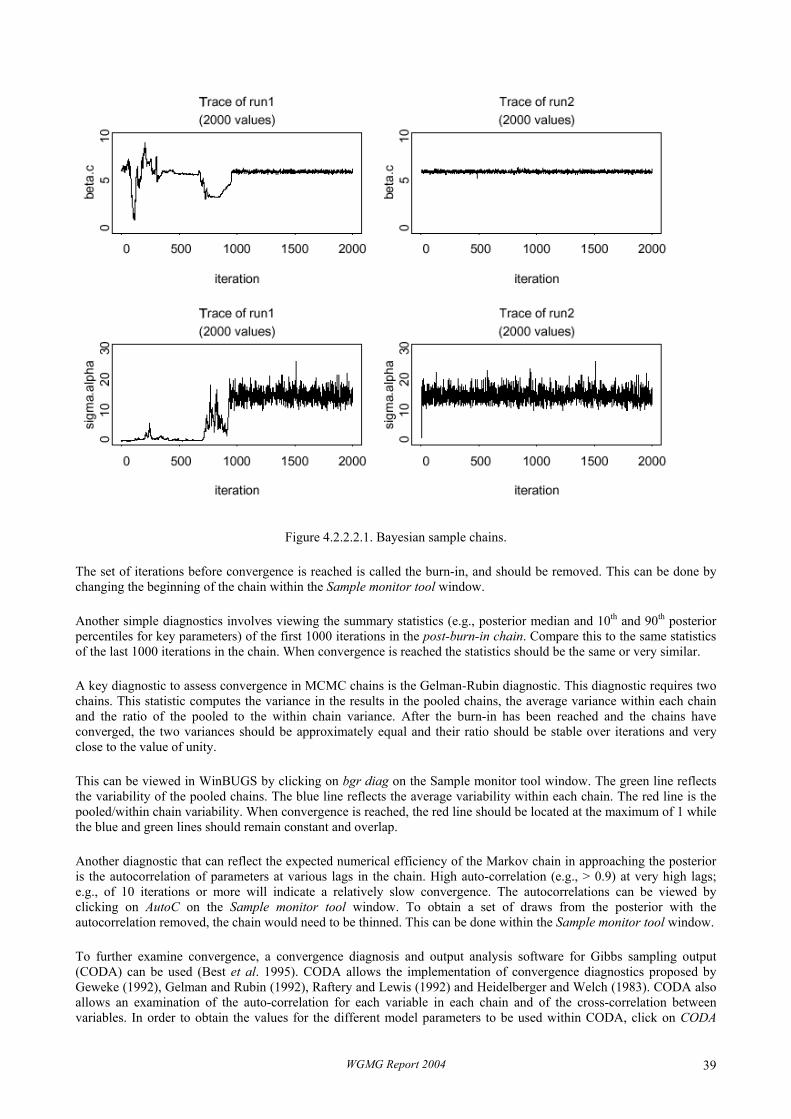
Figure 4.2.2.2.1. Bayesian sample chains.

The set of iterations before convergence is reached is called the burn-in, and should be removed. This can be done by changing the beginning of the chain within the Sample monitor tool window.

Another simple diagnostics involves viewing the summary statistics (e.g., posterior median and 10th and 90th posterior percentiles for key parameters) of the first 1000 iterations in the post-burn-in chain. Compare this to the same statistics of the last 1000 iterations in the chain. When convergence is reached the statistics should be the same or very similar.

A key diagnostic to assess convergence in MCMC chains is the Gelman-Rubin diagnostic. This diagnostic requires two chains. This statistic computes the variance in the results in the pooled chains, the average variance within each chain and the ratio of the pooled to the within chain variance. After the burn-in has been reached and the chains have converged, the two variances should be approximately equal and their ratio should be stable over iterations and very close to the value of unity.

This can be viewed in WinBUGS by clicking on bgr diag on the Sample monitor tool window. The green line reflects the variability of the pooled chains. The blue line reflects the average variability within each chain. The red line is the pooled/within chain variability. When convergence is reached, the red line should be located at the maximum of 1 while the blue and green lines should remain constant and overlap.

Another diagnostic that can reflect the expected numerical efficiency of the Markov chain in approaching the posterior is the autocorrelation of parameters at various lags in the chain. High auto-correlation (e.g., > 0.9) at very high lags; e.g., of 10 iterations or more will indicate a relatively slow convergence. The autocorrelations can be viewed by clicking on AutoC on the Sample monitor tool window. To obtain a set of draws from the posterior with the autocorrelation removed, the chain would need to be thinned. This can be done within the Sample monitor tool window.

To further examine convergence, a convergence diagnosis and output analysis software for Gibbs sampling output (CODA) can be used (Best et al. 1995). CODA allows the implementation of convergence diagnostics proposed by Geweke (1992), Gelman and Rubin (1992), Raftery and Lewis (1992) and Heidelberger and Welch (1983). CODA also allows an examination of the auto-correlation for each variable in each chain and of the cross-correlation between variables. In order to obtain the values for the different model parameters to be used within CODA, click on CODA

WGMG Report 2004 39

within the Sample monitor tool window. This software needs S-plus or R to be run. The documentation of the software can be found on the WinBUGS web-site (http://www.mrc-bsu.cam.ac.uk/bugs/classic/coda04/readme.shtml).

Additional model checking criteria exist for WinBUGS output: residuals, standardised residuals, deviance information criterion (DIC) and Bayesian P-values. Residuals and standardized residuals can be plotted using commands under the WinBUGS inference menu. The same basic interpretations apply as in frequentist statistics.

The relative goodness of fit of alternative structural models to the data can be obtained using the DIC criterion which is analogous to the AIC criterion in frequentist statistics. The model with the smallest DIC would best predict a replicate dataset of the same structure as the one observed.

DIC = Deviance + pD

pD = effective number of parameters

The DIC thus provides a measure of fit discounted by the measure of complexity.

WinBUGS automatically sets up a logical node to measure the deviance. The deviance is defined as –2 * log(likelihood). The deviance can be monitored by typing deviance in the node field of the Sample Monitor Tool. The smaller the deviance, the larger the probability of the data given the set of parameter values. The DIC can be computed and values obtained can be interpreted as instructed in the Help/User Manual.

Bayesian p-values can be defined as the probability that the model replicated data could be greater than the observed data (Gelman et al. 1995)

Bayes’ p-value = p( xrep | θ ) ≥ xobs

where xrep is a simulated observation given the random variable of the parameter vector θ and xobs is the actual observation. A set of p-values for the given dataset should look like a sample from a Uniform(0,1) distribution. So if the model used is actually the same (or similar enough) to the model which generated the data, then from 100 p-values about 2 can be expected to be smaller than 0.025 and about 2 can be expected to be larger than 0.975, about half of them should be smaller than 0.5, and so on. Systematic trends in p-values in a time-series of observations indicates a poor fit of the model to the data.

Some further detail is provided here on the p-value diagnostic. In order to assess the fit of the models to the data, the data can be compared to the posterior predictive distribution of the model; i.e., the distribution of data simulated from the model (Gelman et al. 1995). This will allow us to assess whether the observed data look plausible under the posterior predictive distribution. Systematic differences between the simulations and the data indicate potential failings of the model. We define Rrep as the replicated data that could have been observed as the data if we were to replicate data using the model. Simulation of potential data given the observed data and the joint posterior for θ is easily obtained using WinBUGs. The distribution of Rrep is called the posterior predictive distribution

( ) ( ) ( ) θθθ dRpRpRRp obsrepobsrep ∫=| .

We can thereafter compare the observed data with the posterior predictive distribution. The results of this comparison can be expressed in terms of a Bayesian p-value (Meng 1994; Gelman et al. 1995, 1996). Bayesian p-values can be defined as the probability that the replicated data could be as extreme or more extreme than the observed data (Meng 1994)

( ) obsrep RRpvaluepBayes ≥=− θ|' .

We can also measure the discrepancy between the model and the data using test quantities or discrepancy measures, T(R, θ). A discrepancy measure is a scaler summary of parameters and data that are used as a standard when comparing data to predictive simulations. One test quantity useful for routine checks of goodness-of-fit is the χ2 discrepancy measure (Gelman et al. 1995)

WGMG Report 2004 40

( ) ( )( )( )∑

−=

i i

ii

RRER

RTydiscrepancθθ

θχvar

,:2

2 .

It is therefore possible to compare the realised discrepancy T(R, θ) with the discrepancy under the posterior predictive distribution T(Rrep, θ). In order to do this we take a random sample from the posterior distribution for the full set of parameters in the model, θ. For each set of parameter values θj we can simulate a new data set, Rrep, and we can then plot T(Rrep, θj) against T(R, θj). The estimated Bayesian p-value is the proportion of times that T(Rrep, θj) is greater than T(R,θj) (Brooks et al. 2002). It is recommended that both the graphical summary and Bayesian p-value be used since it is possible for the distributions of T(Rrep, θj) and T(R, θj) to differ even though a p-value of 0.5 is obtained (Brooks et al. 2000).

The p-value model checking criterion can be calculated in WinBUGS using the following lines of code for a likelihood function with tau as the precision in the residuals:

#Model checking

for (i in 1:N){ resid[i] <- Obs[i] – Pred[i] # calculation of residual sresid[i] <- resid[i] * sqrt(tau) # calculation of standardised residuals # tau is the likelihood function precision Rep[i] ~ dnorm(Pred[i], tau) # calculation of replicated data set Pvalue[i] <- step(Rep[i] – Obs[i]) # calculation of p-value for each datapoint i }

4.2.2.3 Diagnostics for Importance Sampling

Importance sampling is less commonly applied than MCMC but still has its uses, for example in sequential Bayesian estimation (ICES 2003; Michielsens 2003). Because a different mechanism for numerical integration is applied in importance sampling different convergence diagnostics apply. These diagnostics are documented in papers including Geweke (1989) and McAllister and Ianelli (1997).

The rate at which the pdf from importance sampling approaches the estimated posterior pdf and the stability of the results obtained from importance sampling are determined by the closeness of approximation of the importance function to the posterior pdf (Geweke 1989). Inefficiency and instability can occur if the importance function is considerably more diffuse than the posterior pdf and a large proportion of the sampling is from regions of parameter space with negligible posterior density. Instability will also result if the tails of the importance function taper off faster than the tails of the posterior pdf. Instability will be manifested by occasional large changes in the computed posterior expected values even after hundreds of thousands of draws from the importance function. If this occurs, sampling should be stopped, the run discarded and the importance function adjusted (Geweke 1989; McAllister and Ianelli 1997).

Convergence of the approximated pdf to a stable result can be evaluated using diagnostics developed in previous works (Geweke 1989; McAllister and Ianelli 1997). One diagnostic is the percentage of the maximum importance weight from the set of draws relative to the sum of the importance weights where the importance weight (W(θk)) for a given draw k is the product of the prior pdf and likelihood, P(θk)•L(data | θk), divided by the density of the importance function, h(θk), all evaluated at the parameter values θk in draw k (i.e., W(θk) = P(θk)•L(data | θk) / h(θk)). If draws were to be obtained from the posterior pdf as the importance function, this percentage should be equal to 100% / m where m is the number of importance samples. This is because W(θk) would be constant across draws if the importance function was the posterior pdf. Thus the percentage maximum weight should drop to a low value within several hundred thousand draws from a well-chosen importance function. A stopping rule for importance sampling can be after this percentage maximum weight drops below 3%.

Also, the coefficient of variation (CV) in the importance weights (CV(W)) can computed and compared with the CV in the product of the prior and likelihood function (CV(P•L)). If draws of parameter values were to be taken from the posterior pdf, the CV(W) should be 0. If the importance function is to give reliable results, then CV(W) can be expected to be not much larger than the CV(P•L). It has been have found from numerical experiments that when CV(W) is approximately five or more times larger than the CV(P•L), the marginal posterior estimates can be strongly biased or numerically unstable and an importance function that is either more similar in central tendency and spread to the posterior pdf or has less sharp tails is required (McAllister and Babcock 2002).

WGMG Report 2004 41

4.3 Analyses

4.3.1 Data generation

The artificial data sets concocted for the large scale comparison of methods by the Committee on Fish Stock Assessment Methods of the US National Research Council were not meant to compare methods per se in every possible context, but nonetheless have the advantage of being among the very few available and widely published (NRC 1998; more details on the analyses made with various methods were reported in the compilation edited by Restrepo 1998). A limitation of these data is that they were generally produced with rather low fishing mortality compared to M, which is a clear handicap for most existing assessment methods. However, in absence of better alternative, the Working Group decided to use some of these sets for this exercise.

In general, the NRC data were generated to simulate violations of the typical assumptions of a number of assessment methods (e.g., changes in catchability through time, changes in fleet selectivity) on top of process and observation error (e.g., variability in M, sampling variance in survey, ageing error in setting up catch-at-age, misreporting). 30-year time-series of data were provided to analysts, including: catches-at-age (15 ages), commercial effort data, and “survey” (in the sense of being less biased, albeit noisy) indices. Commercial CPUE could be used for tuning in isolation or together with the survey indices.

The first data set used by the group is identical to NRC set 3, which involves a change in survey catchability midway in the time-series, fleet catchability changing with stock abundance, and fleet selectivity shifting towards younger ages in the second half of the series. None of this information was known to the members of WGMG before the analyses were carried out, which were therefore blind tests. Since the focus here was on the capacity of diagnostics, the change in survey q was the main reason to choose this set, as this is a major violation of assumptions made in several of the methods considered and diagnostics should reflect it.

The second data set was an amendment of NRC set 4 (a relatively easy one, involving no change in survey q nor in fleet selectivity), with a general (albeit not simply linear) trend in misreporting in catches (not effort) simulated over the last 10 years, reaching 50% in the final year. This misreporting trend coincides with a strong decline in the simulated stock.

The third data set is identical with NRC set 5, where a stock recovery is simulated which means that fishing mortality is even lower than in other data sets. It conforms to the standard assumptions

4.3.2 Results of application of methods

Nine assessment methods were applied to dataset 1, two to dataset 2. In each case the analyst concerned was asked to address three questions:

1) Does the assessment method used describe the data appropriately? 2) If not, what is the nature of the problem, and when (and at what ages) does it occur? 3) How did the diagnostics of the assessment method in question help the analyst in forming conclusions? Here, the term assessment method is intended to refer to the full construct of: the model, the model settings, and the analyst involved. A further issue was that of assessment method evaluation. It was not the express purpose of these analyses to determine which assessment method performed better (that is, got closest to the truth). However, it is of interest to know whether the particular interpretation of a diagnostic by the analyst to modify an assessment method improves the resulting assessment (in terms of consistency with the truth) or makes it worse – if the latter is true, then the diagnostic is misleading. Therefore, this meeting of WGMG decided to use the following overall approach:

1) Use exploratory data-screening and assessment method diagnostics from a standard method fit to attempt to detect the presence and nature of any data problem.

2) Modify the assessment method accordingly, and re-estimate. 3) Compare summary statistics from both the original assessment method fit, and the modified assessment method

fit, with the true values (available in the NRC dataset). Also, compare the diagnostics from the new assessment method fit with those from the old – it may be that the diagnostic used to make the modifications improves, but at the cost of other diagnostics becoming worse.

WGMG Report 2004 42

Following these steps, conclusions were reached for each assessment method as to whether its diagnostics were useful and sufficient, or misleading and deficient.

The summary statistics used for method comparison were in two categories:

1) Time-series of biomass, mean F(5–10) and recruitment at age 2. 2) Interest parameters, namely: mean F(5–10) in 2030, geometric mean recruitment at age 2 from 2001–2030, and

the depletion ratio (i.e., ratio of biomass in 2001 to biomass in 2003). 4.3.2.1 Bayesian VPA

The Bayesian VPA was run for the testing dataset 1 with only the survey data series and using WinBUGS. Although this particular Bayesian modelling application is still under development, the group decided to run the model to see if the approach was able to highlight model specification problems.

Prior information on the fishery and survey data from dataset 1 was not made available to the WG except for the value of natural mortality, assumed to be known. The Bayesian model code used was presented in WD2 and, therefore, separable fishing mortality model and constant catchability by age were assumed. All priors were assumed to be uniform distributions with ranges including possible parameter values. The model was run for only one chain with 14000 iterations.

Convergence diagnostics for the MCMC chain are illustrated in Figure 4.3.2.1.1 for the key stock parameters Fbar (mean F of ages 5–10), biomass and recruitment. The chain for Fbar in most of the years and for recruitment in the last years (from 2027 to 2030) of the analysed period exhibited a regular pattern for the entire chain, indicating reduced influence of starting values. However in several other years and mostly for the biomass, an irregular pattern was observed, from the start of the chain to around 4000 iterations, after which the chains presented an acceptable degree of regularity. This indicated that a burn-in of 4000 iterations should be used to remove the influence of starting values.

Autocorrelations of the parameters were computed for the remaining 10000 iterations. Strong autocorrelations (Figure 4.3.2.1.2) were observed for all the parameters and in almost all years, but diagnostics indicated that this autocorrelation could be removed with a thinning interval of 40 steps. Therefore, after the burn-in and thinning of lag 40 only 250 samples were retained.

Time-series of the catch residuals by age group were computed (Figure 4.3.2.1.3). Clear patterns in the catch residuals are observed over time and three periods are identified: first one from 2001 to 2009, second one from 2010 to 2014 and the third one from around 2015 till the end of the time-series. Several years of catch under prediction were observed for the young and middle ages (e.g., age 3 in 2002, 2007, 2012–2013, 2020 and 2028; age 6 from 2001–2007), while it was observed that mainly in the early period for the older ages catches were over predicted (e.g., ages 12–13 and 15 from 2001–2007/2009). This suggests that age-specific selectivity has changed over time and therefore the assumption of constant age-specific selectivity does not hold for this data set. Moreover, catch residuals show wide credibility intervals mostly in the young and middle ages and several outliers, particularly in the older ages. By outliers we mean 95% probability intervals that do not overlap with zero. There is reason to reject the model when more than 10% of the 95% probability intervals do not overlap with zero. For example, in age group 13 there is 16% of outliers (years 2012–2015 and 2025) while in the age group 15 outliers represent 40% (years 2012–2018 and 2026–2030). This also indicates a mismatch of model assumptions with the data.

The time-series of the estimated catchability (the ratio between survey CPUE and estimated population size) by age group is presented in Figure 4.3.2.1.4. The intervals for one age in a particular year do not overlap with intervals for the corresponding year class in proceeding and subsequent years, therefore indicating a marked change in catchability-at-age over years. This indicates that the assumption of constant catchability-at-age over years is not valid for the analysed data set.

Reparameterisation of the Bayesian VPA model used in this run is under development and has not yet been fully tested. For this reason no further analysis were carried out with this data set.

It should be mentioned that when using Bayesian analysis, the chain should be run for long enough to obtain adequate precision in the estimator, and to be thinned enough to ensure low autocorrelation. To decide when to stop the chain one possible procedure (see Section 4.2.2) is to run several chains in parallel, with different starting values and compare the estimates of the ergodic average of each chain. This procedure is also important to ensure convergence. This was not done with the analysed data set given the exploratory nature of the exercise.

WGMG Report 2004 43

Figu

re 4

.3.2

.1.1

. MC

MC

cha

ins (

1400

0 ite

ratio

ns) f

or F

bar (

left

pane

l), b

iom

ass (

mid

dle

pane

l) an

d re

crui

tmen

t (rig

ht p

anel

) in

year

s 200

2, 2

015,

202

6 an

d 20

30 (t

op to

bot

tom

).

WG

MG

Rep

ort 2

004

44

WG

MG

Rep

ort 2

004

45

Figu

re 4

.3.2

.1.2

. Aut

ocor

rela

tion

plot

for t

he e

ntire

MC

MC

cha

in c

orre

spon

ding

to F

bar (

left

pane

l), b

iom

ass

(mid

dle

pane

l) an

d re

crui

tmen

t (rig

ht p

anel

) in

year

s 20

02 a

nd

2030

.

Figure 4.3.2.1.3. Time-series of catch residuals by age group (note different y scale for age groups 2–7 and 8–15; arms of each box extend to cover 95% of the distribution; horizontal baseline represents the global mean of posterior means).

WGMG Report 2004 46

Figure 4.3.2.1.3. Continued. Time-series of catch residuals by age group (note different y scale for age groups 2–7 and 8–15; arms of each box extend to cover 95% of the distribution; horizontal baseline represents the global mean of posterior means).

WGMG Report 2004 47

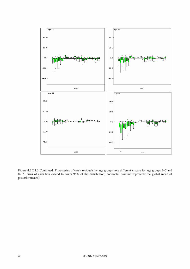
Figure 4.3.2.1.3 Continued. Time-series of catch residuals by age group (note different y scale for age groups 2–7 and 8–15; arms of each box extend to cover 95% of the distribution; horizontal baseline represents the global mean of posterior means).

WGMG Report 2004 48

Figure 4.3.2.1.4. Time-series of estimated catchability by age group (arms of each box extend to cover 95% of the distribution; horizontal baseline represents the global mean of posterior means).

WGMG Report 2004 49

Figure 4.3.2.1.4. Continued. Time-series of estimated catchability by age group (arms of each box extend to cover 95% of the distribution; horizontal baseline represents the global mean of posterior means).

WGMG Report 2004 50

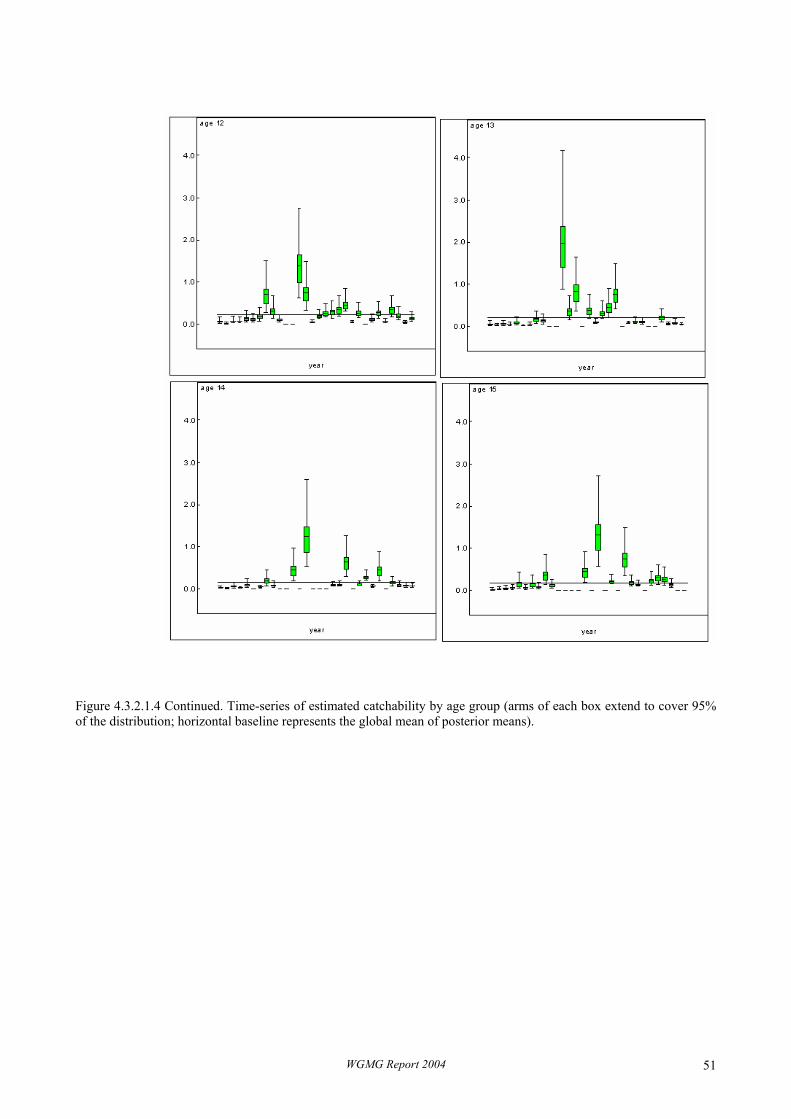
Figure 4.3.2.1.4 Continued. Time-series of estimated catchability by age group (arms of each box extend to cover 95% of the distribution; horizontal baseline represents the global mean of posterior means).

WGMG Report 2004 51

4.3.2.2 CADAPT (including CAMERA)

CADAPT and CAMERA are prototype models with single-fleet tuning. Both models are under development. CADAPT is a modification of the ADAPT model. CAMERA is a simple separable model, with time-invariant catchabilities (see Appendix D).

Plots of catch-at-age and survey index-at-age (Figures 4.3.2.2.1 and 4.3.2.2.2) show a conspicuous mismatch for youngest ages at the end of the period. This could indicative a deficit in the survey for the incoming year classes in the latter part of the index. This mismatch could also be caused by other factors, such as changes in commercial fleet selectivity, discarding or misreporting. During the working group meeting, while the participant running CADAPT and CAMERA was delayed due to technical problems, participants were informed that the survey had been changed at some point, and the analysis was continued with that knowledge.

A 20-year CADAPT retrospective run showed a strong pattern overestimation of total stock biomass for recent years, but prior to ca. 2016 the pattern was less conspicuous. Results were not conclusive as to which survey catchability model was appropriate. A run in which q were estimated for age group 2 and a common q for ages 3 and older was submitted as CADAPT prior to fix. For clarification of the retrospective analysis, two runs with 10 year retrospective windows, from 2021–2030 and 2011–2020, respectively, were made on the CADAPT prior to fix (Figures 4.3.2.2.3 and 4.3.2.2.4).

In the spirit of exploration, , and with prior knowledge of change in survey, based on both mismatch between index-at-age and catch-at-age in recent years, and a retrospective pattern of biomass overestimation in the latter part of the time-series, the survey index series was shortened and only indices-at-age 2016–2030 used in CADAPT tuning.

A CADAPT run, tuned only with the short survey indices-at-age was submitted as CADAPT after fix. Catchabilities were estimated for all age group indices, based on a retrospective of 7 years for the short series run. In all CADAPT runs, catch-at-age 2–14 was used, as a plus group is not programmed. Tuning data were survey ages 2–9, being age groups with observed values > 0 for all years. Cohorts were initiated by setting F-on-the-oldest at the weighted average of F10–13.

Retrospective patterns for different catchability models and long and short survey series led to a choice of models that went from overestimation of total stock biomass 2015–2030, prior to fix, to a model that followed the trajectory given as 'truth', except in the middle of the period.

Two separable models were fitted to the data tuned both with the long and short survey indices, using the CAMERA tool. These runs were submitted as CAMERA before and after fix. A 7 year retrospective, varying starting age of plateau in selectivity, tuned with the shorter (only the most recent) survey indices, using the same survey catchability as in CADAPT after fix, was run (Figure 4.3.2.2.5). Inverse case weights for log-residuals of survey indices and catch-at-age were set a priori with mean square residuals from Shepherd-Nicolson fits to the respective data matrices. The catch and index residuals were given equal weight in the objective function (λ=0.5).

The CAMERA analysis showed the “best” retro when selectivities were estimated for ages 2–8 and a selectivity plateau for age group 9 onwards. In the 'fixed' CAMERA run discrepancies in historic estimates from 'truth' were exaggerated, but performance in the latter half of the period improved. Due to time constraints and technical difficulties, the separable model could not be investigated thoroughly, e.g., compared with AMCI.

Retrospective analysis may be a useful qualitative indicator of model misspecification. A measure/metric for retrospective patterns deserves further study as it could prove a useful diagnostic (see ICES 1991; Mohn 1999; WAB1 Cadigan to the last meeting of WGMG; for analytical retrospective analysis; and Jónsson and Hjörleifsson 2000 for application on assessment performance (real-time retro).

WGMG Report 2004 52

Figure 4.3.2.2.1. Index-at-age for data set 1 (NRC data 3).

Figure 4.3.2.2.2. Catch-at-age for data set 1 (NRC data 3).

WGMG Report 2004 53

Figure 4.3.2.2.3. Retrospective analysis (10 years) of total stock biomass (TSB) and recruitment (R as two year olds) with CADAPT tuned with full set of survey data (2001–2030).

Figure 4.3.2.2.4. Retrospective analysis (10 years) of the first 20 years of total stock biomass (TSB) and recruitment (R as two year olds) with CADAPT tuned with historic part of survey data (2001–2020).

WGMG Report 2004 54

Figure 4.3.2.2.5. Retrospective analysis (7 years) of CAMERA tuning with short set of survey data (2016–2030). Survey catchability model fixed (q's independent of age f. all ages), variable plateau on selectivity.

4.3.2.3 CAMERA

Refer to the previous Section 4.3.2.2.

4.3.2.4 CSA

Dataset 1

The CSA implementation used for this exercise (see Appendix D) only includes fairly elementary diagnostics. Raw and standardised residuals between observed and fitted tuning indices are provided for the recruits and post-recruits stages, and for process error residuals when taken into account, together with Residual Mean Square Error. 'Confidence intervals' for biomass and post-recruits survey catchability estimates are based on non-parametric, model-conditioned bootstrap, where residuals from the base fit are randomly resampled within each category (recruits, post-recruits, process). Retrospective analyses of stock abundance estimates are also carried out, with a limitation to no less than 10 years of data.

WGMG Report 2004 55

Previous trials with simulated data (see, for example, Mesnil 2003) indicated that these diagnostics were insufficient, and even misleading in some cases:

• improvements in SSQ or RMSE could be obtained with some settings, whereas results were further away from the truth;

• trajectories of 10th-90th percentiles obtained by bootstrap could be either very close, indicating a neat assessment, or conversely quite wide with noisy data sets, but nevertheless the envelope did not include the true trajectory;

• retrospective analyses were unable to detect trends in catchability (see e.g., last year's WGMG report).

These conclusions were again apparent in the analysis of this set. Here, the all-observation-error version of CSA was used for estimation and, since this set had been analysed prior to the meeting, the information that the survey vessel had changed was known and could be accounted for in a comparative run where separate survey q's were estimated for each half-period. As shown in the leftmost column of Figure 4.3.2.4.1, the plot of raw log-residuals for recruits showed some pattern, with a group of negative values in the last 10 years, when a single survey was considered but such pattern was not apparent in the residuals for the post-recruits. There was thus no clear indication of the change in survey q. Given that recruits make a very small contribution to catch and biomass, one might have proceeded with this assessment despite the oddity in the recruits residuals. The inability of residuals plots as a sufficient diagnostic is further shown in the rightmost part of the Figure where residuals of a fit where the survey was split into two periods are plotted. Some improvement is apparent in the recruits residuals, with less systematic negative residuals in the last decade, and in the overall SSQ (reduced from 4.8 to 4.0), but the pattern in post-recruits residuals is basically unchanged. No useful indication was provided by the bootstrap nor by retrospective analyses that both showed very wide dispersion.

However, it is apparent from Figure 4.3.2.4.2 that splitting the survey to reflect the change in simulated q did significantly improved the accuracy of stock size estimates, particularly for biomass (or for post-recruits that contribute most biomass; not shown) whose trajectory in the initial period came much closer to the truth. It is notable that for the final period, which is of most interest for management decision, an assessment based on the “erroneous” run would not have resulted in misleading advice since the trends in stock abundance, and even the absolute values, for both recruitment and total stock were reflected with acceptable accuracy. Problems would have arisen if advice was to take account of the whole time-series, e.g., for setting reference points.

Dataset 2

The plot of residuals (Figure 4.3.2.4.3) again shows some systematic pattern in the final decade for the recruits, but no signal is evident from the post-recruits residuals, nor from the retrospective analyses (not shown). None of the available diagnostics was able to detect the misreporting trend imposed in the data simulation for the final decade.

When comparing with the true trajectories and with the results of an equivalent run made on the same set without misreporting (NRC Set 4), it is apparent that using spoiled catch data has worsened the discrepancy in stock size estimates for the earlier years (Figure 4.3.2.4.4). However, as with Set 1, advice based on estimates for the recent period should not have resulted in misleading management advice and problems would only occur if reference was made to the far past.

WGMG Report 2004 56

5 10 15 20 25

-0.2

-0.1

0.0

0.1

0.2

0.3

0.4R

aw lo

g-re

sidu

als

Rec

ruits

1-period Survey

5 10 15 20 25

-0.2

-0.1

0.0

0.1

Split Survey

5 10 15 20 25 30

-0.5

0.0

0.5

Year

Raw

log-

resi

dual

s Fu

llRec

r.

5 10 15 20 25 30

-0.6

-0.4

-0.2

0.0

0.2

0.4

0.6

Year

WGMG Set 1

Figure 4.3.2.4.1. Raw log-residuals by stage from a CSA analysis of dataset 1, assuming either a single survey (left) or two separate surveys (right).

0 5 10 15 20 25 30

0

1000

2000

3000

WGMG Set 1

Rec

ruits

Survey 1pSurvey 2pTrue

0 5 10 15 20 25 30

2000

4000

6000

8000

10000

Bio

mas

s

Year

Figure 4.3.2.4.2 . CSA analysis of dataset 1. Estimates of recruitment (top) and biomass (bottom) compared to the truth (solid circles), assuming a single period or two periods in the survey.

WGMG Report 2004 57

5 10 15 20 25

-0.2

-0.1

0.0

0.1

0.2

Raw

log-

resi

dual

s R

ecru

itswith misrep

5 10 15 20 25

-0.2

-0.1

0.0

0.1

without misrep

5 10 15 20 25 30

-0.4

-0.2

0.0

0.2

0.4

0.6

0.8

Year

Raw

log-

resi

dual

s Fu

llRec

r.

5 10 15 20 25 30

-0.4

-0.2

0.0

0.2

0.4

0.6

Year

WGMG Set 2

Figure 4.3.2.4.3. Raw log-residuals by stage from a CSA analysis of dataset 2.

WGMG Report 2004 58

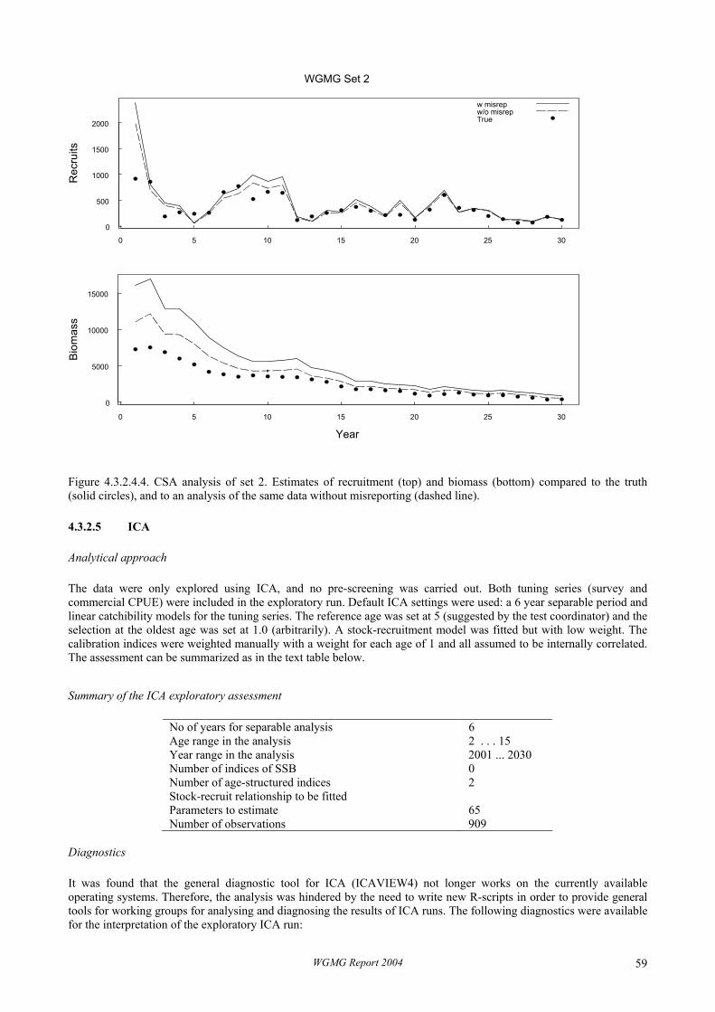
0 5 10 15 20 25 30

0

500

1000

1500

2000

Rec

ruits

w misrepw/o misrepTrue

0 5 10 15 20 25 30

0

5000

10000

15000

Bio

mas

s

Year

WGMG Set 2

Figure 4.3.2.4.4. CSA analysis of set 2. Estimates of recruitment (top) and biomass (bottom) compared to the truth (solid circles), and to an analysis of the same data without misreporting (dashed line).

4.3.2.5 ICA

Analytical approach

The data were only explored using ICA, and no pre-screening was carried out. Both tuning series (survey and commercial CPUE) were included in the exploratory run. Default ICA settings were used: a 6 year separable period and linear catchibility models for the tuning series. The reference age was set at 5 (suggested by the test coordinator) and the selection at the oldest age was set at 1.0 (arbitrarily). A stock-recruitment model was fitted but with low weight. The calibration indices were weighted manually with a weight for each age of 1 and all assumed to be internally correlated. The assessment can be summarized as in the text table below.

Summary of the ICA exploratory assessment

No of years for separable analysis 6 Age range in the analysis 2 . . . 15 Year range in the analysis 2001 ... 2030 Number of indices of SSB 0 Number of age-structured indices 2 Stock-recruit relationship to be fitted Parameters to estimate 65 Number of observations 909

Diagnostics

It was found that the general diagnostic tool for ICA (ICAVIEW4) not longer works on the currently available operating systems. Therefore, the analysis was hindered by the need to write new R-scripts in order to provide general tools for working groups for analysing and diagnosing the results of ICA runs. The following diagnostics were available for the interpretation of the exploratory ICA run:

WGMG Report 2004 59

• Separable model diagnostics (Figures 4.3.2.5.1–2). There is no detectable trend in the catch residuals and so the conclusion would be that there are no apparent problems in the recent catch data.

• CPUE log catchability residuals (Figure 4.3.2.5.3) shows no real trends. There are mostly negative catchability residuals in the first year which could indicate that effort has been poorly estimated in that year.

• Plots of CPUE against stock numbers-at-age with superimposed the estimated catchability from the model (Figures 4.3.2.5.4–5). The plots show that there is a weak relationship between N and CPUE for most of the older ages although there appears to be no real trend.

Diagnostics (e.g., skewness and kurtosis) in the ICA.OUT file were briefly scrutinised and did not suggest that the assumption of log-normal errors does not hold. Retrospective analysis are not routinely available in ICA. A batch-mode version of ICA is available which allows the calculation of retrospective assessments although different datasets have to be set up for each retrospective run. An Excel macro for generating these datasets is available upon request.

In summary: the diagnostics indicate that there are some patterns in the survey residuals in the middle of the time-series. No problems were detected in the catch-at-age data or in the commercial CPUE series, although the high residuals in the beginning of that series are suspect.

Comparison with the truth

A comparison of the ICA exploratory assessment with the “truth” is presented in Figure 4.3.2.5.7 and indicates that the ICA assessment estimates a higher biomass over the whole time-series. It also shows that ICA is the only model that presents an increase in SSB in recent years. Fishing mortality in the ICA assessment is relatively stable whereas in reality it has rapidly increased.

Conclusions

The diagnostics have been useful in detecting a trend in the residuals in the survey series on the younger ages. Other properties of the data (fleet catchability changing with stock abundance and fleet selectivity shifting towards younger ages in the second half of the series) were not detected with the available diagnostics. This is partly due to the short separable period used in the exploration so that a change in selectivity was not apparent from the catch residuals. Plots of catchability residuals against stock abundance were not available (due to the absence of a working version of ICAVIEW): these might have detected the catchability problem in the commercial CPUE data.

No attempt has been made to remedy the observed data problem because considerable time has been spent on writing the R-scripts for presenting the basic diagnostics. It was suggested that a better exploratory use of ICA would involve the following elements:

• a long separable period, as this may highlight discrepancies between calibration series and the catch data. • each tuning series separately because the mixing of the two calibration series in a manually weighted exploratory

analysis may have masked the mismatch between the survey data and the catch data.

WGMG Report 2004 60

Catch residuals

2025 2028

-2-1

01

2

age 2

2025 2028

-2-1

01

2

age 3

2025 2028

-2-1

01

2

age 4

2025 2028

-2-1

01

2

age 5

2025 2028

-2-1

01

2

age 6

2025 2028

-2-1

01

2

age 7

2025 2028

-2-1

01

2

age 8

2025 2028

-2-1

01

2

age 9

2025 2028

-2-1

01

2

age 10

2025 2028

-2-1

01

2

age 11

2025 2028

-2-1

01

2

age 12

2025 2028

-2-1

01

2

age 13

2025 2028

-2-1

01

2

age 14

2025 2028

-2-1

01

2

age 15

Figure 4.3.2.5.1. ICA set 1: Catch residuals over a 6 year separable period with reference age 5 and selection at oldest true age of 1.0.

WGMG Report 2004 61

2 3 4 5 6 7 8 9 11 13 15

age residuals

-1.0

-0.5

0.0

0.5

1.0

1.5

2025 2026 2027 2028 2029 2030

Year residuals

-0.2

-0.1

0.0

0.1

0.2

Figure 4.3.2.5.2. ICA set 1. Marginal total catch residuals for ages (left) and years (right)

WGMG Report 2004 62

Survey

2000 2015 2030

-2-1

01

2

age 2

2000 2015 2030

-2-1

01

2

age 3

2000 2015 2030

-2-1

01

2

age 4

2000 2015 2030

-2-1

01

2

age 5

2000 2015 2030

-2-1

01

2age 6

2000 2015 2030

-2-1

01

2

age 7

2000 2015 2030

-2-1

01

2

age 8

2000 2015 2030

-2-1

01

2

age 9

2000 2015 2030

-2-1

01

2

age 10

2000 2015 2030

-2-1

01

2

age 11

2000 2015 2030-2

-10

12

age 12

2000 2015 2030

-2-1

01

2

age 13

2000 2015 2030

-2-1

01

2

age 14

2000 2015 2030

-2-1

01

2

age 15

Figure 4.3.2.5.3. ICA set 1. Survey log-catchability residuals.

WGMG Report 2004 63

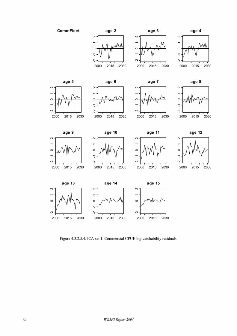
CommFleet

2000 2015 2030

-2-1

01

2

age 2

2000 2015 2030

-2-1

01

2

age 3

2000 2015 2030

-2-1

01

2

age 4

2000 2015 2030

-2-1

01

2

age 5

2000 2015 2030

-2-1

01

2

age 6

2000 2015 2030

-2-1

01

2

age 7

2000 2015 2030

-2-1

01

2

age 8

2000 2015 2030

-2-1

01

2

age 9

2000 2015 2030

-2-1

01

2

age 10

2000 2015 2030

-2-1

01

2age 11

2000 2015 2030

-2-1

01

2

age 12

2000 2015 2030

-2-1

01

2

age 13

2000 2015 2030

-2-1

01

2

age 14

2000 2015 2030

-2-1

01

2

age 15

Figure 4.3.2.5.4. ICA set 1. Commercial CPUE log-catchability residuals.

WGMG Report 2004 64

0 500 1500

015

00

Age 1

Survey 1

Num

bers

at a

ge

0 2000 4000

010

00

Age 2

Survey 1

Num

bers

at a

ge

0 1000 2500

010

00

Age 3

Survey 1

Num

bers

at a

ge

0 1000 3000

060

0

Age 4

Survey 1

Num

bers

at a

ge

0 500 1500

040

0

Age 5

Survey 1

Num

bers

at a

ge

0 500 1500

030

0

Age 6

Survey 1

Num

bers

at a

ge

0 400 800

020

0

Age 7

Survey 1

Num

bers

at a

ge

0 400 800

015

035

0

Age 8

Survey 1

Num

bers

at a

ge

0 200 400

010

025

0

Age 9

Survey 1

Num

bers

at a

ge

0 50 150

010

0

Age 10

Survey 1

Num

bers

at a

ge

0 100 200

010

0

Age 11

Survey 1

Num

bers

at a

ge

0 100 200

010

020

0

Age 12

Survey 1

Num

bers

at a

ge

0 40 80 120

050

150

Age 13

Survey 1

Num

bers

at a

ge

0 40 80 120

060

120

Age 14

Survey 1

Num

bers

at a

ge

Figure 4.3.2.5.5. ICA set 1. Survey plots of CPUE versus stock numbers-at-age with superimposed the catchability estimated by the model.

WGMG Report 2004 65

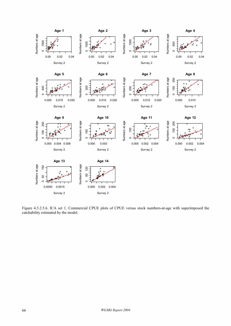
0.00 0.02 0.04

015

00

Age 1

Survey 2

Num

bers

at a

ge

0.00 0.02 0.04

010

00

Age 2

Survey 2

Num

bers

at a

ge

0.00 0.02 0.04

010

00

Age 3

Survey 2

Num

bers

at a

ge

0.00 0.02 0.04

060

0

Age 4

Survey 2

Num

bers

at a

ge

0.000 0.015 0.030

040

0

Age 5

Survey 2

Num

bers

at a

ge

0.000 0.010 0.020

030

0

Age 6

Survey 2

Num

bers

at a

ge

0.000 0.010 0.020

020

0

Age 7

Survey 2

Num

bers

at a

ge

0.000 0.010

015

035

0

Age 8

Survey 2

Num

bers

at a

ge

0.000 0.004 0.008

010

025

0

Age 9

Survey 2

Num

bers

at a

ge

0.000 0.003

010

0

Age 10

Survey 2

Num

bers

at a

ge

0.000 0.002 0.004

010

0

Age 11

Survey 2

Num

bers

at a

ge

0.000 0.002 0.004

010

020

0

Age 12

Survey 2

Num

bers

at a

ge

0.0000 0.0015

050

150

Age 13

Survey 2

Num

bers

at a

ge

0.000 0.002 0.004

060

120

Age 14

Survey 2

Num

bers

at a

ge

Figure 4.3.2.5.6. ICA set 1. Commercial CPUE plots of CPUE versus stock numbers-at-age with superimposed the catchability estimated by the model.

WGMG Report 2004 66

SSB

0

2000

4000

6000

8000

10000

12000

14000

1990 2000 2010 2020 2030 2040

TrueICA

Figure 4.3.2.5.7 . ICA set 1. Comparison of SSB estimates of the ICA exploratory analysis with the true SSB values.

WGMG Report 2004 67

4.3.2.6 KSA

KSA is tested here as a diagnostic tool for fish stock assessments. Its main purpose is to detect when the estimates of interest parameters are strongly sensitive to (a) differences between survey series, and (b) assumptions about the stability of catchability with time or with age. The only user-inputs to KSA apart from the data are the ranges of smoothers to be tested.

For the purpose of this exploration, the interest parameter investigated will be the total biomass at the end of the time-series relative to the total biomass at the start of the time-series.

Some inferences might be made based on the relative likelihood of the solutions found for a range of catchability options, penalised by the equivalent number of parameters being fitted in each case.

Interpretation of KSA diagnostics

The main diagnostic is the contour plot of the interest parameter with respect to the smoother choices. There are three cases:

• Vertical lines indicate that the interest parameter is dependent mostly on the year-range chosen for catchability smoothing. This suggests that catchability changes with time.

• Horizontal lines indicate that the interest parameter is dependent mostly on the age-range chosen for catchability smoothing. This suggests that catchability changes with age (Experience to date suggests that this feature usually appears in trawl-based survey series but not in acoustic survey data).

• Diagonal lines indicate that both effects are important, implying a change in catchability-at-age; i.e., a change in selection pattern.

The magnitude of the effects are indicated by the steepness of the contours.

The other diagnostic is the RPLF. High values of the RPLF contours can, in principle, be used as an indicator of appropriate model choice.

Implementation

The method was initially applied as an automated screening exercise across the range of smoothers from 2 to 10 in both the age- and year- directions. Following the first trial, this range was altered to 2 to 10 in the year-direction but 1 to 10 in the age-direction, following a perception that catchability may often be highly age-dependent, especially at the younger ages.

Summary results are presented as Figures 4.3.2.6.1 to 4.3.2.6.9.

Observation with respect to data set 1:

a) Sensitivity of the interest parameters to smoothing choices:

The survey index leads to inferences of stock status that are relatively independent of choices about catchability, and are in the range of approximately 0.24 to 0.34 (in relative biomass), 0.38 to 0.48 (Fishing mortality) and recruitment estimates of 504 - 508 thousands. These estimates are sensitive to choices about the change of catchability with age, but rather robust to the assumptions about change in catchability with time. This suggests that catchability for this index is relatively constant over time over the period that affects the terminal-year estimates.

The commercial index leads to widely different perceptions of stock status, with relative biomass in the range 0.3 to 0.9, fishing mortality in the range 0.12 to 0.26 and average recruitment 620 000.

The estimates are sensitive to changing assumptions in catchability both by year and by age. This suggests that catchability changes both over time and by age; i.e., that both catchability and selection pattern have changed over time for this index of abundance.

b) RPLF (Bayes Information Criterion):

WGMG Report 2004 68

The RPLF criterion indicates a higher probability of stable catchability over time, but variable catchability by age, for both series. However, the assumption of stable catchability with time in the commercial survey leads to values of relative biomass of around 0.9 (Figure 4.3.2.6.2., panels b. and c.), which conflicts with the inference drawn from the survey index (Figure 4.3.2.6.1., panels b. and c.)

1. There is clearly a strong divergence between the two indices, with the survey index leading to estimates of current stock size at the bottom end of the range of those consistent with the commercial index.

2. There appears to be quite strong internal structure in the commercial index, suggesting either that the index be not used in the assessment or else only very recent data should be included.

3. The estimates are sensitive to assumptions that constrain catchability across different ages. This sensitivity is more important when using the commercial index.

4. Values of the interest parameters consistent with both the survey series, within the explored range of the smoothers (2 to 10 in both age- and year- dimensions), are:

Relative Biomass ... about 0.3 Fishing Mortality ... range 0.2 to 0.3 Recruitment ... range 500 000 to 540 000

Observation with respect to data set 3:

Adaptations: This data set contained a large number of zero observations at the oldest ages. In order to remove these intractable values, the ksa was fitted only over ages 2 to10.

a) Sensitivity of the interest parameters to smoothing choices:

The survey index leads to inference of relative biomass in the range 0.03 to 0.05, being at the lower end of the range when catchability is weakly constrained across ages. If a flat selection pattern is force, then the estimate becomes dependent on the year-smoothing choice. This may indicate some (relatively weak) change in the selection pattern in this abundance index.

The commercial abundance index indicates a slightly higher relative stock size, around 0.04 to 0.06. The most recent information leads to indication of a smaller stock size, closer to 0.04. This suggests an increase in catchability over time occurs in this index. Diagonal contours in the plots of relative biomass for different smoothers suggest some change in selection pattern, but to a lesser extent than for the other abundance index.

b) RPLF (Bayes Information Criterion):

For both indices, a choice based on the RPLF would lead to preferring solutions where catchability is age-independent but constant over time. Although one might not make such a choice based on knowledge of likely fishery characteristics, the RPLF suggests that making choices based on allowing a time-trend in catchability is admitting a rather over-parametersised model.

Observation with respect to data set 3:

a) Sensitivity of the interest parameters to smoothing choices:

The survey index indicates relative SSB range 2.1 to 2.7, and some change in catchability by both year and age.

The commercial index indicates relative SSB range 1.7 to 2.6, with similar change in catchability by year and by age.

b) RPLF (Bayes Information Criterion):

The RPLF indicates that solutions around 2.6 to 2.7 are to be preferred.

Conclusions

The conclusions drawn from fitting the KSA are compared with the true features of the simulated data series below:

WGMG Report 2004 69

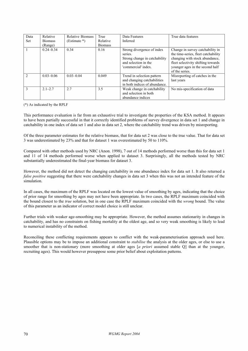
Data Set

Relative Biomass (Range)

Relative Biomass (Estimate *)

True Relative Biomass

Data Features Inferred

True data features

1 0.24–0.34 0.34 0.16 Strong divergence of index series. Strong change in catchability and selection in the 'commercial' index.

Change in survey catchability in the time-series, fleet catchability changing with stock abundance, fleet selectivity shifting towards younger ages in the second half of the series.

2 0.03–0.06 0.03–0.04 0.049 Trend in selection pattern and changing catchabilities in both indices of abundance.

Misreporting of catches in the last years

3 2.1–2.7 2.7 3.5 Weak change in catchability and selection in both abundance indices

No mis-specification of data

(*) As indicated by the RPLF

This performance evaluation is far from an exhaustive trial to investigate the properties of the KSA method. It appears to have been partially successful in that it correctly identified problems of survey divergence in data set 1 and change in catchability in one index of data set 1 and also in data set 2, where the catchability trend was driven by misreporting.

Of the three parameter estimates for the relative biomass, that for data set 2 was close to the true value. That for data set 3 was underestimated by 23% and that for dataset 1 was overestimated by 50 to 110%.

Compared with other methods used by NRC (Anon. 1998), 7 out of 14 methods performed worse than this for data set 1 and 11 of 14 methods performed worse when applied to dataset 3. Surprisingly, all the methods tested by NRC substantially underestimated the final-year biomass for dataset 3.

However, the method did not detect the changing catchability in one abundance index for data set 1. It also returned a false positive suggesting that there were catchability changes in data set 3 when this was not an intended feature of the simulation.

In all cases, the maximum of the RPLF was located on the lowest value of smoothing by ages, indicating that the choice of prior range for smoothing by ages may not have been appropriate. In two cases, the RPLF maximum coincided with the bound closest to the true solution, but in one case the RPLF maximum coincided with the wrong bound. The value of this parameter as an indicator of correct model choice is still unclear.

Further trials with weaker age-smoothing may be appropriate. However, the method assumes stationarity in changes in catchability, and has no constraints on fishing mortality at the oldest age, and so very weak smoothing is likely to lead to numerical instability of the method.

Reconciling these conflicting requirements appears to conflict with the weak-parameterisation approach used here. Plausible options may be to impose an additional constraint to stabilise the analysis at the older ages, or else to use a smoother that is non-stationary (more smoothing at older ages [a priori assumed stable Q] than at the younger, recruiting ages). This would however presuppose some prior belief about exploitation patterns.

WGMG Report 2004 70

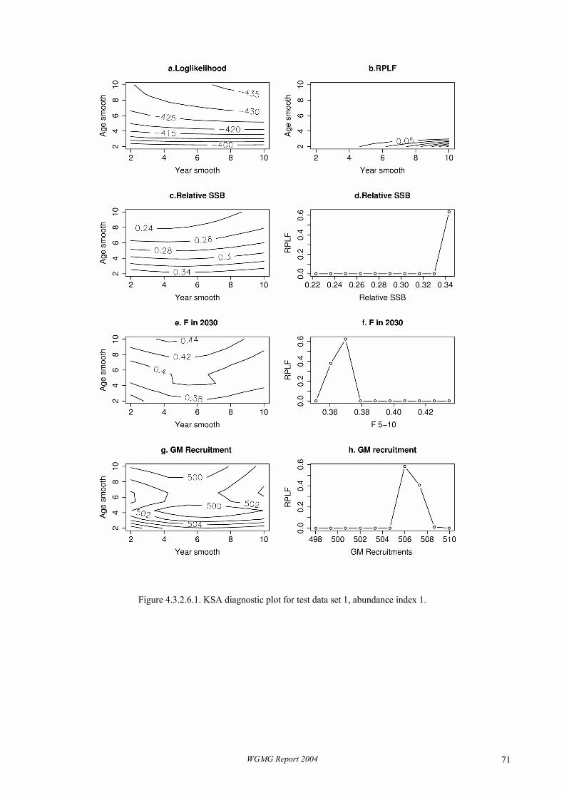
Figure 4.3.2.6.1. KSA diagnostic plot for test data set 1, abundance index 1.

WGMG Report 2004 71

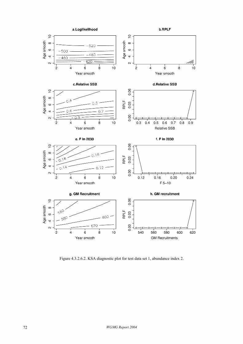
Figure 4.3.2.6.2. KSA diagnostic plot for test data set 1, abundance index 2.

WGMG Report 2004 72

Figure 4.3.2.6.3. KSA diagnostic plot for test data set 1, both abundance indices.

WGMG Report 2004 73

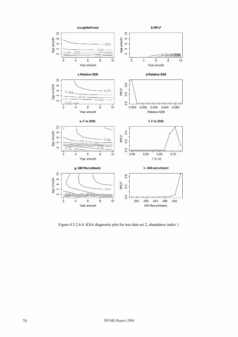
Figure 4.3.2.6.4. KSA diagnostic plot for test data set 2, abundance index 1.

WGMG Report 2004 74

Figure 4.3.2.6.5. KSA diagnostic plot for test data set 2, abundance index 2.

WGMG Report 2004 75

Figure 4.3.2.6.6. KSA diagnostic plot for test data set 6, both abundance indices.

WGMG Report 2004 76

Figure 4.3.2.6.7. KSA diagnostic plot for test data set 3, abundance index 1.

WGMG Report 2004 77

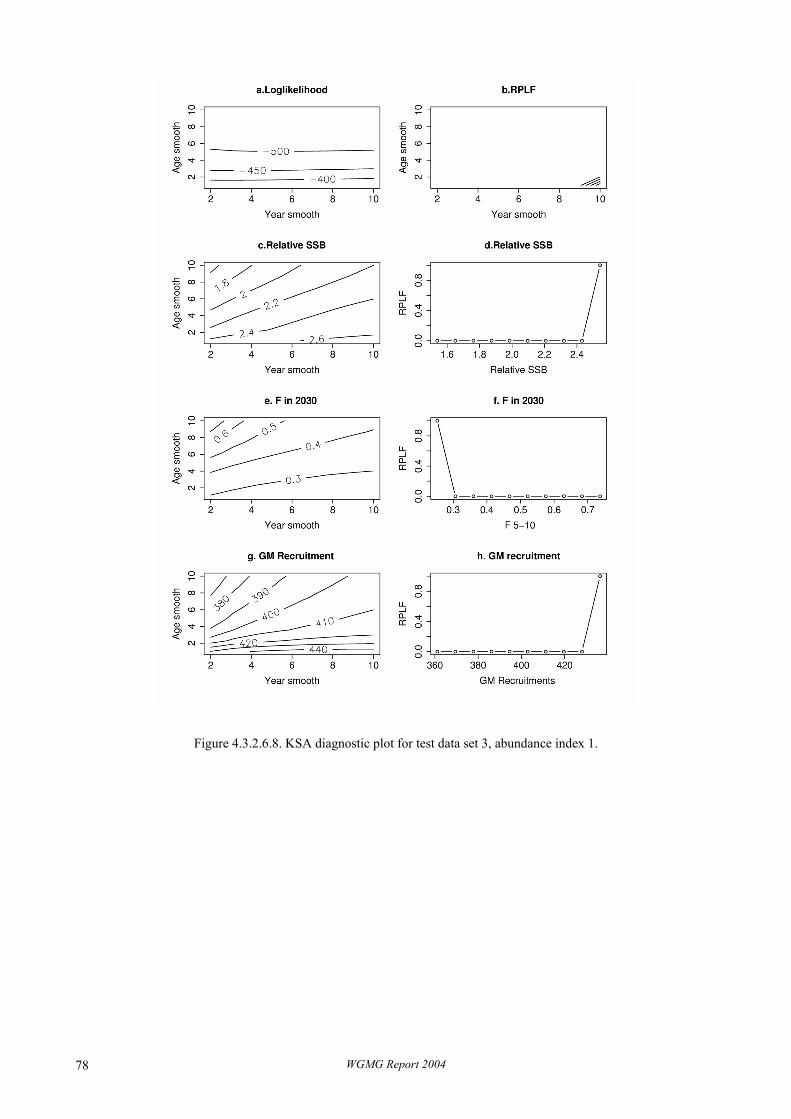
Figure 4.3.2.6.8. KSA diagnostic plot for test data set 3, abundance index 1.

WGMG Report 2004 78

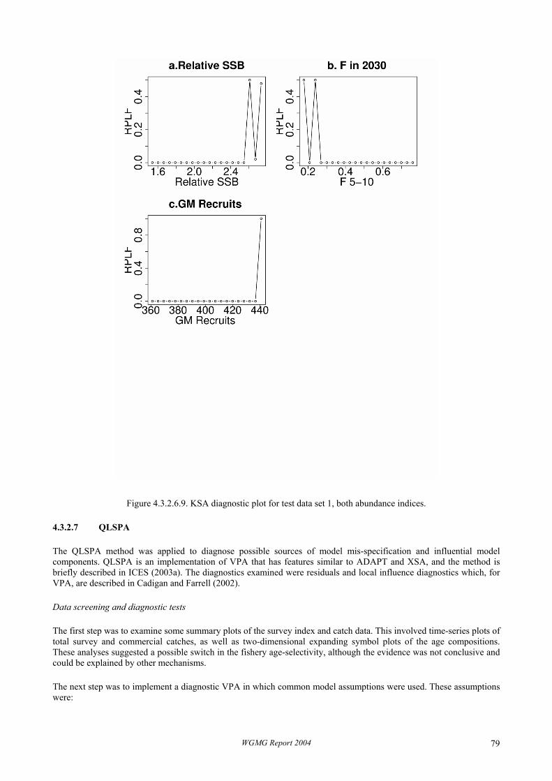
Figure 4.3.2.6.9. KSA diagnostic plot for test data set 1, both abundance indices.

4.3.2.7 QLSPA

The QLSPA method was applied to diagnose possible sources of model mis-specification and influential model components. QLSPA is an implementation of VPA that has features similar to ADAPT and XSA, and the method is briefly described in ICES (2003a). The diagnostics examined were residuals and local influence diagnostics which, for VPA, are described in Cadigan and Farrell (2002).

Data screening and diagnostic tests

The first step was to examine some summary plots of the survey index and catch data. This involved time-series plots of total survey and commercial catches, as well as two-dimensional expanding symbol plots of the age compositions. These analyses suggested a possible switch in the fishery age-selectivity, although the evidence was not conclusive and could be explained by other mechanisms.

The next step was to implement a diagnostic VPA in which common model assumptions were used. These assumptions were:

WGMG Report 2004 79

1) used all catches for ages 2–15 and survey indices for ages 2–14. The age 15 survey index was not used. Initially the plus group (age 15) commercial catches were not used; however, this was added later. The plus group was modelled using the standard ICES approach,

2) M=0.225 for all ages and years, 3) survey catchabilities (q’s) estimated for each age, but constrained to be constant across years, 4) quadratic variance model for the quasi-likelihood fit function, 5) estimated survivors at ages 2–13, 6) estimated population numbers-at-age 14, but penalized F14/Fave,11–13 to 1. The penalty weight was subjectively

chosen to give a good fit (within +4 of the best no-penalty fit) with the fewest parameters. 7) Forty-three parameters were estimated in total, but not all parameters were estimated freely because of the penalty

function. Initial conclusions

The fishery partial recruitment estimates for this run exhibited some cohort trends which usually indicate the F constraints at age 14 in some years are not appropriate (see Figure 4.3.2.7.1). The F shrinkage at age 14 in 2013 and 2017 was decreased 10-fold to reduce this problem.

The next step was to re-estimate the VPA and examine residual plots. Residuals were plotted in a variety of ways and the plots that showed the clearest evidence of mis-specification are shown in Figure 4.3.2.7.2. Average residuals for younger ages (<7) show a step-trend that breaks around 2017.

Local influence diagnostics were computed to further examine for mis-specification and to examine how sensitive model results were to model inputs. These diagnostics measure the influence of model inputs on outputs. The particular output assessed is the influence measure. Input components examined were commercial catches, the nominal M assumption, and the assumptions about survey catchabilities. The fit function influence measure, which was the extended quasi-likelihood, was examined to diagnose possible mis-specification, while model estimators of current total exploitation rate and biomass, and biomass trends, were examined to check if these estimates were unduly influenced by model inputs. This is a useful way to assess if potential mis-specifications have important consequences, because they sometimes may not.

The local influence approach involves examining the geometry of the influence surface that results from perturbing model inputs. The diagnostics are based only on the un-perturbed parameter estimates. The approach is a computationally feasible type of perturbation analysis that can give a good description of influence, especially when the influence surface is approximately linear. In this case influence can be described by a simple linear equation based on the co-ordinates of the direction of maximum slope as well as the maximum slope. In the following analyses, multiple model components are perturbed simultaneously so that the influence surface is high-dimensional.

The maximum slope can be used as an approximate bound on the effect caused by changing model inputs. If the change is expressed as a scalar h times a vector of length one then the change in a model output caused by the perturbation will be approximately less than h times the corresponding local slope for the influence measure. An illustration of this is presented at the end of this section.

Some results are presented in Figures 4.3.2.7.3 and 4.3.2.7.4. Note that the individual elements indicate whether an increase in the input results in an increase (+) or decrease (x) in the output. The size of the symbols indicate the relative magnitude of the change. The maximum slope listed at the top of each panel is proportional to the absolute value of the rate of change. The diagnostics suggest that the goodness-of-fit (Figures 4.3.2.7.3 , top panel) is most sensitive to the fishing mortality constraints used at age 14. The goodness-of-fit is also sensitive to assumptions about survey catchability (Figures 4.3.2.7.4 , top panel), but was less sensitive to perturbations of M (results not shown). The percent maximum slopes in the other two panels in Figure 4.3.2.7.3 also suggest that small changes to the catches at the older ages can have a substantial (> 30%) effect on estimates of total exploitation rates and recruitment. This is also the case for biomass and trends in biomass (results not shown); however, the sensitivity of the biomass estimator is illustrated below. The catch diagnostics have revealed a problem with this model and data, which is that the population estimates are sensitive to somewhat subjective modelling assumptions about F shrinkage as well as any errors in the reported catches at the older ages.

The results in the middle and bottom panels in Figure 4.3.2.7.4 suggest that the changes to the survey catchabilities that have the greatest effect on goodness-of-fit may not have a large effect on other model results. The results for the fit

WGMG Report 2004 80

statistic (top panel) are similar to the residuals shown in Figure 4.3.2.7.2, and suggest a similar potential change in the survey catchabilities.

Model modifications

Two changes to the model were made in an attempt to reduce the sensitivity of the model to the F-shrinkage used for estimation. The first change was that the catchabilities were constrained to be equal for ages 10–14. The age differences in these catchabilities were not statistically significant. Although further sensitivity analyses showed that this did not reduce sensitivity much, this change was maintained in subsequent analyses anyway. The only change that reduced the sensitivity was to increase the amount of shrinkage; however, too much shrinkage was also not satisfactory because cohort trends in the partial recruitment to the fishery became more pronounced. A value was chosen as a compromise between these two considerations. The local influence diagnostics were re-computed for the new model formulation and were very similar to the results in Figures 4.3.2.7.3 and 4.3.2.7.4.

The sensitivity of the model to catches at older ages is illustrated by changing the catches by adding C×d where d is the corresponding element in the direction vector of maximum change. Methods for using local influence diagnostics to assess sensitivities are illustrated in more detail in Cadigan and Farrell (2002). The perturbed catches are shown in Figure 4.3.2.7.5. The largest changes involve the catches at the oldest ages, and they are usually much less than 20% in absolute value. These are not large perturbations in light of the aging errors that often exist for older fish. The effects of the perturbations on some of the model estimates are shown in Figure 4.3.2.7.6. In all years the estimate of total biomass increased by at least 39%, and the largest increase was 58% in 2030 and 2031.

The maximum local slope for total biomass in 2031 was 51%, and this suggests that the maximum effect of a catch perturbation of size 1 (e.g., like in Figure 4.3.2.7.5) is 51%. This “prediction” of the effect of changing the catch is a reasonably good approximation of the increase that was observed (58%) by actually changing the input catches and re-estimating the model. Recall that the local influence diagnostics are computed using only the unperturbed model and parameter estimates.

Conclusions on modified model and reality check

The main conclusions from this analysis are that the model estimates are sensitive to modelling constraints on fishing mortalities at age 14, and that the survey catchabilities at ages less than 7 may have increased around 2017. A model formulation that was less sensitive to assumptions about F’s was not found. The estimated F’s tended to be fairly low and the VPA is not well-converged. In this situation it is not unusual for estimates to be sensitive to how numbers at the terminal age in the VPA are modelled. It does not seem possible to reduce this sensitivity without further information; however, the illustration of the model sensitivity shown in Figure 4.3.2.7.6 demonstrates in this example that is important to incorporate uncertainty about the catches when evaluating uncertainty of parameter estimators and related quantities.

The other potential mis-specification involves the survey catchabilities. The diagnostics indicate the q’s may have changes around 2017, possibly as the result of a change in survey procedures. Indeed the difference in q’s between these two periods seems statistically significant based on the modified diagnostic VPA (chi-square=47.9 with approximately 9 df’s).

The appropriate way to address the potential mis-specification will vary in practice. For example, if there has been no change in survey protocols then one would probably contemplate a different change to the model than if there was a change in the survey gear around 2017. In the former situation it may be advisable not to change the model at all, whereas in the latter situation in may be advisable to estimate different q’s for the two periods, but perhaps with constraints or bounds on the relative differences in q’s to reflect any understanding of the effects of the change in gear type.

The simulated data in this example were generated from a different model than the VPA used. A major difference in the simulation model was a change in survey q’s, but other aspects of the generating model were different as well. Hence, the regression and influence diagnostics correctly identified a source of mis-specification. The fishery selectivity in the generating model also changed, and this was correctly identified as well (results not shown). Note that the latter point is not really a mis-specification in the VPA used here because this model does not assume very much about fishery selectivity, except for the plus group F and F at age 14.

To examine the potential impact of model mis-specification, some estimates from the uncorrected (but modified) and corrected VPA’s are shown in Figure 4.3.2.7.7, along with the true population values. Two corrections were applied. One involved estimating q’s independently in the two periods, and the other correction involved estimating q’s in the

WGMG Report 2004 81

two periods using a small penalty on the size of their relative difference. The penalty-based method reduces differences in q estimates between the two periods unless the data “strongly” suggests otherwise.

The uncorrected VPA estimates were in substantial error for total biomass. For example, in 2030 the difference was 133%. This is consistent with the doubling of q in the generating model. Both corrections resulted in estimates closer to the true values. For example, the penalized-q estimate of total biomass in 2030 was 56% greater than the true value, while the un-penalized estimate was only 14% greater. Note that the absolute difference in biomass for some other years was greater than in 2030. The recruitment estimates improved as well, although not as much as the biomass estimates.

The main conclusion from the “correction” exercise is that it can work, although substantially more investigations need to be conducted to recommend correction methods for practical use.

2000 2005 2010 2015 2020 2025 2030

24

68

1012

14

Year

Age

Partial Recruitment at Age

Figure 4.3.2.7.1. Partial recruitments for the preliminary QLSPA diagnostic run.

WGMG Report 2004 82

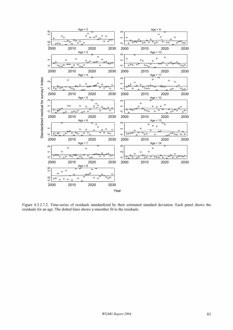
2000 2010 2020 2030-1

.01.

5 Age = 2

2000 2010 2020 2030

-11

Age = 3

2000 2010 2020 2030

-12

Age = 4

2000 2010 2020 2030

-11

3

Age = 5

2000 2010 2020 2030

-11

Age = 6

2000 2010 2020 2030

-11

3

Age = 7

2000 2010 2020 2030

-1.0

1.5 Age = 8

2000 2010 2020 2030

-11

3

Age = 9

2000 2010 2020 2030

-11

3 Age = 10

2000 2010 2020 2030

-11

3

Age = 11

2000 2010 2020 2030-1

13

Age = 12

2000 2010 2020 2030

-11

3Age = 13

2000 2010 2020 2030

-12

5

Age = 14

Year

Sta

ndar

dize

d re

sidu

al fo

r sur

vey1

Inde

x

Figure 4.3.2.7.2. Time-series of residuals standardized by their estimated standard deviation. Each panel shows the residuals for an age. The dotted lines shows a smoother fit to the residuals.

WGMG Report 2004 83

2000 2005 2010 2015 2020 2025 2030

24

68

1014

Change in fit, max slope = 72.3

2000 2005 2010 2015 2020 2025 2030

24

68

1014

Change in 2030 total exploitation rate (ages 2-14), max slope (%) = 60.6

2000 2005 2010 2015 2020 2025 2030

24

68

1014

Change in 2030 recruitment (age 2), max slope (%) = 35.4

Year

Age

POP1 catch LIDs

Figure 4.3.2.7.3. Catch local influence diagnostics for the model fit function (top), total exploitation rates in the last year (middle), and recruitment in the last year (bottom). Each panel shows the diagnostic for each element perturbed. The size and type of the plotting symbols are proportional to the absolute value and sign of the elements, respectively. Negative is denoted by an ×. The maximum slope is shown at the top of each panel, and is expressed in percent of the corresponding estimate in the middle and bottom panels.

WGMG Report 2004 84

2000 2005 2010 2015 2020 2025 2030

24

68

1014

Change in fit, max slope = 62.6

2000 2005 2010 2015 2020 2025 2030

24

68

1014

Change in 2030 total exploitation rate (ages 2-14), max slope (%) = 50.4

2000 2005 2010 2015 2020 2025 2030

24

68

1014

Change in 2030 recruitment (age 2), max slope (%) = 103

Year

Age

POP1 survey1 q shift LIDs

Figure 4.3.2.7.4. Catch local influence diagnostics for the model fit function (top), total exploitation rates in the last year (middle), and recruitment in the last year (bottom). Each panel shows the diagnostic for each element perturbed. The size and type of the plotting symbols are proportional to the absolute value and sign of the elements, respectively. Negative is denoted by an ×. The maximum slope is shown at the top of each panel and is expressed in percent of the corresponding estimate.

WGMG Report 2004 85

2000 2005 2010 2015 2020 2025 2030

-20

-10

010

20

Year

Cat

ch P

ertu

rbat

ions

(% o

f nul

l val

ues)

Figure 4.3.2.7.5 . Catch perturbations to illustrate the VPA sensitivity. Each vertical line shows the perturbation to a catch. Perturbations are clustered by year and shown sequentially for ages 2–15.

2000 2010 2020 2030

010

0030

00 basec_pert

age

2

2000 2010 2020 2030

050

0015

000

Tota

l Bio

mas

s

Figure 4.3.2.7.6. Catch perturbed (dotted lines) and un-perturbed (solid lines) VPA estimates. Top panel: numbers-at-age 2, Bottom panel: total biomass.

WGMG Report 2004 86

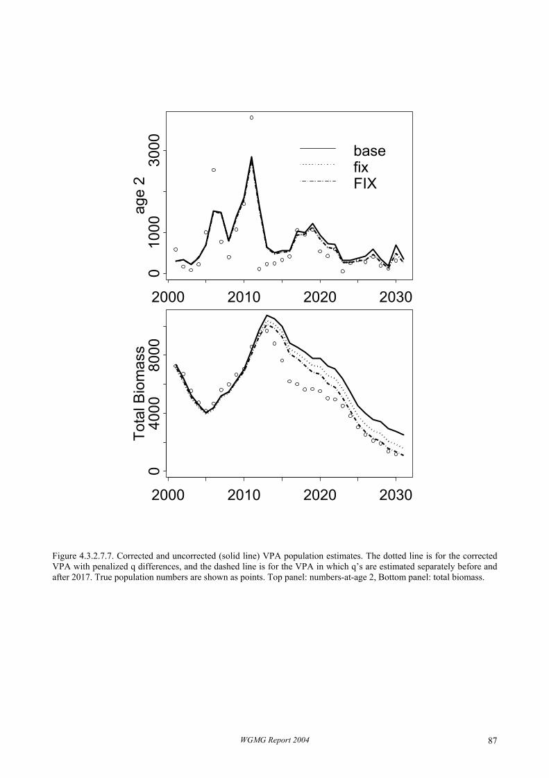
2000 2010 2020 2030

010

0030

00 basefixFIX

age

2

2000 2010 2020 2030

040

0080

00To

tal B

iom

ass

Figure 4.3.2.7.7. Corrected and uncorrected (solid line) VPA population estimates. The dotted line is for the corrected VPA with penalized q differences, and the dashed line is for the VPA in which q’s are estimated separately before and after 2017. True population numbers are shown as points. Top panel: numbers-at-age 2, Bottom panel: total biomass.

WGMG Report 2004 87

4.3.2.8 SURBA

Data screening and diagnostic tests

SURBA is a simple separable model based on survey indices, with the option of generating catchabilities from catch-at-age analysis (see Appendices B and D). The data-screening facilities of SURBA were used to evaluate the consistency of Dataset 1 (Survey series). Approximate survey catchabilities were estimated using an XSA run (full time-series, tuned by survey and commercial series, no time-taper, no power model, no catchability plateau, light shrinkage on 5 ages and 5 years). The XSA run was stopped after 30 iterations, although it had not fully converged. The XSA-derived catchabilities were used in a SURBA run using the Survey series, and the following settings: all age-weightings fixed to 1.0, absolute abundance estimation, index smoothing ( 0.2=ρ ), and unconstrained estimation.

Figure 4.3.2.8.1 gives catch curves (log abundance ratios along cohorts) for the Survey series, smoothed by a cubic spline procedure. These show no signs of a consistent step-change in slope or change in level across cohorts for a particular year, as would consistent with (for example) a change in survey catchability. Following the SURBA model run, various residual plots were examined: however, these failed to show any transgression of model assumptions. An example is the QQ plot of deviance residuals with a simulation envelope in Figure 4.3.2.8.2, in which nearly all points lie within the expected envelope, implying good agreement between data and model assumptions.

Model modifications and comparisons with true data

Neither data-screening plots on survey series in isolation, nor SURBA diagnostics, appear to be sufficient to detect the model misspecification in this dataset. However, in the spirit of exploratory analysis, let us assume that we were given the information that the catchability of the survey changed (at or around 2015) – as indeed is the case with this simulated dataset. One way to model this would be to allow for two separate catchability vectors in SURBA, the first for the years 2001–2014, the second for the years 2015–2030.

XSA was run using both commercial and survey tuning series, both of which were split at 2015 (to make four tuning series in all). Run settings were as listed above. The catchabilities from this run were then used in a run of an ad hoc version of SURBA, modified to allow for two catchability periods. This is not an ideal solution, as the estimated age effects for fishing mortality on the youngest ages (2–3) were negative and the residual pattern is worse than previously at those ages.

Figure 4.3.2.8.3 compares the true values of biomass, recruitment at age 2 and mean F(5–10) with the SURBA estimates, both before and after the modification described above. The original SURBA estimates of biomass agree reasonably well with the true values for the period 2001–2015, and are close to the truth at the end of the time-series, but there is a considerable divergence in between. The modification moves the SURBA estimates closer to the truth across the time-series (except for a short period around 2015), but the improvement is not large. SURBA estimates of recruitment broadly agree with the truth, except for the period 2017–2023 when they deviate considerably, and again the modification makes little difference. Values of mean F(5–10) estimated by SURBA are highly variable (to the extent that two values are negative), but the overall upwards trend in the estimates is consistent with the true values. The modification improves this consistency in some years, but makes it worse in others.

Values of interest parameters from these SURBA runs are: Parameters Original estimates Modified estimates Depletion rate 0.451 0.369 Terminal mean F(5–10) 0.386 0.350 GM recruitment 702.8 688.5

Conclusions

SURBA is lacking the necessary diagnostic tools that would enable the method to detect the particular model-assumption violation that is present in dataset 1. However, this is not surprising. Using an analysis based on a single survey, a step-change in catchability on all ages (such as exists in dataset 1) could only be interpreted as more fish in the population (as there is no conflicting information on which to base comparative catchability estimation). Similarly, SURBA diagnostics would not identify a problem with dataset 2, since misreporting would not affect survey indices.

WGMG Report 2004 88

The primary application of a survey-based assessment method like SURBA should be to fisheries where there are strong anecdotal indications of mis-reporting or unaccounted discarding, so that there are a priori concerns about the use of commercial catch-at-age data. It may be also that partial model residuals arising from fitting SURBA to two or more survey series at once would give more information about possible misspecification, including changes in catchability. In addition, SURBA diagnostics should be able to detect changes in catchability at age. These points need to be addressed in future development work, and other important issues to be considered in such work are listed in Appendix D.

Year2000 2005 2010 2015 2020 2025

-4

-3.5

-3

-2.5

-2

-1.5

-1

-.5

0

.5

1

1.5

2

Log

inde

x (s

moo

thed

)

Survey: smoothed log cohort abundance

Figure 4.3.2.8.1. Smoothed catch-curves for dataset 1 (Survey series).

WGMG Report 2004 89

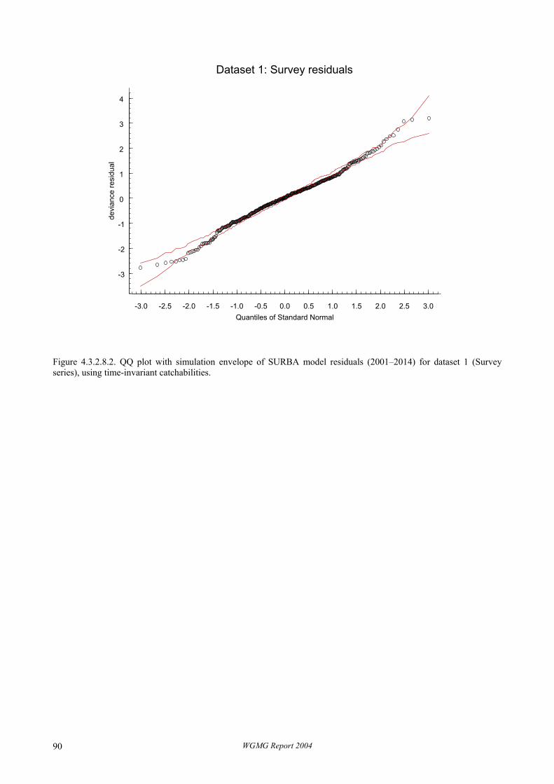
-3.0 -2.5 -2.0 -1.5 -1.0 -0.5 0.0 0.5 1.0 1.5 2.0 2.5 3.0

-3

-2

-1

0

1

2

3

4

Quantiles of Standard Normal

devi

ance

resi

dual

Dataset 1: Survey residuals

Figure 4.3.2.8.2. QQ plot with simulation envelope of SURBA model residuals (2001–2014) for dataset 1 (Survey series), using time-invariant catchabilities.

WGMG Report 2004 90

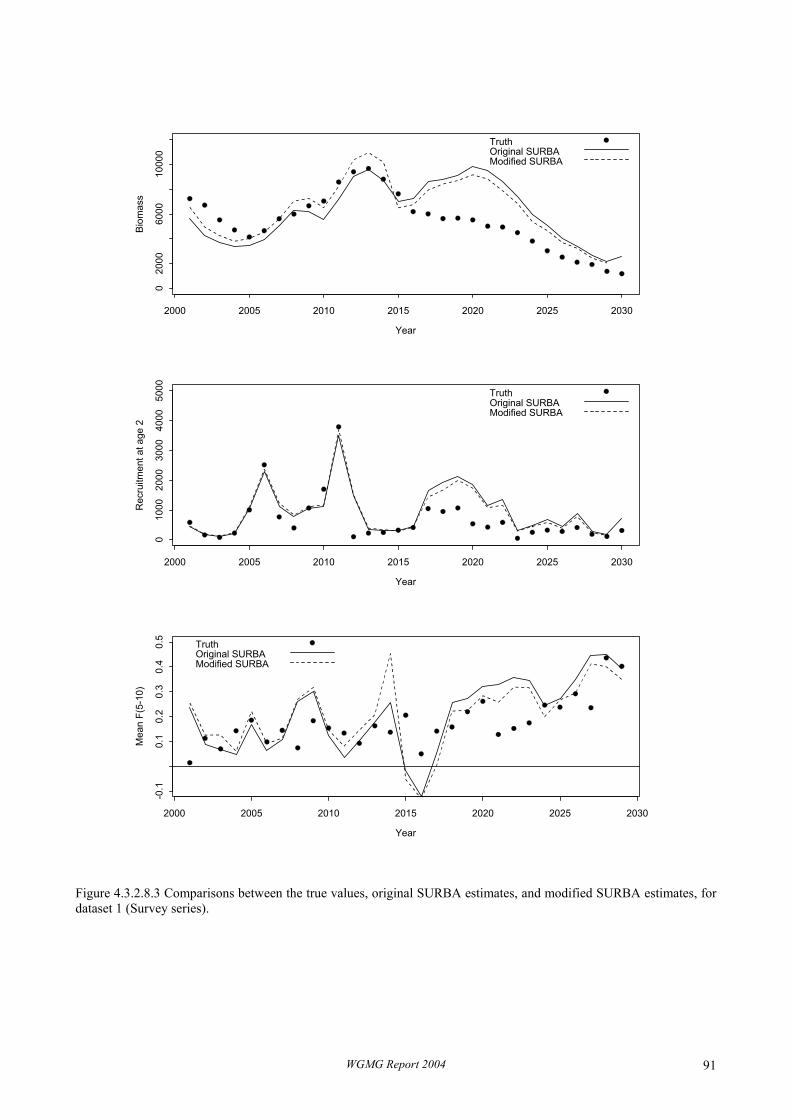
Year

Bio

mas

s

2000 2005 2010 2015 2020 2025 2030

020

0060

0010

000

TruthOriginal SURBAModified SURBA

Year

Rec

ruitm

ent a

t age

2

2000 2005 2010 2015 2020 2025 2030

010

0020

0030

0040

0050

00 TruthOriginal SURBAModified SURBA

Year

Mea

n F(

5-10

)

2000 2005 2010 2015 2020 2025 2030

-0.1

0.1

0.2

0.3

0.4

0.5

TruthOriginal SURBAModified SURBA

Figure 4.3.2.8.3 Comparisons between the true values, original SURBA estimates, and modified SURBA estimates, for dataset 1 (Survey series).

WGMG Report 2004 91

4.3.2.9 XSA+

Data set 1

Exploratory analysis

A series of screening analyses were applied to dataset 1 in order to examine the quality of the catch-at-age and tuning calibration data, prior to applying XSA. The screening process (outlined in Darby and Flatman 1994 and based on the ICES recommendations to Working Groups (The Blue Sheets) examined:

• the consistency of year class strength within cohorts and years (catch curve analysis) and between data sources, • consistency in the time-series of CPUE at age, • patterns and time-series trends in the log catch ratio residuals from a separable VPA model fitted to the catch-at-

age data, • patterns and time-series trends in the log catchability residuals from fits of the Laurec-Shepherd and XSA tuning

algorithms fitted to each CPUE series and the consistency of residual patterns between series . Plots of the commercial CPUE time-series against those from the survey, at each age, indicate consistent differences between the trends in the series in recent years (Figures 4.3.2.9.1 a,b). The series show close correlation until 2025, after which they diverge. The divergence is consistent across ages and raises doubts as to the quality commercial effort series in the most recent years (since ~2025).

Catch curve analysis and the fit of the separable VPA to the catch-at-age data highlighted departure from the assumption of constant selection at age (Figure 4.3.2.9.2). Positive residuals in the most recent years at the youngest ages indicate a change in total mortality at those ages, i.e., higher fishing and or natural mortality; parameters that are confounded in the model formulation. The selection at the oldest ages is noisy but appears to be constant.

The increased selection at the youngest ages suggests that the commercial catch data should not be used for calibrating VPA based models. The change in selection during recent years is a departure from model’s assumption of constant catchability.

The residual patterns from the fit of the Laurec-Shepherd ad-hoc algorithm to a catch-at-age and survey CPUE series indicate systematic departures from the assumption of constant catchability. The survey CPUE (Figure 4.3.2.9.3) show a consistent time-series correlation in the residuals of the younger converged ages. The pattern is consistent with a change in survey selection between 2015 – 2020. Residuals in the final years are closer to zero as a result of the use of the average catchability in the estimation of the terminal year fishing mortalities and should be ignored. The residuals from the Laurec Shepherd model fit could be interpreted as indicating either a change in the survey catchability between 2015 and 2020 or bias (under-reporting) of the catch-at-age data from that time period.

Two XSA model structures were examined. The first used the full time-series of survey data; the second split the survey data into three survey series (2001 – 2010, 2011 – 2020, 2021 –2030) in order to examine the log catchability residual patterns in blocked time periods. The XSA fitted to the full survey time-series generated similar time-series patterns to that of the Laurec Shepherd tuning, positive residuals during the most recent time period. The auto-correlated residuals indicate departure from the assumption of constant catchability and an inappropriate model structure. The fit of the model to the split survey series (Figure 4.3.2.9.4a,b,c) resulted in residuals that show no major departure from the assumption of constant catchability during the early and late periods of the survey series. During the middle period of the time-series the residuals have a strong trend, an increase in catchability.

Modifications to the XSA data structure

Assuming that the mis-specification results from a change in survey catchability, the simplest change to the XSA input data or run settings is to split the series into separate time-series as examined in the second XSA model structure. The residuals from the fitted model are presented in Figures 4.3.2.9.4. The time-series effect estimated for 2011 – 2020 could arise from a step change in catchability or a gradual increase. Varying the time periods used for the split surveys would allow further definition of the time period and magnitude of the change.

Figures 4.3.2.9.5 and 4.3.2.9.6 present non-parametric XSA bootstrap percentiles (with no bias-correction) of the data set 1 stock SSB, average fishing mortality and recruitment at age 2 estimated using the full survey time-series and the

WGMG Report 2004 92

subdivided survey. The bold lines plotted in Figures 4.3.2.9.5 and 4.3.2.9.6 present the “true” SSB and recruitment series (Section 4.3.1), fishing mortality was not available.

When the XSA model is fitted to the full time-series of survey data, over-estimation of historic catchability and underestimation of recent catchability, bias the SSB and recruitment estimates. Fishing mortality which is correlated with stock size would be expected to be under-estimated.

The separation of the survey series to fix the model fit, reduces the width of the confidence intervals due to the addition of the extra catchability parameters for the additional survey series. The bootstrap confidence intervals of the corrected assessment series overlap with the truth. Bias correction of the bootstrap percentiles is required before the degree of bias in the XSA bootstrap algorithm can be determined.

Conclusions based on the exploratory analysis of data set 1

The analysis of the data series indicate:

1) A change in selection towards the youngest ages in the most recent years of the time-series, constant selection at the oldest ages.

2) Use of the commercial CPUE data, with an effort series, for tuning is inappropriate due to a change in selection (catchability) at age.

3) Either, an increase in survey catchability to a new constant level between 2015 – 2020, or the onset of mis-reporting, at a constant rate, during the same period.

4) The commercial series catchability residuals did not indicate a change in catchability during 2015 - 2020 (but a more recent change due to the change in selection). Therefore the model mis-specification was attributed to an increase in survey catchability. A more consistent approach to finding the origin of the model misspecification would require additional information on any changes to the survey gear, ship or coverage for a more robust conclusion to be reached.

5) The uncertainty in the estimates estimated by bootstrapping of the mis-specified XSA model did not cover the truth. It was demonstrated that this method of uncertainty estimation will not provide an elastoplast for poorly specified models.

WGMG Report 2004 93

Figure 4.3.2.9.1a. The time-series of catch per unit effort of the survey (series 1) and the commercial catch data (series 2) for ages 2 – 4. Note the divergence since 2025.

Figure 4.3.2.9.1b. The time-series of catch per unit effort of the survey (series 1) and the commercial catch data (series 2) for ages 5 – 8.

WGMG Report 2004 94

-1

-0.8

-0.6

-0.4

-0.2

0

0.2

0.4

0.6

0.8

1995 2000 2005 2010 2015 2020 2025 2030 2035

Figure 4.3.2.9.2. The time-series of Data Set 1 separable VPA log catch ratio residuals at ages 4 – 7. The patterns illustrate departure from the assumption of constant selection at age across the time-series (increased mortality at the youngest ages).

-2

-1.5

-1

-0.5

0

0.5

1

1.5

1995 2000 2005 2010 2015 2020 2025 2030 2035

Figure 4.3.2.9.3. The time-series of Data Set 1 survey CPUE log catchability residuals at ages 4 – 9 from a Laurec Shepherd tuning. The patterns indicate departure from the assumption of constant catchability after 2015.

WGMG Report 2004 95

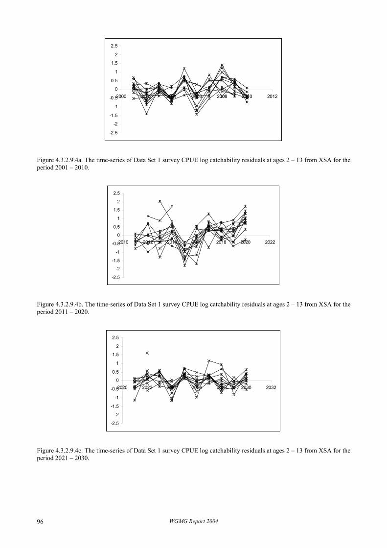
-2.5

-2

-1.5

-1

-0.5

0

0.5

1

1.5

2

2.5

2000 2002 2004 2006 2008 2010 2012

Figure 4.3.2.9.4a. The time-series of Data Set 1 survey CPUE log catchability residuals at ages 2 – 13 from XSA for the period 2001 – 2010.

-2.5

-2

-1.5

-1

-0.5

0

0.5

1

1.5

2

2.5

2010 2012 2014 2016 2018 2020 2022

Figure 4.3.2.9.4b. The time-series of Data Set 1 survey CPUE log catchability residuals at ages 2 – 13 from XSA for the period 2011 – 2020.

-2.5

-2

-1.5

-1

-0.5

0

0.5

1

1.5

2

2.5

2020 2022 2024 2026 2028 2030 2032

Figure 4.3.2.9.4c. The time-series of Data Set 1 survey CPUE log catchability residuals at ages 2 – 13 from XSA for the period 2021 – 2030.

WGMG Report 2004 96

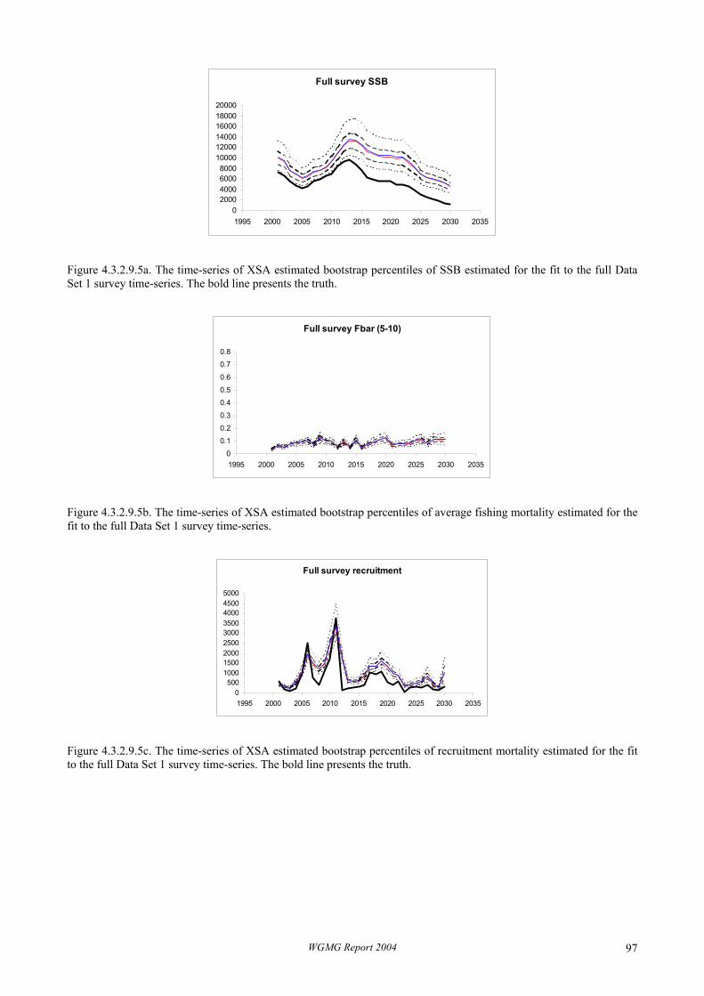
Full survey SSB

02000400060008000

100001200014000160001800020000

1995 2000 2005 2010 2015 2020 2025 2030 2035

Figure 4.3.2.9.5a. The time-series of XSA estimated bootstrap percentiles of SSB estimated for the fit to the full Data Set 1 survey time-series. The bold line presents the truth.

Full survey Fbar (5-10)

0

0.1

0.2

0.3

0.4

0.5

0.6

0.7

0.8

1995 2000 2005 2010 2015 2020 2025 2030 2035

Figure 4.3.2.9.5b. The time-series of XSA estimated bootstrap percentiles of average fishing mortality estimated for the fit to the full Data Set 1 survey time-series.

Full survey recruitment

0500

100015002000250030003500400045005000

1995 2000 2005 2010 2015 2020 2025 2030 2035

Figure 4.3.2.9.5c. The time-series of XSA estimated bootstrap percentiles of recruitment mortality estimated for the fit to the full Data Set 1 survey time-series. The bold line presents the truth.

WGMG Report 2004 97

Separate surveys SSB

0

2000

4000

6000

8000

10000

12000

1995 2000 2005 2010 2015 2020 2025 2030 2035

Figure 4.3.2.9.6a. The time-series of XSA estimated bootstrap percentiles of SSB estimated for the fit to the split Data Set 1 survey time-series. The bold line presents the truth.

Separate surveys Fbar (5-10)

0

0.1

0.2

0.3

0.4

0.5

0.6

0.7

0.8

1995 2000 2005 2010 2015 2020 2025 2030 2035

Figure 4.3.2.9.6b The time-series of XSA estimated bootstrap percentiles of average fishing mortality estimated for the fit to the split Data Set 1 survey time-series.

Separate surveys recruitment

0

500

1000

1500

2000

2500

3000

3500

4000

1995 2000 2005 2010 2015 2020 2025 2030 2035

Figure 4.3.2.9.6c .The time-series of XSA estimated bootstrap percentiles of recruitment mortality estimated for the fit to the split Data Set 1 survey time-series. The bold line presents the truth.

4.4 Conclusions and guidelines

4.4.1 Conclusions

A total of ten assessment methods were applied to between one and three simulated datasets from the NRC collection. The purpose of the exercise was, primarily, to ascertain the ability of general data-screening and the diagnostics of each

WGMG Report 2004 98

model to detect the model misspecifications in these datasets, and subsequently, to determine whether believing in and acting upon a particular diagnostic improves or worsens the fit of the assessment method to the truth.

The diagnostics currently available in these assessment methods are sometimes sufficient to indicate the presence of a problem and the general year or age range over which it applies (and therefore where we should be looking for further information), but they do not often indicate the cause of the problem and it is only very seldom that they can suggest courses of action to alleviate the problem. The exercise was carried out in ignorance of the features of the datasets being examined. Such blind testing is one good way to evaluate diagnostics, but in general, further information about the fishery, the survey, and so on would be required to make progress towards a better stock assessment. In no case did believing in and acting on a diagnostic appear to make the resulting assessment worse, but this may not hold in general.

The specific datasets used all involved much lower values of F than would be commonly encountered in current ICES stock assessments. With such values assessment methods can become unstable or unreliable. In addition, the more complex a model formulation, the more scope there would appear to be for the assessment method to bend to fit the characteristics of the data. For this reason, data evaluation should be done with simple models using limited assumptions.

Generalities are difficult to make on the basis of a limited number of datasets, and the continuation of this work would be beneficial.

Table 4.4.1.1 summarises estimated interest parameters from the assessment methods used in these analyses. Before modifications were applied, there was a general tendency to overestimate both the depletion ratio (B30/B1) and the recruitment (GM-R 1–30). Estimates of mean F in the last year varied widely between methods. After modifications, all methods moved closer to the true values.

Table 4.4.1.1. Comparison of estimated parameters across methods for data set 1, before and after modifications suggested by diagnostics (* = modifications suggested by external information, specifically that the survey vessel changed in 2015).

Summary indicators before modification

Method True CSA XSA KSA ICA SURBA CADAPT CAMERA Bayesian VPA

B30/B1 0.16 0.36 0.467 0.24–0.34 0.58 0.45 0.48 0.46 0.26 GM-R 1–30 412.2 422.2 848 506 882.2 702.8 720.0 444.1 320.4 F(5–10) in 30 n/a n/a 0.125 0.38–0.48 0.09 0.386 0.14 0.23 0.02

Summary indicators after modification

Method True CSA* XSA SURBA* CADAPT CAMERA B30/B1 0.16 0.194 0.182 0.369 0.20 0.18 GM-R 1–30 412.2 452.6 560 688.5 545.0 396.5 Fbar 5–10 0.402 n/a 0.578 0.350 0.43 0.50

4.4.2 General guidelines for stock assessment Working Groups related to ToR d)

The following are general guidelines that stock assessment Working Groups should follow for benchmark assessments:

• A wide range of diagnostics, both data-screening and model-based (see, for example, Section 4.3.1), and assessment methods should be used to explore fully the data, starting with the simplest available methods. The requirement for a wide range is driven by the fact that there is no universally-appropriate diagnostic or method.

• The lack of a retrospective pattern does not necessarily indicate a well-specified model.

WGMG Report 2004 99

4.4.3 Comments related to ToR e): investigate and implement statistical approaches that identify and quantify uncertainty due to conditioning choices in fish stock assessment

The topic is important, because uncertainty due to conditioning choices are believed to be large compared with that induced by stochastic noise around a correctly-specified model. The Working Group could not yet formulate a robust and reliable procedure to quantify such uncertainty in a statistical sense. The extent to which statistical diagnostics based on VPA-type models can be used to identify a degree of assurance that a particular model is correct is not fully understood and is likely to be highly variable across data sets.

One approach to quantifying structural uncertainty has been presented (KSA) but its behaviour has not been sufficiently tested to allow recommendation of generalised use. Either with KSA or other methods, at present only uncertainty due to the choice of abundance index can be easily quantified.

In practice therefore, only ad-hoc estimations of the reliability of particular stock assessments can be made. The methodology by which the assessors normally explore data sets and investigate the characteristics of models and data provides a first step in evaluating structural uncertainty.

Furthermore, it is recommended that the following guidance be given to assessment working groups in addressing the current ToR d). For each stock,

• identify the three parameters or model choices to which the assessment is most sensitive and about which uncertainty is most important;

• perturb those parameters or choices as far as is considered reasonable in the light of available data and information about the stock;

• report the maximum and minimum values of spawning stock biomass (depletion ratio = ratio of biomass from last year to biomass from first year) resulting from such perturbation.

The aims of this approach are to a) evaluate assessment uncertainty, and b) determine the sensitivity of the assessment to influential method inputs and structure. Such perceptions of uncertainty would be an important element to consider in formulating harvest control rules. The success of the approach should be evaluated by WGMG at its next meeting.

Appropriate parameters to perturb may include, amongst others, SE for shrinkage (XSA), choice of abundance index for tuning, age for catchability plateau (XSA), specification of selection model (ICA), weighting of survey series.

4.4.4 Reporting of data input, parameter settings and output tables for Bayesian analyses – provision of basic guidelines

At the May 2003 meeting of ACFM, the reviewers of the Baltic Salmon and Trout Assessment Working Group [WGBAST] requested that WGMG provide guidelines for the reporting of data input, parameter settings and output tables for Bayesian analyses that would be comparable to standard practice with the current analytical approaches commonly used within ICES (e.g., XSA, ICA and ADAPT). This request will be considered as part of the ToRs d) and e).

4.4.4.1 Guidelines for reporting of data inputs

For each annual Bayesian stock assessment, it is recommended that the complete set of data to which the stock assessment model (base case and any alternatives) is fitted be listed in standard formatted tables. For example, where abundance indices are included, the year, index value for the year, the units, for the index, and if available the empirically estimated CV or standard deviation for the observation should be listed. For tagging data, the year of release, the number of tags released in that year, the location of release, estimated age frequency distribution of animals in the release and number of animals of each age in the release should be tabulated. The recapture data should also be tabulated showing in the recapture year in the rows and the number of animals recaptured from each year and location of release in the columns in each row. For commercial catch biomass data, fishing effort and catch-age data, the same standard format as used in other commonly applied analytic approaches (e.g., XSA, ICA and ADAPT) should be used. For example, years should be in the rows, and the fleet or fleets to which the catch and effort data apply, and the units for the numbers given should be clearly indicated in the Table caption.

WGMG Report 2004 100

4.4.4.2 Guidelines for reporting of parameter settings

It is recommended that a table be provided listing all of the parameters used in the stock assessment. This should indicate in the first row, the symbol for the parameter, in the second row a brief description of the parameter, in the third row the units for the parameter,

In Bayesian analysis, input parameter settings include both parameter values that are treated as fixed and prior pdfs of estimated parameters. It is recommended that Tables be provided for parameters that are treated as fixed in the stock assessment. These should include in each row, the symbol for the parameter, the base case value and units for the value. In the table caption, definitions of each parameter symbol should be provided. Where alternative settings to the base case settings are provided, a separate columns for these alternative parameter values should be provided with the columns appropriately labelled as alternatives to base case values evaluated.

It is recommended that separate tables be provided for base case prior pdfs used in the stock assessment. These should include in each row, the symbol for the parameter, a common acronym for the functional form of the prior pdf applied, and the parameter value settings for the prior pdf (e.g., for a normal prior pdf, Normal(-2, 1)), the units for the value. In the table caption, the definitions of each acronym for each prior pdf functional form included should be provided. Also the interpretation of the numerical values should be provided in each pdf acronym. For example, for logNormal(-2, 1) it should be stated explicitly that the first value represents the median of the natural logarithm of the lognormal random variable (RV) and the second value represents, the precision (1/σ2) of the natural logarithm of the random variable where σ is the standard deviation of the natural logarithm of the RV. Where alternative settings to the base case priors are applied, a separate tables for these alternative parameter values should be provided with the same format as for the table with the base case prior pdfs.

A table or set of separate tables should be included to summarize the methods applied to:

• formulate the prior pdf for each parameter, • choose fixed parameter values for those parameters treated as fixed, and • formulate the likelihood functions and appropriate references should be provided in the table. Regarding the methods for the formulation of the priors, it would be sufficient to state, e.g., for the steepness parameter in stock-recruit function, that a hierarchical meta-analysis was applied and some references indicating the particular datasets and methods used should be provided. Regarding the documentation of likelihood function choice, any biological assumptions or fishery-related processes which imply the likelihood function adopted should be briefly stated. For example, stating that a negative binomial is assumed because it seems to fit some pooled data would not be appropriate here. Rather, the particular the biological assumptions about population dynamics and interaction of fish that may suggest the negative binomial likelihood function should be indicated instead.

4.4.4.3 Guidelines for reporting of outputs from Bayesian analyses

It is recommended that a list of the diagnostics applied to assess burn in (if MCMC is applied), goodness of fit of the model to the data, and convergence for the base case run be listed in a single Table. This should include the name of the diagnostic, a reference or references for it, and a comment about the values and observations about this diagnostic. If DIC is applied to evaluate the goodness of fit of alternative models to the data, then an additional table should be provided to indicate the structural form of the alternative model, the DIC value obtained and comments about the potential appropriateness of the model and any decisions made about the model evaluated.

It is recommended that for key interest variables, e.g., estimates of current stock biomass, historical harvest rates or mean fishing mortality rates per year, and depletion relative to some historic reference point, that posterior results be reported in a separate table. This should include for each interest variable the posterior mean and median, the posterior standard deviation (SD), and posterior 10th and 90th percentiles. The units of each variable should also be indicated in the Table.

It is recommended that for key interest variables, that for the base case, the marginal prior and posterior pdfs be plotted on the same axes. For evaluations of the sensitivity of marginal posterior pdfs to priors, it is recommended that the marginal posteriors resulting from the alternative settings of the prior pdfs be plotted on a different graph for each key interest variable.

WGMG Report 2004 101

5 DEVELOPMENT OF SOFTWARE WITHIN ICES’ FISHERIES SCIENCE

5.1 Introduction

Software that is used by ICES to inform advice is generally written and produced by individual scientists or national laboratories. Attempts at ensuring the quality of such software have been made on several occasions in the past; both by this Group, WGMG, as well as by dedicated ICES Study Groups (e.g., SGFADS: ICES 1998/ACFM:9). WGMG has discussed the proposal from the SGFADS at its last two meetings. Subsequently within ICES, the Resource Management Committee (RMC) discussed the use of computing environments for fishery science and management during the 2003 ICES Annual Science Conference (ASC) in Tallin, Estonia.

At that meeting, a framework being developed under an EU-funded Framework V project (Q5RS-2002–01824 FEMS: Framework for the Evaluation of Management Systems) for the investigation of interacting fisheries and their management was discussed. One of the tasks of the FEMS project is to develop a computer-based simulation framework for the evaluation of management strategies. If the framework is to be used easily and flexibly by a range of users for a large variety of tasks then the interface must be both intuitive and able to incorporate tools for a variety of tasks. A demonstration was presented to the Committee of an interface based on R (http://www.r-project.org) - an integrated suite of software tools for data manipulation, exploration, analysis and graphical display. This is essentially a front-end environment which calls assessment and simulation routines, like XSA, ensures transformation of data to fit these routines, and presents the results in a versatile way, creating graphs and tables that allow the analyst to scrutinise both input data and outputs.

R is probably a suitable language for producing such programs, being ‘open source’ and is increasingly being used in a number of ICES Expert Groups (e.g., SGGROMAT, SGSBSA, SGMSNS and SGPA). The EU through its own committee STECF has used R to develop software for multi-fleet investigations and analyses during recent years. This software has recently been reviewed by ICES and used within SGDFF and WGNSSK (WG4 Kraak).

The use of an OpenSource approach to software development within the fisheries context would lead to considerable benefits. It is therefore important that the framework in which such development can occur be as inclusive and usable as possible. The set-up must also be something that can be implemented without requiring an excessive amount of work. The overall structure of a possible framework is shown in Figure 5.1.1. Models must first be accepted onto a central system, and made available for distribution on a central web site. Further development of such models follows a cycle of work by the authors, informed by comments, suggestions and possibly code changes from the user community. The core of the system is a central site that must provide as much help and support to the user/developer community as feasible.

The proposed move within ICES towards an OpenSource approach leads to a need for a new approach to testing, evaluation and validation of fisheries models. Classical validation exercises (e.g., Kraak WG4) are compatible with the OpenSource paradigm, but they can be supplemented by feedback from ongoing use of the models. The challenge is therefore to design a system to allow for both formal and informal evaluation of the models employed. In this Section there is presented a simple and easy to implement framework in which such development can be encouraged, and suggestions on how progress towards specific evaluation methodologies can be made. Some technical notes on the operation of OpenSource development are presented in Section 5.6.

WGMG Report 2004 102

Figure 5.1.1. Overall structure of a framework for the development of software.

5.2 Initial acceptance

As earlier stated, the software tools used for stock assessment purposes within ICES are typically written by individual scientists, and may not be transparent to, or useable by, other researchers. In order to promote a more collaborative OpenSource methodology any application entered on the development system must meet certain requirements. These must be high enough to ensure that the software on the development system is accessible to all users and meets minimum reliability standards. However, the requirements must also be flexible enough to allow for a wide range of tools to be included, and to ensure that tools at an early stage of development are not excluded. Open and Closed Source applications could both be accepted onto such a development system, but the source code should always be available to the ICES Secretariat, even if it is not available for distribution to users. There is a further requirement that the process of accepting a tool to the development system not be excessively time consuming for either the authors or the Committee responsible for the development system.

The method adopted by the International Commission for the Conservation of Atlantic Tunas, ICCAT (2000) (see Appendix F) provides a way to balance these competing requirements, and WGMG suggest that a similar approach could be followed within ICES. In essence, this requires that a new tool be accompanied by sufficient documentation to enable a user to run it, a worked example the user can replicate, and a description of the model itself. Acceptance onto the development system will not constitute certification of the reliability of the application. The initial acceptance procedure should not concern itself with the applicability or accuracy of the model in different situations. Once a model is on the development system such evaluations can be made on an ongoing basis.

It is recommended that an Acceptance Committee should be set up, along the lines employed by ICCAT (ICCAT 2000). Any application submitted to the development system must be accompanied be a catalogue document, similar to that employed by ICCAT (see Appendix F). When an application is submitted to the Acceptance Committee, the Committee would determine whether the authors had adequately provided all the elements required, determine if the documentation was sufficient to use the software, and if the application performed as claimed on the supplied example. These are the

WGMG Report 2004 103

only requirements for acceptance onto the development system. Those responsible for assessing each individual application may choose to conduct further tests, and the results of any such tests should then be made generally available. However, the acceptance of the application onto the development system should not be conditional on the result of such additional tests, otherwise early stage development models would be rejected.

In order to encourage as many programs as possible onto the system, there should not be a requirement that all tools be made OpenSource. However, in order to take advantage of the benefits of OpenSource development contributors to the system should be encouraged to release their code under some sort of OpenSource license. If this is done, and if common programming languages are used, it would be possible to share code between projects, and thus reduce development time.

5.3 Web site

If an OpenSource methodology is to be pursued then a central web site, hosted by ICES, to coordinate and support such collaborative development would be required. In order to be fully effective such a web site should bring together a number of different features in a single location. As well as the software tools themselves, and along with their documentation, the site should host the tools to evaluate these models (both data sets and evaluation software), and the results of previous evaluations. In addition, this web site should contain the guidelines for submitting a new project to the development system, and provide support for users in evaluating and selecting between different software. Each program hosted on the web site should have a standardized directory.

The ICES software download page (http://www.ices.dk/datacentre/software.asp) provides a template on which such a web resource could be based. The addition of the catalogue document recommended in Section 5.2 would ensure that a user would be able to use the software without having to consult the author(s) directly. Further information could also be included here, on a model by model basis or in the form of comparison charts. For instance, information such as the ability to use age and/or length information, the possibility of using more than one age-structured index for cohort models and so on could be listed. For example, the information presented in Appendix D would prove useful.

When an evaluation is conducted on a particular model the results of that evaluation should be submitted to ICES and made available alongside the model on the web page, to enable users to more easily select between models. Such selection would also be aided by having a section where the performance of different models on similar tests could be readily compared. For instance, if standardized test artificial data sets are adopted (Section 5.4), it should be made as easy as possible to compare the relative performance of the different models on each data set. The data sets themselves should be also available on the system, allowing for authors and users to compare the performance of any new models against those already on the system. In addition, feedback from users in a variety of contexts (stock assessment, individual research, universities, etc.) should be channelled to the authors and, where appropriate, made available to other end users via the web site. If standardized assessment tools are available (e.g., Grosjean and Kell WG1) they should be made available on the central web site. This would facilitate end user evaluation of the different models. Furthermore, the standardized format of the output of such a tool would make comparison between different evaluations much simpler and more transparent.

Finally, a mailing list would be an essential part of such a system. This would not only provide a medium for announcing new applications and new versions of existing applications, but would also facilitate the discussion and collaborative development project.

Beyond this minimum, ICES should also consider how much support it wishes to provide (and fund) in the OpenSource development process. The possibility of providing development aids such as version tracking systems, discussion and wish list forums and the like should be investigated. If this is desired it could be hosted either directly by ICES or through an agency such as source forge (Section 5.6.3).

5.4 Artificial data sets

A key tool for evaluating the performance of individual models, and inter-comparison between those models, is the use of simulated data sets with known properties. It is not proposed that models should achieve any pre-set level of performance against simulated data sets in order to be incorporated into the development system. However, it is important that models on the system should be run against standard simulated data sets, and the results of such work should be easily available to those downloading the software. This process would provide guidelines on the range of applicability of the models. The data sets would fulfil two distinct purposes. An initial, relatively small, suite of specific data sets would identify the stability of the models, and possibly cases where individual models are clearly inappropriate. Second, using a data simulator would allow for the possibility of creating multiple datasets with random

WGMG Report 2004 104

noise around specified structure, for use in detailed evaluation of the models. The parameters used in creating these data sets should then be freely available on the website to allow for comparison between models.

It is therefore suggested that WGMG should work inter-sessionally to create and/or select a small number (perhaps only three or four) of standard data sets to be used as basic tests for all tools on the system. A comparison of the performance of tools on the system against these data sets should be conducted and the results placed on the web site. WGMG should decide on what diagnostics will be reported for each experiment.

Further data sets can then be created and placed on the system over time, either as part of a core suite of standard test data sets that all applications should be run against, or as part of a more general library of data sets covering a range of different situations. The number of desirable features of such a suite of simulated data sets is extremely large, and contains features such as: low and high noise situations; data sets with and without outliers; presence or absence of year dependant changes in catchability, mortality, recruitment, etc.; and missing or unreliable years of data. Such a list could be extended in a multitude of directions, and fulfilling all of these requirements would represent a hindrance to ever starting such a project. These data sets should therefore be added individually as required. In each case a data simulator (section 5.5) should be used to create multiple replications of each data structure with added random noise. If a new model is added to the system that is structurally incompatible with the existing simulated data sets then a new, more appropriate, test data set must be created (c.f. Section 4.4).

Once the development system is established an early part of incorporating a new application onto the development system should be to run the applications on the established core suite of basic simulated data sets already used on an existing application. This should represent only a small amount of work for each new application. As models are also run on the randomised multiple datasets the results should be presented on the website.

5.5 Data simulator

Progress has been made on designing an easy-to-use data simulator in line with the description given in ICES (2003a), addressing the ToR c) of this year’s meeting. A prototype graphical user interface program has been developed in Visual Basic which can produce single-species, single-area Gadget age-length structured models. This produces the ability to custom design a simulated data set with a wide range of different possible structures. The part of the package to add known errors to the data sets has not yet been implemented. The Gadget program is freely available, including source code, to download from http://www.hafro.is/gadget. The source code of the graphical user interface will be made OpenSource, as far as possible considering the use of windows libraries.

Further development will take place during the course of 2004, with a target for a working package to be presented at the ICES ASC meeting in September 2004. This would ensure that the program is in place for the next meeting of WGMG in 2005, and for possible subsequent use in generating standard simulated data sets for use in evaluating fisheries models. The development of such a data simulator should be seen as complimentary to the progress towards an OpenSource development paradigm.

In keeping with the ideas advanced elsewhere in this Section 5, the initial version of the program would have a rather sparse set of error filters to add errors to the simulated data set. Once available, the data simulator could then be further extended using the development system outlined in Section 5.1. Additionally, suggestions from WGMG can be incorporated.

5.6 Technical notes on open source

5.6.1 What is OpenSource software?

There are several key references to understand what Free/OpenSource software means. A simple search in Google gives the following definition:

“Any software whose code is available for users to look at and modify freely”.

However, this definition by-passes the philosophical issues about Free/OpenSource software. Richard Stallman of the Free Software Foundation (http://www.fsf.org) is considered the person behind the concept of Free Software. He refers to the subject (http://www.gnu.org/philosophy/free-sw.html) as:

“Free software is a matter of liberty, not price. To understand the concept, you should think of “free” as in “free speech,” not as in “free beer”.”

WGMG Report 2004 105

Free/OpenSource software raises a lot of concerns about intellectual property, responsibilities and so on. These problems can be tackled by licensing the software defining rules for others to use, distribute, change, etc. The GNU (http://www.gnu.org) Public License (GPL) is one example but many others exist. A comprehensive list can be found at (http://www.gnu.org/licenses/license-list.html).

Other valuable resources exist regarding Free/OpenSource software. The OpenSource Initiative (Appendix G) is one of them. Their definition of OpenSource software elaborates criteria (with comments) that software must comply with in order to be considered OpenSource (http://www.opensource.org/docs/definition.php). Richard Stallman's texts about the GNU project are also important references (check at http://www.gnu.org/doc/doc.html, http://www.gnu.org/gnu/thegnuproject.html). Further information about the definition, history, business model, etc. of OpenSource can be found in Chapter 1 of the book OpenSource Development with CVS by Karl Fogel and Moshe Bar (http://cvsbook.red-bean.com/). Eric Raymonds, in his book The Cathedral and the Bazaar (http://www.catb.org/~esr/writings/cathedral-bazaar/), summarizes the advantages of this as Linus Law:

“Given enough eyeballs, all bugs are shallow.”

5.6.2 Technical notes

Developing in an OpenSource cooperative environment creates several technical problems.

If a developer distributes his software and receives several bug fixes and code contributions it can be difficult for him/her to integrate and organize all contributions. In a small project, such as is currently typical of fisheries science, with one or two developers and a small number of users, this process can be conducted manually. However, as the project grows in size it may become necessary to automate the process of tracking and managing changes to the code. In any case this will provide a number of benefits in managing the project. One of the most used programs by the OpenSource community to deal with these problems is CVS or Concurrent Versions System (http://www.cvshome.org/). It allows people all around the world to download a program and developers to submit their changes. CVS deals with all submissions in a transparent way and is able to deal with conflicting changes by obliging the developers to explicitly solve the conflicts. Also, CVS keeps a history of the development process allowing both developers and users to go back to a certain state of development or make comparisons between versions. A lot more can be done with CVS. The book OpenSource Development with CVS (http://cvsbook.red-bean.com/) and other documents can be found at the CVS site.

In order to allow users to examine and modify code, it is essential that that code be written in as user-friendly a fashion as possible. This includes features such as clearly structured code, comments, and documentation.

Communication between users and developers involved with a specific program is also an important matter that is usually solved by the existence of a mailing list where users and developers can keep in touch and share their experience and knowledge about the program. In situations where the community grows to a number of users that makes it impossible to manage unless other lists are created (developers’ list, documentation list, etc.). Within the fisheries context, communication must involve sharing the results of evaluations of performance in different situations between users.

The OpenSource development is based around the internet and so a web page is a crucial element. There are some institutions (e.g., SourceForge (http://sourceforge.net/) on the web that create conditions for OpenSource developers to keep their projects, giving free access to CVS servers, mailing lists, forums, web pages, etc.

5.6.3 Possible examples in fisheries science

The fact that the user community consists of highly educated scientists ensures that they are likely to be directly interested in the algorithms and code, and possess the technical ability to make the best use of OpenSource software. Within fisheries science, OpenSource code is likely to deliver several different benefits to users.

On the one hand, the ability to examine code allows for specific algorithms and their implementation to be checked as and when required. Extending and adding specific features (e.g., different growth assumption, year effects, etc.) to existing models should be possible in a relatively short-time span. This will enable models to be changed on the fly during actual use to fit with different and problematical data sets. If such changes prove useful they can be submitted to the code maintainer for incorporation into the next release, and will thus speed the development of the software considerably. Furthermore, large-scale modifications to the program (e.g., changing the structure of the stock modelled) will be facilitated by the large number of scientists available to contribute to, and examine, the code.

WGMG Report 2004 106

5.7 Conclusions

The approach proposed in last year’s report for guidelines on the formal procedures to be adopted by WGMG for the testing, evaluation and validation of software for use by ICES stock assessment Working Groups is still appropriate (ICES 2003). However, the move this year towards OpenSource has highlighted new concerns but the need to identify a responsible person/co-coordinator for testing and evaluation of software still remains.

The use of OpenSource should be encouraged to maximize end user participation in application development, minimize unnecessary duplication of effort, and allow for the examination of algorithms. In order to facilitate this the following steps need to be taken.

• The priority is to produce a development system, based around a working web site (Section 5.3) with several modelling applications meeting the minimum inclusion criteria (Section 5.2.) available. A mailing list should be established at the same time for general discussion, and announcement of new applications on the system. Establishing and maintaining these web pages will require a commitment of manpower on the part of ICES.

• Criteria for entering an application onto the development system must be adopted, and WGMG suggest using the ICCAT protocol as a template, as modified in this Report. Specific individuals should be appointed to coordinate the inclusion of new models onto the development system.

• Parallel to this a small suite of standard simulated data sets should be established, on which the initial applications on the development system can be tested. Future applications added to the system should then be evaluated, where possible, against the same artificial data sets. In both cases the results should be published on the web site, along with any other evaluations conducted.

5.8 Minimum requirements to implement an OpenSource initiative within ICES

The work involved in implementing the website based OpenSource/collaborative development system suggested in this Section 5 can be divided into two parts. On the one hand the system has been designed in order to ensure that the on-going maintenance of the system involves a relatively small commitment of time and effort. However, a certain amount of concerted work must be initially conducted in order to kick start the project. Specific individuals must be identified, and resources allocated, to fulfil both objectives. In particular, three aspects need to be considered:

Computer web page development

An experienced Webmaster, based at ICES, to design and implement web pages as outlined in 5.3. This would require a competent web page designer, liaising with the scientists in the Acceptance Committee.

On an ongoing basis there must be a Webmaster responsible for updating the web page, incorporating new results into comparison charts, and administering the mailing list. Although this will not require the full time attention of one person, it is vital that resources be committed on an ongoing basis for this work. Nothing will kill the project quicker than a poorly maintained and infrequently updated website.

Acceptance Committee members

Responsible for the basic testing of models submitted to the development system, and accepting or rejected those models onto the system. These would be researchers active in the fisheries assessment field. The amount of time required on an ongoing basis from each Committee member would be minimal, with hopefully no more than one model to be evaluated by each member in a given year, and could be coordinated by email between the Committee members. WGMG could then serve as a point of liaison between the Committee members, and a place to select replacement members as required.

During the initial phase the Committee would have to produce a formal document setting out guidelines for accepting applications onto the system (based on section 5.2 and the ICCAT document presented in Appendix F), adopting an initial minimal suite of 3 or 4 test data suites and running the first models accepted onto the system against those data sets. Finally one or more members of this Committee should liaise with the ICES web designer on the structure and contents of the central web resource. A meeting of those involved may well be required to successfully complete these tasks.

WGMG Report 2004 107

Acceptance Committee Chair

Responsible for co-ordinating the ongoing work of the Acceptance Committee.

Would also have an initial responsibility to drive the project forwards by encouraging researchers in different institutions to submit their applications, accompanied by adequate documentation and a working example. This would be a vital task in ensuring that the system become rapidly operational and the Chair must be carefully selected accordingly. The Chair would also have the responsibility of ensuring that the web site met the requirements of the project.

6 RECOMMENDATIONS AND FURTHER WORK

The Group has made a number of suggestions and recommendations throughout this report and these have been highlighted in the text.

6.1 Suggestions and recommendations

WGMG highlights the following recommendations, specifically in respect of ToRs a) and b), that have been previously stated in the main body of this report.

• Although both biomass and F based reference points are required by international agreements, it appears from simulation studies that F-based reference points may exhibit better properties than biomass based ones. In such cases, management procedures that minimise the reliance on biomass reference points should be developed.

• Current Flim reference points appear to be consistently defined. • If proxies for FMSY are to be used as the basis for providing advice then these will have to be reviewed on a case by

case basis. • HCRs must be developed as a high priority within ICES using available tools and methods, in the first instance. • An initial list of candidate stocks for which to evaluate HCRs has been proposed and amongst these are included

the recently agreed single-species recovery plans for cod stocks and northern hake. • A road map has been proposed that would be appropriate to ICES and so aid in the investigation of management

procedures and HCRs. The request from the May 2003 meeting of ACFM that WGMG provide guidelines for the reporting of data input, parameter settings and output tables for Bayesian analyses has been addressed in Section 4.4.4 of this report.

6.2 Future terms of reference

The Chair reminded the meeting that this is his third consecutive meeting as Chair and invited nominations for the Chair from 2005. Following discussions within WGMG and after seeking guidance from ICES (Henrik Sparholt who attended this meeting), it was unanimously agreed that the current Chair should continue for a second term.

Further, the Working Group on Methods on Fish Stock Assessments [WGMG] (Chair: C.M. O’Brien, UK) meet in Lisbon, Portugal during the 1st quarter of 2005. The Group and the Chair agreed that the ToRs of this current meeting were too extensive – covering both HCRs and diagnostics. For the next meeting, the members of WGMG propose to continue to address the ToR a) from this meeting but to consider the evaluation of specific stocks with respect to candidate HCRs.

A draft ICES Resolution will be developed inter-sessionally before the Consultative Committee’s next meet in June 2004 and finalised after discussion within ACFM.

WGMG Report 2004 108

7 WORKING DOCUMENTS AND BACKGROUND MATERIAL PRESENTED TO THE WORKING GROUP

7.1 Working papers and documents (W)

A total of 17 documents were presented to the meeting as working papers. These are listed in this Section 7.1; together with their assigned code for ease of reference within the various sections of this report.

ToR (A)

WA1 Bogstad, B., Åsnes, M.N. and Skagen, D.W. PROST – a new computer program for stochastic projections for fish stocks.

WA2 Kell, L.T., Pilling, G., Kirkwood, G., Pastoors, M., Abaunza, P., Aps, R., Biseau, A., Korsbrekke, K., Kunzlik, P., Laurec, A., Mesnil, B., Needle, C., Roel, B. and Ulrich, C. An evaluation of the implicit management procedure for ICES roundfish stocks.

WA3 Kell, L.T., Pilling, G., Kirkwood, G., Pastoors, M., Abaunza, P., Aps, R., Biseau, A., Korsbrekke, K., Kunzlik, P., Laurec, A., Mesnil, B., Needle, C., Roel, B. and Ulrich, C. Limiting inter-annual variation in total allowable catch strategies. An application to ICES roundfish stocks.

ToR (B)

WB1 Skagen, D.W. Performance of management regimes with fixed quotas – implications for reference points.

WB2 Kell, L.T. and Bravington, M. A limit fishing mortality reference point based on concave regression.

WB3 Kell, L.T., Pilling, G. and De Oliveira, J. Magic and the Precautionary Approach: an evaluation of target fishing mortality reference points for North Sea cod.

ToR (C)

No working papers submitted under this term of reference but a presentation by Daniel Howell was given during the meeting.

ToR (D)

WD1 Cadigan, N. Influential cases in stock and recruitment models.

WD2 Azevedo, M. Bayesian fish stock assessment with VPA.

ToR (E)

WE1 Patterson, K.R. Assessing structural uncertainty using KSA (kernel survivors analysis).

WE2 Cadigan, N. and Healey, B. Confidence intervals for the change point in a stock-recruit model: a simulation study of the profile likelihood method based on the logistic hockey stick model.

WGMG Report 2004 109

ToR (F)

WF1 Mesnil, B. A crash test of Catch-Survey Analysis (CSA) using the NRC simulated data.

WF2 Needle, C.L. Absolute abundance estimates and other developments in SURBA.

WF3 McAllister, M., Kell, L.T., O’Brien, C.M., Pastoors, M.A., Hunter, E. and Bolle, L. Use of tagging data as part of catch independent assessment and management procedures.

ToR (G)

WG1 Grosjean, P. and Kell, L.T. A general framework for fisheries modelling.

WG2 Scott, R. Assessment of Irish Sea cod using FLR.

WG3 Scott, R. and De Oliveira, J. Comparison of VPA suite and FLR XSA results.

WG4 Kraak, S.B.M. An evaluation of MTAC – a program for the calculation of catch forecasts taking the mixed nature of the fisheries into account.

7.2 Background material (B)

A total of 8 documents were submitted to the meeting as background papers. These are listed in this Section 7.2; together with their assigned code for ease of reference within the various sections of this report.

ToR (B)

BB1 O’Brien, C.M., Kell, L.T. and Smith, M.T. (2003). Evaluation of the use of segmented regression through simulation for a characterisation of the North Sea cod (Gadus morhua l.) stock, in order to determine the properties of Blim (the biomass at which recruitment is impaired). ICES CM 2003/Y:10.

BB2 Hutton, T. and Padda, G. Factors influencing the choice of a HCR: evaluating alternative recovery trajectories with an illustrative example based on speculative data.

BB3 Punt, A.E. (2003). Evaluating the efficacy of managing West Coast groundfish resources through simulations. Fishery Bulletin 101:860–873.

BB4 Patterson, K. and Kirkegaard, E. (2003). Presentation of fisheries advice taking account of mixed fisheries, environmental integration requirements, harvest rule-based fishery evaluations, and yield considerations and economic analysis. ICES CM 2003/ X:18.

BB5 Bravington, M.V., O’Brien, C.M. and Stokes, T.K. (1999). Sustainable recruitment: the bottom line. ICES CM 1999/P:01.

Bravington, M.V., Stokes, T.K. and O’Brien, C.M. (2000). Sustainable recruitment: the bottom line. Marine and Freshwater Research 51:465–475.

WGMG Report 2004 110

ToR (E)

BE1 Darby, C.D., Bowering, W.R. and Mahé, J.-C. (2003). An assessment of stock status of the Greenland halibut resource in NAFO subarea 2 and divisions 3KLMNO based on extended survivors analysis with short and medium-term projections of future stock development. NAFO SCR Doc. 03/64 Revised.

BE2 Lewy, P. and Nielsen, A. (2003). Modelling stochastic fish stock dynamics using Markov Chain Monte Carlo. ICES Journal of Marine Science 60:743–752.

BE3 Nielsen, A. and Lewy, P. (2002). Comparison of the frequentist properties of Bayes and the maximum likelihood estimators in an age-structured fish stock assessment model. Canadian Journal of Fisheries and Aquatic Sciences 59:136–143.

8 REFERENCES

Throughout this report there have been a number of references cited within the Sections 1 through 5. In this Section 8, those references are collated by report Section number. 8.1 Cited in Section 1 ICES (2002). Report of the Working Group on Methods on Fish Stock Assessments, ICES Headquarters, Copenhagen,

Denmark, 3–7 December 2001. ICES CM 2002/D:01. ICES (2003). Report of the Working Group on Methods on Fish Stock Assessments, ICES Headquarters, Copenhagen,

Denmark, 29 January – 5 February 2003. ICES CM 2003/D:03. 8.2 Cited in Section 2 Arnold, G., Davenport, J., O. Maoileidigh, N. and Thorseinsson, V. (2002). Tagging methods for stock assessment and

research in fisheries. Report of Concerted Action FAIR CT/96/1394 (CATAG), Reykjavik, Iceland. Beverton, R.J.H. and S.J. Holt (1957). On the dynamics of exploited fish populations. U.K. Min. Agr. Fish. and Food,

Fish. Invest. Ser. 2, 19:1–533. Bolle, L. J., E. Hunter, A. D. Rijnsdorp, M. A. Pastoors, J. D. Metcalfe and J. D. Reynolds (2001). Do tagging

experiments tell the truth? Using electronic tags to evaluate conventional tagging data. ICES CM 2001/O:02. Brooks, E.N., Pollock, K.H., Hoenig, J.M., and Hearn, W.S. (1998). Estimation of fishing and natural mortality from

tagging studies on fisheries with two user groups. Canadian Journal of Fisheries and Aquatic Sciences 55:2001–2010.

De la Mare, W.K. (1998). Tidier fisheries management requires a new MOP management-oriented paradigm. Reviews of Fish Biology and Fisheries 8:349–356.

Dorazio, R. M. and P. J. Rago (1991). Evaluation of a mark-recapture method for estimating mortality and migration rates of stratified populations. Canadian Journal of Fisheries and Aquatic Sciences 48(2): 254–260.

Gentle, J. E. (2003). Random number generation and Monte Carlo methods. Second Edition. Statistics and Computing. Springer-Verlag: New York. 381pp.

Hilborn, R. (1990). Determination of fish movement patterns from tag recoveries using maximum likelihood estimators. Canadian Journal of Fisheries and Aquatic Sciences 47(3):635–643.

Hilborn, R., Pikitch, E.K. and M.K. McAllister (1994). A Bayesian estimation and decision analysis for an age-structured model using biomass survey data. Fisheries Research 19:17–30.

Hoaglin, D.C. and D.F. Andrews (1975). The reporting of computation-based results in statistics. The American Statistician 29:122–126.

Hoenig, J.M., N.J. Barrowman, W.S. Hearn and K.H. Pollock (1998). Multiyear tagging studies incorporating fishing effort data. Canadian Journal of Fisheries and Aquatic Sciences 55(6):1466–1476.

Holt, S. (1998). Fifty years on. Reviews of Fish Biology and Fisheries 8:357–366. Hunter, E., J.D. Metcalfe, J.D. Reynolds and G.P. Arnold (2001). Subdivision of the North Sea plaice population:

evidence from electronic tags. ICES CM 2001/O:8. ICES (1992). Report of the ICES study group on tagging experiments for juvenile plaice. IJmuiden, Netherlands, 16–22

March 1992. ICES CM 1992/G:10. ICES (1994). Report of the Working Group on Long-term Management Measures. ICES CM 1994/Assess:11. ICES (1999a). Report of the Study Group on Multiannual Assessment Procedures, Vigo, Spain, 22–26 February 1999.

ICES CM 1999/ACFM:11.

WGMG Report 2004 111

ICES (1999b). Workshop on Standard Assessment Tools for Working Groups. ICES CM 1999/ACFM:25. ICES (2001). ICES Fisheries System Working Group. ICES CM2001/D:06. ICES (2002). Report of the Baltic Salmon and Trout Assessment Working Group. ICES CM 2002/ACFM:13. ICES (2003a). Report of the Study Group On the Further Development of the Precautionary Approach to Fishery

Management. ICES CM 2003/ACFM:09. ICES (2003b). Report of the Baltic Salmon and Trout Assessment Working Group. ICES CM 2003/ACFM. IWC (1993). Report of the Scientific Committee. Report of the International Whaling Commission 43:57–64. Kell, L.T., O’Brien, C.M., Smith, M.T., Stokes, T.K., and B.D. Rackham (1999). An evaluation of management

procedures for implementation of the precautionary approach in the ICES context for North Sea plaice Pleuronectes platessa L. ICES Journal of Marine Science 56:834–845.

Kell, L.T., G. Kirkwood, G. Pilling, P. Abaunza, R. Aps, F.A. Van Beek, A. Biseau, C.M. Ulrich, R. Cook, K. Korsbrekke, P.A. Kunzlik, A. Laurec, B. Mesnil, C. Needle, M.A. Pastoors and B.A. Roel (2002). Analysis of possibilities of limiting the annual fluctuations in TACs. Final report FISH/2001/02/02), MATES project, CEFAS, Lowestoft.

Kell L.T., Die, D.J., Restrepo, V.R., Fromentin, J.M., Ortiz de Zarate, V. and P. Pallares (2003a). An evaluation of management strategies for Atlantic tuna stocks. Scientia Marina 67 (Supplement 1):353–370.

Kell, L.T., Pilling, G., Kirkwood, G. Pastoors, M., Abaunza, P., Aps, R., Biseau, A., Korsbrekke, K., Kunzlik, P., Laure, A., Mesnil, B., Needle, C., Roel, B. and C. Ulrich (2003b). Limiting inter-annual variation in total allowable catch strategies - an application to ICES roundfish stocks. ICES CM 2003/X:07.

Kell, L.T., Smith, M.T., Scott, R., Pastoors, M., van Beek, F., Hammond, T., O’Brien, C.M. and G. Pilling (2003c). Limiting inter-annual variation in total allowable catch strategies - an application to ICES flatfish stocks. ICES CM 2003/X:06.

Kuikka, S., Hilden, M., Gislason, H., Hansson, S., Sparholt, H. and O. Varis (1999). Modeling environmentally driven uncertainties in Baltic cod Gadus morhua management by Bayesian influence diagrams. Canadian Journal of Fisheries and Aquatic Sciences 56:629–641.

Louviere, J.J. and G. Woodworth (1983). Design and analysis of simulated consumer choice or allocation experiments: an approach based on aggregate data. Journal of Marine Research 20:350–366.

Martell, S.J.D. and Walters, C.J. (2002). Implementing harvest rate objectives by directly monitoring exploitation rates and estimating changes in catchability. Bull. Mar. Sci. 70(2):695–714.

McAllister, M.K., Starr, P.J., Restrepo, V. and G.P. Kirkwood (1999). Formulating quantitative methods to evaluate fishery management systems: what fishery processes should be modelled and what trade-offs should be made? ICES Journal of Marine Science 56:900–916.

Michielsens, C.G.J. (2003). Bayesian decision theory for fisheries management of migratory species with multiple life histories. Ph.D thesis, Imperial College, London.

Patterson, K.R., Cook, R.M., Darby, C.D., Gavaris, S., Mesnil, B., Punt, A.E., Restrepo, V.R., Skagen, D.W., Stefánsson, G. and M. Smith (2000). Validating three methods for making probability statements in fisheries forecasts. ICES CM 2000/V:06.

Peterman, R.M. (2004). Challenges and opportunities for dealing with complex fisheries. ICES Journal of Marine Science (submitted).

Ravier C. and J. Fromentin (2001). Long-term fluctuations in the eastern Atlantic and Mediterranean bluefin tuna population. ICES Journal of Marine Science 58:1299–1317.

Reynolds, J.D., G.P. Arnold, J.D. Aldridge, J.M. Baveco, L. Bolle, R.R. De Clerck, P. Degnbol, W. Demare, D.P. Edwards, P. Gardiner, B. Holford, E. Hunter, J.D. Metcalfe, H. Nicolaisen, M.N. Nicholson, C.M. O'Brien, E. Ongenae, M.A. Pastoors, A.D. Rijnsdorp, R. Van Kempen and P.I. Van Leeuwen (2001). Migration, Distribution And Spatial Dynamics Of Plaice And Sole In The North Sea And Adjacent Areas. Final report., SBS-UEA, RIVO, CEFAS, DIFRES, CLO-DZ. FAIR PL96–2079.

Rijnsdorp, A.D. and M.A. Pastoors (1995). Modelling the spatial dynamics and fisheries of North Sea Plaice (Pleuronectes platessa L.) based on tagging data. ICES Journal of Marine Science 52:963–980.

Rivot, E. and Prevost, E. (2002). Hierarchical Bayesian analysis of capture-mark-recapture data. Canadian Journal of Fisheries and Aquatic Sciences 1768–1784.

Schwartz, C.J. and Taylor, C.G. (1998). Use of the stratified-Petersen estimator in fisheries management: estimating the number of pink salmon (Oncorhynchus gorbuscha) sapwners in the Fraser River. Canadian Journal of Fisheries and Aquatic Sciences 55:281–296.

Skagen, D.W., Stefánsson, G. and M. Smith (2000). Validating three methods for making probability statements in fisheries forecasts. ICES CM 2000/V:06.

Walters, C.J. and Martell, S.J.D. (2002). Stock assessment needs for sustainable fisheries management. Bull. Mar. Sci. 70(2):629–638.

Wilimovsky, N.J. (1985). The need for formalization of decision algorithms and risk levels in fishery research and management. Canadian Journal of Fisheries and Aquatic Sciences 42:258–262.

Xiao, Y. (2000). An individual-based approach to evaluating experimental designs for estimating rates of fish movement from tag recoveries. Ecological modelling 128:149–163.

WGMG Report 2004 112

8.3 Cited in Section 3

Argue, A.W., Hilborn, R., Peterman, R.M., Staley, M.J., and Walters, C.J. (1983). Strait of Georgia chinook and coho fishery. Can. Bull. of Fish. Aquat. Sci. 211:1–91.

Bailey, C. (1989). Fisheries Development in the Third World: Concepts and Issues. Proceedings, Marine Resource Utilization: A Conference on Social Science Issues. May 1988, Mobile, Alabama: University of South Alabama. pp.137–143.

Basson, M. (1999). The importance of environmental factors in the design of management procedures. ICES Journal of Marine Science 56:933–942.

Bjornstad, O.N. and Fromentin, J.M. and Stenseth, N.C. and Gjosaeter, J. (1999). Cycles and Trends in Cod Populations. Proceedings National Academy Sciences USA 96:5066–5071.

Bravington, M.V., Stokes, T.K. and O’Brien, C.M. (2000). Sustainable recruitment: the bottom line. Mar. Freshwater Res, 51: 465–75.

Clark, C.W. (1976). A delayed recruitment model of population dynamics with application to Baleen whale populations. Journal of Mathematical Biology 31: 381–391.

Clark, W.G. and Hare, S.R. (2002). Effects of climate and stock size on recruitment and growth of Pacific halibut. N. Am. J. Fish. Management 22:852–862.

Collie, J.S and Gislason, H. (2001). Biological reference points for fish stocks in a multi-species context. Canadian Journal of Fisheries and Aquatic Sciences 58:2167–2176.

Cook, R.M. (1998). A sustainability criterion for the exploitation of North Sea cod. ICES Journal of Marine Science 55:1061–1070.

Cushing, D.H., and R.R. Dickson (1976). The biological response in the sea to climatic changes. Adv. Mar. Biol. 14:1–122.

Dickson, R.R., Briffa, K.R., and Osborn, T.J. (1994). Cod and climate: the spatial and temporal context. ICES Mar. Sci. Symp. 198:280–286.

Fortier, L. and Villeneuve, A. (1996). Cannibalism and predation of fish larvae by larvae of Atlantic mackerel, Scomber scombrus, trophodynamics and potential impact on recruitment. Fishery Bulletin 94: 268–281.

Fromentin J.M. and A. Fonteneau. (2001). Fishing effects and life history traits: a case study comparing tropical versus temperate tunas. Fisheries Research 53:133–150.

Gislason, H. (1999). Single and multi-species reference points for Baltic fish stocks. ICES Journal of Marine Science 56:571–583.

Hjort, J. (1914). Fluctuations in the great fisheries of Northern Europe. Rapports et Procès-Verbaux des Réunions du Conseil International pour l'Exploration de la Mer 20:1–228.

Hjort, J. (1926). Fluctuations in the year classes of important food fishes. Journal du Conseil International pour l'Exploration de la Mer 1:5–38.

Hoenig, J.M. and Heisey, D.M. (2001). The abuse of power: the pervasive fallacy of power calculations for data analysis. The American Statistician 55:1–6.

ICES (1999). Report of the Study Group on Multiannual Assessment Procedures, Vigo, Spain, 22–26 February 1999. ICES CM 1999/ACFM:11.

ICES (2001). Report of the Study Group on the Further Development of the Precautionary Approach in Fishery Management. ICES CM 2001/ACFM:11.

ICES (2002). Report of the Study Group on the Further Development of the Precautionary Approach to Fishery Management. ICES CM 2002/ACFM:10 .

ICES (2003a). Report of the Study Group on Biological Reference Points for Northeast Arctic cod, Svanhovd, Norway, 13–17 January 2003. ICES CM 2003/ACFM:11.

ICES (2003b). Report of the Study Group on Multi-species Assessments in the North Sea. ICES CM 2003/D:09. IWC (1993). Report of the Scientific Committee. Report of the International Whaling Commission 43:57–64. Kell, L.T. and P.J. Bromley (2004). Implications for current management advice for North Sea plaice (Pleuronectes

platessa L.): Part II Increased biological realism in recruitment, growth, density dependent sexual maturation and the impact of sexual dimorphism and fishery discards. Journal of Sea Research (accepted).

Kuikka, S., M. Hilden, H. Gislason, S. Hansson, H. Sparholt and O. Varis (1999). Modeling environmentally driven uncertainties in Baltic cod Gadus morhua management by Bayesian influence diagrams. Canadian Journal of Fisheries and Aquatic Sciences 56: 629–641.

Lehodey, P., M. Bertignac, J. Hampton, A. Lewis and J. Picaut (1997). El Nino southern oscillation and tuna Western Pacific. Nature 389:715–718.

Lemons, J., Shrader-Frechette, K. and Cranor, C. (1997). The precautionary principle: scientific uncertainty and type I and II errors. Foundations of Science 2:207–236.

Montgomery, D.C. (2000). Design and Analysis of Experiments (5th edition). Wiley. 672pp. Nicholas, A. and Ashford, J.D. (2002). Implementing a precautionary approach in decisions affecting health, safety, and

the environment: risk, technology alternatives, and trade-off analysis. Published in The Role of Precaution in Chemicals Policy, Favorita.

O’Brien, C.M. (1999). A note on the distribution of Gloss. ICES Journal of Marine Science 56:180–183.

WGMG Report 2004 113

O’Brien, C.M., Kell, L.T. and Smith, M.T. (2003). Evaluation of the use of segmented regression through simulation for a characterisation of the North Sea cod (Gadus morhua L.) Stock, in order to determine the properties of Blim (the biomass at which recruitment is impaired). ICES CM 2003:Y10.

Ottersen, G., Ådlandsvik, B., and Loeng, H. (2000). Predictability of Barents Sea temperature. Fisheries Oceanography 9:121–136.

Ottersen, G. and H. Loeng (2000). Covariability in early growth and year-class strength of Barents Sea cod, haddock and herring: the environmental link. ICES Journal of Marine Science 57:339–348.

Peterman, R.M. (1990). Statistical power analysis can improve fisheries research and management. Canadian Journal of Fisheries and Aquatic Sciences 47:2–15.

Planque, B. and T. Frédou (1999). Temperature and the recruitment of Atlantic cod (Gadus morhua). Canadian Journal of Fisheries and Aquatic Sciences 56:2069–2077.

Skagen, D.W., Bogstad, B., Sandberg, P. and Røttingen, I. (2003). Evaluation of candidate management plans, with reference to North-East Arctic Cod. ICES CM 2003:Y03.

Skagen, D.W. (2004). Performance of management regimes with fixed quotas – implications for reference points. WD (WB1) to 2004 WGMG meeting.

Stocker, M.V., V. Haist and D. Fournier (1985). Environmental variation and recruitment of Pacific herring (Clupea harengus pallasi) in the Strait of Georgia. Canadian Journal of Fisheries and Aquatic Sciences 42 (Supplement 1): 174–180.

Vinther, M., Reeves, S. and Patterson, K. (2003). From single-species advice to mixed-species management: taking the next step. ICES CM 2003/V:01.

8.4 Cited in Section 4 Bernardo, J.M., Berger, J.O., David, A.P. and Smith, A.F.M. (Eds.). Bayesian Statistics, Vol. 6, pp.723–731. Brooks, S.P. (2001). Bayesian analysis of animal abundance data via MCMC. In: Congdon, P. Bayesian Statistical

Modelling. Wiley, New York, 531pp. Brooks, S.P., Catchpole, E.A., Morgan, B.J.T. and Harris, M.P. (2002). Bayesian methods for analysing ringing data.

Journal of Applied Statistics 29:187–206. Cadigan, N.G., and Farrell, P.J. (2002). Generalized local influence with applications to fish stock cohort analysis.

Applied Statistics 51: 469–483. Clark, B. and Gustafson, P. (1998). On the overall sensitivity of the posterior distribution to its inputs. Journal of

Statistical Planning and Inference 71:137–150. Congdon, P. (2003). Applied Bayesian Modelling. Wiley, New York, 457pp. Darby, C.D. and Flatman, S. (1994). Virtual Population Analysis: version 3.1 (Windows/DOS) user guide. MAFF

Information Technology Series No 1. Directorate of Fisheries Research, Lowestoft. Gelman, A., Carlin, J.B., Stern, H.S. and Rubin, R.B. (1995). Bayesian data analysis. Chapman and Hall, London,

526pp. Geweke, J.F. (1989). Bayesian inference in econometric models using Monte Carlo integration. Econometrica 57:

1317–1340. ICES (1991). Report of the Working Group on Methods on Fish Stock Assessment. ICES CM1991/Assess:25. ICES (2002). Report of the Baltic Salmon and Trout Assessment Working Group. ICES CM 2002/ACFM:13. ICES (2003). Report of the Baltic Salmon and Trout Assessment Working Group. ICES CM 2003/ACFM:13. Jónsson, S.T. and Hjörleifsson, E. (2000). Stock assessment bias and variation analyzed retrospectively and introducing

the PA-residual. ICES CM2000/X:9. Link, W.A., Cam, E., Nichols, J.D. and Cooch, E.G. (2002). Of BUGS and birds: Markov chain Monte Carlo for

hierarchical modelling in wildlife research. Journal of wildlife management 66(2):277–291. McAllister, M.K. and Babcock, E.A. (2002). Importance sampling issues in the 1998 large coastal shark assessment.

National Marine Fisheries Service 2002 Shark Evaluation Workshop, Panama City, Florida. SB-02–25. McAllister, M.K., and Ianelli, J.N. (1997). Bayesian stock assessment using catch-age data and the

Sampling/Importance Resampling Algorithm. Canadian Journal of Fisheries and Aquatic Sciences 54: 284–300. McAllister, M.K. and Kirchner, C.H. (2002). Accounting for structural uncertainty to facilitate precautionary fishery

management: illustration with Namibian orange roughy. In Targets, Thresholds, and the Burden of Proof in Fisheries Management, Mangel, M. (ed.) Bulletin of Marine Science 70(2):499–540.

McAllister, M.K. Pikitch, E.K., and Babcock, E.A. (2001). Using demographic methods to construct Bayesian priors for the intrinsic rate of increase in the Schaefer model and implications for stock rebuilding. Canadian Journal of Fisheries and Aquatic Sciences 58(9):1871–1890.

Mesnil, B. (2003). The Catch-Survey Analysis (CSA) method of fish stock assessment: an evaluation using simulated data. Fisheries Research, 63: 193–212.

Meyer, R. and Millar, R.B. (1999). BUGS in Bayesian stock assessments. Canadian Journal of Fisheries and Aquatic Sciences 56, 1078–1086.

Michielsens, C.G.J. (2003). Bayesian decision theory for fisheries management of migratory species with multiple life histories. Ph.D thesis, Imperial College, London.

WGMG Report 2004 114

Mohn R. (1999). The retrospective problem in sequential population analysis: An investigation using cod fishery and simulated data. ICES Journal of Marine Science 56:473–488

NRC (National Research Council) (1998). Improving fish stock assessments. National Academy Press, Washington D.C., 177pp.

Restrepo, V.R. (Ed.) (1998). Analyses of simulated data sets in support of the NRC study on stock assessment methods. NOAA Technical Memorandum NMFS-F/SPO-30, 96pp.

Spiegelhalter, D.J., Best, N.G., Carlin, B.P. and van der Linde, A. (2002). Bayesian measures of model complexity and fit. Journal of the Royal Statistical Society, Series B, 64:583–639.

Spiegelhalter, D., Thomas, A. and Best, N. (2000). WinBUGS Version 1.3 user manual. MRC Biostatistics Unit, Cambridge.

Spiegelhalter, D., Thomas, A., Best, N. and Gilks, W. (1996). BUGS 0.5. Bayesian inference using Gibbs sampling manual (version ii). MRC Biostatistics Unit, Cambridge, 59pp.

Thomas, A., Spiegelhalter, D.J. and Gilks, W.R. (1992). BUGS: a program to perform Bayesian inference using Gibbs sampling. Bayesian statistics 4:837–842.

8.5 Cited in Section 5 ICCAT (2000). Report of the ICCAT Working Group on Stock Assessment Methods, Madrid, Spain, 8–11 May 2000. ICES (2003). Report of the Working Group on Methods on Fish Stock Assessments, ICES Headquarters, Copenhagen,

Denmark, 29 January – 5 February 2003. ICES CM 2003/D:03.

WGMG Report 2004 115

APPENDIX A: WORKING DOCUMENT WD2

Bayesian fish stock assessment with VPA

by

Manica Azevedo

Bayesian analysis in fisheries is not free from bias (e.g., Patterson et al., 2000) but can produce less biased estimates when compared with frequentist approaches based on maximum likelihood estimators (Nielsen and Lewi, 2002).

Bayes’ rule combine the information in the data (observables) with the prior probabilities for the unknown parameters (unobservables) to calculate the posterior distribution of the model parameters. The application of Bayesian analysis to stock assessment (e.g., McAllister and Ianelli, 1997; Meyer and Millar, 1999) increased markedly during the 90´s mostly due to the availability of computing and software facilities, able to deal with the difficulties in applying these methods. Bayesian approaches have not been used commonly for stock assessment and for the provision of management advice in the ICES arena.

In this paper a Bayesian assessment with VPA is performed using the Markov Chain Monte Carlo (MCMC) approach with Gibbs sampling (Gilks et al., 1998) to calculate the posterior probability distributions of key parameters for stock assessment. There are three main steps in Bayesian analysis (e.g., Box and Tiao, 1973; Gelman et al., 2000), namely i) setting up a full probability model; ii) calculating and interpreting the appropriate posterior distribution and iii) evaluating the fit of the model and sensitivity of results to modelling assumptions. In this paper steps i) and ii) are illustrated using the Iberian hake stock as an example. Sensitivity analysis is performed for fishing mortality.

Observations and likelihood:

The Bayesian approach is applied to age structured data for annual catch in number (Ca,y) and relative abundance indices from surveys (CPUEa,y). The likelihood function depends on the probability model chosen for the data. Assuming that both catch and CPUE represent multiplicative effects, the data are assumed to be independently and identically lognormally distributed. The model code (adapted from Nielsen, 2000) is presented in Annex 1 of this Appendix A. This model and its code was tested using simulated datasets.

Unknown parameters:

A uniform prior, U(0,1), is placed on the initial stock size (N2:A,1) and annual recruitment (N1,y). From previous estimates (ICES 2004) one can have an idea of the magnitude of the population size, which is used to fulfil the first column and the first row of the N matrix.

Separable fishing mortality was adopted and therefore Fa,y was modelled as the product of annual fishing level, Fyear, and age-specific selectivity, Sage. From the last assessment of the Iberian hake stock (ICES, 2004) annual fishing level (estimated by the ratio annual catch in weigh/total annual biomass) is estimated to be in the range 0.21–0.43. The interval for the values of the age-specific selectivity is taken to be 0–2. The prior for the natural mortality coefficient, M, takes account of the assumed interval for the longevity of the species and a 5% probability of survival. A uniform prior with mean value of 0.2 and a lognormal prior corresponding to P10% of 0.2 and P90% of 0.3 were assigned to M. It was assumed a constant catchability coefficient by survey over time and a uniform prior in the interval (6.0E-6,1) was adopted. Precision was modelled by the gamma distribution corresponding to a CV of 50% in the catches (less reliable data) and of about 10% in survey series (more reliable data). The MCMC with Gibbs sampling was run using BUGS (BUGS Project: www.mrc-bsu.cam.ac.uk/bugs).

Diagnostics for the chain:

The three main diagnostics relate to the required properties of MCMC chains. One should ensure that the same results are obtained irrespective of different initial values chosen for the unknown parameters. Therefore, two chains were run, with length 50000 and started in over-dispersed values to check for convergence. The burn-in period (establishes the number of initial iterations that must be discarded to remove the influence of starting conditions) was set at 1000 iterations. A thinning interval (the intervals from which to take samples from the chain to ensure uncorrelated samples) of 10 was considered appropriate. Figure 1a-d illustrates some of these diagnostics.

WGMG Report 2004 116

It should be mentioned that convergence diagnostic and statistical analysis of the chains can be performed with the Gelman and Rubin (1992), Geweke (1992) and Raftery and Lewis (1992) approaches, for example (e.g., CODA - Convergence Diagnosis and Output Analysis software for gibbs sampling output). However, visually diagnosing convergence and uncorrelation will often be sufficient.

Posterior distributions of stock key parameters:

For illustrative purposes results are presented for one chain and 900 samples. An alternative way would have been to pool the iterates from several chains to form a single sample from the posterior.

Figure 2a-b summarises the estimated posterior probability distributions of annual fishing level (Fyear) and age-specific selectivity (Sage) with a box-plot. Fishing mortality was the lowest in 1982 (y=1) and higher from 1995 to 1997 (y=14,..,16). It is however observed that Fyear is truncated in the upper bound (0.5) in some years. Sage exhibits an acceptable age-specific selectivity given that several gears (bottom trawl, gillnets and hook and lines), with rather distinct selectivity characteristics, operate in the fishery. Figure 3 presents the scatter plot of Sage against Fyear in year 4, showing uncorrelation between variables but emphasizing truncation of Fyear at 0.5 and of Sage at 2.0 in the older age group (a=9).

An additional run was carried out by adopting a less restrictive Fyear range: U(0,2). The impact in the posterior estimates is shown in Figure 2c-d. For stock assessment purposes it is common to use as a guide for the annual fishing mortality an average F over some selected ages, Fbar. Figure 4 presents the posterior estimates of Fbar (mean F of ages 2–5 for the southern hake stock; note that the first age group for the southern stock is the 0-group and, therefore, in the model code a=3,…,6) for the two options regarding Fyear priors.

Figure 5 presents some of the density plots for catch residuals, population abundance, the spawning biomass and the catchability coefficients (based on 900 samples). These plots can provide information on the range of the confidence intervals (narrow vs. wide), skewness of the posterior distribution, etc.

For illustrative purposes, the stock key parameters like recruitment, SSB and Fbar (mean F for ages 2 to 5), estimated with the Bayesian approach and with frequentist approach (XSA, ICES 2004), are plotted for the entire assessment period (1982–2002) in Figure 6.

A final note to make some comments on several aspects that can be ameliorated or improved in Bayesian analysis. For instance if information is available on a S-R relationship then the Bayesian analysis can easily be extended to include it. Also, despite that in the Bayesian analysis presented in this paper no use was made of commercial CPUE data, there is no impediment to include it in the analysis. Moreover, assumptions regarding constant catchability-at-age can be relaxed as well as uncertainty in the mean weight-at-age.

The choice of priors for the parameters commonly used in fisheries stock assessment is one of the most polemic aspects of the Bayesian analysis. When it is not obvious which prior is the most appropriate, sensitivity analysis of the results to choices of the prior can be examined. There are alternative ways for constructing informative priors (e.g., similarity with other stocks or meta-analysis) (e.g., Myers et al., 2001; Millar, 2002) but apart from which methodology is adopted, discussions with experts should be considered a standard rule in Bayesian analysis.

Using Bayes’ rule with a chosen probability model means that the data affect the posterior inference only through the likelihood function (likelihood principle states that for a given sample of data, any two probability models that have the same likelihood function yield the same inference about the population parameters, Gelman et al., 2000). In fact, it is desirable that inference does not depend on the particular parameterisation of the model. Patterson (1999), for example, showed that for the Norwegian spring-spawning herring stock a normal likelihood appeared more likely than either a lognormal or gamma distributions.

Decision analysis on management actions depend on the stock abundance estimates in the last year of the assessment and, therefore, any increase in the precision of these estimates is most desirable. Bayesian analysis, besides yielding probability density functions of the population parameters, can reduce bias, can incorporate the uncertainty associated with structural model choices, and is not fully accounted for in current ICES advice.

Acknowledgements

This work was carried out within the IPIMAR project NeoMav (http://ipimar-iniap.ipimar.pt/neomav).

WGMG Report 2004 117

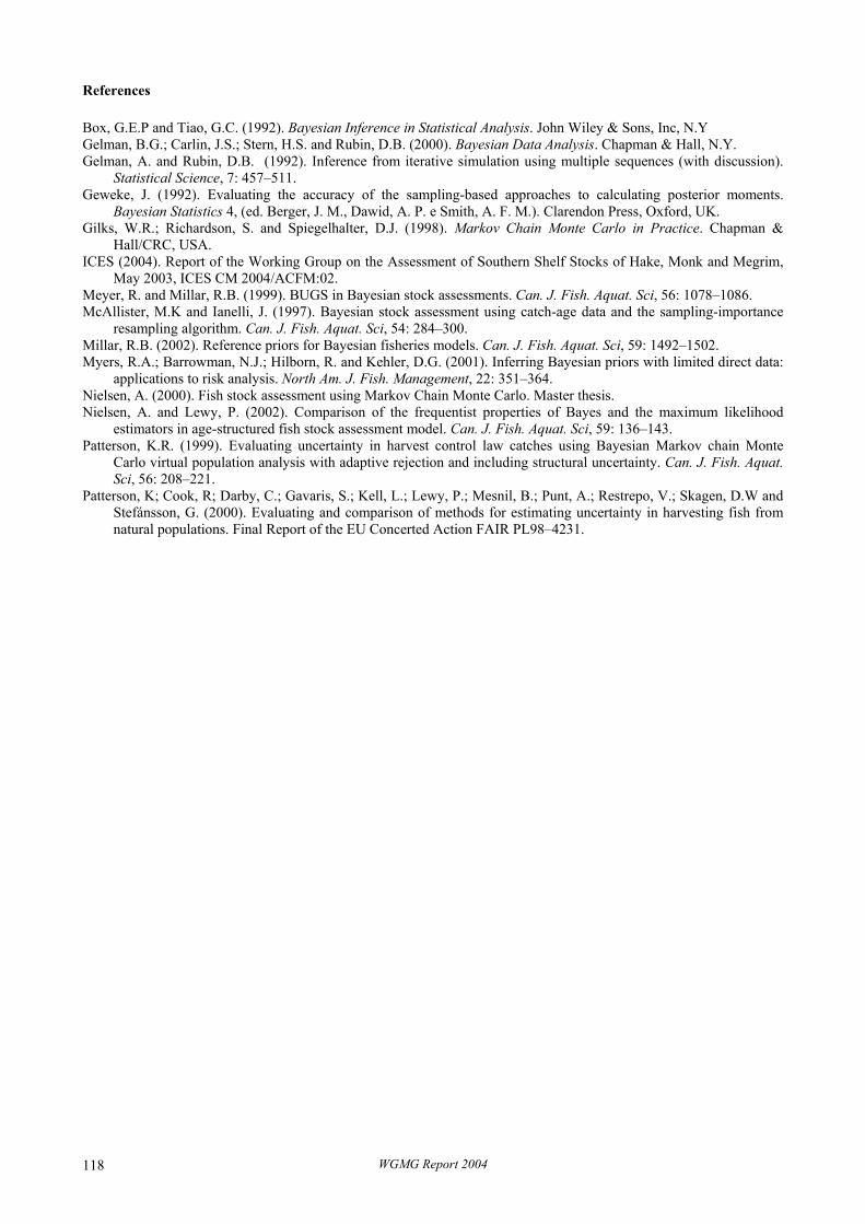
References

Box, G.E.P and Tiao, G.C. (1992). Bayesian Inference in Statistical Analysis. John Wiley & Sons, Inc, N.Y Gelman, B.G.; Carlin, J.S.; Stern, H.S. and Rubin, D.B. (2000). Bayesian Data Analysis. Chapman & Hall, N.Y. Gelman, A. and Rubin, D.B. (1992). Inference from iterative simulation using multiple sequences (with discussion).

Statistical Science, 7: 457–511. Geweke, J. (1992). Evaluating the accuracy of the sampling-based approaches to calculating posterior moments.

Bayesian Statistics 4, (ed. Berger, J. M., Dawid, A. P. e Smith, A. F. M.). Clarendon Press, Oxford, UK. Gilks, W.R.; Richardson, S. and Spiegelhalter, D.J. (1998). Markov Chain Monte Carlo in Practice. Chapman &

Hall/CRC, USA. ICES (2004). Report of the Working Group on the Assessment of Southern Shelf Stocks of Hake, Monk and Megrim,

May 2003, ICES CM 2004/ACFM:02. Meyer, R. and Millar, R.B. (1999). BUGS in Bayesian stock assessments. Can. J. Fish. Aquat. Sci, 56: 1078–1086. McAllister, M.K and Ianelli, J. (1997). Bayesian stock assessment using catch-age data and the sampling-importance

resampling algorithm. Can. J. Fish. Aquat. Sci, 54: 284–300. Millar, R.B. (2002). Reference priors for Bayesian fisheries models. Can. J. Fish. Aquat. Sci, 59: 1492–1502. Myers, R.A.; Barrowman, N.J.; Hilborn, R. and Kehler, D.G. (2001). Inferring Bayesian priors with limited direct data:

applications to risk analysis. North Am. J. Fish. Management, 22: 351–364. Nielsen, A. (2000). Fish stock assessment using Markov Chain Monte Carlo. Master thesis. Nielsen, A. and Lewy, P. (2002). Comparison of the frequentist properties of Bayes and the maximum likelihood

estimators in age-structured fish stock assessment model. Can. J. Fish. Aquat. Sci, 59: 136–143. Patterson, K.R. (1999). Evaluating uncertainty in harvest control law catches using Bayesian Markov chain Monte

Carlo virtual population analysis with adaptive rejection and including structural uncertainty. Can. J. Fish. Aquat. Sci, 56: 208–221.

Patterson, K; Cook, R; Darby, C.; Gavaris, S.; Kell, L.; Lewy, P.; Mesnil, B.; Punt, A.; Restrepo, V.; Skagen, D.W and Stefánsson, G. (2000). Evaluating and comparison of methods for estimating uncertainty in harvesting fish from natural populations. Final Report of the EU Concerted Action FAIR PL98–4231.

WGMG Report 2004 118

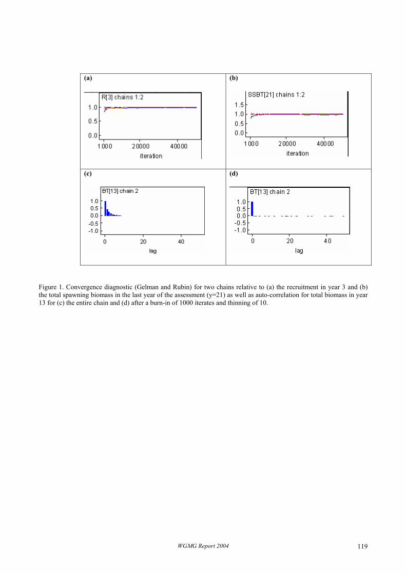
(a)

(b)

(c)

(d)

Figure 1. Convergence diagnostic (Gelman and Rubin) for two chains relative to (a) the recruitment in year 3 and (b) the total spawning biomass in the last year of the assessment (y=21) as well as auto-correlation for total biomass in year 13 for (c) the entire chain and (d) after a burn-in of 1000 iterates and thinning of 10.

WGMG Report 2004 119

(a)

(b)

(c)

(d)

Figure 2. Box-plot of the posterior distributions of annual fishing level, Fyear and age-specific selectivity, Sage, corresponding to (a,b) prior for Fyear U(0.1,0.5) and (c,d) prior for Fyear U(0,2).

WGMG Report 2004 120

Figure 3. Scatterplot of age-specific selectivity (Sage) against annual fishing level (Fyear) in year 4 (1985): prior for Fyear U(0.1,0.5).

Figure 4. Posterior median estimates of Fbar (mean F of ages 2–5) conditional on the adopted priors for the annual fishing level: solid line – Fyear ~ U(0.1,0.5); dashed line – Fyear ~ U(0,2).

WGMG Report 2004 121

Figure 5. Density plots from 900 samples for (upper panel) catch residual for the older age group in 1982, (middle panel) population abundance in the age group 4 in 1990 and spawning biomass in 1999 and (lower panel) catchability at the older age group in 1999 by survey.

WGMG Report 2004 122

(a)

(b)

(c)

Figure 6. Estimates of (a) Recruitment, (b) Spawning biomass and (c) Fbar for the period 1982–2002: Bayesian (thick solid line for P50% and dashed lines for P10% and 90%) and XSA (lighter solid line).

WGMG Report 2004 123

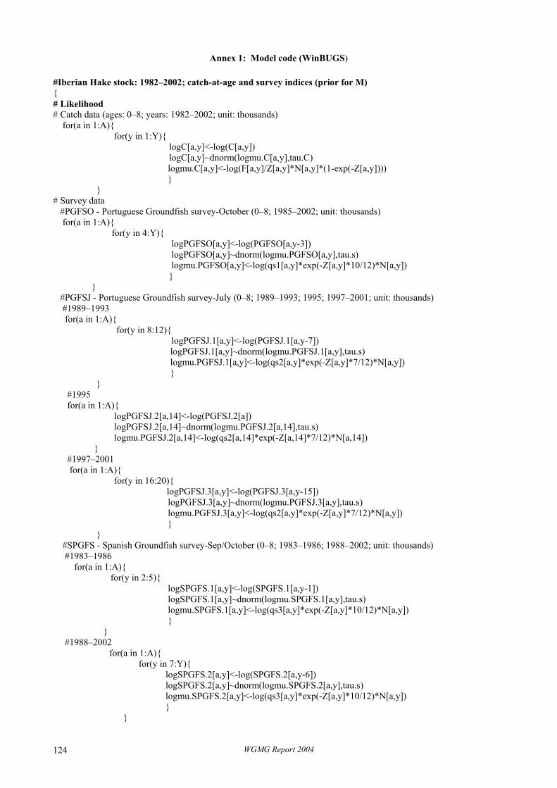
Annex 1: Model code (WinBUGS)

#Iberian Hake stock: 1982–2002; catch-at-age and survey indices (prior for M) { # Likelihood # Catch data (ages: 0–8; years: 1982–2002; unit: thousands) for(a in 1:A){ for(y in 1:Y){ logC[a,y]<-log(C[a,y]) logC[a,y]~dnorm(logmu.C[a,y],tau.C) logmu.C[a,y]<-log(F[a,y]/Z[a,y]*N[a,y]*(1-exp(-Z[a,y]))) } } # Survey data #PGFSO - Portuguese Groundfish survey-October (0–8; 1985–2002; unit: thousands) for(a in 1:A){ for(y in 4:Y){

logPGFSO[a,y]<-log(PGFSO[a,y-3]) logPGFSO[a,y]~dnorm(logmu.PGFSO[a,y],tau.s) logmu.PGFSO[a,y]<-log(qs1[a,y]*exp(-Z[a,y]*10/12)*N[a,y]) }

} #PGFSJ - Portuguese Groundfish survey-July (0–8; 1989–1993; 1995; 1997–2001; unit: thousands) #1989–1993 for(a in 1:A){ for(y in 8:12){

logPGFSJ.1[a,y]<-log(PGFSJ.1[a,y-7]) logPGFSJ.1[a,y]~dnorm(logmu.PGFSJ.1[a,y],tau.s) logmu.PGFSJ.1[a,y]<-log(qs2[a,y]*exp(-Z[a,y]*7/12)*N[a,y]) } } #1995 for(a in 1:A){ logPGFSJ.2[a,14]<-log(PGFSJ.2[a]) logPGFSJ.2[a,14]~dnorm(logmu.PGFSJ.2[a,14],tau.s) logmu.PGFSJ.2[a,14]<-log(qs2[a,14]*exp(-Z[a,14]*7/12)*N[a,14]) } #1997–2001 for(a in 1:A){ for(y in 16:20){

logPGFSJ.3[a,y]<-log(PGFSJ.3[a,y-15]) logPGFSJ.3[a,y]~dnorm(logmu.PGFSJ.3[a,y],tau.s) logmu.PGFSJ.3[a,y]<-log(qs2[a,y]*exp(-Z[a,y]*7/12)*N[a,y]) } } #SPGFS - Spanish Groundfish survey-Sep/October (0–8; 1983–1986; 1988–2002; unit: thousands) #1983–1986 for(a in 1:A){ for(y in 2:5){ logSPGFS.1[a,y]<-log(SPGFS.1[a,y-1]) logSPGFS.1[a,y]~dnorm(logmu.SPGFS.1[a,y],tau.s) logmu.SPGFS.1[a,y]<-log(qs3[a,y]*exp(-Z[a,y]*10/12)*N[a,y]) } } #1988–2002 for(a in 1:A){ for(y in 7:Y){ logSPGFS.2[a,y]<-log(SPGFS.2[a,y-6]) logSPGFS.2[a,y]~dnorm(logmu.SPGFS.2[a,y],tau.s) logmu.SPGFS.2[a,y]<-log(qs3[a,y]*exp(-Z[a,y]*10/12)*N[a,y]) } }

WGMG Report 2004 124

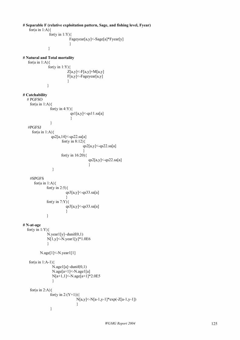
# Separable F (relative exploitation pattern, Sage, and fishing level, Fyear) for(a in 1:A){ for(y in 1:Y){ Fageyear[a,y]<-Sage[a]*Fyear[y] } } # Natural and Total mortality for(a in 1:A){ for(y in 1:Y){ Z[a,y]<-F[a,y]+M[a,y] F[a,y]<-Fageyear[a,y] } } # Catchability # PGFSO for(a in 1:A){ for(y in 4:Y){ qs1[a,y]<-qs11.sa[a] } } #PGFSJ for(a in 1:A){ qs2[a,14]<-qs22.sa[a] for(y in 8:12){ qs2[a,y]<-qs22.sa[a] } for(y in 16:20){ qs2[a,y]<-qs22.sa[a] } } #SPGFS for(a in 1:A){ for(y in 2:5){ qs3[a,y]<-qs33.sa[a] } for(y in 7:Y){ qs3[a,y]<-qs33.sa[a] } } # N-at-age for(y in 1:Y){ N.year1[y]~dunif(0,1) N[1,y]<-N.year1[y]*1.0E6 } N.age[1]<-N.year1[1] for(a in 1:A-1){ N.age1[a]~dunif(0,1) N.age[a+1]<-N.age1[a] N[a+1,1]<-N.age[a+1]*2.0E5 } for(a in 2:A){ for(y in 2:(Y+1)){ N[a,y]<-N[a-1,y-1]*exp(-Z[a-1,y-1]) } }

WGMG Report 2004 125

# Priors # Sage for(a in 1:A){ Sage1[a]~dunif(0,2) Sage[a]<-Sage1[a] } # Fyear for(y in 1:Y){ Fyear1[y]~dunif(0,2) Fyear[y]<-Fyear1[y] } # M for(a in 1:A){ for(y in 1:Y){ M1[a,y]~dunif(0.1,0.3) M[a,y]<-M1[a,y] } } # catchability for(a in 1:A){ qs11.sa[a]~dunif(6.0E-6,1) qs22.sa[a]~dunif(6.0E-6,1) qs33.sa[a]~dunif(6.0E-6,1) } #tau tau.C~dgamma(4,0.4) var.C<-1/tau.C tau.s~dgamma(100,100) var.s<-1/tau.s #Stock characteristics # R for(y in 1:Y){

R[y]<-N[1,y] } # B and SSB for(a in 1:A){ for(y in 1:Y){ B[a,y]<-N[a,y]*w[a,y] SSB[a,y]<-B[a,y]*mat[a,y] } } for(y in 1:Y){ BT[y]<-sum(B[1:A,y]) SSBT[y]<-sum(SSB[1:A,y])

} # Fbar (age range: mina to maxa) for(y in 1:Y){ Fsum[y]<-sum(F[mina:maxa,y]) Fbar[y]<-(Fsum[y])/(maxa-mina+1) } #Catch and ctachability # Catch residuals (by age/year and total) for(a in 1:A){ for(y in 1:Y){ C.est[a,y]<-F[a,y]/Z[a,y]*N[a,y]*(1-exp(-Z[a,y])) C.res[a,y]<-C[a,y]-C.est[a,y] }

WGMG Report 2004 126

} C.resT<-sum(C.res[1:A, 1:Y]) # Catchability for(a in 1:A){ for(y in 1:Y){ q.est[a,y]<-Survey[a,y]/N[a,y] } } } Data: click on one of the arrows to open the data Inits: click on one of the arrows to open the data

WGMG Report 2004 127

APPENDIX B: WORKING DOCUMENT WF2

Absolute abundance estimates and other developments in SURBA

by

Coby Needle

Abstract

Recent developments in the SURBA software are discussed. These include uncertainty estimates, index smoothing, constrained parameter estimates, retrospective analysis, empirical population summaries, and absolute abundance estimates. The principal intention of these modifications is to extend the scope of the method from a survey analysis tool to a survey assessment tool. Characteristics of absolute abundance estimation, the essence of which is to use historical catch data to parameterise current survey data, are demonstrated for assessments of North Sea cod and haddock. While the method seems to have potential as assessment tool, it is emphasised that: a) SURBA population estimates are scaled to the long-term level of abundance indicated by standard catch-based stock assessment, and this level may in itself be misleading, and b) conclusions about populations dynamics and the quality of commercial catch data depend strongly on which particular survey is used. Further work on survey catchability is required to obtain true absolute abundance estimates from this method. However, the method may still be useful in the interim in highlighting particular time-periods when catch data might be unreliable. Furthermore, the ability of the method to generate more realistic estimates of recruitment for stocks where discard estimates are lacking is promising.

1. Introduction

Cook (1997) presented a survey-based assessment model (RCRV1A), which applied a separable model of fishing mortality to relative catch indices from research-vessel surveys to generate relative estimates of abundance, assuming fixed values of survey catchability. Over the past couple of years, I have been (sporadically) developing SURBA, an implementation of this model which refines and extends the method considerably. SURBA has been used to produce comparative stock analyses in several ICES assessment Working Groups (ICES 2002a, ICES 2002b, ICES 2003b, ICES 2003c), and was evaluated favourably by the Review Group of the North Sea Commission Fisheries Partnership (NSCFP 2003). It was also discussed by the previous meeting of the ICES Working Group on Methods of Fish Stock Assessment (WGMG; ICES 2003a)). WGMG raised particular concerns about the requirement for an ad hoc specification of survey catchability, and concluded that this must be addressed in future development work.

The essentials of the SURBA method are described in detail in Needle (2003a), and I do not intend to revisit them here. Rather, the purposes of this note are: firstly, to document the modifications that have been made to SURBA since the previous meeting of WGMG; and secondly, to present case-study analyses of the potential use of SURBA to generate absolute abundance estimates for two key North Sea demersal stocks, thus avoiding the use of recent commercial catch-at-age data which may be thought to be suspect.

2. Recent developments in SURBA

The following developments have been implemented in SURBA version 2.20. I have only described the principal alterations here: there have also been many small changes to the format and presentation of outputs, as well as several minor bug fixes. For example, data can now be read in from standard Lowestoft-style VPA datafiles.

Uncertainty estimation

Much of the concern about current stock assessment methods, expressed by ACFM, NSCFP, STECF and other groups, relates to the general lack of allowance made for the uncertainty of the assessments. SURBA is a statistical model which seeks to minimise the residual error between observed and modelled abundance indices over the entire year and age ranges of the index. A natural way to estimate uncertainty in such models is to bootstrap model residuals, as follows.

Let a yI ,

a denote the observed survey index value for age in year , the assumed catchability of the survey at

age , the user-defined age-weighting for the sum-of-squares estimation, and

a y aq

aw a yr , the residual from a SURBA model fit. Then

WGMG Report 2004 128

( )ˆln ln lna y a y aa yr I I, , ,= − w (1)

where ˆa yI ,

N

are the fitted survey values. These are derived from the product of catchability and estimated stock

abundance , so that ˆ a y,

ˆˆ aa y a yq NI , ,= . (2)

Combining Equations 1 and 2 results in an expression for estimated stock abundance, given an observed survey index value, catchability, age-weighting, and a residual:

ln

ˆ exp ln ln a ya y aa y

a

rI qN w

,,,

= − −

. (3)

If we use a large number of different residuals drawn at random from the entire year and age range of the analysis, we will end up with a large number of different values of estimated stock abundance from the same fitted model. We can hypothesise that the distribution of these residuals approximates the true distribution of stock abundance, according to the fitted model. Furthermore, let W denote mean weight-at-age in the stock, a y, a yMat , proportion mature, and a yM , natural mortality. Then, using the standard expressions for spawning-stock biomass

ˆ a yy a ya ya

S W MatN ,,,= × × ,∑ (4)

and fishing mortality

1 1

ˆln

ˆa y

a y a ya y

NFN

,,

+ , +

M ,= −

, (5)

we can see that, given , , a yr , a yW , a yMat , , a yM , and Equations 3–5, it is a straightforward matter to reconstruct empirical distributions of population abundances and summary statistics.

A SURBA run on a given survey series, assuming fixed values of q , and a aw λ , produces an array of weighted log

residuals . In order to bootstrap the model fit, SURBA generates a new residual array by resampling with

replacement from (note that the resampling scheme I have used is unstructured, because the model sum-of-

squares surface is not structured by year, age or cohort). From Equations 3–5, new time-series of mean and SSB are produced. The bootstrap is repeated 1000 times, and 90% confidence intervals about the summary statistics are generated from the 5% and 95% points of the resulting empirical distributions of mean and SSB. Note that this is not possible if SSQ smoothing is used rather than index smoothing (see § 2) because of the time dependence of the former.

ln a yr , ln a yr∗,ln a yr ,

F

F

Sample output plots from this process are given in Figure 1, for the Scottish groundfish survey dataset on North Sea cod. These demonstrate that the mean fishing mortality 2 4F − estimated by SURBA is far more uncertain than the SSB. These plots also show how the median (50th percentile) of the bootstrap distribution can be used as a smoothed version of the pointwise estimates for 2 4F − and SSB.

Index smoothing

Cook (1997) noted that estimated values of and SSB from the RCRV1A model could be extremely sensitive to noise in the survey indices. Cook (1997) avoided this difficulty by adding a penalty term to the model sum-of-squares, which became

F

WGMG Report 2004 129

( )2

2

1 1 1 1

ˆln lnA Y Y

ya a y a y

a y y y

fSSQ w I I f

λ, ,= = = −

= +−

∑∑ ∑ , (6)

where [0 1]λ∈ , is a smoothing factor. I will refer to this method as SSQ smoothing. While it does produce a less variable estimate, it is difficult to interpret – depending on the scale of the index data, a high value of λ might mean that the model fit is driven more by the penalty term than by the index data. In addition, the time dependence of the residuals for the penalty term mean that it becomes impossible to estimate uncertainty by residual bootstrapping (see § 1).

An alternative is to apply a smoother directly to the survey index data, before they are used in model fitting. Here I will refer to this method as index smoothing. SURBA does this by fitting a cubic spline smoother through the logged index values ln I for all represented ages of each cohort. The user is asked to specify a value for ρ , the smoothing parameter. Missing values are filled in by mean interpolation beforehand, and no smoothing is carried out if there are less than three observations for the cohort in the dataset.

Examples of unsmoothed and smoothed log indices for specific cohorts are given in Figure 2. In the tests I have done so far, index and SSQ smoothing yield fairly similar results for summary statistics mean and SSB. The advantages of index smoothing are that it is less arbitrary (the effect of

Fρ on model fits is far smaller than that of λ ), it allows for

uncertainty estimation, and it produces abundance estimates for years in which there are missing data.

Constrained parameter estimation

Previous versions of SURBA have only allowed unconstrained estimation of the temporal trend, age effect and cohort effect parameters. The advantage of this is that it permits the derivation of standard errors for these parameter estimates, as shown in Figure 3(a). This Figure also shows the key disadvantage, namely that parameter estimates can easily become negative if catchabilities are not defined appropriately. A negative age effect (as seen for age 1 in Figure 3(a)) will result in a negative for that age, which is not physically possible. F

Constrained parameter estimation avoids this potential difficulty by assuming bounds on parameters, although at the cost of standard error estimation. The bounds used are [0 0 3 0]. , . for temporal trends and age effects, and

for cohort effects. The analysis in Figure 3(a) is repeated in Figure 3(b) with constrained estimation. When using absolute abundance estimation (see § 6) the fitted age effects will rarely become negative, in which case unconstrained estimation is probably preferable as it gives information about standard errors.

[ 20 0 20 0]− . , .

However, constraining the estimated parameters may still lead to negative estimates of in the final year, particularly if there is a declining trend in towards the final year. This is because SURBA fixes one value of the temporal trend

FF

yf to avoid over-parameterisation, and following RCRV1A the last value ( )1Yf − is used. This is defined to be

2

11

1Y

Y ii

f Y f−

−=

= − − ,∑

so that the mean of the yf series is 1.0. However, 1Yf − can become negative if fishing mortality is in decline, leading

to negative estimates of mean . SURBA now has the option to fix bounds on F 1Yf − to ensure that it is no lower than

half the previous lowest f , and no higher than twice the previous highest f : in other words,

2

1 1 1 2 1 21

11 such that min { } 2 max { }2

Y

Y i Y ii …Y i …Yiif Y f f f f

−

− − = , , − = , , −=

= − − ∈ × , × . ∑

While this might remove the problem of negative F , it also results in a poorer fit, year-effects in residuals, slightly increased retrospective bias (see § 4), and very large standard errors in unconstrained parameter estimates, so it must be used with caution.

WGMG Report 2004 130

Retrospective analysis

Retrospective analyses are standard diagnostic tools in many catch-at-age stock assessments. The model fit is repeated several times, using the same model settings but with the last year of data removed incrementally. Large differences or consistent biases in the estimates of mean , SSB and recruitment from these different analyses are generally taken to indicate data or model problems which reduce confidence in the full model results. Exactly what constitutes a significant difference in this situation is hard to determine: metrics such as Mohn’s

F

ρ (Mohn 1999) can be used, but they do not have a good statistical interpretation.

SURBA generates retrospective runs automatically, moving back in time a number of years defined by the user (as far back as half the dataset is permitted). Retrospective plots for 2 4F − and SSB for North Sea cod (using the Scottish groundfish survey) are shown in Figure 4. These are typical of SURBA results, and show very little (if any) any retrospective pattern. The only examples of SURBA fits which show bias that I have encountered are when there are missing years in the survey index, in which case the estimates may be revised considerably after each missing year. My hypothesis about the lack of retrospective bias or noise two or more conflicting data sources are required for this to occur, and SURBA uses only one. Further work is required in this area before any firm conclusions can be made.

Empirical calculation of Z and SSB

Modelling relative abundance indices from research-vessel surveys via an assumption about separable fishing mortality is generally a valid approach. The main benefit is that noise in the survey data will be smoothed out, and (it is hoped) the underlying data signal will emerge. However, this is only the case if the corresponding assumptions hold, that both survey catchability and overall mortality selectivity are constant through time. In some cases this may not be true, and violation of the assumption will usually show up as distinct structure in model residuals.

Therefore, it is useful to be able to calculate the empirical total mortality Z and relative SSB directly from survey indices, and SURBA does this automatically. Z is calculated as the natural logarithm of the ratio of the index in age and year , to the index in age and year

ay 1a + 1y + , so that

1 1

ln a ya y

a y

IZ

I,

,+ , +

= .

SURBA reports the mean of Z over the same age-range as used for mean . Relative SSB is calculated in the usual way, as

F

max

min

a a

y aa y a ya a

I WSSB Mat=

y,, ,=

= × ×∑ .

This is then mean-standardised (that is, divided through by the series mean so that 1 0SSB = . ). These calculations are performed for both the original series and the index-smoothed series (see § 2): an example of the latter is given in Figure 5.

Absolute abundance estimation

SURBA and related survey-based analysis methods have thus far been used only in an exploratory capacity in ICES assessment Working Groups, and not to formulate scientific management advice. One reason for this has been that such methods have only been able to generate relative estimates of abundance, not the absolute estimates that are required by the current management framework.

However, it is relatively straightforward to use SURBA to produce such absolute estimates. The proposed approach can be based on any catch-at-age analysis which uses survey indices to “tune” abundance estimates from commercial catch-at-age (or landings-at-age) data: examples include XSA (Darby and Flatman 1994), ICA (Patterson and Melvin 1996), or TSA (Fryer 2001). These methods all estimate catchabilities a yq , , or more often long-term mean catchabilities aq .

If we use the resulting values of aq as the fixed catchability inputs for SURBA, we will generate absolute abundance

WGMG Report 2004 131

estimates that are of the same order as those produced by the catch-at-age analyses. In fact, the term “absolute” is possibly a misnomer, since this procedure is actually scaling the relative abundance estimated by SURBA to the level of abundance indicated by the catch-at-age analysis. Therefore, if misreporting (for example) has always been a problem in a fishery, then the SURBA “absolute” estimates will be biased in the same way as the catch-at-age estimates. If, however, misreporting is likely to have been a relatively recent phenomenon (compared to the full time-period for which data are available), then the SURBA estimates will be driven largely by catchabilities from the earlier (and longer) period for which catch data is thought to be more reliable. The impact of any recent misreporting or unaccounted discards should be alleviated by the use of the long-term mean of historical catchabilities from the catch-at-age analysis. In other words, we are using historical fishery data to parameterise current survey data. The result will be a more accurate reflection of true abundance, if the assumption holds of catch data problems appearing only recently. I will be making this assumption in the following analyses.

Compare the SURBA summary plots in Figures 6(a) and 6(b). The former was produced using the standard fixed catchabilities of 1 for all ages, the latter using 0. aq taken from an XSA assessment of the same stock. The principal difference between them, which causes the rescaling from relative to absolute estimates, is the fitted values of the cohort effect which are much larger in Figure 6(b). Further examples are given in § 3.

3. Absolute abundance estimation examples

The main reason that survey-based analyses are being considered seriously as tools for management advice is the perception that black landings, discarding, and other forms of unaccounted misreporting may have increased in recent years in response to increasingly restrictive fishery quotas. The corollary to this is that catch-at-age analyses based on commercial landings records in the more distant past are less likely to be affected by these aspects, and should be more trustworthy as a result. It would therefore seem reasonable to run a catch-at-age analysis based on data only up to some point in time before TACs became restrictive, and use the resulting estimated survey catchabilities in an absolute-abundance run of SURBA. The abundance estimates from this would be on the same scale as the historical abundance estimates of the catch-at-age analysis, and would not be affected by the recent misreporting problems which are thought to be dogging standard assessment methods. Alternatively, as indicated above, if commercial data problems are a relatively recent phenomenon, then the use of simple unweighted mean catchabilities from the entire time-period should sufficiently reduce the effect of the recent years in the subsequent SURBA analyses.

In the case studies presented below, I use XSA (Darby and Flatman 1994) as the required tuned catch-at-age analysis. For the absolute abundance estimates from SURBA (which refer to the time of the survey) to be a true comparison with those from XSA (which refer to January 1st), they have to be backshifted according to

N(1 Jan) N(survey time) a yZ Pa y a y e ,

, ,=

where is the time of year that the survey takes place expressed as a decimal proportion of the whole. These backshifted abundance estimates can then be used in the calculation of SSB(1 Jan). Unfortunately this value can only currently be estimated up to and including the second-last year in the survey time-series. This is because an estimate of SSB(Jan 1) in the last year would require knowledge of for the whole of that last year, which we cannot have without making assumptions about the development of the fishery for the remaining part of the year.

P

F

Over what time period should the catch-at-age analysis be run? In cases where it is clear when TACs became restrictive, then that should be used as the cut-off point. Generally, however, landings are reported to TACs, and it is often not clear when (if ever) restrictions start to apply. Therefore it is necessary to test the sensitivity of the SURBA model to the time period over which catchabilities are estimated by XSA. The approach I used here is follows:

1. I ran retrospective XSA analyses, starting with the full dataset and going back as far as the program will allow (that is, until one of the survey indices has less than 6 years of data left). These XSA runs were tuned by all available surveys. The mean range and overall age range were as used in the final WG assessment (ICES 2003b). No power model or time-series taper were used, and shrinkage was very light ( ). The catchability plateau was set to the highest possible age, so as to minimise the restrictions placed on the fitted catchabilities.

F2 0SE = .

2. The catchabilities from the retrospective XSA runs were used in separate SURBA runs for each of the surveys in question. Estimates of SSB and mean from these runs were then plotted against the corresponding estimates from an XSA run which used the full time-series: this plot also included the confidence intervals

F

WGMG Report 2004 132

about the SURBA estimate based on the catchabilities from the full-time-series XSA run. In addition, mean and SSB for the last year in the time-series were plotted against the last year in the retrospective XSA analysis which provided the catchabilities on which the relevant SURBA run was based.

F

North Sea cod

Input data were taken from ICES (2003b). Stock weights, maturities and natural mortalities for North Sea cod were only available in the assessment input files up until 2002, while the survey data extended to 2003. The extra year for these inputs was generated using 3-year (2000–2002) means. This made no substantive difference to the estimates (since both mean and SSB(Jan 1) can only currently be calculated to 2002), but was required to avoid a program error. XSA settings were as listed above, with light shrinkage being calculated over 5 years and 3 ages. The tuning series used were from the Q3 Scottish groundfish survey (ScoGFS), the Q3 English groundfish survey (EngGFS), and the Q1 IBTS survey (IBTS Q1).

F

Figures 7 to 9 show the results of sensitivity analyses on the catchabilities used in SURBA runs, along with comparisons between, firstly, the SURBA run based on the XSA-derived catchabilities from the full time-series run (up to and including 2002); and secondly, the estimates from that XSA run. We can see that the XSA estimates of SSB are lower than the SURBA estimates for the mid-1990s when the ScoGFS and EngGFS series are used, but this is not the case when the IBTS Q1 series is used. We can note that the majority of the weighting in XSA tuning at ages 3 and older for this stock is taken by the IBTS Q1 series (ICES 2003b), so it is perhaps not surprising that the IBTS Q1 SURBA and XSA analyses are similar. This may also be due in part to the earlier timing of the IBTS Q1 index, although this is only speculation. In any case, both the ScoGFS and EngGFS series indicate some misreporting during the mid-1990s. Mean

is poorly-estimated by SURBA and confidence intervals are very wide, but for all three surveys the median estimates of mean suggest a sharp increase in the most recent year which does not appear in the XSA results. The catch data used in the final WG assessment for this stock does not include estimates of discards, although Scottish sampling data suggest discard proportions of 60% to 80% for age 1 cod (ICES 2003b). This explains the large discrepancies between the SURBA and XSA estimates for recruitment at age 1 for all three surveys. Finally, the use of catchabilities from retrospective XSA runs does not appear to have made a significant difference to the subsequent SURBA model fits. This supports the view (§ 6) that long-term mean catchabilities from the full time-series XSA run (which covers the years 1963–2002) are not sufficiently affected by recent data problems to cause concern.

FF

How circular is this method of generating catchabilities? That is, in Figures 7 to 9 we are comparing a) SURBA estimates based on XSA-derived catchabilities, with b) XSA estimates from the same run as produced the catchabilities. Therefore, are any similarities or patterns simply artefactual? To address this question, I considered several more runs. In addition to the XSA run tuned by all three surveys, I also generated XSA runs tuned by each survey in turn (single-fleet runs), as well as a separable VPA (Darby and Flatman 1994) with terminal s given by the three-survey XSA runs (default settings otherwise). Finally, I fitted SURBA models for each survey using catchabilities derived from the relevant single-fleet XSA run, as well as the three-fleet XSA run. For example, Figure 9(a) compares the estimated SSB for the three-survey XSA run, the XSA run tuned only by the ScoGFS series, the untuned separable VPA, the SURBA run using catchabilities from the three-survey XSA run, and the SURBA run using catchabilities from the XSA run tuned only by the ScoGFS series. The first three of these (all using catch data) are consistent with each other, as are the last two (using only survey data). This suggests that the indication from the ScoGFS series of a larger SSB in the mid-1990s is not artefactual, but is a true reflection of the data. Similarly, the consistency of IBTS Q1 data and landings data (Figure 9c) can be seen for all the additional trial runs. The results for the EngGFS series (Figure 9b) are less clear, but this may be due to the short time-series used.

F

In conclusion, any judgement of the reliability of landings data for North Sea cod depends on which survey is used for comparison. The ScoGFS series indicates a substantial amount of misreporting during the mid-1990s, the IBTS Q1 series very little or none, and the EngGFS series somewhere in between. However, it is clear that the estimates are consistent in the most recent years: all indicate that spawning stock biomass is at or near the lowest observed level.

North Sea haddock

The basic comparative analyses were repeated for the North Sea haddock stock, following the same method and XSA settings as used for North Sea cod. Only one XSA run was carried out, tuned by all three surveys. SURBA and XSA results are compared in Figures 11 (ScoGFS), 12 (EngGFS) and 13 (IBTS Q1). As for cod, terminal year SURBA estimates for haddock SSB, mean and recruitment at age 1 are not sensitive to the use of different retrospective XSA runs to generate catchabilities. The ScoGFS analysis gives lower estimates of mean and recruitment than XSA, while ScoGFS SURBA SSB estimates are consistently higher than XSA estimates during the 1990s. The IBTS Q1 analysis suggests much smaller differences in the SURBA and XSA estimates of SSB and mean , while SURBA

FF

F

WGMG Report 2004 133

estimates of recruitment from this run are generally lower than those from XSA. This is also the case for the EngGFS analysis, which in addition gives SSB estimates which are lower than the XSA estimate during the 1990s.

The assessment of North Sea haddock includes estimates of proportion discarded, raised from the Scottish sampling programme to the level of the international fleet, so we would not expect to see the considerable underestimation of recruitment by XSA in haddock that we saw in cod. However, recruitment estimated by the IBTS Q1 SURBA analysis is consistently lower than the XSA estimate. The broad spatial coverage of the IBTS Q1 surveys may be such that they are surveying substocks for which the Scottish discard proportion is unlikely to be applicable.

However, the SURBA and XSA estimates of mature fish abundance are somewhat more consistent for haddock than they were for cod. This could indicate that commercial haddock catch records are less likely to be problematic than those for cod. A conclusion like this would at least be consistent with our perception of the situation in the Scottish fleet: haddock are less valuable than cod and are hence more likely to be discarded than landed black (and these discards are accounted for in assessment data, at least partially). This suggests that a haddock assessment based on catch data may not be too wide of the mark, in terms of broad summary statistics like SSB. Estimates of large year classes are still very uncertain, but it is not clear that survey-based assessment would necessarily resolve this problem.

4. Conclusion and future work

SURBA has undergone considerable development in recent months, and is slowly approaching a state in which serious consideration should be given to using it in stock assessments. Further testing is clearly required (particularly with simulated data), but the addition of a means to generate absolute abundance estimates increases the utility of the method. In addition, the use of the method to generate realistic recruitment estimates for stocks which lack good discard time-series is very promising. This will have knock-on effects on stock-recruit modelling and the estimation of biological reference points: examples of the potential changes in the fitted stock-recruit model when different models are fitted is given in Figure 14. There remains the caveat that the absolute abundance estimates are scaled using catchability values based on historical landings records. Hence the method might be more beneficial in situations were the quality of landings records has declined recently, than in cases where the quality has always been bad. There is also the issue of how to interpret conflicting signals from different surveys, such as we have seen here for North Sea cod (§ 1) and haddock (§ 2), and this has not yet been resolved satisfactorily.

The choice of which time period to use when generating catchabilities from a catch-at-age method did not have much of an effect in these analyses. This is because XSA estimates mean catchability at age over a long time period (more than 40 years in these cases), so changes in catchability towards the end of the time-series make little noticeable difference overall. However, this might not be the case with shorter time-series or more drastic catchability changes, and the choice of years over which to parameterise catchability needs to be considered on a case-by-case basis.

Other directions for future development include:

• Catchabilities are estimated externally, which implies that principles of conditional inference should be used in uncertainty estimation. This has not yet been done, but we can hypothesise that the real confidence bounds are probably somewhat wider than shown in this paper.

• Using VPA-derived catchabilities scales SURBA abundance estimates to the level of historical abundance given by the VPA, but not necessarily the true level of stock abundance. A clearer idea of the true level would be obtained from empirical estimates of true catchability. If available, these measured catchabilities would allow for a direct comparison between survey-based and landings-based abundance estimates.

• It is possible to estimate the standard errors of survey index values, although this is not often done as standard assessment methods have no way to account for them. However, a statistical model such as SURBA could readily be modified to incorporate index standard errors as inverse-weighting factors in the model sum-of-squares.

• The trend in fisheries modelling is now firmly towards open-source code, and to meet this demand I intend to develop a version of SURBA using the R language for inputs and outputs, and Fortran-90 or C++ modules for computation.

• It might be beneficial to bring catchability estimation “in-house” by developing a VPA module within SURBA. This would simplify the process for the end user, but would also reduce the scope for testing the effects of different catchability estimates. For this reason catchability estimation should be an optional extra.

WGMG Report 2004 134

• It should also be straightforward to modify the model to allow for several different surveys at once, although the weighting scheme would have to be given some thought. This has the potential the reduce the problem of conflicting surveys, although in a fairly crude way as any such approach is likely to result in an estimate which is the average of the different estimates from the surveys.

• Separable models (such as SURBA) assume that fishing mortality is separable into an age-invariant year effect (effort) and a time-invariant age effect (selectivity) – in other words, that is additive on a log scale. Myers and Quinn II (2002) have shown how this assumption can be relaxed by allowing to be non-additive. It is unlikely that the age effect in mortality will ever really be constant in time, so it is important that the option to test for non-additivity be incorporated into SURBA.

FF

References

Cook, R. M. (1997), ‘Stock trends in six North Sea stocks as revealed by an analysis of research vessel surveys’, ICES Journal of Marine Science 54, 924–933.

Darby, C. D. and S. Flatman (1994), ‘Lowestoft VPA Suite Version 3:1 User Guide’. MAFF: Lowestoft. Fryer, R. F. (2001), ‘TSA: Is it the way?’. Working Document to the ICES Working Group on Methods of Fish Stock

Assessments, Copenhagen, December 2001. ICES (2002a), ‘Appendix to the Report of the Working Group on the Assessment of Demersal Stocks in the North Sea

and Skagerrak’. ICES CM 2003/ACFM:02 Appendix. ICES (2002b), ‘Report of the Working Group on the Asessment of Northern Shelf Demersal Stocks’. ICES CM

2003/ACFM:04. ICES (2003a), ‘Report of the Working Group on Methods of Fish Stock Assessment’. ICES CM 2003/D:03. ICES (2003b), ‘Report of the Working Group on the Assessment of Demersal Stocks in the North Sea and Skagerrak’.

ICES CM 2003/ACFM:07. ICES (2003c), ‘Report of the Working Group on the Assessment of Northern Shelf Demersal Stocks’. ICES CM

2004/ACFM:04. Mohn, R. (1999), ‘The retrospective problem in sequential population analysis: An investigation using cod fishery and

simulated data’, ICES Journal of Marine Science 56, 473–488. Myers, R. A. and T. J. Quinn II (2002), ‘Estimating and testing non-additivity in fishing mortality: Implications for

detecting a fisheries collapse’, Canadian Journal of Fisheries and Aquatic Sciences 59, 597–601. Needle, C. L. (2003), ‘Survey-based assessments with SURBA’. Working Document to the ICES Working Group on

Methods of Fish Stock Assessment, Copenhagen, 29 January – 5 February 2003. NSCFP (2003), ‘Report of Invited Experts to the North Sea Commission Fisheries Partnership – North Sea Stock

Assessment Consultation Meeting, Copenhagen, 6–7 October 2003’. Available from http://www.northsea.org/fisheriespartnership/.

Patterson, K. R. and G. D. Melvin (1996), ‘Integrated Catch-at-age Analysis Version 1:2’, Scottish Fisheries Research Report 56. FRS: Aberdeen.

WGMG Report 2004 135

(a)

(b)

(c) Figure 1. Estimated (a) 2 4F − and (b) relative SSB at survey time for North Sea cod from a SURBA run on the Scottish groundfish survey data. Dots show pointwise estimates, lines show percentage points of empirical bootstrap uncertainty distributions (5%, 25%, 50%, 75%, 90%). Plot (c) compares 2 4F − and relative SSB in 2002, with uncertainty estimates given by contour lines.

WGMG Report 2004 136

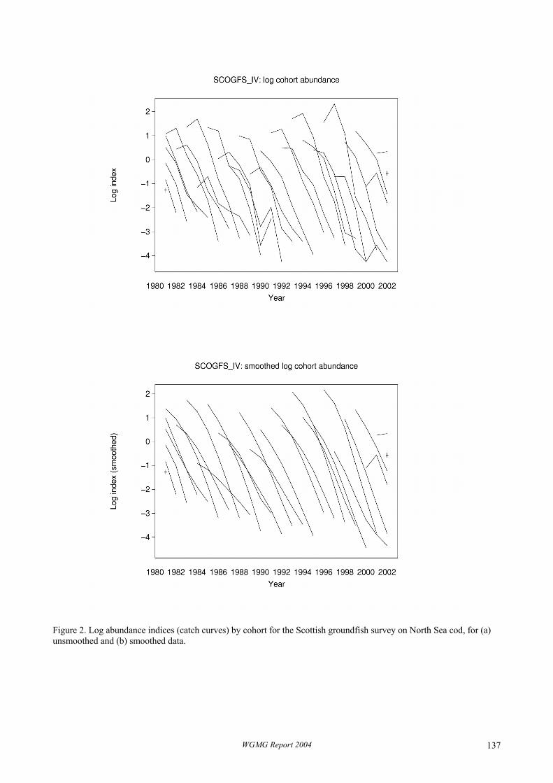
Figure 2. Log abundance indices (catch curves) by cohort for the Scottish groundfish survey on North Sea cod, for (a) unsmoothed and (b) smoothed data.

WGMG Report 2004 137

Figure 3. Estimated age-effect parameters for the Scottish groundfish survey on North Sea cod, using (a) unconstrained and (b) constrained estimation. Vertical bars in (a) show 2s e± . .

WGMG Report 2004 138

(a)

(b)

Figure 4. Retrospective plots for the Scottish groundfish survey on North Sea cod, for (a) 2 4F − and (b) relative SSB at survey time.

WGMG Report 2004 139

(a)

(b)

Figure 5. Empirical plots of (a) 2 4Z - and (b) relative SSB at survey time for the Scottish groundfish survey on North Sea cod.

WGMG Report 2004 140

(a)

(b)

Figure 6. SURBA analysis summary examples for the Scottish groundfish survey on North Sea cod, using (a) relative abundance estimation, and (b) absolute abundance estimation. See caption to Figure 1 for key.

WGMG Report 2004 141

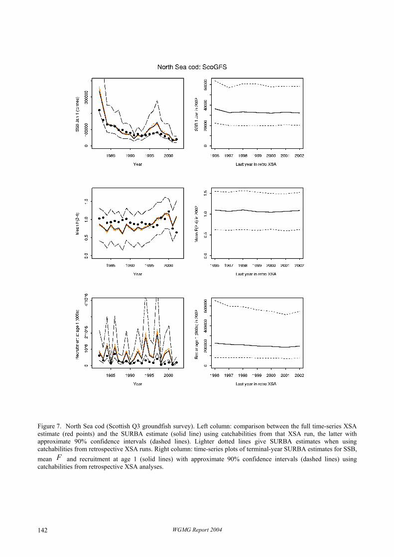
Figure 7. North Sea cod (Scottish Q3 groundfish survey). Left column: comparison between the full time-series XSA estimate (red points) and the SURBA estimate (solid line) using catchabilities from that XSA run, the latter with approximate 90% confidence intervals (dashed lines). Lighter dotted lines give SURBA estimates when using catchabilities from retrospective XSA runs. Right column: time-series plots of terminal-year SURBA estimates for SSB, mean and recruitment at age 1 (solid lines) with approximate 90% confidence intervals (dashed lines) using catchabilities from retrospective XSA analyses.

F

WGMG Report 2004 142

Figure 8. North Sea cod (English Q3 groundfish survey). See Figure 7 for key.

WGMG Report 2004 143

Figure 9. North Sea cod (IBTS Q1 survey). See Figure 7 for key.

WGMG Report 2004 144

Year

SS

B a

t Jan

1 (t

onne

s)

1985 1990 1995 2000

010

0000

2000

0030

0000

4000

00

ScoGFS

XSA (3-survey)Sep VPAXSA (ScoGFS)SURBA with q from XSA (3-survey)SURBA with q from XSA (ScoGFS)

(a)

Year

SS

B a

t Jan

1 (t

onne

s)

1985 1990 1995 2000

010

0000

2000

0030

0000

4000

00

EngGFS

XSA (3-survey)Sep VPAXSA (EngGFS)SURBA with q from XSA (3-survey)SURBA with q from XSA (EngGFS)

(b) Figure 10. North Sea cod. Comparison of absolute SSB estimates from XSA, SURBA and separable VPA runs. See text for details.

WGMG Report 2004 145

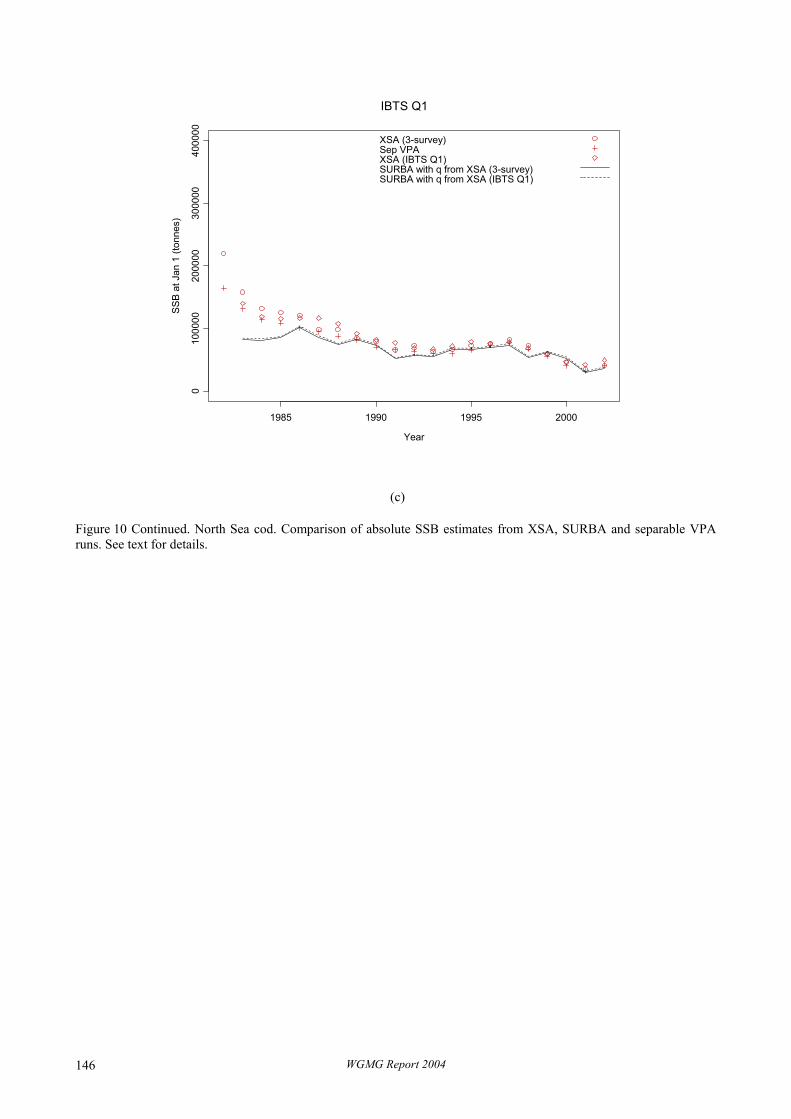
Year

SS

B a

t Jan

1 (t

onne

s)

1985 1990 1995 2000

010

0000

2000

0030

0000

4000

00

IBTS Q1

XSA (3-survey)Sep VPAXSA (IBTS Q1)SURBA with q from XSA (3-survey)SURBA with q from XSA (IBTS Q1)

(c)

Figure 10 Continued. North Sea cod. Comparison of absolute SSB estimates from XSA, SURBA and separable VPA runs. See text for details.

WGMG Report 2004 146

Figure 11. North Sea haddock (Scottish Q3 groundfish survey). Left column: comparison between the full time-series XSA estimate (red points) and the SURBA estimate (solid line) using catchabilities from that XSA run, the latter with approximate 90% confidence intervals (dashed lines). Lighter dotted lines give SURBA estimates when using catchabilities from retrospective XSA runs. Right column: time-series plots of terminal-year SURBA estimates for SSB, mean and recruitment at age 1 (solid lines) with approximate 90% confidence intervals (dashed lines) using catchabilities from retrospective XSA analyses.

F

WGMG Report 2004 147

Figure 12. North Sea haddock (English Q3 groundfish survey). See Figure 11 for key.

WGMG Report 2004 148

Figure 13. North Sea haddock (IBTS Q1 survey). See Figure 11 for key.

WGMG Report 2004 149

(a) (b)

(c) (d)

Figure 14. Stock-recruit scatterplots for four different assessments of North Sea cod. The XSA analysis was tuned by all three available surveys: the SURBA runs were based on catchabilities from that same XSA run. Solid lines give fitted Ricker curves, dotted lines approximate point-wise 95% confidence intervals (models fitted with RecAn 2.20, available from the author).

WGMG Report 2004 150

APPENDIX C: WORKING DOCUMENT WE1

Assessing structural uncertainty using KSA (kernel survivors analysis)

by Ken Patterson

Abstract................................................................................................................................................................................. Introduction .......................................................................................................................................................................... Method.................................................................................................................................................................................. Results .................................................................................................................................................................................. Explanation of the Figures.................................................................................................................................................... Results : Norwegian Spring-Spawning Herring.................................................................................................................... Results : Iberian Sardine....................................................................................................................................................... Results : North Sea Haddock................................................................................................................................................ Discussion............................................................................................................................................................................. Conventional, frequentist interpretation ............................................................................................................................... Bayes interpretation .............................................................................................................................................................. Practical Implications for ICES ............................................................................................................................................ References ............................................................................................................................................................................ Appendix 1. Approach to weighting survey data in age-structured assessments.................................................................. Appendix 2. Implementation notes for KSA code................................................................................................................ Abstract

A “kernel survivors analysis” (KSA) method is presented for assessing structural uncertainty in age-structured stock assessment. It is argued that this method would, de minimis, be a valuable screening tool for ICES assessment working groups. It may assist advice to be better formulated with respect to the confidence that can be placed on assessments.

The method is designed for the systematic exploration of the consequences of different assessment assumptions about the rapidity with which catchability may change, either with respect to time or with respect to age. A posterior odds ratio can be calculated, allowing some probabilistic comparison of the consequences of alternative assumptions for any given interest parameters, or even calculation of a Bayes Model Average. The method is proposed as a contribution principally in the area of quantifying structural uncertainty in fish stock assessment.

This paper describes the method and presents some example cases. It is based on an earlier paper of the same title published as ICES C.M. 2002: V:10 but incorporates corrections, further examples with additional stocks, and an implementation note for the software.

Introduction and Modelling Background

Where sufficient data are available, an often-preferred method for fisheries stock assessment is to use an age-structured model to estimate population parameters and to evaluate the state of the stock with respect to its historic state, its potential for providing yield, and with respect to risks of stock depletion. There exist two broad families, distinguished mainly by the assumptions made about the precision with which catches-at-age can be determined. In models of the virtual population analysis (“VPA”) type, catches-at-age are assumed to be measured precisely, whereas in “statistical” models, these observations are assumed to be realisations from an underlying process whose determining parameters can be estimated. Examples of “VPA” applications include ADAPT (Gavaris, 1988); Survivors analysis (Doubleday, 1981); Laurec-Shepherd method (Pope and Shepherd, 1985); extended survivors analysis (XSA) (Darby and Flatman, 1994; Shepherd, 1999). Statistical modelling of the catch-at-age observations was first elaborated by Fournier and Archibald (1982), with related models described by Deriso et al (1985). A thorough review of such models is provided by Quinn and Deriso (1999).

Taking a very simple example of the structural models used in these applications, then for a period y=1..Y years and for fish aged a=1..A ages, and assuming that catches are taken instantaneously, population abundance N, natural mortality M, fishing mortality F and catches C in number can be assumed to follow relations such as :

a y a y

M

a y

MN N e C e, , ,

/= ++ +1 1

2 (1)

WGMG Report 2004 151

a ya y

a yF M N

N,,

,

ln+ =

+ +1 1 (2)

Given a set of Ca,y and either all NA,Y or all FA,Y , then (1) and (2) can then be used in a recurrence relationship to determine all other Fa,y and Na,y, as described in the well-known paper by Pope (1972). Observations of an index i of stock abundance Ui,a,y are assumed related to stock abundance with constant of proportionality Q and observed according to a chosen observation error model, e.g., a lognormal distribution:

( ) ( )( )σ 2

,,,,,,, ,log~log yaiyayaiyai NQU N (3)

where N (x, σ2) represents the normal distribution with mean x, and σ2 represents the variance of x. Fitting a stock assessment model is usually achieved by adjusting some Qi,a,y, σi,a,y, NA,Y or FA,Y to find a maximum likelihood value L of :

( )( )

−

ΠΠ σσ 22 2

,,

2

2/1

,,,,,,

,,,,,logexp1

yaiyaiyaiyai

NQUU

yayaiyai (4)

or a least-squares analogue, iterative approximation or analogous function for other error-distribution. In this form, the fish stock assessment problem is intractable because it leads to solutions for all Fa,y →0, and all Na,y→∞. Other solutions can only be achieved by imposing some constraints. Constraints that may be imposed to obtain acceptable solutions include :

1. Constraining FA,y to a fixed proportion of an average of Fa,y over younger ages, as in ADAPT and Laurec-Shepherd methods;

2. Constraining FA,y to a fixed proportion of an Fa,y at a single younger age, as in CAGEAN and Fournier-Archibald based models;

3. Constraining (“shrinking”) FA,y towards a weighted average over younger ages, as in XSA; 4. Constraining some Fa,Y as a function of other Fa,Y (e.g., shrinkage in XSA); 5. Constraining σi,a,y to any fixed value, either estimated externally or assigned assumed values; 6. Estimating σi,a,y subject to constraints, which may be year-dependent (Cleveland taper weighting) ; 7. Constraining Qi,a,y to be equal within a specified range of ages up to A, in XSA or ADAPT; 8. Choosing a functional form for Qi,a,y (e.g., as dependent on N, on time, or as a random walk in a time-series model)

Constraints 1 to 4 reflect perceptions of the extent to which fishing mortality is stable across different age-groups (either within the whole fishery, or for a particular fishing gear). For given U, constraints on fishing mortality are equivalent to constraints on catchability.

Constraints 5 and 6 reflect perceptions of the relative accuracy with which different surveys or fishing fleets provide information about stock abundance.

Constraint 7 reflects the perceptions that for some kinds of fishing gear, fish can be considered “fully recruited” above a certain age, i.e., the catchability remains constant with increasing age.

Constraint 8 reflects perceptions that the efficiency of a fishing gear or fishing fleet may alter according to some variate which can be estimated, and that this dependency can be modelled.

The skill of the stock assessment scientist lies in making appropriate choices for such constraints, guided by knowledge of fishery characteristics, interpretation of residual patterns, and examination of the historic consistency of alternative assessment model formulations (“Retrospective analysis”, Anon. 1991). Despite some attempts at formalising the procedure for making appropriate constraining choices (Deriso et al. 1999), objective criteria for making such choices remain elusive. When there is a requirement to propose a single stock assessment model for advisory purposes, it can often be the case that the reasons for choosing one assessment model rather than another will be obscure, subjective,

WGMG Report 2004 152

and to some extent guided by institutional tradition and a desire to maintain consistency of population parameter estimates from one year to the next. It has been argued that for these reasons, fish stock assessment lacks the objectivity with which it is often represented (Hauge, 2000).

It has also been argued (Patterson et al., 2001) that many recent approaches to estimating uncertainty in stock assessments and forecasts fail to include a test of the sensitivity of parameters of interest to plausible alternative model assumptions. A principal conclusion of this review was that “fisheries science has yet to identify a means for identifying appropriate conditioning choices such that the probability distributions which are calculated for management purposes do adequately represent the probabilities of eventual real outcomes. Therefore, we conclude that increased focus should be placed on testing and carefully examining the choices made when conducting these analyses and that more attention must be given to examining the sensitivity to alternative assumptions and model structures.”

It also appears to be the case that calculating uncertainty estimates based on single structural models fails to capture the pertinent uncertainties in such a way that the modelled distribution of outcomes reflects the subsequent distribution of events (Patterson et al., 2000; Anon., 2002).

This paper describes an approach to identifying and quantifying uncertainty due to conditioning choices. The method is based on attempting to quantify the effects of different choices about (a) constraints concerning the stability of catchability by age; (b) constraints concerning the stability of catchability in time; and (c) alternative perceptions about the precision of different survey series. The method does not include consideration of some other important issues such as identification and exclusion of outliers, nor the estimation of variances of some sub-sets of the data.

Method

The idea proposed here is that a more objective stock assessment procedure would allow a systematic evaluation of the estimates of parameters of interest and of the appropriate weighting to be given to various alternative models over a wide range of choices for the three types of constraint identified above.

Addressing the issue of variance constraints is a problem of high dimensionality in cases where there are many different sources of information. However, the problem can be simplified by fitting an assessment model to each individual source of information in turn. This allows identification of the extreme values of the parameters of interest that correspond to extreme variance constraints. For example, fitting an assessment model to a single survey series alone corresponds to the assumption that that survey series is infinitely more precise than the other survey information. Intermediate values of the parameters of interest would then correspond to intermediate variance constraints.

Allowing for different variances at different ages is an important aspect of the problem which is not considered here because it increases the dimensionality of the problem considerably. Three often-used approaches are:

a. to either consider survey data to be data sets with homogenous observation variances; b. to use model-conditioned variance estimates (“iterative reweighing”); c. to use survey-derived variance estimates.

(c.) is clearly the preferred solution where external survey estimates are available. However, complexities of survey design and unmeasurable externalities often hamper the calculation of such variances. The approach (b.) is perhaps most often used, but has the disadvantage of model over parameterisation. Approach (a.) has advantages of simplicity, robustness and stability but appears unrealistic when applied in cases where there are large differences in abundance across ages. For example, an abundance estimate on the more abundant, younger age-classes may be based on many more observations than on the oldest and least abundant age classes. An over-simple approach to assigning variances is used here in Annex I.

For the next discussion, subscript i will be omitted, it being assumed that similar analyses are computed for all sets of survey data which are, a priori considered homogeneous. Subscript i makes a reappearance when combining and comparing the results of such analyses.

If one should desire to represent in a systematic and standardised way the response of an interest parameter to alternative assumptions about the stability of catchability over time or with age, then it becomes necessary to find a simple representation of “stability”, or of smoothness in Q with respect to age and to year. Many such representations of stability or smoothness are possible, but for present purposes some examples based on a simple two-dimensional kernel smooth are suggested. A kernel smoother is used here because it is appropriate for the investigations of small deviations from stationarity (whereas for example a spline would be appropriate to investigate deviations from a linear response).

WGMG Report 2004 153

A simple GAM of catchability can be set up as follows. For given population abundance estimate Na,y and survey estimates Ua,y the estimated catchability is

NUQ yayaya ,,,ˆ = (5)

and a fitted catchability Qa,y can be calculated as :

∑∑

∑ ∑=

=

=

=

=

=

=

== Ab

b

Yz

z zbya

zbya

Ab

b

Yz

z zb

ya

S

SQQ

11 ,,,

,,,1 1 ,

,

ˆ

(6) S in the above is the smoother matrix, which defines the relative weight that an estimate of catchability in year b and at age z has when calculating the weighted mean estimate of Qa,y. In this example it is calculated using (a) an additive Gaussian kernel smoother, defined in the age- and in the year- directions, and (b) an observation-weighting, representing the relative precision of the individual values, as �Ua,y (see Annex I). Values are defined as:

( ) ( )

−

Π+

−

Π= −− eeS J

zy

JEba

EU

zbya 221

221

2

2

2

2

,,, (7)

or, redefining the subscripts for simplicity,

zbblyaakSSS zbyakl

.;,;,,,,

+=+=== (8)

WGMG Report 2004 154

so that (6) may be written as

∑∑

=

=

=

=

kl

l kl

kl

l kll

k SSQ

Q1 ,

1 ,ˆ

(9)

If the data are sufficiently informative, it should then be possible to calculate maximum-likelihood estimates for all relevant NA,Y conditional on E and J by substituting (9) into (4). In principle, parameters of interest (fishing mortality, stock biomass, etc.) are usually simple functions of the NA,Y, so that the dependence of any parameter on year-stability or age-stability assumptions can be explored.

In this simple formulation, E is a measure of the amount by which catchability is expected to vary by age, and J is a measure of the expected variability in catchability by year, comparable to standard deviation of catchability with respect to age and to year.

The advantage of the this formulation is twofold. Firstly, it can be used to represent a number of common formulations in fish stock assessments, and to make a smooth transition among them. For example, choosing very high values for E and for J would closely approximate an assumption of average catchability across all years and ages. Choosing a high J but very low E approximates an assumption that catchability is constant with time but independent of age. Choosing a low J but moderate E corresponds to an assumption that catchability is age-independent and also subject to moderate time-dependent changes. In this way, the formulation allows systematic exploration of the dependence of a population parameter estimate on catchability assumptions.

Secondly, the formulation allows a more formal estimation of the relative goodness of fit of models with alternative choices for E and J. Because catchability has been modelled as a smooth, it is relatively simple to calculate the degrees of freedom of this model (Hastie and Tibshirani, 1990), e.g., as:

p = 2 tr(S) - tr(SST) (10) Such models allow simple calculation of the degrees of freedom as well as the maximised likelihood and can then be compared using model-comparison methods that take account of model parameterisation. For a number of different model fits with different values of E and J, models can be compared and weighted using, inter alia, the relative penalised likelihood factor devised by Buckland et al. (1997). This factor is a ratio of the likelihoods, penalised by a factor which depends on the parameterisation of the model : Models with more parameters (and lower degrees of freedom) attract higher penalties.

Two such penalised criteria are the Akaike information criterion, AIC, given by -2 ln( maximised likelihood) +2 (number of independent parameters estimated), and the Bayes information criterion (BIC). For p parameters and m observations, the BIC is given by -2 ln(maximised likelihood) + p log m.

Buckland (et al. 1997) argue that the ratio of BICs or AICs for two different models can represent the posterior odds ratio for the two models, and this is the approach used here to compare different models fitted with different choices for the catchability smoothing.

Using the Bayes information criterion (BIC), the relative likelihood factor comparing two models each with maximised likelihoods L and L' , and p and p' degrees of freedom for the smoothers is

w= ( )( )( )( )( )( )2log'exp

2logexp

'22

mp

mp

LL

−

− (11)

Buckland et al. term the w the “relative penalised likelihood factor”, RPLF, a usage which is repeated here.

Now consider fitting a large number of models g =1..n, each fitted with different choices for E and J (and consequently different L and p). Based on the above, it is then possible to assign a relative weight to gth the fitted model as:

WGMG Report 2004 155

wg= ( )( )( )

( )( )(( ))∑ =

=−

−nd

d dd

gg

m

m

pLpL

12logexp

2logexp

22

(12)

This suggests a simple approach for evaluating the structural uncertainty in a systematic way, in terms of the sensitivity of the interest parameter to structural choices : For a range of different smoothes in age- and year- dimensions (i.e., a range of values for E and J), calculate the value of the interest parameter corresponding to conditional maximum-likelihood values of NA,Y. Comparison of the interest parameters and corresponding likelihood terms (penalised by the corresponding degrees of freedom of the smoothes) should indicate the degree of robustness of the estimate of the interest parameter to alternative model choices, and (by comparison of the model fitting diagnostics) an indication of the extent to which the data support alternative structural assumptions.

The approach is computationally simple. For any set of catch-at-age and survey data, estimates of the free parameters FA,y and Fa,Y (or, equivalently, NA,y and Na,Y ) are calculated by maximising (4), where the Qi,a,y are estimated from (9). Model fits can be repeated over any desired range of E and J, and the RPLF calculated by (10). Values of desired interest parameters can then be plotted in the plane E,J and compared with the corresponding RPLF. For an interest parameter X estimated using a number of models g, an approximation to the posterior odds ratio that X lies in the interval a,b can then be calculated as :

( ) ;;∑∑

=<>w

kwg

ggbXaXP

.0

,1

=

<>=

k

XXk

g

ggg

otherwise

bafor

(12)

Finally, an ad-hoc measure of the coefficient of variation of an interest parameter due to model uncertainty (MCV) can be calculated as:

( )X

XVARMCV =

where

∑∑

=w

wXg

ggX ; ( )

∑∑ −

=w

wXXg

ggX

2

)(VAR (13)

These calculations have been carried out for four stocks for illustrative purposes. Three interest parameters are calculated:

• The ratio of the spawning stock in the last year of the analysis to the average spawning stock size in the period five to ten years previously;

• The ratio of the fishing mortality rate on a defined age-range in the last year of the analysis to the average fishing

mortality rate in the period five to ten years previously;

• The forecast catch at unchanged fishing mortality for the year subsequent to the last year of the analysis.

These quantities were chosen as parameters of some management interest that are reasonably model-independent and so can be compared meaningfully across different models.

To explore the possible usefulness of this approach, it has been used to estimate structural uncertainty for subsets of age-structured stock assessment data for two stocks. The example of the Norwegian spring-spawning herring using data

WGMG Report 2004 156

to 1999 (Anon. 2000) had few measurable cohorts and a low fishing mortality, and hence is an example of an assessment considered to be very dependent on modelling assumptions.

A further example is provided by the Iberian sardine, a case where different survey time-series (Spanish acoustic surveys in March, Portuguese acoustic surveys in March, and Portuguese acoustic surveys in November) lead to different perceptions of stock size, and in addition the selection pattern in the fishery is believed to have changed over the recent period of exploitation (Anon. 2001).

The third example added is the North Sea haddock, for which substantial evaluation effort was made by ICES (2004: ACFM: 07). Lastly, an example is given based on Greenland Halibut in NAFO area 2J3KLMNO using data to 2000 only.

The examples used here are constructed using parts of published data series. They are not intended as alternative assessments of the stocks, but are example data sets chosen to illustrate the behaviour of the method.

For illustrative purposes, a standard range of E and J from 2 to 10 has been used for all stocks. In a Bayesian sense, these choices represent an assumption of uniform structural priors within the chosen ranges.

Results

Explanation of the Figures

For each example stock, eight figures have been drawn for each survey, and a comparable summary figure has also been drawn. The quantities which are plotted in each figure are given below. Where contour plots are referred to, these are contours of the variable plotted for the different combinations of the age-smoother and the year-smoother (E and J, see Equation 7). The figures are:

a) A contour plot of the maximised log-likelihood Li, for various values of the. This plot is presented for each survey and in the summary plot the total log-likelihood Lt is plotted. This is a sum of Li across surveys for each smoother combination.

b) A contour plot of the RPLF (i.e., wg as given in Eq. 10). c) c., e. and g. Contour plots of the three interest parameters (Relative spawning stock size, Relative F and F-Status-

Quo catch). d) d., f., and h. As an approximation to a posterior probability distribution, the RPLF mass is plotted against each of

three interest parameters, in ten equally-spaced steps from the smallest to the largest value (Equation 11). Results: Norwegian Spring-Spawning Herring

Summary results for Norwegian Spring-Spawning Herring are shown in Figure 1, fitted with the survey data for the 1983, 1992 and 1993 cohorts only. This shows a rather flat surface for the RPLF function (Figure 1b) though with higher values for less smoothing across years. The relative SSB (Figure 1c.) is quite sensitive to the choice of smoother, indicating plausible values in the range of 1 to 2. In contrast, the relative fishing mortality is much more stable (Figures 1e and 1f), and the F-status-quo catch appears relatively insensitive to model choices. This suggests a rather complex interaction of exploitation pattern and fishing mortality.

Results: Iberian Sardine

The case of the Iberian sardine assessment is one well-known to be problematic because of marked differences in perceptions that arise from the use of either the Spanish survey or the Portuguese March survey as indices of stock size. Additional uncertainty is introduced because of possible changes in selection pattern, as described in ICES (Anon. 2001) .

The example assessment calculated here is based on the Spanish March surveys, Portuguese March surveys, and the Portuguese November surveys. Figure 2 shows the model diagnostics for various smoothers (E and J) in the range 2 to 10 when fitting the Spanish March acoustic survey data. Figure 2b shows that highest values of RPLF are obtained for weak smoothing across years, but strong smoothing across ages. Figure 2c shows that the relative stock size falls in the range of about 0.1 to 0.3. Relative fishing mortality estimates fall in the range about 1 to 3, and F-status quo catch in the range of about 75 000 to 95 000t. The values corresponding to the highest RPLF are the top left-hand corners, i.e.,

WGMG Report 2004 157

relative SSB=0.1, relative F = 3 and F-status quo catch less than 75 000t. However, on summing the probabilities, the distributions of these parameters show high uncertainty (Figures 2d, 2f and 2 h).

Figure 3 shows comparable estimates for the Portuguese March acoustic survey. Here the pattern is similar. The RPLF takes its highest values for weak smoothing by year, but strong smoothing by age (Figure 3b.). However, all three interest parameters are rather stable over much of the surfaces, only tending towards lower values of relative SSB and higher values of F at the left margin, but corresponding to the highest RPLF (Figures 3c, 3e and 3g). Although the estimated distributions of the parameters are much narrower than for the Spanish March survey, they indicate a higher fishing mortality and a stock size at the lower end of the range indicated by the March survey.

The results obtained when fitting the Portuguese November survey (Figure 4) indicate a flat RPLF function and stable interest parameters across the chosen range of smoothers. The distributions are however clearly different from those obtained from the other surveys, and show very weak sensitivity of the interest parameters to the smoothing parameters.

The summary plot (Figure 5) captures some of the foregoing features of the models fits. The bimodal distribution for relative SSB shows clearly that either that this parameter is about 0.1 (as indicated by the March surveys) or about 0.5 (as indicated in the November survey) but is unlikely to be in-between.

Results: North Sea Haddock

Figure 6 details model results for the English groundfish survey. The RPLF strongly penalises strong smoothing by ages, indicating that selection changes markedly with age over the age-range of the surveys (Figure 6b.) There is not much evidence of a time trend in catchability, but the interest parameters are moderately insensitive to smoother choice (Figure 6 c, e and g). This survey indicates a relative SSB of about 3.

Inference from the SCOGFS survey (Figure 7) is less robust, with relative SSBs estimated in the range 3 to 7. Higher RPLFs are estimated for age-dependent catchability but there is an indication that a time-trend in the catchability exists (Figure 7b).

The RPLFs calculated for the IBTS survey favour catchability that is year-dependent but age-independent (high values in the top-left corner of Figure 8b), but inference is more robust than from the SCOGFS survey with relative SSB values in the range 3 to 4.

These results are summarised in Figure 8.

Results: Greenland Halibut

Figure 10e indicates relative fishing mortalities in the range 0.8 to 1.6 as being consistent with the Canadian survey data. Higher fishing mortalities are estimated if catchability is assumed to be more stable over time or over ages. However, the RPLF is much higher for weak smoothing in both the age- and year-direction. This may be an indicator that a recent change in survey gear has effectively altered the age-specific catchability in this survey.

In contrast, model fits using the EU survey indicate a preference for stability of catchability over years, but penalise strong smoothing of catchability over ages. This suggests that this survey has performed consistently over time but that the catchability is strongly age-dependent (as would be expected for a fish with marked age-dependent migrations).

Comparison of Assessments

In order to compare the sensitivity of the assessments to model specification, the MCV values for the relative spawning biomass interest parameter are tabulated in the text table below:

Stock MCV of relative SSB Iberian Sardine 0.80 Norwegian Spring-Spawning Herring 0.45 North Sea haddock 0.33 Greenland Halibut 2J3KLMNO 0.29

In this table, the estimate of relative stock size of sardine is clearly identified as the least reliable. This is not unexpected given current knowledge of the assessment of this stock, which is not currently used for management purposes.

WGMG Report 2004 158

The North Sea haddock assessment is, by this score, the most reliable. This assessment has in the past been believed to be consistent, although there are high uncertainties attached to the forecasts because of the uncertainty attached to the effects of recent management actions.

The Greenland halibut assessment appears similar in reliability to the North Sea haddock. This is a stock where the RPLF appears to be strongly informative with respect to smoother choice, and tends to reject hypotheses based on constant catchability in the Canadian surveys. This was a major source of doubt in the assessment made in 2001.

Spring-spawning herring are an intermediate case, having a rather higher MCV than haddock or Greenland halibut, but lower than the sardine. Again, this appears reasonable given the reliance of the assessment of this stock on very few year classes, and ICES' expressed opinions about the assessment of this stock.

Discussion

The simple treatment described here only introduces the use of the method for comparison of point estimates. A full implementation would of course include an evaluation of uncertainty in the interest parameters for each combination of E and J, but this step has not yet been developed. However, the implementation is sufficient to illustrate the key points of the method.

Conventional, frequentist interpretation

Under a frequentist paradigm the “KSA” approach suggested here could be useful as a guide to choice of a “best” model. The RPLF function could be used as one criterion guiding model choice, accompanied by the traditional methodology of interpretation of residual patterns.

It can also serve as a sensitivity test, quantifying how much an interest parameter depends on assumptions about how fast catchability may change either with respect to age or to time. This can be useful to identify the more important parts of the debates about which stock assessment model should be preferred. It can also assist in identifying the areas of study most directly relevant to estimating the interest parameters, such as more detailed investigations into the selection patterns of survey gears or of catchability trends.

Such analysis may also indicate the relative robustness of the interest parameter estimates that are provided for management purposes to alternative model assumptions, and hence some measure or comparable evaluation of structural uncertainty, such as the MCV parameter. However, to use the parameter in this form implies acceptance of the BIC as the only criterion in weighting model choice.

The method can also be used to identify and to illustrate differences in the information provided by different survey series.

Bayes interpretation

Under a Bayes paradigm, the admitted structural models in the range of E and J comprises a prior distribution of admissible structural models. Based on these, posterior probabilities associated with various levels of interest parameters can be calculated. In this example, only the structural uncertainty is evaluated by calculating a point estimate for each structural model. It is however conceptually simple (though computationally intensive) to combine the model-weighting approach with a classic Bayes analysis (e.g., Patterson, 1999). This “Bayes model averaging” (BMA) approach is an attractive solution to the problem, which has attracted enthusiastic support, as for example by Raftery et al. (1996) and in these lines from the abstract of Hoeting et. al (1999):

“Standard statistical practice ignores model uncertainty. Data analysts typically select a model from some class of models and then proceed as if the selected model had generated the data. This approach ignores the uncertainty in model selection, leading to over-confident inferences and decisions that are more risky than one thinks they are. Bayesian model averaging provides a coherent mechanism for accounting for this model uncertainty.”

The KSA method suggested here is a step in developing and applying a general BMA approach to fish stock assessment.

More discussion of the BMA approach is to be found in the review paper by Hoeting et al. (1999) which summarises recent thinking in this field. For the stock assessment case, there are a number of drawbacks to point out:

WGMG Report 2004 159

• Brief experience with a number of other stock assessments suggests that many data sets will not be sufficiently informative that the posterior probability would be effectively independent of the prior range of admitted models. A possible solution would be the use of a “standard prior” which would allow the ranking or comparison of uncertainties in stock assessments.

• Use of simple criteria such as the BIC to assign probabilities to models leaves little scope for expert judgement in model choice or interpretation of residual patterns.

• The choice of criterion may be debatable -there are reasons why an AIC may be preferred in certain cases. • Wholly different model-comparison criteria can also be considered, e.g., the intrinsic Bayes factor (Berger and

Pericchi, 1995) or the Fractional Bayes factor (O'Hagan, 1995). Choice of model-comparison criterion can itself be a source of “model uncertainty”.

• For very low values of E and J, numerical instability in the stock assessment models can be expected, leading to highly implausible results. Such cases would not necessarily be penalised by a model-comparison criterion.

• - The method assumes that the rate of change of catchability with respect to age and to year is stationary. In practice, one would expect a faster change in catchability at younger ages, as the fish recruit to the survey gear.

Despite the drawbacks and limitations of the approach, it should assist in detecting, better understanding and eventually quantifying structural uncertainty in assessments. This would be a useful contribution to improving objectivity in assessments.

Practical Implications for ICES

The KSA approach has a number of advantages:

Simple, rapid application: There are only 4 “options” to be chosen when running the programme, and publication-quality graphs are prepared with no user intervention. Hence, the “cost” in time of using such a method is low.

High information content: The method displays immediately and in user-friendly fashion the extent to which the key population parameters are dependent on (a) survey series; (b) assumptions about stability of catchability. Arguably, the method has a very low cost/benefit ratio, and may be suitable for screening or pre-processing large numbers of assessments in a standardised way.

Statistical transparency: Using a smoother to model catchability is appealing because of the transparency of catchability assumptions. Two simple parameters replace the “nest” of taper-weighting, F-shrinkage, P-shrinkage, minimum s.e. and “q-plateau” choices in KSA.

Statistical criteria for model comparison: Although the BIC clearly does not capture all relevant information when comparing models (no account is taken of residual trends, for example) it does provide one fairly objective criterion for guidance in choosing an assessment model, and may be helpful in warning of over parameterisation.

Objective criterion for comparing model uncertainty: For advisory purposes, ICES and ACFM presently class assessment models as (a) accepted; (b) rejected; or sometimes (c) accepted as indicative of trends. The RPLF distributions might be of use when quantifying or ranking the reliability of assessments and in deciding what statements can be made about particular interest parameters with a high degree of confidence, and which conclusions are much less reliable.

Disadvantages regrettably also exist:

• Being a Bayes-structural method, it is not obvious how such a model can be tested by simulation. Thus, the reliability of the RPLF as a measure of uncertainty is not known.

• Experience in applying the method is limited. Some known problem areas are that specifying very small values for E or J can create numerical instability (the VPA is not well determined). Furthermore, extreme violations of the prior stationarity assumptions can result in highly biased estimates which are not necessarily penalised in the RPLF. This can happen when recruiting year classes which are only very partially selected in survey gear are included in a survey series.

• The method does not measure parametric uncertainty, although in principle it is fairly straightforward to include this.

WGMG Report 2004 160

• The method does not allow for model-conditioned estimation of data variances; These must either be specified externally or, as in these examples, fixed according to a distributional assumption. Hence, there is no inherent robustness to data outliers.

• The method is only informative for those cohorts for which at least one survey observation exists. Hence, the method cannot be used where the interest parameters depend strongly on a number of unobserved cohorts.

References

Anonymous (1991). Report of the working group on methods of fish stock assessments. ICES CM 1991/Assess: 25, 174pp.

Anonymous (2001). Report of the working group on northern pelagic and blue whiting fisheries. ICES C.M. 2001/ACFM:17.

Anonymous (2001). Report of the working group on mackerel, horse mackerel, sardine and anchovy. ICES C.M. 2002/ ACFM:06.

Anonymous (2002). Report of the working group on methods of fish stock assessments. ICES CM 2002/ D:01. Anonymous (2004). Report of the working group on the assessment of demersal stocks in the North Sea and Skagerrak.

ICES C.M. 2004/ACFM:07. Berger, J. and L. Pericchi (1995). The intrinsic Bayes factor for linear models. In: Bayesian Statistics V, eds. J.M.

Bernardo et al., Oxford University Press, London. pp. 23–42. Buckland, S.T., K.P. Burnham and N.H. Augustin (1997). Model selection: an integral part of inference. Biometrics 53,

603–618. Darby, C.D. and Flatman, S. (1994) Virtual Population Analysis: version 3.1 (Windows/Dos) user guide. Information

Technology Series, MAFF Directorate of Fisheries Research, Lowestoft 1, 85pp. Deriso, R.B., Quinn, T.J. II, and Neil, P.R. (1985) Catch-age analysis with auxiliary information. Canadian Journal of

Fisheries and Aquatic Science 42, 815–824. Deriso, R.B., Quinn, T., Collie, J., Hilborn, R., Jones, C., Lindsay, B., Parma, A., Saila, S., Shapiro, L., Smith, S.J. and

Walters, C.J. (1998) Improving Fish Stock Assessments, National Academy Press, Washington D.C. Doubleday, W.G. (1981) A method of estimating the abundance of survivors of an exploited fish population using

commercial fishing catch-at-age and research vessel abundance indices. In: Bottom trawl surveys (Eds. W.G. Doubleday and D. Rivard). Canadian Special Publications of Fisheries and Aquatic Sciences 58, 164–178.

Fournier, D. and Archibald, C.P. (1982) A general theory for analyzing catch-at-age data. Canadian Jounal of Fisheries and Aquatic Science 39, 1195–1207.

Gavaris, S. (1988) An adaptive framework for the estimation of population size. Canadian Atlantic Fisheries Scientific Advisory Committee Research Document No. 88/29, 12 pp.

Hastie, T.J. and R.J. Tibshirani (1990). Generalized additive models. Chapman and Hall, London, New York, Tokyo, Melbourne and Madras. 335pp.

Hauge, K.H. (2000). Fisheries scientists' struggle for objectivity. ICES C.M. 2000/W:06. O'Hagan, A. (1997). Fractional Bayes factors for model comparison (with discussion). Journal of the Royal Statistical

Society Ser. B, 57 99–138. Hoeting, J.A., D. Madigan, A.E. Raftery and C.T. Volinsky (1999). Bayesian model averaging: a tutorial. Statistical

Science 14, 4 Patterson, K.R. (1999). Evaluating uncertainty in harvest control law catches using Bayesian Markov Chain Monte

Carlo virtual population analysis with adaptive rejection sampling and including structural uncertainty. Canadian Journal of Fisheries and Aquatic Science 56, 208–221.

Patterson, K.R., Cook, R., Darby, C., Gavaris, S., Kell, L, Lewy, P, Mesnil, B., Punt, A., Restrepo, V., Skagen, D.W. and Stefánsson, G. (2001). Estimating uncertainty in fish stock assessment and forecasting. Fish and Fisheries 2, 125–157.

Raftery, A.E., Madigan, D. and C.T. Volinsky (1996). Accounting for model uncertainty in survival analysis improves predictive performance (with discussion). In Bernardo, J., Berger, J., Dawid, A. and Smith, A., eds. Bayesian Statistics V, pages 323–349.

Pope, J.G. (1972) An investigation of the accuracy of Virtual Population Analysis using Cohort analysis. Research Bulletin of the international Commission for Northwest Atlantic Fisheries, 9, 65–74.

Pope, J.G. and Shepherd, J.G. (1985). A comparison of the performance of various methods for tuning VPAs using effort data. Journal du Conseil pour l'Exploration de la Mer 42, 129–151.

Shepherd, J. G. (1999) Extended survivors analysis: An improved method for the analysis of catch-at-age data and abundance indices. ICES Journal of Marine Science 56, 584–591.

Quinn, T.J. II and Deriso, R.B. (1999) Quantitative fish dynamics. Oxford University Press, New York and Oxford. 542pp.

WGMG Report 2004 161

Appendix 1. Approach to weighting survey data in age-structured assessments

Consider a demersal trawl being used to sample fish population abundance in a groundfish survey. The trawl is deployed at a number N of stations, at each of which it is towed for a standard time during which its effective swept area is a. Typically in marine surveys, a is a very small fraction of the area of stock distribution A. In a well-designed survey, the component parts of area a will be arranged in a way that is representative of A.

The quantity of interest which the trawl is being used to sample is the fish stock abundance, i.e., the density of fish U over the area A.

Now consider a short time period during which the trawl covers area a and catches no fish of the species in question. It is obvious that very little information has been obtained about the density or abundance of the fish. Although one could in principle derive an inference about the probabilities of fish abundance taking particular values, given that an area a within A has been surveyed and no fish encountered, it is not usual at present to attempt such inference. Only once the first fish has been caught could a conventional estimator of U be formed as 1/a', a' in this case representing the area covered by the trawl until the first fish is caught.

Generalising, one may consider that for the xth fish caught there exists a corresponding estimate Ûx of the fish stock density, being the reciprocal of the area covered since the x-1th fish was caught.

When the trawl is hauled and the fish are counted and recorded (the total being k fish) for a swept area s, the corresponding density estimate D would be:

D = k/s but note that

∑=

==

kxxa

ksk

D

..1

and an area-weighted average of Û would be

DaaaU xkxxkx x

== ∑∑ ==

..1..1

11

For a given trawl haul (if fish are assumed independently distributed) then the catch rate for a tow is equivalent to the (weighted) average of a number of samples of fish density, one derived from each fish caught.

One could therefore expect the accuracy of the density estimator to improve with an increase in the number of samples, and hence the number of fish caught. Under conditions of random distribution the central limit theorem would apply, then the estimate D (the sample mean) would have a normal distribution and the standard deviation of this would vary approximately in proportion with 1/k. This result, indicating that the abundance of scarcer fish is less precisely estimated by a survey covering a constant area, appears intuitively more reasonable than the often-used assumption that variance is constant and independent of abundance.

WGMG Report 2004 162

Appendix 2. Implementation notes for KSA code

1. Introduction

KSA is written in FORTRAN with a facility to plot results written in R. KSA was developed on a LINUX platform and uses only free software:

The gnu fortran compiler R The “PORT” numerical library in FORTRAN that is freely available from ATandT Bell Laboratories (www. whatever).

It can be used on a WINDOWS PC, by installing a UNIX emulator (“CYGWIN”). In practice, this is much like running the KSA in a DOS box while performing all other operations with Windows executables. However, doing this raises some Windows/Linux compatibility problems. Although these can be worked around, the KSA is at present easier to use under LINUX.

An alternative would be to compile the PORT library and KSA code using a WINDOWS FORTRAN compiler, but this is not yet implemented.

2 Installation steps

2.1 Cygwin

Install the unix emulator for windows from www.cygwin.com. It is free, simply follow the instructions. Make sure your installation setup includes the g77 and gcc compilers.

2.2 PORT

Go to the website www.bell-labs.com/topic/swdist, read the instructions, click “go”, scroll down and check the radio button for “PORT” download. Follow the instructions. You will need to obtain a single-user licence from Lucent Technologies but this is rapid, automatic and free.

You will have downloaded two zipfiles, “PORT3” and “PORT3DOC”. Unzip both of these using the stored filenames. “PORT3DOC” holds a large user manual in pdf format.

To set up the library you need to run a “make” which will create a binary library called libport.a.

To do this:

a. cd to the root directory, / b. Give yourself ownership and full access to your files:

chmod -R a+rwx * chown -R username: *

where username is your windows login name.

This will create a PORT library named libport.a to which you will link when creating the executable file.

2.3. R

Go to the website www.cran.org and follow the instructions.

WGMG Report 2004 163

2.4. KSA

2.4.1 KSA Source files

The files are:

ksa.f : Most of the code is here wtab3.f Some routines for printing tables. indatu.inc then common variables as an include file.

2.4.2. KSA compilation and running

First compile the routine for writing output tables:

g77 -o wtab -c -ffree-form wtab3.f

then compile the ksa and link it to both the table-writing code and port library:

g77 -o k ksa.f wtab port3/libport.a

(assuming that the port library is in subdirectory “port3”).

This will create an executable file named “k” which you can run with the command:

./k

3. KSA input files

Each run of KSA will generate a large number of runs, being the product of:

the number of choices of age-smoothing to examine the number of choices of year-smoothing to examine the number of surveys

KSA does not have a command-line interface. On start-up it will read all its operating options from the file k-options.txt in the directory in which it is running.

This file defines:

The number of steps to make in the age-dimension The number of steps to make in the year-dimension The smallest and largest values of E and J for each dimension. The path and name of the “index file” for the Lowestoft-format catch-at-age data. The path and name of the “Tuning File” for the Lowestoft format CPUE or survey data. The age-range for the calculation of average fishing mortality.

4. Defining KSA output

The KSA programme is designed to allow the display of diagnostics concerning any parameter of interest, such as relative SSB, relative fishing mortality or any parameter that can be derived from an age-structured dataset. The number of interest parameters is variable but (for compatibility with the R display graphics) it is better to use four interest parameters (one of which is hard-wired to be the d.f.).

For maximum flexibility, such parameters are programmed directly in the source code.

To do this, write code in the subroutine “CalcInterestParameters” given the available parameters:

N: population abundance on 1 January

WGMG Report 2004 164

SW stock weights-at-age MO proportion mature F Fishing mortality rate NM natural mortality

Matrices are constructed from 1 to no of years and from 1 to no of ages.

Results should be stored in Interest(1..4) and can be labelled with InterestName(1..4).

PM, PF proportion of F and M before spawning (scalars)

4. KSA output files

KSA produces a large number of output files, named as follows:

ko-agespan and ko-yearspan are used to label the year and age axes in the plots drawn by the R routines.

One file is produced for each tuning index and for each interest parameter. These files are given names such as CumRPLFi.k, where i and k represent the tuning index and the interest parameter respectively.

The files are

k-interesti.k Interest parameters ko-LHi values of the log likelihoods ko-dfi stores the values of the degrees of freedom. ko-RPLFi stores the value of the relative penalised likelihoods ko-means interest parameters and MCVs (Eqn. 13)

where i is replaced with “t”, this indicates values over all surveys.

5. Graphical Output using R

A series of small R command files (ksai.r) can be used to create the graphs in the annex to the paper. To change the title of the graphs, alter the penultimate line in each file. These graphs are generated in postscript format, which can be inserted in a “Word” file and printed on a postscript printer. To view these files on the screen, use “ghostview” (downloadable from www.gnu.org).

To insert the resulting graph in a Windows document you may (depending on your Windows installation) need to convert the graph from “postscript” to “encapulated postscript”. Ghostview can do this for you.

The R file ksat.r produces the summary graphs.

6. Warnings

1) When calculating the minimisation the programme can only estimate cohorts for which there is at least one is survey observation. This leaves the problem of what to do for any un-surveyed cohorts. Rather than make an assumption about exploitation pattern and in order to keep the method as assumption-free as possible, non-surveyed cohorts are assigned an arbitrary terminal fishing mortality of 0.4. Therefore, the programme should not be used in cases where non-surveyed cohorts contribute significantly to the interest parameter (or rather, an interest parameter must be defined that is not sensitive to un-surveyed cohorts).

2) Low values of E and J, close to 1 and lower, can cause instability due to lack of convergence. This can be seen in large “spikes” in various parameters.

3) There should not be any cohorts for whom the terminal catch is zero, or this will cause a numerical error.

WGMG Report 2004 165

7. Distribution note

A distribution file “ksa.tar.gz” has been prepared which holds:

the ksa source code (in the top directory) the port3 library (subdirectory/port3)

example data files (assess/haddock/, assess/nssh/, assess/ghal/ etc. used in this text)

To use this,

install the cygwin; create a directory “ksa” copy the file ksa.tar.gz into ksa unzip the file using gzip -dv ksa.tar.gz unpack the file using tar -xvf ksa.tar change the ownership of all files to yours, as above.

You can also open the ksa.tar.gz by using Winzip and specifying “all archives” in the file type box.

Note: You should sign up to the PORT licence conditions by visiting the Lucent Laboratories website, where you can also get the documentation.

WGMG Report 2004 166

Figure 1. Model results for Norwegian Spring-Spawning Herring, fitted using the February-March surveys for the cohorts 1983, 1992 and 1993. Data to 1999.

WGMG Report 2004 167

Figure 2. Model results for Iberian Sardine, using Spanish acoustic surveys in March.

WGMG Report 2004 168

Figure 3. Model results for Iberian Sardine, using Portuguese acoustic surveys in March.

WGMG Report 2004 169

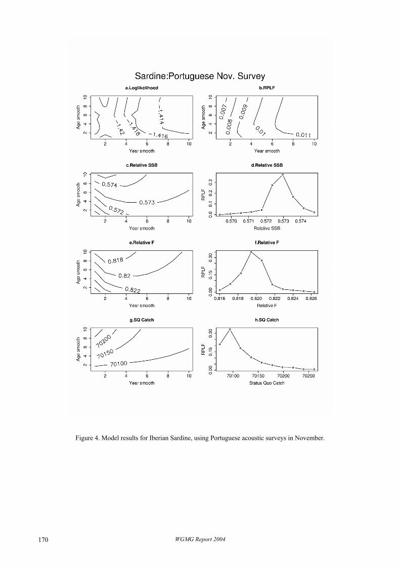
Figure 4. Model results for Iberian Sardine, using Portuguese acoustic surveys in November.

WGMG Report 2004 170

Figure 5. Summary of estimates of relative SSB, relative F and Status-quo catch for all three surveys for Iberian sardine.

WGMG Report 2004 171

Figure 6. Model results for North Sea haddock, using English Groundfish survey data.

WGMG Report 2004 172

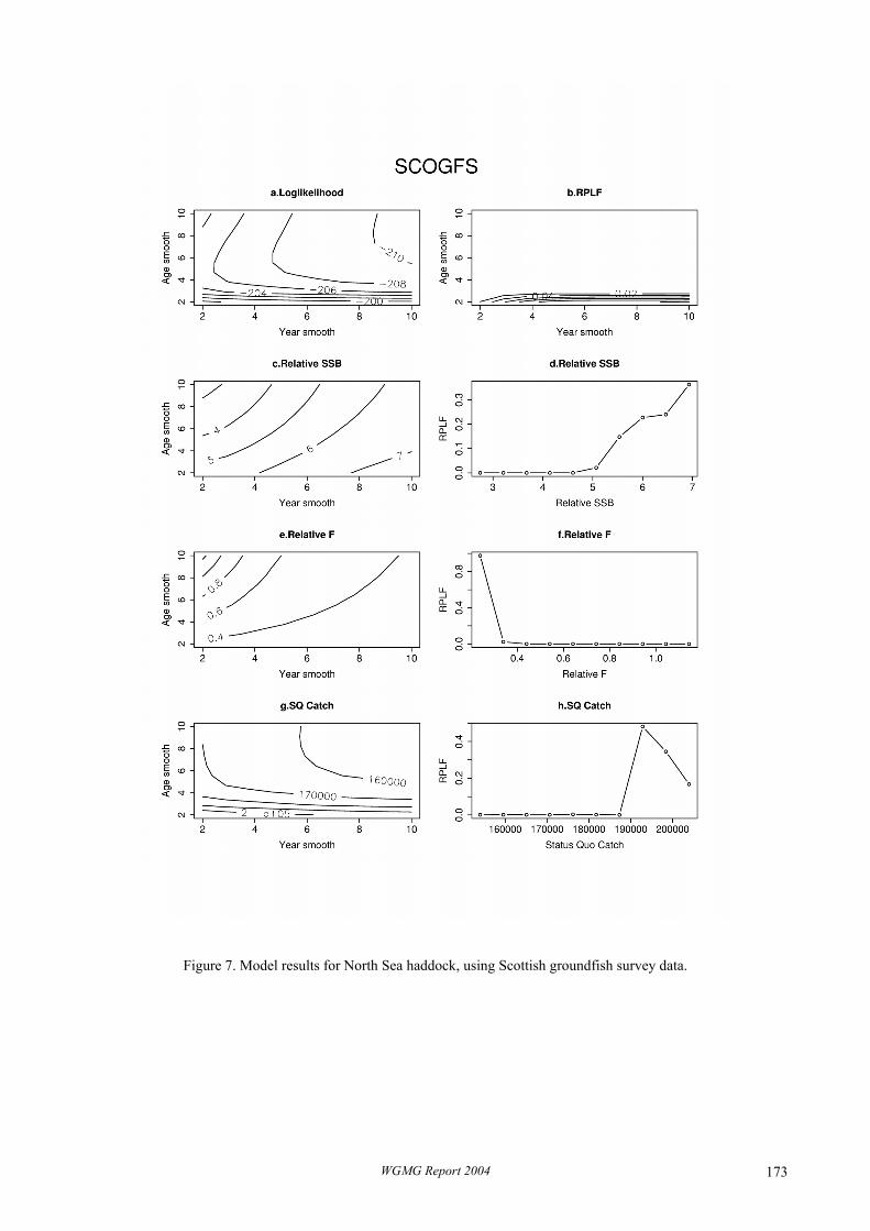
Figure 7. Model results for North Sea haddock, using Scottish groundfish survey data.

WGMG Report 2004 173

Figure 8. Model diagnostics for North Sea haddock using IBTS Q1 survey data.

WGMG Report 2004 174

Figure 9. Summary of estimates of relative SSB, relative F and F-status-quo catch for all three surveys for North Sea haddock.

WGMG Report 2004 175

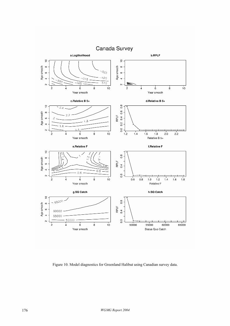
Figure 10. Model diagnostics for Greenland Halibut using Canadian survey data.

WGMG Report 2004 176

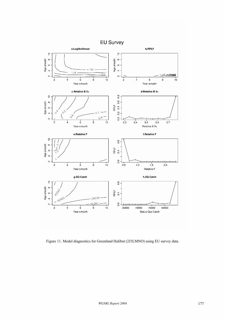
Figure 11. Model diagnostics for Greenland Halibut (2J3LMNO) using EU survey data.

WGMG Report 2004 177

Figure 12. Summary of estimates of relative SSB, relative F and F-status-quo catch for all three surveys for Greenland Halibut.

WGMG Report 2004 178

APPENDIX D: PROGRAMS PRESENTED TO THE WORKING GROUP

D.1 AMCI (source: ICES CM 2003/D:03) Model AMCI Version 2.2 (year: 2002) Model type A separable model is applied to the whole assessment period. Selection can be allowed to

change slowly according to the signal in the catches. The rate of change is determined by the user by specifying a gain factor for the influence of the current catch data. One extreme is then to keep the selection fixed (as in ICA). The population is projected forwards in time.

Selection The selection at one age can be specified as the average over some other ages, but this specification cannot include any multiplier. The selection at oldest age is estimated unless it is linked by the user to some other age.

Estimated parameters

Recruitment, initial stock numbers, annual fishing mortalities, selection-at-age by year, catchability-at-age (and year), natural mortality, quarterly distribution of fishing, quarterly distribution of stock by area. The user decides upon which of these to estimate; the remainder are kept at fixed values.

Catchabilities Catchabilities are in principle modelled as separable, but the age factor can be allowed to vary slowly using the same principle as for the selection-at-age in the catches. In practise, it will most often be kept fixed, and it then behaves as it does in ICA. Proportionality between index and stock abundance is always assumed. The proportionality can be fixed to the value one.

Plus group The plus group is modelled as a dynamic pool. The fishing mortality assumed for the plus age can be estimated, or linked to some younger age. The fit of the modelled plus group is included in the objective function unless specified otherwise.

Objective function There is a variety of objective functions available but most often, the weighted sum of squared log residuals is used. Weighting is decided by the user. AMCI does some implicit weighting internally which implies that the weights assumed in ICA and AMCI are not directly comparable.

Variance estimates/ uncertainty

’Variances’ of the parameter estimates can be derived from the Hessian, which is computed directly. There are also options for estimating uncertainty by parametric or non-parametric bootstrapping.

Other issues AMCI allows the incorporation of tagging data and SSB indices as additional sources of data. It allows for multiple fishing fleets and multiple areas, defining local partial fishing mortalities. Distribution by area is specified as parameters but there is no migration model yet.

Program language FORTRAN 77. No external libraries required. References Draft manual available but no formal publications yet.

D.2 Bayesian VPA/MCMC

Model Bayesian VPA/MCMC References Lewy, P. and Nielsen, A. (2003). Modelling stochastic fish stock dynamics using Markov

Chain Monte Carlo. ICES Journal of Marine Science, 60:743–752. Nielsen, A. and Lewy, P. (2002). Comparison of the frequentist properties of Bayes and the maximum likelihood estimators in an age-structured fish stock assessment model. Canadian Journal of Fisheries and Aquatic Sciences, 59:136–143. Azevedo, M. Bayesian fish stock assessment with VPA. Working Document for the ICES Working Group on Methods of Fish Stock Assessment, Lisbon, 11–18 February 2004.

WGMG Report 2004 179

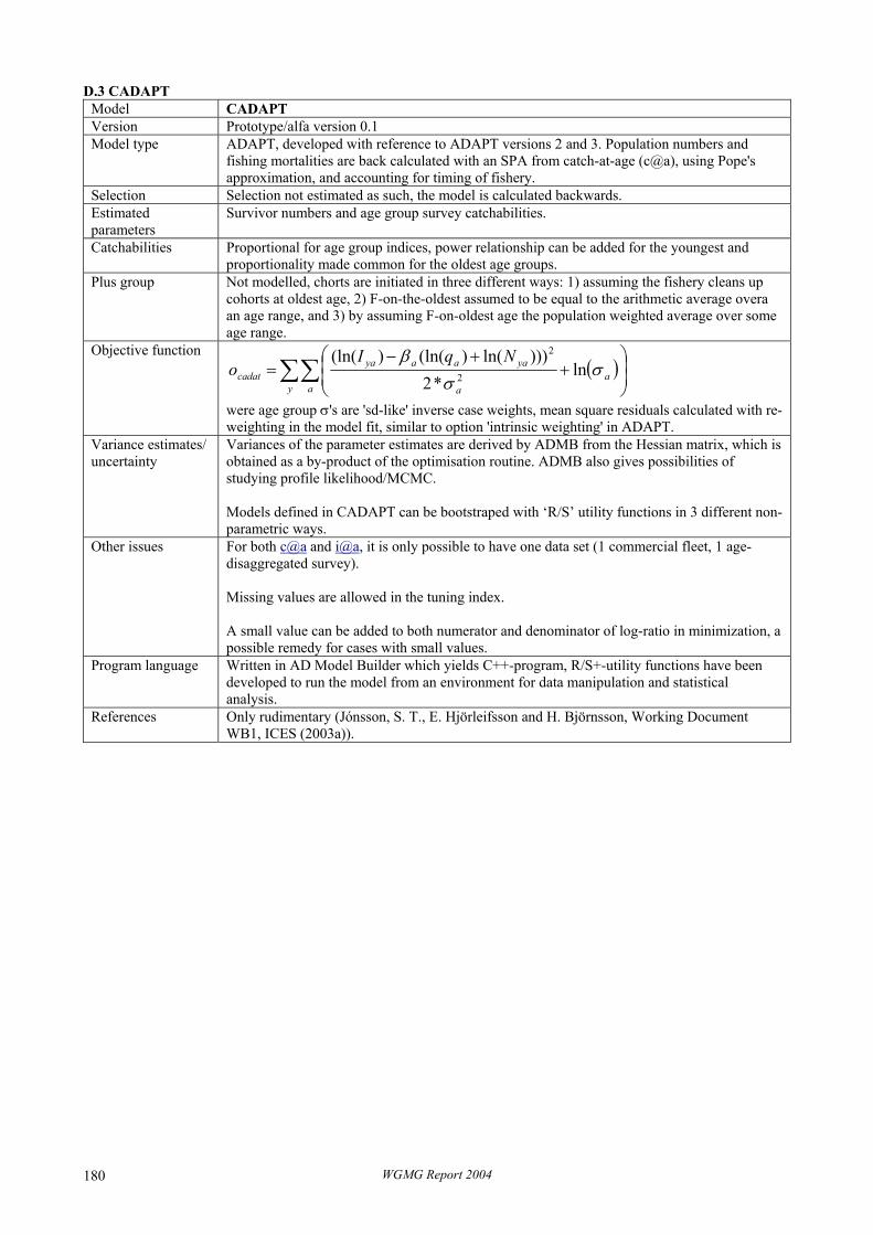
D.3 CADAPT Model CADAPT Version Prototype/alfa version 0.1 Model type ADAPT, developed with reference to ADAPT versions 2 and 3. Population numbers and

fishing mortalities are back calculated with an SPA from catch-at-age (c@a), using Pope's approximation, and accounting for timing of fishery.

Selection Selection not estimated as such, the model is calculated backwards. Estimated parameters

Survivor numbers and age group survey catchabilities.

Catchabilities Proportional for age group indices, power relationship can be added for the youngest and proportionality made common for the oldest age groups.

Plus group Not modelled, chorts are initiated in three different ways: 1) assuming the fishery cleans up cohorts at oldest age, 2) F-on-the-oldest assumed to be equal to the arithmetic average overa an age range, and 3) by assuming F-on-oldest age the population weighted average over some age range.

Objective function ( )∑∑

+

+−=

y aa

a

yaaayacadat

NqIo σ

σβ

ln*2

)))ln()(ln()(ln(2

2

were age group σ's are 'sd-like' inverse case weights, mean square residuals calculated with re-weighting in the model fit, similar to option 'intrinsic weighting' in ADAPT.

Variance estimates/ uncertainty

Variances of the parameter estimates are derived by ADMB from the Hessian matrix, which is obtained as a by-product of the optimisation routine. ADMB also gives possibilities of studying profile likelihood/MCMC. Models defined in CADAPT can be bootstraped with ‘R/S’ utility functions in 3 different non-parametric ways.

Other issues For both c@a and i@a, it is only possible to have one data set (1 commercial fleet, 1 age-disaggregated survey). Missing values are allowed in the tuning index. A small value can be added to both numerator and denominator of log-ratio in minimization, a possible remedy for cases with small values.

Program language Written in AD Model Builder which yields C++-program, R/S+-utility functions have been developed to run the model from an environment for data manipulation and statistical analysis.

References Only rudimentary (Jónsson, S. T., E. Hjörleifsson and H. Björnsson, Working Document WB1, ICES (2003a)).

WGMG Report 2004 180

D.4 CAMERA Model CAMERA Version Prototype/alfa version 0.1 Model type A separable catch at age model for one period (selectivity and catchability fixed). Selection Time invariant selectivity at age is estimated, 1) for each age group (with optional plateau), or

parametrically, 2) with a 2-parameter logistic curve, or 3) a 3-parameter double normal curve. The last option hasn’t been tested much.

Estimated parameters

Initial numbers, recruits, selectivity and catchability parameters along with full selection fishing mortality.

Catchabilities Proportional for age group indices, power relationship can be added for the youngest and proportionality made common for the oldest age groups.

Plus group Not included. Objective function

( )( )

( )( )

( )( )

∑∑

∑

∑∑

∑∑

+

+−

+

=

y aya

Yyy

y a

yaya

a

yaya

y

camera

Fya

X

YY

II

CC

O

1*

ˆ/ln

ln2

ˆ/ln)1(

ln2

ˆ/ln

2

2

2

2

2

ρρ

λ

σσ

λ

where the σ and ρ, 'sd-like' inverse case weights used in the objective function, are given by the user. Mean square residuals from Shepherd-Nicholson fit to i@a and c@a have proven useful in the development phase. The last term is taken from ADMB lore, the multiplier X is set to 1000 until the last phase of the minimization is reach, when its value is switched to 0.001

Variance estimates/ uncertainty

Variances of the parameter estimates are derived by ADMB from the Hessian matrix, which is obtained as a by-product of the optimisation routine. ADMB also gives possibilities of studying profile likelihood/MCMC. Models defined in ‘camera’ can be bootstraped with ‘R/S’ utility functions in 3 different non-parametric ways.

Other issues For both c@a and i@a, it is only possible to have one data set (1 commercial fleet, 1 age-disaggregated survey). A small value can be added to both numerator and denominator of log-ratio in minimization, a possible remedy for cases with small values. Relative importance of c@a and i@a components of objective function can be varied through changing the objective function component multiplier ‘lambda’. Objective function components are included in report-file.

Program language Written in AD Model Builder which yields C++-program, R/S+-utility functions have been developed to run the model from an environment for data manipulation and statistical analysis.

References Only rudimentary (Jónsson, S. T., E. Hjörleifsson and H. Björnsson, Working Document WB1, ICES (2003a)).

D.5 FLR ADAPT

Model FLR ADAPT Version Prototype References Draft manual available but no formal publications yet.

D.6 FLR XSA

Model FLR XSA Version Prototype References Draft manual available but no formal publications yet.

WGMG Report 2004 181

D.7 ICA Model ICA References Patterson, K.R. (1998). Integrated Catch at Age Analysis Version 1.4. Scottish Fisheries

Research Report. No. 38. D.8 ISVPA (source: ICES CM 2003/D:03)

Model ISVPA Version Year:2002 Model type A separable model is applied to one or two periods, determined by the user. The separable

model covers the whole assessment period Selection The selection at oldest age is equal to that of previous age; selections are normalized by their

sum to 1. For the plus group the same mortality as for the oldest true age. Estimated parameters

Catchabilities The catchabilities by ages and fleets can be estimated or assumed equal to 1. Catchabilities are derived analytically as exponents of the average logarithmic residuals between the catch-derived and the survey-derived estimates of abundance.

Plus group The plus group is not modelled, but the abundance is derived from the catch assuming the same mortality as for the oldest true age.

Objective function The objective function is a weighted sum of terms (weights may be given by user). For the catch-at-age part of the model, the respective term is: • sum of squared residuals in logarithmic catches, or • median of distribution of squared residuals in logarithmic catches MDN(M, fn), or • absolute median deviation AMD(M, fn). For SSB surveys it is sum of squared residuals between logarithms of SSB from cohort part. For surveys; for age- structured indexes it is SS, or MDN, or AMD for logarithms of N(a,y).

Variance estimates/ uncertainty

For estimation of uncertainty parametric conditional bootstrap with respect to catch-at-age, (assuming that errors in catch-at-age data are log-normally distributed, standard deviation is estimated in basic run), combined with adding noising to indexes (assuming that errors in indexes are log-normally distributed with specified values of standard deviation) is used.

Other issues Three error models are available for the catch-at-age part of the model: • errors attributed to the catch-at-age data. This is a strictly separable model (“effort-

controlled version”) • errors attributed to the separable model of fishing mortality. This is effectively a VPA but

uses the separable model to arrive at terminal fishing mortalities (“catch-controlled version”)

• errors attributed to both (“mixed version”). For each age and year, F is calculated from the separable model and from the VPA type approach (using Pope’s approximation). The final estimate is an average between the two where the weighting is decided by the user or by the squared residual in that point.

Four options are available for constraining the residuals on the catches: 1. Each row-sum and column-sum of the deviations between fishing mortalities derived

from the separable model and derived from the VPA-type (effort controlled) model are forced to be zero. This is called “unbiased separabilization”

2. As option 1, but applied to catch residuals. 3. As option 1, but the deviations are weighted by the selection-at-age. 4. No constraints on column-sums or row-sums of residuals.

Program language FORTRAN 77. References Vasilyev, D.A. (2001). Cohort models and analysis of commercial bio-resources at

information supply deficit. VNIRO Publishing: Moscow.

WGMG Report 2004 182

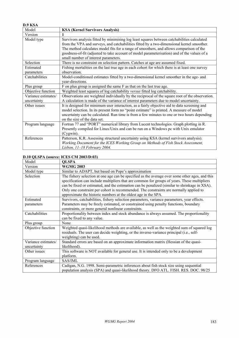
D.9 KSA Model KSA (Kernel Survivors Analysis) Version 1 Model type Survivors analysis fitted by minimising log least squares between catchabilities calculated

from the VPA and surveys, and catchabilities fitted by a two-dimensional kernel smoother. The method calculates model fits for a range of smoothers, and allows comparison of the goodness-of-fit (adjusted to take account of model parameterisation) and of the values of a small number of interest parameters.

Selection There is no constraint on selection pattern. Catches at age are assumed fixed. Estimated parameters

Fishing mortalities on the last true age in each cohort for which there is at least one survey observation.

Catchabilities Model-conditioned estimates fitted by a two-dimensional kernel smoother in the age- and year-directions.

Plus group F on plus group is assigned the same F as that on the last true age. Objective function Weighted least squares of log catchability versus fitted log catchability. Variance estimates/ uncertainty

Observations are weighted individually by the reciprocal of the square root of the observation. A calculation is made of the variance of interest parameters due to model uncertainty.

Other issues It is designed for minimum user interaction, as a fairly objective aid to data screening and model selection. In its present form no “point estimate” is printed. A measure of model uncertainty can be calculated. Run time is from a few minutes to one or two hours depending on the size of the data set.

Program language Fortran 77 and “PORT” numerical library from Lucent technologies. Graph plotting in R. Presently compiled for Linux/Unix and can be run on a Windows pc with Unix emulator (Cygwin).

References Patterson, K.R. Assessing structural uncertainty using KSA (kernel survivors analysis). Working Document for the ICES Working Group on Methods of Fish Stock Assessment, Lisbon, 11–18 February 2004.

D.10 QLSPA (source: ICES CM 2003/D:03)

Model QLSPA Version WGMG 2003 Model type Similar to ADAPT, but based on Pope’s approximation Selection The fishery selection at one age can be specified as the average over some other ages, and this

specification can include multipliers that are common for groups of years. These multipliers can be fixed or estimated, and the estimation can be penalized (similar to shrinkage in XSA). Only one constraint per cohort is recommended. The constraints are normally applied to approximate the historic numbers at the oldest age in the SPA.

Estimated parameters

Survivors, catchabilities, fishery selection parameters, variance parameters, year effects. Parameters may be freely estimated, or constrained using penalty functions, boundary constraints, or more general nonlinear constraints.

Catchabilities Proportionality between index and stock abundance is always assumed. The proportionality can be fixed to any value.

Plus group None Objective function Weighted quasi-likelihood methods are available, as well as the weighted sum of squared log

residuals. The user can decide weighting, or the inverse-variance principal (i.e., self-weighting) can be used.

Variance estimates/ uncertainty

Standard errors are based on an approximate information matrix (Hessian of the quasi-likelihood).

Other issues This software is NOT available for general use. It is intended only to be a development platform.

Program language SAS/IML References Cadigan, N.G. 1998. Semi-parametric inferences about fish stock size using sequential

population analysis (SPA) and quasi-likelihood theory. DFO ATL. FISH. RES. DOC. 98/25

WGMG Report 2004 183

D.11 SURBA Model SURBA Version 2.20 (compiled 13/02/2004) Model type A separable model of fishing mortality is applied to relative CPUE indices from research-

vessel surveys or commercial fleets. Selection Selection (age-effect) on all true ages is estimated. Estimated parameters

Year and age effects in fishing mortality, cohort effects in abundance. The terminal year-effect is not estimated, but is fixed so that the mean of the year-effect time-series is 1.0.

Catchabilities The model can be used to produce relative or “absolute” abundance estimates. In the first case, catchabilities [ ]0.0,1.0Îq , and these are manually and iteratively modified by the user until the fitted age effects look appropriate. In the second case, catchabilities are estimated externally by a catch-at-age analysis method. In both cases catchabilities are time-invariant, but not age-invariant.

Plus group The plus group is not modelled, but the abundance is derived from the catch assuming the same mortality as for the oldest true age.

Objective function Weighted sum of squared log residuals between observed and fitted indices. Weighting may be define manually, or using the inverse-variance of the index at age. A smoothing term can be used to penalise interannual variation in fitted year effects, or the index can be pre-smoothed down cohorts using cubic splines.

Variance estimates/ uncertainty

Parameter estimates may be constrained or unconstrained: if the latter option is used, standard errors of estimates are available. Uncertainty estimates of standard outputs (mean F, SSB, recruitment) are obtained using unstructured residual bootstraps.

Other issues A long wish-list of desirable SURBA developments has been compiled, and is being addressed. The priority items are: • Modelling multiple surveys simultaneously. • Non-additivity in selection (relaxing the separability assumption. • Implementation in the current open-source environment. • Catchability estimation via surface profiling.

Program language Compaq Visual Fortran-90 with Winteracter 5.0 (GUI) and NAG F77 version 20 (numerical analysis) libraries, running under Windows NT/2000/XP.

References Cook, R.M. (1997) Stock trends in six North Sea stocks as revealed by an analysis of research vessel surveys. ICES Journal of Marine Science, 54, 924–933. Needle, C.L. (2003) Survey-based assessments with SURBA. Working Document to the ICES Working Group on Methods on Fish Stock Assessments, Copenhagen, 29 Jan – 5 Feb 2003. See also Appendix XXX.

D.12 TSA

Model TSA References Fryer, R.J. (2002). TSA: is it the way? In Appendix D of the Report of the Working Group on

Methods on Fish Stock Assessments. ICES CM 2002/D:01. Gudmundsson, G. (1994). Time series analysis of catch-at-age observations. Applied Statistics 43:117-126.

D.13 XSA

Model XSA References Darby, C. and Flatman, S. (1994). Lowestoft VPA Suite Version 3.1: User Guide. MAFF:

Lowestoft. Shepherd, J.G. (1999). Extended survivors analysis: an improved method for the analysis of catch-at-age data and abundance indices. ICES Journal of Marine Science, 56:584–591.

D.14 XSA+

Model XSA+ Version Prototype

WGMG Report 2004 184

D.15 CSA Program CSAo Version September 2003 Model type Two-stage Collie-Sissenwine (1983) Data needs Total catches (in number); “survey” indices in number by stage; natural mortality M; timing of

catch in year. Mean weights by stage, to convert stock numbers to biomass. Input settings Ratio of recruits to fully-recruited survey catchability; relative weight of measurement errors

on recruits; timing of catch in year. Catchability Only considers catchability in survey (not in fishery). Fully-recruited catchability assumed

constant in time series. Catchability of recruits is a set fraction of that of fully-recruited. Estimated parameters

Stock size of recruits in all years except the last; stock size of fully recruited in first year; fully-recruited catchability (computed as GM), i.e., Y+1 parameters if Y years of data. Optional: catchability ratio by grid search (“SSQ profiling”)

Estimation approach

Non-linear least squares. Only considers measurement errors on indices, assumed log-normal. Process errors are ignored.

Objective function Weighted sum (user defined weights) of 2 sums of squared log-residuals between model-predicted and observed survey indices, one for recruits, the other for fully-recruited.

Minimisation Marquardt-Levenberg. Variance estimates/ uncertainty

Non-parametric model-conditioned bootstrap: residuals from base run drawn randomly and added to fitted indices, for each stage independently. Table of percentiles produced for biomasses and q; no bias correction (yet) on percentiles. Retrospective analysis.

Other issues Trials on simulated and real data indicate that absolute estimates of stock size are mostly sensitive to the assumed ratio of recruits catchability (s) which has to be set by users based on external information and analyses, but trends are less sensitive to s. Estimates weakly sensitive to weights of error sources in objective function. Estimated q negatively correlated with assumed M. Performance degrade, even for trends, when indices too noisy. Unaccounted trends in survey q result in biased stock size estimates.

Language Fortran; Splus Restrictions Handles maximum of 25 data years (takes 25 last if more in input file) and only one set of

survey (or CPUE) indices; same M for both stages; at least 10 years of data in retrospective analyses. Treatment of missing indices not fully validated.

Reference Collie, J.S. and Sissenwine, M.P. (1983). Estimating population size from relative abundance data measured with error. Canadian Journal of Fisheries and Aquatic Sciences, 40:1871–1879.

Program del2m, del2s Version February 2003 Model type Two-stage Collie-Sissenwine (1983) Data needs Total catches (in number); “survey” indices in number by stage; natural mortality M; timing of

catch in year. Mean weights by stage, to convert stock numbers to biomass. Input settings Ratio of recruits to fully-recruited survey catchability; relative weights of measurement errors

on recruits and of process errors; timing of catch in year. Catchability Only consider catchability in survey (not in fishery). Fully-recruited catchability assumed

constant in time series. Catchability of recruits is a set fraction of that of fully-recruited. Estimated parameters

Recruits indices in all years but the last; fully-recruited indices in all years; fully-recruited catchability, i.e., 2Y parameters if Y years of data. Optional: catchability ratio by grid search (“SSQ profiling”)

Estimation approach

Non-linear least squares. Consider both measurement errors on indices, assumed log-normal, and process errors assumed normal or log-normal; users can choose to ignore the latter.

Objective function Weighted sum (user defined weights) of 3 sums of squared log-residuals between model-predicted and observed survey indices, one for recruits, one for fully-recruited, and one for process error terms.

Minimisation Marquardt-Levenberg (del2m) or Nelder-Mead simplex with quadratic extension (del2s). Variance estimates/ uncertainty

Approximate CV of parameters based on Hessian (del2s only). Non-parametric model-conditioned bootstrap: residuals from base run drawn randomly, for each error source independently, and added to fitted indices. Table of percentiles produced for biomasses and q; no bias correction (yet) on percentiles. Retrospective analysis.

Other issues Trials on simulated and real data indicate that absolute estimates of stock size are mostly sensitive to the assumed ratio of recruits catchability (s) which has to be set by users based on

WGMG Report 2004 185

external information and analyses, but trends are less sensitive to s. Estimates weakly sensitive to weights of error sources in objective function. Estimated q negatively correlated with assumed M. Performance degrade, even for trends, when indices too noisy. Unaccounted trends in survey q result in biased stock size estimates.

Language Fortran Restrictions Handles maximum of 25 data years (takes 25 last if more in input file) and only one set of

survey (or CPUE) indices; same M for both stages; at least 10 years of data in retrospective analyses. Missing indices not allowed.

Reference Collie, J.S. and Sissenwine, M.P. (1983). Estimating population size from relative abundance data measured with error. Canadian Journal of Fisheries and Aquatic Sciences, 40:1871–1879. Conser, R.J. (1994). Stock assessment methods designed to support fishery management decisions in data-limited environments: development and application. PhD dissertation. School of Fisheries, University of Washington, Seattle, 292pp. Mesnil, B. (2003). The Catch-Survey Analysis (CSA) method of fish stock assessment: an evaluation using simulated data. Fisheries Research, 63: 193–212.

WGMG Report 2004 186

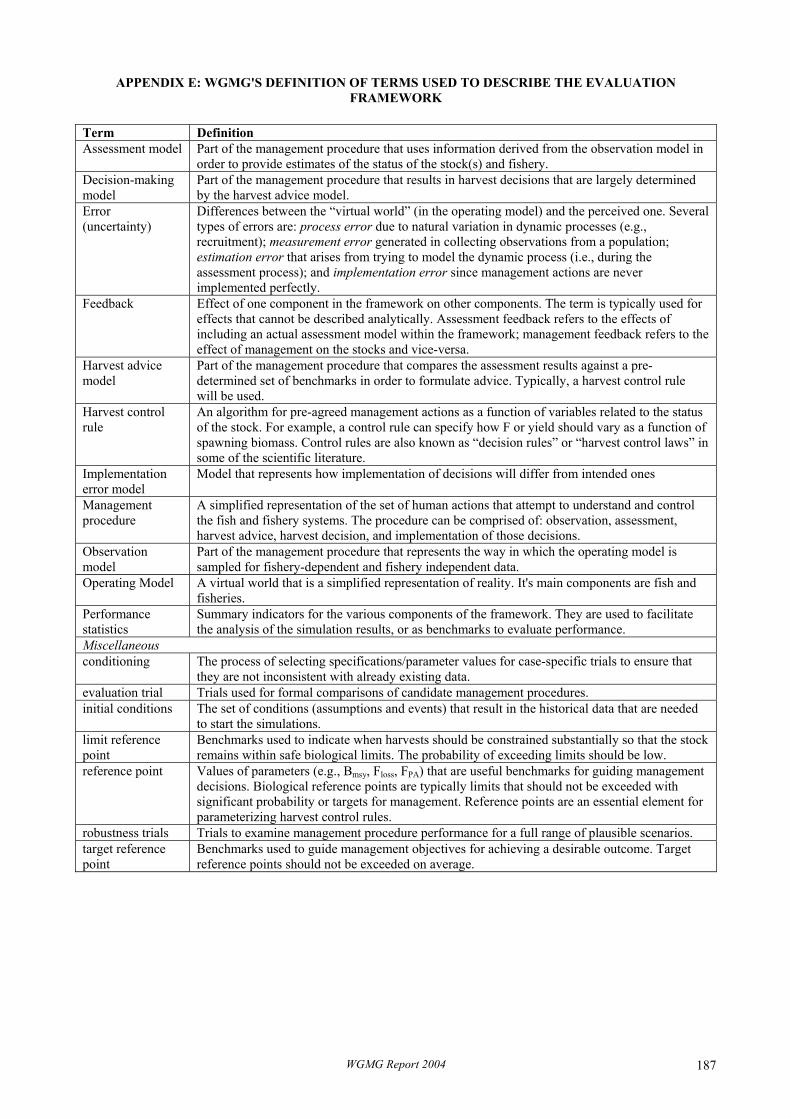
APPENDIX E: WGMG'S DEFINITION OF TERMS USED TO DESCRIBE THE EVALUATION FRAMEWORK

Term Definition Assessment model Part of the management procedure that uses information derived from the observation model in

order to provide estimates of the status of the stock(s) and fishery. Decision-making model

Part of the management procedure that results in harvest decisions that are largely determined by the harvest advice model.

Error (uncertainty)

Differences between the “virtual world” (in the operating model) and the perceived one. Several types of errors are: process error due to natural variation in dynamic processes (e.g., recruitment); measurement error generated in collecting observations from a population; estimation error that arises from trying to model the dynamic process (i.e., during the assessment process); and implementation error since management actions are never implemented perfectly.

Feedback Effect of one component in the framework on other components. The term is typically used for effects that cannot be described analytically. Assessment feedback refers to the effects of including an actual assessment model within the framework; management feedback refers to the effect of management on the stocks and vice-versa.

Harvest advice model

Part of the management procedure that compares the assessment results against a pre-determined set of benchmarks in order to formulate advice. Typically, a harvest control rule will be used.

Harvest control rule

An algorithm for pre-agreed management actions as a function of variables related to the status of the stock. For example, a control rule can specify how F or yield should vary as a function of spawning biomass. Control rules are also known as “decision rules” or “harvest control laws” in some of the scientific literature.

Implementation error model

Model that represents how implementation of decisions will differ from intended ones

Management procedure

A simplified representation of the set of human actions that attempt to understand and control the fish and fishery systems. The procedure can be comprised of: observation, assessment, harvest advice, harvest decision, and implementation of those decisions.

Observation model

Part of the management procedure that represents the way in which the operating model is sampled for fishery-dependent and fishery independent data.

Operating Model A virtual world that is a simplified representation of reality. It's main components are fish and fisheries.

Performance statistics

Summary indicators for the various components of the framework. They are used to facilitate the analysis of the simulation results, or as benchmarks to evaluate performance.

Miscellaneous conditioning The process of selecting specifications/parameter values for case-specific trials to ensure that

they are not inconsistent with already existing data. evaluation trial Trials used for formal comparisons of candidate management procedures. initial conditions The set of conditions (assumptions and events) that result in the historical data that are needed

to start the simulations. limit reference point

Benchmarks used to indicate when harvests should be constrained substantially so that the stock remains within safe biological limits. The probability of exceeding limits should be low.

reference point Values of parameters (e.g., Bmsy, Floss, FPA) that are useful benchmarks for guiding management decisions. Biological reference points are typically limits that should not be exceeded with significant probability or targets for management. Reference points are an essential element for parameterizing harvest control rules.

robustness trials Trials to examine management procedure performance for a full range of plausible scenarios. target reference point

Benchmarks used to guide management objectives for achieving a desirable outcome. Target reference points should not be exceeded on average.

WGMG Report 2004 187

APPENDIX F: ICCAT ASSESSMENT PROGRAM DOCUMENTATION (APPENDIX 1)

1. Program name Name of the application

2. Version (date) *** Version number given by the programmer

3. Language Computer language(s) in which the application is written (e.g., Pascal).

4. Programmer / contact person Name, address, email of the programmer and/or persons that can be contacted with questions about the application

5. Distribution limitations List any limitations imposed by the programmer (e.g., only executable code can be distributed)

6. Compiler needs / stand-alone List additional software needed to run the program (e.g., C++), operating system if other than DOS/Windows, or state if the executable program does not need other software to run

7. Purpose Brief description of what the application does (e.g., “fits a stock production model to catch and effort data making an equilibrium approximation”).

8. Description A full description of what the application does, sufficient to allow replication. It should clearly state the major statistical and biological assumptions.

9. Required inputs Description of the inputs needed.

10. Program outputs Description of the program outputs.

11. Diagnostics A list of the diagnostics produced by the program that can be used to guide modelling.

12. Other features List of special features of the application that are not “traditional” ones (e.g., uses tagging data as auxiliary information).

13. History of method peer review Detailed history of the review of the method, citing publications and reports.

14. Steps taken by programmer for validation Detailed history of how the application itself (as opposed to the method) has been validated by the programmer (e.g., by generating simulated data of known characteristics and then using the program on the simulated data)

15. Tests conducted by others A list of the tests that persons other than the programmer (e.g., the Secretariat) have conducted.

16. Notes by iccat Comments by a Coordinating Committee, group or person in charge of cataloguing the software, especially with reference to validation. This will essentially be the “certification” or “approval” of the software.

APPENDIX 1. Algorithm A list of steps explaining how the program operates. This is intended to complement Item 8 and Appendix 2.

WGMG Report 2004 188

APPENDIX 2. User´s guide A user´s guide, sufficiently detailed to allow others to run the program.

APPENDIX 3. Worked example An example containing inputs, program run options and outputs.

APPENDIX 4. Source code The source code, taking into account copyright restrictions. This code may or may not be distributed to persons outside the Secretariat depending on the entry on Item 5.

*** Note: Each new version of a catalogue entry should be accompanied by documentation that explains the major features associated with the change (e.g., new program options, bug fixes, etc.).

WGMG Report 2004 189

APPENDIX G: THE OPEN SOURCE INITIATIVE (WWW.OPENSOURCE.ORG)

Version 1.9

The indented, italicized sections below appear as annotations to the Open Source Definition (OSD) and are not a part of the OSD.

Introduction

Open source doesn't just mean access to the source code. The distribution terms of open-source software must comply with the following criteria:

1. Free Redistribution

The license shall not restrict any party from selling or giving away the software as a component of an aggregate software distribution containing programs from several different sources. The license shall not require a royalty or other fee for such sale.

Rationale: By constraining the license to require free redistribution, we eliminate the temptation to throw away many long-term gains in order to make a few short-term sales dollars. If we didn't do this, there would be lots of pressure for cooperators to defect.

2. Source Code

The program must include source code, and must allow distribution in source code as well as compiled form. Where some form of a product is not distributed with source code, there must be a well-publicized means of obtaining the source code for no more than a reasonable reproduction cost–preferably, downloading via the Internet without charge. The source code must be the preferred form in which a programmer would modify the program. Deliberately obfuscated source code is not allowed. Intermediate forms such as the output of a pre-processor or translator are not allowed.

Rationale: We require access to un-obfuscated source code because you can't evolve programs without modifying them. Since our purpose is to make evolution easy, we require that modification be made easy.

3. Derived Works

The license must allow modifications and derived works, and must allow them to be distributed under the same terms as the license of the original software.

Rationale: The mere ability to read source isn't enough to support independent peer review and rapid evolutionary selection. For rapid evolution to happen, people need to be able to experiment with and redistribute modifications.

4. Integrity of the Author's Source Code

The license may restrict source-code from being distributed in modified form only if the license allows the distribution of “patch files” with the source code for the purpose of modifying the program at build time. The license must explicitly permit distribution of software built from modified source code. The license may require derived works to carry a different name or version number from the original software.

Rationale: Encouraging lots of improvement is a good thing, but users have a right to know who is responsible for the software they are using. Authors and maintainers have reciprocal right to know what they're being asked to support and protect their reputations.

Accordingly, an open-source license must guarantee that source be readily available, but may require that it be distributed as pristine base sources plus patches. In this way, "unofficial" changes can be made available but readily distinguished from the base source.

WGMG Report 2004 190

5. No Discrimination against Persons or Groups

The license must not discriminate against any person or group of persons.

Rationale: In order to get the maximum benefit from the process, the maximum diversity of persons and groups should be equally eligible to contribute to open sources. Therefore we forbid any open-source license from locking anybody out of the process.

Some countries, including the United States, have export restrictions for certain types of software. An OSD-conformant license may warn licensees of applicable restrictions and remind them that they are obliged to obey the law; however, it may not incorporate such restrictions itself.

6. No Discrimination against Fields of Endeavour

The license must not restrict anyone from making use of the program in a specific field of endeavour. For example, it may not restrict the program from being used in a business, or from being used for genetic research.

Rationale: The major intention of this clause is to prohibit license traps that prevent open source from being used commercially. We want commercial users to join our community, not feel excluded from it.

7. Distribution of License

The rights attached to the program must apply to all to whom the program is redistributed without the need for execution of an additional license by those parties.

Rationale: This clause is intended to forbid closing up software by indirect means such as requiring a non-disclosure agreement.

8. License Must Not Be Specific to a Product

The rights attached to the program must not depend on the program's being part of a particular software distribution. If the program is extracted from that distribution and used or distributed within the terms of the program's license, all parties to whom the program is redistributed should have the same rights as those that are granted in conjunction with the original software distribution.

Rationale: This clause forecloses yet another class of license traps.

9. License Must Not Restrict Other Software

The license must not place restrictions on other software that is distributed along with the licensed software. For example, the license m ust not insist that all other programs distributed on the same medium must be open-source software.

Rationale: Distributors of open-source software have the right to make their own choices about their own software. Yes, the GPL is conformant with this requirement. Software linked with GPLed libraries only inherits the GPL if it forms a single work, not any software with which they are merely distributed.

10. License Must Be Technology-Neutral

No provision of the license may be predicated on any individual technology or style of interface.

Rationale: This provision is aimed specifically aimed at licenses which require an explicit gesture of assent in order to establish a contract between licensor and licensee. Provisions mandating so-called "click-wrap" may conflict with important methods of software distribution such as FTP download, CD-ROM anthologies, and web mirroring; such provisions may also hinder code re-use. Conformant licenses must allow for the possibility that (a) redistribution of the software will take place over non-Web channels that do not support click-wrapping of the download, and that (b) the covered code (or re-used portions of covered code) may run in a non-GUI environment that cannot support popup dialogues.

WGMG Report 2004 191

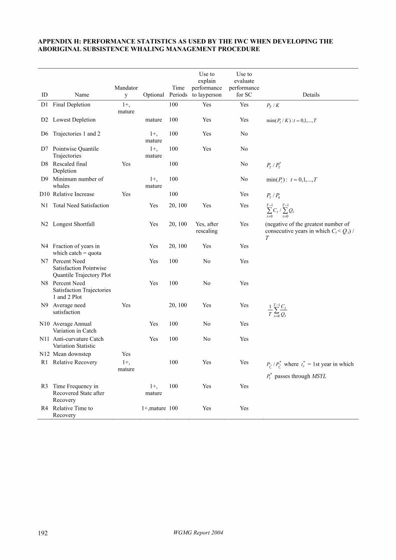
APPENDIX H: PERFORMANCE STATISTICS AS USED BY THE IWC WHEN DEVELOPING THE ABORIGINAL SUBSISTENCE WHALING MANAGEMENT PROCEDURE

ID Name Mandator

y Optional Time

Periods

Use to explain

performance to layperson

Use to evaluate

performance for SC Details

D1 Final Depletion 1+, mature

100 Yes Yes KPT /

D2 Lowest Depletion mature 100 Yes Yes TtKPt ,...,1,0:)/(min =

D6 Trajectories 1 and 2 1+, mature

100 Yes No

D7 Pointwise Quantile Trajectories

1+, mature

100 Yes No

D8 Rescaled final Depletion

Yes 100 No */T TP P

D9 Minimum number of whales

1+, mature

100 No min( ) : 0,1,...,tP t T=

D10 Relative Increase Yes 100 Yes 0/TP P

N1 Total Need Satisfaction Yes 20, 100 Yes Yes ∑∑−

=

−

=

1

0

1

0/

T

tt

T

tt QC

N2 Longest Shortfall Yes 20, 100 Yes, after rescaling

Yes (negative of the greatest number of consecutive years in which Ct < Q t) / T

N4 Fraction of years in which catch = quota

Yes 20, 100 Yes Yes

N7 Percent Need Satisfaction Pointwise Quantile Trajectory Plot

Yes 100 No Yes

N8 Percent Need Satisfaction Trajectories 1 and 2 Plot

Yes 100 No Yes

N9 Average need satisfaction

Yes 20, 100 Yes Yes ∑

−

=

1

0

1 T

t t

t

QC

T

N10 Average Annual Variation in Catch

Yes 100 No Yes

N11 Anti-curvature Catch Variation Statistic

Yes 100 No Yes

N12 Mean downstep Yes R1 Relative Recovery 1+,

mature 100 Yes Yes *

** /rr tt PP

*tP

where = 1st year in which

passes through MSYL

*rt

R3 Time Frequency in Recovered State after Recovery

1+, mature

100 Yes Yes

R4 Relative Time to Recovery

1+,mature 100 Yes Yes

WGMG Report 2004 192

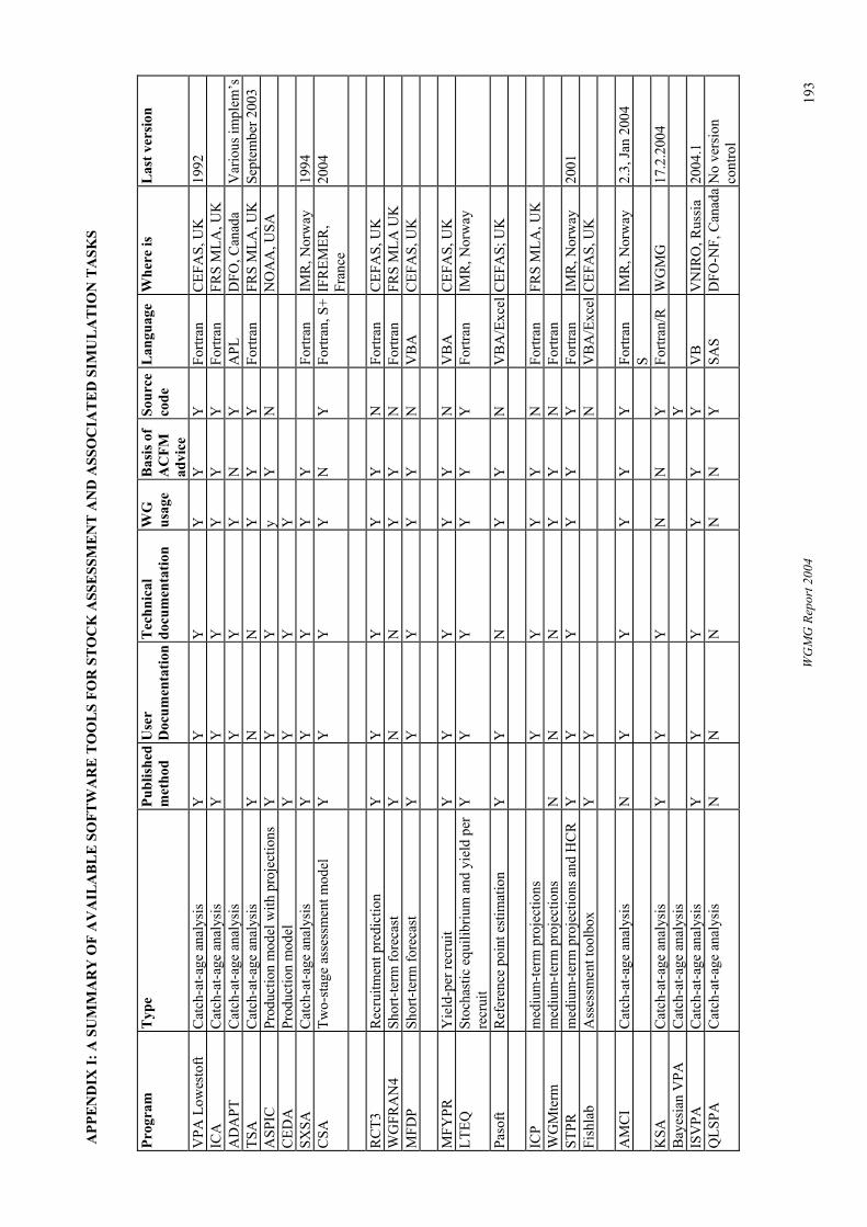
APP

EN

DIX

I: A

SU

MM

AR

Y O

F A

VA

ILA

BL

E S

OFT

WA

RE

TO

OL

S FO

R S

TO

CK

ASS

ESS

ME

NT

AN

D A

SSO

CIA

TE

D S

IMU

LA

TIO

N T

ASK

S

Prog

ram

T

ype

Publ

ishe

dm

etho

d U

ser

Doc

umen

tatio

nT

echn

ical

do

cum

enta

tion

WG

us

age

Bas

is o

f A

CFM

ad

vice

Sour

ce

code

L

angu

age

Whe

re is

Las

t ver

sion

VPA

Low

esto

ft C

atch

-at-a

ge a

naly

sis

Y

Y

YY

Y

YFo

rtran

CEF

AS,

UK

1992

ICA

C

atch

-at-a

ge a

naly

sis

Y

YY

Y

Y

Y

Fortr

an

FRS

MLA

, UK

AD

APT

C

atch

-at-a

ge a

naly

sis

YY

YN

Y

APL

D

FO, C

anad

a V

ario

us im

plem

’s

TSA

C

atch

-at-a

ge a

naly

sis

Y

N

N

Y

Y

Y

Fortr

an

FRS

MLA

, UK

Se

ptem

ber 2

003

A

SPIC

Pr

oduc

tion

mod

el w

ith p

roje

ctio

ns

Y

Y

Y

y Y

N

NO

AA

, USA

CED

A

Prod

uctio

n m

odel

Y

Y

Y

Y

SXSA

C

atch

-at-a

ge a

naly

sis

Y

Y

Y

Y

Y

Fo

rtran

IM

R, N

orw

ay

1994

C

SA

Two-

stag

e as

sess

men

t mod

el

Y

Y

Y

Y

N

Y

Fortr

an, S

+IF

REM

ER,

Fran

ce

2004

RC

T3

Rec

ruitm

ent p

redi

ctio

n Y

Y

Y

Y

Y

N

Fo

rtran

C

EFA

S, U

K

W

GFR

AN

4 Sh

ort-t

erm

fore

cast

Y

N

N

Y

Y

N

Fo

rtran

FR

S M

LA U

K

M

FDP

Shor

t-ter

m fo

reca

st

Y

Y

Y

Y

Y

N

VB

A

CEF

AS,

UK

MFY

PR

Yie

ld-p

er re

crui

t Y

Y

Y

Y

Y

N

V

BA

C

EFA

S, U

K

LT

EQ

Stoc

hast

ic e

quili

briu

m a

nd y

ield

per

re

crui

t Y

YY

YY

YFo

rtran

IMR

, Nor

way

Paso

ft

Ref

eren

ce p

oint

est

imat

ion

YY

NY

YN

VB

A/E

xcel

CEF

AS;

UK

ICP

m

ediu

m-te

rm p

roje

ctio

nsY

YY

Y

N

Fortr

an

FRS

MLA

,UK

WG

Mte

rm

m

ediu

m-te

rm p

roje

ctio

nsN

NN

YY

NFo

rtran

ST

PR

med

ium

-term

pro

ject

ions

and

HC

R

Y

Y

Y

Y

Y

Y

Fortr

an

IMR

, Nor

way

20

01

Fish

lab

Ass

essm

ent t

oolb

ox

Y

Y

N

V

BA

/Exc

elC

EFA

S, U

K

A

MC

I C

atch

-at-a

ge a

naly

sis

N

Y

Y

Y

Y

Y

Fortr

an

IMR

, Nor

way

2.

3, Ja

n 20

04

S K

SA

Cat

ch-a

t-age

ana

lysi

s Y

Y

Y

N

N

Y

Fo

rtran

/R

WG

MG

17.2

.200

4B

ayes

ian

VPA

C

atch

-at-a

ge a

naly

sis

Y

ISV

PA

Cat

ch-a

t-age

ana

lysi

s

Y

YY

Y

Y

Y

VB

VN

IRO

,Rus

sia

2004

.1Q

LSPA

C

atch

-at-a

ge a

naly

sis

N

N

N

N

N

Y

SAS

DFO

-NF,

Can

ada

No

vers

ion

cont

rol

WG

MG

Rep

ort 2

004

193

Prog

ram

T

ype

Publ

ishe

dm

etho

d U

ser

Doc

umen

tatio

nT

echn

ical

do

cum

enta

tion

WG

us

age

Bas

is o

f A

CFM

ad

vice

Sour

ce

code

L

angu

age

Whe

re is

Las

t ver

sion

XSA

+

Cat

ch-a

t-age

ana

lysi

sN

NN

N

NN

Fo

rtran

C

EFA

SU

nder

deve

lopm

ent

SUR

BA

Su

rvey

-bas

ed a

sses

smen

t N

N

N

Y

N

Y

Fo

rtran

FR

S A

berd

een

2.2v

Feb

ruar

y 20

04

FLR

A

sses

smen

t fra

mew

ork

NN

NN

N

RC

EFA

S0.

5–1P

roto

type

only

C

APA

PT

C

atch

-at-a

ge a

naly

sis

NN

NN

NY

AD

MB

,C

++, R

, S

M

RI,

Icel

and

0.1

CA

MER

A

Cat

ch-a

t-age

ana

lysi

s N

N

N

N

N

Y

A

s abo

ve

MR

I, Ic

elan

d 0.

1 C

S4

HC

R S

imul

atio

ns

Y

Y

Y

Y

Y

Y

Fortr

an, R

C

EFA

S, U

K

4 PR

OST

M

ediu

m te

rm p

roje

ctio

ns a

nd H

CR

Y

Ja

va

IMR

, Nor

way

U

nder

de

velo

pmen

t

MTA

C

Mix

ed-s

peci

es a

naly

sis

Y (s

ubm

.)N

YN

NY

RD

IFR

ES,

Den

mar

k O

ct. 2

003

GA

DG

ET

Age

-leng

th si

mul

atio

n m

odel

, mul

ti-ar

ea, m

ulti-

spec

ies,

mul

ti-fle

et

Y

YY

YY

C++

MR

I, Ic

elan

d,an

d IM

R,

Nor

way

16

19/2

004

MSV

PA

Empt

y ce

lls m

ean

that

the

info

rmat

ion

was

not

ava

ilabl

e to

the

WG

MG

par

ticip

ants

WG

MG

Rep

ort 2

004

194

APPENDIX J: DESCRIPTION OF THE FEMS/FLR PROTOTYPE

The various models for assessment of fisheries dynamics and evaluation of management strategies are currently implemented in separate software programs. The input and output formats of these programs are often incompatible, although many are performing similar tasks, and many provide basic analysis tools (model estimation, graphing, result reporting) that are already available in various software platforms. Comparing the results of such models is difficult and requires exporting them to an environment that has efficient analytical tools. Moreover, integration of such different models into a single simulation environment that allows evaluation of the whole fishery system has, so far, been impossible. One possible way to address these limitations would be to develop an integrated framework for modelling and assessment so that quantitative evaluations of management procedures could be done through models incorporating the biological, observational, assessment and management components of the fishery system.

One example of such a framework is the one developed by the EU-funded project "FEMS" (Framework for Evaluation of Management Strategies). FEMS is in an informal cluster with 2 other EU projects, EASE and PKFM, and is attempting to provide software to allow different management strategies to be evaluated. Currently in its second year of the project, the FEMS team has decided to use R, a common, feature-rich environment, to develop a framework in which fishery models can be run and their output analysed. The latest object-oriented features of R (named S4 objects, or classes) allow for the definition of complex and flexible objects with a structure and arithmetic that is appropriate to fishery models. R also allows access to objects (fishery models) already written in C/C++ or FORTRAN and recompilation of these objects into the R environment using a “wrapper”.

Currently the FEMS team has implemented selected key components of the framework into a library called FLR (Fisheries Library based on R). This library includes, for example, FLQUANT, a flexible data object with key fishery dimensions (time, age, space and stock) and FLSTOCK, a collection of FLQUANTs for selected biological properties of a population (e.g., weight, catch, survival).

The current implementation of FLR has proved to be convenient, flexible and capable of using fisheries models in R. The R-FLR environment is currently being evaluated by international fisheries agencies, including the International Council for the Exploration of the Sea (ICES) and the International Commission for the Conservation of Atlantic Tunas (ICCAT). If this evaluation is successful, the R-FLR environment may become an ideal simulation framework for the evaluation of different fisheries models and management structures.

1 The R environment R is an implementation of the S language and provides a powerful and flexible statistical environment that in addition allows the production of high-quality and feature-rich graphs, making it an ideal environment for data analysis and modelling.

It is a fully planned and coherent system that includes

• data handling and storage, • a suite of operators for calculations on arrays and matrices, • a large, coherent, integrated collection of tools for data analysis including graphical facilities, • a well developed programming language. R is “open source”, in that the code is freely available, and many parties are actively developing it. In the R language it is possible to implement third party applications, and methods in the form of packages (or libraries) and external code, already written in other languages, can be combined with R so that heritage code can be incorporated into a single framework.

R is ideal to organise models and data into classes using an object-oriented approach. Once defined in R, classes can be manipulated using commands or scripts written in the R language. This is convenient for developers and expert users that can immediately apply thousands of R functions and graphs to these objects.

WGMG Report 2004 195

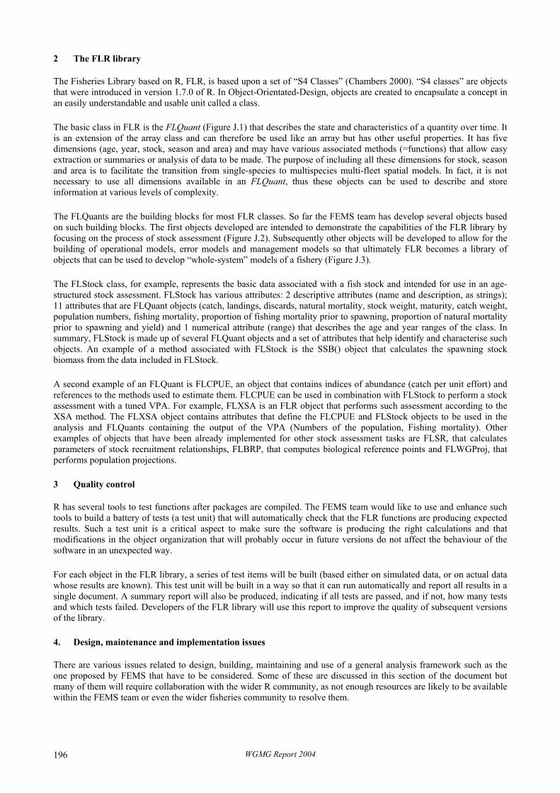
2 The FLR library The Fisheries Library based on R, FLR, is based upon a set of “S4 Classes” (Chambers 2000). “S4 classes” are objects that were introduced in version 1.7.0 of R. In Object-Orientated-Design, objects are created to encapsulate a concept in an easily understandable and usable unit called a class.

The basic class in FLR is the FLQuant (Figure J.1) that describes the state and characteristics of a quantity over time. It is an extension of the array class and can therefore be used like an array but has other useful properties. It has five dimensions (age, year, stock, season and area) and may have various associated methods (=functions) that allow easy extraction or summaries or analysis of data to be made. The purpose of including all these dimensions for stock, season and area is to facilitate the transition from single-species to multispecies multi-fleet spatial models. In fact, it is not necessary to use all dimensions available in an FLQuant, thus these objects can be used to describe and store information at various levels of complexity.

The FLQuants are the building blocks for most FLR classes. So far the FEMS team has develop several objects based on such building blocks. The first objects developed are intended to demonstrate the capabilities of the FLR library by focusing on the process of stock assessment (Figure J.2). Subsequently other objects will be developed to allow for the building of operational models, error models and management models so that ultimately FLR becomes a library of objects that can be used to develop “whole-system” models of a fishery (Figure J.3).

The FLStock class, for example, represents the basic data associated with a fish stock and intended for use in an age-structured stock assessment. FLStock has various attributes: 2 descriptive attributes (name and description, as strings); 11 attributes that are FLQuant objects (catch, landings, discards, natural mortality, stock weight, maturity, catch weight, population numbers, fishing mortality, proportion of fishing mortality prior to spawning, proportion of natural mortality prior to spawning and yield) and 1 numerical attribute (range) that describes the age and year ranges of the class. In summary, FLStock is made up of several FLQuant objects and a set of attributes that help identify and characterise such objects. An example of a method associated with FLStock is the SSB() object that calculates the spawning stock biomass from the data included in FLStock.

A second example of an FLQuant is FLCPUE, an object that contains indices of abundance (catch per unit effort) and references to the methods used to estimate them. FLCPUE can be used in combination with FLStock to perform a stock assessment with a tuned VPA. For example, FLXSA is an FLR object that performs such assessment according to the XSA method. The FLXSA object contains attributes that define the FLCPUE and FLStock objects to be used in the analysis and FLQuants containing the output of the VPA (Numbers of the population, Fishing mortality). Other examples of objects that have been already implemented for other stock assessment tasks are FLSR, that calculates parameters of stock recruitment relationships, FLBRP, that computes biological reference points and FLWGProj, that performs population projections.

3 Quality control R has several tools to test functions after packages are compiled. The FEMS team would like to use and enhance such tools to build a battery of tests (a test unit) that will automatically check that the FLR functions are producing expected results. Such a test unit is a critical aspect to make sure the software is producing the right calculations and that modifications in the object organization that will probably occur in future versions do not affect the behaviour of the software in an unexpected way.

For each object in the FLR library, a series of test items will be built (based either on simulated data, or on actual data whose results are known). This test unit will be built in a way so that it can run automatically and report all results in a single document. A summary report will also be produced, indicating if all tests are passed, and if not, how many tests and which tests failed. Developers of the FLR library will use this report to improve the quality of subsequent versions of the library.

4. Design, maintenance and implementation issues There are various issues related to design, building, maintaining and use of a general analysis framework such as the one proposed by FEMS that have to be considered. Some of these are discussed in this section of the document but many of them will require collaboration with the wider R community, as not enough resources are likely to be available within the FEMS team or even the wider fisheries community to resolve them.

WGMG Report 2004 196

4.1 Refactoring Since the FEMS team intends to implement different fishery models into FLR, the core part of the library should ideally contain all common features to those models so that implementation of a particular model is limited only to its specific parts and code is not duplicated. If the core part of the library is called framework, and the particular implementations for the various models are called customizations, the FEMS team has to study which part of the code should go in the framework and which part should be part of the customization, based on the analysis of a few customizations already implemented in the library. This process is called “refactoring”, and it is now commonly used for object-oriented software (like C++, Java, etc…). Refactoring of the initial version of FLR is an important step that will both enhance its maintainability and its potential to be enhanced and supplemented with many different models, while keeping duplications in code as low as possible.

4.2 Compiling tools

Currently, to supplement code to a library in R, one has to build code from scratch with a text editor (R has no built-in code editor), to edit many files manually (description, online help source, etc…) and to call various scripts to compile the library. It would be easier if appropriate tools were available to facilitate these tasks. An IDE (Integrated Development Environment) would allow everybody to contribute more easily to the FLR library. Ideally, this IDE should have an UML (Universal Modelling Language) module that would allow the building and modification of objects graphically and the creation of code from its diagrams. It should also hide the details of the complex compilation process to the average user. Given a good IDE, in theory, the GPL license would allow all users to easily contribute to the software; otherwise many collaborators of the FEMS project that can write code in R may find the process of having to know all the details of the compilation process too cumbersome to contribute their own functions to the FLR library.

4.3 Graphical User Interface

Some of the targeted users of the FLR library (fishery biologists, managers) do not know the R language. With the current user interface of R, a command line interface, the user has to type instructions at the command line. It means that all users have to learn the R language to use the FLR library. There is a need, thus, for a graphical user interface on top of the system to ease its use by people that do not know the R language, but can use tools with a graphical user interface, like Excel. SciViews (http://www.sciviews.org/software/sciviews.htm) is one of such GUI that fits on top of R. It proposes an original approach of menus and assistants built in HTML, like web pages, to construct R commands in a friendlier way. FEMS is currently testing SciViews as a possible interface to R for FLR (Figure J.4). It is possible that SciViews becomes the GUI to FLR and that new FLR objects are developed to be accessible through the SciViews interface. Other interfaces, like Tcltk are also been considered.

WGMG Report 2004 197

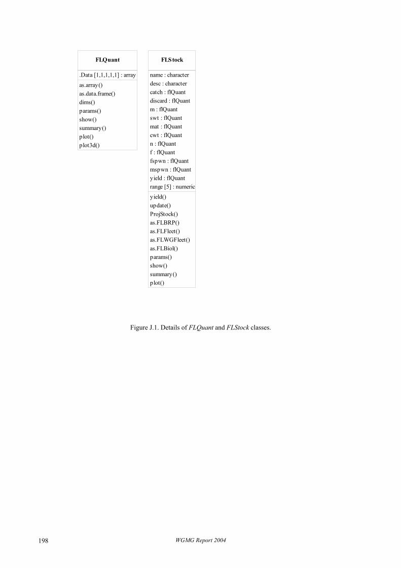
FLQuant FLStock

yield : flQuant

.Data [1,1,1,1,1] : array

as.array()as.data.frame()dims()params()show()summary()plot()plot3d()

name : characterdesc : charactercatch : flQuantdiscard : flQuantm : flQuantswt : flQuantmat : flQuantcwt : flQuantn : flQuantf : flQuantfspwn : flQuantmspwn : flQuant

range [5] : numeric

yield()update()ProjStock()as.FLBRP()as.FLFleet()as.FLWGFleet()as.FLBiol()params()show()summary()plot()

Figure J.1. Details of FLQuant and FLStock classes.

WGMG Report 2004 198

FLStock FLCPUE

FLSRFLSR.control FLBRP

FLXSA.control FLXSA FLXSA.retro

FLWGProj()

rw.phase : integer params [n] : numeric swt : flQuant

.Data : list

show()plot()

desc : character

show()

tol : numericmaxit : integermin.nse : numericfse : numericrage : integerqage : integershk.n : logicalshk.f : logicalshk.yrs : integershk.ages : integerwindow : integertsrange : integertspower : integervpa : logicaluse.plusgroup : logical

show()summary()

supplied [n] : logicalbest [n] : numericuse.bound [n] : logicallower [n] : numericupper [n] : numericphase [n] : integer

yield : flQuant

name : characterdesc : charactermethod : charactern : logicalindex : flQuanteffort : flQuantw : flQuantp : flQuantrange [7] : numeric

index()params()

name : characterdesc : charactercatch : flQuantdiscard : flQuantm : flQuantswt : flQuantmat : flQuantcwt : flQuantn : flQuantf : flQuantfspwn : flQuantmspwn : flQuant

call : characterdesc : charactern : flQuantf : flQuantqres : listcpue : listwts : data.framecontrol : FLXSA.Control

show()summary()plot()

summary()plot()range [5] : numeric

yield()update()ProjStock()MC()as.FLBRP()as.FLFleet()as.FLWGFleet()as.FLBiol()params()show()summary()plot()

model : charactererror : characterssb : arrayr : arrayrhat : arrayresiduals : array

name : characterdesc : charactersel : flQuantdsel : flQuantbyf : flQuantm : flQuant

show()summary()

rw.cv : integerrw.blk : integermaxfn : numericimax : numericcrit : numericmin.improve : numeric

se [n] : numericcovar : matrixvar : numericvara : numericrss : numericL : numeric

fit()predict()show()summary()plot()

control : FLSR.Control

mat : flQuantcwt : flQuantfspwn : flQuantmspwn : flQuantrange [5] : numericsr : charactersr.param [3] : numeric

fit()refpt()show()summary()plot()

f.hat : numericy.hat : numericr.hat : numericssb.hat : numericf.obs : numericy.obs : numericr.obs : numericssb.obs : numericrefpts : array

Figure J.2. Details of FLR stock assessment classes currently implemented.

WGMG Report 2004 199

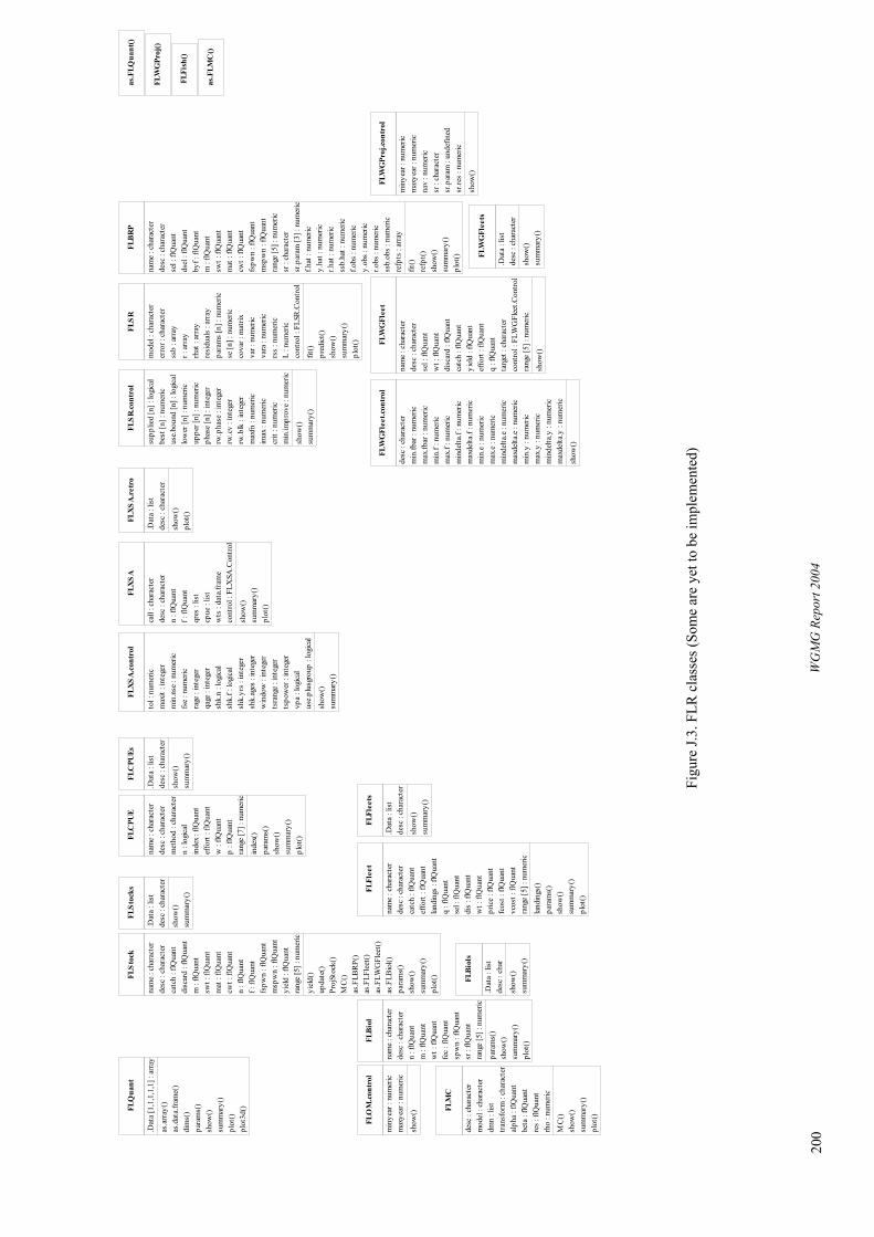
FLQ

uant

FLS

tock

FLC

PUE

FLX

SA

FLS

RFL

SR

.con

trol

FLX

SA

.con

trol

FLX

SA

.ret

roFL

Sto

cks

FLC

PUEs

FLFl

eet

FLFl

eets

FLB

RP

FLW

GFl

eet

FLW

GFl

eet.c

ontr

olFL

WG

Proj

.con

trol

FLW

GFl

eets

FLB

iol

FLO

M.c

ontr

ol

FLB

iols

FLM

C

FLW

GPr

oj()

FLFi

sh()

as.F

LMC

()

as.F

LQua

nt()

low

er [n

] : n

umer

ic

supp

lied

[n] :

logi

cal

use.

boun

d [n

] : lo

gica

l

uppe

r [n]

: nu

mer

ic

best

[n] :

num

eric

phas

e [n

] : in

tege

rrw

.pha

se :

inte

ger

min

.impr

ove

: num

eric

shk.

ages

: in

tege

rsu

mm

ary(

)m

axfn

: nu

mer

ic

min

year

: nu

mer

icm

axye

ar :

num

eric

f : fl

Qua

nt

.Dat

a [1

,1,1

,1,1

] : a

rray

inde

x()

tran

sfor

m :

char

acte

r

as.a

rray

()as

.dat

a.fr

ame(

)di

ms(

)pa

ram

s()

show

()su

mm

ary(

)pl

ot()

plot

3d()

nam

e : c

hara

cter

desc

: ch

arac

ter

catc

h : f

lQua

ntdi

scar

d : f

lQua

ntm

: flQ

uant

swt :

flQ

uant

mat

: flQ

uant

cwt :

flQ

uant

n : f

lQua

nt

.Dat

a : l

ist

show

()su

mm

ary(

)

desc

: ch

arac

ter

.Dat

a : l

ist

show

()su

mm

ary(

)

desc

: ch

arac

ter

nam

e : c

hara

cter

desc

: ch

arac

ter

met

hod

: cha

ract

ern

: log

ical

inde

x : f

lQua

ntef

fort

: flQ

uant

w :

flQua

ntp

: flQ

uant

rang

e [7

] : n

umer

ic

tol :

num

eric

max

it : i

nteg

erm

in.n

se :

num

eric

fse

: num

eric

rage

: in

tege

rqa

ge :

inte

ger

shk.

n : l

ogic

alsh

k.f :

logi

cal

shk.

yrs

: int

eger

call

: cha

ract

erde

sc :

char

acte

rn

: flQ

uant

f : fl

Qua

ntqr

es :

list

cpue

: lis

tw

ts :

data

.fram

eco

ntro

l : F

LXSA

.Con

trol

show

()

.Dat

a : l

ist

show

()

desc

: ch

arac

ter

plot

()

rw.c

v : i

nteg

errw

.blk

: in

tege

r

show

()

desc

: ch

arac

ter

mod

el :

char

acte

rdm

n : l

ist

alph

a : f

lQua

ntbe

ta :

flQua

ntre

s : f

lQua

ntrh

o : n

umer

ic

MC

()sh

ow()

sum

mar

y()

plot

()

m :

flQua

nt

para

ms(

)

nam

e : c

hara

cter

desc

: ch

arac

ter

catc

h : f

lQua

ntef

fort

: flQ

uant

land

ings

: flQ

uant

q : f

lQua

ntse

l : fl

Qua

ntdi

s : f

lQua

ntw

t : fl

Qua

ntpr

ice

: flQ

uant

fcos

t : fl

Qua

ntvc

ost :

flQ

uant

rang

e [5

] : n

umer

ic

land

ings

()

sum

mar

y()

sum

mar

y()

show

()

plot

()

sum

mar

y()

nam

e : c

hara

cter

desc

: ch

arac

ter

n : f

lQua

nt

fspw

n : f

lQua

ntm

spw

n : f

lQua

ntyi

eld

: flQ

uant

rang

e [5

] : n

umer

ic

yiel

d()

upda

te()

Proj

Stoc

k()

MC

()as

.FLB

RP(

)as

.FLF

leet

()as

.FLW

GFl

eet(

)as

.FLB

iol()

para

ms(

)sh

ow()

.Dat

a : l

ist

desc

: ch

arac

ter

show

()

para

ms(

)sh

ow()

sum

mar

y()

plot

()

wt :

flQ

uant

fec

: flQ

uant

spw

n : f

lQua

ntsr

: flQ

uant

rang

e [5

] : n

umer

ic

para

ms(

)sh

ow()

sum

mar

y()

plot

()

.Dat

a : l

ist

desc

: ch

ar

show

()su

mm

ary(

)

plot

()m

ax.fb

ar :

num

eric

use.

plus

grou

p : l

ogic

al

win

dow

: in

tege

rts

rang

e : i

nteg

erts

pow

er :

inte

ger

vpa

: log

ical

show

()su

mm

ary(

)

plot

()

show

()su

mm

ary(

)

imax

: nu

mer

iccr

it : n

umer

ic

desc

: ch

arac

ter

min

.fbar

: nu

mer

ic

min

.f : n

umer

icm

ax.f

: num

eric

min

delta

.f : n

umer

icm

axde

lta.f

: num

eric

min

.e :

num

eric

max

.e :

num

eric

min

delta

.e :

num

eric

max

delta

.e :

num

eric

min

.y :

num

eric

max

.y :

num

eric

min

delta

.y :

num

eric

max

delta

.y :

num

eric

show

()

var :

num

eric

fspw

n : f

lQua

nt

r : a

rray

mod

el :

char

acte

r

resi

dual

s : a

rray

para

ms

[n] :

num

eric

erro

r : c

hara

cter

ssb

: arr

ay

rhat

: ar

ray

se [n

] : n

umer

icco

var :

mat

rix

dsel

: flQ

uant

nam

e : c

hara

cter

desc

: ch

arac

ter

sel :

flQ

uant

byf :

flQ

uant

m :

flQua

ntsw

t : fl

Qua

ntm

at :

flQua

ntcw

t : fl

Qua

nt

rang

e [5

] : n

umer

ic

sr.p

aram

[3] :

num

eric

refp

t()

msp

wn

: flQ

uant

ssb.

hat :

num

eric

y.ob

s : n

umer

ic

ssb.

obs

: num

eric

sel :

flQ

uant

nav

: num

eric

desc

: ch

arac

ter

plot

()

cont

rol :

FLS

R.C

ontr

ol

vara

: nu

mer

icrs

s : n

umer

icL

: num

eric

fit()

pred

ict(

)sh

ow()

sum

mar

y()

f.obs

: nu

mer

ic

sr :

char

acte

r

f.hat

: nu

mer

icy.

hat :

num

eric

r.hat

: nu

mer

ic

r.obs

: nu

mer

ic

fit()

refp

ts :

arra

yna

me

: cha

ract

erde

sc :

char

acte

rm

inye

ar :

num

eric

max

year

: nu

mer

ic

show

()su

mm

ary(

)pl

ot()

cont

rol :

FLW

GFl

eet.C

ontr

ol

disc

ard

: flQ

uant

rang

e [5

] : n

umer

ic

wt :

flQ

uant

catc

h : f

lQua

ntyi

eld

: flQ

uant

effo

rt :

flQua

ntq

: flQ

uant

targ

et :

char

acte

r

show

()

.Dat

a : l

ist

show

()su

mm

ary(

)

sr.p

aram

: un

defin

edsr

.res

: num

eric

sr :

char

acte

r

show

()

Figu

re J.

3. F

LR c

lass

es (S

ome

are

yet t

o be

impl

emen

ted)

WG

MG

Rep

ort 2

004

200

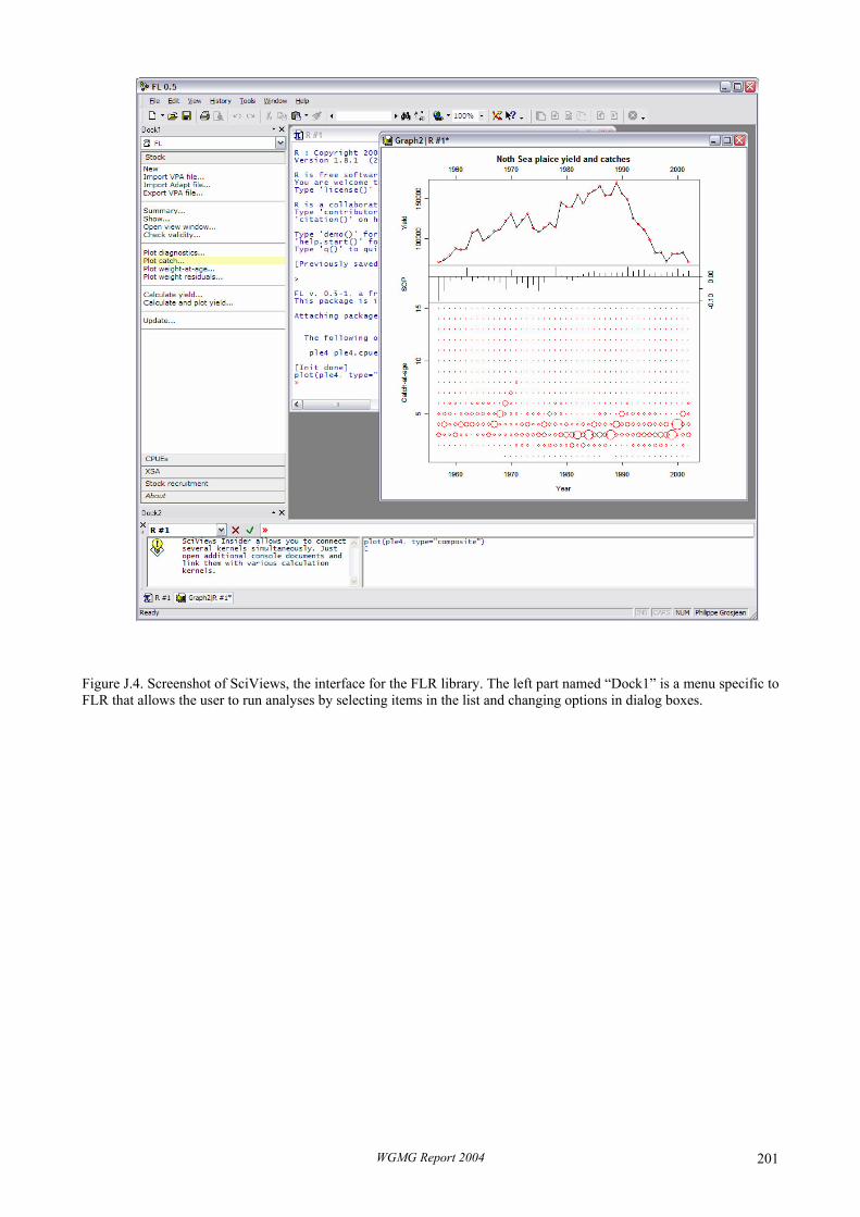
Figure J.4. Screenshot of SciViews, the interface for the FLR library. The left part named “Dock1” is a menu specific to FLR that allows the user to run analyses by selecting items in the list and changing options in dialog boxes.

WGMG Report 2004 201

APPENDIX K: WORKING DOCUMENT WG4

An evaluation of MTAC – a program for the calculation of catch forecasts taking the mixed nature of the fisheries into account3

by

Sarah Kraak

SUMMARY..........................................................................................................................................................................

1. INTRODUCTION ............................................................................................................................................................ 1.1 Why develop software for the calculation of Mixed Species TACs?..................................................................... 1.2 A short history of the development of MTAC .......................................................................................................

2. DESCRIPTION OF THE MTAC MODEL......................................................................................................................

3. ANALYSES OF THE BEHAVIOUR OF THE MODEL ................................................................................................ 3.1 The effects of different settings of p- and q-options, different decision weights, and different target F-

multipliers, on the resulting fleet factors........................................................................................................... 3.1.1 Results...................................................................................................................................................... 3.1.2. Conclusions.............................................................................................................................................

3.2 The effects of decision weights on the resulting MS-TACs................................................................................... 3.2.1. Results..................................................................................................................................................... 3.2.2. Discussion and conclusion ......................................................................................................................

3.3 The effects of uncertainty in the input data concerning stock status on the resulting MS-TACs........................... 3.3.1. Results..................................................................................................................................................... 5.3.2. Discussion. .............................................................................................................................................. 5.3.3. Conclusion. .............................................................................................................................................

4. DISCUSSION...................................................................................................................................................................

5. CONCLUSIONS ..............................................................................................................................................................

6. REFERENCES .................................................................................................................................................................

7. ACKNOWLEDGEMENTS..............................................................................................................................................

3 This paper is modified from a report commissioned by the Dutch ministry of Agriculture, Nature Management, and Food Safety (LNV).

WGMG Report 2004 202

SUMMARY

The International Council for the Exploration of the Sea (ICES) has traditionally given fishery management advice on a stock by stock basis, usually in the form of a catch forecast per stock. This approach is potentially problematic since it disregards technical interactions, i.e., cases where more than one species is caught in the same area, and different fleets catch differing proportions of the various species. Ignoring this mixed-species aspect of the fishery can mean that, for instance, the quota for one species is exhausted early in the season, but boats continue fishing and catching that species because there is still quota available for the other species in the fishery. The MTAC program has been developed to generate stock-based advice that accounts for the technical interactions.

The European Commission aims to use a mixed species based approach for their TAC proposals for, e.g., the demersal stocks of the North Sea. These stocks are very important for the Dutch beam trawl fishery. Therefore, it is a concern to the Dutch ministry of Agriculture, Nature Management, and Food Safety that the working and the merits and limitations of the MTAC program are understood. The Dutch ministry requested that an evaluation of MTAC is undertaken. This report presents this evaluation.

The MTAC program calculates Mixed Species catch forecasts (MS-TACs) for each individual species fished in a given area, taking into account the mixed nature of the fisheries, under the objective to approach set targets (such as, e.g., single species advice) as closely as possible. The resulting MS-TACs can be seen as a compromise that aims to resolve the conflict that arises when fleets have depleted their quota for some species but not for others while these species are unavoidably caught together. MTAC can give fleet based advice in the form of fleet based effort or catch forecasts.

The MTAC program needs some inputs that reflect political choices.

• A political choice has to be made whether to reduce effort of all fleets (1) equally, or (2) proportional to the species catch within the fleet's total catch, or (3) proportional to the fleet's catch of a species as a proportion of the total species catch. This feature is called the p-option. Results vary widely depending on this choice.

• A political choice has to be made on decision weights for each species, which determine relative priority of each species for how closely the target has to be approached in the compromise. Results vary widely depending on this choice.

• A political choice has to be made on whether to modify the decision weights according to the fleets' species compositions. This feature is called the q-option. Results vary widely depending on this choice.

The MTAC program was checked, and it is concluded that MTAC correctly does what it is described to do. Scenario runs illustrate the consequences of the inputs such as the set targets, the chosen p- and q-options, and the chosen decision weights. These consequences can be logically understood. This illustration will help the MTAC user to make these choices a priori. The outcome of MTAC is sensitive to uncertainty with respect to stock status, e.g., population size at the start of the TAC year. Uncertainty in one stock may affect results for another stock if strong technical interactions between the two exist.

The MTAC program was evaluated, and it was found that certain drawbacks exist to its use. The resulting MS-TACs do not necessarily conform to the precautionary approach. In other words, MTAC may generate forecasts such that SSB will fall below Bpa or Fpa will be exceeded. The use of MTAC for fleet based advice confronts us with the political consequences of the assignment of heavy restrictions to some fleets and more lenient restrictions to others. This issue relates to the fact that the use of MTAC is not consistent with relative stability. The use of MTAC for fleet based advice is unacceptable when, due to incompleteness of the data, the advice is biased such that fleets that discard or underreport suffer less from restrictions than fleets that report all catches. In response to the above points, MTAC's experts have claimed that MTAC is not designed for fleet based advice, but for aggregated TAC advice. However, the program is logically designed to calculate fleet based forecasts. Ignoring the fleet based output is illogical, and using only the aggregated MS-TACs does not resolve the conflict the program was meant to resolve. The conclusion is that MTAC is a tool for calculating fleet based effort or catch forecasts.

It can be concluded that MTAC is a transparent model which could be a fine tool for calculating fleet based effort or catch forecasts, if it could be permitted to ignore the precautionary approach and any political problems associated with differentially penalising fleets, and if the data were complete and historical catch compositions would remain stable.

WGMG Report 2004 203

1 Introduction

1.1 Why develop software for the calculation of Mixed Species TACs?

ICES has traditionally given fishery management advice on a stock by stock basis. Advice for each stock is usually given in the form of a catch forecast for next year, which can be interpreted as an advice for next year’s Total Allowable Catch (TAC) for that stock. The TAC is the total catch allowed to be taken from that stock by all fleets together that are fishing that stock. This approach has long been recognised as being potentially problematic since it disregards technical interactions, i.e., cases where more than one species is caught in the same area, and different fleets catch differing proportions of the various species. Ignoring this mixed-species aspect of the fishery can mean that, for instance, the quota for one species is exhausted early in the season, but that boats continue fishing and catching that species because there is still quota available for the other species in the fishery. As a result, the quota for the first species would not provide an effective constraint of fishing mortality on that species. Alternatively, the managers could close the fishery once the quota for one species is reached, but that could result in loss of fishing opportunities on other stocks that might be in a better state.

To account for mixed-species fisheries, it would be desirable to develop approaches of giving advice on a fleet or fishery basis. Such approaches would take time to develop and to implement, but an intermediate step would be an approach that takes the current, stock-based, advice as a starting point, and then uses additional fleet information to generate advice that accounts for the technical interactions. The MTAC program has been developed for such an intermediate approach (Vinther et al. 2003). A short history of the MTAC model is presented in section 1.2.

1.2 A short history of the development of MTAC

In 2002, the European Commission requested that a study group of the STECF4 subgroup SGRST5 would meet in October 2002, to develop a model and to collect the necessary data, for the calculation of catch forecasts that take into account the mixed nature of the fisheries and that are based on the catch advice by ACFM (STECF 2002). The aim was to develop a model that would generate Mixed Species TACs (MS-TACs) for each individual species, so that the fisheries could deplete their quota for the various species synchronously, instead of having some quota depleted while continuing fishing for other species and catching the first species as unavoidable by-catch.

Prior to the meeting of the 2002 STECF/SGRST study group, the Danish Institute for Fisheries Research (DIFRES) had started on the development of the computer program MTAC, according to the technical specifications by the European Commission. The MTAC program was further developed at the meeting, where it was used to run a number of scenarios requested by the European Commission on data for the North Sea. Because these data were not complete (e.g., data from the Nephrops fisheries and data on discards were lacking and age-disaggregated data were not available at the fishery level), the group stated that the results should not be used for advice. On the last day of that meeting MTAC was still being modified.

In February 2003 the ICES Study Group SGDFF6 met for the first time (ICES 2003a) with the aim of further developing the Mixed Fisheries approach within ICES. A working document was presented (Pastoors and Kraak 2002), containing a sensitivity analysis demonstrating that the outcomes of MTAC could not be fully understood (WD2 in ICES 2003a). Sensitivity analyses carried out during that meeting demonstrated again that the working of MTAC was not entirely understood and numerically unstable. Another working document presented (Kraak and Pastoors 2002) showed that the MTAC approach is not consistent with the principle of relative stability (WD3 in ICES 2003a). A few other existing approaches to mixed fisheries forecasts were evaluated in that meeting. One of them was a new model which was implemented in the program SMP7 (WD4 in ICES 2003a). Besides exploring and investigating software for the calculation of mixed fishery based catch forecasts, the Study Group formulated recommendations concerning fleet definitions and a data format for the collection of the required international disaggregated data.

At the Assessment Working Group WGNSSK8 in September 2003 (ICES 2003b) a revised version of MTAC was presented (Vinther et al. 2003). Sensitivity analyses carried out during the meeting demonstrated that the revised version no longer suffered from numerical instability. In other words, all outcomes could be explained by the input data and the optional settings of the model (this is extensively illustrated in section 3). A revised version of the alternative software SMP was also presented.

4 Scientific, Technical, and Economic Committee for Fisheries 5 Subgroup on Resource Status 6 Study Group on the Development of Fishery-based Forecasts 7 Short-term Multi-fleet Prediction 8 Working Group on the assessment of demersal stocks in the North Sea and Skagerrak

WGMG Report 2004 204

In September/October 2003 the program-code was meticulously screened for errors. It was concluded that the revised program does not contain any errors and that it does the calculations that were initially specified by the European Commission for the STECF/SGRST meeting in 2002 (section 3 in STECF 2002) and that are described by Vinther et al. 2003 after the revision of the program.

The ICES Advisory Committee on Fisheries Management (ACFM) evaluated the MTAC approach in October 2003. ACFM concluded that the approach is not suitable for advice as long as the data sets used are so incomplete (ICES 2003c). They argued that, e.g., the lack of discard data could lead to advice which would 'favour' fleets that would underreport or discard, e.g., cod compared to fleets catching fewer cod but reporting more.

The STECF/SGRST study group met again in October 2003 (STECF 2003a). The group responded to the arguments of ACFM (above) by stating that MTAC should indeed not be used for fleet based advice (and was not intended as such), but only for aggregated stock based advice while taking the mixed nature of the fisheries into account. The arguments of ACFM and STECF/SGRST on this issue are further discussed in section 4. MTAC was run on data for the North Sea and on data for the Irish Sea according to scenarios requested by the European Commission. Sensitivity analyses were carried out with the North Sea data to demonstrate to what extent the outcomes are sensitive to the uncertainty of the input data and to the choices of the optional settings by the user. Similar analyses will be presented in section 3.

In January 2004 the ICES Study Group SGDFF met again. This group evaluated the use of MTAC. The group concluded that there are some practical objections against the use of MTAC. The first objection was that MTAC generates outcomes that are not consistent with relative stability; the group thought that it was therefore unlikely that MTAC-generated advice would be applied. The second objection was that MTAC is based on the assumption that fleets will not adjust their fishing strategy in response to management measures; this assumption is unrealistic. The group therefore decided that MTAC should either not be used or should be developed further to accommodate the objections raised above.

2 Description of the MTAC model

A technical description of MTAC is given by Vinther et al. (2003). In this section a less technical description is given.

The Software MTAC is written in the statistical package “R”. “R” is freeware available from the internet (http://cran.r-project.org). The R-package must be installed to run MTAC.

MTAC uses the Single Species advice for the species (stocks) as a basis to generate Mixed-Species forecasts. For each species either a Single Species TAC (SS-TAC) or a F-multiplier (the factor with which status quo fishing mortality has to be multiplied) have to be input into MTAC. Instead of the ACFM advice the MTAC-user can specify his/her own target catch or target F-multiplier for the TAC year.

The final WG9 assessment of each stock is used to derive the status quo fishing mortality at age. The stock numbers at age at the start of the TAC year must also be available. To derive these stock numbers at age an assumption for the current year is necessary, which is either a status quo F assumption or a TAC constraint. In addition, historical catch data for each of the species by each of the fleets considered must be available. These can be catch composition data of the previous year, or an average of several previous years (usually three years). If for a species fleet-specific age-disaggregated catch data are not available for a given fleet, MTAC will estimate these from the fleet catches and the fleet-aggregated catch at age data for that species.

MTAC then calculates for each of the species a temporary catch forecast per fleet, based on the fleet-specific partial status quo F multiplied with species specific fleet factors. The partial status quo Fs are derived from the historical catch data. The species specific fleet factors are calculated by an iterative process, such that the sum of the forecasted fleet catches approaches the SS-TAC as closely as possible. In principle this objective can be reached by an infinite number of combinations of species specific fleet factors; therefore a choice has to be made by the MTAC-user about how these fleet factors should relate to the fleets’ historical catches. Several options for this choice are available in the MTAC program. The MTAC-user has to set one of the so-called “p-options”, according to rationales explained below.

o p=0. When this option is chosen, each of the fleets will get the same species specific fleet factor. In this case,

each of the fleets will have to reduce (or increase) their partial status quo F to the same extent, regardless the historical catch of the considered species by that fleet.

9 Working Group, for example the WGNSSK

WGMG Report 2004 205

o p=1. When this option is chosen, a fleet’s species specific fleet factor becomes lower when the considered species historically represents a larger proportion of the fleet’s catch in weight. In this case, fleets targeting the species will be more affected by reductions than fleets that catch the species as an incidental by-catch. This option does not take into account whether the fleets take large or small portions of the total international species catch.

o p=2. When this option is chosen, a fleet’s species specific fleet factor becomes lower when the fleet historically takes a larger portion of the total international catch of the considered species in weight. In this case, fleets that take a large portion of the international catch of that species will be more affected by reductions than fleets that catch only small numbers of that species. This option does not take into account whether the fleet targets that species or takes it as an incidental by-catch.

o p=3. When this option is chosen, the MTAC-user can specify manually, through an extra input file, the species specific fleet factors relative to each other. In this case, the MTAC-user can decide how much each fleet will be affected by reductions.

The difference between the options p=1 and p=2 is critical, because the implications can be quite different, as is shown in section 3.1.

The species specific fleet factors can be interpreted as multipliers with which the fleets’ partial status quo Fs have to be multiplied. In other words, they can be interpreted as effort multipliers with which the fleets have to multiply their status quo effort. (For example, a factor of 0.5 implies a reduction of effort by half.) However, the species specific fleet factors may conflict with each other. It could be the case, for example, that a fleet would have to reduce her effort by 80% for one species and by 20% for another species. This is the conflict that MTAC is designed to resolve.

Therefore, MTAC finally calculates one overall fleet factor for each fleet, which is a weighted average of the species specific fleet factors for that fleet. The weighting is done by decision weights specified by the MTAC-user. The MTAC-user specifies decision weights for each species that reflect how important it is to closely approach the SS-TAC of that species in the final compromise. The MTAC-user can choose values for the decision weights by any rationale desired. For example, decision weights can be chosen to reflect how far the current SSB of the stock is removed from Bpa (e.g., decision weights equal the ratio Bpa/SSB). In that case, a species would get more weight in the final compromise if the current SSB is further below Bpa.

Moreover, the MTAC-user can choose whether the weighting considers, in addition to the above mentioned decision weight, the relative contribution of a species in a fleet’s catch in weight. To this end, the MTAC-user has to set one of the so-called “q-options”, explained below.

o q=0. When this option is chosen, the relative contribution in the catch is not considered. Only the specified decision weights are used in the weighting procedure.

o q=1. When this option is chosen, the decision weights are multiplied by the proportion of the catch of a species within the fleet’s catch in weight. These products are then used as weighting factors in averaging the species specific fleet factors to arrive at one fleet factor for that fleet. In this case, a species specific fleet factor weighs more heavily in the final average fleet factor if the fleet targets that species than if the fleet takes that species as an incidental by-catch.

Finally, MTAC calculates for each of the species a catch forecast per fleet, using the weighted fleet factors. For each species, these catch forecasts are then summed over the fleets, to arrive at an aggregated Mixed Species TAC (MS-TAC) and an implied F-multiplier (MS-F-mult) for each species.

The output of MTAC displays for each species the aggregated MS-TAC, the MS-F-multiplier and the ratio between the MS-TAC and the SS-TAC (MS-TAC/SS-TAC). If the MS-TAC/SS-TAC ratio is larger than 1, then the MS-TAC is larger than the SS-TAC.

The weighted fleet factors are usually not displayed as output (the reasons for which will be discussed in section 4), but they can be. These fleet factors represent fleet specific effort changes, which give rise to the aggregated forecasted catches (the MS-TACs). In principle, MTAC can give as additional output catch forecasts per fleet (tentatively called “fleet TACs”), based on these fleet factors.

WGMG Report 2004 206

Summarizing:

• Input data necessary for MTAC:

o Population numbers-at-age at the start of the TAC year by species (derived from the WG assessment based on a current year assumption);

o Status quo F-at-age by species (derived from the WG assessment); o M-at-age by species (as in the WG assessment); o Historical weights-at-age in the catch by species, and, if available, by fleet; o Historical catch-at-age in numbers by species, and, if available, by fleet; o For fleets for which age-disaggregated data are not available, historical catch in weight by species and

fleet.

• Input of political choices:

o Setting of the p-option, specifying how the species specific fleet factors should relate to each other (e.g., fleets are affected in proportion to their catch of the species relative to the fleet’s catch or relative to the international species' catch);

o Choosing the decision weights for the species, specifying the relative importance of approaching the SS-TAC for each species;

o Setting of the q-option, specifying whether the weighting for the final fleet factors should be in proportion to the species catch within the fleet’s catch.

• Output: A typical MTAC output table looks as follows.

Fsq SS_F_mult. SS_TAC MS_F_mult MS_TAC MS_TAC/SS_TAC Decision_w AAA 0.613 0.200 27 0.692 56 2.11 0.9 BBB 0.327 1.000 163 0.745 128 0.78 0.1 ... ... More species can be present.

o AAA and BBB represent species names; o Fsq: the input status quo F; o SS_F_mult: the input Single Species F-multiplier, given or implied by the advice or the target; o SS_TAC: the input Single Species TAC, given or implied by the advice or the target; o MS_F_mult: the Mixed Species F-multiplier implied by the output Mixed Species TAC; o MS_TAC: the output Mixed Species TAC (catch forecast): o MS_TAC/SS_TAC: the ratio of the output Mixed Species TAC to the input Single Species TAC; o Decision w: the input decision weight.

The set of fleet factors by fleet are not included in the standard output. These can be interpreted as fleet specific effort multipliers.

Technical note: We as well as the author of MTAC are aware of the fact that the approach would be better if the iterative process searching for catch forecasts that match the SS-TACs as closely as possible would encompass the weighted averaging of the fleet specific fleet factors, instead of what the current program does, namely calculating these averages after the iterative process has taken place. However, attempts that were made to this effect led to the program suffering from numerical instability. This was, in fact, the cause of the problems with the first version of MTAC, which gave rise to outcomes that could not be fully explained.

3 Analyses of the behaviour of the model

In this section the outcomes are presented of runs of various scenarios with semi-fictive data sets. The data sets are based on real data from the North Sea, but the data sets are sometimes incomplete. For the purpose of this section this is not a problem, because it merely aims to explain how the model responds to the various settings and data that have to be chosen by the MTAC user. This will help the reader to become a deliberate MTAC user. As was noted in section 2, MTAC requires several types of input of political choices:

WGMG Report 2004 207

o Setting of the p-option, specifying how the species specific fleet factors should relate to each other (e.g., fleets are affected in proportion to their catch of the species relative to the fleet’s catch or relative to the international species' catch);

o Setting of the q-option, specifying whether the weighting for the final fleet factors should be in proportion to the species catch within the fleet’s catch;

o Choosing the decision weights for the species, specifying the relative importance of approaching the SS-TAC for each species.

In section 3.1 the outcomes are compared of all combinations of different p- and q-settings, and it is explained how these settings affect the outcomes under a range of decision weights and targets F-multipliers. Hereby we illustrate the influences of the choice of decision weights and the choice of targets and how these interact with the choice of p- and q-settings. In section 3.2 the outcomes are compared when different sets of decision weights are used, to illustrate how these affect the results. Whereas section 3.1 focuses on the effects on the fleet factors, section 3.2 focuses on the effects on the aggregated MS-TACs. These sections help the MTAC user to make the political choices for optional settings because it illustrates the consequences of these choices. In section 3.3 the outcomes are compared of runs where different input data were used, to illustrate how uncertainty of stock status affects the outcome. All the analyses are repetitions of analyses performed at the WGNSSK meeting in September 2003 (ICES 2003b) and at the STECF/SGRST meeting in October 2003 (STECF 2003a).

3.1 The effects of different settings of p- and q-options, different decision weights, and different target F- multipliers, on the resulting fleet factors

In this section the effects of the different options that can be chosen in MTAC will be illustrated. In addition, the effects of the chosen decision weights, and the effects of the set targets on the outcomes will be shown. For this exercise a data set was chosen that is suitable for illustration only, with nine fleets (A to I) fishing six species (cod, haddock, plaice, sole, saithe, whiting). The four figures below show respectively the historical catch10 weight by species, the historical catch weight by species and fleet, the historical catch composition of the fleets, and the historical distribution of species catches over the fleets.

Catch weight by species

020000400006000080000

100000120000140000160000180000

COD HAD PLE POK SOL WHG

catc

h w

eigh

t (to

nnes

)

Figure 3.1.1

WGMG Report 2004 208

10 The model assumes that the true catches (landings plus discards) are known. Because the purpose of these analyses is to illustrate the behaviour of the model, we assume that in all analyses of section 3 'catch' indeed includes discards.

Catch weight by species and fleet

0

20000

40000

60000

80000

100000

120000

140000

160000

A B C D E F G H I

fleet

catc

h w

eigh

t (to

nnes

)

WHGSOLPOKPLEHADCOD

HAD

COD

Figure 3.1.2

Catch percentages of species within fleet

0%

20%

40%

60%

80%

100%

A B C D E F G H I

fleet

perc

enta

ge

WHG

SOL

POK

PLE

Figure 3.1.3

WGMG Report 2004 209

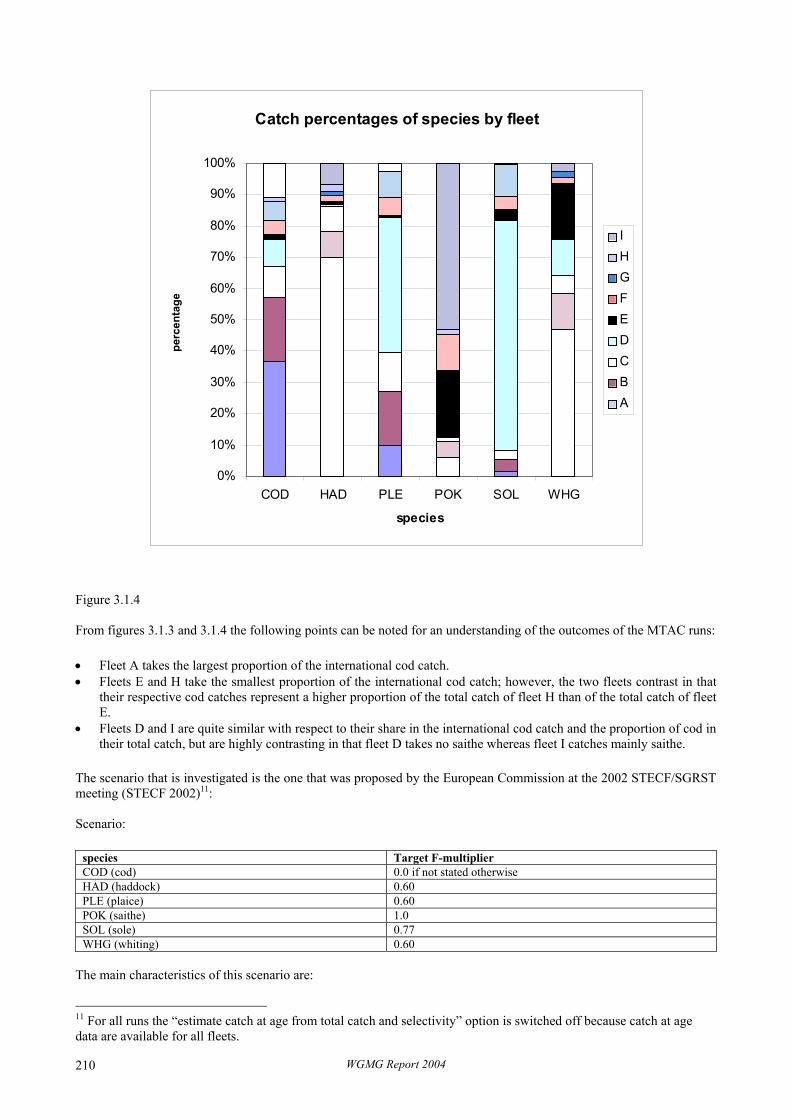
Catch percentages of species by fleet

0%

10%

20%

30%

40%

50%

60%

70%

80%

90%

100%

COD HAD PLE POK SOL WHG

species

perc

enta

ge

IH

EDC

GF

BA

Figure 3.1.4 From figures 3.1.3 and 3.1.4 the following points can be noted for an understanding of the outcomes of the MTAC runs:

• Fleet A takes the largest proportion of the international cod catch. • Fleets E and H take the smallest proportion of the international cod catch; however, the two fleets contrast in that

their respective cod catches represent a higher proportion of the total catch of fleet H than of the total catch of fleet E.

• Fleets D and I are quite similar with respect to their share in the international cod catch and the proportion of cod in their total catch, but are highly contrasting in that fleet D takes no saithe whereas fleet I catches mainly saithe.

The scenario that is investigated is the one that was proposed by the European Commission at the 2002 STECF/SGRST meeting (STECF 2002)11: Scenario:

species Target F-multiplier COD (cod) 0.0 if not stated otherwise HAD (haddock) 0.60 PLE (plaice) 0.60 POK (saithe) 1.0 SOL (sole) 0.77 WHG (whiting) 0.60

The main characteristics of this scenario are:

WGMG Report 2004 210

11 For all runs the “estimate catch at age from total catch and selectivity” option is switched off because catch at age data are available for all fleets.

• that F on cod must be reduced to 0 (or an other low value), • that F on saithe does not have to be reduced at all, • and that F on the other species must be reduced to an intermediate extent.

MTAC contains three options for weighting the species specific fleet effort reduction (p-options) and an option for modifying the decision weights through multiplication by a fleet target factor (q-option) (see section 2). The p-options are:

• p=0: Equal for all fleets. • p=1: Proportional to the catch of the species within the total catch of the fleet. • p=2: Proportional to the fleet's catch of the species as a fraction of the total catch of that species. The q-option can be switched off (q=0) or on (q=1).

All six combinations of options p and q are run. In addition, the influence of the decision weight assigned to cod relative to the other species is explored by running MTAC with all six combinations of options while the decision weight on cod varies from 2 to 40 while the decision weights for all other species are kept at 1. The influence of the value of the target F-multiplier on cod is explored, by running MTAC with all six combinations of options while the target F-multiplier for cod varies from 0.1 to 1 (other F-multipliers as in the scenario given above) with decision weights of 40 for cod versus 1 for all other species.

3.1.1 Results

Figures are presented for each of the six combinations of p and q-options, firstly with varying decision weights (cases 1–6), and then with varying target F-multipliers for cod (cases 7–12). Each figure consists of nine graphs representing the nine example fleets. The dots represent the outcomes of the runs: the fleet factor (fleet effort reduction multiplier) on the y-axis, and the varying decision weight on cod12 or varying target F-multiplier for cod respectively on the x-axis.

12 The values on the x-axis are actually the decision weights on cod as a fraction of the sum of the decision weights of all species. For example, a decision weight of 2 for cod would translate to a value of 2/7 = 0.29 on the x-axis and a decision weight for cod of 40 would translate to a value of 40/45 = 0.89 on the x-axis.

WGMG Report 2004 211

1. p=0, q=0, decision weights on cod vary

The outcome of this run is straightforward. The fleet factors (y-axis) can be interpreted as fleet effort reduction factors. All fleets have to reduce effort equally (p=0). The resulting effort reduction is a compromise between the different targets for the different species (e.g., reduction to 0 for cod and no reduction for saithe). The compromise is the same for all fleets regardless of their catch compositions (because q is set at q=0). The decision weight for cod represents the importance that is given (as a political decision) to approaching the target set for cod relative to the other targets. If banning all fishing on cod has high priority (on the right hand side of the x-axis), then all fleets that historically catch some cod must reduce effort to a very low level. With lower priority given to conserving cod (on the left hand side of the x-axis), the fleets' effort reduction is more moderate.

decision.weight

Flee

t.Fac

tor

0

0.2

0.4

0.6

0.8

1

0.3 0.4 0.5 0.6 0.7 0.8 0.9

A B

0.3 0.4 0.5 0.6 0.7 0.8 0.9

C

D E

0

0.2

0.4

0.6

0.8

1F0

0.2

0.4

0.6

0.8

1 G H

0.3 0.4 0.5 0.6 0.7 0.8 0.9

I

WGMG Report 2004 212

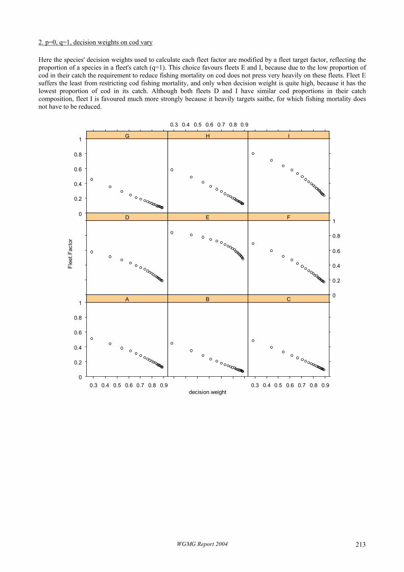
2. p=0, q=1, decision weights on cod vary

Here the species' decision weights used to calculate each fleet factor are modified by a fleet target factor, reflecting the proportion of a species in a fleet's catch (q=1). This choice favours fleets E and I, because due to the low proportion of cod in their catch the requirement to reduce fishing mortality on cod does not press very heavily on these fleets. Fleet E suffers the least from restricting cod fishing mortality, and only when decision weight is quite high, because it has the lowest proportion of cod in its catch. Although both fleets D and I have similar cod proportions in their catch composition, fleet I is favoured much more strongly because it heavily targets saithe, for which fishing mortality does not have to be reduced.

decision.weight

Flee

t.Fac

tor

0

0.2

0.4

0.6

0.8

1

0.3 0.4 0.5 0.6 0.7 0.8 0.9

A B

0.3 0.4 0.5 0.6 0.7 0.8 0.9

C

D E

0

0.2

0.4

0.6

0.8

1F0

0.2

0.4

0.6

0.8

1 G H

0.3 0.4 0.5 0.6 0.7 0.8 0.9

I

WGMG Report 2004 213

3. p=1, q=0, decision weights on cod vary

Choosing the option of reducing species-specific fleet effort in proportion to the species' proportions in the fleets' catches (q=1) differentiates only slightly between the fleets, and gives most of them a slight advantage at low decision weight.

decision.weight

Flee

t.Fac

tor

0

0.2

0.4

0.6

0.8

1

0.3 0.4 0.5 0.6 0.7 0.8 0.9

A B

0.3 0.4 0.5 0.6 0.7 0.8 0.9

C

D E

0

0.2

0.4

0.6

0.8

1F0

0.2

0.4

0.6

0.8

1 G H

0.3 0.4 0.5 0.6 0.7 0.8 0.9

I

WGMG Report 2004 214

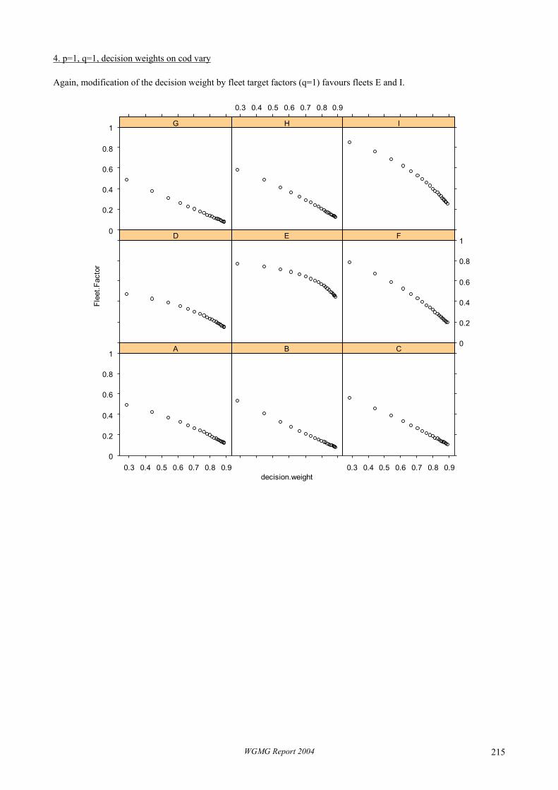
4. p=1, q=1, decision weights on cod vary

Again, modification of the decision weight by fleet target factors (q=1) favours fleets E and I.

decision.weight

Flee

t.Fac

tor

0

0.2

0.4

0.6

0.8

1

0.3 0.4 0.5 0.6 0.7 0.8 0.9

A B

0.3 0.4 0.5 0.6 0.7 0.8 0.9

C

D E

0

0.2

0.4

0.6

0.8

1F0

0.2

0.4

0.6

0.8

1 G H

0.3 0.4 0.5 0.6 0.7 0.8 0.9

I

WGMG Report 2004 215

5. p=2, q=0, decision weights on cod vary

Choosing the option of reducing species-specific fleet effort in proportion to the fleets’ contribution to the total catch of that species (p=2) also differentiates only slightly between the fleets, and slightly favours all fleets except fleet A which takes most of the cod.

decision.weight

Flee

t.Fac

tor

0

0.2

0.4

0.6

0.8

1

0.3 0.4 0.5 0.6 0.7 0.8 0.9

A B

0.3 0.4 0.5 0.6 0.7 0.8 0.9

C

D E

0

0.2

0.4

0.6

0.8

1F0

0.2

0.4

0.6

0.8

1 G H

0.3 0.4 0.5 0.6 0.7 0.8 0.9

I

WGMG Report 2004 216

6. p=2, q=1, decision weights on cod vary

Choosing the option of reducing species-specific fleet effort in proportion to the fleets’ contribution to the total catch of that species (p=2) in combination with the modification of the decision weights by fleet target factors (q=1) differentiates most between the fleets. This differentiation appears to be driven as much by the distribution of saithe catches as by the distribution of cod catches. Fleets that suffer take a high proportion of cod and/or take a low proportion of saithe. Similarly, fleets that benefit take little cod and/or target saithe. Note that this effect comes about because the fishing mortality for saithe does not have to be reduced whereas the fishing mortality for cod has to be reduced to 0. Reduction of fishing mortality for the other species is intermediate.

decision.weight

Flee

t.Fac

tor

0

0.2

0.4

0.6

0.8

1

0.3 0.4 0.5 0.6 0.7 0.8 0.9

A B

0.3 0.4 0.5 0.6 0.7 0.8 0.9

C

D E

0

0.2

0.4

0.6

0.8

1F0

0.2

0.4

0.6

0.8

1 G H

0.3 0.4 0.5 0.6 0.7 0.8 0.9

I

WGMG Report 2004 217

7. p=0, q=0, target F-multiplier for cod varies

The outcome of this run is straightforward: all fleets have to reduce effort equally. Their level of effort linearly increases with the level of the chosen target F-multiplier for cod (on which the decision weight is large).

Fmult

Flee

t.Fac

tor

0

0.2

0.4

0.6

0.8

1

0.2 0.4 0.6 0.8 1

A B

0.2 0.4 0.6 0.8 1

C

D E

0

0.2

0.4

0.6

0.8

1F0

0.2

0.4

0.6

0.8

1 G H

0.2 0.4 0.6 0.8 1

I

WGMG Report 2004 218

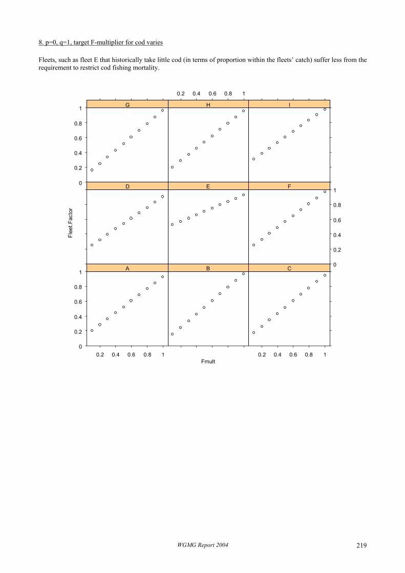
8. p=0, q=1, target F-multiplier for cod varies

Fleets, such as fleet E that historically take little cod (in terms of proportion within the fleets’ catch) suffer less from the requirement to restrict cod fishing mortality.

Fmult

Flee

t.Fac

tor

0

0.2

0.4

0.6

0.8

1

0.2 0.4 0.6 0.8 1

A B

0.2 0.4 0.6 0.8 1

C

D E

0

0.2

0.4

0.6

0.8

1F0

0.2

0.4

0.6

0.8

1 G H

0.2 0.4 0.6 0.8 1

I

WGMG Report 2004 219

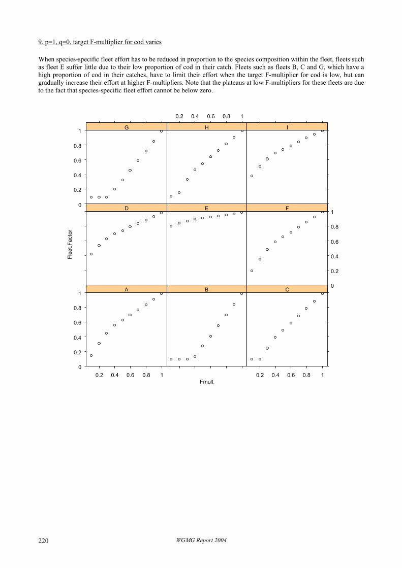
9. p=1, q=0, target F-multiplier for cod varies

When species-specific fleet effort has to be reduced in proportion to the species composition within the fleet, fleets such as fleet E suffer little due to their low proportion of cod in their catch. Fleets such as fleets B, C and G, which have a high proportion of cod in their catches, have to limit their effort when the target F-multiplier for cod is low, but can gradually increase their effort at higher F-multipliers. Note that the plateaus at low F-multipliers for these fleets are due to the fact that species-specific fleet effort cannot be below zero.

Fmult

Flee

t.Fac

tor

0

0.2

0.4

0.6

0.8

1

0.2 0.4 0.6 0.8 1

A B

0.2 0.4 0.6 0.8 1

C

D E

0

0.2

0.4

0.6

0.8

1F0

0.2

0.4

0.6

0.8

1 G H

0.2 0.4 0.6 0.8 1

I

WGMG Report 2004 220

10. p=1, q=1, target F-multiplier for cod varies

Modification of the decision weights by fleet target factors does not bring about much change, except that most fleets seem to suffer a bit more at the highest target F-multipliers for cod.

Fmult

Flee

t.Fac

tor

0

0.2

0.4

0.6

0.8

1

0.2 0.4 0.6 0.8 1

A B

0.2 0.4 0.6 0.8 1

C

D E

0

0.2

0.4

0.6

0.8

1F0

0.2

0.4

0.6

0.8

1 G H

0.2 0.4 0.6 0.8 1

I

WGMG Report 2004 221

11. p=2, q=0, target F-multiplier for cod varies

The contrast between the p-option chosen here (species-specific fleet effort reduction in proportion to the proportion of a species’ total catch taken by a fleet) and the previous p-option (species-specific fleet effort reduction in proportion to the proportion of a species within a fleet’s total catch) is quite clear. In the present setting fleets such as G and H are favoured compared to the previous setting because they contribute little to the total cod catch (although within these fleets’ catches cod represents a high proportion as compared to the other fleets, which is the reason why they are not favoured in the previous setting). Similarly, fleet A, taking a very high proportion of total cod catch, suffers more in this setting than in the previous one.

Fmult

Flee

t.Fac

tor

0

0.2

0.4

0.6

0.8

1

0.2 0.4 0.6 0.8 1

A B

0.2 0.4 0.6 0.8 1

C

D E

0

0.2

0.4

0.6

0.8

1F0

0.2

0.4

0.6

0.8

1 G H

0.2 0.4 0.6 0.8 1

I

WGMG Report 2004 222

12. p=2, q=1, target F-multiplier for cod varies

Modification of the decision weights by fleet target factors does not bring about much change.

Fmult

Flee

t.Fac

tor

0

0.2

0.4

0.6

0.8

1

0.2 0.4 0.6 0.8 1

A B

0.2 0.4 0.6 0.8 1

C

D E

0

0.2

0.4

0.6

0.8

1F0

0.2

0.4

0.6

0.8

1 G H

0.2 0.4 0.6 0.8 1

I

WGMG Report 2004 223

3.1.2 Conclusions

The exercise of varying decision weights on cod on the x-axis of the figures (1–6) illustrates how the priority given to, e.g., conserving cod influences the resulting compromise between the different targets for the different species. It also highlights the difference between choosing to modify the decision weights by fleet target factors or not (q=1 or q=0 respectively). The choice of such modification (q=1) differentiates well between the fleets according to whether they target cod or not. The effects of choosing different p-options are not apparent in this analysis.

The exercise of varying the target F-multiplier for cod on the x-axis (7–12) firstly shows that when the target cod fishing mortality is lower the resulting compromise is also lower. Furthermore, it illustrates the difference between reducing species-specific fleet effort equally, or in proportion to the fraction of a fleet's species catch within the fleet's catch or within the total catch of that species (p=0, p=1or p=2 respectively). Choosing between these options allows managers to either ‘penalize’ fleets when the proportion of cod within the fleet’s catch is high, or when they take a high proportion of the total international cod catch. The effects of choosing different q-options are not apparent in this analysis.

3.2 The effects of decision weights on the resulting MS-TACs

In this section the effects of the choice of decision weights for each species on the resulting MS-TACs are investigated. This is a sensitivity analysis of the model and therefore the data and results are only used for that purpose; they are not meant to convey information on the true dynamics of the North Sea system. The input data used in this analysis are based on the assessments and intermediate year scenarios presented by WGNSSK 2003 (ICES 2003b).

The decision weights for plaice and cod are equal and range from 0 to 0.5; the other fish species receive an equal share of 1 minus the sum of the decision weights of plaice and cod.

The single species target F-multipliers used were as in the scenario table below. The exact values are not relevant for the purpose of this section, which is illustrating the effects of decision weights. It suffices to note that the targets restrict fishing mortality on cod and plaice, but not on the other species.

Target scenario13: Target catch or target F Cod 0.35* Csq Haddock Csq Whiting Csq Plaice 0.6* Csq

Fpa Sole Fpa Saithe Fsq Nephrops

3.2.1 Results

Figure 5.2.1 below illustrates how the MS-TACs are influenced by the decision weights. MS-TACs are presented by open dots and SS-TACs by closed dots (constant).

13 Csq = Status quo catch (landings)

WGMG Report 2004 224

0.0 0.1 0.2 0.3 0.4 0.5

020

4060

80

decision weight

TAC

CO

D

0.0 0.1 0.2 0.3 0.4 0.5

020

4060

8010

012

014

0

decision weight

TAC

HA

D

0.0 0.1 0.2 0.3 0.4 0.5

010

2030

4050

6070

decision weight

TAC

PLE

0.0 0.1 0.2 0.3 0.4 0.5

050

100

150

200

decision weight

TAC

PO

K

0.0 0.1 0.2 0.3 0.4 0.5

05

1015

decision weight

TAC

SO

L

0.0 0.1 0.2 0.3 0.4 0.5

010

2030

4050

6070

decision weight

TAC

WH

G

3.2.2 Discussion and conclusion

The compromises calculated by MTAC tend to result in MS-TACs for cod and plaice higher than their SS-TACs, and therefore not restrictive enough, and MS-TACs for the other species lower than their SS-TACs, and therefore more restrictive than desired. This is indeed the nature of the very conflict entailed in mixed fisheries that MTAC aims to resolve (i.e., find a compromise to). Putting more weight on cod and plaice results in outcomes where the targets for cod and plaice are more closely approached (their MS-TACs become closer to their SS-TACs) at the expense of becoming unnecessarily restrictive for the other species (their MS-TACs become more removed away downward from their SS-TACs). This analysis illustrates that managers can choose how to resolve the mixed fishery conflict by the choice of decision weights. This is a political decision, not a scientific one.

In an analysis carried out at the STECF/SGRST meeting of 2003 (STECF 2003a) it was found that results may differ strongly between scenarios with decision weights for some species set at 0 and scenarios with these decision weights set at very low values, such as 0.01. For example, if for a particular species the target F is higher than the status quo F, this target will play no role in the calculation of a compromise with the decision weight for that species set at 0. The result will be that even fleets that catch almost no other species than this particular one, will still have to reduce their effort because it catches a small proportion of a species with a lower target and a high decision weight. With a non-zero but small decision weight set for the non-endangered species, the compromise will result in higher fleet factors for the fleets that almost exclusively target that species. The study group therefore recommended that, if it is a political choice not to give any priority to achieving the target for a particular species, it is best to give this species a very low but non-zero decision weight, such as 0.01.

WGMG Report 2004 225

3.3 The effects of uncertainty in the input data concerning stock status on the resulting MS-TACs

In this section it is investigated how MTAC responds to uncertainties in input data concerning terminal population sizes and intermediate year assumptions. Again, this is a sensitivity analysis of the model and the data used should therefore be regarded as an arbitrary dataset with no reference to reality (the same data set is used as in section 3.2).

The estimate of fishing mortality in the intermediate year determines the population size assumed at the start of the TAC year, which is the population to which the MTAC model is applied. Uncertainty in the intermediate year (2003) estimate of fishing mortality was examined for two species, namely cod and haddock. For cod, three scenarios were chosen based on the scenarios investigated by WGNSSK (ICES 2003b).

• fishing mortality at age in the intermediate year equal to fishing mortality at age in 2002. • fishing mortality at age in the intermediate year equal to the average of the last 3 years (Fsq). • fishing mortality at age in the intermediate year corresponding to the TAC for 2003 (FTAC), which implies an F-

multiplier of about 0.3 on fishing mortality of 2002.

For haddock, four scenarios were examined.

o fishing mortality at age in the intermediate year (2003) equal to fishing mortality at age in 2002. o fishing mortality at age in the intermediate year equal to the average of the last 3 years (Fsq). o fishing mortality at age in the intermediate year (2003) equal to 0.3 times fishing mortality at age in 2002 (The

combined estimated effect of both decommissioning and days at sea regulations in 2003 is a 70% reduction in effort).

o fishing mortality at age in the intermediate year equal to 0.3 times the average of the last 3 years (Fsq) (The combined estimated effect of both decommissioning and days at sea regulations in 2003 is a 70% reduction in effort).

All combinations of these scenarios were examined giving a total of 12 scenarios, which are summarised in the table below.

scenario COD HAD Fsq 1 F2002

2 F2002 F2002 3 FTAC 4 Fsq Fsq

F2002

Fsq 5 F2002 6 Ftac Fsq 7 Fsq F2002 * 0.3 8 F2002 F2002 * 0.3 9 Ftac F2002 * 0.3

Fsq Fsq * 0.3 10 Fsq * 0.3 11 F2002 Fsq * 0.3 12 Ftac

A function for the “objective” determination of the decision weights was devised14. This function is simply the ratio of Bpa to SSB2003 such that a stock below Bpa would receive more weight than a stock above Bpa. A modification to this function was also considered using the square of the ratio of Bpa to SSB, forcing more contrast into the decision weights. Decision weights are given in the table below. Use of the two decision weight options in conjunction with the 12 scenarios detailed above gave rise to 24 runs.

14 The function is only “objective” to the extent that the decision weights of the respective species are not arbitrarily chosen, but instead according to a systematic rule. It remains a political decision what rule to choose.

WGMG Report 2004 226

SSB 1 Jan 200315Bpa Bpa/SSB (Bpa/SSB)^2 Species

COD 150000 52700 WGNSSK 2.846 8.101 HAD 140000 348200 ACFM 0.402 0.162 WHG 315000 236000 WGNSSK 1.335 1.782 POK 200000 364000 ACFM 0.549 0.302 SOL 35000 29000 ACFM 1.207 1.457 PLE 300000 152000 ACFM 1.974 3.895

Stock numbers at the start of 2004 and fishing mortality at age came from the short term forecast runs obtained from WGNSSK (ICES 2003b). Fleet specific stock weights at age came from the mixed fishery database for 2002 (STECF 2003a) and are not therefore the same as used by WGNSSK 2003. The single species target F-multipliers used were as in section 3.2.

3.3.1 Results

Summary results of the 12 scenarios with the respective weighting functions are given in the figures below (figure 3.3.1). The values for each species are the ratios MS-TAC/SS-TAC for each scenario. Ratios bigger than 1 represent situations where the resulting MS-TAC is higher than the target (not restrictive enough), whereas ratios smaller than 1 represent situations where the resulting MS-TAC is lower than the target (unnecessarily restrictive).

15 The source of the estimates of SSB is either the 2003 WGNSSK report (ICES 2003b), which was not accepted by ACFM, or the 2003 ACFM report (ICES 2003c).

WGMG Report 2004 227

weighting ~ SSB:Bpa

0

0.5

1

1.5

2

2.5

COD HAD NEP PLE POK SOL WHG

ratio

MS-

TAC

/SS-

TAC

weighting ~ (SSB:Bpa)^2

0

0.5

1

1.5

2

2.5

COD HAD NEP PLE POK SOL WHG

ratio

MS-

TAC

/SS-

TAC

Figure 3.3.1. Each colour refers to one of the 12 scenarios described above. The ratios MS-TAC/SS-TAC appear to flip between two or three levels for each species depending on the scenario and is a result of the distribution of catch within fleets. Changing the decision weight model to the squared function increases the decision weight on cod and allows MTAC to get the cod MS-TAC closer to the cod SS-TAC thus implying lower MS-TACs on the other species. The TACs for saithe are relatively unaffected by the scenario assumptions and decision weighting model, which is a function of their relatively clean (reported) catch composition.

3.3.2 Discussion

The scenarios presented here have simplified the implications of intermediate year assumptions. Changes in exploitation pattern due to new technical measures will not affect all fleets in the same way, hence fleet/gear specific selectivities should be derived for input to the model. In the same manner, fleet specific catch weights at age should also be derived. The results presented here may therefore be considered a lower bound on model variability in response to input uncertainty.

WGMG Report 2004 228

WGMG Report 2004 229

3.3.3. Conclusion

These results highlight that the MTAC method is sensitive to uncertainties in the stock status. The fact that model output changes in response to model input is obviously not surprising, but the key point here is that uncertainty in the status of one or two stocks has implications for the entire species assemblage.

4 Discussion

The purpose of MTAC was to find a compromise between TACs for different species that are caught together in the same fisheries. Whatever political choices are made in the setting of p- and q-options and the decision weights, the results will always be a compromise in the sense that the resulting MS-TACs will be too high for some species and too low for other species. Therefore, the MTAC approach does not adhere strictly to the precautionary approach: with MS-TACs higher than the target, fishing mortality will exceed Fpa and/or SSB will fall below Bpa. As was shown in the semi-fictive example in section 3.3, even with high decision weight on cod (based on this stock's SSB being far below Bpa), the resulting MS-TAC for cod exceeds the precautionary target to a very large extent. This can be seen as a major drawback of this approach.

An alternative approach to MTAC has been presented at several meetings (ICES 2003a, ICES 2003b, STECF 2003a). The SMP-approach is to find fleet effort reduction factors and corresponding aggregated catch forecasts, in such a way that set limits for SSB and fishing mortality are not violated. If the user sets as respective limits Bpa and Fpa, the program's outcome is guaranteed to conform to the precautionary approach. The solution depends on the political choice of decision weights (differently defined than in MTAC) and the program maximises the forecasted catches, given the decision weights and the set limits. If it is a political choice to give highest priority to conforming to the precautionary approach, SMP is preferable over MTAC. However, the SMP approach is not yet ready for use, since the algorithm and its implementation have not yet been scrutinised by experts, and it has not yet been extensively tested.

The design of MTAC implies that its purpose is to give fleet based advice. It generates fleet factors, which can be interpreted as effort reduction factors, and it can generate corresponding catch forecasts per fleet. This way, policy makers could restrict effort on a fleet basis, or give quota to individual fleets. However, the policy makers will then have to find the political basis for the assignment of heavy restrictions to some fleets and more lenient restrictions to others. Yet, these restrictions are extremely dependent upon the choice of policy settings (of p and q and the decision weights). At present, the TACs are divided based on the relative stability principle. Relative stability does not address the allocation of quota to fleets within a country, but only the allocation of quota between countries. Most outcomes of MTAC do not closely correspond to relative stability (Kraak and Pastoors 2002). The response of the expert group to this potential problem has been to declare that MTAC's purpose is not to give fleet based advice, but – as an intermediate approach – aggregated TAC advice (STECF 2003a). However, this statement does not hold, in our view, for several reasons:

• It is in opposition to the explicit design of MTAC that is based on fleet factors. • It is in contradiction to the use of p=1 or p=2 options, which are devised to determine rules according to which

effort reduction has to be allocated to fleets. • It is in contradiction to using the q-option q=1, which weights the species specific fleet factors according to a

species' contribution in a fleet's catch. • If the aggregated catch forecasts given by MTAC with p≠0 and q≠0 would be implemented as TACs for the

respective species while ignoring the fleet factors, and these TACs would be allocated according to, e.g., relative stability, the problems entailed in mixed fisheries would remain unsolved. That is to say, the quota would then not be depleted synchronously, leading to over quota fishing and/or the foregoing of catches of target species for which the quota has not yet been exhausted. Using MTAC with p≠0 and q≠0 for aggregated TAC advice on the pretence that it takes the mixed nature of the fisheries into account is nonsense.

Only the use of MTAC with p=0 and q=0 (leading to all fleet factors being equal) for aggregated TAC advice would correspond to the stated purpose of arriving at quota that will be depleted synchronously, even if allocated according to relative stability. However, in this case all fleets would have to suffer equally from the requirement to preserve the endangered species, e.g., cod, and the TACs for the non-endangered species, such as saithe, would correspondingly be very low. Even fleets catching very small proportions of cod, but targeting for example saithe, would have to reduce their effort to a great extent (see the first scenario in section 3.1). Using MTAC with p=0 and q=0 would forego MTAC's sophisticated ability of fine-tuning through differentiating between the fleets (illustrated in section 3.5.1). Through this ability fishing mortality on endangered species can be constrained while keeping fishing opportunities on other species open.

WGMG Report 2004 230

We think that if MTAC is to be used, it should be used for fleet based advice. In that case, policy makers should devise a set of rules according to which effort or catches should be allocated to individual fleets. An advanced version of MTAC could be envisaged that incorporates these rules. For example, an additional objective within the program could be that it minimises the difference between the outcome and relative stability, or any other policy rule. However, at the SGDFF meeting in 2004 (ICES 2004) it was concluded that due to program-technical reasons related to the optimisation procedure this is not possible.

The criticism of ACFM (ICES 2003c) that MTAC should not be used for fleet based advice because of incomplete data has also been raised by STECF (STECF 2003b). ACFM argued that, e.g., the lack of discard data could lead to advice such that fleets catching a lot of cod but underreporting or discarding those catches would have to reduce their effort to a smaller extent than fleets catching fewer cod but reporting more (ICES 2003c). Incomplete data are of course also a problem for aggregated TAC advice. However, in the case of fleet based advice, the possibility of unjustly penalising individual fleets due to biased data seems unacceptable. The 2003 STECF/SGRST study group recognised that effort should be directed to getting more complete data sets, but, as was mentioned above, also stated that MTAC is intended for aggregated TAC advice only, and that therefore the lack of data does not do more harm than with traditional TAC advice. We find that MTAC should not be viewed as a tool for aggregated TAC advice only, because its algorithm is based on fleet factors. The SMP approach suffers from the same problem. The best solution seems to be to focus on getting better data.

Another criticism by ACFM (ICES 2003c) is that the fishery definitions are very course, and this concern is shared by STECF (STECF 2003b). Considerable scientific effort is currently being directed towards improving fishery definitions (e.g., the EU funded TECTAC project). As long as the “fleets” used in MTAC are units that are rather homogeneous with respect to their catch compositions MTAC will perform well. A further requirement, if MTAC is to be used for fleet based advice, is that these “fleets” should be manageable as units.

This report highlights that the MTAC method is sensitive to uncertainties in the stock status. The fact that model output changes in response to model input is obviously not surprising, but the key point here is that uncertainty in the status of one or two stocks has implications for other stocks, especially those stocks for which strong technical interactions exist with the uncertain stocks. Uncertainty in stock status is of course to a large extent a data problem, but it may also be due to limitations in the assessment models themselves.

Both MTAC and SMP work under the explicit assumption that historical catch compositions of the fleets will stay the same in the TAC year. This is a simplification that is unrealistic, because it is likely that fleets will change their effort allocation, e.g., their spatial distribution of effort, and their species targeting in response to management decisions that entail large changes in TACs or allowable effort. This concern was also expressed by STECF (STECF 2003b). Scientific research will have to work towards predicting these responses and incorporating them in catch forecast models. Several scientific projects are currently ongoing (e.g., TECTAC) or about to start (e.g., COMMIT) that aim to quantify the relationships between management and fleet behaviour. However, these projects have not yet delivered useable forecasts of fishermen behaviour that could be applied in mixed fisheries forecast models.

As was noted at the end of section 2, MTAC would technically be better if the averaging of the fleet factors were done within the minimalisation procedure, because then the differences between the MS-TACs and the SS-TACs would be minimised to a smaller level.

The MTAC user may be bewildered by the wide range of outcomes that can be generated depending on political choices of options and decision weights. The risk exists that MTAC users will “play around with the buttons” until an acceptable outcome is reached. Therefore, it is important that the MTAC user determines the choices of optional settings and decision weights a priori (i.e., before running MTAC), based on explicitly stated general policy rules. We hope that this report gives insight in the meaning of the p- and q- options and the decision weights, such that it helps managers to make these choices a priori.

Given these serious drawbacks of MTAC, its merits should be mentioned. The MTAC program could be a fine tool for calculating fleet based effort or catch forecasts, if it could be permitted to exceed respectively undershoot the precautionary approach reference points, and if it could be permitted to ignore relative stability and any political problems associated with penalizing some fleets more than others, and if the data were complete, and if historical catch compositions would remain stable. As such, the program works very well, and, despite its complexity, it is very transparent (to those people who give some effort to understanding it and are not overwhelmed by its complexity). The program does exactly what is said it does in the technical description (Vinther et al. 2003).

WGMG Report 2004 231

5. Conclusions

• The MTAC program calculates MS-TACs for each individual species fished in a given area, taking into account the mixed nature of the fisheries, under the objective to approach set targets (such as, e.g., single species advice) as closely as possible.

• The resulting MS-TACs can be seen as a compromise that aims to resolve the conflict that arises when fleets have depleted their quota for some species but not for others while these species are unavoidably caught together.

• MTAC calculates these MS-TACs by first determining fleet factors, which are fleet fishing mortality or fleet effort multipliers. From these multipliers catch forecasts by fleet are derived, which when summed over the fleets add up to the MS-TACs.

• The MTAC program needs some inputs that reflect political choices.

• A political choice has to be made whether to reduce effort of all fleets (1) equally, or (2) proportionally to the species catch within the fleet's total catch, or (3) proportionally to the fleet's catch of a species as a proportion of the total species catch. This feature is called the p-option. Results vary widely depending on this choice.

• A political choice has to be made on decision weights for each species, which determine relative priority of each species for how closely the target has to be approached in the compromise. Results vary widely depending on this choice.

• A political choice has to be made on whether to modify the decision weights according to the fleets' species compositions. This feature is called the q-option. Results vary widely depending on this choice.

• The MTAC program was checked, and it is concluded that MTAC correctly does what it is described to do.

• Scenario runs illustrate the consequences of the inputs such as the set targets, the chosen p- and q-options, and the chosen decision weights. These consequences can be logically understood. This illustration will help the MTAC user to make these choices a priori.

• The outcome of MTAC is sensitive to uncertainty with respect to stock status, e.g., population size at the start of the TAC year. Uncertainty in one stock may affect results for another stock if strong technical interactions between the two exist.

• The MTAC program was evaluated, and it was found that certain drawbacks exist to its use.

• The resulting MS-TACs do not necessarily conform to the precautionary approach. In other words, MTAC may generate forecasts such that SSB will fall below Bpa or Fpa will be exceeded.

• The use of MTAC for fleet based advice confronts us with the political consequences of the assignment of heavy restrictions to some fleets and more lenient restrictions to others. This issue relates to the fact that the use of MTAC is not consistent with relative stability.

• The use of MTAC for fleet based advice is unacceptable when, due to incompleteness of the data, the advice is biased such that fleets that discard or underreport suffer less from restrictions than fleets that report all catches.

• In response to the two above points, MTAC's experts have claimed that MTAC is not designed for fleet based advice, but for aggregated TAC advice. However, the program is logically designed to calculate fleet based forecasts. Ignoring the fleet based output is illogical, and using only the aggregated MS-TACs does not resolve the conflict the program was meant to resolve. The conclusion is that MTAC is a tool for calculating fleet based effort or catch forecasts.

• MTAC operates under the unrealistic assumption that the historical catch compositions of the fleets will remain constant in the TAC year.

• MTAC is a transparent model which could be a fine tool for calculating fleet based effort or catch forecasts, if it could be permitted to ignore the precautionary approach and any political problems associated with differentially penalising fleets, and if the data were complete and historical catch compositions would remain stable.

6 References

ICES (2003a) Report of the Study Group on the Development of Fishery-based Forecasts. Boulogne sur Mer, France, 18–20 February 2003. ICES CM 2003/ACFM:08 Ref. D

ICES (2003b) Report of the Working Group on the Assessment of Demersal Stocks in the North Sea and Skagerrak (WGNSSK) Boulogne sur Mer , France, 9–18 September 2003. ICES CM 2004/ACFM:07

WGMG Report 2004 232

ICES (2003c) ACFM report ICES (2004) Report of the Study Group on the Development of Fishery-based Forecasts. Oostende, Belgium, 27–30

January 2004. (Report not yet available) Kraak, S.B.M. and Pastoors, M. (2002) Further comments on the mixed fisheries forecast model (SGRST/STECF): the

discrepancy between the TAC distribution over the countries implied by the model and the TAC distribution according to the relative stability. Discussion Document.

Pastoors, M. and Kraak, S.B.M. (2002) Sensitivity analysis of the mixed fisheries prediction model (SGRST/STECF). Discussion Document.

STECF (2002) Report of the Subgroup on Resource Status (SGRST) of the Scientific, Technical and Economic Committee for Fisheries (STECF), Sub-group on Mixed Fisheries, Brussels, 22–26 October, 2002. SEC (2002) 1373

STECF (2003a) Report of the Subgroup on Resource Status (SGRST) of the Scientific, Technical and Economic Committee for Fisheries (STECF), Sub-group on Mixed Fisheries, Brussels, 21–24 October, 2003. SEC (2003)

STECF (2003b) 17th Report of the Scientific, Technical and Economic Committee for Fisheries (STECF), Brussels, 3–7 November, 2003. SEC (2003)

Vinther, M, Reeves, S and Patterson, K (2003) From single-species advice to mixed-species management: taking the next step. ICES CM 2003/V:01

7 Acknowledgements I want to thank the participants of the study groups STECF/SGRST and SGDFF and of the WGNSSK for their work on the development and improvement and testing of MTAC and the discussion of its merits and limitations. Special thanks go to Morten Vinther, the author of MTAC, for discussing his “baby”.