northern pelagic and blue whiting fisheries working group - ICES
Upload
khangminh22Category
view
2download
0
ICES SGBICEPS REPORT 2010 SCICOM STEERING GROUP ON ECOSYSTEMS FUNCTION
ICES CM 2010/SSGEF:03
REF. WGNAS, WGRECORDS, SSGEF SCICOM, ACOM
Report of the Study Group on Biological Characteristics as Predictors of Salmon Abundance (SGBICEPS)
24–26 November 2009
ICES Headquarters, Copenhagen, Denmark
International Council for the Exploration of the Sea
Conseil International pour l’Exploration de la Mer
H. C. Andersens Boulevard 44–46
DK‐1553 Copenhagen V
Denmark
Telephone (+45) 33 38 67 00
Telefax (+45) 33 93 42 15
www.ices.dk
Recommended format for purposes of citation:
ICES. 2010. Report of the Study Group on Biological Characteristics as Predictors of
Salmon Abundance (SGBICEPS), 24–26 November 2009, ICES Headquarters, Copen‐
hagen, Denmark. ICES CM 2010/SSGEF:03. 158 pp.
For permission to reproduce material from this publication, please apply to the Gen‐
eral Secretary.
The document is a report of an Expert Group under the auspices of the International
Council for the Exploration of the Sea and does not necessarily represent the views of
the Council.
© 2010 International Council for the Exploration of the Sea
ICES SGBICEPS REPORT 2010 | i
Contents
Executive summary ................................................................................................................ 3
1 Introduction .................................................................................................................... 4
1.1 Main tasks .............................................................................................................. 4
1.2 Participants ............................................................................................................ 4
1.3 Background ........................................................................................................... 5
2 Summary of literature ................................................................................................... 6
2.1 Salmon life history strategies .............................................................................. 6
2.2 Salmon in the Sea .................................................................................................. 8
2.3 Climatic/oceanic factors ..................................................................................... 18
2.4 Salmon in Freshwater ......................................................................................... 22
3 Data sets ......................................................................................................................... 32
3.1 Data sources and requirements ........................................................................ 32
3.2 Data on biological characteristics – update on developments ...................... 33
3.3 Data quality issues – caveats and limitations ................................................. 35
3.4 Environmental data sets .................................................................................... 39
4 Case Studies .................................................................................................................. 40
4.1 Long‐term changes in biological characteristics of smolts on the
River Bush, N. Ireland and associations with environmental
parameters ........................................................................................................... 40
4.2 Update on biological characteristics of salmon from the River Dee,
North Wales and other monitored rivers in UK (England & Wales)
and associations with environmental parameters .......................................... 44
4.3 Biological characteristics of salmon from the River Frome – UK
(England & Wales) .............................................................................................. 50
4.4 Biological characteristics of salmon from the River Test – UK
(England & Wales) .............................................................................................. 50
4.5 Evidence for later age at maturity in Norwegian salmon stocks in
recent years .......................................................................................................... 51
4.6 Baltic Sea – changes in post‐smolt survival and the factors affecting
it ............................................................................................................................ 52
4.7 Baltic Sea – review of Swedish tagging experiments and
implications for estimating post‐smolt survival ............................................. 62
4.8 Fecundity of Penobscot River broodstock ....................................................... 62
4.9 Smolt summary data for two monitored river sites in UK(Scotland) .......... 62
4.10 Burrishoole wild salmon census programme ................................................. 65
5 Exploratory analyses ................................................................................................... 69
5.1 Analyses of long‐term variation in condition factor in relation to
ocean climate ....................................................................................................... 70

ii | ICES SGBICEPS REPORT 2010
5.2 Biological characteristics data sets – temporal trends ................................... 71
5.3 Biological characteristics data sets – spatial patterns..................................... 73
5.4 Overview of preliminary analyses of temporal and spatial trends ............. 81
5.5 Exploration of two‐way relationships ............................................................. 88
5.6 Long‐term variation and changes in age at smoltification in four
major Scottish salmon rivers ........................................................................... 100
5.7 Among‐river comparisons of mean river age and proportional
river age composition in four major Scottish salmon rivers: 2SW
“summer” salmon (returning May‐August/September) ............................. 107
5.8 Among‐river comparisons of mean river age and proportional
river age composition in four major Scottish salmon rivers: 1SW
grilse (returning April–August/September) .................................................. 113
5.9 Analysis of the time‐series of the emigrant smolt run, River North
Esk (1964–2008) ................................................................................................. 119
5.10 Correlations between the length of returning 1SW salmon and the
PFA of maturing (1SW) salmon ...................................................................... 123
5.11 Is there evidence of a change in overall (egg‐adult) mortality over
time? ................................................................................................................... 126
6 Overview and recommendations ............................................................................ 137
Annex 1: List of participants ............................................................................................. 139
Annex 2: List of working documents/presentations and data sets ............................ 141
Annex 3: References ........................................................................................................... 143

ICES SGBICEPS REPORT 2010 | 3
Executive summary
A second meeting of the Study Group on the identification of biological characteristics
for use as predictors of salmon abundance [SGBICEPS] was agreed by ICES at the
2009 Annual Science Conference (C. Res. 2009/2/SSGEF03) and met at ICES HQ, Co‐
penhagen from 24 to 26 November, 2009.
The meeting was chaired by Ian Russell, UK and attended by 11 people from five
European countries. Data were made available for stocks throughout the geographic
range of Atlantic salmon ‐ Canada, USA, Iceland, Russia, Finland, Norway, Sweden,
UK (Scotland), UK (England & Wales), UK (N. Ireland) and France.
The main objectives of the meeting were to identify and compile time series of data
on biological characteristics of Atlantic salmon and conduct preliminary analyses on
these data as a basis for developing, and where possible testing, hypotheses relating
any observed changes in these characteristics to trends in freshwater/marine mortal‐
ity and/or abundance of Atlantic salmon stocks and/or environmental changes.
The Study Group report, in addressing the ToR, provides: (1) an updated summary of
the available literature; (2) a description of the available data sets and how these were
compiled; (3) a number of case studies; (4) details of exploratory analyses of the full
data set; and (5) an overview and recommendations.
In brief:
Literature ‐ the review summarises the life history strategies of salmon and
changes in biological characteristics of different life stages across the geo‐
graphic range of the species in relation to key environmental variables. A
number of existing, and sometimes conflicting, hypotheses relating to factors
regulating the mortality of salmon are considered.
Data sets – additional data sets providing time series of various biological
characteristics were made available to the Study Group. Information was also
compiled in relation to the various sampling programmes from which data
were derived, and methodological differences noted.
Case studies ‐ information from a number of new river or area‐specific inves‐
tigations were presented and reviewed and other case studies updated. A
number of hypotheses were investigated.
Exploratory analyses ‐ the extended data sets of stock‐specific biological
characteristics were re‐examined for possible temporal trends and to explore
changes in biological characteristics over broader spatial scales. A number of
hypotheses were also explored. Results included a clear relationship between
the size of 1SW salmon returning to Europe and their abundance.
Recommendations – the Study Group highlighted the importance of monitor‐
ing programmes for collecting information on biological characteristics of
salmon and recommended better utilisation of such data sets, recognising
that the value of analysing a number of data sets together far exceeds their
value when analysed separately. While further work was warranted, the
Study Group felt that it had probably gone as far as it could in addressing the
ToR and that further progress might best be made by other groups (e.g. in‐
volving modellers, biological oceanographers), potentially in response to
specific management requirements.
4 | ICES SGBICEPS REPORT 2010
1 Introduction
1.1 Main tasks
In June 2008, NASCO asked ICES to ‘continue the work already initiated to investi‐
gate associations between changes in biological characteristics of all life stages of At‐
lantic salmon, environmental changes and variations in marine survival with a view
to identifying predictors of abundance’. WGNAS had begun work on this question,
but had been unable to make significant progress due to other work pressures. A
need was therefore identified for a separate expert group to take on this task if sig‐
nificant progress was to be made with addressing NASCO’s request for this advice.
At the 2008 Annual Science Conference, ICES made a resolution (C. Res.
2008/2/DFC02) that a Study Group on the identification of biological characteristics
for use as predictors of salmon abundance [SGBICEPS] (Chair: Ian Russell, UK)
should be set up. This met for the first time in Lowestoft, England, from 3 to 5 March,
2009. In June 2009, NASCO repeated its request to ICES (as above) and it was subse‐
quently recommended at the 2009 Annual Science Conference (C. Res.
2009/2/SSGEF03) that the Study Group would meet again at ICES HQ, Copenhagen
from 24 to 26 November 2009 to continue its work. By addressing this topic within a
Study Group, ICES hoped it would be possible to provide the opportunity for scien‐
tists working on both Baltic and Atlantic salmon to contribute to the work. The terms
of reference given by ICES were as follows:
a ) identify data sources and compile time series of data on marine mortality
of salmon, salmon abundance, biological characteristics of salmon and re‐
lated environmental information;
b ) consider hypotheses relating mortality (freshwater and marine) and/or
abundance trends for Atlantic salmon stocks with changes in biological
characteristics of all life stages and environmental changes;
c ) conduct preliminary analyses to explore the available datasets and test the
hypotheses.
The second Study Group meeting was attended by 11 people and these are listed in
Section 1.2; the full address list of the participants is provided at Annex 1. The Study
Group received a number of presentations and considered various working docu‐
ments; these are listed at Annex 2. In addition, the Study Group further updated and
examined data relating to biological characteristics of salmon from a wide range of
stocks around the North Atlantic and Baltic. Data were available for analysis from
salmon stocks in Canada, USA, Iceland, Russia, Finland, Norway, Sweden, UK (Scot‐
land), UK (England & Wales), UK (N. Ireland) and France. A full list of the data
sources and the contributors is also provided at Annex 2.
1.2 Participants
Ian Russell (Chair) UK (England & Wales)
Miran Aprahamian UK (England & Wales)
Ian Davidson UK (England & Wales)
Peder Fiske Norway
Anton Ibbotson UK (England & Wales)
Richard Kennedy UK (N. Ireland)
Julian MacLean UK (Scotland)
Stig Pedersen Denmark

ICES SGBICEPS REPORT 2010 | 5
Ted Potter UK (England & Wales)
Ger Rogan Ireland
Chris Todd UK (Scotland)
Two people who attended the first Study Group meeting, but were unable to attend
the second meeting, also made contributions to this second report of the Study
Group. Subsequent to the completion of the second meeting, Erik Petersson (Sweden)
and Jon Barry (UK (England & Wales)) completed further analyses of the updated
data sets. Their valuable contribution to the work of the Study Group is therefore ac‐
knowledged.
1.3 Background
Over the past 20–30 years there has been a marked decline in the abundance of Atlan‐
tic salmon across the species’ distributional range (Figure 1.3.1). Wild Atlantic salmon
populations are declining across most of their home range and, in some cases, disap‐
pearing (ICES, 2008a). Generally, populations on the southern edge of the distribu‐
tion seem to have suffered the greatest decline (Parrish et al., 1998; Jonsson & Jonsson,
2009; Vøllestad et al., 2009). This may be linked to climatic factors. The decline in
salmon abundance has coincided with a variety of environmental changes linked to
an increase in greenhouse gases and a corresponding increase in temperatures (IPCC,
2001), which is most likely to have manifest effects at the edge of the species range.
However, these areas are often also the ones with higher human population density
and therefore, typically, where potential impacts on the freshwater environment may
also be greater. This has potential implications for the survival of juvenile salmon and
their resulting fitness when they migrate to sea as smolts (e.g. Fairchild et al., 2002). In
addition to changes in climate and potential freshwater issues, various other factors
have been postulated as possibly contributing to the decline in stock abundance, in‐
cluding predation, aquaculture impacts and the effects of fisheries.
Figure 1.3.1. Approximate oceanic distribution area of Atlantic salmon.

6 | ICES SGBICEPS REPORT 2010
Atlantic salmon occupy three aquatic habitats during their life‐cycle: freshwater, es‐
tuarine and marine. Similar factors contribute to mortality in each of these habitats –
competition, predation and environmental factors ‐ but despite occurring in different
habitats these are not independent. Conditions experienced within the freshwater
environment can affect the survival of emigrating smolts and marine conditions may
subsequently modify the spawning success of fish in freshwater.
It should be noted that the decline in salmon populations has occurred despite sig‐
nificant reductions in exploitation, although this does not preclude possible fishery
effects. An underlying cause has been a marked increase in the natural mortality of
salmon at sea – the proportion of fish surviving between the smolts’ seaward migra‐
tion and their return to freshwater as adult fish (e.g. Peyronnet et al., 2008). The proc‐
esses controlling marine survival are relatively poorly understood (Friedland, 1998),
although there is growing support for the hypotheses that survival and recruitment is
mediated by growth during the post‐smolt year, for European stocks at least (Fried‐
land et al., 2009).
In addition to the declines in abundance, changes in salmon life histories are also
widely reported throughout their geographic range, affecting factors such as sea‐age
composition, size at age, age at maturity, condition, sex ratio and growth rates (e.g.
Nicieza & Braña, 1993; Hutchings & Jones, 1998; Niemelä et al., 2006; Peyronnet et al.,
2007; Aprahamian et al., 2008; Todd et al., 2008). Changes are also manifest in fresh‐
water stages, affecting factors such as the size and growth of parr and the age of
smolting (e.g. Davidson & Hazelwood, 2005; Jutila et al., 2006).
In addressing the terms of reference posed by NASCO, the Study Group have been
asked to consider hypotheses relating marine mortality and/or abundance trends for
Atlantic salmon stocks with changes in biological characteristics of all life stages and
environmental changes. The purpose is to determine whether declines in marine sur‐
vival and abundance coincide with changes in the biological characteristics of juve‐
niles in fresh water or are modifying characteristics of adult fish (e.g. size at age, age
at maturity, condition, sex ratio, growth rates, etc.), and whether these changes are
linked with environmental change.
As a foundation for addressing these questions, Section 2 attempts to summarise
available information on the life history strategies of salmon and changes in their bio‐
logical characteristics in relation to some of the key environmental variables, as a ba‐
sis for developing hypotheses as to what the possible underlying mechanisms might
be. This review of the literature was compiled and included as part of the first Study
Group report (ICES, 2009a). However, brief updates have been included here where
new information has come to light.
2 Summary of literature
2.1 Salmon life history strategies
Atlantic salmon have highly diverse and plastic life‐history traits and occupy a di‐
verse array of environments (Elliott et al., 1998). This diversity has been suggested as
the mechanism that enables small populations to persist (Saunders & Schom, 1985).
Atlantic salmon populations vary from fully freshwater resident to anadromous
forms. Freshwater resident populations occur throughout the range of the species in
North America, but are relatively uncommon in Europe (MacCrimmon & Gots, 1979).
Non anadromous populations exist in water courses that are isolated from the sea but
also in sympatry with anadromous populations. In contrast to Arctic charr, there is
ICES SGBICEPS REPORT 2010 | 7
no correlation between the prevalence of anadromous forms and latitude (Klemetsen
et al., 2003). Atlantic salmon also exhibit variability, both within and among popula‐
tions, in factors such as freshwater habitat use, length of freshwater residence and age
at maturity (Klemetsen et al., 2003).
Most Atlantic salmon populations are anadromous, with smolts migrating to sea to
exploit the more abundant marine food resources and attain a large size at maturity
before returning to freshwater to breed. The majority of these fish undergo extensive
oceanic migrations (Hansen & Quinn, 1998). However, stocks in the Baltic Sea (Karls‐
son & Karlström, 1994) and Inner Bay of Fundy (Amiro, 1998) tend to stay within the
confines of these respective areas, although there is evidence that the latter may not
be a successful strategy and may be changing (Hubley et al., 2008). Some stocks at the
northern extremity of the North American distribution remain close to the river, ma‐
ture after just a few months at sea and are known as ‘estuarine’ salmon. There is some
evidence that the incidence of these fish has become more prevalent in recent years in
certain rivers (Downton et al., 2001).
Fish typically return to their natal rivers to spawn, resulting in a certain degree of
reproductive isolation between different populations, although some straying into
other rivers does usually occur (Marshall et al., 1998). Salmon normally spawn in the
same season that they return to freshwater, but this does not always apply (Webb &
Campbell, 2000).
Unlike most Pacific salmon, Atlantic salmon can spawn repeatedly (i.e. they are
iteroparous), although there is wide variability between populations. Salmon mature
at various sea‐ages, typically maturing for the first time as 1 to 3 sea‐winter (SW) fish,
but also sometimes at older sea‐ages. The biological characteristics (e.g. size at age,
sex ratio, smolt age, fecundity, etc.) of these sea‐age groups vary widely among
stocks and with geographic location. For example, maiden 5SW salmon occur in the
River Tana (Teno) in northern Europe (Erkinaro et al., 1997), while stocks in New‐
foundland consist almost entirely of salmon which mature as 1SW fish (Dempson et
al., 1986).
Life‐history characteristics are further complicated by the fact that parr can also be‐
come sexually mature. This is typically restricted to males, although there are isolated
reports of mature female parr (e.g. Power, 1969; Moore & Riley, 1992). Sexually ma‐
ture male parr successfully mate with mature adult females both in the presence and
absence of adult males (Myers & Hutchings, 1987) and are thought to play an impor‐
tant role in maintaining small populations (L’Abée‐Lund, 1989). Reduction of the ef‐
fective population size (Ne) can radically alter the rate of loss of genetic
heterozygosity in any population and this may be especially pertinent to small river
stocks. Martinez et al. (2000), for example, assessed the frequency of successful fertili‐
zations by precocious male parr in three threatened river stocks at the southern dis‐
tributional limit of salmon in Europe. They found frequent multiple paternity of eggs
within redds, and that precocious parr were sufficiently successful to have significant
effects in increasing Ne.
Life‐history strategies are a means to successful reproduction and flexibility of these
strategies is a characteristic of salmonid species (Thorpe, 1990). Stocks of salmonids
are often defined by a propensity to migrate and mature at particular ages, but if
transplanted to a non‐native environment they perform differently (Thorpe, 1990).
Hence, the environment influences their genetic predisposition to follow a particular
life‐history strategy. However, the direction of those decisions may depend on the
current metabolic performance of the individual. Therefore, such developmental de‐

8 | ICES SGBICEPS REPORT 2010
cisions may be viewed within an abiotic‐biotic regulatory continuum, depending on
the abiotic environment for their initiation and the biotic environment for their com‐
pletion (Thorpe, 1990).
The high degree of variability in life‐history characteristics and phenotypic plasticity
needs to be borne in mind and provides a necessary backdrop for reviewing and as‐
sessing recent changes in biological characteristics of the fish. It is also important to
bear in mind that many of these biological characteristics are inextricably linked – e.g.
growth, maturation and run timing – and thus impossible to consider in isolation.
2.2 Salmon in the Sea
Marine survival
Marine survival of salmon is typically expressed as the proportion of emigrating
smolts that return to homewaters (to the coast) or to their river of origin as 1SW or
2SW adults. In reality, these ratios are return rates rather than survival rates (Crozier
et al., 2003) since they reflect the effects of both mortality and maturation. Changes in
the age at maturation may affect the relative proportions of a smolt cohort that return
as 1SW or 2SW fish, but this can also result from changes in natural mortality in dif‐
ferent areas of the ocean. Nevertheless, these return rates can be considered as con‐
venient indicators of survival (Crozier et al., 2003).
Numerous factors are thought to affect the survival of salmon in the sea, both biotic
and abiotic, although their relative impact and the interaction between them are
poorly understood. Marine mortality of salmon is considered to be density‐
independent since salmon abundance is not constrained by the carrying capacity of
the NE Atlantic (Jonsson & Jonsson, 2004). Instead, density‐independent processes
are believed to regulate marine mortality either directly (physiologically) or indirectly
by controlling a fish’s ability to feed (find high densities of prey), migrate or escape
predators.
Sources of marine mortality, in general, are poorly understood due to a lack of basic
knowledge about post‐smolt distributions and habits (Friedland, 1998; Dadswell et
al., 2010), although information on post‐smolt distribution is improving (e.g. Holm et
al., 2000). However, it is generally accepted that the main marine mortality events
take place during the first year of sea life when survival, maturation, and migration
trajectories are being defined (Hansen & Quinn, 1998; Potter & Crozier, 2000; Fried‐
land et al., 2005, 2009). The key factors influencing the mortality of salmon in the sea
are believed to be:
Environment – climatic variations play a key role in shaping the marine
environment, affecting currents, gyres and sea surface temperatures (SST).
Such factors can impact upon salmon directly (e.g. migration routes) or in‐
directly (e.g. effects on the abundance and distribution of prey species or
predators). The broad scale declines in salmon abundance and the more
pronounced declines for MSW salmon point to changes in the marine envi‐
ronment affecting the survival of salmon at sea. Friedland & Reddin (1993)
demonstrated correlations between the area of potential post‐smolt habitat
in the sea, defined as the area combining their optimal temperature and
full salinity, and catches of salmon from that area. More recent studies
have confirmed such links for European stocks occupying the eastern
North Atlantic, though the pattern for North American stocks and the
western North Atlantic (e.g. Gulf of St Lawrence) are rather more complex
(Friedland et al., 2003a, b, 2009).
ICES SGBICEPS REPORT 2010 | 9
Food – growth and survival are likely to be affected by the abundance and
distribution of suitable prey, particularly during the period of initial ma‐
rine residence. When smolts enter saltwater their energy expenditure in‐
creases and scarce food resources at this time may result in increased
mortality. A lack of food would also reduce growth and increase the likeli‐
hood of predation. The diet of salmon has been shown to change over time
(Andreassen et al., 2001; Haugland et al., 2006) and with sea‐age (Jacobsen
& Hansen, 2001), but is still poorly understood. For example, although
stomach contents analysis permits an appraisal and comparison of prey
items taken in differing locations and for salmon of differing size and sea‐
age, no detailed assessment of active prey choice is yet possible because of
a lack of comprehensive data on prey availability.
Growth – salmon exhibit higher rates of growth and mortality than other
pelagic species (Cairns, 2003). This strategy is speculated to represent a
trade‐off between the two and highlights the possible importance of ma‐
rine growth in controlling marine survival and recruitment. It is generally
accepted that mortality at sea is growth mediated (Friedland et al., 1996,)
and significant relationships have been demonstrated between SST, sur‐
vival and growth in the first sea year (Friedland et al., 2000), and particu‐
larly in the first summer (Friedland et al., 2009). Distinguishing between
environmental and genetic influences on growth is difficult. Differences in
growth may reflect variable food supply or more general changes in
oceanographic processes, which could affect some populations more than
others depending on their marine distribution. Differences in growth rates
may also be influenced by natural selection processes in individual rivers.
Predation – this may be the most important source of salmon mortality, al‐
though quantitative information on predation in the sea is scarce. Preda‐
tion is believed to be most severe on smolts and post‐smolts ‐ small fish are
vulnerable to a larger range of predators than large fish and more preda‐
tors occur on the continental shelf than in oceanic areas. Mortality is gener‐
ally lower for larger smolts (Lundqvist et al., 1994). Size clearly is an
important factor determining the survival of hatchery‐reared smolts (e.g.
Kallio‐Nyberg et al., 2004; Lacroix & Knox, 2005) and the typically larger
size of hatchery‐reared smolts may, to some extent, compensate for their
origin in comparison to wild smolts (Jutila et al., 2006; Kallio‐Nyberg et al.,
2004, 2006). But the role of smolt size in influencing the performance of
wild stocks has been poorly studied and remains unclear. For example, for
wild fish from the River North Esk (Scotland), smolt size clearly had no in‐
fluence on resultant survival rate to adulthood, whereas for the River Fig‐
gjo (Norway), adult survival rate was correlated with size at sea entry
(Friedland et al., 2009).
Competition – while intra‐specific competition may be unlikely in the
North Atlantic, there is some evidence to suggest that inter‐specific compe‐
tition could occur. For example, negative relationships have been observed
between herring abundance in the Norwegian Sea and salmon catch and
between herring abundance and marine survival of smolts from the River
Figgjo (Crozier et al., 2003). For salmon in the Baltic Sea, survival indices
have been correlated with both the total production of wild and hatchery‐
reared smolts in the Baltic and herring recruitment (ICES, 2008b).
10 | ICES SGBICEPS REPORT 2010
A number of these possible regulatory factors are considered in greater detail below
in relation to different salmon stock characteristics.
Age at Maturation
Age at maturation is believed to be a key life‐history trait, as fitness is reported to be
more sensitive to changes in this trait than to changes in many other life‐history traits
(Stearns, 1992). Early maturation reduces the generation time and increases the
chance of surviving to breed, but early maturing individuals are smaller and produce
fewer or smaller progeny. Hence, an optimal trade‐off will depend on age‐specific
growth and mortality rates (Stearns, 1992). In salmon, any such trade‐offs are also
likely to be influenced by the levels of repeat spawning. Life‐history theory suggests
that a trait will change in relation to changes in age‐specific mortality, growth and
fecundity to ensure fitness is maximized (Roff, 1992).
Thorpe (2007) cautions that age at first maturity or size at first maturity in salmon can
be misleading measures, since they appear to suggest that steps toward reproductive
ripeness have not taken place until a specific age or size is reached at which spawn‐
ing can occur. In Atlantic salmon, maturation begins in the egg soon after fertilization
and continues intermittently until the individual is capable of spawning. Thorpe
(2007) suggests that the fish’s developmental decisions are likely to be based on
proximate cues, both internal and external, largely independent of size and age.
In Atlantic salmon, fish mature at various ages and this affects the patterns of return ‐
run timing ‐ of adult fish to freshwater.
Run Timing and Sea-age
Run timing in adult Atlantic salmon is highly variable. Different sea‐age classes of
salmon have different patterns of run timing and these vary on a geographic scale,
but also between stocks in a region and within stocks over time. A change in the pat‐
tern of run timing could therefore result from a change in the balance between the
various sea‐age classes, a change in run timing within sea‐age classes or both. There
is widespread evidence of change in the sea‐age composition of salmon throughout
their geographic range (e.g. Gough et al., 1992; Anon., 1994; Summers, 1995; Gudjons‐
son et al., 1995; Welton et al., 1999; Juanes et al., 2005; Quinn et al., 2006; Aprahamian et
al., 2008).
In the UK, 1SW salmon mainly enter rivers from June to August, though some rivers
have strong autumn runs, 2SW fish enter throughout the year, but sometimes with
spring, summer or later peaks, while 3SW fish generally enter rivers early in the year,
with few entering after about May. Fish spawning for a second time tend to adopt
similar run timing to that of their first migration. In Norway, most salmon enter riv‐
ers from May to October, with MSW salmon tending to enter earlier than 1SW fish
(Jonsson et al., 1990a,b). Broadly similar patterns apply in eastern Canada, although
some stocks are characterized as ‘early’ or ‘late’ running stocks (Klemetsen et al.,
2003). In Scotland, some fish have been reported to enter rivers over a year before
they will spawn (Webb & Campbell, 2000).
An analysis of long‐term data sets for 12 salmon stocks in the UK (Anon., 1994), indi‐
cated similar changes in the monthly pattern of catches and in the contribution of dif‐
ferent sea‐age classes. The spring component of the catches increased both
numerically and as a proportion of total catch from 1910 to about 1930, remained
generally stable until the early 1950s, but subsequently showed a steady decline to
the current low levels. It was concluded that the dominant process in these shifts in

ICES SGBICEPS REPORT 2010 | 11
timing of runs and catches was a change in sea‐age composition. While there was
some evidence of a shift in run timing within sea‐age classes, this was evidently not
the main mechanism of change.
Extensive variability in the sea‐age composition of stocks over the past 100 years or
more has been demonstrated in other studies (George, 1984, 1991; Martin & Mitchell,
1985; Summers, 1995; Heddell‐Cowie, 2005), with evidence of 1SW salmon being pre‐
dominant for some periods and MSW salmon at others. These changes have occurred
at broadly similar times among rivers, suggesting that common factors operating in
the marine environment have been the main cause of change in age at maturity
(Aprahamian et al., 2008). Over recent decades, many stocks around the North Atlan‐
tic have experienced long‐term declines in the MSW ‘spring’ component, which ap‐
pears to be driven primarily by an increase in marine mortality (ICES, 2008a).
The sea‐age composition of stocks and adult run timing are influenced by various
factors. Maturation rate is a function of both stock genetics (e.g. Stewart et al., 2002)
and environment, although the relative influence of these factors is not clear (Thorpe,
1994, 2007; Friedland & Haas, 1996; Friedland, 1998). There is evidence for an inher‐
ited link with maturation (Hansen & Jonsson, 1991) – typically, rapidly developing
parents tend to produce early maturing offspring. Environment also plays a role in
determining the sea‐age, maturation and run timing of salmon, operating in both the
marine environment and freshwater (Scarnecchia et al., 1989, 1991; Jonsson et al.,
1991a; Nicieza & Braña, 1993; Anon., 1994; Gudjonsson et al., 1995; Frieldland & Haas,
1996; Friedland, 1998; Friedland et al., 2003a,b; L’Abee‐Lund et al., 2004; Juanes et al.,
2005; Peyronnet et al., 2008). There is, however, no mechanistic framework to explain
how seasonal growth and ocean environment combine to produce annual variability
in maturation. Stocks have very different maturity schedules, often associated with
latitude, and age at maturity can change over time (Anon., 1994; Summers, 1995).
An examination of the variation in sea‐age at maturity in 158 Norwegian rivers over
large spatial and temporal scales (L’Abee‐Lund et al., 2004) found no general tempo‐
ral trend in the proportion of 1SW salmon in the catches: the proportion decreased
significantly in 10 stocks and increased significantly in 11 stocks. There was some
evidence of coherence in temporal patterns at a regional level, and river‐specific fac‐
tors (river discharge, topographic gradient and the presence of lakes) explained a
large percentage of the spatial variation in the proportions of 1SW fish. This propor‐
tion increased with decreasing river size (measured as water discharge), where most
of the discharge occurred during the summer period (the main migration period),
and for rivers located closer to the open ocean, probably reflecting the effect of early
feeding on growth and maturation.
There were large regional differences in the 1SW proportion, not obviously associated
with latitude. However, 1SW proportions were generally higher in the northern part
of Norway than in the south, possibly reflecting large‐scale differences such as oce‐
anic migration routes, although there was no evidence of a general effect of the North
Atlantic Oscillation Index (NAOI) on temporal trends in 1SW fish proportions. How‐
ever, Jonsson & Jonsson (2004) indicated the existence of a correlation between NAOI
and age at maturation for one Norwegian river, with a positive winter NAOI (indica‐
tive of a mild and stormy winter) correlated with a decreased age at maturity. It was
suggested that salmon grow quicker and therefore mature earlier in mild winters,
and that climatic conditions at the time of sea entry may be important for the later
performance (growth) of the spawners.

12 | ICES SGBICEPS REPORT 2010
Selective exploitation of older sea‐age classes can also affect the sea‐age composition
of stocks (Gee & Milner, 1980; Moore et al., 1995). Rod fisheries can be responsible for
much higher levels of exploitation on MSW spring fish than of 1SW fish from the
same stock. The high seas fisheries at West Greenland and Faroes have also mainly
exploited potential 2SW and older returnees.
A correlation between run timing of salmon and water temperature has been demon‐
strated in the Baltic region (Dahl et al., 2004), with a strong correlation between the
migration peak and mean monthly sea and river temperatures in spring: fish ran ear‐
lier in years when the water temperature was higher. It was speculated that this may
reflect earlier gonad maturation at higher temperatures; a condition‐dependent initia‐
tion of migration; or a means to reduce total migration energy costs since the cost of
migration increases with temperature. Further, river conditions can also directly af‐
fect run timing to a river, with low flows potentially causing considerable delays.
It is not entirely clear what role the freshwater environment plays in determining the
sea‐age of salmon through its influence on the growth rate of parr, and the evidence
is inconclusive and sometimes contradictory (Anon., 1994). For some stocks, an in‐
verse ratio hypothesis was proposed that suggested slow‐growing parr which be‐
come smolts at older river age tended to return as younger sea‐age fish. However, in
other stocks it is evident that fish which develop quickly in freshwater continue to do
so once they migrate (Anon., 1994). It has been concluded that there is no fundamen‐
tal causal mechanism linking freshwater growth and sea‐age (Gardner, 1976; Bielak &
Power, 1986; Anon., 1994).
Evidence from long‐term monitoring of marine processes indicates the existence of
major fluctuations in parameters such as temperature, salinity and plankton produc‐
tivity, occurring over a similar timescale to that in the observed shifts in salmon run
timing and in the declines in many stocks (Dickson & Turrell, 1999; Beaugrand &
Reid, 2003). Direct causal links have not been identified and Beaugrand & Reid (2003)
conclude that results are not necessarily indicative of a trophic cascade or bottom‐up
control of salmon abundance. However, it seems clear that fluctuations of such fun‐
damental biological significance in the marine environment are likely to be key proc‐
esses in regulating the sea‐age composition and run timing of salmon, as well as the
overall abundance of stocks.
While the mechanisms by which changing marine conditions may influence the sea‐
age composition of stocks are not clear, there are a number of possibilities. These in‐
clude: direct physiological effects on the growth and maturation processes of indi‐
vidual fish; an increase in total natural mortality throughout the period of marine
residence, thus reducing the proportion of older sea‐age fish as well as the overall
numbers; differential mortality leading to a shift in genetic tendency to a particular
sea‐age; and differential mortality within each smolt year class of fish destined to re‐
turn as 1SW or MSW salmon, since sea‐age groups are known to inhabit different ar‐
eas at different times during their marine migrations.
Friedland (1998) reported that the abundance of 2SW spawners in North America is
directly scaled to the size of over‐wintering thermal habitat in the NW Atlantic, sug‐
gesting a link between maturation and environment. This is consistent with the mi‐
gration‐maturation hypothesis described by Friedland et al. (1998b). This hypothesis
is specified for southern N. American stocks, but is intended as a general hypothesis
applicable to all stocks and speculates that post‐smolts that migrate to more northerly
areas are affected differently by over‐wintering conditions and, at the end of the win‐
ter, find themselves in areas where they fail to receive cues related to sensing their
ICES SGBICEPS REPORT 2010 | 13
home rivers. As a result, the fish feed and grow, join feeding migrations and their
maturation state regresses. Those fish that have a more southerly post‐smolt migra‐
tion experience different over‐winter conditions and are closer to their home rivers
after winter. Thus, they are more likely to sense cues, develop sexually and invoke
behaviours to navigate home.
There are, however, alternative hypotheses relating to the marine migration of Atlan‐
tic salmon. Dadswell et al. (2010) argue that a gyre model for ocean migration is
highly plausible and have termed this scenario, originally formulated by Reddin et al.
(1984), as the ‘Merry‐Go‐Round’ hypothesis. This proposes that salmon undertake
trans‐Atlantic migrations using surface currents of the North Atlantic sub‐polar gyre
(NASpG). European and North American stocks enter the NASpG on their respective
sides of the ocean and migrate counter‐clockwise around the North Atlantic feeding
and growing until they mature after one, two or more years, at which point they de‐
part the NASpG at the appropriate location and return to their native river. They ar‐
gue that it is unlikely that post‐smolts would have the necessary stored navigational
information to make straight line movements to specific areas such as West
Greenland. Rather, they suggest that the interplay of physiology and environmental
cues probably maintain salmon in the appropriate areas of the NASpG for year‐round
maximum growth and survival.
Growth and Age at Maturity
Growth in salmonids is regulated by temperature and typically increases linearly
with water temperature up to an optimum rate given an adequate food supply (Brett,
1979). However, it has been reported that growth in Atlantic salmon post‐smolts has
a non‐linear response to temperature, with optimum growth occurring at 13°C (Han‐
deland et al., 2003). Temperature can act on growth directly by affecting physiological
processes or indirectly by modifying ecosystems (e.g. food availability or changes in
other aspects of the rearing environment). Higher temperatures may increase meta‐
bolic demand beyond available food resources and inhibit growth. Some fish on low
food rations have been shown to have a lower temperature preference than fish on
high rations (Despatie et al., 2001), suggesting that when food is limiting growth will
be optimised at lower temperatures. However, other factors also influence fish
growth and the size that fish attain at maturity.
Large body size confers certain advantages for spawning fish, but can be balanced by
the greater probability of mortality associated with spending more time at sea and by
potential difficulties in accessing spawning habitats, particularly in smaller rivers.
Such factors are thought to drive the adaptation of locally adapted age and size dis‐
tributions for fish (e.g. Jónasson et al., 1997).
Mean body size has been shown to vary consistently among populations with some
rivers supporting large MSW fish, while others support smaller 1SW salmon (Schaffer
& Elson, 1975). River discharge volume may be the main factor determining the
among‐population variation in fish size for rivers where mean annual water dis‐
charge is <40 cumecs (Schaffer & Elson, 1975; Scarnecchia, 1983; Jonsson et al., 1991a).
Mean size and age at maturity increase with river discharge for these smaller rivers,
although there is no such relationship for larger rivers (Jonsson et al., 1991a). Within
populations, temperature may be a key factor influencing temporal differences in
growth rate at sea through its influence on food resources and the growth potential of
the fish (Friedland et al., 1998a; Friedland et al., 2000; Jonsson et al., 2001).

14 | ICES SGBICEPS REPORT 2010
There is conflicting evidence as to whether Atlantic salmon smolt size influences sub‐
sequent post‐smolt growth. Both negative relationships (Skilbrei, 1989; Nicieza &
Braña, 1993; Jonsson & Jonsson, 2007) and positive relationships (Lundquist et al.,
1988; Salminen, 1997) have been reported, and Friedland et al. (2006) indicated that
marine growth of post‐smolts in the Gulf of St. Lawrence from August to October
was independent of freshwater growth history. Various hypotheses have been pro‐
posed to explain the slower growth at sea of larger smolts (Jonsson & Jonsson, 2007).
This has been attributed to growth of the gill surface area, with oxygen consumption
becoming gradually more limiting for growth as the fish get larger (Pauly, 1981).
Wootton (1998) suggested that the surface area for absorbing food may limit growth
in larger fish, and Einum et al. (2002) proposed that fish growing more slowly in
freshwater, and which are small as smolts, may be better adapted to the marine envi‐
ronment.
It has also been demonstrated that the age at sexual maturity decreases with decreas‐
ing first year growth at sea (Jonsson et al., 1991a; Jonsson & Jonsson, 2007). Evidence
of a linkage between higher growth rates during the first winter at sea and higher age
at maturity has also been demonstrated for populations in northern Spain (Nicieza &
Braña, 1993). This contrasts evidence from the Baltic (Salminen, 1997) where sea‐age
at first spawning was inversely related to the marine growth of sea‐ranched salmon.
Jonsson & Jonsson (2007) suggest this discrepancy may be related to the expected fit‐
ness gain of fish exhibiting different growth trajectories resulting in different reaction
norms for growth (Stearns, 1992). Fish that grow fast initially may either attain sexual
maturity relatively early, when later growth is environmentally constrained, or later
when the high growth rate is maintained (Jonsson & Jonsson, 1993, 2004). Thus
salmon and a number of other fishes appear to delay maturity when the growth rate
is consistently high throughout life, but mature early if growth rate starts to level off
(Jonsson & Jonsson, 1993).
Exploitation has also been shown to affect the size and age of returning fish. For ex‐
ample, the cessation of drift net fishing in Norway has been shown to affect the struc‐
ture of the spawning run in a number of Norwegian and Russian salmon populations
(Jensen et al., 1999). In the Miramichi River, Canada ‐ increases in mean length at age
and the abundance of repeat spawners have been attributed to reductions in exploita‐
tion (Moore et al., 1995). Long‐term declines in the size of 2SW salmon and a reduced
proportion of previous spawners were also attributed to the selective effects of fish‐
ing for a stock in Quebec (Bielak & Power, 1986).
Sex Ratio
There is a tendency for male fish to mature and return to freshwater at a younger age
than females. In many stocks the 1SW component of the run is predominantly male
while 2SW fish are predominantly female (Anon., 1994). Female fish have predomi‐
nated in the catch at West Greenland, where most fish are approaching their second
sea winter when caught and where fish from a wide range of stocks are exploited.
Some studies suggest that the sex ratio in 3SW salmon is more even, while others in‐
dicate a bias towards females in some stocks and males in others (Anon., 1994).
Since many stocks have experienced a decline in the proportion of older MSW salmon
and a relative increase in the predominance of 1SW fish this could have a marked
effect on the sex ratio of the spawning stock and the overall level of egg deposition.

ICES SGBICEPS REPORT 2010 | 15
Previous/Repeat Spawners
The proportion of salmon surviving to spawn varies markedly among and within
Atlantic salmon populations. In some stocks very few fish survive after spawning,
while in other populations fish may return repeatedly and fish with a wide range of
life histories can contribute to egg deposition in any year, even within populations
with an apparently simple sea‐age structure. For example, although most stocks in
Newfoundland consist almost entirely of salmon which mature as 1SW fish, signifi‐
cant numbers of these fish can migrate back to sea after spawning to return and
spawn repeatedly (Dempson et al., 1986). Some fish return to spawn in a number of
consecutive years (consecutive spawners) while others return every other year (alter‐
nate spawners), although fish have also been known to switch between these two
strategies (Klemetsen et al., 2003).
Levels of repeat spawning are clearly influenced by the overall level of exploitation
and also the possible size selectivity of fishing gears. Repeat spawning is affected by
the size of the fish, with the proportion of repeat spawners decreasing with size. This
is possibly related to energy expenditure during spawning: 1SW salmon may allocate
50% of their energy for spawning (Jonsson et al., 1991b) compared with 70% in older
fish (Jonsson et al., 1997). A study based on stocks in 18 Norwegian rivers (Jonsson et
al., 1991a) indicated that in small rivers (flow rates <40 m3 sec‐1) salmon tended to ma‐
ture at smaller size and age, but post‐spawning survival was high with fish tending
to spawn annually (consecutively). Large rivers were characterized by larger matur‐
ing salmon, with low post‐spawning survival and the repeat‐spawning fish mainly
returning to spawn in alternate years. Within populations the proportion of alternate
spawners increased with the size at first maturity.
A study conducted in a sub‐arctic region at the border between Finland and Norway
showed that the proportion of repeat spawners has increased in the last 10 years
(Niemelä et al., 2006), more so in females than males. For the Miramichi stock, there
has been a significant recent increase in the rate of salmon returning to spawn for a
second time as consecutive spawners, but not for the alternate spawning life history
strategy, for both 1SW and 2SW maiden salmon (ICES, 2008a). This has been associ‐
ated with years of a high biomass index of small fish in the southern Gulf of St. Law‐
rence, a change attributed to reduced predation pressure resulting from the collapse
of the previously dominant groundfish stocks in this area (cod, skate, flatfish species)
(Benoit & Swain, 2008). It has been suggested that this may reflect bottom‐up effects
of prey availability on adult fish abundance as prey abundance is an important factor
in post‐spawner survival in Atlantic salmon.
Changes in Size at Maturity
Previous investigations have demonstrated that the marine growth of salmon has
decreased over the last 20 years (Crozier & Kennedy, 1999; Jonsson et al., 2003). There
have also been recent widespread reports of unusually small 1SW fish returning to
rivers in many parts of Europe with the mean weight of fish in a number of stocks
being the lowest in the time series (ICES, 2007a, 2008a; Todd et al., 2008). However,
these changes are not manifest in all populations (Davidson & Hazelwood, 2005;
ICES, 2008a). The decrease in growth in recent years has been linked to indirect ef‐
fects of anomalous warming in areas where salmon are located at sea (Todd et al.,
2008). The mean standardised weights of 1SW fish from 20 Norwegian rivers have
also correlated positively with the estimated pre‐fishery abundance (PFA) of the cor‐
responding sea year class, and the annual mean weight of small salmon (< 3 kg) from
16 | ICES SGBICEPS REPORT 2010
the River Drammen has correlated positively with the estimated survival of hatchery
reared smolts released in the same river (ICES, 2008a).
Todd et al. (2008) have indicated almost identical temporal patterns in growth condi‐
tion variation for two Scottish data sets – a single river stock and a mixed stock fish‐
ery ‐ with an overall decrease of 11–14% over the past decade. Growth condition has
fallen as SST has risen, and for each year class, a negative correlation was identified
between the midwinter (January) SST anomalies in the Norwegian Sea and the final
condition of the fish on return during the subsequent summer. The study explicitly
drew no connection with stock abundances, but did also demonstrate that under‐
weight individuals had disproportionately low reserves of stored lipids, which are
crucial for successful spawning of individuals. It was felt that the investigation was
consistent with other analyses in providing evidence of major, recent climate‐driven
changes in northeast Atlantic pelagic ecosystems, and the likely importance of bot‐
tom‐up control mechanisms manifest as changes in the quality and/or quantity of
available prey.
ICES (2008a) cautioned that the growth of salmon during the first year at sea, as as‐
sessed from returning 1SW salmon, provides an indirect measure of growth rate. If
the conditions that smolts experience during the first weeks or months at sea and
growth during this period are crucial for size‐selective mortality, measurements of
circuli on scales during this period (Beamish et al., 2004; McCarthy et al., 2008) may be
better correlated with survival than growth over the whole period. Furthermore, if
mortality is size‐selective, in years with harsh conditions, only the largest fish are
likely to survive and this is likely to compromise potential correlations between sur‐
vival and the size of returning fish.
Peyronnet et al. (2007) noted that the length of 1SW fish returning to the River
Burrishoole had varied little over a 40‐year period and that there was no significant
correlation between average length and marine recruitment. It was suggested that
length at return was unlikely to be a good indicator of the limiting effects of the envi‐
ronment on survival, since such effects would probably manifest mainly when fish
are small and most vulnerable. At larger size, salmon would have potential to feed
and grow intensively at different times. Thus, growth in the first months at sea may
have a strong influence on recruitment, but may have a relatively small effect on
length at return compared with growth experienced after the first winter.
This Burrishoole study looked at various growth measurements based on inter‐circuli
distances and found that the number of scale circuli deposited during the marine
phase was highly correlated to both rates of marine survival and to the time series of
PFA. However, the only significant relationship was found with the distances over
the first ten scale circuli. This was a negative relationship, suggesting that high
growth during early marine residency results in lower overall marine survival.
Davidson & Hazelwood (2005) found only weak correlations between weight‐at‐
return and post‐smolt growth (first‐year marine) increments, indicating that the for‐
mer is not heavily influenced by initial growth at sea. Cairns (2003) suggests that
salmon aim to achieve a target weight prior to return and one of the consequences of
this is that fish must compensate for poor initial growth by increased foraging activ‐
ity but at the cost of greater susceptibility to predation. Relatively stable return
weights for 1SW salmon for stocks in the UK (Rivers Wye and Dee) over the last 40
years are consistent with this target weight hypothesis. Conversely, however, the
weight of 2SW salmon appears to have been increasing in recent years (Rivers Severn,
Wye and Dee). Annual variations in adult weight‐at‐return data for these rivers were
ICES SGBICEPS REPORT 2010 | 17
also highly synchronous, especially within sea‐age groups, but showed no strong as‐
sociations with SST variables or the NAO index.
Long‐term changes have been observed in the mean size of salmon caught in the fish‐
ery at West Greenland, with the mean size of European origin fish declining more
markedly than that of American fish (ICES, 2008a). This may suggest that ocean habi‐
tat has been more limiting for European fish, although appears to be at odds with the
apparent increase in size of 2SW salmon noted for rivers in England and Wales.
Growth and Marine Survival
A number of authors have provided evidence that growth during the first year at sea
has a critical influence over marine survival and that recruitment is strongly linked to
growth (Friedland & Haas, 1996; Friedland et al., 1998a; Friedland et al., 2000; Jonsson
et al., 2003; Friedland et al., 2005; McCarthy et al., 2008; Peyronnet et al., 2007; Peyron‐
net et al., 2008). Beamish & Mahnken (2001) have proposed a ‘critical size and period
hypothesis’ to explain the recruitment of coho salmon. This proposes that the fish
must reach a threshold size (possibly varying with year) by the end of the first sum‐
mer and autumn at sea to be able to cope with the metabolic demands of winter.
However, while Friedland et al. (2009) identified a critical period of Atlantic salmon
post‐smolt growth and survival, their results did not suggest that a critical size
mechanism was controlling adult abundance.
However, Crozier & Kennedy (1999) reported that survival of cohorts to both the
coast (pre fishery) and freshwater for salmon from the River Bush were unrelated to
variation in growth from smolt migration to the end of the first winter in the sea. Fur‐
ther, variability in marine growth was much less than the variation in natural sur‐
vival at sea, suggesting that factors instead of, or in addition to, growth influence
natural marine survival. Davidson & Hazelwood (2005) identified common patterns
of post‐smolt (first‐year marine) growth among salmon stocks around the UK and
Ireland, suggesting these were likely to be influenced by a mixture of environmental
processes operating throughout the post‐smolt period and possibly indicative of
shared trends in sea survival. However, no data were available in this study to ex‐
plore links between smolt survival and post‐smolt growth rate.
Observations that marine survival trends are correlated among some geographically
separated rivers in both the NE Atlantic (Crozier & Kennedy, 1993; Friedland et al.,
1998a) and NW Atlantic (Friedland et al., 1993) imply that major regulating factors
operate when stocks mix and utilise a common shared habitat in the first autumn at
sea. However, analysis of long‐term catch data from Norway and Scotland has dem‐
onstrated high levels of homogeneity at small, local scales, but marked heterogeneity
at larger scales (Vøllestad et al., 2009). This anlysis suggested a trend of healthy popu‐
lations in the north and decline, as evidenced by falling catches, in the more southerly
stocks. It was speculated that northern Norwegian populations were closer to cool
oceanic regions, which are likely to be highly productive. In contrast, southern popu‐
lations must undergo much more extensive migrations through larger areas of the
ocean to reach productive northern feeding areas, leaving them more vulnerable to
mortality factors. However, these studies do not necessarily support the hypothesis
that growth influences natural survival (Crozier & Kennedy, 1999). Further, while
there appear to be critical periods for marine mortality, differences have been indi‐
cated between European and North American stocks of Atlantic salmon.
The survival rates of 1SW and 2SW salmon from two European stocks ‐ the Figgjo
(Norway) and River North Esk (Scotland), both of which discharge into the North Sea
18 | ICES SGBICEPS REPORT 2010
– were found to be correlated both within‐ and between‐stocks (Friedland et al.,
1998a). This coherence in recruitment pattern from non‐neighbouring stocks suggests
that survival effects act on the broad spatial scale or when stocks are mixed. Further,
survival was found to be positively correlated with the area of 8‐10oC water in May.
An analysis of SST distributions indicated that when cool surface waters dominate
the Norwegian coast and North Sea at this time salmon survival was poor, but when
the 8oC isotherm extended along the Norwegian coast during May, survival was
good. Post‐smolt growth increments for returning 1SW fish also showed that en‐
hanced growth was associated with years when temperatures were favourable, in
turn resulting in higher survival rates (Friedland et al., 2000). The evident link be‐
tween growth and survival suggests that growth‐mediated survival mechanisms (e.g.
predation) are the dominant source of recruitment variability and recent work (Fried‐
land et al., 2009) has reinforced this view. Further, similar fluctuations in survival for
both 1SW and 2SW salmon suggest that the possible contribution of variable matura‐
tion can be discounted.
For North American stocks, correlations have also been demonstrated between sur‐
vival and thermal conditions, with similar trends in return rates observed for North
American rivers over a broad geographical range, consistent with factors acting on
fish when they are mixed and utilising a shared habitat. Associations have also been
demonstrated between the increased summer growth of 2SW fish and increased re‐
turns of 1SW fish and a higher 1SW fraction (Friedland & Haas, 1996). Friedland et al.
(1993) showed that the distribution of the winter habitat in the Labrador Sea and
Denmark Strait was critical for post‐smolt survival. However, it was recognised that
the mechanisms for this correlation were somewhat obscure since the observations
conflicted with conventional thinking that the spring period is more important – i.e.
when the smolts first migrate to sea. Subsequent investigations (Friedland et al.,
2003b) compared thermal conditions in potential post‐smolt nursery areas with the
pre‐fishery abundance of North American stocks and found that stock size was nega‐
tively correlated with mean SST during June. The results suggest that post‐smolt sur‐
vival is negatively affected by the early arrival of warm ocean conditions in the smolt
nursery area and indicates that June conditions (the first month at sea for most stocks
in the region) are pivotal to survival.
Hatchery-reared salmon
Many salmon stocks are supplemented by salmon released from hatcheries. In gen‐
eral, wild fish are reported to survive significantly better than hatchery‐reared fish
(e.g. Jonsson et al., 2003). Recent studies have also indicated that hatchery fish seem to
be subject to other mortality events, above those experienced by wild fish (Peyronnet
et al., 2007). Modeling studies (Peyronnet et al., 2008) indicated that survival of hatch‐
ery fish was primarily explained by coastal SSTs one year before the migration of
smolts suggesting that warmer conditions during freshwater rearing appear to affect
fitness at migration.
2.3 Climatic/oceanic factors
The following section reviews certain environmental factors that have been linked
with salmon recruitment; additional information in relation to environmental data
sets is provided in Section 3.5.
ICES SGBICEPS REPORT 2010 | 19
North Atlantic Oscillation (NAO)
The NAO is the dominant atmospheric process in the North Atlantic throughout the
year. It accounts for more than one third of the total variance in sea‐level pressure
and represents the large‐scale shift in atmospheric mass between a ‘high‐index’ pat‐
tern, characterised by an intense Iceland Low with a strong Azores ridge to its south,
and a ‘low‐index’ pattern in which the pattern is reversed. The pressure difference
between these two areas is the conventional index of NAO activity (Dickson & Tur‐
rell, 1999).
The NAO has exhibited considerable long‐term variability, which appears to be am‐
plifying with time, although the index has been weak and variable over the past dec‐
ade. The 1960s exhibited the most protracted and extreme negative phase of the
Index; the late 1980s – early 1990s experienced the most prolonged and extreme posi‐
tive phase. Changes in the NAO Index produce a wide range of physical and biologi‐
cal responses in the North Atlantic, including effects on wind speed, evaporation and
precipitation, SST, ocean circulation, storminess, and the production of zooplankton
and fish recruitment (Dickson & Turrell, 1999).
There is thought to be a link between salmon marine survival and the NAO. There
are various mechanisms by which this might occur through: (a) a positive NAO is
linked to lower transport through the Faroes‐Shetland Channel with important effects
on mixing processes (Parsons & Lear, 2001) and recruitment of other fish species such
as cod; (b) a positive NAO is correlated with high SST and reduced mixing and zoo‐
plankton abundance in the NE Atlantic (Beaugrand & Reid, 2003) and salmon growth
has been negatively correlated with SST (Friedland et al., 2005); (c) a positive phase of
the NAO has also been reported to have had a negative effect on catches from the
River Foyle (Boylan & Adams, 2006). Peyronnet et al. (2008) directly link the NAO
signal to salmon survival (rather than catches).
Davidson & Hazlewood (2005) have demonstrated a strong correlation between the
NAO index and patterns of post‐smolt growth for various 1SW salmon stocks in the
UK. Peyronnet et al. (2008) have also explored the influence of climate and oceanic
conditions on the marine survival of 1SW Irish salmon using Generalised Additive
Models and have demonstrated a link between a positive phase of the NAO, along
with low plankton abundance and high SST in the NE Atlantic with a decrease in
salmon survival.
The NAO is also known to affect freshwater ecosystems via effects on temperature,
rainfall and wind speed, highlighting the over‐riding influence of the NAO as the
dominant atmospheric process in the North Atlantic and one which appears to serve
as a general surrogate for a number of climatic effects operating over land and sea
(Dickson and Turrell, 1999). For example, Jonsson et al. (2005) reported a positive cor‐
relation between NAOI and water temperature & discharge in the River Imsa in
Norway during winter 1976–2002, indicating a significant oceanic influence on winter
river conditions. Thus, while the global decline in abundance of Atlantic salmon is
usually assumed to stem mainly from changes in the marine environment (Friedland,
1998), the potential for large scale processes, such as the NAO, to affect both freshwa‐
ter and marine environments together may mean that the influence of freshwater fac‐
tors in this decline have been understated (Crozier & Kennedy, 2003).
Davidson & Hazlewood (2005) have demonstrated that year‐to‐year variations in
both river and sea surface temperatures around England and Wales, and the NAO
Index were highly synchronous. Further, Peyronnet et al. (2008) have shown that the
NAO in the winter, prior to smolt migration, explained 70% of the deviance in marine

20 | ICES SGBICEPS REPORT 2010
survival of wild 1SW salmon from Ireland. This suggests that the NAO may be affect‐
ing pre‐smolts in freshwater with knock‐on effects for the fitness of fish during their
early marine migration, although various mechanisms might apply. Warmer condi‐
tions during the juvenile rearing period may be detrimental to the future survival at
sea by affecting overall fitness, or the match between the migration time and the op‐
timum migration period.
Long‐term variation in catches for two rivers within the northernmost distribution
area of the species has been related to mean SSTs in the Kola section of the Barents
Sea in July (Niemelä et al., 2004). However, no link was identified for these stocks be‐
tween NAO and catches. In contrast to most of the North Atlantic area, catches in
these rivers demonstrate no consistent recent trend of declining abundance.
The Atlantic Multidecadal Oscillation (AMO) provides an alternative measure of At‐
lantic climate variability to the NAO. Information is provided in Section 3.5.
Gulf Stream North Wall (GSNW)
The latitudinal position of the Gulf Stream is generally defined as the landward edge
of the Gulf Stream (east coast of USA), and is referred to as the North Wall. The posi‐
tion is indicated by isotherm gradient data and is derived from satellite, aircraft and
surface observations. This has also been used as an exploratory variable in relation to
the changing abundance of Atlantic salmon (Crozier et al., 2003). However, while a
variety of relationships between marine conditions (GSNW, NAO & SST) and sur‐
vival and abundance of stocks were indicated, both at single river and wider levels,
these were not always consistent or intuitively correct, and the number of significant
relationships was little greater than expected by chance.
Mixed Layer Depth (MLD)
The MLD describes a thin homogeneous surface layer mixed by the wind which has
consistent temperature & salinity. The thickness of the MLD varies and reflects the
level of oceanic stratification. Warmer spring temperatures result in a shallower MLD
and promote production since nutrients become trapped and phytoplankton can de‐
velop. This link between MLD and plankton productivity has also been related to the
marine survival of coho salmon (Hobday & Boehlert, 2001).
Peyronnet et al. (2008) found that the depth of the MLD in June had a significant con‐
tribution to models of marine survival for Irish salmon, with June MLD < 25m being
generally positively associated with survival. Peyronnet et al. (2008) further noted
that the timing of the formation of the MLD varied between years and suggested that
delays in the formation of a shallow mixed layer could affect salmon survival. This
might occur through reduced primary productivity, or a mismatch between the tim‐
ing of plankton abundance and the presence of post‐smolts. It was also suggested
that since post‐smolts are distributed close to the surface, a shallow mixed layer
might contribute to better survival through keeping their prey close to the surface.
Temperature
Temperature has been identified as an important factor influencing growth and
maturation of Atlantic salmon (Scarnecchia, 1983; Scarnecchia et al., 1991). However,
it has also been suggested that thermal conditions can influence maturation inde‐
pendently of growth by influencing migration patterns (Friedland et al., 1998b). For
example, temperature may directly affect the physiology of post‐smolts through in‐
creased swimming requirements as a response to migration cues or to avoid unfa‐

ICES SGBICEPS REPORT 2010 | 21
vourable thermal conditions (Salminen, 1994). This assumes post‐smolts have very
specific thermal preferences and would seek to locate optimum temperatures during
the first months at sea.
A number of authors have noted a negative correlation between the growth of
salmon and SST, affecting fish in both the NE and NW Atlantic (Peyronnet et al., 2007;
Friedland et al., 2003b) and the Pacific (Wells et al., 2008). Because growth in sal‐
monids typically increases linearly with water temperature up to an optimum rate
given an adequate food supply (Brett, 1979), and there is an evident link between size
and survival, this presents something of a dilemma in making sense of the observa‐
tion that warmer conditions are associated with poorer survival, at least for fish
which are experiencing temperatures which are at or below the optimum for growth.
This possibly suggests a shortage of food ‐ under warmer conditions this could result
in higher mortality rates, possibly due to an increasingly fragmented distribution of
prey exacerbated by the effects of higher temperatures on fish’s metabolism. Fried‐
land et al. (2003b) explored four hypotheses: how ocean conditions may affect growth
of post‐smolts, whether variations in climate have altered predation pressure or prey
abundance, and how migration might be affected by variations in climate. Having
reviewed the evidence, and given that post‐smolts represent a relatively minor com‐
ponent of the food web, they suggested that post‐smolts may not be affected by fluc‐
tuations in predator and prey levels as much as they are controlled by the individual
demands of swimming and migration. Strong migrational behaviours that select for
particular preferred temperature ranges could impose significant energetic costs on
fish as they seek optimal temperatures.
Davidson & Hazlewood (2005) have reported increasing trends in temperature for
rivers and coastal waters in England over the last 20–40 years. These are consistent
with warming trends across the north Atlantic (Hughes & Turrell, 2003) and globally
(IPCC, 2001). Temperature fluctuations among river and sea sites were highly syn‐
chronous, suggesting large‐scale climatic processes are influencing both freshwater
and marine environments simultaneously. However, for both rivers and coastal wa‐
ters there were geographical differences in warming rates with southerly sites warm‐
ing faster than northerly sites. Rises in temperature have been linked to marked
declines in the status of salmon stocks in parts of southern England (Solomon &
Lightfoot, 2007). For example, in some instances ‐ during very warm summers ‐ high
estuarial temperatures appear to deter adult salmon from entering freshwater, or
may even prove lethal (Solomon & Lightfoot, 2007).
Given these common patterns in freshwater and marine temperature change, and the
importance of temperature to the biology of fishes, Davidson & Hazlewood (2005)
suggested that coherent trends in the age and growth of pre‐ and post‐smolt salmon
might be expected. However, SST data were generally poorly associated with post‐
smolt growth patterns. Similarly, more direct measures of sea survival and adult
abundance have shown a poor association with SSTs (Crozier et al., 2003). This does
not mean that environmental temperature is unimportant for salmon in the sea,
rather that other (perhaps more complex) factors have been the main cause of change
and/or the temperature variables examined have poorly represented the true influ‐
ence of temperature on salmonid biology/ecology.
A correlation between SST and survival has been observed for salmon stocks in the
NE Atlantic suggesting temperature either directly affects growth or modifies post‐
smolt behaviour (Friedland et al., 2000). Beaugrand & Reid (2003) demonstrated
highly significant relationships between SST in the NE Atlantic, Northern Hemi‐
22 | ICES SGBICEPS REPORT 2010
sphere temperatures, the NAO and long‐term changes in 3 trophic levels (phyto‐
plankton, zooplankton and salmon). A stepwise shift was identified that started after
a pronounced increase in Northern Hemisphere temperature anomalies at the end of
the 1970s. The biological variables showed a pronounced shift after ~1982 for
euphausiids (decline), 1984 for total abundance of small copepods (increase), 1986 for
phytoplankton biomass (increase) and the copepod Calanus finmarchius (decrease)
and 1988 for salmon (decrease).
Beaugrand & Reid (2003) concluded that regional temperature increases were an im‐
portant parameter currently governing the dynamic equilibrium of NE Atlantic pe‐
lagic ecosystems with possible consequences for fisheries. However, the results did
not necessarily indicate a trophic cascade or bottom‐up control of salmon abundance.
Nonetheless, it was suggested that the findings possibly open the way to the devel‐
opment of predictive tools, based on physical and plankton indicators, which might
be used to assess future changes in the abundance and distribution of salmon.
Scenarios for future climate change (UKCIP, 2002) suggest that warming trends are
likely to be far more severe in the coming decades than those experienced in the past
– even under the best case ‘low emissions’ scenario.
Davidson & Hazlewood (2005) used temperature profiles forecast to the end of this
century (UKCIP, 2002) to predict the growth rates of salmon in freshwater based on
the model of Elliott & Hurley (1997). This indicated that for rivers in the south‐west
and north of England, freshwater growth rates could generally improve under the
‘low emissions’ scenario but may fall below current levels under the ‘high‐emissions’
scenario as temperatures exceed optimum levels in the latter half of the century. On
rivers in the south‐east of England (represented by the Thames) ‐ where warming is
expected to be greatest ‐ declining growth rates may result, with adverse conse‐
quences for abundance and survival.
Warming is only one aspect of climate change that might prove detrimental at ex‐
treme levels; expected increases in the frequency of summer droughts and winter
floods could also adversely affect survival and abundance (UKCIP, 2002). Jonsson &
Jonsson (2009) provide a recent review of the effects of climate change on Atlantic
salmon and brown trout, with particular reference to water temperature and flow.
The authors suggest that there is reason to expect a northward shift in the thermal
niche of anadromous salmonids, with decreased production and population extinc‐
tion in the southern part of the distribution areas. Effects on stocks are expected to
include earlier migrations, later spawning, younger ages at smolting and attainment
of sexual maturity, and increased mortality.
The effects of global warming on salmon in the sea are more speculative given our
poorer knowledge of ocean processes and of the marine life of Atlantic salmon
(Hughes & Turrell, 2003). However, given that temperature increases over land are
expected to exceed those over the surface of the oceans, the changing state of condi‐
tions in freshwater may be the more important factor controlling future distribution
and viability of the species, while change in the marine environment may be the main
factor regulating stock productivity (Friedland et al., 2009).
2.4 Salmon in Freshwater
Both density‐dependent and density‐independent factors regulate the abundance of
Atlantic salmon in freshwater (Elliott, 2001). The carrying capacity for salmon juve‐
niles is limited and the response of juvenile abundance to intra‐specific competition is
strongly compensatory (Elliott, 2001). Aside from the effects that density may have on

ICES SGBICEPS REPORT 2010 | 23
freshwater survival, other factors such as disease, predation and displacement by ad‐
verse environmental conditions may vary with the abundance of juveniles.
There are many estimates of mortality rates for the juvenile stages of salmon because
the freshwater life stages are readily accessible and are not subject to fisheries
(Crozier et al., 2003). Thus, freshwater mortality is relatively well characterised and
tends to be less variable than marine mortality (Friedland, 1998).
Estimating mortality during the marine phase is more difficult because the returning
adults have commonly been exposed to both natural and fishing mortality at sea. Fac‐
tors which act in freshwater, but may be manifest as variations in sea survival (e.g.
Peyronnet et al., 2008) also need to be borne in mind in the context of marine survival.
In addition, conditions experienced within the marine environment (e.g. prey avail‐
ability, growth rate, climatic conditions), clearly have an impact on the subsequent
freshwater stages of the salmon through modifications to run timing and spawning.
High densities of juveniles, among other factors, can affect juvenile growth and ulti‐
mately the size of migrating smolts (Jutila et al., 2006). As there is evidence of size‐
dependent survival at sea, the conditions experienced in freshwater are likely to di‐
rectly affect survival in the ocean. Environmental conditions in freshwater, inde‐
pendent of abundance, can also affect the physiology and energy reserves of salmon
as they migrate to sea.
Recent research has demonstrated very clearly that the conditions experienced within
the freshwater environment are critical to the survival of salmon in the marine envi‐
ronment. For instance exposure of juvenile salmon to diffuse pollution in freshwater
(e.g. pesticides) modifies run timing, development of the parr‐smolt transformation
and the subsequent survival and behaviour of post‐smolts during the freshwa‐
ter/marine transition and once they enter the marine environment (Fairchild et al.,
2002; Moore et al., 2003, 2007, 2008; Lower & Moore, 2007). However, poor water
quality is simply one factor within the freshwater environment that may regulate and
modify juvenile salmonid production. Habitat availability, feeding opportunities, and
modifications to the thermal and flow regimes of rivers and streams may all interact
to influence the “quality” of the smolt, which may compromise its ability to survive
in the marine environment and successfully complete its extensive marine migra‐
tions.
Spawning
Salmon spawn in river systems in the autumn and winter wherever suitable spawn‐
ing and nursery habitat areas exist; spawning habitat requirements are described by
Armstrong et al. (2003). Female fish exhibit a degree of parental care burying their
eggs in redds (Marshall et al., 1998). Fish typically spawn earlier in more northerly
areas and in the upper reaches of rivers where water temperatures are lower and later
in more southerly areas and in the warmer, lower reaches of rivers. Although the
spawning season may last only a few weeks, fish may enter the river at any time and
some fish can spend over a year in freshwater prior to spawning (Webb & Campbell,
2000). It is presumed that entering the river well in advance of spawning confers
some benefit in terms of reproductive success. This might be due to: better survival in
freshwater; easier upstream migration past falls and rapids prior to full gonad devel‐
opment; optimising opportunities for encountering specific, favourable river condi‐
tions for upstream migration; and avoiding migration through estuaries and the
lower reaches of rivers during warmer periods when flows, temperature and water
quality may be less suitable for migration (Anon., 1994).

24 | ICES SGBICEPS REPORT 2010
In many river systems, the earliest running fish in each sea‐age class tend to penetrate
furthest into the river system. It is not clear whether this is because the fish happened
to enter first or whether they specifically did so because they had farthest to go
within the system. A genetic component to run timing has also been indicated (e.g.
Stewart et al., 2002).
Large body size enables female fish to produce more and larger eggs, compete more
effectively for spawning sites and dig deeper redds. Large males are better able to
compete for access to females and are preferred by females as mates (Quinn, 2005).
However, the benefits of large size are likely to be balanced by the greater probability
of mortality associated with spending more time at sea and possibly by difficulties in
accessing spawning sites in smaller streams. In each river, these factors are expected
to drive local adaptations in age and size distribution (e.g. Jónasson et al., 1997).
There is also evidence that females arrive on the spawning ground earlier than males
(Dahl et al., 2004). This could be due to the fact that females are commonly older, and
older individuals often migrate earlier. Another possibility is that females try to mo‐
nopolize preferred spawning sites, while males normally compete only for access to a
specific female. It is also known, however, that pheromones released by female
salmon attract male fish and help to synchronise spawning events (Moore & Waring,
1996).
Spawning date seems to have evolved to allow progeny to emerge at a locally appro‐
priate time in the spring relative to the average temperature regime that occurs dur‐
ing incubation (Quinn, 2005). However, there can be significant variation in the time
of spawning among salmon within a river system (Webb & McLay, 1996), and there is
some evidence to suggest a recent shift in the timing of spawning, in some rivers at
least (W. Riley, pers comm).
The temperatures experienced by female salmon in the months before spawning can
have a major effect on egg quality and subsequent survival. Elevated temperatures
and temperature ‘spikes’ can have a negative effect on egg size and fertility rates
(King et al., 2003, 2007), affect physiological pathways (Watts et al., 2004) and ovula‐
tion (Taranger & Hansen, 1993).
Fecundity
Fecundity is another trait that is highly variable both within and among stocks. Lar‐
ger fish typically produce more and larger eggs (Thorpe et al., 1984; Jonsson et al.,
1996). Thus, absolute fecundity varies greatly among individual fish relative to their
size at maturity. Relative fecundity (eggs per kg total egg mass) varies much less,
typically by a factor of 1.5 to 2.0 within a population (Klemetsen et al., 2003).
Eggs are large and incubation relatively long, with embryos relying on endogenous
food reserves for a lengthy period before first feeding (Marshall et al., 1998). There is a
reported trade‐off between egg size and fecundity (Jonsson et al., 1996) ‐ fish may ei‐
ther spawn large and few eggs or small and many eggs. The faster that fish grow in
freshwater before smolting, the smaller their relative egg size on reaching maturity,
This has been explained as a phenotypic response to the potential growth opportuni‐
ties in the natal river and assumes that the freshwater feeding conditions experienced
by the parents as juveniles is a good predictor of what their offspring would experi‐
ence.

ICES SGBICEPS REPORT 2010 | 25
Sexual maturity in parr
The sexual maturity of salmon parr is common for males. Development is thought to
have both heritable and environmental components. Therefore, the proportion of ma‐
ture male parr can vary considerably between rivers, between river stretches and be‐
tween years depending on stock‐specific characteristics and growing conditions
(Dalley et al., 1983; Bagliniere & Maisse, 1985; Hutchings & Jones, 1998), but usually
increases with parr age (Dalley et al., 1983). O’Connell & Ash (1993) also reported a
higher incidence of precocious parr in lacustrine habitats compared with fluvial habi‐
tats in the same river catchment.
Possible environmental triggers for precocious male parr are fast early growth in fa‐
vourable conditions (e.g. Thorpe, 1990), with high seasonal fat content possibly the
most important precondition for maturation (Rowe & Thorpe, 1990; Rowe et al., 1991;
Simpson, 1992). Prevost et al. (1992) found that large size after the first year and short
winters favoured maturation of 1+ male parr; and that the incidence of maturing 1+
males was greater where high densities of parr were recorded in the second season of
growth.
In northern (sub‐arctic) Atlantic salmon rivers the reported maturation rates of male
parr are low (0–25%, typically ~10%) (Elo et al., 1995; Heinimaa & Erkinaro, 2004;
Hutchings & Jones, 1998) compared with mean reported proportions among 1+ parr
elsewhere – 57% in Newfoundland, 53% in the Maritime Provinces and 22% in Que‐
bec (Hutchings & Jones, 1998); 28–52% in east coast rivers in the U.S.A. (Whalen &
Parrish, 1999); 0–100% in France (Bagliniere & Maisse, 1985). The short growing sea‐
son, poor seasonal growth and long winters consuming body lipid reserves may ex‐
plain this finding (Heinimaa & Erkinaro, 2004).
In New England, U.S.A, where maturation of male 0+ parr is typically rare (~5%)
Letcher & Terrick (1998) reported a high incidence of 0+ parr maturation (74%) fol‐
lowing a massive, localised flood that appeared to be the result of increased growth
of parr following the flood. They suggested that such strong environmental distur‐
bances can alter the direction and timing of salmon life‐histories by influencing
community structure and growth opportunity.
It has also been suggested that maturity in male parr will be evolutionary stable only
if adult mortality is high (Myers, 1984), and that over‐fishing could eventually elimi‐
nate anadromy in male members of a population (Myers & Hutchings, 1987). If true,
male precocity should be expected to be less common in lightly exploited stocks. Ri‐
ley & Power (1987) carried out a study to test this hypothesis using data from land‐
locked and anadromous stocks in Canada. They concluded that high post‐smolt
mortality in anadromous stocks is conducive to male parr maturity at an early age,
and suggested the lower proportion of maturing male parr in landlocked stocks was
related to competition among males for mates and the smaller size of the spawning
adult landlocked salmon.
The incidence of mature female parr is rare (Fleming, 1996), with only a few recorded
incidences in anadromous Atlantic salmon (e.g. Moore & Riley, 1992). There is no
evidence to suggest any change.
Egg and alevin development
Salmon spawning substrates vary in composition (Armstrong et al., 2003). Spawning
redds generally cover areas of 1–11 m2 (Bardonnet & Bagliniere, 2000) and consist of a
‘pot’ or ‘pit’ and a ‘tail’ (Crisp & Carling, 1989). The pot is the deepest excavated part
at the upstream end of the redd, where most eggs are deposited. The depth to which
26 | ICES SGBICEPS REPORT 2010
eggs are buried in spawning gravels is related to female fish length (e.g. Crisp & Car‐
ling, 1989) and typically in the range 15–25 cm. The eggs are buried to protect them
from light, predators and high water flow, which can result in mortality due to me‐
chanical shock (Bardonnet & Bagliniere, 2000). Egg burial depth also has some influ‐
ence on rate of development (temperature) and on the likelihood of washout,
asphyxiation or exposure during low flows (Crisp, 1996).
Egg development is influenced strongly by temperature and this provides the best
predictor of hatching time (Crisp, 1996). However, a number of other factors can in‐
fluence hatching time, including incident light, dissolved oxygen concentration, sub‐
lethal mechanical shock and low temperatures at the time of hatching (Crisp, 1996).
A number of factors also affect the survival of the intragravel stages (eggs and
alevins) of salmon (e.g. Crisp, 1996; Youngson et al., 2004; Lapointe et al., 2004). Tem‐
perature has a direct effect on the survival of eggs and can also influence the size of
alevins at hatching through regulating the relative proportions of the yolk sac used
for metabolism and tissue growth. Oxygen supply rate is also critical. Oxygen re‐
quirements vary at different stages of development and are further influenced by fac‐
tors such as egg size, temperature, the spatial arrangement of eggs within the redd
and the velocity of intragravel water flow (Crisp, 1996; Youngson et al., 2004). Other
factors affecting egg and alevin survival include the gravel composition, stream bed
conformation and hydraulics, patterns of discharge and mechanical shock (Crisp,
1996). A range of factors thus influence the survival of salmonid eggs and alevins,
and these can interact in a complex manner (Crisp, 1996).
Fry emergence and dispersal
The period of emergence and establishment of feeding territories is a time when mor‐
tality can be very high, and during which the strength of a cohort may be established,
and can be regarded as a critical period (Armstrong et al., 2003). The timing of fry
emergence in salmon is influenced by environmental conditions during egg devel‐
opment, most notably water temperature (e.g. Elliott & Hurley, 1998; Garcia de
Leaniz et al., 2000). Thus the combination of spawning date and the temperature‐
dependent rate of egg and alevin development effectively determine when this will
occur (e.g. Jensen et al., 1989). It is generally accepted that spawning dates are
adapted to current thermal and flow conditions such that juvenile emergence timing
is optimized as a result of selection pressures (e.g. Heggberget, 1988; Jensen et al.,
1991). Marked changes in temperature or flow during early development may there‐
fore create a mismatch between emergence and environmental conditions, resulting
in increased levels of early juvenile mortality (Jensen et al., 1991).
Emergence from the redd is generally associated with the initiation of exogenous
feeding (Dill, 1977), although fry may also disperse with varying amounts of unab‐
sorbed yolk sac, particularly during the early part of the dispersal period (Garcia de
Leaniz et al., 2000). Emergence is typically clumped, with the majority of fry from a
redd emerging over a short period (e.g. 80% over a 2–3 day period reported by
Gustafson‐Marjanen & Dowse, 1983), and occurs at night (e.g. Gustafson‐Marjanen &
Dowse, 1983). Clumped emergence at night is considered to be a predator avoidance
tactic through avoidance of visual detection by predators and reducing the individual
risk of predation through being in a large group (Gustafson‐Marjanen & Dowse,
1983). In Chinook salmon (Oncorhynchus tshawytscha), Field‐Dodgson (1988) noted
that flow rate had a strong effect on emergence timing, while the effects of tempera‐
ture and light level were less.
ICES SGBICEPS REPORT 2010 | 27
After emergence from the gravel, some 0+ young‐of‐the‐year fry drift, while others,
so called resident fry, remain close to the redd area and seek to establish and defend
territories (Bujold et al., 2004). It has been suggested that those fry that fail to gain ter‐
ritories close to the redd will be displaced downstream and die (Elliott, 1984), but
others suggest dispersal of viable fry may be an important means of maximizing use
of available habitat, particularly where redds are widely spaced (Crisp, 1995), or of
avoiding densely‐populated areas and obtaining individual territories elsewhere
(Mikheev et al., 1994).
As with emergence, dispersal occurs mostly at night (Kennedy & Strange, 1986), and
is typically downstream of the redd, although upstream dispersal can also occur
(Egglishaw & Shackley, 1973; Crisp, 1995). The most intensive dispersal of 0+ fry oc‐
curs during the two months after emergence (Beall et al., 1994), and Marty & Beall
(1989) reported two distinct waves of dispersal, one soon after emergence and an‐
other 10 to 20 days later. The majority of fry typically remain close to the redd site ‐
less than 1 km downstream, with a high proportion within 50m (e.g. Egglishaw &
Shackley, 1973; Kennedy & Strange, 1986; Marty & Beall, 1989; Crisp, 1995; Webb et
al., 2001). Dispersal distances also appear to be affected by rainfall and thus flow rates
(Crisp, 1995). Once settled, salmon appear to die in situ rather than move during the
summer (Egglishaw & Shackley, 1980; Armstrong et al., 1994), although a further dis‐
persal may occur in autumn (Rimmer et al., 1983; Rimmer et al., 1984).
Garcia de Leaniz et al. (2000) report marked variability in the developmental stage of
fry at dispersal ‐ early in the dispersal period all fry had remnants of a yolk sac, but
fry dispersing later in the season had no yolk sack left. Bujold et al. (2004) report that
larger (but not older) fry tended to stay near the redd while smaller fry tended to
drift/disperse downstream, probably as a result of intraspecific competition for food
and space. Differences in the dispersal behaviour of emerged fry may also be related
to gender; in masu salmon (Nagata & Irvine, 1997) found that male fry were more
likely to remain near the redd and female fry to move downstream.
After dispersal, Garcia de Leaniz et al., (2000) report that individual growth of fry is
highly variable. Crisp (1995) found that the weight of 0+ fry in the autumn following
dispersal was directly related to the distance dispersed and inversely related to popu‐
lation density. Two hypotheses were proposed to explain this observation: (a) that the
fry that dispersed the longest distances tended to be of above average size at the time
of dispersal, and (b) that the fish which dispersed farthest were of average or below
average size at the time of dispersal, but, once dispersed, encountered less competi‐
tion and were able to grow more rapidly. It was noted that hypothesis (a) was con‐
trary to the view that displaced fish are typically smaller than the population average.
Metcalfe & Thorpe (1992) demonstrated that earlier‐feeding fry were dominant over
their later‐feeding siblings, despite not being any larger, but soon established and
maintained a size advantage. This led to an increased probability of early‐feeding fish
migrating to sea as one‐year‐old smolts (rather than 2 or more) (Metcalfe & Thorpe,
1992), indicating the link between growth rates and future life‐history traits (Thorpe,
1989). It was subsequently demonstrated (Metcalfe et al., 1995) that the correlation
between date of first feeding and dominance was a consequence of early‐feeding fry
having relatively higher metabolic rates (Metcalfe et al., 1995). However, environ‐
mental factors such as temperature or flow can also have an important influence on
fry survival. Good et al. (2001) reported that size‐selective mortality of salmon fry was
relatively weak and directed towards the smaller fry in the population during a
drought year (1995), but that during a subsequent wet year (1996), selective mortality

28 | ICES SGBICEPS REPORT 2010
was relatively strong and directed towards the larger fry from the same population.
They concluded that hydoclimatic events can select against either small or large fish
and is a key determinant in the mean size of juvenile salmon fry at the end of their
first summer.
Growth in freshwater
Aprahamian et al. (2008) reported relatively stable freshwater growth of salmon parr
on the River Dee, Wales between the late 1930s and mid‐1980s (using mean lengths
back calculated from adult scales). However, by the end of the 1990s they reported
that juvenile salmon were, by the end of their first and second year, respectively,
~60% and ~ 19% larger, on average, than between the late 1930s and mid‐1980s. Pos‐
sible explanations proposed included: a reduction in density dependent processes; an
increase in river temperature affecting both parr growth rate and timing and size of
alevins at emergence; and changes in agricultural practices in the late 1970s resulting
in enhanced invertebrate production so that food was no longer limiting growth.
Rivot et al. (unpublished data) found a significant increase in the length of one‐year
old juveniles between 1973 and 2002 in Brittany and Lower Normandy. Stable isotope
analysis on archived scales of juveniles showed that the C13 ratio in scales also in‐
creased. They suggested that the changes in juvenile growth were in response to
warming (climate change) and/ or a change in primary production.
Jonsson et al. (2005) reported a positive correlation between growth rate of parr in
their first year and river temperature, flow and NAOI during the winter of egg incu‐
bation, but only NAOI was significant when cross‐correlating the two series using a
time difference of 1 year.
Jensen (2003) analysed the effects of altered water temperature on parr growth, due
to hydropower regulation of the River Alta, northern Norway. After hydropower
development, water temperature decreased 1–2°C during June, July and the first half
of August and parr growth rates decreased; later in the season when water tempera‐
ture increased by up to 3°C parr growth increased. However, only minor overall
changes in annual growth rates were observed.
In contrast, mean annual size‐at‐age of juvenile salmon decreased in the Northwest
Miramichi and Southwest Miramichi Rivers in the Maritime Provinces of eastern
Canada between 1971 and 1999 (Swansburg et al., 2002). Fork lengths of parr were
significantly and negatively associated with spring air and water temperatures.
Therefore, increases in air and water temperatures as predicted from climate change
models may adversely affect growth of juvenile salmon parr, reducing overall pro‐
ductivity.
Davidson & Hazelwood (2005) used the model of Elliott and Hurley (1997) to predict
pre‐smolt (freshwater) growth rates for the Rivers Wye and Dee, Wales. These sug‐
gested that growth rates had improved on these rivers in response to increasing tem‐
peratures, but not significantly so. These relatively stable growth predictions contrast
a marked decline in mean smolt age observed on some rivers (Severn, Wye and Dee),
which began around the early 1980s but has proceeded at different rates thereafter. It
was suggested, therefore, that factors other than, or in addition to, temperature were
promoting faster growth in pre‐smolt salmon on these rivers and, as a result, a de‐
cline in the mean smolt age. Gurney et al. (2008) also reported changes in age at
smolting (and growth) consistent with changes in temperature regime, but indicated
that changes in early density‐dependent mortality, rather than the physiological ef‐
fects of temperature, explained the large attenuation between a dramatic fall in

ICES SGBICEPS REPORT 2010 | 29
spawner numbers and a relatively minor diminution in total smolt production in the
Girnock Burn, Scotland.
In general, it is anticipated that parr would be expected to grow faster (and hence
probably smolt at a younger age) with increased temperature, up to the optimal tem‐
perature for growth (16–19°C) (numerous authors). With further increases in tem‐
perature, growth would be reduced (resulting in probable increased age at
smoltification). However, at temperatures ranging from 22–24°C juveniles seek ref‐
uge from thermal stress (Cunjak et al., 1993), at 28°C they die in 7 days and at 33°C
they die in 10 minutes (Elliot, 1991).
Parr movement/ migration
Downstream movement of salmon parr during the autumn has been recorded in
populations in both North America and Europe (Youngson et al., 1983; Cunjak &
Chadwick, 1989; Riley et al., 2002). Studies of the migration patterns of Atlantic
salmon parr tagged with passive integrated transponder (PIT) tags on the River
Frome, a chalk stream in southern England, have demonstrated that a substantial
proportion (25% of the spring smolt run in absolute terms) of the population can mi‐
grate downstream during the autumn with the peak movement occurring during Oc‐
tober and November (Pinder et al., 2007).
The ecological drivers for autumn migrations of salmon are unknown (Riley et al.,
2008), although a number of mechanisms have been proposed. These include dis‐
placement of subordinates by dominant fish (Bjornn, 1971; Mason, 1976), the re‐
quirement for juvenile salmon to migrate to more suitable freshwater habitats
(Riddell & Leggett, 1981; Huntingford et al., 1992; Riley et al., 2008) or the requirement
for mature male parr to locate mature female adult salmon to maximise reproductive
success (W. Riley unpubl. data for the Kielder Burn, England). In some cases the au‐
tumn migrations of juvenile parr have been associated with elevated stream dis‐
charge (Youngson et al., 1983; A. Pinder, personal communication, for the River
Frome, England; W. Riley, unpubl. data for the River Ceiriog, Wales). Such move‐
ments have also been shown to comprise predominantly precocious male parr (Buck
& Youngson, 1982; W. Riley, unpubl. data for the Kielder Burn, England), but can also
comprise fish of both sexes (Riley et al., 2008).
Recent studies on the River Frome have indicated that the autumn migrants, includ‐
ing those that subsequently move to and reside within the tidal reaches of the river
during the winter months, are not physiologically adapted to permit permanent, or
early, entry into the marine environment (Riley et al., 2008).
Frequency histograms of seasonal downstream movements of juvenile Atlantic
salmon in the UK suggest a dual peak in the autumn/winter migration, the first oc‐
curring in early autumn, the second during the spawning season for the river system
in question (Pinder et al., 2007; Riley et al., 2002; Riley, 2007; W. Riley, unpubl. data for
the River Ceiriog, Wales). Although there is often no information from these studies
on the sex composition of the migrants, it is speculated that the later migration may
involve mature male salmon parr and be related to reproductive activity. These fish
are also older than those migrating during the autumn (Riley, 2007). The extent to
which the timing and relative magnitude of these migrations might vary between
rivers or over time is unclear.
Whilst adult returns have previously been reported from parr leaving highland tribu‐
tary spawning streams during the autumn (Youngson et al., 1994), Riley et al. (2009)
recently reported adult returns from parr that were known to have migrated down‐

30 | ICES SGBICEPS REPORT 2010
stream to the lower river/ tidal reaches thus confirming the importance of these areas
as habitat utilised by juvenile salmon (Cunjak & Chadwick, 1989; Riley et al., 2008)
before they undergo the parr‐smolt transformation.
Smolt Age
The age of smoltification of Atlantic salmon juveniles is closely associated with
growth rates: fast growing populations smoltify at younger ages (Swansburg et al.,
2002). Over the geographic range there is a significant negative correlation between
the age of smoltification and an index of growth potential based on degree days and
photoperiod length (Metcalfe & Thorpe, 1990).
Aprahamian et al. (2008) reported that juvenile salmon on the Welsh Dee were larger
at the end of the 1990s than between the late 1930s and mid‐1980s. This was reflected
in a change in the age composition of smolts, with the mean smolt age declining from
~ 2 years prior to the 1980s to ~1.6 years in the late 1990s. Similarly, Cragg‐Hine et al.
(2006) reported a marked increase in the proportion of 1+ smolts on the Welsh Dee
(from ~5% in the period to 1949, to almost 40% in the decade to 2002). They con‐
cluded that as the Welsh Dee had become colder during the period April to October
(post‐1964 due to flow regulation schemes) factors other than climate change were
likely to be involved.
A decline in mean smolt age has been similarly observed in other British and French
populations of salmon (Bagliniere et al., 2004). Rivot et al. (unpubl.) also reported a
significant reduction in the mean age at smoltification in Brittany and Lower Nor‐
mandy and suggested this reduction may be due to changes in juvenile growth in
response to warming (climate change) and/ or to a change in primary production, yet
acknowledged that selective fishing on late maturing fish could also be responsible
for a decrease in the mean age at sexual maturity. Davidson & Hazlewood (2005) re‐
ported an overall decline in the mean smolt age of 1SW and 2SW salmon returning to
the Dee and Wye (Wales) and Severn (England) since the 1960s. However, the onset
of this decline did not appear until the 1980s, and was notably less marked on the
Severn. On the River North Esk (Scotland) there has been a slow but steady decline in
mean smolt age over the period 1971–2004 (see Figure 4.9.1 and discussion below)
and on the R. Frome (England) the decline in smolt age has resulted in the near
elimination of 2‐year old smolts from the population (Section 4.3).
Englund et al. (1999) reported considerable inter‐annual and tributary specific differ‐
ences in the age structure of smolts in the River Teno, Finland between 1989 and 1995.
Jonsson et al. (2005) reported a positive correlation between river temperature and the
proportion of salmon cohorts smolting and migrating to sea at age‐1 and suggested
that long‐term effects of climate (e.g. NAOI) during early development may be more
important than generally recognised.
Smolt size
Smolt size can vary widely among populations. Within populations, smolt size is
flexibly dependent on growth rate – smolt size typically increases with age. Klemet‐
sen et al. (2003) noted that large smolts (mean lengths typically >20 cm) tend to occur
in rivers that enter a cold ocean, such as rivers in parts of Quebec, while small smolts
(averaging 12–13 cm) can occur in cold rivers flowing into a relatively warm ocean,
such as the glacier‐fed rivers along the west coast of Norway. However, individual
river, or even tributary, characteristics, and year to year fluctuations, may play as
large a part in determining smolt size as any such broad geographical trends.

ICES SGBICEPS REPORT 2010 | 31
Jutila et al. (2006) reported a significant negative regression between the annual mean
smolt size and the density of wild >1 year parr in the previous autumn in a northern
Baltic river, but not between the annual mean smolt size and age. They hypothesised
that the increased density of wild >1 year parr may have contributed to the decreased
smolt size since the 1990s, and that the reduced size of wild smolts could result in
reduced post‐smolt survival.
Smolt run timing
It is generally accepted that there are two distinct processes involved in controlling
the downstream movement of salmon smolts in fresh water. First, the physiological
development of migratory readiness ‐ whereby the juvenile salmon undergo the
physiological and morphological changes associated with smoltification (migration
disposition), and second, the environmental signals (external releasing factors) which
stimulate downstream movement once smoltification has been completed (Bagger‐
man, 1960; Solomon, 1978).
Changing day length has been suggested as the ultimate trigger to smolt migration,
with river conditions such as temperature, discharge, turbidity and nightfall serving
as proximate triggers controlling the smolt run in different rivers (Jutila et al., 2005;
McCormick et al., 1998; Riley, 2007; and many others). Thus the timing of smolt mi‐
gration varies with latitude, with southern populations moving out to sea earlier than
northerly ones. Migration is correlated also to body size, with larger smolts typically
migrating earlier, and also appears to have a genetic component (Stewart et al., 2006).
Jutila et al. (2005) found that the onset of the smolt run was positively correlated with
river temperature during 1972–2002 in a river flowing into the northern Baltic Sea; a
rise in water temperature above 10°C being the main proximate environmental trig‐
ger. In addition, they found that the duration of the main run was shorter in the years
when the onset of the smolt run was delayed. However, Zydlewski et al. (2005) found
that temperature experience over time is more relevant to initiation and termination
of downstream movement than a temperature threshold.
There are concerns that variations in climate might modify the run timing of smolts.
As freshwater conditions are more responsive to air temperatures than the sea, and
smolt migration is cued by water temperatures, mismatches relative to marine condi‐
tions might result and affect return rates. For example, Staurnes et al. (2001) indicated
that smolts transferred to seawater in which the temperature gradient was more than
4–6°C had poorer seawater challenge performance. Evidence from some rivers in
Newfoundland (Crozier et al., 2003) indicated a relationship between run timing and
subsequent survival at sea, indicating a possible optimum window of opportunity for
smolts entering the marine environment. However, this relationship was not consis‐
tent among rivers in the area.
Unusually early runs of smolts were observed on the River Bush in the late 1990s and
a significant linear relationship determined between smolt migration date and marine
survival, suggesting that smolt cohorts which migrated earlier had poorer survival
(Crozier et al., 2003). Average SST taken from a coastal station 25 km north west of the
river mouth indicated a temperature difference of 2.4oC with that of the river mouth
during the years of poor survival, whereas the differential was only 0.3oC during ear‐
lier years when marine survival was higher (Section 4.1).
32 | ICES SGBICEPS REPORT 2010
Role of lacustrine habitat
Klemetsen et al. (2003) have reviewed the importance of lacustrine habitat for juvenile
salmon. It has been suggested that juveniles occupying such sites are displaced from
preferred stream habitats. However, it appears that growth and survival is often bet‐
ter in lacustrine sites and that use of such habitats is of adaptive significance. In New‐
foundland, a positive relationship has been identified between mean smolt size and
the proportion of lacustrine habitat, with some evidence also of better survival to
adult for the larger smolts.
Overall generation times have also been shown to be lower in lacustrine than fluvial
systems. Although mean smolt age was similar in the two systems, there was a pre‐
ponderance of 1SW adults arising from lake origin fish, while fluvial systems pro‐
duced a significant component maturing at older sea‐ages. This was consistent with
the view that given environmental conditions conducive to rapid growth, fish will
mature as soon as developmentally possible and may explain why many Newfound‐
land rivers are dominated by 1SW fish. Studies in other countries have also indicated
that faster‐growing juveniles and larger smolts favoured earlier age at first maturity
(Nicieza & Braña, 1993 – northern Spain; Erkinaro et al., 1997 – Finland). Provisional
results for the Frome and Dee suggest that the sex of smolts may be important to the
strength of relationship between smolt size and age at maturity (Section 5.7).
3 Data sets
3.1 Data sources and requirements
The exploration of biological characteristics for indicator salmon stocks and the pos‐
sible relationship of such metrics with environmental parameters and abun‐
dance/survival measures requires data from three distinct areas. First, time series of
standard biological measures pertaining to particular salmon stocks are needed, ide‐
ally covering an adequate period to account for natural variability and to facilitate
trend analysis. This process was originally initiated through WGNAS (ICES, 2008a)
and was facilitated, at that time, by the production of a data entry spreadsheet for
pertinent biological variables (e.g. mean annual length, weight, sea‐age of returning
adults) to ensure the collection of time series information in a standardised format.
Further substantial progress was made with this compliation of data at the first
SGBICEPS meeting (ICES, 2009a) and at the most recent meeting (Sections 3.2–3.3).
A second requirement is the identification and compilation of appropriate environ‐
mental datasets. The Study Group reviewed the types of information that would be
available in taking forward exploratory analyses at its first meeting (ICES, 2009a), in
particular relating to the marine environment. The Study Group recognised that the
lack of a clear understanding of the distribution of salmon at sea remained a con‐
straint in this regard, and further recognised that specific requirements for environ‐
mental data or efforts to link these with changes in biological characteristics would
need to be refined once clear hypotheses could be developed, for example in relation
to specific stocks or stock complexes. Few further efforts were made to review envi‐
ronmental data sources at the second meeting (see Section 3.4) and no oceanographer
was able to attend this meeting. However, a number of case studies presented at the
second meeting examined changes in biological characteristics in relation to specific
environmenmtal changes. Further details are provided in Sections 4 and 5.
Finally, information on the relative performance of each available indicator stock, or
stock complex, is required in terms of survival, mortality and abundance. The Study
ICES SGBICEPS REPORT 2010 | 33
Group examined the available data relating to these stock status variables at its first
meeting (ICES, 2009a). Some further discussion of the stock status variables for spe‐
cific stocks is provided in Section 3.3 and analyses exploring relationships between
biological characteristics and abundance are provided in Section 5.
3.2 Data on biological characteristics – update on developments
The Study Group previously noted that there is a vast amount of biological data relat‐
ing to salmon stocks potentially available in pursuit of its objectives. Initial efforts to
collate such data in a standardised from were made by WGNAS (ICES, 2008a) using
an Excel spreadsheet developed by Tim Sheehan (USA and Chair of WGNAS at the
time). Additional data sets that might be informative in addressing the Study Group’s
terms of reference were collected in the run up to the first SGBICEPS meeting and
preliminary analyses were completed by the Group (ICES, 2009a).
The data entry spreadsheet requires various background information for each stock,
as well as data for a range of biological characteristics. In summary, the fields are:
Field Description
Year Return year
River
Country
Stock Complex e.g. NAC, northern & southern NEAC
Latitude Latitude of river mouth
Origin Origin of majority of spawning fish – hatch‐
ery/wild
Size Approximated categorical description of the
mean annual size of the spawning popula‐
tion
Status Some standard estimate of stock status (e.g.
count, trap catch) or index of abundance
Status type Description of ʹstatusʹ variable
Median run date Median date of the spawning run
Mean run date Mean date of the spawning run
Mean river age Mean river age of returning fish
Mean sea‐age Mean sea‐age of returning fish
Mean total age Mean total age of returning fish
Proportion of run by sea‐age Proportion of the run by size/age grouping
or by sea‐age
Mean fork length Mean fork length (cm) of returning fish by
size/age grouping or by sea‐age
Mean whole weight Mean whole weight (kg) of returning fish by
size/age grouping or by sea‐age
Proportion female Proportion of returning fish that are female
by size/age grouping or by sea‐age
Proportion maiden spawners Proportion of returning fish that are maiden
spawners by size/age grouping or by sea‐age
Where data were requested by size/age grouping or by sea‐age, the preference was
for information to be split between each sea‐age class – i.e. 1SW (1 sea‐winter), 2SW,
3SW, 4SW, 5SW and previous spawners (PS). Where such data were not available,
information was provided for small/1SW and large/MSW (multi sea‐winter) catego‐
ries.
34 | ICES SGBICEPS REPORT 2010
A number of additional data sets were made available to the Study Group at, and
after, the second meeting, and a number of the existing data sets were updated. This
helped to extend the spatial and temporal coverage of the information available, for
example, with the inclusion of some data for Baltic stocks. However, for a number of
the new data sets, particularly those from Norway, a shorter time series was avail‐
able, typically only extending back as far as 1989. This had implications for the sub‐
sequent time series analyses. However, the Study Group previously indicated that
data sets with less than 15 year time series should be included in the analyses where
these provide greater spatial scale or allow comparison with other available datasets
(ICES, 2009a). Table 3.2.1 summarises the latest information available to the Study
Group. A full list of all those who provided data is provided at Annex 2. These data
were further analysed by the Study Group with the additional assistance of Erik Pe‐
tersson (Sweden) and Jon Barry (UK (England & Wales)), who participated in the first
meeting of the Study Group, but were unable to attend the second meeting.
At the first meeting, the Study Group recognised that freshwater data had been
largely ignored in their initial deliberations and recommended that the collection and
collation of data sets should be extended to include freshwater stages (e.g. smolt age,
smolt size, growth at age, etc.), not least since there was increasing evidence that
freshwater influences might be instrumental to what subsequently happens in the
sea. Such data, other than mean river age (derived from returning adult scales), have
not been included in the data sets reported in Table 3.2.1. However, a number of case
studies and analyses included in Sections 4 and 5 have incorporated analysis of juve‐
nile stages.

ICES SGBICEPS REPORT 2010 | 35
Table 3.2.1. Biological characteristics data provided for each stock (Y denotes data available for
some or all of the time series)
Stock complex
Country
Stock
Hatchery/Wild
Time series
Latitude
Stock status
Median run date
Mean run date
River age mean
Sea age mean
Prop. Run by sea‐age
Mean fork length
Mean whole weight
Condition Factor
Prop. fem
ale by sea‐age
Prop. m
aiden
spaw
ners by sea‐age class
NAC (N) Canada Western Arm Brook W 1971‐06 51.2 Y Y Y Y Y Y Y Y Y Y Y
Canada De la Trinité W 1980‐09 49.4 Y Y Y Y Y Y
Canada Saint‐Jean W 1981‐09 48.8 Y Y Y Y Y Y
Canada Middle Brook W 1975‐05 48.8 Y Y Y Y Y Y Y Y Y Y Y
Canada Conne River W 1986‐06 47.9 Y Y Y Y Y Y Y Y Y Y Y
Canada Miramichi W 1971‐07 47.0 Y Y Y Y Y Y Y Y Y
NAC (S) Canada Nashwaak W 1972‐08 46.0 Y Y Y Y Y Y Y Y Y
Canada St John (Mactaquac) W 1978‐08 45.3 Y Y Y Y Y Y Y Y Y Y Y
Canada St John (Mactaquac) H 1978‐08 45.3 Y Y Y Y Y Y Y Y Y Y Y
Canada La Have W 1970‐08 44.4 Y Y Y Y Y Y Y Y Y Y Y
Canada La Have H 1972‐08 44.4 Y Y Y Y Y Y Y Y Y Y Y
USA Penobscot H 1978‐08 44.5 Y Y Y Y Y Y Y Y Y Y Y
N NEAC Finland/Norway Teno W 1972‐07 70.8 Y Y Y Y Y Y Y Y
Finland/Norway Näätämöjoki W 1975‐06 69.7 Y Y Y Y Y Y Y Y
Russia Tuloma W 1983‐08 68.9 Y Y Y Y Y Y Y Y Y Y Y
Norway Vestre Jakobselv W 1989‐08 70.1 Y Y Y Y Y Y Y
Norway Årgårdsvassdraget W 1992‐08 64.3 Y Y Y Y Y Y Y
Norway Nausta W 1989‐08 61.3 Y Y Y Y Y Y Y
Norway Gaula Sogn og Fjordane W 1989‐08 61.2 Y Y Y Y Y Y Y
Norway Etneelva W 1989‐08 59.4 Y Y Y Y Y Y Y
Norway Skienselva W 1989‐08 59.1 Y Y Y Y Y Y Y
Norway Numedalslågen W 1989‐08 59.1 Y Y Y Y Y Y Y
Norway Enningdalselva W 1990‐08 58.6 Y Y Y Y Y Y Y
Norway Gaula W 1989‐08 63.3 Y Y Y Y Y Y Y
Iceland (N&E) Laxa I Adaldalur W 1974‐08 65.6 Y Y Y Y Y
Iceland (N&E) Hofsa W 1971‐08 65.4 Y Y Y Y Y
S NEAC Iceland (S&W) Nordura W 1968‐08 64.6 Y Y Y Y Y
Iceland (S&W) Ellidaar W 1949‐08 64.1 Y Y Y Y Y
UK (Scot) N. Esk W 1981‐08 56.7 Y Y Y Y Y
UK (NI) Bush W 1973‐07 55.1 Y Y Y Y Y Y Y Y Y Y Y
UK (E&W) Lune W 1987‐08 54.0 Y Y Y Y Y Y Y
UK (E&W) Dee W 1937‐08 53.4 Y Y Y Y Y Y Y Y
UK (E&W) Wye W 1910‐07 51.6 Y Y Y Y Y Y Y Y
UK (E&W) Frome W 1968‐08 50.7 Y Y Y Y
France Bresle W 1984‐08 50.1 Y Y Y
Baltic Sweden Kalix W 1980‐08 65.8 Y Y
Finland/Sweden Tornionjoki W 1980‐09 65.5 Y Y Y Y Y Y
Sweden Ume/Vindel W 1987‐08 63.8 Y Y Y Y
Sweden Ume/Vindel H 1974‐08 63.8 Y Y Y Y Y Y Y Y
3.3 Data quality issues – caveats and limitations
At the first meeting, the Study Group noted the importance of various factors that
might affect data quality, and that these needed to be considered carefully before
reaching conclusions about the relevance of any apparent links between different bio‐
logical variables and measures of salmon abundance or environmental variables
(ICES, 2009a). The Study Group therefore recommended that data for all stocks
should be accompanied by a full description of data sources and of the methodology
used to record each variable to aid interpretation. Further, an email address of an ap‐
propriate contact person, able to provide a more detailed description of each data set,
should be appended to the spreadsheet. In the run up to the second meeting, such
information was therefore sought from all those who contributed data sets (see An‐
nex 2) and the responses collated and included in this report. Table 3.3.1 summarises

36 | ICES SGBICEPS REPORT 2010
the information provided and the following short section provides a brief description
of the key points:
The stocks
The majority of stocks for which data have been provided are regarded as wild popu‐
lations ‐ i.e. not subject to supplementary stocking from hatcheries as part of restora‐
tion, enhancement or mitigation schemes. However, a small number of the stocks are
subject to stocking (Table 3.3.1). In the case of two rivers, the St John (Mactaquac) and
La Have Rivers in Canada, entirely separate hatchery and wild data sets have been
generated, and for the purposes of subsequent analyses these have been treated as
separate stocks. For certain other stocks, varying levels of hatchery contribution have
applied. In these cases, the data presented typically represent a composite of the wild
and hatchery fish in the population.
Stock status
The data sets provided for each country include a “status” column, which provides
some measure of abundance. A wide range of stock sampling methods have been
used to derive information on stock status, and these are variously listed as: adult
traps, counting fences, catches (by rods, nets and both combined), counters, index
trap nets and snorkel surveys (Table 3.3.1). For stocks in North America and a num‐
ber in the Southern NEAC area, the stock status variables are adjusted to take account
of in‐river fishery catches to provide an estimated return to the river. However, for
the majority of Northern NEAC stocks the status variable typically comprises the
catch in freshwater by rods, or by rods and nets combined. For many rivers these
data are compiled over fixed time intervals, but are not adjusted for effort. For the
majority of stocks, no further adjustment was made to estimate returns to the coast
(i.e. before coastal homewater fisheries), either because no such fisheries operated or
due to the lack of robust information to make such estimates (e.g. stock‐specific ex‐
ploitation rates), but this applied in some cases.
This highlights the widely differing approaches used for assessing the various stocks
and highlights that changes in fishery regulations and trends in fishery catches will
have influenced the robustness of the various abundance estimates. The Study Group
noted these potential disparities between the measures available for different rivers
and recognised that caution was therefore needed in their interpretation and use.
Sampling periods
The Study Group previously noted that the extent to which the mean values included
in the spreadsheets (e.g. run dates, weights, lengths, ages and sexes) truly reflect a
particular stock would be affected by the period over which the data were collected
in any year (ICES, 2009a). As indicated above, a wide range of sampling methods has
been used. Some of these methods, typically traps and counting facilities, have the
advantage that data can be collected throughout the entire year, although even these
can be affected by issues such as poor trap efficiency during flood events or counter
‘downtime’. In contrast, fishery derived information (e.g. samples from net or rod
fisheries) is restricted to the fishing season, and may have been subject to change over
time.
Table 3.3.1 indicates that just under half of the stocks for which data were provided
reported that sampling proceeded throughout the year and could be considered rep‐
resentative of the entire run. Such sampling included the majority of the stocks in the
NAC area and many in the NEAC Sothern area; information on run timing is almost
ICES SGBICEPS REPORT 2010 | 37
exclusively confined to these stocks. In the remainder of cases, data were typically
sourced from fishery‐related sampling and were thus constrained by fishing seasons
and potentially also influenced by temporal changes in the methods used and in the
timing and level of fishing effort employed. However, for most such data sets, efforts
have been made to provide data for fixed periods (e.g. June to August inclusive in
respect of the Norwegian data sets) and/or to use logbook schemes or particular
groups of fishermen to ensure consistency.
Accordingly, the accuracy of the estimates of median and mean spawning run dates,
average weights, lengths, ages and sexes will vary depending upon the source of the
data and will need to be accounted for in any analysis.
Fish weight
With respect to fish weight, the Study Group previously noted (ICES, 2009a) that data
derived from net fisheries or sampling facilities close to the coast were most likely to
represent the mass of fresh run fish while those derived from rod fisheries (and pos‐
sibly in some cases trap data) will be derived from a mix of fresh run and earlier run
fish, which may have already lost some body weight compared to when they origi‐
nally entered freshwater. Table 3.3.1 indicates a reasonably even split between sam‐
pling in coastal and more upstream facilities, including fish captured by anglers.
Thus, there are potential issues in comparing both weights and condition factors
among stocks where the weight variable has been recorded from different sources.
Further, there may be problems in interpreting weight trends within a stock using
data derived from a rod fishery as the proportion of fresh to non fresh‐run salmon in
the sample may vary throughout the time series.
Age data
For the majority of rivers, age data for both adults and juveniles have been derived
from scale reading, with scales mainly collected as part of targeted sampling pro‐
grammes. In some instances, scale samples have also been provided by anglers. Sam‐
ples have typically been taken throughout the run (see sampling periods above), but
in some cases may reflect only part of the run – e.g. in Norway the scale samples were
collected by anglers between the start of June and the end of August. The Study
Group previously recognised that scale reading can be subject to potential differences
in methodology and interpretation (ICES, 2009a), which might lead to possible incon‐
sistencies between stocks. However, the use of scale reading guidance, periodic
workshops and interpretation by experienced ‘readers’ is generally considered to
minimise such concerns.
In the case of Iceland and one stock in the Baltic, sea‐age composition has been as‐
sessed from length and/or weight distribution data. Studies in Iceland have indicated
little overlap in size between 1SW and 2SW fish (confirmed by earlier scale reading),
with very few previous spawners or fish of older than 2SW occurring (Scarnecchia,
1983). This approach is thus considered to provide a robust alternative to analysis of
individual scales.
In respect of the river age variable, this has been determined in all but one case
(where smolt scales were read) by the examination of scales from returning adults.
The Study Group previously noted that such data might not accurately reflect the age
composition of smolt cohorts, for example if different age/size classes of smolts are
subject to differential rates of mortality in the sea (ICES, 2009a).

38 | ICES SGBICEPS REPORT 2010
Table 3.3.1. Summary of stock sampling procedures for the different biological characteristics
data sets (see Key for abbreviations).
Stock complex
River name
Wes
tern
Arm
Bro
ok
De
la T
rinité
Sai
nt-J
ean
Mid
dle
Bro
ok
Con
ne R
iver
Mira
mic
hi
Nas
hwaa
k
St
John
(M
acta
quac
)
La H
ave
Pen
obsc
ot
Ten
o
Näätämöjoki
Tul
oma
Ves
tre
Jako
bsel
v
Årgårdsvassdraget
Nau
sta
Gau
la S
ogn
og F
jord
ane
Etn
eelv
a
Ski
ense
lva
Num
edal
slåg
en
Enn
ingd
alse
lva
Gau
la
Laxa
I A
dald
alur
Hof
sa
Nor
dura
Elli
daar
N.
Esk
Bus
h
Lune
Dee
Wye
Fro
me
Bre
sle
Kal
ix
Tor
nion
joki
Um
e/V
inde
l
Wild only (W) or combined wild & hatchery (W/H)? W W W W W W W W/H W/H W/H W W W W W W W W W W W W W W W W W W/H W W W W W W W W/H
Stock sampling procedure
CF AT Sn CF CF IET CF CF AT AT FC FC AT RC RC RC RC RC RC RC RC RC RC RC RC RC Co AT
NC/RC/Co/AT
NC/AT RC Co AT Co RC AT
Stock status variable takes in-river fishery catches into account Y Y Y Y Y Y Y Y Y Y n/a n/a N n/a n/a n/a n/a n/a n/a n/a n/a n/a n/a n/a n/a n/a Y Y Y Y n/a N N N n/a n/a
Returning Stock Estimate (RSE) takes coastal catches into account (Y/N)? N N N N N N N N N N N N N N N N N N N N N N N N N N N Y N N N N N N N N
Does biological sampling of stock cover entire run? Y Y N Y Y Y Y Y Y Y N N Y N N N N N N N N N N N N N Y Y Y Y N Y Y Y N Y
Weight data - where collected?C U U C C C n/a C U C U U C U U U U U U U U U U U U U C C C/U C C/U U C n/a n/a C
Length/weight data - how collected? S S S S S S S S S S Nt/RNt/R S R R R R R R R R R R R R R S S/R
Nt/R/S Nt/S R/Nt R S Co n/a S
Sea-age - how assessed?Sc Sc Sc Sc Sc Sc Sc Sc Sc Sc Sc Sc Sc Sc Sc Sc Sc Sc Sc Sc Sc Sc O O O O Sc Sc Sc Sc Sc Sc Sc O Sc Sc
River-age - how assessed?Sc Sc Sc Sc Sc Sc Sc Sc Sc Sc Sc Sc Sc Sc Sc Sc Sc Sc Sc Sc Sc Sc Sc Sc Sc Sc Sc Sc Sc Sc Sc Sc ScJ n/a Sc Sc
Sex ratio - how assessed?I I I I I I/E E E E E I I I n/a n/a n/a n/a n/a n/a n/a n/a n/a E/I E/I E/I E/I E E E E n/a E/I E n/a I E
Major changes in data collection procedures over time (Y/N)? N N N N N N N N N N N N N N N N N N N N N N N N N N N N N N N N N N N N
Oth
er c
omm
ents
?
Cha
nge
in s
ex d
eter
min
atio
n m
etho
ds
Cha
nges
in h
atch
ery
prac
tices
Sex
val
idat
ion
from
bro
odst
ock.
Cha
nge
in a
ge o
f ha
tche
ry s
mol
ts.
L/W
dat
a fr
om e
xper
ienc
ed f
ishe
rmen
No
fishe
ry b
elow
tra
p
New
fis
h la
dder
Cha
nges
in c
oast
al f
ishe
ry
Cha
nges
in c
oast
al f
ishe
ry
Cha
nges
in c
oast
al f
ishe
ry;
farm
esc
apee
s
Cha
nges
in c
oast
al f
ishe
ry;
farm
esc
apee
s
Cha
nges
in c
oast
al f
ishe
ry;
acid
ifica
tion
Cha
nges
in c
oast
al f
ishe
ry
Cha
nges
in c
oast
al f
ishe
ry
Red
uctio
ns in
coa
stal
net
fis
hery
Sex
rat
io d
ata
only
in la
st 2
yea
rs
Red
uctio
ns in
est
uarin
e ne
t fis
hery
Red
uctio
ns in
est
uarin
e ne
t fis
hery
Con
stru
ctio
n of
dam
with
fis
hway
in 1
991.
Som
e fis
hery
cha
nges
als
o
NEAC (N) NEAC (S) BalticNAC
Key:
Stock sampling procedure: CF = counting fence with adult trap; Sn = snorkel survey; IET = index estuary trap net;
AT = adult trap; FC = Freshwater catch (nets & rods); RC = rod catch; NC = net catch; Co = counter.
Weight data ‐ where collected: C = close to river mouth (recent entry); U = up river (possibly in freshwater for some
time).
Length weight data ‐ how collected: S = scientific sampling; R = rod fishery; Nt = net fishery; Co = counter.
Sea age data: Sc = derived from scale reading; O = other (e.g. use of length/frequency data).
River age data: Sc = derived from scale reading (adults); ScJ = derived from scales (juveniles); O = other (e.g. use of
length/frequency data).
Sex ratio: I = internal examination; E = external appearance; I/E = both internal & external methods used.
Sex ratios
Table 3.3.1 indicates that, where available, sex ratios have been determined by both
internal and external morphometric examination of returning fish. For some rivers, a
combination of methods has been applied and, where possible, assessments based on
external characteristics have been validated from broodstock (e.g. Penobscot). On
some rivers, the methodology has also changed over time (e.g. Miramichi) or only
been introduced recently (e.g. Lune). It is recognised that the more reliable data will
be that obtained from fish dissection since this provides unequivocal confirmation of
a fish’s sex. The allocation of fish to particular sexes by examination of external mor‐
ICES SGBICEPS REPORT 2010 | 39
phometric features will inevitably vary at different times of the season and among
different observers. So, for some catchments sex determination has been restricted to
more mature fish, presumably sampled later in the run. Such uncertainties clearly
carry the risk of introducing some bias into any derived estimates of sex ratios.
For a number of rivers, no effort has been made to assess the sex of returning fish,
particularly where sampling of other biological parameters (e.g. length and weight)
has been provided by anglers or other volunteers, and where are a large number of
‘samplers’ might be involved. This would clearly introduce substantial additional
uncertainty.
Other data quality issues
The original request for information indicated that data should only be included
where this had been derived from sample sizes of at least 10 individual fish. In prac‐
tice, it is not clear that this has been applied in all cases. Provision of a “sample size”
variable would allow a better appreciation of the likely error around the mean values
presented for each of the variables in the spreadsheet. Some concerns were also ex‐
pressed about the use of annual means and that access to raw data might be of par‐
ticular added value in some instances.
The Study Group previously recognised that requests for additional data sets, or for
the raw data behind the annual mean values, should ideally be made in response to
specific lines of enquiry and where worked examples/case studies suggested useful
lines to pursue (ICES, 2009a).
Summary
The foregoing comments highlight the extensive variability that exists in the ap‐
proaches used for assessing stocks and deriving time series of data on various bio‐
logical characteristics. The Study Group therefore recognised the need for cautious
interpretation, particularly where comparisons were made between stocks. However,
the Study Group noted that comparisons over time for a particular stock were likely
to be more robust, provided data had been collected in a consistent manner over
time.
3.4 Environmental data sets
The Study Group reviewed the types of environmental information that could be
employed to develop exploratory analyses at its first meeting (ICES, 2009a), with par‐
ticular emphasis on marine environmental data. The availability of the latest ICES
Report on Ocean Climate (IROC) produced annually by the ICES Working Group on
Oceanic Hydrography (WGOH; Holliday et al., 2009) was noted.
The Study Group previously noted the current lack of a clear understanding of the
distribution of salmon at sea and the multiple possible migratory destinations of in‐
dividuals within the same maturity grouping (e.g. southern European MSW fish mi‐
grating either to the Norwegian Sea or to Greenland). This remained a constraint,
and it was recognised that clarifying specific environmental data requirements or
making efforts to link these with changes in biological characteristics would need to
be refined once clear hypotheses could be developed in relation to, for example, ob‐
served changes in specific stocks or stock complexes.
40 | ICES SGBICEPS REPORT 2010
4 Case Studies
The Study Group reviewed the latest information from the Baltic Salmon Working
Group (WGBAST) and considered updated/new information from monitored stocks
in the North Atlantic that have time series of data on biological characteristics of
salmon or on changes in salmon abundance relative to environmental variables.
These have loosely been grouped into a series of case studies and are described be‐
low. Hypotheses that were considered within these case studies include:
Marine survival is independent of the time of smolt emigration [Section
4.1];
Marine survival is independent of the temperature difference experienced
by smolts when moving from fresh to salt water [Sections 4.1, 4.2];
Recruitment success (e.g. recruits (parr or smolt) produced per spawner) is
independent of river conditions [Section 4.2];
Survival of Norwegian salmon in their second year at sea has not increased
relative to their first year in the sea [Section 4.5];
The proportion of males among 2SW fish has not increased (indicating no
evidence of later maturation of male fish) [Section 4.5];
In addition, case studies from the Baltic were reported by WGBAST which
looked at hypotheses relating to the effects of competition, food availabil‐
ity, sea predation and smolt quality on at‐sea survival [Section 4.6].
4.1 Long-term changes in biological characteristics of smolts on the River Bush, N. Ireland and associations with environmental parameters
The River Bush salmon project represents a long‐term study of the biological charac‐
teristics and stock recruitment dynamics of a typical salmon stock from UK( N. Ire‐
land). The project is based around annual whole river trapping census of returning
adults and emigrating smolts at Bushmills in Co. Antrim. A long‐term data series,
inclusive of a range of biological characteristics, measured on both juvenile and adult
Atlantic salmon, is available for the stock.
Biological characteristics of R. Bush salmon over time
The basic trends in biological characteristics from the River Bush datasets were exam‐
ined at the first meeting of the Study Group and are included in the earlier report.
These data indicated that 2+ smolts were the most commonly encountered age class
across the time series. The annual age structure has been quite variable and unstable
temporally (Figure 4.1.1). The mean weights and lengths of Bush smolts across the
entire time series have illustrated fair levels of variability with little evidence of a dis‐
crete directional temporal trend.
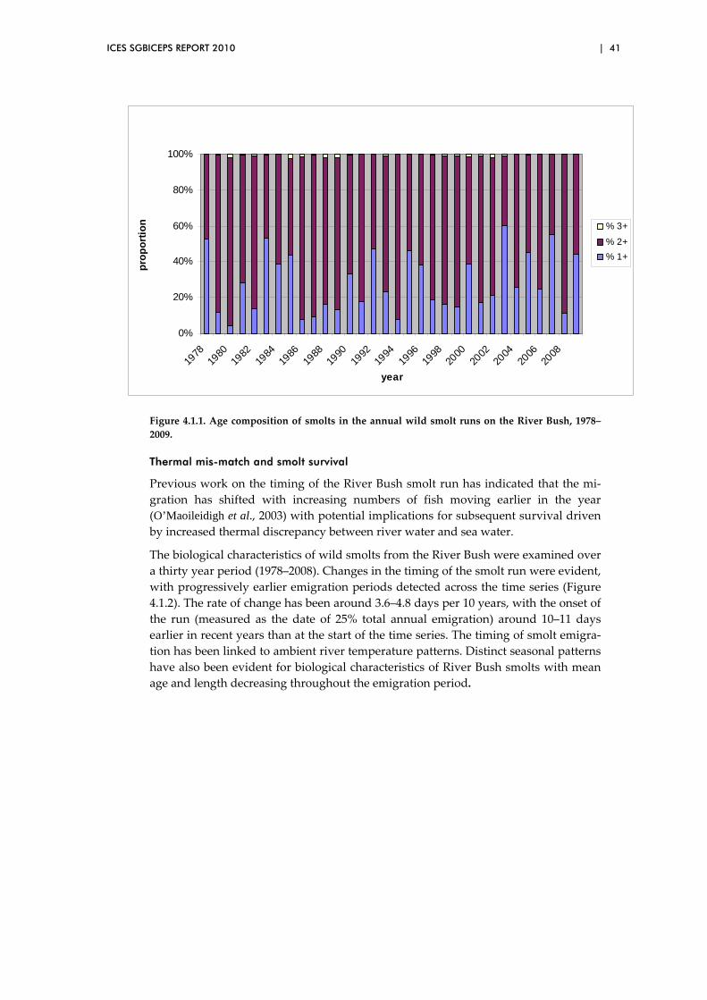
ICES SGBICEPS REPORT 2010 | 41
0%
20%
40%
60%
80%
100%
1978
1980
1982
1984
1986
1988
1990
1992
1994
1996
1998
2000
2002
2004
2006
2008
year
pro
po
rtio
n % 3+
% 2+
% 1+
Figure 4.1.1. Age composition of smolts in the annual wild smolt runs on the River Bush, 1978–
2009.
Thermal mis-match and smolt survival
Previous work on the timing of the River Bush smolt run has indicated that the mi‐
gration has shifted with increasing numbers of fish moving earlier in the year
(O’Maoileidigh et al., 2003) with potential implications for subsequent survival driven
by increased thermal discrepancy between river water and sea water.
The biological characteristics of wild smolts from the River Bush were examined over
a thirty year period (1978–2008). Changes in the timing of the smolt run were evident,
with progressively earlier emigration periods detected across the time series (Figure
4.1.2). The rate of change has been around 3.6–4.8 days per 10 years, with the onset of
the run (measured as the date of 25% total annual emigration) around 10–11 days
earlier in recent years than at the start of the time series. The timing of smolt emigra‐
tion has been linked to ambient river temperature patterns. Distinct seasonal patterns
have also been evident for biological characteristics of River Bush smolts with mean
age and length decreasing throughout the emigration period.

42 | ICES SGBICEPS REPORT 2010
100
110
120
130
140
150
160
1978
1980
1982
1984
1986
1988
1990
1992
1994
1996
1998
2000
2002
2004
2006
2008
Year
Ord
inal
Day
s
Figure 4.1.2. Smolt emigration times (ordinal date) on the River Bush between 1978–2008. The
plots indicate the ordinal date by which standard percentages of the total annual smolt run had
emigrated. Boxes indicate dates at which 25%, 50% and 75% of run had occurred; whiskers indi‐
cate dates at which 5% and 95% of run had occurred.
Marine survival patterns in 1SW salmon from the River Bush have been strongly in‐
fluenced by the run timing of the preceding smolt year, such that later emigrating
cohorts demonstrated increased survival (Figure 4.1.3). A possible mechanism for this
relationship may be the consequence of local climatic variation and potential thermal
mismatch between freshwater and marine environments. The temperature contrast
between fresh and salt water experienced by River Bush smolts is exacerbated by the
absence of an estuary on the river. The River Bush discharges directly into the North
Atlantic Ocean across a relatively steep and narrow stony beach, where the river
mouth fans out to form a shallow braided channel. The physiological stresses associ‐
ated with osmotic regulation upon marine entry may be compounded by an in‐
creased requirement for thermal acclimation over a very limited transitional zone.
Smolts are particularly vulnerable during the transition to salt water and the relative
risk of predation has been demonstrated to increase during the acclimation of smolts
to seawater (Handeland et al., 1996). These processes may have become more pro‐
nounced in recent years on the River Bush due to an observed increasing thermal
disparity between the two discrete aquatic environments (Figure 4.1.4) (Kennedy &
Crozier, 2010).

ICES SGBICEPS REPORT 2010 | 43
0
5
10
15
20
25
30
35
40
23-A
pr
25-A
pr
27-A
pr
29-A
pr
01-M
ay
03-M
ay
05-M
ay
07-M
ay
09-M
ay
Date of 25% smolt emig ra tion
Marine Survival (%
)
Figure 4.1.3. Relationship between the date of the onset of the smolt run (denoted by the data on
which 25% of smolt emigration had occurred) and subsequent marine survival of 1SW River Bush
salmon.
8
8.5
9
9.5
10
10.5
11
11.5
12
1978
1981
1984
1987
1990
1993
1996
1999
2002
Year
Mea
n D
aily
Tem
per
atu
re
oC
River Temp
SST
Figure 4.1.4. Mean daily water temperature (oC) for River Bush (Bushmills) and the sea surface
(Malin Head) recorded on the date of 25% total Bush smolt emigration.

44 | ICES SGBICEPS REPORT 2010
4.2 Update on biological characteristics of salmon from the River Dee, North Wales and other monitored rivers in UK (England & Wales) and associa-tions with environmental parameters
It was noted at the first meeting of the Study Group (ICES, 2009a) that there are eight
monitored rivers (Dee (Wales), Test, Itchen, Frome, Tamar, Fowey, Lune and Kent) in
UK (England & Wales) which report annual Returning Stock Estimates (RSEs) for
salmon. Four of these rivers (Dee [Wales], Tyne, Tamar and Lune) are also identified
as monitored ‘index’ rivers and are distinguished by having established or develop‐
ing (partial) adult trapping programmes to collect biological information (e.g. on age,
size, sex, etc.) (Davidson, 2008). These rivers are spread around UK (England and
Wales) and are broadly representative of the main salmon and sea trout producing
regions. The group includes some of the leading ‘chalk’ rivers of southern England
(e.g. Test, Itchen, Frome) as well as the more usual ‘rain‐fed’ rivers of the west and
north. While the monitoring programmes for individual rivers may differ in their de‐
tail, they share a number of common objectives in terms of the information collected
and its application to management (Davidson, 2008).
Information on changes in biological characteristics of salmon from the River Dee
(UK, England & Wales) was reported at the first meeting of the Study Group (ICES,
2009a). The following provides some new analyses in respect of the River Dee and
also an initial examination of spring river and coastal temperatures to assess whether
there is any evidence of substantive changes over time.
Long-term changes in spring temperatures – any evidence for a thermal ‘mis-match’ between rivers and coastal areas?
Further to the investigations on the River Bush (Section 4.1), where a river/sea tem‐
perature mis‐match at the time of smolt migration has been linked to marine survival,
initial investigations were completed for a number of sites in UK (England & Wales)
to see if similar patterns might be evident. Time‐series of river and sea surface tem‐
perature data were collated/derived for four rivers spread from south to northwest
around the coast ‐ namely: Hampshire Avon; Tamar; Dee and Lune ‐ to explore spa‐
tial and temporal patterns in these data.
In all cases, river temperatures were collected at main stem sites at or close to the
head‐of‐tide. Sea surface temperature data were extracted from records collated and
published by Cefas (http://www.cefas.co.uk/data.aspx) and obtained at various
coastal stations. The proximity of these stations to the selected rivers was variable
and usually amounted to a distance of several km.
There were a number of gaps in the data sets, particularly for the river temperature
time‐series, and to fill these monthly mean temperatures were predicted from simple
linear regression relationships with parallel temperature series. In the case of sea
temperatures, these parallel data series were from the nearest adjacent sampling sta‐
tion to the required data sets. In the case of river temperatures, local air temperature
time‐series (more widely available than river temperature time‐series) were used as
predictors of river temperature. For example, Figure 4.2.1 shows the regression rela‐
tionship between monthly mean observed air temperatures at Slapton Ley (extracted
from the UK Meteorological Office MIDAS Land Surface Station Data set
http://badc.nerc.ac.uk/home/) and water temperatures on the River Tamar.
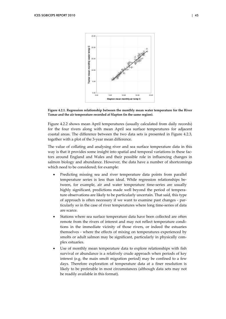
ICES SGBICEPS REPORT 2010 | 45
0.00
5.00
10.00
15.00
20.00
25.00
0.00 5.00 10.00 15.00 20.00
Slapton mean monthly air temp C
Ta
ma
r m
ea
n m
on
thly
wa
ter
tem
p C
Figure 4.2.1. Regression relationship between the monthly mean water temperature for the River
Tamar and the air temperature recorded at Slapton (in the same region).
Figure 4.2.2 shows mean April temperatures (usually calculated from daily records)
for the four rivers along with mean April sea surface temperatures for adjacent
coastal areas. The difference between the two data sets is presented in Figure 4.2.3,
together with a plot of the 3‐year mean difference.
The value of collating and analysing river and sea surface temperature data in this
way is that it provides some insight into spatial and temporal variations in these fac‐
tors around England and Wales and their possible role in influencing changes in
salmon biology and abundance. However, the data have a number of shortcomings
which need to be considered; for example:
Predicting missing sea and river temperature data points from parallel
temperature series is less than ideal. While regression relationships be‐
tween, for example, air and water temperature time‐series are usually
highly significant, predictions made well beyond the period of tempera‐
ture observations are likely to be particularly uncertain. That said, this type
of approach is often necessary if we want to examine past changes ‐ par‐
ticularly so in the case of river temperatures where long time‐series of data
are scarce.
Stations where sea surface temperature data have been collected are often
remote from the rivers of interest and may not reflect temperature condi‐
tions in the immediate vicinity of those rivers, or indeed the estuaries
themselves ‐ where the effects of mixing on temperatures experienced by
smolts or adult salmon may be significant, particularly in physically com‐
plex estuaries.
Use of monthly mean temperature data to explore relationships with fish
survival or abundance is a relatively crude approach when periods of key
interest (e.g. the main smolt migration period) may be confined to a few
days. Therefore exploration of temperature data at a finer resolution is
likely to be preferable in most circumstances (although data sets may not
be readily available in this format).
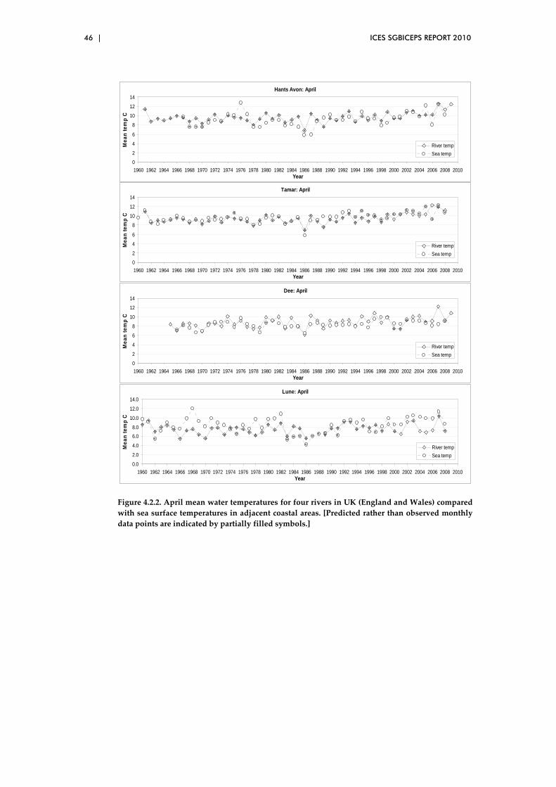
46 | ICES SGBICEPS REPORT 2010
Hants Avon: April
0
2
4
6
8
10
12
14
1960 1962 1964 1966 1968 1970 1972 1974 1976 1978 1980 1982 1984 1986 1988 1990 1992 1994 1996 1998 2000 2002 2004 2006 2008 2010Year
Me
an
te
mp
C
River temp
Sea temp
Tamar: April
0
2
4
6
8
10
12
14
1960 1962 1964 1966 1968 1970 1972 1974 1976 1978 1980 1982 1984 1986 1988 1990 1992 1994 1996 1998 2000 2002 2004 2006 2008 2010Year
Me
an
te
mp
C
River temp
Sea temp
Dee: April
0
2
4
6
8
10
12
14
1960 1962 1964 1966 1968 1970 1972 1974 1976 1978 1980 1982 1984 1986 1988 1990 1992 1994 1996 1998 2000 2002 2004 2006 2008 2010Year
Me
an
te
mp
C
River temp
Sea temp
Lune: April
0.0
2.0
4.0
6.0
8.0
10.0
12.0
14.0
1960 1962 1964 1966 1968 1970 1972 1974 1976 1978 1980 1982 1984 1986 1988 1990 1992 1994 1996 1998 2000 2002 2004 2006 2008 2010Year
Me
an
te
mp
C
River temp
Sea temp
Figure 4.2.2. April mean water temperatures for four rivers in UK (England and Wales) compared
with sea surface temperatures in adjacent coastal areas. [Predicted rather than observed monthly
data points are indicated by partially filled symbols.]
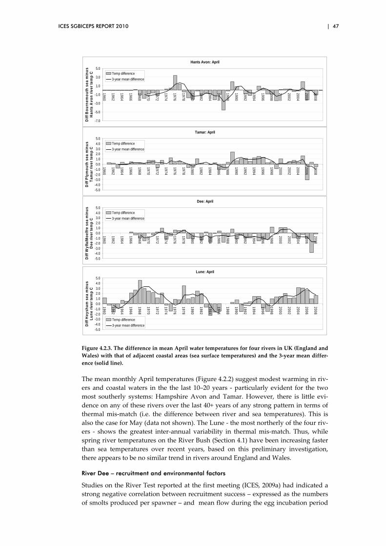
ICES SGBICEPS REPORT 2010 | 47
Hants Avon: April
-7.0
-5.0
-3.0
-1.0
1.0
3.0
5.0
1960
1962
1964
1966
1968
1970
1972
1974
1976
1978
1980
1982
1984
1986
1988
1990
1992
1994
1996
1998
2000
2002
2004
2006
2008
Dif
f Bo
urn
em
ou
th s
ea
min
us
Han
ts A
vo
n r
iver
tem
p C Temp difference
3-year mean difference
Tamar: April
-5.0
-4.0
-3.0-2.0
-1.0
0.0
1.0
2.03.0
4.0
5.0
1960
1962
1964
1966
1968
1970
1972
1974
1976
1978
1980
1982
1984
1986
1988
1990
1992
1994
1996
1998
2000
2002
2004
2006
2008
Dif
f P
lym
ou
th s
ea
min
us
T
am
ar
riv
er
tem
p C
Temp difference
3-year mean difference
Dee: April
-5.0
-4.0-3.0
-2.0-1.0
0.0
1.02.0
3.04.0
5.0
1960
1962
1964
1966
1968
1970
1972
1974
1976
1978
1980
1982
1984
1986
1988
1990
1992
1994
1996
1998
2000
2002
2004
2006
2008
Dif
f W
ylf
a/M
oe
lfre
se
a m
inu
s
De
e r
ive
r te
mp
C
Temp difference
3-year mean difference
Lune: April
-5.0
-4.0
-3.0-2.0
-1.0
0.0
1.0
2.03.0
4.0
5.01960
1962
1964
1966
1968
1970
1972
1974
1976
1978
1980
1982
1984
1986
1988
1990
1992
1994
1996
1998
2000
2002
2004
2006
2008
Dif
f H
ey
sh
am
se
a m
inu
s
Lu
ne
riv
er
tem
p C
Temp difference
3-year mean difference
Figure 4.2.3. The difference in mean April water temperatures for four rivers in UK (England and
Wales) with that of adjacent coastal areas (sea surface temperatures) and the 3‐year mean differ‐
ence (solid line).
The mean monthly April temperatures (Figure 4.2.2) suggest modest warming in riv‐
ers and coastal waters in the the last 10–20 years ‐ particularly evident for the two
most southerly systems: Hampshire Avon and Tamar. However, there is little evi‐
dence on any of these rivers over the last 40+ years of any strong pattern in terms of
thermal mis‐match (i.e. the difference between river and sea temperatures). This is
also the case for May (data not shown). The Lune ‐ the most northerly of the four riv‐
ers ‐ shows the greatest inter‐annual variability in thermal mis‐match. Thus, while
spring river temperatures on the River Bush (Section 4.1) have been increasing faster
than sea temperatures over recent years, based on this preliminary investigation,
there appears to be no similar trend in rivers around England and Wales.
River Dee – recruitment and environmental factors
Studies on the River Test reported at the first meeting (ICES, 2009a) had indicated a
strong negative correlation between recruitment success – expressed as the numbers
of smolts produced per spawner – and mean flow during the egg incubation period

48 | ICES SGBICEPS REPORT 2010
(Figure 4.2.4). More specifically, it was suggested that during high flow periods
sediment mobilisation increases (Figure 4.2.5) with adverse consequences for devel‐
oping eggs and pre‐emergent fry as spawning gravels become clogged with sediment
and intra‐gravel flow and oxygen delivery are reduced.
Figure 4.2.4. Relationship between river discharge during egg incubation and spawning success
(smolts per spawner) on the River Test, southern England.
Figure 4.2.5. Relationship between suspended solids load and spawning success (smolts per
spawner) on the River Test, southern England.
Prompted by these findings, a similar analysis was carried out on salmon stock and
recruitment data from the River Dee, N. Wales to investigate whether any relation‐
ship between recruitment success and flow was evident. In the case of the Dee, no
census data for smolt output were available, but indices of 0+ juvenile recruitment,
derived from the results of extensive autumn electrofishing surveys, were obtained.
Measures of recruitment success (‘recuits per spawner’ or R/S) generated from these
data sets were plotted against spawner numbers and a linear regression fitted to the
data points (Figure 4.2.6). Residuals from the regression line were, in turn, correlated
with mean flows calculated for various periods in the life‐cycle (‘egg incubation’,
‘emergence’ and ‘first summer’). These flow variables are summarised in Table 4.2.1.
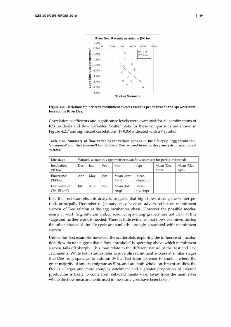
ICES SGBICEPS REPORT 2010 | 49
River Dee: Recruits as autumn (0+) fry
-1.800
-1.600
-1.400
-1.200
-1.000
-0.800
-0.600
-0.400
-0.200
0.000
0 2000 4000 6000 8000 10000
Stock as Spawners
Lo
ge
(R
ec
ruit
s p
er
sp
aw
ne
r)
R2 = 0.26P = 0.101
Figure 4.2.6. Relationship between recruitment success (‘recuits per spawner’) and spawner num‐
bers for the River Dee.
Correlation coefficients and significance levels were examined for all combinations of
R/S residuals and flow variables. Scatter plots for these comparisons are shown in
Figure 4.2.7 and significant correlations (P<0.05) indicated with a # symbol.
Table 4.2.1. Summary of flow variables for various periods in the life‐cycle (‘egg incubation’,
‘emergence’ and ‘first summer’) for the River Dee, as used in exploratory analysis of recruitment
success.
Life stage Variable as monthly (geometric) mean flow (cumecs) for period indicated:
Incubation
(‘IFlow’)
Dec Jan Feb Mar Apr Mean (Dec‐
Mar)
Mean (Mar‐
Apr)
Emergence
(‘EFlow)
Apr May Jun Mean (Apr‐
May)
Mean
(Apr‐Jun)
First summer
(‘0+_SFlow’)
Jul Aug Sep Mean (Jul‐
Aug)
Mean
(Jul‐Sep)
Like the Test example, this analysis suggests that high flows during the winter pe‐
riod, principally December to January, may have an adverse effect on recruitment
success of Dee salmon at the egg incubation phase. However the possible mecha‐
nisms at work (e.g. siltation and/or scour of spawning gravels) are not clear at this
stage and further work is needed. There is little evidence that flows examined during
the other phases of the life‐cycle are similarly strongly associated with recruitment
success.
Unlike the Test example, however, the scatterplots exploring the influence of ‘incuba‐
tion’ flow do not suggest that a flow ‘threshold’ is operating above which recruitment
success falls off sharply. This may relate to the different nature of the Test and Dee
catchments. While both studies refer to juvenile recruitment success at similar stages
(the Dee from spawner to autumn 0+ the Test from spawner to smolt – where the
great majority of smolts emigrate as S1s), and are both whole catchment studies, the
Dee is a larger and more complex catchment and a greater proportion of juvenile
production is likely to come from sub‐catchments – i.e. away from the main river
where the flow measurements used in these analyses have been taken.

50 | ICES SGBICEPS REPORT 2010
906030 80400 100500 604020 453015
0.5
0.0
-0.5
604020
0.5
0.0
-0.5
503010 453015 302010 201510
302010 201510 604020 302010 302010
0.5
0.0
-0.5
302010
0.5
0.0
-0.5
24168
IFlow_DecR
/S r
esid
uals
IFlow_Jan IFlow_Feb IFlow_Mar IFlow_Apr
IFlow_M_Dec_Mar IFlow_M_Mar_Apr EFlow_Apr EFlow_May EFlow_Jun
Eflow_M_Apr_May Eflow_M_Apr_Jun 0+_SFlow_Jul 0+_SFlow_Aug 0+_SFlow_Sep
0+_SFlow_M_Jul_Aug 0+_SFlow_M_Jul_Sep
Scatterplot of R/S residual vs IFlow_Dec, IFlow_Jan, IFlow_Feb, ...
Figure 4.2.7. Scatter plots of recruitment success (R/S) residuals and flow variables at various
stages of the life‐cycle; significant correlations (P<0.05) are indicated with a # symbol.
Accordingly, data from the River Dee should be explored at a sub‐catchment level to
examine relationships between recruitment and flow at a finer resolution and investi‐
gate spatial differences in the flow response.
[Note: In a related analysis of River Dee data to look at recruitment success from
adult spawner to adult spawner, flows during the egg incubation period did not ap‐
pear influential, i.e. any effect was probably lost among a host of other factors acting
over this longer period of the life‐cycle.]
4.3 Biological characteristics of salmon from the River Frome – UK (England & Wales)
Information on changes in biological characteristics of salmon from the River Frome
(UK, England & Wales) was made available at the first meeting of the Study Group
(ICES, 2009a). There were no new data or developments to report at the current
meeting.
4.4 Biological characteristics of salmon from the River Test – UK (England & Wales)
Information on changes in biological characteristics of salmon from the River Test
(UK, England & Wales) was made available at the first meeting of the Study Group
(ICES, 2009a). There were no new data or developments to report at the current
meeting.

ICES SGBICEPS REPORT 2010 | 51
4.5 Evidence for later age at maturity in Norwegian salmon stocks in recent years
The Study Group previously examined information from Norway indicating recent
changes in the age at maturity of returning salmon. This analysis was updated at the
latest meeting to incorporate the most recently available data.
Analysis of the pre‐fishery‐abundance (PFA) of Norwegian salmon stocks indicates a
significant positive relationship between the number of 1SW salmon in one year and
the number of 2SW salmon in the following year (Hansen et al., 2007; Hansen et al.,
unpublished). The regression between PFA for 1SW salmon in year n and PFA of
2SW salmon in year n+1 shows positive residuals in the more recent years in three
regions in Norway (Figure 4.5.1), suggesting that more salmon return as 2SW fish
than expected from the number of 1SW fish the previous year. The most recent data
remain consistent with this observation.
The 1SW component is typically male‐dominated, and if there is a tendency for later
maturity one would expect an increase in the male proportion among 2SW salmon.
The apparent later age at maturity might be explained both by more salmon delaying
age at maturity, or by survival in the second year at sea having increased relative to
survival in the first year at sea. If the first hypothesis is true one might expect an in‐
crease in the proportion of male salmon among the returning 2SW fish, whereas the
sex ratio among 2SW fish is more likely to be unchanged if the second hypothesis is
more valid.
Uns
tand
ardi
zed
resi
tual
s
Year
Southern Norway
Northern Norway
Central Norway
Figure 4.5.1. Unstandardised residuals from the regressions of PFA of 1SW salmon in year n and
2SW salmon in year n+1 in three Norwegian regions.
52 | ICES SGBICEPS REPORT 2010
4.6 Baltic Sea – changes in post-smolt survival and the factors affecting it
The Study Group once again reviewed information on post‐smolt survival arising
from the work of the Baltic Salmon and Trout Assessment Working Group
(WGBAST). WGBAST initiated preliminary analyses during their 2008 meeting to
evaluate the possible reasons for the low at‐sea survival of salmon stocks in the Baltic
Sea; investigations continued in 2009. Further details are available in the WGBAST
reports (ICES, 2008b; ICES, 2009b), and work is expected to continue during the
WGBAST meeting in 2010.
Background
The post‐smolt survival of salmon in the Baltic Sea has decreased in recent years, both
for wild and hatchery‐reared smolts (ICES, 2008b). According to estimates generated
from the assessment model, this decline started in the mid 1990s; the reasons behind
the decline are unclear. It is possible that changes in the Baltic Sea ecosystem have
negatively affected salmon post‐smolt survival rates by, for example, changing the
abundance of prey species or though increased competition or predation from other
species. The Baltic Sea has undergone pronounced changes in the last two decades,
characterised by several regime shifts in species composition (ICES, 2007b). The main
drivers of this process are believed to have been climate changes affecting salinity,
oxygen levels and temperature, but fisheries and eutrophication are also believed to
have had an impact. It has also been hypothesized that increased mortality among
hatchery‐reared post‐smolts may be linked to changed hatchery practices. These have
been subject to continual improvement – for example, the use of feeds with higher fat
and energy content. Favourable river temperatures, especially in autumn, have also
resulted in improved growth rates and increasingly large smolts. There are concerns
that the large size of reared smolts may have negative fitness consequences in the
wild.
Preliminary tests of hypotheses using multivariate analyses
WGBAST initially agreed on the following specific hypotheses to test with multivari‐
ate analyses (ICES, 2008b):
Competition hypothesis: the aim was to test if intra‐specific competition
for food is important in explaining variation in post‐smolt survival. In this
case, the survival of smolts would decrease as the smolt abundance in‐
creases.
Food availability hypothesis: Young herring are considered important prey
for young salmon in the Baltic Sea. Therefore, increased recruitment of 0+
herring in the smolt year should lead to higher survival if herring abun‐
dance is a limiting factor. This hypothesis is directly linked to the competi‐
tion hypothesis above. If herring recruitment directly affects post‐smolt
survival then, by definition, at‐sea survival is density‐dependent and
should be affected by smolt production in rivers and hatcheries.
Seal predation hypothesis: If salmon smolts are subject to substantial seal
predation, then an increase in the number of seals along the migration path
of post‐smolts should coincide with lower survival. If such a pattern is re‐
vealed, the predation hypothesis remains possible, but is not necessarily
more likely than other hypotheses that might lead to similar predictions.
Smolt quality hypothesis: This relates only to hatchery‐reared smolts and
hypothesises that increased mortality is due to changed hatchery practices.

ICES SGBICEPS REPORT 2010 | 53
Pre‐release factors suggested to be important explanatory variables include
size, condition factor and level of fin damage.
In preliminary analyses, the model which included only the seal counts was assigned
the highest probability (>0.4) as a predictor. Models including estimated smolt abun‐
dance were assigned low probability compared to other combinations.
Ongoing analyses during 2009
During the WGBAST meeting in 2009 (ICES, 2009b), three data sets describing salmon
at‐sea survival were evaluated: 1) post‐smolt survival estimates (Mps) for wild
salmon from the Baltic assessment model; 2) return rates to the river of reared salmon
from the River Umeälven (Ume), and 3) tag‐recapture rates of salmon reared in the
River Dalälven. The data for potential explanatory variables characterising the Baltic
Sea ecosystem and the smolt release hatcheries were updated and some more de‐
tailed time series were added.
Statistical procedures
From initial analyses of individual predictor variables using a log‐linear regression
model (ICES, 2008b), a number of variables were selected for further statistical
evaluation. Predictor variables that were considered important included seal abun‐
dance, herring recruitment and abundance, sprat abundance, smolt production esti‐
mates (both wild and hatchery‐reared smolt production) and trawl effort.
Temperature was not included, as previous studies have shown that sea surface tem‐
perature may only have an indirect effect on salmon survival through its positive ef‐
fect on herring recruitment (e.g. Kallio‐Nyberg et al., 2006). The selected predictor
variables were used to test the hypotheses formulated during the previous WG meet‐
ing (see above). The Mps and Ume return rate survival indices were used to test the
seal predation and food abundance hypotheses using two slightly different Bayesian
models, whereas tag‐recapture data from the River Dalälven were used to test the
smolt quality hypothesis.
Post‐smolt survival estimates ‐ Mps estimates were extracted from the assessment
model by calculating the median of the posterior distribution of the instantaneous
mortality rate, and by calculating the correlation matrix of the joint posterior. Then
the median values were used as observations and the correlation matrix was used as
a model for correlated measurements. The mortality was assumed to vary randomly
between years with an annual expected value depending on explanatory variables
according to following equation:
E(My) = qSEALy + exp(α – β1HSD30y+1 – β2HSD31y+1 – γ2HCBy – γ2SCBy)
Where q is the catchability coefficient of seals and α, β1, β2, γ1 and γ2 are regression
coefficients. All these parameters are assumed to be positive, which means that the
increase in seal abundance is assumed to increase the mortality, while the variables
reflecting availability of food are assumed to decrease the mortality. The explanatory
variables are described in the following table. Note that the relative recruitment of 0+
herring was approximated in the model by shifting the estimates of 1+ recruitment
backwards by one year. SD refers to ICES subdivision.

54 | ICES SGBICEPS REPORT 2010
VARIABLE DESCRIPTION
SEAL Total Baltic seal counts in Swedish surveys
HSD30 SD30 1+ herring recruitment / (SD30+SD31 smolts)
HSD31 SD31 1+ herring recruitment / (SD31 smolts)
HCB Herring stock biomass in central Baltic
SCB Sprat stock biomass in central Baltic
The five explanatory variables can be combined in 31 different ways. The relative
credibility of these alternative models was estimated by calculating posterior prob‐
ability for each of the models. Such a Bayesian Model Averaging approach weights
the models based on the goodness of fit and typically induces a penalty for complex‐
ity.
For models that included the number of seals as a predictor, it was possible to calcu‐
late an estimate of the number of smolts eaten by an average seal. These values could
then be used to assess whether the results of the model were plausible compared to
independent knowledge about the diet of seals.
Return rate to River Umeälven ‐ The assumed model structure for the return rate
analysis was very similar to the model used for the estimated post smolt mortality
rates. The main difference was that offshore and coastal fishing effort were included
as predictors in each combination of explanatory variables. Furthermore, instead of
using herring data from SD(ICES subdivision)31, both 0+ and 1+ recruitment of SD30
were included as explanatory variables since it has been suggested that larger reared
post‐smolts may feed on both one year old and young of the year herring (Salminen
et al., 2001). The mortality rates were assumed to vary randomly around the annual
mean which depends on the explanatory variables:
Zy = Fy + My
Fy = q(pCOASTy + (1 ‐ p)OFFSHy)
My = dSEALy + exp(α – β1H1y – β2H0y – γ1CBHy – γ2CBSy)
The mortality rate was then converted to expected return rate as:
Ry = exp(‐My).
In order to compare the results of the modelling of the return rate to the estimated
post‐smolt survival, the expected natural marine survival of released River Ume
smolts was calculated as:
Ry = exp(‐My).
VARIABLE DESCRIPTION
SEAL Total Baltic seal counts in Swedish surveys
H0y = H1y+1 SD30 0+ herring recruitment / (SD30+SD31 smolts)
H1 SD30 1+ herring recruitment / (SD31+SD31 smolts)
HBC Herring stock biomass in central Baltic
CBS Sprat stock biomass in central Baltic
COAST Mean coastal effort during the next two years after the release year,
all gear combined
OFFSH Mean offshore effort during the next two years after the release year,
all gear combined

ICES SGBICEPS REPORT 2010 | 55
Tag‐recapture rates from River Dalälven ‐ Tag‐recapture data is dependent on fish‐
ing effort and the willingness of fishermen to report tags, and is therefore more prob‐
lematic to use for analyses of trends in survival over time if these problems are not
dealt with carefully. This dataset was therefore used only to evaluate the smolt qual‐
ity hypothesis described above, more specifically the effects of smolt length and
hatchery injuries on subsequent survival following release. The fish were divided
into four categories: healthy (no injuries), dorsal fin injured, other fins injured, and
dorsal fin and other fins injured. Release year, release date (Julian date) and length of
fish at tagging were included as continuous variables. The dataset was first analysed
with PROC LOGISTIC (SAS statistical software) in order to investigate the overall
effect of the independent variables. Thereafter, the data was analysed with PROC
GENMOD (SAS statistical software), assuming binary response of recapture, in order
to calculate Least‐square means for the different categories.
2009 results
The work on salmon post‐smolt mortality in the Baltic Sea is still at an initial stage,
and these results should be viewed as preliminary. It is important to highlight the fact
that a correlative approach has been applied, which means that observed associations
between survival estimates and biological predictors are not necessarily due to causal
relationships.
The independent dataset of return rates of reared salmon to the river mouth of the
River Umeälven was in close agreement with the Mps model estimates (Figure
4.6.1.a). The decrease in salmon fishing effort was not taken into account in examin‐
ing the Ume dataset. Despite that, return rate seems to have decreased over the last 8
to 10 years, which supports the model estimates indicating a negative trend in post‐
smolt survival over the last decade. The natural marine survival (Sy) estimated from
the River Umeälven return rates are lower than the post‐smolt survival estimated
using the stock assessment model (Figure 4.6.1.b). The independent survival esti‐
mates show similar annual variation and the decreasing trend, which gives strong
support for the conclusion that post‐smolt survival has been decreasing.

56 | ICES SGBICEPS REPORT 2010
0
0.1
0.2
0.3
0.4
1987
1988
1989
1990
1991
1992
1993
1994
1995
1996
1997
1998
1999
2000
2001
2002
2003
2004
2005
2006
Smolting year
Su
rviv
al r
ate
(Mp
s)
0.00
0.01
0.02
0.03
0.04
0.05
0.06
0.07
0.08
Re
turn
rat
e
Mps wild
Mps reared
Ume return rate
0
0.02
0.04
0.06
0.08
0.1
0.12
0.14
0.16
0.18
0.2
198719
8819
8919
9019
9119
9219
9319
9419
9519
9619
9719
9819
9920
0020
0120
0220
0320
0420
05
Nat
ura
l m
arin
e su
rviv
al
0
0.05
0.1
0.15
0.2
0.25
0.3
Po
st
smo
lt s
urv
ival
River Ume model
Assessment model
a)
b)
Figure 4.6.1. Changes in: a) post‐smolt survival of wild and hatchery‐reared salmon estimated by
the assessment model and the return rate of reared salmon to the River Umeälven, and b) post‐
smolt survival of hatchery‐reared salmon estimated by the assessment model and estimated natu‐
ral marine survival of hatchery‐reared salmon from the River Umeälven, for 1987–2007 smolt year
classes.
The predation and food availability hypotheses
Initial analyses of predictor variables indicated that survival of wild post‐smolts was
negatively correlated with seal abundance (Figure 4.6.2) and total smolt production in
the Gulf of Bothnia (Figure 4.6.3), and positively correlated with herring recruitment
in both the Bothnian Bay (Figure 4.6.4) and Bothnian Sea. No relationships were ob‐
served between survival and total trawl effort in the Bothnian Bay or pelagic trawl
effort in the Bothnian Sea.

ICES SGBICEPS REPORT 2010 | 57
Figure 4.6.2. a) Changes in survival of wild post‐smolts and seal abundance along the Swedish
coast, and, b) indications of a negative correlation between these variables.
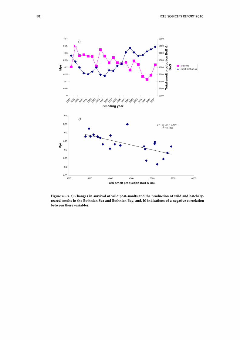
58 | ICES SGBICEPS REPORT 2010
0
0.05
0.1
0.15
0.2
0.25
0.3
0.35
0.4
1987
1988
1989
1990
1991
1992
1993
1994
1995
1996
1997
1998
1999
2000
2001
2002
2003
2004
2005
2006
2007
Smolting year
Mp
s
2000
2500
3000
3500
4000
4500
5000
5500
6000
To
tal s
mo
lt p
rod
uc
tio
n B
oB
&
Bo
S Mps wild
Smolt production
y = -6E-05x + 0.4844
R2 = 0.4492
0.05
0.1
0.15
0.2
0.25
0.3
0.35
0.4
3000 3500 4000 4500 5000 5500 6000
Total smolt production BoB & BoS
Mp
s
a)
b)
Figure 4.6.3. a) Changes in survival of wild post‐smolts and the production of wild and hatchery‐
reared smolts in the Bothnian Sea and Bothnian Bay, and, b) indications of a negative correlation
between these variables.
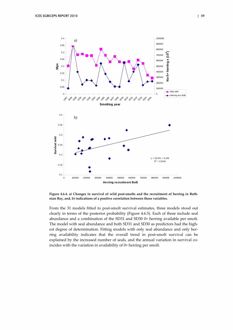
ICES SGBICEPS REPORT 2010 | 59
0
0.05
0.1
0.15
0.2
0.25
0.3
0.35
0.4
1987
1988
1989
1990
1991
1992
1993
1994
1995
1996
1997
1998
1999
2000
2001
2002
2003
2004
2005
Smolting year
Mp
s
0
100000
200000
300000
400000
500000
600000
700000
800000
900000
1000000
No
0+
her
rin
g x
(103 )
Mps wild
Herring recr BoB
y = 1E-07x + 0.199
R2 = 0.2344
0.1
0.15
0.2
0.25
0.3
0.35
0.4
0 100000 200000 300000 400000 500000 600000 700000 800000 900000 1000000
Herring recruitment BoB
Su
rviv
al
wil
d
a)
b)
Figure 4.6.4. a) Changes in survival of wild post‐smolts and the recruitment of herring in Both‐
nian Bay, and, b) indications of a positive correlation between these variables.
From the 31 models fitted to post‐smolt survival estimates, three models stood out
clearly in terms of the posterior probability (Figure 4.6.5). Each of these include seal
abundance and a combination of the SD31 and SD30 0+ herring available per smolt.
The model with seal abundance and both SD31 and SD30 as predictors had the high‐
est degree of determination. Fitting models with only seal abundance and only her‐
ring availability indicates that the overall trend in post‐smolt survival can be
explained by the increased number of seals, and the annual variation in survival co‐
incides with the variation in availability of 0+ herring per smolt.

60 | ICES SGBICEPS REPORT 2010
0 0.05 0.1 0.15 0.2 0.25 0.3
Seal+HSD30
Seal+HSD31+HSD30
Seal+HSD31
Seal+HSD30+HCB
HSD30+HCB
HSD30
Seal+HSD31+HCB
Seal+HSD31+HSD32+HCB
Seal
HCB
Mo
del
Probability
Figure 4.6.5. Posterior probabilities of the 10 most likely predictor variable combinations to ex‐
plain the variation in the survival of wild post‐smolts.
Results from the analysis of the River Umeälven return rate produced a similar pic‐
ture (Figure 4.6.6), although the importance of seal abundance as a predictor was less
pronounced. In general, seal numbers seem to explain the trend in mortality for a
longer time span, while herring abundance in SD 30 is an important predictor for an‐
nual variations.
According to modelling of post‐smolt survival with the assumption of seal predation,
an average seal would have to consume approximately 50–100 smolts per year in or‐
der to generate the estimated increase in mortality. This uncertainty arises mainly
from the uncertainty about the true size of the seal population.
0 0.05 0.1 0.15 0.2 0.25
H1+H0
H0
Seal+H1+H0
H1
Seal+H0
Seal+H1
H0+H1+CBH
Seal
Seal+H1+H0+CBH
Seal+H0+CBH
Mo
del
Probability
Figure 4.6.6. Posterior probabilities of the 10 most likely predictor variable combinations to ex‐
plain the variation in the return rate of reared salmon from River Umeälven.

ICES SGBICEPS REPORT 2010 | 61
The smolt quality hypothesis
There was an overall difference in recapture rate between the four categories of inju‐
ries recorded for the hatchery‐reared smolts. Length at release, and day and year of
release also influenced recapture rate, while smolt length also had a positive effect on
tag recapture rate. In respect of fin injuries, fish with only dorsal fin injuries had the
same recapture rate as healthy fish. However, fish classified as having ‘other’ fins
injured had a recapture rate that was only 60% of that in healthy individuals indicat‐
ing that injuries on fins than the dorsal fin have much more severe effects on survival
following release to the wild. A more detailed description of these analyses was in‐
cluded in the first SGBICEPS report (ICES, 2009a).
Conclusions and future studies
The results suggest that herring recruitment in the Gulf of Bothnia is able to explain a
large proportion of the annual variation in post‐smolt survival, but is not able to ex‐
plain the negative trend in survival over the last decade. The addition of seal abun‐
dance to the models captured this decline. However, it is important to note that
because a correlative approach was used, we cannot conclude that the observed pat‐
terns are due to causal relationships.
The estimated number of salmon that an average seal has to consume per year in or‐
der to explain the estimated reduction in survival is within realistic levels. However,
the available information on seal diet composition is limited, and future studies
should focus on collecting such data in order to evaluate if the present seal popula‐
tion is actually able to have a negative effect on salmon survival, indicating a possible
causal relationship. Information about seal diet would be particularly important for
the summer when migrating smolts are passing the densest seal populations. As re‐
gards herring, previous studies have indicated that the recruitment of this prey spe‐
cies may be one of the most important factors regulating salmon abundance in the
Baltic Sea, and our results support these earlier findings. The next step will be to con‐
sider a model which takes into account detailed information on salmon size, prey size
distribution and predation pressure from seals during the post‐smolt migration to the
southern Main Basin.
Even though it is not clear whether the estimated effects of seal abundance and her‐
ring recruitment represent a true causality, the strong co‐variation can potentially be
utilised when predicting the post‐smolt survival. Smolt production and seal abun‐
dance are both likely to change slowly, whereas the recruitment of herring is proba‐
bly less predictable. However, herring recruitment has been found to be correlated
with the water temperature, which might be predictable to some extent. Since the
number of seals and smolts are not expected to drop in the near future, the observed
co‐variation suggests that post‐smolt survival is expected to remain low for the next
couple of years, at least. Annual variation is more difficult to predict.
It is also evident from this study that fin damage in hatchery‐reared smolts can affect
survival following release to the wild, and while fin damage is certainly not the only
important factor (as noted above) it may, in part at least, explain the comparably low
survival of many hatchery‐reared stocks. Clearly, the way hatcheries are managed
will have an impact on how reared salmon are able to cope with the wild environ‐
ment.
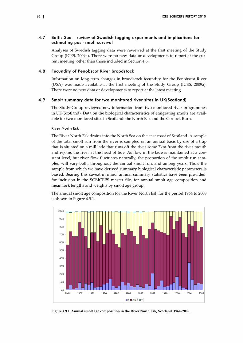
62 | ICES SGBICEPS REPORT 2010
4.7 Baltic Sea – review of Swedish tagging experiments and implications for estimating post-smolt survival
Analyses of Swedish tagging data were reviewed at the first meeting of the Study
Group (ICES, 2009a). There were no new data or developments to report at the cur‐
rent meeting, other than those included in Section 4.6.
4.8 Fecundity of Penobscot River broodstock
Information on long‐term changes in broodstock fecundity for the Penobscot River
(USA) was made available at the first meeting of the Study Group (ICES, 2009a).
There were no new data or developments to report at the latest meeting.
4.9 Smolt summary data for two monitored river sites in UK(Scotland)
The Study Group reviewed new information from two monitored river programmes
in UK(Scotland). Data on the biological characteristics of emigrating smolts are avail‐
able for two monitored sites in Scotland: the North Esk and the Girnock Burn.
River North Esk
The River North Esk drains into the North Sea on the east coast of Scotland. A sample
of the total smolt run from the river is sampled on an annual basis by use of a trap
that is situated on a mill lade that runs off the river some 7km from the river mouth
and rejoins the river at the head of tide. As flow in the lade is maintained at a con‐
stant level, but river flow fluctuates naturally, the proportion of the smolt run sam‐
pled will vary both, throughout the annual smolt run, and among years. Thus, the
sample from which we have derived summary biological characteristic parameters is
biased. Bearing this caveat in mind, annual summary statistics have been provided,
for inclusion in the SGBICEPS master file, for annual smolt age composition and
mean fork lengths and weights by smolt age group.
The annual smolt age composition for the River North Esk for the period 1964 to 2008
is shown in Figure 4.9.1.
0%
10%
20%
30%
40%
50%
60%
70%
80%
90%
100%
1964 1968 1972 1976 1980 1984 1988 1992 1996 2000 2004 2008
1 2 3 4
Figure 4.9.1. Annual smolt age composition in the River North Esk, Scotland, 1964–2008.

ICES SGBICEPS REPORT 2010 | 63
Smolts emigrate from the North Esk after spending between one and four years in
freshwater. Two year old smolts (S2) comprise the majority of the run throughout the
series, followed by S3, then S1, with S4 comprising a very small component.
Throughout the time period there has been a tendency for an increase in the propor‐
tion of younger smolts (S1 and S2) and a decrease in the proportion of older smolts
(S3 and S4).
Figure 4.9.2 shows the mean fork lengths (cm), by smolt age, of emigrating smolts
over the period 1964 to 2008. Generally, in any given year, older smolts have a greater
mean fork length. For all four age groups there is a pattern of decreasing fork length
until the early 1980s with lengths increasing thereafter.
10.0
10.5
11.0
11.5
12.0
12.5
13.0
13.5
14.0
14.5
1960 1965 1970 1975 1980 1985 1990 1995 2000 2005 2010
1 2 3 4
Figure 4.9.2. Mean fork length (cm), by smolt age, in the River North Esk, 1964–2008.
Figure 4.9.3 shows the mean weight (g), by smolt age, of emigrating smolts over the
period 1975 to 2008. The weight data provide a similar picture to that observed for
the length data. Generally, in any given year, older smolts have a greater mean
weight. For all four age groups there is a pattern of decreasing mean weight until the
early 1980s with weights increasing thereafter.
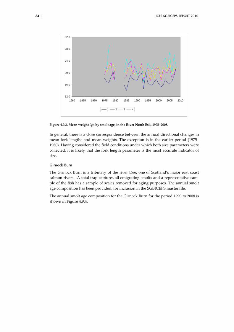
64 | ICES SGBICEPS REPORT 2010
12.0
16.0
20.0
24.0
28.0
32.0
1960 1965 1970 1975 1980 1985 1990 1995 2000 2005 2010
1 2 3 4
Figure 4.9.3. Mean weight (g), by smolt age, in the River North Esk, 1975–2008.
In general, there is a close correspondence between the annual directional changes in
mean fork lengths and mean weights. The exception is in the earlier period (1975–
1980). Having considered the field conditions under which both size parameters were
collected, it is likely that the fork length parameter is the most accurate indicator of
size.
Girnock Burn
The Girnock Burn is a tributary of the river Dee, one of Scotland’s major east coast
salmon rivers. A total trap captures all emigrating smolts and a representative sam‐
ple of the fish has a sample of scales removed for aging purposes. The annual smolt
age composition has been provided, for inclusion in the SGBICEPS master file.
The annual smolt age composition for the Girnock Burn for the period 1990 to 2008 is
shown in Figure 4.9.4.
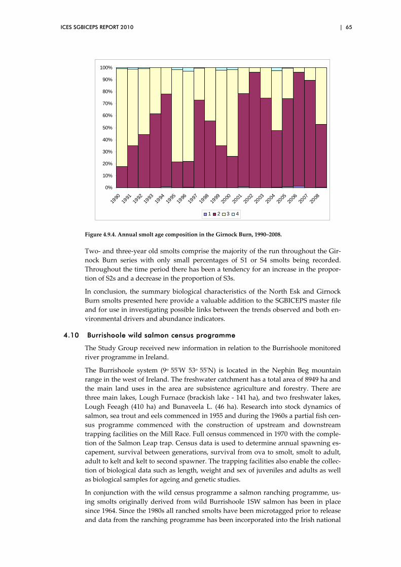
ICES SGBICEPS REPORT 2010 | 65
0%
10%
20%
30%
40%
50%
60%
70%
80%
90%
100%
1990
1991
1992
1993
1994
1995
1996
1997
1998
1999
2000
2001
2002
2003
2004
2005
2006
2007
2008
1 2 3 4
Figure 4.9.4. Annual smolt age composition in the Girnock Burn, 1990–2008.
Two‐ and three‐year old smolts comprise the majority of the run throughout the Gir‐
nock Burn series with only small percentages of S1 or S4 smolts being recorded.
Throughout the time period there has been a tendency for an increase in the propor‐
tion of S2s and a decrease in the proportion of S3s.
In conclusion, the summary biological characteristics of the North Esk and Girnock
Burn smolts presented here provide a valuable addition to the SGBICEPS master file
and for use in investigating possible links between the trends observed and both en‐
vironmental drivers and abundance indicators.
4.10 Burrishoole wild salmon census programme
The Study Group received new information in relation to the Burrishoole monitored
river programme in Ireland.
The Burrishoole system (9o 55ʹW 53o 55ʹN) is located in the Nephin Beg mountain
range in the west of Ireland. The freshwater catchment has a total area of 8949 ha and
the main land uses in the area are subsistence agriculture and forestry. There are
three main lakes, Lough Furnace (brackish lake ‐ 141 ha), and two freshwater lakes,
Lough Feeagh (410 ha) and Bunaveela L. (46 ha). Research into stock dynamics of
salmon, sea trout and eels commenced in 1955 and during the 1960s a partial fish cen‐
sus programme commenced with the construction of upstream and downstream
trapping facilities on the Mill Race. Full census commenced in 1970 with the comple‐
tion of the Salmon Leap trap. Census data is used to determine annual spawning es‐
capement, survival between generations, survival from ova to smolt, smolt to adult,
adult to kelt and kelt to second spawner. The trapping facilities also enable the collec‐
tion of biological data such as length, weight and sex of juveniles and adults as well
as biological samples for ageing and genetic studies.
In conjunction with the wild census programme a salmon ranching programme, us‐
ing smolts originally derived from wild Burrishoole 1SW salmon has been in place
since 1964. Since the 1980s all ranched smolts have been microtagged prior to release
and data from the ranching programme has been incorporated into the Irish national
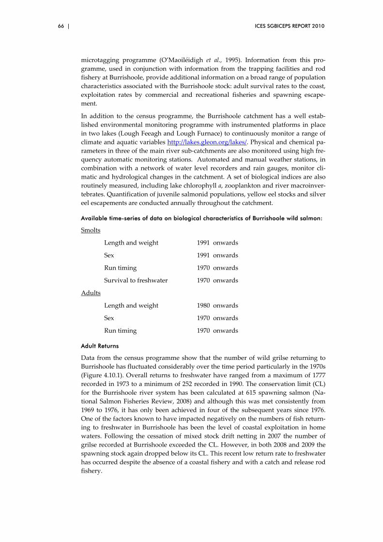
66 | ICES SGBICEPS REPORT 2010
microtagging programme (O’Maoiléidigh et al., 1995). Information from this pro‐
gramme, used in conjunction with information from the trapping facilities and rod
fishery at Burrishoole, provide additional information on a broad range of population
characteristics associated with the Burrishoole stock: adult survival rates to the coast,
exploitation rates by commercial and recreational fisheries and spawning escape‐
ment.
In addition to the census programme, the Burrishoole catchment has a well estab‐
lished environmental monitoring programme with instrumented platforms in place
in two lakes (Lough Feeagh and Lough Furnace) to continuously monitor a range of
climate and aquatic variables http://lakes.gleon.org/lakes/. Physical and chemical pa‐
rameters in three of the main river sub‐catchments are also monitored using high fre‐
quency automatic monitoring stations. Automated and manual weather stations, in
combination with a network of water level recorders and rain gauges, monitor cli‐
matic and hydrological changes in the catchment. A set of biological indices are also
routinely measured, including lake chlorophyll a, zooplankton and river macroinver‐
tebrates. Quantification of juvenile salmonid populations, yellow eel stocks and silver
eel escapements are conducted annually throughout the catchment.
Available time-series of data on biological characteristics of Burrishoole wild salmon:
Smolts
Length and weight 1991 onwards
Sex 1991 onwards
Run timing 1970 onwards
Survival to freshwater 1970 onwards
Adults
Length and weight 1980 onwards
Sex 1970 onwards
Run timing 1970 onwards
Adult Returns
Data from the census programme show that the number of wild grilse returning to
Burrishoole has fluctuated considerably over the time period particularly in the 1970s
(Figure 4.10.1). Overall returns to freshwater have ranged from a maximum of 1777
recorded in 1973 to a minimum of 252 recorded in 1990. The conservation limit (CL)
for the Burrishoole river system has been calculated at 615 spawning salmon (Na‐
tional Salmon Fisheries Review, 2008) and although this was met consistently from
1969 to 1976, it has only been achieved in four of the subsequent years since 1976.
One of the factors known to have impacted negatively on the numbers of fish return‐
ing to freshwater in Burrishoole has been the level of coastal exploitation in home
waters. Following the cessation of mixed stock drift netting in 2007 the number of
grilse recorded at Burrishoole exceeded the CL. However, in both 2008 and 2009 the
spawning stock again dropped below its CL. This recent low return rate to freshwater
has occurred despite the absence of a coastal fishery and with a catch and release rod
fishery.
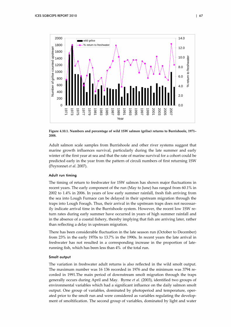
ICES SGBICEPS REPORT 2010 | 67
0
200
400
600
800
1000
1200
1400
1600
1800
2000
19
71
19
73
19
75
19
77
19
79
19
81
19
83
19
85
19
87
19
89
19
91
19
93
19
95
19
97
19
99
20
01
20
03
20
05
20
07
Year
Nu
mb
er
of g
rils
e c
ou
nte
d u
pst
rea
m
0.0
2.0
4.0
6.0
8.0
10.0
12.0
14.0
% r
etu
rn to
fre
shw
ate
r
wild grilse
% return to freshwater
Figure 4.10.1. Numbers and percentage of wild 1SW salmon (grilse) returns to Burrishoole, 1971–
2008.
Adult salmon scale samples from Burrishoole and other river systems suggest that
marine growth influences survival, particularly during the late summer and early
winter of the first year at sea and that the rate of marine survival for a cohort could be
predicted early in the year from the pattern of circuli numbers of first returning 1SW
(Peyronnet et al. 2007).
Adult run timing
The timing of return to freshwater for 1SW salmon has shown major fluctuations in
recent years. The early component of the run (May to June) has ranged from 60.1% in
2002 to 1.4% in 2006. In years of low early summer rainfall, fresh fish arriving from
the sea into Lough Furnace can be delayed in their upstream migration through the
traps into Lough Feeagh. Thus, their arrival in the upstream traps does not necessar‐
ily indicate arrival time in the Burrishoole system. However, the recent low 1SW re‐
turn rates during early summer have occurred in years of high summer rainfall and
in the absence of a coastal fishery, thereby implying that fish are arriving later, rather
than reflecting a delay in upstream migration.
There has been considerable fluctuation in the late season run (October to December)
from 23% in the early 1970s to 13.7% in the 1990s. In recent years the late arrival in
freshwater has not resulted in a corresponding increase in the proportion of late‐
running fish, which has been less than 4% of the total run.
Smolt output
The variation in freshwater adult returns is also reflected in the wild smolt output.
The maximum number was 16 136 recorded in 1976 and the minimum was 3794 re‐
corded in 1991.The main period of downstream smolt migration through the traps
generally occurs during April and May. Byrne et al. (2003), identified two groups of
environmental variables which had a significant influence on the daily salmon smolt
output. One group of variables, dominated by photoperiod and temperature, oper‐
ated prior to the smolt run and were considered as variables regulating the develop‐
ment of smoltification. The second group of variables, dominated by light and water
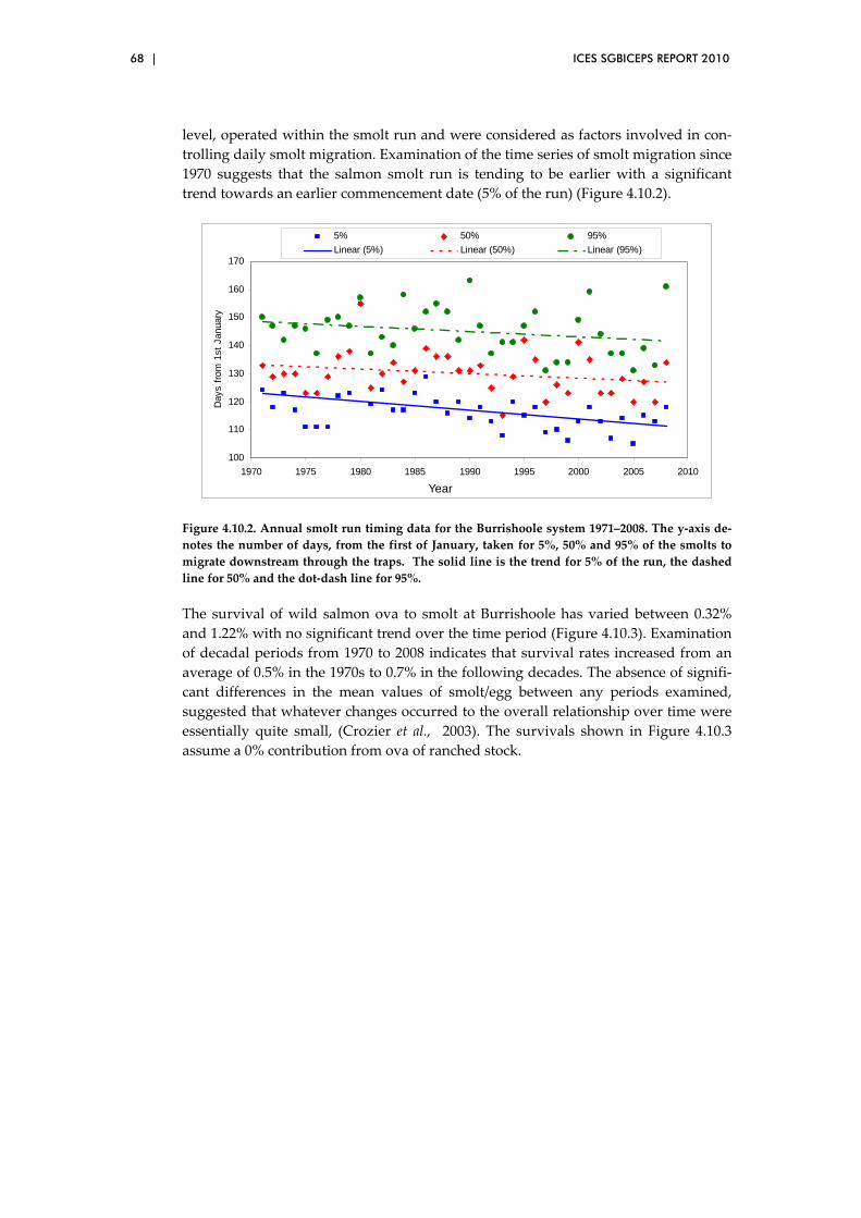
68 | ICES SGBICEPS REPORT 2010
level, operated within the smolt run and were considered as factors involved in con‐
trolling daily smolt migration. Examination of the time series of smolt migration since
1970 suggests that the salmon smolt run is tending to be earlier with a significant
trend towards an earlier commencement date (5% of the run) (Figure 4.10.2).
100
110
120
130
140
150
160
170
1970 1975 1980 1985 1990 1995 2000 2005 2010
Year
Day
s fr
om 1
st J
anua
ry
5% 50% 95%
Linear (5%) Linear (50%) Linear (95%)
Figure 4.10.2. Annual smolt run timing data for the Burrishoole system 1971–2008. The y‐axis de‐
notes the number of days, from the first of January, taken for 5%, 50% and 95% of the smolts to
migrate downstream through the traps. The solid line is the trend for 5% of the run, the dashed
line for 50% and the dot‐dash line for 95%.
The survival of wild salmon ova to smolt at Burrishoole has varied between 0.32%
and 1.22% with no significant trend over the time period (Figure 4.10.3). Examination
of decadal periods from 1970 to 2008 indicates that survival rates increased from an
average of 0.5% in the 1970s to 0.7% in the following decades. The absence of signifi‐
cant differences in the mean values of smolt/egg between any periods examined,
suggested that whatever changes occurred to the overall relationship over time were
essentially quite small, (Crozier et al., 2003). The survivals shown in Figure 4.10.3
assume a 0% contribution from ova of ranched stock.
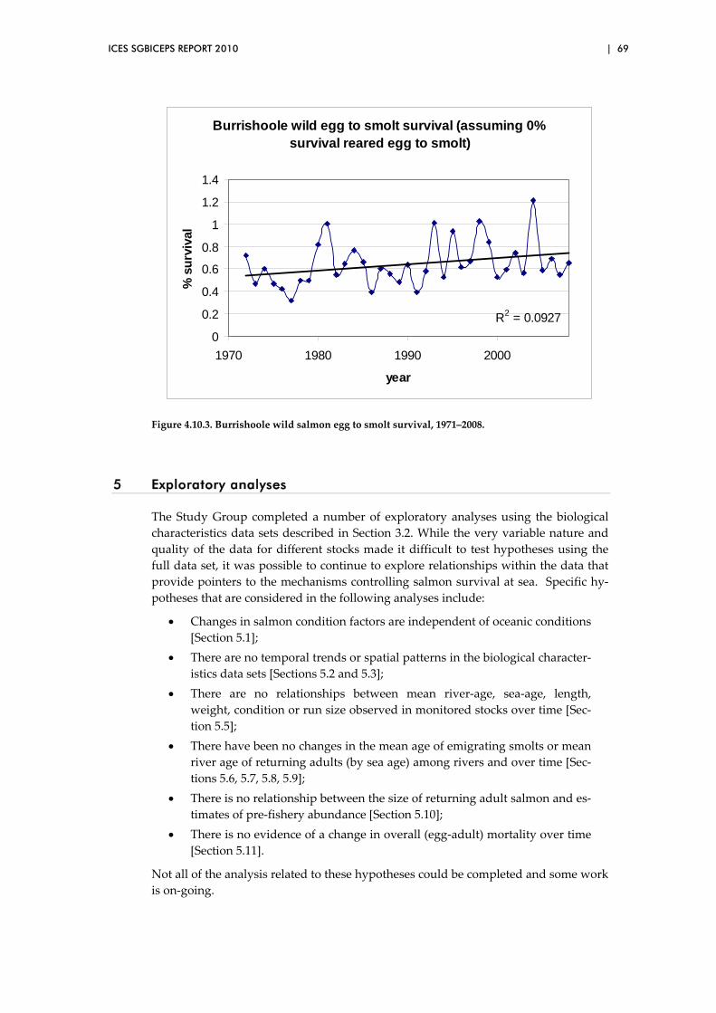
ICES SGBICEPS REPORT 2010 | 69
Burrishoole wild egg to smolt survival (assuming 0% survival reared egg to smolt)
R2 = 0.0927
0
0.2
0.4
0.6
0.8
1
1.2
1.4
1970 1980 1990 2000
year
% s
urv
ival
Figure 4.10.3. Burrishoole wild salmon egg to smolt survival, 1971–2008.
5 Exploratory analyses
The Study Group completed a number of exploratory analyses using the biological
characteristics data sets described in Section 3.2. While the very variable nature and
quality of the data for different stocks made it difficult to test hypotheses using the
full data set, it was possible to continue to explore relationships within the data that
provide pointers to the mechanisms controlling salmon survival at sea. Specific hy‐
potheses that are considered in the following analyses include:
Changes in salmon condition factors are independent of oceanic conditions
[Section 5.1];
There are no temporal trends or spatial patterns in the biological character‐
istics data sets [Sections 5.2 and 5.3];
There are no relationships between mean river‐age, sea‐age, length,
weight, condition or run size observed in monitored stocks over time [Sec‐
tion 5.5];
There have been no changes in the mean age of emigrating smolts or mean
river age of returning adults (by sea age) among rivers and over time [Sec‐
tions 5.6, 5.7, 5.8, 5.9];
There is no relationship between the size of returning adult salmon and es‐
timates of pre‐fishery abundance [Section 5.10];
There is no evidence of a change in overall (egg‐adult) mortality over time
[Section 5.11].
Not all of the analysis related to these hypotheses could be completed and some work
is on‐going.

70 | ICES SGBICEPS REPORT 2010
5.1 Analyses of long-term variation in condition factor in relation to ocean climate
The Study Group reviewed information on salmon condition factor during the first
meeting of the SGBICEPS group and recommended further investigation (ICES,
2009a). Initial analyses (1993–2006) of condition factor variation in relation to ocean
climate change (Todd et al., 2008) involved interrogation of Marine Scotland time‐
series for salmon from the mixed stock fishery at Strathy Point (N. Scotland) and the
in‐river net fishery on the River North Esk (E Scotland). Those analyses included only
1SW fish and were constrained by the netting season to the period late June–end Au‐
gust. Analyses of sea surface temperature (SST) variations focused on the Norwegian
Sea (67.5°N 4.5°E) and utilised the NOAA OISSTv2 SST database, which is based
upon a combination of satellite telemetry and in situ recordings. This time‐series
dates from December 1980 and is available on a monthly basis, and with a gridded
resolution of one degree latitude/longitude.
Analyses of condition factor variation and ocean climate (SST) are ongoing and pres‐
ently include both 1SW and 2SW fish and multiple rivers in Scotland (Tweed, Tay,
Spey, North Esk) and Wales (Dee) as well as three rivers from southern, central and
northern Norway. These data will permit analysis of salmon time‐series from NEAC
southern and northern populations, some of which date back to the early 1960s. With
the incorporation of data for 2SW fish, SST analyses have had to be extended to the
western North Atlantic in order to include the foraging areas of coastal Greenland
and are not yet complete.
One complication of this analytical extension of condition factor lies in the choice of
SST database. OISSTv2 is not available prior to 1980 and alternatives must be sought.
The ERSST, Kaplan and HadSST time‐series have been investigated and, although
they share common data, they differ in how the data have been processed and inter‐
polated to provide gridded predictions for data‐poor areas of ocean, or periods of
missing values. As a generalisation, all these databases show closely similar trends in
SST variation over time, but they differ in the monthly and spatial detail.
SST time‐series present analytical difficulties because of the problem of autocorrela‐
tion – that is, if it is anomalously warm in one month it probably will be also in the
preceding and succeeding months. The monthly SST anomaly values are not, there‐
fore, independent. The outcomes of our analyses (such as whether or not there is a
significant correlation between ocean climate change and salmon condition) rely ul‐
timately on the correlations derived not for the raw SST anomalies, but for their re‐
siduals (i.e. departures of actual monthly observations from the predicted, or
smoothed, trend values). Because these databases often show slightly different SST
values for a given grid box in a given month, the residuals derived by de‐trending in
order to remove autocorrelation are not the same. As a consequence, the different SST
databases ultimately yield different residuals and final analytical outcomes, when
correlated with the residuals from de‐trending (smoothing) the salmon condition fac‐
tor time‐series. That is to say, depending upon the selected SST database, the final
analytical outcome (e.g. a correlation between ocean warming and salmon condition
factor) will differ.

ICES SGBICEPS REPORT 2010 | 71
OISST 250 km kernel (x axis) versus HadSST2 250 km kernel (y axis) RESIDUALS
y = 1.0281x - 2E-05
R2 = 0.6376
-0.8
-0.6
-0.4
-0.2
0
0.2
0.4
0.6
0.8
1
-0.60 -0.40 -0.20 0.00 0.20 0.40 0.60 0.80
OISST 250 km kernel (x axis) versus ERSST 250 km kernel (y axis) RESIDUALS
y = 0.1716x - 7E-05
R2 = 0.1214
-0.3
-0.25
-0.2
-0.15
-0.1
-0.05
0
0.05
0.1
0.15
0.2
0.25
-0.60 -0.40 -0.20 0.00 0.20 0.40 0.60 0.80
OISST 250 km kernel (x axis) versus Kaplan 250 km kernel (y axis) RESIDUALS
y = 0.519x - 7E-05
R2 = 0.3387
-0.6
-0.4
-0.2
0
0.2
0.4
0.6
0.8
-0.60 -0.40 -0.20 0.00 0.20 0.40 0.60 0.80
Figure 5.1.1. Correlations of residuals for OISSTv2 versus HadSST2, ERSST and Kaplan Sea Sur‐
face Temperature databases for the eastern North Atlantic. Monthly values (December 1980 –
March 2008) are temperature anomalies derived from de‐trending (smoothing) the average tem‐
perature recorded for a spatial kernel of standard deviation 250 km, and centred on the grid box at
67.5°N 4.5°E. The residuals are the observed monthly departures from the smoothed (de‐trended)
time‐series.
This problem has been investigated in detail by Hughes et al. (2009). They affirmed
the differences inherent in the data comprising various time‐series. For example, they
noted that particularly prominent monthly SST anomalies in the North Sea could be
up to 6 months apart in different time‐series. Discrepancies in the residuals of the
magnitude illustrated in Figure 5.1.1, and in such timing of unusually anomalous
events (Hughes et al., 2009), present considerable analytical and interpretational chal‐
lenges. For analyses post‐December 1980, the OISST series probably remains the da‐
tabase of choice. Hughes et al. (2009) noted generally good concordance of HadSST2
to OISSTv2 and in situ observations, though HadSST2 did commonly show marked
discrepancies at high latitude in the Arctic, perhaps due to sea ice. One solution to
this seemingly intractable problem might be to undertake an ensemble analysis with
the salmon condition factor time‐series that incorporates all the varying SST data‐
bases. This is subject to ongoing investigation.
5.2 Biological characteristics data sets – temporal trends
At the first Study Group meeting, preliminary examination of the various stock‐
specific data sets indicated substantial evidence of variability in different biological
characteristics both over time and among stocks (ICES, 2009a). These data sets were
subsequently analysed using the non‐parametric Mann‐Kendall statistic (Mann, 1945;
Kendall, 1975) and the statistical programming environment R (R Development Core
Team, 2007) to investigate possible time trends. One of the reasons this method was
selected was that it does not assume any particular functional form for the trend (e.g.
linear, exponential). These initial analyses were performed over a standardised time
period starting from 1984 and extending to the most recently available data, typically
2007 (ICES, 2009a).

72 | ICES SGBICEPS REPORT 2010
At, and subsequent to, the second meeting, a number of additional data sets were
made available; a number of which had slightly shorter time series (see details in Sec‐
tion 3.2). The Mann‐Kendall statistic was once again used to investigate the time
trends in these extended data sets, but over a standardised time period starting from
1989 and extending to the most recently available data (mainly 2008). A number of
the data sets were also updated at the second meeting with the addition of data from
the most recent year(s).
Essentially, the Mann‐Kendall statistic assesses each data point and counts the num‐
ber of data points in future years that exceed it (assigned +1) and also the number that
are less (assigned ‐1). These values are summed over all data points. Thus, if there are
n observations in the time series kY (k=1,...,n) then the statistic is:
),(1 1
j
n
k
n
kjk YYIM
where I(,) is an indicator variable defined by the sign of jk YYD . If D is positive
then I = 1, if D is negative then I = ‐1, if D = 0 then I = 0.
The null distribution of the statistic M (i.e. assuming no trend) was calculated by
Monte‐Carlo simulation. The observations were re‐ordered at random so that they
were potentially assigned to different years and the value of M calculated. This was
repeated 1000 times. These values of M under the null hypothesis were compared
against the observed value of M to estimate the p‐value (Manly, 2001).
The null hypothesis was that there is no trend. It was recognised that a potential
problem with this approach is that it does not taken account of any correlation be‐
tween successive or neighbouring years. The presence of such correlations might af‐
fect the p‐values obtained and may require further consideration in future.
The results are presented in Table 5.2.1 Missing values indicate no time series avail‐
able; ‘o’ indicates a non statistically significant trend (P>0.05); ‘‐‘ is a negative trend
(p<0.05); and ‘+’ is a positive trend (p<0.05). It is evident that there are significant
trends over time for many of the variables explored.

ICES SGBICEPS REPORT 2010 | 73
Table 5.2.1. Trends in biological characteristics over time: ‘o’ means not enough evidence at the
5% level to detect a trend. ‘+’ is a positive trend (p>0.05), ‘‐‘ is a negative trend (p<0.05).
Stock complex
Country
Stock
Hatchery/Wild
Time series
Latitude
Stock status
Median run date
Mean run date
River age mean
Sea age mean
Prop. 1SW
in run
Prop. 2SW
in run
Prop. PS in run
1SW
length
1SW
weight
1SW
condition
2SW
length
2SW
weight
2SW
condition
PS length
PS weight
PS condition
Prop. fem
ale in 1SW
Prop. fem
ale in 2SW
Prop fem
ale in PS
Prop maiden
in 1SW
Prop maiden
in 2SW
NAC (N) Canada Western Arm Brook W 1971‐06 51.2 + ‐ 0 ‐ + 0 0 0 + + + ‐ 0 + + + 0 0 0 0 0 0
Canada De la Trinité W 1980‐09 49.4 ‐ ‐ 0 + + + 0 + + 0 + 0 0 + + 0
Canada Saint‐Jean W 1981‐09 48.8 0 + ‐ 0 + + ‐ + 0 0 + 0 0 0 + 0
Canada Middle Brook W 1975‐05 48.8 0 0 ‐ 0 0 0 0 0 + + 0 + + 0 ‐ 0 0 0
Canada Conne River W 1986‐06 47.9 ‐ 0 0 0 + ‐ + + + + 0 0 0 0 0 0 0 0 ‐ +
Canada Miramichi W 1971‐07 47.0 ‐ ‐ + 0 0 + + 0 ‐ + 0 0 + + 0 ‐ + + 0 0
NAC (S) Canada Nashwaak W 1972‐08 46.0 0 0 0 ‐ ‐ + ‐ 0 + 0 0 + ‐
Canada St John (Mactaquac) W 1978‐08 45.3 ‐ ‐ ‐ ‐ ‐ + ‐ 0 0 0 0 ‐ ‐ 0 0 + ‐
Canada St John (Mactaquac) H 1978‐08 45.3 ‐ ‐ ‐ ‐ ‐ + ‐ 0 0 0 ‐ ‐ ‐ 0 0 + ‐
Canada La Have W 1972‐08 44.4 0 ‐ 0 + 0 0 0 0 0 + + 0 + + 0 0 + 0 + + 0 0
Canada La Have H 1972‐08 44.4 ‐ 0 0 ‐ 0 0 0 0 0 + + 0 + + 0 + 0 0 + 0 0 0
USA Penobscot H 1978‐08 44.5 ‐ ‐ ‐ 0 ‐ + ‐ 0 0 + + 0 0 + 0 0 0 ‐ + 0 + ‐
N NEAC Finland/Norway Teno W 1972‐07 70.8 0 + ‐ 0 0 + 0 0 0 0 0 0 0 0 0 0 0 ‐
Finland/Norway Näätämöjoki W 1975‐06 69.7 0 + ‐ + 0 0 + 0 0 0 0 0 0 0 ‐ 0 ‐ 0
Russia Tuloma W 1983‐08 68.9 0 0 + ‐ 0 0 0 0 0 0 0 ‐ ‐ 0 0 0 0 0 0 0 + 0
Norway Vestre Jakobselv W 1989‐08 70.1 + ‐ 0 0 + 0 0 0 ‐ ‐ ‐ ‐
Norway Årgårdsvassdraget W 1992‐08 64.3 ‐ 0 0 ‐ + 0 0 0 0 0 ‐ 0 0 0 0
Norway Nausta W 1989‐08 61.3 0 0 + ‐ + 0 0 0 ‐ 0 0 0
Norway Gaula Sogn og Fjordane W 1989‐08 61.2 0 0 + ‐ + 0 0 ‐ 0 0 ‐ ‐
Norway Etneelva W 1989‐08 59.4 ‐ ‐ 0 ‐ 0 0 0 0 ‐ ‐ ‐ 0
Norway Skienselva W 1989‐08 59.1 0 0 + ‐ + + 0 0 0 0 0 ‐ .
Norway Numedalslågen W 1989‐08 59.1 0 0 0 0 0 0 0 0 ‐ ‐ ‐ ‐
Norway Enningdalselva W 1990‐08 58.6 0 ‐ + ‐ + 0 0 ‐ 0 0 0 0
Norway Gaula W 1989‐08 63.3 0 ‐ 0 0 0 + 0 0 0 ‐ 0 0 0 0 0
Iceland (N&E) Laxa I Adaldalur W 1974‐08 65.6 ‐ ‐ + ‐ 0 0 ‐
Iceland (N&E) Hofsa W 1971‐08 65.4 ‐ ‐ + ‐ ‐ ‐ 0 +
S NEAC Iceland (S&W) Nordura W 1968‐08 64.6 ‐ ‐ + ‐ ‐ ‐ 0 +
Iceland (S&W) Ellidaar W 1949‐08 64.1 ‐ ‐ + ‐ ‐ ‐ + 0
UK (Scot) N. Esk W 1981‐08 56.7 0 0 0 ‐ ‐ ‐ 0 ‐ 0
UK (NI) Bush W 1973‐07 55.1 ‐ + 0 0 0 0 ‐ 0 ‐ ‐ + 0 0 0 0 0 0 0 0 0 + ‐
UK (E&W) Lune W 1987‐08 54.0 0 0 0 0 0 0 0 0 0 ‐ 0
UK (E&W) Dee W 1937‐08 53.4 ‐ ‐ ‐ + ‐ 0 0 + + + + + ‐ ‐ ‐ 0 + 0
UK (E&W) Wye W 1910‐07 51.6 0 + ‐ ‐ + + ‐ + + 0 0 0 0 ‐ ‐ 0
UK (E&W) Frome W 1968‐08 50.7 ‐ ‐ 0 0
France Bresle W 1984‐08 50.1 0 0 0 0 0 0
Baltic Sweden Kalix W 1980‐08 65.8 +
Finland/Sweden Tornionjoki W 1980‐09 65.5 0 ‐ + 0 0 0 0 0 ‐
Sweden Ume/Vindel W 1987‐08 63.8 + + 0
Sweden Ume/Vindel H 1974‐08 63.8 0 0 0 0 0 0 0 + + 0 +
Summary ‐ all areas No. of stocks for which data available 33 13 14 32 32 36 36 27 31 32 28 30 31 26 17 17 17 23 22 15 13 13
No. of stocks with significant declining trend 12 5 4 18 12 9 11 1 2 7 7 7 13 6 2 2 2 3 2 1 1 6
No. of stocks with significant increasing trend 4 2 2 3 7 12 9 6 8 11 6 5 5 5 5 4 1 2 10 2 6 1
No. of stocks with no significant trend 17 6 8 11 13 15 16 20 21 14 15 18 13 15 10 11 14 18 10 12 6 6
% of stocks with significant declining trend 36 38 29 56 38 25 31 4 6 22 25 23 42 23 12 12 12 13 9 7 8 46
% of stocks with significant increasing trend 12 15 14 9 22 33 25 22 26 34 21 17 16 19 29 24 6 9 45 13 46 8
% of stocks with no significant trend 52 46 57 34 41 42 44 74 68 44 54 60 42 58 59 65 82 78 45 80 46 46
5.3 Biological characteristics data sets – spatial patterns
At the first meeting, the Study Group examined two approaches for assessing pat‐
terns in the changes in biological characteristics over broader spatial scales (ICES,
2009a). The first approach used a standardised (z‐score) analysis to examine the trend
in mean smolt age, by way of an example, for different stock complexes. The second
approach used meta‐analysis. The latter technique was applied to all the biological
characteristics variables. The z‐score and meta analysis approaches provided broadly
consistent results in respect of smolt age. Subsequent to the second meeting, the meta
analysis was repeated using the extended data set available at that time.
The meta‐analysis approach statistically combines the results of several studies (in
this case different rivers) to address a shared research hypothesis. Just as individual
studies summarise data collected from many participants in order to answer a spe‐
cific research question (i.e. each participant is a separate data‐point in the analysis), a
meta‐analysis summarises data from individual studies that concern a specific re‐
search question (i.e. each study is a separate data‐point in the analysis).
This is normally done by identification of a common measure of effect size. An effect
size is a statistical measure portraying the degree to which a given event is present in
a sample (Cohen, 1969). The type of measure (e.g. standardized mean difference) is
called the effect, and its magnitude is considered an effect size. Different measures of
effect size are calculated for different types of primary data, commonly modelled us‐
ing a form of meta‐regression. In this instance, all effect sizes were calculated from

74 | ICES SGBICEPS REPORT 2010
Pearson correlation coefficients between a given variable and year. Resulting overall
averages when controlling for study characteristics can be considered meta‐effect
sizes, which are more powerful estimates of the true effect size than those derived in
a single study under a given single set of assumptions and conditions.
Fail‐Safe Tests were also applied in these analyses. These tests are statistical methods
for estimating the magnitude of the publication bias known as the file‐drawer problem
(Rosenthal, 1979). These techniques calculate the number of non‐significant, unpub‐
lished studies (having effect size = 0) that need to be added to a summary analysis in
order to change the results from significant to non‐significant. A large fail‐safe num‐
ber indicates that many unpublished studies are required to change the statistical re‐
sults, and thus one may be more confident in the results from the summary analysis.
Thus, for example, in the case of mean river age (Figure 5.3.1) we need 551.9 rivers
showing no correlation (r = 0) in order to say that there is no overall change in mean
river age.
The following stock complex groupings were used in the meta analysis [N.B. the
standard WGNAS abbreviations NAC (North American Commission) and NEAC
(North East Atlantic Commission) have been applied]:
Baltic – rivers draining into the Baltic Sea.
Northern NAC ‐ Rivers Western Arm Brook, Middle Brook, Conne and
Miramichi. [N.B. The data for the De La Trinité and Saint‐Jean rivers (in‐
cluded in other analyses) were not available at the time that the meta
analysis was undertaken and have been excluded here.]
Southern NAC ‐ Rivers Nashwaak, St John (Mactaquac), La Have and Pe‐
nobscot.
Northern NEAC north – rivers in Russia, Norway, Finland and Iceland
(N&E).
Southern NEAC south ‐ rivers in UK, Ireland, France and Iceland (S&W).
This approach was used to explore relationships for most of the available biological
characteristics and a selection of results appears in Figure 5.3.1. These provide the
central tendencies (means) for five stock groups and the total effect – if the error bar
crosses the vertical zero‐line the effect is non significant at the p = 0.05‐level. These
analyses were performed over a standardised time period starting from 1989 and ex‐
tending to the most recently available data, typically 2008. All available data were
included, although the completeness of the data sets varied considerably for the dif‐
ferent biological characteristics, as indicated in Table 3.2.1. Median and mean run
dates were converted to day of the year prior to analysis.
All the results arising from the meta analysis are summarised in Table 5.3.1 (where ‘o’
denotes a non‐significant relationship, ‘+’ indicates a significant increase relative to
the mean and ‘‐‘ denotes a significant decrease). These analyses indicated a number
of significant trends over time for certain variables at the stock complex level (Table
5.3.2).
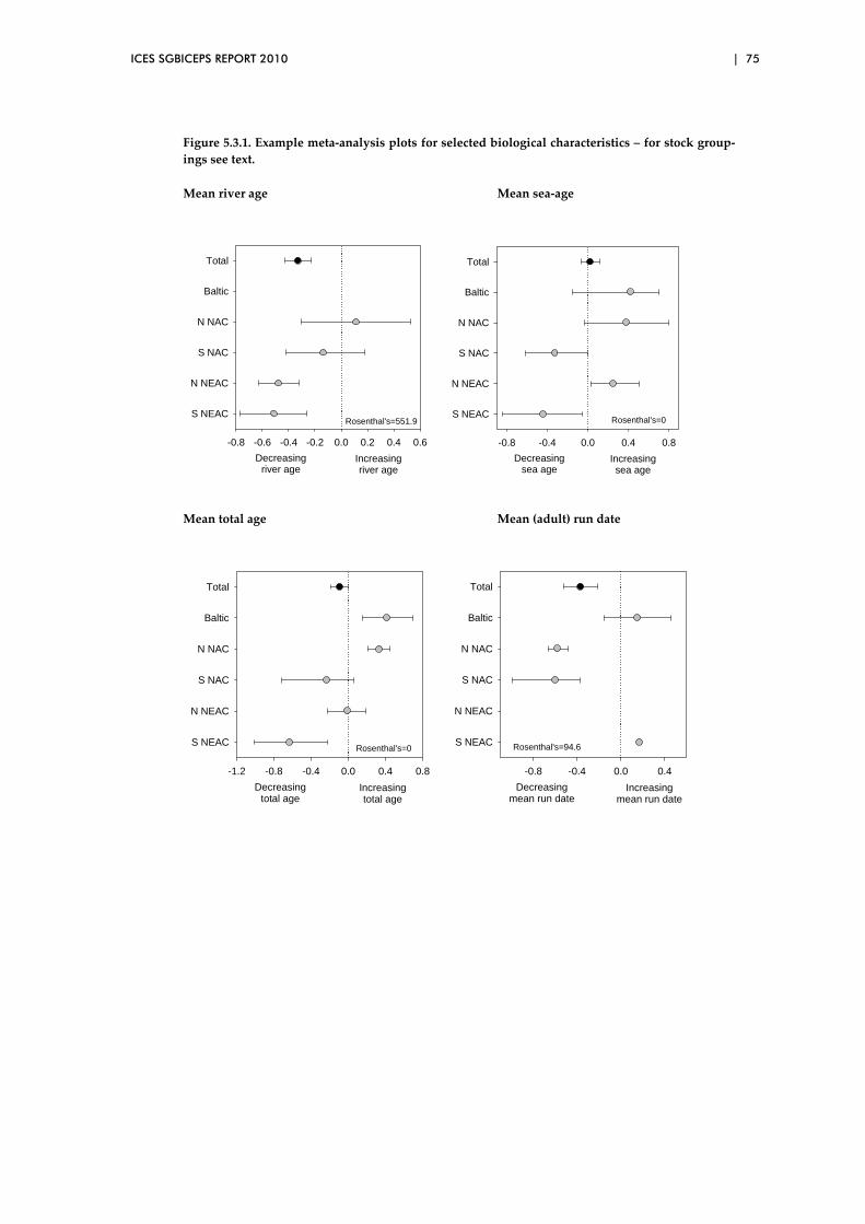
ICES SGBICEPS REPORT 2010 | 75
Figure 5.3.1. Example meta‐analysis plots for selected biological characteristics – for stock group‐
ings see text.
Mean river age Mean sea‐age
-0.8 -0.6 -0.4 -0.2 0.0 0.2 0.4 0.6
S NEAC
N NEAC
S NAC
N NAC
Baltic
Total
Rosenthal's=551.9
Decreasingriver age
Increasingriver age
-0.8 -0.4 0.0 0.4 0.8
S NEAC
N NEAC
S NAC
N NAC
Baltic
Total
Rosenthal's=0
Decreasingsea age
Increasingsea age
Mean total age Mean (adult) run date
-1.2 -0.8 -0.4 0.0 0.4 0.8
S NEAC
N NEAC
S NAC
N NAC
Baltic
Total
Rosenthal's=0
Decreasingtotal age
Increasingtotal age
-0.8 -0.4 0.0 0.4
S NEAC
N NEAC
S NAC
N NAC
Baltic
Total
Rosenthal's=94.6
Decreasingmean run date
Increasingmean run date
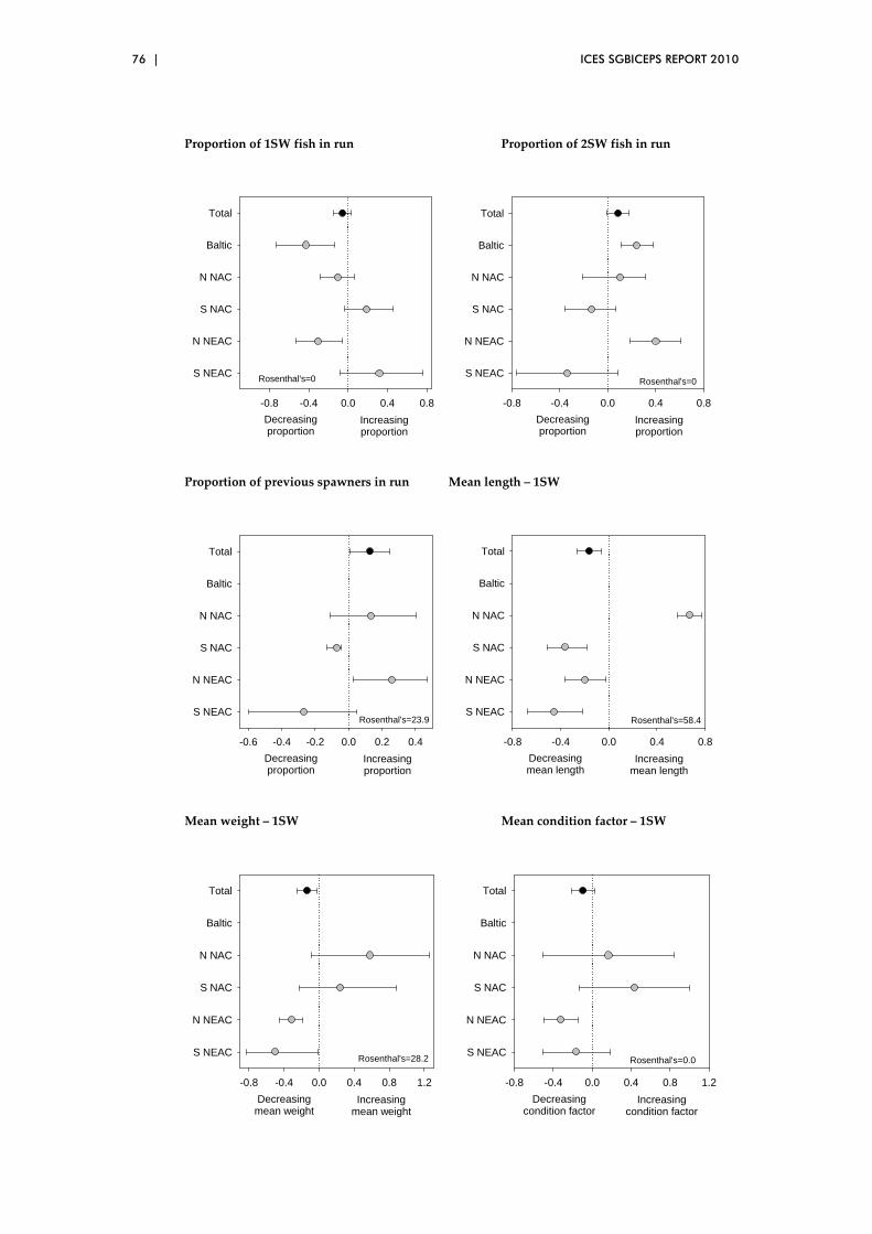
76 | ICES SGBICEPS REPORT 2010
Proportion of 1SW fish in run Proportion of 2SW fish in run
-0.8 -0.4 0.0 0.4 0.8
S NEAC
N NEAC
S NAC
N NAC
Baltic
Total
Rosenthal's=0
Decreasingproportion
Increasingproportion
-0.8 -0.4 0.0 0.4 0.8
S NEAC
N NEAC
S NAC
N NAC
Baltic
Total
Rosenthal's=0
Decreasingproportion
Increasingproportion
Proportion of previous spawners in run Mean length – 1SW
-0.6 -0.4 -0.2 0.0 0.2 0.4
S NEAC
N NEAC
S NAC
N NAC
Baltic
Total
Rosenthal's=23.9
Decreasingproportion
Increasingproportion
-0.8 -0.4 0.0 0.4 0.8
S NEAC
N NEAC
S NAC
N NAC
Baltic
Total
Rosenthal's=58.4
Decreasingmean length
Increasingmean length
Mean weight – 1SW Mean condition factor – 1SW
-0.8 -0.4 0.0 0.4 0.8 1.2
S NEAC
N NEAC
S NAC
N NAC
Baltic
Total
Rosenthal's=28.2
Decreasingmean weight
Increasingmean weight
-0.8 -0.4 0.0 0.4 0.8 1.2
S NEAC
N NEAC
S NAC
N NAC
Baltic
Total
Rosenthal's=0.0
Decreasingcondition factor
Increasingcondition factor
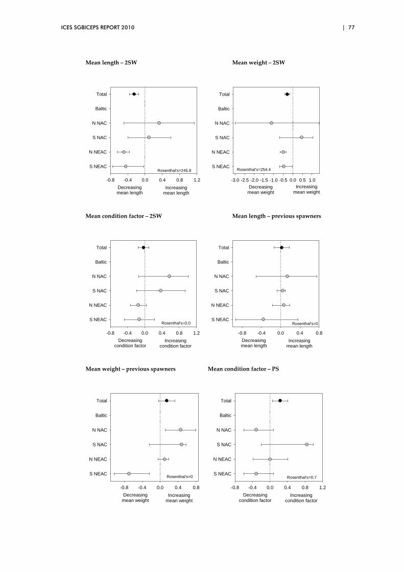
ICES SGBICEPS REPORT 2010 | 77
Mean length – 2SW Mean weight – 2SW
-0.8 -0.4 0.0 0.4 0.8 1.2
S NEAC
N NEAC
S NAC
N NAC
Baltic
Total
Rosenthal's=245.8
Decreasingmean length
Increasingmean length
-3.0 -2.5 -2.0 -1.5 -1.0 -0.5 0.0 0.5 1.0
S NEAC
N NEAC
S NAC
N NAC
Baltic
Total
Rosenthal's=254.4
Decreasingmean weight
Increasingmean weight
Mean condition factor – 2SW Mean length – previous spawners
-0.8 -0.4 0.0 0.4 0.8 1.2
S NEAC
N NEAC
S NAC
N NAC
Baltic
Total
Rosenthal's=0.0
Decreasingcondition factor
Increasingcondition factor
-0.8 -0.4 0.0 0.4 0.8
S NEAC
N NEAC
S NAC
N NAC
Baltic
Total
Rosenthal's=0
Decreasingmean length
Increasingmean length
Mean weight – previous spawners Mean condition factor – PS
-0.8 -0.4 0.0 0.4 0.8
S NEAC
N NEAC
S NAC
N NAC
Baltic
Total
Rosenthal's=0
Decreasingmean weight
Increasingmean weight
-0.8 -0.4 0.0 0.4 0.8 1.2
S NEAC
N NEAC
S NAC
N NAC
Baltic
Total
Rosenthal's=0.7
Decreasingcondition factor
Increasingcondition factor

78 | ICES SGBICEPS REPORT 2010
Prop. female – 1SW Prop. female – 2SW
-0.6 -0.4 -0.2 0.0 0.2 0.4
S NEAC
N NEAC
S NAC
N NAC
Baltic
Total
Rosenthal's=0
Decreasingproportion
Increasingproportion
-0.8 -0.6 -0.4 -0.2 0.0 0.2 0.4 0.6 0.8
S NEAC
N NEAC
S NAC
N NAC
Baltic
Total
Rosenthal's=0
Decreasingproportion
Increasingproportion
Prop. female – previous spawners Prop. maiden spawners – 1SW
-0.4 -0.2 0.0 0.2 0.4 0.6
S NEAC
N NEAC
S NAC
N NAC
Baltic
Total
Rosenthal's=0
Decreasingproportion
Increasingproportion
-0.4 -0.2 0.0 0.2 0.4
S NEAC
N NEAC
S NAC
N NAC
Baltic
Total
Rosenthal's=0
Decreasingproportion
Increasingproportion
Prop. maiden spawners – 2SW Stock size – 1SW
-0.4 -0.2 0.0 0.2 0.4
S NEAC
N NEAC
S NAC
N NAC
Baltic
Total
Rosenthal's=0
Decreasingproportion
Increasingproportion
-0.8 -0.6 -0.4 -0.2 0.0 0.2 0.4 0.6
S NEAC
N NEAC
S NAC
N NAC
Baltic
Total
Rosenthal's=97.5
Decreasingstock size
Increasingstock size

ICES SGBICEPS REPORT 2010 | 79
Stock size – 2SW
-0.8 -0.6 -0.4 -0.2 0.0 0.2 0.4 0.6 0.8
S NEAC
N NEAC
S NAC
N NAC
Baltic
Total
Rosenthal's=0
Decreasingstock size
Increasingstock size
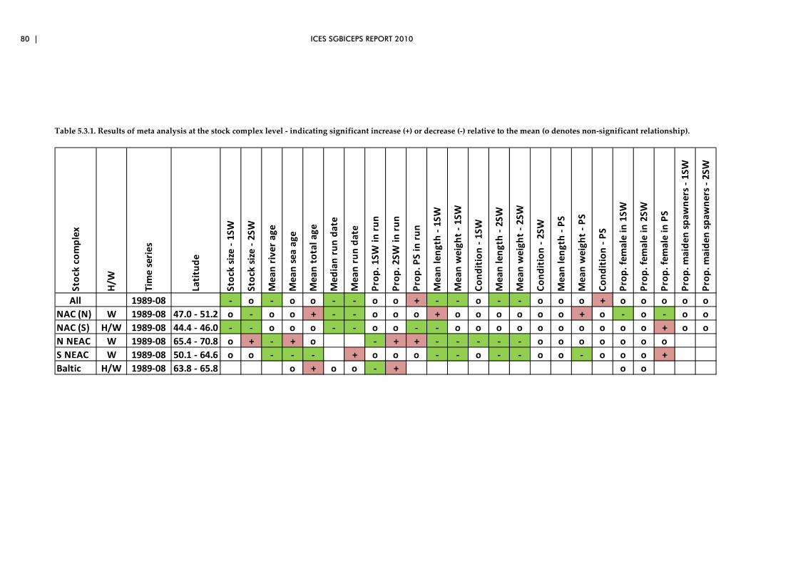
80 | ICES SGBICEPS REPORT 2010
Table 5.3.1. Results of meta analysis at the stock complex level ‐ indicating significant increase (+) or decrease (‐) relative to the mean (o denotes non‐significant relationship).
Stock complex
H/W
Tim
e series
Latitude
Stock size ‐ 1SW
Stock size ‐ 2SW
Mean river age
Mean sea
age
Mean total age
Median run date
Mean run date
Prop. 1SW
in run
Prop. 2SW
in run
Prop. PS in run
Mean length ‐ 1SW
Mean weight ‐ 1SW
Condition ‐ 1SW
Mean length ‐ 2SW
Mean weight ‐ 2SW
Condition ‐ 2SW
Mean length ‐ PS
Mean weight ‐ PS
Condition ‐ PS
Prop. female in 1SW
Prop. female in 2SW
Prop. female in PS
Prop. maiden
spaw
ners ‐ 1SW
Prop. maiden
spaw
ners ‐ 2SW
All 1989‐08 ‐ o ‐ o o ‐ ‐ o o + ‐ ‐ o ‐ ‐ o o o + o o o o o
NAC (N) W 1989‐08 47.0 ‐ 51.2 o ‐ o o + ‐ ‐ o o o + o o o o o o + o ‐ o ‐ o o
NAC (S) H/W 1989‐08 44.4 ‐ 46.0 ‐ ‐ o o o ‐ ‐ o o ‐ ‐ o o o o o o o o o o + o o
N NEAC W 1989‐08 65.4 ‐ 70.8 o + ‐ + o ‐ + + ‐ ‐ ‐ ‐ ‐ o o o o o o o
S NEAC W 1989‐08 50.1 ‐ 64.6 o o ‐ ‐ ‐ + o o o ‐ ‐ o ‐ ‐ o o ‐ o o o +
Baltic H/W 1989‐08 63.8 ‐ 65.8 o + o o ‐ + o o
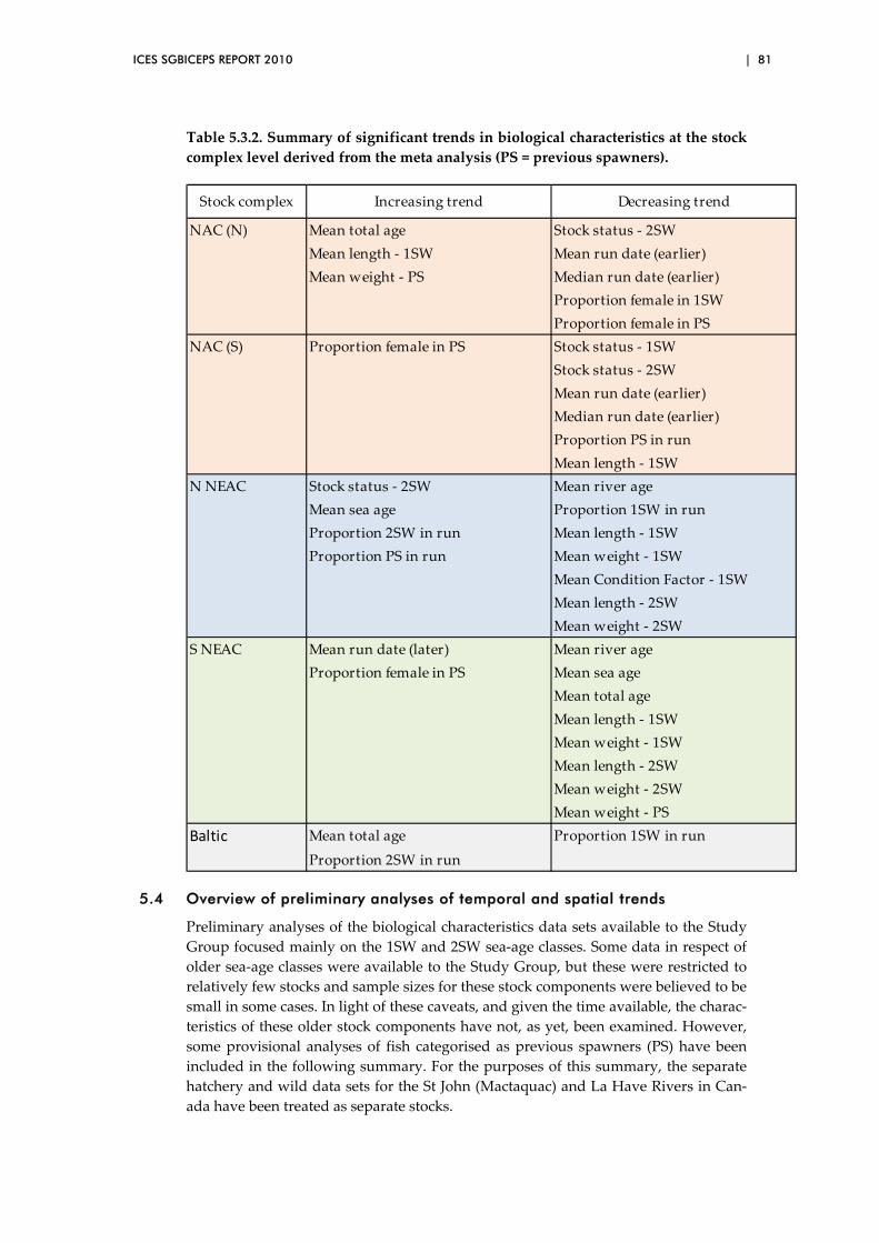
ICES SGBICEPS REPORT 2010 | 81
Table 5.3.2. Summary of significant trends in biological characteristics at the stock
complex level derived from the meta analysis (PS = previous spawners).
Stock complex Increasing trend Decreasing trend
NAC (N) Mean total age Stock status ‐ 2SW
Mean length ‐ 1SW Mean run date (earlier)
Mean weight ‐ PS Median run date (earlier)
Proportion female in 1SW
Proportion female in PS
NAC (S) Proportion female in PS Stock status ‐ 1SW
Stock status ‐ 2SW
Mean run date (earlier)
Median run date (earlier)
Proportion PS in run
Mean length ‐ 1SW
N NEAC Stock status ‐ 2SW Mean river age
Mean sea age Proportion 1SW in run
Proportion 2SW in run Mean length ‐ 1SW
Proportion PS in run Mean weight ‐ 1SW
Mean Condition Factor ‐ 1SW
Mean length ‐ 2SW
Mean weight ‐ 2SW
S NEAC Mean run date (later) Mean river age
Proportion female in PS Mean sea age
Mean total age
Mean length ‐ 1SW
Mean weight ‐ 1SW
Mean length ‐ 2SW
Mean weight ‐ 2SW
Mean weight ‐ PS
Baltic Mean total age Proportion 1SW in run
Proportion 2SW in run
5.4 Overview of preliminary analyses of temporal and spatial trends
Preliminary analyses of the biological characteristics data sets available to the Study
Group focused mainly on the 1SW and 2SW sea‐age classes. Some data in respect of
older sea‐age classes were available to the Study Group, but these were restricted to
relatively few stocks and sample sizes for these stock components were believed to be
small in some cases. In light of these caveats, and given the time available, the charac‐
teristics of these older stock components have not, as yet, been examined. However,
some provisional analyses of fish categorised as previous spawners (PS) have been
included in the following summary. For the purposes of this summary, the separate
hatchery and wild data sets for the St John (Mactaquac) and La Have Rivers in Can‐
ada have been treated as separate stocks.

82 | ICES SGBICEPS REPORT 2010
Stock status
Overall, 36% of the individual salmon stock data sets (Table 5.2.1) indicate a signifi‐
cant declining trend in the stock status variable (all sea‐age groups combined) over
the time series analysed (1989–2008). Stocks with declining trends were more preva‐
lent in North America and the NEAC Southern area; only 2 stocks (17%) in the NEAC
Northern area indicated a negative trend. Overall, only two North Atlantic stocks, the
Western Arm Brook in Canada and the Vestre Jakobselv in Norway, showed a sig‐
nificant positive trend over the period. These are among the most northerly stocks for
which data are available. Two of the three Baltic stocks for which data were available
also showed a significant positive trend over the period.
Meta analysis at the stock complex level and split by sea‐age (Table 5.3.1) indicates a
significant decrease in the stock status variable for both 1SW and 2SW salmon in the
southern part of the NAC and for 2SW salmon in the northern part of the NAC area,
but a significant increase in stock status for 2SW salmon in the NEAC Northern area.
Mean river age
The majority of the data sets (56%) indicate a significant decline in mean river (smolt)
age over the standard time series (1989–2008) (Table 5.2.1). Relatively few stocks (9%)
indicate a significant positive trend over the period and these are restricted to the
NAC Southern area (only the La Have River ‐ wild) and the NEAC Northern area
(the two most northerly stocks for which data were available). The data are summa‐
rised in Figure 5.4.1; limited data not included for the Baltic.
0
10
20
30
40
50
60
70
80
90
100
NAC(N)
NAC(S)
NEA
C(N)
NEA
C(S)
%
River age
No sig. trend
Sig. increasing trend
Sig. declining trend
Figure 5.4.1. Percentage of rivers in each stock complex indicating significant trends in mean river
age.
Despite the evidence of declining smolt age in all areas of the North Atlantic, the
meta analysis only indicates a significant decrease in mean river age for the NEAC
Northern and Southern stock complexes (Table 5.3.1).
The decline in mean smolt age may be the consequence of an increase in growth rate
as the faster growing parr migrate to sea earlier (Metcalfe et al., 1989; Økland et al.,
1993). The increase in growth rate may relate to an increase in temperature (Elliott et
al. 2000; Jonsson et al., 2005), and/or an increase in growth as a result of density‐
dependent processes (Gibson, 1993; Jenkins et al., 1999; Imre et al., 2005; Lobón‐
Cerviá, 2005), and/or increased freshwater production. A possible consequence of the
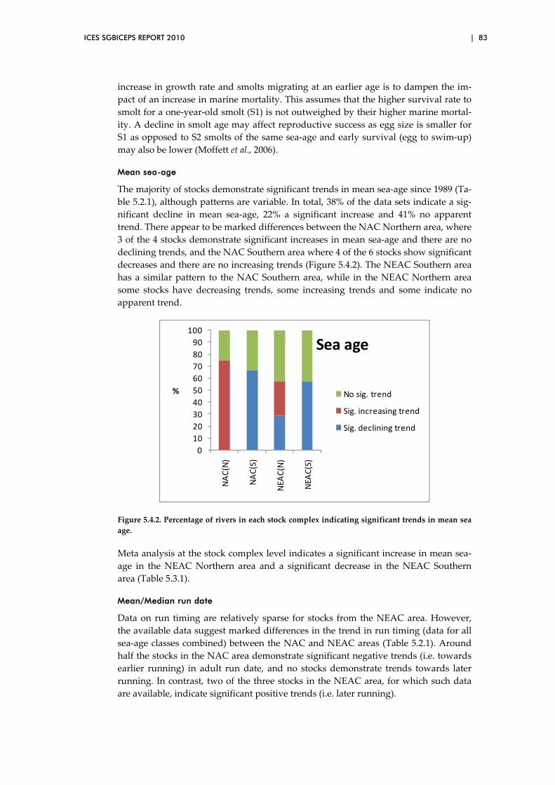
ICES SGBICEPS REPORT 2010 | 83
increase in growth rate and smolts migrating at an earlier age is to dampen the im‐
pact of an increase in marine mortality. This assumes that the higher survival rate to
smolt for a one‐year‐old smolt (S1) is not outweighed by their higher marine mortal‐
ity. A decline in smolt age may affect reproductive success as egg size is smaller for
S1 as opposed to S2 smolts of the same sea‐age and early survival (egg to swim‐up)
may also be lower (Moffett et al., 2006).
Mean sea-age
The majority of stocks demonstrate significant trends in mean sea‐age since 1989 (Ta‐
ble 5.2.1), although patterns are variable. In total, 38% of the data sets indicate a sig‐
nificant decline in mean sea‐age, 22% a significant increase and 41% no apparent
trend. There appear to be marked differences between the NAC Northern area, where
3 of the 4 stocks demonstrate significant increases in mean sea‐age and there are no
declining trends, and the NAC Southern area where 4 of the 6 stocks show significant
decreases and there are no increasing trends (Figure 5.4.2). The NEAC Southern area
has a similar pattern to the NAC Southern area, while in the NEAC Northern area
some stocks have decreasing trends, some increasing trends and some indicate no
apparent trend.
0
10
20
30
40
50
60
70
80
90
100
NAC(N)
NAC(S)
NEA
C(N)
NEA
C(S)
%
Sea age
No sig. trend
Sig. increasing trend
Sig. declining trend
Figure 5.4.2. Percentage of rivers in each stock complex indicating significant trends in mean sea
age.
Meta analysis at the stock complex level indicates a significant increase in mean sea‐
age in the NEAC Northern area and a significant decrease in the NEAC Southern
area (Table 5.3.1).
Mean/Median run date
Data on run timing are relatively sparse for stocks from the NEAC area. However,
the available data suggest marked differences in the trend in run timing (data for all
sea‐age classes combined) between the NAC and NEAC areas (Table 5.2.1). Around
half the stocks in the NAC area demonstrate significant negative trends (i.e. towards
earlier running) in adult run date, and no stocks demonstrate trends towards later
running. In contrast, two of the three stocks in the NEAC area, for which such data
are available, indicate significant positive trends (i.e. later running).
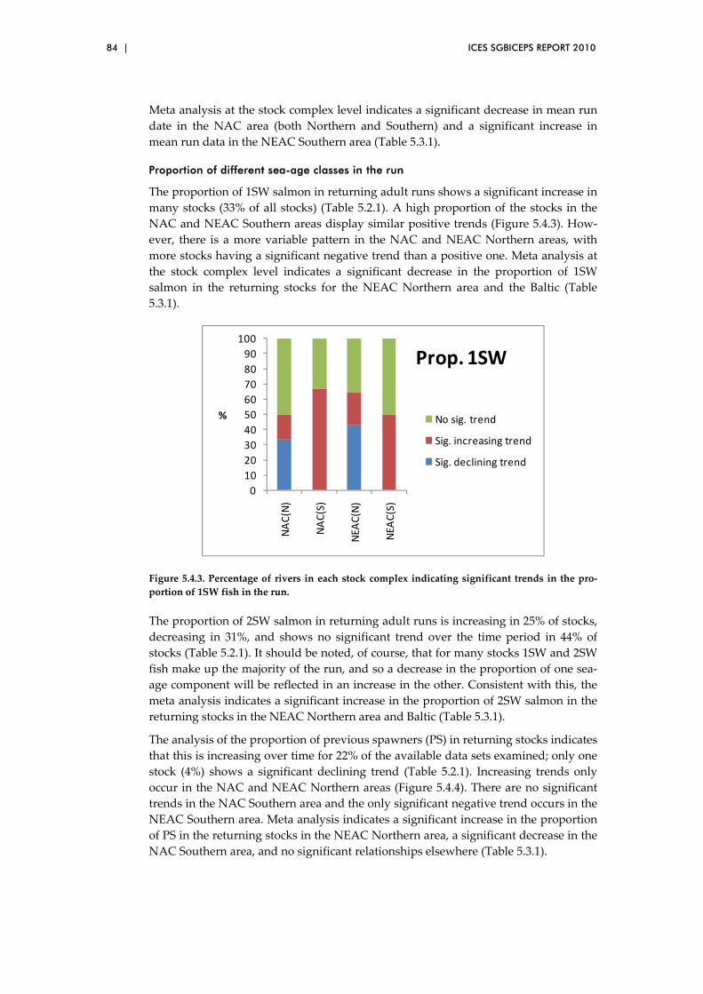
84 | ICES SGBICEPS REPORT 2010
Meta analysis at the stock complex level indicates a significant decrease in mean run
date in the NAC area (both Northern and Southern) and a significant increase in
mean run data in the NEAC Southern area (Table 5.3.1).
Proportion of different sea-age classes in the run
The proportion of 1SW salmon in returning adult runs shows a significant increase in
many stocks (33% of all stocks) (Table 5.2.1). A high proportion of the stocks in the
NAC and NEAC Southern areas display similar positive trends (Figure 5.4.3). How‐
ever, there is a more variable pattern in the NAC and NEAC Northern areas, with
more stocks having a significant negative trend than a positive one. Meta analysis at
the stock complex level indicates a significant decrease in the proportion of 1SW
salmon in the returning stocks for the NEAC Northern area and the Baltic (Table
5.3.1).
0
10
20
30
40
50
60
70
80
90
100
NAC(N)
NAC(S)
NEA
C(N)
NEA
C(S)
%
Prop. 1SW
No sig. trend
Sig. increasing trend
Sig. declining trend
Figure 5.4.3. Percentage of rivers in each stock complex indicating significant trends in the pro‐
portion of 1SW fish in the run.
The proportion of 2SW salmon in returning adult runs is increasing in 25% of stocks,
decreasing in 31%, and shows no significant trend over the time period in 44% of
stocks (Table 5.2.1). It should be noted, of course, that for many stocks 1SW and 2SW
fish make up the majority of the run, and so a decrease in the proportion of one sea‐
age component will be reflected in an increase in the other. Consistent with this, the
meta analysis indicates a significant increase in the proportion of 2SW salmon in the
returning stocks in the NEAC Northern area and Baltic (Table 5.3.1).
The analysis of the proportion of previous spawners (PS) in returning stocks indicates
that this is increasing over time for 22% of the available data sets examined; only one
stock (4%) shows a significant declining trend (Table 5.2.1). Increasing trends only
occur in the NAC and NEAC Northern areas (Figure 5.4.4). There are no significant
trends in the NAC Southern area and the only significant negative trend occurs in the
NEAC Southern area. Meta analysis indicates a significant increase in the proportion
of PS in the returning stocks in the NEAC Northern area, a significant decrease in the
NAC Southern area, and no significant relationships elsewhere (Table 5.3.1).

ICES SGBICEPS REPORT 2010 | 85
0
10
20
30
40
50
60
70
80
90
100
NAC(N)
NAC(S)
NEA
C(N)
NEA
C(S)
%
Prop. PS
No sig. trend
Sig. increasing trend
Sig. declining trend
Figure 5.4.4. Percentage of rivers in each stock complex indicating significant trends in the pro‐
portion of 1SW fish in the run.
Mean length, weight and condition – 1SW salmon
The available data sets indicate differing patterns in the mean size of returning 1SW
salmon both among stocks and over time (Table 5.2.1). Significant increasing size
trends are apparent for all of the stocks in the NAC Northern (Figure 5.4.5), whereas
none of the stocks in the NAC Southern area show significant increasing trends in
mean length, although over half do in respect of mean weight and condition factor;
there are no negative trends in either length or weight in the NAC area.
0
10
20
30
40
50
60
70
80
90
100
NAC(N)
NAC(S)
NEA
C(N)
NEA
C(S)
%
1SW length
No sig. trend
Sig. increasing trend
Sig. declining trend
Figure 5.4.5. Percentage of rivers in each stock complex indicating significant trends in the length
of returning 1SW fish.
There is little evidence for trends over time in the NEAC Northern area, although
there are significant increases in the mean length of 1SW salmon returning to one
river (8%). There is greater variability in the NEAC Southern area, with some stocks
showing significant decreases in fish size, while others in relatively close geographic
proximity show significant increases (Figure 5.4.5).
Meta analysis (Table 5.3.1) indicates a significant increase in the mean length of 1SW
salmon in the NAC Northern area, but a significant decrease in mean 1SW length in

86 | ICES SGBICEPS REPORT 2010
the NAC Southern area; there are no significant trends in weight or condition factor.
There is a significant decrease in mean 1SW length, weight and condition factor for
the NEAC Northern area, and a significant decrease in mean 1SW length and weight
for the NEAC Southern area.
Mean length, weight and condition – 2SW salmon
As with the 1SW fish, the available data sets indicate widely differing patterns in the
mean size of returning 2SW salmon both among stocks and over time (Table 5.2.1).
Both significant increases and significant decreases in the size of 2SW fish are appar‐
ent for different stocks in the NAC area, but with no clear geographical pattern (Fig‐
ure 5.4.6). In the NEAC Northern area, 5 stocks (42%) indicate a significant decline in
the mean length of returning 2SW salmon over the period, with no stocks showing an
increase. In contrast, in the NEAC Southern area no stocks indicate a significant de‐
cline in 2SW length (Figure 5.4.6), although there are significant increases in mean
weight of 2SW fish for 4 stocks (57%) (Table 5.2.1).
0
10
20
30
40
50
60
70
80
90
100
NAC(N)
NAC(S)
NEA
C(N)
NEA
C(S)
%
2SW length
No sig. trend
Sig. increasing trend
Sig. declining trend
Figure 5.4.6. Percentage of rivers in each stock complex indicating significant trends in the length
of returning 2SW fish.
Meta analysis indicates a significant decrease in mean length and weight of 2SW
salmon in both the NEAC Northern and Southern areas, but no significant relation‐
ships in the NAC areas (Table 5.3.1). There are also no statistically significant trends
in the condition factor of 2SW salmon at the stock complex level.
Mean length, weight and condition – Previous Spawners (PS)
The length and weight of previous spawning (PS) fish is increasing in around half the
stocks in the NAC area and there are no negative trends in length, weight or condi‐
tion factor (Table 5.2.1). The pattern in trends in the NAC area appears to be consis‐
tent with that seen in the 1SW salmon, the dominant sea‐age group in many of these
stocks. In the NEAC Northern area, 2 of the stocks (25%) have declining trends in the
length, weight and condition of PS, but no trends in the other stocks. Size data for PS
are only available for three stocks in the NEAC Southern area and these indicate no
apparent trend in one instance, but decreasing trends in length and weight for the
other two stocks (Table 5.2.1).
Meta analysis indicates a significant increase in the mean weight of PS in the NAC
Northern area, and a significant decrease in the mean weight of PS in the NEAC
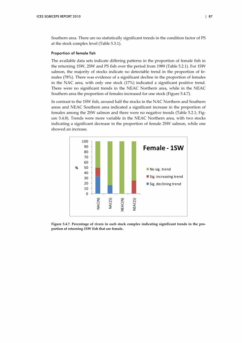
ICES SGBICEPS REPORT 2010 | 87
Southern area. There are no statistically significant trends in the condition factor of PS
at the stock complex level (Table 5.3.1).
Proportion of female fish
The available data sets indicate differing patterns in the proportion of female fish in
the returning 1SW, 2SW and PS fish over the period from 1989 (Table 5.2.1). For 1SW
salmon, the majority of stocks indicate no detectable trend in the proportion of fe‐
males (78%). There was evidence of a significant decline in the proportion of females
in the NAC area, with only one stock (17%) indicated a significant positive trend.
There were no significant trends in the NEAC Northern area, while in the NEAC
Southern area the proportion of females increased for one stock (Figure 5.4.7).
In contrast to the 1SW fish, around half the stocks in the NAC Northern and Southern
areas and NEAC Southern area indicated a significant increase in the proportion of
females among the 2SW salmon and there were no negative trends (Table 5.2.1; Fig‐
ure 5.4.8). Trends were more variable in the NEAC Northern area, with two stocks
indicating a significant decrease in the proportion of female 2SW salmon, while one
showed an increase.
0
10
20
30
40
50
60
70
80
90
100
NAC(N)
NAC(S)
NEA
C(N)
NEA
C(S)
%
Female ‐ 1SW
No sig. trend
Sig. increasing trend
Sig. declining trend
Figure 5.4.7. Percentage of rivers in each stock complex indicating significant trends in the pro‐
portion of returning 1SW fish that are female.
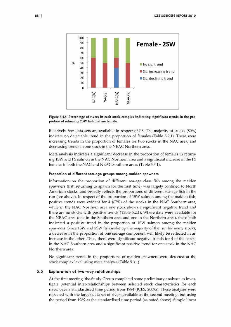
88 | ICES SGBICEPS REPORT 2010
0
10
20
30
40
50
60
70
80
90
100
NAC(N)
NAC(S)
NEA
C(N)
NEA
C(S)
%
Female ‐ 2SW
No sig. trend
Sig. increasing trend
Sig. declining trend
Figure 5.4.8. Percentage of rivers in each stock complex indicating significant trends in the pro‐
portion of returning 2SW fish that are female.
Relatively few data sets are available in respect of PS. The majority of stocks (80%)
indicate no detectable trend in the proportion of females (Table 5.2.1). There were
increasing trends in the proportion of females for two stocks in the NAC area, and
decreasing trends in one stock in the NEAC Northern area.
Meta analysis indicates a significant decrease in the proportion of females in return‐
ing 1SW and PS salmon in the NAC Northern area and a significant increase in the PS
females in both the NAC and NEAC Southern areas (Table 5.3.1).
Proportion of different sea-age groups among maiden spawners
Information on the proportion of different sea‐age class fish among the maiden
spawners (fish returning to spawn for the first time) was largely confined to North
American stocks, and broadly reflects the proportions of different sea‐age fish in the
run (see above). In respect of the proportion of 1SW salmon among the maiden fish,
positive trends were evident for 4 (67%) of the stocks in the NAC Southern area,
while in the NAC Northern area one stock shows a significant negative trend and
there are no stocks with positive trends (Table 5.2.1). Where data were available for
the NEAC area (one in the Southern area and one in the Northern area), these both
indicated a positive trend in the proportion of 1SW salmon among the maiden
spawners. Since 1SW and 2SW fish make up the majority of the run for many stocks,
a decrease in the proportion of one sea‐age component will likely be reflected in an
increase in the other. Thus, there were significant negative trends for 4 of the stocks
in the NAC Southern area and a significant positive trend for one stock in the NAC
Northern area.
No significant trends in the proportions of maiden spawners were detected at the
stock complex level using meta analysis (Table 5.3.1).
5.5 Exploration of two-way relationships
At the first meeting, the Study Group completed some preliminary analyses to inves‐
tigate potential inter‐relationships between selected stock characteristics for each
river, over a standardised time period from 1984 (ICES, 2009a). These analyses were
repeated with the larger data set of rivers available at the second meeting, but using
the period from 1989 as the standardised time period (as noted above). Simple linear

ICES SGBICEPS REPORT 2010 | 89
regression models were used to test each relationship since the analyses were essen‐
tially exploratory in nature. The relationships investigated were:
1SW weight v 2SW weight (fish sampled in the same year)
1SW weight (in year ‘n’) v 2SW weight (in year ‘n + 1’)
1SW condition factor v 2SW condition factor (fish sampled in the same
year)
1SW condition factor (in year ‘n’) v 2SW condition factor (in year ‘n + 1’)
Mean river age v mean sea‐age
1SW length v 1SW weight
2SW length v 2SW weight
Mean river age v 1SW weight
Mean river age v 2SW weight
1SW weight v total run size
2SW weight v total run size
1SW weight v 1SW run size
2SW weight v 2 SW run size
A series of plots were produced for each of the above relationships for each stock for
which appropriate data were available (Figure 5.5.1 provides two examples). Each of
the individual river plots also includes the p‐value to assess the statistical significance
of the slope of the linear regression model. The Study Group noted that even if this p‐
value is not small it does not necessarily mean that there is no relationship – only that
we are unable to detect it with these data. Table 5.5.1 summarises the results of all the
linear regression models for each of the above relationships ‐ ‘o’ means that there was
not enough evidence at the 5% level to detect a trend; ‘+’ denotes a positive trend
(p>0.05), and ‘‐‘ denotes a negative trend (p<0.05). The results are discussed briefly
below.

90 | ICES SGBICEPS REPORT 2010
Figure 5.5.1. Example two‐way plots for each individual stock of: (a) mean weight of 1SW salmon
against the mean weight of 2SW salmon returning in the same year (i.e. from an earlier smolt
cohort), and (b) mean weight of 1SW salmon against the mean weight of 2SW salmon returning in
the following year (i.e. from the same smolt cohort). For stocks with both wild (W) and hatchery
(H) stock components the data are plotted separately. The p‐values provide the statistical signifi‐
cance of the slope of each linear regression model. [N.B. the plots are presented by river name in
alphabetical order.]
(a)
2.5 3.0 3.5
1.0
1.2
1.4
Mean Weight 2SW
Mea
n W
eigh
t 1S
W
Argard (p= 0.05 )
3.0 3.5 4.0 4.5
1.9
2.2
2.5
Mean Weight 2SW
Mea
n W
eigh
t 1S
W
Bush (p= 0.82 )
4.0 4.5 5.0
1.4
1.8
2.2
Mean Weight 2SW
Mea
n W
eigh
t 1S
W
De la Trinite (p= 0 )
4.5 5.5 6.5
2.6
3.0
3.4
Mean Weight 2SW
Mea
n W
eigh
t 1S
W
Dee (p= 0 )
4.0 4.5 5.0 5.5
1.9
2.2
2.5
Mean Weight 2SW
Mea
n W
eigh
t 1S
W
Ellidaar (p= 0.12 )
4.0 4.5 5.0 5.5
1.4
1.8
2.2
Mean Weight 2SW
Mea
n W
eigh
t 1S
W
Enningdalselva (p= 0.31 )
3.5 4.0 4.5 5.0 5.5
1.4
1.6
1.8
2.0
Mean Weight 2SW
Mea
n W
eigh
t 1S
W
Etneelva (p= 0.13 )
5.0 5.5 6.0
1.6
2.0
2.4
Mean Weight 2SW
Mea
n W
eigh
t 1S
W
Gaula (p= 0.1 )
3.5 4.0 4.5 5.0
1.2
1.5
1.8
Mean Weight 2SW
Mea
n W
eigh
t 1S
W
Gaula Sogn (p= 0 )

ICES SGBICEPS REPORT 2010 | 91
4.5 5.5 6.5
1.8
2.1
2.4
Mean Weight 2SW
Mea
n W
eigh
t 1S
WHofsa (p= 0.68 )
3.5 4.0 4.5 5.0
1.5
1.8
2.1
Mean Weight 2SW
Mea
n W
eigh
t 1S
W
LaHaveW (p= 0 )
4.0 4.5 5.0 5.5
1.6
2.0
Mean Weight 2SW
Mea
n W
eigh
t 1S
W
LaHaveH (p= 0 )
5.2 5.6 6.0 6.4
2.3
2.6
2.9
Mean Weight 2SW
Mea
n W
eigh
t 1S
W
Laxa i Adaldalur (p= 0.3 )
4.5 5.5 6.5 7.5
2.4
2.8
3.2
Mean Weight 2SW
Mea
n W
eigh
t 1S
WLune (p= 0.49 )
4.0 4.2 4.4 4.6 4.8
1.5
1.7
Mean Weight 2SW
Mea
n W
eigh
t 1S
W
Miramichi (p= 0.55 )
3.8 4.2 4.6 5.0
1.4
1.8
Mean Weight 2SW
Mea
n W
eigh
t 1S
W
Naatamojoki (p= 0.03 )
3.8 4.0 4.2 4.4 4.6
1.1
1.3
1.5
1.7
Mean Weight 2SW
Mea
n W
eigh
t 1S
W
Nausta (p= 0.8 )
4.2 4.6 5.0
2.0
2.2
2.4
Mean Weight 2SW
Mea
n W
eigh
t 1S
W
Nordura (p= 0.02 )

92 | ICES SGBICEPS REPORT 2010
4.0 4.5 5.0 5.5
1.6
2.0
2.4
2.8
Mean Weight 2SW
Mea
n W
eigh
t 1S
W
North Esk (p= 0 )
4.5 5.0 5.5 6.0
1.6
2.0
2.4
Mean Weight 2SW
Mea
n W
eigh
t 1S
W
Numedalslagen (p= 0 )
4.0 5.0 6.0
1.5
2.0
2.5
Mean Weight 2SW
Mea
n W
eigh
t 1S
W
Penobscot (p= 0.14 )
4.0 4.5 5.0 5.5
1.50
1.65
Mean Weight 2SW
Mea
n W
eigh
t 1S
W
Saint-Jean (p= 0.04 )
4.8 5.2 5.6
2.0
2.4
2.8
Mean Weight 2SW
Mea
n W
eigh
t 1S
WSaint John W (p= 0.75 )
4.8 5.2 5.6 6.0
2.0
2.6
3.2
Mean Weight 2SW
Mea
n W
eigh
t 1S
W
Saint John H (p= 0.31 )
3.2 3.6 4.0 4.4
1.3
1.5
1.7
Mean Weight 2SW
Mea
n W
eigh
t 1S
W
Skienselva (p= 0.98 )
3.0 3.5 4.0 4.5 5.0 5.5
1.4
1.6
1.8
2.0
Mean Weight 2SW
Mea
n W
eigh
t 1S
W
Teno (p= 0.35 )
2.5 3.5 4.5
1.5
1.7
1.9
Mean Weight 2SW
Mea
n W
eigh
t 1S
W
Tuloma (p= 0.49 )

ICES SGBICEPS REPORT 2010 | 93
4.0 4.5 5.0 5.5 6.0
1.2
1.6
2.0
Mean Weight 2SW
Mea
n W
eigh
t 1S
W
Ume_VindelH (p= 0.19 )
4.0 5.0 6.0
1.6
1.8
2.0
Mean Weight 2SW
Mea
n W
eigh
t 1S
W
Vestre Jakobselv (p= 0.97 )
3.4 3.6 3.8 4.0
1.6
2.0
Mean Weight 2SW
Mea
n W
eigh
t 1S
W
Western Arm Brook (p= 0.87
4.6 5.0 5.4 5.8
2.0
2.6
3.2
Mean Weight 2SW
Mea
n W
eigh
t 1S
W
Wye (p= 0.7 )
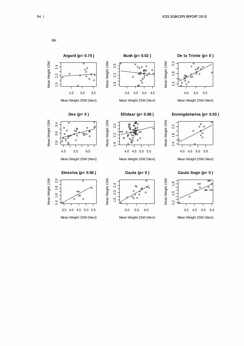
94 | ICES SGBICEPS REPORT 2010
(b)
2.5 3.0 3.5
1.0
1.2
1.4
Mean Weight 2SW (Next)
Mea
n W
eigh
t 1S
W
Argard (p= 0.74 )
3.0 3.5 4.0 4.5
1.9
2.2
2.5
Mean Weight 2SW (Next)
Mea
n W
eigh
t 1S
W
Bush (p= 0.52 )
4.0 4.5 5.0
1.4
1.8
2.2
Mean Weight 2SW (Next)
Mea
n W
eigh
t 1S
W
De la Trinite (p= 0 )
4.5 5.5 6.5
2.6
3.0
3.4
Mean Weight 2SW (Next)
Mea
n W
eigh
t 1S
W
Dee (p= 0 )
4.0 4.5 5.0 5.5
1.9
2.2
2.5
Mean Weight 2SW (Next)
Mea
n W
eigh
t 1S
W
Ellidaar (p= 0.08 )
4.0 4.5 5.0 5.5
1.4
1.8
2.2
Mean Weight 2SW (Next)
Mea
n W
eigh
t 1S
W
Enningdalselva (p= 0.03 )
3.5 4.0 4.5 5.0 5.5
1.4
1.6
1.8
2.0
Mean Weight 2SW (Next)
Mea
n W
eigh
t 1S
W
Etneelva (p= 0.06 )
5.0 5.5 6.0
1.6
2.0
2.4
Mean Weight 2SW (Next)
Mea
n W
eigh
t 1S
W
Gaula (p= 0 )
3.5 4.0 4.5 5.0
1.2
1.5
1.8
Mean Weight 2SW (Next)
Mea
n W
eigh
t 1S
W
Gaula Sogn (p= 0 )

ICES SGBICEPS REPORT 2010 | 95
4.5 5.5 6.5
1.8
2.1
2.4
Mean Weight 2SW (Next)
Mea
n W
eigh
t 1S
W
Hofsa (p= 0.08 )
3.5 4.0 4.5 5.0
1.5
1.8
2.1
Mean Weight 2SW (Next)
Mea
n W
eigh
t 1S
W
LaHaveW (p= 0 )
4.0 4.5 5.0 5.5
1.6
2.0
Mean Weight 2SW (Next)
Mea
n W
eigh
t 1S
W
LaHaveH (p= 0.15 )
5.2 5.6 6.0 6.4
2.3
2.6
2.9
Mean Weight 2SW (Next)
Mea
n W
eigh
t 1S
W
Laxa i Adaldalur (p= 0.11 )
4.5 5.5 6.5 7.5
2.4
2.8
3.2
Mean Weight 2SW (Next)
Mea
n W
eigh
t 1S
W
Lune (p= 0.55 )
4.0 4.2 4.4 4.6 4.8
1.5
1.7
Mean Weight 2SW (Next)
Mea
n W
eigh
t 1S
W
Miramichi (p= 0.36 )
3.8 4.2 4.6 5.0
1.4
1.8
Mean Weight 2SW (Next)
Mea
n W
eigh
t 1S
W
Naatamojoki (p= 0 )
3.8 4.0 4.2 4.4 4.6
1.1
1.3
1.5
1.7
Mean Weight 2SW (Next)
Mea
n W
eigh
t 1S
W
Nausta (p= 0.2 )
4.2 4.6 5.0
2.0
2.2
2.4
Mean Weight 2SW (Next)
Mea
n W
eigh
t 1S
W
Nordura (p= 0 )
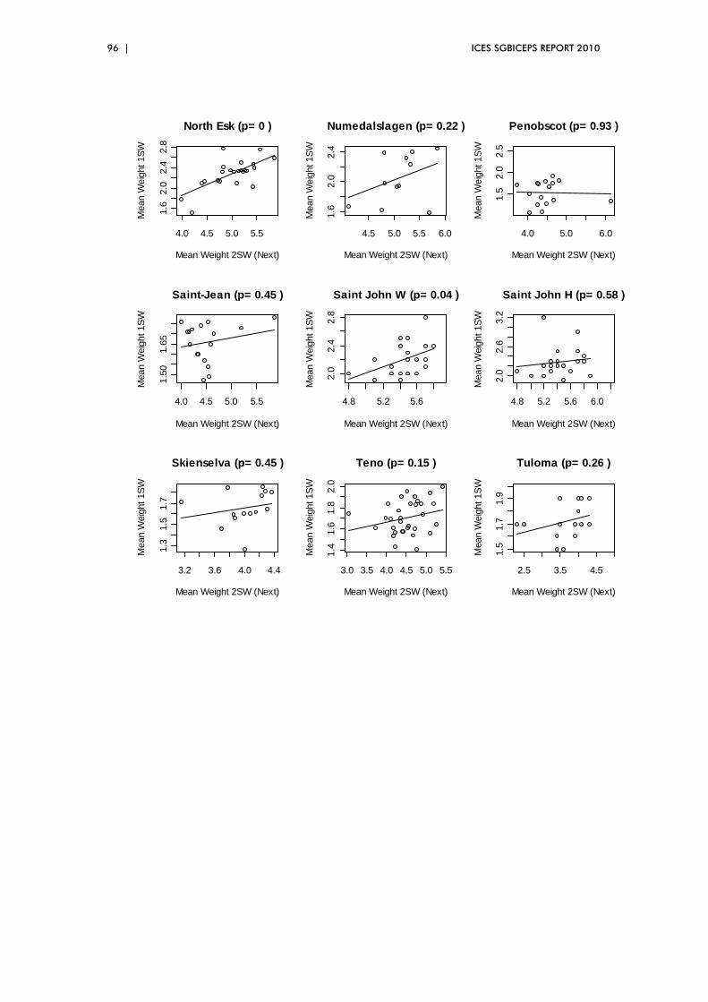
96 | ICES SGBICEPS REPORT 2010
4.0 4.5 5.0 5.5
1.6
2.0
2.4
2.8
Mean Weight 2SW (Next)
Mea
n W
eigh
t 1S
W
North Esk (p= 0 )
4.5 5.0 5.5 6.0
1.6
2.0
2.4
Mean Weight 2SW (Next)
Mea
n W
eigh
t 1S
W
Numedalslagen (p= 0.22 )
4.0 5.0 6.0
1.5
2.0
2.5
Mean Weight 2SW (Next)
Mea
n W
eigh
t 1S
W
Penobscot (p= 0.93 )
4.0 4.5 5.0 5.5
1.50
1.65
Mean Weight 2SW (Next)
Mea
n W
eigh
t 1S
W
Saint-Jean (p= 0.45 )
4.8 5.2 5.6
2.0
2.4
2.8
Mean Weight 2SW (Next)
Mea
n W
eigh
t 1S
W
Saint John W (p= 0.04 )
4.8 5.2 5.6 6.0
2.0
2.6
3.2
Mean Weight 2SW (Next)
Mea
n W
eigh
t 1S
W
Saint John H (p= 0.58 )
3.2 3.6 4.0 4.4
1.3
1.5
1.7
Mean Weight 2SW (Next)
Mea
n W
eigh
t 1S
W
Skienselva (p= 0.45 )
3.0 3.5 4.0 4.5 5.0 5.5
1.4
1.6
1.8
2.0
Mean Weight 2SW (Next)
Mea
n W
eigh
t 1S
W
Teno (p= 0.15 )
2.5 3.5 4.5
1.5
1.7
1.9
Mean Weight 2SW (Next)
Mea
n W
eigh
t 1S
W
Tuloma (p= 0.26 )
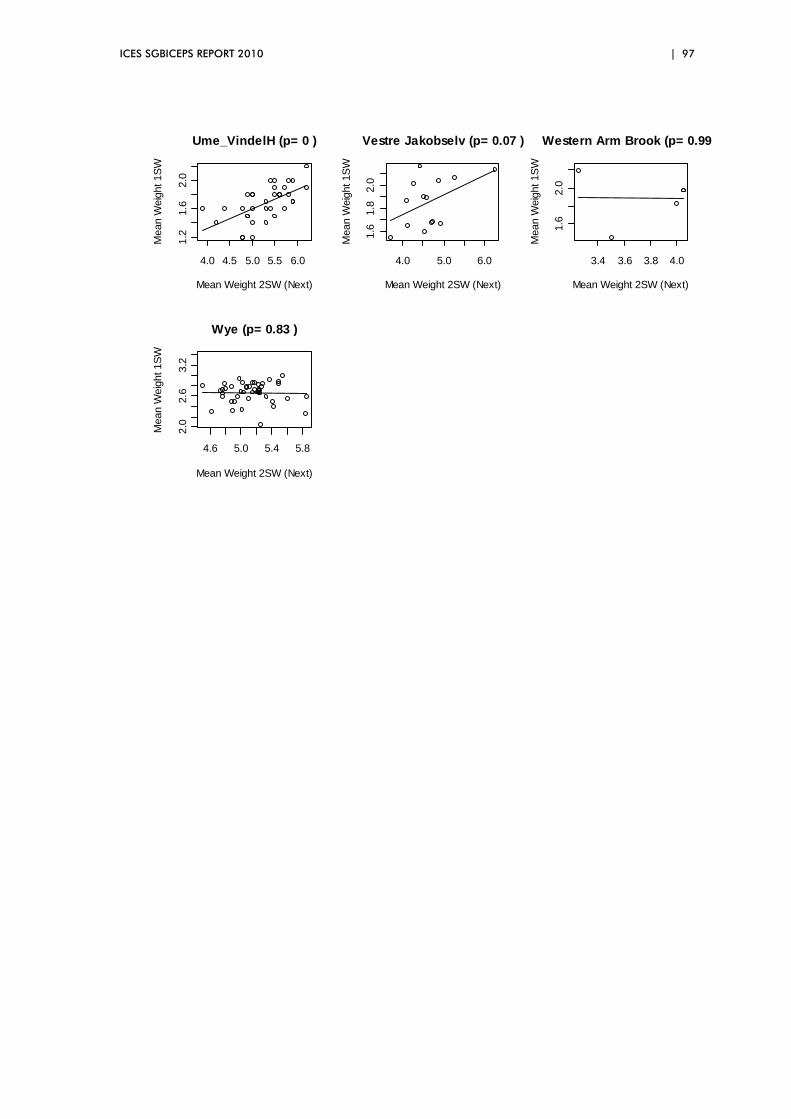
ICES SGBICEPS REPORT 2010 | 97
4.0 4.5 5.0 5.5 6.0
1.2
1.6
2.0
Mean Weight 2SW (Next)
Mea
n W
eigh
t 1S
W
Ume_VindelH (p= 0 )
4.0 5.0 6.0
1.6
1.8
2.0
Mean Weight 2SW (Next)
Mea
n W
eigh
t 1S
W
Vestre Jakobselv (p= 0.07 )
3.4 3.6 3.8 4.0
1.6
2.0
Mean Weight 2SW (Next)
Mea
n W
eigh
t 1S
W
Western Arm Brook (p= 0.99
4.6 5.0 5.4 5.8
2.0
2.6
3.2
Mean Weight 2SW (Next)
Mea
n W
eigh
t 1S
W
Wye (p= 0.83 )

98 | ICES SGBICEPS REPORT 2010
Table 5.5.1. Results of analysis of two‐way relationships based on simple linear regression mod‐
els: ‘o’ means that there was not enough evidence at the 5% level to detect a trend; ‘+’ denotes a
positive trend (p>0.05), ‘‐‘ denotes a negative trend (p<0.05).
Stock complex
Country
Stock
H/W
Time series
Latitude
1SW
wt (yr n) v
2SW
wt (yr n)
1SW
wt (yr n) v
2SW
wt (yr n+1)
1SW
CF (yr n) v
2SW
CF (yr n)
1SW
CF (yr n) v
2SW
CF (yr n+1)
River age v Sea
age
1SW
Length v
1SW
Wt
2SW
Length v
2SW
Wt
River age v 1SW
Wt
River age v 2SW
Wt
1SW
wt v Total
Run
1SW
wt v 1SW
Run
2SW
wt v Total
Run
2SW
wt v 2SW
Run
NAC (N) Canada Western Arm Brook W 1984‐06 51.2 o o o o ‐ + o ‐ o + + o o
Canada De la Trinité W 1980‐09 49.4 + + o o + + ‐ ‐ ‐ ‐
Canada Saint‐Jean W 1981‐09 48.8 + o + o + + ‐ o o o
Canada Middle Brook W 1984‐05 48.8 + + o o o
Canada Conne River W 1984‐06 47.9 o + + o o o
Canada Miramichi W 1984‐07 47.0 o o o + o + + o o o o o o
NAC (S) Canada Nashwaak W 1984‐07 46.0 +
Canada St John (Mactaquac) W 1984‐07 45.3 o + o + o + + o o o o o o
Canada St John (Mactaquac) H 1984‐07 45.3 o o o o o + + o o o o o +
Canada La Have W 1984‐07 44.4 + + + + o + + + + o o ‐ ‐
Canada La Have H 1984‐07 44.4 + o + + ‐ + + o o ‐ ‐ o o
USA Penobscot H 1984‐07 44.5 o o o o o o o o o o o o o
N NEAC Finland/Norway Teno W 1984‐07 70.8 o o + o ‐ + + o o o + o o
Finland/Norway Näätämöjoki W 1984‐06 69.7 + + o o o + + o o + o o +
Russia Tuloma W 1984‐08 68.9 o o o + o + + o o o o o o
Norway Vestre Jakobselv W 1989‐08 70.1 o o o + o + + o + o o ‐ o
Norway Årgårdsvassdraget W 1992‐08 64.3 + o o o o + + o o o o o +
Norway Nausta W 1989‐08 61.3 o o o o o + + o + + + o ‐
Norway Gaula Sogn og Fjorda W 1989‐08 61.2 + + + o o + + o o o + o o
Norway Etneelva W 1989‐08 59.4 o o o o o + + o o o o o o
Norway Skienselva W 1989‐08 59.1 o o + o o + + o o o o o o
Norway Numedalslågen W 1989‐08 59.1 + o + o o + + o o o o o o
Norway Enningdalselva W 1990‐08 58.6 o + o + o + + o o o o o o
Norway Gaula W 1989‐07 63.3 o + o o o + + o o o o o o
Iceland (N&E) Laxa I Adaldalur W 1984‐07 65.6 o o + ‐ o
Iceland (N&E) Hofsa W 1984‐07 65.4 o o o o +
S NEAC Iceland (S&W) Nordura W 1984‐07 64.6 + + o + o
Iceland (S&W) Ellidaar W 1984‐07 64.1 o o + ‐ o
UK (Scot) N. Esk W 1984‐07 56.7 + + + + + + o o o o
UK (NI) Bush W 1984‐07 55.1 o o o o o + + o o o o o o
UK (E&W) Lune W 1987‐07 54.0 o o o o o o + o o o o ‐ o
UK (E&W) Dee W 1984‐07 53.4 + + o o + + + ‐ ‐ o o ‐ ‐
UK (E&W) Wye W 1984‐07 51.6 o o + o + + + ‐ o o o o o
UK (E&W) Frome W 1984‐08 50.7
France Bresle W 1984‐08 50.1
Baltic Sweden Kalix W 1980‐08 65.8
Finland/Sweden Tornionjoki W 1980‐09 65.5
Sweden Ume/Vindel W 1987‐08 63.8
Sweden Ume/Vindel H 1974‐08 63.8 o +
Summary ‐ all areas No. of stocks for which data available 31 31 26 26 30 28 27 30 28 28 28 26 26
% of stocks with significant declining trend 0 0 0 0 10 0 0 17 4 11 7 19 15
% of stocks with significant increasing trend 35 35 35 31 20 93 93 7 14 11 14 0 12
% of stocks with no significant trend 65 65 65 69 70 7 7 77 82 79 79 81 73
The size and condition of 1SW and 2SW fish returning in the same year
It is evident that for a number of stocks (35%) there is a significant positive relation‐
ship between the weight of 1SW and 2SW salmon returning in the same year (i.e. de‐
rived from different smolt cohorts) (Table 5.5.1). In no instances are significant
negative trends identified, and the majority of the plots in Figure 5.5.1(a) suggest
positive trends even if the relationships are not significant. Significant positive rela‐
tionships are evident in all areas of the North Atlantic. A very similar pattern is evi‐
dent for mean condition factor. These common patterns of larger (or smaller) 1SW
fish coinciding with larger (or smaller) 2SW fish in returning stocks in any year are
consistent with common factors operating on the fish from the two sea‐group groups
during their return migration. However, it should be noted that there was also evi‐
dence of a correlation between size and condition of 1SW fish in year ‘n’ and 2SW fish
returning in the following year (‘n+1’) (Figure 5.5.1.b) suggesting common influences

ICES SGBICEPS REPORT 2010 | 99
in the early part of the marine phase (see below). The Study Group recognised that
further analysis of such data would be valuable to explore temporal and spatial pat‐
terns.
The size and condition of 1SW in year ‘n’ and 2SW fish returning in the following year (‘n+1’)
Similar positive relationships are also evident for many stocks (35%) between the
weight of 1SW returning in one year and the weight of 2SW salmon returning in the
following year (i.e. derived from the same smolt cohort). As with fish returning in the
same year, there is no evidence of any negative relationships (Table 5.5.1 and Figure
5.5.1.b), and similar patterns are evident for mean condition factor. Significant posi‐
tive relationships are evident in all areas of the North Atlantic and for one hatchery
stock in the Baltic. These concurrent patterns for particular smolt cohorts suggest that
common factors operating in the first period at sea may have a large influence on
growth and size at maturity of returning adult fish. Again, the Study Group recog‐
nised that further analysis of such data would be valuable.
For some stocks, significant positive relationships are apparent between the
weight/condition factor of returning 1SW salmon and the weight/condition factor of
returning 2SW salmon in both the same and the following year. For other stocks, sig‐
nificant relationships were only evident for one of these two‐way comparisons. There
is no apparent spatial pattern to these differences.
Mean river age v mean sea-age
Analyses indicate very different relationships between river age and sea‐age for dif‐
ferent stocks (Table 5.5.1). In some rivers, significant positive relationships apply (i.e.
older smolts tend to produce older adults). However, significant negative relation‐
ships are evident for some other stocks. Viewed spatially, there appears to be more
evidence of variability in these relationships in the NAC and Northern NEAC areas,
where both significant positive and negative relationships are evident. Only signifi‐
cant positive relationships (n = 3, 50% of the available data sets) are evident in the
Southern NEAC area.
Length v Weight
Unsurprisingly, the length and weight of returning 1SW and 2SW fish are positively
correlated. In most, but not all, instances these relationships are significant (Table
5.5.1).
Mean river age v size of returning adults
The age of smolts (ages determined from adult scales) and the size of returning 1SW
and 2SW adults was compared to see whether there were any consistent patterns be‐
tween the age, and by inference the size of smolts, and the subsequent size (weight)
of the returning adults. A number of significant relationships were apparent (Table
5.5.1). For 17% of the stocks (n = 5) there was a significant negative relationship be‐
tween river age and 1SW weight – i.e. older/larger smolts tended to result in smaller
returning adults, while for 7% of stocks (n = 2) the opposite was true. The former is
consistent with other evidence that smolt size can influence the subsequent growth
rate of salmon, with larger smolts showing slower growth at sea (Jonsson & Jonsson,
2007). However, when comparing river age with the weight of returning 2SW sal‐
mon, more stocks (14%) had significant positive than negative relationships (4%),
indicating that older/ larger smolts tended to result in larger returning adults. Such
100 | ICES SGBICEPS REPORT 2010
observations would appear to be at odds with the hypothesis that larger smolts have
slower growth at sea, although the impact of smolt age/size on subsequent matura‐
tion (1SW or 2SW) may also be a factor.
Size of returning fish v stock status variable
Provisional analyses were also completed to investigate possible links between the
size (weight) of returning adult 1SW and 2SW fish in any year and the stock‐specific
status variable for that year (Table 5.5.1). For these purposes, two‐way relationships
were explored between the mean size of returning fish and both the total stock status
(i.e. all sea‐age groups) and the age‐specific stock status (i.e. 1SW or 2SW), simply
derived from the total returning stock figure and the estimated proportion of each
sea‐class in the stock. The latter is expected to be more informative. The Study Group
recognised that these analyses should be treated with some caution given the con‐
cerns noted previously (Section 3.3), perhaps in particular with regard to the robust‐
ness of the stock status variable.
Considering only the comparisons between fish size and the age‐specific stock status
variables, a small number of significant relationships are apparent (Table 5.5.1); these
are both positive (i.e. fish of larger mean size associated with better stock status) and
negative (i.e. fish of smaller mean size associated with better stock status). There is no
apparent spatial pattern to these differences. However, the relationship between
mean length and stock size is explored further, at the stock complex rather than indi‐
vidual stock level, in Section 5.10.
5.6 Long-term variation and changes in age at smoltification in four major Scottish salmon rivers
Several recent publications have highlighted recent changes in age at smoltification
(so‐called ‘river age’), as well as run‐timing and sea‐age composition of returning
adult salmon populations in the British Isles (e.g. Cragg‐Hine et al., 2006; Quinn et al.,
2006; Aprahamian et al., 2008). One working hypothesis is that a general warming of
terrestrial/freshwater climate in recent decades might explain increases in length of
the growing season, and hence smoltification of juveniles at a younger river age (e.g.
Aprahamian et al., 2008). Aprahamian et al. (2008) showed that mean river tempera‐
tures of the Welsh Dee rose by ~0.02°C y‐1 between 1965 and 1999, and this may un‐
derlie an increased juvenile growth rate and observed switch to an earlier average
age at smolting.
A clear pattern of a marked and persistent increase in the proportion of S1 fish (i.e.
fish that migrated at river age one) – and a concomitant fall in the proportion of S2
fish (Figure 5.6.1) – can be seen for the Welsh Dee from 1980 onwards (as determined
from scale analysis in returning adults). However, Cragg‐Hine et al. (2006) reported
that the Dee has become colder during the April‐October period since the mid‐1970s
as a result of flow regulation. It remains rather unclear, therefore, whether or not
freshwater climate warming alone accounts for this obvious multidecadal shift from
S2 to S1 smolts in the Welsh Dee. Undoubtedly, it is important to obtain a wider
geographic perspective on this aspect of salmon biology, and putative responses to a
changing climate in both the freshwater and marine environments.
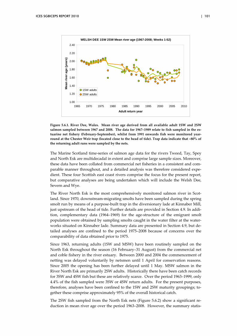
ICES SGBICEPS REPORT 2010 | 101
WELSH DEE 1SW 2SW Mean river age (1967-2008; Weeks 1-52)
1.00
1.20
1.40
1.60
1.80
2.00
2.20
2.40
1965 1970 1975 1980 1985 1990 1995 2000 2005 2010
Adult return year
Me
an r
iver
ag
e (y
ear
s)
1SW adults
2SW adults
Figure 5.6.1. River Dee, Wales. Mean river age derived from all available adult 1SW and 2SW
salmon sampled between 1967 and 2008. The data for 1967–1989 relate to fish sampled in the es‐
tuarine net fishery (February‐September), whilst from 1991 onwards fish were monitored year‐
round at the Chester Weir trap (located close to the head of tide). Trap data indicate that ~80% of
the returning adult runs were sampled by the nets.
The Marine Scotland time‐series of salmon age data for the rivers Tweed, Tay, Spey
and North Esk are multidecadal in extent and comprise large sample sizes. Moreover,
these data have been collated from commercial net fisheries in a consistent and com‐
parable manner throughout, and a detailed analysis was therefore considered expe‐
dient. These four Scottish east coast rivers comprise the focus for the present report,
but comparative analyses are being undertaken which will include the Welsh Dee,
Severn and Wye.
The River North Esk is the most comprehensively monitored salmon river in Scot‐
land. Since 1970, downstream‐migrating smolts have been sampled during the spring
smolt run by means of a purpose‐built trap in the diversionary lade at Kinnaber Mill,
just upstream of the head of tide. Further details are provided in Section 4.9. In addi‐
tion, complementary data (1964–1969) for the age‐structure of the emigrant smolt
population were obtained by sampling smolts caught in the water filter at the water‐
works situated on Kinnaber lade. Summary data are presented in Section 4.9, but de‐
tailed analyses are confined to the period 1975–2008 because of concerns over the
comparability of data obtained prior to 1975.
Since 1963, returning adults (1SW and MSW) have been routinely sampled on the
North Esk throughout the season (16 February–31 August) from the commercial net
and coble fishery in the river estuary. Between 2000 and 2004 the commencement of
netting was delayed voluntarily by netsmen until 1 April for conservation reasons.
Since 2005 the opening has been further delayed until 1 May. MSW salmon in the
River North Esk are primarily 2SW adults. Historically there have been catch records
for 3SW and 4SW fish but these are relatively scarce. Over the period 1963–1999, only
4.4% of the fish sampled were 3SW or 4SW return adults. For the present purposes,
therefore, analyses have been confined to the 1SW and 2SW maturity groupings; to‐
gether these comprise approximately 95% of the overall historical catch.
The 2SW fish sampled from the North Esk nets (Figure 5.6.2) show a significant re‐
duction in mean river age over the period 1963–2008. However, the summary statis‐

102 | ICES SGBICEPS REPORT 2010
tic – mean river age (that is, age at emigration of the smolt) – hides much ecologically
important variation, and even statistically significant patterns in the data may be an
artefact of the sampling regime. Importantly, mean river age may show no trend
over time and yet the age‐structure of the population could have changed radically.
It could also be argued that river age should be considered a categoric variable, rather
than a continuous variable (and therefore not averaged within years). Because
smoltification is an annual “all or none” decision, if a juvenile parr fails to smolt in
one spring then it remains in the river for one or more further full years. There is
therefore no such thing as an emigrant smolt of, say, 1.68 years river age.
NORTH ESK 2SW Mean River Age (1963-2008; February-August )
2
2.1
2.2
2.3
2.4
2.5
2.6
2.7
1963
1966
1969
1972
1975
1978
1981
1984
1987
1990
1993
1996
1999
2002
2005
2008
Mea
n R
iver
Ag
e
Figure 5.6.2. River North Esk, Scotland. Mean river age (± se) for all available returning adult
2SW salmon sampled between February and August, 1963–2008. The downward linear trend is
significant (r = 0.521; P <0.001). [The data for 1982 and 1983 were derived from Shearer (1990), his
summary Tables 2 and 3.]
Figure 5.6.3 indicates that the recent, relatively low mean river age (Figure 5.6.2) is
attributable to increases in the proportions of 2SW adults that migrated as S2 and, to
a lesser extent, S1 smolts, and is reflected as a decline in the S3 component. However,
it is important to stress that these are proportional data – a decline in one river age
proportion will be reflected by an increase in one or more other components and the
data are therefore not independent. Given the ecological improbability of a short‐
term downshift from S3 to S1, the likelihood is that these trends simply reflect a ten‐
dency to shift down from S3 to S2. Similarly, the most cautious interpretation of the
Welsh Dee data (Aprahamian et al., 2008; Figure 2) is that a greater proportion of ju‐
veniles that previously would have smolted at S2 have tended to smolt at S1 since the
1980s.
In the knowledge that the delays in the commencement of the netting season on the
River North Esk since 1999 have led to a seasonal bias in the data time‐series, is the
recent decline in mean river age of North Esk 2SW adults (Figures 5.6.2 and 5.6.3)
real, or is it an artefact of the data?

ICES SGBICEPS REPORT 2010 | 103
North Esk 2SW ALL DATA (1963-99 February-August; 2000-04 April-August; 2005-08 May-August)
0
0.1
0.2
0.3
0.4
0.5
0.6
0.7
0.8
0.9
1963
1966
1969
1972
1975
1978
1981
1984
1987
1990
1993
1996
1999
2002
2005
2008
Pro
ipo
rtio
n R
iver
Ag
e
S1
S2
S3
Figure 5.6.3. River North Esk, Scotland. Proportions of returning 2SW adults of varying river age
(S1–S3; river ages 1 to 3 years, respectively). S4 and S5 fish are relatively rare in the data set and
for clarity have not been plotted here. [The data for 1982 and 1983 were derived from Shearer
(1990), his summary Tables 2 and 3.]
Figure 5.6.4 shows the fluctuations in mean river age for the 2SW fish sampled
throughout the netting season between February and August over the period 1963–
1999. This time‐series therefore comprises seasonally comparable catches in every
year. Despite the among‐year fluctuations, there is an apparent overall downward
trend, but this is not statistically significant for a linear decrease (P >0.05). Figure
5.6.5 includes the separation of these 2SW adult data into their proportional river
ages. Despite the inevitable between‐year variations – and although there is some
suggestion of an increase in S1 and S2, in concert with a relative decrease in the S3
component – it is apparent that there is overall stability in the river age‐structure of
the February–August 2SW samples over the available time‐series.
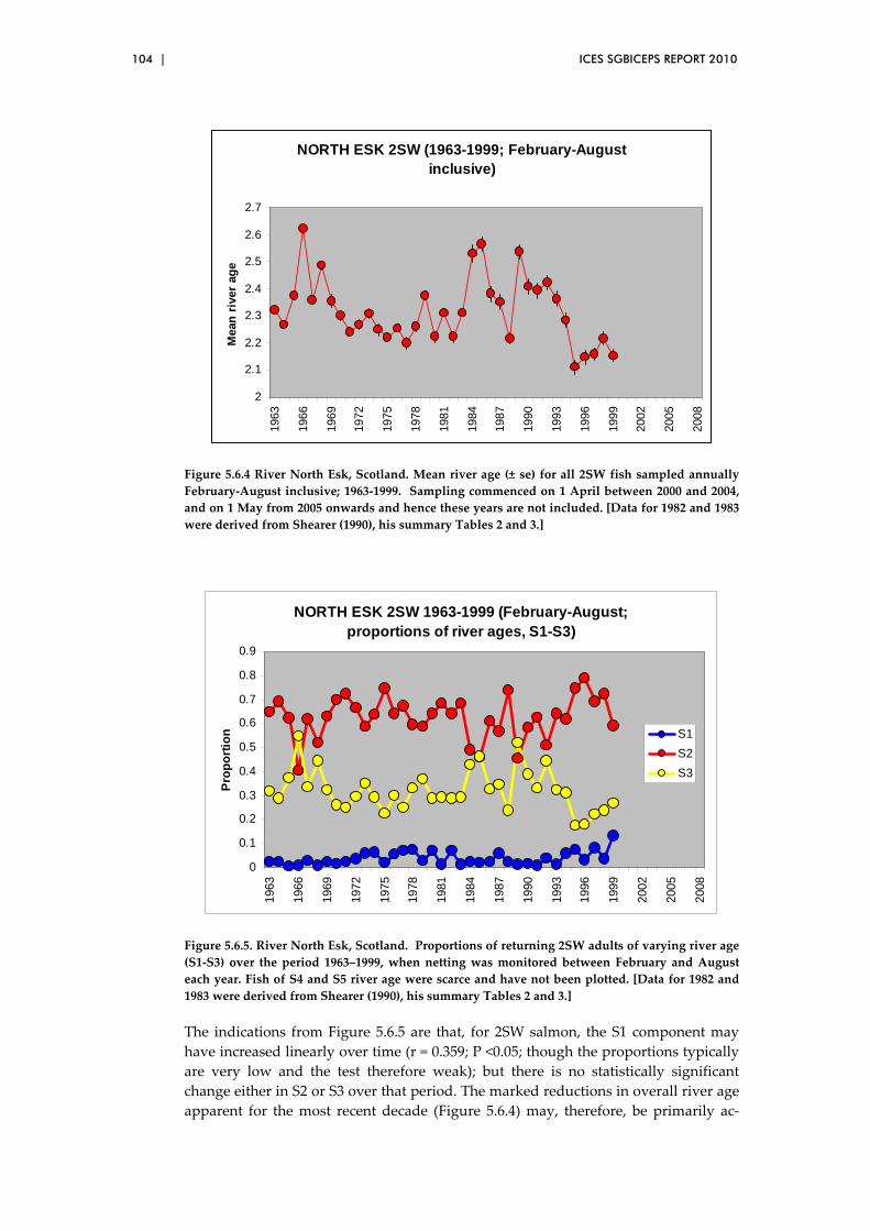
104 | ICES SGBICEPS REPORT 2010
NORTH ESK 2SW (1963-1999; February-August inclusive)
2
2.1
2.2
2.3
2.4
2.5
2.6
2.7
1963
1966
1969
1972
1975
1978
1981
1984
1987
1990
1993
1996
1999
2002
2005
2008
Mea
n r
iver
ag
e
Figure 5.6.4 River North Esk, Scotland. Mean river age (± se) for all 2SW fish sampled annually
February‐August inclusive; 1963‐1999. Sampling commenced on 1 April between 2000 and 2004,
and on 1 May from 2005 onwards and hence these years are not included. [Data for 1982 and 1983
were derived from Shearer (1990), his summary Tables 2 and 3.]
NORTH ESK 2SW 1963-1999 (February-August; proportions of river ages, S1-S3)
0
0.1
0.2
0.3
0.4
0.5
0.6
0.7
0.8
0.9
1963
1966
1969
1972
1975
1978
1981
1984
1987
1990
1993
1996
1999
2002
2005
2008
Pro
po
rtio
n S1
S2
S3
Figure 5.6.5. River North Esk, Scotland. Proportions of returning 2SW adults of varying river age
(S1‐S3) over the period 1963–1999, when netting was monitored between February and August
each year. Fish of S4 and S5 river age were scarce and have not been plotted. [Data for 1982 and
1983 were derived from Shearer (1990), his summary Tables 2 and 3.]
The indications from Figure 5.6.5 are that, for 2SW salmon, the S1 component may
have increased linearly over time (r = 0.359; P <0.05; though the proportions typically
are very low and the test therefore weak); but there is no statistically significant
change either in S2 or S3 over that period. The marked reductions in overall river age
apparent for the most recent decade (Figure 5.6.4) may, therefore, be primarily ac‐

ICES SGBICEPS REPORT 2010 | 105
countable as an artefact in the data because the start of sampling has been seasonally
delayed since 2000.
Figures 5.6.2 to 5.6.5 include both early‐running “spring” salmon and summer‐
running salmon. Notwithstanding our inability to categorically distinguish “spring”
and “summer” salmon, pooling all the available data (February‐August) may there‐
fore occlude differences or contrasts in performance of the early and late‐running
cohorts.
The river age composition of early‐running 2SW spring salmon (Figure 5.6.6) typi‐
cally comprises adults of somewhat higher river ages compared to the later‐running
2SW salmon (included in Figure 5.6.3), with proportionally more S3 fish and S1
barely represented among the early‐running (February/March) 2SW adults. (N.B. one
cannot infer that S2 are scarcer amongst these early‐running fish compared to the
complete data in Figure 5.6.2, because a decrease in one proportion will lead to an
increase in one or more others. The likelihood is that the critical difference here is a
higher relative abundance of S3 among the early‐running spring salmon.) In inter‐
preting Figure 5.6.5 it is important, therefore, to ascertain the proportions of early
(e.g. February/March) fish sampled in any one year relative to the later summer fish.
As might be expected, the relative sample sizes of 2SW salmon taken in February‐
March versus April onwards has fluctuated considerably over the 1963–1999 time‐
series (Figure 5.6.7). The samples of early‐running 2SW spring salmon were consis‐
tently relatively large throughout the late 1960s and 1970s and this further com‐
pounds the difficulties in interpreting the long‐term shifts in river ages for 2SW fish.
For these particular samples, the relative scarcity of early‐running 2SW salmon fol‐
lowing the mid‐1980s will result in a bias in the data towards rather younger river
ages. Resolution of this problem will require more detailed modelling, but the likeli‐
hood is that over the period 1963–1999 there has been stability in the river age‐
structure of returnimg adult 2SW salmon (both in spring and in summer) for the river
North Esk. The lack of data for the early‐running 2SW fish from 2000 onwards is re‐
grettable and precludes further analysis of changes apparent for the most recent
years.
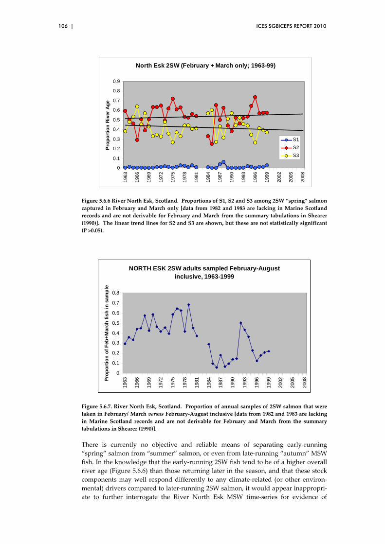
106 | ICES SGBICEPS REPORT 2010
North Esk 2SW (February + March only; 1963-99)
0
0.1
0.2
0.3
0.4
0.5
0.6
0.7
0.8
0.9
1963
1966
1969
1972
1975
1978
1981
1984
1987
1990
1993
1996
1999
2002
2005
2008
Pro
po
rtio
n R
iver
Ag
e
S1
S2
S3
Figure 5.6.6 River North Esk, Scotland. Proportions of S1, S2 and S3 among 2SW “spring” salmon
captured in February and March only [data from 1982 and 1983 are lacking in Marine Scotland
records and are not derivable for February and March from the summary tabulations in Shearer
(1990)]. The linear trend lines for S2 and S3 are shown, but these are not statistically significant
(P >0.05).
NORTH ESK 2SW adults sampled February-August inclusive, 1963-1999
0
0.1
0.2
0.3
0.4
0.5
0.6
0.7
0.8
1963
1966
1969
1972
1975
1978
1981
1984
1987
1990
1993
1996
1999
2002
2005
2008P
rop
ort
ion
of
Feb
+M
arch
fis
h i
n s
amp
le
Figure 5.6.7. River North Esk, Scotland. Proportion of annual samples of 2SW salmon that were
taken in February/ March versus February‐August inclusive [data from 1982 and 1983 are lacking
in Marine Scotland records and are not derivable for February and March from the summary
tabulations in Shearer (1990)].
There is currently no objective and reliable means of separating early‐running
“spring” salmon from “summer” salmon, or even from late‐running “autumn” MSW
fish. In the knowledge that the early‐running 2SW fish tend to be of a higher overall
river age (Figure 5.6.6) than those returning later in the season, and that these stock
components may well respond differently to any climate‐related (or other environ‐
mental) drivers compared to later‐running 2SW salmon, it would appear inappropri‐
ate to further interrogate the River North Esk MSW time‐series for evidence of

ICES SGBICEPS REPORT 2010 | 107
climate‐related shifts in river age‐structure for MSW salmon. Certainly, the data for
the early‐running stock component give no indication of any marked, persistent or
statistically significant trend between 1963 and 1999 – either for mean river age of
returning adults (Figure 5.6.4), or for the proportional representation of the various
river ages (Figure 5.6.5). By contrast, the 1SW stock component is clearly identifiable.
The timing of the netting season ensures that in every year the beginning of the 1SW
return migration is effectively sampled, though the data are truncated by the close of
the netting season before all 1SW fish have returned. Notwithstanding the latter
qualification, the possibilities of detecting, with confidence, any evidence of demo‐
graphic shifts in time‐series for the 1SW component are clear and are discussed in
Section 5.8.
5.7 Among-river comparisons of mean river age and proportional river age composition in four major Scottish salmon rivers: 2SW “summer” salmon (returning May-August/September)
Time‐series data (from in‐river net fisheries) are available for the rivers North Esk,
Tweed, Tay and Spey, with some extending back to the early 1960s. Historically, all
these fisheries opened in February (Tay 6th, Spey 11th, Tweed 15th and North Esk 16th)
though the opening has been voluntarily delayed by netsmen in recent years as a
conservation measure. The close season either falls in August (Tay 20th, Spey 26th,
North Esk 31st) or in September (Tweed 14th). On the strength of the foregoing analy‐
ses, and in recognition of the distinction between early‐running (“spring”) and late‐
running (“summer”) 2SW salmon, the following comparative analyses for 2SW fish
are confined to years when sample data were available from early May onwards. All
available data after the beginning of May within years have been retained and ana‐
lyzed so, for example, the Tweed analyses include September fish caught after the
remaining three river fisheries had closed. Years in which sampling ceased >10 days
prior to the seasonal close were deleted. The time‐series for the rivers Spey and Tay
terminated in 1993 and 1996 respectively when the net fisheries were closed for con‐
servation reasons.
The available time‐series for the rivers Tay, Tweed and Spey are not as complete as
for River North Esk (Figure 5.7.1). Samples for the Tweed are available up to 2008,
but the variations in the commencement and cessation dates of sampling within the
netting season resulted in recent years of incomplete and non‐comparable data. The
conservative approach was adopted throughout here in deleting from analysis all
such years.

108 | ICES SGBICEPS REPORT 2010
TWEED 2SW Mean River Age (May onwards)
1.3
1.5
1.7
1.9
2.1
2.3
2.5
1963
1966
1969
1972
1975
1978
1981
1984
1987
1990
1993
1996
1999
2002
2005
2008
Mea
n R
iver
Ag
e
TAY 2SW Mean river age (May onwards)
1.3
1.5
1.7
1.9
2.1
2.3
2.519
63
1966
1969
1972
1975
1978
1981
1984
1987
1990
1993
1996
1999
2002
2005
2008
Mea
n R
iver
Ag
e
NORTH ESK 2SW Mean river age (May onwards)
1.3
1.5
1.7
1.9
2.1
2.3
2.5
1963
1966
1969
1972
1975
1978
1981
1984
1987
1990
1993
1996
1999
2002
2005
2008
Mea
n R
iver
Ag
e
SPEY 2SW Mean river age (May onwards)
1.3
1.5
1.7
1.9
2.1
2.3
2.5
1963
1966
1969
1972
1975
1978
1981
1984
1987
1990
1993
1996
1999
2002
2005
2008
Mea
n R
iver
Ag
e
Figure 5.7.1. Rivers Tweed, Tay, Spey and North Esk, Scotland. Mean river age (at smoltification)
(± se) for returning 2SW “summer” salmon sampled between May and the end of the netting sea‐
son (Spey, Tay, North Esk – August; Tweed – September).
As a generalization, the 2SW summer fish in all four rivers are dominated either by
S2 or by S2 and S3 river ages. The Tweed, however, apparently differs fundamen‐
tally from the remaining three rivers in typically comprising an overall younger age‐
structure, although this varies considerably from year to year (see further discussion
below).

ICES SGBICEPS REPORT 2010 | 109
Table 5.7.1. Correlation matrix for mean river age for 2SW “summer” salmon sampled on the four
Scottish rivers (from data in Figure 5.7.1). Correlations in bold type are significant at the P = 0.05
level. The correlation in bold italics remains significant following Bonferroni Correction.
___________________________________________________________________________
SPEY r 0.186
P 0.490
TAY r 0.558 0.688
P 0.025 0.005
NORTH ESK r 0.221 0.521 0.329
P 0.349 0.027 0.182
TWEED SPEY TAY
___________________________________________________________________________
Analysis of the mean river ages illustrated in Figure 5.7.1 shows three significant cor‐
relations (Table 5.7.1), but only one (Spey–Tay) remains significant following Bon‐
ferroni Correction for multiple comparisons (critical value P = 0.008). The overall
outcome here is that there is no strong evidence that these four Scottish rivers are re‐
sponding similarly – in terms of long‐term variation in mean river age of 2SW
“summer” salmon – over the period from the late 1960s to the late 1990s. But as dis‐
cussed above, mean river age as a summary statistic occludes a considerable amount
of ecologically relevant variation in the detailed age‐structure of return cohorts or
year‐classes. Pair‐wise comparisons of, for example, the correlations between S2 and
S3 fish within years are confounded by the lack of independence of proportional
data, so in order to progress this a hierarchical analytical approach was adopted
within a framework of generalized additive models (GAMs). River age for these four
catchments was analyzed with a general model structure of:
Model<‐gam Proportion river age~
s(Other proportional river ages)
s(Year)
s(Year, by=River)
River
Family=quasibinomial
Gamma=1.4
Year and River (Tweed, Tay, North Esk, Spey) were treated as factors, and the quasi‐
binomial error structure was used due to the limitations of the response variable: the
Proportion of sample population in the age‐class is a decimal that can range only be‐
tween 0 and 1. This error structure also controls for the over‐dispersion in the pro‐
portion data. Gamma was increased to 1.4 to control for over‐fitting within the
model. Models were simplified to find the most parsimonious structure, with the
validity and utility of the model being determined by the General Cross Validation
(GCV) procedure.
Model Forms:
1 ) ProportionS1 vs ProportionS2 + ProportionS3 + ProportionS4
2 ) ProportionS2 vs ProportionS3 + ProportionS4

110 | ICES SGBICEPS REPORT 2010
3 ) ProportionS3 vs ProportionS4
A separate model was used to test the relationship between each river age proportion
and those above it (i.e. older). In each model, the Proportion of fish in the river age‐
class was compared with the (grouping of) older age class(es). The factors Year and
River, and the Year*River interaction, were modelled as smooth functions. In the
summary Table 5.7.2, the effects of River are assessed by comparing the River North
Esk to the remaining three rivers. River North Esk is the comparator simply because
it is first in the alphabetical list.
Table 5.7.2. Rivers Tweed, Tay, North Esk, Spey, Scotland. Summary of significant F ratios and
probabilities from generalized additive model analysis of the variation in proportions of river age
classes over the period 1963–2008 (data in Figure 5.7.2) ns = not significant.
___________________________________________________________________________
GAM outputs for 2SW return adults (River comparisons Tweed, Spey, Tay against
North Esk)
S1 vs S2+S3+S4 Year River River*Year
F P
2042 <<0.001 ns ns ns
S2 vs S3+S4
F P F P F P
82.46 <<0.001 2.49 0.024 ns 19.78<<0.001
(Tweed)
S3 vs S4
F P F P F P F P
9.95 0.002 4.10 0.001 ‐3.56 0.001 4.68<0.001
(Tweed) (Tweed)
‐2.79 0.006
(Spey)
___________________________________________________________________________

ICES SGBICEPS REPORT 2010 | 111
TWEED 2SW proportional river ages (May-September fish)
0
0.1
0.2
0.3
0.4
0.5
0.6
0.7
0.8
0.9
1
1963
1966
1969
1972
1975
1978
1981
1984
1987
1990
1993
1996
1999
2002
2005
2008
Pro
po
rtio
n
S1
S2
S3
TAY 2SW proportional river ages (May-August fish)
0
0.1
0.2
0.3
0.4
0.5
0.6
0.7
0.8
0.9
119
63
1966
1969
1972
1975
1978
1981
1984
1987
1990
1993
1996
1999
2002
2005
2008
Pro
po
rtio
n
S1
S2
S3
NORTH ESK 2SW proportional river ages (May-August fish)
0
0.1
0.2
0.3
0.4
0.5
0.6
0.7
0.8
0.9
1
1963
1966
1969
1972
1975
1978
1981
1984
1987
1990
1993
1996
1999
2002
2005
2008
Pro
po
rtio
n
S1
S2
S3
SPEY 2SW proportional river ages (May-August fish)
0
0.1
0.2
0.3
0.4
0.5
0.6
0.7
0.8
0.9
1
1963
1966
1969
1972
1975
1978
1981
1984
1987
1990
1993
1996
1999
2002
2005
2008
Pro
po
rtio
n
S1
S2
S3
Figure 5.7.2. Rivers Tweed, Tay, North Esk and Spey, Scotland. Proportions of “summer” 2SW
adults of varying river age (S1‐S3) sampled between May and August/September each year. S4
fish were rare and have not been included.

112 | ICES SGBICEPS REPORT 2010
Figure 5.7.3. Rivers Tweed, Tay, North Esk, Spey, Scotland. Proportions of river ages S1‐S4
amongst return adult 2SW “summer” salmon.
Figure 5.7.3 indicates the marked contrasts in river age composition of “summer”
2SW salmon among the group of four rivers. Whilst the rivers Tay, Spey and North
Esk show considerable similarity in overall age‐structure and temporal variation, the
Tweed is clearly distinct: the major between‐river contrasts lie in the relative propor‐
tions of S1 and S3 fish.
For the proportions of all the separate river ages (S1, S2, S3) there were consistent and
significant effects of the proportions of the older river age(s) pooled. Indeed, for S1
fish this was the only significant outcome (Table 5.7.2), and the data for the River
Tweed are especially notable in their variation over time. Given the scarcity of S4
fish, the comparison S2 vs S3+S4 essentially is a contrast between S2 and S3. The pro‐
portion of S2 vs S3+S4 showed a significant Year effect and, for the River Tweed, a
significant interaction with Year. For S3, there was a significant Year effect (the pro‐
portion of S3 fish increased over time relative to the proportion of S4 [NOTE: for clar‐
ity, S4 data are not plotted in Figure 5.7.2]) and the Rivers Tweed and Spey showed
declines in proportions of S3 (relative to S4) in comparison to the River North Esk.
As a generalization, for the Tweed the demographic changes over time have largely
been attributable to downward shifts from S2 to S1 smolts, whereas for the River
North Esk the shift over the past decade has been from S3 to S2. The lack of compara‐
ble data for the other three rivers over the most recent decade does, however, restrict
this observation to that one river. Whether or not this change is typical of Scottish
rivers remains unclear. The higher prevalence of S1 smolts in the river Tweed pre‐
sumably is a reflection of this being essentially a lowland catchment with relatively
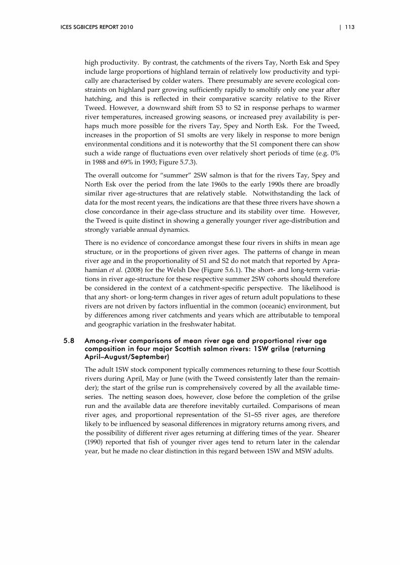
ICES SGBICEPS REPORT 2010 | 113
high productivity. By contrast, the catchments of the rivers Tay, North Esk and Spey
include large proportions of highland terrain of relatively low productivity and typi‐
cally are characterised by colder waters. There presumably are severe ecological con‐
straints on highland parr growing sufficiently rapidly to smoltify only one year after
hatching, and this is reflected in their comparative scarcity relative to the River
Tweed. However, a downward shift from S3 to S2 in response perhaps to warmer
river temperatures, increased growing seasons, or increased prey availability is per‐
haps much more possible for the rivers Tay, Spey and North Esk. For the Tweed,
increases in the proportion of S1 smolts are very likely in response to more benign
environmental conditions and it is noteworthy that the S1 component there can show
such a wide range of fluctuations even over relatively short periods of time (e.g. 0%
in 1988 and 69% in 1993; Figure 5.7.3).
The overall outcome for “summer” 2SW salmon is that for the rivers Tay, Spey and
North Esk over the period from the late 1960s to the early 1990s there are broadly
similar river age‐structures that are relatively stable. Notwithstanding the lack of
data for the most recent years, the indications are that these three rivers have shown a
close concordance in their age‐class structure and its stability over time. However,
the Tweed is quite distinct in showing a generally younger river age‐distribution and
strongly variable annual dynamics.
There is no evidence of concordance amongst these four rivers in shifts in mean age
structure, or in the proportions of given river ages. The patterns of change in mean
river age and in the proportionality of S1 and S2 do not match that reported by Apra‐
hamian et al. (2008) for the Welsh Dee (Figure 5.6.1). The short‐ and long‐term varia‐
tions in river age‐structure for these respective summer 2SW cohorts should therefore
be considered in the context of a catchment‐specific perspective. The likelihood is
that any short‐ or long‐term changes in river ages of return adult populations to these
rivers are not driven by factors influential in the common (oceanic) environment, but
by differences among river catchments and years which are attributable to temporal
and geographic variation in the freshwater habitat.
5.8 Among-river comparisons of mean river age and proportional river age composition in four major Scottish salmon rivers: 1SW grilse (returning April–August/September)
The adult 1SW stock component typically commences returning to these four Scottish
rivers during April, May or June (with the Tweed consistently later than the remain‐
der); the start of the grilse run is comprehensively covered by all the available time‐
series. The netting season does, however, close before the completion of the grilse
run and the available data are therefore inevitably curtailed. Comparisons of mean
river ages, and proportional representation of the S1–S5 river ages, are therefore
likely to be influenced by seasonal differences in migratory returns among rivers, and
the possibility of different river ages returning at differing times of the year. Shearer
(1990) reported that fish of younger river ages tend to return later in the calendar
year, but he made no clear distinction in this regard between 1SW and MSW adults.

114 | ICES SGBICEPS REPORT 2010
TWEED 1SW Mean River Age (April-September)
1.3
1.5
1.7
1.9
2.1
2.3
2.5
19
63
19
66
19
69
19
72
19
75
19
78
19
81
19
84
19
87
19
90
19
93
19
96
19
99
20
02
20
05
20
08
Me
an
Riv
er
Ag
e (
se
)
TAY 1SW Mean River Age (April-August)
1.3
1.5
1.7
1.9
2.1
2.3
2.5
19
63
19
66
19
69
19
72
19
75
19
78
19
81
19
84
19
87
19
90
19
93
19
96
19
99
20
02
20
05
20
08
Me
an
Riv
er
Ag
e (
se
)
NORTH ESK 1SW River Age (April-August)
1.3
1.5
1.7
1.9
2.1
2.3
2.5
19
63
19
66
19
69
19
72
19
75
19
78
19
81
19
84
19
87
19
90
19
93
19
96
19
99
20
02
20
05
20
08
Me
an
Riv
er
Ag
e (
se
)
SPEY 1SW River Age (April-August)
1.3
1.5
1.7
1.9
2.1
2.3
2.5
19
63
19
66
19
69
19
72
19
75
19
78
19
81
19
84
19
87
19
90
19
93
19
96
19
99
20
02
20
05
20
08
Me
an
Riv
er
Ag
e (
se
)
Figure 5.8.1. Rivers Tweed, Tay, North Esk and Spey, Scotland. Mean river age (at smoltification)
(± se) for adult 1SW salmon sampled between April and the end of the netting season (Spey, Tay,
North Esk – August; Tweed – September).
The 1SW data for the four rivers (Figure 5.8.1) all include the beginning of the 1SW
run, but the cessation of the netting season differs among rivers. The Tweed, for ex‐
ample, closes later, but the start of the grilse run is typically also later here than for
the other three rivers. Over the complete 46‐year period, the mean river age of 1SW
fish on the River North Esk has remained remarkably stable, and notably so over the
past decade. Although variation was more marked in the earlier years, the overall
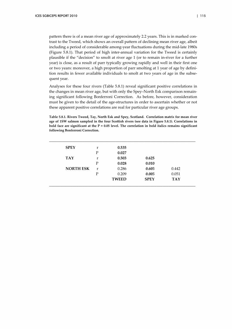
ICES SGBICEPS REPORT 2010 | 115
pattern there is of a mean river age of approximately 2.2 years. This is in marked con‐
trast to the Tweed, which shows an overall pattern of declining mean river age, albeit
including a period of considerable among‐year fluctuations during the mid‐late 1980s
(Figure 5.8.1). That period of high inter‐annual variation for the Tweed is certainly
plausible if the “decision” to smolt at river age 1 (or to remain in‐river for a further
year) is close, as a result of parr typically growing rapidly and well in their first one
or two years: moreover, a high proportion of parr smolting at 1 year of age by defini‐
tion results in fewer available individuals to smolt at two years of age in the subse‐
quent year.
Analyses for these four rivers (Table 5.8.1) reveal significant positive correlations in
the changes in mean river age, but with only the Spey–North Esk comparison remain‐
ing significant following Bonferroni Correction. As before, however, consideration
must be given to the detail of the age‐structures in order to ascertain whether or not
these apparent positive correlations are real for particular river age groups.
Table 5.8.1. Rivers Tweed, Tay, North Esk and Spey, Scotland. Correlation matrix for mean river
age of 1SW salmon sampled in the four Scottish rivers (see data in Figure 5.8.1). Correlations in
bold face are significant at the P = 0.05 level. The correlation in bold italics remains significant
following Bonferroni Correction.
___________________________________________________________________________
SPEY r 0.535
P 0.027
TAY r 0.503 0.625
P 0.028 0.010
NORTH ESK r 0.286 0.605 0.442
P 0.209 0.005 0.051
TWEED SPEY TAY
___________________________________________________________________________
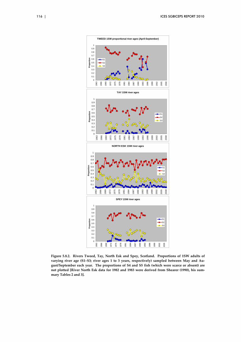
116 | ICES SGBICEPS REPORT 2010
TWEED 1SW proportional river ages (April-September)
0
0.1
0.2
0.3
0.4
0.5
0.6
0.7
0.8
0.9
1
1963
1966
1969
1972
1975
1978
1981
1984
1987
1990
1993
1996
1999
2002
2005
2008
Pro
po
rtio
n
S1
S2
S3
TAY 1SW river ages
0
0.1
0.2
0.3
0.4
0.5
0.6
0.7
0.8
0.9
11
96
3
19
66
19
69
19
72
19
75
19
78
19
81
19
84
19
87
19
90
19
93
19
96
19
99
20
02
20
05
20
08
Pro
po
rtio
n
S1
S2
S3
NORTH ESK 1SW river ages
0
0.1
0.2
0.3
0.4
0.5
0.6
0.7
0.8
0.9
1
19
63
19
66
19
69
19
72
19
75
19
78
19
81
19
84
19
87
19
90
19
93
19
96
19
99
20
02
20
05
20
08
Pro
po
rtio
n
S1
S2
S3
SPEY 1SW river ages
0
0.1
0.2
0.3
0.4
0.5
0.6
0.7
0.8
0.9
1
1963
1966
1969
1972
1975
1978
1981
1984
1987
1990
1993
1996
1999
2002
2005
Pro
po
rtio
n S1
S2
S3
Figure 5.8.2. Rivers Tweed, Tay, North Esk and Spey, Scotland. Proportions of 1SW adults of
varying river age (S1–S3; river ages 1 to 3 years, respectively) sampled between May and Au‐
gust/September each year. The proportions of S4 and S5 fish (which were scarce or absent) are
not plotted [River North Esk data for 1982 and 1983 were derived from Shearer (1990), his sum‐
mary Tables 2 and 3].
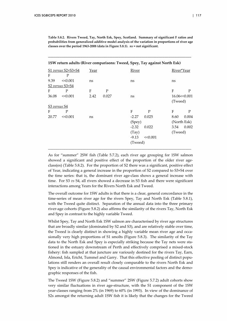
ICES SGBICEPS REPORT 2010 | 117
Table 5.8.2. Rivers Tweed, Tay, North Esk, Spey, Scotland. Summary of significant F ratios and
probabilities from generalized additive model analysis of the variation in proportions of river age
classes over the period 1963‐2008 (data in Figure 5.8.1). ns = not significant.
___________________________________________________________________________
1SW return adults (River comparisons: Tweed, Spey, Tay against North Esk)
S1 versus S2+S3+S4 Year River River*Year
F P
9.39 <<0.001 ns ns ns
S2 versus S3+S4
F P F P F P
36.08 <<0.001 2.42 0.027 ns 16.06<<0.001
(Tweed)
S3 versus S4
F P F P F P
20.77 <<0.001 ns ‐2.27 0.025 8.60 0.004
(Spey) (North Esk)
‐2.32 0.022 3.54 0.002
(Tay) (Tweed)
‐9.13 <<0.001
(Tweed)
___________________________________________________________________________
As for “summer” 2SW fish (Table 5.7.2), each river age grouping for 1SW salmon
showed a significant and positive effect of the proportion of the older river age‐
class(es) (Table 5.8.2). For the proportion of S2 there was a significant, positive effect
of Year, indicating a general increase in the proportion of S2 compared to S3+S4 over
the time series: that is, the dominant river age‐class shows a general increase with
time. For S3 vs S4, all rivers showed a decrease in S3 fish and there were significant
interactions among Years for the Rivers North Esk and Tweed.
The overall outcome for 1SW adults is that there is a clear, general concordance in the
time‐series of mean river age for the rivers Spey, Tay and North Esk (Table 5.8.1),
with the Tweed quite distinct. Separation of the annual data into the three primary
river‐age cohorts (Figure 5.8.2) also affirms the similarity of the rivers Tay, North Esk
and Spey in contrast to the highly variable Tweed.
Whilst Spey, Tay and North Esk 1SW salmon are characterised by river age structures
that are broadly similar (dominated by S2 and S3), and are relatively stable over time,
the Tweed is clearly distinct in showing a highly variable mean river age and occa‐
sionally very high proportions of S1 smolts (Figure 5.8.3). The similarity of the Tay
data to the North Esk and Spey is especially striking because the Tay nets were sta‐
tioned in the estuary downstream of Perth and effectively comprised a mixed‐stock
fishery: fish sampled at that juncture are variously destined for the rivers Tay, Earn,
Almond, Isla, Ericht, Tummel and Garry. That this effective pooling of distinct popu‐
lations still renders an overall result closely comparable to the rivers North Esk and
Spey is indicative of the generality of the causal environmental factors and the demo‐
graphic responses of the fish.
The Tweed 1SW (Figure 5.8.2) and “summer” 2SW (Figure 5.7.2) adult cohorts show
very similar fluctuations in river age‐structure, with the S1 component of the 1SW
year‐classes ranging from 2% (in 1969) to 60% (in 1993). In view of the dominance of
S2s amongst the returning adult 1SW fish it is likely that the changes for the Tweed

118 | ICES SGBICEPS REPORT 2010
are typified by a tendency for earlier smoltification and a downshift from S2 to S1.
For the remaining three rivers there is a striking consistency of overall river age
throughout the time series. Assuming that the river age‐structures of returning adult
1SW and 2SW adult salmon analyzed here are a reflection of the original annual emi‐
grant smolt cohorts, this indicates that changes in river age‐structure of the returning
adult populations are a feature of the specific river catchment (the freshwater envi‐
ronment) and not the shared oceanic environment.
Figure 5.8.3. Rivers Tweed, Tay, North Esk, Spey, Scotland. Proportions of river ages S1‐S4
amongst returning adult 1SW salmon.
For the River North Esk, the trend for both the 1SW and “summer” 2SW cohorts in
the most recent decade has been a slight but progressive shift towards younger over‐
all river age and this is reflected in a downshift from S3 to S2. It has to be reiterated
that a decline in one proportion must lead to a compensatory increase in one or more
other proportion(s), and that the present data cannot unequivocally identify if these
changes relate to either or both of the S2 and S3 categories. However, considering the
known relationship between growth rate and age at smoltification (e.g. Økland et al.,
1993), the most cautious explanation is of an increasing recent tendency for River
North Esk parr to undergo smoltification at two, rather than three years of age.
Whether this recent pattern over the last decade is confined to the River North Esk, or
is more widespread among these Scottish rivers, is not testable due to the lack of
suitably comprehensive sampling on the remaining three rivers over that time period.

ICES SGBICEPS REPORT 2010 | 119
5.9 Analysis of the time-series of the emigrant smolt run, River North Esk (1964–2008)
The comprehensive smolt trap and net samples for the River North Esk present the
only opportunity of comparing the age‐structure of the annual emigrant smolt popu‐
lation with the river age‐structure of returning adults. Smolts have been sampled on
the River North Esk since 1964. Data between 1964 and 1969 were derived from
smolts caught in the filter screens of the waterworks at Kinnaber Mill Lade in the
lower river. From 1970 onwards the data were derived from smolts sampled in a
purpose‐built trap at Kinnaber Mill. Figure 5.9.1 indicates the age composition of the
emigrating smolts for the two time‐series (1964–1969, 1970–2008).
NORTH ESK, emigrant smolts 1964-2008
0.0
0.1
0.2
0.3
0.4
0.5
0.6
0.7
0.8
0.9
1.0
1964 1968 1972 1976 1980 1984 1988 1992 1996 2000 2004 2008
Pro
po
rtio
n
S1 S2 S3 S4
Figure 5.9.1. River North Esk, Scotland. Proportional composition of the river ages of emigrant
smolts, 1964–2008.
There has been a slight, but significant, increase in the proportion of S1 smolts (P =
0.037), no change in the proportion of S2 smolts (P = 0.068) and marked and signifi‐
cant decreases in both the S3 (P = 0.004) and S4 (P = 0.001) smolts. Given the scarcity
of S4 juveniles throughout the time series, it appears that the major population‐level
change in proportional age‐structure has been the decrease in the relative abundance
of S3 smolts, reflected by the slight proportional increase in S1s and decrease in S4s.
An overall slight downward shift in mean river age of the total emigrant smolt popu‐
lation (which includes fish which will subsequently mature as a mixture of 1SW and
MSW adults) over the 45 years is therefore apparent. Such a trend may well be expli‐
cable by recent warming of the freshwater environment.
For comparisons between the age‐structure of the returning adult cohorts and the
relevant year‐classes of emigrant smolts, only the data between 1975 and 1999 are
analyzed. These data include all years that adult salmon samples (1SW & 2SW) are
available between February and August inclusive, and can be compared with the
emigrant smolt data for just the Kinnaber trap. The latter excludes data between 1970
and 1974 (owing to concerns about the reliability of the data in those years) so that a
period of inter‐annual comparability is assured. Although there is no netting be‐
tween 1 September and February 15, it is apparent (from the automated fish counter
at Craigo in the lower River North Esk) that the bulk of both the 1SW and MSW stock
components are effectively ‘sampled’ by the nets. 1SW fish continue to enter the river
through September and October and MSW fish return in all months of the year, but
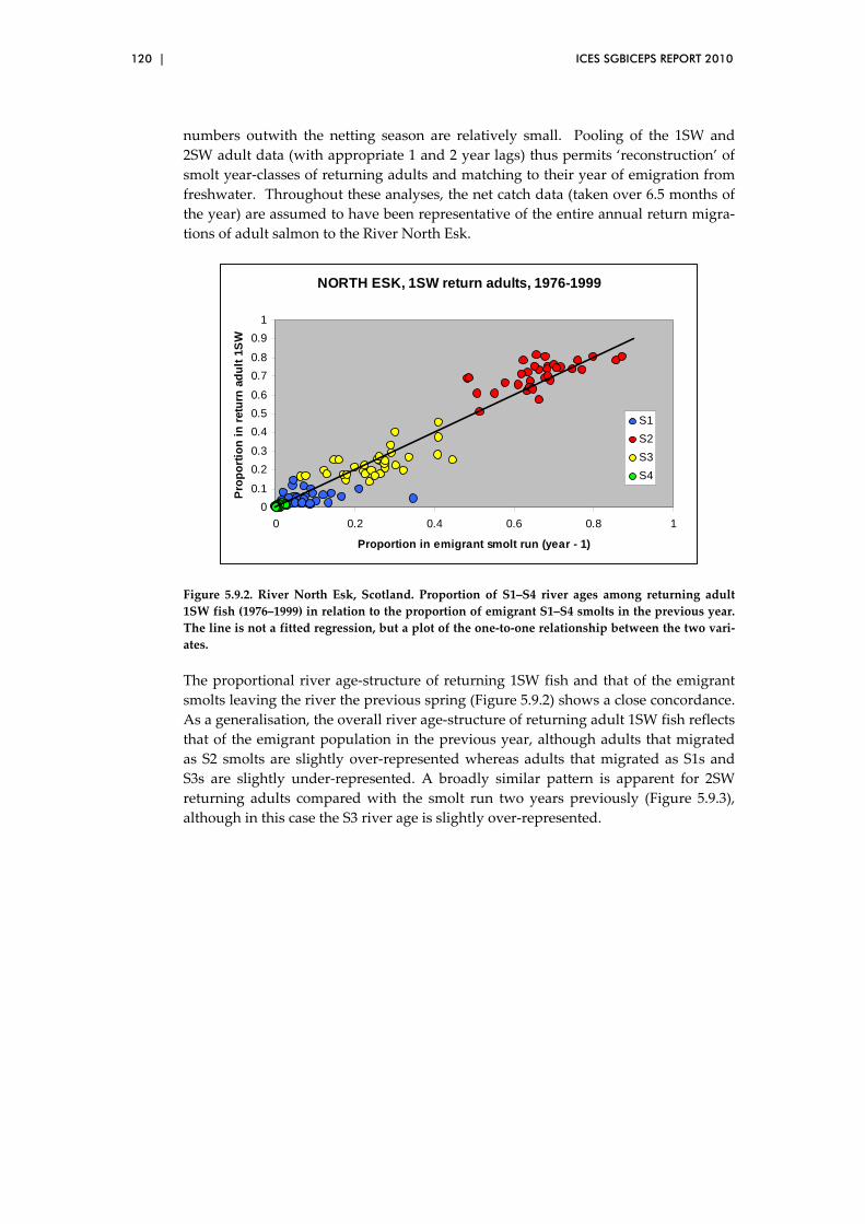
120 | ICES SGBICEPS REPORT 2010
numbers outwith the netting season are relatively small. Pooling of the 1SW and
2SW adult data (with appropriate 1 and 2 year lags) thus permits ‘reconstruction’ of
smolt year‐classes of returning adults and matching to their year of emigration from
freshwater. Throughout these analyses, the net catch data (taken over 6.5 months of
the year) are assumed to have been representative of the entire annual return migra‐
tions of adult salmon to the River North Esk.
NORTH ESK, 1SW return adults, 1976-1999
0
0.1
0.2
0.3
0.4
0.5
0.6
0.7
0.8
0.9
1
0 0.2 0.4 0.6 0.8 1
Proportion in emigrant smolt run (year - 1)
Pro
po
rtio
n i
n r
etu
rn a
du
lt 1
SW
S1
S2
S3
S4
Figure 5.9.2. River North Esk, Scotland. Proportion of S1–S4 river ages among returning adult
1SW fish (1976–1999) in relation to the proportion of emigrant S1–S4 smolts in the previous year.
The line is not a fitted regression, but a plot of the one‐to‐one relationship between the two vari‐
ates.
The proportional river age‐structure of returning 1SW fish and that of the emigrant
smolts leaving the river the previous spring (Figure 5.9.2) shows a close concordance.
As a generalisation, the overall river age‐structure of returning adult 1SW fish reflects
that of the emigrant population in the previous year, although adults that migrated
as S2 smolts are slightly over‐represented whereas adults that migrated as S1s and
S3s are slightly under‐represented. A broadly similar pattern is apparent for 2SW
returning adults compared with the smolt run two years previously (Figure 5.9.3),
although in this case the S3 river age is slightly over‐represented.
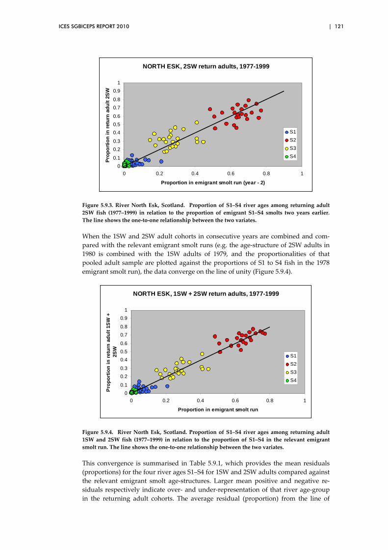
ICES SGBICEPS REPORT 2010 | 121
NORTH ESK, 2SW return adults, 1977-1999
0
0.1
0.2
0.3
0.4
0.5
0.6
0.7
0.8
0.9
1
0 0.2 0.4 0.6 0.8 1
Proportion in emigrant smolt run (year - 2)
Pro
po
rtio
n i
n r
etu
rn a
du
lt 2
SW
S1
S2
S3
S4
Figure 5.9.3. River North Esk, Scotland. Proportion of S1–S4 river ages among returning adult
2SW fish (1977–1999) in relation to the proportion of emigrant S1–S4 smolts two years earlier.
The line shows the one‐to‐one relationship between the two variates.
When the 1SW and 2SW adult cohorts in consecutive years are combined and com‐
pared with the relevant emigrant smolt runs (e.g. the age‐structure of 2SW adults in
1980 is combined with the 1SW adults of 1979, and the proportionalities of that
pooled adult sample are plotted against the proportions of S1 to S4 fish in the 1978
emigrant smolt run), the data converge on the line of unity (Figure 5.9.4).
NORTH ESK, 1SW + 2SW return adults, 1977-1999
0
0.1
0.2
0.3
0.4
0.5
0.6
0.7
0.8
0.9
1
0 0.2 0.4 0.6 0.8 1
Proportion in emigrant smolt run
Pro
po
rtio
n i
n r
etu
rn a
du
lt 1
SW
+
2SW
S1
S2
S3
S4
Figure 5.9.4. River North Esk, Scotland. Proportion of S1–S4 river ages among returning adult
1SW and 2SW fish (1977–1999) in relation to the proportion of S1–S4 in the relevant emigrant
smolt run. The line shows the one‐to‐one relationship between the two variates.
This convergence is summarised in Table 5.9.1, which provides the mean residuals
(proportions) for the four river ages S1–S4 for 1SW and 2SW adults compared against
the relevant emigrant smolt age‐structures. Larger mean positive and negative re‐
siduals respectively indicate over‐ and under‐representation of that river age‐group
in the returning adult cohorts. The average residual (proportion) from the line of

122 | ICES SGBICEPS REPORT 2010
unity for the respective S2, S3 and S4 river ages in the melded year‐classes was 0.011
or less.
Table 5.9.1. Mean residuals (proportions) for the four river ages S1–S4 for 1SW adults 1976–1999
and 2SW adults 1977–1999 compared against the relevant emigrant smolt age‐structures for 1975–
1998. Note the convergence of the residuals for the melded population both for S2 and S3.
___________________________________________________________________________
S1 S2 S3 S4
1SW adults ‐0.013 0.038 ‐0.023 ‐0.002
2SW adults ‐0.027 0.024 0.043 0.008
1SW+2SW (meld) ‐0.019 0.011 0.004 0.004
___________________________________________________________________________
For the period 1975–1999, there is a clear concordance between the age‐structure of
the River North Esk emigrant smolt year‐classes and the age‐structure of the subse‐
quent returning adult cohorts one (1SW) and two (2SW) years later. This result may
have important implications for our understanding of mortality of salmon at sea and
in informing management strategies. If generally applicable to other river catch‐
ments, this implies that monitoring of the river‐age structure of emigrant smolts has
predictive value for subsequent returning adults. Similarly, by ascertaining annual
variation in the river age‐distribution from adult scale archives, the hindcasting of
changes in age at smoltification can be undertaken with confidence.
Perhaps the most important outcome from the data in Figure 5.9.4 is the clear evi‐
dence, for both the 1SW and 2SW stock components, of an overall lack of systematic,
river age‐related variation in survival at sea, and an absence of any ocean‐related in‐
fluence on returning adult age‐structures. The River North Esk data show that river
age at smoltification has no influence on ultimate adult survivorship probabilities
and different aged smolts appear to have an effectively equal probability of returning
to reproduce. Thus, for example, that S2 and S3 smolts appear to show no clear in‐
crease or decrease in their ultimate survivorship (Figure 5.9.4) indicates that early
mortality at sea (which is generally perceived to be critical to adult recruitment) is not
river‐age dependent. Since there is a clear tendency for older smolts to be slightly
larger at first entry to seawater (Figures 4.9.2 & 4.9.3) and to migrate earlier in the
spring smolt run (J.C. MacLean; unpublished data for River North Esk), this suggests
that early mortality at sea is also independent of smolt size and timing of sea entry.
Any specific statistical test for the extremes of river age is rendered weak for the
River North Esk because of the relative scarcity of S1 and S4 fish. In this context, emi‐
grant smolt data for other rivers, such as the River Tweed, where S1 fish comprise a
larger part of the smolt run, would have been invaluable. However, for the majority
of River North Esk fish it is clear that S2 and S3 smolts have comparable rates of sur‐
vivorship at sea and probabilities of returning to spawn, either as 1SW or 2SW adults.
These data also can further inform analyses of the possibilities of temperature / food /
environment match‐mismatch hypotheses affecting salmon growth and survivorship
early in their marine migration. If these data for the River North Esk are characteristic
of other UK and southern NEAC populations, the possibility is that environmental
match‐mismatch is not a driver of short‐ and long‐term variations in the age‐structure
of returning adults. That is, at least for the period 1975–1999, earlier‐migrating (older
and typically larger) smolts do not appear to have been subject to disproportionately
high (or low) survivorship compared to younger (possibly later‐emigrating and typi‐
cally smaller) smolts. It has to be emphasized here that the present analyses focus on

ICES SGBICEPS REPORT 2010 | 123
relative frequencies of the river age‐classes, and not on abundances of the distinct
maturity groupings and year‐classes. Environmental match‐mismatch may well in‐
fluence overall year‐class success in terms of adult recruitment abundances, but it
appears unlikely to influence the river age‐structure of successful return adults.
The combined River North Esk time‐series for emigrant smolt age‐structure, 1964–
2008 (Figure 5.9.1), indicates an overall trend of reducing mean river age and de‐
creases in the proportions of S3 and S4 smolts. This long‐term pattern is detectable
also in the age‐structures of returning summer 2SW and 1SW adults (Figures 5.8.2. &
5.7.2), but objective and comprehensive testing of this is compromised by the lack of
data for early spring 2SW fish from 2000 onwards. For the River North Esk, the last
decade appears to have been characterised by progressive changes in the age‐
structures of both emigrant smolts and returning 1SW and 2SW adults. Unfortu‐
nately, the lack of comprehensive data for the remaining three monitored Scottish
rivers (due to temporally inadequate sampling within years, voluntary deferment of
the commencement of netting for conservation purposes, and the complete closure of
two of the net fisheries) precludes among‐river comparisons for the most recent
years.
5.10 Correlations between the length of returning 1SW salmon and the PFA of maturing (1SW) salmon
The extended data sets of length at return made available to the Study Group enabled
new analyses to be completed for NEAC stocks. In order to compare the size of 1SW
salmon across a number of rivers in both the Northern and Southern NEAC areas, the
size of maiden 1SW salmon was standardised using the mean and standard deviation
for individual populations over the period 1989–2007. This period was chosen as it
enabled information from as many rivers as possible to be included; data for 12 rivers
in the Northern NEAC area and 6 rivers from Southern NEAC were examined. The z‐
score for 2008 was also calculated using the 1989–2007 period to standardise, though
data for 2008 were only available for six rivers in Northern NEAC and three rivers in
the Southern NEAC area.
The mean length of 1SW salmon from Northern and Southern NEAC was found to be
significantly correlated over the period 1989–2008 (r = 0.60, n = 20, p = 0.006, Figure
5.10.1 and Figure 5.10.2), suggesting that 1SW salmon across a large area experience
similar growth conditions during their first year at sea. Furthermore, z‐scores of 1SW
length were also significantly correlated with the pre‐fishery‐abundance of maturing
1SW salmon for both the Northern and Southern NEAC areas (N NEAC: r = 0.70, n =
20, p = 0.001, Figure 5.10.3; S NEAC: r = 0.49, n = 20, p = 0.027, Figure 5.10.4). This
suggests that reduced growth leads to reduced survival or delayed maturation in the
smolt cohorts experiencing lower growth, and/or that better growth leads to in‐
creased survival or earlier maturation.
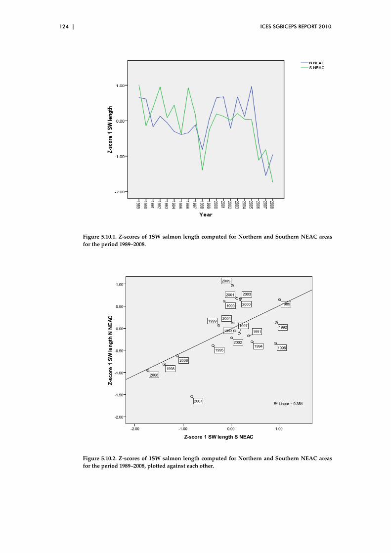
124 | ICES SGBICEPS REPORT 2010
Figure 5.10.1. Z‐scores of 1SW salmon length computed for Northern and Southern NEAC areas
for the period 1989–2008.
Figure 5.10.2. Z‐scores of 1SW salmon length computed for Northern and Southern NEAC areas
for the period 1989–2008, plotted against each other.

ICES SGBICEPS REPORT 2010 | 125
Figure 5.10.3. PFA of maturing 1SW salmon plotted against the z‐score of 1SW length for North‐
ern NEAC populations.
Figure 5.10.4. PFA of maturing 1SW salmon plotted against the z‐score of 1SW length for South‐
ern NEAC populations.

126 | ICES SGBICEPS REPORT 2010
5.11 Is there evidence of a change in overall (egg-adult) mortality over time?
This was explored using a simple life‐history model (Aprahamian et al., 2008). For
salmon, Aprahamian et al. (2008) suggested that age at maturity was optimised to
maximise life time fecundity, defined as the average number of eggs per female sur‐
viving to spawn. The optimal age at maturity is a function of mortality, growth (af‐
fecting smolt age) and fecundity. The model assumes a steady state, in that the
number of eggs spawned in a particular year equals the number of eggs deposited by
that cohort over its lifetime. The model requires the following input parameters:
mean smolt age, proportion of fish maturing by sea age, fecundity by sea age and sex
ratio of the returning adults.
To validate the outputs of the model (number of spawning adults by sea age) the
model was run on data from five Southern NEAC index rivers: Welsh Dee,
Burrishoole, Bush, Frome and River North Esk, for various, ~ 5 year time periods. For
each of the rivers and time periods, river specific estimates of smolt age and sea age
were available; for fecundity, river specific values were available for all the rivers
except the Frome and Bush where default values were used (Table 5.11.1). For all riv‐
ers the sex ratio for all sea age classes was assumed to be 1:1.
To estimate the optimal age at maturity which maximises lifetime fecundity, the
model was re‐run using the same life‐history parameters (smolt age, sex ratio, fecun‐
dity), the mortality estimate from the life history model, but with no constraint on the
maturation schedule. (For ease of differentiating between the two models this model
will be referred to as the Optimal Age model).
Mortality
A comparison between the total number of salmon estimated to spawn (Observed)
and that estimated from the life‐history model (Estimated) was within ±10% for the
Frome, Dee, Burrishoole and for the Bush with the exception of the sample 1975–1979
(Table 5.11.2). For the River North Esk, the life‐history model consistently overesti‐
mated the number of spawning salmon by between 12 and 28%. The overestimation
may arise if the fecundity estimate is too low and/or if the proportion of females is
higher than 50%.
For the rivers North Esk, Bush and Burrishoole where the time period extended pre
and post‐1989, the year when the increase in marine mortality was perceived to have
occurred, there does not appear to have been a systematic increase in the overall life‐
time mortality (Table 5.11.2) for these three stocks.
Sea age at maturity
A comparison between the observed sea age structure of adult salmon spawning and
that estimated from the model for a given egg deposition was compared using chi‐
square. There was no significant difference between the proportion of fish maturing
at 1SW and 2SW between that observed and that estimated from the model for the
rivers NorthEsk, Frome, Bush and Burrishoole (Table 5.11.2). However, for the Dee
the life‐history model over estimated the proportion of MSW salmon, with the mean
sea age being significantly higher by between 0.02 and 0.03 years when compared
with the observed sea age structure. The fact that the difference in the case of the Dee
was small (<5%) and that there was no significant difference between the observed
and expected proportions for the other index rivers suggests that the life‐history
model provides a reasonable estimate of the maturation schedule.
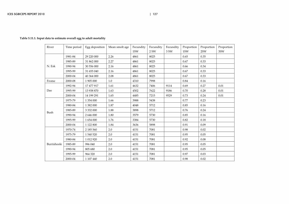
ICES SGBICEPS REPORT 2010 | 127
Table 5.11.1. Input data to estimate overall egg to adult mortality
River Time period Egg deposition Mean smolt age Fecundity
1SW
Fecundity
2 SW
Fecundity
3 SW
Proportion
1SW
Proportion
2SW
Proportion
3SW
N. Esk
1981‐84 29 220 000 2.26 4861 8025 0.65 0.35
1985‐89 31 862 000 2.27 4861 8025 0.67 0.33
1990‐94 30 556 000 2.16 4861 8025 0.66 0.34
1995‐99 31 655 040 2.16 4861 8025 0.67 0.33
2000‐04 40 364 000 2.08 4861 8025 0.67 0.33
Frome 2000‐08 1 905 000 1.0 4310 7998 0.84 0.16
Dee
1992‐94 17 477 917 1.61 4632 7406 9114 0.69 0.27 0.01
1995‐99 13 938 870 1.63 4502 7622 9186 0.70 0.28 0.01
2000‐04 14 199 291 1.65 4485 7215 9529 0.73 0.24 0.01
Bush
1975‐79 1 354 000 1.66 3988 5438 0.77 0.23
1980‐84 1 382 000 1.87 4048 5712 0.85 0.16
1985‐89 3 332 000 1.88 3898 5712 0.76 0.24
1990‐94 2 646 000 1.80 3579 5730 0.85 0.16
1995‐99 1 654 000 1.76 3384 5730 0.82 0.18
2000‐04 1 122 800 1.84 3636 5898 0.91 0.09
Burrishoole
1970‐74 2 185 560 2.0 4151 7081 0.98 0.02
1975‐79 1 540 520 2.0 4151 7081 0.95 0.05
1980‐84 1 012 920 2.0 4151 7081 0.92 0.08
1985‐89 996 040 2.0 4151 7081 0.95 0.05
1990‐94 805 680 2.0 4151 7081 0.95 0.05
1995‐99 964 320 2.0 4151 7081 0.97 0.03
2000‐04 1 107 440 2.0 4151 7081 0.98 0.02

128 | ICES SGBICEPS REPORT 2010
Table 5.11.2. A comparison between the observed and the estimated number of salmon, by sea age, from the life history model, from a given egg deposition.
River Time
period
Lifetime
Mortality
Z
Number
1SW
(Obs.)
Number
2SW
(Obs.)
Number
3SW
(Obs.)
Mean sea‐
age (Obs.)
Number
1SW (Est.)
Number
2SW (Est.)
Number
3SW (Est.)
Number
4SW (Est.)
Mean sea‐
age (Est.)
Number
Estimate /
Observed
Significance
Chi‐square
N. Esk
81‐84 1.665 5165 2721 1.35 6431 3387 1.34 1.24 P>0.05
85‐89 1.666 5688 2745 1.33 7289 3526 1.33 1.28 P>0.05
90‐94 1.700 5701 2906 1.34 6822 3483 1.34 1.20 P>0.05
95‐99 1.702 6367 3169 1.33 7154 3555 1.33 1.12 P>0.05
00‐04 1.730 7874 3938 1.33 9104 4545 1.33 1.16 P>0.05
Frome 00‐08 2.303 614 117 1 1.16 653 124 1 1.16 1.06 P>0.05
Dee
92‐94 1.815 4577 1736 91 1.30 4436 1743 136 20 1.33 1.02 P<0.05
95‐99 1.856 3768 1394 32 1.28 3593 1451 65 4 1.31 1.02 P<0.05
00‐04 1.843 4078 1343 35 1.26 3990 1347 74 6 1.28 1.02 P<0.05
Bush
75‐79 1.874 624 186 1.23 483 144 1.23 0.77 P>0.05
80‐84 1.830 530 97 1.16 542 100 1.16 1.02 P>0.05
85‐89 1.779 1292 399 1.24 1169 369 1.24 0.91 P>0.05
90‐94 1.834 1147 210 1.16 1133 210 1.16 0.99 P>0.05
95‐99 1.832 638 144 1.18 713 156 1.18 1.11 P>0.05
00‐04 1.865 518 52 1.09 532 53 1.09 1.03 P>0.05
Burrishoole
70‐74 1.886 965 15 1.02 1018 21 1.02 1.06 P>0.05
75‐79 1.858 638 33 1.05 681 36 1.05 1.07 P>0.05
80‐84 1.835 398 33 1.08 425 37 1.08 1.07 P>0.05
85‐89 1.858 414 20 1.05 440 23 1.05 1.07 P>0.05
90‐94 1.858 337 15 1.04 356 19 1.05 1.06 P>0.05
95‐99 1.876 416 12 1.03 441 14 1.03 1.06 P>0.05
00‐04 1.886 482 11 1.02 516 11 1.02 1.07 P>0.05

ICES SGBICEPS REPORT 2010 | 129
Optimal age at maturity
The model was re‐run to predict the optimal sea age at maturity that maximised the
number of eggs produced per female for the value of mortality estimated for the
various periods from the five index rivers. The optimal age model used the estimate
of lifetime mortality from the life‐history model, the same estimates of smolt age,
growth and fecundity, but with no constraint on the sea age composition. There was
no significant difference between the observed proportion of salmon maturing at dif‐
ferent sea ages and that estimated from the model for the rivers NorthEsk, Frome,
Bush and Burrishoole (Table 5.11.3). This suggested that for these four rivers lifetime
fecundity is maximised. However, for the Dee the model suggests a significantly
higher proportion of MSW salmon than the proportion observed if fecundity is
maximised. The difference in terms of the mean sea age is between 13 and 30% (Table
5.11.3).
For the Welsh Dee, the difference between the observed and expected sea age at ma‐
turity may relate to smolt age. The optimal age model predicts that for any given
level of mortality the tendency is for S1 smolts to mature at a higher sea age than S2
or older smolts (Figure 5.11.1). This is also evident from the data, where for female
salmon there is a significantly higher proportion of S1 smolts maturing as MSW
salmon (47.2%) when compared to S2 smolts (30.7%) (Table 5.11.4). For males the
proportion is much similar, 16.4% and 14.0% for S1 and S2 smolts maturing as MSW
salmon, respectively.
1.0
1.5
2.0
2.5
3.0
3.5
1.50 1.75 2.00 2.25 2.50
Egg-Adult instantanenous mortality
Me
an
se
a a
ge
S1
S2
Figure 5.11.1. The optimal sea age at maturity for S1 and S2 smolts at different levels of mortality.
To explore the effect of gender differences, and as the model was based on optimising
age at maturity for female salmon (with the assumption that males would respond in
a similar manner), an analysis of just the female component was undertaken for the
River Dee. The mean smolt age and sea age composition of female salmon from the
Dee are shown in Table 5.11.5, together with the estimated life time mortality and the
estimated sea age composition from the life‐history model. There was no significant
difference between the observed and estimated sea age composition. The egg‐adult
mortality estimated from the life‐history model and the mean smolt age of females
were used in the optimal age model to estimate the sea age composition which

130 | ICES SGBICEPS REPORT 2010
maximises life time fecundity (Table 5.11.6). There was a significant difference be‐
tween the observed sea age composition and that estimated by the model; the optimal
age model over‐estimated mean sea age by between 4.6 and 16.1% (Table 5.11.6). The
model predicted a higher proportion of MSW females than observed. However, the
difference between the observed and expected was less when the analysis focused
solely on females than when both sexes were included in the analysis (Table 5.11.3).
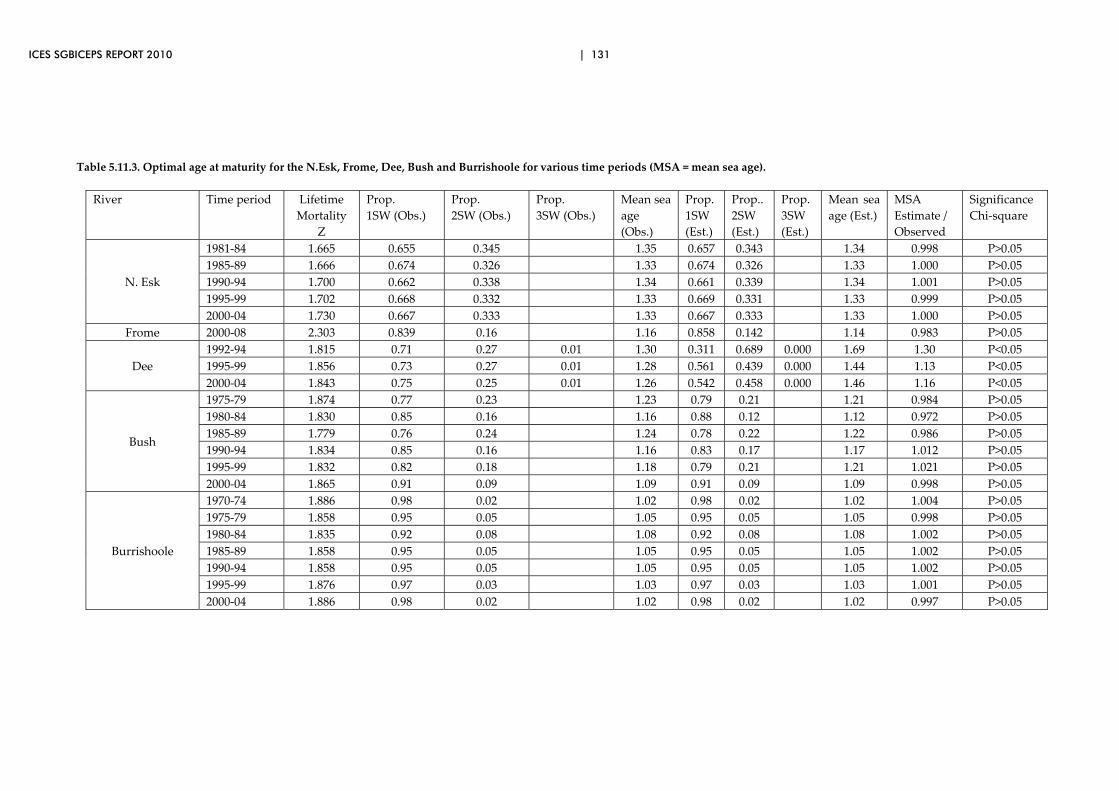
ICES SGBICEPS REPORT 2010 | 131
Table 5.11.3. Optimal age at maturity for the N.Esk, Frome, Dee, Bush and Burrishoole for various time periods (MSA = mean sea age).
River Time period Lifetime
Mortality
Z
Prop.
1SW (Obs.)
Prop.
2SW (Obs.)
Prop.
3SW (Obs.)
Mean sea
age
(Obs.)
Prop.
1SW
(Est.)
Prop..
2SW
(Est.)
Prop.
3SW
(Est.)
Mean sea
age (Est.)
MSA
Estimate /
Observed
Significance
Chi‐square
N. Esk
1981‐84 1.665 0.655 0.345 1.35 0.657 0.343 1.34 0.998 P>0.05
1985‐89 1.666 0.674 0.326 1.33 0.674 0.326 1.33 1.000 P>0.05
1990‐94 1.700 0.662 0.338 1.34 0.661 0.339 1.34 1.001 P>0.05
1995‐99 1.702 0.668 0.332 1.33 0.669 0.331 1.33 0.999 P>0.05
2000‐04 1.730 0.667 0.333 1.33 0.667 0.333 1.33 1.000 P>0.05
Frome 2000‐08 2.303 0.839 0.16 1.16 0.858 0.142 1.14 0.983 P>0.05
Dee
1992‐94 1.815 0.71 0.27 0.01 1.30 0.311 0.689 0.000 1.69 1.30 P<0.05
1995‐99 1.856 0.73 0.27 0.01 1.28 0.561 0.439 0.000 1.44 1.13 P<0.05
2000‐04 1.843 0.75 0.25 0.01 1.26 0.542 0.458 0.000 1.46 1.16 P<0.05
Bush
1975‐79 1.874 0.77 0.23 1.23 0.79 0.21 1.21 0.984 P>0.05
1980‐84 1.830 0.85 0.16 1.16 0.88 0.12 1.12 0.972 P>0.05
1985‐89 1.779 0.76 0.24 1.24 0.78 0.22 1.22 0.986 P>0.05
1990‐94 1.834 0.85 0.16 1.16 0.83 0.17 1.17 1.012 P>0.05
1995‐99 1.832 0.82 0.18 1.18 0.79 0.21 1.21 1.021 P>0.05
2000‐04 1.865 0.91 0.09 1.09 0.91 0.09 1.09 0.998 P>0.05
Burrishoole
1970‐74 1.886 0.98 0.02 1.02 0.98 0.02 1.02 1.004 P>0.05
1975‐79 1.858 0.95 0.05 1.05 0.95 0.05 1.05 0.998 P>0.05
1980‐84 1.835 0.92 0.08 1.08 0.92 0.08 1.08 1.002 P>0.05
1985‐89 1.858 0.95 0.05 1.05 0.95 0.05 1.05 1.002 P>0.05
1990‐94 1.858 0.95 0.05 1.05 0.95 0.05 1.05 1.002 P>0.05
1995‐99 1.876 0.97 0.03 1.03 0.97 0.03 1.03 1.001 P>0.05
2000‐04 1.886 0.98 0.02 1.02 0.98 0.02 1.02 0.997 P>0.05

132 | ICES SGBICEPS REPORT 2010
Table 5.11.4. Proportion of S1 and S2 smolts from the River Dee maturing at different sea ages for female and male salmon, mean ± 95 CL for the period 1992–2008.
Smolt age
Sea age
Female Male
1SW 2SW 3SW 1SW 2SW 3SW
S1 Smolt 0.528 ± 0.089 0.458 ± 0.087 0.015 ± 0.009 0.836 ± 0.040 0.157 ± 0.037 0.008 ± 0.003
S2 Smolt 0.693 ± 0.039 0.299 ± 0.039 0.008 ± 0.004 0.860 ± 0.046 0.134 ± 0.043 0.006 ± 0.003
Table 5.11.5. The mean smolt age and sea age composition of female salmon from the Dee and the estimated egg‐adult mortality and sea age composition from the life history
model for three time periods.
Year Mean
smolt age
Prop.
1SW
(Obs.)
Prop.
2SW
(Obs.)
Prop.
3SW
(Obs.)
Mean sea
age
(Obs)
Lifetime
Mortality
Z
Prop.
1SW
(Est.)
Prop.
2SW
(Est.)
Prop.
3SW
(Est.)
Mean sea
age (Est.)
Significance
Chi‐square
1992‐94 1.674 0.681 0.305 0.015 1.33 1.972 0.681 0.304 0.014 1.34 P>0.05
1995‐99 1.667 0.649 0.346 0.005 1.36 2.007 0.649 0.346 0.001 1.36 P>0.05
2000‐04 1.717 0.651 0.341 0.008 1.36 1.977 0.651 0.341 0.008 1.36 P>0.05
Table 5.11.6. The mean observed sea age composition and that estimated from the optimal age model which maximises life time of female from the River Dee for three time periods,
together with the mean smolt age and life time mortality used to estimate the optimal sea age (MSA = Mean Sea Age)
Year Prop.
1SW
(Obs.)
Prop.
2SW
(Obs.)
Prop.
3SW
(Obs.)
Mean sea
age
(Obs)
Lifetime
Mortality
Z
Mean
smolt
age
Prop.
1SW
(Est.)
Prop.
2SW
(Est.)
Prop.
3SW
(Est.)
Mean sea
age (Est.) MSA
Est. / Obs.
Significance
Chi‐square
1992‐94 0.681 0.305 0.015 1.33 1.972 1.674 0.452 0.548 0.000 1.55 1.161 P<0.05
1995‐99 0.649 0.346 0.005 1.36 2.007 1.667 0.581 0.419 0.000 1.42 1.046 P<0.05
2000‐04 0.651 0.341 0.008 1.36 1.977 1.717 0.569 0.431 0.000 1.43 1.055 P<0.05

ICES SGBICEPS REPORT 2010 | 133
Discussion
The close agreement between the sea age at maturity estimated from the model and
that observed suggests that fitness, defined as the number of eggs per female, is
maximised indicating that the age at maturity is being optimised. This is supported
from the findings from the rivers North Esk, Frome, Bush and Burrishoole and from
females from the River Dee. There are significant differences between the observed
and expected sea age composition and part of these differences may arise from the
values of the parameters used in the model (sex ratio, fecundity). In addition, the
analysis of the River Dee data indicates that for a given level of mortality and growth,
males cannot automatically be assumed to respond in a similar manner as females
and this is likely to be more evident when there are marked gender differences in life
history parameters.
In terms of whether biological characteristics, specifically sea age at maturity, can be
used to predict changes in mortality seems unlikely. Changes in life history character‐
istics reflect changes in mortality and/or changes in growth and fecundity, as such, a
change in mortality will only retrospectively manifest itself in terms of a change in
age at maturity after an (unknown) number of generations.
The findings presented here do not indicate that there has been any major change in
total mortality, from egg to spawning adult, since the late 1970s – early 1980s in the
rivers North Esk, Bush and Burrishoole. This is presumably because the decline in
natural mortality, notably in marine survival around 1989, has been off‐set by an
equivalent decline in fishing mortality and/or other anthropogenic mortalities. This
would explain why there has been no major change in the age (sea) at maturity in
these rivers over the time period.
It is possible to retrospectively estimate mortality (lifetime mortality) using the life
history model. For some river systems historic information are available on the smolt
age and sea age composition and from these data together with default estimates for
sex ratio and fecundity (as these are generally unknown) it is possible to estimate the
lifetime mortality. This was undertaken for two river systems where a long time se‐
ries of data on biological characteristics were available: the Dee and Hampshire
Avon, to investigate how the level of mortality had changed over a 60 year period
(Table 5.11.7). The life history model estimates that the mortality on the Avon had
been higher than on the Dee for all time periods, by between 5–13%. For both rivers it
is estimated that mortality had increased, for the Dee mortality was estimated to have
increased by 2.9% and the Avon by 6.4% between the late1930s and 1960s. However,
between the late 1960s and 1990s there was estimated to be a larger increase in mor‐
tality on the Dee (22.5%) than on the Avon (13.6%). Over the entire 60 years the esti‐
mated increase in mortality on the Dee was slightly higher (26.0%) than on the Avon
(20.9%).
If the age at maturity is optimized then it is possible to use the optimal age model to
examine the consequences of a change in mortality on the sea age composition for
any given set of conditions (growth, smolt age, fecundity and sex ratio). A reduction
in overall mortality has the effect of increasing the mean sea age (Figure 5.11.1) but
will reduce the number of returning adults, an increase in mortality will have the op‐
posite effect. This was examined on the rivers Bush and North Esk where data were
available on the number of salmon returning before exploitation in the net and rod
fisheries. For these rivers it was assumed that the number of salmon returning to the
river spawned (i.e. fishing mortality and all other anthropogenic mortality was zero).
134 | ICES SGBICEPS REPORT 2010
The instantaneous egg‐adult mortality in the absence of any mortality once the fish
arrive in home waters was estimated as follows:
Z = (LnN0‐LnNt)/t equation 1
Where:
N0 = the number of eggs deposited
Nt = Number of salmon returning (prior to the fishery (Ntpf) or on the spawn‐
ing grounds (Nts))
t = total age.
As the value of Z was not estimated in the same manner as in the life history model
the value was adjusted as follows:
Zadj =(Zpf)/(Zs)* Zslh.
Where:
Zpf = the estimate of mortality prior to the fishery using equation 1
Zs = the estimate of mortality at the time of spawning using equation 1
Zslh = the estimate of mortality at the time of spawning using the life history
model.
In the absence of any fishing mortality the optimal age model estimated a higher
mean sea age indicating a higher proportion of MSW salmon than was observed (Ta‐
ble 5.11.8). If fishing mortality was reduced to zero, it is hypothesized that there
would be an increase in the number of spawners until the carrying capacity was
reached and then numbers of spawning adults would decrease as the age at maturity
increased in order to maximise fecundity. It is appreciated that this is a simplistic ap‐
proach and that the change in sea age composition would not increase by the amount
suggested in Table 5.11.8 if fishing mortality was reduced to zero. This is because the
increase in the number of spawners would result in an increase in density dependent
mortality resulting in a reduction in the age at maturity, assuming the catchment was
at carrying capacity. Though the analysis must be viewed with caution it does illus‐
trate that it might be possible to increase the MSW component of the stock through a
reduction in fishing (or other) mortality. It is thus important that such models inte‐
grate with population models. Certainly both the life history and optimal age models
would benefit from estimating / using life stage specific values of mortality. This
would then enable changes in mortality at specific life stages on the age at maturity to
be evaluated. In terms of population models the fact that age at maturity appears to
be optimized provides a feedback mechanism for such models, in that the overall
mortality must be the same.
Similar data as used in the life‐history model, namely the numbers of male and fe‐
male smolts emigrating and the numbers of adults returning by sex and sea age can
be used to derive estimates of natural mortality during the marine phase for stocks
which mature at two or more different sea ages (Ricker, 1976). One particular ap‐
proach referred to as “Murphy’s Method” (Ricker, 1975) was used to estimate the
mortality of Icelandic ranched Atlantic salmon over their second year at sea (Jonasson
et al. 1994). Chaput et al. (2003) described a variation of this method which allows
estimation of mortality in both the first and second years in the sea. Application of
this approach to the results described above (e.g. Table 5.11.5) might therefore allow
partitioning of the life‐time mortality into separate life stages, namely freshwater and

ICES SGBICEPS REPORT 2010 | 135
the first and second years at sea. The Study Group recommended that this be inves‐
tigated further.
Table 5.11.7 Estimates of total egg‐adult mortality (Z) for the rivers Dee and Hampshire Avon, for
three time periods using the life‐history model.
River 1937‐39 1967‐69 1997‐99
Dee 1.495 1.538 1.884
Hampshire Avon 1.635 1.739 1.976
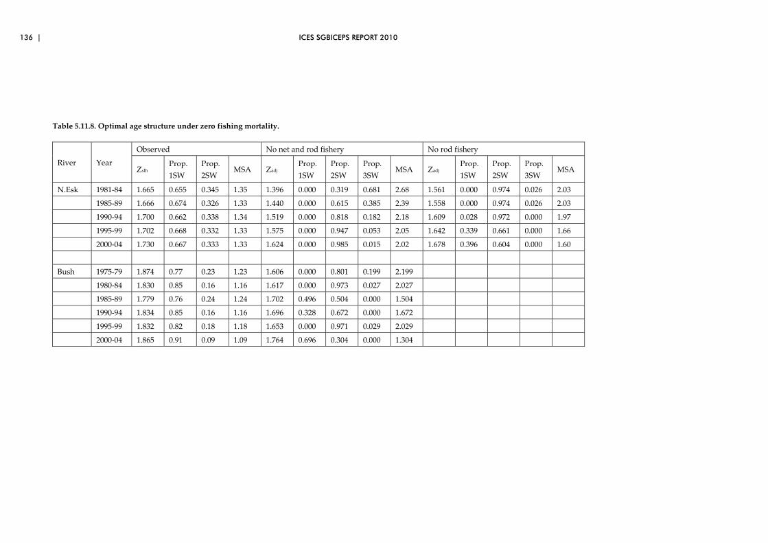
136 | ICES SGBICEPS REPORT 2010
Table 5.11.8. Optimal age structure under zero fishing mortality.
River Year
Observed No net and rod fishery No rod fishery
Zslh Prop.
1SW
Prop.
2SW MSA Zadj
Prop.
1SW
Prop.
2SW
Prop.
3SW MSA Zadj
Prop.
1SW
Prop.
2SW
Prop.
3SW MSA
N.Esk 1981‐84 1.665 0.655 0.345 1.35 1.396 0.000 0.319 0.681 2.68 1.561 0.000 0.974 0.026 2.03
1985‐89 1.666 0.674 0.326 1.33 1.440 0.000 0.615 0.385 2.39 1.558 0.000 0.974 0.026 2.03
1990‐94 1.700 0.662 0.338 1.34 1.519 0.000 0.818 0.182 2.18 1.609 0.028 0.972 0.000 1.97
1995‐99 1.702 0.668 0.332 1.33 1.575 0.000 0.947 0.053 2.05 1.642 0.339 0.661 0.000 1.66
2000‐04 1.730 0.667 0.333 1.33 1.624 0.000 0.985 0.015 2.02 1.678 0.396 0.604 0.000 1.60
Bush 1975‐79 1.874 0.77 0.23 1.23 1.606 0.000 0.801 0.199 2.199
1980‐84 1.830 0.85 0.16 1.16 1.617 0.000 0.973 0.027 2.027
1985‐89 1.779 0.76 0.24 1.24 1.702 0.496 0.504 0.000 1.504
1990‐94 1.834 0.85 0.16 1.16 1.696 0.328 0.672 0.000 1.672
1995‐99 1.832 0.82 0.18 1.18 1.653 0.000 0.971 0.029 2.029
2000‐04 1.865 0.91 0.09 1.09 1.764 0.696 0.304 0.000 1.304

ICES SGBICEPS REPORT 2010 | 137
6 Overview and recommendations
Substantial further progress has been made, as detailed in this report, in addressing
the three areas identified in the ToR, namely: (a) identifying data sources and compil‐
ing time series of data; (b) considering hypotheses relating to changes in biological
characteristics of all life stages and relating these to mortality (freshwater and marine)
and/or abundance trends; and (c) conducting preliminary analyses to explore the
available datasets and test the hypotheses. A number of additional data sets were
made available to the Study Group, and these further reinforced the evidence that the
biological characteristics of Atlantic salmon stocks are changing markedly across the
geographical range of the species (Sections 5.2–5.5). In addition, a number of hy‐
potheses were developed and explored through various case studies (Section 4) and
other exploratory analyses (Section 5).
The background to the original request from NASCO stemmed from an ‘interest in
determining if declines in marine survival of Atlantic salmon coincide with changes in the
biological characteristics of juveniles in freshwater or are modifying characteristics of adult
fish (size at age, age at maturity, condition, sex ratio, growth rates, etc.) and with environ‐
mental change’. Evidence reported in the two Study Group reports clearly indicates
marked changes in various biological characteristics coincident with a sharp decline
in the marine survival for specific stocks. NASCO further asked ICES to ‘investigate
associations between changes in biological characteristics of all life stages of Atlantic salmon,
environmental changes and variations in marine survival with a view to identifying predic‐
tors of abundance’. The Study Group has identified links between the size of returning
1SW fish and their pre‐fishery abundance, for the NEAC area at least (Section 5.10),
suggesting that reduced growth leads to reduced survival or delayed maturation in
the smolt cohorts experiencing lower growth. However, while this suggests a direct
link between growth/mortality and abundance, it seems unlikely that this could be
used in any predictive capacity.
In considering progress and possible next steps, the Study Group recognises that this
is a vast subject area and that the time available did not allow a full appraisal of the
topic, or even the available data. Further, in the absence of oceanographic expertise at
the second meeting, or representation from the NW Atlantic at either meeting, the
Study Group also recognises that its ability to explore changes in biological character‐
istics of salmon across the entire range of the species and relate these to environ‐
mental variables was inevitably somewhat constrained. The Study Group therefore
recognises that further work to better explore temporal and spatial trends, investigate
possible common patterns or regional groupings, and develop and test hypotheses
would be of value. Members of the Group are involved with some ongoing investiga‐
tions and the production of a number of peer‐reviewed outputs from analyses initi‐
ated and reported here. However, it was felt that the Group had probably gone as far
as it could in addressing the ToR and that further progress might best be made by
other groups (e.g. involving modellers, biological oceanographers), potentially in re‐
sponse to more targeted questions or to address specific management requirements.
The Study Group made the following recommendations:
i ) The Study Group reiterated the importance of monitoring programmes
to collect age, growth and other biological data from salmon stocks and
the need for these to be continued. Such studies are important for exam‐
ining variations in marine recruitment and links with environmental
conditions. Where possible, such studies should extend to the collection

138 | ICES SGBICEPS REPORT 2010
and collation of data sets on freshwater stages (e.g. smolt age, smolt size,
growth at age, etc.), since there was increasing evidence that freshwater
influences might be instrumental to the growth and survival of the fish in
the sea. Changes in freshwater or marine growth may be among the first
signs that climate is modifying salmonid populations and can be useful
in understanding and explaining fluctuations in abundance and inform‐
ing fisheries management in a period of potentially unprecedented envi‐
ronmental change.
ii ) The Study Group reiterated the view that such data sets needed to be bet‐
ter utilised and reported, and felt that (subject to funding being available)
the development of an inventory of relevant data sets would be a useful
initiative. Furthermore the value of a number of data sets when analysed
together far exceeds their value when analysed separately. In this con‐
text, feedback from NASWG (ICES, 2010) had recommended that the
data sets collated by the Study Group should be fully utilised and made
available to NASWG in support of further analyses as appropriate. Pre‐
liminary discussions were held with the ICES Data Centre and further
consideration will be given to archiving the data sets and providing suit‐
able supporting documentation. This could perhaps comprise part of an
ICES Co‐operative Research Report in which the work of the Study
Group could be consolidated.
iii ) The Study Group noted that different members were developing peer‐
reviewed outputs related to investigations discussed at the meetings (and
reported herein) and recommended that efforts continue to finalise these.
Subjects included: smolt run‐timing and potential mis‐match with envi‐
ronmental variables; condition factor analyses of returning adults; life‐
cycle modelling and model validation; sea‐age/river‐age relationships;
and an overview of spatial/temporal changes in salmon biological charac‐
teristics.
iv ) The Study Group recommends that relationships between mortality
(freshwater and marine) and growth, and resulting biological characteris‐
tics, might usefully be explored further through the application of ap‐
propriate life‐history models, including partitioning of the life‐time
mortality into separate life stages.
With the exception of the recommendation for a possible Co‐operative Research Re‐
port, which ICES would need to approve, these recommendations are addressed
largely to the Study Group and to members of WGNAS and WGBAST.

ICES SGBICEPS REPORT 2010 | 139
Annex 1: List of participants
NAME ADDRESS PHONE/FAX EMAIL
Miran
Aprahamian
Environment Agency
Richard Fairclough
House
Knutsford Road
Warrington
WA4 1HG
United Kingdom
TEL: +44 1925 542713
FAX: +44 1925 415961
miran.aprahamian@environment‐
agency.gov.uk
Ian Davidson Environment Agency
Chester Road
Buckley
Flintshire CH7 3AJ
United Kingdom
TEL: +44 1244 894520
FAX: +44 1244 550144
ian.davidson@environment‐
agency.gov.uk
Peder Fiske Norwegian Institute for
Nature Research
NO‐7485 Trondheim
Norway
TEL: +47 73 80 1522
FAX: +47 73 80 14 01
Anton Ibbotson Game and Wildlife
Conservation Trust,
Burgate Manor,
Fordingbridge,
Hampshire SP6 1EF
United Kingdom
TEL: +44 1929 401873
Richard
Kennedy
River Bush Salmon
Station, 21 Church
Street
Bushmills, Co Antrim
BT57 8QJ
United Kingdom
TEL: +44 28 20731435 [email protected]
Julian C.
MacLean
Marine Scotland, FRS
FL Field Station
Inchbraoch House
South Quay, Ferryden
Montrose, Angus DD10
9SL
United Kingdom
TEL: +44 1674 677070
FAX: +44 1674 672604
Stig Pedersen National Institute of
Aquatic Resources,
Department of Inland
Fisheries, Vejlsøvej 39 ‐
8600 Silkeborg, Den‐
mark
TEL: +45 89213100
Ted Potter Cefas Lowestoft
Laboratory, Pakefield
Road, Lowestoft,
Suffolk NR33 0HT
United Kingdom
TEL: +44 1502 524260
FAX: +44 1502 513865

140 | ICES SGBICEPS REPORT 2010
Ger Rogan Aquaculture & Catch‐
ment Management Ser‐
vices,
Marine Institute,
Furnace,
Newport,
Co. Mayo,
Ireland
TEL: +353 9842300
FAX: +353 9842340
Ian Russell
(Chair)
Cefas Lowestoft
Laboratory, Pakefield
Road, Lowestoft,
Suffolk NR33 0HT
United Kingdom
TEL: +44 1502 524330
FAX: +44 1502 513865
Chris Todd Scottish Oceans
Institute,
University of St
Andrews School of
Biology,
St Andrews, Fife
KY16 8LB
United Kingdom
TEL: +44 1334 463454
FAX: +44 1334 463443
cdt@st‐andrews.ac.uk

ICES SGBICEPS REPORT 2010 | 141
Annex 2: List of working documents/presentations and data sets
Aprahamian M. Is there evidence for optimal age at maturity in salmon ?
Barry J. Re‐examination of updated biological characteristics datasets from different
stocks – trend analysis.
Barry J. Re‐examination of updated biological characteristics datasets from different
stocks –linear regression analysis of two‐way relationships.
Davidson I. Preliminary investigations into the effect of environmental factors, par‐
ticularly river flow, on recruitment success of salmon on the River Dee, UK (England
& Wales).
Davidson I. Investigation of long‐term trends in spring temperatures for selected
monitored rivers in UK (England & Wales) and adjacent inshore coastal areas – any
evidence of thermal mis‐match?
Fiske P. Evidence of later age at maturity in Norwegian salmon stocks in recent years.
Fiske P. Correlations between the length of returning 1 SW salmon and the PFA of 1
SW salmon.
Kennedy R. Long term changes in biological characteristics of smolts on the River
Bush, N. Ireland and associations with environmental parameters).
MacLean J. Long term changes in the biological characteristics of smolts emigrating
from two rivers in Scotland.
Pedersen S. Update on work completed by the Baltic Salmon and Trout Assessment
Working Group (WGBAST) ‐ changes in post‐smolt survival in the Baltic Sea and the
factors affecting it.
Petersson E. Re‐examination of updated biological characteristics datasets from dif‐
ferent stocks utilising Meta analysis.
Rogan G. Report on the wild salmon census programme on the Burrishoole River,
Ireland.
Russell I. Update on salmon biological characteristics data sets available and review
of earlier analyses and progress.
Todd C. Analyses of long‐term variation in condition factor in relation to ocean cli‐
mate – update on progress.
Todd C. & MacLean J. Long‐term variation and changes in age at smoltification in
four major Scottish salmon rivers.
Todd C. & MacLean J. Among‐river comparisons of mean river age and proportional
river age composition in four major Scottish salmon rivers: 2SW “summer” salmon
(returning May‐August/September).
Todd C. & MacLean J. Among‐river comparisons of mean river age and proportional
river age composition in four major Scottish salmon rivers: 1SW grilse (returning
April‐August/September).
Data sets - as compiled at both meetings (and subsequently)
Amiro P. & Gibson J. Salmon biological characteristics data for the La Have River
(wild and hatchery‐origin) (1970‐08) ‐ Canada, Scotia Fundy Region.

142 | ICES SGBICEPS REPORT 2010
Chaput G. Salmon biological characteristics data for Miramichi River (1971‐07) ‐
Canada, Gulf Region.
Dannewitz J. Salmon biological characteristics data for the Rivers Ume/Vindel (wild
and hatchery‐origin) (1974‐08) and Kalix (1980‐08) – Baltic Sea (Sweden).
Davidson I., Aprahamian M. & Russell I. Salmon biological characteristics data for
the Rivers Wye (1910‐07), Dee (1937‐07) and Lune (1987‐07) – UK (England & Wales).
Dionne M. Salmon biological characteristics data for the Rivers Saint‐Jean (1981‐09)
and De La Trinité (1980‐09) ‐ Canada, Quebec Region.
Erkinaro J. Salmon biological characteristics data for the Rivers Teno (1972‐07) and
Naatamojoki (1975‐06) ‐ Finland/Norway.
Euzenat G. Salmon biological characteristics data for the River Bresle (1984‐08) –
France.
Fiske P. Salmon biological characteristics data for the Rivers Gaula (1989‐08), Årgård
(1992‐08), Enningdalselva (1990‐08), Etneelva (1989‐08), Gaula Sogn og Fjordane
(1989‐08), Nausta (1989‐08), Numedalslågen (19989‐08), Skienselva (1989‐08) and
Vestre Jakobselv (1989‐08) ‐ Norway.
Gudbergsson G. Salmon biological characteristics data for Rivers Laxa i Aldaldalur
(1974‐08), Hofsa (1971‐08), Ellidaar (1949‐08) and Nordura (1968‐08) ‐ Iceland.
Ibbotson A. Salmon biological characteristics data for the River Frome (1968‐08) – UK
(England & Wales).
Jones R. Salmon biological characteristics data for the St John (Mactaquac) (wild and
hatchery‐origin) (1978‐08); and Nashwaak Rivers (1972‐08) ‐ Canada, Scotia Fundy
Region.
Kennedy R. Salmon biological characteristics data for the River Bush (1973‐07) ‐ UK
(N. Ireland).
Maclean J. & Smith G. Salmon biological characteristics data for the River N. Esk
(1981‐08) – UK (Scotland).
Reddin D. Salmon biological characteristics data for Middle Brook (1975‐05) and
Western Arm Brook (1971‐06) ‐ Canada, Newfoundland.
Reddin D. & Dempson B. Salmon biological characteristics data for Conne River
(1986‐06) ‐ Canada, Newfoundland/Labrador.
Romakkaniemi A. Salmon biological characteristics data for the River Tornionjoki
(1980‐09) – Baltic Sea (Finland/Sweden).
Sheehan T. Salmon biological characteristics ‐ standardised spreadsheet design and
set up.
Trial J. Salmon biological characteristics data for the Penobscot River (1978‐08) ‐ USA.
Zubchenko A. Salmon biological characteristics data for the River Tuloma (1983‐08) –
Russia.

ICES SGBICEPS REPORT 2010 | 143
Annex 3: References
Amiro, P.G. (1998). The mystery of the missing inner Bay of Fundy salmon. Atlantic Salmon
Journal 47: 50‐53.
Andreasson, P.M.R., Martinussen, M.B., Hvidsten, N.A. & Stefansson, S.O. (2001). Feeding and
prey selection of wild Atlantic salmon post‐smolts. Journal of Fish Biology 58: 1667‐1679.
Anon. (1994). Run timing of salmon. Report of the Salmon Advisory Committee. London,
MAFF: 55pp.
Aprahamian, M.W., Davidson, I.C. & Cove, R.J. (2008). Life history changes in Atlantic salmon
from the river Dee, Wales. Hydrobiologia 602: 61‐78.
Armstrong, J.D., Shackley, P.E. & Gardiner, R. (1994). Redistribution of juvenile salmonid
fishes after local catastrophic depletion. Journal of Fish Biology 45: 1027‐1039.
Armstrong, J.D., Kemp, P.S., Kennedy, G.J.A., Ladle, M. & Milner, N.J. (2003). Habitat require‐
ments of Atlantic salmon and brown trout in rivers and streams. Fisheries Research 62(2):
143‐170.
Atkins, C.F. (1873). On the salmon of Eastern North America and its culture. Report of the
Commission of Fish and Fisheries. pp 226‐337.
Baggerman, B. (1960). Factors in the diadromous migrations of fish. Zoological Society Sympo‐
sium I: 33‐60.
Bagliniere, J.L., Denais, L., Rivot, E., Porcher, J.P., Prevost, E., Marchland, F. & Vauclin, V.
(2004). Length and age structure modifications of the Atlantic salmon (Salmo salar) popu‐
lations of Brittany and Lower Normandy from 1972 to 2002. Rennes, Institut National de la
Recherche Agronomique and Conseil Superieur de la Peche.
Bardonnet, A. & Bagliniere, J.L. (2000). Freshwater habitat of Atlantic salmon (Salmo salar).
Canadian Journal of Fisheries and Aquatic Sciences 57: 497‐506.
Baum, E.T. & Meister A.L. (1971). Fecundity of Atlantic salmon (Salmo salar) from two Maine
rivers. Journal of the Fisheries Research Board of Canada 28(5): 764‐767.
Baum, E.T. (1997). Maine Atlantic Salmon: A national treasure. Atlantic Salmon Unlimited. 224
pp.
Beall, E., Dumas, J., Claireaux, D., Barrière, L. & Marty, C. (1994). Dispersal patterns and sur‐
vival of Atlantic salmon (Salmo salar L.) juveniles in a nursery stream. ICES Journal of Ma‐
rine Science 51: 1‐9.
Beamish, R.J. & Mahnken, C. (2001). A critical size and period hypothesis to explain natural
and regulation of salmon abundance and the linkage to climate and climate change. Pro‐
gress in Oceanography 49: 423‐437.
Beamish, R.J., Mahnken, C. & Neville, C.M. (2004). Evidence that reduced early marine growth
is associated with lower marine survival of coho salmon. Transactions of the American
Fisheries Society 133: 26‐33.
Beaugrand, G. & Reid, F.C. (2003). Long term changes in phytoplankton, zooplankton and
salmon related to climate. Global Change Biology 9: 801‐817.
Benoit, H.P. & Swain, D.P. (2008). Impacts of environmental change and direct and indirect
harvesting effects on the dynamics of marine fish community. Canadian Journal of Fisher‐
ies and Aquatic Sciences 65(10): 2088‐2104.
Bielak, A.T. & Power, G. (1986). Independence of sea‐age and river‐age in Atlantic salmon
(Salmo salar) from Quebec North Shore Rivers. In: Meerburg D.J. (ed) 1986. Salmonid age
at maturity. Canadian Special Publications in Fisheries and Aquatic Sciences 89: 70‐78.
144 | ICES SGBICEPS REPORT 2010
Bjornn, T.C. (1971). Trout and salmon movements in two Idaho streams as related to tempera‐
ture, stream flow, cover and population density. Transactions of the American Fisheries
Society 100: 423‐438.
Boylan, P. & Adams, C.E. (2006). The influence of broad scale climatic phenomena on long term
trends in Atlantic salmon population size: an example from the River Foyle, Ireland. Jour‐
nal of Fish Biology 68: 276‐283.
Brett, J.R. (1979). Environmental factors and growth. In: Fish Physiology, Vol VIII, pp 599‐675.
Eds W.S. Hoar, D.J. Randall & J.R. Brett. Academic Press, London.
Buck, R.J.G. & Youngson, A.F. (1982). The downstream migration of precociously mature At‐
lantic salmon, Salmo salar L., parr in autumn; its relation to the spawning migration of
mature adult fish. Journal of Fish Biology 20: 279‐288.
Bujold, V., Cunjak, R.A., Dietrich, J.P. & Courtemanche, D.A. (2004). Drifters versus residents:
assessing size and age differences in Atlantic salmon (Salmo salar) fry. Canadian Journal
of Fisheries and Aquatic Sciences 61: 273‐282.
Byrne, C.J., Poole R., Rogan, G., Dillane, M. & Whelan. K.F. (2003). Temporal and environ‐
mental influences on the variation in Atlantic salmon smolt migration in the Burrishoole
system 1970‐2000. Journal of Fish Biology 63:6, 1552‐1564.
Cairns, D.K. (2003). Temperature mortality relations in marine phase Atlantic salmon, (Salmo
salar L.): the search for underlying mechanisms. In: Marine mortality of Atlantic salmon:
methods and measures (ed. E.C.E. Potter, N. O’Maoileidigh & G. Chaput). Fisheries and
Oceans Canada; Canadian Science Advisory Secretariat Research Document 2003/101, 150‐
160.
Cannaby, H. & Hüsrevoğlu, Y.S. (2009). The influence of low‐frequency variability and long‐
term trends in North Atlantic sea surface temperature on Irish waters. ICES Journal of
Marine Science 10.1093/icesjms/fsp062.
Cefas & Environment Agency (2008). Annual assessment of salmon stocks and fisheries in Eng‐
land and Wales 2007: Preliminary assessment prepared for ICES, April 2008 (ISBN 978 0
907545 25 4).
Chaput, G., F. Caron, L. Marshall. (2003). Estimates of survival of Atlantic salmon in the first
and second years at sea. In: E.C.E. Potter, N. Ó Maoiléidigh, and G. Chaput (Eds.), p.83‐
109. Marine mortality of Atlantic salmon, Salmo salar L: methods and measures. DFO Can.
Science Adv. Secr. Res. Doc. 2003/101.
Cohen, J. (1969). Statistical power analysis for the behavioural sciences. Academic Press, New
York.
Cragg‐Hine, D., Bradley, D.C. & Hendry, K. (2006). Changes in salmon smolt ages in the Welsh
River Dee over a 66 year period. Journal of Fish Biology 68: 1891‐1895.
Crisp, D.T. & Carling, P. A. (1989). Observations on siting, dimensions and structure of sal‐
monid redds. Journal of Fish Biology 34: 119‐134.
Crisp, D.T. (1995). Dispersal and growth rate of 0‐group salmon (Salmo salar L.) from point‐
stocking together with some information from scatter‐stocking. Ecology of Freshwater Fish
4: 1‐8.
Crisp, D.T. (1996). Environmental requirements of common riverine European salmonid fish
species in fresh water with particular reference to physical and chemical aspects. Hydrobi‐
ologia 323: 201‐221.
Crozier, W.W. & Kennedy, G.J.A. (1993). Marine survival of wild and hatchery reared Atlantic
salmon (Salmo salar L.) from the river Bush, Northern Ireland. In: D. Mills (ed.) Salmon in
the Sea and New Enhancement Strategies. Oxford: Fishing News Books, Blackwell Scien‐
tific Publications, pp. 139‐162.

ICES SGBICEPS REPORT 2010 | 145
Crozier, W.W. & Kennedy, G.J.A. (1994a). Application of semi‐quantitative electrofishing to
juvenile salmonid stock surveys. Journal of Fish Biology 45: 159‐164.
Crozier W.W. & Kennedy G.J.A. (1994b). Marine exploitation of Atlantic salmon (Salmo salar
L) from the River Bush, N. Ireland. Fisheries Research 19: 141‐155.
Crozier, W.W. & Kennedy, G.J.A. (1999). Relationships between marine growth and marine
survival of one sea winter Atlantic salmon, Salmo salar L., from the River Bush, Northern
Ireland. Fisheries Management and Ecology 6: 89‐96.
Crozier, W.W. & Kennedy, G.J.A. (2003). Freshwater influences on marine survival of Atlantic
salmon (Salmo salar L.): evidence from the River Bush, Northern Ireland. In: E.C.E. Potter,
N. O’Maoileidigh, G. Chaput (eds.) Marine mortality of Atlantic salmon, Salmo salar L.:
methods and measures. Research document, Canadian Science Advisory Secretariat
2003/101, pp124‐129.
Crozier, W.W., Potter, E.C.E., Prevost, E., Schon, P.J., & O’Maoiléidigh, N. (2003). A co‐
ordinated approach towards development of a scientific basis for management of wild At‐
lantic salmon in the North‐East Atlantic (SALMODEL). An EU Concerted Action ‐ Quality
of Life and Management of Living Resources Key Action 5: Sustainable agriculture, fisher‐
ies and forestry, and integrated development of rural areas including mountain areas.
Contract No. QLK5‐CT1999‐01546, 431 pp.
Cunjak, R.A. & Chadwick, E.M.P. (1989). Downstream movements and estuarine residence by
Atlantic salmon parr (Salmo salar). Canadian Journal of Fisheries and Aquatic Sciences 46:
1466‐1471.
Cunjak, R.A., Caissie, D., El‐Jabi, N., Hardie, P., Conlon, J.H., Pollock, T.L., Giberson, D.J. &
Komadina‐Douthwright, S. (1993). The Catamaran Brook (New Brunswick) habitat re‐
search project: biological, physical and chemical conditions (1990‐1992). Canadian Techni‐
cal Report of Fisheries and Aquatic Science 1914.
Dadswell, M.J., Spares, A.D., Reader, J.M. & Stokesbury, M.J.W. (2010). The North Atlantic
subpolar gyre and the marine migration of Atlantic salmon Salmo salar: the ‘Merry‐Go‐
Round’ hypothesis. Journal of Fish Biology 77: 435‐467.
Dahl, J., Dannewitz, J., Karlsson, L., Petersson, E., Löf, A. & Ragnarsson, B. (2004). The timing
of spawning migration: implications of environmental variation, life history, and sex. Ca‐
nadian Journal of Zoology 82: 1864‐1870.
Dalley, E.L., Andrews, C.W. & Green, J.M. (1983). Precocious male Atlantic salmon parr
(Salmon salar) in insular Newfoundland. Canadian Journal of Fisheries and Aquatic Sci‐
ences 40: 647‐652.
Davidson, I.C. & Hazelwood, M.S. (2005). Effects of climate change on salmon fisheries. Science
Report W2‐047/SR, Environment Agency, Bristol, 52pp.
Davidson, I.C., Hazlewood, M.S. & Cove, R.J. (2006). Predicted growth of juvenile trout and
salmon in four rivers in England and Wales based on past and possible future temperature
regimes linked to climate change. Proceedings of Biology and Management of Sea Trout
Conference, 6‐8 July 2004, Cardiff, Wales.
Davidson, I.C. (2008). Index river monitoring for salmon and sea trout: A progress report on
the monitoring programmes on the Tyne, Tamar, Dee and Lune, July 2008. Environment
Agency Wales. GEWA 108BOTB‐E‐E.
Dempson, J.B., Myers, R.A. & Reddin, D.G. (1986). Age at first maturity of Atlantic salmon
(Salmo salar) ‐ influences of the marine environment. In: Meerburg D.J. (ed) 1986. Sal‐
monid age at maturity. Canadian Special Publication of Fisheries and Aquatic Sciences 89:
79‐89.
Despatie, S.P., Castonguay, M., Chabot, D. & Audet, C. (2001). Final thermal preferendum of
Atlantic cod: effect of food ration. Transactions of the American Fisheries Society 130: 263‐
275.
146 | ICES SGBICEPS REPORT 2010
Dickson, R.R. & Turrell, W.R. (1999). The NAO: the dominant atmospheric process affecting
oceanic variability in home, middle and distant waters of European Atlantic salmon. In:
The Ocean Life of Atlantic Salmon (ed. D. Mills). Fishing News Books, Oxford, pp. 92‐115.
Dill, P.A. (1977). Development of behaviour of alevins of Atlantic salmon, Salmo salar, and
rainbow trout, Salmo gairdneri. Animal Behaviour 25: 116‐121.
Downton, P.R., Reddin, D.G. & Johnson, R.W. (2001). Status of Atlantic salmon (Salmo salar L.)
in Campbellton River, Notre Dame Bay (SFA 4), Newfoundland in 2000. Canadian Science
Advisory Secretariat Research Document: 73.
Egglishaw, H.J. & Shackley, P.E. (1973). An experiment on faster growth of salmon Salmo salar
L. in a Scottish stream. Journal of Fish Biology 5: 197‐204.
Egglishaw, H.J. & Shackley, P.E. (1980). Survival and growth of salmon, Salmo salar, planted in
a Scottish stream. Journal of Fish Biology 16: 565‐584.
Einum, S., Thorstad, E.B. & Naesje, T.F. (2002). Growth rate correlations across life stages in
female Atlantic salmon. Journal of Fish Biology 60: 780‐784.
Elliott J.M. (1984). Numerical changes and population regulation in young migratory trout,
Salmo trutta, in a Lake District stream, 1966‐1983. Journal of Animal Ecology 53: 327‐350.
Elliott J.M. (1991). Tolerance and resistance to thermal stress in juvenile Atlantic salmon, Salmo
salar. Freshwater Biology 25: 61‐70.
Elliott, J.M., Hurley, M.A. & Fryer, R.J. (1995). A new, improved growth model for brown trout,
Salmo trutta. Functional Ecology 9: 290‐298.
Elliott, J.M. & Hurley, M.A. (1997). A functional model for maximum growth of Atlantic
salmon parr, Salmo salar, from two populations in northwest England. Functional Ecology
11: 592‐603.
Elliott, J.M. & Hurley, M.A. (1998). An individual‐based model for predicting the emergence
period of sea‐trout fry in a Lake District stream. Journal of Fish Biology 53: 414‐433.
Elliott, J.M., Hurley, M.A. & Maberly, S.C. (2000). The emergence period of sea trout fry in a
Lake District stream correlates with the North Atlantic Oscillation. Journal of Fish Biology
56: 208‐210.
Elliott, J.M. (2001). The relative role of density in the stock‐recruitment relationship of sal‐
monids. In: E. Prevost, Chaput, G. (eds.) Stock, recruitment and reference points ‐ Assess‐
ment and management of Atlantic salmon. Hydrobiologie et aquaculture, INRA, Paris, 25‐
66.
Elo, K., Erkinaro, J., Vuorinen, J.A. & Niemela, E. (1995). Hybridization between Atlantic
salmon (Salmo salar) and brown trout (S.trutta) in the Teno and Naatamo River systems,
northernmost Europe. Nordic Journal of Freshwater Research 70: 56‐61.
Enfield, D.B., Mestas‐Nunez, A.M. & Trimble, P.J. (2001). The Atlantic multidecadal oscillation
and its relationship to rainfall and river flows in the continental US. Geophysical Research
Letters 28: 2077‐2080.
Englund, V., Niemela, E., Lansman, M. & Heino, M. (1999). Variations in Atlantic salmon,
Salmo salar L., smolt age in tributaries of the River Teno, Finland. Fisheries Management
and Ecology 6: 83‐86.
Erkinaro, J., Dempson, J.B., Julkunen, M. & Niemela, E. (1997). Importance of ontogenetic habi‐
tat shifts to juvenile output and life history of Atlantic salmon in a large subarctic river: an
approach based on analysis of scale characteristics. Journal of Fish Biology 51: 1174‐1185.
Fairchild, W.L., Brown, S.B. & Moore, A. (2002). Effects of freshwater contaminants on marine
survival in Atlantic salmon. NPAFC: 30‐32.
Field‐Dodgson, M.S. (1988). Size characteristics and diet of emergent Chinook salmon in a
small, stable, New Zealand stream. Journal of Fish Biology 32: 27‐40.
ICES SGBICEPS REPORT 2010 | 147
Fleming, I.A. (1996). Reproductive strategies of Atlantic salmon: ecology and evolution. Re‐
views in Fish Biology and Fisheries 6: 379‐416.
Friedland, K.D. & Reddin, D.G. (1993). Marine survival of Atlantic salmon from indices of post‐
smolt growth and sea temperature. Salmon in the sea and new enhancement strategies. D.
Mills (ed.). Oxford, Fishing News Books. Blackwell Scientific Publications: 119‐138.
Friedland, K.D., Reddin, D.G. & Kocik, J.F. (1993). Marine survival of North American and
European Atlantic salmon: effects of growth and environment. ICES Journal of Marine Sci‐
ence 50: 481‐492.
Friedland, K.D. & Haas, R.E. (1996). Marine post‐smolt growth and age at maturity of Atlantic
salmon. Journal of Fish Biology 48: 1‐15.
Friedland, K.D., Haas, R.E. & Sheehan, T.S. (1996). Post‐smolt growth, maturation, and survival
of two stocks of Atlantic salmon. Fisheries Bulletin 94: 654‐663.
Friedland, K.D. (1998). Ocean climate influences on critical Atlantic salmon (Salmo salar) life
history events. Canadian Journal of Fisheries and Aquatic Sciences 55 (supplement 1): 119‐
130.
Friedland, K.D., Hansen, L.P. & Dunkley, D.A. (1998a). Marine temperature experienced by
post‐smolts and the survival of Atlantic salmon, Salmo salar L. in the North Sea area. Fish‐
eries Oceanography 7(1): 22‐34.
Friedland, K.D., Reddin, D.G., Shimizu, N., Haas, R.E. & Youngson, A.F. (1998b). Stron‐
tium:calcium ratios in Atlantic salmon (Salmo salar) otoliths and observations on growth
and maturation. Canadian Journal of Fisheries and Aquatic Sciences 55: 1158‐1168.
Friedland, K.D., Hansen, L.P., Dunkley, D.A. & MacLean, J.C. (2000). Linkage between ocean
climate, post‐smolt growth and survival of Atlantic salmon (Salmo salar L.) in the North
Sea area. ICES Journal of Marine Science 57: 419‐429.
Friedland, K.D., Reddin, D.G., McMenemy, J.R. & Drinkwater, K.F. (2003a). Multidecadal
trends in North American Atlantic salmon (Salmo salar) stocks and climate trends relevant
to juvenile survival. Canadian Journal of Fisheries and Aquatic Sciences 60: 563‐583.
Friedland, K.D., Reddin, D.G. & Castonguay, M. (2003b). Ocean thermal conditions in the post‐
smolt nursery of North American Atlantic salmon. ICES Journal of Marine Science 60: 343‐
355.
Friedland, K.D., Chaput, G. & Maclean, J.C. (2005). The emerging role of climate in post‐smolt
growth of Atlantic salmon. ICES Journal of Marine Science 62: 1338‐1349.
Friedland, K.D., Clarke, L.M., Dutil, J‐D. & Salminen, M. (2006). The relationship between
smolt and postsmolt growth for Atlantic salmon (Salmo salar) in the Gulf of St. Lawrence.
Fisheries Bulletin 104: 149‐155.
Friedland, K.D., MacLean, J.C., Hansen, L.P., Peyronnet, A.J., Karlsson, L., Reddin, D.G., Ó
Maoiléidigh, N. & McCarthy, J.L. (2009). The recruitment of Atlantic salmon in Europe.
ICES Journal of Marine Science 66: 289‐304.
Garcia de Leaniz, C., Fraser, N. & Huntingford, F.A. (2000). Variability in performance in wild
Atlantic salmon, Salmo salar L., fry from a single redd. Fisheries Management and Ecology
7: 489‐502.
Gardner, M.L. (1976). A review of factors which may influence the sea‐age and maturation of
Atlantic salmon (Salmo salar). Journal of Fish Biology 9: 289‐328.
Gee, A.S. & Milner, N.J. (1980). Analysis of 70‐year catch statistics for Atlantic salmon (Salmo
salar) in the River Wye and implications for management of the stocks. Journal of Applied
Ecology 17: 41‐57.
George, A.F. (1984). Scottish salmon and 1SW fish return‐migration variations over 200 years.
Proceedings of the Institute of Fisheries Management 15th Annual Study Course, Stirling
University. Institute of Fisheries Management, Nottingham. A. H. Holden (ed.): 23‐32.

148 | ICES SGBICEPS REPORT 2010
George, A.F. (1991). Climate and the Salmon. Salmon, Trout and Sea‐trout. December 1991.
Gibson, R.J. (1993). The Atlantic salmon in freshwater: spawning, rearing and production. Re‐
views in Fish Biology and Fisheries 3: 39‐73.
Gjerde, B. (1984). Response for individual selection for age at sexual maturity in Atlantic
salmon. Aquaculture 38: 229‐240.
Good, S.P., Dodson, J.J., Meekan, M.G. & Ryan, D.A.J. (2001). Annual variation in size‐selective
mortality of Atlantic salmon (Salmo salar) fry. Canadian Journal of Fisheries and Aquatic
Sciences 58: 1187‐1195.
Gough, P.G., Winstone, A.J. & Hilder, P.G. (1992). Spring salmon. A review of factors affecting
spring salmon from the River Wye and elsewhere, and proposals for stock maintenance
and enhancement. Cardiff, National Rivers Authority: 57pp.
Gudjonsson, S., Einarsson, S.M., Antonsson, Th. & Gudbergsson, G. (1995). Relation of 1SW
fish to salmon ratio to environment changes in several wild stocks of Atlantic salmon
(Salmo salar) in Iceland. Canadian Journal of Fisheries and Aquatic Sciences 52: 1385‐1398.
Gurney, W.S.C., Bacon, P.J., Tyldesley, G. & Youngson, A.F. (2008). Process‐based modelling of
decadal trends in growth, survival, and smolting of wild salmon (Salmo salar) parr in a
Scottish upland stream. Canadian Journal of Fisheries and Aquatic Sciences 65: 2606–2622.
Gustafson‐Marjanen, K.I. & Dowse, H.B. (1983). Seasonal and diel patterns of emergence from
the redd of Atlantic salmon (Salmo salar) fry. Canadian Journal of Fisheries and Aquatic
Sciences 40(6): 813‐817.
Handeland, S., Järvi, T., Fernö, T. & Stefansson, S. (1996). Osmotic stress, antipredatory behav‐
iour, and mortality of Atlantic salmon (Salmo salar) smolts. Canadian Journal of Fisheries
and Aquatic Science. 53(12), 2673–2680.
Handeland, S.O. Björnsson, B.T., Arnesen, A.M. & Stefansson S.O. (2003). Seawater adaptation
and growth of post‐smolt Atlantic salmon (Salmo salar) of wild and farmed strains. Aqua‐
culture 220: 367‐384.
Hansen, L.P. & Jonsson B. (1991). Evidence for a genetic component in the seasonal return pat‐
tern of Atlantic salmon, Salmo salar L. Journal of Fish Biology 38: 251‐258.
Hansen, L.P. & Quinn, T.P. (1998). The marine phase of Atlantic salmon (salmo salar) life cycle,
with comparison to Pacific salmon. Canadian Journal of Fisheries and Aquatic Sciences
55(supplement 1): 104‐118.
Hansen, L.P., Diserud, O., Fiske, P., Holm, M., Jensen, A.J., Melle, W., Mork, K.A., Friedland,
K.D. & Reddin, D.G. (2007). Developments of models to predict marine survival and re‐
turn of salmon to Norway. ICES Working Paper, WP2007/12, 1‐11.
Hansen, M.J. & Nate, N.A. (2005). A method for correcting the relative weight (Wr) index for
seasonal patterns in relative condition (Kn) with length as applied to walleye in Wisconsin.
North American Journal of Fisheries Management 25: 1256‐1262.
Haugland, M., Holst, J.C., Holm, M. & Hansen, L.P. (2006). Feeding of Atlantic salmon (Salmo
salar L.) post‐smolts in the Northeast Atlantic. ICES Journal of Marine Science 63: 1488‐
1500.
Heddell‐Cowie, M. (2005). Importance of the River Teviot to Atlantic salmon, Salmo salar, rod
catches in the River Tweed, Scotland. Fisheries Management and Ecology 12: 137‐142.
Heggberget, T.G. (1988). Timing of spawning in Norwegian Atlantic salmon (Salmo salar). Ca‐
nadian Journal of Fisheries and Aquatic Sciences 45: 845‐849.
Heinimaa, S. & Erkinaro, J. (2004). Characteristics of mature male parr in the northernmost
Atlantic salmon populations. Journal of Fish Biology 64: 219‐226.

ICES SGBICEPS REPORT 2010 | 149
Hodbay, A.J. & Boehlert, G.W. (2001). The role of coastal ocean variation in spatial and tempo‐
ral patterns in survival and size of coho salmon (Oncorhynchus kisutch). Canadian Journal
of Fisheries and Aquatic Sciences 58: 2021‐2036.
Holliday, N. P., Hughes, S. L. & Beszczynska‐Möller, A. (Eds.) (2009). ICES Report on Ocean
Climate 2008. ICES Cooperative Research Report No. 298. 66 pp.
Holm, M., Holst, J.C. & Hansen, L.P. (2000). Spatial and temporal distribution of post‐smolts of
Atlantic salmon (Salmo salar L.) in the Norwegian Sea and adjacent areas. ICES Journal of
Marine Science 57: 955–964.
Hubley, P.B., Amiro, P.G. & Gibson, A.J.F. (2008). Changes in scale circulus spacings of an en‐
dangered Atlantic salmon Salmo salar population: evidence of a shift in marine migration?
Journal of Fish Biology 73: 2321‐2340.
Hughes, S. & Turrell, W.R. (2003). Prospects for improved oceanic conditions. In: Salmon at the
edge. D. Mills (ed.), Oxford, Blackwell Science Ltd.: 255‐267.
Hughes, S.L., Holliday, N.P. & Beszczynska‐Möller, A. (eds.) (2008). ICES Report on Ocean
Climate (2007). ICES Cooperative Research Report No. 291. 64 pp. ICES, Copenhagen,
Denmark.
Hughes, S.L., Holliday, N.P., Colbourne, N.E., Ozhigin, V., Valdimarsson, H., Østerhus, S. &
Wiltshire, K. (2009). Comparison of in situ time‐series of temperature with gridded sea
surface temperature datasets in the North Atlantic. ICES Journal of Marine Science, 66:
1467‐1479.
Huntingford, F.A., Thorpe, J.E., Garcia de Leaniz, C. & Hay, D.W. (1992). Patterns of growth
and smolting in autumn migrants from a Scottish population of Atlantic salmon, Salmo
salar L. Journal of Fish Biology 41: 43‐51.
Hurrell, J.W. & Dickson, R.R. (2004). Climate variability over the North Atlantic. In Marine
Ecosystems and Climate Variation, N.C. Stenseth et al. (eds). Oxford, U.K.: Oxford Univer‐
sity Press, 15–23.
Hurrell, J.W., (1995). Decadal trends in the North Atlantic Oscillation: regional temperatures
and precipitation. Science 269: 676‐679.
Hutchings, J.A. & Jones, M.E.B. (1998). Life history variation and growth rate thresholds for
maturity in Atlantic salmon, Salmo salar. Canadian Journal of Fisheries and Aquatic Sci‐
ences 55 (supplement 1): 22‐47.
ICES (2006). ICES Report on Ocean Climate 2005. ICES Cooperative Research Report No. 280.
47 pp.
ICES (2007a). Report of the Working Group on North Atlantic salmon (WGNAS), ICES. Inter‐
national Council for the Exploration of the Sea. ICES CM 2007/ACFM:13. 253 pp.
ICES (2007b). Report of the Working Group on Integrated Assessments of the Baltic Sea. ICES
CM 2007/BCC:04.
ICES (2008a). Report of the Working Group on North Atlantic salmon (WGNAS), ICES. Inter‐
national Council for the Exploration of the Sea. ICES CM 2008/ACOM:18. 235 pp.
ICES (2008b). Report of the Baltic Salmon and Trout Assessment Working Group (WGBAST).
ICES CM 2008/ACOM:05, 267 pp.
ICES (2009a). Report of the Study Group on Biological Characteristics as Predictors of Salmon
Abundance (SGBICEPS). ICES CM 2009/DFC:02, 119 pp.
ICES (2009b). Report of the Baltic Salmon and Trout Assessment Working Group 2009
(WGBAST), 24–31 March 2009, Oulu, Finland. ICES CM 2009/ACOM:05, 280 pp.
ICES (2010). Report of the Working Group on North Atlantic salmon (WGNAS), ICES. Interna‐
tional Council for the Exploration of the Sea. ICES CM 2010/ACOM:09. 294 pp.
150 | ICES SGBICEPS REPORT 2010
Imre, I., Grant, J.W.A. & Cunjak R.A. (2005). Density‐dependent growth of young‐of‐the‐year
Atlantic salmon Salmo salar in Catamaran Brook, New Brunswick. Journal of Animal
Ecology 74: 508‐516.
IPCC (2001) IPCC third assessment report: climate change 2001. Synthesis report (ed. R.T. Wat‐
son and the Core Writing Team). IPPC, Geneva, Switzerland , 184 pp.
Irish National Salmon Fisheries Review 2008. Report to the Minister of Communications, Ma‐
rine and Natural Resources. Prepared by the Marine Institute and Central Fisheries Board.
Jacobsen, J.A. & Hansen, L.P. (2001). Feeding habits of wild and escaped farmed Atlantic
salmon, Salmo salar L., in the Northeast Atlantic. ICES Journal of Marine Science 59: 916‐
933.
Jenkins, T.M.Jr., Diehl, S., Kratz, K.W. & Cooper, S.D. (1999). Effects of population density on
individual growth of brown trout in streams. Ecology 80: 941‐956.
Jensen, A.J., Johnsen, B.O. & Saksgård, L. (1989). Temperature requirements in Atlantic salmon
(Salmo salar), brown trout (Salmo trutta), and Arctic char (Salvelinus alpinus) from hatch‐
ing to initial feeding compared with geographic distribution. Canadian Journal of Fisher‐
ies and Aquatic Sciences 46: 786‐789.
Jensen, A.J., Johnsen, B.O. & Heggberget, T.G. (1991). Initial feeding time of Atlantic salmon
(Salmo salar L.) alevins compared to river flow and water temperature in Norwegian
streams. Environmental Biology of Fishes 30: 379‐385.
Jensen, A.J., Zubchenko, A.V., Heggberget, T.G., Hidsten, N.A., Johnsen, B.O., Kuzmin, O.,
Loenko, A.A., Lund, R.A., Martynov, V.G., Næsje, T.F., Sharov, A.F. & Økland, F. (1999).
Cessation of the Norwegian drift net fishery: changes observed in Norwegian and Russian
populations of Atlantic salmon. ICES Journal of Marine Science 56: 84‐95.
Jensen, A.J. (2003). Atlantic salmon (Salmo salar) in the regulated river Alta: effects of altered
water temperature on parr growth. River research and Applications 19(7): 733‐747.
Jónasson, J., V. Johannsson, and S. Oskarsson. (1994). Ocean mortality of ranched Atlantic
salmon during the second year in the sea. Nordic. J. Freshw. Res. 69: 79‐83.
Jónasson, J., Gjerde, B. & Gjedrem, T. (1997). Genetic parameters for return rate and body
weight of sea‐ranched Atlantic salmon. Aquaculture 154: 219‐231.
Jones, R.E., Petrell, R.J. & Pauly, D. (1999). Using modified length‐weight relationships to as‐
sess the condition of fish. Aquaculture Management 20: 261‐276.
Jonsson, N., Jonsson, B. & Hansen, L.P. (1990a). Partial segregation in the timing of migration
of Atlantic salmon of different ages. Animal Behaviour 40: 313‐321.
Jonsson, B., Jonsson, N. & Hansen, L.P. (1990b). Does juvenile experience affect migration and
spawning of adult Atlantic salmon? Behavioural Ecology and Sociobiology 26: 225‐230.
Jonsson, N., Hansen, L.P. & Jonsson, B. (1991a). Variation in age, size and repeat spawning of
adult Atlantic salmon in relation to river discharge. Journal of Animal Ecology 60: 937‐947.
Jonsson, N., Jonsson, B. & Hansen, L.P. (1991b). Energetic cost of repeat spawning in male and
female Atlantic salmon (Salmo salar L.). Journal of Fish Biology 39: 739‐744.
Jonsson, B. & Jonsson, N. (1993). Partial migration: niche shift versus sexual maturation in
fishes. Reviews in Fish Biology and Fisheries 3: 348‐365.
Jonsson, N., Jonsson, B. & Fleming, I.A. (1996). Does early growth cause a phenotypically plas‐
tic response in egg production of Atlantic salmon? Functional Ecology 10: 89‐96.
Jonsson, N., Jonsson, B. & Hansen, L.P. (1997). Changes in proximate composition and esti‐
mates of energetic costs during upstream migration and spawning in Atlantic salmon
Salmo salar. Journal of Animal Ecology 66: 425‐436.
Jonsson, B., Forseth, T., Jensen, A.J. & Næsje, T.F. (2001). Thermal performance of juvenile At‐
lantic salmon, Salmo salar L. Functional Ecology 15: 701‐711.
ICES SGBICEPS REPORT 2010 | 151
Jonsson, N., Jonsson, B. & Hansen, L.P. (2003). The marine survival and growth of wild and
hatchery‐reared Atlantic salmon. Journal of Applied Ecology 40: 900‐911.
Jonsson, N. & Jonsson, B. (2004). Size and age at maturity of Atlantic salmon correlate with the
North Atlantic Oscillation Index (NAOI). Journal of Fish Biology 64: 241‐247.
Jonsson, N., Jonsson, B. & Hansen, L.P. (2005). Does climate during embryonic development
influence parr growth and age of seaward migration in Atlantic salmon (Salmo salar)? Ca‐
nadian journal of Fisheries and Aquatic Sciences 62: 2502‐2508.
Jonsson, N. & Jonsson, B. (2007). Sea growth, smolt age at sexual maturation in Atlantic
salmon. Journal of Fish Biology 71: 245‐252.
Jonsson, B. & Jonsson, N. (2009). A review of the likely effects of climate change on anadro‐
mous Atlantic salmon Salmo salar and brown trout Salmo trutta, with particular reference
to water temperature and flow. Journal of Fish Biology 75: 2381‐2447.
Juanes, F., Gephard, S. & Beland, K.F. (2004). Long‐term changes in migration timing of adult
Atlantic salmon (Salmo salar) at the southern edge of the species distribution. Canadian
Journal of Fisheries and Aquatic Sciences 61: 2392‐2400.
Jutila, E., Jokikokko, E. & Julkunen, M. (2005). The smolt run and post‐smolt survival of Atlan‐
tic salmon, Salmo salar L., in relation to early summer water temperatures in the northern
Baltic Sea. Ecology of Freshwater Fish 14: 69‐78.
Jutila, E., Jokikokko, E. & Julkunen, M. (2006). Long‐term changes in the smolt size and age of
Atlantic salmon, Salmo salar L., in a northern Baltic river related to parr density, growth
opportunity and post‐smolt survival. Ecology of Freshwater Fish 15: 321‐330.
Kallio‐Nyberg, I., Jutila, E., Saloniemi, I. & Jokikokko, E. (2004). Association between environ‐
mental factors, smolt size and the survival of wild and reared Atlantic salmon from the
Simojoki River in the Baltic Sea. Journal of Fish Biology 65: 122–134.
Kallio‐Nyberg, I., Jutila, E. Jokikokko E. & Saloniemi, I. (2006). Survival of reared Atlantic
salmon and sea trout in relation to marine conditions of smolt year in the Baltic Sea. Fish‐
eries Research 80: 295–304.
Karlsson, L. & Karlström, O. (1994). The Baltic salmon (Salmo salar L.): its history, present
situation and future. Dana 10: 61‐85.
Kennedy, G.J.A. & Strange, C.D. (1986). The effects of intra‐specific competition on the distri‐
bution of stocked juvenile Atlantic salmon, Salmo salar L., in relation to depth and gradi‐
ents in an upland trout, Salmo trutta L., stream. Journal of Fish Biology 29: 199‐214.
Kennedy R.J. & Crozier W.W. (2010). Evidence of changing migratory patterns of wild Atlantic
salmon (Salmo salar L.) smolts in the River Bush, Northern Ireland, and possible associa‐
tions with climate change. Journal of Fish Biology 76: 1786‐1805.
Kendall, M.G. (1975). Rank correlation methods. Fourth edition, Charles Griffith: London.
King, H.R., Pankhurst, N.W., Watts, M. & Pankhurst, P.M. (2003). Effect of elevated summer
temperature on gonadal steroid production, vitellogenesis and egg quality in Tasmanian
female Atlantic salmon. Journal of Fish Biology 63: 153‐167.
King, H.R., Pankhurst, N.W. & Watts, M. (2007). Reproductive sensitivity to elevated water
temperatures in female Atlantic salmon is heightened at certain stages of vitellogenesis.
Journal of Fish Biology 70: 190‐205.
Klemetsen, A., Amundsen, P‐A., Dempson, J.B., Jonsson, B., Jonsson, N., OʹConnell, M.F. &
Mortensen, E. (2003). Atlantic salmon Salmo salar L., brown trout Salmo trutta L. and Arc‐
tic charr Salvelinus alpinus L.: a review of aspects of their life histories. Ecology of Fresh‐
water Fish 12: 1‐59.
LʹAbée‐Lund, J.H. (1989). Significance of mature male parr in a small population of Atlantic
salmon (Salmo salar). Canadian Journal of Fisheries and Aquatic Sciences 48: 1015‐1021.

152 | ICES SGBICEPS REPORT 2010
LʹAbée‐Lund, J.H., Vøllestad, L.A. & Beldring, S. (2004). Spatial and temporal variation in the
grilse proportion of Atlantic salmon in Norwegian rivers. Transactions of the American
Fisheries Society 133: 743‐761.
Lacroix, G.L., & Knox, D. (2005). Distribution of Atlantic salmon (Salmo salar) postsmolts of
different origin in the Bay of Fundy and Gulf of Maine and evaluation of factors affecting
migration, growth, and survival. Canadian Journal of Fisheries and Aquatic Sciences 62:
1363–1376.
Lapointe, M.F., Bergeron, N.E., Bérubé, F., Pouliot, M.A. & Johnston, P. (2004). Interactive ef‐
fects of substrate sand and silt contents, redd‐scale hydraulic gradients, and interstitial ve‐
locities on egg‐to‐emergence survival of Atlantic salmon (Salmo salar). Canadian Journal
of Fisheries and Aquatic Sciences 61: 2271‐2277.
Letcher, B.H. & Terrick, T.D. (1998). Maturation of male age‐0 Atlantic salmon following a
massive, localized flood. Journal of Fish Biology 53(6): 1243‐1252.
Lobón‐Cerviá, J. (2005). Spatial and temporal variation in the influence of density dependence
on growth of stream‐living brown trout (Salmo trutta). Canadian Journal of Fisheries and
Aquatic Sciences 62: 1231‐1242
Lower, N. & Moore, A. (2007). The impact of a brominated flame retardant on smoltification
and olfactory function in Atlantic salmon smolts. Marine and Freshwater Behaviour and
Physiology 40: 267‐284.
Lundqvist, H., Clarke, W.C. & Johansson, H. (1988). The influence of sexual maturation on sur‐
vival to adulthood of river stocked Baltic salmon, Salmo salar, smolts. Holarctic Ecology
11: 60‐69.
Lundqvist, H., McKinnell, S., Fangstam, I. & Berglund, I. (1994). The effect of time, size and sex
on recapture rates and yield after river releases of Salmo salar smolts. Aquaculture 121:
245‐257.
MacCrimmon, H.R. & Gots, B.L. (1979). World distribution of Atlantic salmon, Salmo salar.
Journal of the Fisheries Research Board of Canada 36: 422‐457.
Manly B.F.J. (2001). Randomization, bootstrap and Monte Carlo methods in biology. Chapman
and Hall/CRC, London, 399 pp.
Mann, H.B. (1945). Non‐parametric tests against trend. Econometrica 13: 245‐259.
Marshall, C.T., Needle, C.L., Yaragina, N.A., Ajiad, A.M. & Gusev, E. (2004). Deriving condi‐
tion indices from standard fisheries databases and evaluating their sensitivity to variation
in stored energy reserves. Canadian Journal of Fisheries and Aquatic Sciences 61: 1900‐
1917.
Marshall, E.A., Quinn, T.P., Roff, D.A., Hutchings, J.A., Metcalfe, N.B., Bakke, T.A., Saunders,
R.L. & LeRoy Poff, N. (1998). A framework for understanding Atlantic salmon (Salmo
salar) life history. Canadian Journal of Fisheries and Aquatic Sciences 55 (supplement 1):
48‐58.
Martin, J.H.A. & Mitchell, K.A. (1985). Influence of sea temperature upon the numbers of grilse
and multi‐sea‐winter Atlantic salmon (Salmo salar) caught in the vicinity of the river Dee
(Aberdeenshire). Canadian Journal of Fisheries and Aquatic Sciences 42: 1513‐1521.
Martinez J.L., Moran P., Perez J., De Gaudemar B., Beall E., & Garcia‐Vazquez E. (2000). Multi‐
ple paternity increases effective size of southern Atlantic salmon populations. Molecular
Ecology 9: 293–298.
Marty, C. & Beall, E. (1989). Modalities spatio‐temporalles de la dispersion d’alevins de sau‐
mon atlantique (Salmo salar L.) a l’emergence. Revue des Sciences de l’eau 2 : 831‐846.
Mason, J.C. (1976). Response of underyearling coho salmon to supplemental feeding in a natu‐
ral stream. Journal of Wildlife Management 40: 775‐788.

ICES SGBICEPS REPORT 2010 | 153
McCarthy, J.L., Friedland, K.D. & Hansen, L.P. (2008). Monthly indices of the post‐smolt
growth of Atlantic salmon from the Drammen river, Norway. Journal of Fish Biology 72:
1572‐1588.
McCormick, S.D., Hansen, L.P., Quinn, T.P. & Saunders, R.L. (1998). Movement, migration, and
smolting of Atlantic salmon (salmo salar). Canadian Journal of Fisheries and Aquatic Sci‐
ences 55 (supplement 1): 77‐92.
Metcalfe, N.B., Huntingford, F.A., Graham W.D. & Thorpe J.E. (1989). Early social status and
the development of life‐history strategies in Atlantic salmon. Proceedings of the Royal So‐
ciety London B 236: 7‐19.
Metcalfe, N.B. & Thorpe, J.E. (1990). Determinants of geographic variation in the age of sea‐
ward‐migrating salmon, Salmo salar. Journal of Animal Ecology 59: 135‐145.
Metcalfe, N.B. & Thorpe, J.E. (1992). Early predictors of life‐history events: the link between
first feeding date, dominance and seawater migration in Atlantic salmon, Salmo salar.
Journal of Fish Biology 41(supplement B): 93‐99.
Metcalfe, N.B., Taylor, A.C. & Thorpe, J.E. (1995). Metabolic rate, social status and life‐history
strategies in Atlantic salmon. Animal Behaviour 49: 431‐436.
Mikheev, V.N., Metcalfe, N.B., Huntingford, F.A. & Thorpe J.E. (1994). Size‐related differences
in behaviour and spatial distribution of juvenile Atlantic salmon in a novel environment.
Journal of Fish Biology 45: 379‐386..
Moffett, I.J.J., Allen, M., Flanagan, C.F., Crozier W.W. & Kennedy, G.J.A. (2006). Fecundity, egg
size and early hatchery survival for wild Atlantic salmon, from the River Bush. Fisheries
Management and Ecology 13: 73‐79.
Moore, A., Cotter, D., Rogan, G., Quayle, V., Lower, N. & Privitera, L. (2008). The impact of a
pesticide on the physiology and behaviour of hatchery reared salmon smolts during the
transition from the freshwater to marine environment. Fisheries Management and Ecology
15: 339‐345.
Moore, A., Lower, N., Mayer, I. & Greenwood, L. (2007). The impact of a pesticide on migra‐
tory activity and olfactory function in Atlantic salmon (Salmo salar L.) smolts. Aquacul‐
ture 273: 350‐359.
Moore, A. & Riley, W.D. (1992). A sexually mature female Atlantic salmon, Salmo salar L.,
smolt. Aquaculture and Fisheries Management 23: 273‐274.
Moore, A., Scott, A.P., Lower, N., Katsiadaki, I. & Greenwood, L. (2003). The effects of 4‐
nonylphenol and atrazine on Atlantic salmon (Salmo salar L.) smolts. Aquaculture 222:
253‐263.
Moore, A. & Waring, C.P. (1996). Electrophysiological and endocrinological evidence that F‐
series prostaglandins function as priming pheromones in mature male Atlantic salmon
parr. Journal of Experimental Biology 199: 2307‐2316.
Moore, D.S., Chaput, G.L. & Pickard, P.R. (1995). The effect of fisheries on the biological char‐
acteristics and survival of mature Atlantic salmon (Salmo salar) from the Miramichi river.
Water, Science and the Public: The Miramichi Ecosystem. E.M.P. Chadwick (ed.), Special
Publications of Canadian Journal of Fisheries and Aquatic Sciences 123: 229‐247.
Myers, R.A. (1984). Demographic consequences of precocious maturation pf Atlantic salmon
(Salmo salar). Canadian Journal of Fisheries and Aquatic Sciences 41: 1349‐1353.
Myers, R.A. & Hutchings, J.A. (1987). Mating of anadromous Atlantic salmon, Salmo salar L.,
with mature male parr. Journal of Fish Biology 31: 143‐146.
Nagata, M. & Irvine, J.R. (1997). Differential dispersal patterns of male and female masu
salmon fry. Journal of Fish Biology 51: 601‐606.

154 | ICES SGBICEPS REPORT 2010
Neff, B.D. & Cargnelli, L.M. (2004). Relationships between condition factors, parasite load and
paternity in bluegill sunfish, Lepomis macrochirus. Environmental Biology of Fishes 71:
297‐304.
Nicieza, A.G. & Braña, F. (1993). Relationships among smolt size, marine growth, and sea‐age
at maturity of Atlantic salmon (Salmo salar) in northern Spain. Canadian Journal of Fisher‐
ies and Aquatic Sciences 50: 1632‐1640.
Niemelä, E., Erkinaro, J., Dempson, J.B., Julkunen, M., Zubchenko, A., Prusov, S., Svenning,
M.A., Ingvaldsen, R., Holm, M. & Hassinen, E. (2004). Temporal synchrony and variation
in abundance of Atlantic salmon (Salmo salar) in two subarctic Barents Sea rivers: influ‐
ence of oceanic conditions. Canadian Journal of Fisheries and Aquatic Sciences 61: 2384‐
2391.
Niemelä, E., Erkinaro, J., Julkunen, M., Hassinen, E., Länsman, M. & Brørs, S. (2006). Temporal
variation in abundance, return rate and life histories of previously spawned Atlantic
salmon in a large subatrctic river. Journal of Fish Biology 68: 1222‐1240.
O’Connell, M.F. & Ash, E.G.M. (1993). Smolt size in relation to age at first maturity of Atlantic
salmon (Salmo salar): the role of lacustrine habitat. Journal of Fish Biology 42: 551‐569.
Økland, F., Jonsson, D., Jensen A.J. & Hansen L.P. (1993). Is there a threshold size regulating
seaward migration of brown trout and Atlantic salmon? Journal of Fish Biology 42: 541‐
550.
O’Maoiléidigh N., Potter, E.C.E., McGinnity, P., Crozier, W.W., Hansen, L.P., Gudbergsson,G.,
Prevost, E., Karlsson, L. and Maclean, J. (2003) Examination of marine survival datasets for
Atlantic salmon (Salmo salar, L.) in the north‐east Atlantic area. In: Marine mortality of At‐
lantic salmon, Salmo salar, L: methods and measures (ed. E.C.E. Potter, N. O’Maoiléidigh
and G. Chaput). Fisheries and Oceans Canada; Canadian Science Advisory Secretariat. Re‐
search Document 2003/101, pp
O’Maoiléidigh, N., Browne, J., McDermott, T., Cullen, A., Bond, N., O’Farrell, M. and Rogan,
G. (1996). Marine survival and exploitation of Irish salmon stock. In “Irish Marine sci‐
ence 1995”. Eds – Keegan, B.F. and O’Connor R., Galway University Press Ltd.
Parrish, D.L., Behnke, R.J., Gephard, S.R., McCormick, S.D. & Reeves, G.H. (1998). Why arenʹt
there more Atlantic salmon (Salmo salar)? Canadian Journal of Fisheries and Aquatic Sci‐
ences 55 (supplement 1): 281‐287.
Parsons, L.S. &, Lear, W.H. (2001). Climate variability and marine ecosystems impacts. A north
Atlantic perspective. Progress in Oceanography 49: 167‐188.
Pauly, D. (1981). The relationship between gill surface area and growth performance in fish: a
generalization of von Bertalanffyʹs theory of growth. Journal du Conseil‐Conseil perma‐
nent pour lʹExploration de la Mer 39: 251‐282.
Peyronnet, A., Friedland, K.D., O’Maoiléidigh, N., Manning, M. & Poole, W.R. (2007). Links
between patterns of marine growth and survival of Atlantic salmon Salmo salar, L. Journal
of Fish Biology 71(3): 684‐700.
Peyronnet, A., Friedland, K.D. & O’Maoiléidigh, N. (2008). Different ocean and climate factors
control the marine survival of wild and hatchery Atlantic salmon Salmo salar in the north‐
east Atlantic Ocean. Journal of Fish biology 73: 945‐962.
Pinder, A.C., Riley, W.D., Ibbotson, A.T. & Beaumont, W.R.C. (2007). Evidence for an autumn
seaward migration and the subsequent estuarine residence of 0+ juvenile Atlantic salmon
Salmo salar L., in England. Journal of Fish Biology 71: 260‐264.
Potter, E.C.E. & Crozier, W.W. (2000). A perspective on the marine survival of Atlantic salmon.
In: The Ocean life of Atlantic salmon: environmental and biological factors influencing
survival. D. Mills (ed.), Oxford, Fishing News Books, Blackwell Science: 19‐36.
Power, G. (1969). The salmon of Ungava Bay. Institute of North America: 72.
ICES SGBICEPS REPORT 2010 | 155
Prevost, E., Chadwick, E.M.P. & Claytor, R.R. (1992). Influence of size, winter duration and
density on sexual maturation of Atlantic salmon (Salmo salar) juveniles in Little Codroy
River (southwest Newfoundland). Journal of Fish Biology 41: 1013‐1019.
Quinn, T.P. (2005). The behaviour and ecology of Pacific salmon and trout. University of Wash‐
ington Press, Seattle.
Quinn, T.P., McGinnity, P. & Cross, T.F. (2006). Long‐term declines in body size and shifts in
run timing of Atlantic salmon in Ireland. Journal of Fish Biology 68: 1713‐1730.
R Development Core Team (2007). R: A language and environment for statistical computing. R
Foundation for Statistical Computing, Vienna, Austria. ISBN 3‐900051‐07‐0, URL
http://www.R‐project.org.
Randall, R.G. (1989). Effect of sea‐age on the reproductive potential of Atlantic salmon (Salmo
salar) in eastern Canada. Canadian Journal Fisheries and Aquatic Sciences 46: 221‐2218.
Rayner, N.A., Parker, D.E., Horton, E.B., Folland, C.K., Alexander, L.V., Rowell, D.P., Kent E.C.
& Kaplan, A. (2003). Global analyses of sea surface temperature, sea ice, and night marine
air temperature since the late Nineteenth Century. Journal of Geophysical Research 108,
(D14), 4407. doi:10.1029/2002JD002670
Reddin, D.G., Shearer, W.M. & Burfitt, R.F. (1984). Intercontinental migrations of Atlantic
salmon (Salmo salar L.). ICES CM 1984/M11.
Ricker, W.E. (1975). Computation and Interpretation of Biological Statistics of Fish Populations.
Bull. Fish. Res. Bd Can. 191.
Ricker, W.E. (1976). Review of the rate of growth and mortality of Pacific salmon in salt water,
and noncatch mortality caused by fishing. J. Fish. Res. Bd Can. 33: 1483‐1524.
Riddell, B.E. & Leggett, W.C. (1981). Evidence of an adaptive basis for geographic variation of
body morphology, and time of downstream migration of Juvenile Atlantic salmon (Salmo
salar). Canadian Journal of Fisheries and Aquatic Sciences. 38: 308‐320.
Riley, S.C. & Power, G. (1987). Age at maturity in landlocked and anadromous Atlantic salmon
parr from two Quebec rivers. Environmental Biology of Fishes 19: 223‐228.
Riley, W.D., Eagle, M.O. & Ives, S.J. (2002). The onset of downstream movement of juvenile
Atlantic salmon, Salmo salar L., in a chalk stream. Fisheries Management and Ecology 9:
87‐94.
Riley, W.D. (2007). Seasonal downstream movements of juvenile Atlantic salmon, Salmo salar
L., with evidence of solitary emigration of smolts. Aquaculture 273: 194‐199.
Riley, W.D., Ibbotson, A.T., Lower, N., Cook, A.C., Moore, A., Mizuno, S., Pinder, A.C., Beau‐
mont, W.R.C. & Privitera, L. (2008). Physiological seawater adaptation in juvenile Atlantic
salmon, Salmo salar L. autumn migrants. Freshwater Biology 53: 745‐755.
Riley, W.D., Ibbotson, A.T. & Beaumont, W.R.C. (2009). Adult returns from Atlantic salmon,
Salmo salar L., parr autumn migrants. Fisheries Management and Ecology 16: 75‐76.
Rimmer, D.M., Paim, U. & Saunders, R.L. (1983). Autumnal habitat shift of juvenile Atlantic
salmon (Salmo salar) in a small river. Canadian Journal of Fisheries and Aquatic Sciences
40: 671‐680.
Rimmer, D.M., Paim, U. & Saunders, R.L. (1984). Changes in the selection of microhabitat by
juvenile Atlantic salmon (Salmo salar) at the summer‐autumn transition in a small river.
Canadian Journal of Fisheries and Aquatic Sciences 41: 469‐475.
Ritter, J.A. (1993). Changes in Atlantic salmon (Salmo salar) harvest and stock status in the
North Atlantic. In: Salmon in the sea and new enhancement strategies, Mills, D.H. (ed.),
Fishing News Books, Oxford, 3‐25.

156 | ICES SGBICEPS REPORT 2010
Rivot, E., Perrier, C., Jouanin, C., Roussel, J‐M., Riera, P. & Bagliniere, J‐L. (Poster) Climate
change may affect growth and life history in Atlantic salmon juveniles over the last 30
years.
Roff, D.A. (1992). The evolution of life history. Chapman & Hall, New York & London.
Rogers, J.C. (1984). The Association between the North Atlantic Oscillation and the Southern
Oscillation in the Northern Hemisphere. Monthly Weather Review 112: 1999–2015.
Rosenthal, R. (1979). The “file drawer problem” and tolerance for null results. Psychological
Bulletin 86: 638‐641.
Rowe, D.K. & Thorpe, J.E. (1990). Suppression of maturation in male Atlantic salmon (Salmo
salar L.) parr by reduction in feeding and growth during spring months. Aquaculture 86:
291‐313.
Rowe, D.K., Thorpe, J.E. & Shanks, A.M. (1991). Role of fat stores in maturation of male Atlan‐
tic salmon (Salmo salar) parr. Canadian Journal of Fisheries and Aquatic Sciences 48: 405‐
413.
Russell, I.C., Ives, M.J., Potter, E.C.E., Buckley, A.A. & Duckett L. (1995) Salmon and migratory
trout statistics for England and Wales, 1951‐1990. MAFF Directorate of Fisheries Research,
Data Report No. 38, 252 pp.
Salminen, M. (1997). Relationships between smolt size and sea‐age at maturity in Atlantic
salmon ranched in the Baltic Sea. Journal of Applied Ichthyology 13: 121‐130.
Salminen, M., Kuikka, S. & Erkamo, E. (1994). Divergence in the feeding migration of Baltic
salmon (Salmo salar L.); the significance of smolt size. Nordic Journal of Freshwater Re‐
search 69: 32‐42.
Salminen, M, Kuikka, S. and Erkamo, E. (1995). Annual variability in survival of sea‐ranched Baltic salmon, Salmo salar L.: significance of smolt size and marine conditions. Fisheries
Management and Ecology: 2, 171‐184.
Saunders, R.L. & Schom, C.B. (1985). Importance of the variation in life history parameters of
Atlantic salmon (Salmo salar). Canadian Journal of Fisheries and Aquatic Sciences 42: 615‐
618.
Scarnecchia, D.L. (1983). Age at sexual maturity in Icelandic stocks of Atlantic salmon (Salmo
salar). Canadian Journal of Fisheries and Aquatic Sciences 40: 1456‐1468.
Scarnecchia, D.L., Isaksson, A. & White, S.E. (1989). Effects of oceanic variations and the West
Greenland fishery on age at maturity of Icelandic west coast stocks of Atlantic salmon
(Salmo salar). Canadian Journal of Fisheries and Aquatic Sciences 46(1): 16‐27.
Scarnecchia, D.L., Isaksson, A. & White, S.E. (1991). Effects of the Faroese long line fishery,
other oceanic fisheries and oceanic variations on age at maturity of Icelandic north coast
stocks of Atlantic salmon (Salmo salar). Fisheries Research 10: 207‐228.
Schaffer, W.M. & Elson, P.F. (1975). The adaptive significance of variation in life history among
local populations of Atlantic salmon in North America. Ecology 56: 577‐590.
Shearer, W.M. (1990). The Atlantic salmon (Salmo salar L.) of the North Esk with particular
reference to the relationship between both river and sea age and time of return to home
waters. Fisheries Research, 10: 93‐103.
Simpson, A.L. (1992). Differences in body size and lipid reserves between maturing and non‐
maturing Atlantic salmon parr, Salmo salar L. Canadian Journal of Zoology 70: 1737‐1742.
Skilbrei, O.T. (1989). Relationship between smolt length and growth and maturation in the sea
of individually tagged Atlantic salmon (Salmo salar). Aquaculture 83: 95‐108.
Solomon, D.J. (1978). Migration of smolts of Atlantic salmon (Salmo salar L.) and sea trout
(Salmo trutta L.) in a chalkstream. Environmental Biology of Fishes 3: 223‐229.
ICES SGBICEPS REPORT 2010 | 157
Solomon, D.J. & Lightfoot, G. (2007). Climate change and chalkstream salmon. Environment
Agency, South West Region report. South Wessex Area, Environment Agency. V 1.5: 23pp.
Staurnes, M., Sigholt, T., Asgard, T. & Baeverfjord, G. (2001). Effects of a temperature shift on
seawater challenge test performance in Atlantic salmon (Salmo salar) smolts. Aquaculture
201: 153‐159.
Stearns, S.C. (1992). The evolution of life histories. Oxford, Oxford University Press.
Stewart, D.C., Smith, G.W. & Youngson, A.F. (2002). Tributary‐specific variation in timing of
return of Atlantic salmon (Salmo salar) to fresh water has a genetic component. Canadian
Journal of Fisheries and Aquatic Sciences 59: 276‐281.
Stewart, D.C, Middlemas, S.J. & Youngson A.F. (2006). Population structuring in Atlantic
salmon (Salmo salar): evidence of genetic influence on the timing of smolt migration in
sub‐catchment stocks. Ecology of Freshwater Fish 15: 552‐558.
Summers, D.W. (1995). Long‐term changes in the sea‐age at maturity and seasonal time of re‐
turn of salmon, Salmo salar L., to Scottish rivers. Fisheries Management & Ecology 2: 147‐
156.
Sutton, S.G., Bult, T.P. & Haedrich, R.L. (2000). Relationships among fat weight, body weight,
water weight, and condition factors in wild Atlantic salmon parr. Transactions of the
American Fisheries Society 129: 527‐538.
Sutton, R.T. & Hodson, D.L.R. (2005). Atlantic forcing of North American and European sum‐
mer climate. Science 309: 115‐118.
Swansburg, E., Chaput, G., Moore, D., Caissie, D. & El‐Jabi, N. (2002). Size variability of juve‐
nile Atlantic salmon: links to environmental conditions. Journal of fish Biology 61: 661‐683.
Taranger, G.L. & Hansen, T. (1993). Ovulation and egg survival following exposure of Atlantic
salmon, Salmo salar L., broodstock to different water temperatures. Aquaculture and Fish‐
eries Management 24: 151‐156.
Thorpe, J.E., Morgan, R.I.G., Talbot, C. & Miles, M.S. (1983). Inheritance of developmental rates
in Atlantic salmon, Salmo salar L. Aquaculture 33:119‐128.
Thorpe, J.E., Miles, M.S. & Keay, D.S. (1984). Developmental rate, fecundity and egg size in
Atlantic salmon, Salmo salar L. Aquaculture 43: 289‐305.
Thorpe, J.E. (1989). Developmental variation in salmonid populations. Journal of Fish Biology
35 (supplement A): 295‐303.
Thorpe, J.E. (1990). Variation in life‐history strategies in salmonids. Polskie Archiwum Hydro‐
biologii 37(1‐2): 3‐12.
Thorpe, J.E. (1994). Reproductive strategies in Atlantic salmon (Salmo salar L.). Aquaculture &
Fisheries Management 25: 77‐87.
Thorpe, J.E. (2007). Maturation responses of salmonids to changing developmental opportuni‐
ties. Marine Ecology Progress Series 335: 285‐288.
Todd, C.D., Hughes, S.L., Marshall, C.T., MacLean, J.C., Lonergan, M.E. & Biuw, E.M. (2008).
Detrimental effects of recent ocean surface warming on growth condition of Atlantic
salmon. Global Change Biology 14: 958‐970.
Turrell, W.R. & Shelton, R.G.J. (1993). Climatic change in the north‐eastern Atlantic and its im‐
pacts on salmon stocks. In: Salmon in the sea and new enhancement strategies, Mills, D.H.
(ed.), Fishing News Books, Oxford, 40‐78.
UK Climate Impacts Programme (2002). Climate change scenarios for the UK: The UKCIPO2
Briefing Report, April 2002.
Vøllestad, L.A., Hirst, D., LʹAbée‐Lund, J.H., Armstrong, J.D., MacLean, J.C., Youngson, A.F. &
Stenseth, N.C. (2009). Divergent trends in anadromous salmonid populations in Norwe‐

158 | ICES SGBICEPS REPORT 2010
gian and Scottish rivers. Proceedings of the Royal Society B‐Biological Sciences, 276: 1021‐
1027.
Watts, M., Pankhurst, N.W. & King, H.R. (2004). Maintenance of Atlantic salmon, (Salmo salar)
at elevated temperatures inhibits cytochrome P450 aromatase activity in isolated ovarian
follicles. General and Comparative Endocrinology 135: 381‐390.
Webb, J.H. & McLay, H.A. (1996). Variation in the time of spawning of Atlantic salmon (Salmo
salar) and its relationship to temperature in the Aberdeenshire Dee, Scotland. Canadian
Journal of Fisheries and Aquatic Sciences 53: 2739‐2744.
Webb, J.H. & Campbell, R.N.B. (2000). Patterns of run timing in adult Atlantic salmon return‐
ing to Scottish rivers ‐ some new perspectives and management implications. In: Manag‐
ing wild Atlantic salmon: New challenges ‐ New techniques. F.G.J. Whoriskey & Whelan,
K.E. (eds.), The Atlantic Salmon Trust, 100‐138.
Webb, J.H., Fryer, R.J., Taggart, J.B., Thompson, C.E. & Youngson, A.F. (2001). Dispersion of
Atlantic salmon (Salmo salar) fry from competing families as revealed by DNA profiling.
Canadian Journal of Fisheries and Aquatic Sciences 58: 2386‐2395.
Wells, B.K., Grimes, C.B., Sneva, J.G., McPherson, S. & Waldvogel, J.B. (2008). Relationships
between oceanic conditions and growth of Chinook salmon (Oncorhynchus tshawytscha)
from California, Washington and Alaska, USA. Fisheries Oceanography 17(2): 101‐125.
Welton, J.S., Beaumont, R.C. & Ladle, M. (1999). Timing of migration and changes in age struc‐
ture of Atlantic salmon, Salmo salar L., in the River Frome, a Dorset chalk stream, over a
24‐year period. Fisheries Management and Ecology 6: 437‐458.
Whalen, K.G. & Parrish, D.L. (1999). Effect of maturation on parr growth and smolt recruitment
of Atlantic salmon. Canadian Journal of Fisheries and Aquatic Sciences 56: 79‐86.
Wilkie, N.F. (2006). Phenotypic and genetic variation within and among seven populations (six
endangered) of Maine Atlantic salmon (Salmo salar). University of Maine MS Thesis, 65pp.
Wootton, R.J. (1998). Ecology of Teleost Fish. Second edition, Kluwer, London.
Youngson, A.F., Buck, R.J.G., Simpson, T.H. & Hay, D.W. (1983). The autumn and spring emi‐
grations of juvenile Atlantic salmon, Salmo salar L., from the Girnock Burn, Aberdeen‐
shire, Scotland: environmental release of migration. Journal of Fish Biology 23: 625‐639.
Youngson, A.F., Jordan, W.C. & Hay, D.W. (1994). Homing of Atlantic salmon (Salmo salar L.)
to a tributary spawning stream in a major river catchment. Aquaculture 121: 259‐267.
Youngson, A.F., Malcolm, I.A., Thorley, J.L., Bacon, P.J. & Soulsby, C. (2004). Long‐residence
groundwater effects on incubating salmonid eggs: low hyporheic oxygen impairs embryo
development. Canadian Journal of Fisheries and Aquatic Sciences 61: 2278‐2287.
Zydlewski, G.B., Haro, A. & McCormick, S.D. (2005). Evidence for cumulative temperature as
an initiating and terminating factor in downstream migratory behavior of Atlantic salmon
(Salmo salar) smolts. Canadian Journal of Fisheries and Aquatic Sciences 62: 68‐78.
Copyright © 2022 FDOKUMEN