Methods for combining experts' probability assessments

REVIEW Communicated by David Wolpert

Methods For Combining Experts’ Probability Assessments

Robert A. Jacobs Department of Brain and Cognitive Sciences, University of Rochester, Rochester, NY 14627 USA

This article reviews statistical techniques for combining multiple probability distributions. The framework is that of a decision maker who consults several experts regarding some events. The experts express their opinions in the form of probability distributions. The decision maker must aggregate the experts’ distributions into a single distribution that can be used for decision making. Two classes of aggregation methods are reviewed. When using a supra Bayesian procedure, the decision maker treats the expert opinions as data that may be combined with its own prior distribution via Bayes’ rule. When using a linear opinion pool, the decision maker forms a linear combination of the expert opinions. The major feature that makes the aggregation of expert opinions difficult is the high correlation or dependence that typically occurs among these opinions. A theme of this paper is the need for training procedures that result in experts with relatively independent opinions or for aggregation methods that implicitly or explicitly model the dependence among the experts. Analyses are presented that show that m dependent experts are worth the same as k independent experts where k 5 rn. In some cases, an exact value for k can be given; in other cases, lower and upper bounds can be placed on k.

1 Introduction

Biological perceptual systems are often conceptualized as containing two stages of processing: An early stage detects individual stimulus features; a later stage combines the detected features into abstract representations that facilitate thought, decision making, or action. Graham (1989, p. vii), for example, writes, ”Visual perception can be described crudely as a two-part process: First, the visual system breaks the information in the visual stimulus into parts, and then second, the visual system puts the information back together again (not in its original form, however).” Graham goes on to ask, “Why should there be this analysis followed by a synthesis?” and observes that “current visual science knows much more about the parts than about the subsequent computations that put them back together again.”

Neural Computation 7, 867-888 (1995) @ 1995 Massachusetts Institute of Technology

868 Robert A. Jacobs

In recent years there has been an increase in the number of inves- tigations into the processes responsible for combining the outputs of low-level feature analyzers. These processes are being studied from the perspectives of neuroscience (e.g., Stein and Meredith 1993; Zeki 1993), psychophysics (e.g., Nakayama and Shimojo 1990; Trueswell and Hay- hoe 1993), and computational modeling (e.g., Abidi and Gonzalez 1992; Clark and Yuille 1990). Consistent with this interest in the integration of multiple feature analyzers, though directed at a more abstract level, is the recent activity among statisticians who are studying methods for combining estimators for the purpose of density estimation or function approximation (e.g., Breiman 1992; Wolpert 1992).

This article reviews statistical techniques for combining multiple probability distributions. The framework with which we are concerned is that of a decision maker, henceforth referred to as the DM, who consults several experts regarding some events. The experts express their opinions to the DM in the form of probability distributions. The experts’ opinions may differ due to the fact that they consider different data sets, or because they make different assumptions, or perhaps because they have different underlying theories concerning the events in question. The DM must aggregate the experts’ distributions into a single distribution that can be used for decision making. This framework has been extensively studied by statisticians over the past 20 years, especially those working in the field of economic forecasting (e.g., Bates and Granger 1969; Clemen 1986; Genest and McConway 1990).

Although this framework is posed at a domain-independent level, we believe that it can be usefully applied to the study of many cognitive and perceptual processes, particularly the situation discussed above in which the outputs of multiple feature analyzers are combined during perception. Suppose, for example, that different portions of the brain each uses different monocular or binocular cues to judge the depth of a visual surface. Or suppose that different portions consider the same cues but make different assumptions regarding the visual environment and, thus, evaluate the cues differently. In either case, the brain must combine the judgments of these different portions in order to form an integrated per- cept of depth. This situation, as well as many other related situations, are increasingly being studied in the visual science literature. Dosher et al. (19861, for example, found that a weighted linear combination ex- plained their data for combinations of binocular disparity and proximity- luminance covariance cues in conjunction with the kinetic depth effect. A second example is provided by Young et al. (1993) who found that the extraction of depth information based on object motion and texture gradients was consistent with a linear combination procedure.

There are many possible ways of combining probability distributions. Two classes of techniques are reviewed in this article. The first class is known as supra Bayesian methods (e.g., French 1985; Lindley 1985). The philosophy underlying this approach is that, from the viewpoint of the

Experts’ Probability Assessments 869

DM, the opinions expressed by the experts are “data.” Consequently, a DM using a supra Bayesian method combines the probability distributions provided by the experts with its own prior distribution via Bayes’ rule. Let

0 0 denote the quantity of interest; 0 rn denote the number of experts; 0 P, = p l ( B I HI) denote expert i’s probability distribution for 0 when

0 p ( B I H ) denote the DMs prior probability for H given its knowledge

0 p ( B I H , PI, . . . , P m ) denote the DM’s posterior probability for 0 given

0 p(P1 , . . . , P, I 0 , H ) denote the likelihood of the experts’ opinions

its knowledge is HI;

H;

knowledge H and the experts’ opinions PI. . . . , P,; and

given 0 and H .

Then Bayes’ rule

p ( 0 1 H,P1,. . ’ ,Pm) 0: p(P1,. . ’ , P m I 0 , H ) p ( 0 I H ) (1.1)

states that the DMs posterior probability is proportional to the product of its prior probability and the likelihood of the experts’ opinions.

The second class of techniques reviewed in this article is referred to as linear opinion pools (e.g., Bates and Granger 1969; Genest and McConway 1990). A DM using a linear opinion pool defines its own opinion to be the linear combination of the experts’ distributions with the constraint that the resulting combination is also a distribution:

m

(1.2)

where wi are the linear coefficients. It may be the case that the DM treats itself as one of the experts, so that one of the Pi is the DMs prior distribution for 0.

The supra Bayesian and linear opinion pool approaches may be viewed as lying at opposite ends of a continuum. Supra Bayesian techniques are theoretically well-motivated and normative. That is, in many situations, supra Bayesian techniques are what one would ideally like to use. The disadvantage of these techniques is that they may be impractical on some real-world tasks. Defining an appropriate likelihood function for the experts’ opinions can involve much guesswork. Moreover, evaluating this likelihood function can be computationally expensive. Because Markov chain Monte Carlo methodology can be used to evaluate complex posterior distributions, recent research using this methodology may be useful for overcoming these limitations. Gelfand et al. (1995), for example, modeled the likelihood function for the experts’ opinions as a finite mixture of Beta distributions, and used Gibbs sampling to evaluate the DMs posterior distribution. It is our opinion that, due at least in part to advances


in Bayesian statistics, supra Bayesian techniques will play an increasingly important role in future research.

Lying at the opposite end of the continuum are linear opinion pools. These pools are currently the most popular class of aggregation methods. They have the advantage that they are relatively simple, and frequently yield useful results with a moderate amount of computation. Their disadvantage is that they often lack a solid theoretical foundation. Special circumstances in which supra Bayesian techniques and linear opinion pools yield identical results are discussed below.

This review is relatively limited in its scope. It is not concerned with methods for combining the outputs of experts when these outputs are general function approximations. For example, some researchers have recently proposed using methods based on computational learning theory, particularly the PAC framework, to combine multiple function approximations (e.g., Drucker et al. 1993). These techniques will not be covered here. Our view is that there is extra structure that can be exploited if only methods for combining probability distributions are considered. Also the review covers only two out of the many possible techniques for combining distributions. More comprehensive reviews are given by Abidi and Gonzalez (1992), Chatterjee and Chatterjee (19871, French (1985), Genest and Zidek (19861, and Xu et al. (1992).

Section 2 covers supra Bayesian methods. Emphasis will be placed on making the computations tractable by adopting certain distributional assumptions. Section 3 reviews the linear opinion pool. Several methods for selecting the coefficients will be presented. It will be shown that, under some circumstances, a linear opinion pool can be justified from a Bayesian perspective. The major difficulty with combining expert opinions is that these opinions tend to be correlated or dependent. Conse- quently, a theme of this paper is the need for training procedures that result in experts with relatively independent opinions (cf. Meir 1994; Jordan and Jacobs 1994) or for aggregation methods that implicitly or explicitly model the dependence among the experts (cf. Hashem 1993; LeBlanc and Tibshirani 1993; Perrone 1993; Wolpert 1992). Section 4 presents analyses that show that m dependent experts are worth the same as k independent experts where k 5 m. In some cases, an exact value for k can be given; in other cases, lower and upper bounds can be placed on k.

2 Supra Bayesian Methods

Supra Bayesian methods have been developed by Agnew (19851, French (1980, 1985), Gelfand ef al. (19951, Lindley (1982, 1985, 1988), Lindley ef al. (1979), Morris (1974, 1977), and Winkler (19811, among others. We adopt the approach advocated by Lindley (1985) because this approach has dominated the study of supra Bayesian methods, because it makes explicit many of the underlying issues, and because it yields simple and


intuitive results. The presentation here follows closely that of Lindley (1985, 1988) and, unless otherwise noted, the results are due to Lindley.

We start by considering the case in which there is a single expert, and the quantity of interest, 0, can only assume the value 6’ = 1 (henceforth denoted by the event A) or B = 0 (henceforth denoted by A). The DM assumes that the expert’s assessment of the probability of A, P1 = pl(A I H I ) , should be treated as data and, thus, combines this assessment with its own prior probability, p(A 1 H ) , via Bayes’ rule. This combination is the posterior probability for A, and Bayes‘ rule assumes the form:

P(A I H,Pl) P(P1 I A?H)P(A I HI (2.1)

where p(P1 I A , H ) is the probability assigned by the DM to P1 given event A and knowledge H . An analogous equation may be written for the posterior probability of event A. Dividing the equation for A by the equation for A gives the odds form:

(2.2) P(A I H,Pl) - - P(P1 IA,H) P(A I H ) p ( A I H . P1) p(P1 I A, H ) P ( A I H ) ’

and taking logarithms yields

where

(2.3)

(2.4)

denotes the log-odds for event A given knowledge H . Equation 2.3 states that the posterior log-odds is equal to the sum of two terms. One term is the prior log-odds. The other term is the logarithm of the ratio of the probabilities of PI when A occurs to when A occurs. These two probabilities are typically referred to as the likelihoods for A and for A; the logarithm of the ratio is, therefore, called a log-likelihood ratio.

This equation is a sensible way of forming posterior probabilities. Because the DM’s posterior log-odds is equal to the sum of its prior log-odds and the expert’s log-likelihood ratio, the posterior log-odds is either bigger or smaller than the prior log-odds depending on whether the log-likelihood ratio is a positive or negative number. This ratio is a measure of how much the DM values the expert’s opinion. This measure can either be positive, negative, or equal to zero. If the DM believes that the particular value that the expert has assigned to PI is indicative of the event A, then the ratio p(P1 I A , H ) / p ( P 1 I A , H ) is greater than one, and the logarithm of this ratio is positive. The D M s posterior log- odds for A is, therefore, greater than its prior log-odds. The likelihood ratio is less than one when the DM believes that the stated value of P1 is indicative of A. In this instance, the log-likelihood ratio is negative,


and the DM’s posterior log-odds for A is smaller than its prior log-odds. Similar logic shows that when an expert is equally likely to provide the value PI given the events A or A, then the log-likelihood ratio is zero, and the DM’s posterior log-odds equals its prior log-odds.

Despite the intuitive and theoretical appeal of the supra Bayesian approach, it can be impractical on some real-world tasks. As mentioned above, defining an appropriate likelihood function can be problematic, and evaluating this function once it is selected can be computationally expensive. It is common, therefore, for the DM to adopt certain distributional assumptions to ameliorate these problems.

Equation 2.3 expresses the relationship between the DM’s prior and posterior log-odds in terms of the expert’s probabilities. It is useful if we express this relationship in terms of the expert’s log-odds. Let qi denote expert i’s log-odds of the event A:

Then equation 2.3 may be rewritten as

(2.5)

(2.6)

A common assumption is that the two distributions for the log-odds q l , one given A and the other given A, are both normal with the same variance:

where the subscript to p indicates whether Q = 1 (denoted by the event A) or H = 0 (denoted by A). This allows us to rewrite equation 2.6 as

(2.8)

The DM’s posterior log-odds is a linear combination of its prior log-odds and the expert’s log-odds. First the DM adjusts the expert’s log-odds, 41,

by a bias term (jL1 + p0)/2. The bias term equals zero when = -PO, a situation referred to as the symmetric case. Next the adjusted value is multiplied by (p1 - jLo)/c? and added to the DM’s prior log-odds. This linear combination is not a weighted average, however, because the DM always attaches a coefficient of one to its own value.

Typically the DM has a good opinion of the expert; it will expect that the expert produces a higher probability for the event A when A occurs than when it does not occur. In this case, j r l > jL0. If it is expected that the expert’s probability for A is greater than 1 /2 when A occurs, and less than 1 /2 when A occurs, then ji1 > 0 > jL0. A special case is when the DM has no prior view of its own and, thus, wants to adopt


the expert’s opinion as its posterior. This occurs when the DMs prior log-odds equals zero, meaning that it considers the events A and A to be equally probable. By setting p 1 = -po and (PI - po)/a2 = 1, the D M s posterior log-odds equals the expert’s log-odds. The opposite alternative is that the DM has a poor opinion of the expert, in which case it may be that p1 < /LO. Here the DM thinks that the expert usually predicts the wrong event. This does not make the expert’s opinion less valuable; it means that the DM should expect the opposite of what the expert states.

Several examples of the use of the supra Bayesian procedure are presented in Lindley (1982). In one example, the data provided by a weather forecaster are combined with the DM’s prior distribution to generate a predictor of rain whose performance is modestly better than that of either the forecaster or the DM alone. The weather forecaster supplied probabilities of rain in a subsequent 12-hr period in Chicago from July 1972 to June 1976. The DM summarized the forecaster’s stated probabilities in the event of rain, and in the event of no rain, using normal distributions. The normal distributions were fit to the forecaster’s data using maximum likelihood estimation. The forecaster’s predictions were then combined with the DM’s prior distribution using equation 2.8. The prior probability of rain in any time period was 0.25. The analyses revealed that the normal distributions provided a good fit to the forecaster’s data, though there is some evidence of mild skewness in this data. In addition, it was shown that the forecaster had a slight tendency to underestimate the probability of rain.

The supra Bayesian approach as presented so far is easily extended to the case of multiple experts. Let q = [91, . . . . q,IT denote the vector of the experts’ log-odds for the event A. Bayes’ rule is as above (equation 2.6) with the vector q replacing the scalar 41:

lo(A I H , q) = log p(q ’ A’H) + lo(A I H) P(9 I A . W

(2.9)

The first term on the right-hand side involves the DM’s joint distribution for the expert log-odds 91,. . . . qm and, thus, includes the D M s views concerning dependencies among the experts. The normal assumption studied above extends by using the multivariate normal distribution:

(2.10)

where the vectors p1 and po are the rn-dimensional means for q given A and A, respectively, and C is the rn x rn covariance matrix. The D M s posterior log-odds is given by

1 lo(A I H , 4) = [q - +o + Pl)lT c-’ ( P I - Po) + W A I HI (2.11)

This equation includes a bias adjustment term (po+p,)/2 and a coefficient C-’ (pl - p o ) for the experts’ log-odds q.


Supra Bayesian techniques are also applicable when there are multiple discrete events. Suppose that there are n exclusive events A, ~ . . . ,A,,, and suppose that each expert provides a probability distribution for each event. Let p, , = pI(A, I HI) denote the probability assigned by expert i to event A,, and let qi, = Iogp,, denote the logarithm of this probability. Then the logarithm of the DMs posterior probability for event A, is given

(2.12)

where Q is an m x n matrix with element qil in the ith row and jth column, and c is a constant (c is used as a generic symbol for a constant, though it is not the same constant each time that it appears). The DM assumes that for each event As, the logarithms of the expert probabilities q,, have a multivariate normal distribution with means

(2.13)

by

logp(As 1 Q,W = c + logp(Q 1 As,W + logp(As 1 H )

E ( q , I As, H) = /+

and covariances

cOv(qij3 qkl I As, H ) = aijkl (2.14)

A consequence of this assumption is that logp(Q I A,,H), the second term on the right-hand side of equation 2.12, is a quadratic form in the qs plus a normalizing term that depends only on the covariances and, thus, not on the event As. This normalizing term can be incorporated into the constant c, so that logp(Q 1 A,,H) can be written as

(2.15)

where dJki are the elements of a matrix that is inverse to that with elements Uijkl. The equation for computing the DMs posterior log-probability for event A, (equation 2.12) may now be rewritten as

log p(As I Q j H) = c + C Pijsqij + as + log p(As I H ) (2.16)

1 logp(Q 1 A s , H ) = c - 5 C (9;) - Pijs) ( q k l - M I S )

JW

i >I

where

(2.17)

and

(2.18)

That is, for the DM to use the opinions provided by the m experts about the n events, it should form its posterior log-probabilities by linearly combining its prior log-probabilities with the logarithms of the experts'

1 l]kl as = 5 /'ip cr /'kls

,,iM


stated probabilities. The linear coefficients depend on the DM’s assessments of the experts, expressed through the means p+ and covariances

Lindley (1985, 1988) provides many more details regarding the supra Bayesian procedure. For example, he notes that the assumption that the experts’ log-probabilities have a normal distribution is often untenable, and discusses how, in many situations, this problem can be overcome by considering contrasts instead of log-probabilities. He also shows that the computational requirements of the supra Bayesian procedure can be considerably reduced by assuming that the means and covariances of the normal distribution that characterizes the experts’ log-probabilities have a restricted structure. The reader is referred to the Lindley papers for these and other matters.

In summary, we have shown how a DM can use Bayes’ rule to combine its prior beliefs with experts’ probability assessments. To make the resulting computations tractable, it is often necessary to assume that either the experts’ log-odds or log-probabilities are normally distributed. The framework was reviewed in the cases of a single expert, multiple experts, a single discrete event, and multiple discrete events. In all in- stances, it was shown that with the normality assumption the DMs posterior log-odds (or log-probabilities) is the linear combination of its prior log-odds (or log-probabilities) and those of the experts.

We have already raised concerns about the supra Bayesian approach based on issues of computational expense. Some researchers have also expressed reservations based on more theoretical matters. Note, for example, that the DM assesses the joint probability of the experts’ opinions given the quantity of interest 8 and its knowledge H , whereas each expert’s opinion is based on its knowledge Hi. Because the DM does not know each expert’s knowledge, it would appear as if the DM needs to assess the probability of each expert’s knowledge to evaluate the joint probability of the experts’ opinions. This assessment, however, is omit- ted from the supra Bayesian framework.’

Other theoretical reservations concern the order in which particular operations are performed (cf. French 1985; Genest and Zidek 1986). For example, suppose that some objective evidence becomes available such that all experts agree on the likelihood function derived from this evidence. Consider the following two procedures for determining a final distribution: (1) each expert updates its prior belief via Bayes’ rule and then the experts’ opinions are combined into an aggregate distribution; (2) the aggregate distribution of the experts’ prior beliefs is first formed and then this distribution is updated through Bayes’ rule. An aggregation method that produces the same final distribution regardless of which procedure is followed is said to possess the property of external Bayesian- ify. This property is often considered a reasonable requirement of an

“ijkl.

‘We thank an anonymous reviewer for raising this issue.


aggregation technique. Note, however, that supra Bayesian methods are not externally Bayesian.

As a second example, suppose that subsets of the original events A l . . . . ,A,, are grouped into a new set of events B1, . . . , B,, where r < n. For instance, let the events be defined in terms of two discrete quanti- ties, X and Y, and, using new subscript notation, let Alk denote the event where X = j and Y : k. Let B, denote the event that X = j (Y may take on any value). The DM is interested in the marginal probabilities of the events B,, but the experts provide probabilities for the original events Alk. There are at least two procedures that the DM can use to obtain the marginal probabilities: (1) compute the marginals for each expert by p , ( B , ) = Ekpl(Alk) and then combine the results; (2) combine the experts’ probabilities about A,k to obtain p(A,k 1 (2, H ) and then compute the marginal probabilities by p ( B , ) = Ckp(A,k I Q . H ) . If an aggregation method produces the same final marginal distribution regardless of which procedure is followed, it is said to possess the marginalization property. This property is often considered a desirable property of an aggregation technique, but it is not characteristic of supra Bayesian methods. Lindley (1985,1988) argued that neither external Bayesianity nor the marginalization property is a reasonable requirement and, therefore, it is of no consequence that supra Bayesian techniques do not possess these features. Interestingly, McConway (1981) has shown that the only aggregation technique to possess the marginalization property is the linear opinion pool.

3 Linear Opinion Pools

This section reviews the use of linear opinion pools. When using this aggregation procedure, the DM defines its own opinion to be the linear combination of the experts’ distributions with the constraint that the resulting combination is also a distribution:

where wi are linear coefficients or weights. A necessary condition to meet the constraint is that the weights sum to one. It is also often assumed that the weights are nonnegative (see Lawson and Hanson (1974) for the solution to least squares problems with nonnegativity constraints). The focus of this section is on methods for assigning values to the weights. Two cases are considered: weights as veridical probabilities and minimum error weights.

Wrights as veridical probabilities-The DM adopts the veridical assumption when it assumes that the quantity of interest, 0, is generated by one of the experts‘ distributions PI, . . . , P,, though it i s tincertain as to which one. The weight wi is the probability that Pi is the ”true” distribution and, thus, the linear opinion pool gives the marginal distribution for 19.


Statistical models known as mixture models typically adopt the veridical assumption. For example, within the artificial neural network literature, the veridical assumption is used in the mixtures-of-experts (ME) architecture proposed by Jacobs et al. (1991). It is assumed that each data item is generated as follows: given an input, one of several processes is selected from a conditional multinomial probability distribution (the distribution is conditioned on the input); the quantity of interest is sampled from the conditional distribution associated with the chosen process (again, the distribution is conditioned on the input). The ME architecture is a multinetwork architecture consisting of a “gating” network and several ”expert” networks. It uses the gating network to learn the multinomial distribution, and the different expert networks to learn the distributions associated with the different processes.

The output of the architecture is the linear combination of the outputs of the expert networks. The gating network‘s outputs, which are nonnegative and sum to one, serve as the weights. The architecture’s training procedure combines aspects of associative and competitive learning. This procedure adjusts the parameters of the gating network so that, for a given input, the ith weight tends toward the probability that the distribution produced by the ith expert network is the true distribution. The training of the experts is as follows. Given an input, each expert produces an estimate of the true distribution of the quantity of interest. The expert whose estimate most closely matches the true distribution is called the winner of the competition; all other experts are called losers. It is assumed that one, and only one, expert’s estimate can match the true distribution. Each expert updates its parameters in proportion to its relative performance in the competition. The overall effect is that the experts adaptively partition the data set so that each expert tends to closely approximate the true distribution for a restricted set of inputs, and different experts tend to learn the true distribution for different input sets. Because different experts receive training information on different sets of inputs, the experts’ outputs are relatively independent. The veridical assumption is, therefore, often appropriate in this context.

One example of the use of the veridical assumption is provided by Nowlan (1990) who trained a mixtures-of-experts architecture on a vowel classification task. The data consisted of the first two formant values for 10 vowels spoken by 75 different speakers (Peterson and Barney 1952). In one set of simulations, 20 expert networks and a single gating network comprised the architecture; all networks received the formant values as inputs. During the course of training, different expert networks became specialized for classifying different sets of vowels. Nowlan (1990) sug- gested that the nature of the task decomposition discovered by the architecture is related to the positions of the vocal articulators for each of the vowel utterances; in one instance, for example, an expert network became specialized for distinguishing among the set of vowels that is spoken with the tongue toward the front of the mouth.


Despite the successes of statistical mixture models, there exist many circumstances requiring the combination of multiple experts’ opinions in which it is unrealistic to assume that the experts’ opinions are independent, and that the veridical assumption is valid. The experts may be nonadaptive, in which case they may come to the situation in which their opinions need to be aggregated with correlated outputs. Alternatively, the experts may be adaptive, but have opinions that are dependent because they have similar biases or receive correlated training information. For these reasons, other methods for choosing a linear opinion pool’s weights have been studied.

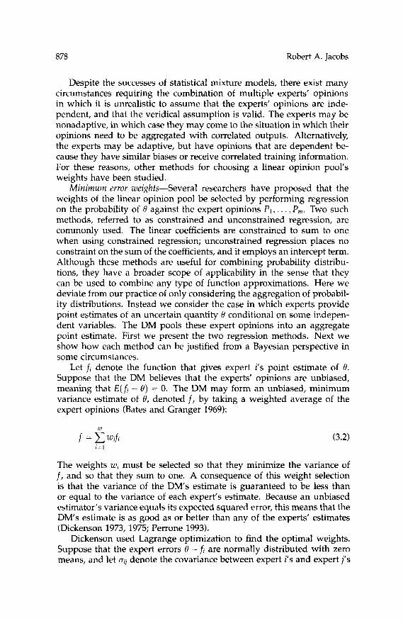
Minimum error weights-Several researchers have proposed that the weights of the linear opinion pool be selected by performing regression on the probability of H against the expert opinions P I , . . . , P,. Two such methods, referred to as constrained and unconstrained regression, are commonly used. The linear coefficients are constrained to sum to one when using constrained regression; unconstrained regression places no constraint on the sum of the coefficients, and it employs an intercept term. Although these methods are useful for combining probability distributions, they have a broader scope of applicability in the sense that they can be used to combine any type of function approximations. Here we deviate from our practice of only considering the aggregation of probability distributions. Instead we consider the case in which experts provide point estimates of an uncertain quantity H conditional on some independent variables. The DM pools these expert opinions into an aggregate point estimate. First we present the two regression methods. Next we show how each method can be justified from a Bayesian perspective in some circumstances.

Let f l denote the function that gives expert i’s point estimate of 8. Suppose that the DM believes that the experts’ opinions are unbiased, meaning that E(f; - 0) = 0. The DM may form an unbiased, minimum variance estimate of H, denoted f , by taking a weighted average of the expert opinions (Bates and Granger 1969):

The weights wi must be selected so that they minimize the variance of f , and so that they sum to one. A consequence of this weight selection is that the variance of the DMs estimate is guaranteed to be less than or equal to the variance of each expert’s estimate. Because an unbiased estimator’s variance equals its expected squared error, this means that the DMs estimate is as good as or better than any of the experts’ estimates (Dickenson 1973,1975; Perrone 1993).

Dickenson used Lagrange optimization to find the optimal weights. Suppose that the expert errors 0 - fi are normally distributed with zero means, and let q denote the covariance between expert i’s and expert j’s


errors. The weights are found by minimizing the objective function

(3.3)

The first term on the right-hand side is the variance or expected squared error off. The second term gives the constraint that the weights sum to one. The solution to this optimization problem is

w = c - ’ I ( I T E - y (3.4)

where w = (w1, . . . , win) is the vector of weights, C is the covariance matrix for the experts’ errors, and I is a vector whose elements are equal to one. If, for example, the DM believes that the experts’ errors are independent, then the ith weight is proportional to the ith expert’s precision I / var(fl).

Disadvantages of this constrained regression procedure can be illus- trated by considering the case of two experts (Granger and Ramanathan 1984). The DM’s estimate is

(3.5) f = Wfl + (1 - w)f2

which can be rewritten as

8 - fz = w ( fl - f 2 ) + f (3.6)

where t = 8 -f is the error. The weight w is chosen so as to minimize the expected squared error. A drawback of this procedure is that although the error t is uncorrelated with the difference f1 - fZ, it is not necessarily uncorrelated with the individual expert estimates f1 and f 2 . It is, therefore, possible to estimate the error from the expert estimates. In this sense, the constrained regression procedure is not optimal. One possibility is to remove the constraint that the weights sum to one, but then it would no longer be the case that the DM’s estimate is unbiased so long as the experts’ estimates are unbiased.

An alternative is to include an additional unbiased estimate of 8, namely its unconditional mean € ( B ) . In this case, the quantity 8 is given

(3.7)

where w1 + w2 + w3 = 1. The weights are chosen via least-squares regression in which w3€(8) is a constant and w1 and w2 are unconstrained. Because w3E(B) is a constant, the DM’s estimate is a linear combination of the expert estimates plus an intercept term. The error E is uncorrelated with the expert estimates.

Granger and Ramanathan (1984) advocated the use of an intercept term and the removal of the constraint that the weights sum to one. That is, the DM’s estimate should be a linear combination of the expert

by

8 = wlfi + ~ 2 f 2 + ~ 3 E ( 8 ) + t


estimates plus an intercept term, and the weights should be selected via unconstrained least-squares regression. This method has the advantage that it yields an unbiased pooled estimate even if the expert estimates are biased.

Researchers have debated the relative merits of the constrained regression (no intercept term, weights sum to one) and unconstrained regression (intercept term, no constraint on the weights) procedures. It is clear that the unconstrained method has more “degrees-of-freedom” and, thus, will achieve a smaller sum of squared error on a set of training items (Granger and Ramanathan 1984). Nonetheless, due to possible overfit- ting of the training data, it is uncertain which procedure will perform better on novel data (Clemen 1986).

Meir (1994) quantified the bias and variance of linear opinion pools in the case of linear least-squares regression. Of greatest interest for our purposes is that he studied the situation where the data set is partitioned into disjoint subsets, and a different subset is used to train each expert. As compared to the case in which all experts are trained on the full data set, this training scheme can, in many situations, lead to a linear opinion pool with good performance because it results in a large decrease in the pool’s variance due to the independence of the experts’ opinions. This decrease tends to more than offset the concomitant increase in the pool’s bias.

Bordley (1982,1986) has shown that the constrained and unconstrained regression methods can be deduced from a Bayesian approach. In the case of constrained regression, Bordley (1982) assumed that (1) the DM’s prior distribution on 8 is diffuse (that is, any value of 0 is equally likely); (2) the DM considers the expert errors 0 - fi to be normally distributed with mean zero and covariance matrix C; and (3) the expert errors are uncorrelated with the DM’s prior estimates of 0. Using these assumptions, p ( 0 I f , . . . . , fm), the DM’s posterior distribution on 0, is a multivariate normal whose mean is given by the linear opinion pool without an intercept term and whose weights sum to one. The weights are the optimal weights selected via Lagrange optimization as described above (equation 3.4).

In the case of unconstrained regression, Bordley (1 986) replaced assumptions (1) and (3) with the assumptions that the DM’s prior distribution on 0 is normal, and that the expert errors are correlated with the DM’s prior estimates. Using these assumptions, the mean of the DMs posterior distribution is given by a linear opinion pool with an intercept term, and with no constraints on the weights. The weights are selected via unconstrained least-squares regression. When the experts’ estimates are biased, the DM’s estimate may be written in the form

m

where E( f;) is the DMs expected value for expert i’s estimate. That is, the DM computes its posterior expectations by adjusting its prior expecta-

Experts’ Probability Assessments 88 1

tions, either positively or negatively, in proportion to the degree to which the experts’ estimates deviate from what it had expected their values to be. This is reasonable in the sense that if the experts’ estimates are what the DM expects them to be, then the DM has not gained any information, and its posterior expectation equals its prior expectation.

Perrone (1993) presented several examples of the use of linear opinion pools when the experts are neural networks. One set of simulations compared different classifiers on a face recognition task. The database consisted of images of 16 human male faces. Different images of the faces were generated under various lighting conditions and with a variety of locations and orientations of the faces. During the first stage of training, 10 neural networks were individually trained to classify the faces. The networks had identical architectures, though they differed in the initial values of their weights. The outputs of the networks were combined into a linear opinion pool during a second stage of training using constrained least-squares regression. It was found that the linear opinion pool signif- icantly outperformed all of the individual networks that comprised the pool on a novel set of images. Additional empirical results can be found in Hashem (1993) and Perrone (1993).

Recently, researchers have proposed combining linear opinion pools based on constrained or unconstrained least-squares regression with model selection techniques to achieve systems with good generalization properties (e.g., Breiman 1992; LeBlanc and Tibshirani 1993; Wolpert 1992). This combination is a special case of what Wolpert (1992) referred to as stacked generalization. To illustrate the combination, we contrast it with leave-one-out cross-validation, a common model selection procedure. Let { X k : & } be a set of input-output data items, and let f , ’ - k ’ ( ~ k )

denote the output of the ith expert in response to the input x k when this expert has been trained using all data except data item k. The prediction error for expert i is defined as

(3.9)

Leave-one-out cross-validation is a “winner-take-all” model selection scheme that selects the expert with the smallest prediction error. In contrast, the combination of linear opinion pools with leave-one-out cross- validation defines the prediction error in terms of the linear aggregation of the experts’ outputs:

r 7 2

(3.10)

The weights wi are selected to minimize the prediction error via constrained or unconstrained regression.

Breiman (1992) compared stacked generalization with a variety of con- ventional statistical techniques on a wide range of linear regression tasks.


The target functions had 40 input variables and one output variable. In the first stage of the simulations, a set of experts was formed. Each expert was a linear model, and the experts differed because they each received a different subset of the input variables. The outputs of the experts were aggregated in a second stage of the simulations via a least-squares procedure that did not contain an intercept term, and that was constrained so that all the coefficients were nonnegative. The performance of this system was superior to the performances of three regression methods based upon cross-validation methodology. Additional empirical and theoretical results regarding stacked generalization can be found in Breiman (19921, LeBlanc and Tibshirani (1993), and Wolpert (1992).

In summary, we have reviewed methods that a DM can use to linearly combine experts’ probability assessments. Two cases were considered: weights as veridical probabilities and minimum error weights. In practice, linear opinion pools have proven popular because they often yield useful results with a moderate amount of computation. Objections to their use have been raised, however, based on theoretical grounds. To give just one example, it has been argued that the DM should combine the experts’ opinions in such a way as to preserve any form of expert agreement regarding the independence of the events in question (Genest and Wagner 1987). That is, it should be the case that

(3.11) whenever it is each expert’s belief that p,(A n B) = p l ( A ) p l ( B ) V i for events A and B. This property is referred to as the independence preservation property. Note that it is not possessed by linear opinion pools except when a single expert has a weight of one and all other experts have a weight of zero, a situation referred to as a dictatorship. Genest and Wagner (1987) argued, however, that the independence preservation property is not a reasonable requirement of an aggregation procedure.

p(A n B I P I , . . . , P m ) = p ( A I PI ’ . . $ pr,,) p ( B I Pi, . . . , P,,,)

4 Value of Information from Dependent Experts

The major feature that makes the aggregation of expert opinions difficult is the high correlation or dependence that typically occurs among these opinions. This problem was alluded to in the preceding discussion; it is explicitly studied in this section where we review the results of Clemen and Winkler (1985). These authors showed that, given certain assumptions, m dependent experts are worth the same as k independent experts where k 5 m. In some cases, an exact value for k can be given; in other cases, lower and upper bounds can be placed on k.

Clemen and Winkler (1985) assumed that the experts provide point estimates f, of the uncertain quantity 8, and that these estimates are unbiased, meaning that E(fi - Q) = 0. The vector E = ( F 1 , . . . , em) denotes the experts’ errors where F , = f, - 0. It is assumed that the joint probability of the experts’ errors, p ( ~ I Q), is normally distributed with mean

Experts' Probability Assessments 883

zero and covariance matrix C. The DMs prior distribution for 8, p ( 8 ) , is a normal distribution with mean [LO and variance go'. It is assumed that the DM's prior estimation error po - 0 is uncorrelated with any of the experts' errors. Using Bayes' rule, the DMs posterior distribution is given by

(4.1) P(8 I f l , . ' ' 3 f m ) 0: P ( E I 0)

This distribution is normal with mean

p* = (o&o + ITC-'f)r?

and variance

(4.2)

where I is a vector whose elements are equal to one, and f = (f1, . . . , f m ) is the vector of expert opinions. Much of the analysis given below uses the fact that the posterior mean p* is a weighted average of the prior mean and the experts' estimates, and that the weights depend on the covariance matrix C. The posterior variance 0: also depends on C.

Suppose that the expert errors are independent, and that each expert has an error variance of cr*. As a matter of notation, we use m to denote the number of experts when these experts are dependent, and k to denote the number when they are independent. The DM's prior variance can be written in the form C T ~ = g2 /ko . The posterior variance is then

(4.4)

By comparing equations 4.3 and 4.4, we can determine the number of independent experts with error variance 0' that yields the same posterior variance as m dependent experts with covariance matrix C. This number, denoted k ( g 2 , C) can be written

(4.5)

That is, under the given assumptions, k(a2, C) independent experts are equivalent to m dependent experts.

Clemen and Winkler (1985) considered three cases. The first case assumes that C is an intraclass correlation matrix, meaning that all expert variances are equal and all correlations are equal. The common variance and correlation are denoted LT* and p, with p > 0. The inverse of the covariance matrix, C-', takes a relatively simple form under these conditions, and the equivalent number of independent experts is

k ( d , C) = a21 TC-'I

k ( 0 2 , C) = m[l + (m - 1)pI-l (4.6)

If m > 1, then k ( u 2 , C ) < m, meaning that positive dependence among the experts' errors reduces the information value of their opinions. The stronger the dependence, the greater is the reduction because dk(o*> C ) / d p


< 0. The equivalent number of independent experts is a concave function of rn, whose limit may be written as

lim k ( 0 2 , C) = p-I m-cc (4.7)

In other words, there is an upper limit on the number of equivalent independent experts, and on the precision of the information that can be attained by consulting dependent experts. This limit is surprisingly low. For example, if p = 0.8, then k(rr2, C) = 1.25. After the first expert, who is worth one independent expert, all other experts combined are worth only one-fourth of an independent expert. As a second example, if p = 0.25, then k(a2, C) = 4.0. Consulting an infinite number of dependent experts, in this case, is no better than consulting four independent experts.

The second case considered by Clemen and Winkler (1985) assumes that the correlations among the expert errors are positive and equal, but that the error variances may differ. It is also assumed that the weights used to compute the DMs posterior mean are positive (equation 4.2). Define ah and as follows:

oM 2 = max{a?}; a: = min{o~) I I

(4.8)

where o,? is expert 2s variance. Then it can be shown that

k(a2, E M ) < k ( a 2 , C) < k(a2, E m ) (4.9)

where EM and C, have intraclass correlation structure with correlation p and variances af and u i , respectively. In other words, an increase in the expert variances leads to a decrease in the equivalent number of independent experts.

In the general case, both the correlations among the expert errors and the expert variances may vary. As before, assume that the weights used to compute the DM’s posterior mean are positive. Define

PR = max{p,,}; Pr = min{p,,); PO = 0 (4.10)

where pI, is the correlation between expert i’s and expert j’s errors. Let CR have common correlation p ~ , C, have common correlation p,, and Co have common correlation po, with variances equal to those in C. It can be shown that

I > I * J

k(a2. CR) < k ( a 2 . C) < k(a2, C , ) < k(a2, Co) (4.11)

An increase in the correlation among expert errors leads to a decrease in the equivalent number of independent experts.

As Clemen and Winkler (1985) pointed out, dependence among the experts can occasionally be helpful. For example, suppose that the expert errors have a common variance and correlation, but that the correlation

Experts' Probability Assessments 885

is negative (-m-l 5 p < 0; the lower bound is necessary to make C positive definite). Then

m < k ( d , C ) < m2 (4.12)

where m > 1. Negative dependence can, therefore, lead to increases in the number of equivalent independent experts. As a second example, when one expert has a very large variance, it may be useful to include additional experts whose errors have high positive correlations with those of the first expert, but with smaller variances. Despite these examples, Clemen and Winkler concluded that it will generally be advantageous to include experts that are believed not to be highly correlated with each other or with the prior information, even if this means using experts with relatively high variance.

In conclusion, it appears to be the case that different aggregation procedures are appropriate for different situations. The simplest circumstance occurs when the experts' errors are uncorrelated. This may occur if it is possible to train different experts on independent data sets (Meir 1994). Alternatively, this situation may be approximated if the experts are competitive; the experts learn different mappings because they adaptively partition the data set (Jacobs et al. 1991). Aggregation is more com- plicated when the experts' opinions are dependent. In this case, it may be necessary for the DM to model the dependencies among the experts to achieve good performance. Two classes of aggregation procedures were reviewed in this article. With problems of easy or moderate difficulty, a "quick and dirty" procedure such as the linear opinion pool may be sufficient. A more computationally intensive technique, such as a supra Bayesian method, may be necessary for problems of greater complexity.

Recent years have seen a large increase in the number of studies on how people combine multiple sources of information, particularly in the context of visual perception. Linear opinion pools are often used to model people's perceptual cue aggregations, though some experimental results suggest that such pools are not always perfectly suited for this role. Modifications of these pools are, therefore, often explored. For example, Young et al. (1993), in their study of how people combine object motion and texture gradient visual cues to extract depth information, proposed two modifications to the basic linear opinion pool. One modification, called cue promotion, involves the use of one visual cue to provide missing information required by another cue to yield accurate perceptual judgments. The second modification is that the coefficients of the linear opinion pool may change with the visual environment, a technique referred to as dynamic reweighting. Unfortunately, there is currently no well-articulated theory to guide researchers in the selection of a model that is well-suited for the circumstance that they study. That is, it is not known which perceptual or cognitive phenomenon are best modeled using a linear opinion pool, which phenomenon should be char- acterized using a modified linear opinion pool, or which phenomenon


requires a more complex model such as a supra Bayesian model. This will surely be a topic of many future studies.

Acknowledgments ~

This work was supported in part by NIH grant MR-54770.

References

Abidi, M. A., and Gonzalez, R. C. 1992. Data Fusion in Robotics and Machine Intelligence. Academic Press, San Diego, CA.

Agnew, C. E. 1985. Multiple probability assessments by dependent experts. 1. A m . Stat. Assoc. 80, 343-347.

Bates, J. M., and Granger, C. W. J. 1969. The combination of forecasts. Opera- tional Res. Q. 20, 451467.

Bordley, R. F. 1982. The combination of forecasts: A Bayesian approach. J. Op- erational Res. SOC. 33, 171-174.

Bordley, R. F. 1986. Linear combination of forecasts with an intercept: A Bayesian approach. 1. Forecasting 5, 243-249.

Breiman, L. 1992. Stacked Regression. Tech. Rep. TR-367, Department of Statistics, University of California, Berkeley.

Chatterjee, S., and Chatterjee, S. 1987. On combining expert opinions. A m . J. Math. Management Sci. 7, 271-295.

Clark, J. J., and Yuille, A. L. 1990. Data Fusion for Sensory Information Processing Systems. Kluwer Academic Publishers, Norwell, MA.

Clemen, R. T. 1986. Linear constraints and the efficiency of combined forecasts. J. Forecasting 5, 31-38.

Clemen, R. T., and Winkler, R. L. 1985. Limits for the precision and value of information from dependent sources. Oper. Res. 33, 427-442.

Cooke, R. M. 1990. Statistics in expert resolution: A theory of weights for combining expert opinion. In Statistics in Science: The Foundations of Statistical Methods in Biology, Physics, and Economics, R. Cooke and D. Costantini, eds. Kluwer Academic Publishers, The Netherlands.

DeGroot, M. H., and Fienberg, S. E. 1986. Comparing probability forecasters: Basic binary concepts and multivariate extensions. In Bayesian Inference and Decision Techniques, I? Goel and A. Zellner, eds. Elsevier Science Publishers, Amsterdam.

Dickenson, J. P. 1973. Some statistical results in the combination of forecasts. Oper. Res. Q. 24, 253-260.

Dickenson, J. P. 1975. Some comments on the Combination of forecasts. Oper. Res. Q. 26,205-210.

Dosher, B. A., Sperling, G., and Wurst, S. A. 1986. ‘Tradeoffs between stereop- sis and proximity luminance covariance as determinants of perceived 3D structure. Vision Res. 26, 973-990.

Drucker, H., Schapire, R., and Simard, P. 1993. Improving performance in neural networks using a boosting algorithm. In Advances in Neural Information


Processing Systems 5, S. J. Hanson, J. D. Cowan, and C. L. Giles, eds. Morgan Kaufmann, San Mateo, CA.

French, S. 1980. Updating of belief in the light of someone else’s opinion. J. Royal Statist. SOC. A 143, 4348.

French, S. 1985. Group consensus probability distributions: A critical survey. In Bayesian Statistics 2, J. M. Bernardo, M. H. DeGroot, D. V. Lindley, and A. F. M. Smith, eds. Elsevier Science Publishers, North-Holland.

Gelfand, A. E., Mallick, B. K., and Dey, D. K. 1995. Modeling expert opinion arising as a partial probabilistic specification. J. Am. Statist. Assoc. 90, 598- 604.

Genest, C., and McConway, K. J. 1990. Allocating the weights in the linear opinion pool. 1. Forecasting 9, 53-73.

Genest, C., and Wagner, C. G. 1987. Further evidence against independence preservation in expert judgement synthesis. Aequat. Math. 32, 74-86.

Genest, C., and Zidek, J. V. 1986. Combining probability distributions: A cri- tique and an annotated bibliography. Statist. Sci. 1, 114-148.

Graham, N. V. S. 1989. Visual Pattern Analyzers. Oxford University Press, New York.

Granger, C. W. J., and Ramanathan, R. 1984. Improved methods of combining forecasts. 1. Forecasting 3, 197-204.

Hashem, S. 1993. Optimal Linear Combinations of Neural Networks. Tech. Rep. SMS 94-4, School of Industrial Engineering, Purdue University.

Jacobs, R. A., Jordan, M. I., Nowlan, S. J., and Hinton, G. E. 1991. Adaptive mixtures of local experts. Neural Comp. 3, 79-87.

Jordan, M. I., and Jacobs, R. A. 1994. Hierarchical mixtures of experts and the EM algorithm. Neural Comp. 6, 181-214.

Lawson, C. L., and Hanson, R. J. 1974. Solving Least Squares Problems. Prentice- Hall, Englewood Cliffs, NJ.

LeBlanc, M., and Tibshirani, R. 1993. Combining Estimates in Regression and Clas- sification. Tech. Rep., Department of Preventive Medicine and Biostatistics, University of Toronto.

Lindley, D. V. 1982. The improvement of probability judgements. 1. Royal Statist.

Lindley, D. V. 1985. Reconciliation of discrete probability distributions. In Bayesian Statistics 2, J. M. Bernardo, M. H. DeGroot, D. V. Lindley, and A. F. M. Smith, eds. North-Holland, Amsterdam.

Lindley, D. V. 1988. The use of probability statements. In Accelerated Life Testing and Experts’ Opinions in Reliability, C. A. Clarotti and D. V. Lindley, eds. North-Holland, Amsterdam.

Lindley, D. V., Tversky, A., and Brown, R. V. 1979. On the reconciliation of probability assessments. J. Royal Statist. SOC. A 142, 146-180.

McConway, K. J. 1981. Marginalization and linear opinion pools. J . A m . Statis. Assoc. 76, 410-414.

Meir, R. 1994. Bias, Variance, and the Combination of Estimators: The Case of Linear Least Squares. Tech. Rep. 922, Department of Electrical Engineering, Tech- nion, Haifa, Israel.

SOC. A 145, 117-126.

Morris, P. A. 1974. Decision analysis expert use. Manage. Sci. 20, 1233-1241.


Morris, P. A. 1977. Combining expert judgements: A Bayesian approach. Man- age. Sci. 23, 679-693.

Nakayama, K., and Shimojo, S. 1990. Toward a neural understanding of visual surface representation. Cold Spring Harbor Symp. Quant. Biol. 55, 911-924.

Nowlan, 5. J. 1990. Competing Experts: An Experimental Investigation of Associative Mixture Models. Tech. Rep. CRG-TR-90-5, Department of Computer Science, University of Toronto.

Perrone, M. P. 1993. Improving regression estimation: Averaging methods for variance reduction with extensions to general convex measure optimization. P1i.D. thesis, Department of Physics, Brown University.

Peterson, G. E., and Barney, H. L. 1952. Control methods used in a study of vowels. 1. Aconst. SOC. Am. 24, 175-184.

Roberts, H. V. 1965. Probabilistic prediction. J. Am. Stat. Assoc. 60, 50-62. Shuford, E. H., Albert, A., and Massengil, H. E. 1966. Admissible probability

measurement procedures. Psychometrika 31, 125-145. Stein, B. E., and Meredith, M. A. 1993. The Merging of the Senses. MIT Press,

Cambridge, MA. Trueswell, J. C., and Hayhoe, M. M. 1993. Surface segmentation mechanisms

and motion perception. Vision Res. 33, 313-328. Winkler, R. L. 1969. Scoring rules and the evaluation of probability assessors.

J. Am. Statist. Assoc. 64, 1073-1078. Winkler, R. L. 1981. Combining probability distributions from dependent infor-

mation sources. Manage. Sci. 27, 479-488. Wolpert, D. H. 1992. Stacked generalization. Neural Networks 5, 241-259. Xu, L., Krzyzak, A., and Suen, C. Y. 1992. Methods of combining multiple

classifiers and their applications to handwriting recognition. IEEE Trans. Systems, Man, Cybernet. 22, 418-435.

Young, M. J., Landy, M. S., and Maloney, L. T. 1993. A perturbation analysis of depth perception from combinations of texture and motion cues. Vision Res.

Zeki, S. 1993. A Vision of the Brain. Blackwell Scientific Publications, Oxford, 33, 2685-2696.

UK.

_ _ _ _ Received March 29, 1994; accepted March 3, 1995.

Methods for combining experts' probability assessments

Documents

Transcript of Methods for combining experts' probability assessments