Parametrization of algebraic curves defined by sparse equations

AAECC (2007) 18:127–150DOI 10.1007/s00200-006-0026-5

Parametrization of algebraic curves definedby sparse equations

Tobias Beck · Josef Schicho

Received: 6 June 2005 /Revised: 4 October 2006 /Published online: 9 January 2007© Springer-Verlag 2006

Abstract We present a new method for the rational parametrization of planealgebraic curves. The algorithm exploits the shape of the Newton polygon ofthe defining implicit equation and is based on methods of toric geometry.

Keywords Parametrization · Toric geometry · Sparse

1 Introduction

Given a bivariate polynomial f ∈ K[x, y] over some field K we will describea method to find a proper parametrization of the curve defined implicitly byf . That is we will find (X(t), Y(t)) ∈ K(t) s.t. f (X(t), Y(t)) = 0 and (X(t), Y(t))induces a birational morphism from the affine line to the curve. This is theproblem of finding a rational parametrization, a well-studied subject in alge-braic geometry. There are already several algorithms, e.g., [12,15]. But up to nowthese methods do not take into account whether the defining equation is sparseor not. We will present an algorithm which exploits the shape of the Newtonpolygon of the defining polynomial by embedding the curve in a well-chosen

The authors were supported by the FWF (Austrian Science Fund) in the frame of the researchprojects SFB 1303 and P15551.

T. Beck · J. Schicho (B)Johann Radon Institute for Computational and Applied Mathematics,Austrian Academy of Sciences, Altenbergerstraße 69, 4040 Linz, Austriae-mail: [email protected]

T. Becke-mail: [email protected]

128 T. Beck, J. Schicho

complete surface. In this article we do not care for the involved extensions ofthe coefficient field and therefore assume that K is algebraically closed.

This article is organized as follows. In Sect. 2 we recall some basic construc-tions of toric geometry. In particular we show how to embed a curve into asuitable complete toric surface. In Sect. 3 we show how to compute the genusof the curve in this setting and how to find a linear system of rational functionson the curve that allows to find a parametrization. We state the main theoremwhich proves the algorithm to be correct. Finally, we give a coarse descriptionof the algorithm in pseudo-code and an example. The last section is devotedto a different proof of correctness using sheaf theoretical and cohomologicalarguments.

The reason for giving two different proofs is a historical one. When con-structing the algorithm, we were looking for a suitable vector space of rationalfunctions for the parametrization map. We found it by computing the first coho-mology of certain sheaves of rational functions. Afterwards it turned out thatmore elementary arguments (using only the notion of divisors) can also be usedto prove correctness of the algorithm. So in one sense the second proof is redun-dant. We decided to keep it nevertheless in the hope that it provides additionalinsight. When not seen in another context, the fact that a certain vector spacehas exactly the right dimension looks like a nice coincidence.

2 Preliminaries on toric varieties

Let K be an algebraically closed field. We are going to parametrize (if possible)a plane curve F ′ that is given by an absolutely irreducible polynomial f ∈ K[x, y]on the torus T := (K∗)2. Actually we will study a curve F which is the Zariskiclosure of F ′ in a complete surface containing the torus, i.e., F ∩T = F ′. We willfirst show how to realize this surface and then recall some basic definitions andpropositions. A good introduction to toric varieties can be found in [3].

2.1 Embedding the curve into a complete toric surface

Parametrization by rational functions is a “global problem”. In order to applysome theorems of global content we have to embed T in a complete surface. Onepossible complete surface, which is often used in this context, is the projectiveplane P

2K

. We will choose a complete toric surface instead, whose constructionis guided by the shape of the Newton polygon of f .

The Newton polygon Π(f ) ⊂ R2 is defined as the convex hull of all lattice

points (r, s) ∈ Supp(f ) (i.e., all (r, s) ∈ Z2 s.t. xrys appears with a non-zero

coefficient in f ). A sample Newton polygon is illustrated in Fig. 1.

Remark 1 If f is a dense polynomial, i.e., if it has total degree d and compre-hends all monomials of degree less than or equal to d, then the Newton polygonwill be an equilateral triangle with vertices (0, 0), (d, 0) and (0, d). (For this it isof course sufficient that the support contains the vertices only.) The toric surface

Parametrization of algebraic curves defined by sparse equations 129

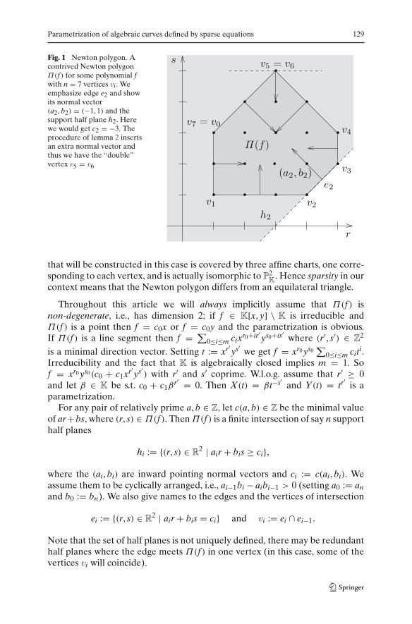
Fig. 1 Newton polygon. Acontrived Newton polygonΠ(f ) for some polynomial fwith n = 7 vertices vi. Weemphasize edge e2 and showits normal vector(a2, b2) = (−1, 1) and thesupport half plane h2. Herewe would get c2 = −3. Theprocedure of lemma 2 insertsan extra normal vector andthus we have the “double”vertex v5 = v6

that will be constructed in this case is covered by three affine charts, one corre-sponding to each vertex, and is actually isomorphic to P

2K

. Hence sparsity in ourcontext means that the Newton polygon differs from an equilateral triangle.

Throughout this article we will always implicitly assume that Π(f ) isnon-degenerate, i.e., has dimension 2; if f ∈ K[x, y] \ K is irreducible andΠ(f ) is a point then f = c0x or f = c0y and the parametrization is obvious.If Π(f ) is a line segment then f = ∑

0≤i≤m cixr0+ir′ys0+is′ where (r′, s′) ∈ Z

2

is a minimal direction vector. Setting t := xr′ys′ we get f = xr0 ys0

∑0≤i≤m citi.

Irreducibility and the fact that K is algebraically closed implies m = 1. Sof = xr0 ys0(c0 + c1xr′

ys′) with r′ and s′ coprime. W.l.o.g. assume that r′ ≥ 0and let β ∈ K be s.t. c0 + c1β

r′ = 0. Then X(t) = βt−s′ and Y(t) = tr′

is aparametrization.

For any pair of relatively prime a, b ∈ Z, let c(a, b) ∈ Z be the minimal valueof ar+bs, where (r, s) ∈ Π(f ). ThenΠ(f ) is a finite intersection of say n supporthalf planes

hi := {(r, s) ∈ R2 | air + bis ≥ ci},

where the (ai, bi) are inward pointing normal vectors and ci := c(ai, bi). Weassume them to be cyclically arranged, i.e., ai−1bi − aibi−1 > 0 (setting a0 := anand b0 := bn). We also give names to the edges and the vertices of intersection

ei := {(r, s) ∈ R2 | air + bis = ci} and vi := ei ∩ ei−1.

Note that the set of half planes is not uniquely defined, there may be redundanthalf planes where the edge meets Π(f ) in one vertex (in this case, some of thevertices vi will coincide).


Lemma 2 We can assume that ai−1bi − aibi−1 = 1 for 1 < i ≤ n.

Proof The values det((ai−1, bi−1)T , (ai, bi)

T) = ai−1bi − aibi−1 are invariantunder unimodular transformations (i.e., linear transformations of the vectorsby an integral matrix with determinant 1). Assume that ai0−1bi0 − ai0 bi0−1 > 1for some i0. By a suitable unimodular transformation we may assume (ai0 , bi0) =(0, 1). It follows that ai0−1 > 1.

We insert a new index, for simplicity say i0 − 12 , set ai0− 1

2:= 1 and determine

bi0− 12

by integer division s.t. 0 ≤ ai0−1bi0− 12

− bi0−1 < ai0−1. It follows

ai0− 12bi0 − ai0 bi0− 1

2= 1 · 1 − 0 · bi0− 1

2= 1 and

ai0−1bi0− 12

− ai0− 12bi0−1 = ai0−1bi0− 1

2− 1 · bi0−1 < ai0−1

= ai0−1 · 1 − 0 · bi0−1 = ai0−1bi0 − ai0 bi0−1.

By inserting the additional support half plane with normal vector(ai0− 1

2, bi0− 1

2) and support line through the vertex vi0 , we “substitute” the

value ai0−1bi0 − ai0 bi0−1 by the smaller value ai0−1bi0− 12

− ai0− 12bi0−1 and add

ai0− 12bi0 − ai0 bi0− 1

2= 1 to the list. All other values stay fixed. Repeating this

process the statement in the proposition can be achieved. Now we construct the toric surface. For 1 ≤ i ≤ n let Ui := A

2K

be cop-ies of the affine plane with coordinates ui and vi. Again we identify U0 andUn. We denote the coordinate axes by Li := {(ui, vi) ∈ Ui | ui = 0} andRi := {(ui, vi) ∈ Ui | vi = 0} and define open embeddings of the torus

ψi : T → Ui : (x, y) �→ (ui, vi) = (xbi y−ai , x−bi−1 yai−1).

The isomorphic image of ψi is Ui \ (Li ∪ Ri) and there it has the inverse

Ui \ (Li ∪ Ri) → T : (ui, vi) �→ (x, y) = (uai−1i vai

i , ubi−1i vbi

i ).

For i, j ∈ {1, . . . , n}, i �= j we define open subsets

Ui,j :=⎧⎨

⎩

Ui \ Li if i ≡ j − 1 mod n,Ui \ Ri if i ≡ j + 1 mod n,Ui \ (Li ∪ Ri) = ψi(T) else.

For 1 ≤ i ≤ n the following maps are mutually inverse and thereforeisomorphisms:

φi−1,i : Ui−1,i → Ui,i−1 : (ui−1, vi−1) �→ (ui, vi) = (uai−2bi−aibi−2i−1 vi−1, u−1

i−1)

φi,i−1 : Ui,i−1 → Ui−1,i : (ui, vi) �→ (ui−1, vi−1) = (v−1i , uiv

ai−2bi−aibi−2i )


If i and j are non-neighboring indices we set

φi,j := ψj ◦ ψ−1i : Ui,j → Uj,i.

The above morphisms are compatible in the sense that φj,i = φ−1i,j and for each k

we have φi,j(Ui,j ∩Ui,k) = Uj,i ∩Uj,k and φi,k = φj,k ◦φi,j. Under these conditionsthe general gluing construction provides an abstract variety V and morphismsιi : Ui → V that embed Ui as open subsets into V. (This also works in the moregeneral context of schemes, see e.g., [10, Exercise II.2.12].) By abuse of notationwe will from now on identify Ui and its image ιi(Ui) ⊂ V. Then {Ui}1≤i≤n is anopen cover of V.

Notation 3 In the sequel V will denote a surface constructed as above. Thepolynomial f used for its construction is implicitly understood.

It is not hard to see that Ei := Ri ∪ Li+1 is an irreducible curve on V andisomorphic to P

1K

. We call it an edge curve. The curves Ei−1 and Ei intersecttransversally in a point Vi ∈ Ui, corresponding to the origin (ui, vi) = (0, 0) ofthe corresponding chart. For non-neighboring indices i and j the edge curves Eiand Ej are disjoint. The complement of the union of all edge curves is the torusT, which is also the intersection of all open sets Ui.

Now the curve F given by f is defined to be the Zariski closure of F ′ in V. Wewill see its local equations in the next section. For the rest of the article we fix fand the corresponding curve F ⊂ V, i.e., in particular the data ai, bi, ci derivedfrom its Newton polygon.

Remark 4 There is a standard procedure for the construction of the toricvariety corresponding to a polytope that can be found for example in [3] or[6]. It is always projective and therefore complete. The above construction isbasically the same, except that it always results in a smooth surface becauseit is covered by copies of the affine plane A

2K

. Indeed the proof of Lemma 2corresponds to the resolution procedure for toric surfaces (see e.g., [4]). Forthe parametrization algorithm this is not strictly necessary (although it may beuseful, see Remark 18). Also the theoretical arguments that follow do not reallyneed a smooth surface. Everything would go through as well using affine toriccharts. We use this construction mainly for simplifying notation.

Embedding the curve F into the surface V is a very “economic” choice of abirational model of that curve. It anticipates the simple part of a resolution ofsome of the singularities of the curve, i.e., F is less singular (e.g., in terms of thedelta invariants) than the corresponding model one would get by embeddinginto P

2K

. From a theoretical point of view this should save time when deter-mining the genus of the curve (see Proposition 9) and when computing theparametrizing linear system (see Definition 15).

2.2 Toric invariant divisors

Irreducible closed curves on V are also called prime (Weil) divisors. A generaldivisor D is defined to be a formal sum (i.e., a linear combination over Z) of


prime divisors. The set of divisors forms a free Abelian group Div(V). The edgecurves Ei of the previous section are the special “toric invariant” prime divisors.Consequently a toric invariant divisor is a formal sum of the Ei. One associatesto a rational function g ∈ K(x, y) its principal divisor (g). Roughly speaking ghas poles and zeros on V along certain subvarieties of codimension one; then(g) is the divisor of zeros minus the divisor of poles (with multiplicities). For adetailed introduction to divisors we refer to [14]. Two divisors are called linearlyequivalent iff they differ only by a principal divisor. The divisor class group isdefined as the group of divisors modulo this equivalence.

The coordinate ring of the torus is K[x, y, x−1, y−1] which is a unique factor-ization domain. Hence any divisor on the torus is a principal divisor and the classgroup is trivial. This implies that the class group of the surface V is generatedby the toric invariant divisors Ei. We will now show how to find representativesin terms of these divisors.

Lemma 5 Let g ∈ K[x, y, x−1, y−1]. Then g defines a curve on the torus T. LetG be its closure in the surface V. Then the divisor G is linearly equivalentto G0 := ∑

1≤i≤n −ciEi where ci = min(r,s)∈Supp(g)(air + bis), more preciselyG = G0 + (g).

Proof On the affine open subset Ui let

gi(ui, vi) := u−ci−1i v−ci

i g(uai−1i vai

i , ubi−1i vbi

i ).

Then gi ∈ K[ui, vi] is the local equation of G. Further gi differs fromu−ci−1

i v−cii only by the rational function g. Now we can associate to both sides of

that equation the corresponding (locally) principal divisors on Ui. This showsthat locally G is linearly equivalent to −ci−1Ei−1 − ciEi. This equivalence isdemonstrated by the rational function g(uai−1

i vaii , ubi−1

i vbii ) = g(x, y) which is the

same on each affine open set. Together we see that globally G = G0 + (g). For example if f ∈ K[x, y] is a dense polynomial then (as remarked before)

the constructed toric surface V is P2K

. The toric invariant divisors will be thetwo coordinate lines corresponding to x = 0 and y = 0 and the line at infinity.Now let g ∈ K[x, y] be some polynomial of total degree d > 0 and not divisibleby x or y. Then the projective curve G ⊂ P

2K

is a divisor linearly equivalent tod times the line at infinity.

This result holds for any g ∈ K[x, y, x−1, y−1] and of course in particular forg = f , G = F and ci = ci from Sect. 2.1. From the proof we get the localequations of the curve F embedded in V

fi(ui, vi) := u−ci−1i v−ci

i f (uai−1i vai

i , ubi−1i vbi

i ) (1)

and a linearly equivalent divisor F0 := ∑1≤i≤n −ciEi. Note that the divisor G0

in the proposition depends only on the support of g, so we define:


Definition 6 Given a lattice polygon Π ⊂ R2. We define the associated divisor

div(Π) := ∑1≤i≤n −ciEi with ci = min(r,s)∈Π(air + bis).

With this definition of course div(Π(g)) = G0. In the sequel we will mainlydeal with toric invariant divisors.

2.3 Linear systems of toric invariant divisors

A divisor D is called effective (or greater or equal to 0) iff it is a non-negativesum of prime divisors. The linear system of rational functions associated to adivisor D is the vector space of rational functions g ∈ K(x, y) s.t. D + (g) iseffective. If D is in particular a toric invariant divisor, then (g) must not haveany poles on the torus. Thus we define:

Definition 7 Given a toric invariant divisor D ∈ Div(V), we define the linearsystem L(D) := {g ∈ K[x, y, x−1, y−1] | (g)+ D ≥ 0}.

As a corollary to Lemma 5 we see that if the divisor is given by a latticepolygon this linear system is non-empty and has a simple description.

Corollary 8 Let Π ⊂ R2 be a lattice polygon, let D = div(Π) = ∑

1≤i≤n −ciEi

and defineΠ := ⋂1≤i≤n{(r, s) ∈ R

2 | air+bis ≥ ci}. Then L(D) = 〈xrys〉(r,s)∈Π∩Z2

as a K-vector space.

HereΠ is the smallest polygon containingΠ and given by an intersection oftranslates of the half planes hi.

3 Sparse parametrization

It is well-known that a curve is parametrizable iff it has genus 0. In this sectionwe will first show how to compute the genus in our setting. Afterwards we givea linear system of rational functions that is used to find the parametrizing map.Finally we describe the algorithm and execute it on an example.

3.1 The genus

If the curve F was embedded in the projective plane P2K

and had total degree

d, we would have the genus formula g(F) = (d−1)(d−2)2 − ∑

P∈F δP. The numberδP is a measure of singularity, which is defined as the dimension of the quotientof the integral closure of the local ring by the local ring at P (cf. [10, exerciseIV.1.8]). For instance, if P is an ordinary singularity of multiplicity μ, i.e., aself-intersection point where μ branches meet transversally, then δP = μ(μ−1)

2 .In particular the sum may be restricted to range over all singular points P ∈ F.If Π ⊂ R

2 is a bounded domain we denote by #(Π) := |Π ∩ Z2| the number of

lattice points in Π . We also write Π◦ for the interior of a domain. In the toricsituation the genus can be computed as follows:

Proposition 9 The genus of F is equal to the number of interior lattice points ofΠ(f ) minus the sum of the delta invariants of all points of F :


g(F) = #(Π(f )◦)−∑

P∈F

δP.

(The sum actually ranges over the singular points of F only.)

Proof Let F → F be the normalization of the curve. The genus of F can bedefined as the arithmetic genus ga(F) of its normalization. It is known thatga(F) = ga(F)− ∑

P∈F δP (cf. [10, Exercise IV.1.8]).The fact that the arithmetic genus ga(F) equals the number of interior lattice

points of Π(f ) is a consequence of the adjunction formula (cf. [6, p. 91]).

3.2 The parametrizing linear system

First we define a family of special divisors on V.

Definition 10 Choose 1 ≤ m < n and let

c′i =

{ci if 1 ≤ i ≤ m andci + 1 else,

where the ci originate from the lattice polygon Π(f ). We define Dm := F0 −∑m+1≤i≤n Ei = ∑

1≤i≤n −c′iEi ∈ Div(V) and denote by di := #(ei ∩ Π(f )) − 1

the integer length of edge i. Further we define the constant dm := ∑1≤i≤m di.

From now on fix such an m. Note that we deliberately excluded m = n.

Remark 11 Since a non-degenerate polygon is at least a triangle we have n ≥ 3and it is easy to see that we can achieve dm ≥ 2. By a small trick we can evenachieve dm ≥ 3; For if n = 3 we can add an additional half plane and thusartificially increase n. A small example may be illustrative.

If Π(f ) is the standard triangle then it is given by the intersection of threehalf planes that are governed by the following data:

v1 = (0, 0), (a1, b1) = (0, 1), c1 = 0, d1 = 1

v2 = (1, 0), (a2, b2) = (−1, −1), c2 = −1, d2 = 1

v3 = (0, 1), (a3, b3) = (1, 0), c3 = 0, d3 = 1

Now we artificially double the vertex v1 and set

v4 = (0, 0), (a4, b4) = (1, 1), c4 = 0, d4 = 0.

Now n = 4 and we may set m := 3 to get dm = 3. If Π(f ) has only three latticepoints on its boundary but is not the standard triangle (or more precisely is notobtained from the standard triangle by a unimodular transformation) then bythe procedure of Lemma 2 one of the vertices is doubled anyway and we canachieve the same effect by just renumbering indices.


Now we compute the intersection number F0 · Dm, i.e., the number of intersec-tions of F0 and Dm counting multiplicities.

Lemma 12 If dm ≥ 2 then F0 · Dm = 2#(Π(f )◦)+ dm − 2.

Proof Let vi0 = (ri0 , si0) be the vertex of Π(f ) common to the edges ei0−1 andei0 . The intersection number is invariant w.r.t. linear equivalence of divisors.Then

F0 · Ei0 = (F0 + (xri0 ysi0 )) · Ei0

= (∑1≤i≤n −ciEi + ∑

1≤i≤n(airi0 + bisi0)Ei) · Ei0

= ∑1≤i≤n(−ci + airi0 + bisi0)Ei · Ei0

1)= (−ci0−1 + ai0−1ri0 + bi0−1si0)Ei0−1 · Ei0

+ (−ci0 + ai0 ri0 + bi0 si0)Ei0 · Ei0

+ (−ci0+1 + ai0+1ri0 + bi0+1si0)Ei0+1 · Ei02)= ai0+1(ri0 − ri0+1)+ bi0+1(si0 − si0+1)

= 〈(ai0+1, bi0+1), (ri0 − ri0+1, si0 − si0+1)〉

where 1) holds because Ei and Ei0 are disjoint for non-neighboring indices iand i0 and 2) holds because of the choice of (ri0 , si0) and Ei0 , Ei0+1 intersectingtransversally. Finally the vector (ri0 − ri0+1, si0 − si0+1) is equal to di0(−bi0 , ai0)

(because gcd(ai0 , bi0) = 1). Computing the scalar product and applying theidentity ai0 bi0+1 − bi0 ai0+1 = 1 yields F · Ei0 = di0 .

Further we compute

F0 · Dm = F0 · F0 − F0 · ∑m+1≤i≤n Ei

1)= 2Vol(�)− ∑m+1≤i≤n di

2)= (2#(Π(f )◦)− 2 + ∑

1≤i≤n di) − ∑

m+1≤i≤n di

= 2#(Π(f )◦)+ dm − 2

where 1) follows from the self-intersection formula for toric invariant divisorsand 2) from Pick’s formula (cf. [6, pp. 111, 113]).

We can also determine the dimension of the associated linear system.

Lemma 13 We have dimK(L(Dm)) = #(Π(f )◦)+ dm − 1.

Proof The divisor Dm is associated to a lattice polygonΠ which is obtained “bysubtracting certain edges of Π(f )”, compare Fig. 2. For the number of latticepoints one verifies the formula

#(Π) = #(Π(f ))− (∑m+1≤i≤n di

) − 1 = #(Π(f )◦)+ dm − 1.


Fig. 2 Dimension of thelinear system. We illustratethe point counting argumentof lemma 13. Let m = 3. Thepolygon Π corresponding toL(Dm) containsd1 + d2 + d3 − 1 = 4 latticepoints more than the interiorof Π(f )

ButΠ is already given by an intersection of translates of the half planes hi. Thelemma now follows from Corollary 8.

We define a subspace of the linear system L(Dm) by adding linear con-straints derived from conductor ideals. Afterwards we state and prove the maintheorem.

Definition 14 Let R be a commutative ring and R its integral closure. The set

C(R) := {r ∈ R | rR ⊆ R}

is an ideal of both R and R. It is called the conductor (cf. [16, Chap. V, Sect. 5]).

Definition 15 We define the linear system of adjoint polynomials Am ⊆ L(Dm).Let g ∈ L(Dm) be arbitrary. For 1 ≤ i ≤ n let fi be as in Eq. (1) and

gi(ui, vi) := u−c′

i−1i v

−c′i

i g(uai−1i vai

i , ubi−1i vbi

i )

with c′i as in definition 10. Then g ∈ Am iff gi + 〈fi〉 ∈ C(K[ui, vi]/〈fi〉) for all

1 ≤ i ≤ n.

There are other equivalent ways to define the adjoint system. For example ifF has an ordinary singularity P of multiplicity μ then g (resp. one of the gi) hasto vanish on P with multiplicity at leastμ−1. For more complicated singularitiesalso infinitely close neighboring points have to be taken into account.

To each g ∈ Am we have an effective divisor Dm + (g). Let A ⊆ L(Dm) besome K-vector space. Now for all points P ∈ F we can define the number

fixF,Dm(A, P) := ming∈A

(F ·P (Dm + (g)))


of fixed intersections at P. Here ·P denotes the local intersection number. The(global) number of free intersections is then

freeF,Dm(A) := F · Dm −∑

P∈F

fixF,Dm(A, P).

Lemma 16 Let A ⊆ L(Dm) be a K-vector space. Then freeF,Dm(A) ≥dimK(A)− 1.

Proof In the case dimK(A) = 0 the statement is trivial. If dimK(A) ≥ 1 we canchoose a smooth point P0 ∈ F s.t. fixF,Dm(A, P0) = 0. (Such a point always existsbecause K is infinite.) Then we can find g ∈ A s.t. Dm + (g) locally intersects F inP0 with multiplicity at least dimK(A)−1; For this one develops a general elementof A (respectively one of its chart representations, see Definition 15) w.r.t. a localparameter at P0 and finds that at most dimK(A) − 1 linear constraints have tobe imposed. But then freeF,Dm(A) = F ·Dm −∑

P∈F fixF,Dm(A, P) = ∑P∈F(F ·P

(Dm + (g))− fixF,Dm(A, P)) ≥ F ·P0 (Dm + (g))− fixF,Dm(A, P0) ≥ dimK(A)− 1.

For the special vector space Am defined as above we can show that equalityholds and we can explicitly compute its dimension.

Theorem 17 Assume dm ≥ 2 and g(F) = 0. Then freeF,Dm(Am) = dm − 2 anddimK(Am) = dm − 1.

Proof For being adjoint to F each curve G given by g ∈ Am has to pass throughthe singularities of F in a certain way and therefore has to meet additional linearconstraints. In fact each singularity P locally imposes δP constraints and givesrise to a local intersection multiplicity 2δP (cf. [7]).

Then we can bound the number of free intersections from above:

freeF,Dm(Am) ≤ F0 · Dm − (∑P∈F 2δP

)

lem. 12= 2#(Π(f )◦)+ dm − 2 − 2(∑

P∈F δP)

= 2(#(Π(f )◦)− ∑

P∈F δP)

︸︷︷︸=0

+dm − 2.

We can also compute a lower bound for the dimension of the system:

dimK(Am) ≥ dimK(L(Dm))− (∑P∈F δP

)

lem. 13= #(Π(f )◦)+ dm − 1 − (∑P∈F δP

)

= (#(Π(f )◦)− ∑

P∈F δP)

︸︷︷︸=0

+dm − 1

In both cases we have finally applied the genus formula of proposition 9.Combining the inequalities with the previous lemma we get dm − 2 ≥


freeF,Dm(Am) ≥ dimK(Am) − 1 ≥ dm − 2 and hence the result. For anotherargument we refer to Remark 22.

This result is the main ingredient of the sparse parametrization algorithm.Assume dm ≥ 3. Choosing dm − 3 additional smooth points {Pj}1≤j≤dm−3 ⊂ F

we restrict the system Am to a system Am by requiring that g ∈ Am (resp. thecorresponding gi) also has to vanish on each of the Pj. We get dimK(Am) = 2 andthe number of free intersections drops to 1. (Actually the dimension will be atleast 2, the number of free intersections will be at most 1 and the rest again fol-lows from Lemma 16.) Now let {p, q} ⊂ Am be a basis, then F and Dm + (p+ tq)have (for generic values of t) one intersection in the torus depending on t. Thecoordinates of this intersection point can be expressed as rational functions int; this is the parametrization. It is birational by construction, the inverse is givenby t = −p/q.

3.3 The algorithm

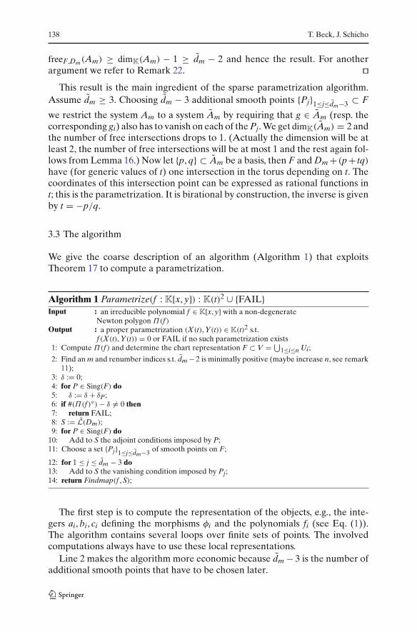
We give the coarse description of an algorithm (Algorithm 1) that exploitsTheorem 17 to compute a parametrization.

Algorithm 1 Parametrize(f : K[x, y]) : K(t)2 ∪ {FAIL}Input : an irreducible polynomial f ∈ K[x, y] with a non-degenerate

Newton polygon Π(f )Output : a proper parametrization (X(t), Y(t)) ∈ K(t)2 s.t.

f (X(t), Y(t)) = 0 or FAIL if no such parametrization exists1: Compute Π(f ) and determine the chart representation F ⊂ V = ⋃

1≤i≤n Ui;

2: Find an m and renumber indices s.t. dm −2 is minimally positive (maybe increase n, see remark11);

3: δ := 0;4: for P ∈ Sing(F) do5: δ := δ + δP;6: if #(Π(f )◦)− δ �= 0 then7: return FAIL;8: S := L(Dm);9: for P ∈ Sing(F) do

10: Add to S the adjoint conditions imposed by P;11: Choose a set {Pj}1≤j≤dm−3 of smooth points on F;

12: for 1 ≤ j ≤ dm − 3 do13: Add to S the vanishing condition imposed by Pj;14: return Findmap(f , S);

The first step is to compute the representation of the objects, e.g., the inte-gers ai, bi, ci defining the morphisms φi and the polynomials fi (see Eq. (1)).The algorithm contains several loops over finite sets of points. The involvedcomputations always have to use these local representations.

Line 2 makes the algorithm more economic because dm − 3 is the number ofadditional smooth points that have to be chosen later.


Then (in lines 3–7) we compute the genus, applying Proposition 9, in order todecide rationality and return FAIL if the curve is not parametrizable. In char-acteristic 0 the values δP can be computed as follows: In [1, Sect. 8.4] it is shownhow to deduce the “system of multiplicity sequences” from the Puiseux expan-sions of a singularity (and the intersection multiplicities of the branches). By [10,Example 3.9.3] this data determines δP. In positive characteristic the necessarydata can be gathered from the Hamburger-Noether expansions (see [2]).

Now we compute the parametrizing linear system (lines 8–13). We startwith L(Dm). In a real implementation this could mean, we make anindetermined Ansatz g = ∑

(r,s) c(r,s)xrys for a polynomial in L(Dm), the sumranging only over a finite number of indices, compare Lemma 13 and Fig. 2.

In order to add to S the adjoint conditions in characteristic 0, one couldcompute the Puiseux expansions of the curve branches at the singular points,substitute those expansions into g (or one of the gi respectively, see Definition15) and extract the linear constraints by enforcing the result to vanish with acertain minimal order. More precisely let (ku, kv) ∈ Ui be a singular point. Setf := fi(ui +ku, vi +kv) and g := gi(ui +ku, vi +kv). Then for each Puiseux seriesσ(ui) ∈ ⋃

d∈NK[[u1/d

i ]] s.t. σ(0) = 0 and f (ui, σ(ui)) = 0 we get adjoint condi-

tions by requiring ordui(g(ui, σ(ui))) > ordui

(∂ f∂vi(ui, σ(ui))

)− 1. Note that the

order function maps to the rationals in this case. In positive characteristic, whenPuiseux expansions are generally not available, the adjoint conditions can bedetermined using Hamburger–Noether expansions (see [2]). Another methodwould be to compute (locally) the conductor ideal (see [11]), reduce g (resp. gi)w.r.t. this ideal and extract the linear constraints by enforcing ideal membership.In order to add to S the vanishing conditions for the smooth points, one simplysubstitutes the coordinates of a Pj into g (resp. gi) and equates to zero. Anothermethod to compute adjoints using resolution of singularities can be found in [9].

In the final step we call a procedure Findmap to actually compute the para-metrizing map. It could for example choose a basis {p, q} ⊂ S and then solvethe zero-dimensional system f = p + tq = 0 in K(t)[x, y] for (x, y) �∈ K

2 (usingGröbner bases or resultants).

Remark 18 As mentioned before it is not strictly necessary to carry out theresolution process of Lemma 2. But if one does, one can compute locally usingbivariate polynomial representations. In this setting some computer algebrasystems (e.g., Singular [8] and Maple) provide functions to compute thedelta invariants, certain series expansions of plane curves, etc. They can be usedto determine the adjoint conditions.

A general remark on complexity: Our algorithm of course requires tocompute the Newton polygon of the defining equation. But this additionalcomplexity should be negligible compared to the rest of the computations. Wewould also like to mention, that in the worst case (namely if the input poly-nomial is dense) our algorithm degenerates more or less to the one given in[12]. In all other cases the singularities of our curve F are tamer than the onesoccuring in that algorithm and our version should therefore perform better.


3.4 An example

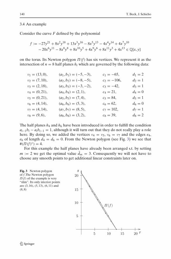
Consider the curve F defined by the polynomial

f := −27y21 + 8x2y18 + 13x3y16 − 8x5y13 − 4x4y14 + 4x7y10

− 20x6y11 − 8x8y8 + 8x10y5 + 4x9y6 + 8x11y3 + 4x13 ∈ Q[x, y]

on the torus. Its Newton polygon Π(f ) has six vertices. We represent it as theintersection of n = 8 half planes hi which are governed by the following data:

v1 = (13, 0), (a1, b1) = (−5, −3), c1 = −65, d1 = 2

v2 = (7, 10), (a2, b2) = (−8, −5), c2 = −106, d2 = 1

v3 = (2, 18), (a3, b3) = (−3, −2), c3 = −42, d3 = 1

v4 = (0, 21), (a4, b4) = (2, 1), c4 = 21, d4 = 0

v5 = (0, 21), (a5, b5) = (7, 4), c5 = 84, d5 = 1

v6 = (4, 14), (a6, b6) = (5, 3), c6 = 62, d6 = 0

v7 = (4, 14), (a7, b7) = (8, 5), c7 = 102, d7 = 1

v8 = (9, 6), (a8, b8) = (3, 2), c8 = 39, d8 = 2

The half planes h4 and h6 have been introduced in order to fulfill the conditionai−1bi − aibi−1 = 1, although it will turn out that they do not really play a rolehere. By doing so, we added the vertices v4 = v5, v6 = v7 and the edges e4,e6 of length d4 = d6 = 0. From the Newton polygon (see Fig. 3) we see that#(Π(f )◦) = 4.

For this example the half planes have already been arranged s.t. by settingm := 2 we get the optimal value dm = 3. Consequently we will not have tochoose any smooth points to get additional linear constraints later on.

Fig. 3 Newton polygonof f .The Newton polygonΠ(f ) of the example is very“slim”. Its only interior pointsare (3, 16), (5, 13), (6, 11) and(8, 8)


The curve F is (by our construction) embedded in a toric surface V =⋃1≤i≤8 Ui. We compute the representation of F in local coordinates using

Eq. (1):

f1 = −27v21u3

1 − 4v31u1 + 13v2

1u21 + 8v1u3

1 − 20v21u1

− 8v1u21 + 4v2

1 − 8v1u1 + 4u21 + 8v1 + 8u1 + 4,

f2 = −4v42u3

2 + 4v42u2

2 − 20v32u2

2 + 8v32u2 + 13v2

2u22

− 8v22u2 − 27v2u2

2 + 4v22 − 8v2u2 + 8v2 + 8u2 + 4,

f3 = 4v33u4

3 + 8v33u3

3 − 4v23u4

3 + 4v33u2

3 − 20v23u3

3

− 8v23u2

3 + 8v23u3 + 13v3u2

3 − 8v3u3 + 4v3 − 27u3 + 8,

f4 = 4v54u3

4 + 8v44u3

4 + 8v44u2

4 + 4v34u3

4 − 8v34u2

4

+ 4v34u4 − 20v2

4u24 − 8v2

4u4 − 4v4u24 + 13v4u4 + 8v4 − 27,

f5 = 4v75u5

5 + 8v65u4

5 + 8v55u4

5 + 4v55u3

5 − 8v45u3

5

+ 4v35u3

5 − 8v35u2

5 − 20v25u2

5 + 8v25u5 + 13v5u5 − 4u5 − 27,

f6 = 4v36u7

6 + 8v36u6

6 + 4v36u5

6 + 8v26u5

6 − 8v26u4

6

− 8v26u3

6 + 8v26u2

6 + 4v6u36 − 20v6u2

6 + 13v6u6 − 27v6 − 4,

f7 = 4v47u3

7 + 8v47u2

7 + 8v37u3

7 − 8v37u2

7 + 4v27u3

7

− 27v37u7 − 8v2

7u27 + 13v2

7u7 + 8v7u2 − 20v7u7 + 4u7 − 4,

f8 = 8v38u4

8 − 27v38u3

8 + 4v28u4

8 − 8v28u3

8 + 13v28u2

8

+ 8v8u38 − 8v8u2

8 − 20v8u8 + 4u28 − 4v8 + 8u8 + 4.

It turns out that F has a singular point P on the toric invariant divisor E1. Itshows up in the open subsets U1 and U2 and has coordinates (u1, v1) = (−1, 0),(u2, v2) = (0, −1) respectively. Another singular point Q ∈ E8 is lying in U1 andU8 with coordinates (u1, v1) = (0, −1) and (u8, v8) = (−1, 0). The curves F ∩ Uifor i ∈ {3, 4, 5, 6, 7} are smooth. Hence all the information on the singularitiescan be gathered in U1. For this purpose we compute the Puiseux expansions atthe points P and Q:

σP(u1 + 1) = −14(u1 + 1)+ α(u1 + 1)2 +

(435608

α − 512432

)

(u1 + 1)3 . . .

σQ(u1) = −1 − 52

u1 + βu21 +

(214β + 195

16

)

u31 . . .


Here α denotes a root of 1024α2 + 516α + 63 and β denotes a root of 16β2 +24β − 45. Taking conjugates into account we have two curve branches througheach of the singular points.

From these expansions one can compute amongst others the delta invariantsδP = δQ = 2. We compute the genus g(F) = #(Π(f )◦)−δP −δQ = 4−2−2 = 0,i.e., the curve F is indeed parametrizable.

Now we make an indetermined Ansatz for a polynomial in L(Dm). The sup-port of such a polynomial has to lie within Π(f ) but not on the edges ei fori ∈ {3, . . . , 8}.

g := c1x3y16 + c2x5y13 + c3x7y10 + c4x6y11 + c5x8y8 + c6x10y5.

For obvious reasons, we only have to compute the local representation in U1(see Definition 15):

g1 = c1v21u1 + c4v

21 + c2v1u1 + c5v1 + c3u1 + c6.

In order to be adjoint g1(σP) has to vanish with order at least 2 aroundu1 = −1 and g1(σQ) has to vanish with order at least 2 around u1 = 0. Exe-cuting the substitutions and equating lowest terms to 0 one gets the linearconstraints 1

4 c2 + c3 − 14 c5 = 0, −c3 − c6 = 0 (from P) and c4 − c5 + c6 = 0,

c1 − c2 + c3 + 5c4 − 52 c5 = 0 (from Q). We solve this system w.r.t. parameters c3,

c4 and substitute the result into g to get a polynomial g ∈ Am (for any concretevalue of c3 and c4).

g =(

−32

x3y16 − 3x5y13 + x7y10 + x8y8 + x10y5)

c3

+(

−32

x3y16 + x5y13 + x6y11 + x8y8)

c4.

As a final step we solve the equations f = 0 and g |c3=1,c4=t= 0 for x and y inQ(t). We find two distinct solutions. One is (x, y) = (0, 0) which corresponds tothe two singular points P and Q, the other one yields the parametrization:

X(t) = −256(2t2 + 4t − 1)3(t + 1)7t8

(−1 + 8t)3(2t2 + 7t − 1)5,

Y(t) = −32t5(2t2 + 4t − 1)2(t + 1)4

(−1 + 8t)2(2t2 + 7t − 1)3.

For illustrative purposes assume we had chosen m := 3 non-optimal (or wewere in a situation where a choice s.t. dm = 3 is not possible). We would get thefollowing indetermined Ansatz for a polynomial in L(Dm):

g := c0x2y18 + c1x3y16 + c2x5y13 + c3x7y10 + c4x6y11 + c5x8y8 + c6x10y5.


We compute the local representations in U1 and U5.

g1 = c1v21u1 + c0v1u2

1 + c4v21 + c2v1u1 + c5v1 + c3u1 + c6,

g5 = c6v55u3

5 + c3v45u2

5 + c5v35u2

5 + c2v25u5 + c4v5u5 + c0v5 + c1.

Proceeding as before, i.e., substituting the Puiseux expansions at the singularpoints P and Q in U1 into g1 we get the linear constraints − 1

4 c0+ 14 c2+c3− 1

4 c5 =0,−c3 + c6 = 0, c4 − c5 + c6 = 0 and c1 − c2 + c3 + 5c4 − 5

2 c5 = 0. Now we have tochoose an additional smooth point on F, e.g., (u5, v5) = (− 27

4 , 0) in U5. Pluggingthese coordinates into g5 and equating the result to zero we get c1 = 0. Weagain solve the system and substitute into g.

g = (−4x5y13 − x6y11 + x7y10 + x10y5)c6

+(

x2y18 + 53

x5y13 + 23

x6y11 + 23

x8y8)

c0

Now in the same way as above we arrive at the following parametrization:

X(t) = (135 − 108t + 20t2)3(14t − 27)7(−3 + 2t)8

429981696(16t2 − 18t − 27)5(t − 2)8t3,

Y(t) = −(135 − 108t + 20t2)2(14t − 27)4(−3 + 2t)5

248832t2(16t2 − 18t − 27)3(t − 2)5

Remark 19 A conventional algorithm based on an embedding of the curve inthe projective plane P

2Q

has to work very hard on that example. The corre-sponding complete curve would have again two singular points, but now thedelta invariants are 119 and 71. These complicated singularities show up onlybecause the structure of the Newton polygon is not taken into account. Pro-ceeding in this setting like we did, the involved linear systems are found assubspaces of a vector space of dimension greater than 200. The excellent Mapleimplementation of a parametrization algorithm produced around 40 DIN A4pages of output due to coefficient explosion. (Of course we admit that thechosen example is especially well-fit for our method.)

4 Another proof of correctness

This section is devoted to another proof of correctness using sheaf theoreticaland cohomological arguments. Also Theorem 17 could be deduced from whatfollows. From now on let F be the normalization of F. We are in the followingsituation

Fπ� F

ι↪→ V

and assume that F is parametrizable, i.e., g(F) = g(F) = 0.


4.1 Some exact sequences

The curve F is a closed subscheme of V. Let I(F) denote its ideal sheaf. Wehave an exact sequence of sheaves on V:

0 → I(F) → OVι#→ ι∗(OF) → 0

Now we define the conductor ideal sheaf on F, F and V. Let CF denote the sheafdefined by U �→ C(OF(U)) (see Definition 14) and CF := π∗(CF). Observe thatπ∗(CF)

∼= CF because the conductor is an ideal sheaf on both F and F. SinceCF is a subsheaf of OF trivially ι∗(CF) is a subsheaf of ι∗(OF). Now we define theconductor sheaf CV on the surface by CV(U) := (ι#)−1(ι∗(CF)(U)) for all openU ⊆ V. Clearly CV is a subsheaf of OV containing ker(ι#) and the restriction ofι# is still surjective. Thus we have an exact sequence

0 → I(F) → CV → ι∗(CF) → 0.

The invertible sheaf L(D) associated to a Weil divisor D on the smoothvariety V is a subsheaf of the sheaf of rational functions KV defined locally by

L(D)(U) = {g ∈ KV(U) | (g)+ D |U≥ 0}

for all open U ⊆ V. This is a sheafified version of the Definition 7. In factL(D) = �(V, L(D)). Tensoring with invertible sheaves is exact so we get theexact sequence

0 → I(F)⊗ L(Dm) → CV ⊗ L(Dm) → ι∗(CF)⊗ L(Dm) → 0.

Now we define the following sheaf on F:

J := CF ⊗ (ι ◦ π)∗(L(Dm))

Applying the projection formula (cf. [10, Exercise II.5.1]) we see that

(ι ◦ π)∗(J ) = (ι ◦ π)∗(CF ⊗ (ι ◦ π)∗(L(Dm)))

∼= (ι ◦ π)∗(CF)⊗ L(Dm)

∼= ι∗(CF)⊗ L(Dm).

Since I(F) = L(−F) ∼= L(−F0) we have I(F) ⊗ L(Dm) ∼= L(Dm) with Dm :=Dm − F0 = −∑

m+1≤j≤n Ej. Putting things together, we get

0 → L(Dm) → CV ⊗ L(Dm) → (ι ◦ π)∗(J ) → 0. (2)


Finally, the global sections functor is left-exact which yields

0 → �(V, L(Dm)) → �(V, CV ⊗ L(Dm)) → �(V, (ι ◦ π)∗(J )) = �(F, J ).(3)

But Dm is the inverse of an effective divisor and consequently has no globalsections, i.e., �(V, L(Dm)) = 0. In other words:

�(V, CV ⊗ L(Dm)) ↪→ �(F, J ) (4)

The global sections�(V, CV ⊗L(Dm)) are very suitable for computation. Indeedif we write CV ⊗ L(Dm) as a sheaf of rational functions, we see that its globalsections correspond exactly to the system Am of Definition 15. In fact the lastmap of sequence (3) is also surjective and thus (4) is an isomorphism. We post-pone the cohomological proof of this statement to the last section. Instead weproceed now with a brief study of the sheaf J and interpret the isomorphismin the context of the parametrization problem.

4.2 The sheaf on the normalized curve

First we reinterpret Lemma 12 in the context of sheaves. In general for any divi-sor D ∈ Div(V) it is true that deg((ι◦π)∗(L(D))) = F ·D. Then F ·Dm = F0 ·Dmimplies the following corollary.

Corollary 20 deg((ι ◦ π)∗(L(Dm))) = 2#(Π(f )◦)+ dm − 2.

Proposition 21 If∑

1≤j≤m dj ≥ 2 then deg(J ) = dm − 2.

Proof We compute the degree of J using deg(CF) = −2∑

P∈F δP (cf. [7]),corollary 20 and applying the genus formula of proposition 9:

deg(J ) = deg(CF ⊗ (ι ◦ π)∗(L(Dm)))

= deg(CF)+ deg((ι ◦ π)∗(L(Dm)))

= −2∑

P∈F

δP + 2#(�(f )◦)+ dm − 2

= 2

(

#(�(f )◦)−∑

P∈F

δP

)

+ dm − 2

= dm − 2.

Assume dm ≥ 3 and let d := dm − 2. Since F is assumed parametrizable, its

normalization F is isomorphic to P1K

. Assume we have homogeneous coordi-nates u, v on P

1K

. Let P ∈ Div(P1K) be the prime divisor corresponding to u = 0.


Any invertible sheaf of degree d on P1K

is isomorphic to L(dP). This sheaf is gen-erated by its global sections�(P1

K, L(dP)) = 〈vd/ud, vd−1u/ud, . . . , ud/ud〉. They

constitute a closed immersionψ : P1K

→ PdK

: [u : v] �→ [vd : vd−1u : · · · : ud]. Inother words, a basis of the global section space �(F, J ) defines an isomorphismbetween F and the rational normal curve in P

dK

.

Remark 22 From this one could also get a slightly different proof of Theorem 17because deg(J ) corresponds to the number of free intersections. The resulton the dimension follows from the above arguments because dimK(Am) =dimK(�(V, CV ⊗ L(Dm))) = dimK(�(F, J )) = deg(J )+ 1.

4.3 Reduction of the parametrization problem to rational normal curves

Write CV ⊗ L(Dm) as a sheaf of rational functions and identify J with L(dP)on P

1K

as above. The functions in �(V, CV ⊗ L(Dm)) do not have a pole alongF. The reader may check that isomorphism (4) is in fact given by the pullback(ι ◦ π)∗ of rational functions.

Now let {s0, . . . , sd} ⊂ �(V, CV ⊗L(Dm))) be a basis s.t. (ι◦π)∗(si) = vd−iui/ud

and define a rational map by

φ : T → PdK

: (x, y) �→ [s0 : s1 : · · · : sd]

on the torus. We find that it maps F (and hence also F) birationally to therational normal curve in P

dK

:

F ∼= P1K

ι◦π

ψ

V

φ

PdK

In the algorithm we finally choose a set of dm − 3 = d − 1 smooth points andrestrict the linear system using vanishing conditions imposed by these points. Inour current setting this corresponds to choosing points on the rational normalcurve and projecting until we reach the projective line P

1K

; the natural way toparametrize a rational normal curve.

4.4 Vanishing of the first cohomology

It remains to show that the last map of sequence (3) is surjective. We will useCech cohomology w.r.t. the natural affine cover U := {Ui}1≤i≤n to derive thedesired result. From the short exact sequence (2) we get a long exact sequence

0 → �(V, L(Dm)) → �(V, CV ⊗ L(Dm)) → �(V, (ι ◦ π)∗(J ))→ H

1(U, L(Dm)) → . . .

So we have to show that H1(U, L(Dm)) = 0.


To define Cech cohomology we use the following set of half planes:

hi := {(r, s) ∈ R2 | air + bis ≥ �i} where �i =

{0 for 1 ≤ i ≤ m and1 else

Using the coordinate transformations of Sect. 2 and these half planes onedescribes the needed sections of L(Dm) as K-vector spaces:

�(Ui, L(Dm)) = 〈xrys〉(r,s)∈hi−1∩hifor 1 ≤ i ≤ n,

�(Ui−1 ∩ Ui, L(Dm)) = 〈xrys〉(r,s)∈hi−1for 2 ≤ i ≤ n,

�(Ui ∩ Uj, L(Dm)) = 〈xrys〉(r,s)∈Z2 for 1 ≤ i < j ≤ n and j − i ≥ 2,

�(Ui ∩ Uj ∩ Uk, L(Dm)) = 〈xrys〉(r,s)∈Z2 for 1 ≤ i < j < k ≤ n

The first objects in the Cech complex are given by

C0(U, L(Dm)) =∏

1≤i≤n

�(Ui, L(Dm)),

C1(U, L(Dm)) =∏

1≤i<j≤n

�(Ui ∩ Uj, L(Dm)),

C2(U, L(Dm)) =∏

1≤i<j<k≤n

�(Ui ∩ Uj ∩ Uk, L(Dm))

and the first maps by

d0 : (gi)i �→ (gj − gi)i<j,

d1 : (gi,j)i<j �→ (gj,k − gi,k + gi,j)i<j<k.

Since Π(f ) is a non-degenerate polygon the cone spanned by the set of nor-mal vectors (ai, bi)must be the whole of R

2. It can be shown that for each latticepoint (r, s) ∈ Z

2 there is at least one i s.t. (r, s) ∈ hi and there is at least one i s.t.(r, s) �∈ hi. Moreover each (r, s) separates the half planes into those containingthe point and those not containing the point. It turns out that the half planescontaining (r, s) have cyclically consecutive indices. This is equivalent to thefollowing lemma.

Lemma 23 Let J = {l, . . . , j0, . . . , k} ⊆ {1, . . . , n} (with l, j0, k pairwise distinct) bea set of cyclically consecutive indices and (r, s) ∈ Z

2 a lattice point. If (r, s) �∈ hl∪hkand (r, s) ∈ hj0 then (r, s) �∈ hi for all i ∈ {1, . . . , n} \ J.

Proof If J = {1, . . . , n} there is nothing to show. So let J �= {1, . . . , n}, choosei0 ∈ {1, . . . , n} \ J and assume indirectly (r, s) ∈ hi0 . We distinguish two cases:


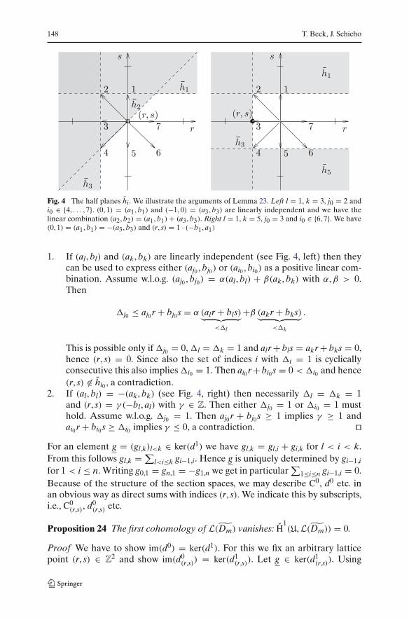
Fig. 4 The half planes hi. We illustrate the arguments of Lemma 23. Left l = 1, k = 3, j0 = 2 andi0 ∈ {4, . . . , 7}. (0, 1) = (a1, b1) and (−1, 0) = (a3, b3) are linearly independent and we have thelinear combination (a2, b2) = (a1, b1)+ (a3, b3). Right l = 1, k = 5, j0 = 3 and i0 ∈ {6, 7}. We have(0, 1) = (a1, b1) = −(a3, b3) and (r, s) = 1 · (−b1, a1)

1. If (al, bl) and (ak, bk) are linearly independent (see Fig. 4, left) then theycan be used to express either (aj0 , bj0) or (ai0 , bi0) as a positive linear com-bination. Assume w.l.o.g. (aj0 , bj0) = α(al, bl) + β(ak, bk) with α,β > 0.Then

�j0 ≤ aj0 r + bj0 s = α (alr + bls)︸︷︷︸<�l

+β (akr + bks)︸︷︷︸

<�k

.

This is possible only if�j0 = 0,�l = �k = 1 and alr + bls = akr + bks = 0,hence (r, s) = 0. Since also the set of indices i with �i = 1 is cyclicallyconsecutive this also implies�i0 = 1. Then ai0 r + bi0 s = 0 < �i0 and hence(r, s) �∈ hi0 , a contradiction.

2. If (al, bl) = −(ak, bk) (see Fig. 4, right) then necessarily �l = �k = 1and (r, s) = γ (−bl, al) with γ ∈ Z. Then either �j0 = 1 or �i0 = 1 musthold. Assume w.l.o.g. �j0 = 1. Then aj0 r + bj0 s ≥ 1 implies γ ≥ 1 andai0 r + bi0 s ≥ �i0 implies γ ≤ 0, a contradiction.

For an element g = (gl,k)l<k ∈ ker(d1) we have gl,k = gl,i + gi,k for l < i < k.From this follows gl,k = ∑

l<i≤k gi−1,i. Hence g is uniquely determined by gi−1,i

for 1 < i ≤ n. Writing g0,1 = gn,1 = −g1,n we get in particular∑

1≤i≤n gi−1,i = 0.Because of the structure of the section spaces, we may describe C0, d0 etc. inan obvious way as direct sums with indices (r, s). We indicate this by subscripts,i.e., C0

(r,s), d0(r,s) etc.

Proposition 24 The first cohomology of L(Dm) vanishes: H1(U, L(Dm)) = 0.

Proof We have to show im(d0) = ker(d1). For this we fix an arbitrary latticepoint (r, s) ∈ Z

2 and show im(d0(r,s)) = ker(d1

(r,s)). Let g ∈ ker(d1(r,s)). Using


lemma 23 we may assume w.l.o.g. that there is an l < n s.t. (r, s) ∈ hi for1 ≤ i ≤ l but (r, s) �∈ hi for l < i ≤ n.

We can find a d0(r,s)-preimage of g by setting g1 := 0, gi := gi−1 + gi−1,i for

1 < i ≤ l and gi := 0 for l < i ≤ n. First observe that with this definition wereally have (gi)i ∈ C0

(r,s)(U, L(Dm)) because gi �= 0 implies (r, s) ∈ hi−1 ∩ hi.Now we check that g = d0

(r,s)((gi)i): For 1 < i ≤ l we get gi−1,i = gi − gi−1

by definition. For l + 1 < i ≤ n we know that (r, s) �∈ hi−1 and (r, s) �∈ hi, i.e.,gi−1,i = gi = gi−1 = 0, hence again gi−1,i = gi − gi−1. This also implies

0 =∑

1≤i≤n

gi−1,i =∑

1<i≤l+1

gi−1,i

=⎛

⎝∑

1<i≤l

gi − gi−1

⎞

⎠ + gl,l+1 = gl + gl,l+1

or equivalently gl,l+1 = 0 − gl = gl+1 − gl.

5 Conclusion

We presented a method for the rational parametrization of plane algebraiccurves (on the torus). The main idea was to embed the curve in a toric surfacethat is adapted to the shape of the Newton polygon. We showed one possiblemethod to parametrize in this setting. But also other algorithms like [15] couldpossibly benefit from this approach.

Up to now sparsity of the defining equation is used as far as the Newtonpolygon is considerably smaller than a full triangle. Another sort of sparsitywould be when the lattice spanned by the support of the equation is not thewhole of Z

2 but only a sublattice. We also think about studying that case.In this article we have assumed an algebraically closed coefficient field. We

have not taken into account the degree of the field extension needed to repre-sent the parametrization when starting from a non-closed field. This has beenaddressed for example in [13]. The ideas should carry over to our situation.Parametrization of rational normal curves using a field extension of least pos-sible degree can also be achieved using the Lie algebra method in [5].

References

1. Brieskorn, E., Knörrer, H.: Ebene algebraische Kurven. Birkhäuser Verlag, Basel (1981)2. Campillo, A., Farrán, J.I.: Symbolic Hamburger–Noether expressions of plane curves and

applications to AG codes. Math. Comp. 71(240), 1759–1780 (electronic) (2002)3. Cox, D.: What is a toric variety? In: Topics in Algebraic Geometry and Geometric Model-

ing, vol. 334 of Contemporary Mathematics, pp. 203–223. American Mathematical Society,Providence, Rhode Island, 2003. Workshop on Algebraic Geometry and Geometric Modeling(Vilnius, 2002)

4. Cox, D.A.: Toric varieties and toric resolutions. In: Resolution of singularities (Obergurgl,1997), vol. 181 of Progr. Math., pp. 259–284. Birkhäuser, Basel (2000)


5. de Graaf, W.A., Harrison, M., Pilnikova, J., Schicho, J.: A Lie Algebra Method for RationalParametrization of Severi–Brauer Surfaces. 2005. submitted for publication and electronicallyavailable at http://www:arxiv.org/abs/math.AG/0501157

6. Fulton, W.: Introduction to toric varieties, vol 131 of Annals of Mathematics Studies. PrincetonUniversity Press, Princeton, 1993. The William H. Roever Lectures in Geometry

7. Gorenstein, D.: An arithmetic theory of adjoint plane curves. Trans. Am. Math. Soc. 72, 414–436 (1952)

8. Greuel, G.-M., Pfister, G., Schönemann, H.: Singular 2.0. A Computer Algebra System forPolynomial Computations, Centre for Computer Algebra, University of Kaiserslautern, 2001.http://www.singular.uni-kl.de

9. Haché, G., Le Brigand, D.: Effective construction of algebraic geometry codes. IEEE Trans.Inform. Theory. 41(6, part 1):1615–1628, 1995. Special issue on algebraic geometry codes

10. Hartshorne, R.: Algebraic geometry. Springer, New York (1977) Graduate Texts in Mathe-matics, No. 52

11. Mnuk, M.: An algebraic approach to computing adjoint curves. J. Symbol. Comput. 23(2–3),229–240, (1997) Parametric algebraic curves and applications (Albuquerque, NM, 1995)

12. Sendra, J.R., Winkler, F.: Symbolic parametrization of curves. J. Symbol. Comput. 12(6), 607–631 (1991)

13. Sendra, J.R., Winkler, F.: Parametrization of algebraic curves over optimal field extensions.J. Symbol. Comput. 23(2–3), 191–207 (1997) Parametric algebraic curves and applications(Albuquerque, NM, 1995)

14. Shafarevich I.R.: Basic algebraic geometry, second edition, vol. 1. Springer Berlin, HeidelebergNewyork. 1994. Varieties in projective space, Translated from the 1988 Russian edition andwith notes by Miles Reid

15. van Hoeij, M.: Rational parametrizations of algebraic curves using a canonical divisor.J. Symbol. Comput. 23(2–3), 209–227 (1997) Parametric algebraic curves and applications(Albuquerque, NM, 1995)

16. Zariski, O., Samuel, P.: Commutative algebra. Vol. I. Springer Berlin Heidelberg New York,1975. With the cooperation of I. S. Cohen, Corrected reprinting of the 1958 edition, GraduateTexts in Mathematics, No. 28

Parametrization of algebraic curves defined by sparse equations

Documents

Transcript of Parametrization of algebraic curves defined by sparse equations