Otoacoustic emissions in time-domain solutions of nonlinear non-local cochlear models

Otoacoustic emissions in time-domain solutions of nonlinearnon-local cochlear models

Arturo Moleti and Nicolò PaternosterDipartimento di Fisica, Università di Roma Tor Vergata, 00133, Rome, Italy

Daniele BertacciniDipartimento di Matematica, Università di Roma Tor Vergata, 00133, Rome, Italy

Renata Sisto and Filippo SanjustDipartimento Igiene del Lavoro, ISPESL, 00040, Monte Porzio Catone, Rome, Italy

�Received 10 June 2009; revised 17 August 2009; accepted 17 August 2009�

A nonlinear and non-local cochlear model has been efficiently solved in the time domainnumerically, obtaining the evolution of the transverse displacement of the basilar membrane at eachcochlear place. This information allows one to follow the forward and backward propagation of thetraveling wave along the basilar membrane, and to evaluate the otoacoustic response from the timeevolution of the stapes displacement. The phase/frequency relation of the response can be predicted,as well as the physical delay associated with the response onset time, to evaluate the relationbetween different cochlear characteristic times as a function of the stimulus level and of the physicalparameters of the model. For a nonlinear cochlea, simplistic frequency-domain interpretations of theotoacoustic response phase behavior may give inconsistent results. Time-domain numericalsolutions of the underlying nonlinear and non-local full cochlear model using a large number�thousands� of partitions in space and an adaptive mesh in time are rather time and memoryconsuming. Therefore, in order to be able to use standard personal computers for simulationsreliably, the discretized model has been carefully designed to enforce sparsity of the matrices usinga multi-iterative approach. Preliminary results concerning the cochlear characteristic delays are alsopresented. © 2009 Acoustical Society of America. �DOI: 10.1121/1.3224762�

PACS number�s�: 43.64.Jb, 43.64.Kc �BLM� Pages: 2425–2436

I. INTRODUCTION

Otoacoustic emissions �OAEs� are a physiological by-product of the activity of the mammalian cochlea �Probstet al., 1991�. The OAE generation and backward transmis-sion is effectively described by transmission line cochlearmodels, including tonotopically resonant transverse imped-ance terms �e.g., Talmadge et al., 1998�. These terms mustalso model the active feedback mechanism mediated by theouter hair cells �OHCs�, which is responsible for the excel-lent threshold sensitivity and frequency resolution of themammalian hearing system. A comprehensive cochlearmodel must be, to some extent, both nonlinear and non-local,and based on the knowledge of the OHC mechanoelectricbehavior. Several models of the OHC feedback mechanismhave been developed �e.g., Nobili and Mammano, 1996; deBoer and Nuttall, 2003� including detailed analyses of theOHC coupling to the basilar membrane �BM� and to thetectorial membrane, and they have been tested and refined inthe past decades through comparison with experimental data,reaching a fairly high degree of complexity, and a corre-spondingly high number of free parameters. Most modelsused to predict the OAE generation adopt a simplified viewof the OHC active mechanism. This attitude is partly justifiedby the fact that OAE generation is only a by-product of thecochlear amplifier activity, and the OAE measurable param-eters may be critically dependent on cochlear transmission
properties other than the details of the local cochlear ampli-
J. Acoust. Soc. Am. 126 �5�, November 2009 0001-4966/2009/126�5

fier at the generation place�s�. Nevertheless, some key prop-erties of the OHC physiology must be retained in a full co-chlear model, even if one’s main purpose is getting correctpredictions of the OAE phenomenology.

Nonlinearity is an intrinsic feature of the cochlear physi-ology, so the frequency-domain solutions of the linearizedproblem can only approximately predict the behavior of thesystem, and only in a perturbative regime. Much care musttherefore be used when applying to such a system conceptsthat are fully meaningful for linear systems only, such as thecomplex frequency response, defined as the Fourier trans-form �FT� of the impulsive response, or the group delay,defined as the negative slope of the phase/frequency relation.The intrinsically nonlinear equations describing the cochlearmicromechanics require, in a nonperturbative regime, a so-lution in the time domain. On the other hand, the time-domain numerical solutions may become expensive in termsof computational time and memory demanding, if sufficientspatial and time resolutions have to be achieved. High spatialresolution is necessary because the discontinuous variation inthe transverse impedance parameters caused by discretizationitself must not cause significant spurious reflection of theforward traveling wave �TW�. High time resolution is auto-matically provided by the adaptive integration time step setby the routines used to solve the differential equations, and
the related computational cost depends strongly not only on
© 2009 Acoustical Society of America 2425�/2425/12/$25.00

the number of elements of the discretized cochlea but also onthe frequency content of the stimulus and on the character-istic frequencies of the system.

Elliott et al. �2007� proposed a matrix formalism, ap-plied to a finite-difference solution method of cochlear mod-els, which is used in this study to model the propagation ofthe TW and the generation and backward propagation ofOAEs. Elliott et al. �2007� originally applied this solutionscheme to an active linear and local model developed byNeely and Kim �1986�. In the Neely and Kim �1986� model,each micromechanical element is a two degree of freedomsystem of coupled oscillators, simulating some the active co-chlear amplifier properties �negative resistance, or anti-damping, in a limited region close to the resonant place�. Thesame scheme can be modified to represent several differentcochlear models. In the model by Kim and Xin �2005��adapted from Lim and Steele, 2002 and generalized tomodel cochlear impairment in Bertaccini and Fanelli, 2009�,the forces applied by the OHCs on the BM are schematizedby a nonlinear non-local feed-forward term.

In this work, a feed-forward nonlinear non-local modelsimilar to that proposed by Kim and Xin �2005�, in which theOHC additional pressure is assumed proportional to the totalpressure on the BM within a slightly more basal region, isimplemented in the Elliott et al. �2007� semidiscrete scheme,including as well random spatial variations in the impedanceparameters �cochlear roughness�, which are needed to getappreciable OAE response through coherent reflection �Tal-madge et al., 1998�, acting as backscattering centers for theforward TW. The semidiscrete model is then fully dis-cretized, and the resulting discrete model is solved effi-ciently. A nontrivial mass matrix and stiffness of the BMmicromechanics �in the numerical analysis sense, i.e., thepresence of high Lipschitz constants in the nonlinear model�are suggested using an implicit time-step integrator. There-fore, at each time step, a large system of fully couplednonlinear algebraic equations should be solved in order togenerate the numerical approximations, and this is computa-tionally expensive. In this work, an efficient and reliable nu-merical simulation is enforced by decoupling the differentialpart of the discretization of the integrodifferential model bysolving sparse linear systems using multi-iterative projectionalgorithms instead of inverting matrices. A graphical userinterface has been added to facilitate the parameters inputtedand the analysis of the results. The backward TW associatedwith OAEs is observed as a displacement wave at the stapes,and some properties of the otoacoustic delays are analyzed.

A variation in the above model was also considered, inwhich the feed-forward coupling is obtained assuming thatthe OHC additional pressure is directly proportional to theBM velocity. In this model, this additional force explicitlybehaves as a simple anti-damping term.

This discrete model, implemented in our package, afterits necessary optimization through comparison with theavailable data, could be a useful tool to design future OAEexperiments, predicting the OAE response at different stimu-
lus levels, and, in particular, to study in more detail the gen-
2426 J. Acoust. Soc. Am., Vol. 126, No. 5, November 2009

eration place and time of the different components of theOAE response, as well as their direction of propagationalong the BM.

In Sec. II, we recall the physical meaning of the cochlearcharacteristic times that are estimated with different experi-mental techniques. In Sec. III A we briefly describe the ap-plication of Elliott’s solution scheme to a very simple one-dimensional �1D� linear, passive, and local cochlear model,to help the reader through Sec. III B, where we discuss itsgeneralization to more realistic, still semidiscrete models, in-cluding feed-forward nonlinear and non-local terms. In Sec.III C, we propose a fully discrete feed-forward analog of theunderlying model and notes concerning its implementation inthe MATLAB environment. In Sec. IV, we discuss our prelimi-nary results, focusing on the relation between different char-acteristic times in a nonlinear cochlea.

II. BACKGROUND ON COCHLEAR DELAYS INMODEL AND EXPERIMENT

The study of the characteristic times of the OAE re-sponse may provide important information about the co-chlear mechanics and the otoacoustic generation mecha-nisms, complementing other measures coming, e.g., fromdirect observations of the BM vibration �Ren, 2004; Heet al., 2007� and from the analysis of the auditory brainstemresponse �ABR� �e.g., Neely et al., 1988; Donaldson andRuth, 1993�.

A. TEOAE latency from time-frequency analysis andcochlear transmission delay

In the case of transient evoked OAEs �TEOAEs� and,particularly for click-evoked OAEs �CEOAEs�, the latencymay be defined in the time domain as the interval betweenthe impulsive stimulus and the onset of the otoacoustic re-sponse at a given frequency, which can be measured usingtime-frequency analysis techniques, based on the wavelettransform or on the MATCHING PURSUIT algorithm �Tognolaet al., 1997; Sisto and Moleti, 2002; Jedrzejczak et al.,2004�. As the middle ear roundtrip transmission introducesonly a very short time delay, of order 0.1–0.2 ms �Puria,2003; Voss and Shera, 2004�, the OAE latency is almostentirely of cochlear origin, being associated for each fre-quency with the time needed to transmit forward the stimulusfrom the cochlear base to each tonotopic place as a TW, andbackward to the base. This delay is a function of the geo-metrical and mechanical characteristics of the BM, includingthose of active filter associated with the feedback mechanismthat is mediated by the OHCs. The tonotopic structure of theBM causes the overall decrease in latency with increasingfrequency, simply because the cochlear round trip path islonger for lower frequencies. The frequency selectivity of theactive cochlear filter is also related to the OAE delay, whichincreases by increasing the tuning factor Q of the resonance.As a consequence, the OAE latency is a decreasing functionof both frequency and stimulus level �Sisto and Moleti,2007�. This property has also been found in the wave-V ABRdelay, which is made up �Eggermont and Don, 1980; Neely
et al., 1988; Don et al., 1993; Donaldson and Ruth, 1993;
Moleti et al.: Otoacoustic emissions in nonlinear cochlear models

Abdala and Folsom, 1995� of a constant term of neural origin�this is surely true for its main contribution, the delay be-tween wave-I and wave-V�, independent of frequency andstimulus level, and of a cochlear term, decreasing with in-creasing frequency and stimulus level, which is evidentlyassociated with the forward cochlear transmission delay.

Transmission line cochlear models �Furst and Lapid,1988; Talmadge et al., 1998; Shera et al., 2005� are usuallyin agreement in representing the acoustic signal propagationalong the BM as a TW. Due to the tonotopicity of the BM,each Fourier component of the stimulus propagates up to itsresonant place, where it produces the maximum transversaldisplacement of the BM, associated with that tone percep-tion, and then it is locally absorbed.

B. OAE generation mechanisms

It is generally accepted that OAEs are produced by twodifferent mechanisms: nonlinear distortion and linear reflec-tion �Shera and Guinan, 1999�.

The cochlear response nonlinearity generates distortionat moderate and high BM excitation levels. A threshold forthe onset of nonlinearity can be fixed at some transversedisplacement amplitude of order 10 nm. At these stimuluslevels, significant OAE generation is expected from the non-linear generation mechanism. If a given cochlear region issimultaneously excited by two tones of different frequencies,the system nonlinearity also produces tones at frequenciesthat are linear combinations of those of the stimulus, as inthe case of the distortion product OAEs �DPOAEs�. The non-linear distortion generation always occurs at the tonotopiccochlear place of the stimulus frequency, or, as in theDPOAE case, in a place that is a well-defined function of thefrequencies of the stimulus �primary tones�; this generationmechanism is therefore called “wave-fixed” �Shera andGuinan, 1999�. Linearized transmission line cochlear models�Talmadge et al., 1998, 2000; Shera et al., 2005�, solved inthe frequency domain, predict for OAEs generated by wave-fixed mechanisms a flat phase spectrum �at least, in the scale-invariant limit�. If the resulting null “group delay” were sim-plistically interpreted as instantaneous cochlear response,there would be obvious contradiction with the hypothesisthat the otoacoustic response is generated at �or near� thetonotopic place, for each frequency, because at least the for-ward propagation of the stimulus �one could argue that thebackward OAE propagation could be much faster� wouldneed a significant and well-measurable transmission time,from a few to several milliseconds, dependent on frequency.

OAE generation is also expected to be associated withthe reflection of a significant fraction of the forward TW. It isnecessary to postulate the presence of randomly distributedmicroirregularities of the cochlear mechanical structure,which act as backscattering centers for the forward TW�Zweig and Shera, 1995�. Perturbative estimates of the co-chlear reflectivity, based on the osculating parameters tech-nique �Shera and Zweig, 1991; Talmadge et al., 2000�, sug-gest that most of the linearly reflected wave should comefrom a region close to the resonant place. Recent estimates
based on a linear model by Choi et al. �2008� suggest instead
J. Acoust. Soc. Am., Vol. 126, No. 5, November 2009 Mole

that a significant contribution to the overall SFOAE responsemay come from cochlear regions remote from the resonantplace. Coherent reflection from a rather broad cochlear re-gion slightly basal to the resonant place is predicted by thecoherent reflection filtering �CRF� theory, which also intro-duces time-delayed stiffness terms in the BM micromechan-ics to get the necessary tall and broad activity pattern. These“Zweig” terms, due to their rather fine-tuned delays, act aseffective damping and anti-damping terms in that cochlearregion, providing the negative resistance region required bythe solution of the inverse cochlear problem applied to ex-perimental BM transfer function data. As already remarked,similar results could be obtained with different mathematicalapproaches, e.g. modeling each cochlear partition as a twodegree of freedom system of linear actively coupled oscilla-tors �Neely and Kim, 1986�, or by introducing active non-local terms. In the CRF theory, the OAE generation mecha-nism is considered “place-fixed” because the backscatteringcenters are localized at fixed positions. The CRF theory pre-dicts, for such a place-fixed mechanism, a rapidly rotatingphase spectrum �Talmadge et al., 1998; Shera et al., 2005�.The additional reflection from more basal cochlear regionssuggested by Choi et al. �2008� would imply a flatter phase-frequency relation, and the vector superposition of the twosources would explain the observed stimulus-frequency OAE�SFOAE� spectral fine structure, without having to assumecontributions from nonlinear distortion.

C. Relation among different cochlear characteristictimes

Much experimental evidence has been gathered aboutthe relation among different cochlear characteristic times. Ageneral warning applies to such comparisons. In classicalBM transfer function measurements �e.g., Rhode, 1971�, theplace of measurement is fixed as the frequency changes. Thephase slope represents a partial derivative. In OAE experi-ments, this is not generally the case. The relation betweenOAE phase-gradient delays and the actual time delay of eachfrequency component of the OAE response is not straightfor-ward, and depends on the wave-fixed or place-fixed nature ofthe OAE generator. OAE phase-gradient delays are actuallymeasured by computing the slope of the phase-frequencyrelation, but the phase is a function of both the frequency ofthe OAE and the position of the source. The experimentallymeasured slope is therefore a total derivative, which includesan additional term for wave-fixed generation, which almosttotally cancels, in the WKB approximation �Sisto et al.,2007�, the one associated with the roundtrip transmissiondelay. For place-fixed generation, instead, the phase is afunction of frequency only, and the phase-gradient delay istherefore expected to approximately coincide with the physi-cal transmission delay.

At low stimulus levels, the OAE response should bedominated by linear place-fixed mechanisms, the SFOAEphase-gradient delay is therefore expected to be closely re-lated to the physical delay associated with the forward andbackward transmissions along the BM. Early applications ofthe CRF theory predicted indeed that the SFOAE phase-
gradient delay is twice the BM group delay �Shera and
ti et al.: Otoacoustic emissions in nonlinear cochlear models 2427

Guinan, 2003�, while refined calculations �Shera et al., 2005�concluded that the phase-gradient delay should be slightlyless than twice the BM group delay.

Accurate studies on chinchillas �Siegel et al., 2005�demonstrated that the SFOAE phase-gradient delay is sig-nificantly less than twice the BM group delay, particularly atlow-frequency. This result has been considered in agreementwith the CRF theory assuming that some contribution fromnonlinear distortion is also present in the SFOAE response�Shera et al., 2006�. Another explanation of these discrepan-cies could be provided by the linear reflection sources remotefrom the resonance place proposed by Choi et al. �2008�. Ithas also been shown �Sisto et al., 2007� that the roundtripcochlear delay measured by time-frequency analysis ofCEOAE waveforms closely matches the phase-gradient de-lay of the same OAE spectra, at click stimulus levels from 60to 90 dB peak SPL �pSPL�, concluding that linear reflectionfrom roughness is the main source of TEOAEs in this stimu-lus level range. We recall that the pSPL level of a click isgiven by the ratio between its peak amplitude and the stan-dard reference pressure level �20 �Pa�, expressed in deci-bels. The associated spectral density is a function of the clickduration.

For DPOAEs, the relation between latency, phase-gradient delay, BM group delay and frequency is even lessstraightforward, and depends on the experimental sweepingparadigm �Prijs et al., 2000; Schoonhoven et al., 2001�. Ifthe ratio f2 / f1 is kept constant, from the solution of the lin-earized cochlear equations �Talmadge et al., 2000�, it followsthat the nonlinear distortion component, originated in x�f2�,should have flat phase spectrum, while the linear reflectionsource coming from x�fDP� should give a contribution withrapidly rotating phase. In the time domain, it is clear that thenonlinear generation may start only after the transmissiontime needed for the f1 and f2 tones to reach the nonlineargeneration place x�f2�. After that, an additional �shorter� timeis necessary for the backward TW at frequency fDP to reachthe base. The backward delay is shorter because the wavepacket of frequency fDP moves away from a region that isalready more basal than its tonotopic region, where its groupvelocity would be considerably lower �Moleti and Sisto,2003� �this slowing-down effect near the resonant place issometimes called “filter build-up time,” it may be seen as asignificant contribution to the path integral of the inversevelocity coming from a rather short part of the path�. Thesecond DPOAE source �from linear reflection at x�fDP�� issignificantly more delayed because the distortion tone gener-ated in x�f2� must reach its own tonotopic place x�fDP� to beamplified and reflected back by roughness. Therefore, itsoverall onset delay in the time domain is expected to be closeto the latency of the component of frequency fDP of a corre-spondently high TEOAE response �neglecting the depen-dence on the stimulus level, which makes a little shorter theforward transmission delay to x�f2� of the primary tones f1

and f2, due to their higher level�. Summarizing, observingthe phase of the two DPOAE components in the frequencydomain, one should see a flat phase component and a rotatingphase component �which can be separated using time-
domain filtering�, whereas observing the onset of the re-

sponse in the time domain, one should observe an early �butnot instantaneous� response from the first source and a moredelayed onset of the linear reflection contribution. Long et al.�2008� recently exploited the different phase behaviors of thetwo DPOAE components to separate them by using suffi-ciently fast-sweeping primary tones. Whitehead et al. �1996�were able to measure �in humans and rabbits� the onset timeof DPOAEs elicited by high-level primaries �75 dB soundpressure level �SPL�� using a clever differential acquisitiontechnique based on phase rotation of the primary tones. Theymeasured delays from 2 to 5–10 ms �depending also on thedata analysis algorithm� in the 1–8 kHz range, with the ex-pected frequency dependence. These delays are compatiblewith those expected from the nonlinear distortion source,which should be dominant at high stimulus levels.

D. OAE backward propagation

By comparing the OAE latency to the ABR wave-V la-tency in the same stimulus level range, it has been shownthat the part of the ABR latency that is independent of fre-quency and stimulus level �associated with the forward co-chlear path of the stimulus� is approximately equal to halfthe OAE latency �Moleti and Sisto, 2008�, supporting thehypothesis that the backward propagation of OAEs is due toa slow transverse TW on the BM. This conclusion is inagreement with analyses of the data from Allen–Fahey ex-periments �Shera et al., 2007�, and with direct measurementsby Dong and Olson �2008�, but it is contradicted by the slopeof the DP phase at different cochlear places measured byaccurate observations of the BM vibration either by movingthe observation place �He et al., 2007� or by moving theprimary frequencies �de Boer et al., 2008�. These contradic-tory observations could be attributed to a dominant forwardtraveling DP within the cochlea, which would obscure theobservation of reverse waves.

The above list of interesting issues, which can only beapproximately evaluated with frequency-domain solutions,due to the intrinsic nonlinearity of the problem, was meant todemonstrate the strong need for time-domain solutions of thefull cochlear problem. In the following, we will discuss somepreliminary results from the time-domain solution of a non-linear non-local active cochlear model, focusing on possibleapplications to the study of the OAE delays.

III. COCHLEAR MODELS

A. Linear 1D box model

In this subsection, we apply the scheme of Elliott et al.�2007� to a very simple linear passive model, to help thereader getting through the formalism before going to Sec.III B, where the feed-forward model is described. A list ofthe parameter values used in the model is reported in Table I.

For an incompressible fluid, in a cochlear duct of rect-angular constant cross section of constant half-height H andlength L, divided by a tonotopically resonant elastic BM, thewave propagation along the cochlea on the BM �z=0�, re-duces to the 1D transmission line equation for the differential
pressure p:

�2p�x,0,t��x2 =

2�

H�̈�x,t� , �1�

where � is the fluid density and � is the BM transverse dis-placement at the longitudinal position x and time t.

Equation �1� is obtained, as usual, assuming the fluidincompressibility, using the boundary condition on the BM:

� �p�x,z,t��z

�z=0

= 2��̈�x,t� , �2�

and that on the rigid upper wall:

� �p�x,z,t��z

�z=H

= 0. �3�

As in Elliott et al., 2007, the first of the N elements of thesemidiscretized model includes the middle ear dynamics andthe boundary condition for the wave equation �1� at the basalend:

� �p

�x�

x=0= 2��̈ow, �4�

where �̈ow is the acceleration of the stapes. Elliott et al.�2007� wrote this acceleration as the linear combination oftwo components: the acceleration due to external excitationand that due to the loading by the internal pressure responsein the cochlea at x=0. We prefer to choose a slightly differ-ent approach, putting the term associated with the stimulus inthe ear canal as a forcing term in the dynamical equation forthe first element of the partition, according to Eq. �10� of

TABLE I. Model parameters used in this study. Some of the parametervalues listed below are taken from Talmadge et al. �1998�, they are indicatedby �T98�.

Parameter Value Definition

� 103 kg m−3 Fluid densityL 3.510−2 m Length of the BMk0 3.1103 m−1 Cochlear geometrical wavenumber �T98��0 2.08104 ·2 s−1 Greenwood’s map frequency coefficient

�T98��bm 5.510−2 kg m−2 BM density �T98��1 −145·2 s−1 Greenwood’s map frequency offset �T98�k� 1.382102 m−1 Greenwood’s map inverse length scale

�T98��0 5.035103 s−1 Cochlear damping map coefficient �T98��1 100 s−1 Cochlear damping map offset �T98�k� 1.382102 m−1 Cochlear damping map inverse length

scale �T98�Kow 2108 N m−3 Effective middle ear-oval window stiffness�ow 5103 s−1 Effective middle ear-oval window damping�ow 2 kg m−2 Effective middle ear-oval window density�nl 10−8 m OHC gain saturation length scale� 0.36 OHC gain parameter� 1.210−7 m2 OHC non-local interaction range

�squared�

Talmadge et al., 1998:


�̈ow�t� + �ow�̇ow�t� + �ow2 ��t� =

p�0,t� + GmePdr�t��ow

, �5�

where, �ow, Kow=�ow2 �ow, and �ow are the phenomenological

parameters reported in Table I, chosen to represent the filter-ing properties of the middle ear, Pdr is the calibrated pressurein the ear canal �for a rigid ear drum�, and Gme is the middleear mechanical gain of the ossicles.

The last element of the spatially discretized cochlea isthe helicotrema, which is described, as usual, by a pressurerelease �short-circuit� boundary condition:

p�L,z,t� = 0. �6�

Considering the dynamical equation that relates the BMtransversal displacement to the p acting on the tonotopic os-cillator, we have for the elements from 2 to N−1:

�̈�x,t� + �bm�x,�, �̇��̇�x,t� + �bm2 �x,�, �̇��x,t� =

p�x,0,t��bm

.

�7�

The height H is related to the BM density and to the cochleargeometrical wavenumber k0, defined in Talmadge et al.,1998 by H=2� /k0

2�bm.In the simplest form of the model, each tonotopic place

is schematized by a single passive oscillator, and both damp-ing and stiffness are smooth functions of the x only, accord-ing to the Greenwood map �Greenwood, 1990�:

�bm�x� = �0e−k�x + �1,

�bm�x� = �0e−k�x + �1. �8�

In the limit k�=k�, and �1=�1=0, the map is also scale-invariant. This symmetry is violated in the real cochlea, par-ticularly at low-frequency, due to the constant terms �1 and�1, and also because k��k�. Indeed, cochlear tuning Q=� /� increases with frequency, as shown by behavioral andotoacoustic data �e.g., Glasberg and Moore, 1990; Sheraet al., 2002; Unoki et al., 2007; Sisto and Moleti, 2007�.

Elliott et al. �2007� described each element of the co-chlear partition as a system of two coupled linear oscillators,including active terms, according to a model by Neely andKim �1986�. In this study, we chose a different approach,describing each partition with a single oscillator, and intro-ducing, in the next subsection, active amplification and non-linear saturation terms as additional forces triggered by theOHCs and acting on the BM, generated by non-local feed-forward longitudinal interaction, similar to what has beenproposed by Kim and Xin �2005�, see also Bertaccini andFanelli, 2009, in different solution schemes.

Using finite-difference approximation for the spatial de-rivatives, the semidiscrete models can be written in matrixform

FP�t� = �̈�t� , �9�

where F is Elliott’s NN finite-difference matrix, whosefirst and last lines include, respectively, the boundary condi-

¨
tions, Eqs. �4� and �6�, P�t� and ��t� are the N-dimensional

vectors of the differential pressure and cochlear partition ac-celeration, respectively:

F =H

2��x�2�−

�x

H

�x

H0 0

1 − 2 1 0 0

0 1 − 2 1 0

. . . 1 − 2 1 0

1 − 2 1

0 0 −2��x�2

H

� ,

�10�

where �x=xi−xi-1=L / �N−3�.As in Elliott et al., 2007, we cast the dynamic variables

��̇ j�xj , t�, � j�xj , t�� of the micromechanical elements in asingle vector of state variables U of dimension 2N.

Equations �4�–�7� can be written for the whole set ofdiscrete tonotopic oscillators in the form of combined matrixequations:

U̇�t� = AEU�t� + BE�P�t� + S�t�� , �11a�

�̇�t� = CEU�t� , �11b�

where S�t� is a vector whose only non-null element is thefirst one, which is equal to GmePdr�t�.

The matrices AE �2N2N�, BE �2NN�, and CE �N2N� are block diagonal. In particular, each block Ai of thematrix AE, for i=2, . . . ,N−1, contains the dynamics of theith resonant tonotopic oscillator:

AE = �A1

. . .

AN� �the same rule applies to BE and CE� ,

�12�

with

Ai � − �bm�xi� − �bm2 �xi�

1 0, Bi

� 1

�bm0 T

for i = 2, . . . ,N − 1,

A1 � − �ow − �ow2

1 0, B1 � 1

�ow0 T

, AN

� 0, BN � 0,

Ci � �1 0 � . �13�

The finite-difference matrix F is invertible, so we can writeEq. �9� as

P�t� = F−1�̈�t� = F−1CEU̇�t� . �14�

Substituting Eq. �14� into Eq. �11a�, the overall state spaceequation with distributed micromechanics and boundary con-
ditions can be written in the general form

MlinU̇�t� = AEU�t� + BES�t� , �15�

where Mlin is the 2N2N mass matrix of the system:

Mlin = I − BEF−1CE. �16�

B. Nonlinear feed-forward model

In a more advanced model, the OHCs-BM interactioncan be schematized as a nonlinear, non-local active systemthat can be included into the same matrix solution scheme.

In the model by Kim and Xin �2005�, the pressure ap-plied by OHCs on the BM is assumed proportional to thetotal pressure on the BM, and, due to the longitudinal tilt ofOHCs, forces acting on the cilia at x cause OHCs to push ata point x+� downstream on the BM:

q�x + �,t� = ��,x,t�pBM = ��,x,t��p�x,t� + q�x,t�� ,

�17�

where q is the additional pressure given by the OHCs, pBM isthe total pressure on the BM, and is a nonlinear non-localgain factor, which depends on the BM displacement � in acochlear region around the considered position x.

For the gain function, we use the integral expression�Kim and Xin, 2005�:

�x,�,t� =�

��

0

L

exp −�x − x��2

��g��x�,t��dx�, �18�

where � is a dimensionless parameter controlling thestrength of the non-local terms, and �� is a characteristiclength �a constant in a scale-invariant cochlea�, representingthe longitudinal range of the non-local interaction.

Here we choose the nonlinear analytical gain functiong��x , t��:

g��x,t�� = tanh �nl2

��x,t� − �0�2� , �19�

which approximately matches the nonlinear gain functionshown by Kim and Xin �2005� and by Lim and Steele�2002�, where �nl is a transverse BM displacement scale forthe nonlinear saturation of the OHC gain, and �0 is a param-eter controlling the vertical asymmetry of the OHC gain �inour simulations �nl=10−8 m and �0=0�. This is surely anoversimplified version of the actual physiology of the OHCmechanism, which is much more accurately described else-where �e.g., Nobili and Mammano, 1996�. The inclusion of amore realistic description of the OHC physiology, whichwould increase the complexity of the numerical solution ofthe problem and would also introduce a much higher numberof parameters, is beyond the scope of the present study.

Including Eq. �17�, Eq. �7� is modified as follows:

p�x,t� + q�x,t� = �̈�x,t� + �bm�x��̇�x,t� + �bm2 �x��̇�x,t� ,

q�x,t� = �x − �,�,t��p�x − �,t� + q�x − �,t�� for �

� x � L� ,


q�x,t� = 0 �for 0 � x � �� . �20�

In the semidiscrete model, the feed-forward term is related tothe pressure by

q�xi,t� − �xi−K,�,t�q�xi−K,t� = �xi−K,�,t�p�xi−K,t� , �21�

where K is an integer number such that

� = K�x . �22�

Equation �24� can be expressed as a matrix equation:

BQ�t� = CP�t� . �23�

Q�t� and P�t� are, respectively, the column vectors for q�xi , t�and p�xi , t�. The matrix B has 1’s on its diagonal and off-diagonal nonzero elements:

B�i + K,i� = − �xi,�,t� for i = 2, . . . ,N − K . �24�

The matrix C is a matrix whose nonzero elements are

C�i + K,i� = �xi,�,t� for i = 2, . . . ,N − K . �25�

The B and C matrices are both functions of the BM displace-ment. In particular, B is invertible.

After same manipulations, it can be shown that the fol-lowing equation for the state vectors U holds

MnlU̇�t� = AEU�t� + BES�t� , �26�

where the nonlinear mass matrix is

Mnl = �I − BEG�U�F−1CE� , �27�

and G�U� is the NN gain matrix:

G�U� = B−1C + I . �28�

In the limit in which the nonlinear coupling term is zero,the matrix B reduces to the identity matrix and C is zero. Inthis limit the gain matrix, G�U� is coincident with the iden-tity matrix. This is the limit in which the linear passive equa-tions hold, Eq. �26� reduces to Eq. �15�, and the mass matrixof the system reduces to Mlin �Eq. �16��. For �0, in thecase K=0, there is no feed-forward asymmetry, but themodel is still nonlinear and non-local. Different values of Kcould be chosen, providing the desired amount of asymme-try, to match the experimentally measured shape of the BMactivity patterns.

The same scheme could be easily adapted to describedifferent models of the OHC function. For example, onecould assume that the additional OHC pressure is propor-tional to the BM velocity. This assumption may be question-able on a physiological basis, but it is, however, interestingto note that it would lead to a model in which the OHC forcewould act as an explicit anti-damping term everywhere alongthe BM, not only near the resonant place. As this assumptionis implicitly made, when one uses simple 1D transmissionline models in which the anti-damping term is just a negativedamping constant at each cochlear place and saturation isgiven by a quadratic damping term �e.g., a Van der Pol os-cillator model�, it could be interesting to compare the timebehavior of OAEs produced by such a model with that pre-dicted by the previous one.

Equation �21� would formally change to


q�xi,t� = ��xi−K,t��bm�bm�xi��̇�xi−K,t� , �29�

where ��xi� is the local damping constant and � is obtainedfrom an integral like that of Eq. �18�, with a different value�� of the dimensionless constant � that controls the stabilityof the resonance.

The mass matrix of Eq. �27� becomes

Mnl� = I − BE�F−1CE + CDE� , �30�

where DE is a block diagonal matrix, whose elements are

Di�1 = �0 �bm�bm�xi��, D1 = �0 0� , �31�

whereas the other matrices are unchanged.If the nonlinear gain function g��x , t�� is also changed

to

g��x,t�� = 1 −�2

�nl2 , �32�

one gets a nonlinear non-local model with explicit anti-damping and quadratic nonlinear damping at each cochlearplace x:

��x,�� = �bm�x� − � + 1 + ��2

�nl2 � . �33�

We note that the generalization to a wide class of differentmodels is a simple task, in the scheme of Elliott et al. �2007�,exploiting the fact that one is free to select the BM velocity

as the first component of each element of the state vector U̇or as the second component of each element of U using thematrices CE and DE, respectively. This freedom of choice isimportant because it allows one to put the nonlinear terminto the mass matrix of the system.

C. A fully discrete nonlinear active model and itsnumerical implementation

In this section, we discuss a numerical approximationtechnique for the semidiscrete model �26�. We recall thatsemidiscrete means that we have to do it with a model that isno longer based on partial differential equations, still con-tinuous, but now only ordinary derivatives are present. Weconsider a uniform mesh on a rectified model of the BM.Discretization with respect to the spatial variable x imposedon the BM gives the sequence of systems of nonlinear inte-grodifferential equations �26�, �18�, and �19� with null initialconditions, where each of the systems as in Eq. �26� is pa-rametrized by the spatial step �x of the mesh. We recall thatthe integral part of both the continuous and the semidiscretemodel �26� is due to the nonlocality of the gain factor �� ,x , t� in Eq. �18� and hidden in the matrix functions B, C,and G�U� in Eq. �26�, computed for each time step. In orderto simplify the overall calculation and to avoid potential in-stabilities, we computed the gain factor by using informationfrom the previous step; i.e., we considered a sort of semi-implicit reduction of the models �26�, �18�, and �19�.

We remark that the differential systems in Eq. �26� havea nontrivial mass matrix whose expression can be simplified
in

Mnl = I − BEB−1F−1CE, �34�

by using Eq. �28� and observing that C=−B+ I; i.e., the ex-pression of the gain matrix can be reduced to G�U�=B−1.

In order to provide time-step integration of Eq. �26�, weobserve that, whenever the mass matrix is different from theidentity, using a package based on implicit or on explicitformulas has similar computational costs. In particular, inorder to advance in time, one needs to solve algebraic non-linear equations requiring the solution of algebraic linearsystems of neq equations, where neq is the number of singledifferential equations in Eq. �26� even using a code based onexplicit formulas. Therefore, we modified for the use of amulti-iterative procedure a stable package based on Back-ward Differentiation Formulas �BDF-like� variable step,variable order �from order 1 to 5� formulas that are of im-plicit type, ode15s, that is part of MATLAB, by Mathworks©.The underlying linear algebraic systems to be solved at eachtime step of ode15s have matrices that can be decomposed inthe form

A = Mnl − �t · a · J , �35�

where Mnl is the mass matrix, �t is the actual time step, J isthe Jacobian matrix, and a is a constant. In our setting, theJacobian matrix J is constant. On the other hand, we stressthat the mass matrix Mnl is not and does depend on thesolution, i.e., on the BM position �. Moreover, the formalexpression of Mnl in Eqs. �26�, �30�, and �35� includes theinverse of matrix function B �lower bidiagonal, changingwith the solution � at each time step� and of the matrix F�tridiagonal, constant, generated by the five-point finite-difference discretization of the Laplacian� that are full matri-ces; i.e., all entries of B−1 ,F−1 are different from zero. There-fore, in order to avoid full coupling of the differentialsystems �26�, requiring a computational cost per time step ofO��2N�3� and a storage for O�N2� double precision floatingpoint entries, we should not invert any matrix explicitly. Un-fortunately, due to the nature of the matrix A in Eq. �35� as asum of two components, we cannot use direct solvers for thelinear systems of the form Ax=b. A popular way to approachthis is the use of fixed-point iteration algorithms, as in Kimand Xin, 2005. However, fixed-point iteration algorithmsconverge slowly and often impose restrictions on the param-eters of the model for convergence. In particular, artificialrestrictions on the time step and/or on the admitted values ofsome parameters are an issue and this was the case for Kimand Xin �2005� approach, see Bertaccini and Fanelli, 2009for a way to overcome this. In view of this, we propose herethe use of iterative Krylov subspace solvers as the coresolver for the linear algebraic systems with matrices as in Eq.�35�. Indeed, by using iterative Krylov subspace solvers, weare able to lower the computational cost per step to at mostlinear in N �the number of mesh points on the BM�. Werecall that working with iterative Krylov subspace solversdoes not require forming or storing the matrix A or its inter-mediate components. It is enough to access A throughmatrix-vector products, e.g,, there is no need to form Mnl.The only requirement is to provide a fast procedure that,
given a vector v, computes the vector

w = A · v , �36�

and the operation �36� is performed at each iteration of theKrylov solvers. Therefore, the operation �36� becomes thecore “outer” operation in the solution of the underlying dis-cretized model and it is performed through the solution ofseveral “inner” steps, consisting in the solution of two sparselinear systems by sparse direct methods and in some othermatrix-vector products and linear combinations of vectors.We experienced that the Krylov subspace iterative solverchosen, GMRES, converges to the required tolerance within amoderate average number of iterations that does not increasewith N, the mesh size on the BM. More details on the tech-nical solutions adopted and an analysis of the convergenceprocess will be given in a forthcoming paper.

IV. RESULTS

In this section, we present some preliminary results toshow that the nonlinear and non-local model described inSec. II B, fully discretized and optimized in Sec. II C, maybecome, after having been tuned by careful comparison withthe experimental available data, a useful complement to fu-ture experiments, to study some of the OAE issues men-tioned in Sec. III. In the following, we show that the model isable to produce OAEs as a response to both impulsive�TEOAEs� and stationary stimuli �DPOAEs�. The simulatedTEOAEs show the expected time-frequency behavior, withshorter latency at higher frequency, consistent with the hy-pothesis that their backward transmission is associated with aslow transverse TW on the BM. The DPOAE componentsare produced at the cochlear places predicted by the theoryafter the corresponding forward transmission delays.

A. TEOAEs

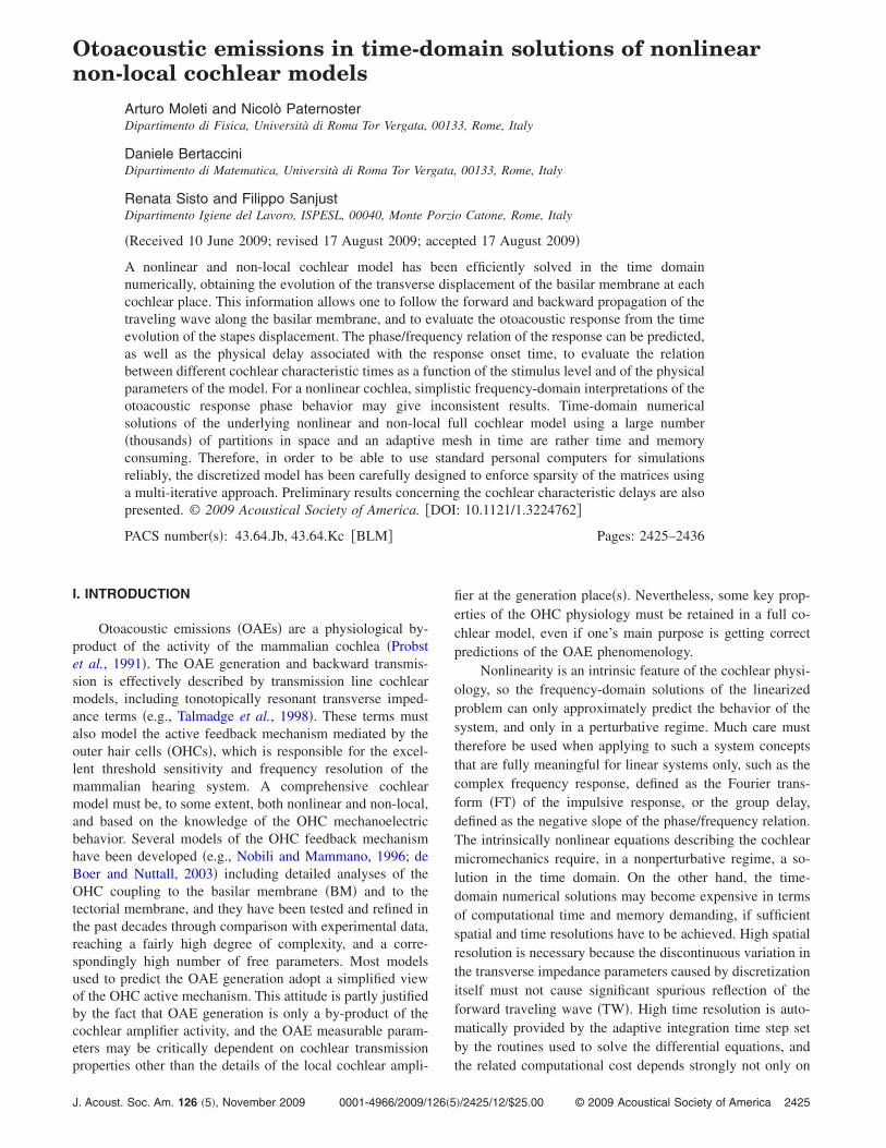
The result of a numerical simulation �N=1000 parti-tions� using a broad-band click stimulus �level correspondingto 80 dB pSPL, duration of 80 �s in the ear canal, similar tothat routinely used in the clinical practice� is shown in Fig.1�a�, where we plot the computed BM transverse displace-ment as a function of time �in a 20 ms interval� and cochlearposition x. One could choose to plot the BM velocity insteadof displacement, obtaining a different vertical shape, due tothe factor �, which would amplify the basal part of the TW.From the top view shown in Fig. 1�b�, the expected relationbetween the forward transmission time delay �BM forwarddelay� and the position x�� of the tonotopic resonant placeof each frequency component � is more clearly visible. Thisrelation may be converted into a relation between BM delayand frequency using the Greenwood map �Greenwood,1990�.

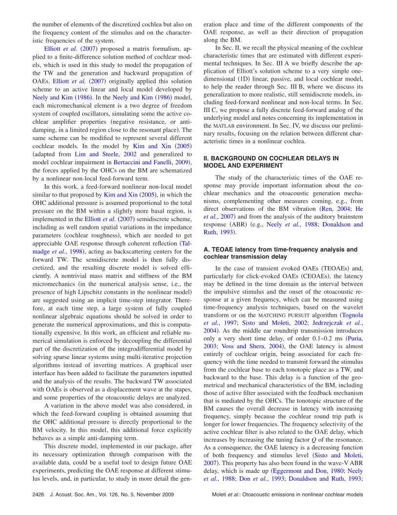
Including randomly distributed mechanical irregularities�roughness� as spatial stiffness variations in relative ampli-tude �=0.05, the click stimulus produces the delayed re-sponse at the stapes shown �for a total time of 50 ms� in Fig.2 �the data are windowed to cancel the stimulus and to allowspectral analysis�. This response would be transmitted backthrough the middle ear producing a TEOAE in the ear canal.
A high level of fluctuations is used in the example to get a

strong TEOAE signal. The waveform of Fig. 2 has beenanalyzed using time-frequency wavelet techniques to esti-mate the time delay of each frequency component. This de-lay closely corresponds to that of the TEOAE that would bemeasured in the ear canal because the delay introduced bythe middle ear transmission, neglected in this model, is neg-ligible �of order 100–200 �s�. The TEOAE wavelet delay

FIG. 1. BM response to a broad-band pulse �an 80 dB pSPL click of dura-tion 80 �s�, as a function of time and cochlear longitudinal position x.

FIG. 2. “Otoacoustic” response computed at the stapes for 50 ms after the
click, corresponding to the cochlear activation pattern of Fig. 1.

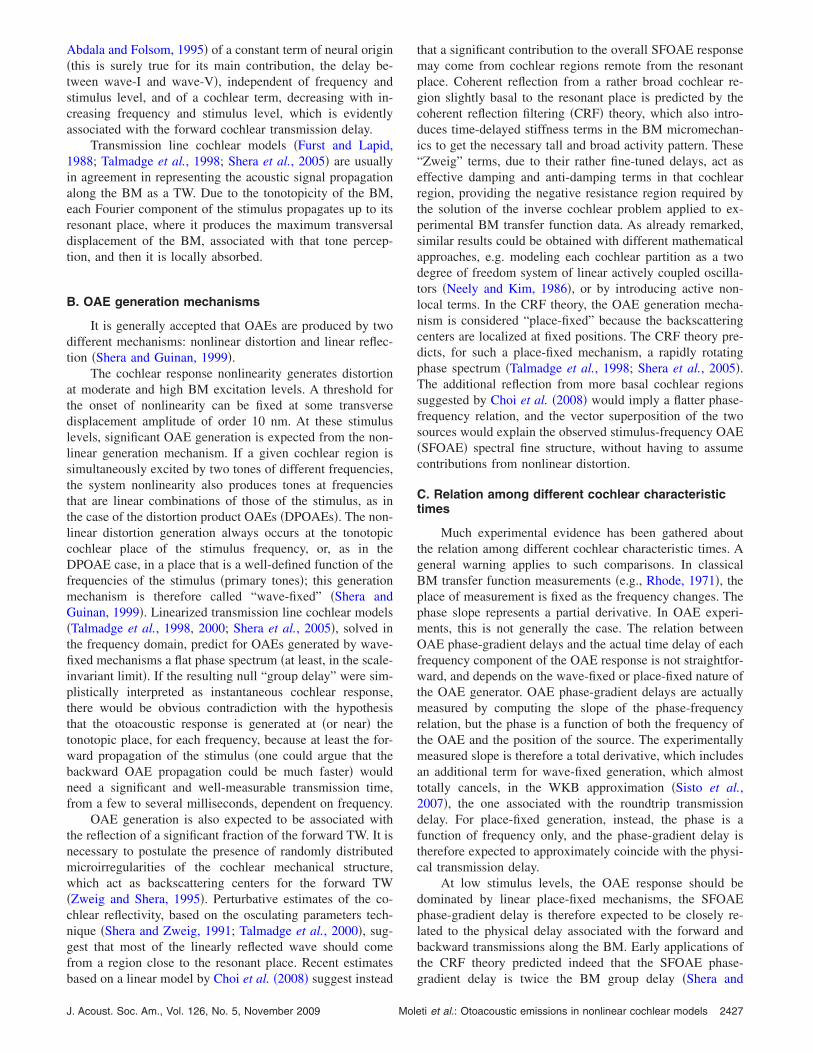
computed for the waveform of Fig. 2 is shown in Fig. 3�a�.In Fig. 3�b�, we show twice the BM forward latency, esti-mated from Fig. 1�b� as the time of the maximum BM exci-tation and attributed to the frequency that is the best fre-quency for each place according to the Greenwood map�Greenwood, 1990�. In Fig. 3�c�, we show the phase-gradientdelay estimated from the slope of the fast Fourier transform�FFT� phase. The good agreement confirms that the signalobserved at the stapes comes from a backward slow TW onthe BM, generated, for each frequency component of thestimulus, near its resonant place. In this model, the backwardwave is generated by linear reflection from roughness. In-deed, the same simulation without roughness �not shown�

(a)

(b)

(c)

FIG. 3. Wavelet analysis estimate of the latency/frequency relation �a� of theresponse at the base of Fig. 2, compared to twice the delay of the BMresponse at each tonotopic place �b� and to the phase-gradient delay mea-sured from the FFT of the same waveform �c�.

produces no “OAE” response at the stapes. We note that the


time-domain solution permits a direct estimate of the re-sponse waveform at the base �and at all other cochlearplaces� allowing us to compute time delays directly, withoutany assumption about the linearity of the system.

B. DPOAEs

In Fig. 4, we show the generation of the 2f1− f2 distor-tion product due to nonlinear interaction of two primarytones �f1=2000 Hz, f2 / f1=1.22, L1−L2=10 dB, and L2

=60 dB SPL�. In Fig. 4, the spectrum of the cochlear dis-placement is shown at different cochlear positions. The twoprimary tones propagate up to x�f2�, where the DPOAE is

fdp

f2

fdp

f1

(a)

(b)

(c)

(d)

FIG. 4. Generation of the 2f2− f1 distortion product due to nonlinear inter-action of two primary tones �f1=2000 Hz, f2 / f1=1.22�. The distortion toneis generated at x�f2��a�, its amplitude constantly increases reaching first x�f1��b�, and then x�fDP� �c�. The response at the stapes includes several other DPlines �d�.

generated and the f2 tone is absorbed �and partially reflected


by roughness� �Fig. 4�a��, then the f1 tone is absorbed �andpartially reflected by roughness� at its resonant place �Fig.4�b��, whereas the distortion tone propagates forward to itstonotopic place, where it is amplified �Fig. 4�c��, absorbed,and partially reflected by roughness. The continuum spec-trum, shifting to lower frequencies with increasing x, whichcan be observed below the spectral lines, is due to a smallspurious broad-band TW. Several distortion product lines arevisible in the spectrum of the response at the stapes �Fig.4�d��, the most intense being that of frequency fDP=2f1− f2,which is about 30 dB below the primary stimulus level.These DP levels are rather high, which is an indication thatthe parameters of the model still need to be optimized. At thepresent stage, a high level of DPOAE response may helpshow the qualitative behavior of the model.

The time-domain solution allows one to follow the gen-eration of the DPOAE response also looking at displacementat fixed cochlear positions x as a function of time or at fixedtimes as a function of the position x. At the same three co-chlear places of Figs. 4�a�–4�c�, one gets the time evolutionshown in Figs. 5�a�–5�c�. From these plots, one can visuallyappreciate the different onset times of the response at differ-ent cochlear positions and the different frequency contents of

(a)

(b)

(c)

FIG. 5. Time evolution of the cochlear response at the three cochlear placesof Figs. 4�a�–4�c�.

the signal.


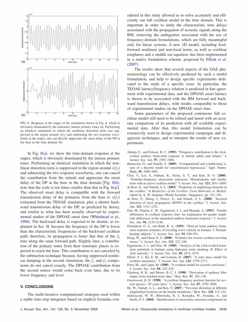
In Fig. 6�a�, we show the time-domain response at thestapes, which is obviously dominated by the intense primarytones. Performing an identical simulation in which the non-linear distortion term is suppressed in the region around x�f2�and subtracting the two response waveforms, one can cancelthe contribution from the stimuli and appreciate the onsetdelay of the DP at the base in the time domain �Fig. 6�b�,note that the scale is ten times smaller than that in Fig. 6�a��.The observed onset delay is compatible with the forwardtransmission delay of the primaries from the base to x�f2�estimated from the TEOAE simulation, plus a shorter back-ward transmission delay of the DP, as predicted by theory,and similar to what has been actually observed by experi-mental studies of the DPOAE onset time �Whitehead et al.,1996�. The backward delay is expected to be shorter, as ex-plained in Sec. II, because the frequency of the DP is lowerthan the characteristic frequencies of the backward cochlearpath; therefore, its propagation is faster that that of the f2

tone along the same forward path. Slightly later, a contribu-tion of the primary tones from their tonotopic places is ex-pected to reach the base. This contribution is not canceled bythe subtraction technique because, having suppressed nonlin-ear damping in the second simulation, the f1 and f2 compo-nents do not cancel exactly. The DPOAE contribution fromthe second source would come back even later, due to itslower frequency and level.

V. CONCLUSIONS

The multi-iterative computational strategies used within

(a)

(b)

FIG. 6. Response at the stapes of the simulation shown in Fig. 4. which isobviously dominated by the stationary intense primary tones �a�. Performingan identical simulation in which the nonlinear distortion term was sup-pressed in the region around x�f2� and subtracting the two response wave-forms at the stapes, one can directly appreciate the onset delay of the DP atthe base in the time domain �b�.

a stable time-step integrator based on implicit formulas con-


sidered in this study allowed us to solve accurately and effi-ciently our full cochlear model in the time domain. This isimportant in order to study the characteristic time delaysassociated with the propagation of acoustic signals along theBM, removing the ambiguities associated with the use offrequency-domain formulations, which are fully meaningfulonly for linear systems. A new 1D model, including feed-forward nonlinear and non-local terms, as well as cochlearroughness and a middle ear equation, has been implementedin a matrix formulation scheme, proposed by Elliott et al.�2007�.

The results show that several aspects of the OAE phe-nomenology can be effectively predicted by such a modelformulation, and help to design specific experiments dedi-cated to the study of a specific issue. In particular, theTEOAE latency/frequency relation is predicted in fine agree-ment with experimental data, and the DPOAE onset latencyis shown to be associated with the BM forward and back-ward transmission delays, with results comparable to thoseof experimental studies on the DPOAE onset time.

Some parameters of the proposed continuous full co-chlear model still need to be refined and tuned with an accu-rate comparison of its prediction with all available experi-mental data. After that, this model formulation can beextensively used to design experimental campaigns and di-agnostic techniques, and to interpret the results of new ex-periments.

Abdala, C., and Folsom, R. C. �1995�. “Frequency contribution to the click-evoked auditory brain-stem response in human adults and infants,” J.Acoust. Soc. Am. 97, 2394–2404.

Bertaccini, D., and Fanelli, S. �2009�. “Computational and conditioning is-sues of a discrete model for sensorineaural hypoacusia,” Appl. Numer.Math. 59, 1989–2001.

Choi, Y., Lee, S., Parham, K., Neely, S. T., and Kim, D. O. �2008�.“Stimulus-frequency otoacoustic emissions: Measurements and simula-tions with an active cochlear model,” J. Acoust. Soc. Am. 123, 2651–2669.

de Boer, E., and Nuttall, A. L. �2003�. “Properties of amplifying elements inthe cochlea,” in Biophysics of the Cochlea: From Molecules to Models,edited by A. W. Gummer �World Scientific, Singapore�, pp. 331–342.

de Boer, E., Zheng, J., Porsov, E., and Nuttall, A. L. �2008�. “Inverteddirection of wave propagation �IDWP� in the cochlea,” J. Acoust. Soc.Am. 123, 1513–1521.

Don, M., Ponton, C. W., Eggermont, J. J., and Masuda, A. �1993�. “Genderdifferences in cochlear response time: An explanation for gender ampli-tude differences in the unmasked auditory brainstem response,” J. Acoust.Soc. Am. 94, 2135–2148.

Donaldson, G. S., and Ruth, R. A. �1993�. “Derived band auditory brain-stem response estimates of traveling wave velocity in humans. I: Normal-hearing subjects,” J. Acoust. Soc. Am. 93, 940–951.

Dong, W., and Olson, E. S. �2008�. “Evidence for reverse cochlear travelingwaves,” J. Acoust. Soc. Am. 123, 222–240.

Eggermont, J. J., and Don, M. �1980�. “Analysis of the click-evoked brain-stem potentials in humans using high-pass noise masking. II. Effect ofclick intensity,” J. Acoust. Soc. Am. 68, 1671–1675.

Elliott, S. J., Ku, E. M., and Lineton, B. �2007�. “A state space model forcochlear mechanics,” J. Acoust. Soc. Am. 122, 2759–2771.

Furst, M., and Lapid, M. �1988�. “A cochlear model for acoustic emissions,”J. Acoust. Soc. Am. 84, 222–229.

Glasberg, B. R., and Moore, B. C. J. �1990�. “Derivation of auditory filtershapes from notched-noise data,” Hear. Res. 47, 103–138.

Greenwood, D. D. �1990�. “A cochlear frequency position function for sev-eral species—29 years later,” J. Acoust. Soc. Am. 87, 2592–2605.

He, W., Nuttall, A. L., and Ren, T. �2007�. “Two-tone distortion at differentlongitudinal locations on the basilar membrane,” Hear. Res. 228, 112–122.

Jedrzejczak, W. W., Blinowska, K. J., Konopka, W., Grzanka, A., and
Durka, P. J. �2004�. “Identification of otoacoustic emission components by

means of adaptive approximations,” J. Acoust. Soc. Am. 115, 2148–2158.Kim, J., and Xin, J. �2005�. ““A two-dimensional nonlinear nonlocal feed-

forward cochlear model and time domain computation of multitone inter-actions,” Multiscale Model. Simul. 4, 664–690.

Lim, K. M., and Steele, C. R. �2002�. “A three-dimensional nonlinear activecochlear model analyzed by the WKB-numeric method,” Hear. Res. 170,190–205.

Long, G. R., Talmadge, C. L., and Lee, J. �2008�. “Measuring distortionproduct otoacoustic emissions using continuously sweeping primaries,” J.Acoust. Soc. Am. 124, 1613–1626.

Moleti, A., and Sisto, R. �2003�. “Objective estimates of cochlear tuning byotoacoustic emission analysis,” J. Acoust. Soc. Am. 113, 423–429.

Neely, S. T., and Kim, D. O. �1986�. “A model for active elements incochlear biomechanics,” J. Acoust. Soc. Am. 79, 1472–1480.

Neely, S. T., Norton, S. J., Gorga, M. P., and Jesteadt, W. �1988�. “Latencyof auditory brain-stem responses and otoacoustic emissions using tone-burst stimuli,” J. Acoust. Soc. Am. 83, 652–656.

Nobili, R., and Mammano, F. �1996�. “Biophysics of the cochlea II: Station-ary nonlinear phenomenology,” J. Acoust. Soc. Am. 99, 2244–2255.

Prijs, V. F., Schneider, S., and Schoonhoven, R. �2000�. “Group delays ofdistortion product otoacoustic emissions: Relating delays measured withf1- and f2-sweep paradigms,” J. Acoust. Soc. Am. 107, 3298–3307.

Probst, R., Lonsbury-Martin, B. L., and Martin, G. K. �1991�. “A review ofotoacoustic emissions,” J. Acoust. Soc. Am. 89, 2027–2067.

Puria, S. �2003�. “Measurements of human middle ear forward and reverseacoustics: Implications for otoacoustic emissions,” J. Acoust. Soc. Am.113, 2773–2789.

Ren, T. �2004�. “Reverse propagation of sound in the gerbil coclea,” Nat.Neurosci. 7, 333–334.

Rhode, W. S. �1971�. “Observations of the vibration of the basilar mem-brane in squirrel monkeys using the Mössbauer technique,” J. Acoust. Soc.Am. 49, 1218–1231.

Schoonhoven, R., Prijs, V. F., and Schneider, S. �2001�. “DPOAE groupdelays versus electrophysiological measures of cochlear delay in normalhuman ears,” J. Acoust. Soc. Am. 109, 1503–1512.

Shera, C. A., and Guinan, J. J., Jr. �1999�. “Evoked otoacoustic emissionsarise from two fundamentally different mechanisms: A taxonomy formammalian OAEs,” J. Acoust. Soc. Am. 105, 782–798.

Shera, C. A., and Guinan, J. J., Jr. �2003�. “Stimulus-frequency emissiongroup delay: A test of coherent reflection filtering and a window on co-chlear tuning,” J. Acoust. Soc. Am. 113, 2762–2772.

Shera, C. A., Guinan, J. J., Jr., and Oxenham, A. J. �2002�. “Revised esti-mates of human cochlear tuning from otoacoustic and behavioral measure-ments,” Proc. Natl. Acad. Sci. 99, 3318–3323.

Shera, C. A., Tubis, A., and Talmadge, C. L. �2005�. “Coherent reflection ina two-dimensional cochlea: Short-wave versus long-wave scattering in thegeneration of reflection-source otoacoustic emissions,” J. Acoust. Soc.


Am. 118, 287–313.Shera, C. A., Tubis, A., and Talmadge, C. L. �2006� “Delays of SFOAEs and

cochlear vibrations support the theory of coherent reflection filtering,”Association for Research in Otolaryngology 2006 Meeting Poster.

Shera, C. A., Tubis, A., Talmadge, C. L., de Boer, E., Fahey, P. F., andGuinan, J. J., Jr. �2007�. “Allen–Fahey and related experiments support thepredominance of cochlear slow-wave otoacoustic emissions,” J. Acoust.Soc. Am. 121, 1564–1575.

Shera, C. A., and Zweig, G. �1991�. “Reflection of retrograde waves withinthe cochlea and at the stapes,” J. Acoust. Soc. Am. 89, 1290–1305.

Siegel, J. H., Cerka, A. J., Recio-Spinoso, A., Temchin, A. N., van Dijk, P.,and Ruggero, M. A. �2005�. “Delays of stimulus-frequency otoacousticemissions and cochlear vibrations contradict the theory of coherent reflec-tion filtering,” J. Acoust. Soc. Am. 118, 2434–2443.

Sisto, R., and Moleti, A. �2002�. “On the frequency dependence of theotoacoustic emission latency in hypoacoustic and normal ears,” J. Acoust.Soc. Am. 111, 297–308.

Sisto, R., and Moleti, A. �2007�. “Transient evoked otoacoustic emissionlatency and cochlear tuning at different stimulus levels,” J. Acoust. Soc.Am. 122, 2183–2190.

Sisto, R., Moleti, A., and Shera, C. A. �2007�. “Cochlear reflectivity intransmission-line models and otoacoustic emission characteristic time de-lays,” J. Acoust. Soc. Am. 122, 3554–3561.

Talmadge, C. L., Tubis, A., Long, G. R., and Piskorski, P. �1998�. “Model-ing otoacoustic emission and hearing threshold fine structures,” J. Acoust.Soc. Am. 104, 1517–1543.

Talmadge, C. L., Tubis, A., Long, G. R., and Tong, C. �2000�. “Modelingthe combined effect of basilar membrane nonlinearity and roughness onstimulus frequency otoacoustic emission fine structure,” J. Acoust. Soc.Am. 108, 2911–2932.

Tognola, G., Ravazzani, P., and Grandori, F. �1997�. “Time-frequency dis-tributions of click-evoked otoacoustic emissions,” Hear. Res. 106, 112–122.

Unoki, M., Miyauchi, R., and Tan, C.-T. �2007�. “Estimates of tuning ofauditory filter using simultaneous and forward notched-noise masking,” inHearing—From Sensory Processing to Perception, edited by B. Koll-meier, G. Klump, V. Hohmann, U. Langemann, M. Mauermann, S. Up-penkamp, and J. Verhey �Springer, Berlin�, pp. 19–26.

Voss, S. E., and Shera, C. A. �2004�. “Simultaneous measurement of middle-ear input impedance and forward/reverse transmission in cat,” J. Acoust.Soc. Am. 116, 2187–2198.

Whitehead, M. L., Stagner, B. B., Martin, G. K., and Lonsbury-Martin, B. L.�1996�. “Visualization of the onset of distortion-product otoacoustic emis-sions, and measurement of their latency,” J. Acoust. Soc. Am. 100, 1663–1679.

Zweig, G., and Shera, C. A. �1995�. “The origin of periodicity in the spec-trum of otoacoustic emissions,” J. Acoust. Soc. Am. 98, 2018–2047.


Otoacoustic emissions in time-domain solutions of nonlinear non-local cochlear models

Documents

Transcript of Otoacoustic emissions in time-domain solutions of nonlinear non-local cochlear models