Are spontaneous otoacoustic emissions generated by self-sustained cochlear oscillators?

Carrick L. Talmadge and Arnold Tubis Department of Physics, Purdue University, West Lafayette, Indiana 4 7907

Hero P. Wit

Institute of Audiology, University Hospital, P.O. Box 30. 001, 9700 RB Groningen, The Netherlands

Glenis R. Long Department of ,4udiology and Speech Science, Purdue University, West Lafayette, Indiana 4 7907

(Received 5 June 1990; accepted for publication 19 December 1990)

Theoretical analyses supporting the assumption that spontaneous otoacoustic emissions (SOAEs) can be described as self-sustained oscillations (requiring a power source) are reviewed and extended. Spectral and statistical properties of spontaneous otoacoustic emissions are examined and shown to be consistent with this assumption. Several alternative models of spontaneous emissions (noise-driven saturating memoryless nonlinearity, noise-driven nonlinear-stiffness oscillator) are examined. Although some of these models are able to produce the types of statistical distributions of amplitude and displacement similar to those observed in the experimental data, this similarity is destroyed upon narrow-band filtering.

PACS numbers: 43.64.Jb, 43.64. Bt

INTRODUCTION

Spontaneous otoacoustic emissions (SOAEs) (re- viewed in Zurek, 1985) are weak narrow band signals of cochlear origin that are measurable in the ear canal with a sensitive microphone. These emissions are associated with normal hearing in primates and their existence has been cited as evidence that the sensitivity and resolution of the normal mammalian inner ear depends on active signal filter- ing. Consequently, a better understanding of the nature of such emissions is thought to be important in furthering our understanding of the processes underlying normal hearing. In this regard, most of the discussion has focused on two types of processes in the cochlea which may give rise to SOAEs: ( 1 ) noise-perturbed cochlear self-sustaining or lim- it-cycle oscillations produced by active-nonlinear cochlear filtering, proposed many years ago by Gold ( 1948 ); and (2) passive narrow-band filtering of cochlear noise. In this pa- per, experimental data on the spectral and statistical proper- ties of SOAEs and related theoretical arguments that sup- port the first of these two possible underlying mechanisms for SOAEs are reviewed and extended.

Although data on the interactions of SOAEs with exter- nal tones provide further support for the limit-cycle-oscilla- tion interpretation of SOAEs (e.g., Wilson, 1980; Zwicker and Schloth, 1984; Long et al., 1988; Long and Tubis, 1988; Tubis et al., 1988; Van Dijk and Wit, 1988, 1990a), we con- fine the discussion of this paper to the spectral and statistical properties of SOAEs because: ( 1 ) they provide the simplest means for distinguishing between the two possible underly- ing mechanisms for SOAEs; and (2) they have recently been the source of some controversy and confusion (Wit, 1989; Furst, 1989; see also Sec. V of this paper).

We present SOAE data in Sec. I that exhibit the typical

spectral and statistical ear-canal pressure and pressure-am- plitude distributions characteristic of a sine wave embedded in noise, the signal expected to be produced by a limit-cycle oscillator perturbed by noise. These statistical characteris- tics of emissions can be used to distinguish which models of SOAEs are viable. In Sec. II, we consider self-sustained os- cillators in the presence of noise, and show that such models are consistent with the statistical properties reported in Sec. I. In the next two sections, we study possible classes of pas- sive SOAE models (noise-driven saturating memoryless nonlinearity in Sec. III, and noise-driven nonlinear stiffness in Sec. IV), and show that these classes of models do not meet the statistical criteria discussed in Sec. I.

I. PROPERTIES OF SOAEs

The spectral bandwidth of a human SOAE is of the or- der of 1 Hz (Wit and van Dijk, 1989). A typical SOAE spectrum is shown in Fig. 1. The dots in this figure represent the measured spectral values, and the solid line shows the results of a fit of these values to a Lorentzian curve. In order

to obtain more insight into the nature of the underlying sig- nal, two different analyses were performed.

First, the distribution density function for the amplified and bandpass filtered microphone voltage was generated. Figure 2 (a) and (b) includes results from data collected by one of us (HPW) in the Netherlands using a Datalab 4000 system in the amplitude histogram mode (60-Hz band- width, 160-s sample ofa 1398 Hz, 20-dB SPL emission), and by GRL in the U.S.A. by digitally sampling the signal with a Data Translation 2827 D/A board and analyzing the signal using a Zenith 386 computer (31.6-Hz bandwidth, 30-s sam- ple of a 1620-Hz, 12-dB SPL emission). The noise reflected in the data is probably mainly due to the noise of the measur-

2391 J. Acoust. Soc. Am. 89 (5), May 1991 0001-4966/91/052391-09500.80 ¸ 1991 Acoustical Society of America 2391

Downloaded 12 Jun 2013 to 146.96.38.40. Redistribution subject to ASA license or copyright; see http://asadl.org/terms

1.5

:3 1.0

v

ß ,-, 0.5

E

0.0 1396 13'97 13'98 13'99 1400

f(Hz)

FIG. 1. Typical frequency spectrum of an SOAE.

ing system, which still remains after bandpass filtering around the SOAE frequencies. Theoretically, the possibility exists that extremely narrow-band-filtered noise accounts for the results in Fig. 2. This possibility, however, is very unlikely because the sampling time for the distribution den- sity function ( 160 s) was much larger than the reciprocal of the bandwidth of the SOAE shown in Fig. 1 (3.7 s).

The SOAEs from human subjects were also investigated by obtaining the density distribution of the amplitude enve- lope of the signal. Figure 3 (a) was obtained by one of us (HPW) in the Netherlands using the Datalab 4000 system to record the distribution function for the signal envelope. Rectification and subsequent low-pass filtering of the signal was used to obtain the signal's envelope, which was then used to produce the averaged density distribution shown in Fig. 3(a). Figure 3(b) was obtained by one of us (GRL) in the U.S.A. using the Data Translation 2827 D/A board and analyzing the signal using the Zenith 386 computer. The signal envelope was obtained using peak picking software that produced best fit amplitude values for the five nearest data points to each maximum or minimum of the digitized signal.

If the SOAE were a perfectly stable sine wave, the spec- tral width would be much smaller than the 0.3 Hz shown in

Fig. 1. An SOAE exhibits small amplitude and frequency fluctuations that can be satisfactorily described with a model in which a self-sustaining oscillator is driven by a weak ran- dom noise force (Bialek and Wit, 1984; Wit and Van Dijk, 1989; Van Dijk and Wit, 1990b).

If an SOAE is subjected to an externally applied tone of slightly different frequency, it shows the typical entrainment or phase-locking behavior of a self-sustaining oscillator with some internal noise (Bialek and Wit, 1984; Long et al., 1988; Long and Tubis, 1988; Tubis et al., 1988; Van Dijk and Wit,

(a)

-20 o 20 40 ' x

20000

15000

x 1.0000 z

5OOO

(b)

_O2o00 ..... -1000 0 1000 2000 X

FIG. 2. Measured displacement distribution function for an SOAE. (a) Data collected by HPW in the Netherlands and (b) data collected in the U.S.A. as described in the text.

16

0 ...... fo- ...... -•0--3b 4'0 a

, ---;. _ _ :e e

50 6O

(a)

70

8OOO

7000

6000

5000

4000

3000

2000

1000

0 0 500 1000

a

(b)

15bO'' 2000

FIG. 3. Measured envelope distribution function for an SOAE: (a) from data collected in Holland, and (b) from data collected in the U.S.A. as described in the text.

2392 J. Acoust. Soc. Am., Vol. 89, No. 5, ,May 1991 Talmadge et al.: Source of spontaneous otoacoustic emissions 2392

Downloaded 12 Jun 2013 to 146.96.38.40. Redistribution subject to ASA license or copyright; see http://asadl.org/terms

1988; Wit and Van Dijk, 1990a). This behavior cannot be accounted for by a narrow-band-noise model of an SOAE (e.g., Talmadge et al., 1989).

The observed displacement and amplitude distributions for real SOAEs may be used as a means for discriminating between the variofis classes of models that give rise to nar- row-band frequency spectrums, since only models that have the statistical properties described above can be considered viable models. In the following sections, we will study the predicted displacement and amplitude distributions for var- ious classes of models, and compare these results to those observed for real SOAEs.

II. SELF-SUSTAINED OSCILLATORS

For present purposes, we define a self-sustained oscilla- tor (e.g., Poincar(•, 1892; Stoker, 1950; Nayfeh and Mook, 1979; Hanggi and Riseborough, 1983) as a device in which the output signal x (t) ( where t denotes time ) has the follow- ing properties:

( 1 ) If Jc (t) [ = dx/dt] is plotted against x (t), the re- sulting path in the x, 5c phase space approaches a stable tra- jectory or limit cycle (which implies a periodic behavior), irrespective of the initial point in phase space (with the ex- ception of certain discrete initial points).

(2) The input signal does not contain a stable compo- nent with the frequency of the limit cycle. In the context of modern theories of chaotic behavior (see, e.g., Lauterborn and Parlitz, 1988), the limit cycle is one of the possible forms of an attractor.

A textbook example of a physically realizable self-sus- taining oscillator is the Van der Pol oscillator (e.g., Van der Pol, 1927; Stoker, 1950; Nayfeh and Mook, 1979; Hanggi and Riseborough, 1983) in which energy is supplied for small values of the oscillator displacement, with stabilizing energy dissipation occurring for larger values of the dis- placement [i.e., the resistance term in the differential equa- tion for x(t) is negative for small Ix l and positive for larger Ixl],

In general, a power supply is essential for a self-sustain- ing oscillator. Note that the simple device shown in Fig. 4 (sine wave generator connected to two resistors in series) satisfies requirement 1 above for a self-sustaining oscillator, but does not satisfy requirement 2. A self-sustaining oscilla- tor must, in fact, be a nonlinear device, because only nonlin- ear systems can transform energy from one frequency to an- other (e.g., Guillemin, 1963). In the case of many self-sustaining oscillators, the input frequency is zero (dc power supply).

A self-sustaining oscillator is sometimes referred to as an active (in contrast to passive) device in that the power supply is used to compensate for some of the passive damp- ing. However, even for linear systems, it is difficult to give a precise definition for an active device (e.g., Guillemin, 1963). We will therefore not attempt to give a general defini- tion of an active nonlinear system, but will rather attempt to illustrate the types of systems we have in mind with reference to active and passive electronic filters.

In an active filter, which requires a power supply, posi-

R1 • o

sin wave in R 2 out

o o

FIG. 4. Example of passive filter consisting of two resistors in series that will produce a sine-wave output signal. Since the input signal contains a stable frequency component, this example does not constitute a self-sustained os- cillator.

tive feedback, and amplification are employed to compen- sate for losses in the resistive elements (e.g., Millman and Halkias, 1972). No amplification occurs in a passive filter, which does not contain a power supply. The bandwidth (quality factor) of a bandpass active filter is adjustable by setting the amount of positive feedback. If positive feedback is so large that it fully compensates for the losses in the resis- tive elements, the filter may become a self-sustaining oscilla- tor. Evidence is growing that nature has chosen to employ active filters instead of passive ones in the inner ear, as was proposed more than 40 years ago by Gold (1948).

Bialek and Wit (1984) first pointed out that when seek- ing evidence for self-sustaining cochlear oscillations from actual data on the ear canal pressure, the data must be checked with respect to the implications of models of noise- perturbed self-sustaining oscillations. Such models typically give signals very similar to sine waves in noise. It is instruc- tive to demonstrate this using an exactly soluble • model (Caughey and Payne, 1967), which is described by the sto- chastic differential equation

)• -- e( 1 -- x 2 -- œ2)5c + x = tb(t), ( 1 )

where E>0, œ=dx/dt, •:=d2x/dt2,. tb(t)=dw/dt, t = time, and w(t) isa white noise signal with zero mean and covariance given by

(w( t)w( t ') ) = 2D6( t -- t '), (2)

where 6(t) is the Dirac delta function. In the absence of noise, Eq. ( 1 ) has the exact limit-cycle

solution,

x(t) = sin(t q- •b), (3)

where •b is arbitrary. This solution has a single-line spectrum and a probability density for displacement, Px (x), given by

rrx/1 -- x 2 x2< 1,

x2> 1. (4)

In the presence of noise, the spectrum ofx(t) will broad- en, and the peaks of Px (x) will also broaden but retain the same qualitative behavior as those of P• (x) in Eq. (4). The

2393 J. Acoust. Soc. Am., Vol. 89, No. 5, May 1991 Talmadge eta/.: Source of spontaneous otoacoustic emissions 2393

Downloaded 12 Jun 2013 to 146.96.38.40. Redistribution subject to ASA license or copyright; see http://asadl.org/terms

latter can be shown analytically by considering the station- ary joint probability function, P(x,Jc), which is independent of both time and the initial conditions, and satisfies the Fokker-Plank equation (e.g., Caughey, 1963 ),

0=_/co•P t_ o • -•-x- •- [{--•[1--x 2--•2]•q_x)e] +D•. (5)

c•x 2

The exact solution ofEq. (5) is (Caughey and Payne, 1967)

P(x,5c) =Nexp ---• (x 2+ -- 1) , (6) where Nis a positive normalization constant, defined so that

dx dicP(x,5c) = 1, (7)

and therefore

N -' = rrx/rrD/6 [ 1 + err(«d eld ) ]. ( 8 ) We finally have

Px (x) = N die exp[ - (e/4D) (x 2 + Jc 2 -- 1 )2].

(9)

Equation (9) gives the displacement density distribution P• (x) for the noise perturbed limit cycle oscillator given by Eq. ( 1 ). Since the integral in Eq. (9) has no simple closed- form solution, we instead numerically integrated Eq. (9) as needed.

It is easily verified that P• (x) in Eq. ( 8 ) becomes equal to the deterministic result of Eq. (4) in the limit of D-• 0 +, as we show below:

lim Px (x) = lim N dic D-.O+ D-.O+ •o

Xexp[ -- (e/4D)(x 2 + 5c 2-- 1)2]. (10)

We note that for x 2 > 1 the term (x 2 q- 5c 2 -- 1 ) 2 will be non- zero for all values ofic. Thus, as D-•0 + the integrand of Eq. (10) will vanish for all values of/t, and, hence,

lim P• (x) = 0, D-.O+

For x 2 < 1, we have

(x2> 1). (11)

lim Px (x) = lim N dic exp [ - (e/4D) D-.O+ D-.O+ •o

X (5c + x/1 - x 2 )2(5c - x/1 - x 2 )2]

= lim 2N dJc exp [ - (e/D) D-.O+ •o

X ( 1 -- x 2) (5c -- x/1 -- x 2 )2]

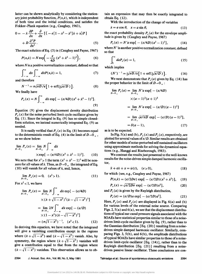
-- (rr•/1 - x 2 ) - •, (x 2 < 1 ). (12)

In deriving this equation, we have noted that the integrand will give a vanishing contribution except in the regions where (5c + x/1 -- x 2 ) and (5c -- x/1 -- x 2 ) vanish. Also, by symmetry, the region where (5c + •/1 -- x 2 ) vanishes will give a contribution equal to that from the region where (5c -- •/1 -- x 2 ) vanishes. This observation allows us to ob-

tain an expression that may then be exactly integrated to obtain Eq. (12).

With the introduction of the change of variables

Jc = a cos 0, x=asinO, (13)

the exact probability density Pe (a) for the envelope ampli- tude is given by (Caughey and Payne, 1967)

Pc(a) =N'aexp[ -- (e/4D)(a 2 -- 1)2], (14)

where N' is another positive normalization constant, defined so that

o © daP e (a) = 1, (15) which implies

(N') -• = «x/rrD/6[ 1 + erf(«x/-•) ]. (16) We next demonstrate that Pe (a) given by Eq. (14) has

the proper behavior in the limit of D-• 0 +:

lim Pe (a) -- lim N 'a exp [ -- (e/4D) D-.O+ D-.O+

X (a - 1 )2(a q- 1)2

= lim N'a exp[ -- (e/D) (a -- 1)2] D-.O+

= lim e/x/--f-• exp[ -- (e/D) (a -- 1)2], D-.O+

= 6(a -- 1), (17)

as is to be expected. In Fig. 5(a) and (b), P• (x) andPe (x), respectively, are

plotted for several values ofe/D. Similar results are obtained for other models of noise-perturbed self-sustained oscillators using approximate methods for solving the dynamical equa- tions (e.g., Hanggi and Riseborough, 1983).

We contrast the results just presented to the well-known results for the noise-driven simple damped harmonic oscilla- tor,

)• + eic + x = tb(t), (6>0),

for which (see, e.g., Caughey and Payne, 1967)

P(x,5c) = (e/2Drr) exp[ -- (e/2D)(x 2 + 5c 2) ],

(18)

(19)

P• (x) = x/e/2Drr exp[ -- (e/2D)x2], (20) and Pe (a) is given by the Rayleigh distribution,

Pe (a) = (e/D)a exp[ -- (e/2D)a2]. (21)

Here, P• (x) and Pa (x) are displayed in Fig. 6(a) and (b) for various levels of the external noise source. Comparing Figs. 2, 5 (a) and 6(a), we see that the displacement distribu- tions of typical ear-canal pressure signals associated with the SOAEs have statistical properties similar to those of a noise- driven limit-cycle oscillator given by Eq. (9), rather than to the Gaussian distribution [ Eq. (20) ] resulting from a noise- driven simple damped harmonic oscillator. Similarly, com- paring Figs. 3, 5(b), and 6(b), the amplitude distributions of typical SOAEs have similar properties to those of a noise- driven limit-cycle oscillator [ Eq. (14) ], rather than to the Rayleigh distribution [Eq. (21)] resulting from a noise- driven passive linear oscillator. These conclusions are con-

2394 J. Acoust. Soc. Am., Vol. 89, No. 5, May 1991 Talmadge eta/.' Source of spontaneous otoacoustic emissions 2394

Downloaded 12 Jun 2013 to 146.96.38.40. Redistribution subject to ASA license or copyright; see http://asadl.org/terms

2.0

1.5

0.5

(a) 4.0

œ/D .... œ/D =lee

..... E,/D = •0 œ/O

-1 0 1 2 X

3.0

1.0

.... œ/D = lee

..... œ/O

(a)

6 •:• •1•'0 [ /IX (b)[ (b) 6

5 7.•7 œ/D: 10 I i/i I l .... ]oo 4 ----œ/o:1 ] i i 5'1i • I ..... œ/D:10

•- •' 4 3

• • 3

1

ø0 1 2 0 1 2 a a

FIG. 5. (a) Displacement density distribution and (b) amplitude envelope distribution functions for the noise-driven Van der Pol-Rayleigh oscillator discussed in the text.

FIG. 6. (a) Displacement density distribution and (b) amplitude envelope distribution functions for a noise-driven simple damped harmonic oscilla- tor.

sistent with results previously reported by Bialek and Wit (1984), and by Long et al. (1988).

III. SATURATING NONLINEARITY DRIVEN BY RANDOM NOISE AS A POSSIBLE SOAE MODEL

We consider the question: "Can a system that is made up of passive (linear and/or nonlinear) elements driven by noise produce a sine wave?" We will consider a "passive element" to be one in which no energy is added back to the system (e.g., in an electrical network: resistors, inductances, capacitors, diodes, switches). An example of a system that will yield a positive answer to the above question is one in which noise, after rectification and low-pass filtering, is used as the dc power supply for a self-sustained oscillator. In the following we will exclude such systems from consideration.

A system that produces a signal with some of the char- acteristics of an SOAE is the nonlinear network shown in Fig. 7 (a), whose input/output function shown in Fig. 7 (b) is that of a saturating nonlinearity. If this network is driven by Gaussian white noise of sufficiently large amplitude, the resulting output density function (histogram of voltage val- ues ) shown in Fig. 7 (c) closely resembles that obtained for a

pure noise-perturbed limit-cycle oscillator [see Figs. 2 and 5 (a) ]. However, the signal obtained from this nonlinear fil- ter is still very broad band, so that when the signal is band- pass filtered (12% bandwidth) before the histograming is performed (which is akin to the actual experimental proce- dure used in obtaining displacement distributions such as Fig. 2), the resulting distribution density function again has a Gaussian shape.

This example shows that, while a density function with a shape similar to those of Fig. 2 or 7 (c) may be a necessary condition for a stable sine-wave component to be present in the signal, it is certainly not a sufficient one, and that an additional (necessary) condition is that the signal has a nar- row band frequency spectrum.

The nonlinear network of Fig. 7 (a) belongs to the class of zero-memory nonlinearities, for which the value of the output function at any instance in time is determined only by the value of the input function at the same instance in time (e.g., Stratonovich, 1963). It can be rigorously shown that, when the input of a zero-memory nonlinear system is Gaus- sian, and the output of the system is subjected to a sufficient- ly narrow-band filtering, then this filtered output is again Gaussian (Middleton, 1960, p. 763).

2395 J. Acou•t. Soc. Am., Vol. 89, No. 5, May 1991 T almadge et al.: Source of spontaneous otoacoustic emissions 2395

Downloaded 12 Jun 2013 to 146.96.38.40. Redistribution subject to ASA license or copyright; see http://asadl.org/terms

(a)

(b)

in

470 gl

out

v T 2v

øut• ,'• I I I I I •[ I

--4 .•t :2 ------ _L_ 2

Vin

(c)

-2 0 2

V (volts)

FIG. 7. (a) Physical realization of zero memory nonlinear filter; (b) input- output characteristics of this filter; and (c) measured displacement distri- bution of the output of this filter for a 3 Vrm , white noise input signal. Note that (c) was obtained from a signal that was not bandpass filtered. When such processing of the output signal is performed, the resultant signal will produce a Gaussian displacement distribution.

On the basis of the above discussion, it does not appear

possible that a saturating nonlinearity driven by noise could constitute a satisfactory SOAE model.

IV. OSCILLATORS WITH NONLINEAR STIFFNESS DRIVEN BY RANDOM NOISE

We next consider several examples of nonlinear oscilla- tors that have only passive damping and are driven by exter- nal Gaussian white noise sources. Since these oscillators are

comprised of entirely passive elements, they will not produce self-sustaining oscillations. We thus choose to refer to these oscillators as "nonlinear passive filters." Since the output state of these filters clearly depends upon their previous states, these filters will not have "zero-memory," and hence should be distinguished from the filters considered in the previous section. We describe this class of "filters" by the differential equation

•i d- eJc d- g ( x ) = tb(t), (22)

where ß is a positive constant and co(t) is a Gaussian white noise source, as before. In order that the solutions be bound- ed, we also require that g(0)= 0, with g(x)-• d- • for

2396 J. Acoust. Soc. Am., Vol. 89, No. 5, May 1991

x-•d-• and g(x)-•-o• for x-•-•. Caughey and Payne (1967) demonstrated for this case that

P(x,dc) = 4e/2•rDNexp( -- (e/D)[«do 2 + G(x) ]), (23)

(24)

(25)

Px (x) = Nexp[ -- (ß/D)G(x) ],

Pe (a) = N'a exp[ -- (ß/D)G(a) ], where

N - • = dx exp -•G(x) , (N') -] - da a exp[ - (ß/D)G(a) ],

G(x) - fo x dxg(x). (26) We consider as a first example of this type of system the

classic Duffing oscillator (e.g., Stoker, 1950; Nayfeh and Mook, 1979),

• + ßJc + x + yx 3 = tb(t),

with 7' a constant. Using Eqs. (23)-(26), we find

(27)

p(x,jc) = 4 ß 2•rD _ ß 7'

(28)

Px (x)= Nexp(- (ß/2D)x211 + (7'/2)x2]},

Pe (a) = N'a exp( -- (ß/2D)a2[ 1 + (7'/2)a2] },

N 2x•e - e/SDr X/e7'/7rD e - e/4Dr = , N'= , K]/4 (ß/8Dy) 1 -- erf(«x/e/D)/)

(29)

(30)

(31)

where K•/4 (x) is the modified Bessel function of the third kind (e.g., Abramowitz and Stegun, 1972). We see from Eqs. (28)-(30) that the density distributions for a noise- driven Duffing oscillator are quite similar to those for a noise-driven linear system given by Eqs. ( 19)-(21 ), and that the principal effect of the nonlinear stiffness is to distort the otherwise Gaussian or Rayleigh nature of the distribu- tions.

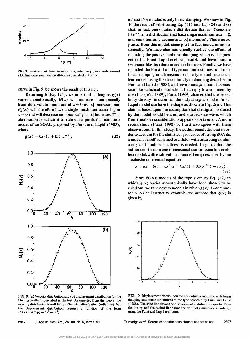
For illustrative purposes, we consider a particular phys- ical realization of the noise-driven Duffing system discussed above, which we have modeled as an RCL-filter with nonlin- ear capacitance. For this system, the current i plays the elec- trical analog of the velocity Jc in Eq. (27) and the charge q = œidt plays the role of the displacement x. The nonlinear capacitance was made up of 100 variable capacitance double diodes (Philips BB212) in parallel, and the resonance curve for the filter is shown in Fig. 8. This resonance curve has the shape typical for the "hardening spring" type Duffing oscil- lator (Nayfeh and Mook, 1979; Parlitz and Lauterborn, 1985). We plot in Fig. 9(a) and (b) the measured current (velocity) and charge (displacement) density distributions when the filter is driven by an external noise source. As would be expected from Eq. (28), the current distribution was found to be consistent with a Gaussian distribution, and

this is the solid curve which is shown in Fig. 9(a). Also as expected from Eq. (29), the charge distribution was not con- sistent with a Gaussian distribution, but was fit satisfactorily with the distribution P(x) = a exp ( -- bx 2 -- cx 4) [ the solid

Talmadge eta/.: Source of spontaneous otoacoustic emissions 2396

Downloaded 12 Jun 2013 to 146.96.38.40. Redistribution subject to ASA license or copyright; see http://asadl.org/terms

20

• 10 >

2 4 6 8 10 12

f (kHz)

FIG. 8. Input-output characteristics for a particular physical realization of a Duffing-type nonlinear oscillator, as described in the text.

curve in Fig. 9(b) shows the result of this fit]. Returning to Eq. (24), we note that as long as g(x)

varies monotonically, G(x) will increase monotonically from its absolute minimum at x = 0 as Ixl increases, and Px (x) will therefore have a single maximum occurring at x = 0 and will decrease monotonically as Ixl increases. This observation is sufficient to rule out a particular nonlinear model of an SOAE proposed by Furst and Lapid (1988), where

g(x) = kx/(1 + 0.5Ix[ø"), (32)

1.0

0.8

0.6

0.4

0.2

0.0 0 _ a)

20 40 60 80 100 120 V

1.0

0.8

x 0.6

0.4

0.2

0.0 0

(b)

; , , , , , , , , , -

20 40 60 80 100 120 X

FIG. 9. (a) Velocity distribution and (b) displacement distribution for the Duffing oscillator described in the text. As expected from the theory, the velocity distribution is well fit by a Gaussian distribution (solid line), but the displacement distribution requires a function of the form P,, (x) = a exp( -- bx 2 -- cx4),

at least if one includes only linear damping. We show in Fig. 10 the result of substituting Eq. (32) into Eq. (24) and see that, in fact, one obtains a distribution that is "Gaussian- like" (i.e., a distribution that has a single maximum at x = 0, and monotonically decreases as Ixl increases). This is as ex- pected from this model, since g(x) in fact increases mono- tonically. We have also numerically studied the effects of including the passive nonlinear damping which is also pres- ent in the Furst-Lapid cochlear model, and have found a Gaussian-like distribution even in this case. Finally, we have included the Furst-Lapid type nonlinear stiffness and non- linear damping in a transmission line type nonlinear coch- lear model, using the discontinuity in damping described in Furst and Lapid ( 1988 ), and have once again found a Gaus- sian-like statistical distribution. In a reply to a comment by one of us (Wit, 1989 ), Furst ( 1989 ) claimed that the proba- bility density function for the output signal of the Furst- Lapid model can have the shape as shown in Fig. 2 (a). This claim is based upon the assumption that the signal produced by the model would be a noise-disturbed sine wave, which from the above considerations appears to be in error. A more recent study (Furst, 1990) by Furst also agrees with these observations. In this study, the author concludes that in or- der to account for the statistical properties of strong SOAEs, a model of a self-sustained oscillator with saturating nonlin- earity and nonlinear stiffness is needed. In particular, the author constructs a one-dimensional transmission line coch-

lear model, with each section of model being described by the stochastic differential equation

)• + ado -- b( 1 -- ,dc2)dc + kx/( 1 + 0,51xl ø.' ) - (33)

Since SOAE models of the ty. pe given by Eq. (22) in which g(x) varies monotonically have been shown to be ruled out, we turn next to models in which g(x) is not mono- tonic. As an instructive example, we suppose that g(x) is given by

1250

lOOO

750

5OO

250

0 -2 -1 0 1 2 3

FIG. 10. Displacement distribution for noise-driven oscillator with linear damping and nonlinear stiffness of the type proposed by Furst and Lapid (1988). The solid line shows the displacement distribution expected from the theory, and the dashed line shows the result of a numerical simulation using the Furst and Lapid oscillator.

2397 J. Acoust. Soc. Am., Vol. 89, No. 5, May 1991 Talmadge et aL' Source of spontaneous otoacoustic emissions 2397

Downloaded 12 Jun 2013 to 146.96.38.40. Redistribution subject to ASA license or copyright; see http://asadl.org/terms

g(x) = -- kx d- k 'X 3, (34)

with k and k' being positive constants [for a discussion of this system in the absence of noise, see, for example, Gucken- heimer and Holmes (1983) ]. The variation ofg(x) withx is shown in Fig. 11 (a) for k -- k' = 88.831 s - •-. These values were chosen so that the oscillator would have stable equilib- rium points at x = 4- 1, as can be seen from the graph of the potential G(x) in Fig. 11 (b). Additionally, the natural fre- quency for Ixl • 1 was chosen to be near 1500 Hz. We also note that the effective stiffness g'(x) will be negative for

Ixl /3k' = 1/v•. In general, there are three identifiable modes of oscilla-

tion for this system, as can be seen in Fig. 11 (c), which displays a typical sample of the numerically integrated solu- tion for this system. For a small external noise source, the system will generally oscillate about x = d- 1 or x- -- 1, and its motion (for small enough oscillations around the equilibrium point) will look very much like that of a noise- driven linear oscillator. Additionally, there will be time in- tervals where noise fluctuations are large enough to drive the oscillator out of these stable oscillation modes, and the sys- tem will consequently spend a short time oscillating through the region containing both stable points, before settling back down into one of the two stable modes again. From this ob- served behavior, it is expected that one would obtain a distri- bution which would have local maxima at Ixl = 1, and, in fact, this is what is found both from numerical studies and by inserting Eq. (34) into Eq. (24). In Fig. 11 (d), we display typical displacement density distributions obtained from Eq. (24) for different choices of the level of the noise source.

The displacement density distributions shown in Fig. 11 (d) are those obtained if one does not pass x (t) through a bandpass filter before the histograming is performed (a pro-

(a) (b)

400

2OO

g(x) o

-200

G(x)

100

50

0

-2 -1 0 1 2 -2 -1 0 1 2 x x

(c) (d) 2.5 6

._. 4

ß y(t) 3 -0.5

2

-1.5 1

00 02 04 06 08 10 0 2

t [seconds] x

FIG. 11. (a) "Stiffness function" g(x) = -- kx + k 'x 3 for k = k' = 88.831 s - 2; (b) integral of g(x); (c) example time series signal; (d) typical dis- placement distributions for various levels of the external noise. Note that the output signals of this oscillator have not been narrow-band filtered be- fore being histogramed. If this operation is performed, the two "Gaussian- like" peaks are collapsed to the origin, and we obtain a single Gaussian-like peak.

cedure that is always performed in the actual measurements on SOAEs). To understand the effects of the bandpass filter, it is sufficient to observe that the oscillator spends much of its time in the two stable modes during which the signal qualitatively differs in the two states by only a dc offset. Thus the effect of bandpass filtering would be expected to remove the dc offset, and hence "collapse" the two maxima seen in Fig. 11 (d) into a single Gaussian-like distribution. This is, in fact, what is observed when the numerically integrated solu- tion is bandpass filtered and then histogramed.

The above discussion can easily be generalized to noise- driven systems for which there are more than two stable modes. As before, for a sufficiently weak noise source, the system will spend much of its time oscillating in one of its stable modes. These modes can, in general, have different natural frequencies of oscillation, and some modes may be statistically favored compared to other modes (this would arise if some local minima are deeper than others), but oth- erwise the signal component from each stable region will differ only by a dc offset. When the output of the filter is bandpass filtered about the natural frequency of one of its oscillation modes, the dc offsets among the various modes will be removed from the signal, as well as signal compo- nents from all of those modes that are not degenerate (or nearly degenerate) in frequency with the central frequency of the bandpass filter. Consequently, we will obtain a signal whose displacement density distribution consists of the sum of Gaussian-like distributions centered about x = 0 and

hence the displacement distribution of the total bandpass- filtered signal will again be Gaussian-like.

We have thus demonstrated that a broad class of noise-

perturbed oscillators with nonlinear stiffness [described by Eq. (22) ] may account for some but not all of the statistical properties characteristic of SOAEs. Similar conclusions have been reached (using approximation methods) con- cerning passive oscillators with nonlinear stiffness that fall outside of this class.

V. SUMMARY AND CONCLUDING REMARKS

The spectral and statistical distribution functions for ear canal signals associated with SOAEs are well represented by noise-perturbed self-sustaining oscillator models. Some of the features of the SOAE data may be qualitatively fit with passive models, but, to date, no passive SOAE model has been shown to give both a narrow-band spectrum as well as the statistical properties characteristic of a sine wave in noise that are revealed by the data.

The evidence for a self-sustaining-oscillator picture of SOAEs is even stronger if data on external-tone interactions with SOAEs (frequency locking, amplitude suppression, etc.) (e.g., Wilson, 1980; Zwicker and Schloth, 1984; Long et al., 1988; Long and Tubis, 1988; Tubis et al., 1988; Van Dijk and Wit, 1988, 1990a) are taken into account. The data and the analyses of this paper are consequently strongly sup- portive of the use of SOAE spectral and statistical data alone for determining the essential character of the generating mechanisms.

SOAEs and other types ofcochlear emissions, which are presumably associated with normal hearing function, pro-

2398 J. Acoust. Soc. Am., Vol. 89, No. 5, May 1991 Talmadge ot a/.' Source of spontaneous otoacoustic emissions 2398

Downloaded 12 Jun 2013 to 146.96.38.40. Redistribution subject to ASA license or copyright; see http://asadl.org/terms

vide a unique window for probing the workings of the intact cochlea. The experimental/modeling studies of the statisti- cal properties of these emissions and their interactions with external tones should continue to contribute significantly in the search for knowledge of underlying biomechanical mechanisms.

ACKNOWLEDGMENTS

The authors wish to thank William J. Murphy for assis- tance in producing the envelope distribution shown in Fig. 3(b). We would also like to thank Pim van Dijk, Miriam Furst, and Savithri Sivaramakrishnan for their contribu-

tions to valuable discussions. This work was supported in part by NIH-NIDCD Grant 9 RO 1 DC00307-04A 1 to Pur- due University.

• This example was chosen in order to simplify the discussion. It is exactly soluble, in contrast, with, for instance, the Van der Pol equation J/- e( 1 - x 2)jc + x = 0, which can only be solved by approximation. [We do not address the question of how an oscillator obeying Eq. ( 1 ) can be constructed. ]

Abramowitz, M. and Stegun, I. A. (1972). Handbook of Mathematical Functions (Dover, New York), pp. 374-378.

Bialek, W., and Wit, H. P. (1984). "Quantum limits to oscillator stability: theory and experiments on acoustic emissions from the human ear," Phys. Lett. 104A, 173-173.

Caughey, T. K. (1963). "Derivation and application of the Fokker-Planck equation to discrete nonlinear dynamic systems subjected to white ran- dom excitation," J. Acoust. Soc. Am. 35, 1683-1692.

Caughey, T. K., and Payne, H. J. (1967). "On the response of a class of self- excited oscillators to stochastic excitation," Int. J. Non-Linear Mechan- ics 2, 125-151.

Furst, M. (1989). "Reply to 'Comment on A cochlear model for acoustic emissions,' "J. Acoust. Soc. Am. 85, 2218-2220.

Furst, M. (1990). "Is the nonlinear transmission line model able to predict the statistical properties of spontaneous otoacoustic emissions? ," in Me- chanics and Biophysics of Hearing (Springer-Verlag, New York).

Furst, M., and Lapid, M. (1988). "A cochlear model for acoustic emis- sions," J. Acoust. Soc. Am. 84, 222-229.

Gold, T. (1948). "Hearing II. The physical basis of the action of the coch- lea," Proc. R. Soc. London, Ser. B 135, 492-498.

Guckenheimer, J., and Holmes, P. (1983). Nonlinear Oscillations, Dynami- cal Systems, and Bifurcations of vector fields (Springer-Verlag, New York), pp. 82-91.

Guillemin, E. A. (1963). Theory of Linear Physical Systems (Wiley, New York).

Hanggi, P., and Riseborough, P. (1983). "Dynamics of nonlinear dissipa- tive oscillators," Am. J. Phys. 51, 347-352.

Long, G. R., and Tubis, A. (1988). "Investigations into the nature of the

association between threshold microstructure and otoacoustic emis-

sions," Hear. Res. 36, 125-138. Long, G. R., Tubis, A., Jones, K. L., and Sivaramakrishnan, S. (1988).

"Modifications of the external-tone synchronization and statistical prop- erties of spontaneous otoacoustic emissions by aspirin consumption," in Basic Issues in Hearing, edited by H. Duifhuis, J. W. Horst, and H. P. Wit (Academic, London), pp. 93-100.

Lauterborn, W., and Parlitz, U. (1988) "Methods of chaos physics and their application to acoustics," J. Acoust. Soc. Am. 84, 1975-1993.

Middleton, D. (1960). An Introduction to Statistical Communication Theo- ry (McGraw-Hill, New York), pp. 606-610.

Millman, J., and Halkias, C. C. (1972). Integrated Electronics: Analog and Digital Circuits and Systems (McGraw-Hill, New York).

Nayfeh, A. H., and Mook, D. T. (1979). Nonlinear Oscillations (Wiley, New York).

Parlitz, U., and Lauterborn, W. (1985). "Superstructure in the bifurcation set of the Duffing equation :i + dœ + x + x 3 = f cos(wt)," Phys. Lett. 107A, 351-355.

Poincar6, H. (1892). Sur les courbes dbfiniespar une bquation di./•rentielle, Oeuvres Vol. I ( Gauthier-¾illars, Paris).

Stoker, J. J. (1950). Nonlinear Vibration in Mechanical and Electrical Sys- tems (Wiley, New York).

Stratonovich, R. L. (1963). Topics in the Theory of Random Noise, Vol. I (Gordon and Breach, New York), pp. 203-242.

Talmadge, C., Tubis, A., and Long, G. R. (1989). "Some implications of nonlinear passive models of spontaneous otoacoustic emissions," J. Acoust. Soc. Am. Suppl. 1 52, 615-632.

Tubis, A., Long, G. R., Sivaramakrishnan, S., and Jones, K. L. (1988). "Tracking and interpretive models of the active-nonlinear cochlear re- sponse during reversible changes induced by aspirin consumption," in Cochlear Mechanisms, Structure, Function, and Models, edited by J.P. Wilson and D. T. Kemp (Plenum, New York), pp. 323-330.

van der Pol, B. (1927). "Forced oscillations in a circuit with nonlinear re- sistance," Philos. Mag. 3, 65-80.

van Dijk, P., and Wit, H. P. (1988). "Phase-lock of spontaneous otoacous- tic emissions to a cubic difference tone," in Basic Issues of Hearing, edited by H. Duifhuis, J. W. Horst, and H. P. Wit (Academic, London), pp. 101-105.

van Dijk, P., and Wit, H. P. (1990a). "Synchronization of spontaneous otoacoustic emissions to a 2f• --f2 distortion product," J. Acoust. Soc. 88, 850-856.

van Dijk, P., and Wit, H. P. (1990b). "Amplitude and frequency fluctu- ations of spontaneous otoacoustic emissions," J. Acoust. Soc. Am. 88, 1779-1793.

Wilson, J.P. (1980). "Evidence for a cochlear origin for acoustic re-emis- sions, threshold fine structure, and tonal tinnitus," Hear. Res. 2, 233- 252.

Wit, H. P. (1989). "Comment on 'A cochlear model for acoustic emis- sions,' "J. Acoust. Soc. Am. 85, 2217.

Wit, H. P., and van Dijk, P. (1989). "Spectral line width of spontaneous otoacoustic emissions," in Cochlear Mechanisms and Otoacoustic Emis- sions, edited by F. Grandori, G. Cianfrone, and D. T. Kemp, Adv. Audio- logy, Vol. 7 (Kruger, Basel, Switzerland), pp. 110-116.

Zurek, P.M. (1985). "Acoustic emissions from the ear: A summary of re- sults from humans and animals," J. Acoust. Soc. Am. 78, 340-344.

Zwicker, E., and Schloth, E. (1984). "Interrelation of different oto-acous- tic emissions," J. Acoust. Soc. Am. 75, 1148-1154.

2399 J. Acoust. Soc. Am., Vol. 89, No. 5, May 1991 Talmadge et aL: Source of spontaneous otoacoustic emissions 2399

Downloaded 12 Jun 2013 to 146.96.38.40. Redistribution subject to ASA license or copyright; see http://asadl.org/terms