Optimisation of the Koeberg nuclear power plant controls by ...
97
Optimisation of the Koeberg nuclear power plant controls by implementing customised transfer functions KL Molele 11705086 Dissertation submitted in partial fulfilment of the requirements for the degree Magister in Nuclear Engineering at the Potchefstroom Campus of the North-West University Supervisor: Dr A Cilliers May 2016
-
Upload
khangminh22 -
Category
Documents
-
view
3 -
download
0
Transcript of Optimisation of the Koeberg nuclear power plant controls by ...

Optimisation of the Koeberg nuclear power plant controls by implementing
customised transfer functions
KL Molele
11705086
Dissertation submitted in partial fulfilment of the requirements for the degree Magister in Nuclear Engineering at the Potchefstroom Campus of the North-West University
Supervisor: Dr A Cilliers
May 2016

i
ABSTRACT Koeberg Nuclear Power Station, like most of the current operating plants, was built
with the technology of the 1970s and 1980s. Most of the plants build around that time
were using analog technology (IAEA, 1999). The shift in technological development
has led to the progression of digital technology which resulted in the analog Control
and Instrumentation (C&I) Systems being replaced with digital C&I Systems. While
the analog C&I Systems have proven to be safe and operable for years, digital
technology is not only safe but also has advantages over the analog system. That is,
digital systems are free of drift, process data at a faster rate, have higher data
storage capacity, and are easy to troubleshoot, calibrate and maintain their
calibration better (IAEA, 1999).
The new, advanced Control and Instrumentation systems have been implemented
successfully in Nuclear Power Plants (NPPs) around the world using digital
technology. Almost all NPPs that operate in North America, Europe and Asia are
partially using digital C&I systems (IAEA, 1999). The deployment of digital C&I
systems has allowed these plants to operate more productively and efficiently than
the old analog C&I systems. The use of digital C&I systems is estimated to reduce
C&I - related operations and maintenance costs by 10% and increase plant power
output by 5% (IAEA, 1999).
Koeberg Power Plant (KPP) is replacing its aging analog C&I systems with digital
ones. Some of the analog C&I systems have already been replaced with digital C&I
systems which includes the Rod Drive Control System and the Generator Control
and Governing System. The KPP management has established an Engineering
Department responsible for replacing the analog C&I System with digital ones.
Optimization of the selected Koeberg Power Plant Controls by implementing the
customised Transfer Functions has been studied. The four KPP Controllers that have
been selected for this study are the Primary Temperature Controller, Pressurizer
Pressure Controller, Pressurizer Level Controller and Steam Generator Level
Controller (Eskom, 2008). The simulation software Matlab® has been used for
analysis of the current KPP analog controllers and for the optimization and analysis
of digital controllers.

ii
This study intention is to explore the possibility of optimizing the old controllers to
obtain better performing controllers in digital form. This was achieved by first
obtaining the Koeberg Power Plant analog controllers from the KPP manuals and by
using the process variables or plant dynamic equations obtained from literature
survey. The four controllers are analysed using Matlab® Simulation software to
obtain four performance values which are the overshoot, rise time, peak time and
settling time. Optimization of the KPP controller is achieved by developing new
controllers using PIDTUNER which is a Matlab® optimization function used to
develop optimize both analog and digital controllers. The new controllers are
obtained in digital form and analysis is done to obtain similar performances which are
mentioned above. Comparative study has been done to determine the performance
of these two types on controllers. Verification is performed for the two controllers
which are the Digital Cascaded Steam Generator Level Control (SGLC) controller
and Pressurizer Level Controller.
Optimizations of the KPP Controls by implementing customised transfer functions
have been achieved. The developed digital transfer functions perform better when
compared with the current analog controllers. The developed optimized digital
controller have the settling times of the has less than 3 minutes which is reasonable
compared to number of days provided analog controller.
Therefore, KPP could use the opportunity of digital controller upgrade program to
implement optimized digital controllers when converting from analog C&I system to
digital C&I systems. Furthermore, it would be interesting for KPP to consider
additional studies, in order to verify, validate and improve the performance of the
controllers. Literature study shows that it is possible to improve the performer of
controllers by using a different method. The other optimization techniques, such as,
the fuzzy-neural network, Zeiger Nicholes and Tyreus Luyben tuning could be
employed.
Keywords: Analog, Controllers, Digital, Response, Performance values, Steady
state and Feedback, Pressurizer Water Reactor, and Koeberg Power Plant.

iii
ACKNOWLEDGEMENTS I would like to thank all of my friends and family for the support and especially Dr AC
Cilliers, my promoter, for advice. I would also like to extend my gratitude to Dr Mark
Gordon, Dr Given Mabala and Aluwani Siala for the contributions they have provided.
Further thanks and acknowledgements are due to the following entities and
individuals:
Eskom for financial support,
My manager Sadika Touffie for granting me an opportunity to study,
Allen Foster and Neil Solomon a very outstanding Control and Instrumentation Engineer working for Koeberg Power Plant for his assistance, and
My wife, Dineo Molele for moral support and taking care of my sons whilst I was busy with the project challenges.

iv
TABLE OF CONTENTS
ABSTRACT ................................................................................................................ i
ACKNOWLEDGEMENTS ......................................................................................... iii
LIST OF FIGURES ................................................................................................... vii
LIST OF TABLES ..................................................................................................... ix
LIST OF ABBREVIATIONS ........................................................................................ x
DEFINITIONS OF TERMS ........................................................................................ xii
CHAPTER 1 ................................................................................................................ 1
Introduction .............................................................................................................. 1
1.1. Background ......................................................................................................... 1
1.2. Problem Statement ............................................................................................. 2
1.3. Research Objective .............................................................................................. 2
1.4. Methodology ........................................................................................................ 3
1.5. Thesis Structure ................................................................................................... 4
CHAPTER 2 ................................................................................................................ 5
Literature Study ........................................................................................................ 5
2.1. Control System ..................................................................................................... 5
2.1.1. Feedback Loop .............................................................................................. 5
2.1.2 Digital and Analog Systems ........................................................................... 7
2.1.3 Design and Analysis of a Feedback Control Loop ......................................... 8
2.1.4. Different Controller Types .......................................................................... 10
2.1.5. Optimization Techniques ............................................................................. 12
2.2. Literature Survey ............................................................................................... 12
2.2.1. Studies Reviews .......................................................................................... 14
2.2.2 Studies Reviews Conclusions ...................................................................... 20
CHAPTER 3 .............................................................................................................. 21
Koeberg Nuclear Steam Supply Controllers ....................................................... 21
3.1. Four Koeberg Nuclear Steam System ............................................................... 21
3.1. 1. Analog Primary Temperature Control ........................................................ 21
3.1.2. Pressurizer Pressure Control ....................................................................... 30
3.1.3. Pressurizer Level Control ............................................................................. 34
3.1.4. Steam Generator Level Control ................................................................... 37

v
CHAPTER 4 .............................................................................................................. 41
Koeberg Power Plant Analog Controllers Analysis ............................................. 41
4.1. Analog Controllers Analysis Methodology ......................................................... 41
4.2. Koeberg Power Plant Analog Controllers Analysis ........................................... 41
4.2.1. Analog Primary Temperature Controller Analysis ....................................... 41
4.2.2. Analog Pressurizer Pressure Controller Analysis ....................................... 44
4.2.3. Analog Pressurizer Level Controller Analysis ............................................. 46
4.2.4. Analog Steam Generator Level Controller Analysis .................................... 48
CHAPTER 5 .............................................................................................................. 52
Implementing Personalized Customized Transfer Functions ............................. 52
5.1. Digital Controllers Implementation and Analysis Process ................................. 52
5.2. Optimization and Analysis of the Controllers ..................................................... 52
5.2.1. Primary Temperature Controller Optimization and Analysis ........................ 53
5.2.2. Primary Pressurizer Pressure Controller Optimization and Analysis .......... 55
5.2.3. Pressurizer Level Controller Optimization and Analysis .............................. 58
5.2.4. Steam Generator Level Controller Optimization and Analysis .................... 60
CHAPTER 6 ............................................................................................................. 65
Comparison of the Results ................................................................................... 65
6.1. Comparison Methodology .................................................................................. 65
6.2. Analog and Digital Controllers Comparison ...................................................... 65
6.2.1. Analog and Digital Temperature Controllers Comparison .............................. 65
6.2.2. Analog and Digital Pressurizer Pressure Controllers Comparison ................. 66
6.2.3. Analog and Digital Pressurizer Level Controllers Comparison ...................... 66
6.2.4. Analog and Digital Steam Generator Level Comparison ............................... 67
CHAPTER 7 ............................................................................................................. 69
Verification of the Results ..................................................................................... 69
7.1. Verification Methodology .................................................................................... 69
7.2. Cascaded Optimized Digital Controllers Verification ......................................... 69
7.2.1. Digital Steam Generator Level Controller Verification ..................................... 69
7.2.2. Digital Pressurizer Level Controllers Verification ........................................... 70
vi
CHAPTER 8 .............................................................................................................. 72
8.1. Summary, Conclusion and Recommendations ............................................ 72
8.1. Summary ............................................................................................................ 72
8.2. Conclusions ........................................................................................................ 73
8.3. Recommendations ............................................................................................. 74
LIST OF REFERENCES .......................................................................................... 76
APPENDIX A ........................................................................................................... 78
PIDTUNER Optimization Function ........................................................................ 78
APPENDIX B ............................................................................................................ 81
IMC Controller Function Analysis Program .......................................................... 81
APPENDIX C ............................................................................................................ 82
Analog Controllers Analysis .................................................................................. 82
APPENDIX D ............................................................................................................ 83
Digital Primary Temperature Controller Optimization and Analysis ................. 83
vii
LIST OF FIGURES Figure 1.1: Process .................................................................................................... 3
Figure 2.1: Feedback Control System ....................................................................... 6
Figure 2.2: Analog Proportional Integral and Derivative Controller ........................... 7
Figure 2.3: Digital Control System ............................................................................. 8
Figure 2.4: Step Response Second Order Function ................................................. 9
Figure 2.5: Second Order Performance Characteristics ......................................... 10
Figure 2.6: Boiler Drum Controller Step Response ................................................. 16
Figure 2.7: SFIC Controller Step Response ............................................................ 18
Figure 3.1: Reactor Vessel and Associated Components ........................................ 23
Figure 3.2: Rod Cluster ............................................................................................ 25
Figure 3.3: Power Range Detectors ......................................................................... 27
Figure 3.4: Primary Temperature Measurement Sensors ....................................... 28
Figure 3.5: Koeberg Power Plant Turbine Arrangement ......................................... 29
Figure 3.6: Primary Temperature Controller Functional Characteristics .................. 30
Figure 3.7: Pressurizer ............................................................................................ 32
Figure 3.8: Pressurizer and Associated Components ............................................. 33
Figure 3.9: Pressurizer Pressure Functional Characteristics ................................... 34
Figure 3.10: Pressurizer Level Controller ................................................................. 35
Figure 3.11: Pressurizer Level Functional Diagram ................................................ 35
Figure 3.12: Pressurizer Level Functional Characteristics ...................................... 36
Figure 3.13: Steam Generator ................................................................................ 38
Figure 3.14: Feed Water Level Control System ....................................................... 39
Figure 3.15: Steam Generator Level Functional Characteristics ............................ 40
Figure 4.1: Analog Primary Temperature Controller Feedback Loop ...................... 42
Figure 4.2: Analog Primary Temperature Controller Step Response ....................... 43
Figure 4.3: Analog Primary Pressure Controller Feedback Loop ............................. 44
Figure 4.4: Analog Pressurizer Pressure Controller Step Response ....................... 45
Figure 4.5: Analog Pressurizer Level Controller Feedback Loop ............................. 46
Figure 4.6: Analog Pressurizer Level Controller Step Response ............................. 47
Figure 4.7: Analog Steam Generator Level Controller -2 Feedback Loop ............... 48
Figure 4.8: Analog Steam Generator Level Controller - 2 Step Responses ............ 49
Figure 4.9: Cascaded Analog Steam Generator Level Controller Feedback Loop .. 50

viii
Figure 4.10: Analog Cascaded Steam Generator Level Controller Step Response 51
Figure 5.1: Digital Primary Temperature Controller Feedback Loop ........................ 54
Figure 5.2: Digital Primary Temperature Controller Step Response ........................ 54
Figure 5.3: Digital Pressurizer Pressure Controller Feedback Loop ........................ 56
Figure 5.4: Digital Pressurizer Pressure Controller Step Response ........................ 57
Figure 5.5: Digital Pressurizer Level Controller Feedback Loop .............................. 59
Figure 5.6: Digital Pressurizer Level Controller Step Response .............................. 59
Figure 5.7: Digital Steam Generator Level Controller Feedback Loop .................... 61
Figure 5.8: Digital Steam Generator Level Controller Step Response ..................... 62
Figure 5.9: Steam Generator Level Controller Feedback Loop ............................... 63
Figure 5.10: Digital Steam Generator Level Controller Step Response ................... 64

ix
LIST OF TABLES Table 2.1: Performance Values for PID and Fuzzy Controllers ................................... 15
Table 2.2: Boiler Drum Performance Values ................................................................... 16
Table 2.3: Pressurizer Level Transfer Functions ............................................................ 18
Table 2.4: SFIC Controller Performance Values ............................................................ 19
Table 4.1: Analog Primary Temperature Controller Performance Values .................. 43
Table 4.2: Analog Pressurizer Pressure Controller Performance Values ................ 45
Table 4.3: Analog Pressurizer Level Controller Performance Values ...................... 47
Table 4.4: Analog Steam Generator Level Controller -2 Performance Values ......... 49
Table 4.5: Cascaded Steam Generator Level Controller Performance Values ........ 51
Table 5.1: Digital Primary Temperature Controller Values ....................................... 53
Table 5.2: Digital Primary Temperature Controller Performance Values ................. 54
Table 5.3: Digital Primary Pressure Controller Values ............................................. 56
Table 5.4: Digital Pressurizer Pressure Controller Performance Values .................. 57
Table 5.5: Digital Pressurizer Level Controller Values ............................................. 58
Table 5.6: Digital Pressurizer Level Controller Performance Values ........................ 60
Table 5.7: Digital Steam Generator Level Controller Values .................................... 61
Table 5.8: Digital Steam Generator Level Controller Performance Values .............. 62
Table 5.9: Digital Steam Cascaded Generator Level Controller Values ................... 63
Table 5.10: Digital Steam Cascaded Generator Level Controller Performance Values
64
Table 6.1: Analog and Digital PTC Performances Values ....................................... 65
Table 6.2: Analog and Digital PPC Performances Values ........................................ 66
Table 6.3: Analog and Digital PLC Performances Values ........................................ 66
Table 6.4: Analog and Digital SGLC Performances Values ..................................... 67
Table 6.5: Cascaded Analog and Digital SGLC Performances Values .................... 68
Table 7.1: Cascaded SGL Level and Boiler Drum Level Controllers Values ........... 69
Table 7.2: Digital Pressurizer Level Controller and SFIC ........................................ 70

x
LIST OF ABBREVIATIONS +HV Positive High Voltage
C Capacitor
C&I Control and Instrumentation
MWe Megawatt electric
HP High Pressure
HV High Voltage
C&I Control and Instrumentation
IAEA International Atomic Energy Agency
IAT Integral of Time Multiple by Absolute Error
IEEE Institute of Electrical and Electronics Engineers
IMC Internal Modelling Control
ISE Integral Square of Error
ITAE Integral of Time Multiple by Absolute Error
ITSE Integral of Time Multiple by Squared Error
KPP Koeberg Power Plant
LP Low Pressure
LS Level Sensor
m meters
mA Milli Amperes
MPC Model Predictive Control
MWe Megawatt Electrical
MWth Megawatt Thermal
NIS Nuclear Instrumentation System
NPP Nuclear Power Plant
NS Nuclear Sensor
NSSS Nuclear Steam Supply System
OpAmp Operational Amplifier
PI Proportional and Integral
PID Proportional Integral and Derivative
PLC Pressurizer Level Controller
PPC Pressurizer Pressure Control
PS Power Station

xi
PTC Primary Temperature Controller
PWR Pressurised Water Reactor
R Resistor
RCV Reactor Chemical and Volume Control System
RPV Reactor Pressure Vessel
RSM Response Surface Methodology
SAR Safety Analysis Report
SG Steam Generator
SGLC Steam Generator Level Control
TS Temprature Sensor
OPR Optimized Power Reactor

xii
DEFINITIONS OF TERMS
Absolute Pressure: Is zero-referenced pressure measurement against a
perfect vacuum.
Bandwidth: The frequency range where the closed loop gain is
1/√2 of the low-frequency gain (low-pass), mid-frequency gain (band-pass) or high frequency gain (high-pass).
Cascaded Controller: Is a combination of two controllers.
Component: One of the parts that make up a system. A component
may be hardware or software and may be subdivided
into other components.
Computer program: A combination of computer instructions and data
definitions that enable computer hardware to perform
computational or control functions.
Computer: A functional programmable unit that consists of one or
more associated processing units and peripheral
equipment, that is controlled by internally stored
programs, and that can perform substantial
computation, including numerous arithmetic or logic
operations, without human intervention.
Gain cross frequency: Is the frequency where the open loop gain is equal one.
Resonant peak: Is a maximum of the gain which corresponding to the
peak frequency.
Software: Computer programs, procedures, and associated
documentation and data pertaining to the operation of a
computer system.
Thermal efficiency: Is the performance measure of a device that uses
thermal energy.
Transient: Transient as referred to in this thesis is the period in
which the plant is in transition between operational
modes.
Ultimate gain: The gain at which the output of the controller oscillates
with constant amplitude.

1
CHAPTER 1
Introduction This chapter provides a broad introduction to the current study. The background of
what prompted this study and associated challenges are given in this chapter in the
following manner:
Background
Purpose
Methodology and
Thesis structure
1.1 Background
Koeberg Power Plant (KPP) like most of the current operating nuclear plants was
built with the Control and Instrumentation (C&I) technology of the 1970s and 1980’s.
The majority of the Nuclear Power Plants (NPPs) built around that time were using
analog C&I Systems (IAEA, 1999). The shift in technological development has led to
the progression of the digital technology which resulted in the analog C&I systems
being replaced with the digital C&I systems. While the analog C&I systems have
proven to be safe and operable for years, digital C&I systems are not only safe but
also have advantages over analog C&I systems, as they are:
free of drift,
easy to calibrate and maintain their calibration better,
process data at the faster rate,
have higher data storage capability, and
Are easy to troubleshoot.
The new and advanced C&I systems have been implemented successfully in NPPs
around the world using digital C&I systems. Almost all power plants that operate in
North America, Europe and Asia are using digital C&I systems (IAEA, 1999). The
deployment of digital C&I systems has allowed these plants to operate more
productively and efficiently than those using the old analog C&I systems. The use of
digital control systems is estimated to reduce the Control and Instrumentation-
related operations and maintenance costs by 10% and increase plant power output
by 5% (IAEA, 1999).

2
The KPP like most of the NPPs in the world is also replacing its aging analog C&I
systems with the digital ones. Some of its systems have already been replaced with
digital ones, which include the Rod Drive C&I System, the Generator Control and
Governing System. The next C&I systems to be replaced will include the Nuclear
Steam Supply System (NSSS) controllers, which forms part of this study.
1.2 Problem Statement
Koeberg Power Plant analog control and instrumentation systems are being
upgraded. These systems are replaced with the digital ones, in order to be in line
with the advance technological development. The next phase will include
replacement of analog Primary Temperature Control, Pressurizer Pressure Control,
Pressurizer Level Control and the Steam Generator Level Control with digital ones.
During this replacement, there is a need to replace these controllers with better
performing ones rather than simply converting analog controllers to digital ones and
implementing them in a digital computer. As a result, this study is an initial phase to
determine if it is possible to optimize the KPP controller by developing customized
transfer functions in digital form.
1.3 Research Objective
The purpose of this study is to optimize the KPP selected analog controls by
implementing a customized transfer function in digital form. This is achieved by
providing optimum solutions to the transfer function for the Primary Temperature
Controller (PTC), Pressurizer Pressure Controller (PPC), Pressurizer Level Controller
(PLC) and the Steam Generator Level Control (SGLC). This will provide KPP with the
opportunity to look into implementing optimized digital controllers when performing
the digital C&I upgrade.

3
1.4 Methodology
The methodology depicted in Figure 1 has been used to develop the optimised digital
KPP Controllers by implementing personalized transfer functions. This process
methodology is further elaborated in the section that follows.
Figure 1: Process
The process involves optimizations of the selected four controllers for this study by
developing new controllers.
This was achieved by first obtaining the Koeberg Power Plant analog
controllers from the KPP manuals and by using the process variables or plant
dynamic equations obtained from literature survey.
The four controllers are analysed using Matlab®1 Simulation software to
obtain four performance values which are the overshoot, rise time, peak time
and settling time.
Optimization of the KPP controller is achieved by developing new controllers
using PIDTUNER2 which is a Matlab® optimization function.
1 1 High-level technical computing software and interactive environment for algorithm development, data visualization, data analysis, etc. 2 PIDTUNER is the process of finding the values of proportional, integral, and derivative gains of a PID controller to achieve optimum performance.

4
The new controllers are obtained in digital form and analysis is done to obtain
similar performances which are the overshoot, rise time, peak time and
settling time.
Comparisons study is done on these two controllers types,
Verification is performed for the two controllers which are the Digital
Cascaded SGLC controller and Pressurizer Level Controller, and
Conclusions and recommendations are made on this study.
1.5 Thesis Structure
This thesis is structured as follows:
Chapter 2 provides an overview of the concepts related to the current study.
Included is the theory on control systems, the concept of the transfer function,
response of the first and second order functions and the optimization technique used
for transfer function optimization. This chapter also provides a summary of the past
papers related to the current study.
Chapter 3 describes the KPP four controllers which are the Primary Temperature
Controller, Pressurizer Pressure Controller, Pressurizer Level Controller and the
Steam Generator Level Controller to be optimized.
Chapter 4 presents the analysis of the KPP analog controller. The software
simulation Matlab® has been used to obtain the performance values.
Chapter 5 provides the optimization and analysis of the customized transfer function.
Chapter 6 outlines the comparison between the KPP analog controllers and the new
optimized customized ones and also provides the optimized controllers.
Chapter 7 outlines the verification by compering selected developed new optimized
customized controllers with ones in literature survey.
Chapter 8 provides summary, conclusions and recommendations reached in the
thesis.

5
CHAPTER 2
Literature Study This chapter provides an overview of concepts related to the study for optimization of
the KPP controllers by implementing the customized transfer functions. This includes
theory on control systems, concept of the transfer, response of the first and second
order functions, analog and digital control loops and optimization. This chapter also
provide summary of the past papers related to this study.
2.1 Control Systems
Control engineering practice involves the use of control design strategies for
improving the manufacturing process and power plant energy efficiency (Richard and
Roberts, 2008). It is based on the concept of a feedback theory and linear analysis of
control loops. Similar design approaches provided by Richard and Roberts are used
for this study. The concepts that need to be explored to ensure success are:
Understanding of the concept of a feedback control loop,
Representing a feedback loop by a transfer function equation ,
Design a controller in frequency domain,
Developing a transfer function, designing a controller and obtaining feedback
loop performance,
Operation of the analog and digital control theory,
Operation of the Proportional Integral (PI) and Proportional Integral
Differential (PID) controllers, and
Understanding of some of the optimization techniques used to control
systems including Matlab® Pidtune function which is used in this study.
2.1.1 Feedback Loop
The control system is an interconnection of components forming a control loop
arrangement that delivers a favourable output response. As stated in section 2.1, the
basis for the analysis of the system is provided by the concept of linear theory, which
allows the process controlled to be represented by a closed feedback system, as
shown in Figure 2.1 (Richard and Roberts, 2008). The feedback control loop consists
of the following:

6
System Output, which represents the ideal system parameter,
Desired output, which is the set point,
Comparison Module, used to compare the difference between the measured
system output and the preferred output response,
Measured error signal, which is the output from the comparison module,
Controller, responsible for making correction based on the measured error
signal,
System processes are the dynamic physical devices responsible for making
correction of the comparison differences,
Sensor measurement which measure and feed the system output, and
Comparison.
Figure 2.1: Feedback Control System (Richard and Roberts, 2008)
The feedback control system in Figure 2.1 is employed to generate the following
transfer function, T(s) which is the ratio of the Laplace transform of the output
variable to the Laplace transform of the input variable, with all initial conditions
assumed to be zero. The transfer function is given as:
𝑇(𝑠) = 𝑌(𝑠)
𝑅(𝑠)=
𝐺𝑐(𝑠)𝐺𝑝(𝑠)
1+𝐻𝐺𝑐(𝑠)𝐺𝑆(𝑠) 2.1
Where, the parameters are defined as:
T(s), the transfer function,
Y(s), is the output,
R(s), is an input,
Gp(s), represents the plant dynamic behaviour,

7
Gc(s), represents the controller dynamics, and
H(s) represents the behaviour of the sensor measurement.
Thus, Eq. 2.1 represents the characteristics for a feedback control loop (Richard and
Roberts, 2008).
2.1.2 Digital and Analog Systems
The analog C&I systems may be described as hard-wired systems that have a direct
physical connection, such as, wire, cable or controlled by wiring of the hardware,
rather than by software (IAEA, 2007). Alternatively, hard-coded may be defined as an
aspect of an electronic circuit which is determined by wiring of the hardware, as
opposed to being programmable in software or controlled by a switch (IAEA, 2007).
The analog control systems directly used passive devices such as capacitors,
inductors and resistors to directly represent algorithms of a controller.
Figure 2.2 shows the high level description of the analog Proportional, Differential
and Integral (PID) analog type used by one of the KPP control system (Koeberg,
1997). This controller is made up of passive components which include the resistors
(R), operational amplifiers (OpAmp) and capacitors (C). They are arranged to give a
PID algorithm which is used to represent a controller in Figure 2.2.
Figure 2.2: Analog Proportional Integral and Derivative Controller (Koeberg, 1997)
The digital systems distinguish themselves from analog C&I systems due to the
presence of active hardware and software components, their capabilities and
limitations, and the manner in which they are interconnected. The digital computers
receive and operate on signals in digital or numerical form (Richard and Roberts,
2008). The measured data are converted from analog form to digital form by means
of the analog –to–digital converter as shown in Figure 2.3. Subsequent to processing
the input, the digital computer provides an output in digital form. The output is then
8
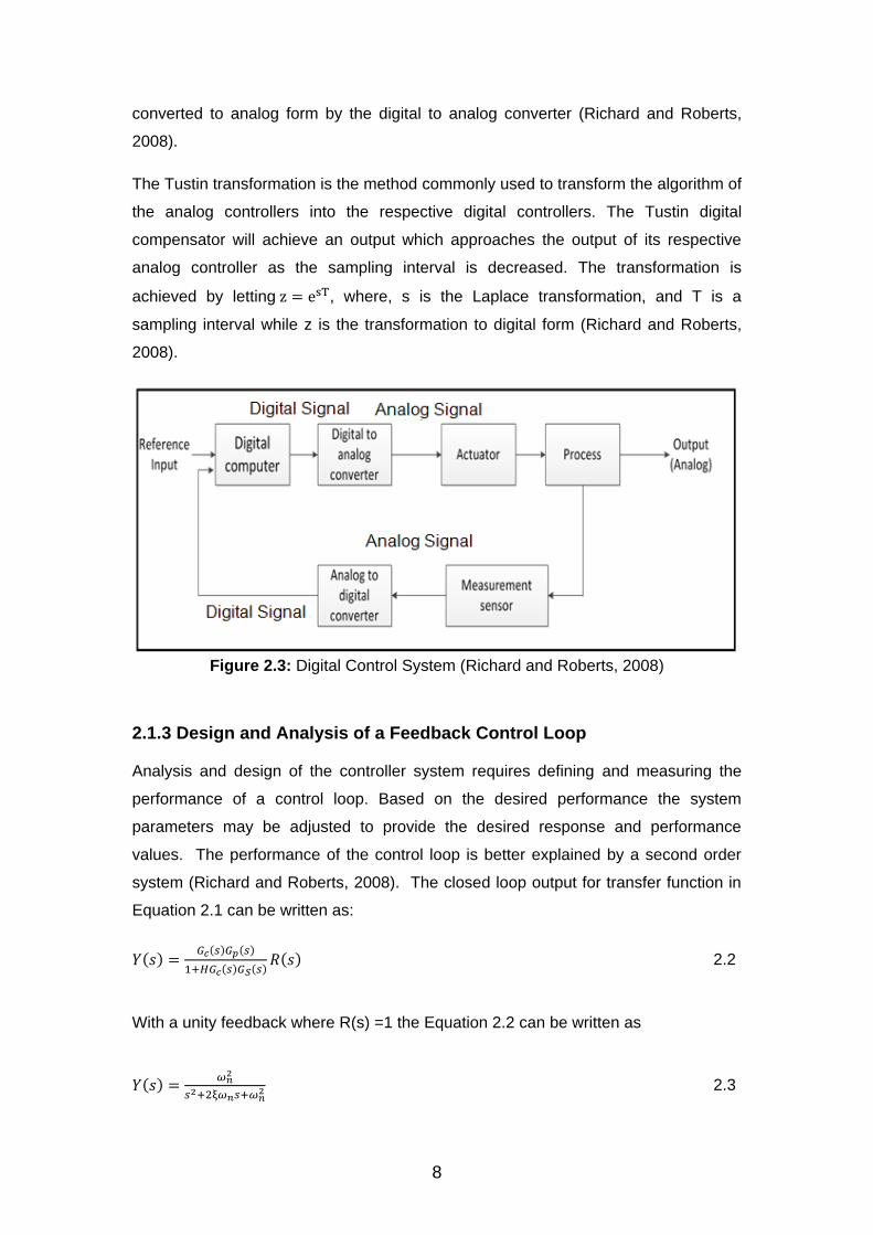
converted to analog form by the digital to analog converter (Richard and Roberts,
2008).
The Tustin transformation is the method commonly used to transform the algorithm of
the analog controllers into the respective digital controllers. The Tustin digital
compensator will achieve an output which approaches the output of its respective
analog controller as the sampling interval is decreased. The transformation is
achieved by letting z = esT, where, s is the Laplace transformation, and T is a
sampling interval while z is the transformation to digital form (Richard and Roberts,
2008).
Figure 2.3: Digital Control System (Richard and Roberts, 2008)
2.1.3 Design and Analysis of a Feedback Control Loop Analysis and design of the controller system requires defining and measuring the
performance of a control loop. Based on the desired performance the system
parameters may be adjusted to provide the desired response and performance
values. The performance of the control loop is better explained by a second order
system (Richard and Roberts, 2008). The closed loop output for transfer function in
Equation 2.1 can be written as:
𝑌(𝑠) =𝐺𝑐(𝑠)𝐺𝑝(𝑠)
1+𝐻𝐺𝑐(𝑠)𝐺𝑆(𝑠)𝑅(𝑠) 2.2
With a unity feedback where R(s) =1 the Equation 2.2 can be written as
𝑌(𝑠) =𝜔𝑛
2
𝑠2+2ξ𝜔𝑛𝑠+𝜔𝑛2 2.3

9
Where, the parameters are defined as:
𝜔𝑛2 is resonance frequency,
ξ is the overshot parameter which is referred to as dumping ratio, and
𝑠 is the Laplace transformation symbol.
The transient output is given by:
𝑦(𝑡) = 1 −1
𝛽𝑒ξ𝜔𝑛𝑡Sin (𝜔𝑛𝛽𝑡 + 𝜃) 2.4
where 𝛽 = √1−ξ2, 𝜃 = 𝑐𝑜𝑠−1ξ and 0< ξ <1. Figure 2.4 shows the transient response
of this second order functions. This figure shows the step response with multiple
dumping ratio which shows that the dumping ration can be selected to provide the
better response. The response of the second order function can further be
represented by Figure 2.5 which contains the standard performs characteristics
which are the settling time, peak response, the percentage overshoot and the rise
time.
Figure 2.4: Step Response Second Order Function (Richard and Roberts, 2008)
10
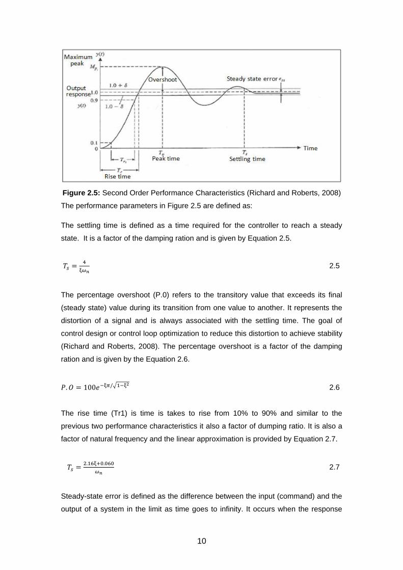
Figure 2.5: Second Order Performance Characteristics (Richard and Roberts, 2008)
The performance parameters in Figure 2.5 are defined as:
The settling time is defined as a time required for the controller to reach a steady
state. It is a factor of the damping ration and is given by Equation 2.5.
𝑇𝑠 =4
ξ𝜔𝑛 2.5
The percentage overshoot (P.0) refers to the transitory value that exceeds its final
(steady state) value during its transition from one value to another. It represents the
distortion of a signal and is always associated with the settling time. The goal of
control design or control loop optimization to reduce this distortion to achieve stability
(Richard and Roberts, 2008). The percentage overshoot is a factor of the damping
ration and is given by the Equation 2.6.
𝑃. 𝑂 = 100𝑒−ξ𝜋/√1−ξ2 2.6
The rise time (Tr1) is time is takes to rise from 10% to 90% and similar to the
previous two performance characteristics it also a factor of dumping ratio. It is also a
factor of natural frequency and the linear approximation is provided by Equation 2.7.
𝑇𝑠 =2.16ξ+0.060
𝜔𝑛 2.7
Steady-state error is defined as the difference between the input (command) and the
output of a system in the limit as time goes to infinity. It occurs when the response

11
has reached steady state (Richard and Roberts, 2008). Steady state error does not
form part the study. The performance parameter above is obtained for analysis and
design of the optimum controller.
2.1.4 Different Controller Types
Controllers are designed to provide required responses which allow the mechanical
or electrical systems to perform efficiently (Richard and Roberts, 2008). The primary
functions of the controllers are to provide a fast response to overcome the system
disturbance. A properly designed controller allows a feedback control loop to settle
faster reducing maintenance costs. Different types of controllers are in existence to
provide different response depending on the design of the system. The most
commonly used controllers are described:
Proportional only controller (P): by which the proportional term makes a
change to the output that is proportional to the current error value,
Integral only controller (I): reduces the magnitude of the error and the duration
of the error,
Proportional and Integral controller: is a combination of P and I controllers; it
accelerates the movement of the process towards set point and eliminates
the residual steady- stat,
Derivative controller (D): the derivative term slows the rate of change of the
controller output and this effect is most noticeable close to the controller set
point, and
Proportional, Integral and Derivative controller (PID): this controller performs
the functions of the above three controllers.
The controller used for this study is the PID type controller. This controller is given in
in Eqs 2.2 and 2.3 in analog and digital forms respectively.
In Analog form, the equation is given by:
ss
s KK
KG d
i
pC)( 2.2
12
where Gc(s), is the transfer function of the PID controller in analog form, Kp is a
proportional gain, Ki is an integral gain, Kd is proportional gain and s is the Laplace
transformation symbol in analog platform.
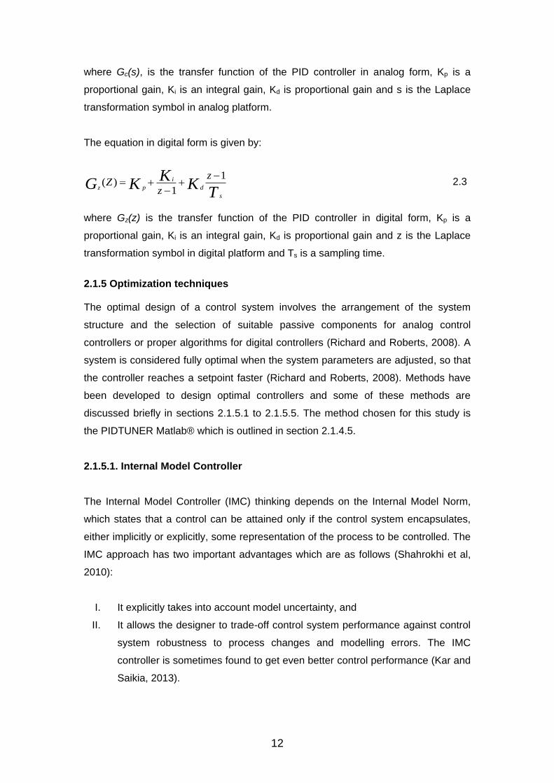
The equation in digital form is given by:
TK
KKG
s
d
i
pz
z
zZ
1
1)(
2.3
where Gz(z) is the transfer function of the PID controller in digital form, Kp is a
proportional gain, Ki is an integral gain, Kd is proportional gain and z is the Laplace
transformation symbol in digital platform and Ts is a sampling time.
2.1.5 Optimization techniques The optimal design of a control system involves the arrangement of the system
structure and the selection of suitable passive components for analog control
controllers or proper algorithms for digital controllers (Richard and Roberts, 2008). A
system is considered fully optimal when the system parameters are adjusted, so that
the controller reaches a setpoint faster (Richard and Roberts, 2008). Methods have
been developed to design optimal controllers and some of these methods are
discussed briefly in sections 2.1.5.1 to 2.1.5.5. The method chosen for this study is
the PIDTUNER Matlab® which is outlined in section 2.1.4.5.
2.1.5.1. Internal Model Controller
The Internal Model Controller (IMC) thinking depends on the Internal Model Norm,
which states that a control can be attained only if the control system encapsulates,
either implicitly or explicitly, some representation of the process to be controlled. The
IMC approach has two important advantages which are as follows (Shahrokhi et al,
2010):
I. It explicitly takes into account model uncertainty, and
II. It allows the designer to trade-off control system performance against control
system robustness to process changes and modelling errors. The IMC
controller is sometimes found to get even better control performance (Kar and
Saikia, 2013).
13
2.1.5.2. Zeiger Nichols Method
The Zeiger–Nichols method is heuristic method of designing and tuning a controller.
The method is used for tuning a PID controller type. When tuning this type of
controller, the Integral term, Ki and Derivative Kd term are set to zero and the
Proportional term Kp is adjusted from zero until it reaches the ultimate gain. The
ultimate gain oscillation period is then used to set the Kp, Ki, and Kd (Ziegler and
Nichols, 1942).
2.1.5.3. Tyreus Luyben Method
The Tyreus-Luyben method is quite similar to the Ziegler–Nichols one, but the final
controller settings are different. This method only proposes settings for PI and PID
controllers (Zanga et al, 2009). These settings are based on the ultimate gain. This
method is time - consuming and forces the system to margin if there is instability.
2.1.5.4. Fuzzy Logic Method Control
The control system models are described by mathematical models that follow the
laws of physics, stochastic models or mathematical logic models. Fuzzy logic
controllers are rules-based systems which are useful in the context of complex ill-
defined process, especially those which can be controlled by skilled human operator
without knowledge of their underlying dynamics (Herrera et al, 1995). Fuzzy logic is a
multifaceted scientific technique that permits solving challenging simulated problems
with many inputs and output variables. Fuzzy logic is able to give results in the form
of recommendation for a specific interval of output state (Fuller et al, 1996).
. , and J. L. Verdegay 2.1.5.5. Pidtune Matlab® Optimization Method
The Pidtune Matlab® Method (Matlab, 2003) automatically designs an optimal
controller for the plant. It allows the designer of the controller to specify the controller
type and provide the values of the controller in parallel form. A Matlab® Code for this
optimization technique is given in Appendix A. This method has been selected for
this study because it is easy to implement, does not require knowledge of Applied
Mathematics and conventional optimization methods mentioned above. The
operation of the Pidtune function works as follows:

14
It automatically tunes the PID gains ki, kp and kd of the PID controller to
balance the performance (response time) and robustness (stability &margins)
of a feedback controller in Figure 2.1.
C = PIDTUNE (G, TYPE), designs a PID controller for the single-input single-
output plant G which is the system process and the TYPE can be a controller
given below:
'P' Proportional only control
'I' Integral only control
'PI' PI control 'PD' PD control
'PID' PID control
‘PIDF’ PID control with first order derivative filter
The Pidtune specifies a target value WC in rad/time unit relative to the time units of
the system process in Figure 2.1 for a 0dB gain crossover frequency of the open-loop
response. It provides the performance for feedback loop based on the ratio of the
output and input.
Typically, it is found that WC relates to the control bandwidth and 1/WC relates to the
closed-loop response time. Then WC is increased to speed up the response and
1/WC is decreased to improve stability and when omitted, WC is peaked
automatically based on the plant dynamics.
The PIDTUNE then returns the coefficients of the parameters of the controller which
depend on the controller type.
2.2 Literature Survey
2.2.1 Studies Reviews
Studies have been conducted to, design effective control systems of the NPPs and
fossil plants. Some of the information from these studies will be used in Chapter 4 for
the analysis, optimization and verifications of the NSSS control loops. This includes
the following studies:
Automatic control of the Triga Reactor , Experiment B#6 (Power and
Edwards, 2005),

15
Optimization of the parameters of feed water control system for OPR 1000
nuclear power plants ( Kim et al, 2006),
Research on pressurizer water level control of pressurized water reactor
nuclear power station (Zanga et al, 2009),
Performance of Different Control Strategies for Boiler Drum Level Control
Using Labview (Kar and Saikia, 2013).
Comparison of state feedback and PID control of pressurizer water level in
nuclear power plant (Czaplin et al, 2013),
Water level control for a nuclear steam generator (Tau, 2013), and
Model Based Predictive Control for Load Following of a Pressurized Water
Reactor.
2.2.1.1 Automatic Control of the Triga Reactor Experiment B#6 An experiment was performed to design and implement an automatic controller for
regulating the Triga reactor (Power and Edwards, 2005). A controller was designed
and tested with Matlab®/Simulink which was used during their earlier lab
experiments to develop an automatic controller for the Triga Reactor. The controller
was converted from Simulink to C-Code software generator and down-loaded into the
computer, which was responsible for controlling the rods in real time. Continued
optimization was done on a designed PID controller and better regulating for the
Triga reactor was achieved.

16
2.2.1.2 Optimization of the Parameters of Feed Water Control System for OPR 1000 NPS The optimization of the parameter of the feed water control system was performed to
minimize the Steam Generator (SG) level deviation from the reference level during
transient for UCN 5 and 6 of the South Korean two loop 100 MWe Nuclear Reactor
(Kim et al, 2006). Since the objective functions were not available in the form of
analytical equations, the response for the input was evaluated by computer
simulations using the NPP system simulation code. The method that was used to
successfully optimize the feed water control loop was the Response Surface
Methodology (RSM). This optimization method utilizes useful regression models that
can easily be manipulated by the designer and also smooth’s out high frequency
noises. The results obtained shows that the optimized parameters have better SG
level control performance which resulted in reduction of reactor trips, reduction of
operator’s mental stress during transients and reduces mechanical stress on feed
water valves and pumps.
2.2.1.3 Research on Pressurizer Water Level Control of PWR NPS In the study by (Zanga et al, 2009), the subject of the water level control inside the
pressurizer in the nuclear power plant have investigated. Two types of the controllers
are developed to control the water level inside the pressuriser which is the PID
controller and fuzzy controller (Zanga et al, 2009), the controllers were designed
using Simulink and the performances of these controllers are provided in Table 2.2
which is the overshoot, adjacent time and first peak.
Table 2.1: Performance Values for the PID and PID + Fuzzy Controllers
Parameter PID PID + Fuzzy
Overshoot (%) 2.4 1.4
Time to reach
Peak (s)
390 250
Adjustable time 1000s 6500s
The mixed of PID with a Fuzzy controller performed better than the PID control alone.
The time to reach a first peak of 1.4 compared to 2.4 and the adjustable time sets
1000s and 6500s respectively.

17
2.2.1.4 Performance of different control strategies for Boiler Drum Level Control The performance of different control strategies of the drum level control system was
evaluated and different control methodologies including the Zeiger Nicholes, IMC
controller, Tyreus Luyben PID tuning and fuzzy logic method control was used to
design a controller for the Boiler Drum Level controller (Kar and Saikia 2013). The
IMC controller equation is selected for verification in for this study and its feedback
equation is given by equation 2.4 where Q(s) is the transfer function. The
performance of this controller is simulated using Matlab® program in Appendix B to
obtain similar performance parameters.
Q(s) =0.08s3+0.02002s2+0.4005s+0.001142.8
0.0016s4+0.032s3+0.24s2+0.8s+1 2.4
2.2.1.4.1Boiler Drum Controller Analysis
By using the equation 2.4, the step response and the corresponding performance for
this equation is provided in Figure 2.6 and Table 2.3.
Figure 2.6: Boiler Drum Controller Step Response

18
Table 2.2: Boiler Drum Controller Performance Values
Parameter Value
Overshoot 6.5635e+04
Peak time (s) 0.0515
Rise time (s) 1.8849e-05
Settling time (s) 6.0587
The controller has a peak time of 0.0515, rise time of 1.884e-0.5 and settling time of
6.0587. The controller takes 6.0587 to reach a setpoint of 85%.
The performance of different control strategies of the drum level control system
concluded the following:
The IMC controller was found to get even better and smoother results than
the simple PID controller,
The Fuzzy logic controller have shown to perform better than IMC, Zeiger
Nicholes and Tyreus Luyben tuning methods, and
Another novel approach for a better controller was using fuzzy logic to control
the drum level.
2.2.1.5 Comparison of State Feedback and PID control of Pressurizer Water Level In this paper a water level control system for a pressurizer is designed from scratch,
and the PID controller is replaced by a control algorithm which consists of state
feedback integral controller (SFIC) and reduced – order Luenberger state observer
(Czaplin et al, 2013). The main purpose of this study is redesign the existing solution
in NPP by replacing a PID controller with a better performing controller in order to
obtain better performance which will enable the plant to function efficiently. The
transfer functions for these two controllers are provided in Table 2.3. The SFIC
equation is used in Chapter 6 for validation of the pressurizer level controller
performance.
19
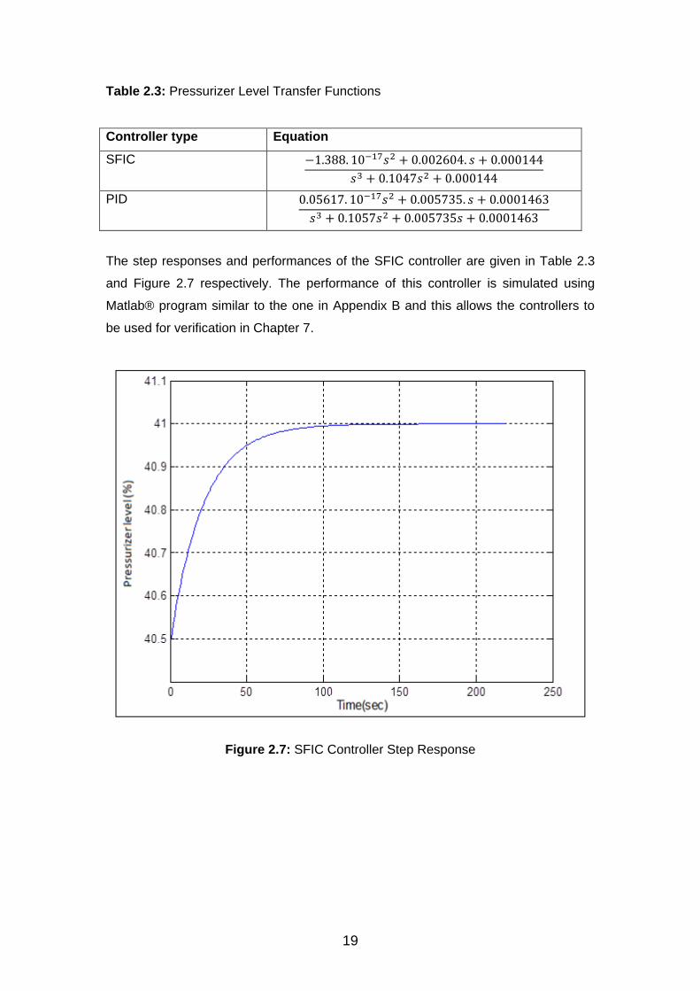
Table 2.3: Pressurizer Level Transfer Functions
Controller type Equation
SFIC −1.388. 10−17𝑠2 + 0.002604. 𝑠 + 0.000144
𝑠3 + 0.1047𝑠2 + 0.000144
PID 0.05617. 10−17𝑠2 + 0.005735. 𝑠 + 0.0001463
𝑠3 + 0.1057𝑠2 + 0.005735𝑠 + 0.0001463
The step responses and performances of the SFIC controller are given in Table 2.3
and Figure 2.7 respectively. The performance of this controller is simulated using
Matlab® program similar to the one in Appendix B and this allows the controllers to
be used for verification in Chapter 7.
Figure 2.7: SFIC Controller Step Response

20
Table 2.4: SFIC Controller Performance Values
Parameter Value
Overshoot 0
Peak time (s) 17.0000
Rise time (s) 0.5000
Settling time (s) 200
The controller has a zero overshoot, peak time of 17, and rise time of 0.5 and settling
time of 200 seconds. The controller takes 200 seconds to reach a setpoint of 41%
level.
This study suggests the following:
It is possible to design a state feedback controller with integral action and
state observer for the purpose of water level control in nuclear plant
pressurizer,
Even if the control quality of a SFIC controller is not better than the quality of
the PID controller it shows that the order approach to the problem can be also
successful,
This can be used as a base for the further research on the subject of SFC use
in NPS control system.
A further works should be to check the work of the SFIC control system in
professional environment dedicated to the simulation of NPPs such as
APROS or Flownex, which use more complex models of a pressurizer
2.2.1.6 Water Level Control for a Nuclear Steam Generator A steam water level controller for the PWR power plant was designed using a simple
gain schedule (Tau, 2013). The control system designed was based on Internal
Modelling Control (IMC) principle, and the performance the system can be tuned on-
line. It was concluded that compared with advanced control techniques such as linear
matrix inequality (LMI), the design procedure using IMC was much simpler and the
simple gain scheduled controller could a achieve good performance. He also
concluded that unlike the LMI method stability can be granted for the gain scheduled
controller.

21
2.2.1.7 Model Based Predictive Control for Load Following of a Pressurized Water Reactor A study was conducted to develop an MPC controller for the control of the PWR plant
during load following operations (Human, 2009). To develop the MPC controller a
model was first developed from measured data taken from the PWR simulator. By
using a process of system identification Matlab® tool several sets of measured data
from the simulator was collected and several nonlinear models were obtained. The
model were first linearized and transformed to linear state models and once that was
done, the best fit approach was used verify the models and the best performing
model was used as an input for developing this MPC controller. The Simulink ®
simulation was also created to evaluate the performance of the MPC controller
against the data from the PWR simulator which represent the plant. The developed
controller was also evaluated using the ITAE performance criteria.
The following conclusions, closure and recommendations were obtained:
System identification is feasible methods to be used for creating a model for
PWR and can further be used to develop control strategy for the plant,
MPC controller developed controller outputs exceptionally,
The identified plant model used to develop the MPC controller be evaluated
on plant model created from the first principle,
Separate research studies into the topics of system identification and MPC
controller is recommended for fine tuning the method of creating the plant
models and the MPC controller, and
The MPC controller performed successfully controlled the PWR plant and
outperformed the conventional controller in two of the three main controls.
2.2.2 Studies Reviews Conclusions
The literature survey have been conducted to, design effective control systems of the
NPPs and fossil plants. It is noted from different studies that different existing control
design method can be used to obtain better performance of controlling power plants.
This includes method such as Internal Modelling Control, linear Matrix Inequality,
state feedback controller reduced – order Luenberger state Observer and Fuzzy
Neural Networks. These provide confidence that obtaining controller with better
performs for KPP can be achieved.
22
CHAPTER 3
Koeberg Nuclear Steam Supply Controllers
In this chapter, a description and operation characteristics of the four selected
controllers are discussed. These controllers are the Primary Temperature Control
Loop (PTC), Pressurizer Pressure Control Loop (PPC), Pressurizer Level Control
Loop (PLC) and the Steam Generator Level Control Loop (SGLC).
3.1 Koeberg Nuclear Steam Supply Systems
KPP like all the other Eskom coal power stations is required to operate steadily when
coupled with the South African grid. This is assured by the Nuclear Steam Supply
Controllers. The KPP has two reactor units. The units are designed to be controlled
manually when operating at less than 15% of rated power and operate automatically
between 15% and 100% (Koeberg, 1997). However, owing to low-cost price of
uranium fuel and power constraints of the South African grid, units of KPP are
normally operated on manual closer to 100% during normal operation (Eskom, 2008).
The units of KPP are designed to operate in the reactor following mode, mechanical
power generated by a turbine is adjusted in accordance with the grid demand in a
steady manner. The Nuclear Steam Supply Controllers enable the plant to achieve
stability by performing the following functions:
Mitigation against transients created by operating requirements,
Allows the manoeuvrability of power to meet the desired electrical grid
demand, and
Limits the actuation of the reactor protection system and as a result increase
the plants availability and reliability (Eskom, 2008).
3.1.1 Primary Temperature Control
In Pressurized Water Reactor (PWR) type, the primary pressure is restricted to a
constant value and for the units of KPP pressure is kept at 155 Bars (absolute)
during normal operations (Eskom, 2008). In order to increase the thermal efficiency
cycle of the plant, the coolant temperature from the reactor fuel to the Steam
Generator (SG) must be increased. It is also important to manage the primary

23
coolant temperature in order to maintain system operating pressure and to avoid
failure of the primary system. As a result, the Primary Temperature Controller is a
very important controller for organization of both the efficiency and the integrity of the
nuclear power station.
The primary temperature control is achieved by insertion and removal of the control
rods (Eskom, 2008) in and out the reactor core respectively, which generates heat.
To fully appreciate the operation of this controller, the following concepts which
directly influence this PTC controller are explained:
Reactor pressure vessel and reactor core,
The rod control system,
Nuclear instrumentation system,
Average primary temperature measurements, and
The primary temperature controller characteristics.
3.1.1.1 Reactor Pressure Vessel and Reactor Core
The Reactor Pressure Vessel (RPV) is a cylindrical vessel with hemispherical bottom
and removable top head. The top head is removable to allow for the refuelling of the
reactor core during outages. The cylindrical vessel consist of three inlet nozzles to
allow cold water from the steam generator and three outlet nozzles to allow water
into the steam generators (Koeberg, 2006). The purpose of the RPV is to provide the
following:
Support fuel assembly,
Distribute the primary coolant for efficient transfer of heat,
Support the control rod drive mechanism,
Support the in-core instrument used for core power analysis, and
Also serves as a secondary radiation barrier by providing separation between
the fuel elements and the environment (Koeberg, 2006).
The coolant enters the reactor vessel at the inlet nozzles and hits against the core
barrel which forces the water to flow downwards in the spacer located between the
reactor vessel wall and the core barrel (Koeberg, 2006). The flow will then turns
upwards and pass though the fuel assembly peaking up heat. The hot water will then
be routed to the outlet nozzle via upper internal to the steam generator’s heat
exchanger where it losses heat to the secondary system. Shown in Figure 3.1 are the

24
components of the reactor vessel and the order components associated with it
(Koeberg, 2006). The included components are:
The control rod drive mechanism and rod travel housing,
Instruments ports,
Upper support plate and internal support ledge,
Lifting lug,
Core barrel,
Control rod guide tube and control rod driveshaft,
Support column and upper core plate,
Inlet shaft and upper core plate,
Outlet nozzle and control rod cluster,
Access port and baffle radial support,
Baffle, lower core plate and instrument thimble guides, and
Radial support and core support.
Figure 3.1: Reactor Vessel and Associated Components (Koeberg, 2006)

25
The reactor core is located inside the reactor vessel and is responsible for generating
heat. The core is supported by the lower core structure which is surrounded by the
core barrel and held in place by the upper and lower support structures shown in
Figure 3.1. Each reactor core consists of 157 fuel elements set vertically and
adjacent to each other with the height of 3.658 m (Koeberg, 2006). Seventy - two
tons of uranium is used to produce 2775 MWth of thermal heat at full load which
generates 960 MWe of electrical power. Each fuel element is 214 mm by 214 mm
and about 4 m length and has a total mass of 666 kg. Each fuel element has 264 fuel
rods set in a 17 x 17 array. The remaining 25 positions in the array have guide tubes
for control rods, temperature and flux monitoring instruments inserts (Koeberg,
2006).
3.1.1.2 Control Rod Cluster System
The KPP unit consists of a 48 rod cluster assembly and these rods are divided into
six groups (Koeberg, 2007). Each group is denoted by letters A, B, C, D, SA and SB.
The six groups are then divided into sub-groups of 4 each and are referred to as
SA1, SA2, SB1, SB2, A1, A2, etc. SA and SB rods clusters are responsible for the
reactor trip function and does not form part of this study.
The rod control clusters A, B, C and D are designed to automatically control the
reactor in the steady state by regulating the reactivity in the core and as a result
regulating the primary temperature (Koeberg, 2007). The rod control cluster is made
of alloy of 80% Sliver, 15% Indium and 5% Cadmium enclosed in the stainless steel
tubing which is sealed and welded. A rod cluster is shown in Figure 3.2. The control
rods move up and down inside the zircaloy tubes positioned within the fuel assembly.
These rods are attached to the spider assembly which is attached to the drive shaft
responsible for movement. As shown in Figure 3.2, the rod cluster components are
the hold down spring, top nozzle, grid spring, bottom nozzle, thimble tube, mixing
vanes and thimble screw.

26
Figure 3.2: Rod Cluster (Koeberg, 2007)
3.1.1.3 Nuclear Instrumentation System
The purpose of the Nuclear Instrumentation System (NIS) is to provide continued
monitoring of reactor power or changes in power level and flux distribution on bases
of the neutron flux measurement, by means of a series of detectors (Koeberg, 2009).
The neutron flux measurement is a reflection of neutrons population which
represents the reactor power. Three types of detectors are used for measuring this
reactor power during all operating power conditions which are the source range,
intermediate range and power range. During steady state operation, only the four
power range and two Intermediate range detectors are operational while the
remaining two source range detectors are out of service with their supply voltage
sources removed. These detectors are discussed in the next three paragraphs.
The source range detectors are of the Proportional Counter type. These detectors
are lined with Boron -10 and then the Boron layer absorbing neutron and produce
Lithium-7 and Helium nuclides are (Koeberg, 2009). The Helium nuclide then ionizes
the Argon gas, which under the presence of a high voltage generates an electrical

27
impulse. This electric pulse is then amplified and used to determine power at a lower
level at less than 10% of the rated power thermal power.
The role of the intermediate detectors is to provide values of the reactor power when
the power is above 10%. These detectors are Compensated Ion Chamber types and
each detector is made up of two chambers. One chamber is lined with Boron and
emits a signal that is proportional to the gamma and neutron radiation (Koeberg,
2009) and the other chamber emits a signal proportional to the gamma radiation. The
algebraic difference of these two signals is proportional to neutron flux and produces
the signal which is used to measure power during power supply shutdowns or reactor
trip.
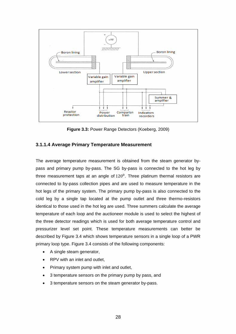
Four power range detectors are used during normal operations to reflect the power of
the reactor core and to regulate power by supplying values to the primary
temperature control loop. The detectors are of the Non-Compensated Ion Chamber
type and are shown in Figure 3.3. Each of the detectors has two ion chambers with
one covering the upper half of the core and the other covering the lower half. As the
neutron flux is far greater than the gamma flux, the detectors are uncompensated
and contain Boron lining. They produce a current which is amplified before being
used for both reactor trip and primary temperature control. The Power Range
Detectors shown in Figure 3.3 consist of the following components:
The upper and lower sections,
2 variable gain amplifiers,
Summer & amplifier module, and
+HV high voltage supply.
28
Figure 3.3: Power Range Detectors (Koeberg, 2009)
3.1.1.4 Average Primary Temperature Measurement
The average temperature measurement is obtained from the steam generator by-
pass and primary pump by-pass. The SG by-pass is connected to the hot leg by
three measurement taps at an angle of 1200. Three platinum thermal resistors are
connected to by-pass collection pipes and are used to measure temperature in the
hot legs of the primary system. The primary pump by-pass is also connected to the
cold leg by a single tap located at the pump outlet and three thermo-resistors
identical to those used in the hot leg are used. Three summers calculate the average
temperature of each loop and the auctioneer module is used to select the highest of
the three detector readings which is used for both average temperature control and
pressurizer level set point. These temperature measurements can better be
described by Figure 3.4 which shows temperature sensors in a single loop of a PWR
primary loop type. Figure 3.4 consists of the following components:
A single steam generator,
RPV with an inlet and outlet,
Primary system pump with inlet and outlet,
3 temperature sensors on the primary pump by pass, and
3 temperature sensors on the steam generator by-pass.

29
Figure 3.4: Primary System Temperature Measurements Sensors (Koeberg, 1997)
3.1.1.4 Turbine Power Measurement
The turbine power is also one of the parameter used to regulate the primary
temperature. This power is represented by the first stage pressure on the high
pressure turbine. Pressure sensor is placed in the turbine which is located between
the regulating valves and the low pressure turbine is shown by KPP turbine
arrangement in Figure 3.5 (Eskom, 1985). Displayed on the Figure are the following
components:
3 steam lines,
4 moisture separators,
High pressure turbine (HP),
3 low pressure (LP) turbines, and
6 main stop valves and 6 regulating valves.

30
Figure 3.5: Koeberg Power Plant Turbine Arrangement (Eskom, 1985)
3.1.1.6 Primary Temperature Controller Characteristics
The PTC functional characteristics are shown is shown in Figure 3.6. The controllers
got their readings from nuclear power, turbine load, average primary temperature,
first stage pressure readings and insert the control rods into the reactor core. The
PTC characteristics consist of the following:
Nuclear power measurement (NS),
Turbine power (PS),
Average temperature measurement (TS),
Controller -1 and its equation,
Controller -2 and its equation,
Summer, and
Control rods position dynamics obtained from Experiment B#6 by M.A. Power
and R.M. Edwards (Zanga et al, 2009).

31
Figure 3.6 Primary Temperature Functional Characteristics (Koeberg, 1997, Power
and Edwards, 2005 and Koeberg, 2006)
The PTC functional characteristics reflected in Figure 3.6 operate as follows:
Nuclear power is measured by the power range level sensor (NS),
The value from the level sensor feed into the controller -1,
Average temperature is measured by a temperature sensor (TS) and is
processed by controller-2,
Unit power is measured by first stage pressure, and
Signal from the unit power, output of controllers -1 and -2 are cascaded using
a summer and feed into the control rods dynamics (GR(s)).
3.1.2 Pressurizer Pressure Control
The pressurizer pressure control is one of the most important parameters of the PWR
type. Pressure in the primary circuit is maintained at the pressure value of 155 Bars

32
(Koeberg, 2009). However, during power generation there are thermal transients in
the reactor coolant system which results in large swings in pressurizer liquid volume.
The pressurizer pressure control loop allows for the management of these pressure
swings by using electrical heaters and the spraying of the cooler water into the
pressurizer. The main purpose of the Pressuriser Pressure Control is to maintain
primary pressure at a constant value of 155 Bars absolute to avoid boiling of the
primary coolant (Koeberg, 2009). To fully understand the operation of the PPC, three
concepts that need to be understood are:
PWR pressurizer,
Pressurizer associated components, and
Pressurizer pressure functional characteristics.
These concepts are being discussed briefly in the sections 3.1.2.1 and 3.1.2.2.
3. 1.2.1 Pressurizer
The pressuriser is a cylindrical vessel of about 13 m high and 2 m in diameter and is
connected to the piping of the primary system. It is the component of the PWR in
which liquid and vapour can be maintained in equilibrium under saturated conditions
for PWR pressure control purposes. The pressuriser used by units of KPP is` shown
in Figure 3.5 and its major components include the Spray nozzle, safety valve nozzle,
relief valve nozzle, manway, upper head, upper instrumentation nozzle, insulation
support, valve support brackets, seismic lugs, shell barrel, lower instrumentation
nozzle, bottom head, immersion heaters, support skirt and surge nozzle (Koeberg,
2006).

33
Figure 3.7: Pressurizer (Koeberg, 2006)
3. 1.2.2 Pressurizer Pressure Functional Characteristics
The pressurizer pressure is controlled by either increasing power to the heaters to
elevate the saturation conditions or by spraying water into the steam space to
condense some steam which then results in the reduction of the saturation
conditions. Banks of electrical heaters at the base maintain the pressuriser at the
saturation temperature which corresponds to the primary system pressure. The PPC
is described in Figure 3.8, highlighting the pressuriser and the following associated
components:
Groups of heaters used to heat water,
One spray system using two circuits which have two valves,
Three relief valves,
Safety valves, and

34
Pressurizer relief tank.
Figure 3.8: Pressurizer Associated Components (Eskom, 2009 and Koeberg, 1997)
The function of the heaters is to increase the pressure when it falls below 155 Bars
(absolute). The water inside the system is heated and steam is produced which will
increase the pressure. The electrical heating consists of 6 groups of heaters. The
heaters’ elements use a three-phase 220/380 V-50Hz current power supply and are
assembled in a delta configuration. Two types of heaters are used namely the
proportional heaters and the on – off heater. On – off heaters are turned on when the
pressure is too low or the level is too high and are also in use during unit start up. Of
the six groups of heaters two groups have variable power controllers and are used to
compensate for pressure heat losses and the cooling owing to the control spray
system (Koeberg, 2006).
The spray system is used to reduce high pressure. The spray is directly operated by
the control system which draws the colder water from the cold loops of the primary
loop into the pressuriser. This colder water in droplets form makes contact with the
steam and results in the reduction of the pressure.
The Primary Pressure Controller is shown in Figure 3.9, pressure is measured by the
sensors and fed in to the controller. The controller then actuate four actuates based
on the pressure value. The four controlled actuators are the proportional heaters, on-

35
off spray, on-off heaters and proportional spray. Only the heater function is used for
this study.
Figure 3.9 Pressurizer Pressure Functional Characteristics (Koeberg, 1997, Zanga
et al, 2009 and Koeberg, 2006)
3. 1.3. Pressurizer Level Control
The pressuriser level control system shown in Figure. 3.10 functions in close co-
operation with the pressure control system. The pressurizer level and pressure affect
each other. The spray valve used for reducing pressure is also used to increase the
level inside the pressurizer.
During normal operations, the pressuriser liquid level must be carefully monitored
and controlled so that the correct liquid-vapour ratio exists for proper pressure control
during normal and transient plant operation. In order to control the main circuit
pressure of the reactor, the pressurizer needs to maintain water and steam saturation
in the balance. During steady state, approximately 40 % of the lower part of the
pressure cavity is filled with water and 60 % of the upper cavity is filled with steam
(Eskom, 1997).

36
Figure 3.10: Pressurizer Level Control (Koeberg, 2006)
3.1.3.1 Pressuriser Level Functional Operation
Three level transmitters are placed inside the pressurizer and one of them is used for
level control. The water level in the pressurizer is programmed as a function of the
reactor coolant average temperature. Figure 3.11 indicates the pressurizer functional
diagram. In this diagram, the amount of solid liquid water inside the pressurizer is
around 40%. The remaining 60% is the saturated steam. The water level is controlled
from 19% to 42.5% of pressurizer liquid water and with variation powers of about
15% to 100% (Herrera et al, 1995).
Figure 3.11: Pressurizer Level Functional Diagram (Eskom, 2006)

37
3.1.2.2 Pressurizer Level Functional Characteristics
The pressurizer level controls operating characteristics are shown in Figure 3.12. As
shown in this figure the level is measured by the pressurizer sensor and the pressure
is then fed into the pressurizer program. The signal from the pressurizer program is
then used to control the spray valve as shown below.
Figure 3.12: Pressurizer Level Functional Characteristics (Koeberg, 1997, Zanga et
al, 2009 and Koeberg, 2009)
The Pressurizer level functional characteristics work as follows:
Pressurizer level is measured by the pressure level sensor (LS)
The value from the pressure is fed into the controller,
The control actuates the proportional heaters, on-off spray, on-off heaters and
proportional spray.
38
3.1.4 Steam Generator Level Control
The nuclear power plant is composed of three major energy conversion systems. The
primary system transports the heat generated in the fuel to the steam generators,
where the heat is transferred to the secondary system. The secondary system
converts this heat energy to mechanical work output of the turbine and the third
energy conversion system is the circulating water which serves as a necessary heat
sink for the entire PWR system (Koeberg, 1997). This controller is unique since it is
designed to stop water from over following into the turbine which can result with the
turbine blades been damage. To appreciate the operation of this SG Level Controller,
the following concepts which directly influence controller are discussed:
The steam generator, and
Feed water system.
3.1.4.1 Steam Generator
The steam generator is a vertical shell heat exchanger used to convert water into
steam using heat generated by the reactor core. The primary coolant water enters
the lower end of the steam generator through one of the water boxes and flows
through the inverted U-tubes, leaving the steam generator by the other water-box.
Steam is generated from the feed-water on the secondary side and flows upward
past the tube bundle. It then flows through the moisture separator components to the
outlet nozzle at the top of the vessel (Shahrokhi et al, 2010). The components of the
steam generators as shown in Figure 3.18 are:
Chevron dryers Efflux, Feed Water inlet,
Secondary manway,
Narrow range level measurement, J-Tubes Feed ring Riser,
Cyclone driers, Down comer, Tube wrapper,
APG blow down, Hand hole, Inspection hole, Primary coolant outlet,
Primary coolant inlet, Flow distribution baffle, Tube bundle,
Ant vibration spaces, Intermediate tube, support plate,
Tube bundle (U-tubes), and
Flow disruption baffle.

39
Figure 3.13: Steam Generator (Eskom, 2009)
3.1.4.2. Feed Water System
The feed water controller system is responsible for the management of the water
level inside the steam generator. Water level regulation is achieved by maintaining
the level inside the steam generator below the edge of the cyclone dryer’s wrapper
and above the steam generator feed water ring. This level is not allowed to rise too
high as this would lead to excessive moisture carryover causing turbine damage. The
water level must also not be allowed to fall too low as this would uncover the feed
water ring which could result in water hammer in the feed water pipes. The water
level also has nuclear safety implications because it allows heat removal. The steam

40
generator level controller is shown in Figure 3.14, which shows the flow of water from
the three steam generators to the high pressure turbine and back into the steam
generators. This Figure also demonstrate how level is measured by the narrow range
sensors (MD) and 1st stage pressure (MP) and their signal feed into the PID and PI
controllers. It also shows the valve that is being manipulated to increase and
decrease the flow and the level programme generator.
Figure 3.14: Feed Water Level Control System (Eskom, 2008)
3.1.4.3 Steam Generator Level Controller Characteristics
The steam generator level operating characteristics are shown in Figure 3.15 that
illustrates the following functionalities:
Narrow range level sensor (LS),
1st Stage pressure measurement (PS),
Steam flow measurement (FS1),
Feed flow (FS2),
Controller -1 (PI) level error controller,
Controller -2 (PI) and its equation,
Drum level process variable, and
A Summer-1 and Summer-2.

41
Figure 3.15: Steam Generator Level Functional Characteristics (Koeberg, 1997 and
Kar and Saikia, 2013)
The operations of the SG level operation characteristic shown in Figure 3.15 operate
as follows:
Narrow range, 1st stage pressure, steam flow and feed water flow are
measured by different sensors,
Narrow range level measurement from the sensor MN is cascaded with 1st
stage pressure measurement (MP) by summer -1,
The signal from summer -1 is the corrected by PI level error controller,
Similar to the second step steam flow measurement (MD 1) and feed flow
measurement (MD 2) are cascaded using a summer-2, and
The output from summer-2 together with the output from PI (level error
controller) are feed into controller -2 which is used to control the drum level
processed variable obtained from (Kar and Saikia, 2013).

42
CHAPTER 4
Koeberg Power Plant Analog Controllers Analysis
Optimization of the Koeberg Power Plant by implementing customized transfer
functions requires analysis of the current analog controls to be compared with new
customized digital ones. In this chapter analysis of the four KPP analog controllers
has been done.
4.1 Analog Controllers Analysis Methodology
Analyses of the KPP analog controllers are performed using Matlab®. Using the
control loop feedback function method described in chapter 2, the following
characteristics of the control loops are obtained:
The feedback control loop transfer function equations which are used for
developing step responses and control loop performances,
Step responses, and
Performance of the control loops which includes the settling time, percentage
overshoot, peak time and rise time. Even though a few of the performance
parameters are provided only the settling time shall be used to explain the
controller performance.
4.2 Analog Controllers Analysis
The analysis of the KPP analog controllers involves the:
Primary Temperatures Controller,
Pressurizer Pressure Controller,
Pressurizer Level Controller, and
Steam Generator Level Controller respectively.
4.2 .1 Analog Primary Temperature Controller Analysis The PWR Primary Temperature Control is performed by inserting the control rods
into the reactor core which determine the amount of primary loop temperature and
power produced as discussed in Chapter 3. Varying the position of the control rods is
performed by the Primary Temperature Controller (PTC) which is been examined this

43
section. The PTC comprises of two controllers. Analysis of the PTC is performed
using controller-1 and control rods position dynamics.
Analog PTC with controller-1 in use can be represented by the analog PTC feedback
loop in Figure 4.1, which consists of the following features:
Temperature step input with the set point at 310 oC,
Controller -1 equation used to control the temperature,
GR(s) control rods position dynamics equation, and
Y(s), Output Temperature.
Figure 4.1: Analog Primary Temperature Controller Feedback Loop Primary
(Koeberg, 1997 and Power and Edwards, 2005 )
The analog PTC feedback loop in Figure 4.1 is used to generate the following transfer function:
T1(s) =Y(s)
R(s)=
Gc((s)GR(s)
1+Gc((s)GR(s)=
1.143 X 10⁶ X S2 + 1.143 X 1005S
S4+ 200S3+1.143 X 1006S2+1.143 X 1005 4.1
where,
T1(s) is the transfer function,
R(s) is the input,
Gc(s) is the controller-1,
s is a Laplace convention symbol,
GR(s) is the control rods position dynamics, and
Y(s) is the output.

44
Using Matlab®, the analog PTC step response has been generated by providing the
unit step function to obtain the temperature shown in Figure 4.2 and its
corresponding performance values Table in Table 4.1.
Figure 4.2: Analog Primary Temperature Controller Step Response
Table 4.1: Analog Primary Temperature Controller Performance Values
Parameter Value
Overshoot 0
Peak time (s) 1.049e+5
Rise time (s) 2.0980e+04
Settling time (s) 3.8879e+5
The behaviour of the analog PTC controller is shown by a step response graph in
Figure 4.1 and the performance values are provided in Table 4.1.The controller has a
zero overshoot, peak time of 1.049e+5 , rise time of 2.0980e+04 and settling time of
3.8879e+5 seconds. The controller will take a long time to reach a setpoint of 310.2
oC and improvement can be done to obtain better performance of less than 3
seconds.
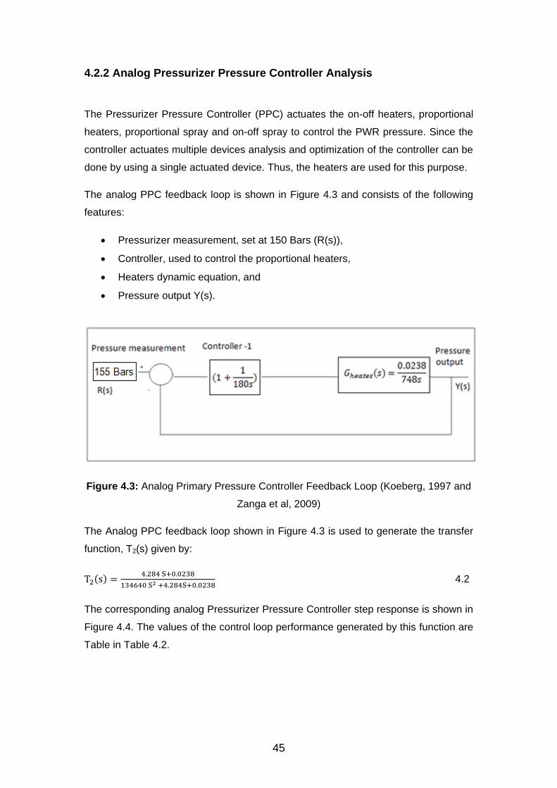
45
4.2.2 Analog Pressurizer Pressure Controller Analysis
The Pressurizer Pressure Controller (PPC) actuates the on-off heaters, proportional
heaters, proportional spray and on-off spray to control the PWR pressure. Since the
controller actuates multiple devices analysis and optimization of the controller can be
done by using a single actuated device. Thus, the heaters are used for this purpose.
The analog PPC feedback loop is shown in Figure 4.3 and consists of the following
features:
Pressurizer measurement, set at 150 Bars (R(s)),
Controller, used to control the proportional heaters,
Heaters dynamic equation, and
Pressure output Y(s).
Figure 4.3: Analog Primary Pressure Controller Feedback Loop (Koeberg, 1997 and
Zanga et al, 2009)
The Analog PPC feedback loop shown in Figure 4.3 is used to generate the transfer
function, T2(s) given by:
T2(s) =4.284 S+0.0238
134640 S2 +4.284S+0.0238 4.2
The corresponding analog Pressurizer Pressure Controller step response is shown in
Figure 4.4. The values of the control loop performance generated by this function are
Table in Table 4.2.

46
Figure 4.4: Analog Pressurizer Pressure Controller Step Response
Table 4.2: Analog Pressurizer Pressure Controller Performance Values
Parameter Value
Overshoot (%) 88.7991
Peak time (s) 7.4722e+03
Rise time (s) 3.0010e+03
Settling time (s) 2.4014e+05
The behaviour of the analog PPC controller is shown by a step response graph in
Figure 4.4 and the performance values are provided in Table 4.2. The controller has
an overshoot of 88.799, peak time of 7.4722e+03, rise time of 3.0010e+03 and
settling time of 2.4014e+05 seconds. The controller will take a long time to reach a
set-point of 155 Bars and improvement can be done to obtain better performance of
less than 3 seconds.

47
4.2.3 Analog Pressurizer Level Controller Analysis
The Pressurizer Level Control represents the PWR primary system level. It is one of
the critical parameter for operation of the PWR type reactor, in a sense that it works
in conjunction with the PTC to determine the power, primary system inventory and
covering of the reactor core. The analog PLC feedback loop shown in Figure 4.5 has
a single controller and the following associated parameters:
A level set point, at 41 %,
Controller, which is used to vary the level,
Pressurizer level dynamic process, and
PRZ level output.
Figure 4.5: Analog Pressurizer Level Controller Feedback Loop Characteristics
(Koeberg, 1997 and Zanga et al, 2009)
The transfer function, T4(s) generated from the analog PLC feedback loop shown in
Figure. 4.5 are given by:
T4(s) =6.314 X 1007 S3+2.87 X 1006 S2 +0.2892
2.183 X 1008 S4+6.536 X S07 S3+2.875 X 1006 S2+0.2892 4.3
The corresponding analog PLC step response is shown in Figure 4.6, while the
analog PLC performance values are given in Table 4.3.

48
Figure 4.6: Analog Pressurizer Level Controller Step Response
Table 4.3: Analog Pressurizer Level Controller Performance Values
Parameter Value
Overshoot 17.971
Peak time (s) 77.4000
Rise time (s) 37.6000
Settling time (s) 147.3500
The behaviour of the analog PLC controller is shown by a step response graph in
Figure 4.6 and the performance values are provided in Table 4.3. The controller has
an overshoot of 17.971, peak time of 77.4000, rise time of 37.6000 and settling time
of 147.3500seconds. Unlike the previous two controllers in sections 4.2.1 and 4.2.2,
the analog PLC has a shorter settling time. Improvement can also be done to get a
better performance of less than 3 seconds.

49
4.2.4 Analog Steam Generator Level Controller Analysis
The analog SG Level Controller (SGLC) is represented by a feedback system
consisting of two controllers as shown in Figure 3.16 in Chapter 3. In order to analyse
the analog SGLC, the two steps given below allow the controller to be optimized
easily in the next chapter.
Investigation is first performed using controller - 2 and the drum level process
variable, and
Analysis will be done using a combination of controller -1 and 2 with the drum
level process variable
4.2.4.1 Analog Steam Generator Level Controller-2 Analysis
The feedback control loop for the analog SG level controller with controller-2 in
presence is demonstrated by Figure 4.7 which contains the following:
R(s) is a step input with the level set point at 60%,
Controller -2,
Drum level process variable, and
Y(s) is the level output.
Figure 4.7: Analog Steam Generator Level Controller -2 Feedback Loop (Koeberg,
1997 and Kar and Saikia, 2013)
The transfer function, T5(s) generated from the analog sglc-2 feedback loop depicted
in figure. 4.7. Eq 4.4, step response is given in Figure 4.8 and its corresponding
performance values are Table in Table 4.4.

50
T5(s) =0.1S+5 X 10−0.5
2000S3 +10000S2+2 X 10⁴S+5 X 5−0.5 4.4
Figure 4.8: Analog Steam Generator Level Controller - 2 Step Response
Table 4.4: Analog Steam Generator Level Controller -2 Performance Values
Parameter Value
Overshoot 0
Peak time 4.2180e+09
Rise time 1.1778e+09
Settling time 1.5648e+09
The behaviour of the analog SGLC- 2 controller is shown by a step response graph
in Figure 4.8 and the performance values are provided in Table 4.4. The controller
has a zero overshoot, peak time of 4.2180e+09, and rise time of 1.1778e+ 09 and
settling time of 1.5648e+09 seconds. The controller will take a long time to reach a
setpoint of 85% and improvement can be done to obtain better performance of less
than 3 minutes.

51
4.2.4.2 Analog SG Level Cascaded Controllers Analysis
The feedback loop for the cascaded controller is shown in Figure 4.9 which consists
of the following:
R(s) is a step input,
Controller -1 and controller 2,
Drum level process variable, and
Y(s) is the level output.
Figure 4.9: Cascaded Analog Steam Generator Level Controller Feedback Loop
(Koeberg, 1997 and Kar and Saikia, 2013)
The transfer function for the cascaded analog SGLC feedback loop is given by Eq
4.5, its step response is shown in Figure 4.10 and the corresponding performance
values are Table 4.5.
T5(s) =32200S2+18.13S
3.2 X 10⁴ +1.6 X 1007 S3+ 3.20 X 1007S2+18.13S 4.5

52
Figure 4.10: Analog Cascaded Steam Generator Level Controller Step Response
Table 4.5: Cascaded Steam Generator Level Controller Performance Values
Parameter Value
Overshoot 0
Peak time (s) 1.8638e+07
Rise time (s) 5.2036e+06
Settling time (s) 6.9120e+06
The behaviour of the analog cascaded SGLC controller is shown by a step response
graph in Figure 4.10 and the performance values are provided in Table 4.5. The
controller has a zero overshoot, peak time of 1.8638e+07, and rise time of
5.2036e+06 and settling time of 6.9120e+06 seconds. The controller will also take
long time to reach a setpoint of 85% and improvement can be done to obtain better
performance of less than 3 minutes.

53
CHAPTER 5
Implementation of Personalized Customized Transfer Functions
Implementation of customized transfer functions for the four Koeberg Power Plant
controllers are discussed in this chapter. The customized transfer functions were
developed in digital form and then analysis was done to obtain their performance
values.
5.1 Digital Controllers Implementation and Analysis Method Implementation of the Controllers was performed using the software, Matlab®1. The
Matlab® function, Pidtune (Matlab, 2003) was used to determine the Proportional,
Integral and Derivative (PID) values of the customized transfer functions. The
transfer functions in digital form were then analysed to obtain performance values.
Appendix B shows a Matlab® program that was used for Optimization and Analysis
of the Primary Temperature Controller. Similar programming methodology was used
for the remaining three (Pressurizer Pressure Controller, Pressurizer Level Controller
and Steam Generator Level Controller) KPP Controllers. The following approach was
followed to develop the customized optimized transfer functions in digital form:
The process or plant dynamic equation was converter from analog to digital
form using a sampling rate of T = 0.05 seconds,
Personalized PID digital controller are developed using Matlab® Pidtune
algorithm and process or plant dynamic equation,
The digital controller feedback loop is obtained by combining the digital PID
process or plant dynamic equation, and
Analysis of the digital controllers feedback loop was performed to obtain the
Step Response and Performance Values.
5.2 Optimization and Analysis of the Digital Controllers Optimizations of the customized personalized controllers transfer function are
developed in sections 5.2.1 to 5.2.4. The developed transfer functions are
proportional, integral and differential type in digital form given by Eq 5.1.
PID = Kp + Ki x TS
Z−1+ Kd
Z−1
Ts 5.1

54
Where PID indicate the proportional, integral and differential controller, Kp is a
proportional constant, Ki is a proportional constant, Kd is a differential constant, Ts is
sampling time of 1/20 seconds and Z is the Laplace parameter which symbolizes
digital form equation.
5.2.1 Primary Temperature Controller Optimization and Analysis The PTC consists of two controllers which are controller 1 and 2; optimization and
analysis will only be for single controller (see Chapter 4). Optimization and analysis
for the controller is shown in sections 5.2.1.1 and 5.2.1.2 respectively.
5.2.1.1 Primary Temperature Controller Optimization The PTC control is optimised by using the program shown in Appendix A. The control
rod dynamic equation GR(s) is converted into digital form and it is given by equation
Eq 5.2.
Dy0(s) =1143.5 Z−142.8
Z2−Z−4.5e−0.5X S05 5.2
Where Dy0(s) is the control rod dynamic and Z represent the Laplace transformation
in digital form. The digital PPC values are provided by Table 5.1.
Table 5.1: Digital Primary Temperature Controller Values
Controller type Parameter Value
PID
Kp 0.000247
Ki 0.00494
Ks 3.09e-06
Ts 0.05
5.2.1.2 Digital Primary Temperature Controller Analysis PTC can be represented by the feedback loop in Figure 5.1, which consists of the
following features:
Temperature input with the set point at 310.2 oC (R(s)),
PTC digital Controller used to control the temperature , Kp, Ki and Ks are PID
constants,
GR(s) control rods position dynamics equation, and

55
Y(s), Output temperature.
Figure 5.1: Digital Primary Temperature Controller Feedback Loop
Eq 5.3 provides the digital PTC transfer function which is used to obtain the digital
primary temperature controller step response in Figure 5.2 and the digital primary
temperature controller performance Values in Table 5.2.
Tz1(z) =0.008868z3+0.008912z2− 0.00878−0.008824
1.009z3−1.991z2+0.9913z−0.08869 5.3
Where the Tz1 (z) is the control rod dynamic equation and Z represents the Laplace
transformation symbol in digital form.
Figure 5.2: Digital Primary Temperature Controller Step Response

56
Table 5.2: Digital Primary Temperature Controller Performance Values
Parameter Value
Overshoot (%) 9.123
Peak time (s) 6.7000
Rise time (s) 2.7500
Settling time (s) 21.300
The behaviour of the digital PTC controller is shown by a step response graph in
Figure 5.2 and the performance values are provided in Table 5.2. The controller has
an overshoot of 9.123, peak time of 6.7000, and rise time of 2.7500 and settling time
of 21.300 seconds. The controller is taking less than 3 minutes to reach a setpoint of
310 oC.
5.2.2 Primary Pressure Controller Optimization and Analysis
The PPC consists of a single loop and only the pressurizer heater equation is used
for controller optimization and analysis (as discussed in Chapter 4). Optimization and
analysis of the PPC are given in section 5.2.2.1 and 5.2.2.2 respectively.
5.2.2.1 Pressurizer Pressure Controller Optimization
The heaters equation is converted into digital form and it’s given by equation by Eq
5.4.
Dy1(s) =1.608e−06
z−1 5.4
where z represents the Laplace transformation symbol in digital form. The digital
PPC values are provided by Table 5.3.
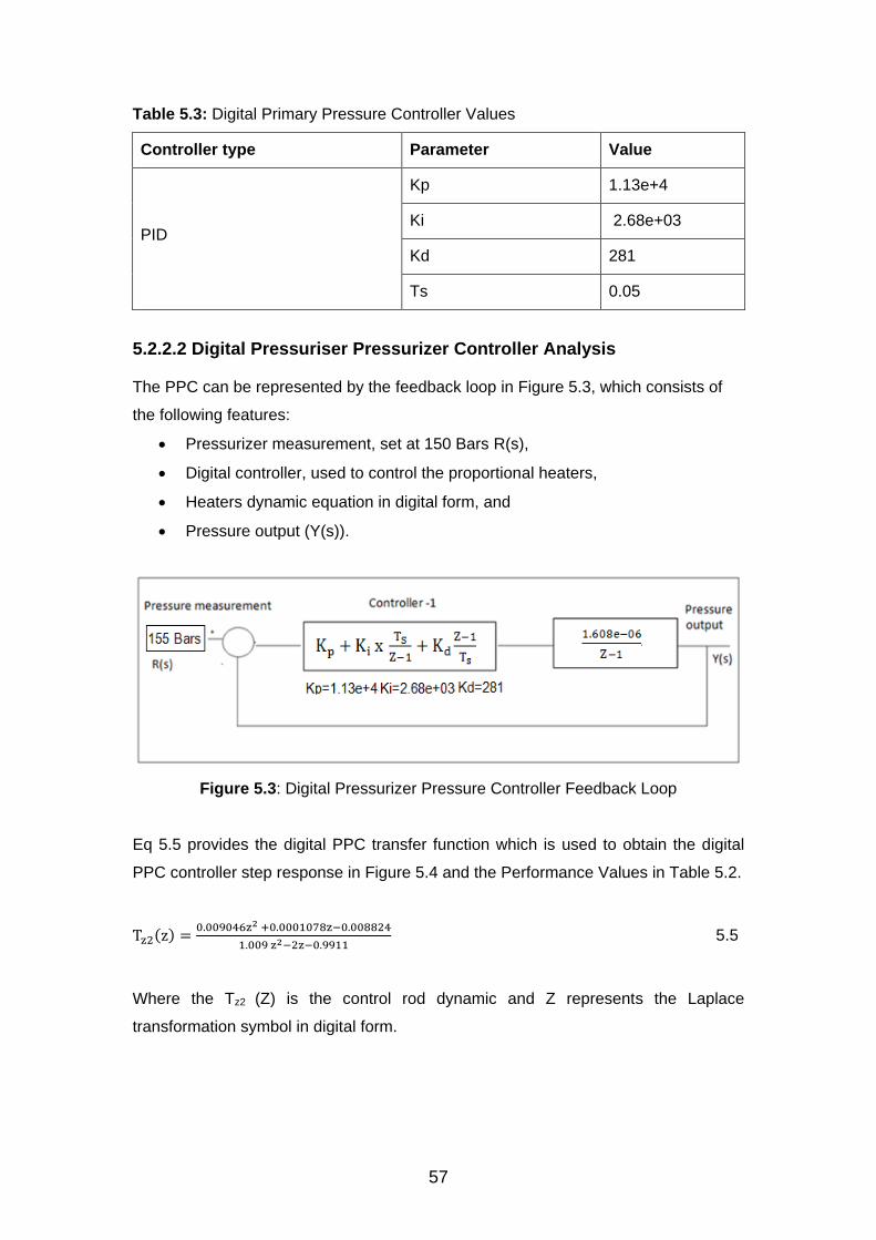
57
Table 5.3: Digital Primary Pressure Controller Values
Controller type Parameter Value
PID
Kp 1.13e+4
Ki 2.68e+03
Kd 281
Ts 0.05
5.2.2.2 Digital Pressuriser Pressurizer Controller Analysis The PPC can be represented by the feedback loop in Figure 5.3, which consists of
the following features:
Pressurizer measurement, set at 150 Bars R(s),
Digital controller, used to control the proportional heaters,
Heaters dynamic equation in digital form, and
Pressure output (Y(s)).
Figure 5.3: Digital Pressurizer Pressure Controller Feedback Loop
Eq 5.5 provides the digital PPC transfer function which is used to obtain the digital
PPC controller step response in Figure 5.4 and the Performance Values in Table 5.2.
Tz2(z) =0.009046z2 +0.0001078z−0.008824
1.009 z2−2z−0.9911 5.5
Where the Tz2 (Z) is the control rod dynamic and Z represents the Laplace
transformation symbol in digital form.

58
Figure 5.4: Digital Pressurizer Pressure Controller Step Response
Table 5.4: Digital Pressurizer Pressure Controller Performance Values
Parameter Value
Overshoot (%) 24.80
Peak time (s) 7.85
Rise time (s) 3.4500
Settling time (s) 22.800
The behaviour of the digital PPC controller is shown by a step response graph in
Figure 5.4 and the performance values are provided in Table 5.4. The controller has
an overshoot of 24.80, peak time of 7.85, and rise time of 3.4500 and settling time of
22.800 seconds. The controller is taking less than 3 minutes to reach a setpoint of
150 Bars.

59
5.2.3 Pressurizer Level Controller Optimization and Analysis
The PPL consists on a single controller feeding into the pressurizer level process
variable. Optimization and analysis of the PPL are given in section 5.2.3.1 and
5.2.3.2 respectively.
5.2.3.1 Digital Pressurizer Level Controller Optimization The pressurizer level process variable equation is converted into digital form and it is
given by the equation Eq 5.6.
Dy2(s) =0.01447 z2+0.02891z+0.0144
z3−2.999 z2+2.999z−0.995 5.6
where the Dy2(s) is the pressurizer level process variable equation and Z represent
the Laplace transformation symbol in digital form. The customized for the digital PLC
values are provided by Table 5.3.
Table 5.5: Digital Pressurizer Level Controller Values
Controller type Parameter Value
PID
Kp 0.0102
Ki 1.72e-0.6
Kd 0.0313
Ts 0.05
5.2.3.2 Digital Pressurizer Level Controller Analysis The digital PPL can be represented by the feedback loop in Figure 5.5, which
consists of the following features:
A level set point, at 41 %,
Controller, which is used to vary the level,
Pressurizer level dynamic process in digital form, and
PRZ level output.

60
Figure 5.5: Digital Pressurizer Level Controller Feedback Loop
Eq 5.7 provides the digital PLC transfer function which is used to obtain the digital
controller step response in Figure 5.6 and the performance values in Table 5.6.
Tz3(z) =0.008868z3 +0.008912z2−0.00878z−0.008824
1.009 z3−1.991z2+0.9913z−0.008869 5.7
Where the Tz3 (Z) is the pressurizer level process variable equation and Z represents
the Laplace transformation symbol in digital form.
Figure 5.6: Digital Pressurizer Level Controller Step Response

61
Table 5.6: Digital Pressurizer Level Controller Performance Values
Parameter Value
Overshoot (%) 7.36740
Rise time (s) 8.33409
Peak time (s) 16.8382
Settling time(s) 47.0982
The behaviour of the digital PPC controller is shown by a step response graph in
Figure 5.6 and the performance values are provided in Table 5.6. The controller has
an overshoot of 7.36740, peak time of 8.33409, and rise time of 16.8382 and settling
time of 47.0982seconds. The controller is taking less than 3 minutes to reach a set-
point of 41%.
5.2.4 Steam Generator Level Controller Optimization and Analysis The following process is followed to optimize and analyse the SGLC which consists
of two controllers (see Chapter 3):
- Digital controller -1 is developed,
- Analysis and performance is done for controller -1,
- Controller -1 is cascaded with the drum level variable equation,
- Digital controller -2 is developed using the controller -1 cascaded with drum
level equation, and
- Optimized and analysis is done for digital controller-1.
5.2.4.1 Digital Steam Generator Level Controller- 2 Optimization
The drum level process variable equation is converted into digital form and it is given
by equation by Eq 5.8.
Dy3(s) =0.07878z+0.007452
z2−1.831z+0.8465 5.8
Where the Dy3(s) is the drum level process variable equation and z represents the
Laplace transformation symbol in digital form. The customized for the digital SGLC
values are provided by Table 5.7.

62
Table 5.7: Digital Steam Generator Level Controller Values
Controller type Parameter Value
PID
Kp 2.24
Ki 3.65
Kd 0.311
Ts 0.05
5.2.4.2 Digital Steam Generator Level Controller- 2 Analysis The digital SGLC-1 can be represented by the Feedback Loop in Figure 5.7, which
consists of the following features:
A level set point, at 41 %,
Controller, which is used to vary the level,
Pressurizer level dynamic process in digital form,
PRZ level output
R(s) is a step input with the level set point at 60%,
Controller -2 ,
Drum level process variable, and
Y(s) is the level output.
Eq 5.9 provides the transfer function for the feedback loop for the digital SGLC which
is used to obtain optimized digital SGLC step response in Figure 5.4 and the digital
SGLC performance in Table 5.2.
Figure 5.7: Digital Steam Generator Level Controller-2
Tz1(z) =0.9012z4+3.279z3+4.456z2−2.68z−0.6021
1.901z4−7.2780 z3−10.45z2−6.679z+1.602 5.9

63
Figure 5.8: Digital Steam Generator Level Controller Step Response
Table 5.8: Digital Steam Generator Level Controller Performance Values
Parameter Value
Overshoot (%) 12.4917
Peak time (s) 0.9000
Rise time (s) 0.3500
Settling time (s) 2
The behaviour of the digital SGLC controller is shown by a step response graph in
Figure 5.8 and the performance values are provided in Table 5.8. The controller has
an overshoot of 12.4917, peak time of 0.9, and rise time of 0.3500 and settling time
of 2 seconds. The controller is taking less than 3 minutes to reach a setpoint of 85%.

64
5.2.5.1 Digital Cascaded Steam Generator Level Controller Optimization Optimized SGLC values in Table 5.7 are cascaded with drum level process variable
and converted into digital equation given by Eq 5.10. The controller values are given
by Table 5.9.
Dy4(s) =0.04906z3−0.03406−0.04327z+0.03107
z3−2.831z2−2.678z+0.8465 5.10
Table 5.9: Digital Cascaded Steam Generator Level Controller Values
Controller type Parameter Value
PID
Kp -0.00391
Ki -1.42e-05
Kd -0.269
Ts 0.05
5.2.5.2 Digital Steam Generator Level Controller Analysis The steam generator level controller feedback loop can be represented by Figure 5.8.
Figure 5.9: Steam Generator Level Controller Feedback Loop
Eq 5.11 has been generated from Figure 5.9 and it provides the transfer function for
the feedback loop for digital SGLC which is used to obtain optimized digital SGLC
step response in Figure 5.5 and the digital SGLC performance in Table 5.2.
Tz1(z) =1.42z7+6.664z6+11.2z5+5.678z4−5.749z3+9.4130z2−4.845z−0.8981
1.42z7+6.664z6+12.2 z5−10.51z4+3.591z3−0.3799z2+0.4739z−0.051663 5.11
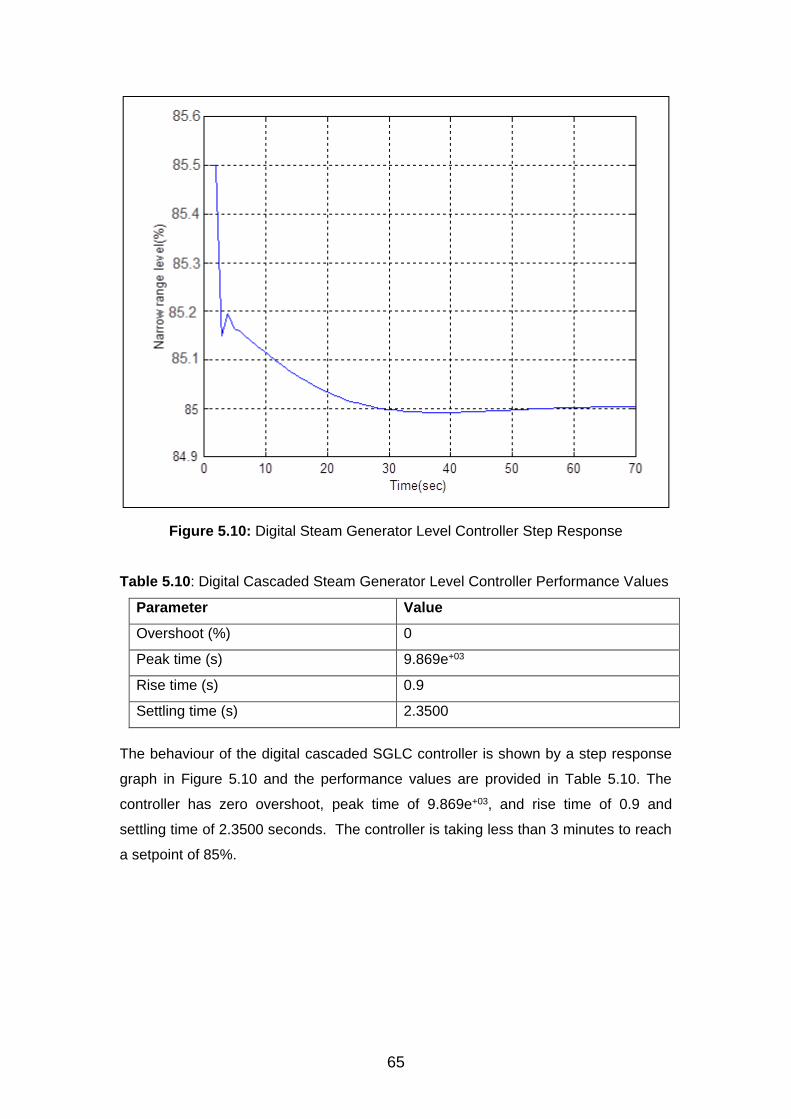
65
Figure 5.10: Digital Steam Generator Level Controller Step Response
Table 5.10: Digital Cascaded Steam Generator Level Controller Performance Values
Parameter Value
Overshoot (%) 0
Peak time (s) 9.869e+03
Rise time (s) 0.9
Settling time (s) 2.3500
The behaviour of the digital cascaded SGLC controller is shown by a step response
graph in Figure 5.10 and the performance values are provided in Table 5.10. The
controller has zero overshoot, peak time of 9.869e+03, and rise time of 0.9 and
settling time of 2.3500 seconds. The controller is taking less than 3 minutes to reach
a setpoint of 85%.

66
CHAPTER 6
Comparison of the Results Comparison of the analog KPP control loops and customized digital controllers are
performed in this chapter. This chapter also provide the customised optimized
controls transfer functions in digital form.
6.1 Comparison Methodology
Comparison of the performance of the customized digital controller transfer functions
and digital ones is made by comparing the performance values of the two controller
types which are given in Chapter 4 and 5. The performance values which are the
overshoot, peak time, rise time and settling time are compared for the analog
controllers and customized digital controllers.
6.2 Analog and Digital Primary Control Controllers Comparison
The comparisons of the controllers are given in sections 6.2.1, 6.2.2, 6.2.3 and 6.2.4
for the PCL, PPC, PLC and SGLC respectively.
6.2 1 Analog and Digital Primary Temperature Controllers
The comparison values of the two PTCs are given in Table 6.1 which is followed by
discussions.
Table 6.1: Analog and Digital PTC Performances Values
Parameter Analog PTC Values Digital PTC Values
Overshoot (%) 0 9.1231
Peak time (s) 1.049e+5 6.7000
Rise time(s) 2.0980e+04 2.7500
Settling time(s) 3.8879e+5 21.3000
The digital controller has an overshoot set point of 9.1231 % while and Analog PTC
has a zero overshoot. The peak time and the rise time of the analog PTC is very
long, larger than that of the analog PTC with the analog and the digital PTC values of
about 1.049e+5, 2.0980e+04 and 6.700, 2.7000 respectively. The settling time of the
digital controller is 21.3 seconds which is far too less than 3.8879e+5 of the analog
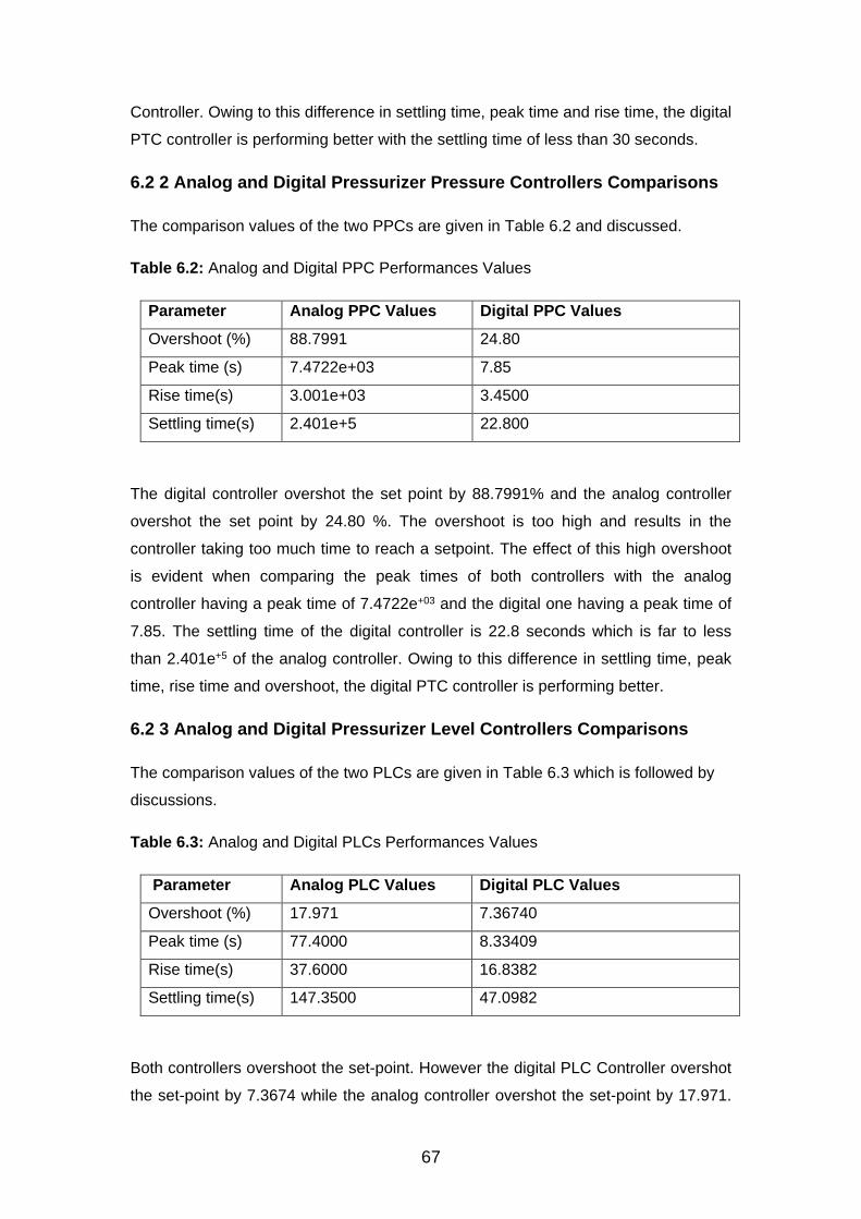
67
Controller. Owing to this difference in settling time, peak time and rise time, the digital
PTC controller is performing better with the settling time of less than 30 seconds.
6.2 2 Analog and Digital Pressurizer Pressure Controllers Comparisons
The comparison values of the two PPCs are given in Table 6.2 and discussed.
Table 6.2: Analog and Digital PPC Performances Values
Parameter Analog PPC Values Digital PPC Values
Overshoot (%) 88.7991 24.80
Peak time (s) 7.4722e+03 7.85
Rise time(s) 3.001e+03 3.4500
Settling time(s) 2.401e+5 22.800
The digital controller overshot the set point by 88.7991% and the analog controller
overshot the set point by 24.80 %. The overshoot is too high and results in the
controller taking too much time to reach a setpoint. The effect of this high overshoot
is evident when comparing the peak times of both controllers with the analog
controller having a peak time of 7.4722e+03 and the digital one having a peak time of
7.85. The settling time of the digital controller is 22.8 seconds which is far to less
than 2.401e+5 of the analog controller. Owing to this difference in settling time, peak
time, rise time and overshoot, the digital PTC controller is performing better.
6.2 3 Analog and Digital Pressurizer Level Controllers Comparisons
The comparison values of the two PLCs are given in Table 6.3 which is followed by
discussions.
Table 6.3: Analog and Digital PLCs Performances Values
Parameter Analog PLC Values Digital PLC Values
Overshoot (%) 17.971 7.36740
Peak time (s) 77.4000 8.33409
Rise time(s) 37.6000 16.8382
Settling time(s) 147.3500 47.0982
Both controllers overshoot the set-point. However the digital PLC Controller overshot
the set-point by 7.3674 while the analog controller overshot the set-point by 17.971.

68
The peak time and the rise time of the analog PTC is very slightly longer than that of
the digital controller which are 77.40, 37.60 and 8.33409, 16.8382 respectively. The
settling time of the digital controller is 47.0982 seconds which is less than 147.35 of
the analog controller. Owing to this difference in settling time, peak time, rise time
and overshoot, the digital PTC controller is performing better.
6.2.4 Analog and Digital SG Level Controllers Comparisons
The Steam Generator Level Controller consists of two controllers as discussed in
previous chapters. Sections 6.2.3.1 and 6.2.3.1 provide the comparison between
these two controllers.
6.2.4.1 Analog and Digital SG Level Controllers- 2 Comparisons
The comparison values of the SGLC- 2 are given in Table 6.4 which is followed by
discussions.
Table 6.4: Analog and Digital SGLC Performances Values
Parameter Analog SGLC- 2 Values Digital SGLC- 2 Values
Overshoot (%) 0 12.4917
Peak time (s) 4.2180e+09 0.9000
Rise time(s) 1.1778e+09 0.3500
Settling time(s) 1.5648e+09 2
The digital controller-2 overshot a set point by of 12.4917 % while and analog PTC
has a zero overshoot. The peak time and the rise time of the analog SGLC-2 are also
longer than those of the analog controller which is 1.1778e+5, 1.5648e+04 and 0.35, 2
seconds respectively. The settling time of the digital controller is 2 seconds which is
far to less than 1.5648e+09 of the analog controller. Owing to this difference in settling
time, peak time, rise time and overshoot, the digital PTC controller is performing
better.

69
6.2.4.2 Cascaded Analog and Cascaded Digital SG Level Controllers
Comparisons
The comparison values of the Cascaded SGLC are given in Table 6.5 which is
followed by discussions.
Table 6.5: Cascaded Analog and Digital SGLC Performances Values
Parameter Analog SGLC
Cascaded Values
Digital Cascaded SGLC Values
Overshoot (%) 0 9.869e+03
Peak time (s) 1.8638e+07 0
Rise time(s) 5.2036e+06 0.9
Settling time(s) 6.9120e+06 2.3500
The digital controller has an overshoot the set point by of 9.869e+03 % while the
analog controller has a zero overshoot. The peak time for the digital controller is 0
(Indicate no peak value) and together with the overshoot which is too large makes
this controller unique that others. However the digital controller perform better than
the analog one as it has a settling time of 2.3 seconds which is small compared to
the analog Controller of 6.9120e+06.
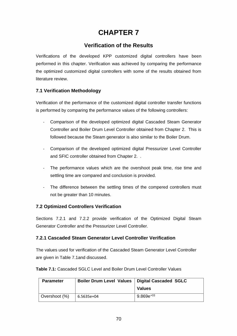
70
CHAPTER 7
Verification of the Results Verifications of the developed KPP customized digital controllers have been
performed in this chapter. Verification was achieved by comparing the performance
the optimized customized digital controllers with some of the results obtained from
literature review.
7.1 Verification Methodology
Verification of the performance of the customized digital controller transfer functions
is performed by comparing the performance values of the following controllers:
- Comparison of the developed optimized digital Cascaded Steam Generator
Controller and Boiler Drum Level Controller obtained from Chapter 2. This is
followed because the Steam generator is also similar to the Boiler Drum.
- Comparison of the developed optimized digital Pressurizer Level Controller
and SFIC controller obtained from Chapter 2. .
- The performance values which are the overshoot peak time, rise time and
settling time are compared and conclusion is provided.
- The difference between the settling times of the compered controllers must
not be greater than 10 minutes.
7.2 Optimized Controllers Verification
Sections 7.2.1 and 7.2.2 provide verification of the Optimized Digital Steam
Generator Controller and the Pressurizer Level Controller.
7.2.1 Cascaded Steam Generator Level Controller Verification
The values used for verification of the Cascaded Steam Generator Level Controller
are given in Table 7.1and discussed.
Table 7.1: Cascaded SGLC Level and Boiler Drum Level Controller Values
Parameter Boiler Drum Level Values Digital Cascaded SGLC
Values
Overshoot (%) 6.5635e+04 9.869e+03

71
Peak time (s) 0.0515 0
Rise time(s) 1.8849e-05 0.9
Settling time(s) 6.0587 2.3500
The digital Cascaded SGLC does not have an overshoot and the Boiler Drum Level
controller overshoot a set-point by 6.5635e+04. The peak time and rise times of both
controllers are 0.0515, 0 and 1.8849e-05, 0.9 respectively. The most important
parameter is the settling time is 2.35 for the Digital Cascaded SGLC and 6.058
seconds for the Boiler Drum Level Controller. It is clear from this value that the newly
developed optimized Digital Cascaded SGLC performs even better than the Boiler
Drum Level Controller. However, verification for the performance of the digital
controller is achieved as the settling times of the two controllers are within the same
order of magnitude. They are not in days as compared to the old analog controllers
but rather in seconds.
The digital controller-2 overshot a set point by of 12.4917 % while and analog PTC
has a zero overshoot. The peak time and the rise time of the analog SGLC-2 are also
longer than those of the analog controller which is 1.1778e+5, 1.5648e+04 and 0.35, 2
seconds respectively. The settling time of the digital controller is 2 seconds which is
far to less than 1.5648e+09 of the analog controller. Owing to this difference in settling
time, peak time, rise time and overshoot, the digital PTC controller is performing
better.
7.2. 2 Digital Pressurizer Level Controllers Verification
The values used for verification of the Pressurizer Level Controller are given in Table
7.2 and discussed.
Cascaded SGLC Level and Boiler Drum Level Controller Values
Table 7.2: Digital Pressurizer Level Controller and SFIC Controller Values
Parameter SFIC Values Digital PLC Values
Overshoot (%) 0 7.36740
Peak time (s) 17.0000 8.33409
Rise time(s) 0.5000 16.8382
Settling time(s) 200 47.0982

72
The SFIC controller has a zero overshoot and the developed digital PLC controller
has an overshoot of 7.36740. The peak time and rise times of both controllers are
17.0, 8.33409 and 0.500, 16.8382 respectively. However, the most important
parameter which is the settling time is 47.0982 for the digital PLC controller and 200
seconds for the SFIC controller. It is apparent from this study that, the newly
developed optimized Pressurize level Controller performs better than the SFIC
controller. However, verification for the performance of the digital PLC controller is
achieved as the settling times of the two controllers are within the same order of
magnitudes. They are not in days as compared to the old analog controllers but
rather in seconds, less than 4 minutes.

73
CHAPTER 8
Summary, Conclusions and Recommendations
This chapter provides the brief summary, conclusions and recommendations.
8.1 Summary
This study entails developing optimized controllers for Koeberg Power Plant which
are been replaced due to technological development. These controllers are replaced
with the digital ones, in order to be in line with the advance technological
development. The next replacements will include replacement of analog Primary
Temperature Control, Pressurizer Pressure Control, Pressurizer Level Control and
the Steam Generator Level Control with digital ones. During this replacement, there
is a need to replace these controllers with better performing ones rather than simply
converting analog controllers to digital ones and implementing them in a digital
computer.
The Koeberg Power Plant analog controllers are obtained from the KPP manuals and
are combined with the process variables or plant dynamic equations obtained from
literature survey to develop controllers. The four controllers are analysed using
Matlab® Simulation software to obtain four performances values which are the
overshoot, rise time, peak time and settling time.
Optimization of the controller is achieved by developing new controllers using
PIDTUNER which is a Matlab® optimization function used to develop optimize
controllers both in analog and digital forms. The new controllers are obtained in
digital form and analysis is done to obtain same performances values as analog
controllers. Comparative study has been done to determine the performance of these
two types on controllers. Verification is performed for the two controllers which are
the Digital Cascaded Steam Generator Level Control (SGLC) controller and
Pressurizer Level Controller.

74
8.2 Conclusions
Optimizations of the Koeberg Power Plant controls by implementing customised
transfer functions have been accomplished successfully. The four digital NSSS
controllers perform better than the analog controllers. This is evident from the
comparisons performed in Chapter 6.
The newly developed digital Primary Temperature Controller has an overshoot while
the old analog Primary Temperature Controller and this result with a settling time
which is significantly less settling times. Due to this settling time differences the
digital controller will perform better in the field. The behaviour and the performance of
the Pressurizer Pressuriser Controller are similar to the Primary Temperature
Controller. However unlike the analog Primary Temperature Controller the analog
Pressurizer Pressure Controller has an overshoot. The analog Pressurizer Pressure
Controller has a very large percentage overshoot which courses the controller to take
long time to settle. The digital Pressurizer Pressure Controller overshoot is less
which results with the controller reaching the controller very fast.
The analog Pressurizer Level Controller performance is better than the two previous
analog controllers. However improvement can still be done to this controller. This is
visible when comparing the digital Pressurizer Controller and the analog one. The
analog controller has a slightly high overshoot resulting in longer overshoot than that
of that of the digital controller and as a result the digital controller reaches a setpoint
faster than the analog controller.
The steam generator controller is complicated compared to the last three controllers.
Unlike the previous controller this one has two controllers which are the SG Level
Controller-2 and the Cascaded SG Level Controller. The Cascaded SG Level
Controller is the combination of controller-1 and controller-2. The cascaded SG
Level Controller is also showing a different behaviour as it has high peak time.
Similar behaviour is observed for the Drum Level Controller in Chapter 2 which is
used for validation in Chapter 7. Proper studies must be done to understand this
phenomenon. The analog Steam Generator Level Controller -2 has a zero overshoot
and the digital one has an overshoot which result in better performance. The analog
cascaded Steam Generator Controller also has zero overshoot which result in higher
settling time. Improvement is achieved by introducing an overshoot. The digital
controller has a better controller performance.

75
Verification of the results is performed in Chapter 7 by comparing the performance
values of the cascaded digital Steam Generator Controller with a Drum Level
Controller and SFIC controller with the digital Pressurizer Level Controller. This is to
show that the settling times of the controllers are not fair apart. The settling time of
the Drum Level Controller and cascaded digital Steam Generator Level Controller is
not far-off the only. The difference is around 4 seconds and for the digital
Pressurizer Level Controller and the SFIC controller is 157 seconds. This is
reasonable compared to the most of the analog controller which are in days rather
than seconds.
Optimization of controllers of the Nuclear Power Station is also apparent from the
literature study. Studies have shown that it is possible to optimize Nuclear Power
Plants controllers in digital or analog form using traditional methods and simulation
software’s. Included is the study of optimization of the parameter of a feed water
control system to minimize the SG level deviation from the reference level during
transient for UCN 5 and 6 of the South Korean two loops 1000 MWe Nuclear reactor
(Kim et al, 2006). Uns Soo Kim at el was able to optimize this control loop by using
RSM methodology. Kar and Saikia have also evaluated the performance of different
control strategies of the drum level system by implementing different control
methodology including Zeiger Nicholes, IMS, and Tyreus Luyben PID tuning and
fuzzy logic method control. Evaluating the performance of this control loops showed
that IMC optimization methodology have shown to performer better than all tried
method.
Optimization of the Koeberg Power Plant controls by implementing customised
transfer functions is possible using traditional methods and advanced optimization
method like PIDTUNER. Eskom can therefore use the digital upgrade opportunity to
implement not just digital controllers but optimized ones. This method can be
expended further to other Power Station controllers.
8.3 Recommendations
The optimization of the four controllers has been optimized successfully. However
the following additional studies can be done:
Proper analysis of the controllers to incorporate decay ration, steady and
non-steady state,

76
Detailed analysis to understand the behaviour of the Steam Generator Level
Controller,
Verification and validation of the software and developed software algorithms,
Proper study on the s=stepinfo(sysopt_1,'RiseTimeLimits',[0.05,0.95])
Optimized the controllers using different methods such as fuzzy -neural
network, Zeiger Nicholes and Tyreus Luyben tuning methods, and
Extend these studies by including other KPP controllers.

77
LIST OF REFERENCES
(Czaplin’ Ski at el, 2013) Mariusz Czaplin´ Ski, Paweł Sokólski, Kazimierz
Duzinkiewicz, Robert Piotrowski and Tomasz
Rutkowski, Comparison of state feedback and PID
control of pressurizer water level in nuclear power
plant, 2013.
(Dorf and Bishop, 2008) Richard C. Dorf and Roberts H Bishop, Modern control
systems, Technology & engineering, Prentice Hall,
2008.
(Eskom, 1985) Eskom, Koeberg Safety Analysis Report, KPP-14,
published 1985.
(Fuller et al, 1996) Fuller R, Hassanein, H and Ali, A N, Neural fuzzy
systems: towards IMT-advanced networks. Ab, Abo
akademi, xxvii, 275 p. ISBN 95-165-0624-0, 1996.
(Herrera et al, 1995) Herrera F, Lozano M and Verdegay J L, Tuning Fuzzy
Logic Controllers by Generic Algorithms, International
Journal of Approximate Reasoning, University of
Granada, Spain, 1995.
(Human, 2004) Gerhardus Human, model based predictive control for
load following of a pressurised water reactor, North
West University, Thesis 2004.
(IAEA, 1999) International Atomic Energy Agency, Control and
Instrumentation for Nuclear Power Plants: A
Guidebook, Vienna, Austria, 1999.
(IAEA, 2007) International Atomic Energy Agency, dynamic reliability
modelling of digital Control and Instrumentation
systems for nuclear reactor probabilistic risk
assessments, NUREG/CR-6942, October 2007.
(Kar and Saikia, 2013) Pragyan Paramita Kar and Priyam Saikia, Performance
of different control strategies for boiler drum level
control using LabVIEW, Department of Electronics &
78
Communication Engineering, National Institute of
Technology, Rourkela, India, 2013.
(Kim et al, 2006) Ung Soo Kim, In Ho Song, Jong Joo Sohn and Eur Kee
Kim, Optimization of the parameters of feed water
control system for OPR 1000 nuclear power plants,
November 2006.
(Koeberg, 1997) Koeberg Pressurized Water Reactor Setpoint Manual,
Nuclear Steam Supply System Control Loops, 1997.
(Koeberg, 2001) Koeberg Reactor Protection, Maintenance Manual,
2001.
(Koeberg, 2007) Koeberg, Control and Instrumentation Manual, Rod
Control System, 2007.
(Koeberg, 2008) Koeberg, Primary System Manual, 2008.
(Koeberg, 2009) Koeberg, Primary System Manual, Nuclear
Instrumentation, 2009.
(Matlab, 2003) Matlab® simulating software, PIDTUNER function,
2003.
(Power and Edwards, 2005) Power M.A. and Edwards R.M, Experiment B#6:
Automatic control of the Triga Reactor, 2005.
(Zhanga et al, 2009) Guo-Duo Zhanga, Xu-Hong Yanga, Xiao-Long Yea,
Hang Xua, Dong-Qing Lua and Wen Chen, research on
pressurizer water level control of pressurized water
reactor nuclear power station, Shanghai University of
electric power, Shanghai, 2009.
(Ziegler and Nichols, 1942) Ziegler, J.G and Nichols, N. B. Optimal settings for
automatic controllers (http:// www2. eie.ucr.ac.cr/
~valfaro/docs/ Ziegler%26Nichols.pdf) Transactions of
the ASME 64. pp. 759–768, 1942.

79
APPENDIX A:
PIDTUNE Optimization Matlab® Function
This program provide the Matlab® PIDTUNE PID Controller design
algorithm(Matlab, 2003)
%PIDTUNE Tune PID controller. % %PIDTUNE designs a PID controller C for the unit feedback loop % % r --->O--->[C] --->[ G ]---+---> y % - | | % +---------------------+ %
%given a plant model G, PIDTUNE automatically tunes the PID gains to
%balance performance (response time) and robustness (stability
&margins).
%One can select from various PID configure rations and specify your
%own response time and phase margin targets. Note that increasing
%performance typically decreases robustness and vice versa.
%C = PIDTUNE(G,TYPE) designs a PID controller for the single-input,
%single-output plant G. You can specify any type of linear system for
%G (see LTI). The string TYPE specifies the controller type among the
%following:
% 'P' Proportional only control
% 'I' Integral only control
% 'PI' PI control
% 'PD' PD control
% 'PDF' PD control with first order derivative filter
% 'PID' PID control
% ‘PIDF’ PID control with first order derivative filter
%
% PIDTUNE returns a PID object C with the same sampling time as G.
%If G is an array of LTI models, PIDTUNE designs a controller for
%each plant model and returns an array C of PID objects.
%C = PIDTUNE (G,C0) constrains C to match the structure of the PID or
%PIDSTD object C0. The resulting C has the same type, form, and
% integrator/derivative formulas as C0. For example, to tune a
%discrete-time PI controller in Standard Form with the sampling time
%of 0.1 and the Trapezoidal formula, set
% C0 = pidstd(1,1,'Ts',0.1,'IFormula','T')

80
% C = PIDTUNE(G,TYPE,WC) and C = PIDTUNE(G,C0,WC) specify a target
%value % WC (in rad/TimeUnit relative to the time units of G) for
%the 0dB gain crossover frequency of the open-loop response L = G*C.
%Typically, WC roughly sets the control bandwidth and 1/WC roughly
%sets the closed-loop response time. Increase WC to speed up the
%response and decrease WC to improve sTableility. When omitted, WC is
%peaked automatically based on the plant dynamics.
% C = PIDTUNE (G,..., OPTIONS) specifies additional tuning options
% such as the target phase margin. Use PIDTUNEOPTIONS command to
%create the option set OPTIONS.
%[C, INFO] = PIDTUNE (G,...) also returns a structure INFO with
%information about closed-loop sTableility, the selected gain
%crossover frequency, and the actual phase margin.
% Example: G = tf(1,[1 3 3 1]); % plant model % % Design a PI controller in parallel form % [C Info] = pidtune(G,'pi')
% Double the crossover frequency for faster response % wc = 2*Info.CrossoverFrequency; % [C Info] = pidtune(G,'pi',wc) % % Improve stability margins by adding derivative action % C Info] = pidtune(G,'pidf',wc) % Design a discrete-time PIDF controller in Standard Form % C0 = pidstd(1,1,1,1,'Ts',0.1,'IFormula','Trapezoidal',... % 'DFormula','BackwardEuler'); % [C info] = pidtune(c2d(G,0.1),C0) % % See also PIDTUNEOPTIONS, PIDTOOL, LTI.
% Author(s): Rong Chen 01-Mar-2010 % Copyright 2009-2011 The MathWorks, Inc. % $Revision: 1.1.8.3 $ $Date: 2012/03/05 22:51:37 $ ni = nargin; no = nargout; narginchk(2,4)
% pre-process G: SISO SingleRateSystem if ~(isa(G,'ltipack.SingleRateSystem') && issiso(G)) error(message('Control:design:pidtune1','pidtune')) end
% pre-process Ts: -1 is not accepted Ts = G.Ts; if Ts<0 error(message('Control:design:pidtune4','pidtune')) end
% pre-process Type and C if ischar(C) % get type if any(strcmpi(C,{'p','i','pi','pd','pdf','pid','pidf'})) C = ltipack.getPIDfromType(C,'parallel',Ts,G.TimeUnit);

81
else error(message('Control:design:pidtune2','pidtune','pidtune')) end elseif isa(C,'pid') || isa(C,'pidstd') % Validate C0 if nmodels(C)~=1 error(message('Control:design:pidtune2','pidtune','pidtune')) elseif ~(C.Ts==Ts && strcmp(C.TimeUnit,G.TimeUnit)) error(message('Control:design:pidtune10','pidtune')) end C.TimeUnit = G.TimeUnit; else error(message('Control:design:pidtune2','pidtune','pidtune')) end
% Look for option set if ni==2 || (ni==3 && isnumeric(varargin{1})) Options = pidtuneOptions; % default else Options = varargin{ni-2}; ni = ni-1; if ~(isa(Options,'ltioptions.pidtune') && isscalar(Options)) error(message('Control:design:pidtune3')) end end
% Look for WC convenience input if ni>2 try % Overwrite value of corresponding (hidden) option Options.CrossoverFrequency = varargin{1}; catch ME throw(ME) end end
% For discrete time PID, if specified, WC must be smalled than pi/Ts if Ts>0 && ~isempty(Options.CrossoverFrequency) &&
Options.CrossoverFrequency>=pi/Ts error(message('Control:design:pidtune5')) end
% Tune PID [PID,varargout{1:no-1}] = pidtune_(G,C,Options);

82
Appendix B
IMC CONTROLER FUNCTION ANALYIS PROGRAM % Transfer function Inputs
num1=[0.08 0.0002 0.4005 0.001]; den1=[0.0016 0.032 0.24 0.8 1];
sys1=tf(num1,den1);
% Analysis of the PTCL
sysopt_1=feedback(sys1,1);
nazz=85+step(sysopt_1); % plot(nazz),grid % s=stepinfo(sysopt_1,'RiseTimeLimits',[0.05,0.95])

83
APPENDIX C:
ANALOG PRIMARY TEMPERATURE CONTROLLER ANALYSIS
% Primary Temperatures Controller Analysis. % % Analysis of the controller requires representing a controller using
a %
% unity feedback loop shown by the Figure below.
% - % r --->O--->[ Controller-1 ]--->[ GR((s]---+---> y % | | % +----------------------------------+
% % (s+0.1) % Given a control rods position dynamic equation GR((s)= ---------
and
% s(s+200)
% 1+ 50s
%controller-1 equation -----------, a feedback transfer
function with
% 1+10.1s
%a unity feedback is developed. After this transfer is achieved
%analysis is performed by plotting the Primary Temperature Controller
%Step Response and obtaining the performance values.
% Controller-1 inputs
a=1;b=50;c=10.1;
Tem_num=[a a/b];Tem_den=[a a/c]; sys1=tf(Tem_num,Tem_den)
% Control Rods Position Dynamics Input
a1=1;b1=0.1;c1=200;d1=0;
Con_num=[a1 b1];Con_den=[a1 c1 d1]; sys2=tf(Con_num,Con_den)
% Analog Primary temperature Controller Feedback Loop % Obtaining Analog Transfer Equation
sys3=series(sys1,sys2);sys4=feedback(sys3,1);
%Plotting the Analog PTC Step Response
y1=310+step(sys4); plot(y1),grid
% Obtaining the Analog PTC Performance Values
s1=stepinfo(sys4,'RiseTimeLimits',[0.05,0.95])

84
APPENDIX D:
DIGITAL PRIMARY TEMPERATURE CONTROLLER OPTIMIZATION AND ANALYISIS
% Optimization and Analysis of the Primary Temperatures Controller
%The Control Rod Position Dynamics is converted into digital using
%sampling %time of T=1/20 and a Digital Proportional Integral and
%Differential %Controller is developed using a PIDTUNE Methodology
%given in Appendix A. %Analysis of the controller is done using the
%methodology in Appendix B.
%Control Rods Position Dynamics Input
e1=1;e2=0.1;f1=200;g1=0; Con_num1=[e1 e2]; Con_den1=[e1 f1 g1]; syss1=tf(Con_num1,Con_den1)
%Conversion of Control Rods Position Dynamics in digital form
T=1/20; syss1_z=c2d(syss1,T,'zoh') opt_c= pidtune(syss1_z,'pid')
% Analysis of the New Digital Primary Temperatures Controller
% Transfer function for the Digital PTC
sysopt_1=feedback(opt_c*syss1_z,1)
Y_z=310+step(sysopt_1);
% Plotting a Digital PTC Step Response
plot(Y_z),grid;
% obtaining the performance value
s=stepinfo(sysopt_1,'RiseTimeLimits',[0.05,0.95])