Deliverable 4.2 Integrated Optimisation Strategies and Low ...
319
Deliverable 4.2 Integrated Optimisation Strategies and Low Cost Methods Date of delivery: 08/12/2011 Revision: 3.0 Dissemination: PU
-
Upload
khangminh22 -
Category
Documents
-
view
2 -
download
0
Transcript of Deliverable 4.2 Integrated Optimisation Strategies and Low ...

Deliverable 4.2 Integrated Optimisation Strategies and Low Cost Methods Date of delivery: 08/12/2011 Revision: 3.0 Dissemination: PU

ASSET-Road consortium Dec-11 Page 2/319
Project Information
Project Duration:
01/07/2008 – 31/12/2011
Project Coordinator:
Walter Maibach ([email protected])
PTV Planung Transport Verkehr AG Kriegerstr.15 70191 Stuttgart Germany
Technical Coordinator:
Rigobert Opitz ([email protected])
ROC Systemtechnik GmbH Elisabethstr. 69 8010 Graz Austria

ASSET - Integrated optimisation strategies and low cost methods
ASSET-Road consortium Dec-11 Page 3/319
Document information
Version Date Action Partner
0.1 28.05.2010 1st draft ROC
0.2 08.11.2010 Structure ROC
0.3 08.12.2010 Contributions from IASI TUI
0.4 28.12.2010 Contributions from ROC low cost sensing ROC
0.5 13.02.2011 Contributions from UCD NUID UCD
0.6 04.03.2011 Draft Integration ROC
0.7 15.03.2011 Workshop Dublin NUID UCD/ UNOTT/
TUI/ROC
0.8 23.03.2011 Integration Recycling ROC/TUI
0.9 31.05.2011 Workshop Budapest NUID UCD/ UNOTT/
TUI/ROC
0.10 08.06.2011 Integration UCD and formatting ROC
0.11 28.07.2011 Final integration review meeting Graz ROC/TUI
0.12 08.08.2011 Final reading & check All
1.0 15.08.2011 Finalization and submission PTV
1.1 10.11.2011 Amendments NUID UCD
2.0 22.11.2011 Finalization PTV
2.1 05.12.2011 Amendments ROC
3.0 08.12.2011 Finalization PTV
Title: ASSET – DEL 4.2 Integrated optimisation strategies and low cost methods
Authors: The ASSET-Road Consortium
Reviewer: Walter Maibach (PTV)
Copyright: © Copyright 2009 – 2011. The ASSET-Road Consortium

ASSET - Integrated optimisation strategies and low cost methods
ASSET-Road consortium Dec-11 Page 4/319
This document and the information contained herein may not be copied, used or disclosed in whole or part except with the prior written permission of the partners of the ASSET-Road Consortium. The copyright and foregoing restriction on copying, use and disclosure extend to all media in which this information may be embodied, including magnetic storage, computer print-out, visual display, etc.
The information included in this document is correct to the best of the authors’ knowledge. However, the document is supplied without liability for errors and omissions.
All rights reserved.

ASSET - Integrated optimisation strategies and low cost methods
ASSET-Road Consortium Dec-11 Page 5/319
Contents
Project Information ........................................................................................................ 2
Document information ................................................................................................... 3
Contents ........................................................................................................................ 5
Executive Summary ........................................................................................................ 8
1 Integrated Pavement Monitoring ........................................................................ 18
1.1 Introduction ................................................................................................. 18
1.2 Objectives and specification ........................................................................ 20
1.3 Effects for road deterioration ..................................................................... 21
1.4 Pavement monitoring system concept ....................................................... 31
1.5 Impacts of wheel load ................................................................................. 34
2 State of the Art of Pavement Sensing .................................................................. 41
2.1 Overview...................................................................................................... 41
2.2 Pressure sensors .......................................................................................... 46
2.3 Pavement strain sensors ............................................................................. 53
2.4 Displacement sensors (DMS COST 347) ...................................................... 60
2.5 Other sensors (temperature, humidity, ..) .................................................. 70
2.6 Pavement parameters & behaviour ............................................................ 77
2.7 Nottingham simulation................................................................................ 79
2.8 Comments ................................................................................................... 81
2.9 Installation example of Japanese sensor ..................................................... 83
3 Pavement Sensor Layout and Dimensions ......................................................... 106
3.1 Pavement sensor layout ............................................................................ 106
3.2 Summary sensor specification ................................................................... 107
3.3 Mechanical design ..................................................................................... 108
3.4 Electronic design ....................................................................................... 113
3.5 Sensor house simulation ........................................................................... 113
3.6 Geometry design impact ........................................................................... 114
3.7 System overview ....................................................................................... 119
3.8 Pavement sensor microcontroller ............................................................. 120

ASSET - Integrated optimisation strategies and low cost methods
ASSET-Road Consortium Dec-11 Page 6/319
3.9 Interaction sensor versus pavement FEA analysis .................................... 120
3.10 Specification of traffic measurements (WIM) ........................................... 122
4 Cyclic Models for Granular Materials................................................................. 124
4.1 Background ................................................................................................ 124
4.2 Experimental procedure ............................................................................ 126
4.3 Results of triaxial tests on sand ................................................................. 128
4.4 The effect of cyclic loading ........................................................................ 134
4.5 Conclusions ................................................................................................ 140
5 Optimal Bridge Monitoring ............................................................................... 141
5.1 Summary ................................................................................................... 141
5.2 Low cost damage detection method (accelerometers) ............................ 144
5.3 Low cost bridge monitoring (Wavelet transformation) ............................ 157
5.4 Integrated bridge protection and monitoring ........................................... 172
5.5 Bridge sensor concept ............................................................................... 180
6 Pavement Deterioration Model ........................................................................ 186
6.1 Introduction and features ......................................................................... 186
6.2 GUI, customisable framework and modularisation .................................. 187
6.3 Models description .................................................................................... 194
6.4 Approach to optimum maintenance strategies ........................................ 209
6.5 Simulations and results ............................................................................. 210
6.6 Conclusions ................................................................................................ 215
7 Recycling and Pavement Upgrading .................................................................. 217
7.1 Replacement/recycling technologies ........................................................ 217
7.2 Selection of a recycling method ................................................................ 222
7.3 Structural design of recycled pavements .................................................. 225
8 Economic Evaluation of Recycling Technologies ................................................. 230
8.1 Introduction ............................................................................................... 230
8.2 The salvage value of a pavement structure .............................................. 232
8.3 Investigation of asphalt pavement carbon tool ........................................ 237
9 Optimised Infrastructure Strategies and Visions ................................................ 245
9.1 Road pricing strategies .............................................................................. 245

ASSET - Integrated optimisation strategies and low cost methods
ASSET-Road Consortium Dec-11 Page 7/319
9.2 Strategies and visions ................................................................................ 262
9.3 Overall conclusions .................................................................................... 278
10 References ....................................................................................................... 281
Annex 1: WIM sensors and systems ............................................................................ 290
List of Figures ............................................................................................................. 303
Glossary..................................................................................................................... 314

ASSET - Integrated optimisation strategies and low cost methods
ASSET-Road Consortium Dec-11 Page 8/319
Executive Summary
Background
For road authorities in responsibility of road infrastructure design, plan, built and maintain it’s essential to know mechanical pavement and bridge performance and failure in order to develop appropriate and efficient maintenance strategies and calculate and evaluate repairing costs.
Road infrastructure construction, maintenance and repair are important factors concerning road network operation and traffic management for European countries and their economies.
To have information about the “health” of pavements and bridges there are available several investigation procedures and analytical pavement design methods. Due to complex material behaviour and alternating boundary conditions, structural designs are not sufficiently validated yet and future research is necessary.
Another important issue for road authorities is the assessment of pavement performance and bearing capacity using non-destructive methods like deflection measurements preferably on a network level and without disturbance of the traffic flow.
Objectives
WP 4 addresses the protection of road and bridge infrastructure. It analysis, improves and develops the possible important technologies and methodologies to reduce damage to infrastructure, the cost of maintenance and congestion by applying useful and appropriate interventions.
A major goal of WP4 of ASSET-Road is the development of low-cost methods of monitoring for road infrastructure, i.e., of road bridges and pavements. The cost of sensors is falling steadily, technologies for data processing, storage and transmission are improving essentially and it is reasonable to expect increases in ‘health monitoring’ of road infrastructure in the future.
In WP4, sensors and sensing strategies have been investigated, developed and numerical methods of extracting useful information from sensors and sensor arrays. Future integrated concepts are recommended.
Results will be recommended and implemented for different test sites in future. The main objectives of WP4 – Safe and Sustainable Infrastructure were to:
Adopt and improve innovative key technologies and methodologies to improve safety and sustainability of infrastructure
Develop system to predict the risk of bridge overload using WIM data
Develop more accurate predictions of pavement life

ASSET - Integrated optimisation strategies and low cost methods
ASSET-Road Consortium Dec-11 Page 9/319
Recommend low-cost methods to monitor road and road safety conditions
Pavement maintenance strategies and techniques
Pavement rehabilitation techniques which minimise disruption to traffic
Sustainable strategies and visions for the management of infrastructural assets.
The main chapters of this document are structured as follows:
Integrated Pavement Monitoring including state of the art of pavement sensing and sensor specification
Integrated Bridge Monitoring
Pavement Deterioration Models incl. cyclic models for granular materials
Evaluation of recycling technologies and its economy
Optimised infrastructure strategies and visions including road pricing strategies.
Integrated pavement monitoring
Road pavements are some of the most complex structures in civil engineering. By allowing the fast, safe and reliable transfer of goods they form the basis of our economy and society. Nonetheless, the general public seems often unaware of the impact these structures can have on their lives and of the benefits everyone could get thanks to a better, more efficient road infrastructure.
Road engineering is a discipline that can potentially involve a very large number of different aspects and points of view. The users are interested in going from one place to the other quickly (avoiding road works and traffic jams), safely (without the car skidding on the asphalt and avoiding collisions), comfortably (without bumps, glares and sharp bends) and cheaply (without consuming too much petrol, tyres and in general without damaging the car). It is easy, therefore, to see how roads directly affect the life of a very large number of people without anyone even realising it. For this reason, it is of capital importance to conduct research in this field and constantly improve our knowledge of how roads behave. Roads are not a simple system to study: their behaviour evolves of time periods of tens of years, they are affected by the traffic they carry (which is almost uncontrollable), by the environmental conditions (often hard to predict) and by the material’s characteristics and their inherent variability. In order to predict the behaviour of roads as a function of all these parameters, numerous models have been developed around the world and numerous more complex ones will be developed in future, requiring mainly two things:
1. Real life data for calibration
2. A common platform for people to use them
Since the timescale of road pavement’s behaviour is so large, it is very difficult to gather complete and reliable sets of data. The information that needs to be

ASSET - Integrated optimisation strategies
ASSET-Road Consortium Dec
associated with a pavement in order to really understand its performance needs to include:
Climatic data (temperatures and moisture throughout the pavement, precipitations etc.);
Traffic data (type of vehicles, number of axles, contact stresses, speed, accelerations, vehicle dynamic parameters, number of vehicles per year etc.);
Material data (stiffness, stresses, strains, resistance to deformation, fatigue properties, thermal pro
In order to gather this information in an efficient reliable way, in ASSETwe have dedicated an important effort to developing a novel Pavement Sensor capable to measure most of these variables.
State of the art of pspecification
Included in WP4 was the investigation and development of a low cost pavement and bridge sensors in combination with WIM Sensors as an integrated monitoring system for achieving better and more comprehensive on pavements and the reaction in the pavement layers itself.
Figure 1: Example of the new pavement sensor
The general objectives and recommended innovations in the pavement sensor design are to create an efficient measurement system for
Measuring the pavement performance under real heavy vehicle traffic;
Using non-destructive methods;
That operate for every different environment and kind of pavements
Possible measurement at different depths
Using the values to integrate into pavement analytics models
Analysis of the state of the art of pavement sensors
Investigate impacts for road infrastructure
trategies and low cost methods
Dec-11
associated with a pavement in order to really understand its performance needs to
Climatic data (temperatures and moisture throughout the pavement, precipitations etc.);
Traffic data (type of vehicles, number of axles, contact stresses, speed, vehicle dynamic parameters, number of vehicles per year etc.);
Material data (stiffness, stresses, strains, resistance to deformation, fatigue properties, thermal properties, hydraulic properties etc.)
In order to gather this information in an efficient reliable way, in ASSETwe have dedicated an important effort to developing a novel Pavement Sensor capable to measure most of these variables.
of pavement sensing and sensor
Included in WP4 was the investigation and development of a low cost pavement and bridge sensors in combination with WIM Sensors as an integrated monitoring system for achieving better and more comprehensive data concerning the load flow on pavements and the reaction in the pavement layers itself.
Example of the new pavement sensor
The general objectives and recommended innovations in the pavement sensor ate an efficient measurement system for
Measuring the pavement performance under real heavy vehicle traffic;
destructive methods;
That operate for every different environment and kind of pavements
Possible measurement at different depths
the values to integrate into pavement analytics models
Analysis of the state of the art of pavement sensors
Investigate impacts for road infrastructure
Page 10/319
associated with a pavement in order to really understand its performance needs to
Climatic data (temperatures and moisture throughout the pavement,
Traffic data (type of vehicles, number of axles, contact stresses, speed, vehicle dynamic parameters, number of vehicles per year etc.);
Material data (stiffness, stresses, strains, resistance to deformation, fatigue
In order to gather this information in an efficient reliable way, in ASSET-Road WP4 we have dedicated an important effort to developing a novel Pavement Sensor
Included in WP4 was the investigation and development of a low cost pavement and bridge sensors in combination with WIM Sensors as an integrated monitoring
data concerning the load flow
The general objectives and recommended innovations in the pavement sensor
Measuring the pavement performance under real heavy vehicle traffic;
That operate for every different environment and kind of pavements

ASSET - Integrated optimisation strategies and low cost methods
ASSET-Road Consortium Dec-11 Page 11/319
Design a new pavement sensing system and Integrate different measurement principles
Innovative IT technologies applications
Combination with new WIM sensors design and build a first prototype
Main innovative features could be achieved:
Embedded electronics, A/D converting and pre-processing capabilities in the sensor
Low cost sensing (no separate data logger and signal converters are required)
Standard interfaces (CAN Bus) and connectivity to PC/Laptops
Multipurpose measurement concept: stress, strain, temperature, vibrations, accelerations, humidity
Nowadays there are different pavement sensors (see the chapter “State of art”), for different measurements of pavement properties available. The new ASSET-Road version is done by integration of different measurements to have the different value from only one sensor and it is proposed to correlate pavement and weight in motion sensor (WIM).
Figure 2: ROC matching system of pavement and weigh-in-motion sensors

ASSET - Integrated optimisation strategies and low cost methods
ASSET-Road Consortium Dec-11 Page 12/319
Integrated bridge monitoring
Alternative strategies for the monitoring of bridges have been investigated. Sensors can be installed at critical points on bridges to detect damage as bridges deteriorate over time. This approach involves considerable challenges – for example, it is possible to monitor a critical point and not to detect damage at another important point, less than one metre away.
Bridge damage detection using sensors on the bridge
Methods are developed in ASSET-Road WP4 to use measurements from bridge sensors to detect damage throughout the bridge. These are mostly based on numerical techniques such as Wavelet Transforms of the signals coming from the sensors.
Bridge damage detection using sensors on a vehicle
An alternative strategy for the monitoring of bridges is ‘Drive By’ inspection, i.e., using acceleration sensors attached to a vehicle to detect damage on the bridge as the vehicle drives over it. This is a considerable challenge but it is proven in ASSET-Road to be a feasible strategy. The advantage is that this is very low cost – one vehicle can monitor many bridges in a day. In the near term, the method has greatest potential as a pre-screening tool in which case it does not need to be very accurate – it is sufficient if the method can detect possible damage. In such cases, it can be used to optimise the process, diverting resources to carry out more detailed inspections of bridges that the vehicle identifies as being possibly damaged.
In ASSET-Road WP4, Drive By inspection is proven to be feasible in numerical simulations. The method is also tested using laboratory scale models. (It was not possible to damage a full size bridge to find out if such damage could be detected). For both the numerical simulations and the scale model tests, Drive By inspection is shown to be feasible for most situations. There were some problems identified with smaller bridges for which the vehicle is on the bridge for a shorter period of time.
Bridge Weigh-in-Motion
Finally, a design is proposed for a sensing system to detect vehicle axles as they pass over a bridge. This is a key component in the emerging technology of Bridge Weigh-in-Motion (Bridge WIM). Bridge WIM uses an existing bridge to weigh trucks that pass overhead. While the concept was first developed in the 1970’s, there is still only one company in the world marketing commercial Bridge WIM systems (Cestel, a Slovenian SME). Bridge WIM has great potential for bridge monitoring as the same sensors can be used to detect the weights of passing vehicles and the response of the bridge to those vehicles. Both the applied load and the response of the bridge to the load are key elements in any assessment of bridge safety.
In ASSET-Road, numerical tests were carried out to assess the feasibility of using the new ROC shear strain sensor to detect axles. Bridge WIM involves an array of

ASSET - Integrated optimisation strategies and low cost methods
ASSET-Road Consortium Dec-11 Page 13/319
sensors, some measuring the flexure of the bridge in response to the weight of the truck and others detecting axles in order to relate axle weight to bridge response. It is shown that the ROC sensor has considerable potential for future use as an axle detecting sensor in a Bridge WIM system.
Pavement deterioration model
This chapter includes the evaluation of recycling technologies. Since the aspects that must be taken into consideration when studying the behaviour of roads can be so numerous, the number of models required to deal with these different aspects is also very large. Different research groups usually focus on different research areas but ultimately for this knowledge to be useful the different models have to be integrated with each other.
In WP4 of the ASSET-Road project the structure and the initial working version of software for predicting long-term pavement performance has been developed that will allow users and researchers to modify the simulation depending on their needs and their expertise. The software will be modular and open source in order to allow the community of users to build a library of modules to test and compare different approaches and ultimately to be able to always use the most up to date state of the art model within the framework of one single software.
The software is currently being referred to as “VPI – Vehicle-Pavement Interaction” and its initial prototype (alpha version) is being tested at the universities of Nottingham and Cambridge and has been employed on a few studies. A first release of the software is expected to be made available for beta testers (a selected group of field experts and researchers) by the end of 2011. This will be followed by a period of scrutiny during which the suggestions and recommendations from the testers will be developed and implemented. After this final stage the full version of the VPI software will be released to the public (expected date August 2012).
The software will be made freely downloadable from the following web pages:
www.pavementsimulation.com;
www.pavementsimulation.org.
Redirection links to these websites will also be provided on the ASSET Project website, the University of Nottingham NTEC pages and the University of Cambridge Transportation Research Group.
Cyclic models for granular materials
A cyclic loading model for sub-base and sub-soil layers has been developed. Whilst there are many cyclic loading models available for soil, most were developed to predict strain accumulation resulting from sinusoidal loading, where the maximum stress is applied for a short time period. In many situations, e.g. near junctions and on roads where congestion is common, the loading time can be relatively long. A series of laboratory experiments are described where the effect of prolonged loading of granular soil was assessed. It was found that for cases where the applied

ASSET - Integrated optimisation strategies and low cost methods
ASSET-Road Consortium Dec-11 Page 14/319
stress equalled or exceeded the past maximum stress, creep strains occurred during periods of constant load. A simple creep model was calibrated to describe this behaviour and it was found that when this was incorporated into a popular cyclic loading model that excellent predictions of cyclic strain accumulation could be obtained.
Recycling and pavement upgrading
The recycling of existing pavement materials to produce new pavement materials results in considerable savings of material, money, and energy. At the same time, recycling of existing material also helps to solve disposal problems. Because of the reuse of existing material, pavement geometrics and thickness can also be maintained during construction. In some cases, traffic disruption is less than that for other rehabilitation techniques.
After a short introduction defining the concept of recycling, the main advantages of recycling technology, in comparison with other upgrading techniques, are fully described, demonstrating the importance of the selection of the appropriate time for intervention, based on the suggestive diagram which plots the evolution of the pavement condition versus its design life.
This document gives also a comprehensive answer to questions related with the pavement recycling technology used for upgrading and rehabilitation:
Why rehabilitate pavements?
Which other alternatives of upgrading are available?
Which methods recycling technology exists, what is their applicability and how to select the most appropriate one for a specific project?
The existing design methods for new pavement are also applicable for recycled pavements. For the specific aspects of in place recycling technologies envisaged in the frame of the ASSET-Road project a design module according the Mechanistic-Empirical approach was envisaged. Finally, some specific methods of structural design of recycled asphalt pavements are presented, with the recommendation to use the modern Mechanistic –Empirical Pavement Design Guide (ME-PDG), recently developed and implemented in USA.
Recycling economic evaluation
An important factor in identifying and performing economic analyses of various alternatives in the design of new pavement construction and/or the repair and rehabilitation of existing pavement is the life cycle of the alternative under consideration. After introducing the main concepts of specific service lives, describing typical life cycles for new pavement construction and pavement this document, focusing on the specific recycling alternative, presents the results of a detailed comparative study from the point of view of CO2 emissions for two distinct pavements construction alternatives (PA 1 – new pavements construction, PA –

ASSET - Integrated optimisation strategies and low cost methods
ASSET-Road Consortium Dec-11 Page 15/319
recycled pavements construction) by using the asPECT software, recently developed by TRL – Transport Research Laboratory, in UK.
The study concludes that by adopting the recycle technology for existing deteriorated asphalt pavements, significant reduction (up to 50%) of CO2 emissions can be obtained on the road projects. Beside the significant reduction of CO2 emissions, important reduction of construction cost and extention of design life can be obtained as shown in previous chapters. Finally for the specific aspects of in place recycling technologies envisaged in the frame of the ASSET-Road project, the recommendation to develop a structural design module according the Mechanistic-Empirical ME-PDG approach is is formulated.
Optimised infrastructure strategies and visions including road pricing strategies
As shown in the chapter 9 there is a tremendous potential of using IT and innovative sensor technologies for improving the whole process of road planning, design, built an maintain in all the stages of road life and to achieve a more sustainable road infrastructure including new financing and costing schemes.
Figure 3: Holistic approach of cyclic pavement management
Realistic pavement models
The implication of WIM technology for investigating road and traffic conditions is described in order to provide reasonable and appropriate data for pavement and
WIM
Technology
Pavement
Sensors
Road
ModellingTraffic
Parameters
Environ-
ment
FeasabilityStudy
ProjectDesign
ProjectConstruction
TransferTake Over
Monitoring Traffic & Road Condition
OptimisedLife Cycle
Holistic Operation& Economy
SustainableRoad Infrastructure
OngoingVerifikation
& Improvement
WIM & Pavement Sensing Implications
of a Holistic Approach for Cyclic Management of Sustainable Road Infrastructure

ASSET - Integrated optimisation strategies and low cost methods
ASSET-Road Consortium Dec-11 Page 16/319
bridge management systems including structural design will be based on the real data and performance of materials and their modelling.
Figure 4: Realistic pavement modelling
Self protected road infrastructure
WIM and the opportunity to detect overloaded axles, overloaded gross weight and also in combination underinflated tires could lead to “Road and Bridge Access Control Systems” for avoiding overloaded transports on roads and improvements on safety and driving economy checking the tire pressure concerning safety and optimal rolling resistance.
Several important enhancements of the WIM technologies are the base of the different innovations and achievable benefits and a implementation strategy leading to improvements of economy and competitiveness and opening the framework for a future “Intelligent and Interactive Road”:
Optimised materials
Optimised structural design
Optimised costs and best economy
Better risk management
A logical and interesting next step could be the combination of “New WIM Technology” with the “New Pavement Sensor Systems” as recommended by the ASSET-Road project giving the opportunity of cross-correlation of load patterns and effects in pavement structures.

ASSET - Integrated optimisation strategies and low cost methods
ASSET-Road Consortium Dec-11 Page 17/319
The implication of WIM technology for investigating road and traffic conditions is described in order to provide reasonable and appropriate data for pavement and bridge management systems including structural design will be based on the real data and performance of materials.
This approach could lead to a “Holistic Road Operation Concept” assisted by the output of WIM systems and technologies characterised by:
Protection of road and bridge infrastructure
Cost reduction
Better service
Environment protection.
New road pricing strategies
Heavy trucks and buses are responsible for the largest part of the pavement damage. An original for a new tolling system for heavy trucks, based on real damage produced to roads, was presented. It is governed by the idea that each vehicle must pay for the produced pavement damages. Unfortunately, to appreciate the real damages produced by each vehicle and educate the transportation community in this philosophy is not so easy.

ASSET - Integrated optimisation strategies and low cost methods
ASSET-Road Consortium Dec-11 Page 18/319
1 Integrated Pavement Monitoring
1.1 Introduction
The knowledge of mechanical performance, failure mechanisms and long term behaviour of pavements are of important concern for road authorities to develop maintenance strategies and calculate repair costs. With an increasing number of public-private-partnership projects worldwide and privately financed, built and operated roads the development of reliable pavement management systems including indicators for the structural performance of a pavement during its life cycle gains more and more importance. Analytical pavement design methods are available but not sufficiently validated yet. Due to complex material behaviour and alternating boundary conditions structural testing of material samples or full scale pavement tests are and will still be necessary in future to obtain important information about the mechanical performance of a pavement and its materials under load. Another important issue for road authorities is the assessment of pavement performance and bearing capacity using non-destructive methods like deflection measurements preferably on a network level and without disturbance of the traffic flow. Reliable accelerated full scale tests and bearing capacity measurements need input from the knowledge of mechanical behaviour of a pavement under real heavy vehicle traffic.
With regard to these objectives a series of projects at the instrumented full scale pavement test facility at Germany’s Federal Highway Research Institute have been conducted. The results - essential for understanding current and future pavement performance - focus on stress and strain measurements in eight different pavement constructions caused by various truck and trailer overruns as well as Falling Weight Deflectometer loading and accelerated loading by impulse generators.
The main objectives which influenced the design and the concept of the test track and the instrumentation was to asses the impact of various vehicle parameters on the mechanical performance of a representative selection of asphalt pavement constructions. The results are used to validate analytical models and to optimize the boundary conditions of small scale laboratory test with regard to realistic loading.
Replacing of a wearing course damaged by rutting causes relatively low maintenance costs.
Failures in the lower layers of the structure result in a replacement of the entire asphalt package and sometimes the damaged granular base course. For the structural design of a pavement construction, fatigue cracking caused by tension strains at the bottom of the asphalt base course and plastic deformation of the unbound granular base are the decisive criterions which have to be avoided using the appropriate materials and layer thickness.
The two main failure mechanisms which determined the methods of pavement instrumentation are shown in the following figure:

ASSET - Integrated optimisation strategies
ASSET-Road Consortium Dec
Figure 5: Principle of fatigue cracking and permanent deformation (
The potential of monitoring roads and bridges for optimising maintenance, repair and overall life cycle is generally well known.
Current measurement and sensor technologies show different deficiencies in accuracy, repeatability and data logging and processing. A new generation of multipurpose pavement and bridge sensor and processing systems was specified and is under design.
Main innovative features
Embedded electronics, A/D converting and presensor
Low cost sensing (no separate data logger and signal converters are required)
Standard interfaces (CAN Bus)
Connectability to PC/Laptops
Multipurpose measurement concept: stress, strain, temperature, vibrations, accelerations, humidity
Figure 6: Example of a pavement sensor
trategies and low cost methods
Dec-11
Principle of fatigue cracking and permanent deformation (Source: BAST)
The potential of monitoring roads and bridges for optimising maintenance, repair and overall life cycle is generally well known.
Current measurement and sensor technologies show different deficiencies in accuracy, repeatability and data logging and processing. A new generation of multipurpose pavement and bridge sensor and processing systems was specified
innovative features are:
Embedded electronics, A/D converting and pre-processing capabilities in the
Low cost sensing (no separate data logger and signal converters are
Standard interfaces (CAN Bus)
Connectability to PC/Laptops
e measurement concept: stress, strain, temperature, vibrations, accelerations, humidity
pavement sensor
Page 19/319
BAST)
The potential of monitoring roads and bridges for optimising maintenance, repair
Current measurement and sensor technologies show different deficiencies in accuracy, repeatability and data logging and processing. A new generation of multipurpose pavement and bridge sensor and processing systems was specified
processing capabilities in the
Low cost sensing (no separate data logger and signal converters are
e measurement concept: stress, strain, temperature, vibrations,

ASSET - Integrated optimisation strategies and low cost methods
ASSET-Road Consortium Dec-11 Page 20/319
1.2 Objectives and specification
1.2.1 Objectives
A core objective of the ASSET-Road project is to develop a more accurate generation of road deterioration models. Existing models are inaccurate which can lead to premature failure of pavements or excessive conservatism in design. Premature failure results in unexpected additional costs and unscheduled maintenance and repair operations.
A sensor system is essential to validate/test the current and new pavement damage models. While there are different existing sensors, both for WIM and for pavement strain measurement, there is no integrated system which will provide information on both the applied load and the resulting strains, long term, due to real traffic in the field. Pavement condition depends not only on ageing, but also on deformation behaviour of the asphalt layer and the sub-base and subgrade material as a function of dynamic loads due to traffic.
During pavement construction, the increasing static loads which act on the subsoil along with large deflections of the top layers. After completion, dynamic loads due to traffic act on the soil layers and hence, an increasing compression of the subsoil occurs, inducing additional deflections and stresses. When the stress levels reach a critical point in addition to cumulative effects, stress cracks and damages occur in the pavement and/or in the soil layers.
Figure 7: Some of different kind of pavements (Source: BAST)

ASSET - Integrated optimisation strategies and low cost methods
ASSET-Road Consortium Dec-11 Page 21/319
1.2.2 Pavement structure parameters and calculation models
According to the RStO 2001, one pavement structure for primary roads and one for secondary roads are chosen (cf. Figure 2.11). It is in both cases a construction with asphalt wearing course on an asphalt base course and road base. These bounded asphalt layers lie on the unbound sub-base.
Figure 8: Chosen pavement construction for further analysis ((left: primary roads, right: secondary
roads)
Figure 9: Calculation model of road structures and lanes and possible sensor placements
1.3 Effects for road deterioration
There are different effects and kinds of failure of road pavements even in a combination of the different effects may appear.
An important aim is to assess the validity of existing pavement models, assess the accuracy of the new modules and validate the overall model by investigations
4 cm wearing course8 cm basecourse
22 cm roadbase
34 cm
sub-base
subgrade
asph
alt l
ayer
s
wearing course 4 cm basecourse 4 cm
roadbase 14 cm
22 cm
u45 N/mm2
sub-base
subgradeu
45 N/mm2
4 cm wearing course8 cm basecourse
22 cm roadbase
34 cm
sub-base
subgrade
asph
alt l
ayer
s
wearing course 4 cm basecourse 4 cm
roadbase 14 cm
22 cm
u45 N/mm2
sub-base
subgradeu
45 N/mm2
4 cm wearing course8 cm basecourse
22 cm roadbase
34 cmsub-base
subgradeu
45 N/mm2
asphalt layers (primary roads)
wearingcourse4 cm basecourse4 cm
roadbase14 cm
22 cm
asphalt layers (secondary roads)
embedded sensor
4 cm wearing course8 cm basecourse
22 cm roadbase
34 cmsub-base
subgradeu
45 N/mm2
asphalt layers (primary roads)
wearingcourse4 cm basecourse4 cm
roadbase14 cm
22 cm
asphalt layers (secondary roads)
embedded sensor

ASSET - Integrated optimisation strategies and low cost methods
ASSET-Road Consortium Dec-11 Page 22/319
allowed by an innovative “Integrated Pavement Monitoring and Load Measurement system”.
To be useful for the validation activity, the test datasets must contain considerable information: pavement design specifications, traffic and load flow data, climatic data, road surface profiles and their evolution over long periods of time. Such complete data sets are rare.
Pothole
Fatigue cracks
Blowout
Reflection cracks
Sinkholes
Block/shrinkage cracks
Rutting
Ravelling
Slippage cracks
Shoving/corrugation
Root cracks and seam cracks
Peeling bleeding
Potholes are what most people think of when they think of pavement failures. These are usually non-functional pavement areas where the pavement has completely failed, exposing the base aggregate beneath it. Potholes usually pose liability issues such as causing vehicular suspension damage, or tripping hazards if they reside within pedestrian walkways. Potholes are often the result of several years of failing pavement in areas of fatigue where pre-emptive repair was not done until the area has completely failed. Potholes should be saw cut around the entire failing area, excavated, and base repaired using fresh ABC stone. Then proper placement of the asphalt design specification. The asphalt design specification varies from job to job. Typically the asphalt design will range from 3" of asphalt (2" of base asphalt, with 1" of surface wear asphalt).
Figure 10: Example of pothole
ASSET - Integrated optimisation strategies and low cost methods
ASSET-Road Consortium Dec-11 Page 23/319
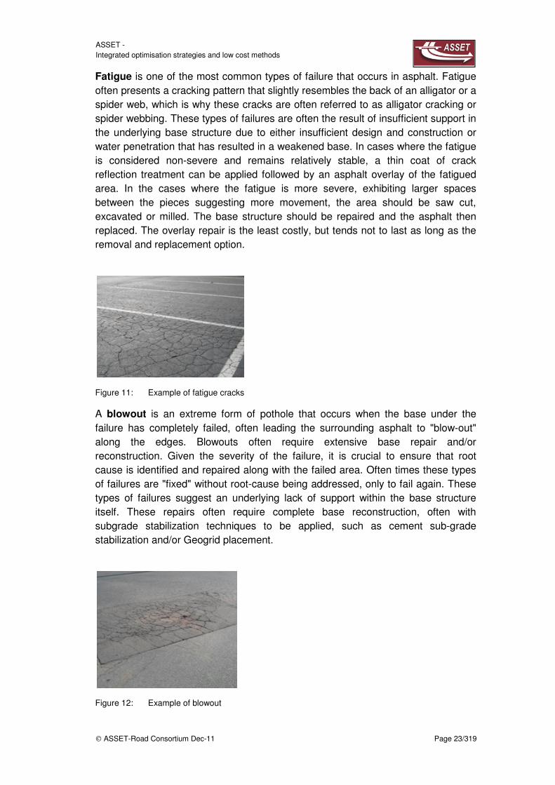
Fatigue is one of the most common types of failure that occurs in asphalt. Fatigue often presents a cracking pattern that slightly resembles the back of an alligator or a spider web, which is why these cracks are often referred to as alligator cracking or spider webbing. These types of failures are often the result of insufficient support in the underlying base structure due to either insufficient design and construction or water penetration that has resulted in a weakened base. In cases where the fatigue is considered non-severe and remains relatively stable, a thin coat of crack reflection treatment can be applied followed by an asphalt overlay of the fatigued area. In the cases where the fatigue is more severe, exhibiting larger spaces between the pieces suggesting more movement, the area should be saw cut, excavated or milled. The base structure should be repaired and the asphalt then replaced. The overlay repair is the least costly, but tends not to last as long as the removal and replacement option.
Figure 11: Example of fatigue cracks
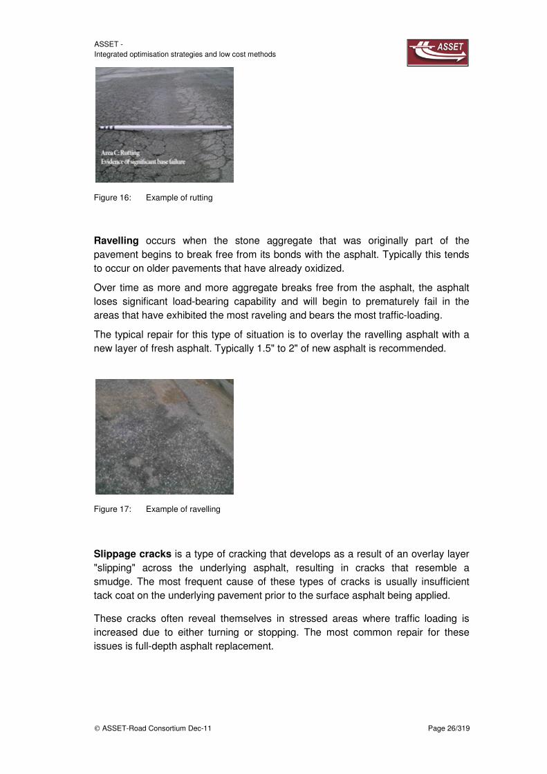
A blowout is an extreme form of pothole that occurs when the base under the failure has completely failed, often leading the surrounding asphalt to "blow-out" along the edges. Blowouts often require extensive base repair and/or reconstruction. Given the severity of the failure, it is crucial to ensure that root cause is identified and repaired along with the failed area. Often times these types of failures are "fixed" without root-cause being addressed, only to fail again. These types of failures suggest an underlying lack of support within the base structure itself. These repairs often require complete base reconstruction, often with subgrade stabilization techniques to be applied, such as cement sub-grade stabilization and/or Geogrid placement.
Figure 12: Example of blowout

ASSET - Integrated optimisation strategies and low cost methods
ASSET-Road Consortium Dec-11 Page 24/319
Reflection cracks tend to occur whenever older cracked asphalt or concrete is overlaid with a fresh layer of asphalt typically about 1" to 2" thick. The cracks underneath the new asphalt eventually will reflect up through the new layer of asphalt. This is typically the result of the original pavement structure and the overlay moving relative to each other. This movement tends to wear on the underside of the new asphalt and work its way upward to the surface, resulting in a crack in the new asphalt that is identical to the crack underneath. Sinkholes are often the result of subsurface drainage that erodes the underlying support substructures of the pavement. Over time, this erosion results in a cavity underneath the pavement. Sinkholes are often observed as an area that has a sudden and often significant drop in elevation, sometimes resulting in a complete open cavity that may pose significant liability risk. Sinkholes located in the drive lanes that support significant traffic should be repaired immediately as they can result in significant failures overnight. It is crucial to ensure that root cause is properly identified and repaired while repairing the sinkhole itself. Often times these types of failures can be caused by plumbing, sewer, or drainage leaks. Additional causes may be drainage avenues opening along laid utility lines underground.
Figure 13: Example of reflection cracks
Sinkholes are often the result of subsurface drainage that erodes the underlying support substructures of the pavement. Over time, this erosion results in a cavity underneath the pavement.
Sinkholes are often observed as an area that has a sudden and often significant drop in elevation, sometimes resulting in a complete open cavity that may pose significant liability risk. Sinkholes located in the drive lanes that support significant traffic should be repaired immediately as they can result in significant failures overnight.
It is crucial to ensure that root cause is properly identified and repaired while repairing the sinkhole itself. Often times these types of failures can be caused by plumbing, sewer, or drainage leaks. Additional causes may be drainage pipes opening along laid utility lines underground.

ASSET - Integrated optimisation strategies and low cost methods
ASSET-Road Consortium Dec-11 Page 25/319
Figure 14: Example of sinkholes
Block cracks, otherwise referred to as shrinkage cracks, present themselves as linear cracks several feet apart but often at different angles. These types of cracks often appear in older asphalt that sees a light traffic loading. They are the result of the asphalt being allowed to shrink horizontally with little stress being applied vertically as the asphalt ages. These typically should be filled with and sealed with a hot pour crack filler material to prevent water penetration.
Figure 15: Example of block cracks
Another effect is rutting, which is accelerated by overloaded axles in combination with high temperature environmental conditions. Additional effects could be cumulative damage and micro-cracks. Rutting involves depressions in the pavement that occur within the wheel tracks of vehicles. This is usually due to insufficient load-bearing capability of the asphalt/base design within that area. It most often occurs in fatigued drive lanes, or close to overly stressed areas such as at stop signs, or in front of dumpster pads.
ASSET - Integrated optimisation strategies and low cost methods
ASSET-Road Consortium Dec-11 Page 26/319
Figure 16: Example of rutting
Ravelling occurs when the stone aggregate that was originally part of the pavement begins to break free from its bonds with the asphalt. Typically this tends to occur on older pavements that have already oxidized.
Over time as more and more aggregate breaks free from the asphalt, the asphalt loses significant load-bearing capability and will begin to prematurely fail in the areas that have exhibited the most raveling and bears the most traffic-loading.
The typical repair for this type of situation is to overlay the ravelling asphalt with a new layer of fresh asphalt. Typically 1.5" to 2" of new asphalt is recommended.
Figure 17: Example of ravelling
Slippage cracks is a type of cracking that develops as a result of an overlay layer "slipping" across the underlying asphalt, resulting in cracks that resemble a smudge. The most frequent cause of these types of cracks is usually insufficient tack coat on the underlying pavement prior to the surface asphalt being applied.
These cracks often reveal themselves in stressed areas where traffic loading is increased due to either turning or stopping. The most common repair for these issues is full-depth asphalt replacement.

ASSET - Integrated optimisation strategies and low cost methods
ASSET-Road Consortium Dec-11 Page 27/319
Figure 18: Example of slippage cracks
Shoving and corrugation present bumps or corrugations where the surface asphalt has been "shoved" or bunched up. This is most often the result of extreme horizontal stress caused where heavy traffic loads typically stop or start.
The most common repair for these areas is to perform full-depth repair. This exposes the base, allowing for any base weaknesses to be repaired.
Figure 19: Example of shoving and corrugation
Seam cracks develop along the joints of asphalt where different paving sections come together. These usually exhibit themselves as long linear cracks that should simply be crack filled on a regular basis.
If left unsealed, these cracks can become central points for fatigue as water seeps under the pavement. Once a seam crack opens wider into a fatigued area, it should be treated as a fatigue area since adequately sealing these types of cracks is difficult.

ASSET - Integrated optimisation strategies and low cost methods
ASSET-Road Consortium Dec-11 Page 28/319
Figure 20: Example of seam cracks
Peeling typically occurs on pavement that had previously been overlaid with asphalt and the overlay layer of asphalt has begun to fail as a result of underlying fatigue “reflecting” up through the overlay layer.
This usually occurs many years after the overlay has been installed. The overlay layer oxidizes, and becomes brittle and much more susceptible to the underlying fatigue cracking reflecting through. Once the fatigue failure has reflected through, the overlay now exhibits the same fatigue failure as the underlying asphalt.
The pieces from the overlay tend to break free, exposing the original, fatigued asphalt beneath it.
The only permanent repair for these areas is a complete removal and replacement of the entire failed area along with the underlying fatigued asphalt.
Figure 21: Example of peeling
Root cracks Tree roots can cause significant cracking and upheaval of asphalt pavements. This can result in significant tripping hazards, posing liability risk for the owners of the property.
Unfortunately, the best method of repairing these cracks may place the adjoining tree at risk of dying. This is a consequence that the property owner/manager needs to be aware of. This method requires the area to be cut out and the offending roots sawcut and removed from the area prior to reconstruction of the base and asphalt.

ASSET - Integrated optimisation strategies and low cost methods
ASSET-Road Consortium Dec-11 Page 29/319
Sometimes the increased risk of harm to the associated tree is unacceptable. In these cases, the cracks can be sealed with hot-pour crack filler, but this treatment will not address the potential tripping hazard. Alternatively, a thick layer of asphalt can be placed over the roots to smooth out the tripping hazards, but the roots cracks will eventually reflect through.
Figure 22: Example of root cracks
Bleeding occurs when the asphalt contains too much asphalt cement relative to the aggregate. In these cases, the asphalt cement tends to "bleed" throughout the surface.
These types of issues are typically still functional but present an unsightly appearance to the pavement. Typical repairs for these areas are to either apply a chip seal application using absorbent aggregate or to mill off the top layer of asphalt and apply a new course of hot mix asphalt that contains lower asphalt cement content.
Figure 23: Example of bleeding
All the different pavement structure deteriorations are due to different conditions and pavement life. Obviously vertical and horizontal stresses and environment are the most important causes for pavement deterioration. They are always harmful for the structure, but it’s possible to give for each different kind of deterioration the principal causes.

ASSET - Integrated optimisation strategies and low cost methods
ASSET-Road Consortium Dec-11 Page 30/319
In the followings chapter we shall have some range values of stress and strain to understand the pavement health. The aim is to preview the pavement deterioration from these values.
Kind of pavement deterioration
Vertical
stress
Horizontal
stress Environment
Pothole x
Fatigue cracks x
Blowout x x x
Reflection cracks x
Sinkhole x
Block/shrinkage cracks x x
Rutting x x
Ravelling x
Slippage cracks x
Shoving/corrugation x
Seam cracks x x
Peeling x x
Root cracks x
Bleeding x
Figure 24: Measurement relevant matrix
Figure 25: Example of damaged pavement
The intended pavement failure model will be capable of predicting the accumulated damage and the remaining service life of a pavement section based on deterministic calculations of pavement response to heavy vehicle loading and environmental effects.
However, before any new model can be used confidently, its predictive abilities must be validated against experimental test results of full-scale pavement performance.

ASSET - Integrated optimisation strategies and low cost methods
ASSET-Road Consortium Dec-11 Page 31/319
An important aim is to assess the validity of existing pavement models, assess the accuracy of the new modules and validate the overall model by investigations allowed by an innovative “Integrated Pavement Monitoring and Load Measurement system”.
To be useful for the validation activity, the test datasets must contain considerable information: pavement design specifications, traffic and load flow data, climatic data, road surface profiles and their evolution over long periods of time. Such complete data sets are rare.
For early detection of pavement deterioration, an enhanced pavement monitoring system using new types of different embedded pavement sensors and an advanced type of data processing (CAN Bus) will be developed and installed at the selected test sites. This will provide benefits at two levels:
Firstly, it will be used to validate the improved computer models
Secondly, it will be used as a stand-alone method for real-time monitoring of pavement conditions.
This will allow early notification of pavement damage, yielding positive benefits for road safety and maintenance planning and optimisation. Overall, this will combine the advantages of direct measurement with those of computer simulations.
The Integrated Pavement Monitoring System addresses the topic of analysing traffic patterns, individual load flow created by HGV & pavement interaction for better understanding and better preparation measures for infrastructure protection.
It improves and develops the most important technologies and methodologies to analyse and monitor damage to pavement infrastructure, durability and the cost of maintenance depending on traffic and load flow impacts.
1.4 Pavement monitoring system concept
The “Integrated Pavement Simulation Tool and Monitoring System” will consist of:
Pavement damage modelling and simulation tool consisting of different modules (materials, structure, climate, topology, wheel load, axle configuration, aging) designed by Nottingham University in cooperation with UCD and LUH
WIM sensor arrays with extended force measurements combined with a
Multi-purpose integrated pavement sensor
An important aim is to assess the validity of existing pavement models, assess the accuracy of the new modules and validate the overall model by investigations allowed by an innovative “Integrated Pavement Monitoring and Load Measurement system”.
To be useful for the validation activity, the test datasets must contain considerable information: pavement design specifications, traffic and load flow data, climatic data, road surface profiles and their evolution over long periods of time.

ASSET - Integrated optimisation strategies and low cost methods
ASSET-Road Consortium Dec-11 Page 32/319
Figure 26: Complete pavement/traffic parameters & monitoring
Basic issues and key points related to pavement engineering can be summarised as follows:
Flexibility: ductility and compressibility to resist the transmitted movements
Fatigue resistance: to resist repeated dynamic loads
Strong Bond: strong adhesive and cohesive bond to transfer loads and movements
Tightness: seal the gap to avoid structure’s corrosion
Stability: of the thermo-plastic asphalt body under vertical load is necessary
The innovative approach of the ASSET-Road holistic concept (correlation of
WIM system data measuring tire loads and pavement sensing in a multi
sensor configuration) is to develop an integrated system. Wheel weight (WIM
Sensor) and the pavement response (Pavement sensor) can be compared and
correlated at the same time (and by the same data acquisition system using
embedded sensing and electronic pre-processing in the sensor). The data
acquisition uses a compatible integrated system and a common database.

ASSET - Integrated optimisation strategies and low cost methods
ASSET-Road Consortium Dec-11 Page 33/319
Figure 27: Overall system architecture of “Integrated Pavement Monitoring System”
The Integrated Pavement Monitoring System will be based on improved high resolution WIM sensor technologies combined with a new multidimensional pavement measurement unit allowing the cross correlation of load data and with the different effects in the pavement. The main objectives for the Integrated Pavement Monitoring System are to:
Create an extended pavement and traffic load monitoring and data collection system combining a precision high resolution WIM (tyre force and roll over lane position measurement) and a new Pavement Sensor Systems, allowing a correlation (time and space) of load flow over the pavement and pavement behaviour in pavement layers.
Develop better methods to monitor road and road status conditions depending on traffic impacts and patterns
Adopt and improve innovative and low costs measurement technologies and methodologies
Prediction of stress distribution patterns due to different types of tyres
Contribute to develop more accurate predictions of pavement life
Analyse additional and more accurate impacts for pavement maintenance strategies and replacement techniques
Contribute to sustainable strategies and visions for the management of infrastructure assets including road protection

ASSET - Integrated optimisation strategies and low cost methods
ASSET-Road Consortium Dec-11 Page 34/319
1.5 Impacts of wheel load
The durability of infrastructure is mostly influenced by vehicle load and the multidimensional and combined tire forces on the pavement.
Most analytic analyses are done only with static load of axles, axle groups and gross weight. Reality is different: and much worse, depending on the driving and environmental conditions:
Figure 28: Example of complete load on pavement
As we can see in the example static weight is only a simple component of the load condition. Also if the condition showed in the figure never happen simultaneously the real load on the pavement layer is bigger than the simple static one; and really load could be almost twice.
Movement of vehicles takes place by running wheels by the action of forces and moments, as follows: From the engine the moment is transmitted to the wheel, through the wheels axes of which acting forces are pulled on the wheels.
Functions of the real conditions and complete load in roads
We recommend considering all these parameters and conditions as shown in the figure above in future by a certain extent in road damage calculation and in the structural design of road pavements. Below examples of the different functions:
Rolling resistance
25 to 30% of the required energy of the vehicle is generated by the rolling resistance of the tires. The rolling resistance is created by all axles and tires.

ASSET - Integrated optimisation strategies and low cost methods
ASSET-Road Consortium Dec-11 Page 35/319
Figure 29: Rolling resistance (Source: Michelin)
The distribution to the different axles is:
Figure 30: Rolling resistance distribution (Source: Michelin)
The wheels on the track running surface are contacts resulting from tire deformation and path deformation. As a result there is a deformation in the tire tread that depends on the regime of movement of the vehicle, the stiffness of tire type and condition of the track rolling and rolling radius. It means that the vehicle-track interaction isn’t just a point but it a little surface in motion with the tire.
Vertical forces are based on the static vehicle weight while dynamic force are generated during driving; horizontal and longitudinal forces by acceleration or braking of the vehicle and horizontal transverse forces by the centrifugal force in curves and finally the Coriolis force:
Depending on location and driving direction that each wheel /axle applies to the road pavement surface or the total force that the truck applies on the road structure.
All different kinds of vector load are going to be explained in this chapter.
In the following figure tire force and torque are showed as constrain resistance.

ASSET - Integrated optimisation strategies and low cost methods
ASSET-Road Consortium Dec-11 Page 36/319
Figure 31: Tire forces: static, dynamic horizontal and vertical forces and torques
We have to take in consideration the climb up (or climb down) of the track. This generates unbalanced load among the different axels truck; furthermore it is important to take into consideration a possible acceleration or brake.
Figure 32: Example of climb up and acceleration or brake
Currently most WIM systems measure axle weight and calculate gross weight. Much more important would be the individual wheel weight (also considering unbalanced loading for the same axle which is sometimes more than 30%) and the investigation of its effects on pavements (in layers) and its traverse distribution on the lane.
If axle weight is significantly over the legal limits, it can do great damages to road pavements. Thin pavements are particularly sensitive to this.
Different Weigh in Motion technologies are applied to measure axle and gross weight, but accuracy and long term stability are still a problem. Semi automatic weigh stations are used with “Pre selection WIM Systems” to identify overloaded vehicles. Enforcement is only possible with static or slow motion weighing systems which are approved by “Weight and Measure Institutes” (OIML R 143 for dynamic overload enforcement is in preparation).
On board weighing of axles (basic technology already existing – but installation on all trucks is complex and hard to achieve due to additional costs and servicing)

ASSET - Integrated optimisation strategies and low cost methods
ASSET-Road Consortium Dec-11 Page 37/319
could be used to inform the driver if his axles are overweight (calibration and long term accuracy has to be considered and solved).
To allow for the hugely increased sensitivity of thin pavements to overweight axles, this information should be transmitted in future and in real time and on site from the road authority to the vehicle with an indicator of the degree of importance. As most drivers slow down when the road is rougher, it would be very useful to artificially activate the suspension system to give the driver a ‘bumpier’ ride when he is overweight and a particularly bumpy ride when he is overweight on a thin pavement. Active suspension systems are not yet implemented in trucks (to my knowledge) but exist in cars so this would be conceptually feasible.
The interface between tyre and road depends from tire deformation and path deformation; but it is strongly linked to tyre inflation that could be over or under inflated.
This is an issue for safety but is also important for road damage as an over- or under-inflated tyre may transmit considerably higher stresses to the pavement and hence more damage.
New WIM systems should also measures this parameter combining foot print seize and load on the wheel. Basic technology already exists to monitor tyre inflation in some new technology trucks, so the issue then is how to alert the driver. Tyre pressure is manipulated by truck drivers to reduce the rolling resistance and save fuel consumption.
In addition to the static axle weight, the dynamic force applied by an axle to the road is an important factor influencing the damage caused, especially if the axle is overweight. Road-friendly suspension technologies such as air suspensions should be encouraged as they result in less damage and conversely, steel suspensions discouraged. Dynamic forces are influenced by the road profile and driving behaviour.
To some extent, the problem is self-correcting as drivers experience a less comfortable ride when dynamic motion in the vehicle is high. However, currently the emphasis has been on driver comfort – this need to be complemented with inputs on the road damage implications. In other words, we don’t want new suspension systems to be developed that give the driver a very smooth ride while hitting the road very hard – this would encourage faster driving that does more damage to the road. Dynamic forces can achieve up to 20% of the static load depending on the pavement evenness (important parameter for WIM sites – see cost 232 definitions)
Monitoring of pavement properties depends strongly on load and traffic impacts (static weights, dynamic forces like in stop and go curves and the overall tyre force vectors). The vehicle load impacts can be analysed and clustered as follows:
GW Gross Weight is distributed on the different axles and wheels (static and dynamic). GW is important also for acceleration/deceleration of the vehicle and its mass on hills, mountains, intersections and during stop and go conditions.

ASSET - Integrated optimisation strategies and low cost methods
ASSET-Road Consortium Dec-11 Page 38/319
AW Axle Weights are normally used for calculation of wear and tear on pavements. Axle overloads are the most serious problem. Most of the WIM systems measure axle loads on the lane. Axle configurations and their distances are important for bridge impacts.
WL Wheel Loads are the true interface (all forces and torques) between the vehicle and the pavement and the direct influencing stress elements for the pavement. Wheel loads of one axle are often unequally distributed (traversal load distribution). On top of the static loads the dynamic loads have to be considered. Wheels can be operated with different tyres and pressures and roll over different positions – with extreme distributions- on the lane width. During the acceleration of a vehicle severe force and torque overlays as total force vector can occur.
Overweight trucks, special axle conglomerates (see bridge formula USA) and truck platoons causes fatigue damage in certain types of bridge (steel structures) and their presence in the traffic increases the risk of a combination of overloaded vehicles occurring on the bridge that could cause collapse.
Again, WIM or on-board weighing should inform the driver if their vehicle is overweight. In addition, vehicles with permits for higher than normal weights should have their weight information transmitted to the network manager so that real time information is available on the numbers of extremely overloaded vehicles on the road at any time.
The loading on pavement systems is intensively influenced by the patterns and dimensions of tyres, tyre configuration and axle configuration. To evaluate these, better measurement systems and tools are needed. Classical calculations by means of multi layer programs are not able to allow considerations of non homogenously distributed stresses within the footprint and the differences in the stresses in the direction of motion and the transverse direction.
Figure 33: Stress distributions in pavement sub-structures under two different tyres
In order to study the development of rutting and fatigue as a function of loading parameters and pavement properties, typical constructions used in Europe will be chosen (exemplary) and their performance will be estimated.
The effects of super single tyres have not been considered in the past even though, in central Europe, nearly all trailers have changed from dual to super single tyres.

ASSET - Integrated optimisation strategies and low cost methods
ASSET-Road Consortium Dec-11 Page 39/319
This is likely to have a very significant impact on the longevity of pavements. The following steps will be carried out:
Choice of a typical pavement systems
Use of related current existing pavement modelling
Definition of the pavement measurement system
Definition of the tire weight measurement system
Definition of the pavement/weight cross correlation scheme
Definition of the vehicle type measurement and classification system
Collection of measured tyre patterns and dimensions
Collection of typical tyre configuration
Collection of axle configurations
Collection of environmental parameters (temperature and humidity)
Evaluation of tyre type, tyre and axle configuration
Estimation of sensitivity of pavements to rutting and fatigue
Load parameters such as: magnitude, frequency, contact area, axle configuration, suspensions, tyre type, under/over inflation is important. Increased rest period at traffic lights creates creep damage. Bends are more susceptible to higher loading.
Figure 34: Tire and force/torque inputs to pavements (Source: Pirelli)
To conclude this chapter is done a simple example to have a complete view of the loads on the road structure. Actually is impossible that the entire load happen simultaneously, but in this example there are all the possible kinds of load starting from a static weight of 5 t.
Firstly we can divide load into vertical loads, horizontal loads in driving direction and horizontal loads in transversal direction. In the following table it is possible to see the value for each load starting from a static load F=5t.

ASSET - Integrated optimisation strategies and low cost methods
ASSET-Road Consortium Dec-11 Page 40/319
To make this calculation we used some coefficients:
α=12°
crs=1
ρ=1.29 kg/m3
Ss=6 m2
Vs=180 km/h=50m/s
µ=10^-5 m
r=0,5 m
crf=0,8
Sf=30 m2
Formula Values Load Total load
Vertical total
load
Weight W=F 5t
7t
~10t
Dynamic effect D~20%F 1t
Climb up/down C=Fsenα 1t
Transversal
total load
Curve effect Ce=m*a 2t
4t
Coriolis effect Fc=-2m*ω*v ~0t
Unbalanced load Ul=20%F 1t
Side wind Rws=0,5*crs*ρ*Ss*vs2~0,25% 1t
Longitudinal
total load
Rolling friction Fr=µ*F/r ~1,5t
6t
Brake or acceleration B=m*a 4t
Front wind Rws=0,5*crf*ρ*Sf*vf2 0,5t
Figure 35: Example of 3D force load on a road by a tire
According 3D vectors summation of the different possible load cases the
total force on the pavement and the road structure under real solicitation
have to support a load that is up to 100% higher than the simple static weight
depending on the occurrence of the different factors!

ASSET - Integrated optimisation strategies and low cost methods
ASSET-Road Consortium Dec-11 Page 41/319
2 State of the Art of Pavement Sensing
2.1 Overview
This chapter describes various sensors from different companies and research institutions. Some are describing the individual functions in the road sensor to be integrated.
Currently many different types of pavement sensors are available and are investigated. The German Federal Highway Research Institute (BASt) is busy on studies of roads maintenance. There are various sensor and measurement systems being developed and tested.
As shown in the next figure there are pressure cells (DMD) and strain gauges (DMS) that can be integrated into the roadway, a relevant topic for the BASt. On this subject the Federal Highway Research Institute is working as has already been referred to.
Figure 36: DMD and DMS from BASt
To understand the impact of heavy trucks, some proofs were done from BAST. Strain gauges were installed in longitudinal and lateral direction in different kinds of pavement tests. Soil pressure cells assess the vertical and horizontal stress at the top of the granular base courses underneath the asphalt package. The temperature

ASSET - Integrated optimisation strategies and low cost methods
ASSET-Road Consortium Dec-11 Page 42/319
gradient in the asphalt layers is measured with thermocouples placed between the layers of the asphalt package. The principle of the measuring instrumentation is shown in figure.
Figure 37: Measuring gauges inside the pavement structure (Source: BASt))
The entire BAST project consists of the following principal phases:
Measuring pavement response induced by selected heavy vehicle combinations for examining the functional dependencies between axle and tire configuration, axle load and vehicle speed
Accelerated load application with hydraulic impulse generators on selected sections until failure of the pavement structure
Regular measurements with Falling Weight Deflectometer throughout the entire test program
Each figure compares measured asphalt strain and granular stress measured in two comparable pavement construction types of the strongest construction:

ASSET - Integrated optimisation strategies and low cost methods
ASSET-Road Consortium Dec-11 Page 43/319
Figure 38: Measuring longitudinal strain with high stress situation (Source: BASt)
Figure 39: Measuring vertical strain with high stress situation (Source: BASt)
2.1.1 Influence of static wheel load and vehicle speed
To describe the influence of the static wheel load on the pavement constructions, the peak values of longitudinal asphalt strain and vertical granular stress under the wheel of the 1st trailer single-tired axle of a 2-axle articulated truck with 3-axle trailer were examined. The overruns with four different load stages were all conducted within a range of average asphalt temperatures from 11.0 °C to 14.0 °C.
The different kind of pavements were validated section 8 was the weakest (14 cm asphalt on granular base) and section 1 was the strongest (30 cm asphalt on 20 cm

ASSET - Integrated optimisation strategies and low cost methods
ASSET-Road Consortium Dec-11 Page 44/319
cement stabilized layer). Taking the slope of each function as an indicator for the stiffness of the construction, the stiffness of the strongest section 1 (slope = 0.008) is 7 times higher than the stiffness of section 8 (slope = 0.0558) for the asphalt strain. In regard to granular stress section 1 (slope = 0.095) is 7.4 times higher than section 4 (slope = 0.704).
Figure 40: Longitudinal strain versus static wheel load (Source: BASt)
Figure 41: Vertical strain versus static wheel load (Source: BASt)
The influence of vehicle speed on the asphalt strain and granular stress is based on the peak values of strain and stress and the four speed steps under the 1st wheel of the trailer of an articulated 2-axle truck with a trailer induced by a static wheel load of ~3700 kg was done. The functions were extrapolated to a speed of 90 km/h while the verified and the extrapolated intervals of the function are clearly indicated.
A distinct line can be drawn between each construction class and each section. The evaluation confirms that the stress and strain levels decrease with increasing speed

ASSET - Integrated optimisation strategies and low cost methods
ASSET-Road Consortium Dec-11 Page 45/319
as an effect of the visco-elastic properties of asphalt. Higher loading speed results in an increasing E-modulus.
Assuming the extrapolation to be valid, the asphalt strain at traffic speed of 80 km/h can decrease to 56 % (section 7) of the value induced by a quasi-static wheel load. The stress level of the granular material at traffic speed can level off to 42 % of the quasi-static values.
Pavement constructions with asphalt on a cement stabilized base do not show the influence of speed to that extent due to the higher amount of non-visco-elastic material (lean concrete, cement stabilized sand) in the bound layer package. Stress/strain at 90 km/h may be reduced to 60 % in unbound material and to 87 % in asphalt referring to the quasi-static stress/strain level.
Figure 42: Longitudinal asphalt strain versus vehicle speed for each section (Source: BASt)
Figure 43: Vertical asphalt strain versus vehicle speed for each section (Source: BASt)

ASSET - Integrated optimisation strategies and low cost methods
ASSET-Road Consortium Dec-11 Page 46/319
2.2 Pressure sensors
Currently many different types of pavement sensors are available on the marked and are investigated and described as follows:
2.2.1 Model 3500 series earth pressure cells GEOKON
Figure 44: Model 3500 earth pressure cell Installed under railroad tracks
Earth pressure cells are construed from two stainless steel plates connected around their periphery and separated by a narrow gap filled with hydraulic fluid.
External pressures squeeze the internal fluid. A length of stainless steel tubing connects the fluid pressure in an electrical transmitted by cable t the readout location.
The 3500 series uses semi-conductor type transducers to enable the measurement of dynamic pressures. This transducer can have an output of 2mV/V or 4-20 mA. Typical applications are the measurement of traffic induced stress on roadway sub grades, airport or under railroad tracks (as it is showed in the below figure).

ASSET - Integrated optimisation strategies and low cost methods
ASSET-Road Consortium Dec-11 Page 47/319
Transducer type Semi-Conductor
Output 2 mV/V,0-5 VDC or 4-20 mA
Standard ranges 100; 250; 400; 600 kPa; 1; 2,5 ;6 Mpa
Over rage 150% F.S. (maximum)
Resolution Infinite
Accuracy ±0,5% F.S.
Linearity <0,5% F.S.
Thermal effect on Zero <0,05% F.S.
Typical long-term drift <±0,02% F.S./yr
Standard cell dimension (HxD) 6 x230 mm
Transducer dimension (LxD) 150 x32 mm
Excitation voltage 10 V maximum
Excitation frequency n/a
Material 304 Stainless Sree
Temperature range -20°C to +80°C
Figure 45: Model 3500: Features
2.2.2 Kulite 0234 / (Geokon 3500) pressure sensor:
The BG Series of solid state load cells is designed to meet the demands of soil stress measurement. Being fluid filled the diaphragms exhibit virtually zero deflection under load and the active/total area ratio has been designed so that the intrusion of the cell into the material under study has the minimum effect on its properties. The transducer utilizes a solid state silicon pressure transducer as the basic sensing element coupling extreme robustness with high output. The unit is available with or without an additional reinforcing plate.

ASSET - Integrated optimisation strategies and low cost methods
ASSET-Road Consortium Dec-11 Page 48/319
Figure 46: Model Kulite 0234
This sensor is designed to achieve the requirements of a measurement in the soil. Since the membranes are filled with liquid, they have virtually no deformation under a load. The converter uses a solid-state silicon pressure sensor as a basic sensor element.
Sensor type Vertical sensoring
CTL Kulite 0234 functions
Pressure ranges: 0,07; 0,35; 0,7 N /mm²
Operating temperature: -18 °C --- +120 °C
Resistance: 1000 Ω
Switching scheme: full bridge
Accuracy: ±0,5 % full scale
Figure 47: CTL Kulite 0234 properties
Figure 48: CTL Kulite 0234

ASSET - Integrated optimisation strategies and low cost methods
ASSET-Road Consortium Dec-11 Page 49/319
The Geokon 3500 is also very similar to the specifications of the previous sensors of it is a type with semiconductor-type transducer features, which allows the measurement of dynamic pressures. Typical applications are the stresses caused by traffic in the roadway and in the soil. This sensor is used in roads and airport runways, as used in railway tracks.
Figure 49: Geokon 3500
Figure 50: Geokon 3500
2.2.3 Kulite LQ-080U series
The LQ-080U Series of soil stress gauges is designed to meet the requirements of weapons test labs, in the civil engineering field to make accurate measurements of blast induced soil reactions.
Insertion of a gauge in soil disrupts the stress field and induces either stress concentrations or reliefs depending on gauge thickness. This stress-transfer phenomenon can seriously affect gauge accuracy. To overcome this problem, the LQ-080U employs a pair of extremely stiff diaphragms with a diameter-to-thickness ratio of greater than 5 and a diameter-to-deflection ratio of greater than 2000. This design together with good gauge-medium matching ensures accuracy and repeatability of readings.
Sensor type Vertical sensoring
Geokon 3500 functions
Pressure ranges: 1 – 6 N/mm²
Operating temperature: -20 °C --- +80 °C
Resistance: 350 Ω
Switching scheme: full bridge
Accuracy: ±0,5 % full scale

ASSET - Integrated optimisation strategies and low cost methods
ASSET-Road Consortium Dec-11 Page 50/319
The DC powered sensing element of the LQ-080U comprises 4-active semiconductor strain gauges directly bonded to the measuring diaphragms. The output may be conveniently monitored on most conventional instrument systems. During assembly, the entire unit is given a conformal coating to prevent any ingress of moisture after final on-site-installation.
The LQ-080U Series is available calibrated or uncalibrated, with or without mounting ring. No mounting ring available for 10K PSI.
Figure 51: Kulite LQ-080U
2.2.4 Asphalt strain gauge ASG-152, CTL Group
CTL Groups Asphalt Strain Gauge strain designed to withstand the high temperatures and compaction loads associated with asphalt pavement construction. The ASG-152 is a field-proven design that uses durable materials to ensure accurate long-term data collection. Its full-bridge configuration reduces costs by eliminating the need for expensive data-acquisition and signal-conditioning systems to provide bridge completion.
Braided shielding protects the lead wire from electrical noise, while an abrasion-resistant, Teflon polymer coating with stands temperatures up to 205C (400F). This all leads to longer sensor life and long-term savings, by reducing redundancy in your instrumentation plan.
Sensor type Extensometer
Sensor functions
Strain range: ± 1500 µstrains
Operating temperature: -30 °C --- +200 °C
Voltage: up to 10 V
Switching scheme: full bridge
Resistance: 350 Ω
E-Modulus:2,4 N/mm²
Sensibility: 0,11 N/µstrains
Output: ~2 mV/V bei 1500µstrain
Figure 52: CTL ASG-152 properties

ASSET - Integrated optimisation strategies and low cost methods
ASSET-Road Consortium Dec-11 Page 51/319
Figure 53: CTL ASG-152
2.2.5 The CTL AVSG asphalt strain gauge vertical sensor
The CTL AVSG has been designed to achieve the high temperatures and pressures to resist the asphalt introduction. Given the choice of permanent materials, this sensor can be used for long-term data collection. The circuit diagram of the full bridge reduces costs by eliminating the expensive data acquisition and signal conditioning usually they need.
Sensor type Extensometer
Sensor functions
Strain range: ± 1500 µstrains
Operating temperature: -34 °C --- +204 °C
Voltage: up to 10 V
Switching scheme: full bridge
Resistance: 350 Ω
E-Modulus 2344 N/mm²
Output: ~2 mV/V at 1500µstrain
Figure 54: CTL AVSG properties
Figure 55: CTL AVSG

ASSET - Integrated optimisation strategies and low cost methods
ASSET-Road Consortium Dec-11 Page 52/319
2.2.6 Geokon Model 3900
The Model 3900 Embedment Strain Gauge is designed for the measurement of dynamic strains in concrete structures, asphalt roadways and soils. It comprises a full-bridge strain gauge proving ring element coupled in series with a tension spring which is stretched between two end flanges. An outer PVC tube sealed with O-rings provides a waterproof housing. The end flanges are embedded and move in accordance with the surrounding material. The voltage signals from the strain gauge are transmitted via cable to the readout location.
The strain gauge can be read out by means of the Geokon Model 501 Readout Box or by applying a 2 to 12 Volt excitation to the input leads, and reading the corresponding millivolt output. The output at full range is approximately 3mV/V. The standard wiring for use with the GK501 readout box is configured to compensate for the use of long cables by the remote sensing of the input voltage at the sensor. A Thermostat is included inside the sensor to measure temperatures. This requires a cable with 4 shielded pairs of conductors.
Sensor type Extensometers
CTL CSG sensor functions
Strain range: ± 2000 µstrains
Operating temperature: -30 °C --- +100 °C
Switching scheme: full bridge
Resistance: 350 Ω
Sensibility: 2,40 mV/V
Figure 56: CTL CSG properties
Figure 57: CTL Inc. CSG

ASSET - Integrated optimisation strategies and low cost methods
ASSET-Road Consortium Dec-11 Page 53/319
Sensor type Extensometers
Geokon Model 3900 sensors functions
Strain range: ± 5000 µstrains
Operating temperature: -20 °C --- +80 °C
Switching scheme: full bridge
Resistance: 350 Ω
Sensibility: 0,125 mV/V
Figure 58: Geokon Model 3900 properties
Figure 59: The Model 3900 embedment strain gauge
Tests have shown that the temperature effect is such that the embedment gauge reading goes down (compression) as the temperature goes up. The required temperature correction factor is +6 microstrain/°C.
2.3 Pavement strain sensors
Currently many different types of pavement sensors are available and are investigated:
Asphalt
Concrete
CTLGroup’s Asphalt Strain Gauges are designed to withstand the high temperatures and compaction loads associated with the construction of asphalt pavements. Full-bridge configuration provides higher signal output and reduces cost, because no expensive data acquisition or signal conditioning systems are necessary for bridge completion.

ASSET - Integrated optimisation strategies and low cost methods
ASSET-Road Consortium Dec-11 Page 54/319
2.3.1 BASt strain sensor
Figure 60: BASt strain sensor
2.3.2 CTL compression gauge
CTLGroup’s Soil Compression Gauges are designed to withstand the rigors of compaction loads associated with the construction of pavement layers. Individual soil compression gauges can be used in conjunction with CTLGroup’s multi-depth deflectometer, (SnapMDD) to provide additional layer deflections throughout the area of interest. The soil compression gauge can also be a cost-effective alternative to the SnapMDD in applications where soil layer deflections are needed at only singular points. The soil gauge utilizes industry standard electronics for connection to simple readout devices and widely available data loggers.
Figure 61: CTL SCG
2.3.3 CTL asphalt strain gauges
CTL’s asphalt strain gauges are designed to withstand the high temperatures and compaction loads associated with asphalt pavement construction. The ASG-VS is a

ASSET - Integrated optimisation strategies and low cost methods
ASSET-Road Consortium Dec-11 Page 55/319
field-proven design that uses durable materials to ensure accurate long-term data collection. Its full-bridge configuration reduces costs by eliminating the need minimum1 in for expensive data-acquisition and signal-conditioning systems to provide bridge completion. Braided shielding protects the lead wire from electrical noise, while an abrasion-resistant, Teflon polymer coating withstands temperatures up to 205°C (400°F). This all leads to longer sensor life and long-term savings, by reducing redundancy in your instrumentation plan.
Figure 62: CTL asphalt strain gauges
Figure 63: CTL asphalt strain gauges
2.3.4 CTL concrete strain gauges
Figure 64: CTL Groups concrete strain gauges

ASSET - Integrated optimisation strategies and low cost methods
ASSET-Road Consortium Dec-11 Page 56/319
CTL Group’s concrete strain gages feature a field-proven design that uses durable materials to ensure accurate long-term data collection. Its full-bridge configuration reduces costs by eliminating the need for expensive data-acquisition and signal-conditioning systems to provide bridge completion. Shielded, twisted-pair design protects the lead wire from electrical noise. This all leads to longer sensor life and long-term savings, by reducing redundancy in your instrumentation plan.
Figure 65: CTL Groups concrete strain gauges
2.3.5 The measurement capability by dowel rods from CTL
With the dowel rods of the CTL Group, it is possible to measure shear forces and moments on wooden beams. Here, too, as the full bridge switching scheme has been chose. This allows for the avoidance of expensive data processing.
Sensor type
Load cell
Shear force sensor
Torque sensor
Sensors functions
Resistance: 350 Ω
Switching scheme: Full bridge
Voltage: 5 – 10 V DC
individually calibrated
Figure 66: Properties measuring dowel bars from CTL

ASSET - Integrated optimisation strategies and low cost methods
ASSET-Road Consortium Dec-11 Page 57/319
Figure 67: CTL measuring dowel rods
2.3.6 KM 100 HAS (Japan)
Figure 68: KM-100HAS specifically for embedding in road paving developed from asphalt
The transducer consists of two reinforcing bars provided with end plates, between which a deformable, hermetically sealed metal tube. In this metal tube sits a thin

ASSET - Integrated optimisation strategies and low cost methods
ASSET-Road Consortium Dec-11 Page 58/319
spring element which is connected to the end caps and fitted with strain gauges in full bridge circuit. Due to the expansion occurring in the asphalt are the reinforcing rods and from the end of the caps on the shock passed and registered by the strain gauges. The particular structure of the strain it possible to detect even the smallest expansion reliably. In addition, the sensor has an integrated temperature sensor, which can be evaluated using a conventional strain gauge amplifier. The whole construction is completely waterproof and heat resistant to 180 ° C. Measuring range: ± 5.000 µm/m.
Rated signal: ± 2.5 mV /
Linearity deviation max: 1% of range
Modulus: 40 Mpa
Temperature Range: -20 °C; +180 ° C
Inputs bridge voltage recommended: 1 ~ 2V, maximum permissible 10 V
Full bridge: 350 Ohm full bridge in 4-wire (elongation)
Resistance: 350 Ohm quarter bridge in 3-wire (temperature)
Electrical connection 5-wire shielded cable (Fluoroplastic), 0.3 mm ², Ø 6 mm, standard length 2 m (other Lengths available on request).
This arrangement consists of four film-like strain gauges, which are mounted on a small cantilever beam. Each of these four strain gauges has a resistance of 350 Ω. The elastic modulus is ² 40 N / mm, the recommended working temperature is between -20 and +80 ° C. This transducer is 155 mm long, with tie rods having 85 mm long.
Figure 69: KM-100HAS

ASSET - Integrated optimisation strategies and low cost methods
ASSET-Road Consortium Dec-11 Page 59/319
Figure 70: Japanese KM-100HAS
Sensor type Strain gauges
Sensor functions
Strain ranges: ± 5.000 µstrains
Rated signal: ± 2,5 mV/V
Linearity:
Max. 1% of range
E-Modulus: 40 N/mm²
Bridge supply voltage:
Recommended 1 - 2V, max. allowable 10 V
Circuit diagram: Bridge (350 Ohm 4-wire)
Resistance: quarter bridge (350 Ohm in 3-wire)
Production/development TML – Tokyo Sokki Kenkyujo, Ltd.
Temperature Utility temperature: -20 ; +180 °C
Operating temperature: -20 ; +80 C
Figure 71: KM-100HAS properties
The strain of type KM-100HAS was made specifically to be embedded in road surfaces asphalt developed. The transducer consists of two discs provided with reinforcing bars, between which a deformable, hermetically sealed metal tube is. In this metal tube sits a thin spring element which is connected to the end caps and fitted with strain gauges in a full bridge circuit. The changes will see in the asphalt in that class of the reinforcement bars and the end caps on the shock passed and registered by the strain gauges. The particular structure of the strain it possible to detect even the smallest expansion reliably. In addition, the sensor has an integrated temperature sensor, which can be evaluated with a conventional strain gauge amplifier. The whole construction is completely waterproof and heat resistant to 180 ° C.

ASSET - Integrated optimisation strategies and low cost methods
ASSET-Road Consortium Dec-11 Page 60/319
Measuring range ±5000µm/m
Call signal ±2,5 mV/V
Linearity deviation Max. 1% of measuring range
Elastic modulus 40 N/mm2
Temperature range used -20° ; +180°C
Bridging supply voltage Recommended 1~2V max permissible 10V
Resistance
Full bridge 350Ω in 4-wire system (strain)
Quarter bridge 350Ω in 3-wire system (temperature)
Electrical connection 5 wire, shielded cable (fluoroplastic). 0,3 mm2; ϕ 6 mm; standard lenght 2m (other lenght available by request)
Figure 72: KM-100HAS features
2.4 Displacement sensors (DMS COST 347)
A strain gauge consists of a metal strip, a loop or something similar. This is glued to an object whereby an elongation should be measured. Occurring at a length change also extends to the DMS. This creates an electrical resistance that changes are measurable. In this way it becomes possible to measure very small deformations using strain gauges.
2.4.1 BASt (Germany)
BASt + HBM (BAST + HBM strain transducer):
This instrument consists of two parallel strips which are embedded in epoxy resin. The length of each unit is 133 mm. The anchor pieces have a longitudinal dimension of 80 mm and 16 mm thick. The resistance is 175 Ω. The modulus is square at 20,000 N / mm2.
Figure 73: BASt + HBM strain transducer

ASSET - Integrated optimisation strategies and low cost methods
ASSET-Road Consortium Dec-11 Page 61/319
2.4.2 CEDEX (Spain)
MM EA- 06-10CBE-120:
The deformation of the strip gauge is applied to a transparent plastic film. The length is 25.4 mm. The operating temperature range is between -75 and +175 ° C. The resistance of the strain gauge is 120 Ω ± 0.3% for "normal"operating temperature (24 ° C). The E-modulus is 165 N/ mm2.
Figure 74: MM EA- 06-10CBE-120
2.4.3 ETHZ (Switzerland)
KYOWA KM-120-120-H2-11 W1M3:
There is a uniaxially insertable strain gauge with a resistance of 120 Ω ± 1%. This product contains proprietary temperature compensation. The dimensions of this strip are measured at 120 mm in the longitudinal direction and 15 x 4.5 mm in lateral direction. The modulus is about 2800 N / mm ², the working temperature between -10 and +70 ° C.
Figure 75: KYOWA KM-120-120-H2-11 W1M3

ASSET - Integrated optimisation strategies and low cost methods
ASSET-Road Consortium Dec-11 Page 62/319
2.4.4 LAVOC (Switzerland)
Figure 76: Details for LAVOC strain gauges
2.4.5 LCPC (Schweiz)
This strain gauge sensor is used for the self-temperature compensation necessary to connect a second strain gauge.
Figure 77: Strain gauge sensor of LCPC
2.4.6 LAVAL University (Canada)
This strain gauge is mainly based on the technology of optical fibres (GOF). It contains two mirrors placed opposite each other. A source sends light against the meter and this reflects the light to the sensor reading.

ASSET - Integrated optimisation strategies and low cost methods
ASSET-Road Consortium Dec-11 Page 63/319
Figure 78: Strain gauge from LAVL University
2.4.7 Asphalt strain gauges CTL Group
CTLGroup’s asphalt strain gauges are designed to withstand the high temperatures and compaction loads associated with the construction of asphalt pavements. Full-bridge configuration provides higher signal output and reduces cost, because no expensive data acquisition or signal conditioning systems are necessary for bridge completion.
Figure 79: CTL asphalt strain gauge
2.4.8 Concrete strain gauges
Embedment strain gauges are ideal for measuring dynamic strains in concrete pavements. Full-bridge configuration allows for higher bridge excitation and lower long-term drift. CTLGroup also provides economical quarter-bridge sister-bar gages for measurement projects lasting less than one year.

ASSET - Integrated optimisation strategies and low cost methods
ASSET-Road Consortium Dec-11 Page 64/319
Figure 80: CTL Asphalt strain gauge
2.4.9 SnapMulti-Depth DeflectometerTM
Measuring the load-bearing performance of multi-layer strata (Schicht) and pavements (~3 m) can be tricky, cumbersome and costly. With the development of the SnapMDD, CTLGroup however has simplified the use of the multi-depth deflectometer. A significant field-testing innovation, the SnapMDD solves the problems that accompany old MDD technology:
Struggles with the clumsy field assembly procedures
Lengthy roadway “down” time
Limited range/flexibility
Labor-intensive, costly installation
Expensive sensor elements
CTLGroup’s patented SnapMDD uses proven geotechnical soil measurement devices in a unique configuration that improve measurement program productivity and reliability in a number of significant ways.
With Mutli-Depth Deflectometer it is possible to measure the behaviour of a multilayered pavement structure up to a depth of about three meters. There are problems of older systems such as:
Inaccurate layering process,
Limited range and flexibility,
High installation costs and expensive sensor components now solved.
Sensor type Extensometers
Sensors function
Converters: Voltage divider
Resolution: Unlimited
Measurement points: Up to six
Figure 81: CTL Snap MMD properties

ASSET - Integrated optimisation strategies and low cost methods
ASSET-Road Consortium Dec-11 Page 65/319
Figure 82: SnapMulti-Depth DeflectometerTM
2.4.10 Compression gauges
Compression gauges are ideal for measuring in-situ soil or pavement layer compression. They come in standard 2-in. to 12-in. lengths, with other sizes available at no additional charge.
Figure 83: Instrumented dowel bars
Full-bridge instrumented dowel bars are made to your specification. These sensors can include dowels instrumented to measure shear, bending, or axial loads.
CTLGroup’s instrumented dowel bars are an ideal way to measure shear forces and bending loads at the joints of PCC slabs. These instrumented dowel bars are custom-fabricated utilizing the same dowel bar material as that placed in the pavement. They are delivered with calibration documentation for both shear and bending forces. CTLGroup’s instrumented dowel bars utilize a full-bridge design, making expensive completion resistors and signal conditioning equipment unnecessary.

ASSET - Integrated optimisation strategies and low cost methods
ASSET-Road Consortium Dec-11 Page 66/319
2.4.11 Water sensors
Figure 84: Psychrometers
In a psychrometer there are two thermometers, one with a dry bulb and one with a wet bulb. Evaporation from the wet bulb lowers the temperature, so that the wet-bulb thermometer usually shows a lower temperature than that of the dry-bulb thermometer, which measures dry-bulb temperature. When the air temperature is below freezing, however, the wet bulb is covered with a thin coating of ice and yet may be warmer than the dry bulb. Relative humidity is computed from the ambient temperature as shown by the dry-bulb thermometer and the difference in temperatures as shown by the wet-bulb and dry-bulb thermometers. Relative humidity can also be determined by locating the intersection of the wet- and dry-bulb temperatures on a psychrometric chart.
Figure 85: Gypsum Blocks
The principle of operation is that the resistance of electrodes embedded in a porous block is proportional to its water content. Thus, the wetter a block is, the lower the resistance measured across two embedded electrodes. Unfortunately, any change

ASSET - Integrated optimisation strategies and low cost methods
ASSET-Road Consortium Dec-11 Page 67/319
in soil conductivity not related to moisture (such as adding fertilizer) will also be detected.
When DC voltages are used, polarization effects occur and create distorted results and probe deterioration. Although it is quick and easy to use a voltage divider to supply a small voltage to a soil probe, this is only appropriate for very short duration measurements. To prevent this polarization, a small AC voltage can be placed across the soil probe, but most data acquisition systems do not digitize AC voltages. Thus the AC probe signal must be converted back to DC output voltage suitable for continuous monitoring.
This type of sensor is suited to various irrigation applications where only "full" and "refill" points are required. For more exacting work, gypsum blocks tend not to have the range, sensitivity or reaction time required. Upon drying, they may become uncoupled with the soil solution.
2.4.12 Advantages
Inexpensive allowing many replicates. This sort of sensor can be left in field to automatically monitor continuously.
2.4.13 Disadvantages
All such types of blocks suffer from hysteresis (more resistance to wetting up or drying out (or vice versa) at a given suction). The sensitivity in the dry range is usually very flat (a large change in dryness reflects small changes in measured resistance).
The gypsum was an attempt to buffer soil salinity changes which does work to some extent. The result is, however, that the block will degrade over time, and eventually dissolves completely into the soil solution. The time this takes may be in the order of a year depending on conditions. The more extreme the water content - the quicker this occurs.
Figure 86: Time-domain reflectometers – TDRs

ASSET - Integrated optimisation strategies and low cost methods
ASSET-Road Consortium Dec-11 Page 68/319
A TDR transmits a short rise time pulse along a conductor. If the conductor is of uniform impedance and properly terminated, the entire transmitted pulse will be absorbed in the far-end termination and no signal will be reflected toward the TDR. Any impedance discontinuities will cause some of the incident signal to be sent back towards the source. This is similar in principle to radar.
Increases in the impedance create a reflection that reinforces the original pulse whilst decreases in the impedance create a reflection that opposes the original pulse. The resulting reflected pulse that is measured at the output/input to the TDR is displayed or plotted as a function of time and, because the speed of signal propagation is relatively constant for a given transmission medium, can be read as a function of cable length.
Consider the case where the far end of the cable is shorted (that is, it is terminated into zero ohms impedance). When the rising edge of the pulse is launched down the cable, the voltage at the launching point "steps up" to a given value instantly and the pulse begins propagating down the cable towards the short. When the pulse hits the short, no energy is absorbed at the far end. Instead, an opposing pulse reflects back from the short towards the launching end. It is only when this opposing reflection finally reaches the launch point that the voltage at this launching point abruptly drops back to zero, signalling the fact that there is a short at the end of the cable. That is, the TDR had no indication that there is a short at the end of the cable until its emitted pulse can travel down the cable at roughly the speed of light and the echo can return back up the cable at the same speed. It is only after this round-trip delay that the short can be perceived by the TDR. Assuming that one knows the signal propagation speed in the particular cable under test, the distance to the short can be measured.
A similar effect occurs if the far end of the cable is an open circuit (terminated into infinite impedance). In this case, though, the reflection from the far end is polarized identically with the original pulse and adds to it rather than cancelling it out. So after a round-trip delay, the voltage at the TDR abruptly jumps to twice the originally-applied voltage.
Time domain reflectometers are commonly used for in-place testing of very long cable runs, where it is impractical to dig up or remove what may be a kilometres-long cable. They are indispensable for preventive maintenance of telecommunication lines, as they can reveal growing resistance levels on joints and connectors as they corrode, and increasing insulation leakage as it degrades and absorbs moisture long before either leads to catastrophic failures. Using a TDR, it is possible to pinpoint a fault to within centimetres.
In a TDR-based level measurement device, a low-energy electromagnetic impulse generated by the sensor’s circuitry is propagated along a thin wave guide (also referred to as a probe) – usually a metal rod or a steel cable. When this impulse hits the surface of the medium to be measured, part of the impulse energy is reflected back up the probe to the circuitry which then calculates the fluid level from the time

ASSET - Integrated optimisation strategies and low cost methods
ASSET-Road Consortium Dec-11 Page 69/319
difference between the impulse sent and the impulse reflected (in nanoseconds). The sensors can output the analyzed level as a continuous analog signal or switch output signals. In TDR technology, the impulse velocity is primarily affected by the permittivity of the medium through which the pulse propagates, which can vary greatly by the moisture content and temperature of the medium. In most cases, this can be corrected for without undue difficulty.
For this reason, TDR is used to determine moisture content in soil and porous media, where over the last two decades substantial advances have been made, including in soils, grains and food stuffs, and in sediments.
2.4.14 Advantages
The key to TDR’s success is its ability to accurately determine the permittivity (dielectric constant) of a material from wave propagation, and the fact that there is a strong relationship between the permittivity of a material and its water content, as demonstrated in the pioneering works of Hoekstra and Delaney (1974) and Topp et al. (1980). Recent reviews and reference work on the subject include, Topp and Reynolds (1998), Noborio (2001), Pettinellia et al. (2002), Topp and Ferre (2002) and Robinson et al. (2003). The TDR method is a transmission line technique, and determines an apparent TDR permittivity (Ka) from the travel time of an electromagnetic wave that propagates along a transmission line, usually two or more parallel metal rods embedded in a soil or sediment. TDR probes are usually between 10 and 30 cm in length and connected to the TDR via a coaxial cable.
2.4.15 Disadvantages
Underground water can be contaminated by fertilisers and other substances that greatly affect permittivity and electrical conductivity.
2.4.16 Percometers
Figure 87: Percometers
A percometer is an instrument for simultaneous measurements of dielectric permittivity, electrical conductivity and temperature. The measurement of electrical

ASSET - Integrated optimisation strategies and low cost methods
ASSET-Road Consortium Dec-11 Page 70/319
conductivity solves the problems encountered by simple TDRs as it allows monitoring the water’s purity.
2.5 Other sensors (temperature, humidity, ..)
2.5.1 Tyco thermal controls, pavement sensor SIT-6E
The SIT–6E accurately measures pavement temperature while reliably detecting snow and ice conditions on pavement surfaces. A built-in hold-on timer in the SIT–6E keeps heaters operating for an hour after snow stops to help ensure complete snow melting.
Mounting these sensors close to the deicing heaters ensures that pavement and sensor become dry at about the same time. An adjustable mounting system aligns the SIT–6E with the pavement surface. Six conduit locations add to installation flexibility. The sensor subassembly is field replaceable without disturbing the pavement.
Sensors are easy to install and may be mounted up to 2000 ft (609 m) from a control panel. A combination of up to six sensors may be used with a control panel to best match site performance requirements.
.
Type of sensor Temperature sensor
Humidity sensor
Sensor functions
Temperature of activation: 3,37 °C
Operation temperture: -40 °C --- +71 °C
Save temperature: -45 °C --- +82 °C
Connection Circuit type NEC Class 2
Supply voltage: 24 Volt AC
Figure 88: Tyco SIT-E6
Figure 89: Tyco Thermal Controls SIT-E6

ASSET - Integrated optimisation strategies and low cost methods
ASSET-Road Consortium Dec-11 Page 71/319
2.5.2 Tyco Thermal Controls, gutter sensor GIT-1
The GIT–1 mounts directly in gutters and down spouts sensing actual environmental conditions.
Figure 90: Tyco Thermal Controls GIT-1
The ETI® CIT–1, GIT–1 and SIT–6E snow and ice melting sensors combine to reliably detect moisture and temperature for surface snow melting and roof and gutter de-icing applications. The CIT–1 sensor may be paired with either the GIT–1 sensor for gutter applications or the SIT–6E sensor for pavement applications. These sensors detect precipitation as snow at temperatures below 38°F (3.3°C). Control panels are signaled only if moisture occurs below this temperature, thus saving energy and ensuring reliable ice melting. They provide the industry’s most versatile and cost effective automatic snow melting control when used with any APS or EUR series control panel. Reliability and sensitivity are key features in the CIT–1, GIT–1 and SIT–6E sensors. The solid state design, combined with a rugged housing and epoxy potting, ensure many years of trouble free service. Precision precipitation and temperature sensing provide the sensitivity required for effective automatic control. All three are NEC Class 2 low voltage device which simplifies
installation.
The CIT–1, GIT–1 and SIT–6E’s unique microcontroller design frees their moisture sensors from ice bridging. Ice bridging happens if incomplete melting occurs near the heater or sensor leaving an air space. The air insulates thus preventing effective heater and sensor operation. Additional features prevent heater operation under conditions favorable to heater ice tunneling.
2.5.3 G. Lufft Measurement and Control Engineering GmbH
This road sensor (IRS21) is flush with the top edge of the roadway Pavement. Thanks to two-piece housing design, it is possible at any time to combine unit share sensors and electronics for maintenance and calibration.

ASSET - Integrated optimisation strategies and low cost methods
ASSET-Road Consortium Dec-11 Page 72/319
Sensor type
Temperature sensor
Humidity sensor
Chemical sensor
Sensor functions
Determination for road surface:
- Dry
- Wet
- Humidity
- Icy
- Snowy
- Remaining salt
- Freezing
- Rain
- Diameter: 130 mm
- Height: 50 mm
- Weight. 900 g
Detectable road conditions
- Road surface temperature
- Two more low temperatures
- Water film to 4 mm
- Freezing temperature for NACL
Temperature
Principle: NTC
- Operating temperature: -40 ° C ; +70 ° C
- Accuracy: ± 0.2 ° C at -10 - +10 ° C
otherwise ± 0.5 ° C
- Resolution: 0.1 ° C
Save temperature: -50 ° C ; +70 ° C
Water film weight
Principle radar
- Accuracy: ± 0.1 mm + 20% of value
- Resolution 0.01 mm freezing temperature
- Range: -20 - 0 ° C
- Accuracy: ± 1 ° C for t> -10 ° C
- Resolution: 0.1 ° C
Connection
- Interface: CAN / RS485
- Baud rate: 2400 -38400 bit/s (default: 19200)
- Rated current: <200mA
- Voltage: 9 -14 V DC
- Protection: IP68
- Power supply: 9 - 14 VDC, typical 12 V
- Plug: CAGE CLAMP, WAGO (cross section <0.5 mm)
- Operating temperature: -30 - 70 ° C
- Permissible rel. humidity: 0 - 100%
Figure 91: Lufft properties

ASSET - Integrated optimisation strategies and low cost methods
ASSET-Road Consortium Dec-11 Page 73/319
Figure 92: Lufft IRS21
2.5.4 FP 2000 of Quixote
Knowing the condition of the pavement will result in more proactive and efficient operations. QTT’s FP 2000 passive surface sensor monitors pavement conditions on roadways and runways, and determines if water or a chemical solution is on the pavement. The data is used for maintenance operations during critical winter periods and throughout the year.
The FP 2000 is durable, reliable and constructed to withstand heavy traffic, tire chains, snowplows and extreme weather conditions. The in-pavement sensor utilizes a combination of temperature, capacitance and two sets of four-point sensing nodes to measure pavement conditions. A well on top of the sensor collects moisture and chemical information.
Figure 93: FP 2000
Benefits
Most accurate way to measure pavement temperature
Sensors can be placed at key locations
Cost-effective for maintenance operations by reducing labor operating costs and chemical usage

ASSET - Integrated optimisation strategies and low cost methods
ASSET-Road Consortium Dec-11 Page 74/319
Applications
Remote locations
Bridge decks
Problem areas
Gather data for anti-icing operations and pavement forecasts
Features
Passive sensor with no maintenance requirements
Uses two sets of four-point sensing nodes
Durable electrodes withstand tire compression, chains and temperature fluctuations
Flush mounting unaffected by traffic and snowplows
Operates at cable lengths up to 5000 feet (1524 meters)
Durable construction, reliable and long-lasting
Figure 94: Key specifications
2.5.5 The Wireless WxT
The Wireless wxT sensor is designed to continuously deliver traffic and weather information. This integrated road sensor detects magnetic (VMI Vehicle Magnetic Imaging) over moving vehicles. In this way the number, speed and vehicle type are detected. Additional road temperature and road conditions can be determined. Wirelessly sends data to a computer located in the vicinity.
The Wireless WxT sensor is a permanent solution for collecting both traffic and weather data. It is a self-contained, in-pavement sensor that utilizes Vehicle Magnetic Imaging (VMI) technology to detect vehicle count, speed and classification. In addition, the Wireless WxT sensor measures pavement temperature and condition.

ASSET - Integrated optimisation strategies and low cost methods
ASSET-Road Consortium Dec-11 Page 75/319
The Wireless WxT sensor reports wirelessly to a site controller alongside the roadway, or to a road weather station (RWIS). It provides accurate and essential data necessary for effective traffic analysis, control and management during adverse weather conditions such as fog, icy roads, high winds, or flooding. When used with QTT RWIS, the Wireless WxT sensor helps decision makers determine the effects of weather on traffic.
Type of sensor
Temperature sensor
Humidity sensor
Chemical sensor
Sensors function
Provision of road condition: dry, wet, wet, icy, chemical stocks
Diameter: 152.4 mm
Height: 82.6 mm
Detectable states
Road surface temperature
Two more additional sensor
Humidity
Chemicals
Vehicle count (VMI)
Vehicle speed (VMI)
Car (VMI)
Temperature Operating temperature: -40 °C ; +85 °C
Connection
ISM 902-928 MHz or
ISM 2.4000 - 2.4835 GHz
Recommended distance: 91.4 m
Max. distance: 183 m
Power supply: 3 V
Figure 95: QQT Wireless WxT properties
Figure 96: QQT Wireless WxT

ASSET - Integrated optimisation strategies and low cost methods
ASSET-Road Consortium Dec-11 Page 76/319
2.5.6 The Thermo SCAN
The thermal scan represents a passive sensor which receives only temperature. This concept covers the "low cost" - from industry, if only the temperature reading is interesting. It is set up a "thermo-linear" network to perform the measurements more accurate. The Thermo SCAN is a passive pavement sensor made of the same durable material as the FP 2000, but is designed to measure temperature only. The in-pavement sensor is easy to install and provides a low cost solution for gathering pavement data. The Thermo SCAN sensor uses a thermo-linear network to measure pavement.
Type of sensors Sensor of temperature
Function of sensor
Operating temperature: -51 °C – +80 °C
Accuracy: 0,2 °C
Length: 101,6 mm
Width: 31,7 mm
Height: 30,2 mm
Figure 97: QQT Thermo SCAN properties
Figure 98: Thermo SCAN
Specifications:
Operating Temperature Range : -60° F to 176° F (-51° C to 80° C)
Temperature Sensing Element: +0.36° F (+.20° C) over the range of -40° F to 176° F (-40° C to 80° C) +0.72° F (+ .40 ° C)
Accuracy : over the range of -60° F to - 40° F (-51° C to -40° C)
Physical Size: 1 inch (2.54cm) Wide Top, 1 1/4 inch (3.17 cm) Wide Base by 3 7/8 inch (9.8 cm) Long Top, 4 inch (10.16cm) Long. Base X Height 1 3/16”( 3.02cm)
Cable: Special SSI Type IIA attached and molded into sensor with non-removable water proof cable entrance
Cable Length: 150 feet (45.72 meters) standard, attached to sensor

ASSET - Integrated optimisation strategies and low cost methods
ASSET-Road Consortium Dec-11 Page 77/319
300 feet (91.44 meters) optional, attached to sensor
500 feet (152.40 meters) optional, attached to sensor
Maximum Cable Length from RPU: 5000 feet (1524 meters)
Reliability: MTBF of 87,600 hours
Maintenance: Sealed unit, none required
2.5.7 Sub-Surface
The sub-surface temperature probe typically measures temperature 17 inches below the roadway surface to determine frost-depth and is utilized in pavement forecasting. The sub-surface probe provides a measurement of the amount of heat beneath the pavement.
The surface temperature of a pavement is strongly affected by the pavement and soil temperature below the surface. The sub-surface temperature probe typically measures temperature 17 inches below the roadway surface.
Sub-surface probes are used to determine frost-depth, assist in predicting the pavement surface temperature and can be utilized in pavement forecasting. Similar to the Thermo SCAN, the sub-surface probe uses a thermo-linear network to measure temperature, providing accurate data readings.
Type of Sensors Temperature sensor
Sensors functions
Operating temperature: -40 °C ; +80 °C
Accuracy: 0,4 °C
Diameer: 25,4 mm
Lenght: 101,6 mm
Figure 99: QQT sub-surface properties
Features:
Measures temperatures 17 inches (43.18 cm) below the roadway surface
Pavement forecasting model
Frost depth determination
Integrates with a RWIS tower
2.6 Pavement parameters & behaviour
Monitoring pavement properties and analysing existing problems is depending mainly on load impacts (roll over by vehicles) and on used pavement types and structures.

ASSET - Integrated optimisation strategies and low cost methods
ASSET-Road Consortium Dec-11 Page 78/319
Pavement structures cover three main categories. These are flexible, rigid and composite pavements.
Flexible pavements are so named because the total pavement structure deflects, or flexes, under loading. A flexible pavement structure is typically composed of several layers of material. Each layer receives the loads from the above layer, spreads them out, and then passes on these loads to the next layer below. Typical pavement layers in flexible pavements are the subgrade, a granular sub-base material onto which asphaltic layers are laid, and two asphaltic layers which usually consist of a high modulus base material and a less stiff surfacing layer.
Rigid pavements are not able to flex under traffic loading. They tend to be made up of a subgrade onto which is placed a hydraulically bound sub-base. This is then covered with Pavement Quality Concrete slabs, with the option of a surface course on top.
Composite pavements as their name would suggest are a hybrid of flexible and rigid pavements. They tend to consist of a subgrade, covered by a granular sub-base. Onto this is laid a hydraulically bound lower base and then an asphaltic upper base. This is then topped off by an asphaltic surface course.
Each of the different pavement categories undergo different distresses leading to different types of failure. The two major forms of distress seen in flexible pavements are “Rutting” and “Fatigue cracking”.
Flexible pavements tend to be susceptible to rutting in their surface layers. This is caused by a build of plastic deformation associated with the number of wheel loads that they see. Over time these permanent strains build up in the wheel path leading to ruts. As the ruts become deeper, they become hazardous to traffic, especially in wet weather when they can fill with water. In the UK road surfaces are typically rehabilitated when the rut depth reaches 15 mm.
Fatigue cracking occurs as a result of tensile strains at the bottom of the asphaltic layers which are induced by the traffic loading at the surface. If they become high enough, cracks will initiate at the bottom of the asphaltic layers and propagate upwards towards the surface. In the case of thin flexible pavements, tensile strains can be high enough at the top surface for fatigue cracking to initiate at the surface and then propagate downwards.
The main form of distress in rigid pavements is again fatigue cracking. Fatigue cracking occurs in the same way as the process in flexible pavements, where tensile strains are induced at the bottom of the concrete layers, which can lead to cracks initiating after repeated load cycles.
Composite pavements can be susceptible to rutting in the asphaltic layers at the surface in much the same way as flexible pavements. However they can also be susceptible to reflection cracking. This is a process by which the joints in the hydraulically bound or concrete base layer act as initiation sites for fatigue cracking in the asphaltic layers above. This gives rise to cracks propagating to the surface of the asphaltic layers directly above the joints in the rigid layers below.

ASSET - Integrated optimisation strategies and low cost methods
ASSET-Road Consortium Dec-11 Page 79/319
All pavement types are susceptible to thermal cracking. This process occurs due to thermal expansions and contractions as a result of temperature variation. This can either be diurnal variations due to differences between day and night temperatures. Rigid and flexible pavements are sensitive to this type of cracking if the spacing between joints is too large. Very stiff asphaltic flexible pavements can also be susceptible if the temperature difference is particularly large between the day and night or summer and winter.
Another distress mode which can be seen in all types of pavement is moisture susceptibility. If water is allowed to get into a pavement, it can lead to cracking and damage. This can be as a result of the expansion of water as it turns to ice. It can also be due to the hydraulic action of moving wheel loads forcing water within and between voids and cracks in the pavement and its associated high stresses.
Expected load distribution cones (general)
The E modulus is different for each layer/layer package of the pavement structure. In the following it is described on what basis the E modulus of the several layers or layer packages are determined and respectively defined.
Figure 100: Load distributions in layer
Using the BISAR software, version 3 the following diagrams and tables are developed. The software uses two simplified pavement structure, namely a thin and thick structure.
2.7 Nottingham simulation
From Nottingham studies we have basic value ranges to define our pavement sensor in quantity and quality.
Nottingham University uses software for simulating behaviour of different pavement structures.
The simulation to features our problems had placed by a load of 4 tons on a circle surface of 30 cm of radium, in hot summer, summer, winter, cold winter.

ASSET - Integrated optimisation strategies and low cost methods
ASSET-Road Consortium Dec-11 Page 80/319
Figure 101: Simulation of tyre force and footprint
Simulation generates of stress and strain values for the different layers. The trends depend on the mechanical response of the pavement structure. The following picture shows these trends.
Figure 102: Impacts on pavement structure and stress trends
Note how the vertical stress trend is compressive and decreases by the depth, whereas the transversal stress change signalled by depth. This is clearly due to a bending of the asphalt layer. Then the top part will be under tension, while the lower under compression. Obviously the lower layers are all in compression.
2.7.1 Selected pavement structures
There are many different structures for road construction. And their behaviour is different depending on the conditions placed on it. Four different cases were simulated for our sensor design to better approach the real condition of the sensor in the future.
40.000 N
30 cm
σxx,yy
σzz
Asphalt
Sub-base
Sub-grade
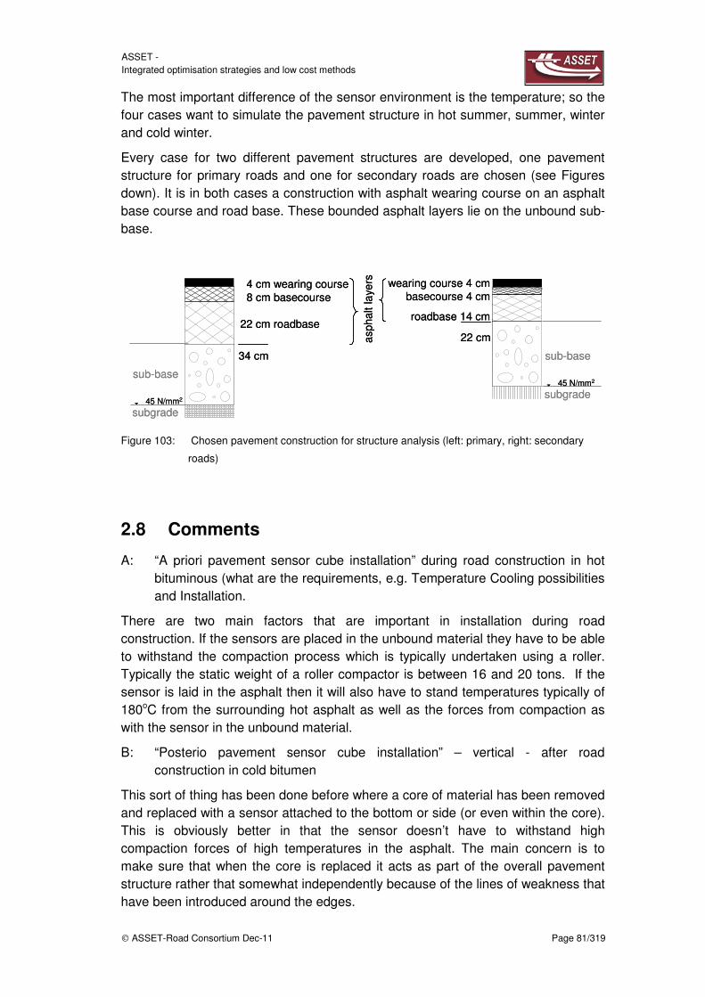
ASSET - Integrated optimisation strategies and low cost methods
ASSET-Road Consortium Dec-11 Page 81/319
The most important difference of the sensor environment is the temperature; so the four cases want to simulate the pavement structure in hot summer, summer, winter and cold winter.
Every case for two different pavement structures are developed, one pavement structure for primary roads and one for secondary roads are chosen (see Figures down). It is in both cases a construction with asphalt wearing course on an asphalt base course and road base. These bounded asphalt layers lie on the unbound sub-base.
Figure 103: Chosen pavement construction for structure analysis (left: primary, right: secondary
roads)
2.8 Comments
A: “A priori pavement sensor cube installation” during road construction in hot bituminous (what are the requirements, e.g. Temperature Cooling possibilities and Installation.
There are two main factors that are important in installation during road construction. If the sensors are placed in the unbound material they have to be able to withstand the compaction process which is typically undertaken using a roller. Typically the static weight of a roller compactor is between 16 and 20 tons. If the sensor is laid in the asphalt then it will also have to stand temperatures typically of 180oC from the surrounding hot asphalt as well as the forces from compaction as with the sensor in the unbound material.
B: “Posterio pavement sensor cube installation” – vertical - after road construction in cold bitumen
This sort of thing has been done before where a core of material has been removed and replaced with a sensor attached to the bottom or side (or even within the core). This is obviously better in that the sensor doesn’t have to withstand high compaction forces of high temperatures in the asphalt. The main concern is to make sure that when the core is replaced it acts as part of the overall pavement structure rather that somewhat independently because of the lines of weakness that have been introduced around the edges.
4 cm wearing course8 cm basecourse
22 cm roadbase
34 cm
sub-base
subgrade
asph
alt l
ayer
s
wearing course 4 cm basecourse 4 cm
roadbase 14 cm
22 cm
u45 N/mm2
sub-base
subgradeu
45 N/mm2
4 cm wearing course8 cm basecourse
22 cm roadbase
34 cm
sub-base
subgrade
asph
alt l
ayer
s
wearing course 4 cm basecourse 4 cm
roadbase 14 cm
22 cm
u45 N/mm2
sub-base
subgradeu
45 N/mm2

ASSET - Integrated optimisation strategies and low cost methods
ASSET-Road Consortium Dec-11 Page 82/319
C: “Posterior pavement sensor cube installation” – declined - after road construction in cold bituminous
Installation depth into the pavement layer, dimension and shape of the bore diameter
Definition of embedding material (type and viscosity of resin or layer material).
If possible it’s best to embed in asphalt or something with a similar stiffness modulus so that additional stress is not attracted to the sensor (or away from the sensor). Ideally, the stiffness of the embedding material should change with temperature and loading time in the same way that the stiffness of asphalt changes with temperature and loading time. This might not be possible and some compromises may have to be made but a material should be chosen with as close stiffness as possible to asphalt.
Definition of number of sensors and its alignment
We’ve talked about this above. The most important measurements are horizontal tensile stresses and strains at the bottom of the asphalt layers and vertical compressive stresses and strains at the top of the subgrade. In addition, it would be nice to measure vertical stress and strain in the granular material and perhaps vertical and horizontal stress and strain near to the pavement surface. Temperature should ideally be measured throughout the depth of the pavement structure and it is most important to measure moisture in the granular sub-base and subgrade.
Definition of core samples (position within the lane and depth and timing)
The most important location will be in the wheel path as this is where most of the traffic applies its loading. If possible it would be nice to look at a few locations adjacent to the wheel path so that we could get some idea about the effect of lateral wander on stresses and strains.
Installation layout, method and installation instructions

ASSET - Integrated optimisation strategies and low cost methods
ASSET-Road Consortium Dec-11 Page 83/319
2.9 Installation example of Japanese sensor
Figure 104: Sensor distribution (Japanese version literature taken)
2.9.1 Proposed pavement sensor locations and orientation
The simulation sensor positions are the most interesting for understanding the pavement health and deterioration, and later the sensors in real pavement structures could have the same coordinates.
Our sensor is able to measures pavement stress through the strain which pavement is subject.
Generally it is in use to take place different sensor to have stress values in different direction and other important pavement features, but in our case, we are able to measure more features from the same sensor. One sensor can measure driving direction stresses, vertical stresses and temperature. If we need the transversal

ASSET - Integrated optimisation strategies and low cost methods
ASSET-Road Consortium Dec-11 Page 84/319
stress value we can rotate the sensor 90° with respect to the vertical axle. In the next figure we can better understand the different measure of the sensor and the coordinate-system.
Figure 105: Pavement sensor distribution
The pavement structure is not subject in every point to the same stress and strain condition, we have already spoke about vertical and horizontal stresses which have change a lot by depth. On the other hand we can imagine how the vertical and horizontal stresses cannot be the same in transversal direction. Iin fact there is always a zone of the road which is subject always to high solicitation.
The philosophy was to allocate sensors for the wheel path (high wear and tear conditions) and for the centre line (only minor impacts on pavements). These two areas can be compared later on to analyse the different effects on the pavement layers. In the next figures it is possible to see the road structure and better understanding the different sensor position.

ASSET - Integrated optimisation strategies and low cost methods
ASSET-Road Consortium Dec-11 Page 85/319
Figure 106: Road characterization and coordinates used
We can appreciate in x-direction as driving direction; y as transversal direction and z as vertical direction.
Figure 107: Road characterization and dimensions

ASSET - Integrated optimisation strategies and low cost methods
ASSET-Road Consortium Dec-11 Page 86/319
Figure 108: Road frontal dimensions
Pavement structure
Thick Thin
a 34 22 cm
b 34 22 cm
Figure 109: Road characterization for thin and thick structure.
In the following figure some pavement layer are made transparent to appreciate some sensor position. This figure is an example; the real positions are described later.
Figure 110: Road section and sensor position

ASSET - Integrated optimisation strategies and low cost methods
ASSET-Road Consortium Dec-11 Page 87/319
Interesting sensor positions are:
Surface
Conglomerate bituminous base
All layers surfaces of granular material
Other interesting points
We are interested in stress and strain in each layer and we measure them to all the top layers. Furthermore we know vertical stresses in each layer, horizontal stresses and strains to the asphalt bottom, because all the mathematical models are based on them to provide the pavement fatigue behaviour. Finally we have sensors in the middle of each layer only to better understand the pavement structural health. In the followings tables we recommend for approval (by NOT) the coordinates of the 18 sensors in the road section and in the different pavement layers (used in the simulation).
Wheel-paths Diagram - 0.6m and 3.1m from hard shoulder
L: longitudinal; Tr: transversal
W: wheel path; C: centerline
T: top; M: middle; B: bottom.
Figure 111: Sensor position for wheel path
LWT LWM TrW
M
TrWB LWB TrWT
2m
22m
2 1 3
4 5
6 7
8
9
13
14 15
16
17
18
12 11 10

ASSET - Integrated optimisation strategies and low cost methods
ASSET-Road Consortium Dec-11 Page 88/319
Centerline Diagram - 1.85m from hard shoulder
Figure 112: Sensor position for centreline (colours = layer 1,2 and 3)
Figure 113: Table of sensor coordinates for primary structure and wheel path
Primary structure
Layer Sensor x y z [l]
Wheel path
1
1 0 0,6 0,00E+00 m
2 4 0,6 1,70E-01 m
3 8 0,6 3,40E-01 m
2
4 0 0,6 3,40E-01 m
5 4 0,6 4,60E-01 m
6 8 0,6 5,90E-01 m
3
7 0 0,6 6,00E-01 m
8 4 0,6 8,00E-01 m
9 8 0,6 1,10E+00 m
LCT TrCT TrCM TrCB TrCB LCM
2m
22m
1 2 3
10 11 12
4 5
6
7
8
9
13 14
15
16 17
18

ASSET - Integrated optimisation strategies and low cost methods
ASSET-Road Consortium Dec-11 Page 89/319
Primary structure
Layer Sensor x y z [l]
Centreline
1
10 2 1,85 0,00E+00 m
11 6 1,85 1,70E-01 m
12 10 1,85 3,40E-01 m
2
13 2 1,85 3,40E-01 m
14 6 1,85 4,60E-01 m
15 10 1,85 5,90E-01 m
3
16 2 1,85 6,00E-01 m
17 6 1,85 8,00E-01 m
18 10 1,85 1,10E+00 m
Figure 114: Table of sensor coordinates for secondary structure and centerline
Secondary structure
Layer Sensor x y z [l]
Wheel path
1
1 0 0,6 0,00E+00 m
2 4 0,6 1,10E-01 m
3 8 0,6 2,20E-01 m
2
4 0 0,6 2,20E-01 m
5 4 0,6 3,40E-01 m
6 8 0,6 4,70E-01 m
3
7 0 0,6 4,70E-01 m
8 4 0,6 6,80E-01 m
9 8 0,6 9,80E-01 m
Figure 115: Table of sensor coordinates for secondary structure and wheel path

ASSET - Integrated optimisation strategies and low cost methods
ASSET-Road Consortium Dec-11 Page 90/319
Secondary structure
Layer Sensor x y z [l]
Centreline
1
10 2 1,85 0,00E+00 m
11 6 1,85 1,10E-01 m
12 10 1,85 2,20E-01 m
2
13 2 1,85 2,20E-01 m
14 6 1,85 3,40E-01 m
15 10 1,85 4,70E-01 m
3
16 2 1,85 4,70E-01 m
17 6 1,85 6,80E-01 m
18 10 1,85 9,80E-01 m
Figure 116: Table of sensor coordinates for secondary structure and centreline
2.9.2 Simulation results for thin structure
Our new sensor conception measures both, vertical stress in zz direction, and longitudinal stress in xx direction. It is possible also to have transversal values (yy direction) turning the sensor 90° with respect to the z-axis. To define the measurement ranges and the calibration of the sensors we need the measurement ranges and values of stress and strain in all the different direction.

ASSET - Integrated optimisation strategies and low cost methods
ASSET-Road Consortium Dec-11 Page 91/319
Figure 117: Trend values for a thin structure

ASSET - Integrated optimisation strategies and low cost methods
ASSET-Road Consortium Dec-11 Page 92/319
Positio
n Layer
Depth
(m) Stress Stress Strain Strain
Displacem
ent
Displacem
ent
Numb
er
Numb
er XX ZZ XX ZZ UZ UX at 0.2m
(MPa) (MPa) (µstrain) (µstrain) (µm) (µm)
1 1
0,00E+
00
-5,28E-
01
-1,42E-
01
-
9,80E+0
1
7,61E+0
1 4,40E+02 -1,80E+01
2 1
1,10E-
01
-4,91E-
02
-9,41E-
02
3,43E-
01
-
1,99E+0
1 4,43E+02 2,17E-01
3 1
2,20E-
01
4,19E-
01
-3,77E-
02
9,53E+0
1
-
1,10E+0
2 4,36E+02 1,73E+01
4 2
2,20E-
01
-4,59E-
02
-3,77E-
02
-
3,06E+0
2
-
2,69E+0
2 4,36E+02 1,73E+01
5 2
3,40E-
01
-3,81E-
02
-2,52E-
02
-
2,54E+0
2
-
2,10E+0
2 4,08E+02 1,85E+01
6 2
4,70E-
01
-2,98E-
02
-1,74E-
02
-
1,99E+0
2
-
1,97E+0
2 3,82E+02 2,43E+01
7 3
4,70E-
01
-7,99E-
04
-1,74E-
02
1,30E+0
2
-
3,35E+0
2 3,82E+02 2,43E+01
8 3
6,80E-
01
-4,39E-
04
-1,23E-
02
9,28E+0
1
-
2,38E+0
2 3,23E+02 1,78E+01
9 3
9,80E-
01
-1,72E-
04
-8,20E-
03
6,35E+0
1
-
1,61E+0
2 2,64E+02 1,24E+01
Figure 118: Thin analysis results for a thick thin pavement-summer time-wheel path

ASSET - Integrated optimisation strategies and low cost methods
ASSET-Road Consortium Dec-11 Page 93/319
Posit
ion
Laye
r
Depth
(m)
Stress
(MPa)
Stress
(MPa)
Strain
µstrain)
Strain
(µstrain)
Displaceme
nt (µm)
Displaceme
nt (µm)
Num
ber
Num
ber XX ZZ XX ZZ UZ UX at \0.2m
1 1
0,00E
+00
-4,31E-
01
-1,42E-
01
-
2,89E+0
1 2,01E+01 1,15E+02 -5,31E+00
2 1
1,10E-
01
-6,14E-
02
-1,02E-
01
-5,14E-
01
-
7,42E+00 1,16E+02 -3,79E-02
3 1
2,20E-
01
2,92E-
01
-5,04E-
02
2,59E+0
1
-
3,18E+01 1,14E+02 4,68E+00
4 2
2,20E-
01
-7,36E-
02
-5,04E-
02
-
9,20E+0
1
-
6,90E+01 1,14E+02 4,68E+00
5 2
3,40E-
01
-5,56E-
02
-3,09E-
02
-
6,94E+0
1
-
5,22E+01 1,06E+02 5,05E+00
6 2
4,70E-
01
-4,18E-
02
-1,95E-
02
-
5,22E+0
1
-
5,04E+01 1,00E+02 7,00E+00
7 3
4,70E-
01
-4,00E-
04
-1,95E-
02
3,77E+0
1
-
9,57E+01 1,00E+02 7,00E+00
8 3
6,80E-
01
-2,45E-
04
-1,33E-
02
2,59E+0
1
-
6,55E+01 8,34E+01 4,93E+00
9 3
9,80E-
01
-9,36E-
05
-8,66E-
03
1,71E+0
1
-
4,30E+01 6,75E+01 3,31E+00
Figure 119: Thin analysis results for a thick thin pavement-winter time-wheel path

ASSET - Integrated optimisation strategies
ASSET-Road Consortium Dec
2.9.3 Simulation results
Figure 120: Trend values for a
trategies and low cost methods
Dec-11
Simulation results for thick structure
Trend values for a thick structure
Page 94/319

ASSET - Integrated optimisation strategies and low cost methods
ASSET-Road Consortium Dec-11 Page 95/319
Posit
ion
Laye
r
De
pth
Stress
(MPa)
Stress
(MPa)
Strain
(µstrain)
Strain
(µstrain)
Displaceme
nt (µm)
Displaceme
nt (µm)
Num
ber
Num
ber (m) XX ZZ XX ZZ UZ UX at 0.2m
1 1
0,0
0 -0,3460
-1,42E-
01
-
5,84E+01 3,35E+01 3,18E+02 -1,11E+01
2 1
0,1
7 -0,0247
-8,80E-
02 4,91E+00
-
2,36E+01 3,19E+02 9,84E-01
3 1
0,3
4 0,2700
-1,92E-
02 6,08E+01
-
6,95E+01 3,11E+02 1,12E+01
4 2
0,3
4 -0,0279
-1,92E-
02
-
1,86E+02
-
1,47E+02 3,11E+02 1,12E+01
5 2
0,4
6 -0,0248
-1,32E-
02
-
1,65E+02
-
1,16E+02 2,96E+02 1,12E+01
6 2
0,5
9 -0,0214
-9,67E-
03
-
1,43E+02
-
1,10E+02 2,81E+02 1,37E+01
7 3
0,6
0 -0,0004
-9,53E-
03 7,09E+01
-
1,83E+02 2,79E+02 1,35E+01
8 3
0,8
0 -0,0004
-7,25E-
03 5,36E+01
-
1,39E+02 2,48E+02 1,04E+01
9 3
1,1
0 -0,0002
-5,24E-
03 3,92E+01
-
1,01E+02 2,12E+02 7,69E+00
Figure 121: Thick analysis results for a thick thin pavement-summer time-wheel path

ASSET - Integrated optimisation strategies and low cost methods
ASSET-Road Consortium Dec-11 Page 96/319
Posit
ion
Laye
r Depth
Stress
(MPa)
Stress
(MPa)
Strain
(µstrain)
Strain
(µstrain)
Displace-
ment (µm)
Displace-
ment (µm)
Num
ber
Num
ber (m) XX ZZ XX ZZ UZ UX at 0.2m
1 1
0,00E
+00
-3,01E-
01
-1,42E-
01
-
1,83E+01 8,65E+00 8,65E+01 -3,47E+00
2 1
1,70E
-01
-3,08E-
02
-9,35E-
02 1,59E+00
-
8,99E+00 8,62E+01 3,18E-01
3 1
3,40E
-01
2,08E-
01
-2,71E-
02 1,80E+01
-
2,15E+01 8,38E+01 3,29E+00
4 2
3,40E
-01
-5,48E-
02
-2,71E-
02
-
6,84E+01
-
4,06E+01 8,38E+01 3,29E+00
5 2
4,60E
-01
-4,13E-
02
-1,70E-
02
-
5,17E+01
-
3,10E+01 7,96E+01 3,31E+00
6 2
5,90E
-01
-3,04E-
02
-1,14E-
02
-
3,80E+01
-
2,98E+01 7,58E+01 4,24E+00
7 3
6,00E
-01
-1,47E-
04
-1,12E-
02 2,20E+01
-
5,55E+01 7,52E+01 4,17E+00
8 3
8,00E
-01
-2,02E-
04
-8,29E-
03 1,60E+01
-
4,06E+01 6,57E+01 3,08E+00
9 3
1,10E
+00
-1,48E-
04
-5,81E-
03 1,12E+01
-
2,85E+01 5,56E+01 2,19E+00
Figure 122: Thick analysis results for a thick thin pavement-winter time-wheel path
The E modulus is different for each layer/layer package of the pavement structure. In the following it is described on what basis the E modulus of the several layers or layer packages are determined and respectively defined.
2.9.4 Asphalt package dynamic properties
The E modulus is different for each layer/layer package of the pavement structure. It is strongly dependent on the temperature and frequency of load on asphalt layers.
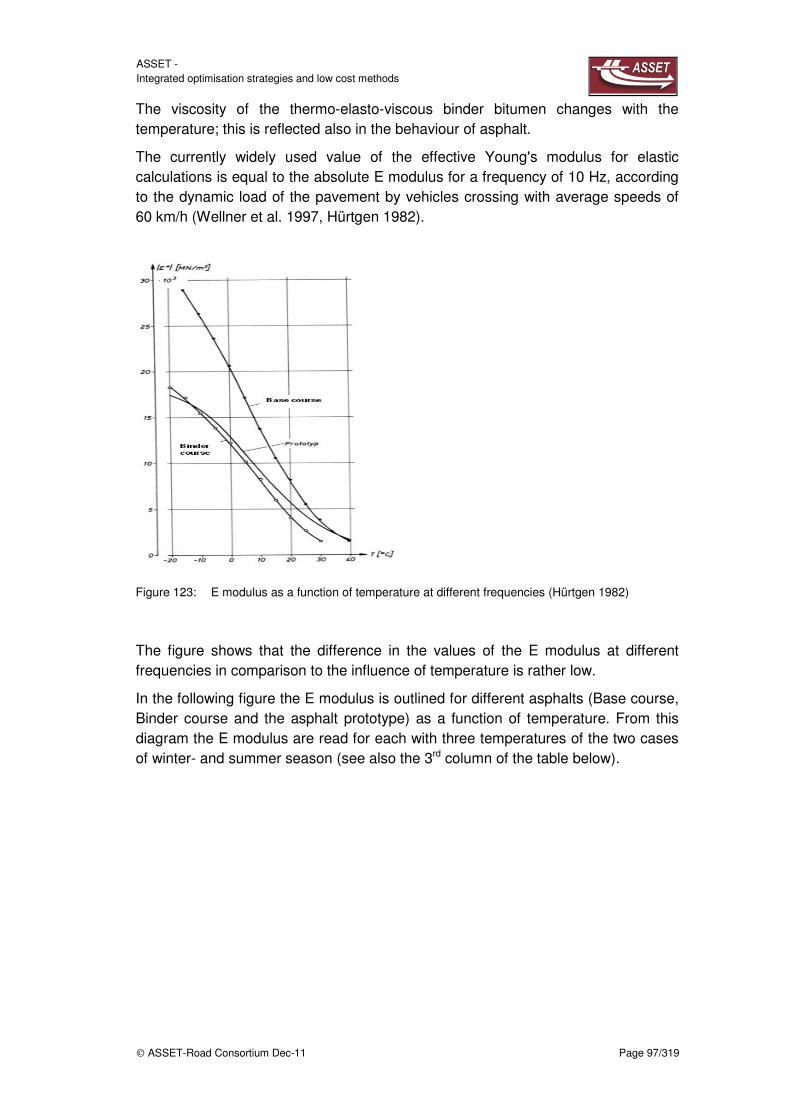
ASSET - Integrated optimisation strategies and low cost methods
ASSET-Road Consortium Dec-11 Page 97/319
The viscosity of the thermo-elasto-viscous binder bitumen changes with the temperature; this is reflected also in the behaviour of asphalt.
The currently widely used value of the effective Young's modulus for elastic calculations is equal to the absolute E modulus for a frequency of 10 Hz, according to the dynamic load of the pavement by vehicles crossing with average speeds of 60 km/h (Wellner et al. 1997, Hürtgen 1982).
Figure 123: E modulus as a function of temperature at different frequencies (Hürtgen 1982)
The figure shows that the difference in the values of the E modulus at different frequencies in comparison to the influence of temperature is rather low.
In the following figure the E modulus is outlined for different asphalts (Base course, Binder course and the asphalt prototype) as a function of temperature. From this diagram the E modulus are read for each with three temperatures of the two cases of winter- and summer season (see also the 3rd column of the table below).

ASSET - Integrated optimisation strategies and low cost methods
ASSET-Road Consortium Dec-11 Page 98/319
Figure 124: E modulus at f=10Hz as a function of temperature (Hürtgen 1982)
To understand the behaviour of the pavement layers and its structure, the following table presume the different values of E-modus and Poisson ratio for different conditions.
First principal structure (motorways/main roads)
Layer Temperature Thickness Stiffness
(E-modulus)
Poisson
ratio (v)
Hot summer
Asphalt 60 °C 34 cm 1GPa 0.35
Sub-base 34 cm 150MPa 0.3
Sub-grade 50MPa 0.4
Summer Asphalt 20-25 °C 34 cm 3GPa 0.35
Sub-base 34 cm 150MPa 0.3
Sub-grade 50MPa 0.4
Winter Asphalt 0 °C 34 cm 8GPa 0.35
Sub-base 34 cm 800MPa 0.3
Sub-grade 34 cm 200MPa 0.4
Cold winter
Asphalt -20 °C 34 cm 20GPa 0.35
Sub-base 34 cm 800MPa 0.3
Sub-grade 200MPa 0.4
Figure 125: Table for main roads features in different seasons

ASSET - Integrated optimisation strategies and low cost methods
ASSET-Road Consortium Dec-11 Page 99/319
Second principal structure(secondary road)
Layer Temperature Thickness Stiffness
(E-modulus)
Poisson
ratio (v)
Hot summer
Asphalt 60 °C 22 cm 1GPa 0.35
Sub-base 22 cm 150MPa 0.3
Sub-grade 50MPa 0.4
Summer Asphalt 20-25 °C 22 cm 3GPa 0.35
Sub-base 22 cm 150MPa 0.3
Sub-grade 50MPa 0.4
Winter Asphalt 0 °C 22 cm 8GPa 0.35
Sub-base 22 cm 800MPa 0.3
Sub-grade 200MPa 0.4
Cold winter
Asphalt -20 °C 22 cm 20GPa 0.35
Sub-base 22 cm 800MPa 0.3
Sub-grade 200MPa 0.4
Figure 126: Table for secondary roads features in different seasons
2.9.5 Measurement ranges (stress)
Unfortunately the transversal and longitudinal stress values are the same because of the kind of simulation; in fact, the simulation is static, from a circle surface side in the middle of the upper surface. In any case the difference shouldn’t be too high.
xx
Mpa
Thick structure Thin structure
summer winter summer winter
Layer1
min -3,46E-01 -0,301 -0,528 -0,431
max 2,70E-01 0,208 0,419 0,292
Layer2
min -0,02794 -0,05475 -0,04585 -0,07361
max -0,02141 -0,0304 -0,02978 -0,04178
Layer3
min -0,00044 -0,0002 -0,0008 -0,0004
max -0,00023 -0,00015 -0,00017 -9,4E-05
Figure 127: Table of horizontal stresses
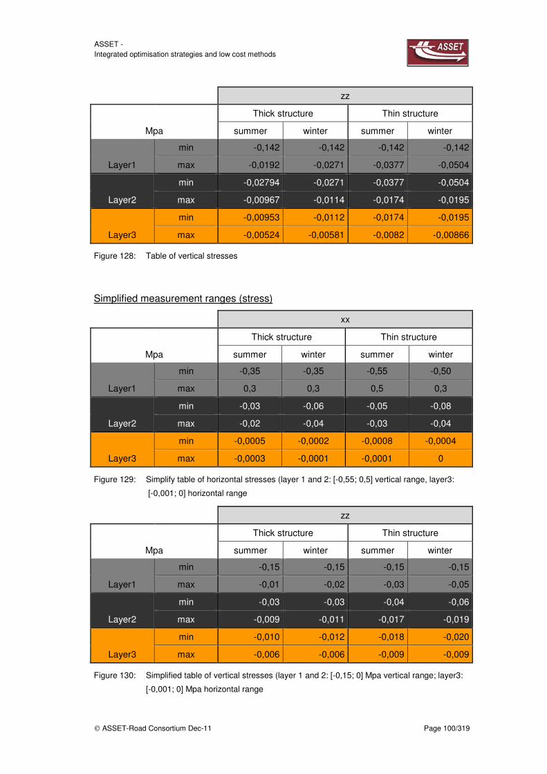
ASSET - Integrated optimisation strategies and low cost methods
ASSET-Road Consortium Dec-11 Page 100/319
zz
Mpa
Thick structure Thin structure
summer winter summer winter
Layer1
min -0,142 -0,142 -0,142 -0,142
max -0,0192 -0,0271 -0,0377 -0,0504
Layer2
min -0,02794 -0,0271 -0,0377 -0,0504
max -0,00967 -0,0114 -0,0174 -0,0195
Layer3
min -0,00953 -0,0112 -0,0174 -0,0195
max -0,00524 -0,00581 -0,0082 -0,00866
Figure 128: Table of vertical stresses
Simplified measurement ranges (stress)
xx
Mpa
Thick structure Thin structure
summer winter summer winter
Layer1
min -0,35 -0,35 -0,55 -0,50
max 0,3 0,3 0,5 0,3
Layer2
min -0,03 -0,06 -0,05 -0,08
max -0,02 -0,04 -0,03 -0,04
Layer3
min -0,0005 -0,0002 -0,0008 -0,0004
max -0,0003 -0,0001 -0,0001 0
Figure 129: Simplify table of horizontal stresses (layer 1 and 2: [-0,55; 0,5] vertical range, layer3:
[-0,001; 0] horizontal range
zz
Mpa
Thick structure Thin structure
summer winter summer winter
Layer1
min -0,15 -0,15 -0,15 -0,15
max -0,01 -0,02 -0,03 -0,05
Layer2
min -0,03 -0,03 -0,04 -0,06
max -0,009 -0,011 -0,017 -0,019
Layer3
min -0,010 -0,012 -0,018 -0,020
max -0,006 -0,006 -0,009 -0,009
Figure 130: Simplified table of vertical stresses (layer 1 and 2: [-0,15; 0] Mpa vertical range; layer3:
[-0,001; 0] Mpa horizontal range

ASSET - Integrated optimisation strategies and low cost methods
ASSET-Road Consortium Dec-11 Page 101/319
BASt values
Thick structure, zz direction, max value: 0.28 Mpa. We have 0.15 Mpa.
Thin structure, zz direction, max value: 0.09 Mpa. We have 0.15 Mpa.
BASt’s values and our values have the same order of magnitude, but values are different.
BASt uses two pavement structures different from ours and we don’t know in which point is collocate the sensor.
GEOCON standard ranges for MODEL 3500
0,1 - 0,25 - 0,4 - 0,6 – 1 - 2,5 - 6 Mpa
Our values are all in the first two of the Geocon ranges.
2.9.6 Measurement ranges (strain)
Max Min
Layer Strain xx Strain zz Strain xx Strain zz
1 9,53E+01 7,61E+01 -9,80E+01 -1,10E+02
2 1,30E+02 -2,98E+01 1,77E+01 -2,69E+02
3 1,30E+02 -2,85E+01 1,12E+01 -3,35E+02
Figure 131: Strain values
BASt values
Thin structure, xx direction strain range: (-110; 230)µm.
We have (-98; 130) µm.
2.9.7 Other measurement ranges
Another way to calculate the stress in the asphalt is using the simple cone formulation: according to this idea the vertical stress is reducing like a cone of 30° by the depth.
The formula became:
σ=F/(π*(r+tg(30°)2)

ASSET - Integrated optimisation strategies and low cost methods
ASSET-Road Consortium Dec-11 Page 102/319
Figure 132: Stress distribution
Generally Nottingham simulation should be more appropriate because it take in consideration also horizontal stresses so the Poisson ratio (ν) and the structure not continuous for the pavement.
Here are the following different tables for stress and strain for different simulations:
Season Temperature T
[°°°°C]
E modulus[MN/m2] Average of E modulus [MN/m
2]
Winter
-20
Base course: 30.000
21.833 Binder course: 18.000
Prototype: 17.500
-15
Base course: 27.500
20.500 Binder course: 17.000
Prototype: 17.000
-10
Base course: 25.500
18.700 Binder course: 15.100
Prototype: 15.500

ASSET - Integrated optimisation strategies and low cost methods
ASSET-Road Consortium Dec-11 Page 103/319
Season Temperature T
[°°°°C]
E modulus[MN/m2] Average of E modulus [MN/m
2]
Summer
+20
Base course: 7.800
5.933 Binder course: 4.200
Prototype: 5.800
+25
Base course: 6.000
4.333 Binder course: 2.800
Prototype: 4.200
+30
Base course: 4.000
3.300 Binder course: 2.100
Prototype: 3.800
Figure 133: Averaged E modulus for different temperature cases with the frequency f = 10 Hz
Sub-base
The E modulus of the unbound sub-base (layer thickness according to RStO 01), results from the minimum required value of the deformation module on the unbound layers of Ev2 = 120 MN/m2 calculated from a simulated plate pressure test with the software BISAR (Bitumen Stress Analysis in Roads). Thus the E modulus of the unbound layer in both pavement structures are E = 170 MN/m2.
Subgrade
On the plane according to the RStO 01, a deformation modulus of at least Ev2 = 45 MN/m2 is required, which is identified by a plate-loading test. It results from the demand for an Ev2 value of 45 MN/m2 on the plane and an E modulus of 45 MN/m2 for the subgrade. Due to the averaged values the following E modulus values are chosen:
Figure 134: Averaged E modulus chosen for different season and different layer with the frequency
f = 10 Hz
Asphalt layer Hot summer Summer Winter Cold winter
Temperature
Pavement
60°C 20-25 °C 0°C -20°C
Modulus (MPa)
Asphalt 1-3 layers
1,000 MPa 3,000 MPa 8,000 MPa 15,000 MPa
Subbase 150 MPa 800 MPa
Subgrade 50 MPa 200 MPa

ASSET - Integrated optimisation strategies and low cost methods
ASSET-Road Consortium Dec-11 Page 104/319
2.9.8 General discussion of pavement sensing
Position of the sensors - The definition of the position of measuring points within the layer and within the lane and placement was presented in detail in the sub-chapters before.
Stresses and strains – the most critical locations tend to be close to the interfaces between layers (bottom of asphalt and top of granular layers) and possibly close to the road surface.
Temperature and moisture – possibly uniformly distributed through the pavement depth.
Detect aging effects on pavements and layers - Ageing affects mainly the stiffness of the asphalt layer which increases. If you measure stress and strain in the asphalt you can get stiffness and can see how it changes over the life of the pavement. You have to take out the effects of temperature and the trend might be for the stiffness to gradually decrease due to accumulation of damage being more dominant than ageing although you might see some early increases in stiffness.
Correlate pavement effects with WIM load - measurements (tire based and speed plus position within the lane) (to be integrated with embedded sensor report (Hothan).
Speed relationship of damages - Due to the viscous nature of asphalt, loading
speed has an important effect on the pavement response and stiffness (E
modulus). American research and investigations are confirming this statement (low speed increasing, middle speed is maximum damage and at higher speed damage is lower).
A given load travelling at a low speed generates larger deflections than at higher speeds and it is supposed to generate more damage to the pavement. It is,
therefore, a point of interest the possibility to study this relationship by
linking the WIM data to the pavement instrumentation.
Lateral wandering of the wheel path can also be an important factor in studying the evolution of modes of distress (such as rutting). A more canalised traffic corresponds to a more aggressive loading condition that could be monitored linking the WIM data to the pavement instrumentation. To directly relate WIM measurements to damage you would need to undertake simulations (this is what we are proposing to do in ASSET-Road).
Analysing shock waves by approaching/disappearing vehicles/tires
There are three types of waves: Pressure waves, shear waves and Rayleigh
waves. Rayleigh waves are a special case where a shear wave meets a surface and are the easiest to detect because they decay less quickly than pressure waves and shear waves. Having said that, asphalt tends to be a heavily damped material and Rayleigh waves are not as easy to measure as in other systems. There has been quite a lot of work on this in the past (as noted below) and if you measure Rayleigh wave speed you can get an indication of the shear modulus and hence

ASSET - Integrated optimisation strategies and low cost methods
ASSET-Road Consortium Dec-11 Page 105/319
Young’s modulus although this is a low strain value which is quite different from what you would measure in the laboratory. You can also get more sophisticated and measure dispersion curves to try and estimate how the modulus changes with depth although this is pretty difficult to do and requires significant processing of measurements.
Measuring wave speeds
There are 3 different types of waves in pavements: Pressure waves, Shear waves (stronger damping) and Rayleigh waves (attenuate less). The shear wave velocity is given by:
V= √(G/ρ) = 500 m/s Speed on Pavements of Shear waves
Modulus G=E/3 Mpa
Elasticity E=2.000 Mpa
Density ρ=2600 kg/m³
The Rayleigh wave speed (vR) is slightly lower than the shear wave speed and can be approximated by this simple equation:
vR=vT√(0.44+K)/(0.58+K)
Where:
vT is the transverse bulk wave velocity: vT=√(E-G)/2 ρ
K=v/(1-ν),with ν is the Poisson’s ratio.
Paper on waves in roads: Ken Stokoe III and Nazarion (Taxas)
Investigating underground WIM (in pavement embedded)
The diameter of the force/pressure load cell should be more than 10 cm. Not sure what this is but it sounds like a pressure measurement. A trial would be interesting.

ASSET - Integrated optimisation strategies and low cost methods
ASSET-Road Consortium Dec-11 Page 106/319
3 Pavement Sensor Layout and Dimensions
3.1 Pavement sensor layout
Different pavement sensor mechanical design versions were elaborated and investigated:
Figure 135: Pavement sensor concept

ASSET - Integrated optimisation strategies and low cost methods
ASSET-Road Consortium Dec-11 Page 107/319
3.2 Summary sensor specification
Temperature - 20 to + 80 Celsius
Vertical acceleration 10 g
Longitudinal acceleration 10 g
Stress in asphalt layers ≈ 0.3 - 0.5 MPa
Horizontal stress ± 2 MPa, (surface layer: ≤ 5 MPa);
Stress in granular layers < 0.1 MPa
Strain (vertical) < 500 µstrains
Strain (horizontal) < ±200 µstrains; much higher creep strain possible (in 1.7 5000 µm/m are mentioned)
Accoustic 0 - 1 kHZ
3.2.1 Measurements and parameters
Measurement 1: Vertical Stress in the top pavement layer:
Initial stress is according to the tyre pressure on the surface distribution of the tyre
Pressure:
≈ 0.3-0.5 MPa in asphalt layers (absolute max: 800KPa)
≈ 0.1 MPa in granular layers
up to 5 MPa.
Measurement 2: Vertical strains
< 500 µ strains
Measurement 3: Horizontal stress
Horizontal stress due to bending my reach ± 2.0 MPa Especially for surface asphalt courses, additional to stress induced by traffic loads, at low temperatures the cooling of the asphalt material may induce cryogenic stress which may increase.
Measurement 4: Horizontal strain (in diving direction):
Esp. Below asphalt base course ≈ 200-500 µ strains (Measurement range 1500 µ strains) Comparison with current displacement sensor KM-100HAS: Measurement Range ± 5.000 µm/m (5mm/m) 5000 µ strains
Linearity max. 1% Elastizitätsmodul 40 N/mm² Temperature Range -20 ~ +180°C For dynamic strain measurements resolution of values shall be higher than 10
µm/m

ASSET - Integrated optimisation strategies and low cost methods
ASSET-Road Consortium Dec-11 Page 108/319
Measurement 5: Horizontal strain (90° to driving direction)
Esp. below asphalt base course centrally below load path, differently to measurement 3, only tension strain occur which will accelerate fatigue. For measurement 3, each tension load is accompanied by two compression peak which may close a micro crack again.
Optional the strain measurement at the road surface next to the wheel path would be interesting as well as there occur tension stress due to material cooling and bending
Measurement 6: Acceleration in layer up to 10 g (1g = 9,81 m/s²) in 2 axles
Measurement 7: Speed in layers
Measurement 8: Displacement in layers
Measurement 9: Temperature (-25°C to 80°C) survival temperature 180°C
Measurement 10: Dynamic range
0 – 1 to 2 kHz max,
Specific sample rates to be used (e.g. temperature every 10 min)
Measurement 11: Humidity
Measurement 12: Acoustic
3.3 Mechanical design
3.3.1 Mechanical pavement sensor soncepts
During the project an analysis of different pavement sensor concept variations was done in 2010 concerning orientation, displacement and force input interfaces and the general structure:

ASSET - Integrated optimisation strategies and low cost methods
ASSET-Road Consortium Dec-11 Page 109/319
Figure 136: Concept 1 (Ø=100 mm, h=60 mm / 160 mm) and Concept 2
Figure 137: Concept 3 (double-leg version vertical)
Figure 138: Concept 4 (double-leg version vertical, height reduced to 29mm): FINAL
There were 5 different versions for pavement sensors investigated. For complete plans and different pieces it is possible to see straight the last version (version 5).
Version 1
The first version has a pipe to protect the strain gauge sensor and the sensor is positioned on a plate linked to two springs that we will call “the sensor house”.

ASSET - Integrated optimisation strategies and low cost methods
ASSET-Road Consortium Dec-11 Page 110/319
Figure 139: First conception and encumbrance
The simulation of the sensor house piece shows how the springs get compressed from the movement and we can appreciate the movement of the sensor plate towards the bottom, but there will not be any deformation, it means that our sensor won’t give out any signal.
Figure 140: Simulation for sensor house
All the following versions have almost the same encumbrance. For the complete tables it is possible to see just the last version (version N.5).
Version 2
Now the idea is to take advantage of bending to increase the strain through the arm of the bending moment, in other words we have got more space removing the protecting pipe.

ASSET - Integrated optimisation strategies and low cost methods
ASSET-Road Consortium Dec-11 Page 111/319
Figure 141: Second version
In the second version the sensor house is designed to have the maximum deformation on the plate face that the strain gauge sensor is set on. It is impossible to make the plate face thinner, because the strain gauge sensors have a fixed size. Another difference is the body hole, now it is square to simplify the building of the slide.
Version 3
The strain gauge sensor has a size, so in the old version it is impossible to design the plate face with a lower size. To amplify more the deformation on the sensor face we turn it around the z axle (see the figure below).
Figure 142: Third version
Thanks to this idea we have more space and it is possible to fix the sensor house by two scrubs.

ASSET - Integrated optimisation strategies and low cost methods
ASSET-Road Consortium Dec-11 Page 112/319
Version 4
In this version we made a modification to the slide to have a better stiffness for the sensor house.
Figure 143: Fourth version
Version 5
In our last version we have doubled the sensor house, so now there are two sensor plates, one below and one above.
Figure 144: Fifth version, isometric view
In the new figure we can see the last version for the sensor house.

ASSET - Integrated optimisation strategies and low cost methods
ASSET-Road Consortium Dec-11 Page 113/319
3.4 Electronic design
It will be improved and updated due to a new microprocessor generation.
Figure 145: Draft electronic design
3.5 Sensor house simulation
From the Nottingham simulation we know all the stress, strain and displacement for the point of interest. At this particular moment we need to know the displacement in the horizontal direction to have a good sensor house simulation.
The software used for the simulation programme isn’t able to simulate a complex 3d drawing assembly, but only simple pieces. Another important limitation for our simulation is that there isn’t the constraint slide, that we need, but only the joint. Anyway for the last sensor house it seems not be a problem. In the next figure we can appreciate the piece used for our simulation.

ASSET - Integrated optimisation strategies and low cost methods
ASSET-Road Consortium Dec-11 Page 114/319
Figure 146: Sensor house used for simulation
From the Nottingham studies we know the displacement values in the transversal direction. The highest value is 2,43E1 µm. For an easy simulation the value of 0,03
mm is used. In solidworks it is not possible to define the displacement for simulation, but only the load, so for simulating there were different test force simulations done to obtain a displacement in the x-direction of 0,03 mm, the load found was about 40 N.
Figure 147: Sensor house under load simulation
In the figure it is possible to appreciate how the displacement in y-direction is about twice the displacement in x-direction of the left-slide.
3.6 Geometry design impact
The result taken from this first simulation is dependent generally from the design of our sensor house.
Obviously it is possible to change the geometry to better understand the geometrical impact on our results. Basically is possible to vary the:
Sensor house height

ASSET - Integrated optimisation strategies and low cost methods
ASSET-Road Consortium Dec-11 Page 115/319
Sensor house length
Sensor house thickness
When looking at the next figure it is easier to understand the tables.
Figure 148: Parameters
In each case we have to find a new load value to have always the same displacement value in x-direction (0,03 mm). The following graphs and tables show this load and the vertical displacement for the sensor house with a fixed x-displacement.
Height variable
Figure 149: Load vs height for a constant displacement
05
1015202530354045
0 5 10 15 20 25 30
high [mm]
F [
N]
F [N]

ASSET - Integrated optimisation strategies and low cost methods
ASSET-Road Consortium Dec-11 Page 116/319
Figure 150: Vertical displacement vs height
From this second diagram we can note how vertical displacement decreases by the high.
Length variable
Figure 151: Vertical displacement vs length
For this variable, the load seems to be always about the same (40 N).
Thickness variable
Changing the thickness in different simulations we got the following table:
0,00
0,01
0,02
0,03
0,04
0,05
0,06
0,07
0 5 10 15 20 25 30
high [mm]
ve
ric
al
dip
lac
em
en
t [m
m]
verical diplacement [mm]
0
0,01
0,02
0,03
0,04
0,05
0,06
0,07
0 10 20 30 40 50 60 70 80
lenght [mm]
vert
ical
dis
pla
cem
en
t [m
m]
lenght [mm]

ASSET - Integrated optimisation strategies and low cost methods
ASSET-Road Consortium Dec-11 Page 117/319
Thickness [mm] F [N] Vertical displacement [mm]
0,5 5 0,05
1 40 0,06
2 200 0,05
Figure 152: Table for thickness variable
In this case the load change is a lot, but the vertical displacement seems to be not affected by the thickness, so in the next step we shall give different value for thickness1 and thickness 2. The result is in the table below:
Thickness [mm] F [N] Vertical displacement [mm]
mix (2 and 1 mm) 35 0,06
Figure 153: Table for a mixed thickness
Also in this case the vertical displacement doesn’t seem be affected by thickness.
To conclude it seems that to maximize the vertical strain we should design use the shortest height and longest length.
Last simulation has:
Height=3 mm
Length=100 mm
The results are:
X displacement= 0,03 mm
F= 200N in compression/tension
Y displacement= 0,11 mm (more then twice of x-displacement).
This simulation gives for the sensor house some dimensions that are not implementable in the last geometry here showed, because the length is too big, respect the diameter of the body (both are 100 mm). Actually, it is possible to have for the sensor house higher then 100mm to obtain more vertical deformation, but it means that the body geometry must be changed.

ASSET - Integrated optimisation strategies and low cost methods
ASSET-Road Consortium Dec-11 Page 118/319
Figure 154: Displacement simulation
Figure 155: Stress simulation through Von Mises theory
The maximal stress is about 172 MPa, while the yield point is about 620 MPa, about 3.5 times more.
Sensor placement
The idea is to place the strain gauge sensors where the deformation is higher. In the following figure we can appreciate sensor locations.

ASSET - Integrated optimisation strategies and low cost methods
ASSET-Road Consortium Dec-11 Page 119/319
Figure 156: Sensor placement
3.7 System overview
Figure 157: System architecture
P1 P2
P3
P4

ASSET - Integrated optimisation strategies and low cost methods
ASSET-Road Consortium Dec-11 Page 120/319
3.8 Pavement sensor microcontroller
The currently used microcontroller PIC 18F6880 will be replaced by a new Microcontroller: dsPIC33FFJ128GP804 new device, support guaranteed for next 10 years 16 bit arithmetic, 40Mips @ 40MHz (single cycle instruction) code and pin compatible with PIC24 series (same device w/o DSP) larger number and count of application specific peripherals available 3,3V operating level shifter necessary for 5V peripherals 24 bit instr., 16 bit data, 16x16 / 32:16 plus 40 bit DSP Accumulator DSP-unit for noise stream processing (microphones and acceleration) up to 128K Flash memory for instruction and 8 K data RAM.
Figure 158: Pavement sensor microcontroller
3.9 Interaction sensor versus pavement FEA analysis
An FEA model exists and was used on an asphalt layer (30cm) with a modulus of 5,000 MPa for something like summertime (40°C) and 12,000 MPa for winter (0°C). Below this layer there is a sub base with a modulus of 250 MPa and a soil sub grade with a modulus of 90 MPa down to a depth of about 5 meters.
For the FEA investigation the dimension of the sensor which is in the middle of the model, directly on the top of the base layer has dimensions of 6x6x60cm with a modulus of 50,000 MPa. The load at the top represents a known truck used in Germany to assess bridge dimensions for example with a distributed load of a 20t axle and an area of 20x60cm.
The stress distribution within the road can be seen in the following figures. First of all, the picture shows two different dimensions.

ASSET - Integrated optimisation strategies and low cost methods
ASSET-Road Consortium Dec-11 Page 121/319
Two different situations are shown one with the whole model and one without the sensor. This is to see if the difference in stress is in the road construction or in the sensor itself. In every picture you can see in the right lower corner the short description of the model and the asphalt modulus.
As you can see, there is a huge difference in stresses in that case where the modulus of the asphalt is low. In this case the difference in stresses is very large and it can be seen that there is also a difference when the sensor is taken into consideration So, as a first result, it can be assumed that under such conditions the effect of such a sensor will be large and that the sensor itself will be the focus of the stress contribution.
In the other case where stiff asphalt is considered, the difference between the calculated stresses is not so large. This can be seen in the figures.
The fact that the modulus of asphalt changes with temperature also has implications on using embedded sensors for measuring stress and strain parameters.
Figure 159: Pavement sensor interaction simulation (I)
Figure 160: Sensor body embedding simulation

ASSET - Integrated optimisation strategies and low cost methods
ASSET-Road Consortium Dec-11 Page 122/319
3.10 Specification of traffic measurements (WIM)
A new generation of high-tech weigh-in-motion sensors (integrated measurement matrix) based on reliable and precise strain gauges technology and embedded microelectronic for signal processing and CAN/Ethernet bus interfacing will be used.
Figure 161: The proposed ROC WIM matrix
Different measurements and data can be recorded:
Tire force (new precision WIM)
Wheel load measurement
Axle weight
Gross weight
Typical footprint areas
Tire Footprint traverse position measurement (lane passing area).
Tire pressure calculation
Axle distances and configurations
Static and dynamic weight measurement (measurement point matrix with 4 cm resolution)
High sensor accuracy and high sampling rate.
Long term calibration stability - Static calibration and approval as base for dynamic operation.

ASSET - Integrated optimisation strategies and low cost methods
ASSET-Road Consortium Dec-11 Page 123/319
Prepared for bi-directional sensor fields using basic sensor modules (32 x 6 cm)
Single/double tire recognition
Axle width measurement
Axle configuration analysis
Lateral wheel position measurement across lane
Features of the new WIM system
Flat sensor design, easy installation and exchange of sensors modules in minutes.
Replacement on road in less than 15 minutes
Analogue sensor signals are converted to digital in close proximity to the shear beam sensors. This ensures minimal environmental noise influence on the sensor signals.
Minimal analogue circuitry avoids drift problems due to electronic component tolerances.
Low power consumption by use of modern micro controller technology.
Less cabling effort due to CAN bus network topology.
No proprietary interface boards necessary.
Links to standard PC via CAN-converters as used in high volume car industry.
Automatic failure compensation by reassignment of shear beam transducers
Applications
Future WIM systems for fully automatic axle and vehicle overload enforcement
High accuracy WIM sites for data collection and pre-selection
Research projects for new pavement deterioration models with extended parameters
Wear and tear analysis (groove effects)

ASSET - Integrated optimisation strategies and low cost methods
ASSET-Road Consortium Dec-11 Page 124/319
4 Cyclic Models for Granular Materials
4.1 Background
For large strain cyclic loading of granular materials (including sub-base fills and sub-grade soils), plastic deformation and strain accumulation is evident after a small number of load cycles. Traffic loading causes very small strains in soils, and no visible deformation of the ground may occur. However, after a large number of load cycles strain accumulation may become critical, initiate damage and cause a reduction of road serviceability.
Investigation of soil deformation due to cyclic loading was first considered by Seed (Seed et al. 1955, 1956, 1958, 1960). Widespread interest in the area has resulted in significant research effort and a number of models to predict the response of soils to cyclic loading have been proposed. These range from simple empirical approaches to relatively complex constitutive models which are typically implemented in numerical analyses. The latter models although theoretically more rigorous are often difficult to implement as the material parameters required for the constitutive models are not available and models have not been extensively calibrated for different soil types. Simple empirical models are thus widely used in practice. These models can generally by in two groups. In the first group, a power low is applied to link the number of load cycles (N) and the accumulated strain (εaccu) e.g. Monismith et al. (1975), Marr & Christian (1981), Diyaljee & Raymond (1982), Bouckovalas et al. (1984), Kaggwa et al. (1991), Wolff & Visser (1994), Li & Selig (1996), Chai & Miura (2002) and Abdelkrim et al. (2003).
b
accu NA 0εε = (1)
Where:
εaccu is permanent accumulated plastic deformation, ε0 is the strain measured in the first cycle, N is number of load repetition and A and b are material parameters which are regression coefficients from test data.
In second group of models, a logarithmic formulation is applied to describe the development of strain accumulation e.g. Barksdale (1972), Lentz & Balady (1980), Sawicki & Swidzinski (1989), Sweere (1990), Triantafyllidis et al. (2003), Niemunis et al. (2005) and Wichtmann (2005). The model is of the general form:
( )Naaccu log0 += εε (2)
Where:
a is a material constant.

ASSET - Integrated optimisation strategies and low cost methods
ASSET-Road Consortium Dec-11 Page 125/319
A summary of various empirical relationships for describing the variation of permanent strains with the number of load cycles is presented in the list below.
Author Relationship Parameters
Barksdale (1972) ( )Nbaaccu log+=ε a, b
Lentz & Baladi (1980) ( )Nbaaccu log+=ε a, b
Marr & Christian
(1981)
1−= Dav
accu CDNeηε η is q/p, C, D
Diyaljee & Raymond
(1982)
snx
accu NBe=ε B, n, x, s
Khedr (1985) baccu NA
N
−×=ε
A, b
Tseng and Lytton
(1989) ( )β
ρ
εε
−
×= N
accu eN 0 ε0, ρ, β
Sweere (1990) b
accu Na ×=ε a, b
Hornych et al. (1993)
−+=
−B
accuaccu
NA
1001*εε ε*
accu is axial strain after
100 cycles, A, B
Vuong (1994) Cr
accu Nb
a
= εε
εr is resilient axial
strain, a, b, c
Wolff and Visser
(1994) ( )( )bN
accu eacN−−+= 1ε a, b, c
Li & Selig (1996) b
m
f
ampl
accu Nq
qa
=ε a, m, b
Huurman (1997) ( )
−×+
×= 1
10001000
ND
B
accu eCN
ANε A, B, C, D
One of the serious drawbacks of the models in this table is that they were largely developed from tests where sinusoidal cyclic loading was undertaken (See Figure 1b). In cases where traffic is stationary it is important to consider the period of time when the peak maximum load is applied. This loading can best be described using a ramped loading shape (Figure 1a). Poulos (1988) suggested that the models developed by Lentz & Baladi (1980) and Diyaljee & Raymond (1982) have the ability to be adopted for a range of geotechnical applications. A series of laboratory tests undertaken to investigate the effect of ramped loading are presented and an extended cyclic load model is described.

ASSET - Integrated optimisation strategies and low cost methods
ASSET-Road Consortium Dec-11 Page 126/319
Figure 162: Ramped cyclic loading (a), sinusoidal cyclic loading (b)
4.2 Experimental procedure
4.2.1 Introduction
The cyclic triaxial tests were performed on samples of sand obtained from the University College Dublin (UCD) dense sand test bed site. The experimental procedure and material properties are described herein.
4.2.2 UCD triaxial cell
A GDS Triaxial Testing System (GDSTTS) which is a fully automated advanced triaxial testing system designed principally for stress path testing was used in this study, See Figure 2. The system offers direct actuation of the axial stress through a hydraulically controlled ram in the base of cell. The GDSTTS can run advanced tests such as stress paths, slow sinusoidal and ramped cyclic, and creep measurements using control programmed through GDSLAB software (GDS, 2002). The system uses the classic Bishop and Wesley type stress path triaxial cell, and works with three standard 3MPa/200cc pressure/volume controllers. These three pressure controllers link the computer to the test cell. One is used for axial stress and axial displacement control, one for cell pressure control and one for setting back pressure and measuring volume change. The Bishop and Wesley type triaxial cell has a maximum cell pressure/axial load 1700kPa/7kN and the axial displacement of the specimen is monitored by a hybrid rectilinear potentiometer displacement transducer (with an accuracy/linearity: ± 0.25% range) which is fixed on triaxial cell body.
Lo
ad
Time
Constant load in a time period
(a)
Time
Lo
ad
(b)

ASSET - Integrated optimisation strategies and low cost methods
ASSET-Road Consortium Dec-11 Page 127/319
Figure 163: Schematic of the UCD GDSTTS system (GDS, 2002)
4.2.3 Sample preparation
Reconstituted samples of sand were formed using a procedure described by Tolooiyan (2010). In this method a PVC cylinder (with a diameter of 50 mm and length 100 mm), which was lubricated on the inside surface, was filled with sand at the natural moisture content. The sample which was compacted into layers using a vibrating hammer. It was then placed in a modified oedometer cell (see below figure a) and a vertical pressure of 800 kPa was applied for a period of days. The sample was then extruded into a triaxial membrane (see below figure b).
The sand was taken from the UCD dense sand test site located in Blessington, Co. Wicklow. The sand is heavily over-consolidated in-situ as a result of a history of glacial action, sand extraction and water level variation. The water table level was approximately 13m below the level from which the samples were recovered. The natural water content obtained from samples is approximately 11-12%, indicating that the material at this level is partially saturated. The relative density of the in-situ material is close to 100%. The degree of saturation is estimated to be in the region of 71%, while the pre-consolidation pressure is close to 800kPa and the unit weight of the material is 20kN/m3. The minimum and maximum void ratios, emin and emax are 0.373 and 0.733 respectively and constant volume friction angles were found to be 37° from direct shear box and triaxial tests carried out on samples reconstituted to the in-situ density at the natural moisture content.

ASSET - Integrated optimisation strategies and low cost methods
ASSET-Road Consortium Dec-11 Page 128/319
Figure 164: Preparation of samples for triaxial tests (Tolooiyan, 2010)
4.3 Results of triaxial tests on sand
4.3.1 Estimation of the yield stress
Before performing the cyclic and creep loading tests, the yield stress level of sand samples was determined in order to avoid conditions where the deviator stress applied in a test exceeded the materials yield stress. To estimate the yield stress, triaxial tests were performed at three different isotropic cell pressures of 50kPa, 100kPa and 150kPa respectively. The results of these tests are shown in Figure. 4 as plots of the normalised cell pressure (where the deviator stress is normalised by cell pressure). The normalised stress-strain curves were seen to be linear until the deviator stress reached a stress equal to five times the cell pressure, when yield occurs. The yield stress of Blessington sand can therefore be simply described as a constant function of the cell pressure:
35 σ×=ultq (3)
Where
qult is the yield stress or maximum deviator stress in elastic region and σ3 is the lateral (cell) pressure.
a b

ASSET - Integrated optimisation strategies and low cost methods
ASSET-Road Consortium Dec-11 Page 129/319
Figure 165: Determination of the yield stress of Blessington sand
To investigate the effect of strain rate on the response of Blessington sand tests were performed in which the shearing rate was varied from 1.2 mm/min to 6 mm/min. All the tests were performed at a constant cell pressure of 100 kPa. The test results presented in Figure 5 indicate that the stiffness response of the sand was not significantly affected by the loading rate for stresses below the yield stress.
Figure 166: Effect of shearing rate on stiffness of Blessington sand
0
2
4
6
8
10
0 1 2 3 4
Strain (%)
( σσ σσ' 1
- σσ σσ' 3
)/σσ σσ
' 3
50kPa
100kPa
150kPa
Yield Stress=5σσσσ'3
0
200
400
600
800
1000
0 1 2 3 4
Strain (%)
σσ σσ' 1
- σσ σσ' 3
(k
Pa)
1.2 mm/min1.8 mm/min3.0 mm/min6.0 mm/min
Yield Stress=500kPa

ASSET - Integrated optimisation strategies and low cost methods
ASSET-Road Consortium Dec-11 Page 130/319
4.3.2 The effect of creep or secondary settlement at constant stress
Gavin et al. (2009) describe the significant effect of creep on settlements recorded beneath shallow foundations founded in sand. In order to investigate the effect of creep on the response of Blessington sand, a series of field plate load tests were performed (See Gavin et al 2012). The results of two load tests are shown in Figure 6. Both tests were performed on 300 mm diameter steel plates. The loads were applied using a 20 tonne Cone Penetration Test Truck as reaction. The applied load was measured using a load cell and the plate settlement was measured using two LVDT’s. All readings were logged using a Strain Smart data logger. The first test performed was a maintained load test (MLT) in which load increments were applied for a period of five minutes and the settlement under constant stress was observed. In the second test the load was applied using a constant rate of penetration (CRP) methodology. This ensures that creep effects do not affect the pressure-settlement response.
Figure 167: Plate load tests performed to investigate the effect of creep on Blessington sand
It is clear from the test results that the response of both tests was similar until the applied pressure approached the pre-consolidation stress of the in-situ material (800 kPa). Up to this point creep effects were negligible. In the MLT test significant creep effects were noted once the applied pressure exceeded the pre-consolidation stress.
The effects of creep were investigated in the four triaxial creep tests performed in the laboratory. All tests were performed using a 100kPa cell pressure. The sample

ASSET - Integrated optimisation strategies and low cost methods
ASSET-Road Consortium Dec-11 Page 131/319
was vertically loaded to a constant stress level which varied from a minimum of 32kPa to a maximum of 340kPa. The load was maintained for a period of 10,000 seconds and the creep strain was measured. The results of the four creep tests are presented below. The time tref required for the stress to become constant increased slightly as the stress level increased. Once the stress was constant a reference strain εref was recorded.
(a)
(b)
Figure 168: Effect of deviator stress on creep of Blessington sand
The creep rate was clearly influenced by the deviator stress level. This is illustrated in the above figure b) which plots the accumulated strain against normalised time. Buisman (1936) considered the creep settlement of soil and performed classical creep tests to develop a one dimensional creep model. The form has been used

ASSET - Integrated optimisation strategies and low cost methods
ASSET-Road Consortium Dec-11 Page 132/319
widely in recent settlement approaches including Lehane et al. (2008) and Gavin et al. (2009).
ε = ln
(4)
The coefficient m is plotted against the normalised stress level (applied stress/ultimate stress) in Figure 8 which suggests that a simple equation to estimate m for Blessington sand is given by:
= 0.02
.
(5)
Figure 169: Relationship between creep coefficient and deviatoric stress level
Combining Equations 4 and 5, an expression to describe the creep behaviour of Blessigton sand can be written as follows:
ε = 0.02
.
ln
(6)
The accuracy of Equation 6 was investigated by preparing a sample of Blessington sand at a cell pressure of 100 kPa. The sample was initially loaded in four Increments: 32 kPa, 135kPa, 230kPa and 330kPa. Each load increment was maintained for 10,000 seconds. Equation 6 was used to predict the creep response shown in Figure 9. Good agreement was achieved between the predicted and measured response, when the deviator stress level was higher than that previously experienced by the sand.

ASSET - Integrated optimisation strategies and low cost methods
ASSET-Road Consortium Dec-11 Page 133/319
Figure 170: Comparison of predicted and measured creep strain of Blessington sand
4.3.3 The effect of load history on creep strain
The effect of load history on the creep strain experienced was considered by performing triaxial creep tests at two deviator stress levels on two different samples of Blessington sand. The first sample was initially loaded to a deviator stress of 240kPa and this stress level was maintained for 10,000 seconds – stage 1 (See Figure 10a). The deviator stress was then reduced to 135kPa – stage 2 (i.e. ≈ 56% of the previous maximum stress) for a period of 2000 seconds. The second sample was initially loaded to a stress of 340kPa for a period of 10,000 seconds, following which the stress was reduced to 240kPa (i.e. ≈ 71% of the previous maximum stress). Whilst significant creep strains developed during the first loading stage, no creep developed in samples which were loaded to between 56 to 71% of the previous maximum deviator stress.
0
0.3
0.6
0.9
1.2
1 10 100 1000 10000
Time (sec)
0
0.3
0.6
0.9
1.2
1 10100
1000
10000
Str
ain
(%
) ExperimentModel
0
0.3
0.6
0.9
1.21 10 10
010
0010
000
0
0.3
0.6
0.9
1.2
1 10 100 1000 10000
Time (sec)
Str
ain
(%
)
q=32kPa
q=135kP
q=230kP
q=330kP
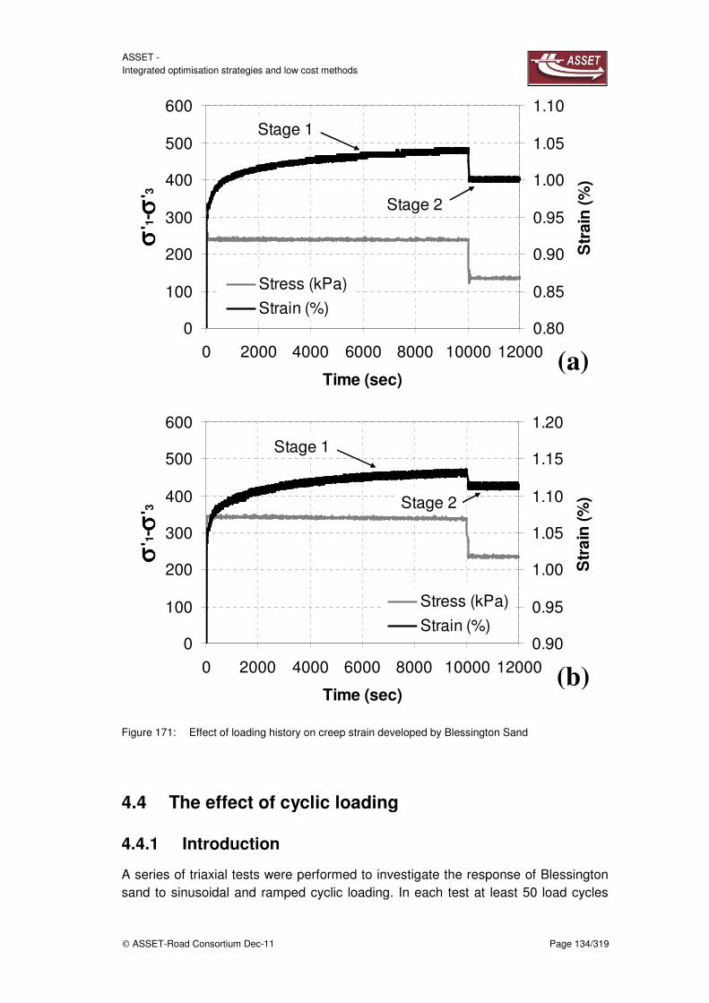
ASSET - Integrated optimisation strategies and low cost methods
ASSET-Road Consortium Dec-11 Page 134/319
Figure 171: Effect of loading history on creep strain developed by Blessington Sand
4.4 The effect of cyclic loading
4.4.1 Introduction
A series of triaxial tests were performed to investigate the response of Blessington sand to sinusoidal and ramped cyclic loading. In each test at least 50 load cycles
0
100
200
300
400
500
600
0 2000 4000 6000 8000 10000 12000
Time (sec)
σσ σσ' 1
- σσ σσ' 3
0.80
0.85
0.90
0.95
1.00
1.05
1.10
Str
ain
(%
)
Stress (kPa)
Strain (%)
Stage 1
Stage 2
0
100
200
300
400
500
600
0 2000 4000 6000 8000 10000 12000
Time (sec)
σσ σσ' 1
- σσ σσ' 3
0.90
0.95
1.00
1.05
1.10
1.15
1.20
Str
ain
(%
)Stress (kPa)
Strain (%)
Stage 1
Stage 2
(a)
(b)

ASSET - Integrated optimisation strategies and low cost methods
ASSET-Road Consortium Dec-11 Page 135/319
were applied. In section 1 it was noted that the cyclic loading models of Lentz & Baladi (1980) and Diyaljee & Raymond (1982) had the potential to be adopted for a range of geotechnical applications. Lentz & Balady (1980) developed their model based on the results of a series of laboratory triaxial tests on sand. Their expression (Equation 2) considers the number of applied load cycles and estimates the strain accumulation based on the value of permanent strain occurring during the first cycle (ε0) and a material constants (b) that depends on the materials stress history, confining pressure and relative density and should be estimated using cyclic triaxial tests. Diyaljee & Raymond (1982) developed a model where the effect of cyclic stress level was considered explicitly:
snx
accu Ne0εε = (7)
Where
εaccu is the accumulated strain, x is ratio of the cyclic stress level to the failure stress, ε0 is the permanent strain for the first cycle when the soil is reloaded (at x=0), N is number of cycles and n and s are experimentally derived parameters for a particular soil.
4.4.2 Sinusoidal cyclic load tests
Triaxial tests were performed on Blessington sand at a range of cyclic stress levels. In the first test a cyclic deviator stress of 240 kPa was applied for 50 cycles with a period of 60 seconds. During each cycle the sample was unloaded to a minimum stress of 32kPa to avoid separation of load cell from the top of the sample. The model parameters n and s used in Equation 7 were calibrated using the first test (n
= 0.055 and s = 0.06). In the second test the deviator stress was increased to 350 kPa and in the third test the deviator stress level of 240kPa was applied for a period of 120 seconds. Equation 9 was employed to estimate the strain accumulation and the predictions are compared with the measured response in Figure 11. It is apparent that the model provides excellent predictions of the measured response. However, it should be noted that the predicted response is very sensitive to the permanent strain during the first cycle. The value used in this comparison was the measured value.

ASSET - Integrated optimisation strategies and low cost methods
ASSET-Road Consortium Dec-11 Page 136/319
(a)
(b)
(c)
Figure 172: Comparison between measured and predicted response of Blessington sand to cyclic
sinusoidal loading

ASSET - Integrated optimisation strategies and low cost methods
ASSET-Road Consortium Dec-11 Page 137/319
4.4.3 Ramped cyclic load tests
Two triaxial tests were performed where ramped loading was applied. In both tests the applied maximum and minimum deviator stress was 240kPa and 32 kPa respectively. In the first test the period was 60 seconds and in the second the period was doubled to 120 seconds, See Figure 12. It is apparent that the Diyaljee & Raymond model (Equation 7) overestimated the accumulated strain in both tests, the difference between the measured and predicted values increased as the period increased.
(a)
(b)
Figure 173: Comparison between measured and predicted response of Blessington sand to cyclic
ramped loading
0.7
0.8
0.9
1
0 10 20 30 40 50
Cycle, N
εε εεaccu (
%)
Expriment
Modelq=240 kPa 60 sec
60 sec
0.7
0.8
0.9
1
0 10 20 30 40 50
Cycle, N
εε εεaccu (
%)
Expriment
Model
q=240 kPa 120 sec
120 sec

ASSET - Integrated optimisation strategies and low cost methods
ASSET-Road Consortium Dec-11 Page 138/319
Whilst the Diyaljee & Raymond model is able to capture accumulated strain caused by sinusoidal cyclic loading, the model overestimated the accumulated strain which occurred as a result of ramped cyclic loading, particularly in the test with the longest period (120sec). In an attempt to understand this discrepancy, the raw strain and stress data measured during the first two load-cycles of the 120 sec period test are plotted against time Figure 13. It is clear from the Figure that there is a short time-lag at the start of the cycle where the stress builds up to the pre-determined level (240 kPa). When the sample reaches the applied stress on the first cycle the measured sample strain is 0.84%. During the remainder of the 120 second period creep effects caused the strain value to reach a maximum of 0.89 %. It is clear that in the second (and subsequent load cycles) the effects of creep are much lower. Since the parameter B in the Diyaljee & Raymond model is based on the settlement of the first load-cycle, it is clear from Figure 13 that this value will increase as the period increases. The additional creep strain measured in the first cycle therefore caused an overestimation of the total accumulated strain over the subsequent 50 cycles.
Figure 174: Stress and strain measured during the first two load cycles during the ramped loading
experiment with a period of 120 seconds
0.7
0.75
0.8
0.85
0.9
0.95
0 100 200 300 400
Time (sec)
Str
ain
(%
) Creep
B value
0
50
100
150
200
250
300
0 100 200 300 400
Time (sec)
Str
es
s (
kP
a)

ASSET - Integrated optimisation strategies and low cost methods
ASSET-Road Consortium Dec-11 Page 139/319
4.4.4 Extended cyclic loading model
To overcome this limitation the effects of creep need to be considered. Firstly the creep component should be incorporated into the B parameter determined from the first load cycle and secondly, a time dependent creep component should be added to give the total permanent strain in each cycle. The Diyaljee & Raymond model can easily be extended to account for these effects in the manner described below:
( )
−−
×+
−=
refref
snx
ref
accut
tNm
t
tNmNe
t
tmB
1lnlnlnε (8a)
or
−+
−=
1lnln
N
NmNe
t
tmB
snx
ref
accuε (8b)
To check the ability of the extended model, predictions using Equation 8 are compared to the unmodified Diyaljee & Raymond model in below figure. It is clear that the extended model captures the strain accumulated during ramped cyclic loading, accurately.
(a)
0.7
0.8
0.9
1
0 10 20 30 40 50
Cycle, N
εε εεaccu (
%)
Expriment
Diyaljee and Raymond Model
New Model
q=240 kPa 60 sec
60 sec

ASSET - Integrated optimisation strategies and low cost methods
ASSET-Road Consortium Dec-11 Page 140/319
(b)
Figure 175: Comparison of original and extended Diyaljee and Raymond model predictions
4.5 Conclusions
An experimental programme was undertaken to develop model capable of predicting the accumulation of strain in sand subjected to ramped cyclic loading. Samples of dense Blessington sand were formed and tested in a GDSTTS triaxial apparatus. Tests were performed to determine the strength, rate dependence, creep characteristics and response to sinusoidal and ramped cyclic loading. A standard creep model was calibrated for dense Blessington sand.
A well known cyclic loading model developed by Diyaljee and Raymond (1982) was employed to model strain accumulation in response to sinusoidal and ramped cyclic loading. The model was seen to provide excellent predictions of the soils response to sinusoidal cyclic loading. However, it over-estimated the strain accumulation experienced due to ramped cyclic loading. The error was shown to result from significant creep effects experienced during the first cycle of loading. An extended model which integrated creep effects was developed to overcome this limitation. Predictions made using the extended model showed excellent agreement with the results of experiments performed in the triaxial cell.
0.7
0.8
0.9
1
0 10 20 30 40 50
Cycle, N
εε εεaccu (
%)
Expriment
Diyaljee and Raymond Model
New Model
q=240 kPa 120 sec
120 sec

ASSET - Integrated optimisation strategies and low cost methods
ASSET-Road Consortium Dec-11 Page 141/319
5 Optimal Bridge Monitoring
5.1 Summary
5.1.1 Low cost damage detection method using accelerometers
Highway structures such as bridges are subject to continuous degradation due to many factors such as ageing, loading and environmental conditions. Most developed economies now require the implementation of Bridge Management Systems for the monitoring of this transport infrastructure in order to provide adequate maintenance, guarantee the required levels of transport service and safety and budget accordingly. In Europe, it is now a legal requirement - a European Directive requires all member states of the European Union to implement such systems. Thus, increasingly in recent years, bridges are being instrumented and monitored on an ongoing basis – so called Structural Health Monitoring (Farrar and Worden, 2007). In general the purpose is to measure bridge modes and frequencies of vibration. However, the process is expensive, requiring the installation of sensors and data acquisition electronics on the bridge. For widespread implementation of Bridge Management Systems, a large number of bridges must be instrumented and monitored. This section investigates the use of a low cost method consisting of instrumented vehicle fitted with accelerometers on its axles to monitor bridge dynamic behaviour. This method would eliminate the need to install measuring equipment directly on the bridge and would allow the monitoring of bridges to become a much easier and more efficient task.
A numerical analysis is carried out on the use of an instrumented vehicle to identify the structural damping of a bridge. The structural damping of a bridge has been shown to be damage sensitive hence it is the focus of this method - it can be used as an indicator of the structural condition of the bridge. A three stage process is described for the identification of structural damping. This requires input of measured accelerations from the instrumented vehicle as it crosses a bridge. Measured data is generated by a vehicle-bridge interaction model created in Matlab. The structural damping of the bridge model is set at 3% and this is the target value to be identified. The contact forces of the vehicle wheels with the road and bridge surfaces and the total displacements under each wheel are calculated by utilising the equations of motion of the vehicle model and integration of the accelerations. These calculated contact forces and displacements are then used as input to an optimisation process which uses least squares error minimisation to identify the structural damping of the bridge. The process is repeated for a number of bridge spans and vehicle velocities. The damping estimates are very good for longer span bridges (Figure 1). Also, the effect of noise on results is investigated. Results are shown in Figure 1. It is found that noise does not have a significant effect on damping estimates for longer span bridges. As the damping estimates are

ASSET - Integrated optimisation strategies and low cost methods
ASSET-Road Consortium Dec-11 Page 142/319
quite accurate, it suggests that this low cost method could be used as a tool for the structural health monitoring of bridges.
Figure 176: Bridge structural damping estimates from noisy accelerations with SNR = 20 for bridge
spans of (a) 15 m (b) 25 m (c) 35m and (d) 40m. Vehicle velocity ranges from 10 m/s to
30 m/s.
An experimental investigation was carried out on the detection of bridge dynamic parameters from the dynamic response of a vehicle. Similar to the approach presented in the first section, this method involves the measurement of vehicle accelerations as it crosses a bridge. The aim is to detect both the natural frequency of the bridge and changes in bridge damping from the vehicle vibration. The experimental vehicle and beam models are shown in Figure 2. In the experiments, the vehicle is fitted with accelerometers at the centre of the front and rear axles while the beam is also instrumented with accelerometers and displacement transducers.
The vehicle crosses the steel beam along a track which has road surface roughness. The acceleration responses of the vehicle and beam are recorded and compared. The analysis involves the inspection of frequency spectra of the accelerations to identify frequencies of vibration and changes in response magnitude with damping. Results are presented for two vehicle models, two vehicle velocities and 3 damping scenarios. Results illustrate that the bridge frequency and changes in damping are detected successfully.

ASSET - Integrated optimisation strategies and low cost methods
ASSET-Road Consortium Dec-11 Page 143/319
Figure 177: (a) Experimental beam (b) Experimental vehicle
5.1.2 Low cost bridge monitoring system
In the field of SHM highway bridges are a particularly interesting set of structures for two reasons: Firstly, the bridge stock of many developed countries contains a significant portion of bridges that are approaching or have exceeded the design life originally envisaged for them. Secondly, the increasing demand in transport is leading to heavier traffic loads, so effectively as the bridges get older they are required to work harder. The aim of this work package is to try and develop new cost effective bridge monitoring techniques that would alert road authorities to the fact that there was a problem with a particular structure. Thereby allowing them to take corrective action before the fault became critical.
Damage in a structure often results in a localised loss in stiffness, this in turn can lead to localised discontinuities in the response of the structure. Wavelet analysis can be used to identify these discontinuities and thereby identify the damage. In terms of detecting damage in beams and plates much of the research in the literature focuses on using mode shape data. While good results are reported the difficulty is that to obtain accurate mode shape data from a real structure requires many sensors. The required level of instrumentation is potentially expensive and time consuming. In this work package the possibility of using a limited number of sensors to detect damage is investigated. A mathematical model of a cracked bridge subject to a moving load is employed to simulate the ‘measured’ data.
The mid-span displacement signal of a cracked beam subject to a moving constant load is simulated. It is shown that by analysing the displacement signal using a Continuous Wavelet Transform (CWT) it is possible to identify the location of the damage. It is also shown that by applying a similar approach to the mid-span acceleration signal of the bridge this too was successful at identifying the damage. Acceleration has the advantage of being easier to record on a real bridge than displacement. A novel approach which utilises 3 recording location and a range of wavelet scales is developed. The new approach was found to perform significantly better at detecting small damage than the traditional approach of just using one wavelet scale. The new technique was tested on more realistic acceleration signals produced using a Vehicle Bridge Interaction (VBI) model and while there was some loss in spatial resolution the approach was still found to be effective.

ASSET - Integrated optimisation strategies and low cost methods
ASSET-Road Consortium Dec-11 Page 144/319
The source of the local discontinuity in the bridge acceleration signal as the moving load passes over the damaged section was investigated. The question was addressed by separating the displacement signal into its component parts and differentiating each twice with respect to time. It was found that the amplitude of the damaged component of the acceleration signal was very small relative to the dynamic component, this makes its identification challenging. However, it is shown that in certain circumstances the presence and location of damage can be determined by simply applying an appropriate filtering method to the recorded acceleration signal.
5.2 Low cost damage detection method (accelerometers)
5.2.1 Introduction
There has been a significant increase in recent years in the number of bridges which are being instrumented and monitored on an ongoing basis - so called Structural Health Monitoring (Farrar and Worden, 2007) - in part due to the introduction of Bridge Management Systems. This is very effective and provides a high level of protection to the public and early warning if the bridge becomes unsafe. However, monitoring via direct instrumentation of the bridge can be expensive and time consuming, requiring the installation of sensors and data acquisition electronics on the bridge. Given the very large number of bridges that are not instrumented, some alternative method is needed to detect any change in behaviour of the structure which might be an indicator of some form of damage.
This section investigates the use of a vehicle fitted with accelerometers on its axles to monitor the dynamic behaviour of bridges. The approach eliminates the need for any equipment to be installed on the bridge and it is aimed at allowing the assessment of bridge condition to become a simplified and much less difficult and time consuming process. It would facilitate more effective and widespread monitoring of the condition of existing bridge structures in a transport network while its development would enable maintenance to be carried out at an earlier stage in degradation, which generally results in more economical repairs.This method focuses on the structural damping of the bridge as it has been shown (Curadelli et al, 2008; Modena et al, 1999) to be a damage sensitive property. The following sections present both theoretical and experimental investigations of this method and discuss its validity for damage detection.
5.2.2 Theoretical estimation of bridge structural damping
The feasibility of detecting bridge dynamic parameters, such as frequency, from the dynamic response of a vehicle passing over a bridge has been verified theoretically (Yang et al, 2004; Oshima et al, 2008, McGetrick et al, 2009) and experimentally in field tests (Lin and Yang, 2005). Experimental investigations have also been carried

ASSET - Integrated optimisation strategies and low cost methods
ASSET-Road Consortium Dec-11 Page 145/319
out which indicate the feasibility of the approach as part of a drive-by inspection system for bridge monitoring (Kim and Kawatani, 2009; Toshinami et al, 2010).
Recent evidence (Curadelli et al, 2008; Modena et al, 1999) suggests that the presence of cracks can result in a change in the dynamic response of a bridge to passing traffic. Specifically, it has been found that the bridge’s structural damping is quite sensitive to this kind of damage. Theoretical investigations carried out by McGetrick et al (2009) and González et al (2010) aimed to identify not only bridge frequencies but changes in the bridge’s structural damping. Both conclude that the bridge’s frequency of vibration and structural damping can be identified with ease from the dynamic response of a vehicle for a smooth road profile, while in the presence of a rough road profile the same properties become very difficult to identify. González et al also noted that frequency matching between the axle hop of the vehicle and the natural frequency of the bridge is beneficial for the detection of that bridge frequency.
This investigation builds upon the theoretical analyses by McGetrick et al and González et al. One shortcoming from their analyses was that their approaches were based on the detection of damage related to changes in damping. However, the approach did not identify a value for the structural damping of the bridge; it only indicated a change from one state to another. In this investigation, the aim is to identify the absolute value of bridge structural damping from the dynamic response of a vehicle.
For this theoretical investigation, a vehicle-bridge interaction (VBI) model is created in MATLAB. The vehicle is modelled as a 2-degree-of-freedom half-car and the bridge is modelled as a Finite Element beam. The investigation involves three distinct stages.
1. Generation of “measured” vehicle accelerations using the VBI model.
2. Estimation of wheel contact forces (Ri) and wheel displacements (wvi)
3. Identification of optimal value for structural damping (ξ) using optimisation process
Simulations are carried out for simply supported bridge spans of 15, 25, 35 and 40 metres and vehicle velocities of 10 m/s to 30 m/s. A rough road profile is included in simulations and the irregularities of this profile are randomly generated according to ISO (1995) for a ‘very good’ profile or road class ‘A’. Also, the effect of noise on the algorithm is investigated for a signal to noise ratio (SNR) of 20. The results will indicate the most favourable conditions in which this method can be used to detect bridge structural damping with a reasonable degree of accuracy.
Vehicle bridge interaction model
A theoretical half-car model is used to represent the behaviour of the vehicle (Figure 178). It is a simplified version of a vehicle but its response still illustrates many of the important characteristics of dynamic tyre forces (Cebon, 1999). It has two degrees of freedom which correspond to sprung mass bounce displacement

ASSET - Integrated optimisation strategies and low cost methods
ASSET-Road Consortium Dec-11 Page 146/319
and sprung mass pitch rotation. The vehicle body and axle component masses are represented by the sprung mass. This mass connects to the road surface via a combination of springs of stiffness and viscous dampers of value which represent the combined tyre and suspension components for the front and rear axles ( =1,2). Also defined are the sprung mass moment of inertia, , and the distance of each axle to the vehicle’s centre of gravity (o), i.e., (=1.95 m) and (=1.05 m) in Figure 178. The half-car property values are listed in Figure 179 and are based on values obtained from work by González et al (2010) and Cebon (1999).
Figure 178: Degree-of-freedom half-car model
1.1
P
rop
erty
1.2
B
od
y m
ass (k
g)
1.3
S
tatic
Lo
ad
(N)
1.4
S
usp
en
sio
n
Stiffn
ess (N
/m)
1.5
S
usp
en
sio
n
Da
mp
ing
(Ns/m
)
1.6
M
om
en
t of In
ertia
(kg
m2
)
1.7
S
ym
bo
l
Value 18000 61778 114730 2 × 10⁶ 5 × 10⁶ 10 × 103 20 × 103 55500
Figure 179: Half-car model properties

ASSET - Integrated optimisation strategies and low cost methods
ASSET-Road Consortium Dec-11 Page 147/319
The half-car equations of motion for the sprung mass bounce and pitch motions, ! and " respectively, are given by:
!# +% +% = 0 "# +% −% = 0
The quantity % represents the dynamic wheel contact force at axle : % = '! −(−1)" −+,- +'!. −(−1)". − +. ,-; = 1,2
Where
+, is the total displacement under the wheel of axle . This parameter can be defined in terms of the road profile displacement and bridge displacement under a wheel, 1 and +23 respectively:
+, = 4+23 + 1 4; = 1,2
The total wheel contact force is represented by5: 5 = −%; = 1,2
Where
is the static load of the vehicle at axle . In simulations it is assumed that there are two measurement sources; accelerations are obtained above the suspension of each axle (Figure 178) for use in the analysis. They are obtained from the model using the following equation:
!# = !# −(−1)"#; = 1,2
The half-car travels at constant velocity, c, over a simply supported Finite Element beam (Figure 180) which has constant cross section and mass per unit length, µ. It has span L, modulus of elasticity E, second moment of area J and structural damping ξ. The properties of the three bridge spans used in this investigation are given. The dynamic interaction between the vehicle and bridge is implemented using an iterative procedure described by Green and Cebon (1995).
Figure 180: Finite Element Beam model

ASSET - Integrated optimisation strategies and low cost methods
ASSET-Road Consortium Dec-11 Page 148/319
Span
length, L
(m)
Modulus of
elasticity, E
(N/m2)
Second moment
of area, J (m4)
Mass per unit
length, µ
(kg/m)
1st natural frequency
of vibration, fbridge1(Hz)
15 3.5 × 10¹⁰ 0.5273 28125 5.66
25 3.5 × 10¹⁰ 1.3901 18358 4.09
35 3.5 × 10¹⁰ 3.4162 21752 3.01
40 3.5 × 10¹⁰ 4.8218 23752 2.62
Figure 181: Finite Element Beam properties
5.2.3 Methodology
It has already been noted that there are 3 stages involved in this method. In the first stage, the structural damping of the bridge is set equal to 3%. This is the target value to identify. The “measured” vehicle acceleration, !# , are generated in Matlab using the VBI model. These accelerations are then converted to sprung mass bounce and pitch accelerations using Equation 1.6 for use in Equations 1.1 and 1.2. In the second stage, the total wheel contact forces (5) and total displacements under each wheel (+,)are obtained. The forces % are obtained by solving Equations 1.1 and 1.2 simultaneously. It is assumed all the vehicle properties are known. The total wheel contact forces can then be obtained from Equation 1.5. The total displacements under each wheel are obtained by solving Equation 1.3 as a 1st order differential equation in +,. This equation is solved using the Runge-Kutta method. Assuming their initial conditions are known, the sprung mass bounce and pitch velocities (!., ".) and displacements (!, ") can be obtained by integration of the measured accelerations from stage 1.
The third and final stage is the estimation of structural damping. The forces 5 obtained in stage 2 are applied to a Finite Element Beam model with structural damping ξest. The displacement response of the beam,+23, under each force is recorded. This process is repeated for a range of damping value estimates (ξest) ranging from 0.5% up to 6% in steps of 0.1%. Taking advantage of and rearranging Equation 1.4, values of 1 for each ξest are obtained by subtracting each range of +23 from the solution of +, obtained in stage 2. The values of 1 are effectively road profile height estimates under each wheel. For the correct value of structural damping value, the profile estimates under each wheel should be equal. To identify the optimal value for damping, a least squares error minimisation process is used. The optimal solution provides the minimum least squares error between the profile estimates under each wheel. It should be noted that an inherent advantage of this method is that road profile surface roughness does not affect its accuracy.

ASSET - Integrated optimisation strategies and low cost methods
ASSET-Road Consortium Dec-11 Page 149/319
Results
The simulations in this section are carried out using the VBI model and the 3 stage process described earlier. The bridge span length and vehicle velocity are varied and the scanning frequency used for measured accelerations is 8192 Hz. Figure 182 shows an example of the total wheel contact forces calculated in stage 2 for the vehicle crossing the 15 m bridge at a velocity of 10m/s. The calculated forces are very accurate as expected as they are extracted directly from the equations of motion for the vehicle.
Figure 182: Comparison of actual and calculated total wheel contact force, R7, for a 15 m bridge.
Vehicle velocity is 10 m/s.
Next figure shows the solution for the total displacements under each wheel for the vehicle crossing the 15 m bridge at 10 m/s. The solution is very accurate for this case. In general, this solution was found to be very accurate for other bridge span lengths and vehicle velocities investigated.

ASSET - Integrated optimisation strategies and low cost methods
ASSET-Road Consortium Dec-11 Page 150/319
Figure 183: Comparison of actual and calculated total displacements, w97, under each wheel for a
15 m bridge. Vehicle velocity is 10 m/s.
The results of the structural damping estimates for the vehicle crossing all bridge spans at all velocities investigated are shown in Figure 184. The dashed black lines indicate the target damping value of 3%. It can be seen clearly that the estimates for a bridge span of 15 m are the poorest. This appears to be due to the shorter time the vehicle is on the bridge to record data. Also, it can be observed in Figure 184 (c) for a velocity of 28 m/s and in Figure 184 (d) for velocities of 15 m/s and 28 m/s that estimates are considerably less accurate than for other velocities. This suggests that particular velocities should be avoided when implementing this method. The results shown in Figure 184 imply that the estimation method is quite accurate, especially for spans over 15 m, with the error less than 10% for most velocities. This suggests it could be implemented for the identification of bridge structural damping and hence structural health monitoring.

ASSET - Integrated optimisation strategies and low cost methods
ASSET-Road Consortium Dec-11 Page 151/319
Figure 184: Bridge structural damping estimates for bridge spans of (a) 15 m (b) 25 m (c) 35m and
(d) 40m. Vehicle velocity ranges from 10 m/s to 30 m/s.
The results presented in Figure 184 are obtained from measured accelerations which are noise free. In a realistic situation, there will be some noise corruption of the recorded data. Hence, the accelerations are corrupted with noise using an additive noise model with a signal to noise ratio (SNR) of 20. This model randomly adds noise to the original accelerations by sampling a normal distribution of zero mean and standard deviation equal to the average standard deviation of the two original acceleration data sources divided by 20. The noise corrupted accelerations are passed through a low pass filter with a cut-off frequency of 100 Hz before being used to obtain the contact forces and wheel displacements in stage 2. Figure 185 shows the estimates obtained from the noisy accelerations. It can be seen that in Figure 185(a), the estimates become considerably less accurate for the 15 m span compared to the noise free estimates. In general for all other spans, the accuracy remains reasonable at most vehicle velocities despite the presence of noise in the recorded data. The use of the low pass filter appears to be beneficial in counteracting the effect of noise on the accuracy of damping estimates.

ASSET - Integrated optimisation strategies and low cost methods
ASSET-Road Consortium Dec-11 Page 152/319
Figure 185: Bridge structural damping estimates from noisy accelerations with SNR = 20 for bridge
spans of (a) 15 m (b) 25 m (c) 35m and (d) 40m. Vehicle velocity ranges from 10 m/s to
30 m/s.
Conclusions
A novel method for the identification of bridge structural damping from the dynamic response of a vehicle has been discussed. The results show that it is possible to detect the bridge structural damping from the vehicle vibration in the presence of a rough road profile. It has also been highlighted that the method is more accurate for longer span bridges and in general is not very sensitive to noise in the recorded accelerations. However, the method is quite sensitive to the Initial Conditions of the vehicle degrees of freedom. Further study is required to overcome this inaccuracy to enable the development of an instrumented vehicle as an efficient low-cost method for monitoring bridge dynamic behaviour.
5.2.4 Experimental investigation
The experimental work presented in this section aims to validate the theoretical analyses of McGetrick et al and González et al. It also aims to add to the experimental approaches of Kim and Kawatani and Toshinami et al by focusing on the detection of not only bridge frequency but the structural damping of the bridge also. The study investigates the feasibility of using an instrumented vehicle to detect bridge dynamic parameters, such as natural frequency and structural damping, in a scaled laboratory experiment. In the experiment, a scaled vehicle model crosses a steel beam which has been adopted as the bridge model. The bridge model also includes a scaled road surface profile. The two-axle vehicle model is fitted with accelerometers on its axles. The investigation involves the

ASSET - Integrated optimisation strategies and low cost methods
ASSET-Road Consortium Dec-11 Page 153/319
analysis of the frequency spectra of vehicle accelerations obtained from the dynamic response of the vehicle model as it crosses the bridge. The frequencies of vibration are identified in the vehicle acceleration spectra and compared to the frequencies obtained from bridge free vibration tests. The effects of varying vehicle model mass and velocity are investigated. Bridge damping is also varied. Results indicate the best conditions for the approach.
Experimental setup
The experimental setup is comprised of a scaled steel beam bridge model (Figure 186(a)) and a scaled two axle sprung mass vehicle model (Figure 186 (b)). The vehicle travels along a track on the beam which has a scaled road surface profile. An electronic controller maintains a constant velocity for the vehicle. Two vehicle velocities of 0.93m/s and 1.63m/s are adopted for the experiment. Adjustments can be made to the vehicle in order to obtain different mass and dynamic properties. For this experiment, two vehicle models are used (V1 and V2 respectively) and their properties are given in Figure 187. The vehicle model is fitted with 2 accelerometers; at the centre of the front and rear axles respectively. It is also equipped with a wireless data acquisition system. The scanning frequency used in all experiments is 100 Hz.
Figure 186: (a) Experimental beam (b) Experimental vehicle
The bridge model is a simply supported 5.6 m long steel beam which has a Modulus of Elasticity of 2 × 10¹¹ N/m2 and mass per unit length of 53.66 kg/m. To monitor the response of the beam, accelerometers and displacement transducers are fitted at quarter span, mid span and three-quarter span. The beam’s dynamic properties obtained from free vibration tests are given in Figure 188. Only the natural frequency corresponding to the first bending mode of the beam is presented here as this frequency is the focus of this section. Three damping scenarios are tabulated. The Intact scenario represents the beam with no adjustments. The other two scenarios represent the beam with adjusted damping. To vary the damping of the beam, old displacement transducers are applied at particular points on the beam in addition to a 17.8kg mass added at midspan. The layout of the transducers is illustrated in Figure 189. The old transducers provide frictional resistance to bridge displacements at the chosen locations thus increasing the damping of the beam. The additional mass is used to adjust the frequency of the beam as

ASSET - Integrated optimisation strategies and low cost methods
ASSET-Road Consortium Dec-11 Page 154/319
frequently damage which causes changes in damping may cause some changes in frequency. The two damping scenarios which include the mass are chosen as they provide a suitable range of values for the beam’s structural damping.
Vehicle
model
Bounce
frequency (Hz)
Pitch
frequency (Hz) Mass (g)
V1 2.93 4.24 21345
V2 2.93 3.52 25885
Figure 187: Vehicle properties
Scenario Additional mass
(kg) Frequency (Hz)
Structural
damping (%)
Intact 0 2.7 1.4
Damper @C 17.8 2.5 2.1
Dampers @ABCDE 17.8 2.5 4.3
Figure 188: Beam properties (See Figure 7)
Figure 189: Locations of dampers and additional mass
5.2.5 Results
Detection of frequency from vehicle response
This section discusses the results obtained for the ‘Intact’ scenario i.e. no dampers or additional mass are applied to the beam. To determine if beam frequency is detected by the vehicle, the frequency spectra of vehicle accelerations are analysed and compared to the frequency spectra of beam accelerations. Figure 190 shows the frequency spectra obtained from accelerations of the beam during the crossing of vehicle model V1 over the beam at a velocity of 0.93m/s. The frequency peak at 2.41 Hz visible in Figure 190(a) corresponds to the first natural frequency of the beam and it also occurs in the vehicle spectra. Therefore it can be confirmed that for this vehicle model and velocity it is possible to detect the bridge frequency from the vehicle response in this experiment. However, it should be noted that the peak corresponding to the bridge in the vehicle spectra is not always the most dominant peak – for axle 1 of the vehicle in Figure 190(b) the dominant peak is at 3.95 Hz which corresponds to the body pitch of the vehicle.

ASSET - Integrated optimisation strategies and low cost methods
ASSET-Road Consortium Dec-11 Page 155/319
It is observed that lower velocity gives better spectral resolution but less dominant bridge peaks in the vehicle spectra. While it is difficult to obtain high enough resolution in the vehicle spectra for a velocity of 1.63m/s, a clear bridge frequency peak can still be identified for this velocity at 3.13 Hz in Figure 191(b). Also, vehicle acceleration spectra magnitude increases with increasing velocity. Axle 1 tends to give the maximum response due to its lighter axle weight and this can be observed in Figure 190(b) and Figure 191(b). Similar results are obtained for vehicle V2.
Figure 190: Fourier spectra of acceleration response of (a) Beam midspan and (b) V1 axles for
velocity 0.93m/s
Figure 191: Fourier spectra of acceleration response of (a) Beam midspan and (b) V1 axles for
velocity 1.63m/s
Detection of changes in damping from vehicle response
This section considers changes in damping for the scenarios ‘Damper @C’ and ‘Dampers @ABCDE’. Detecting the bridge frequency peak is more difficult in vehicle spectra as the increased beam damping reduces the magnitude of the spectra relative to the level of noise in the signal. To account for this, the accelerations are passed through a low pass filter with a cut off frequency of 8 Hz
(a) (b)
(a) (b)

ASSET - Integrated optimisation strategies and low cost methods
ASSET-Road Consortium Dec-11 Page 156/319
and the power spectral density of accelerations is analysed in place of Fourier amplitude. As a result, the frequency peaks are clearer and easier to identify in the spectra for the purpose of analysing damping scenarios. Figure 192 compares the mean acceleration spectra of the beam and vehicle obtained in all scenarios for 5 crossings of vehicle V1 at 0.93m/s. The bridge frequency peak at 2.44 Hz occurs in both Figure 192(a) and (b). It can be seen that as the damping increases i.e. from ‘Intact’ to ‘C’ to ‘ABCDE’, the peak magnitude at the bridge frequency in the vehicle spectra decreases. This trend also occurs at the peak in vehicle spectra at 3.91 Hz. This suggests it is possible to detect changes in bridge structural damping.
Figure 192: Spectra of mean acceleration responses of (a) Beam midspan and (b) Axle 1 of V1 for
velocity 0.93m/s
5.2.6 Conclusions
This section has investigated the feasibility of using an instrumented vehicle to detect the natural frequency and changes in structural damping of a bridge in a scaled laboratory experiment. For all scenarios investigated, the bridge frequency was identified in the vehicle spectra. It is clear that selection of vehicle velocity is an important factor in the detection of the bridge frequency. The higher velocity of 1.63 m/s provides peaks of larger magnitude in the spectra but the spectral resolution is not as high as for 0.93m/s. For vehicle 1 and 0.93 m/s, changes in damping are detected in the vehicle spectra. These results indicate that it is possible to detect both the bridge frequency and changes in damping from the acceleration measurements of a moving vehicle. (To confirm the feasibility of the system, further investigation of the vehicle configuration, velocity and beam damping scenarios is necessary).
Acknowledgement
The authors would like to acknowledge the funding received towards this experimental investigation from the Japanese Society for the Promotion of Science
(b) (a)

ASSET - Integrated optimisation strategies and low cost methods
ASSET-Road Consortium Dec-11 Page 157/319
Postdoctoral Fellowship for North American and European Researchers (Short-Term).
5.3 Low cost bridge monitoring (Wavelet transformation)
5.3.1 Introduction
Structural Health Monitoring (SHM) has been around for some time, however, the past decade has seen a significant increase in the amount of research carried out in the area. The increased interest in SHM is motivated by the potential safety and economic benefits that could be reaped, if a fault in a structure could be flagged before the defect becomes critical. In the field of SHM highway bridges are a particularly interesting set of structures for two reasons: Firstly, the bridge stock of many developed countries contains a significant portion of bridges that are approaching or have exceeded the design life that was envisaged for them when they were first built. Secondly, the increasing demand in transport is leading to heavier traffic loads, so effectively as the bridges get older they are required to work harder. If the service life of these older structures can be successfully extended, the potential economic benefits are very substantial. Doebling et al (1998) give a summary review of vibration based damage identification methods, and they describe how the fundamental principle involved in all vibration based damage identification techniques is that the modal parameters (such as frequency and mode shapes) are determined by the physical properties of the structure (such as stiffness, mass and damping), therefore any changes in the physical properties of the structure will cause detectable changes in the modal properties. A number of authors (Dimarogonas, 1996; Carden & Fanning, 2004) provide informative review papers describing the different work that has been carried out in the field of SHM. In terms of detecting damage in beam and plate structures much of the research to date has focused on using mode shape data. While good results have been reported the difficulty is that to obtain accurate mode shape data from a real bridge requires a large number of sensors. Considering the number of existing bridges the level of instrumentation required to implement an extensive monitoring program may be unfeasible. In this subtask the possibility of developing a reliable damage detection technique which requires fewer sensors is investigated.
5.3.2 Using the Wavelet transform to detect damage
Traditionally the Fourier transform was used to determine the frequency content of a signal. When the Fourier transform is applied to a signal, it defines the different frequencies present in the signal but it gives no time information. It does not show if a given frequency is present for the full duration of the signal or if it is present for just for a short period. Wavelet analysis was developed to give better frequency-time information about a signal. A wavelet is a waveform of effectively limited duration that has an average value of zero, Mallat (1998) gives a comprehensive

ASSET - Integrated optimisation strategies and low cost methods
ASSET-Road Consortium Dec-11 Page 158/319
mathematical guide to wavelet analysis. However, in practical terms, the way a wavelet transform works is as follows: The wavelet is compared to a portion of the original time series signal, and the wavelet coefficient (W) is calculated. ‘W’ represents how closely the wavelet is correlated with this portion of the signal. The entire length of the signal is checked resulting in a plot of the wavelet coefficients versus time. Then the wavelet is scaled (i.e. stretched) and the process is repeated. Ultimately the wavelet transform returns a wavelet coefficient for each scale at each point in time. When the wavelet transform is applied to a continuous time series signal, the result is a 3-dimensional surface. In this plot, time and scale are represented on the two mutually perpendicular horizontal axes, and wavelet coefficient on the vertical axis. However, it is more common to represent the 3D wavelet surface as a 2D contour plot where the magnitude of the wavelet coefficients is represented using colour, the larger wavelet coefficients are represented using a lighter colour (see Figure 195). One significant advantage of wavelet analysis is its ability to analyse a localised portion of a larger signal. Damage in a structure can lead to localised discontinuities in the response of the structure. The notion of damage introducing a singularity into the response signal of a structure and using wavelets to detect this singularity is described in (Pakrashi et al, 2007). Kim & Melhem (2004) and Reda Taha et al (2006) give reviews of the research that has been carried out on damage detection using wavelet analysis.
5.3.3 Computer model of damaged structure
A mathematical model of the response of a cracked bridge to a constant moving load is employed to simulate the ‘measured’ signals that will subsequently be analysed. The model used was a 1D finite element beam model. The governing equation of motion is shown in Eq. 1.7:
:;<= >?@>? + :<= >@>+:<=(!)=F(t)
Where:
y is the displacement of the model nodes, [Mg] is the consistent mass matrix, [Cg] is the damping matrix, [Kg] is the stiffness matrix and F(t) is the vector of forcing functions. It was assumed that the mass of the structure was unaffected by the crack so the mass matrix for the damaged structure was the same as for the undamaged structure. However, the stiffness matrix for the structure will be affected by the crack so before modelling the bridge deck a method for calculating the elemental stiffness matrices for the damaged structural elements was needed. The stiffness reduction method used was that proposed by Sinha et al (2005) who based their approach on earlier work by Christides & Barr (1984). For further details of the model see (Hester & González, 2008). Figure 193 shows the model used, a constant load P crosses the structure at a given speed and F(t) describes the distribution of P to the degrees of freedom at each time ‘t’. In order to perform a dynamic simulation of a load crossing the bridge it is necessary to convert the equilibrium equations of motion into a discrete time integration scheme. This scheme is solved using the Wilson-θ method. The results of the beam response to

ASSET - Integrated optimisation strategies and low cost methods
ASSET-Road Consortium Dec-11 Page 159/319
the moving load were found to be in agreement with those published by Mahmoud (2001) for different crack severities in a 50 m long beam. In this section of work the severity of the damage is characterized by the term ‘delta’, where delta is the ratio of crack height (h) to beam depth (d).
Figure 193: Sketch of a beam discretized model subject to a moving force
5.3.4 Detecting damage in a displacement signal
Figure 194: Mid-span displacement of a beam subject to a moving force when there is a delta=0.5
crack at the 1/3 point of the span
Figure 194 shows the mid-span displacement when a constant load crosses a 50m beam at a 1m/s. The global properties of the beam are the same as those used by (Zhu & Law, 2006; Mahmoud, 2001). The beam has a delta=0.5 crack at the 1/3 point of the span and the first natural frequency of the damaged beam is 0.89Hz. A visual inspection of the signal shows little indication of the damage however, if the signal is analysed using the CWT the wavelet surface shown in Figure 195 is obtained. Figure 195 represents the 3-dimensional wavelet surface using a 2D plot, the magnitude of the wavelet coefficients is represented using colour, the lighter colour indicates a high value of wavelet coefficients. In this study the Mexican Hat wavelet is used as the mother wavelet for all analyses. A number of wavelet bases were tested but the Mexican Hat was found to give the best performance with respect to damage detection. The first thing to note about Figure 195 is that the
0 0.2 0.4 0.6 0.8 1-4
-3
-2
-1
0
1x 10
-3
Normalised Position of Load on Beam (x(t)/L)
Mid
-spa
n D
efle
ctio
n (m
)
y
x
b(t) P Beam element
Node
d
L delta= h/d
Zone experiencing loss in stiffness
3d
h
delta= h/d

ASSET - Integrated optimisation strategies and low cost methods
ASSET-Road Consortium Dec-11 Page 160/319
continuous Wavelet Transform gives time-scale information as opposed to time-frequency information. However, scale is related to frequency in the sense that high scale implies low frequency, whereas low scale implies high frequency. A high wavelet coefficient at a particular scale indicates the frequency content of the signal at that time. If Figure 195 is examined it is evident that there are a series of high wavelet coefficients at a scale of 28 for the full duration of the signal. The approximate frequency (pseudo frequency) corresponding to this scale can be calculated using Eq. 1.8:
Fa = Fc / a∆
Where:
Fa is the pseudo frequency corresponding to scale ‘a’ in Hz, Fc is the centre frequency of the wavelet in Hz (Centre frequency effectively means the frequency of a periodic signal that most closely resembles the wavelet), ‘a’ is the scale of the wavelet, and ∆ is the sampling period used to record the signal. The wavelet used to generate Figure 195 was the Mexican Hat wavelet with Fc = 0.25 Hz, and ∆ = 0.01 seconds, which for a scale of 28 results into a pseudo frequency of 0.89 Hz, which is the first natural frequency of the beam. At scales appreciably above those corresponding to the first natural frequency of the beam there is a local increase in the wavelet coefficients at x(t)/L=0.33, i.e. there is a localised increase in the wavelet coefficients as the load passes over the damage.
A coefficient line plot shows how the wavelet coefficients at a particular scale vary with time/space, essentially it is like taking a section through the wavelet surface at a particular scale. Figure 196 shows the coefficient line plots at a scale of 170 when the mid-span displacement signals for various levels of damage are analysed. The displacement signals have had 3% noise added to them. From the figure it can be seen that damage levels of delta=0.4 and 0.6 can be detected relatively easily, however, it is difficult to reliably detect a damage level of delta=0.2 when the displacement is recorded at just one location. The plots obtained concur with results of similar work published in SHM literature.

ASSET - Integrated optimisation strategies and low cost methods
ASSET-Road Consortium Dec-11 Page 161/319
Figure 195: Wavelet transform of signal shown in Figure 2 plotted in 2D, the absolute value of the
wavelet coefficients are represented using colour, lighter colour indicates higher value.
Figure 196: Identifying the damage location for different levels of damage
Figure 197: Identifying damage when displacement is recorded at four locations
Normalised position of load on Beam (x(t)/L)
Sca
le
0.1 0.2 0.3 0.4 0.5 0.6 0.7 0.8 0.9 1 1 11 21 31 41 51 61 71 81 91101111121131141151161171181191
0 0.2 0.4 0.6 0.8 1-2
-1
0
1
2x 10
-3
Normalised Position of Load on Beam ( x(t)/L )
Wav
elet
Cof
ficie
nt
delta=0.0
delta=0.2
delta=0.4
delta=0.6
0 0.2 0.4 0.6 0.8 1-2
-1
0
1x 10
-3
Normalised Position of Load on Beam ( x(t)/L )
Wav
elet
Cof
ficie
nt
delta=0.0
delta=0.2
delta=0.4
Increase in wavelet coefficients as load crosses damage

ASSET - Integrated optimisation strategies and low cost methods
ASSET-Road Consortium Dec-11 Page 162/319
Improved damage detection can be achieved if the displacement is recorded at a number of points on the structure simultaneously. For a damage levels of delta=0.0, the vertical displacement was recorded at the 1/5th, 2/5th, 3/5th and 4/5th point of the beam. Then each displacement signal was analysed using the wavelet transform which produced 4 coefficient line plots. These four plots were then averaged to give the black plot shown in Figure 197. A similar approach was used to generate the delta=0.2 and delta=0.4 plots shown in Figure 197. If Figure 197 is compared it can be seen that increasing the number of recording locations makes it possible to identify damage of delta=0.2 and it makes the damage of delta=0.4 very easy to identify. For further details refer to (González & Hester, 2009).
5.3.5 Detecting damage in an acceleration signal
In the previous section it was shown that if the displacement signal of a beam subject to a moving load is analysed using the CWT it is possible to identify damage in the structure. However, it is difficult to monitor displacement to the required level of accuracy on a real bridge site. Therefore in this section the possibility of detecting damage in a bridge by analysing its acceleration response to a moving load is investigated. In the past acceleration data has been used in SHM to determine the natural frequencies and mode shapes of a structure, however to the authors knowledge it has not been analysed directly to detect damage. In this section the structure modelled as a 40 m simply supported span. The properties of the 40 m beam are those typical of a 15 m wide bridge consisting of 10 SY6 precast concrete beams spaced at 1.5 m centres with a 195 mm thick deck slab, resulting into inertia of 6.02 m4, a Young’s modulus of 3.5x10⁹ N/m2, and a total cross sectional area of 10 m2. The first natural frequency of the healthy structure is 2.88 Hz. The approach of Sinha et al (2005) for the modelling of a cracked beam was developed for rectangular beams, where a given ratio of crack height to beam depth implies a certain loss of stiffness. For example when the crack height is 10% of the total section depth the inertia at the damaged location can be shown to be 71% of the inertia at a healthy location. In this section non rectangular beams are modelled however, to be consistent with previous published work the traditional notion of crack height to beam depth is maintained as the measure of damage severity. This allows meaningful comparison of results. Figure 198 shows the mid-span acceleration signal of the beam when it has a delta=0.3 crack at the 1/3 point of the span and it is traversed by a point load moving at 3m/s. For comparison purposes the mid-span acceleration of the healthy bridge is also included. The time step used in this simulation was 0.005 seconds and both of the acceleration signals in the figure have had 3% noise added to them.

ASSET - Integrated optimisation strategies and low cost methods
ASSET-Road Consortium Dec-11 Page 163/319
Figure 198: Corrupted mid-span acceleration signal of healthy and damaged bridges
Figure 199 shows the wavelet transform of a damaged mid-span acceleration signal. Similar to Figure 195 there are a series of high wavelet coefficients along the bottom of the plot, using Eq. (1.8) these can be shown to correspond to the first natural frequency of the bridge. At scales appreciably above the first natural frequency it can be seen that there are a series of high wavelet coefficients at x(t)/L=0.33, i.e. when the load crosses the damage. In section 1.4, coefficient line plots were used to detect damage in a deflection signal. Figure 200 and Figure 201 show the results of carrying out coefficient line analysis on acceleration signals with 2 different levels of damage.
Figure 199: Wavelet transform of the mid-span acceleration signal when the bridge has a crack at
the 1/3 point of the span
0 0.2 0.4 0.6 0.8 1-4
-2
0
2
4x 10
-3
x(t) / L
Mid
-spa
n A
ccel
erat
ion
(m/s2
)delta=0.0
delta=0.3
x(t) / L
Sca
le
0 0.2 0.4 0.6 0.8 1.0 1
121
241
361
481
601
721
841
961
1081

ASSET - Integrated optimisation strategies and low cost methods
ASSET-Road Consortium Dec-11 Page 164/319
Figure 200: Coefficient line plot of acceleration signal with a delta=0.3 crack at the one third point
Figure 201 : Coefficient line plot of acceleration signal with a delta=0.1 crack at the one third point
For a damage of delta=0.3 there is a series of high wavelet coefficients evident at the 1/3 point (Figure 200). Figure 201 shows the coefficient line plot when delta = 0.1 at the 1/3 point. Both coefficient line plots correspond to a scale of 700. The unevenness of the coefficient line plot is as a result of noise in the acceleration signal. Therefore, when the damage is small (Figure 201 ), the discontinuity due to the damage may appear masked by noise, and the coefficient line approach will result insufficient. Therefore a new method of extracting damage features from the wavelet transform surface was developed. It can be seen in Figure 199 that the discontinuity exerts its influence not only at one scale but across a broad range of scales from approximately 500 to 1200. This is demonstrated in Figure 202 by taking a series of vertical sections through the 3-D wavelet surface. This increase in wavelet coefficient across a range of scales is exploited to improve the sensitivity of the algorithm to small damages.
0 0.2 0.4 0.6 0.8 1
-2
0
2
x 10-3
x(t) / L
Wav
elet
Coe
ffic
ient delta=0.3
0 0.2 0.4 0.6 0.8 1
-2
0
2
x 10-3
x(t) / L
Wav
elet
Coe
ffic
ient delta=0.1

ASSET - Integrated optimisation strategies and low cost methods
ASSET-Road Consortium Dec-11 Page 165/319
(a) (b)
Figure 202: Vertical sections through wavelet transform surface: (a) Wavelet transform surface
when delta = 0.2 at the 1/3 point, (b) Absolute value of wavelet coefficients for vertical
sections at different positions of the moving load, (c) Absolute value of wavelet at
different positions of the moving load for scale range between 500 and 1200.
Figure 202(a) shows the wavelet transform surface obtained when the bridge has a delta = 0.2 crack at the 1/3 point of the span. Figure 202(b) shows five different vertical sections through the wavelet transform surface from scales 1-1200. At each section a peak occurs at a scale of approximately 173 (scale corresponding to the 1st natural frequency) and low value of wavelet coefficients are obtained at scales greater than 500. Figure 202(c) shows a magnified view of the wavelet coefficients for the range of scales between 500-1200. From the point of view of damage detection it is the scales 500 to 1200 that prove to be most useful. It can be seen that the wavelet coefficients at x(t)/L = 0.3 (which of all vertical sections under investigation is the closest to the damaged section at 0.33) are significantly higher across this range of scales than at any of the other locations. If the area under each of the curves shown in Figure 202(c) was calculated, the area under the 0.3 curve
x(t)/L
Sca
le
0.0 0.2 0.4 0.6 0.8 1.0 1
121 241 361 481 601 721 841 9611081
200 400 600 800 1000 12000
0.01
0.02
0.03
0.04
0.05
Scale
Wav
elet
Coe
ffic
ient
0.3
0.4
0.50.6
0.7
500 600 700 800 900 1000 1100 12000
1
2
3
4
5
6x 10
-4
Scale
Wav
elet
Coe
ffic
ient
0.3
0.4
0.50.6
0.7
0.3L 0.5L 0.7L
(c)

ASSET - Integrated optimisation strategies and low cost methods
ASSET-Road Consortium Dec-11 Page 166/319
would be significantly larger than the area under any of the other curves. However, calculating the area under individual sections taken at regular intervals could be very sensitive to noise for low levels of damage, so a more systematic approach was developed. The 3D wavelet surface was broken up into a series of vertical strips. Each of these strips corresponds to a particular location of the load on the bridge. Using a technique analogous to calculating the volume under particular strips of the wavelet surface, the wavelet energy content per strip interval was calculated. The results of applying a refined version of the technique described above to signals generated for varying levels of damage at the 1/3 point of the span are shown in Figure 203. It can be seen that when there is no damage in the bridge (delta=0.0) a practically flat line results. For a delta=0.1 crack at the 1/3 point of the span a small peak is observed at the damaged location and for a delta=0.2 crack a large and distinct peak is observed at the damaged location. If the delta=0.1 plot in Figure 203 is compared to the coefficient line plot shown in Figure 201 it is clear that the new method is significantly more successful at detecting small damage than the simpler coefficient line plot.
Figure 203: Average relative energy when acceleration simulated at 3 locations simultaneously for
different damage levels
The above figures demonstrate that the acceleration signal of a bridge subject to a moving load contains information about damage in the bridge and that the novel approach of wavelet energy content per strip is potentially an effective method of identifying the damage. However, the bridge acceleration signals generated by a moving constant load model are significantly smoother and more regular than the kind of acceleration signals likely to be recorded on a bridge subject to a moving vehicle. Therefore, the next step was to was to apply the technique to acceleration signals generated in a Vehicle Bridge Interaction (VBI) model. The bridge is modelled as having a class ‘A’ road profile. An iterative approach was employed to implement the VBI model (Yang & Fonder, 1996; Green & Cebon 1997). The vehicle was modelled as a planar 2-axle rigid truck with 4 DOFs: the pitch and
0.2 0.3 0.4 0.5 0.6 0.7 0.8-5
0
5
10
15
20x 10
-5
x(t)/L
Rel
ativ
e E
nerg
y
delta=0.0
delta=0.1
delta=0.2

ASSET - Integrated optimisation strategies and low cost methods
ASSET-Road Consortium Dec-11 Page 167/319
vertical displacement of the sprung mass and the displacement of the two unsprung masses.
Figure 204: Mid-span acceleration signal with road profile on bridge including 3% noise
Figure 205: Wavelet transform of signal shown in Figure 12 for scales between 1 and 1500
Figure 204 shows the mid-span acceleration signal of the bridge when it is traversed by a 15 tonne truck moving at 3 m/s and there is a delta=0.3 crack at the 1/3 point of the span. 3% noise has been added to this signal. The inclusion of a road profile in the model means that the contact forces between the bridge and the vehicle are not constant. As a consequence the resulting acceleration signal is
0 5 10 15-0.01
-0.005
0
0.005
0.01
time (s)
Mid
-spa
n A
ccel
erat
ion
(m/s
2 )
Front axle leaves bridge (13.3s)
Rear axle enters bridge (1.26s)

ASSET - Integrated optimisation strategies and low cost methods
ASSET-Road Consortium Dec-11 Page 168/319
significantly rougher than the acceleration signal from the constant load model. The wheel base of the vehicle is 3.78m so the rear axle enters the bridge after 1.26 seconds and the front axle leaves the bridge after 13.3 seconds. Figure 205 shows the wavelet transform of the signal shown in Figure 204. If the wavelet surface shown in Figure 205 is compared with the wavelet surface in Figure 199 two significant differences are observed. Firstly the zone of scales between 500 and 1100 has become full of high wavelet coefficients due to the interference of the road profile, thereby hindering any damage discontinuity that could be detected at these scales. For this reason, the use of scales greater than 1100 becomes necessary. The second thing to note is that there are a series of high wavelet coefficients at 1.26 seconds and at 13.3 seconds. The latter are not due to damage but as a result of the wavelet transform identifying the discontinuities in the acceleration signal due to the rear and front axles entering and leaving the bridge respectively. The large discontinuities in the acceleration signal due to the axles entering and leaving the bridge generate very high wavelet coefficients locally which tend to mask any damage that might be present close to the supports.
In an attempt to reduce the influence of these axle discontinuities, before carrying out the wavelet transform the recorded signal is refined. The portions at the start and the end of the signal that contain the axle discontinuities are removed. Then to minimise edge effects the remainder of the signal is padded. After the wavelet transform is complete the wavelet surface is divided into strips and the same process as was used to detect damage in acceleration signals from constant load models is implemented. The results are shown in Figure 206. Broadly speaking the technique performs quite well, when there is no damage in the bridge (delta=0.0) there are no dominant peaks evident. As the damage level increases so does the height of the peaks. In Figure 206 it is noticeable that when analysing acceleration signals from the VBI model, it is more difficult to precisely locate the damaged section than when using signals from a single P-load model. For example if the plot for delta = 0.2 in Figure 203 is examined, there is a narrow peak just at the location of the damaged section. In Figure 206, the delta = 0.2 crack is located at 0.5L, but instead of getting a narrow peak at 0.5L a broad peak extending from approx 0.45L to 0.58L results. Essentially, as each axle passes over the damage there is a small discontinuity in the acceleration signal. However, at scales greater than 1200 and the length of the wavelet being used in the analysis is too long to be able to separate two small discontinuities that are so close together, and consequently, they are in effect interpreted as one broad discontinuity. For damages of delta = 0.2 and delta = 0.3, the influence of the individual axles is not completely lost and the top of the damage peaks have twin crests.

ASSET - Integrated optimisation strategies and low cost methods
ASSET-Road Consortium Dec-11 Page 169/319
Figure 206: Damage detection when bridge loaded with vehicle model for various damage levels at
different locations (class ‘A’ road profile, speed = 3 m/s, 3% noise)
5.3.6 Nature of discontinuity in acceleration signal
0.2 0.3 0.4 0.5 0.6 0.7 0.8
0
5
10
15x 10
-5
x(t)/L
Rel
ativ
e E
nerg
ydelta=0.0
delta=0.1 @0.33Ldelta=0.2 @0.5L
delta=0.3 @0.66L
0 0.2 0.4 0.6 0.8 1
-6
-4
-2
0
2
4
x 10-4Total Mid-Span Displacement
x(t)/L
Dis
plac
emen
t (m
)
0 0.2 0.4 0.6 0.8 1
-6
-4
-2
0
2
4
x 10-4Components of Displacement
x(t)/L
Dis
plac
emen
t (m
)
static
dynamicdamage static
0 0.2 0.4 0.6 0.8 1
-5
0
5
x 10-4 Total Mid-span Velocity
x(t)/L
Vel
ocity
(m
/s)
0 0.2 0.4 0.6 0.8 1
-5
0
5
x 10-4
x(t)/L
Vel
ocity
(m
/s)
Components of Velocity
static
dynamicdamage
(a) (d)
(e)

ASSET - Integrated optimisation strategies and low cost methods
ASSET-Road Consortium Dec-11 Page 170/319
Figure 207: Total response signals and their component parts
In the previous section it was shown that the wavelet transform can detect a local discontinuity in the acceleration signal as the load passes over the damage. However, it is not intuitively clear why there should be any bumps or discontinuities in the acceleration signal due to damage. To gain an understanding of why this is the case, the displacement signal is separated into its component parts. Each of the components is differentiated twice with respect to time to give the component parts of acceleration signal. This procedure is illustrated in Figure 207, the bridge model is the same as the one used in section 1.5. Figure 207(a) shows the mid-span displacement as a constant load of 10 tonnes crosses the bridge at 6 m/s. The bridge has a crack at the third point of the span with delta equal to 0.2. The x-axis in the figure shows the normalised position of the load on the bridge (0 and 1 when the load is at the start and end of the bridge respectively). Figure 207(b) shows the mid-span velocity of the bridge, this is obtained by differentiating the mid-span displacement signal with respect to time. Figure 207(c) shows the mid-span acceleration signal which is obtained by differentiating the velocity signal shown in Figure 207(b). Figure 207(d) shows the total mid-span displacement broken up into its component parts. ‘Static’ refers to the displacement that would be experienced at mid-span if the load was moved incrementally across the ‘healthy’ structure and was applied statically at each location. The ‘damage’ component is the extra static displacement experienced at mid-span due to the damage. It should be noted that the ‘damage’ component is quite small compared to the ‘static’ component and the maximum value of the ‘damage’ component occurs when the load is at 0.33L. ‘dynamic’ is simply the dynamic component of the mid-span displacement. If the ‘static’, ‘damage’ and ‘dynamic’ components are added together, the total mid-span displacement shown in Figure 207(a) is obtained. Figure 207(e) shows the component parts of the velocity signal, and they are obtained by differentiating each of the three components of displacement with respect to time. The sum of the three velocity components in Figure 207(e) is equal to the total mid-span velocity shown
0 0.2 0.4 0.6 0.8 1
-5
0
5
10
x 10-3Total Mid-Span Acceleration
x(t)/L)
Acc
eler
atio
n (m
/s2 )
0 0.2 0.4 0.6 0.8 1
-5
0
5
10
x 10-3
x(t)/L
Acc
eler
atio
n (m
/s2 )
Components of Acceleration
static
dynamicdamage
(b)
(c) (f)

ASSET - Integrated optimisation strategies and low cost methods
ASSET-Road Consortium Dec-11 Page 171/319
in Figure 207(b). Finally, the three components of the acceleration signal are obtained by differentiating the components of the velocity signal with respect to time. Again the three acceleration components in Figure 207(f) sum to give the total mid-span acceleration shown in Figure 207(c). The ‘static’ component and the ‘damage’ component of the acceleration signal are very small relative to the ‘dynamic’ component, thus, they practically look like straight lines in Figure 207(f). However, Figure 208 shows the ’static’ and ‘damaged’ components of acceleration plotted at a magnified scale and they are not straight lines. It can be seen that the static component increases linearly from zero to a maximum at the recording location and then decreases linearly back to zero. The damage component is zero everywhere except at the damage location. Therefore if an appropriate method of filtering out the dynamic component of the acceleration signal is employed it should be possible to locate damage in a bridge by analysing its acceleration signal.
Figure 208: Magnified view of static and damaged parts of the acceleration signal
Figure 209 shows the result of applying a moving average filter to the acceleration signal from a healthy bridge and a bridge with a delta=0.2 crack at the one third point of the span. The span of the moving average filter was determined by doing a Fourier transform on the acceleration signal to determine the dominant frequency. In the healthy case (delta=0.0) once the dynamic component of the acceleration signal is removed all that remains is the triangular shaped static component, indicating that the beam is healthy. In the damaged case (delta=0.2), the triangular profile of the static component is still evident however this time there is a bump at x(t)/L=0.33 which indicates that there is damage at the 1/3 point of the span. Essentially the damaged plot in Figure 209 is the sum of the ‘static’ and ‘damaged’ components shown in Figure 208. For further details see (Hester and Gonzalez, 2010). To the best of the authors knowledge a demonstration of how damage presents in acceleration signals has not previously been presented in the literature.
0 0.2 0.4 0.6 0.8 1-5
0
5
10
15
20x 10
-5
x(t)/L
Acc
eler
atio
n (m
/s2 ) static
damaged

ASSET - Integrated optimisation strategies and low cost methods
ASSET-Road Consortium Dec-11 Page 172/319
Figure 209: Acceleration signals from healthy and damaged bridge smoothed using moving average
filter
5.4 Integrated bridge protection and monitoring
The objective of this section is to describe the concept of a comprehensive bridge structural health monitoring system that gives information on axle locations associated with measured bending strains.
Bridge Weigh-in-Motion (BWIM) is an established technology for weighing trucks when they are travelling at full highway speeds. This provides useful information on the loading on bridges due to traffic while, incidentally, providing some direct information on bridge response to traffic load. A shortcoming in existing BWIM systems is the component used to detect axles. Axle detectors are needed to find out the number of axles, their spacing and the vehicle speed. Detectors on the road surface have great problems of durability and issues relating to the safety of staff during installation and maintenance operations. In recent years, Nothing-On-Road (NOR) BWIM systems have been favoured. These work by having axle-detecting strain sensors underneath the bridge. The purpose of this research is to develop more effective and reliable NOR axle detecting sensors.
In the report are included technical data of the monitoring system, the calculations for concrete and steel bridges and also the required resolution of the sensor on concrete bridge and steel bridges.
0.1 0.2 0.3 0.4 0.5 0.6 0.7 0.8 0.9
0
10
20x 10
-5
x(t)/L
Acc
eler
atio
n (m
/s2)
delta=0.2
delta=0.0

ASSET - Integrated optimisation strategies and low cost methods
ASSET-Road Consortium Dec-11 Page 173/319
Figure 210: Integrated concept: WIM and bridge load sensing
5.4.1 Objectives
Overweight trucks, heavy axle groups (see bridge formula USA) and truck platoons are the reasons for fatigue damage and risk of overload in bridges. For concrete bridges, risk of extremely rare loading events that could cause collapse governs the design. For steel bridges, on the other hand, fatigue – repetitions of frequent heavy vehicles and axle groups – plays an important role.
The purpose of a bridge load monitoring system – Bridge Weigh-in-Motion (BWIM) – is to collect data on truck weights and frequencies. However, BWIM systems require information on the location, speed and spacing of axles. Axle detectors on the road surface have poor durability characteristics and require dangerous and disruptive road closures to install and replace. There has therefore been a shift in favour of Nothing-On-Road (NOR) BWIM in recent years. A NOR system uses strain sensors underneath the bridge to detect axles as they pass overhead. The objective of this research is to develop a better NOR axle detector for use in a BWIM system. It is proposed here to measure shear in the bridge beams as opposed to the traditional approach of measuring direct (axial) strain on the underside of the slab. This will make a significant contribution to the development of a holistic integrated Structural Health Monitoring system for bridges which can collect traffic loading data at the same time as collecting bridge condition data. In effect, it will address the current weak link in this integrated approach to bridge monitoring.
A secondary benefit of this research is that it will provide a sensor for measuring shear strain on a bridge. Traditionally, shear strain can only be inferred from

ASSET - Integrated optimisation strategies and low cost methods
ASSET-Road Consortium Dec-11 Page 174/319
measurements of direct strain in two directions at right angles to each other. In this research, shear will be measured directly.
Initially the range of typical bridge dimensions, structures and material/design parameters, to develop standardized sensors applicable for a wide range of bridge types has to be defined.
Two typical bridge types will be selected and modelled and investigated:
Steel girder bridges and
Concrete bridges (priority) of the beam and slab type.
In a fully functioning integrated monitoring system, vehicles with permits for higher than normal weights should have their weight information transmitted to the network manager so that real time information is available on the numbers of extremely overloaded vehicles on the road and bridge at any time. In addition, bridge condition data will be provided, using direct strain sensors needed for BWIM and information on bridge safety can be updated on a real time basis.
The potential of using modern technology for measurement, pre-processing, communication and data representation (GUI) will be investigated by implementing and designing the following functions for:
Shear beam sensors and sensor arrays
Embedded signal processing and digitisation
Sensor networking Can BUS networking
Database and GUI
Future wireless sensing
5.4.2 State of the art of bridge sensor systems
When applying standard calculation methods in the safety evaluation of bridges, there are many cases where bridges that seem to carry normal traffic satisfactorily, fail to pass the assessment calculation. One reason for this is because the normal methods for calculating the bridge resistance tend to be conservative and often do not take into account some reserve capacity that comes from additional sources of strength (composite action between slab and girders in bridges that were designed as non-composite, rigid or semi-rigid connections that were designed as flexible, etc.).
The objective of load testing is to optimise bridge assessment by better understanding behaviour in response to load (calibrating computer models) and finding reserves in its load carrying capacity. Savings in such optimised assessment and, consequently, reductions in the numbers of rehabilitation measures on deteriorated structures, can be significant.
However, execution of a load test is costly, not only because a number of loaded trucks or other means for loading the bridge must be available, but also because the bridge under investigation must be closed, which causes interruption for the

ASSET - Integrated optimisation strategies and low cost methods
ASSET-Road Consortium Dec-11 Page 175/319
users. Thus, use of load testing is only recommended when the benefits from the data gathered in the test are higher than the costs of its execution.
The bridges that are in general the best candidates for a load test are those for which structural idealisation is particularly difficult and bridges with a lack of documentation (drawings, calculations…). In this case, the test uses pre-weighed vehicles and is aimed to supplement and check the assumptions and simplifications made in the theoretical assessment. Diagnostic tests serve to verify and adjust the predictions of an analytical model. The bridge is closed to normal traffic and the applied load is at a level similar to the serviceability conditions or normal use of the bridge (up to 70% of the characteristic live load from the design codes). As a consequence, extrapolation of the analytical models to the assessment of bridge performance at the ultimate limit states is not feasible.
Normally, diagnostic tests are classified according to the variation with position/time of the load applied to the bridge. Therefore, they are divided into:
Static (the load, a vehicle or a weight, is applied at fixed points),
Pseudo-static (a vehicle moves across the bridge at a crawl speed) and
Dynamic (the vehicle moves at different ‘typical’ speeds over the bridge).
One of the main objectives of this type of test is to estimate correctly the traffic load distribution between the main load carrying members and the boundary conditions. Countries like Estonia, Slovenia, Spain, Latvia and others are still obliged to perform diagnostic load test on every larger bridge after construction or major rehabilitation (strengthening).
Selected reports on steel structures
Vibration based damage identification has been the focus of many scientific projects and research topics. Using natural frequency changes to identify structural damage is attractive because the requirements on the instrumentation are relatively low. One or two sensors are sufficient and the procedure of extracting eigenfrequencies from an acceleration signal is easy. High accuracy of the extracted frequencies can be achieved using longer measurement periods. On the other hand, the frequency changes due to most damage cases are also quite small.
The question is if the accuracy of the extracted eigenfrequencies is sufficient to detect a particular damage (Doebling, 1999). The results of long-term monitoring of various bridges showed that the eigenfrequencies are subject to environmental influences like temperature (Peeters, 2000). Heavy traffic may also have an influence by adding mass to the system and thus reducing the eigenfrequency. If the extent of frequency changes during normal bridge operation is not considered in damage identification, it produces false positive detections of damage. It is reasonable to describe the particular sources of frequency changes during normal bridge operation as well as to evaluate the accuracy of the extracted frequencies in terms of standard deviations.

ASSET - Integrated optimisation strategies and low cost methods
ASSET-Road Consortium Dec-11 Page 176/319
Selected reports on concrete structures
In the assessment of existing highway bridges measurements of site-specific traffic can be used to estimate the characteristic traffic load effects (bending moments, shear forces etc.). Eurocode 1 for the design of new bridges is based on the load effects with a 1000 year return period, i.e., 5% probability of exceedance in a 50 year design life (EC1 1994, Bruls et al 1996, Flint & Jacob 1996). An approach used to derive the Eurocode (O'Connor et al 1998) and adopted by many authors (Nowak 1993, Caprani et al 2008, O'Connor 2001, Bruls et al 1996) is to measure traffic data for some weeks, to derive statistical distributions for vehicle weights, inter-vehicle gaps and other parameters from the measured traffic, and to use these distributions as the basis for Monte Carlo simulations. Simulated load effect statistics such as daily, monthly or yearly maxima, are plotted on probability paper. This is a plot of cumulative frequency versus load effect (a cumulative frequency distribution) but the frequencies are rescaled to a standard extremal variate which better illustrates the parts of the graph where probabilities are small.
Simulation tools
To address the ‘weak link’ of axle detection in Bridge Weigh-in-Motion (BWIM), a new shear strain sensor is developed in this project. To determine the required resolution of such a sensor, it was necessary to model the strains in a typical concrete and steel bridge due to the passage of an axle. The model used here is a full 3-dimensional ‘brick’ finite element model. [Donya – please describe your Nastran model here (briefly).]
5.4.3 Introduction to bridge WIM
The traditional weigh-in-motion (WIM) technique involves the embedment of pressure-sensitive materials in a groove cut in the road pavement and converts the resulting signals to axle weights. Bridge WIM is an alternative approach – an existing bridge is instrumented with strain sensors and these are used to calculate the weights of trucks passing overhead. Bridge WIM has a number of advantages – it is very accurate for gross weight, largely overcoming inaccuracies due to truck bouncing and rocking motions on rough road surfaces. It is also portable and can be moved from one bridge to another at relatively little cost.
A Bridge WIM system traditionally consists of two components: (i) A device which monitors a varying property of the bridge structure, usually longitudinal strain, using strain sensors. (ii) A device which detects the presence of an axle and hence finds the speed and axle spacing of the vehicles crossing the bridge. The passage of a vehicle is usually in the order of seconds which can help to reduce inaccuracies due to high frequency axle hopping motions in vehicles travelling at speed.
The conventional bridge weigh-in-motion (B-WIM) algorithm is credited to Moses (1979). It finds static axle weights by minimizing the sum of squares of differences

ASSET - Integrated optimisation strategies and low cost methods
ASSET-Road Consortium Dec-11 Page 177/319
between measured bridge strains and corresponding theoretical strains. Generally, two axle detectors in each lane were used to provide the times of occurrence of each axle of the vehicle and thus the axle spacing, velocity and vehicle class. In the original Bridge WIM systems, the axle detectors were tape switches or pneumatic hoses attached to the road surface. However, in recent years, these have been replaced by sensors attached to the slab underneath the bridge. This latter approach is the so-called ‘Nothing-On-Road’ (NOR) or ‘Free-of-Axle-Detector’ (FAD) Bridge WIM system. It has many advantages of durability and safety as no part of the Bridge WIM system is on the road surface. In the current NOR systems, strain transducers are used to detect bending in the bridge slab as axles pass overhead. Anecdotal evidence is that its success is mixed, i.e., it does not always work, especially for lighter axles.
(a) Surface mounted detectors
(b) NOR axle detectors
Figure 211: Axle detection
5.4.4 Scope of measurements
Specification of measurements
Traffic loads (vehicle types, axle weights and configurations) have to be defined and simulated for the bridge sensor specification. The Bridge WIM system will calculate all of these parameters provided the position of all axles can be detected accurately on the bridge.
Consistent with normal practice, constant velocity is assumed so that it is enough to detect the precise point in time when the axle passes the sensor. To achieve this, a minimum scanning frequency of 500 Hz is desired and an absolute minimum of 200 Hz is required. At a speed of 80 km/h, these correspond to movements of the axle

ASSET - Integrated optimisation strategies and low cost methods
ASSET-Road Consortium Dec-11 Page 178/319
of 0.044 m and 0.111 m respectively. Given that a tyre footprint is in excess of 0.2 m, this seems reasonable. It is also worth noting that 0.044 m is 0.2% of the length of a 20 m bridge.
A typical loaded truck axle is about 8 tonnes weight (about 80 kN force). However, lighter axles are also important. Even a car, which has a negligible effect on the loading of bridges, is significant for Bridge WIM as its weight is enough to cause error in the calculations if it is ignored. An acceptable axle detector should be able to detect an unloaded or light truck – say 10 kN force and an excellent one should be able to detect an axle of a car – say 2 kN. Furthermore, individual axles in a tandem should be distinguishable, i.e. the system should be able to detect two 10 kN axles at a minimum of 1.3 m apart.
Specification for bridge structure sensing
Bridge Weigh-in-Motion is the concept of using an existing bridge as weighing scales to weigh trucks that are passing overhead. A bridge WIM has a number of advantages over conventional pavement-based WIM systems. It is reusable, which is a considerable advantage in sparsely populated/trafficked regions where samples of WIM data are required from several different locations. Also, while WIM data from any source can be used for bridge load monitoring, many bridge engineers prefer to use the bridge itself to collect all the required data.
A bridge WIM system consists of:
1. Longitudinal strain transducers, usually located at the centre on several parallel beams (see Figure 1),
2. Axle detectors to identify the location of axles, axle spacing and vehicle speed,
3. Data acquisition and storage electronics and
4. Software to calculate axle weights from the strain measurements.
The weak link in today’s bridge WIM systems is the axle detection. Electrical tape switches and pneumatic tubes bonded to the road surface have been used but are problematic due to their lack of durability. In recent years, Nothing On Road (NOR) systems have been developed which use additional strain transducers near the quarter points to detect the axles as they pass overhead. This is an immensely more desirable approach as it results in a WIM system that requires no road or lane closure for installation or maintenance.
However, success of NOR Bridge WIM systems has been somewhat mixed. There is anecdotal evidence that they do not always work. Axle detecting transducers are generally placed in the slab between beams in Beam and Slab bridges. They are sometimes oriented longitudinally, sometimes transversely (to detect transverse bending) and sometimes at other angles.

ASSET - Integrated optimisation strategies and low cost methods
ASSET-Road Consortium Dec-11 Page 179/319
Figure 212: Section through beam and slab bridge
Figure213: Axle detecting strain transducers (courtesy ZAG Slovenia)
The principle of axle detecting strain gauges is that there is a sharp spike in the bending (direct) strain signal as an axle of a truck passes overhead. This is true when a wheel of the vehicle passes directly on the slab overhead and causes local bending in that beam.
However, if the wheel passes directly over one of the main bridge beams, there may be little of no bending in the slab. In these circumstances, axles may be missed and NOR Bridge WIM will fail.
The goal of this proposal is to develop a new system of axle detection for Bridge WIM systems that will be reliable and will consistently detect axles for a given family of target bridges, regardless of the transverse location of the wheel overhead.
The new sensor system will be attached to the side of one of the main beams of the bridge and will measure shear strain rather than longitudinal strain.
Longitudinal strain transducers (measure strain)
Existing axle detecting transducer
Proposed new shear strain
sensor

ASSET - Integrated optimisation strategies and low cost methods
ASSET-Road Consortium Dec-11 Page 180/319
Figure 214: Axle detecting strain transducers (courtesy ZAG Slovenia)
5.5 Bridge sensor concept
5.5.1 ROC shear strain sensor
An electrical resistance strain gauge takes advantage of the physical property of electrical resistance and its relationship with the strain of the material. The WIM sensor developed by ROC Company in the ASSET-Road project uses four electrical resistance strain gauges to measure the shear deformation in a small plate. In its usual configuration as a WIM sensor, the force is applied at the two corners on top. However, if subjected to a shear force, it will deform as illustrated. The purpose of this study is to determine if it is feasible to use the ROC shear strain sensor as an axle detector in a NOR Bridge WIM system.
Location of new axle detector

ASSET - Integrated optimisation strategies
ASSET-Road Consortium Dec
(a) Photograph of sensor
Figure 215: ROC shear strain
Figure 216: ROC shear strain s
5.5.2 Bridge model
A bridge and loading were selected to numerically test the concept of using the ROC shear strain sensor as an axle detection device. The effectiveness of the system will clearly depend on the geometry of the bridge and the location of the wheels over the main structural elements (over beam or slab). For the purposes of this study one ‘typical’ simply suppoend of the range considered suitable for
trategies and low cost methods
Dec-11
(b) Deformation of sensor in response to shear force
train sensor
strain sensor, adaptation and first electronic
odel
A bridge and loading were selected to numerically test the concept of using the ROC shear strain sensor as an axle detection device. The effectiveness of the system will clearly depend on the geometry of the bridge and the location of the wheels over the main structural elements (over beam or slab). For the purposes of
‘typical’ simply supported bridge was selected. A span at the longer end of the range considered suitable for bridge WIM was chosen, namely 30 m. A
Strain gauges
Page 181/319
(b) Deformation of sensor in response to shear force
A bridge and loading were selected to numerically test the concept of using the ROC shear strain sensor as an axle detection device. The effectiveness of the system will clearly depend on the geometry of the bridge and the location of the wheels over the main structural elements (over beam or slab). For the purposes of
. A span at the longer ridge WIM was chosen, namely 30 m. A

ASSET - Integrated optimisation strategies and low cost methods
ASSET-Road Consortium Dec-11 Page 182/319
beam-and-slab configuration was chosen with the webs simplified as rectangular. A span/depth ratio of 1:20 was selected implying a depth of 1.5 m.
Figure 217: Dimensions of bridge Finite Element model
Figure 218: Bridge loading and supports
The ‘Patran’ software was used for the analysis using 3-dimensional solid ‘brick’ elements. A simplified load case was considered of a knife edge load of magnitude 10 kN/m (900 kN in total).
The sign convention is illustrated where X is longitudinal (direction of span), Y is transverse (perpendicular to span) and Z is vertical (out of plane). The shear stresses of interest are:
τxz: X-face and Z-direction
τyx, Y-face and X-direction
The former is the usual shear stress considered (for which shear links are usually provided) – it would be expected to vary parabolically with Z and to be a maximum

ASSET - Integrated optimisation strategies and low cost methods
ASSET-Road Consortium Dec-11 Page 183/319
about mid-depth in the web. Significantly, it will change sign as a knife edge load passes over that point, making it a good candidate for an axle detector.
The latter stress, τyx, is also known as interface shear stress. This is caused by the dispersion of longitudinal axial stresses into the flanges as moment increases. Again, it will change sign as a knife edge load passes as the situation changes from one of increasing moment (with X) to one of decreasing moment.
Figure 219: Shear stresses
5.5.3 Results
Figure shows the distribution of vertical shear stress on the X-face at mid-span (x = 15 m) when the knife edge load is just before that point (x = 14.9 m). The stress does not vary parabolically with Z as might be expected – this is because of its proximity to the point of application of the load (it is parabolic 1m earlier). There is an extreme stress in the edge cantilever but this could not be easily measured. Apart from this local edge effect, the maximum stress in the web is near the top (where it meets the flange) and it is about 160 kN/m2.
(a) τxz, at x = 15 when load is at x = 14.9

ASSET - Integrated optimisation strategies and low cost methods
ASSET-Road Consortium Dec-11 Page 184/319
(b) τxz, at x = 15 when load is at x = 15.1
Figure 220: Vertical shear stress distributions on X-face
The figure shows the corresponding distribution at mid-span (x = 15 m) when the load has just passed that point (i.e., load at x = 15.1 m). This distribution is similar but of opposite sign to that when the load is approaching. Apart from the local minimum at the edge, the minimum in the web is where it meets the slab and is about -160 kN/m2. It can be concluded that the shear stress changes from 160 to -160 as the 900 kN load passes, a change of 320 kN/m2.
Figure 7 shows the interface shear stresses just before and just after the knife edge load passes. Again, there is a reversal in sign between them. The maximum stress evident in Figure 7(a) is about 180 kN/m2 occurring in the slab just where it meets the web.
(a) τxy (=τyx) at x = 15 when load is at x = 14.9
(b) τxy (=τyx) at x = 15 when load is at x = 15.1
Figure 221: Interface shear stress distributions on X-face

ASSET - Integrated optimisation strategies and low cost methods
ASSET-Road Consortium Dec-11 Page 185/319
This is matched by a stress of about -180 kN/m2 at the same point just after the load has passed. The difference is 360 kN/m2 corresponding to a knife edge load of 900 kN. It would appear that the maximum shears in Figures 6 and 7 correspond to each other, i.e., there is a shear flow of about 170 kN/m2 that changes from vertical to horizontal at the point where the web meets the flange. This changes sign as the load passes, giving a total change (in both the web and flange stresses) of approx. 340 kN/m2.
Shear strain is τ GC , where G = D(EF) =
FG(E.H). = 13x106 kN/m2.
Hence, the change in shear strain as 900 kN axle passes is (340/13x106 =) 26 microstrain. As a 5 kN axle passes (representing a car axle), the expected change in shear strain is 0.14 microstrain. For a sensor that is 50 mm long, this change of 0.14 microstrain corresponds to a deformation of (50x0.14 =) 0.0072 mm.
Figure 222: Recommended sensor location
5.5.4 Conclusion
If the ROC shear strain sensor can consistently detect a change in shear strain of 0.14 microstrain. Then it should be capable of detecting car axles as light as 5 kN in a 30 m span bridge of typical dimensions.
Even if it fails this test, a less sensitive sensor could be used for truck axle detection. For example, a sensor 10 times less accurate would still have value as an axle detector in the Bridge WIM industry (as it could detect 50 kN axles).
The recommended location for the axle detector is at the interface of the web and the flange, as illustrated in figure above.

ASSET - Integrated optimisation strategies and low cost methods
ASSET-Road Consortium Dec-11 Page 186/319
6 Pavement Deterioration Model
6.1 Introduction and features
This section describes the characteristics and implementation of novel software for predicting long term pavement performance and is the continuation of the work presented in the previous deliverable of the ASSET-Road project DEL 4.1. For the purpose of clarity it will be appropriate to summarise briefly the reasoning behind this part of the project and the concepts that have led to the current stage of the tool.
Given the very high costs involved during both construction and maintenance phases and the very large environmental, economical and social impact that a road has on the communities that it serves, one of the main challenges that researchers, planners and designers in the field of pavement engineering have always faced is the prediction of how that road would perform throughout its service life under variable conditions of traffic and environment. For this reason in the past decades a number of ever more sophisticated models (numerical, analytical or empirical) have been developed by researchers and practitioners and have often been implemented into software packages of various complexities. These tools can range from a simple analysis of a few sections along the road under some standard load conditions to more detailed simulations of numerous points along the road with dynamic load and environmental conditions updated daily or monthly. It is easy therefore to see how in some cases computational power and efficiency can be vital to the outcome of a project and hence it is not only important to develop reliable analytical models but also to implement them in the best possible way.
As one can understand, software can only be considered as good as the analytical models it uses, and once these become obsolete due to the advancements in the field usually the programs that use them would need to be replaced or updated. In order to address this issue that can be seen as a limitation of the currently available software packages, a program is being developed within the Work Package 4 of the ASSET-Road project to predict Long Term Pavement Performance (LTPPS) that will have the characteristics of being modular and open-source. This is a very large and ambitious project that involves the Universities of Nottingham and Cambridge and significant additional funding for some of the detailed model development and programming has been obtained from the New South Wales Road Traffic Authority and the Nottingham Asphalt Research Consortium.
The idea behind this approach is to supply a fully functional software that can be used to design new roads or plan maintenance on existing ones while at the same time allowing users and researchers to modify it in order to implement at any moment in time the models that are considered more appropriate for certain situations. By doing this it is possible to deliver a tool built to withstand the test of time, where advancements in the field of pavement engineering can be applied instantly and new models and approaches can be compared to older ones. The

ASSET - Integrated optimisation strategies and low cost methods
ASSET-Road Consortium Dec-11 Page 187/319
vision is that of a global community of users that will develop new modules for the software and share them online in such a way that the software will effectively become a platform where all new knowledge and state of the art models will be made available to everyone, hence speeding up the dissemination and the adoption of new ideas.
Keeping in mind these main objectives, it is evident how much of the effort in the development of this software needs to be dedicated to the software structure itself. Although the various modules that the software will run have the important role of constituting the most visible part of the software, allowing it to output reliable results since the very first release, they still represent a “temporary” part of the program that will eventually be replaced by new modules designed by the user and plugged on the original framework of the software, therefore the main focus of this research project has been the development of a software architecture that will allow the user to customise every aspect of the simulation in an intuitive way.
For this reasons the next sections will be dedicated first of all to the customisation of the Graphical User Interface and the extension of this concept to a customisable framework, with a glance at the creation of an online user’s community, then to the description of the particular modules employed in the current version of the program and finally to some applications and practical examples.
6.2 GUI, customisable framework and modularisation
The Graphical User Interface (GUI) is the part of the software that allows users to input all the information needed for the simulation to run. In the case of this software, this information will be relative to each aspect of a pavement’s life such as structure, traffic conditions, micro-climate, resilient and plastic behaviour of materials, damage calculation etc.,
The following figures are snapshots of the GUI currently implemented in the software, where we can see the level of details that is needed for some of the modules to run. They show, for instance, the inputs needed for the general simulation settings and for the climate module.

ASSET - Integrated optimisation strategies and low cost methods
ASSET-Road Consortium Dec-11 Page 188/319
Figure 223: Customisable GUI snapshot
Figure 224: Customisable GUI snapshot
While on a traditional software the GUI is effectively fixed since the software has a fixed structure and requires always the same inputs, the fact of giving the user freedom to modify each module and add their own ones means that the appearance of the GUI cannot be determined a priori but has to be generated dynamically by the software once the user has decided what modules to use, therefore we will refer to it as a customisable GUI.

ASSET - Integrated optimisation strategies and low cost methods
ASSET-Road Consortium Dec-11 Page 189/319
The way we have approached this problem is the following. Although the tabs in figures seemingly belong to one single form, each of them is actually a separate form independent from the others. The software loads this collection of forms following the instructions from a configuration file such as the one in the figure and displays them as a GUI. Modifying the GUI is, therefore, as simple as modifying a text file in a text editor.
Figure 225: GUI configuration file
In order for the software to be able to display the requested form, this form must have been saved by the user as a .dll, which is a partially compiled file. If the user wishes to modify a form relative to a particular module he can do so by creating a new form, saving it as a new .dll file and referring to it in the configuration file.
As can be seen, the configuration file for the GUI has three columns. The first column lists the .dll file names (each of which contains enough to create a tab-page of the GUI), the second column lists the object type (within the .dll) which is the template for the corresponding tab-page of the GUI, while the third column lists the name by which we will call the corresponding tab-page of the GUI.
This concept of a customisable GUI can now be extended to that of a customisable Framework, where the user will be able to decide the whole flow of the simulation by using very simple command lines in another configuration file that will look similar to the figure.

ASSET - Integrated optimisation strategies and low cost methods
ASSET-Road Consortium Dec-11 Page 190/319
Figure 226: Example of customisable framework
In order for the modules to be able to feed into each other in an organic way while keeping the general software structure as simple and intuitive as possible, a large effort has been placed into foreseeing possible scenarios of future applications. This part of the work has been summarised into the following modularisation specifications.
User groups
At this point of the project we have foreseen three main groups of users:
1. Users who use software as is with no customisation (common user type).
2. Users who add in some different modules to the standard ones, but obtain these as ready compiled files, therefore requiring only to alter some settings (or configuration file/s) to add them in, without having to install C# compilers or altering any code (evolution of the previous group).
3. Users who add in some different modules to the standard ones, some or all being custom code, and so will have the C# compiler installed so that the customised modules can be compiled (not a very common group). Note that the use of C# means it is not necessary to recompile the code for the specific platform of Windows on which the code is being used.

ASSET - Integrated optimisation strategies and low cost methods
ASSET-Road Consortium Dec-11 Page 191/319
It is perceived that the majority of work in defining a modularisation specification goes to benefitting the second group of users, since users of the first group would be easily provided for with a fully-compiled, fixed piece of code while users of the third group would be easily provided for with an un-compiled piece of code and a compiler.
It is envisaged that not all modules will be compatible: the input and output variables of the set of modules and the system as a whole must match up (i.e. for every input there must be a corresponding output from the system or a module, though it is not necessary for every output to be utilised).
Inclusion of system files
If it is felt required to include some system code into the module files (e.g. routines to help the user interface with the database, or to allow the user to more easily relate to indices in supplied arrays of data, etc.) then these must be setup to avoid modules having to be recompiled to include updates in the system code. It is perceived that a safe way to do this (and maybe the only way to do this) is to include a system dll (or raw code file) which provides the user with front ends to functions, but behind the scenes it would be set up to call a subsequent dll file (it would not include a reference to this file, but would call it using strings for name/location of dll, class/es inside dll, and chosen methods) which would not be present when the module was compiled, but would be supplied as part of the main set of software code files. Save for a mistake in front end file, all updates to this part of the modules would be achieved by changing the main dll, part of the main installation.
Ability to fetch required data from database
In order to specify this part of the modularisation protocol, it is first suggested to categorise the different kinds of methods that might be implemented in a module. For this purpose, a pre-amble is needed.
We are passed a set of tyre forces and access to the database, and we need to work out the damage below a point due to the tyre forces above. As a standard protocol, we will only cause damage due to the loads directly above, and will not assume damage is caused to adjacent points by the given force point above and to the side one or more points. We may implement this as needing to be passed all the points down through the road from one longitudinal location, or all the road points if this is a more ‘economical’ way to retrieve and handle them all, or we may even need this to a certain extent if we wish to allow a load point to have influence on the damage of adjacent points (i.e. we would just retrieve 3 columns of points if the influence of a force point was below and one point either side, but would this be wasteful if we then threw these points away, only to retrieve two of the three points and the next point along).
On these bases, the database access categories could be simply:

ASSET - Integrated optimisation strategies and low cost methods
ASSET-Road Consortium Dec-11 Page 192/319
1. Retrieve a single point at last time-step (all requested info).
2. Retrieve a single column of points at last time-step (all requested info).
3. Retrieve all points at last time-step (all requested info).
In order for the modules to be able to extract the required information from the database, it is envisaged that the range of data to be extracted will be defined by using “intuitive” indices in the form described hereafter in Table. These examples refer to the general extraction from the database of a certain number of time-steps (t), points along the road (x) and at given depths (z) to be used in a module. The following indices have to be used when querying database:
Range Variable Meaning
current t Current time-step
all t All time-steps
n t nth time-step
current-2:current t From two time-steps ago until now
current:current-2 t From now to two time-steps ago (reverse order from before)
current:start t From now to start
current-n:current t From n time-steps ago to now
current x Current point
all x All points along the road
n x nth point along the road
start+2:end x From two points after the start until the end of the road
all z All layers through the pavement
n z nth layer through the road
surface: bottom z From surface to bottom of the pavement
\asphalt z All layers defined as “asphalt” with top layer first
\granular z All layers defined as granular ordered with the top layer first
/granular z All layers defined as “granular” ordered with the bottom layer first
\granular1,\granular2 z Layers defined as “granular 1” first top to bottom, then layers defined as “granular 2” top to bottom

ASSET - Integrated optimisation strategies and low cost methods
ASSET-Road Consortium Dec-11 Page 193/319
Those reported in the table are just some examples of intuitive indexing. A more detailed list of the acceptable indices will be supplied with the first release of the software, together with an updated version of this modularisation protocol.
Ability to place generated data
Having created a class with appropriate variables in it, and appropriate dimensions, we can place this into the database by using a function which we passed the class to along with information which conveys which dimensions correspond to the indices, and also conveys the values ascribed to them.
As a general protocol, at the start of the time-step a copy is made of the previous time-steps data, and is saved as the current time-step. Then the modules read and/or manipulate the current time-steps data, replacing entries such as where the temperature has changed and been recalculated, or adding to entries such as deformation or damage with every vehicles increment of these quantities.
A key limitation of this approach is that the only data one can add in or manipulate is for the current time-step (though it is possible to read data from previous time-steps. Nonetheless this is probably not an issue. At this point in the project it is envisaged that the only occasion a user might want to manipulate the data generated from previous time-steps would be when iterating a time-steps with a variable step solver. This type of solver tries to reach a solution by optimising the size of the time-step and effectively going forward and backward in time. In this case, anyway, the module can perform any kind of manipulation, as long as the final output of the module is not meant to be manipulated any more. As a safety check, all outputted points which are written to are a subset of the points which were read from. The software should flag an error if this is not the case.
Issues of database access packet size
As the majority of the access time for the database is taken up by the access itself, rather than by how much information is being accessed at any one time, to retrieve or place one piece of information at any one time would make the operation of the software package as a whole very slow. For this reason each access should attempt to handle multiples of objects, possibly hundreds of thousands of records each time, in order to minimise the database access time.
Units and indexes
The I/O handling routines should force the user to specify what units the data is required in. In practice it may only flag a warning if they ask for anything other than metric units, but at least this way it forces the user to acknowledge that metric units are being used before they start coding and causing problems.

ASSET - Integrated optimisation strategies and low cost methods
ASSET-Road Consortium Dec-11 Page 194/319
In a similar way, it should also force the users to set the index base to zero, so that they acknowledge that this is the case.
6.3 Models description
As discussed in the previous chapter, the software has been conceived in such a way to allow users to swap modules and customise the simulation, therefore the modules that have currently been coded should not be considered as being the “best” ones available. In some cases they are simply the most commonly used or the most familiar for the people who have coded them. It has to be kept in mind that once a community of users will be established the plan is to collaborate with the users themselves to produce a much larger number of interchangeable modules, each one with pros and cons, and will eventually be up to the users and researchers to decide (under convenient guidance) what model to employ for a particular simulation.
The models about traffic, temperature and moisture that are used in this version of the software have already been discussed thoroughly in DEL 4.1 of the ASSET-Road project and will be, therefore, only mentioned very briefly in this chapter, others (asphalt permanent deformation, asphalt fatigue, asphalt dependence on temperature, granular materials resilient behaviour and granular materials permanent deformation) will have to be described more in detail.
Traffic modelling
Traditionally, vehicle weight has been empirically related to decreased pavement serviceability through the Equivalent Single Axle Load (ESAL) calculated using the ‘fourth-power law’. ESALs implicitly incorporate a road damage relationship, which is independent of the structure of the road and mode of failure. A more detailed approach is the one adopted by the AASHTO Mechanistic-Empirical Pavement Design Guide (ME-PDG) traffic module, where axle load probability distributions and the assumed number of vehicles are used to quantify pavement distress.
Both ESALs and axle load probability distributions assume that the axle loads generated by heavy vehicles are static and therefore constant at all points along the road. In practice, heavy vehicles vibrate in response to rough road surfaces, generating dynamically varying tyre forces. These “dynamic tyre forces” or “dynamic axle loads” are known to be repeatable in space because heavy vehicles often travel at similar speeds with similar payloads, dimensions, suspensions, and tyres. As a result, each vehicle will apply its peak forces at approximately the same places along the pavement surface (Cole, Cebon 1992).
This spatial repeatability can be defined as:
(7.1)
- -[( ( ) )( ( ) )]x y
x y
E x t m y t mSRI
σ σ=

ASSET - Integrated optimisation strategies and low cost methods
ASSET-Road Consortium Dec-11 Page 195/319
Where:
x and y are dynamic tyre forces histories, mx and my are the mean forces of x and y, respectively, and σx and σy are the standard deviations of x and y, respectively (Cole, Cebon 1992; Cole et al. 1996). Using the SRI statistics for a given fleet it is possible to model the entire fleet by “phase-shifting” the Quarter Car Models that represent the vehicles in the fleet by following Collop’s method (Collop et al. 1996). Figure 7.4 shows how the phase shifted QCMs match the target fleet’s forces.
Figure 227: Comparison of fleet normalised aggregate force histories for each of the four simulated
vehicle fleets
Given the substantial computational benefit of this method, and the excellent agreement of the SRI statistics, it is believed that the phase-shifted QCMs are the best available method for simulating dynamic tyre forces for whole-life pavement performance calculations in which the effects of millions of axle loads need to be simulated over the lifetime of the road surface.
Temperature modelling
The behaviour of asphalt bound materials depends greatly on temperature therefore a model that estimates temperature profiles in the pavement structure is an important part of any predictive tool. The model that is initially being implemented in this software is based on the generally established Dempsey model, consisting in calculating an energy balance at the pavement’s surface in order to estimate the amount of energy entering (or leaving) the pavement due to radiation and convection and then using a finite differences to simulate heat transfer through the pavement layers.

ASSET - Integrated optimisation strategies and low cost methods
ASSET-Road Consortium Dec-11 Page 196/319
The energy that enters (or leaves) the ground comes from different sources such as the sun, the objects that surround the pavement and the air. This energy balance can be expressed as:
Qg = Qs + Ql + Qc (7.2)
Figure 228: Energy balance
Where Qg is the energy absorbed by the ground, Qs is the net short wave radiation (high frequency energy radiated by the sun that reaches the pavement surface and part of which is visible to the human eye), Ql is the net long wave radiation (low frequency energy radiated by objects) and Qc is the convective heat transfer (energy exchanged with surrounding air).
The model has been validated against the Mechanical Empirical Pavement Design Guide (ME-PDG) climatic model and against real data collected in the US and available on their Long Term Pavement Performance (LTPP) database and has given satisfactory performances that have been reported in detail in DEL4.1 of the ASSET-Road project.

ASSET - Integrated optimisation strategies and low cost methods
ASSET-Road Consortium Dec-11 Page 197/319
Moisture modelling
The resilient and permanent behaviour of granular materials are affected by moisture content and, therefore, we need to provide a model to simulate how moisture changes in the pavement and how this affects the performance of the granular layers. The moisture model adopted in this program is used in the ME-PDG and takes into account the effect of moisture by multiplying the resilient modulus of the granular material at optimum moisture content by an environmental factor Fenv, which can assume the three forms Ff (for frozen material), Fr (for thawing material) or Fu (for unfrozen material).
The relationship between suction (which is a function of gradation) and degree of saturation for a soil is described by the Soil-Water Characteristic Curve (SWCC). The minimum inputs required to calculate the SWCC for a given soil are the plasticity index, PI, the percentage by weight passing the sieve #200, P200, and the effective grain size corresponding to 60% passing by weight, D60. Finally, when the soil is thawing the environmental factor becomes a function of time and its value is at a minimum at the beginning of the recovering period, when the material is weakest, and tends gradually to Fu as the material returns to its normal state.
Figure 229: Evolution of Fenv with time
Although water table is considered constant throughout the year there can be cases when the moisture content distribution changes in the pavement, such as the appearance of full depth cracks or the bursting of a pipe. These are very traumatic events for a pavement and it can be important to simulate how and when they might take place and the amount of damage they might cause. In order to take into

ASSET - Integrated optimisation strategies and low cost methods
ASSET-Road Consortium Dec-11 Page 198/319
account this type of events we have also presented in DEL 4.1 a variably saturated flow model that implements the two-dimensional finite difference algorithm discussed by Clement et al. and requires each time step to be solved iteratively by means of a Picard iteration, where each iteration consists in solving a system of linear equations.
Elastic behaviour
Given a certain load, stresses and strains through the pavement depend on the stiffness of its layers. Asphalt is temperature-dependent material, which means that it will behave differently at different temperatures (the lower the temperature, the stiffer the asphalt), while granular layers are stress-dependent, meaning that their behaviour will be affected by the level of stress they experience (the higher the stresses, the stiffer the asphalt).
Temperature dependency of asphalts
The relationship between asphalt stiffness and temperature currently implemented in the software is derived from data from the FHWA LTPP program’s SMP and can be found in [xxx]. Figure shows a sample of these data.
Figure 230: Back-calculated stiffness moduli against temperature
Although this work is focussed on the temperature correction of back-calculated asphalt moduli, it is felt that these results can probably be applied to the modelling approach used in this software. The process of back-calculation consists in measuring the deflection at various points of a pavement surface subject to an impact load, usually by means of a Falling Weight Deflectometer (FWD). The deflections measured closer to the loading point are usually related to the stiffness of the asphalt layers, while the deflections measured away from the load are related to the stiffness of the lower, granular layers of the structure. The shape and the size

ASSET - Integrated optimisation strategies and low cost methods
ASSET-Road Consortium Dec-11 Page 199/319
of this deflection basin is then analysed by means of layered elastic programs that try to estimate what combination of layer stiffnesses might have generated it. Since our software also uses a layered elastic solver, it is reasonable to assume that if it is used in conjunction with stiffness values obtained by back-calculation it will deliver deflections (and in general a structural response) acceptably close to what measured on the field by FWDs.
The FWHA study that we referred to suggests a semi-logarithmic format of the equation relating asphalt modulus to the mid-depth asphalt temperature, allows for a simple means of correcting asphalt modulus for the effect of temperature. The approach is to calculate a modulus temperature adjustment factor using the following equation:
ETr = ATAF · ETm (7.3)
ATAF = 10slope(Tr-Tm)
Where:
Tr = reference temperature (usually 20ºC)
Tm = temperature in the middle of the asphalt layer
ATAF = asphalt temperature adjustment factor
Slope = slope of the log modulus versus temperature equation (-0.0195 for the wheel-path and -0.021 for mid-lane are recommended)
Our software, therefore, uses the inverse of this equation, since our aim is to replicate the field conditions starting from a standard reference stiffness value. Hence the equation that has been implemented is the following:
ETm = ATAF-1 · ETr (7.4)
Stress dependency of UGMs
The stress-dependency of granular materials is often referred to as non-linearity because the relationship between stresses and strains for these materials cannot be expressed by a straight line. For a purely elastic material, the stiffness can be represented by the slope of the line in the stresses and strains plane. As can be seen from Figure for a granular material this slope is not constant, hence the dependency of stiffness from the stress level.

ASSET - Integrated optimisation strategies and low cost methods
ASSET-Road Consortium Dec-11 Page 200/319
Figure 231 and Figure 232: Linear and non-linear behaviour of UGMs
The elastic behaviour of unbound granular materials is usually defined in terms resilient modulus (which replaces the modulus of elasticity to indicate the nonlinearity of the behaviour) and Poisson’s ratio. Historically, the main models that deal with this non-linearity are the K-Theta model and the Boyce model.
The K-Theta model is an empirically derived relationship that, in its most general form, expresses the resilient modulus as a function of the sum of the principal stresses, or bulk stress, Θ.
2
0
1
k
rp
kM
⋅=
θ
(7.5)
Where:
Mr is the resilient modulus;
Θ is the bulk stress;
p0 is the reference atmospheric pressure;
k1 and k2 are the model’s parameters.
Thanks to its simplicity, this model has been widely adopted for analysis of stress dependence of material stiffness. However, it has the drawbacks of assuming a constant Poisson’s ratio and of ignoring the effect of other stress parameters apart from the bulk stress. For this reason, several more elaborated versions of this model have been suggested such as, for instance, the so called “Universal Model”, first suggested by Uzan and then adopted by the ME-PDG:
3
0
2
0
01 1
k
oct
k
rpp
pkM
+⋅
⋅⋅=
τθ
(7.6)
This model includes the 3D effect of shear, or deviator, stress by means of the octahedral stress τ. The K-Theta model adopted is currently used in our software in
ε ε
σ σ
Constant E Variable E

ASSET - Integrated optimisation strategies and low cost methods
ASSET-Road Consortium Dec-11 Page 201/319
its general, original form but it is envisaged that different modified versions of this module will be easily made available to (and by) the users at a second stage of release.
The Boyce model is, instead, a more theoretical approach that characterises the nonlinear elastic stress-strain relationship of granular materials by decomposing stresses and strains into volumetric and shear components. In this case, the main properties of the material are bulk and shear moduli:
rv
pK
,ε=
(7.7)
rs
qG
,3ε=
(7.8)
Where:
( )31 23
1σσ +=p
31 σσ −=q
rrrv ,3,1, 2εεε +=
( )rrrs ,3,1,3
2εεε −=
In its general form, the Boyce model calculates the bulk and shear moduli through the following equations:
( )( )2
1
/1
/
pq
ppKK
n
aa
⋅−
⋅=
−
β (7.9)
( ) n
aa ppGG−
⋅=1
/ (7.10)
Where:
Ka, Ga, n and βare model’s parameters, p is the mean principal stress, q is the deviatoric stress and pa is the reference atmospheric pressure.
This model has been employed by many other researchers, particularly in mainland Europe, and as the K-Theta model it too has been developed into a number of different versions to take into account other material characteristics such as, for instance, anisotropy. Since the most commonly used mechanical properties for granular materials still remain resilient modulus and Poisson’s ratio, it is important to know that it is possible to obtain them from bulk and shear moduli:
KG
KGM r
3
9
+=
(7.11)

ASSET - Integrated optimisation strategies and low cost methods
ASSET-Road Consortium Dec-11 Page 202/319
12
−=G
M rν (7.12)
These relationships can be useful considering that the current approach that our software takes to include the effect of moisture content in granular materials is based on resilient moduli; hence they allow us to use the Boyce model to simulate structural response.
Calculating structural response
In order to calculate the structural response throughout the pavement we have implemented a linear elastic solver called ELSYM into our software. The current version of the solver takes the following takes as inputs:
1. Structure (number of layers, thicknesses, stiffnesses and Poisson’s ratios;
2. Load (position, radius and force);
3. Response points (the points in the pavement for which we desire a response)
and returns the following outputs stresses and strains in the principal directions. The use of a linear elastic solver to model the layers of a road pavement can be limitative and has to be handled with care since, as discussed earlier, the granular materials in the pavement cannot be considered to behave linearly. In order to perform a more realistic analysis, therefore, our software first runs the linear elastic solver with tentative stiffness values, obtains a set of stresses and strains, then uses these stresses and strains to calculate new more realistic stiffness values by means of the constitutive model that the user has chosen for the granular materials and repeats this process until the newly calculated stresses and strains aren’t within a certain range from the previously calculated ones. Once this convergence has been reached, the last set of stiffness values is kept and is used for any other calculation.
This process can sometimes prove to be quite time consuming if the number of steps required to reach convergence is too large, therefore it is advised to set the maximum number of iterations to, say, 10 in order to keep the simulation time reasonable. Usually a convergence is reached within 4-6 iterations.
Permanent deformation of asphalt
Permanent deformation in the asphalt layers (rutting) is a very common mode of pavement deterioration and one of the principal reasons for regular maintenance. The development of ruts can not only bring discomfort to the road users but also pose a serious threat to their safety since vehicles might struggle to adhere to the road with full force and a thick layer of water could accumulate in the surface

ASSET - Integrated optimisation strategies and low cost methods
ASSET-Road Consortium Dec-11 Page 203/319
depressions, both of which are factors leading to a reduced skid resistance and higher accident probability. This is why large efforts keep being made to deliver more realistic models to predict asphalt behaviour, particularly in the permanent deformation domain. Over the course of 10 years a constitutive model for the nonlinear visco-elastic behaviour of bituminous materials has been developed at the University of Cambridge (Deshpande, Cebon 1999; Ossa et al. 2005) called the Modified Cross Model (MCM), which accurately captures the behaviour of bituminous materials using only a few parameters derived from uni-axial compression and constant-strain rate tests (Ossa et al. 2005). Recently, Costanzi implemented the MCM in the ABAQUS finite element package (Costanzi 2009) applied it to the permanent deformation of asphalt in the finite element analysis of a pavement structure.
Tests conducted at the University of Nottingham NTEC on HMA and DBM asphalts have allowed the calibration of the model, which has then been validated against data from large and small-scale wheel tracking tests performed again at the NTEC. Although the results of the FEM simulations conducted during these tests are very promising, it is considered unfeasible to implement a finite element model into our software as it would take a very long time to simulate the pass of each vehicle for the whole duration of a pavement’s life, therefore a compromise between time consumption and model accuracy had to be reached.
For this purpose, a multidimensional lookup table of asphalt permanent deformation has been generated using the ABAQUS FE model. This table stores the result of a very large number of FE simulations of the response of the NTEC HMA material for a range of vehicle speeds, temperatures, asphalt layer thicknesses, asphalt layer stiffnesses and base layer stiffnesses, and it is queried by our software to estimate the permanent deformation for each particular situation. The software retrieves the values of permanent deformations in all conditions similar to the particular one being simulated at each instant, interpolates linearly between them and adds this result to the current total permanent deformation for each element. Figure 7.9 shows an example or road profile, aggregate tyre forces generated with Quarter Car Models and the resulting permanent deformations.

ASSET - Integrated optimisation strategies and low cost methods
ASSET-Road Consortium Dec-11 Page 204/319
Figure 233 Road profile, dynamic loads and permanent deformations
Permanent deformation of granular materials
Permanent deformation in UGMs is mainly related to resilient stresses or strains and number of load cycles. These two factors don’t seem to influence each other and can therefore be treated separately. The models for predicting permanent deformations can therefore assume the form:
( ) ( ) ( )maxmax1 , qpgNfNp ⋅=ε (7.13)
Where:
e1p is the permanent strain in the vertical direction, N is the number of loading
cycles, pmax and qmax are the respectively the maximum mean stress and the maximum deviatoric stress experienced during the loading cycle.
Amongst the numerous models that are available in the literature, Hornych (2004) shows that the Gidel model is particularly suitable to describe the variation of permanent deformations with stress level:
−+
=
max
max
max
max
011
1
p
q
p
sm
p
Ln
a
pp εε
(7.14)
Where:

ASSET - Integrated optimisation strategies and low cost methods
ASSET-Road Consortium Dec-11 Page 205/319
e1p0, n, m and s are model parameters obtained by fitting the model to triaxial tests
results and Lmax is the maximum length of the stress path in the p-q plane and can therefore be calculated as:
2
max
2
maxmax qpL += (7.15)
The link between permanent deformation and number of load cycles can instead be expressed by the simple Sweere model:
BANNf =)( (7.16)
Where:
N is the number of cycles and A and B are model parameters.
Hornych proposed a slightly more elaborated model of the following form:
−=
−B
N
NANf
0
1)(
(7.17)
These models are all quite similar in principle as they are all derived empirically by fitting curves to laboratory data. At the moment our software implements the Sweere model but it can be seen how easy it would be to code a few more modules that use the Hornych or model or some other ones available from the literature. A drawback of these types of models is the fact that they do not take into account the effect that moisture content has on the permanent behaviour of the granular material. In theory, a different set of fitting parameters would need to be calculated for each value of moisture content considered. ME-PDG, instead, uses a modified version of the Tseng and Lytton model that relates permanent strains to resilient strains, number of cycles and moisture content:
heN v
N
r
a εε
εβδ
βρ
−
= 0
1)(
(7.18)
Where
β, ρ and ε0/εr are functions of water content, εv is the vertical elastic strain and h is the layer’s thickness.
Fatigue cracking
Fatigue of a material can be defined as mode of damage occurring under a repeated load (lower than the material’s strength) and can be observed generally after a very large number of cycles. Figure illustrates the different types of behaviour that can exist for an asphalt mixture. Fatigue can usually be seen around 106 cycles applied at a strain of about 10-5 which corresponds to a normal traffic loading.

ASSET - Integrated optimisation strategies and low cost methods
ASSET-Road Consortium Dec-11 Page 206/319
Figure 234: Behaviours of asphalt mixtures
This phenomenon is mainly characterised by a decrease of the stiffness of the mixture which leads to a lower life expectancy. By definition, the fatigue life of a material is taken as the number of cycles for which the stiffness is reduced to 50% of its original value. Usually it is possible to identify three stages in a fatigue curve:
1. Quick drop of stiffness modulus due to complex;
2. Stable rate of damage with a slow evolution;
3. Quick drop of the stiffness with concentration of the stresses around the damaged zones, initiation and propagation of cracks until failure of the material.
In pavements, fatigue is usually associated with cracking as one of the main criterion for pavement design. This kind of distress can be particularly aggressive as it can affect the other layers of the pavement by quickly decreasing the stiffness of the asphalt layer and allowing water to infiltrate, leading to the deterioration of the granular layers. This results in accelerated surface deterioration, structural rutting and crack propagation. For this reason fatigue cracking has to be taken seriously and possibly foreseen before total failure of the pavement occurs.
The classical theory of fatigue cracking is based on the flexural movement of a pavement under a wheel load. The asphalt layers are considered as beams where compression appears at the top and tension at the bottom of the layer. Like concrete, asphalt is a material liable to fail more easily during tension than compression therefore the strain at the bottom of the asphalt layer is considered the main parameter used to design against fatigue cracking.

ASSET - Integrated optimisation strategies
ASSET-Road Consortium Dec
Figure 235: Mechanism of fatigue cracking
For this reason, most of the laboratory tests that aim at investigating the fatigue behaviour of asphalt consist in a repeated loading of an asphalt specimen in conditions of controlled strain, such as the Four-point Bending TCompression Test.
The result of these tests is a fatigue curve that shows the change of stiffness with the number of loading cycles, such as in the below f
Figure 236: Typical fatigue test
trategies and low cost methods
Dec-11
Mechanism of fatigue cracking
For this reason, most of the laboratory tests that aim at investigating the fatigue behaviour of asphalt consist in a repeated loading of an asphalt specimen in conditions of controlled strain, such as the Indirect Tensile Fatigue Test (ITFT)
Test, Trapezoidal Cantilever Test and Uniaxial Tension
The result of these tests is a fatigue curve that shows the change of stiffness with of loading cycles, such as in the below figure:
ical fatigue test results
Page 207/319
For this reason, most of the laboratory tests that aim at investigating the fatigue behaviour of asphalt consist in a repeated loading of an asphalt specimen in
Indirect Tensile Fatigue Test (ITFT), the Uniaxial Tension-
The result of these tests is a fatigue curve that shows the change of stiffness with

ASSET - Integrated optimisation strategies and low cost methods
ASSET-Road Consortium Dec-11 Page 208/319
As can be seen, in general stiffness can be considered to change linearly until it reaches 50% reduction. The number of cycles at which this 50% reduction is achieved is called number of cycles to failure and, as shown in Figure, is a function only of the initial constant strain level (and, of course, of the mixture).
Figure 237: Mixture fatigue line
This information is enough to build a model to predict fatigue behaviour defined as follows:
B
hf AN ε⋅= (7.19)
Where:
Nf is the number of cycles to failure, A and B are the model’s parameters and εh is the horizontal strain at the bottom of the asphalt layer. The damage caused by multiple passes of the same type of vehicle (inducing the same horizontal strain) can be cumulated using the so-called Miner’s Law:
fi
i
iN
ND =
(7.20)
Where:
Di is the damage induced by the ith type of vehicle, Ni is the number of passes of the ith type of vehicle and Nfi is the number of cycles to failure for the ith type of vehicle.

ASSET - Integrated optimisation strategies and low cost methods
ASSET-Road Consortium Dec-11 Page 209/319
6.4 Approach to optimum maintenance strategies
When deciding between several alternative maintenance strategies a number of engineering and economical factors need to be taken into account. The most important ones are probably the life cycle of an infrastructure and its salvage value. Although these concepts are going to be discussed in more detail in Chapter 9, some main points will be highlighted here in order to discuss the role the software can play in optimising maintenance strategies.
The life cycle is defined as the number of years an infrastructure (or an intervention) is expected to last before extensive rehabilitation is needed. For a particular intervention this will vary depending on location, traffic, thickness, existing pavement condition, etc. Since important economical decisions are taken on the basis of these estimations, it is vital to be able to predict life cycles as accurately as possible using appropriate tools, therefore a software such as the one being described in this chapter can have a great influence in these decisions.
The residual or salvage value of an asset is the value remaining at the end of the analysis period and can be often considered zero if there are no data available to calculate otherwise.
At any moment in time, the current cost of keeping the serviceability of an infrastructure up to a certain standard is given by the sum of all costs of future interventions minus the salvage value:
1 1 1PW=C+Mi ...
1 1 1
ni ni N
Mj Sr r r
+ −
+ + + (7.21)
Where:
PW = Present value of all costs
C = Present cost of initial rehabilitation activity
Mi = Cost of the ith maintenance & rehabilitation (M&R) alternative in terms of constant dollars
r = Discount rate
ni = Number of years from the present to the ith M & R activity
S = Salvage value at the end of the analysis period
N = Length of the analysis period in years
This total cost can be spread over the analysis period in order to calculate an Equivalent Uniform Annual Cost as follows:
( , )EUAC PW crf r N= ∗ (7.22)

ASSET - Integrated optimisation strategies and low cost methods
ASSET-Road Consortium Dec-11 Page 210/319
(1 ) (1 ) -1
N
N
r rPW
r
+= ∗
+ (7.23)
In order to estimate these costs, therefore, it is important to know the costs of the different road works for maintenance interventions. An example of these costs is given in Table xxx in Chapter 9 so will not repeated here. Moreover, the discount rate greatly affects the analysis. Therefore it is advisable to perform the same analysis using three or four discount rates between 4% and 8%.
6.5 Simulations and results
Although some parts still need to be calibrated, it is possible to use the current version of the software in order to investigate the effects of rutting and fatigue due to dynamic loads in certain environmental conditions. Moreover, using the concepts discussed in the previous section, some maintenance considerations can be made on the examples shown hereafter.
The structure used in the following example was as follows:
Asphalt layer
Thickness = 0.25m
Stiffness @ 20°C = 2GPa
Poisson’s ratio = 0.35
Fatigue parameters: A =4*1014 , B = -4.602
Granular layers
Thickness = 1m
K-Theta model parameters: K1 = 200MPa, K2 = 0.3
Poisson’s ratio = 0.35
Gidel model parameters: e1p0, = 29.32, s = 46.82, n = 0.62, m = 2410.
In these examples the vehicle used is a quarter car model with truck parameters defined as follows:
Sprung mass = 45000 N;
Unsprung mass = 5000 N;
Suspension stiffness = 400000 N/m;
Tyre stiffness = 2000000 N/m;
Suspension damping = 12000 N*s/m.
The climatic information used were those for the Alabama site described in DEL 4.1. The environmental conditions have been calculated for the first year of the analysis and then they have been repeated for the rest of the analysis time. The

ASSET - Integrated optimisation strategies and low cost methods
ASSET-Road Consortium Dec-11 Page 211/319
following sections focus on the main aspects of pavement’s performance, i.e. rutting in the asphalt and granular layers and fatigue in the asphalt layer.
Rutting
The initial road profile was generated randomly and a speed bump (sleeping policeman) was placed at the start of the road in order to expose the effects of dynamic loads. The structure parameters have been chosen purposely weak in order to show rutting and fatigue without having to traffic the road for too long and therefore to keep the simulation time short. Hence, the analysis simulates 100,000 vehicle passes per month over a time of 2 years. Moreover, a section of the road between the 150th and the 200th metres has been given an even weaker foundation in order to compare the effect of different parameters.
The figure shows the evolution of the road profile throughout the analysis period. Rutting at the surface of the pavement is evident in particular after the speed bump, where dynamic loads are more aggressive, and in correspondence of the weaker foundation between the 150th and the 200th metre.
Figure 238: Evolution of road profile
The figures show the amount of permanent deformation accumulated during each time step changes with time. In the asphalt layer it is evident the effect of the dynamic loads where the two natural frequencies of the sprung and un-sprung masses cause deformations of different wavelengths, while the permanent

ASSET - Integrated optimisation strategies and low cost methods
ASSET-Road Consortium Dec-11 Page 212/319
deformation in the granular layers is, mostly dependent on the stiffness of the structure.
Figure 239 and Figure 240: Incremental deformation of the layers
It has to be kept in mind that permanent deformations are not completely independent from fatigue, since the effect of fatigue is a reduction in stiffness

ASSET - Integrated optimisation strategies and low cost methods
ASSET-Road Consortium Dec-11 Page 213/319
modulus that induces a different stress distribution through the pavement, with the granular layers being gradually subject to increasing stresses.
Fatigue
The following figure shows how the stiffness model that was chosen for the simulation affects the deterioration of stiffness during the pavement’s life.
Figure 241: Cumulative fatigue damage
The damage proportion shown in the figure is the proportion by which the stiffness of the asphalt layer has decreased. It is possible to see how the most damaged areas are those after the speed bump (due to the dynamic loads) and between the 150th and 200th meter (due to the lack of support from the granular layers).
Currently 15 more fatigue models are being tested for this software as part of the process of developing more modules for this software and will be made available to the users at the first release.
Although the modelling of the fatigue phenomenon can be considered quite realistic, we should not forget the fact that there are other factors that may affect the asphalt stiffness that are not being considered in this simulation. The two most important ones are probably ‘ageing’ and healing. Ageing is the common term used to describe the fact that when exposed to the various environmental conditions encountered during its service life asphalt will change its physical properties, usually becoming stiffer and more brittle. On the other hand, healing is a property of asphalt that allows it to recover from damage that at first seemed unrecoverable, and is a characteristic that descends from it viscous and chemical properties.

ASSET - Integrated optimisation strategies and low cost methods
ASSET-Road Consortium Dec-11 Page 214/319
Determination of possible rehabilitation strategies
Although the maintenance module for this software is still under development, some early results can be shown here in order to illustrate the approach that is being undertaken and the effect a similar tool can have on the decision-making process.
Table shows in a simple example how it is possible to have different maintenance strategies on the same road, and how by applying Equations and the calculated present value of all costs PW can be quite different depending on the approach used.
The below table reflects the calculations of an optimum maintenance strategy:
Year Present worth factor
Strategy #1 Strategy #2
Intervention Cost $/m2
Present worth
Intervention Cost $/m2
Present worth
0 1.00 Crack sealing 1.08 1.08 Cold recycling 8.25 8.25
1 0.96
2 0.92
3 0.89
4 0.85 Crack sealing 1.08 0.92
5 0.82
6 0.79
7 0.76
Crack sealing 1.08 0.82
8 0.73 Hot recycling 10.12 7.39
9 0.70
10 0.68
11 0.65
Heat scarification 2.34 1.52
12 0.62
13 0.60
14 0.58
15 0.56
16 0.53 Chip seal 1.56 0.83
17 0.51
18 0.49
19 0.47
20 0.46
Salvage value
0.91
-1.03
PW
9.32
11.62

ASSET - Integrated optimisation strategies and low cost methods
ASSET-Road Consortium Dec-11 Page 215/319
The maintenance lives used in the table are those recommended by the literature, but it can be seen in this example how their accuracy can greatly affect the choice of one maintenance strategy over another. A predictive tool that is able to consider the details of each intervention, the relative costs and the expected life through a purpose built maintenance module such as the one being currently developed in this study will be of great help for designers and planners.
Material properties can vary greatly influencing the efficacy and reliability of the interventions planned, and only some of them might be suitable under certain traffic and environmental conditions. Moreover, maintenance costs and depreciation are parameters that should not be set a priori but will depend on Country and location.
A more detailed discussion of this approach can be found in Chapter 9 of this document.
6.6 Conclusions
With this research we have put into place the structure for a fundamentally new approach to pavement modelling. The idea of having a simulation platform common to all researchers in the field is fascinating and can potentially boost the dissemination and application of new knowledge much more efficiently than before.
Given the flexible nature of the tool being developed, the models that have been implemented so far, although they are considered state of the art and perfectly acceptable for any level of reliability required, are destined to become obsolete once users start modifying them and writing their own new modules. Therefore the main effort has been placed in making sure that the structure itself of this software will be able to cope with the desire for flexibility that different users with different needs and aims will require.
In this chapter we have presented the general approach that has been adopted to achieve this goal and some of the challenges related to this task, plus a description of the models that are currently employed in the software. Some of these models had already been discussed in the previous DEL4.1 so they’ve only been summarised in here, some others needed to be treated in more detail, such as the permanent deformation models, the fatigue models and the maintenance model.
In conclusion, it is possible to say that this project has tried to achieve the remarkable goal of laying the foundation for something that is meant to last virtually forever in the world of pavement research, a tool that will be used by every other researcher in our field in order to test new models, compare them with existing ones and rapidly spread research breakthroughs. This same tool will, at the same time, used by planners to design and maintain roads in the most efficient and modern way possible and will eventually have a very important positive impact in the community.
The current prototype (alpha version) of the software is being tested at the universities of Nottingham and Cambridge where it has been employed in small scale studies related to temperature propagation and fatigue modelling. Given the

ASSET - Integrated optimisation strategies and low cost methods
ASSET-Road Consortium Dec-11 Page 216/319
large variety of professionals and researchers this tool is aimed for, it is of vital importance for the project success that all different point of views are taken into account in order to deliver a product that can be used in a similar way by planners, expert researchers and students. For this purpose, a first release of the software is expected to be made available for beta testers by the end of 2011. During this phase of testing a selected group of users will be expected to provide any kind of useful feedback regarding the software and it usability and functionality, leading to the final version which is therefore expected to be released to the public towards August 2012.
The software is being named VPI (Vehicle-Pavement Interaction) and will be made freely downloadable from the following web pages:
www.pavementsimulation.com;
www.pavementsimulation.org;
where we are going to provide general information on the ASSET project and more specific details about the VPI software. During the beta testing phase only beta testers will be granted access to a restricted area to download the software, but once the first release is made public this restriction will be removed.
Redirection links to these websites will also be provided on the ASSET Project official website, the University of Nottingham NTEC pages and the University of Cambridge Transportation Research Group.

ASSET - Integrated optimisation strategies and low cost methods
ASSET-Road Consortium Dec-11 Page 217/319
7 Recycling and Pavement Upgrading
Recycling of existing pavement materials to produce new pavement materials results in considerable savings of material, money, and energy and at the same time also helps to solve disposal problems. Because of the reuse of existing material, pavement geometrics and thickness can also be maintained during construction. In some cases, traffic disruption is less than that for other rehabilitation techniques.
After a short introduction defining the concept of recycling, the main advantages of recycling technology, in comparison with upgrading techniques, are fully described, demonstrating the importance of selection of the appropriate time for intervention, based on the suggestive diagram which plots the evolution of the pavement condition versus its design life.
This document gives also a comprehensive answer to the following questions related with the pavement recycling technology used for upgrading and rehabilitation:
Why rehabilitate pavements and when this rehabilitation should be performed?
Which other alternatives of upgrading are available, when and why the recycling alternative is recommended to be used? The answer to this important question is given by presenting the recent comparative research results, obtained at Technical University “Gh. Asachi” Iasi, by investigating the specific environmental impact, expressed in carbon dioxide emissions (CO2e), derived from the application of the powerful TRL asPECT software, to a new constructed asphalt pavement and to a recycled one.
Which methods recycling technology exists, what is their applicability and how to select the most appropriate one for a specific project?
The existing design methods for new pavement are also applicable for recycled pavements. For the specific aspects of in place recycling technologies envisaged in the frame of the ASSET-Road project a design module according the mechanistic-empirical approach was envisaged. Finally, some specific methods of structural design of recycled asphalt pavements are presented, with the recommendation to use the modern Mechanistic –Empirical Pavement Design Guide (ME-PDG), recently developed and implemented in USA.
7.1 Replacement/recycling technologies
Recycling or reuse of existing pavement material to produce new pavement materials is a very simple but powerful concept and results in considerable savings of material, money, and energy [1]. At the same time, recycling of existing material also helps to solve disposal problems. Because of the reuse of existing material, pavement geometrics and thickness can also be maintained during construction. In

ASSET - Integrated optimisation strategies and low cost methods
ASSET-Road Consortium Dec-11 Page 218/319
some cases, traffic disruption is less than that for other rehabilitation techniques. The specific benefits of recycling can be summarized as follows:
Reduced costs of construction.
Conservation of aggregate and binders.
Preservation of the existing pavement geometrics.
Preservation of the environment.
Conservation of energy.
Less user delay.
Recycling as a rehabilitation alternative
During the recent years, other efficient technologies such as the so called TERRA SYSTEMS [2] consisting in principle from milling-up by special machines of existing granular layers and at the same time middling in place the same material with the specific additives (e.g. TERRA 3000) followed by appropriate compaction without excavating and removal of this material as it is done with the classical recycling.
Figure 242: Milling-up the existing granular layers after removal of the surface asphalt layers and
middling by in-place the same material with specific additives
Figure 243: Compaction of the TERRA SYSTEM layer
Over this new in-place constructed layer according this new technology two thinner surface asphalt layers can be laid as shown. Iconducting finally to an asphaltic layer significantly cheaper in comparison with conventional road work systems. Thus providing greater benefits and saving construction costs.

ASSET - Integrated optimisation strategies and low cost methods
ASSET-Road Consortium Dec-11 Page 219/319
Figure 244: Comparison between classical/recycled granular layers and TERRA SYSTEM layer
Figure 245: Comparison between classical/recycled granular layers and TERRA SYSTEM layer
including the thicknesses of the asphalt base layers plus the wearing layers
Recycling is only one of the several rehabilitation alternatives available for asphalt pavements [2]. The choice of rehabilitation alternative depends on observed pavement distress, laboratory and field evaluation of existing material, and design parameters [3]. In addition, maintenance of geometrics and original thickness of pavements, especially in underpasses, influence the choice of rehabilitation method. However, recycling has some unique advantages which are not available with any other types of rehabilitation techniques. For example, recycling can result in savings, help in conservation of natural resources, and can maintain pavement geometrics as well as thickness. Different recycling methods are now available to address specific pavement distress and structural needs.

ASSET - Integrated optimisation strategies and low cost methods
ASSET-Road Consortium Dec-11 Page 220/319
Figure 246: Plot of pavement condition versus time
All pavements deteriorate over time due to traffic and environmental factors [1]. Rehabilitation is needed to maintain the pavement at a certain condition. Rehabilitation may be required in case of inadequate ride quality, because of excessive pavement distress. It also may be required when the coefficient of friction between tire and pavement is reduced, or when there is low structural capacity or inadequate capacity to carry projected traffic volumes.
Recycling methods and processes
The Asphalt Recycling and Reclaiming Association [5] define different types of recycling methods as follows:
Hot mix asphalt recycling
Hot in-place recycling
Cold in-place recycling
Full depth recycling
Hot mix asphalt recycling is the process in which reclaimed asphalt pavement materials are combined with new materials, sometimes along with a recycling agent, to produce hot mix asphalt (HMA) mixtures. Both batch and drum type hot mix plants are used to produce recycled mix. The reclaimed asphalt pavement material can be obtained by milling or ripping and crushing operation. The mix placement and compaction equipment and procedures are the same as for regular HMA.
Figure 247: Hot mix asphalt recycling [1]

ASSET - Integrated optimisation strategies and low cost methods
ASSET-Road Consortium Dec-11 Page 221/319
Figure 248: Hot in-place recycling [1]
Hot in-place recycling consists of a method in which the existing pavement is heated and softened, and then scarified/milled to a specified depth.
Cold in-place recycling involves reuse of the existing pavement material without the application of heat. Except for any recycling agent, no transportation of materials is usually required, and aggregate can be added, therefore hauling cost is very low. Normally, an asphalt emulsion is added as a recycling agent or binder.
Figure 249: Cold in-place recycling [1]
Full depth recycling has been defined as a recycling method where all of the asphalt pavement section and a predetermined amount of underlying base material is treated to produce a stabilized base course. It is basically a cold mix recycling process in which different types of additives such as asphalt emulsions and chemical agents such as calcium chloride, Portland cement, fly ash, and lime, are added to obtain an improved base.

ASSET - Integrated optimisation strategies and low cost methods
ASSET-Road Consortium Dec-11 Page 222/319
7.2 Selection of a recycling method
If recycling is chosen as a rehabilitation alternative, there is a variety of recycling methods available for rehabilitation of HMA pavements. These recycling methods offer a number of advantages, which include the following [5]:
Allows the use of existing material with the elimination of disposal problems
The asphalt mix may be improved through changes to the aggregate and/or asphalt binder.
The pavement profile may be corrected and the ride improved.
Cost reductions may be achieved over conventional rehabilitation methods.
A guide for the selection of the method according to the literature is presented in the below table [5].

ASSET - Integrated optimisation strategies and low cost methods
ASSET-Road Consortium Dec-11 Page 223/319
Type of pavement
distress
Hot recycling Hot in-place Cold in-place Full depth
Surface defects
Raveling x x
Bleeding x x
Slipperiness x x
Deformation
Corrugations x x
Rutting - shallow x x
Rutting - deep x x
Cracking/load associated
Alligator x x x
Longitudinal - wheel path x x x x
Pavement edge x x x
Slippage x x
Cracking/non-load associated
Block (shrinkage) x x x
Longitudinal-joint x x
Transverse (thermal) x x x
Reflection x x x
Maintenance patching
Pothole x x x
Problem base/subgrade (soft, wet)
x
Ride quality/roughness
General unevenness x x
Depressions (settlement) x x x
High spots (heaving) x x x
A detailed discussion of applicability for the use of different recycling techniques and considerations is presented in the next table [6].

ASSET - Integrated optimisation strategies and low cost methods
ASSET-Road Consortium Dec-11 Page 224/319
Process Applicability Considerations
Hot mix
recycling
Can be used to treat surface defects,
deformation, load and non-load associated
cracks, and maintenance patching. Material
obtained from an existing pavement can be
stockpiled for future use. Also, stockpiled RAP
material can be carefully blended in a plant
with other materials to achieve proper mix.
Percentage of RAP that can be used
depends on recycling mix properties
and the type of hot mix plant.
RAP/virgin material blend is typically
10:90 to 30:70, with a maximum of
50:50 (drum plant).
Hot in-place
recycling
Can be used to treat surface defects,
corrugation and surface rutting; and
longitudinal and slippage cracking up to 50
mm (2 in) depth. The existing pavement
material can be used fully, resulting in a
minimal demand for virgin materials. Hence,
substantial savings in transportation cost can
be realized. This method can reduce
rehabilitation time significantly, and is
particularly suitable for busy highways or
streets which cannot be kept closed for a long
time.
Hot in-place recycling can involve
significant amounts of heavy machinery
and equipment. Because of high
mobilization costs, there should be
enough work in a particular area (either
for a single project or for a number of
projects) to make this process cost
effective. Also, since this method
frequently involves long equipment
trains, it may not be suitable for local
residential streets with very limited
space for maneuvering of equipment.
This process can produce air quality
problems, for pavements with a
significant amount of patches made
with liquid bituminous materials and/or
crack sealing material.
Cold in-place
recycling
Can be used to treat rutting in asphalt layers
below the surface; load associated block and
thermal cracks; and maintenance patching.
The existing pavement material can be used
fully and, therefore, substantial savings can be
achieved by avoiding transportation of new
materials. Also, since no heat is used in this
technique, there are no air quality concerns
associated with it, and savings are also
realized in energy and money. This method
can improve the structural capacity on an
existing pavement. Also, disturbance to traffic
is limited and can be used for busy highways
which cannot be kept closed for a long time.
In most cases cold in-place recycled
materials require a curing period,
followed by an application of a wearing
course. Although smaller machines are
available, this technique can involve
long trains which may not be suitable
for local residential streets with very
limited space for manoeuvring of
equipment.

ASSET - Integrated optimisation strategies and low cost methods
ASSET-Road Consortium Dec-11 Page 225/319
7.3 Structural design of recycled pavements
Structural design of pavements takes into consideration those aspects of design which provide required strength or stiffness to the pavement structure. The design methods have evolved from the application of engineering judgment to predominantly mechanistic or semi-mechanistic procedures. For the purpose of structural design for recycled pavements the following methods have been investigated:
AASHTO Method
Asphalt Institute Method
Mechanistic Empirical Pavement Design Guide ME-PDG
7.3.1 AASHTO method
Pavement materials can be characterized by resilient modulus and fatigue characteristics. Pavement materials with different strength and structure can be considered by appropriate “structural numbers.” Recycled asphalt materials can provide pavements similar or even better than pavements constructed with conventional hot mix asphalt. However, the wide range of properties of recycled mixes, resulting from variation in material and construction methods must be considered during structural design of recycled pavements [7]. On an average, the coefficients for both recycled surface and recycled base courses are found to be greater than the coefficients for respective conventional mixes determined in the AASHTO Road Test. The AASHTO guide indicates that in essence there is no difference between hot recycled and virgin HMA material, and recommends the structural rehabilitation analysis method (for conventional mix) for design of recycled pavements as well. However, it also cautions that since long-term performance data is not available for recycled mixes, engineering judgment should always be applied for design of such mixes.
The AASHTO guide [7] proposed a method of overlay design based primarily on structural number, thickness of underlying layers, and drainage coefficients. Basically, a nomograph is used to calculate a combined total structural number for the whole pavement section, based on performance period, traffic, and change in Present Serviceability Index (PSI). The structural number can be represented by a combination of product of depth, structural number, and drainage coefficients for each of the pavement layers. The structural number of the recycled layer required is calculated by subtracting the effective structural number of the existing pavement from the structural number required by the “new pavement,” which includes the recycled layer. The effective structural number of the existing pavement is modified by a remaining life factor for the existing pavement. The equation is as follows:
SNOL = SNY - (FRL X Snxeff)
Where:
SNOL = structural number of the required overlay

ASSET - Integrated optimisation strategies and low cost methods
ASSET-Road Consortium Dec-11 Page 226/319
SNY = structural number required for a “new” pavement to carry the estimated future traffic for the prevailing roadbed soil support conditions
FRL = remaining life factor
Structural design of recycled pavements
Snxeff = effective structural number of the existing pavement at the time the overlay is placed.
Structural number (SN) is defined as follows:
SN = a1D1 + a2D2m2 + a3D3m3
Where:
a1, a2, a3 = layer coefficients representative of surface, base, and subbase courses,
D1, D2, D3 = actual thickness (in mm, inch) of surface, base and subbase courses,
m2, m3 = drainage coefficients for untreated base and subbase layers, respectively
One important feature of the design method is the inclusion of reliability factor in traffic and performance prediction. A simplified flow chart is shown below.
Figure 250: Flow chart for AASHTO design method [7].
7.3.2 The Asphalt Institute method
According Asphalt Institute recommendations [8] for hot-mix recycling the design procedure show the same as for conventional mixes. The parameters required for designing the pavement thickness include the following:

ASSET - Integrated optimisation strategies and low cost methods
ASSET-Road Consortium Dec-11 Page 227/319
Equivalent 18-kip single-axle load (ESAL) applications: The design ESAL is calculated by the summation of the products of number of vehicles and the corresponding truck and growth factors.
Resilient Modulus, MR of the subgrade: This can be determined by testing or through correlations with CBR or R-value.
Type of surface and base: The total required pavement thickness can be calculated by entering the design traffic and MR values in the design charts.
In the comparison of properties of recycled materials to those of new materials, the recycled materials have been considered equivalent to the conventional mix.
The overlay design procedure can also be used for thickness design. The overlay thickness is calculated as the difference between the thickness required by a new pavement to the design traffic ESAL and the effective thickness of the existing pavement. The effective thickness of the existing pavement can be determined based on the Present Serviceability Index, and equivalency factors for converting various pavement materials to equivalent thicknesses of asphalt concrete are used. Also the conversion factors for each pavement layer (based on the condition of each layer prior to overlay) can be used to convert each layer to an equivalent thickness of asphalt concrete. The effective thickness of the existing pavement should be subtracted from the thickness of the recycled layer
7.3.3 The Mechanistic Empirical Pavement Design Guide
The Mechanistic Empiric Design Guide ME-PDG [9] is a method for overlay design based on the determination of the most suitable overlay thickness for the given site, climate, and existing pavement conditions. However, before actual overlay thickness design some preparatory measures are often required to ensure adequate overlay performance. Examples of these measures include:
Existing pavement data collection
Existing pavement evaluation
Selection of overlay type
Material selection for overlay
Pre-overlay repair strategy selection (e.g., repair of localized distresses, tack coats, reflection crack treatments, drainage improvements)
Separation layer design for unbounded JPCP
If these issues are not adequately addressed, the overlay will likely fail prematurely even if designed with an adequate thickness for future traffic. Additional overlay thickness is usually a poor, ineffective substitute for direct treatments of these factors.

ASSET - Integrated optimisation strategies and low cost methods
ASSET-Road Consortium Dec-11 Page 228/319
Figure 251: Typical framework for mechanistic-empirical (M-E) overlay design
The performance measures typically used in mechanistic design are fatigue cracking, thermal cracking, reflection cracking, and rutting for flexible pavements and transverse and corner cracking, faulting, and punchouts for rigid pavements. The effect of distress on overall user comfort or smoothness is evaluated by predicting future pavement smoothness using the predicted distress as input data. Smoothness is an appropriate index for measuring user comfort and serviceability because it is an objective measurement that can be predicted using quasi mechanistic-empirical models with predicted distress as inputs.
From a theoretical perspective, this M-E approach represents the most rational approach to model overlaid pavement behaviour by offering the following advantages:
Ability to model the pavement structurally.
Ability to predict the occurrence of specific types of distress.
Ability to extrapolate general pavement performance from limited field and laboratory results.
Ability to more accurately model the behaviour of pavement sections.
Revise trial design
NoRequirements
Satisfied?
Pavement Evaluation • Causes of deterioration • Extent of deterioration • Variation along project
Pavement Data Collection • Distress survey • Traffic data • Environment data • Materials/foundation data (NDT)
Select Type of Overlay
•AC/AC
•AC/PCC
•JPCP/JPCP
•CRCP/CRCP
•AC/PCC
Select
•Preoverlay repair strategy
•Separation layer
Design of AC layer/PCC layer
joints, and shoulders
Final design plans with construction recommendations for project
Yes

ASSET - Integrated optimisation strategies and low cost methods
ASSET-Road Consortium Dec-11 Page 229/319
Pavement Type Performance Indicator Criterion
Flexible
Rutting < 0.5 in
Fatigue cracking < 5 percent of wheelpath area
Smoothness < 175 in/mile
Thermal cracking < 5 percent of wheelpath area
Rigid (jointed)
Faulting < 0.2 in
Cracking < 25 percent slabs
Smoothness < 175 in/mile
Rigid (continuous) Punchouts < 10/mile
Smoothness < 175 in/mile
Figure 252: Summary of the typical performance criteria used for overlay design
7.3.4 Recycling technology in Romania
According to the Romanian technical norm [8], hot in-place recycling technology of bituminous road pavements can be applied in the following alternatives, working principle:
Cold milling of the existing bituminous layers, followed by recycling itself, made by mixing of added material in a mobile plant.
Infrared heating of the existing bituminous layers, followed by their scarification and mixing with added materials over the sub base.
Compacting operation is performed under the same conditions as for conventional asphalt mixes.
The bituminous layers made by hot recycling may serve as wearing or base course layers.
Hot recycling road pavements are constructed during the warm seasons, between April 15 and October 15, when the atmospheric temperature is at least +5° C.
When the bearing capacity of road structure is appropriate, the hot recycled road layers will be covered with wearing course.

ASSET - Integrated optimisation strategies and low cost methods
ASSET-Road Consortium Dec-11 Page 230/319
8 Economic Evaluation of Recycling Technologies
8.1 Introduction
An important factor in identifying and performing economic analyses of various alternatives in the design of new pavement construction and/or the repair and rehabilitation of existing pavement is the life cycle of the alternative under consideration. After introducing the main concepts of specific service lives, describing typical life cycles for new pavement construction and pavement this document, focusing on the specific recycling alternative, presents the results of a detailed comparative study from the point of view of CO2 emissions for two distinct pavements construction alternatives (PA 1 – new pavements construction, PA – recycled pavements construction) by using the asPECT software, recently developed by TRL – Transport Research Laboratory, in UK. The study concludes that by adopting the recycle technology for existing deteriorated asphalt pavements, significant reduction (up to 50%) of CO2 emissions can be obtained on the road projects. Beside the significant reduction of CO2 emissions, important reduction of construction cost and extention of design life can be obtained as shown in previous chapters. Finally for the specific aspects of in place recycling technologies envisaged in the frame of the ASSET-Road project, the recommendation to develop a structural design module according the Mechanistic-Empirical ME-PDG approach is formulated.
In order to conclude on the advantages and disadvantages of asPECT, Beta Version, has been used an example, previously applied with Alfa Version. The results obtained have been compared. Due to the fact that aspect Beta Version is more complex and implies more information of the process, the new results are different in numbers as compared to the ones obtained while using the Alfa Version. But still the main objective of the analysis has been achieved and is similar. This
way, the recycled mixture reduces the CO2 emissions to almost 50% as
compared to the traditional asphalt mixtures.
The following table lists the estimated life cycles of new pavements and overlays:

ASSET - Integrated optimisation strategies and low cost methods
ASSET-Road Consortium Dec-11 Page 231/319
Pavement type Representative ranges*
New PCC 15 - 25
PCC Overlay 7 - 14
New AC 12 - 20
AC Overlay 8 - 12
Note: * Varies depending on location, traffic, thickness, existing pavement condition, etc.
PCC - Portland Cement Concrete, AC - Asphalt Concrete
According USA practices [1] the following estimated average repair, maintenance and recycle lives are recommended to be considered in the life – cycle optimization, as shown inthe below table on maintenance strategy alternatives and their recommended life:
Maintenance activity Life cycle (years)
Crack sealing (flexible) 4
Chip seal (flexible) 5
Shallow patch (flexible) 3
Deep patch (flexible) 6
Slurry seal (flexible) 6
Cold milling (flexible) 10
Heater planning (flexible) 6
Crack sealing (rigid) 5
Joint sealing (rigid) 7
Shallow patch (rigid) 5
Deep patch (rigid) 8
Slab replacement (rigid) 19
Grinding (rigid) 11
Mud jacking (rigid) 16
Pavement life, service life, economic life, analysis life
In performing economic studies of projects under consideration an economic life, service life and analysis life must be established. The service life is the time period of actual use. The economic life is the time period over which a project is economically profitable, or until the service by the project can be provided by another facility at lower costs. The economic life may be less than the service life. Lack of capital may extend a project service life beyond the end of its economic life.

ASSET - Integrated optimisation strategies and low cost methods
ASSET-Road Consortium Dec-11 Page 232/319
Economic life usually ends when the physical deterioration of a pavement proceeds to the point where reduced service and increased maintenance costs justify replacement with an alternative having expected lower life-cycle costs.
Analysis life may not be the same as the service life or economic life of a project, but it is a realistic estimate for use in an economic analysis. The analysis life period selected should be long enough to include the time between major rehabilitation actions for the various alternatives under study, but not so long as to make the analysis uncertain. Suggested values to use for analysis life are shown in below table.
Activity Pavement surface type Recommended analysis
life, years
New construction, PCC and AC 45
reconstruction or thick PCC only 45
overlays AC only 30
Rehabilitation PCC only 20
AC only 20
Maintenance PCC only 20
AC only 10
Note: PCC - Portland Cement Concrete, AC - Asphalt Concrete.
8.2 The salvage value of a pavement structure
Definition: Simplify approach for estimation.
In general, it is practical to assume that the salvage value is zero unless specific data are available to calculate otherwise. However, the facility may possess useful life after the analysis period, and if so, the salvage value should be included in the life-cycle cost analysis. The residual value of the last rehabilitation action based on its anticipated remaining life appears to be the best method for determining salvage value.
The Residual or Salvage Value is the value of an investment or capital outlay remaining at the end of the study or analysis period. The equation for determining the present value or rehabilitation and maintenance costs for a given facility is as follows:
1 1 1PW=C+Mi ...
1 1 1
ni ni N
Mj Sr r r
+ −
+ + +
Where:
PW = Present value of all costs

ASSET - Integrated optimisation strategies and low cost methods
ASSET-Road Consortium Dec-11 Page 233/319
C = Present cost of initial rehabilitation activity
Mi = Cost of the ith maintenance & rehabilitation (M&R) alternative in terms of constant dollars
r = Discount rate
Note:
Discount Rate (Interest rate): A percentage figure - usually expressed as an annual rate - representing the rate of interest money can be assumed to earn over the period of time under analysis. A governmental unit that decides to spend money improving a highway, for example, loses the opportunity to "invest" this money elsewhere. That rate at which money could be invested elsewhere is sometimes known as the "Opportunity Cost of Capital" and is the appropriate discount rate for use in economic studies. Discount factors derived as a function of the discount rate and time period relative to the present can be used to convert periodic benefits and costs for a project into present value or into equivalent uniform annual cost.
ni = Number of years from the present to the ith M & R activity
S = Salvage value at the end of the analysis period
N = Length of the analysis period in years
The term 1
1
ni
r
+ is commonly called the single payment present value factor.
The present value of all costs over the analysis period can be stated in terms of EUAC - Equivalent Uniform Annual Cost by multiplying PW by the uniform series capital recovery factor:
Note:
Equivalent Uniform Annual Cost (or Benefit): A uniform annual cost (or benefit) that is the equivalent, spread over the entire period of analysis, of all incremental disbursements or costs incurred on (or benefits received from) a project. The present value of the uniform series of equivalent annual costs equals the present value of all project disbursements.
( , )EUAC PW crf r N= ∗
(1 )
(1 ) -1
N
N
r rPW
r
+= ∗
+
Where:
PW = Present value as before
crf (r, N) = Uniform series capital recovery factor for discount rate r and analysis period N

ASSET - Integrated optimisation strategies and low cost methods
ASSET-Road Consortium Dec-11 Page 234/319
The major initial and recurring costs that should be considered in the economic evaluation of alternative techniques include the following: agency costs and users costs.
The Agency Costs include: initial construction costs, future construction or rehabilitation costs (overlays, seal coats, reconstruction, etc.), maintenance costs, recurring throughout the design period, salvage return or residual value at the end of the design period (which may be a "negative" cost), engineering and administration costs and traffic control costs if any are involved.
The User Costs include: travel time, vehicle operation, accidents, discomfort, time delay and extra vehicle operating costs during resurfacing or major maintenance. For a simplified analysis, the following costs are usually considered for life cycle analysis: initial capital costs of rehabilitation, future capital costs of reconstruction or rehabilitation, maintenance costs and salvage value.
For present value calculation, a discount rate of four percent is suggested. It is recommended that because the results of present value analyses are sensitive to the discount rate, economic calculations at two or three discount rates of 4, 7, and 10 percent be made for a sensitivity analysis [3]. Alternatives with large initial costs and low maintenance or user costs are favored by low rates of return. On the other hand, high discount rates favor strategies that combine low initial costs and higher maintenance and user costs.
A simplified, but adequate, method for estimating the salvage value can be calculated with the following equation:
Where:
SV = Salvage value (or residual value) of rehabilitation alternative
LA = Analysis life of rehabilitation alternative in years, i.e., difference between the year of construction and the year of termination of the life cycle analysis
LE = Expected life of the rehabilitation alternative
C = Cost of the rehabilitation alternative
Use of this simplified approach in estimating salvage value is justified by the fact that there are several uncertainties associated with the service lives and costs for the different pavement component layers, and the relatively small impact that salvage value actually has on life cycle comparisons.
The following is an example situation [1] in which the above equation can be used to calculate the estimated salvage value: If an analysis period of 20 years is used on a project where a rehabilitation alternative has a life cycle of nine years, the residual or salvage value of the second rehabilitation action is equal to the straight-line depreciated value of the alternative at the end of the analysis period as follows:
A
E
LS V = 1 - C
L

ASSET - Integrated optimisation strategies and low cost methods
ASSET-Road Consortium Dec-11 Page 235/319
21 $3,12 $2,43
9SV
= − =
(assuming cost of the rehabilitation alternative is 3.12 per square meter)
Figure 253: Evaluation of PSI for a road pavement in time
Cost of road works for rehabilitation alternatives
The table below shows some representative costs of various rehabilitation alternatives:
Rehabilitation Alternative Costs $/m2
Asphalt cement chip seal 1.08
Asphalt-rubber chip seal or interlayer 1.56
Fabric interlayer 1.50
Heater scarification 1.12
Asphalt concrete - 25 mm (one in) 2.06
Asphalt rubber interlayer with 36 mm (1.4 in) asphalt concrete 4.66
Fabric interlayer with 38 mm (1.5 in) asphalt concrete 4.60
Heater scarification with 38 mm (1.5 in) asphalt concrete 2.79
Cold recycling 152 mm + 50 mm (6 in + 2 in) asphalt concrete 8.25
Hot recycling 177.8 mm (7 in) 10.12

ASSET - Integrated optimisation strategies and low cost methods
ASSET-Road Consortium Dec-11 Page 236/319
Project summary sheet
Description of project:
Location: Southwestern United States
Type of facility: Runway, length 975.36 m (3,200 ft) - width 22.8 m (75 ft)
Critical aircraft: 10.89 Mg (24,000 lbs.) gross weight
Annual departures: 3,000
Existing pavement:
Type of material Thickness Condition Equivalency Equivalent thickness
mm factor mm
AC Surface 100 Fair 1.2 122
Untreated base 254 Good 1.0 254
Subgrade
Total: 376
Condition of pavement:
Condition survey: Alligator cracking, moderate 20 percent of area; transverse cracking, moderate, 1-4 per station; longitudinal cracks, moderate, 45.72 m per station
Skid resistance: Good
Required thickness of new pavement: 457 mm min. 50 mm AC, 127 mm base
Equivalent thickness of old pavement: 376 mm; required overlay thickness: 76 mm AC
Rehabilitation alternatives:
First costs
$/m2
Life cycle PW,
$/m2
Time for
rehab.
Chance
for
success
1. Asphalt-rubber chip seal to delay overlay 1.56 9.14 2 days 90
2. 75 mm ( 3 in) AC overlay 6.19 12.35 5 days 95
3. Heater scarification + 50 mm (2 in) 5.25 9.15 4 days 97
4. Asphalt-rubber interlayer + 50 mm (2 in) overlay
5.69 8.45 4 days 97
5. Fabric interlayer + 50 mm (2 in) overlay 5.62 9.52 4 days 97
6. Cold recycle with asphalt emulsion 152 + 50 mmAC (6" + 2"AC)
8.15 9.45 6 days 97
7. Hot recycle with AC 178 mm (7") 10.16 10.57 6 days 99

ASSET - Integrated optimisation strategies and low cost methods
ASSET-Road Consortium Dec-11 Page 237/319
8.3 Investigation of asphalt pavement carbon tool
8.3.1 Introduction
The Protocol for the Calculation of Life Cycle Greenhouse Gases Generated by
Asphalt used in Highways and its supporting guide have been used to assist us in the application of the Asphalt Pavement Embodied Carbon Tool (asPECT) computer software created by TRL – Transport Research Laboratory.
The asPECT software enables the user to calculate the CO2e emissions associated with individual asphalt products and applications. This software is designed to gather information on materials used, transport and mixing plant characteristics in order to assess the CO2e emissions at product and project level. The overall CO2e emissions figures generated can be broken down in detail to give per ton figures for each life cycle step and mixture in the project.
To the user, the asPECT software appears as a series of forms which need to be completed in order to make an assessment of the CO2e emissions associated with asphalt products and applications.
AsPECT uses the information entered by the user in calculations together with emissions factors and default data referred to in the protocol to conduct the assessments. The entry forms guide the user through a partial life cycle GHG emissions assessment for asphalt, using asphalt plants as a focus.
The overall program gathers three main parts: materials, plants and projects. Each of these has a number of steps to be followed in order to obtain relevant results. Skipping one phase implies errors in the program. A detailed presentation of asPECT software associated with an example can be seen in Annex 1. Here will be mentioned only the results obtained be using the program.
The first phase of the program is concerned with building a “materials” database. Here is captured information relating to raw material acquisition.
The second phase concerns the characteristics of “plants” used to create asphalt. Transport information is then added. At this point there can be made specific product level assessments. With a particular “project” in mind, products from different plants can be combined in the required quantities, associated with laying and compacting data (default or specific as required) to make an assessment at this level.
The data required to make an assessment is detailed in the individual clauses of the protocol. These are summarized under each of the screenshots throughout this document.
The calculator software has been updated in October 2010 to make changes based on the feedback from the consultation process. It is likely that it will then be updated at least once more in 2011 to add the extra features which will allow the calculator to make full life cycle GHG emissions assessments of asphalt and other highway products. Updated versions are available via the www.sustainabilityofhighways.org.uk website.

ASSET - Integrated optimisation strategies and low cost methods
ASSET-Road Consortium Dec-11 Page 238/319
AsPECT is computer software based on Microsoft Excel. It is designed to be downloaded, saved and backed up on the computers of company representatives who can coordinate the data collection which it requires to operate, for all or part of the company. Ideally, data collection will be coordinated once per year and then reviewed periodically. The data stored can be used as required to produce product level assessments or to make CO2e emissions assessments for specific applications (individual works or large projects).
As the first version of asPECT software, which was also used for the examples, uses Microsoft Excel as base to complete its calculations, due to the complexity of the calculator it will tend to monopolize Excel’s resources and prevent the user from accessing other spreadsheets.
8.3.2 Example of application of the as PECT software
In Annex 1, is presented in detail, a suggestive example of application of the asPECT software to a complex project including the evaluation of a road pavement having a length of 1000 m and a carriage wag of 7 m, using two evaluation alternatives.
Alternative 1 (PA1): construction of an complete new pavement structure,
Alternative 2 (PA): rehabilitation of an existing road, having the same pavement structure as that of the alternative one, but where all the existing asphalt layers: BA 16, BAD 25 & AB 2 are realized with plant recycled mix.
The objective of this study was to compare these two alternatives from the CO2e emissions point of view.
In the following, the sinthetic results of this detailed study are presented.

ASSET - Integrated optimisation strategies and low cost methods
ASSET-Road Consortium Dec-11 Page 239/319
Figure 254: Environmental impact assessment for alternative PA 1
According the detailed study, described in Annex 1, in Fig.from above, the synthesis of the Environmental Impact expressed in kg of CO2e/t as a result of the main phases of application of the asPECT softwareto the first PA 1 alternative is presented.
A similar environmental impact syntesis for the PA – second alternative using recycled asphalt is presented in the below figure.

ASSET - Integrated optimisation strategies and low cost methods
ASSET-Road Consortium Dec-11 Page 240/319
Figure 255: Environmental impact assessment for alternative PA
In the following two tables the synthesis of the final results of the environmental assessment for each of investigated alternative, broken down for each asphalt layer are presented.
Important final note
As mentioned in the beginging, the whole CO2e study has been conducted by using the TRL asPECT software, the initial Alpha version. The final version of asPECT software is named Beta Version and has the capacity to improve the analysis results obtained while using older versions of the software that have been delivered in 2009 and 2010. An important feature of Beta Version is the “cradle to grave” analysis and the „full life cycle of GHG emissions”, by applying the 10 steps assessment.
The initial study, performed with the Alpha version has been repeated by using the recently released new Beta version.
The main advantages observed while using the new version of asPECT software are:
Interface no longer uses Microsoft Excel,
More easy to use,

ASSET - Integrated optimisation strategies and low cost methods
ASSET-Road Consortium Dec-11 Page 241/319
Can open and work simultaneously with the three main windows: materials, plants and projects or can pass easy from one to another,
Analysis is more complex due to the fact that all ten stages of the life cycle are being covered,
Asphalt life time is considered in a cradle to grave perspective for CO2 e assessment etc.
In order to conclude on the advantages and disadvantages of asPECT, Beta Version, has been used an example, previously applied with Alfa Version. The results obtained have been compared. Due to the fact that aspect Beta Version is more complex and implies more information of the process, the new results are different in numbers as compared to the ones obtained while using the Alfa Version. But still the main objective of the analysis has been achieved and is similar. This way, the recycled mixture reduces the CO2 e emissions to almost 50% as compared to the traditional asphalt mixtures.
The environmental impact assessment for Alternative PA 1, broken down for each type of mix, is listed in the below table:
New road structure
1 Layer Layer
thickness
Quantity of
mixture (t)
Consumption in
kg CO2e/t
Total consumption of kg
CO2e/km road (7000 m2)
2 BA 16 4 cm 644 t 164,7 kg CO2e/t 106070 kg CO2e
3 BAD 25
6 cm 1008 t 87,3 kg CO2e/t 88036 kg CO2e
4 AB 2 15 cm 2520 t 76,2 kg CO2e/t 192009 kg CO2e
5 TOTAL
25 cm 4172 t 328,2 kg CO2e/t 386115 kg CO2e
The environmental impact assessment for Alternative PA, broken down for each type of mix is as follows:

ASSET - Integrated optimisation strategies and low cost methods
ASSET-Road Consortium Dec-11 Page 242/319
Recycled road structure
1 Layer Layer
thickness
Quantity of
mixture (t)
Consumption in kg
CO2e/t
Total consumption of kg
CO2e/km road
(7000 m2)
2 BAr 16 4 cm 644 t 147,8 95209
3 BADr 25 6 cm 1008 t 45 45345
4 ABr 2 15 cm 2520 t 54,8 138069
5 TOTAL 25 cm 4172 t 247,6 278623
8.3.3 General conclusion
A detailed comparative study from the point of view of CO2e emissions for two distinct pavements construction alternatives (PA 1 – new pavements construction, PA – recycled pavements construction) have been undertaken by using the TRL – Transport Research Laboratory, asPECT software, version one.
The final comparative results of the environmental impact assessment for the investigated alternatives we given in Table 10,
In relation with the table, one may conclude that by adopting the recycle Technology for existing deteriorated asphalt pavements, significant reduction (up to 50%) of CO2e emissions can be obtained on the road projects.
Beside the significant reduction of CO2e emissions, important reduction of construction cost and extension of design life can be obtained as shown in previous chapters.
The final comparative results of the environmental impact assessment expressed in kg CO2e/t for the investigated pavements emissions alternatives PA1 &PA.

ASSET - Integrated optimisation strategies and low cost methods
ASSET-Road Consortium Dec-11 Page 243/319
New process Recycled pavement S
pe
cif
ic e
nv
iro
nm
en
tal
imp
ac
t
for
CO
2e
as
ta
rge
t a
ss
ess
men
t
Alternative (PA 1) Alternative PA
BA 16 BAD
25
AB 2 Total BAr
16
BADr
25
ABr 2 Total
kg
CO2e
/t
164,7 87,3 76,2 328,2 147,8 45 54,8 247,6
kg
CO2e
/ km
106070 88036 192009 386115 95209 45345 138069 278623
Re
du
cti
on
of
CO
2e
em
iss
ion
s d
ue
to
th
e
rec
yc
lin
g p
roce
ss
kg
CO2e
/t
- - - - 16,9 42,3 21,4 80,6
kg
CO2e
/ km
- - - - 10861 42691 53940 10749
2
In the first part of this material the following aspects related with life cycle optimization for PCC and AC overlays are defined: pavement life, service life, economic life and analysis life.
The cost of road works for various rehabilitations alternatives are considered based on existing literature. Detailed information about the results of the analysis can be found in Annex 1 to the documents.
The final comparative results of the environmental impact assessment for the investigated alternatives were listed in tables.
In relation with the tables one may conclude that by adopting the recycle technology for existing deteriorated asphalt pavements, a significant reduction (up to 50%) of CO2e emissions can be obtained on the road projects.
Beside the significant reduction of CO2e emissions, important reduction of construction cost and extention of design life can be obtained as shown in previous chapters.
A detailed comparative study from the point of view of CO2e emissions for two distinct pavements construction alternatives (PA 1 – new pavements construction, PA – recycled pavements construction) have been undertaken by using the TRL – Transport Research Laboratory, asPECT software, version one.

ASSET - Integrated optimisation strategies and low cost methods
ASSET-Road Consortium Dec-11 Page 244/319
Note: In order to develop the analysis, TRL - Transport Reserach Laboratory, UK, has created a new version of asPECT computer software starting since Octomber 2010 with a new and improved interface which isn’t based on Microsoft Excel. Due to certain problems related to the new software application, in the current analysis has been used only the first version of this computer program. It is our intention to extend this incipient study by using the new asPECT

ASSET - Integrated optimisation strategies and low cost methods
ASSET-Road Consortium Dec-11 Page 245/319
9 Optimised Infrastructure Strategies and Visions
9.1 Road pricing strategies
9.1.1 Introduction pavement damage
Given that highway pavements represent an important part of nations’ infrastructure and hence, have a significant impact on the economy, engineers are committed to addressing the ongoing issue of pavement damage. Increasing commercial traffic over recent years is inflicting increased damage to roadways. Additionally, over the past few decades, we have seen a significant increase in commercial truck loadings. Increased allowable axle and gross vehicle weights is further causing additional damage to roadways. As a result, measuring the impact that commercial trucks have on road assets is essential to properly monitor pavement performance. The primary cause of pavement damage is the traffic loading.
A basic element in pavement design is estimating the ESALs a specific pavement will encounter over its design life. There are two standard U.S. ESAL equations (one each for flexible and rigid pavements). The equation outputs are load equivalency factors (LEFs) or ESAL factors. This factor relates various axle load combinations to the standard 80 kN (18,000 lbs) single axle load.
Figure 256: Standard axle load F
The AASHTO load equivalency equation is quite complicated and not easy to remember. Therefore, for reasonably strong pavement surfaces, as a rule-of-thumb, the damage caused by a particular load is roughly related to the load by a power of four
4
80
≈
FD (1)
Where:
F is the axle load and 80 kN is the standard axle load.
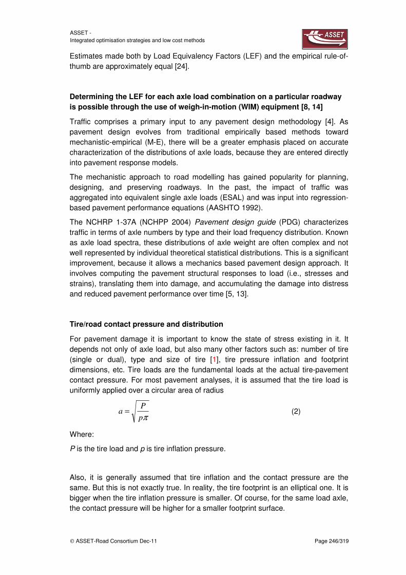
ASSET - Integrated optimisation strategies and low cost methods
ASSET-Road Consortium Dec-11 Page 246/319
Estimates made both by Load Equivalency Factors (LEF) and the empirical rule-of-thumb are approximately equal [24].
Determining the LEF for each axle load combination on a particular roadway
is possible through the use of weigh-in-motion (WIM) equipment [8, 14]
Traffic comprises a primary input to any pavement design methodology [4]. As pavement design evolves from traditional empirically based methods toward mechanistic-empirical (M-E), there will be a greater emphasis placed on accurate characterization of the distributions of axle loads, because they are entered directly into pavement response models.
The mechanistic approach to road modelling has gained popularity for planning, designing, and preserving roadways. In the past, the impact of traffic was aggregated into equivalent single axle loads (ESAL) and was input into regression-based pavement performance equations (AASHTO 1992).
The NCHRP 1-37A (NCHPP 2004) Pavement design guide (PDG) characterizes traffic in terms of axle numbers by type and their load frequency distribution. Known as axle load spectra, these distributions of axle weight are often complex and not well represented by individual theoretical statistical distributions. This is a significant improvement, because it allows a mechanics based pavement design approach. It involves computing the pavement structural responses to load (i.e., stresses and strains), translating them into damage, and accumulating the damage into distress and reduced pavement performance over time [5, 13].
Tire/road contact pressure and distribution
For pavement damage it is important to know the state of stress existing in it. It depends not only of axle load, but also many other factors such as: number of tire (single or dual), type and size of tire [1], tire pressure inflation and footprint dimensions, etc. Tire loads are the fundamental loads at the actual tire-pavement contact pressure. For most pavement analyses, it is assumed that the tire load is uniformly applied over a circular area of radius
πp
Pa = (2)
Where:
P is the tire load and p is tire inflation pressure.
Also, it is generally assumed that tire inflation and the contact pressure are the same. But this is not exactly true. In reality, the tire footprint is an elliptical one. It is bigger when the tire inflation pressure is smaller. Of course, for the same load axle, the contact pressure will be higher for a smaller footprint surface.

ASSET - Integrated optimisation strategies and low cost methods
ASSET-Road Consortium Dec-11 Page 247/319
Figure 257: Tire/road contact area depends on inflation pressure
Example of the footprint surface for different inflation pressures (tire load P = 22kN)
Inflation pressure [bar] 3 3,5 4,1 4,8 5,5 6,2 6,9 7,6 8
Footprint surface [cm2] 748 645 536 458 407 361 363 290 277
(a) (b)
Figure 258: Contact area between tire and road is elliptical one (a); typical normal load distribution
along the footprint (b), [18, 20]
9.1.2 Road pricing strategies
This chapter describes various types of road pricing, which charge the motorist directly for driving on a particular roadway or in a particular area (10). “Congestion pricing” (also called “value pricing”) refers to variable tolls, with higher prices under congested conditions and lower prices under less congested conditions, intended to reduce the peak-period traffic volumes to optimal levels. “Toll roads” and “toll lanes” are roadway facilities financed by tolls. “High Occupant Toll (HOT) lanes” are High Occupant Vehicle (HOV) lanes that can also be used by low-occupant vehicles that pay a toll.

ASSET - Integrated optimisation strategies and low cost methods
ASSET-Road Consortium Dec-11 Page 248/319
Figure 259: Road pricing dependencies
Road pricing principles
An effective and fair road pricing system should reflect the following principles:
Easy for users to understand.
Convenient – does not require vehicles to stop at toll booths.
Transport options – consumers have viable travel options available (i.e., alternative modes, travel times, routes, destinations).
Payment options – easy to use with multiple payment options (cash, prepaid card, credit card etc.)
Transparent – charges evident before trip is undertaken.
Anonymous – privacy of users is assured.
Traffic authority perspective
Traffic impacts – does not require each vehicle to stop at toll booths or in other ways traffic delays.
Efficient and equitable – charges reflect true user costs.
Effective – reduces traffic congestion and other transportation problems by changing travel behaviour.
Flexible – easily accommodates occasional users and different vehicle types.
Reliable – minimal incorrect charges.
Secure and enforceable – minimal fraud or non-compliance.

ASSET - Integrated optimisation strategies and low cost methods
ASSET-Road Consortium Dec-11 Page 249/319
Cost effective – positive return on investments.
Implementation – minimum disruption during development phase. Can be expanded as needed.
Road pricing means that motorists pay directly for driving on a particular roadway or in a particular area.
Value pricing is a marketing term which emphasizes that road pricing can directly benefit motorists through reduced congestion or improved roadways.
Managed lanes is a general term for various roadway management strategies, including HOV, HOT, and congestion priced lanes.
Economists have long advocated Road Pricing as an efficient and equitable way to Finance Roads other Transportation Programs, and encourage more efficient transportation. Road Pricing has two general objectives: revenue generation and congestion management (16). They differ in several ways, as compared in the table below.
The following table compares road pricing objectives (market principles):
Revenue generation Congestion management
Generates funds.
Rates set to maximize revenues or recover specific costs.
Revenue often dedicated to roadway projects.
Shifts to other routes and modes not desired (because this reduces revenues).
Reduces peak-period vehicle traffic.
Is a TDM (Transportation Demand Management) strategy.
Revenue not dedicated to roadway projects.
Requires variable rates (higher during congested periods).
Travel shifts to other modes and times considered desirable.
Different types of road pricing
Road tolls
Tolls are a common way to fund highway and bridge improvements. Such tolls are a fee-for-service, with revenues dedicated to roadway project costs. This is considered more equitable and economically efficient than other roadway improvement funding options which cause non-users to help pay for improvements. Tolling is often proposed in conjunction with road privatization (i.e., highways built by private companies and funded by tolls). Tolls are often structured to maximize revenues and success is measured in terms of project cost recovery. Tolling authorities may discourage development of alternative routes or modes.
Congestion pricing
Congestion pricing (also called Value pricing) refers to variable road tolls (higher prices under congested conditions and lower prices at less congested times and

ASSET - Integrated optimisation strategies and low cost methods
ASSET-Road Consortium Dec-11 Page 250/319
locations) intended to reduce the peak-period traffic volumes to optimal levels. Tolls can vary based on a fixed schedule, or they can be dynamic, meaning that rates change depending on the level of congestion that exists at a particular time. It can be implemented when road tolls are implemented to raise revenue, or on existing roadways as a demand management strategy to avoid the need to add capacity. Some highways have a combination of unpriced lanes and value priced lanes, allowing motorists to choose between driving in congestion and paying a toll for an uncongested trip. This is a type of Responsive pricing, meaning that it is intended to change consumption patterns.
Cordon (area) tolls
Cordon tolls are fees paid by motorists to drive in a particular area, usually a city centre. Some cordon tolls only apply during peak periods, such as weekdays. This can be done by simply requiring vehicles driven within the area to display a pass, or by tolling at each entrance to the area.
HOT lanes
High Occupancy Toll (HOT) lanes are High Occupancy Vehicle (HOV) lanes that also allow the use by a limited number of low occupancy vehicles if they pay a toll. It is a type of Managed lane. This allows more vehicles to use HOV lanes while maintaining an incentive for mode shifting, and raises revenue. HOT lanes are often proposed as a compromise between HOV lanes and road pricing.
Vehicle use fees
Distance-based charges such as mileage fees can be used to fund roadways or reduce traffic impacts, including congestion, pollution and accident risk. A proposal by the UK Commission for Integrated Transport (CFIT, 2002) proposes that existing vehicle registration fees and fuel taxes to be replaced by a variable road user charge using GPS-based Pricing Methods, as a way to reduce traffic congestion and more equitably reflect the roadway costs imposed by each vehicle. Pay-As-You-Drive vehicle insurance prorates premiums by mileage so vehicle insurance becomes a variable cost, which gives motorists an incentive to reduce traffic impacts, but provides no additional revenue.
Road space rationing
A variation of road pricing is to ration peak period vehicle-trips or vehicle-miles using a revenue-neutral credit-based system. For example, each resident in a region could receive credits for 100 peak-period vehicle-miles each. Residents can use the credits themselves, or trade or sell them to somebody else. The result is a form of congestion pricing in which the benefits are captured by residents rather than road owners or governments.
The table summarizes these different categories of road pricing and their objectives. Some provide revenues, some reduce peak-period congestion, some

ASSET - Integrated optimisation strategies and low cost methods
ASSET-Road Consortium Dec-11 Page 251/319
reduce total traffic impacts (congestion, pollution, accident risks, road and parking facility costs etc.), and some help to achieve a combination of objectives.
Road pricing categories
This table summarizes the major categories of road pricing.
Name Description Objectives
Road toll (fixed rates)
A fixed fee for driving on a particular road. To raise revenues.
Congestion pricing (time-variable)
A fee that is higher under congested conditions than uncongested conditions, intended to shift some vehicle traffic to other routes, times and modes.
To raise revenues and reduce traffic congestion.
Cordon fees Fees charged for driving in a particular area.
To reduce congestion in major urban centres.
HOT lanes
A high-occupant-vehicle lane that accommodates a limited number of lower-occupant vehicles for a fee.
To favour HOVs compared with a general-purpose lane, and to raise revenues compared with an HOV lane.
Distance-based fees
A vehicle use fee based on how many miles a vehicle is driven.
To raise revenues and reduce various traffic problems.
Pay-As-You-Drive insurance
Pro-rata premiums by mileage so vehicle insurance becomes a variable cost.
To reduce various traffic problems, particularly accidents.
Road space rationing
Revenue-neutral credits used to ration peak-period roadway capacity.
To reduce congestion on major roadways or urban centres.
Road pricing impacts vary depending on various factors, including the type of pricing, how it is structured, and the transportation and geographic conditions in which it is implemented. For example, a fixed road toll may do little to reduce congestion if alternative routes and modes are poor, but it may provide significant congestion reductions if transportation alternatives (such as car pooling, transit and telecommuting) are relatively attractive, and so a modest fee will cause a relatively large mode shift. In some situations, pricing will shift traffic and congestion problems to other routes or areas. Table 5 summarizes the benefits of various pricing strategies. Actual impacts will vary depending on circumstances. For example, in some situations HOT lanes will have greater congestion reduction impacts than others. The point is that these differences should be considered when evaluating and selecting pricing options.

ASSET - Integrated optimisation strategies and low cost methods
ASSET-Road Consortium Dec-11 Page 252/319
Road pricing benefits
Strategy Revenue
generation
Congestion
reduction
Pollution
reduction
Increased
safety
Road toll (fixed rates) 3 2 1 1
Congestion pricing (time-variable)
2 3 2 1
HOT lanes 1 2 1 0
Cordon fees 2 3 1 1
Distance-based fees 3 2 2 2
Pay-As-You-Drive insurance 0 2 2 3
Road space rationing 0 3 1 1
Ranges from 3 (very beneficial) to -3 (very harmful); a 0 indicates no impact or mixed
impacts
Implementation of road pricing
Road pricing is usually implemented by public or private highway agencies or local authorities as part of transportation project funding packages, for transportation demand management, or through privatization of highway construction and operation. Implementation may require approval of other levels of government.
Road pricing can be implemented at various scales:
Spot: Pricing a particular point in the road network, such as a bridge or a tunnel
Facility: Pricing a roadway section
Corridor: Pricing all roadways in a corridor
Cordon: Pricing all roads in an area, such as a central business district
Regional: Pricing roadways at regional centres or throughout a region
The below table illustrates the appropriate scales of various pricing strategies:
Strategy Spot Facility Corridor Cordon Regional
Toll roads (fixed rates) X X X
Congestion Pricing (time-variable)
X X X X
HOT lanes X X
Cordon fees X X
Distance-based fees X

ASSET - Integrated optimisation strategies and low cost methods
ASSET-Road Consortium Dec-11 Page 253/319
A variety of pricing methods can be used to collect fees. The below table summarizes them. Newer methods tend to have lower costs, greater convenience and price adjustability, making them more cost effective and politically acceptable.
Type Description Equipment
costs
Operating
costs
User
inconvenience
Price
adjustability
Pass Motorists must purchase a pass to enter a cordoned area.
Low Low Medium Poor to medium
Toll Booths Motorists stop and pay at a booth.
High High High Medium to
high
Electronic Tolling
An electronic system bills users as they pass a point in the road system.
High Medium Low High
Optical Vehicle Recognition
An optical system bills users as they pass a point in the road system.
High Medium Low High
GPS GPS is used to track vehicle location. Data are automatically transmitted to a central computer that bills users.
High Medium Low High
Benefits and costs
Road pricing benefits and costs vary depending on travel impacts, what is assumed to be the alternative, and other factors (Pricing Evaluation).
Road pricing that reduces total vehicle travel can reduce road and parking facility costs, increase road safety, protect the environment, encourage more efficient land use, and improve community liveability.
Road pricing that funds additional highway capacity can increase total automobile travel (rebound effects), and so may increase downstream traffic congestion, parking costs, crashes, pollution, and sprawl. Expanding highway size and traffic volumes tends to reduce the liveability of communities they cut, it is argued that that highway privatization can result in fragmented planning and inefficient pricing.
Value pricing and HOT lanes can increase transportation options. On unpriced roads, travellers have no alternative to being delayed by congestion. Value pricing and HOT lanes allow travellers to choose between driving in congestion, avoiding congestion by car pooling, or avoiding congestion by paying a toll. This lets individual consumers choose the option that best meets their needs for a particular trip. It also tends to improve transportation choice indirectly by increasing demand for car pooling and transit services.

ASSET - Integrated optimisation strategies and low cost methods
ASSET-Road Consortium Dec-11 Page 254/319
Road pricing increases motorists’ direct costs, but these are economic transfers payments by motorists are offset by revenues to the tolling agency or government (Evaluating pricing). Overall consumer impacts from road pricing depend on how revenues are used. If returned as rebates or reductions in other taxes, or used in other ways that consumers get value, consumers may be no worse off financially.
Resource costs are primarily the transaction costs to highway agencies and to users of collecting fees. Toll collection costs range from about 10% of total tolling revenue for electronic toll collection, up to 40% for toll booths. Toll collection that requires motorists to stop at booths causes motorists delays and increases energy consumption and air pollution. New electronic tolling can reduce these transaction costs (pricing methods).
Pricing research case studies
The report Pricing European Transport Systems (PETS), funded by the European Commission, describes several case studies that were modelled, including several interregional, and two urban traffic management programs to control traffic congestion, crash risk and pollution emissions.
German government approves tolls for trucks
In August 2001 the German cabinet has approved plans drawn up by transport minister Kurt Bodewig that will introduce tolls on trucks using roadways beginning in 2003. Vehicles over 12 tons would be required to pay 0.14-0.19 Euros per kilometre, with variation depending on exhaust emissions and axles. The intent of the plan is to shift the financing of road use away from the general taxpayer and onto heavy road users. The toll rate was established by computing the costs of the extra wear and tear on roads and maintenance costs incurred by trucks. Revenue from the tolls will be used for further transport investment, including an anti-congestion program. Nature conservation group Nabu applauded the plan but urged the government to consider putting the revenue into something other than road building (ENDS Environment Daily, August 16, 2001).
World Bank analysis of toll roads
A World Bank study came to the following conclusions about the prospects of privately financed toll roads:
The demand for road services will continue to grow and hence so will the need for investment. Worldwide, the stock of motor vehicles is growing at nearly three percent per year. Since the number of vehicle kilometres travelled tends to grow somewhat faster than the stock of motor vehicles, this implies that at least for some segments of the road network, the demand prospects are quite good. The fast urbanization of the developing world adds another dimension that cannot be ignored and explains the strong demand for urban access roads in many of the most populated countries of the world.

ASSET - Integrated optimisation strategies and low cost methods
ASSET-Road Consortium Dec-11 Page 255/319
The challenge here is to bet on the right horses. Demand will increase but only on some segments of the network and it is tempting for a government to oversell a specific road based on aggregate traffic growth prospects. Even holding the effects of toll levels constant, traffic volumes are very sensitive to income and economic growth. The failure to recognize this may be one of the main reasons why so many toll road projects have failed or ended in bitter renegotiations. Motorization and vehicle-kilometres travelled tend to increase faster than income levels. This high income elasticity, especially for leisure trips, makes toll roads especially sensitive to macroeconomic conditions. For roads that serve export activities, exchange rate changes can dramatically affect trade, leading to major changes in demand patterns.
Pay-As-You-Drive in the Netherlands
In 2008 the Netherlands government committed to implementing a new electronic road pricing system that charges vehicles based on its environmental characteristics, and the time and place of each journey, with higher rates under congested conditions. An independent government agency will be set up to administer the payments, which is expected to begin in 2011. This will replace the current vehicle tax (Motorrijtuigenbelasting or MRB) and vehicle sales tax (Belasting Personenauto’s en Motoren or BPM). Motorists who drive less will pay less, and those who drive more will pay more. Cars that pollute more will be more expensive than cleaner cars. Total government revenues will not increase. This is considered fairer and more efficient than the current system, which imposes very high vehicle ownership taxes. The program is therefore deliberately named A Different Way of
Paying for Mobility. Eventually, each vehicle will be fitted with a mobimeter that will record the number of kilometres driven and the charge payable (www.minvenw.nl/cend/dco/home/data/international/gb/eng1201.html). An open standard will be used, so the private sector can play an important role and incorporate ancillary services such as travel information, automatic breakdown notification and payment for parking. A public/private platform is to be set up in order to develop such services.
Highway vehicle weight management
The size and weight of trucks allowed have been increased over the years to reduce transportation costs. The concerns of accelerated infrastructure deterioration and traffic safety are the main constraints for further increase in truck size and weight. Both technical engineering and system policy management solutions are needed to support economic development while still preserving highway infrastructure. The challenge for the European countries is to find a good balance between the demands for higher vehicle weight for more highways to support economic development and for the financial sustainability of highway infrastructure.
It is important to have a good understanding of issues related to vehicle weight management for primary weight review and policy development. The related issues

ASSET - Integrated optimisation strategies and low cost methods
ASSET-Road Consortium Dec-11 Page 256/319
include regulatory aspect of vehicle weight management, historical evolvement of the current system, pavement design and performance, and countries economy.
Regulatory aspect of vehicle weight management
Maximum vehicle weight and dimensions are established to protect bridges, pavements, roadbeds, overpasses, other users of the roads, and to ensure vehicle stability. The Vehicle Weight and Dimension Regulations provide detailed axle/vehicle weights allowed for different vehicle configurations on individual highways and road networks.
Weights allowed on public highways are separate from the registered weight of a vehicle. A heavy vehicle is usually registered to a specific weight determined by its business and the maximum weight it will generally carry on. In order to protect highway infrastructure and support economic development, all public highways are currently classified under one of the following categories in terms of vehicle weights allowed:
Primary weight highways
Secondary weight highways
Year-round weight restricted highways
Seasonal weight changes (reflect road strength: winter weight, spring road restrictions)
Weight permits.
Almost all changes made are in one direction, which is the increased size of the primary weight highway system, or increased access to the primary weight system, or increased size /weight of trucks allowed on highways. The driving forces for these changes historically have been the carriers/shippers demanding for higher allowed weights to reduce their transportation costs, or the national and international harmonization drive for uniformed market access and increased productivity for transportation industry. The concerns of increased infrastructure damage and traffic safety are the main constraints for further changes. Over the last 20 years, the primary weight highway network had been largely steady, and changes to the network were mainly related to winter and spring weight limits and duration.
Factors affecting the performance of highway infrastructure
Many factors affect the life and performance of highway infrastructure. These factors can be categorized broadly into three categories: traffic loading, pavement structure, and environmental conditions. There are also complicated interactions among these factors as well as many uncertainties. The most common measure of traffic loading damage to pavement has been ESAL (Equivalent Single Axle Load), which is primarily dependent upon the axle weight, axle configurations, truck volume, and pavement types. Pavement deterioration can be seen as the result of the cumulative traffic loading ESAL on pavements over the design period. It is generally accepted that axle weight and ESAL equivalency factor follows a (third to)

ASSET - Integrated optimisation strategies and low cost methods
ASSET-Road Consortium Dec-11 Page 257/319
fourth power relationship for a given pavement type. For example, an equivalency
factor of 3.84th
power has been used in pavement design (16). According to this relationship, 10% increase in axle weight will result in 44% increase in pavement damage; a 2-axle six tire single unit truck hauling primary weight will cause 133% more damage than the same unit truck hauling secondary weight, although its GVW (gross vehicle weight) is only increased by about 20%. This is why highway engineers are always concerned for the increase in vehicle weight on highways.
The highway pavements have been constructed to different structures according to subgrade conditions and forecasted traffic loading to achieve the cost effectiveness. Roadways may be constructed as one of following structures (9):
AC (asphalt concrete) pavement of 15 year design life, consisting of asphalt concrete, base and subbase
Granular pavements with different standards for 5 to15 years design life, consisting of base and subbase with a seal coat
TMS (Thin Membrane Surface), a thin layer of soft asphalt (40-50 mm) placed on top of subgrade to provide a dust free surface for rural light traffic
Gravel roads, or compacted earth roads.
Different road structures have different capacities to handle vehicle weight. Even for the same type of structure, the load bearing capacity varies due to different subgrade, materials and environmental conditions. AC and granular pavements normally use high quality materials and are more expensive to build, and they can provide much better load bearing capacity. Over the years, TMS and other sub-standard pavements had been built to extend dust free highway network. These highways were never built to handle heavy truck traffic. If the heavy truck load is applied to non-structured roads (such as TMS) or low quality pavements, the risk of catastrophic failure (such as shear) will be high. With the rapid changes in economic activities, traffic loading patterns may have also changed after the roadways have been constructed. The changed transportation demand may not be matched with the timely and adequate pavement upgrading, which may lead to accelerated pavement deterioration.
Environmental conditions also have great impact on pavement deterioration. Low temperature can cause pavement thermal cracking, high temperature will soften the surface asphalt materials which lead to increased rutting and bleeding, and freezing-thaw-cycle can cause pavement frost action damage.
New economic reality and transportation demand
The European economy is expected to grow mainly from expanded trade in natural resources, processing and manufacturing exports. Many of the new entrants into the European economy operate in areas with commodities/volumes where trucking is the only viable means of transportation.
With increasing diversification, the volume of products being moved continues to rise. Most of this movement is by road.

ASSET - Integrated optimisation strategies and low cost methods
ASSET-Road Consortium Dec-11 Page 258/319
The truck travel trend is clearly pointed to further increase in the future. It is believed that railways are not likely to reduce road traffic due to the increasingly complex nature of the trip patterns and special requirements for commodity transport. A rationalized and expanded primary weight highways network will certainly help improve commercial transportation efficiency.
Economic reasons for primary weight requirement
The costs of freight transportation on highways mainly include trucking and road infrastructure costs. Both of these costs vary by truck type, carried weight and road surface structure. As discussed earlier, higher vehicle weight (increased ESAL) will lead to much higher infrastructure costs due to the power relationship between axle weight and ESAL. For trucking costs, the major components include equipment depreciation, fuel consumption, repairs and maintenance, licensing and insurance, wages, and administration. The equipment depreciation, fuel consumption and wages are the most important cost components and they are all proportional to the number of trips or distance travelled.
For high-density bulk commodities mostly seen in Europe, their unit weight price and storage are relatively cheap and are normally ordered in large quantity, the maximum payload usually is controlled by weight limits on highways. Comparing the primary and secondary weight, the GVWs (Gross Vehicle Weight) of most truck types are just increased by 10% to 20%. However, the payload increase will be more significant, the increase may be in the range of 24% to 50% depending on truck configuration.
Problems identified and principles for new policy
To review current primary weight system and to develop a new policy framework for the primary weight system, it is critical to identify the major problems with the existing one. The following major problems for the system were identified:
The extent of the primary weight highway system: the current primary weight highway network is extensive. The primary weight highways covered most high truck traffic highways, but there are still areas and corridors where primary weight is not available for high truck traffic demand. This is largely due to changes in economic activities and transportation patterns.
The management of the primary weight highway system: there was no documentation, defined rationale, criteria, and review process for the system. As a result, the system cannot meet the rapidly changing demands. There was also no long-term plan for the system.
The primary weight policy co-ordination: there was little co-ordination between primary weight policy and overall economic development demand. Policy co-ordination for enforcement, partnership, design standard, and project prioritization could also be improved.
Many technical unknowns affected the primary weight related policy development: such as how to estimate incremental costs by higher weight for

ASSET - Integrated optimisation strategies and low cost methods
ASSET-Road Consortium Dec-11 Page 259/319
different highway structures? Does speed affect pavement damage rate on granular pavement? etc.
Based on the assessment for the identified problems, some major principles for the new primary weight policy were established. One of the major principles is to balance the often conflicting requirements of supporting economic development of rural communities & industries and long term financial sustainability for the highway infrastructure system. Other major principles include criteria development for primary weight highways and a transparent review process to rationalize the network and to meet changing demand.
The objectives of the new policy are to provide a rational, transparent, and consistent primary weight system and review process to gradually meet the reasonable demand for primary weight highways.
Based on the Axle Weight Survey, the overweight ratio (combined axle weight and GVW) is lower than 16% on primary weight highways and 23% for secondary highways. However, if considering allowable ESAL/truck, only about 3.3% trucks were above allowable ESAL (the ESAL of allowed axle and vehicle weight) on primary weight highways, and 10% trucks on secondary highways. Obviously, the overweight is not a big concern for the primary weight highways, and this is partly due to more visible enforcement of the primary weight highway network. It should be noted that most trucks will need to make at least a portion of their trip on a secondary weight highways or municipal roads during their grain delivery. The audited result showed that the portion of trucks over secondary weight was between 40% and 75%, and trucks over primary weight were about 14% (10).
The new effort of enforcement need to focus more on reducing overweight of concentrated haul and on secondary highways. The new strategy may include increased enforceable audit activities to businesses involving concentrated haul, and promote self-enforcement for stakeholders.
Communication strategy consists of a stakeholder awareness program and an information dissemination initiative. The stakeholder awareness program should educate the public and stakeholders about infrastructure costs and vehicle weight impact on pavement deteriorations. The information dissemination initiative should be developed to help local communities, businesses, shippers/carriers to understand alternatives for primary weight access. It should also assist truckers to find the best primary weight routes for their haul activities.
The annual incremental infrastructure costs for the new primary weight segment of highways can be computed as following:
( ) ⋅ ⋅ ⋅ ⋅ ⋅ − ⋅ ∑j j j j 6-m i PS i SSAIIC = TAADT TLP L D PP UC SP UC
(3)
Where:
AIICj = Annual incremental infrastructure costs for highway segment j;
TAADTj = Annual incremental infrastructure costs for highway segment j;

ASSET - Integrated optimisation strategies and low cost methods
ASSET-Road Consortium Dec-11 Page 260/319
TLP = % truck loaded to primary weight;
i = Truck type (single unit i = 1, single trailer i = 2, multi-trailer i = 3);
PPi = Primary payload for truck type i in ton;
Lj = Primary payload for truck type i in ton;
D6-m = Days in 6-month (9-month primary weight, including 3 months winter weight that is the same for both primary and secondary weight highways);
UCPS = Unit cost for primary weight on secondary highways;
SPi = Secondary weight payload for truck type i in ton;
UCSS = Unit cost for secondary weight on secondary highways.
Considering the new primary weight vehicles will also travel on the existing primary weight highways after travelling through these new segments of primary weight highway, these journeys would have been on secondary weight highways without the expansion these new primary weight highways. These incremental primary weight journeys will incur extra pavement consumption to the existing primary weight highways. This extra pavement cost to existing primary weight highways largely depends on the distances these primary weight vehicles will travel. The average trip distances for each type of trucks loaded to above secondary weight on different classes of highways were derived from analysis of the O-D data of Axle Weight Survey. The incremental infrastructure costs of existing primary weight highway by the additional primary weight trucks can be calculated by using the average trip distance of the additional primary weight trucks and 26% of unit trucking costs for primary weight trucks on primary weight highways. The 26% value is used because the ESAL value is increased by about 26% between primary and secondary weight for a given amount of goods being transported by the same truck type (7).
It is expected that different methods will generate different incremental infrastructure cost results. The small difference between the results from the two different methods provides reasonable confidence to the estimated range of actual incremental costs. It should be noted that the infrastructure cost analysis did not consider the three month spring time differently from other times when the primary weight would have incur more damage to the new primary weight pavement. This is due to the fact that ESAL is an annual average pavement damage measure. This fact makes the estimated incremental infrastructure costs on the conservative (high) side.
9.1.3 Conclusions
Axle load spectra, these distributions of axle weight is a significant improvement, because it allows a mechanics based pavement design approach. It involves computing the pavement structural responses to load (i.e., stresses and strains),

ASSET - Integrated optimisation strategies and low cost methods
ASSET-Road Consortium Dec-11 Page 261/319
translating them into damage, and accumulating the damage into distress and reduced pavement performance over time.
Nowadays there are three basic WIM sensors currently available on the commercial market, representative of most of the WIM technologies in use around the world: single load cell, bending plate and piezo-electric.
A Bridge Weigh in Motion (B-WIM) system is based on the measurement of the deformation of a bridge and the use of the measurements to estimate the attributes of passing traffic loads. Tests of this system showed that it is capable of approximating the gross weights of vehicles to within 6-10%, and individual axle weights to within 13-15%.
In order to have a more realistic image of the pavement state of stress and its damage, we must know the real contact pressure between tire and road. Unfortunately, commercial WIM sensors cannot provide this information. For this purpose, a new category of network sensors has been developed.
They are called “Stress-in-motion” sensors (SIM). Having a network of small sensors instead of a single load cell for one WIM sensor seems to be an interesting solution. ). Knowing the distance between sensors (network pitch), the loaded (with output) and unloaded (without output) matrix’s sensors, one can appreciate the tire footprint dimensions. Similarly, one can determinate the number of tires (single or dual), lateral position of vehicle tires with respect to the lane edge and one can detect the flat tires. For a network of WIM sensors we need small and cheap load cells, having a good accuracy and reliability.
A WIM system able to measure the tire/road contact forces on three axes can measure not only the vertical load (tire/axle load) but also the two forces in the road plane (produced by acceleration, breaking, etc.).
Wheel force dynamometers can be used on test vehicles, servo-hydraulic simulators and roller test stands. These efficient tools are required to measure the data serving as the basis for simulations and for the design of vehicle bodies, chassis, drive trains and tires. Although the system could be adapted as a WIM system used on heavy trucks (with a sensor on which wheel and telemetry system), is difficult to see, in the near future, a commercial application in this field for it.
On the market there are also other weighing-in-built systems (WIBS), more practical for WIM applications. They may be installed on existing multi-axle vehicles without modifying original trailer parts, which potentially weaken the trailer structure. Usually, it takes only one-day for WIBS system installation and calibration on a heavy truck is necessary.
A cabin display reads out gross weight, net weight or even per axle load. A data collection system makes it possible to retrieve and store information on customers, job site data, and product codes for material data, wheel loader reports, driver reports, individual weights and total weights. WIBS collects data for customer reports, driver reports, time between customer pickups, vehicle reports, container reports, product codes in the case of recycling and exception reports. WIBS provide

ASSET - Integrated optimisation strategies and low cost methods
ASSET-Road Consortium Dec-11 Page 262/319
the best solution for the loading of trucks efficiently on-site no matter where the job site is.
Heavy truck loads can damage road and highway pavements, especially in spring time, when they are weakened because the soil and subgrade are saturated with water, and in summer time, when asphalt behaves visco-elastic at elevated temperatures. The local authority can impose weight limits on a highway or bridge that they believe will be damaged because of roadbed weakness or other special conditions
Truck weight and dimension limits control the amount of payload on a truck. Higher vehicle weight will reduce freight transportation costs however it will also result in faster deterioration of the pavements.
Because the increase in truck weight and dimension limits will increase the payload per trip, fewer truck trips are required to carry the same amount of freight.
Pavement deteriorations, including rutting, fatigue cracking, shear failure, and increased roughness, are the result of the interactions of traffic loading, pavement materials, and environmental conditions. The damage to pavement increases exponentially with the increase of vehicle weight. Effective enforcement to reduce overweight trucks is essential for the system’s sustainability.
9.2 Strategies and visions
There is a tremendous potential of using IT Information Technologies and innovative sensor technologies for improving the whole process of road planning, design, built an maintain in all the stages of road life and to achieve a more sustainable road infrastructure including new financing and costing schemes.

ASSET - Integrated optimisation strategies and low cost methods
ASSET-Road Consortium Dec-11 Page 263/319
Figure 260: Holistic approach of cyclic pavement management
Realistic pavement models
The implication of WIM technology for investigating road and traffic conditions is described in order to provide reasonable and appropriate data for pavement and bridge management systems including structural design will be based on the real data and performance of materials and their modelling.
Self protected road infrastructure
WIM and the opportunity to detect overloaded axles, overloaded gross weight and also in combination underinflated tires could lead to “Road and Bridge Access
Control Systems” for avoiding overloaded transports on roads and improvements on safety and driving economy checking the tire pressure concerning safety and optimal rolling resistance.
Several important enhancements of the WIM technologies are the base of the different innovations and achievable benefits and a implementation strategy leading to improvements of economy and competitiveness and opening the framework for a future “Intelligent and Interactive Road”:
Optimised materials
Optimised structural design
WIM
Technology
Pavement
Sensors
Road
ModellingTraffic
Parameters
Environ-
ment
FeasabilityStudy
ProjectDesign
ProjectConstruction
TransferTake Over
Monitoring Traffic & Road Condition
OptimisedLife Cycle
Holistic Operation& Economy
SustainableRoad Infrastructure
OngoingVerifikation
& Improvement
WIM & Pavement Sensing Implications
of a Holistic Approach for Cyclic Management of Sustainable Road Infrastructure

ASSET - Integrated optimisation strategies and low cost methods
ASSET-Road Consortium Dec-11 Page 264/319
Optimised costs and best economy
Better risk management
A logical and interesting next step could be the combination of “New WIM Technology” with the “New Pavement Sensor Systems” as recommended by the ASSET-Road project giving the opportunity of cross-correlation of load patterns and effects in pavement structures
The implication of WIM technology for investigating road and traffic conditions is described in order to provide reasonable and appropriate data for pavement and bridge management systems including structural design will be based on the real data and performance of materials.
Figure 261: WIM and pavement sensing implications on life cycle
This approach could lead to a “Holistic Road Operation Concept” assisted by the output of WIM systems and technologies characterised by:
Protection of road and bridge infrastructure
Cost reduction
Better service
Environment protection

ASSET - Integrated optimisation strategies and low cost methods
ASSET-Road Consortium Dec-11 Page 265/319
New road pricing strategies
Heavy trucks and buses are responsible for the largest part of the pavement damage. An original for a new tolling system for heavy trucks, based on real damage produced to roads, was presented. It is governed by the idea that each vehicle must pay for the produced pavement damages. Unfortunately, to appreciate the real damages produced by each vehicle and educate the transportation community in this philosophy is not so easy.
9.2.1 New ideas and technologies
This report intends to present a short state-of-art report of the forward-looking visions on sustainable road transport infrastructures, considered from the point of view of technological change combined with global institutional and social changes experienced by our society.
In the frame of technological changes new ideas and technologies which are envisaged to be developed in the future are seeking mainly the following aspects:
Multi-functional use of space
Multi-purpose road structures
Smart transport and concepts for physical infrastructure
New energy sources for the transport sector (hydrogen, fuel cells, hybrid systems, solar panels etc.)
New concepts for traffic and axle load monitoring, including weigh in motion (WIM), innovations and implications for maintaining and management of an efficient and sustainable road infrastructure and DBOT/PPP project schemes.
New approaches for a road pricing system for heavy vehicles.
Multiple functional use of space
In densely populated areas in order to make the best use of the limited urban space, the new concept of multiple use of space defined as [3] ”the fulfilment of several functions in a certain space and at a certain time” could be applied. The motorway house is an illustrative example of this concept consisting from a combination of two dimensional (2D) motorway and the three dimensional (3D) building into a new type of four dimensional (4D) ”habitat”.
According to this concept, a multifunctional multilayer motorway house, the 2D road is gradually raised-up to become a 3D volume the traffic being accommodated on the top surface with local incisions which allow cars to drive into the structure. Each lane accommodates a specific speed (e.g.120 km/h for traffic at higher level, 90km/h for lanes in the middle sections and 60km/h for the lanes leading to the residential domains).
The cars communicate in real time with the roadscape and are electronically controlled to their domain of destination. In the motorway home the normal stops for

ASSET - Integrated optimisation strategies and low cost methods
ASSET-Road Consortium Dec-11 Page 266/319
gas, food, and lodging are transformed into mobility hubs. The concept facilitates the ecological connection between the two sides of the motorway because traffic is lifted to the upper floors of the structure while the lower floors leave way for ecological corridors necessary for flora and fauna.
Multiple purposes road structures
According this new concept, the road space can be used for other purposes other than just for traffic, and for other functions such as space for soil decontamination, heat storage under the road, piezoelectric elements in the road surface and solar panels and wind turbines on the roof over the road. Also noise barriers alongside roads are already now used to carry photovoltaic panels. In the cities, according to this concept, various utilities such as gas, water, electricity, sewers, and data cables are accommodated in small underground tunnels.
Smart transport and concepts for physical infrastructures
In order to manage in a more efficient way the well known transport systems (railways, trams, buses, light weight rail, undergoing metro etc.), the following solutions have been developed.
Managerial measures, in order to enlarge the capacity of the existing systems without rebuilding the existing physical infrastructure
New concepts for physical infrastructure, like aero rail systems, elevated above the ground level provide free movement and natural areas which in comparison with underground metros cause less disruption to underground utilities and existing buildings They also take a shorter time to be build and cause less inconvenience to road traffic during construction
Automatic highway systems and intelligent systems in the vehicle which can assist the driver either by means of improving the information about the driving environment or by actively aiding the driver in the driving task combine on-board vehicle intelligence with the range of intelligent technologies.
The development of sensor technology such as ABS installation, will play a key role in this field, an example of such a sensor system would be a combination of laser and radar “ladar”-technology [4].
9.2.2 New concepts for traffic and axle load monitoring
In this chapter we develop and present new concepts for traffic and axle load monitoring, including Weigh in motion (WIM) Innovations and their implications for maintaining and management of an efficient and sustainable road infrastructure in the frame of DBOT/PPP project schemes.
Very often traffic patterns and loading on roads are changing during the duration of a PPP or DBOT road infrastructure project – not adequate considered in the
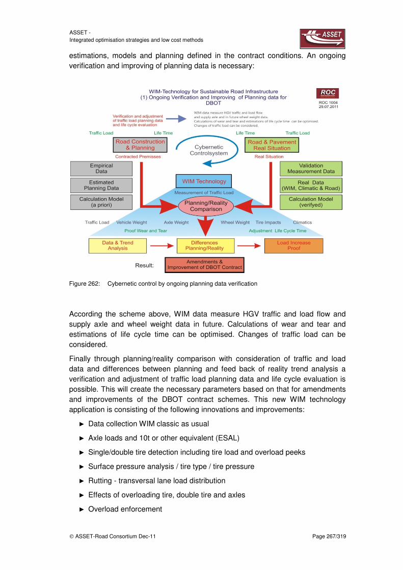
ASSET - Integrated optimisation strategies and low cost methods
ASSET-Road Consortium Dec-11 Page 267/319
estimations, models and planning defined in the contract conditions. An ongoing verification and improving of planning data is necessary:
Figure 262: Cybernetic control by ongoing planning data verification
According the scheme above, WIM data measure HGV traffic and load flow and supply axle and wheel weight data in future. Calculations of wear and tear and estimations of life cycle time can be optimised. Changes of traffic load can be considered.
Finally through planning/reality comparison with consideration of traffic and load data and differences between planning and feed back of reality trend analysis a verification and adjustment of traffic load planning data and life cycle evaluation is possible. This will create the necessary parameters based on that for amendments and improvements of the DBOT contract schemes. This new WIM technology application is consisting of the following innovations and improvements:
Data collection WIM classic as usual
Axle loads and 10t or other equivalent (ESAL)
Single/double tire detection including tire load and overload peeks
Surface pressure analysis / tire type / tire pressure
Rutting - transversal lane load distribution
Effects of overloading tire, double tire and axles
Overload enforcement

ASSET - Integrated optimisation strategies and low cost methods
ASSET-Road Consortium Dec-11 Page 268/319
Pavement temperature
Structural forces
Sensor family, sensor arrays and configurations
Certification R134 by weight and measures for enforcement
Figure 263: Innovations and implications of a new WIM technology
The following new weigh in motion technology implications could be envisaged for the road designer and road operators:
Detailed traffic data measurement
Trend analysis and implications of traffic flow changes
Trend analysis and implications of HGV flow changes
Detailed axle and wheel load data for calculation models
Implications and analysis of wheel and axle overloading
Rutting effects per lane
Comparison of planned and real traffic loads
Life cycle calculation and model enhancement
Deviation analysis and representation

ASSET - Integrated optimisation strategies and low cost methods
ASSET-Road Consortium Dec-11 Page 269/319
Risk analysis and management
Approval of traffic flow changes
Calculations of implications and model optimisation
Optimisation repair and maintenance cycles
Substantial risk management and risk compensation
Optimization cost benefit ratio
In addition in relation with the figure below it will be possible as necessary to verify and optimise the existing pavement deterioration models used currently.
Figure 264: Deterioration model optimisation cycles
This means:
Consideration of extended and new parameters (not yet measured or available)
Higher precision of the used parameters and estimations
Better resolution concerning road geometries and load placements
Higher sensor dynamics and force/displacement/ resolution
Low cost measurement systems and remote communication
Better data base an analysis tools

ASSET - Integrated optimisation strategies and low cost methods
ASSET-Road Consortium Dec-11 Page 270/319
The next diagram describes the different enhancements of the WIM technologies as base of the different innovations and achievable benefits and a implementation strategy leading to improvements of economy and competitiveness and opening the framework for a future “Intelligent and Interactive Road”:
Optimised materials
Optimised structural design
Optimised costs and best economy
Better risk management
Figure 265 WIM technology enhancement and “ Intelligent roads”
In the next diagram is described the implication of WIM technology for investigating road and traffic conditions in order to provide reasonable and appropriate data for pavement and bridge management systems including structural design will be based on the real data and performance of materials.

ASSET - Integrated optimisation strategies and low cost methods
ASSET-Road Consortium Dec-11 Page 271/319
Figure 266: Implications of new WIM technology for pavement management
This approach could lead to a “Holistic Road Operation Concept” assisted by the output of WIM systems and technologies characterised by:
Protection of road and bridge infrastructure
Cost reduction
Better service
Environmental protection

ASSET - Integrated optimisation strategies and low cost methods
ASSET-Road Consortium Dec-11 Page 272/319
Figure 267: Holistic road and bridge management
A significant example of the actual use of WIM Technology innovation demonstrated and investigated in the frame of the ASSET-Road project (German test site in Rosenheim) is shown in the next diagram.

ASSET - Integrated optimisation strategies and low cost methods
ASSET-Road Consortium Dec-11 Page 273/319
Figure 268: WIM technology for overload detection and identification
A logical and interesting next step could be the combination of “New WIM Technology” with the “New Pavement Sensor Systems” as recommended by the ASSET-ROAD project giving the opportunity of cross-correlation of load patterns and effects in pavement structures.

ASSET - Integrated optimisation strategies and low cost methods
ASSET-Road Consortium Dec-11 Page 274/319
Figure 269: Correlation of WIM and pavement system data
Self protected road infrastructure
WIM and the opportunity to detect overloaded axles, overloaded gross weight and also in combination underinflated tires could lead to “Road and Bridge Access Control Systems” for avoiding overloaded transports on roads and improvements on safety and driving economy checking the tire pressure concerning safety and optimal rolling resistance.
9.2.3 New approaches to road pricing of heavy vehicles
Heavy trucks and buses are responsible for the largest part of the pavement damage. An original proposal, resulted from specific studies undertaken in the frame of Technical University of Iasi, Faculty of Mechanical Engineering, Strength of Materials Department, for a new tolling system for heavy trucks, based on real damage produced to roads, is presented below [2]. It is governed by the idea that each vehicle must pay for the produced pavement damages. Unfortunately, to appreciate the real damages produced by each vehicle and educate the transportation community in this philosophy is not so easy.
The current road pricing (tolling) system [5] has the following disadvantages:
It doesn’t take into consideration the real wearing of the roads and bridges produced by each vehicle [1];

ASSET - Integrated optimisation strategies and low cost methods
ASSET-Road Consortium Dec-11 Page 275/319
For the vehicles from the same category, the same price is paid regardless of the transported load, the distance, the road structure type (asphalt, concrete, earth roads), regardless of the bridge usage etc.;
The same price is paid, even if the vehicles circulate or not;
It is hidden and inequitable;
The penalty for the overloaded vehicles (if they are traced down!) depends on the overloading percentage above the maximum allowable axle load (MAAL), regardless of the transportation distance;
The overloading inspections (WIM or static weighing performed with mobile platforms) are not so common and they are not discouraging enough this type of practice (the WIM systems are costly, very few are mounted in localities, and the use of platforms produce traffic jams);
The new road pricing (tolling) system will have to ensure:
The elimination of the previously related deficiencies;
The adjustment of the road pricing principle to the actual pavement damage;
The data acquisition without causing traffic jams (or just causing minimum traffic disruption).
In order to eliminate or reduce the significant disadvantages experienced with the existing methods, an original concept for a tolling system, based on a modified Weighing-In-Built System (WIBS), has been conceived and illustrated with significant examples. This system will be compulsory for all heavy vehicles, which implies:
EU legislation modification;
Installing of the modified WIBS kit on all existing trucks;
Attaching of this kit on the new trucks (from factory);
WIBS periodical inspection.
On the market there are some weighing-in-built systems (WIBS), which can be installed on existing multi-axle vehicles, without modifying original trailer parts [7]. The kit consists in pressure/force sensors installed on different points (truck axles etc.), an analogue to digital converter, a computer, software etc. The input data of this computer are coming from all axle-groups. Depending on the requirements, the Cabin Display reads out and records gross weight, net weight or even the load per axle. Although this WIBS has been designed in order to give data especially for drivers and transport managers, it may be adapted also for WIM purposes. Only a GPS is added to an existing WIBS for our purposes. Actually, many trucks have a GPS system. But, for our purposes, the GPS output will be sent in the computer and it will provides information about the truck path (roads, bridges and distances etc.). Alternatively the GPS, a simpler system could be used: the output of the odometer (counter km device, existing on truck dashboard). Unfortunately, in this case, only information about distances could be obtained.

ASSET - Integrated optimisation strategies and low cost methods
ASSET-Road Consortium Dec-11 Page 276/319
As a rule-of-thumb, the pavement damage caused by a particular load is roughly related to the load by a power of four [6]:
4
80
≈
FD
(1)
Where:
F is the axle load and 80 kN is the standard axle load.
Figure 270: A modified weighing-in-built system WIBS
The route of a truck (equipped with the modified WIBS) within a specified time period is presented above.
In the hypothesis that the gross weight is uniformly distributed, in accordance with, truck axle A2, running on this route, caused the following total pavement damage calculated with equation (1):
×
+×
+×
≈ 3
4
2
4
1
4
2
80
25.1
80
5.0
80d
Fd
Fd
FCFTD
A
T
(2)
The coefficients in the above equation are: 5.0
%100
%50=
, etc.
CFT = Correction Factor for a tandem axle
Similarly the pavement damage produced by other truck axles, A1 and A3 are calculated.
Consequently, the total pavement damage caused by the three axle truck in this period is:
321 A
T
A
T
A
T
T
T DDDD ++= (3)

ASSET - Integrated optimisation strategies and low cost methods
ASSET-Road Consortium Dec-11 Page 277/319
The road pricing (tolling system) for trucks will be proportional with T
TD and it also could take into account other factors (road structure types, crossed bridges etc.), if it is equipped with GPS.
If the truck load (net weight) is not correctly distributed, one or more axles may be overloaded, although the gross weight does not exceed the maximum allowed weight. Even these situations can be appropriately solved by the system, using Load Equivalency Factors LEF [3] and adequate software.
The acquired data can be transmitted to the authorities by the transporter:
At previously established regulated time intervals (monthly, annually) and locations (e.g. along with the digital tachograph data, i.e. driving/resting diagram);
With random inspections;
Telemetrically (for example, when truck passing through WIM stations, the WIBSs can be checked, the transporter can be informed about the possible loss of calibration).
The damage produced by the axels carrying a load bigger than 100%FS will be paid (taking into account the travel distance, the road structure type, the crossed bridges etc.). The overloading penalty already imposed by existing regulation will also be added.
The new pricing system has the following advantages:
The pricing is proportional to the real damage caused to roads and bridges;
The new road pricing system is more transparent and equitable;
The axle overloading can be better supervised at the national level;
Structural pavement integrity protection;
The system is also useful for transportation management;
It allows the weighing in motion inside all localities (nowadays they have very few available WIM systems)
The taxes are not paid for the trucks which are not utilised etc.
On the other hand, it has the following disadvantages:
It implies modification of the EU legislation and the national road pricing systems;
Longer implementation time;
The increase of the truck purchase price;

ASSET - Integrated optimisation strategies and low cost methods
ASSET-Road Consortium Dec-11 Page 278/319
9.3 Overall conclusions
As shown in the chapters before there is a tremendous potential of using technologies (scaled according priority) as enablers as there are:
ICT information and communication technologies
innovative sensor technologies
communication infrastructure
new integrated approaches and improved algorithmns
innovative vehicle control and technical analysis
innovative pavement sensing, modelling and deterioation prediction
new financing and life cyle management schemes
innovative user interfaces (HMI)
for improving the whole process of road planning, design, built an maintain in all the stages of road life and to achieve a more sustainable road infrastructure including new financing and costing schemes.
Main priorities and most important application domains are:
Traffic measurement and analysis on road and bridges
Axle load spectra, these distributions of axle weight is a significant improvement, because it allows a mechanics based pavement design approach. It involves computing the pavement structural responses to load (i.e., stresses and strains), translating them into damage, and accumulating the damage into distress and reduced pavement performance over time.
Nowadays there are three basic WIM sensors currently available on the commercial market, representative of most of the WIM technologies in use around the world: single load cell, bending plate and piezo-electric.
A Bridge Weigh in Motion (B-WIM) system is based on the measurement of the deformation of a bridge and the use of the measurements to estimate the attributes of passing traffic loads. Tests of this system showed that it is capable of approximating the gross weights of vehicles to within 6-10%, and individual axle weights to within 13-15%.
Pavement and bridge monitoring
In order to have a more realistic image of the pavement state of stress and its damage, we must know the real contact pressure between tire and road. Unfortunately, commercial WIM sensors cannot provide this information. For this purpose, a new category of network sensors has been developed.
A WIM system able to measure the tire/road contact forces on three axes can measure not only the vertical load (tire/axle load) but also the two forces in the road plane (produced by acceleration, breaking, etc.).

ASSET - Integrated optimisation strategies and low cost methods
ASSET-Road Consortium Dec-11 Page 279/319
Wheel force dynamometers can be used on test vehicles, servo-hydraulic simulators and roller test stands. These efficient tools are required to measure the data serving as the basis for simulations and for the design of vehicle bodies, chassis, drive trains and tires. Although the system could be adapted as a WIM system used on heavy trucks (with a sensor on which wheel and telemetry system), is difficult to see, in the near future, a commercial application in this field for it.
Truck weight and dimension limits control the amount of payload on a truck. Higher vehicle weight will reduce freight transportation costs however it will also result in faster deterioration of the pavements.
Because the increase in truck weight and dimension limits will increase the payload per trip, fewer truck trips are required to carry the same amount of freight.
Pavement deteriorations, including rutting, fatigue cracking, shear failure, and increased roughness, are the result of the interactions of traffic loading, pavement materials, and environmental conditions. The damage to pavement increases exponentially with the increase of vehicle weight. Effective enforcement to reduce overweight trucks is essential for the system’s sustainability.
Realistic pavement models
The implication of WIM technology for investigating road and traffic conditions is described in order to provide reasonable and appropriate data for pavement and bridge management systems including structural design will be based on the real data and performance of materials and their modelling.
Self protected road infrastructure
WIM and the opportunity to detect overloaded axles, overloaded gross weight and also in combination underinflated tires could lead to “Road and Bridge Access
Control Systems” for avoiding overloaded transports on roads and improvements on safety and driving economy checking the tire pressure concerning safety and optimal rolling resistance.
Several important enhancements of the WIM technologies are the base of the different innovations and achievable benefits and a implementation strategy leading to improvements of economy and competitiveness and opening the framework for a future
“Intelligent and Interactive Road”:
Optimised materials
Optimised structural design
Optimised costs and best economy
Better risk management
A logical and interesting next step could be the combination of “New WIM Technology” with the “New Pavement Sensor Systems” as recommended by the ASSET-Road project giving the opportunity of cross-correlation of load patterns and effects in pavement structures.

ASSET - Integrated optimisation strategies and low cost methods
ASSET-Road Consortium Dec-11 Page 280/319
New road pricing strategies
Heavy trucks and busses are responsible for the largest part of the pavement damage. An original for a new tolling system for heavy trucks, based on real damage produced to roads, was presented. It is governed by the idea that each vehicle must pay for the produced pavement damages. Unfortunately, to appreciate the real damages produced by each vehicle and educate the transportation community in this philosophy is not so easy.
"Holistic Road Operation Concept” This approach could lead to a best total solution assisted by the application and integration of new technology modules combined with the output of WIM systems, algorithms and multiple sensors/arrays characterised by:
Protection of road and bridge infrastructure
Cost reduction
Better service
Environment protection

ASSET - Integrated optimisation strategies and low cost methods
ASSET-Road Consortium Dec-11 Page 281/319
10 References
1. Carden, E.P. and Fanning, P. (2004): ‘Vibration based condition monitoring: A Review.’ Structural Health Monotoring, 3(4), 355-377.
2. Cebon D., (1999): ‘Handbook of vehicle-road interaction’, Swets and Zeitlinger Publishers, Lisse.
3. Christides, S. and Barr, D.S. (1984): ‘One-dimensional theory of cracked Bernoulli-Euler beams’. International Journal of Mechanical Science, 26, 639-648.
4. Curadelli, R. O., Riera, J. D., Ambrosini, D. and Amani, M. G. (2008), “Damage detection by means of structural damping identification”, Engineering Structures, Vol. 30, 3497-3504.
5. Dimarogonas, A.D. (1996). ‘Vibration of cracked structures: a state of the art review’. Engineering Fracture Mechanics, 55, 831-857
6. Doebling, S.W., Farrar, C.R. and Prime, M.B., (1998). ‘A summary review of vibration based damage identification methods.’ Shock and Vibration Digest, 30, 91-105.
7. Farrar, C. and K. Worden (2007): “An introduction to structural health monitoring”, Philosophical Transactions of the Royal Society A, 365, 303–315.
8. González, A. and Hester, D. (2009): ‘The use of wavelets on the response of a beam to a calibrated vehicle for damage detection’, Proceedings of the 7th International symposium on non-destructive testing in civil engineering. Nantes, France, 743-748.
9. Hester, D. and Gonzalez, A. (2011) 'A wavelet-based damage detection algorithm based on bridge acceleration response to a vehicle'. Mechanical Systems and Signal Processing, in press.
10. González, A., OBrien, E. and McGetrick, P. (2010): ‘Detection of Bridge Dynamic Parameters Using an Instrumented Vehicle’, Proceedings of the Fifth World Conference on Structural Control and Monitoring, Tokyo, Japan.
11. Green, M.F. and Cebon, D. (1997): ‘Dynamic interaction between heavy vehicles and highway bridges’. Computers and Structures, 62(2), 253-264.
12. Hester, D., González, A. and Rowley C.W. (2008): ‘Examining the dynamic response of a deteriorated bridge due to the passage of moving loads’. Proceedings of the Bridge and Infrastructure research in Ireland concrete in Ireland conference, Galway, Ireland
13. Hester, D. and González, A. (2010): ‘Detecting damage in a beam subject to a moving load using localised variation in the vibration response’. The joint symposium proceedings of concrete in Ireland 2010 and Bridge & Infrastructure research in Ireland 2010, Cork, Ireland

ASSET - Integrated optimisation strategies and low cost methods
ASSET-Road Consortium Dec-11 Page 282/319
14. ISO 8608:1995 (1995), ‘Mechanical vibration-road surface profiles-reporting of measured data’, International Standards Organisation.
15. Kim, C. W. and Kawatani, M. (2009), “Challenge for a Drive-by Bridge Inspection”, Proceedings of the 10th International Conference on Structural Safety and Reliability, ICOSSAR2009, Osaka, Japan, 758-765.
16. Kim, H. and Melhem, H. (2004): ‘Damage detection of structures by wavelet analysis’. Engineering Structures, 26, 347-362
17. Lin, C. W. and Yang, Y. B. (2005), “Use of a passing vehicle to scan the fundamental bridge frequencies. An experimental verification”, Engineering Structures, Vol. 27, 1865-1878
18. Mahmoud, M.A. (2001) ‘Effect of cracks on the dynamic response of a simple beam subject to a moving load’. Proceedings of the Institute of Mechanical Engineers, Part F: Journal of Rail and Transit, 15, 207-215.
19. Mallet, S.G. (1998). ‘A wavelet tour of signal processing, second ed. Academic Press
20. McGetrick, P. J., González, A. and OBrien, E.J. (2009), “Theoretical investigation of the use of a moving vehicle to identify bridge dynamic parameters”, Insight, Vol. 51(8), 433-438.
21. McGetrick, P., Gonzalez, A. and OBrien, E.J. (2010) Monitoring Bridge Dynamic Behaviour Using an Instrumented 2-axle Vehicle . In: Eds. N.A. Ní Nualláin, D. Walsh, R. West, E. Cannon, C. Caprani, B. McCabe eds. Bridge and Infrastructure Research in Ireland, BCRI2010 Cork, Ireland, , 02-SEP-10 - 03-SEP-10 , pp.281-288.
22. Modena, C., Sonda, D., Zonta, D. (1999), “Damage Localization in a Reinforced Concrete Structures by Using Damping Measurements”, Key Engineering Materials, 167-168, 132-141.
23. Oshima, Y., Yamaguchi, T., Kobayashi, Y. and Sugiura, K. (2008), “Eigenfrequency estimation for bridges using the response of a passing vehicle with excitation system”, Proceedings of the Fourth International Conference on Bridge Maintenance, Safety and Management, IABMAS2008, Seoul, Korea, 3030-3037
24. Pakrashi, V., O’Conner, A. and Basu, B. (2007): ‘A study on the effects of damage models and wavelet bases for damage identification and calibration in beams’. Computer-Aided Civil and Infrastructure Engineering, 22, 555-569
25. Reda Taha, M.M., Noureldin, A., Lucero, J.L. and Baca, T.J. (2006): ‘Wavelet transform for structural health monitoring: a compendium of uses and features’, Structural Health Monitoring, 5(3), 267-295
26. Sinha, K.J., Friswell, M.I. and Edwards. S. (2002): ‘Simplified models for the location of cracks in beam structures using measured vibration data’. Journal of Sound and Vibration, 251(1), 13-38

ASSET - Integrated optimisation strategies and low cost methods
ASSET-Road Consortium Dec-11 Page 283/319
27. Taheri, A, O’Brien, E., Iwnicki, S, Tolooiyan, A and Gavin, K. (2011)The Influence of Train/Track Dynamic Interaction on Railway Track Settlement, Paper submitted to the Journal Structure and Infrastructure Engineering.
28. Toshinami, T., Kawatani, M. and Kim, C.W. (2010), “Feasibility investigation for identifying bridge’s fundamental frequencies from vehicle vibrations”, Proceedings of the Fifth International Conference on Bridge Maintenance, Safety and Management, IABMAS2010, Philadelphia, USA, 317-322
29. Yang, Y. B., Lin, C. W. and Yau, J. D. (2004): “Extracting bridge frequencies from the dynamic response of a passing vehicle”, Journal of Sound and Vibration, Vol. 272, 471-493
References Chapter 4:
1. Abdelkrim, M.; Bonnet, G. & de Buhan, P. (2003): A computational procedure for predicting the long term residual settlement of a platform induced by repeated traffic loading. Computers and Geotechnics, 30, p. 463-476.
2. Barksdale, R.D. (1972): Laboratory evaluation of rutting in base course materials, Proc. 3rd Int. Conf on the Structural Design of Asphalt Pavements, London
3. Bouckovalas G., Whitman R.V., Marr W.A. (1984): Permanent Displacement of Sand with Cyclic Loading, J Geotech Eng 110 (11), p. 1606–1623.
4. Buisman, A.S.K. (1936): Results of long duration settlement tests, First international conference on soil mechanic and foundation engineering. Cambridge. vol.1, p. 103-107
5. Chai, J. C. and Miura, N. (2002): Traffic-load-induced permanent deformation of road on soft subsoil, Journal of Geotechnical and Geoenvironmental Engineering. 128(11), p. 907-916
6. Diyaljee, V. A., and Raymond, G. P. (1982): Repetitive Load Deformation of Cohesionless Soil, Journal of the Geotechnical Engineering Division, ASCE, Vol. 108, No. GT10. p. 1215-1229
7. Gavin, K., Adekunte, A., and O'Kelly, B. (2009): A field investigation of vertical footing response on sand. Proceedings of the Institution of Civil Engineers-Geotechnical Engineering, 162 (5), p. 257-267.
8. Gavin, K., Tolooiyan, A. and O’Kelly. B. (2012): Consideration of creep effects on the bearing resistance of sand, Submitted to ASCE Geofrontiers Conference, 2012 (under review)
9. GDS (2002): Manual of GDS Triaxial Testing System (GDSTTS): Unit 32 Murrell Green Business Park, London Road, Hook, Hampshire, RG27 9GR, U.K.

ASSET - Integrated optimisation strategies and low cost methods
ASSET-Road Consortium Dec-11 Page 284/319
10. Hornych P., Corté J.F., Paute J.L. (1993). Etude des déformations permanentes sous chargement répétés de trois graves non traitées, Bull liaison Labo P et Ch, 184, pp 45-55.
11. Huurman, M. (1997): Permanent deformation in concrete block pavements, PhD Thesis, Delft University of Technology.
12. Kaggwa, W.S., Booker, J.R. and Carter, J.P. (1991) Residual strains in calcareous sand due to irregular cyclic loading, Journal of Geotechnical Engineering, American Society of Civil Engineers, 117, p. 201-218.
13. Khedr S. (1985). Deformation characteristics of granular base course in flexible pavements, Transportation Research Record no1043, pp. 131-138.
14. Lehane B.M., Doherty J.P., and Schneider J.A. (2008). Settlement prediction for footings on sand, Deformational Characteristics of Geomaterials, Vol. 1, IOS-Millpress, Rotterdam: p. 133-150
15. Lentz, R. W., and Baladi, G. Y. (1980): A Simplified Procedure to Characterize Permanent Strain in Sand Subjected to Cyclic Loading, International Symposium on Soils under Cyclic and Transient Loading, Swansea; Balkema Publishers; Rotterdam, the Netherlands.
16. Li, D., and Selig, E. T. (1996): Cumulative plastic deformation for fine-grained subgrade soils, Journal of Geotechnical Engineering, ASCE. 122(12), p. 1006-1013.
17. Marr, W. A. and Christian, J. T. (1981): Permanent displacement due to cyclic wave loading, Journal of the Geotechnical Engineering Division, ASCE. 107(GT8), p. 1129-1149.
18. Monismith, C. L., Ogawa, N., Freeme, C. R. (1975): Permanent Deformation Characteristics of Subgrade Soils due to Repeated Loading, TRR 537, Washington D.C., TRB, p. 1-17.
19. Niemunis, A., Wichtmann, T., Triantafyllidis, T. (2005):. Long term deformations in soils due to cyclic loading; Modern trends in geomechanics, International Workshop Vienna
20. Poulos, H.G. (1988): Marine geotechnics. London: Unwin Hyman. p. 136-13.
21. Sawicki, A. & Swidzinski, W. (1989): Mechanics of a sandy subsoil subjected to cyclic loadings. International Journal for Numerical and Analytical Methods in Geomechanics, 13, p. 511-529.
22. Seed, H. B., and Chan, C. K. (1958), Effects of Stress History and Frequency of Stress Application on Deformation of Clay Subgrades Under Repeated Loading, HRB Proceeding, No.37. p. 555-575.
23. Seed, H. B., Chan, C. K., and Monismith, C. L. (1955), Effects of Repeated Loading on the Strength and Deformation of Compacted Clay, HRB Proceedings, No. 34. p. 541-558.

ASSET - Integrated optimisation strategies and low cost methods
ASSET-Road Consortium Dec-11 Page 285/319
24. Seed, H. B., and McNeill, R. L. (1956): Soils Deformation in Normal Compression and Repeated Loading Tests, HRB Bulletin 141.
25. Seed, H. B., McNeill, R. L., and Guenin, J. D (1960):. Clay Strength Increase Caused by Repeated Loading, ASCE Transactions, Paper No. 3018, Vol. 125. p. 141-161.
26. Sweere, G.T.H. (1990): Unbound granular bases for roads, Doctoral thesis, Delft University of Technology
27. Tolooiyan, A. (2010). FE approaches to evaluate the capacity of foundations on sand using insitu test results. PhD thesis in preparation, University College Dublin, Ireland
28. Triantafyllidis, Th., Wichtmann, T., and Niemunis, A. (2003): Explicit accumulation model for granular materials under multiaxial cyclic loading. Proc. of the 6th International Workshop on Mathematical Methods in Scattering Theory and Biomechanical Engineering, Tsepelovo, Greece (September 2003), World Scientific, p. 394-405
29. Tseng, K.H., Lytton, R.L. (1989): Prediction of permanent deformation in flexible pavement materials, Implication of Aggregates in the Design, Construction and Performance of Flexible Pavements, ASTM STP 1016, pp 154-172.
30. Vuong, B. (1994). Evaluation of back-calculation and performance models using a full scale granular pavement tested with the accelerated loading facility (ALF), Proceedings 4th Int. Conf. on the Bearing Capacity of Roads and Airfields, Minneapolis, USA, pp 183-197
31. Wichtmann, T., Niemunis, A., Triantafyllidis, Th. (2005): Strain accumulation in sand due to cyclic loading: drained triaxial tests, Soil Dynamics and Earthquake Engineering 25, No. 12, p. 967-979
32. Wolff, H., and Visser A.T. (1994): Incorporating elasto-plasticity in granular layer pavement design, Proceedings Institution of Civil Engineers Transport, vol 105, p. 259-272
References Chapter 6
1. Al-Qadi I.L., Elseifi M., Yoo P.J., “Pavement damage due to different tires and vehicle configurations”, Final Report, Virgnia Tech Univ., Transportation Institute, 2004
2. American Society for Testing and Materials ASTM E1318–02, “Standard specification for highway weigh-in-motion (WIM) systems with user requirements and test method”, West Conshohocken, Pa., 2002
3. Barsanescu P.D., Carlescu P., Stoian A., “WIM Sensors”, Tehnopress, Iasi, ISBN 978-973-702-685-9 (in Romanian), 2009

ASSET - Integrated optimisation strategies and low cost methods
ASSET-Road Consortium Dec-11 Page 286/319
4. Belay A., O’Brien E., Kroese D., “Truck fleet model for design and assessment of flexible pavements”, Journal of Sound and Vibration 311, 1161–1174, 2008
5. Berthelot C., Loewen T., Taylor B., “Mechanistic-Empirical Load Equivalencies Using Weigh in Motion”, 6th International Conference on Heavy Vehicle Weights and Dimensions Proceedings, Saskatoon, pp. 135-144, 2000
6. Chatterjee P., O’Brien E., Li Y., Gonzalez A., “Wavelet domain analysis for identification of vehicle axles from bridge measurements”, Computers and Structures 84, 1792–1801, 2006
7. Dore G., Drouin P., Desrochers P., and Pierre P., “Estimation of relationships of road deterioration due to traffic and weather in Canada”, Final draft to Transport Canada, BPR and University Laval, April, 2005
8. Garber J.N., Hoel A.L., “Traffic in highway Eng.”, PWS Pub., 2nd ed., 1999
9. Hajek J., Billing J., Tighe S., “Impact on Pavements. Chapter 5, Technical Report - Impact on the highway infrastructure of existing and alternative vehicle configurations and weight limits”, Ministry of Transportation of Ontario, May, 1997
10. Liu A., “Provincial Highway Primary Weight Review and New Policy Framework” Final Report, Saskatchewan Highways and Transportation, July, 2005
11. Marinakis D., Dudek G., “Self-calibration of a vision-based sensor network, Image and Vision Computing”, 27, 116–130, 2009
12. Martin P., Feng Y., Wang X., “Detector Technology Evaluation”, University of Utah, November 2003
13. National Cooperative Highway Research Program (NCHRP), “Design of new and rehabilitated pavement structures” NCHRP Study 1-37, A Draft Final Report, NCHRP, Washington, D.C., 2004
14. Papagiannakis A. T., Bracher M., Li J., and Jackson N., “Optimization of traffic data collection for specific pavement design applications”, Rep. FHWA-HRT-05-079, Federal Highway Administration, Washington, D.C., 2005
15. Pinkaew T., “Identification of vehicle axle loads from bridge responses using updated static component technique”, Engineering Structures, 28, 1599–1608, 2006
16. Stantec Consulting Ltd., “Comprehensive assessment of primary weight surfacing structure requirements” Final report, prepared for Sask. Highways and Transportation, April, 2004
17. Tsekeris T., Voss S., “Design and evaluation of road pricing: state-of-the-art and methodological advances”, Netnomics, 10:5–52, 2009
18. Wit C.C. and others, Dynamic Friction Models for Road/Tire Longitudinal Interaction, Vehicle System Dynamics, 2002

ASSET - Integrated optimisation strategies and low cost methods
ASSET-Road Consortium Dec-11 Page 287/319
19. Whitten Schutz and others, Traffic monitoring/control and real condition monitoring using fiber optic based systems, Oregon, Transportation Research
20. Woodside A.R., Woodward WDH. and Siegfried, The Determination of Dynamic Contact Stress, Paper Number CS5-2, Highway Engineering Research Group, Transport & Road Assessment Centre School of the Built Environment University of Ulster, Jordanstown, Northern Ireland, UK
21. Zhou Z-f., Cai P., “Weighing axle weight of moving vehicle based on empirical mode decomposition”, J Shanghai Univ. (Engl Ed), 12(1): 76–79, 2008***, “Using Weight Limits to Protect Local Roads”, Wisconsin Transportation Bulletin no. 8, November, 2003
22. ***, Transportation Policy, Saskatchewan Highways and Transportation Sustainable Infrastructure Branch: 2003 Axle Weight Survey, 2004
23. ***Using Weight Limits to Protect Local Roads, Wisconsin Transportation Bulletin no. 8, November, 2003
24. http//pavementinteractive.org/index.php?title=ESAL
25. Spinning Wheel Integrated Force Transducer (SWIFT), Accurate and Reliable Data Acquisition and Vehicle Testing, MTS Systems Corporation
26. ***Introducing Improved Loading Assumptions into Analytical Pavement Models Based on Measured Contact Stresses of Tires, Ronald Blab, Paper Submitted to the International Conference on Accelerated Pavement Testing, Reno, NV, 1999, Paper Number: CS5-3, Institute of Transportation Studies University of California
27. ***Contact stresses of pneumatic tires measured with the Vehicle-Road Surface Pressure Transducer Array (VRSPTA) system for the University of California at Berkeley (UCB) and the Nevada Automotive Test Center (NATC), Beer M. and Fisher C., Contract ResearchCR-97/053, VOLUME 1, June 1997
28. ***Caltrans accelerated pavement test, J. T. Harvey, , UC Berkeley, Paper prepared for AAPT Symposium on Accelerated Pavement Testing, Boston, MA, March 16-18, 1998
29. ***Weighing-in-motion of Axles and Vehicles for Europe (WAVE), FP4, Transport, WP1.2 Report, Bridge WIM Systems (B-WIM), 2001
30. ***Weighing-in-motion of Axles and Vehicles for Europe (WAVE), FP4, Transport, WP1.2 Report, Optical WIM systems, technology for the future, 2000
31. ***LoadMan Weighing in Built System, United Electronics Inc., Philadelphia, USA
32. ***Stress-in-Motion (SIM) Pad System, Dynatest Comp., USA
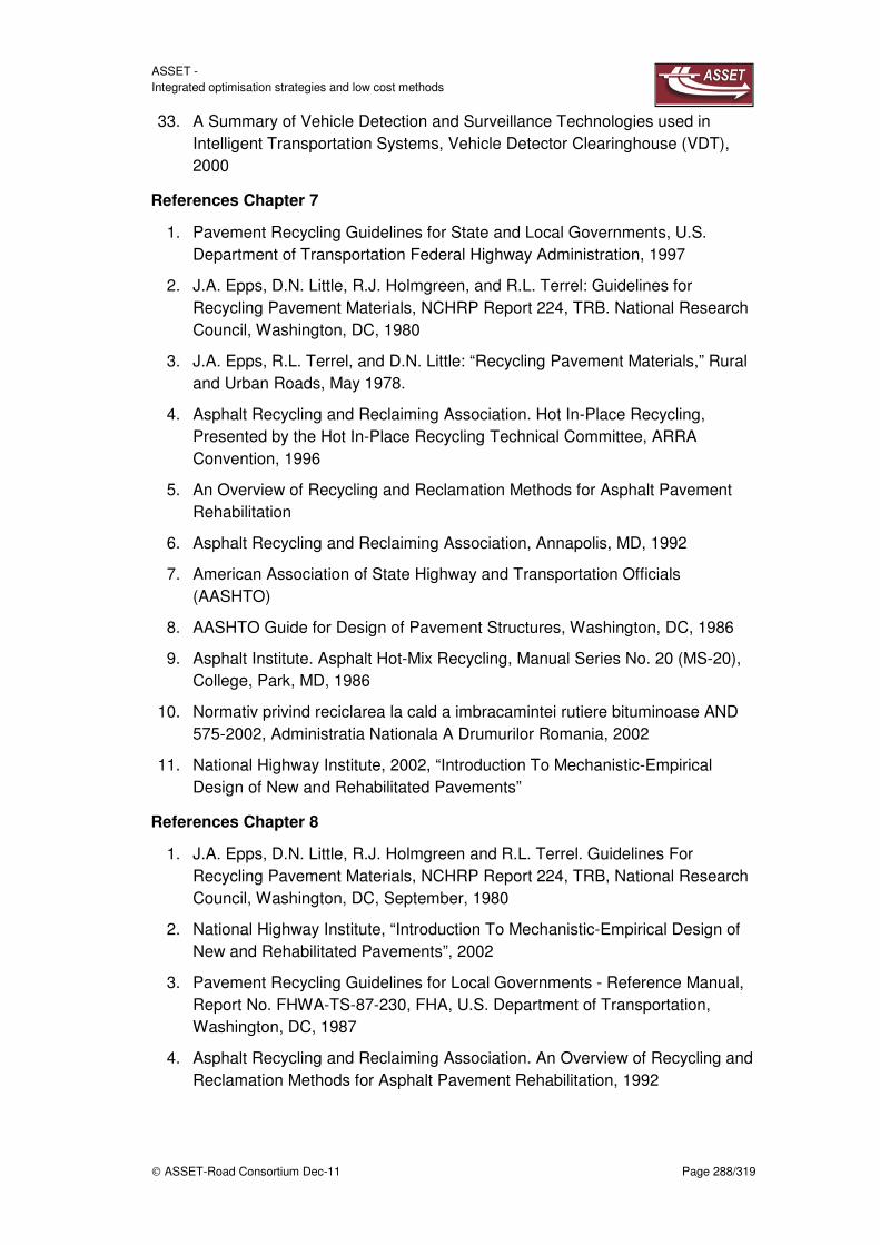
ASSET - Integrated optimisation strategies and low cost methods
ASSET-Road Consortium Dec-11 Page 288/319
33. A Summary of Vehicle Detection and Surveillance Technologies used in Intelligent Transportation Systems, Vehicle Detector Clearinghouse (VDT), 2000
References Chapter 7
1. Pavement Recycling Guidelines for State and Local Governments, U.S. Department of Transportation Federal Highway Administration, 1997
2. J.A. Epps, D.N. Little, R.J. Holmgreen, and R.L. Terrel: Guidelines for Recycling Pavement Materials, NCHRP Report 224, TRB. National Research Council, Washington, DC, 1980
3. J.A. Epps, R.L. Terrel, and D.N. Little: “Recycling Pavement Materials,” Rural and Urban Roads, May 1978.
4. Asphalt Recycling and Reclaiming Association. Hot In-Place Recycling, Presented by the Hot In-Place Recycling Technical Committee, ARRA Convention, 1996
5. An Overview of Recycling and Reclamation Methods for Asphalt Pavement Rehabilitation
6. Asphalt Recycling and Reclaiming Association, Annapolis, MD, 1992
7. American Association of State Highway and Transportation Officials (AASHTO)
8. AASHTO Guide for Design of Pavement Structures, Washington, DC, 1986
9. Asphalt Institute. Asphalt Hot-Mix Recycling, Manual Series No. 20 (MS-20), College, Park, MD, 1986
10. Normativ privind reciclarea la cald a imbracamintei rutiere bituminoase AND 575-2002, Administratia Nationala A Drumurilor Romania, 2002
11. National Highway Institute, 2002, “Introduction To Mechanistic-Empirical Design of New and Rehabilitated Pavements”
References Chapter 8
1. J.A. Epps, D.N. Little, R.J. Holmgreen and R.L. Terrel. Guidelines For Recycling Pavement Materials, NCHRP Report 224, TRB, National Research Council, Washington, DC, September, 1980
2. National Highway Institute, “Introduction To Mechanistic-Empirical Design of New and Rehabilitated Pavements”, 2002
3. Pavement Recycling Guidelines for Local Governments - Reference Manual, Report No. FHWA-TS-87-230, FHA, U.S. Department of Transportation, Washington, DC, 1987
4. Asphalt Recycling and Reclaiming Association. An Overview of Recycling and Reclamation Methods for Asphalt Pavement Rehabilitation, 1992

ASSET - Integrated optimisation strategies and low cost methods
ASSET-Road Consortium Dec-11 Page 289/319
5. Cordell B., Wayman M., asPECT calculator user guide – beta release Part of the asphalt Pavement Embodied Carbon Tool (asPECT), October 2009
6. Wayman M., Schiavi-Mellor I. & Cordell B., Protocol for the calculation of life cycle greenhouse gas emissions generated by asphalt used in highways Part of the asphalt Pavement Embodied Carbon Tool (asPECT), October 2009
References Chapter 9
1. Al-Qadi I.L., Elseifi M., Yoo P.J., Pavement damage due to different tires and vehicle configurations, Final Report, Virginia Tech Univ., Transportation Institute (2004)
2. Barsanescu P.D., A New Approach for Road Pricing System for Heavy Vehicles, Buletinul Institutului Politehnic din Iasi, Constructii de Masini, Ed. Politehnium (in print)
3. Garber J.N., Hoel A.L., Traffic in highway Eng., PWS Pub., 2nd ed. (1999)
4. Lathi P., e.a, Towards sustainable urban infrastructure, COST Action C8, Best Practice in Sustainable Urban Infrastructure, Multiprint Oy, Helsinki, Finland, 6, ISBN 978-92-898-0035-8, pp. 316-327
5. Tsekeris T., Voss S., Design and evaluation of road pricing: state-of-the-art and methodological advances, Netnomics (2009) 10:5–52
6. Equivalent single axle load, http//pavementinteractive.org/index.php?title=ESAL
7. LoadMan Weighing in Built System, United Electronics Inc., Philadelphia, USA

ASSET - Integrated optimisation strategies and low cost methods
ASSET-Road Consortium Dec-11 Page 290/319
Annex 1: WIM sensors and systems
Since pavement damage is a direct function of axle loads, highway engineers always need timely and reliable traffic data, such as truck traffic percentage and axle loads, to design and maintain pavement structures. The collection of large representative samples of traffic load data has become both common and efficient with the advent of weigh-in-motion (WIM) technology. The dynamic loads can be accurately quantified for the planning of bridge or road construction/reconstruction and pavement repairs, and this facilitates planning of the most appropriate reconstruction methods and road or bridge maintenance. WIM systems are the most efficient devices in this respect, both for traffic management and for monitoring purposes. At a moderate operating cost, WIM systems not only measure and store loads and axle spacing for each vehicle that passes through the WIM site, but also record supplementary data such as the date, time, speed, lane of travel, station identification, and vehicle class [2].
Weigh-in-motion (WIM) devices have been developed for weighing trucks with varying axle configurations at highway speeds. WIM sensors are intrusive detectors which are embedded in the pavement or the subgrade. They require cutting into the pavement for installation and maintenance.
The major complaints against these sensors consist of need to close the traffic lanes for their installation and maintenance. However the traffic managers continue to use in-roadway sensors for a number of reasons, including:
Aesthetic considerations;
Integration with axle counting and weigh-in-motion applications requiring sensors under or on the road surface;
Cost and safety issues associated with mounting over-roadway sensors where existing structures are unavailable;
Policies that prohibit over-roadway sensors in certain locations.
Usual WIM sensors
Nowadays there are three basic WIM sensors currently available on the commercial market, representative of most of the WIM technologies in use around the world:
Single load cell;
Bending plate;
Piezo electric.
Usually, the operating temperature ranges for all these WIM devices is from –40°C to +80°C.
This type of traffic data collection devices available on the market has changed little in the past decade.

ASSET - Integrated optimisation strategies and low cost methods
ASSET-Road Consortium Dec-11 Page 291/319
Load cell WIM systems typically consist of two weighing platforms per lane with one or more single load cells per platform. Strain gauge load cells record the strain and calculate dynamic load. Some load cells have two in-line scales, one detects the axle and the other weighs the right and left side of the axle. The load cells add the weights for both sides to obtain the axle weight. Steel frames are commonly installed in the road with concrete and then platforms are placed into the steel frames. The scale platforms are bolted to the scale frames, flush with the road surface. This sensor has the best accuracy but, unfortunately, it is expensive, has a big cross section and requires a concrete foundation.
Bending plate technology is most frequently used for collecting weigh-in-motion data. The device typically consists of a weigh pad attached to a metal frame installed into the travel lane. A vehicle passes over the metal frame causing it to slightly "bend." Strain gauge weighing elements measure the strain on the metal plate induced by the vehicle passing over it. This yields a weight based on wheel/axle loads on each of two scales installed in a lane. The device is also used to obtain classification and speed data.
(a) (b)
Figure 271: Installation of a single load cell sensor frame (a); two single load cell WIM sensors and
one axle sensor (b), [5, 12]
Bending plate technology is most frequently used for collecting weigh-in-motion data. The device typically consists of a weigh pad attached to a metal frame installed into the travel lane. A vehicle passes over the metal frame causing it to slightly "bend." Strain gauge weighing elements measure the strain on the metal plate induced by the vehicle passing over it. This yields a weight based on wheel/axle loads on each of two scales installed in a lane. The device is also used to obtain classification and speed data.
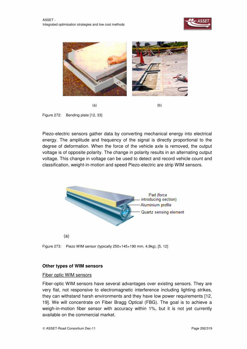
ASSET - Integrated optimisation strategies and low cost methods
ASSET-Road Consortium Dec-11 Page 292/319
(a) (b)
Figure 272: Bending plate [12, 33]
Piezo-electric sensors gather data by converting mechanical energy into electrical energy. The amplitude and frequency of the signal is directly proportional to the degree of deformation. When the force of the vehicle axle is removed, the output voltage is of opposite polarity. The change in polarity results in an alternating output voltage. This change in voltage can be used to detect and record vehicle count and classification, weight-in-motion and speed Piezo-electric are strip WIM sensors.
(a)
Figure 273: Piezo WIM sensor (typically 250×145×190 mm, 4,9kg), [5, 12]
Other types of WIM sensors
Fiber optic WIM sensors
Fiber-optic WIM sensors have several advantages over existing sensors. They are very flat, not responsive to electromagnetic interference including lighting strikes, they can withstand harsh environments and they have low power requirements [12, 19]. We will concentrate on Fiber Bragg Optical (FBG). The goal is to achieve a weigh-in-motion fiber sensor with accuracy within 1%, but it is not yet currently available on the commercial market.

ASSET - Integrated optimisation strategies and low cost methods
ASSET-Road Consortium Dec-11 Page 293/319
(a) (b)
Figure 274: Fiber optic WIM sensor: Sketch of cross section (a) and sensor in road installed (b), [12,
30]
Bridge WIM system
A Bridge Weigh in Motion (B-WIM) system is based on the measurement of the deformation of a bridge and the use of the measurements to estimate the attributes of passing traffic loads [6, 15, 29]. The idea of using a bridge as a scale for the weigh-in-motion (WIM) of trucks was explored by Snyder and Kriss as early as 1972 (Snyder & Kriss, 1972, Kriss, 1979). In this system, strain gauges were installed on the girders below the bridge, and axle sensors were placed at the entrance and exit of the bridge. The system was calibrated using a known truck. Tests of this system showed that it was capable of approximating the gross weights of vehicles to within 6-10%, and individual axle weights to within 13-15% (Kriss, 1979). The B-WIM system uses several strain gauges or optic fiber [19], which can be installed underneath the deck, making installation difficult and costly.
However, the currently available on the market WIM sensors have some deficiencies:
WIM sensors are limited to measuring surface dynamic vertical loads. This is the primary response under dynamic loading that is of significant interest to road structural engineers;
WIM sensors cannot detect the forces in the road plane (produced by acceleration, brake etc.). These forces have also a contribution to pavement deterioration;
WIM systems cannot record the lateral position of each vehicle within the lane of travel. The lateral position of vehicle tires with respect to the edge of the lane is important because it can be used to describe the edge loading for slabs and the rutting pattern on asphalt pavements;

ASSET - Integrated optimisation strategies and low cost methods
ASSET-Road Consortium Dec-11 Page 294/319
WIM sensors cannot record the number of tires (single or dual) at the end of each axle;
WIM sensors cannot record the tire footprint, size and type of tire (balloon etc.). States generally limit the allowable load per mm width of tire. This tire load limitation varies from a maximum of 140 N/mm to a minimum of 79 N/mm;
WIM sensors cannot detect flat tires etc.
New WIM systems
Smart sensors and network sensor systems
Today, agencies often look favourably on eliminating a sawcut or replacing it with some drilled holes. The increased occurrence of deteriorating pavements has produced more interest in installing preformed micro sensors, or pavement slabs with sensors already in place. The same concerns may lead to the selection of above-roadway sensors, if is possible.
Measurement systems of today that have been designed to accommodate large numbers of sensors are very capable systems. They have a variety of features and capabilities that have been developed over the years to satisfy the needs of the test and measurement communities. A typical system can generally be broken down into 4 sections: sensors, analog signal conditioning, analog-to-digital conversion, and digital signal processing & communications. The last two sections are usually referred to as data acquisition.
A variety of different analog sensors may be used including accelerometers, pressure sensors, temperature sensors, strain gauges and others [11]. There as many as four to six wires from each sensor, this will mean a large number of wires for a large number of sensors. Depending on the type of sensor, analog signal conditioners will perform the necessary conditioning of the sensor signal which might include charge conversion for piezoelectric, bridge completion for strain gauges, filtering, gain adjustment and other functions.
Matrix network WIM sensor systems
In order to have a more realistic image of the pavement state of stress and its
damage, we must know the real contact pressure between tire and road.
Unfortunately, commercial WIM sensors cannot provide this information. For this
purpose, a new category of network sensors has been developed. They are called
“Stress-in-motion” sensors (SIM).
Having a network of small sensors instead of a single load cell for one WIM sensor (as is presented in seems to be an interesting solution.
A network of small sensors would have the following advantages:
A smaller sensor thickness, which will need shallower sawcut in the road for installation;

ASSET - Integrated optimisation strategies and low cost methods
ASSET-Road Consortium Dec-11 Page 295/319
A smaller sensor’s cross section, which will require a smaller sawcut;
Less expensive installation costs, since it is proportional with sensor’s cross section;
For a network with enough small sensors, important additional information could be obtained, with an acceptable accuracy: dimensions of tire/road contact area, flat tire detection, number of tires (single or dual) at the end of each axle, lateral position of vehicle tires with respect to the edge of the lane etc.;
One or more small sensors can fail, without affecting too much the global WIM sensor performance;
Combinations of the different sensors in the same network are possible (load cells, pressure, temperature, accelerometers) if this is necessary;
Small sensors are usually cheap (mass production) etc.
On the other hand, a network with a large number of sensors has also some important disadvantages:
Handling a lot of wires and connections;
Much more complex electronic system;
Huge volume of data acquisition etc.
The determination of the tire footprint dimensions using matrix network sensors is presented (top view). Knowing the distance between sensors (network pitch), the loaded (with output) and unloaded (without output) matrix’s sensors, one can appreciate the tire footprint dimensions. Similarly, one can determinate the number of tires (single or dual), lateral position of the vehicle tires with respect to the lane edge and one can detect flat tires.
For a network of WIM sensors we need small and cheap load cells, having a good accuracy and reliability. In Figure a flat load cell is presented. It consists of two conical springs (spread on the market), welded together on the contour of the biggest circle, with an elastic strip in the middle. The central strip is instrumented with electrical strain gauges [3].

ASSET - Integrated optimisation strategies and low cost methods
ASSET-Road Consortium Dec-11 Page 296/319
Figure 275: Determination of tire footprint dimensions using matrix network sensors (top view)
(a) (b)
Figure 276: Load cell (cross section and axonometric view): Conic springs (1, 2); elastic strip (3);
strain gauges (5, 6); weld (4), [3]
Force measurement on three axes
The below figures illustrate a proposal for a WIM system able to measure the tire/road contact forces on three axes. The system consists of a box with a network placed on hollow bolts with strain gages. The box is filled with silicon rubber up to the top. The rubber includes sensors (sensitive bolts), wires and some electronic systems. The system can measure not only the vertical load (tire/axle load) but also the two forces in the road plane (produced by acceleration, breaking, etc.). Strain gauges from SG1 to SG4 and SG5 to SG8 are mounted in two full bridges which are able to determinate Fz and Fy forces, respectively. The output of one bridge depends on force magnitude (Fz or Fy), b distance between strain gages, bolt cross section and material [3].
11
223344
4455
66
11
33
55
44

ASSET - Integrated optimisation strategies
ASSET-Road Consortium Dec
Figure 277: WIM system with sensitive bolts [3]: basic plate (1); box (2); sensitive bolt (3)
Figure 278: Sensitive bolt with strain gauges: SG = strain gauge, TR = “T” rosette [3]
SIM system with sensitive pins
In this figure a WIM system able to measure the vertical, transverse and longitudinal interface stress under a moving wheel load is presented. This technology, named Stressinputs into pavement design for optimizing theSIM systems have been developed in laboratories since the early 1990s. It has been tested in vehicle monitoring stations in South Africa. The system has many pins mounted in a network on a plate. Only the central row instrumented with strain gauges (sensitive pins). The other pins, without strain gauges, have only a supporting
trategies and low cost methods
Dec-11
WIM system with sensitive bolts [3]: basic plate (1); box (2); sensitive bolt (3)
Sensitive bolt with strain gauges: SG = strain gauge, TR = “T” rosette [3]
SIM system with sensitive pins
a WIM system able to measure the vertical, transverse and longitudinal interface stress under a moving wheel load is presented. This technology, named Stress-in Motion (SIM) provides some of the most important inputs into pavement design for optimizing the cost of roads over their design life. SIM systems have been developed in laboratories since the early 1990s. It has been tested in vehicle monitoring stations in South Africa. The system has many pins mounted in a network on a plate. Only the central row instrumented with strain gauges (sensitive pins). The other pins, without strain gauges, have only a supporting role [26, 27, 28, 32].
Page 297/319
WIM system with sensitive bolts [3]: basic plate (1); box (2); sensitive bolt (3)
Sensitive bolt with strain gauges: SG = strain gauge, TR = “T” rosette [3]
a WIM system able to measure the vertical, transverse and longitudinal interface stress under a moving wheel load is presented. This
in Motion (SIM) provides some of the most important cost of roads over their design life.
SIM systems have been developed in laboratories since the early 1990s. It has been tested in vehicle monitoring stations in South Africa. The system has many pins mounted in a network on a plate. Only the central row of 20 pins is instrumented with strain gauges (sensitive pins). The other pins, without strain

ASSET - Integrated optimisation strategies and low cost methods
ASSET-Road Consortium Dec-11 Page 298/319
(a)
(b)
(c)
Figure 279: SIM system: top view of plate with pins (a); tire loading the system (b); vertical contact
stress, σzz, distributions (c); (Goodyear radial tire 11R22.5; inflation pressure 720kPa;
vertical load 41kN), [26-28]

ASSET - Integrated optimisation strategies and low cost methods
ASSET-Road Consortium Dec-11 Page 299/319
10.1.1 Weighing-in-built system (WIBS)
Spinning Wheel Integrated Force Transducer (SWIFT)
The SWIFT sensor has independent strain gauge bridges which measure forces and moments about three orthogonal axes. The new telemetry systems offer data acquisition without requiring slip rings and anti-rotate devices. This makes it especially useful for road tests in traffic. On the market there are SWIFT systems for testing and data acquisition on medium and heavy trucks and other large vehicles.
Various wheel measuring rims are available on the market to gather data on wheel load distribution and fluctuation and tire contact and cornering forces, or to measure irregularities in the field of tire development.
These wheel force dynamometers can be used on test vehicles, servo-hydraulic simulators and roller test stands. These efficient tools are required to measure the data serving as the basis for simulations and for the design of vehicle bodies, chassis, drive trains and tires. Although the system could be adapted as a WIM system used on heavy trucks (with a sensor on which wheel and telemetry system), is difficult to see, in the near future, a commercial application in this field for it.
(a) (b)
Figure 280: Spinning Wheel Integrated Force Transducer (SWIFT) and telemetry system [25]
WIBS for multi-axle vehicle
On the market there are also other weighing-in-built systems (WIBS), more practical for WIM applications. They may be installed on existing multi-axle vehicles without any cutting, welding, and/or modifying original trailer parts, which potentially weaken the trailer structure. Usually, one-day for WIBS system installation and

ASSET - Integrated optimisation strategies and low cost methods
ASSET-Road Consortium Dec-11 Page 300/319
calibration on a heavy truck is necessary. As soon as the load hits the pit of the vehicle, WIBS gets activated and starts measuring the payload.
The main components functions of this WIBS are illustrated below. The pressure sensor converts the load pressure into an electrical signal ready to be carried away for further manipulation. The load coder takes this signal, digitizes it and feeds it in a central location. The cabin display is the location where the entire axle-group readings are being added. Depending on the requirement, the cabin display reads out gross weight, net weight or even per axle load.
Figure 281: Weighing In-Built System (WIBS) for multi-axle vehicles [31]
(a) (b)
Figure 282: Sensors installation for WIBS [31]
The computerized data collection system using WIBS provides valuable information in real time on the performance of the vehicles and their operations. The data collection system enables retrieval and storage information on customers, job site data, and product codes for material data, wheel loader reports, driver reports, individual weights and total weights. WIBS collects data for customer reports, driver reports, time between customer pickups, vehicle reports, container reports, product codes in the case of recycling and exception reports. WIBS provide the best solution for the loading of trucks efficiently on-site no matter where the job site is.

ASSET - Integrated optimisation strategies and low cost methods
ASSET-Road Consortium Dec-11 Page 301/319
Pavement protection
Heavy truck loads can damage road and highway pavements, especially in spring time, when they are weakened because the soil and subgrade are saturated with water, and in summer time, when asphalt behaves visco-elastic at elevated temperatures.
Some road authorities undertake temporary protective measures especially during spring time like thaw-freezing barriers in France or similar measures such as:
Temporarily declaring vulnerable some highways and roadways;
Regulating the maximum allowable weight to be carried on certain roads, during the spring thaw period;
Requiring heavy traffic to run at night or in the early morning during spring thaw period (when roads may be stronger due to overnight freezing) or during the summer’s hottest periods, but must be careful not to overuse the approach etc.
According to literature, to be effective, truck weights should be reduced between late February and early May by at least 20%, while a reduction over 60% may have little added benefit. In U.S.A., national average reduction is 44% [23]
According FHWA, USA, the effects of load reduction during spring thaw [23] is:
Load reduction Increase in pavement life
20% 62%
30% 78%
40% 88%
50% 90%
In addition to restricting load limits, there may be also other ways of protecting pavements such as route modification, reduction of travel distance and physical changes leading to elimination of standing water in roadside ditches and the filling in of pavement surface cracks to reduce the amount of water getting to the freezing zone etc.
The local authority can impose weight limits on a highway or bridge that they believe will be damaged because of roadbed weaknesses or other special conditions, using proper temporary signs or warning panels which can be changed by remote control by operators from the traffic monitoring centers.
Effective communication with the public is also essential. Mass-media must be alerted when weight restrictions are imminent. Industries which make local deliveries or local supply services must be called and informed about these limits and the period when they will be applied. Local officials may make exceptions, but are not required to.

ASSET - Integrated optimisation strategies and low cost methods
ASSET-Road Consortium Dec-11 Page 302/319
In establishing weight restrictions, the authorities must carefully balance the public interest in protecting roads against maintaining commerce and an efficient transportation system.

ASSET - Integrated optimisation strategies and low cost methods
ASSET-Road Consortium Dec-11 Page 303/319
List of Figures
Figure 1: Example of the new pavement sensor 10
Figure 2: ROC matching system of pavement and weigh-in-motion sensors 11
Figure 3: Holistic approach of cyclic pavement management 15
Figure 4: Realistic pavement modelling 16
Figure 5: Principle of fatigue cracking and permanent deformation (Source: BAST) 19
Figure 6: Example of a pavement sensor 19
Figure 7: Some of different kind of pavements (Source: BAST) 20
Figure 8: Chosen pavement construction for further analysis ((left: primary roads, right: secondary roads) 21
Figure 9: Calculation model of road structures and lanes and possible sensor placements 21
Figure 10: Example of pothole 22
Figure 11: Example of fatigue cracks 23
Figure 12: Example of blowout 23
Figure 13: Example of reflection cracks 24
Figure 14: Example of sinkholes 25
Figure 15: Example of block cracks 25
Figure 16: Example of rutting 26
Figure 17: Example of ravelling 26
Figure 18: Example of slippage cracks 27
Figure 19: Example of shoving and corrugation 27
Figure 20: Example of seam cracks 28
Figure 21: Example of peeling 28
Figure 22: Example of root cracks 29
Figure 23: Example of bleeding 29
Figure 24: Measurement relevant matrix 30
Figure 25: Example of damaged pavement 30
Figure 26: Complete pavement/traffic parameters & monitoring 32
Figure 27: Overall system architecture of “Integrated Pavement Monitoring System” 33

ASSET - Integrated optimisation strategies and low cost methods
ASSET-Road Consortium Dec-11 Page 304/319
Figure 28: Example of complete load on pavement 34
Figure 29: Rolling resistance (Source: Michelin) 35
Figure 30: Rolling resistance distribution (Source: Michelin) 35
Figure 31: Tire forces: static, dynamic horizontal and vertical forces and torques 36
Figure 32: Example of climb up and acceleration or brake 36
Figure 33: Stress distributions in pavement sub-structures under two different tyres 38
Figure 34: Tire and force/torque inputs to pavements (Source: Pirelli) 39
Figure 35: Example of 3D force load on a road by a tire 40
Figure 36: DMD and DMS from BASt 41
Figure 37: Measuring gauges inside the pavement structure (Source: BASt)) 42
Figure 38: Measuring longitudinal strain with high stress situation (Source: BASt) 43
Figure 39: Measuring vertical strain with high stress situation (Source: BASt) 43
Figure 40: Longitudinal strain versus static wheel load (Source: BASt) 44
Figure 41: Vertical strain versus static wheel load (Source: BASt) 44
Figure 42: Longitudinal asphalt strain versus vehicle speed for each section (Source: BASt) 45
Figure 43: Vertical asphalt strain versus vehicle speed for each section (Source: BASt) 45
Figure 44: Model 3500 earth pressure cell Installed under railroad tracks 46
Figure 45: Model 3500: Features 47
Figure 46: Model Kulite 0234 48
Figure 47: CTL Kulite 0234 properties 48
Figure 48: CTL Kulite 0234 48
Figure 49: Geokon 3500 49
Figure 50: Geokon 3500 49
Figure 51: Kulite LQ-080U 50
Figure 52: CTL ASG-152 properties 50
Figure 53: CTL ASG-152 51

ASSET - Integrated optimisation strategies and low cost methods
ASSET-Road Consortium Dec-11 Page 305/319
Figure 54: CTL AVSG properties 51
Figure 55: CTL AVSG 51
Figure 56: CTL CSG properties 52
Figure 57: CTL Inc. CSG 52
Figure 58: Geokon Model 3900 properties 53
Figure 59: The Model 3900 embedment strain gauge 53
Figure 60: BASt strain sensor 54
Figure 61: CTL SCG 54
Figure 62: CTL asphalt strain gauges 55
Figure 63: CTL asphalt strain gauges 55
Figure 64: CTL Groups concrete strain gauges 55
Figure 65: CTL Groups concrete strain gauges 56
Figure 66: Properties measuring dowel bars from CTL 56
Figure 67: CTL measuring dowel rods 57
Figure 68: KM-100HAS specifically for embedding in road paving developed from asphalt 57
Figure 69: KM-100HAS 58
Figure 70: Japanese KM-100HAS 59
Figure 71: KM-100HAS properties 59
Figure 72: KM-100HAS features 60
Figure 73: BASt + HBM strain transducer 60
Figure 74: MM EA- 06-10CBE-120 61
Figure 75: KYOWA KM-120-120-H2-11 W1M3 61
Figure 76: Details for LAVOC strain gauges 62
Figure 77: Strain gauge sensor of LCPC 62
Figure 78: Strain gauge from LAVL University 63
Figure 79: CTL asphalt strain gauge 63
Figure 80: CTL Asphalt strain gauge 64
Figure 81: CTL Snap MMD properties 64
Figure 82: SnapMulti-Depth DeflectometerTM 65
Figure 83: Instrumented dowel bars 65
Figure 84: Psychrometers 66
Figure 85: Gypsum Blocks 66

ASSET - Integrated optimisation strategies and low cost methods
ASSET-Road Consortium Dec-11 Page 306/319
Figure 86: Time-domain reflectometers – TDRs 67
Figure 87: Percometers 69
Figure 88: Tyco SIT-E6 70
Figure 89: Tyco Thermal Controls SIT-E6 70
Figure 90: Tyco Thermal Controls GIT-1 71
Figure 91: Lufft properties 72
Figure 92: Lufft IRS21 73
Figure 93: FP 2000 73
Figure 94: Key specifications 74
Figure 95: QQT Wireless WxT properties 75
Figure 96: QQT Wireless WxT 75
Figure 97: QQT Thermo SCAN properties 76
Figure 98: Thermo SCAN 76
Figure 99: QQT sub-surface properties 77
Figure 100: Load distributions in layer 79
Figure 101: Simulation of tyre force and footprint 80
Figure 102: Impacts on pavement structure and stress trends 80
Figure 103: Chosen pavement construction for structure analysis (left: primary, right: secondary roads) 81
Figure 104: Sensor distribution (Japanese version literature taken) 83
Figure 105: Pavement sensor distribution 84
Figure 106: Road characterization and coordinates used 85
Figure 107: Road characterization and dimensions 85
Figure 108: Road frontal dimensions 86
Figure 109: Road characterization for thin and thick structure. 86
Figure 110: Road section and sensor position 86
Figure 111: Sensor position for wheel path 87
Figure 112: Sensor position for centreline (colours = layer 1,2 and 3) 88
Figure 113: Table of sensor coordinates for primary structure and wheel path 88
Figure 114: Table of sensor coordinates for secondary structure and centerline 89
Figure 115: Table of sensor coordinates for secondary structure and wheel path 89

ASSET - Integrated optimisation strategies and low cost methods
ASSET-Road Consortium Dec-11 Page 307/319
Figure 116: Table of sensor coordinates for secondary structure and centreline 90
Figure 117: Trend values for a thin structure 91
Figure 118: Thin analysis results for a thick thin pavement-summer time-wheel path 92
Figure 119: Thin analysis results for a thick thin pavement-winter time-wheel path 93
Figure 120: Trend values for a thick structure 94
Figure 121: Thick analysis results for a thick thin pavement-summer time-wheel path 95
Figure 122: Thick analysis results for a thick thin pavement-winter time-wheel path 96
Figure 123: E modulus as a function of temperature at different frequencies (Hürtgen 1982) 97
Figure 124: E modulus at f=10Hz as a function of temperature (Hürtgen 1982) 98
Figure 125: Table for main roads features in different seasons 98
Figure 126: Table for secondary roads features in different seasons 99
Figure 127: Table of horizontal stresses 99
Figure 128: Table of vertical stresses 100
Figure 129: Simplify table of horizontal stresses (layer 1 and 2: [-0,55; 0,5] vertical range, layer3: [-0,001; 0] horizontal range 100
Figure 130: Simplified table of vertical stresses (layer 1 and 2: [-0,15; 0] Mpa vertical range; layer3: [-0,001; 0] Mpa horizontal range 100
Figure 131: Strain values 101
Figure 132: Stress distribution 102
Figure 133: Averaged E modulus for different temperature cases with the frequency f = 10 Hz 103
Figure 134: Averaged E modulus chosen for different season and different layer with the frequency f = 10 Hz 103
Figure 135: Pavement sensor concept 106
Figure 136: Concept 1 (Ø=100 mm, h=60 mm / 160 mm) and Concept 2 109
Figure 137: Concept 3 (double-leg version vertical) 109
Figure 138: Concept 4 (double-leg version vertical, height reduced to 29mm): FINAL 109

ASSET - Integrated optimisation strategies and low cost methods
ASSET-Road Consortium Dec-11 Page 308/319
Figure 139: First conception and encumbrance 110
Figure 140: Simulation for sensor house 110
Figure 141: Second version 111
Figure 142: Third version 111
Figure 143: Fourth version 112
Figure 144: Fifth version, isometric view 112
Figure 145: Draft electronic design 113
Figure 146: Sensor house used for simulation 114
Figure 147: Sensor house under load simulation 114
Figure 148: Parameters 115
Figure 149: Load vs height for a constant displacement 115
Figure 150: Vertical displacement vs height 116
Figure 151: Vertical displacement vs length 116
Figure 152: Table for thickness variable 117
Figure 153: Table for a mixed thickness 117
Figure 154: Displacement simulation 118
Figure 155: Stress simulation through Von Mises theory 118
Figure 156: Sensor placement 119
Figure 157: System architecture 119
Figure 158: Pavement sensor microcontroller 120
Figure 159: Pavement sensor interaction simulation (I) 121
Figure 160: Sensor body embedding simulation 121
Figure 161: The proposed ROC WIM matrix 122
Figure 162: Ramped cyclic loading (a), sinusoidal cyclic loading (b) 126
Figure 163: Schematic of the UCD GDSTTS system (GDS, 2002) 127
Figure 164: Preparation of samples for triaxial tests (Tolooiyan, 2010) 128
Figure 165: Determination of the yield stress of Blessington sand 129
Figure 166: Effect of shearing rate on stiffness of Blessington sand 129
Figure 167: Plate load tests performed to investigate the effect of creep on Blessington sand 130
Figure 168: Effect of deviator stress on creep of Blessington sand 131
Figure 169: Relationship between creep coefficient and deviatoric stress level 132

ASSET - Integrated optimisation strategies and low cost methods
ASSET-Road Consortium Dec-11 Page 309/319
Figure 170: Comparison of predicted and measured creep strain of Blessington sand 133
Figure 171: Effect of loading history on creep strain developed by Blessington Sand 134
Figure 172: Comparison between measured and predicted response of Blessington sand to cyclic sinusoidal loading 136
Figure 173: Comparison between measured and predicted response of Blessington sand to cyclic ramped loading 137
Figure 174: Stress and strain measured during the first two load cycles during the ramped loading experiment with a period of 120 seconds 138
Figure 175: Comparison of original and extended Diyaljee and Raymond model predictions 140
Figure 176: Bridge structural damping estimates from noisy accelerations with SNR = 20 for bridge spans of (a) 15 m (b) 25 m (c) 35m and (d) 40m. Vehicle velocity ranges from 10 m/s to 30 m/s. 142
Figure 177: (a) Experimental beam (b) Experimental vehicle 143
Figure 178: Degree-of-freedom half-car model 146
Figure 179: Half-car model properties 146
Figure 180: Finite Element Beam model 147
Figure 181: Finite Element Beam properties 148
Figure 182: Comparison of actual and calculated total wheel contact force, Ri, for a 15 m bridge. Vehicle velocity is 10 m/s. 149
Figure 183: Comparison of actual and calculated total displacements, wvi, under each wheel for a 15 m bridge. Vehicle velocity is 10 m/s. 150
Figure 184: Bridge structural damping estimates for bridge spans of (a) 15 m (b) 25 m (c) 35m and (d) 40m. Vehicle velocity ranges from 10 m/s to 30 m/s. 151
Figure 185: Bridge structural damping estimates from noisy accelerations with SNR = 20 for bridge spans of (a) 15 m (b) 25 m (c) 35m and (d) 40m. Vehicle velocity ranges from 10 m/s to 30 m/s. 152
Figure 186: (a) Experimental beam (b) Experimental vehicle 153
Figure 187: Vehicle properties 154
Figure 188: Beam properties (See Figure 7) 154
Figure 189: Locations of dampers and additional mass 154

ASSET - Integrated optimisation strategies and low cost methods
ASSET-Road Consortium Dec-11 Page 310/319
Figure 190: Fourier spectra of acceleration response of (a) Beam midspan and (b) V1 axles for velocity 0.93m/s 155
Figure 191: Fourier spectra of acceleration response of (a) Beam midspan and (b) V1 axles for velocity 1.63m/s 155
Figure 192: Spectra of mean acceleration responses of (a) Beam midspan and (b) Axle 1 of V1 for velocity 0.93m/s 156
Figure 193: Sketch of a beam discretized model subject to a moving force 159
Figure 194: Mid-span displacement of a beam subject to a moving force when there is a delta=0.5 crack at the 1/3 point of the span 159
Figure 195: Wavelet transform of signal shown in Figure 2 plotted in 2D, the absolute value of the wavelet coefficients are represented using colour, lighter colour indicates higher value. 161
Figure 196: Identifying the damage location for different levels of damage 161
Figure 197: Identifying damage when displacement is recorded at four locations 161
Figure 198: Corrupted mid-span acceleration signal of healthy and damaged bridges 163
Figure 199: Wavelet transform of the mid-span acceleration signal when the bridge has a crack at the 1/3 point of the span 163
Figure 200: Coefficient line plot of acceleration signal with a delta=0.3 crack at the one third point 164
Figure 201 : Coefficient line plot of acceleration signal with a delta=0.1 crack at the one third point 164
Figure 202: Vertical sections through wavelet transform surface: (a) Wavelet transform surface when delta = 0.2 at the 1/3 point, (b) Absolute value of wavelet coefficients for vertical sections at different positions of the moving load, (c) Absolute value of wavelet at different positions of the moving load for scale range between 500 and 1200. 165
Figure 203: Average relative energy when acceleration simulated at 3 locations simultaneously for different damage levels 166
Figure 204: Mid-span acceleration signal with road profile on bridge including 3% noise 167
Figure 205: Wavelet transform of signal shown in Figure 12 for scales between 1 and 1500 167

ASSET - Integrated optimisation strategies and low cost methods
ASSET-Road Consortium Dec-11 Page 311/319
Figure 206: Damage detection when bridge loaded with vehicle model for various damage levels at different locations (class ‘A’ road profile, speed = 3 m/s, 3% noise) 169
Figure 207: Total response signals and their component parts 170
Figure 208: Magnified view of static and damaged parts of the acceleration signal 171
Figure 209: Acceleration signals from healthy and damaged bridge smoothed using moving average filter 172
Figure 210: Integrated concept: WIM and bridge load sensing 173
Figure 211: Axle detection 177
Figure 212: Section through beam and slab bridge 179
Figure213: Axle detecting strain transducers (courtesy ZAG Slovenia) 179
Figure 214: Axle detecting strain transducers (courtesy ZAG Slovenia) 180
Figure 215: ROC shear strain sensor 181
Figure 216: ROC shear strain sensor, adaptation and first electronic 181
Figure 217: Dimensions of bridge Finite Element model 182
Figure 218: Bridge loading and supports 182
Figure 219: Shear stresses 183
Figure 220: Vertical shear stress distributions on X-face 184
Figure 221: Interface shear stress distributions on X-face 184
Figure 222: Recommended sensor location 185
Figure 223: Customisable GUI snapshot 188
Figure 224: Customisable GUI snapshot 188
Figure 225: GUI configuration file 189
Figure 226: Example of customisable framework 190
Figure 227: Comparison of fleet normalised aggregate force histories for each of the four simulated vehicle fleets 195
Figure 228: Energy balance 196
Figure 229: Evolution of Fenv with time 197
Figure 230: Back-calculated stiffness moduli against temperature 198
Figure 231 and Figure 232: Linear and non-linear behaviour of UGMs 200
Figure 233 Road profile, dynamic loads and permanent deformations 204
Figure 234: Behaviours of asphalt mixtures 206

ASSET - Integrated optimisation strategies and low cost methods
ASSET-Road Consortium Dec-11 Page 312/319
Figure 235: Mechanism of fatigue cracking 207
Figure 236: Typical fatigue test results 207
Figure 237: Mixture fatigue line 208
Figure 238: Evolution of road profile 211
Figure 239 and Figure 240: Incremental deformation of the layers 212
Figure 241: Cumulative fatigue damage 213
Figure 242: Milling-up the existing granular layers after removal of the surface asphalt layers and middling by in-place the same material with specific additives 218
Figure 243: Compaction of the TERRA SYSTEM layer 218
Figure 244: Comparison between classical/recycled granular layers and TERRA SYSTEM layer 219
Figure 245: Comparison between classical/recycled granular layers and TERRA SYSTEM layer including the thicknesses of the asphalt base layers plus the wearing layers 219
Figure 246: Plot of pavement condition versus time 220
Figure 247: Hot mix asphalt recycling [1] 220
Figure 248: Hot in-place recycling [1] 221
Figure 249: Cold in-place recycling [1] 221
Figure 250: Flow chart for AASHTO design method [7]. 226
Figure 251: Typical framework for mechanistic-empirical (M-E) overlay design 228
Figure 252: Summary of the typical performance criteria used for overlay design 229
Figure 253: Evaluation of PSI for a road pavement in time 235
Figure 254: Environmental impact assessment for alternative PA 1 239
Figure 255: Environmental impact assessment for alternative PA 240
Figure 256: Standard axle load F 245
Figure 257: Tire/road contact area depends on inflation pressure 247
Figure 258: Contact area between tire and road is elliptical one (a); typical normal load distribution along the footprint (b), [18, 20] 247
Figure 259: Road pricing dependencies 248
Figure 260: Holistic approach of cyclic pavement management 263
Figure 261: WIM and pavement sensing implications on life cycle 264

ASSET - Integrated optimisation strategies and low cost methods
ASSET-Road Consortium Dec-11 Page 313/319
Figure 262: Cybernetic control by ongoing planning data verification 267
Figure 263: Innovations and implications of a new WIM technology 268
Figure 264: Deterioration model optimisation cycles 269
Figure 265 WIM technology enhancement and “ Intelligent roads” 270
Figure 266: Implications of new WIM technology for pavement management 271
Figure 267: Holistic road and bridge management 272
Figure 268: WIM technology for overload detection and identification 273
Figure 269: Correlation of WIM and pavement system data 274
Figure 270: A modified weighing-in-built system WIBS 276
Figure 271: Installation of a single load cell sensor frame (a); two single load cell WIM sensors and one axle sensor (b), [5, 12] 291
Figure 272: Bending plate [12, 33] 292
Figure 273: Piezo WIM sensor (typically 250×145×190 mm, 4,9kg), [5, 12] 292
Figure 274: Fiber optic WIM sensor: Sketch of cross section (a) and sensor in road installed (b), [12, 30] 293
Figure 275: Determination of tire footprint dimensions using matrix network sensors (top view) 296
Figure 276: Load cell (cross section and axonometric view): Conic springs (1, 2); elastic strip (3); strain gauges (5, 6); weld (4), [3] 296
Figure 277: WIM system with sensitive bolts [3]: basic plate (1); box (2); sensitive bolt (3) 297
Figure 278: Sensitive bolt with strain gauges: SG = strain gauge, TR = “T” rosette [3] 297
Figure 279: SIM system: top view of plate with pins (a); tire loading the system (b); vertical contact stress, σzz, distributions (c); (Goodyear radial tire 11R22.5; inflation pressure 720kPa; vertical load 41kN), [26-28] 298
Figure 280: Spinning Wheel Integrated Force Transducer (SWIFT) and telemetry system [25] 299
Figure 281: Weighing In-Built System (WIBS) for multi-axle vehicles [31] 300
Figure 282: Sensors installation for WIBS [31] 300

ASSET - Integrated optimisation strategies and low cost methods
ASSET-Road Consortium Dec-11 Page 314/319
Glossary
In the following there is a list of main acronyms and abbreviations used in this ASSET-Road report.
ARC African Road Control
ABDS Autobahndirektion Südbayern
ABS Automatic Braking System
ACC Adaptive Cruise Control
ADA Advanced Driving Assistance
ADAS Advanced Driving Assistance Systems
APDL ANSYS Parametric Design Language
ASSET-Road Advanced Safety & Driver Support for Essential Road Transport
AVC Automatic Vehicle Counting and Classification
AVG Automated Vehicle Guidance
BAB Bundesautobahn (Germany)
BAG Bundesamt für Güterverkehr (Germany)
BASt Bundesanstalt für Strassenwesen (German Federal Highway Research Institute)
CALM Communication on Air Interface, Long and Medium range
CAN Control Area Bus
CAPM Communauté d’Agglomération du Pays de Montbéliard
CCD Charge-Couple Device
CCTV Closed-Circuit Television
CG25 Conseil régional
CG90 Conseil général

ASSET - Integrated optimisation strategies and low cost methods
ASSET-Road Consortium Dec-11 Page 315/319
CMOS Complementary Metal Oxide Semiconductor
CN Cellular Networks
COST European Cooperation in the field of Scientific and Technical research
DEKRA Deutscher Kraftfahrzeug Überwachungs-Verein (German institution for monitoring the operational reliability of systems)
DMS Driver Monitoring System
DSRC Dedicated Short Range Communication
DTV Daily Traffic Volume
DWS Driver Warning System
EC European Commission
ETC Electronic Toll Collection
EU European Union
FCD Floating Car Data
FEM Finite Elements Method
Flash-OFDM Fast Low-latency Access with Seamless Handoff Orthogonal Frequency Division Multiplexing
FMS Friction Monitoring System
FOC Fibre Optic Cable
FPGA Field Programmable Gate Array
GIS Geographical Information System
GNSS Global Navigation Satellite System
GPRS General Packet Radio Service
GPS Global Positioning System
GPSIB General Positioning System Interface Bus (special module for cRIO mobile module)

ASSET - Integrated optimisation strategies and low cost methods
ASSET-Road Consortium Dec-11 Page 316/319
GSM Global System for Mobile telecommunications
HGV Heavy Goods Vehicle
HIL Hardware-In-the-Loop
HMI Human-Machine Interaction (not Interface!)
HS-WIM High Speed Weigh In Motion
HVI Human-Vehicle Interface
IAS Integrated ADAS System
ICT Information and Communications Technology
ID Identification
IEG European Institute of Geoposition
IP67 International Protection rating for electrical enclosures (6 = dust tight, 7 = protected against ingress of water up to a submersion of 1 m)
IR Infra-Red
IRI International Roughness Index
IRIG-B Inter Range Instrumentation Group (whereby B = time code format name)
ISA Intelligent Speed Adaptation
ITI Intelligent Transportation Infrastructure
ITS Intelligent Transport System
IVT In-Vehicle Terminal
LabVIEW Laboratory Virtual Instrumentation Engineering Workbench
LED Light-Emitting Diode
LISA Life In vehicle Smart Assistant
LPR License plate reader

ASSET - Integrated optimisation strategies and low cost methods
ASSET-Road Consortium Dec-11 Page 317/319
LS WIM Low Speed Weigh In Motion
MHÜ Manfred Hügel Thermal Imaging
MOID Ministry of Infrastructure Development
MPD Mean Profile Depth
MS-WIM Multiple Sensor Weigh-in-Motion
M2M Mobile IP communication
OBU On-Board Unit
OIML International Organization of legal Metrology
OWL-S Semantic Markup for Web Services
PAD Passive Acoustic Detector
PAL Phase Alternation Line
PC Personal computer
PDA Personal Digital Assistant
PMS Pavement Management System
PWC Parking place with WC (Toilette)
RCP Rapid Control Prototyping
RDS Radio Data Systems
RFID Radio Frequency Identification
ROC Rigobert Opitz Consult
RSU Road side unit
RWIS Road Weather Information System
R&D Research and Development
SFM Single fibre mode
SFS Shear force sensor

ASSET - Integrated optimisation strategies and low cost methods
ASSET-Road Consortium Dec-11 Page 318/319
SKA Modular shear force transducers
SME Small or Medium Seized enterprise
SMS Short message service
SMTD Sensor Measured Texture Depth
SOA Service oriented architecture
SOAP Simple Object Access Protocol
TCC Traffic Control Centre
TCP Transmission Control Protocol
TERN Trans-European Road Network
TMC Traffic Message Channel
TÜV Technischer Überwachungsverein (Germany)
T&T Tracking & Tracing
UBM Université de Technologie de Belfort-Montbéliard
UDDI Universal Description, Discovery and Integration
UML Unified Markup Language
UMTS Universal Mobile Telecommunication System
UTC Universal Time Coordinated
VID Vehicle Identification
VMS Variable Message Sign
VPN Virtual Private Network
VTT Valtion teknillinen tutkimuskeskus (Technical Research Centre of Finland)
V2I Vehicle to Infrastructure Communication
V2V Vehicle to Vehicle Communication

ASSET - Integrated optimisation strategies and low cost methods
ASSET-Road Consortium Dec-11 Page 319/319
WAN Wide Area Network
WAVE Wireless Access for Vehicular Environment
WIM Weigh-in-Motion
WLAN Wireless Local Area Network
WP Work package
XML Extensible Markup Language
3D Three dimensional