Deliverable D4.2-3 - wiser.eu
163
Deliverable D4.2-3: coastal macroflora indicators Collaborative Project (large-scale integrating project) Grant Agreement 226273 Theme 6: Environment (including Climate Change) Duration: March 1 st , 2009 – February 29 th , 2012 Deliverable D4.2-3: Report/manuscript on benthic macroflora indicators for coastal waters, including classification boundaries, definition of reference conditions and uncertainty Lead contractor: Agencia Estatal del Consejo Superior de Investigaciones Científicas (CSIC) Contributors: Oriol Mascaró (CSIC), Teresa Alcoverro (CSIC), Núria Marbà (CSIC), Kristina Dencheva (IO-BAS), Dorte Krause-Jensen (AU), Thorsten J. S. Balsby (AU), Jacob Carstensen (AU), Iñigo Muxika (AZTI), João Neto (IMAR), Sotiris Orfanidis (USalento), Are Pedersen (NIVA) Due date of deliverable: Month 36 Actual submission date: Month 37
-
Upload
khangminh22 -
Category
Documents
-
view
0 -
download
0
Transcript of Deliverable D4.2-3 - wiser.eu
Deliverable D4.2-3: coastal macroflora indicators
Collaborative Project (large-scale integrating project) Grant Agreement 226273 Theme 6: Environment (including Climate Change) Duration: March 1st, 2009 – February 29th, 2012
Deliverable D4.2-3: Report/manuscript on benthic macroflora indicators for coastal waters, including classification boundaries, definition of reference conditions and uncertainty
Lead contractor: Agencia Estatal del Consejo Superior de Investigaciones Científicas (CSIC) Contributors: Oriol Mascaró (CSIC), Teresa Alcoverro (CSIC), Núria Marbà (CSIC), Kristina Dencheva (IO-BAS), Dorte Krause-Jensen (AU), Thorsten J. S. Balsby (AU), Jacob Carstensen (AU), Iñigo Muxika (AZTI), João Neto (IMAR), Sotiris Orfanidis (USalento), Are Pedersen (NIVA) Due date of deliverable: Month 36 Actual submission date: Month 37

Deliverable D4.2-3: coastal macroflora indicators
Page 3/39
Content
Non-technical summary .................................................................................................................4
1. Introduction ................................................................................................................................5
2. Description of methods studied in WISER to classify coastal water status with macrophytes .6
2.1. Description of the classification methods for coastal waters using macrophytes developed with WISER .............................................................................................................................16
2.1.1. Marine Macroalgae Assessment Tool ........................................................................16
2.1.2. Rocky Intertidal Communities ...................................................................................19
3. Assessment of uncertainty of classification of coastal waters status using macrophyte indicators ......................................................................................................................................20
3.1. Sources of uncertainty associated with the monitoring of the “Maximum depth limit in eelgrass (Zostera marina)”.......................................................................................................20
3.2. Uncertainty of classification of coastal waters using “Posidonia oceanica multivariate index (POMI)”..........................................................................................................................21
3.2.1. Uncertainty of classification using POMI of Catalan coastal waters.........................21
3.2.1. Sources of uncertainty and quantification of the risk of misclassification of Catalan, Balearic and Croatia coastal waters using POMI.................................................................21
3.3. Exploring the robustness of different macrophyte-based classification methods to assess the ecological status of coastal and transitional ecosystems under the WFD ...............22
3.3.1. Methods ......................................................................................................................22
3.3.2. Results ........................................................................................................................25
i. Multi Species Maximum Depth Index (MSMDI) .............................................................25
ii. Eelgrass Depth Limit (EDL) ............................................................................................25
iii. Posidonia oceanica Multivariate Index (POMI) .............................................................27
iv. Rocky Intertidal Community Quality Index (RICQI) .....................................................30
v. Ecological Evaluation Index (EEI-c) ...............................................................................31
3.3.3. Discussion ..................................................................................................................33
3.3.4. Conclusions ................................................................................................................35
4. Recommendations ....................................................................................................................35
5. References ................................................................................................................................36
6. Annex .......................................................................................................................................39
Deliverable D4.2-3: coastal macroflora indicators
Page 4/39
Non-technical summary The requirement of the EU Water Framework Directive (WFD) to classify all surface water bodies according to their “ecological status” has shifted management objectives from merely pollution control to ensuring ecosystem integrity as a whole. This requires that complex and dynamic biological communities are quantified into a single numeric score, which measures the status of the system relative to established reference conditions. This is being carried out within a large number of water body types. Because each Member State can develop methods for water body quality assessment fulfilling the complex requirements of the WFD, a wide variety of methods throughout Europe differing greatly in the way of defining reference conditions, type vs. site-specific assessment, the number and nature of indices (metrics) used, etc. have mushroomed. Several indices using macrophytes to assess the ecological status of coastal waters were developed prior the start of WISER project, but some have been developed during the project. It is crutial to evaluate the robustness and reliability of the different indices developed. This is to be done mainly through quantification of pressure-indicator responses (see Deliverable 4.2-2) and uncertainty analysis, a powerful tool that allows the identification of the factors contributing to the potential misclassification of the ecological status class of water bodies.
The objectives of this deliverable are: (1) to summarize the characteristics of the macroflora classification methods studied in WISER; (2) to describe the new macroflora classification methods developed within WISER Project; and (3) to determine which sources of variability (factors) associated with the sampling design different coastal WFD monitoring programmes using classification methods based on macrophytes, most greatly influence the classifications of water bodies.
WISER consortium is using 7 different classification methods based on macrophyte metrics: i) “Multi Species Maximum Depth Index” (MSMDI, North Atlantic - Norway), ii) “RSLA” (North Atlantic-Norway), iii) “Eelgrass Depth Limit” (EDL, Baltic Sea - Denmark), iv) “Posidonia oceanica Multivariate Index” (POMI, Mediterranean - Spain and Croatia), v) “Ecological Index” (EEI-c, Black Sea – Bulgaria; Mediterranean Sea- Greece, Cyprus, Slovenia), vi) “Marine Macroalgae Assessment Tool” (MarMAT, North Atlantic- Portugal) and vii) “Rocky Intertidal Community Quality Index” (RICQI, North Atlantic - Spain). MarMAT, RICQI and RSLA have been developed in collaboration with WISER Project, and the rest have been developed prior the onset of WISER Project. The analysis of the uncertainty associated to the ecological quality status classification of water bodies is a good proxy to identify and quantify the factors that may affect the risk of misclassification. When applied to macrophyte monitoring programs, we have observed that the main sources of uncertainty are mostly associated to the sampling spatial scales, while temporal or human-induced errors seem to be less relevant. As a guide for taking management decisions, adequate sampling designs that include replication at different spatial scales within water bodies may substantially reduce this uncertainty. In some cases, it is not increasing the sampling effort but distributing it more efficiently within the allocated time and budget constrains that we will be able to maximize the confidence of estimations when assessing ecosystem health under the WFD.
Deliverable D4.2-3: coastal macroflora indicators
Page 5/39
1. Introduction The requirement of the EU Water Framework Directive (WFD; Directive 2000) to classify all surface water bodies according to their “ecological status” has precipitated a fundamental change in management objectives from merely pollution control to ensuring ecosystem integrity as a whole (Hering et al. 2010). The concept of “ecological status”, as defined by the WFD, is the quality of the structure and functioning of aquatic ecosystems associated with surface waters (Bennett et al. 2011). Rather than focus only on limited aspects of chemical quality, the WFD establishes that the ecological status has to be determined by monitoring and assessing the so-called Biological Quality Elements (BQEs; Moss 2007, Lopez y Royo et al. 2011), which must be integrated into an index with the aim to detect temporal and spatial changes in the quality of water bodies (Bennett et al. 2011).
However, this innovativeness comes with a number of substantial challenges for ecologists in requiring complex and dynamic biological communities to be quantified into a single numeric score, for reference conditions to be established from which to measure the degree of change, and for this all to be carried out within a large number of water body types (Hering et al. 2010). The development of methods for water body quality assessment fulfilling the complex requirements of the WFD has been faced by each Member State individually (Søndergaard et al. 2005), resulting in the appearance of a wide variety of methods throughout Europe that differ greatly in the way of defining reference conditions, type vs. site-specific assessment, the number and nature of indices (metrics) used, etc. (Hering et al. 2010).
The workpackages of Module 4 of WISER Project (Water bodies in Europe: Integrative Systems to assess Ecological status and Recovery; www.wiser.eu) were conceived to evaluate the robustness and reliability of the different indices developed by the EU members prior the start of WISER as well as of those developed in collaboration with WISER. This is to be done mainly through quantification of pressure-indicator responses (see Deliverable 4.2-2) and uncertainty analysis, a powerful tool that allows the identification of the factors contributing to the potential misclassification of the ecological status class of water bodies (Clarke and Hering 2006, Staniszewski et al. 2006). The estimation of uncertainty is a central element in WFD-compliant assessment methods, since they are based on biological communities that show both spatial and temporal heterogeneity, and because errors will be introduced during sampling and analytical stages (Clarke and Hering 2006, Carstensen 2007, Kelly et al. 2009). If the major sources of variability are known, they can potentially be minimised through the re-design of sampling schemes (additional sampling sites or frequency), through improved training by operating procedures, CEN (European Committee for Standardization) guidance, taxonomic training or through the use of model-based assessment methods (Pont et al. 2009). For this reason, ecological status classification results should always be given in terms of probabilities depending upon the variability associated with these communities over time and space (Hering et al. 2010). However, only a small proportion of classification methods have put this into practice and the uncertainty analyses available in the literature are relatively scarce at the moment (but see Staniszewski et al. 2006, Kelly et al. 2009, Bennett et al. 2011).
Deliverable D4.2-3: coastal macroflora indicators
Page 6/39
The objectives of this deliverable are:
1. To summarize the characteristics (i.e. the target species, metrics used, definition of reference conditions, EQR calculation and classification boundaries, if pressure responses, and which pressures. have been tested) of the macroflora classification methods studied in WISER
2. To describe the new macroflora classification methods developed within WISER project
3. To determine which sources of variability (factors) associated with the sampling design different coastal Water Framework Directive monitoring programmes (implemented in Norway, Denmark, Bulgaria, Spain, Croatia, Slovenia, Cyprus, Greece and Portugal), encompassing 5 different classification methods based on macrophytes (either macroalgae or seagrasses), most greatly influence ecological status classifications of water bodies.
2. Description of methods studied in WISER to classify coastal water status with macrophytes WISER consortium is using 7 different classification methods based on macrophyte metrics developed under the WFD to monitor the ecological quality of coastal water bodies in different regions of Europe. These indices and their corresponding regions and countries of application are: i) “Multi Species Maximum Depth Index” (MSMDI, North Atlantic - Norway), ii) “RSLA” (North Atlantic-Norway), iii) “Eelgrass Depth Limit” (EDL, Baltic Sea - Denmark), iv) “Posidonia oceanica Multivariate Index” (POMI, Mediterranean - Spain and Croatia), v) “Ecological Index” (EEI-c, Black Sea – Bulgaria; Mediterranean Sea- Greece, Cyprus, Slovenia), vi) “Marine Macroalgae Assessment Tool” (MarMAT, North Atlantic- Portugal) and vii) “Rocky Intertidal Community Quality Index” (RICQI, North Atlantic - Spain). The indices differed in their target macrophyte species, from a list of specific macroalgae (MSMDI) to a single seagrass species (POMI), as well as in the nature and number of metrics used. Thus, whereas some indices included one single metric (e.g. lower depth limit, EDL), others were calculated integrating a series of attributes spanning different levels of organization (e.g. physiological, morphological, population and community levels, POMI). In the multimetric indices, there are also differences in the method used to integrate the variables, from a sum of metrics (EEI-c) to ordination techniques to integrate the group of variables (Principal Component Analysis, POMI). Finally, one of the most important differences among indices is how the EQR range is split into the five quality status classes established by the WFD (bad/poor/moderate/good/high; Birk and Hering 2006). Whereas the EQR range is split into 5 equal classes in most of the indices (0.2/0.4/0.6/0.8 boundary class values for MSMDI, RSLA, MarMAT), some others present status classes of unequal wide due to particular methodological restrictions (EDL, POMI, RICQI and EEI-c). All relevant information regarding the 7 indices included in the present study is summarized in Table 1.
Most of these classification methods have been developed prior the onset of WISER project (Table 1). MarMAT, RICQI and RSLA, on the contrary, have been developed in collaboration
Deliverable D4.2-3: coastal macroflora indicators
Page 7/39
with WISER project. A brief description of MarMAT and RICQI is included in the following section.
Deliverable D4.2-3: coastal macroflora indicators
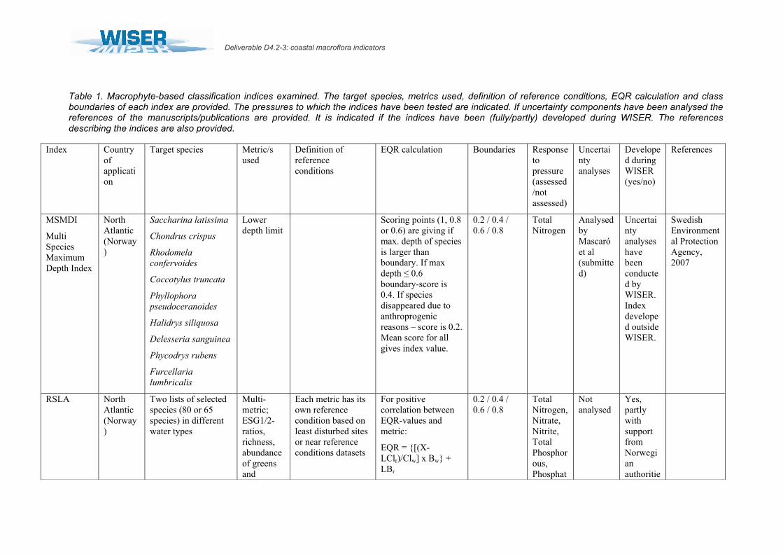
Table 1. Macrophyte-based classification indices examined. The target species, metrics used, definition of reference conditions, EQR calculation and class boundaries of each index are provided. The pressures to which the indices have been tested are indicated. If uncertainty components have been analysed the references of the manuscripts/publications are provided. It is indicated if the indices have been (fully/partly) developed during WISER. The references describing the indices are also provided.
Index Country of application
Target species Metric/s used
Definition of reference conditions
EQR calculation Boundaries Response to pressure (assessed/not assessed)
Uncertainty analyses
Developed during WISER (yes/no)
References
MSMDI
Multi Species Maximum Depth Index
North Atlantic (Norway)
Saccharina latissima
Chondrus crispus
Rhodomela confervoides
Coccotylus truncata
Phyllophora pseudoceranoides
Halidrys siliquosa
Delesseria sanguinea
Phycodrys rubens
Furcellaria lumbricalis
Lower depth limit
Scoring points (1, 0.8 or 0.6) are giving if max. depth of species is larger than boundary. If max depth ≤ 0.6 boundary-score is 0.4. If species disappeared due to anthroprogenic reasons – score is 0.2. Mean score for all gives index value.
0.2 / 0.4 / 0.6 / 0.8
Total Nitrogen
Analysed by Mascaró et al (submitted)
Uncertainty analyses have been conducted by WISER. Index developed outside WISER.
Swedish Environmental Protection Agency, 2007
RSLA North Atlantic (Norway)
Two lists of selected species (80 or 65 species) in different water types
Multi-metric; ESG1/2-ratios, richness, abundance of greens and
Each metric has its own reference condition based on least disturbed sites or near reference conditions datasets
For positive correlation between EQR-values and metric:
EQR = [(X-LClr)/Clw] x Bw + LBr
0.2 / 0.4 / 0.6 / 0.8
Total Nitrogen, Nitrate, Nitrite, Total Phosphorous, Phosphat
Not analysed
Yes, partly with support from Norwegian authoritie
Deliverable D4.2-3: coastal macroflora indicators
Page 9/39
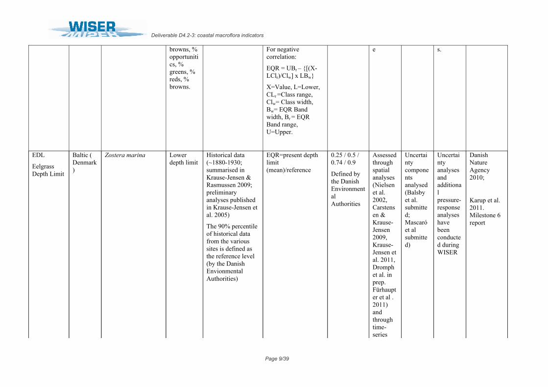
browns, % opportunitics, % greens, % reds, % browns.
For negative correlation:
EQR = UBr – [(X-LClr)/Clw] x LBw
X=Value, L=Lower, CLr =Class range, Clw= Class width, Bw= EQR Band width, Br = EQR Band range, U=Upper.
e s.
EDL
Eelgrass Depth Limit
Baltic ( Denmark)
Zostera marina Lower depth limit
Historical data (~1880-1930; summarised in Krause-Jensen & Rasmussen 2009; preliminary analyses published in Krause-Jensen et al. 2005)
The 90% percentile of historical data from the various sites is defined as the reference level (by the Danish Envionmental Authorities)
EQR=present depth limit (mean)/reference
0.25 / 0.5 / 0.74 / 0.9
Defined by the Danish Environmental Authorities
Assessed through spatial analyses (Nielsen et al. 2002, Carstensen & Krause-Jensen 2009, Krause-Jensen et al. 2011, Dromph et al. in prep. Fürhaupter et al . 2011) and through time-series
Uncertainty components analysed (Balsby et al. submitted; Mascaró et al submitted)
Uncertainty analyses and additional pressure-response analyses have been conducted during WISER
Danish Nature Agency 2010;
Karup et al. 2011. Milestone 6 report
Deliverable D4.2-3: coastal macroflora indicators
Page 10/39
analyses (Markager et al. 2010, Carstensen et al. in prep.)
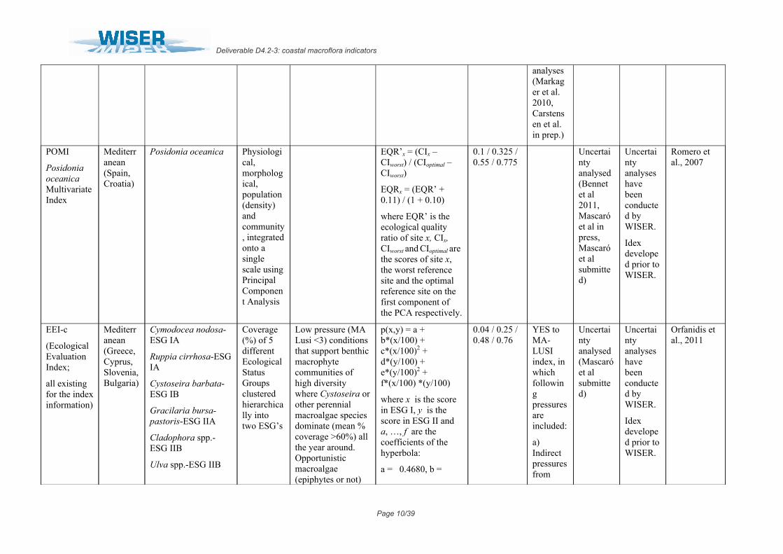
POMI
Posidonia oceanica Multivariate Index
Mediterranean (Spain, Croatia)
Posidonia oceanica Physiological, morphological, population (density) and community, integrated onto a single scale using Principal Component Analysis
EQR’x = (CIx – CIworst) / (CIoptimal – CIworst)
EQRx = (EQR’ + 0.11) / (1 + 0.10)
where EQR’ is the ecological quality ratio of site x, CIx, CIworst and CIoptimal are the scores of site x, the worst reference site and the optimal reference site on the first component of the PCA respectively.
0.1 / 0.325 / 0.55 / 0.775
Uncertainty analysed (Bennet et al 2011, Mascaró et al in press, Mascaró et al submitted)
Uncertainty analyses have been conducted by WISER.
Idex developed prior to WISER.
Romero et al., 2007
EEI-c
(Ecological Evaluation Index;
all existing for the index information)
Mediterranean (Greece, Cyprus, Slovenia, Bulgaria)
Cymodocea nodosa-ESG IA
Ruppia cirrhosa-ESG IA
Cystoseira barbata-ESG IB
Gracilaria bursa-pastoris-ESG IIA
Cladophora spp.-ESG IIB
Ulva spp.-ESG IIB
Coverage (%) of 5 different Ecological Status Groups clustered hierarchically into two ESG’s
Low pressure (MA Lusi <3) conditions that support benthic macrophyte communities of high diversity where Cystoseira or other perennial macroalgae species dominate (mean % coverage >60%) all the year around. Opportunistic macroalgae (epiphytes or not)
p(x,y) = a + b*(x/100) + c*(x/100)2 + d*(y/100) + e*(y/100)2 + f*(x/100) *(y/100)
where x is the score in ESG I, y is the score in ESG II and a, …, f are the coefficients of the hyperbola:
a = 0.4680, b =
0.04 / 0.25 / 0.48 / 0.76
YES to MA-LUSI index, in which following pressures are included:
a) Indirect pressures from
Uncertainty analysed (Mascaróet al submitted)
Uncertainty analyses have been conducted by WISER.
Idex developed prior to WISER.
Orfanidis et al., 2011
Deliverable D4.2-3: coastal macroflora indicators
Page 11/39
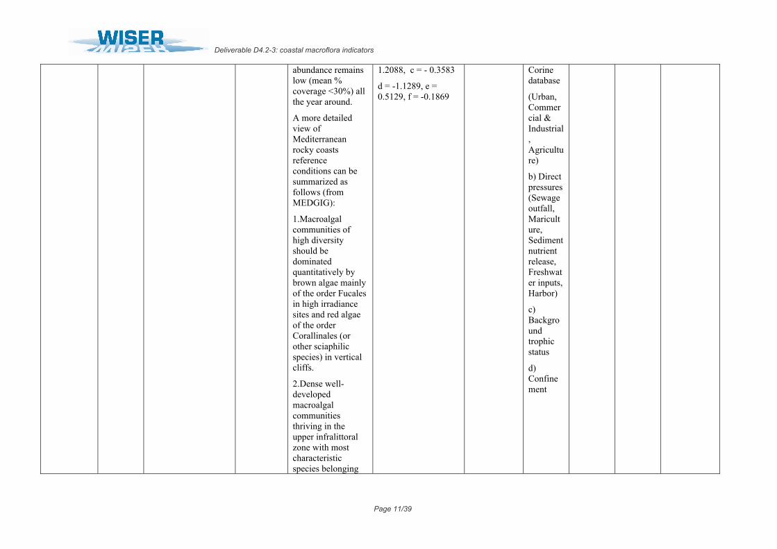
abundance remains low (mean % coverage <30%) all the year around.
A more detailed view of Mediterranean rocky coasts reference conditions can be summarized as follows (from MEDGIG):
1.Macroalgal communities of high diversity should be dominated quantitatively by brown algae mainly of the order Fucales in high irradiance sites and red algae of the order Corallinales (or other sciaphilic species) in vertical cliffs.
2.Dense well-developed macroalgal communities thriving in the upper infralittoral zone with most characteristic species belonging
1.2088, c = - 0.3583
d = -1.1289, e = 0.5129, f = -0.1869
Corine database
(Urban, Commercial & Industrial, Agriculture)
b) Direct pressures (Sewage outfall, Mariculture, Sediment nutrient release, Freshwater inputs, Harbor)
c) Background trophic status
d) Confinement
Deliverable D4.2-3: coastal macroflora indicators
Page 12/39
to the genera Cystoseira, Sargassum, Lithophyllum, Peyssonnelia, Corallina and Padina. Other common species belong to the genera Halopteris, Stypocaulon, Dictyota, Dictyopteris, Laurencia, Cladophora and Jania.
3.In the shadow zones (exposed steep vertical cliffs) Lithophyllum byssoides develops, forming important organogenic structures (trottoir). In marine caves with scarce light conditions a sciaphilic vegetation of red and green algae is dominant.
4. Spatio-temporal variability of the community’s composition and abundance affected by hard substrata availability, intense
Deliverable D4.2-3: coastal macroflora indicators
Page 13/39
and frequency of natural disturbances, e.g. hydrodynamism, grazing, by seasonal cycle of light period and intense, and by limiting factors like nutrients.
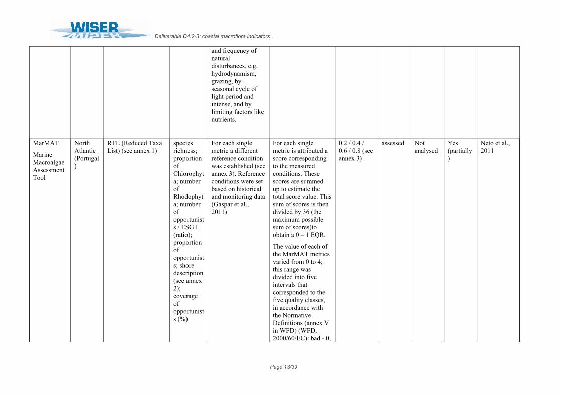
MarMAT
Marine Macroalgae Assessment Tool
North Atlantic (Portugal)
RTL (Reduced Taxa List) (see annex 1)
species richness; proportion of Chlorophyta; number of Rhodophyta; number of opportunists / ESG I (ratio); proportion of opportunists; shore description (see annex 2); coverage of opportunists (%)
For each single metric a different reference condition was established (see annex 3). Reference conditions were set based on historical and monitoring data (Gaspar et al., 2011)
For each single metric is attributed a score corresponding to the measured conditions. These scores are summed up to estimate the total score value. This sum of scores is then divided by 36 (the maximum possible sum of scores)to obtain a 0 – 1 EQR.
The value of each of the MarMAT metrics varied from 0 to 4; this range was divided into five intervals that corresponded to the five quality classes, in accordance with the Normative Definitions (annex V in WFD) (WFD, 2000/60/EC): bad - 0,
0.2 / 0.4 / 0.6 / 0.8 (see annex 3)
assessed Not analysed
Yes (partially)
Neto et al., 2011
Deliverable D4.2-3: coastal macroflora indicators
Page 14/39
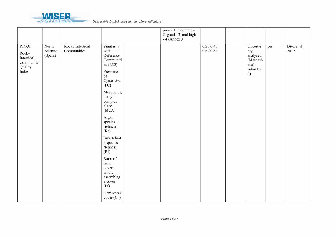
poor - 1, moderate - 2, good - 3, and high - 4 (Annex 3)
RICQI
Rocky Intertidal Community Quality Index
North Atlantic (Spain)
Rocky Intertidal Communities
Similarity with Reference Communities (ESS)
Presence of Cystoseira (PC)
Morphologically complex algae (MCA)
Algal species richness (Ra)
Invertebrate species richness (Rf)
Ratio of faunal cover to whole assemblage cover (Pf)
Herbivores cover (Ch)
0.2 / 0.4 / 0.6 / 0.82
Uncertainty analysed (Mascaróet al submitted)
yes Díez et al., 2012
Deliverable D4.2-3: coastal macroflora indicators
Page 15/39
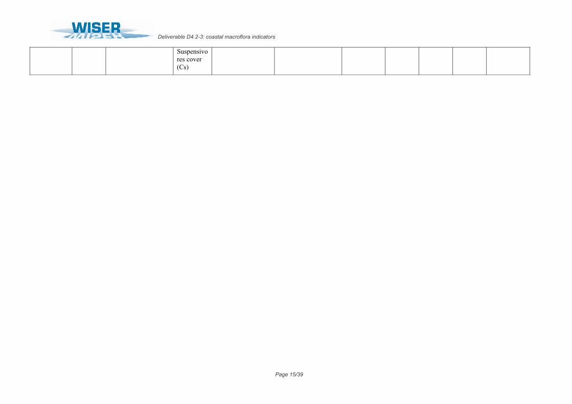
Suspensivores cover (Cs)
Deliverable D4.2-3: coastal macroflora indicators
2.1. Description of the classification methods for coastal waters using macrophytes developed with WISER
2.1.1. Marine Macroalgae Assessment Tool
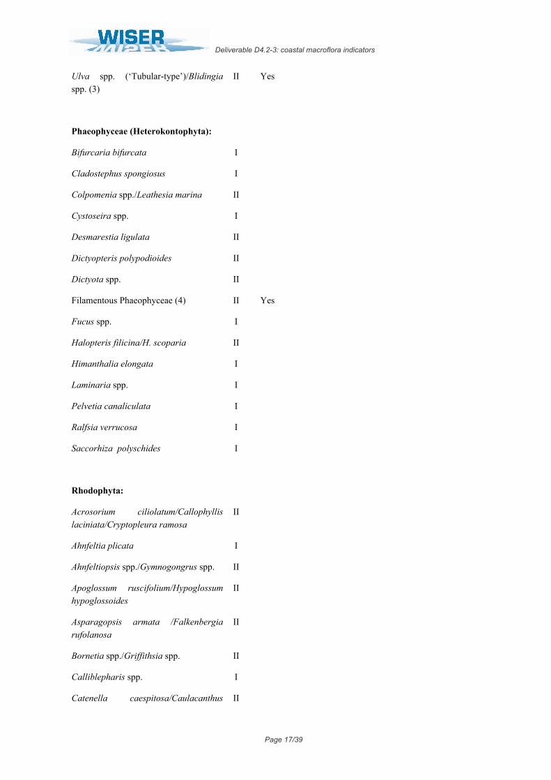
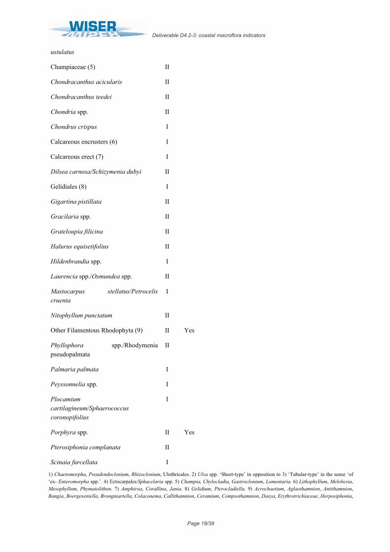
Under the scope of the Water Framework Directive (WFD, 2000/60/EC), ecological reference conditions and quality states were established for the biological quality element of macroalgae. The work combined both historical and current monitoring data from northern Portuguese coastal waters (Portuguese ‘A5 typology’, matching the European ‘NEA1 typology’). Representative intertidal rocky shore sites were selected to: (1) have a robust variability in macroalgal communities within the water body type and (2) cover a gradient of anthropogenic pressure to understand the communities’ changes due to disturbance. First, a ‘reduced taxa list’ (RTL, Table 2) was developed by selecting and grouping macroalgal taxa common in the study area, in proportion to the naturally occurring macroalgal taxonomic groups (Chlorophyta, Phaeophyceae – Heterokontophyta and Rhodophyta) and comprising taxa that require a moderate level of taxonomical identification expertise. Second, based on the RTL, the metrics of composition, i.e., species richness; the number and proportion of Chlorophyta, Phaeophyceae and Rhodophyta; the number and proportion of opportunists; ecological status groups (ESG) I, and ESG II; the ratios ESG I/ESG II, the number of opportunists/ESG I and the number of opportunists/ESG II; plus an abundance metric coverage of opportunists were studied to understand their behaviour under different levels of disturbance. The thresholds between the five quality conditions (‘high’, ‘good’, ‘moderate’, ‘poor’ and ‘bad’, similar to those required by the WFD to calculate the ecological quality status, Table 3) were defined for the above macroalgal metrics in compliance with the WFD (Gaspar et al. 2011). Hence, reference conditions – pristine situations that exist or would exist with no or very minor disturbances from anthropogenic pressures – were established together, since this class of excellent quality is included in the ‘high’ quality condition.
Table 2 – Reduced Taxa List (RTL) for the A5 Portuguese Coastal Water (CW) typology (NEA 1 for Portuguese northern coast). ESG = Ecological Status Groups.
Reduced Taxa List: (CW A5 PT type) ESG
Opportunistic
Chlorophyta:
Bryopsis spp. II Yes
Other Filamentous Chlorophyta (1) II Yes
Cladophora spp. II Yes
Codium spp. II
Ulva spp. (‘Sheet-type’)/Ulvaria obscura/Prasiola stipitata (2)
II Yes
Deliverable D4.2-3: coastal macroflora indicators
Page 17/39
Ulva spp. (‘Tubular-type’)/Blidingia spp. (3)
II Yes
Phaeophyceae (Heterokontophyta):
Bifurcaria bifurcata I
Cladostephus spongiosus I
Colpomenia spp./Leathesia marina II
Cystoseira spp. I
Desmarestia ligulata II
Dictyopteris polypodioides II
Dictyota spp. II
Filamentous Phaeophyceae (4) II Yes
Fucus spp. I
Halopteris filicina/H. scoparia II
Himanthalia elongata I
Laminaria spp. I
Pelvetia canaliculata I
Ralfsia verrucosa I
Saccorhiza polyschides I
Rhodophyta:
Acrosorium ciliolatum/Callophyllis laciniata/Cryptopleura ramosa
II
Ahnfeltia plicata I
Ahnfeltiopsis spp./Gymnogongrus spp. II
Apoglossum ruscifolium/Hypoglossum hypoglossoides
II
Asparagopsis armata /Falkenbergia rufolanosa
II
Bornetia spp./Griffithsia spp. II
Calliblepharis spp. I
Catenella caespitosa/Caulacanthus II
Deliverable D4.2-3: coastal macroflora indicators
Page 18/39
ustulatus
Champiaceae (5) II
Chondracanthus acicularis II
Chondracanthus teedei II
Chondria spp. II
Chondrus crispus I
Calcareous encrusters (6) I
Calcareous erect (7) I
Dilsea carnosa/Schizymenia dubyi II
Gelidiales (8) I
Gigartina pistillata II
Gracilaria spp. II
Grateloupia filicina II
Halurus equisetifolius II
Hildenbrandia spp. I
Laurencia spp./Osmundea spp. II
Mastocarpus stellatus/Petrocelis cruenta
I
Nitophyllum punctatum II
Other Filamentous Rhodophyta (9) II Yes
Phyllophora spp./Rhodymenia pseudopalmata
II
Palmaria palmata I
Peyssonnelia spp. I
Plocamium cartilagineum/Sphaerococcus coronopifolius
I
Porphyra spp. II Yes
Pterosiphonia complanata II
Scinaia furcellata I
1) Chaetomorpha, Pseudendoclonium, Rhizoclonium, Ulothricales. 2) Ulva spp. ‘Sheet-type’ in opposition to 3) ‘Tubular-type’ in the sense ‘of ‘ex- Enteromorpha spp.’. 4) Ectocarpales/Sphacelaria spp. 5) Champia, Chylocladia, Gastroclonium, Lomentaria. 6) Lithophyllum, Melobesia, Mesophyllum, Phymatolithon. 7) Amphiroa, Corallina, Jania. 8) Gelidium, Pterocladiella. 9) Acrochaetium, Aglaothamnion, Antithamnion, Bangia, Boergeseniella, Brongniartella, Colaconema, Callithamnion, Ceramium, Compsothamnion, Dasya, Erythrotrichiaceae, Herposiphonia,
Deliverable D4.2-3: coastal macroflora indicators
Page 19/39
Heterosiphonia, Janczewskia, Leptosiphonia, Lophosiphonia, Ophidocladus, Pleonosporium, Plumaria, Polysiphonia, Pterosiphonia (except P. complanata), Pterothamnion, Ptilothamnion, Rhodothamniella, Streblocladia, Vertebrata
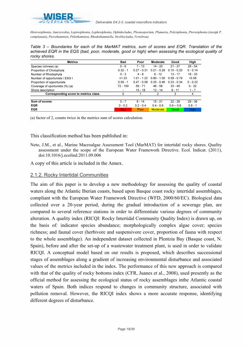
Table 3 – Boundaries for each of the MarMAT metrics, sum of scores and EQR. Translation of the achieved EQR in the EQS (bad, poor, moderate, good or high) when assessing the ecological quality of rocky shores.
(a) factor of 2, counts twice in the metrics sum of scores calculation.
This classification method has been published in:
Neto, J.M., et al., Marine Macroalgae Assessment Tool (MarMAT) for intertidal rocky shores. Quality assessment under the scope of the European Water Framework Directive. Ecol. Indicat. (2011), doi:10.1016/j.ecolind.2011.09.006
A copy of this article is included in the Annex.
2.1.2. Rocky Intertidal Communities
The aim of this paper is to develop a new methodology for assessing the quality of coastal waters along the Atlantic Iberian coasts, based upon Basque coast rocky intertidal assemblages, compliant with the European Water Framework Directive (WFD, 2000/60/EC). Biological data collected over a 20-year period, during the gradual introduction of a sewerage plan, are compared to several reference stations in order to differentiate various degrees of community alteration. A quality index (RICQI: Rocky Intertidal Community Quality Index) is drawn up, on the basis of: indicator species abundance; morphologically complex algae cover; species richness; and faunal cover (herbivore and suspensivore cover, proportion of fauna with respect to the whole assemblage). An independent dataset collected in Plentzia Bay (Basque coast, N. Spain), before and after the set-up of a wastewater treatment plant, is used in order to validate RICQI. A conceptual model based on our results is proposed, which describes successional stages of assemblages along a gradient of increasing environmental disturbance and associated values of the metrics included in the index. The performance of this new approach is compared with that of the quality of rocky bottoms index (CFR, Juanes et al., 2008), used presently as the official method for assessing the ecological status of rocky assemblages inthe Atlantic coastal waters of Spain. Both indices respond to changes in community structure, associated with pollution removal. However, the RICQI index shows a more accurate response, identifying different degrees of disturbance.
Deliverable D4.2-3: coastal macroflora indicators
Page 20/39
This classification method has been published in:
Díez I, M. Bustamante, A. Santolaria, J. Tajadura, N. Muguerza, A. Borja, I. Muxika, J.I. Saiz-Salinas, J.M. Gorostiaga. 2012. Development of a tool for assessing the ecological quality status of intertidal coastal rocky assemblages, within Atlantic Iberian coasts. Ecological Indicators 12: 58–71
A copy of this article is included in the Annex.
3. Assessment of uncertainty of classification of coastal waters status using macrophyte indicators We have quantified the uncertainty of classification of coastal waters status using macrophyte indicators and identified the components of monitoring programs that mostly contribute to the risk of misclassification. We first separately analysed the uncertainty of classification of coastal waters in monitoring programs using two macrophyte indicators (namely, “Maximum eelgrass depth limit” for Danish waters and “Posidonia multivariate index-POMI” for Catalan, Balearic and Croatian waters, see sections 3.1 and 3.2). We present a summary of the results on uncertainty assessments conducted for “Maximum eelgrass depth limit” and “Posidonia multivariate index-POMI” in sections 3.1 and 3.2 and include a copy of the respective articles/submitted manuscripts in the Annex. Then, we compared the magnitude of sources of uncertainty and the risk of misclassification across 5 macrophyte classification methods used in the WFD (see section 3.3). A detailed description of the uncertainty analyses conducted across classification methods is provided in section 3.3.
3.1. Sources of uncertainty associated with the monitoring of the “Maximum depth limit in eelgrass (Zostera marina)”
Based on a long-term marine monitoring program of eelgrass maximum depth limit in Danish coastal waters we estimated the uncertainty contribution of year, diver, transect and replicates for each water body. For all variables the uncertainty increased with the maximum depth limit, which suggested that eelgrass depth limits were more difficult to determine or less well defined at large depths. We used either a Spheric or a Gaussian function to describe the relation between uncertainty and the maximum depth limit for each variable. This parameterization of the depth specific uncertainty allowed estimation of the total variance, which can be used to evaluate survey designs. The total variance was compared with the time budget for a survey in a water body. If a maximum time limit was allocated to survey a water body, the surveys that resulted in the lowest variance of the maximum depth limit used 2 divers if 100 h were available and 3 divers if 200h were available, 2 or 3 years of survey and 4 to 8 transects.
The results of this study are provided in the submitted manuscript:
Thorsten J. S. Balsby, Jacob Carstensen, Dorte Krause-Jensen. Sources of uncertainty in estimation of eelgrass depth limits. Hydrobiologia (submitted).
A copy of this manuscript is included in the Annex.
Deliverable D4.2-3: coastal macroflora indicators
Page 21/39
3.2. Uncertainty of classification of coastal waters using “Posidonia oceanica multivariate index (POMI)”.
3.2.1. Uncertainty of classification using POMI of Catalan coastal waters
We assessed the Posidonia oceanica multivariate index (POMI) bio-monitoring program for its robustness in classifying the ecological status of Catalan coastal waters (Spain, W Mediterranean) within the Water Framework Directive. We used a 7-year dataset, covering 30 sites along 500 km of the Catalan coastline to examine which version of POMI (14 or 9 metrics) maximizes precision in classifying the ecological status of meadows. Five factors (zones within a site, sites within a water body, depth, years and surveyors) that potentially generate classification uncertainty were examined in detail. Of these, depth was a major source of uncertainty, while all the remaining spatial and temporal factors displayed low variability. POMI 9 matched POMI 14 in all factors, and could effectively replace it in future monitoring programs.
This study has been published in:
BENNETT, S., ROCA, G., ROMERO, J., ALCOVERRO, T. (2011) Ecological status of seagrass ecosystems: An uncertainty analysis of meadow classification based on the Posidonia multivariate index (POMI). Marine Pollution Bulletin: 62: 1616-1621.
A copy of this article is included in the Annex.
3.2.1. Sources of uncertainty and quantification of the risk of misclassification of Catalan, Balearic and Croatia coastal waters using POMI
Uncertainty analyses allow the identification and quantification of the factors that contribute to the potential misclassification of the ecological status of water bodies, helping to improve the sampling design used in monitoring. Here we used a Posidonia oceanica multivariate index (POMI) biomonitoring dataset covering a total of 81 sites distributed throughout 28 water bodies from the coast of Catalonia, Balearic Islands and Croatia to determine the levels of uncertainty associated with each region and how they change according to the quality status of water bodies. Overall, variability among sites (meadows) within water bodies was the factor that generated the greatest risk of misclassification among the three regions, within which the Balearic Islands had the lowest uncertainty, followed by Croatia and Catalonia. When water bodies classified in good/high quality were separated from those in moderate/poor status classes, we found that the latter displayed higher levels of uncertainty than the former.
The results of this study are in this submitted manuscript:
MASCARO, O., BENNETT, S., MARBA, N., NIKOLIC, V., ROMERO, J., DUARTE, C.M., ALCOVERRO, T.. Uncertainty analysis along the ecological quality status of water bodies: the response of the Posidonia oceanica multivariate index (POMI) in three Mediterranean regions. Marine Pollution Bulletin. (submitted)
A copy of this manuscript is included in the Annex.
Deliverable D4.2-3: coastal macroflora indicators
Page 22/39
3.3. Exploring the robustness of different macrophyte-based classification methods to assess the ecological status of coastal and transitional ecosystems under the WFD
We compiled extensive bio-monitoring data from several macrophyte-based classification methods developed by different EU Members, which include data addressing spatial, temporal and human-induced sources of variability, to identify, through the application of uncertainty analysis, the major sources of uncertainty for coastal water classification. This exercise should help to design monitoring programs that minimise the risk of misclassification.
The analyses are be based on EQR datasets of either official or non-official bio-monitoring programmes of the different indices from which a data set including enough temporal and spatial replication was available, and the factors analysed will include spatial scales of sampling (variability among zones within a site, among sites within a water body, variability among regions and variability among depths), the temporal scale of sampling (variability among years) and the human-associated source of error (variability between surveyors). These factors represent some the key sources of variability associated with the design and implementation of a bio-monitoring program, and highlight how certain elements of a sampling design can influence the reliability and robustness of the ecological status classification of coastal water bodies. With this approach, we try to gain insight into the current status of these methodologies proposed for European waters under the WFD and detect their main weaknesses to provide robust foundation for monitoring as well as guide decision in management plans.
3.3.1. Methods
• 3.3.1.1. Methods of classification examined We compared the magnitude of the sources of uncertainty and the risk of misclassification of European coastal waters using the following methods of classification:
- Multi Species Maximum Depth Index (MSMDI)
- Eelgrass Depth Limit (EDL)
- Posidonia multivariate Index (POMI)
- Ecological Evaluation Index coastal (EEI-c)
- Rocky Intertidal Community Quality Index (RICQI)
The characteristics of these methods of classification are described in section 2 and summarised in Table 1.
• 3.3.1.2. Variance extraction In the current study, the factors examined that potentially contribute to the uncertainty of the EQR estimations of coastal water bodies differ greatly among the 5 indices, especially due to differences in both the metrics used and their corresponding spatial and temporal sampling designs (Table 4). The total variance and variance components associated to each factor were estimated for all indices using a linear mixed effects model in the lme4 package of R (Bates 2005 and 2007, Version 2.10.1, R_Development_Core_Team 2009). When sufficient data was
Deliverable D4.2-3: coastal macroflora indicators
Page 23/39
available, factors were treated as random intercepts, either nested or crossed depending on the index (Table 4). Note that the variability among water bodies, whilst important in the analysis of variance components, is not discussed in this study because by definition they should differ in their ecological status. Variance components were determined by calculating the proportion of the total variance (σ2
T) explained by each individual factor. Thus, total variance in mean EQR values for each index was given by the sum of variances associated to each of the factors included in the model (σ2
X) plus the variance not explained by the model (σ2R; Table 4). The
proportion of total variance (Psamp; Table 4) explained by each factor was given by the equation, following Clarke et al. (2006):
Psamp = 100 σ2X / σ2
T (1)
Posteriorly for each index, the extracted variances were grouped into four main sources of uncertainty: i) temporal scale of sampling (variability among years), ii) spatial scale of sampling (including variability among zones within a site, among sites within a water body, variability among regions, variability among depths, etc.), iii) human-associated source of error (variability among surveyors) and iv) the residual term of the analysis (the variance in mean EQR values not explained by the model) in order to allow a further comparison of the results among indices that would help drawing general conclusions about these macrophyte-based classification methods (see Table 4).
All data satisfied the assumption of homogeneity of variance based on plots of the residuals against the fitted EQR values; therefore, no transformation of the data took place.
• 3.3.1.3. Uncertainty analysis Having calculated the variation in mean EQR scores for all factors within each index, the uncertainty in ecological status classification was estimated using WISERBUGS (WISER Bioassessment Uncertainty Guidance Software®, Clarke 2010). WISERBUGS helps determine whether an observed ecological status classification is indeed the most probable classification for a particular site, given the inherent sources of variability. WISERBUGS sums the observed value for a given site with a random standard normal deviate, of the known SD, with a mean of zero (Clarke and Hering 2006). It repeats this simulation 104 times to produce a frequency distribution of possible EQR values for the particular site or water body. The simulated EQR values are grouped into their corresponding status classes, from which the probability of misclassifying the original observed value can be determined. Because the current study was interested in the uncertainty in classification generated by a particular factor (rather than the probability of misclassifying individual sites), the simulation was repeated for the full range of possible observed EQR values (0 - 1).

Deliverable D4.2-3: coastal macroflora indicators
Table 4. Factors of the different groups included in the main sources of uncertainty, and the variance components.
Main sources of uncertainty Index
Temporal scale Spatial scale Human-associated error
Variance components
MSMDI
Multi Species Maximum Depth Index
· Year (σ2Y) · Region (σ2
Rg)
· Water Body:Region (σ2WB)
· Site:(Water Body:Region) (σ2Si)
· Surveyor (σ2Su) σ2
T = σ2Y + σ2
Rg + σ2WB + σ2
Si + σ2Sur + σ2
R
EDL
Eelgrass Depth Limit
· Year (σ2Y) · Region (σ2
Rg)
· Water Body:Region (σ2WB)
· Site:(Water Body:Region) (σ2Si)
- σ2T = σ2
Y + σ2Rg + σ2
WB + σ2Si + σ2
R
POMI
Posidonia oceanica Multivariate Index
· Year (σ2Y) · Region (σ2
Rg)
· Water Body:Region (σ2WB)
· Site:(Water Body:Region) (σ2Si)
· Zone:(Site:Water Body:Region) (σ2Z)
· Depth (σ2D)
· Surveyor (σ2Su) σ2
T = σ2Y + σ2
Rg + σ2WB + σ2
Si + σ2Z + σ2
D + σ2Su + σ2
R
RICQI
Rocky Intertidal Community Quality Index
· Year (σ2Y) ·Site:Water Body (σ2
Si) - σ2T = σ2
Y + σ2Si + σ2
R
EEI-c
Ecological Evaluation Index
- · Water Body (σ2WB)
· Site:Water Body (σ2Si)
- σ2T = σ2
WB + σ2Si + σ2
R
Deliverable D4.2-3: coastal macroflora indicators
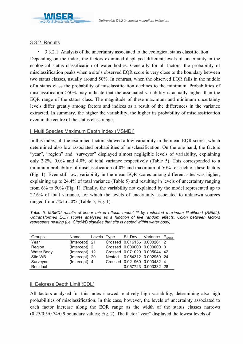
3.3.2. Results
• 3.3.2.1. Analysis of the uncertainty associated to the ecological status classification Depending on the index, the factors examined displayed different levels of uncertainty in the ecological status classification of water bodies. Generally for all factors, the probability of misclassification peaks when a site’s observed EQR score is very close to the boundary between two status classes, usually around 50%. In contrast, when the observed EQR falls in the middle of a status class the probability of misclassification declines to the minimum. Probabilities of misclassification >50% may indicate that the associated variability is actually higher than the EQR range of the status class. The magnitude of these maximum and minimum uncertainty levels differ greatly among factors and indices as a result of the differences in the variance extracted. In summary, the higher the variability, the higher its probability of misclassification even in the centre of the status class ranges.
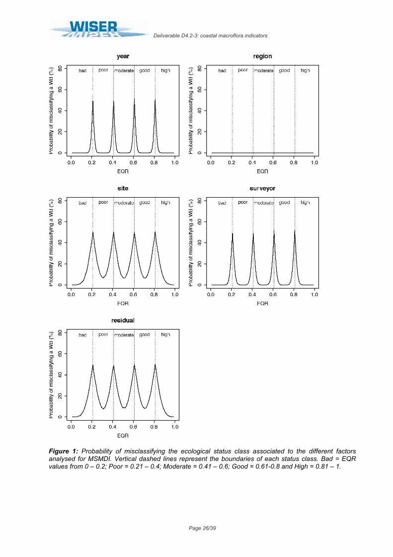
i. Multi Species Maximum Depth Index (MSMDI)
In this index, all the examined factors showed a low variability in the mean EQR scores, which determined also low associated probabilities of misclassification. On the one hand, the factors “year”, “region” and “surveyor” displayed almost negligible levels of variability, explaining only 2.2%, 0.0% and 4.0% of total variance respectively (Table 5). This corresponded to a minimum probability of misclassification of 0% and maximum of 50% for each of these factors (Fig. 1). Even still low, variability in the mean EQR scores among different sites was higher, explaining up to 24.4% of total variance (Table 5) and resulting in levels of uncertainty ranging from 6% to 50% (Fig. 1). Finally, the variability not explained by the model represented up to 27.6% of total variance, for which the levels of uncertainty associated to unknown sources ranged from 7% to 50% (Table 5, Fig. 1).
Table 5. MSMDI results of linear mixed effects model fit by restricted maximum likelihood (REML). Untransformed EQR scores analysed as a function of five random effects. Colon between factors represents nesting (i.e. Site:WB signifies that site is nested within water body).
Groups Name Levels Type St. Dev. Variance Psamp Year (Intercept) 21 Crossed 0.016156 0.000261 2 Region (Intercept) 2 Crossed 0.000000 0.000000 0 Water Body (Intercept) 12 Crossed 0.071020 0.005044 42 Site:WB (Intercept) 20 Nested 0.054312 0.002950 24 Surveyor (Intercept) 4 Crossed 0.021960 0.000482 4 Residual 0.057723 0.003332 28
ii. Eelgrass Depth Limit (EDL)
All factors analysed for this index showed relatively high variability, determining also high probabilities of misclassification. In this case, however, the levels of uncertainty associated to each factor increase along the EQR range as the width of the status classes narrows (0.25/0.5/0.74/0.9 boundary values; Fig. 2). The factor “year” displayed the lowest levels of
Deliverable D4.2-3: coastal macroflora indicators
Page 26/39
Figure 1: Probability of misclassifying the ecological status class associated to the different factors analysed for MSMDI. Vertical dashed lines represent the boundaries of each status class. Bad = EQR values from 0 – 0.2; Poor = 0.21 – 0.4; Moderate = 0.41 – 0.6; Good = 0.61-0.8 and High = 0.81 – 1.
Deliverable D4.2-3: coastal macroflora indicators
Page 27/39
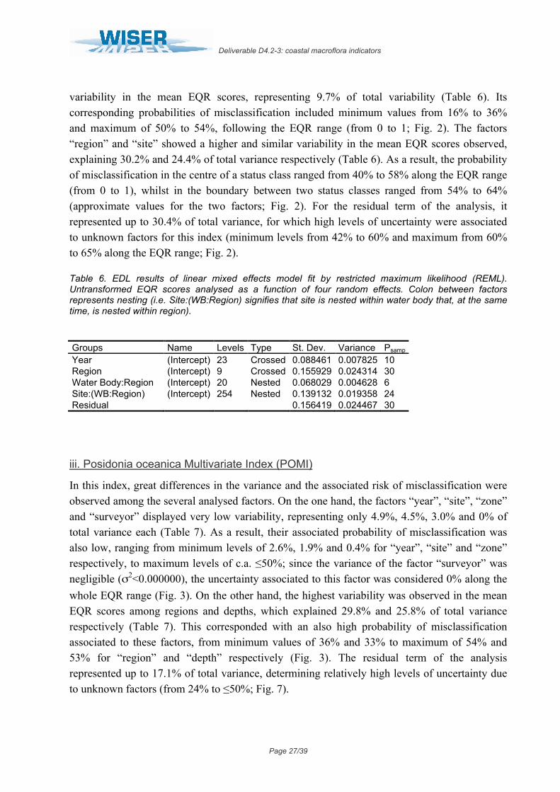
variability in the mean EQR scores, representing 9.7% of total variability (Table 6). Its corresponding probabilities of misclassification included minimum values from 16% to 36% and maximum of 50% to 54%, following the EQR range (from 0 to 1; Fig. 2). The factors “region” and “site” showed a higher and similar variability in the mean EQR scores observed, explaining 30.2% and 24.4% of total variance respectively (Table 6). As a result, the probability of misclassification in the centre of a status class ranged from 40% to 58% along the EQR range (from 0 to 1), whilst in the boundary between two status classes ranged from 54% to 64% (approximate values for the two factors; Fig. 2). For the residual term of the analysis, it represented up to 30.4% of total variance, for which high levels of uncertainty were associated to unknown factors for this index (minimum levels from 42% to 60% and maximum from 60% to 65% along the EQR range; Fig. 2).
Table 6. EDL results of linear mixed effects model fit by restricted maximum likelihood (REML). Untransformed EQR scores analysed as a function of four random effects. Colon between factors represents nesting (i.e. Site:(WB:Region) signifies that site is nested within water body that, at the same time, is nested within region).
Groups Name Levels Type St. Dev. Variance Psamp Year (Intercept) 23 Crossed 0.088461 0.007825 10 Region (Intercept) 9 Crossed 0.155929 0.024314 30 Water Body:Region (Intercept) 20 Nested 0.068029 0.004628 6 Site:(WB:Region) (Intercept) 254 Nested 0.139132 0.019358 24 Residual 0.156419 0.024467 30
iii. Posidonia oceanica Multivariate Index (POMI)
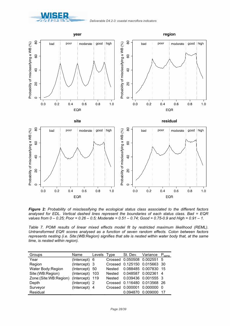
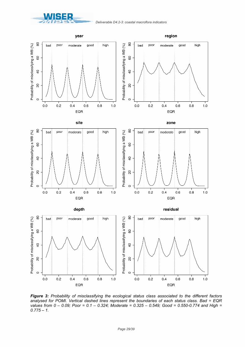
In this index, great differences in the variance and the associated risk of misclassification were observed among the several analysed factors. On the one hand, the factors “year”, “site”, “zone” and “surveyor” displayed very low variability, representing only 4.9%, 4.5%, 3.0% and 0% of total variance each (Table 7). As a result, their associated probability of misclassification was also low, ranging from minimum levels of 2.6%, 1.9% and 0.4% for “year”, “site” and “zone” respectively, to maximum levels of c.a. ≤50%; since the variance of the factor “surveyor” was negligible (σ2<0.000000), the uncertainty associated to this factor was considered 0% along the whole EQR range (Fig. 3). On the other hand, the highest variability was observed in the mean EQR scores among regions and depths, which explained 29.8% and 25.8% of total variance respectively (Table 7). This corresponded with an also high probability of misclassification associated to these factors, from minimum values of 36% and 33% to maximum of 54% and 53% for “region” and “depth” respectively (Fig. 3). The residual term of the analysis represented up to 17.1% of total variance, determining relatively high levels of uncertainty due to unknown factors (from 24% to ≤50%; Fig. 7).
Deliverable D4.2-3: coastal macroflora indicators
Page 28/39
Figure 2: Probability of misclassifying the ecological status class associated to the different factors analysed for EDL. Vertical dashed lines represent the boundaries of each status class. Bad = EQR values from 0 – 0.25; Poor = 0.26 – 0.5; Moderate = 0.51 – 0.74; Good = 0.75-0.9 and High = 0.91 – 1.
Table 7. POMI results of linear mixed effects model fit by restricted maximum likelihood (REML). Untransformed EQR scores analysed as a function of seven random effects. Colon between factors represents nesting (i.e. Site:(WB:Region) signifies that site is nested within water body that, at the same time, is nested within region).
Groups Name Levels Type St. Dev. Variance Psamp Year (Intercept) 6 Crossed 0.050508 0.002551 5 Region (Intercept) 3 Crossed 0.125150 0.015663 30 Water Body:Region (Intercept) 50 Nested 0.088485 0.007830 15 Site:(WB:Region) (Intercept) 103 Nested 0.048587 0.002361 4 Zone:(Site:WB:Region) (Intercept) 119 Nested 0.039436 0.001555 3 Depth (Intercept) 2 Crossed 0.116480 0.013568 26 Surveyor (Intercept) 4 Crossed 0.000001 0.000000 0 Residual 0.094870 0.009000 17
Deliverable D4.2-3: coastal macroflora indicators
Page 29/39
Figure 3: Probability of misclassifying the ecological status class associated to the different factors analysed for POMI. Vertical dashed lines represent the boundaries of each status class. Bad = EQR values from 0 – 0.09; Poor = 0.1 – 0.324; Moderate = 0.325 – 0.549; Good = 0.550-0.774 and High = 0.775 – 1.
Deliverable D4.2-3: coastal macroflora indicators
Page 30/39
iv. Rocky Intertidal Community Quality Index (RICQI)
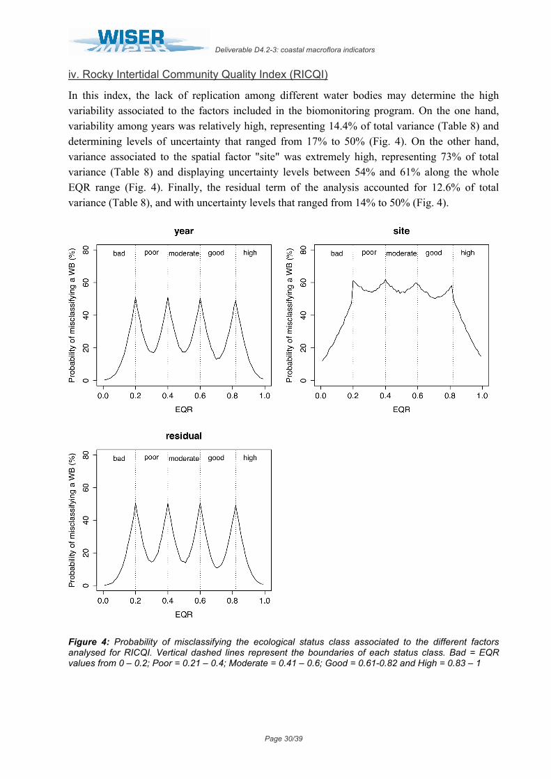
In this index, the lack of replication among different water bodies may determine the high variability associated to the factors included in the biomonitoring program. On the one hand, variability among years was relatively high, representing 14.4% of total variance (Table 8) and determining levels of uncertainty that ranged from 17% to 50% (Fig. 4). On the other hand, variance associated to the spatial factor "site" was extremely high, representing 73% of total variance (Table 8) and displaying uncertainty levels between 54% and 61% along the whole EQR range (Fig. 4). Finally, the residual term of the analysis accounted for 12.6% of total variance (Table 8), and with uncertainty levels that ranged from 14% to 50% (Fig. 4).
Figure 4: Probability of misclassifying the ecological status class associated to the different factors analysed for RICQI. Vertical dashed lines represent the boundaries of each status class. Bad = EQR values from 0 – 0.2; Poor = 0.21 – 0.4; Moderate = 0.41 – 0.6; Good = 0.61-0.82 and High = 0.83 – 1
Deliverable D4.2-3: coastal macroflora indicators
Page 31/39
Table 8. RICQI results of linear mixed effects model fit by restricted maximum likelihood (REML). Untransformed EQR scores analysed as a function of four random effects. Colon between factors represents nesting (i.e. Site:(WB:Region) signifies that site is nested within water body that, at the same time, is nested within region).
Groups Name Levels Type St. Dev. Variance Psamp Year (Intercept) 3 Crossed 0.073332 0.005378 14 Site (Intercept) 7 Crossed 0.164836 0.027171 73 Residual 0.068418 0.004681 13
v. Ecological Evaluation Index (EEI-c)
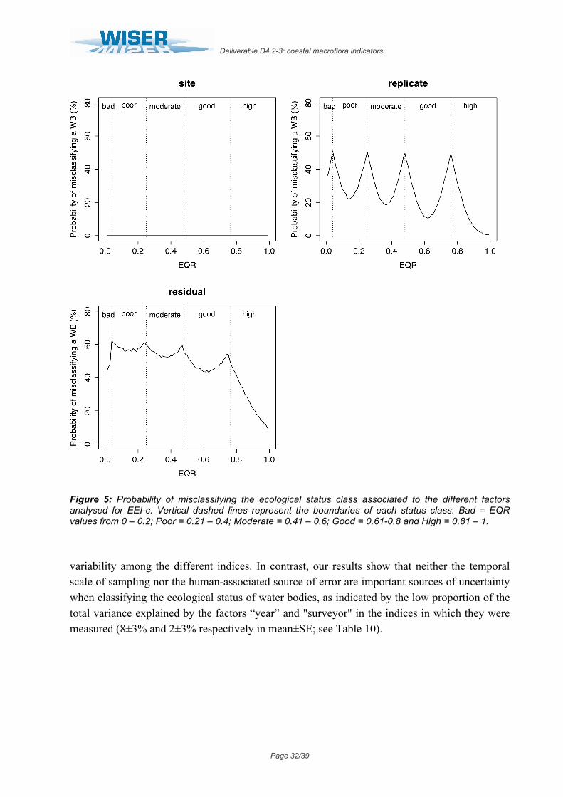
In this index, variability among sites was negligible (σ2<0.000000; Table 9), for which the risk of misclassification associated to this factor was 0% along the whole EQR range (Fig. 5). In contrast, the residual variance in mean EQR values was high, accounting for 30.5% of total variance (Table 9) and determining high levels of uncertainty that remained ≥50% almost along the whole EQR range (Fig. 5). The increasing width of the status classes along the EQR range (from 0 to 1) promoted that the general risk of misclassification decreased from "poor" to "high" status.
Table 9. EEI-c results of linear mixed effects model fit by restricted maximum likelihood (REML). Untransformed EQR scores analysed as a function of three random effects. Colon between factors represents nesting (i.e. Replicate:(Site:WB) signifies that replicate is nested within site that, at the same time, is nested within WB).
Groups Name Levels Type St. Dev. Variance Psamp Water Body (Intercept) 4 Crossed 0.292036 0.085285 68 Site:WB (Intercept) 6 Nested 0.000006 0.000000 0 Replicate:(Site:WB) (Intercept) 18 Nested 0.086976 0.007565 6 Residual 0.179911 0.032368 26
• 3.3.2.2. Main common sources of uncertainty among indices For each index, the variances extracted for the different factors were grouped into four main sources of uncertainty: i) the temporal scale of sampling (variability among years), ii) the spatial scale of sampling (including variability among zones within a site, among sites within a water body, variability among regions, variability among depths, etc.), iii) human-associated sources of error (variability among surveyors) and iv) the residual term of the analysis (the variance in mean EQR values not explained by the model).
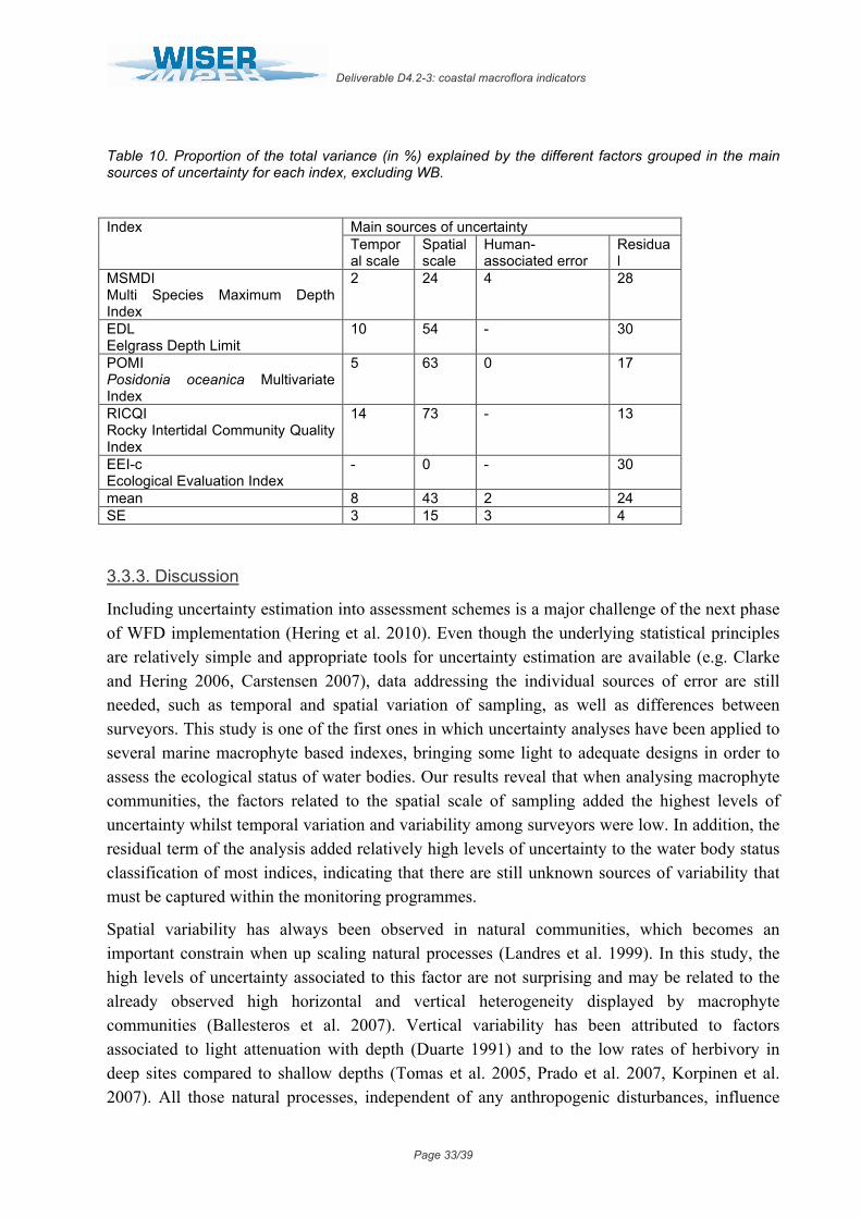
The spatial scale of sampling (excluding variability among water bodies) represented the main source of uncertainty, accounting for an average proportion of 43±15 % of total variance among the different indices (mean±SE; see Table 10). However, the factors grouped in this category and their associated variability differed greatly among the indices. Another important general source of uncertainty is the residual variance of the model, which accounted for an average of 24±4 % (in mean±SE; see Table 10,) of the total
Deliverable D4.2-3: coastal macroflora indicators
Page 32/39
Figure 5: Probability of misclassifying the ecological status class associated to the different factors analysed for EEI-c. Vertical dashed lines represent the boundaries of each status class. Bad = EQR values from 0 – 0.2; Poor = 0.21 – 0.4; Moderate = 0.41 – 0.6; Good = 0.61-0.8 and High = 0.81 – 1.
variability among the different indices. In contrast, our results show that neither the temporal scale of sampling nor the human-associated source of error are important sources of uncertainty when classifying the ecological status of water bodies, as indicated by the low proportion of the total variance explained by the factors “year” and "surveyor" in the indices in which they were measured (8±3% and 2±3% respectively in mean±SE; see Table 10).
Deliverable D4.2-3: coastal macroflora indicators
Page 33/39
Table 10. Proportion of the total variance (in %) explained by the different factors grouped in the main sources of uncertainty for each index, excluding WB.
Main sources of uncertainty Index Temporal scale
Spatial scale
Human-associated error
Residual
MSMDI Multi Species Maximum Depth Index
2 24 4 28
EDL Eelgrass Depth Limit
10 54 - 30
POMI Posidonia oceanica Multivariate Index
5 63 0 17
RICQI Rocky Intertidal Community Quality Index
14 73 - 13
EEI-c Ecological Evaluation Index
- 0 - 30
mean 8 43 2 24 SE 3 15 3 4
3.3.3. Discussion
Including uncertainty estimation into assessment schemes is a major challenge of the next phase of WFD implementation (Hering et al. 2010). Even though the underlying statistical principles are relatively simple and appropriate tools for uncertainty estimation are available (e.g. Clarke and Hering 2006, Carstensen 2007), data addressing the individual sources of error are still needed, such as temporal and spatial variation of sampling, as well as differences between surveyors. This study is one of the first ones in which uncertainty analyses have been applied to several marine macrophyte based indexes, bringing some light to adequate designs in order to assess the ecological status of water bodies. Our results reveal that when analysing macrophyte communities, the factors related to the spatial scale of sampling added the highest levels of uncertainty whilst temporal variation and variability among surveyors were low. In addition, the residual term of the analysis added relatively high levels of uncertainty to the water body status classification of most indices, indicating that there are still unknown sources of variability that must be captured within the monitoring programmes.
Spatial variability has always been observed in natural communities, which becomes an important constrain when up scaling natural processes (Landres et al. 1999). In this study, the high levels of uncertainty associated to this factor are not surprising and may be related to the already observed high horizontal and vertical heterogeneity displayed by macrophyte communities (Ballesteros et al. 2007). Vertical variability has been attributed to factors associated to light attenuation with depth (Duarte 1991) and to the low rates of herbivory in deep sites compared to shallow depths (Tomas et al. 2005, Prado et al. 2007, Korpinen et al. 2007). All those natural processes, independent of any anthropogenic disturbances, influence
Deliverable D4.2-3: coastal macroflora indicators
Page 34/39
structural and physiological parameters of macrophyte communities (Martínez-Crego et al. 2008), for which sampling at multiple depths result in highly variable EQR scores (from 25% to 37% of total variance in POMI and EI respectively). To reduce the risk of misclassification when assessing the ecological status of macrophyte communities, a relatively easy solution is that depth should remain fixed or be controlled in monitoring programs (see also Bennett et al. 2011). On the other hand, horizontal variability has been attributed to several factors acting from local (i.e. nutrient availability, sediment redox potential; Alcoverro et al. 1995) to regional scales (i.e. light, temperature; Marbà et al. 1996) that again influence structural and physiological parameters (Martínez-Crego et al. 2008). To capture this horizontal heterogeneity, bio-monitoring programmes must include sampling at different spatial scales, providing robust estimates of the ecological quality status classification at the water body level that include as much of this variability as possible, thereby minimizing the risk of misclassification (Kelly et al. 2009, Bennett et al. 2011). Even though bio-monitoring programmes from the different indices include sampling at several sites within each water body, only few of them include additional scales of replication below this level (POMI), resulting in a generally high uncertainty associated to the "site" factor (MSMDI, EDL, EI, RICQI). In these indices, it is strongly recommended to increase the sampling effort by adding a larger number of sites and within them, collecting different samples and averaging the metric values to provide robust estimates and minimize their associated risk of misclassification. This greater sampling effort may substantially increase the time and expense of the monitoring programmes, although it can be partially solved by maintaining the same number of replicates but just modifying the spatial sampling design to achieve a balance between financial constrains and a desirable index reliability. At a broader spatial scale, high variability among regions may indicate that they are separating groups of water bodies of similar ecological quality status. However, since this variability is above the scale of water body, at which the quality status is measured in the WFD, the risk of misclassification does not need to be minimized but included in the model and take into consideration when interpreting the uncertainty analysis results.
For the remaining factors, the uncertainty surrounding estimates in ecological status classification was very low within water bodies. Especially surprising is the case of inter-annual variability, which represented only between 1% and 9.7% of total variance depending on the index. As also reported by Bennett et al. (2011), this signifies that the EQR scores of water bodies are fairly consistent throughout the years, for which the frequency of sampling could be increased without greatly reducing the precision of ecological status estimates. Also surprising is the low variability among surveyors, which accounted only from 0% to 4% of total variance (for POMI and MSDMI respectively). This may be attributed to the fact that these particular macrophyte-based indices do not require complicated taxonomic identifications, which can greatly affect the precision of the EQR estimations in the case of other classification methods based on diatoms (Prygiel et al. 2002, Kelly et al. 2009) or freshwater macrophyte communities (Staniszewski et al. 2006). Finally, the residual term of the analysis represents all the variance that cannot be attributed to any of the factors included in the model, giving an idea of the accuracy of our approximation. In our study, it represented a relatively large proportion of total variance among the different indices (24±4% in mean±SE), indicating that other unknown
Deliverable D4.2-3: coastal macroflora indicators
Page 35/39
sources of uncertainty may be affecting the ecological status classification of water bodies. In order to keep this variance to the minimum, further data concerning other factors related to the sampling design may need to be collected in those indices where it is relatively large (spatial variance, temporal variance, variance among surveyors, etc.).
Furthermore, our results showed that the risk of misclassifying the quality status of water bodies is also affected by the width of the status class in which the EQR score falls, as reported in Kelly et al. (2009), with narrower classes leading to greater probabilities of misclassification. Thus, indices in which the EQR range is not equally split into the 5 official classes present, for a certain variance associated to a factor, different uncertainty levels depending on the status class (see EDL, POMI, RICQI and EEI-c). This fact have drastic implications for bio-monitoring programs, because a greater sampling effort may need to be assigned to water bodies whose EQR score falls within the narrower status classes in order to reduce their associated variability and increase the confidence of the classification.
3.3.4. Conclusions
In summary, our study confirmed that the analysis of the uncertainty associated to the ecological quality status classification of water bodies are a good proxy to identify and quantify the factors that may affect the risk of misclassification. When applied to macrophyte monitoring programs, we have observed that the main sources of uncertainty are mostly associated to the sampling spatial scales, while temporal or human-induced errors seem to be less relevant. As a guide for taking management decisions, adequate sampling designs that include replication at different spatial scales within water bodies may substantially reduce this uncertainty. In some cases, it is not increasing the sampling effort but distributing it more efficiently within the allocated time and budget constrains that we will be able to maximize the confidence of estimations when assessing ecosystem health under the WFD.
The results of this study are in this submitted manuscript:
MASCARO, O., ALCOVERRO, T., DENCHEVA, K., KRAUSE-JENSEN, D., MARBÀ, N., MUXIKA, I., NETO, J., NIKOLIC, V., ORFANIDIS, S., PEDERSEN, A., PEREZ, M., ROMERO, J. Exploring the robustness of different macrophyte-based classification methods to assess the ecological status of coastal and transitional ecosystems under the WFD. Hydrobiologia (submitted).
A copy of this manuscript is included in the Annex.
4. Recommendations The identification of the major sources of uncertainty of classification of coastal European waters using macrophyte indices helps improving the WFD monitoring programs in order to minimise the risk of misclassification of water bodies. According with our results:
- Horizontal spatial heterogeneity must be captured by sampling at different scales, providing robust estimates of the ecological quality status classification at the water body level that minimize the risk of misclassification.
Deliverable D4.2-3: coastal macroflora indicators
Page 36/39
- When using indices where water depth is not a component of it, depth should remain fixed or be controlled in monitoring programs in order to minimise vertical heterogeneity.
- Those indices where the distance between boundary classes is not uniform across the EQR range may need to assign a greater sampling effort to water bodies whose EQR score falls within the narrower status classes, in order to reduce their associated variability and increase the confidence of the classification. In contrast, sampling frequency has little effect on the precision of ecological status estimates.
- A greater replication effort should be assigned to those water bodies classified in moderate/poor/bad status, in order to capture the extra spatial variability coming from the effects of human pressures. On the other hand, it may be also a first warning that the spatial extent of water bodies may need to be redefined when differences in mean EQR values among different meadows of the same water body are excessively high, since an adequate spatial replication design will not be able to reduce the uncertainty associated to the classification system. A redefinition of the spatial extent and number of water bodies is strongly recommended in such cases.
5. References Badalamenti, F., Di Carlo, G., D’Anna, G., Gristina M., Toccaceli, M., 2006. Effects of dredging
activities on population dynamics of Posidonia oceanica (L.) Delile in the Mediterranean sea: the case study of Capo Feto (SW Sicily, Italy). Hydrobiologia 555, 253–261.
Balsby TJS, Carstensen J, Krause-Jensen D. In prep. Sources of uncertainty in estimation of eelgrass depth limits.
Bennett, S., Roca, G., Romero, J., Alcoverro, T., 2011. Ecological status of seagrass ecosystems: An uncertainty análisis of the meadow classification based on the Posidonia oceanica multivariate index (POMI). Marine Pollution Bulletin 62, 1616-1621.
Bouduresque, C.F., Bernard, G., Pergent, G., Shili, A., Verlaque, M., 2009. Regression of Mediterranean seagrasses caused by natural processes and anthropogenic disturbances and stress: a critical review. Botanica Marina 52, 395-418.
Buia, M.C., Silvestre, F., Iacono, G., Tiberti, L., 2005. Identificazione delle biocenosi di maggior preggio ambientale al fine della classificazione della qualita delle acque costiere. In: Metodologie per il rilevamento e la classificazione dello stato di qualita ecologico e chimico delle acque, con particolare riferimento all’aplicazione del decreto legislativo 152/99. APAT, Rome, pp. 269–303.
Carstensen et al. in prep. Carstensen, J. & Krause-Jensen, D., 2009: Fastlæggelse af miljømål og indsatsbehov ud fra ålegræs i de
indre danske farvande. Danmarks Miljøundersøgelser, Aarhus University. 48 pp. In Danish with English summary – Report from NERI no. 256. http://www.dmu.dk/Pub/AR256.pdf
Casazza, G., Lopez y Royo, C., Silvestri, C., 2006. Seagrass as key coastal ecosystems: an overview of the recent EU WFD requirements and current applications. Biologia Marina Mediterranea 13, 189–193.
Clarke, R.T., 2010. WISERBUGS 1.1 (WISER Bioassessment Uncertainty Guidance Software) tool for assessing confidence of WFD ecological status. User and Manual Software. Bournemouth University.
Deliverable D4.2-3: coastal macroflora indicators
Page 37/39
Clarke, R.T., Davy-Bowker, J., Sandin, L., Friberg, N., Johnson, R.K., Bis, B., 2006. Estimates and comparisons of the effects of sampling variation using “national” macroinvertebrate sampling protocols on the precision of metrics used to assess ecological status. Hydrobiologia 566, 477–503.
Clarke, R.T., Hering, D., 2006. Errors and uncertainty in bioassessment methods – major results and conclusions from the STAR project and their application using STARBUGS. Hydrobiologia 566, 433-439.
Danish Nature Agency 2010. Fastlæggelse af referenceforhold og miljømål samt beregning af indsatsbehov for de marine områder. Appendix 5 in ’Retningslinier for udarbejdelse af indsatsprogrammer’.
Dencheva, K. Improvements in sampling design and estimation of Ecological Index – EI (modified Ecological Evaluation Index) of macrophytobenthic communities as a tool for implementation of European Water Framework Directive. In press. Compt Rend. des Acad. of Sci.
Dromph K, Krause-Jensen D, Carstensen J, Blomqvist M, Boström C, Fürhaupter K, Karez R, Moy F. In prep. Eelgrass depth limits along physicochemical gradients in the Baltic Sea region
EC, 2000. DIRECTIVE 2000/60/EC of the European parliament and of the council, of 23 October 2000, establishing a framework for Community action in the field of water policy. Official Journal of the European Communities, G.U.C.E. 22/12/ 2000, L 327.
Ferreira, J.G., Nobre, A.M., Simas, T.C., Silva, M.C., Newton, A., Bricker, S.B., Wolff, W.J., Stacey, P.E., Sequeira, A., 2006. A methodology for defining homogeneous water bodies in estuaries – Application to the transitional systems of the EU Water Framework Directive. Estuarine, Coastal and Shelf Science 66, 468-482.
Fürhaupter K, Wilken H, Krause-Jensen D, Hansen JW, Dahl K & Karez R (2011). Intercalibration exercise of macrophytes (macroalgae and angiosperms) between Germany and Denmark. Baltic GIG intercalibration. pp. 47
Gobert, S., Sartoretto, S., Rico-Raimondino, V., Andral, B., Chery, A., Lejeune, P., Boissery, P., 2009. Assessment of the ecological status of Mediterranean French coastal waters as required by the Water Framework Directive using the Posidonia oceanica Rapid Easy Index: PREI. Marine Pollution Bulletin 58, 1727-1733.
Institute of Environment and Sustainability. Karup H (ed) 2011. WFD Intercalibration Phase 2: Milestone 6 report (version2) Coastal and transitional
waters Baltic Sea GIG Macrovegetation (macroalgae and angiosperms). European Commission Directorate General, JRC Joint Research Centre,
Kelly, M., Bennion, H., Burgess, A., Ellis, J., Juggins, S., Guthrie, R., Jamieson, J., Adriaenssens, V., Yallop, M., 2009. Uncertainty in ecological status assessments of lakes and rivers using diatoms. Hydrobiologia 633, 5-15.
Krause-Jensen D, Carstensen J, Nielsen SL, Dalsgaard T, Christensen PB, Fossing H, Rasmussen MB. 2011. Sea bottom characteristics affect depth limits of eelgrass (Zostera marina L.). MEPS. 425: 91–102. doi: 10.3354/meps09026
Krause-Jensen, D. & Rasmussen, M.B. 2009. Historisk udbredelse af ålegræs i danske kystområder. Danmarks Miljøundersøgelser, Aarhus University. 38 pp. – Scientific report from NERI no. 755. In Danish with English summary. http://www.dmu.dk/Pub/FR755.pdf
Landres, P.B., Morgan, P., Swanson, F.J., 1999. Overview of the use of natural variability concepts in managing ecological systems. Ecological Applications 9(4), 1179-1188.
Lopez y Royo, C., Pergent, G., Alcoverro, T., Buia, M.C., Casazza, G., Martínez-Crego, B., Pérez, M., Silvestre, F., Romero, J., 2011. The seagrass Posidonia oceanica as indicador of coastal water quality: Experimental intercalibration of classification Systems. Ecological Indicators 11, 55-563.
Markager S, Carstensen J, Krause-Jensen D, Windolf J, Timmermann K. 2010. Effekter af øgede kvælstoftilførsler på miljøet i danske fjorde. Danmarks Miljøundersøgelser, Aarhus Universitet. 54. Faglig rapport fra DMU nr. 787. http://www.dmu.dk/Pub/FR787.pdf
Martínez-Crego, B., Vergés, A., Alcoverro, T., Romero, J., 2008. Selection of multiple seagrass indicators for environmental biomonitoring. Marine Ecology Progress Series 361, 93-109.
Deliverable D4.2-3: coastal macroflora indicators
Page 38/39
Med-GIG, 2007. WFD Intercalibration technical report for coastal and transitional waters in the Mediterranean eco-region. In: WFD Intercalibration technical report – Part 3: Coastal and transitional waters. URL http://circa.europa.eu/Public/irc/jrc/jrceewai/library?l=/intercalibration2&vm=detailed&sb=Title.
Nielsen SL, Sand-Jensen K, Borum J, Geertz-Hansen O. 2002. Depth colonization of eelgrass (Zostera marina) and macroalgae as determined by water transparency in Danish coastal waters. Estuaries 25: 1025–1032
Orfanidis, S., Panayotidis, P., Ugland, K.I., 2011. Ecological Evaluation Index continuous formula (EEI-c) application: a step forward for functional groups, the formula and reference condition values. The Mediterranean Marine Science Journal 12 (2): 199-231.
Orth, R.J., Carruthers, T.J.B., Dennison, W.C., Duarte, C.M., Fourqurean, J.W., Heck, K.L., Hughes, A.R., Kendrick, G.A., Kenworthy, W.J., Olyarnik, A., Short, F.T., Waycott, M., Williams, S.L., 2006. A global crisis for seagrass ecosystems. Bioscience 56, 987–996.
Pergent-Martini, C., Leoni, V., Pasqualini, V., Ardizzone, G.D., Balestri, E., Bedini, R., Belluscio, A., Belsher, T., Borg, J., Boudouresque, C.F., Boumaza, S., Bouquegneau, J.M., Buia, M.C., Calvo, S., Cebrian, J., Charbonnel, E., Cinelli, F., Cossu, A., Di Maida, G., Dural, B., Francour, P., Gobert, S., Lepoint, G., Meinesz, A., Molenaar, H., Mansour, H.M., Panayotidis, P., Peirano, A., Pergent, G., Piazzi, L., Pirrotta, M., Relini, G., Romero, J., Sanchez-Lizaso, J.L., Semroud, R., Shembri, P., Shili, A., Tomasello, A., Velimirov, B., 2005. Descriptors of Posidonia oceanica meadows: use and application. Ecological Indicators 5, 213–230.
Pergent, G., Pergent-Martini, C., Boudouresque, C.F., 1995. Utilisation de l’herbier à Posidonia oceanica comme indicateur biologique de la qualité du milieu littoral en Méditerranée: Etat des connaissances. Mesogée 54, 3–29.
Pinheiro, J.C., Bates, D.M., 2000. Mixed-Effects models in S and S-Plus. Springer. ISBN 0-387-98957-0.
Pinheiro, J.C., Bates, D.M., DebRoy, S., Sarkar, D., 2005. The nlme package: Linear and nonlinear mixed effects models. URL http: //CRAN.R-project.org. R package version 3.1-98.
Procaccini, G., Buia, MC., Gambi, M.C., Pérez, M., Pergent-Marini, C., Romero, J., 2003. The seagrasses of the western Mediterranean. In: Green, E.P., Short, F.T. (Eds.), World Atlas of Seagrasses. University of California Press, Berkeley (USA). pp. 298.
Romero, J., Martínez-Crego, B., Alcoverro, T., Pérez, M., 2007. A multivariate index based on the seagrass Posidonia oceanica (POMI) to assess ecological status of coastal waters under the Water Framework Directive (WFD). Marine Pollution Bulletin 55, 196–204.
Staniszewski, R., Szoszkiewicz, K., Zbierska, J., Lesny, J., Jusik, S., Clarke, R.T., 2006. Assessment of sources of uncertainty in macrophyte surveys and the consequences for river classification. Hydrobiologia 566, 235-246.
Swedish Environmental Protection Agency: Handbook 2007:4. Status, Potential and Quality Measures for Lakes, Rivers, Coastal and Transitional Waters, Appendix B.
Deliverable D4.2-3: coastal macroflora indicators
Page 39/39
6. Annex
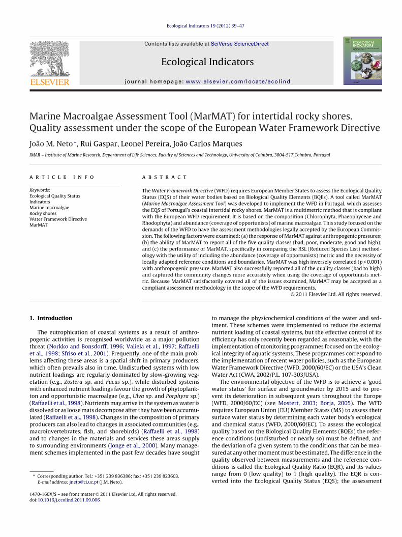
MQ
JI
a
KEIMRWM
1
ptelwnewt(dlpmatm
1d
Ecological Indicators 19 (2012) 39–47
Contents lists available at SciVerse ScienceDirect
Ecological Indicators
jo ur nal homep age: www.elsev ier .com/ locate /eco l ind
arine Macroalgae Assessment Tool (MarMAT) for intertidal rocky shores.uality assessment under the scope of the European Water Framework Directive
oão M. Neto ∗, Rui Gaspar, Leonel Pereira, João Carlos MarquesMAR – Institute of Marine Research, Department of Life Sciences, Faculty of Sciences and Technology, University of Coimbra, 3004-517 Coimbra, Portugal
r t i c l e i n f o
eywords:cological Quality Statusndicators
arine macroalgaeocky shoresater Framework DirectivearMAT
a b s t r a c t
The Water Framework Directive (WFD) requires European Member States to assess the Ecological QualityStatus (EQS) of their water bodies based on Biological Quality Elements (BQEs). A tool called MarMAT(Marine Macroalgae Assessment Tool) was developed to implement the WFD in Portugal, which assessesthe EQS of Portugal’s coastal intertidal rocky shores. MarMAT is a multimetric method that is compliantwith the European WFD requirement. It is based on the composition (Chlorophyta, Phaeophyceae andRhodophyta) and abundance (coverage of opportunists) of marine macroalgae. This study focused on thedemands of the WFD to have the assessment methodologies legally accepted by the European Commis-sion. The following factors were examined: (a) the response of MarMAT against anthropogenic pressures;(b) the ability of MarMAT to report all of the five quality classes (bad, poor, moderate, good and high);and (c) the performance of MarMAT, specifically in comparing the RSL (Reduced Species List) method-
ology with the utility of including the abundance (coverage of opportunists) metric and the necessity oflocally adapted reference conditions and boundaries. MarMAT was high inversely correlated (p < 0.001)with anthropogenic pressure. MarMAT also successfully reported all of the quality classes (bad to high)and captured the community changes more accurately when using the coverage of opportunists met-ric. Because MarMAT satisfactorily covered all of the issues examined, MarMAT may be accepted as aethod
compliant assessment m. Introduction
The eutrophication of coastal systems as a result of anthro-ogenic activities is recognised worldwide as a major pollutionhreat (Norkko and Bonsdorff, 1996; Valiela et al., 1997; Raffaellit al., 1998; Sfriso et al., 2001). Frequently, one of the main prob-ems affecting these areas is a spatial shift in primary producers,
hich often prevails also in time. Undisturbed systems with lowutrient loadings are regularly dominated by slow-growing veg-tation (e.g., Zostera sp. and Fucus sp.), while disturbed systemsith enhanced nutrient loadings favour the growth of phytoplank-
on and opportunistic macroalgae (e.g., Ulva sp. and Porphyra sp.)Raffaelli et al., 1998). Nutrients may arrive in the system as water isissolved or as loose mats decompose after they have been accumu-
ated (Raffaelli et al., 1998). Changes in the composition of primaryroducers can also lead to changes in associated communities (e.g.,acroinvertebrates, fish, and shorebirds) (Raffaelli et al., 1998)
nd to changes in the materials and services these areas supplyo surrounding environments (Jonge et al., 2000). Many manage-
ent schemes implemented in the past few decades have sought
∗ Corresponding author. Tel.: +351 239 836386; fax: +351 239 823603.E-mail address: [email protected] (J.M. Neto).
470-160X/$ – see front matter © 2011 Elsevier Ltd. All rights reserved.oi:10.1016/j.ecolind.2011.09.006
ology in the scope of the WFD requirements.© 2011 Elsevier Ltd. All rights reserved.
to manage the physicochemical conditions of the water and sed-iment. These schemes were implemented to reduce the externalnutrient loading of coastal systems, but the effective control of itsefficiency has only recently been regarded as reasonable, with theimplementation of monitoring programmes focused on the ecolog-ical integrity of aquatic systems. These programmes correspond tothe implementation of recent water policies, such as the EuropeanWater Framework Directive (WFD, 2000/60/EC) or the USA’s CleanWater Act (CWA, 2002/P.L. 107-303/USA).
The environmental objective of the WFD is to achieve a ‘goodwater status’ for surface and groundwater by 2015 and to pre-vent its deterioration in subsequent years throughout the Europe(WFD, 2000/60/EC) (see Mostert, 2003; Borja, 2005). The WFDrequires European Union (EU) Member States (MS) to assess theirsurface water status by determining each water body’s ecologicaland chemical status (WFD, 2000/60/EC). To assess the ecologicalquality based on the Biological Quality Elements (BQEs) the refer-ence conditions (undisturbed or nearly so) must be defined, andthe deviation of a given system to the conditions that can be mea-sured at any other moment must be estimated. The difference in the
quality observed between measurements and the reference con-ditions is called the Ecological Quality Ratio (EQR), and its valuesrange from 0 (low quality) to 1 (high quality). The EQR is con-verted into the Ecological Quality Status (EQS); the assessment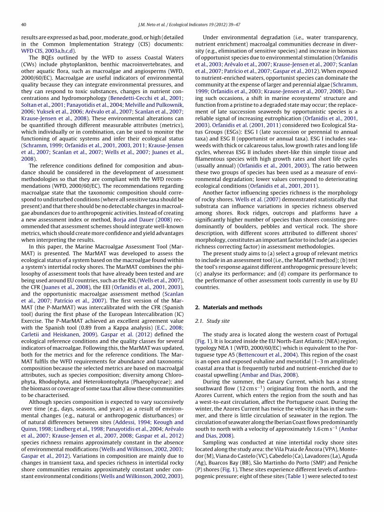
4 al Ind
riW
(o2qtcS2Kbwf(e2
dmmmspgaomw
MealbtaeMtEwCeibMcaptt
omoQesoGcss
0 J.M. Neto et al. / Ecologic
esults are expressed as bad, poor, moderate, good, or high (detailedn the Common Implementation Strategy (CIS) documents:
FD CIS, 2003a,b,c,d).The BQEs outlined by the WFD to assess Coastal Waters
CWs) include phytoplankton, benthic macroinvertebrates, andther aquatic flora, such as macroalgae and angiosperms (WFD,000/60/EC). Macroalgae are useful indicators of environmentaluality because they can integrate environmental pressures, andhey can respond to toxic substances, changes in nutrient con-entrations and hydromorphology (Benedetti-Cecchi et al., 2001;oltan et al., 2001; Panayotidis et al., 2004; Melville and Pulkownik,006; Yuksek et al., 2006; Arévalo et al., 2007; Scanlan et al., 2007;rause-Jensen et al., 2008). These environmental alterations cane quantified through different measurable attributes (metrics),hich individually or in combination, can be used to monitor the
unctioning of aquatic systems and infer their ecological statusSchramm, 1999; Orfanidis et al., 2001, 2003, 2011; Krause-Jensent al., 2007; Scanlan et al., 2007; Wells et al., 2007; Juanes et al.,008).
The reference conditions defined for composition and abun-ance should be considered in the development of assessmentethodologies so that they are compliant with the WFD recom-endations (WFD, 2000/60/EC). The recommendations regardingacroalgae state that the taxonomic composition should corre-
pond to undisturbed conditions (where all sensitive taxa should beresent) and that there should be no detectable changes in macroal-ae abundances due to anthropogenic activities. Instead of creating
new assessment index or method, Borja and Dauer (2008) rec-mmended that assessment schemes should integrate well-knownetrics, which should create more confidence and yield advantageshen interpreting the results.
In this paper, the Marine Macroalgae Assessment Tool (Mar-AT) is presented. The MarMAT was developed to assess the
cological status of a system based on the macroalgae found within system’s intertidal rocky shores. The MarMAT combines the phi-osophy of assessment tools that have already been tested and areeing used around EU countries, such as the RSL (Wells et al., 2007),he CFR (Juanes et al., 2008), the EEI (Orfanidis et al., 2001, 2003),nd the opportunistic macroalgae assessment method (Scanlant al., 2007; Patrício et al., 2007). The first version of the Mar-AT (the P-MarMAT) was intercalibrated with the CFR (Spanish
ool) during the first phase of the European Intercalibration (IC)xercise. The P-MarMAT achieved an excellent agreement valueith the Spanish tool (0.89 from a Kappa analysis) (E.C., 2008;arletii and Heiskanen, 2009). Gaspar et al. (2012) defined thecological reference conditions and the quality classes for severalndicators of macroalgae. Following this, the MarMAT was updated,oth for the metrics and for the reference conditions. The Mar-AT fulfils the WFD requirements for abundance and taxonomic
omposition because the selected metrics are based on macroalgalttributes, such as species composition; diversity among Chloro-hyta, Rhodophyta, and Heterokontophyta (Phaeophyceae); andhe biomass or coverage of some taxa that allow these communitieso be characterised.
Although species composition is expected to vary successivelyver time (e.g., days, seasons, and years) as a result of environ-ental changes (e.g., natural or anthropogenic disturbances) or
f natural differences between sites (Addessi, 1994; Keough anduinn, 1998; Lindberg et al., 1998; Panayotidis et al., 2004; Arévalot al., 2007; Krause-Jensen et al., 2007, 2008; Gaspar et al., 2012)pecies richness remains approximately constant in the absencef environmental modifications (Wells and Wilkinson, 2002, 2003;
aspar et al., 2012). Variations in composition are mainly due tohanges in transient taxa, and species richness in intertidal rockyhore communities remains approximately constant under con-tant environmental conditions (Wells and Wilkinson, 2002, 2003).icators 19 (2012) 39–47
Under environmental degradation (i.e., water transparency,nutrient enrichment) macroalgal communities decrease in diver-sity (e.g., elimination of sensitive species) and increase in biomassof opportunist species due to environmental stimulation (Orfanidiset al., 2003; Arévalo et al., 2007; Krause-Jensen et al., 2007; Scanlanet al., 2007; Patrício et al., 2007; Gaspar et al., 2012). When exposedto nutrient-enriched waters, opportunist species can dominate thecommunity at the expense of larger and perennial algae (Schramm,1999; Orfanidis et al., 2003; Krause-Jensen et al., 2007, 2008). Dur-ing such occasions, a shift in marine ecosystems’ structure andfunction from a pristine to a degraded state may occur; the replace-ment of late succession seaweeds by opportunistic species is areliable signal of increasing eutrophication (Orfanidis et al., 2001,2003). Orfanidis et al. (2001, 2011) considered two Ecological Sta-tus Groups (ESGs): ESG I (late succession or perennial to annualtaxa) and ESG II (opportunist or annual taxa). ESG I includes sea-weeds with thick or calcareous talus, low growth rates and long lifecycles, whereas ESG II includes sheet-like thin simple tissue andfilamentous species with high growth rates and short life cycles(usually annual) (Orfanidis et al., 2001, 2003). The ratio betweenthese two groups of species has been used as a measure of envi-ronmental degradation; lower values correspond to deterioratingecological conditions (Orfanidis et al., 2001, 2011).
Another factor influencing species richness is the morphologyof rocky shores. Wells et al. (2007) demonstrated statistically thatsubstrata can influence variations in species richness observedamong shores. Rock ridges, outcrops and platforms have asignificantly higher number of species than shores consisting pre-dominantly of boulders, pebbles and vertical rock. The shoredescription, with different scores attributed to different shores’morphology, constitutes an important factor to include (as a speciesrichness correcting factor) in assessment methodologies.
The present study aims to (a) select a group of relevant metricsto include in an assessment tool (i.e., the MarMAT method); (b) testthe tool’s response against different anthropogenic pressure levels;(c) analyse its performance; and (d) compare its performance tothe performance of other assessment tools currently in use by EUcountries.
2. Materials and methods
2.1. Study site
The study area is located along the western coast of Portugal(Fig. 1). It is located inside the EU North-East Atlantic (NEA) region,typology NEA 1 (WFD, 2000/60/EC) which is equivalent to the Por-tuguese type A5 (Bettencourt et al., 2004). This region of the coastis an open and exposed euhaline and mesotidal (1–3 m amplitude)coastal area that is frequently turbid and nutrient-enriched due tocoastal upwelling (Ambar and Dias, 2008).
During the summer, the Canary Current, which has a strongsouthward flow (12 cm s−1) originating from the north, and theAzores Current, which enters the region from the south and hasa west-to-east circulation, affect the Portuguese coast. During thewinter, the Azores Current has twice the velocity it has in the sum-mer, and there is little circulation of seawater in the region. Thecirculation of seawater along the Iberian Coast flows predominantlysouth to north with a velocity of approximately 1.6 cm s−1 (Ambarand Dias, 2008).
Sampling was conducted at nine intertidal rocky shore siteslocated along the study area: the Vila Praia de Âncora (VPA), Monte-
dor (M), Viana do Castelo (VC), Cabedelo (Ca), Lavadores (La), Aguda(Ag), Buarcos Bay (BB), São Martinho do Porto (SMP) and Peniche(P) shores (Fig. 1). These sites experience different levels of anthro-pogenic pressure; eight of these sites (Table 1) were selected to test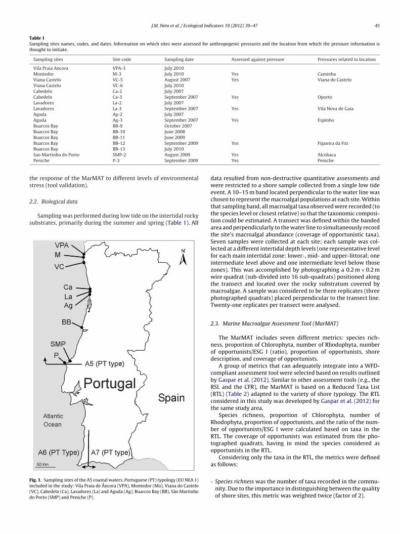
J.M. Neto et al. / Ecological Indicators 19 (2012) 39–47 41
Table 1Sampling sites names, codes, and dates. Information on which sites were assessed for anthropogenic pressures and the location from which the pressure information isthought to initiate.
Sampling sites Site code Sampling date Assessed against pressure Pressures related to location
Vila Praia Ancora VPA-3 July 2010Montedor M-3 July 2010 Yes CaminhaViana Castelo VC-5 August 2007 Yes Viana do CasteloViana Castelo VC-6 July 2010Cabedelo Ca-2 July 2007Cabedelo Ca-3 September 2007 Yes OportoLavadores La-2 July 2007Lavadores La-3 September 2007 Yes Vila Nova de GaiaAguda Ag-2 July 2007Aguda Ag-3 September 2007 Yes EspinhoBuarcos Bay BB-9 October 2007Buarcos Bay BB-10 June 2008Buarcos Bay BB-11 June 2009Buarcos Bay BB-12 September 2009 Yes Figueira da Foz
ts
2
s
Fi(d
Buarcos Bay BB-13 July 2010Sao Martinho do Porto SMP-2 August 2009
Peniche P-3 September 2009
he response of the MarMAT to different levels of environmentaltress (tool validation).
.2. Biological data
Sampling was performed during low tide on the intertidal rockyubstrates, primarily during the summer and spring (Table 1). All
ig. 1. Sampling sites of the A5 coastal waters, Portuguese (PT) typology (EU NEA 1)ncluded in the study: Vila Praia de Âncora (VPA), Montedor (Mo), Viana do CasteloVC), Cabedelo (Ca), Lavadores (La) and Aguda (Ag), Buarcos Bay (BB), São Martinhoo Porto (SMP) and Peniche (P).
Yes AlcobacaYes Peniche
data resulted from non-destructive quantitative assessments andwere restricted to a shore sample collected from a single low tideevent. A 10–15 m band located perpendicular to the water line waschosen to represent the macroalgal populations at each site. Withinthat sampling band, all macroalgal taxa observed were recorded (tothe species level or closest relative) so that the taxonomic composi-tion could be estimated. A transect was defined within the bandedarea and perpendicularly to the water line to simultaneously recordthe site’s macroalgal abundance (coverage of opportunistic taxa).Seven samples were collected at each site; each sample was col-lected at a different intertidal depth levels (one representative levelfor each main intertidal zone: lower-, mid- and upper-littoral; oneintermediate level above and one intermediate level below thosezones). This was accomplished by photographing a 0.2 m × 0.2 mwire quadrat (sub-divided into 16 sub-quadrats) positioned alongthe transect and located over the rocky substratum covered bymacroalgae. A sample was considered to be three replicates (threephotographed quadrats) placed perpendicular to the transect line.Twenty-one replicates per transect were analysed.
2.3. Marine Macroalgae Assessment Tool (MarMAT)
The MarMAT includes seven different metrics: species rich-ness, proportion of Chlorophyta, number of Rhodophyta, numberof opportunists/ESG I (ratio), proportion of opportunists, shoredescription, and coverage of opportunists.
A group of metrics that can adequately integrate into a WFD-compliant assessment tool were selected based on results outlinedby Gaspar et al. (2012). Similar to other assessment tools (e.g., theRSL and the CFR), the MarMAT is based on a Reduced Taxa List(RTL) (Table 2) adapted to the variety of shore typology. The RTLconsidered in this study was developed by Gaspar et al. (2012) forthe same study area.
Species richness, proportion of Chlorophyta, number ofRhodophyta, proportion of opportunists, and the ratio of the num-ber of opportunists/ESG I were calculated based on taxa in theRTL. The coverage of opportunists was estimated from the pho-tographed quadrats, having in mind the species considered asopportunists in the RTL.
Considering only the taxa in the RTL, the metrics were definedas follows:
- Species richness was the number of taxa recorded in the commu-nity. Due to the importance in distinguishing between the qualityof shore sites, this metric was weighted twice (factor of 2).
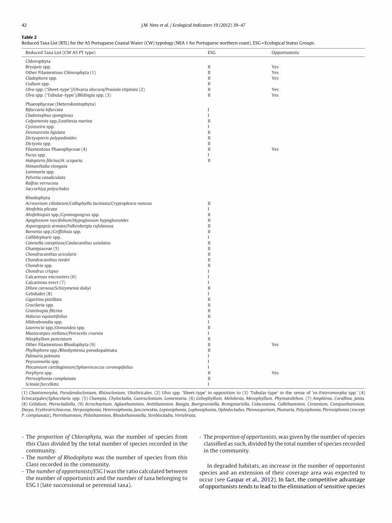
42 J.M. Neto et al. / Ecological Indicators 19 (2012) 39–47
Table 2Reduced Taxa List (RTL) for the A5 Portuguese Coastal Water (CW) typology (NEA 1 for Portuguese northern coast). ESG = Ecological Status Groups.
Reduced Taxa List (CW A5 PT type) ESG Opportunistic
ChlorophytaBryopsis spp. II YesOther Filamentous Chlorophyta (1) II YesCladophora spp. II YesCodium spp. IIUlva spp. (‘Sheet-type’)/Ulvaria obscura/Prasiola stipitata (2) II YesUlva spp. (‘Tubular-type’)/Blidingia spp. (3) II Yes
Phaeophyceae (Heterokontophyta)Bifurcaria bifurcata ICladostephus spongiosus IColpomenia spp./Leathesia marina IICystoseira spp. IDesmarestia ligulata IIDictyopteris polypodioides IIDictyota spp. IIFilamentous Phaeophyceae (4) II YesFucus spp. IHalopteris filicina/H. scoparia IIHimanthalia elongataLaminaria spp.Pelvetia canaliculataRalfsia verrucosaSaccorhiza polyschides
RhodophytaAcrosorium ciliolatum/Callophyllis laciniata/Cryptopleura ramosa IIAhnfeltia plicata IAhnfeltiopsis spp./Gymnogongrus spp. IIApoglossum ruscifolium/Hypoglossum hypoglossoides IIAsparagopsis armata/Falkenbergia rufolanosa IIBornetia spp./Griffithsia spp. IICalliblepharis spp. ICatenella caespitosa/Caulacanthus ustulatus IIChampiaceae (5) IIChondracanthus acicularis IIChondracanthus teedei IIChondria spp. IIChondrus crispus ICalcareous encrusters (6) ICalcareous erect (7) IDilsea carnosa/Schizymenia dubyi IIGelidiales (8) IGigartina pistillata IIGracilaria spp. IIGrateloupia filicina IIHalurus equisetifolius IIHildenbrandia spp. ILaurencia spp./Osmundea spp. IIMastocarpus stellatus/Petrocelis cruenta INitophyllum punctatum IIOther Filamentous Rhodophyta (9) II YesPhyllophora spp./Rhodymenia pseudopalmata IIPalmaria palmata IPeyssonnelia spp. IPlocamium cartilagineum/Sphaerococcus coronopifolius IPorphyra spp. II YesPterosiphonia complanata IIScinaia furcellata I
(1) Chaetomorpha, Pseudendoclonium, Rhizoclonium, Ulothricales. (2) Ulva spp. ‘Sheet-type’ in opposition to (3) ‘Tubular-type’ in the sense of ‘ex-Enteromorpha spp.’ (4)Ectocarpales/Sphacelaria spp. (5) Champia, Chylocladia, Gastroclonium, Lomentaria. (6) Lithophyllum, Melobesia, Mesophyllum, Phymatolithon. (7) Amphiroa, Corallina, Jania.(8) Gelidium, Pterocladiella. (9) Acrochaetium, Aglaothamnion, Antithamnion, Bangia, Boergeseniella, Brongniartella, Colaconema, Callithamnion, Ceramium, Compsothamnion,D LophoP rata.
-
-
-
asya, Erythrotrichiaceae, Herposiphonia, Heterosiphonia, Janczewskia, Leptosiphonia,
. complanata), Pterothamnion, Ptilothamnion, Rhodothamniella, Streblocladia, Verteb
The proportion of Chlorophyta, was the number of species fromthis Class divided by the total number of species recorded in thecommunity.
The number of Rhodophyta was the number of species from this
Class recorded in the community.The number of opportunists/ESG I was the ratio calculated betweenthe number of opportunists and the number of taxa belonging toESG I (late successional or perennial taxa).siphonia, Ophidocladus, Pleonosporium, Plumaria, Polysiphonia, Pterosiphonia (except
- The proportion of opportunists, was given by the number of speciesclassified as such, divided by the total number of species recordedin the community.
In degraded habitats, an increase in the number of opportunistspecies and an extension of their coverage area was expected tooccur (see Gaspar et al., 2012). In fact, the competitive advantageof opportunists tends to lead to the elimination of sensitive species
J.M. Neto et al. / Ecological Indicators 19 (2012) 39–47 43
Table 3Field sampling form for the shore descriptions.
General informationShore name DateWater body Tidal heightLatitude/Longitude Time of low tideShore descriptionsPresence of turbidity Yes = 0 Sand scour Yes = 0 No = 2(known to be non-anthropogenic) No = 2 Chalk shore Yes = 0 No = 2Dominant shore type SubhabitatsRock ridges/outcrops/platforms 4 Wide shallow rock poolsIrregular rock 3 (>3 m wide and <50 cm deep) 4Boulders large, medium and small 3 Large rockpools (>6 m long) 4Steep/vertical rock 2 Deep rockpools (50% >100 cm deep) 4Non-specific hard substrate 2 Basic rockpools 3Pebbles/stones/smallrocks 1 Large crevices 3Shingle/gravel 0 Large overhangs and vertical rock 2
Others habitats (please specify) 2Dominant biota Caves 1Ascophyllum None 0FucoidRhodophyta mosaics Total number of sub-habitatsChlorophyta >4 3 2 1 0MusselsBarnacles General commentsLimpetsPeriwinkles
Sum of categories’ scores N/A 15–18 12–14 8–11 1–7
A
asattp(
C
wmo
rMb
smcsFfptcmtefottd2
w
Shore description equivalent score 0
dapted from Wells et al. (2007).
nd to an increase in biomass and coverage area for r-selectedpecies. The coverage of opportunists (CO), expressed as a percent-ge, is given by the area covered by these taxa (only opportunisticaxa included in the RTL) in relation to the whole area covered byhe macroalgae (all species corresponded to 100% coverage). Eachhotographed replicate was analysed using the following formulaEq. (1)):
O(%) = QCO × 10016 − EQ
(1)
here QCO is the number of sub-quadrats with opportunisticacroalgae and EQ is the number of empty sub-quadrats. A res-
lution of ¼ of a sub-quadrat was used for the calculations.The CO was calculated as the arithmetic average of all of the
eplicates from a site. Because the CO is the only metric in the Mar-AT that accounts for abundance, one of the parameters required
y the WFD, it was double weighted (factor of 2).The objective of including a shore description metric was to make
hores with different substrata comparable and, consequently,ake different environmental conditions for macroalgae growth
omparable. Shore descriptions serve as a correction factor forpecies richness scores, which is a metric included in the MarMAT.or this purpose, Wells et al. (2007) proposed that a field samplingorm should be used to record basic shore descriptions during sam-ling visits (Table 3). The numbers on the sampling sheet attachedo each of the shore/habitat categories are based on how much theyontribute to the overall species richness (Wells et al., 2007). Infor-ation on the dominant biota, although it does not contribute to
he overall scoring system, may be useful in subsequent years toxplain ecological changes, if they occur (Wells et al., 2007). Scoresrom each of the categories were added together, and dependingn their range, an equivalent score (Table 3) was used to calculatehe final classification. Only the highest score was used to estimatehe sum of categories’ scores for categories with more than one
escription recorded (e.g., shore type and habitat type) (Wells et al.,007).The value of each of these metrics varied from 0 to 4; this rangeas divided into five intervals that corresponded to the five quality
1 2 3 4
classes, in accordance with the Normative Definitions (annex V inWFD) (WFD, 2000/60/EC): bad – 0, poor – 1, moderate – 2, good –3, and high – 4 (Table 4).
The scores of the different metrics were integrated to providean overall classification of the shore. For example, if 15 taxa werefound on a given shore, the shore received a score of 2 for speciesrichness (moderate); if the proportion of Chlorophyta on a givenshore was 0.15, the shore received a score of 3 (good) (Table 3). Thesum of the scores obtained for the different individual metrics wasintegrated in the ‘sum of scores’ (0–36).
The EQR (Eq. (2)) converts the ‘sum of scores’ values to a scalefrom 0 to 1, in accordance with the definition provided in the WFD(WFD, 2000/60/EC).
EQR = Sum of Scores36
(2)
EQR values close to 1 correspond to high quality ecological sta-tus, while EQR values close to 0 correspond to low quality ecologicalstatus. The 0–1 EQR interval is subsequently translated into the EQSclasses (bad, poor, moderate, good and high) using the boundariesprovided in Table 4.
2.4. Assessment of anthropogenic pressures
Three indicators were considered to be proxies of anthropogenicpressures that may influence the sampling sites: (a) urban landuse (represented by the number of inhabitants); (b) industrial landuse; and (c) agricultural, forest and fishing areas (sensu the LandUses Simplified Index (LUSI); Royo et al., 2009). This method ofassessing the anthropogenic pressures that affect coastal areas wasbased on pressures identified from land, which may be related toimpacts (e.g., macroalgal communities degradation) observed inthese zones.
Pressures were calculated from information available from theNational Institute of Statistics (http://www.ine.pt) for the study
period and were scored from 1 to 4 following the criteria shownin Table 5. Eight sites were analysed; the locations (cities) consid-ered to have a significant influence on the anthropogenic pressurelevel for each site are shown in Table 1.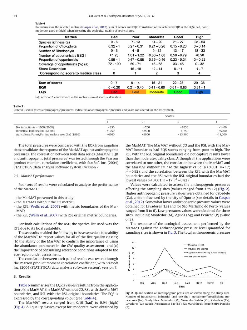
44 J.M. Neto et al. / Ecological Indicators 19 (2012) 39–47
Table 4Boundaries for the selected metrics (Gaspar et al., 2012), sum of scores and EQR. Translation of the achieved EQR in the EQS (bad, poor,moderate, good or high) when assessing the ecological quality of rocky shores.
(a) Factor of 2, counts twice in the metrics sum of scores calculation.
Table 5Criteria used to assess anthropogenic pressures. Indicators of anthropogenic pressure and years considered for the assessment.
Scores
1 2 3 4
spapS
2
o
---
-
R
o(tte
tI
3
tbe
(
of 3).The response of the ecological assessment performed by the
MarMAT against the anthropogenic pressure level quantified forsampling sites is shown in Fig. 3. The total anthropogenic pressure
No. inhabitants × 1000 (2008) <350Industrial land use (ha) (2008) <1250
Agriculture/Forest/Fishing surface area (ha) (1999) <4500
The total pressures were compared with the EQR from samplingites to validate the response of the MarMAT against anthropogenicressures. The correlation between both data series (MarMAT EQRnd anthropogenic total pressures) was tested through the Pearsonroduct moment correlation coefficient, with StatSoft Inc. (2004)TATISTICA (data analysis software system), version 7.
.5. MarMAT performance
Four sets of results were calculated to analyse the performancef the MarMAT:
the MarMAT presented in this study;the MarMAT without the CO metric;
the RSL (Wells et al., 2007) with metric boundaries of the Mar-MAT;
the RSL (Wells et al., 2007) with RSL original metric boundaries.
For both calculations of the RSL, the species list used was theTL due to its local suitability.
These results enabled the following to be assessed: (a) the abilityf the MarMAT to report values for all of the five quality classes;b) the ability of the MarMAT to confirm the importance of usinghe abundance parameter in the CW quality assessment; and (c)he importance of considering reference conditions adapted to theco-region under assessment.
The correlation between each pair of results was tested throughhe Pearson product moment correlation coefficient, with StatSoftnc. (2004) STATISTICA (data analysis software system), version 7.
. Results
Table 6 summarises the EQR’s values resulting from the applica-ion of the MarMAT, the MarMAT without CO, RSL with the MarMAT
oundaries, and RSL with the RSL original boundaries. The EQS isxpressed by the corresponding colour (see Table 4).The MarMAT results ranged from 0.19 (bad) to 0.94 (high)Fig. 4). All quality classes except for ‘moderate’ were obtained by
<700 <1050 <1400<2500 <3750 <5000<9000 <13,500 <18,000
the MarMAT. The MarMAT without CO and the RSL with the Mar-MAT boundaries had EQS scores ranging from poor to high. TheRSL with the RSL original boundaries did not capture results lowerthan the moderate quality class. Although all the applications werecorrelated to one other, the correlation between the MarMAT andthe MarMAT without CO had the highest value (p < 0.001; n = 17;r2 = 0.92), and the correlation between the RSL with the MarMATboundaries and the RSL with the RSL original boundaries had thelowest value (p < 0.001; n = 17; r2 = 0.82).
Values were calculated to assess the anthropogenic pressuresaffecting the sampling sites (values ranged from 3 to 12) (Fig. 2).Higher anthropogenic pressure values were obtained for Cabedelo(Ca), a site influenced by the city of Oporto (see details in Gasparet al., 2012). Somewhat lower anthropogenic pressure values wereobtained for Lavadores (La) and for São Martinho do Porto (valuesranged from 5 to 6). Low pressures values were obtained for threesites, including Montedor (M), Aguda (Ag) and Peniche (P) (value
Fig. 2. Quantification of anthropogenic pressures observed along the study area.Number of inhabitants; industrial land use (ha); agriculture/forest/fishing sur-face area (ha). Study sites: Montedor (M); Viana do Castelo (VC); Cabedelo (Ca);Lavadores (La); Aguda (Ag); Buarcos Bay (BB); São Martinho do Porto (SMP); Peniche(P).
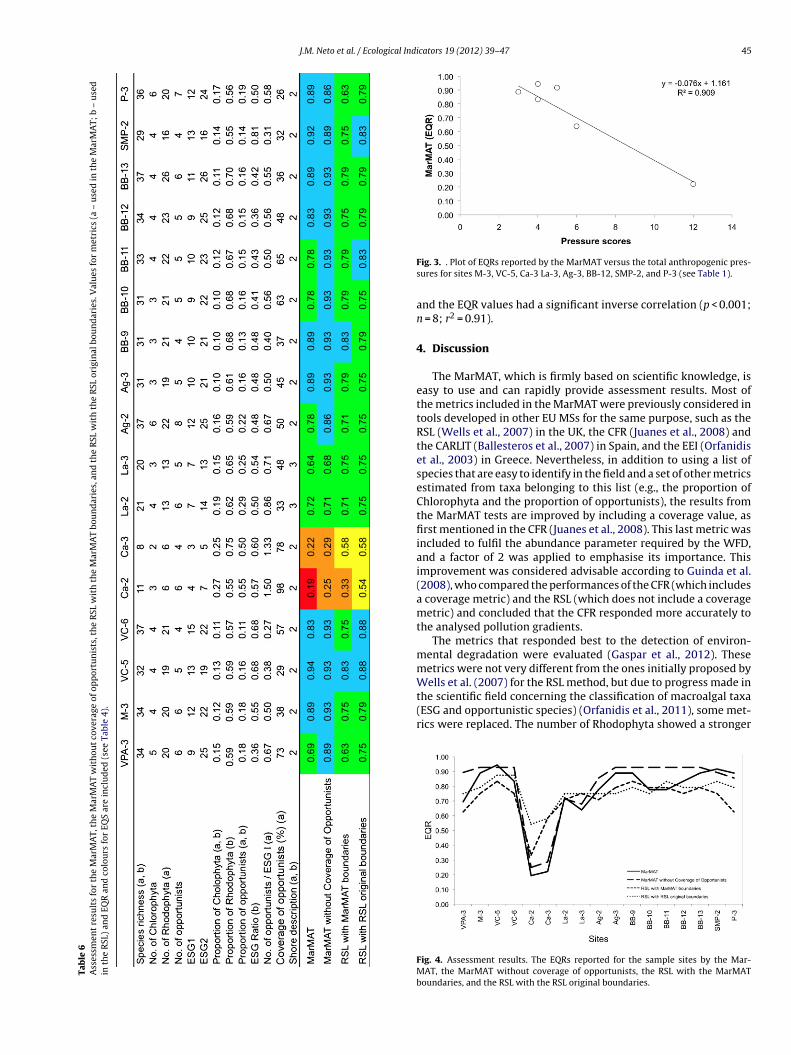
J.M. Neto et al. / Ecological Indicators 19 (2012) 39–47 45
Tab
le
6A
sses
smen
t
resu
lts
for
the
Mar
MA
T,
the
Mar
MA
T
wit
hou
t
cove
rage
of
opp
ortu
nis
ts, t
he
RSL
wit
h
the
Mar
MA
T
bou
nd
arie
s,
and
the
RSL
wit
h
the
RSL
orig
inal
bou
nd
arie
s.
Val
ues
for
met
rics
(a
–u
sed
in
the
Mar
MA
T;
b
–u
sed
in
the
RSL
)
and
EQR
and
colo
urs
for
EQS
are
incl
ud
ed
(see
Tabl
e
4).
Fig. 3. . Plot of EQRs reported by the MarMAT versus the total anthropogenic pres-sures for sites M-3, VC-5, Ca-3 La-3, Ag-3, BB-12, SMP-2, and P-3 (see Table 1).
and the EQR values had a significant inverse correlation (p < 0.001;n = 8; r2 = 0.91).
4. Discussion
The MarMAT, which is firmly based on scientific knowledge, iseasy to use and can rapidly provide assessment results. Most ofthe metrics included in the MarMAT were previously considered intools developed in other EU MSs for the same purpose, such as theRSL (Wells et al., 2007) in the UK, the CFR (Juanes et al., 2008) andthe CARLIT (Ballesteros et al., 2007) in Spain, and the EEI (Orfanidiset al., 2003) in Greece. Nevertheless, in addition to using a list ofspecies that are easy to identify in the field and a set of other metricsestimated from taxa belonging to this list (e.g., the proportion ofChlorophyta and the proportion of opportunists), the results fromthe MarMAT tests are improved by including a coverage value, asfirst mentioned in the CFR (Juanes et al., 2008). This last metric wasincluded to fulfil the abundance parameter required by the WFD,and a factor of 2 was applied to emphasise its importance. Thisimprovement was considered advisable according to Guinda et al.(2008), who compared the performances of the CFR (which includesa coverage metric) and the RSL (which does not include a coveragemetric) and concluded that the CFR responded more accurately tothe analysed pollution gradients.
The metrics that responded best to the detection of environ-mental degradation were evaluated (Gaspar et al., 2012). Thesemetrics were not very different from the ones initially proposed by
Wells et al. (2007) for the RSL method, but due to progress made inthe scientific field concerning the classification of macroalgal taxa(ESG and opportunistic species) (Orfanidis et al., 2011), some met-rics were replaced. The number of Rhodophyta showed a strongerFig. 4. Assessment results. The EQRs reported for the sample sites by the Mar-MAT, the MarMAT without coverage of opportunists, the RSL with the MarMATboundaries, and the RSL with the RSL original boundaries.
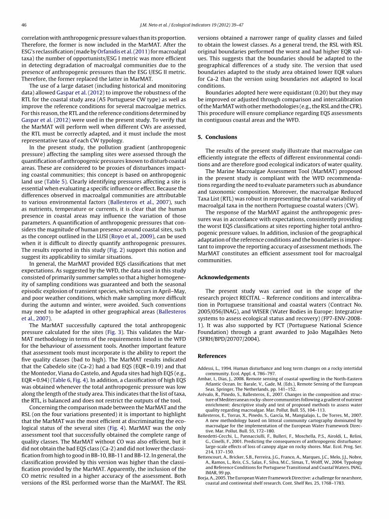
4 al Ind
cTEtipT
dRiFGttr
pqailedtappsawTs
ecieadme
pMftfittEwat
RtlaqdficfiCv
6 J.M. Neto et al. / Ecologic
orrelation with anthropogenic pressure values than its proportion.herefore, the former is now included in the MarMAT. After theSG’s reclassification (made by Orfanidis et al. (2011) for macroalgalaxa) the number of opportunists/ESG I metric was more efficientn detecting degradation of macroalgal communities due to theresence of anthropogenic pressures than the ESG I/ESG II metric.herefore, the former replaced the latter in MarMAT.
The use of a large dataset (including historical and monitoringata) allowed Gaspar et al. (2012) to improve the robustness of theTL for the coastal study area (A5 Portuguese CW type) as well as
mprove the reference conditions for several macroalgae metrics.or this reason, the RTL and the reference conditions determined byaspar et al. (2012) were used in the present study. To verify that
he MarMAT will perform well when different CWs are assessed,he RTL must be correctly adapted, and it must include the mostepresentative taxa of each CW typology.
In the present study, the pollution gradient (anthropogenicressure) affecting the sampling sites were assessed through theuantification of anthropogenic pressures known to disturb coastalreas. These are considered to be proxies of disturbances impact-ng coastal communities; this concept is based on anthropogenicand use (Table 5). Clearly identifying pressures affecting a site isssential when evaluating a specific influence or effect. Because theifferences observed in macroalgal communities are attributableo various environmental factors (Ballesteros et al., 2007), suchs nutrients, temperature or currents, it is clear that the humanresence in coastal areas may influence the variation of thosearameters. A quantification of anthropogenic pressures that con-iders the magnitude of human presence around coastal sites, suchs the concept outlined in the LUSI (Royo et al., 2009), can be usedhen it is difficult to directly quantify anthropogenic pressures.
he results reported in this study (Fig. 2) support this notion anduggest its applicability to similar situations.
In general, the MarMAT provided EQS classifications that metxpectations. As suggested by the WFD, the data used in this studyonsisted of primarily summer samples so that a higher homogene-ty of sampling conditions was guaranteed and both the seasonalpisodic explosion of transient species, which occurs in April–May,nd poor weather conditions, which make sampling more difficulturing the autumn and winter, were avoided. Such conventionsay need to be adapted in other geographical areas (Ballesteros
t al., 2007).The MarMAT successfully captured the total anthropogenic
ressure calculated for the sites (Fig. 3). This validates the Mar-AT methodology in terms of the requirements listed in the WFD
or the behaviour of assessment tools. Another important featurehat assessment tools must incorporate is the ability to report theve quality classes (bad to high). The MarMAT results indicatedhat the Cabedelo site (Ca-2) had a bad EQS (EQR = 0.19) and thathe Montedor, Viana do Castelo, and Aguda sites had high EQS (e.g.,QR = 0.94) (Table 6, Fig. 4). In addition, a classification of high EQSas obtained whenever the total anthropogenic pressure was low
long the length of the study area. This indicates that the list of taxa,he RTL, is balanced and does not restrict the outputs of the tool.
Concerning the comparison made between the MarMAT and theSL (on the four variations presented) it is important to highlighthat the MarMAT was the most efficient at discriminating the eco-ogical status of the several sites (Fig. 4). MarMAT was the onlyssessment tool that successfully obtained the complete range ofuality classes. The MarMAT without CO was also efficient, but itid not obtain the bad EQS class (Ca-2) and did not lower the classi-cation from high to good in BB-10, BB-11 and BB-12. In general, the
lassification provided by this version was higher than the classi-cation provided by the MarMAT. Apparently, the inclusion of theO metric resulted in a higher accuracy of the assessment. Bothersions of the RSL performed worse than the MarMAT. The RSLicators 19 (2012) 39–47
versions obtained a narrower range of quality classes and failedto obtain the lowest classes. As a general trend, the RSL with RSLoriginal boundaries performed the worst and had higher EQR val-ues. This suggests that the boundaries should be adapted to thegeographical differences of a study site. The version that usedboundaries adapted to the study area obtained lower EQR valuesfor Ca-2 than the version using boundaries not adapted to localconditions.
Boundaries adopted here were equidistant (0.20) but they maybe improved or adjusted through comparison and intercalibrationof the MarMAT with other methodologies (e.g., the RSL and the CFR).This procedure will ensure compliance regarding EQS assessmentsin contiguous coastal areas and the WFD.
5. Conclusions
The results of the present study illustrate that macroalgae canefficiently integrate the effects of different environmental condi-tions and are therefore good ecological indicators of water quality.
The Marine Macroalgae Assessment Tool (MarMAT) proposedin the present study is compliant with the WFD recommenda-tions regarding the need to evaluate parameters such as abundanceand taxonomic composition. Moreover, the macroalgae ReducedTaxa List (RTL) was robust in representing the natural variability ofmacroalgal taxa in the northern Portuguese coastal waters (CW).
The response of the MarMAT against the anthropogenic pres-sures was in accordance with expectations, consistently providingthe worst EQS classifications at sites reporting higher total anthro-pogenic pressure values. In addition, inclusion of the geographicaladaptation of the reference conditions and the boundaries is impor-tant to improve the reporting accuracy of assessment methods. TheMarMAT constitutes an efficient assessment tool for macroalgalcommunities.
Acknowledgements
The present study was carried out in the scope of theresearch project RECITAL – Reference conditions and intercalibra-tion in Portuguese transitional and coastal waters (Contract No.2005/056/INAG), and WISER (Water Bodies in Europe: Integrativesystems to assess ecological status and recovery) (FP7-ENV-2008-1). It was also supported by FCT (Portuguese National ScienceFoundation) through a grant awarded to João Magalhães Neto(SFRH/BPD/20707/2004).
References
Addessi, L., 1994. Human disturbance and long term changes on a rocky intertidalcommunity. Ecol. Appl. 4, 786–797.
Ambar, I., Dias, J., 2008. Remote sensing of coastal upwelling in the North-EasternAtlantic Ocean. In: Barale, V., Gade, M. (Eds.), Remote Sensing of the EuropeanSeas. Springer, The Netherlands, pp. 141–152.
Arévalo, R., Pinedo, S., Ballesteros, E., 2007. Changes in the composition and struc-ture of Mediterranean rocky-shore communities following a gradient of nutrientenrichment: descriptive study and test of proposed methods to assess waterquality regarding macroalgae. Mar. Pollut. Bull. 55, 104–113.
Ballesteros, E., Torras, X., Pinedo, S., García, M., Mangialajo, L., De Torres, M., 2007.A new methodology based on littoral community cartography dominated bymacroalgae for the implementation of the European Water Framework Direc-tive. Mar. Pollut. Bull. 55, 172–180.
Benedetti-Cecchi, L., Pannacciulli, F., Bulleri, F., Moschella, P.S., Airoldi, L., Relini,G., Cinelli, F., 2001. Predicting the consequences of anthropogenic disturbance:large-scale effects of loss of canopy algae on rocky shores. Mar. Ecol. Prog. Ser.214, 137–150.
Bettencourt, A., Bricker, S.B., Ferreira, J.G., Franco, A., Marques, J.C., Melo, J.J., Nobre,
A., Ramos, L., Reis, C.S., Salas, F., Silva, M.C., Simas, T., Wolff, W., 2004. Typologyand Reference Conditions for Portuguese Transitional and Coastal Waters. INAG.IMAR, 99 pp.Borja, A., 2005. The European Water Framework Directive: a challenge for nearshore,coastal and continental shelf research. Cont. Shelf Res. 25, 1768–1783.
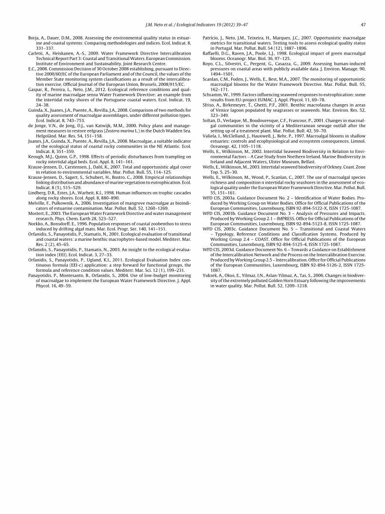
al Indi
B
C
E
G
G
d
J
K
K
K
L
M
M
N
O
O
O
P
J.M. Neto et al. / Ecologic
orja, A., Dauer, D.M., 2008. Assessing the environmental quality status in estuar-ine and coastal systems: Comparing methodologies and indices. Ecol. Indicat. 8,331–337.
arletii, A., Heiskanen, A.-S., 2009. Water Framework Directive IntercalibrationTechnical Report Part 3: Coastal and Transitional Waters. European Commission.Institute of Environment and Sustainability. Joint Research Centre.
.C., 2008. Commission Decision of 30 October 2008 establishing, pursuant to Direc-tive 2000/60/EC of the European Parliament and of the Council, the values of theMember State monitoring system classifications as a result of the intercalibra-tion exercise. Official Journal of the European Union, Brussels, 2008/915/EC.
aspar, R., Pereira, L., Neto, J.M., 2012. Ecological reference conditions and qual-ity of marine macroalgae sensu Water Framework Directive: an example fromthe intertidal rocky shores of the Portuguese coastal waters. Ecol. Indicat. 19,24–38.
uinda, X., Juanes, J.A., Puente, A., Revilla, J.A., 2008. Comparison of two methods forquality assessment of macroalgae assemblages, under different pollution types.Ecol. Indicat. 8, 743–753.
e Jonge, V.N., de Jong, D.J., van Katwijk, M.M., 2000. Policy plans and manage-ment measures to restore eelgrass (Zostera marina L.) in the Dutch Wadden Sea.Helgoländ. Mar. Res. 54, 151–158.
uanes, J.A., Guinda, X., Puente, A., Revilla, J.A., 2008. Macroalgae, a suitable indicatorof the ecological status of coastal rocky communities in the NE Atlantic. Ecol.Indicat. 8, 351–359.
eough, M.J., Quinn, G.P., 1998. Effects of periodic disturbances from trampling onrocky intertidal algal beds. Ecol. Appl. 8, 141–161.
rause-Jensen, D., Carstensen, J., Dahl, K., 2007. Total and opportunistic algal coverin relation to environmental variables. Mar. Pollut. Bull. 55, 114–125.
rause-Jensen, D., Sagert, S., Schubert, H., Bostro, C., 2008. Empirical relationshipslinking distribution and abundance of marine vegetation to eutrophication. Ecol.Indicat. 8 (5), 515–529.
indberg, D.R., Estes, J.A., Warheit, K.I., 1998. Human influences on trophic cascadesalong rocky shores. Ecol. Appl. 8, 880–890.
elville, F., Pulkownik, A., 2006. Investigation of mangrove macroalgae as bioindi-cators of estuarine contamination. Mar. Pollut. Bull. 52, 1260–1269.
ostert, E., 2003. The European Water Framework Directive and water managementresearch. Phys. Chem. Earth 28, 523–527.
orkko, A., Bonsdorff, E., 1996. Population responses of coastal zoobenthos to stressinduced by drifting algal mats. Mar. Ecol. Progr. Ser. 140, 141–151.
rfanidis, S., Panayotidis, P., Stamatis, N., 2001. Ecological evaluation of transitionaland coastal waters: a marine benthic macrophytes-based model. Mediterr. Mar.Res. 2 (2), 45–65.
rfanidis, S., Panayotidis, P., Stamatis, N., 2003. An insight to the ecological evalua-tion index (EEI). Ecol. Indicat. 3, 27–33.
rfanidis, S., Panayotidis, P., Ugland, K.I., 2011. Ecological Evaluation Index con-
tinuous formula (EEI-c) application: a step forward for functional groups, theformula and reference condition values. Mediterr. Mar. Sci. 12 (1), 199–231.anayotidis, P., Montesanto, B., Orfanidis, S., 2004. Use of low-budget monitoringof macroalgae to implement the European Water Framework Directive. J. Appl.Phycol. 16, 49–59.
cators 19 (2012) 39–47 47
Patrício, J., Neto, J.M., Teixeira, H., Marques, J.C., 2007. Opportunistic macroalgaemetrics for transitional waters. Testing tools to assess ecological quality statusin Portugal. Mar. Pollut. Bull. 54 (12), 1887–1896.
Raffaelli, D.G., Raven, J.A., Poole, L.J., 1998. Ecological impact of green macroalgalblooms. Oceanogr. Mar. Biol. 36, 97–125.
Royo, C.L., Silvestri, C., Pergent, G., Casazza, G., 2009. Assessing human-inducedpressures on coastal areas with publicly available data. J. Environ. Manage. 90,1494–1501.
Scanlan, C.M., Foden, J., Wells, E., Best, M.A., 2007. The monitoring of opportunisticmacroalgal blooms for the Water Framework Directive. Mar. Pollut. Bull. 55,162–171.
Schramm, W., 1999. Factors influencing seaweed responses to eutrophication: someresults from EU-project EUMAC. J. Appl. Phycol. 11, 69–78.
Sfriso, A., Birkemeyer, T., Ghetti, P.F., 2001. Benthic macrofauna changes in areasof Venice lagoon populated by seagrasses or seaweeds. Mar. Environ. Res. 52,323–349.
Soltan, D., Verlaque, M., Boudouresque, C.F., Francour, P., 2001. Changes in macroal-gal communities in the vicinity of a Mediterranean sewage outfall after thesetting up of a treatment plant. Mar. Pollut. Bull. 42, 59–70.
Valiela, I., McClelland, J., Hauxwell, J., Behr, P., 1997. Macroalgal blooms in shallowestuaries: controls and ecophysiological and ecosystem consequences. Limnol.Oceanogr. 42, 1105–1118.
Wells, E., Wilkinson, M., 2002. Intertidal Seaweed Biodiversity in Relation to Envi-ronmental Factors – A Case Study from Northern Ireland. Marine Biodiversity inIreland and Adjacent Waters, Ulster Museum, Belfast.
Wells, E., Wilkinson, M., 2003. Intertidal seaweed biodiversity of Orkney. Coast. ZoneTop. 5, 25–30.
Wells, E., Wilkinson, M., Wood, P., Scanlan, C., 2007. The use of macroalgal speciesrichness and composition n intertidal rocky seashores in the assessment of eco-logical quality under the European Water Framework Directive. Mar. Pollut. Bull.55, 151–161.
WFD CIS, 2003a. Guidance Document No. 2 – Identification of Water Bodies. Pro-duced by Working Group on Water Bodies. Office for Official Publications of theEuropean Communities, Luxembourg, ISBN 92-894-5122-X, ISSN 1725-1087.
WFD CIS, 2003b. Guidance Document No. 3 – Analysis of Pressures and Impacts.Produced by Working Group 2.1 – IMPRESS. Office for Official Publications of theEuropean Communities, Luxembourg, ISBN 92-894-5123-8, ISSN 1725-1087.
WFD CIS, 2003c. Guidance Document No. 5 – Transitional and Coastal Waters– Typology, Reference Conditions and Classification Systems. Produced byWorking Group 2.4 – COAST. Office for Official Publications of the EuropeanCommunities, Luxembourg, ISBN 92-894-5125-4, ISSN 1725-1087.
WFD CIS, 2003d. Guidance Document No. 6 – Towards a Guidance on Establishmentof the Intercalibration Network and the Process on the Intercalibration Exercise.Produced by Working Group 2.5 – Intercalibration. Office for Official Publications
of the European Communities, Luxembourg, ISBN 92-894-5126-2, ISSN 1725-1087.Yuksek, A., Okus, E., Yilmaz, I.N., Aslan-Yilmaz, A., Tas, S., 2006. Changes in biodiver-sity of the extremely polluted Golden Horn Estuary following the improvementsin water quality. Mar. Pollut. Bull. 52, 1209–1218.
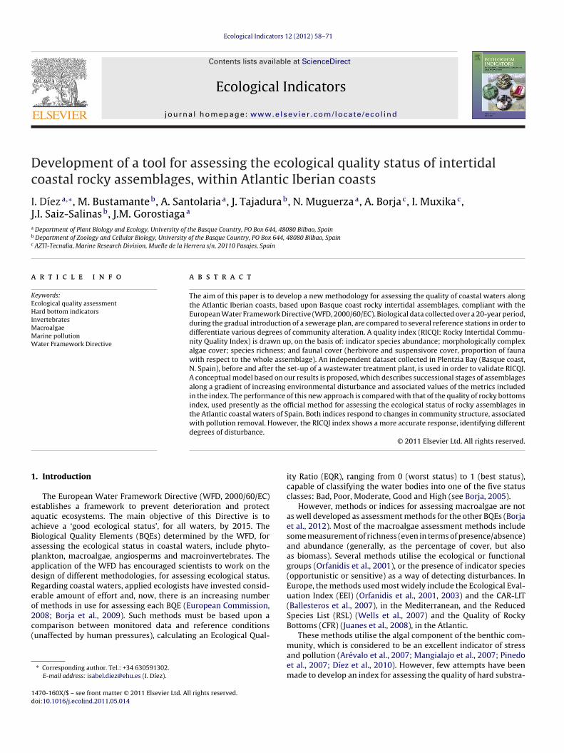
Dc
IJa
b
c
a
KEHIMMW
1
eaaBapadReo2c(
1d
Ecological Indicators 12 (2012) 58–71
Contents lists available at ScienceDirect
Ecological Indicators
journa l homepage: www.e lsev ier .com/ locate /eco l ind
evelopment of a tool for assessing the ecological quality status of intertidaloastal rocky assemblages, within Atlantic Iberian coasts
. Díeza,∗, M. Bustamanteb, A. Santolariaa, J. Tajadurab, N. Muguerzaa, A. Borjac, I. Muxikac,
.I. Saiz-Salinasb, J.M. Gorostiagaa
Department of Plant Biology and Ecology, University of the Basque Country, PO Box 644, 48080 Bilbao, SpainDepartment of Zoology and Cellular Biology, University of the Basque Country, PO Box 644, 48080 Bilbao, SpainAZTI-Tecnalia, Marine Research Division, Muelle de la Herrera s/n, 20110 Pasajes, Spain
r t i c l e i n f o
eywords:cological quality assessmentard bottom indicators
nvertebratesacroalgaearine pollutionater Framework Directive
a b s t r a c t
The aim of this paper is to develop a new methodology for assessing the quality of coastal waters alongthe Atlantic Iberian coasts, based upon Basque coast rocky intertidal assemblages, compliant with theEuropean Water Framework Directive (WFD, 2000/60/EC). Biological data collected over a 20-year period,during the gradual introduction of a sewerage plan, are compared to several reference stations in order todifferentiate various degrees of community alteration. A quality index (RICQI: Rocky Intertidal Commu-nity Quality Index) is drawn up, on the basis of: indicator species abundance; morphologically complexalgae cover; species richness; and faunal cover (herbivore and suspensivore cover, proportion of faunawith respect to the whole assemblage). An independent dataset collected in Plentzia Bay (Basque coast,N. Spain), before and after the set-up of a wastewater treatment plant, is used in order to validate RICQI.A conceptual model based on our results is proposed, which describes successional stages of assemblages
along a gradient of increasing environmental disturbance and associated values of the metrics includedin the index. The performance of this new approach is compared with that of the quality of rocky bottomsindex, used presently as the official method for assessing the ecological status of rocky assemblages inthe Atlantic coastal waters of Spain. Both indices respond to changes in community structure, associatedwith pollution removal. However, the RICQI index shows a more accurate response, identifying differentdegrees of disturbance.. Introduction
The European Water Framework Directive (WFD, 2000/60/EC)stablishes a framework to prevent deterioration and protectquatic ecosystems. The main objective of this Directive is tochieve a ‘good ecological status’, for all waters, by 2015. Theiological Quality Elements (BQEs) determined by the WFD, forssessing the ecological status in coastal waters, include phyto-lankton, macroalgae, angiosperms and macroinvertebrates. Thepplication of the WFD has encouraged scientists to work on theesign of different methodologies, for assessing ecological status.egarding coastal waters, applied ecologists have invested consid-rable amount of effort and, now, there is an increasing numberf methods in use for assessing each BQE (European Commission,
008; Borja et al., 2009). Such methods must be based upon aomparison between monitored data and reference conditionsunaffected by human pressures), calculating an Ecological Qual-∗ Corresponding author. Tel.: +34 630591302.E-mail address: [email protected] (I. Díez).
470-160X/$ – see front matter © 2011 Elsevier Ltd. All rights reserved.oi:10.1016/j.ecolind.2011.05.014
© 2011 Elsevier Ltd. All rights reserved.
ity Ratio (EQR), ranging from 0 (worst status) to 1 (best status),capable of classifying the water bodies into one of the five statusclasses: Bad, Poor, Moderate, Good and High (see Borja, 2005).
However, methods or indices for assessing macroalgae are notas well developed as assessment methods for the other BQEs (Borjaet al., 2012). Most of the macroalgae assessment methods includesome measurement of richness (even in terms of presence/absence)and abundance (generally, as the percentage of cover, but alsoas biomass). Several methods utilise the ecological or functionalgroups (Orfanidis et al., 2001), or the presence of indicator species(opportunistic or sensitive) as a way of detecting disturbances. InEurope, the methods used most widely include the Ecological Eval-uation Index (EEI) (Orfanidis et al., 2001, 2003) and the CAR-LIT(Ballesteros et al., 2007), in the Mediterranean, and the ReducedSpecies List (RSL) (Wells et al., 2007) and the Quality of RockyBottoms (CFR) (Juanes et al., 2008), in the Atlantic.
These methods utilise the algal component of the benthic com-
munity, which is considered to be an excellent indicator of stressand pollution (Arévalo et al., 2007; Mangialajo et al., 2007; Pinedoet al., 2007; Díez et al., 2010). However, few attempts have beenmade to develop an index for assessing the quality of hard substra-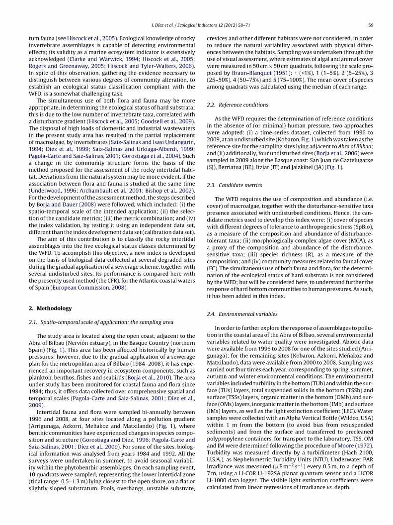
l Indic
tieaRIdeW
ataTio1Pamta(Fbsttd
atodsto
2
2
ASpprpu1t2
1(bsSisi1(s
I. Díez et al. / Ecologica
um fauna (see Hiscock et al., 2005). Ecological knowledge of rockynvertebrate assemblages is capable of detecting environmentalffects; its validity as a marine ecosystem indicator is extensivelycknowledged (Clarke and Warwick, 1994; Hiscock et al., 2005;ogers and Greenaway, 2005; Hiscock and Tyler-Walters, 2006).
n spite of this observation, gathering the evidence necessary toistinguish between various degrees of community alteration, tostablish an ecological status classification compliant with theFD, is a somewhat challenging task.The simultaneous use of both flora and fauna may be more
ppropriate, in determining the ecological status of hard substrata;his is due to the low number of invertebrate taxa, correlated withdisturbance gradient (Hiscock et al., 2005; Goodsell et al., 2009).he disposal of high loads of domestic and industrial wastewatersn the present study area has resulted in the partial replacementf macroalgae, by invertebrates (Saiz-Salinas and Isasi Urdangarin,994; Díez et al., 1999; Saiz-Salinas and Urkiaga-Alberdi, 1999;agola-Carte and Saiz-Salinas, 2001; Gorostiaga et al., 2004). Suchchange in the community structure forms the basis of theethod proposed for the assessment of the rocky intertidal habi-
at. Deviations from the natural system may be more evident, if thessociation between flora and fauna is studied at the same timeUnderwood, 1996; Archambault et al., 2001; Bishop et al., 2002).or the development of the assessment method, the steps describedy Borja and Dauer (2008) were followed, which included: (i) thepatio-temporal scale of the intended application; (ii) the selec-ion of the candidate metrics; (iii) the metric combination; and (iv)he index validation, by testing it using an independent data set,ifferent than the index development data set (calibration data set).
The aim of this contribution is to classify the rocky intertidalssemblages into the five ecological status classes determined byhe WFD. To accomplish this objective, a new index is developedn the basis of biological data collected at several degraded sitesuring the gradual application of a sewerage scheme, together witheveral undisturbed sites. Its performance is compared here withhe presently used method (the CFR), for the Atlantic coastal watersf Spain (European Commission, 2008).
. Methodology
.1. Spatio-temporal scale of application: the sampling area
The study area is located along the open coast, adjacent to thebra of Bilbao (Nervión estuary), in the Basque Country (northernpain) (Fig. 1). This area has been affected historically by humanressures; however, due to the gradual application of a seweragelan for the metropolitan area of Bilbao (1984–2008), it has expe-ienced an important recovery in ecosystem components, such aslankton, benthos, fishes and seabirds (Borja et al., 2010). The areander study has been monitored for coastal fauna and flora since984; thus, it offers data collected over comprehensive spatial andemporal scales (Pagola-Carte and Saiz-Salinas, 2001; Díez et al.,009).
Intertidal fauna and flora were sampled bi-annually between996 and 2008, at four sites located along a pollution gradientArrigunaga, Azkorri, Menakoz and Matxilando) (Fig. 1), whereenthic communities have experienced changes in species compo-ition and structure (Gorostiaga and Díez, 1996; Pagola-Carte andaiz-Salinas, 2001; Díez et al., 2009). For some of the sites, biolog-cal information was analysed from years 1984 and 1992. All theurveys were undertaken in summer, to avoid seasonal variabil-
ty within the phytobenthic assemblages. On each sampling event,0 quadrats were sampled, representing the lower intertidal zonetidal range: 0.5–1.3 m) lying closest to the open shore, on a flat orlightly sloped substratum. Pools, overhangs, unstable substrate,ators 12 (2012) 58–71 59
crevices and other different habitats were not considered, in orderto reduce the natural variability associated with physical differ-ences between the habitats. Sampling was undertaken through theuse of visual assessment, where estimates of algal and animal coverwere measured in 50 cm × 50 cm quadrats, following the scale pro-posed by Braun-Blanquet (1951): + (<1%), 1 (1–5%), 2 (5–25%), 3(25–50%), 4 (50–75%) and 5 (75–100%). The mean cover of speciesamong quadrats was calculated using the median of each range.
2.2. Reference conditions
As the WFD requires the determination of reference conditionsin the absence of (or minimal) human pressure, two approacheswere adopted: (i) a time-series dataset, collected from 1996 to2009, at an undisturbed site (Kobaron, Fig. 1) which was taken as thereference site for the sampling sites lying adjacent to Abra of Bilbao;and (ii) additionally, four undisturbed sites (Borja et al., 2006) weresampled in 2009 along the Basque coast: San Juan de Gaztelugatxe(SJ), Berriatua (BE), Itziar (IT) and Jaizkibel (JA) (Fig. 1).
2.3. Candidate metrics
The WFD requires the use of composition and abundance (i.e.cover) of macroalgae, together with the disturbance-sensitive taxapresence associated with undisturbed conditions. Hence, the can-didate metrics used to develop this index were: (i) cover of specieswith different degrees of tolerance to anthropogenic stress (SpBio),as a measure of the composition and abundance of disturbance-tolerant taxa; (ii) morphologically complex algae cover (MCA), asa proxy of the composition and abundance of the disturbance-sensitive taxa; (iii) species richness (R), as a measure of thecomposition; and (iv) community measures related to faunal cover(FC). The simultaneous use of both fauna and flora, for the determi-nation of the ecological status of hard substrata is not consideredby the WFD; but will be considered here, to understand further theresponse of hard bottom communities to human pressures. As such,it has been added in this index.
2.4. Environmental variables
In order to further explore the response of assemblages to pollu-tion in the coastal area of the Abra of Bilbao, several environmentalvariables related to water quality were investigated. Abiotic datawere available from 1996 to 2008 for one of the sites studied (Arri-gunaga); for the remaining sites (Kobaron, Azkorri, Menakoz andMatxilando), data were available from 2000 to 2008. Sampling wascarried out four times each year, corresponding to spring, summer,autumn and winter environmental conditions. The environmentalvariables included turbidity in the bottom (TUb) and within the sur-face (TUs) layers, total suspended solids in the bottom (TSSb) andsurface (TSSs) layers, organic matter in the bottom (OMb) and sur-face (OMs) layers, inorganic matter in the bottom (IMb) and surface(IMs) layers, as well as the light extinction coefficient (LEC). Watersamples were collected with an Alpha Vertical Bottle (Wildco, USA)within 1 m from the bottom (to avoid bias from resuspendedsediments) and from the surface and transferred to precleanedpolypropylene containers, for transport to the laboratory. TSS, OMand IM were determined following the procedure of Moore (1972).Turbidity was measured directly by a turbidimeter (Hach 2100,U.S.A.), as Nephelometric Turbidity Units (NTU). Underwater PAR
irradiance was measured (E m−2 s−1) every 0.5 m, to a depth of7 m, using a LI-COR LI-192SA planar quantum sensor and a LICORLI-1000 data logger. The visible light extinction coefficients werecalculated from linear regressions of irradiance vs. depth.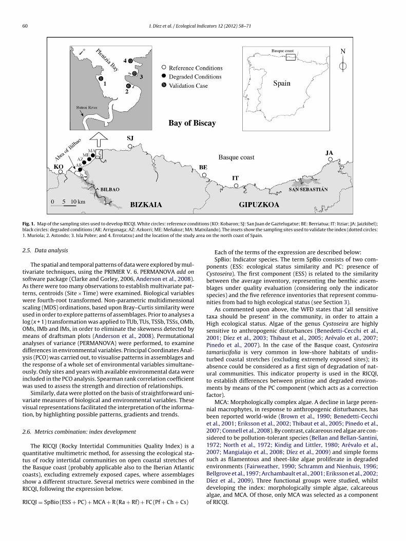
60 I. Díez et al. / Ecological Indicators 12 (2012) 58–71
F ditionb Matxi1 area o
2
tsAtwsulOmadytoiw
vvt
2
qttcsR
R
ig. 1. Map of the sampling sites used to develop RICQI. White circles: reference conlack circles: degraded conditions (AR: Arrigunaga; AZ: Azkorri; ME: Menakoz; MA:. Muriola; 2. Astondo; 3. Isla Pobre; and 4. Errotatxu) and the location of the study
.5. Data analysis
The spatial and temporal patterns of data were explored by mul-ivariate techniques, using the PRIMER V. 6. PERMANOVA add onoftware package (Clarke and Gorley, 2006, Anderson et al., 2008).s there were too many observations to establish multivariate pat-
erns, centroids (Site × Time) were examined. Biological variablesere fourth-root transformed. Non-parametric multidimensional
caling (MDS) ordinations, based upon Bray–Curtis similarity weresed in order to explore patterns of assemblages. Prior to analyses a
og (x + 1) transformation was applied to TUb, TUs, TSSb, TSSs, OMb,Ms, IMb and IMs, in order to eliminate the skewness detected byeans of draftsman plots (Anderson et al., 2008). Permutational
nalyses of variance (PERMANOVA) were performed, to examineifferences in environmental variables. Principal Coordinates Anal-sis (PCO) was carried out, to visualise patterns in assemblages andhe response of a whole set of environmental variables simultane-usly. Only sites and years with available environmental data werencluded in the PCO analysis. Spearman rank correlation coefficient
as used to assess the strength and direction of relationships.Similarly, data were plotted on the basis of straightforward uni-
ariate measures of biological and environmental variables. Theseisual representations facilitated the interpretation of the informa-ion, by highlighting possible patterns, gradients and trends.
.6. Metrics combination: index development
The RICQI (Rocky Intertidal Communities Quality Index) is auantitative multimetric method, for assessing the ecological sta-us of rocky intertidal communities on open coastal stretches ofhe Basque coast (probably applicable also to the Iberian Atlanticoasts), excluding extremely exposed capes, where assemblages
how a different structure. Several metrics were combined in theICQI, following the expression below.ICQI = SpBio (ESS + PC) + MCA + R (Ra + Rf) + FC (Pf + Ch + Cs)
s (KO: Kobaron; SJ: San Juan de Gaztelugatxe; BE: Berriatua; IT: Itziar; JA: Jaizkibel);lando). The insets show the sampling sites used to validate the index (dotted circles:n the north coast of Spain.
Each of the terms of the expression are described below:SpBio: Indicator species. The term SpBio consists of two com-
ponents (ESS: ecological status similarity and PC: presence ofCystoseira). The first component (ESS) is related to the similaritybetween the average inventory, representing the benthic assem-blages under quality evaluation (considering only the indicatorspecies) and the five reference inventories that represent commu-nities from bad to high ecological status (see Section 3).
As commented upon above, the WFD states that ‘all sensitivetaxa should be present’ in the community, in order to attain aHigh ecological status. Algae of the genus Cystoseira are highlysensitive to anthropogenic disturbances (Benedetti-Cecchi et al.,2001; Díez et al., 2003; Thibaut et al., 2005; Arévalo et al., 2007;Pinedo et al., 2007). In the case of the Basque coast, Cystoseiratamariscifolia is very common in low-shore habitats of undis-turbed coastal stretches (excluding extremely exposed sites); itsabsence could be considered as a first sign of degradation of nat-ural communities. This indicator property is used in the RICQI,to establish differences between pristine and degraded environ-ments by means of the PC component (which acts as a correctionfactor).
MCA: Morphologically complex algae. A decline in large peren-nial macrophytes, in response to anthropogenic disturbances, hasbeen reported world-wide (Brown et al., 1990; Benedetti-Cecchiet al., 2001; Eriksson et al., 2002; Thibaut et al., 2005; Pinedo et al.,2007; Connell et al., 2008). By contrast, calcareous red algae are con-sidered to be pollution-tolerant species (Bellan and Bellan-Santini,1972; North et al., 1972; Kindig and Littler, 1980; Arévalo et al.,2007; Mangialajo et al., 2008; Díez et al., 2009) and simple formssuch as filamentous and sheet-like algae proliferate in degradedenvironments (Fairweather, 1990; Schramm and Nienhuis, 1996;Bellgrove et al., 1997; Archambault et al., 2001; Eriksson et al., 2002;
Díez et al., 2009). Three functional groups were studied, whilstdeveloping the index: morphologically simple algae, calcareousalgae, and MCA. Of those, only MCA was selected as a componentof RICQI.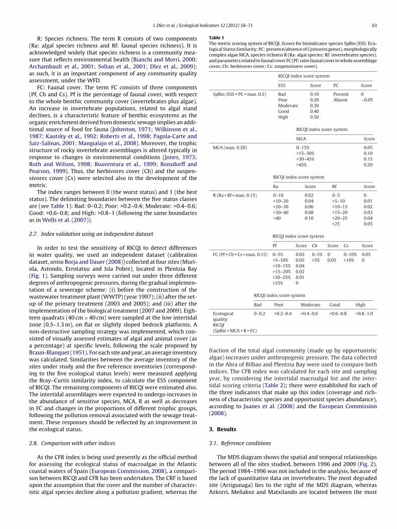
l Indicators 12 (2012) 58–71 61
(asAaa
(tAdot1SsrRPsm
saGa
2
ido(dtwuitznsaBwsitoTtifmt
2
fcsui
Table 1The metric scoring system of RICQI. Scores for bioindicator species SpBio (ESS: Eco-logical Status Similarity; PC: presence/absence of Cystoseira genus), morphologicallycomplex algae MCA, species richness R (Ra: algal species; Rf: invertebrates species),and parameters related to faunal cover FC (Pf: ratio faunal cover to whole assemblagecover, Ch: herbivores cover; Cs: suspensivores cover).
RICQI index score system
ESS Score PC Score
SpBio (ESS + PC = max. 0.5) Bad 0.10 Present 0Poor 0.20 Absent −0.05Moderate 0.30Good 0.40High 0.50
RICQI index score system
MCA Score
MCA (max. 0.20) 0–15% 0.05>15–30% 0.10>30–45% 0.15>45% 0.20
RICQI index score system
Ra Score Rf Score
R (Ra + Rf = max. 0.15) 0–10 0.02 0–5 0>10–20 0.04 >5–10 0.01>20–30 0.06 >10–15 0.02>30–40 0.08 >15–20 0.03>40 0.10 >20–25 0.04
>25 0.05
RICQI index score system
Pf Score Ch Score Cs Score
FC (Pf + Ch + Cs = max. 0.15) 0–5% 0.03 0–5% 0 0–10% 0.05>5–10% 0.05 >5% 0.05 >10% 0>10–15% 0.04>15–20% 0.02>20–25% 0.01>25% 0
RICQI index score system
Bad Poor Moderate Good High
Ecologicalquality
0–0.2 >0.2–0.4 >0.4–0.6 >0.6–0.8 >0.8–1.0
I. Díez et al. / Ecologica
R: Species richness. The term R consists of two componentsRa: algal species richness and Rf: faunal species richness). It iscknowledged widely that species richness is a community mea-ure that reflects environmental health (Bianchi and Morri, 2000;rchambault et al., 2001; Soltan et al., 2001; Díez et al., 2009);s such, it is an important component of any community qualityssessment, under the WFD.
FC: Faunal cover. The term FC consists of three componentsPf, Ch and Cs). Pf is the percentage of faunal cover, with respecto the whole benthic community cover (invertebrates plus algae).n increase in invertebrate populations, related to algal standeclines, is a characteristic feature of benthic ecosystems as therganic enrichment derived from domestic sewage implies an addi-ional source of food for fauna (Johnston, 1971; Wilkinson et al.,987; Kautsky et al., 1992; Roberts et al., 1998; Pagola-Carte andaiz-Salinas, 2001; Mangialajo et al., 2008). Moreover, the trophictructure of rocky invertebrate assemblages is altered typically inesponse to changes in environmental conditions (Jones, 1973;oth and Wilson, 1998; Boaventura et al., 1999; Bonsdorff andearson, 1999). Thus, the herbivores cover (Ch) and the suspen-ivores cover (Cs) were selected also in the development of theetric.The index ranges between 0 (the worst status) and 1 (the best
tatus). The delimiting boundaries between the five status classesre (see Table 1): Bad: 0–0.2; Poor: >0.2–0.4; Moderate: >0.4–0.6;ood: >0.6–0.8; and High: >0.8–1 (following the same boundariess in Wells et al. (2007)).
.7. Index validation using an independent dataset
In order to test the sensitivity of RICQI to detect differencesn water quality, we used an independent dataset (calibrationataset, sensu Borja and Dauer (2008)) collected at four sites (Muri-la, Astondo, Errotatxu and Isla Pobre), located in Plentzia BayFig. 1). Sampling surveys were carried out under three differentegrees of anthropogenic pressures, during the gradual implemen-ation of a sewerage scheme: (i) before the construction of theastewater treatment plant (WWTP) (year 1997); (ii) after the set-p of the primary treatment (2003 and 2005); and (iii) after the
mplementation of the biological treatment (2007 and 2009). Eigh-een quadrats (40 cm × 40 cm) were sampled at the low intertidalone (0.5–1.3 m), on flat or slightly sloped bedrock platforms. Aon-destructive sampling strategy was implemented, which con-isted of visually assessed estimates of algal and animal cover (aspercentage) at specific levels, following the scale proposed by
raun-Blanquet (1951). For each site and year, an average inventoryas calculated. Similarities between the average inventory of the
ites under study and the five reference inventories (correspond-ng to the five ecological status levels) were measured applyinghe Bray–Curtis similarity index, to calculate the ESS componentf RICQI. The remaining components of RICQI were estimated also.he intertidal assemblages were expected to undergo increases inhe abundance of sensitive species, MCA, R as well as decreasesn FC and changes in the proportions of different trophic groups,ollowing the pollution removal associated with the sewage treat-
ent. These responses should be reflected by an improvement inhe ecological status.
.8. Comparison with other indices
As the CFR index is being used presently as the official methodor assessing the ecological status of macroalgae in the Atlantic
oastal waters of Spain (European Commission, 2008), a compari-on between RICQI and CFR has been undertaken. The CRF is basedpon the assumption that the cover and the number of character-stic algal species decline along a pollution gradient, whereas the
RICQI(SpBio + MCA + R + FC)
fraction of the total algal community (made up by opportunisticalgae) increases under anthropogenic pressure. The data collectedin the Abra of Bilbao and Plentzia Bay were used to compare bothindices. The CFR index was calculated for each site and samplingyear, by considering the intertidal macroalgal list and the inter-tidal scoring criteria (Table 2); there were established for each ofthe three indicators that make up this index (coverage and rich-ness of characteristic species and opportunist species abundance),according to Juanes et al. (2008) and the European Commission(2008).
3. Results
3.1. Reference conditions
The MDS diagram shows the spatial and temporal relationshipsbetween all of the sites studied, between 1996 and 2009 (Fig. 2).
The period 1984–1996 was not included in the analysis, because ofthe lack of quantitative data on invertebrates. The most degradedsite (Arrigunaga) lies to the right of the MDS diagram, whereasAzkorri, Menakoz and Matxilando are located between the most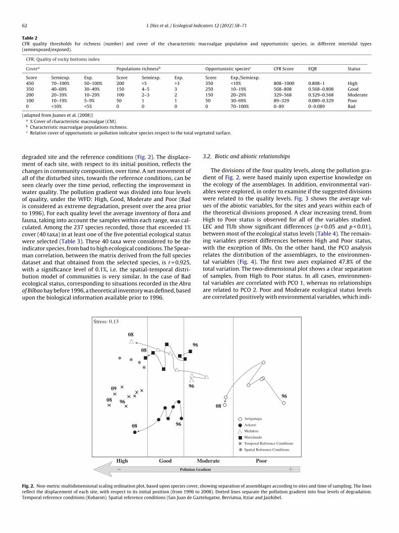
62 I. Díez et al. / Ecological Indicators 12 (2012) 58–71
Table 2CFR quality thresholds for richness (number) and cover of the characteristic macroalgae population and opportunistic species, in different intertidal types(semiexposed/exposed).
CFR: Quality of rocky bottoms index
Covera Populations richnessb Opportunistic speciesc CFR Score EQR Status
Score Semiexp. Exp. Score Semiexp. Exp. Score Exp./Semiexp.450 70–100% 50–100% 200 >5 >3 350 <10% 808–1000 0.808–1 High350 40–69% 30–49% 150 4–5 3 250 10–19% 568–808 0.568–0.808 Good200 20–39% 10–29% 100 2–3 2 150 20–29% 329–568 0.329–0.568 Moderate100 10–19% 5–9% 50 1 1 50 30–69% 89–329 0.089–0.329 Poor0 <10% <5% 0 0 0 0 70–100% 0–89 0–0.089 Bad
(adapted from Juanes et al. (2008))a % Cover of characteristic macroalgae (CM).b
l vege
dmcaswoitfccwimdwbeou
tal variables are correlated with PCO 1, whereas no relationships
FrT
Characteristic macroalgae populations richness.c Relative cover of opportunistic or pollution indicator species respect to the tota
egraded site and the reference conditions (Fig. 2). The displace-ent of each site, with respect to its initial position, reflects the
hanges in community composition, over time. A net movement ofll of the disturbed sites, towards the reference conditions, can beeen clearly over the time period, reflecting the improvement inater quality. The pollution gradient was divided into four levels
f quality, under the WFD: High, Good, Moderate and Poor (Bads considered as extreme degradation, present over the area prioro 1996). For each quality level the average inventory of flora andauna, taking into account the samples within each range, was cal-ulated. Among the 237 species recorded, those that exceeded 1%over (40 taxa) in at least one of the five potential ecological statusere selected (Table 3). These 40 taxa were considered to be the
ndicator species, from bad to high ecological conditions. The Spear-an correlation, between the matrix derived from the full species
ataset and that obtained from the selected species, is r = 0.925,ith a significance level of 0.1%, i.e. the spatial-temporal distri-
ution model of communities is very similar. In the case of Badcological status, corresponding to situations recorded in the Abra
f Bilbao bay before 1996, a theoretical inventory was defined, basedpon the biological information available prior to 1996.Stress: 0.13
96
High Good Mo
09
96
96
9608
08
* * **
08
Pollution Grad
08
ig. 2. Non-metric multidimensional scaling ordination plot, based upon species cover, sheflect the displacement of each site, with respect to its initial position (from 1996 to 2emporal reference conditions (Kobaron). Spatial reference conditions (San Juan de Gazte
tated surface.
3.2. Biotic and abiotic relationships
The divisions of the four quality levels, along the pollution gra-dient of Fig. 2, were based mainly upon expertise knowledge onthe ecology of the assemblages. In addition, environmental vari-ables were explored, in order to examine if the suggested divisionswere related to the quality levels. Fig. 3 shows the average val-ues of the abiotic variables, for the sites and years within each ofthe theoretical divisions proposed. A clear increasing trend, fromHigh to Poor status is observed for all of the variables studied.LEC and TUb show significant differences (p < 0.05 and p < 0.01),between most of the ecological status levels (Table 4). The remain-ing variables present differences between High and Poor status,with the exception of IMs. On the other hand, the PCO analysisrelates the distribution of the assemblages, to the environmen-tal variables (Fig. 4). The first two axes explained 47.8% of thetotal variation. The two-dimensional plot shows a clear separationof samples, from High to Poor status. In all cases, environmen-
are related to PCO 2. Poor and Moderate ecological status levelsare correlated positively with environmental variables, which indi-
derate Poor
96
08
Arrigunaga
Azkorri
Meñakoz
Matxilando
Temporal Reference Conditions
Spatial Reference Conditions*
ient
owing separation of assemblages according to sites and time of sampling. The lines008). Dotted lines separate the pollution gradient into four levels of degradation.lugatxe, Berriatua, Itziar and Jaizkibel.
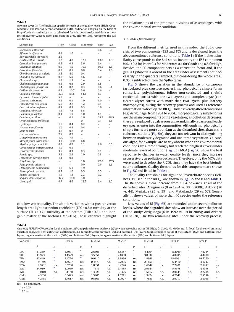
I. Díez et al. / Ecological Indic
Table 3Average cover (in %) of indicator species for each of the quality levels (High, Good,Moderate, and Poor) differentiated in the nMDS ordination analysis, on the basis ofBray–Curtis dissimilarity matrix calculated for 4th root-transformed data. A theo-retical inventory, based upon data from the area, prior to 1996, represents the badconditions.
Species list High Good Moderate Poor Bad
Bachelotia antillarum – – – 0.6 6.3Bifurcaria bifurcata 6.2 1.0 – – –Boergeseniella thuyoides 2.4 – – – –Caulacanthus ustulatus 1.2 4.8 12.2 13.0 1.6Ceramium botrycarpum 0.5 0.3 3.6 6.4 –Ceramium ciliatum 0.5 1.6 10.5 10.5 1.3Ceramium flaccidum 0.3 0.1 6.8 5.4 1.3Chondracanthus acicularis 3.6 4.0 0.4 – –Chondria coerulescens 0.7 5.0 5.6 4.0 –Chthamalus spp. 1.2 1.3 1.4 – –Cladophora lehmanniana 0.8 0.4 2.9 1.5 –Cladostephus spongiosus 1.4 0.2 0.3 0.6 0.1Codium decorticatum 0.3 10.7 5.6 0.6 –Corallina elongata 37.3 51.8 54.5 6.3 –Cystoseira tamariscifolia 5.8 – – – –Dictyota dichotoma 0.2 0.1 1.0 1.0 –Falkenbergia rufolanosa 5.5 2.7 1.2 0.1 –Gastroclonium reflexum 0.1 0.3 0.3 3.6 –Gelidium spinosum 1.8 7.2 5.6 – –Gelidium pulchellum 0.1 1.9 1.0 1.1 –Gelidium pusillum – 0.1 1.6 38.2 48.5Gymnogongrus griffthsiae – – 0.1 0.1 1.1Hyale spp. 1.0 0.4 0.2 – –Hypnea musciformis 1.0 0.4 0.4 – –Jania rubens 3.7 0.7 0.1 – –Laurencia obtusa 7.9 0.7 – – –Lithophyllum incrustans 10.7 7.9 1.1 – –Mesophyllum lichenoides 4.3 10.0 6.8 – –Mytilus galloprovincialis 0.5 0.7 2.1 8.6 0.5Ophidocladus simpliciusculus 1.0 0.1 – – –Paracentrotus lividus 3.5 0.3 0.3 0.1 –Patella spp. 5.2 2.9 1.0 0.8 –Plocamium cartilagineum 1.1 0.8 – – –Polydora spp. – – 1.0 27.0 37.5Polysiphonia atlantica – – 0.0 0.6 1.1Pterosiphonia complanata 1.7 6.1 1.9 – –Pterosiphonia pennata 0.7 1.0 0.5 0.5 –Ralfsia verrucosa 1.4 1.4 2.2 0.2 –Stypocaulon scoparium 32.2 11.0 3.0 – –Ulva rigida 0.7 4.6 12.5 3.4 2.0
clsg
Low values of Rf (Fig. 6B) are recorded under severe pollutionlevels, where the degraded sites show an increase over the period
TOvl
n
ate low water quality. The abiotic variables with a greater vectorength are: light extinction coefficient (LEC = 0.8); turbidity at the
urface (TUs = 0.7); turbidity at the bottom (TUb = 0.8); and inor-anic matter at the bottom (IMb = 0.6). These variables highlightable 4ne-way PERMANOVA results for the main test (F) and pair-wise comparisons (t) betweeariables analysed: light extinction coefficient (LEC), turbidity at the surface (TUs) and bayers, organic matter at the surface (OMs) and bottom (OMb) layers, inorganic matter at
Variable H vs. G G vs. M M vs
F p t p t p t
LEC 31.230 ** 2.6091 * 2.6603 * 3.638TUb 13.923 ** 1.1529 n.s. 3.5554 * 2.186TUs 23.449 ** 3.4754 ** 0.9110 n.s. 2.895TSSb 9.1592 ** 1.5607 n.s. 0.4879 n.s. 2.700TSSs 2.9710 n.s. 0.5260 n.s. 1.0051 n.s. 0.977IMb 14.010 ** 1.0959 n.s. 1.7579 n.s. 2.488IMs 3.0101 n.s. 0.1150 n.s. 1.3926 n.s. 0.932OMb 4.5659 * 0.3495 n.s. 1.3805 n.s. 1.571OMs 4.2452 * 1.4617 n.s. 0.5563 n.s. 1.297
.s. – no significant.* p < 0.05.
** p < 0.01.
ators 12 (2012) 58–71 63
the relationships of the proposed divisions of assemblages, withthe environmental water condition.
3.3. Index functioning
From the different metrics used in this index, the SpBio con-sists of two components (ESS and PC) and is developed from theabovementioned reference conditions (Table 1). If the highest sim-ilarity corresponds to the Bad status inventory the ESS componentis 0.1; 0.2 for Poor; 0.3 for Moderate; 0.4 for Good; and 0.5 for High.Besides, the PC component acts as a correction factor and, if thegenus Cystoseira is absent in the area under assessment (not nec-essarily in the quadrats sampled, but considering the whole area),0.05 is subtracted from the SpBio term.
Fig. 5 shows the variation in the abundance of calcareous(articulated plus crustose species), morphologically simple forms(uniseriate, polysiphonous, foliose non-corticated and slightlycorticated: cortex with one-two layers) and complex algae (cor-ticated algae: cortex with more than two layers, plus leatherymacrophytes), during the recovery process and used as referenceinformation to develop the RICQI. Under severely altered conditions(e.g. Arrigunaga, from 1984 to 2004), morphologically simple formsare the main components of the vegetation; as pollution decreases,these are replaced by calcareous algae and, finally, coarse and leath-ery species enter into the communities. Although morphologicallysimple forms are more abundant at the disturbed sites, than at thereference stations (Fig. 5A), they are not relevant in distinguishingbetween moderately degraded and unaltered vegetation. Calcare-ous algae, for example, are nearly absent when the environmentalconditions are altered strongly but reach their highest covers undermoderate levels of pollution (Fig. 5B). MCA (Fig. 5C) show the bestresponse to changes in water quality levels, since they increaseprogressively as pollution decreases. Therefore, only the MCA datawere used to develop the RICQI, since they have the best bioindi-cator attributes. Quality thresholds for this component are shownin Fig. 5C and listed in Table 1.
The quality thresholds for algal and invertebrate species rich-ness, as used in the RICQI, are shown in Fig. 6A and B and Table 1.The Ra shows a clear increase from 1984 onwards, at all of thedisturbed sites: Arrigunaga (8 in 1984 vs. 30 in 2008); Azkorri (20vs. 44); Menakoz (25 vs. 39); and Matxilando (29 vs. 57). Gener-ally, it shows values of more than 40 species under the referenceconditions.
of the study: Arrigunaga (6 in 1992 vs. 19 in 2008); and Azkorri(20 vs. 28). The two remaining sites under the recovery process,
n ecological status (H: High; G: Good; M: Moderate; P: Poor) for the environmentalottom (TUb) layers, total suspended solids at the surface (TSSs) and bottom (TSSb)the surface (IMs) and bottom (IMb) layers.
. P H vs. M H vs. P G vs. P
p t p t p t p
7 * 4.4994 ** 8.2069 ** 7.3264 **
0 * 3.8334 ** 4.0785 ** 4.4700 **
0 n.s. 1.9946 * 18.060 * 10.7270 **
5 n.s. 2.1650 * 5.4410 ** 3.6237 **
6 n.s. 1.6047 n.s. 2.2201 * 2.1287 n.s.5 n.s. 2.9644 * 5.5678 ** 4.8398 *
5 n.s. 1.5017 n.s. 2.0644 n.s. 2.2288 n.s.1 n.s. 1.9424 n.s. 4.2041 ** 2.9599 *
7 n.s. 1.7589 n.s. 2.9717 * 2.4016 *
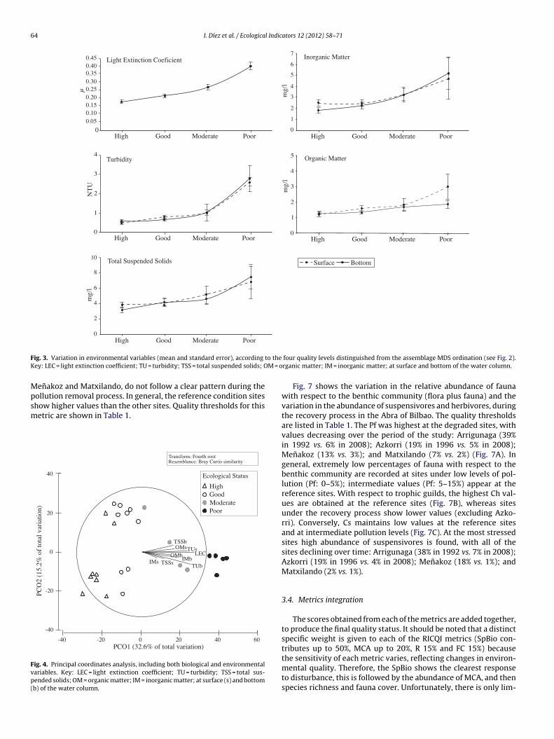
64 I. Díez et al. / Ecological Indicators 12 (2012) 58–71
µ
Surface Bottom
High Good Moderate Poor
Light Extinction Coeficient0.450.400.350.300.250.200.150.100.05
0High Good Moderate Poor
mg/
l
Inorganic Matter7
6
5
4
3
2
1
0
mg/
l
High Good Moderate Poor
Total Suspended Solids10
8
6
4
0
2
NT
U
High Good Moderate Poor
Turbidity
3
2
1
0
4
mg/
l
High Good Moderate Poor
Organic Matter
2
4
3
0
1
5
F to theK M = o
Mpsm
Fvp(
ig. 3. Variation in environmental variables (mean and standard error), accordingey: LEC = light extinction coefficient; TU = turbidity; TSS = total suspended solids; O
enakoz and Matxilando, do not follow a clear pattern during theollution removal process. In general, the reference condition sites
how higher values than the other sites. Quality thresholds for thisetric are shown in Table 1.-40 0 2 60 040-20
-40
0
20
40
-20
PCO1 (32.6% of total variation)
PCO
2 (1
5.2%
of
tota
l var
iatio
n)
Transform: Fourth rootResemblance: Bray Curtis similarity
HighGoodModeratePoor
Ecological Status
TSSs
TSSb
TUb
TUs
IMbIMs
OMsOMb LEC
ig. 4. Principal coordinates analysis, including both biological and environmentalariables. Key: LEC = light extinction coefficient; TU = turbidity; TSS = total sus-ended solids; OM = organic matter; IM = inorganic matter; at surface (s) and bottomb) of the water column.
four quality levels distinguished from the assemblage MDS ordination (see Fig. 2).rganic matter; IM = inorganic matter; at surface and bottom of the water column.
Fig. 7 shows the variation in the relative abundance of faunawith respect to the benthic community (flora plus fauna) and thevariation in the abundance of suspensivores and herbivores, duringthe recovery process in the Abra of Bilbao. The quality thresholdsare listed in Table 1. The Pf was highest at the degraded sites, withvalues decreasing over the period of the study: Arrigunaga (39%in 1992 vs. 6% in 2008); Azkorri (19% in 1996 vs. 5% in 2008);Menakoz (13% vs. 3%); and Matxilando (7% vs. 2%) (Fig. 7A). Ingeneral, extremely low percentages of fauna with respect to thebenthic community are recorded at sites under low levels of pol-lution (Pf: 0–5%); intermediate values (Pf: 5–15%) appear at thereference sites. With respect to trophic guilds, the highest Ch val-ues are obtained at the reference sites (Fig. 7B), whereas sitesunder the recovery process show lower values (excluding Azko-rri). Conversely, Cs maintains low values at the reference sitesand at intermediate pollution levels (Fig. 7C). At the most stressedsites high abundance of suspensivores is found, with all of thesites declining over time: Arrigunaga (38% in 1992 vs. 7% in 2008);Azkorri (19% in 1996 vs. 4% in 2008); Menakoz (18% vs. 1%); andMatxilando (2% vs. 1%).
3.4. Metrics integration
The scores obtained from each of the metrics are added together,to produce the final quality status. It should be noted that a distinctspecific weight is given to each of the RICQI metrics (SpBio con-tributes up to 50%, MCA up to 20%, R 15% and FC 15%) because
the sensitivity of each metric varies, reflecting changes in environ-mental quality. Therefore, the SpBio shows the clearest responseto disturbance, this is followed by the abundance of MCA, and thenspecies richness and fauna cover. Unfortunately, there is only lim-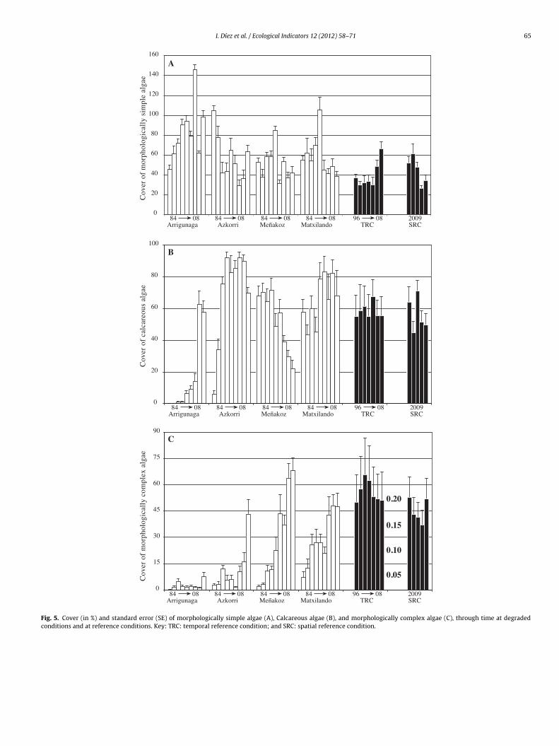
I. Díez et al. / Ecological Indicators 12 (2012) 58–71 65
0
20
40
60
80
100
120
140
160
Cov
er o
f m
orph
olog
ical
ly s
impl
e al
gae
Arrigunaga Azkorri Meñakoz Matxilando TRC SRC84 08 84 08 84 08 84 08 96 08 2009
A
0
20
40
60
80
100
Cov
er o
f ca
lcar
eous
alg
ae
Arrigunaga Azkorri Meñakoz Matxilando TRC SRC84 08 84 08 84 08 84 08 96 08 2009
B
Cov
er o
f m
orph
olog
ical
ly c
ompl
ex a
lgae
0.15
0.05
0.10
0
15
30
45
60
75
90
0.20
Arrigunaga Azkorri Meñakoz Matxilando TRC SRC84 08 84 08 84 08 84 08 96 08 2009
C
Fig. 5. Cover (in %) and standard error (SE) of morphologically simple algae (A), Calcareous algae (B), and morphologically complex algae (C), through time at degradedconditions and at reference conditions. Key: TRC: temporal reference condition; and SRC: spatial reference condition.
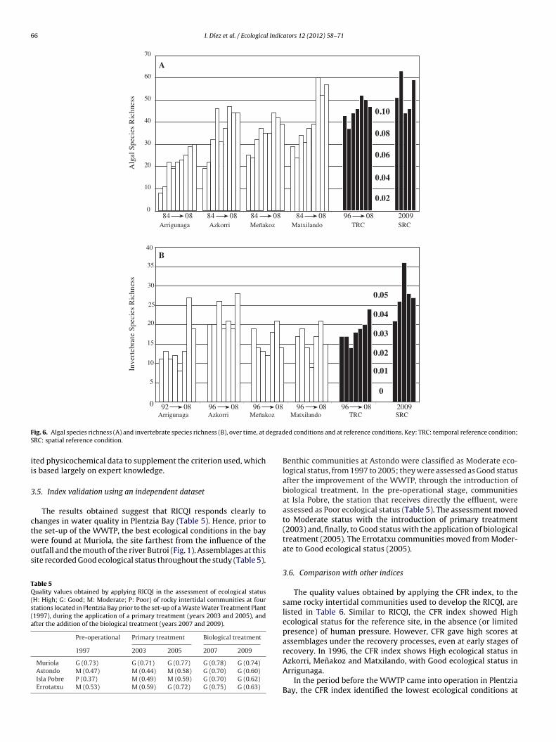
66 I. Díez et al. / Ecological Indicators 12 (2012) 58–71
Alg
al S
peci
es R
ichn
ess
Inve
rteb
rate
Spe
cies
Ric
hnes
s
0.02
0.04
0.06
0.08
0.10
0
10
20
30
40
50
60
70
Arrigunaga Azkorri Meñakoz Matxilando TRC SRC84 08 84 08 84 08 84 08 96 08 2009
0
0.01
0.02
0.03
0.04
0.05
0
5
10
15
20
25
30
35
40
Arrigunaga Azkorri Meñakoz Matxilando92 08 96 08 96 08 96 08 96 08 2009
TRC SRC
A
B
F degradS
ii
3
ctwos
TQ(s(a
ig. 6. Algal species richness (A) and invertebrate species richness (B), over time, atRC: spatial reference condition.
ted physicochemical data to supplement the criterion used, whichs based largely on expert knowledge.
.5. Index validation using an independent dataset
The results obtained suggest that RICQI responds clearly tohanges in water quality in Plentzia Bay (Table 5). Hence, prior to
he set-up of the WWTP, the best ecological conditions in the bayere found at Muriola, the site farthest from the influence of theutfall and the mouth of the river Butroi (Fig. 1). Assemblages at thisite recorded Good ecological status throughout the study (Table 5).
able 5uality values obtained by applying RICQI in the assessment of ecological status
H: High; G: Good; M: Moderate; P: Poor) of rocky intertidal communities at fourtations located in Plentzia Bay prior to the set-up of a Waste Water Treatment Plant1997), during the application of a primary treatment (years 2003 and 2005), andfter the addition of the biological treatment (years 2007 and 2009).
Pre-operational Primary treatment Biological treatment
1997 2003 2005 2007 2009
Muriola G (0.73) G (0.71) G (0.77) G (0.78) G (0.74)Astondo M (0.47) M (0.44) M (0.58) G (0.70) G (0.60)Isla Pobre P (0.37) M (0.49) M (0.59) G (0.70) G (0.62)Errotatxu M (0.53) M (0.59) G (0.72) G (0.75) G (0.63)
ed conditions and at reference conditions. Key: TRC: temporal reference condition;
Benthic communities at Astondo were classified as Moderate eco-logical status, from 1997 to 2005; they were assessed as Good statusafter the improvement of the WWTP, through the introduction ofbiological treatment. In the pre-operational stage, communitiesat Isla Pobre, the station that receives directly the effluent, wereassessed as Poor ecological status (Table 5). The assessment movedto Moderate status with the introduction of primary treatment(2003) and, finally, to Good status with the application of biologicaltreatment (2005). The Errotatxu communities moved from Moder-ate to Good ecological status (2005).
3.6. Comparison with other indices
The quality values obtained by applying the CFR index, to thesame rocky intertidal communities used to develop the RICQI, arelisted in Table 6. Similar to RICQI, the CFR index showed Highecological status for the reference site, in the absence (or limitedpresence) of human pressure. However, CFR gave high scores atassemblages under the recovery processes, even at early stages ofrecovery. In 1996, the CFR index shows High ecological status in
Azkorri, Menakoz and Matxilando, with Good ecological status inArrigunaga.In the period before the WWTP came into operation in PlentziaBay, the CFR index identified the lowest ecological conditions at
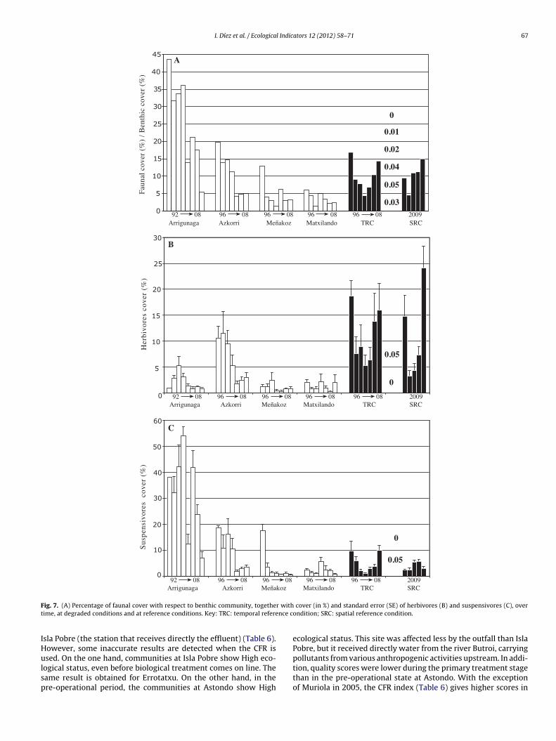
I. Díez et al. / Ecological Indicators 12 (2012) 58–71 67
0
0.05
0
5
10
15
20
25
30
Arrigunaga Azkorri Meñakoz Matxilando TRC SRC92 08 96 08 96 08 96 08 96 08 2009
Her
bivo
res
cove
r (%
)S
uspe
nsiv
ores
co
ver
(%)
92 08 96 08 96 08 96 08 96 08 20090
10
20
30
40
50
60
0
0.05
Arrigunaga Azkorri Meñakoz Matxilando TRC SRC
92 08 96 08 96 08 96 08 96 08 2009
Fau
nal
cove
r (%
) /
Ben
thic
cov
er (
%)
0
5
10
15
20
25
30
35
40
45
Arrigunaga Azkorri Meñakoz Matxilando TRC SRC
0.03
0.05
0.04
0.02
0.01
0
A
B
C
F r witht nce c
IHulsp
ig. 7. (A) Percentage of faunal cover with respect to benthic community, togetheime, at degraded conditions and at reference conditions. Key: TRC: temporal refere
sla Pobre (the station that receives directly the effluent) (Table 6).owever, some inaccurate results are detected when the CFR is
sed. On the one hand, communities at Isla Pobre show High eco-ogical status, even before biological treatment comes on line. Theame result is obtained for Errotatxu. On the other hand, in there-operational period, the communities at Astondo show High
cover (in %) and standard error (SE) of herbivores (B) and suspensivores (C), overondition; SRC: spatial reference condition.
ecological status. This site was affected less by the outfall than IslaPobre, but it received directly water from the river Butroi, carrying
pollutants from various anthropogenic activities upstream. In addi-tion, quality scores were lower during the primary treatment stagethan in the pre-operational state at Astondo. With the exceptionof Muriola in 2005, the CFR index (Table 6) gives higher scores in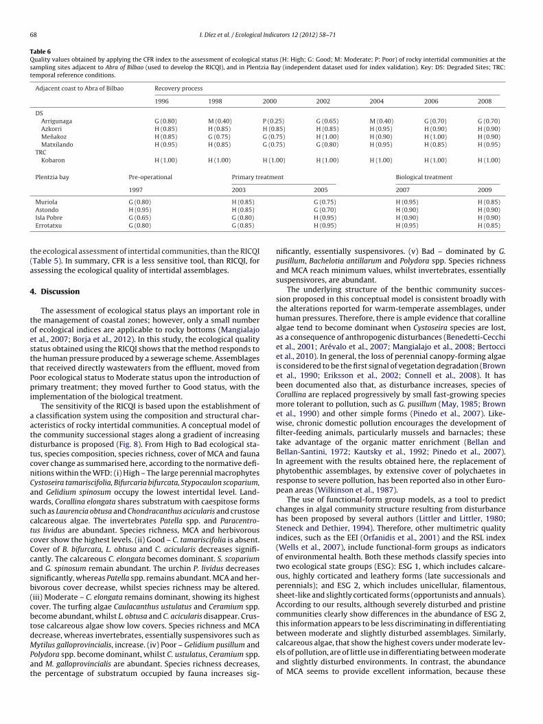
68 I. Díez et al. / Ecological Indicators 12 (2012) 58–71
Table 6Quality values obtained by applying the CFR index to the assessment of ecological status (H: High; G: Good; M: Moderate; P: Poor) of rocky intertidal communities at thesampling sites adjacent to Abra of Bilbao (used to develop the RICQI), and in Plentzia Bay (independent dataset used for index validation). Key: DS: Degraded Sites; TRC:temporal reference conditions.
Adjacent coast to Abra of Bilbao Recovery process
1996 1998 2000 2002 2004 2006 2008
DSArrigunaga G (0.80) M (0.40) P (0.25) G (0.65) M (0.40) G (0.70) G (0.70)Azkorri H (0.85) H (0.85) H (0.85) H (0.85) H (0.95) H (0.90) H (0.90)Menakoz H (0.85) G (0.75) G (0.75) H (1.00) H (0.90) H (1.00) H (0.90)Matxilando H (0.95) H (0.85) G (0.75) G (0.80) H (0.95) H (0.85) H (0.95)
TRCKobaron H (1.00) H (1.00) H (1.00) H (1.00) H (1.00) H (1.00) H (1.00)
Plentzia bay Pre-operational Primary treatment Biological treatment
1997 2003 2005 2007 2009
Muriola G (0.80) H (0.85) G (0.75) H (0.95) H (0.85)Astondo H (0.95) H (0.85) G (0.70) H (0.90) H (0.90)
t(a
4
toesttPpi
aatdtcnCawsctcCcasb(cbtdMPat
Isla Pobre G (0.65) G (0.80)Errotatxu G (0.80) G (0.85)
he ecological assessment of intertidal communities, than the RICQITable 5). In summary, CFR is a less sensitive tool, than RICQI, forssessing the ecological quality of intertidal assemblages.
. Discussion
The assessment of ecological status plays an important role inhe management of coastal zones; however, only a small numberf ecological indices are applicable to rocky bottoms (Mangialajot al., 2007; Borja et al., 2012). In this study, the ecological qualitytatus obtained using the RICQI shows that the method responds tohe human pressure produced by a sewerage scheme. Assemblageshat received directly wastewaters from the effluent, moved fromoor ecological status to Moderate status upon the introduction ofrimary treatment; they moved further to Good status, with the
mplementation of the biological treatment.The sensitivity of the RICQI is based upon the establishment of
classification system using the composition and structural char-cteristics of rocky intertidal communities. A conceptual model ofhe community successional stages along a gradient of increasingisturbance is proposed (Fig. 8). From High to Bad ecological sta-us, species composition, species richness, cover of MCA and faunaover change as summarised here, according to the normative defi-itions within the WFD: (i) High – The large perennial macrophytesystoseira tamariscifolia, Bifurcaria bifurcata, Stypocaulon scoparium,nd Gelidium spinosum occupy the lowest intertidal level. Land-ards, Corallina elongata shares substratum with caespitose forms
uch as Laurencia obtusa and Chondracanthus acicularis and crustosealcareous algae. The invertebrates Patella spp. and Paracentro-us lividus are abundant. Species richness, MCA and herbivorousover show the highest levels. (ii) Good – C. tamariscifolia is absent.over of B. bifurcata, L. obtusa and C. acicularis decreases signifi-antly. The calcareous C. elongata becomes dominant. S. scopariumnd G. spinosum remain abundant. The urchin P. lividus decreasesignificantly, whereas Patella spp. remains abundant. MCA and her-ivorous cover decrease, whilst species richness may be altered.iii) Moderate – C. elongata remains dominant, showing its highestover. The turfing algae Caulacanthus ustulatus and Ceramium spp.ecome abundant, whilst L. obtusa and C. acicularis disappear. Crus-ose calcareous algae show low covers. Species richness and MCAecrease, whereas invertebrates, essentially suspensivores such as
ytilus galloprovincialis, increase. (iv) Poor – Gelidium pusillum andolydora spp. become dominant, whilst C. ustulatus, Ceramium spp.nd M. galloprovincialis are abundant. Species richness decreases,he percentage of substratum occupied by fauna increases sig-
H (0.95) H (0.90) H (0.90)H (0.95) H (0.95) H (0.85)
nificantly, essentially suspensivores. (v) Bad – dominated by G.pusillum, Bachelotia antillarum and Polydora spp. Species richnessand MCA reach minimum values, whilst invertebrates, essentiallysuspensivores, are abundant.
The underlying structure of the benthic community succes-sion proposed in this conceptual model is consistent broadly withthe alterations reported for warm-temperate assemblages, underhuman pressures. Therefore, there is ample evidence that corallinealgae tend to become dominant when Cystoseira species are lost,as a consequence of anthropogenic disturbances (Benedetti-Cecchiet al., 2001; Arévalo et al., 2007; Mangialajo et al., 2008; Bertocciet al., 2010). In general, the loss of perennial canopy-forming algaeis considered to be the first signal of vegetation degradation (Brownet al., 1990; Eriksson et al., 2002; Connell et al., 2008). It hasbeen documented also that, as disturbance increases, species ofCorallina are replaced progressively by small fast-growing speciesmore tolerant to pollution, such as G. pusillum (May, 1985; Brownet al., 1990) and other simple forms (Pinedo et al., 2007). Like-wise, chronic domestic pollution encourages the development offilter-feeding animals, particularly mussels and barnacles; thesetake advantage of the organic matter enrichment (Bellan andBellan-Santini, 1972; Kautsky et al., 1992; Pinedo et al., 2007).In agreement with the results obtained here, the replacement ofphytobenthic assemblages, by extensive cover of polychaetes inresponse to severe pollution, has been reported also in other Euro-pean areas (Wilkinson et al., 1987).
The use of functional-form group models, as a tool to predictchanges in algal community structure resulting from disturbancehas been proposed by several authors (Littler and Littler, 1980;Steneck and Dethier, 1994). Therefore, other multimetric qualityindices, such as the EEI (Orfanidis et al., 2001) and the RSL index(Wells et al., 2007), include functional-form groups as indicatorsof environmental health. Both these methods classify species intotwo ecological state groups (ESG): ESG 1, which includes calcare-ous, highly corticated and leathery forms (late successionals andperennials); and ESG 2, which includes unicellular, filamentous,sheet-like and slightly corticated forms (opportunists and annuals).According to our results, although severely disturbed and pristinecommunities clearly show differences in the abundance of ESG 2,this information appears to be less discriminating in differentiatingbetween moderate and slightly disturbed assemblages. Similarly,
calcareous algae, that show the highest covers under moderate lev-els of pollution, are of little use in differentiating between moderateand slightly disturbed environments. In contrast, the abundanceof MCA seems to provide excellent information, because these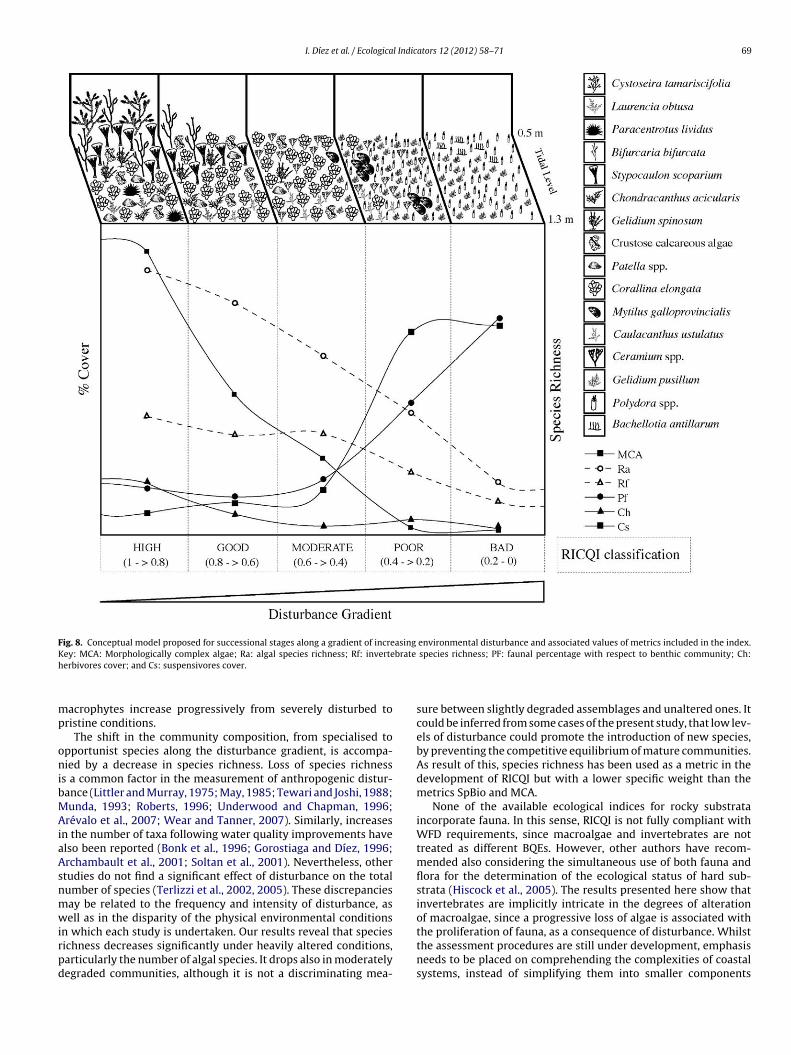
I. Díez et al. / Ecological Indicators 12 (2012) 58–71 69
Fig. 8. Conceptual model proposed for successional stages along a gradient of increasing environmental disturbance and associated values of metrics included in the index.K brateh
mp
onibMAiaAsnmwirpd
ey: MCA: Morphologically complex algae; Ra: algal species richness; Rf: inverteerbivores cover; and Cs: suspensivores cover.
acrophytes increase progressively from severely disturbed toristine conditions.
The shift in the community composition, from specialised topportunist species along the disturbance gradient, is accompa-ied by a decrease in species richness. Loss of species richness
s a common factor in the measurement of anthropogenic distur-ance (Littler and Murray, 1975; May, 1985; Tewari and Joshi, 1988;unda, 1993; Roberts, 1996; Underwood and Chapman, 1996;
révalo et al., 2007; Wear and Tanner, 2007). Similarly, increasesn the number of taxa following water quality improvements havelso been reported (Bonk et al., 1996; Gorostiaga and Díez, 1996;rchambault et al., 2001; Soltan et al., 2001). Nevertheless, othertudies do not find a significant effect of disturbance on the totalumber of species (Terlizzi et al., 2002, 2005). These discrepanciesay be related to the frequency and intensity of disturbance, asell as in the disparity of the physical environmental conditions
n which each study is undertaken. Our results reveal that speciesichness decreases significantly under heavily altered conditions,articularly the number of algal species. It drops also in moderatelyegraded communities, although it is not a discriminating mea-
species richness; PF: faunal percentage with respect to benthic community; Ch:
sure between slightly degraded assemblages and unaltered ones. Itcould be inferred from some cases of the present study, that low lev-els of disturbance could promote the introduction of new species,by preventing the competitive equilibrium of mature communities.As result of this, species richness has been used as a metric in thedevelopment of RICQI but with a lower specific weight than themetrics SpBio and MCA.
None of the available ecological indices for rocky substrataincorporate fauna. In this sense, RICQI is not fully compliant withWFD requirements, since macroalgae and invertebrates are nottreated as different BQEs. However, other authors have recom-mended also considering the simultaneous use of both fauna andflora for the determination of the ecological status of hard sub-strata (Hiscock et al., 2005). The results presented here show thatinvertebrates are implicitly intricate in the degrees of alterationof macroalgae, since a progressive loss of algae is associated with
the proliferation of fauna, as a consequence of disturbance. Whilstthe assessment procedures are still under development, emphasisneeds to be placed on comprehending the complexities of coastalsystems, instead of simplifying them into smaller components
7 l Indic
(raawemcbeiefrie
eg(ttcmusrtciiltsusiCu
faosb
A
awIiRP(PUot
R
A
0 I. Díez et al. / Ecologica
Diaz et al., 2004). Seaweeds represent an important biologicalesource for animals that make use of the algae for food, shelternd support (Hayward, 1988). Over the mid-intertidal, algal turfsllow the presence of many invertebrate species, that otherwiseould be absent at the same tidal level (Bejín et al., 2004; Bertness
t al., 2006) and influence the ecological patterns of associated ani-als (Hauser et al., 2008). At the same time, the patchiness that
haracterises the rocky benthos worldwide is generated mainlyy invertebrates (Sousa, 1984; Branch, 1985). The classification ofcological status of rocky substrata is challenging, since algae andnvertebrates covary, both naturally and with the alteration of thenvironmental conditions. Given the close link between flora andauna the WFD policies might consider extending their definitionsegarding BQEs. Otherwise, essential information will be lost in ournterpretation of changes, especially in the case of humanly alteredcosystems, as it has been demonstrated in this study.
Two boundaries between the five ecological status levels arespecially relevant: (i) between Good and Moderate, as it distin-uishes between acceptable and unacceptable levels of qualityaccording to the WFD); and (ii) between Good and High sta-us. If slightly disturbed assemblages are mistakenly consideredo show pristine conditions, environmental management decisionsould lead to a progressive loss of biodiversity. Therefore, theain challenge when developing a biotic quality index is to draw
p a sensitive tool for detecting differences between moderately,lightly altered and undisturbed communities. In this regard, ouresults suggest that the RICQI is a more sensitive method thanhe CFR, for assessing the ecological status of the rocky intertidalommunities of the Iberian coast. Discrepancies between the twondices may be due largely to the way in which species sensitiv-ty to pollution is classified. CFR is based mainly upon two speciesists: a “characteristic” species list, which includes the most sensi-ive macrophytes; and an “opportunistic” species list, composed ofpecies tolerant to anthropogenic disturbances. In contrast, RICQIses five theoretical inventories, with the relative abundance ofpecies varying from the bad status inventory to the high statusnventory. As a result, under CFR, Corallina spp., S. scoparium andystoseira baccata are considered to be equally tolerant to pollution;nder RICQI, they show different degrees of tolerance.
The RICQI has been developed for the Basque Country and, there-ore, reference conditions as well as the ecological class boundariesre relevant to this coastal area and may not transpose directly intother regions. Thus, all metrics will have to be intercalibrated sub-equently in order to guarantee that metrics assess the same waterodies in the same status.
cknowledgements
This work was supported by the local water supplynd sewerage authority Consorcio de Aguas Bilbao Bizkaia,ww.consorciodeaguas.com. In this investigation, Angel Borja and
nigo Muxika were supported by the project WISER (Water bodiesn Europe: Integrative Systems to assess Ecological status andecovery) funded by the European Union under the 7th Frameworkrogramme, Theme 6 (Environment including Climate Change)contract No. 226273), www.wiser.eu. We wish to thank alsorofessor Michael Collins (School of Ocean and Earth Science,niversity of Southampton, UK and AZTI-Tecnalia) for advising usn some details of this paper. This is contribution number 546 ofhe Marine Research Division (AZTI-Tecnalia).
eferences
nderson, M.J., Gorley, R.N., Clarke, K.R., 2008. PERMANOVA+ for PRIMER: Guide toSoftware and Statistical Methods. PRIMER-E, Plymouth, UK, 214 pp.
ators 12 (2012) 58–71
Archambault, P., Banwell, K., Underwood, A.J., 2001. Temporal variation in the struc-ture of intertidal assemblages following the removal of sewage. Mar. Ecol. Prog.Ser. 222, 51–62.
Arévalo, R., Pinedo, S., Ballesteros, E., 2007. Changes in the composition and struc-ture of Mediterranean rocky-shore communities following a gradient of nutrientenrichment: descriptive study and test of proposed methods to assess waterquality regarding macroalgae. Mar. Pollut. Bull. 55, 104–113.
Ballesteros, E., Torras, X., Pinedo, S., García, M., Mangialajo, L., De Torres, M., 2007.A new methodology based on littoral community cartography dominated bymacroalgae for the implementation of the European Water Framework Direc-tive. Mar. Pollut. Bull. 55, 172–180.
Bejín, C., Jonson, L.E., Himmelman, J.H., 2004. Macroalgal canopies: distribution anddiversity of associated invertebrates and effects on the recruitment and growthof mussels. Mar. Ecol. Prog. Ser. 271, 121–132.
Bellan, G., Bellan-Santini, D., 1972. Influence de la pollution sur les peuplementsmarins de la region de Marseille. In: Ruivo, M. (Ed.), Marine Pollution and SeaLife. FAO Publication. Fishing News (Books), London, pp. 396–401.
Bellgrove, A., Clayton, M.N., Quinn, G.P., 1997. Effects of secondarily treated sewageeffluent on intertidal macroalgal recruitment processes. Mar. Fresh Water Res.48, 137–146.
Benedetti-Cecchi, L., Pannacciulli, F., Bulleri, F., Moschella, P.S., Airoldi, L., Relini,G., Cinelli, F., 2001. Predicting the consequences of anthropogenic disturbance:large-scale effects of loss of canopy algae on rocky shores. Mar. Ecol. Prog. Ser.214, 137–150.
Bertness, M.D., Crain, C.M., Silliman, B.R., Bazterriza, M.C., Reyna, M.V., Hidalgo, F.,Farina, J.K., 2006. The community structure of western Atlantic Patagonian rockyshores. Ecol. Monogr. 76, 439–460.
Bertocci, I., Arenas, F., Matias, M., Vaselli, S., Araújo, R., Abreu, H., Pereira, R., Vieira, R.,Sousa-Pinto, I., 2010. Canopy-forming species mediate the effects of disturbanceon macroalgal assemblages on Portuguese rocky shores. Mar. Ecol. Prog. Ser. 414,107–116.
Bianchi, C.N., Morri, C., 2000. Marine biodiversity of the Mediterranean Sea: sit-uation, problems and prospects for future research. Mar. Pollut. Bull. 40,367–376.
Bishop, M.J., Underwood, A.J., Archambault, P., 2002. Sewage and environmentalimpacts on rocky shores: necessity of identifying relevant spatial scales. Mar.Ecol. Progr. Ser. 236, 121–128.
Boaventura, D., Cancela de Fonseca, L., Teles-Ferreira, C., 1999. Trophic structureof macrobenthic communities on the Portuguese coast. A review of lagoonal,estuarine and rocky littoral habitat. Acta Oecol. 20, 407–415.
Bonk, T.L., Moy, F.E., Walday, M., 1996. Improvement of the shallow water com-munities following reductions of industrial outlets and sewage discharge in theHvaler estuary, Norway. Hydrobiologia 326/327, 297–304.
Bonsdorff, E., Pearson, T.H., 1999. Variation in the sublittoral macrozoobenthos of theBaltic Sea along environmental gradients; a functional-group approach. Aust. J.Ecol. 24, 312–326.
Borja, A., Basset, A., Bricker, S., Dauvin, J.C., Elliott, M., Harrison, T., Marques, J.C.,Weisberg, S., West, R., 2012. Classifying ecological quality and integrity of estu-aries. In: Wolanski, E., McLusky, D. (Eds.), Treatise on Estuarine and CoastalScience’. Elsevier, doi: 00109 is 10.1016/B978-0-12-374711-2.00109-1.
Borja, A., Dauer, D., Elliott, M., Simenstad, C., 2010. Medium- and long-term recoveryof estuarine and coastal ecosystems: patterns rates and restoration effective-ness. Estuar. Coasts 33, 1249–1260.
Borja, A., Miles, A., Occhipinti-Ambrogi, A., Berg, T., 2009. Current status of macroin-vertebrate methods used for assessing the quality of European marine waters:implementing the Water Framework Directive. Hydrobiologia 633, 181–196.
Borja, A., Dauer, D.M., 2008. Assessing the environmental quality status in estuar-ine and coastal systems: comparing methodologies and indices. Ecol. Indic. 8,331–337.
Borja, A., Galparsoro, I., Solaun, O., Muxika, I., Tello, E.M., Uriarte, A., Valencia, V.,2006. The European Water Framework Directive and the DPSIR, a methodologi-cal approach to assess the risk of failing to achieve good ecological status. Estuar.Coast. Shelf Sci. 66, 84–96.
Borja, A., 2005. The European water framework directive: a challenge for nearshore,coastal and continental shelf research. Cont. Shelf Res. 25, 1768–1783.
Branch, G.M., 1985. Limpets: their role in littoral and sublittoral community dynam-ics. In: Moore, P.G., Seed, R. (Eds.), The Ecology of Rocky Coasts. Hodder andStoughton, London, pp. 98–116.
Braun-Blanquet, J., 1951. Plant Sociology: the study of Plant Communities. McGrawHill, New York, USA.
Brown, V.B., Davies, S.A., Synnot, R.N., 1990. Long-term monitoring of the effectsof treated sewage effluent on the intertidal macroalgal community near CapeSchanck, Victoria, Australia. Bot. Mar. 33, 85–98.
Clarke, K.R., Warwick, R.M., 1994. Change in Marine Communities. An Approach toStatistical Analysis and Interpretation. Natural Environment Research Council,UK.
Connell, S.D., Russell, B.D., Turner, D.J., Shepherd, S.A., Kildea, T., Miller, D., Airoldi,L., Cheshire, A., 2008. Recovering a lost baseline: missing kelp forests from ametropolitan coast. Mar. Ecol. Prog. Ser. 360, 63–72.
Diaz, R., Solan, M., Valente, M., 2004. A review of approaches for classifying benthichabitats and evaluating habitat quality. J. Environ. Manag. 73, 165–181.
Díez, I., Santolaria, A., Gorostiaga, J.M., 2010. Different levels of macroalgal samplingresolution for pollution assessment. Mar. Pollut. Bull. 60, 1779–1789.
Díez, I., Santolaria, A., Secilla, A., Gorostiaga, J.M., 2009. Recovery stages over a long-term monitoring of the intertidal vegetation in the ‘Abra de Bilbao’ area and onthe adjacent coast N Spain. Eur. J. Phycol. 44, 1–14.
l Indic
D
D
E
E
F
G
G
G
H
H
H
H
J
J
J
K
K
L
L
M
M
M
I. Díez et al. / Ecologica
íez, I., Santolaria, A., Gorostiaga, J.M., 2003. Relationships of environmentalfactors with the structure and distribution of subtidal seaweed vegeta-tion of the western Basque coast (N. Spain). Estuar. Coast. Shelf Sci. 56,1041–1054.
íez, I., Secilla, A., Santolaria, A., Gorostiaga, J.M., 1999. Phytobenthic intertidal com-munity structure along an environmental pollution gradient. Mar. Pollut. Bull.38, 463–472.
riksson, B.K., Johansson, G., Snoeijs, P., 2002. Long-term changes in the macroalgalvegetation of the inner Gullmar Fjord. Swedish Skagerrak coast. J. Phycol. 38,284–296.
uropean Commission, 2008. Commission Decision of 30 October 2008, estab-lishing, pursuant to Directive 2000/60/EC of the European Parliament and ofthe Council, the values of the Member State monitoring system classificationsas a result of the intercalibration exercise (notified under document numberC(2008) 6016) (2008/915/EC). Official Journal of the European Union L332,pp. 20–44.
airweather, P.G., 1990. Sewage and biota on seashores: assessment of impact inrelation to natural variability. Environ. Monit. Assess. 14, 197–210.
oodsell, P.J., Underwood, A.J., Chapman, M.G., 2009. Evidence necessary for taxa tobe reliable indicators of environmental conditions or impacts. Mar. Pollut. Bull.58, 323–331.
orostiaga, J.M., Borja, A., Díez, I., Frances, G., Pagola-Carte, S., Saiz-Salinas, J.I., 2004.Recovery of benthic communities in polluted systems. In: Borja, A., Collins, M.(Eds.), Oceanography and Marine Environment of the Basque Country. ElsevierOceanography Series, Amsterdam, pp. 549–578.
orostiaga, J.M., Díez, I., 1996. Changes in the sublittoral benthic marine macroalgaein the polluted area of Abra de Bilbao and proximal coast (Northern Spain). Mar.Ecol. Prog. Ser. 130, 157–167.
auser, A., Atrill, M.J., Cotton, P.A., 2008. Effect of habitat complexity on the diversityand abundance of macrofauna colonizing artificial kelp holdfasts. Mar. Ecol. Prog.Ser. 325, 93–100.
ayward, P.J., 1988. In: Corbet, S.A., Disney, R.H.L. (Eds.), Animals on Seaweed. TheRichmond Publishing Co. Ltd., p. 108.
iscock, K., Tyler-Walters, H., 2006. Assessing the sensitivity of seabed species andbiotopes – the Marine Life Information Network (MarLIN). Hydrobiologia 555,309–332.
iscock, K., Smith, A, Jenkins, S., Sewell, J., Hawkins, S., 2005. Development of ahard substratum Benthic invertebrate Water Framework Directive compliantclassification tool. Report to the Environment Agency and the Joint Nature Con-servation Committee from the Marine Biological Association. Marine BiologicalAssociation. Inc., Plymouth, Contract F90-01-790, 54 pp.
ohnston, C.S., 1971. Macroalgae and their environment. Proc. R. Soc. Edinburgh 71,195–207, /1972.
ones, D.J., 1973. Variation in trophic structure and species composition of someinvertebrate communities in polluted kelp forests in the North Sea. Mar. Biol.20, 351–365.
uanes, J.A., Guinda, X., Revilla, J.A., 2008. Macroalgae, a suitable indicator of theecological status of coast rocky communities in the NE Atlantic. Ecol. Indic. 8,351–359.
autsky, H., Kautsky, L., Kautsky, N., Kautsky, V., Lindblad, C., 1992. Studies on theFucus vesiculosus community in the Baltic Sea. Acta Phytogeogr. Suec. 78, 33–48.
indig, A.C., Littler, M.M., 1980. Growth and primary productivity of marine macro-phytes exposed to domestic sewage effluents. Mar. Environ. Res. 3, 81–100.
ittler, M.M., Littler, D.S., 1980. The evolution of thallus form and survival strategiesin benthic marine macroalgae: field and laboratory tests of a functional formmodel. Am. Nat. 116, 25–44.
ittler, M.M., Murray, S.N., 1975. Impact of sewage on the distribution, abundanceand community structure of rocky intertidal macro-organisms. Mar. Biol. 30,277–291.
angialajo, L., Chiantore, M., Cattaneo-Vietti, R., 2008. Loss of fucoid algae along agradient of urbanisation, and structure of benthic assemblages. Mar. Ecol. Prog.Ser. 358, 63–74.
angialajo, L., Ruggieri, N., Asnaghi, V., Chiantore, M., Povero, P., Cattaneo-Vietti, R.,2007. Ecological status in the Ligurian Sea: the effect of coastline urbanisationand the importance of proper reference sites. Mar. Pollut. Bull. 55, 30–41.
ay, V., 1985. Observations on algal floras close to two sewage outlets. Cunning-hamia 1, 385–394.
ators 12 (2012) 58–71 71
Moore, P.G., 1972. Particulate matter in the sublittoral zone of an exposed coast andits ecological significance with special reference to the fauna inhabiting kelpholdfasts. J. Exp. Mar. Biol. Ecol. 10, 59–80.
Munda, I.M., 1993. Changes and degradation of seaweed stands in the NorthernAdriatic. Hydrobiologia 261, 239–253.
North, W.J., Stephens, G.C., North, B.B., 1972. Marine algae and their relations topollution problems. In: Ruivo, M. (Ed.), Marine Pollution and Sea Life. FAO Pub-lication. Fishing News (Books), London, pp. 330–340.
Orfanidis, S., Panayotidis, P., Stamatis, N., 2003. An insight to the Ecological Evalua-tion Index (EEI). Ecol. Indic. 3, 27–33.
Orfanidis, S., Panayotidis, P., Stamatis, N., 2001. Ecological evaluation of transitionaland coastal waters: a marine benthic macrophytes-based model. Mediterr. Mar.Sci. 2, 45–65.
Pagola-Carte, S., Saiz-Salinas, J.I., 2001. Changes in the sublittoral faunal biomassinduced by the discharge of a polluted river along the adjacent rocky coast (N.Spain). Mar. Ecol. Prog. Ser. 212, 13–27.
Pinedo, S., García, M., Satta, M.P., De Torres, M., Ballesteros, E., 2007. Rocky-shorecommunities as indicators of water quality: a case study in the NorthwesternMediterranean. Mar. Pollut. Bull. 55, 126–135.
Roberts, D.E., Smith, A., Ajani, P., Davis, A.R., 1998. Rapid changes in encrust-ing marine assemblages exposed to anthropogenic point-source pollution: a‘Beyond BACI’ approach. Mar. Ecol. Prog. Ser. 163, 213–224.
Roberts, D.E., 1996. Patterns in subtidal marine assemblages associated with a deep-water sewage outfall. Mar. Fresh Water Res. 47, 1–9.
Rogers, S.I., Greenaway, B., 2005. A UK perspective on the development of marineecosystem indicators. Mar. Pollut. Bull. 50, 9–19.
Roth, S., Wilson, J.G., 1998. Functional analysis by trophic guilds of macrobenthiccommunity structure in Dublin Bay, Ireland. J. Exp. Mar. Biol. Ecol. 222, 195–217.
Saiz-Salinas, J.I., Urkiaga-Alberdi, J., 1999. Faunal responses to turbidity in a man-modified bay (Bilbao, Spain). Mar. Environ. Res. 47, 331–347.
Saiz-Salinas, J.I., Isasi Urdangarin, I., 1994. Response of subtlittoral hard substrateinvertebrates to Estuarine Sedimentation in the outer Harbour of Bilbao (N.Spain). Mar. Ecol. 15, 105–131.
Schramm, W., Nienhuis, P.N., 1996. Marine benthic vegetation: recent changes andthe effects of eutrophication. Ecol. Studies, 123. Springer-Verlag, Berlin. 470 pp.
Soltan, D., Verlaque, M., Boudouresque, C.F., Francour, P., 2001. Changes in macroal-gal communities in the vicinity of a Mediterranean sewage outfall after thesetting up of a treatment plant. Mar. Pollut. Bull. 42, 59–70.
Sousa, W.P., 1984. Intertidal mosaics: patch size, propagule availability, and spatiallyvariable patterns of sucesión. Ecology 65, 1918–1935.
Steneck, R.S., Dethier, M.N., 1994. A functional group approach to the structure ofalgal-dominated communities. Oikos 69, 476–498.
Terlizzi, A., Scuderi, D., Fraschetti, S., Anderson, M.J., 2005. Quantifying the effectsof pollution on biodiversity: a case study of highly diverse assemblages in theMediterranean. Mar. Biol. 148, 293–305.
Terlizzi, A., Fraschetti, S., Guidetti, P., Boero, F., 2002. The effects of sewage dischargeon shallow hard substrate sessile assemblages. Mar. Pollut. Bull. 44, 544–550.
Tewari, A., Joshi, H.V., 1988. Effect of domestic sewage and industrial effluents onbiomass and species diversity of seaweeds. Bot. Mar. 31, 389–397.
Thibaut, T., Pinedo, S., Torras, X., Ballesteros, E., 2005. Long-term decline of the pop-ulations of Fucales (Cystoseira spp. and Sargassum spp.) in the Albères coast(France, North-western Mediterranean). Mar. Pollut. Bull. 50, 1472–1489.
Underwood, A.J., 1996. Detection, interpretation, prediction and management ofenvironmental disturbances: some roles for experimental marine ecology. J. Exp.Mar. Biol. Ecol. 200, 1–27.
Underwood, A.J., Chapman, M.G., 1996. Subtidal assemblages on rocky reefs at acliff-face sewage outfall (north Head, Sidney, Australia): what happen when theoutfall was turned off? Mar. Pollut. Bull. 33, 293–302.
Wear, R.J., Tanner, J.E., 2007. Spatio-temporal variability in faunal assemblages sur-rounding the discharge of secondary treated sewage. Estuar. Coast. Shelf Sci. 73,630–638.
Wells, E., Wilkinson, M., Wood, P., Scanlan, C., 2007. The use of macroalgal species
richness and composition on intertidal rocky seashores in the assessment ofecological quality under the European Water Framework Directive. Mar. Pollut.Bull. 55, 151–161.Wilkinson, M., Scanlan, C.M., Tittley, I., 1987. The attached algal flora of the estuaryFirth of Furth, Scotland. Proc. R. Soc. Edinburgh 93B, 343–354.
1
Sources of uncertainty in estimation of eelgrass depth limits
Thorsten J. S. Balsby1a, Jacob Carstensen1b & Dorte Krause-Jensen1a
1Department of Bioscience, Aarhus University, a)Vejlsøvej 25, DK-8600 Silkeborg, Denmark,
b)Frederiksborgvej 151, 4000 Roskilde, Denmark
Keywords: eelgrass, depth limit, uncertainty, indicator, water framework directive
Corresponding author:
E-mail: [email protected]
Phone: + 45 25580696
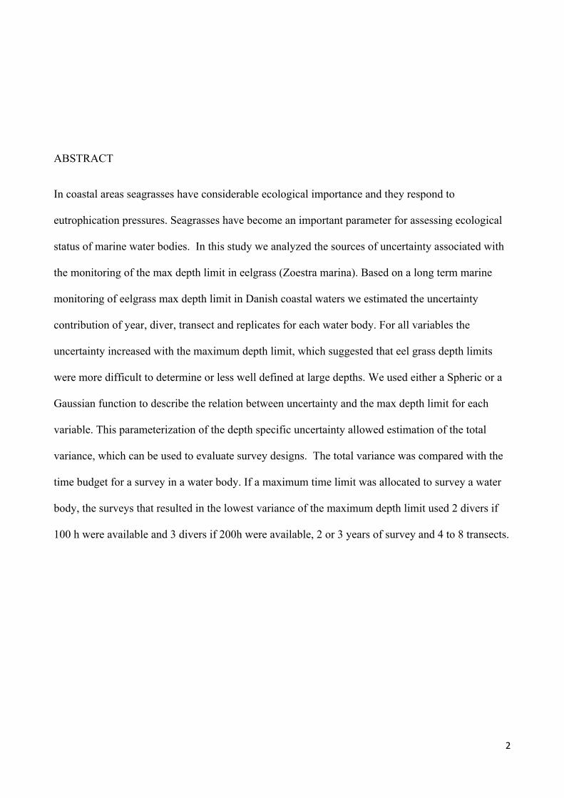
2
ABSTRACT
In coastal areas seagrasses have considerable ecological importance and they respond to
eutrophication pressures. Seagrasses have become an important parameter for assessing ecological
status of marine water bodies. In this study we analyzed the sources of uncertainty associated with
the monitoring of the max depth limit in eelgrass (Zoestra marina). Based on a long term marine
monitoring of eelgrass max depth limit in Danish coastal waters we estimated the uncertainty
contribution of year, diver, transect and replicates for each water body. For all variables the
uncertainty increased with the maximum depth limit, which suggested that eel grass depth limits
were more difficult to determine or less well defined at large depths. We used either a Spheric or a
Gaussian function to describe the relation between uncertainty and the max depth limit for each
variable. This parameterization of the depth specific uncertainty allowed estimation of the total
variance, which can be used to evaluate survey designs. The total variance was compared with the
time budget for a survey in a water body. If a maximum time limit was allocated to survey a water
body, the surveys that resulted in the lowest variance of the maximum depth limit used 2 divers if
100 h were available and 3 divers if 200h were available, 2 or 3 years of survey and 4 to 8 transects.
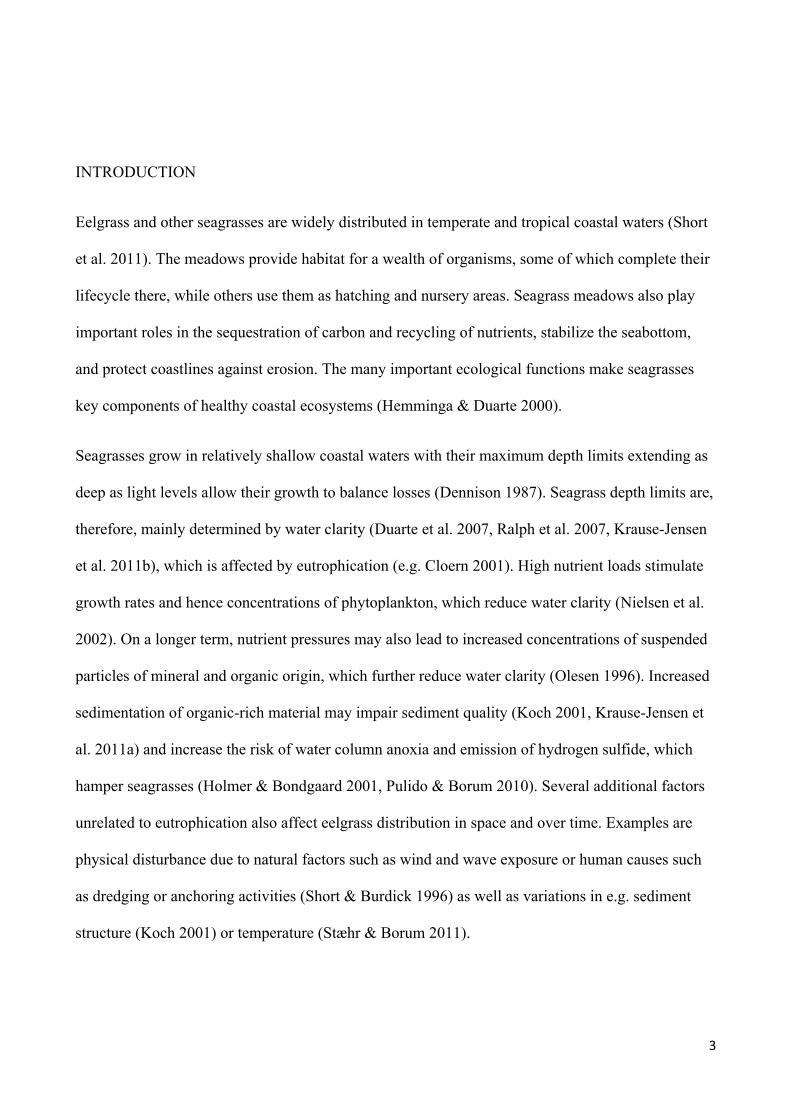
3
INTRODUCTION
Eelgrass and other seagrasses are widely distributed in temperate and tropical coastal waters (Short
et al. 2011). The meadows provide habitat for a wealth of organisms, some of which complete their
lifecycle there, while others use them as hatching and nursery areas. Seagrass meadows also play
important roles in the sequestration of carbon and recycling of nutrients, stabilize the seabottom,
and protect coastlines against erosion. The many important ecological functions make seagrasses
key components of healthy coastal ecosystems (Hemminga & Duarte 2000).
Seagrasses grow in relatively shallow coastal waters with their maximum depth limits extending as
deep as light levels allow their growth to balance losses (Dennison 1987). Seagrass depth limits are,
therefore, mainly determined by water clarity (Duarte et al. 2007, Ralph et al. 2007, Krause-Jensen
et al. 2011b), which is affected by eutrophication (e.g. Cloern 2001). High nutrient loads stimulate
growth rates and hence concentrations of phytoplankton, which reduce water clarity (Nielsen et al.
2002). On a longer term, nutrient pressures may also lead to increased concentrations of suspended
particles of mineral and organic origin, which further reduce water clarity (Olesen 1996). Increased
sedimentation of organic-rich material may impair sediment quality (Koch 2001, Krause-Jensen et
al. 2011a) and increase the risk of water column anoxia and emission of hydrogen sulfide, which
hamper seagrasses (Holmer & Bondgaard 2001, Pulido & Borum 2010). Several additional factors
unrelated to eutrophication also affect eelgrass distribution in space and over time. Examples are
physical disturbance due to natural factors such as wind and wave exposure or human causes such
as dredging or anchoring activities (Short & Burdick 1996) as well as variations in e.g. sediment
structure (Koch 2001) or temperature (Stæhr & Borum 2011).
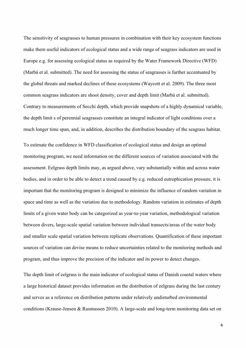
4
The sensitivity of seagrasses to human pressures in combination with their key ecosystem functions
make them useful indicators of ecological status and a wide range of seagrass indicators are used in
Europe e.g. for assessing ecological status as required by the Water Framework Directive (WFD)
(Marbá et al. submitted). The need for assessing the status of seagrasses is further accentuated by
the global threats and marked declines of these ecosystems (Waycott et al. 2009). The three most
common seagrass indicators are shoot density, cover and depth limit (Marbá et al. submitted).
Contrary to measurements of Secchi depth, which provide snapshots of a highly dynamical variable,
the depth limit s of perennial seagrasses constitute an integral indicator of light conditions over a
much longer time span, and, in addition, describes the distribution boundary of the seagrass habitat.
To estimate the confidence in WFD classification of ecological status and design an optimal
monitoring program, we need information on the different sources of variation associated with the
assessment. Eelgrass depth limits may, as argued above, vary substantially within and across water
bodies, and in order to be able to detect a trend caused by e.g. reduced eutrophication pressure, it is
important that the monitoring program is designed to minimize the influence of random variation in
space and time as well as the variation due to methodology. Random variation in estimates of depth
limits of a given water body can be categorized as year-to-year variation, methodological variation
between divers, large-scale spatial variation between individual transects/areas of the water body
and smaller scale spatial variation between replicate observations. Quantification of these important
sources of variation can devise means to reduce uncertainties related to the monitoring methods and
program, and thus improve the precision of the indicator and its power to detect changes.
The depth limit of eelgrass is the main indicator of ecological status of Danish coastal waters where
a large historical dataset provides information on the distribution of eelgrass during the last century
and serves as a reference on distribution patterns under relatively undisturbed environmental
conditions (Krause-Jensen & Rasmussen 2010). A large-scale and long-term monitoring data set on
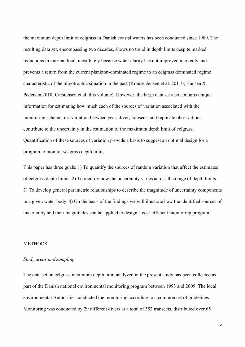
5
the maximum depth limit of eelgrass in Danish coastal waters has been conducted since 1989. The
resulting data set, encompassing two decades, shows no trend in depth limits despite marked
reductions in nutrient load, most likely because water clarity has not improved markedly and
prevents a return from the current plankton-dominated regime to an eelgrass dominated regime
characteristic of the oligotrophic situation in the past (Krause-Jensen et al. 2011b; Hansen &
Pedersen 2010; Carstensen et al. this volume). However, the large data set also contains unique
information for estimating how much each of the sources of variation associated with the
monitoring scheme, i.e. variation between year, diver, transects and replicate observations
contribute to the uncertainty in the estimation of the maximum depth limit of eelgrass.
Quantification of these sources of variation provide a basis to suggest an optimal design for a
program to monitor seagrass depth limits.
This paper has three goals: 1) To quantify the sources of random variation that affect the estimates
of eelgrass depth limits. 2) To identify how the uncertainty varies across the range of depth limits.
3) To develop general parametric relationships to describe the magnitude of uncertainty components
in a given water body. 4) On the basis of the findings we will illustrate how the identified sources of
uncertainty and their magnitudes can be applied to design a cost-efficient monitoring program.
METHODS
Study areas and sampling
The data set on eelgrass maximum depth limit analyzed in the present study has been collected as
part of the Danish national environmental monitoring program between 1993 and 2009. The local
environmental Authorities conducted the monitoring according to a common set of guidelines.
Monitoring was conducted by 29 different divers at a total of 352 transects, distributed over 65
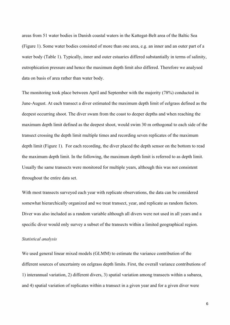
6
areas from 51 water bodies in Danish coastal waters in the Kattegat-Belt area of the Baltic Sea
(Figure 1). Some water bodies consisted of more than one area, e.g. an inner and an outer part of a
water body (Table 1). Typically, inner and outer estuaries differed substantially in terms of salinity,
eutrophication pressure and hence the maximum depth limit also differed. Therefore we analysed
data on basis of area rather than water body.
The monitoring took place between April and September with the majority (78%) conducted in
June-August. At each transect a diver estimated the maximum depth limit of eelgrass defined as the
deepest occurring shoot. The diver swam from the coast to deeper depths and when reaching the
maximum depth limit defined as the deepest shoot, would swim 30 m orthogonal to each side of the
transect crossing the depth limit multiple times and recording seven replicates of the maximum
depth limit (Figure 1). For each recording, the diver placed the depth sensor on the bottom to read
the maximum depth limit. In the following, the maximum depth limit is referred to as depth limit.
Usually the same transects were monitored for multiple years, although this was not consistent
throughout the entire data set.
With most transects surveyed each year with replicate observations, the data can be considered
somewhat hierarchically organized and we treat transect, year, and replicate as random factors.
Diver was also included as a random variable although all divers were not used in all years and a
specific diver would only survey a subset of the transects within a limited geographical region.
Statistical analysis
We used general linear mixed models (GLMM) to estimate the variance contribution of the
different sources of uncertainty on eelgrass depth limits. First, the overall variance contributions of
1) interannual variation, 2) different divers, 3) spatial variation among transects within a subarea,
and 4) spatial variation of replicates within a transect in a given year and for a given diver were
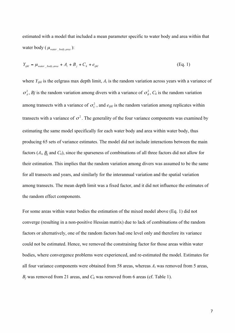
7
estimated with a model that included a mean parameter specific to water body and area within that
water body ( ):
(Eq. 1)
where Yijkl is the eelgrass max depth limit, Ai is the random variation across years with a variance of
, Bj is the random variation among divers with a variance of , Ck is the random variation
among transects with a variance of , and eijkl is the random variation among replicates within
transects with a variance of . The generality of the four variance components was examined by
estimating the same model specifically for each water body and area within water body, thus
producing 65 sets of variance estimates. The model did not include interactions between the main
factors (Ai, Bj and Ck), since the sparseness of combinations of all three factors did not allow for
their estimation. This implies that the random variation among divers was assumed to be the same
for all transects and years, and similarly for the interannual variation and the spatial variation
among transects. The mean depth limit was a fixed factor, and it did not influence the estimates of
the random effect components.
For some areas within water bodies the estimation of the mixed model above (Eq. 1) did not
converge (resulting in a non-positive Hessian matrix) due to lack of combinations of the random
factors or alternatively, one of the random factors had one level only and therefore its variance
could not be estimated. Hence, we removed the constraining factor for those areas within water
bodies, where convergence problems were experienced, and re-estimated the model. Estimates for
all four variance components were obtained from 58 areas, whereas Ai was removed from 5 areas,
Bj was removed from 21 areas, and Ck was removed from 6 areas (cf. Table 1).
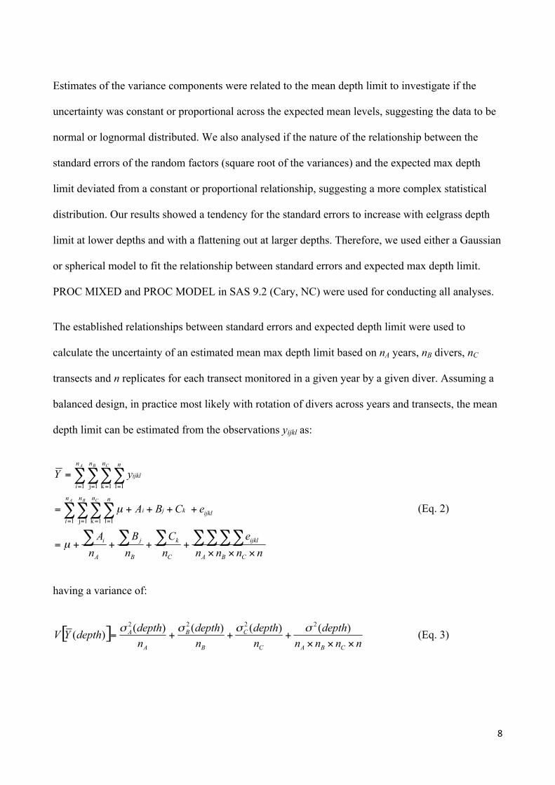
8
Estimates of the variance components were related to the mean depth limit to investigate if the
uncertainty was constant or proportional across the expected mean levels, suggesting the data to be
normal or lognormal distributed. We also analysed if the nature of the relationship between the
standard errors of the random factors (square root of the variances) and the expected max depth
limit deviated from a constant or proportional relationship, suggesting a more complex statistical
distribution. Our results showed a tendency for the standard errors to increase with eelgrass depth
limit at lower depths and with a flattening out at larger depths. Therefore, we used either a Gaussian
or spherical model to fit the relationship between standard errors and expected max depth limit.
PROC MIXED and PROC MODEL in SAS 9.2 (Cary, NC) were used for conducting all analyses.
The established relationships between standard errors and expected depth limit were used to
calculate the uncertainty of an estimated mean max depth limit based on nA years, nB divers, nC
transects and n replicates for each transect monitored in a given year by a given diver. Assuming a
balanced design, in practice most likely with rotation of divers across years and transects, the mean
depth limit can be estimated from the observations yijkl as:
(Eq. 2)
having a variance of:
(Eq. 3)
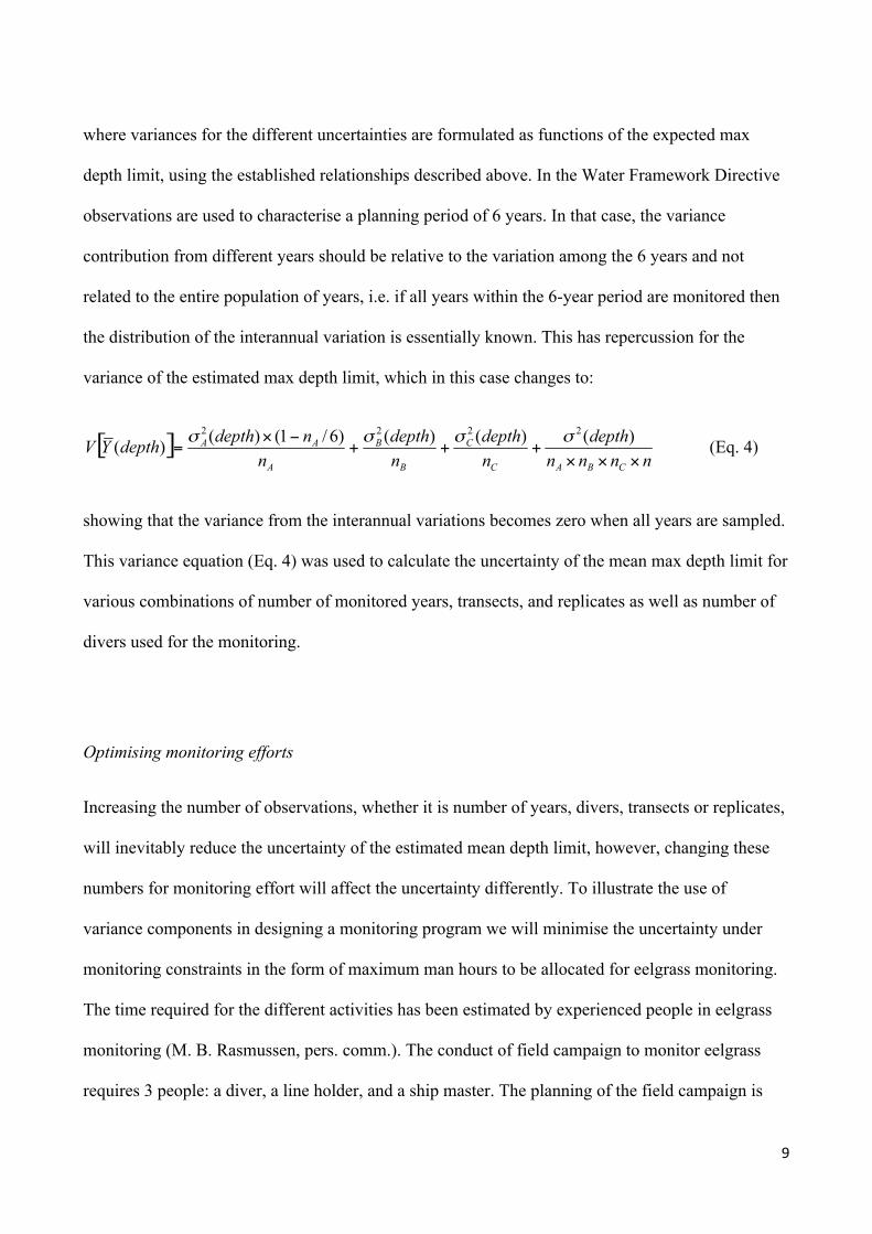
9
where variances for the different uncertainties are formulated as functions of the expected max
depth limit, using the established relationships described above. In the Water Framework Directive
observations are used to characterise a planning period of 6 years. In that case, the variance
contribution from different years should be relative to the variation among the 6 years and not
related to the entire population of years, i.e. if all years within the 6-year period are monitored then
the distribution of the interannual variation is essentially known. This has repercussion for the
variance of the estimated max depth limit, which in this case changes to:
(Eq. 4)
showing that the variance from the interannual variations becomes zero when all years are sampled.
This variance equation (Eq. 4) was used to calculate the uncertainty of the mean max depth limit for
various combinations of number of monitored years, transects, and replicates as well as number of
divers used for the monitoring.
Optimising monitoring efforts
Increasing the number of observations, whether it is number of years, divers, transects or replicates,
will inevitably reduce the uncertainty of the estimated mean depth limit, however, changing these
numbers for monitoring effort will affect the uncertainty differently. To illustrate the use of
variance components in designing a monitoring program we will minimise the uncertainty under
monitoring constraints in the form of maximum man hours to be allocated for eelgrass monitoring.
The time required for the different activities has been estimated by experienced people in eelgrass
monitoring (M. B. Rasmussen, pers. comm.). The conduct of field campaign to monitor eelgrass
requires 3 people: a diver, a line holder, and a ship master. The planning of the field campaign is
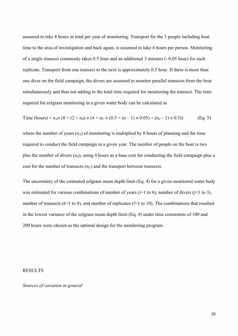
10
assumed to take 8 hours in total per year of monitoring. Transport for the 3 people including boat
time to the area of investigation and back again, is assumed to take 4 hours per person. Monitoring
of a single transect commonly takes 0.5 hour and an additional 3 minutes (~0.05 hour) for each
replicate. Transport from one transect to the next is approximately 0.5 hour. If there is more than
one diver on the field campaign, the divers are assumed to monitor parallel transects from the boat
simultaneously and thus not adding to the total time required for monitoring the transect. The time
required for eelgrass monitoring in a given water body can be calculated as
Time (hours) = nA× (8 + (2 + nB) × (4 + nC × (0.5 + (n – 1) × 0.05) + (nC - 1) × 0.5)) (Eq. 5)
where the number of years (nA) of monitoring is multiplied by 8 hours of planning and the time
required to conduct the field campaign in a given year. The number of people on the boat is two
plus the number of divers (nB), using 4 hours as a base cost for conducting the field campaign plus a
cost for the number of transects (nC) and the transport between transects.
The uncertainty of the estimated eelgrass mean depth limit (Eq. 4) for a given monitored water body
was estimated for various combinations of number of years (i=1 to 6), number of divers (j=1 to 3),
number of transects (k=1 to 8), and number of replicates (l=1 to 10). The combinations that resulted
in the lowest variance of the eelgrass mean depth limit (Eq. 4) under time constraints of 100 and
200 hours were chosen as the optimal design for the monitoring program.
RESULTS
Sources of variation in general
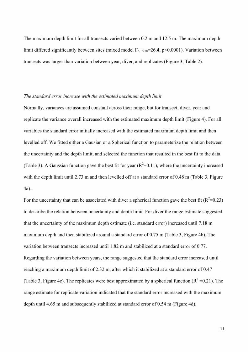
11
The maximum depth limit for all transects varied between 0.2 m and 12.5 m. The maximum depth
limit differed significantly between sites (mixed model F6, 7278=26.4, p<0.0001). Variation between
transects was larger than variation between year, diver, and replicates (Figure 3, Table 2).
The standard error increase with the estimated maximum depth limit
Normally, variances are assumed constant across their range, but for transect, diver, year and
replicate the variance overall increased with the estimated maximum depth limit (Figure 4). For all
variables the standard error initially increased with the estimated maximum depth limit and then
levelled off. We fitted either a Gausian or a Spherical function to parameterize the relation between
the uncertainty and the depth limit, and selected the function that resulted in the best fit to the data
(Table 3). A Gaussian function gave the best fit for year (R2=0.11), where the uncertainty increased
with the depth limit until 2.73 m and then levelled off at a standard error of 0.48 m (Table 3, Figure
4a).
For the uncertainty that can be associated with diver a spherical function gave the best fit (R2=0.23)
to describe the relation between uncertainty and depth limit. For diver the range estimate suggested
that the uncertainty of the maximum depth estimate (i.e. standard error) increased until 7.18 m
maximum depth and then stabilized around a standard error of 0.75 m (Table 3, Figure 4b). The
variation between transects increased until 1.82 m and stabilized at a standard error of 0.77.
Regarding the variation between years, the range suggested that the standard error increased until
reaching a maximum depth limit of 2.32 m, after which it stabilized at a standard error of 0.47
(Table 3, Figure 4c). The replicates were best approximated by a spherical function (R2 =0.21). The
range estimate for replicate variation indicated that the standard error increased with the maximum
depth until 4.65 m and subsequently stabilized at standard error of 0.54 m (Figure 4d).
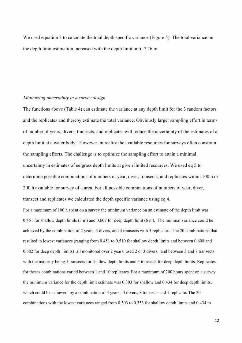
12
We used equation 3 to calculate the total depth specific variance (Figure 5). The total variance on
the depth limit estimation increased with the depth limit until 7.26 m.
Minimizing uncertainty in a survey design
The functions above (Table 4) can estimate the variance at any depth limit for the 3 random factors
and the replicates and thereby estimate the total variance. Obviously larger sampling effort in terms
of number of years, divers, transects, and replicates will reduce the uncertainty of the estimates of a
depth limit at a water body. However, in reality the available resources for surveys often constrain
the sampling efforts. The challenge is to optimize the sampling effort to attain a minimal
uncertainty in estimates of eelgrass depth limits at given limited resources. We used eq 5 to
determine possible combinations of numbers of year, diver, transects, and replicates within 100 h or
200 h available for survey of a area. For all possible combinations of numbers of year, diver,
transect and replicates we calculated the depth specific variance using eq 4.
For a maximum of 100 h spent on a survey the minimum variance on an estimate of the depth limit was
0.451 for shallow depth limits (3 m) and 0.607 for deep depth limit (6 m). The minimal variance could be
achieved by the combination of 2 years, 3 divers, and 4 transects with 5 replicates. The 20 combinations that
resulted in lowest variances (ranging from 0.451 to 0.510 for shallow depth limits and between 0.608 and
0.682 for deep depth limits) all monitored over 2 years, used 2 or 3 divers, and between 3 and 7 transects
with the majority being 5 transects for shallow depth limits and 3 transects for deep depth limits. Replicates
for theses combinations varied between 1 and 10 replicates. For a maximum of 200 hours spent on a survey
the minimum variance for the depth limit estimate was 0.303 for shallow and 0.434 for deep depth limits,
which could be achieved by a combination of 3 years, 3 divers, 8 transects and 1 replicate. The 20
combinations with the lowest variances ranged from 0.303 to 0.353 for shallow depth limits and 0.434 to
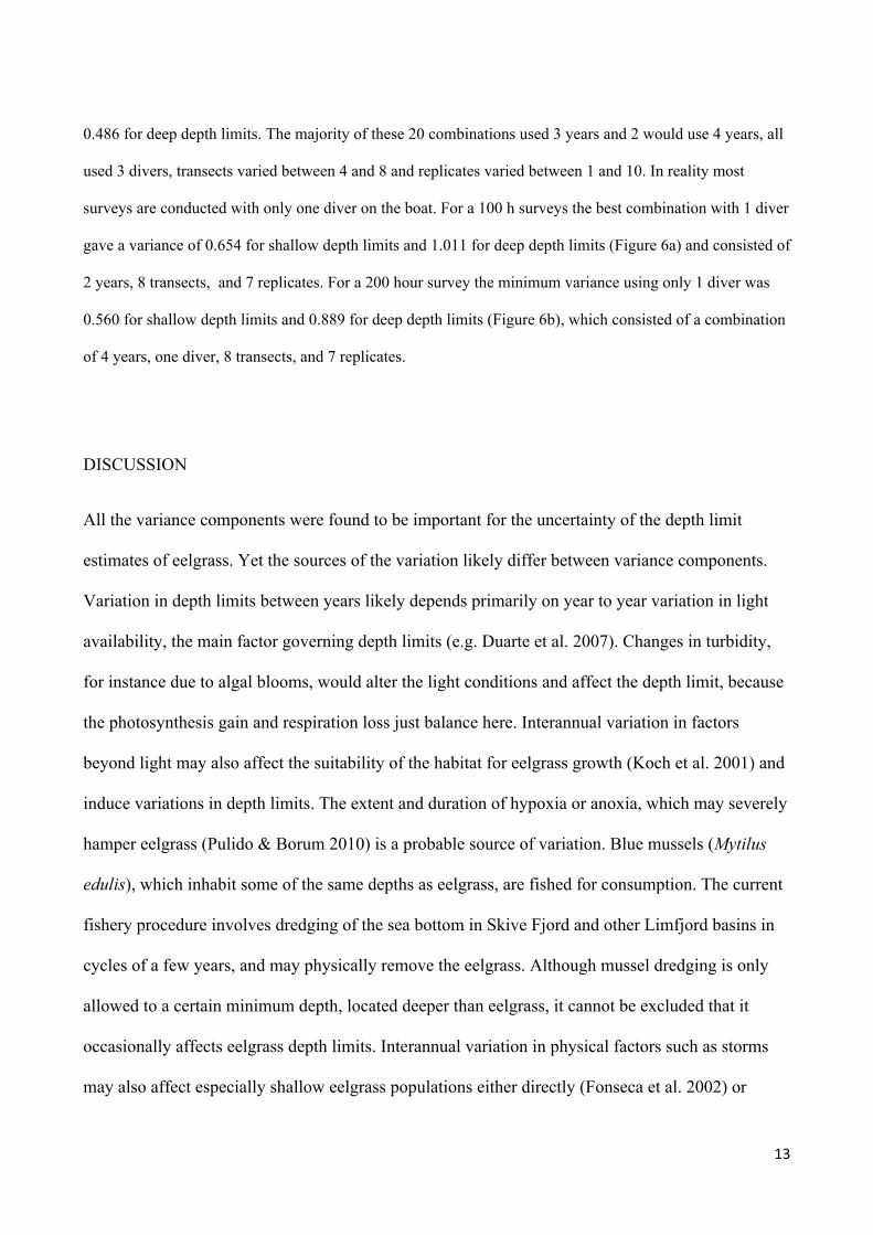
13
0.486 for deep depth limits. The majority of these 20 combinations used 3 years and 2 would use 4 years, all
used 3 divers, transects varied between 4 and 8 and replicates varied between 1 and 10. In reality most
surveys are conducted with only one diver on the boat. For a 100 h surveys the best combination with 1 diver
gave a variance of 0.654 for shallow depth limits and 1.011 for deep depth limits (Figure 6a) and consisted of
2 years, 8 transects, and 7 replicates. For a 200 hour survey the minimum variance using only 1 diver was
0.560 for shallow depth limits and 0.889 for deep depth limits (Figure 6b), which consisted of a combination
of 4 years, one diver, 8 transects, and 7 replicates.
DISCUSSION
All the variance components were found to be important for the uncertainty of the depth limit
estimates of eelgrass. Yet the sources of the variation likely differ between variance components.
Variation in depth limits between years likely depends primarily on year to year variation in light
availability, the main factor governing depth limits (e.g. Duarte et al. 2007). Changes in turbidity,
for instance due to algal blooms, would alter the light conditions and affect the depth limit, because
the photosynthesis gain and respiration loss just balance here. Interannual variation in factors
beyond light may also affect the suitability of the habitat for eelgrass growth (Koch et al. 2001) and
induce variations in depth limits. The extent and duration of hypoxia or anoxia, which may severely
hamper eelgrass (Pulido & Borum 2010) is a probable source of variation. Blue mussels (Mytilus
edulis), which inhabit some of the same depths as eelgrass, are fished for consumption. The current
fishery procedure involves dredging of the sea bottom in Skive Fjord and other Limfjord basins in
cycles of a few years, and may physically remove the eelgrass. Although mussel dredging is only
allowed to a certain minimum depth, located deeper than eelgrass, it cannot be excluded that it
occasionally affects eelgrass depth limits. Interannual variation in physical factors such as storms
may also affect especially shallow eelgrass populations either directly (Fonseca et al. 2002) or
14
indirectly through modifications of the substrate (Koch et al. 2001; Krause et al 2011a).
Furthermore, the exact location of transects may vary between years, thereby causing variation in
depth limits, especially if the eelgrass distribution is patchy.
Small deviations in individual divers practice during estimation of the depth limit and the accuracy
with which they can correct for fluctuation in water level during a day of surveys is the likely main
cause of diver variation. Furthermore, when divers swim the zigzag across the depth limit they will
invariably cross the depth limits at different locations, which could lead to different estimates
especially if the distribution of eelgrass is patchy.
Large-scale spatial variation between transects in a water body is most probably caused by some of
the same factors causing interannual variation in depth limits, e.g. difference in light climate,
oxygen conditions and substrate conditions e.g. due to difference in eutrophication pressures and
wind exposure within the water body.
The replicates within a transect reflect small scale spatial variation which is strongly dependent on
the patchiness of eelgrass. Replicates representing the same large eelgrass patch are likely less
variable than those reflecting a patchy eelgrass distribution.
Differences in patchiness may, thus, explain some of the difference in variation between transects
and replicates in Figure 2a and 2b.
Why does the uncertainty increase with the estimated max depth limit?
The increase in uncertainty of all variance components with increased maximum depth limit (Figure
4 & 5) suggests that deeper depth limits were more variable on temporal as well as on spatial scales
and also more difficult for the divers to determine. The reason could be that the zone of light levels
15
supporting eelgrass at the depth limit is more extended in clear than in turbid waters. Large depth
limits reflect relatively clear water and hence less light attenuation, which means that the area
exposed to for instance 5 % surplus light (photosynthesis relative to respiration) and 0 % surplus
light (max depth limit) would be larger for large depth limits. Given this scenario the observed
depth limit at large depth could be expected to fluctuate more than at shallow depth limits.
Also, the range of possible depth limits is larger in clear water with deep depth limits than in turbid
waters with shallow depth limits and thereby allows a large inherent variation. The shore line thus
sets a lower boundary for the depth limit estimates which limits the variation in shallow depth
limits.
The uncertainty for divers continued to increase until 7.3 m before it leveled off. This may reflect
an increased difficulty in estimating the depth limit at deeper depths and, again, an increased range
of possible depth limits. Despite a well-defined start point for the transects, the diver may drift to
either side of the transect, such drift may accumulate in long transects resulting in larger variation in
long transects (i.e. at larger max depth limit). However, the relative variation in depth limits
actually declines with larger max depth limit, as the variation makes up a smaller proportion of the
larger than the smaller estimated depth limits. This decrease in relative variation also means that it
should be easier to detect relative changes in deeper depth limits than in shallower depth limits. The
higher relative variation in shallow depth limits may be due to larger effect of physical exposure,
causing larger variability in eelgrass distribution and abundance towards the shore (Krause-Jensen
et al 2000, Fonseca et al. 2002). For the variance components ‘year’ and ‘transect’ the uncertainty
leveled off already around 2 m, which could be the depths where physical factors such as wind
exposure have smaller effect and the variation between transects and years therefore becomes
stable.
16
Parameterization of uncertainty
In this study we parameterized the uncertainty for the variables associated with the survey design.
Such quantification of the uncertainty is important for evaluating the accuracy of ecological status
class assessment in surveys to test for compliance with the water framework directive (Carstensen
2007).
The formulas that we here present are generally applicable to marine monitoring programs and
should be taken into account when designing a survey. In our study it was possible to estimate the
parameters empirically as we had access to a large database where no time series trend existed in
the eelgrass depth limit (Hansen & Petersen 2011; Carstensen et al. 2012). Our eelgrass data set had
special characteristics as the uncertainty for all variables increased with the depth limit. At shallow
depths the uncertainty increased with the depth limit i.e. log normally distributed, this can usually
be transformed to fit normality with a log transformation, whereas the uncertainty at larger depth
limits remained unaffected by increases in the depth limit and thus follow a normal distribution.
Implications for survey designs
We can use the parameterization of the variance component to estimate the variance for different
survey designs. The results of our case studies give clear recommendations for design of surveys
that can reduce the uncertainty relative to the current survey designs. In particular using 2 or 3
divers simultaneously instead of just 1 diver can apparently reduce the variance with up to 40 %.
Despite that a six year period was available for the survey the variance on the depth limit estimation
would be smallest for only 2 or 3 years of survey for both time-limited scenarios, and transects
17
varied between 4 and 8 transects per water body. It is, however, interesting that the residuals
seemed to have little effect on the uncertainty.
We admit that our approach to calculation of a time budget is simplified, but it illustrates an
important point, which is that the diver can have large effects on the uncertainty and survey would
need to limit the uncertainty with which they contribute. Similar effect of surveyor has been
documented for benthic invertebrates (Benedetti-Cecchi et al 1996). The use of multiple divers
surveying a transect will undoubtedly improve the accuracy of the estimate of the depth limit for a
water body. However, given the individual differences between divers it would be easier to detect a
change in a water body if transects were surveyed by the same diver year after year. Some regional
surveys have employed the strategy of using the same diver to survey specific transects. Such
strategy, however, is vulnerable to changes in diver, which would disrupt the reliability of the whole
time series. Unless one is sure to be able to use the same diver for many years such a sampling
strategy would not benefit the accuracy of estimates of eelgrass depth limit over longer time span.
ACKNOWLEDGEMENT
This research is a contribution to the WISER project (contract #FP7-‐226273), funded by the
European Commission and to the WATERS project. We are grateful to the Danish
Environmental Centers responsible for data collection under the Danish Nationwide Aquatic
Monitoring and Assessment Program
18
LITERATURE
Benedetti-Cecchi, L., L.Airoldi, M. Abbiati, & F. Cinelli, 1996. Estimating the abundance of
benthic invertebrates: a comparison of producers and variability between observers. Marine
Ecology Progress series 138: 93-101.
Carstensen, J. 2007. Statistical principles for ecological status classification of Water Framework
Directive monitoring data. Marine Pollution Bulletin 55: 3-15.
Carstensen, J., D. Krause-Jensen, S. Markager, K. Timmermann, J. Windolf (this issue) Water
clarity and eelgrass responses to nitrogen reductions in the eutrophic Skive Fjord, Denmark.
Submitted to Hydrobiologia.
Cloern, J.E. 2001. Our evolving conceptual model of the coastal eutrophication problem. Marine
Ecology Progress Series 210: 223-253.
Dennison, W.C., 1987. Effects of light on seagrass photosynthesis, growth and depth distribution.
Aquatic Botany 27: 15-26.
19
Duarte, C.M., N. Marbà, D. Krause-Jensen, M. Sánchez-Camacho, 2007. Testing the predictive
power of seagrass depth limit models. Estuaries Coasts 30: 652–656.
Fonseca, M. S., P. E. Whitfield, N. M. Kelly & S. S. Bell, 2002. Modelling seagrass landscape pattern and
associated ecological attributes. Ecological Applications 12:218–237.
Hansen, J.W., D.L.J. Petersen, (eds.) 2011.Marine områder 2010. NOVANA. Tilstand og udvikling
i miljø- og naturkvaliteten. Aarhus University, DCE - National Center for the Environment and
Energy. 120 pp. – Scientific report no. 6. http://www2.dmu.dk/Pub/SR6.pdf.
Hemminga M.A., C. M. Duarte, 2000. Seagrass ecology. Cambridge University Press, Cambridge.
Holmer M, E. J. Bondgaard, 2001. Photosynthetic and growth response of eelgrass to low oxygen
and high sulfide concentrations during hypoxic events. Aquatic Botany 70: 29–38.
Koch, E. M.. 2001. Beyond light: physical, geological, and geochemical parameters as possible
submersed aquatic vegetation habitat requirements. Estuaries 24: 1–17.
Krause-Jensen, D., A. L. Middelboe, K. Sand-Jensen & P. B Christensen, 2000. Eelgrass, Zostera
marina, growth along depth gradients: Upper boundaries of the variation as a powerful predictive
tool. Oikos 91: 233-244.
20
Krause-Jensen, D, M. F. Pedersen & C. Jensen, 2003. Regulation of Eelgrass (Zostera marina)
Cover along depth gradients in Danish coastal waters. Estuaries 26: 866-877.
Krause Jensen, D., J. Carstensen, , S.L. Nielsen, T. Dalsgaard, P. B. Christensen, H. Fossing, M. B.
Rasmussen, 2011a. Sea bottom characteristics affect depth limits of eelgrass Zostera marina.
Marine Ecology Progress Series 425: 91-102.
Krause-Jensen D, S. Markager, T. Dalsgaard T. 2011b. Benthic and pelagic primary production in
different nutrient regimes. Estuaries and Coasts. DOI: 10.1007/s12237-011-9443-1
Krause-Jensen, D., M. B. Rasmussen, 2009. Historisk udbredelse af ålegræs i danske kystområder,
National Environmental Research Institute, Aarhus University. Scientific report No. 755, 38 pp.
http://www.dmu.dk/Pub/FR755.pdf.
Marbà, N., Krause-Jensen, D., T. Alcoverro, S. Birk, A. Pedersen, J. M. Neto, S. Orfanidis, J. M.
Garmendia, I. Muxika, A. Borja, & K. Dencheva, Diversity of European seagrass indicators -
Patterns within and across regions. Submitted to Ecological Indicators.
21
Nielsen, S.L., K. Sand-Jensen, J. Borum, J. & O. Geertz-Hansen, 2002. Depth colonization of
eelgrass (Zostera marina) and macroalgae as determined by water transparency in Danish coastal
waters. Estuaries 25:1025–1032.
Olesen B. 1996 Regulation of light attenuation and eelgrass Zostera marina depth distribution in a
Danish embayment. Mar Ecol Prog Ser 134:187–194.
Pulido C. & J. Borum 2010. Eelgrass (Zostera marina) tolerance to anoxia. J Exp Mar Biol Ecol
385:8–13
Ralph, P.J., M. J. Durako, S. Enriquez,C. J. Collier & M. A. Doblin, 2007. Impact of light limitation
on seagrasses. Journal of Experimental Marine Biology and Ecology 350: 176-193.
Short, F. T. & D. M. Burdick, 1996. Quantifying eelgrass habitat loss in relation to housing
development and nitrogen loading in Waquoit Bay, Massachusetts. Estuaries 19:730-739.
Short F. T., B. Polidoro, S. R.Livingstone, K. E. Carpenter, S. Bandeira, J. S. Bujang, H. P.
Calumpong, T. J. B. Carruthers, R. G. Cole, W. C. Dennison, P. L. A. Erftemeijer, M. D. Fortes, A.
S. Freeman, T. G. Jagtap, A. H. M. Kamal, G. A. Kendrick, K. W. Kenworthy, La Nafie YAn, I. M.
Nasution, R. J. Orth, A. Prathep, J. C. Sanciangco, B. van Tussenbroek, S. G. Vergara, M. Waycott,
J. C. Zieman, 2011. Extinction risk assessment of the world’s seagrass species. Biological
Conservation 144: 1961–1971.
22
Stæhr P & J. Borum, 2011. Seasonal acclimation in metabolism reduces light requirements of
eelgrass (Zostera marina). Journal of Experimental Marine Biology and Ecology 407: 139–146.
Waycott M., C. M. Duarte, T. J. B. Carrouthers, R. J. Orth & others (2009) Accelerating loss of
seagrasses across the globe threatens coastal ecosystems. Proc Natl Acad Sci USA 106: 12377–
12381.
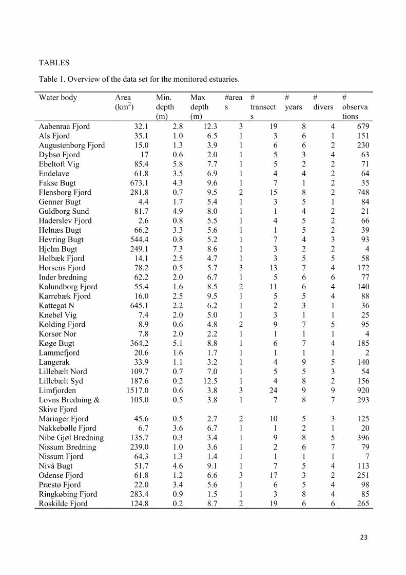
23
TABLES
Table 1. Overview of the data set for the monitored estuaries.
Water body Area (km2)
Min. depth (m)
Max depth (m)
#areas
# transects
# years
# divers
# observations
Aabenraa Fjord 32.1 2.8 12.3 3 19 8 4 679 Als Fjord 35.1 1.0 6.5 1 3 6 1 151 Augustenborg Fjord 15.0 1.3 3.9 1 6 6 2 230 Dybsø Fjord 17 0.6 2.0 1 5 3 4 63 Ebeltoft Vig 85.4 5.8 7.7 1 5 2 2 71 Endelave 61.8 3.5 6.9 1 4 4 2 64 Fakse Bugt 673.1 4.3 9.6 1 7 1 2 35 Flensborg Fjord 281.8 0.7 9.5 2 15 8 2 748 Genner Bugt 4.4 1.7 5.4 1 3 5 1 84 Guldborg Sund 81.7 4.9 8.0 1 1 4 2 21 Haderslev Fjord 2.6 0.8 5.5 1 4 5 2 66 Helnæs Bugt 66.2 3.3 5.6 1 1 5 2 39 Hevring Bugt 544.4 0.8 5.2 1 7 4 3 93 Hjelm Bugt 249.1 7.3 8.6 1 3 2 2 4 Holbæk Fjord 14.1 2.5 4.7 1 3 5 5 58 Horsens Fjord 78.2 0.5 5.7 3 13 7 4 172 Inder bredning 62.2 2.0 6.7 1 5 6 6 77 Kalundborg Fjord 55.4 1.6 8.5 2 11 6 4 140 Karrebæk Fjord 16.0 2.5 9.5 1 5 5 4 88 Kattegat N 645.1 2.2 6.2 1 2 3 1 36 Knebel Vig 7.4 2.0 5.0 1 3 1 1 25 Kolding Fjord 8.9 0.6 4.8 2 9 7 5 95 Korsør Nor 7.8 2.0 2.2 1 1 1 1 4 Køge Bugt 364.2 5.1 8.8 1 6 7 4 185 Lammefjord 20.6 1.6 1.7 1 1 1 1 2 Langerak 33.9 1.1 3.2 1 4 9 5 140 Lillebælt Nord 109.7 0.7 7.0 1 5 5 3 54 Lillebælt Syd 187.6 0.2 12.5 1 4 8 2 156 Limfjorden 1517.0 0.6 3.8 3 24 9 9 920 Lovns Bredning & Skive Fjord
105.0 0.5 3.8 1 7 8 7 293
Mariager Fjord 45.6 0.5 2.7 2 10 5 3 125 Nakkebølle Fjord 6.7 3.6 6.7 1 1 2 1 20 Nibe Gjøl Bredning 135.7 0.3 3.4 1 9 8 5 396 Nissum Bredning 239.0 1.0 3.6 1 2 6 7 79 Nissum Fjord 64.3 1.3 1.4 1 1 1 1 7 Nivå Bugt 51.7 4.6 9.1 1 7 5 4 113 Odense Fjord 61.8 1.2 6.6 3 17 3 2 251 Præstø Fjord 22.0 3.4 5.6 1 6 5 4 98 Ringkøbing Fjord 283.4 0.9 1.5 1 3 8 4 85 Roskilde Fjord 124.8 0.2 8.7 2 19 6 6 265
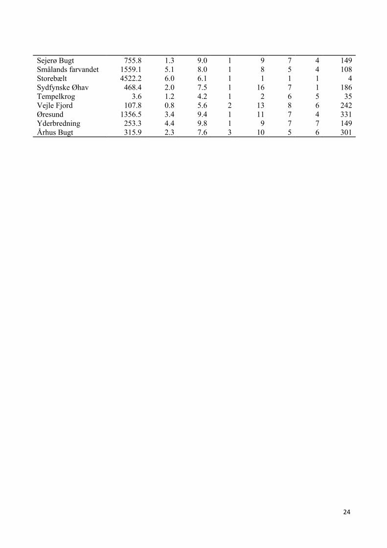
24
Sejerø Bugt 755.8 1.3 9.0 1 9 7 4 149 Smålands farvandet 1559.1 5.1 8.0 1 8 5 4 108 Storebælt 4522.2 6.0 6.1 1 1 1 1 4 Sydfynske Øhav 468.4 2.0 7.5 1 16 7 1 186 Tempelkrog 3.6 1.2 4.2 1 2 6 5 35 Vejle Fjord 107.8 0.8 5.6 2 13 8 6 242 Øresund 1356.5 3.4 9.4 1 11 7 4 331 Yderbredning 253.3 4.4 9.8 1 9 7 7 149 Århus Bugt 315.9 2.3 7.6 3 10 5 6 301
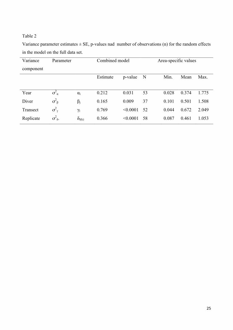
25
Table 2
Variance parameter estimates ± SE, p-values nad number of observations (n) for the random effects
in the model on the full data set.
Variance
component
Parameter Combined model Area-specific values
Estimate p-value N Min. Mean Max.
Year σ2α αi 0.212 0.031 53 0.028 0.374 1.775
Diver σ2β βj 0.165 0.009 37 0.101 0.501 1.508
Transect σ2γ γl 0.769 <0.0001 52 0.044 0.672 2.049
Replicate σ2δ. δl(k) 0.366 <0.0001 58 0.087 0.461 1.053
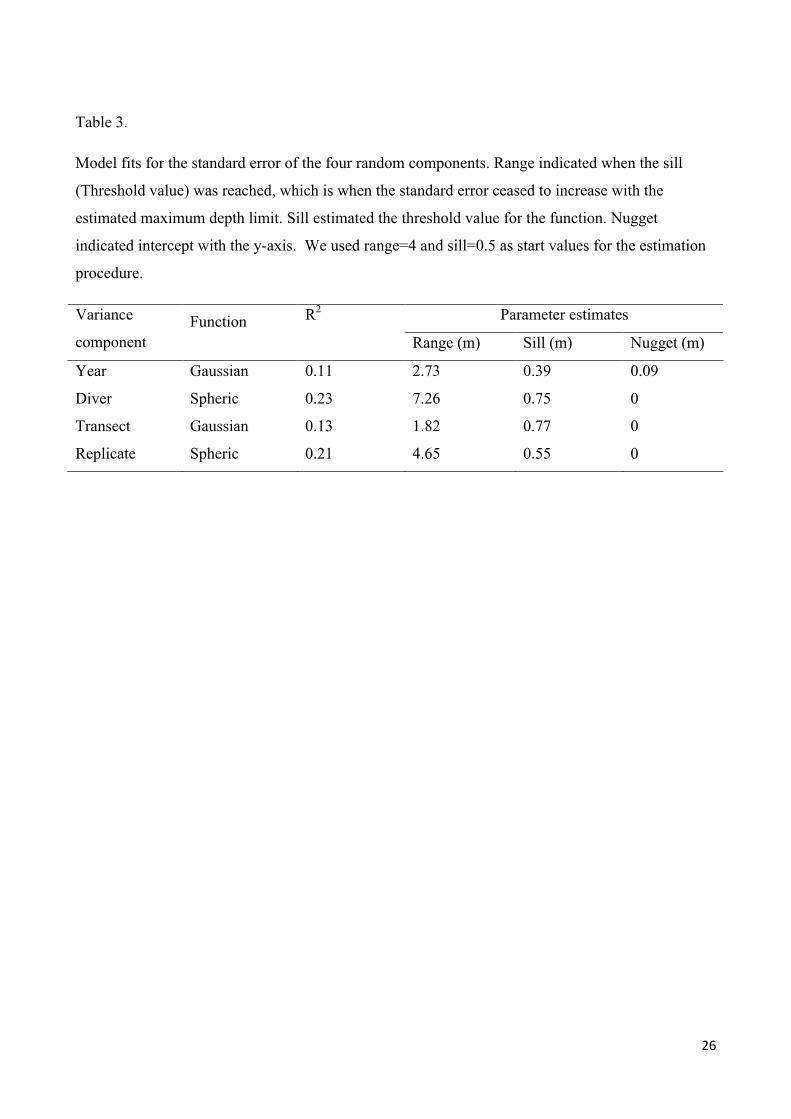
26
Table 3.
Model fits for the standard error of the four random components. Range indicated when the sill
(Threshold value) was reached, which is when the standard error ceased to increase with the
estimated maximum depth limit. Sill estimated the threshold value for the function. Nugget
indicated intercept with the y-axis. We used range=4 and sill=0.5 as start values for the estimation
procedure.
Parameter estimates Variance
component Function R2
Range (m) Sill (m) Nugget (m)
Year Gaussian 0.11 2.73 0.39 0.09
Diver Spheric 0.23 7.26 0.75 0
Transect Gaussian 0.13 1.82 0.77 0
Replicate Spheric 0.21 4.65 0.55 0
27
FIGURE LEGENDS
Figure 1. A. Water bodies in Denmark where eelgrass depth limits are surveyed. B. Example of
distribution of Transects in Vejle Fjord. C. The solid line marks the transects and the dotted line
illustrates the diver zigzag route crossing the max depth limit.
Figure 2. Replicate observations of the depth limit for three transects at each site between 2001 and
2009. The replicate observations of the depth limit of eelgrass within a transect within a year vary
considerably. Observation from the three transects in each area are marked with +, -, X. Transects
were located in Vejle fjord (A), and Aabenraa fjord (B).
Figure 3. The estimates for the uncertainty (SE) contribution of year, diver, transect and replicate on
maximum depth limit.
Figure 4. The standard error as a function of the estimated maximum depth limit for eelgrass for
Transect; Diver; Year; and Replicate. Lines show the fitted spherical or Gaussian functions.
Figure 5. Total variance as a function of depth calculated by equation 4.
Figure 6. Minimum variance at different depths for one diver(black), two divers (white) and 3
divers (hatched) for A) 100 h survey and B) 200 h survey. The variance is calculated by eq 3.
Marine Pollution Bulletin xxx (2011) xxx–xxx
Contents lists available at ScienceDirect
Marine Pollution Bulletin
journal homepage: www.elsevier .com/locate /marpolbul
Ecological status of seagrass ecosystems: An uncertainty analysis of themeadow classification based on the Posidonia oceanica multivariate index (POMI)
Scott Bennett a,⇑, Guillem Roca a, Javier Romero b, Teresa Alcoverro a
a Centro de Estudios Avanzados de Blanes, CSIC, C/ Acceso a la Cala St. Francesc 14, 17300 Blanes, Girona, Spainb Departamento de Ecología, Facultad de Biología, Universidad de Barcelona, Av. Diagonal 645, 08028 Barcelona, Spain
a r t i c l e i n f o
Keywords:Posidonia oceanicaSeagrassBiological indicatorsCoastal watersUncertainty analysisWater Framework Directive
0025-326X/$ - see front matter 2011 Elsevier Ltd. Adoi:10.1016/j.marpolbul.2011.06.016
⇑ Corresponding author. Present address: UWA OceBiology, The University of Western Australia, 35 Sti6009, Australia. Tel.: +61 (0)8 6488 8118.
E-mail address: [email protected] (S.
Please cite this article in press as: Bennett, S., etthe Posidonia oceanica multivariate index (POM
a b s t r a c t
Quantifying the uncertainty associated with monitoring protocols is essential to prevent the misclassifi-cation of ecological status and to improve sampling design. We assessed the Posidonia oceanica multivar-iate index (POMI) bio-monitoring program for its robustness in classifying the ecological status of coastalwaters within the Water Framework Directive. We used a 7-year data set covering 30 sites along 500 kmof the Catalonian coastline to examine which version of POMI (14 or 9 metrics) maximises precision inclassifying the ecological status of meadows. Five factors (zones within a site, sites within a water body,depth, years and surveyors) that potentially generate classification uncertainty were examined in detail.Of these, depth was a major source of uncertainty, while all the remaining spatial and temporal factorsdisplayed low variability. POMI 9 matched POMI 14 in all factors, and could effectively replace it in futuremonitoring programs.
2011 Elsevier Ltd. All rights reserved.
1. Introduction
Degradation in water quality resulting from anthropogenic dis-turbance poses a large threat to both freshwater and marine eco-systems. In response to this, the European Union has developedthe Water Framework Directive (WFD), a trans-national strategyaimed at maintaining and, where necessary, recovering the waterquality of aquatic ecosystems across European member states.The main objective of the WFD is to achieve, at least, a ‘good eco-logical status’ for all water bodies across Europe by 2015. The con-cept of ‘ecological status’, as defined by the WFD, is the quality ofthe structure and functioning of aquatic ecosystems associatedwith surface waters. The ecological status is determined by moni-toring and assessing biological indicators relevant to the waterbody in question that are integrated into an index with the aimto detect temporal and spatial changes in water bodies. Underthe WFD, the values of this index, typically from zero to one, areused to classify each water body into one of five classes, frombad to high. However, a reliable biotic index should not only beable to detect change, but also know that the change it is detectingis meaningful and not an artefact of the methodology, sampling de-sign or execution. Uncertainty analyses are a useful tool to identifythe factors which contribute to the potential misclassification of
ll rights reserved.
ans Institute, School of Plantrling Highway, Crawley, WA
Bennett).
al. Ecological status of seagrassI). Mar. Pollut. Bull. (2011), doi
the ecological status class of water bodies (Clarke and Hering,2006; Staniszewski et al., 2006), which could result in considerablesocial, economic and ecological losses to the region.
Within coastal waters, four biological quality elements (BQEs)have been identified: phytoplankton, macroalgae, angiospermsand benthic invertebrate fauna. These BQEs are sensitive to anthro-pogenic disturbances and, therefore, are potential indicators of theecological status within the water body. Seagrass ecosystems, andin particular for the Mediterranean Posidonia oceanica meadows,make an ideal BQE for monitoring ecological status because of theirhigh sensitivity to disturbance (Delgado et al., 1999; Francour etal., 1999; Ruiz et al., 2001; Ruiz and Romero, 2003), wide distribu-tion (Procaccini et al., 2003) and well understood biology and ecol-ogy (Romero et al., 2007). In regions of Spain and Croatia, the POMIindex (P. oceanica multivariate index; Romero et al., 2007) is usedto monitor, evaluate and classify the ecological status of coastalwater bodies. POMI incorporates 14 metrics from physiological,individual, population and community levels, making it sensitiveto both lethal and sub lethal stressors impacting multiple levelsof organisation (Martinez-Crego et al., 2008). These metrics areintegrated, using principal components analysis (PCA), into a singlevalue from which an EQR (ecological quality ratio, from zero toone) is obtained (Romero et al., 2007).
Posidonia oceanica meadows are dynamic systems, with a con-stant flux of intrinsic and extrinsic factors influencing their struc-ture and function over multiple spatial and temporal scales. Suchdynamics have the potential to obfuscate meaningful trends inecological status predictions, if the sources of variability are not
ecosystems: An uncertainty analysis of the meadow classification based on:10.1016/j.marpolbul.2011.06.016
Mediterranean Sea
Catalonian coast
50 Km
1
12
17
15
13
1416
11
10
9
7654
32
8
Girona
Barcelona
Lleida
Tarragona
Fig. 1. Map of the location of the 30 sampling sites (small black dots) and 17 waterbodies along the Catalonian coast, where the index was applied.
2 S. Bennett et al. / Marine Pollution Bulletin xxx (2011) xxx–xxx
recognised and where possible, reduced. When designing a moni-toring program, decisions must be taken on how to assign the totalsampling effort within the allocated time and budget constraints.The number and distribution of replicates should be taken withthe objective of maximising precision in mind. For example, sea-grass meadows usually display horizontal heterogeneity (e.g. zonesof different density, structure, depth, etc.) within a meadow, andmultiple, spatially independent meadows may exist within a waterbody. Whilst it is expected that sites within a water body reflectsimilar ecological statuses, a certain level of variability among sitesis inevitable. Establishing a measure of the variability amongmeadows within a water body enables an estimation of the likelyprecision of ecological status estimates from water bodies whereonly a single site is present. Uncertainty analyses enable us to visu-alise how our sampling precision is influenced by alternative sam-pling designs. However, despite its fundamental importance, thereis little information on how these different scales and factors canbe used to minimise uncertainty in coastal waters, particularly inseagrass meadows.
The current study analyses uncertainty in classifying the eco-logical status of P. oceanica ecosystems, based on the POMI bio-monitoring program, with two key areas of focus. The first is tocompare POMI (hereafter referred to as POMI14) to a condensed9 metric version (POMI 9) to assess how uncertainty estimatesare affected by the reduction in the number of metrics. The secondarea of focus will be to determine which sources of variability (fac-tors) associated with the sampling design of the POMI monitoringprogram most greatly influence ecological status classifications ofP. oceanica meadows. The analyses will be based on a seven yeardata series that includes over 30 meadows and the factors analysedwill include spatial scales of sampling (variability among zoneswithin a meadow, among meadows within a water body, variabil-ity among depths), the temporal scale of sampling (variabilityamong years) and the human-associated source of error (variabil-ity between surveyors). These five factors represent some the keysources of variability associated with the design and implementa-tion of a regional scale bio-monitoring program, and highlight howcertain elements of a sampling design can influence the precisionand the probability of misclassifying the ecological status of coastalwater bodies.
2. Materials and methods
2.1. Site selection and sampling
Bio-monitoring data from P. oceanica meadows were collectedfrom 30 sites spanning 500 km of the Catalonian coastline (Spain).Sampling took place in autumn (September–October) throughoutthe years 2002–2009, with the exception of 2004, when samplingtook place during early summer (June) and was, therefore, ex-cluded from the analysis. Sites used in the study covered a wideenvironmental gradient and a broad ecological status range, repre-senting 17 coastal water bodies along the Catalonian coastline(Fig. 1). The spatial extent and division of coastal water bodyboundaries are classified by the WFD according to the water qual-ity and anthropogenic pressures to which the coastline is exposed,independent of the number, or status, of seagrass meadows withinthe area per se. The number of sites within a water body rangesfrom 1 to 7 along the Catalonian coastline and sites within a waterbody can be up to 50 km apart. Within each site, 14 biological met-rics were determined for POMI. Among them, 5 metrics are repre-sentative of the physiological level (phosphorous, nitrogen andsucrose content and d15N and d34S isotopic ratios in rhizomes); 2of the individual level (percentage of leaves with necrosis andshoot leaf surface area); 3 of the population level (meadow cover,
Please cite this article in press as: Bennett, S., et al. Ecological status of seagrassthe Posidonia oceanica multivariate index (POMI). Mar. Pollut. Bull. (2011), doi
shoot density and percent of plagiotrophic rhizomes); 1 of thecommunity level (nitrogen content in the epiphytes) and 3 are pol-lution indicators (copper, lead and zinc concentration in rhizomes).POMI 9 was based on the same group of metrics as POMI 14,excluding, however, phosphorous and nitrogen content in rhi-zomes, copper and zinc concentrations in rhizomes and percentof plagiotrophic rhizomes. POMI 9 attempts to minimise theredundancy of metrics within the different organisational levelspresent in POMI 14, whilst retaining a high sensitivity to change.
2.2. Classification of the ecological status
To determine the ecological status class of P. oceanica meadows,each meadow (site) was scored on a scale from 0 (worst conditions,BQE severely damaged or missing) to 1 (optimal reference condi-tions of BQE). Scores were obtained as EQRs (ecological quality ra-tio), which is the ratio between the POMI scores from a given siteand the scores for the reference conditions. To do this (1) referenceconditions for each POMI metric were identified and (2) POMI met-rics were combined onto a single scale (see below). In the currentstudy, the reference conditions were taken to be the mean value ofthe best three scores for each respective metric, following Romeroet al. (2007). Similarly, the worst condition of each metric was re-corded as the mean value of the three worst scores for that partic-ular metric. Note that optimal conditions reflected either high orlow values depending on the metric in question (e.g. high shootdensity is optimal whilst low lead concentration is optimal). Met-rics for POMI 9 and POMI 14 were each combined onto a singlescale using principal component analyses (PCA). The resultantscore of each sampling site, on the first axis of the PCA was thenused to calculate its EQR and determine its ecological status class.EQRs were calculated for each site using the equation:
EQR0x ¼ ðCIx CIworstÞ=ðCIoptimal CIworstÞ ð1Þ
where EQR0 is the ecological quality ratio of site x, CIx, CIworst andCIoptimal are the scores of site x, the worst reference site and theoptimal reference site on the first component respectively.
The ecological status of each site was classified into one of fiveclasses from ‘high’ to ‘bad’, set within the 0–1 EQR scale. Because ofits sensitivity to anthropogenic disturbance, P. oceanica does notsurvive in extremely bad conditions, therefore, no matter how de-graded the meadow, all sites used in the current study were con-sidered better than ‘bad’ (because P. oceanica was present). TheEQR for the ‘‘bad’’ class was set to the range 0–0.1, and the upperfour status class boundaries were determined by dividing the
ecosystems: An uncertainty analysis of the meadow classification based on:10.1016/j.marpolbul.2011.06.016
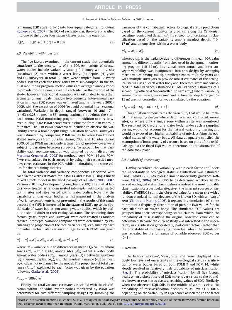
S. Bennett et al. / Marine Pollution Bulletin xxx (2011) xxx–xxx 3
remaining EQR scale (0.1–1) into four equal categories, followingRomero et al. (2007). The EQR of each site was, therefore, classifiedinto one of the upper four status classes using the equation:
EQRx ¼ ðEQR0 þ 0:11Þ=ð1þ 0:10Þ ð2Þ
2.3. Variability within factors
The five factors examined in the current study that potentiallycontribute to the uncertainty of the EQR estimations of coastalwater bodies include variability among (1) zones within a site(meadow), (2) sites within a water body, (3) depths, (4) yearsand (5) surveyors. In total, 30 sites were sampled from 17 waterbodies. Within each site three zones were sub-sampled. In the an-nual monitoring program, metric values are averaged among zonesto provide robust estimates within each site. For the purpose of thestudy, however, inter-zonal variation was estimated to establishestimates of small scale meadow heterogeneity. Inter-annual vari-ation in mean EQR scores was estimated among the years 2002–2009, with the exception of 2004 (to avoid potential inter-seasonalvariation). Variation in depth ranged between 10 and 17 m(14.63 ± 0.28 m, mean ± SE) among stations, throughout the stan-dard annual POMI monitoring program. In addition to this, how-ever, during 2002 POMI scores were estimated from 5 m zones infour sites. The 5 m POMI scores were included to observe the var-iability across a broad depth range. Variation between ‘surveyors’was estimated by comparing POMI values between two trained,skilled surveyors from 30 sites during 2008 and 16 sites during2009. Of the POMI metrics, only estimations of meadow cover weresubject to variation between surveyors. To account for that vari-ability each replicate quadrat was sampled by both divers (seeMartinez-Crego et al. (2008) for methodology). POMI 14 and POMI9 were calculated for each surveyor, by using their respective mea-dow cover estimates in the PCA, whilst maintaining the same val-ues for the remaining metrics.
The total variance and variance components associated witheach factor were estimated for POMI 14 and POMI 9 using a linearmixed effects model in the lme4 package of R (Bates, 2005, 2007,Version 2.10.1, R_Development_Core_Team 2009). The spatial fac-tors were treated as random nested intercepts, with zones nestedwithin sites and sites nested within water bodies. Note that thevariability among water bodies, whilst important in the analysisof variance components is not presented in the results of this studybecause the WFD is interested in the status of BQE’s up to the spa-tial scale of water bodies, not among water bodies, which by defi-nition should differ in their ecological status. The remaining threefactors, ‘year’, ‘depth’ and ‘surveyor’ were each treated as randomcrossed intercepts. Variance components were determined by cal-culating the proportion of the total variance (r2
T) explained by eachindividual factor. Total variance in EQR for each POMI was givenby:
r2T ¼ r2
Z þ r2Si þ r2
WB þ r2Y þ r2
Su þ r2D þ r2
R ð3Þ
where r2 = variance due to differences in mean EQR values amongzones (r2
Z) within a site, among sites (r2Si) within a water body,
among water bodies (r2WB), among years (r2
Y), between surveyors(r2
Su), among depths (r2D), and the residual variance (r2
R) in meanEQR values not explained by the model. The proportion of total var-iance (Psamp) explained by each factor was given by the equation,following Clarke et al. (2006):
Psamp ¼ 100r2x=r
2T ð4Þ
Finally, the total variance estimates associated with the classifi-cation within individual water bodies monitored by POMI wasdetermined for two different sampling designs by summing the
Please cite this article in press as: Bennett, S., et al. Ecological status of seagrassthe Posidonia oceanica multivariate index (POMI). Mar. Pollut. Bull. (2011), doi
variances of the contributing factors. Ecological status predictionsbased on the current monitoring program along the Cataloniancoastline (controlled design, r2
CD) is subject to uncertainty in clas-sification based on the variability among meadow depths (10–17 m) and among sites within a water body
r2CD ¼ r2
Si þ r2D ð5Þ
whereby r2D is the variance due to differences in mean EQR value
among the different depths from sites used in the annual monitor-ing program (10–17 m). Inter-zonal, inter-annual and inter-sur-veyor variability was incorporated into this design by averagingmetric values among multiple replicate zones, multiple years andwith multiple surveyors to provide robust estimates of the ecolog-ical status class of each water body and, therefore, were not consid-ered in total variance estimations. Total variance estimates of asecond, hypothetical ‘uncontrolled design’ (r2
UD) where variabilityamong zones, years, surveyors and a broader depth range (5–15 m) are not controlled for, was simulated by the equation:
r2UD ¼ r2
Z þ r2Si þ r2
Y þ r2Su þ r2
D ð6Þ
This equation demonstrates the variability that would be impli-cit in a sampling design where depth was not controlled amongsites, or where only a single zone within a site was monitored.The resultant EQR score for a water body, under such a samplingdesign, would not account for the natural variability therein, andwould be exposed to a higher probability of misclassifying the eco-logical status of the water body. All data adequately satisfied theassumption of homogeneity of variance based on plots of the resid-uals against the fitted EQR values, therefore, no transformation ofthe data took place.
2.4. Analysis of uncertainty
Having calculated the variability within each factor and index,the uncertainty in ecological status classification was estimatedusing STARBUGS (STAR bioassessment uncertainty guidance soft-ware, Clarke, 2004). STARBUGS helps determine whether an ob-served ecological status classification is indeed the most probableclassification for a particular site, given the inherent sources of var-iability. STARBUGS sums the observed value for a given site with arandom standard normal deviate, of the known SD, with a mean ofzero (Clarke and Hering, 2006). It repeats this simulation 104 timesto produce a frequency distribution of possible EQR values for theparticular site or water body: The simulated EQR values aregrouped into their corresponding status classes, from which theprobability of misclassifying the original observed value can bedetermined. Because the current study was interested in the uncer-tainty in classification generated by particular factors (rather thanthe probability of misclassifying individual sites), the simulationwas repeated for the full range of possible observed EQR values(0–1).
3. Results
The factors ‘surveyor’, ‘year’, ‘site’ and ‘zone’ displayed rela-tively low levels of uncertainty in the ecological status classifica-tion of water bodies based on both POMI 9 and POMI14, whilst‘depth’ resulted in relatively high probability of misclassification(Fig. 2). The probability of misclassification, for all five factors,peaks when a site’s observed EQR score is very close to the bound-ary between two status classes, reaching values of 50%. Similarly,when the observed EQR falls in the middle of a status class theprobability of misclassification declines to as low as <0.001%,depending on the variability in EQR scores associated to the factor
ecosystems: An uncertainty analysis of the meadow classification based on:10.1016/j.marpolbul.2011.06.016
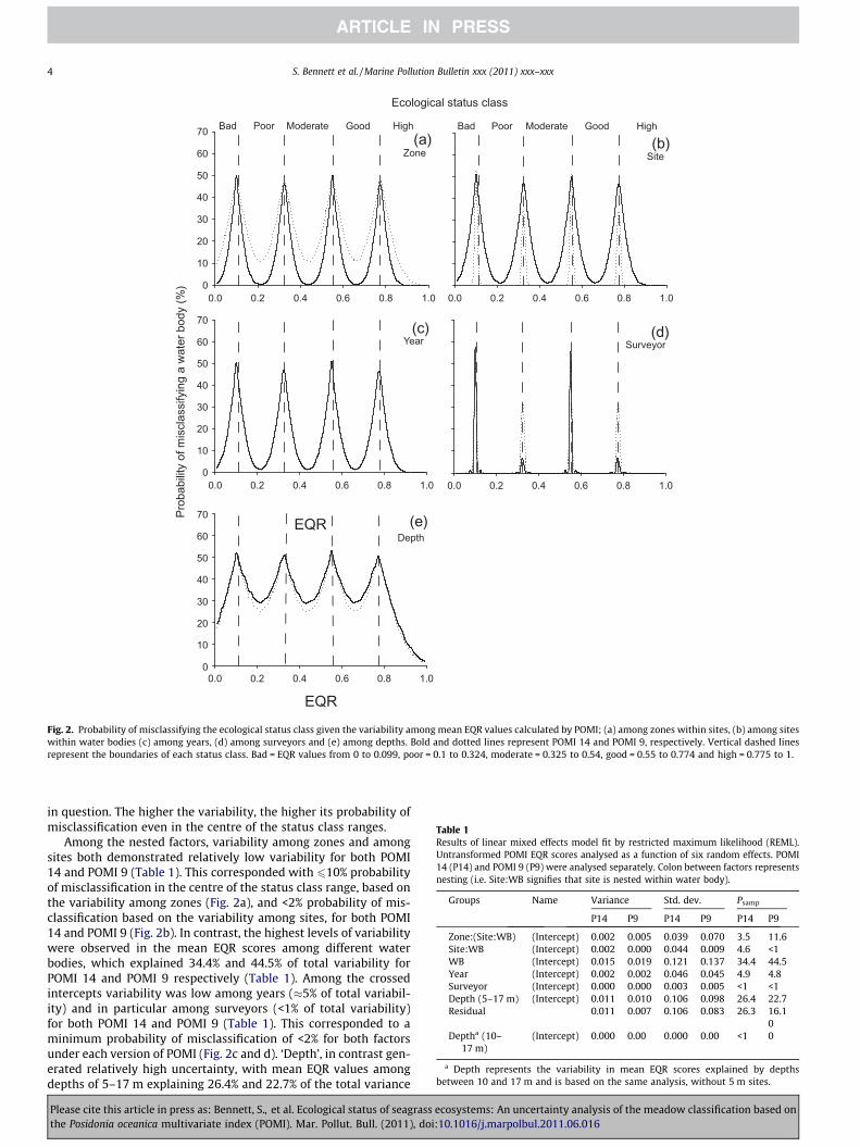
Zone
0.0 0.2 0.4 0.6 0.8 1.00
10
20
30
40
50
60
70
Site
0.0 0.2 0.4 0.6 0.8 1.0
Year
0.0 0.2 0.4 0.6 0.8 1.0
Prob
abilit
y of
mis
clas
sify
ing
a w
ater
bod
y (%
)
0
10
20
30
40
50
60
70
DepthEQR
0.0 0.2 0.4 0.6 0.8 1.0
Surveyor
EQR
0.0 0.2 0.4 0.6 0.8 1.0
0
10
20
30
40
50
60
70
Bad Poor Moderate Good High Bad Poor Moderate Good High
Ecological status class
(a) (b)
(c)
(e)
(d)
Fig. 2. Probability of misclassifying the ecological status class given the variability among mean EQR values calculated by POMI; (a) among zones within sites, (b) among siteswithin water bodies (c) among years, (d) among surveyors and (e) among depths. Bold and dotted lines represent POMI 14 and POMI 9, respectively. Vertical dashed linesrepresent the boundaries of each status class. Bad = EQR values from 0 to 0.099, poor = 0.1 to 0.324, moderate = 0.325 to 0.54, good = 0.55 to 0.774 and high = 0.775 to 1.
Table 1Results of linear mixed effects model fit by restricted maximum likelihood (REML).Untransformed POMI EQR scores analysed as a function of six random effects. POMI14 (P14) and POMI 9 (P9) were analysed separately. Colon between factors representsnesting (i.e. Site:WB signifies that site is nested within water body).
Groups Name Variance Std. dev. Psamp
P14 P9 P14 P9 P14 P9
Zone:(Site:WB) (Intercept) 0.002 0.005 0.039 0.070 3.5 11.6Site:WB (Intercept) 0.002 0.000 0.044 0.009 4.6 <1WB (Intercept) 0.015 0.019 0.121 0.137 34.4 44.5Year (Intercept) 0.002 0.002 0.046 0.045 4.9 4.8Surveyor (Intercept) 0.000 0.000 0.003 0.005 <1 <1Depth (5–17 m) (Intercept) 0.011 0.010 0.106 0.098 26.4 22.7Residual 0.011 0.007 0.106 0.083 26.3 16.1
0Deptha (10–
17 m)(Intercept) 0.000 0.00 0.000 0.00 <1 0
a Depth represents the variability in mean EQR scores explained by depthsbetween 10 and 17 m and is based on the same analysis, without 5 m sites.
4 S. Bennett et al. / Marine Pollution Bulletin xxx (2011) xxx–xxx
in question. The higher the variability, the higher its probability ofmisclassification even in the centre of the status class ranges.
Among the nested factors, variability among zones and amongsites both demonstrated relatively low variability for both POMI14 and POMI 9 (Table 1). This corresponded with 610% probabilityof misclassification in the centre of the status class range, based onthe variability among zones (Fig. 2a), and <2% probability of mis-classification based on the variability among sites, for both POMI14 and POMI 9 (Fig. 2b). In contrast, the highest levels of variabilitywere observed in the mean EQR scores among different waterbodies, which explained 34.4% and 44.5% of total variability forPOMI 14 and POMI 9 respectively (Table 1). Among the crossedintercepts variability was low among years (5% of total variabil-ity) and in particular among surveyors (<1% of total variability)for both POMI 14 and POMI 9 (Table 1). This corresponded to aminimum probability of misclassification of <2% for both factorsunder each version of POMI (Fig. 2c and d). ‘Depth’, in contrast gen-erated relatively high uncertainty, with mean EQR values amongdepths of 5–17 m explaining 26.4% and 22.7% of the total variance
Please cite this article in press as: Bennett, S., et al. Ecological status of seagrass ecosystems: An uncertainty analysis of the meadow classification based onthe Posidonia oceanica multivariate index (POMI). Mar. Pollut. Bull. (2011), doi:10.1016/j.marpolbul.2011.06.016
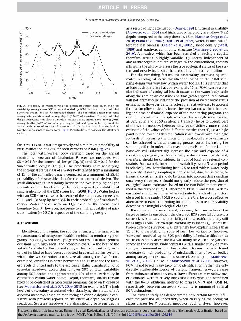
EQR
0.0 0.2 0.4 0.6 0.8 1.0
Prob
abilit
y of
mis
clas
sify
ing
a W
B (%
)
0
10
20
30
40
50
60
70uncontrolled designcontrolled design
4
15
16
1217
7
7
12
17
13
13
1415
14
6 3
19
3
2
19
8
8
6
5
5
4
16 2
10
1011
11
Fig. 3. Probability of misclassifying the ecological status class given the totalvariability among mean EQR values calculated by POMI 14 based on a ‘controlledsampling design’ and an ‘uncontrolled design’. The controlled design representsamong site variation and among depth (10–17 m) variation. The uncontrolleddesign represents cumulative variation, among zones, among sites, among years,among depths (5–17 m) and among surveyors. Full and open circles represent theactual probability of misclassification for 17 Catalonian coastal water bodies.Numbers represent the water body (Fig. 1). Probabilities are based on the 2008 dataseries.
S. Bennett et al. / Marine Pollution Bulletin xxx (2011) xxx–xxx 5
for POMI 14 and POMI 9 respectively and a minimum probability ofmisclassification of >25% for both versions of POMI (Fig. 2e).
The total within-water body variation based on the annualmonitoring program of Catalonian P. oceanica meadows wasSD = 0.04 for the ‘controlled design’ (Eq. (5)) and SD = 0.13 for the‘uncontrolled design’ (Eq. (6)). The probability of misclassifyingthe ecological status class of a water body ranged from a minimumof 1% for the controlled design, compared to a minimum of 38.4%probability of misclassification for the uncontrolled design. Thestark difference in uncertainty between the two sampling designsis made evident by observing the superimposed probabilities ofmisclassification of the EQR scores from 2008 (Fig. 3). Water bodieswith an EQR score close to the centre of the status class range (e.g.9, 11 and 13) vary by over 35% in their probability of misclassifi-cation. Water bodies with an EQR close to the status classboundary (e.g. 5), however, are prone to a high probability of mis-classification ( 50%) irrespective of the sampling design.
4. Discussion
Identifying and gauging the sources of uncertainty inherent inthe assessment of ecosystem health is critical in monitoring pro-grams, especially when these programs can result in managementdecisions with high social and economic costs. To the best of theauthors’ knowledge, the current study is the first uncertainty anal-ysis of its kind to have been conducted in coastal marine systemswithin the WFD member states. Overall, among the five factorsexamined, variations in depth between 5 and 15 m added the high-est levels of uncertainty to the ecological status classification of P.oceanica meadows, accounting for over 20% of total variabilityamong EQR scores and approximately 60% of total variability inestimation within water bodies. Depth, therefore, should remainfixed or be controlled in monitoring programs based on P. oceanica(see Montefalcone et al., 2007, 2009, 2010 for examples). The highlevels of uncertainty associated with classifying the status of a P.oceanica meadows based on monitoring at variable depths is con-sistent with previous reports on the effect of depth on seagrassmeadows. Seagrass meadows vary dramatically between depths
Please cite this article in press as: Bennett, S., et al. Ecological status of seagrassthe Posidonia oceanica multivariate index (POMI). Mar. Pollut. Bull. (2011), doi
as a result of light attenuation (Duarte, 1991), nutrient availability(Alcoverro et al., 2001) and high rates of herbivory in shallow (5 m)depths compared to the deep sites (i.e. 15 m, Martinez-Crego et al.,2010; Prado et al., 2007; Tomas et al., 2005) which in turn can af-fect the leaf biomass (Olesen et al., 2002), shoot density (West,1990) and epiphytic community structure (Martinez-Crego et al.,2010). A meadow which has been sampled at multiple depths,therefore, results in highly variable EQR scores, independent ofany anthropogenic induced changes to the environment, therebyinhibiting the ability to assess the true ecological status of the sys-tem and greatly increasing the probability of misclassification.
For the remaining factors, the uncertainty surrounding esti-mates in ecological status classification, based on the POMI sam-pling design was very low within water bodies. This signifies thatas long as depth is fixed at approximately 15 m, POMI can be a pre-cise indicator of ecological health status at the water body scalealong the Catalonian coastline and that greater spatial replicationwill not dramatically influence the precision of water body statusestimations. However, certain factors are relatively easy to accountfor in a sampling design by increasing replication, without increas-ing the time or financial expense of the monitoring program. Forexample, monitoring multiple zones within a single meadow (i.e.at 0 m, 25 m and at 50 m along a transect) helps to absorb partof the within-meadow heterogeneity, by providing a more robustestimate of the values of the different metrics than if just a singlepoint is monitored. As this replication is achievable within a singlescuba dive, increasing the precision of ecological status estimatescan be achieved without incurring greater costs. Increasing thesampling effort in order to increase the precision of other factors,however, will substantially increase the time and expense of amonitoring program, without greatly reducing uncertainty and,therefore, should be considered in light of local or regional con-straints. For example, inter-annual variability over a 3-year periodis relatively low, contributing just 12% to total within water bodyvariability. If yearly sampling is not possible, due, for instance, tofinancial constraints, it should be taken into account that samplingonce every three years should not greatly reduce the precision ofecological status estimates, based on the two POMI indices exam-ined in the current study. Furthermore, POMI 9 and POMI 14 dem-onstrated similar estimates of uncertainty for each of the factorsobserved in the study. POMI 9 could, therefore, be a cost effectivealternative to POMI 14 pending further studies to test its viabilitydetecting meaningful ecological change.
It is important to keep in mind, however, that irrespective of thefactor or index in question, if the observed EQR score falls close to astatus class boundary the probability of misclassification may stillbe as high as 50%. For example, variability in mean EQR scores be-tween different surveyors was extremely low, explaining less than1% of total variability. In spite of such low variability, however,‘surveyor’ recorded up to 50% probability of misclassification atstatus class boundaries. The low variability between surveyors ob-served in the current study contrasts with a similar study on mac-rophyte communities in freshwater streams, which foundmoderate to high probability of misclassification of water bodiesamong surveyors (15–40% at the status class mid-point, Staniszew-ski et al., 2006). Unlike in Staniszewski et al. (2006), however,POMI is not based in any taxonomic identification; rather, the onlydirectly attributable source of variation among surveyors camefrom estimates of meadow cover. Raw differences in meadow cov-er estimates were relatively low among surveyors and combinedwith the 8–13 additional metrics to form POMI 9 and POMI 14,respectively, between surveyors variability is minimised in finalEQR estimations.
The current study has demonstrated how certain factors influ-ence the precision or uncertainty when classifying the ecologicalstatus classes for P. oceanica meadows. Such analyses, however,
ecosystems: An uncertainty analysis of the meadow classification based on:10.1016/j.marpolbul.2011.06.016
6 S. Bennett et al. / Marine Pollution Bulletin xxx (2011) xxx–xxx
cannot describe the accuracy of the indices predictions. A func-tional index should be a balance between one that will detectchange at practical spatial and temporal scales for managementand one that will reduce uncertainty in classification. An index,for example, that only monitors meadow cover, may generate verylow uncertainty, however, respond too slowly to changes in waterquality to provide constructive feedback to managers. Future stud-ies must continue to weigh up the tradeoffs between detectingmeaningful change and reliable classification ecosystem health.
5. Conclusions
The findings from the current study indicate that variations indepth between 5 and 15 m contribute relatively high levels ofuncertainty to the ecological status classification P. oceanica mead-ows. These results emphasise the importance of controlling thesampling depth in P. oceanica meadows monitoring programs.Low variability among zones within sites and among sites withinwater bodies, suggests that both POMI 14 and POMI 9 are precisemonitoring indices at the scale of water bodies along the Catalo-nian coastline.
Acknowledgements
We thank all the different people involved in the long-termmonitoring for their work in the field and laboratory. We alsothank Ralph Clarke, Michael Dunbar and Jordi Pages for their assis-tance in statistical analyses. This research was financially sup-ported by l’Agencia Catalana de l’Aigua and WISER (Water bodiesin Europe: Integrative Systems to assess Ecological status andRecovery) funded under the 7th EU Framework Programme, Theme6, Environment including Climate Change, Contract No.: 226273).
References
Alcoverro, T., Cerbian, E., Ballesteros, E., 2001. The photosynthetic capacity of theseagrass Posidonia oceanica: influence of nitrogen and light. Journal ofExperimental Marine Biology and Ecology 261, 107–120.
Bates, D., 2005. Fitting linear mixed models in R. R News 5(1), 27–30. <http://CRAN.R-project.org/doc/Rnews/>.
Bates, D., 2007. lme4: Linear mixed-effects models using S4 classes. R packageversion 0.99875-9. <http://CRAN.R-project.org>.
Clarke, R.T., 2004. STARBUGS 1.1 (STAR bioassessment uncertainty guidancesoftware). Error/uncertainty module software, Centre for Hydrology andEcology in Dorset (CEH).
Clarke, R.T., Hering, D., 2006. Errors and uncertainty in bioassessment methods –major results and conclusions from the STAR project and their applicationusings STARBUGS. Hydrobiologia 566, 433–439.
Please cite this article in press as: Bennett, S., et al. Ecological status of seagrassthe Posidonia oceanica multivariate index (POMI). Mar. Pollut. Bull. (2011), doi
Clarke, R.T., Davy-Bowker, J., Sandin, L., Friberg, N., Johnson, R.K., Bis, B., 2006.Estimates and comparisons of the effects of sampling variation using ‘national’macroinvertebrate sampling protocols on the precision of metrics used toassess ecological status. Hydrobiologia 566, 477–503.
Delgado, O., Ruiz, J.M., Pérez, M., Romero, J., Ballesteros, E., 1999. Effects of fishfarming on seagrass (Posidonia oceanica) beds in a Mediterranean bay: seagrassdecline after organic matter cessation. Oceanologica Acta 22 (1), 109–117.
Duarte, C.M., 1991. Seagrass depth limits. Aquatic Botany 40, 363–377.Francour, P., Ganteaume, A., Poulain, M., 1999. Effects of boat anchoring in Posidonia
oceanica seagrass bed in the Port-Cros National Park (north-westernMediterranean Sea). Aquatic Conservation: Marine and FreshwaterEcosystems 9, 391–400.
Martinez-Crego, B., Vergés, A., Alcoverro, T., Romero, J., 2008. Selection of multipleseagrass indicators for environmental biomonitoring. Marine Ecology ProgressSeries 361, 93–109.
Martinez-Crego, B., Prado, P., Alcoverro, T., Romero, J., 2010. Composition ofepiphytic leaf community of Posidonia oceanica as a tool for environmentalbiomonitoring. Estuarine, Coastal and Shelf Sciences 88, 199–208.
Montefalcone, M., Albertelli, G., Morri, C., Bianchi, C.N., 2007. Urban seagrass: statusof Posidonia oceanica facing the Genoa city waterfront (Italy) and implicationsfor management. Marine Pollution Bulletin 54, 206–213.
Montefalcone, M., Albertelli, G., Morri, C., Parravicini, V., Bianchi, C.N., 2009. Legalprotection is not enough: Posidonia oceanica meadows in marine protectedareas are not healthier than those in unprotected areas of the northwestMediterranean Sea. Marine Pollution Bulletin 58, 515–519.
Montefalcone, M., Albertelli, G., Morri, C., Bianchi, C.N., 2010. Pattern of wide-scalesubstitution within Posidonia oceanica meadows of NW Mediterranean sea:invaders are stronger than natives. Aquatic Conservation: Marine andFreshwater Ecosystems 20, 507–515.
Olesen, B., Enríquez, S., Duarte, C.M., Sand-Jensen, K., 2002. Depth-acclimation ofphotosynthesis, morphology and demography of Posidonia oceanica andCymodocea nodosa in the Spanish Mediterranean Sea. Marine Ecology ProgressSeries 236, 89–97.
Prado, P., Tomas, F., Alcoverro, T., Romero, J., 2007. Extensive direct measurementsof Posidonia oceanica defoliation confirm the importance of herbivory intemperate seagrass meadows. Marine Ecology Progress Series 340, 63–71.
Procaccini, G., Buia, M.C., Gambi, M.C., Pérez, M., Pergent-Marini, C., Romero, J.,2003. The seagrasses of the western Mediterranean. In: Green, E.P., Short, F.T.(Eds.), World Atlas of Seagrasses. University of California Press, Berkeley, USA,pp. 48–58, 298.
Romero, J., Martínez-Crego, B., Alcoverro, T., Pérez, M., 2007. A multivariate indexbased on the seagrass Posidonia oceanic (POMI) to assess ecological status ofcoastal waters under the Water Framework Directive (WFD). Marine PollutionBulletin 55, 196–204.
Ruiz, J., Pérez, M., Romero, J., 2001. Effects of fish farm loadings on seagrass(Posidonia oceanica) distribution, growth and photosynthesis. Marine PollutionBulletin 42 (9), 749–760.
Ruiz, J.M., Romero, J., 2003. Effects of disturbances caused by coastal constructionson spatial structure, growth dynamics and photosynthesis of the seagrassPosidonia oceanica. Marine Pollution Bulletin 46, 1523–1533.
Staniszewski, R., Szoszkiewicz, K., Zbierska, J., Lesny, J., Jusik, S., Clarke, R.T., 2006.Assessment of sources of uncertainty in macrophyte surveys and theconsequences for river classification. Hydrobiologia 566, 235–246.
Tomas, F., Turon, X., Romero, J., 2005. Seasonal and small-scale spatial variability ofherbivory pressure on the temperate seagrass Posidonia oceanica. MarineEcology Progress Series 301, 95–107.
West, R.J., 1990. Depth-related structural and morphological variations in anAustralian Posidonia seagrass bed. Aquatic Botany 36 (2), 153–166.
ecosystems: An uncertainty analysis of the meadow classification based on:10.1016/j.marpolbul.2011.06.016
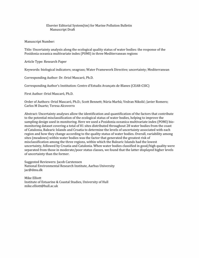
Elsevier Editorial System(tm) for Marine Pollution Bulletin Manuscript Draft Manuscript Number: Title: Uncertainty analysis along the ecological quality status of water bodies: the response of the Posidonia oceanica multivariate index (POMI) in three Mediterranean regions Article Type: Research Paper Keywords: biological indicators; seagrass; Water Framework Directive; uncertainty; Mediterranean Corresponding Author: Dr. Oriol Mascaró, Ph.D. Corresponding Author's Institution: Centre d'Estudis Avançats de Blanes (CEAB-CSIC) First Author: Oriol Mascaró, Ph.D. Order of Authors: Oriol Mascaró, Ph.D.; Scott Bennett; Núria Marbà; Vedran Nikolić; Javier Romero; Carlos M Duarte; Teresa Alcoverro Abstract: Uncertainty analyses allow the identification and quantification of the factors that contribute to the potential misclassification of the ecological status of water bodies, helping to improve the sampling design used in monitoring. Here we used a Posidonia oceanica multivariate index (POMI) bio-monitoring dataset covering a total of 81 sites distributed throughout 28 water bodies from the coast of Catalonia, Balearic Islands and Croatia to determine the levels of uncertainty associated with each region and how they change according to the quality status of water bodies. Overall, variability among sites (meadows) within water bodies was the factor that generated the greatest risk of misclassification among the three regions, within which the Balearic Islands had the lowest uncertainty, followed by Croatia and Catalonia. When water bodies classified in good/high quality were separated from those in moderate/poor status classes, we found that the latter displayed higher levels of uncertainty than the former. Suggested Reviewers: Jacob Carstensen National Environmental Research Institute, Aarhus University [email protected] Mike Elliott Institute of Estuarine & Coastal Studies, University of Hull [email protected]

Marine Ecology Department Centre d'Estudis Avançats de Blanes (CEAB-CSIC) C/ d'Accés a la Cala St. Francesc, 14 E-17300 Blanes (GIRONA) SPAIN +0034 972336101 [email protected]
> Uncertainty estimation is a central element in WFD-compliant classification methods > Uncertainty associated to POMI index changes depending on the region of application > Uncertainty associated to POMI depends on the quality status of water bodies > Monitoring programmes design must respond to the specific conditions of water bodies
Highlights
1 2 3 4 5 6 7 8 9 10 11 12 13 14 15 16 17 18 19 20 21 22 23 24 25 26 27 28 29 30 31 32 33 34 35 36 37 38 39 40 41 42 43 44 45 46 47 48 49 50 51 52 53 54 55 56 57 58 59 60 61 62 63 64 65
1
Uncertainty analysis along the ecological quality status of
water bodies: the response of the Posidonia oceanica
multivariate index (POMI) in three Mediterranean regions
Oriol Mascaró a*
Scott Bennett b
Núria Marbà c
Vedran Nikolić d
Javier Romero e
Carlos M. Duarte c,f
Teresa Alcoverro a
a Centre d‟Estudis Avançats de Blanes (CSIC). C/ d‟Accés a la Cala St. Francesc 14,
17300 – Blanes (Girona). Spain
b UWA Oceans Institute. School of Plant Biology. The University of Western Australia.
35 Stirling Highway, 6009 - Crawley (WA). Australia
c Department of Global Change Research. IMEDEA (CSIC-UIB), Institut Mediterrani
d‟Estudis Avançats. Miquel Marquès 21, 07190 Esporles (Illes Balears). Spain
d Institute of Oceanography and Fisheries. I. Meštrovića 63, HR-21000 Split. Croatia
*ManuscriptClick here to view linked References
1 2 3 4 5 6 7 8 9 10 11 12 13 14 15 16 17 18 19 20 21 22 23 24 25 26 27 28 29 30 31 32 33 34 35 36 37 38 39 40 41 42 43 44 45 46 47 48 49 50 51 52 53 54 55 56 57 58 59 60 61 62 63 64 65
2
e Departament d‟Ecologia. Facultat de Biologia (Universitat de Barcelona). Av.
Diagonal 645, 08028 - Barcelona. Spain
f UWA Oceans Institute. The University of Western Australia. 35 Stirling Highway, 6009
- Crawley (WA). Australia
*Corresponding author: Tel.: +34 972 336 101; E-mail: [email protected]
1 2 3 4 5 6 7 8 9 10 11 12 13 14 15 16 17 18 19 20 21 22 23 24 25 26 27 28 29 30 31 32 33 34 35 36 37 38 39 40 41 42 43 44 45 46 47 48 49 50 51 52 53 54 55 56 57 58 59 60 61 62 63 64 65
3
Abstract
Uncertainty analyses allow the identification and quantification of the factors that
contribute to the potential misclassification of the ecological status of water bodies,
helping to improve the sampling design used in monitoring. Here we used a
Posidonia oceanica multivariate index (POMI) bio-monitoring dataset covering a total
of 81 sites distributed throughout 28 water bodies from the coast of Catalonia,
Balearic Islands and Croatia to determine the levels of uncertainty associated with
each region and how they change according to the quality status of water bodies.
Overall, variability among sites (meadows) within water bodies was the factor that
generated the greatest risk of misclassification among the three regions, within which
the Balearic Islands had the lowest uncertainty, followed by Croatia and Catalonia.
When water bodies classified in good/high quality were separated from those in
moderate/poor status classes, we found that the latter displayed higher levels of
uncertainty than the former.
Keywords: biological indicators; seagrass; Water Framework Directive; uncertainty;
Mediterranean
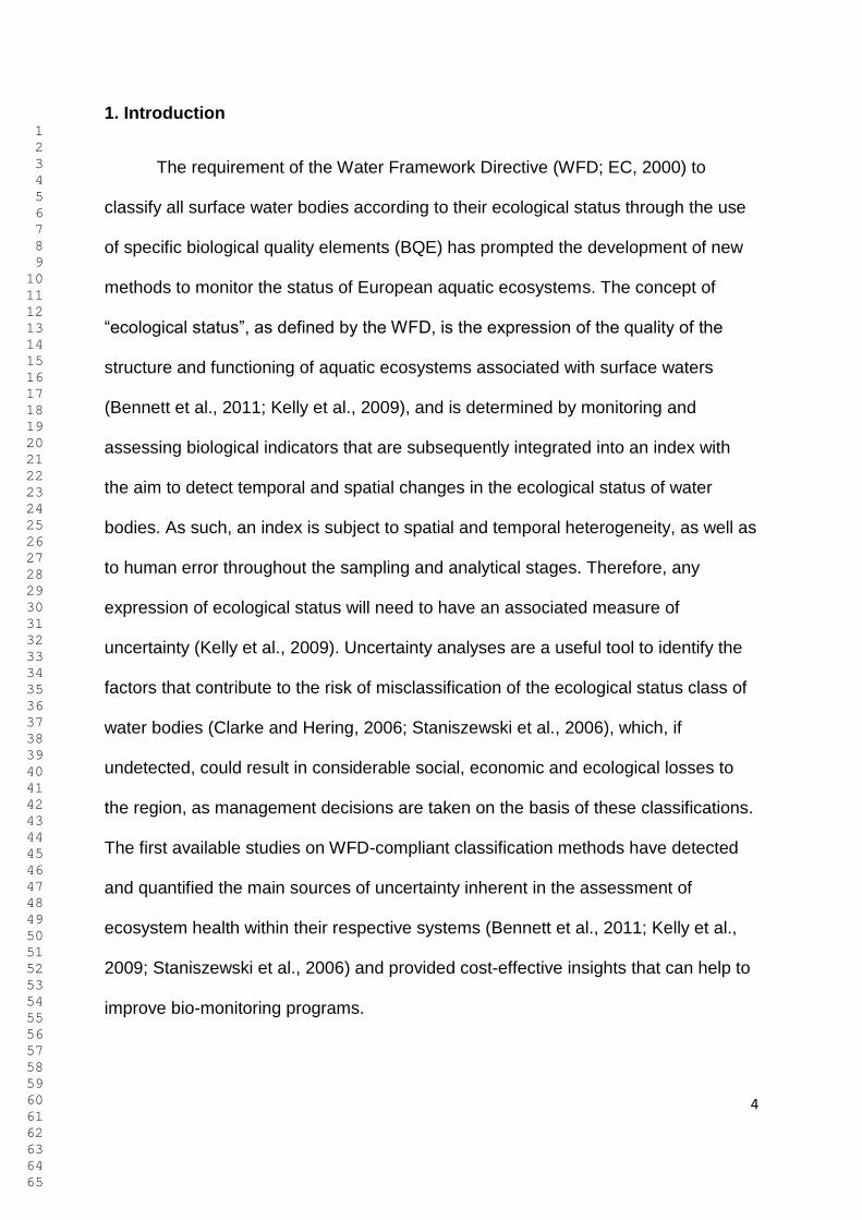
1 2 3 4 5 6 7 8 9 10 11 12 13 14 15 16 17 18 19 20 21 22 23 24 25 26 27 28 29 30 31 32 33 34 35 36 37 38 39 40 41 42 43 44 45 46 47 48 49 50 51 52 53 54 55 56 57 58 59 60 61 62 63 64 65
4
1. Introduction
The requirement of the Water Framework Directive (WFD; EC, 2000) to
classify all surface water bodies according to their ecological status through the use
of specific biological quality elements (BQE) has prompted the development of new
methods to monitor the status of European aquatic ecosystems. The concept of
“ecological status”, as defined by the WFD, is the expression of the quality of the
structure and functioning of aquatic ecosystems associated with surface waters
(Bennett et al., 2011; Kelly et al., 2009), and is determined by monitoring and
assessing biological indicators that are subsequently integrated into an index with
the aim to detect temporal and spatial changes in the ecological status of water
bodies. As such, an index is subject to spatial and temporal heterogeneity, as well as
to human error throughout the sampling and analytical stages. Therefore, any
expression of ecological status will need to have an associated measure of
uncertainty (Kelly et al., 2009). Uncertainty analyses are a useful tool to identify the
factors that contribute to the risk of misclassification of the ecological status class of
water bodies (Clarke and Hering, 2006; Staniszewski et al., 2006), which, if
undetected, could result in considerable social, economic and ecological losses to
the region, as management decisions are taken on the basis of these classifications.
The first available studies on WFD-compliant classification methods have detected
and quantified the main sources of uncertainty inherent in the assessment of
ecosystem health within their respective systems (Bennett et al., 2011; Kelly et al.,
2009; Staniszewski et al., 2006) and provided cost-effective insights that can help to
improve bio-monitoring programs.
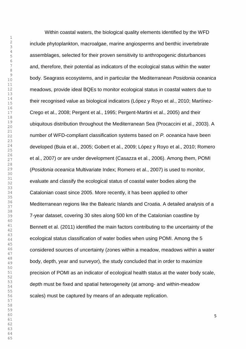
1 2 3 4 5 6 7 8 9 10 11 12 13 14 15 16 17 18 19 20 21 22 23 24 25 26 27 28 29 30 31 32 33 34 35 36 37 38 39 40 41 42 43 44 45 46 47 48 49 50 51 52 53 54 55 56 57 58 59 60 61 62 63 64 65
5
Within coastal waters, the biological quality elements identified by the WFD
include phytoplankton, macroalgae, marine angiosperms and benthic invertebrate
assemblages, selected for their proven sensitivity to anthropogenic disturbances
and, therefore, their potential as indicators of the ecological status within the water
body. Seagrass ecosystems, and in particular the Mediterranean Posidonia oceanica
meadows, provide ideal BQEs to monitor ecological status in coastal waters due to
their recognised value as biological indicators (López y Royo et al., 2010; Martínez-
Crego et al., 2008; Pergent et al., 1995; Pergent-Martini et al., 2005) and their
ubiquitous distribution throughout the Mediterranean Sea (Procaccini et al., 2003). A
number of WFD-compliant classification systems based on P. oceanica have been
developed (Buia et al., 2005; Gobert et al., 2009; López y Royo et al., 2010; Romero
et al., 2007) or are under development (Casazza et al., 2006). Among them, POMI
(Posidonia oceanica Multivariate Index; Romero et al., 2007) is used to monitor,
evaluate and classify the ecological status of coastal water bodies along the
Catalonian coast since 2005. More recently, it has been applied to other
Mediterranean regions like the Balearic Islands and Croatia. A detailed analysis of a
7-year dataset, covering 30 sites along 500 km of the Catalonian coastline by
Bennett et al. (2011) identified the main factors contributing to the uncertainty of the
ecological status classification of water bodies when using POMI. Among the 5
considered sources of uncertainty (zones within a meadow, meadows within a water
body, depth, year and surveyor), the study concluded that in order to maximize
precision of POMI as an indicator of ecological health status at the water body scale,
depth must be fixed and spatial heterogeneity (at among- and within-meadow
scales) must be captured by means of an adequate replication.
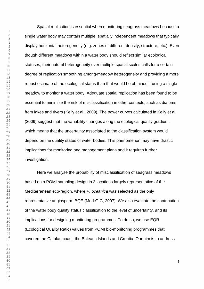
1 2 3 4 5 6 7 8 9 10 11 12 13 14 15 16 17 18 19 20 21 22 23 24 25 26 27 28 29 30 31 32 33 34 35 36 37 38 39 40 41 42 43 44 45 46 47 48 49 50 51 52 53 54 55 56 57 58 59 60 61 62 63 64 65
6
Spatial replication is essential when monitoring seagrass meadows because a
single water body may contain multiple, spatially independent meadows that typically
display horizontal heterogeneity (e.g. zones of different density, structure, etc.). Even
though different meadows within a water body should reflect similar ecological
statuses, their natural heterogeneity over multiple spatial scales calls for a certain
degree of replication smoothing among-meadow heterogeneity and providing a more
robust estimate of the ecological status than that would be obtained if using a single
meadow to monitor a water body. Adequate spatial replication has been found to be
essential to minimize the risk of misclassification in other contexts, such as diatoms
from lakes and rivers (Kelly et al., 2009). The power curves calculated in Kelly et al.
(2009) suggest that the variability changes along the ecological quality gradient,
which means that the uncertainty associated to the classification system would
depend on the quality status of water bodies. This phenomenon may have drastic
implications for monitoring and management plans and it requires further
investigation.
Here we analyse the probability of misclassification of seagrass meadows
based on a POMI sampling design in 3 locations largely representative of the
Mediterranean eco-region, where P. oceanica was selected as the only
representative angiosperm BQE (Med-GIG, 2007). We also evaluate the contribution
of the water body quality status classification to the level of uncertainty, and its
implications for designing monitoring programmes. To do so, we use EQR
(Ecological Quality Ratio) values from POMI bio-monitoring programmes that
covered the Catalan coast, the Balearic Islands and Croatia. Our aim is to address
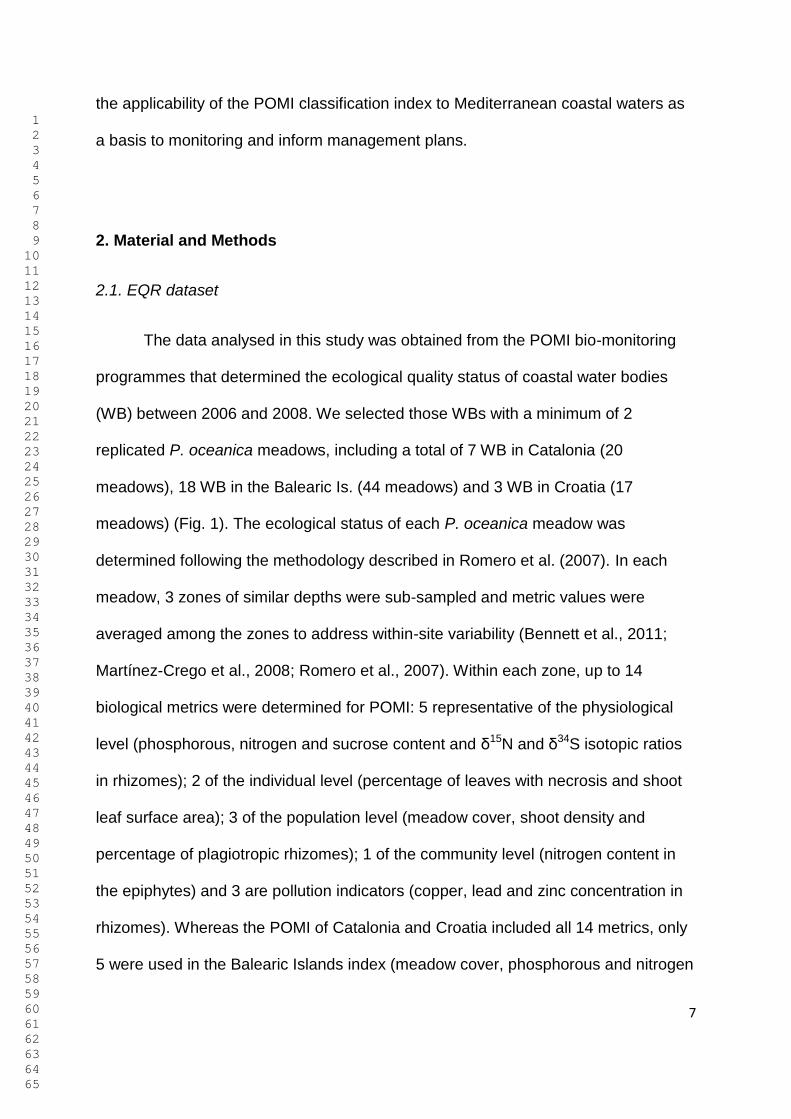
1 2 3 4 5 6 7 8 9 10 11 12 13 14 15 16 17 18 19 20 21 22 23 24 25 26 27 28 29 30 31 32 33 34 35 36 37 38 39 40 41 42 43 44 45 46 47 48 49 50 51 52 53 54 55 56 57 58 59 60 61 62 63 64 65
7
the applicability of the POMI classification index to Mediterranean coastal waters as
a basis to monitoring and inform management plans.
2. Material and Methods
2.1. EQR dataset
The data analysed in this study was obtained from the POMI bio-monitoring
programmes that determined the ecological quality status of coastal water bodies
(WB) between 2006 and 2008. We selected those WBs with a minimum of 2
replicated P. oceanica meadows, including a total of 7 WB in Catalonia (20
meadows), 18 WB in the Balearic Is. (44 meadows) and 3 WB in Croatia (17
meadows) (Fig. 1). The ecological status of each P. oceanica meadow was
determined following the methodology described in Romero et al. (2007). In each
meadow, 3 zones of similar depths were sub-sampled and metric values were
averaged among the zones to address within-site variability (Bennett et al., 2011;
Martínez-Crego et al., 2008; Romero et al., 2007). Within each zone, up to 14
biological metrics were determined for POMI: 5 representative of the physiological
level (phosphorous, nitrogen and sucrose content and δ15N and δ34S isotopic ratios
in rhizomes); 2 of the individual level (percentage of leaves with necrosis and shoot
leaf surface area); 3 of the population level (meadow cover, shoot density and
percentage of plagiotropic rhizomes); 1 of the community level (nitrogen content in
the epiphytes) and 3 are pollution indicators (copper, lead and zinc concentration in
rhizomes). Whereas the POMI of Catalonia and Croatia included all 14 metrics, only
5 were used in the Balearic Islands index (meadow cover, phosphorous and nitrogen
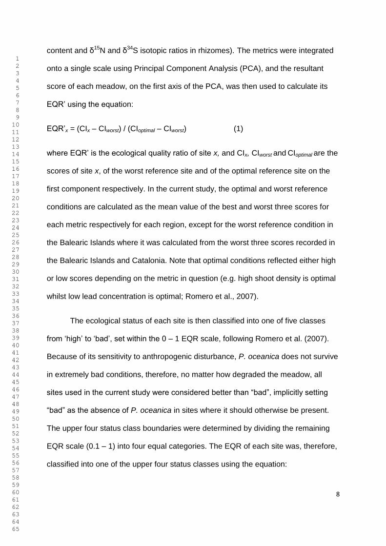
1 2 3 4 5 6 7 8 9 10 11 12 13 14 15 16 17 18 19 20 21 22 23 24 25 26 27 28 29 30 31 32 33 34 35 36 37 38 39 40 41 42 43 44 45 46 47 48 49 50 51 52 53 54 55 56 57 58 59 60 61 62 63 64 65
8
content and δ15N and δ34S isotopic ratios in rhizomes). The metrics were integrated
onto a single scale using Principal Component Analysis (PCA), and the resultant
score of each meadow, on the first axis of the PCA, was then used to calculate its
EQR‟ using the equation:
EQR‟x = (CIx – CIworst) / (CIoptimal – CIworst) (1)
where EQR‟ is the ecological quality ratio of site x, and CIx, CIworst and CIoptimal are the
scores of site x, of the worst reference site and of the optimal reference site on the
first component respectively. In the current study, the optimal and worst reference
conditions are calculated as the mean value of the best and worst three scores for
each metric respectively for each region, except for the worst reference condition in
the Balearic Islands where it was calculated from the worst three scores recorded in
the Balearic Islands and Catalonia. Note that optimal conditions reflected either high
or low scores depending on the metric in question (e.g. high shoot density is optimal
whilst low lead concentration is optimal; Romero et al., 2007).
The ecological status of each site is then classified into one of five classes
from „high‟ to „bad‟, set within the 0 – 1 EQR scale, following Romero et al. (2007).
Because of its sensitivity to anthropogenic disturbance, P. oceanica does not survive
in extremely bad conditions, therefore, no matter how degraded the meadow, all
sites used in the current study were considered better than “bad”, implicitly setting
“bad” as the absence of P. oceanica in sites where it should otherwise be present.
The upper four status class boundaries were determined by dividing the remaining
EQR scale (0.1 – 1) into four equal categories. The EQR of each site was, therefore,
classified into one of the upper four status classes using the equation:
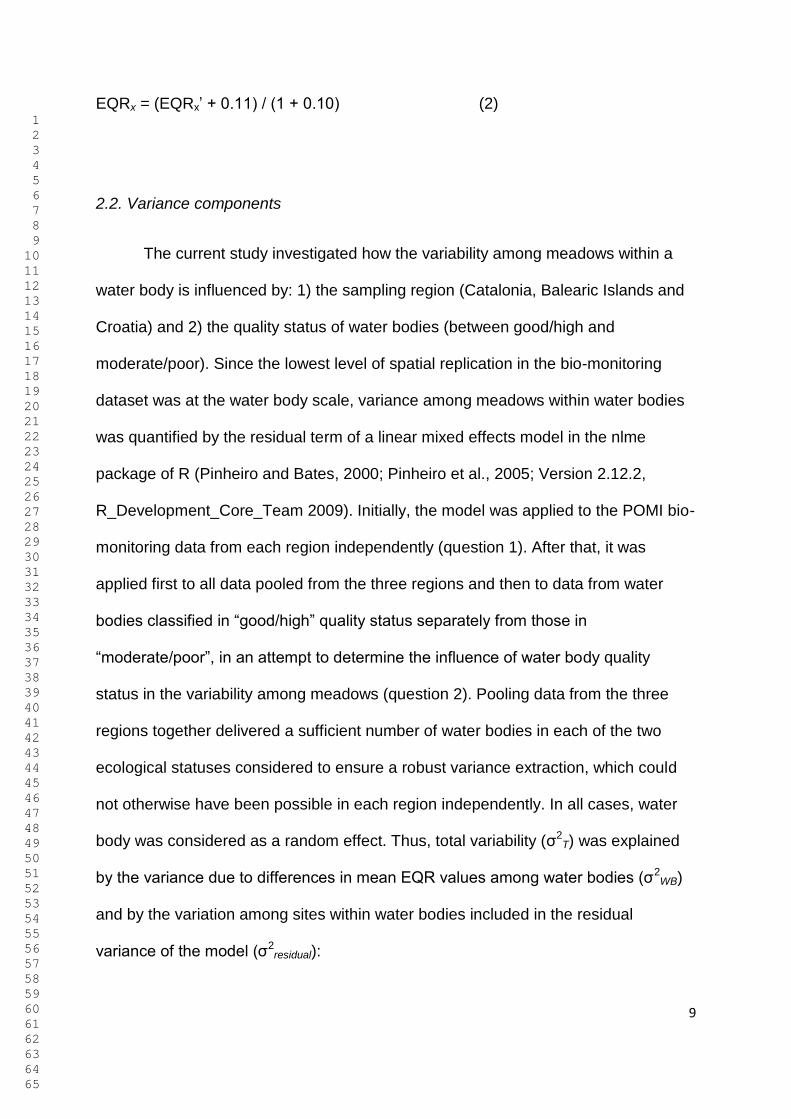
1 2 3 4 5 6 7 8 9 10 11 12 13 14 15 16 17 18 19 20 21 22 23 24 25 26 27 28 29 30 31 32 33 34 35 36 37 38 39 40 41 42 43 44 45 46 47 48 49 50 51 52 53 54 55 56 57 58 59 60 61 62 63 64 65
9
EQRx = (EQRx‟ + 0.11) / (1 + 0.10) (2)
2.2. Variance components
The current study investigated how the variability among meadows within a
water body is influenced by: 1) the sampling region (Catalonia, Balearic Islands and
Croatia) and 2) the quality status of water bodies (between good/high and
moderate/poor). Since the lowest level of spatial replication in the bio-monitoring
dataset was at the water body scale, variance among meadows within water bodies
was quantified by the residual term of a linear mixed effects model in the nlme
package of R (Pinheiro and Bates, 2000; Pinheiro et al., 2005; Version 2.12.2,
R_Development_Core_Team 2009). Initially, the model was applied to the POMI bio-
monitoring data from each region independently (question 1). After that, it was
applied first to all data pooled from the three regions and then to data from water
bodies classified in “good/high” quality status separately from those in
“moderate/poor”, in an attempt to determine the influence of water body quality
status in the variability among meadows (question 2). Pooling data from the three
regions together delivered a sufficient number of water bodies in each of the two
ecological statuses considered to ensure a robust variance extraction, which could
not otherwise have been possible in each region independently. In all cases, water
body was considered as a random effect. Thus, total variability (σ2T) was explained
by the variance due to differences in mean EQR values among water bodies (σ2WB)
and by the variation among sites within water bodies included in the residual
variance of the model (σ2residual):
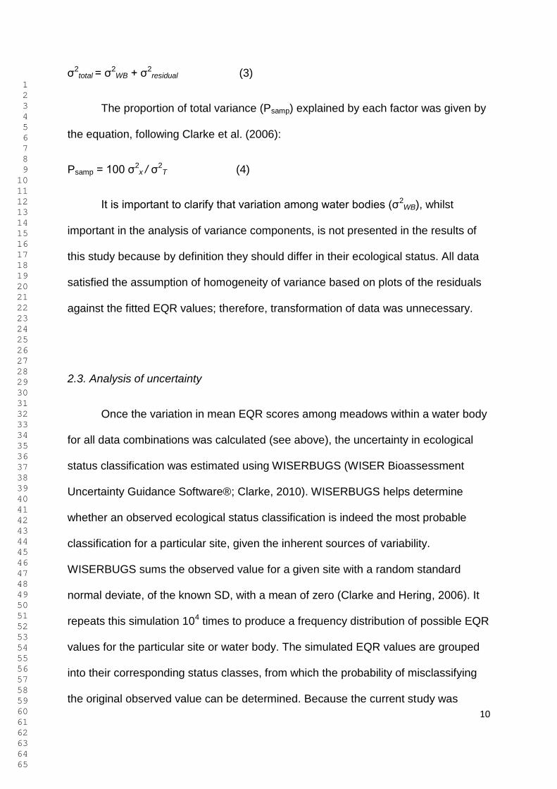
1 2 3 4 5 6 7 8 9 10 11 12 13 14 15 16 17 18 19 20 21 22 23 24 25 26 27 28 29 30 31 32 33 34 35 36 37 38 39 40 41 42 43 44 45 46 47 48 49 50 51 52 53 54 55 56 57 58 59 60 61 62 63 64 65
10
σ2total = σ2
WB + σ2residual (3)
The proportion of total variance (Psamp) explained by each factor was given by
the equation, following Clarke et al. (2006):
Psamp = 100 σ2x / σ
2T (4)
It is important to clarify that variation among water bodies (σ2WB), whilst
important in the analysis of variance components, is not presented in the results of
this study because by definition they should differ in their ecological status. All data
satisfied the assumption of homogeneity of variance based on plots of the residuals
against the fitted EQR values; therefore, transformation of data was unnecessary.
2.3. Analysis of uncertainty
Once the variation in mean EQR scores among meadows within a water body
for all data combinations was calculated (see above), the uncertainty in ecological
status classification was estimated using WISERBUGS (WISER Bioassessment
Uncertainty Guidance Software®; Clarke, 2010). WISERBUGS helps determine
whether an observed ecological status classification is indeed the most probable
classification for a particular site, given the inherent sources of variability.
WISERBUGS sums the observed value for a given site with a random standard
normal deviate, of the known SD, with a mean of zero (Clarke and Hering, 2006). It
repeats this simulation 104 times to produce a frequency distribution of possible EQR
values for the particular site or water body. The simulated EQR values are grouped
into their corresponding status classes, from which the probability of misclassifying
the original observed value can be determined. Because the current study was
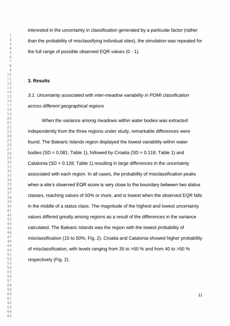
1 2 3 4 5 6 7 8 9 10 11 12 13 14 15 16 17 18 19 20 21 22 23 24 25 26 27 28 29 30 31 32 33 34 35 36 37 38 39 40 41 42 43 44 45 46 47 48 49 50 51 52 53 54 55 56 57 58 59 60 61 62 63 64 65
11
interested in the uncertainty in classification generated by a particular factor (rather
than the probability of misclassifying individual sites), the simulation was repeated for
the full range of possible observed EQR values (0 - 1).
3. Results
3.1. Uncertainty associated with inter-meadow variability in POMI classification
across different geographical regions
When the variance among meadows within water bodies was extracted
independently from the three regions under study, remarkable differences were
found. The Balearic Islands region displayed the lowest variability within water
bodies (SD = 0.081; Table 1), followed by Croatia (SD = 0.118; Table 1) and
Catalonia (SD = 0.128; Table 1) resulting in large differences in the uncertainty
associated with each region. In all cases, the probability of misclassification peaks
when a site‟s observed EQR score is very close to the boundary between two status
classes, reaching values of 50% or more, and is lowest when the observed EQR falls
in the middle of a status class. The magnitude of the highest and lowest uncertainty
values differed greatly among regions as a result of the differences in the variance
calculated. The Balearic Islands was the region with the lowest probability of
misclassification (15 to 50%, Fig. 2). Croatia and Catalonia showed higher probability
of misclassification, with levels ranging from 35 to >50 % and from 40 to >50 %
respectively (Fig. 2).
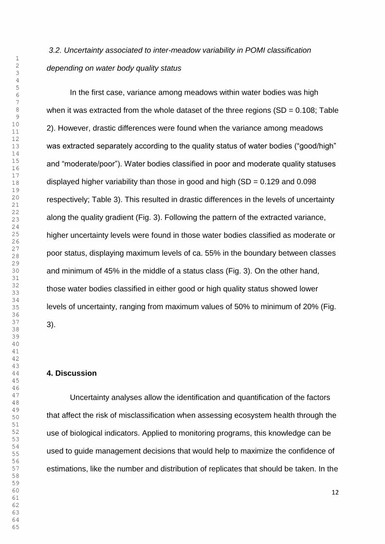
1 2 3 4 5 6 7 8 9 10 11 12 13 14 15 16 17 18 19 20 21 22 23 24 25 26 27 28 29 30 31 32 33 34 35 36 37 38 39 40 41 42 43 44 45 46 47 48 49 50 51 52 53 54 55 56 57 58 59 60 61 62 63 64 65
12
3.2. Uncertainty associated to inter-meadow variability in POMI classification
depending on water body quality status
In the first case, variance among meadows within water bodies was high
when it was extracted from the whole dataset of the three regions (SD = 0.108; Table
2). However, drastic differences were found when the variance among meadows
was extracted separately according to the quality status of water bodies (“good/high”
and “moderate/poor”). Water bodies classified in poor and moderate quality statuses
displayed higher variability than those in good and high (SD = 0.129 and 0.098
respectively; Table 3). This resulted in drastic differences in the levels of uncertainty
along the quality gradient (Fig. 3). Following the pattern of the extracted variance,
higher uncertainty levels were found in those water bodies classified as moderate or
poor status, displaying maximum levels of ca. 55% in the boundary between classes
and minimum of 45% in the middle of a status class (Fig. 3). On the other hand,
those water bodies classified in either good or high quality status showed lower
levels of uncertainty, ranging from maximum values of 50% to minimum of 20% (Fig.
3).
4. Discussion
Uncertainty analyses allow the identification and quantification of the factors
that affect the risk of misclassification when assessing ecosystem health through the
use of biological indicators. Applied to monitoring programs, this knowledge can be
used to guide management decisions that would help to maximize the confidence of
estimations, like the number and distribution of replicates that should be taken. In the
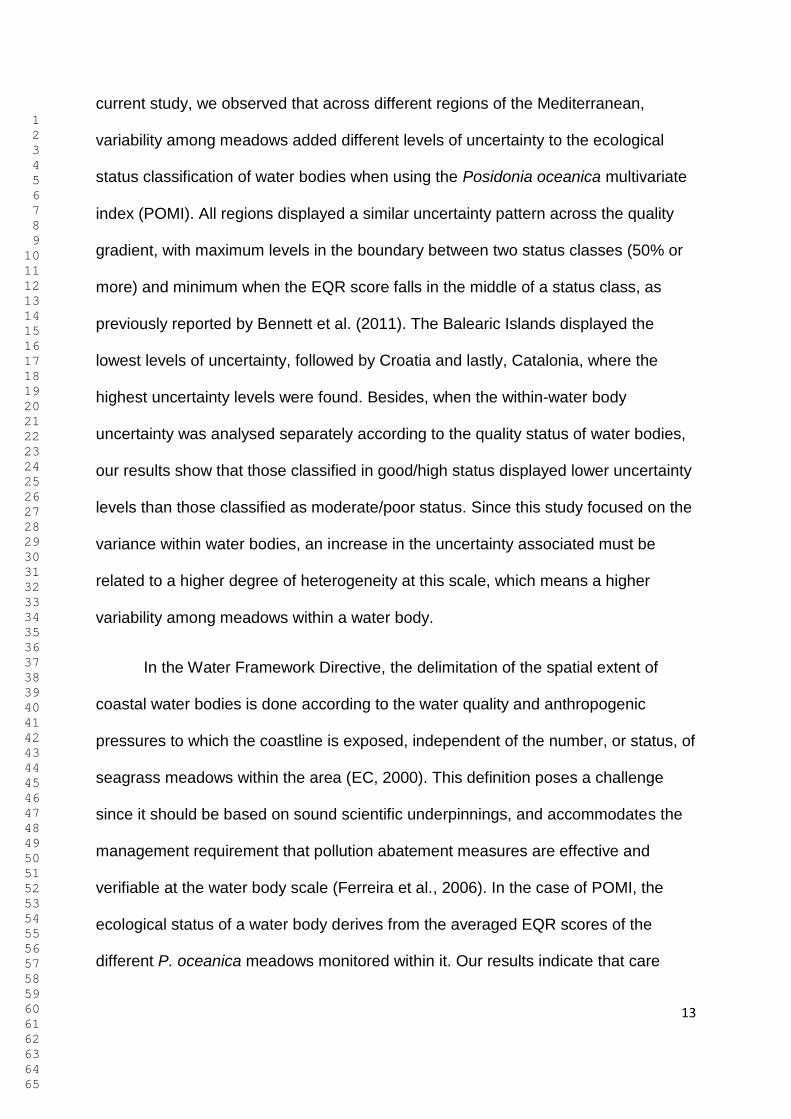
1 2 3 4 5 6 7 8 9 10 11 12 13 14 15 16 17 18 19 20 21 22 23 24 25 26 27 28 29 30 31 32 33 34 35 36 37 38 39 40 41 42 43 44 45 46 47 48 49 50 51 52 53 54 55 56 57 58 59 60 61 62 63 64 65
13
current study, we observed that across different regions of the Mediterranean,
variability among meadows added different levels of uncertainty to the ecological
status classification of water bodies when using the Posidonia oceanica multivariate
index (POMI). All regions displayed a similar uncertainty pattern across the quality
gradient, with maximum levels in the boundary between two status classes (50% or
more) and minimum when the EQR score falls in the middle of a status class, as
previously reported by Bennett et al. (2011). The Balearic Islands displayed the
lowest levels of uncertainty, followed by Croatia and lastly, Catalonia, where the
highest uncertainty levels were found. Besides, when the within-water body
uncertainty was analysed separately according to the quality status of water bodies,
our results show that those classified in good/high status displayed lower uncertainty
levels than those classified as moderate/poor status. Since this study focused on the
variance within water bodies, an increase in the uncertainty associated must be
related to a higher degree of heterogeneity at this scale, which means a higher
variability among meadows within a water body.
In the Water Framework Directive, the delimitation of the spatial extent of
coastal water bodies is done according to the water quality and anthropogenic
pressures to which the coastline is exposed, independent of the number, or status, of
seagrass meadows within the area (EC, 2000). This definition poses a challenge
since it should be based on sound scientific underpinnings, and accommodates the
management requirement that pollution abatement measures are effective and
verifiable at the water body scale (Ferreira et al., 2006). In the case of POMI, the
ecological status of a water body derives from the averaged EQR scores of the
different P. oceanica meadows monitored within it. Our results indicate that care
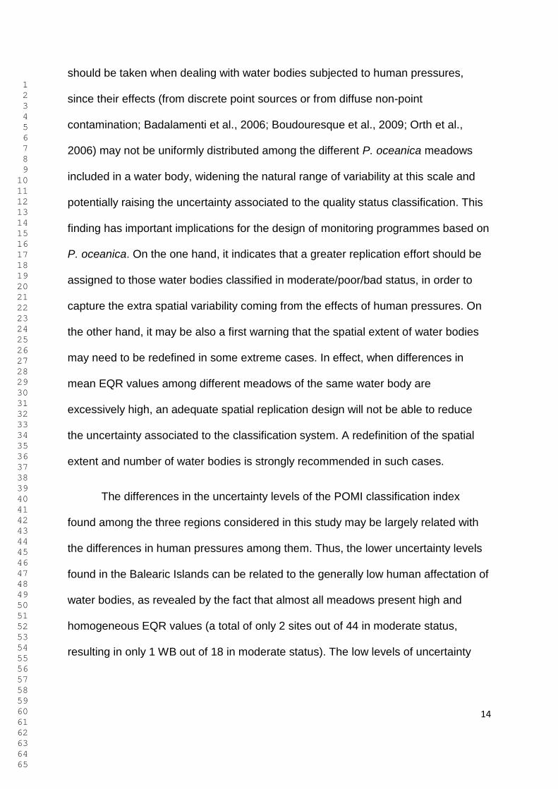
1 2 3 4 5 6 7 8 9 10 11 12 13 14 15 16 17 18 19 20 21 22 23 24 25 26 27 28 29 30 31 32 33 34 35 36 37 38 39 40 41 42 43 44 45 46 47 48 49 50 51 52 53 54 55 56 57 58 59 60 61 62 63 64 65
14
should be taken when dealing with water bodies subjected to human pressures,
since their effects (from discrete point sources or from diffuse non-point
contamination; Badalamenti et al., 2006; Boudouresque et al., 2009; Orth et al.,
2006) may not be uniformly distributed among the different P. oceanica meadows
included in a water body, widening the natural range of variability at this scale and
potentially raising the uncertainty associated to the quality status classification. This
finding has important implications for the design of monitoring programmes based on
P. oceanica. On the one hand, it indicates that a greater replication effort should be
assigned to those water bodies classified in moderate/poor/bad status, in order to
capture the extra spatial variability coming from the effects of human pressures. On
the other hand, it may be also a first warning that the spatial extent of water bodies
may need to be redefined in some extreme cases. In effect, when differences in
mean EQR values among different meadows of the same water body are
excessively high, an adequate spatial replication design will not be able to reduce
the uncertainty associated to the classification system. A redefinition of the spatial
extent and number of water bodies is strongly recommended in such cases.
The differences in the uncertainty levels of the POMI classification index
found among the three regions considered in this study may be largely related with
the differences in human pressures among them. Thus, the lower uncertainty levels
found in the Balearic Islands can be related to the generally low human affectation of
water bodies, as revealed by the fact that almost all meadows present high and
homogeneous EQR values (a total of only 2 sites out of 44 in moderate status,
resulting in only 1 WB out of 18 in moderate status). The low levels of uncertainty
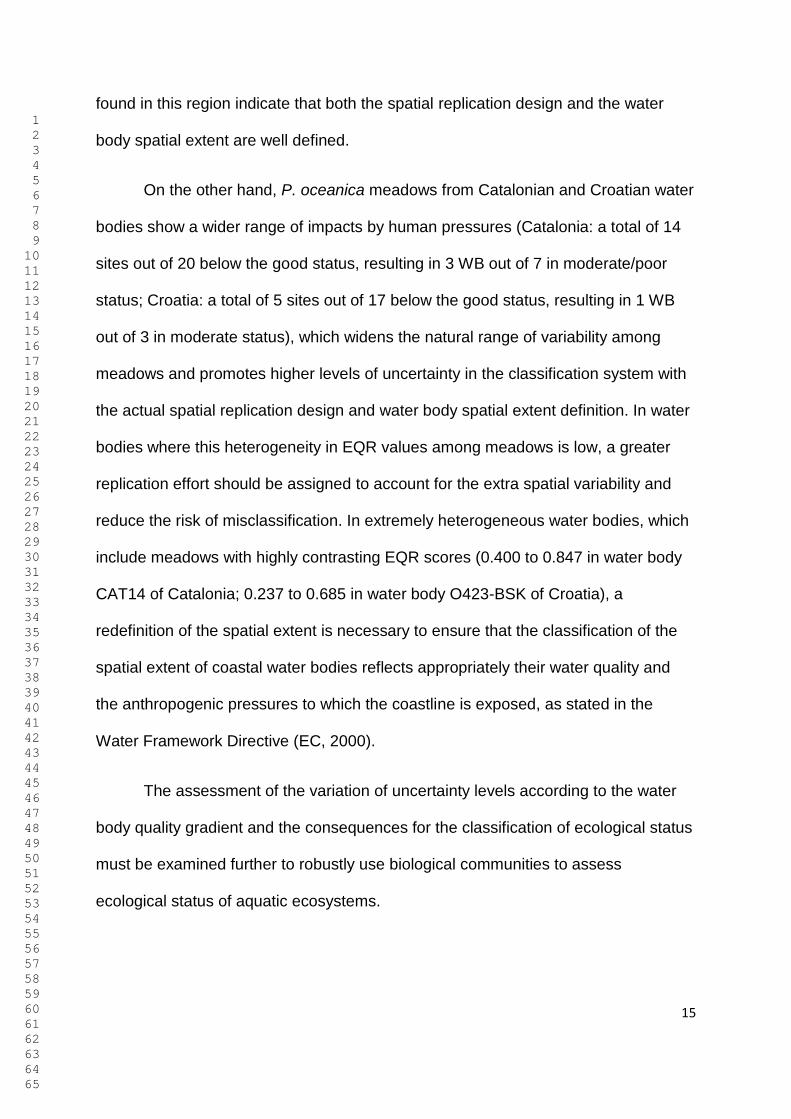
1 2 3 4 5 6 7 8 9 10 11 12 13 14 15 16 17 18 19 20 21 22 23 24 25 26 27 28 29 30 31 32 33 34 35 36 37 38 39 40 41 42 43 44 45 46 47 48 49 50 51 52 53 54 55 56 57 58 59 60 61 62 63 64 65
15
found in this region indicate that both the spatial replication design and the water
body spatial extent are well defined.
On the other hand, P. oceanica meadows from Catalonian and Croatian water
bodies show a wider range of impacts by human pressures (Catalonia: a total of 14
sites out of 20 below the good status, resulting in 3 WB out of 7 in moderate/poor
status; Croatia: a total of 5 sites out of 17 below the good status, resulting in 1 WB
out of 3 in moderate status), which widens the natural range of variability among
meadows and promotes higher levels of uncertainty in the classification system with
the actual spatial replication design and water body spatial extent definition. In water
bodies where this heterogeneity in EQR values among meadows is low, a greater
replication effort should be assigned to account for the extra spatial variability and
reduce the risk of misclassification. In extremely heterogeneous water bodies, which
include meadows with highly contrasting EQR scores (0.400 to 0.847 in water body
CAT14 of Catalonia; 0.237 to 0.685 in water body O423-BSK of Croatia), a
redefinition of the spatial extent is necessary to ensure that the classification of the
spatial extent of coastal water bodies reflects appropriately their water quality and
the anthropogenic pressures to which the coastline is exposed, as stated in the
Water Framework Directive (EC, 2000).
The assessment of the variation of uncertainty levels according to the water
body quality gradient and the consequences for the classification of ecological status
must be examined further to robustly use biological communities to assess
ecological status of aquatic ecosystems.
1 2 3 4 5 6 7 8 9 10 11 12 13 14 15 16 17 18 19 20 21 22 23 24 25 26 27 28 29 30 31 32 33 34 35 36 37 38 39 40 41 42 43 44 45 46 47 48 49 50 51 52 53 54 55 56 57 58 59 60 61 62 63 64 65
16
5. Conclusions
When designing monitoring programs to classify the ecological quality status
of water bodies using the Posidonia oceanica Multivariate Index (POMI), sampling
effort must be set according to the specific conditions of each water body, region and
associated human pressures. A greater replication effort must be assigned to
regions and water bodies that are subject to significant human pressures (high
population density, industrialization, etc.), spanning a sufficient number of meadows
within each water body to provide a robust and reliable average value of their quality
status. In water bodies where only a single or few meadows exist, uncertainty
estimates should be calibrated with water bodies of similar ecological status. Water
bodies encompassing meadows with highly contrasting EQR scores need be split
into different water bodies to clearly delineate areas affected by human impacts from
those less influenced.
Acknowledgements: We thank all the different people involved in the monitoring
programmes of Catalonia, Balearic Islands and Croatia for their work in the field and
laboratory. We also thank Michael Dunbar and Ralph Clarke for his assistance in
statistical analyses. This research was funded by l‟Agencia Catalana de l‟Aigua, the
Govern de les Illes Balears and WISER (Water bodies in Europe: Integrative
Systems to assess Ecological status and Recovery) funded under the 7th EU
Framework Programme, Theme 6 (Environment including Climate Change), Contract
No.: 226273).
1 2 3 4 5 6 7 8 9 10 11 12 13 14 15 16 17 18 19 20 21 22 23 24 25 26 27 28 29 30 31 32 33 34 35 36 37 38 39 40 41 42 43 44 45 46 47 48 49 50 51 52 53 54 55 56 57 58 59 60 61 62 63 64 65
17
References
Badalamenti, F., Di Carlo, G., D‟Anna, G., Gristina M., Toccaceli, M., 2006. Effects of dredging activities on population dynamics of Posidonia oceanica (L.) Delile in the Mediterranean Sea: the case study of Capo Feto (SW Sicily, Italy). Hydrobiologia 555, 253–261.
Bennett, S., Roca, G., Romero, J., Alcoverro, T., 2011. Ecological status of seagrass ecosystems: An uncertainty analysis of the meadow classification based on the Posidonia oceanica multivariate index (POMI). Marine Pollution Bulletin 62, 1616-1621.
Boudouresque, C.F., Bernard, G., Pergent, G., Shili, A., Verlaque, M., 2009. Regression of Mediterranean seagrasses caused by natural processes and anthropogenic disturbances and stress: a critical review. Botanica Marina 52, 395-418.
Buia, M.C., Silvestre, F., Iacono, G., Tiberti, L., 2005. Identificazione delle biocenosi di maggior preggio ambientale al fine della classificazione della qualita delle acque costiere. In: Metodologie per il rilevamento e la classificazione dello stato di qualita ecologico e chimico delle acque, con particolare riferimento all‟aplicazione del decreto legislativo 152/99. APAT, Rome, pp. 269–303.
Casazza, G., Lopez y Royo, C., Silvestri, C., 2006. Seagrass as key coastal ecosystems: an overview of the recent EU WFD requirements and current applications. Biologia Marina Mediterranea 13, 189–193.
Clarke, R.T., Hering, D., 2006. Errors and uncertainty in bioassessment methods – major results and conclusions from the STAR project and their application using STARBUGS. Hydrobiologia 566, 433-439.
Clarke, R.T., Davy-Bowker, J., Sandin, L., Friberg, N., Johnson, R.K., Bis, B., 2006. Estimates and comparisons of the effects of sampling variation using “national” macroinvertebrate sampling protocols on the precision of metrics used to assess ecological status. Hydrobiologia 566, 477–503.
Clarke, R.T., 2010. WISERBUGS 1.1 (WISER Bioassessment Uncertainty Guidance Software) tool for assessing confidence of WFD ecological status. User and Manual Software. Bournemouth University.
EC, 2000. DIRECTIVE 2000/60/EC of the European parliament and of the council, of 23 October 2000, establishing a framework for Community action in the field of water policy. Official Journal of the European Communities, G.U.C.E. 22/12/ 2000, L 327.
Ferreira, J.G., Nobre, A.M., Simas, T.C., Silva, M.C., Newton, A., Bricker, S.B., Wolff, W.J., Stacey, P.E., Sequeira, A., 2006. A methodology for defining homogeneous water bodies in estuaries – Application to the transitional systems of the EU Water Framework Directive. Estuarine, Coastal and Shelf Science 66, 468-482.
1 2 3 4 5 6 7 8 9 10 11 12 13 14 15 16 17 18 19 20 21 22 23 24 25 26 27 28 29 30 31 32 33 34 35 36 37 38 39 40 41 42 43 44 45 46 47 48 49 50 51 52 53 54 55 56 57 58 59 60 61 62 63 64 65
18
Gobert, S., Sartoretto, S., Rico-Raimondino, V., Andral, B., Chery, A., Lejeune, P., Boissery, P., 2009. Assessment of the ecological status of Mediterranean French coastal waters as required by the Water Framework Directive using the Posidonia oceanica Rapid Easy Index: PREI. Marine Pollution Bulletin 58, 1727-1733.
Kelly, M., Bennion, H., Burgess, A., Ellis, J., Juggins, S., Guthrie, R., Jamieson, J., Adriaenssens, V., Yallop, M., 2009. Uncertainty in ecological status assessments of lakes and rivers using diatoms. Hydrobiologia 633, 5-15.
Lopez y Royo, C., Pergent, G., Alcoverro, T., Buia, M.C., Casazza, G., Martínez-Crego, B., Pérez, M., Silvestre, F., Romero, J., 2011. The seagrass Posidonia oceanica as indicator of coastal water quality: Experimental intercalibration of classification systems. Ecological Indicators 11, 55-563.
Martínez-Crego, B., Vergés, A., Alcoverro, T., Romero, J., 2008. Selection of multiple seagrass indicators for environmental biomonitoring. Marine Ecology Progress Series 361, 93-109.
Med-GIG, 2007. WFD Intercalibration technical report for coastal and transitional waters in the Mediterranean eco-region. In: WFD Intercalibration technical report – Part 3: Coastal and transitional waters. URL http://circa.europa.eu/Public/irc/jrc/jrceewai/library?l=/intercalibration2&vm=detailed&sb=Title.
Orth, R.J., Carruthers, T.J.B., Dennison, W.C., Duarte, C.M., Fourqurean, J.W., Heck, K.L., Hughes, A.R., Kendrick, G.A., Kenworthy, W.J., Olyarnik, A., Short, F.T., Waycott, M., Williams, S.L., 2006. A global crisis for seagrass ecosystems. Bioscience 56, 987–996.
Pergent, G., Pergent-Martini, C., Boudouresque, C.F., 1995. Utilisation de l‟herbier à Posidonia oceanica comme indicateur biologique de la qualité du milieu littoral en Méditerranée: Etat des connaissances. Mesogée 54, 3–29.
Pergent-Martini, C., Leoni, V., Pasqualini, V., Ardizzone, G.D., Balestri, E., Bedini, R., Belluscio, A., Belsher, T., Borg, J., Boudouresque, C.F., Boumaza, S., Bouquegneau, J.M., Buia, M.C., Calvo, S., Cebrian, J., Charbonnel, E., Cinelli, F., Cossu, A., Di Maida, G., Dural, B., Francour, P., Gobert, S., Lepoint, G., Meinesz, A., Molenaar, H., Mansour, H.M., Panayotidis, P., Peirano, A., Pergent, G., Piazzi, L., Pirrotta, M., Relini, G., Romero, J., Sanchez-Lizaso, J.L., Semroud, R., Shembri, P., Shili, A., Tomasello, A., Velimirov, B., 2005. Descriptors of Posidonia oceanica meadows: use and application. Ecological Indicators 5, 213–230.
Pinheiro, J.C., Bates, D.M., 2000. Mixed-Effects models in S and S-Plus. Springer. ISBN 0-387-98957-0.
Pinheiro, J.C., Bates, D.M., DebRoy, S., Sarkar, D., 2005. The nlme package: Linear and nonlinear mixed effects models. URL http: //CRAN.R-project.org. R package version 3.1-98.
1 2 3 4 5 6 7 8 9 10 11 12 13 14 15 16 17 18 19 20 21 22 23 24 25 26 27 28 29 30 31 32 33 34 35 36 37 38 39 40 41 42 43 44 45 46 47 48 49 50 51 52 53 54 55 56 57 58 59 60 61 62 63 64 65
19
Procaccini, G., Buia, MC., Gambi, M.C., Pérez, M., Pergent-Marini, C., Romero, J., 2003. The seagrasses of the western Mediterranean. In: Green, E.P., Short, F.T. (Eds.), World Atlas of Seagrasses. University of California Press, Berkeley (USA). pp. 298.
Romero, J., Martínez-Crego, B., Alcoverro, T., Pérez, M., 2007. A multivariate index based on the seagrass Posidonia oceanica (POMI) to assess ecological status of coastal waters under the Water Framework Directive (WFD). Marine Pollution Bulletin 55, 196–204.
Staniszewski, R., Szoszkiewicz, K., Zbierska, J., Lesny, J., Jusik, S., Clarke, R.T., 2006. Assessment of sources of uncertainty in macrophyte surveys and the consequences for river classification. Hydrobiologia 566, 235-246.
Figure 1: Map of the location of the sampling sites (meadows) and water bodies along the Catalonian, Balearic and Croatian coasts, from where bio-monitoring POMI data was obtained.
Figure 2: Probability of misclassifying the ecological status class associated to the variability among sites within water bodies (included in the residual variance of the model) for the three regions under study (Catalonia, Balearic Is. and Croatia). Vertical dashed lines represent the boundaries of each status class. Bad = EQR values from 0 – 0.099; Poor = 0.1 – 0.324; Moderate = 0.325 – 0.54; Good = 0.55-0.774 and High = 0.775 – 1.
Figure 3: Probability of misclassifying the ecological status class associated to the variability among sites within water bodies (included in the residual variance of the model) for the data pooled from the three regions under study and according to their quality status. Vertical dashed lines represent the boundaries of each status class. Bad = EQR values from 0 – 0.099; Poor = 0.1 – 0.324; Moderate = 0.325 – 0.54; Good = 0.55-0.774 and High = 0.775 – 1.
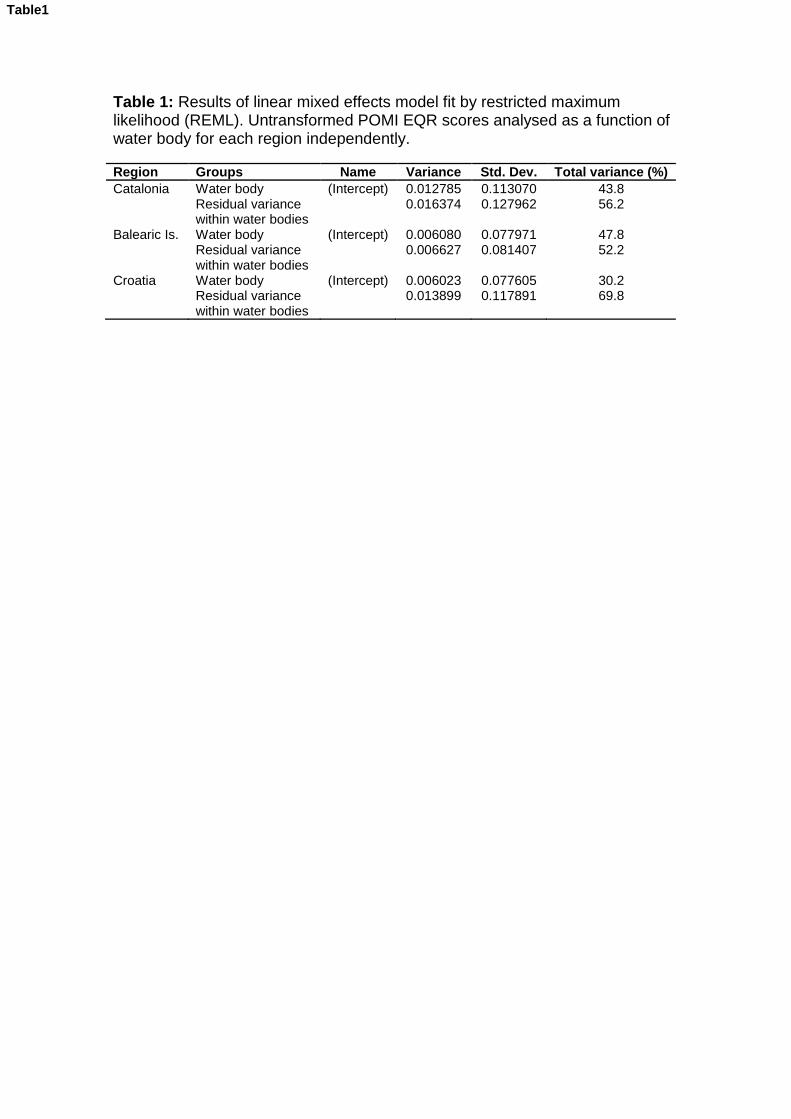
Table 1: Results of linear mixed effects model fit by restricted maximum likelihood (REML). Untransformed POMI EQR scores analysed as a function of water body for each region independently.
Region Groups Name Variance Std. Dev. Total variance (%)
Catalonia Water body (Intercept) 0.012785 0.113070 43.8 Residual variance
within water bodies 0.016374 0.127962 56.2
Balearic Is. Water body (Intercept) 0.006080 0.077971 47.8 Residual variance
within water bodies 0.006627 0.081407 52.2
Croatia Water body (Intercept) 0.006023 0.077605 30.2 Residual variance
within water bodies 0.013899 0.117891 69.8
Table1
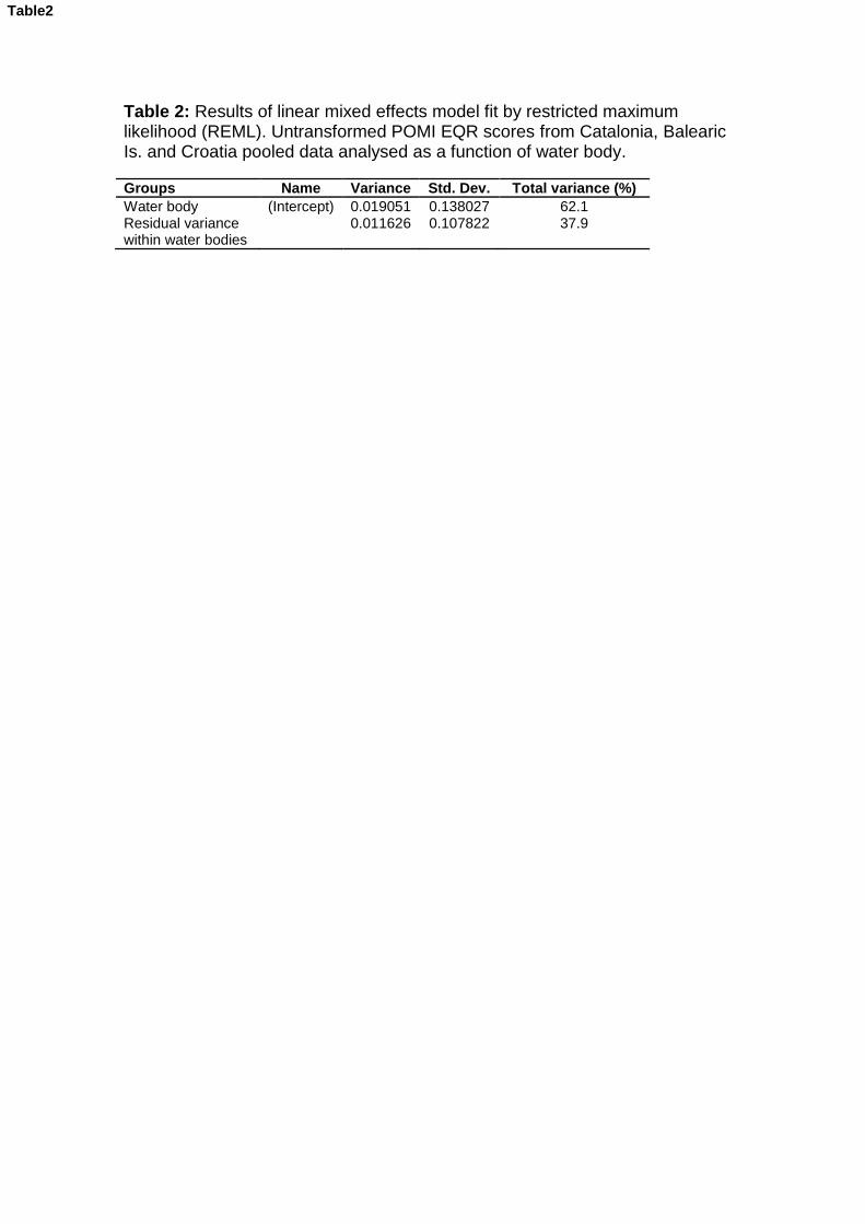
Table 2: Results of linear mixed effects model fit by restricted maximum likelihood (REML). Untransformed POMI EQR scores from Catalonia, Balearic Is. and Croatia pooled data analysed as a function of water body.
Groups Name Variance Std. Dev. Total variance (%)
Water body (Intercept) 0.019051 0.138027 62.1 Residual variance within water bodies
0.011626 0.107822 37.9
Table2
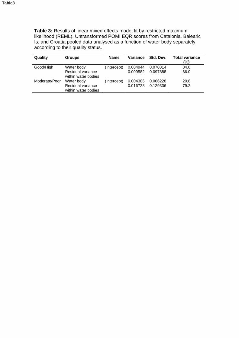
Table 3: Results of linear mixed effects model fit by restricted maximum likelihood (REML). Untransformed POMI EQR scores from Catalonia, Balearic Is. and Croatia pooled data analysed as a function of water body separately according to their quality status.
Quality Groups Name Variance Std. Dev. Total variance (%)
Good/High Water body (Intercept) 0.004944 0.070314 34.0 Residual variance
within water bodies 0.009582 0.097888 66.0
Moderate/Poor Water body (Intercept) 0.004386 0.066228 20.8 Residual variance
within water bodies 0.016728 0.129336 79.2
Table3
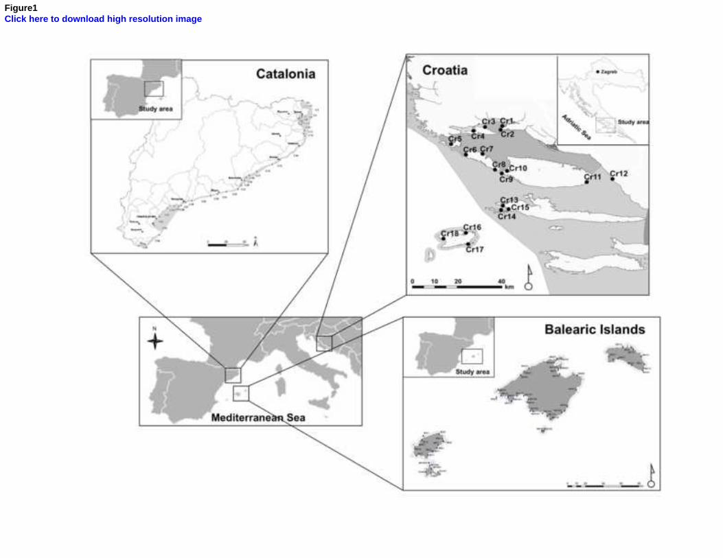
Figure1Click here to download high resolution image
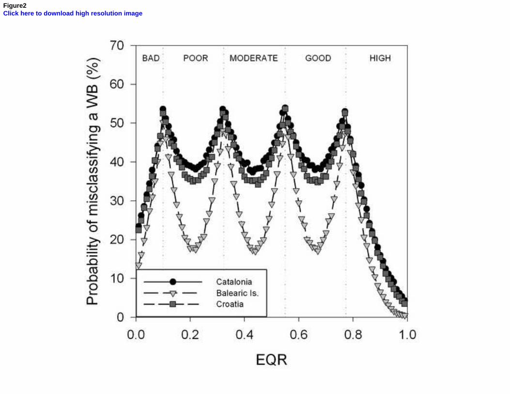
Figure2Click here to download high resolution image
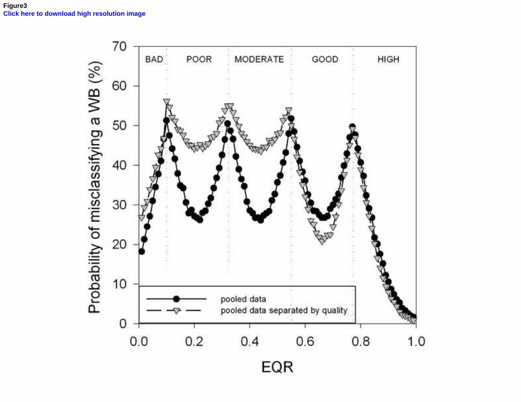
Figure3Click here to download high resolution image
Exploring the robustness of different macrophyte-based 1
classification methods to assess the ecological status of 2
coastal and transitional ecosystems under the WFD 3
4
Oriol Mascaróa*, Teresa Alcoverroa, Kristina Denchevab, Dorte 5
Krause-Jensenc, Núria Marbàd, Iñigo Muxikae, João Netof, Vedran 6
Nikolićg, Sotiris Orfanidish, Are Pederseni, Marta Pérezj, Javier 7
Romeroj 8
9
a Centre d’Estudis Avançats de Blanes (CSIC). C/ d’Accés a la Cala St. 10
Francesc 14, 17300 – Blanes (Girona). Spain 11
b Institute of Oceanology - BAS, "Parvi may str. N 40", PoBox 152, 9000 Varna, 12
Bulgaria 13
c Department of Bioscience, Aarhus University. Vejlsøvej 25 DK-8600, 14
Silkeborg. Denmark 15
d Department of Global Change Research. IMEDEA (CSIC-UIB), Institut 16
Mediterrani d’Estudis Avançats. Miquel Marquès 21, 07190 Esporles (Illes 17
Balears). Spain 18
e 19
2
f Institute of Marine Research. Dept. of Life Sciences, University of 20
Coimbra. Largo Marques Pombal 3004-517 Coimbra, Portugal 21
g Institute of Oceanography and Fisheries. I. Meštrovića 63, HR-21000 Split. 22
Croatia 23
h National Agricultural Research Foundation. Fisheries Research Institute, 640 24
07 Nea Peramos, Kavala. Greece 25
i Center for Coastal and Marine Research, Norwegian Institute for Water 26
Research - NIVA, Gaustadalléen 21, NO-0349 Oslo. Norway 27
j Department of Ecology, University of Barcelona. Av. Diagonal 645, 08028 28
Barcelona, Spain 29
30
31
*Corresponding author: Tel.: +34 972 336 101; E-mail: [email protected] 32
33
34
3
Abstract 35
Identifying and quantifying the factors that contribute to the potential misclassification 36
of the ecological status of water bodies is a major challenge of the next phase of 37
WFD implementation, and one of the main goals of the WISER Project. The present 38
study compiles extensive bio-monitoring data from several macrophyte-based 39
classification methods developed by different EU Members, which include data 40
addressing spatial, temporal and human-induced sources of variability. Through the 41
application of uncertainty analysis, we determined that factors related to the spatial 42
scale of sampling added the highest levels of uncertainty to the ecological status 43
classification of water bodies, probably due to the high horizontal and vertical 44
heterogeneity displayed by macrophyte communities. On the contrary, the 45
uncertainty associated to temporal variability and human-induced errors was very 46
low, for which the frequency of sampling could be decreased and the number of 47
surveyors minimized without greatly reducing the precision of ecological status 48
estimates. 49
50
Keywords: biological quality elements; Water Framework Directive; uncertainty; 51
52
4
1. Introduction 52
The requirement of the EU Water Framework Directive (WFD; Directive 2000) 53
to classify all surface water bodies according to their “ecological status” has 54
precipitated a fundamental change in management objectives from merely pollution 55
control to ensuring ecosystem integrity as a whole (Hering et al. 2010). The concept 56
of “ecological status”, as defined by the WFD, is the quality of the structure and 57
functioning of aquatic ecosystems associated with surface waters (Bennett et al. 58
2011). Rather than focus only on limited aspects of chemical quality, the WFD 59
establishes that the ecological status has to be determined by monitoring and 60
assessing the so-called Biological Quality Elements (BQEs; Moss 2007, Lopez y 61
Royo et al. 2011), which must be integrated into an index with the aim to detect 62
temporal and spatial changes in the quality of water bodies (Bennett et al. 2011). 63
However, this innovativeness comes with a number of substantial challenges 64
for ecologists in requiring complex and dynamic biological communities to be 65
quantified into a single numeric score, for reference conditions to be established 66
from which to measure the degree of change, and for this all to be carried out within 67
a large number of water body types (Hering et al. 2010). The development of 68
methods for water body quality assessment fulfilling the complex requirements of the 69
WFD has been faced by each Member State individually (Søndergaard et al. 2005), 70
resulting in the appearance of a wide variety of methods throughout Europe that 71
differ greatly in the way of defining reference conditions, type vs. site-specific 72
assessment, the number and nature of indices (metrics) used, etc. (Hering et al. 73
2010). 74
5
The WISER Project (Water bodies in Europe: Integrative Systems to assess 75
Ecological status and Recovery; www.wiser.eu) was conceived to evaluate the 76
robustness and reliability of the different indices developed by the EU members, 77
addressing all water categories, organism groups and environmental stressor types. 78
This is to be done mainly through the use of uncertainty analysis, a powerful tool that 79
allows the identification of the factors contributing to the potential misclassification of 80
the ecological status class of water bodies (Clarke and Hering 2006, Staniszewski et 81
al. 2006). The estimation of uncertainty is a central element in WFD-compliant 82
assessment methods, since they are based on biological communities that show 83
both spatial and temporal heterogeneity, and because errors will be introduced 84
during sampling and analytical stages (Clarke and Hering 2006, Carstensen 2007, 85
Kelly et al. 2009). If the major sources of variability are known, they can potentially 86
be minimised through the re-design of sampling schemes (additional sampling sites 87
or frequency), through improved training by operating procedures, CEN (European 88
Committee for Standardization) guidance, taxonomic training or through the use of 89
model-based assessment methods (Pont et al. 2009). For this reason, ecological 90
status classification results should always be given in terms of probabilities 91
depending upon the variability associated with these communities over time and 92
space (Hering et al. 2010). However, only a small proportion of classification 93
methods have put this into practice and the uncertainty analyses available in the 94
literature are relatively scarce at the moment (but see Staniszewski et al. 2006, Kelly 95
et al. 2009, Bennett et al. 2011). 96
The objective of this contribution is to determine which sources of variability 97
(factors) associated with the sampling design of a subset of different monitoring 98
6
programmes (6 different classification methods) based on macrophytes (either 99
macroalgae or seagrasses) developed by EU Member States under the Water 100
Framework Directive (Norway, Denmark, Bulgaria, Spain, Croatia, Italia and 101
Portugal), most greatly influence ecological status classifications of these biological 102
communities. The analyses will be based on EQR datasets of either official or non-103
official bio-monitoring programmes of the different indices from which a data set 104
including enough temporal and spatial replication was available, and the factors 105
analysed will include spatial scales of sampling (variability among zones within a 106
site, among sites within a water body, variability among regions and variability 107
among depths), the temporal scale of sampling (variability among years) and the 108
human-associated source of error (variability between surveyors). These factors 109
represent some the key sources of variability associated with the design and 110
implementation of a bio-monitoring program, and highlight how certain elements of a 111
sampling design can influence the reliability and robustness of the ecological status 112
classification of coastal water bodies. With this approach, we try to gain insight into 113
the current status of these methodologies proposed for European waters under the 114
WFD and detect their main weaknesses to provide robust foundation for monitoring 115
as well as guide decision in management plans. 116
117
118
2. Material and Methods 119
2.1. Indices included in the study 120
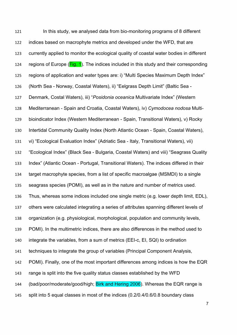
7
In this study, we analysed data from bio-monitoring programs of 8 different 121
indices based on macrophyte metrics and developed under the WFD, that are 122
currently applied to monitor the ecological quality of coastal water bodies in different 123
regions of Europe (Fig. 1). The indices included in this study and their corresponding 124
regions of application and water types are: i) “Multi Species Maximum Depth Index” 125
(North Sea - Norway, Coastal Waters), ii) “Eelgrass Depth Limit” (Baltic Sea - 126
Denmark, Costal Waters), iii) “Posidonia oceanica Multivariate Index” (Western 127
Mediterranean - Spain and Croatia, Coastal Waters), iv) Cymodocea nodosa Multi-128
bioindicator Index (Western Mediterranean - Spain, Transitional Waters), v) Rocky 129
Intertidal Community Quality Index (North Atlantic Ocean - Spain, Coastal Waters), 130
vi) “Ecological Evaluation Index” (Adriatic Sea - Italy, Transitional Waters), vii) 131
“Ecological Index” (Black Sea - Bulgaria, Coastal Waters) and viii) “Seagrass Quality 132
Index” (Atlantic Ocean - Portugal, Transitional Waters). The indices differed in their 133
target macrophyte species, from a list of specific macroalgae (MSMDI) to a single 134
seagrass species (POMI), as well as in the nature and number of metrics used. 135
Thus, whereas some indices included one single metric (e.g. lower depth limit, EDL), 136
others were calculated integrating a series of attributes spanning different levels of 137
organization (e.g. physiological, morphological, population and community levels, 138
POMI). In the multimetric indices, there are also differences in the method used to 139
integrate the variables, from a sum of metrics (EEI-c, EI, SQI) to ordination 140
techniques to integrate the group of variables (Principal Component Analysis, 141
POMI). Finally, one of the most important differences among indices is how the EQR 142
range is split into the five quality status classes established by the WFD 143
(bad/poor/moderate/good/high; Birk and Hering 2006). Whereas the EQR range is 144
split into 5 equal classes in most of the indices (0.2/0.4/0.6/0.8 boundary class 145
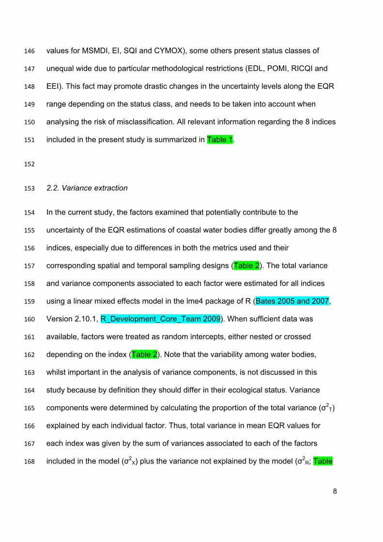
8
values for MSMDI, EI, SQI and CYMOX), some others present status classes of 146
unequal wide due to particular methodological restrictions (EDL, POMI, RICQI and 147
EEI). This fact may promote drastic changes in the uncertainty levels along the EQR 148
range depending on the status class, and needs to be taken into account when 149
analysing the risk of misclassification. All relevant information regarding the 8 indices 150
included in the present study is summarized in Table 1. 151
152
2.2. Variance extraction 153
In the current study, the factors examined that potentially contribute to the 154
uncertainty of the EQR estimations of coastal water bodies differ greatly among the 8 155
indices, especially due to differences in both the metrics used and their 156
corresponding spatial and temporal sampling designs (Table 2). The total variance 157
and variance components associated to each factor were estimated for all indices 158
using a linear mixed effects model in the lme4 package of R (Bates 2005 and 2007, 159
Version 2.10.1, R_Development_Core_Team 2009). When sufficient data was 160
available, factors were treated as random intercepts, either nested or crossed 161
depending on the index (Table 2). Note that the variability among water bodies, 162
whilst important in the analysis of variance components, is not discussed in this 163
study because by definition they should differ in their ecological status. Variance 164
components were determined by calculating the proportion of the total variance (σ2T) 165
explained by each individual factor. Thus, total variance in mean EQR values for 166
each index was given by the sum of variances associated to each of the factors 167
included in the model (σ2X) plus the variance not explained by the model (σ2
R; Table 168
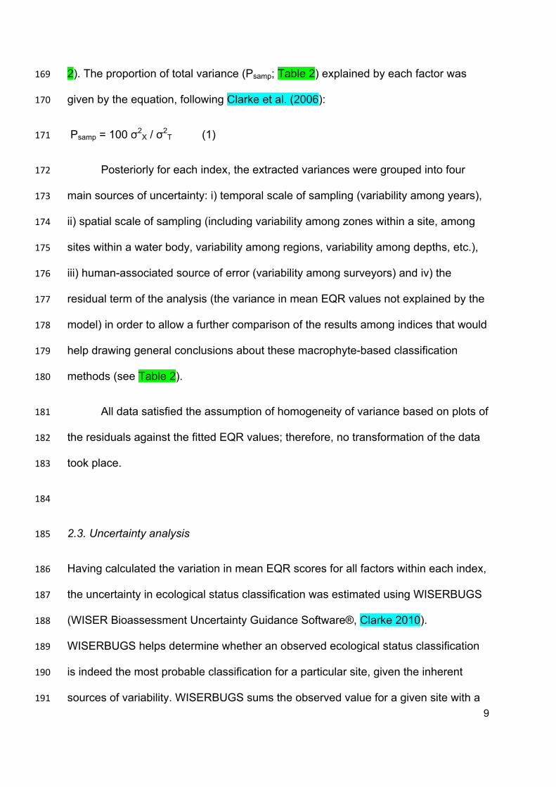
9
2). The proportion of total variance (Psamp; Table 2) explained by each factor was 169
given by the equation, following Clarke et al. (2006): 170
Psamp = 100 σ2X / σ2
T (1) 171
Posteriorly for each index, the extracted variances were grouped into four 172
main sources of uncertainty: i) temporal scale of sampling (variability among years), 173
ii) spatial scale of sampling (including variability among zones within a site, among 174
sites within a water body, variability among regions, variability among depths, etc.), 175
iii) human-associated source of error (variability among surveyors) and iv) the 176
residual term of the analysis (the variance in mean EQR values not explained by the 177
model) in order to allow a further comparison of the results among indices that would 178
help drawing general conclusions about these macrophyte-based classification 179
methods (see Table 2). 180
All data satisfied the assumption of homogeneity of variance based on plots of 181
the residuals against the fitted EQR values; therefore, no transformation of the data 182
took place. 183
184
2.3. Uncertainty analysis 185
Having calculated the variation in mean EQR scores for all factors within each index, 186
the uncertainty in ecological status classification was estimated using WISERBUGS 187
(WISER Bioassessment Uncertainty Guidance Software®, Clarke 2010). 188
WISERBUGS helps determine whether an observed ecological status classification 189
is indeed the most probable classification for a particular site, given the inherent 190
sources of variability. WISERBUGS sums the observed value for a given site with a 191
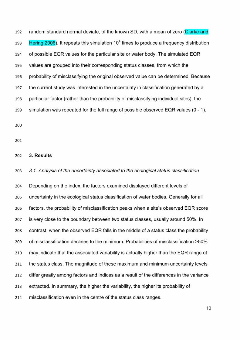
10
random standard normal deviate, of the known SD, with a mean of zero (Clarke and 192
Hering 2006). It repeats this simulation 104 times to produce a frequency distribution 193
of possible EQR values for the particular site or water body. The simulated EQR 194
values are grouped into their corresponding status classes, from which the 195
probability of misclassifying the original observed value can be determined. Because 196
the current study was interested in the uncertainty in classification generated by a 197
particular factor (rather than the probability of misclassifying individual sites), the 198
simulation was repeated for the full range of possible observed EQR values (0 - 1). 199
200
201
3. Results 202
3.1. Analysis of the uncertainty associated to the ecological status classification 203
Depending on the index, the factors examined displayed different levels of 204
uncertainty in the ecological status classification of water bodies. Generally for all 205
factors, the probability of misclassification peaks when a site’s observed EQR score 206
is very close to the boundary between two status classes, usually around 50%. In 207
contrast, when the observed EQR falls in the middle of a status class the probability 208
of misclassification declines to the minimum. Probabilities of misclassification >50% 209
may indicate that the associated variability is actually higher than the EQR range of 210
the status class. The magnitude of these maximum and minimum uncertainty levels 211
differ greatly among factors and indices as a result of the differences in the variance 212
extracted. In summary, the higher the variability, the higher its probability of 213
misclassification even in the centre of the status class ranges. 214
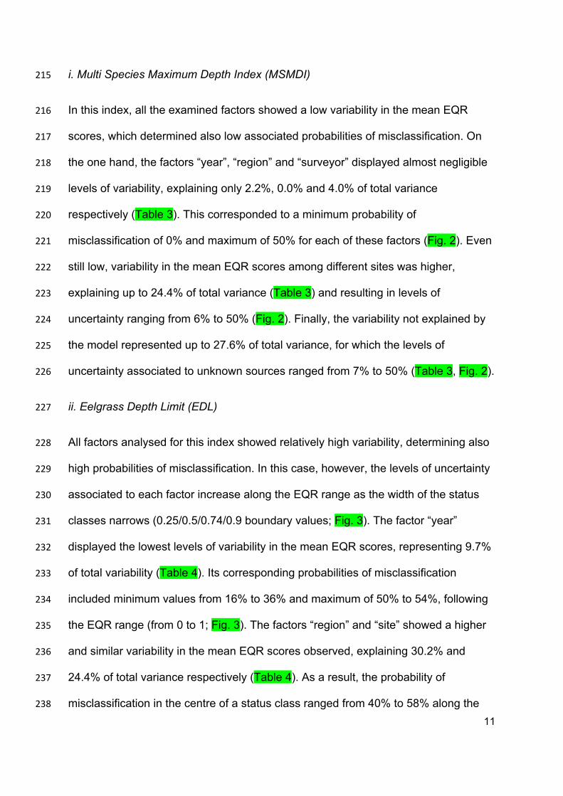
11
i. Multi Species Maximum Depth Index (MSMDI) 215
In this index, all the examined factors showed a low variability in the mean EQR 216
scores, which determined also low associated probabilities of misclassification. On 217
the one hand, the factors “year”, “region” and “surveyor” displayed almost negligible 218
levels of variability, explaining only 2.2%, 0.0% and 4.0% of total variance 219
respectively (Table 3). This corresponded to a minimum probability of 220
misclassification of 0% and maximum of 50% for each of these factors (Fig. 2). Even 221
still low, variability in the mean EQR scores among different sites was higher, 222
explaining up to 24.4% of total variance (Table 3) and resulting in levels of 223
uncertainty ranging from 6% to 50% (Fig. 2). Finally, the variability not explained by 224
the model represented up to 27.6% of total variance, for which the levels of 225
uncertainty associated to unknown sources ranged from 7% to 50% (Table 3, Fig. 2). 226
ii. Eelgrass Depth Limit (EDL) 227
All factors analysed for this index showed relatively high variability, determining also 228
high probabilities of misclassification. In this case, however, the levels of uncertainty 229
associated to each factor increase along the EQR range as the width of the status 230
classes narrows (0.25/0.5/0.74/0.9 boundary values; Fig. 3). The factor “year” 231
displayed the lowest levels of variability in the mean EQR scores, representing 9.7% 232
of total variability (Table 4). Its corresponding probabilities of misclassification 233
included minimum values from 16% to 36% and maximum of 50% to 54%, following 234
the EQR range (from 0 to 1; Fig. 3). The factors “region” and “site” showed a higher 235
and similar variability in the mean EQR scores observed, explaining 30.2% and 236
24.4% of total variance respectively (Table 4). As a result, the probability of 237
misclassification in the centre of a status class ranged from 40% to 58% along the 238
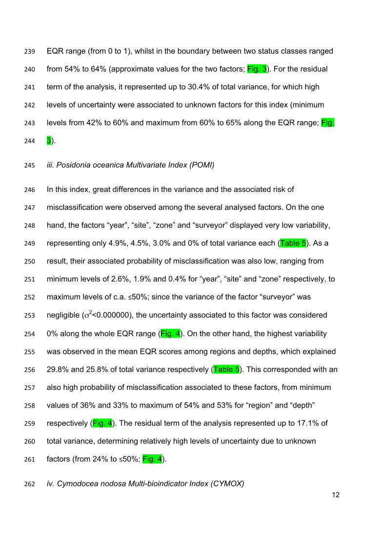
12
EQR range (from 0 to 1), whilst in the boundary between two status classes ranged 239
from 54% to 64% (approximate values for the two factors; Fig. 3). For the residual 240
term of the analysis, it represented up to 30.4% of total variance, for which high 241
levels of uncertainty were associated to unknown factors for this index (minimum 242
levels from 42% to 60% and maximum from 60% to 65% along the EQR range; Fig. 243
3). 244
iii. Posidonia oceanica Multivariate Index (POMI) 245
In this index, great differences in the variance and the associated risk of 246
misclassification were observed among the several analysed factors. On the one 247
hand, the factors “year”, “site”, “zone” and “surveyor” displayed very low variability, 248
representing only 4.9%, 4.5%, 3.0% and 0% of total variance each (Table 5). As a 249
result, their associated probability of misclassification was also low, ranging from 250
minimum levels of 2.6%, 1.9% and 0.4% for “year”, “site” and “zone” respectively, to 251
maximum levels of c.a. ≤50%; since the variance of the factor “surveyor” was 252
negligible (σ2<0.000000), the uncertainty associated to this factor was considered 253
0% along the whole EQR range (Fig. 4). On the other hand, the highest variability 254
was observed in the mean EQR scores among regions and depths, which explained 255
29.8% and 25.8% of total variance respectively (Table 5). This corresponded with an 256
also high probability of misclassification associated to these factors, from minimum 257
values of 36% and 33% to maximum of 54% and 53% for “region” and “depth” 258
respectively (Fig. 4). The residual term of the analysis represented up to 17.1% of 259
total variance, determining relatively high levels of uncertainty due to unknown 260
factors (from 24% to ≤50%; Fig. 4). 261
iv. Cymodocea nodosa Multi-bioindicator Index (CYMOX) 262
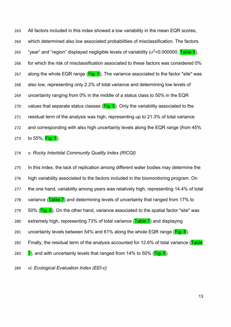
13
All factors included in this index showed a low variability in the mean EQR scores, 263
which determined also low associated probabilities of misclassification. The factors 264
“year” and “region” displayed negligible levels of variability (σ2<0.000000; Table 6), 265
for which the risk of misclassification associated to these factors was considered 0% 266
along the whole EQR range (Fig. 5). The variance associated to the factor "site" was 267
also low, representing only 2.2% of total variance and determining low levels of 268
uncertainty ranging from 0% in the middle of a status class to 50% in the EQR 269
values that separate status classes (Fig. 5). Only the variability associated to the 270
residual term of the analysis was high, representing up to 21.3% of total variance 271
and corresponding with also high uncertainty levels along the EQR range (from 45% 272
to 55%; Fig. 5). 273
v. Rocky Intertidal Community Quality Index (RICQI) 274
In this index, the lack of replication among different water bodies may determine the 275
high variability associated to the factors included in the biomonitoring program. On 276
the one hand, variability among years was relatively high, representing 14.4% of total 277
variance (Table 7) and determining levels of uncertainty that ranged from 17% to 278
50% (Fig. 6). On the other hand, variance associated to the spatial factor "site" was 279
extremely high, representing 73% of total variance (Table 7) and displaying 280
uncertainty levels between 54% and 61% along the whole EQR range (Fig. 6). 281
Finally, the residual term of the analysis accounted for 12.6% of total variance (Table 282
7), and with uncertainty levels that ranged from 14% to 50% (Fig. 6). 283
vi. Ecological Evaluation Index (EEI-c) 284
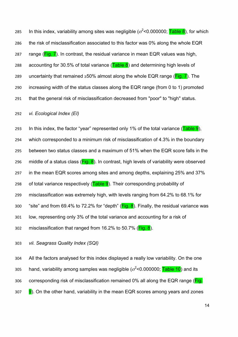
14
In this index, variability among sites was negligible (σ2<0.000000; Table 8), for which 285
the risk of misclassification associated to this factor was 0% along the whole EQR 286
range (Fig. 7). In contrast, the residual variance in mean EQR values was high, 287
accounting for 30.5% of total variance (Table 8) and determining high levels of 288
uncertainty that remained ≥50% almost along the whole EQR range (Fig. 7). The 289
increasing width of the status classes along the EQR range (from 0 to 1) promoted 290
that the general risk of misclassification decreased from "poor" to "high" status. 291
vi. Ecological Index (EI) 292
In this index, the factor “year” represented only 1% of the total variance (Table 9), 293
which corresponded to a minimum risk of misclassification of 4.3% in the boundary 294
between two status classes and a maximum of 51% when the EQR score falls in the 295
middle of a status class (Fig. 8). In contrast, high levels of variability were observed 296
in the mean EQR scores among sites and among depths, explaining 25% and 37% 297
of total variance respectively (Table 9). Their corresponding probability of 298
misclassification was extremely high, with levels ranging from 64.2% to 68.1% for 299
“site” and from 69.4% to 72.2% for “depth” (Fig. 8). Finally, the residual variance was 300
low, representing only 3% of the total variance and accounting for a risk of 301
misclassification that ranged from 16.2% to 50.7% (Fig. 8). 302
vii. Seagrass Quality Index (SQI) 303
All the factors analysed for this index displayed a really low variability. On the one 304
hand, variability among samples was negligible (σ2<0.000000; Table 10) and its 305
corresponding risk of misclassification remained 0% all along the EQR range (Fig. 306
9). On the other hand, variability in the mean EQR scores among years and zones 307
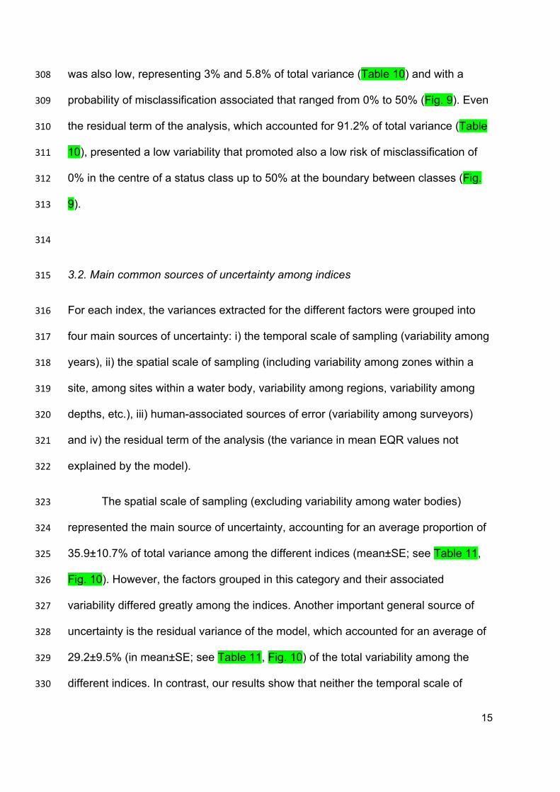
15
was also low, representing 3% and 5.8% of total variance (Table 10) and with a 308
probability of misclassification associated that ranged from 0% to 50% (Fig. 9). Even 309
the residual term of the analysis, which accounted for 91.2% of total variance (Table 310
10), presented a low variability that promoted also a low risk of misclassification of 311
0% in the centre of a status class up to 50% at the boundary between classes (Fig. 312
9). 313
314
3.2. Main common sources of uncertainty among indices 315
For each index, the variances extracted for the different factors were grouped into 316
four main sources of uncertainty: i) the temporal scale of sampling (variability among 317
years), ii) the spatial scale of sampling (including variability among zones within a 318
site, among sites within a water body, variability among regions, variability among 319
depths, etc.), iii) human-associated sources of error (variability among surveyors) 320
and iv) the residual term of the analysis (the variance in mean EQR values not 321
explained by the model). 322
The spatial scale of sampling (excluding variability among water bodies) 323
represented the main source of uncertainty, accounting for an average proportion of 324
35.9±10.7% of total variance among the different indices (mean±SE; see Table 11, 325
Fig. 10). However, the factors grouped in this category and their associated 326
variability differed greatly among the indices. Another important general source of 327
uncertainty is the residual variance of the model, which accounted for an average of 328
29.2±9.5% (in mean±SE; see Table 11, Fig. 10) of the total variability among the 329
different indices. In contrast, our results show that neither the temporal scale of 330
16
sampling nor the human-associated source of error are important sources of 331
uncertainty when classifying the ecological status of water bodies, as indicated by 332
the low proportion of the total variance explained by the factors “year” and "surveyor" 333
in the indices in which they were measured (5.4±2.3% and 2±2% respectively in 334
mean±SE; see Table 11, Fig. 10). 335
336
337
4. Discussion 338
Including uncertainty estimation into assessment schemes is a major challenge of 339
the next phase of WFD implementation (Hering et al. 2010). Even though the 340
underlying statistical principles are relatively simple and appropriate tools for 341
uncertainty estimation are available (e.g. Clarke and Hering 2006, Carstensen 2007), 342
data addressing the individual sources of error are still needed, such as temporal 343
and spatial variation of sampling, as well as differences between surveyors. This 344
study is one of the first ones in which uncertainty analyses have been applied to 345
several marine macrophyte based indexes, bringing some light to adequate designs 346
in order to assess the ecological status of water bodies. Our results reveal that when 347
analysing macrophyte communities, the factors related to the spatial scale of 348
sampling added the highest levels of uncertainty whilst temporal variation and 349
variability among surveyors were low. In addition, the residual term of the analysis 350
added relatively high levels of uncertainty to the water body status classification of 351
most indices, indicating that there are still unknown sources of variability that must 352
be captured within the monitoring programmes. 353
17
Spatial variability has always been observed in natural communities, which 354
becomes an important constrain when up scaling natural processes (Landres et al. 355
1999). In this study, the high levels of uncertainty associated to this factor are not 356
surprising and may be related to the already observed high horizontal and vertical 357
heterogeneity displayed by macrophyte communities (Ballesteros et al. 2007). 358
Vertical variability has been attributed to factors associated to light attenuation with 359
depth (Duarte 1991) and to the low rates of herbivory in deep sites compared to 360
shallow depths (Tomas et al. 2005, Prado et al. 2007, Korpinen et al. 2007). All 361
those natural processes, independent of any anthropogenic disturbances, influence 362
structural and physiological parameters of macrophyte communities (Martínez-Crego 363
et al. 2008), for which sampling at multiple depths result in highly variable EQR 364
scores (from 25% to 37% of total variance in POMI and EI respectively). To reduce 365
the risk of misclassification when assessing the ecological status of macrophyte 366
communities, a relatively easy solution is that depth should remain fixed or be 367
controlled in monitoring programs (see also Bennett et al. 2011). On the other hand, 368
horizontal variability has been attributed to several factors acting from local (i.e. 369
nutrient availability, sediment redox potential; Alcoverro et al. 1995) to regional 370
scales (i.e. light, temperature; Marbà et al. 1996) that again influence structural and 371
physiological parameters (Martínez-Crego et al. 2008). To capture this horizontal 372
heterogeneity, bio-monitoring programmes must include sampling at different spatial 373
scales, providing robust estimates of the ecological quality status classification at the 374
water body level that include as much of this variability as possible, thereby 375
minimizing the risk of misclassification (Kelly et al. 2009, Bennett et al. 2011). Even 376
though bio-monitoring programmes from the different indices include sampling at 377
several sites within each water body, only few of them include additional scales of 378
18
replication below this level (POMI and SQI), resulting in a generally high uncertainty 379
associated to the "site" factor (MSMDI, EDL, EI, RICQI). In these indices, it is 380
strongly recommended to increase the sampling effort by adding a larger number of 381
sites and within them, collecting different samples and averaging the metric values to 382
provide robust estimates and minimize their associated risk of misclassification. This 383
greater sampling effort may substantially increase the time and expense of the 384
monitoring programmes, although it can be partially solved by maintaining the same 385
number of replicates but just modifying the spatial sampling design to achieve a 386
balance between financial constrains and a desirable index reliability. At a broader 387
spatial scale, high variability among regions may indicate that they are separating 388
groups of water bodies of similar ecological quality status. However, since this 389
variability is above the scale of water body, at which the quality status is measured in 390
the WFD, the risk of misclassification does not need to be minimized but included in 391
the model and take into consideration when interpreting the uncertainty analysis 392
results. 393
For the remaining factors, the uncertainty surrounding estimates in ecological 394
status classification was very low within water bodies. Especially surprising is the 395
case of inter-annual variability, which represented only between 1% and 9.7% of 396
total variance depending on the index. As also reported by Bennett et al. (2011), this 397
signifies that the EQR scores of water bodies are fairly consistent throughout the 398
years, for which the frequency of sampling could be increased without greatly 399
reducing the precision of ecological status estimates. Also surprising is the low 400
variability among surveyors, which accounted only from 0% to 4% of total variance 401
(for POMI and MSDMI respectively). This may be attributed to the fact that these 402
19
particular macrophyte-based indices do not require complicated taxonomic 403
identifications, which can greatly affect the precision of the EQR estimations in the 404
case of other classification methods based on diatoms (Prygiel et al. 2002, Kelly et 405
al. 2009) or freshwater macrophyte communities (Staniszewski et al. 2006). Finally, 406
the residual term of the analysis represents all the variance that cannot be attributed 407
to any of the factors included in the model, giving an idea of the accuracy of our 408
approximation. In our study, it represented a relatively large proportion of total 409
variance among the different indices (29.2±9.5% in mean±SE), indicating that other 410
unknown sources of uncertainty may be affecting the ecological status classification 411
of water bodies. In order to keep this variance to the minimum, further data 412
concerning other factors related to the sampling design may need to be collected in 413
those indices where it is relatively large (spatial variance, temporal variance, 414
variance among surveyors, etc.). 415
Furthermore, our results showed that the risk of misclassifying the quality 416
status of water bodies is also affected by the width of the status class in which the 417
EQR score falls, as reported in Kelly et al. (2009), with narrower classes leading to 418
greater probabilities of misclassification. Thus, indices in which the EQR range is not 419
equally split into the 5 official classes present, for a certain variance associated to a 420
factor, different uncertainty levels depending on the status class (see EDL, POMI, 421
RICQI and EEI-c). This fact have drastic implications for bio-monitoring programs, 422
because a greater sampling effort may need to be assigned to water bodies whose 423
EQR score falls within the narrower status classes in order to reduce their 424
associated variability and increase the confidence of the classification. 425
426
20
427
5. Conclusions 428
In summary, our study confirmed that the analysis of the uncertainty associated to 429
the ecological quality status classification of water bodies are a good proxy to identify 430
and quantify the factors that may affect the risk of misclassification. When applied to 431
macrophyte monitoring programs, we have observed that the main sources of 432
uncertainty are mostly associated to the sampling spatial scales, while temporal or 433
human-induced errors seem to be less relevant. As a guide for taking management 434
decisions, adequate sampling designs that include replication at different spatial 435
scales within water bodies may substantially reduce this uncertainty. In some cases, 436
it is not increasing the sampling effort but distributing it more efficiently within the 437
allocated time and budget constrains that we will be able to maximize the confidence 438
of estimations when assessing ecosystem health under the WFD. 439
440
441
Acknowledgements: We thank all the different people involved in the monitoring 442
programmes of Catalonia, Balearic Is. and Croatia for their work in the field and 443
laboratory. We also thank Michael Dunbar and Ralph Clarke for his assistance in 444
statistical analyses. This research was funded by l’Agencia Catalana de l’Aigua and 445
WISER (Water bodies in Europe: Integrative Systems to assess Ecological status 446
and Recovery) funded under the 7th EU Framework Programme, Theme 6 447
(Environment including Climate Change), Contract No.: 226273). 448
449
21
450
References 451
Swedish Environmental Protection Agency: Handbook 2007:4. Status, Potential and 452 Quality Measures for Lakes, Rivers, Coastal and Transitional Waters, 453 Appendix B. 454
Badalamenti, F., Di Carlo, G., D’Anna, G., Gristina M., Toccaceli, M., 2006. Effects of 455 dredging activities on population dynamics of Posidonia oceanica (L.) Delile in 456 the Mediterranean sea: the case study of Capo Feto (SW Sicily, Italy). 457 Hydrobiologia 555, 253–261. 458
Bennett, S., Roca, G., Romero, J., Alcoverro, T., 2011. Ecological status of seagrass 459 ecosystems: An uncertainty análisis of the meadow classification based on 460 the Posidonia oceanica multivariate index (POMI). Marine Pollution Bulletin 461 62, 1616-1621. 462
Bouduresque, C.F., Bernard, G., Pergent, G., Shili, A., Verlaque, M., 2009. 463 Regression of Mediterranean seagrasses caused by natural processes and 464 anthropogenic disturbances and stress: a critical review. Botanica Marina 52, 465 395-418. 466
Buia, M.C., Silvestre, F., Iacono, G., Tiberti, L., 2005. Identificazione delle biocenosi 467 di maggior preggio ambientale al fine della classificazione della qualita delle 468 acque costiere. In: Metodologie per il rilevamento e la classificazione dello 469 stato di qualita ecologico e chimico delle acque, con particolare riferimento 470 all’aplicazione del decreto legislativo 152/99. APAT, Rome, pp. 269–303. 471
Casazza, G., Lopez y Royo, C., Silvestri, C., 2006. Seagrass as key coastal 472 ecosystems: an overview of the recent EU WFD requirements and current 473 applications. Biologia Marina Mediterranea 13, 189–193. 474
Clarke, R.T., Hering, D., 2006. Errors and uncertainty in bioassessment methods – 475 major results and conclusions from the STAR project and their application 476 using STARBUGS. Hydrobiologia 566, 433-439. 477
Clarke, R.T., Davy-Bowker, J., Sandin, L., Friberg, N., Johnson, R.K., Bis, B., 2006. 478 Estimates and comparisons of the effects of sampling variation using 479 “national” macroinvertebrate sampling protocols on the precision of metrics 480 used to assess ecological status. Hydrobiologia 566, 477–503. 481
Clarke, R.T., 2010. WISERBUGS 1.1 (WISER Bioassessment Uncertainty Guidance 482 Software) tool for assessing confidence of WFD ecological status. User and 483 Manual Software. Bournemouth University. 484
Dencheva, K. Improvements in sampling design and estimation of Ecological Index – 485 EI (modified Ecological Evaluation Index) of macrophytobenthic communities 486 as a tool for implementation of European Water Framework Directive. In 487 press. Compt Rend. des Acad. of Sci. 488
22
EC, 2000. DIRECTIVE 2000/60/EC of the European parliament and of the council, of 489 23 October 2000, establishing a framework for Community action in the field of 490 water policy. Official Journal of the European Communities, G.U.C.E. 22/12/ 491 2000, L 327. 492
Ferreira, J.G., Nobre, A.M., Simas, T.C., Silva, M.C., Newton, A., Bricker, S.B., 493 Wolff, W.J., Stacey, P.E., Sequeira, A., 2006. A methodology for defining 494 homogeneous water bodies in estuaries – Application to the transitional 495 systems of the EU Water Framework Directive. Estuarine, Coastal and Shelf 496 Science 66, 468-482. 497
Gobert, S., Sartoretto, S., Rico-Raimondino, V., Andral, B., Chery, A., Lejeune, P., 498 Boissery, P., 2009. Assessment of the ecological status of Mediterranean 499 French coastal waters as required by the Water Framework Directive using 500 the Posidonia oceanica Rapid Easy Index: PREI. Marine Pollution Bulletin 58, 501 1727-1733. 502
Kelly, M., Bennion, H., Burgess, A., Ellis, J., Juggins, S., Guthrie, R., Jamieson, J., 503 Adriaenssens, V., Yallop, M., 2009. Uncertainty in ecological status 504 assessments of lakes and rivers using diatoms. Hydrobiologia 633, 5-15. 505
Landres, P.B., Morgan, P., Swanson, F.J., 1999. Overview of the use of natural 506 variability concepts in managing ecological systems. Ecological Applications 507 9(4), 1179-1188. 508
Lopez y Royo, C., Pergent, G., Alcoverro, T., Buia, M.C., Casazza, G., Martínez-509 Crego, B., Pérez, M., Silvestre, F., Romero, J., 2011. The seagrass Posidonia 510 oceanica as indicador of coastal water quality: Experimental intercalibration of 511 classification Systems. Ecological Indicators 11, 55-563. 512
Martínez-Crego, B., Vergés, A., Alcoverro, T., Romero, J., 2008. Selection of 513 multiple seagrass indicators for environmental biomonitoring. Marine Ecology 514 Progress Series 361, 93-109. 515
Med-GIG, 2007. WFD Intercalibration technical report for coastal and transitional 516 waters in the Mediterranean eco-region. In: WFD Intercalibration technical 517 report – Part 3: Coastal and transitional waters. URL 518 http://circa.europa.eu/Public/irc/jrc/jrceewai/library?l=/intercalibration2&vm=de519 tailed&sb=Title. 520
Orfanidis, S., Panayotidis, P., Ugland, K.I., 2011. Ecological Evaluation Index 521 continuous formula (EEI-c) application: a step forward for functional groups, 522 the formula and reference condition values. The Mediterranean Marine 523 Science Journal 12 (2): 199-231. 524
Orth, R.J., Carruthers, T.J.B., Dennison, W.C., Duarte, C.M., Fourqurean, J.W., 525 Heck, K.L., Hughes, A.R., Kendrick, G.A., Kenworthy, W.J., Olyarnik, A., 526 Short, F.T., Waycott, M., Williams, S.L., 2006. A global crisis for seagrass 527 ecosystems. Bioscience 56, 987–996. 528
23
Pergent, G., Pergent-Martini, C., Boudouresque, C.F., 1995. Utilisation de l’herbier à 529 Posidonia oceanica comme indicateur biologique de la qualité du milieu littoral 530 en Méditerranée: Etat des connaissances. Mesogée 54, 3–29. 531
Pergent-Martini, C., Leoni, V., Pasqualini, V., Ardizzone, G.D., Balestri, E., Bedini, 532 R., Belluscio, A., Belsher, T., Borg, J., Boudouresque, C.F., Boumaza, S., 533 Bouquegneau, J.M., Buia, M.C., Calvo, S., Cebrian, J., Charbonnel, E., 534 Cinelli, F., Cossu, A., Di Maida, G., Dural, B., Francour, P., Gobert, S., 535 Lepoint, G., Meinesz, A., Molenaar, H., Mansour, H.M., Panayotidis, P., 536 Peirano, A., Pergent, G., Piazzi, L., Pirrotta, M., Relini, G., Romero, J., 537 Sanchez-Lizaso, J.L., Semroud, R., Shembri, P., Shili, A., Tomasello, A., 538 Velimirov, B., 2005. Descriptors of Posidonia oceanica meadows: use and 539 application. Ecological Indicators 5, 213–230. 540
Pinheiro, J.C., Bates, D.M., 2000. Mixed-Effects models in S and S-Plus. Springer. 541 ISBN 0-387-98957-0. 542
Pinheiro, J.C., Bates, D.M., DebRoy, S., Sarkar, D., 2005. The nlme package: Linear 543 and nonlinear mixed effects models. URL http: //CRAN.R-project.org. R 544 package version 3.1-98. 545
Procaccini, G., Buia, MC., Gambi, M.C., Pérez, M., Pergent-Marini, C., Romero, J., 546 2003. The seagrasses of the western Mediterranean. In: Green, E.P., Short, 547 F.T. (Eds.), World Atlas of Seagrasses. University of California Press, 548 Berkeley (USA). pp. 298. 549
Romero, J., Martínez-Crego, B., Alcoverro, T., Pérez, M., 2007. A multivariate index 550 based on the seagrass Posidonia oceanica (POMI) to assess ecological 551 status of coastal waters under the Water Framework Directive (WFD). Marine 552 Pollution Bulletin 55, 196–204. 553
Staniszewski, R., Szoszkiewicz, K., Zbierska, J., Lesny, J., Jusik, S., Clarke, R.T., 554 2006. Assessment of sources of uncertainty in macrophyte surveys and the 555 consequences for river classification. Hydrobiologia 566, 235-246. 556
557
Figure 1: Map of the locations where bio-monitoring data from the different indices 558 was obtained. 559
Figure 2: Probability of misclassifying the ecological status class associated to the 560 different factors analysed for MSMDI. Vertical dashed lines represent the boundaries 561 of each status class. Bad = EQR values from 0 – 0.2; Poor = 0.21 – 0.4; Moderate = 562 0.41 – 0.6; Good = 0.61-0.8 and High = 0.81 – 1. 563
Figure 3: Probability of misclassifying the ecological status class associated to the 564 different factors analysed for EDL. Vertical dashed lines represent the boundaries of 565 each status class. Bad = EQR values from 0 – 0.25; Poor = 0.26 – 0.5; Moderate = 566 0.51 – 0.74; Good = 0.75-0.9 and High = 0.91 – 1. 567
Figure 4: Probability of misclassifying the ecological status class associated to the 568 different factors analysed for POMI. Vertical dashed lines represent the boundaries 569
24
of each status class. Bad = EQR values from 0 – 0.09; Poor = 0.1 – 0.324; Moderate 570 = 0.325 – 0.549; Good = 0.550-0.774 and High = 0.775 – 1. 571
Figure 5: Probability of misclassifying the ecological status class associated to the 572 different factors analysed for CYMOX. Vertical dashed lines represent the 573 boundaries of each status class. Bad = EQR values from 0 – 0.2; Poor = 0.21 – 0.4; 574 Moderate = 0.41 – 0.6; Good = 0.61-0.8 and High = 0.81 – 1. 575
Figure 6: Probability of misclassifying the ecological status class associated to the 576 different factors analysed for RICQI. Vertical dashed lines represent the boundaries 577 of each status class. Bad = EQR values from 0 – 0.2; Poor = 0.21 – 0.4; Moderate = 578 0.41 – 0.6; Good = 0.61-0.82 and High = 0.83 – 1. 579
Figure 7: Probability of misclassifying the ecological status class associated to the 580 different factors analysed for EEI-c. Vertical dashed lines represent the boundaries 581 of each status class. Bad = EQR values from 0 – 0.2; Poor = 0.21 – 0.4; Moderate = 582 0.41 – 0.6; Good = 0.61-0.8 and High = 0.81 – 1. 583
Figure 8: Probability of misclassifying the ecological status class associated to the 584 different factors analysed for EI. Vertical dashed lines represent the boundaries of 585 each status class. Bad = EQR values from 0 – 0.2; Poor = 0.21 – 0.4; Moderate = 586 0.41 – 0.6; Good = 0.61-0.8 and High = 0.81 – 1. 587
Figure 9: Probability of misclassifying the ecological status class associated to the 588 different factors analysed for SQI. Vertical dashed lines represent the boundaries of 589 each status class. Bad = EQR values from 0 – 0.2; Poor = 0.21 – 0.4; Moderate = 590 0.41 – 0.6; Good = 0.61-0.8 and High = 0.81 – 1. 591
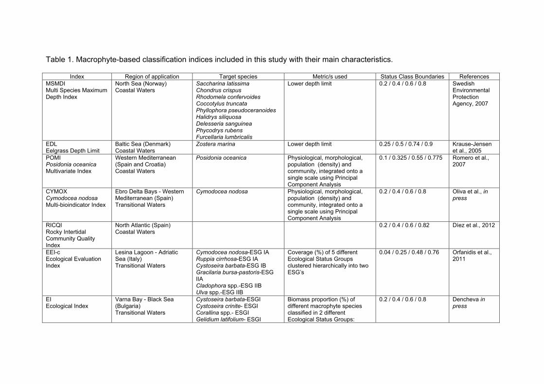
Table 1. Macrophyte-based classification indices included in this study with their main characteristics.
Index Region of application Target species Metric/s used Status Class Boundaries References MSMDI Multi Species Maximum Depth Index
North Sea (Norway) Coastal Waters
Saccharina latissima Chondrus crispus Rhodomela confervoides Coccotylus truncata Phyllophora pseudoceranoides Halidrys siliquosa Delesseria sanguinea Phycodrys rubens Furcellaria lumbricalis
Lower depth limit 0.2 / 0.4 / 0.6 / 0.8 Swedish Environmental Protection Agency, 2007
EDL Eelgrass Depth Limit
Baltic Sea (Denmark) Coastal Waters
Zostera marina Lower depth limit 0.25 / 0.5 / 0.74 / 0.9 Krause-Jensen et al., 2005
POMI Posidonia oceanica Multivariate Index
Western Mediterranean (Spain and Croatia) Coastal Waters
Posidonia oceanica Physiological, morphological, population (density) and community, integrated onto a single scale using Principal Component Analysis
0.1 / 0.325 / 0.55 / 0.775 Romero et al., 2007
CYMOX Cymodocea nodosa Multi-bioindicator Index
Ebro Delta Bays - Western Mediterranean (Spain) Transitional Waters
Cymodocea nodosa Physiological, morphological, population (density) and community, integrated onto a single scale using Principal Component Analysis
0.2 / 0.4 / 0.6 / 0.8 Oliva et al., in press
RICQI Rocky Intertidal Community Quality Index
North Atlantic (Spain) Coastal Waters
0.2 / 0.4 / 0.6 / 0.82 Díez et al., 2012
EEI-c Ecological Evaluation Index
Lesina Lagoon - Adriatic Sea (Italy) Transitional Waters
Cymodocea nodosa-ESG IA Ruppia cirrhosa-ESG IA Cystoseira barbata-ESG IB Gracilaria bursa-pastoris-ESG IIA Cladophora spp.-ESG IIB Ulva spp.-ESG IIB
Coverage (%) of 5 different Ecological Status Groups clustered hierarchically into two ESG’s
0.04 / 0.25 / 0.48 / 0.76 Orfanidis et al., 2011
EI Ecological Index
Varna Bay - Black Sea (Bulgaria) Transitional Waters
Cystoseira barbata-ESGI Cystoseira crinite- ESGI Corallina spp.- ESGI Gelidium latifolium- ESGI
Biomass proportion (%) of different macrophyte species classified in 2 different Ecological Status Groups:
0.2 / 0.4 / 0.6 / 0.8 Dencheva in press
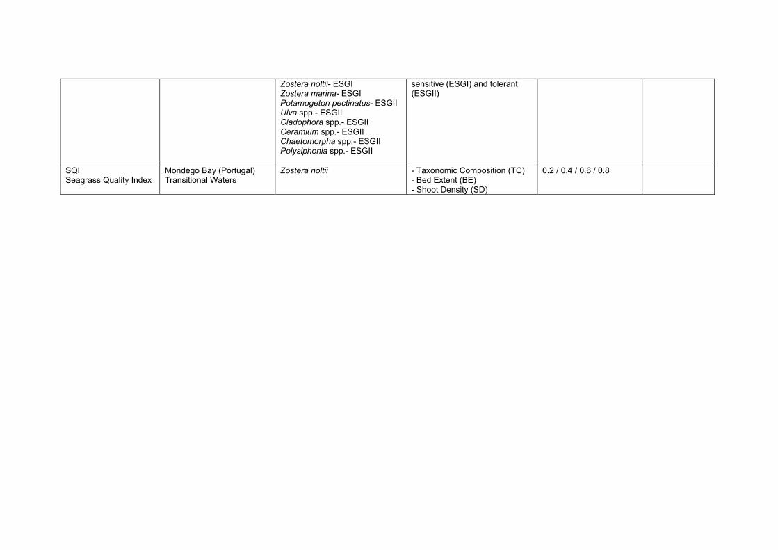
Zostera noltii- ESGI Zostera marina- ESGI Potamogeton pectinatus- ESGII Ulva spp.- ESGII Cladophora spp.- ESGII Ceramium spp.- ESGII Chaetomorpha spp.- ESGII Polysiphonia spp.- ESGII
sensitive (ESGI) and tolerant (ESGII)
SQI Seagrass Quality Index
Mondego Bay (Portugal) Transitional Waters
Zostera noltii - Taxonomic Composition (TC) - Bed Extent (BE) - Shoot Density (SD)
0.2 / 0.4 / 0.6 / 0.8
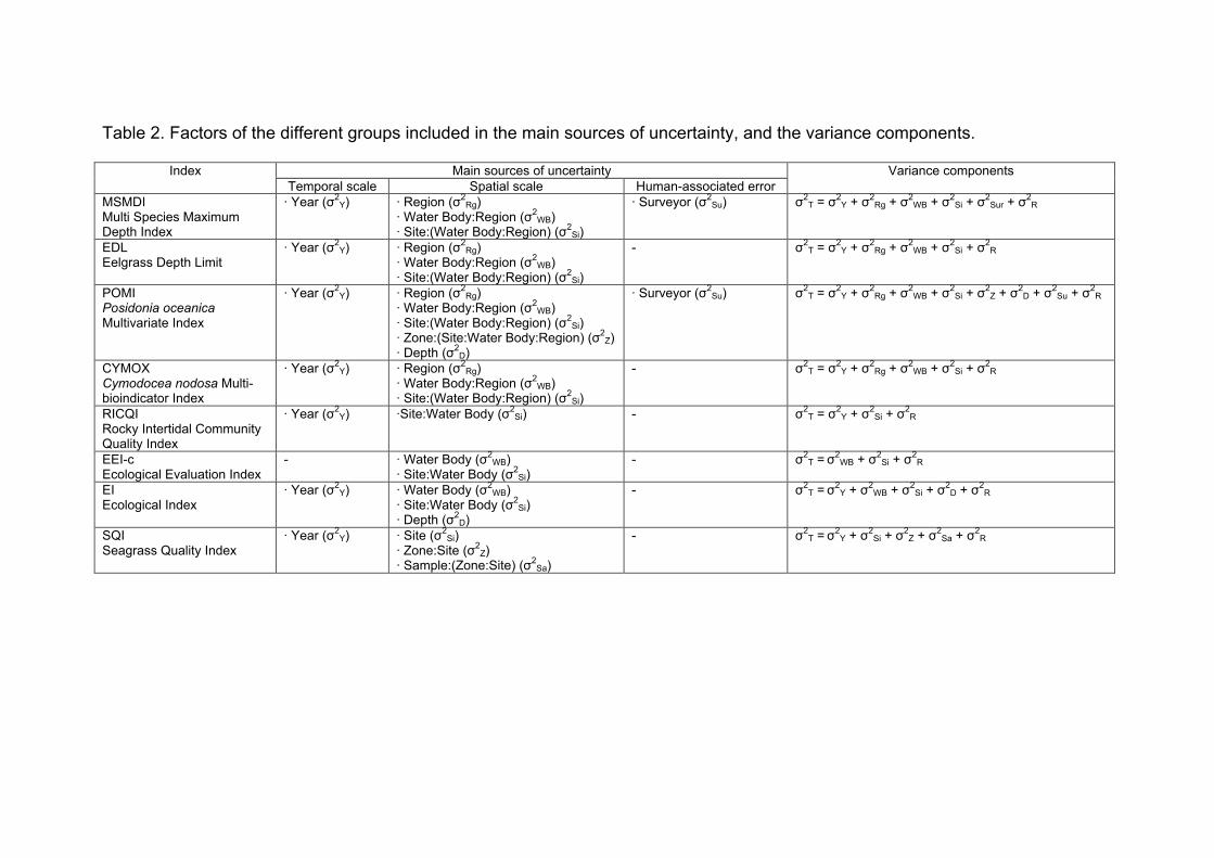
Table 2. Factors of the different groups included in the main sources of uncertainty, and the variance components.
Main sources of uncertainty Index Temporal scale Spatial scale Human-associated error
Variance components
MSMDI Multi Species Maximum Depth Index
· Year (σ2Y) · Region (σ2
Rg) · Water Body:Region (σ2
WB) · Site:(Water Body:Region) (σ2
Si)
· Surveyor (σ2Su) σ2
T = σ2Y + σ2
Rg + σ2WB + σ2
Si + σ2Sur + σ2
R
EDL Eelgrass Depth Limit
· Year (σ2Y) · Region (σ2
Rg) · Water Body:Region (σ2
WB) · Site:(Water Body:Region) (σ2
Si)
- σ2T = σ2
Y + σ2Rg + σ2
WB + σ2Si + σ2
R
POMI Posidonia oceanica Multivariate Index
· Year (σ2Y) · Region (σ2
Rg) · Water Body:Region (σ2
WB) · Site:(Water Body:Region) (σ2
Si) · Zone:(Site:Water Body:Region) (σ2
Z) · Depth (σ2
D)
· Surveyor (σ2Su) σ2
T = σ2Y + σ2
Rg + σ2WB + σ2
Si + σ2Z + σ2
D + σ2Su + σ2
R
CYMOX Cymodocea nodosa Multi-bioindicator Index
· Year (σ2Y) · Region (σ2
Rg) · Water Body:Region (σ2
WB) · Site:(Water Body:Region) (σ2
Si)
- σ2T = σ2
Y + σ2Rg + σ2
WB + σ2Si + σ2
R
RICQI Rocky Intertidal Community Quality Index
· Year (σ2Y) ·Site:Water Body (σ2
Si) - σ2T = σ2
Y + σ2Si + σ2
R
EEI-c Ecological Evaluation Index
- · Water Body (σ2WB)
· Site:Water Body (σ2Si)
- σ2T = σ2
WB + σ2Si + σ2
R
EI Ecological Index
· Year (σ2Y) · Water Body (σ2
WB) · Site:Water Body (σ2
Si) · Depth (σ2
D)
- σ2T = σ2
Y + σ2WB + σ2
Si + σ2D + σ2
R
SQI Seagrass Quality Index
· Year (σ2Y) · Site (σ2
Si) · Zone:Site (σ2
Z) · Sample:(Zone:Site) (σ2
Sa)
- σ2T = σ2
Y + σ2Si + σ2
Z + σ2Sa + σ2
R
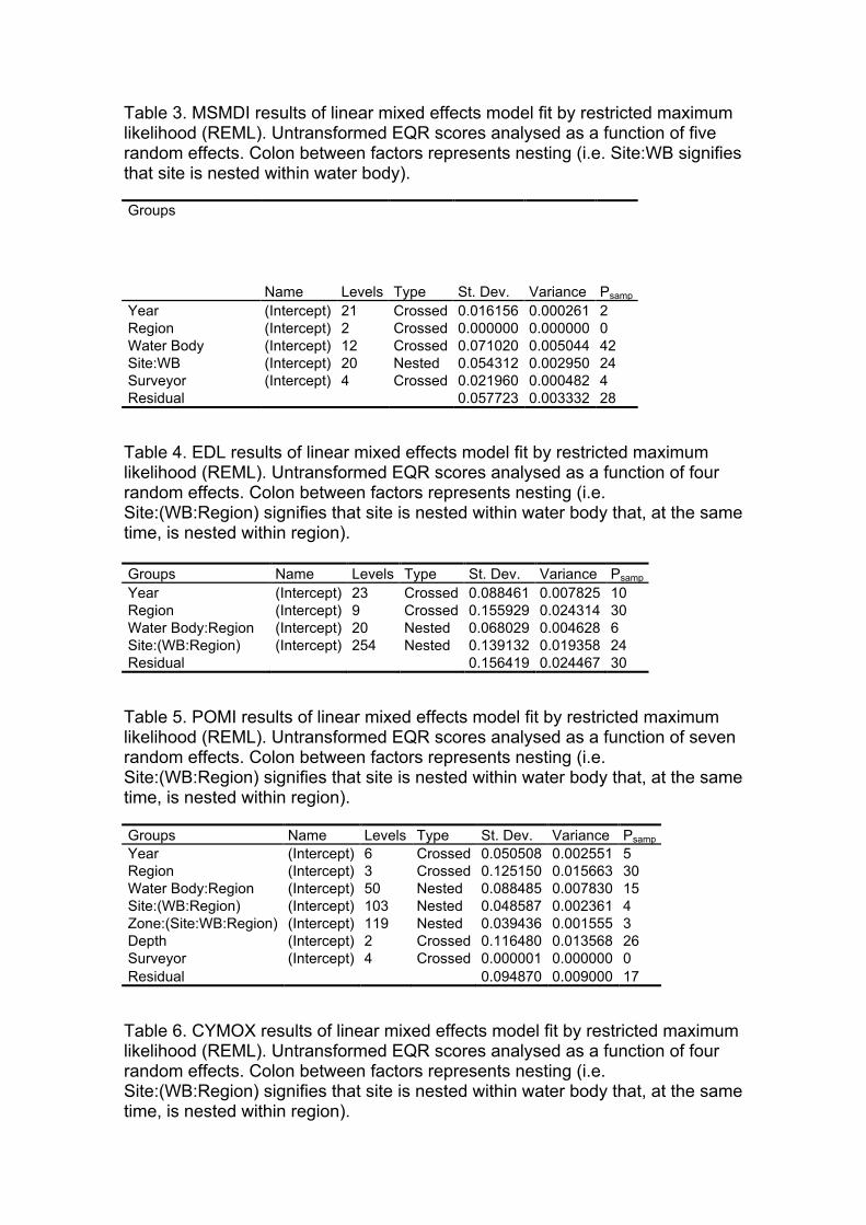
Table 3. MSMDI results of linear mixed effects model fit by restricted maximum likelihood (REML). Untransformed EQR scores analysed as a function of five random effects. Colon between factors represents nesting (i.e. Site:WB signifies that site is nested within water body). Groups
Name Levels Type St. Dev. Variance Psamp Year (Intercept) 21 Crossed 0.016156 0.000261 2 Region (Intercept) 2 Crossed 0.000000 0.000000 0 Water Body (Intercept) 12 Crossed 0.071020 0.005044 42 Site:WB (Intercept) 20 Nested 0.054312 0.002950 24 Surveyor (Intercept) 4 Crossed 0.021960 0.000482 4 Residual 0.057723 0.003332 28 Table 4. EDL results of linear mixed effects model fit by restricted maximum likelihood (REML). Untransformed EQR scores analysed as a function of four random effects. Colon between factors represents nesting (i.e. Site:(WB:Region) signifies that site is nested within water body that, at the same time, is nested within region). Groups Name Levels Type St. Dev. Variance Psamp Year (Intercept) 23 Crossed 0.088461 0.007825 10 Region (Intercept) 9 Crossed 0.155929 0.024314 30 Water Body:Region (Intercept) 20 Nested 0.068029 0.004628 6 Site:(WB:Region) (Intercept) 254 Nested 0.139132 0.019358 24 Residual 0.156419 0.024467 30 Table 5. POMI results of linear mixed effects model fit by restricted maximum likelihood (REML). Untransformed EQR scores analysed as a function of seven random effects. Colon between factors represents nesting (i.e. Site:(WB:Region) signifies that site is nested within water body that, at the same time, is nested within region). Groups Name Levels Type St. Dev. Variance Psamp Year (Intercept) 6 Crossed 0.050508 0.002551 5 Region (Intercept) 3 Crossed 0.125150 0.015663 30 Water Body:Region (Intercept) 50 Nested 0.088485 0.007830 15 Site:(WB:Region) (Intercept) 103 Nested 0.048587 0.002361 4 Zone:(Site:WB:Region) (Intercept) 119 Nested 0.039436 0.001555 3 Depth (Intercept) 2 Crossed 0.116480 0.013568 26 Surveyor (Intercept) 4 Crossed 0.000001 0.000000 0 Residual 0.094870 0.009000 17 Table 6. CYMOX results of linear mixed effects model fit by restricted maximum likelihood (REML). Untransformed EQR scores analysed as a function of four random effects. Colon between factors represents nesting (i.e. Site:(WB:Region) signifies that site is nested within water body that, at the same time, is nested within region).
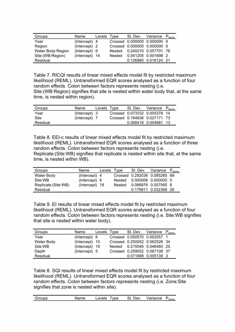
Groups Name Levels Type St. Dev. Variance Psamp Year (Intercept) 4 Crossed 0.000000 0.000000 0 Region (Intercept) 2 Crossed 0.000005 0.000000 0 Water Body:Region (Intercept) 6 Nested 0.240210 0.057701 76 Site:(WB:Region) (Intercept) 14 Nested 0.041205 0.001698 2 Residual 0.126980 0.016124 21 Table 7. RICQI results of linear mixed effects model fit by restricted maximum likelihood (REML). Untransformed EQR scores analysed as a function of four random effects. Colon between factors represents nesting (i.e. Site:(WB:Region) signifies that site is nested within water body that, at the same time, is nested within region). Groups Name Levels Type St. Dev. Variance Psamp Year (Intercept) 3 Crossed 0.073332 0.005378 14 Site (Intercept) 7 Crossed 0.164836 0.027171 73 Residual 0.068418 0.004681 13 Table 8. EEI-c results of linear mixed effects model fit by restricted maximum likelihood (REML). Untransformed EQR scores analysed as a function of three random effects. Colon between factors represents nesting (i.e. Replicate:(Site:WB) signifies that replicate is nested within site that, at the same time, is nested within WB). Groups Name Levels Type St. Dev. Variance Psamp Water Body (Intercept) 4 Crossed 0.292036 0.085285 68 Site:WB (Intercept) 6 Nested 0.000006 0.000000 0 Replicate:(Site:WB) (Intercept) 18 Nested 0.086976 0.007565 6 Residual 0.179911 0.032368 26 Table 9. EI results of linear mixed effects model fit by restricted maximum likelihood (REML). Untransformed EQR scores analysed as a function of four random effects. Colon between factors represents nesting (i.e. Site:WB signifies that site is nested within water body). Groups Name Levels Type St. Dev. Variance Psamp Year (Intercept) 6 Crossed 0.050570 0.002557 1 Water Body (Intercept) 10 Crossed 0.250052 0.062526 34 Site:WB (Intercept) 19 Nested 0.215546 0.046460 25 Depth (Intercept) 5 Crossed 0.259052 0.067108 37 Residual 0.071688 0.005139 3 Table 8. SQI results of linear mixed effects model fit by restricted maximum likelihood (REML). Untransformed EQR scores analysed as a function of four random effects. Colon between factors represents nesting (i.e. Zone:Site signifies that zone is nested within site). Groups Name Levels Type St. Dev. Variance Psamp

Site (Intercept) 2 Crossed 0.024843 0.000617 3 Zone:Site (Intercept) 4 Nested 0.034845 0.001214 6 Sample:(Zone:Site) (Intercept) 8 Nested 0.000000 0.000000 0 Residual 0.139830 0.019054 91

Table 9. Proportion of the total variance (in %) explained by the different factors grouped in the main sources of uncertainty for each index, excluding WB.
Index
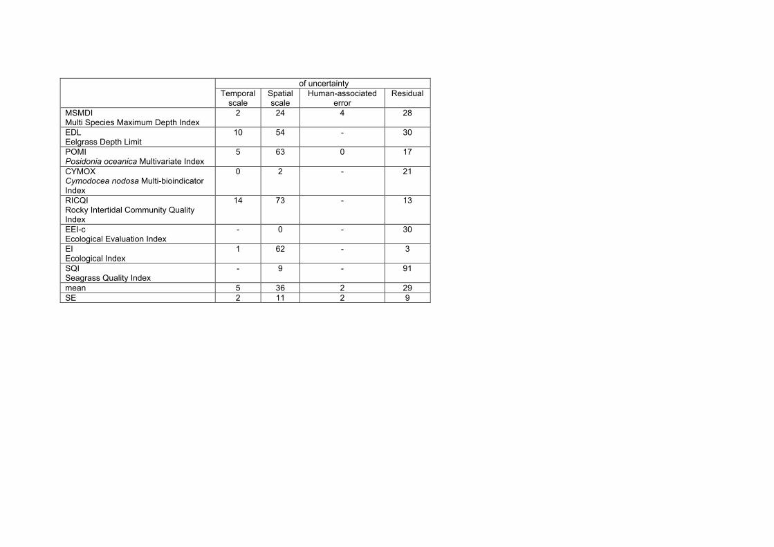
of uncertainty Temporal
scale Spatial scale
Human-associated error
Residual
MSMDI Multi Species Maximum Depth Index
2 24 4 28
EDL Eelgrass Depth Limit
10 54 - 30
POMI Posidonia oceanica Multivariate Index
5 63 0 17
CYMOX Cymodocea nodosa Multi-bioindicator Index
0 2 - 21
RICQI Rocky Intertidal Community Quality Index
14 73 - 13
EEI-c Ecological Evaluation Index
- 0 - 30
EI Ecological Index
1 62 - 3
SQI Seagrass Quality Index
- 9 - 91
mean 5 36 2 29 SE 2 11 2 9
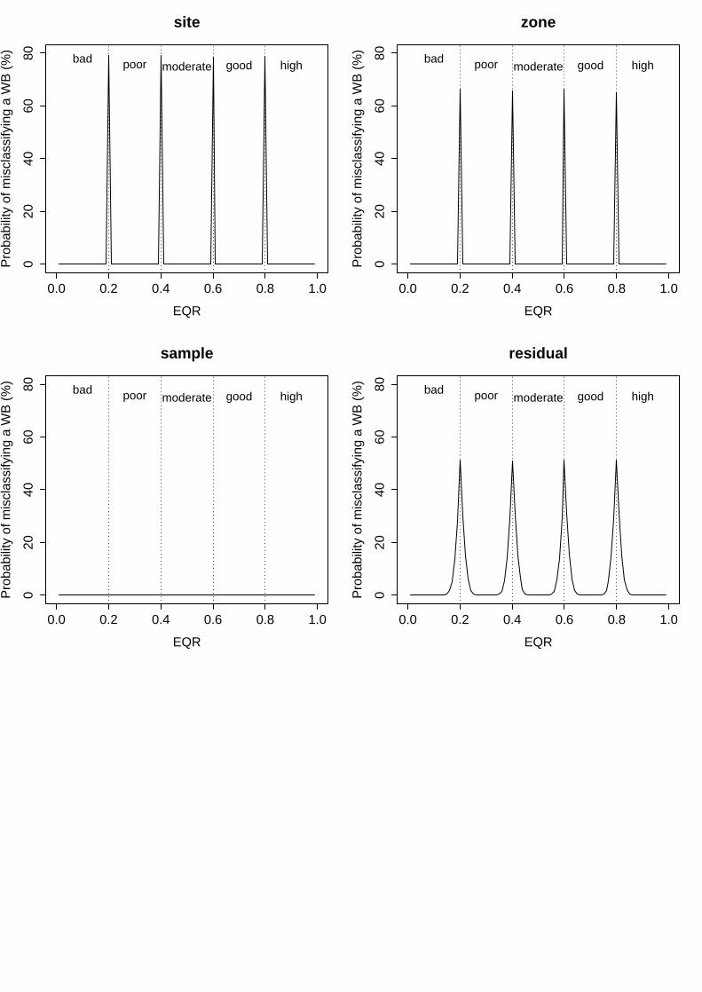
0.0 0.2 0.4 0.6 0.8 1.0
020
4060
80site
EQR
Pro
babi
lity
of m
iscl
assi
fyin
g a
WB
(%
)
bad poor moderate good high
0.0 0.2 0.4 0.6 0.8 1.0
020
4060
80
zone
EQR
Pro
babi
lity
of m
iscl
assi
fyin
g a
WB
(%
)
bad poor moderate good high
0.0 0.2 0.4 0.6 0.8 1.0
020
4060
80
sample
EQR
Pro
babi
lity
of m
iscl
assi
fyin
g a
WB
(%
)
bad poor moderate good high
0.0 0.2 0.4 0.6 0.8 1.0
020
4060
80
residual
EQR
Pro
babi
lity
of m
iscl
assi
fyin
g a
WB
(%
)
bad poor moderate good high
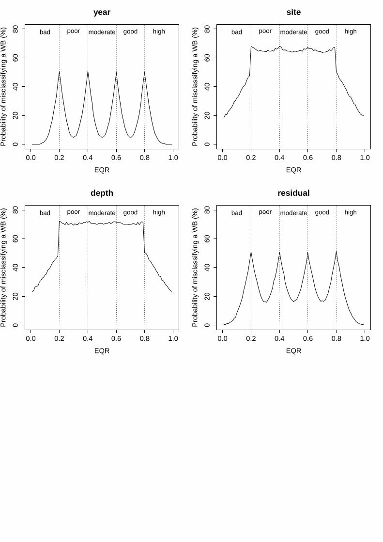
0.0 0.2 0.4 0.6 0.8 1.0
020
4060
80year
EQR
Pro
babi
lity
of m
iscl
assi
fyin
g a
WB
(%
)
bad poor moderate good high
0.0 0.2 0.4 0.6 0.8 1.0
020
4060
80
site
EQR
Pro
babi
lity
of m
iscl
assi
fyin
g a
WB
(%
)
bad poor moderate good high
0.0 0.2 0.4 0.6 0.8 1.0
020
4060
80
depth
EQR
Pro
babi
lity
of m
iscl
assi
fyin
g a
WB
(%
)
bad poor moderate good high
0.0 0.2 0.4 0.6 0.8 1.0
020
4060
80
residual
EQR
Pro
babi
lity
of m
iscl
assi
fyin
g a
WB
(%
)
bad poor moderate good high
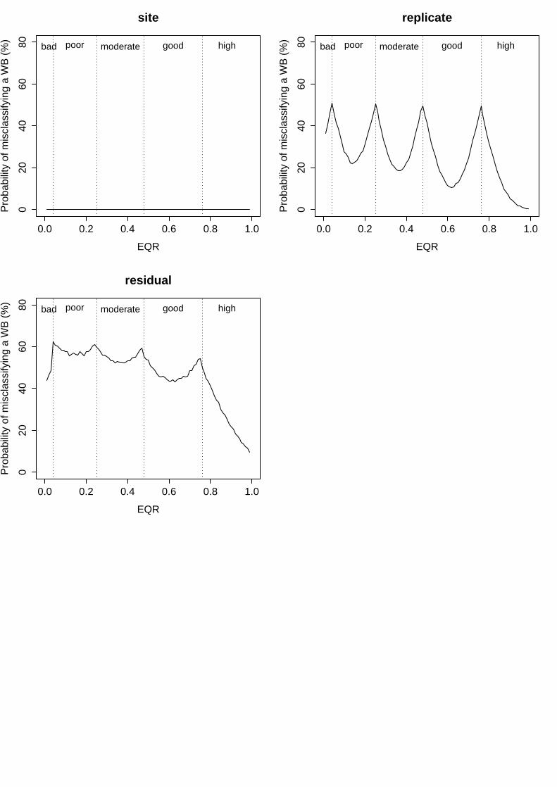
0.0 0.2 0.4 0.6 0.8 1.0
020
4060
80site
EQR
Pro
babi
lity
of m
iscl
assi
fyin
g a
WB
(%
)
bad poor moderate good high
0.0 0.2 0.4 0.6 0.8 1.0
020
4060
80
replicate
EQR
Pro
babi
lity
of m
iscl
assi
fyin
g a
WB
(%
)
bad poor moderate good high
0.0 0.2 0.4 0.6 0.8 1.0
020
4060
80
residual
EQR
Pro
babi
lity
of m
iscl
assi
fyin
g a
WB
(%
)
bad poor moderate good high
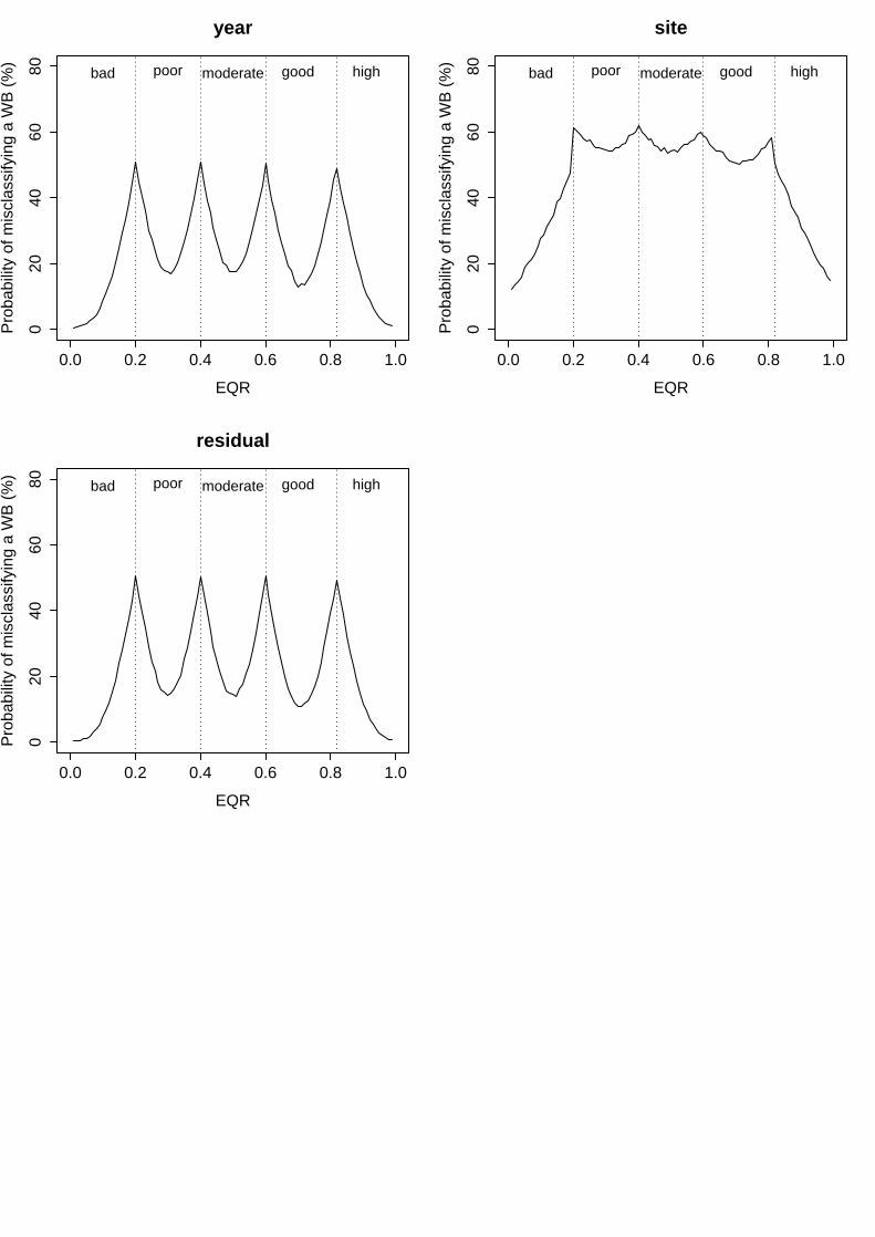
0.0 0.2 0.4 0.6 0.8 1.0
020
4060
80year
EQR
Pro
babi
lity
of m
iscl
assi
fyin
g a
WB
(%
)
bad poor moderate good high
0.0 0.2 0.4 0.6 0.8 1.0
020
4060
80
site
EQR
Pro
babi
lity
of m
iscl
assi
fyin
g a
WB
(%
)
bad poor moderate good high
0.0 0.2 0.4 0.6 0.8 1.0
020
4060
80
residual
EQR
Pro
babi
lity
of m
iscl
assi
fyin
g a
WB
(%
)
bad poor moderate good high

0.0 0.2 0.4 0.6 0.8 1.0
020
4060
80year
EQR
Pro
babi
lity
of m
iscl
assi
fyin
g a
WB
(%
)
bad poor moderate good high
0.0 0.2 0.4 0.6 0.8 1.0
020
4060
80
region
EQR
Pro
babi
lity
of m
iscl
assi
fyin
g a
WB
(%
)
bad poor moderate good high
0.0 0.2 0.4 0.6 0.8 1.0
020
4060
80
site
EQR
Pro
babi
lity
of m
iscl
assi
fyin
g a
WB
(%
)
bad poor moderate good high
0.0 0.2 0.4 0.6 0.8 1.0
020
4060
80
residual
EQR
Pro
babi
lity
of m
iscl
assi
fyin
g a
WB
(%
)
bad poor moderate good high
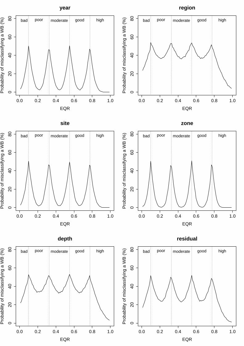
0.0 0.2 0.4 0.6 0.8 1.0
020
4060
80year
EQR
Pro
babi
lity
of m
iscl
assi
fyin
g a
WB
(%
)
bad poor moderate good high
0.0 0.2 0.4 0.6 0.8 1.0
020
4060
80
region
EQR
Pro
babi
lity
of m
iscl
assi
fyin
g a
WB
(%
)
bad poor moderate good high
0.0 0.2 0.4 0.6 0.8 1.0
020
4060
80
site
EQR
Pro
babi
lity
of m
iscl
assi
fyin
g a
WB
(%
)
bad poor moderate good high
0.0 0.2 0.4 0.6 0.8 1.0
020
4060
80
zone
EQR
Pro
babi
lity
of m
iscl
assi
fyin
g a
WB
(%
)
bad poor moderate good high
0.0 0.2 0.4 0.6 0.8 1.0
020
4060
80
depth
EQR
Pro
babi
lity
of m
iscl
assi
fyin
g a
WB
(%
)
bad poor moderate good high
0.0 0.2 0.4 0.6 0.8 1.0
020
4060
80
residual
EQR
Pro
babi
lity
of m
iscl
assi
fyin
g a
WB
(%
)
bad poor moderate good high
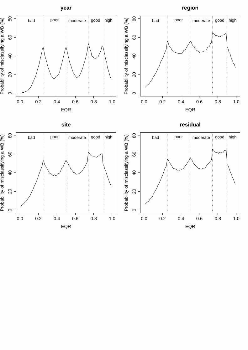
0.0 0.2 0.4 0.6 0.8 1.0
020
4060
80year
EQR
Pro
babi
lity
of m
iscl
assi
fyin
g a
WB
(%
)
bad poor moderate good high
0.0 0.2 0.4 0.6 0.8 1.0
020
4060
80
region
EQR
Pro
babi
lity
of m
iscl
assi
fyin
g a
WB
(%
)
bad poor moderate good high
0.0 0.2 0.4 0.6 0.8 1.0
020
4060
80
site
EQR
Pro
babi
lity
of m
iscl
assi
fyin
g a
WB
(%
)
bad poor moderate good high
0.0 0.2 0.4 0.6 0.8 1.0
020
4060
80
residual
EQR
Pro
babi
lity
of m
iscl
assi
fyin
g a
WB
(%
)
bad poor moderate good high
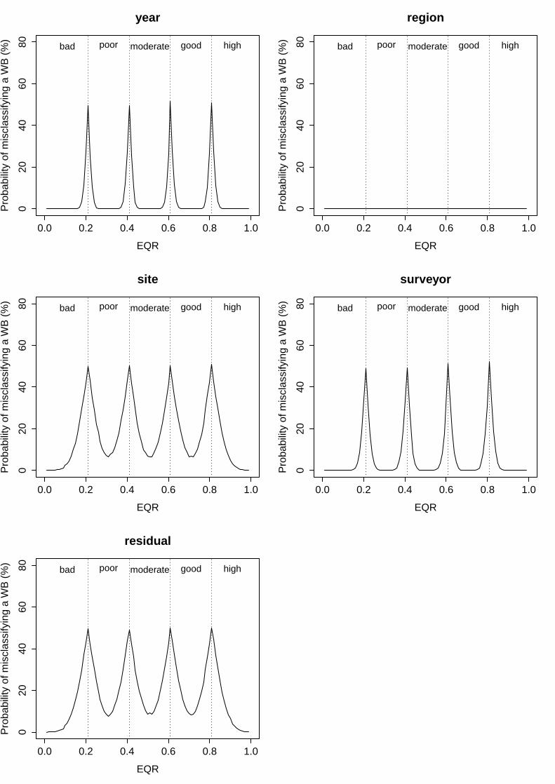
0.0 0.2 0.4 0.6 0.8 1.0
020
4060
80year
EQR
Pro
babi
lity
of m
iscl
assi
fyin
g a
WB
(%
)
bad poor moderate good high
0.0 0.2 0.4 0.6 0.8 1.0
020
4060
80
region
EQR
Pro
babi
lity
of m
iscl
assi
fyin
g a
WB
(%
)
bad poor moderate good high
0.0 0.2 0.4 0.6 0.8 1.0
020
4060
80
site
EQR
Pro
babi
lity
of m
iscl
assi
fyin
g a
WB
(%
)
bad poor moderate good high
0.0 0.2 0.4 0.6 0.8 1.0
020
4060
80
surveyor
EQR
Pro
babi
lity
of m
iscl
assi
fyin
g a
WB
(%
)
bad poor moderate good high
0.0 0.2 0.4 0.6 0.8 1.0
020
4060
80
residual
EQR
Pro
babi
lity
of m
iscl
assi
fyin
g a
WB
(%
)
bad poor moderate good high