DELIVERABLE 4.1-4.4 APPLYING THE RAGES RISK-BASED ...
44
RAGES Deliverable 4.1-4.4 1 DELIVERABLE 4.1-4.4 APPLYING THE RAGES RISK-BASED APPROACH TO MSFD DESCRIPTOR 11, UNDERWATER NOISE Work Package RAGES Work Package 4 Deliverable 4.1 Deliverable 4.2 Deliverable 4.3 Deliverable 4.4 Lead Partner UCC, Ireland: Emma Verling, Tim O’Higgins, Maria Gkaragkouni Contributing Partners UPV, Spain: Ramón Miralles, Guillermo Lara Martinéz IEO, Spain: Manuel Bou-Cabo DGRM, Portugal: Ana Paula Simão, Vera Lopes, Joana Otero DRAM, Portugal (Azores): Gilberto Carreira, José Macedo (IMAR: Mónica Silva) Version FINAL Date June 2021 Citation Verling E, Miralles R, Bou-Cabo M, Martinéz GL, Garagouni M, O’Higgins T. (2021). Applying the RAGES Risk-Based Approach to MSFD Descriptor 11 of the MSFD. Risk Based Approaches to Good Environmental Status (RAGES) Project Deliverable 4.1, 4.2, 4.3, 4.4. 44 pp.
-
Upload
khangminh22 -
Category
Documents
-
view
2 -
download
0
Transcript of DELIVERABLE 4.1-4.4 APPLYING THE RAGES RISK-BASED ...
RAGES Deliverable 4.1-4.4
1
DELIVERABLE 4.1-4.4 APPLYING THE RAGES RISK-BASED APPROACH TO MSFD
DESCRIPTOR 11, UNDERWATER NOISE
Work Package
RAGES Work Package 4 Deliverable 4.1 Deliverable 4.2 Deliverable 4.3 Deliverable 4.4
Lead Partner UCC, Ireland: Emma Verling, Tim O’Higgins, Maria Gkaragkouni
Contributing Partners
UPV, Spain: Ramón Miralles, Guillermo Lara Martinéz IEO, Spain: Manuel Bou-Cabo DGRM, Portugal: Ana Paula Simão, Vera Lopes, Joana Otero DRAM, Portugal (Azores): Gilberto Carreira, José Macedo (IMAR: Mónica Silva)
Version FINAL
Date June 2021
Citation
Verling E, Miralles R, Bou-Cabo M, Martinéz GL, Garagouni M, O’Higgins T. (2021). Applying the RAGES Risk-Based Approach to MSFD Descriptor 11 of the MSFD. Risk Based Approaches to Good Environmental Status (RAGES) Project Deliverable 4.1, 4.2, 4.3, 4.4. 44 pp.
RAGES Deliverable 4.1-4.4
2
Preface This document outlines the Risk Based Approach (RBA) developed by the RAGES project and demonstrates its
applicability to Descriptor 11 of the Marine Strategy Framework Directive (MSFD), Underwater Noise. A fully detailed
account of the RBA, which is adapted from the ISO Risk Management standards (ISO, 2009; 2018) can be found in
RAGES Deliverable 2.3. The work in this document covers Deliverables 4.1, 4.2, 4.3 and 4.4 (partially) within Work
Package 4, and the work applying to each Deliverable is clearly marked in red throughout the document. Please note
that the deliverables do not appear in sequence here, as due the evolution of the work, the order of tasks has
slightly changed from what was originally envisaged.
This current document focusses specifically on applying the RBA at two different spatial scales in the North East
Atlantic, first at a subregional scale and then at a local scale. It illustrates the applicability of the RBA in these
differing scenarios and highlights how it can be adapted to different types of datasets and situations. As such, the
document also fulfills the requirements of Deliverable 4.4, (Perform Risk Assessment), by applying the approach at
two different spatial scales. The document will also make reference to a case study off the west coast of Ireland
illustrating how the method could be applied to an impulsive noise scenario, as well as to a modelling study in the
Azores area (thanks to a collaboration between the RAGES and JONAS projects), in which the model outputs was
compared to the shipping data in the region. Both of these studies provide additional information about the
application of the risk-based approach in a wider context.
The final part of this document provides an appraisal of the RBA and describes how any challenges with its
application were overcome, finally making some recommendations as to what is needed to improve the outputs.
This analysis should help others in the future when applying the approach and will build the understanding of the
broad applicability of the RBA to the MSFD.
RAGES Deliverable 4.1-4.4
3
Table of Contents
Preface .............................................................................................................................................................................. 2
Table of Contents .............................................................................................................................................................. 3
Introduction ...................................................................................................................................................................... 5
Additional Case studies ................................................................................................................................................. 6
a. Impulsive noise data off the Southwest Coast of Ireland ..................................................................................... 6
b. Azores Noise Modelling Case Study ...................................................................................................................... 6
Step 1. Establishing the Context ....................................................................................................................................... 7
Policy Context ............................................................................................................................................................... 7
Assessment Scale .......................................................................................................................................................... 8
Ecosystem elements (receptors)................................................................................................................................... 8
Step 2. Risk Identification ............................................................................................................................................... 11
Subregional-scale datasets ......................................................................................................................................... 12
Data collection for The Bay of Biscay noise model ..................................................................................................... 12
Step 3: Risk Analysis (for Continuous Noise) .................................................................................................................. 14
Subregional-Scale Risk Analysis .................................................................................................................................. 14
Preliminary analysis ................................................................................................................................................ 14
Consequence Analysis ............................................................................................................................................. 14
Likelihood Analysis (Exposure) ................................................................................................................................ 18
Local-Scale Risk Analysis (Bay of Biscay modelling work) ........................................................................................... 20
Consequence Analysis ............................................................................................................................................. 20
Likelihood Analysis .................................................................................................................................................. 20
Step 4: Risk Evaluation .................................................................................................................................................... 21
Risk Evaluation at a subregional scale ........................................................................................................................ 21
Risk Evaluation at a local scale .................................................................................................................................... 22
Step 5: Risk Treatment .................................................................................................................................................... 23
Lessons learned and Recommendations ........................................................................................................................ 23
Determining what each risk step entails..................................................................................................................... 23
Quality of receptor data for Descriptor 11 ................................................................................................................. 24
Quality of pressures data for Descriptor 11 ................................................................................................................ 24
Consequence analysis for Descriptor 11 ..................................................................................................................... 25
Summary Table ............................................................................................................................................................... 26
References ...................................................................................................................................................................... 27
ANNEX 1. Impulsive Noise Case Study ............................................................................................................................ 31
Background and Purpose ................................................................................................................................................ 32
The RAGES Risk-based approach .................................................................................................................................... 32
Step 1. Establishing the Context ..................................................................................................................................... 33
RAGES Deliverable 4.1-4.4
4
Policy Context ............................................................................................................................................................. 33
Local Context ............................................................................................................................................................... 34
Assessment Scale ........................................................................................................................................................ 34
Ecosystem elements (receptors)................................................................................................................................. 35
Step 2: Risk Identification ............................................................................................................................................... 37
Step 3: Risk Analysis ........................................................................................................................................................ 37
Likelihood Analysis ...................................................................................................................................................... 37
Consequence analysis ................................................................................................................................................. 39
Step 4: Risk Evaluation .................................................................................................................................................... 41
Step 5: Risk Treatment .................................................................................................................................................... 43
Summary Table ............................................................................................................................................................... 43
References ...................................................................................................................................................................... 44
RAGES Deliverable 4.1-4.4
5
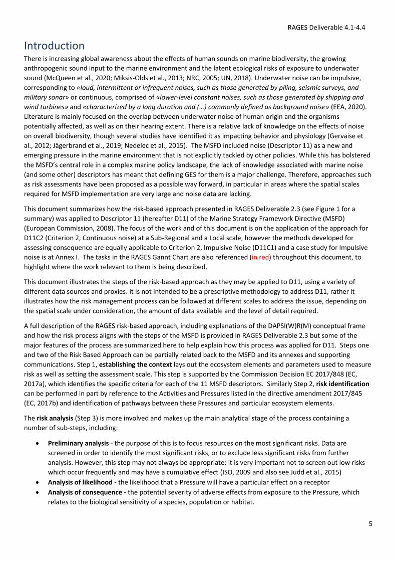
Introduction There is increasing global awareness about the effects of human sounds on marine biodiversity, the growing
anthropogenic sound input to the marine environment and the latent ecological risks of exposure to underwater
sound (McQueen et al., 2020; Miksis-Olds et al., 2013; NRC, 2005; UN, 2018). Underwater noise can be impulsive,
corresponding to «loud, intermittent or infrequent noises, such as those generated by piling, seismic surveys, and
military sonar» or continuous, comprised of «lower-level constant noises, such as those generated by shipping and
wind turbines» and «characterized by a long duration and (…) commonly defined as background noise» (EEA, 2020).
Literature is mainly focused on the overlap between underwater noise of human origin and the organisms
potentially affected, as well as on their hearing extent. There is a relative lack of knowledge on the effects of noise
on overall biodiversity, though several studies have identified it as impacting behavior and physiology (Gervaise et
al., 2012; Jägerbrand et al., 2019; Nedelec et al., 2015). The MSFD included noise (Descriptor 11) as a new and
emerging pressure in the marine environment that is not explicitly tackled by other policies. While this has bolstered
the MSFD’s central role in a complex marine policy landscape, the lack of knowledge associated with marine noise
(and some other) descriptors has meant that defining GES for them is a major challenge. Therefore, approaches such
as risk assessments have been proposed as a possible way forward, in particular in areas where the spatial scales
required for MSFD implementation are very large and noise data are lacking.
This document summarizes how the risk-based approach presented in RAGES Deliverable 2.3 (see Figure 1 for a
summary) was applied to Descriptor 11 (hereafter D11) of the Marine Strategy Framework Directive (MSFD)
(European Commission, 2008). The focus of the work and of this document is on the application of the approach for
D11C2 (Criterion 2, Continuous noise) at a Sub-Regional and a Local scale, however the methods developed for
assessing consequence are equally applicable to Criterion 2, Impulsive Noise (D11C1) and a case study for Impulsive
noise is at Annex I. The tasks in the RAGES Gannt Chart are also referenced (in red) throughout this document, to
highlight where the work relevant to them is being described.
This document illustrates the steps of the risk-based approach as they may be applied to D11, using a variety of
different data sources and proxies. It is not intended to be a prescriptive methodology to address D11, rather it
illustrates how the risk management process can be followed at different scales to address the issue, depending on
the spatial scale under consideration, the amount of data available and the level of detail required.
A full description of the RAGES risk-based approach, including explanations of the DAPSI(W)R(M) conceptual frame
and how the risk process aligns with the steps of the MSFD is provided in RAGES Deliverable 2.3 but some of the
major features of the process are summarized here to help explain how this process was applied for D11. Steps one
and two of the Risk Based Approach can be partially related back to the MSFD and its annexes and supporting
communications. Step 1, establishing the context lays out the ecosystem elements and parameters used to measure
risk as well as setting the assessment scale. This step is supported by the Commission Decision EC 2017/848 (EC,
2017a), which identifies the specific criteria for each of the 11 MSFD descriptors. Similarly Step 2, risk identification
can be performed in part by reference to the Activities and Pressures listed in the directive amendment 2017/845
(EC, 2017b) and identification of pathways between these Pressures and particular ecosystem elements.
The risk analysis (Step 3) is more involved and makes up the main analytical stage of the process containing a
number of sub-steps, including:
• Preliminary analysis - the purpose of this is to focus resources on the most significant risks. Data are
screened in order to identify the most significant risks, or to exclude less significant risks from further
analysis. However, this step may not always be appropriate; it is very important not to screen out low risks
which occur frequently and may have a cumulative effect (ISO, 2009 and also see Judd et al., 2015)
• Analysis of likelihood - the likelihood that a Pressure will have a particular effect on a receptor
• Analysis of consequence - the potential severity of adverse effects from exposure to the Pressure, which
relates to the biological sensitivity of a species, population or habitat.
RAGES Deliverable 4.1-4.4
6
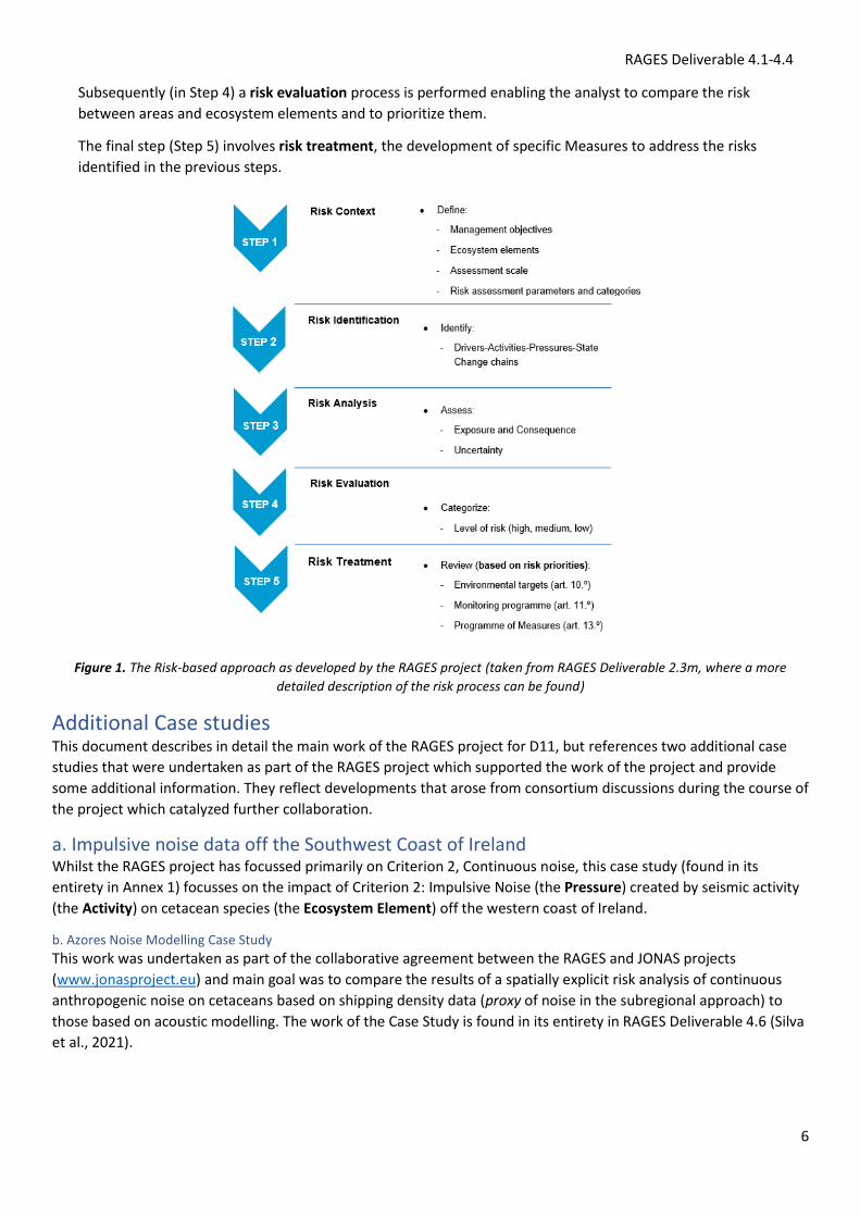
Subsequently (in Step 4) a risk evaluation process is performed enabling the analyst to compare the risk
between areas and ecosystem elements and to prioritize them.
The final step (Step 5) involves risk treatment, the development of specific Measures to address the risks
identified in the previous steps.
Figure 1. The Risk-based approach as developed by the RAGES project (taken from RAGES Deliverable 2.3m, where a more
detailed description of the risk process can be found)
Additional Case studies This document describes in detail the main work of the RAGES project for D11, but references two additional case
studies that were undertaken as part of the RAGES project which supported the work of the project and provide
some additional information. They reflect developments that arose from consortium discussions during the course of
the project which catalyzed further collaboration.
a. Impulsive noise data off the Southwest Coast of Ireland Whilst the RAGES project has focussed primarily on Criterion 2, Continuous noise, this case study (found in its
entirety in Annex 1) focusses on the impact of Criterion 2: Impulsive Noise (the Pressure) created by seismic activity
(the Activity) on cetacean species (the Ecosystem Element) off the western coast of Ireland.
b. Azores Noise Modelling Case Study
This work was undertaken as part of the collaborative agreement between the RAGES and JONAS projects
(www.jonasproject.eu) and main goal was to compare the results of a spatially explicit risk analysis of continuous
anthropogenic noise on cetaceans based on shipping density data (proxy of noise in the subregional approach) to
those based on acoustic modelling. The work of the Case Study is found in its entirety in RAGES Deliverable 4.6 (Silva
et al., 2021).
RAGES Deliverable 4.1-4.4
7
Step 1. Establishing the Context (TASK 4.2, DELIVERABLE 4.2-DEFINE RELEVANT CRITERIA ELEMENTS)
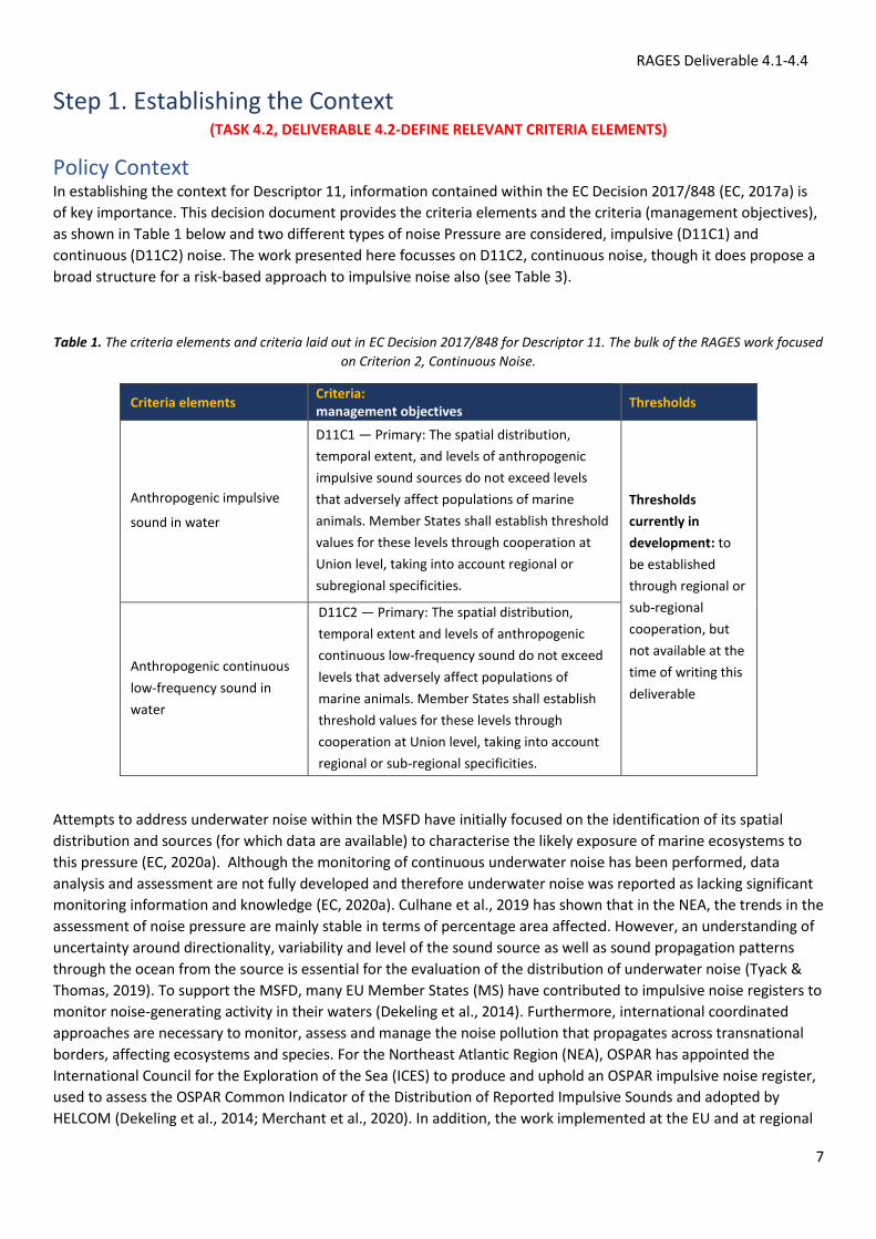
Policy Context In establishing the context for Descriptor 11, information contained within the EC Decision 2017/848 (EC, 2017a) is
of key importance. This decision document provides the criteria elements and the criteria (management objectives),
as shown in Table 1 below and two different types of noise Pressure are considered, impulsive (D11C1) and
continuous (D11C2) noise. The work presented here focusses on D11C2, continuous noise, though it does propose a
broad structure for a risk-based approach to impulsive noise also (see Table 3).
Table 1. The criteria elements and criteria laid out in EC Decision 2017/848 for Descriptor 11. The bulk of the RAGES work focused
on Criterion 2, Continuous Noise.
Criteria elements Criteria: management objectives
Thresholds
Anthropogenic impulsive
sound in water
D11C1 — Primary: The spatial distribution,
temporal extent, and levels of anthropogenic
impulsive sound sources do not exceed levels
that adversely affect populations of marine
animals. Member States shall establish threshold
values for these levels through cooperation at
Union level, taking into account regional or
subregional specificities.
Thresholds
currently in
development: to
be established
through regional or
sub-regional
cooperation, but
not available at the
time of writing this
deliverable
Anthropogenic continuous
low-frequency sound in
water
D11C2 — Primary: The spatial distribution,
temporal extent and levels of anthropogenic
continuous low-frequency sound do not exceed
levels that adversely affect populations of
marine animals. Member States shall establish
threshold values for these levels through
cooperation at Union level, taking into account
regional or sub-regional specificities.
Attempts to address underwater noise within the MSFD have initially focused on the identification of its spatial
distribution and sources (for which data are available) to characterise the likely exposure of marine ecosystems to
this pressure (EC, 2020a). Although the monitoring of continuous underwater noise has been performed, data
analysis and assessment are not fully developed and therefore underwater noise was reported as lacking significant
monitoring information and knowledge (EC, 2020a). Culhane et al., 2019 has shown that in the NEA, the trends in the
assessment of noise pressure are mainly stable in terms of percentage area affected. However, an understanding of
uncertainty around directionality, variability and level of the sound source as well as sound propagation patterns
through the ocean from the source is essential for the evaluation of the distribution of underwater noise (Tyack &
Thomas, 2019). To support the MSFD, many EU Member States (MS) have contributed to impulsive noise registers to
monitor noise-generating activity in their waters (Dekeling et al., 2014). Furthermore, international coordinated
approaches are necessary to monitor, assess and manage the noise pollution that propagates across transnational
borders, affecting ecosystems and species. For the Northeast Atlantic Region (NEA), OSPAR has appointed the
International Council for the Exploration of the Sea (ICES) to produce and uphold an OSPAR impulsive noise register,
used to assess the OSPAR Common Indicator of the Distribution of Reported Impulsive Sounds and adopted by
HELCOM (Dekeling et al., 2014; Merchant et al., 2020). In addition, the work implemented at the EU and at regional
RAGES Deliverable 4.1-4.4
8
levels through the Technical Group on Noise focuses on monitoring issues and relates to activities undertaken in
Regional Seas Conventions (RSC). It has also included the production of monitoring guidance on underwater noise
(EC, 2020b). Criteria to monitor and assess the adverse impacts of continuous underwater noise are in progress,
under the MSFD and Regional Seas Conventions outlines (EEA, 2020; TG Noise, 2019), but this work is in an earlier
stage of development.
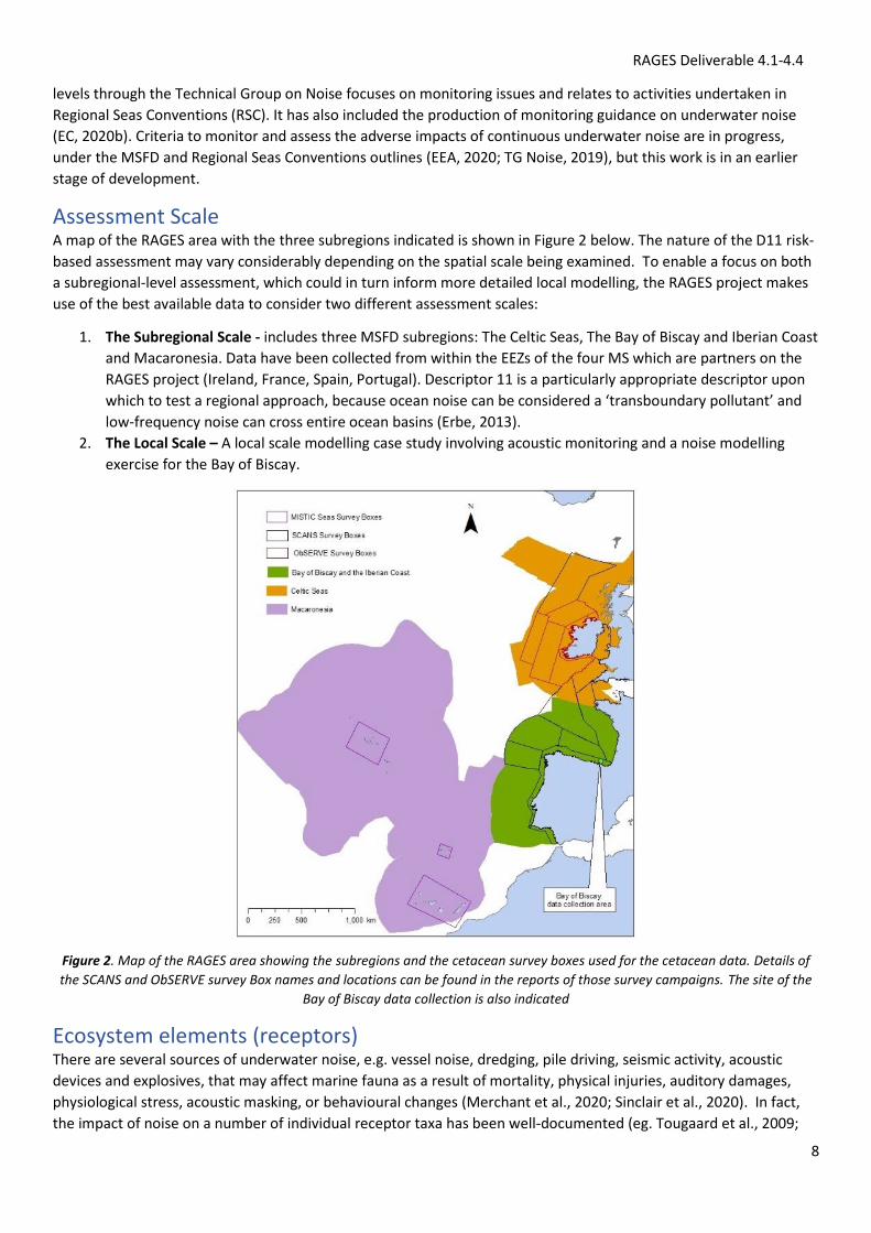
Assessment Scale A map of the RAGES area with the three subregions indicated is shown in Figure 2 below. The nature of the D11 risk-
based assessment may vary considerably depending on the spatial scale being examined. To enable a focus on both
a subregional-level assessment, which could in turn inform more detailed local modelling, the RAGES project makes
use of the best available data to consider two different assessment scales:
1. The Subregional Scale - includes three MSFD subregions: The Celtic Seas, The Bay of Biscay and Iberian Coast
and Macaronesia. Data have been collected from within the EEZs of the four MS which are partners on the
RAGES project (Ireland, France, Spain, Portugal). Descriptor 11 is a particularly appropriate descriptor upon
which to test a regional approach, because ocean noise can be considered a ‘transboundary pollutant’ and
low-frequency noise can cross entire ocean basins (Erbe, 2013).
2. The Local Scale – A local scale modelling case study involving acoustic monitoring and a noise modelling
exercise for the Bay of Biscay.
Figure 2. Map of the RAGES area showing the subregions and the cetacean survey boxes used for the cetacean data. Details of
the SCANS and ObSERVE survey Box names and locations can be found in the reports of those survey campaigns. The site of the
Bay of Biscay data collection is also indicated
Ecosystem elements (receptors) There are several sources of underwater noise, e.g. vessel noise, dredging, pile driving, seismic activity, acoustic
devices and explosives, that may affect marine fauna as a result of mortality, physical injuries, auditory damages,
physiological stress, acoustic masking, or behavioural changes (Merchant et al., 2020; Sinclair et al., 2020). In fact,
the impact of noise on a number of individual receptor taxa has been well-documented (eg. Tougaard et al., 2009;
RAGES Deliverable 4.1-4.4
9
Blair et al., 2016; McCauley et al, 2017), but there remains a knowledge gap in terms of the overall impact of
underwater noise at the broader ecosystem level (Merchant, 2019).
Marine mammals use sound for numerous reasons and thus are potentially vulnerable to high levels of human noise
in their environment (Sinclair et al., 2020). Much work has focused on the impact of noise on cetacean species, with
potential Impacts including behavioural changes and displacement due to processes such as acoustic masking and
hearing loss (Nowacek et al., 2007; Erbe, 2012). However, despite long-standing research efforts, it has proven very
difficult to draw robust statistical conclusions between noise and cetacean behavior. A scale ranking the severity of
response for cetaceans has been proposed to overcome this (Southall et al, 2007, 2019; Ellison et al., 2012) but an
extensive review of evidence by Gomez et al. (2016) suggests a simpler, binary “behavioural response/no
behavioural response” approach may be more appropriate given the lack of evidence and data in many cases. The
review by Gomez et al (2016) provides a summary of evidence for response to noise in a large number of cetacean
species and a good basis for a broad assessment of cetacean species.
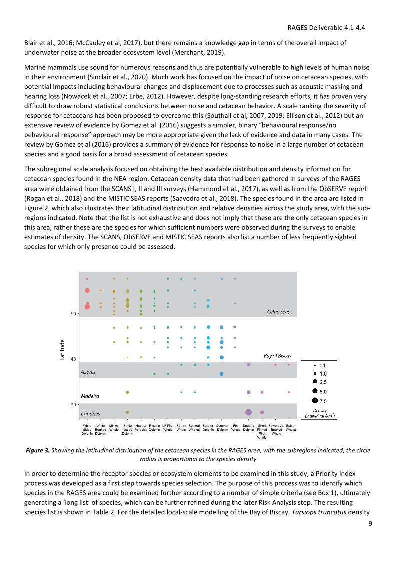
The subregional scale analysis focused on obtaining the best available distribution and density information for
cetacean species found in the NEA region. Cetacean density data that had been gathered in surveys of the RAGES
area were obtained from the SCANS I, II and III surveys (Hammond et al., 2017), as well as from the ObSERVE report
(Rogan et al., 2018) and the MISTIC SEAS reports (Saavedra et al., 2018). The species found in the area are listed in
Figure 2, which also illustrates their latitudinal distribution and relative densities across the study area, with the sub-
regions indicated. Note that the list is not exhaustive and does not imply that these are the only cetacean species in
this area, rather these are the species for which sufficient numbers were observed during the surveys to enable
estimates of density. The SCANS, ObSERVE and MISTIC SEAS reports also list a number of less frequently sighted
species for which only presence could be assessed.
Figure 3. Showing the latitudinal distribution of the cetacean species in the RAGES area, with the subregions indicated; the circle
radius is proportional to the species density
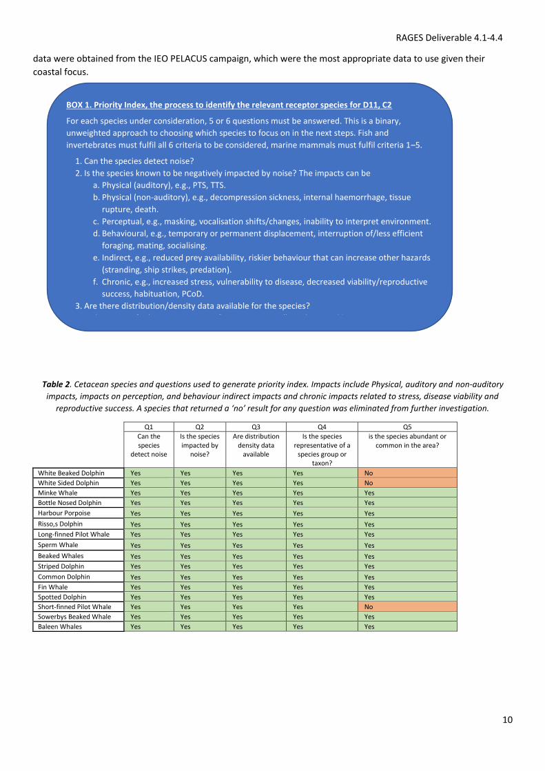
In order to determine the receptor species or ecosystem elements to be examined in this study, a Priority Index
process was developed as a first step towards species selection. The purpose of this process was to identify which
species in the RAGES area could be examined further according to a number of simple criteria (see Box 1), ultimately
generating a ‘long list’ of species, which can be further refined during the later Risk Analysis step. The resulting
species list is shown in Table 2. For the detailed local-scale modelling of the Bay of Biscay, Tursiops truncatus density
RAGES Deliverable 4.1-4.4
10
data were obtained from the IEO PELACUS campaign, which were the most appropriate data to use given their
coastal focus.
Table 2. Cetacean species and questions used to generate priority index. Impacts include Physical, auditory and non-auditory
impacts, impacts on perception, and behaviour indirect impacts and chronic impacts related to stress, disease viability and
reproductive success. A species that returned a ‘no’ result for any question was eliminated from further investigation.
Q1 Q2 Q3 Q4 Q5
Can the species
detect noise
Is the species impacted by
noise?
Are distribution density data
available
Is the species representative of a
species group or taxon?
is the species abundant or common in the area?
White Beaked Dolphin Yes Yes Yes Yes No
White Sided Dolphin Yes Yes Yes Yes No
Minke Whale Yes Yes Yes Yes Yes
Bottle Nosed Dolphin Yes Yes Yes Yes Yes
Harbour Porpoise Yes Yes Yes Yes Yes
Risso,s Dolphin Yes Yes Yes Yes Yes
Long-finned Pilot Whale Yes Yes Yes Yes Yes
Sperm Whale Yes Yes Yes Yes Yes
Beaked Whales Yes Yes Yes Yes Yes
Striped Dolphin Yes Yes Yes Yes Yes
Common Dolphin Yes Yes Yes Yes Yes
Fin Whale Yes Yes Yes Yes Yes
Spotted Dolphin Yes Yes Yes Yes Yes
Short-finned Pilot Whale Yes Yes Yes Yes No
Sowerbys Beaked Whale Yes Yes Yes Yes Yes
Baleen Whales Yes Yes Yes Yes Yes
BOX 1. Priority Index, the process to identify the relevant receptor species for D11, C2
For each species under consideration, 5 or 6 questions must be answered. This is a binary,
unweighted approach to choosing which species to focus on in the next steps. Fish and
invertebrates must fulfil all 6 criteria to be considered, marine mammals must fulfil criteria 1–5.
1. Can the species detect noise?
2. Is the species known to be negatively impacted by noise? The impacts can be
a. Physical (auditory), e.g., PTS, TTS.
b. Physical (non-auditory), e.g., decompression sickness, internal haemorrhage, tissue
rupture, death.
c. Perceptual, e.g., masking, vocalisation shifts/changes, inability to interpret environment.
d. Behavioural, e.g., temporary or permanent displacement, interruption of/less efficient
foraging, mating, socialising.
e. Indirect, e.g., reduced prey availability, riskier behaviour that can increase other hazards
(stranding, ship strikes, predation).
f. Chronic, e.g., increased stress, vulnerability to disease, decreased viability/reproductive
success, habituation, PCoD.
3. Are there distribution/density data available for the species?
4. Is the species fairly representative of a species group (broader taxon)?
5. Is the species fairly abundant/commonly occurring within the area of interest?
RAGES Deliverable 4.1-4.4
11
Step 2. Risk Identification Risk identification involves identifying a pathway between the risk sources creating the Pressure and the sensitive
Receptors within the study area.
Activities (Drivers)
As mentioned in the previous section, Commission Directive 2017/845 (EC, 2017b) lists a number of Activities, all of
which could generate anthropogenic noise to a greater or lesser extent. Examples include:
• Transport - shipping
• Extraction of oil and gas
• Extraction of minerals
• Fish and shellfish harvesting
• Military Operations (eg. low-frequency sonar, mid-frequency sonar)
• Renewable energy generation (wind, wave and tidal power)
Despite the range of activities, the disruption of ambient ocean soundscapes by the continuous low-frequency noise
generated by commercial shipping can be considered the most spatially widespread and persistent problem globally,
in particular in the northern hemisphere (Hildebrand, 2009; Cominielli, 2018). Therefore, data collection focused on
this activity as the most significant generator of continuous noise in the RAGES area.
Pressures
The relevant Pressures for Descriptor 11 have been listed in the Commission Decision 2017/848 (EC, 2017a) as:
• Input of anthropogenic sound;
• Input of other forms of energy.
The work of the RAGES project focused on the first of these and Table 1 shows that the MSFD includes two criteria,
one focusing on impulsive (resulting from e.g., drilling and oil and gas activity) and the other on continuous noise
(resulting from Activities such as shipping, offshore wind turbines). Regulation of ocean noise has usually tended to
focus on the impulsive noise sources, with the MSFD being regarded as one of the first regulatory attempts to tackle
continuous noise (Erbe, 2013, Erbe et al., 2014 but see also IMO/MEPC, 2014). Therefore, whilst the RAGES project
has placed considerable focus on developing a risk-based approach for continuous noise, we did also address the
impulsive noise criterion (see Annex I).
RAGES Deliverable 4.1-4.4
12
(DELIVERABLE 4.1, TASK 4.1 - DATA COLLECTION ON D11)
Subregional-scale datasets At a subregional scale, no dataset of continuous noise exists at present for European waters. Active efforts to
develop regional models of continuous noise for the North East Atlantic are currently underway as part of a number
of EU projects including JONAS, SATURN and private initiatives such as the Quiet Oceans Noise service and these
could be incorporated into the RAGES risk process once they become available. In the meantime, in the absence of a
noise dataset at the appropriate regional scale, a shipping density dataset based on AIS data is used here as a proxy
for continuous noise. The Human Activities Data Portal of The European Marine Observation and Data Network,
EMODnet (www.emodnet-humanactivities.eu) has developed a processed shipping dataset from AIS (Automatic
Identification System) data for European waters. At present, this represents the only freely available dataset that can
provide European-scale shipping information to inform studies of continuous underwater noise. For this study, the
data from 2017 only were used by way of illustration, however the EMODnet website now also includes AIS data
from 2018 and 2019. These AIS data were originally acquired from and pre-processed by a commercial provider
(Collecte Localisation Satellites-CLS). The data were further processed by EMODnet such that density was expressed
as ship hours per square kilometer per month. A detailed description of all pre-processing, processing and
interpolation routines employed can be found in the EMODnet method statement (Falco et al., 2019).
The RAGES project is facilitating subregional cooperation to develop a risk-based approach and to do this, products
that are freely available at a broad scale were being used. However, the flexibility of the approach means that it can
be followed with any dataset, for example, if in the future broadscale noise models are available, the process can
again be followed in the same way. Although shipping density is being used as a proxy layer in this study, it is not
assumed that it replaces quantitative noise models. Further modelling work is needed to establish the true impact of
shipping and its relation to overall noise in a given area and therefore, there are a number of important caveats
associated with using shipping density, which are detailed below:
• Many factors are known to affect the propagation of sound underwater, such as bathymetry, seafloor
composition and oceanographic factors. As a result, shallower ocean basins (eg. North Sea) will have very
different noise profiles to very deep ones (eg. North East Atlantic) and animals in each of these areas would
perceive the same noise in very different ways.
• The EMODnet data currently has a coastal bias and under-represents data far from shore. This should be borne
in mind when interpreting the results of the analysis, especially when comparing coastal and offshore regions.
• A recent noise model study in the North Sea and Celtic Sea (Farcas et al., 2020) indicates that while the
association between sAIS (satellite AIS) and overall noise is weaker in deeper water and at lower frequencies,
sAIS shipping data can dominate noisescapes and closely follow the patterns of underwater noise at higher
frequencies. In the Azores case study undertaken as part of this work (See RAGES Deliverable 4.6), the noisiest
locations in the study area corresponded reasonably well to locations with higher density of ships, but
modelling results showed that noise propagated over areas beyond shipping routes. This should be taken into
account when interpreting the data shown here.
• It is known that exposure should be calculated separately for varying ship types (for example as shown by
McKenna, 2012), because the noise generated differs between them. However although the data within
EMODnet is divided into ship types, these types cannot easily be equated with a particular noise profile.
Therefore, for this initial analysis, data for all ship types were considered together.
Data collection for The Bay of Biscay noise model The approach to risk assessment at a local scale was the same as that used at a subregional scale with continuous
noise emitted by ship traffic also being the focus. However, in this case a true pressure map (as opposed to a proxy
layer) reflecting ship noise was created. Considering GES in relation to noise is complicated because some areas can
have high noise levels but may not have species sensitive to noise, and some species can be more vulnerable to
noise than others. Therefore, risk-based models in this study use Sound Pressure Level (SPL ref 1microPa) to
RAGES Deliverable 4.1-4.4
13
measure exposure for a single highly sensitive species, Tursiops truncatus (the bottlenose dolphin). The type of
exposure considered was based on the Communication Distance Reduction (CDR) for this species. At present, the
Commission Decision EC 2017/848 indicates that 1/3 octave band of 63Hz and 125Hz should be reported but for this
work, which considered the effect of acoustic masking for a selected species, the frequencies 1kHz, 5kHz and 10kHz
were considered. These specific frequency bands were selected due to their overlapping with the sound repertoire
of the Tursiops truncatus, which ranges from 0.8kHz to 24kHz (Lilly and Miller, 1961; Caldwell et al., 1990; Wang et
al., 1995).
In order to assess the noise linked to ship traffic at the Gulf of Biscay, an annual AIS ship traffic dataset was used. The
AIS database contained information on speed over ground, length and tonnage of each ship. Ships were treated as
acoustic sources by applying a Randi Model (Breeding et al., 1996) for 10kHz frequency. In addition, seasonal
variations of speed of sound in water column were considered using Argo data (www.emodnet.eu) and using the
MacKenzie equation (Mackenzie, 1981) to combine sound velocity with temperature, salinity and depth. Using all of
these information sources, a noise model was created of the area that was later validated with data from a passive
acoustic monitoring campaign in the Bay of Biscay (N43º36,682; W02º39,419) carried out from June 20th, 2019 until
September 20th, 2019, during which 25 days of acoustic data were collected. Ambient noise indicators of 1/3 octave
at different frequencies (63Hz, 125 Hz, 2 kHz and 5 kHz) were obtained (Lara et al., 2019) to assess the accuracy of
the model.
RAGES Deliverable 4.1-4.4
14
TASK 4.4, DELIVERABLE 4.4 – APPLY RISK ASSESSMENT
Step 3: Risk Analysis (for Continuous Noise) Subregional-Scale Risk Analysis In order to define ecological values relevant to assessing noise at a subregional level, both the consequence
(sensitivity) of the receptor and the extent of exposure need to be understood. Although identifying a spatial overlap
of underwater noise (or proxy thereof) and a particular cetacean species does not necessarily imply that an Impact
will result, it is a necessary first step and therefore a good starting point to test the risk-based approach.
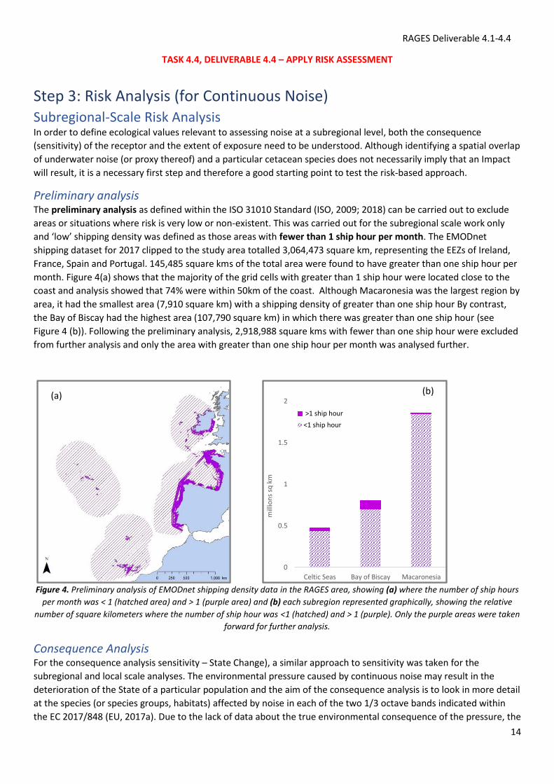
Preliminary analysis The preliminary analysis as defined within the ISO 31010 Standard (ISO, 2009; 2018) can be carried out to exclude
areas or situations where risk is very low or non-existent. This was carried out for the subregional scale work only
and ‘low’ shipping density was defined as those areas with fewer than 1 ship hour per month. The EMODnet
shipping dataset for 2017 clipped to the study area totalled 3,064,473 square km, representing the EEZs of Ireland,
France, Spain and Portugal. 145,485 square kms of the total area were found to have greater than one ship hour per
month. Figure 4(a) shows that the majority of the grid cells with greater than 1 ship hour were located close to the
coast and analysis showed that 74% were within 50km of the coast. Although Macaronesia was the largest region by
area, it had the smallest area (7,910 square km) with a shipping density of greater than one ship hour By contrast,
the Bay of Biscay had the highest area (107,790 square km) in which there was greater than one ship hour (see
Figure 4 (b)). Following the preliminary analysis, 2,918,988 square kms with fewer than one ship hour were excluded
from further analysis and only the area with greater than one ship hour per month was analysed further.
Figure 4. Preliminary analysis of EMODnet shipping density data in the RAGES area, showing (a) where the number of ship hours
per month was < 1 (hatched area) and > 1 (purple area) and (b) each subregion represented graphically, showing the relative
number of square kilometers where the number of ship hour was <1 (hatched) and > 1 (purple). Only the purple areas were taken
forward for further analysis.
Consequence Analysis For the consequence analysis sensitivity – State Change), a similar approach to sensitivity was taken for the
subregional and local scale analyses. The environmental pressure caused by continuous noise may result in the
deterioration of the State of a particular population and the aim of the consequence analysis is to look in more detail
at the species (or species groups, habitats) affected by noise in each of the two 1/3 octave bands indicated within
the EC 2017/848 (EU, 2017a). Due to the lack of data about the true environmental consequence of the pressure, the
0
0.5
1
1.5
2
Celtic Seas Bay of Biscay Macaronesia
mill
ion
s sq
km
>1 ship hour
<1 ship hour
(b) (a)
RAGES Deliverable 4.1-4.4
15
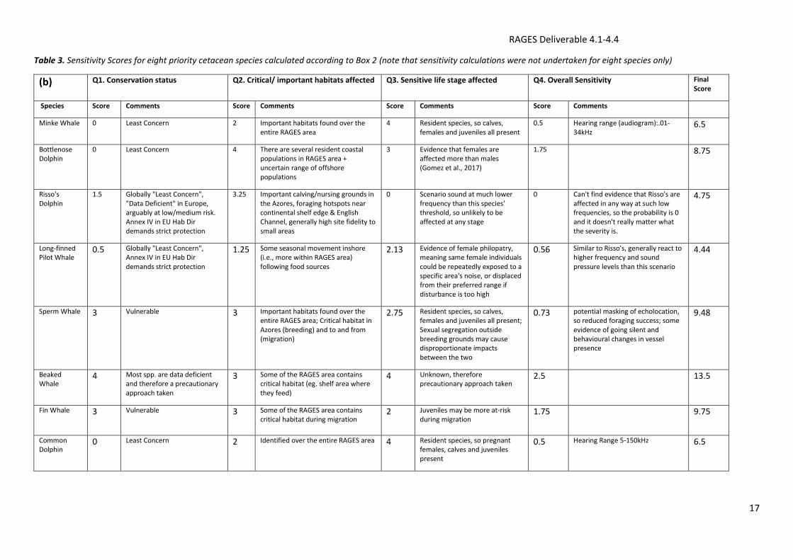
sensitivity of the species is essentially used as a proxy for consequence. The species to be taken through this process
would ideally be all of those identified from the Step 1 (see Table 2 and Box 1 above). However, despite decades of
research, as well as increasing concern about underwater noise impacts on cetaceans, it is accepted that
quantitative data describing cetacean’s sensitivity to ship noise remains inconclusive (see Erbe et al., 2013 and
Southall et al., 2019). Therefore the sensitivity process was conducted by performing a qualitative expert judgement-
based scoring process, designed to identify the species likely to be most affected by exposure. The method used is
described in Box 2 below and eight of the species emerging from Step 1 were taken through this process: Beaked
Whales, Bottlenose Dolphins, Bottlenose Dolphins, Sperm Whales, Common Dolphins, Minke Whales, Risso’s
Dolphin and Fin Whales. The number of species represents the extent of expert evidence that was available at the
time of this work. At least one expert completed the process for each of the eight species, and where more than one
expert completed the process, the mean of their scores was used. The results are illustrated in Table 3 (b). These
species were chosen to illustrate how the process could be applied to a range of species with differing ecologies and
geographical distributions. Ideally all of the species on the long list from Step 1 should be taken through this
process, but further input from experts would be required to achieve this (see comments on page 25 for further
details).
RAGES Deliverable 4.1-4.4
16
Box 2: Sensitivity Analysis to identify the most relevant receptor species
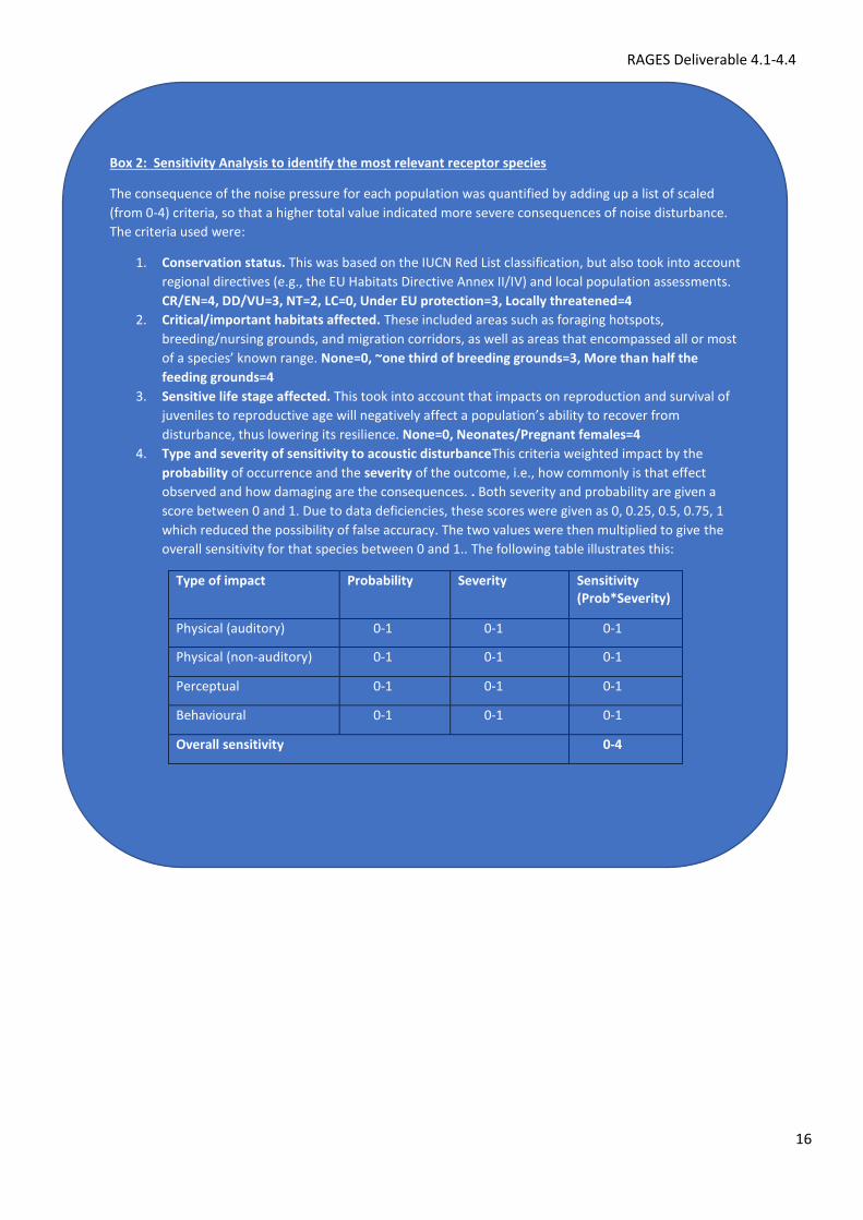
The consequence of the noise pressure for each population was quantified by adding up a list of scaled
(from 0-4) criteria, so that a higher total value indicated more severe consequences of noise disturbance.
The criteria used were:
1. Conservation status. This was based on the IUCN Red List classification, but also took into account
regional directives (e.g., the EU Habitats Directive Annex II/IV) and local population assessments.
CR/EN=4, DD/VU=3, NT=2, LC=0, Under EU protection=3, Locally threatened=4
2. Critical/important habitats affected. These included areas such as foraging hotspots,
breeding/nursing grounds, and migration corridors, as well as areas that encompassed all or most
of a species’ known range. None=0, ~one third of breeding grounds=3, More than half the
feeding grounds=4
3. Sensitive life stage affected. This took into account that impacts on reproduction and survival of
juveniles to reproductive age will negatively affect a population’s ability to recover from
disturbance, thus lowering its resilience. None=0, Neonates/Pregnant females=4
4. Type and severity of sensitivity to acoustic disturbanceThis criteria weighted impact by the
probability of occurrence and the severity of the outcome, i.e., how commonly is that effect
observed and how damaging are the consequences. . Both severity and probability are given a
score between 0 and 1. Due to data deficiencies, these scores were given as 0, 0.25, 0.5, 0.75, 1
which reduced the possibility of false accuracy. The two values were then multiplied to give the
overall sensitivity for that species between 0 and 1.. The following table illustrates this:
Type of impact Probability Severity Sensitivity (Prob*Severity)
Physical (auditory) 0-1 0-1 0-1
Physical (non-auditory) 0-1 0-1 0-1
Perceptual 0-1 0-1 0-1
Behavioural 0-1 0-1 0-1
Overall sensitivity 0-4
RAGES Deliverable 4.1-4.4
17
Table 3. Sensitivity Scores for eight priority cetacean species calculated according to Box 2 (note that sensitivity calculations were not undertaken for eight species only)
(b) Q1. Conservation status Q2. Critical/ important habitats affected Q3. Sensitive life stage affected Q4. Overall Sensitivity Final Score
Species Score Comments Score Comments Score Comments Score Comments
Minke Whale 0 Least Concern 2 Important habitats found over the entire RAGES area
4 Resident species, so calves, females and juveniles all present
0.5 Hearing range (audiogram):.01-34kHz
6.5
Bottlenose Dolphin
0 Least Concern 4 There are several resident coastal populations in RAGES area + uncertain range of offshore populations
3 Evidence that females are affected more than males (Gomez et al., 2017)
1.75 8.75
Risso's Dolphin
1.5 Globally "Least Concern", "Data Deficient" in Europe, arguably at low/medium risk. Annex IV in EU Hab Dir demands strict protection
3.25 Important calving/nursing grounds in the Azores, foraging hotspots near continental shelf edge & English Channel, generally high site fidelity to small areas
0 Scenario sound at much lower frequency than this species' threshold, so unlikely to be affected at any stage
0 Can't find evidence that Risso's are affected in any way at such low frequencies, so the probability is 0 and it doesn't really matter what the severity is.
4.75
Long-finned Pilot Whale
0.5 Globally "Least Concern", Annex IV in EU Hab Dir demands strict protection
1.25 Some seasonal movement inshore (i.e., more within RAGES area) following food sources
2.13 Evidence of female philopatry, meaning same female individuals could be repeatedly exposed to a specific area's noise, or displaced from their preferred range if disturbance is too high
0.56 Similar to Risso's, generally react to higher frequency and sound pressure levels than this scenario
4.44
Sperm Whale 3 Vulnerable 3
Important habitats found over the entire RAGES area; Critical habitat in Azores (breeding) and to and from (migration)
2.75 Resident species, so calves, females and juveniles all present; Sexual segregation outside breeding grounds may cause disproportionate impacts between the two
0.73 potential masking of echolocation, so reduced foraging success; some evidence of going silent and behavioural changes in vessel presence
9.48
Beaked Whale
4 Most spp. are data deficient and therefore a precautionary approach taken
3 Some of the RAGES area contains critical habitat (eg. shelf area where they feed)
4 Unknown, therefore precautionary approach taken
2.5 13.5
Fin Whale 3 Vulnerable 3 Some of the RAGES area contains critical habitat during migration
2 Juveniles may be more at-risk during migration
1.75 9.75
Common Dolphin
0 Least Concern 2 Identified over the entire RAGES area 4 Resident species, so pregnant females, calves and juveniles present
0.5 Hearing Range 5-150kHz 6.5
RAGES Deliverable 4.1-4.4
18
Likelihood Analysis (Exposure) The purpose of the likelihood analysis is to undertake an analysis of the overlap between the Pressure under
assessment and the ecosystem elements selected (i.e. the exposure). Likelihood analysis should consider both
temporal and spatial exposure and the candidate indicator currently being developed via the OSPAR ICG-Noise group
could be applied once it is in a more advanced stage of development. To consider the issue of underwater noise at a
subregional level, the RAGES project used AIS data processed by EMODnet to create an activity layer as a proxy
Pressure layer to identify areas where continuous noise Pressure is likely to be high. A full description of the data
and the processing undertaken can be found on the EMODnet website
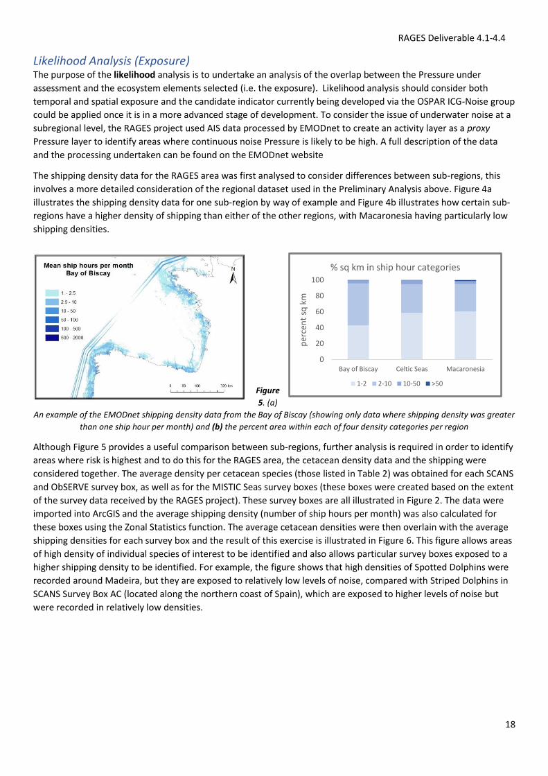
The shipping density data for the RAGES area was first analysed to consider differences between sub-regions, this
involves a more detailed consideration of the regional dataset used in the Preliminary Analysis above. Figure 4a
illustrates the shipping density data for one sub-region by way of example and Figure 4b illustrates how certain sub-
regions have a higher density of shipping than either of the other regions, with Macaronesia having particularly low
shipping densities.
Figure
5. (a)
An example of the EMODnet shipping density data from the Bay of Biscay (showing only data where shipping density was greater
than one ship hour per month) and (b) the percent area within each of four density categories per region
Although Figure 5 provides a useful comparison between sub-regions, further analysis is required in order to identify
areas where risk is highest and to do this for the RAGES area, the cetacean density data and the shipping were
considered together. The average density per cetacean species (those listed in Table 2) was obtained for each SCANS
and ObSERVE survey box, as well as for the MISTIC Seas survey boxes (these boxes were created based on the extent
of the survey data received by the RAGES project). These survey boxes are all illustrated in Figure 2. The data were
imported into ArcGIS and the average shipping density (number of ship hours per month) was also calculated for
these boxes using the Zonal Statistics function. The average cetacean densities were then overlain with the average
shipping densities for each survey box and the result of this exercise is illustrated in Figure 6. This figure allows areas
of high density of individual species of interest to be identified and also allows particular survey boxes exposed to a
higher shipping density to be identified. For example, the figure shows that high densities of Spotted Dolphins were
recorded around Madeira, but they are exposed to relatively low levels of noise, compared with Striped Dolphins in
SCANS Survey Box AC (located along the northern coast of Spain), which are exposed to higher levels of noise but
were recorded in relatively low densities.
0
20
40
60
80
100
Bay of Biscay Celtic Seas Macaronesia
per
cen
t sq
km
% sq km in ship hour categories
1-2 2-10 10-50 >50
RAGES Deliverable 4.1-4.4
19
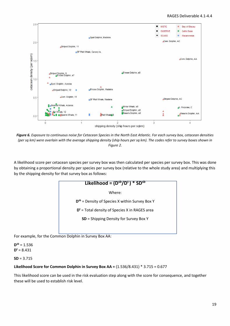
Figure 6. Exposure to continuous noise for Cetacean Species in the North East Atlantic. For each survey box, cetacean densities
(per sq km) were overlain with the average shipping density (ship hours per sq km). The codes refer to survey boxes shown in
Figure 2.
A likelihood score per cetacean species per survey box was then calculated per species per survey box. This was done
by obtaining a proportional density per species per survey box (relative to the whole study area) and multiplying this
by the shipping density for that survey box as follows:
Likelihood = (Dsb/Dt ) * SDsb
Where:
Dsb = Density of Species X within Survey Box Y
Dt = Total density of Species X in RAGES area
SD = Shipping Density for Survey Box Y
For example, for the Common Dolphin in Survey Box AA:
Dsb = 1.536 Dt = 8.431
SD = 3.715
Likelihood Score for Common Dolphin in Survey Box AA = (1.536/8.431) * 3.715 = 0.677
This likelihood score can be used in the risk evaluation step along with the score for consequence, and together
these will be used to establish risk level.
RAGES Deliverable 4.1-4.4
20
Local-Scale Risk Analysis (Bay of Biscay modelling work) Consequence Analysis The results of the consequence analysis at the subregional scale were also relevant for local scale work and in this
case, the Bottlenose Dolphin (Tursiops truncatus) was considered a suitable species for the development and
application of a risk-based model. This is because data are readily available for this species and in addition, the
frequency range of their whistles goes from 0.8kHz to 24kHz (Lilly and Miller, 1961; Wang et al., 1995) and their
hearing sensitivity is 1-180kHz (Finneran et al., 2010; Houser et al., 2008). It is known that acoustic attenuation
during propagation depends on frequency and that higher frequencies are strongly attenuated. Considering also that
the acoustic emission of ships is stronger at lower frequency values, the lower frequency limit on T. truncatus
whistles makes them likely to be affected by ship noise.
Likelihood Analysis Coming up with a measure of likelihood (or ‘exposure’) at the local scale involved a consideration of the noise maps
produced using AIS data. This analysis considered the masking effect of noise on the receptor, defined as the rise of
the hearing threshold for a given frequency band due to a presence of noise overlapping in time and space (Erbe et
al., 2016). Analysis of masking is not trivial and depending on the acoustic variable used, the information retrieved
can have different interpretations. The most direct way to try to evaluate the potential threat of acoustic masking
would be to consider the noise map and Sound Pressure Level (SPL) at each cell of the simulated area. However, the
absence of thresholds makes it difficult to establish a direct relationship between cause (ship traffic noise) and effect
(in our case acoustic masking). Moreover, it is not easy to apply other metrics like Sound Exposure Level (SEL) to
continuous noise because the time exposure is different from that of impulsive noise. For this reason, a
Communication Distance Reduction (CDR) from pristine ambient has been considered as an acoustic related variable
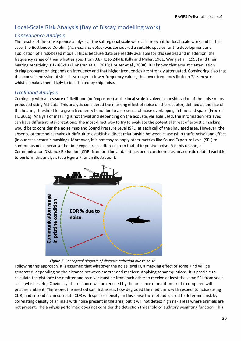
to perform this analysis (see Figure 7 for an illustration).
Figure 7. Conceptual diagram of distance reduction due to noise.
Following this approach, it is assumed that whatever the noise level is, a masking effect of some kind will be
generated, depending on the distance between emitter and receiver. Applying sonar equations, it is possible to
calculate the distance the emitter and receiver must be from each other to receive at least the same SPL from social
calls (whistles etc). Obviously, this distance will be reduced by the presence of maritime traffic compared with
pristine ambient. Therefore, the method can first assess how degraded the medium is with respect to noise (using
CDR) and second it can correlate CDR with species density. In this sense the method is used to determine risk by
correlating density of animals with noise present in the area, but it will not detect high risk areas where animals are
not present. The analysis performed does not consider the detection threshold or auditory weighting function. This
RAGES Deliverable 4.1-4.4
21
simplifies the calculation and circumvents the lack of knowledge or agreement between experts about values of
these variables for different species as such it represents a logical and defensible risk-based approach.
Step 4: Risk Evaluation (TASK 4.3, DELIVERABLE 4.3 - DEFINE RISK CRITERIA SIGNIFICANCE LEVELS)
Risk Evaluation at a subregional scale The aim of risk evaluation is to arrive at a measure of relative risk, which will in turn inform GES assessments and
enable prioritization of Measures. Following the ISO process and building on work carried out in the MISTIC SEAS II
project (Saavedra et al., 2018), the likelihood and consequence information were considered together as follows:
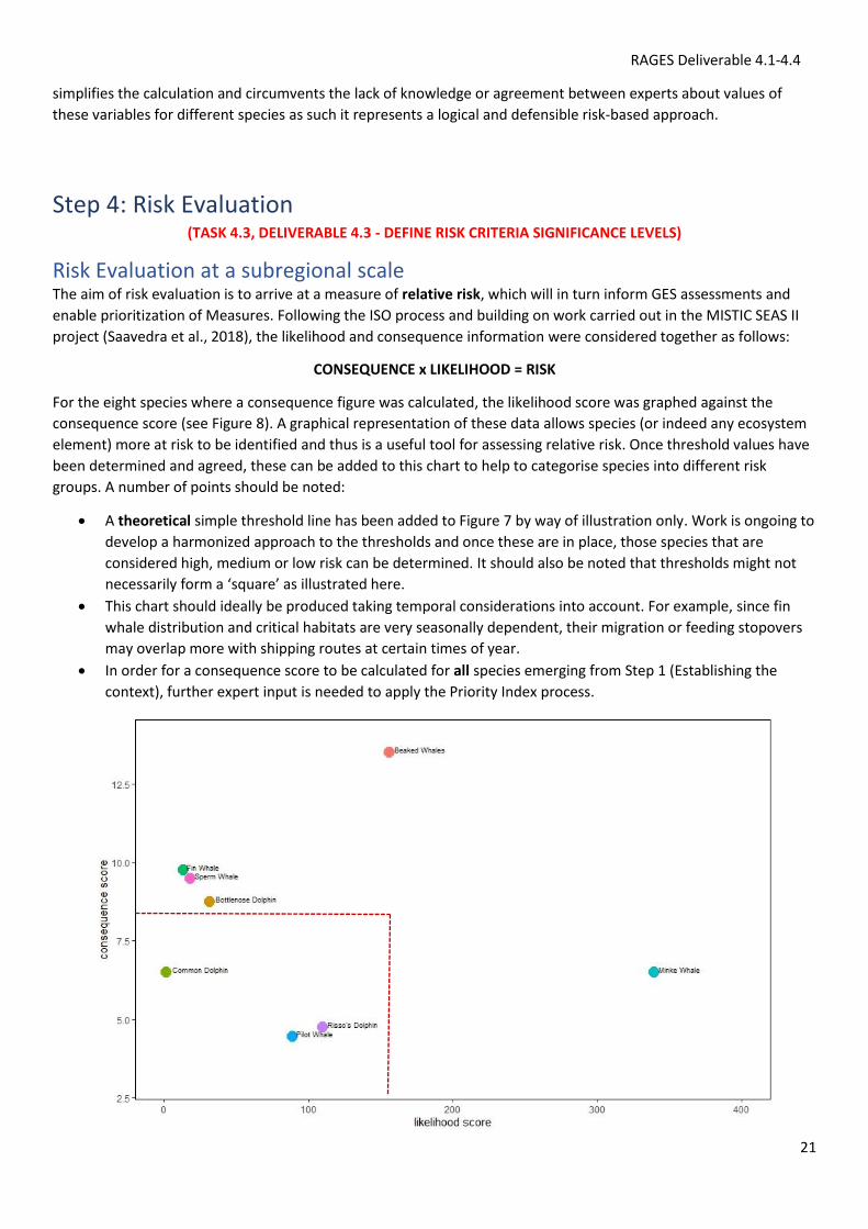
CONSEQUENCE x LIKELIHOOD = RISK
For the eight species where a consequence figure was calculated, the likelihood score was graphed against the
consequence score (see Figure 8). A graphical representation of these data allows species (or indeed any ecosystem
element) more at risk to be identified and thus is a useful tool for assessing relative risk. Once threshold values have
been determined and agreed, these can be added to this chart to help to categorise species into different risk
groups. A number of points should be noted:
• A theoretical simple threshold line has been added to Figure 7 by way of illustration only. Work is ongoing to
develop a harmonized approach to the thresholds and once these are in place, those species that are
considered high, medium or low risk can be determined. It should also be noted that thresholds might not
necessarily form a ‘square’ as illustrated here.
• This chart should ideally be produced taking temporal considerations into account. For example, since fin
whale distribution and critical habitats are very seasonally dependent, their migration or feeding stopovers
may overlap more with shipping routes at certain times of year.
• In order for a consequence score to be calculated for all species emerging from Step 1 (Establishing the
context), further expert input is needed to apply the Priority Index process.
RAGES Deliverable 4.1-4.4
22
Figure 8. Risk Evaluation – consequence based on sensitivity analysis and likelihood based on average exposure scores (per
survey box) for each of eight species. This would allow relative risk to be determined once Threshold Values are in place. Red
dashed lines represent theoretical likelihood and consequence Threshold Values for illustration purposes only.
Risk Evaluation at a local scale The use of communication distance reduction (CDR) provides the opportunity to study the masking effect over
whistles and other social calls at frequencies <= 10kHz. The hypothesis in this case considers that the presence of
ship traffic produces a certain signal overlap from the physical point of view, even if noise level is lower than the
signal arriving to an ideal receiver from a conspecific. The calculation of CDR depends on the total noise in the area,
making it possible to study the percentage CDR in ambient noise with or without ship traffic, which allows a
comparison to be made between pristine ambient and the current situation. Cases illustrated in this work were
developed assuming ambient noise for 1kHz, 5kHz and 10kHz and sea state 1 (following the Beaufort Scale where
wind speed is 1 - 3 knots and wave height is 10cm) and using tabulated values for Wenz curves (Wenz, 1962). As
expected, the % CDR with respect to pristine ambient decreased with increasing frequency, due to the level of ship
noise present in the area. At 1kHz, maximum values of CDR were 82.7%, at 5kHz, the maximum value of CDR was
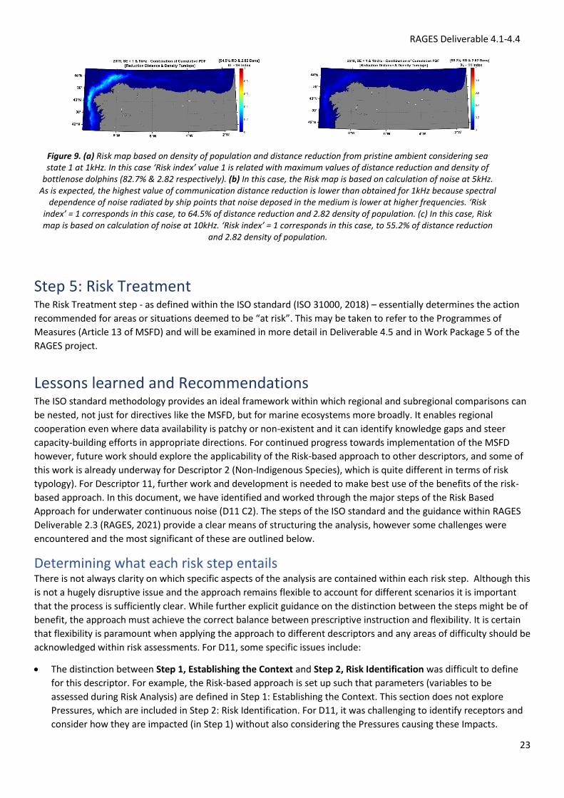
64.5%. and for 10kHz, the maximum value of CDR was 55.2%. In all cases, T. truncatus density was 2.82 and the Risk
Index was 1; see Table 4 for detailed statistics.
The calculation of CDR from pristine ambient due to ship traffic gives an idea of the auditory effect of noise on
certain marine species, using as a ‘baseline’ the distance at which an ideal emitter and receiver can communicate in
a no ship traffic situation. Risk evaluation can be based on the possibility of a masking effect occurring in areas
where T. truncates is present. Both related acoustic variables allow areas with a potential threat of masking to be
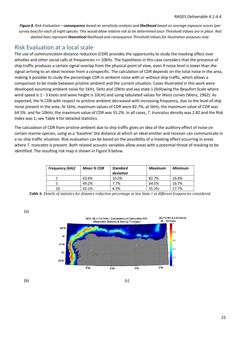
identified. The resulting risk map is shown in Figure 9 below.
Frequency [kHz] Mean % CDR Standard deviation
Maximum Minimum
1 63.6% 10.5% 82.7% 16.6%
5 49.2% 7.7% 64.5% 16.7%
10 42.1% 6.5% 55.2% 17.7%
Table 4. Details of statistics for distance reduction percentage at Sea State 1 at different frequencies considered.
(a)
(b) (c)
RAGES Deliverable 4.1-4.4
23
Figure 9. (a) Risk map based on density of population and distance reduction from pristine ambient considering sea state 1 at 1kHz. In this case ‘Risk index’ value 1 is related with maximum values of distance reduction and density of
bottlenose dolphins (82.7% & 2.82 respectively). (b) In this case, the Risk map is based on calculation of noise at 5kHz. As is expected, the highest value of communication distance reduction is lower than obtained for 1kHz because spectral
dependence of noise radiated by ship points that noise deposed in the medium is lower at higher frequencies. ‘Risk index’ = 1 corresponds in this case, to 64.5% of distance reduction and 2.82 density of population. (c) In this case, Risk map is based on calculation of noise at 10kHz. ‘Risk index’ = 1 corresponds in this case, to 55.2% of distance reduction
and 2.82 density of population.
Step 5: Risk Treatment The Risk Treatment step - as defined within the ISO standard (ISO 31000, 2018) – essentially determines the action
recommended for areas or situations deemed to be “at risk”. This may be taken to refer to the Programmes of
Measures (Article 13 of MSFD) and will be examined in more detail in Deliverable 4.5 and in Work Package 5 of the
RAGES project.
Lessons learned and Recommendations The ISO standard methodology provides an ideal framework within which regional and subregional comparisons can
be nested, not just for directives like the MSFD, but for marine ecosystems more broadly. It enables regional
cooperation even where data availability is patchy or non-existent and it can identify knowledge gaps and steer
capacity-building efforts in appropriate directions. For continued progress towards implementation of the MSFD
however, future work should explore the applicability of the Risk-based approach to other descriptors, and some of
this work is already underway for Descriptor 2 (Non-Indigenous Species), which is quite different in terms of risk
typology). For Descriptor 11, further work and development is needed to make best use of the benefits of the risk-
based approach. In this document, we have identified and worked through the major steps of the Risk Based
Approach for underwater continuous noise (D11 C2). The steps of the ISO standard and the guidance within RAGES
Deliverable 2.3 (RAGES, 2021) provide a clear means of structuring the analysis, however some challenges were
encountered and the most significant of these are outlined below.
Determining what each risk step entails There is not always clarity on which specific aspects of the analysis are contained within each risk step. Although this
is not a hugely disruptive issue and the approach remains flexible to account for different scenarios it is important
that the process is sufficiently clear. While further explicit guidance on the distinction between the steps might be of
benefit, the approach must achieve the correct balance between prescriptive instruction and flexibility. It is certain
that flexibility is paramount when applying the approach to different descriptors and any areas of difficulty should be
acknowledged within risk assessments. For D11, some specific issues include:
• The distinction between Step 1, Establishing the Context and Step 2, Risk Identification was difficult to define
for this descriptor. For example, the Risk-based approach is set up such that parameters (variables to be
assessed during Risk Analysis) are defined in Step 1: Establishing the Context. This section does not explore
Pressures, which are included in Step 2: Risk Identification. For D11, it was challenging to identify receptors and
consider how they are impacted (in Step 1) without also considering the Pressures causing these Impacts.
RAGES Deliverable 4.1-4.4
24
Mentioning Pressures in Step 1 was unavoidable in this case, but this did seem to somewhat negate the purpose
of Step 2, which examined pathways.
• Step 2, Risk Identification has been approached such that it is rooted in the Pressures in the geographic area of
study. Thus, we have included data collection for the Pressure proxy in Risk Identification. This may not be
considered appropriate and others may feel Data collection fits better within Step 3, Risk Analysis.
• At Step 3, Risk Analysis, the work at the subregional scale done as part of the Preliminary Analysis could instead
have been included in the Likelihood Analysis. It doesn’t have a material impact on the work, but in some cases
excluding areas prior to a likelihood analysis may not be considered appropriate.
Quality of receptor data for Descriptor 11 Due to the differing spatial resolution of the cetacean datasets made available to the RAGES project, the density
information has been analysed at a high level of aggregation (to survey box). Although the data from the MISTIC Seas
work was provided at a much more detailed level (per square km), it was not possible to use the data in this way for
a regionally harmonized approach as it was necessary to have all datasets at a similar level of detail. Clearly, were
SCANS and ObSERVE datasets available at a higher level of spatial resolution, more detailed analyses could be
conducted. A harmonised database of cetacean density distribution is needed; one that is spatially standardised,
freely available, accompanied by appropriate metadata and crucially, that allows for temporal considerations to be
taken into account. The latter is particularly important for migrating cetacean species such as the Fin Whale, for
which risk levels will vary at different periods throughout the year. All of these recommendations are supported by
the stipulations of the Aarhus Convention on Access to Information, Public Participation and Access to Justice in
Environmental Matters (United Nations Economic Commission for Europe, 1998), for which data sharing, data
archive centres and freely available environmental data are central pillars. Despite these caveats, the data used here
remain the best information available and the most appropriate to use at this scale. As was the case with pressures
data, the risk process can be applied to new and improved datasets once they become available.
Quality of pressures data for Descriptor 11 The subregional work in this study used AIS data as a proxy for pressure data, because at present, modelled noise
data is simply not available at this scale for European waters. There has been considerable debate within the RAGES
project as to the appropriateness of AIS data as a proxy for noise. While qualitatively the latest publications suggest
that shipping noise dominates noisescapes in some cases, (Farcas et al., 2020), they also caution that this does not
apply in all cases, particularly in deeper water and for lower frequencies. Further modelling work will thus be
required to establish how reliable a proxy approach is in identifying areas of risk. Continued developments in the
science of noise modelling will increase our understanding of ocean soundscapes but it will also improve the
knowledge base for the use of risk-based approaches. Such work continues apace in Europe within initiatives such as
the JONAS and SATURN projects, which should be tightly linked to policy needs in order to maximise its application
and usefulness. In the meantime, a European-scale map of maritime transport (including offshore shipping) that can
be accurately related to noise is required in order to improve the accuracy and utility of risk-based approach at a
broadscale level
Although noise models covering the entire RAGES were not available, their use was demonstrated at a local scale in
the Bay of Biscay. A series of further noise models like this could also be created in other key areas in order to build
up a fuller picture of the overall noise profile within the busy shipping areas of European waters. Passive acoustic
monitoring campaigns and measuring stations alongside automatic detection algorithms of cetaceans could also help
to validate density models and create sensitivity maps for species. There is also potential for modelling approaches
to be harmonised, for example by filling gaps at the regional level and indeed, repeated studies could track areas of
increasing or decreasing risk by identifying changes in cetacean population density, migration to other zones as well
changes to ship traffic volume. Finally, one of the great benefits of the risk approach is that it has been developed in
RAGES Deliverable 4.1-4.4
25
such a way that it can be applied to any type of dataset and the work undertaken in RAGES will be equally applicable
once modelled data does become available.
Consequence analysis for Descriptor 11 Development and refinement of the Priority Index and alignment with current regional initiatives is vital if these are
to inform MSFD implementation nationally. While work to understand the impact of noise on cetacean (and other)
species will no doubt continue, this will take considerable time and resources, and in the meantime an expert
judgement led sensitivity process provides a realistic and effective solution. There is a flexibility to expert judgement
processes that lends itself very well to a broad process encompassing different jurisdictions; in the example provided
here, some judgements were made by an individual expert but it may be more robust - and transferrable - if
completed by a panel of experts who agree on a shared set of scores for use more broadly. Considerable progress
could be made by convening a workshop of one or two days to facilitate a discussion and build consensus on the
Priority Index and Sensitivity approach outlined here.
Development of agreed qualitative working thresholds should also be a priority, and much work is currently
underway on this issue, particularly within the TGNoise group. Although the absence of threshold values is seen as
an impediment to progress in policy decisions, the final Risk Evaluation step (Step 5) provides a simple and easily
understood graphical representation that nonetheless summarizes a wealth of data and expertise. This graphic has
the potential to underpin policy decisions by allowing relative risk of species (or indeed any ecosystem elements) to
be visualized.
The most recent work on underwater noise continues to advocate for improved national and international
regulation and management of this ocean pressure, even in the face of knowledge gaps and the complexity of filling
them (Duarte et al., 2021). To that end, the Risk-based approach is a robust process that can be deployed again and
again, even as data are enhanced and understanding increases. It provides a clear, repeatable structure on which the
determination of GES can be anchored, supporting continued regional harmonisation and consistency into the
future.
RAGES Deliverable 4.1-4.4
26
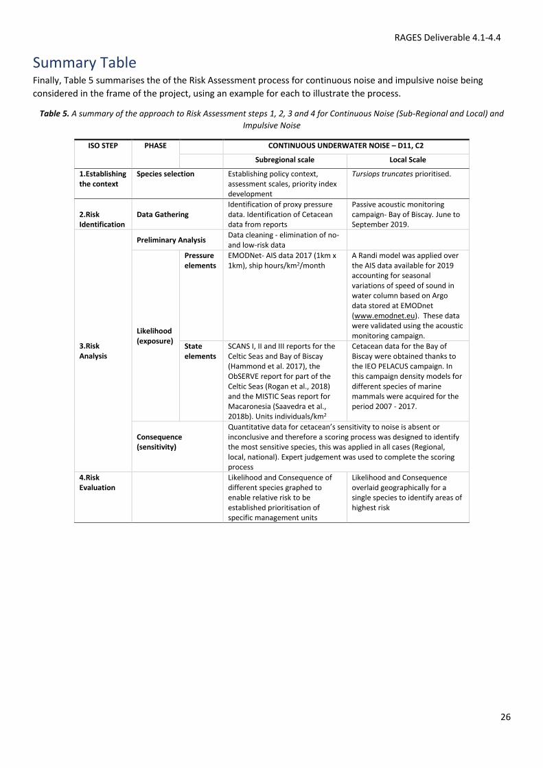
Summary Table Finally, Table 5 summarises the of the Risk Assessment process for continuous noise and impulsive noise being
considered in the frame of the project, using an example for each to illustrate the process.
Table 5. A summary of the approach to Risk Assessment steps 1, 2, 3 and 4 for Continuous Noise (Sub-Regional and Local) and
Impulsive Noise
ISO STEP PHASE
CONTINUOUS UNDERWATER NOISE – D11, C2
Subregional scale Local Scale
1.Establishing the context
Species selection Establishing policy context, assessment scales, priority index development
Tursiops truncates prioritised.
2.Risk Identification
Data Gathering
Identification of proxy pressure data. Identification of Cetacean data from reports
Passive acoustic monitoring campaign- Bay of Biscay. June to September 2019.
3.Risk Analysis
Preliminary Analysis Data cleaning - elimination of no- and low-risk data
Likelihood (exposure)
Pressure elements
EMODNet- AIS data 2017 (1km x 1km), ship hours/km2/month
A Randi model was applied over the AIS data available for 2019 accounting for seasonal variations of speed of sound in water column based on Argo data stored at EMODnet (www.emodnet.eu). These data were validated using the acoustic monitoring campaign.
State elements
SCANS I, II and III reports for the Celtic Seas and Bay of Biscay (Hammond et al. 2017), the ObSERVE report for part of the Celtic Seas (Rogan et al., 2018) and the MISTIC Seas report for Macaronesia (Saavedra et al., 2018b). Units individuals/km2
Cetacean data for the Bay of Biscay were obtained thanks to the IEO PELACUS campaign. In this campaign density models for different species of marine mammals were acquired for the period 2007 - 2017.
Consequence (sensitivity)
Quantitative data for cetacean’s sensitivity to noise is absent or inconclusive and therefore a scoring process was designed to identify the most sensitive species, this was applied in all cases (Regional, local, national). Expert judgement was used to complete the scoring process
4.Risk Evaluation
Likelihood and Consequence of different species graphed to enable relative risk to be established prioritisation of specific management units
Likelihood and Consequence overlaid geographically for a single species to identify areas of highest risk
RAGES Deliverable 4.1-4.4
27
References Blair HB, Merchant ND, Friedlaender AS, Wiley DN and Parks SE. (2016). Evidence for ship noise impacts on
humpback whales foraging behaviour. Biology Letters 12: 20160005.
Breeding JE, Plug LA, Bradley EL, Walrod MH, and McBride W. (1996) Ambient noise Directionality (RANDI) 3.1 –
Physics description. Technical Report NRL/FR/7176-95-9628, Naval Research Laboratory.
Caldwell MC, Caldwell DK and Tyack PL (1990) A review of the signature-whistle-hypothesis for the Atlantic
bottlenose dolphin. In: Leatherwood S, Reeves RR (eds) The bottlenose dolphin. Academic Press, San Diego, pp 199-
234.
Cominielli S, Devillers R, Yurk H, Macgillivray AO, Mcwhinnie LH and Canessa R. (2018). Noise exposure from
commercial shipping for the southern resident killer whale population. Marine Pollution Bulletin 136:177-200
Culhane F, Frid C, Royo Gelabert E and Robinson L. (2019). EU Policy-Based Assessment of the Capacity of Marine
Ecosystems to Supply Ecosystem Services. ETC/ICM Technical Report 2/2019: European Topic Centre on Inland,
Coastal and Marine Waters. Environment Agency (EEA). Copenhagen, Denmark.
Dekeling RPA, Tasker ML, Van der Graaf AJ, Ainslie MA, Andersson MH, André M, Borsani JF, Brensing K, Castellote
M, and Cronin D. (2014). Monitoring guidance for underwater noise in European seas. Part I: Executive summary
(JRC Scientific and Policy Report EUR 26557 EN). Brussels, Belgium: Publications Office of the European Union.
Publications Office of the European Union, Luxembourg.
Duarte, CM (and 32 others) (2021). The soundscape of the Anthropocene ocean. Science 371 (Issue 6529). DOI:
10.1126/science.aba4658
Ellison W, Southall B, Clark C, and Franke A. (2012). A new context-based approach to assess marine mammal
behavioral responses to anthropogenic sounds. Conservation Biology 26(1): 21–28.
Erbe C. (2012) The effects of underwater noise on marine mammals. In: Popper AN, Hawkins AD, editors. The Effects
of Noise on Aquatic Life Advances in Experimental Medicine and Biology 730. New York: Springer Verlag. pp. 17–22.
Erbe C. (2013) International regulation of underwater noise. Acoustics Australia 41: 12–19.
Erbe C. Williams R, Sandilands D and Ashe E. (2014) Identifying Modeled Ship Noise Hotspots for Marine Mammals of
Canada's Pacific Region. PLoS ONE 9(3): e89820.
Erbe C, Reichmuth C, Cunningham K, Lucke K and Dooling R. (2016) Communication masking in marine mammals: A
review and research strategy. Marine Pollution Bulletin 103 (1-2): 15-38.
European Commission (2008). Directive 2008/56/EC of the European Parliament and of the Council of 17 June 2008
Establishing a Framework for Community Action in the Field of Marine Environmental Policy (Marine Strategy
Framework Directive). Official Journal of the European Union L 164:19-40.
European Commission (2017a). Commission Decision 2017/848 of 17 May 2017 laying down criteria and
methodological standards on good environmental status of marine waters and specifications and standardised
methods for monitoring and assessment, and repealing Decision 2010/477/EU. Official Journal of the European
Union L 125: 43-74.
European Commission (2017b). Commission Directive 2017/845 of 17 May 2017. Amending Directive 2008/56/EC of
the European Parliament and of the Council as regards the indicative lists of elements to be taken into account for
the preparation of marine strategies. Official Journal of the European Union L 125: 27-33.

RAGES Deliverable 4.1-4.4
28
European Commission (2020a). Review of the status of the marine environment in the European Union towards
clean, healthy and productive oceans and seas. Accompanying the Report from the Commission to the European
Parliament and the Council on the implementation of the Marine Strategy.
European Commission (2020b). The EU Blue Economy Report 2020. European Commission (EC).
European Environment Agency (2020). Environmental noise in Europe — 2020. European Environment Agency (EEA).
Copenhagen, Denmark.
Falco L, Pititto A, Adnams W, Earwaker N and Greidanus H. (2019) EU Vessel Density Map Detailed Method. Joint
Research Centre, Cogea and Lovell Johns. https://www.emodnet-
humanactivities.eu/documents/Vessel%20density%20maps_method_v1.5.pdf.
Farcas A, Powell CF, Brookes KL and Merchant ND. (2020) Validated shipping noise maps of the Northeast Atlantic.
Science of The Total Environment 735: 139509.
Finneran JJ, Schlundt, CE (2010). “Frequency-dependent and longitudinal changes in noise-induced hearing loss in a
bottlenose dolphin (Tursiops truncatus),” The Journal of the Acoustical Society of America. 128, 567–570.
Gervaise C, Simard Y, Roy N, Kinda B, and Ménard N. (2012). Shipping noise in whale habitat: Characteristics,
sources, budget, and impact on belugas in Saguenay–St. Lawrence Marine Park hub. The Journal of the Acoustical
Society of America 132(1): 76–89.
Gomez C, Lawson JW, Wright AJ, Buren AD, Tollit D and Lesage V. 2016. A systematic review on the behavioural
responses of wild marine mammals to noise: the disparity between science and policy. Canadian Journal of Zoology
94: 801–819.
Hammond PS, Lacey C, Gilles A, Viquerat S, Börjesson P, Herr H, Macleod K, Ridoux V, Santos MB, Scheidat M,
Teilmann J, Vingada J and Øien N. (2017). Estimates of cetacean abundance in European Atlantic waters in summer
2016 from the SCANS-III aerial and shipboard surveys. https://synergy.st-
andrews.ac.uk/scans3/files/2017/05/SCANS-III-design-based-estimates-2017-05-12-final-revised.pdf
Hildebrand JA. (2009). Anthropogenic and natural sources of ambient noise in the ocean. Marine Ecology-Progress
Series 395: 5–20.
Houser DS, Gomez-Rubio A, Finneran JJ. (2008). Evoked potential audiometry of 13 Pacific bottlenose dolphins
(Tursiops truncatus gilli). Marine Mammal Science 24(1): 28-41.
IMO/MEPC. (2014). Guidelines for the reduction of underwater noise from commercial shipping to address adverse
impacts on marine life. Technical Report MEPC.1/Circ.833, 7 Apr 2014.
ISO (2009). International Standard. Risk Management - Risk assessment techniques. Edition 1.0 2009-11
International Standards Organisation, Geneva.
ISO (2018). International Standard. Risk Management - Guidelines. Second Edition 2018-02. International Standards
Organisation, Geneva.
Jägerbrand AK, Brutemark A, Barthel Svedén J, and Gren I-M. (2019). A review on the environmental impacts of
shipping on aquatic and nearshore ecosystems. Science of The Total Environment, 695, 133637.
Judd A, Backhaus T and Goodsir F. 2015. An effective set of principles for practical implementation of marine
cumulative effects assessment. Environmental Science and Policy 54: 254-262.
Lara G, Bou-Cabo,M, Esteban JA, Espinosa V and Miralles R. (2019). Design and application of a passive acoustic
monitoring system in the Spanish implementation of the marine strategy framework directive. In: 6th International
Electronic Conference on Sensors and Applications, pp 1–7. MDPI.
RAGES Deliverable 4.1-4.4
29
Lilly JC and Miller AM. (1961). Vocal Exchanges between Dolphins: Bottlenose dolphins "talk" to each other with
whistles, clicks, and a variety of other noises. Science 134(3493):1873-1876.
Mackenzie KV. (1981). Nine-term equation for sound speed in the oceans. Journal of the Acoustical Society of
America 70: 807-808.
McCauley RD, Day RD, Swadling KM, Fitzgibbon QP, Watson RA and Semmems JM (2017). Widely used marine
seismic survey air gun operations negatively impact zooplankton. Nature Ecology and Evolution 1: 0195.
McKenna MF, Ross D, Wiggins SM and Hildebrand JA. (2012). Underwater Radiated Noise From Modern Commercial
Ships. Journal of the Acoustical Society of America 131(1):92-103. doi: 10.1121/1.3664100
McQueen AD, Suedel BC, Jong C and Thomsen F. (2020). Ecological Risk Assessment of Underwater Sounds from
Dredging Operations. Integrated Environmental Assessment and Management, 16(4), 481–493.
Merchant, ND (2019). Underwater noise abatement: Economic factors and policy options. Environmental Science &
Policy 92: 116-123.
Merchant ND, Andersson MH, Box T, Le Courtois F, Cronin D, Holdsworth N, Kinneging N, Mende S, Merck T, Mouat
J, Norro AMJ, Ollivier B, Pinto C, Stamp P and Tougaard J. (2020). Impulsive noise pollution in the Northeast Atlantic:
Reported activity during 2015–2017. Marine Pollution Bulletin, 152, 110951.
Miksis-Olds JL, Bradley DL and Maggie Niu X. (2013). Decadal trends in Indian Ocean ambient sound. The Journal of
the Acoustical Society of America, 134(5), 3464–3475.
Nedelec SL, Simpson SD, Morley EL, Nedelec B and Radford AN. (2015). Impacts of regular and random noise on the
behaviour, growth and development of larval Atlantic cod ( Gadus morhua ). Proceedings of the Royal Society B:
Biological Sciences, 282(1817), 20151943.
National Research Council (2005). Marine Mammal Populations and Ocean Noise: Determining When Noise Causes
Biologically Significant Effects. National Research Council (NRC). The National Academies Press. Washington, DC,
USA.
Nowacek DP, Thorne LH, Johnston DW and Tyack PL. (2007). Responses of cetaceans to anthropogenic noise.
Mammal Review 37: 81–115.
Rogan E, Breen P, Mackey M, Cañadas A, Scheidat M, Geelhoed S. and Jessopp M. (2018). Aerial surveys of cetaceans
and seabirds in Irish waters: Occurrence, distribution and abundance in 2015-2017. Department of Communications,
Climate Action & Environment and National Parks and Wildlife Service (NPWS), Department of Culture, Heritage and
the Gaeltacht, Dublin, Ireland. 297pp.
Saavedra C, Santos B, Valcarce P, Freitas L, Silva M, Pipa T, Bécares J and 26 others (2018). Mistic Seas II
Macaronesian Roof Report. https://drive.google.com/file/d/18o07F31ebB4QjiaFXxhtWb90ne1UEAs0/view
Sinclair R, Lacey C, Tyler-Walters H, Sparling C and Tillin HM. (2020). Developing FeAST for mobile marine species.
Scottish Natural Heritage Research Report No. 1175. Scottish Natural Heritage, Edinburgh, Scotland.
Southall BL, Bowles AE, Ellison WT, Finneran JJ, Gentry RL and others (2007). Marine Mammal Noise Exposure
Criteria: Initial Scientific Recommendations. Aquatic Mammals 33: 411–521.
Southall BL, Finneran JJ, Reichmuth C, Nachtigall PE, Ketten DR, Bowles AE, Ellison WT, Nowacek DP and Tyack PL.
(2019). Marine Mammal Noise Exposure Criteria: Updated Scientific Recommendations for Residual Hearing Effects.
Aquatic Mammals 45(2): 125-232.
Task Group on Noise. (2019). Towards thresholds for underwater noise Common approaches for interpretation of
data obtained in (Joint) Monitoring Programmes, Technical Report No GES_22-2019-18, 22nd Meeting of the Marine
Strategy Coordination Group (WG GES). Brussels, Belgium.
RAGES Deliverable 4.1-4.4
30
Tougaard J, Cartensen J, Teilmann J, Skov H and Rasmussen P. (2009). Pile-driving zone of responsiveness extends
beyond 20km for harbor porpoises (Phocoena phocoena (L)). Journal of the Acoustical Society of America 126: 11-14.
Tyack PL and Thomas L. (2019) Using dose-response functions to improve calculations of the impact of
anthropogenic noise. Aquatic Conservation: Marine and Freshwater Ecosystems 29(S1):242–253.
United Nations (2018). Oceans and law of the sea—Report of the Secretary‐General A/73/68. United Nations (UN)
General Assembly, New York.
United Nations Economic Commission for Europe (1998). Convention on Access to Information, public participation
in decision-making and access to justice in environmental matters, 25 June 1998 (Aarhus Convention). Geneva:
UNECE.
Wang D, Würsig B and Evans WE. (1995). Whistles of bottlenose dolphins: comparisons among populations. Aquatic
Mammalogy 21: 65-77.
Wenz, GM. (1962). Acoustic Ambient Noise in the Ocean: Spectra and Sources. The Journal of the Acoustical Society
of America 34: 1936. DOI: https://doi.org/10.1121/1.1909155
RAGES Deliverable 4.1-4.4
31
ANNEX 1. Impulsive Noise Case Study
APPLYING THE RAGES RISK-BASED APPROACH TO MSFD DESCRIPTOR
11, CRITERIA 1: IMPULSIVE UNDERWATER NOISE
March 2021
Work Package
RAGES Work Package 4 Deliverable 4.4 Perform Risk Assessment (Impulsive Noise Application)
Lead Partner UCC, Ireland: Emma Verling, Tim O’Higgins, Maria Gkaragkouni
Contributing Partners
UPV, Spain: Ramón Miralles, Guillermo Lara IEO, Spain: Manuel Bou Cabo DGRM, Portugal: Ana Paula Simão, Vera Lopes, Joana Otero DRAM, Portugal (Azores): Gilberto Carreira, José Macedo (IMAR: Mónica Silva)
Version FINAL
Date May 2021
Citation
RAGES (2021). APPLYING THE RAGES RISK-BASED APPROACH TO MSFD DESCRIPTOR 11, CRITERIA 1: IMPULSIVE UNDERWATER NOISE. RAGES DELIVERABLE 4.4 (IMPULSIVE NOISE APPLICATION). RISK BASED APPROACHES TO GOOD ENVIRONMENTAL STATUS PROJECT. 11 PP.
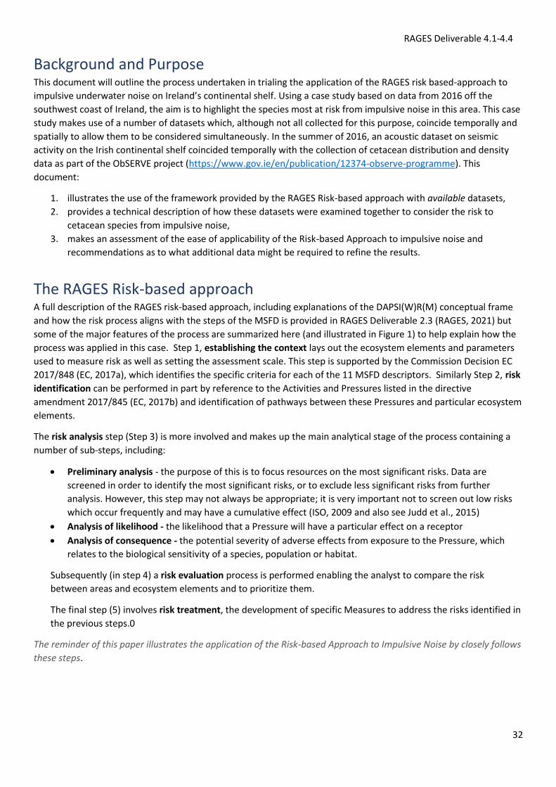
RAGES Deliverable 4.1-4.4
32
Background and Purpose This document will outline the process undertaken in trialing the application of the RAGES risk based-approach to
impulsive underwater noise on Ireland’s continental shelf. Using a case study based on data from 2016 off the
southwest coast of Ireland, the aim is to highlight the species most at risk from impulsive noise in this area. This case
study makes use of a number of datasets which, although not all collected for this purpose, coincide temporally and
spatially to allow them to be considered simultaneously. In the summer of 2016, an acoustic dataset on seismic
activity on the Irish continental shelf coincided temporally with the collection of cetacean distribution and density
data as part of the ObSERVE project (https://www.gov.ie/en/publication/12374-observe-programme). This
document:
1. illustrates the use of the framework provided by the RAGES Risk-based approach with available datasets,
2. provides a technical description of how these datasets were examined together to consider the risk to
cetacean species from impulsive noise,
3. makes an assessment of the ease of applicability of the Risk-based Approach to impulsive noise and
recommendations as to what additional data might be required to refine the results.
The RAGES Risk-based approach A full description of the RAGES risk-based approach, including explanations of the DAPSI(W)R(M) conceptual frame
and how the risk process aligns with the steps of the MSFD is provided in RAGES Deliverable 2.3 (RAGES, 2021) but
some of the major features of the process are summarized here (and illustrated in Figure 1) to help explain how the
process was applied in this case. Step 1, establishing the context lays out the ecosystem elements and parameters
used to measure risk as well as setting the assessment scale. This step is supported by the Commission Decision EC
2017/848 (EC, 2017a), which identifies the specific criteria for each of the 11 MSFD descriptors. Similarly Step 2, risk
identification can be performed in part by reference to the Activities and Pressures listed in the directive
amendment 2017/845 (EC, 2017b) and identification of pathways between these Pressures and particular ecosystem
elements.
The risk analysis step (Step 3) is more involved and makes up the main analytical stage of the process containing a
number of sub-steps, including:
• Preliminary analysis - the purpose of this is to focus resources on the most significant risks. Data are
screened in order to identify the most significant risks, or to exclude less significant risks from further
analysis. However, this step may not always be appropriate; it is very important not to screen out low risks
which occur frequently and may have a cumulative effect (ISO, 2009 and also see Judd et al., 2015)
• Analysis of likelihood - the likelihood that a Pressure will have a particular effect on a receptor
• Analysis of consequence - the potential severity of adverse effects from exposure to the Pressure, which
relates to the biological sensitivity of a species, population or habitat.
Subsequently (in step 4) a risk evaluation process is performed enabling the analyst to compare the risk
between areas and ecosystem elements and to prioritize them.
The final step (5) involves risk treatment, the development of specific Measures to address the risks identified in
the previous steps.0
The reminder of this paper illustrates the application of the Risk-based Approach to Impulsive Noise by closely follows
these steps.
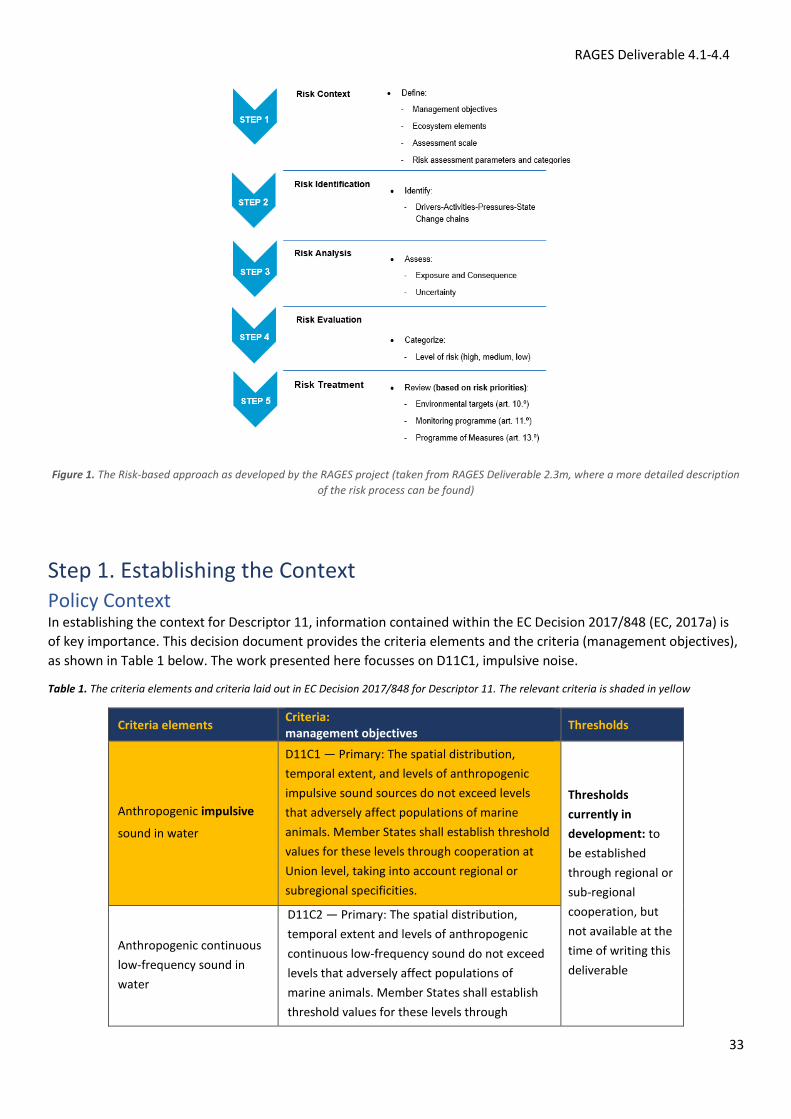
RAGES Deliverable 4.1-4.4
33
Figure 1. The Risk-based approach as developed by the RAGES project (taken from RAGES Deliverable 2.3m, where a more detailed description
of the risk process can be found)
Step 1. Establishing the Context Policy Context In establishing the context for Descriptor 11, information contained within the EC Decision 2017/848 (EC, 2017a) is
of key importance. This decision document provides the criteria elements and the criteria (management objectives),
as shown in Table 1 below. The work presented here focusses on D11C1, impulsive noise.
Table 1. The criteria elements and criteria laid out in EC Decision 2017/848 for Descriptor 11. The relevant criteria is shaded in yellow
Criteria elements Criteria: management objectives
Thresholds
Anthropogenic impulsive
sound in water
D11C1 — Primary: The spatial distribution,
temporal extent, and levels of anthropogenic
impulsive sound sources do not exceed levels
that adversely affect populations of marine
animals. Member States shall establish threshold
values for these levels through cooperation at
Union level, taking into account regional or
subregional specificities.
Thresholds
currently in
development: to
be established
through regional or
sub-regional
cooperation, but
not available at the
time of writing this
deliverable
Anthropogenic continuous
low-frequency sound in
water
D11C2 — Primary: The spatial distribution,
temporal extent and levels of anthropogenic
continuous low-frequency sound do not exceed
levels that adversely affect populations of
marine animals. Member States shall establish
threshold values for these levels through
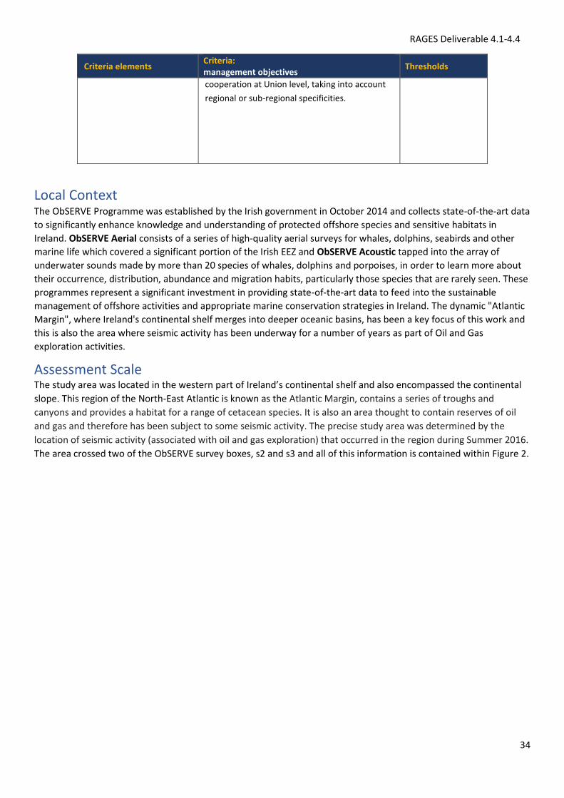
RAGES Deliverable 4.1-4.4
34
Criteria elements Criteria: management objectives
Thresholds
cooperation at Union level, taking into account
regional or sub-regional specificities.
Local Context The ObSERVE Programme was established by the Irish government in October 2014 and collects state-of-the-art data
to significantly enhance knowledge and understanding of protected offshore species and sensitive habitats in
Ireland. ObSERVE Aerial consists of a series of high-quality aerial surveys for whales, dolphins, seabirds and other
marine life which covered a significant portion of the Irish EEZ and ObSERVE Acoustic tapped into the array of
underwater sounds made by more than 20 species of whales, dolphins and porpoises, in order to learn more about
their occurrence, distribution, abundance and migration habits, particularly those species that are rarely seen. These
programmes represent a significant investment in providing state-of-the-art data to feed into the sustainable
management of offshore activities and appropriate marine conservation strategies in Ireland. The dynamic "Atlantic
Margin", where Ireland's continental shelf merges into deeper oceanic basins, has been a key focus of this work and
this is also the area where seismic activity has been underway for a number of years as part of Oil and Gas
exploration activities.
Assessment Scale
The study area was located in the western part of Ireland’s continental shelf and also encompassed the continental
slope. This region of the North-East Atlantic is known as the Atlantic Margin, contains a series of troughs and
canyons and provides a habitat for a range of cetacean species. It is also an area thought to contain reserves of oil
and gas and therefore has been subject to some seismic activity. The precise study area was determined by the
location of seismic activity (associated with oil and gas exploration) that occurred in the region during Summer 2016.
The area crossed two of the ObSERVE survey boxes, s2 and s3 and all of this information is contained within Figure 2.
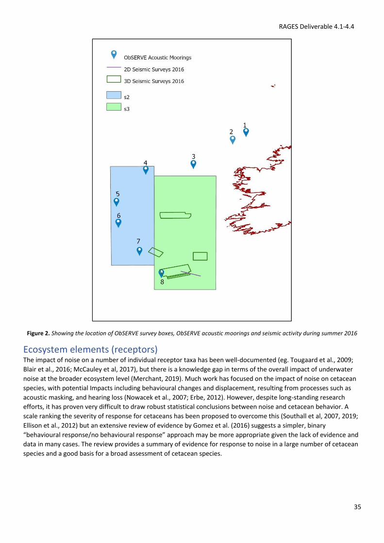
RAGES Deliverable 4.1-4.4
35
Figure 2. Showing the location of ObSERVE survey boxes, ObSERVE acoustic moorings and seismic activity during summer 2016
Ecosystem elements (receptors) The impact of noise on a number of individual receptor taxa has been well-documented (eg. Tougaard et al., 2009;
Blair et al., 2016; McCauley et al, 2017), but there is a knowledge gap in terms of the overall impact of underwater
noise at the broader ecosystem level (Merchant, 2019). Much work has focused on the impact of noise on cetacean
species, with potential Impacts including behavioural changes and displacement, resulting from processes such as
acoustic masking, and hearing loss (Nowacek et al., 2007; Erbe, 2012). However, despite long-standing research
efforts, it has proven very difficult to draw robust statistical conclusions between noise and cetacean behavior. A
scale ranking the severity of response for cetaceans has been proposed to overcome this (Southall et al, 2007, 2019;
Ellison et al., 2012) but an extensive review of evidence by Gomez et al. (2016) suggests a simpler, binary
“behavioural response/no behavioural response” approach may be more appropriate given the lack of evidence and
data in many cases. The review provides a summary of evidence for response to noise in a large number of cetacean
species and a good basis for a broad assessment of cetacean species.
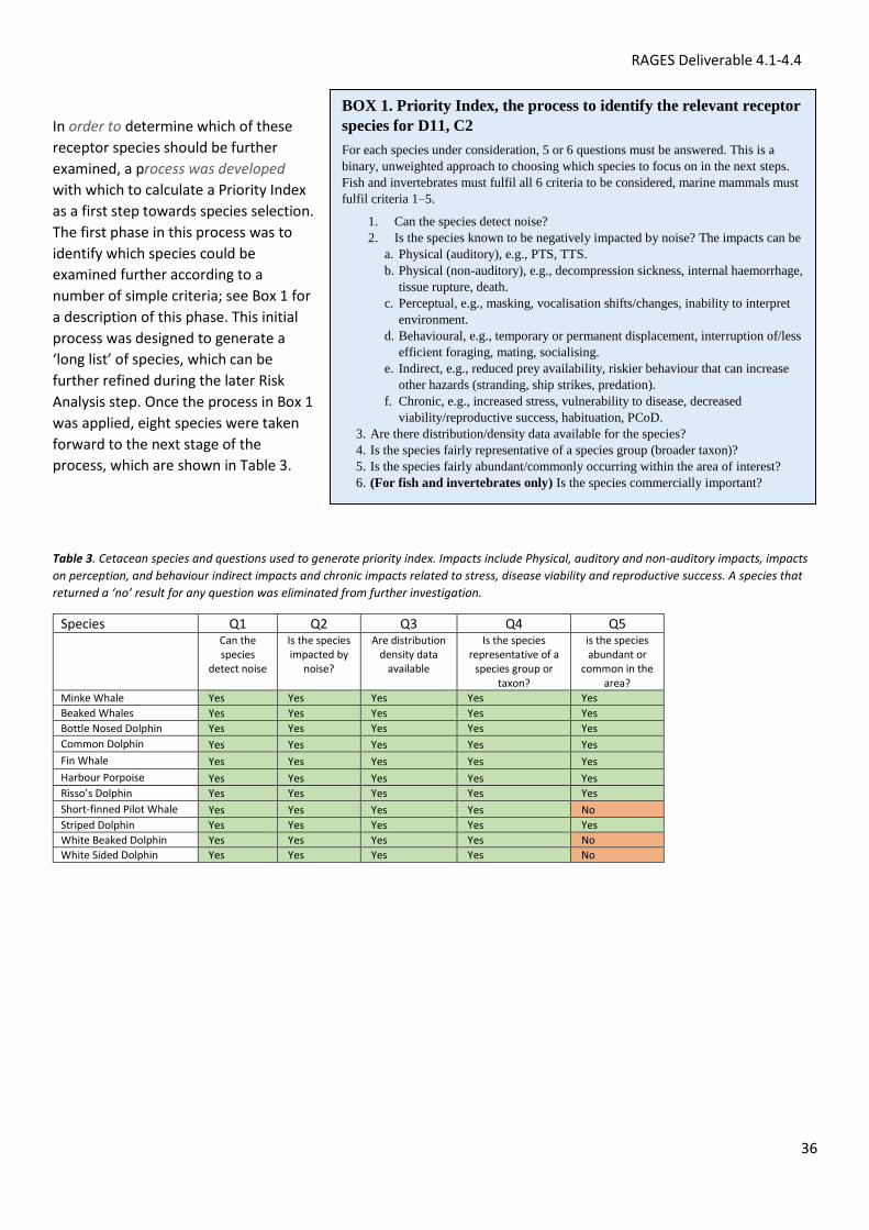
RAGES Deliverable 4.1-4.4
36
In order to determine which of these
receptor species should be further
examined, a process was developed
with which to calculate a Priority Index
as a first step towards species selection.
The first phase in this process was to
identify which species could be
examined further according to a
number of simple criteria; see Box 1 for
a description of this phase. This initial
process was designed to generate a
‘long list’ of species, which can be
further refined during the later Risk
Analysis step. Once the process in Box 1
was applied, eight species were taken
forward to the next stage of the
process, which are shown in Table 3.
Table 3. Cetacean species and questions used to generate priority index. Impacts include Physical, auditory and non-auditory impacts, impacts
on perception, and behaviour indirect impacts and chronic impacts related to stress, disease viability and reproductive success. A species that
returned a ‘no’ result for any question was eliminated from further investigation.
Species Q1 Q2 Q3 Q4 Q5
Can the species
detect noise
Is the species impacted by
noise?
Are distribution density data
available
Is the species representative of a
species group or taxon?
is the species abundant or
common in the area?
Minke Whale Yes Yes Yes Yes Yes
Beaked Whales Yes Yes Yes Yes Yes
Bottle Nosed Dolphin Yes Yes Yes Yes Yes
Common Dolphin Yes Yes Yes Yes Yes
Fin Whale Yes Yes Yes Yes Yes
Harbour Porpoise Yes Yes Yes Yes Yes
Risso’s Dolphin Yes Yes Yes Yes Yes
Short-finned Pilot Whale Yes Yes Yes Yes No
Striped Dolphin Yes Yes Yes Yes Yes
White Beaked Dolphin Yes Yes Yes Yes No
White Sided Dolphin Yes Yes Yes Yes No
BOX 1. Priority Index, the process to identify the relevant receptor
species for D11, C2
For each species under consideration, 5 or 6 questions must be answered. This is a
binary, unweighted approach to choosing which species to focus on in the next steps.
Fish and invertebrates must fulfil all 6 criteria to be considered, marine mammals must
fulfil criteria 1–5.
1. Can the species detect noise?
2. Is the species known to be negatively impacted by noise? The impacts can be
a. Physical (auditory), e.g., PTS, TTS.
b. Physical (non-auditory), e.g., decompression sickness, internal haemorrhage,
tissue rupture, death.
c. Perceptual, e.g., masking, vocalisation shifts/changes, inability to interpret
environment.
d. Behavioural, e.g., temporary or permanent displacement, interruption of/less
efficient foraging, mating, socialising.
e. Indirect, e.g., reduced prey availability, riskier behaviour that can increase
other hazards (stranding, ship strikes, predation).
f. Chronic, e.g., increased stress, vulnerability to disease, decreased
viability/reproductive success, habituation, PCoD.
3. Are there distribution/density data available for the species?
4. Is the species fairly representative of a species group (broader taxon)?
5. Is the species fairly abundant/commonly occurring within the area of interest?
6. (For fish and invertebrates only) Is the species commercially important?
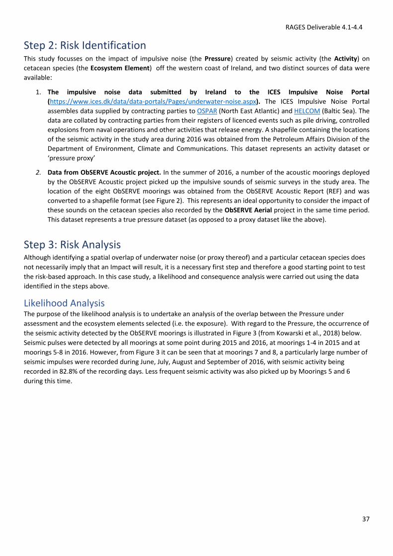
RAGES Deliverable 4.1-4.4
37
Step 2: Risk Identification This study focusses on the impact of impulsive noise (the Pressure) created by seismic activity (the Activity) on
cetacean species (the Ecosystem Element) off the western coast of Ireland, and two distinct sources of data were
available:
1. The impulsive noise data submitted by Ireland to the ICES Impulsive Noise Portal
(https://www.ices.dk/data/data-portals/Pages/underwater-noise.aspx). The ICES Impulsive Noise Portal
assembles data supplied by contracting parties to OSPAR (North East Atlantic) and HELCOM (Baltic Sea). The
data are collated by contracting parties from their registers of licenced events such as pile driving, controlled
explosions from naval operations and other activities that release energy. A shapefile containing the locations
of the seismic activity in the study area during 2016 was obtained from the Petroleum Affairs Division of the
Department of Environment, Climate and Communications. This dataset represents an activity dataset or
‘pressure proxy’
2. Data from ObSERVE Acoustic project. In the summer of 2016, a number of the acoustic moorings deployed
by the ObSERVE Acoustic project picked up the impulsive sounds of seismic surveys in the study area. The
location of the eight ObSERVE moorings was obtained from the ObSERVE Acoustic Report (REF) and was
converted to a shapefile format (see Figure 2). This represents an ideal opportunity to consider the impact of
these sounds on the cetacean species also recorded by the ObSERVE Aerial project in the same time period.
This dataset represents a true pressure dataset (as opposed to a proxy dataset like the above).
Step 3: Risk Analysis Although identifying a spatial overlap of underwater noise (or proxy thereof) and a particular cetacean species does
not necessarily imply that an Impact will result, it is a necessary first step and therefore a good starting point to test
the risk-based approach. In this case study, a likelihood and consequence analysis were carried out using the data
identified in the steps above.
Likelihood Analysis The purpose of the likelihood analysis is to undertake an analysis of the overlap between the Pressure under
assessment and the ecosystem elements selected (i.e. the exposure). With regard to the Pressure, the occurrence of
the seismic activity detected by the ObSERVE moorings is illustrated in Figure 3 (from Kowarski et al., 2018) below.
Seismic pulses were detected by all moorings at some point during 2015 and 2016, at moorings 1-4 in 2015 and at
moorings 5-8 in 2016. However, from Figure 3 it can be seen that at moorings 7 and 8, a particularly large number of
seismic impulses were recorded during June, July, August and September of 2016, with seismic activity being
recorded in 82.8% of the recording days. Less frequent seismic activity was also picked up by Moorings 5 and 6
during this time.
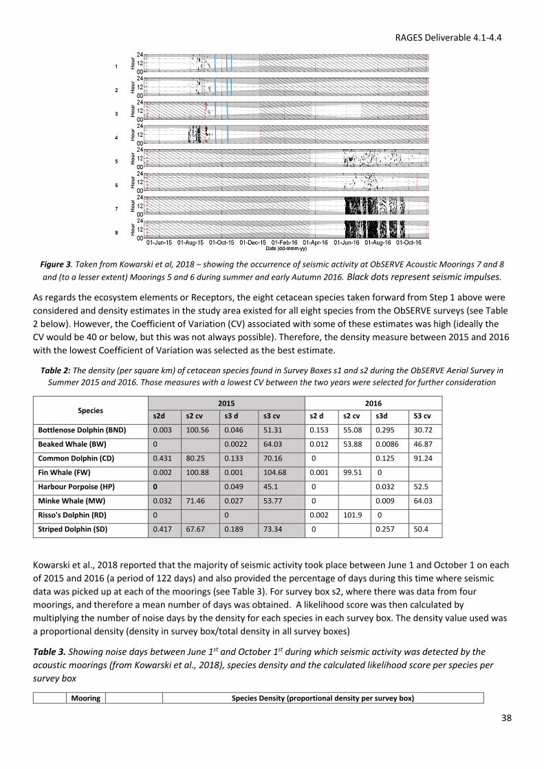
RAGES Deliverable 4.1-4.4
38
Figure 3. Taken from Kowarski et al, 2018 – showing the occurrence of seismic activity at ObSERVE Acoustic Moorings 7 and 8
and (to a lesser extent) Moorings 5 and 6 during summer and early Autumn 2016. Black dots represent seismic impulses.
As regards the ecosystem elements or Receptors, the eight cetacean species taken forward from Step 1 above were
considered and density estimates in the study area existed for all eight species from the ObSERVE surveys (see Table
2 below). However, the Coefficient of Variation (CV) associated with some of these estimates was high (ideally the
CV would be 40 or below, but this was not always possible). Therefore, the density measure between 2015 and 2016
with the lowest Coefficient of Variation was selected as the best estimate.
Table 2: The density (per square km) of cetacean species found in Survey Boxes s1 and s2 during the ObSERVE Aerial Survey in
Summer 2015 and 2016. Those measures with a lowest CV between the two years were selected for further consideration
Species 2015 2016
s2d s2 cv s3 d s3 cv s2 d s2 cv s3d S3 cv
Bottlenose Dolphin (BND) 0.003 100.56 0.046 51.31 0.153 55.08 0.295 30.72
Beaked Whale (BW) 0
0.0022 64.03 0.012 53.88 0.0086 46.87
Common Dolphin (CD) 0.431 80.25 0.133 70.16 0 0.125 91.24
Fin Whale (FW) 0.002 100.88 0.001 104.68 0.001 99.51 0
Harbour Porpoise (HP) 0
0.049 45.1 0 0.032 52.5
Minke Whale (MW) 0.032 71.46 0.027 53.77 0 0.009 64.03
Risso's Dolphin (RD) 0
0 0.002 101.9 0
Striped Dolphin (SD) 0.417 67.67 0.189 73.34 0 0.257 50.4
Kowarski et al., 2018 reported that the majority of seismic activity took place between June 1 and October 1 on each
of 2015 and 2016 (a period of 122 days) and also provided the percentage of days during this time where seismic
data was picked up at each of the moorings (see Table 3). For survey box s2, where there was data from four
moorings, and therefore a mean number of days was obtained. A likelihood score was then calculated by
multiplying the number of noise days by the density for each species in each survey box. The density value used was
a proportional density (density in survey box/total density in all survey boxes)
Table 3. Showing noise days between June 1st and October 1st during which seismic activity was detected by the
acoustic moorings (from Kowarski et al., 2018), species density and the calculated likelihood score per species per
survey box
Mooring Species Density (proportional density per survey box)
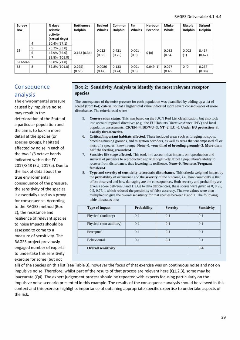
RAGES Deliverable 4.1-4.4
39
Survey Box
% days seismic activity (actual days)
Bottlenose Dolphin
Beaked Whales
Common Dolphin
Fin Whales
Harbour Porpoise
Minke Whale
Risso’s Dolphin
Striped Dolphin
S2
4 30.4% (37.1)
0.153 (0.34) 0.012 (0.58)
0.431 (0.76)
0.001 (0.5)
0 (0) 0.032 (0.54)
0.002 (1)
0.417 (0.62)
5 76.2% (93.0)
6 45.9% (56.0)
7 82.8% (101.0)
S2 Mean 58.8% (71.8)
S3 8 82.8% (101.0) 0.295) (0.65)
0.0086 (0.42)
0.133 (0.24)
0.001 (0.5)
0.049 (1) 0.027 (0.46)
0 (0) 0.257 (0.38)
Consequence analysis The environmental pressure
caused by impulsive noise
may result in the
deterioration of the State of
a particular population and
the aim is to look in more
detail at the species (or
species groups, habitats)
affected by noise in each of
the two 1/3 octave bands
indicated within the EC
2017/848 (EU, 2017a). Due to
the lack of data about the
true environmental
consequence of the pressure,
the sensitivity of the species
is essentially used as a proxy
for consequence. According
to the RAGES method (Box
2), the resistance and
resilience of relevant species
to noise Impacts should be
assessed to come to a
measure of sensitivity. The
RAGES project previously
engaged number of experts
to undertake this sensitivity
exercise for some (but not
all) of the species on this list (see Table 3), however the focus of that exercise was on continuous noise and not on
impulsive noise. Therefore, whilst part of the results of that process are relevant here (Q1,2,3), some may be
inaccurate (Q4). The expert judgement process should be repeated with experts focusing particularly on the
impulsive noise scenario presented in this example. The results of the consequence analysis should be viewed in this
context and this exercise highlights importance of obtaining appropriate specific expertise to undertake aspects of
the risk.
Box 2: Sensitivity Analysis to identify the most relevant receptor
species
The consequence of the noise pressure for each population was quantified by adding up a list of
scaled (from 0-4) criteria, so that a higher total value indicated more severe consequences of noise
disturbance. The criteria used were:
5. Conservation status. This was based on the IUCN Red List classification, but also took
into account regional directives (e.g., the EU Habitats Directive Annex II/IV) and local
population assessments. CR/EN=4, DD/VU=3, NT=2, LC=0, Under EU protection=3,
Locally threatened=4
6. Critical/important habitats affected. These included areas such as foraging hotspots,
breeding/nursing grounds, and migration corridors, as well as areas that encompassed all or
most of a species’ known range. None=0, ~one third of breeding grounds=3, More than
half the feeding grounds=4
7. Sensitive life stage affected. This took into account that impacts on reproduction and
survival of juveniles to reproductive age will negatively affect a population’s ability to
recover from disturbance, thus lowering its resilience. None=0, Neonates/Pregnant
females=4
8. Type and severity of sensitivity to acoustic disturbance. This criteria weighted impact by
the probability of occurrence and the severity of the outcome, i.e., how commonly is that
effect observed and how damaging are the consequences. Both severity and probability are
given a score between 0 and 1. Due to data deficiencies, these scores were given as 0, 0.25,
0.5, 0.75, 1 which reduced the possibility of false accuracy. The two values were then
multiplied to give the overall sensitivity for that species between 0 and 1. The following
table illustrates this:
Type of impact Probability Severity Sensitivity
Physical (auditory) 0-1 0-1 0-1
Physical (non-auditory) 0-1 0-1 0-1
Perceptual 0-1 0-1 0-1
Behavioural 0-1 0-1 0-1
Overall sensitivity 0-4
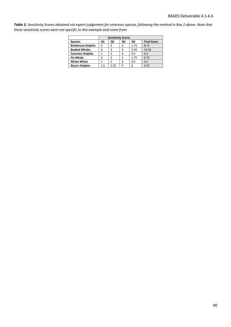
RAGES Deliverable 4.1-4.4
40
Table 3. Sensitivity Scores obtained via expert judgement for cetacean species, following the method in Box 2 above. Note that
these sensitivity scores were not specific to this example and come from
Sensitivity Scores
Species Q1 Q2 Q3 Q4 Final Score
Bottlenose Dolphin 0 4 3 1.75 8.75
Beaked Whales 4 3 4 2.56 13.56
Common Dolphin 1 2 4 0.5 6.5
Fin Whale 3 3 2 1.75 9.75
Minke Whale 1 2 4 0.5 6.5
Risso's Dolphin 1.5 3.25 0 0 4.75
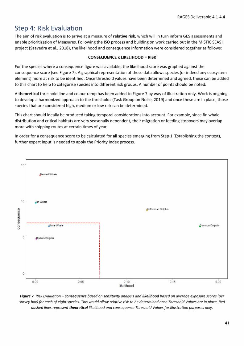
RAGES Deliverable 4.1-4.4
41
Step 4: Risk Evaluation The aim of risk evaluation is to arrive at a measure of relative risk, which will in turn inform GES assessments and
enable prioritization of Measures. Following the ISO process and building on work carried out in the MISTIC SEAS II
project (Saavedra et al., 2018), the likelihood and consequence information were considered together as follows:
CONSEQUENCE x LIKELIHOOD = RISK
For the species where a consequence figure was available, the likelihood score was graphed against the
consequence score (see Figure 7). A graphical representation of these data allows species (or indeed any ecosystem
element) more at risk to be identified. Once threshold values have been determined and agreed, these can be added
to this chart to help to categorise species into different risk groups. A number of points should be noted:
A theoretical threshold line and colour ramp has been added to Figure 7 by way of illustration only. Work is ongoing
to develop a harmonized approach to the thresholds (Task Group on Noise, 2019) and once these are in place, those
species that are considered high, medium or low risk can be determined.
This chart should ideally be produced taking temporal considerations into account. For example, since fin whale
distribution and critical habitats are very seasonally dependent, their migration or feeding stopovers may overlap
more with shipping routes at certain times of year.
In order for a consequence score to be calculated for all species emerging from Step 1 (Establishing the context),
further expert input is needed to apply the Priority Index process.
Figure 7. Risk Evaluation – consequence based on sensitivity analysis and likelihood based on average exposure scores (per
survey box) for each of eight species. This would allow relative risk to be determined once Threshold Values are in place. Red
dashed lines represent theoretical likelihood and consequence Threshold Values for illustration purposes only.

RAGES Deliverable 4.1-4.4
42
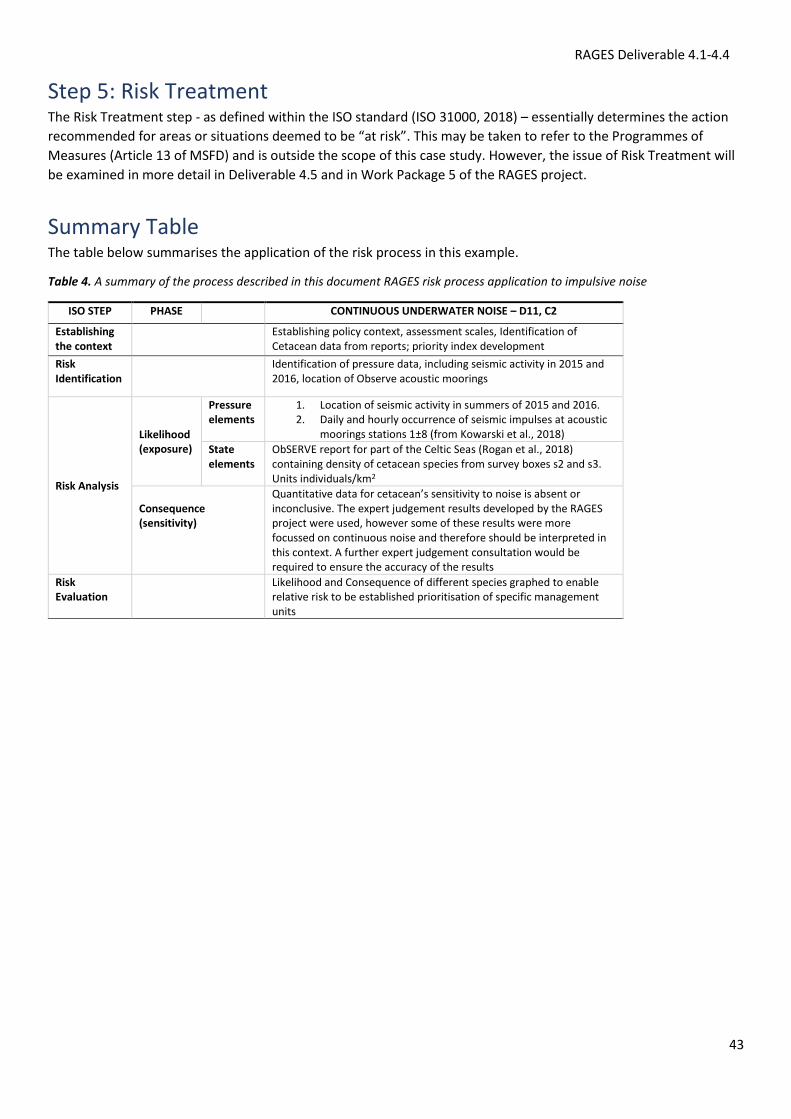
RAGES Deliverable 4.1-4.4
43
Step 5: Risk Treatment The Risk Treatment step - as defined within the ISO standard (ISO 31000, 2018) – essentially determines the action
recommended for areas or situations deemed to be “at risk”. This may be taken to refer to the Programmes of
Measures (Article 13 of MSFD) and is outside the scope of this case study. However, the issue of Risk Treatment will
be examined in more detail in Deliverable 4.5 and in Work Package 5 of the RAGES project.
Summary Table The table below summarises the application of the risk process in this example.
Table 4. A summary of the process described in this document RAGES risk process application to impulsive noise
ISO STEP PHASE
CONTINUOUS UNDERWATER NOISE – D11, C2
Establishing the context
Establishing policy context, assessment scales, Identification of Cetacean data from reports; priority index development
Risk Identification
Identification of pressure data, including seismic activity in 2015 and 2016, location of Observe acoustic moorings
Risk Analysis
Likelihood (exposure)
Pressure elements
1. Location of seismic activity in summers of 2015 and 2016. 2. Daily and hourly occurrence of seismic impulses at acoustic
moorings stations 1±8 (from Kowarski et al., 2018)
State elements
ObSERVE report for part of the Celtic Seas (Rogan et al., 2018) containing density of cetacean species from survey boxes s2 and s3. Units individuals/km2
Consequence (sensitivity)
Quantitative data for cetacean’s sensitivity to noise is absent or inconclusive. The expert judgement results developed by the RAGES project were used, however some of these results were more focussed on continuous noise and therefore should be interpreted in this context. A further expert judgement consultation would be required to ensure the accuracy of the results
Risk Evaluation
Likelihood and Consequence of different species graphed to enable relative risk to be established prioritisation of specific management units
RAGES Deliverable 4.1-4.4
44
References Blair HB, Merchant ND, Friedlaender AS, Wiley DN and Parks SE. (2016). Evidence for ship noise impacts on
humpback whales foraging behaviour. Biology Letters 12: 20160005.
Ellison W, Southall B, Clark C, and Franke A. (2012). A new context-based approach to assess marine mammal
behavioral responses to anthropogenic sounds. Conservation Biology 26(1): 21–28.
Erbe C. (2012) The effects of underwater noise on marine mammals. In: Popper AN, Hawkins AD, editors. The Effects
of Noise on Aquatic Life Advances in Experimental Medicine and Biology 730. New York: Springer Verlag. pp. 17–22.
European Commission (2017a). Commission Decision 2017/848 of 17 May 2017 laying down criteria and
methodological standards on good environmental status of marine waters and specifications and standardised
methods for monitoring and assessment, and repealing Decision 2010/477/EU. Official Journal of the European
Union L 125: 43-74.
European Commission (2017b). Commission Directive 2017/845 of 17 May 2017. Amending Directive 2008/56/EC of
the European Parliament and of the Council as regards the indicative lists of elements to be taken into account for
the preparation of marine strategies. Official Journal of the European Union L 125: 27-33.
Gomez C, Lawson JW, Wright AJ, Buren AD, Tollit D and Lesage V. 2016. A systematic review on the behavioural
responses of wild marine mammals to noise: the disparity between science and policy. Canadian Journal of Zoology
94: 801–819.
Kowarski K, Delarue J, Martin B, O’Brien J, Meade R, Ó’Cadhla O, Berrow, S. (2018). Signals from the deep: Spatial
and temporal acoustic occurrence of beaked whales off western Ireland. PLOS ONE 13(6):
e0199431. https://doi.org/10.1371/journal.pone.0199431
McCauley RD, Day RD, Swadling KM, Fitzgibbon QP, Watson RA and Semmems JM (2017). Widely used marine
seismic survey air gun operations negatively impact zooplankton. Nature Ecology and Evolution 1: 0195.
Merchant, ND (2019). Underwater noise abatement: Economic factors and policy options. Environmental Science &
Policy 92: 116-123.
Nowacek DP, Thorne LH, Johnston DW and Tyack PL. (2007). Responses of cetaceans to anthropogenic noise.
Mammal Review 37: 81–115.
RAGES (2021). Developing a Risk-based Approach to Good Environmental Status. Risk Based Approaches to Good
Environmental Status (RAGES) Project Deliverable 2.3. GRANT AGREEMENT Nº 110661/2018/794607/SUB/ENV.C.2.
Silva, M.A., Cascão, I., Romagosa, M., Soares C., Jesus, S.M. (2021). The Azores case study: comparing risk analyses
based on shipping density and acoustic modelling. Report to RAGES Project – WP4: Applying the RAGES Risk-Based
Approach to MSFD Descriptor 11, Underwater Noise, 15 pp + 1 annex.
Southall BL, Bowles AE, Ellison WT, Finneran JJ, Gentry RL and others (2007). Marine Mammal Noise Exposure
Criteria: Initial Scientific Recommendations. Aquatic Mammals 33: 411–521.
Southall BL, Finneran JJ, Reichmuth C, Nachtigall PE, Ketten DR, Bowles AE, Ellison WT, Nowacek DP and Tyack PL.
(2019). Marine Mammal Noise Exposure Criteria: Updated Scientific Recommendations for Residual Hearing Effects.
Aquatic Mammals 45(2): 125-232.
Tougaard J, Cartensen J, Teilmann J, Skov H and Rasmussen P. (2009). Pile-driving zone of responsiveness extends
beyond 20km for harbor porpoises (Phocoena phocoena (L)). Journal of the Acoustical Society of America 126: 11-14.