
My-TRAC Deliverable 2.3
121
My TRAvel Companion. Deliverable D2.3 Modelling Framework for Analysing Users’ Choices Project funded by the European Union’s Horizon 2020 Research and Innovation Programme (2014 – 2020) Ref. Ares(2019)7393179 - 01/12/2019
-
Upload
khangminh22 -
Category
Documents
-
view
1 -
download
0
Transcript of My-TRAC Deliverable 2.3
Deliverable 2.3: Modelling framework for analysing users’ choices Page 1 of 121
My TRAvel Companion.
Deliverable D2.3 Modelling Framework for Analysing Users’
Choices
Project funded by the European Union’s Horizon 2020 Research and Innovation Programme (2014 – 2020)
Ref. Ares(2019)7393179 - 01/12/2019

Deliverable 2.3: Modelling framework for analysing users’ choices Page 2 of 121
Deliverable 2.3: Modelling Framework for Analysing Users’ Choices
Due date of deliverable: 30 November 2019
Actual submission date: 29 November 2019
Start date of project: 01/09/2018 Duration: 36 months
Dissemination Level
PU Public X
CO Confidential, restricted under conditions set out in Model Grant Agreement
CI Classified, information as referred to in Commission Decision 2001/844/EC

Deliverable 2.3: Modelling framework for analysing users’ choices Page 3 of 121
1 Document Control Sheet Deliverable number: D2.3
Deliverable responsible: TECHNISCHE UNIVERSITEIT DELFT
Work package: WP2
Main editor: Sanmay Shelat
Editor name Organisation
Sanmay Shelat TECHNISCHE UNIVERSITEIT DELFT
Eleni Mantouka, Konstantinos Mavromatis
AETHON SYMVOULI MICHANIKI MONOPROSOPI IKE
Alexandros Zamichos, Maria Tsourma
ETHNIKO KENTRO EREVNAS KAI TECHNOLOGIKIS ANAPTYXIS
Modifications Introduced
Version Date Reason Editor
0.1 18 Sep 2018 Outline of deliverable Sanmay Shelat
0.2 5 Aug 2019 AETHON contribution 1st draft Eleni Mantouka
0.2.1 2 Sep 2019 General review and comments on AETHON’s contribution
Sanmay Shelat
0.3 10 Sep 2019 AETHON revised contribution 2nd draft Konstantinos Mavromatis
1.1 12 Nov 2019 Full deliverable (with contributions from TUD, AETHON, CERTH-ITI) 1st draft
Sanmay Shelat
1.1.1 20 Nov 2019 Internal review Pablo Chamoso
1.1.2 22 Nov 2019 Internal review Joan Guisado-Gámez
1.2.1 25 Nov 2019 TUD revised contribution Sanmay Shelat
1.2.2 27 Nov 2019 AETHON revised contribution Eleni Mantouka
1.2.3 28 Nov 2019 CERTH revised contribution Maria Tsourma, Anastasios Drosou
1.3 28 Nov 2019 Full revised deliverable 2nd draft (based on comments from internal review)
Sanmay Shelat
1.3.1 29 Nov 2019 2nd internal review Pablo Chamoso
1.3.2 29 Nov 2019 2nd internal review Joan Guisado-Gámez
1.4 29 Nov 2019 Final version Sanmay Shelat
Legal Disclaimer
The information in this document is provided “as is”, and no guarantee or warranty is given that the information is fit for any particular purpose. The above referenced consortium members shall have no liability to third parties for damages of any kind including without limitation direct, special, indirect, or consequential damages that may result from the use of these materials subject to any liability which is mandatory due to applicable law. © 2017 by My-TRAC Consortium.
Deliverable 2.3: Modelling framework for analysing users’ choices Page 4 of 121
EXECUTIVE SUMMARY One of the most important objectives of My-TRAC is to develop an innovative mobile application that can act as a companion for travellers, providing them with timely, meaningful, and personalized advice on various decisions related to their trips. Understanding the behaviour of decision-makers is crucial to providing recommendations. Apart from hard factors, such as minimizing travel time, we need to pay close attention to softer factors, such as emotions, attitudes, and perceptions of risk and uncertainty.
Given the importance of understanding the behaviour of travellers, task 2.3 (T2.3) aims to model the various choices travellers make before and during a journey. Specifically, three choice dimensions are considered: (i) travel mode (e.g., car, public transport, bicycle), (ii) departure time, and (iii) route choice. We assume that these choices are made sequentially and under the random utility maximization paradigm. The selected choice dimensions modelled should be sufficient to describe the movement of a traveller from their origin to destination. For each choice dimension, the trade-off between all relevant hard attributes (e.g., waiting time, in-vehicle time) as well as the effect of attitudinal and perception-based attributes are analysed. Thus, the main output of this deliverable, D2.3, is a set of baseline models of the population’s (i.e., average, non-personalized) behavioural characteristics over different choice dimensions – a framework for analysing users’ choices.
For the analysis, we mainly use stated preferences data collected from three locations where the pilots will be conducted, namely, the Netherlands, Greece (Athens), and Portugal (Lisbon). The general workflow involved designing the experiment, collecting data (either online or on-site), processing the collected data (removing invalid responses, encoding responses for analyses), and through trial-and-error estimating the final choice model (which is based on some model fit criteria). The estimated models include information about: (i) personal characteristics, including socio-demographics, mobility characteristics, and other qualitative factors (e.g., regret, tolerance); (ii) trip contexts, including trip purpose and other factors describing conditions under which the trip is made; and (iii) attributes of available (and considered) alternatives. Therefore, we are able to discuss how travellers of different backgrounds and personalities behave in different travel situations.
For mode choice, hard factors such as travel time, cost, and comfort are considered. Amongst the choices offered in the experiment were car, public transport, bicycle (in the Netherlands), and motorcycle (in Greece and Portugal). Departure time choice is between depart ‘on time’, ‘early’, or ‘late’, and is only modelled for public transport modes, considering travel time, walking time (to station), frequency of vehicles, and fare discount (as percentage) as the main alternative attributes. We discuss the effect of different attributes in detail, also comparing results across pilot locations and with literature.
For route choice, three models are presented. In the first model, the focus is on capturing waiting time uncertainty that travellers in public transport networks feel. This is done through a stated preference experiment with a novel choice situation that permits the quantification of subjective beliefs regarding uncertainty as well as the effect of context and personal characteristics on this uncertainty. Findings indicated an average preference for certainty, with travellers willing to accept between 3 and 10 minutes of extra in-vehicle time to avoid uncertainty in waiting time. We further report the effects of context and personal characteristics on beliefs regarding uncertainty for the three countries.
As more and more data becomes available, through the My-TRAC application and other sources, revealed preferences will be the main source for behaviour analyses and consumer studies in the future. To this end, the next two route choice models focus on studying revealed preferences from the pre-dominant source of such data today: smart card data. The first model in this category develops a methodology to automatically calibrate the composition of route choice sets using the non-compensatory elimination-by-aspects decision
Deliverable 2.3: Modelling framework for analysing users’ choices Page 5 of 121
rule. Analysing the alternatives considered by decision-makers when choosing is critical to both accurate behaviour modelling as well as presenting application users with appropriate options.
In the third and final route choice model (also estimated from smart card data), we present a comparison of different representations of risky waiting time in choice models. To do this we first outline a generic methodology to estimate route choice models from revealed preference data sources. Comparison results show the importance of including information on both deviation from schedule and dispersion of waiting times in choice models.
Finally, the activity model developed in two other deliverables (D2.2, D3.3), is briefly presented here to align with the complete set of user choices. Moreover, the data required for re-estimation of the models (based on continuous observations from the My-TRAC application) described in this deliverable using such data are also tabulated.
In conclusion, this deliverable produces a set of baseline population choice models that may be personalized to individuals and provide recommendations in subsequent tasks of this project using continuous observations from the My-TRAC application. Apart from this, the scientific contribution highlights a few avenues for future research. For instance, more research is required on better connecting attitudes and perceptions with eventual travel behaviour. Specifically, methodologies that allow us to separate the effects of the different aspects will be helpful in providing more targeted and meaningful policies. Another important area, is to use revealed preferences to study the effects of situational contexts on choice behaviour, which stated preferences may not be able to fully capture.

Deliverable 2.3: Modelling framework for analysing users’ choices Page 6 of 121
Consortium of partners
UNIVERSITAT POLITECNICA DE CATALUNYA
Spain
ETHNIKO KENTRO EREVNAS KAI TECHNOLOGIKIS ANAPTYXIS
Greece
TECHNISCHE UNIVERSITEIT DELFT Netherlands AETHON SYMVOULI MICHANIKI MONOPROSOPI IKE
Greece
EXPERIS MANPOWERGROUP SL Spain STRA LDA Portugal
ATTIKO METRO AE Greece
UNIVERSIDAD DE SALAMANCA Spain
UNION INTERNATIONALE DES TRANSPORTS PUBLICS
Belgium
Deliverable 2.3: Modelling framework for analysing users’ choices Page 7 of 121
Table of Contents
Executive Summary 4
1 Introduction 13 1.1 Why Model Behaviour? 13 1.2 Task 2.3 Objective, Workflow, and Position in My-TRAC 14 1.3 General Assumptions 14 1.4 Deliverable Structure 15
2 Mode and Departure Time Choice 16 2.1 Methodology 17
2.1.1 The Multinomial Logit Model 18 2.2 Experiment Design 18
2.2.1 Questionnaire Design 18 2.3 Data Collection 21
2.3.1 Descriptive Statistics 22 2.4 Model Implementation, Results , and Discussion 28
2.4.1 Travel Mode Choice 28 2.4.2 Time of Departure Choice 35
2.5 Summary 40
3 Route Choice 41 3.1 Model 1: Capturing Waiting Time Uncertainty 42
3.1.1 Theoretical Framework 43 3.1.2 Choice Situation 45 3.1.3 Research Approach: Stated Preferences Experiment 47 3.1.4 Results & Discussion 52 3.1.5 Summary 58
3.2 Model 2: Inferring Route Choice Sets 59 3.2.1 Behavioural Models for Choice Set Formation 61 3.2.2 Route Choice Set Generation Methodology 62 3.2.3 Case Study: The Hague Tram & Bus Network 68 3.2.4 Summary 72
3.3 Model 3: Estimating Route Choice Models from Revealed Preferences 73 3.3.1 Methodology 73 3.3.2 Case Study: The Hague Tram & Bus Network 76 3.3.3 Summary 79
4 Activity Modelling 81 4.1 Activity Prediction module 84 4.2 Activity Recognition module and Twitter data collector 85 4.3 Recommendation system 86
5 Data Requirements 89 5.1 Data Sources and Acquisition 89
6 Conclusions 92 6.1 Future Research 93

Deliverable 2.3: Modelling framework for analysing users’ choices Page 8 of 121
7 References 94
8 Appendices 98
Appendix A Comparison of Travellers in Spain and Greece 99
Appendix B Mode and Departure Time Choice Stated Preferences Questionnaire 101
B.1 Netherlands 101 B.2 Greece & Portugal 104
Appendix C Route Choice Stated Preferences Questionnaires 107
Deliverable 2.3: Modelling framework for analysing users’ choices Page 9 of 121
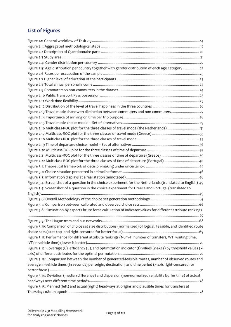
List of Figures
Figure 1.1: General workflow of Task 2.3 .............................................................................................................. 14 Figure 2.1: Aggregated methodological steps ..................................................................................................... 17 Figure 2.2 Description of Questionnaire parts .................................................................................................... 20 Figure 2.3 Study area ............................................................................................................................................. 21 Figure 2.4: Gender distribution per country ........................................................................................................ 22 Figure 2.5: Age distribution per country together with gender distribution of each age category ................. 22 Figure 2.6 Rates per occupation of the sample ................................................................................................... 23 Figure 2.7 Higher level of education of the participants ..................................................................................... 23 Figure 2.8 Total annual personal income ............................................................................................................ 24 Figure 2.9 Commuters vs non-commuters in the dataset .................................................................................. 24 Figure 2.10 Public Transport Pass possession ...................................................................................................... 25 Figure 2.11 Work time flexibility ............................................................................................................................ 25 Figure 2.12 Distribution of the level of travel happiness in the three countries ............................................... 26 Figure 2.13 Travel mode share with distinction between commuters and non-commuters ............................. 27 Figure 2.14 Importance of arriving on time per trip purpose ............................................................................. 28 Figure 2.15 Travel mode choice model – Set of alternatives .............................................................................. 29 Figure 2.16 Multiclass-ROC plot for the three classes of travel mode (the Netherlands) ................................. 31 Figure 2.17 Multiclass-ROC plot for the three classes of travel mode (Greece) ................................................. 33 Figure 2.18 Multiclass-ROC plot for the three classes of travel mode ................................................................ 35 Figure 2.19 Time of departure choice model – Set of alternatives .................................................................... 36 Figure 2.20 Multiclass-ROC plot for the three classes of time of departure ...................................................... 37 Figure 2.21 Multiclass-ROC plot for the three classes of time of departure (Greece) ...................................... 39 Figure 2.22 Multiclass-ROC plot for the three classes of time of departure (Portugal) ................................... 40 Figure 3.1: Theoretical framework of decision-making under uncertainty. ...................................................... 44 Figure 3.2: Choice situation presented in a timeline format .............................................................................. 46 Figure 3.3: Information displays at a real station (annotated) .......................................................................... 48 Figure 3.4: Screenshot of a question in the choice experiment for the Netherlands (translated to English) 49 Figure 3.5: Screenshot of a question in the choice experiment for Greece and Portugal (translated to English) ................................................................................................................................................................. 49 Figure 3.6: Overall Methodology of the choice set generation methodology ................................................. 63 Figure 3.7: Comparison between calibrated and observed choice sets ............................................................ 66 Figure 3.8: Elimination-by-aspects brute force calculation of indicator values for different attribute rankings .............................................................................................................................................................................. 67 Figure 3.9: The Hague tram and bus networks ................................................................................................... 68 Figure 3.10: Comparison of choice set size distributions (normalized) of logical, feasible, and identified route choice sets (axes top- and right-censored for better focus) ............................................................................. 69 Figure 3.11: Performance for different attribute rankings (Num-T: number of transfers, WT: waiting time, IVT: in-vehicle time) (lower is better) .................................................................................................................. 70 Figure 3.12: Coverage (C), efficiency (E), and optimization indicator (I) values (y-axes) by threshold values (x-axis) of different attributes for the optimal permutation ................................................................................. 70 Figure 3.13: Comparison between the number of generated-feasible routes, number of observed routes and average in-vehicle times (in seconds) per origin, destination, and time period (x-axis right-censored for better focus) ......................................................................................................................................................... 71 Figure 3.14: Deviation (median difference) and dispersion (non-normalized reliability buffer time) of actual headways over different time periods ................................................................................................................ 78 Figure 3.15: Planned (left) and actual (right) headways at origins and plausible times for transfers at Thursdays 0800h-0900h ...................................................................................................................................... 78

Deliverable 2.3: Modelling framework for analysing users’ choices Page 10 of 121
Figure 4.1: Flow of information implemented within WP2 and WP3. Activity Prediction and Activity Recognition modules implemented within WP2 are used periodically to create the sequences of user’s daily activity types, used to form the user’s activity profile. User’s activity profile is provided as input for the Activity Prediction module, aiming at providing personalized predictions of the user’s anticipated activity type. When a user plans a trip from My-TRAC application, the recommendation system is used to provide recommendations about several places of interest that a user could visit based the user’s anticipated activity provided via the Activity Prediction module and the information retrieved by the My-TRAC application regarding the destination of the trip planned. ............................................................................... 82 Figure 4.2: Creation of sequences of activities included in a user’s activity profile based on the input provided by both Activity Prediction and Activity Recognition mechanism. Example of the update of the sequence of activities is provided. ...................................................................................................................... 85 Figure 8.1 Mean values of attributes for each travel mode for Greece and Spain [from D2.1] ........................ 99 Figure 8.2 Average values of the importance of factors on travel mode choice per country [from D2.1] ..... 100
Deliverable 2.3: Modelling framework for analysing users’ choices Page 11 of 121
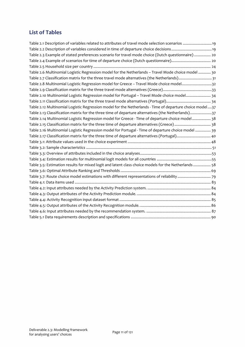
List of Tables
Table 2.1 Description of variables related to attributes of travel mode selection scenarios ............................ 19 Table 2.2 Description of variables considered in time of departure choice decisions ....................................... 19 Table 2.3 Example of stated preferences scenario for travel mode choice (Dutch questionnaire) ................ 20 Table 2.4 Example of scenarios for time of departure choice (Dutch questionnaire)...................................... 20 Table 2.5 Household size per country ................................................................................................................. 24 Table 2.6 Multinomial Logistic Regression model for the Netherlands – Travel Mode choice model ............ 30 Table 2.7 Classification matrix for the three travel mode alternatives (the Netherlands) ................................ 31 Table 2.8 Multinomial Logistic Regression model for Greece – Travel Mode choice model ............................. 32 Table 2.9 Classification matrix for the three travel mode alternatives (Greece) ............................................... 33 Table 2.10 Multinomial Logistic Regression model for Portugal – Travel Mode choice model ........................ 34 Table 2.11 Classification matrix for the three travel mode alternatives (Portugal)........................................... 34 Table 2.12 Multinomial Logistic Regression model for the Netherlands - Time of departure choice model .... 37 Table 2.13 Classification matrix for the three time of departure alternatives (the Netherlands) ..................... 37 Table 2.14 Multinomial Logistic Regression model for Greece - Time of departure choice model .................. 38 Table 2.15 Classification matrix for the three time of departure alternatives (Greece) ................................... 38 Table 2.16 Multinomial Logistic Regression model for Portugal - Time of departure choice model ............... 39 Table 2.17 Classification matrix for the three time of departure alternatives (Portugal) ................................. 40 Table 3.1: Attribute values used in the choice experiment ................................................................................ 48 Table 3.2: Sample characteristics ......................................................................................................................... 51 Table 3.3: Overview of attributes included in the choice analyses ..................................................................... 53 Table 3.4: Estimation results for multinomial logit models for all countries .....................................................55 Table 3.5: Estimation results for mixed logit and latent class choice models for the Netherlands ................. 58 Table 3.6: Optimal Attribute Ranking and Thresholds ....................................................................................... 69 Table 3.7: Route choice model estimations with different representations of reliability ................................ 79 Table 4.1: Data items used ................................................................................................................................... 83 Table 4.2: Input attributes needed by the Activity Prediction system. ............................................................. 84 Table 4.3: Output attributes of the Activity Prediction module. ....................................................................... 84 Table 4.4: Activity Recognition input dataset format ........................................................................................ 85 Table 4.5: Output attributes of the Activity Recognition module. .................................................................... 86 Table 4.6: Input attributes needed by the recommendation system. .............................................................. 87 Table 5.1 Data requirements description and specifications ............................................................................. 90
Deliverable 2.3: Modelling framework for analysing users’ choices Page 12 of 121
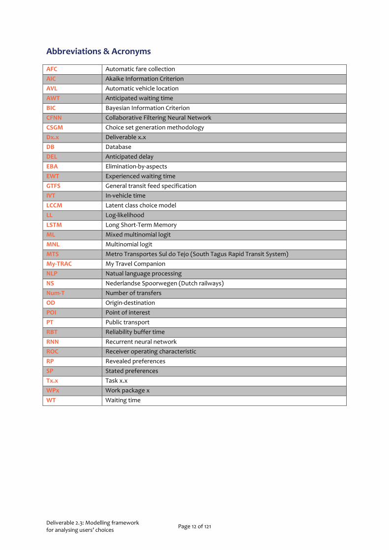
Abbreviations & Acronyms
AFC Automatic fare collection AIC Akaike Information Criterion AVL Automatic vehicle location AWT Anticipated waiting time BIC Bayesian Information Criterion CFNN Collaborative Filtering Neural Network CSGM Choice set generation methodology Dx.x Deliverable x.x DB Database DEL Anticipated delay EBA Elimination-by-aspects EWT Experienced waiting time GTFS General transit feed specification IVT In-vehicle time LCCM Latent class choice model LL Log-likelihood LSTM Long Short-Term Memory ML Mixed multinomial logit MNL Multinomial logit MTS Metro Transportes Sul do Tejo (South Tagus Rapid Transit System) My-TRAC My Travel Companion NLP Natual language processing NS Nederlandse Spoorwegen (Dutch railways) Num-T Number of transfers OD Origin-destination POI Point of interest PT Public transport RBT Reliability buffer time RNN Recurrent neural network ROC Receiver operating characteristic RP Revealed preferences SP Stated preferences Tx.x Task x.x WPx Work package x WT Waiting time

Deliverable 2.3: Modelling framework for analysing users’ choices Page 13 of 121
1 INTRODUCTION One of the most important objectives of My-TRAC is to develop an innovative mobile application that can act as a companion for travellers, providing them with timely, meaningful, and personalized advice on various decisions related to their trips. Understanding the travel behaviour of users is crucial to providing recommendations. To this end, within the My-TRAC project, work package 2 (WP2) focusses on ‘user-centred behaviour and analysis’. After identifying key factors affecting travel behaviour in deliverable 2.1 (D2.1), in this deliverable for task 2.3 (T2.3) we focus on modelling travellers’ choices. In this introductory section, we will first briefly argue why describing travel behaviour is important for providing useful recommendations and to which aspects we must pay special attention. Next in section 1.2, the objective of this task, its output, the general methodology, and relationship with other parts of the project are presented. For practical reasons, we make some general assumptions in the choice modelling parts of the report; these are presented in section 1.3. Finally, the deliverable structure is outlined in section 1.4.
1.1 WHY MODEL BEHAVIOUR?
In everyday life, we see a lot of recommendations; for instance, the next video auto-played on YouTube, an advertisement recommending that we buy a particular brand of cereal, or an investment portfolio recommendation. Clearly, each recommendation has a different purpose which describes what the recommender would like the decision-maker to do. Regardless of the intention of the normative action (i.e., what should be done), each recommender, in general, and each recommendation, specifically, must have one. However, often defining normative behaviour is not as straightforward increasing the sale of a particular brand of cereal. Consider the case of investment portfolio composition. For a ‘rational’ (basically, the investor must like more money than less – see Kreps [1] for the specific behavioural axioms required) investor of a particular level of wealth and intended investment period, given historical data, there exists an optimal portfolio which should be recommended as it maximizes expected returns. Yet, before providing any recommendations, an investment advisor would first assess the investor’s risk profile which indicates the level of risk with which the investor is comfortable. This indicates that the normative action is not as simple as maximizing one’s profit but something more complicated and personal. In contrast, personal preferences may also be used to remove biases such as risk aversion or loss aversion [2], in order to provide suggestions that are objectively more rational. Furthermore, to provide impactful recommendations, it is necessary understand what affects decision-makers most. For instance, cereal brands may want to know what consumers are interested in (e.g., iron content of cereal) so that those aspects can be emphasised in advertisements. Similarly, if the aim of an online media provider is to keep users on their platform for as long as possible, then they may suggest the next video based on users’ past views and search histories. A related consideration may be the timing of advice – depending on our aim we would like decision-makers to either make a conscious, calculated decision (change their behaviour or reinforce their current behaviour) or we would like them to unconsciously maintain the status quo (for e.g., keep watching videos or scrolling through social media) (see [3] and [4] for notes on when and how decision-makers decide when to decide).
From the above discussion, it is clear that understanding the behaviour of decision-makers is crucial to providing recommendations. Apart from hard factors, such as maximizing profit, we need to pay close attention to softer factors, such as emotions, attitudes, and perceptions of risk and uncertainty. In the context of My-TRAC, recommendations are on various decisions related to travelling, such as when to leave or which route to take. Here, the normative action is a benevolent one wherein we would like to provide recommendations that, as a travel companion, are as useful as possible to the travellers. Therefore, it is a complicated construct accounting for preferences in different aspects of travelling (as opposed to just minimizing total travel time) as well as various soft factors. To this end, a construct such as the travel happiness concept, exemplified in D2.1 of this project, may be used to define the end target (i.e.,
Deliverable 2.3: Modelling framework for analysing users’ choices Page 14 of 121
maximizing happiness). For instance, some travellers will be happier with longer travel times if the comfort level in that travel mode is high enough (see section 2.4), or if that removes uncertainty related to waiting for a train (see section 3.1), or if, in general, that route is more reliable (see section 3.3).
1.2 TASK 2.3 OBJECTIVE, WORKFLOW, AND POSITION IN MY-TRAC
Given the importance of understanding the behaviour of travellers, T2.3 aims to model the various choices travellers make before and during a journey. These choice dimensions modelled should be sufficient to describe the movement of a traveller from their origin to destination. For each choice dimension, the trade-off between all relevant hard attributes (e.g., waiting time, in-vehicle time) as well as the effect of emotional, attitudinal, and perception-based attributes have to be analysed. Ultimately, the output of this task, T2.3, is a set of baseline models of the population’s1 behavioural characteristics over different choice dimensions – a framework for analysing users’ choices.
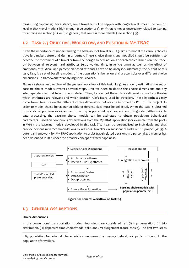
Figure 1.1 shows an overview of the general workflow of this task (T2.3). As shown, estimating the set of baseline choice models involves several steps. First we need to decide the choice dimensions and any interdependencies that have to be modelled. Then, for each of these choice dimensions, we hypothesise which attributes are relevant and which decision rule/s is/are used by travellers. These hypotheses may come from literature on the different choice dimensions but also be informed by D2.1 of this project. In order to model choice behaviour suitable preference data must be collected. When the data is obtained from a stated preferences experiment, this step is preceded by an experiment design step. After suitable data processing, the baseline choice models can be estimated to obtain population behavioural parameters. Based on continuous observations from the My-TRAC application (for example from the pilots in WP6), the baseline models developed in this task (T2.3) can be personalized to individuals and thus provide personalized recommendations to individual travellers in subsequent tasks of this project (WP3). A potential framework for My-TRAC application to assist travel related decisions in a personalized manner has been described in D2.1 under the broader concept of travel happiness.
Figure 1.1: General workflow of Task 2.3
1.3 GENERAL ASSUMPTIONS
Choice dimensions
In the conventional transportation models, four-steps are considered [5]: (i) trip generation, (ii) trip distribution, (iii) departure time choice/modal split, and (iv) assignment (route choice). The first two steps 1 By population behavioural characteristics we mean the average behavioural patterns found in the population of travellers.
§ Decide Choice Dimensions
§ Attribute Hypotheses§ Decision Rule Hypotheses
§ Experiment Design§ Data Collection§ Data processing
§ Choice Model Estimation
Literature review
Stated/Revealed preference data
§ Integration with project
Baseline choice models with population parameters
inpu
t:
attr
ibut
e va
lues
output:
alternative probability
Rest of project
D2.1

Deliverable 2.3: Modelling framework for analysing users’ choices Page 15 of 121
are related to estimating traveller demand in the network whereas the subsequent steps relate to different choices travellers. In this task, these three choice dimensions (mode, departure time, route) are modelled. Note that departure time is not the same as the time of day choice (e.g. morning rush hour) which is typically dictated by travel purpose. The dependencies between these different choice dimensions may be modelled in a number of ways. Ideally, the order in which choices are made are also hypotheses to be tested under different situations. However, given the practical needs of task distribution and the time available for this task, the three choices are assumed to be made independently and sequentially. Travellers are assumed to first choose their modes, then the departure time, and, finally, the route choice.
Decision rules
Regarding decision rules, the multinomial logit (MNL) under the random utility maximization framework has long dominated the field of choice analysis because, although, the model consists of a few drawbacks (e.g., independence of irrelevant alternatives), it is quite strong on many other fronts. The main advantages of the MNL model are that it is intuitive, simple to formulate, and because of its closed form, can be analytically solved, meaning that it can be applied to large datasets very efficiently. Therefore, with an eye on the practical nature of this work, we assume MNL as the default decision rule.
Data collection
For all three choices, we use stated preference experiments to collect data. While these experiments are conducted in three of the countries where the pilots are to be conducted, the Netherlands, Greece, and Portugal, unfortunately, we did not have the resources to conduct a separate experiment in Spain. Within the framework of T2.1, a questionnaire survey was conducted as well aiming at identifying the most significant factors affecting travel behaviour. Exploiting the data collected and thoroughly presented in D2.1, we performed a comparison between travel related choice attitudes of travellers in Spain with those in other countries. We found that they behaved most similar to travellers in Greece (see Appendix A) and therefore models developed for Greece will also be used to describe travel behaviour in Spain as well. Data collected in the My-TRAC application may later be used to re-calibrate the model specifically for travellers in Spain.
For route choice models, in addition to stated preferences, we also make use of revealed preferences from smart card data. Unfortunately, such data could only be procured for the Netherlands and therefore models using revealed preferences are developed for Dutch travellers.
1.4 DELIVERABLE STRUCTURE
In the next two sections, choice analyses for the three dimensions discussed above are presented: mode and departure time choice in section 2 and route choice in section 3. In both of these sections, the different steps shown in the general workflow (Figure 1.1) above are discussed in detail. Mode and departure time choices are observed through a stated preferences experiment. For route choices, however, we present three different models that analyse behaviour in this dimension using different data sources. In the first model, the effect of uncertainty is analysed also using a conventional stated preference experiment. For the next two models, we use revealed preferences from smart card data. By demonstrating how revealed preferences may be used, we can also take advantage of the data collected in My-TRAC later. In these models, first a methodology to automatically calibrate the composition of route choice sets is laid out followed by a comparison of different representations of risky waiting time in choice models. In section 4, a brief discussion on modelling of activities, carried over from D2.2 and D3.3 is presented. Section 5 presents the data requirements required for the development of the choice models presented here for use in the pilots (see WP6). Finally, we conclude the deliverable, summarising the various parts of the report, highlighting important results, and proposing avenues of future research.
Deliverable 2.3: Modelling framework for analysing users’ choices Page 16 of 121
2 MODE AND DEPARTURE TIME CHOICE Travel behaviour, as any other human behaviour is always changing based on the conditions, people’s perceptions and preferences. Travellers are engaging in a variety of alternatives when planning their trip which are usually evaluated through a utility function 𝑈𝑈𝑗𝑗𝑖𝑖, describing the importance of each parameter to the decision-making process. The most common formulation of the utility function is the following [6]:
𝑈𝑈𝑗𝑗𝑖𝑖 = ∑ 𝛽𝛽𝑘𝑘𝑋𝑋𝑘𝑘𝑗𝑗 𝑛𝑛𝑘𝑘=1 (2.1)
where Xkj represents both choice makers’ (i) characteristics and choice alternatives (j) attributes and βk the corresponding weights. The utility maximization theory assumes that the decision-maker is rational and consistent. This means that the decision-maker will always choose the best alternative (maximum utility) given all the available information.
The literature highlights a plethora of factors that affect travel choices, which may be predetermined for the traveller, factors that change in every trip, trip’s attributes and system’s characteristics. Some recent studies have also highlighted the importance of affective factors (emotions, feelings), such as travel happiness in the decision-making process of travelling [7]. In the era of new services in transportation and intelligent transportation systems, current requirements and behaviours of the travellers need to be revised and new needs and travel actions should be defined, basically for three main reasons:
1. Urban transportation landscape is constantly changing with new services being introduced to the system, such as car sharing, carpooling and bike sharing. Thus, travellers have a variety of travel mode alternatives to consider while planning their trip and therefore, factors that are considered may be different from the traditional ones (travel cost, travel time) [8].
2. Travellers have access to all the essential information concerning their daily travel, mode and route alternatives, due to high penetration rates of information and communication technologies in our lives [9]. This fact results in having travellers with increased needs and requirements over the system and with different preferences. In order for the policy makers and system operators to meet their users’ needs and requirements travel behaviour models have to be re-examined.
3. EU has committed to reduce greenhouse gas emissions with special emphasis on those coming from the transport sector. The massive use of private vehicles for everyday travel is one of the maim causes of air pollution and therefore needs to be reduced in order for the EU to achieve its goals. To this end, policy and decision makers need to identify parameters that raise the attractiveness of public transport and in addition define strategies to promote public transport usage and ecological travel modes as well (e.g., bicycle, walking) as more eco-friendly alternatives to private vehicles.
In this context, the My-TRAC project aims to re-estimate the importance of well-known factors that drive travel behaviour nowadays and include some affective parameters that seem to affect decision-making when planning to travel or while travelling. As thoroughly discussed in D2.1, both cognitive and emotional factors are taken into consideration in order for My-TRAC application to properly recommend those travel alternatives that fulfil the requirements and preferences of each user. To this context, the notion of travel happiness was introduced and highlighted the manner in which traditional utility-based models can be enriched with affective parameters that describe users’ perception on the system and users’ individual preferences. Each of the three travel choices (see section 1.3) made by an individual before travelling were considered when travel happiness was studied. In this deliverable we focus on developing the utility functions for each of the alternatives of the three travel choices, which is the main component of the travel happiness function (for more details see D2.1).
In this section, we focus on the first two components of travel behaviour, namely travel mode and time of departure choices. First, we investigate factors affecting travel mode choices and then time of departure
Deliverable 2.3: Modelling framework for analysing users’ choices Page 17 of 121
choices are analysed specifically in the case where PT is used. These choices are seen as two distinct steps and therefore the modelling part was conducted independently. To investigate the factors that affect travel related choices, based on the most relevant literature in the field of travel behaviour analysis [10-13] two multinomial logistic regression models were developed. The methodological approach and the data used for this purpose are thoroughly presented in the next sections.
2.1 METHODOLOGY
The identification of the factors that affect travel mode choice and time of departure choice decisions for everyday trips is a very interesting topic which has been exhaustively studied in the literature [10, 14]. Every day trips are performed from both commuters and non-commuters. Models developed here describe choices of both of them. Only in section 2.3.1 we make a comparison between the two groups if the findings are interesting. Such an investigation of the affecting parameters requires the formulation of a discrete choice model which predicts an individual’s choice based on utility theory [11]. In the presence of more than two alternatives in the choice set, multinomial logistic regression models appeared. Multinomial logistic regression is the regression analysis conducted when the dependent variable is nominal with more than two levels.
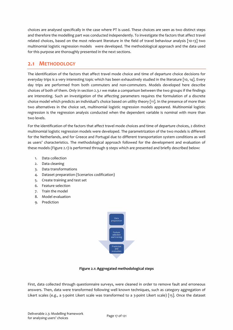
For the identification of the factors that affect travel mode choices and time of departure choices, 2 distinct multinomial logistic regression models were developed. The parametrization of the two models is different for the Netherlands, and for Greece and Portugal due to different transportation system conditions as well as users’ characteristics. The methodological approach followed for the development and evaluation of these models (Figure 2.1) is performed through 9 steps which are presented and briefly described below:
1. Data collection 2. Data cleaning 3. Data transformations 4. Dataset preparation (Scenarios codification) 5. Create training and test set 6. Feature selection 7. Train the model 8. Model evaluation 9. Prediction
Figure 2.1: Aggregated methodological steps
First, data collected through questionnaire surveys, were cleaned in order to remove fault and erroneous answers. Then, data were transformed following well known techniques, such as category aggregation of Likert scales (e.g., a 5-point Likert scale was transformed to a 3-point Likert scale) [15]. Once the dataset
Deliverable 2.3: Modelling framework for analysing users’ choices Page 18 of 121
was ready, data were then coded in a proper way for the analysis (e.g., for mode choice: car = 0, PT = 1, bicycle = 2). The analysis of the sample of each country was conducted using R which is a programming language for statistical analysis.
Data were split into training and test sets with the corresponding proportions being 80% and 20%. In typical supervised learning analysis, the training set is used for the development of the model, while the testing set is used for the evaluation of the final model.
Using the training set, several R packages were used for an automatic subset selection of the most significant variables to be included in model training process. The best subset of the variables is selected after an exhaustive search of several model formulations, by means of several measures such as Akaike’s information criterion (AIC), Bayesian information criterion (BIC), adjusted R2, etc.
The Multinomial Logistic Regression model was developed using the “mlogit” R package which deals with datasets that include stated preferences scenarios [16]. The model with the best goodness-of-fit measures is selected (AIC, Log-Likelihood, R2). Lastly, the final model is used for performing prediction over the test set whose prediction capability was evaluated by taking into account accuracy, precision, recall and area under the curve metrics.
2.1.1 THE MULTINOMIAL LOGIT MODEL
In the simple MNL model, the utility to person n from choosing alternative j in choice scenario t is given by equation (2.2):
𝑈𝑈𝑛𝑛𝑗𝑗𝑛𝑛 = 𝛽𝛽𝑥𝑥𝑛𝑛𝑗𝑗𝑛𝑛 + 𝜀𝜀𝑛𝑛𝑗𝑗𝑛𝑛 𝑛𝑛 = 1, … ,𝑁𝑁; 𝑗𝑗 = 1, … , 𝐽𝐽; 𝑡𝑡 = 1, … ,𝑇𝑇 (2.2)
where xnjt is a K-vector of observed attributes of alternative j, β is a vector of utility weights (homogenous across users), and εnjt ∼ i.d. extreme value is the “idiosyncratic” error [17].
In such a model, a “base” should be defined to indicate the category that is used as the baseline comparison group. In the specific case of the two models produced by the present task, the utility function of the car as well as the utility function of departing early are not a function of user-specific variables, but rather only a function of alternative-specific variables.
The MNL model is a widespread approach to assess the effect of explanatory parameters on the dependent variable if the latter takes more than two distinct values. In the case of travel related choices, MNL models assume that the traveller possesses a utility for each alternative and that they will adopt the alternative that maximizes the utility [13].
2.2 EXPERIMENT DESIGN
A well-known data collection process that is traditionally used for collecting travel behaviour data is stated preferences survey. For the purpose of My-TRAC, 3 distinct questionnaires were created, and the corresponding data collection was conducted in three countries: The Netherlands, Greece and Portugal. The questionnaires used for each site’s survey followed the same structure, although some of the questions were modified in order to conform to site-specific constraints and characteristics. It should be noted that modifications were introduced only to facilitate the data collection process and do not affect the content or the structure of the questionnaire.
2.2.1 QUESTIONNAIRE DESIGN
The questionnaire designed in order to capture travel mode choice and time of departure choice decisions, consisted of 3 parts and 12 questions as well as several stated-preferences scenarios.
Deliverable 2.3: Modelling framework for analysing users’ choices Page 19 of 121
The first part of the questionnaire attempts to identify respondent’s mobility profile. To this end respondents were asked to indicate their usual trip purpose, the frequency of usage of each travel mode per week as well as the number of trips performed for their most usual trip purpose. Moreover, this part of the questionnaire included questions about work time flexibility and public transport pass possession. In addition, the importance of arriving on time was stated in a 3-point scale for each of trip purposes (work, leisure, other). Finally, respondents were asked to indicate their level of happiness during their everyday trips in a 5-point Likert scale, from 1 (very unhappy) to 5 (Very happy).
The second part of the questionnaire included stated preferences scenarios which were created using the R package ‘AlgDesign’ [18, 19]. The first step is to create a full factorial design by defining the number of levels for each of the factors included in the scenario and the number of alternatives included in the choice set.
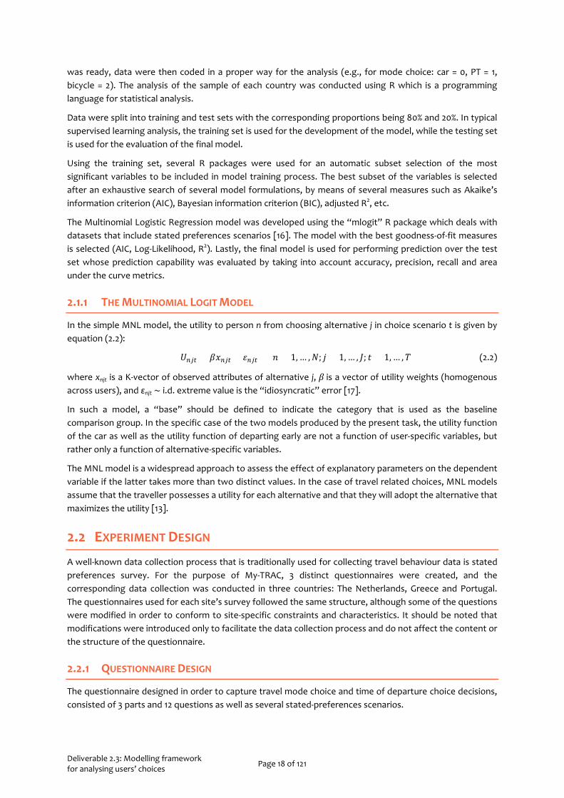
For the travel mode scenarios, the full factorial design consists of (3x2x2) 12 combinations of the levels of each factor. Table 2.1 provides the explanation of the variables presented in each scenario. Travel cost for public transport is different for regular users or users who are entitled to a reduced fare, compared to a single ticket. Travel time is set to take 3 different values while level of comfort is either low or high.
Table 2.1 Description of variables related to attributes of travel mode selection scenarios
Variable Description Range Distinct values for each alternative
Travel time (in mins) Total travel time of the trip 3
Cost (in euros) Generalized travel cost of the trip 2
Level of comfort Level of comfort based on both traffic conditions and level of crowdedness as well as on the occurrence of unexpected events.
2
In the case of time of departure scenarios for PT, the full factorial design includes (3x2x2) 12 scenarios in the case of Greece and Portugal and (3x2x2x2) 24 combinations in the case of the Netherlands. The corresponding levels and the description of the attributes is provided in Table 2.2. The scenarios included total travel time from origin to destination and walking time for each of the alternatives, frequency of mode as well as fare discount which depends on the time using the travel mode. In the case of Greece and Portugal there was no fare discount.
Table 2.2 Description of variables considered in time of departure choice decisions
Variable Description Range of values for each alternative
Travel time (in mins) Total travel time of the trip (including in vehicle time and walking time)
3
Walking time (in mins) Sum of time for reaching the station and time reaching the destination
2
Frequency (per mins) Time distance between two successive trains 2
Fare discount Fare discount for regular users or users that are entitled a reduced fare
2
Subsequently, a fractional factorial design is applied in order to reduce the number of the scenarios and make the questionnaire more flexible. To do so, the optFederov() command from R package ‘AlgDesign’ was used and the minimum number of scenarios was estimated by optimizing the D-criterion [20].

Deliverable 2.3: Modelling framework for analysing users’ choices Page 20 of 121
Finally, 6 stated preferences scenarios concerning travel mode choice decisions were presented to the respondents. An example is given in Table 2.3. The scenarios were supposed to be answered for a hypothetical trip of 10km at 8:00 am, with available travel mode alternatives being car, public transport (train and metro) and bicycle for the Netherlands, car, public transport and motorcycle for Greece and Portugal. The scenarios included total travel time per mode and costs per mode for the particular trip, together with the comfort level. The level of comfort depends on the traffic conditions, crowdedness and other events (expected or unexpected) that may affect the conditions of the trip.
Table 2.3 Example of stated preferences scenario for travel mode choice (Dutch questionnaire)
Car PT Bike Travel Time (in mins) 35 30 25
Cost (in euros) 5 2 0 Level of Comfort High Low Low
Select
Then, stated preferences scenarios concerning time of departure choice (Table 2.4) were presented assuming that the traveller performs the specific trip by public transport. The respondent was provided with three alternatives: Departing earlier, on time or later.
Table 2.4 Example of scenarios for time of departure choice (Dutch questionnaire)
Early On time Late Travel Time (in mins) 30 45 30
Walking time (in mins) 20 10 20 Frequency (per mins) 5 3 7
Fare discount 0% 20% 40% Select
The last part of the questionnaire included the demographics of the respondents: gender, age, education level, total annual personal income, occupation and household size.
An overview of the content of the questionnaire is depicted in Figure 2.2
Figure 2.2 Description of Questionnaire parts

Deliverable 2.3: Modelling framework for analysing users’ choices Page 21 of 121
2.3 DATA COLLECTION
The questionnaire described above was translated in three languages (Dutch, Greek and Portuguese) and then was used for data collection in each of the corresponding countries. The three questionnaires share a common structure and content although small modifications were introduced to in order to fulfil each site’s transport network constraints. The corresponding questionnaires are provided in Appendix B.
The survey in the case of the Netherlands was conducted online through the PanelClix platform. First, a test round was conducted in order to identify potential issues on the completion of the questionnaire. Then, a second round of the survey was conducted with a total duration of 4 days. The raw data included 739 responses, but after excluding malicious and fault answers2, the final dataset includes 737 unique responses. For the Greek case, the questionnaire survey was conducted onsite using the electronic version of the questionnaire, created using Google Forms. The survey took place in critical points of the Athens metropolitan area such as the campus of the National Technical University of Athens, metro stations and other key areas. The survey had a total duration of approximately 1 month (February - March 2019). In Portugal, questionnaire survey took place both online and onsite (in Lisbon) where 362 respondents participated. In this case as well, the survey had a total duration of 1 month (March – April 2019). Continuous monitoring of the quality of the sampling during the data collection process, resulted in having 350 and 362 responses from Greece and Portugal respectively, which were ready to be used for the modelling part.
Figure 2.3 Study area
2 Household size>10
Lisbon (Portugal) Sample: 362
Athens (Greece) Sample: 350
The Netherlands Sample: 737
Deliverable 2.3: Modelling framework for analysing users’ choices Page 22 of 121
2.3.1 DESCRIPTIVE STATISTICS
This section provides a complete overview of the data collected from the questionnaire survey in all three countries. In addition, a preliminary comparison between the responses of the three samples is performed. The results are presented in diagrammatic and table formats and follow the categorization of the questions in the questionnaire.
2.3.1.1 DEMOGRAPHICS
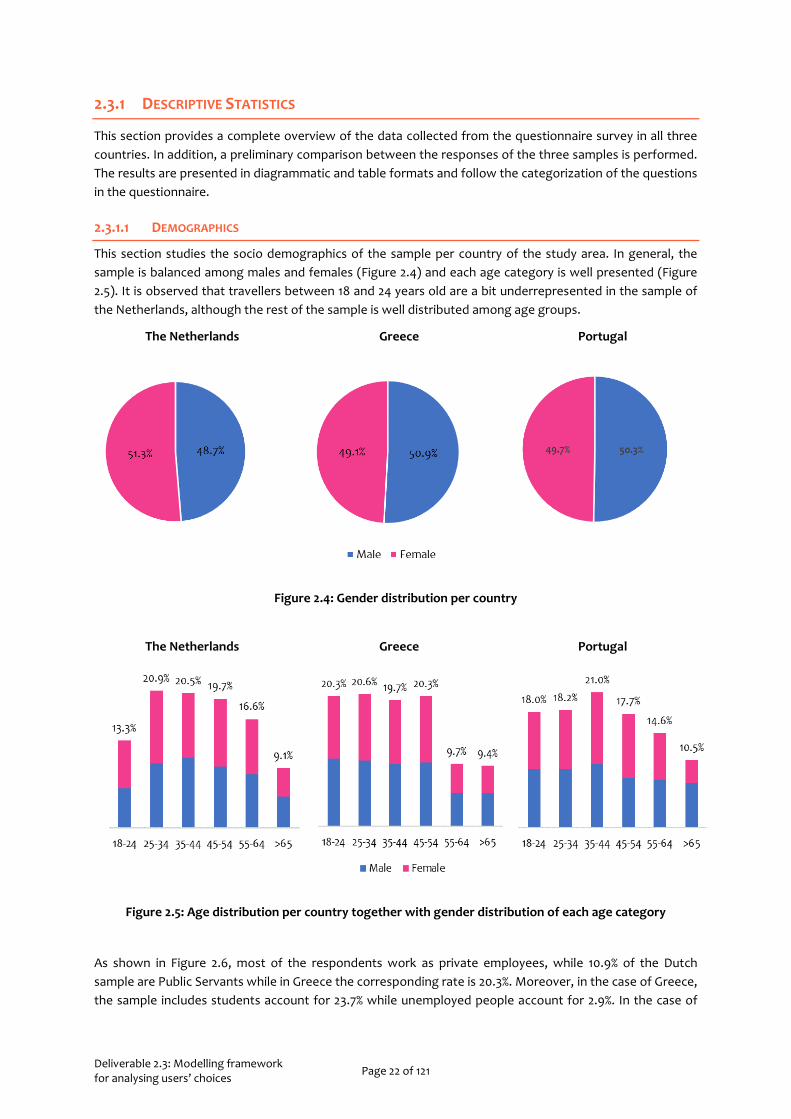
This section studies the socio demographics of the sample per country of the study area. In general, the sample is balanced among males and females (Figure 2.4) and each age category is well presented (Figure 2.5). It is observed that travellers between 18 and 24 years old are a bit underrepresented in the sample of the Netherlands, although the rest of the sample is well distributed among age groups.
The Netherlands Greece Portugal
Figure 2.4: Gender distribution per country
The Netherlands Greece Portugal
Figure 2.5: Age distribution per country together with gender distribution of each age category
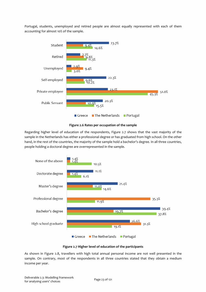
As shown in Figure 2.6, most of the respondents work as private employees, while 10.9% of the Dutch sample are Public Servants while in Greece the corresponding rate is 20.3%. Moreover, in the case of Greece, the sample includes students account for 23.7% while unemployed people account for 2.9%. In the case of
Deliverable 2.3: Modelling framework for analysing users’ choices Page 23 of 121
Portugal, students, unemployed and retired people are almost equally represented with each of them accounting for almost 10% of the sample.
Figure 2.6 Rates per occupation of the sample
Regarding higher level of education of the respondents, Figure 2.7 shows that the vast majority of the sample in the Netherlands has either a professional degree or has graduated from high school. On the other hand, in the rest of the countries, the majority of the sample hold a bachelor’s degree. In all three countries, people holding a doctoral degree are overrepresented in the sample.
Figure 2.7 Higher level of education of the participants
As shown in Figure 2.8, travellers with high total annual personal income are not well presented in the sample. On contrary, most of the respondents in all three countries stated that they obtain a medium income per year.

Deliverable 2.3: Modelling framework for analysing users’ choices Page 24 of 121
Figure 2.8 Total annual personal income
Concerning the number of household members, based on the results presented in Table 2.5, in Greece the majority of the sample (31.1%) stated that they belong in a 4-member family, while the corresponding results for the Netherlands and Portugal are 20.4% and 19.9%.
Table 2.5 Household size per country
Household size The Netherlands Greece Portugal 1 19.4% 14.6% 16.3% 2 36.5% 25.4% 22.1% 3 16.0% 22.3% 31.8% 4 20.4% 31.1% 19.9%
>4 7.7% 6.6% 9.9%
2.3.1.2 MOBILITY PROFILE
In this section, some interesting insights on how travellers on each country prefer to perform their everyday trips are provided. Results are presented with a distinction among commuters and non-commuters. Commuters are considered those travellers whose most usual trip purpose is work and in addition, they perform more than 4 trips per week for this purpose. The allocation of the sample between commuters and non-commuters is depicted in Figure 2.9.
Figure 2.9 Commuters vs non-commuters in the dataset
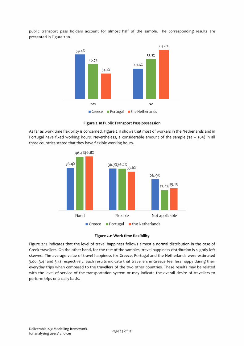
In the Netherlands, 65.8% of the sample stated that they do not own a public transport seasonal pass will the corresponding percentage of the Greek sample was 40.6%. On the contrary, in the case of Portugal,
Deliverable 2.3: Modelling framework for analysing users’ choices Page 25 of 121
public transport pass holders account for almost half of the sample. The corresponding results are presented in Figure 2.10.
Figure 2.10 Public Transport Pass possession
As far as work time flexibility is concerned, Figure 2.11 shows that most of workers in the Netherlands and in Portugal have fixed working hours. Nevertheless, a considerable amount of the sample (34 – 36%) in all three countries stated that they have flexible working hours.
Figure 2.11 Work time flexibility
Figure 2.12 indicates that the level of travel happiness follows almost a normal distribution in the case of Greek travellers. On the other hand, for the rest of the samples, travel happiness distribution is slightly left skewed. The average value of travel happiness for Greece, Portugal and the Netherlands were estimated 3.06, 3.41 and 3.41 respectively. Such results indicate that travellers in Greece feel less happy during their everyday trips when compared to the travellers of the two other countries. These results may be related with the level of service of the transportation system or may indicate the overall desire of travellers to perform trips on a daily basis.

Deliverable 2.3: Modelling framework for analysing users’ choices Page 26 of 121
Figure 2.12 Distribution of the level of travel happiness in the three countries
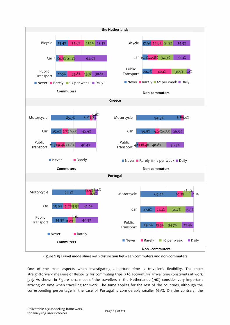
Based on the results illustrated in Figure 2.13, the majority of commuters (64%) in the Netherlands are using in a daily basis their private vehicle while only 30.1% of them commute by public transport. Interestingly, results indicated that 35.5% of the non-commuters use bicycle as a means of transport for their everyday trips.
In the case of Greece, commuters choose to perform their everyday trips either by private vehicle or public transport, while only 5.6% of them commute by motorcycle. On the other hand, most of the non-commuters prefer to use public transport for their everyday trips, with the corresponding percentage being 36.7%.
Results in the case of Portugal are very similar to those of the Greek sample. More specifically, the vast majority of commuters prefer to travel to work by car or by public transport. Interestingly, there is also a considerable percentage of commuters who choose to travel at least 1 time per week by motorcycle, for work purposes.
Deliverable 2.3: Modelling framework for analysing users’ choices Page 27 of 121
the Netherlands
Commuters
Non-commuters
Greece
Commuters Non-commuters
Portugal
Commuters
Non - commuters
Figure 2.13 Travel mode share with distinction between commuters and non-commuters
One of the main aspects when investigating departure time is traveller’s flexibility. The most straightforward measure of flexibility for commuting trips is to account for arrival time constraints at work [21]. As shown in Figure 2.14, most of the travellers in the Netherlands (76%) consider very important arriving on time when travelling for work. The same applies for the rest of the countries, although the corresponding percentage in the case of Portugal is considerably smaller (61%). On the contrary, the
22.5%
5.3%
23.4%
33.8%
9.8%
32.6%
13.7%
21.4%
21.2%
30.1%
64.0%
23.3%
PublicTransport
Car
Bicycle
Never Rarely 1-2 per week Daily
20.2%
10.4%
17.9%
40.1%
20.8%
24.8%
31.9%
32.9%
21.2%
7.2%
35.2%
35.5%
PublicTransport
Car
Bicycle
Never Rarely 1-2 per week Daily
11.5%
25.0%
85.7%
19.4%
12.7%
6.0%
22.6%
19.4%
2.8%
46.4%
42.9%
5.6%
PublicTransport
Car
Motorcycle
Never Rarely
4.1%
39.8%
94.9%
18.4%
9.2%
3.1%
40.8%
24.5%
36.7%
26.5%
1.0%
PublicTransport
Car
Motorcycle
Never Rarely 1-2 per week Daily
34.5%
25.0%
74.2%
11.0%
17.4%
12.9%
6.1%
15.5%
6.4%
48.5%
42.0%
6.4%
PublicTransport
Car
Motorcycle
Never Rarely
29.6%
27.6%
69.4%
13.3%
22.4%
10.2%
34.7%
34.7%
16.3%
22.4%
15.3%
4.1%
PublicTransport
Car
Motorcycle
Never Rarely 1-2 per week Daily

Deliverable 2.3: Modelling framework for analysing users’ choices Page 28 of 121
majority of travellers in all three countries of study consider as somewhat important arriving on time when travelling for leisure or other personal purposes. Interestingly, almost 23% of travellers in Portugal stated that arriving on time when travelling for leisure purposes is not important at all.
Figure 2.14 Importance of arriving on time per trip purpose
Results presented here indicate generally well-balanced datasets for all three countries with adequate distribution among gender, different age groups and occupations. The analysis of the data collected through the questionnaire surveys highlights the existing differences between the countries examined here and thereby highlights the need of conducting the analysis separately.
2.4 MODEL IMPLEMENTATION, RESULTS , AND DISCUSSION
For the implementation of the MNL models, a country-specific approach was followed due to the diversity of travel behaviour of users in each country and the differences in the transportation network. Each country’s transportation system offers a specific set of alternatives when it comes to available travel modes and in addition, the same travel mode may be considered worst in terms of level of service in different countries. The ultimate goal of our approach is to develop choice models that are easy transferable, and their results may be applied in different cities and different networks.
Based on the above, the model developed using data from the Netherlands, which was the biggest sample available, was the first model to be estimated and therefore some of the parameters that were dimmed significant for it, were tested for being included in the rest of the models.
2.4.1 TRAVEL MODE CHOICE
Urban transportation systems offer a plethora of travel mode alternatives to travellers regarding their everyday trips. The various means of transport can be classified into three types: ecological means of
Deliverable 2.3: Modelling framework for analysing users’ choices Page 29 of 121
transport, such as walking and cycling, private vehicles, such as car and motorcycle and public transport (bus, tram, train and metro).
Travel mode choices vary with person characteristics such as age and gender [22, 23], as well as household characteristics such as income, house location, and transport availability [24]. Moreover, studies have highlighted the importance of trip purpose and environmental characteristics, such as land use, when comes to travel mode choice decisions [25]. During the last decade some researchers have investigated the importance of affective factors in the decision-making process of travelling [26]. More specifically, some studies have introduced the notion of travel happiness which actually reflects the general feeling that someone experiences during their everyday trips [7, 27].
As mentioned before, travel mode decisions, as any other travel related decision, are usually being investigated through utility theories [28]. Utility theory assumes that the traveller is rational and consistent which means that they will always choose the best alternative (maximum utility) given all the available information. Nevertheless, there is no single method to determine what drives travel mode choice decisions, neither of why travellers prefer one travel mode over the others under specific circumstances [29].
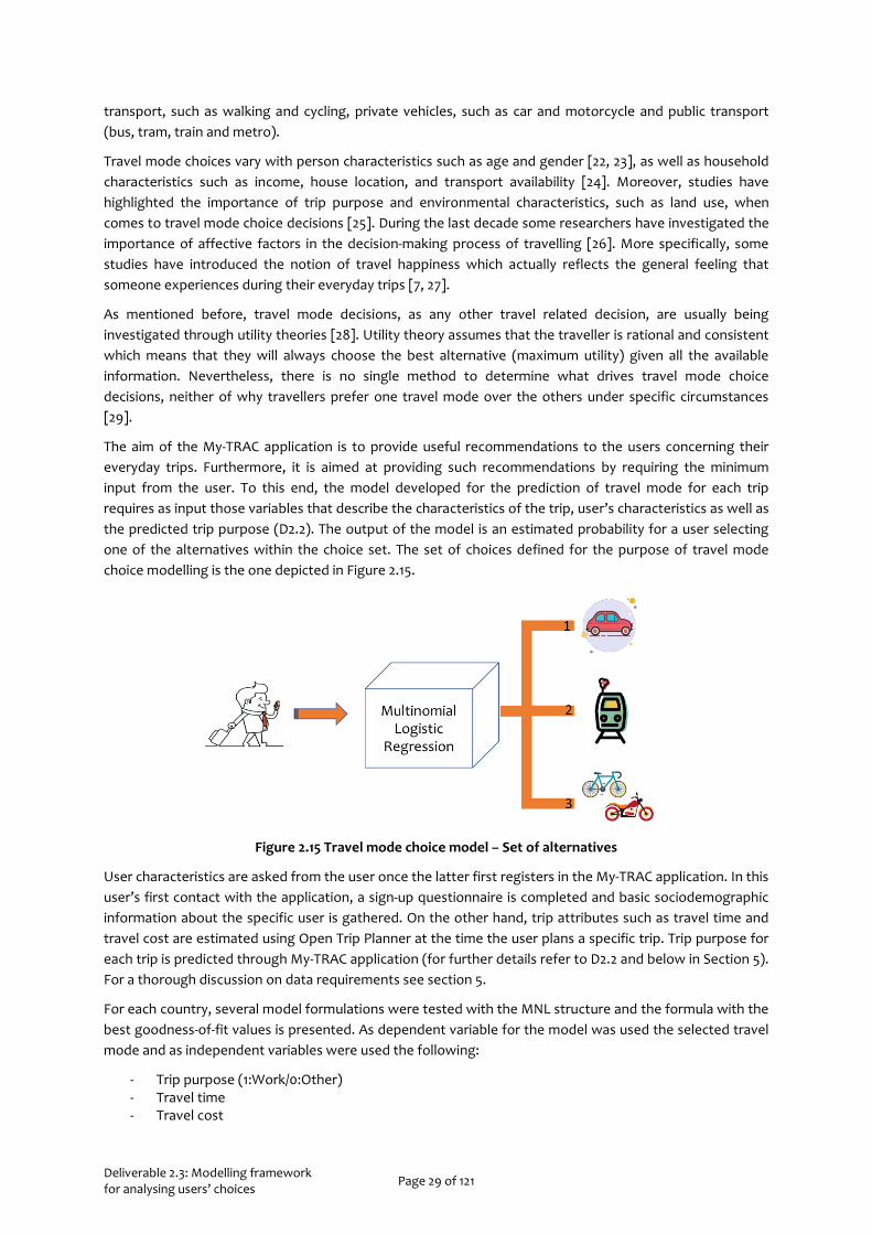
The aim of the My-TRAC application is to provide useful recommendations to the users concerning their everyday trips. Furthermore, it is aimed at providing such recommendations by requiring the minimum input from the user. To this end, the model developed for the prediction of travel mode for each trip requires as input those variables that describe the characteristics of the trip, user’s characteristics as well as the predicted trip purpose (D2.2). The output of the model is an estimated probability for a user selecting one of the alternatives within the choice set. The set of choices defined for the purpose of travel mode choice modelling is the one depicted in Figure 2.15.
Figure 2.15 Travel mode choice model – Set of alternatives
User characteristics are asked from the user once the latter first registers in the My-TRAC application. In this user’s first contact with the application, a sign-up questionnaire is completed and basic sociodemographic information about the specific user is gathered. On the other hand, trip attributes such as travel time and travel cost are estimated using Open Trip Planner at the time the user plans a specific trip. Trip purpose for each trip is predicted through My-TRAC application (for further details refer to D2.2 and below in Section 5). For a thorough discussion on data requirements see section 5.
For each country, several model formulations were tested with the MNL structure and the formula with the best goodness-of-fit values is presented. As dependent variable for the model was used the selected travel mode and as independent variables were used the following:
- Trip purpose (1:Work/0:Other) - Travel time - Travel cost

Deliverable 2.3: Modelling framework for analysing users’ choices Page 30 of 121
- Level of comfort (0:Low/1:High) - Age (1-6) - Occupation (1-6) - Number of trips performed by PT per week (0:Never – 3:Daily) - Number of trips performed by car per week (0:Never – 3:Daily)
During the training phase of the models, several model formulations were tested and assessed using AIC criterion and Log-likelihood tests [12]. Then, the model with the best goodness-of-fit measures is finally selected and its prediction ability is tested using well known measures of accuracy and area under the ROC curve.
2.4.1.1 THE NETHERLANDS
In the case of the Netherlands, the MNL model which describes factors affecting travel mode choice, has an estimated McFadden R2: 0.15, which means that the model captures accurately 15% of the phenomenon. Nevertheless, when human behaviour and decision-making is being modelled, Mc Fadden stated that a R2 between 0.10 – 0.40 indicates a well fitted model [30]. As base alternative travel mode was considered “car”. The results of the utility function of public transport and bicycle are summarized in Table 2.6.
Table 2.6 Multinomial Logistic Regression model for the Netherlands – Travel Mode choice model
Variables Public Transport Bicycle
Coeff. Std. Error Pr (>|z|) Coeff. Std. Error Pr (>|z|) (Intercept) 0.849 1.60 Travel Cost -0.167 0.014 0.000 *** -0.167 0.014 0.000 *** Travel Time -0.046 0.003 0.000 *** -0.046 0.003 0.000 *** Level of Comfort 0.525 0.042 0.000 *** 0.525 0.042 0.000 *** Age -0.143 0.041 0.001 *** -0.078 0.04 0.05 * Trip purpose -0.364 0.166 0.028 * -0.572 0.154 0.000 *** Numb. of trips by car -0.572 0.058 0.000 *** -0.689 0.058 0.000 *** Numb. of trips by PT 0.683 0.051 0.000 *** 0.183 0.049 0.000 *** Occupation|Private Employee 0.523
0.159 0.001 *** 0.472
0.154 0.002
**
Occupation|Self-employed -0.341 0.166 0.04 * -0.328 0.157 0.037 * Occupation|Student 0.478 0.208 0.022 * Occupation|Retired -0.779 0.233 0.001 *** -1.148 0.219 0.000 *** Occupation|Unemployed -0.395 0.211 0.061 . -0.941 0.202 0.000 ***
0 ‘***’ 0.001 ‘**’ 0.01 ‘*’ 0.05 ‘.’
Findings revealed that the utility of public transport is significantly affected from the trip attributes, namely travel cost, travel time and the level of comfort. As expected, when travel time and travel cost are increasing, travellers tend to use their private vehicle instead of public transport. On the other hand, higher levels of comfort attract more travellers to public transport services.
As far as users’ characteristics are concerned, findings indicated that the younger travellers are more likely to use public transport than the elderly. Interestingly, private employees are also more likely to use public transport for their everyday trips, when compared to travellers with other occupations. Moreover, as it is expected, travellers who usually travel by car are less likely to use public transport for their trips.
Finally, it appears that travellers are more likely to use public transport when travelling for other purposes either than work or education. This finding can be seen in relation to how important travellers consider that they arrive on time when travelling for work. If so, results indicate that travellers do not consider public transport as a reliable travel mode and thus are less likely to use it when travelling for work purposes. The use of bicycle as a means of transport significantly depends on the trip purpose. Findings revealed that those who travel for work purposes are less likely to use bicycle. Moreover, travellers who usually travel by car are less likely to use bicycle for their everyday trips when compared to those who travel by public

Deliverable 2.3: Modelling framework for analysing users’ choices Page 31 of 121
transport. Furthermore, students and private employees are more likely to use their bicycle than public servants. Results also indicated that the elderly is less likely to use a bicycle for everyday trips.
Finally, in this case as well, if travel cost and travel times of bicycle increase, travellers would prefer to use their private vehicle instead of the bicycle. The above described model was also used for prediction over the test set. Results of the classification are presented in the classification matrix below (Table 2.7).
Table 2.7 Classification matrix for the three travel mode alternatives (the Netherlands)
Response
Car PT Bike Pr
edic
ted Car 205 62 104
PT 54 174 80
Bike 61 63 139
Figure 2.16 Multiclass-ROC plot for the three classes of travel mode (the Netherlands)
It is observed that due to the limited observations of bicycle, the model cannot predict accurately the third class (bicycle), which results in poor prediction capability of our model. The area under the multiclass-ROC plot was estimated 0.63. In case where more data are available there is room for further improvement of the model. Nevertheless, these results provide a sufficient depiction of the manner in which travellers choose between the alternatives that they have for a specific trip and more specifically, highlight the importance of the parameters that should be taken into consideration when travel behaviour is being analysed.
2.4.1.2 GREECE
The model developed for the case of Greece, is quite similar to the one that describes travel choices in the Netherlands. The McFadden R2 was estimated 0.14 which indicates that the model adequately captures such a complex phenomenon. Utility functions of both public transport and motorcycle are presented in Table 2.8.
Deliverable 2.3: Modelling framework for analysing users’ choices Page 32 of 121
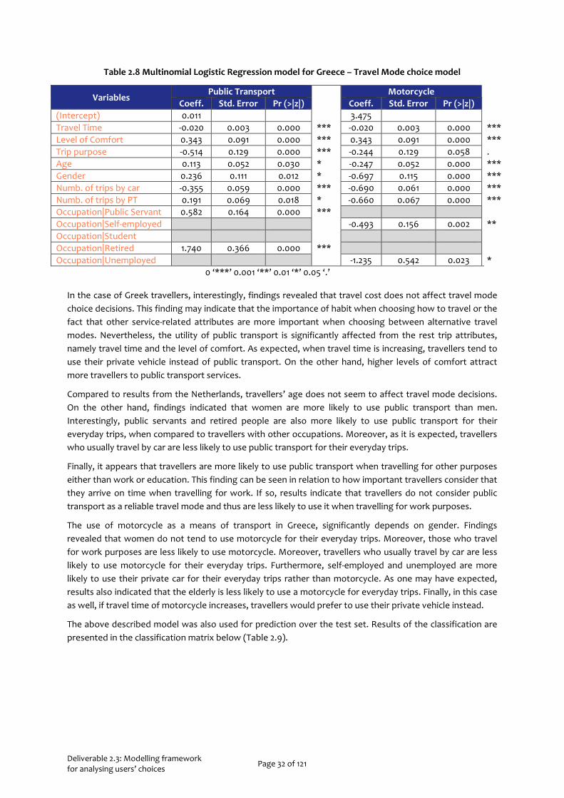
Table 2.8 Multinomial Logistic Regression model for Greece – Travel Mode choice model
Variables Public Transport Motorcycle
Coeff. Std. Error Pr (>|z|) Coeff. Std. Error Pr (>|z|) (Intercept) 0.011 3.475 Travel Time -0.020 0.003 0.000 *** -0.020 0.003 0.000 *** Level of Comfort 0.343 0.091 0.000 *** 0.343 0.091 0.000 *** Trip purpose -0.514 0.129 0.000 *** -0.244 0.129 0.058 . Age 0.113 0.052 0.030 * -0.247 0.052 0.000 *** Gender 0.236 0.111 0.012 * -0.697 0.115 0.000 *** Numb. of trips by car -0.355 0.059 0.000 *** -0.690 0.061 0.000 *** Numb. of trips by PT 0.191 0.069 0.018 * -0.660 0.067 0.000 *** Occupation|Public Servant 0.582 0.164 0.000 *** Occupation|Self-employed -0.493 0.156 0.002 ** Occupation|Student Occupation|Retired 1.740 0.366 0.000 *** Occupation|Unemployed -1.235 0.542 0.023 *
0 ‘***’ 0.001 ‘**’ 0.01 ‘*’ 0.05 ‘.’
In the case of Greek travellers, interestingly, findings revealed that travel cost does not affect travel mode choice decisions. This finding may indicate that the importance of habit when choosing how to travel or the fact that other service-related attributes are more important when choosing between alternative travel modes. Nevertheless, the utility of public transport is significantly affected from the rest trip attributes, namely travel time and the level of comfort. As expected, when travel time is increasing, travellers tend to use their private vehicle instead of public transport. On the other hand, higher levels of comfort attract more travellers to public transport services.
Compared to results from the Netherlands, travellers’ age does not seem to affect travel mode decisions. On the other hand, findings indicated that women are more likely to use public transport than men. Interestingly, public servants and retired people are also more likely to use public transport for their everyday trips, when compared to travellers with other occupations. Moreover, as it is expected, travellers who usually travel by car are less likely to use public transport for their everyday trips.
Finally, it appears that travellers are more likely to use public transport when travelling for other purposes either than work or education. This finding can be seen in relation to how important travellers consider that they arrive on time when travelling for work. If so, results indicate that travellers do not consider public transport as a reliable travel mode and thus are less likely to use it when travelling for work purposes.
The use of motorcycle as a means of transport in Greece, significantly depends on gender. Findings revealed that women do not tend to use motorcycle for their everyday trips. Moreover, those who travel for work purposes are less likely to use motorcycle. Moreover, travellers who usually travel by car are less likely to use motorcycle for their everyday trips. Furthermore, self-employed and unemployed are more likely to use their private car for their everyday trips rather than motorcycle. As one may have expected, results also indicated that the elderly is less likely to use a motorcycle for everyday trips. Finally, in this case as well, if travel time of motorcycle increases, travellers would prefer to use their private vehicle instead.
The above described model was also used for prediction over the test set. Results of the classification are presented in the classification matrix below (Table 2.9).
Deliverable 2.3: Modelling framework for analysing users’ choices Page 33 of 121
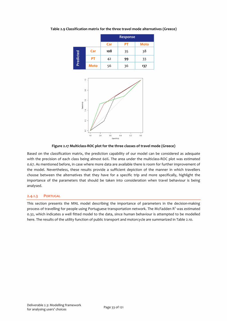
Table 2.9 Classification matrix for the three travel mode alternatives (Greece)
Response
Car PT Moto
Pred
icte
d Car 108 35 38
PT 42 99 33
Moto 56 36 137
Figure 2.17 Multiclass-ROC plot for the three classes of travel mode (Greece)
Based on the classification matrix, the prediction capability of our model can be considered as adequate with the precision of each class being almost 60%. The area under the multiclass-ROC plot was estimated 0.67. As mentioned before, in case where more data are available there is room for further improvement of the model. Nevertheless, these results provide a sufficient depiction of the manner in which travellers choose between the alternatives that they have for a specific trip and more specifically, highlight the importance of the parameters that should be taken into consideration when travel behaviour is being analysed.
2.4.1.3 PORTUGAL
This section presents the MNL model describing the importance of parameters in the decision-making process of travelling for people using Portuguese transportation network. The McFadden R2 was estimated 0.32, which indicates a well fitted model to the data, since human behaviour is attempted to be modelled here. The results of the utility function of public transport and motorcycle are summarized in Table 2.10.
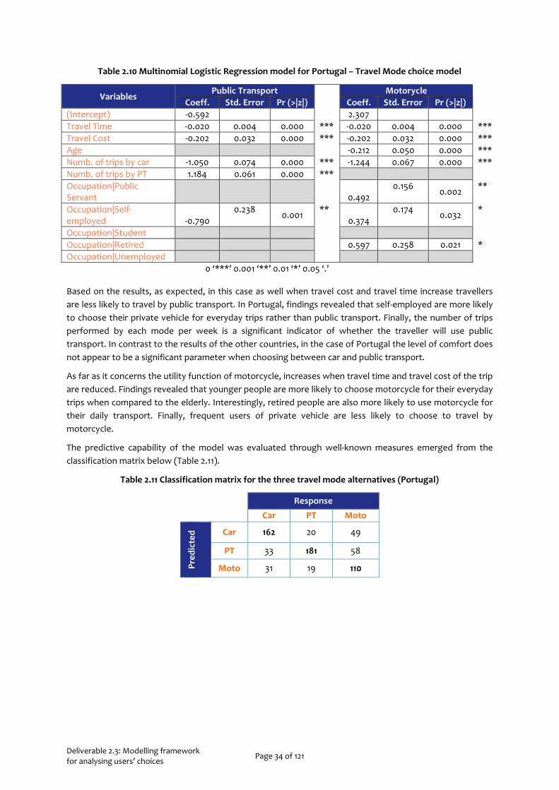
Deliverable 2.3: Modelling framework for analysing users’ choices Page 34 of 121
Table 2.10 Multinomial Logistic Regression model for Portugal – Travel Mode choice model
Variables Public Transport Motorycle
Coeff. Std. Error Pr (>|z|) Coeff. Std. Error Pr (>|z|) (Intercept) -0.592 2.307 Travel Time -0.020 0.004 0.000 *** -0.020 0.004 0.000 *** Travel Cost -0.202 0.032 0.000 *** -0.202 0.032 0.000 *** Age -0.212 0.050 0.000 *** Numb. of trips by car -1.050 0.074 0.000 *** -1.244 0.067 0.000 *** Numb. of trips by PT 1.184 0.061 0.000 *** Occupation|Public Servant
0.492
0.156 0.002 **
Occupation|Self-employed -0.790
0.238 0.001 ** 0.374
0.174 0.032 *
Occupation|Student Occupation|Retired 0.597 0.258 0.021 * Occupation|Unemployed
0 ‘***’ 0.001 ‘**’ 0.01 ‘*’ 0.05 ‘.’
Based on the results, as expected, in this case as well when travel cost and travel time increase travellers are less likely to travel by public transport. In Portugal, findings revealed that self-employed are more likely to choose their private vehicle for everyday trips rather than public transport. Finally, the number of trips performed by each mode per week is a significant indicator of whether the traveller will use public transport. In contrast to the results of the other countries, in the case of Portugal the level of comfort does not appear to be a significant parameter when choosing between car and public transport.
As far as it concerns the utility function of motorcycle, increases when travel time and travel cost of the trip are reduced. Findings revealed that younger people are more likely to choose motorcycle for their everyday trips when compared to the elderly. Interestingly, retired people are also more likely to use motorcycle for their daily transport. Finally, frequent users of private vehicle are less likely to choose to travel by motorcycle.
The predictive capability of the model was evaluated through well-known measures emerged from the classification matrix below (Table 2.11).
Table 2.11 Classification matrix for the three travel mode alternatives (Portugal)
Response
Car PT Moto
Pred
icte
d Car 162 20 49
PT 33 181 58
Moto 31 19 110

Deliverable 2.3: Modelling framework for analysing users’ choices Page 35 of 121
Figure 2.18 Multiclass-ROC plot for the three classes of travel mode
2.4.2 TIME OF DEPARTURE CHOICE
Time of departure choice models are well studied in the literature since choosing time of departure is another critical decision of everyday travel. Motivating people to change their departure time could play a key role in reducing peak- hour congestion, which remains a critical transportation problem in large urban areas. To achieve this behavioural change, it is necessary to better understand the factors that influence departure time choice. So far, departure time choice modelling focuses on objective factors, such as travel time and travel costs as main behavioural determinants. Most of the studies focus on the work trip, since commuters’ departure time is highly connected with limitations on their arrival time [31]. More specifically, travellers who travel for work purposes may have work time flexibility constraints and therefore choose their departure time differently [32]. Several studies have shown that travellers are more likely to change their departure time in order to avoid congestion rather than to change their travel mode [21].
The My-TRAC application will activate the time of departure choice model only in case where the trip will be performed by public transport. This relies on the assumption that travelling by a private vehicle offers an increased flexibility regarding not only departure time but also route choice and congestion avoidance. On the contrary, when travelling by public transport, the traveller should adjust their choices with respect to each mode’s itineraries and trajectory. The choice set of departure time consists of three alternatives: Depart on time, depart earlier or depart later (Figure 2.19). Each of the alternatives corresponds to a different arrival time. The alternative “depart on time” refers to the situation where the traveller will depart at that time when the sum of the estimated travel time of the trip will give exactly the desired time of arrival at the destination. Departing earlier results in arriving earlier or right on time, while departing later result in arriving later.
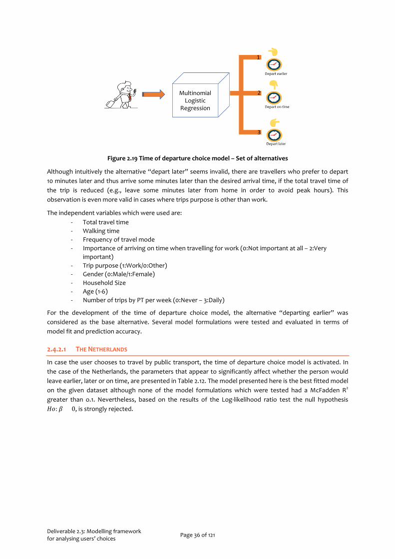
Deliverable 2.3: Modelling framework for analysing users’ choices Page 36 of 121
Figure 2.19 Time of departure choice model – Set of alternatives
Although intuitively the alternative “depart later” seems invalid, there are travellers who prefer to depart 10 minutes later and thus arrive some minutes later than the desired arrival time, if the total travel time of the trip is reduced (e.g., leave some minutes later from home in order to avoid peak hours). This observation is even more valid in cases where trips purpose is other than work.
The independent variables which were used are: - Total travel time - Walking time - Frequency of travel mode - Importance of arriving on time when travelling for work (0:Not important at all – 2:Very
important) - Trip purpose (1:Work/0:Other) - Gender (0:Male/1:Female) - Household Size - Age (1-6) - Number of trips by PT per week (0:Never – 3:Daily)
For the development of the time of departure choice model, the alternative “departing earlier” was considered as the base alternative. Several model formulations were tested and evaluated in terms of model fit and prediction accuracy.
2.4.2.1 THE NETHERLANDS
In case the user chooses to travel by public transport, the time of departure choice model is activated. In the case of the Netherlands, the parameters that appear to significantly affect whether the person would leave earlier, later or on time, are presented in Table 2.12. The model presented here is the best fitted model on the given dataset although none of the model formulations which were tested had a McFadden R2
greater than o.1. Nevertheless, based on the results of the Log-likelihood ratio test the null hypothesis 𝐻𝐻𝐻𝐻: 𝛽𝛽 = 0, is strongly rejected.

Deliverable 2.3: Modelling framework for analysing users’ choices Page 37 of 121
Table 2.12 Multinomial Logistic Regression model for the Netherlands - Time of departure choice model
Variables Depart on time Depart Later
Coeff. Std. Error Pr (>|z|) Coeff. Std. Error Pr (>|z|) (Intercept) 0.685 0.560 Total travel time -0.033 0.003 0.000 *** -0.033 0.003 0.000 *** Walking time -0.042 0.005 0.000 *** -0.042 0.005 0.000 *** Fare discount 2.753 0.136 0.000 *** 2.753 0.136 0.000 *** Frequency -0.070 0.018 0.000 *** -0.070 0.018 0.000 *** Importance of arriving on time|Work -0.104 0.066 0.114 -0.329 0.068 0.000 ***
Gender -0.439 0.075 0.000 *** -0.231 0.080 0.004 ** Trip purpose -0.239 0.099 0.016 *
0 ‘***’ 0.001 ‘**’ 0.01 ‘*’ 0.05 ‘.’ 0.1 ‘ ’ Findings indicate that those travellers who consider important arriving on time when travelling for work purposes are more likely to depart earlier. Moreover, it appears that men are more likely to depart on time when compared to women who are more likely to depart earlier. Finally, as expected, travellers will choose to depart on time rather than earlier if there is a fare discount. These findings are in line with the literature since many researchers have highlighted the importance of work time flexibility and not arriving on time penalties in the decision making process of time of departure choice [33]. The above described model was also used for prediction over the test set. Results of the classification of departure time are presented in the classification matrix below ( Table 2.13). The area under the multiclass-ROC plot was estimated 0.68 and the multi-class roc plot is depicted in Figure 2.20.
Table 2.13 Classification matrix for the three time of departure alternatives (the Netherlands)
Response
Earlier On-time Later
Pred
ict Earlier 215 155 70
On-time 79 154 79 Later 63 110 229
Figure 2.20 Multiclass-ROC plot for the three classes of time of departure
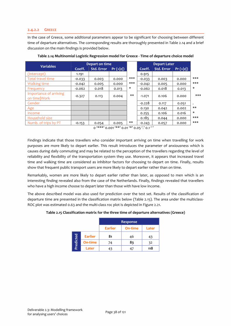
Deliverable 2.3: Modelling framework for analysing users’ choices Page 38 of 121
2.4.2.2 GREECE
In the case of Greece, some additional parameters appear to be significant for choosing between different time of departure alternatives. The corresponding results are thoroughly presented in Table 2.14 and a brief discussion on the main findings is provided below.
Table 2.14 Multinomial Logistic Regression model for Greece - Time of departure choice model
Variables Depart on time Depart Later
Coeff. Std. Error Pr (>|z|) Coeff. Std. Error Pr (>|z|) (Intercept) 1.191 0.915 Total travel time -0.033 0.003 0.000 *** -0.033 0.003 0.000 *** Walking time -0.042 0.005 0.000 *** -0.042 0.005 0.000 *** Frequency -0.062 0.018 0.013 * -0.062 0.018 0.013 * Importance of arriving on time|Work -0.327 0.113 0.004 ** -1.071 0.106 0.000 ***
Gender -0.228 0.117 0.051 . Age 0.130 0.042 0.002 ** Income 0.255 0.106 0.016 * Household size 0.185 0.044 0.000 *** Numb. of trips by PT -0.153 0.054 0.005 ** -0.243 0.057 0.000 ***
0 ‘***’ 0.001 ‘**’ 0.01 ‘*’ 0.05 ‘.’ 0.1 ‘ ’
Findings indicate that those travellers who consider important arriving on time when travelling for work purposes are more likely to depart earlier. This result introduces the parameter of anxiousness which is causes during daily commuting and may be related to the perception of the travellers regarding the level of reliability and flexibility of the transportation system they use. Moreover, it appears that increased travel time and walking time are considered as inhibitor factors for choosing to depart on time. Finally, results show that frequent public transport users are more likely to depart earlier rather than on time.
Remarkably, women are more likely to depart earlier rather than later, as opposed to men which is an interesting finding revealed also from the case of the Netherlands. Finally, findings revealed that travellers who have a high income choose to depart later than those with have low income.
The above described model was also used for prediction over the test set. Results of the classification of departure time are presented in the classification matrix below (Table 2.15). The area under the multiclass-ROC plot was estimated 0.63 and the multi-class roc plot is depicted in Figure 2.21.
Table 2.15 Classification matrix for the three time of departure alternatives (Greece)
Response
Earlier On-time Later
Pred
icte
d Earlier 81 46 43 On-time 74 83 32
Later 43 47 118

Deliverable 2.3: Modelling framework for analysing users’ choices Page 39 of 121
Figure 2.21 Multiclass-ROC plot for the three classes of time of departure (Greece)
2.4.2.3 PORTUGAL
The utility function of time of departure alternatives seem to be very similar with those emerged from the Dutch sample. The importance of the parameters that are included in the utility functions as well as the coefficient estimates are presented in the table below (Table 2.16).
Table 2.16 Multinomial Logistic Regression model for Portugal - Time of departure choice model
Variables Depart on time Depart Later
Coeff. Std. Error Pr (>|z|) Coeff. Std. Error Pr (>|z|) (Intercept) 0.834 2.627 Total travel time -0.033 0.005 0.000 *** -0.033 0.005 0.000 *** Walking time -0.018 0.005 0.000 *** -0.018 0.005 0.000 *** Frequency -0.085 0.045 0.058 . -0.085 0.045 0.058 . Importance of arriving on time|Work -0.473 0.094 0.000 *** -1.602 0.097 0.000 ***
Gender -0.235 0.104 0.023 * -0.692 0.114 0.000 *** Trip purpose 0.316 0.137 0.021 * 0.449 0.144 0.002 **
0 ‘***’ 0.001 ‘**’ 0.01 ‘*’ 0.05 ‘.’ 0.1 ‘ ’
In line with the results of the other countries, findings indicate that those travellers who consider important arriving on time when travelling for work purposes are more likely to depart earlier. Moreover, it appears that men are more likely to depart on time when compared to women who are more likely to depart earlier. Finally, as expected, in order to avoid increased travel and walking times, travellers would choose to depart earlier.
Interestingly, gender is even more significant when the alternative of departing later is being evaluated. More specifically, findings indicate that women are more likely to depart earlier rather than later on contrary to men.
The above described model was also used for prediction over the test set. Results of the classification of departure time are presented in the classification matrix below in (Table 2.17). The area under the multiclass-ROC plot was estimated 0.63 and the multi-class roc plot is depicted in Figure 2.22. The model does not perform well when it comes to the alternative of “departing on time”, although the recall of the two other classes is estimated approximately 60%.
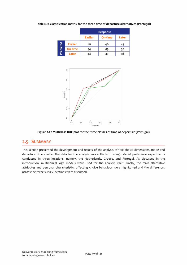
Deliverable 2.3: Modelling framework for analysing users’ choices Page 40 of 121
Table 2.17 Classification matrix for the three time of departure alternatives (Portugal)
Response
Earlier On-time Later
Pred
icte
d Earlier 111 46 43 On-time 34 83 32
Later 48 47 118
Figure 2.22 Multiclass-ROC plot for the three classes of time of departure (Portugal)
2.5 SUMMARY
This section presented the development and results of the analysis of two choice dimensions, mode and departure time choice. The data for the analysis was collected through stated preference experiments conducted in three locations, namely, the Netherlands, Greece, and Portugal. As discussed in the introduction, multinomial logit models were used for the analysis itself. Finally, the main alternative attributes and personal characteristics affecting choice behaviour were highlighted and the differences across the three survey locations were discussed.

Deliverable 2.3: Modelling framework for analysing users’ choices Page 41 of 121
3 ROUTE CHOICE In this chapter, we model travel behaviour associated with route choice. Given the close association of My-TRAC with Shift2Rail, and the general focus on public transport, route choice models are explicitly modelled for public transport networks. Similar to the choice models developed in the previous section, as well as in D2.1, special attention is paid to travellers’ attitudes towards and perceptions of risk under uncertainty. Such attitudes and perceptions cause unexpected deviations from rational behaviour. Thus, it is important to not only describe how people will behave but also to work towards prescriptive action that will help us give people meaningful travel advice. Furthermore, we study how behaviour may be assessed from observations of actual trips.
Conventionally, travel behaviour and consumer satisfaction are studied by distributing survey to riders inside public transport stations and vehicles. However, as more and more data becomes available to researchers and transportation authorities, through the My-TRAC application and other sources, revealed preferences will be the main source for behaviour analyses and consumer studies. To this end, we also focus on studying revealed preferences from the pre-dominant source of such data today: smart card data. We understand that respecting consumer privacy is an important aspect today and therefore it has been an important vision for the My-TRAC consortium. To this end, the data we use has been fully scrambled from the origin – we are unable to link smart cards to individual nor are we able to link journeys to smart cards. All journeys are assessed on their own merit without linking them together by a single identity.
The structure of this section is different from that of the previous one, since we undertake different lines of research. First, we focus on capturing waiting time uncertainty that travellers in public transport networks feel (Model 1: section 3.1). This is done through conventional stated preference experiments, albeit with a novel choice situation that permits the quantification of subjective beliefs regarding uncertainty as well as the effect of context and personal characteristics on this uncertainty. Results from the Netherlands, Greece, and Portugal are presented. In the next two sections, we present analyses of smart card data and revealed behaviour. Unfortunately, such data could not be secured from Greece and Portugal; therefore, we focus on the Netherlands. We first study an extremely important aspect of choice analysis: choice sets (Model 2: section 3.2). Analysing the alternatives considered by decision-makers when choosing is critical to both accurate behaviour modelling as well as presenting application users with appropriate options. If we do not model this aspect of choice behaviour, we are likely to miss an option that a traveller would have taken, or we might present the traveller with an option that they would never take. Once a decision-maker has their choice set, they are likely to move on to a fully compensatory choice that trades off different attributes of all the alternatives included in the choice set. Thus, we finally use the same smart card dataset to estimate a fully compensatory route choice model (Model 3: section 3.3).
Deliverable 2.3: Modelling framework for analysing users’ choices Page 42 of 121
3.1 MODEL 1: CAPTURING WAITING TIME UNCERTAINTY3
Given the large number of sources of stochasticity, transportation networks are associated with inherent uncertainty. Understanding route choice behaviour under such uncertainty leads to improved understanding of network flows and traveller satisfaction. On the supply side, this is important for transportation authorities to plan service levels and prioritise relevant investments. On the other hand, knowing how travellers make choices gives authorities an opportunity to be more proactive and influence demand in a way that is optimal for the system as a whole. To this end, this section proposes a method to quantify the level of uncertainty perceived by travellers in public transport networks.
In decision theory, the Knightian classification of uncertainty is based on whether, for a set of (possibly infinite) events, objective probabilities exist or not. Decisions under the former regime (when probabilities exist) are said to be made under ‘risk’ while those under the latter are under ‘ambiguity’ or ‘uncertainty’ [35]. The assumptions that objective probabilities are available and trusted by decision makers are seldom fulfilled in the real world. Most real world events indeed occur under ambiguity wherein decisions are made based on subjective beliefs [35, 36].
In most road or public transport networks too, not only do travellers not have access to objective travel time probability distributions but any information provided regarding travel time or its reliability will be distorted by travellers’ beliefs borne from a number of factors such as previous experiences, habits, and contexts. Despite this, in most studies on the effect of reliability on route choice behaviour, choices observed have been made and/or analysed using objective probabilities. Studies on the impact of travel time reliability have used observations from one of the following sources: stated preference experiments, actual trips, or laboratory experiments. Stated preference experiments, which are by far the most commonly employed methodology, typically present respondents with route alternatives with risky travel time attributes. Apart from the departure from the uncertainty paradigm in the real world, such experiments face difficulties in conveying probabilities (see Bates, et al. [37], Carrion and Levinson [38]) and usually do not take into account subjective weighting [39] of the presented probabilities or apply out-of-context parameters to do so (e.g., Li and Hensher [40]). Studies using revealed preferences from real-world observations have been limited, and mainly focused on car traffic networks, because of the lack of suitable data and control over the choice situation. In these studies, although decisions are made under ambiguity, analysis is, nevertheless, carried out using objective probabilities [38]. Laboratory experiments, which offer more control over the choice situation, typically focus on analysing learning mechanisms (e.g., Avineri and Prashker [41]) and comparing the effects of different levels and accuracies of information (e.g., Ben-Elia, et al. [42], Ben-Elia, et al. [43]). These studies assume a fixed learning period and for situations where information is provided either (implicitly) assume a risky paradigm or do not quantify subjects’ travel time reliability perceptions.
This section proposes a method to assess travellers’ route choice behaviour under natural ambiguity without using objective probabilities or assuming specific learning behaviour — important drawbacks in existing studies. Specifically, a route choice situation is proposed whereby travellers’ beliefs towards waiting time uncertainty can be quantified in terms of a certainty equivalent. For a given risky or uncertain prospect, its certainty equivalent is that risk-less outcome for which the decision-maker becomes indifferent to either prospects. For decisions under ambiguity, the certainty equivalent simultaneously represents how probable an outcome is thought to be and ambiguity aversion. In addition, it measures how other context variables affect travellers’ perception of uncertainty. The choice situation is contextualised
3 Parts of this section are based on [34]S. Shelat, O. Cats, and J. W. C. van Lint, "Quantifying Subjective Beliefs Regarding Waiting Time Uncertainty in Public Transport Networks," presented at the The 24th International Conference of Hong Kong Society for Transportation Studies, Hong Kong, 14-16 December 2019, 2019. and an associated working paper under the same name.
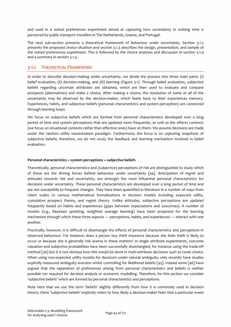
Deliverable 2.3: Modelling framework for analysing users’ choices Page 43 of 121
and used in a stated preferences experiment aimed at capturing how uncertainty in waiting time is perceived by public transport travellers in The Netherlands, Greece, and Portugal.
The next sub-section presents a theoretical framework of behaviour under uncertainty. Section 3.1.2 presents the proposed choice situation and section 3.1.3 describes the design, presentation, and sample of the stated preferences experiment. This is followed by the choice analyses and discussion in section 3.1.4 and a summary in section 3.1.5.
3.1.1 THEORETICAL FRAMEWORK
In order to describe decision-making under uncertainty, we divide the process into three main parts: (i) belief evaluation, (ii) decision-making, and (iii) learning (Figure 3.1). Through belief evaluation, subjective beliefs regarding uncertain attributes are obtained, which are then used to evaluate and compare prospects (alternatives) and make a choice. After making a choice, the resolution of some or all of the uncertainty may be observed by the decision-maker, which feeds back to their experiences memory. Experiences, habits, and subjective beliefs (personal characteristics and system perception) are connected through learning loops.
We focus on subjective beliefs which are formed from personal characteristics developed over a long period of time and system perceptions that are updated more frequently, as well as the effects contexts (we focus on situational contexts rather than affective ones) have on them. We assume decisions are made under the random utility maximization paradigm. Furthermore, the focus is on capturing snapshots of subjective beliefs; therefore, we do not study the feedback and learning mechanism involved in belief evaluation.
Personal characteristics + system perceptions = subjective beliefs
Theoretically, personal characteristics and (subjective) perceptions of risk are distinguished to study which of these are the driving forces behind behaviour under uncertainty [44]. Anticipation of regret and attitudes towards risk and uncertainty, are amongst the most influential personal characteristics for decisions under uncertainty. These personal characteristics are developed over a long period of time and are not susceptible to frequent changes. They have been quantified in literature in a number of ways from Likert scales to various mathematical formalizations in decision models including expected utility, cumulative prospect theory, and regret theory. Unlike attitudes, subjective perceptions are updated frequently based on habits and experiences (gaps between expectations and outcomes). A number of models (e.g., Bayesian updating, weighted average learning) have been proposed for the learning mechanism through which these three aspects — perceptions, habits, and experiences — interact with one another.
Practically, however, it is difficult to disentangle the effects of personal characteristics and perceptions in observed behaviour. For instance: does a person buy theft insurance because she feels theft is likely to occur or because she is generally risk averse in these matters? In single attribute experiments, outcome valuation and subjective probabilities have been successfully disentangled, for instance using the trade-off method [36] but it is not obvious how this would be done in multi-attribute decisions such as route choice. When using non-expected utility models for decisions under natural ambiguity, only recently have studies explicitly measured ambiguity aversion whilst controlling for likelihood beliefs [45]. Indeed some [46] have argued that the separation of preferences arising from personal characteristics and beliefs is neither possible nor required for decision analysis or economic modelling. Therefore, for this section we consider ‘subjective beliefs’ which are formed by personal characteristics and perceptions.
Note here that we use the term ‘beliefs’ slightly differently from how it is commonly used in decision theory; there ‘subjective beliefs’ explicitly refers to how likely a decision-maker feels that a particular event
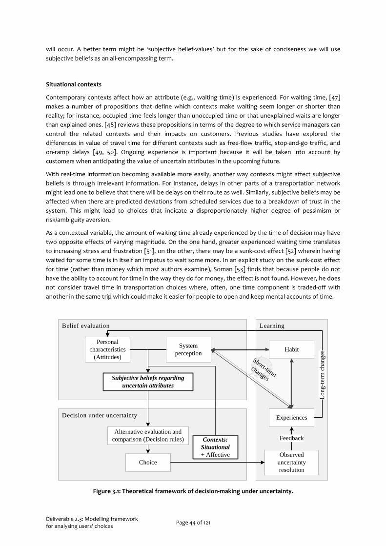
Deliverable 2.3: Modelling framework for analysing users’ choices Page 44 of 121
will occur. A better term might be ‘subjective belief-values’ but for the sake of conciseness we will use subjective beliefs as an all-encompassing term.
Situational contexts
Contemporary contexts affect how an attribute (e.g., waiting time) is experienced. For waiting time, [47] makes a number of propositions that define which contexts make waiting seem longer or shorter than reality; for instance, occupied time feels longer than unoccupied time or that unexplained waits are longer than explained ones. [48] reviews these propositions in terms of the degree to which service managers can control the related contexts and their impacts on customers. Previous studies have explored the differences in value of travel time for different contexts such as free-flow traffic, stop-and-go traffic, and on-ramp delays [49, 50]. Ongoing experience is important because it will be taken into account by customers when anticipating the value of uncertain attributes in the upcoming future.
With real-time information becoming available more easily, another way contexts might affect subjective beliefs is through irrelevant information. For instance, delays in other parts of a transportation network might lead one to believe that there will be delays on their route as well. Similarly, subjective beliefs may be affected when there are predicted deviations from scheduled services due to a breakdown of trust in the system. This might lead to choices that indicate a disproportionately higher degree of pessimism or risk/ambiguity aversion.
As a contextual variable, the amount of waiting time already experienced by the time of decision may have two opposite effects of varying magnitude. On the one hand, greater experienced waiting time translates to increasing stress and frustration [51], on the other, there may be a sunk-cost effect [52] wherein having waited for some time is in itself an impetus to wait some more. In an explicit study on the sunk-cost effect for time (rather than money which most authors examine), Soman [53] finds that because people do not have the ability to account for time in the way they do for money, the effect is not found. However, he does not consider travel time in transportation choices where, often, one time component is traded-off with another in the same trip which could make it easier for people to open and keep mental accounts of time.
Figure 3.1: Theoretical framework of decision-making under uncertainty.
Decision under uncertainty
LearningBelief evaluation
System perception
Experiences
Personal characteristics
(Attitudes)
Contexts: Situational + Affective
Long
-term
cha
nges
Subjective beliefs regarding uncertain attributes
Alternative evaluation and comparison (Decision rules)
ChoiceObserved
uncertainty resolution
Feedback
HabitShort-term
changes

Deliverable 2.3: Modelling framework for analysing users’ choices Page 45 of 121
3.1.2 CHOICE SITUATION
Travellers in public transport networks are likely to select a hyperpath (a set of attractive lines) and then apply a strategy (such as board the first line that arrives) [54]. Not only does the importance of making sequential decisions increase with uncertainty in the network but the type of strategy employed depends on the reliability perception and information available regarding the network [54, 55]. To understand traveller behaviour under uncertainty, one such sequential choice is analysed — whether to board a particular vehicle — in the context of the following situation (Figure 3.2).
Consider a traveller who arrives at a public transport stop. From here, either of the next two vehicles can take her to her destination. Both of these vehicles are identical in every way except for their departure and arrival times at the origin and destination stations, respectively. Furthermore, both of these vehicles will take her directly, without any transfers, to the destination station. As is prevalent in many mass transit systems worldwide, the scheduled departure times from the origin stop as well as any anticipated delays (real-time information) are shown to the traveller. Moreover, she is assumed to know the time both vehicles will take to reach her destination station (either from experience or a travel planner). When the first vehicle (VEH1) arrives, she must make a decision, based on the information available to her and her beliefs regarding the network, whether to board it or to wait for the next one (VEH2).
Although the vehicles are identical, the options available to the traveller (unlike route alternatives in most choice situations) are not unlabelled — in fact, the traveller is comparing a certain (as in risk-less) option against an ambiguous one. The vehicle that has already arrived has a certain waiting time which is almost zero due to the, usually, negligible difference between doors closing and departure. Although the anticipated waiting time for the next vehicle is displayed, it is ambiguous for the traveller since no concrete probabilities regarding its accuracy are supplied. Rather, she will draw from her own subjective perceptions of this natural source of ambiguity and make a decision.

Deliverable 2.3: Modelling framework for analysing users’ choices Page 46 of 121
10:15 10:45
10:15 10:45
10:15 10:45
VE
H2
VE
H1
Trav
elle
r
10:37DestinationScheduled
Arrival Time
10:42Destination
Anticipated DelayedArrival Time
10:23Origin
ScheduledDeparture Time
10:28Origin
Anticipated DelayedDeparture Time
10:23 - 10:28Anticipated Delay
10:32Next Alternative
10:28Decision Point
10:18Arrival
at Origin
10:18 - 10:28Experienced Waiting Time
10:28 - 10:32Anticipated Waiting Time
10:32 - 10:40In-vehicle Time
10:35DestinationScheduled
Arrival Time
10:27Origin
ScheduledDeparture Time
10:27 - 10:32Anticipated Delay
10:32Origin
Anticipated DelayedDeparture Time
10:40Destination
Anticipated DelayedArrival Time
10:28 - 10:42In-vehicle Time
Figure 3.2: Choice situation presented in a timeline format
Thus, from this situation the certainty equivalent of ambiguous waiting time can be calculated. This is because, in addition to observing the trade-off between the difference in in-vehicle times and the anticipated waiting time, we also observe the value assigned to the certain option which represents the traveller’s subjective beliefs regarding the anticipated waiting time. The traveller’s subjective beliefs, and therefore her value of certainty, may also be affected by delays in the system and the time she already spent waiting before the decision point. Equation (3.1) (in section 3.1.4) describes the utilities of the two options. Since travellers are not likely to believe that the actual waiting time will be significantly lower than the displayed prediction, it is reasonable to expect that they do not dislike certainty. This implies that if travellers, in general, believe the shown anticipated waiting time, the value of certainty would be lower than if there is a general perception of poor reliability.
To assess the value of certainty in waiting time, choices between non-(strictly)-dominated alternatives must be observed. Assuming that travellers either like or are indifferent to certainty in waiting time, to ensure that the certain alternative does not dominate the uncertain one, the former must arrive at the destination later than the latter taking into account any weighting of travel time components. The uncertain vehicle can arrive at the destination before the certain one if it can either overtake the latter along a common path or if they serve two distinct lines.
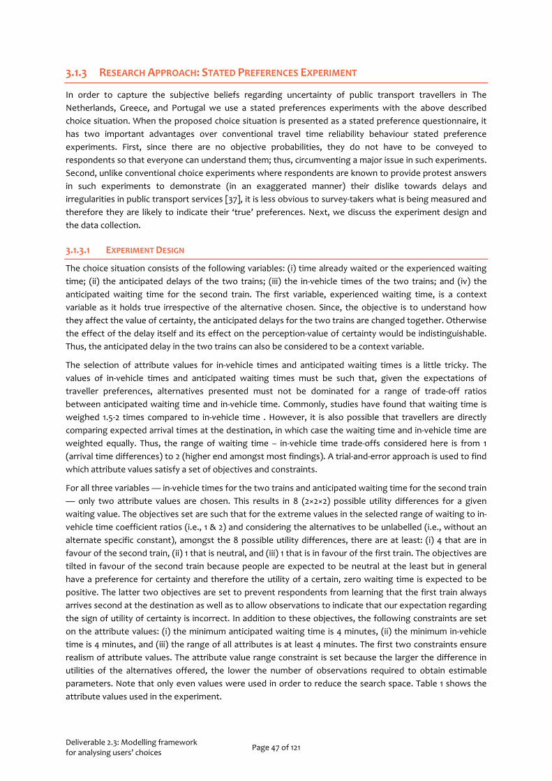
Deliverable 2.3: Modelling framework for analysing users’ choices Page 47 of 121
3.1.3 RESEARCH APPROACH: STATED PREFERENCES EXPERIMENT
In order to capture the subjective beliefs regarding uncertainty of public transport travellers in The Netherlands, Greece, and Portugal we use a stated preferences experiments with the above described choice situation. When the proposed choice situation is presented as a stated preference questionnaire, it has two important advantages over conventional travel time reliability behaviour stated preference experiments. First, since there are no objective probabilities, they do not have to be conveyed to respondents so that everyone can understand them; thus, circumventing a major issue in such experiments. Second, unlike conventional choice experiments where respondents are known to provide protest answers in such experiments to demonstrate (in an exaggerated manner) their dislike towards delays and irregularities in public transport services [37], it is less obvious to survey-takers what is being measured and therefore they are likely to indicate their ‘true’ preferences. Next, we discuss the experiment design and the data collection.
3.1.3.1 EXPERIMENT DESIGN
The choice situation consists of the following variables: (i) time already waited or the experienced waiting time; (ii) the anticipated delays of the two trains; (iii) the in-vehicle times of the two trains; and (iv) the anticipated waiting time for the second train. The first variable, experienced waiting time, is a context variable as it holds true irrespective of the alternative chosen. Since, the objective is to understand how they affect the value of certainty, the anticipated delays for the two trains are changed together. Otherwise the effect of the delay itself and its effect on the perception-value of certainty would be indistinguishable. Thus, the anticipated delay in the two trains can also be considered to be a context variable.
The selection of attribute values for in-vehicle times and anticipated waiting times is a little tricky. The values of in-vehicle times and anticipated waiting times must be such that, given the expectations of traveller preferences, alternatives presented must not be dominated for a range of trade-off ratios between anticipated waiting time and in-vehicle time. Commonly, studies have found that waiting time is weighed 1.5-2 times compared to in-vehicle time . However, it is also possible that travellers are directly comparing expected arrival times at the destination, in which case the waiting time and in-vehicle time are weighted equally. Thus, the range of waiting time – in-vehicle time trade-offs considered here is from 1 (arrival time differences) to 2 (higher end amongst most findings). A trial-and-error approach is used to find which attribute values satisfy a set of objectives and constraints.
For all three variables — in-vehicle times for the two trains and anticipated waiting time for the second train — only two attribute values are chosen. This results in 8 (2×2×2) possible utility differences for a given waiting value. The objectives set are such that for the extreme values in the selected range of waiting to in-vehicle time coefficient ratios (i.e., 1 & 2) and considering the alternatives to be unlabelled (i.e., without an alternate specific constant), amongst the 8 possible utility differences, there are at least: (i) 4 that are in favour of the second train, (ii) 1 that is neutral, and (iii) 1 that is in favour of the first train. The objectives are tilted in favour of the second train because people are expected to be neutral at the least but in general have a preference for certainty and therefore the utility of a certain, zero waiting time is expected to be positive. The latter two objectives are set to prevent respondents from learning that the first train always arrives second at the destination as well as to allow observations to indicate that our expectation regarding the sign of utility of certainty is incorrect. In addition to these objectives, the following constraints are set on the attribute values: (i) the minimum anticipated waiting time is 4 minutes, (ii) the minimum in-vehicle time is 4 minutes, and (iii) the range of all attributes is at least 4 minutes. The first two constraints ensure realism of attribute values. The attribute value range constraint is set because the larger the difference in utilities of the alternatives offered, the lower the number of observations required to obtain estimable parameters. Note that only even values were used in order to reduce the search space. Table 1 shows the attribute values used in the experiment.

Deliverable 2.3: Modelling framework for analysing users’ choices Page 48 of 121
Table 3.1: Attribute values used in the choice experiment
Attribute Attribute values (in minutes)
Experienced waiting time 0, 5, 10, 15
Anticipated delays in both trains 0, 5, 10, 15
In-vehicle time for the first train 14, 28
In-vehicle time for the second train 4, 8
Anticipated waiting time for the second train 4, 10
With these attributes and values, a simultaneous orthogonal fractional factorial design is found with NGENE. To limit the number of questions per respondent, the design is blocked into two parts. With this specification, a design with a total of 16 choice situations is found with 8 choice situations per respondent.
3.1.3.2 PRESENTATION
The choice experiment section begins with an explanation of the choice situation. Next, the respondent faces a sample question which is not used in the analysis and finally the 8 choice situations that will be used for the analysis. Each choice situation is prefaced by the instruction that there were two trains that could take them to their destination from the platform.
Respondents are shown information regarding the waiting times and anticipated delays of the two trains (TRN1, TRN2) in a format similar to what they are familiar with. In the Netherlands, this is a signboard found at platforms of the Dutch railways (Figure 3.3) and in the other countries it is a countdown clock displayed in minutes and seconds. Respondents are informed that the information regarding waiting times and delays are as per the state of the signboards at the decision point (as described in section 3.1.2). To remind survey-takers in the Netherlands of the information shown in different parts of the signboard, an annotated version is also displayed in the example question. Separately from this, information regarding the in-vehicle times and the time already waited is shown as a table and a line of text, respectively. Finally, the respondents are asked to choose whether they would board TRN1 or wait for TRN2 (see Figure 3.4, Figure 3.5). In the online survey in the Netherlands, the order of the 8 situations as well as that of the two options in each situation were scrambled to avoid any biases.
Figure 3.3: Information displays at a real station (annotated)
Current Time Scheduled departure TRN1 Anticipated delay TRN1
Scheduled departure TRN2 Anticipated delay TRN2
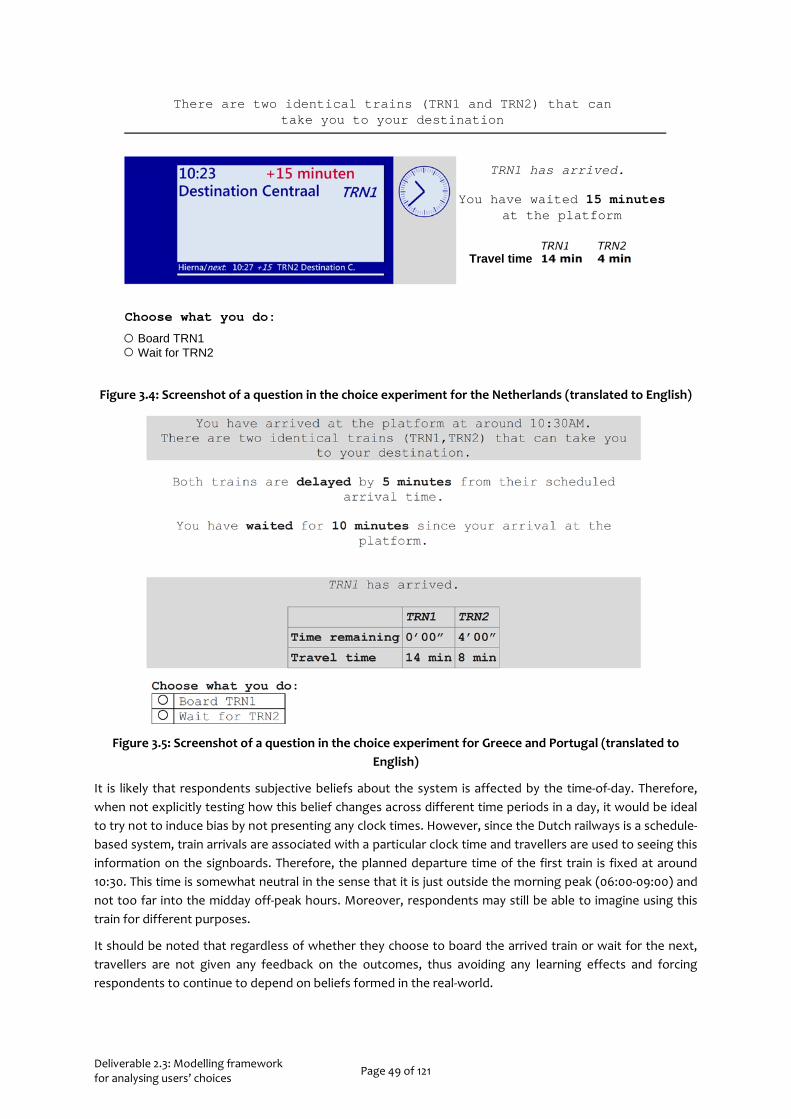
Deliverable 2.3: Modelling framework for analysing users’ choices Page 49 of 121
Figure 3.4: Screenshot of a question in the choice experiment for the Netherlands (translated to English)
Figure 3.5: Screenshot of a question in the choice experiment for Greece and Portugal (translated to English)
It is likely that respondents subjective beliefs about the system is affected by the time-of-day. Therefore, when not explicitly testing how this belief changes across different time periods in a day, it would be ideal to try not to induce bias by not presenting any clock times. However, since the Dutch railways is a schedule-based system, train arrivals are associated with a particular clock time and travellers are used to seeing this information on the signboards. Therefore, the planned departure time of the first train is fixed at around 10:30. This time is somewhat neutral in the sense that it is just outside the morning peak (06:00-09:00) and not too far into the midday off-peak hours. Moreover, respondents may still be able to imagine using this train for different purposes.
It should be noted that regardless of whether they choose to board the arrived train or wait for the next, travellers are not given any feedback on the outcomes, thus avoiding any learning effects and forcing respondents to continue to depend on beliefs formed in the real-world.
There are two identical trains (TRN1 and TRN2) that can take you to your destination
TRN1 has arrived.
You have waited 15 minutes at the platform
Travel time
Choose what you do:
Board TRN1Wait for TRN2

Deliverable 2.3: Modelling framework for analysing users’ choices Page 50 of 121
3.1.3.3 DATA COLLECTION
The choice experiment was included within a larger survey that consisted of four parts, in this order: (0) screening, (1) socio-demographics, (2) choice experiment, and (3) qualitative measurements (see Appendix C). The structure, content, and design of an initial draft of the survey was refined based on comments received from a small pilot of about 20 persons. The final version of the survey was offered in the respective local languages and had an expected completion time of 10 minutes.
The same data collection methods are used as for the mode and departure time choice experiments (see section 2.3). In the Netherlands, it was distributed to a predefined sample size of 700 respondents through an online panel, PanelClix. Given that most people in the Netherlands have access to the internet, this method of data collection does not create any obvious biases. The data collection took place in November-December 2018. For Greece and Portugal, the predefined sample size was 300-350 respondents. In Greece, the data was collected offline in February-March 2019 by surveying respondents on university campus (National Technical University of Athens), public transport stations and other important areas in Athens. In Portugal, a combination of online and offline methods is used and data was collected during March-April 2019.
Screening and socio-demographics
For the Netherlands, respondents were screened out if they used the trains less than once per month on the basis that if respondents do not meet this criterion, they are likely to not have well-formed subjective beliefs regarding the railways. Regarding trip purpose, in the Netherlands, the survey aimed to collect about 80% of responses from those who used the railways for commuting either to work or education, and the rest from those with other purposes. The greater focus on commuters and efforts was to ensure that those travelling more frequently are included is due to the fact this group is more likely to have more well-formed value systems and subjective beliefs. Furthermore, for the Netherlands, desired socio-demographic quotas were obtained from the data collected between 2011 to 2015 by a national, one-day, trip diary survey, OViN (Onderzoek Verplaatsingen in Nederland) conducted by the Dutch Central Bureau of Statistics (2011–2015, Centraal Bureau voor de Statistiek [56]. The distribution of age, gender, and household incomes of respondents in that survey who use the railways at least once (during the day of reporting) are used as the desired stratification. It should be noted that these distributions were not weighted by the individual weights given in the survey as the group was reasonably large in itself. For the other countries, the trip purpose criterion was somewhat relaxed to make data collection easier. Moreover required socio-demographics for these countries only focused on age and gender. Table 3.2 shows the distribution of respondent characteristics and completion times for the final set of valid responses.
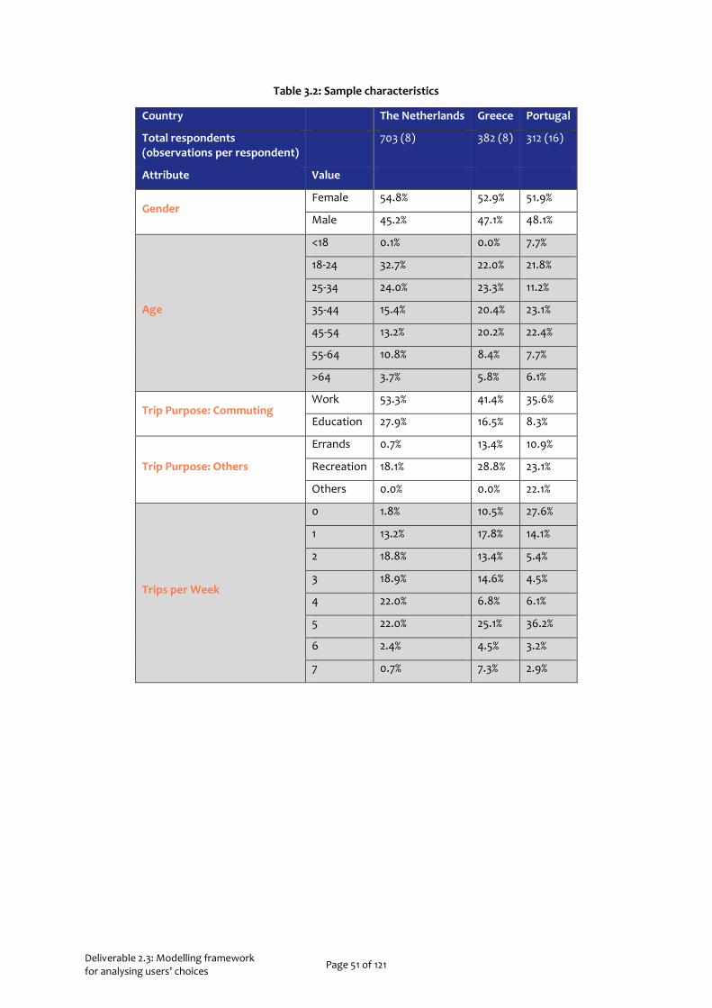
Deliverable 2.3: Modelling framework for analysing users’ choices Page 51 of 121
Table 3.2: Sample characteristics
Country The Netherlands Greece Portugal
Total respondents (observations per respondent)
703 (8) 382 (8) 312 (16)
Attribute Value
Gender Female 54.8% 52.9% 51.9%
Male 45.2% 47.1% 48.1%
Age
<18 0.1% 0.0% 7.7%
18-24 32.7% 22.0% 21.8%
25-34 24.0% 23.3% 11.2%
35-44 15.4% 20.4% 23.1%
45-54 13.2% 20.2% 22.4%
55-64 10.8% 8.4% 7.7%
>64 3.7% 5.8% 6.1%
Trip Purpose: Commuting Work 53.3% 41.4% 35.6%
Education 27.9% 16.5% 8.3%
Trip Purpose: Others
Errands 0.7% 13.4% 10.9%
Recreation 18.1% 28.8% 23.1%
Others 0.0% 0.0% 22.1%
Trips per Week
0 1.8% 10.5% 27.6%
1 13.2% 17.8% 14.1%
2 18.8% 13.4% 5.4%
3 18.9% 14.6% 4.5%
4 22.0% 6.8% 6.1%
5 22.0% 25.1% 36.2%
6 2.4% 4.5% 3.2%
7 0.7% 7.3% 2.9%

Deliverable 2.3: Modelling framework for analysing users’ choices Page 52 of 121
Qualitative measurements
The following factors are measured qualitatively on a Likert scale: (i) regret anticipation, (ii) perception of reliability, and (iii) engagement level while waiting. The first, anticipation of regret, is considered to be one of the main psychological driving forces of risk aversion which leads to a preference for certainty. A standardized regret scale consisting of five items adopted from Schwartz, et al. [57] is used to measure it. This contains statements such as ‘Whenever I make a choice, I try to get information about how the other alternatives turned out’ to which respondents indicate their level of agreement. The second factor assesses the perception of reliability of the network in general and in the presence of delays, and the perceived accuracy of displayed real-time information. This is tested using questions such as ‘How reliable do you feel is the train arrival information?’ or ‘When you at an NS platform, to what extent is your perception of reliability (for your trip) affected if the next two consecutive trains that you can take to your destination are delayed?’. Finally, as discussed in section 3.1.1, context can affect how waiting time is experienced. Occupied time has been consistently shown to reduce perceived waiting time [48] which could in turn affect beliefs regarding anticipated waiting time; therefore, the level of engagement of respondents at train platforms is measured through the following question: ‘Usually, how engaged are you with the activity you perform while waiting at a railway platform?’’
3.1.4 RESULTS & DISCUSSION
Discrete choice models are used to analyse the choices observed in the stated preference experiment under the conventional framework of utility maximization. First, we formulate utility equations that account for the certainty effect as an alternate specific constant. Then, multinomial logit (MNL) models are estimated for all the countries. From this model we are able to evaluate the subjective beliefs regarding uncertainty in waiting time, and the effect of context variables and personal characteristics on this. For the Netherlands, where we have more responses available, we also analyse heterogeneity in behaviour through mixed logit (ML) and latent class choice models (LCCM). While the former accounts for taste variations in the value of choice model coefficients, the latter identifies distinct behaviour profiles. The ML model also measures the effect of socio-demographics, general travel characteristics, and personal factors on travellers’ subjective beliefs. All choice model estimations are carried out using PythonBiogeme [58].
Four attributes are involved in the choice situation: two main variables — in-vehicle times (IVT) and anticipated waiting time (AWT) — and two contextual variables — experienced waiting time (EWT) and anticipated delay (DEL). Considering only the above variables, the utilities of the two alternatives, TRN1 and TRN2, would be as specified in equation (3.1). As discussed in section 3.1.2, the alternatives are labelled and therefore, the train that arrives at the origin first is assigned an alternative specific constant (βcertainty) that represents the value of certainty attached to it.
TRN1 certainty IVT AWT EWT DEL
1 2TRN2
( )
0
U IVT IVT AWT EWT DELU
β β β β β= + ⋅ − + ⋅ + ⋅ + ⋅
= (3.1)
Table 3.3 gives an overview of all the attributes included in the analysis.

Deliverable 2.3: Modelling framework for analysing users’ choices Page 53 of 121
Table 3.3: Overview of attributes included in the choice analyses
Attributes Symbol Explanation
Choice situation
Certainty constant βcertainty -
In-vehicle time βIVT
All time attributes are in minutes Anticipated waiting time βAWT
Experienced waiting time
βEWT
Anticipated delays βDEL
Personal characteristics
Socio-demographics
Age βage Ordinal in ascending order: <18, 18-24, 25-34, 35-44, 45-54, 55-64, >64
Gender βfemale Categorical(effect coded):
male, female
Net personal income βincome Ordinal in ascending order
Trip purpose βwork, βeducation, βerrand, βleisure
Categorical (effect coded): work, education, errands, leisure
Train use frequency βfrequency Average number of days train is used in a week
Qualitative measures
Anticipation of regret βregret Average of the scores on 5 Likert scale items (higher value: more anticipation of regret)
System perception βperception Average of the scores on 2 Likert scale items (higher value: system perceived to be more reliable)
Effect of delays on perception
βdelay-effect Likert scale (higher value: perception more strongly negatively affected by delays)
Level of engagement while waiting
βengagement Likert scale (higher value: more engaged)
3.1.4.1 MULTINOMIAL LOGIT MODELS FOR THE 3 COUNTRIES
Similar to section 2.4 here, too, MNL models are implemented for the three countries under study. We briefly describe MNL models again for reference before presenting the rest of the analysis. The utility of an alternative a, Ua, consists of systematic (Va) and random (ε) components. The systematic component is the product of the vector of taste preferences (β) and the vector of alternative attributes (xa). In an MNL model, the random component is Gumbel distributed. The probability of choosing alternative i from I alternatives is given by the following:
1
; ; i
a
V
a a a a ni I Va
eU V V x Pe
e β=
= + = ⋅ =∑
(3.2)
Deliverable 2.3: Modelling framework for analysing users’ choices Page 54 of 121
First, we estimate pure choice situation MNL models for all countries (MNLCS) and then estimate the MNL models that also accounts for personal characteristics (MNLALL). This gives us an indication of the improvement in model fit brought about by the variables extraneous to the choice situation. The final models are developed by removing insignificant parameters (p>0.2) one-by-one. Table 3.5 shows the final models for all three countries.
The model fit for Portugal is surprisingly good while that for the Netherlands and Greece is good and fair, respectively. Unlike the other countries, for the Netherlands, only a few personal characteristics remain significant and do not improve the model fit enough to justify their inclusion (based on the log-likelihood ratio test and a p-value threshold of 0.05).
For all the models, the signs of the travel times and certainty preference are in the expected direction. Travellers prefer the first train more in general (indicating a preference for certainty), and also prefer it more as anticipated waiting time for the second train increases and as the differences in in-vehicle time (in favour of the second train) reduces. There are no specific expectations regarding the direction of the effect of experienced waiting time and it indeed varies. The effect of delay seems to be in the wrong direction – one would expect that as the delays become higher, travellers would lose confidence in the system and become more uncertain regarding their waiting time.
On average, travellers in the Netherlands, Greece, and Portugal are willing to trade-off 9.12, 10.62, and 3.67 minutes of extra in-vehicle time in order to have certainty in their waiting time. In contrast with literature (where uncertainty is not accounted for), the ratio of the weights of waiting and in-vehicle time becomes less than 1 in the Netherlands (0.65). In Greece and Portugal this ratio remain pretty high at 1.79 and 1.66, respectively, despite accounting for certainty preference. For experienced waiting time, as discussed in section 3.1.1, there is no clear intuition regarding the effect direction since travellers might either experience frustration or take into account sunk costs. Moreover, some people may begin to engage in an activity that distracts them from waiting after some threshold of experienced waiting time. An overall negative and positive effect in favour of TRN1 is found for Greece and Portugal respectively. However, the effect sizes are comparatively quite small.
In the Netherlands and Portugal, female travellers seem to slightly prefer the certain option more than their male counterparts similar to results obtained by de Palma and Picard [59] for their departure time choice model. In Greece, higher income individuals prefer the faster option and have more trust in the displayed waiting times. Commuters in Portugal feel substantially less uncertain regarding waiting times than non-commuters and prefer to wait for the second train. Those going to work are more likely to wait for the second train than those going for education. Furthermore, those running an errand prefer to take the first train more strongly than those using public transport for recreational trips. In Greece, those going to work or running an errand seem to show a higher preference for certainty than for other trips. For leisure trips, respondents seem to be especially relaxed, choosing to wait for the second trip.
Greater anticipation of regret is correlated with a preference for certainty in Greece but, surprisingly, has the opposite effect in Portugal. Poorer perception of the system’s reliability also has an effect opposite to what is expected in Portugal. The level of engagement, however, has the correct sign for both these countries with people who report to be more engaged preferring more often to wait for the second train. Additionally, respondents in Portugal whose perception is reportedly negatively affected by delays, demonstrate a slightly increased preference for certainty.
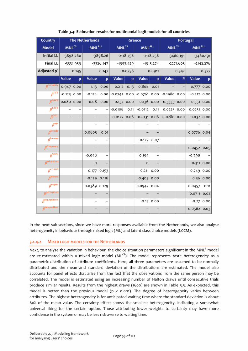
Deliverable 2.3: Modelling framework for analysing users’ choices Page 55 of 121
Table 3.4: Estimation results for multinomial logit models for all countries
Country The Netherlands Greece Portugal
Model MNLCS MNLALL MNLCS MNLALL MNLCS MNLALL
Initial LL -3898.260 -3898.26 -2118.258 -2118.258 -3460.191 -3460.191
Final LL -3331.959 -3326.147 -1953.429 -1915.274 -2271.605 -2142.276
Adjusted ρ2 0.145 0.147 0.0756 0.0911 0.342 0.377
Value p Value p Value p Value p Value P Value p
βcertainty 0.947 0.00 1.13 0.00 0.212 0.13 0.808 0.01 – – 0.777 0.00
βIVT -0.123 0.00 -0.124 0.00 -0.0742 0.00 -0.0761 0.00 -0.1980 0.00 -0.212 0.00
βAWT 0.080 0.00 0.08 0.00 0.132 0.00 0.136 0.00 0.3333 0.00 0.351 0.00
βEWT – – – – -0.0108 0.11 -0.0112 0.11 0.0225 0.00 0.0231 0.00
βDEL – – – – -0.0127 0.06 -0.0131 0.06 -0.0280 0.00 -0.032 0.00
βage – – – – – –
βfemale 0.0805 0.01 – – 0.0776 0.04
βincome – – -0.127 0.07 – –
βfrequency – – – – 0.0452 0.05
βwork -0.048 – 0.194 – -0.798 –
βeducation 0 – 0 – -0.311 0.00
βerrand 0.177 0.153 0.211 0.00 0.749 0.00
βleisure -0.129 0.116 -0.405 0.00 0.36 0.00
βregret -0.0389 0.129 0.0947 0.04 -0.0457 0.11
βperception – – – – 0.0711 0.02
βengagement – – -0.17 0.00 -0.27 0.00
βdelay-effect – – – – 0.0562 0.03
In the next sub-sections, since we have more responses available from the Netherlands, we also analyse heterogeneity in behaviour through mixed logit (ML) and latent class choice models (LCCM).
3.1.4.2 MIXED LOGIT MODELS FOR THE NETHERLANDS
Next, to analyse the variation in behaviour, the choice situation parameters significant in the MNLL model are re-estimated within a mixed logit model (MLCS). The model represents taste heterogeneity as a parametric distribution of attribute coefficients. Here, all three parameters are assumed to be normally distributed and the mean and standard deviation of the distributions are estimated. The model also accounts for panel effects that arise from the fact that the observations from the same person may be correlated. The model is estimated using an increasing number of Halton draws until consecutive trials produce similar results. Results from the highest draws (1600) are shown in Table 3.5. As expected, this model is better than the previous model (p < 0.001). The degree of heterogeneity varies between attributes. The highest heterogeneity is for anticipated waiting time where the standard deviation is about 60% of the mean value. The certainty effect shows the smallest heterogeneity, indicating a somewhat universal liking for the certain option. Those attributing lower weights to certainty may have more confidence in the system or may be less risk averse to waiting time.

Deliverable 2.3: Modelling framework for analysing users’ choices Page 56 of 121
To assess the effect of socio-demographics, general travel characteristics, and personal factors on travellers’ subjective beliefs (thus, value of certainty), another mixed logit model is estimated with these variables added to the utility of TRN1. For the estimation, all factors measured on Likert scales and categorical variables such as age and income are assumed to be continuous for the sake of model simplicity. Where multiple scales measure the same factor (e.g., regret) the mean of the responses is used. Finally, all categorical variables that cannot be interpreted as continuous are effect coded. The final results are arrived at by starting with all variables and sequentially removing those that are small and/or highly insignificant (although quite insignificant, the standard deviation of the value of certainty remains to ensure that the models can be easily compared). The likelihood ratio test indicates that the resulting extension of the MLCS model, MLALL, outperforms the original (p < 0.001). Results indicate that younger and female travellers have a higher preference for certainty. These results are in line with de Palma and Picard [59] who also find these categories to be more risk averse. Furthermore, as expected, respondents who indicated that they were more engaged while waiting and those who said that they found the railways and displayed information to be highly reliable place a lower value in certainty. It should be noted that the values for the qualitative measures (engagement, perception) and the categorical age variable ranged between 1–7.
3.1.4.3 LATENT CLASS CHOICE MODEL FOR THE NETHERLANDS
Latent class choice models represent heterogeneity basically through a discrete mixture of choice models. In LCCM, individuals are probabilistically allocated to latent classes each of which have their own choice models. Depending on the objective, different choice models may be used in each class but in this study, the MNL model from utility equations in (3.1) is used as the underlying behaviour model for each class. To represent this mathematically, consider individual n who belongs to class s (amongst S classes) with probability πns. Then the probability that this individual selects alternative i is the product sum of the class membership probabilities and the probability of selecting that alternative for each class (given the vector of taste parameters in that class, βs).
1
( )S
ni ns ni ss
P Pπ β=
= ⋅∑ (3.3)
If we assume intra-individual homogeneity in sensitivities, that is, account for panel effects, we essentially say that a particular individual is allocated to each class with the same probability for every choice they make. Thus, the likelihood of observing the sequence of choices i:i1,…,iT by individual n over T situations is given by the following:
1 1
( )t
TS
ni ns ni ss t
L Pπ β= =
=∑ ∏ (3.4)
Apart from accounting for heterogeneity in tastes, an important advantage with LCCM is that individuals’ preferences can be explained by using a class membership model to link membership probabilities with individuals’ characteristics. The commonly used, logit function is also used here as the class membership model. Furthermore, we use the socio-demographic and qualitative measures collected as the individual characteristics influencing class membership. For this vector of individual characteristics, zn, and to-be-estimated, class-specific regression parameters, coefficient vectors, γs, and constants, δs, the class membership probability is given by:
g( , )
g( , )1
s s n
a a n
z
ns S za
ee
δ g
δ gπ
+
+=
=∑
(3.5)

Deliverable 2.3: Modelling framework for analysing users’ choices Page 57 of 121
In this section, the MNL model from utility equations in (3.1) is used as the underlying behaviour model for each class. Although a 4-class model yielded the best between efficiency and model fit, two classes had a membership of less than 10%; therefore, a 3-class model is used (Table 3.5, LCC-3) which did not perform too poorly on model fit in comparison, has reasonable class sizes, and offers better interpretability. In the largest class (49.20%), behaviour is similar to the MNLL model with an additional effect wherein value of certainty increases slightly with delays. The second (33.31%) and third (17.48%) groups show a lexicographic preference for faster trains and the first train, respectively (at least, up to the attribute levels used in the survey). In addition to their inherent preferences, it is possible that those who strongly prefer the faster train, may have translated the offered alternatives into real-life services, where the trains are, in fact, different, and chosen one train type over another for reasons not measured in the survey. In the Netherlands, the express trains (Intercity) offer additional services such as air-conditioning and Wi-Fi internet.
The class membership model tries to explain individuals’ association with the different behavioural regimes in each class on the basis of socio-demographic, attitudinal, or revealed behaviour variables. Holding the smallest group as reference, younger travellers and those with a lower perception of reliability tend to make more complete trade-offs between certainty in waiting time and travel time. This may indicate that those who trust the system less are more deliberate in their choices. On the other hand, older travellers and those who report to be more engaged while waiting have a strong preference for the faster train. As discussed previously, higher engagement may lower the perception of waiting time tilting the choice in favour of a smaller in-vehicle time.

Deliverable 2.3: Modelling framework for analysing users’ choices Page 58 of 121
Table 3.5: Estimation results for mixed logit and latent class choice models for the Netherlands
Model MLCS MLALL
Initial LL -3898.260 -3898.260
Final LL -3123.075 -3113.413
BIC 6299.867 6313.175
Value p Value p Value p
βcertainty 1.240 0.00 2.090 0.00 βage -0.067 0.06
βIVT -0.169 0.00 -0.171 0.00 βfemale 0.115 0.03
βAWT 0.102 0.00 0.102 0.00 βengagement -0.082 0.02
βEWT - - - - βperception -0.063 0.07
βDEL - - - -
σcertainty 0.416 0.04 0.294 0.27
σIVT 0.075 0.00 0.078 0.00
σAWT 0.062 0.00 0.062 0.00
Model LCCM-3 class
Class size 49.20% 33.31% 17.48% Class membership
Class 1 Class 2 Class 3 Class 3 (ref.) Class 1 Class 2
Value p Value p Value p Value p Value p Value p
βcertainty 1.590 0.00 - - 0.923 0.01 βintercept 0 - 2.66 0.00 -1.280 0.04
βIVT -0.286 0.00 -0.061 0.00 -0.042 0.01 βage - - -0.206 0.02 0.203 0.03
βAWT 0.238 0.00 - - 0.123 0.00 βengagement - - - - 0.272 0.00
βEWT - - - - 0.0285 0.10 βperception - - -0.162 0.03 - -
βDEL 0.019 0.15 - - - -
3.1.5 SUMMARY
This section proposes a realistic route choice situation where travellers’ subjective beliefs towards waiting time uncertainty can be quantified in terms of a certainty equivalent. A stated preferences experiment with the choice situation is carried out. Findings indicated an average preference for certainty, with travellers willing to accept between 3 and 10 minutes of extra in-vehicle time to avoid uncertainty. We further report the effects of context and personal characteristics on beliefs regarding uncertainty for the three countries. Finally, heterogeneity in behaviour is analysed for the Netherlands where we have more data.
A limitation of this analysis was that stated preferences experiments may not be very conducive in eliciting the effects of context variables. Future studies could focus on designing experiments that can make respondents ‘feel’ the changes in perception of uncertainty due to contextual variables such as elapsed waiting time and delays. Alternatively, given the increasing availability of smart card and vehicle location data for public transport networks, subjective beliefs towards uncertainty may be assessed using revealed preferences from the proposed choice situation.
Deliverable 2.3: Modelling framework for analysing users’ choices Page 59 of 121
3.2 MODEL 2: INFERRING ROUTE CHOICE SETS4
There is widespread agreement in the marketing field that consumption choices occur in a two-stage process whereby consumers first form a consideration choice set and then make the final choice from this set [61]. Choice set composition and size can affect the ultimate decision in a number of ways [62], with the most obvious being that the exclusion of an alternative from the choice set means that it cannot be selected. Identification of choice sets may be straightforward when the number of alternatives are limited but it becomes more difficult as this number increases. In these cases, correctly identifying the choice set is important not only for real-world application of estimated choice models but also for the estimation of choice models from revealed preferences where choices are observed but choice sets are not.
Public transportation provides vital, sustainable transportation in many regions, making their planning, maintenance and operation a priority for authorities. In order to provide an appropriate level of service, understanding traveller behaviour to correctly model network flows has become increasingly important. Amongst other traveller decisions, route choices have a significant impact on network flows. Therefore, for both, estimation and application of route choice models, identification of route choice sets is a crucial step [62].
However, identifying route choice sets for origin-destination (OD) pairs in a network is a non-trivial task for several reasons. First, due to the combinatorial nature of the problem, the number of available and attractive routes is usually large. Second, public transport characteristics, such as fixed routes, schedules, and headways, which are usually time-dependent, add to the complexity of the task. Finally, the existence of different forms of travel costs, for instance, transferring or in-vehicle time, mean that traveller preferences have to be taken into account when identifying route choice sets.
Given the importance and complexity of route choice set identification, several studies in transportation literature have either entirely focussed on or have employed some form of route choice set identification methodology. These methodologies can be broadly divided into: (i) direct identification of choice sets and (ii) choice set generation methodologies (CSGMs).
Direct identification of choice sets may be based on reporting or observations of non-selected and selected alternatives, respectively. In the former, surveyed travellers are asked to report alternatives to their chosen route that they did not select but considered. This method has the obvious advantage that researchers do not have to guess what travellers have in their mind and the consideration set is known at the individual level. However, this reporting is subject to a number of errors (e.g., forgetfulness) and, as suggested in [63], is ‘at best a subset of the true choice set’. Furthermore, such interview techniques are time consuming and difficult to implement when choice sets are required for network-wide analysis.
For network-wide identification of choice sets, observations of selected alternatives offer a more suitable data source. In this method, the sets of unique routes observed are assumed to be the choice set for the respective OD pairs. The argument is that, if such data is collected over a long period of time it should include all routes considered by travellers. Practically, this is facilitated by the creation of large data sources as an increasing number of public transport services turn to automatic fare collection (AFC) technologies. As a result, several studies using smart card data employ this method for the identification of choice sets. However, this technique precludes the possibility of taking into account why some non-selected but feasible routes are never chosen [64]. Moreover, the transferability of behaviour parameters, estimated with choice sets thus obtained, is precarious because matching choice set generation methodologies are not available for other public transport networks [65].
4 This section is based on [60]S. Shelat, O. Cats, N. v. Oort, and H. v. Lint, "Calibrating Route Choice Sets for an Urban Public Transport Network using Smart Card Data," in 2019 6th International Conference on Models and Technologies for Intelligent Transportation Systems (MT-ITS), 2019, pp. 1-8, 2019.
Deliverable 2.3: Modelling framework for analysing users’ choices Page 60 of 121
Some drawbacks of direct identification of route choice sets can be overcome by using CSGMs. The aim with this approach is to develop a generic algorithm, that satisfies requirements associated with the purpose of the choice set [66], for identification of route alternatives. Thus, route CSGMs are suitable for network-wide application and by nature more transferable than direct identification techniques. These methods are typically classified into: (i) deterministic and stochastic shortest path, (ii) constrained enumeration, and (iii) probabilistic approaches [66, 67]. Although, a complete literature review is out of scope (see [66, 67]); below, the most important approaches are discussed and the comparison of their performance is reviewed.
Shortest path-based methodologies, which compose the largest group of models, search for optimal routes in the network and assume them to be the route choice set. Variations are based on the link impedances optimized, route constraints, and other search criteria [66, 67]. Approaches in this category that are based on either purely topological criteria or use only travel time have the drawback that the choice sets do not reflect traveller preferences. On the other hand, methods that do have some degree of behavioural sophistication, such as the link-labelling approach [68], are criticised for their dependence on analyst judgments to make assumptions regarding traveller behaviour for the definition of objective functions [66, 67, 69]. Furthermore, shortest path methods tend to produce more homogenous routes and are, therefore, typically unable to reproduce all observed routes.
Unlike the above approaches, constrained enumeration methodologies are based on rules other than minimum cost paths. Since these methods aim to generate all possible routes between OD pairs whilst being constrained by some rules, they usually perform better in terms of reproducing observed routes than the shortest path CSGMs [66]. Constraints used to reduce the number of irrelevant routes generated may be based on logic or common sense, feasibility, degree of choice set heterogeneity, or behavioural preferences [63, 70]. The disadvantages of this approach include the high computational effort required for route enumeration and the fact that, here too, the method depends on the definition of behavioural constraints which have been typically based on the expertise of analysts. Despite this drawback, in a comparison of various (uncalibrated) route CSGMs, a branch-and-bound based enumeration with threshold-based behavioural constraints performed better than other shortest path approaches on all the validation criteria considered [70, 71].
From the common disadvantages of the above approaches, it is clear that calibration of behavioural parameters is an important aspect of route CSGMs. Yet, while studies often validate their models against observed (selected) or reported (non-selected) route alternatives, calibration is rarely performed. A Scopus search5 for studies that perform such calibration returned only five relevant studies, including two studies that considered public transport modes [72, 73]. The latter studies use trial-and-error methods to calibrate their models on the basis of analyst judgments and, observed and reported route alternatives. However, a shortcoming of these studies is that sample sizes of the data used are relatively small in comparison to the networks considered (which may be at least in part due to data collection difficulties).
Given the importance of identifying route choice sets in public transport networks and the drawbacks of existing studies, we propose a methodology that adopts an intuitive and accepted behavioural model of choice set formation, and includes calibration of parameters of the same using smart card data. The proposed CSGM takes a constrained enumeration approach similar to those used (and proven to perform well) in [63, 70]. However, the methodology developed here avoids (almost completely) the need for any subjective assumptions regarding traveller preferences by delaying the application of behavioural constraints until after all logical and feasible routes have been generated. Instead of assumptions, behavioural constraints are directly obtained from AFC data, the increasing availability of which makes it possible to more easily collect network-wide route choice observations. Moreover, the constraints, which 5Search term: ( TITLE-ABS-KEY ( calibr* ) AND TITLE-ABS-KEY ( ( route OR path ) ) AND TITLE-ABS-KEY ( ( "choice set*" OR "consideration set*" ) ) ); Access date: 8 February 2019

Deliverable 2.3: Modelling framework for analysing users’ choices Page 61 of 121
are based on a non-compensatory decision model, offer an intuitive insight into travellers’ choice set formation preferences (section 3.2.2). To demonstrate the methodology, it is applied to the urban public transport network of The Hague, Netherlands.
In the next section, the behavioural model used for choice set formation is discussed. Section 3.2.2 describes the choice set generation methodology which is applied to the urban public transport network of The Hague, Netherlands in section 3.2.3. Section Summary3.2.4 concludes with a summary.
3.2.1 BEHAVIOURAL MODELS FOR CHOICE SET FORMATION
When a large number of alternatives are involved, consumers are likely to apply heuristic decision rules, rather than perform a comprehensive evaluation, when forming their considered choice set. These choice set formation heuristics are usually more reasonable because of the relatively high (cognitive and explicit) costs of complete evaluations [61]. Therefore, since the number of route alternatives available in transportation networks is typically large, travellers can be reasonably expected to use such heuristics to identify their choice sets [66, 67].
While complete evaluations are typically compensatory in nature, heuristics involve non-compensatory decision rules. Compensatory models take into account trade-offs between alternative attributes whereas non-compensatory models only apply constraints on individual attributes. A number of non-compensatory decision models have been proposed in literature, such as: (i) disjunctive, (ii) conjunctive, (ii) lexicographic, and (iv) elimination-by-aspects [74]. Some of these have been used in the route choice set generation literature.
Disjunctive and conjunctive rules both set minimum thresholds for all important attributes. The former accepts alternatives that comply with at least one requirement while the latter needs all attribute thresholds to be met. Most route CSGMs that apply detour thresholds to different attributes (e.g., [63, 70]) are applying conjunctive rules. In these studies, thresholds are usually set as multiplicative factors (greater than one but not necessarily integers) of the attribute value of the best performing alternative (for that particular attribute).
Under lexicographic decision-making, first, attributes are ranked by importance; then alternatives are selected on the basis of their performance of the top-ranking attribute. In case of a tie, the performance on the second-best attribute is checked, and so on. Since this method does not set thresholds, desired choice set sizes need to be defined for their formation (lexicographic and conjunctive decision rules become the same if choice set size is defined for both) [61]. The link-labelling route CSGM [68], which assumes that travellers optimize paths for different attributes, is an example of this category.
Elimination-by-aspects (EBA) combines attribute ranking and setting of thresholds. Although the original version [75] was proposed as a probabilistic rule, most applications for choice set formation use a deterministic version [61]. For the choice set formation, first the most important attribute is selected and alternatives that do not meet its threshold are eliminated. This is repeated until all attribute thresholds have been checked although in another version, elimination stops once the required choice set size has been achieved [61]. Based on the literature review conducted here, no route CSGM could be found that uses this behavioural model. A possible reason could be that in the absence of a calibration method, because this model combines ranking and setting thresholds, researchers are required to make more assumptions regarding traveller behaviour.
This study assumes deterministic EBA as the behavioural model for route choice set formation. In the version employed here, no assumptions are made regarding choice set size. Deterministic EBA implies that the choice set for an OD pair at a given time is the same for all travellers. Attribute values are obtained from the general transit feed specification (GTFS) data. Therefore, attributes included in the process are limited to those observable in this data.
Deliverable 2.3: Modelling framework for analysing users’ choices Page 62 of 121
The output of the methodology proposed here are route choice sets per OD pairs and time periods. Each alternative in the route choice set is defined uniquely by the sequence of alighting stations and the common lines (lines passing through the same sequence of stations) connecting the respective stations. Although common lines are thus accounted for, issues concerning partial route overlap are assumed to be handled at the next stage of choice modelling. In addition to the route choice sets, calibration of the choice set formation model returns two insights regarding traveller behaviour: (i) the importance ranking of attributes and (ii) the acceptable detour threshold for each attribute.
3.2.2 ROUTE CHOICE SET GENERATION METHODOLOGY
To give structure to the complexity of route choice set identification, a hierarchy of route choice sets (for a given OD pair and time period) is proposed in [76] and presented from traveller and researcher perspectives in [63]. Similar to those, for the methodology presented here, the following hierarchy is used (Figure 3.6, right hand side): (i) complete network containing the universal set of all possible paths from origins to destinations, (ii) logical routes per OD pair, (iii) feasible routes per OD pair for different times (OD-T), (iv) considered routes per OD-T, and finally (v) chosen routes. Here, the consideration route set is obtained from the generated-feasible and observed route sets. The following sub-sections describe the steps in the proposed methodology (Figure 3.6, centre) that take some inputs and produce the desired outputs (Figure 3.6, left hand side), by progressively moving down the hierarchy.
3.2.2.1 INPUTS
Two main data sources are required for the route CSGM proposed here: (i) GTFS and (ii) AFC. GTFS data contains information regarding the service layer of the network and its properties. These define public transport lines connecting different sequences of stops in the network, the in-vehicle travel time (time taken by a vehicle) between OD pairs, and the frequencies (vehicle departures per hour) of each line. Although, a frequency-based system is assumed in this CSGM, line frequencies are allowed to be time-dependent. AFC data is used to generate the set of selected route alternatives. Ideally, for each observation, the data should contain information regarding the sequence of stops (i.e., origin, transfers, and destination), the lines used between each stop, and boarding times. It should be noted, however, that for data from nearly all AFC systems, at the least, transfer inference will be required.
In addition to the above data sources, rules regarding which routes are logical, and which aspects and thresholds are considered by the calibration process are also inputs to the methodology. However, in the current implementation, these inputs are defined as part of the methodology.
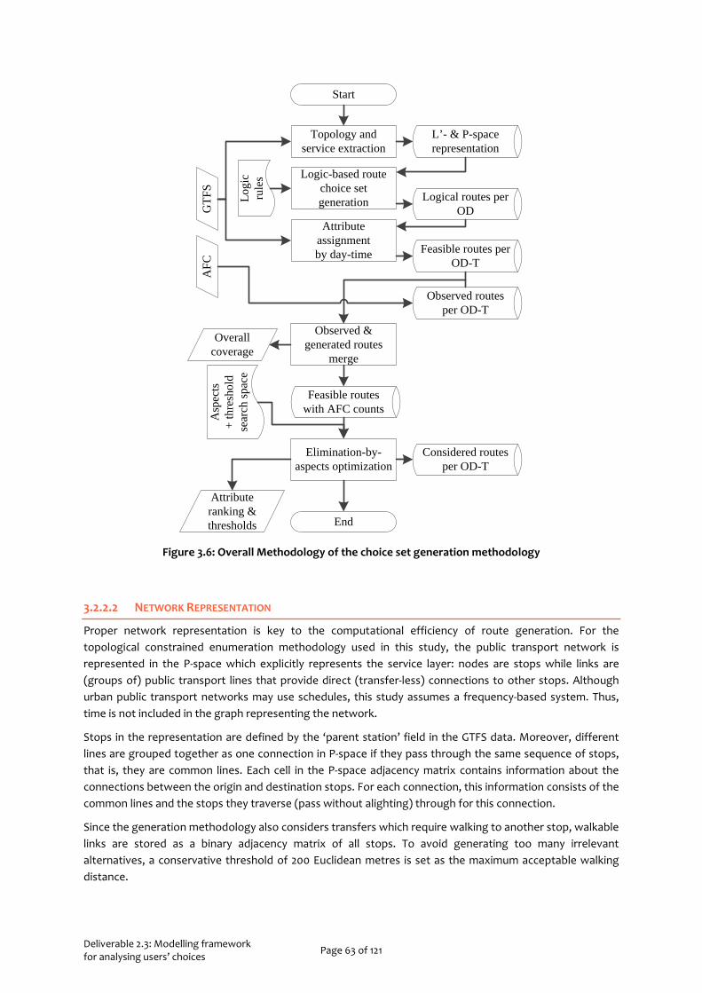
Deliverable 2.3: Modelling framework for analysing users’ choices Page 63 of 121
Topology and service extraction
GTF
SA
FC
Logic-based route choice set generation
L’- & P-space representation
Attribute assignment by day-time
Logical routes per OD
Feasible routes per OD-T
Observed routes per OD-T
Logi
c ru
les
Observed & generated routes
merge
Overall coverage
Feasible routes with AFC counts
Attribute ranking & thresholds
Start
Elimination-by-aspects optimization
End
Considered routes per OD-T
Asp
ects
+ th
resh
old
sear
ch sp
ace
Figure 3.6: Overall Methodology of the choice set generation methodology
3.2.2.2 NETWORK REPRESENTATION
Proper network representation is key to the computational efficiency of route generation. For the topological constrained enumeration methodology used in this study, the public transport network is represented in the P-space which explicitly represents the service layer: nodes are stops while links are (groups of) public transport lines that provide direct (transfer-less) connections to other stops. Although urban public transport networks may use schedules, this study assumes a frequency-based system. Thus, time is not included in the graph representing the network.
Stops in the representation are defined by the ‘parent station’ field in the GTFS data. Moreover, different lines are grouped together as one connection in P-space if they pass through the same sequence of stops, that is, they are common lines. Each cell in the P-space adjacency matrix contains information about the connections between the origin and destination stops. For each connection, this information consists of the common lines and the stops they traverse (pass without alighting) through for this connection.
Since the generation methodology also considers transfers which require walking to another stop, walkable links are stored as a binary adjacency matrix of all stops. To avoid generating too many irrelevant alternatives, a conservative threshold of 200 Euclidean metres is set as the maximum acceptable walking distance.

Deliverable 2.3: Modelling framework for analysing users’ choices Page 64 of 121
3.2.2.3 CONSTRAINED ENUMERATION OF LOGICAL ROUTES
In this section, we detail the enumeration – how different routes are obtained – and the constraints on this enumeration – how the enumeration procedure is stopped.
Enumeration
The enumeration methodology applied here uses a one-to-all, breadth-first search algorithm, similar to that used in [77]. The methodology is applied to the P-space graph representation of the network as defined above.
First, a stop is selected as the origin and the vertex root of the search tree. The stops it is directly connected to in the P-space graph of the network become destinations; this is the first level of the search tree. The information contained in the connections (lines and traversed stops) are stored for the respective OD pairs. For the next level of the search tree, the following become intermediate origins: transfer stops (stops connected by more than one line) amongst the neighbouring stops and stops accessible by walking from the neighbouring stops. Then the stops directly connected to these intermediate origins become destinations and connection information is stored, retrospectively from the origin stop (vertex root), for the respective OD pairs. For the next level, intermediate origins are selected in the same way as above, and the process is repeated up to a desired depth of the search tree. This way, all route alternatives between the origin stop and others are generated and stored. The procedure can then be repeated with another stop as the origin.
Constraints
Obviously, simply enumerating this universal set of routes would be unending. To prune the search tree, the depth is constrained by assuming that travellers accept a maximum of two transfers. This behavioural assumption should be reasonable for most urban public transport networks. Additionally, to ensure that only logical routes are produced, two rules are used as breadth-wise constraints to the enumeration. (i) No loops – traversing through, alighting at, or walking to stops previously traversed through or boarded from is not allowed. (ii) No transferring between common lines – alighting at a stop which is connected by the same set of lines as the previous connection is not allowed. Since travellers may want to shift time spent waiting for a particular line downstream, transferring to stops with a subset of the previous connection’s lines is permitted. In this case, this subset of lines is removed from the previous connection to ensure that transfers do not occur between the same lines. In the current implementation, it is assumed that travellers do not shift their waiting times by walking to another stop, hence, walking to a stop connected by a subset of the lines as the previous connection is not allowed. These logical constraints are only applied after the first level of the search tree.
3.2.2.4 ATTRIBUTE ASSIGNMENT FOR FEASIBLE ROUTES
In this step, route alternatives, that were generated from an unweighted graph, are assigned attribute values. This is required to remove infeasible routes as well as for the consideration set formation in section 3.2.2.6.
Attribute Values
The following route attributes are observable from the GTFS data, and therefore included in the study: (i) waiting time, (ii) in-vehicle time, and (iii) number of transfers. Currently, the waiting and in-vehicle times over different legs of the route are not considered separately and only the total values are used.
Deliverable 2.3: Modelling framework for analysing users’ choices Page 65 of 121
Expected waiting time for connections between two stops is calculated as the inverse of the sum of frequencies of the connecting lines, implicitly assuming them to be evenly spaced as well as assuming uniform arrivals of travellers at stops. The time-dependent nature of public transport line frequencies is taken into account by assigning them separately for each hour of the day in weekdays and weekends, respectively. Routes that become infeasible at a certain time (because a link has zero frequency) are eliminated from the feasible choice set for the respective time period. Values of the other attributes are time-independent. Although there might be small time-dependent fluctuations in the planned in-vehicle times, they are ignored for the sake of computational efficiency.
As discussed in section 3.2.1, the consideration set formation model employed here uses the EBA behavioural model, which requires setting threshold constraints to different attributes. These thresholds are some factors of the attribute values of the alternatives (in the same time period) that perform best on the respective attributes. In preparation for the calibration step, these factors are calculated for each attribute in all the alternatives. Since waiting and in-vehicle times are more continuous in nature, multiplicative factors are employed, whereas for number of transfers an additive factor is used.
Dominated Alternatives
Once attribute values have been assigned, alternatives that are state-wise dominated, that is, perform worse on all attributes, by others (in the same time period) are removed. It is rarely disputed that choosing such a dominated alternative is irrational. Although the existence of dominated alternatives in the choice set may have a decoy effect (see [78]), such effects are rarely modelled in the route choice context.
3.2.2.5 MERGE GENERATED AND OBSERVED ROUTES
The calibration uses generated-feasible routes as well as those observed from AFC data. This step merges these two route sets on the basis of the sequence of stops boarded, lines used, the hour of the first boarding, and the final destination stop. For the calibration, only those observed routes that were also generated are considered. Given that the constraints assumed during route enumeration are not very restrictive, discarding observations that are not generated should not affect the final calibration too much. In case, the overall coverage does turn out to be low, it may make sense to check the AFC data for issues such as improper transfer inference.
3.2.2.6 CALIBRATION USING ELIMINATION-BY-ASPECTS
In EBA, travellers are assumed to rank and set threshold cut-offs for attributes. In order to deduce these preferences, the generated feasible route alternatives may be compared with the observed ones. For such a comparison, two indicators are commonly used in literature, albeit for validation purposes rather than calibration: (i) coverage – the proportion of observed routes that have been generated, and (ii) efficiency – the proportion of generated routes that are observed.
With respect to calibration, clearly, the likeliest combination of choice set formation preferences is one that maximize both coverage and efficiency; that is, reproduces as many observed routes as possible while not generating too many irrelevant alternatives. Thus, to derive EBA preferences, an optimization problem that maximizes these indicators is setup. First, however, small modifications to the above indicators are proposed.
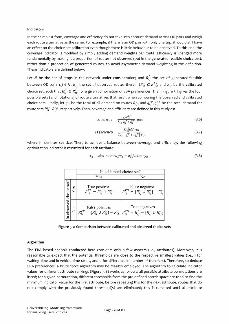
Deliverable 2.3: Modelling framework for analysing users’ choices Page 66 of 121
Indicators
In their simplest form, coverage and efficiency do not take into account demand across OD pairs and weigh each route alternative as the same. For example, if there is an OD pair with only one trip, it would still have an effect on the choice set calibration even though there is little behaviour to be observed. To this end, the coverage indicator is modified by simply adding demand weights per route. Efficiency is changed more fundamentally by making it a proportion of routes not observed (but in the generated feasible choice set), rather than a proportion of generated routes, to avoid asymmetric demand weighting in the definition. These indicators are defined below.
Let 𝑁𝑁 be the set of stops in the network under consideration; and 𝑅𝑅𝑖𝑖𝑗𝑗𝑓𝑓 the set of generated-feasible
between OD pairs 𝑖𝑖, 𝑗𝑗 ∈ 𝑁𝑁, 𝑅𝑅𝑖𝑖𝑗𝑗𝑜𝑜 the set of observed routes therein (𝑅𝑅𝑖𝑖𝑗𝑗𝑜𝑜 ⊆ 𝑅𝑅𝑖𝑖𝑗𝑗𝑓𝑓 ), and 𝑅𝑅𝑖𝑖𝑗𝑗𝑐𝑐 be the calibrated
choice set, such that 𝑅𝑅𝑖𝑖𝑗𝑗𝑐𝑐 ⊆ 𝑅𝑅𝑖𝑖𝑗𝑗𝑓𝑓 , for a given combination of EBA preferences. Then, Figure 3.7 gives the four
possible sets (and notations) of route alternatives that result when comparing the observed and calibrated choice sets. Finally, let 𝑞𝑞𝑖𝑖𝑗𝑗 be the total of all demand on routes 𝑅𝑅𝑖𝑖𝑗𝑗𝑜𝑜 , and 𝑞𝑞𝑖𝑖𝑗𝑗𝑇𝑇𝑇𝑇, 𝑞𝑞𝑖𝑖𝑗𝑗𝐹𝐹𝐹𝐹 be the total demand for
route sets 𝑅𝑅𝑖𝑖𝑗𝑗𝑇𝑇𝑇𝑇 ,𝑅𝑅𝑖𝑖𝑗𝑗𝐹𝐹𝐹𝐹, respectively. Then, coverage and efficiency are defined in this study as:
𝑐𝑐𝐻𝐻𝑐𝑐𝑐𝑐𝑐𝑐𝑐𝑐𝑐𝑐𝑐𝑐 =∑ 𝑞𝑞𝑖𝑖𝑖𝑖
𝑇𝑇𝑇𝑇𝑖𝑖,𝑖𝑖
∑ 𝑞𝑞𝑖𝑖𝑖𝑖𝑇𝑇𝑇𝑇+𝑞𝑞𝑖𝑖𝑖𝑖
𝐹𝐹𝐹𝐹𝑖𝑖,𝑖𝑖
, 𝑐𝑐𝑛𝑛𝑎𝑎 (3.6)
𝑐𝑐𝑒𝑒𝑒𝑒𝑖𝑖𝑐𝑐𝑖𝑖𝑐𝑐𝑛𝑛𝑐𝑐𝑒𝑒 =∑ �𝑅𝑅𝑖𝑖𝑖𝑖
𝑇𝑇𝐹𝐹�𝑞𝑞𝑖𝑖𝑖𝑖𝑖𝑖,𝑖𝑖
∑ (�𝑅𝑅𝑖𝑖𝑖𝑖𝐹𝐹𝑇𝑇�+�𝑅𝑅𝑖𝑖𝑖𝑖
𝑇𝑇𝐹𝐹�)𝑞𝑞𝑖𝑖𝑖𝑖𝑖𝑖,𝑖𝑖, (3.7)
where |⋅| denotes set size. Then, to achieve a balance between coverage and efficiency, the following optimization indicator is minimized for each attribute:
𝑥𝑥𝑎𝑎 = abs(𝑐𝑐𝐻𝐻𝑐𝑐𝑐𝑐𝑐𝑐𝑐𝑐𝑐𝑐𝑐𝑐𝑎𝑎 − 𝑐𝑐𝑒𝑒𝑒𝑒𝑖𝑖𝑐𝑐𝑖𝑖𝑐𝑐𝑛𝑛𝑐𝑐𝑒𝑒𝑎𝑎). (3.8)
Figure 3.7: Comparison between calibrated and observed choice sets
Algorithm
The EBA based analysis conducted here considers only a few aspects (i.e., attributes). Moreover, it is reasonable to expect that the potential thresholds are close to the respective smallest values (i.e., 1 for waiting time and in-vehicle time ratios, and 0 for difference in number of transfers). Therefore, to deduce EBA preferences, a brute force algorithm may be feasibly employed. The algorithm to calculate indicator values for different attribute rankings (Figure 3.8) works as follows: all possible attribute permutations are listed; for a given permutation, different thresholds from the pre-defined search space are tried to find the minimum indicator value for the first attribute; before repeating this for the next attribute, routes that do not comply with the previously found threshold(s) are eliminated; this is repeated until all attribute
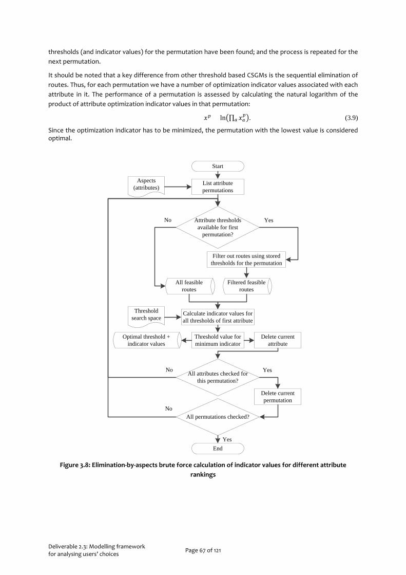
Deliverable 2.3: Modelling framework for analysing users’ choices Page 67 of 121
thresholds (and indicator values) for the permutation have been found; and the process is repeated for the next permutation.
It should be noted that a key difference from other threshold based CSGMs is the sequential elimination of routes. Thus, for each permutation we have a number of optimization indicator values associated with each attribute in it. The performance of a permutation is assessed by calculating the natural logarithm of the product of attribute optimization indicator values in that permutation:
𝑥𝑥𝑝𝑝 = ln�∏ 𝑥𝑥𝑎𝑎𝑝𝑝
𝑎𝑎 �. (3.9)
Since the optimization indicator has to be minimized, the permutation with the lowest value is considered optimal.
All feasible routes
Aspects (attributes)
Threshold search space
List attribute permutations
Calculate indicator values for all thresholds of first attribute
Filtered feasible routes
Filter out routes using stored thresholds for the permutation
Attribute thresholds available for first
permutation?
No Yes
Threshold value for minimum indicator
Yes
Yes
No
No
Start
End
All attributes checked for this permutation?
All permutations checked?
Optimal threshold + indicator values
Delete current attribute
Delete current permutation
Figure 3.8: Elimination-by-aspects brute force calculation of indicator values for different attribute rankings
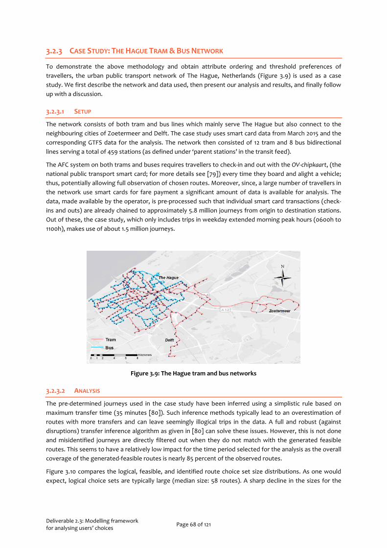
Deliverable 2.3: Modelling framework for analysing users’ choices Page 68 of 121
3.2.3 CASE STUDY: THE HAGUE TRAM & BUS NETWORK
To demonstrate the above methodology and obtain attribute ordering and threshold preferences of travellers, the urban public transport network of The Hague, Netherlands (Figure 3.9) is used as a case study. We first describe the network and data used, then present our analysis and results, and finally follow up with a discussion.
3.2.3.1 SETUP
The network consists of both tram and bus lines which mainly serve The Hague but also connect to the neighbouring cities of Zoetermeer and Delft. The case study uses smart card data from March 2015 and the corresponding GTFS data for the analysis. The network then consisted of 12 tram and 8 bus bidirectional lines serving a total of 459 stations (as defined under ‘parent stations’ in the transit feed).
The AFC system on both trams and buses requires travellers to check-in and out with the OV-chipkaart, (the national public transport smart card; for more details see [79]) every time they board and alight a vehicle; thus, potentially allowing full observation of chosen routes. Moreover, since, a large number of travellers in the network use smart cards for fare payment a significant amount of data is available for analysis. The data, made available by the operator, is pre-processed such that individual smart card transactions (check-ins and outs) are already chained to approximately 5.8 million journeys from origin to destination stations. Out of these, the case study, which only includes trips in weekday extended morning peak hours (0600h to 1100h), makes use of about 1.5 million journeys.
Figure 3.9: The Hague tram and bus networks
3.2.3.2 ANALYSIS
The pre-determined journeys used in the case study have been inferred using a simplistic rule based on maximum transfer time (35 minutes [80]). Such inference methods typically lead to an overestimation of routes with more transfers and can leave seemingly illogical trips in the data. A full and robust (against disruptions) transfer inference algorithm as given in [80] can solve these issues. However, this is not done and misidentified journeys are directly filtered out when they do not match with the generated feasible routes. This seems to have a relatively low impact for the time period selected for the analysis as the overall coverage of the generated-feasible routes is nearly 85 percent of the observed routes.
Figure 3.10 compares the logical, feasible, and identified route choice set size distributions. As one would expect, logical choice sets are typically large (median size: 58 routes). A sharp decline in the sizes for the
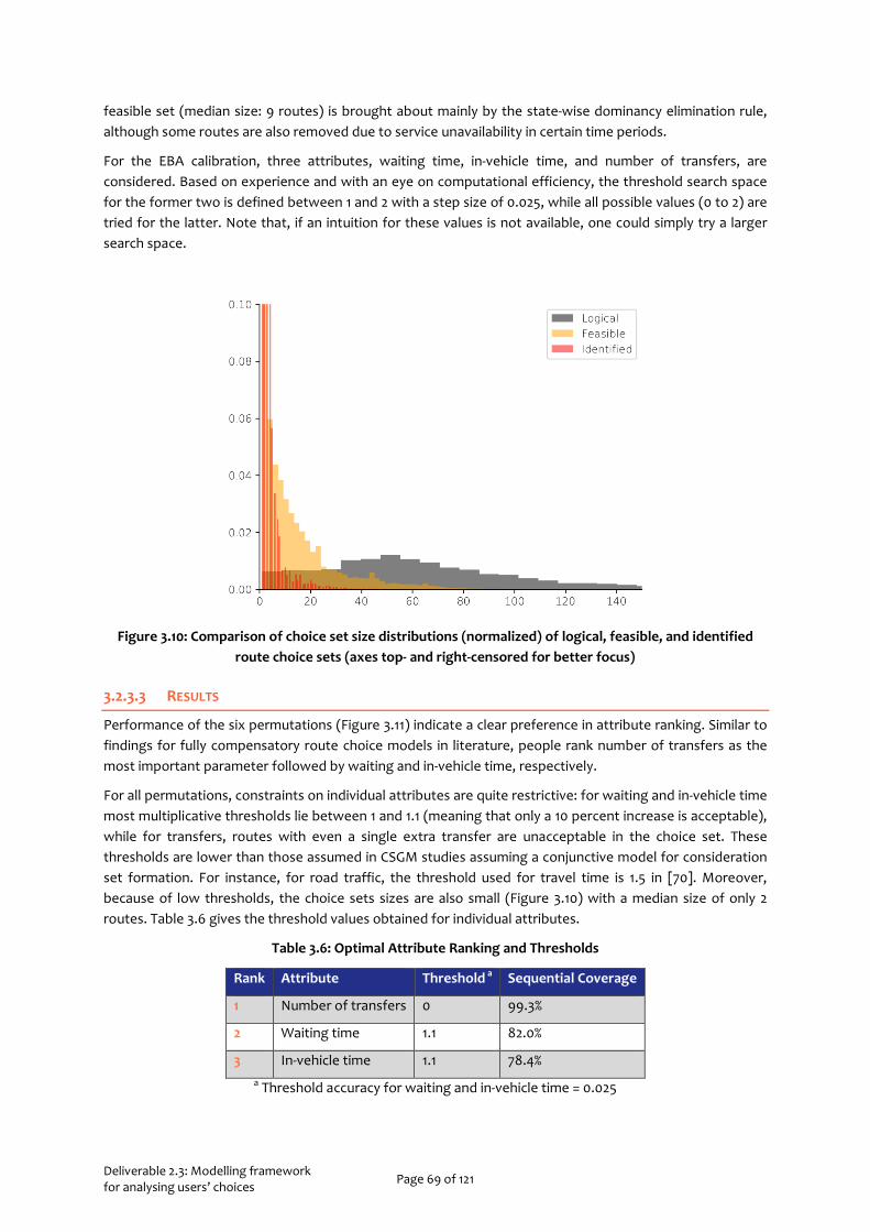
Deliverable 2.3: Modelling framework for analysing users’ choices Page 69 of 121
feasible set (median size: 9 routes) is brought about mainly by the state-wise dominancy elimination rule, although some routes are also removed due to service unavailability in certain time periods.
For the EBA calibration, three attributes, waiting time, in-vehicle time, and number of transfers, are considered. Based on experience and with an eye on computational efficiency, the threshold search space for the former two is defined between 1 and 2 with a step size of 0.025, while all possible values (0 to 2) are tried for the latter. Note that, if an intuition for these values is not available, one could simply try a larger search space.
Figure 3.10: Comparison of choice set size distributions (normalized) of logical, feasible, and identified route choice sets (axes top- and right-censored for better focus)
3.2.3.3 RESULTS
Performance of the six permutations (Figure 3.11) indicate a clear preference in attribute ranking. Similar to findings for fully compensatory route choice models in literature, people rank number of transfers as the most important parameter followed by waiting and in-vehicle time, respectively.
For all permutations, constraints on individual attributes are quite restrictive: for waiting and in-vehicle time most multiplicative thresholds lie between 1 and 1.1 (meaning that only a 10 percent increase is acceptable), while for transfers, routes with even a single extra transfer are unacceptable in the choice set. These thresholds are lower than those assumed in CSGM studies assuming a conjunctive model for consideration set formation. For instance, for road traffic, the threshold used for travel time is 1.5 in [70]. Moreover, because of low thresholds, the choice sets sizes are also small (Figure 3.10) with a median size of only 2 routes. Table 3.6 gives the threshold values obtained for individual attributes.
Table 3.6: Optimal Attribute Ranking and Thresholds
Rank Attribute Threshold a Sequential Coverage
1 Number of transfers 0 99.3%
2 Waiting time 1.1 82.0%
3 In-vehicle time 1.1 78.4% a Threshold accuracy for waiting and in-vehicle time = 0.025

Deliverable 2.3: Modelling framework for analysing users’ choices Page 70 of 121
To assess the performance of the calibration the overall coverage of the EBA model can be calculated as the product of the coverage values obtained sequentially for each attribute (Table 3.6). The overall coverage for this case study is 63.9%.
Figure 3.11: Performance for different attribute rankings (Num-T: number of transfers, WT: waiting time, IVT: in-vehicle time) (lower is better)
Figure 3.12: Coverage (C), efficiency (E), and optimization indicator (I) values (y-axes) by threshold values (x-axis) of different attributes for the optimal permutation
-14
-12
-10
-8
-6
-4
Perfo
rman
ce
Permutations
0
0.2
0.4
0.6
0.8
1
0 0.5 1 1.5 2
Indi
cato
r val
ues
Threshold
WT (I)
IVT (I)
Num-T (I)
WT (C)
IVT (C)
Num-T (C)
WT (E)
IVT (E)
Num-T (E)

Deliverable 2.3: Modelling framework for analysing users’ choices Page 71 of 121
Figure 3.13: Comparison between the number of generated-feasible routes, number of observed routes and average in-vehicle times (in seconds) per origin, destination, and time period (x-axis right-censored
for better focus)
3.2.3.4 DISCUSSION
Figure 3.12 takes a deeper look into the values of individual thresholds for the optimal permutation. It can be seen that for the first attribute – number of transfers – at 99.3 percent, coverage is already extremely high with no extra transfers; a clear reflection of travellers’ dislike for transferring. Thus, any increase in the transfer threshold only decreases efficiency thereby increasing the indicator value. For waiting time too, the initial coverage is quite high, meaning that improvements in coverage tend to be quite slow. Accepting twice the least possible waiting time only increases coverage from 79.9 to 93.3 percent. On the other hand, efficiency quickly decreases by approximately 40 percentage points. Although the initial slope for coverage is slightly higher than efficiency, the overall change in the latter is higher for in-vehicle time too. The fact that the initial value of coverage is more moderated for this attribute could be because the values are calculated after the feasible choice set has been filtered based on the thresholds of the previous two attributes. Finally, it should be noted that the for all three attributes, the optimal indicator values are unambiguous.
A possible explanation for the restrictive constraints may be a combination of the following statistical observations and hypothesis. The statistical observations are (Figure 3.13) (i) OD pairs with a high demand tend to be nearby (in terms of in-vehicle time) and (ii) OD pairs that are farther away tend to have more feasible routes generated by the CSGM. The hypothesis is that (iii) travellers are either able to evaluate alternatives better or have a lower threshold acceptance for OD pairs that are nearby. From statistical observation (i), the hypothesis in (iii), and the definition given in equation (3.6), it can be seen why the
Deliverable 2.3: Modelling framework for analysing users’ choices Page 72 of 121
coverage values are already quite high at low thresholds. This increase in coverage is mainly due to the highly-used routes between OD pairs that are close to one another. On the other hand, statistical observation (ii) and the definition in equation (3.7) explain why non-selected alternatives from farther away OD pairs might play a larger role in the value of efficiency. This potential disconnect might cause a decrease in efficiency that is not sufficiently balanced by the increase in coverage, leading to smaller thresholds. The larger slopes of efficiency in comparison to coverage (Figure 3.12) seem to indicate that this is indeed the case here.
Finally, while the coverage (63.9%) on its own is a somewhat moderate performance, it may be expected because, in an effort to be more transferable, the model trades-off coverage for an increase in efficiency.
3.2.4 SUMMARY
Route choice set identification for public transport networks is a vital but complicated task. Identifying the correct route choice sets are crucial for both, estimation and application, of route choice models. However, approaches developed and commonly employed in literature either lack transferability (observation-driven methods) or require strong assumptions regarding traveller behaviour (uncalibrated CSGMs).
Given this key scientific gap, and the context of increasing availability of smart card data for public transport networks, this research makes two crucial contributions. First, a choice set generation methodology is proposed which uses elimination-by-aspects as the consideration set formation model. This model adds more behavioural dimensions over those used previously by taking into account attribute ranking as well as threshold constraints. Second, rather than making subjective assumptions regarding traveller preferences, the elimination-by-aspects model is calibrated using revealed behaviour observations from smart card data. The proposed methodology can be used to identify choice sets for estimating route choice models from revealed preferences as well as to predict alternative shares on the basis of available choice parameters.
Application of the proposed methodology to the urban public transport network of The Hague revealed that the number of transfers is the most important attribute for travellers, followed by waiting time, and in-vehicle time. Furthermore, the thresholds obtained for individual attributes are quite restrictive indicating that travellers make more optimal choices than previously assumed. Although the overall coverage for the EBA model is on the lower side, it makes up for this by being a more transferable model rather than a network-specific one.
An important limitation in the current implementation of the model is the assumption that the public transport services are frequency-based. Based on this, waiting times are calculated from the headways of individual lines under the assumption of evenly spaced arrivals of public transport lines and uniformly distributed traveller arrivals at stops. These assumptions may not hold outside rush hours or for non-urban networks where line frequencies are often lower, or when lines are explicitly synchronised to reduce transfer waiting time.
To overcome issues arising from the assumption of a frequency-based system, future implementations may consider using the following: (i) a schedule-based network which includes time in its representation and (ii) more complex traveller arrival models. Further improvements to the model could include taking into account that travellers behave differently for OD pairs that are relatively near, as hypothesised in the discussion of the case study results. Finally, future research could focus on using the calibration procedure proposed here, for the comparison of different behavioural models of route choice set formation.
Deliverable 2.3: Modelling framework for analysing users’ choices Page 73 of 121
3.3 MODEL 3: ESTIMATING ROUTE CHOICE MODELS FROM REVEALED
PREFERENCES6
In the previous section, the focus was on the first of the two steps in a decision process, that is, choice set formation. We applied our proposed elimination-by-aspects methodology to calibrate choice sets of travellers in The Hague using revealed preferences observed from smart card data in the urban public transport network. In this section, we use the same dataset to analyse the second step which we assume to be a fully compensatory choice. In addition to a conventional route choice model, we also compare different reliability representations to assess which can best model travellers’ reactions to waiting time variations. Specifically, we consider the regular deviations from schedule and the spread of these deviations. Compare the analysis of behaviour here with the discussions in section 3.1 – as is common in revealed preference studies, travellers make decisions under natural ambiguity but we analyse behaviour as if the travellers were aware of the distributions of waiting time reliability.
First, we present a generic methodology to estimate such route choice models in different public transport systems. Then, we apply our methodology to the smart card data from The Hague and present our results.
3.3.1 METHODOLOGY
To estimate the value of reliability from the revealed preferences offered by smart card data, a conventional sequence of steps are followed. First, the required data is prepared for the subsequent steps, followed by the identification of choice sets and assignment of attribute values, which allows the final step of choice model estimation.
3.3.1.1 REQUIRED DATA AND PREPARATION
Three main data sources from the public transport system under study are required: (i) automatic fare collection (AFC), (ii) automatic vehicle location (AVL), and the (iii) general transit feed specification data. While AFC data provides behavioural observations, the latter two, being data on the executed and scheduled operations, give information on trip characteristics including service reliability.
To analyse route choice behaviour, complete journeys — as a sequence of trips (i.e., rides on a single vehicle) without intervening trip-generating activities — have to be known. However, this is usually not directly possible from the AFC data and, depending on the fare structure and the AFC system, one or more of the following may have to be inferred from the data: trip origin, trip destinations, and transfers between trips [82].
For vehicle-based AFC systems (e.g., London buses) that do not store vehicle locations — typically, in networks with a flat fare structure — both origins and destinations must be inferred. Since travellers usually pay upfront, the origin can be inferred by linking the AFC and AVL data to obtain the vehicle location. To deduce the destination, commonly, proposed methodologies assume that the destination location must be close to the boarding location of the subsequent trip. For destination inference in station-based AFC systems (e.g., New York city subway), either individual trip destinations are inferred using a route inference methodology, or only the final location where the traveller leaves the network is deduced.
Finally, trips with observed or inferred origins and destinations have to be chained together to form journeys so that there should not have been any intervening trip-generating activities. Transfer inference methodologies are rule-based with the simplest setting an upper limit on the time between alighting and boarding, and more complex ones using a combination of temporal, spatial, and other logical conditions.
6 Parts of this section are based on the working paper: [81]S. Shelat, "A comparison of reliability representations in random ut
Deliverable 2.3: Modelling framework for analysing users’ choices Page 74 of 121
3.3.1.2 CHOICE SET IDENTIFICATION
Similar to other studies analysing travel behaviour using AFC data, in this study, the route choice set for each origin-destination (OD) pair is identified directly from this set of observed routes. For this method, the AFC data must cover the entire network over a reasonably long period of time so that most of the routes used by travellers are observed. By deriving the choice sets from route observations, the need for behavioural assumptions or parameter estimations regarding choice set formation are obviated. Despite this important advantage, one drawback of such direct identification is that it may be unable to explain why some feasible routes are not selected.
In public transport networks, route choice is usually intertwined with access and egress stop choice because different lines do not necessarily serve the same stops. The influence of not being able to observe access and egress stop choice (since the first origin and final destination location is not observed) on route choice behaviour can be mitigated by merging stops within reasonable proximity to act as single origins and destinations for the route choice analysis.
For the choice analysis, routes have to be uniquely defined such that travellers can be reasonably expected to perceive one route to be different from another. In this study, routes alternatives for an OD pair are defined by the sequence of lines boarded and stops traversed. Since the focus here is on evaluating the effect of waiting time reliability, transfers at different stops along overlapping lines are not differentiated as separate routes.
Finally, to obtain the OD pairs and associated route alternatives suitable for route choice analysis, the following rules are applied: (i) each OD pair must have a minimum number of route alternatives, (ii) each OD pair must be observed a certain number of times, and (iii) each route alternative must make up a minimum percent of the observations of its OD pair. The first rule ensures that a given choice model can analyse trade-offs. The lower limits on the number of observations ensure that there is sufficient information to estimate behavioural parameters as well as to eliminate unusual observations that do not take place regularly.
3.3.1.3 ATTRIBUTE ASSIGNMENT
Once all eligible OD pairs and the associated choice sets are obtained, attribute values for the alternatives are assigned. The following attributes are used for the choice analysis: for each leg of the route, its (i) mode, (ii) in-vehicle time, and (iii) waiting time (and its components), and for the route alternative as a whole, its (iv) path size factor and the (v) number of routes.
The first and last attributes, mode per leg and number of transfers, are already known from route definition. The mode per leg is used to understand how travel time components are weighed for different modes by travellers. The number of transfers is used to evaluate the transfer penalty — the additional disutility beyond the extra waiting time.
The travel time attributes may be planned, that is, based on the schedule; or actual, that is, based on the executed operations. Typically, these attributes may be obtained from the GTFS and AVL datasets, respectively. Since the focus here is on waiting time reliability, only planned in-vehicle times are used whereas for waiting times, both planned and actual values are obtained. Waiting times are recorded as the time difference between the arrival of a line at a stop and the departure of another line either from the same stop or from another within a reasonable walking distance. This is done for all stop and line combinations, separately for planned and actual trips.
In station-based AFC systems, the travel time attributes described above can be obtained for the first instance of each route alternative after the arrival of the traveller at the first stop. However, since the arrival time of travellers at origin stops is not known in vehicle-based systems, route alternatives cannot be assigned trip-specific attributes. Instead, statistical measures are used, and to account for the fact that
Deliverable 2.3: Modelling framework for analysing users’ choices Page 75 of 121
travel time attributes might vary over time, a separate indicator is calculated for each pre-specified time period (e.g., weekdays 0900h–1000h).
For in-vehicle times only the average over each time period is used whereas for waiting times, a centrality indicator is calculated for both planned and actual trips and a dispersion indicator is calculated for the latter. The difference between the averages of the planned and actual waiting times (average actual minus average planned) describes the regular deviation from schedule and the spread represents the level of irregularity in the system. In this study, the median is used as the centrality indicator and the spread is described by the reliability buffer time (RBT) which is given as the difference between the 95th and 50th percentile values and is normalized by the median.
When arrival times of travellers are unknown, an arrival process has to be assumed. Based on this process, the expected waiting times at the origin stop can be calculated as fractions of the respective waiting time indicators recorded above. On the other hand, waiting times while transferring are fully observed and equal to the full value of the respective records. It should be noted that, to avoid endogeneity issue in the choice estimation, the route definition does not make any behavioural assumptions regarding which lines travellers perceive to be common. Therefore, there are no common lines with a reduced waiting time.
Finally, to account for overlap between route alternatives, the path size factor for each route is calculated. The travel time attributes calculated above also define which route alternatives are available for each OD pair at different time periods. Here, the amount of overlap between two routes is given by the number of shared links. If route k of an OD pair covers 𝑙𝑙 ∈ 𝐿𝐿k L-space network links, and the number of alternatives for this OD using a link 𝑙𝑙 is 𝑛𝑛𝑙𝑙, then the route’s path size factor, 𝑝𝑝n, is given by equation (3.10). Since the factor itself may be quite small, its natural logarithm is used in the choice model.
𝑝𝑝k = ∑ 1𝑛𝑛𝑙𝑙𝑙𝑙∈𝐿𝐿k (3.10)
3.3.1.4 CHOICE MODELS ESTIMATION
The effect of waiting time reliability on route choice behaviour is assessed under the conventional utility maximisation paradigm. Three multinomial logit (MNL) models are estimated, each accounting for more information on waiting time: (i) only planned waiting times, (ii) plus regular deviations, and (iii) plus level of irregularity. In the most generic form of the models, all attributes associated with separate legs of the route are mode-specific.
Equations (3.11–3.13) describe the structural part of the three MNL models. Attributes — number of transfers, path size factor, mode, in-vehicle time, and waiting times at origin and transfer stops — are given by 𝑛𝑛trans, 𝑝𝑝, 𝑚𝑚, 𝑡𝑡ivt, 𝑡𝑡owt, and 𝑡𝑡twt; and their respective coefficients by 𝛽𝛽. Subscripts describe whether a variable refers to the planned values, regular deviations from the planned values (median actual minus median planned), or the level of irregularity (RBT of the actual values) and are denoted by 0, d, and r, respectively.
𝑉𝑉1 = 𝛽𝛽trans ∙ 𝑛𝑛trans + 𝛽𝛽ps ∙ 𝑝𝑝
+∑ 𝛽𝛽0,𝑚𝑚ivt ∙ 𝑡𝑡0,𝑚𝑚
ivt + 𝛽𝛽0,𝑚𝑚owt ∙ 𝑡𝑡0,𝑚𝑚
owt + 𝛽𝛽0,𝑚𝑚twt ∙ 𝑡𝑡0,𝑚𝑚
twt𝑚𝑚∈M (3.11)
𝑉𝑉2 = 𝛽𝛽trans ∙ 𝑛𝑛trans + 𝛽𝛽ps ∙ 𝑝𝑝
+∑ 𝛽𝛽0,𝑚𝑚ivt ∙ 𝑡𝑡0,𝑚𝑚
ivt + 𝛽𝛽0,𝑚𝑚owt ∙ 𝑡𝑡0,𝑚𝑚
owt + 𝛽𝛽0,𝑚𝑚twt ∙ 𝑡𝑡0,𝑚𝑚
twt𝑚𝑚∈M
+∑ 𝛽𝛽d,𝑚𝑚owt ∙ 𝑡𝑡d,𝑚𝑚
owt + 𝛽𝛽d,𝑚𝑚twt ∙ 𝑡𝑡d,𝑚𝑚
twt𝑚𝑚∈M (3.12)
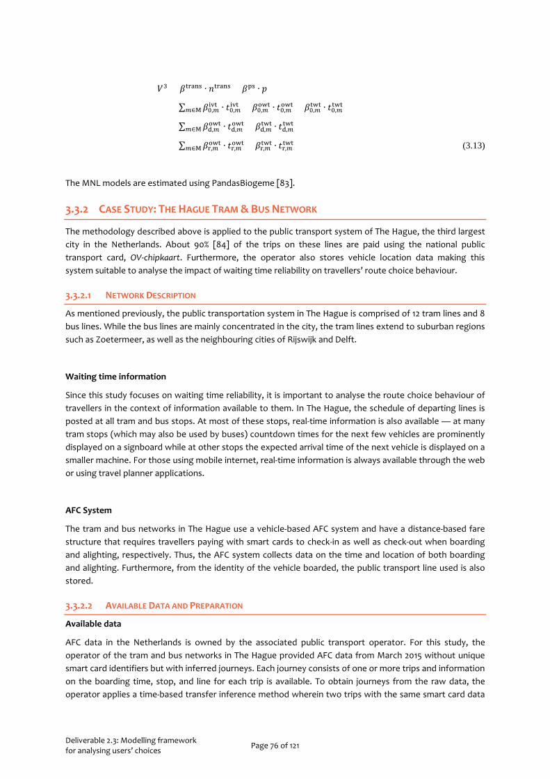
Deliverable 2.3: Modelling framework for analysing users’ choices Page 76 of 121
𝑉𝑉3 = 𝛽𝛽trans ∙ 𝑛𝑛trans + 𝛽𝛽ps ∙ 𝑝𝑝
+∑ 𝛽𝛽0,𝑚𝑚ivt ∙ 𝑡𝑡0,𝑚𝑚
ivt + 𝛽𝛽0,𝑚𝑚owt ∙ 𝑡𝑡0,𝑚𝑚
owt + 𝛽𝛽0,𝑚𝑚twt ∙ 𝑡𝑡0,𝑚𝑚
twt𝑚𝑚∈M
+∑ 𝛽𝛽d,𝑚𝑚owt ∙ 𝑡𝑡d,𝑚𝑚
owt + 𝛽𝛽d,𝑚𝑚twt ∙ 𝑡𝑡d,𝑚𝑚
twt𝑚𝑚∈M
+∑ 𝛽𝛽r,𝑚𝑚owt ∙ 𝑡𝑡r,𝑚𝑚
owt + 𝛽𝛽r,𝑚𝑚twt ∙ 𝑡𝑡r,𝑚𝑚
twt𝑚𝑚∈M (3.13)
The MNL models are estimated using PandasBiogeme [83].
3.3.2 CASE STUDY: THE HAGUE TRAM & BUS NETWORK
The methodology described above is applied to the public transport system of The Hague, the third largest city in the Netherlands. About 90% [84] of the trips on these lines are paid using the national public transport card, OV-chipkaart. Furthermore, the operator also stores vehicle location data making this system suitable to analyse the impact of waiting time reliability on travellers’ route choice behaviour.
3.3.2.1 NETWORK DESCRIPTION
As mentioned previously, the public transportation system in The Hague is comprised of 12 tram lines and 8 bus lines. While the bus lines are mainly concentrated in the city, the tram lines extend to suburban regions such as Zoetermeer, as well as the neighbouring cities of Rijswijk and Delft.
Waiting time information
Since this study focuses on waiting time reliability, it is important to analyse the route choice behaviour of travellers in the context of information available to them. In The Hague, the schedule of departing lines is posted at all tram and bus stops. At most of these stops, real-time information is also available — at many tram stops (which may also be used by buses) countdown times for the next few vehicles are prominently displayed on a signboard while at other stops the expected arrival time of the next vehicle is displayed on a smaller machine. For those using mobile internet, real-time information is always available through the web or using travel planner applications.
AFC System
The tram and bus networks in The Hague use a vehicle-based AFC system and have a distance-based fare structure that requires travellers paying with smart cards to check-in as well as check-out when boarding and alighting, respectively. Thus, the AFC system collects data on the time and location of both boarding and alighting. Furthermore, from the identity of the vehicle boarded, the public transport line used is also stored.
3.3.2.2 AVAILABLE DATA AND PREPARATION
Available data
AFC data in the Netherlands is owned by the associated public transport operator. For this study, the operator of the tram and bus networks in The Hague provided AFC data from March 2015 without unique smart card identifiers but with inferred journeys. Each journey consists of one or more trips and information on the boarding time, stop, and line for each trip is available. To obtain journeys from the raw data, the operator applies a time-based transfer inference method wherein two trips with the same smart card data

Deliverable 2.3: Modelling framework for analysing users’ choices Page 77 of 121
are included in one journey if the boarding time of the second trip is within 35 minutes of the alighting time of the first.
In the Netherlands, public transport operators are required to publish their AVL data. However, since the AFC dataset used here is from some time ago, the operator also made available the historical AVL dataset from the same time period. The AVL data published by the operator in The Hague contains both the actual and planned arrival and departure times of vehicles at their respective stops. Since the planned times were already available in the AVL dataset, GTFS data was not needed for this case study.
Preparation
Based on the data stored from the AFC system, as required by the methodology in section 3.3.1, complete journeys can already be observed. However, since time-based transfer inference algorithms tend to over-estimate the number of transfers [80], another inference algorithm is applied that checks if the trips in each journey inferred by the operator are indeed linked.
The transfer inference algorithm applies one spatial and one temporal rule [82]. The spatial rule ensures that the alighting stop of one trip and the boarding stop of the next are within 400 Euclidean metres of one another. This places an upper bound on the distance travellers will walk to transfer. The temporal rule checks whether, after alighting, the first plausible service of the line used in the next trip is boarded. The idea is that if travellers transfer to the first plausible service of the next line they use, they are unlikely to perform a trip-generating activity. If the boarding stop is the same as the alighting stop of the previous trip, then the first plausible service is the same as the first service. If the two stops are different then it is the first service after adding the time required by most people to walk between the two stations. For this a walking speed of 0.66 m/s (2.5 percentile of the population) is used and all distances are assumed to be Euclidean. The parameter values used here are obtained from [80].
It should be noted that journeys containing transfer between the same lines are not removed if they pass the above temporal criterion. This is done to accommodate travellers affected by planned and unplanned short-turning, stop-skipping or dead-heading [80]. This is especially important for The Hague since certain public transport lines here are short-turned on a planned basis although the shortened versions are not marked as such. Since travellers do not have information upfront regarding which services are shortened and thus did not include this in their route choice, wherever the temporal criterion is passed for such transfers, the trips involved are merged into one.
Overall, the re-inference reduced the number of journeys with at least one transfer from 18.7% of all journeys in the dataset provided by the operator to 10.8%. Surprisingly, although the same system is studied in [80], the percentages found in that study are higher in both, pre- (32%) and post-inference (18%). However, this difference may be because: (i) they report results for AFC data over a selection of lines and times more suitable for their analysis and (ii) they do not merge the trips between which transfers to the same line occur.
3.3.2.3 WAITING TIME STATISTICS
To assign travel time attributes, in-vehicle times and headways, statistical indicators are calculated per hour per day of week. It is reasonable to expect that attribute values within each time period will be similar and will not be different simply on account of the time. Since waiting times at origins is not recorded with the AFC system used in The Hague, we assume uniform arrival of passengers to calculate the waiting time at origin. Transfer waiting time can be obtained from observations of traveller interactions with the AFC system since they are expected to check-in and out of every vehicle. Figure 3.14 and Figure 3.15 show some statistics of the waiting times at the origin and at transfers. We can see from Figure 3.14 that the average deviation of actual waiting times from the planned values is negligible but there is significant dispersion. For
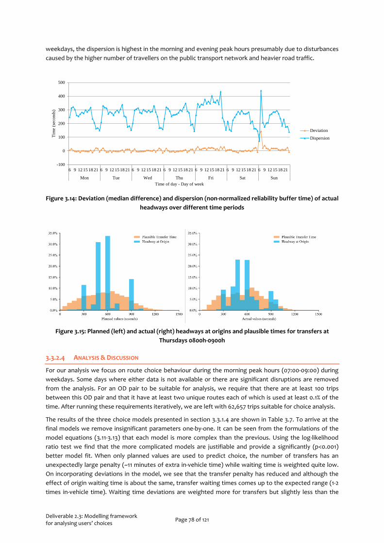
Deliverable 2.3: Modelling framework for analysing users’ choices Page 78 of 121
weekdays, the dispersion is highest in the morning and evening peak hours presumably due to disturbances caused by the higher number of travellers on the public transport network and heavier road traffic.
Figure 3.14: Deviation (median difference) and dispersion (non-normalized reliability buffer time) of actual headways over different time periods
Figure 3.15: Planned (left) and actual (right) headways at origins and plausible times for transfers at Thursdays 0800h-0900h
3.3.2.4 ANALYSIS & DISCUSSION
For our analysis we focus on route choice behaviour during the morning peak hours (07:00-09:00) during weekdays. Some days where either data is not available or there are significant disruptions are removed from the analysis. For an OD pair to be suitable for analysis, we require that there are at least 100 trips between this OD pair and that it have at least two unique routes each of which is used at least 0.1% of the time. After running these requirements iteratively, we are left with 62,657 trips suitable for choice analysis.
The results of the three choice models presented in section 3.3.1.4 are shown in Table 3.7. To arrive at the final models we remove insignificant parameters one-by-one. It can be seen from the formulations of the model equations (3.11-3.13) that each model is more complex than the previous. Using the log-likelihood ratio test we find that the more complicated models are justifiable and provide a significantly (p<0.001) better model fit. When only planned values are used to predict choice, the number of transfers has an unexpectedly large penalty (~11 minutes of extra in-vehicle time) while waiting time is weighted quite low. On incorporating deviations in the model, we see that the transfer penalty has reduced and although the effect of origin waiting time is about the same, transfer waiting times comes up to the expected range (1-2 times in-vehicle time). Waiting time deviations are weighted more for transfers but slightly less than the
-100
0
100
200
300
400
500
6 9 12 15 18 21 6 9 12 15 18 21 6 9 12 15 18 21 6 9 12 15 18 21 6 9 12 15 18 21 6 9 12 15 18 21 6 9 12 15 18 21
Mon Tue Wed Thu Fri Sat Sun
Tim
e (s
econ
ds)
Time of day - Day of week
Deviation
Dispersion

Deliverable 2.3: Modelling framework for analysing users’ choices Page 79 of 121
respective planned values. This also holds true for the final model where transfer waiting time is weighted almost 2 times in-vehicle time. Transfer penalty is further reduced to about 7 minutes of in-vehicle time. Origin waiting time (planned and deviations) remains similar to values in the previous models. Moreover, for origin waiting time the effect of dispersion seems to be in the wrong direction.
The low weights for origin waiting time can be explained by the fact that much of this is often under the passengers’ control. Since, departure times are often known, especially by regular travellers they can make a departure time choice that would reduce their origin waiting time. This behaviour would not be captured here since we assume uniform arrivals of passengers. Thus, since origin waiting time can be controlled up to a large extent, it has a comparatively lower weight.
Each minute of planned transfer waiting times is equivalent to approximately two in-vehicle minutes. Further, deviations are weighted almost similarly. In fact, a model that used actual waiting time values (rather than the planned values + deviations) did just as well in terms of the final log-likelihood and yet had one parameter less. This indicates that people do not seem to use planned waiting time for their decision but already take into consideration average deviations. Furthermore, a significant effect of the dispersion of waiting times is also observed – every minute increase in the difference between the 95th percentile and median waiting time is considered as an extra 3/4th of an in-vehicle minute.
Table 3.7: Route choice model estimations with different representations of reliability
Model MNL1 (planned values)
MNL2 (planned values +
deviations)
MNL3 (planned values +
deviations + dispersion)
Initial LL -51106.15 -51106.15 -51106.15
Final LL -45916.97 -45826.73 -45793.5
Adjusted ρ2 0.101 0.103 0.104
Value p 𝜷𝜷/𝜷𝜷𝟎𝟎𝐢𝐢𝐢𝐢𝐢𝐢 Value p 𝜷𝜷/𝜷𝜷𝟎𝟎𝐢𝐢𝐢𝐢𝐢𝐢 Value p 𝜷𝜷/𝜷𝜷𝟎𝟎𝐢𝐢𝐢𝐢𝐢𝐢
𝜷𝜷𝐢𝐢𝐭𝐭𝐭𝐭𝐭𝐭𝐭𝐭 -2.49 0.00 11.27 -2.13 0.00 9.91 -1.48 0.00 6.82
𝜷𝜷𝟎𝟎𝐢𝐢𝐢𝐢𝐢𝐢 -0.221 0.00 1 -0.215 0.00 1 -217 0.00 1
𝜷𝜷𝟎𝟎𝐨𝐨𝐨𝐨𝐢𝐢 -0.18 0.00 0.81 -0.181 0.00 0.84 -0.167 0.00 0.77
𝜷𝜷𝟎𝟎𝐢𝐢𝐨𝐨𝐢𝐢 -0.212 0.00 0.95 -0.313 0.00 1.46 -0.424 0.00 1.95
𝜷𝜷𝐝𝐝𝐨𝐨𝐨𝐨𝐢𝐢 -0.218 0.00 1.01 -0.201 0.00 0.93
𝜷𝜷𝐝𝐝𝐢𝐢𝐨𝐨𝐢𝐢 -0.267 0.00 1.24 -0.397 0.00 1.82
𝜷𝜷𝐭𝐭𝐨𝐨𝐨𝐨𝐢𝐢 0.196 0.00 -0.90
𝜷𝜷𝐭𝐭𝐢𝐢𝐨𝐨𝐢𝐢 -0.161 0.00 0.74
3.3.3 SUMMARY
Having proposed a methodology to identify route choice sets in the previous section, in this section we outlined a generic methodology to estimate route choice models from revealed preference data sources. Further, we established that it is important to include information on both deviation from schedule and dispersion of waiting times in the choice models. As is common in revealed preference studies but in contradiction with the model presented in section 3.1, here we study choices as if they were made under risk, that is, using known probabilities of different outcomes. Bridging this contradiction, in a working paper Shelat, et al. [85] use revealed preferences to study subjective beliefs regarding uncertainty. Several trips in

Deliverable 2.3: Modelling framework for analysing users’ choices Page 80 of 121
line with the choice situation proposed in section 3.1 and suitable for analysis are found in the urban public transport network of Amsterdam.
Deliverable 2.3: Modelling framework for analysing users’ choices Page 81 of 121
4 ACTIVITY MODELLING This section serves as the connective link between the activity prediction mechanism implemented within WP2 and the recommendation system implemented in WP3. In particular, herein the flow of information among specific modules implemented in the aforementioned WPs is described. More specifically, in the activity prediction mechanism described in WP2 includes the Activity Recognition and Activity Prediction module. The Activity Prediction module aims at predicting the type of the users’ anticipated activity. Furthermore, the Activity Recognition module aims at recognizing the activity type described in the provided tweet’s text provided via the Twitter data collector, described in D2.2. In WP3, a recommendation system has been implemented, whose objective is to provide personalized recommendations about places of interests (POI) that the users of the My-TRAC application could visit.
The evaluation of each of the utilized modules is presented in:
1) Activity Prediction module Deliverable D2.2 “Model for analysing user’s trip purpose (activities)”
2) Activity Recognition module Deliverable D2.2 “Model for analysing user’s trip purpose (activities)”
3) Recommendation system Deliverable D3.3 “Definition and elaboration of user-service algorithm”
It needs to be highlighted that no new algorithms are introduced at this stage; as such, no evaluation of each one of the above submodules is presented here. For more information about their evaluation, the reader should be referred to the corresponding deliverables (i.e. D2.2, D3.3).
The technical contribution of this section lies in the fact that it provides a formal definition of the connection among these modules and the flow of information among them. The connection among the Activity Prediction module, Activity Recognition module and the Recommendation system is presented in Figure 4.1. The main concept is that through My-TRAC application users will be able to plan their next trip and receive personalized recommendations, from the recommendation module, for places of interest that they could visit. The input parameters of the recommendation system are:
• Ratings provided by user for several POI • Information about the POI stored on the MySQL database • Destination of the user’s trip • Date of the planned trip • Type of the User’s next activity predicted
Information about the ratings a user has provided, the POI and the user’s activity profile are stored in the data storage system of the My-TRAC Platform. The destination of the user’s trip is retrieved from the My-TRAC application and will be used to filter the places recommended based on their coordinates, aiming to provide recommendations for places that are near the user’s destination. More information is provided in below, in the recommendation system’s description. User’s next activity predicted is the result of the Activity prediction module, and refers to the predicted type of activity that a user will perform in the next time interval.
The output of the recommendation system is a list with the top M places that the user could visit according to their next activity predicted and the destination of their trip.
For predicting the type of the user’s next activity, the Activity Prediction module uses as input the user’s activity profile. User’s activity profile includes the sequences of activities that a user has performed daily, the time that each activity has started, alongside with several user’s demographic characteristics (i.e. gender, age, occupation, marital status), as it is described in D2.2 section 3.2. The activity types included in the sequences of daily user activities are provided either by social media by receiving user’s tweet’s posted via the Twitter data collector and recognized from the Activity Recognition mechanism, or from a trained model via Activity Prediction module. More detailed information about the algorithms used in each module is provided below.

Deliverable 2.3: Modelling framework for analysing users’ choices Page 82 of 121
Figure 4.1: Flow of information implemented within WP2 and WP3. Activity Prediction and Activity Recognition modules implemented within WP2 are used
periodically to create the sequences of user’s daily activity types, used to form the user’s activity profile. User’s activity profile is provided as input for the Activity Prediction module, aiming at providing personalized predictions of the user’s anticipated activity type. When a user plans a trip from My-TRAC application, the
recommendation system is used to provide recommendations about several places of interest that a user could visit based the user’s anticipated activity provided via the Activity Prediction module and the information retrieved by the My-TRAC application regarding the destination of the trip planned.
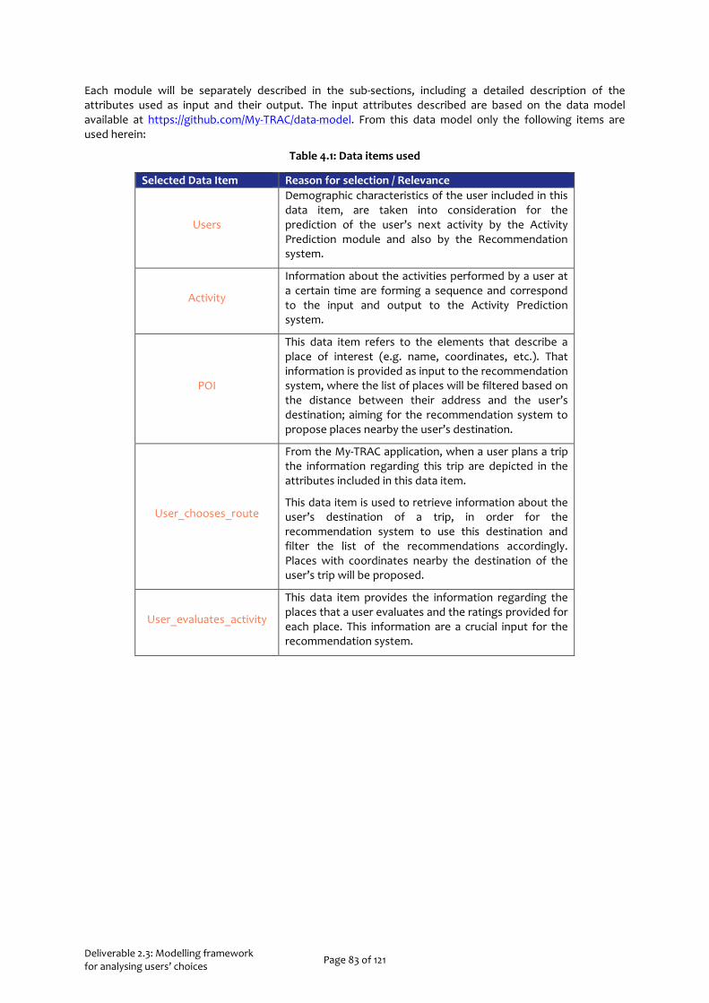
Deliverable 2.3: Modelling framework for analysing users’ choices Page 83 of 121
Each module will be separately described in the sub-sections, including a detailed description of the attributes used as input and their output. The input attributes described are based on the data model available at https://github.com/My-TRAC/data-model. From this data model only the following items are used herein:
Table 4.1: Data items used
Selected Data Item Reason for selection / Relevance
Users
Demographic characteristics of the user included in this data item, are taken into consideration for the prediction of the user’s next activity by the Activity Prediction module and also by the Recommendation system.
Activity
Information about the activities performed by a user at a certain time are forming a sequence and correspond to the input and output to the Activity Prediction system.
POI
This data item refers to the elements that describe a place of interest (e.g. name, coordinates, etc.). That information is provided as input to the recommendation system, where the list of places will be filtered based on the distance between their address and the user’s destination; aiming for the recommendation system to propose places nearby the user’s destination.
User_chooses_route
From the My-TRAC application, when a user plans a trip the information regarding this trip are depicted in the attributes included in this data item.
This data item is used to retrieve information about the user’s destination of a trip, in order for the recommendation system to use this destination and filter the list of the recommendations accordingly. Places with coordinates nearby the destination of the user’s trip will be proposed.
User_evaluates_activity
This data item provides the information regarding the places that a user evaluates and the ratings provided for each place. This information are a crucial input for the recommendation system.
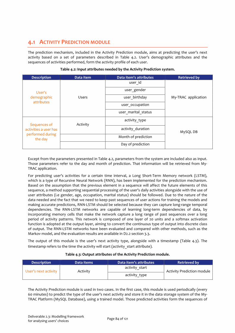
Deliverable 2.3: Modelling framework for analysing users’ choices Page 84 of 121
4.1 ACTIVITY PREDICTION MODULE
The prediction mechanism, included in the Activity Prediction module, aims at predicting the user’s next activity based on a set of parameters described in Table 4.2. User’s demographic attributes and the sequences of activities performed, form the activity profile of each user.
Table 4.2: Input attributes needed by the Activity Prediction system.
Description Data item Data item’s attributes Retrieved by
User‘s demographic
attributes Users
user_id
My-TRAC application
user_gender
user_birthday
user_occupation
user_marital_status
Sequences of activities a user has performed during
the day
Activity activity_type
MySQL DB activity_duration
Month of prediction
Day of prediction
Except from the parameters presented in Table 4.2, parameters from the system are included also as input. Those parameters refer to the day and month of prediction. That information will be retrieved from My-TRAC application.
For predicting user’s activities for a certain time interval, a Long Short-Term Memory network (LSTM), which is a type of Recursive Neural Network (RNN), has been implemented for the prediction mechanism. Based on the assumption that the previous element in a sequence will affect the future elements of this sequence, a method supporting sequential processing of the user’s daily activities alongside with the use of user attributes (i.e gender, age, occupation, marital status) should be followed. Due to the nature of the data needed and the fact that we need to keep past sequences of user actions for training the models and making accurate predictions, RNN-LSTM should be selected because they can capture long-range temporal dependencies. The RNN-LSTM networks are capable of learning long-term dependencies of data, by incorporating memory cells that make the network capture a long range of past sequences over a long period of activity patterns. This network is composed of one layer of 20 units and a softmax activation function is adopted at the output layer, aiming to convert the continuous type of output into discrete class of output. The RNN-LSTM networks have been evaluated and compared with other methods, such as the Markov model, and the evaluation results are available in D2.2 section 3.3.
The output of this module is the user’s next activity type, alongside with a timestamp (Table 4.3). The timestamp refers to the time the activity will start (activity_start attribute).
Table 4.3: Output attributes of the Activity Prediction module.
Description Data items Data item’s attributes Retrieved by
User’s next activity Activity activity_start
Activity Prediction module activity_type
The Activity Prediction module is used in two cases. In the first case, this module is used periodically (every 60 minutes) to predict the type of the user’s next activity and store it in the data storage system of the My-TRAC Platform (MySQL Database), using a trained model. Those predicted activities form the sequences of
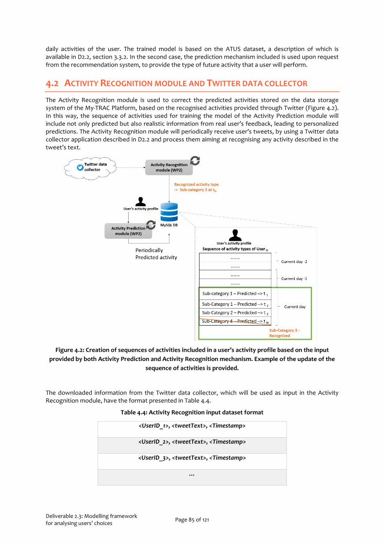
Deliverable 2.3: Modelling framework for analysing users’ choices Page 85 of 121
daily activities of the user. The trained model is based on the ATUS dataset, a description of which is available in D2.2, section 3.3.2. In the second case, the prediction mechanism included is used upon request from the recommendation system, to provide the type of future activity that a user will perform.
4.2 ACTIVITY RECOGNITION MODULE AND TWITTER DATA COLLECTOR
The Activity Recognition module is used to correct the predicted activities stored on the data storage system of the My-TRAC Platform, based on the recognised activities provided through Twitter (Figure 4.2). In this way, the sequence of activities used for training the model of the Activity Prediction module will include not only predicted but also realistic information from real user’s feedback, leading to personalized predictions. The Activity Recognition module will periodically receive user’s tweets, by using a Twitter data collector application described in D2.2 and process them aiming at recognising any activity described in the tweet’s text.
Figure 4.2: Creation of sequences of activities included in a user’s activity profile based on the input provided by both Activity Prediction and Activity Recognition mechanism. Example of the update of the
sequence of activities is provided.
The downloaded information from the Twitter data collector, which will be used as input in the Activity Recognition module, have the format presented in Table 4.4.
Table 4.4: Activity Recognition input dataset format
<UserID_1>, <tweetText>, <Timestamp>
<UserID_2>, <tweetText>, <Timestamp>
<UserID_3>, <tweetText>, <Timestamp>
…
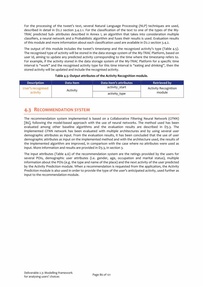
Deliverable 2.3: Modelling framework for analysing users’ choices Page 86 of 121
For the processing of the tweet’s text, several Natural Language Processing (NLP) techniques are used, described in detail in D2.2 section 3.4.2.1. For the classification of the text to one of the types of the My-TRAC predicted Sub- attributes described in Annex I, an algorithm that takes into consideration multiple classifiers, a neural network and a Probabilistic algorithm and fuses their results is used. Evaluation results of this module and more information about each classification used are available in D2.2 section 3.4.2.
The output of this module includes the tweet’s timestamp and the recognized activity’s type (Table 4.5). The recognised type of activity will be stored in the data storage system of the My-TRAC Platform, based on user Id, aiming to update any predicted activity corresponding to the time where the timestamp refers to. For example, if the activity stored in the data storage system of the My-TRAC Platform for a specific time interval is “work” and the recognised activity type for this time interval is “eating and drinking”, then the stored activity will be updated and include the recognised activity.
Table 4.5: Output attributes of the Activity Recognition module.
Description Data item Data item’s attributes Retrieved by
User’s recognised activity Activity
activity_start Activity Recognition module activity_type
4.3 RECOMMENDATION SYSTEM
The recommendation system implemented is based on a Collaborative Filtering Neural Network (CFNN) [86], following the model-based approach with the use of neural networks. The method used has been evaluated among other baseline algorithms and the evaluation results are described in D3.3. The implemented CFNN network has been evaluated with multiple architectures and by using several user demographic attributes as input. From the evaluation results, it has been concluded that the use of user demographic attributes as input on the implemented method and with the architecture used, the results of the implemented algorithm are improved, in comparison with the case where no attributes were used as input. More information and results are provided in D3.3, in section 3.
The input attributes (Table 4.6) of the recommendation system are the ratings provided by the users for several POIs, demographic user attributes (i.e. gender, age, occupation and marital status), multiple information about the POIs (e.g. the type and name of the place) and the next activity of the user predicted by the Activity Prediction module. When a recommendation is requested from the application, the Activity Prediction module is also used in order to provide the type of the user’s anticipated activity, used further as input to the recommendation module.
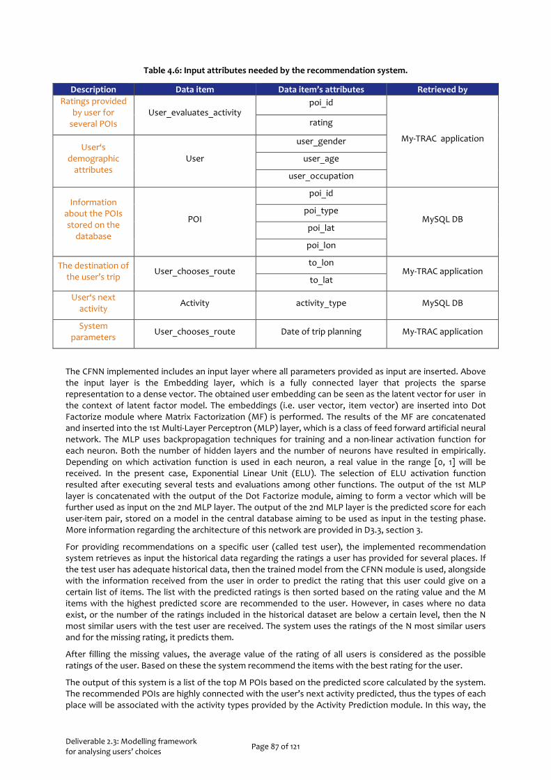
Deliverable 2.3: Modelling framework for analysing users’ choices Page 87 of 121
Table 4.6: Input attributes needed by the recommendation system.
Description Data item Data item’s attributes Retrieved by Ratings provided
by user for several POIs
User_evaluates_activity poi_id
My-TRAC application
rating
User‘s demographic
attributes User
user_gender
user_age
user_occupation
Information about the POIs stored on the
database
POI
poi_id
MySQL DB poi_type
poi_lat
poi_lon
The destination of the user’s trip User_chooses_route
to_lon My-TRAC application
to_lat
User‘s next activity Activity activity_type MySQL DB
System parameters User_chooses_route Date of trip planning My-TRAC application
The CFNN implemented includes an input layer where all parameters provided as input are inserted. Above the input layer is the Embedding layer, which is a fully connected layer that projects the sparse representation to a dense vector. The obtained user embedding can be seen as the latent vector for user in the context of latent factor model. The embeddings (i.e. user vector, item vector) are inserted into Dot Factorize module where Matrix Factorization (MF) is performed. The results of the MF are concatenated and inserted into the 1st Multi-Layer Perceptron (MLP) layer, which is a class of feed forward artificial neural network. The MLP uses backpropagation techniques for training and a non-linear activation function for each neuron. Both the number of hidden layers and the number of neurons have resulted in empirically. Depending on which activation function is used in each neuron, a real value in the range [0, 1] will be received. In the present case, Exponential Linear Unit (ELU). The selection of ELU activation function resulted after executing several tests and evaluations among other functions. The output of the 1st MLP layer is concatenated with the output of the Dot Factorize module, aiming to form a vector which will be further used as input on the 2nd MLP layer. The output of the 2nd MLP layer is the predicted score for each user-item pair, stored on a model in the central database aiming to be used as input in the testing phase. More information regarding the architecture of this network are provided in D3.3, section 3.
For providing recommendations on a specific user (called test user), the implemented recommendation system retrieves as input the historical data regarding the ratings a user has provided for several places. If the test user has adequate historical data, then the trained model from the CFNN module is used, alongside with the information received from the user in order to predict the rating that this user could give on a certain list of items. The list with the predicted ratings is then sorted based on the rating value and the M items with the highest predicted score are recommended to the user. However, in cases where no data exist, or the number of the ratings included in the historical dataset are below a certain level, then the N most similar users with the test user are received. The system uses the ratings of the N most similar users and for the missing rating, it predicts them.
After filling the missing values, the average value of the rating of all users is considered as the possible ratings of the user. Based on these the system recommend the items with the best rating for the user.
The output of this system is a list of the top M POIs based on the predicted score calculated by the system. The recommended POIs are highly connected with the user’s next activity predicted, thus the types of each place will be associated with the activity types provided by the Activity Prediction module. In this way, the

Deliverable 2.3: Modelling framework for analysing users’ choices Page 88 of 121
recommended places will be filtered based on the predicted activity type provided by the Activity Prediction module, such as if the next activity of the user is “eating and drinking”, the recommendation system will provide a list of restaurants, bars, etc. Alongside, the destination of the trip planned by the user will be associated with the address of the places, thus the recommendation system will suggest places that are nearby the trip’s destination.
Deliverable 2.3: Modelling framework for analysing users’ choices Page 89 of 121
5 DATA REQUIREMENTS The My-TRAC application aims at assisting travellers in planning their daily trips and thus, understanding travel related choices is vital for its success. In this context, choice models were developed in order to accurately predict users’ travel behaviour and provide valuable travel related information to the user. These models, developed using stated and revealed preferences, describe how the characteristics of decision-makers and of the available alternatives affect the choice behaviour. In order to model travellers’ choices, four categories of data are used: (1) personal characteristics, including socio-demographics, mobility characteristics, and other qualitative factors (e.g., regret, tolerance); (2) trip contexts, including trip purpose and other factors describing conditions under which the trip is made; (3) attributes of available (and considered) alternatives; and (4) user feedback in the form of actual choices made by the travellers. The minimum data required for the development and implementation of choice models that describe and subsequently predict behaviours, as they emerged from the analysis performed in this task, are described in this section. Note that the data requirements of activity modelling are already described in D2.2 and D3.3 and therefore not discussed here.
5.1 DATA SOURCES AND ACQUISITION
Data requirements refer to the data that are needed in order for My-TRAC application to deploy the models developed within the framework of Task 2.3. Data presented in Table 5.1 are required for the My-TRAC application to be able to perform accurate predictions concerning travel mode and time of departure choice decisions for each trip. Data specifications are described based on the following elements:
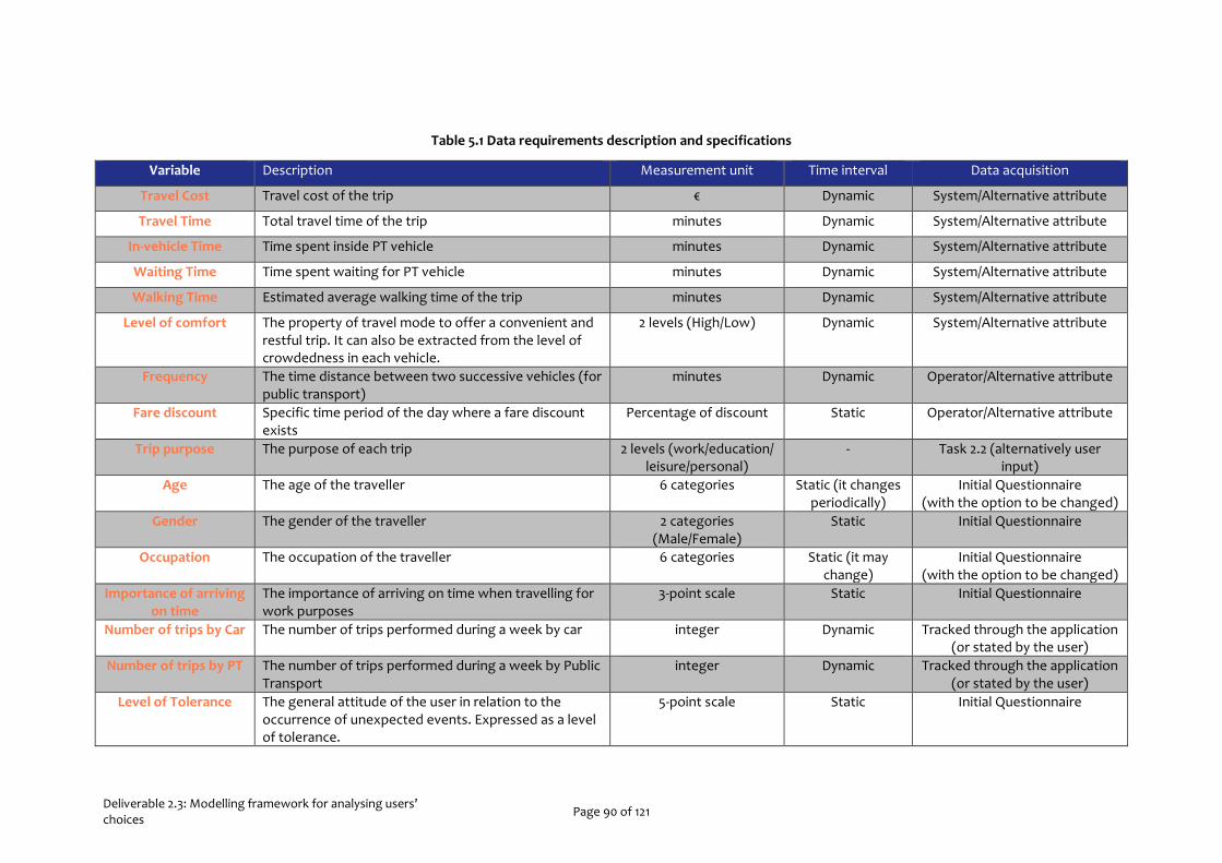
Deliverable 2.3: Modelling framework for analysing users’ choices Page 90 of 121
Table 5.1 Data requirements description and specifications
Variable Description Measurement unit Time interval Data acquisition
Travel Cost Travel cost of the trip € Dynamic System/Alternative attribute
Travel Time Total travel time of the trip minutes Dynamic System/Alternative attribute
In-vehicle Time Time spent inside PT vehicle minutes Dynamic System/Alternative attribute
Waiting Time Time spent waiting for PT vehicle minutes Dynamic System/Alternative attribute
Walking Time Estimated average walking time of the trip minutes Dynamic System/Alternative attribute
Level of comfort The property of travel mode to offer a convenient and restful trip. It can also be extracted from the level of crowdedness in each vehicle.
2 levels (High/Low) Dynamic System/Alternative attribute
Frequency The time distance between two successive vehicles (for public transport)
minutes Dynamic Operator/Alternative attribute
Fare discount Specific time period of the day where a fare discount exists
Percentage of discount Static Operator/Alternative attribute
Trip purpose The purpose of each trip 2 levels (work/education/ leisure/personal)
- Task 2.2 (alternatively user input)
Age The age of the traveller 6 categories Static (it changes periodically)
Initial Questionnaire (with the option to be changed)
Gender The gender of the traveller 2 categories (Male/Female)
Static Initial Questionnaire
Occupation The occupation of the traveller 6 categories Static (it may change)
Initial Questionnaire (with the option to be changed)
Importance of arriving on time
The importance of arriving on time when travelling for work purposes
3-point scale Static Initial Questionnaire
Number of trips by Car The number of trips performed during a week by car integer Dynamic Tracked through the application (or stated by the user)
Number of trips by PT The number of trips performed during a week by Public Transport
integer Dynamic Tracked through the application (or stated by the user)
Level of Tolerance The general attitude of the user in relation to the occurrence of unexpected events. Expressed as a level of tolerance.
5-point scale Static Initial Questionnaire

Deliverable 2.3: Modelling framework for analysing users’ choices Page 91 of 121
Probability of Random Event Occurrence
The probability of the occurrence of any random event during every day trip being assigned from the user.
% percentage Static Initial Questionnaire
Regret Measurement The level of anticipated regret 7-point scale Static Initial Questionnaire
Perception of System Reliability
The perceived reliability of PT system 7-point scale Static Initial Questionnaire
Level of Engagement The level of engagement while waiting for a PT vehicle 7-point scale Static Initial Questionnaire
Delay effect The perceived reliability of PT system in case of delays in the network
7-point scale Static Initial Questionnaire
Level of Happiness The level of happiness that someone experiences during a trip.
3-point scale Dynamic User feedback
Household Size The size of the household Integer >0 Static Initial Questionnaire
Income The income of the traveller 3 categories Static Initial Questionnaire
Car availability The number of cars that the person owns or has access to
Integer Static (it may change)
Initial Questionnaire
Moto availability The number of motorcycles that the person owns or has access to
Integer Static (it may change)
Initial Questionnaire
Bike availability The number of bicycles that the person owns or has access to
Integer Static (it may change)
Initial Questionnaire
Selected alternative The alternative selected by the user categorical Dynamic System

Deliverable 2.3: Modelling framework for analysing users’ choices Page 92 of 121
6 CONCLUSIONS In this deliverable, we focussed on understanding behaviour of travellers, which is crucial to providing timely, meaningful, and personalized advice on various travel decisions. Since providing travel recommendations through a mobile application is one of the most important objectives of My-TRAC, this deliverable is critical to the project.
An analysis of three choice dimensions, (i) travel mode, (ii) departure time, and (iii) route choice was presented, which allows us to describe the most important decisions made by travellers before and during their trips. The analyses produced a set of baseline population choice models for each dimension which can also be re-estimated as more data comes in from the use of the My-TRAC application. The estimated models include information about: (i) personal characteristics, including socio-demographics, mobility characteristics, and other qualitative factors (e.g., regret, tolerance); (ii) trip contexts, including trip purpose and other factors describing conditions under which the trip is made; and (iii) attributes of available (and considered) alternatives. We discussed how travellers of different backgrounds and personalities behave in different travel situations. These choice models can be further extended for personalization and recommendation in subsequent tasks of the project.
For the analysis, we mainly use stated preferences data collected from three locations where the pilots will be conducted, namely, the Netherlands, Greece (Athens), and Portugal (Lisbon). The data was collected both online and on-site. However, as more and more passive travel-related data becomes available (including from the My-TRAC application), it is likely that revealed preferences will be the main source for behaviour analysis in the future. Therefore, in addition to the stated preference experiments, two route choice models were also based on revealed preferences from smart card data.
As noted in D2.1, apart from hard factors, such as minimizing travel time, we need to pay close attention to softer factors, such as emotions, attitudes, and perceptions of risk and uncertainty. To this end, for mode and departure time, the effect of reported travel happiness on mode and departure time choice is studied. For route choice, a choice situation is identified to capture the effect of subjective-beliefs regarding waiting time uncertainties. Moreover, the effects of including different waiting time risk measures, such as deviation of waiting times from schedule (regular disturbances) and dispersion of waiting time (irregular disturbances) are compared.
For mode choice, hard factors such as travel time, cost, and comfort are considered. Amongst the choices offered in the experiment were car, public transport, bicycle (in the Netherlands), and motorcycle (in Greece and Portugal). Departure time choice is between depart ‘on time’, ‘early’, or ‘late’, and is only modelled for public transport modes, considering travel time, walking time (to station), frequency of vehicles, and fare discount (as percentage) as the main alternative attributes. We discussed the effect of different attributes in detail, also comparing results across pilot locations and with literature.
For route choice, three models were presented. In the first model, the focus is on capturing waiting time uncertainty that travellers in public transport networks feel. Findings indicated an average preference for certainty, with travellers willing to accept between 3 and 10 minutes of extra in-vehicle time to avoid uncertainty in waiting time. We further reported the effects of context and personal characteristics on beliefs regarding uncertainty for the three countries. Analysing the alternatives considered by decision-makers is critical to both accurate behaviour modelling as well as presenting application users with appropriate options. Therefore, the second model developed a methodology to automatically calibrate the composition of route choice sets using the non-compensatory elimination-by-aspects decision rule. In the third and final route choice model (also estimated from smart card data), we presented a comparison of different representations of risky waiting time in choice models and showed the importance of including information on both deviation from schedule and dispersion of waiting times in choice models.

Deliverable 2.3: Modelling framework for analysing users’ choices Page 93 of 121
Finally, the activity model developed in two other deliverables (D2.2, D3.3), is briefly presented here to align with the complete set of user choices. Moreover, the data required for re-estimation of the models (based on continuous observations from the My-TRAC application) described in this deliverable using such data are also tabulated.
6.1 FUTURE RESEARCH
Apart from the practical contribution of producing the baseline population choice models for different travel-related choice dimensions, the scientific aspects of this deliverable point a number of different avenues:
• While we assume the choices to be sequential for practical reasons, future research could employ simultaneous estimation of different choice dimensions together with the various attitude and perception-based attributes considered here. Moreover, as shown models that describe heterogeneity in some detail (such as mixed logit and latent class choice models) may also be used for this. We may consider such improvements in D2.5.
• One limitation of stated preferences experiments is that they may not be very conducive in eliciting the effects of context variables, since it is very difficult for people to hypothesise about feeling in a particular way. Future studies could focus on designing experiments that can make respondents ‘feel’ the changes in perception of uncertainty due to contextual variables such as elapsed waiting time and delays. Alternatively, given the increasing availability of smart card and vehicle location data for public transport networks, subjective beliefs towards uncertainty may be assessed using revealed preferences from the proposed choice situation. In a working paper Shelat, et al. [85] use revealed preferences to study subjective beliefs regarding uncertainty. Several trips in line with the choice situation proposed in section 3.1.2 and suitable for analysis are found in the urban public transport network of Amsterdam.
• As noted in section 3.1.1, the effects of attitudes and perceptions on travel behaviour are difficult to disentangle. However, if this was to be done, we could produce more impactful recommendations and policies that specifically target each of these aspects. For instance, if we know that a poor perception of system reliability is causing travellers to make decisions that make them less happy, we can specifically work on this.
• While we used elimination-by-aspects as the governing decision rule (because of several advantages) for generating route choice sets (section 3.2), it might be the case that different people employ different non-compensatory heuristics (e.g., lexicographic, conjunctive/disjunctive). It is interesting to study, if there exist a mixture of such rule-users in the population.
• Only the more common risk representations (deviation, dispersion) are currently used in section 3.3. Studies [87, 88] have indicated that there are other important moments of distribution that should be included in such a comparison. Including these indicators will be an important aim in further extending the mentioned working paper [81].
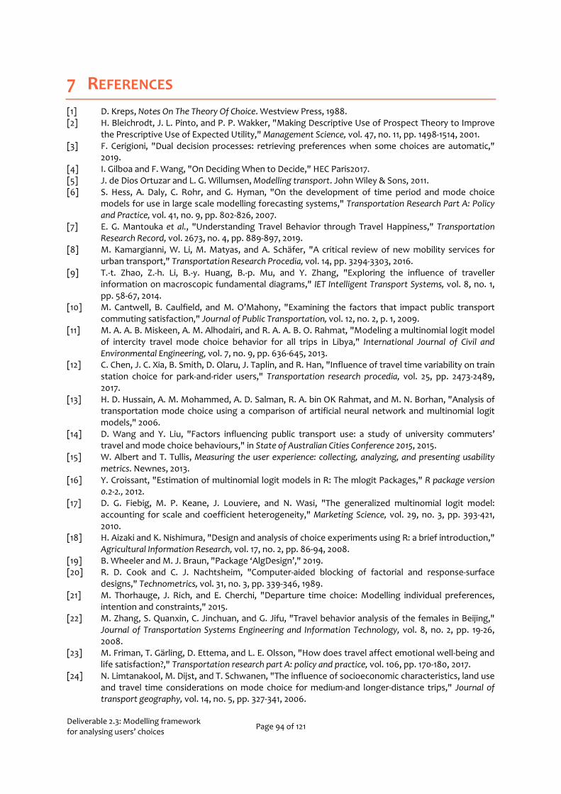
Deliverable 2.3: Modelling framework for analysing users’ choices Page 94 of 121
7 REFERENCES [1] D. Kreps, Notes On The Theory Of Choice. Westview Press, 1988. [2] H. Bleichrodt, J. L. Pinto, and P. P. Wakker, "Making Descriptive Use of Prospect Theory to Improve
the Prescriptive Use of Expected Utility," Management Science, vol. 47, no. 11, pp. 1498-1514, 2001. [3] F. Cerigioni, "Dual decision processes: retrieving preferences when some choices are automatic,"
2019. [4] I. Gilboa and F. Wang, "On Deciding When to Decide," HEC Paris2017. [5] J. de Dios Ortuzar and L. G. Willumsen, Modelling transport. John Wiley & Sons, 2011. [6] S. Hess, A. Daly, C. Rohr, and G. Hyman, "On the development of time period and mode choice
models for use in large scale modelling forecasting systems," Transportation Research Part A: Policy and Practice, vol. 41, no. 9, pp. 802-826, 2007.
[7] E. G. Mantouka et al., "Understanding Travel Behavior through Travel Happiness," Transportation Research Record, vol. 2673, no. 4, pp. 889-897, 2019.
[8] M. Kamargianni, W. Li, M. Matyas, and A. Schäfer, "A critical review of new mobility services for urban transport," Transportation Research Procedia, vol. 14, pp. 3294-3303, 2016.
[9] T.-t. Zhao, Z.-h. Li, B.-y. Huang, B.-p. Mu, and Y. Zhang, "Exploring the influence of traveller information on macroscopic fundamental diagrams," IET Intelligent Transport Systems, vol. 8, no. 1, pp. 58-67, 2014.
[10] M. Cantwell, B. Caulfield, and M. O’Mahony, "Examining the factors that impact public transport commuting satisfaction," Journal of Public Transportation, vol. 12, no. 2, p. 1, 2009.
[11] M. A. A. B. Miskeen, A. M. Alhodairi, and R. A. A. B. O. Rahmat, "Modeling a multinomial logit model of intercity travel mode choice behavior for all trips in Libya," International Journal of Civil and Environmental Engineering, vol. 7, no. 9, pp. 636-645, 2013.
[12] C. Chen, J. C. Xia, B. Smith, D. Olaru, J. Taplin, and R. Han, "Influence of travel time variability on train station choice for park-and-rider users," Transportation research procedia, vol. 25, pp. 2473-2489, 2017.
[13] H. D. Hussain, A. M. Mohammed, A. D. Salman, R. A. bin OK Rahmat, and M. N. Borhan, "Analysis of transportation mode choice using a comparison of artificial neural network and multinomial logit models," 2006.
[14] D. Wang and Y. Liu, "Factors influencing public transport use: a study of university commuters’ travel and mode choice behaviours," in State of Australian Cities Conference 2015, 2015.
[15] W. Albert and T. Tullis, Measuring the user experience: collecting, analyzing, and presenting usability metrics. Newnes, 2013.
[16] Y. Croissant, "Estimation of multinomial logit models in R: The mlogit Packages," R package version 0.2-2., 2012.
[17] D. G. Fiebig, M. P. Keane, J. Louviere, and N. Wasi, "The generalized multinomial logit model: accounting for scale and coefficient heterogeneity," Marketing Science, vol. 29, no. 3, pp. 393-421, 2010.
[18] H. Aizaki and K. Nishimura, "Design and analysis of choice experiments using R: a brief introduction," Agricultural Information Research, vol. 17, no. 2, pp. 86-94, 2008.
[19] B. Wheeler and M. J. Braun, "Package ‘AlgDesign’," 2019. [20] R. D. Cook and C. J. Nachtsheim, "Computer-aided blocking of factorial and response-surface
designs," Technometrics, vol. 31, no. 3, pp. 339-346, 1989. [21] M. Thorhauge, J. Rich, and E. Cherchi, "Departure time choice: Modelling individual preferences,
intention and constraints," 2015. [22] M. Zhang, S. Quanxin, C. Jinchuan, and G. Jifu, "Travel behavior analysis of the females in Beijing,"
Journal of Transportation Systems Engineering and Information Technology, vol. 8, no. 2, pp. 19-26, 2008.
[23] M. Friman, T. Gärling, D. Ettema, and L. E. Olsson, "How does travel affect emotional well-being and life satisfaction?," Transportation research part A: policy and practice, vol. 106, pp. 170-180, 2017.
[24] N. Limtanakool, M. Dijst, and T. Schwanen, "The influence of socioeconomic characteristics, land use and travel time considerations on mode choice for medium-and longer-distance trips," Journal of transport geography, vol. 14, no. 5, pp. 327-341, 2006.

Deliverable 2.3: Modelling framework for analysing users’ choices Page 95 of 121
[25] J. De Vos, "The influence of land use and mobility policy on travel behavior: A comparative case study of Flanders and the Netherlands," Journal of Transport and Land Use, vol. 8, no. 1, pp. 171-190, 2015.
[26] A. Duarte, C. Garcia, G. Giannarakis, S. Limão, A. Polydoropoulou, and N. Litinas, "New approaches in transportation planning: happiness and transport economics," NETNOMICS: Economic Research and Electronic Networking, vol. 11, no. 1, pp. 5-32, 2010.
[27] L. E. Olsson, T. Gärling, D. Ettema, M. Friman, and S. Fujii, "Happiness and satisfaction with work commute," Social indicators research, vol. 111, no. 1, pp. 255-263, 2013.
[28] D. McFadden, "The choice theory approach to market research," Marketing science, vol. 5, no. 4, pp. 275-297, 1986.
[29] K. Lucas, E. Blumenberg, and R. Weinberger, Auto motives: understanding car use behaviours. Emerald Group Publishing Limited, 2011.
[30] T. A. Domencich and D. McFadden, "Urban travel demand-a behavioral analysis," 1975. [31] R. Noland and K. A. Small, "Travel-time uncertainty, departure time choice, and the cost of morning
commutes," Transportation research record, no. 1493, pp. 150-158, 1995. [32] C. Hendrickson and E. Plank, "The flexibility of departure times for work trips," Transportation
Research Part A: General, vol. 18, no. 1, pp. 25-36, 1984. [33] G. De Jong, A. Daly, M. Pieters, C. Vellay, M. Bradley, and F. Hofman, "A model for time of day and
mode choice using error components logit," Transportation Research Part E: Logistics and Transportation Review, vol. 39, no. 3, pp. 245-268, 2003.
[34] S. Shelat, O. Cats, and J. W. C. van Lint, "Quantifying Subjective Beliefs Regarding Waiting Time Uncertainty in Public Transport Networks," presented at the The 24th International Conference of Hong Kong Society for Transportation Studies, Hong Kong, 14-16 December 2019, 2019.
[35] M. J. Machina and M. Siniscalchi, "Chapter 13 - Ambiguity and Ambiguity Aversion," in Handbook of the Economics of Risk and Uncertainty, vol. 1, M. Machina and K. Viscusi, Eds.: North-Holland, 2014, pp. 729-807.
[36] P. P. Wakker, Prospect theory: For risk and ambiguity. Cambridge university press, 2010. [37] J. Bates, J. Polak, P. Jones, and A. Cook, "The valuation of reliability for personal travel,"
Transportation Research Part E: Logistics and Transportation Review, vol. 37, no. 2, pp. 191-229, 2001/04/01/ 2001.
[38] C. Carrion and D. Levinson, "Value of travel time reliability: A review of current evidence," Transportation Research Part A: Policy and Practice, vol. 46, no. 4, pp. 720-741, 2012/05/01/ 2012.
[39] A. Tversky and D. Kahneman, "The framing of decisions and the psychology of choice," Science, vol. 211, no. 4481, pp. 453-458, 1981.
[40] Z. Li and D. Hensher, "Prospect Theoretic Contributions in Understanding Traveller Behaviour: A Review and Some Comments," Transport Reviews, vol. 31, no. 1, pp. 97-115, 2011/01/01 2011.
[41] E. Avineri and J. N. Prashker, "Sensitivity to travel time variability: Travelers’ learning perspective," Transportation Research Part C: Emerging Technologies, vol. 13, no. 2, pp. 157-183, 2005/04/01/ 2005.
[42] E. Ben-Elia, I. Erev, and Y. Shiftan, "The combined effect of information and experience on drivers’ route-choice behavior," Transportation, journal article vol. 35, no. 2, pp. 165-177, March 01 2008.
[43] E. Ben-Elia, R. Di Pace, G. N. Bifulco, and Y. Shiftan, "The impact of travel information’s accuracy on route-choice," Transportation Research Part C: Emerging Technologies, vol. 26, pp. 146-159, 2013/01/01/ 2013.
[44] E. U. Weber and R. A. Milliman, "Perceived Risk Attitudes: Relating Risk Perception to Risky Choice," Management Science, vol. 43, no. 2, pp. 123-144, 1997.
[45] A. Baillon, Z. Huang, A. Selim, and P. P. Wakker, "Measuring Ambiguity Attitudes for All (Natural) Events," Econometrica, vol. 86, no. 5, pp. 1839-1858, 2018.
[46] R. F. Nau, "De Finetti was Right: Probability Does Not Exist," Theory and Decision, vol. 51, no. 2, pp. 89-124, 2001/12/01 2001.
[47] D. Maister, "The psychology of waiting lines," in The Service Encounter, J. A. Czepiel, M. Solomon, and C. S. Surprenant, Eds.: Lexington Books, 1985.
[48] P. Jones, "Managing perceptions of waiting times in service queues," International Journal of Service Industry Management, vol. 7, no. 5, pp. 47-61, 1996.
[49] D. A. Hensher, "Measurement of the Valuation of Travel Time Savings," Journal of Transport Economics and Policy (JTEP), vol. 35, no. 1, pp. 71-98, // 2001.

Deliverable 2.3: Modelling framework for analysing users’ choices Page 96 of 121
[50] D. Levinson, K. Harder, J. Bloomfield, and K. Winiarczyk, "Weighting Waiting: Evaluating Perception of In-Vehicle Travel Time Under Moving and Stopped Conditions," Transportation Research Record, vol. 1898, no. 1, pp. 61-68, 2004.
[51] E. E. Osuna, "The psychological cost of waiting," Journal of Mathematical Psychology, vol. 29, no. 1, pp. 82-105, 1985/03/01/ 1985.
[52] R. Thaler, "Toward a positive theory of consumer choice," Journal of Economic Behavior & Organization, vol. 1, no. 1, pp. 39-60, 1980/03/01/ 1980.
[53] D. Soman, "The mental accounting of sunk time costs: why time is not like money," Journal of Behavioral Decision Making, vol. 14, no. 3, pp. 169-185, 2001.
[54] H. Spiess and M. Florian, "Optimal strategies: A new assignment model for transit networks," Transportation Research Part B: Methodological, vol. 23, no. 2, pp. 83-102, 1989/04/01/ 1989.
[55] J.-D. Schmöcker, H. Shimamoto, and F. Kurauchi, "Generation and Calibration of Transit Hyperpaths," Procedia - Social and Behavioral Sciences, vol. 80, pp. 211-230, 2013/06/07/ 2013.
[56] Centraal Bureau voor de Statistiek, "Onderzoek Verplaatsingen in Nederland 2014," 2015. [57] B. Schwartz, A. Ward, J. Monterosso, S. Lyubomirsky, K. White, and D. R. Lehman, "Maximizing
versus satisficing: Happiness is a matter of choice," Journal of Personality and Social Psychology, vol. 83, no. 5, pp. 1178-1197, 2002.
[58] M. Bierlaire, "PythonBiogeme: a short introduction," in "Series on Biogeme," Transport and Mobility Laboratory, School of Architecture, Civil and Environmental Engineering, Ecole Polytechnique Fédérale de Lausanne, SwitzerlandTRANSP-OR 160706, 2016.
[59] A. de Palma and N. Picard, "Route choice decision under travel time uncertainty," Transportation Research Part A: Policy and Practice, vol. 39, no. 4, pp. 295-324, 2005/05/01/ 2005.
[60] S. Shelat, O. Cats, N. v. Oort, and H. v. Lint, "Calibrating Route Choice Sets for an Urban Public Transport Network using Smart Card Data," in 2019 6th International Conference on Models and Technologies for Intelligent Transportation Systems (MT-ITS), 2019, pp. 1-8, 2019.
[61] J. R. Hauser, "Consideration-set heuristics," Journal of Business Research, vol. 67, no. 8, pp. 1688-1699, 2014/08/01/ 2014.
[62] C. Prato and S. Bekhor, "Modeling Route Choice Behavior: How Relevant Is the Composition of Choice Set?," Transportation Research Record: Journal of the Transportation Research Board, vol. 2003, pp. 64-73, 2007.
[63] S. Hoogendoorn-Lanser, "Modelling travel behaviour in multi-modal networks," PhD PhD Thesis, Delft University of Technology, Delft, The Netherlands, 2005.
[64] S. Raveau, "Modelling Travel Choices on Public Transport Systems with Smart Card Data," in Public Transport Planning with Smart Card Data, F. Kurauchi and J.-D. Schmocker, Eds. Boca Raton: CRC Press, 2017.
[65] D. Ton, D. Duives, O. Cats, and S. Hoogendoorn, "Evaluating a data-driven approach for choice set identification using GPS bicycle route choice data from Amsterdam," Travel Behaviour and Society, vol. 13, pp. 105-117, 2018/10/01/ 2018.
[66] P. H. L. Bovy, "On Modelling Route Choice Sets in Transportation Networks: A Synthesis," Transport Reviews, vol. 29, no. 1, pp. 43-68, 2009/01/01 2009.
[67] C. G. Prato, "Route choice modeling: past, present and future research directions," Journal of Choice Modelling, vol. 2, no. 1, pp. 65-100, 2009/01/01/ 2009.
[68] M. Ben-Akiva, M. Bergman, A. J. Daly, and R. Ramaswamy, "Modeling inter-urban route choice behaviour," in Proceedings of the 9th international symposium on transportation and traffic theory, 1984, pp. 299-330: VNU Science Press Utrecht, The Netherlands.
[69] Z. Guo and N. H. M. Wilson, "Assessing the cost of transfer inconvenience in public transport systems: A case study of the London Underground," Transportation Research Part A: Policy and Practice, vol. 45, no. 2, pp. 91-104, 2011/02/01/ 2011.
[70] C. G. Prato and S. Bekhor, "Applying Branch-and-Bound Technique to Route Choice Set Generation," Transportation Research Record, vol. 1985, no. 1, pp. 19-28, 2006.
[71] S. Bekhor and C. G. Prato, "Methodological transferability in route choice modeling," Transportation Research Part B: Methodological, vol. 43, no. 4, pp. 422-437, 2009/05/01/ 2009.
[72] S. Hoogendoorn-Lanser, P. Bovy, and R. van Nes, "Application of Constrained Enumeration Approach to Multimodal Choice Set Generation," Transportation Research Record, vol. 2014, no. 1, pp. 50-57, 2007.
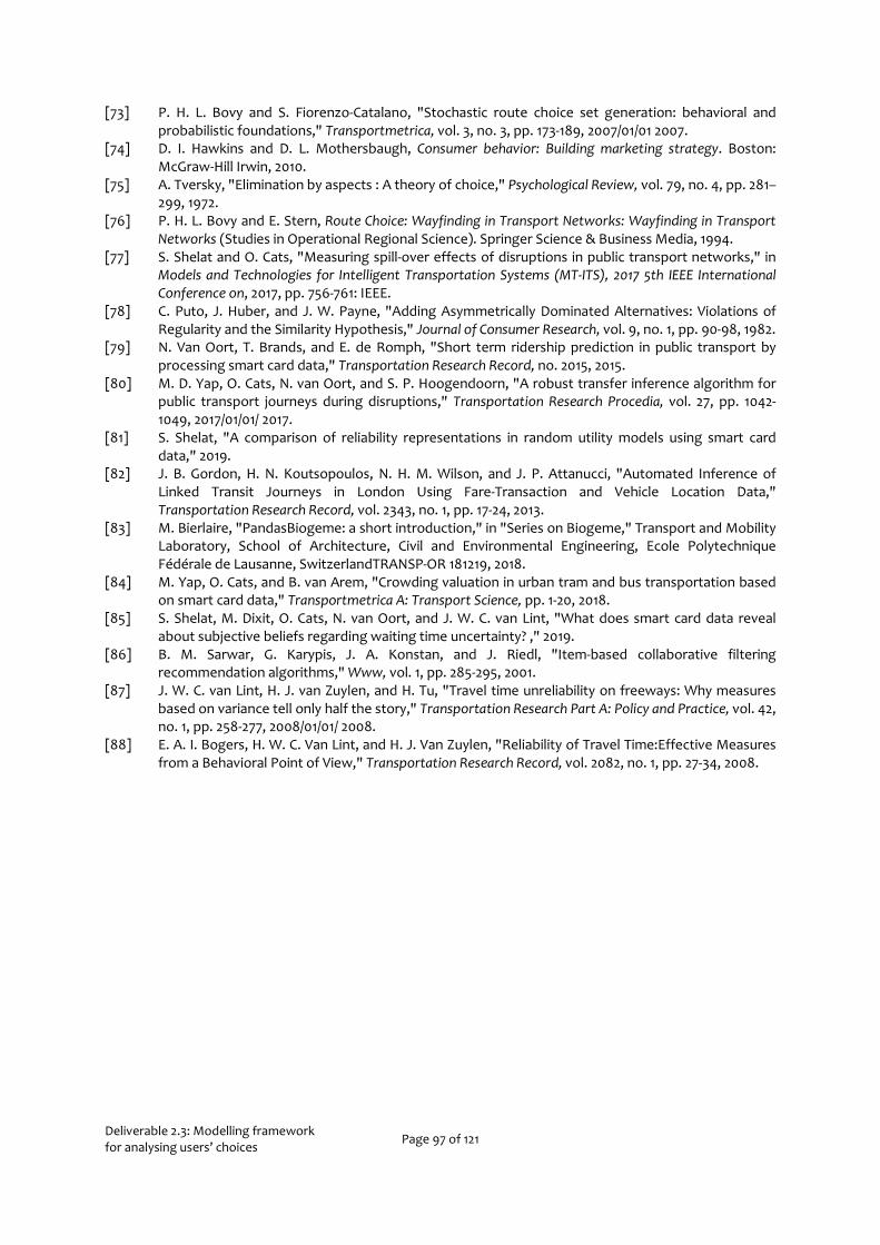
Deliverable 2.3: Modelling framework for analysing users’ choices Page 97 of 121
[73] P. H. L. Bovy and S. Fiorenzo-Catalano, "Stochastic route choice set generation: behavioral and probabilistic foundations," Transportmetrica, vol. 3, no. 3, pp. 173-189, 2007/01/01 2007.
[74] D. I. Hawkins and D. L. Mothersbaugh, Consumer behavior: Building marketing strategy. Boston: McGraw-Hill Irwin, 2010.
[75] A. Tversky, "Elimination by aspects : A theory of choice," Psychological Review, vol. 79, no. 4, pp. 281–299, 1972.
[76] P. H. L. Bovy and E. Stern, Route Choice: Wayfinding in Transport Networks: Wayfinding in Transport Networks (Studies in Operational Regional Science). Springer Science & Business Media, 1994.
[77] S. Shelat and O. Cats, "Measuring spill-over effects of disruptions in public transport networks," in Models and Technologies for Intelligent Transportation Systems (MT-ITS), 2017 5th IEEE International Conference on, 2017, pp. 756-761: IEEE.
[78] C. Puto, J. Huber, and J. W. Payne, "Adding Asymmetrically Dominated Alternatives: Violations of Regularity and the Similarity Hypothesis," Journal of Consumer Research, vol. 9, no. 1, pp. 90-98, 1982.
[79] N. Van Oort, T. Brands, and E. de Romph, "Short term ridership prediction in public transport by processing smart card data," Transportation Research Record, no. 2015, 2015.
[80] M. D. Yap, O. Cats, N. van Oort, and S. P. Hoogendoorn, "A robust transfer inference algorithm for public transport journeys during disruptions," Transportation Research Procedia, vol. 27, pp. 1042-1049, 2017/01/01/ 2017.
[81] S. Shelat, "A comparison of reliability representations in random utility models using smart card data," 2019.
[82] J. B. Gordon, H. N. Koutsopoulos, N. H. M. Wilson, and J. P. Attanucci, "Automated Inference of Linked Transit Journeys in London Using Fare-Transaction and Vehicle Location Data," Transportation Research Record, vol. 2343, no. 1, pp. 17-24, 2013.
[83] M. Bierlaire, "PandasBiogeme: a short introduction," in "Series on Biogeme," Transport and Mobility Laboratory, School of Architecture, Civil and Environmental Engineering, Ecole Polytechnique Fédérale de Lausanne, SwitzerlandTRANSP-OR 181219, 2018.
[84] M. Yap, O. Cats, and B. van Arem, "Crowding valuation in urban tram and bus transportation based on smart card data," Transportmetrica A: Transport Science, pp. 1-20, 2018.
[85] S. Shelat, M. Dixit, O. Cats, N. van Oort, and J. W. C. van Lint, "What does smart card data reveal about subjective beliefs regarding waiting time uncertainty? ," 2019.
[86] B. M. Sarwar, G. Karypis, J. A. Konstan, and J. Riedl, "Item-based collaborative filtering recommendation algorithms," Www, vol. 1, pp. 285-295, 2001.
[87] J. W. C. van Lint, H. J. van Zuylen, and H. Tu, "Travel time unreliability on freeways: Why measures based on variance tell only half the story," Transportation Research Part A: Policy and Practice, vol. 42, no. 1, pp. 258-277, 2008/01/01/ 2008.
[88] E. A. I. Bogers, H. W. C. Van Lint, and H. J. Van Zuylen, "Reliability of Travel Time:Effective Measures from a Behavioral Point of View," Transportation Research Record, vol. 2082, no. 1, pp. 27-34, 2008.

Deliverable 2.3: Modelling framework for analysing users’ choices Page 98 of 121
8 APPENDICES
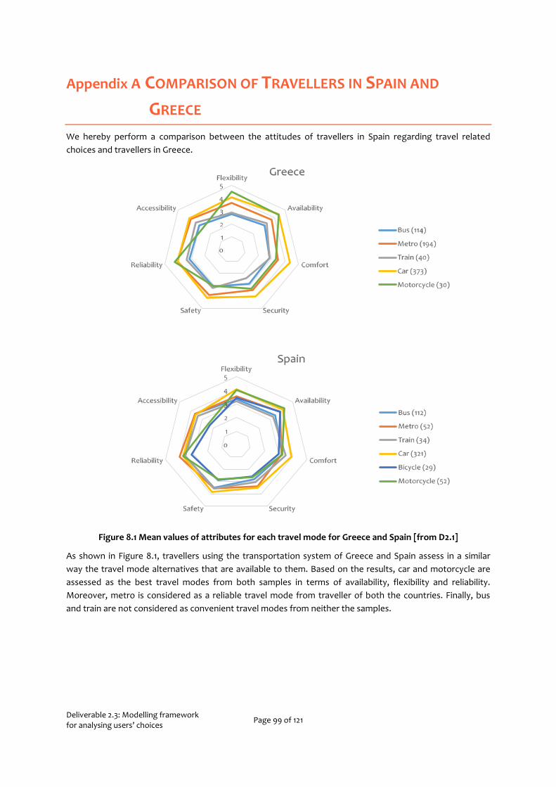
Deliverable 2.3: Modelling framework for analysing users’ choices Page 99 of 121
Appendix A COMPARISON OF TRAVELLERS IN SPAIN AND
GREECE We hereby perform a comparison between the attitudes of travellers in Spain regarding travel related choices and travellers in Greece.
Figure 8.1 Mean values of attributes for each travel mode for Greece and Spain [from D2.1]
As shown in Figure 8.1, travellers using the transportation system of Greece and Spain assess in a similar way the travel mode alternatives that are available to them. Based on the results, car and motorcycle are assessed as the best travel modes from both samples in terms of availability, flexibility and reliability. Moreover, metro is considered as a reliable travel mode from traveller of both the countries. Finally, bus and train are not considered as convenient travel modes from neither the samples.
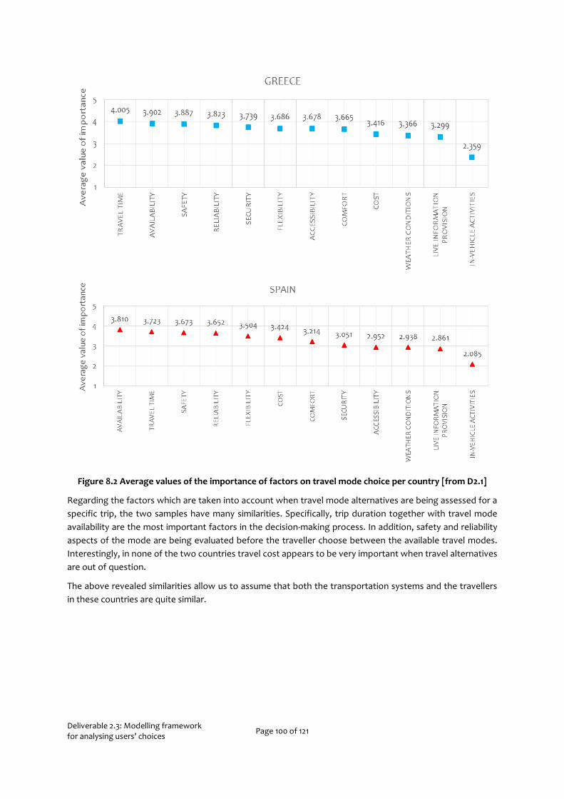
Deliverable 2.3: Modelling framework for analysing users’ choices Page 100 of 121
Figure 8.2 Average values of the importance of factors on travel mode choice per country [from D2.1]
Regarding the factors which are taken into account when travel mode alternatives are being assessed for a specific trip, the two samples have many similarities. Specifically, trip duration together with travel mode availability are the most important factors in the decision-making process. In addition, safety and reliability aspects of the mode are being evaluated before the traveller choose between the available travel modes. Interestingly, in none of the two countries travel cost appears to be very important when travel alternatives are out of question.
The above revealed similarities allow us to assume that both the transportation systems and the travellers in these countries are quite similar.

Deliverable 2.3: Modelling framework for analysing users’ choices Page 101 of 121
Appendix B MODE AND DEPARTURE TIME CHOICE STATED
PREFERENCES QUESTIONNAIRE All questionnaires were presented in the respective local languages.
B.1 NETHERLANDS
TRAVEL BEHAVIOR ANALYSIS
Τhis survey is conducted within the framework of the project My – TRAC (CORDIS ID: 777640) and is aimed at identifying the factors that affect travel mode and time of departure choices for everyday trips. For the purpose of this research, no personal information is required. Every answer will be treated confidentially and abiding to European and local laws and ethics.
MOBILITY PROFILE
A1. Which is your usual trip purpose? Work / education □ Other □
A2. How many times per week do you travel for your usual trip purpose? A3. How often do you use each of the following travel modes for your usual trip purpose? Never Rarely 1-2 times per week Daily Public Transportation □ □ □ □ Car □ □ □ □ Bicycle □ □ □ □
A4. How important is for you to arrive on time in the following cases?
Not
important at all
Somewhat important
Very important
Work/education trip □ □ □ Leisure trip □ □ □ Other trip □ □ □ A5. Describe your work time flexibility: Fixed start/end work time □ Flexible start/end work time □ NA □

Deliverable 2.3: Modelling framework for analysing users’ choices Page 102 of 121
A6. Do you have a Public Transport seasonal Pass? Yes □ No □ A7. How do you feel during your everyday trips?
Very unhappy□ Unhappy □ Neutral □ Happy □ Very happy
SCENARIOS
For a hypothetical journey of 10km from at 8:00 am, available modes are car, public transport (train and metro) and bicycle. In the following tables, total travel time per mode and costs per mode for the particular trip are presented, together with the comfort level. The level of comfort depends on the traffic conditions, crowdedness and other events (expected or unexpected) that may affect the conditions of the trip. For each of the following scenarios, which alternative mode would you prefer?
Car PT Bike Travel Time (in mins) 35 30 25
Cost (in euros) 5 2 0 Comfort High Low Low Select
Car PT Bike Travel Time (in mins) 25 30 25
Cost (in euros) 8 1.4 5 Comfort High High High Select
Car PT Bike
Travel Time (in mins) 35 25 35 Cost (in euros) 8 1.4 0
Comfort Low Low High Select
Car PT Bike Travel Time (in mins) 25 45 20
Cost (in euros) 5 2 5 Comfort Low High High Select
Car PT Bike
Travel Time (in mins) 15 45 20 Cost (in euros) 5 1.4 0
Comfort High Low Low Select
Car PT Bike Travel Time (in mins) 15 25 35
Cost (in euros) 8 2 5 Comfort Low High High Select
For the following scenarios consider that you perform the same trip of 10km by Public Transport (metro or train) during the morning peak (6:30 – 9:00). What time would you choose to start your trip in each of the below presented scenarios?
Early On time Late Travel Time (in mins) 30 45 30
Walking time (in mins) 20 10 20 Frequency (per mins) 5 3 7
Fare discount 0% 20% 40% Select
Early On time Late Travel Time (in mins) 25 35 25
Walking time (in mins) 20 20 20 Frequency (per mins) 3 5 5
Fare discount 20% 20% 0% Select
Early On time Late
Travel Time (in mins) 30 35 30 Walking time (in mins) 10 10 10 Frequency (per mins) 3 3 7
Fare discount 20% 0% 0% Select
Early On time Late Travel Time (in mins) 40 45 25
Walking time (in mins) 20 20 10 Frequency (per mins) 3 3 7
Fare discount 0% 0% 40% Select
Early On time Late
Travel Time (in mins) 25 40 40 Walking time (in mins) 10 10 10 Frequency (per mins) 3 5 5
Fare discount 0% 0% 40% Select
Early On time Late Travel Time (in mins) 40 40 40
Walking time (in mins) 10 20 20 Frequency (per mins) 5 3 7
Fare discount 20% 20% 0% Select

Deliverable 2.3: Modelling framework for analysing users’ choices Page 103 of 121
DEMOGRAPHICS
C1. Select your gender: Female □ Male □
C2. Select your age group: 18 – 24 □ 25 – 34 □ 35 – 44 □ 45 – 54 □ 55 – 64 □ ≥ 65 □
C3. Select your higher education level:
High school graduate □ Bachelor’s degree □ Master’s degree □ Professional degree □ Doctorate degree □ None of the above □
C4. Select your total annual personal income: Low □ Medium □ High □
C5. Select your occupation: Public servant □ Private employee □ Self-employed □ Unemployed □ Retired □ Student □
C6. Number of household members (including yourself): ____________

Deliverable 2.3: Modelling framework for analysing users’ choices Page 104 of 121
B.2 GREECE & PORTUGAL
TRAVEL BEHAVIOR ANALYSIS
Τhis survey is conducted within the framework of the project My – TRAC (CORDIS ID: 777640) and is aimed at identifying the factors that affect travel mode and time of departure choices for every day trips. For the purpose of this research, no personal information is required. Every answer will be treated confidentially and abiding to European and local laws and ethics.
MOBILITY PROFILE
A1. Which is your usual trip purpose? Work / education □ Other □ A2. How many times per week do you travel for your usual trip purpose? ______ A3. How often do you use each of the following travel modes for your usual trip purpose? Never Rarely 1-2 times per week Daily Public Transportation □ □ □ □ Car □ □ □ □ Motorcycle □ □ □ □ A4. How important is for you to arrive on time in the following cases?
Not
important at all
Somewhat important
Very important
Work/education trip □ □ □ Leisure trip □ □ □ Other trip □ □ □ A5. Describe your work time flexibility: Fixed start/end work time □ Flexible start/end work time □ NA □
A6. Do you have a Public Transport seasonal Pass? Yes □ No □
Α6.1 If yes, select its type: Combined (more than one operator) □ Single (One operator) □
A7. How do you feel during your everyday trips? Very unhappy□ Unhappy □ Neutral □ Happy □ Very happy □
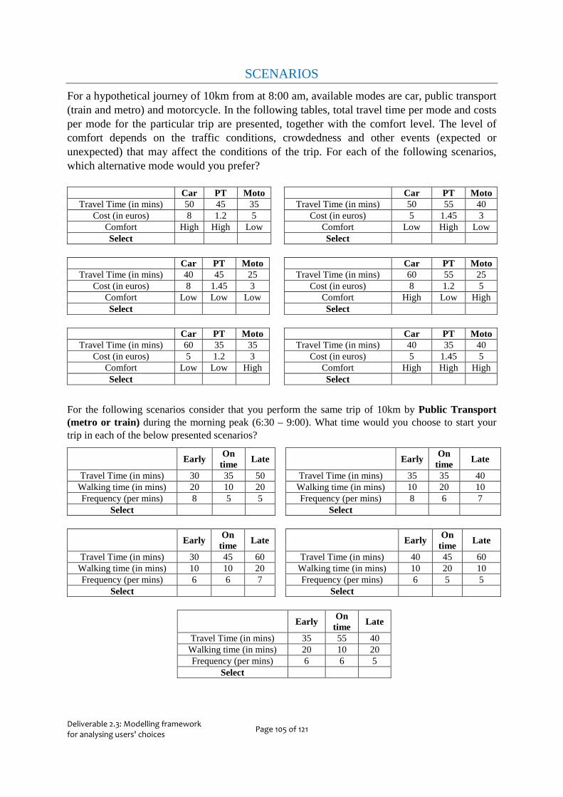
Deliverable 2.3: Modelling framework for analysing users’ choices Page 105 of 121
SCENARIOS For a hypothetical journey of 10km from at 8:00 am, available modes are car, public transport (train and metro) and motorcycle. In the following tables, total travel time per mode and costs per mode for the particular trip are presented, together with the comfort level. The level of comfort depends on the traffic conditions, crowdedness and other events (expected or unexpected) that may affect the conditions of the trip. For each of the following scenarios, which alternative mode would you prefer?
Car PT Moto Travel Time (in mins) 50 45 35
Cost (in euros) 8 1.2 5 Comfort High High Low Select
Car PT Moto Travel Time (in mins) 50 55 40
Cost (in euros) 5 1.45 3 Comfort Low High Low Select
Car PT Moto
Travel Time (in mins) 40 45 25 Cost (in euros) 8 1.45 3
Comfort Low Low Low Select
Car PT Moto Travel Time (in mins) 60 55 25
Cost (in euros) 8 1.2 5 Comfort High Low High Select
Car PT Moto
Travel Time (in mins) 60 35 35 Cost (in euros) 5 1.2 3
Comfort Low Low High Select
Car PT Moto Travel Time (in mins) 40 35 40
Cost (in euros) 5 1.45 5 Comfort High High High Select
For the following scenarios consider that you perform the same trip of 10km by Public Transport (metro or train) during the morning peak (6:30 – 9:00). What time would you choose to start your trip in each of the below presented scenarios?
Early On time Late
Travel Time (in mins) 30 35 50 Walking time (in mins) 20 10 20 Frequency (per mins) 8 5 5
Select
Early On time Late
Travel Time (in mins) 35 35 40 Walking time (in mins) 10 20 10 Frequency (per mins) 8 6 7
Select
Early On
time Late
Travel Time (in mins) 30 45 60 Walking time (in mins) 10 10 20 Frequency (per mins) 6 6 7
Select
Early On time Late
Travel Time (in mins) 40 45 60 Walking time (in mins) 10 20 10 Frequency (per mins) 6 5 5
Select
Early On
time Late
Travel Time (in mins) 35 55 40 Walking time (in mins) 20 10 20 Frequency (per mins) 6 6 5
Select

Deliverable 2.3: Modelling framework for analysing users’ choices Page 106 of 121
DEMOGRAPHICS C1. Select your gender: Female □ Male □
C2. Select your age group: 18 – 24 □ 25 – 34 □ 35 – 44 □ 45 – 54 □ 55 – 64 □ ≥ 65 □
C3. Select your higher education level:
High school graduate □ Bachelor’s degree □ Master’s degree □ Professional degree □ Doctorate degree □ None of the above □
C4. Select your total annual personal income: Low □ Medium □ High □
C5. Select your occupation: Public servant □ Private employee □ Self-employed □ Unemployed □ Retired □ Student □
C6. Number of household members (including yourself): ____________

Deliverable 2.3: Modelling framework for analysing users’ choices Page 107 of 121
Appendix C ROUTE CHOICE STATED PREFERENCES
QUESTIONNAIRES All questionnaires were presented in the respective local languages. In the next page, the questionnaire is presented in the format used for offline data collection in Greece and Portugal. In the Netherlands, data was only collected online and the choice situations remained the same but were presented as shown in Figure 3.4. For a discussion on why different formats were used, see section 3.1.3.2. In the survey the respective local public transport network (PTN) names were used: NS (Netherlands), Attiko Metro (Greece), Fertagus. MTS (Portugal).

Deliverable 2.3: Modelling framework for analysing users’ choices Page 108 of 121
Thank you for agreeing to fill in this survey on travel behaviour!
This survey has 4 sections and should take about 10 minutes in total.
Project: My-TRAC (CORDIS ID: 777640). No personal information is collected. Responses are treated in accordance with European and local laws.
Section 1
In each situation, you have arrived at [a/an PTN] station from which there are two trains that can take you to your destination.
These trains are identical except for their scheduled arrival time and travel time.
After (potentially) waiting for some time at the station, the first train arrives.
You must choose whether you will board the first train or wait for the second train.
Please assume all conditions to be the same as your usual experience with [PTN].
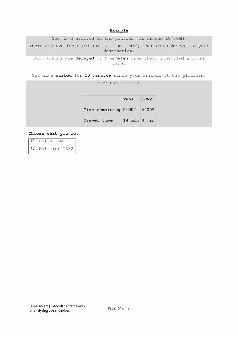
Deliverable 2.3: Modelling framework for analysing users’ choices Page 109 of 121
Example
You have arrived at the platform at around 10:30AM.
There are two identical trains (TRN1,TRN2) that can take you to your destination.
Both trains are delayed by 5 minutes from their scheduled arrival time.
You have waited for 10 minutes since your arrival at the platform.
TRN1 has arrived.
TRN1 TRN2
Time remaining 0’00” 4’00”
Travel time 14 min 8 min
Choose what you do:
Board TRN1
Wait for TRN2
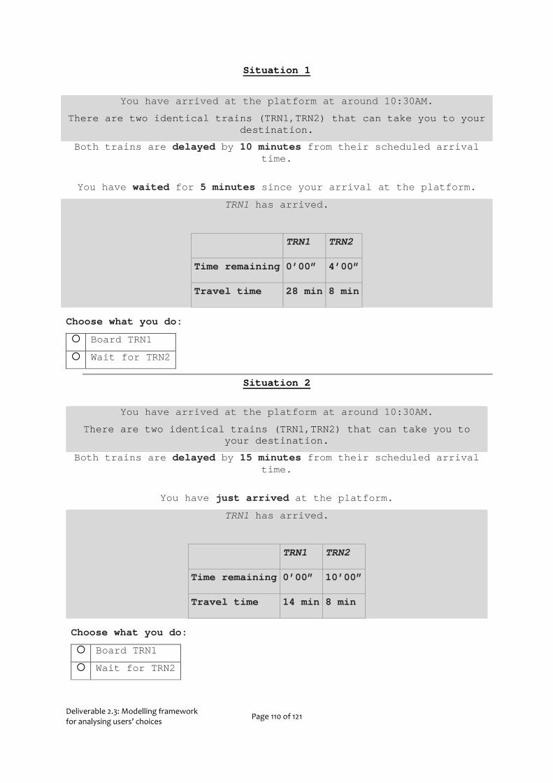
Deliverable 2.3: Modelling framework for analysing users’ choices Page 110 of 121
Situation 1
You have arrived at the platform at around 10:30AM.
There are two identical trains (TRN1,TRN2) that can take you to your destination.
Both trains are delayed by 10 minutes from their scheduled arrival time.
You have waited for 5 minutes since your arrival at the platform.
TRN1 has arrived.
TRN1 TRN2
Time remaining 0’00” 4’00”
Travel time 28 min 8 min
Choose what you do:
Board TRN1
Wait for TRN2
Situation 2
You have arrived at the platform at around 10:30AM.
There are two identical trains (TRN1,TRN2) that can take you to your destination.
Both trains are delayed by 15 minutes from their scheduled arrival time.
You have just arrived at the platform.
TRN1 has arrived.
TRN1 TRN2
Time remaining 0’00” 10’00”
Travel time 14 min 8 min
Choose what you do:
Board TRN1
Wait for TRN2
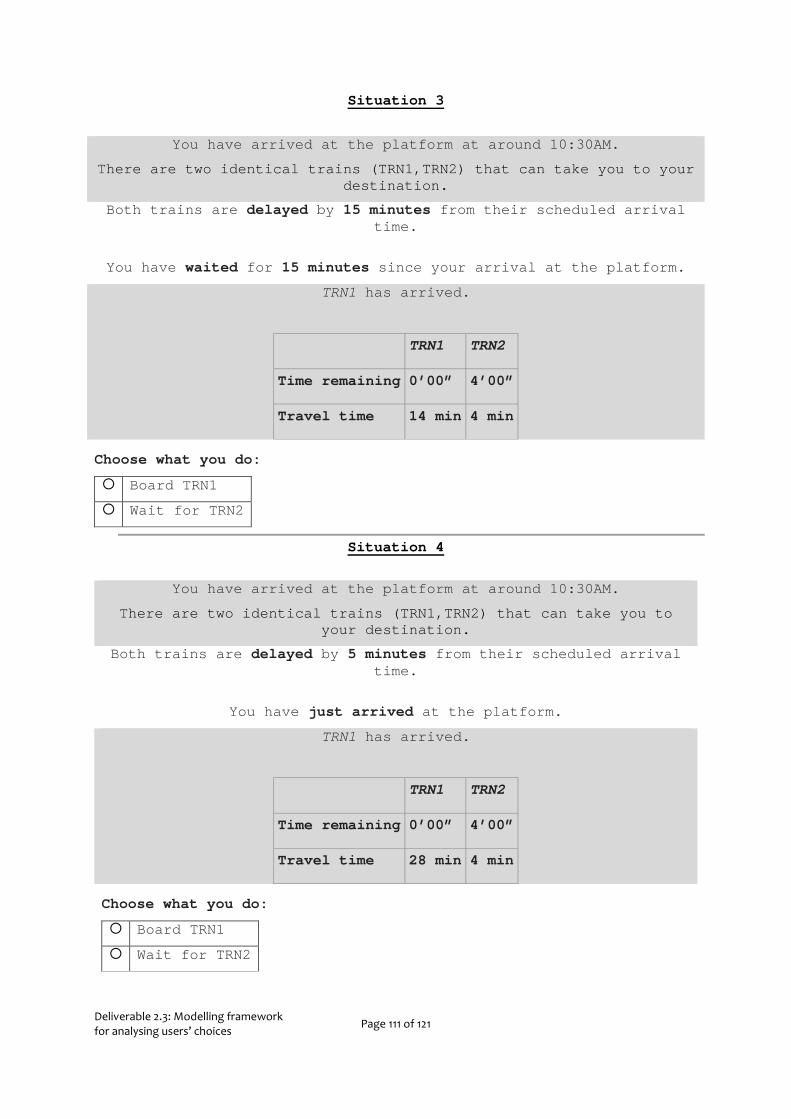
Deliverable 2.3: Modelling framework for analysing users’ choices Page 111 of 121
Situation 3
You have arrived at the platform at around 10:30AM.
There are two identical trains (TRN1,TRN2) that can take you to your destination.
Both trains are delayed by 15 minutes from their scheduled arrival time.
You have waited for 15 minutes since your arrival at the platform.
TRN1 has arrived.
TRN1 TRN2
Time remaining 0’00” 4’00”
Travel time 14 min 4 min
Choose what you do:
Board TRN1
Wait for TRN2
Situation 4
You have arrived at the platform at around 10:30AM.
There are two identical trains (TRN1,TRN2) that can take you to your destination.
Both trains are delayed by 5 minutes from their scheduled arrival time.
You have just arrived at the platform.
TRN1 has arrived.
TRN1 TRN2
Time remaining 0’00” 4’00”
Travel time 28 min 4 min
Choose what you do:
Board TRN1
Wait for TRN2
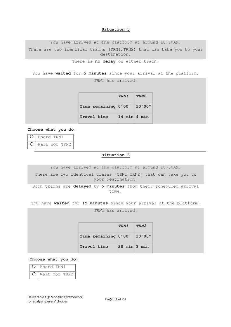
Deliverable 2.3: Modelling framework for analysing users’ choices Page 112 of 121
Situation 5
You have arrived at the platform at around 10:30AM.
There are two identical trains (TRN1,TRN2) that can take you to your destination.
There is no delay on either train.
You have waited for 5 minutes since your arrival at the platform.
TRN1 has arrived.
TRN1 TRN2
Time remaining 0’00” 10’00”
Travel time 14 min 4 min
Choose what you do:
Board TRN1
Wait for TRN2
Situation 6
You have arrived at the platform at around 10:30AM.
There are two identical trains (TRN1,TRN2) that can take you to your destination.
Both trains are delayed by 5 minutes from their scheduled arrival time.
You have waited for 15 minutes since your arrival at the platform.
TRN1 has arrived.
TRN1 TRN2
Time remaining 0’00” 10’00”
Travel time 28 min 8 min
Choose what you do:
Board TRN1
Wait for TRN2

Deliverable 2.3: Modelling framework for analysing users’ choices Page 113 of 121
Situation 7
You have arrived at the platform at around 10:30AM.
There are two identical trains (TRN1,TRN2) that can take you to your destination.
There is no delay on either train.
You have waited for 10 minutes since your arrival at the platform.
TRN1 has arrived.
TRN1 TRN2
Time remaining 0’00” 4’00”
Travel time 14 min 8 min
Choose what you do:
Board TRN1
Wait for TRN2
Situation 8
You have arrived at the platform at around 10:30AM.
There are two identical trains (TRN1,TRN2) that can take you to your destination.
Both trains are delayed by 10 minutes from their scheduled arrival time.
You have waited for 10 minutes since your arrival at the platform.
TRN1 has arrived.
TRN1 TRN2
Time remaining 0’00” 10’00”
Travel time 28 min 4 min
Choose what you do:
Board TRN1
Wait for TRN2
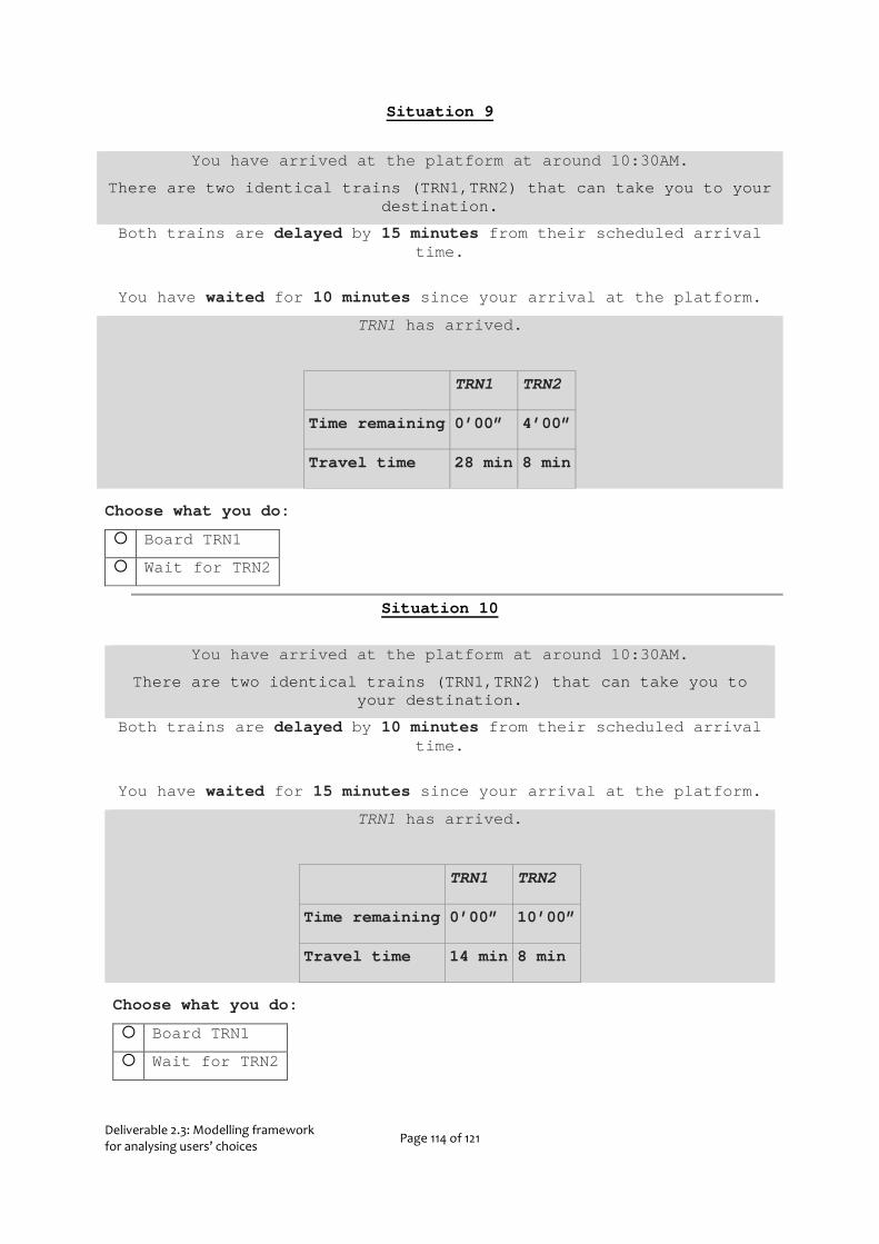
Deliverable 2.3: Modelling framework for analysing users’ choices Page 114 of 121
Situation 9
You have arrived at the platform at around 10:30AM.
There are two identical trains (TRN1,TRN2) that can take you to your destination.
Both trains are delayed by 15 minutes from their scheduled arrival time.
You have waited for 10 minutes since your arrival at the platform.
TRN1 has arrived.
TRN1 TRN2
Time remaining 0’00” 4’00”
Travel time 28 min 8 min
Choose what you do:
Board TRN1
Wait for TRN2
Situation 10
You have arrived at the platform at around 10:30AM.
There are two identical trains (TRN1,TRN2) that can take you to your destination.
Both trains are delayed by 10 minutes from their scheduled arrival time.
You have waited for 15 minutes since your arrival at the platform.
TRN1 has arrived.
TRN1 TRN2
Time remaining 0’00” 10’00”
Travel time 14 min 8 min
Choose what you do:
Board TRN1
Wait for TRN2

Deliverable 2.3: Modelling framework for analysing users’ choices Page 115 of 121
Situation 11
You have arrived at the platform at around 10:30AM.
There are two identical trains (TRN1,TRN2) that can take you to your destination.
Both trains are delayed by 10 minutes from their scheduled arrival time.
You have just arrived at the platform.
TRN1 has arrived.
TRN1 TRN2
Time remaining 0’00” 4’00”
Travel time 14 min 4 min
Choose what you do:
Board TRN1
Wait for TRN2
Situation 12
You have arrived at the platform at around 10:30AM.
There are two identical trains (TRN1,TRN2) that can take you to your destination.
There is no delay on either train.
You have waited for 15 minutes since your arrival at the platform.
TRN1 has arrived.
TRN1 TRN2
Time remaining 0’00” 4’00”
Travel time 28 min 4 min
Choose what you do:
Board TRN1
Wait for TRN2

Deliverable 2.3: Modelling framework for analysing users’ choices Page 116 of 121
Situation 13
You have arrived at the platform at around 10:30AM.
There are two identical trains (TRN1,TRN2) that can take you to your destination.
Both trains are delayed by 5 minutes from their scheduled arrival time.
You have waited for 10 minutes since your arrival at the platform.
TRN1 has arrived.
TRN1 TRN2
Time remaining 0’00” 10’00”
Travel time 14 min 4 min
Choose what you do:
Board TRN1
Wait for TRN2
Situation 14
You have arrived at the platform at around 10:30AM.
There are two identical trains (TRN1,TRN2) that can take you to your destination.
There is no delay on either train.
You have just arrived at the platform.
TRN1 has arrived.
TRN1 TRN2
Time remaining 0’00” 10’00”
Travel time 28 min 8 min
Choose what you do:
Board TRN1
Wait for TRN2

Deliverable 2.3: Modelling framework for analysing users’ choices Page 117 of 121
Situation 15
You have arrived at the platform at around 10:30AM.
There are two identical trains (TRN1,TRN2) that can take you to your destination.
Both trains are delayed by 5 minutes from their scheduled arrival time.
You have waited for 5 minutes since your arrival at the platform.
TRN1 has arrived.
TRN1 TRN2
Time remaining 0’00” 4’00”
Travel time 14 min 8 min
Choose what you do:
Board TRN1
Wait for TRN2
Situation 16
You have arrived at the platform at around 10:30AM.
There are two identical trains (TRN1,TRN2) that can take you to your destination.
Both trains are delayed by 15 minutes from their scheduled arrival time.
You have waited for 5 minutes since your arrival at the platform.
TRN1 has arrived.
TRN1 TRN2
Time remaining 0’00” 10’00”
Travel time 28 min 4 min
Choose what you do:
Board TRN1
Wait for TRN2
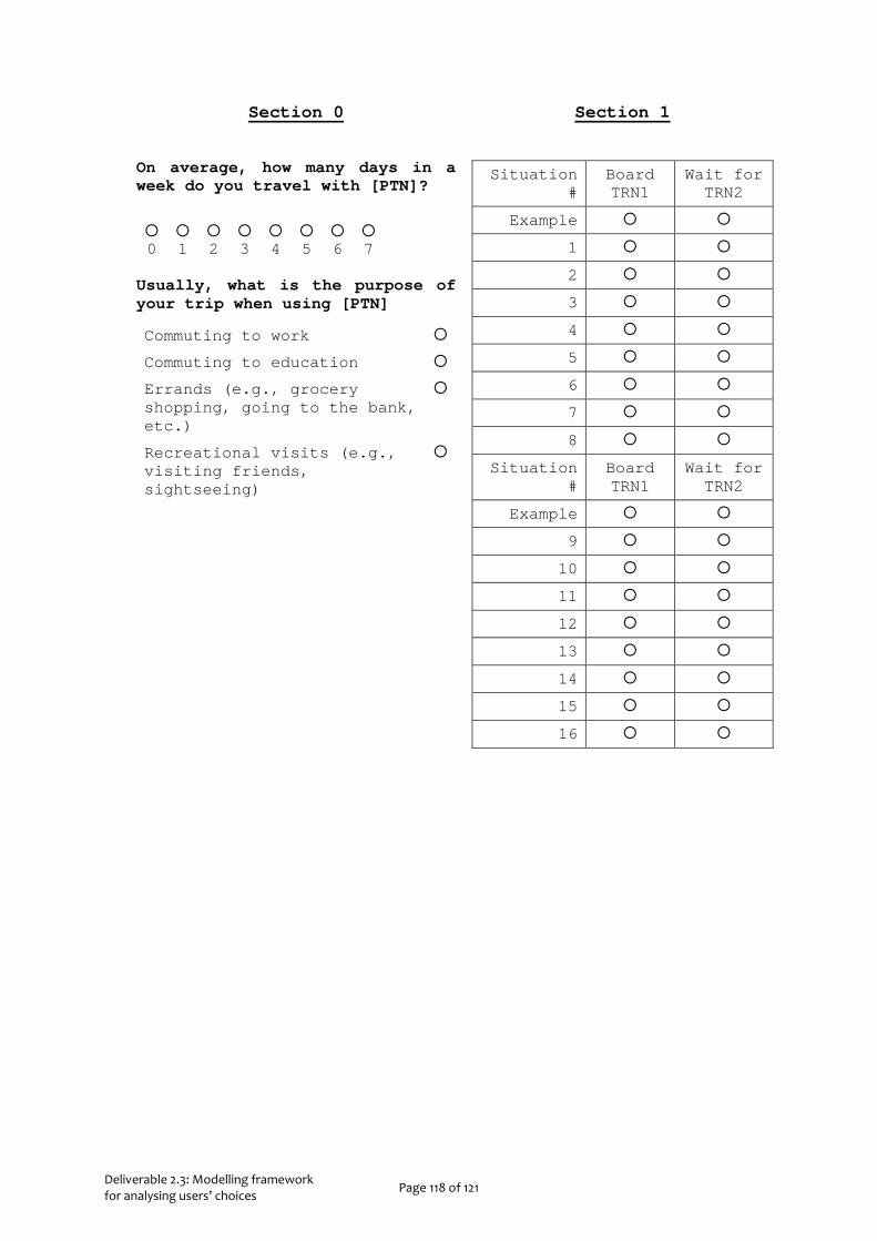
Deliverable 2.3: Modelling framework for analysing users’ choices Page 118 of 121
Section 0
On average, how many days in a week do you travel with [PTN]?
0 1 2 3 4 5 6 7
Usually, what is the purpose of your trip when using [PTN]
Commuting to work
Commuting to education
Errands (e.g., grocery shopping, going to the bank, etc.)
Recreational visits (e.g., visiting friends, sightseeing)
Section 1
Situation #
Board TRN1
Wait for TRN2
Example
1
2
3
4
5
6
7
8
Situation #
Board TRN1
Wait for TRN2
Example
9
10
11
12
13
14
15
16
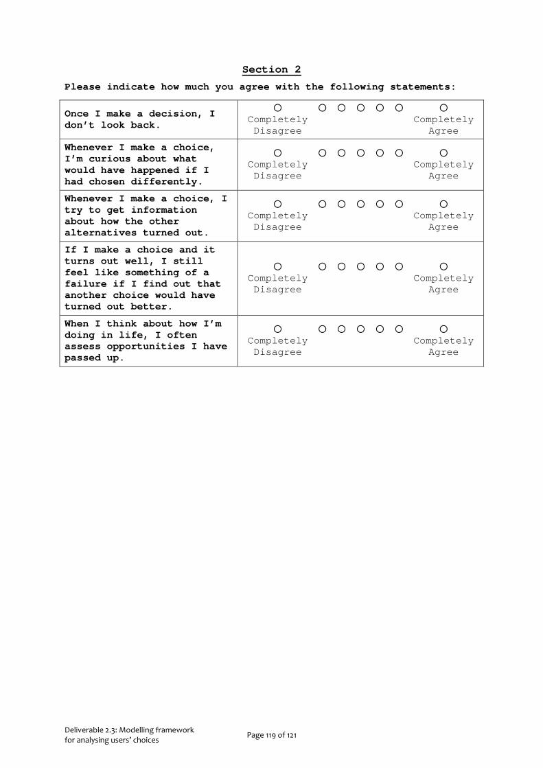
Deliverable 2.3: Modelling framework for analysing users’ choices Page 119 of 121
Section 2
Please indicate how much you agree with the following statements:
Once I make a decision, I don’t look back.
Completely Disagree Completely
Agree
Whenever I make a choice, I’m curious about what would have happened if I had chosen differently.
Completely Disagree Completely
Agree
Whenever I make a choice, I try to get information about how the other alternatives turned out.
Completely Disagree Completely
Agree
If I make a choice and it turns out well, I still feel like something of a failure if I find out that another choice would have turned out better.
Completely Disagree Completely
Agree
When I think about how I’m doing in life, I often assess opportunities I have passed up.
Completely Disagree Completely
Agree
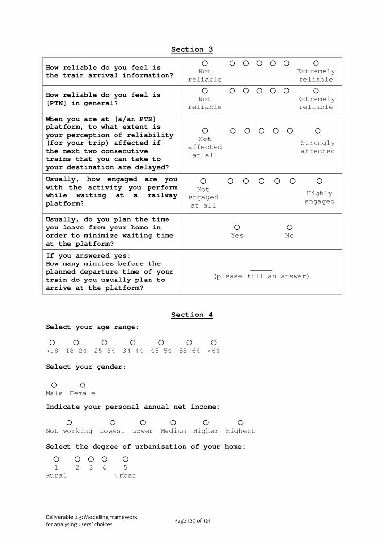
Deliverable 2.3: Modelling framework for analysing users’ choices Page 120 of 121
Section 3
How reliable do you feel is the train arrival information?
Not
reliable Extremely reliable
How reliable do you feel is [PTN] in general?
Not
reliable Extremely reliable
When you are at [a/an PTN] platform, to what extent is your perception of reliability (for your trip) affected if the next two consecutive trains that you can take to your destination are delayed?
Not
affected at all
Strongly affected
Usually, how engaged are you with the activity you perform while waiting at a railway platform?
Not
engaged at all
Highly engaged
Usually, do you plan the time you leave from your home in order to minimize waiting time at the platform?
Yes No
If you answered yes: How many minutes before the planned departure time of your train do you usually plan to arrive at the platform?
_____ (please fill an answer)
Section 4
Select your age range: <18 18-24 25-34 34-44 45-54 55-64 >64 Select your gender:
Male Female
Indicate your personal annual net income:
Not working Lowest Lower Medium Higher Highest Select the degree of urbanisation of your home:
1
Rural 2 3 4 5
Urban

Deliverable 2.3: Modelling framework for analysing users’ choices Page 121 of 121