Semi-automated scenario analysisof optimisation models

Jani Strandberg

School of Science

Thesis submitted for examination for the degree of Master ofScience in Technology.Helsinki 1.8.2019

Supervisor

Prof. Antti Punkka

Advisor

D.Sc. Anssi Käki

The document can be stored and made available to the public on the open internetpages of Aalto University. All other rights are reserved.

Aalto University, P.O. BOX 11000, 00076 AALTOwww.aalto.fi

Abstract of the master’s thesis

Author Jani StrandbergTitle Semi-automated scenario analysis of optimisation modelsDegree programme Mathematics and Operations ResearchMajor Systems and Operations Research Code of major SCI3055Supervisor Prof. Antti PunkkaAdvisor D.Sc. Anssi KäkiDate 1.8.2019 Number of pages 71+7 Language EnglishAbstractMathematical optimisation models have been succesfully used for solving problemsacross multiple industries. Often, the purpose of these models is to provide decisionsupport by guiding the development of effective plans and decisions. In the processof providing decision support, obtaining the numerical solution of an optimisationmodel is usually not limiting, and increasingly large and complex models are solvableas a result of increased computation resources and improved solution algorithms.However, analysing and understanding the model results can be difficult for largeand complex problems. Analysing model results often involves processing one orseveral model scenarios with varying parameters, so that related conclusions becomeavailable to the user. This part of the mathematical programming process is usuallydone by the analyst on a case-by-case basis, but this could be aided through com-puter assisted tools known as Intelligent Mathematical Programming Systems (IMPS).

In this Thesis, we develop a method for analysing and comparing the results ofoptimisation scenarios. This method forms a basis for a new form of IMPS thatcan be used to analyse both individual model scenarios and differences betweentwo scenarios. The method is based on the idea of preserving the structure of themathematical model along with the optimisation results, by representing the resultsas a graph. While the use of the method is considered in the context of supply chainsand linear programming, the approach is fairly general and could be applied in othertypes of optimisation problems as well. The implementation of the IMPS is donewith open-source technologies and can be coupled with any modelling environmentand solver.

The usability of the developed method for scenario analysis is evaluated through acase study related to an existing supply chain optimisation model at a large pulp andpaper company. We identify some scenario related questions where the developedmethod has advantages over the traditional approaches where the model structure isnot explicitly preserved. The case study illustrates that the developed method hasmany potential use cases, especially in conjunction with other methods. Furthermore,multiple development needs and avenues for further study are identified.Keywords Optimisation, mathematical programming, decision support system,

model analysis system, scenario, supply chain, graph

Aalto-yliopisto, PL 11000, 00076 AALTOwww.aalto.fi

Diplomityön tiivistelmä

Tekijä Jani StrandbergTyön nimi Semi-automatisoitu optimointimallien skenaarioanalyysiKoulutusohjelma Matematiikan ja operaatiotutkimuksen maisteriohjelmaPääaine Systems and Operations Research Pääaineen koodi SCI3055Työn valvoja Prof. Antti PunkkaTyön ohjaaja TkT Anssi KäkiPäivämäärä 1.8.2019 Sivumäärä 71+7 Kieli EnglantiTiivistelmäMatemaattisia optimointimalleja on käytetty menestyksekkäästi ongelmanratkaisuunmonilla eri teollisuuden aloilla. Usein optimointimallien tarkoitus on tarjota päätök-senteon tukea ohjaamalla tehokkaiden suunnitelmien ja päätöksen tekemistä. Tässäpäätöksenteon tukiprosessissa optimointimallin numeerisen ratkaisun saavuttami-nen ei ole useimmiten rajoittava tekijä, ja yhä laajempia sekä monimutkaisempiamalleja voidaan ratkaista lisääntyneiden laskentaresurssien sekä kehittyneiden rat-kaisualgoritmien avulla. Sen sijaan mallin tulosten analysointi ja ymmärtäminenvoi olla vaikeaa laajojen ja monimutkaisten ongelmien tapauksessa. Mallin tulostenanalysointiin sisältyy usein yhden tai useamman mallin skenaarion prosessointi si-ten, että relevantit johtopäätökset tuloksista tulevat käyttäjän saataville. Tämä osamatemaattisesta mallinnusprosessista tehdään usein tapauskohtaisesti analyytikontoimesta, mutta tätä voidaan auttaa tietokoneavusteisilla työkaluilla.

Tässä diplomityössä kehitetään menetelmä optimointimallien skenaarioiden analy-sointiin ja vertailemiseen. Tämä menetelmä luo perustan uudenlaiselle aputyökalulle,jota voidaan käyttää sekä yksittäisten mallin skenaarioiden että kahden skenaarionvälisten erojen analysointiin. Menetelmä pohjautuu matemaattisen mallin raken-teen säilyttämiseen optimiratkaisun lisäksi, mikä tapahtuu tallentamalla tuloksetgraafimuodossa. Vaikka menetelmän käyttöä tarkastellaan lähinnä toimitusketju-jen ja lineaarisen ohjelmoinnin näkökulmasta, lähestymistapa on melko yleinen javoi soveltua myös muihin optimointiongelmiin. Kehitetyn aputyökalun pohjana onkäytetty avoimen lähdekoodin teknologioita, ja se voidaan yhdistää mihin tahansamallinnusympäristöön ja ratkaisijaan.

Kehitetyn menetelmän käytettävyyttä skenaarioanalyysiin arvioidaan erään toi-mitusketjun optimointimalliin liittyvän tapaustutkimuksen avulla suuressa pape-riteollisuuden yrityksessä. Työssä tunnistetaan skenaarioihin liittyviä kysymyksiä,joissa kehitetyllä menetelmällä on etuja verrattuna lähestymistapoihin, joissa mallinrakennetta ei eksplisiittisesti säilytetä. Tutkimus havainnollistaa menetelmän mah-dollisia käyttökohteita, erityisesti muihin menetelmiin yhdistettynä. Lisäksi työssätunnistetaan menetelmään liittyviä kehitystarpeita ja jatkokehityksen suuntia.Avainsanat Optimointi, matemaattinen ohjelmointi, päätöksenteon tukijärjestelmä,

mallianalyysijärjestelmä, skenaario, toimitusketju, graafi

4

PrefaceThis thesis was written for UPM Advanced Analytics. First, I want to thank myinstructor Anssi Käki for his invaluable guidance, support, and giving me the op-portunity to work at UPM. This thesis would have been impossible without hisencouragement and expertise.

I also want to thank the other members of the Advanced Analytics team, Jesse andJoona, who provided valuable feedback and ideas throughout the creation of thisThesis. I feel very privileged for having the opportunity of working with such atalented group of people.

I am also thankful for my supervisor Antti Punkka, for his valuable comments andconstructive feedback. His input had a very positive impact on the quality of thiswork. Thanks also to other faculty at the Aalto University who have provided mewith such valuable education.

Last but not least, I wish to express my deep gratitude for my family. I want tothank my parents Mika and Susanna, who have always supported me in everythingI have chosen to pursue. Thanks to my sister Jenny for showing me that it’s okayto chase your dreams. Finally, special thanks to my partner Aino, who has been asource of inspiration and joy throughout my university studies.

Helsinki, 1.8.2019

Jani Strandberg

5

ContentsAbstract 2

Abstract (in Finnish) 3

Preface 4

Contents 5

Symbols and abbreviations 7

1 Introduction 81.1 Background . . . . . . . . . . . . . . . . . . . . . . . . . . . . . . . . 81.2 Thesis objective and scope . . . . . . . . . . . . . . . . . . . . . . . . 91.3 Thesis structure . . . . . . . . . . . . . . . . . . . . . . . . . . . . . . 10

2 Background 112.1 Mathematical programming process . . . . . . . . . . . . . . . . . . . 112.2 Analysis of supply chains . . . . . . . . . . . . . . . . . . . . . . . . . 132.3 Linear Programming . . . . . . . . . . . . . . . . . . . . . . . . . . . 17

2.3.1 Dual variables and sensitivity analysis . . . . . . . . . . . . . 182.4 Model analysis systems . . . . . . . . . . . . . . . . . . . . . . . . . . 19

3 Scenario analysis for supply chain optimisation models 213.1 Characterisation of model changes . . . . . . . . . . . . . . . . . . . . 213.2 Frequent analysis questions . . . . . . . . . . . . . . . . . . . . . . . 223.3 Questions as driver for scenario analysis . . . . . . . . . . . . . . . . 26

4 Methodology for building Intelligent Mathematical ProgammingSystem 284.1 Approaches to building IMPS . . . . . . . . . . . . . . . . . . . . . . 284.2 IMPS description . . . . . . . . . . . . . . . . . . . . . . . . . . . . . 30

4.2.1 Linear program in graph form . . . . . . . . . . . . . . . . . . 304.2.2 Expanding the graph information . . . . . . . . . . . . . . . . 324.2.3 Schematic view and file structure . . . . . . . . . . . . . . . . 364.2.4 MPS Parser . . . . . . . . . . . . . . . . . . . . . . . . . . . . 38

4.3 Constructing individual graphs . . . . . . . . . . . . . . . . . . . . . 394.4 The comparison of graphs . . . . . . . . . . . . . . . . . . . . . . . . 394.5 Detecting substitutions . . . . . . . . . . . . . . . . . . . . . . . . . . 444.6 Automatic report writing . . . . . . . . . . . . . . . . . . . . . . . . . 454.7 Visual network analysis . . . . . . . . . . . . . . . . . . . . . . . . . . 464.8 Aggregation of graphs . . . . . . . . . . . . . . . . . . . . . . . . . . 51

5 Case study 535.1 Supply chain description . . . . . . . . . . . . . . . . . . . . . . . . . 535.2 Visual network analysis . . . . . . . . . . . . . . . . . . . . . . . . . . 55

6

5.3 Ad hoc queries . . . . . . . . . . . . . . . . . . . . . . . . . . . . . . 585.4 Automatic report writing . . . . . . . . . . . . . . . . . . . . . . . . . 61

6 Conclusions and further developments 666.1 Future research directions . . . . . . . . . . . . . . . . . . . . . . . . 67

A MPS parsing algorithm 72

B Graph Construction algorithm 73

C Graph comparison algorihm 75

D Substitution detection algorithm 78

7

Symbols and abbreviations

SymbolsA matrix AAij matrix entry in ith row and jth columnG = (V, E) Graph G with node set V and edge set EG = (U, V, E) Bipartite graph G with disjoint node sets U and V , and edge set E

OperatorsxT transpose of vector xA ∩ B interesection of sets A and BA ∪ B union of sets A and BA \ B difference of sets A and B

AbbreviationsIMPS Intelligent Mathematical Programming SystemLP Linear ProgrammingMILP Mixed Integer Linear ProgrammingAPS Advanced Planning SystemDMAS Deductive Model Analysis SystemIMAS Inductive Model Analysis SystemDSS Decision Support System

1 Introduction

1.1 Background

Since the development of mathematical programming, the ability to solve larger andmore complex optimisation problems has significantly improved as a result of bettersolution algorithms and abundant computing power. The numerical computation ofa solution is no longer the bottleneck in most mathematical programming processes.Rather, the tasks related to creating, analysing, understanding and communicatingthese models and their various instances have an increasing role in applications.

While the technical purpose of mathematical programming is to find the optimalvalue of a given objective function subject to given constraints, in practice thisis done to provide some form of decision support by guiding the development ofeffective plans and decisions. Thus, mathematical models are sometimes embeddedinto a larger Decision Support System (DSS). In addition to providing decisionrecommendations, these systems are used to validate whether or not the model is anaccurate enough representation of the real underlying system, as well as to establishcredibility of the model in the eyes of the often non-technical decision makers withrich reporting and visualisation of the results, for instance.

At the core of both providing sound decision recommendations and establishingmodel credibility is the process of developing fundamental insights into why themodel solution is what it is. This extends far beyond the question of what particularnumerical values the decision variables of the optimal solution are. Such insights areimportant in many applications of mathematical programming, where there seldomexists a single perfect model solution that fully encapsulates the underlying modeluncertainties and directly translates into actionable plans.

To enhance model understanding, it is often beneficial to consider several model runswith varying parameters and structures, reflecting the alternative assumptions, ob-jectives and uncertainties regarding the mathematical model. These model instancesreflecting various possible realities are often referred to as scenarios (Rönnqvistet al., 2015). The term scenario analysis refers to how these model scenarios areorganised and processed so that important conclusions are available to the modeluser (Greenberg and Chinneck, 1999). Depending on the case, the decision makermay be interested in one particular scenario, or they may be interested in knowingwhat are the key differences between two, or even multiple scenarios.

In terms of solving the mathematical model to optimality, there is usually a somewhatclear path to victory: Assuming that the model is not ill-structured, one only needsto have an appropriate solver that is capable of solving the problem, and ensureadequate computing resources. However, there is no standard procedure for distillingkey insights from the mathematical model, as these are arguably more difficult to

9

generalise or even define in exact terms which are often preferred by mathematicallyinclined analysts. This is not to say that no quantitative tools exist: For example,most commercial mathematical programming environments are able to performelementary sensitivity analysis, enabling the analyst to study how small, individualparameter changes affect the model solution. However, this type of analysis can onlyanswer a fraction of the questions that may be relevant to the decision maker.

The process of gathering insights from models and their scenarios is usually done ona case-by-case basis, since there exists no industry standard tool that would aid theanalyst in this regard. Furthermore, this process often falls to the analyst responsiblefor creating and programming the model, as the ability to gather insights oftenrequires understanding the model structure. Clearly, this part of the mathematicalprogramming process could benefit from automated assistance, where some computerprogram would provide the analyst with ready-made tools to analyse and comparemodel scenarios. Such systems equipped with computer-assisted model analysis arereferred to in the literature as Intelligent Mathematical Programming Systems (IMPS)(Greenberg and Chinneck, 1999). Although numerous systems have been developedfor general model analysis, few of these have focused on the aspect of scenario analysis,and computer-assisted tools for scenario analysis reported in literature are virtuallynonexistent.

1.2 Thesis objective and scope

This thesis develops a new form of IMPS for analysis purposes in practical applicationsat an industrial case company. The IMPS is based on ideas previously presented byGreenberg (1983), where optimisation models are modelled as graphs. In this thesis,we extend this notion to the two-scenario case, which allows the comparison of twoindividual model scenarios. The usefulness of the developed IMPS is validated in aparticipatory development process with optimisation experts at the case company,where several questions pertaining to the case company’s optimisation models werecollected and categorised.

Although the problem of gathering insights from models is a very general one,we mostly limit our considerations to optimisation models related to supply chainplanning. This is because such models are at the heart of the case company’s business,and focusing on a slightly more specific model category is a more approachableproblem than trying to build a system that would fit to any type of mathematicalmodel.

In terms of mathematical models, this thesis is limited to Linear Programming (LP)models, as they are the main workhorse at the case company, simpler to analysethan e.g. nonlinear or mixed-integer-linear programming (MILP) models, and theMPS file format, which is a core input of the implemented IMPS, supports only LPmodels and MILP models. The aforementioned considerations are not to say that

10

the approach suggested in this Thesis would not work for other types of models:Even though we have limited our attention to a more specific level, the same ideasare applicable to other model types as well.

1.3 Thesis structure

The remainder of this thesis is organised as follows. Chapter 2 introduces thebackground by providing a review of the existing literature regarding automatedmodel analysis and supply chain optimisation. We also review linear programmingto provide further context.

Chapter 3 describes some of the common questions related to supply chain optimi-sation analysis, collected from discussions with multiple optimisation and subjectexperts. We categorise the questions into different types, and assess for each typethe amount of scenarios involved and the difficulty of answering these questions.We also explain and characterise different types of model changes related to thesequestions.

Chapter 4 describes different general approaches for building an IMPS and explainsthe foundation behind the approach taken in this Thesis. We present an overviewof the developed IMPS, describing its main inputs, outputs and functionalities.In addition, we describe the practical requirements, design choices and the mainalgorithms used in the IMPS in detail.

Chapter 5 describes the use of the IMPS by performing a case study related to anexisting paper supply chain optimisation model at the case company. We illustratethrough multiple examples how the IMPS can be used to review and analyse differentscenarios and model results.

Finally, Chapter 6 summarises the thesis, provides further development needs andpresents the most important conclusions drawn from the entire body of work.

11

2 Background

2.1 Mathematical programming process

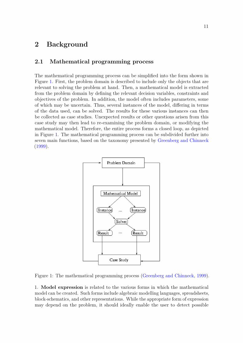
The mathematical programming process can be simplified into the form shown inFigure 1. First, the problem domain is described to include only the objects that arerelevant to solving the problem at hand. Then, a mathematical model is extractedfrom the problem domain by defining the relevant decision variables, constraints andobjectives of the problem. In addition, the model often includes parameters, someof which may be uncertain. Thus, several instances of the model, differing in termsof the data used, can be solved. The results for these various instances can thenbe collected as case studies. Unexpected results or other questions arisen from thiscase study may then lead to re-examining the problem domain, or modifying themathematical model. Therefore, the entire process forms a closed loop, as depictedin Figure 1. The mathematical programming process can be subdivided further intoseven main functions, based on the taxonomy presented by Greenberg and Chinneck(1999).

Figure 1: The mathematical programming process (Greenberg and Chinneck, 1999).

1. Model expression is related to the various forms in which the mathematicalmodel can be created. Such forms include algebraic modelling languages, spreadsheets,block-schematics, and other representations. While the appropriate form of expressionmay depend on the problem, it should ideally enable the user to detect possible

12

errors and omissions. Two important functions related to model expression aredocumentation and verification. Documentation entails recording a descriptionof the model, such that people other than the original creator may understand it.Verification, in turn, is related to ensuring that the computer-resident model coincideswith our functional description.

2. Model viewing refers to the forms in which the model and its solutions canbe viewed to the user. These views may employ the same structure as the originalmodel expression, although other views based on graphical or natural languagerepresentations are possible as well. As is the case in model expression, there is oftenno "best" view, as this may depend on both the preferences of the modeler, and theproblem itself. A related function is reporting, which may include functionalitiessuch as interactive query, the generation of some internal files for further analysis, orcreating some other form of report for presentation.

3. Model simplification refers to various methods of finding simpler model expres-sions that still capture the essence of the original problem. Some form of simplificationfunctionality is often included in commercial-quality solvers, but their main purposeis usually to increase optimisation performance, rather than deliver new insights intothe problem.

4. Debugging is the process of finding and removing the possible mechanical errorsin the model. Such errors may lead to problems such as infeasibility, unboundednessor non-viability. Note, however, that the viability of the model as a representationof reality cannot usually be answered by debugging alone.

5. Data management refers to the structures and techniques applied to managethe various information that is generated and collected in the mathematical program-ming process. These structures may have varying complexity, ranging from simplespreadsheets to large databases.

6. Scenario analysis refers to various methods of processing and filtering theinformation generated from multiple model instances, representing various scenarios.An important application is cross-scenario analysis, where the purpose is to findand ideally also explain the main differences between scenarios. It is worth notingthat Greenberg and Chinneck (1999) uses the term scenario management to referto this function. However, this term is also used to describe how and why differenttypes of scenarios are created in the problem context. In the scope of this thesis, weconsider the scenarios as given by subject experts, and assume that these scenariosappropriately capture the significant uncertainties related to the problem. Therefore,our main focus is in the function of how different scenarios are analysed and compared,rather than how these scenarios were created. The field of scenario managementrelated to the generation of various scenarios is an interesting field of study in itself,see e.g. Seeve (2018).

7. General analysis refers to other general questions one might have about the

13

mathematical model, unanswered by the previous functions. These include, forexample, finding important relationships in the data, and finding the root causeof the price of a certain variable. General analysis tools provide the user withmeans to explore the model structure in further detail, thus helping the user answersome model-related questions. Related functions include validation and redundancyanalysis. The purpose of validation is to determine how well our model representsreality, given the context of decision support that the model is designed to offer.Redundancy analysis, as the name suggests, is related to finding possible redundanciesin the model.

Based on this taxonomy, functions 6 and 7 are the main focus of this Thesis. How-ever, it is important to note that these functions are not separate entities in themathematical programming process, but they are rather intertwined. For example,different model views can be beneficial in general analysis.

2.2 Analysis of supply chains

With the growth of Enterprise Resource Planning (ERP) applications in organisations,supply chain management has become a major area for model-driven decision supportsystems and mathematical programming (Power and Sharda, 2007). Supply chainsare complex entities involving multiple phases, each involving their own planningdecisions. Many of these planning problems can be translated into mathematicalmodels, provided that there is sufficient data available to model the supply chainadequately. As ERP systems have made this data more accessible to analysts, theuse of mathematical programming has seen increasing use in many supply chainactivities, including the planning of logistics, production and demand (Power andSharda, 2007).

Although supply chains have no single definition in the literature, they can be seenas systems of organisations, people and activities that are involved in moving aproduct from supplier to customer (Press, 2011). Typical activities in supply chainsinvolve the transformation of resources, such as energy and raw materials, intofinished products, transporting those products, and finally distributing them tocustomers. Between these end points, there may be multiple value adding activitiesthat in combination are necessary in order to deliver the final product (Janvier-James,2012).

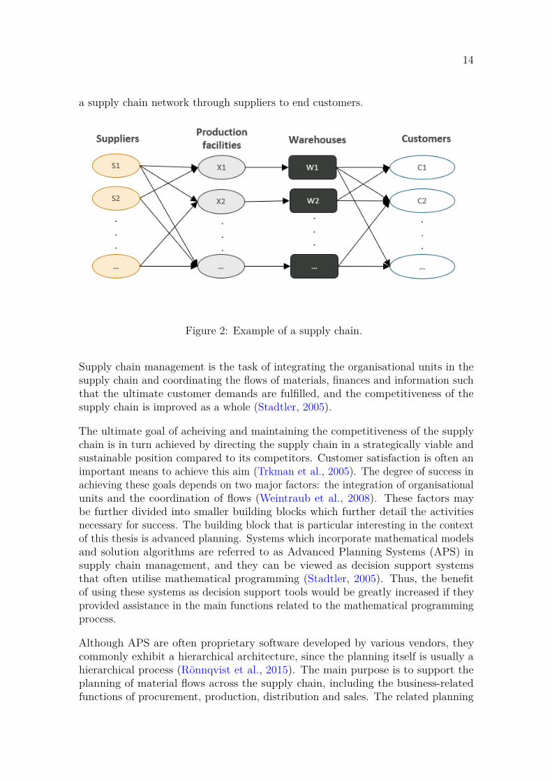
Common entities in the supply chain include suppliers, manufacturers, warehouses,transportation companies, distribution centers and retailers. A supply chain canbe represented as a network between these entities. The nodes of such a networkmay depict these different entities, such as suppliers and production facilities, andlinks between the nodes depict the material flow through the network, e.g. theprocurement of raw materials from suppliers to the production facilities. Figure 2shows one simple example of a supply chain ,which shows how materials flow through

14

a supply chain network through suppliers to end customers.

Figure 2: Example of a supply chain.

Supply chain management is the task of integrating the organisational units in thesupply chain and coordinating the flows of materials, finances and information suchthat the ultimate customer demands are fulfilled, and the competitiveness of thesupply chain is improved as a whole (Stadtler, 2005).

The ultimate goal of acheiving and maintaining the competitiveness of the supplychain is in turn achieved by directing the supply chain in a strategically viable andsustainable position compared to its competitors. Customer satisfaction is often animportant means to achieve this aim (Trkman et al., 2005). The degree of success inachieving these goals depends on two major factors: the integration of organisationalunits and the coordination of flows (Weintraub et al., 2008). These factors maybe further divided into smaller building blocks which further detail the activitiesnecessary for success. The building block that is particular interesting in the contextof this thesis is advanced planning. Systems which incorporate mathematical modelsand solution algorithms are referred to as Advanced Planning Systems (APS) insupply chain management, and they can be viewed as decision support systemsthat often utilise mathematical programming (Stadtler, 2005). Thus, the benefitof using these systems as decision support tools would be greatly increased if theyprovided assistance in the main functions related to the mathematical programmingprocess.

Although APS are often proprietary software developed by various vendors, theycommonly exhibit a hierarchical architecture, since the planning itself is usually ahierarchical process (Rönnqvist et al., 2015). The main purpose is to support theplanning of material flows across the supply chain, including the business-relatedfunctions of procurement, production, distribution and sales. The related planning

15

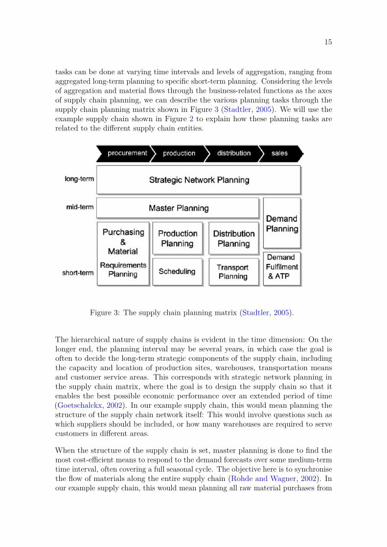
tasks can be done at varying time intervals and levels of aggregation, ranging fromaggregated long-term planning to specific short-term planning. Considering the levelsof aggregation and material flows through the business-related functions as the axesof supply chain planning, we can describe the various planning tasks through thesupply chain planning matrix shown in Figure 3 (Stadtler, 2005). We will use theexample supply chain shown in Figure 2 to explain how these planning tasks arerelated to the different supply chain entities.

Figure 3: The supply chain planning matrix (Stadtler, 2005).

The hierarchical nature of supply chains is evident in the time dimension: On thelonger end, the planning interval may be several years, in which case the goal isoften to decide the long-term strategic components of the supply chain, includingthe capacity and location of production sites, warehouses, transportation meansand customer service areas. This corresponds with strategic network planning inthe supply chain matrix, where the goal is to design the supply chain so that itenables the best possible economic performance over an extended period of time(Goetschalckx, 2002). In our example supply chain, this would mean planning thestructure of the supply chain network itself: This would involve questions such aswhich suppliers should be included, or how many warehouses are required to servecustomers in different areas.

When the structure of the supply chain is set, master planning is done to find themost cost-efficient means to respond to the demand forecasts over some medium-termtime interval, often covering a full seasonal cycle. The objective here is to synchronisethe flow of materials along the entire supply chain (Rohde and Wagner, 2002). Inour example supply chain, this would mean planning all raw material purchases from

16

suppliers, quantities of production at facilities, distribution to different warehouses,and finally sales to customers. The plans at this stage are done to provide anoverview of how the supply chain should be operated on an aggregate level, as themore detailed plans are done on separate stages.

After the production flows have been assigned to different sites, more detailedproduction planning and scheduling is often done within each production facility.The aim with these planning stages is to determine a more detailed productionschedule, which shows for example how different machines or flow lines should beoperated, and what should be done on different work shifts. (Stadtler, 2002a) In ourexample supply chain, this planning stage would solve how the different productionfacilities should be operated in detail, for example on a daily basis.

Based on the directives from master plans as well as shorter-term production planningand scheduling, procurement quantities can be planned with a purchasing and materialrequirements planning module. This module is necessary for planning non-bottleneckoperations, since usually only potential bottlenecks in raw material availability areplanned for in production planning and scheduling (Stadtler, 2005). In our examplesupply chain, this planning stage would solve in detail how and when different rawmaterials should be purchased from different suppliers.

The distribution planning module considers the flow of goods between sites as wellas in the distribution network of the supply chain. Although the master planningphase may include some seasonal stock level requirements at some points of thesupply chain, the transports of goods to customers directly or through warehousesand distribution centers are planned in this module in greater detail (Fleischmann,2002). Even more detailed is transport planning, where specific vehicle loading plansbased on production orders to be completed during the next day or shift are formed.This planning phase thus requires order-level knowledge, as well as informationon customer-specific needs, including legal restrictions and delivery time windows(Stadtler, 2005). In our example supply chain, these planning stages would showwhich links between suppliers, warehouses and customers should be used, and whatthe quantities of flows should be in detail between these entities.

The aforementioned planning tasks clearly indicate the importance of different timeintervals in supply chain planning, but other dimensions in the planning processoften have hierarchical dimensions as well. For example, in the product dimension,some stock keeping units are different versions of the same product, and similarproducts may belong in some common product families or groups. On the customerside, some customers operate in different countries, which may in turn be part ofdifferent geographical regions (Miller, 2002).

In many cases, the decision maker may not be particularly interested in what ishappening to a specific product or customer, but would rather understand thedecisions in terms of product families or customer regions (Miller, 2004). As such,an ideal decision support system should enable the user to perform model analysis

17

on different hiearchical levels. Naturally, the level of detail used in the underlyingmathematical model sets the lowest possible level of analysis, but the ability toconsider the model in terms of its upper hierarchical dimensions, such as productfamilies or customer regions, could provide much more informative decision supportin some situations.

2.3 Linear Programming

Linear programming (LP), also called linear optimisation, is a special case of themore general concept of mathematical programming. It is a method for achievingthe best numerical outcome in a mathematical model where all relationships arelinear. In other words, linear programming refers to techniques for the maximisationor minimisation of a linear objective function, subject to linear equality or inequalityconstraints. All linear programs can be described with the following form (Bertsimasand Tsitsiklis, 1997):

min cT xs.t. Ax ≤ b (1)

x ≥ 0

where x is the vector of decision variables, c is the cost coefficient vector, b is theright-hand side vector and A is the matrix of coefficients related to the problemconstraints. In general, we assume that all parameter values A,b, c are known whenthe optimisation is run, and the objective is to find the vector x that minimisesthe objective function cT x, while satisfying the constraints. Note that by "knowing"in this context we do not mean that there must be absolute certainty what the"correct" values for each parameter are. Rather, we mean that for a single model run,each parameter has a certain value that does not change. The actual uncertaintyin the parameter values can be addressed by running multiple scenarios, where theuncertain parameters are varied.

The inequalities Ax ≤ b and x ≥ 0 are the constraints which specify the feasibleregion, the set of all possible solutions of the optimisation problem that satisfy all ofthe constraints. In linear programming, this feasible region is a convex polyhedron,a set defined as the intersection of finitely many half spaces, each defined by a linearinequality constraint. A linear programming algorithm, such as the simplex method,finds the point in the feasible region where the objective function has the smallestvalue, if such a point exists (Bertsimas and Tsitsiklis, 1997).

Note that any maximisation problem can easily be changed to the correspondingminimisation problem, because minimising some function f(x) is equivalent to

18

maximising the function −f(x). That is, one needs to only multiply the objectivefunction by -1 to change from one to the other.

Linear programming is applicable in a vast field of problems, where quantities can takeany real values, and are only restricted by linear constraints. Linear programming hasmany applications in various industries; In supply chain planning, it has been usedfor example in solving planning tasks related to master planning and distributionplanning. Many powerful solution algorithms for solving linear programming havebeen developed, and these can be used to solve models involving thousands ofconstraints and variables in a short period of time (Stadtler, 2002b).

2.3.1 Dual variables and sensitivity analysis

Given any linear programming problem, we can associate with it another problemcalled the dual linear programming problem. Each variable in the dual problemis associated with a constraint of the original problem, and these can be seen aspenalties for violating the constraints (Bertsimas and Tsitsiklis, 1997). The dual oflinear program (1) can be formulated as

max pT bs.t. pT A ≤ cT (2)

p ≤ 0

Where p is the vector of dual variables. In linear programming, the optimal objectivefunction value to the primal problem is equal to optimal objective function value ofthe dual problem, if an optimal solution exists (Bertsimas and Tsitsiklis, 1997).

These optimal dual variable values are important in traditional sensitivity analysisof linear programming models, as they can be used to determine how sensitive theoptimal solution is to small changes in model parameters. Specifically, these dualvariable values can be used to determine a range for each individual objective functionand right-hand side vector coefficient, over which the individual coefficient can varywithout having to solve the optimisation again. This information is readily availablein most commercial solvers, and can be used to analyse the effect that small individualparameter changes would have on the optimal solution (Bradley et al., 1977).

While the appeal of this traditional sensitivity analysis is apparent as it provides exactquantitative information on the mathematical model, its applicability in practicalmodel analysis setting is limited. This is because traditional sensitivity analysiscan only be used to analyse small changes in individual objective function or right-hand side vector coefficients, or multiple smaller changes under some very limitingconditions (Bradley et al., 1977). Especially in large linear programming models, a

19

change in a single model parameter is rarely a topic of interest. Furthermore, suchsensitivity analysis does not allow for all types of constraint changes, namely thoserelated to constraint coefficients. Also, many practically relevant changes to themodel alter the model structure: For example, adding a new customer or warehousein the supply chain usually entails the addition of multiple decision variables andconstraints. In such cases, traditional sensitivity analysis offers little assistance.

2.4 Model analysis systems

A model created by mathematical programming can be embedded in a model-drivenDecision Support System (DSS). By definition, such systems support managersin their decision-making efforts by applying one or several quantitative models tothe problem at hand. In addition, model-driven DSS allow users to manipulatemodel parameters, thus enabling sensitivity analysis of the model outputs as wellas more ad hoc "what if" - analyses. Furthermore, DSS can be differentiated frommore specific decision analytic studies by two characteristics: Firstly, they make thequantitative model easily accessible to non-technical specialists trough user interfaces,and secondly, they are intended for repeated use in similar decision situations (Powerand Sharda, 2007).

One of the purposes of a DSS is to help the decision maker develop a better un-derstanding of the complex system represented by the mathematical model. Thereare multiple potential sources of increasing this understanding in the mathematicalprogramming process. Perhaps the most direct source is the actual model formulationphase: During model formulation, the decision makers may modify their mental modelbased on the discoveries of new relationships between key factors, counterexamplesof assumed relationships or fallacies in deductive logic (Steiger, 1998).

Another source is the deductive analysis of a single model instance, consideringall of the knowledge inherent in the model structure, as well as the solution. Forinstance, the sensitivity analysis of an LP model solution can help the decision makerunderstand which parameters are more important than others, and what kind ofan effect some small parameter change would have on the solution. An additionalsource of understanding is the inductive analysis of multiple solved model instances.An example of this would be to solve several model instances while varying someparameters over appropriate ranges, after which these instances can be analysed toassess the relative importance of the individual parameters and their interactions(Steiger, 1998).

The previously mentioned sources of understanding motivate to examine the potentialof model analysis systems. Model analysis systems are systems built to enhance thedecision maker’s understanding of the business environment represented by the model,by helping them interpret and manipulate the output of model solvers and analyseexisting knowledge, or extract new knowledge from the business environment the

20

system represents. Model analysis systems can be roughly divided into two classesbased on their primary type of processing logic: These classes are deductive analysissystems (DMASs) and inductive analysis systems (IMASs). These systems aredistuingished from each other by both their required input as well as the processinglogic employed. Whereas DMASs operate on singular model instances and applyexisting model-specific knowledge, IMASs operate on many solved instances andapply inductive analysis to generate new knowledge (Steiger, 1998).

DMAS are systems that apply paradigm- or model-specific knowledge to a specificmodel instance, addressing questions such as "Why is this the solution?", or "why isthis instance infeasible?". Perhaps the most prominent example of a DMAS to thisdate is called ANALYZE, described in detail by Greenberg (1983). It is a computer-assisted analysis system for linear programming models, providing interactive queryof the LP matrix and solution values, as well as other functionalities, including modelsimplification and network path analysis.

IMASs are systems that operate on a set of solved model instances, where someparameter values are varied and the goal is to find the "key parameters" which havethe greatest impact on the model solution. One simple form of IMAS is applyingregression analysis to multiple model runs, in order to determine the impact ofchanges in model input parameters to the output. In other words, the goal is to builda metamodel which would help the decision maker build insights into the businessenvironment being modeled (Steiger and Sharda, 1996).

One related approach for generating insights from mathematical models is the use ofsimplified auxiliary models in conjunction with the original model (Geoffrion, 1976).Geoffrion suggests that these auxiliary models should be both intuitively plausible,and solvable in closed form or by simple arithmetic. Ideally, the solution behaviorof the auxiliary model is far more transparent than that of the full model, yet itshould yield fairly good predictions of the general solution characteristics of the fullmodel.

21

3 Scenario analysis for supply chain optimisationmodels

When supply chain optimisation is used to support decision making, the decisionmakers typically want to understand the model results and further see how theresults change in different scenarios. In this chapter, we outline the principles ofscenario analysis for supply chain optimisation. First, some characterisations fortypical changes between scenarios are given. Then, a framework for some commonanalysis questions is presented along with considerations for how these questions canbe answered.

3.1 Characterisation of model changes

When comparing various scenarios of an optimisation model, the possible changescan be divided into two categories: parameter-based and structure-based changes.Parameter-based changes are those where the value(s) of some input parameter(s)of the model is(are) changed. In linear programming, such parametric changes arerelated to either i) the cost coefficients of the problem, represented by the cost vectorc, ii) the constraint limits, represented by the right-hand side vector b, iii) thecoefficients of the constraint matrix A, or some combination of the above. However,the structure of the model remains unchanged. Structure-based changes are thosewhere the model structure itself is modified in some way. In linear programming,these are related to the addition or deletion of constraints, decision variables, or bothat the same time. Note that adding new constraints adds new rows to the constraintmatrix and the right-hand side vector, whereas adding new decision variables addsnew rows to the decision variable vector, new columns to the constraint matrix andnew entries to the cost vector. This obviously involves adding the correspondingparameters to the model as well.

It is important to note that the decision maker does not typically understandhow their business questions translate into the mathematical model: The decisionmaker considers the problem through the physical entities of the supply chain. Itis the responsibility of the analyst to ensure that the appropriate changes in modelparameters or structure are made to reflect the changes that the business caserepresents. Depending on the business question and model itself, this translationprocess may range in difficulty from very simple to prohibitively complex.

Ideally, the model is structured in a way that allows easy manipulation of componentsthat are likely to be of interest to the decision maker. For example, a change in thecurrency exchange rate may affect multiple separate entities in the supply chain, fromraw material procurement to customer sales. Instead of having to change each relatedcost coefficient separately, the exchange rate could be included as a parameter, whichautomatically changes all related model parameters accordingly. Another example

22

would be to allow removing a raw material supplier from the supply chain, such thatall directly related decision variables and constraints are removed.

3.2 Frequent analysis questions

We next describe some of the common business questions related to supply chainoptimisation. These questions were collected from discussions with multiple opti-misation and subject matter experts at the case company, including people fromdifferent subdivisions and backgrounds. These individuals work with different kindsof supply chains, ranging from wood sourcing to paper production. Our objectiveis to present the collected questions in the most general setting possible. However,it should be acknowledged that while these questions were identified as relevantfor multiple supply chains, the case company is still somewhat limited to a specificindustry. Thus, there is a possibility of bias towards the problems related to thespecific company and its industry. We believe that these questions may be found inother types of supply chains as well, but their applicability to other settings is notevaluated here.

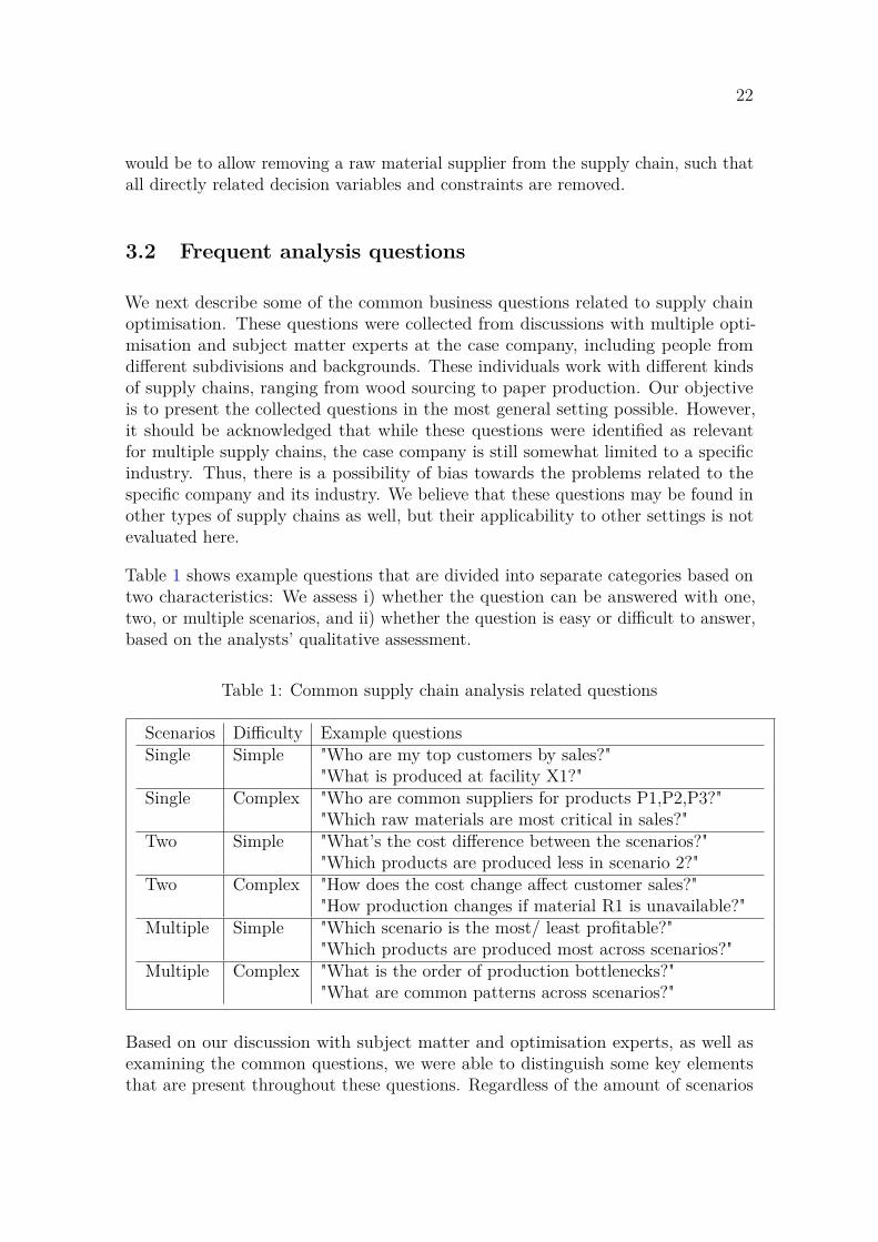
Table 1 shows example questions that are divided into separate categories based ontwo characteristics: We assess i) whether the question can be answered with one,two, or multiple scenarios, and ii) whether the question is easy or difficult to answer,based on the analysts’ qualitative assessment.

Table 1: Common supply chain analysis related questions

Scenarios Difficulty Example questionsSingle Simple "Who are my top customers by sales?"

"What is produced at facility X1?"Single Complex "Who are common suppliers for products P1,P2,P3?"

"Which raw materials are most critical in sales?"Two Simple "What’s the cost difference between the scenarios?"

"Which products are produced less in scenario 2?"Two Complex "How does the cost change affect customer sales?"

"How production changes if material R1 is unavailable?"Multiple Simple "Which scenario is the most/ least profitable?"

"Which products are produced most across scenarios?"Multiple Complex "What is the order of production bottlenecks?"

"What are common patterns across scenarios?"

Based on our discussion with subject matter and optimisation experts, as well asexamining the common questions, we were able to distinguish some key elementsthat are present throughout these questions. Regardless of the amount of scenarios

23

and difficulty of the question, they are all linked to one or both of the followingmodel-related factors:

• The optimal values or cost impacts of individual decisions and constraints

• The relationships between individual decisions and constraints

The first factor is quite clear when we consider that the primary objective in mostsupply-chain related optimisation models is to minimise costs or maximise profits.Here, the cost impact refers to the total effect a decision has on the objective function,taking into account both the value and the unit cost related to the decision. Theseallow us to assess the relative importance of individual decisions in terms of costsassociated with them. However, for constraints and potentially some decisions, theremay not be explicit costs involved. Furthermore, the optimal values of decisions areoften important in their own right, as they provide the actual decision recommenda-tions that interest the decision maker. Thus, both the values and cost impacts ofthe individual model components are often at the center of model analysis relatedquestions, whether we are studying an individual model solution, or comparing thedifferences between two model scenarios.

While the individual decisions and constraints can be interesting to study, therelationships between different model decisions and constraints are often equallyimportant. This is because most individual decisions in the model are made inconjunction with other decisions, depending on the constraints that bind themtogether. For example, a decision to produce some quantity of a product P1 infacility X1 requires some capacity, which means there is less capacity available toproduce other products, which are governed by separate decisions in the model.Many of the more complicated questions related to supply chains are of this type:The decision maker wants to understand not only what the individual decisionrecommendations are, but how they are related to each other.

In the following, we provide an overview of the different question categories, andexplain how these are related to the aforementioned model factors. While not anexhaustive list by any means, it provides motivation for why these factors can beconsidered as the focal points for many analysis purposes. How exactly our developedIMPS utilizes these factors is discussed in further detail in Sections 4.2 and 4.4.

Single scenario, Simple questionsThis category includes questions that can be answered directly from the modelsolution, without paying attention to the model structure or relationships betweendifferent entities. The ability to sort and filter the results based on desired attributesis sufficient. Examples include obtaining a list of top customers by sales, or a list ofproducts produced at facility X1. Considering our example supply chain in Figure2, the first example would require us to find the total cost impacts of all decisionsrelated to customer sales, then group and sort these cost impacts by customer. Forthe second example, we would have to find all production quantity values of decisions

24

related to facility X1. In both cases, only individual decision variable cost impactsand values were required to answer the question.

Single scenario, Complex questionsThis category contains questions related to a single model run, but the answer cannotbe found without considering the model structure and the relationships betweendecision variables. The main difference with the previous category is that individualcost impacts or values are no longer enough, as we now need the ability to relatedifferent decisions together. An example would be to find the common raw materialsuppliers for a list products such as P1, P2 and P3, or finding the raw materials thatare involved in the most customer sales. Considering our example supply chain inFigure 2, the first example would require us to find all possible paths from differentproduction facilities, where procuts P1, P2 and P3 are being produced at somenon-zero quantity, to all suppliers that supply the raw materials required for theseproducts. The second example would require us find paths from customer salesdecisions to the different raw material purchase decisions from suppliers, then groupand sort the total cost impacts of the customer sales by each individual raw material.Thus, not only the cost impacts and values of individual decisions are required, butalso the connections between them.

Two scenarios, Simple questionsSimple questions related to comparing two scenarios are queries such as "What is theoverall cost difference between these scenarios?" which can be answered by comparingthe optimal values of the objective function, or "Which products are produced less inscenario 2", which can be determined by comparing individual production quantitydecisions between the scenarios. Similar to the single-scenario case, answering thesequestions is straightforward, requiring only the ability to aggregate the results asdesired. In our example supply chain in Figure 2, the first example would requireto sum together the total cost impacts of all decisions made in the supply chain:These include raw material costs from suppliers, production costs, transportationcosts and sales profits. After this is done for both model scenarios, these sums can besubtracted to obtain a total cost difference between them. The second example wouldrequire finding the total values of production quantity decisions made at differentproduction facilities, grouping them by each individual product, and subtracting thesescenario-specific values. While perhaps slightly more complex than the individualscenario case, basically the cost impacts and values are again enough to answer thesetypes of questions.

Two scenarios, Complex questionsMany of the simple questions regarding scenario comparison can be considered ata more detailed level. For example, instead of simply calculating the overall costdifference, the decision maker may be interested in the primary sources that causethis difference: maybe the overall logistics costs have increased, but is it becauseindividual routes from facility X1 to customers C1, C2 and C3 have become moreexpensive, or due to small increase in costs everywhere? Note that the change between

25

the two comparable scenarios might not have anything to do with logistics costs butrather there could have been a change in customer demands, which eventually leadsto increased logistics volumes somewhere. The decision maker may be interestedin understanding how certain changes are related to each other: For instance, thismay involve questions such as "How does a change in currency rates affect customersales?", or "How does production change if capacity is increased at facility X1?". Inthe example supply chain shown in Figure 2, for the first example we would have toidentify all the affected customers, for whom there is a difference in sales volumes, inother words the optimal values of the various sales decisions, between the scenarios.Then, the analyst might try to link these changes to the different warehouses, inorder to observe how the production flows change throughout the supply chain, or todifferent production facilities to examine how the product mix has changed as a resultof the changes in costs. The second example could be explored by first checking whatthe differences in production quantity decisions related to facility X1 are between thescenarios, and then try to find connections from these to customer sales, as well asproduction quantity decisions at other production facilities. Answering these typesof questions exhaustively is very difficult without considering the entire supply chain,as there is generally no pattern that is guaranteed to occur.

However, there is one special occurrence between two scenarios that was foundprevalent in the case company: These are cases where the optimal value of somedecision in one scenario seems to have an approximately opposite effect to someother decision in the other scenario. For example, considering the example supplychain in Figure 2, it could be that the production quantity of product P1 increases atfacility X1, while at the same time the production quantity of product P1 decreasesat facility X2 by a similar amount. Another example could be that the transportationof product P1 to some customer C1 is switched from warehouse W1 to warehouseW2. These effects may happen due to various reasons, either through a direct or anindirect change in the factors that affect the optimal value of the related decisionvariables.

Furthermore, these substitution effects can be found at varying hierarchical levels:If substitution seems to happen at a higher level of hierarchy, then it is likely tobe a sum of smaller substitutions that happen on the lower levels. As such, thesesubstitutions are often sought first at higher hierarchy levels, since these can be usedto explain the changes at lower levels. In terms of decision support, these may providemore valuable information to the decision maker. As an example, the fact that theproduction of an entire product group is switched from site to another carries moreweight than stating that these products individually are produced at different sites.These substitution effects were found pervasive enough that we created a specialalgorithm for finding these between scenarios. This is explained in further detail inSection 4.5.

Multiple scenarios, simple questionsWhen comparing multiple scenarios, the simple questions a decision maker may

26

be interested in are such as "How do all these scenarios compare in terms of totalprofits?" or "What are the most commonly produced products?". In our examplesupply chain in Figure 2, for the first example we would simply sum over all totalcost impacts for each individual scenario, after which they could be sorted in anydesired order. For the second example, we would collect the production quantitiesfor each individual product across all production facilities and scenarios, after whichwe could sort the products by total volume. These questions follow a common themewith other simple cases: As long as there is no need to consider how the supply chainentities (or model elements) are related to each other, there is not much difficultyinvolved, even if there are multiple scenarios to consider.

Multiple scenarios, complex questionsThis is the most general category of questions, where multiple scenarios are comparedin ways that require deeper knowledge than the overall results, and some methodof linking together decisions between multiple scenarios. As an example, a decisionmaker could be interested in the order of production bottlenecks that arise whendemand is increased. Answering such a question requires solving the optimisationproblem multiple times with varying customer demands, as well as information thatlinks these demands to production entities. For our example supply chain in Figure 2,we would then observe how the different production facilities operate with increasingcustomer demand. Another possibly interesting query would be to find the potentialcommon patterns between all considered scenarios: Such patterns would suggest thatthe decisions involved are robust and should be made regardless of the considereduncertainties. For the example supply chain, we might find for example that facilityX1 always produces product P1, even if the costs or the structure of the supply chainchanges. However, this category of questions is very difficult to answer, even moreso than two-scenario comparisons, and they will not be explored in more detail inthis Thesis.

3.3 Questions as driver for scenario analysis

The mathematical programming process can be viewed as a series of transitions fromthe real world into the model world: Often, the process starts after some need forchange is recognised in the real world (Keisler and Noonan, 2012). In a supply chainoptimisation context, this starting step may be the decision maker recognising theneed for decision support in managing the supply chain more efficiently. The initialtransition from the real world to the model world then happens as the mathematicalmodel is formulated by the analyst.

After the mathematical model has been formulated, it can be used to perform variousanalyses that interest the decision maker. Scenario analysis can thus be seen asthe process of connecting the decision maker’s interests into the model world, andtranslating the corresponding model results or changes back into the real world.This view of scenario analysis emphasises that parsing the model results is only

27

part of the process, and that it is equally important for the analyst to understandwhat the decision maker’s key interests are. The main purpose of gathering businessquestions from decision makers is to facilitate the scenario analysis process byidentifying the relevant matters the analyst should focus on. Moreover, answeringthese business questions with the mathematical model is by itself a method ofproviding decision support, thus they are often related to the primary reason for themodel’s existence.

Furthermore, categorising the business questions can help the analyst obtain abroader understanding of the decision maker’s key interests, and what the practicalrequirements for answering these questions are. For example, in terms of scenarios,are most questions related to a single scenario, or is there a clear need for additionalmodel runs? Additionally, understanding the general difficulty of the questionsthat interest the decision maker can help the analyst in deciding the best practicalapproach for scenario analysis: For instance, if the majority of the business questionsare simple, there is probably no need for complicated analysis tools, and simplereporting capabilities will suffice.

28

4 Methodology for building Intelligent Mathemat-ical Progamming System

In this section, we describe different technical approaches to scenario analysis in use ofoptimisation models, and their benefits and drawbacks. Our focus is not on evaluatingcommercial optimisation packages (such as IBM ILOG Decision studio, AMPL orAIMMS), but instead focus on general approaches that are based on analysing theinformation about the optimisation model structure and the solution. Typically,these kinds of systems are based on spreadsheet technologies (e.g., Microsoft’s Excel)or programmable environments (e.g., Python, R).

4.1 Approaches to building IMPS

Simple approachIn a simple IMPS, the amount of data saved from the model is minimal and it isused only for simple visual representations and comparisons. An example of thiswould be to save the model solutions to a spreadsheet, which could then be usedto assess simple queries, such as listing the largest changes, or plotting the resultsbased on some preset function. The most significant benefit of such an approachis that it usually requires less model-specific knowledge than its more advancedcounterparts. Spreadsheet software have achieved widespread popularity due to theirhigh availability and ease of use, and they are widely used also for model analysispurposes (Grossman, 2008). However, the functionality offered by the built-in toolsof spreadsheets is often limited, and writing more complicated functions can becometedious. Furthermore, a supply chain model can have millions of decision variables,which alone can make the use of spreadsheets very difficult (LeBlanc and Galbreth,2007).

Results oriented approachA more advanced approach is to use a relational database system to store and managethe information obtained from various scenarios. The various entities related to theproblem can be saved as separate data tables, and relationships between differententities can be described with additional tables. This entire database can then beprocessed in a business analytics platform, such as Microsoft’s PowerBI or TableauSoftware’s Tableau, which allow the user to construct different types of dashboardsand views into the model solutions. The main advantage of this approach overthe simple one is that the additional data and the relationships between entities ofthe supply chain, described by relational tables, allow for more advanced queriesinto the model solutions. In addition, the hierarchical structure of the system canbe represented as additional attributes or additional tables, thus preserving thehierarchical structure and allowing the user to view results on any desired level ofaggregation.

29

A typical example of this approach would be to save each of the entities of the supplychain, such as suppliers, products and customers, as a separate table. In additionto providing an identification code for each entity, these tables may contain thehierarchical levels as additional attributes. Then, the optimal solution can be storedinto the database as separate tables for each type of decision variable, along withany relevant attributes.

One drawback of this approach is that the user must have model-specific knowledgeand experience to find the desired connections in the data. For example, while thedata related to the model structure is saved, the structure of the model itself is notpreserved. As a result, it becomes difficult if not impossible to determine how twodecision variable values, such as production quantities of products P1 and P2, aredependent on each other by some common constraint, such as a production capacityconstraint.

Model oriented approachAs previously mentioned, the dependencies between variables are obscured in theresults oriented approach: For example, we know the optimum value of a decisionvariable, as well as its impact on the objective function value. However, based on thisinformation alone, we cannot say which other decision variables are related to thisdecision variable, and how these relate to the discovery of the optimal solution.

Suppose that in the optimal solution, the value of the decision variable related to theproduction quantity of product P1 is non-zero. This alone can raise several questionsthat may be interesting to the decision maker: For instance, why is this exact amountproduced? Is there a capacity constraint that is limiting the production, and ifso, then what other products are competing for the limited capacity? Then, howdoes this product flow through the supply chain - which warehouses is it sent to,and which customers’ demand is satisfied by this decision? In order to answer suchquestions, one clearly needs some form of access into the relationships of the supplychain entities.

This lack of information related to the relationships between model components in theprevious approach motivates the form of IMPS developed in this Thesis. We call thisthe model oriented approach. Here, the main difference compared to the previousapproach is that the structure of the original model is preserved, which enablesqueries that are related to the model structure. Whereas the previous approachonly considers the optimal decision variable values, in this approach the constraintsrelated to the decision variables, as well as the links between them, are processedand saved as part of the solution data.

In the following section, we present the structure of the IMPS we have developed.We first describe the basic idea behind our model structure based approach, afterwhich we provide a schematic view of the IMPS and a brief description of the usedtechnologies and the IMPS’s functionalities.

30

4.2 IMPS description

4.2.1 Linear program in graph form

Consider again the general linear program

min cT xs.t. Ax ≤ b

x ≥ 0

Each row of the LP constraint matrix A corresponds to one constraint in the opti-misation problem, whereas each column corresponds to one decision variable. Thenon-zero coefficients in row Ai of the matrix present which decision variables aredirectly linked to this constraint, whereas the non-zero coefficients in a column aj

correspond to links from this decision variable to different constraints. The afore-mentioned ideas indicate that the structure of a linear programming problem maybe given in the form of a graph, which we define as follows (Diestel, 2016).

Definition 4.1. An undirected graph is an ordered pair G = (V, E), where V isa set whose elements are called nodes, and E is a set of two-sets of nodes, whoseelements are called edges.

Depending on the context, the edges of the graph may link two nodes symmetrically,in which case the graph is called undirected. The edges may also link two nodesasymmetrically, in which case each edge has a distinct start and end node, and thegraph is called directed. These directed edges can be given as a set of ordered pairs:For example, an edge from node u to node v would be given as the pair (u, v). Theformal definition for a directed graph is as follows.

Definition 4.2. A directed graph is an ordered pair G = (V, E), comprising of aset of nodes V , and E is a set of ordered pairs of distinct nodes, whose elements arecalled directed edges.

Considering also the aforementioned fact that in an LP model, decision variables aredirectly linked only to constraints and vice versa, we note that the nodes form twodisjoint sets U and V , corresponding to the rows and columns of the LP constraintmatrix A, respectively. Each edge in the graph links one decision variable andconstraint, or a node in U to a node in V . Graphs that satisfy such a condition arecalled bipartite graphs (Diestel, 2016).

Definition 4.3. A bipartite graph is a graph G = (U, V, E) whose nodes can bedivided into two disjoint and independent sets U and V , such that every edge in theset of edges E connects a node in U to a node in V .

31

With the help of these definitions, we can now present the definition of the funda-mental digraph of a LP problem, which was originally given by Greenberg (1983).

Definition 4.4. (Greenberg, 1983) The fundamental digraph of a LP constraintmatrix A is a bipartite, directed graph G = (U, V, E) with node sets U and V ,corresponding to the constraints and decision variables of A, respectively. The set ofedges E is defined by the non-zero elements of A, and they are directed based on thesigns of the values in A: ∀i ∈ U, j ∈ V : Aij < 0 ⇔ (i, j) ∈ E, Aij > 0 ⇔ (j, i) ∈ E.

The directions of the edges in the fundamental digraph can be explained as follows:For each entry in the constraint matrix A, the edge is from the constraint i to thedecision variable j, if the corresponding matrix entry Aij is negative, thus the edgeis given as the pair (i, j). Likewise, the edge is from the decision variable j to theconstraint i, if the corresponding matrix entry Aij is positive, and the edge is givenas the pair (j, i). Note that for each constraint node, the directions of incoming edgescan be switched around by multiplying the corresponding constraint by -1. In thecase of an inequality constraint, this naturally switches the direction of inequality aswell. The problem is then no longer in the general form, but the logical structure ofthe problem is not changed.

We illustrate how the fundamental digraph can be formed by using a simple example.Consider a manufacturing company that can only produce two types of products, P1and P2. Producing both products requires two raw materials, R1 and R2. Each unitof P1 requires 1 unit of R1 and 3 units of R2, and each unit of P2 requires 1 unit ofR1 and 2 units of R2. The total availability of these raw materials is 5 units of R1and 12 units of R2. Each unit of P1 can be sold for a profit of 6 per unit, and eachunit of P2 can be sold for a profit of 5 per unit. The company wants to maximise isprofit. Denoting the production quantities of the products xP 1 and xP 2 respectively,we formulate the corresponding linear programming problem as

max 6xP 1 + 5xP 2 (3)s.t. xP 1 + xP 2 ≤ 5 (4)

3xP 1 + 2xP 2 ≤ 12. (5)

This problem contains two decision variables, xP 1 and xP 2, and two constraints (4)and (5) that limit the availability of each raw material. The corresponding constraint

matrix is A =[1 13 2

], thus both decision variables are linked to both constraints, and

since all entries of A are positive, the edges are directed from the decision variables toconstraints, as described in the definition of the fundamental digraph. The resultingdigraph for this problem is shown in Figure 4.

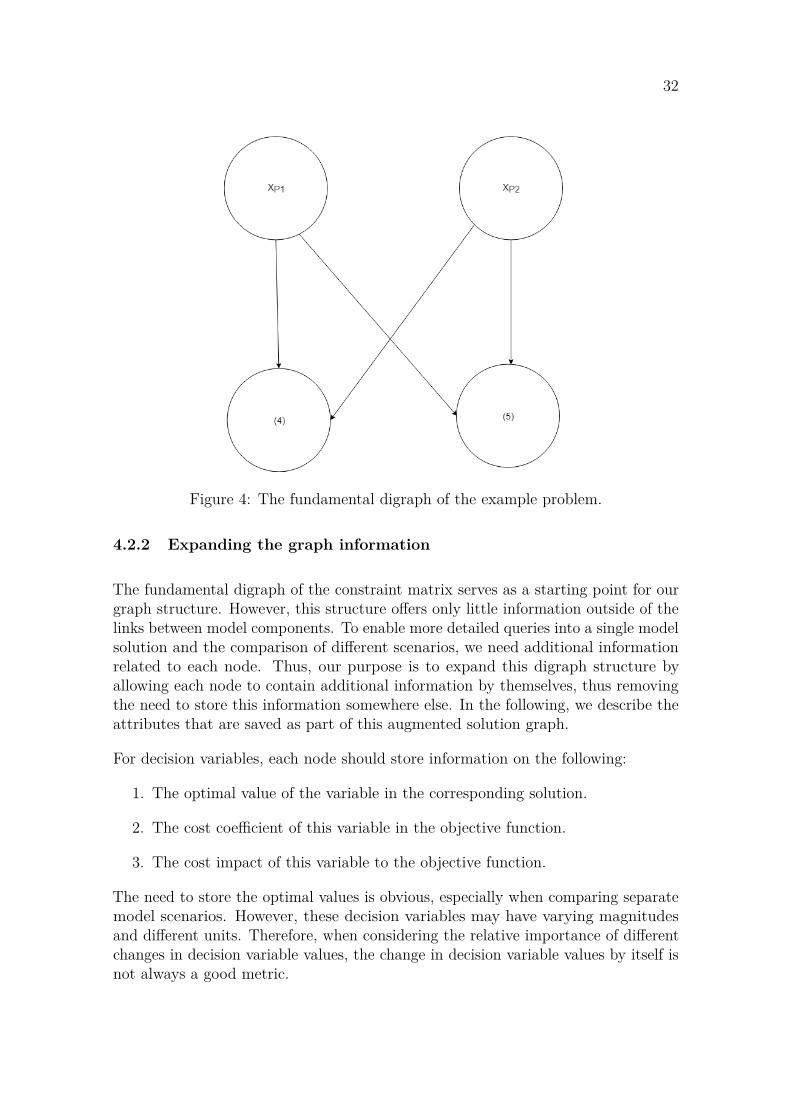
32

Figure 4: The fundamental digraph of the example problem.

4.2.2 Expanding the graph information

The fundamental digraph of the constraint matrix serves as a starting point for ourgraph structure. However, this structure offers only little information outside of thelinks between model components. To enable more detailed queries into a single modelsolution and the comparison of different scenarios, we need additional informationrelated to each node. Thus, our purpose is to expand this digraph structure byallowing each node to contain additional information by themselves, thus removingthe need to store this information somewhere else. In the following, we describe theattributes that are saved as part of this augmented solution graph.

For decision variables, each node should store information on the following:

1. The optimal value of the variable in the corresponding solution.

2. The cost coefficient of this variable in the objective function.

3. The cost impact of this variable to the objective function.

The need to store the optimal values is obvious, especially when comparing separatemodel scenarios. However, these decision variables may have varying magnitudesand different units. Therefore, when considering the relative importance of differentchanges in decision variable values, the change in decision variable values by itself isnot always a good metric.

33

Instead, the cost impact of each decision variable provides a more unified metric forassessing how impactful each change is, since the units of all decision variables areconverted to the unit of the objective function. In linear programming, this costimpact is simply calculated as the corresponding cost coefficient multiplied by thedecision variable value.

It may be unapparent at first glance why we would need to store information on thecost coefficient separately. However, when comparing scenarios where some of thecost coefficients change, explicitly determining this change can be beneficial, as thiscannot be exactly deduced from the changes in value and cost impact alone.

For constraints, each node should store information on the following:

1. The row sum of the constraint, or Aix.

2. The right-hand side (RHS) of the constraint.

The row sums of the constraints provide valuable information on how each constraintis satisfied. Furthermore, when comparing scenarios, a change in the row sumcorresponds to a change in the flows through that constraint.

A change in the right-hand side for an inequality constraint corresponds to changein the upper or lower bound of the constraint, e.g. the upper bound for maximumcapacity, or the lower bound for a minimum production constraint. In situationswhere we want the focus of the analysis is on such changes, such information isessential.

Consider also the edges between nodes in the fundamental digraph: They are createdsolely based on the signs of elements in the constraint matrix A, and there is noinformation on the exact value of the dependency between the constraints anddecision variables, which are given by the entries in the constraint matrix. To enablecomparisons between solutions where these values are changed, it makes sense tostore these values exactly as they are, instead of simply connecting the nodes based onnon-zero entries in the constraint matrix. Thus, we augment each edge in the graphto contain the exact value of the corresponding entry in the constraint matrix.

The aforementioned attributes form what we generally refer to as the attribute vector.Each node and edge in the graph is associated with exactly one attribute vector,and the contents depend on whether the entity in question is a constraint node, adecision variable node, or an edge.

Definition 4.5. The attribute vector associated with decision variable xj is

sxj=

⎡⎢⎣ x∗j

cjx∗j

cj

⎤⎥⎦,

34

where x∗j is the optimal value of the decision variable, and cj is the cost vector

component associated with the decision variable xj.

Definition 4.6. The attribute vector associated with constraint yi is

syi=

[bi∑

j Aijx∗j

],

where bi is the right-hand side vector component associated with constraint yi, andAij is jth column (decision variable) of ith row (constraint) of the constraint matrix A.

Definition 4.7. The attribute (scalar) associated with edges is s = Aij, wherethe edge is (yi, xj) if Aij < 0 and (xj, yi) if Aij > 0

For the aforementioned attribute vectors, we only need the decision variable valuesof the optimal solution, and the right-hand side and cost vectors b and c, in additionto the constraint matrix A. However, to further enrich our ability to find specificpatterns and relationships in the model, it is useful to map the decision variables andconstraints to the real entities of the supply chain. The specifics obviously depend onthe particular problem, but we attempt to give some general guidelines here basedon our experiences.

Each node should have a unique identification code that links it to the specificdecision variable or constraint. This is necessary, since otherwise we would be unableto match the same nodes between different scenarios. This clearly requires thatthe identification scheme should also be consistent across scenarios. One should beespecially careful when using automatic numbering, since these may change afterthe addition or deletion of a decision variable or constraint. The MPS file formatsupports variable naming, so this is not an issue in practice.

Furthermore, a classification based on different node types is useful. In a supplychain context, these often include information on whether the node is related toe.g. the acquisition of raw materials, production of goods, or satisfying customerdemand. The purpose of including such information is to incorporate the logicalstructure of the problem, enabling the IMPS to look for more specific patterns theuser might be interested in. The node types could coincide with the mathematicalmodel formulation, so that each different type of decision variable and constraint isincluded as the type of the respective node.

In addition, nodes should have more specific information on their distinct dimensions,based on the node type. For each node in the graph, we define the dimensions asfollows.

Definition 4.8. The dimensions of node n are defined as a function Dn: Kn → Ln,where Kn is the set of keys for node n, and Ln is the set of values for node n.

35

We assume that the node keys match between all nodes of equal type, which meansthat when comparing the dimensions of two nodes of the same type, we can usethe set of keys from either of these nodes. These dimensions should also be quiteclear from the mathematical model, as these coincide with the properties each de-cision variable and constraint has. For example, consider a decision variable noden1 for the production quantity of some product P1, in some production facilityA1, at some time period T1. Then, the keys of Dn1 are the names of these dimen-sions, such as productID, facilityID, and periodID, with the corresponding values:Dn1(productID) = P1, Dn1(facilityID) = A1, Dn1(periodID) = T1. For anotherproduction decision variable node n2, the production quantity of the same productat the same facility, but at time period T2, the corresponding dimensions would beDn2(productID) = P1, Dn2(facilityID) = A1, Dn2(periodID) = T2.

For constraint nodes, we may include the type of the constraint as an additionalkey-value pair in its dimensions: In other words, each constraint node’s dimensionscan include a special key, with a corresponding value depending the type of theconstraint: ’≤’ (L), ’=’ (E), or ’≥’ (G). This can be useful in situations where wewant to filter results based on binding inequality constraints, for instance.

As discussed in Section 2.2, supply chains often include multiple hierarchies. Toenable queries where some of these hierarchies are the focal point of interest, thenodes should also carry information on the hierarchies relevant to the node. Forexample, a node related to a product would contain information on the relatedproduct family, in addition to the specific product. This approach is inefficient interms of space usage, since this hierarchical information is duplicated for each nodethat share some of their attributes. However, if we want to maintain the graph as anexact representation of the model structure, this approach is necessary. These can bethen included as additional key-value pairs into the corresponding node dimensionsDn.

Finally, it may be beneficial to distinguish between two separate types of entities inthe optimisation model: i) entities that can be linked to physical entities of the supplychain, such as decision variables related to production, or material flow constraints,and ii) virtual entities that are included in the problem formulation, but do not havea physical interpretation. Entities such as minimum production levels or penaltieswhose goal is to guide the solution in some direction are part of this category.

We provide an example to illustrate how the aforementioned information wouldbe augmented into the fundamental digraph. Consider again the simple linearprogramming problem (3)-(5), and its fundamental digraph. Obtaining the optimalsolution results in decision variable values x∗

P 1 = 2, x∗P 2 = 3. The cost coefficients

of these decision variables are obtained directly from the first row, thus we havecP 1 = 6, cP 2 = 5. The cost impacts of the decision variables are easily calculated asx∗

P 1cP 1 = 2 × 6 = 12, and x∗P 2cP 2 = 3 × 5 = 15. For the constraints (4) and (5), we

observe that both of them are less-than constraints, and their right-hand sides are 5and 12, respectively. Their row sums can be calculated as x∗

P 1 + x∗P 2 = 2 + 3 = 5, and

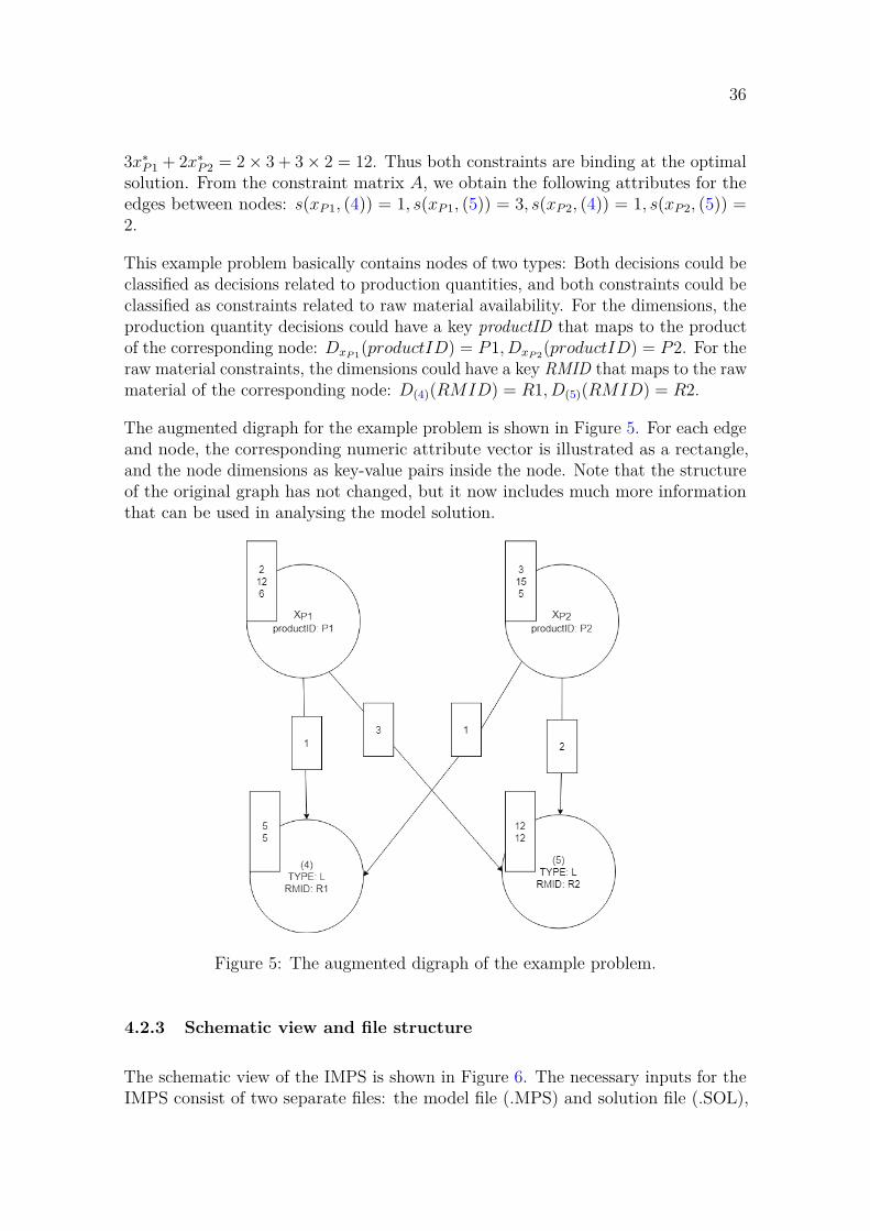
36

3x∗P 1 + 2x∗

P 2 = 2 × 3 + 3 × 2 = 12. Thus both constraints are binding at the optimalsolution. From the constraint matrix A, we obtain the following attributes for theedges between nodes: s(xP 1, (4)) = 1, s(xP 1, (5)) = 3, s(xP 2, (4)) = 1, s(xP 2, (5)) =2.

This example problem basically contains nodes of two types: Both decisions could beclassified as decisions related to production quantities, and both constraints could beclassified as constraints related to raw material availability. For the dimensions, theproduction quantity decisions could have a key productID that maps to the productof the corresponding node: DxP 1(productID) = P1, DxP 2(productID) = P2. For theraw material constraints, the dimensions could have a key RMID that maps to the rawmaterial of the corresponding node: D(4)(RMID) = R1, D(5)(RMID) = R2.

The augmented digraph for the example problem is shown in Figure 5. For each edgeand node, the corresponding numeric attribute vector is illustrated as a rectangle,and the node dimensions as key-value pairs inside the node. Note that the structureof the original graph has not changed, but it now includes much more informationthat can be used in analysing the model solution.

Figure 5: The augmented digraph of the example problem.

4.2.3 Schematic view and file structure

The schematic view of the IMPS is shown in Figure 6. The necessary inputs for theIMPS consist of two separate files: the model file (.MPS) and solution file (.SOL),

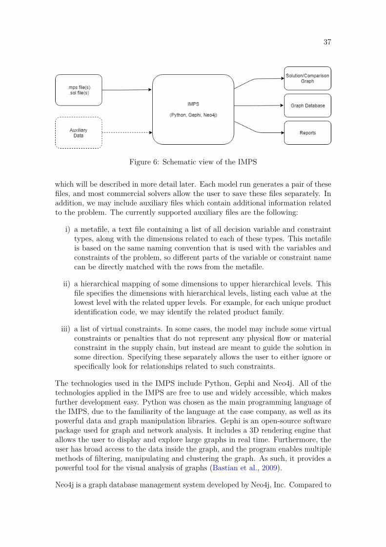
37

Figure 6: Schematic view of the IMPS

which will be described in more detail later. Each model run generates a pair of thesefiles, and most commercial solvers allow the user to save these files separately. Inaddition, we may include auxiliary files which contain additional information relatedto the problem. The currently supported auxiliary files are the following:

i) a metafile, a text file containing a list of all decision variable and constrainttypes, along with the dimensions related to each of these types. This metafileis based on the same naming convention that is used with the variables andconstraints of the problem, so different parts of the variable or constraint namecan be directly matched with the rows from the metafile.

ii) a hierarchical mapping of some dimensions to upper hierarchical levels. Thisfile specifies the dimensions with hierarchical levels, listing each value at thelowest level with the related upper levels. For example, for each unique productidentification code, we may identify the related product family.

iii) a list of virtual constraints. In some cases, the model may include some virtualconstraints or penalties that do not represent any physical flow or materialconstraint in the supply chain, but instead are meant to guide the solution insome direction. Specifying these separately allows the user to either ignore orspecifically look for relationships related to such constraints.

The technologies used in the IMPS include Python, Gephi and Neo4j. All of thetechnologies applied in the IMPS are free to use and widely accessible, which makesfurther development easy. Python was chosen as the main programming language ofthe IMPS, due to the familiarity of the language at the case company, as well as itspowerful data and graph manipulation libraries. Gephi is an open-source softwarepackage used for graph and network analysis. It includes a 3D rendering engine thatallows the user to display and explore large graphs in real time. Furthermore, theuser has broad access to the data inside the graph, and the program enables multiplemethods of filtering, manipulating and clustering the graph. As such, it provides apowerful tool for the visual analysis of graphs (Bastian et al., 2009).

Neo4j is a graph database management system developed by Neo4j, Inc. Compared to

38

traditional relational database management systems, the foundational element behindthis system is a graph that represents relationships in the data. In Neo4j, all entitiesare stored as nodes, edges, or attributes. Each node and edge can have multipleattributes, and they can be labelled with different names to narrow graph searchesto desired labels. The representation of optimisation model runs as graphs directlytranslates into a graph database of this form: each decision variable and constraintis a node in the graph database, with the attributes and labels corresponding to itstype. Relationships between nodes are the same as the connections between decisionvariables and constraints.

4.2.4 MPS Parser

MPS (Mathematical Programming System) is a file format for presenting LP andMILP problems. The format is column-oriented, meaning that the structure of thefile is based on the decision variables, as opposed to row equations. Furthermore,all model components receive names, which can be used advantageously in the post-processing steps as we describe below. The format is compatible with essentiallyall commercial LP solvers, which is why it was chosen as the standard input of ourIMPS. To convert the MPS file into a feasible data structure, an MPS parser is built.We briefly describe how our MPS parser functions through the various fields of theMPS file.

The MPS file starts with a NAME record, which our MPS parser skips since this isarbitrary and has no significance in model structure. Then, the parser reads throughthe following ROWS section, corresponding to each constraint in the model, savingeach row name as a new key in a hash table. The type of the constraint, E forequality (=) rows, L for less-than (≤) rows, and G for greater-than (≥) rows, is savedas an attribute. Note that the objective function is specified as a special row withname ’OBJ’ of special non-constraining type N. Then, the following COLUMNSsection contains the non-zero coefficients of the constraint matrix. Here, the parserchecks each entry, and saves the column-coefficient pair as a key-value pair under thecorresponding row key. Next, the RHS section contains the right-hand sides of theconstraints. The parser saves these as attributes under the corresponding row key.Missing entries are assumed to have a right-hand side of zero. The optional sectionsof BOUNDS and RANGES are not considered in the current implementation, sincethey are only specific forms of constraints that could be described in the COLUMNSsection as well. As a final result, our parser results in a hash table- type data structurewith keys corresponding to the rows of the model, and columns related each row forman inner hash table of key-value pairs of column names and coefficients, along withthe other row-related attributes. This is similar to an adjacency list representationof the graph, which is efficient when the underlying graph is sparse.

Note that the MPS format we have used is an extended format, which allows forvariable and constraint names longer than 8 characters, the maximum limit in the

39

traditional MPS format. This format allows the use of whitespace characters asfield limiters, but the names used cannot contain whitespaces. Furthermore, thenaming convention of variables and constraints we currently use is based on theformat automatically generated by some commercial solvers, e.g. Gurobi. Here, thevariable or constraint name starts with the type, followed by square brackets thatcontain comma-separated values for each related attribute. The pseudocode for thisalgorithm is given in appendix A.

4.3 Constructing individual graphs

After obtaining the parsed MPS (PMPS) file, the graph construction is straightfor-ward. The only additional information necessary to create an augmented solutiongraph is the solution (.sol) file, containing the optimal decision variable values forthe specific model run. Assuming that the decision variable names are consistentwith the ones specified in the MPS file, we simply look up the optimum value foreach decision variable from the solution file when creating the corresponding node.These can then be used to calculate the cost impacts of each decision variable, aswell as the row sum of each constraint. Finally, if any auxiliary data is included,these files are parsed and the relevant attributes are added to each node.

As a final result, we obtain a graph data structure in Python that can either betransferred into Gephi for visualisation, or into a graph database from which we canquery any model-related information that is relevant to the business questions of thedecision maker.

The pseudocode for the graph construction algorithm is given in appendix B. In thealgorithm, the word ’row’ refers to the set of key-value pairs indentified by a rowkey, and a specific attribute ’val’ in this row is referred to as ’row[val]’. Thus, forcolumns, ’col’ refers to the column name, while ’row[col]’ refers to the multiplier ofthe decision variable ’col’ in the constraint ’row’. Similarly, we refer to the optimaldecision variable values and cost coefficients by referring the respective mappingsby the column name. Notice that the row with key ’OBJ’, identifying the costcoefficients of decision variables, is treated separately from the other rows.

4.4 The comparison of graphs

Given two augmented digraphs for the same model, G and H, we then wish tocompute their difference to produce a comparison graph. We denote this new graphas C = G−H. In this section we describe how this operation is done. It is importantto note here that there may be alternative methods for constructing such a graph,but this version has proved to be reasonable for our purposes.

40

The main idea behind the construction of the comparison graph is performing anode-by-node comparison of the graphs. This is done by subtracting the attributevector of each node in H from the corresponding node’s attribute vector in G. Forexample, consider two nodes nG, nH , which are the corresponding nodes from graphsG and H, respectively. Then, the corresponding node in the comparison graph,denoted nC , is going to have the attribute vector:

snC= snG

− snH(6)

The comparison graph is then constructed based on the difference in each decisionvariable’s attribute vector. Specifically, if the optimum value or the cost impact ofa decision variable has changed between scenarios, it is included as a node in thecomparison graph. It is important to consider these changes simultaneously, sincethere may be cases where the change can only be seen in one of these elements. Wemotivate this further by considering several examples.

For instance, some decision variables may not carry explicit costs by themselves:Consider a supply chain case where we have separate decision variables for thepurchasing of raw materials and the consumption of these raw materials. Naturally,the cost incurred by purchasing some raw material should only be accounted foronce, therefore the decision variables that control the consumption of these materialsare zero cost. If we were to consider only the cost changes between the scenarios, wewould only see that some raw material was purchased more or less, and not how thisaffects its consumption.

Likewise, some decision variables may have the same optimum value in the scenarios,even though the cost impact of these decision has changed. Consider again a supplychain example, where the margin profit for selling some product has changed betweenscenarios. In such a situation, it may be that the optimum decision is still to sell thesame amount of that product as before. Thus, if we were only checking the changesin volume, we might miss a significant part of the change in the objective functionvalue.

Note that there is also a potential case where the only difference in the attributevector is in the cost coefficient. However, this is only possible if the optimal value ofthe decision variable is zero in both scenarios. This implies that the decision is nottaken in either of the considered scenarios, thus it can be considered irrelevant interms of scenario differences.

It is worth mentioning that comparing these total cost impacts may be somewhatunreasonable in cases where the cost coefficient has also changed. For example, con-sider a case where the marginal profit obtained by selling some product is "worsened"by some change between scenarios. As a result, the optimum solution may be toeither reduce or completely stop selling this specific product. Then, this decision byitself has a negative cost impact, since less profits are obtained due to this decision.

41

However, the cost impact obtained simply by comparing the profits obtained byselling this product in different scenarios are misleading, because it does not take intoaccount the fact that if we were to continue selling this product, our profits wouldhave also been less than previously. Thus, a fair comparison would be to considerthe loss based on the new cost parameter too, not just the old one.

The decision variable nodes, where neither the cost impact nor optimum value haschanged, are not included in the comparison graph. This includes both cases whereoptimum variable values are zero and non-zero, and there is no distinction beingmade between these cases. If the optimum value of a decision variable stays thesame, and its cost impact remains the same as well, then we can safely ignore it.This is because such decisions clearly have no impact on the difference between themodel scenarios, which are the primary reason for studying the comparison graphin the first place. In practice, we set some small tolerance value, and consider allabsolute changes less than this as equivalent. This tolerance allows us to ignore verysmall changes that are either rounding differences, or otherwise have a negligibleimpact on the solution difference.

In addition to the relevant decision variable nodes, the comparison graph includes allincoming and outgoing edges from these nodes, as well as the constraint nodes at theother end point of each edge. This means that all constraints that are directly affectingany relevant decision variable are included in the comparison graph. Note that similarto irrelevant decision variables, there may be constraints that are irrelevant in termsof scenario difference: For instance, there may be constraints that are linked only tothese irrelevant decision variables, thus they can be ignored.

There are a few special cases worth discussing. First, to enable the addition ordeletion of decision variables and constraints between scenarios, we must be able toinclude nodes that are only part of one model scenario. Our approach with suchnodes is as follows: For decision variable nodes, we set the missing attribute vectorto the zero vector 0. In other words, if the decision variable node nG is only in Gbut not in H, we set snH

= 0, and similarly for decision variables only in H but notin G, we set snG

= 0, then compute the difference in attribute vectors as describedin equation 6. As a result, all decision variable nodes that are only part of onescenario are included in the comparison graph, if the decision variable has a non-zerovalue, cost impact or both. For constraint nodes, we can use the same approach forcalculating the difference in the attribute vector, but only include the constraintnodes that share an edge with a relevant decision variable node in the comparisongraph.

With the aforementioned considerations, we can define our comparison graph formallyas follows. Note that the two node sets are not treated equally in the definition: Thedecision variables define the primary structure of the comparison graph.

Definition 4.9. Let G = (UG, VG, EG), H = (UH , VH , EH) be two augmented di-graphs of the same model, where UG and UH are the sets of constraint nodes in

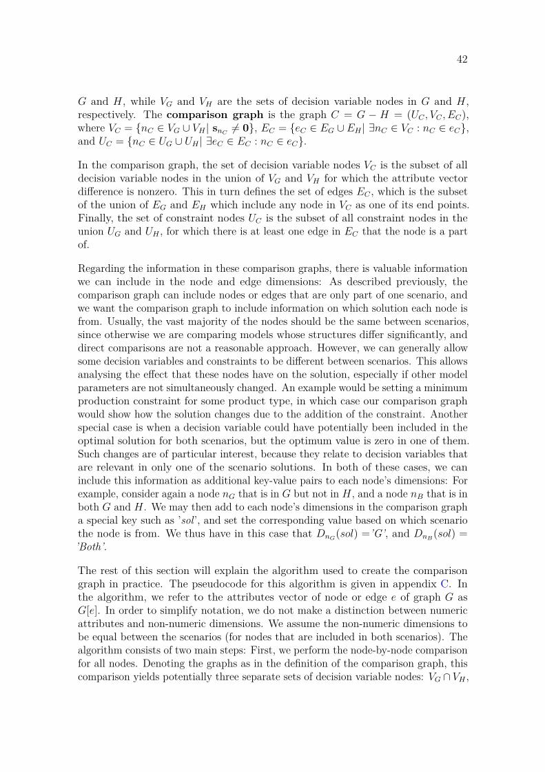
42

G and H, while VG and VH are the sets of decision variable nodes in G and H,respectively. The comparison graph is the graph C = G − H = (UC , VC , EC),where VC = {nC ∈ VG ∪ VH | snC

= 0}, EC = {eC ∈ EG ∪ EH | ∃nC ∈ VC : nC ∈ eC},and UC = {nC ∈ UG ∪ UH | ∃eC ∈ EC : nC ∈ eC}.

In the comparison graph, the set of decision variable nodes VC is the subset of alldecision variable nodes in the union of VG and VH for which the attribute vectordifference is nonzero. This in turn defines the set of edges EC , which is the subsetof the union of EG and EH which include any node in VC as one of its end points.Finally, the set of constraint nodes UC is the subset of all constraint nodes in theunion UG and UH , for which there is at least one edge in EC that the node is a partof.

Regarding the information in these comparison graphs, there is valuable informationwe can include in the node and edge dimensions: As described previously, thecomparison graph can include nodes or edges that are only part of one scenario, andwe want the comparison graph to include information on which solution each node isfrom. Usually, the vast majority of the nodes should be the same between scenarios,since otherwise we are comparing models whose structures differ significantly, anddirect comparisons are not a reasonable approach. However, we can generally allowsome decision variables and constraints to be different between scenarios. This allowsanalysing the effect that these nodes have on the solution, especially if other modelparameters are not simultaneously changed. An example would be setting a minimumproduction constraint for some product type, in which case our comparison graphwould show how the solution changes due to the addition of the constraint. Anotherspecial case is when a decision variable could have potentially been included in theoptimal solution for both scenarios, but the optimum value is zero in one of them.Such changes are of particular interest, because they relate to decision variables thatare relevant in only one of the scenario solutions. In both of these cases, we caninclude this information as additional key-value pairs to each node’s dimensions: Forexample, consider again a node nG that is in G but not in H, and a node nB that is inboth G and H. We may then add to each node’s dimensions in the comparison grapha special key such as ’sol’, and set the corresponding value based on which scenariothe node is from. We thus have in this case that DnG

(sol) =’G’, and DnB(sol) =

’Both’.

The rest of this section will explain the algorithm used to create the comparisongraph in practice. The pseudocode for this algorithm is given in appendix C. Inthe algorithm, we refer to the attributes vector of node or edge e of graph G asG[e]. In order to simplify notation, we do not make a distinction between numericattributes and non-numeric dimensions. We assume the non-numeric dimensions tobe equal between the scenarios (for nodes that are included in both scenarios). Thealgorithm consists of two main steps: First, we perform the node-by-node comparisonfor all nodes. Denoting the graphs as in the definition of the comparison graph, thiscomparison yields potentially three separate sets of decision variable nodes: VG ∩ VH ,

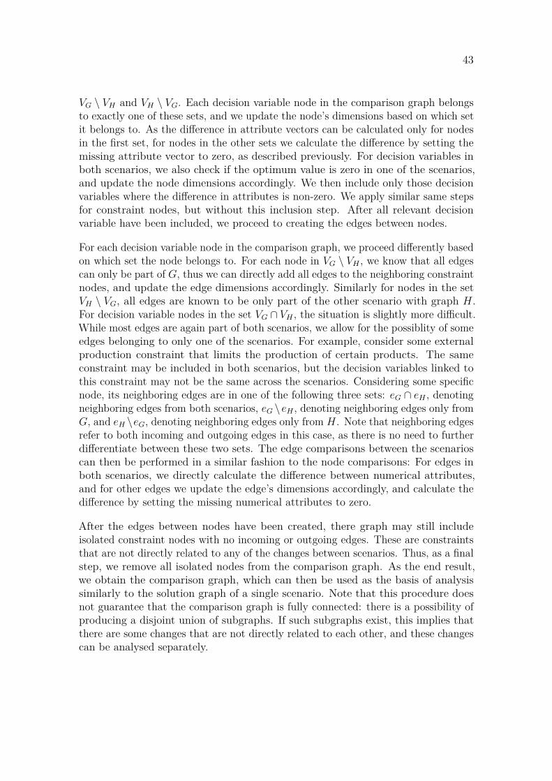
43

VG \ VH and VH \ VG. Each decision variable node in the comparison graph belongsto exactly one of these sets, and we update the node’s dimensions based on which setit belongs to. As the difference in attribute vectors can be calculated only for nodesin the first set, for nodes in the other sets we calculate the difference by setting themissing attribute vector to zero, as described previously. For decision variables inboth scenarios, we also check if the optimum value is zero in one of the scenarios,and update the node dimensions accordingly. We then include only those decisionvariables where the difference in attributes is non-zero. We apply similar same stepsfor constraint nodes, but without this inclusion step. After all relevant decisionvariable have been included, we proceed to creating the edges between nodes.

For each decision variable node in the comparison graph, we proceed differently basedon which set the node belongs to. For each node in VG \ VH , we know that all edgescan only be part of G, thus we can directly add all edges to the neighboring constraintnodes, and update the edge dimensions accordingly. Similarly for nodes in the setVH \ VG, all edges are known to be only part of the other scenario with graph H.For decision variable nodes in the set VG ∩ VH , the situation is slightly more difficult.While most edges are again part of both scenarios, we allow for the possiblity of someedges belonging to only one of the scenarios. For example, consider some externalproduction constraint that limits the production of certain products. The sameconstraint may be included in both scenarios, but the decision variables linked tothis constraint may not be the same across the scenarios. Considering some specificnode, its neighboring edges are in one of the following three sets: eG ∩ eH , denotingneighboring edges from both scenarios, eG \eH , denoting neighboring edges only fromG, and eH \eG, denoting neighboring edges only from H. Note that neighboring edgesrefer to both incoming and outgoing edges in this case, as there is no need to furtherdifferentiate between these two sets. The edge comparisons between the scenarioscan then be performed in a similar fashion to the node comparisons: For edges inboth scenarios, we directly calculate the difference between numerical attributes,and for other edges we update the edge’s dimensions accordingly, and calculate thedifference by setting the missing numerical attributes to zero.

After the edges between nodes have been created, there graph may still includeisolated constraint nodes with no incoming or outgoing edges. These are constraintsthat are not directly related to any of the changes between scenarios. Thus, as a finalstep, we remove all isolated nodes from the comparison graph. As the end result,we obtain the comparison graph, which can then be used as the basis of analysissimilarly to the solution graph of a single scenario. Note that this procedure doesnot guarantee that the comparison graph is fully connected: there is a possibility ofproducing a disjoint union of subgraphs. If such subgraphs exist, this implies thatthere are some changes that are not directly related to each other, and these changescan be analysed separately.

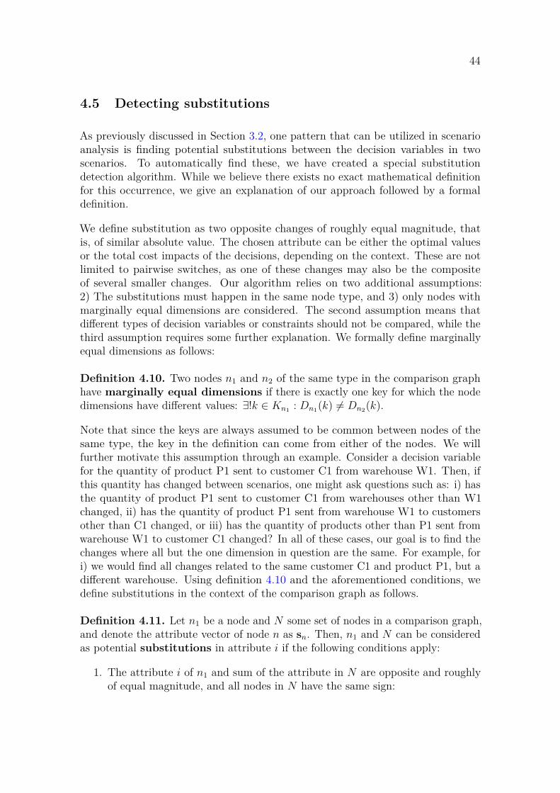
44

4.5 Detecting substitutions

As previously discussed in Section 3.2, one pattern that can be utilized in scenarioanalysis is finding potential substitutions between the decision variables in twoscenarios. To automatically find these, we have created a special substitutiondetection algorithm. While we believe there exists no exact mathematical definitionfor this occurrence, we give an explanation of our approach followed by a formaldefinition.

We define substitution as two opposite changes of roughly equal magnitude, thatis, of similar absolute value. The chosen attribute can be either the optimal valuesor the total cost impacts of the decisions, depending on the context. These are notlimited to pairwise switches, as one of these changes may also be the compositeof several smaller changes. Our algorithm relies on two additional assumptions:2) The substitutions must happen in the same node type, and 3) only nodes withmarginally equal dimensions are considered. The second assumption means thatdifferent types of decision variables or constraints should not be compared, while thethird assumption requires some further explanation. We formally define marginallyequal dimensions as follows:

Definition 4.10. Two nodes n1 and n2 of the same type in the comparison graphhave marginally equal dimensions if there is exactly one key for which the nodedimensions have different values: ∃!k ∈ Kn1 : Dn1(k) = Dn2(k).

Note that since the keys are always assumed to be common between nodes of thesame type, the key in the definition can come from either of the nodes. We willfurther motivate this assumption through an example. Consider a decision variablefor the quantity of product P1 sent to customer C1 from warehouse W1. Then, ifthis quantity has changed between scenarios, one might ask questions such as: i) hasthe quantity of product P1 sent to customer C1 from warehouses other than W1changed, ii) has the quantity of product P1 sent from warehouse W1 to customersother than C1 changed, or iii) has the quantity of products other than P1 sent fromwarehouse W1 to customer C1 changed? In all of these cases, our goal is to find thechanges where all but the one dimension in question are the same. For example, fori) we would find all changes related to the same customer C1 and product P1, but adifferent warehouse. Using definition 4.10 and the aforementioned conditions, wedefine substitutions in the context of the comparison graph as follows.

Definition 4.11. Let n1 be a node and N some set of nodes in a comparison graph,and denote the attribute vector of node n as sn. Then, n1 and N can be consideredas potential substitutions in attribute i if the following conditions apply:

1. The attribute i of n1 and sum of the attribute in N are opposite and roughlyof equal magnitude, and all nodes in N have the same sign:

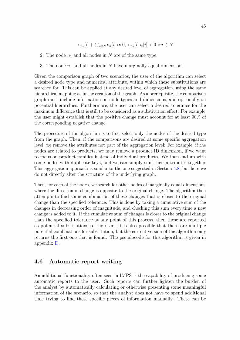
45

sn1 [i] + ∑n∈N sn[i] ≈ 0, sn1 [i]sn[i] < 0 ∀n ∈ N .

2. The node n1 and all nodes in N are of the same type.

3. The node n1 and all nodes in N have marginally equal dimensions.

Given the comparison graph of two scenarios, the user of the algorithm can selecta desired node type and numerical attribute, within which these substitutions aresearched for. This can be applied at any desired level of aggregation, using the samehierarchical mapping as in the creation of the graph. As a prerequisite, the comparisongraph must include information on node types and dimensions, and optionally onpotential hierarchies. Furthermore, the user can select a desired tolerance for themaximum difference that is still to be considered as a substitution effect: For example,the user might establish that the positive change must account for at least 90% ofthe corresponding negative change.

The procedure of the algorithm is to first select only the nodes of the desired typefrom the graph. Then, if the comparisons are desired at some specific aggregationlevel, we remove the attributes not part of the aggregation level: For example, if thenodes are related to products, we may remove a product ID dimension, if we wantto focus on product families instead of individual products. We then end up withsome nodes with duplicate keys, and we can simply sum their attributes together.This aggregation approach is similar to the one suggested in Section 4.8, but here wedo not directly alter the structure of the underlying graph.

Then, for each of the nodes, we search for other nodes of marginally equal dimensions,where the direction of change is opposite to the original change. The algorithm thenattempts to find some combination of these changes that is closer to the originalchange than the specified tolerance. This is done by taking a cumulative sum of thechanges in decreasing order of magnitude, and checking this sum every time a newchange is added to it. If the cumulative sum of changes is closer to the original changethan the specified tolerance at any point of this process, then these are reportedas potential substitutions to the user. It is also possible that there are multiplepotential combinations for substitution, but the current version of the algorithm onlyreturns the first one that is found. The pseudocode for this algorithm is given inappendix D.

4.6 Automatic report writing

An additional functionality often seen in IMPS is the capability of producing someautomatic reports to the user. Such reports can further lighten the burden ofthe analyst by automatically calculating or otherwise presenting some meaningfulinformation of the scenario, so that the analyst does not have to spend additionaltime trying to find these specific pieces of information manually. These can be

46

especially powerful in situations where similar pieces of analysis would be repeatedfor different scenarios.

Naturally, there are many potential points of interest when analysing supply chainscenarios, thus no single report can address all potential questions a decision makermay have. Nevertheless, some pieces of information can certainly be generalised, atleast in the context of the supply chain. Focusing on the capabilities of the modeloriented approach, the simplest informative reports that can be written are thoserelated to constraint information. For example, on the production side, we can reportthe capacity bottlenecks that are occurring in the supply chain, or contrastinglywhere some capacity is left unused. On the customer side, we can report unsatisfieddemands for specific products or customers. Such reports can be directly generatedfrom the solution graph, and the user only has to specify which node types (machinecapacity, customer demand) they want to see.

In order to fully utilise the capabilities offered by the model oriented approach,reports based on more complex relationships can be created on top of the solutiongraph. These reports are more oriented towards answering specific questions thedecision maker may have, and they often need to be more customised to the specificoptimisation model. An example of such a report is ranking the most critical rawmaterials in the supply chain, in terms of total sales of products that are reliant onthe specific raw material. Another example is ranking the unmet demands in thesupply chain, in terms of total profits that are currently not obtained.

The main difference between these automatic reports and ad hoc queries made into agraph database is that these automatic reports are designed such that they attemptto fully answer some pre-specified question, whereas the ad hoc queries are moreflexible but also require the analyst to specify the model relationships they are lookingfor.

4.7 Visual network analysis

In scenario analysis, the ability to simply visualise the model graph as a network ofnodes is potentially useful, especially in cases where the main concern is to assessthe impact of different decisions in one scenario, or the various changes that havehappened between scenarios. In this visual graph representation, we can performdifferent types of highlighting and manipulation based on the subject of interest. Forexample, we can make node size reflect their respective cost coefficient or cost impact,thus drawing attention to the nodes where most significant cost contributions happen.Another possibility is considering the actual values of the decision variables, whichcorrespond to volumes flowing through the supply chain. Thus, highlighting decisionvariable nodes based on their values could be used to show the most significant flowsof materials through the supply chain. These can be applied both when analysing asingle scenario, in which case we visualise the individual solution graph, and when

47

comparing two scenarios, where we visualise the comparison graph instead. There isobviously a slight difference in the interpretation of these cases: with a single scenario,we are highlighting the most impactful decisions in terms of cost or volume, andwith two scenarios we are actually considering the most impactful changes regardingthese decisions. In both cases, these visualisations can provide the analyst with ameaningful overview of the model results.

Although the emphasis of costs or volumes are perhaps the most obvious use cases,there are many other possibilities of using network analysis tools in a model analysissetting. For example, in single scenario analysis, the information saved on constraintnodes can be used to highlight binding inequality constraints. In the case of less-thanconstraints, these often indicate bottlenecks in the supply chain, such as limitedwarehousing or production capacity. Emphasising these bottlenecks can provide thedecision maker with useful information on how the supply chain operates, at leastaccording to the underlying optimisation model. Furthermore, these results canprovide ideas for new interesting scenarios that could be explored.

In scenario comparison, nodes can be filtered based on the flags that indicate inwhich scenarios the node is active (non-zero) or even present at all. This wouldallow the analyst to observe which parts of the supply chain are most affected bythe change between scenarios, not in absolute terms but rather by showing whichpreviously unused options have become attractive, or which previously attractivedecisions are no longer made. This can highlight many interesting facts, such aspreviously unused production capabilities that have become active, or previouslyunmet customer demands that are now being satisfied. Similarly, we may highlightproduction decisions that are no longer made, or customer demands that are nolonger profitable enough to satisfy.

Furthermore, any of the other node attributes can be used in filtering the network toshow only the specific parts of the graph that the analyst is interested in. For example,if the analyst wants to know what is happening to a specific product, customer, or rawmaterial, they can filter the graph to show only the nodes with matching informationon the desired attribute, such as a specific product identification code. Such filteringcan be very useful if the interest of the decision maker can be narrowed down toa more detailed level that corresponds to some of these attributes. However, thelimitation with this filtering approach is that it does not include nodes without therelevant attributes, even though they might be considered relevant otherwise.

Some of the aforementioned visualization capabilities are illustrated in figures 7, 8and 9 below. These figures are visualizations of a particular supply chain relatedscenario comparison graph, the details of which are omitted here. In all of thesefigures, the size of the nodes is scaled relative to their cost impact, such that decisionswith larger cost impacts (either positive or negative) have a larger size. Althoughthe figures are all related to the same scenario comparison, they highlight differentfactors.

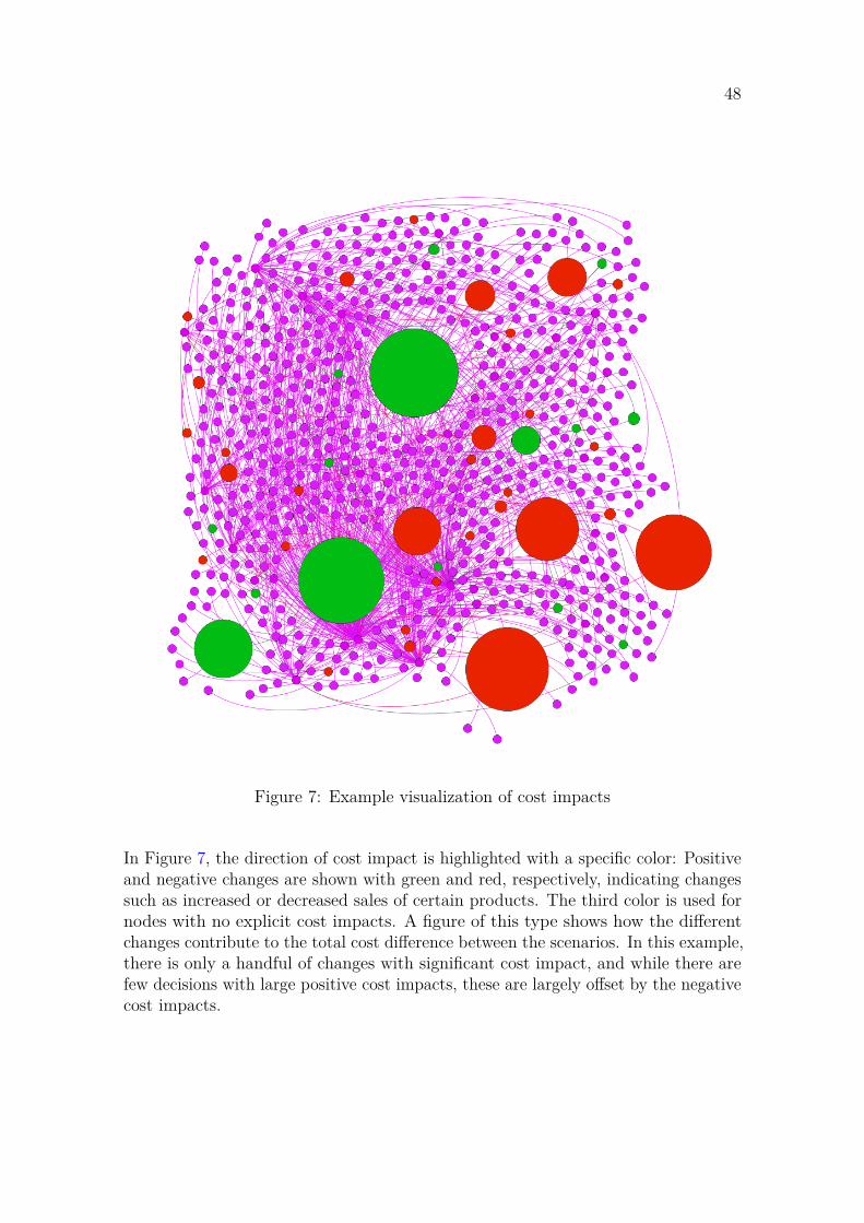
48

Figure 7: Example visualization of cost impacts

In Figure 7, the direction of cost impact is highlighted with a specific color: Positiveand negative changes are shown with green and red, respectively, indicating changessuch as increased or decreased sales of certain products. The third color is used fornodes with no explicit cost impacts. A figure of this type shows how the differentchanges contribute to the total cost difference between the scenarios. In this example,there is only a handful of changes with significant cost impact, and while there arefew decisions with large positive cost impacts, these are largely offset by the negativecost impacts.

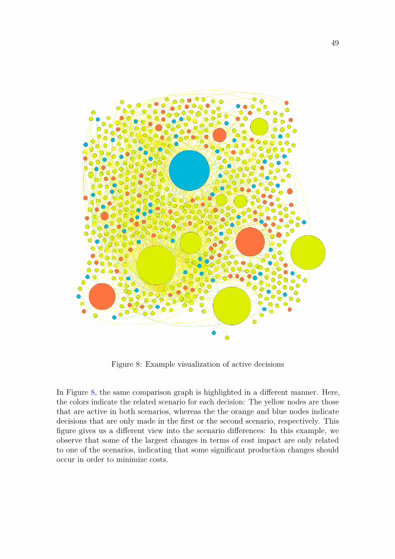
49

Figure 8: Example visualization of active decisions

In Figure 8, the same comparison graph is highlighted in a different manner. Here,the colors indicate the related scenario for each decision: The yellow nodes are thosethat are active in both scenarios, whereas the the orange and blue nodes indicatedecisions that are only made in the first or the second scenario, respectively. Thisfigure gives us a different view into the scenario differences: In this example, weobserve that some of the largest changes in terms of cost impact are only relatedto one of the scenarios, indicating that some significant production changes shouldoccur in order to minimize costs.

50

Figure 9: Example visualization of filtered graph

In Figure 9, the colours are the same as previously, but the graph is filtered to includeonly decisions and constraints related to a specific product, e.g. product P1 as inthe previously considered examples. This filtering makes the resulting graph moresparse, as only decisions and constraints directly related to product P1 are shown.This also makes the results easier to interpret, as there is less clutter from nodes thatare not interesting to the decision maker. In this example, we observe that many ofthe impactful decisions are actually related to the product that we have chosen tofilter here, which means that the production and sales of this particular product arelargely affected by the scenario changes.

51

4.8 Aggregation of graphs

As discussed previously, supply chains are often embedded with hierarchical struc-tures, such as products belonging in product families and customers in differentregions. In many situations, we may not be interested in specific changes in a singledecision variable, but would rather know what the important changes are on a higherhierarchical level. Here, we consider one possibility of comparing results hierarchicallyusing a process known in graph theory as node contraction, or vertex identification(Pemmaraju and Skiena, 2003). We will first give a formal definition, and thenexplain how this process could be used in diagnostic aggregation.

Definition 4.12. Let u, v be a pair of nodes in the graph G = (V, E). The contrac-tion of nodes u, v consists of merging them together into a new node w, such that wis adjacent to the union of nodes to which u and v were adjacent. This results in anew graph G′ = (V ′, E), where V ′ = (V \ {u, v}) ∪ {w}.

We assume that the nodes are not required to share an incident edge between them.Note also that in general, this operation may result in a graph with self-loops ormultiple edges between nodes, even if the original graph did not contain these.

Consider the graph G = (V, E), that contains all decision variable changes as well asthe related constraints. Let us assume that we would like aggregate the results oversome specific hierarchical dimension h that is one of the keys for node dimensions,related to an original dimension d. Aggregation over this hierarchical node dimensionis then equal to merging together any two nodes of the same type n1,n2 that i) havethe same value in dimension h: Dn1(h) = Dn2(h), and ii) have the same values in allother dimensions except the original dimension: ∀k ∈ Kn1 \ {d} : Dn1(k) = Dn2(k).In other words, we combine nodes of marginally equivalent dimensions, where themarginal difference is in dimension d. After the two nodes have been merged togetherinto a new node, the edges incident to this new node correspond to the edges thatwere incident to the original nodes. This aggregation process can be done by firstremoving the original dimension d from all nodes that contain it, after which somenodes have identical dimensions. Then, for each subset of nodes that have identicaldimensions, we can perform pairwise node contraction in any order, until there isonly one node left in the subset.

In the comparison graph setting, the process of node contraction can be appliedto the comparison graph to produce a smaller graph, where each node correspondsto an aggregation of several decision variables or constraints. Naturally, after suchoperation the result is no longer an exact representation of the underlying system.However, in the case that we are interested in the changes on an aggregate level, thisoperation may indeed provide us with a simpler and more manageable representationof the original problem.

One important and nontrivial question is what node contraction does to node

52

attributes. There is no clear answer as to what should happen, since by definition ofnode contraction, the result of contracting two nodes is always a new node, whichis simply incident to the union of nodes that were indicent to the old two nodes.However, in an optimisation setting, we are minimising some objective function, andthe cost effects of each change on the graph is known. Therefore, a natural numericalrepresentation of the cost effect of a contracted node is to sum the individual costeffects together. With this notion, the aggregated graph remains consistent with theoriginal one in the sense that the total difference in the objective function remainsthe same.

Clearly, this notion of summing the values together could be applied to all othernumerical node attributes as well, although their interpretation may not be quite asstraightforward. For example, the sum of cost coefficients between contracted decisionvariable nodes does not provide meaningful information. However, an average ormedian over these changes may be more informative. Following this idea, perhaps itwould be possible to define a separate aggregation function for all different types ofnumerical node attributes, such that the result from aggregation is then conduciveto the analysis of these aggregate results.

However, it is also possible that some attributes cannot be reasonably describedin aggregate form. Consider, for example, the non-numeric attributes that flag thesolutions in which the decision variable was active. Then, after performing nodecontraction over some dimension, the resulting supernode may include nodes thatwere active in different solutions. There is no clear answer what would be the bestform of aggregation.

In the case when the optimisation problem consists of several time steps, one specialform of aggregation would be to aggregate the results over time. If we are notinterested in what happens in the model at a specific time step, but rather wantto know what the model does on a more aggregate level, then this approach cansimplify the graph by making it considerably smaller. However, as with other forms ofgraph aggregations, there are potential cases where such aggregation is problematic:For example, if some model parameters change over time, we lose the informationregarding when these changes happen.

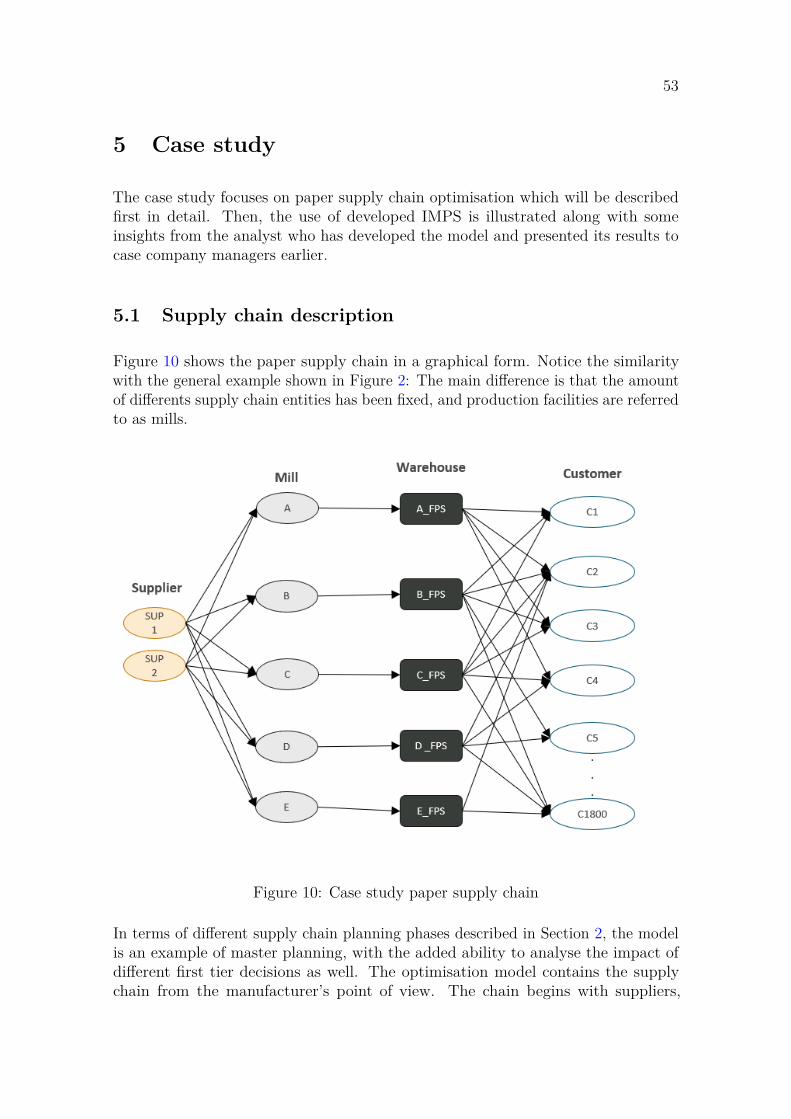
53

5 Case study

The case study focuses on paper supply chain optimisation which will be describedfirst in detail. Then, the use of developed IMPS is illustrated along with someinsights from the analyst who has developed the model and presented its results tocase company managers earlier.

5.1 Supply chain description

Figure 10 shows the paper supply chain in a graphical form. Notice the similaritywith the general example shown in Figure 2: The main difference is that the amountof differents supply chain entities has been fixed, and production facilities are referredto as mills.

Figure 10: Case study paper supply chain

In terms of different supply chain planning phases described in Section 2, the modelis an example of master planning, with the added ability to analyse the impact ofdifferent first tier decisions as well. The optimisation model contains the supplychain from the manufacturer’s point of view. The chain begins with suppliers,

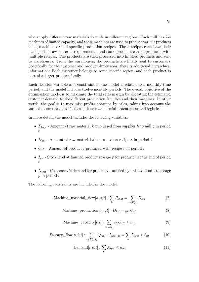
54

who supply different raw materials to mills in different regions. Each mill has 2-4machines of limited capacity, and these machines are used to produce various productsusing machine- or mill-specific production recipes. These recipes each have theirown specific raw material requirements, and some products can be produced withmultiple recipes. The products are then processed into finished products and sentto warehouses. From the warehouses, the products are finally sent to customers.Specifically for the customer and product dimensions, there is additional hierarchicalinformation: Each customer belongs to some specific region, and each product ispart of a larger product family.

Each decision variable and constraint in the model is related to a monthly timeperiod, and the model includes twelve monthly periods. The overall objective of theoptimisation model is to maximise the total sales margin by allocating the estimatedcustomer demand to the different production facilities and their machines. In otherwords, the goal is to maximise profits obtained by sales, taking into account thevariable costs related to factors such as raw material procurement and logistics.

In more detail, the model includes the following variables:

• Pkhqt - Amount of raw material k purchased from supplier h to mill q in periodt

• Dkrt - Amount of raw material k consumed on recipe r in period t

• Qrit - Amount of product i produced with recipe r in period t

• Ipit - Stock level at finished product storage p for product i at the end of periodt

• Xipct - Customer c’s demand for product i, satisfied by finished product storagep in period t

The following constraints are included in the model:

Machine_material_flow[k, q, t] :∑

h

Pkhqt =∑

r∈R(q)Dkrt (7)

Machine_production[k, r, t] : Dkrt = pkrQrit (8)

Machine_capacity[l, t] :∑

r∈R(l)slrQrit ≤ mlt (9)

Storage_flow[p, i, t] :∑

r∈R(q,i)Qrit + Ipi(t−1) =

∑c

Xipct + Ipit (10)

Demand[i, c, t] :∑

p

Xipct ≤ dict (11)

55

Here, R(q) denotes the recipes that belong to the mill q. pkr is the amount of rawmaterial k needed to produce one unit of recipe r. R(l) is the set of all recipes thatcan be produced with machine l, slr is the capacity used with machine l for each unitof recipe r, mlt is the maximum capacity of machine l at period t. R(q, i) denotes allrecipes that can be produced in mill q whose end product is i, and finally dict is thecustomer c’s estimated demand for product i at period t.

The constraints (7) state that all material bought to the mill at each time periodmust be consumed by some recipe that the mill is using during the same period.Constraints (8) state that each recipe has a specific conversion rate from eachraw material to product. Constraints (9) state that each recipe has some capacityrequirement for each unit produced, and that the total capacity used should notexceed the given maximum capacity. Constraints (10) state that the flows of materialthrough each finished product storage should be conserved. Finally, constraints(11) state that there is some specified demand for each customer, product and timeperiod, and that this demand is an upper limit of what can be satisfied throughthe different storages. In addition to these physical constraints, there are additionalvirtual constraints, which are not discussed here. The exact details of the modelparameters are not crucially important: Rather, the key is to understand how thedifferent model components are connected to each other. The immediate connectionsbetween the nodes of the model can be seen in the constraints, as they show exactlywhich constraint is linked to which decision variables.

In this study, we consider both the case where we only have one scenario, and thecase where we compare two scenarios. All of the single-scenario examples refer tothe same baseline scenario, where the supply chain is operated according to the bestcurrent information on all related factors, such as demand forecasts and raw materialavailability. For the two-scenario comparisons, various different scenarios based onreal business questions are compared against this baseline scenario. The objectivehere is to broadly illustrate different possibilities of analysing these model results byusing the functionalities implemented in the IMPS. Without explicitly mentioningthis in each separate case, when we only have one scenario, the graph is constructedby parsing the corresponding MPS and solution files, and then running the algorithmdescribed in Section 4.3. When comparing two scenarios, we first create the singlegraphs, after which we create the comparison graph using the algorithm described inSection 4.4. In addition, we include the node types, their respective dimensions andthe hierarchies for the product and customer dimensions as additional properties foreach node in the graphs. These steps enable us to perform the analyses describedbelow.

5.2 Visual network analysis

Figure 11 shows a visualisation of a complete scenario comparison graph between twosupply chain optimisation scenarios for the model. This visualisation was created

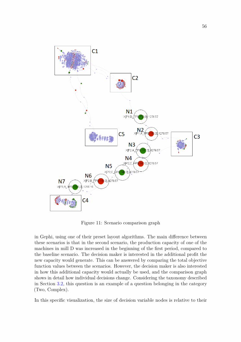
56

Figure 11: Scenario comparison graph

in Gephi, using one of their preset layout algorithms. The main difference betweenthese scenarios is that in the second scenario, the production capacity of one of themachines in mill D was increased in the beginning of the first period, compared tothe baseline scenario. The decision maker is interested in the additional profit thenew capacity would generate. This can be answered by comparing the total objectivefunction values between the scenarios. However, the decision maker is also interestedin how this additional capacity would actually be used, and the comparison graphshows in detail how individual decisions change. Considering the taxonomy describedin Section 3.2, this question is an example of a question belonging in the category(Two, Complex).

In this specific visualization, the size of decision variable nodes is relative to their

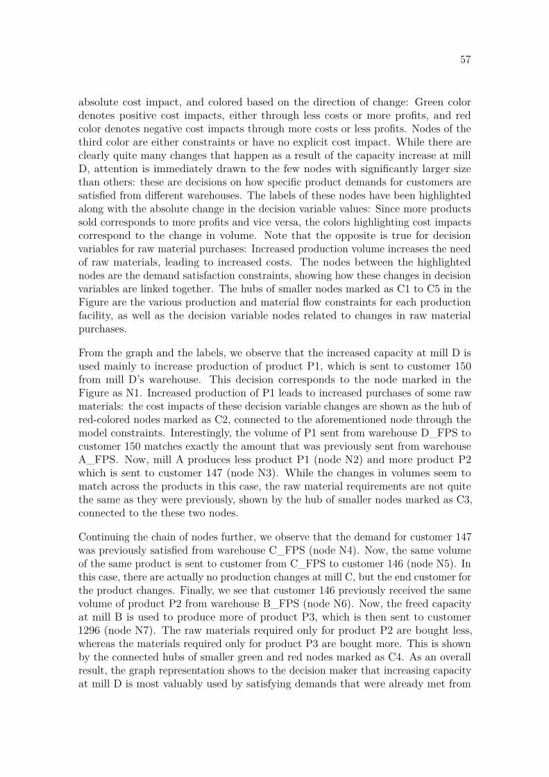
57

absolute cost impact, and colored based on the direction of change: Green colordenotes positive cost impacts, either through less costs or more profits, and redcolor denotes negative cost impacts through more costs or less profits. Nodes of thethird color are either constraints or have no explicit cost impact. While there areclearly quite many changes that happen as a result of the capacity increase at millD, attention is immediately drawn to the few nodes with significantly larger sizethan others: these are decisions on how specific product demands for customers aresatisfied from different warehouses. The labels of these nodes have been highlightedalong with the absolute change in the decision variable values: Since more productssold corresponds to more profits and vice versa, the colors highlighting cost impactscorrespond to the change in volume. Note that the opposite is true for decisionvariables for raw material purchases: Increased production volume increases the needof raw materials, leading to increased costs. The nodes between the highlightednodes are the demand satisfaction constraints, showing how these changes in decisionvariables are linked together. The hubs of smaller nodes marked as C1 to C5 in theFigure are the various production and material flow constraints for each productionfacility, as well as the decision variable nodes related to changes in raw materialpurchases.

From the graph and the labels, we observe that the increased capacity at mill D isused mainly to increase production of product P1, which is sent to customer 150from mill D’s warehouse. This decision corresponds to the node marked in theFigure as N1. Increased production of P1 leads to increased purchases of some rawmaterials: the cost impacts of these decision variable changes are shown as the hub ofred-colored nodes marked as C2, connected to the aforementioned node through themodel constraints. Interestingly, the volume of P1 sent from warehouse D_FPS tocustomer 150 matches exactly the amount that was previously sent from warehouseA_FPS. Now, mill A produces less product P1 (node N2) and more product P2which is sent to customer 147 (node N3). While the changes in volumes seem tomatch across the products in this case, the raw material requirements are not quitethe same as they were previously, shown by the hub of smaller nodes marked as C3,connected to the these two nodes.

Continuing the chain of nodes further, we observe that the demand for customer 147was previously satisfied from warehouse C_FPS (node N4). Now, the same volumeof the same product is sent to customer from C_FPS to customer 146 (node N5). Inthis case, there are actually no production changes at mill C, but the end customer forthe product changes. Finally, we see that customer 146 previously received the samevolume of product P2 from warehouse B_FPS (node N6). Now, the freed capacityat mill B is used to produce more of product P3, which is then sent to customer1296 (node N7). The raw materials required only for product P2 are bought less,whereas the materials required only for product P3 are bought more. This is shownby the connected hubs of smaller green and red nodes marked as C4. As an overallresult, the graph representation shows to the decision maker that increasing capacityat mill D is most valuably used by satisfying demands that were already met from

58

other mills, and through several links throughout the supply chain, increased profitsare mostly generated by satisfying previously unmet demand through a different mill.These sorts of insights are valuable to the decision maker when planning capacityincreases or any other related activities where an overview of the scenario differencesis required.

5.3 Ad hoc queries

In this section, we illustrate how the graph database representation can be usedto answer more complex questions related to analysing the supply chain, usingdifferent ad hoc queries on the graph database. We first present a few examplesfor the single scenario case, then a few examples for the two-scenario comparisoncase. All of the examples shown use the syntax of Cypher, the native graph querylanguage used by Neo4j. An extensive user manual, covering the language in detail,is maintained by the Neo4j team and can be downloaded from their website athttps://neo4j.com/docs/.

One question considered is finding the common material suppliers for products P1,P2and P3 in the baseline scenario, which is an example of a question of category(Single,Complex) in our question taxonomy described in Section 3.2. In this case, theproblem can be broken into the following steps: First, find the decision variable nodesthat are related to the production of the specified products. Then, find all directpaths from this node to decision variable nodes that are related to the procurementof raw materials. From these nodes, collect the distinct supplier identification codesfor each product. As a result, we then obtain a list of suppliers for each product ofinterest, which we can further check for differences or commonalities. Note that inthis question, the interest is not in exact values or cost impacts, but finding whatconnections exist between the production decisions and suppliers.

In a graph database, performing such a query is quite straightforward. One needsonly the ability to describe the path of decision variables and constraints that isassumed between the end points. In this case, the path is through the productiondecision variable (Q), a Machine production constraint, raw material consumptionvariable (D), Machine material flow constraint and finally the decision variable forpurchasing of raw material (P). The corresponding query with Cypher is as follows.As a result, we obtained that all these products use the exact same supplier, whichwas the expected outcome.

WITH [P1,P2,P3] as productsMATCH (q:Q)–(:Machine_production)–(:D)–(:Machine_material_flow)–(p:P)WHERE q.ProductID in products and q.value <> 0RETURN q.ProductID, collect(DISTINCT p.SupplierID)

Another interesting question of the same category was the following: Which of our

59

customers would potentially suffer in the baseline scenario as a result of a shortagein raw material R1? In order to answer such a question, we obviously have to firstfind out which products require this raw material. This alone requires the ability tolink all possible paths from the relevant raw material procurement nodes to differentproduction nodes, in a similar fashion to the previous example. In addition, we haveto proceed from these production nodes to the storage flow nodes, and finally to thenodes that show which customers receive the related final products. Overall, thisquestion amounts to finding all related paths through the supply chain, all the wayfrom raw material purchases to the selling of finished products to customers. Similarto the previous question, the main interest is in the connections, not exact values orcost impacts, although these could be calculated if necessary. While slightly morecomplicated than the previous example, the corresponding Cypher query is still quitemanageable. Denoting the raw material of interest as ’R1’, the corresponding queryis as follows. This query showed that there was a large population of customerswho were reliant on the availability of this raw material, which would suggest to thedecision maker that there is significant risk of losing customers, should this shortagebecome a reality.

MATCH (x:X)–(:Storage_flow)–(q:Q)–(:Machine_production)–(:D)–(:Machine_material_flow)–(p:P)WHERE p.RMID = ’R1’RETURN DISTINCT x.CustomerID

Note that answering these types of questions could be possible with a result orientedapproach using relational databases. However, this would likely require several joinoperations between different tables. For the examples above, forming a comparableanswer would likely include joining together multiple tables with information on thedifferent supply chain entities, such as suppliers, raw materials, production facilities,as well as the relationships between them. For an entire supply chain, this approachcan become unmanageable.

In scenario comparison, the decision makers were interested in a few questions thatcan be categorized as (Two,Complex) in our question taxonomy presented in Section3.2. First, they were interested in knowing how additional capacity at mill D would beused in production, and ultimately increasing profits. We can begin answering such aquestion by starting with the capacity constraint nodes where the RHS attribute hasincreased. We first check whether this new capacity is actually used, by checking thatthe row sum attribute has increased as well. Then, from these constraints, we easilyobtain the connected nodes, the decisions variables related to production, wherethe value and thus production amount has increased. In case we are also interestedin where these products are shipped, we can include material flow constraints andcustomer- specific shipping decision variables. An example of such a query is givenbelow. The result is a list of products and customers, with the corresponding volumeincreases. This is a similar example to the one presented in Section 5.2, but here weobtain a list of volumes, instead of a visual representation. Furthermore, this form

60

of query does not show the entire chain of events through all different warehouseslike the visual representation does.

MATCH (m:Machine_capacity)–(q:Q)–(:Storage_flow)–(x:X)WHERE m.RHS < 0 and m.RSUM < 0 and q.value < 0 and x.value < 0RETURN x.ProductID, x.CustomerID, x.value

Another question of interest was the case where raw material R1 has become unavail-able, thus rendering some production recipes unusable. The contrast to the similarone-scenario case is that here, instead of trying to find the affected customers, ourobjective is to explore how this change actually affects how the supply chain shouldbe operated. The natural starting point here is the raw material nodes that wereflagged to be available only in the first solution, in other words with the dimension’SOL1’. We then find the corresponding material flow constraints, through whichwe find the affected nodes related to resource consumption, production recipes, andultimately the production quantity variables that are affected by this change. Sucha query would be

MATCH (q:Q)–(:Machine_production)–(:D)–(:Machine_material_flow)–(p:P)WHERE p.sol = ’SOL1’RETURN q.ProductID, q.value

We thus find the directly affected decisions and the corresponding volumes, butthere are multiple other questions that may arise as a result. First, if there aremultiple recipes for the same product, then we might want to know if there exists arecipe that does not use these lacking raw materials. If such a recipe exists, then wecan find out if it is actually used to supplement the previously available productioncapabilities. There are several possibilities that arise: It may be that such actions arenot as profitable, and the unused capacity, assuming that capacities have not changedsimultaneously, is used to produce some completely different products to satisfysome previously unmet demand. Another possibility is that no other products areprofitable to produce, and the lack of raw materials results in excess capacity. In thisexample, we found that there were no additional recipes in use, and that the unusedcapacity would be mostly used to produce other products that were not reliant on themissing raw material. The increased production volumes were found out through anadditional query, where we used the previously found production quantity decisionsas a starting point. Referring to the list of affected product quantity decisions asAffectedProducts, the query is

MATCH (q1:Q)–(:Machine_capacity)–(q2:Q)WHERE q1 IN AffectedProducts and NOT q2 IN AffectedProductsRETURN q2.ProductID,q.value

The example above illustrates the difficulty of finding a general approach that couldanswer any type of question, regardless of the underlying changes between scenarios.However, such queries can aid the analyst to find possible directions of further

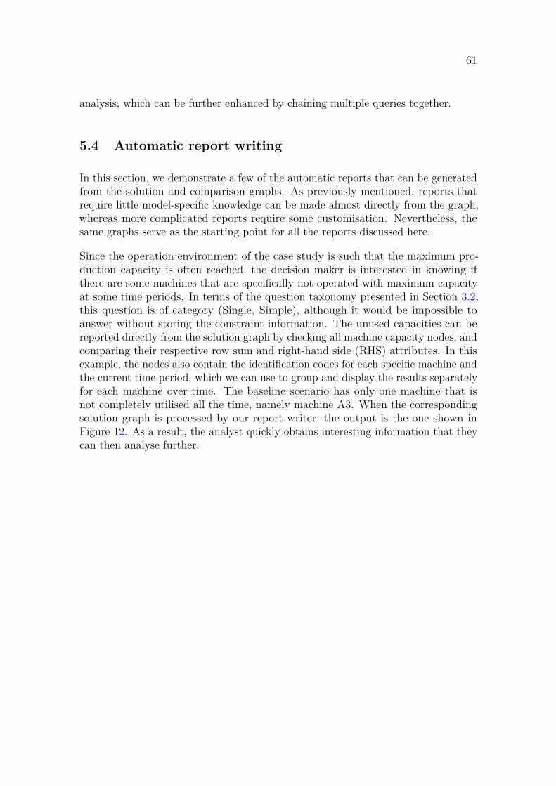
61

analysis, which can be further enhanced by chaining multiple queries together.

5.4 Automatic report writing

In this section, we demonstrate a few of the automatic reports that can be generatedfrom the solution and comparison graphs. As previously mentioned, reports thatrequire little model-specific knowledge can be made almost directly from the graph,whereas more complicated reports require some customisation. Nevertheless, thesame graphs serve as the starting point for all the reports discussed here.

Since the operation environment of the case study is such that the maximum pro-duction capacity is often reached, the decision maker is interested in knowing ifthere are some machines that are specifically not operated with maximum capacityat some time periods. In terms of the question taxonomy presented in Section 3.2,this question is of category (Single, Simple), although it would be impossible toanswer without storing the constraint information. The unused capacities can bereported directly from the solution graph by checking all machine capacity nodes, andcomparing their respective row sum and right-hand side (RHS) attributes. In thisexample, the nodes also contain the identification codes for each specific machine andthe current time period, which we can use to group and display the results separatelyfor each machine over time. The baseline scenario has only one machine that isnot completely utilised all the time, namely machine A3. When the correspondingsolution graph is processed by our report writer, the output is the one shown inFigure 12. As a result, the analyst quickly obtains interesting information that theycan then analyse further.

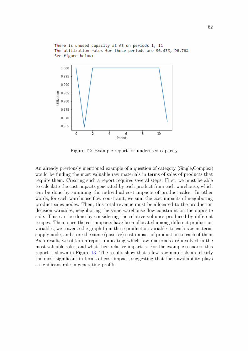
62

Figure 12: Example report for underused capacity

An already previously mentioned example of a question of category (Single,Complex)would be finding the most valuable raw materials in terms of sales of products thatrequire them. Creating such a report requires several steps: First, we must be ableto calculate the cost impacts generated by each product from each warehouse, whichcan be done by summing the individual cost impacts of product sales. In otherwords, for each warehouse flow constraint, we sum the cost impacts of neighboringproduct sales nodes. Then, this total revenue must be allocated to the productiondecision variables, neighboring the same warehouse flow constraint on the oppositeside. This can be done by considering the relative volumes produced by differentrecipes. Then, once the cost impacts have been allocated among different productionvariables, we traverse the graph from these production variables to each raw materialsupply node, and store the same (positive) cost impact of production to each of them.As a result, we obtain a report indicating which raw materials are involved in themost valuable sales, and what their relative impact is. For the example scenario, thisreport is shown in Figure 13. The results show that a few raw materials are clearlythe most significant in terms of cost impact, suggesting that their availability playsa significant role in generating profits.

63

Figure 13: Example report for critical raw materials

For the scenario comparison case, we present an example of applying the substitutiondetection algorithm to two scenarios, where in the second scenario the currency ratebetween two major operating currencies has changed significantly. Here, the decisionmaker wants to find out what kind of production or customer demand switchesare caused by this change. This is a special example of a question of category(Two,Complex) in our question taxonomy in Section 3.2. We focus on the decisionvariable nodes that quantify the amount of demand satisfied for each product andcustomer from each warehouse (X). This analysis could focus on either costs orvolumes, but since in this case the costs are largely affected by the currency ratechange, we are more interested in how the actual volumes would change. We firstattempt to find substitutions on the highest hierarchical level: This means findingpotential substitutions on a regional and product family level, between the differentwarehouses. As a result, we obtain the a list of potential substitutions, which isshown in Figure 14.

In this specific case, the analyst can immediately notice that some significant changes

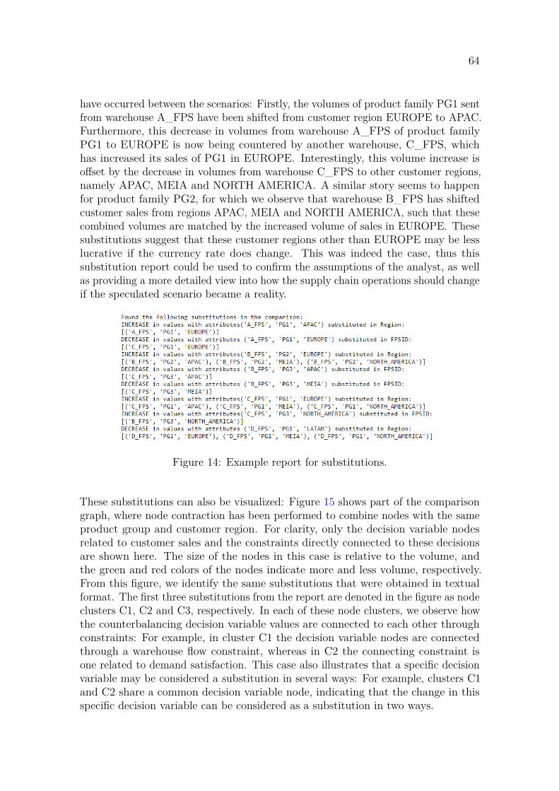
64

have occurred between the scenarios: Firstly, the volumes of product family PG1 sentfrom warehouse A_FPS have been shifted from customer region EUROPE to APAC.Furthermore, this decrease in volumes from warehouse A_FPS of product familyPG1 to EUROPE is now being countered by another warehouse, C_FPS, whichhas increased its sales of PG1 in EUROPE. Interestingly, this volume increase isoffset by the decrease in volumes from warehouse C_FPS to other customer regions,namely APAC, MEIA and NORTH AMERICA. A similar story seems to happenfor product family PG2, for which we observe that warehouse B_FPS has shiftedcustomer sales from regions APAC, MEIA and NORTH AMERICA, such that thesecombined volumes are matched by the increased volume of sales in EUROPE. Thesesubstitutions suggest that these customer regions other than EUROPE may be lesslucrative if the currency rate does change. This was indeed the case, thus thissubstitution report could be used to confirm the assumptions of the analyst, as wellas providing a more detailed view into how the supply chain operations should changeif the speculated scenario became a reality.

Figure 14: Example report for substitutions.

These substitutions can also be visualized: Figure 15 shows part of the comparisongraph, where node contraction has been performed to combine nodes with the sameproduct group and customer region. For clarity, only the decision variable nodesrelated to customer sales and the constraints directly connected to these decisionsare shown here. The size of the nodes in this case is relative to the volume, andthe green and red colors of the nodes indicate more and less volume, respectively.From this figure, we identify the same substitutions that were obtained in textualformat. The first three substitutions from the report are denoted in the figure as nodeclusters C1, C2 and C3, respectively. In each of these node clusters, we observe howthe counterbalancing decision variable values are connected to each other throughconstraints: For example, in cluster C1 the decision variable nodes are connectedthrough a warehouse flow constraint, whereas in C2 the connecting constraint isone related to demand satisfaction. This case also illustrates that a specific decisionvariable may be considered a substitution in several ways: For example, clusters C1and C2 share a common decision variable node, indicating that the change in thisspecific decision variable can be considered as a substitution in two ways.

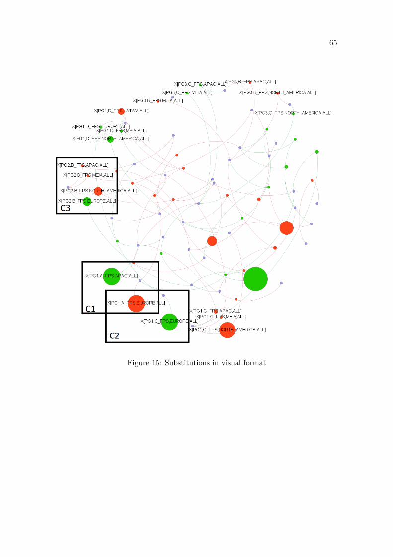
65

Figure 15: Substitutions in visual format

66

6 Conclusions and further developments

This Thesis explores the potential of providing semi-automated assistance in supplychain planning problems by creating an Intelligent Mathematical ProgrammingSystem (IMPS) to aid the analyst. The approach is based on using the underlyingmathematical model as the primary driver for the analysis by translating it to a graph,in addition to the actual optimisation results. This differs from other traditionalapproaches, where the structure of the model is not explicitly used as a tool foranalysis. We refer to this methodology as the model oriented approach.

The presented algorithm for creating a graph out of a single LP model solution isbased on an extension of the fundamental digraph described by Greenberg (1983) andin this Thesis, it was further extended to the case where two separate model scenariosare compared by creating a special comparison graph out of individual model graphs.This comparison graph algorithm allows analysis of both simple parameter-based andmore complex model structure-based changes. In addition to technical details of theapproach, we explored some potential uses by considering different types of questionsdecisions makers may have related to the supply chain. The main objective was toexplore how the approach could help an analyst answer such questions. Potentialuses included visual network analysis of scenarios, automatic report writing, andstoring the graph into a graph database, which the analyst can use for ad hoc orstructured graph queries.

Based on the initial results of the case study and discussions with the case companyexperts, at least some of the business questions related to the supply chain aredirectly related to the underlying model structure. These questions include findingconnections between various entities of the supply chain, and they can extendthrough the entire chain from suppliers to final customers. In these cases, the modeloriented approach is a potential alternative to the traditional approaches, since themodel oriented approach maintains the connections between model entities. TheThesis classified typical business questions in Section 3, and most of the questionsconsidered in the case study belong to the "complex" category considering either oneor two scenarios. While the distinction between "simple" and "complex" questions isdebatable and the amount of interesting questions in our case study is limited, thefew successes nevertheless demonstrate the values of the proposed approach. It isalso clear that from the case company experts’ perspective that the model orientedapproach is not a substitute to the traditional results oriented approach, but rathera complementary one.

There are challenges related to the proposed approach: for example, visual analysisbecomes computationally challenging for large problems with millions of decisionvariables. Also, the effectiveness of querying the graph database relies heavily onthe analyst’s ability to translate the business questions into the appropriate modelcomponents and their relationships, as there is no automated process in place thatwould automatically select only the relevant parts of the model into the query.

67

Furthermore, these queries still require the user to understand the model structurequite extensively, therefore limiting the usability of the system. These problems canbe somewhat alleviated by manipulating the directions of links between nodes tomatch the direction of physical flows in the supply chain, but this again requiresmodel expertise. Finally, the automatic reports that can be written with the currentsystem are very limited in their functionality, as there were few simple reports thatwere seen as both i) useful in a practical setting, and ii) where the implementationwith the model oriented approach was considered to be easier than other approaches.Our aim was not to recreate the capabilities already offered by spreadsheets or BIplatforms, but rather try to explore some previously unutilised methods of reportingmodel results. More complex automated reports may require a more model-specificapproach.

While our approach is quite general and easily applicable to different types of supplychain optimisation models, and theoretically to any LP model, making conclusionson the benefits offered by the system requires more use cases. It also remains to beseen how general this kind of tool can be: the less individual model-specific detailsand quirks can be accounted for, the more limited is the depth of analysis. The lackof a unifying framework between the different suggested forms of scenario analysis,supply chain optimisation models and various business questions is also evidentthroughout the Thesis: almost all choices and methodologies are motivated throughspecific examples instead of attempting to explain them more generally.

6.1 Future research directions

In addition to abovementioned further testing of the IMPS, the approach couldbe developed further from its theoretical foundations, too. First, none of the corecomponents of the IMPS specifically utilise graph-theoretic results. Here, boththe network visualisation and some presented and new algorithms could potentiallybenefit from existing advances in graph theory. Examples include finding specificgraph structures and interpreting them; generating richer automated textual reportsthat follow "paths" or exploit the graph structures in some other way; making thepresented substitution algorithm smarter by allowing more complex comparisons orby grouping similar substitutions together.

Regarding the structure of comparison graphs, it would be beneficial to somehow beable to estimate which changes are most strongly related to each other. Currently, itremains unclear whether specific changes in the optimal solution between scenarioscan be attributed to some small subset of other changes, or if the changes must alwaysbe considered as a whole. As there is often a large amount of individual changes thatresult from even a few parameter changes between scenarios, the ability to clusterrelated changes together, instead of having to consider them on an individual level,could provide significant improvements on the current analysis capabilities. As aprerequisite, this would require us to find an appropriate measure for "relatedness"

68

between different nodes in the context of the comparison graph. One simple candidatewould be to measure the distance between different nodes as the shortest path ofundirected links between them. Intuitively, it would make sense that the shorter thispath between two nodes, the more likely it is that they are related: Consider, forexample, changes in production quantity decision variables that are neighbors to thesame capacity constraint. While this approach seems reasonable at first, it wouldneglect the possibility of significant interaction between entities that are more distantfrom each other. This is an undesirable result, as many of the examples presentedin this Thesis already show that such distant interactions do exist. Therefore, webelieve more appropriate measures for node relatedness need to be developed.

The aggregation of graphs is another interesting subject where further study couldprovide a more robust method of simplifying the often large solution and comparisongraphs that are created from optimisation models. The main concerns here arenot related to practicalities, as we managed to describe a procedure that couldbe applied to produce such aggregated graphs. Rather, it is their interpretabilitythat is still unclear: For instance, what exactly do the aggregate nodes and edgesrepresent in general, or must these always be interpreted in the specific contextof the underlying mathematical model? Moreover, can we define an appropriateaggregation function for all types of attributes, such that all the resulting aggregatevalues have a meaningful interpretation?

In terms of model analysis, the main focus of this Thesis was in considering one ortwo scenarios at a time, thus adopting the deductive model analysis paradigm similarto the one in systems such as Greenberg’s ANALYZE. The alternative paradigmthat we shortly described in Section 2 is inductive model analysis, where a largenumber of scenarios is processed to increase understanding of model relationships.While the obvious drawback of such an approach is that it requires more modelruns, there are potential benefits over the deductive paradigm as well. First andforemost, an inductive approach could allow us to create a metamodel on top of theoriginal optimisation model, which could then be used to explain how different modelparameters affect the solution, ideally enabling the analysis of both individual andmultiple scenarios. Since many of the decision makers’ complex questions can betranslated to finding and understanding the causal relationships between differententities of the modelled system, it is clear why such a metamodel could be a usefultool for the analyst. There are multiple methods with which such metamodels couldbe created: For example, the use of neural networks, a field with much ongoingresearch, was considered much earlier as a tool for inductive learning of mathematicalmodels for example by Steiger and Sharda (1996). It would be interesting to see ifsome of the recent advances in this field could be transferred to the field of modelanalysis.

69

ReferencesM. Bastian, S. Heymann, and M. Jacomy. Gephi: An open source software for

exploring and manipulating networks. In International AAAI Conference on Weband Social Media, 2009. URL https://www.aaai.org/ocs/index.php/ICWSM/09/paper/view/154/1009.

D. Bertsimas and J. Tsitsiklis. Introduction to Linear Optimization. AthenaScientific, 1st edition, 1997. ISBN 1886529191.

S. Bradley, A. Hax, and T. Magnanti. Applied Mathematical Programming. Addison-Wesley Publishing Company, 1977.

R. Diestel. Graph Theory, volume 173 of Graduate Texts in Mathematics. Springer-Verlag, 5th edition, August 2016.

B. Fleischmann. Distribution and transport planning. In H. Stadtler andC. Kilger, editors, Supply Chain Management and Advanced Planning, pages195–210. Springer, Berlin, Heidelberg, 2nd edition, 2002. ISBN 978-3-662-10142-1. doi: 10.1007/978-3-662-10142-1_12. URL https://doi.org/10.1007/978-3-662-10142-1_12.

A. Geoffrion. The purpose of mathematical programming is insight, not numbers.Interfaces, 7(1):81–92, November 1976.

M. Goetschalckx. Strategic network planning. In H. Stadtler and C. Kilger, editors,Supply Chain Management and Advanced Planning, pages 105–121. Springer,Berlin, Heidelberg, 2nd edition, 2002. ISBN 978-3-662-10142-1. doi: 10.1007/978-3-662-10142-1_7. URL https://doi.org/10.1007/978-3-662-10142-1_7.

H. Greenberg. A functional description of analyze: A computer-assisted analysissystem for linear programming models. ACM Transactions on MathematicalSoftware, 9(1):18–56, March 1983.

H. Greenberg and J. Chinneck. Intelligent mathematical programming software:Past, present and future. INFORMS Computing Society Newsletter, 20(1):1,4–9,Spring 1999.

T. Grossman. A primer on spreadsheet analytics. In EuSpRIG: In Pursuit ofSpreadsheet Excellence, pages 129–140. European Spreadsheet Risks Interest Group,2008. ISBN 978-905617-69-2. URL http://arxiv.org/abs/0809.3586.

A. Janvier-James. A new introduction to supply chains and supply chain management:Definitions and theories perspective. International Business Research, 5(1):194–207, January 2012.

J. Keisler and P. Noonan. Communicating analytic results: A tutorial for decisionconsultants. Decision Analysis, 9(3):274–292, 2012. doi: 10.1287/deca.1120.0238.URL https://doi.org/10.1287/deca.1120.0238.

70

L. LeBlanc and M. Galbreth. Implementing large-scale optimization models in excelusing vba. Interfaces, 37(4):370–382, 2007. ISSN 00922102, 1526551X. URLhttp://www.jstor.org/stable/20141515.

T. Miller. Hierarchical Operations and Supply Chain Planning. Springer, London,2002. ISBN 978-1-4471-1110-8. doi: 10.1007/978-1-4471-0305-9. URL https://doi.org/10.1007/978-1-4471-0305-9.

T. Miller. A hierarchical supply chain planning approach, business briefing. Globalpurchasing & Supply Chain Strategies, pages 42–57, January 2004.

S. Pemmaraju and S. Skiena. Computational Discrete Mathematics: Combinatoricsand Graph Theory with Mathematica. Cambridge University Press, 2003.

D. Power and R. Sharda. Model-driven decision support systems: Concepts andresearch directions. Decision support systems, 43:1044–1061, April 2007.

Cambridge University Press. Cambridge business English dictionary. CambridgeUniversity Press, 2011.

J. Rohde and M. Wagner. Master planning. In H. Stadtler and C. Kilger, editors,Supply Chain Management and Advanced Planning, pages 143–160. Springer,Berlin, Heidelberg, 2nd edition, 2002. ISBN 978-3-662-10142-1. doi: 10.1007/978-3-662-10142-1_9. URL https://doi.org/10.1007/978-3-662-10142-1_9.

M. Rönnqvist, S. D’Amours, A. Weintraub, A. Jofre, E. Gunn, R. Haight, D. Martell,A. Murray, and C. Romero. Operations research challenges in forestry: 33 openproblems. Annals of Operations Research, 232(1):11–40, September 2015. ISSN1572-9338. doi: 10.1007/s10479-015-1907-4. URL https://doi.org/10.1007/s10479-015-1907-4.

T. Seeve. A structured method for identifying and visualizing scenarios. Master’sthesis, Aalto University School of Science, 2018.

H. Stadtler. Production planning and scheduling. In H. Stadtler and C. Kil-ger, editors, Supply Chain Management and Advanced Planning, pages 177–193. Springer, Berlin, Heidelberg, 2nd edition, 2002a. ISBN 978-3-662-10142-1. doi: 10.1007/978-3-662-10142-1_11. URL https://doi.org/10.1007/978-3-662-10142-1_11.

H. Stadtler. Linear and mixed integer programming. In H. Stadtler andC. Kilger, editors, Supply Chain Management and Advanced Planning, pages391–401. Springer, Berlin, Heidelberg, 2nd edition, 2002b. ISBN 978-3-662-10142-1. doi: 10.1007/978-3-662-10142-1_25. URL https://doi.org/10.1007/978-3-662-10142-1_25.

H. Stadtler. Supply chain management and advanced planning - basics, overviewand challenges. European Journal of Operational Research, 163(3):575–588, June2005.

71

D. Steiger. Enhancing user understanding in a decision support system: A theoreticalbasis and framework. Journal of Management Information Systems, 15(2):199–220,1998.

D. Steiger and R. Sharda. Analyzing mathematical models with inductive learningnetworks. European Journal of Operational Research, 93(2):387–401, September1996.

P. Trkman, M. Stemberger, and J. Jaklič. Information transfer in supply chainmanagement. Issues in Informing Science and Information Technology, 2, January2005. doi: 10.28945/851.

A. Weintraub, S. D’Amours, and M. Rönnqvist. Using operational research for supplychain planning in the forest products industry. INFOR: Information Systems andOperational Research, 46, November 2008. doi: 10.3138/infor.46.4.265.

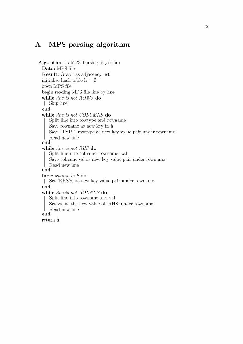
72

A MPS parsing algorithm

Algorithm 1: MPS Parsing algorithmData: MPS fileResult: Graph as adjacency listinitialise hash table h = ∅open MPS filebegin reading MPS file line by linewhile line is not ROWS do

Skip lineendwhile line is not COLUMNS do

Split line into rowtype and rownameSave rowname as new key in hSave ’TYPE’:rowtype as new key-value pair under rownameRead new line

endwhile line is not RHS do

Split line into colname, rowname, valSave colname:val as new key-value pair under rownameRead new line

endfor rowname in h do

Set ’RHS’:0 as new key-value pair under rownameendwhile line is not BOUNDS do

Split line into rowname and valSet val as the new value of ’RHS’ under rownameRead new line

endreturn h

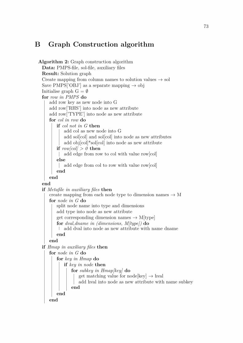
73

B Graph Construction algorithm

Algorithm 2: Graph construction algorithmData: PMPS-file, sol-file, auxiliary filesResult: Solution graphCreate mapping from column names to solution values → solSave PMPS[’OBJ’] as a separate mapping → objInitialise graph G = ∅for row in PMPS do

add row key as new node into Gadd row[’RHS’] into node as new attributeadd row[’TYPE’] into node as new attributefor col in row do

if col not in G thenadd col as new node into Gadd sol[col] and sol[col] into node as new attributesadd obj[col]*sol[col] into node as new attribute

if row[col] > 0 thenadd edge from row to col with value row[col]

elseadd edge from col to row with value row[col]

endend

endif Metafile in auxiliary files then

create mapping from each node type to dimension names → Mfor node in G do

split node name into type and dimensionsadd type into node as new attributeget corresponding dimension names → M[type]for dval,dname in (dimensions, M[type]) do

add dval into node as new attribute with name dnameend

endif Hmap in auxiliary files then

for node in G dofor key in Hmap do

if key in node thenfor subkey in Hmap[key] do

get matching value for node[key] → hvaladd hval into node as new attribute with name subkey

endend

end

74

if virtcons in auxiliary files thenfor node in G do

if node[type] in virtcons thenget neighboring edges of node → eG

for edge in eG doadd label ’Virtual’ into edge as new attribute

endendreturn G

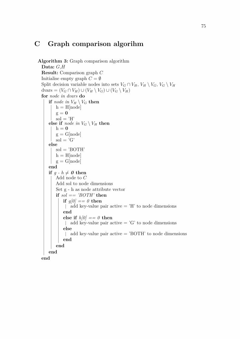
75

C Graph comparison algorihm

Algorithm 3: Graph comparison algorithmData: G,HResult: Comparison graph CInitialise empty graph C = ∅Split decision variable nodes into sets VG ∩ VH , VH \ VG, VG \ VH

dvars = (VG ∩ VH) ∪ (VH \ VG) ∪ (VG \ VH)for node in dvars do

if node in VH \ VG thenh = H[node]g = 0sol = ’H’

else if node in VG \ VH thenh = 0g = G[node]sol = ’G’

elsesol = ’BOTH’h = H[node]g = G[node]

endif g - h = 0 then

Add node to CAdd sol to node dimensionsSet g - h as node attribute vectorif sol == ’BOTH’ then

if g[0] == 0 thenadd key-value pair active = ’H’ to node dimensions

endelse if h[0] == 0 then

add key-value pair active = ’G’ to node dimensionselse

add key-value pair active = ’BOTH’ to node dimensionsend

endend

end

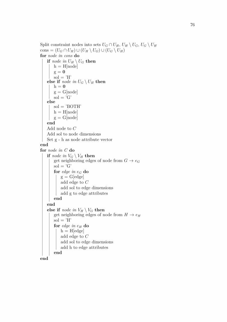
76

Split constraint nodes into sets UG ∩ UH , UH \ UG, UG \ UH

cons = (UG ∩ UH) ∪ (UH \ UG) ∪ (UG \ UH)for node in cons do

if node in UH \ UG thenh = H[node]g = 0sol = ’H’

else if node in UG \ UH thenh = 0g = G[node]sol = ’G’

elsesol = ’BOTH’h = H[node]g = G[node]

endAdd node to CAdd sol to node dimensionsSet g - h as node attribute vector

endfor node in C do

if node in VG \ VH thenget neighboring edges of node from G → eG

sol = ’G’for edge in eG do

g = G[edge]add edge to Cadd sol to edge dimensionsadd g to edge attributes

endendelse if node in VH \ VG then

get neighboring edges of node from H → eH

sol = ’H’for edge in eH do

h = H[edge]add edge to Cadd sol to edge dimensionsadd h to edge attributes

endend

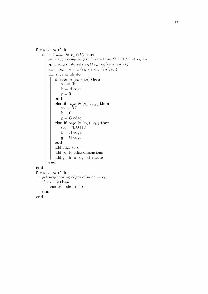
77

for node in C doelse if node in VG ∩ VH then

get neighboring edges of node from G and H, → eG,eH

split edges into sets eG ∩ eH , eG \ eH , eH \ eG

all = (eG ∩ eH) ∪ (eH \ eG) ∪ (eG \ eH)for edge in all do

if edge in (eH \ eG) thensol = ’H’h = H[edge]g = 0

endelse if edge in (eG \ eH) then

sol = ’G’h = 0g = G[edge]

else if edge in (eG ∩ eH) thensol = ’BOTH’h = H[edge]g = G[edge]

endadd edge to Cadd sol to edge dimensionsadd g - h to edge attributes

endendfor node in C do

get neighboring edges of node → eC

if eC = ∅ thenremove node from C

endend

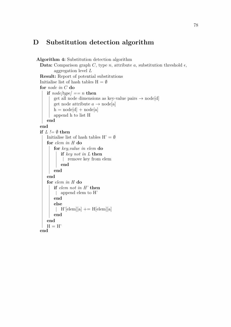
78

D Substitution detection algorithm

Algorithm 4: Substitution detection algorithmData: Comparison graph C, type n, attribute a, substitution threshold ϵ,

aggregation level LResult: Report of potential substitutionsInitialise list of hash tables H = ∅for node in C do

if node[type] == n thenget all node dimensions as key-value pairs → node[d]get node attribute a → node[a]h = node[d] + node[a]append h to list H

endendif L != ∅ then

Initialise list of hash tables H’ = ∅for elem in H do

for key,value in elem doif key not in L then

remove key from elemend

endendfor elem in H do

if elem not in H’ thenappend elem to H’

endelse

H’[elem][a] += H[elem][a]end

endH = H’

end

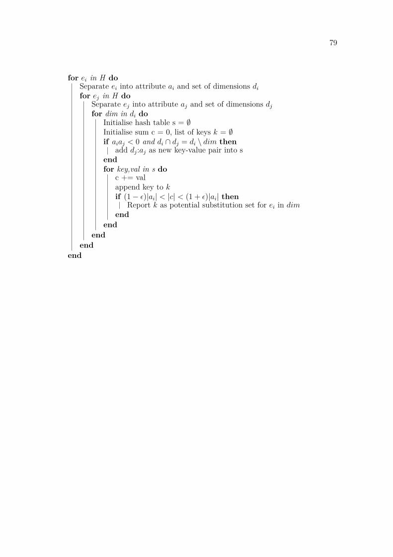
79

for ei in H doSeparate ei into attribute ai and set of dimensions di

for ej in H doSeparate ej into attribute aj and set of dimensions dj

for dim in di doInitialise hash table s = ∅Initialise sum c = 0, list of keys k = ∅if aiaj < 0 and di ∩ dj = di \ dim then

add dj:aj as new key-value pair into sendfor key,val in s do

c += valappend key to kif (1 − ϵ)|ai| < |c| < (1 + ϵ)|ai| then

Report k as potential substitution set for ei in dimend

endend

endend