
BIANCA, A Genetic Algorithm for Engineering Optimisation
88
HAL Id: hal-00767468 https://hal.archives-ouvertes.fr/hal-00767468 Preprint submitted on 19 Dec 2012 HAL is a multi-disciplinary open access archive for the deposit and dissemination of sci- entific research documents, whether they are pub- lished or not. The documents may come from teaching and research institutions in France or abroad, or from public or private research centers. L’archive ouverte pluridisciplinaire HAL, est destinée au dépôt et à la diffusion de documents scientifiques de niveau recherche, publiés ou non, émanant des établissements d’enseignement et de recherche français ou étrangers, des laboratoires publics ou privés. BIANCA, A Genetic Algorithm for Engineering Optimisation - User guide Marco Montemurro, Paolo Vannucci, Angela Vincenti To cite this version: Marco Montemurro, Paolo Vannucci, Angela Vincenti. BIANCA, A Genetic Algorithm for Engineering Optimisation - User guide. 2011. hal-00767468
-
Upload
khangminh22 -
Category
Documents
-
view
3 -
download
0
Transcript of BIANCA, A Genetic Algorithm for Engineering Optimisation

HAL Id: hal-00767468https://hal.archives-ouvertes.fr/hal-00767468
Preprint submitted on 19 Dec 2012
HAL is a multi-disciplinary open accessarchive for the deposit and dissemination of sci-entific research documents, whether they are pub-lished or not. The documents may come fromteaching and research institutions in France orabroad, or from public or private research centers.
L’archive ouverte pluridisciplinaire HAL, estdestinée au dépôt et à la diffusion de documentsscientifiques de niveau recherche, publiés ou non,émanant des établissements d’enseignement et derecherche français ou étrangers, des laboratoirespublics ou privés.
BIANCA, A Genetic Algorithm for EngineeringOptimisation - User guide
Marco Montemurro, Paolo Vannucci, Angela Vincenti
To cite this version:Marco Montemurro, Paolo Vannucci, Angela Vincenti. BIANCA, A Genetic Algorithm for EngineeringOptimisation - User guide. 2011. �hal-00767468�

BIANCA, A Genetic Algorithm forEngineering Optimisation
Version 3.1 User’s guide
M. MontemurroInstitut d’Alembert UMR7190 CNRS -Universite Pierre et Marie Curie Paris 6,
Case 162, 4, Place Jussieu, 75252 Paris Cedex 05, France.
P. VannucciUniversite de Versailles et St Quentin,
45 Avenue des Etats-Unis, 78035 Versailles, France and
Institut d’Alembert UMR7190 CNRS -Universite Pierre et Marie Curie Paris 6,
Case 162, 4, Place Jussieu, 75252 Paris Cedex 05, France.
A. Vincenti
Institut d’Alembert UMR7190 CNRS - Universite Pierre et Marie Curie Paris 6,
Case 162, 4, Place Jussieu, 75252 Paris Cedex 05, France.

2

Contents
1 Introduction to BIANCA 51.1 Capabilities of BIANCA . . . . . . . . . . . . . . . . . . . . . 51.2 Background and mathematical formulations . . . . . . . . . . 61.3 General features of BIANCA . . . . . . . . . . . . . . . . . . . 81.4 The structure of the individual’s genotype . . . . . . . . . . . 111.5 Encoding/decoding of the variables . . . . . . . . . . . . . . . 12
2 BIANCA tutorial 152.1 Compiling BIANCA . . . . . . . . . . . . . . . . . . . . . . . 152.2 Running BIANCA . . . . . . . . . . . . . . . . . . . . . . . . 152.3 Inputs to BIANCA . . . . . . . . . . . . . . . . . . . . . . . . 16
2.3.1 Genetic parameters . . . . . . . . . . . . . . . . . . . . 162.3.2 Optimisation parameters . . . . . . . . . . . . . . . . . 182.3.3 The library.inp file . . . . . . . . . . . . . . . . . . . . 242.3.4 The post processing.inp file . . . . . . . . . . . . . . . . 28
2.4 Outputs from BIANCA . . . . . . . . . . . . . . . . . . . . . . 302.4.1 The .bio output file . . . . . . . . . . . . . . . . . . . . 302.4.2 The .pop output file . . . . . . . . . . . . . . . . . . . 312.4.3 The .sta output file . . . . . . . . . . . . . . . . . . . . 33
2.5 The macro MACRO MY PROBLEM.f95 . . . . . . . . . . . . . 342.5.1 The my problem subroutine . . . . . . . . . . . . . . . 352.5.2 The my problem var subroutine . . . . . . . . . . . . . 36
2.6 Structure of the interface with external codes in BIANCA . . 372.6.1 The input file from BIANCA to the external code . . . 382.6.2 The output file from the external code to BIANCA . . 41
3 Examples 453.1 Test function example . . . . . . . . . . . . . . . . . . . . . . 453.2 Library function example . . . . . . . . . . . . . . . . . . . . . 51
3.2.1 Fixed number of chromosomes/plies . . . . . . . . . . . 513.2.2 Variable number of chromosomes/plies . . . . . . . . . 56
3

4 CONTENTS
3.3 User-defined model example . . . . . . . . . . . . . . . . . . . 613.4 Example of interface with MATLAB R© code . . . . . . . . . . 683.5 Example of interface with ANSYS R© code . . . . . . . . . . . 743.6 Example of interface with ABAQUS R© code . . . . . . . . . . 803.7 Example of interface with CAST3M R© code . . . . . . . . . . 85
Bibliography 86
Chapter 1
Introduction to BIANCA
1.1 Capabilities of BIANCA
The genetic algorithm (GA) BIANCA 3.1 is a multi-population GA able todeal and solve constrained and unconstrained hard combinatorial optimisa-tion problems in engineering. The effectiveness and robustness of BIANCAreside upon the generality and richness in the representation of the informa-tion, and on the way the information is extensively exploited during geneticoperations. For more details see [1, 2].
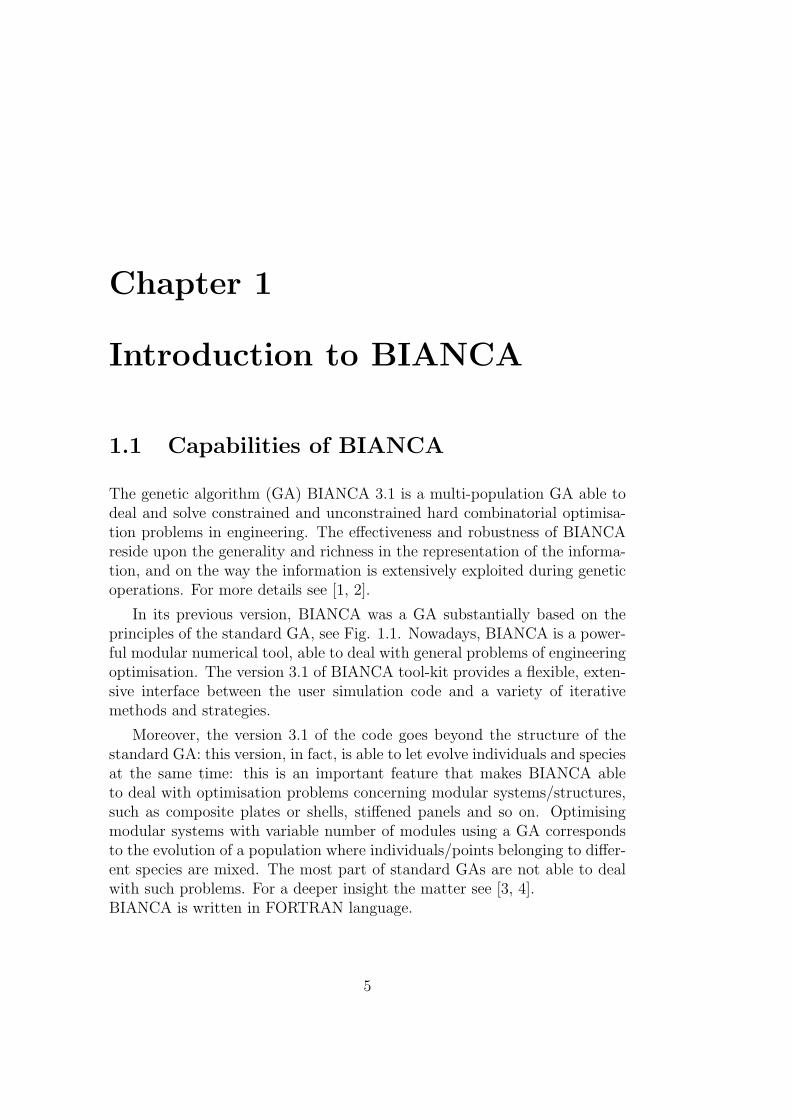
In its previous version, BIANCA was a GA substantially based on theprinciples of the standard GA, see Fig. 1.1. Nowadays, BIANCA is a power-ful modular numerical tool, able to deal with general problems of engineeringoptimisation. The version 3.1 of BIANCA tool-kit provides a flexible, exten-sive interface between the user simulation code and a variety of iterativemethods and strategies.
Moreover, the version 3.1 of the code goes beyond the structure of thestandard GA: this version, in fact, is able to let evolve individuals and speciesat the same time: this is an important feature that makes BIANCA ableto deal with optimisation problems concerning modular systems/structures,such as composite plates or shells, stiffened panels and so on. Optimisingmodular systems with variable number of modules using a GA correspondsto the evolution of a population where individuals/points belonging to differ-ent species are mixed. The most part of standard GAs are not able to dealwith such problems. For a deeper insight the matter see [3, 4].BIANCA is written in FORTRAN language.
5
6 CHAPTER 1. INTRODUCTION TO BIANCA
Figure 1.1: Standard GA’s scheme.
1.2 Background and mathematical formula-
tions
A general optimization problem is formulated as follows:
minx
f (x)
subject to :
gi (x) ≤ 0 i = 1, ..., rhj (x) = 0 j = 1, ...,m
xL ≤ x ≤ xU
(1.1)
where vectors and matrix terms are marked in bold typeface. In this formu-lation x is the n-dimensional vector of design variables, while xL and xU arethe n-dimensional vectors representing the lower and upper bounds of thedesign variables, i.e. the design space. Design variables can be of differenttype: continuous, regular discrete, scattered discrete or grouped.The optimisation goal is to minimize the objective function f (x) subject toa given number of constraints: gi (x) is the r-dimensional vector of inequalityconstraints, while hj (x) is the m-dimensional vector of equality constraints.
The optimization problem type can be characterized both by the typesof constraints present in the problem and by the linearity or non-linearityof the objective and constraint functions. A problem where at least some ofthe objective and constraint functions are non-linear is called a non-linearprogramming (NLPP) problem. These NLPP problems predominate in en-gineering applications and are the primary focus of BIANCA 3.0.
In BIANCA the equality and inequality constraints are treated by meansof a particular strategy which is based on the combination between classi-
1.2. BACKGROUND AND MATHEMATICAL FORMULATIONS 7
cal penalisation methods and the exploitation of the distributed informationover the population along the generations. The name of this technique isADP, which stands for Automatic Dynamic Penalisation.Classical penalisation methods transform Eq.(1.1) into an unconstrained op-timisation problem through the definition of a new modified objective func-tion F (x):
minx
F (x)
F (x) =
f (x) if gk (x) ≤ 0 k = 1, ..., r
and hj (x) = 0 j = 1, ...,m
f (x) +r∑
k=1
ckGk (x) +m∑
j=1
rjHj (x) if gk (x) > 0 k = 1, ..., r
and hj (x) 6= 0 j = 1, ...,m
(1.2)In Eq.(1.2) ck and rj are the penalisation coefficients for inequality and equal-ity constraints respectively. The quantities Gk (x) and Hj (x) are defined as:
Gk (x) = max [0, gk (x)] k = 1, ..., r
Hj (x) = max [0, | hj (x) | − ǫ] j = 1, ...,m(1.3)
In Eq.(1.2) and (1.3) the equality constraints have been transformed intoinequality constraints having the form | hj (x) |≤ ǫ. Concerning the param-eters ck and rj, in classical penalisation methods, the user must set theirvalues to an appropriate level in order to ensure the search of solutions forthe optimisation problem to be forced within the feasible domain. Neverthe-less, the choice of these coefficients is very difficult and it is common practiceto estimate their values by trial and error. Moreover, it could be useful to ad-just penalisation pressure along the generations by tuning these coefficients,but this is directly linked on a guess or on a deep knowledge of the nature ofthe optimisation problem by the user.
The idea of the ADP is that it is possible to exploit the information re-strained in the population, at the current generation, in order to guide thesearch in the case of constrained optimisation problem. Generally, in thefirst generation the population is generated randomly. With high probabil-ity the individuals are evenly distributed over both feasible and unfeasibledomain and the corresponding values of objective functions and constraintscan be used to estimate an appropriate level of penalisation, i.e. the valuesof penalisation coefficients ck and rj. At the current generation, inside thepopulation it is possible to separate feasible and unfeasible individuals and

8 CHAPTER 1. INTRODUCTION TO BIANCA
it is also possible classify each group in terms of increasing values of the ob-jective function or constraint violation. The first individual in each group isthe best candidate to be solution of the optimisation problem on the feasibleand unfeasible side of the domain, respectively. One possible definition ofthe penalisation coefficients is the follow:
ck (t) =| fbestF − fbest
NF |Gkbest
NFk = 1, ..., r
rj (t) =| fbestF − fbest
NF |Hjbest
NFj = 1, ...,m
(1.4)
In Eq.(1.4) the coefficients ck and rj are evaluated at the current generationt, while the apexes F and NF stand for feasible and non-feasible respectively.It is clear that the estimation of penalisation coefficients, according to theEq.(1.4), can be repeated at each generation, thus tuning the appropriatepenalisation pressure on the current population. The main advantages ofthis approach are substantially two: first of all this procedure is automaticbecause the GA can automatically calculate the values of the penalisationcoefficients, secondly the method is dynamic since the evaluation of the pe-nalisation level is updated at each generation.
1.3 General features of BIANCA
The version 3.1 of BIANCA shows several original features. As well as theprevious version, one of the main features is the decomposition of the GAin a certain number of macros : it is possible to assembly them in variousways in order to suit many different optimisation problems and also to testand compare the effectiveness of different numerical strategies. In this sense,BIANCA is a bunch of genetic tools which the user can use as bricks to buildup several GAs.
Another important feature of BIANCA is the representation of the infor-mation which is rich and detailed, but also non redundant. The biologicalmetaphor in GAs is a simple but powerful mean to return the richness andcompleteness of information linked to design variables. The information re-strained in the population along the generation is treated in a peculiar man-ner in such a way to allow a deep mixing of the individuals’ genotype bymeans of the reproduction operators, i.e. cross-over and mutation, which acton every single gene of the individuals. For a deep insight the matter see [2].
In order to allow the reproduction phase among individuals belonging todifferent species, in BIANCA 3.1 the structure of the individual and, con-

1.3. GENERAL FEATURES OF BIANCA 9
sequently, the representation of the information as well as the reproductionoperators of cross-over and mutation have been modified in order to dealwith the optimisation problem of modular systems. We have introduced newgenetic operators in BIANCA 3.1 for cross-over and mutation of individualsbelonging to different species.
BIANCA 3.1 has the following qualities:
• objective function evaluation: a library of functions corresponding toobjective and constraint functions of different optimisation problems,in addition in BIANCA the user can write its model by means of aspecial macro;
• fitness evaluation: several choices are available for fitness evaluationdepending on the kind of problem, i.e. minimisation or maximisation,and on the selection pressure that the user decides to introduce. Thefitness is evaluated in such a way that the fitness function can assumeall the possible values in the range [0 1];
• selection: two known techniques of selection are included, i.e. roulettewheel, tournament;
• standard genetic operators: the main genetic operators are cross-overand mutation, applying with a certain probability on each gene of theindividual’s genotype;
• additional genetic operators: elitism operator which preserve the bestindividual during each generation;
• handling constraints: automatic dynamic penalisation method for han-dling constraints;
• handling multiple populations: the need to simultaneously explore dif-ferent regions of the design space, as well as the search of optima re-sponding to distinct design criteria, led us to introduce the option ofworking with multiple populations in BIANCA. Moreover, a migrationoperator has been introduced in order to allow exchanges of informa-tions between populations evolving through parallel generations. Thismigration operator is the classical ring-type.
• stop criterion: maximum number of generations reached or test of con-vergence, i.e. no improvements of the mean fitness of the populationafter a given number of cycles.
10 CHAPTER 1. INTRODUCTION TO BIANCA
• new genetic operators: to deal with the problem which considers thenumber of variables among the optimisation variables, as in the case ofmodular systems, new genetic operators have been developed, such asthe chromosome shift operator, the chromosome reorder operator, thechromosome addition/deletion operator. These new operators modifythe reproduction phase allowing the reproduction among individuals ofdifferent species, see [3];
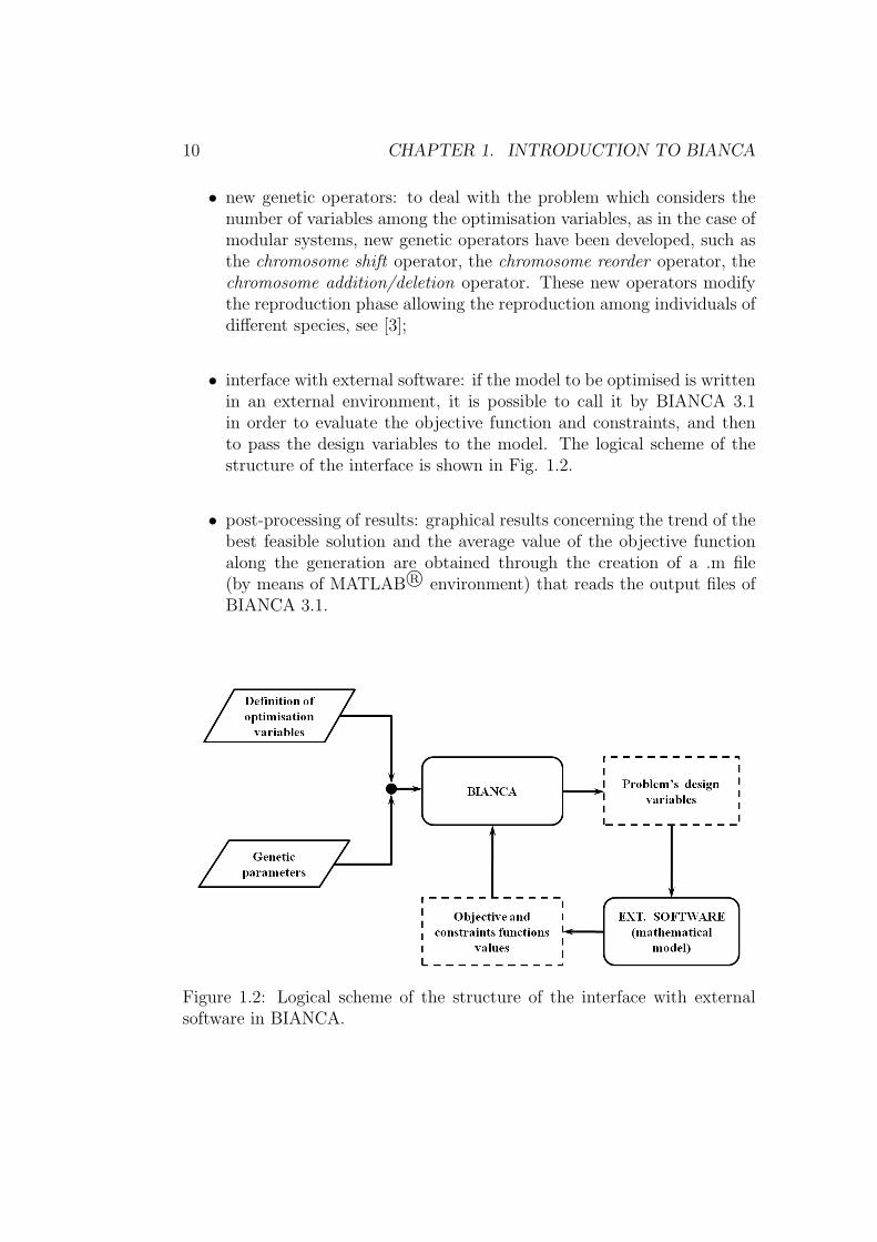
• interface with external software: if the model to be optimised is writtenin an external environment, it is possible to call it by BIANCA 3.1in order to evaluate the objective function and constraints, and thento pass the design variables to the model. The logical scheme of thestructure of the interface is shown in Fig. 1.2.
• post-processing of results: graphical results concerning the trend of thebest feasible solution and the average value of the objective functionalong the generation are obtained through the creation of a .m file(by means of MATLAB R© environment) that reads the output files ofBIANCA 3.1.
Figure 1.2: Logical scheme of the structure of the interface with externalsoftware in BIANCA.
1.4. THE STRUCTURE OF THE INDIVIDUAL’S GENOTYPE 11
1.4 The structure of the individual’s geno-
type
The biological metaphor in GAs is a simple but powerful mean to returnthe richness and completeness of information linked to design variables. Thenecessity to deal with any type of design variables, i.e. continuous, discrete,scattered led us to the choice of a discrete representation of the information.As explained in Sec. 1.5, it exits a two-way relation among the variablesand the pointers, i.e. integer numbers, which refer to the set of feasiblediscrete values for each variable. In a standard GA it is usual to encodeinteger values in the form of binary strings, in order to use the minimalistalphabet which increases the number of schemes, according to the theoremof the implicit parallelism that ensures improvement of the exploration of thedomain and exploitation of information [5, 6]. In addition the use of binaryrepresentation allows the use of binary cross-over and mutation which arevery effective when dealing with particular classes of optimisation problems.
In the previous version of BIANCA, an individual was represented byan array of dimensions nchrom × ngene. The number of rows, nchrom, is thenumber of chromosomes, while the number of columns, ngene, is the numberof genes. Basically, each design variable is coded in the form of a gene, andits meaning is linked both to the position and to the value of the gene withinthe chromosome. In principle, no limit is imposed on the number of genesand chromosomes for an individual in BIANCA. A number nind of individualscompose a population, and in BIANCA it is possible to work, at the sametime, with several populations whose number, npop, can be defined by theuser.
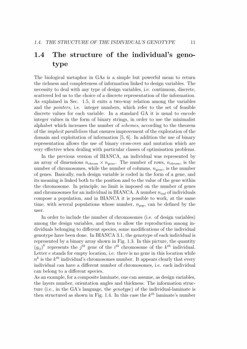
In order to include the number of chromosomes (i.e. of design variables)among the design variables, and then to allow the reproduction among in-dividuals belonging to different species, some modifications of the individualgenotype have been done. In BIANCA 3.1, the genotype of each individual isrepresented by a binary array shown in Fig. 1.3. In this picture, the quantity(gij)
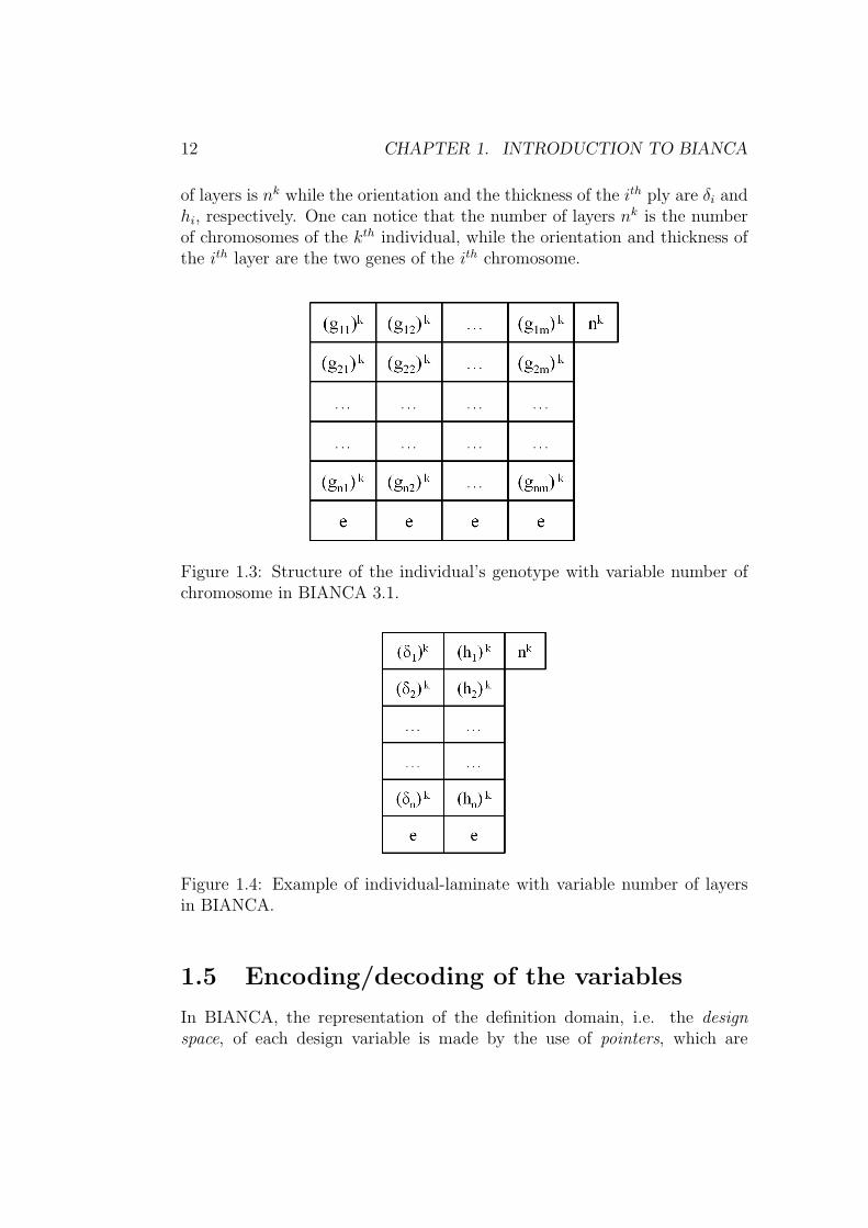
k represents the jth gene of the ith chromosome of the kth individual.Letter e stands for empty location, i.e. there is no gene in this location whilenk is the kth individual’s chromosomes number. It appears clearly that everyindividual can have a different number of chromosomes, i.e. each individualcan belong to a different species.As an example, for a composite laminate, one can assume, as design variables,the layers number, orientation angles and thickness. The information struc-ture (i.e., in the GA’s language, the genotype) of the individual-laminate isthen structured as shown in Fig. 1.4. In this case the kth laminate’s number
12 CHAPTER 1. INTRODUCTION TO BIANCA
of layers is nk while the orientation and the thickness of the ith ply are δi andhi, respectively. One can notice that the number of layers nk is the numberof chromosomes of the kth individual, while the orientation and thickness ofthe ith layer are the two genes of the ith chromosome.
Figure 1.3: Structure of the individual’s genotype with variable number ofchromosome in BIANCA 3.1.
Figure 1.4: Example of individual-laminate with variable number of layersin BIANCA.
1.5 Encoding/decoding of the variables
In BIANCA, the representation of the definition domain, i.e. the designspace, of each design variable is made by the use of pointers, which are

1.5. ENCODING/DECODING OF THE VARIABLES 13
themselves integer values. It exists a two-way relation between the variablesand the pointers. This relation is clear in the case of discrete or groupedvariables, in fact if the domain of definition have a finite dimension N , itis possible to enumerate all admissible values vi, (i = 1, ..., N) and build areference between each value vi and its index i, i.e. the pointer of that value.When the definition domain does not have finite dimension, it is necessary torestrict it, defining lower and upper bounds to the space of admissible valuesof vi, i.e. vmin and vmax respectively. In the case of continuous variables, thefirst step is the discretisation of the definition domain by choosing a givenprecision p, and then it is possible to apply the same system of referencingby pointers as for discrete and grouped variables, see Fig.1.5.
In BIANCA pointers constitute the genotype of the individual, more pre-cisely the single pointer corresponds to a gene, and all genetic operators aredirectly applied on the pointers representing the variables. Therefore, a stepof decoding/encoding is necessary to translate the value of the pointer intothe corresponding value of the design variable, and vice-versa. More detailscan be found in [1, 2].
Figure 1.5: Two-way relation between continuous variables and pointers inBIANCA.

14 CHAPTER 1. INTRODUCTION TO BIANCA
Chapter 2
BIANCA tutorial
2.1 Compiling BIANCA
The BIANCA batch file is named BIANCA 3.1.bat. You can compile BIANCAby a simple double click on this file. In the BIANCA 3.1 folder you musthave the following files:
• libBIANCA.a: this is a library of BIANCA macros containing all thesubroutines that BIANCA needs to run;
• MACRO MY PROBLEM.f95: this is the subroutine that you must useif you want to realise your model in FORTRAN environment as sub-routine of BIANCA. The structure of this macro is explained in Sec2.5.
After the compilation, the executable file BIANCAv3.1.exe is created.
2.2 Running BIANCA
The BIANCA executable file is named BIANCAv3.1.exe. You can run thecode in two different way:
• by double click on the icon BIANCAv3.1.exe;
• by entering the command BIANCAv3.1 in the command prompt, afteryou have specified the correct path for BIANCAv3.1.
In both case, after the run of BIANCA, the code requires the specificationof the name of the current job session. The choice of the job’s name iscompletely arbitrary, but it must observe the following condition: the name ofthe current job session must be the same as the two input files with extension.gen and .opt, described in the following section.
15

16 CHAPTER 2. BIANCA TUTORIAL
2.3 Inputs to BIANCA
There are two different kind of inputs for BIANCA. In particular, the maininputs of the code are written in two input files with extension .gen and .optrespectively. As explained beforehand, these files must have the same nameas the current job session.The input file with extension .gen contains the genetic parameters of thesimulation, whilst the one with extension .opt contains the optimisation pa-rameters.
Moreover, in BIANCA there are two additional input files that have fixedname and structure, i.e. you can modify these input files but you can notchange their name. These files are library.inp and post processing.inp andthey contain the information about some library functions concerning thelaminates’ design (already implemented within BIANCA) and the informa-tion about the post-processing operations, respectively.In the following subsections the structure of all these input files is describedin details.
2.3.1 Genetic parameters
As already explained, the input file with extension .gen contains the geneticparameters of the simulation. The structure of the file is defined below (weremark that each item-number in the list corresponds to the informationrestrained in a single line of the file):
1. npop, number of population (integer), the maximum allowable numberof population is 10;
2. nind, number of individuals (integer), the maximum allowable numberof individuals is 2000;
3. stop crit., stop criterion (character):
• fixed generations, to stop the GA after a given number of thegeneration;
• threshold, to stop the GA when the best individual satisfy the sillvalue on the objective function;
• mixed, is a combination of the two previous criteria;
4. in this line the user must write some values according to the stop cri-terion selected in line 3:

2.3. INPUTS TO BIANCA 17
• ngen, number of generations (integer) if fixed generations ;
• tresh, threshold value (double precision) if threshold ;
• tresh ngen, threshold value (double precision) and number ofgenerations (integer) if mixed ;
5. pcross, crossover probability (double precision);
6. pmut, mutation probability (double precision);
7. pshift, shift operator probability (double precision);
8. pmutchrom, mutation probability of the number of chromosomes (doubleprecision);
9. SEL, selection operator (integer):
• 1, for roulette wheel selection;
• 2, for tournament selection;
10. fit. pres., fitness pressure (double precision);
11. ELIT , elitism strategy (integer):
• 0, the elitism is not applied;
• 1, the elitism is applied;
12. Itime, isolation time (integer): when in line 1 npop is greater then 1 youmust choice this value. It represents the number of generation duringwhich the populations are isolated. Every Itime generations an exchangeof the best feasible individuals among the populations is realised.
As example, we show here the structure of the .gen input file.
1
100
fixed generations
200
0.85
0.01
0.5
0.04
1
1.0
18 CHAPTER 2. BIANCA TUTORIAL
1
0
In this example we use a single population with 100 individuals. The stopcriterion is based on a fixed number of generations, i.e. the code stops thesimulation after 200 generations; crossover probability is equal to 0.85, mu-tation probability is equal to 0.01, shift operator probability is 0.5 whilst themutation probability of the number of chromosomes is 0.04. The selectionoperator is roulette wheel selection and it acts with a fitness pressure of 1.0.The elitism strategy is applied and the isolation time is set equal to 0 becausein this example we have only one population.
2.3.2 Optimisation parameters
As said previously, the input file with extension .opt contains the optimisa-tion parameters of the simulation. The structure of the file is defined below(we remark that each item-number in the list corresponds to the informationrestrained in a single line of the file):
1. ENV , flag variable (character) that denotes the type of the environ-ment in which your physical model is realised:
• internal, if the model is realised in FORTRAN language as sub-routine of BIANCA or if you want to use some internal functionimplemented within BIANCA ;
• external, for models realised in a different environment by meansof external codes;
2. KINDF , flag variable (character) that must be set only if you wantto perform an optimisation with some functions already written withinBIANCA or if you want to write your physical model in FORTRANlanguage (when in line 1 the internal option is active):
• test function, to access to the library of BIANCA test functions;
• library function, to access to BIANCA composite laminate func-tion;
• my problem, if you want to write your physical/mathematical modelin FORTRAN environment. The model must be written as sub-routine of BIANCA;
2.3. INPUTS TO BIANCA 19
3. CODE, flag variable (character) which must be set only if you wantto perform an optimisation process on a model realised by means ofexternal software (when in line 1 the external option is active):
• MATLAB, for models realised in MATLAB R© environment;
• ANSYS, for models realised in ANSYS R© environment;
• ABAQUS, for models realised in ABAQUS R© environment;
4. MODEL NAME, name of the file (character) that describe the phys-ical/mathematical model which you want to optimise (valid only whenin line 1 the external option is active). BEWARE: the name of thefile must contain the extension (e.g. for an ANSYS file a possible namecan be cantilevered beam.lgw). EXCEPTION: in case of MATLABfiles the user do not write the extension (e.g. not rotorcraft dynamic.mbut rotorcraft dynamic);
5. MODEL I, name of the input file (character) which passes the designvariables from BIANCA to the external model (valid only when in line1 the external option is active). BEWARE: the name of the file mustcontain the extension. The structure of this file is explained in Sec.2.6;
6. MODEL O, name of the output file (character) which passes the val-ues of constraint and objective functions from the external model toBIANCA (valid only when in line 1 the external option is active). BE-WARE: the name of the file must contain the extension. The structureof this file is explained in Sec. 2.6;
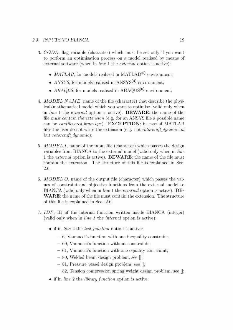
7. IDF , ID of the internal function written inside BIANCA (integer)(valid only when in line 1 the internal option is active):
• if in line 2 the test function option is active:
– 6, Vannucci’s function with one inequality constraint;
– 60, Vannucci’s function without constraints;
– 61, Vannucci’s function with one equality constraint;
– 80, Welded beam design problem, see [];
– 81, Pressure vessel design problem, see [];
– 82, Tension compression spring weight design problem, see [];
• if in line 2 the library function option is active:
20 CHAPTER 2. BIANCA TUTORIAL
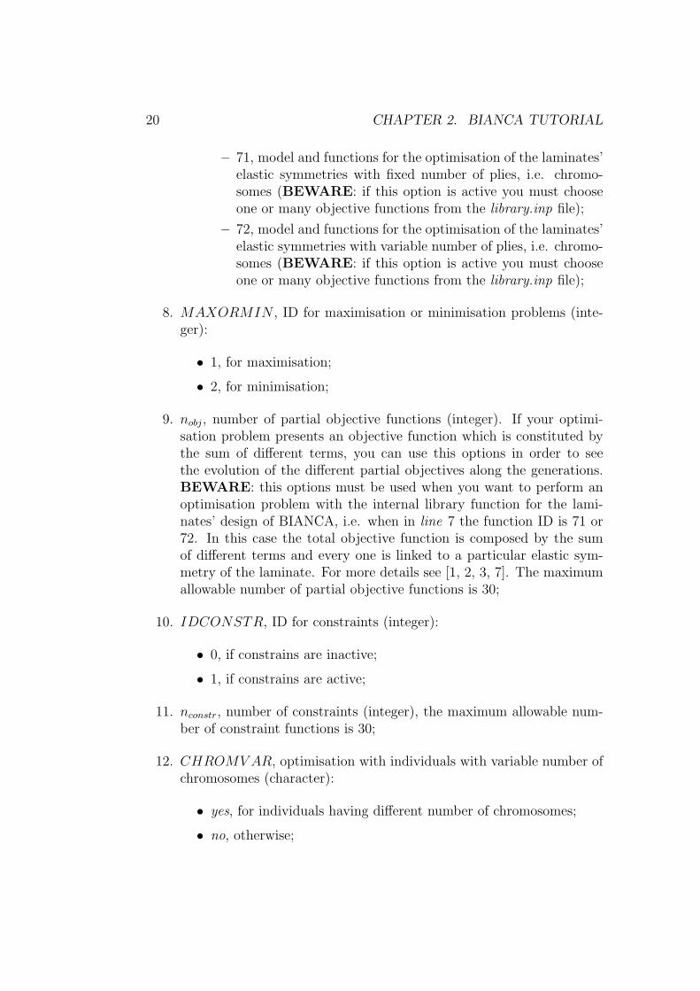
– 71, model and functions for the optimisation of the laminates’elastic symmetries with fixed number of plies, i.e. chromo-somes (BEWARE: if this option is active you must chooseone or many objective functions from the library.inp file);
– 72, model and functions for the optimisation of the laminates’elastic symmetries with variable number of plies, i.e. chromo-somes (BEWARE: if this option is active you must chooseone or many objective functions from the library.inp file);
8. MAXORMIN , ID for maximisation or minimisation problems (inte-ger):
• 1, for maximisation;
• 2, for minimisation;
9. nobj, number of partial objective functions (integer). If your optimi-sation problem presents an objective function which is constituted bythe sum of different terms, you can use this options in order to seethe evolution of the different partial objectives along the generations.BEWARE: this options must be used when you want to perform anoptimisation problem with the internal library function for the lami-nates’ design of BIANCA, i.e. when in line 7 the function ID is 71 or72. In this case the total objective function is composed by the sumof different terms and every one is linked to a particular elastic sym-metry of the laminate. For more details see [1, 2, 3, 7]. The maximumallowable number of partial objective functions is 30;
10. IDCONSTR, ID for constraints (integer):
• 0, if constrains are inactive;
• 1, if constrains are active;
11. nconstr, number of constraints (integer), the maximum allowable num-ber of constraint functions is 30;
12. CHROMV AR, optimisation with individuals with variable number ofchromosomes (character):
• yes, for individuals having different number of chromosomes;
• no, otherwise;
2.3. INPUTS TO BIANCA 21
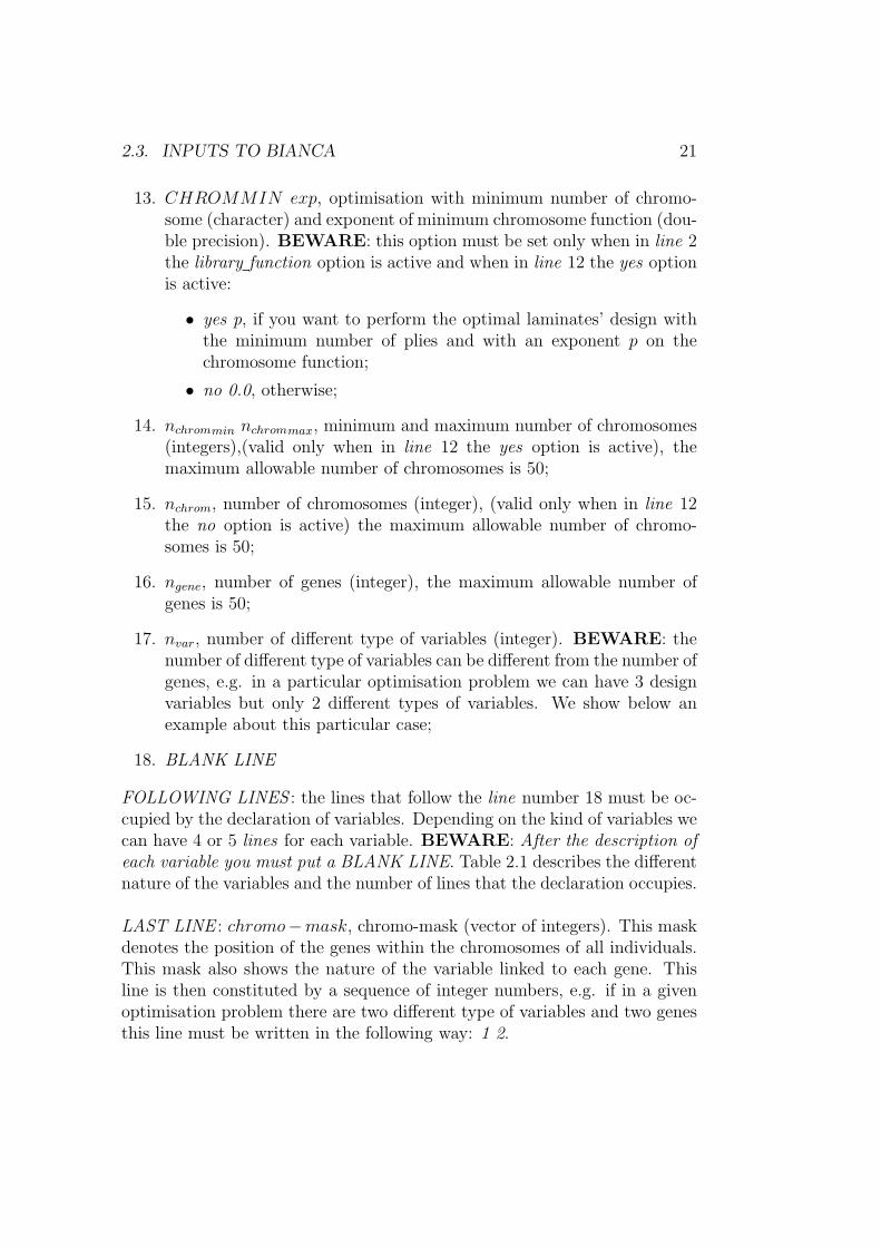
13. CHROMMIN exp, optimisation with minimum number of chromo-some (character) and exponent of minimum chromosome function (dou-ble precision). BEWARE: this option must be set only when in line 2the library function option is active and when in line 12 the yes optionis active:
• yes p, if you want to perform the optimal laminates’ design withthe minimum number of plies and with an exponent p on thechromosome function;
• no 0.0, otherwise;
14. nchrommin nchrommax, minimum and maximum number of chromosomes(integers),(valid only when in line 12 the yes option is active), themaximum allowable number of chromosomes is 50;
15. nchrom, number of chromosomes (integer), (valid only when in line 12the no option is active) the maximum allowable number of chromo-somes is 50;
16. ngene, number of genes (integer), the maximum allowable number ofgenes is 50;
17. nvar, number of different type of variables (integer). BEWARE: thenumber of different type of variables can be different from the number ofgenes, e.g. in a particular optimisation problem we can have 3 designvariables but only 2 different types of variables. We show below anexample about this particular case;
18. BLANK LINE
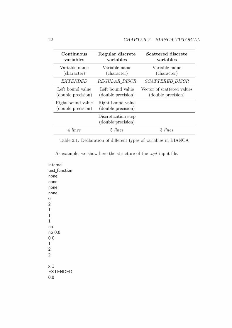
FOLLOWING LINES : the lines that follow the line number 18 must be oc-cupied by the declaration of variables. Depending on the kind of variables wecan have 4 or 5 lines for each variable. BEWARE: After the description ofeach variable you must put a BLANK LINE. Table 2.1 describes the differentnature of the variables and the number of lines that the declaration occupies.
LAST LINE : chromo−mask, chromo-mask (vector of integers). This maskdenotes the position of the genes within the chromosomes of all individuals.This mask also shows the nature of the variable linked to each gene. Thisline is then constituted by a sequence of integer numbers, e.g. if in a givenoptimisation problem there are two different type of variables and two genesthis line must be written in the following way: 1 2.
22 CHAPTER 2. BIANCA TUTORIAL
Continuous Regular discrete Scattered discretevariables variables variables
Variable name Variable name Variable name(character) (character) (character)
EXTENDED REGULAR DISCR SCATTERED DISCR
Left bound value Left bound value Vector of scattered values(double precision) (double precision) (double precision)
Right bound value Right bound value(double precision) (double precision)
Discretization step(double precision)
4 lines 5 lines 3 lines
Table 2.1: Declaration of different types of variables in BIANCA
As example, we show here the structure of the .opt input file.
internal
test function
none
none
none
none
6
2
1
1
1
no
no 0.0
0 0
1
2
2
x 1
EXTENDED
0.0
2.3. INPUTS TO BIANCA 23
12.566
x 2
EXTENDED
0.0
6.283
1 2
For this example we use an internal test function written within BIANCA:the Vannucci’s function with one inequality constraints. We want to minimisethis function. So we perform an optimisation process with fixed number ofchromosome. The structure of the individual’s genotype is made by a singlechromosome with two genes and, hence, with two different type of variables.The name of the first variable is x 1 while the name of the second one is x 2.Both variables are continuous, and we have defined their bounds. x 1 variesin a continuous way between 0.0 and 4π, while x 2 varies in a continuousway between 0.0 and 2π. Since there are two different types of variables thechromo-mask is made by two components 1 2.
Concerning the meaning of the parameter nvar, i.e. the number of differ-ent types of variables, and difference between this parameter and the numberof genes ngene we show here below an example in order to understand in abetter way how you must compile the .opt input file for this kind of situation:
internal
my problem
none
none
none
none
0
2
1
1
4
no
no 0.0
0 0
2
3
2

24 CHAPTER 2. BIANCA TUTORIAL
angle
EXTENDED
0.0
90.0
height
REGULAR DISCR
2.0
5.0
0.1
1 2 1
In this example we use an user self-created model, written in FORTRANlanguage as subroutine of BIANCA. The model has 1 objective functionwith 4 constraints. We want to minimise this function. The structure of theindividual’s genotype is made by 2 chromosomes with 3 genes, hence we have6 design variables but only 2 different types of variables. The name of thefirst variable’s type is angle while the name of the second one is height. Thefirst type is continuous, whilst the second one is a discrete variable. We havealso defined their bounds. angle varies in a continuous way between 0.0◦ and90◦, while height varies between 2.0mm and 5.0mm, with a discretisationstep of 0.1mm. Since there are 2 different types of variables but 3 genesthe chromo-mask is made up by 3 components: 1 2 1. The chromo-maskidentifies the position of each design variable and also of each gene withinthe chromosome. So in this example each one of the two chromosomes, thatconstitute the genotype of the individual, is composed by 3 variables belong-ing to 2 different types: the first variable associated to the correspondinggene is an angle, e.g. α, and it varies between the bounds described by thevariable type angle, the second variable is a height h and varies between thebounds described by the variable type height, while the third variable is alsoan angle, e.g. φ, which has a different physical meaning in our problem butthat belongs to the same type of variable as the first one.
2.3.3 The library.inp file
The library.inp file must be compiled only when in the line 1 and line 2of the .opt input file the options internal and library function are active,respectively. Moreover, in the line 7 of the .opt input file the only valid IDare 71 or 72.
2.3. INPUTS TO BIANCA 25
The ID 71 identifies the problem of the optimal design of laminates’ elasticsymmetries with fixed number of plies, i.e. chromosomes: in this case theonly design variables are the plies’ orientations. The user must declare thebounds, and eventually the discretisation step, in degrees. A little remarkoccurs for this kind of design problem: the number of plies is equal to thenumber of chromosomes increased by one, e.g. when you set, in the .optinput file, the number of chromosomes equal to 10 you perform an analysison a laminate with 11 layers, where the first layer has a fixed orientationequal to 0◦. An example of this kind of analysis can be found in Sec. 3.2.1.The ID 72 identifies the problem of the optimal design of laminates’ elasticsymmetries with variable number of plies, i.e. chromosomes: in this case youmust perform an analysis with cross-over on species and the design variablesare the plies’ orientations and thickness. The user must declare the bounds,and eventually the discretisation step, of the orientations in degrees, whilethe ones of the thickness must be declared in mm. A little remark occurs forthis kind of design problem: unlike the previous function ID, in this case thenumber of plies is equal to the number of chromosomes. An example of thiskind of analysis can be found in Sec. 3.2.2.
The library.inp file presents a list of all the possible elastic symmetries ofthe laminate in terms of stiffness and compliance matrices. Each symmetryis characterised by a name, and every names are written in the file itself.You can copy the name of each symmetry over the line which contains thefollowing words: Don’t modify the following lines. You can see an exampleof the structure of this file in Fig. 2.1.

26 CHAPTER 2. BIANCA TUTORIAL
Figure 2.1: Structure of the library.inp input file.
BEWARE: the number of elastic symmetries must be equal to the num-ber of partial objective function written in the input file with extension .optat line 9.We show here below an example of the structure of both .opt and library.inpinput files.
.opt input file
internal
library function
none
none
none
none
71
2

2.3. INPUTS TO BIANCA 27
3
0
0
no
no 0.0
0 0
12
1
1
angle
REGULAR DISCR
-90.0
90.0
5.0
1
library.inp input file
membrane stiffness isotropy
bending stiffness orthotropy K=0
uncoupling
In this example we want to find a laminate which posses the followingelastic symmetries:
• elastic uncoupling;
• in-plane stiffness isotropy;
• bending stiffness orthotropy.
We use the internal function 71 and the objective function is made up by3 partial objective: each one is associated to the symmetries cited before-hand. The number of chromosomes is associated to the number of plies(BEWARE, for the library function 71 the number of laminates’plies isequal to the number of chromosomes increased by one, so in this example wehave 12 chromosomes and the laminate has 13 plies. In fact the first ply is

28 CHAPTER 2. BIANCA TUTORIAL
oriented at 0.0◦). For each chromosome-ply we have one gene, i.e. one designvariable: the angle which varies with a discretisation step of 5.0◦ between−90.0◦ and 90.0◦. We remark that the number of partial objective functionis 3 and is equal to the number of the elastic symmetries written in the filelibrary.inp.
2.3.4 The post processing.inp file
The post processing.inp input file contains several options that you can set ifyou want to perform the graphical post processing of the simulation’s results.
Post processing operations are performed via MATLAB R© software. Atthe end of the simulation BIANCA writes a file named graphic results.mwhich contains all the instructions for the plotting of the results. This fileautomatically reads the data restrained in the output files of BIANCA, whosestructure is explained in the next Section.These MATLAB R© instructions are strictly linked with what you write in thepost processing.inp file. The graphical results that you obtain, after you havecompiled in a correct way the post processing.inp input file, are substantially2 files whose name is the same as the current job session preceded by thefollowing words:
• obj min (job’s session name) for the file which contains the plot of thebest feasible solution vs. generations;
• obj mean (job’s session name) for the file which contains the plot ofthe average value of the penalised objective function vs. generations;
The structure of the post processing.inp input file is defined below (weremark that each item-number in the list corresponds to the informationrestrained in a single line of the file):
1. POST ENV , post processing environment (character). This is a flagvariable that you must set if you want to activate the graphical treat-ment of results:
• MATLAB, if you want to use MATLAB R© package for the postprocessing of results;
• none, otherwise;
2. axis, flag variable (character) that allows you to choice the axis kindof the results’ plot:
• linear, for a linear scale;
2.3. INPUTS TO BIANCA 29
• semilog, for a semi-logarithmic scale;
3. grid, flag variable (character) that allows you to activate/deactivatethe grid on the plots:
• on, grid is active;
• off , grid is not active;
4. plot format, flag variable (character) that allows you to choice theformat for the simulation’s plots:
• bmp, the graphical results are saved as Windows bitmap file;
• emf , the graphical results are saved as Enhanced metafile;
• eps, the graphical results are saved as EPS level 1;
• jpg, the graphical results are saved as JPEG image;
• pbm, the graphical results are saved as Portable bitmap;
• pcx, the graphical results are saved as Paintbrush 24-bit;
• pdf , the graphical results are saved as Portable Document Format;
• pgm, the graphical results are saved as Portable Graymap;
• png, the graphical results are saved as Portable Network Graphics;
• ppm, the graphical results are saved as Portable Pixmap;
• tif , the graphical results are saved as TIFF image, compressed;
We show here below an example of the structure of post processing.inpinput file.
MATLAB
linear
off
png
In this case we have performed a post processing treatment of results viaMATLAB software. We obtain two file obj min (job’s session name).png andobj mean (job’s session name).png which contain the results of the simula-tion. The graphics are in linear scale and without grid.
30 CHAPTER 2. BIANCA TUTORIAL
2.4 Outputs from BIANCA
In BIANCA, at the end of the optimisation process, we have 3 output files.The name of these files is the same as the one of the current job session.These output files have 3 different extension: .bio, .pop and .sta respectively.We describe the structure and the contents of those files in the followingsubsections.
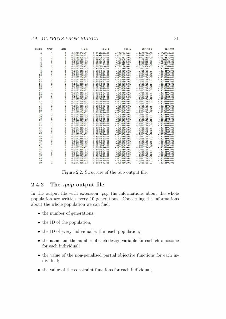
2.4.1 The .bio output file
This file contains the informations about the best feasible individual for everygenerations. In particular in this file we can find:
• the number of generations;
• the ID of the population;
• the ID of the best individual within the population;
• the name and the number of each design variable for each chromosomeof the best individual;
• the value of the non-penalised partial objective functions of the bestindividual;
• the value of the constraint functions of the best individual;
• the value of the total objective function of the best individual.
Fig. 2.2 shows the structure of the .bio output file for the Vannucci’s functionproblem with one inequality constraint. In this simulation we consider apopulation of 10 individuals evolving through 50 generations.
2.4. OUTPUTS FROM BIANCA 31
Figure 2.2: Structure of the .bio output file.
2.4.2 The .pop output file
In the output file with extension .pop the informations about the wholepopulation are written every 10 generations. Concerning the informationsabout the whole population we can find:
• the number of generations;
• the ID of the population;
• the ID of every individual within each population;
• the name and the number of each design variable for each chromosomefor each individual;
• the value of the non-penalised partial objective functions for each in-dividual;
• the value of the constraint functions for each individual;

32 CHAPTER 2. BIANCA TUTORIAL
• the value of the total objective function for each individual.
Fig. 2.3 shows the structure of the .pop output file for the Vannucci’s functionproblem with one inequality constraint. In this simulation we consider apopulation of 10 individuals evolving through 50 generations.
Figure 2.3: Structure of the .pop output file.
2.4. OUTPUTS FROM BIANCA 33
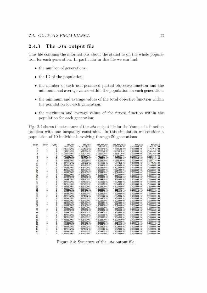
2.4.3 The .sta output file
This file contains the informations about the statistics on the whole popula-tion for each generation. In particular in this file we can find:
• the number of generations;
• the ID of the population;
• the number of each non-penalised partial objective function and theminimum and average values within the population for each generation;
• the minimum and average values of the total objective function withinthe population for each generation;
• the maximum and average values of the fitness function within thepopulation for each generation;
Fig. 2.4 shows the structure of the .sta output file for the Vannucci’s functionproblem with one inequality constraint. In this simulation we consider apopulation of 10 individuals evolving through 50 generations.
Figure 2.4: Structure of the .sta output file.

34 CHAPTER 2. BIANCA TUTORIAL
2.5 The macro MACRO MY PROBLEM.f95
If you want to perform an optimisation process on your model, by meansof the GA BIANCA, one possible way to do that is to write your modelin FORTRAN environment. In this case you must observe the followingconditions:
1. you must write your physical/mathematical model in FORTRAN lan-guage;
2. you must write your model as subroutine of BIANCA.
The macro MACRO MY PROBLEM.f95 has been realised in order to allowyou to write in an easily way your model in FORTRAN language and tounderstand how your model can be interfaced within the code BIANCA.This macro contains 2 subroutines named my problem and my problem varwhich have some input and output quantities. Fig. 2.5 shows the structureof the macro.
Figure 2.5: Structure of the macro MACRO MY PROBLEM.f95.
2.5. THE MACRO MACRO MY PROBLEM.F95 35
In the next subsections we explain in detail the structure of the twosubroutines restrained in this macro and how and when you can use them.We show also an example on how you can write your model as subroutine ofBIANCA, by means of the MACRO MY PROBLEM.f95, in Sec. 3.3.
2.5.1 The my problem subroutine
The my problem subroutine must be used when you want to write your math-ematical model in FORTRAN environment, as subroutine of BIANCA, andwhen you have an optimisation problem where the number of design vari-ables is fixed. In this case the cross-over between individuals belonging todifferent species is no longer required and you have to perform a standardgenetic optimisation process.
The input quantities of this subroutine are:
• npop, number of populations (input derived from the input file .gen,line 1);
• nind, number of individuals for each population (input derived fromthe input file .gen, line 2);
• nchrom, number of chromosomes of each individual (input derived fromthe input file .opt, line 15);
• ngene, number of genes within each chromosome of the individual (in-put derived from the input file .opt, line 16);
• n obj, number of partial objectives (input derived from the input file.opt, line 9);
• n constr: number of constraints (input derived from the input file .opt,line 11);
• x being: phenotype of the whole population, the real size of this 4-dimensional array is x being(npop, nind, nchrom, ngene). This arraycontains the value of each design variable, linked to each gene, for thewhole population.
The output quantities of this subroutine are:
• obj: 3-dimensional array which contains the values of the partial ob-jective functions for every individuals of each population. The real sizeof this array is obj(npop, nind, n obj);

36 CHAPTER 2. BIANCA TUTORIAL
• constr ineq: 3-dimensional array which contains the values of the in-equality constraint functions for every individuals of each population.The real size of this array is constr ineq(npop, nind, n constr).
2.5.2 The my problem var subroutine
The my problem var subroutine must be used when you want to write yourmathematical model in FORTRAN environment, as subroutine of BIANCA,and when you have an optimisation problem where the number of designvariables is also a variable of the process, such as the case of the optimisationof modular systems where the number of modules and, hence, the number ofvariables is also a design variable for the problem. In this case the cross-overbetween individuals belonging to different species is required and you haveto perform a non-standard genetic optimisation process.
The input quantities of this subroutine are:
• npop, number of populations (input derived from the input file .gen,line 1);
• nind, number of individuals for each population (input derived fromthe input file .gen, line 2);
• nchrom min, minimum number of chromosomes (input derived fromthe input file .opt, line 14);
• nchrom max, maximum number of chromosomes (input derived fromthe input file .opt, line 14);
• ngene, number of genes within each chromosome of the individual (in-put derived from the input file .opt, line 16);
• n obj, number of partial objectives (input derived from the input file.opt, line 9);
• n constr: number of constraints (input derived from the input file .opt,line 11);
• x being: phenotype of the whole population, the size of this 4-dimensionalarray can change for each individual because each one can belong toa different specie and can have a different number of chromosome. Inparticular, the effective number of chromosomes of each individual isalso restrained into the phenotype in a particular position of the array;if we consider the jth individual of the ith population the number of

2.6. STRUCTUREOF THE INTERFACEWITH EXTERNAL CODES IN BIANCA37
chromosomes of this individual, nchrom(i, j), is uniquely individuatedby the following equality: nchrom(i, j) = x being(i, j, 1, ngene+1). Sofor each individual the real size of the 4-dimensional array x being isx being(npop, nind, nchrom(npop, nind), ngene + 1). This array con-tains the value of each design variable, linked to each gene, for thewhole population.
The output quantities of this subroutine are:
• obj: 3-dimensional array which contains the values of the partial ob-jective functions for every individuals of each population. The real sizeof this array is obj(npop, nind, n obj);
• constr ineq: 3-dimensional array which contains the values of the in-equality constraint functions for every individuals of each population.The real size of this array is constr ineq(npop, nind, n constr).
2.6 Structure of the interface with external
codes in BIANCA
In several problems, the value of the objective function and/or of the con-straints, cannot be computed analytically, but it has to be evaluated usingspecial numerical codes. Typically, this is the case of structural optimization,where the most part of times the structural response is numerically assessedusing finite element (FE) codes. For these cases, a very general interfacehas been developed, which renders BIANCA able to exchange input/outputinformations with mathematical models supported by an external software.
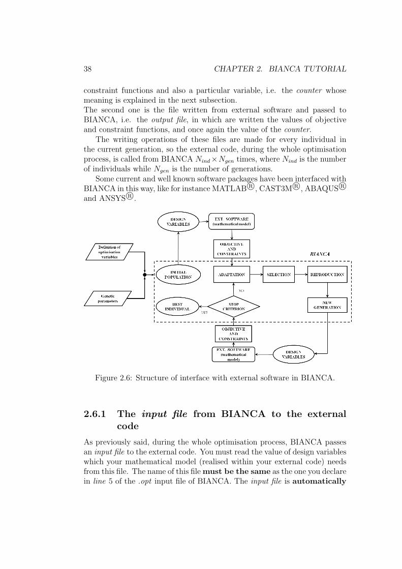
Fig. 2.6 shows the structure of the data-exchange between BIANCA anda generic external software. For each individual, BIANCA performs thegenetic operations, such as selection, cross-over, mutation and so on, andthen passes the design variables to the mathematical model written in adifferent environment. At this point, the external software evaluates theobjective and the eventual constraint functions values, and then passes themback to BIANCA. The data-exchange between BIANCA and the externalsoftware is simply done by means of two I/O files.
The first one is the file written from BIANCA and passed to the externalsoftware, i.e. the input file, which contains the informations related to thecurrent individual at the current generation, i.e. the number and the valuesof the design variables restrained in that individual’s genotype. This inputfile also contains additional information such as the number of objective and
38 CHAPTER 2. BIANCA TUTORIAL
constraint functions and also a particular variable, i.e. the counter whosemeaning is explained in the next subsection.The second one is the file written from external software and passed toBIANCA, i.e. the output file, in which are written the values of objectiveand constraint functions, and once again the value of the counter.
The writing operations of these files are made for every individual inthe current generation, so the external code, during the whole optimisationprocess, is called from BIANCA Nind×Ngen times, where Nind is the numberof individuals while Ngen is the number of generations.
Some current and well known software packages have been interfaced withBIANCA in this way, like for instance MATLAB R©, CAST3M R©, ABAQUS R©and ANSYS R©.
Figure 2.6: Structure of interface with external software in BIANCA.
2.6.1 The input file from BIANCA to the externalcode
As previously said, during the whole optimisation process, BIANCA passesan input file to the external code. You must read the value of design variableswhich your mathematical model (realised within your external code) needsfrom this file. The name of this filemust be the same as the one you declarein line 5 of the .opt input file of BIANCA. The input file is automatically

2.6. STRUCTUREOF THE INTERFACEWITH EXTERNAL CODES IN BIANCA39
written from BIANCA for each individual at the current generation. Itappears clearly that, within your model, you must provide a reading processof the design variables from that file.
The structure of the input file which BIANCA passes to your model isshown in Fig. 2.7.
Figure 2.7: Structure of the input file which BIANCA passes to the externalsoftware.
As shown in Fig. 2.7, in this input file BIANCA automatically writes:
• the number of chromosomes, nchrom, for the current individual at thecurrent generation. In the case of an optimisation process where thenumber of chromosomes is fixed this value is equal to the one youdeclare in line 15 of the .opt input file of BIANCA, while in the caseof an optimisation process where the number of chromosomes is also avariable of the problem, in this line you can find any possible integervalue between the bounds that you declare in in line 14 of the .optinput file of BIANCA;
• the array of design variables for your model. The dimensions of thisarray are nchrom × m where m is equal to the number of genes ngene
which you declare in line 16 of the .opt input file of BIANCA;
• the number of partial objective functions, nobj, which you declare inline 9 of the .opt input file of BIANCA;
• the number of constraint functions, nconstr, which you declare in line11 of the .opt input file of BIANCA;

40 CHAPTER 2. BIANCA TUTORIAL
• the counter. This is an integer variable which ensures the synchronisa-tion between BIANCA and the external code. Within your model youmust read the value of the counter from the input file and your modelhas to return this value to BIANCA by means of the creation of theoutput file, whose structure is explained in the next subsection.
As example, we show here below the structure of the .opt input file forBIANCA and the structure of the input file which BIANCA passes to theexternal software, in the case where the user mathematical model is realisedby means of the MATLAB R© package.
test matlab.opt input file (for more details about this .opt input file seeSec. 3.4):
external
none
MATLAB
Vannucci
input mat.txt
output mat.txt
0
2
1
0
0
no
no 0.0
0 0
1
2
2
x 1
EXTENDED
0.0
12.556
x 2
EXTENDED
0.0

2.6. STRUCTUREOF THE INTERFACEWITH EXTERNAL CODES IN BIANCA41
6.283
1 2
Structure of the input mat.txt input file which BIANCA passes to MATLAB R©:
1
1.4186705767350929 0.97096774193548396
1
0
30
In this simulation we have used the MATLAB R© code for the construc-tion of our mathematical model. This model is described in the example ofSec. 3.4. In this subsection we want to remark the parallelism which existsbetween the correct compilation of the .opt input file and the input file thatBIANCA passes to the external code.
For our example, in the test matlab.opt input file, we can see that thename of the MATLAB R© script is Vannucci, as written in line 4; at line 5 wehave named the input file for our MATLAB R© model as input mat.txt ; thename of the output file which our MATLAB R© model passes to BIANCA isoutput mat.txt. Moreover, the optimisation problem described in MATLAB R©environment has two design variables, i.e. x 1 and x 2. In addition thestructure of the genotype is made up by one chromosome with 2 genes. Theproblem has one objective function and no constraint function. You can seethe coherence between what we have write in the test matlab.opt input filefor BIANCA and what BIANCA writes in the input mat.txt. You can seethe structure of the MATLAB R© script in Sec. 3.4.
Concerning the input mat.txt (input file from BIANCA to MATLAB R©),for the current individual at the current generation BIANCA automaticallywrites the number of chromosomes, 1, the value of both design variables,x1 = 1.4186705767350929 and x2 = 0.97096774193548396, the number ofpartial objective functions, 1, the number of constraint functions, 0, andfinally the value of the counter, 30.
2.6.2 The output file from the external code to BIANCA
As said beforehand, during the whole optimisation process, the external codepasses an output file to BIANCA. You must include the writing operation ofthis file within your mathematical model (realised with your external code).The name of this file must be the same as the one you declare in line 6 of

42 CHAPTER 2. BIANCA TUTORIAL
the .opt input file of BIANCA. The output file must be written from yourmodel.
The structure of the output file which your model passes to BIANCA isshown in Fig. 2.8.
Figure 2.8: Structure of the output file which the external software passes toBIANCA.
As shown in Fig. 2.8, in this output file the following quantities must bewritten from your model:
• the counter. As previously said, this is an integer variable which ensuresthe synchronisation between BIANCA and the external code;
• the array of partial objective functions for your model. The dimen-sions of this array is nobj, where nobj is the number of partial objectivefunctions which you declare in line 9 of the .opt input file of BIANCA;
• the array of constraint functions for your model. The dimensions ofthis array is nconstr, where nconstr is the number of constraint functionswhich you declare in line 11 of the .opt input file of BIANCA.
As example, we show here below the structure of the output file whichthe external software passes to BIANCA, in the case where the user mathe-matical model is realised by means of the MATLAB R© package.
Structure of the output mat.txt output file which MATLAB R© passes toBIANCA:
2.6. STRUCTUREOF THE INTERFACEWITH EXTERNAL CODES IN BIANCA43
30
-0.550094
In this simulation we have used the MATLAB R© code for the construc-tion of our mathematical model. This model is described in the example ofSec. 3.4. In this subsection we want to remark the parallelism which existsbetween the correct compilation of the .opt input file and what the outputfile (written by your model) passes to BIANCA.
For our example, the structure of the .opt input file is the same as theone described in the previous subsection. The name of the .opt input file istest matlab.opt. The name of the output file which our MATLAB R© modelpasses to BIANCA is output mat.txt, as written in line 6.
You can see that in the output mat.txt we can find the value of the counter,30, and the value of the objective function, −0.550094. Since our optimi-sation problem is an unconstrained problem we cannot write the value ofconstraint functions in the output mat.txt file.

44 CHAPTER 2. BIANCA TUTORIAL

Chapter 3
Examples
3.1 Test function example: welded beam de-
sign problem
In this section we show the input and output files concerning a particular testcase optimisation problem: the welded beam design problem. This problemwas firstly studied by Rao. The objective is to design a welded beam forminimum cost subject to several constraints, e.g. on shear stress, bendingstress, buckling load, deflection of the beam and other side constraints. Thereare 4 design variables: the height of the weld h(x1), the length of the weldl(x2), and finally the height t(x3) and the width b(x4) of the beam.
Mathematically, the problem can be stated as follows:
minx
f (x) = 1.10471x12x2 + 0.04811x3x4 (14.0 + x2)
subject to :
g1 (x) = τ (x)− 13000 ≤ 0
g2 (x) = σ (x)− 30000 ≤ 0
g3 (x) = x1 − x4 ≤ 0
g4 (x) = 0.10471x12 + 0.04811x3x4 (14.0 + x2)− 5.0 ≤ 0
g5 (x) = 0.125− x1 ≤ 0
g6 (x) = δ (x)− 0.25 ≤ 0
g7 (x) = 6000− Pc (x) ≤ 0(3.1)
where:
45
46 CHAPTER 3. EXAMPLES
τ (x) =
√
(τ1)2 + 2τ1τ2
x2
2R+ (τ2)
2
τ1 =6000√2x1x2
τ2 =MR
J
M = 6000(
14 +x2
2
)
R =
√
x22
4+
(
x1 + x3
2
)2
J = 2
{
√2x1x2
[
x22
12+
(
x1 + x3
2
)2]}
σ (x) =504000
x32x4
δ (x) =2.1952
x32x4
Pc (x) = 64746.022 (1− 0.0282346x3) x3x43
(3.2)
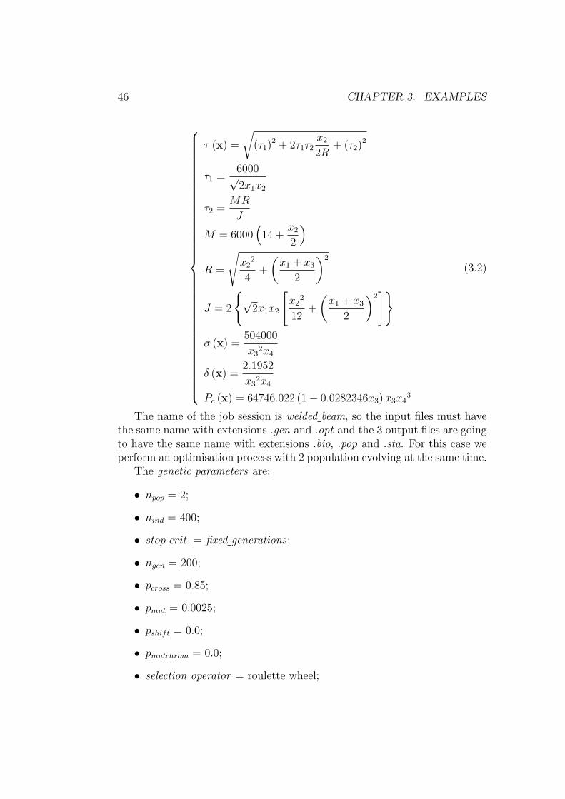
The name of the job session is welded beam, so the input files must havethe same name with extensions .gen and .opt and the 3 output files are goingto have the same name with extensions .bio, .pop and .sta. For this case weperform an optimisation process with 2 population evolving at the same time.
The genetic parameters are:
• npop = 2;
• nind = 400;
• stop crit. = fixed generations ;
• ngen = 200;
• pcross = 0.85;
• pmut = 0.0025;
• pshift = 0.0;
• pmutchrom = 0.0;
• selection operator = roulette wheel;

3.1. TEST FUNCTION EXAMPLE 47
• selection pressure = 1.0;
• elitism operator = active;
• isolation time = 50.
We show here below the structure of the welded beam.gen input file:
2
400
fixed generations
200
0.85
0.0025
0.0
0.0
1
1.0
1
50
The optimisation parameters are:
• simulation environment type = internal;
• kind of problem = test function;
• external code = none;
• external code model file = none;
• external code input file = none;
• external code output file = none;
• function ID = 80;
• minimisation or maximisation = minimisation;
• nobj = 1;
• constr. active or not = active;
• nconstr = 7;
• CHROMV AR = no;

48 CHAPTER 3. EXAMPLES
• CHROMMIN exp = no 0.0;
• nchrommin nchrommax = 0 0;
• nchrom = 1;
• ngene = 4;
• nvar = 4;
• variables :
– x 1, extended, bounds [0.1 2.0]mm;
– x 2, extended, bounds [0.1 10.0]mm;
– x 3, extended, bounds [0.1 10.0]mm;
– x 4, extended, bounds [0.1 2.0]mm;
Then we show here below the structure of the welded beam.opt input file:
internal
test function
none
none
none
none
80
2
1
1
7
no
no 0.0
0 0
1
4
4
x 1
EXTENDED
0.1
2.0

3.1. TEST FUNCTION EXAMPLE 49
x 2
EXTENDED
0.1
10.0
x 3
EXTENDED
0.1
10.0
x 4
EXTENDED
0.1
2.0
1 2 3 4
You can see the structure of the welded beam.bio, welded beam.pop and welded beam.staoutput files in the following paths:
BIANCA 3.1 User guide\ Examples\ welded beam.bio;BIANCA 3.1 User guide\ Examples\ welded beam.pop;BIANCA 3.1 User guide\ Examples\ welded beam.sta.
We perform also the post processing of results and we show here below thestructure of the post processing.inp input file:
MATLAB
linear
off
png
In this case we obtain two image files saved as Portable Network Graphicsfiles named obj min welded beam.png and obj mean welded beam.png. Youcan find those files in the following paths:
BIANCA 3.1 User guide\ Examples\ obj min welded beam.png;BIANCA 3.1 User guide\ Examples\ obj mean welded beam.png.
Figs. 3.1 and 3.2 show the curves of the best feasible solution vs generationsand the average value of the objective function vs generations, respectively.

50 CHAPTER 3. EXAMPLES
Figure 3.1: Best feasible solution vs generations for the welded beam designproblem.
Figure 3.2: Average value of the objective function vs generations for the forthe welded beam design problem.
3.2. LIBRARY FUNCTION EXAMPLE 51
3.2 Library function example: laminates’ de-
sign problem
In this section we show the input and output files concerning the optimisationprocess on the laminate’s elastic properties design problem. For more detailsabout this kind of problem see [1, 7, 3]. Here we want to find a laminate thathas the following symmetries:
• elastic uncoupling;
• in-plane stiffness isotropy;
• bending stiffness orthotropy.
We make 2 kind of simulations: in the first one the number of layers isfixed and only the orientations are the design variables, while in the secondone the number of plies is variable and the design variables are the orientationand the thickness of each layer. In this last case the reproduction betweendifferent species is required. In the following subsections we show how toperform the optimisation process by means of the library functions for thedesign of laminate elastic symmetries developed within BIANCA.
3.2.1 Fixed number of chromosomes/plies
In this first simulation we use the library function with ID 71.The name of the job session is Symmetries, so the input files must have thesame name with extensions .gen and .opt and the 3 output files are going tohave the same name with extensions .bio, .pop and .sta. In addition we mustcompile in a correct way the library.inp input file.
The genetic parameters are:
• npop = 1;
• nind = 500;
• stop crit. = fixed generations;
• ngen = 500;
• pcross = 0.85;
• pmut = 0.002;
• pshift = 0.0;
52 CHAPTER 3. EXAMPLES
• pmutchrom = 0.0;
• selection operator = roulette wheel;
• selection pressure = 1.0;
• elitism operator = active;
• isolation time = 0.
We show here below the structure of the Symmetries.gen input file:
1
500
fixed generations
500
0.85
0.002
0.0
0.0
1
1.0
1
0
For our example, the laminate has 14 plies and the only variables are thelayers’ orientations. According to what we have already explained in Sec.2.3 about the library.inp input file and about the structure of individual’sgenotype, in this case the number of variables is 13 (the first ply has a fixedorientation, i.e. 0.0◦). Each ply corresponds to a chromosome in the struc-ture of the genotype and the layer’s orientation is linked to a single gene.Then, the optimisation parameters are:
• simulation environment type = internal;
• kind of problem =library function;
• external code = none;
• external code model file = none;
• external code input file = none;
• external code output file = none;
3.2. LIBRARY FUNCTION EXAMPLE 53
• function ID = 71;
• minimisation or maximisation = minimisation;
• nobj = 3;
• constr. active or not = not active;
• nconstr = 0;
• CHROMV AR = no;
• CHROMMIN exp = no 0.0;
• nchrommin nchrommax = 0 0;
• nchrom = 13;
• ngene = 1;
• nvar = 1;
• variables :
– angle, regular discrete, step 1.0◦, bounds [−90.0◦ 90.0◦];
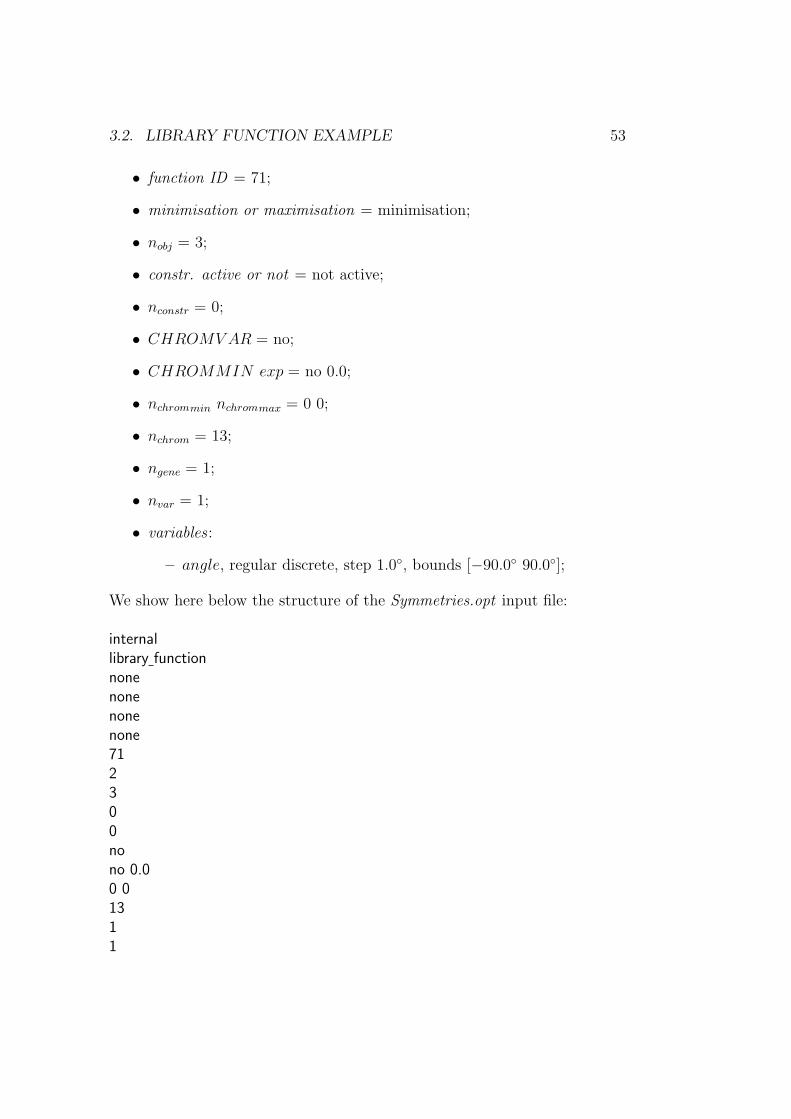
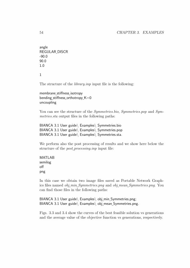
We show here below the structure of the Symmetries.opt input file:
internal
library function
none
none
none
none
71
2
3
0
0
no
no 0.0
0 0
13
1
1
54 CHAPTER 3. EXAMPLES
angle
REGULAR DISCR
-90.0
90.0
1.0
1
The structure of the library.inp input file is the following:
membrane stiffness isotropy
bending stiffness orthotropy K=0
uncoupling
You can see the structure of the Symmetries.bio, Symmetries.pop and Sym-metries.sta output files in the following paths:
BIANCA 3.1 User guide\ Examples\ Symmetries.bio
BIANCA 3.1 User guide\ Examples\ Symmetries.pop
BIANCA 3.1 User guide\ Examples\ Symmetries.sta.
We perform also the post processing of results and we show here below thestructure of the post processing.inp input file:
MATLAB
semilog
off
png
In this case we obtain two image files saved as Portable Network Graph-ics files named obj min Symmetries.png and obj mean Symmetries.png. Youcan find those files in the following paths:
BIANCA 3.1 User guide\ Examples\ obj min Symmetries.png;BIANCA 3.1 User guide\ Examples\ obj mean Symmetries.png.
Figs. 3.3 and 3.4 show the curves of the best feasible solution vs generationsand the average value of the objective function vs generations, respectively.

3.2. LIBRARY FUNCTION EXAMPLE 55
Figure 3.3: Best feasible solution vs generations for the design of laminate’selastic symmetries.
Figure 3.4: Average value of the objective function vs generations for thedesign of laminate’s elastic symmetries.
56 CHAPTER 3. EXAMPLES
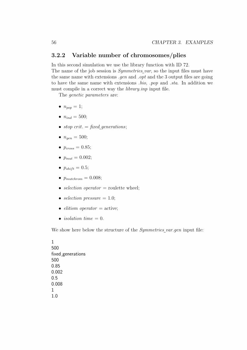
3.2.2 Variable number of chromosomes/plies
In this second simulation we use the library function with ID 72.The name of the job session is Symmetries var, so the input files must havethe same name with extensions .gen and .opt and the 3 output files are goingto have the same name with extensions .bio, .pop and .sta. In addition wemust compile in a correct way the library.inp input file.
The genetic parameters are:
• npop = 1;
• nind = 500;
• stop crit. = fixed generations ;
• ngen = 500;
• pcross = 0.85;
• pmut = 0.002;
• pshift = 0.5;
• pmutchrom = 0.008;
• selection operator = roulette wheel;
• selection pressure = 1.0;
• elitism operator = active;
• isolation time = 0.
We show here below the structure of the Symmetries var.gen input file:
1
500
fixed generations
500
0.85
0.002
0.5
0.008
1
1.0
3.2. LIBRARY FUNCTION EXAMPLE 57
1
0
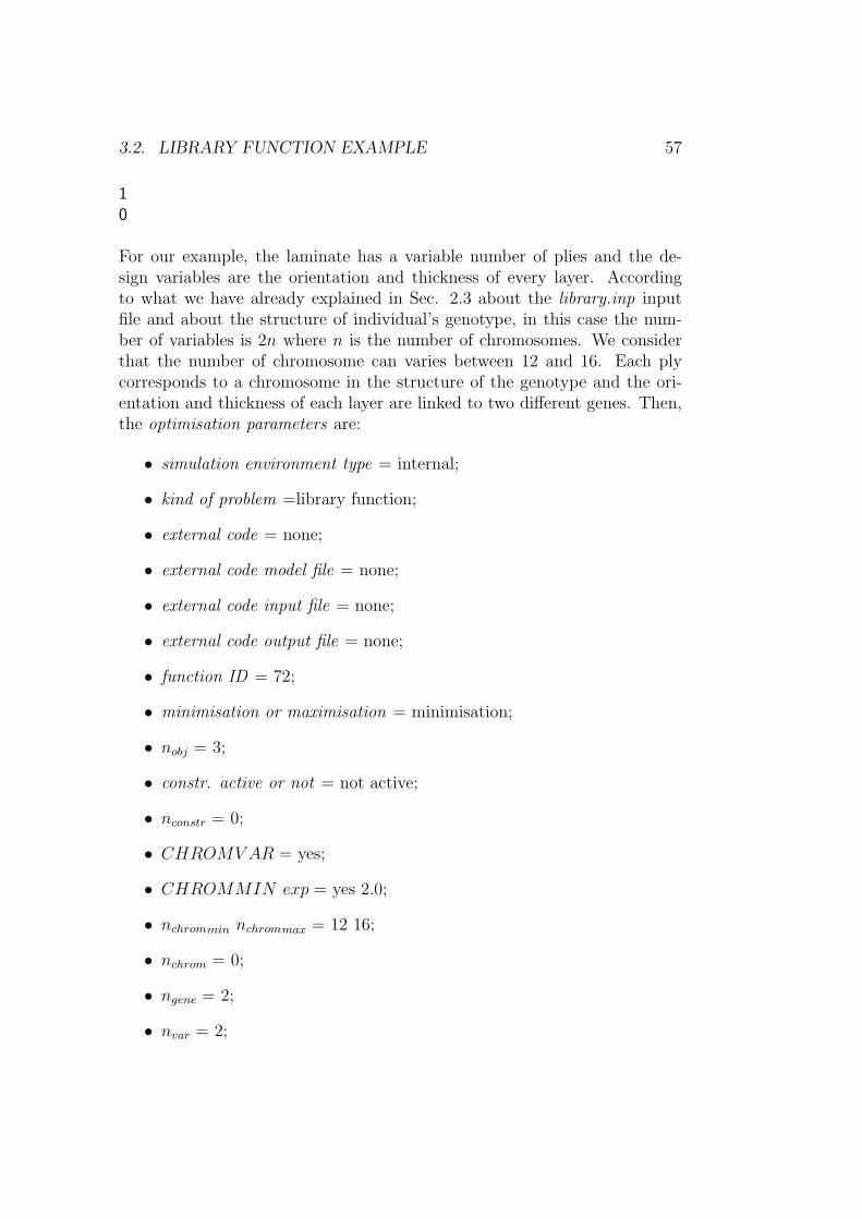
For our example, the laminate has a variable number of plies and the de-sign variables are the orientation and thickness of every layer. Accordingto what we have already explained in Sec. 2.3 about the library.inp inputfile and about the structure of individual’s genotype, in this case the num-ber of variables is 2n where n is the number of chromosomes. We considerthat the number of chromosome can varies between 12 and 16. Each plycorresponds to a chromosome in the structure of the genotype and the ori-entation and thickness of each layer are linked to two different genes. Then,the optimisation parameters are:
• simulation environment type = internal;
• kind of problem =library function;
• external code = none;
• external code model file = none;
• external code input file = none;
• external code output file = none;
• function ID = 72;
• minimisation or maximisation = minimisation;
• nobj = 3;
• constr. active or not = not active;
• nconstr = 0;
• CHROMV AR = yes;
• CHROMMIN exp = yes 2.0;
• nchrommin nchrommax = 12 16;
• nchrom = 0;
• ngene = 2;
• nvar = 2;
58 CHAPTER 3. EXAMPLES
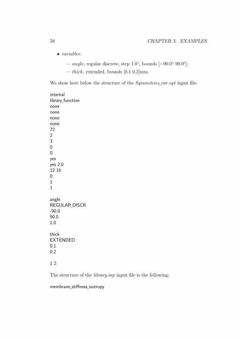
• variables :
– angle, regular discrete, step 1.0◦, bounds [−90.0◦ 90.0◦];
– thick, extended, bounds [0.1 0.2]mm.
We show here below the structure of the Symmetries var.opt input file:
internal
library function
none
none
none
none
72
2
3
0
0
yes
yes 2.0
12 16
0
1
1
angle
REGULAR DISCR
-90.0
90.0
1.0
thick
EXTENDED
0.1
0.2
1 2
The structure of the library.inp input file is the following:
membrane stiffness isotropy
3.2. LIBRARY FUNCTION EXAMPLE 59
bending stiffness orthotropy K=0
uncoupling
You can see the structure of the Symmetries var.bio, Symmetries var.popand Symmetries var.sta output files in the following paths:
BIANCA 3.1 User guide\ Examples\ Symmetries var.bio
BIANCA 3.1 User guide\ Examples\ Symmetries var.pop
BIANCA 3.1 User guide\ Examples\ Symmetries var.sta.
We perform also the post processing of results and we show here below thestructure of the post processing.inp input file:
MATLAB
semilog
off
png
In this case we obtain two image files saved as Portable Network Graphicsfiles named obj min Symmetries var.png and obj mean Symmetries var.png.You can find those files in the following paths:
BIANCA 3.1 User guide\ Examples\ obj min Symmetries var.png;BIANCA 3.1 User guide\ Examples\ obj mean Symmetries var.png.
Figs. 3.5 and 3.6 show the curves of the best feasible solution vs generationsand the average value of the objective function vs generations, respectively.
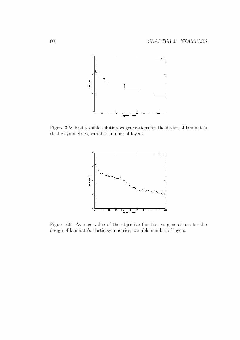
60 CHAPTER 3. EXAMPLES
Figure 3.5: Best feasible solution vs generations for the design of laminate’selastic symmetries, variable number of layers.
Figure 3.6: Average value of the objective function vs generations for thedesign of laminate’s elastic symmetries, variable number of layers.
3.3. USER-DEFINED MODEL EXAMPLE 61
3.3 User-defined model example: beam de-
sign problem
In this section we show the input and output files concerning the optimi-sation process on a possible user-defined model and also how to write themathematical model in the MACRO MY PROBLEM.f95.
In this example we consider a simple optimisation problem about beams’design. We have a clamped beam subject to a tip load P of 1000 N. Thebeam is made up by an Aluminium alloy with a Young modulus E equal to72 GPa and a tensile yield stress σy of 345 MPa. The beam has a circularsection. The design variables are the beam’s length L and the beam’s radiusR.We want to find the optimal values of L and R which minimise the tipdisplacement δ and respect both constraints imposed on the maximum stressand on the beam’s volume. The reference value of the volume Vref is 140000mm3.
The problem can be formulated as follows:
minL,R
δ (L,R) =4PL3
3πER4
subject to :
4PL
πR3− σy ≤ 0
LπR2 − Vref ≤ 0
(3.3)
The name of the job session is beam design, so the input files must havethe same name with extensions .gen and .opt and the 3 output files are goingto have the same name with extensions .bio, .pop and .sta.Since the problem do not require the cross-over between species, the structureof the individual’s genotype is made up by a single chromosome with twogenes which identify the design variables, i.e. the length L and the radiusR. In addition, since the number of chromosome is fixed we must write ourmodel by means of the subroutine my problem. We have written our modelin the MACRO MY PROBLEM.f95 as shown in Fig. 3.7.

62 CHAPTER 3. EXAMPLES
Figure 3.7: Structure of the macro MACRO MY PROBLEM.f95 for thebeam design problem.
3.3. USER-DEFINED MODEL EXAMPLE 63
The genetic parameters are:
• npop = 1;
• nind = 100;
• stop crit. = fixed generations;
• ngen = 200;
• pcross = 0.85;
• pmut = 0.01;
• pshift = 0.0;
• pmutchrom = 0.0;
• selection operator = roulette wheel;
• selection pressure = 1.0;
• elitism operator = active;
• isolation time = 0.
Then we show here below the structure of the beam design.gen input file:
1
100
fixed generations
200
0.85
0.01
0.0
0.0
1
1.0
1
0
The optimisation parameters are:
• simulation environment type = internal;
• kind of problem = my problem;

64 CHAPTER 3. EXAMPLES
• external code = none;
• external code model file = none;
• external code input file = none;
• external code output file = none;
• function ID = 0;
• minimisation or maximisation = minimisation;
• nobj = 1;
• constr. active or not = active;
• nconstr = 2;
• CHROMV AR = no;
• CHROMMIN exp = no 0.0;
• nchrommin nchrommax = 0 0;
• nchrom = 1;
• ngene = 2;
• nvar = 2;
• variables :
– Length, regular discrete, step 1.0 mm, bounds [100.0 500.0]mm;
– Radius, regular discrete, step 1.0 mm, bounds [10.0 50.0]mm.
Then we show here below the structure of the beam design.opt input file:
internal
my problem
none
none
none
none
0
2
1

3.3. USER-DEFINED MODEL EXAMPLE 65
1
2
no
no 0.0
0 0
1
2
2
Length
REGULAR DISCR
100.0
500.0
1.0
Radius
REGULAR DISCR
10.0
50.0
1.0
1 2
You can see the structure of the beam design.bio, beam design.pop and beamdesign.sta output files in the following paths:
BIANCA 3.1 User guide\ Examples\ beam design.bio;BIANCA 3.1 User guide\ Examples\ beam design.pop;BIANCA 3.1 User guide\ Examples\ beam design.sta.
We perform also the post processing of results and we show here below thestructure of the post processing.inp input file:
MATLAB
linear
off
png
In this case we obtain two image files saved as Portable Network Graph-ics files named obj min beam design.png and obj mean beam design.png. Youcan find those files in the following paths:

66 CHAPTER 3. EXAMPLES
BIANCA 3.1 User guide\ Examples\ obj min beam design.png;BIANCA 3.1 User guide\ Examples\ obj mean beam design.png.
Figs. 3.8 and 3.9 show the curves of the best feasible solution vs generationsand the average value of the objective function vs generations, respectively.
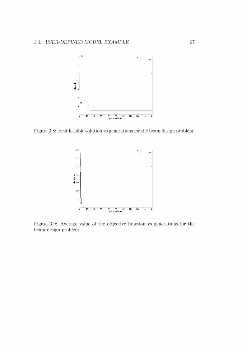
3.3. USER-DEFINED MODEL EXAMPLE 67
Figure 3.8: Best feasible solution vs generations for the beam design problem.
Figure 3.9: Average value of the objective function vs generations for thebeam design problem.

68 CHAPTER 3. EXAMPLES
3.4 Example of interface with MATLAB R©
code: Vannucci’s function problem
In order to have a general idea on how BIANCA 3.1 works when it is inter-faced with external codes, we show here the input and output files concerningthe optimisation process on the unconstrained Vannucci’s function problem.The problem can be stated as follows:
min f (x1, x2) = −eka√
x2
1+x2
2sin (ax1) cos (2bx2)
0 ≤ x1 ≤ 4π
0 ≤ x2 ≤ 2π
(3.4)
Although this problem is already implemented as test function withinBIANCA, we have rewrite this problem in MATLAB R© environment in orderto explain how you can easily interface with BIANCA any model realisedwithin the MATLAB R© code.
First of all we can consider the structure of the model written withinMATLAB R©. The structure is completely free, except for the part concerningthe exchange of data with BIANCA. For our example the model is written asMATLAB R© script whose name is Vannucci.m and whose structure is shownin Fig 3.10. The data exchange between BIANCA and our model is realisedaccording to what we have explained in Sec. 2.6.
You can see the structure of this MATLAB R© script in the following path:
BIANCA 3.1 User guide\ Examples\ Vannucci.m;
The name of the job session is test matlab, so the input files must havethe same name with extensions .gen and .opt and the 3 output files are goingto have the same name with extensions .bio, .pop and .sta.
The genetic parameters are:
• npop = 1;
• nind = 100;
• stop crit. = fixed generations ;
• ngen = 200;
• pcross = 0.85;
• pmut = 0.01;
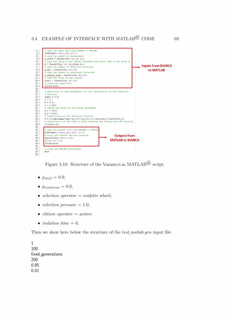
3.4. EXAMPLE OF INTERFACE WITH MATLAB R© CODE 69
Figure 3.10: Structure of the Vannucci.m MATLAB R© script.
• pshift = 0.0;
• pmutchrom = 0.0;
• selection operator = roulette wheel;
• selection pressure = 1.0;
• elitism operator = active;
• isolation time = 0.
Then we show here below the structure of the test matlab.gen input file:
1
100
fixed generations
200
0.85
0.01
70 CHAPTER 3. EXAMPLES
0.0
0.0
1
1.0
1
0
The optimisation parameters are:
• simulation environment type = external;
• kind of problem = none;
• external code = MATLAB;
• external code model file = Vannucci;
• external code input file = input mat.txt;
• external code output file = output mat.txt;
• function ID = 0;
• minimisation or maximisation = minimisation;
• nobj = 1;
• constr. active or not = not active;
• nconstr = 0;
• CHROMV AR = no;
• CHROMMIN exp = no 0.0;
• nchrommin nchrommax = 0 0;
• nchrom = 1;
• ngene = 2;
• nvar = 2;
• variables :
– x 1, extended, bounds [0.0 12.556];
– x 2, extended, bounds [0.0 6.283];

3.4. EXAMPLE OF INTERFACE WITH MATLAB R© CODE 71
Then we show here below the structure of the test matlab.opt input file:
external
none
MATLAB
Vannucci
input mat.txt
output mat.txt
0
2
1
0
0
no
no 0.0
0 0
1
2
2
x 1
EXTENDED
0.0
12.556
x 2
EXTENDED
0.0
6.283
1 2
You can see the structure of the test matlab.bio, test matlab.pop and test matlab.staoutput files in the following paths:
BIANCA 3.1 User guide\ Examples\ test matlab.bio;BIANCA 3.1 User guide\ Examples\ test matlab.pop;BIANCA 3.1 User guide\ Examples\ test matlab.sta.
We perform also the post processing of results and we show here below thestructure of the post processing.inp input file:

72 CHAPTER 3. EXAMPLES
MATLAB
linear
off
png
In this case we obtain two image files saved as Portable Network Graph-ics files named obj min test matlab.png and obj mean test matlab.png. Youcan find those files in the following paths:
BIANCA 3.1 User guide\ Examples\ obj min test matlab.png;BIANCA 3.1 User guide\ Examples\ obj mean test matlab.png.
Figs. 3.11 and 3.12 show the curves of the best feasible solution vs generationsand the average value of the objective function vs generations, respectively.
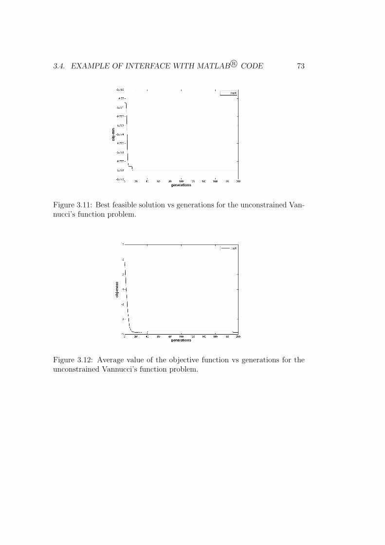
3.4. EXAMPLE OF INTERFACE WITH MATLAB R© CODE 73
Figure 3.11: Best feasible solution vs generations for the unconstrained Van-nucci’s function problem.
Figure 3.12: Average value of the objective function vs generations for theunconstrained Vannucci’s function problem.

74 CHAPTER 3. EXAMPLES
3.5 Example of interface with ANSYS R© code:
stiffened plate design problem
In order to have a general idea on how BIANCA 3.1 works when it is inter-faced with external codes, we show here the input and output files concerningthe optimisation process on the engineering problem of the optimal designof an aeronautical stiffened panel. Here, the optimal design of the stiffenedpanel is intended in terms of minimizing its weight and, at the same time,respecting a constraint imposed on its buckling load. The problem to obtaina minimum weight panel which presents particular characteristics in termsof buckling load, is a very important issue in the aeronautics.
We show here that this optimisation problem can be formulated andsolved in a very general way by applying our approach for the optimisa-tion of modular engineering systems where not only the characteristics ofeach module, but also the number of the constitutive modules are taken intoaccount as optimisation variables. In addition, this problem is numericallymore complex than the ones presented in the previous sections: in fact it isa constrained optimisation problem where either the objective or the con-straint function are evaluated by means of a Finite Element (FE) code. Torepresent the wing-box section we use the ANSYS R© FE code. The optimi-sation variables are: the number of stiffeners n, and for each stiffener thereare two design variables, i.e. the thickness tsi and the height hi, (i = 1...n).The total number of design variables is 2n.
Concerning the mathematical formalisation of the constrained optimisa-tion problem, it can be stated as:
{
minn,ts,h
[
Wupstiff (n, ts,h)
]
subject to : pref − pcr (n, ts,h) ≤ 0(3.5)
In Eq.(3.5), W upstiff (n, ts,h) stands for the weight of the upper panel’s stiff-
eners, while the quantities n, ts,h represent the number of stiffeners for eachpanel and the vectors of stiffeners’ thickness and heights respectively, i.e. thedesign variables. The quantity pcr (n, ts,h) stands for the first buckling loadof the structure, while pref is a reference value for this quantity. More detailsabout this problem can be found in [4].
First of all we can consider the structure of the model written withinANSYS R©. The structure is completely free, except for the part concern-ing the exchange of data with BIANCA. As well explained in Sec. 2.6 theinterface between the two codes is realised by means of the creation of two in-put/output files which pass the design variables from BIANCA to ANSYS R©

3.5. EXAMPLE OF INTERFACE WITH ANSYS R© CODE 75
and the objective and constraints from ANSYS R© to BIANCA. For our casethe name of the ANSYS R© file which contains all the information about thewing-box FE model is panel.lgw. You can see the structure of this file in thefollowing path:
BIANCA 3.1 User guide\ Examples\ panel.lgw;
The structure of this file is substantially articulated in three parts: thefirst one concerns the reading operations of design variables that BIANCApasses to the FE model, the second one concerns the creation of the modeland, finally, the third one concerns the writing operations of the output filethat contains the counter, objective function and constraint that ANSYS R©passes to BIANCA.
The name of the job session is test ansys, so the input files must have thesame name with extensions .gen and .opt and the 3 output files are going tohave the same name with extensions .bio, .pop and .sta.
The genetic parameters are:
• npop = 1;
• nind = 150;
• stop crit. = fixed generations;
• ngen = 200;
• pcross = 0.85;
• pmut = 0.0067;
• pshift = 0.5;
• pmutchrom = 0.04;
• selection operator = tournament;
• selection pressure = 1.0;
• elitism operator = active;
• isolation time = 0.
Then we show here below the structure of the test ansys.gen input file:
1
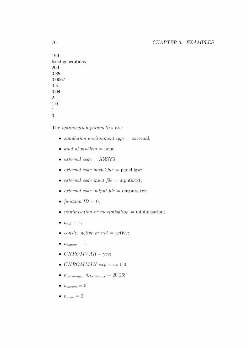
76 CHAPTER 3. EXAMPLES
150
fixed generations
200
0.85
0.0067
0.5
0.04
2
1.0
1
0
The optimisation parameters are:
• simulation environment type = external;
• kind of problem = none;
• external code = ANSYS;
• external code model file = panel.lgw;
• external code input file = inputs.txt;
• external code output file = outputs.txt;
• function ID = 0;
• minimisation or maximisation = minimisation;
• nobj = 1;
• constr. active or not = active;
• nconstr = 1;
• CHROMV AR = yes;
• CHROMMIN exp = no 0.0;
• nchrommin nchrommax = 20 26;
• nchrom = 0;
• ngene = 2;
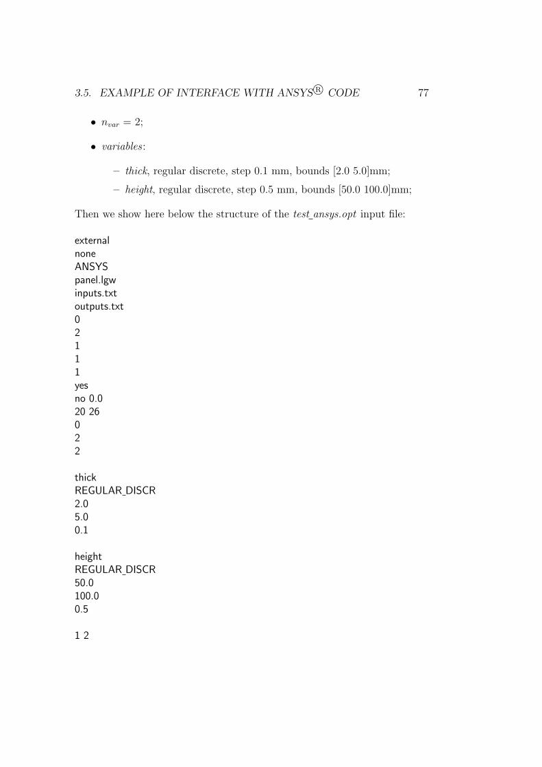
3.5. EXAMPLE OF INTERFACE WITH ANSYS R© CODE 77
• nvar = 2;
• variables :
– thick, regular discrete, step 0.1 mm, bounds [2.0 5.0]mm;
– height, regular discrete, step 0.5 mm, bounds [50.0 100.0]mm;
Then we show here below the structure of the test ansys.opt input file:
external
none
ANSYS
panel.lgw
inputs.txt
outputs.txt
0
2
1
1
1
yes
no 0.0
20 26
0
2
2
thick
REGULAR DISCR
2.0
5.0
0.1
height
REGULAR DISCR
50.0
100.0
0.5
1 2

78 CHAPTER 3. EXAMPLES
You can see the structure of the test ansys.bio, test ansys.pop and test ansys.staoutput files in the following paths:
BIANCA 3.1 User guide\ Examples\ test ansys.bio;BIANCA 3.1 User guide\ Examples\ test ansys.pop;BIANCA 3.1 User guide\ Examples\ test ansys.sta.
We perform also the post processing of results and we show here below thestructure of the post processing.inp input file:
MATLAB
linear
off
png
In this case we obtain two image files saved as Portable Network Graph-ics files named obj min test ansys.png and obj mean test ansys.png. You canfind those files in the following paths:
BIANCA 3.1 User guide\ Examples\ obj min test ansys.png;BIANCA 3.1 User guide\ Examples\ obj mean test ansys.png.
Figs. 3.13 and 3.14 show the curves of the best feasible solution vs generationsand the average value of the objective function vs generations, respectively.
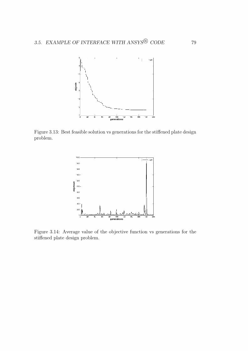
3.5. EXAMPLE OF INTERFACE WITH ANSYS R© CODE 79
Figure 3.13: Best feasible solution vs generations for the stiffened plate designproblem.
Figure 3.14: Average value of the objective function vs generations for thestiffened plate design problem.
80 CHAPTER 3. EXAMPLES
3.6 Example of interface with ABAQUS R©
code: beam design problem
In this section we consider a simple optimisation problem about beams’ de-sign. We have a clamped beam subject to a tip load P of 1000 N. The beamis made up by a Steel alloy with a Young modulus E equal to 200 GPa. Thebeam has a rectangular cross section. The design variables are the beam’slength L and the beam’s height h. The width b of the section is equal to10 mm. The model of the beam is realised by means of the ABAQUS R© FEcode.We want to find the optimal values of L and h which minimise the absolutevalue of the tip displacement |δ|.
The problem can be formulated as follows:
minL,h
|δ (L, h) | (3.6)
First of all we must consider the structure of the model written withinABAQUS R©. Again, the structure is completely free, except for the partconcerning the exchange of data with BIANCA. As well explained in Sec.2.6 the interface between the two codes is realised by means of the creationof two input/output files which pass the design variables from BIANCA toABAQUS R© and the objective and constraints from ABAQUS R© to BIANCA.For our case the name of the ABAQUS R© file which contains all the infor-mation about the beam FE model is cantilevered beam.py. You can see thestructure of this file in the following path:
BIANCA 3.1 User guide\ Examples\ cantilevered beam.py;
The structure of this file is substantially articulated in three parts: thefirst one concerns the reading operations of design variables that BIANCApasses to the FE model, the second one concerns the creation of the modeland, finally, the third one concerns the writing operations of the output filethat contains the counter, objective function and constraint that ABAQUS R©passes to BIANCA.
The name of the job session is test abaqus, so the input files must havethe same name with extensions .gen and .opt and the 3 output files are goingto have the same name with extensions .bio, .pop and .sta.
The genetic parameters are:
• npop = 1;

3.6. EXAMPLE OF INTERFACE WITH ABAQUS R© CODE 81
• nind = 30;
• stop crit. = fixed generations;
• ngen = 100;
• pcross = 0.85;
• pmut = 0.033;
• pshift = 0.0;
• pmutchrom = 0.0;
• selection operator = tournament;
• selection pressure = 1.0;
• elitism operator = active;
• isolation time = 0.
Then we show here below the structure of the test abaqus.gen input file:
1
30
fixed generations
100
0.85
0.033
0.0
0.0
2
1.0
1
0
The optimisation parameters are:
• simulation environment type = external;
• kind of problem = none;
• external code = ABAQUS;
• external code model file = cantilevered beam.py;

82 CHAPTER 3. EXAMPLES
• external code input file = input.txt;
• external code output file = out.txt;
• function ID = 0;
• minimisation or maximisation = minimisation;
• nobj = 1;
• constr. active or not = not active;
• nconstr = 0;
• CHROMV AR = no;
• CHROMMIN exp = no 0.0;
• nchrommin nchrommax = 0 0;
• nchrom = 1;
• ngene = 2;
• nvar = 2;
• variables :
– Length, extended, bounds [500.0 1000.0]mm;
– Height, extended, bounds [10.0 50.0]mm;
Then we show here below the structure of the test abaqus.opt input file:
external
none
ABAQUS
cantilevered beam.py
input.txt
out.txt
0
2
1
0
0
no
3.6. EXAMPLE OF INTERFACE WITH ABAQUS R© CODE 83
no 0.0
0 0
1
2
2
Lenght
EXTENDED
500.0
1000.0
Height
EXTENDED
10.0
50.0
1 2
You can see the structure of the test abaqus.bio, test abaqus.pop and test abaqus.staoutput files in the following paths:
BIANCA 3.1 User guide\ Examples\ test abaqus.bio;BIANCA 3.1 User guide\ Examples\ test abaqus.pop;BIANCA 3.1 User guide\ Examples\ test abaqus.sta.
We perform also the post processing of results and we show here below thestructure of the post processing.inp input file:
MATLAB
linear
off
png
In this case we obtain two image files saved as Portable Network Graph-ics files named obj min test abaqus.png and obj mean test abaqus.png. Youcan find those files in the following paths:
BIANCA 3.1 User guide\ Examples\ obj min test abaqus.png;BIANCA 3.1 User guide\ Examples\ obj mean test abaqus.png.
Figs. 3.15 and 3.16 show the curves of the best feasible solution vs generations
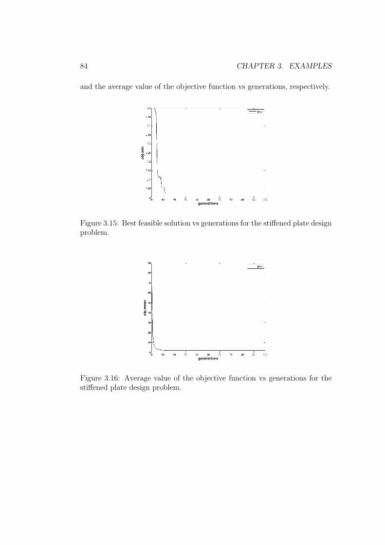
84 CHAPTER 3. EXAMPLES
and the average value of the objective function vs generations, respectively.
Figure 3.15: Best feasible solution vs generations for the stiffened plate designproblem.
Figure 3.16: Average value of the objective function vs generations for thestiffened plate design problem.

3.7. EXAMPLE OF INTERFACE WITH CAST3M R© CODE 85
3.7 Example of interface with CAST3M R© code:
plate design problem

86 CHAPTER 3. EXAMPLES
Bibliography
[1] A. Vincenti. Conception et optimisation de composites par methode po-laire et algorithmes genetiques. PhD thesis, Universite de Bourgogne,France, 2002.
[2] A. Vincenti, M.R. Ahmadian, and P. Vannucci. Bianca: a genetic algo-rithm to solve hard combinatorial optimisation problems in engineering.Journal of Global Optimisation, 48:399–421, 2010.
[3] M. Montemurro, A. Vincenti, P. Vannucci, and A. Makradi. Design oflaminate’s elastic properties with minimum number of plies. CompositesPart A, (Submitted), 2010.
[4] M. Montemurro, P. Vannucci, and A. Vincenti. A genetic algorithmwith cross-over on species for structural optimisation. Computers andStructures, (Submitted), 2010.
[5] D.E. Goldberg. Genetic algorithms. New York: Addison and Wesley,1994.
[6] Z. Michalewicz. Genetic algorithms + data structures = evolutionaryprogramming. Berlin: Springer, 1994.
[7] P. Vannucci. Designing the elastic properties of laminates as an opti-misation problem: a unified approach based on polar tensor invariants.Structural and Multidisciplinary Optimisation, 31(5):378–387, 2006.
87