HAL Id: tel-00910097https://tel.archives-ouvertes.fr/tel-00910097

Submitted on 27 Nov 2013

HAL is a multi-disciplinary open accessarchive for the deposit and dissemination of sci-entific research documents, whether they are pub-lished or not. The documents may come fromteaching and research institutions in France orabroad, or from public or private research centers.

L’archive ouverte pluridisciplinaire HAL, estdestinée au dépôt et à la diffusion de documentsscientifiques de niveau recherche, publiés ou non,émanant des établissements d’enseignement et derecherche français ou étrangers, des laboratoirespublics ou privés.

Optimisation de chaine logistique et planning dedistribution sous incertitude d’approvisionnement

Hugues Dubedout

To cite this version:Hugues Dubedout. Optimisation de chaine logistique et planning de distribution sous incerti-tude d’approvisionnement. Automatique. Ecole des Mines de Nantes, 2013. Français. �NNT :2013EMNA0072�. �tel-00910097�

Mémoire présenté en vue de l’obtention du grade de Docteur de l’École Nationale Supérieure des Mines de Nantes sous le label de L’Université Nantes Angers Le Mans École doctorale : STIM Discipline : Informatique et applications Spécialité : Recherche Opérationnelle Unité de recherche : Irccyn Soutenue le 03/06/2013 Thèse N° : 2013EMNA0072

SUPPLY CHAIN DESIGN AND DISTRIBUTION PLANNING UNDER

SUPPLY UNCERTAINTY APPLICATION TO BULK LIQUID GAS DISTRIBUTION

JURY

Rapporteurs : M. Phillipe LACOMME ; professeur, ISIMA Clermont Ferrand M. Scott J. MASON, Professeur, Clemson University

Examinateurs : M. Jean-Pierre CAMPAGNE, Professeur Emérite, INSA de Lyon M. Van-Dat CUNG, Professeur, Institut Polytechnique de Grenoble

Invité : M Vincent GOURLAOUEN, Air Liquide Directeur de thèse : M. Pierre DEJAX, Professeur, Ecole des Mines de Nantes Co-directeurs de thèse : Mme Nicoleta NEAGU, Ingénieur-chercheur, Air Liquide

M. Thomas YEUNG, Maître assistant, Ecole des mines de Nantes

Hugues DUBEDOUT

Maitre de conference avec HDR, ISIMA Clermont Ferrand

2

Résumé et mots-clés

La distribution de liquide cryogénique a l’aide de vrac, ou camions citernes, est un cas particulier

des problèmes d’optimisation logistique. Il suit des règles précise et obéit a des contraintes

particulières, et requière donc des outils et méthodes d’optimisation spécifiques. Ces problèmes

d’optimisation de chaines logistiques et/ou de transport sont habituellement traités sous

l’hypothèse que les données sont certaines. Or, la majorité des problèmes d’optimisation

industriels se placent dans un contexte incertain. Les travaux de recherche présentés dans cette

thèse ont donc pour but de proposer des solutions innovatrices pour l’optimisation de la chaine

logistique de gaz en vrac en contexte incertain, appliquée au cas réel d’Air Liquide. Mes travaux

de recherche s’intéresseront aussi bien aux méthodes d’optimisation robuste que stochastiques.

Mes travaux portent sur deux problèmes distincts. Le premier est un problème de tournées de

véhicules avec gestion des stocks. L’objectif est d’obtenir un plan de distribution qui reste efficace

même si des pannes courtes (allant de quelque heures a quelque jours). Je propose donc une

méthodologie basée sur les méthodes d’optimisation robuste, qui prend en compte aussi bien la

qualité de la représentation des pannes possible par des scenarios ainsi que le temps de calcul

alloué. Je montre qu’en acceptant une légère augmentation du cout logistique, il est possible de

trouver des solutions qui réduisent de manière significative l’impact des pannes d’usine sur la

distribution. Je montre aussi comment la méthode proposée peut aussi être appliquée à la version

déterministe du problème en utilisant la méthode GRASP, et ainsi améliorer significativement les

résultats obtenu par l’algorithme en place.

Le deuxième problème étudié concerne la planification de la production et d’affectation les clients.

L’objectif est cette fois de prendre des décisions tactiques long terme, et permet donc de prendre

en compte des pannes d’une durée longue, pouvant durer plusieurs mois. Je propose de

modéliser ce problème à l’aide d’un modèle d’optimisation stochastique avec recours. Le

problème maitre prend les décisions avant qu’une panne ce produise, tandis que les problèmes

esclaves optimisent le retour à la normale après la panne. Le but est de minimiser le cout de la

chaine logistique ainsi que le cout de pénalité appliquée lorsqu’un client n’est pas livré. Les

résultats présentés contiennent non seulement la solution optimale, mais aussi des indicateurs

clés de performances, afin de permettre l’utilisation de l’outil dans le cadre de l’analyse de chaine

logistique. Je montre qu’il est possible de trouver des solutions ou les pannes n’ont qu’un impact

mineur, en induisant par exemple un cout de pénalité cinquante fois plus faible.

Mots-Clés : Chaine Logistique, Gaz Cryogéniques, Incertitudes, Optimisation

Robuste, Optimisation Stochastique.

3

Abstract and Keywords

The distribution of liquid gazes (or cryogenic liquids) using bulks and tractors is a particular aspect

of a fret distribution supply chain and thus obeys specific objectives and constraints, and requires

specific tools and methods to optimize. Traditionally, the optimisation models for

transportation/distribution and supply chain problems are treated under certainty assumptions

where all the data about the problem is assumed to be known with certitude prior to its solving.

However, a large part of real world optimisation problems are subject to significant uncertainties

due to noisy, approximated or unknown objective functions, data and/or environment parameters.

The research presented in this thesis thus aims at proposing innovative solutions for the

optimisation of a sustainable supply chain under supply uncertainty, with an application to the

liquid bulk distribution problem encountered by Air Liquide. In this research we investigate both

robust and stochastic solutions, depending on the desired objectives.

We study both an inventory routing problem (IRP) and a production planning and customer

allocation problem. For the IRP, we aim at obtaining a routing plan with a small time horizon (15

days) that is robust to short plant outages (e.g., several days). Thus, we present a robust

methodology with an advanced scenario generation methodology that balances a representation

of all possible plant outage cases as well as the computation time allowed. We show that with

minimal cost increase, we can significantly reduce the number of customers not delivered in case

of a plant outage, thus minimizing the impact of the outage on the supply chain. We also show

how the solution generation used in this method can also be applied to the deterministic version of

the problem to create an efficient GRASP (Greedy Randomized Adaptative Search Procedure)

and significantly improve the results of the existing algorithm.

The production planning and customer allocation problem aims at making tactical decisions over a

longer time horizon (from several months to one year) and thus is more suited to deal with longer

plant outages. We propose a single-period, two-stage stochastic model, where the first stage

decisions represent the initial decisions taken for the entire period, and the second stage

representing the recovery decision taken after an outage. We minimize both the production and

delivery cost, and apply a penalty cost when a customer is not delivered. We aim at making a tool

that can be used both for decision making and supply chain analysis. Therefore, we not only

present the optimized solution, but also key performance indicators, such as the most critical

plants in the supply chain. We show on multiple real-life test cases that it is often possible to find

solutions where a plant outage has only a minimal impact, reducing by a factor of more than 50 the

penalty cost for undelivered customers.

Keywords: Supply Chain, uncertainty, Robust Optimisation, Stochastic

Optimisation

4

Table of contents

TABLE OF CONTENTS ...................................................................... 4

RÉSUMÉ LONG FRANÇAIS ............................................................ 12

1. Introduction ........................................................................................................... 12

2. Etat de l’art ............................................................................................................ 18

2.1. Gestion des risques ............................................................................................................................. 18

2.2. Incertitude dans les problèmes d’optimisation. ................................................................................. 20

2.3. Optimisation Stochastique .................................................................................................................. 20

2.4. Optimisation Robuste ......................................................................................................................... 22

2.5. Optimisation Robuste vs Stochastique ............................................................................................... 24

3. Tournées de véhicules avec gestion d’inventaire ..................................................... 25

3.1. Description du problème .................................................................................................................... 26

3.2. Méthodologie générale ....................................................................................................................... 27

3.3. Méthode de génération des solutions. ............................................................................................... 28

3.4. Génération des solutions .................................................................................................................... 30

3.5. Sélection de la solution ....................................................................................................................... 31

3.6. Expérimentations et résultats. ............................................................................................................ 32

4. Une méthodologie GRASP ...................................................................................... 33

4.1. Description du problème .................................................................................................................... 33

4.3. Etat de l’art .......................................................................................................................................... 34

4.4. Phase de construction ......................................................................................................................... 35

4.5. Phase d’optimisation et paralellisation ............................................................................................... 36

4.6. Tests et résultats obtenus ................................................................................................................... 37

4.7. Conclusion ........................................................................................................................................... 38

5. Gestion de la production et affectation des clients ................................................. 39

5.1. Définition du problème ....................................................................................................................... 39

5.2. Modele stochastique avec recours ..................................................................................................... 41

5.3. Hypotheses de modelisation ............................................................................................................... 41

5

5.4. Résultats présentés ............................................................................................................................. 42

5.5. Modèle mathématique ....................................................................................................................... 43

5.5.1 Paramètres ................................................................................................................................... 43

5.5.2 Variables de décisions .................................................................................................................. 44

5.5.3 Fonction Objectif .......................................................................................................................... 44

5.5.4 Problemes esclaves ...................................................................................................................... 45

5.6. Génération des scenarios. ................................................................................................................... 46

5.7. Expérimentations et résultats ............................................................................................................. 47

5.8. Conclusions ......................................................................................................................................... 47

6. Conclusion ............................................................................................................. 48

CHAPTER I : INTRODUCTION ........................................................ 52

1. Context .................................................................................................................. 52

2. Contributions ......................................................................................................... 55

2.1. A real-world inventory routing problem ............................................................................................. 55

2.1.1 Problem Statement ...................................................................................................................... 55

2.2. Inventory Routing under Uncertainty ................................................................................................. 58

2.3. Inventory Routing: A GRASP methodology ......................................................................................... 58

2.4. Production planning and customer allocation under uncertainty ...................................................... 59

2.4.1 Customer Sourcing Problem Statement ....................................................................................... 59

2.4.2 Contributions ................................................................................................................................ 60

3. Acknowledgements ................................................................................................ 61

CHAPTER II: STATE OF ART .......................................................... 62

1. Introduction ........................................................................................................... 62

2. Risk management ................................................................................................... 63

3. Handling Uncertainty in optimisation problems ...................................................... 66

3.1. Introduction ........................................................................................................................................ 66

3.2. Stochastic optimisation Models .......................................................................................................... 66

3.2.1 Stochastic programming ............................................................................................................... 66

3.2.2 Applications to supply chain design and planning problems ....................................................... 69

3.3. Robust optimisation models ............................................................................................................... 72

6

3.3.1 Min-max models ........................................................................................................................... 73

3.3.2 Other robustness measures ......................................................................................................... 76

3.3.3 Applications to supply chain design and planning problems ....................................................... 80

3.4. Robust versus stochastic optimisation ................................................................................................ 80

4. Inventory Routing Problem .................................................................................... 83

4.1. Deterministic Inventory Routing Problem .......................................................................................... 83

4.1.1 Heuristics ...................................................................................................................................... 83

4.1.2 Exact Methods .............................................................................................................................. 86

4.1.3 Industrial Implementations .......................................................................................................... 87

4.2. The Uncertain Inventory Routing Problem ......................................................................................... 88

4.2.1 Stochastic Inventory Routing Problem ......................................................................................... 88

4.2.2 Robust Inventory Routing Problem .............................................................................................. 89

4.2.3 Conclusions on uncertain IRP ....................................................................................................... 91

5. Greedy Randomized Adaptative Search Procedure ................................................. 92

CHAPTER III: ROBUST INVENTORY ROUTING UNDER SUPPLY

UNCERTAINTY ................................................................................ 94

1. Introduction ........................................................................................................... 95

2. Problem Description ............................................................................................... 97

3. Proposed methodology .......................................................................................... 98

3.1. Robust discrete optimisation approach .............................................................................................. 98

4. Scenario Generation Method................................................................................ 101

4.1. Clustering and computation of the weights ...................................................................................... 104

4.1.1 Clustering by duration ................................................................................................................ 105

4.1.2 Clustering by duration and plant ................................................................................................ 105

4.2. Desired Precision ............................................................................................................................... 106

4.2.1 Precision based on the number of scenarios ............................................................................. 107

4.2.2 Precision based on the deviation distribution ............................................................................ 108

4.2.3 Global precision .......................................................................................................................... 109

4.3. Scenario Generation .......................................................................................................................... 109

4.3.1 Finding the minimum number of scenarios ............................................................................... 109

4.3.2 Feasibility Check ......................................................................................................................... 110

4.3.3 Maximize the precision .............................................................................................................. 111

7

5. Solution Generation Method ................................................................................ 112

5.1. Parallel solution generation .............................................................................................................. 112

5.2. Scenario optimized solution .............................................................................................................. 113

5.3. Guided heuristic ................................................................................................................................ 114

6. Evaluation of robustness and solution selection ................................................... 115

6.1. Evaluate all the solutions using robustness criteria .......................................................................... 115

6.2. Pareto optimality and solution selection .......................................................................................... 116

6.3. Example ............................................................................................................................................. 117

7. Evaluation and testing .......................................................................................... 119

7.1. Test cases .......................................................................................................................................... 119

7.2. Testing method ................................................................................................................................. 120

7.3. Results ............................................................................................................................................... 120

7.4. Comparison to the best found solution ............................................................................................ 121

8. Conclusion ........................................................................................................... 125

9. Publications ......................................................................................................... 126

CHAPTER IV: INVENTORY ROUTING - A GRASP METHODOLOGY

........................................................................................................ 127

1. Introduction ......................................................................................................... 127

2. GRASP Design and implementation Methodology ................................................. 128

2.1. Single start GRASP ............................................................................................................................. 129

2.1.1 Construction phase..................................................................................................................... 129

2.1.2 Improvement phases .................................................................................................................. 129

2.2. Multi start GRASP .............................................................................................................................. 131

2.2.1 Construction Phase ..................................................................................................................... 131

2.2.2 Improvement phase ................................................................................................................... 133

3. Testing & Results .................................................................................................. 134

3.1. Testing methodology......................................................................................................................... 134

3.2. Test instances .................................................................................................................................... 134

4. Results obtained .................................................................................................. 136

4.1. Overall results ................................................................................................................................... 136

8

4.2. Result analysis ................................................................................................................................... 138

4.3. Computation time sensitivity ............................................................................................................ 139

4.3.1 C_4 Test Case.............................................................................................................................. 139

4.3.2 B1 test case................................................................................................................................. 140

5. Conclusions and future work ................................................................................ 142

6. Publications ......................................................................................................... 142

CHAPTER V: PRODUCTION PLANNING AND CUSTOMER

ALLOCATION UNDER SUPPLY UNCERTAINTY ......................... 143

1. Introduction ......................................................................................................... 143

2. A two stage programming approach ..................................................................... 144

2.1. General Methodology. ...................................................................................................................... 144

2.2. Modelling assumptions ..................................................................................................................... 146

2.3. Model outputs ................................................................................................................................... 147

3. Mathematical model ............................................................................................ 149

3.1. Input Parameters .............................................................................................................................. 149

3.2. Allowed lists ...................................................................................................................................... 152

3.3. Mathematical model ......................................................................................................................... 152

3.3.1 Objective .................................................................................................................................... 152

3.3.2 First stage constraints ................................................................................................................ 152

3.3.3 Scenario parameters .................................................................................................................. 154

3.3.4 Scenario variables ....................................................................................................................... 156

3.3.5 Scenario Constraints ................................................................................................................... 158

3.3.6 Expected recovery cost computation ......................................................................................... 160

3.3.7 Full mathematial model ............................................................................................................. 162

3.4. Feasibility .......................................................................................................................................... 164

4. Scenario Generation ............................................................................................. 165

4.1. Estimating the probability of a plant failure ..................................................................................... 167

4.2. Estimating the probability of a specific plant to fail .......................................................................... 167

4.3. Estimating the duration and start time of plant failures ................................................................... 168

5. Implementation & results ..................................................................................... 168

5.1. Global Results .................................................................................................................................... 169

9

5.2. Detailed results ................................................................................................................................. 171

6. Conclusions and further research ......................................................................... 172

7. Publications ......................................................................................................... 173

CHAPTER VI: CONCLUSIONS ...................................................... 174

BIBLIOGRAPHY ............................................................................. 178

ANNEXE 1 : PUBLICATION LIST .................................................. 191

10

Index of figures

Figure 1: Risk Matrix ...................................................................................................................... 65

Figure 2: Robust Methodology ................................................................................................... 101

Figure 3: Parallel local search pseudo code. ............................................................................ 113

Figure 4 : Scenario_Optimised_solution ................................................................................... 114

Figure 5. Selection of the best solution ..................................................................................... 117

Figure 6 : Deterministic Greedy Algorithm. .............................................................................. 129

Figure 7 : Parallel local search pseudo code. ........................................................................... 130

Figure 8 : Pseudo code of the generic randomized greedy procedure .................................. 131

Figure 9 : Pseudo code of the randomized greedy procedure. .............................................. 132

Figure 10: Pseudo Code for the GRASP meta-heuristic. ......................................................... 133

Figure 11 : Computation Time Influence: C_4. ......................................................................... 140

Figure 12 : Time Influence over time: B _1................................................................................ 141

Figure 13 : Global Methodology ................................................................................................. 146

Figure 14: Model Outputs............................................................................................................ 148

Figure 15 : Scenario Definition ................................................................................................... 156

Figure 16 : Recovery Cost Computation ................................................................................... 161

Figure 17: Scenario tree example .............................................................................................. 167

11

INDEX OF TABLES

Table 1 Main papers on stochastic supply chain optimisation................................................. 72

Table 2 : Job-scheduling example ............................................................................................... 81

Table 3 : Stochastic vs. Robust Optimisation............................................................................. 82

Table 4 : Main Papers on Uncertain IRP ...................................................................................... 91

Table 5 : Robust Approach Example ......................................................................................... 118

Table 6 : Robust IRP test cases ................................................................................................. 120

Table 7: original solution versus best found solution ............................................................. 121

Table 8: Comparison between the best found solution and the most robust solution ........ 122

Table 9: Comparison between the best found solution and the best robust solution ......... 122

Table 10 : Result Quality Evaluation .......................................................................................... 124

Table 11 : Heuristic (Greedy + Local search) NbIteration increase ........................................ 137

Table 12: Local search vs. Single Start GRASP ....................................................................... 137

Table 13: Local search vs. Multi Start GRASP .......................................................................... 138

Table 14 : Improvement over time .............................................................................................. 140

Table 15: Average Improvement over time ............................................................................... 141

Table 16 : Input Parameters ........................................................................................................ 149

Table 17 : Auxiliary Variables ..................................................................................................... 151

Table 18 : Decision Variables ..................................................................................................... 151

Table 19 : Scenario Parameters ................................................................................................. 155

Table 20 : Auxiliary Variables ..................................................................................................... 156

Table 21 : Decision Variables ..................................................................................................... 158

Table 22 : Test cases ................................................................................................................... 169

Table 23 : Sourcing Results ........................................................................................................ 170

Table 24: Detailed results for Country 1 case. .......................................................................... 172

12

Résumé long français

1. INTRODUCTION

La distribution de gaz liquides (liquides cryogéniques) en vrac (par camions

citernes) concerne une application particulière de distribution de fret dans un

réseau logistique qui obéit à des contraintes et objectifs spécifiques nécessitant le

développement de méthodes et outils adaptés. Etant donné la « banalisation » et

la faible valeur intrinsèque du « produit (oxygène, azote…) », l’enjeu de

performance économique ainsi que la qualité du service rendu sont essentiels

dans un contexte concurrentiel exacerbé au niveau mondial, et avec la nécessité

de se conformer aux objectifs du développement durable. Des applications

voisines, mais également spécifiques se rencontrent dans le domaine de la

distribution de produits pétroliers.

13

L’Air Liquide, leader de cette activité sur le plan mondial a entrepris un

programme de recherche ambitieux pour proposer des solutions innovantes à la

Direction Stratégique et aux Directions Opérationnelles. La clientèle est de nature

très diverse et obéit à des contraintes particulières : aéronautique, automobile,

métallurgie, centres de santé, semi-conducteurs etc. La notion d’incertitude joue

un rôle très important pour mettre au point des solutions performantes fiables et

robustes à ce problème et est au cœur de la problématique originale de ce projet.

La production des gaz liquides se fait dans des « usines » et les produits sont

distribués à partir des stocks de ces « sources » vers les zones de clientèles par

des véhicules originaires de « bases », qui acheminent les produits par tournées

vers les clients. La livraison des clients doit être planifiée sur plusieurs jours de

façon à éviter la rupture de stock en clientèle et se base sur un système de

gestion des stocks en clientèle et des modèles de prévision de consommation

relativement fiables. Ce problème est connu sous le terme de « tournées avec

gestion des stocks » (« inventory routing » ou « vendor managed distribution »)

(Bertazzi et al., 2008) et se place dans le cadre général de la planification et de

l’optimisation de la chaîne d’approvisionnement (supply chain) (Dejax, 2001 ; de

Kok et Graves, 2003) La distribution se fait soit à partir de prévisions soit sur

commande des clients et obéit à de nombreuses contraintes, notamment

géographiques et temporelles. Elle s’effectue dans un cadre multi périodique sur

un horizon de temps glissant d’environ deux semaines. Elle repose sur la qualité

des prévisions de demande et sur la disponibilité des stocks de produits en

usines, mais celle-ci soufre de nombreux aléas difficiles à cernés et notamment

dus à des pannes.

La problématique de la recherche est donc de proposer des solutions innovantes

à l’ensemble du système de distribution afin de disposer de méthodes et outils

d’optimisation robuste d’une chaîne logistique durable de distribution de liquide

cryogénique en vrac correspondant à la problématique de l’Air Liquide ou à

d’autres cas similaires et intégrant la notion de risque afin d’atteindre le plus haut

niveau de performance (Ritchie et Brindley, 2007).

14

La notion de robustesse se réfère à la maîtrise de l’incertitude sur la demande,

mais aussi sur la production afin de proposer des solutions performantes et

stables malgré les risques et aléas (Mulvey et al. 1995; Bertsimas et al. 2003). La

notion de durabilité fait référence aux préoccupations du développement durable

appliquées aux chaînes logistiques (Kleindorfer et al. 2005), qui recouvre la

performance économique (réduction des coûts de la distribution et des stocks), de

performance environnementale (en particulier par la réduction de la

consommation énergétique et de la pollution (réduction des gaz à effet de serre)

résultant de l’optimisation des transports tout au long de la chaîne, et l’impact

sociétal par l’amélioration des conditions de travail des personnels et la réduction

des urgences (notamment pour les conducteurs des véhicules) mais aussi par

l’augmentation et la fiabilisation de la qualité de service à la clientèle (livraison en

temps voulu, respect des stocks de sécurité).

Avec la prise en compte de la notion d’incertitude, une spécificité importante du

problème repose sur la nécessaire optimisation globale des opérations sur

l’ensemble de la chaîne logistique depuis les usines et non pas seulement au

niveau de l’optimisation des tournées de distribution. Par ailleurs il est nécessaire

de revoir les opérations de planification du système sur l’ensemble des niveaux

stratégique, tactique et opérationnel (rappelés plus loin), et non pas seulement de

considérer l’optimisation des opérations à court terme sans remettre en cause la

configuration du système.

Toutes les caractéristiques de ce projet industriel à fort enjeu pour l’entreprise un

projet scientifique complexe et original qui justifie pleinement la recherche sous

forme de thèse de doctorat en en collaboration étroite entre l’entreprise et le

laboratoire de recherche.

15

En effet, traditionnellement, les modèles d’optimisation pour le transport et la

distribution et la chaîne d’approvisionnement sont traités sous l’hypothèse de la

certitude, selon laquelle les données des problèmes sont connues avec certitude

avant la résolution. Néanmoins les problèmes d’optimisation sont soumis aux

incertitudes du monde réel avec, par exemple, des fonctions objectifs, des

données ou paramètres d’environnement approximés ou inconnus. L’incertitude

sur les données concerne généralement la demande des clients, notamment pour

les problèmes de tournées avec gestion des stocks. Cependant les problèmes de

distribution de gaz d’Air Liquide sont autant concernés par l’incertitude sur la

fluctuation de la demande en aval que sur celles de la production en amont (arrêt

non planifié des usines, disponibilité des ressources).

D’autre part, les décisions de gestion de chaîne d'approvisionnement sont prises

à des niveaux différents, allant du niveau stratégique qui fixe l'emplacement des

usines/installations, au tactique de planification globale des flux sur le moyen

terme et au niveau opérationnel, qui décide de la planification fine des itinéraires

et des horaires pour livrer les produits. Ces niveaux de décisions sont souvent

considérés comme indépendant alors qu’ils sont en fait interdépendants et qu’il

est nécessaire de s’assurer de la cohérence des décisions prises aux différents

niveaux et de l’impact de l’incertitude sur ces différentes décisions.

Ma thèse vise donc vise à améliorer la robustesse de l’optimisation de la chaîne

logistique vrac, en prenant en différents niveaux de décisions. La thèse permettra

d’explorer de nouveaux modèles d’optimisation et de méthodes pour construire

une chaîne d’approvisionnement robuste (c’est-à-dire, qui minimise le coût de

distribution & d’exploitation en prenant en compte les incertitudes sur les

données). Les incertitudes et aléas seront étudiés aux niveaux stratégiques,

tactiques et opérationnels. Les modèles d’optimisation prendront en compte les

interactions entre ces niveaux. Ces modèles viendront s’intégrer dans les outils

actuels ou en cours de développement d’Air Liquide, notamment pour la prévision

de la demande, la planification de la production, la distribution des produits et

l’optimisation des tournées et des stocks chez les clients.

16

En définitive, les travaux de thèse contribuent à accroître la performance de la

chaîne d’approvisionnement, en réduisant le coût de la distribution et en

améliorant la qualité du service de la fourniture de gaz pour les clients d’Air

Liquide. Le développement de modèles d’optimisation prenant en compte

l’incertitude permet de développer des solutions robustes et de réduire l’écart

entre le coût et la qualité de service théorique (issus des modèles) et réels. En

même temps les travaux développés contribueront au progrès scientifique dans le

domaine concerné et pourront être transposés pour d’autres cas d’application.

Démarche

Comme évoqué plus haut, les problèmes concernés par ma thèse ont été étudiés

suivant l’approche de planification hiérarchisée des décisions car ils relèvent de

ces différents niveaux et de leur interaction, à savoir :

- au niveau de la planification tactique (moyen terme) : planification de la

production des stocks et des flux de distribution sur le moyen terme (ex : sur 12

mois)

- au niveau de la planification opérationnelle (à moins d’un mois) : gestion des

stocks de production et des stocks chez les clients, optimisation des tournées de

distribution.

Mon travail présenté de la façon suivante :

Chapitre 1 : Définition de la problématique et état de l’art

Une première phase de l’étude sera d’identifier les principaux facteurs

d'incertitude qui se produisent et génèrent des écarts entre la solution fournie par

l’optimisation et la réalité (pannes des usines, indisponibilité de ressources…).

Dans une première phase, un état de l’art sera établi sur la planification des

chaînes d'approvisionnement robustes et les problèmes de tournées de véhicule

avec gestion de stocks, l’optimisation multi-niveaux et plus spécifiquement la

modélisation des incertitudes et des aléas relatifs à la problématique d’Air Liquide.

A l’issue de cette étape seront identifiés précisément les problèmes sur lesquels

se focalisera la recherche et les modèles à développer.

Chapitre 2 : Tournées de véhicules sous incertitude de production

17

En me basant sur la métaheuristique développée, je prends ensuite en

considération les incertitudes liées à la production, en particulier les pannes

d’usine. Je propose une méthode permettant de caractériser les pannes d’usine

par des scenarios de pannes, de générer différentes solutions de distribution

répondant aux contraintes de la chaine de distribution d’Air Liquide, et finalement

de sélectionner la meilleure solution trouvée, i.e. la solution minimisant le cout

total de distribution tout en maximisant la robustesse.

Chapitre 3 : Tournée de véhicules : Application de la métaheuristique

GRASP.

La première contribution de ma thèse se concentre sur la résolution de la

problématique de tournées de véhicule rencontrée par Air Liquide. Afin

d’améliorer les résultats obtenus par l’heuristique existante, et de faciliter

l’utilisation de calcul parallèle, nous intégrons celle-ci dans une métaheuristique

GRASP.

Chapitre 4 : Planning de production et affectation de client

La troisième contribution de ma thèse se situe au niveau de la planification

tactique. Il s’agit alors de d’optimiser les quantités produites par chaque usine et

de d’affecter chaque client a une ou plusieurs usine pour prendre en charge sa

demande. De la même façon que pour la problématique précédente, la possibilité

de panne d’usine est prise en compte. Cependant, comme l’horizon de temps est

plus élevé que pour la problématique de tournées de véhicules, une approche

stochastique a été préférée à l’approche robuste.

Chapitre 5 : Conclusion

Ce chapitre rappelle les principales contributions de la thèse, et présente les

conclusions de ce travail de recherche appliquées sur des problèmes industriels.

Il propose aussi des pistes de recherche pour approfondir ces problématiques.

L’ensemble de cette thèse a été réalisé en étroite collaboration entre le centre de

recherche Claude Delorme d’Air Liquide et l’Equipe Systèmes Logistiques et de

Production (SPL) de l’IRCCyN (Ecole des Mines de Nantes).

Je résume en français chaque chapitre de ma thèse dans les sections suivantes.

18

2. ETAT DE L’ART

Les chaines logistiques de distribution sont utilisées pour optimiser la production

de biens matériels, leur manufacture, ainsi que leur distribution aux clients. Lors

de l’optimisation de chaine logistique, plusieurs questions doivent trouver

réponse : Ou placer les usines de production ? Quel centre de distribution utiliser

pour fournir une zone de demande donnée ? Quelles routes utiliser pour la

livraison ?

Les chaines logistiques sont prévues pour fonctionner pendant des années, et il

est donc important de prendre en compte le risque de perturbation pouvant

interrompre le bon fonctionnement de la chaine logistique dès sa conception. La

conception de chaine logistique en concept incertain est donc logiquement un

sujet de recherche important. Cette section présente les travaux principaux

effectués sur ces sujets.

2.1. Gestion des risques

Les perturbations de la chaine logistiques peuvent mener à des pertes

importantes, et les entreprises ont donc logiquement commencé à mettre en place

des stratégies de gestion des risques afin de minimiser les pertes potentielles.

Ces stratégies s’appuient sur l’identification des causes possibles, et sur des

plans d’atténuation de l’impact de ces causes. Bien que les méthodes de gestion

des risques n’utilisent généralement pas de modèle mathématique ou de méthode

d’optimisation, il est important de comprendre les réactions des entreprises face

aux incertitudes afin de pouvoir proposer des modèles robustes ou stochastiques.

Les causes de perturbation dans une chaine logistiques sont multiples et peuvent

avoir des effets dévastateurs. Norman et Jansson (2004) donnent plusieurs

exemples :

Catastrophe naturelles : En 1999, la tornade Floyd a détruit une usine de

production de pièce de suspension à GreenVille. La non-production de ces

pièces a conduit sept autres usines à ne pas pouvoir fonctionner pendant

une semaine.

19

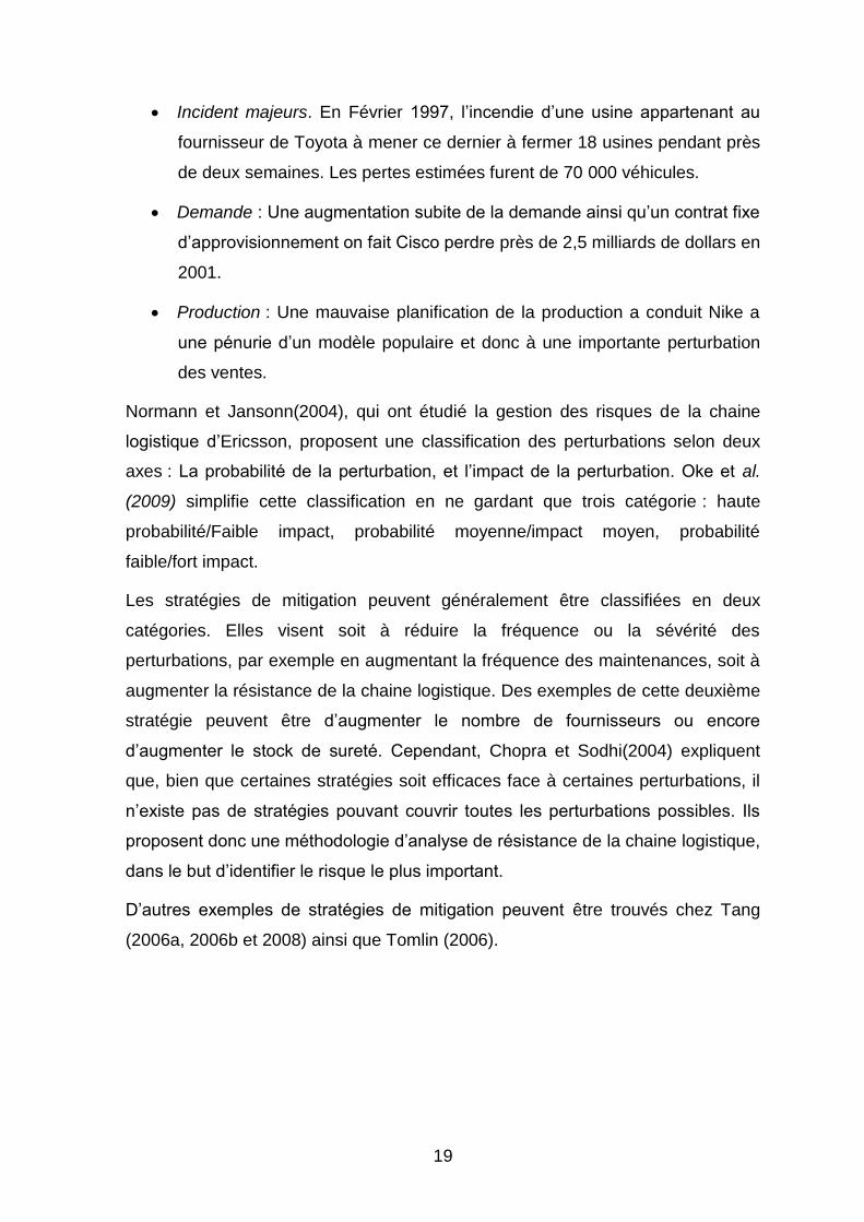
Incident majeurs. En Février 1997, l’incendie d’une usine appartenant au

fournisseur de Toyota à mener ce dernier à fermer 18 usines pendant près

de deux semaines. Les pertes estimées furent de 70 000 véhicules.

Demande : Une augmentation subite de la demande ainsi qu’un contrat fixe

d’approvisionnement on fait Cisco perdre près de 2,5 milliards de dollars en

2001.

Production : Une mauvaise planification de la production a conduit Nike a

une pénurie d’un modèle populaire et donc à une importante perturbation

des ventes.

Normann et Jansonn(2004), qui ont étudié la gestion des risques de la chaine

logistique d’Ericsson, proposent une classification des perturbations selon deux

axes : La probabilité de la perturbation, et l’impact de la perturbation. Oke et al.

(2009) simplifie cette classification en ne gardant que trois catégorie : haute

probabilité/Faible impact, probabilité moyenne/impact moyen, probabilité

faible/fort impact.

Les stratégies de mitigation peuvent généralement être classifiées en deux

catégories. Elles visent soit à réduire la fréquence ou la sévérité des

perturbations, par exemple en augmentant la fréquence des maintenances, soit à

augmenter la résistance de la chaine logistique. Des exemples de cette deuxième

stratégie peuvent être d’augmenter le nombre de fournisseurs ou encore

d’augmenter le stock de sureté. Cependant, Chopra et Sodhi(2004) expliquent

que, bien que certaines stratégies soit efficaces face à certaines perturbations, il

n’existe pas de stratégies pouvant couvrir toutes les perturbations possibles. Ils

proposent donc une méthodologie d’analyse de résistance de la chaine logistique,

dans le but d’identifier le risque le plus important.

D’autres exemples de stratégies de mitigation peuvent être trouvés chez Tang

(2006a, 2006b et 2008) ainsi que Tomlin (2006).

20

2.2. Incertitude dans les problèmes d’optimisation.

Dans les modèles d’optimisation en contexte incertains, la quantité d’information

disponible sur les incertitudes varient énormément d’un problème à l’autre. On

identifie trois types d’informations. Dans le meilleur des cas, l’incertitude peux être

identifiée par une distribution aléatoire. Dans ce cas, le problème est le plus

souvent résolu en utilisant les méthodes d’optimisation stochastique. Dans le

second cas, l’incertitude est identifié, mais ne peux pas être caractérisée par une

loi de probabilités. Dans ce cas, les méthodes d’optimisation robuste sont souvent

efficaces. Enfin, si aucune information n’est disponible sur les perturbations, le

recours à l’analyse de risque décrite dans la section précédente est nécessaire.

Je décris dans cette section l’état de l’art sur les méthodes d’optimisation en

contexte incertain, à savoir les méthodes d’optimisation stochastique et robuste.

2.3. Optimisation Stochastique

Les méthodes d’optimisation stochastiques supposent que l’incertitude présentée

en compte est caractérisée par une loi de probabilité connue. Certains

paramètres du problème sont alors considérés comme des variables aléatoires.

L’ensemble des réalisations possibles de ces variables aléatoire crée un jeu de

scénarios potentiellement infini.

Une première approche naïve, serait de fixer tous les paramètres aléatoire à leur

espérance, créant ainsi un ‘scenario moyen’, puis de d’optimiser ce scenarios.

Sen et Higle (1999) montrer que cette approche mène rarement a des solutions

optimales, et peux même donner des solutions irréalisables sur certains

scenarios.

C’est pourquoi les méthodes d’optimisation stochastique se concentrent sur la

minimisation de l’Esperance de la fonction objective du problème.

)),(()(min xGExgx

Avec ),( xG représentant la fonction objective, l’ensemble des solutions

réalisables et l’ensemble des scenarios.

21

Cette formulation est le plus souvent appelée “programmation stochastique” dans

la littérature (cf. Kleywegt & Shapiro 2007). Le nombre de scenarios

potentiellement infini rend cependant cette formulation extrêmement difficile à

résoudre. Son caractère abstrait la rend aussi difficile à appliquer sur des

problèmes réels. Une alternative, l’optimisation stochastique avec recours a été

introduite par Dantzig (1955).

L’optimisation stochastique avec recours consiste en deux types de problèmes

d’optimisation. Le problème maitre optimise le problème avant que la réalisation

des paramètres aléatoires soient connus, en optimisant une fonction déterministe

ainsi que l’espérance des problèmes esclave. Chaque problème esclave optimise

le cout de la chaine logistique après réalisations des variables aléatoire.

Une application classique concerne l’optimisation de chaine logistique. Le

problème maitre optimisera la localisation des usines avant que les demandes

exactes soient connues. Les problèmes esclaves optimisent la distribution une

fois les demandes connues. Une étude des modèles d’optimisation stochastique

avec recours peut être trouvée chez Birge et Levaux (1997). Dans le cas où le

nombre de scenarios et fini, Ils montrent comment reformuler le problème

d’optimisation stochastique avec recours sous la forme d’un unique problème

d’optimisation linéaire. La complexité de ce modèle est cependant fortement

dépendante du nombre de scenarios. Dans le cas où celui-ci est trop élevé,

l’utilisation de méthodes d’échantillonnage est nécessaire.

La notion de problèmes d’optimisation stochastique avec recours peut être

étendue avec la notion d’optimisation stochastique à recours multiple. Un

exemple serait l’optimisation multi-périodique, ou la demande des clients

changerait à chaque période. Ces problèmes sont par contre trop larges pour être

résolu sauf pour un faible nombre de scenarios.

Aune autre approche consiste à optimiser un sous ensemble de scenario, puis

d’analyser les solutions obtenues par une analyse de sensitivité de Monte-Carlo

(voir Saltelli et al. ou encore Shapiro (2003)). Choisir la meilleure solution peut

cependant être difficile. Une procédure pour choisir la solution, en utilisant par

exemple le critère de Pareto-Optimalité, ou encore la dominance stochastique a

été proposé par Lowe et al. (2002)

22

2.4. Optimisation Robuste

Historiquement, les méthodes d’optimisation stochastique étaient utilisées pour

résoudre les problèmes d’optimisation en contexte incertain. Cependant,

déterminer la loi de probabilité associée à chaque variable ou paramètre aléatoire

peut s’avérer une tache particulièrement ardue. Des méthodes d’optimisation

robuste, ne nécessitant pas de loi de probabilités ont donc été développées.

Le premier usage de méthode d’optimisation robuste apparait en 1968 avec

Gupta et al. qui fournissent des solutions flexibles dans un contexte incertain. Ces

solutions peuvent facilement être modifiées pour s’adapter aux différentes

réalisations possibles. Cependant, les méthodes d’optimisation robustes récentes

semblent plutôt se concentrer sur trouver des solutions qui sont capable de

résister aux aléas. (voir Roy 2002 et Roy 2008). Les méthodes d’optimisation

robuste nécessitent un ensemble de scenarios représentants des réalisations

possibles de paramètres aléatoires. Cependant, aucune probabilité n’est associée

à ces scenarios. Ces scenarios peuvent être discret, ou encore continus,

indiquant un intervalle dans lequel le paramètre aléatoire peut prendre valeur.

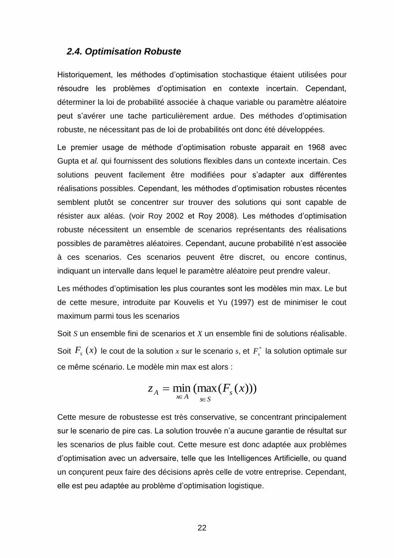
Les méthodes d’optimisation les plus courantes sont les modèles min max. Le but

de cette mesure, introduite par Kouvelis et Yu (1997) est de minimiser le cout

maximum parmi tous les scenarios

Soit S un ensemble fini de scenarios et X un ensemble fini de solutions réalisable.

Soit )(xFs le cout de la solution x sur le scenario s, et *

sF la solution optimale sur

ce même scénario. Le modèle min max est alors :

)))(((maxmin xFz sSsAx

A

Cette mesure de robustesse est très conservative, se concentrant principalement

sur le scenario de pire cas. La solution trouvée n’a aucune garantie de résultat sur

les scenarios de plus faible cout. Cette mesure est donc adaptée aux problèmes

d’optimisation avec un adversaire, telle que les Intelligences Artificielle, ou quand

un conçurent peux faire des décisions après celle de votre entreprise. Cependant,

elle est peu adaptée au problème d’optimisation logistique.

23

C’est pourquoi Kouvelis et Yu s’intéressent aussi au regret d’une solution, soit la

différence (absolue ou relative) entre le cout de la solution et la valeur de la

solution optimale des scenarios. Cela permet à chaque scenario d’avoir la même

importance dans la solution finale.

L’algorithme général des méthodes robuste minimax est le suivant :

Trouver une solution candidate x.

Calculer le regret maximum de la solution x sur l’ensemble des scenarios.

Garder la solution si le regret maximum est plus faible.

Trouver une nouvelle solution et recommencer les trois premières étapes.

La solution candidate peut être trouvée par un algorithme d’optimisation

classique, heuristique ou exact.

La difficulté de la deuxième étape dépend du type de scenarios. Si le nombre de

scénario est fini, il suffit de calculer le regret sur l’ensemble des scenarios. Par

contre, dans le cas de scenarios intervalle, calculer le regret maximum est

beaucoup plus compliqué. Les méthodes existantes s’appuient sur le fait que le

scenario maximisant le regret de la solution x à tous ses paramètres fixé à une

extrémité de leur intervalle de valeur. On pourrait alors imaginer de générer tous

les scenarios ‘extrêmes’ possible. Mais cela reste intraitable si le nombre de

paramètre à intervalle est trop élevé. Par exemple, dans le cas de l’optimisation

d’une chaine logistique ou la demande des clients est connue sur un intervalle, le

nombre de scenarios ‘extrême’ est égale à 2n, ou n est le nombre de clients.

Mausser et Laguna proposent une méthode heuristique (1999a) permettant de

résoudre les plus grands problèmes, ainsi qu’une méthode exacte (1999b) pour

les problèmes de tailles réduites.

Les modèles d’optimisation robuste sont au cœur des travaux de Ben-Tal et al.

(1999, 2000, 2002 et 2009). Leurs travaux sont basés sur une des premières

applications de l’optimisation robuste proposée par Soyster (1973). Soyster

propose un modèle qui permet d’obtenir une solution réalisable pour tout

paramètre appartenant à un ensemble convexe. A partir de ce modèle, Ben-Tal et

al. vont développer un modèle permettant de trouver une solution réalisable sur

l’ensemble des paramètres incertain, et minimisant le cout en pire cas.

24

Bien que cette approche reste conservative, Ben Tal et al. la justifie en rappelant

que la plupart des problèmes réels sont composés de contraintes dure, et que la

solution doit rester réalisable. Ils citent en exemple la construction d’un pont, ou

de petits changements peuvent mener à une structure instable.

Ils introduisent en 2000 la notion de fiabilité pour gérer le fait que leur modèle soit

conservatif. Ils considèrent que chaque paramètre doit se trouver dans un

intervalle donné. De plus pour chaque contrainte, la solution finale ne doit pas

dévier de la solution optimale de plus d’un seuil fixé à l’avance. Ils appliquent

cette méthode en 2009 pour résoudre un problème d’optimisation de chaine

logistique multi-échelons et multi-périodes sous incertitude de demandes.

Berstimas et Sim (2004) notent que les modèles proposés par Ben-Tal et

Nemirovski (2000) nécessitent trop de variables supplémentaires et ne sont donc

pas adaptés pour traiter les problèmes réels. Ils proposent donc une nouvelle

formulation qui limite l’impact des paramètres incertains sur la méthode robuste.

Pour chaque contrainte, ils introduisent une variable i qui limite le nombre de

paramètre pouvant varier, les autres étant fixés à leur valeur médiane. Cela a

pour effet de limiter le nombre de scenarios, simplifiant significativement le

problème. Le paramètre i contrôle le compromis entre la prise en compte des

incertitudes et l’impact sur le problème. Leurs travaux sont approfondis dans

Bertsimas et al. (2004)

Vladimirou et Zenios (1997) introduisent une troisième notion de robustesse : La

robustesse au recours. Cette notion pénalise la solution si les recours sont trop

différents les uns des autres. Dans leur modèle, ils commencent par forcer

l’égalité de tous les variables des problèmes esclaves, puis relâchent

progressivement cette contrainte jusqu’à l’obtention d’une solution réalisable.

2.5. Optimisation Robuste vs. Stochastique

Si l’optimisation stochastique possède l’avantage de minimiser efficacement les

couts sur le long terme, elle possède aussi quelque désavantage justifiant

l’utilisation des méthodes d’optimisation robuste.

25

Le premier désavantage consiste en la nécessité de connaitre une loi de

probabilité pour chaque paramètre aléatoire. Comme indiqué plus haut,

déterminer ces lois de probabilité peut se révéler extrêmement difficile, du a un

faible nombre de réalisation antérieure, ou plus simplement du a un manque de

données historiques. En utilisant pas de probabilités, les méthodes robustes

esquivent cette difficulté.

Ensuite, même si la loi de probabilité est connue, les méthodes d’optimisations

stochastiques ne fournissent une garantie que sur l’espérance de la solution, et

non sur l’efficacité de la solution par rapport à une réalisation donnée. Même une

solution avec une espérance de cout faible peut mener à des couts importants en

cas de ‘malchance’. Au contraire, les méthodes d’optimisation robustes

garantissent que la solution fournie restera bonne quelles que soient les

réalisations des paramètres aléatoires.

Ainsi, les méthodes d’optimisation robuste et stochastique sont donc

complémentaires dans la gestion des problèmes en contexte incertain. En face de

décisions à haut risque, pouvant mener à des pertes importantes, ou bien face à

des aléas difficiles à caractériser, les méthodes d’optimisation robuste sont

préférables. Au contraire, face à des décisions long termes, ou bien avec des

variations faible et facilement caractérisable, les méthodes d’optimisation

stochastique se révèlent plus efficace.

3. TOURNEES DE VEHICULES AVEC GESTION DES STOCKS

Je m’attaque en premier au problème de tournées de véhicules avec gestion

d’inventaire rencontré par AIR LIQUIDE. Ce problème est bien connu et a été

souvent étudiés. Cependant, la majorité des travaux concernant ce problème en

contexte incertain considère comme incertitude la demande des clients. Dans

mes travaux, je m’attaque à une incertitude très peu étudiée, celle de la possibilité

de panne d’usine.

26

3.1. Description du problème

Je m’attaque au problème de tournées de véhicules avec gestion des stocks dans

un contexte industriel. Du gaz liquide est produit en continu dans des usines de

production et doit être livrés aux clients. Les usines comme les clients stockent

leur produit dans des réservoirs cryogéniques. Pour chaque client, une prévision

de consommation fiable est connue pour la totalité de l’horizon de temps

considéré.

Le fournisseur propose deux types de services pour la gestion des stocks :

Le premier service, connu sous le nom de « vendor managed inventory » est une

gestion complète des stocks par le fournisseur. Celui-ci décide les horaires des

livraisons ainsi que les quantités livrées en fonction de la prévision de

consommation. Le fournisseur s’engage à ce que le stock client passe en

dessous d’un seuil de sécurité.

Le second service s’appelle « order based ressuply ». Celui-ci permet au client de

passer commande auprès du fournisseur. Le client indique la quantité désirée

ainsi qu’une fenêtre de temps durant laquelle la livraison devra être effectuée.

L’optimisation est à objectif triple. Les trois objectifs sont hiérarchisés, chacun

étant strictement plus important que les suivants. Il s’agit de minimiser le nombre

de commandes non satisfaites, ou « missed order », puis de de minimiser le

nombre de pas de temps passé sous le seuil de sécurité pour chaque client, les

« run-outs », et, pour finir, de minimiser le cout logistique des livraisons.

Bien sûr, de nombreuse contraintes doivent être satisfaites, telles que les fenêtres

de temps, la capacité maximum des citernes de livraisons et des réservoirs

cryogéniques, et les horaires de travails des chauffeurs. Ce grand nombre de

contraintes, spécifique aux problèmes industriels réels, lié à un temps de

résolution qui se doit de rester court, représente toute la difficulté de ce problème.

27

3.2. Méthodologie générale

Afin de résoudre ce problème, je propose une méthodologie robuste, basée sur

les travaux de Kouvelis et Yu (1997). Cette méthodologie se base sur des

scenarios de pannes pour trouver une solution robuste. La méthodologie

proposée est générique mais appliquées au problème de tournées de véhicules.

La méthodologie est multi-objective, et optimise non seulement les couts de

distribution dans le case ou aucune panne ne survient, mais aussi la robustesse

de la chaine de distribution.

La méthodologie est compose de quatre étapes successives.

1. Génération d’un jeu de scenarios : Un jeu de scénario représentant des

pannes possible est créé. Le choix des scénarios crée est un élément

crucial de la méthodologie robuste. En effet, il faut générer des scenarios

réalistes, représentatifs des pannes possible, mais éviter de trop en

générer. Dans la méthodologie robuste, les scenarios sont tous

équiprobable. Cela permet de savoir comment la chaine logistique se

comporte face à des scenarios peu probables, mais cependant plausibles.

Cela implique aussi que chaque scénario a un impact important sur la

solution finale. Afin d’assurer que les scénarios soient aussi proche que

possible de la réalité, leur génération se base sur les données de pannes.

2. Génération d’un jeu de solutions : L’étape suivante consiste à générer un

ensemble de solutions pour faire face à ces scenarios. Pour générer ces

solutions, j’utilise l’heuristique développée par Benoist et al. Cette

recherche locale est efficace pour résoudre le problème de tournées de

véhicules avec gestion des stocks déterministe. Cependant, pour trouver

une solution robuste, il est important de générer des solutions avec des

structures différentes. Pour cela, je développe plusieurs stratégies

d’utilisation de la recherche locale.

28

De plus il est important d’inclure la solution obtenue par le solveur

déterministe afin de pouvoir comparer les résultats. Il est aussi important

de noter que toutes les solutions obtenues sont réalisables pour tous les

scenarios. En effet, les paramètres et données d’entrée du problème liés

au contraintes dures (fenêtre de temps, durées maximale des tournées)

sont identiques pour tous les scénarios. Il est cependant probable que la

panne d’usine implique que certains clients ne soient pas suffisamment

livrés. Cela mène à un cout de pénalité important, mais ne rend pas les

solutions non réalisables.

3. Evaluation de la robustesse des solutions : Une fois les scenarios et

solutions généré, le cout de chaque solution appliquée à chaque scenario

est évalué. Une fois ces couts connus, j’utilise une approche min max afin

de calculer la robustesse de chaque solution

4. Pareto-optimalité et sélection de la meilleure solution : Le problème de

tournée de véhicules robuste possède deux objectifs : minimiser les couts

logistiques de la distribution et maximiser la robustesse. On peut facilement

imaginer qu’une solution plus robuste aura des couts logistiques plus

élevés qu’une solution peu robuste. C’est pourquoi je me base sur la

Pareto-optimalité pour choisir la meilleure solution.

3.3. Méthode de génération des solutions.

La génération de scenarios est un élément important de la méthodologie robuste.

En effet, les scenarios représentent les réalisations possibles des incertitudes

contre lesquelles la méthode robuste va nous protéger. Lister tous les scenarios

nécessiterai un temps de calcul trop long, et mènerai de plus vers des solutions

trop conservatrices. C’est pourquoi il est important d’identifier un sous ensemble

de scenarios représentatifs des pannes possibles.

Afin de limiter le nombre de scenarios, il a été décidé après étude des données

historiques des pannes d’usine chez Air Liquide que les scenarios ne

comporteraient qu’une seule panne. Les scénarios sont donc caractérisés par

trois paramètres : L’usine touchée par la panne, la date de départ de la panne

ainsi que la durée de la panne.

29

Je propose dans cette section une méthode permettant de générer un ensemble

de scenarios représentatifs des données historiques. Cela signifie que plus une

panne est probable, plus il y a de chance qu’elle soit représentée par un scenario.

Pour cela, les scenarios choisis seront tirés aléatoirement parmi des clusters de

scenarios similaires, en fonction de la probabilité de panne associée à chaque

cluster. Le nombre de scenarios crée est fonction de la précision voulue par le

décideur, ainsi que du temps de calcul alloué. Le modèle mathématique de la

méthode peut être trouvé dans la section 4 du chapitre II de ma thèse.

Dans cette section, je suppose que les paramètres suivant sont connus :

Le nombre minimum de solution à générer.

La précision voulue (une précision de 100% nécessitant de générer tous

les scenarios possibles)

Le temps de calcul maximum alloué à la méthode robuste

Des lois de probabilités associées aux paramètres des scenarios (durée

des pannes, usines concernées par la panne)

La première étape consiste à créer les clusters de scenarios. Les deux

paramètres les plus influents sur l’impact des scenarios sont, et donc selon

lesquels les scenarios devraient être rassemblés sont la durée de la panne et

l’usine concernée. Les deux possibilités de clusters sont donc

Des clusters rassemblant les scenarios de même durée

Des clusters rassemblant les scenarios de même durée, sur la même

usine.

Dans chaque cas, il est possible d’attribuer un poids à chaque cluster en utilisant

les lois de probabilités associées à ces paramètres. La section 4 du Chapitre II de

ma thèse décrit plus en détails comment le poids de chaque cluster est calculé.

30

Une fois le poids de chaque cluster connu, je calcul le nombre de scenarios

nécessaire à prendre dans chaque cluster pour obtenir la précision voulue. La

précision de chaque cluster est calculée soit en utilisant le rapport du nombre de

scenarios choisi sur le nombre de scenarios total du cluster, soit, si des données

suffisantes sont disponibles, en se basant sur la probabilité de robustesse d’une

solution dans un cluster. La précision finale est calculée en faisant la somme

pondérée des précisions de chaque cluster. Pour obtenir le nombre minimum de

scenarios nécessaires pour atteindre la précision voulue, un simple programme

linéaire est utilisé.

Je détermine ensuite si ce nombre de scenarios permet à la méthode robuste de

s’exécuter dans le temps de calcul imparti. Si oui, je génère alors des solutions

supplémentaires tant que la méthode robuste respecte le temps de calcul alloué.

Si non, je maximise la précision pouvant être obtenue avec le temps de calcul

spécifié.

3.4. Génération des solutions

Afin d’augmenter les chances de trouver une « bonne » solution robuste, le jeu de

scenarios doit contenir des solutions possédants des couts, structures et

caractéristiques différentes. Pour atteindre ce but, j’implémente plusieurs

méthodes pour générer les solutions.

Ce chapitre présente les trois méthodes implémentées pour générer les solutions.

La première se contente de lancer plusieurs instances de recherche locale en

parallèle, avec des graines aléatoires différentes. En effet, le choix des

modifications appliquées à la solution courante durant la recherche locale utilise

cette graine aléatoire. Ainsi, l’utilisation de graines aléatoires différentes assure

que les solutions trouvées seront différentes les unes des autres.

Cependant, cette méthode ne produit que des solutions optimisées pour le cas où

aucune panne ne survient. La deuxième utilise des scenarios comme données

d’entrée, et fournit donc des scenarios optimisés pour la gestion des pannes. Ces

solutions restent réalisables dans le cas où aucune panne ne survient, le surplus

de produit ne compromettant aucune contrainte dure.

31

Enfin, des méthodes pour guider l’heuristique vers des solutions plus robustes

sont présentées. Ces méthodes se basent sur l’ajout de contraintes

supplémentaires dans le modèle afin que les solutions trouvées soient

naturellement plus robustes. Ces contraintes additionnelles s’inspirent des

méthodes utilisées par les entités opérationnelles pour gérer les arrêts d’usine

pour maintenances.

1. Créations de stock de sureté aux usines.

2. Augmenter le nombre de livraisons aux clients critiques

Les tests préliminaires ont montrés que ces heuristiques produisaient des

solutions bien plus robustes que les autres méthodes. Cependant, le cout de ces

solutions était aussi beaucoup plus élevé, et cette méthode c’est avérée inefficace

pour produire des solutions robustes à faible cout.

3.5. Sélection de la solution

Une fois tous les scénarios et toutes les solutions générées, le cout de chaque

solution appliqué à chaque scenario est calculé. Cela permet d’obtenir une

matrice des couts.

La robustesse de chaque solution est ensuite évaluée en utilisant le critère de

regret min max introduit par Kouvelis et Yu (1997). Le but de ce critère est de

minimiser la différence maximum entre la valeur d’une solution sur un scenario, et

la valeur de la meilleure solution sur ces scenarios. Cela permet de garantir que la

solution finale choisie se comportera ‘bien’ sur l’ensemble des scenarios.

Une fois la robustesse de chaque solution connue, l’étape suivante consiste à

sélectionner la meilleure solution. Pour cela, il faut prendre en compte deux

objectifs : Le cout de la solution, ainsi que sa robustesse. Une approche classique

dans le cas d’optimisation bi-objective est de se limiter aux solutions Pareto-

Optimales, à savoir l’ensemble des solutions telles que, pour chaque solution de

cet ensemble, les autres solutions ont soit une robustesse plus faible, soit un cout

plus élevé.

32

Il n’y a cependant aucune garantie que cela mène à une solution unique. Plutôt

que de présenter plusieurs solutions à l’utilisateur et lui demander de choisir,

j’utilise la méthode suivant pour sélectionner la meilleure solution. Je fixe une

limite de cout arbitraire, en sélectionnant la solution de cout minimum, et en

multipliant son cout par un facteur arbitraire, par exemple 1.05, pour obtenir une

augmentation de 5%. Je sélectionne ensuite la solution la plus robuste qui reste

en dessous de la limite de cout.

3.6. Expérimentations et résultats.

La méthode a été implémentée en C# .NET 3.5 et testée sur 16 instances

différentes générées à partir de données réelles. Pour chaque instance, le

nombre de solution généré est limité à 20, le temps de calcul alloué est de 20

minutes et la précision demandée est de 100%. Les résultats complets sont

présentés dans le chapitre II de ma thèse.

Ces résultats indiquent que cette méthode permet efficacement de réduire les

run-outs lies aux pannes d’usine dans le problème de tournées de véhicule avec

gestion des stocks. En effet, avec une augmentation de couts inferieure a 2 % en

moyenne, le regret maximum des solutions est améliorer de près de 45%. On

observe aussi que les meilleures solutions trouvée ont équitablement été

générées par les deux méthodes de génération de solutions présentées.

Afin de valider la méthode de génération de solution, les solutions sont à nouveau

évaluées, cette fois ci sur l’intégralité des scenarios possibles. On s’aperçoit que

dans toutes les instances sauf deux, la solution la plus robuste est la même que

celle trouvée en utilisant un ensemble réduite, générer par la méthode

Dans le prochain chapitre, j’étudie l’utilisation de la génération de solution

appliquée au problème déterministe, et je montre qu’elle permet d’obtenir des

gains significatifs.

33

4. UNE METHODOLOGIE GRASP

J’ai montré dans la section précédente comment la génération multiple de

scenarios et de solution peut être utilisée pour l’optimisation robuste de la

distribution au jour le jour. Cependant, il est possible aussi d’utiliser uniquement la

génération de solution, et de l’intégrer dans une méthodologie GRASP afin

d’optimiser d’avantage les tournées de véhicules dans un contexte déterministe.

Cette section sera découpée de la façon suivante : Dans un premier temps, je

rappellerai le problème industriel auquel je m’attaque. Je présenterai ensuite les

différentes implémentations possibles de la métaheuristique GRASP.

4.1. Description du problème

Ce problème est similaire à celui traité dans le chapitre précèdent, mais sans la

prise en compte des pannes. Je rappelle ici le contexte :

Je m’attaque au problème de tournées de véhicules avec gestion des stocks dans

un contexte industriel. Du gaz liquide est produit en continu dans des usines de

production et doit être livrés aux clients. Les usines comme les clients stockent

leur produit dans des réservoirs cryogéniques. Pour chaque client, une prévision

de consommation fiable est connue pour la totalité de l’horizon de temps

considéré.

Le fournisseur propose deux types de services pour la gestion des stocks :

Le premier service, connu sous le nom de « vendor managed inventory » est une

gestion complète des stocks par le fournisseur. Celui-ci décide les horaires des

livraisons ainsi que les quantités livrées en fonction de la prévision de

consommation. Le fournisseur s’engage à ce que le stock client passe en

dessous d’un seuil de sécurité.

Le second service s’appelle « order based ressuply ». Celui-ci permet au client de

passer commande auprès du fournisseur. Le client indique la quantité désirée

ainsi qu’une fenêtre de temps durant laquelle la livraison devra être effectuée.

34

L’optimisation est à objectif triple. Les trois objectifs sont hiérarchisés, chacun

étant strictement plus important que les suivants. Il s’agit de minimiser le nombre

de commandes non satisfaites, ou « missed order », puis de de minimiser le

nombre de pas de temps passé sous le seuil de sécurité pour chaque client, les

« run-outs », et, pour finir, de minimiser le cout logistique des livraisons.

De nombreuse contraintes doivent être satisfaites, telles que les fenêtres de

temps, la capacité maximum des citernes de livraisons et des réservoirs

cryogéniques, et les horaires de travails des chauffeurs. Ce grand nombre de

contraintes, spécifique aux problèmes industriels réels, lié à un temps de

résolution qui se doit de rester court, représente toute la difficulté de ce problème.

Afin de résoudre ce problème, une heuristique a déjà été proposée par Benoist et

al. (2010). Cette recherche locale fonctionne en testant un maximum de

perturbations ou mouvements durant le temps de calcul imparti. Cette heuristique,

bien que très efficace, peut cependant se retrouver bloquée dans un optimum

local. Afin de continuer l’exploration de l’espace des solutions, il est nécessaire de

diversifier la recherche. Une solution consiste à générer plusieurs solutions, puis

de sélectionner la meilleure solution. Cette solution est à la base de la

métaheuristique GRASP.

4.2. Etat de l’art

La méthodologie GRASP « Greedy Randomized Adaptative Search Procedure »

est une métaheuristique a départ multiple qui fut introduite par Leo et Resende

(1989, 1995). Cette métaheuristique consiste en plusieurs itérations de deux

phases successives : une phase de construction et une phase d’optimisation.

Durant la phase de construction, une solution initiale est créée itérativement en

utilisant un algorithme glouton avec des éléments aléatoires. Puis, durant la

phase d’optimisation, une recherche locale améliore cette solution initiale. A la fin

de la procédure, la meilleure solution générée est retenue.

35

La métaheuristique GRASP a été appliquée avec succès à de nombreuses

problématiques d’optimisation. Resende et Ribeiro (2003) ainsi que Festa et

Resende (2001) présentent des applications dans des champs aussi diversifiés

que la distribution, l’ordonnancement ou les problèmes d’affectation. Grellier et al.

(2004) propose une application au problème de tournées de véhicules avec

gestion des stocks.

Afin de réduire le temps de calcul, l’utilisation de méthodes de calcul parallèle est

une approche naturelle. Cung et al. (2001) expliquent que, parce que chaque

itération peut être effectuée dans un fil d’exécution parallèle séparé, et que

chaque tâche est effectuée indépendamment les unes des autres, sans

interactions nécessaires, le gain de temps lié à l’utilisation du parallélisme est

quasiment linéaire en fonction du nombre de processeurs utilisés.

Dans ce chapitre, je compare deux implémentations de la métaheuristique

GRASP : Le premier est la métaheuristique classique a départ multiple. Le

second est par contre a départ simple. Dans cette dernière, une unique phase de

construction est effectuée au début de la procédure, et chaque itération ne

possède qu’une phase d’optimisation, avec une graine aléatoire différente afin

d’assurer la diversité des solutions générées à chaque itération.

Je vais donc décrire dans ce chapitre les algorithmes utilisés lors des phases de

construction et d’optimisation des métaheuristiques GRASP que j’utilise.

4.3. Phase de construction

Comme indiqué au paragraphe précèdent, j’utilise deux phase de construction

différentes pour chaque implémentation de la méthodologie GRASP. Je présente

en premier la version déterministe de l’algorithme glouton servant à construire la

solution initiale, puis la version avec aléas.

36

Pour construire la solution initiale dans le cas déterministe, j’utilise l’algorithme

glouton proposé par Benoist et al. (2012). Cette algorithme démarre d’une

solution vide, et liste toute les livraisons nécessaires pour éviter les prochains

runouts de clients. La livraison la plus urgente est alors sélectionnée, et le cout

d’insertion dans chaque tournée existante ainsi que le cout de création d’une

nouvelle tournée est alors évalué. La livraison est alors insérée à la position de

cout minimum. Une fois la livraison insérée, la liste des demandes est alors mise

à jour, et la nouvelle livraison la plus urgente est alors sélectionnée pour être

insérée à son tour. L’heuristique continue ainsi jusqu’à ce que toutes les livraisons

aient été insérées.

Cette heuristique gloutonne est entièrement déterministe. Afin de l’utiliser dans le

cadre d’une procédure GRASP a départ multiple, je l’ai modifiée afin d’y introduire

une part d’aléatoire et donc de permettre de générer plusieurs solutions de

départ. Pour cela, je continue à sélectionner la livraison la plus urgente, mais, au

lieu de l’insérer dans la position optimale, je retiens une liste de position

d’insertion possible (appelée Restricted Candidate List, ou bien RCL). La livraison

sera ensuite insérée dans une de ces positions choisie aléatoirement. En utilisant

une graine aléatoire différente à chaque itération, on s’assure ainsi que les

solutions générées seront différentes les unes des autres.

La taille de la RCL a été choisie arbitrairement après les tests préliminaires. Si

celle-ci est trop grande, alors la qualité de la solution initiale est trop faible pour

mener à des améliorations de la solution finale. Si au contraire celle-ci est de taille

1, alors la solution initiale sera toujours identique à celle obtenue par l’heuristique

déterministe. En me basant sur les résultats préliminaires, j’ai décidé de

sélectionner les 3 insertions de couts minimums pour construire la RCL.

4.4. Phase d’optimisation et paralellisation

Les phases d’optimisation utilisée par les deux implémentations du méta

heuristique GRASP que je propose sont identiques. Dans chaque cas, je pars de

la solution initiale générée par la phase de construction correspondante que

j’améliore en utilisant la recherche locale proposée par Benoist et al. (2011).

37

Celle-ci consiste en une descente simple optimisée pour le problème traité. A

chaque itération de la recherche locale, une modification possible de la solution

courante est testée. Si celle-ci mène à une amélioration, elle est alors retenue et

la solution courante est modifiée en conséquence. Dans le cas où elle détériore la

solution courante, elle est simplement ignorée. Benoist et al. ont montrés que les

choix de modifications qu’ils proposent sont efficaces pour traiter le problème de

tournée véhicule avec gestion des stocks dans un contexte industriel, en un

temps inférieur à cinq minutes.

Cependant, celle-ci devant être utilisée à chaque itération de la métaheuristique

GRASP, il est nécessaire, afin de garder un temps de calcul raisonnable, d’utiliser

les méthodes de calcul parallèle. Pour cela, j’ai modifié la condition d’arrêt de

l’heuristique afin d’utiliser le nombre d’itérations au lieu du temps écoulé. Chaque

itération de l’heuristique est ensuite effectuée en parallèle. Une fois que toutes les

itérations sont finies, la meilleure solution est choisie comme solution finale.

Le pseudo code de chaque procédure décrite dans cette section peut être trouvé

dans le chapitre 4 de ma thèse.

4.5. Tests et résultats obtenus

Les deux méthodologies décrites dans la section précédentes ont été

implémentées en C# et testées sur un ordinateur possédant 16 processeur et

8GB de mémoire vive. 16 instances différentes ont été créées à partir de données

réelles. Trois heuristiques sont comparées. La première est basée sur

l’heuristique locale existante, et utilise dont une phase de construction

déterministe suivi d’une unique phase d’optimisation. La seconde est la

métaheuristique GRASP à départ unique, consistant donc d’une phase de

construction déterministe, puis de plusieurs itérations contenant chacune une

phase d’optimisation. Enfin, la dernière heuristique testée est la métaheuristique

GRASP classique.

38

Afin d’obtenir des résultats comparable, il est important que le temps de calcul

utilisé par chaque heuristique soit similaire. Initialement, l’heuristique de

recherche locale effectuait 4 millions de tests dans un temps moyen de 264

secondes. De plus, les tests préliminaires ont montrés que, dans les cas les plus

complexes, la recherche locale continue à améliorer la solution durant ces 4

millions d’itérations. J’ai donc décidé de garder ces 4millions de test comme la

base de chaque phase d’optimisation des itérations. Pour obtenir un temps de

calcul similaire, j’ai donc augmenté le nombre d’itération de la recherche locale à

16 millions.

Les résultats complets peuvent sont présentés dans le chapitre 5 de la thèse. On

y voit que l’augmentation du nombre d’itérations de la recherche locale permet

une amélioration de 1.66% par rapport à l’heuristique déjà en place, en environ 20

minutes de temps de calcul. Dans un temps similaire, les méthodes GRASP à

départ simple et à départ multiple, mènent respectivement à une amélioration de

5.44% et 5.07%, démontrant par la même occasion l’efficacité de la

métaheuristique GRASP.

Les deux procédures affichent des résultats finaux similaires, cependant, une

analyse plus détaillée montre que les résultats obtenus par la procédure à départ

multiple sont beaucoup plus variables que les résultats obtenus en partant d’une

solution simple. Dans deux instances, les résultats obtenus sont même inférieur à

ceux obtenus par l’heuristique déjà en place. Dans l’optique d’obtenir des

résultats stables, l’utilisation d’une seule solution de départ est donc préféré.

4.6. Conclusion

Afin d’améliorer les résultats de l’heuristique déjà en place pour la résolution du

problème de tournées de véhicules avec gestion des stocks, j’ai proposé

l’utilisation de la métaheuristique GRASP. J’ai proposé et comparer deux

variations de cette métaheuristique et utilisé les méthodes d’optimisation parallèle

afin de réduire le temps de calcul nécessaire.

39

J’ai ensuite testé et comparer ces deux variations sur des jeux de données

représentant fidèlement les données réelles. Je montre que dans un temps de

calcul raisonnable (moins de 20 minutes), j’arrive à obtenir des résultats

significativement meilleurs que de simplement laisser l’heuristique en place

tourner pendant un temps similaire. La performance obtenue dans le temps limité

alloué est cruciale dans un contexte industriel. Cette méthode pourrait mener à

une amélioration notable de la chaine logistique.

Des travaux futurs sur cette problématique pourraient explorer différentes

méthodes pour créer la Restricted Candidate List de la méthode à départ multiple,

et potentiellement améliorer les résultats obtenus par celle-ci.

La section suivante s’attaque à un nouveau problème en contexte incertain : la

gestion de la production et l’affectation des clients.

5. GESTION DE LA PRODUCTION ET AFFECTATION DES CLIENTS

La troisième contribution de ma thèse s’attaque à un tout autre problème que les

tournées de véhicules. On considère cette fois-ci un problème tactique de

conception de chaine logistique.

5.1. Définition du problème

Le but de ce problème est de décider les quantités optimales de gaz liquide à

produire dans les usines et à livrer aux clients afin de satisfaire leurs demandes.

L’horizon de temps couvert s’étend de plusieurs mois a une année. Bien

évidemment, la solution se doit de respecter des contraintes de production, de

stock ainsi que de livraisons. L’objectif est de minimiser les couts de production,

de livraison ainsi que les couts contractuels.

La problématique est modélisée de la manière suivante :

Un ensemble de clients, avec chacun une demande connue, doit être affecté à

une ou plusieurs usine de production afin de se « sourcer », c’est-à-dire se faire

livrer une certaine quantité de produit.

40

Les usines de production considérées appartiennent soit à Air Liquide soit à un

concurrent. Dans le premier cas, chaque usine possède une capacité de

production minimum et maximum, un cout de production par unité de produit, ainsi

qu’une capacité de stockage maximum. La quantité exacte à produire est une

variable de décision du problème. En cas de production excessive, la quantité ne

pouvant pas être stockée doit être relâchée dans l’air et est définitivement perdue.

Dans les cas d’usine appartenant à un concurrent, la capacité de production et de

stockage est ignorée, et la quantité de produit disponible, ainsi que son prix

unitaire, est définie par un contrat.

Chaque client a une demande en produit fixe pour l’intégralité de l’horizon de

temps et peut être source par une ou plusieurs usines. Dans le cas d’un multi-

sourcin, une quantité minimum doit être livrée. Les clients possèdent aussi une

capacité de stockage maximum et un inventaire initial.

Pour effectuer les livraison, des camions, ou ressources, sont utilisées. Ces

ressources sont initialement dans des dépôts, qui peuvent être situé sur un site

de production ou bien séparément. Chaque ressource possède une capacité

maximum, et requière donc le plus souvent plusieurs trajets pour satisfaire la

demande des clients.

Les contrats sont des accords bilatéraux entre Air Liquide et ses concurrents.

Dans le modèle présenté ici, je ne prends en compte que les contrats entrant, qui

permettent à Air Liquide d’acheter du produit à un de ses concurrents. Chaque

contrat défini un prix d’achat, une quantité maximale ainsi qu’un ensemble d’usine

éligible pour acheter le produit. Il est donc possible d’acheter du produit d’un

même contrat dans plusieurs usines concurrentes.

Enfin, comme dans le problème de tournées de véhicules, nous prenons en

compte le contexte incertain des problématiques industrielles. Encore une fois,

l’aléa considéré est la possibilité de panne d’usine. Toutefois, comme l’horizon

considéré est plus long que dans le problème précédent, il nous est possible de

considérer des pannes plus longues ainsi que d’utiliser un modèle stochastique

avec recours. Les décisions du problème maitre étant les décisions prisent avant

une éventuelle panne, les décisions des problèmes esclaves concernent le retour

à la normale après une panne. Il est par exemple possible d’augmenter les

quantités produites ou bien de réaffecter les clients à des sources différentes.

41

5.2. Modele stochastique avec recours

Comme indiqué plus haut, nous proposons une modélisation stochastique pour

résoudre le problème d’affectation des clients et de planning de la production en

contexte incertain. La méthodologie que nous proposons est constituée de deux

étapes principales.

La première consiste à générer un jeu de scenarios réalistes. Le but de ces

scenarios et d’identifier les pannes à considérer lors de l’optimisation. Les

scenarios peuvent être soit générés en utilisant des données historiques

existantes, soit en utilisant la maitrise du sujet d’experts, dans le cas ou de telles

données historiques ne seraient pas disponibles.

La deuxième étape consiste en l’optimisation proprement dite du planning de

production et de l’affectation des clients. Cette étape repose sur un modèle

mathématique présenté dans la section 5.3. Comme indiqué précédemment, la

résolution utilise un modèle d’optimisation avec recours.

Le problème maitre prend des décisions au début de l’horizon de temps, sans

savoir avec certitude si une panne arrivera. Le but est de minimiser les couts de

production, de contrats et de distribution, ainsi que l’espérance du cout de retour

à la normale après une panne. Le cout de retour à la normale pour chaque

scenario est calculé par les problèmes esclaves. Je fais l’hypothèse qu’une panne

puisse arriver à n’importe quel moment durant l’horizon de temps. Quand une

usine tombe en panne, la production ainsi que la distribution prévue par le

problème maitre doit être recalculée afin de permettre la livraison d’un maximum

de clients malgré le manque de produit.

5.3. Hypotheses de modelisation

Je décris ici les hypothèses faites lors de la modélisation du problème.

Je suppose que la durée de la panne est connue des qu’elle arrive. En

pratique, la durée de la panne est très fortement liée à sa nature, qui est

rapidement identifiée. Cette hypothèse est donc tout à fait vraisemblable.

42

Le modèle ignore la planification des livraisons. Le problème traité étant un

problème tactique couvrant un grand horizon de temps, ajouter les

livraisons mènerait à un problème insoluble en temps raisonnable. A la

place, je fais l’hypothèse que les couts sont directement proportionnels au

temps passé. Par exemple, si 50000 unités de produits doivent être livrées

sur la totalité de l’horizon de temps, je considère que, à la moitié de

l’horizon, 25000 unités ont été livrées.

Afin de simplifier la résolution du problème, j’ai décidé de faire une

relaxation linéaire du nombre de voyage nécessaires aux livraisons des

clients par les ressources. En pratique, cela signifie que le cout de la

livraison est le cout par unité dans le cas d’une livraison d’un camion

complet, multiplié par la quantité totale livrée.

Finalement, afin de limiter les nombres de scenarios, je considère qu’une

seule usine tombe en panne durant la totalité de l’horizon de temps.

Chaque scenario est donc identifié par l’usine qu’il concerne, la date de

début de la panne, et la durée de la panne.

5.4. Résultats présentés

Le but des travaux présentés dans ce chapitre est de fournir un outil qui puisse

être utilisé aussi bien pour l’optimisation de chaine logistique que pour l’analyse

de celle-ci. C’est pourquoi il est important de pouvoir présenter plusieurs types de

résultats différents. Je décris ici les différents résultats pouvant être affichés par

l’outil que je propose :

Le premier résultat présenté est la valeur optimale des variables de décisions du

problème maitre, soit la solution minimisant les couts de production, de livraison,

de contrat ainsi que l’espérance des couts de retour à la normale après une

panne éventuelle.

Le second résultat présenté est la valeur des variables de décisions des

problèmes esclaves. Celles-ci représentent en effet la réallocation optimale des

clients ainsi que le nouveau planning de production après une panne.

43

Finalement, l’outil se doit aussi d’être capable de présenter des indicateur clés de

performance indiquant la criticité des usines dans la chaine logistique. Les

indicateurs identifiés sont les suivants :

L’espérance du cout de retour à la normal pour les pannes concernant

une usine en particulier.

Le nombre moyen de clients non livrés, dû au manque de produit

résultant des pannes d’une usine. Ne pas livrer un client pouvant mener à

la perte du client en question, cet indicateur efficace pour représenter

l’efficacité de la chaine logistique après une panne

La quantité de produit non livrée. Cela représente la quantité de produit

manquant pour pouvoir satisfaire l’intégralité de la demande des clients

après une panne d’une usine. Cet indicateur, bien que très proche du

nombre moyen de clients non livrés, permet d’obtenir une indication plus

précise de ce qui manque à la chaine logistique pour faire face aux

pannes.

5.5. Modèle mathématique

Le modèle mathématique complet est présenté dans le chapitre V de ma thèse.

Je me contente ici de résumer les éléments les plus importants. Je vais dans un

premier temps me concentrer sur le problème maitre, la formulation des

problèmes esclaves étant très similaire à celui-ci.

5.5.1 Paramètres

Les données d’entrée du problème consistent en une liste de sources, pour

lesquelles sont précisés les couts de production, de ventage, ainsi que les valeurs

maximum et minimum de production. L’inventaire maximum est aussi indiqué.

Une liste de clients, possédant chacun une demande, un nombre maximum

d’usine pouvant servir pour approvisionner ce client, ainsi qu’une quantité

minimum et maximum de livraison totale à partir d’une usine.

La liste des contrats possibles est aussi fournie. Chaque contrats concerne une

liste donnée de source, possède une valeur minimum et maximum de produit à

prélever. Enfin le prix de vente par unité du produit est aussi connu.

44

Enfin, une liste des dépôts est fournie. Chaque dépôt possède un unique type de

ressources, possédant une capacité maximum, un cout fixe de livraison, ainsi

qu’un cout par unité de distance parcourue.

5.5.2 Variables de décisions

Les variables de décisions du problème maitre sont les suivantes :

La quantité de gaz cryogénique produite à chaque usine ainsi la quantité de gaz

relâchée à chaque usine. Pour chaque triplet de livraison dépôt-client-source, la

quantité livrée est décidé. Une variable binaire indiquant si le triplet est utilisé est

aussi présente. De la même façon, les quadruplets contrat-dépôt-client-sources

possèdent une variable binaire de décisions indiquant s’ils sont utilisés ou non

ainsi qu’une variable indiquant la quantité livrée d’une source vers un client,

utilisant les ressources d’un dépôt, dans le cadre d’un contrat.

5.5.3 Fonction Objective

La fonction objective est compose de quatre composants:

Les couts de distributions. Pour chaque triplet, le nombre de trajets

nécessaire pour effectuer la livraison est calculé, et est multiplié par le cout

d’un trajet. Comme indiqué plus haut, j’effectue une relaxation linéaire du

nombre de trajet à effectuer afin de simplifier le problème.

Les couts de production : Ceux-ci inclue les couts de productions ainsi que

le cout de pénalité quand du produit et relâché dans l’atmosphère du a un

excès de production.

Le cout lié aux contrats : Ce cout inclus uniquement le cout lié à l’achat de

produits dans le cadre de contrats. Le cout de distribution lié au contrat est

inclus dans les couts de distributions.

Enfin l’espérance du cout de retour à la normal. Comme indiqué

précédemment, le cout de retour à la normale pour chaque scenario est

calculé par les problèmes esclaves

Je décris plus en détail les problèmes esclaves dans la section suivante.

45

5.5.4 Problemes esclaves

Le but des problèmes esclaves est d’optimiser le retour à la normale après une

panne d’usine. Pour cela, les quantités produites ainsi que les allocations clients

sont réévalués sur la durée restante de l’horizon de temps.

Chaque scenario possède 4 paramètres différents :

La date du début de la panne

La durée de la panne

L’usine tombant en panne

La probabilité associée au scénario.

A l’aide de ces paramètres, il est possible d’évaluer les valeurs des stocks et

quantités déjà livrées, donc de la demande restante, au début de la panne. Ces

valeurs sont cependant dépendantes des choix effectués par le problème maitre.

Il est aussi possible de calculer les capacités de production minimum et maximum

des usines sur l’horizon de temps restant après la panne.

Avec ces valeurs, le problème de planning de production et d’allocation des

clients est à nouveau résolu, et permet ainsi d’obtenir la solution optimale de

retour à un fonctionnement normal de la chaine logistique. Pour s’assurer de la

faisabilité du problème malgré une quantité réduite de produit disponible, il est

possible de ne pas entièrement satisfaire la demande de client. Cependant, pour

chaque unité de produit non livré, un cout important de pénalité sera appliqué.

Cependant, le cout de la solution obtenue par le problème esclave n’est pas

directement comparable au cout de la solution obtenue sur le problème maitre. En

effet, le problème esclave couvrant une période de temps plus courte que le

problème maitre, il est donc naturel que le cout obtenu soit plus faible. Du coup, je

m’intéresse à la différence de cout sur la même période, donc le cout

supplémentaire engendré par la panne. Tous les couts du problème maitre étant

linéaires, il suffit de multiplier le cout total du problème maitre par la portion de

l’horizon couvert par le scenario, et de soustraire cette valeur au cout du

problème esclave pour obtenir le cout supplémentaire lié à la panne. Ce cout est

ensuite multiplié par la probabilité associé au scenario, puis ajouter à la valeur de

la fonction objective du problème maitre.

46

5.6. Génération des scenarios

Le but de la génération de scenarios est de créer un ensemble de scenarios

représentant aussi fidèlement que possible la réalité des pannes pouvant

survenir. Afin de rendre l’outil final aussi flexible que possible, je propose deux

méthodes différentes pour générer les scenarios.

La première se base sur la connaissance des experts ainsi que des preneurs de

décision. Afin de permettre l’utilisation de cet outil pour l’analyse de la chaine

logistique, il est important que l’utilisateur soit capable de choisir lui-même les

scenarios qu’il souhaite prendre en compte.

La deuxième méthode se base sur l’existence de données historique pour

générer les scenarios. Pour prendre en compte toutes les possibilités, l’outil

génère un nombre égal de scenario pour chaque usine. Afin d’estimer la

probabilité associée à chacun d’entre eux. Il est nécessaire de répondre aux

questions suivantes :

Quelle est la probabilité d’une panne quelconque ? Afin de répondre à

cette question, il est nécessaire de comparer sur un grand nombre de

périodes, de durée semblables à celle de l’horizon de temps considérer, le

nombre de période ayant eu une panne par rapport à celles n’ayant pas eu

de pannes.

Si une usine tombe en panne, quelle est la probabilité que ce soit une

usine donnée ?

Pour répondre à cette question, l’historique des pannes des pannes des

toutes les usines doit être disponible. Il suffit alors de regarder la proportion

de pannes affectant l’usine considérée par rapport aux nombre de pannes

totales.

Quelles doivent être les dates de départ et durée des pannes ? La

difficulté d’estimer la probabilité d’une date de départ précise nous a

conduits à considérer les différentes durées comme équiprobable. La

durée des pannes est estimée de façon similaire à la méthode présentée

dans le chapitre 2.

47

5.7. Expérimentations et résultats

Le modèle présenté a été implémenté en C# .net 3.5, et le solveur CPLEX 12.2 a

été utilisé pour résoudre le problème. Pour évaluer les performances, j’ai obtenu

quatre jeux de données réels, correspondant à la situation de quatre pays ou

groupes de pays différents.

Les résultats obtenus sont présentés dans le chapitre 5 de ma thèse. ON y

compare le cout de retour à la normal obtenus sur les scenarios lorsque ceux-ci

sont pris en compte, et le cout de retour à la normale si les scenarios n’ont pas

été pris en compte. Ces résultats montrent que la méthode proposée arrive

efficacement à réduire le cout de retour à la normale, en réduisant

considérablement ( de plus de 98%) le cout de pénalité lié à la non livraison de

clients.

De plus, malgré le fait qu’aucune limite n’ai été fixée l’augmentation de la

solution, la version stochastique mène à une augmentation du cout de la chaine

logistique inferieure a 3.5%.

Je présente aussi des résultats détaillés dur un jeu de donnés précis. Ces

résultats montrent clairement la différence de l’impact des pannes en fonction de

l’usine touchée. Les pannes affectant l’usine 3 peuvent mener à plus de 25 clients

non livrés en moyenne, alors que celles affectant d’autres usines mènent a moins

d’un client non livré.

Ces résultats peuvent donc être exploité mettre en place des plans de secours

permettant de minimiser l’impact sur la chaine logistique des pannes de longue

durées.

5.8. Conclusions

J’ai présenté ici les travaux effectués sur le problème de planning de production

et d’affectation des clients. J’ai proposé une méthodologie basée sur les

méthodes d’optimisation stochastique avec recours.

48

La méthodologie que je propose est constituée de deux étapes. La première

consiste à générer un jeu de scenarios, basé soit sur la connaissance des

décideurs, soit sur la base de données historiques. Une fois les scénarios de

pannes connus, le problème de planning de production et d’affectation des

clients, en contexte incertain, est modélisé par un programme stochastique avec

recours.

La méthode a été appliquée sur différents jeu de donnés réels fournis par AIR

LIQUIDE. Les résultats montrent que cette méthode permet efficacement de

réduire le cout supplémentaire engendré par les pannes.

6. CONCLUSION

J’ai étudié tout au long de ma thèse une chaine logistique complexe de

distribution de gaz en vrac. J’ai proposé plusieurs solutions afin de prendre en

compte les incertitudes et aspects aléatoires, en particulier les pannes d’usines.

Mes travaux contiennent trois contributions majeures :

La première contribution est une amélioration de l’heuristique en place pour la

résolution du problème de tournées de véhicules avec gestion des stocks J’ai

proposé deux versions de la méta heuristique GRASP (avec une solution initiale

unique, et avec solution initiale multiple) qui améliorent les obtiennent de

meilleures résultats que l’heuristique en place. Les deux procédures utilisent cette

heuristique spécialisée pour générer des solutions réalisables. Afin de réduire le

temps de calcul nécessaire, j’ai utilisé les méthodes de génération parallèle afin

de paralléliser les itérations de la méthode GRASP.

49

Des tests ont été effectués sur 16 instances représentatives des jeux de données

réels. Les résultats obtenus montrent que dans un temps de calcul raisonnable

(moins de 25 minutes), il est possible de réduire la valeur de la fonction objective

normalement obtenue par l’heuristique existante de 5.44% en moyenne. Cette

amélioration est bien plus importante que celle obtenue en donnant 20 minutes de

calcul a l’heuristique existante, méthode qui ne réduite la fonction objective que

de 1.6% en moyenne. Dans un contexte industriel, il est crucial d’obtenir les

meilleures performances possibles en un temps réduit. Les améliorations

apportées par l’utilisation du méta heuristique GRASP représentantes des

réductions de cout considérables sure ce large problème industriel.

La deuxième contribution est une méthode de prise de décision robuste en

contexte incertain pour le problème de tournées de véhicules avec gestion des

stocks. Cette méthode inclue une procédure de génération de scenarios réalistes,

une procédure de génération de solution réalisable ainsi qu’une procédure pour

choisir la solution la plus robuste. La méthode a été appliquée à la chaine

logistique de distribution de gaz en vrac d’AIR LIQUIDE, avec possibilité de panne

d’usine. Je montre que le problème de tournée de véhicule avec gestion des

stocks déterministe peut être adapté à un contexte incertain grâce à cette-

méthode.

La procédure de génération de scenarios se base sur les données d’anciennes

pannes, et optimise le nombre de scenarios pris en compte en fonction de la

précision voulue ainsi que du temps de calcul maximum alloué. Les solutions

réalisables sont générées par deux méthodes différentes, chacune pouvant

apporter la solution optimale selon les jeux de données. Les résultats obtenus

montrent que la méthode de prise de décision robuste permet de réduire le

nombre de run out de clients évitable de plus de 50% en moyenne, avec une

augmentation du cout logistique inférieure à 2% en moyenne. Les tests effectués

sur un problème réels particulièrement complexe montrent que la méthode peut

être appliquée efficacement. La méthode est générique et peut être appliquée à

d’autres problèmes de tournée de véhicules et/ou d’autre problèmes

d’optimisation.

50

Ma troisième contribution concerne un sujet diffèrent. Je m’attaque au problème

de planning de production et d’allocation de clients dans un contexte incertain.

Encore une fois, je me concentre sur la possibilité de panne d’usine. Je propose

une modélisation stochastique du problème, avec un modelé à deux étages. Afin

de simplifier le problème, pour pouvoir le résoudre dans un temps raisonnable, je

fais l’hypothèse que la production ainsi que les livraisons se font linéairement, et

n’optimise donc que les quantité produite et livrée totale sur l’intégralité de

l’horizon de temps. Afin de maximiser l’utilisation de cet outil dans un contexte

industriel, il est important qu’il soit non seulement capable de trouver la meilleure

solution possible en un temps réduit, mais aussi qu’il puisse fournir les indicateurs

de performance nécessaire à l’analyse de l’efficacité de la chaine logistique au

preneur de décision. Ainsi, l’outil peut non seulement donner la solution optimale,

mais aussi donner les plans de secours optimaux en cas de panne ainsi que

certains indicateurs de performances tels que la quantité de produit manquant

pour satisfaire la demande de tous les clients en cas de panne, ou encore le

nombre de clients non livrés. Cela permet par exemple d’estimer la criticité d’une

usine dans la chaine logistique. La méthode proposée a été testé sur plusieurs

jeux de données réels, et les résultats montre qu’il est possible de réduire

significativement la pénalité de non livraison (en la divisant par plus de 50 dans le

pire des cas), avec une augmentation du cout logistique inferieure a 3.3% en

moyenne. Je montre aussi des résultats, qui permettent d’identifier une usine

critique dont chaque panne mène à des pénalités importantes.

Le but de ma thèse est de proposer des solutions pour prendre en compte le

contexte incertain inhérent aux problèmes industriels réels, avec un accent sur les

pannes d’usine. Les trois contributions de ma thèse montrent l’efficacité des

méthodes robustes et stochastiques pour prendre en compte les incertitudes dans

les problèmes d’optimisation. Les méthodes proposées dans cette thèse serviront

de base à de prochain projet R&D, qui viseront cette fois à produire des outils

opérationnels pour le design et l’analyse de chaines logistiques.

51

Bien sûr, de plus amples recherches peuvent être faites. Les travaux présentés

ne se concentrent que sur une seule incertitude : les pannes d’usine. Une

prochaine amélioration pourrait être de prendre en compte d’autres incertitudes

proches, telles que les pannes d’unités on-site, de pic de consommation imprévu,

voire même d’ajout ou de perte de clients. Toutes ces incertitudes ont un impact

similaire sur la chaine logistique, à savoir mener à un manque de produits et

potentiellement à des clients non livrés. Ces incertitudes pourraient donc être

modélisées de manière similaire aux pannes d’usines et être traitées de la même

façon. Cela mènerait par contre à d’avantage de scenarios et donc à une

augmentation du temps de calcul nécessaire. Une amélioration de l’algorithme

pourrait être nécessaire afin de garder le temps de calcul aussi court que

possible.

D’autre incertitudes, plus traditionnelles, pourraient aussi être prise en compte.

Les variations de la demande des clients ou bien les incertitudes sur le temps de

trajets sont des extensions classiques des problèmes d’optimisation logistiques.

Cependant, étant donné qu’ils ont un impact plus faible sur la chaine logistique, ils

devraient être traités par d’autres méthodes que celles présentées dans cette

thèse.

Une amélioration majeure des méthodes présentées dans cette thèse serait la

quantification du ‘cout’ de non livraison d’un client. Dans le problème de tournés

de véhicules, je fais l’hypothèse que ce cout est proportionnellement liée au cout

de run-out utilisé dans l’heuristique. Dans le problème d’allocation de client aux

sources, une valeur arbitraire est utilisée pour comparer les décisions prisent au

premier niveau et le cout de retour à la normale des scenarios. Dans les deux

cas, être capable de quantifier l’impact et l’importance du non livraison d’un client.

Cet impact peut bien entendu varier d’un client à l’autre, certains clients étant plus

importants que d’autres.

Enfin, les méthodes proposées ici pourront être appliquées à d’autres

problématiques d’optimisation rencontrées par Air Liquide. Cela peut être d’autres

problématiques liées à la distribution de gaz en vrac, telles que le problème de

localisation d’usine ou de gestion de la flotte de camion. Ces méthodes peuvent

aussi être appliquées à d’autres méthodes de distributions telles que la

distribution bouteille qui est aussi confrontée aux incertitudes de production.

52

Chapter I : Introduction

1. CONTEXT

The distribution of liquid gazes (or cryogenic liquids) using trailers and tractors, is

a particular aspect of a fret distribution supply chain, and thus obeys specific

objectives and constraints, and requires specific tools and methods. Most of the

product sold have low intrinsic values and would hardly be classified as rare

(oxygen, nitrogen, CO2). Thus, the performance of the supply chain, the

distribution as well as the quality of service offered are essential to survive in a

highly competitive global market. Moreover, the supply chain must also comply

with the sustainable objectives of the company. Similar problems can be found in

related businesses, such as oil distribution, however the intrinsic value of oil is

obviously much greater.

53

Air Liquide, a world leader in gas for manufacturing/production, health and the

environment has undertaken an ambitious research program to improve the

performance of its supply chain. This program aims to develop optimisation and

simulation tools for multiple suply chain components, from the strategic to

operational levels. Obtaining stable performance despite the large variety of

different customers (aeronautics, car manufacturers, food industry, health centers,

etc.) is at the core of this research program.

Liquid gas distribution includes multiple distribution modes. These range from

pipeline distribution to the use of on-site units, as well as cylinder and bulk

distribution via specialized vehicles. The research presented in this paper focuses

on the bulk distribution supply chain. In the bulk distribution, gas production is

made in plants denoted as “sources”, in which it remains stored until delivered to

“customers” using vehicles originating from “depots”. Multiple optimisation

problems emerge from this kind of supply chain (Dejax, 2001; de Kok and Graves,

2003). At the operational decision level, the daily deliveries of product must be

planned and routed over several days in order to avoid any customer running out

of product. Therefore, policies are based on a reliable consumption and

production forecast model that manages both the plant and customer inventory.

Distribution is planned from customer consumption forecasts as well as additional

ad-hoc orders and must obey numerous real life constraints. Such a problem is

known within the operation research community as the inventory routing problem

(IRP), in our case, with ‘vendor managed inventory’ (see for example Bertazzi et

al. 2008). At the tactical decision level, consideration is made as to the quantity

produced over a longer time horizon (from several months to a year), as well as

the assignment of customers to plants. In this context, Air Liquide’s plants are

taken into account as well as competitors’ plants. The amount of product that can

be purchased from competitors as well as the purchase price is fixed by contracts

between Air Liquide and its individual competitor. We denote this problem the

production planning and customer allocation problem. While additional problems

that require optimisation tools can be found within Air Liquide’s supply chain (such

as the facility location problem, or the fleet sizing problem), we have focused firstly

on the inventory routing problem and secondly on the production planning and

customer allocation problem in this thesis.

54

Traditionally, these optimisation models for transportation/distribution and supply

chain problems are treated under an assumption of data certainty wherein all

parameter information concerning the problem is assumed to be known with

certitude prior to it’s solving. However, a large number of real world optimisation

problems are subject to uncertainties due to approximated or unknown objective

functions, data and environment parameters. Gas distribution problems at Air

Liquide are particularly concerned by the presence of uncertainty in their data

(e.g., unplanned plant outages, resource availability, and demand fluctuations).

The uncertainty in the focus of this work is the supply uncertainty. Product

shortage is a major issue for Air Liquide as staying competitive in a global market

environment often means being able to sustain a good quality of service, even

during supply disruption. Because of this, any unplanned supply shortage places

a huge stress on the supply chain, and often leads to severe additional costs in

order to continue delivering product to customers. In worst case scenarios, it can

lead to the loss of a customer. The main reason behind supply shortage is the

failure or outage of a production plant. There are multiple reasons for an

unplanned plant failure to occur. It can be due to a small component failure, which

only takes a few hours to replace, leading to a relatively small down time (from a

few hours to a few days), or a motor failure which may take months to replace.

This range of possible downtime is what led to the decision of dealing with plant

outages at two different decision levels.

The research work presented in this thesis thus aims at proposing innovative

solutions for the optimisation of a sustainable supply chain under supply

uncertainty with an application to the bulk liquid gas distribution problem

encountered by Air Liquide. In this research, we investigate both robust and

stochastic solutions, depending on the goal that needs to be achieved. The

models developed will extend Air Liquide’s current optimisation tool set and are

viewed in the sustainable logistics framework. The result of this thesis contributes

to increase the performance of the supply chain in terms of costs and quality of

service of Air Liquide.

The structure of the thesis is as follows:

55

This introduction presents the two problems that are considered, namely the

inventory routing problem as well as the production planning and customer

allocation problem.

Chapter 2 presents a state of the art on supply chain design under uncertainty.

We investigate the different methods that have been traditionally used in the

supply chain optimisation literature to deal with the various uncertainties

encountered. As one of the contributions made in this thesis also concerns the

deterministic inventory routing problem, we also present a state of the art on this

topic.

Chapter 3 presents the proposed solution methodology for the inventory routing

problem under supply uncertainty. We present a robust methodology based on

the work of Kouvelis and Yu (1997), with an advanced scenario generation

methodology that balances adequate representation of all possible plant outage

cases with the computation time allowed.

Chapter 4 demonstrates how the existing local search algorithm used at Air

Liquide can be embedded within a GRASP methodology to significantly improve

its results.

Chapter 5 present the solution proposed for solving the production planning and

customer allocation problem under supply uncertainty. We present a two-stage

stochastic programming model, aimed at dealing with a long duration plant failure

(several weeks or months).

Lastly, Chapter 6 gives an overview of the contributions presented in this thesis.

We also discuss future work and research as well as the impact it will have on Air

Liquide supply chain optimisation tools.

2. CONTRIBUTIONS

2.1. A real-world inventory routing problem

2.1.1 Problem Statement

We start by presenting the rich inventory routing problem faced by Air Liquide.

56

Gases are produced at the vendors’ plants and are consumed at customers’ sites

and both plants and customers store their product in tanks. Reliable forecast of

production at plants is known over a short-term horizon. The following two kinds of

supply are managed by the vendor at the customer site:

1. “Vendor managed inventory”, or VMI, corresponds to customers for which the

supplier decides the delivery schedule. For most of these customers a

consumption forecast is available over a short-term horizon. The inventory of each

customer must be replenished by tank trucks so as to never fall under its safety

level.

2. “Order-based resupply" corresponds to customers who send orders to the

vendor, specifying the desired quantity and the time window in which the delivery

must be made.

Some customers can ask for both type of supply management: their inventory is

replenished by the vendor using monitoring and forecasting, but they keep the

possibility of ordering (for example, to deal with an unexpected increase in their

consumption).

The constraints that consist of satisfying orders and maintaining inventory levels

above safety levels are defined as soft, since the existence of an admissible

solution is not ensured under real-world conditions.

The transportation of product is performed by vehicles composed of three kinds of

heterogeneous resources: drivers, tractors, and trailers. Each resource is

assigned to a base or depot, from which it starts and ends all trips. A vehicle is

formed by associating one driver, one tractor and one trailer. Some triplets of

resources are not admissible (e.g., a particular driver might not have a license to

operate a particular tractor). The availability of each resource is defined through a

set of time-windows. Each site (plant or customer) is accessible to a subset of

resources (e.g., special skills or certifications are required to work on certain

sites). Thus, scheduling a shift consists of defining a base, a triplet of resources

(driver, tractor, and trailer), and a set of operations each one defined by a triplet

(site, date, quantity) corresponding to the pickups or deliveries performed along

the shift.

57

A shift must start from a base to which the resources are assigned to and end at

the same base. The working and driving times of drivers are limited: as soon as

the maximum duration is reached, the driver must take a rest for a minimum

duration according to Department of Transportation rules. In addition, the duration

of a shift cannot exceed a maximal value depending on the driver’s availability.

The sites visited along the shift must be accessible to the resources composing

the vehicle. A resource can be used only during one of its availability time

windows, and the pickup/delivery date must be within one of the open time

windows of the visited site.

Finally, the inventory dynamics, which can be modelled by flow equations, must

be respected at each time step, for each site inventory and each trailer. In

particular, the sum of quantities delivered to a customer (respectively, loaded at a

plant) minus (resp. plus) the sum of quantities consumed by this customer (resp.

produced by this plant) over a time step must be smaller (resp. greater) than the

capacity of its storage (resp. zero). Note that the duration of an operation does not

depend on the delivered or loaded quantity. This duration is fixed and is a function

of the site where the operation is performed.

For Air Liquide, reliable forecasts (for both plants and customers) are available

over a 15-day horizon. Thus, shifts are planned deterministically day after day with

a rolling horizon of 15 days. Thus, every morning a distribution plan is built for the

next 15 days, but only shifts starting on the current day are fixed.

The objective of the planning is to:

Respect the soft constraints described above over the long run (satisfying

orders, maintaining safety levels). In practice, the situations where these

constraints cannot be met are extremely rare as missed orders and stock outs

are unacceptable to customers. Of course, safety levels must be finely tuned

according to customer consumption rates in order to assure this.

Minimize the logistic ratio over the long term. The logistic ratio is defined as the

sum of the costs of shifts divided by the sum of the quantities delivered to

customers. i.e., this logistic ratio corresponds to the cost per unit of delivered

product.

58

2.2. Inventory Routing under Uncertainty

In this section we address the rich inventory routing problem presented in section

2.1. In most of the current research studies the considered uncertainty is on the

demand whereas the uncertainty on product availability (i.e., supply) has been

widely neglected. Within the current study, we consider that uncertainty occurs on

the supply side and consists of outages at the production plant.

We propose a general methodology for generating, classifying and selecting

‘robust’ solutions: solutions that are less impacted when uncertain events occur

such as plant outages. The goal is to increase the robustness of ‘optimized’

solutions relative to uncertain events such as unexpected plant outages. The

proposed methodology is based on optimisation models and methods that

include, in a proactive manner, assumptions about unexpected events while

searching for solutions. The final goal is to identify robust solutions which provide

an efficient trade-off between reliability to plant outages and the induced extra

cost.

Our methodology includes a method to generate a set of representative

scenarios. This method takes into account both the allowed computation time and

the precision of the representation desired. We also present multiple ways of

generating feasible solutions. Lastly, we explain how to compute the robustness

of each solution, and how to select the solution with the best trade-off between

cost and robustness. Based on real test cases from bulk gas distribution at Air

Liquide, we show that the robust solutions found based on the proposed

methodology, can bring an average of 3-5% of cost savings in case of plant

failures with only a slight increase in distribution cost of 1%.

2.3. Inventory Routing: A GRASP methodology

This contribution also considers the Inventory Routing Problem (IRP) in the

context of bulk gas distribution application. This time, A heuristic algorithm is

already in place in Air Liquide that consists of a sophisticated local search. In

order to improve the results obtained, we propose two different versions of the

GRASP (Greedy Randomized Adaptative Search Procedure) meta-heuristic.

59

The first version is a classic GRASP with multiple initial solutions, while the

second version only uses a single initial solution. We compare the efficiency of

these two approaches and show by testing on real life test cases that within a

reasonable computation time (less than 25 minutes) we manage to reduce the

objective function value by 5.44% on average.

2.4. Production planning and customer allocation under

uncertainty

2.4.1 Customer Sourcing Problem Statement

Within Air Liquide the distribution costs of gas product to clients are a significant

part of the supply chain delivery cost and are highly impacted by the strategic

decisions of clients sourcing. In this context, the sourcing decision, thus the

optimal assignment of clients to the sources, is an important decision needed to

be taken by the business analysts for bulk gas distribution. Moreover, uncertainty

of the supply at production sites (e.g., production plant outages) might have a

significant impact on the sourcing decision and thus needs to be taken into

account. To that aim, we investigate decision models of the sourcing problem

under uncertainty of plant failures.

The sourcing problem can be modelled as a customer allocation problem: a set of

customers with a given demand must be assigned to a set of sources with a given

capacity in a way that minimizes the distribution cost while satisfying the demand

of all customers. Both production sources and competitor sources are considered.

Production sources have an initial amount of product available, a maximum

inventory capacity, as well as a minimum and maximum production capacity,

associated with a production cost per unit. The exact quantity to be produced

during the whole period is a decision variable.

60

In the case where the maximum inventory in reached, any extra gas produced will

be vented and lost. Competitors’ sources do not have a production capacity, but

product can be bought if a contract exists with the competitor owning the source.

A list of customers is also provided. Each customer has a known demand over the

time horizon, and is either single-sourced (assigned to only one plant) or multi-

sourced (may receive product from multiple plants). In the case of multi-sourced

customers, a set minimum quantity must be delivered by any sources assigned to

this customer. This excludes the possibility of minuscule deliveries. As for

production sources, customers have an initial and maximum inventory.

In order to deliver product, delivery resources are used. Resources represent the

aggregation of a driver, a bulk trailer as well as a tractor. Resources are assigned

to a depot which may be collocated with a source or located separately. Each

delivery resource possesses a maximum capacity and thus may require multiple

trips to fully satisfy the demand.

Contracts are bilateral agreement between Air Liquide and its competitors. A

contract where Air Liquid receives product is called an incoming contract, whereas

a contract where Air Liquide provides product is an outgoing contract. In this

model, we only take into account the incoming contracts, allowing us to purchase

additional product at competitor sources, normally at a higher price than the

production price. Each contract can be supplied by a given set of sources, and

includes the maximum and minimum quantity that can be picked up depending of

its type.

2.4.2 Contributions

In the sourcing context we also deal with plant failure uncertainty as stated in the

introduction. We propose a scenario-based approach where several scenarios are

created, each with an associated probability. We propose a two-stage, stochastic

approach to solve this problem with the first-stage decision being the decision

taken prior to the knowledge of a failure, and the second stage decision being the

recovery action taken after the failure until the end of the time horizon. We

minimize both the cost of the supply chain and the expected recovery cost of all

scenarios.

61

A unique point of our model is that the second stage deals with the same decision

variables within the same period as the first stage model, with the start date of the

failure being different for each scenario. This is different from traditional two-stage

stochastic programs that consider the stages to be different periods in time and

that the second stage presents a different set of decisions. Furthermore, the

incorporation of contractual constrains as well as those other constrains

mentioned above which are particular to bulk gas distribution make our model

unique from those considered in the literature.

We show that, at the reasonable cost of a 3% supply chain cost increase, we

manage to deliver all the customers for almost all scenarios for a solution

optimized over multiple failure scenarios. The tool we propose is also able to

provide the decision maker with valuable key performance indicators such as the

average missing quantity of product for all scenarios of a given production source.

3. ACKNOWLEDGEMENTS

This research work was financed by a CIFRE contract, and made possible thanks

to the close collaboration between the Claude & Delorme Research Center from

Air Liquide and the “Systeme Logistique et de Production” (SLP) team of the

Ecole des Mines de Nantes. This Ph.D. thesis was part of an industrial project and

thus maintains a balance between theoretical scientific contribution and industrial

applications. Please note that due to confidentiality issues, all the test cases have

been made anonymous.

62

Chapter II: State of Art

1. INTRODUCTION

Supply Chain Networks (SCNs) are used to procure, produce and distribute goods

to customers. They include up to five different entities types: external suppliers,

production centers, distribution centers, demand zones and transportation assets.

When designing a supply chain, one has to make strategic and tactical decisions

regarding each of these entities. Where shall the production center be located?

Which distribution center should be used to deliver a given demand zone? Would

train or truck transportation be the most efficient? Which routes should be used to

deliver the customers? These questions and many more are decisions that dictate

how a supply chain network will be operating on a day to day basis.

As SCNs are designed to function during several years, it is important to take

possible disruption risk into consideration while designing or reengineering the

supply chain. This chapter presents a state of the art of what has been published

in the open literature in this domain.

63

In the first part of this state of the art, we examine risk management strategies that

were developed by companies to mitigate risk within the supply chain. We give

several examples of how supply chain disruption can lead to severe costs, and on

the different approaches chosen to reduce this impact.

Section 3 focuses on handling uncertainty within optimisation problems. The first

part of this section focuses on stochastic optimisation, followed by a study on

robust optimisation. Finally, a comparison between the two approaches is made,

explaining the positive and negative points of each method, and when they should

be used.

Lastly, we give a state of art of the optimisation problems tackled in this Ph.D.

thesis. These include the well-known Inventory Routing Problem as well as a brief

overview on the tactical supply chain design problem under uncertainty.

2. RISK MANAGEMENT

As the future of the business environment is generally unknown, any decision

made assuming a deterministic future may lead to severe disruption in case an

uncertain event occurs. Thus, companies have begun implementing Supply Chain

Risk Management (SCRM) in order to prevent losses originating from these

disruptions. The goal of SCRM is to identify potential disruption causes for the

supply chain and to propose mitigation strategies to reduce the impact of these

disruptions. While no optimisation or mathematical modeling is usually used in

SCRM, understanding how companies react to unplanned disruption is useful to

provide robust or stochastic models. This section gives a summary of the current

SCRM literature.

The SCRM literature covers a very wide variety of possible disruptions. Here are a

few example of supply chain disruption with very high impact (from Norrman and

Jansson (2004)):

Natural disasters: In 1999, Hurricane Floyd destroyed a plant producing

suspension parts in Greenville. As a result, seven other plants had to be

shut down for seven days.

64

Major Incidents: In February 1997, Toyota was force to shut down 18

plants for almost two weeks after a fire at one of its suppliers. The loss

was estimated at 70,000 vehicles.

Demands: Rapidly decreasing demand as well as a locked-in supply

agreement caused Cisco to lose $2.5 billion in 2001.

Supply: Inaccurate supply planning led Nike to an inventory shortage of

‘hot’ models and thus greatly disrupted sales.

It is easy to note that the disruption direct cost is often low compared to the

indirect cost related to business interruption and rerouting of material. A more

detailed description of the impact of the disruption on the supply chain

performance (from a management point of view) can be found in Sheffi et

al.(2005) They define 8 different steps for describing the impact of the disruption,

ranging from preparation and initial impact to the recovery and long-term impact

phases. Hendricks and Singhal (2005) show the impact of supply chain glitches

on economic performance.

Normann and Jansson, who studied supply chain risk management for Ericsson

(2004), classified the different risks based on their probability to occur, as well as

their impact on the business (See Figure 1). This matrix allows supply chain

managers to take into account a very wide variety of potential disruption causes.

This classification was also used by Kleindorfer et al. (2005). Based on the study

of a retail supply chain, Oke et al. (2009) suggest a simplified classification with

only three categories: high likelihood/low impact, low likelihood/high impact,

medium likelihood/medium impact. This is due to the fact that there is usually no

high likelihood/high impact disruption, and the low likelihood/low impact disruption

can most of the time be ignored.

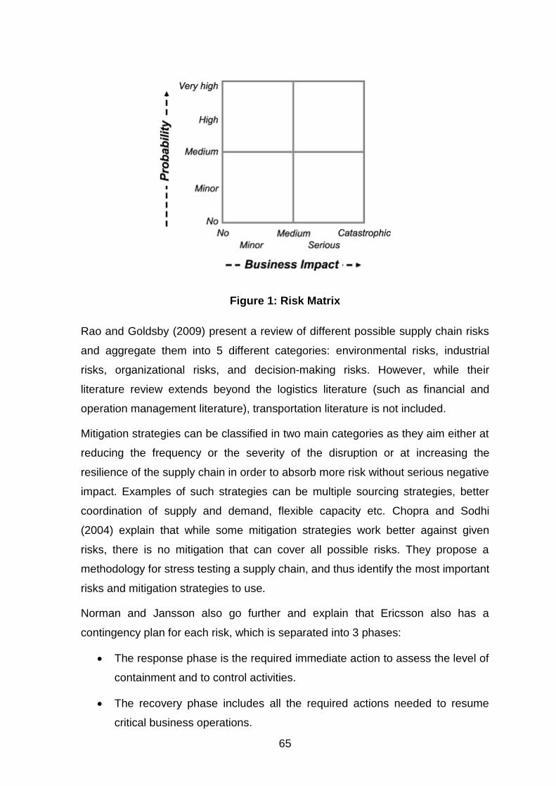
65

Figure 1: Risk Matrix

Rao and Goldsby (2009) present a review of different possible supply chain risks

and aggregate them into 5 different categories: environmental risks, industrial

risks, organizational risks, and decision-making risks. However, while their

literature review extends beyond the logistics literature (such as financial and

operation management literature), transportation literature is not included.

Mitigation strategies can be classified in two main categories as they aim either at

reducing the frequency or the severity of the disruption or at increasing the

resilience of the supply chain in order to absorb more risk without serious negative

impact. Examples of such strategies can be multiple sourcing strategies, better

coordination of supply and demand, flexible capacity etc. Chopra and Sodhi

(2004) explain that while some mitigation strategies work better against given

risks, there is no mitigation that can cover all possible risks. They propose a

methodology for stress testing a supply chain, and thus identify the most important

risks and mitigation strategies to use.

Norman and Jansson also go further and explain that Ericsson also has a

contingency plan for each risk, which is separated into 3 phases:

The response phase is the required immediate action to assess the level of

containment and to control activities.

The recovery phase includes all the required actions needed to resume

critical business operations.

66

The restoration phase is the planning of operations to be done in order to

allow the organization to return to normal service level.

Other paper presenting generic mitigation strategies includes Tang (2006a, 2006,

and 2008) as well as Tomlin (2006).

3. HANDLING UNCERTAINTY IN OPTIMISATION PROBLEMS

3.1. Introduction

When designing an optimisation model under uncertainty, one must take into

account the quantity and quality of information available. Three different types of

information have been identified in the literature: randomness, hazard and deep

uncertainty. Randomness is usually characterized by a random variable with a

known probability distribution. The random variables are most of the time related

to day-to-day business. Hazard is characterized by low probability/high impact

events, and deep uncertainty by the lack of information regarding the likelihood of

possible future events.

Many different methods have appeared over the last decades as handling

uncertainty has become one of the major research trends in the operation

research community. Most of these methods can be classified as one of two main

approaches to uncertain problems: stochastic optimisation and robust

optimisation. In Section 3.2 we present the work done on stochastic models, and

how it can be applied to different optimisation problems arising in the field of

supply chain optimisation. Section 3.3 presents the state of the art on robust

optimisation as well as its applications. Lastly in Section 3.4 we compare the two

approaches and identify the strength and weakness of each.

3.2. Stochastic optimisation Models

3.2.1 Stochastic programming

67

As stated before, stochastic models are used to deal with randomness. As such,

some of the model parameters are considered as random variables with a known

probability distribution. Suppose we have an objective function ),( xG where x

denotes the decisions to be made. Let X be the set of all feasible solutions and

the set of all possible outcomes. Note that might not be finite. In many cases, a

random variable can take any value in a given interval, creating an infinite number

of possible outcomes.

A naïve approach would be to set all the random variables to their expected value

)(xE (i.e., creating an ‘average’ scenario), and to optimize the deterministic

problem. However, Sen and Higle (1999) show that solutions obtained in this way

are rarely optimal, and may even be infeasible for some scenarios.

Another approach would be to optimize on multiple subsets of scenarios and then

analyze the solution obtained using a Monte-Carlo sensitivity analysis (see Saltelli

et al. (2004), Shapiro (2003)). However, choosing the best solution amongst all

solutions found may be difficult. A screening procedure, using criteria such as

Pareto Optimality, or stochastic dominance was proposed by Lowe et al. (2002).

An application can be found in Mohamed (1999).

Therefore, the main approach to deal with stochastic models consists of

minimizing the expected value of the objective function:

)),(()(min xGExgx

This formulation is often referred as stochastic programming in the operations

research literature (see Kleywegt and Shapiro, 2007). It is however extremely

difficult to solve due to the possibly infinite number of scenarios, and difficult to

adapt to real life problems due to the formulation being too abstract and general.

Therefore, stochastic programming with recourse was introduced by Dantzig

(1955).

Stochastic programming with recourse is a two- or multi-stage decision problem.

At the first stage, before the realization of the random variable, the decision maker

chooses the first stage decision variable x to optimize the expected value

)),(()( xGExg of a function ),( xG which depends on the optimal second

stage stochastic function.

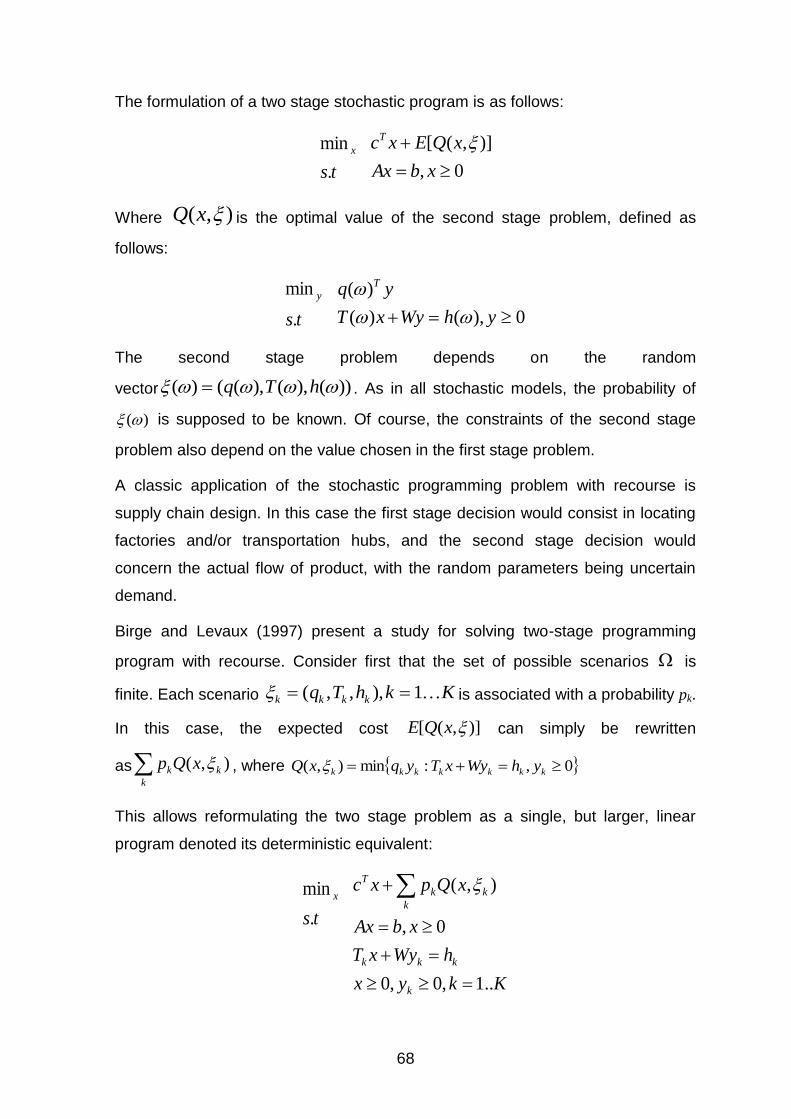
68

The formulation of a two stage stochastic program is as follows:

ts

x

.

min

0,

)],([

xbAx

xQExcT

Where ),( xQ is the optimal value of the second stage problem, defined as

follows:

ts

y

.

min

0),()(

)(

yhWyxT

yq T

The second stage problem depends on the random

vector ))(),(),(()( hTq . As in all stochastic models, the probability of

)( is supposed to be known. Of course, the constraints of the second stage

problem also depend on the value chosen in the first stage problem.

A classic application of the stochastic programming problem with recourse is

supply chain design. In this case the first stage decision would consist in locating

factories and/or transportation hubs, and the second stage decision would

concern the actual flow of product, with the random parameters being uncertain

demand.

Birge and Levaux (1997) present a study for solving two-stage programming

program with recourse. Consider first that the set of possible scenarios is

finite. Each scenario KkhTq kkkk 1),,,( is associated with a probability pk.

In this case, the expected cost )],([ xQE can simply be rewritten

as ),( k

k

k xQp , where 0,:min),( kkkkkkk yhWyxTyqxQ

This allows reformulating the two stage problem as a single, but larger, linear

program denoted its deterministic equivalent:

ts

x

.

min

Kkyx

hWyxT

xbAx

xQpxc

k

kkk

k

k

k

T

..1,0,0

0,

),(

69

This numerical approach works if the number of scenarios remains tractable.

However, one can easily see that the number of scenarios grow exponentially in

the number of random variables. For example, if the random vector )( contains

n random variables, with each having 5 possible realizations, the total number of

scenarios would be nK 5 . If the number of random variables increases to

100m , then the number of scenarios rapidly becomes intractable, and the linear

program unsolvable, even by very powerful computers. Therefore, for higher

numbers of scenarios, the sampling method must be introduced in order to keep

the model solvable.

The notion of the two-stage programming model can be further extended to a

multi-stage stochastic model. A practical example would be a multi-period supply

chain design, where, at each period, the customer demand may vary. This model

however becomes too large to remain solvable very quickly. This method can only

be used with a relatively small number of scenarios.

Having introduced stochastic models, we present in the following section several

applications, of stochastic programming with and without recourse. We focus on

its application to supply chain design problems.

3.2.2 Applications to supply chain design and planning problems

MirHassani et al., (2000) propose a two-stage stochastic optimisation program for

supply chain network design, which takes into account uncertain demand. The

uncertain demand follows a discrete distribution of hundreds of scenarios. The

advantage of a two-stage stochastic program is that it allows the decision maker

to mix the decision to be made before the realization of the demand is known

(firstage decision) and the decision to be made after the realization of the demand

is known (second stage decision).

The goal is to minimize the cost of the strategic decision (deterministic) and the

expected cost of the operational decision (stochastic). Bender’s decomposition is

used to solve the two-stage stochastic program. Mir Hassani et al. also propose a

scenario analysis algorithm that requires much computation time but provides

good information for sensitivity analysis.

70

(Santoso et al., 2005) follows the ideas developed in (Mir Hassani et al., 2000)

and extends them by considering a wider variety of uncertainties. This leads to a

drastic increase in the number of scenarios and thus in the complexity and

resolution time of the optimisation problem. Therefore, they use a Monte Carlo

sampling, or sample average approximation (see Shapiro 2003 ) to reduce the

number of scenarios

Another method for multi-level optimisation is presented by (Sabri et al., 2000),

which propose a simultaneous optimisation of the strategic and operational level,

taking into account production, delivery and demand uncertainty. The algorithm

has the following steps:

Step1: Optimize the strategic sub-model with base values for unit and

transportation cost

Step2: Use the output variables of the strategic sub-model to optimize the

operational sub-model.

Step 3: Optimize the strategic sub-model using the unit and transportation

cost computed in step 2.

Step 4: If convergence, compute the SC performance vector and stop, else

repeat from step 2.

This method optimizes both levels simultaneously, using the result of the

optimisation from each sub-model to find a better solution for the other one. The

algorithm stops when the strategic sub-model converges, i.e., when all the binary

decision variables are equal.

71

Snyder (2003) proposes a stochastic programming model for the facility location

problem which takes into account the possibility of plant failure. Each plant in the

model has a given probability of failure; therefore, each customer is assigned both

a plant and a set of back-up facilities which will be used in case the main plant

fails. The objective is to minimize the expected failure cost. A multi-objective

model is also proposed, the first objective being the operating cost, and the

second being the expected failure cost. The decision maker should assign a

weight to each of the objectives, and the model minimizes a weighted sum of the

two objectives. By using different values for the weight of each objective, trade-off

curves are also constructed. In the example shown, one can see that the

expected failure cost can be reduced by 27%, with an increase of 7% of the

operating cost. However reducing the expected failure by a significant margin

requires a severe increase in the operating cost. For example, reducing the

expected failure cost by 60% would require increasing the operating cost by about

100%.

You et al., (2009) consider multi-period, mid-term planning under demand and

freight rate uncertainty. They also propose a two-stage stochastic programming

model. However, where Mir Hassani makes a strategic decision in the first stage,

and tactical in the second, You et al., makes a decision for the first period in the

first stage and a decision for all period in the second stage. Combined with the

use of a rolling horizon, they show that 5% saving can be achieved.

Lastly Qi et al. (2009) study a facility location and customer allocation problem

with supply disruption. They formulate a nonlinear integer programming model,

and use an effective approximation of the objective function in order to make the

model easier to solve. Note that this model does not take into account dynamic

sourcing, one of the main characteristics of our problem.

72

Table 1 Main papers on stochastic supply chain optimisation

Paper Year Problem Characteristics Uncertainty Approach

Snyder 2003 Facility Location Supply

Disruption

Back-up Facilities

Santoso et al. 2004 Supply chain design Multiple 2 stage stochastic Programming

with+ Benders Decomposition

You et al. 2009 Tactical supply chain design Demand/Freight

rate

2 stage stochastic programming

with a Sample Average Approach

Qi et al. 2010 Facility location and customer

allocation under supply

disruption

Supply

Disruption

Nonlinear Integer Programming

with objective function

approximation

Our approach 2012 Customer allocation and

production level

Supply

Disruption

Stochastic programming with

recourse

Table 1 summarizes the main papers covering supply chain design under

uncertainty. We also added our approach to the production planning and

customer allocation problem under supply disruption (in our case, plant failure) to

highlight the difference between our research and the existing literature.

3.3. Robust optimisation models

Treating uncertainties in operation research has always been a major concern.

Historically, stochastic optimisation was used to deal with uncertainties. However,

stochastic optimisation requires fitting a probability distribution with the

uncertainties and such a law is not always easy to find. Moreover, in most cases,

stochastic optimisation optimizes the expected cost of the problem. However, the

realization of the uncertain parameters may be such that the stochastic solution is

much worse than expected. The first use of robust optimisation appears in 1968

(Gupta et al., 1968) and aims to provide solutions with flexibility in the context of

an uncertain future.

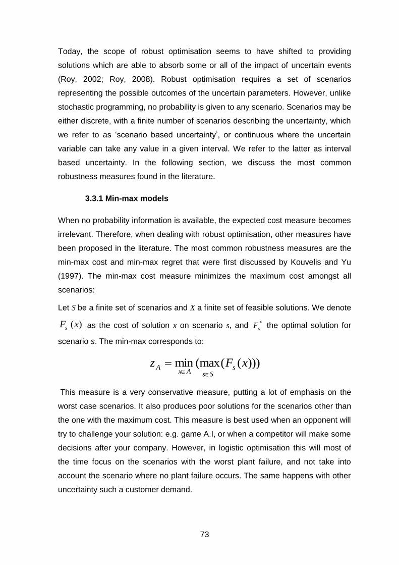
73

Today, the scope of robust optimisation seems to have shifted to providing

solutions which are able to absorb some or all of the impact of uncertain events

(Roy, 2002; Roy, 2008). Robust optimisation requires a set of scenarios

representing the possible outcomes of the uncertain parameters. However, unlike

stochastic programming, no probability is given to any scenario. Scenarios may be

either discrete, with a finite number of scenarios describing the uncertainty, which

we refer to as ‘scenario based uncertainty’, or continuous where the uncertain

variable can take any value in a given interval. We refer to the latter as interval

based uncertainty. In the following section, we discuss the most common

robustness measures found in the literature.

3.3.1 Min-max models

When no probability information is available, the expected cost measure becomes

irrelevant. Therefore, when dealing with robust optimisation, other measures have

been proposed in the literature. The most common robustness measures are the

min-max cost and min-max regret that were first discussed by Kouvelis and Yu

(1997). The min-max cost measure minimizes the maximum cost amongst all

scenarios:

Let S be a finite set of scenarios and X a finite set of feasible solutions. We denote

)(xFs as the cost of solution x on scenario s, and *

sF the optimal solution for

scenario s. The min-max corresponds to:

)))(((maxmin xFz sSsAx

A

This measure is a very conservative measure, putting a lot of emphasis on the

worst case scenarios. It also produces poor solutions for the scenarios other than

the one with the maximum cost. This measure is best used when an opponent will

try to challenge your solution: e.g. game A.I, or when a competitor will make some

decisions after your company. However, in logistic optimisation this will most of

the time focus on the scenarios with the worst plant failure, and not take into

account the scenario where no plant failure occurs. The same happens with other

uncertainty such a customer demand.

74

In order to find less conservative solutions, two other measures are suggested by

Kouvelis and Yu (1997). They consider the regret of a solution, which is the

difference between the cost of a solution when applied to a given scenario, and

the cost of the optimal solution for this scenario. Note that both the absolute or

relative difference can be used, and thus models trying to minimize the maximum

regret of a solution amongst all scenario are called min-max absolute regret

models, or min-max relative regret models.

Because min-max regret models give the same importance for all scenarios, it

appears more often in the literature. A survey presenting the main theoretical

results found regarding min-max models has been conducted by Aissi et al.

(2009).

The general algorithm of min-max models is the following

1. Find a candidate solution x.

2. Determine the maximum regret amongst all scenarios if solution x is

chosen.

3. Repeat steps 1 and 2 with a new candidate solution.

The candidate solution for the first step is usually obtained using an exact

algorithm or heuristic.

The difficulty of step 2 depends on the scenario definition in the model. If the

numbers of scenarios are finite (scenario-based uncertainty), then computing the

maximum regret is straight forward: compute the cost of the solution amongst all

the scenarios, and compare it to the optimal cost for the scenario. Once the regret

is computed for every scenario, simply select the highest regret. However, for

interval based-uncertainty, computing the maximum regret can prove to be a

difficult task. Several techniques exist based on the fact that the regret-maximizing

scenario has all parameters set to an extremity of their intervals.

75

One could simply focus on generating all the extreme case scenarios, but this

remains intractable in most cases. If we consider for example a supply chain

design problem with customer demand uncertainty where n is the number of

customers, the number of extreme case scenarios would be 2n. In order to solve

this, Mausser and Laguna (1999a) proposed a search heuristic with search

diversification to avoid falling into local optima. They proposed as well as an exact

method (1999b) that requires adding several constraints for each uncertain

parameter, and thus only remains practical for medium sized linear programs.

Following the same train of thought, if the number of feasible solutions is finite,

one can examine all of them in order to find the solution with the lowest maximum

regret. If this is not the case, one can either iterate on multiple solutions with a

stopping criterion (e.g., computation time), or use clever cuts to generate a new

solution with smaller regret (see Mausser and Laguna 1999b).

A lot of work has also been done during the last decades studying the complexity

of min-max models. One can remark that the complexity of the min-max version of

a problem P has at least the same complexity of P itself given that P is a particular

case of the min-max version (with 1 scenario or deteriorated intervals).

Kouvelis and Yu (1997) give several example of the complexity of min-max

problems with scenario-based uncertainty (shortest path, assignment, knapsack,

etc.). They show that if the number of scenarios is unknown (i.e., not part of the

input), the min-max version of these problem becomes strongly NP-Hard, even

when the original problem is solvable in polynomial time. If the number of

scenarios is part of the input data, the min-max model becomes either weakly NP-

hard or strongly NP-hard.

In the interval-based uncertainty case, results are slightly different. Most problems

go from weakly NP-hard in the scenario-based uncertainty case to strongly NP-

hard. Some problems however become solvable in polynomial time with interval

scenarios. One example is the problem of selecting the p most profitable items as

studied by Averbackh (2001).

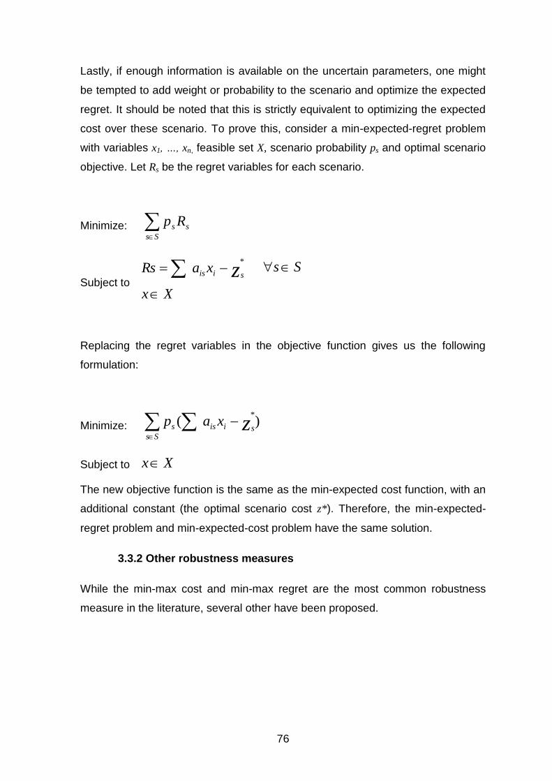
76

Lastly, if enough information is available on the uncertain parameters, one might

be tempted to add weight or probability to the scenario and optimize the expected

regret. It should be noted that this is strictly equivalent to optimizing the expected

cost over these scenario. To prove this, consider a min-expected-regret problem

with variables x1, …, xn, feasible set X, scenario probability ps and optimal scenario

objective. Let Rs be the regret variables for each scenario.

Minimize: Ss

ss Rp

Subject to Xx

xaRs zsiis

*

Ss

Replacing the regret variables in the objective function gives us the following

formulation:

Minimize:

Ss

siiss zxap )(*

Subject to Xx

The new objective function is the same as the min-expected cost function, with an

additional constant (the optimal scenario cost z*). Therefore, the min-expected-

regret problem and min-expected-cost problem have the same solution.

3.3.2 Other robustness measures

While the min-max cost and min-max regret are the most common robustness

measure in the literature, several other have been proposed.

77

Mulvey, Vanderbei and Zenios (1995) and Mulvey and Ruszczynski (1997)

propose a general framework for robust optimisation. They differentiate between

two types of robustness: (1) the solution robustness measures how close the

solution is to the optimal value amongst all scenarios, whereas (2) the model

robustness measures how close the solution is to feasibility amongst all scenarios.

Generic penalty functions are applied to minimize both robustness measures

balanced with a parameter set by the modeler indicating the weight of each

measure in the objective function. Examples of the solution robustness measures

are the maximum regret and the expected cost. The model robustness can be

penalized using, for example, the sum of the squared violations of the constraints.

The authors present several applications of the robust optimisation they propose

with both discrete scenarios and intervals and with or without probability

information.

Due to the generality of this model, it has been used in various applications.

Trafalis et al. (1999) use this framework to solve a production planning problem

with scenario based uncertainty and a stochastic formulation. Yu and Li (2000)

apply the same framework to large scale logistic systems. They improve the

model proposed by Mulvey et al. (1995) and manage to reduce the required

computation time by up to 30%. Killmer Anandalingam and Malcom (2001) apply

this framework to a facility location problem with uncertain demand, production

and transportations costs. They minimize the expected cost and penalize regret

(ensuring solution robustness), unused capacity as well as unmet demand

(ensuring model robustness). Other applications of this framework include Laguna

et al. (2000) in the field of parallel machine scheduling and Darlington et al. (2000)

for chemical engineering.

Model robustness is at the core of Ben-Tal et al.’s work (1999, 2000, 2002, and

2009). They base their work on one of the first applications of robust optimisation

proposed by Soyster (1973). Soyster proposed a linear optimisation model to

construct a solution that is feasible for all data that belong in a convex set. Ben-

Tal et al. started from this point and further developed a whole branch of robust

optimisation theory. They consider a standard linear program,

bAxxcT

x:min

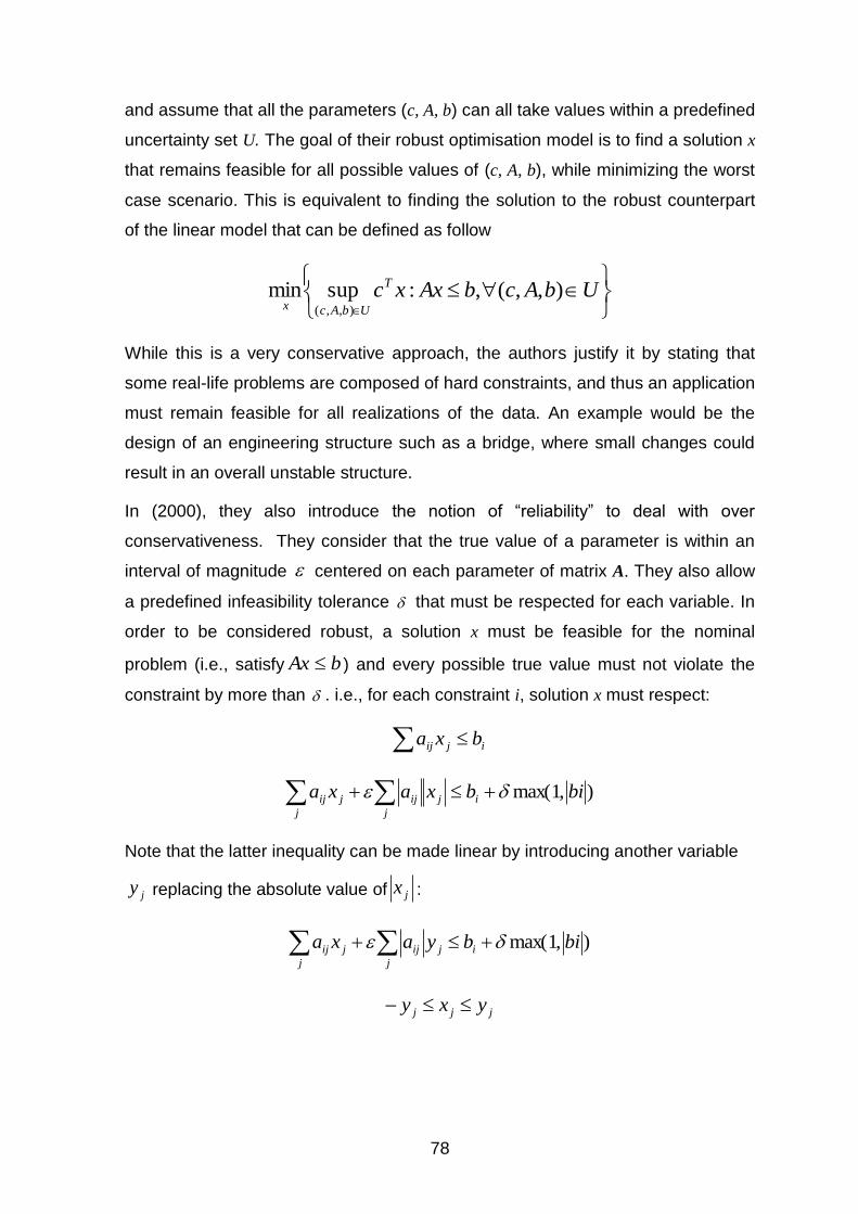
78

and assume that all the parameters (c, A, b) can all take values within a predefined

uncertainty set U. The goal of their robust optimisation model is to find a solution x

that remains feasible for all possible values of (c, A, b), while minimizing the worst

case scenario. This is equivalent to finding the solution to the robust counterpart

of the linear model that can be defined as follow

UbAcbAxxcT

UbAcx),,(,:supmin

),,(

While this is a very conservative approach, the authors justify it by stating that

some real-life problems are composed of hard constraints, and thus an application

must remain feasible for all realizations of the data. An example would be the

design of an engineering structure such as a bridge, where small changes could

result in an overall unstable structure.

In (2000), they also introduce the notion of “reliability” to deal with over

conservativeness. They consider that the true value of a parameter is within an

interval of magnitude centered on each parameter of matrix A. They also allow

a predefined infeasibility tolerance that must be respected for each variable. In

order to be considered robust, a solution x must be feasible for the nominal

problem (i.e., satisfy bAx ) and every possible true value must not violate the

constraint by more than . i.e., for each constraint i, solution x must respect:

ijij bxa

),1max( bibxaxa i

j

jij

j

jij

Note that the latter inequality can be made linear by introducing another variable

jy replacing the absolute value of jx :

),1max( bibyaxa i

j

jij

j

jij

jjj yxy

79

Lastly they extend their model to the case where the parameters ija are affected

by random perturbation. They define a solution as “almost reliable” if it is feasible

for the nominal problem, and the probability of a constraint being violated by more

than the predefined infeasibility tolerance value is below a given “reliability level” k

> 0. Other work on the same topic has been conducted by El-Ghaoui et al. (1997,

1998).

Ben-Tal et al. applied this methodology to a robust multi-echelon, multi-periodic

inventory control problem (2009). The goal is to minimize the sum of

manufacturing costs, inventory costs and backlogging costs within a multi-echelon

supply chain under demand uncertainty. While their approach allows them to find

robust solutions that minimize the bullwhip effect, it comes at the cost of

dimensional limitation. The model was already large with only 3 echelons and 20

periods.

Bertsimas and Sim (2004) note that the models proposed by Ben-Tal and

Nemirovski (2000) require adding many additional variables and constraints and

thus are not very attractive for solving robust discrete optimisation problems.

Therefore, they propose a new robust formulation that does not excessively affect

the objective function. For each constraint i, they introduce a new parameter i

that limits the number of parameters that are subject to parameter uncertainty.

The intuition behind this is that it is unlikely that all uncertain parameters will

change at the same time. Therefore, they only protect themselves against the

case where at most i parameters are subject to variations. The goal is to control

the tradeoff between the probability of violating hard constraints and the effect on

the nominal problem, which they call “the price of robustness”. They formulate a

new linear problem using this formulation which possesses several advantages

over the model proposed by Ben-Tal and Nemirovski. Firstly, this model requires

less additional variables and constraints, making it more easily solvable. It also

preserves the sparsity of matrix A, which can be observed in many real life

problems. Lastly, as the worst case scenarios (i.e., scenarios where all

parameters change) are not considered, the solution found is also much less

conservative.

80

Vladimirou and Zenios (1997) introduce a third notion of robustness: recourse

robustness. Recourse robustness penalizes the recourse solutions if they are

different across scenarios. In the model they propose, recourse robustness is

progressively enforced, firstly by forcing all second stage variables (or recourse

variables) to be equal, and then progressively loosening this constraint until a

feasible solution is found. The authors compare 3 different stochastic models with

restricted recourse, and successfully solve small to medium instances with up to

64 different scenarios. The authors show that restricted recourses often come with

a significant increase in cost, and thus a cost-robustness tradeoff should be

analyzed.

3.3.3 Applications to supply chain design and planning problems

The facility location problem focuses only on the strategic component of the

supply chain design: the location of production facilities. Snyder (2003) presents

two optimisation models for the uncapacitated facility location problem (UFLP)

under plant failure uncertainty. The first one focuses on minimizing the maximum

failure cost. The logistic cost is estimated using a fixed cost per mile per unit. If a

plant fails, any customer sourced at this plant is delivered from the next closest

plant (or backup facility), without any production/capacity constraint. Multiple

relaxations for MILP formulations are discussed, however, a Tabu search heuristic

is found to achieve the best solution.

For a more complete review of facility location under uncertainty, we refer the

reader to Snyder (2006).

3.4. Robust versus stochastic optimisation

In stochastic optimisation, the uncertain parameters are assumed to be random,

and thus are assumed to follow a known, or at least partially known, probability

distribution. Stochastic optimisation then optimizes the expected objective function

of the model. However, in practical settings, assuming perfect knowledge of the

uncertainty is often impossible.

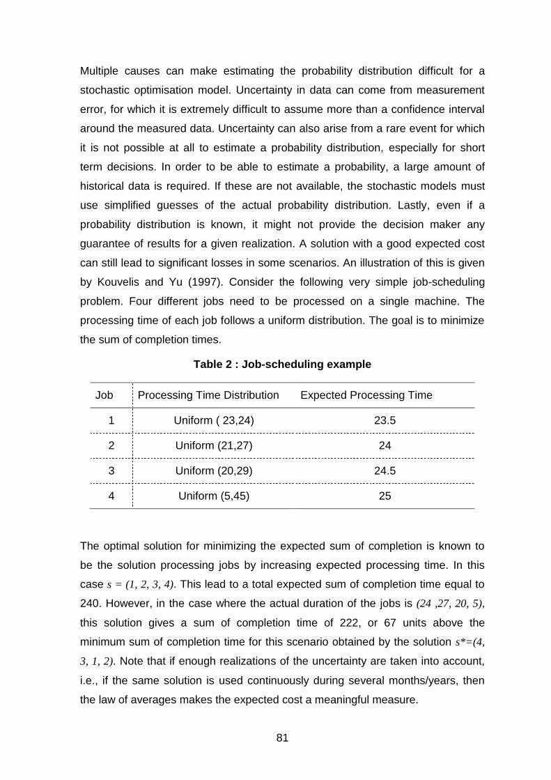
81

Multiple causes can make estimating the probability distribution difficult for a

stochastic optimisation model. Uncertainty in data can come from measurement

error, for which it is extremely difficult to assume more than a confidence interval

around the measured data. Uncertainty can also arise from a rare event for which

it is not possible at all to estimate a probability distribution, especially for short

term decisions. In order to be able to estimate a probability, a large amount of

historical data is required. If these are not available, the stochastic models must

use simplified guesses of the actual probability distribution. Lastly, even if a

probability distribution is known, it might not provide the decision maker any

guarantee of results for a given realization. A solution with a good expected cost

can still lead to significant losses in some scenarios. An illustration of this is given

by Kouvelis and Yu (1997). Consider the following very simple job-scheduling

problem. Four different jobs need to be processed on a single machine. The

processing time of each job follows a uniform distribution. The goal is to minimize

the sum of completion times.

Table 2 : Job-scheduling example

Job Processing Time Distribution Expected Processing Time

1 Uniform ( 23,24) 23.5

2 Uniform (21,27) 24

3 Uniform (20,29) 24.5

4 Uniform (5,45) 25

The optimal solution for minimizing the expected sum of completion is known to

be the solution processing jobs by increasing expected processing time. In this

case s = (1, 2, 3, 4). This lead to a total expected sum of completion time equal to

240. However, in the case where the actual duration of the jobs is (24 ,27, 20, 5),

this solution gives a sum of completion time of 222, or 67 units above the

minimum sum of completion time for this scenario obtained by the solution s*=(4,

3, 1, 2). Note that if enough realizations of the uncertainty are taken into account,

i.e., if the same solution is used continuously during several months/years, then

the law of averages makes the expected cost a meaningful measure.

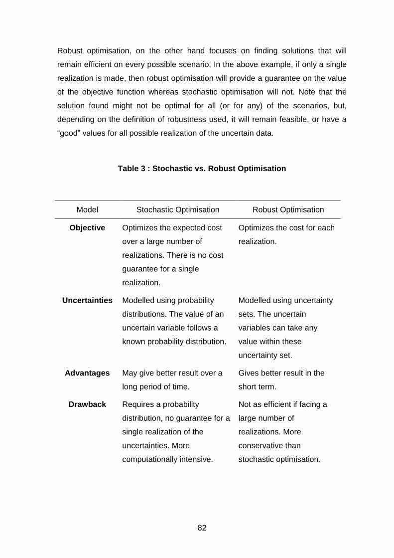
82

Robust optimisation, on the other hand focuses on finding solutions that will

remain efficient on every possible scenario. In the above example, if only a single

realization is made, then robust optimisation will provide a guarantee on the value

of the objective function whereas stochastic optimisation will not. Note that the

solution found might not be optimal for all (or for any) of the scenarios, but,

depending on the definition of robustness used, it will remain feasible, or have a

“good” values for all possible realization of the uncertain data.

Table 3 : Stochastic vs. Robust Optimisation

Model Stochastic Optimisation Robust Optimisation

Objective Optimizes the expected cost

over a large number of

realizations. There is no cost

guarantee for a single

realization.

Optimizes the cost for each

realization.

Uncertainties Modelled using probability

distributions. The value of an

uncertain variable follows a

known probability distribution.

Modelled using uncertainty

sets. The uncertain

variables can take any

value within these

uncertainty set.

Advantages May give better result over a

long period of time.

Gives better result in the

short term.

Drawback Requires a probability

distribution, no guarantee for a

single realization of the

uncertainties. More

computationally intensive.

Not as efficient if facing a

large number of

realizations. More

conservative than

stochastic optimisation.

83

This makes stochastic and robust optimisation two complementary approaches for

handling the uncertainty of data in optimisation problems with each approach

having its own advantages and drawbacks. When facing high risk decisions,

which may lead to important losses, one may prefer robust optimisation. If,

however, one is facing small variation with low impact, or long-term decisions

leading to many realizations of the uncertain data (e.g., daily demand in a supply

chain design problem), then stochastic optimisation could be a more logical

choice. Table 2 summarizes the characteristics of each approach.

4. INVENTORY ROUTING PROBLEM

This section presents the state of the art on the inventory routing problem.

4.1. Deterministic Inventory Routing Problem

4.1.1 Heuristics

The first inventory routing models (IRP) appeared in the 1980s. These papers are,

for the most part, inspired by applications of vehicle routing where inventory is

considered. In order to overcome the high complexity of IRP models, most papers

only take into consideration short term planning. For example Golden et al.

(1984) focus on maintaining a “good” level of inventory at the customer on a

single day while minimizing cost. Their heuristic computes the urgency of each

customer in order to decide which customers should be delivered. Customers are

then iteratively added into shifts until the time limit for all shifts are reached. In this

model, each day is treated as a different entity.

Chien et al. (1989) also use a single day model, but consider a multiple-day time

horizon. After the decisions are made for the first day, the result is passed to the

next day in order to compute the profit for the following days. A mixed integer

program (MIP) is used for both the inventory and routing decisions and a

Lagrangean dual ascent method is used to solve the program.

84

In 2000, Bertazzi, Speranza and Ukovich propose a model based on the previous

work of Speranza and Ukovich (1994). They consider a supplier and several

customers with a given production rate and demand. The specificity of their model

is that the shipment from the supplier to any customer can only occur within a

given set of frequencies e.g., a customer would be delivered every 5 days. Even

with a single customer, this problem is NP-Hard, and thus, a local search-based

heuristic is used to find solutions.

Bertazzi et al. (2005) focus on the order up to level policy. They consider a single

vehicle model, with inventory costs, both at the supplier and the customer site.

The inventory cost is computed at each time step, and is equal to the quantity of

product stored times an inventory cost, which is a parameter for each customer.

They use a two-step heuristic, the first step being a greedy algorithm to create a

feasible solution. They then improve the solution by removing a pair of customers

and then reinserting them in the current solution. If a better solution is created,

then they repeat the whole improvement phase, if not, then they continue until all

pairs of customers have been removed and reinserted. This algorithm is a local

search with no random parameters.

Bertazzi et al. (2005) go further and propose solutions for different delivery

policies, and also compare the vendor managed inventory (VMI) policy with the

retailer managed (RMI), in which the retailers place orders to be delivered. The

specificity of their model is that the decision variables include the production to be

made for each time period. The production cost includes a fixed set up cost, and a

variable cost that is charged for each unit produced. Two different VMI policies are

studied. The first one is the order-up-to level policy where the quantity shipped to

the retailer fills the tank capacity, the second one is the fill-fill-dump policy, in

which the order-up-to level quantity is shipped to all but the last retailer of each

route, and the quantity delivered to the last customer is the minimum between the

order-up-to level policy and the remaining capacity of the vehicle. Bertazzi et al.

decomposed the problem into two sub problems: (1) the distribution sub problem

and then (2) the production sub problem. Two approaches are suggested: in the

first one, the distribution sub problem is solved first, assuming that all retailers are

served every day. After which the production problem is solved again. The other

approach consists of solving first the distribution sub problem and then the

production sub problem. Both approaches show similar results.

85

The RMI policy is simulated with the following rule: each customer that will have a

run out at time t +1 is visited at time t. The tests were run on a set of instances

with 50 customers and a time horizon of 30 days. The results clearly indicate that

the VMI-based heuristic yields much better results than the RMI policy, with an

average 60% total cost decrease. Savelsbergh and Song (2008) study a real-

world industrial problem. A randomized greedy heuristic is used to solve the IRP

with continuous moves, whereas the volume to be delivered is being computed

via linear programming. They also propose a discrete time mathematical model,

solved with a branch and cut algorithm. The results are presented on instances

with a 5-day time horizon with 2 plants, 50 customers and a 1 hour time step. The

branch and cut algorithm manages to find the optimal solution with an average

computation time of 30 minutes. However, with bigger time steps (2 hours for the

first 2 days, then 4 hours for the next 3) , computation time can be reduced to less

than 2 minutes with a solution quality decrease of only 3%. On larger instances (3

plants, 3 vehicles, and 100 customers), the computation time increases to an

average of 2 days, thus making the use of the exact model unusable in practice.

However, the proposed heuristic manages to find solutions with less than 5%

optimality gap in less than 5 minutes.

Abdelmaguid et al. (2009) propose a mixed integer programming formulation for a

single depot, multi vehicle, backlogging model. However, even with less than 15

customers and 2 vehicles, they could not obtain the optimal solution within a one

hour time limit, thus motivating a heuristic approach. As with many heuristic

approaches, the approach proposed by Abdelmaguid et al. consists of a

constructive phase in which a solution is built, and an improvement phase in

which the solution is further improved. The constructive heuristic is an estimated

transportation cost heuristic, in which all decisions are taken based on an

estimation of the transportation costs. Then, a local search is performed in order

to improve the solution found. The local search focuses on modifying the

quantities delivered and on delivery exchanges. For large instances, the heuristic

gives better results than the CPLEX solver. However, precise computation times

for the heuristic are not given.

86

Boudia and Prins (2007) propose a memetic algorithm with population

management to solve an integrated production-distribution problem. They apply

their algorithm to instances with up to 200 customers and 20 periods and compare

the results obtained to the improved GRASP presented in Boudia et al. (2006).

They show that better results are obtained at the cost of a reasonable

computation time increase.

Due to the extensive research done on the inventory routing problem, it would be

impossible to have an exhaustive literature survey here. We refer the interested

reader to the survey made by Andersson et al. (2010) for additional references on

the inventory routing problem.

4.1.2 Exact Methods

Due to the complexity of the inventory routing problem, very few effective exact

methods have been developed. Some papers gives a standard MIP formulation

(e.g. Abdelmaguid and Dessouky (2009)) and solve it within a given time limit in

order to obtain lower and upper bounds for the cost of the optimal solution. These

bounds are then used as benchmarks for heuristics. Most of these MIP

formulations are computationally intractable for large instances. However, several

recent papers have developed efficient algorithms for finding the optimal solution

of the inventory routing problems.

Archetti et al. (2009) consider a model with a single vehicle and deterministic

demand, an order-up-to-level policy and do not allow backlogging of demand. A

branch-and-cut algorithm is implemented. The second paper is from Solyali and

Süral (2011). They improved the results of Archetti et al. (2009) by proposing a

strong MIP formulation within a branch and cut algorithm. While both use a two-

index vehicle flow formulation for the routing decision, Archetti et al. (2009) used

standard inventory balance constraints whereas Solyali and Süral (2011) used a

shortest path formulation which seems to yield better results.

Another MIP formulation was proposed by Solyali, Cordeau and Laporte (2010)

for a single vehicle, deterministic demand model with a backlogging penalty.

Using a tight formulation for inventory decisions and a two-index flow formulation

for the routing decisions, they propose a branch and cut algorithm that yields

better results than Abdelmaguid and Dessouky’s (2009) MIP formulation.

87

Oppen et al. (2010) propose a column generation method to solve a rich inventory

routing problem in the field of meat industry. They present results on multiple

instances, with 20 to 27 orders. While solutions are found for problems with less

than 25 customers, the computation times range from several minutes to several

hours depending on the characteristics of the instance.

Due to the intrinsic complexity of the inventory routing problem, most solutions

developed for the deterministic version are heuristic approaches. Such heuristics

include Lagrangian relaxation, local search, and decompositions into sub

problems.

4.1.3 Industrial Implementations

In 2004, a collaboration work started between Praxair and the Georgia Institute of

Technology. The Ph.D. Thesis of J-H Song (2004) is one of the results of this

collaboration. He introduces new upper and lower bound for the inventory routing

problem, and then proceeds to define the inventory routing problem with

continuous moves, where shifts can cover multiple time periods. The results of

this Ph.D. thesis have been published in several papers Savelsbergh and song

(2006) and Savelsbergh and Song (2008).

A randomized greedy heuristic is used to solve the IRP with continuous moves

and the volume to be delivered is computed via linear programming. Song then

proposes a discrete time mathematical model, solved with a branch and cut

algorithm. The results are presented on instances with a 5-days’ time horizon with

2 plants and 50 customers and 1-hour time steps. The branch and cut algorithm

manages to find the optimal solution with a 30 minute average computation time.

However, with bigger time steps (2 hours for the first 2 days, then 4 hours for the

next 3), computation times can be reduced to less than 2 minutes with a solution

quality decrease of only 3%. On larger instances (3 plants, 3 vehicles, 100

customers), the computation time increases to an average of 2 days, thus making

the use of the exact model unusable in practice. However, the proposed heuristic

manages to find solutions with less than a 5% optimality gap in less than 5

minutes.

88

To our knowledge, this is the first time that such a model is considered in the

inventory routing literature. However, a close model was introduced in 1999 by

Christiansen (1999) for a ship routing/inventory management problem. She

proposes Dantzig-Wolfe decomposition coupled with a branch and bound

algorithm to solve this problem. However, ship transportation only has to deal with

a small number of harbours, and thus the solution proposed by Christiansen, does

not apply to IRP for liquid gas distribution.

4.2. The Uncertain Inventory Routing Problem

4.2.1 Stochastic Inventory Routing Problem

Even though the first papers to introduce the inventory routing problem

considered all input data to be deterministic, it did not take long before other

authors started considering uncertainties.

The first paper to introduce uncertainty in the inventory routing problem is from

Dror and Ball (1985). In this paper, the authors consider a multiple day horizon,

and use a probability distribution for the day when a specific customer will run out

of product. Using this probability distribution as well as the anticipated cost of a

stock out, they compute the delivery day. Once each customer is assigned to a

day and a vehicle (using an integer program), a traveling salesman problem (TSP)

or VRP algorithm can be used for computing the routing. The routing is only

computed for the first few days of the horizon (the short-term planning). If the

optimal delivery day is outside of the short term planning, the cost is still computed

taking into account the routing decisions taken in the short term planning. This

allows taking into account the effect of short term decisions on the long term.

Jaillet et al. (2002 ) as well as Bard et al. extend this method. They use a rolling

horizon approach and include satellite facilities where the trucks can be refilled.

As Dror and Ball (1985), they compute the optimal replenishment day for each

customer, considering an uncertain demand. They also try to minimize

incremental cost, i.e. cost occurring from serving a customer on a day other than

the optimal one. A local search algorithm is then used to solve the VRP problem

for each day.

89

Kleywegt et al. (2002) proposed a Markov decision process model for the

inventory routing problem with vendor managed inventory. However the models

they propose only consider direct trip deliveries, i.e., each trip delivers at most one

customer. However in Kleywegt et al. (2004), they extended both the formulation

and the approach in order to handle multiple deliveries per trip. The models they

propose consider a single facility and multiple vehicles, with random variables

denoting the customer demand at each time. The probability distribution is

assumed to be known to the decision maker. Decisions that are made for each

day include the customer to be replenished, quantities to be delivered and routes

to be taken in order to minimize the transportation and delivery costs.

Adelman et al (2004) also propose a Markov decision process solution. They use

the same model as Kleywegt et al. but use linear programming approach to obtain

the value function approximation. The implantation of the control policy is solved

using integer bin-packing whereas Kleywegt et al. use a heuristic algorithm.

4.2.2 Robust Inventory Routing Problem

Robust optimisation regroups different methodologies to solve problems involving

uncertain parameters with no information on their probability distribution. This is

achieved by finding solutions that ensure feasibility, and to a further extent good

result, regardless of the realization of the uncertainty, whereas stochastic

optimisation optimizes the expected result, but might lead to very bad

performance depending on the realization. The very first robust optimisation

model was developed by Soyster (1973) in which each uncertain parameter was

set to its worst possible value, thus ensuring feasibility. As a result, overly

conservative solutions were found.

In order to deal with this over conservativeness, Bertsimas and Sims (2004)

developed a robustness approach called “the price of robustness” where only a

limited number of uncertain parameters are allowed to deviate from their original

value. This allows the decision-maker to take into account only the plausible

scenarios, and avoid the over conservativeness of the solutions.

90

Ben-tal et al. (2002) propose a different resolution method: they assume that the

uncertainty set, in which the uncertain parameters take their values, is known to

the decision- maker. One key result of their work is that if both the uncertainty set

and the deterministic version of the problem are computationally tractable, then

the robust counterpart of the problem remains computationally tractable.

Both the Bertsimas and Ben-tal methods are directed at including robust aspects

in linear optimisation models. Kouvelis and Yu (1997) turn their attention to a

robust framework for discrete optimisation. Their approach allows the use of a

discrete set of uncertain scenarios. Several robustness criteria based on a min-

max evaluation are proposed, with different conservativeness.

While robust optimisation is a topic of interest among the operations research

community, it has rarely been used in the context of inventory routing problem. To

our knowledge, only three papers deal with robustness within IRP.

The first is a study by Aghezzaf (2008) who considers normally distributed

demands at customer sites and travel times with constant averaged and bounded

standard deviations. He claims that a cyclic distribution strategy gives a good

approximation to the optimal solution, and uses a MIP program to compute a

minimum cost solution that is feasible for all realizations of demand and travel

time within their support.

Solyali, Cordeau and Laporte (2010) propose the second robust IRP model in the

literature. They use a single supplier, single vehicle with uncertain demand model.

The demand is assumed to take a value in an interval centred in the forecasted

demand. Backlogging is allowed, but a backlogging cost is used in order to

penalize when a customer is not delivered. They propose a new MIP formulation

solved using a branch-and-cut algorithm. Then, using the Bertsimas and Sims

robustness approach, they formulate the robust counterpart.

The instances were solved within a two-hour time limit and included up to 30

customers with up to 5% demand variation. The results show that solutions with a

90% probability of feasibility under uncertainty (2.5% demand variation) lead to an

increase of only 3% for the global cost.

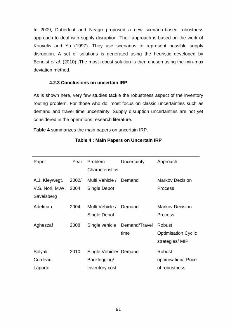
91

In 2009, Dubedout and Neagu proposed a new scenario-based robustness

approach to deal with supply disruption. Their approach is based on the work of

Kouvelis and Yu (1997). They use scenarios to represent possible supply

disruption. A set of solutions is generated using the heuristic developed by

Benoist et al. (2010) .The most robust solution is then chosen using the min-max

deviation method.

4.2.3 Conclusions on uncertain IRP

As is shown here, very few studies tackle the robustness aspect of the inventory

routing problem. For those who do, most focus on classic uncertainties such as

demand and travel time uncertainty. Supply disruption uncertainties are not yet

considered in the operations research literature.

Table 4 summarizes the main papers on uncertain IRP.

Table 4 : Main Papers on Uncertain IRP

Paper Year Problem

Characteristics

Uncertainty Approach

A.J. Kleywegt,

V.S. Nori, M.W.

Savelsberg

2002/

2004

Multi Vehicle /

Single Depot

Demand Markov Decision

Process

Adelman 2004 Multi Vehicle /

Single Depot

Demand Markov Decision

Process

Aghezzaf 2008 Single vehicle Demand/Travel

time

Robust

Optimisation Cyclic

strategies/ MIP

Solyali

Cordeau,

Laporte

2010 Single Vehicle/

Backlogging/

Inventory cost

Demand Robust

optimisation/ Price

of robustness

92

While stochastic optimisation has been used in the past, the new trend tends to

favour the use of robust optimisation. The fact that no knowledge on the

probability distribution for the uncertainty is needed makes robust optimisation an

appealing choice for short-term decision making. This is due to the fact that

describing the future with a probability distribution is easier when focusing on

long-term decisions. However, robust optimisation has only been use to solve

uncertain demand problems. To our knowledge, it has not been used yet to solve

supply disruption problems such as plant outages.

5. GREEDY RANDOMIZED ADAPTATIVE SEARCH PROCEDURE

In Chapter IV of my thesis, I use the GRASP meta-heuristic to improve the results

obtained by a simple yet effective local search. I detail in this section a short state

of art on the GRASP meta-heuristic.

The Greedy Randomized Adaptive Search Procedure (GRASP) is a multi-start

meta-heuristic that was first described by Feo and Resende (1989, 1995). Each

iteration of the procedure consists of two phases: a construction phase and an

optimisation phase. During the construction phase, a feasible solution is iteratively

constructed, using a randomized greedy algorithm (see Section 5.2). Then, during

the optimisation phase, this feasible solution is improved, often by the use of a

local search procedure.

The GRASP methodology has been used in many different problems. Resende

and Ribeiro (2003) as well as Festa and Resende (2001) present applications in

fields such as routing, assignment problems, scheduling and telecommunication.

An example of application of the GRASP methodology to an IRP can be found in

Grellier et al. (2004).

Parallelization approaches are very appropriate for the GRASP methodology, as

explained in Cung et al. (2001). As each iteration can be run in a different thread

with the need to interact with each other, the gain in time for using parallelization

is close to linear in the number of processors used.

93

Boudia et al. (2006) use the GRASP for solving a combined production-

distribution problem. The GRASP methodology they propose is improved using

either a reactive mechanism or path relinking. The reactive mechanism optimizes

the value of one parameter after each iteration, trying to obtain the value that

gives the best result in average. Path relinking is used as a post optimisation

procedure where the path between several elite solutions found by the GRASP is

explored, thus potentially finding better solutions. Results show that both the

reactive GRASP and the path relinking method provide better results than a

simple GRASP.

These papers shows that the GRASP, is not only easy to implement with an

existing local search, but also prove to be effective on many different problem

types and is easy to parallelize. In order to verify the usefulness of multiple initial

solutions, we compare the results obtained by a single-start GRASP and a multi-

start GRASP.

94

Chapter III: Robust inventory routing under

supply uncertainty

We address the ‘rich’ (i.e., with real-world features) inventory routing problem for

bulk gas distribution under uncertainty. In most of the current research studies, the

considered uncertainty is demand whereas the uncertainty on product availability,

and thus the supply, has been widely neglected. Within the current study, we

consider that the uncertainty occurs on the supply side and consists of outages at

the production plant.

We propose a general methodology for generating, classifying and selecting

‘robust’ solutions: solutions that are less impacted when uncertain events occur

such as plant outages. The goal is to increase the robustness of ‘optimized’

solutions relative to uncertain events such as unexpected plant outages. We

propose a robust methodology that is based on optimisation models and methods

that include, in a proactive manner, assumptions about unexpected events while

searching for solutions.

95

The final goal is to identify robust solutions which provide a good trade-off

between reliability to plant outages and the induced extra cost should no outage

occur.

Based on real test cases from bulk gas distribution we show that the robust

solutions found based on the proposed methodology, can bring an average of 3-

5% of cost savings in case of plant failures with only a slight increase in

distribution cost of 1%.

1. INTRODUCTION

The bulk gas distribution problem is a combinatorial problem that must consider

factors such as non-periodical production and demand forecast, inventory levels,

customer orders, routing, and availability of trailers, tractors, and drivers. Within

the operations research literature this problem is belong to the class of inventory

routing problems (IRP).

In the literature, IRP appears less often than the more common vehicle routing

problem (VRP). In the vehicle routing problem, no production (for the supplier) or

consumption (for the customer) of product is taken into account. Customers place

orders and it is assumed that the supplier has enough product quantity to deliver

to all customers. This is mainly due to the fact that the introduction of inventory

management along with vehicle routing adds more complexity to the problem and

thus makes heuristic approaches less efficient and exact method such as mixed

integer programming computationally intractable on large instances. However, in

many real-life problems, it is not possible to avoid dealing with inventory

management combined with vehicle routing, especially in the context of vendor-

managed inventory (VMI) where the supplier is responsible for the management of

the customer’s inventory.

Multiple variants of the IRP exist, the main differences being the nature of the

customer demand (deterministic or stochastic), the nature of the supply

(capacitated or infinite), the number of vehicles used (single or multiple) and the

length of the planning horizon.

96

In most of the literature on IRP under uncertainty, the uncertain data is on the

demand. Few papers consider other uncertainties such as measurement errors,

unexpected events, supply disruptions, for which very few probability distributions

are available. However, in real life, these other uncertainties must Moreover,

within the supply chain of bulk gas distribution it has been observed that

disruption on supply due to plant outages has a high impact on the distribution

costs besides other side effects such management of emergency situations (e.g.,

get product from competitors etc.).

The scope of our study is twofold:

First, it considers one of the major uncertainties in IRP: supply disruption

(due to plant failure)

Second, it creates robust routes and schedules that perform well even

when uncertain events occur, and when no information on the probability

distribution on the uncertain data is provided.

Based on statistical studies on plant outage data of our bulk gas provider and

distributor, we observed that the outages at production plants have an important

impact on the distribution cost and quality of service to the clients. Thus, the

unexpected events on the supply side cannot be neglected. The final goal is to

identify robust solutions which provide a good trade-off between reliability to plant

outages and the induced extra distribution cost.

This chapter is organized as follows:

Section 2 describes the inventory routing problem as encountered at Air

Liquid. The uncertainty to be studied is also presented.

Section 3 describes the robust scenario-based methodology we propose to

find robust solutions for the inventory routing problem. A description of the four

steps (scenario generation, solution generation, robustness evaluation and

selection of the best solution) is given.

Section 4 focuses on scenario generation. It describes how to generate

realistic scenarios, based on historical data. It also describes the method used to

generate a good sample of scenarios with regards both to computation time and

the desired precision for the robust solution.

97

Section 5 describes different methods to generate multiple solutions. We show

how to use the randomness within the local search heuristic to generate different

solutions. As generating multiple solutions can also be used to increase the

performance of the deterministic IRP problem, we present an adaptation of the

GRASP metaheuristics to the local search model.

Lastly, section 6 will present the tests performed as well as the results

obtained.

2. PROBLEM DESCRIPTION

The problem treated has already been described in the introduction. We give in

this section a brief recap of the inventory routing problem under uncertainty.

Gases are produced at the vendor's plants and are consumed at customer sites.

Both plants and customers store the product in tanks. Reliable forecast of

production at plants is known over a short-term horizon (i.e., 15 days). The

following two kinds of supply are managed by the vendor at the customer site:

The first one, called the “Vendor Managed Inventory”, corresponds to

customers for which the supplier decides the delivery schedule. For most of these

customers, a consumption forecast is available over a short-term horizon. The

inventory of each customer must be replenished by tank trucks so as to never fall

under its safety level.

The second one, called “Order-based resupply", corresponds to customers

who send orders to the vendor, specifying the desired quantity and the time

window in which the delivery must be done.

Some customers can ask for both types of supply management: their inventory is

replenished by the vendor using monitoring and forecasting, but they keep the

possibility of ordering (for example, to deal with an unexpected increase in their

consumption).

The objective function is composed of three hierarchical objectives:

The most important objective is to minimize the number of unfilled orders.

Minimize the total time spent under the safety level for each customer.

98

Minimize the logistic ratio over the long term. The logistic ratio is defined as the

sum of the costs of shifts divided by the sum of the quantities delivered to

customers. In other words, it corresponds to the cost per unit of delivered

product.

The possibility that a plant failure may happen needs to be taken into account in

the computation of the robust routes and schedules as it might have a significant

impact on the bulk gas distribution. Thus, it represents high risk of emergency

situations and increase in distribution costs. We consider that plant failures

happen after the deliveries have been scheduled. If a plant fails during a given

period, its production for this period would be null. The vehicles delivering from

this plant may still use the remaining inventory in storage.

If a plant shutdown is known before the optimisation is started (e.g. planned

maintenance shutdown, or because a plant has been stopped for several days

and is not expected to resume the production soon), modifying the input data to

take into account the disruption would allow the deterministic solver to take the

best possible decisions

3. PROPOSED METHODOLOGY

3.1. Robust discrete optimisation approach

The solution method we propose for solving the IRP under uncertainty of plant

outages is based on the work of Kouvelis and Yu (1997). It uses a scenario-based

approach to generate a more robust solution. We define a generic framework

which uses discrete robust optimisation applied to large-scale IRP under

uncertainty. Our framework is multi-objective and optimizes not only the operating

case when no outage occurs (i.e., the nominal cost), but also the robustness or

resilience of the supply chain under supply disruptions.

In developing the robust discrete optimisation framework we pursue the following

main steps:

99

1. Generation of a pool of scenarios: A set of scenarios characterizing

multiple plausible future realizations is first defined. Scenario planning is

one of the most important steps of the robust optimisation approach as we

want to find solutions for realistic events, but not all possible events. The

scenarios represent several contrasting realizations of the future, in our

case the possible failure of a plant. In this robustness approach, no

probabilities are attached to the scenarios. In doing so, we avoid having too

much focus on high probability scenarios and too little on those with low

probability. Therefore, the decision maker will be ready to face even the

unconventional, but yet possible, outcome of the uncertain data. The fact

that no probabilities are attached to the scenarios also makes the

structuring of uncertain data much more challenging. Each scenario has an

important impact on the final decision, and therefore the forecast of the

future should be as accurate as possible.

2. Generation of a pool of solutions: The next step is to generate a set of

feasible solutions to face these scenarios. In order to generate the

solutions, a deterministic solver, based on the local search proposed by

Benoist et al. (2010) that has proven to be effective for finding good

solution for the deterministic problem. The solver starts by generating a

feasible solution using a greedy algorithm, and then improves it by

randomly testing different moves and by selecting only those improving the

solution. However, as we are trying to find a robust solution, it is important

to generate different solutions with different characteristics. In order to

achieve this, several strategies have been developed.

For comparison purposes, the solution pool should also always contain the

solution that would be given by the solver if no consideration for

uncertainties were made.

100

It is important to note that all the solutions generated by any of these

methods remains feasible for any of the scenarios. This is due to the fact

that all parameters and input data related to hard constraints (time

windows, maximum driving time, etc.) are identical for all scenarios. The

only changes among the scenarios are the amount of product available at

the supplier. If more product than expected is available (e.g., if the solution

was optimized for an outage), then each shift trivially remains feasible. If

the quantity of product available is less than expected, then we consider

that the truck will load as much product as possible and will continue on his

shift delivering the minimum between the planned delivery and the quantity

remaining in the trailer. This might lead to an increase of the backlogging

cost, but would not violate any of the hard constraints. Section 5 describes

the strategies used to generate the solutions.

3. Evaluate all solutions using robustness criteria: Once all scenarios and

solution have been generated, each solution must be evaluated. In order to

do this, we compute the cost of each solution applied to each scenario.

Once these costs are known, we use a min-max approach to compute the

robustness of each solution.

4. Pareto-optimality and solution selection: The robust inventory routing

problem has dual objectives. The nominal cost of the solution must be

minimized, and the robustness of the solution has to be maximized. We

can intuitively imagine that the most robust solution will have a much higher

nominal cost, and that solutions with a low nominal cost have a low

reliability. Therefore, we propose a method using Pareto optimality to

identify the solution with the best nominal cost versus robustness trade off.

Section 6 describes the method we propose, and provides a clear example

on how it is applied.

Figure 2 summarizes the different steps of the methodology. Each step of this

methodology will be presented in details in the following sections of this paper.

.

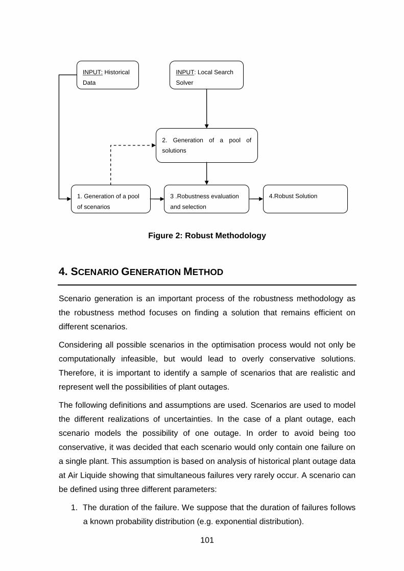
101

Figure 2: Robust Methodology

4. SCENARIO GENERATION METHOD

Scenario generation is an important process of the robustness methodology as

the robustness method focuses on finding a solution that remains efficient on

different scenarios.

Considering all possible scenarios in the optimisation process would not only be

computationally infeasible, but would lead to overly conservative solutions.

Therefore, it is important to identify a sample of scenarios that are realistic and

represent well the possibilities of plant outages.

The following definitions and assumptions are used. Scenarios are used to model

the different realizations of uncertainties. In the case of a plant outage, each

scenario models the possibility of one outage. In order to avoid being too

conservative, it was decided that each scenario would only contain one failure on

a single plant. This assumption is based on analysis of historical plant outage data

at Air Liquide showing that simultaneous failures very rarely occur. A scenario can

be defined using three different parameters:

1. The duration of the failure. We suppose that the duration of failures follows

a known probability distribution (e.g. exponential distribution).

1. Generation of a pool

of scenarios

2. Generation of a pool of

solutions

3 .Robustness evaluation

and selection

4.Robust Solution

INPUT: Local Search

Solver

INPUT: Historical

Data

102

2. The plant affected by the failure (if the instance contains multiple plants). If

the reliability of all the plants is unknown, we consider that all plants are

equally likely to fail.

3. The starting time of the failure. Note that the failure must be fully included

within the time horizon and thus, a 5-day failure cannot start on the last day

of the time horizon. It would simply be modeled by shorter failure duration.

For a given duration, we consider that the starting day of a failure follows a

uniform distribution over the entire time horizon minus the duration of that

failure. This prevents a failure from exceeding the time horizon.

Each of these parameters follows a probability distribution that can be determined

by studying the historical data.

The natural way to generate the sample of scenarios is to use the distribution law

of each of the 3 parameters defining a scenario. However, with small sets of

scenarios, it is possible to get ‘unlucky’ while generating the scenarios where the

set of scenarios generated do not correspond well to the distribution, especially

the duration distribution.

In order to ensure a good representation of the scenarios, we use stratified

sampling, see Cochran (1977) .Stratification is the process of dividing members of

the population into homogeneous subgroups or clusters before sampling. Within

each cluster, one or more of the parameters (failure duration, plant, and start time)

is fixed. A given number of scenarios are then randomly drawn from each cluster,

depending of the cluster weight. See Section 0 for more information on how

clusters and their weight are defined.

Generating only a limited number of scenarios also means that some possible

outages are not taken into account when searching for a robust solution and value

of the robustness will lack precision. As stated before, obtaining a precision of

100% (i.e., taking all the possible scenarios into account) is not be possible due to

computational constraints. Additional details on how to compute the precision of a

solution can be found inSection 4.2

Inputs:

103

X is the minimum number of solutions desired for the robust methodology

(e.g. X = 15).

Z is the desired precision. A precision of 100% means that all scenarios

should be generated.

CT is the maximum computation time allowed.

Parameters:

Si the number of scenarios to be generated from the cluster i.

Pi is the precision obtained on cluster i. Note that the precision is a function

of the number of scenarios of each cluster.

Wi: is the weight of each cluster i. The computation of these weights is

described in Section 0.

Methodology:

1. Compute the weight of each cluster. This is done via a statistical analysis of

historical data.

2. Compute the minimum number of scenarios Si per cluster needed to

achieve the specified precision.

3. Verify if it is possible to run the robustness methodology with the minimum

number of solutions specified, and the number of scenarios as computed in

Step 1. It returns YES if the computation time is not exceeded.

a. If YES: enough scenarios have been generated, the goal is to

maximize the number of solutions to be generated without

exceeding the allowed computation time.

b. If NO: It is not possible to obtain the desired precision within the

specified computation time. The goal of this step is then to maximize

the precision without exceeding the computation time.

104

Outputs:

The number of scenarios Si to be drawn from each cluster and the total

number of solutions X* to generate.

Section 0 describes the methodology used for creating the cluster as well as the

method used for computing the precision depending on the number of scenarios

created

4.1. Clustering and computation of the weights

In this section, we describe the method used for creating the clusters, and

identifying the weight of each of these clusters. As stated previously, we assume

to know the probability distribution of each parameter of the scenarios

characterizing the supply uncertainty: outage duration, plant concerned and

outage starting time.

However, with small sets of scenarios, we found out that it was frequent that we

got ‘unlucky’ while generating the scenarios, and that the set of scenarios

generated did not follow the distribution, especially the distribution of the Outage

Duration parameter. In order to avoid this issue, we used the stratified sampling

method, in which the elements are randomly selected from groups of

homogeneous sets.

We call a homogeneous set of scenarios, a set for which each scenario within the

set has a similar impact on distribution. For example, it is reasonable to assume

that a 1 day outage and a 7 day outage have a very different impact on the

distribution. However, two different 1 day outages occurring at same plant may

have a similar impact.

This leads to two different definitions for the cluster:

105

Duration: Each cluster contains all scenarios representing an outage of

a similar duration.

Duration + Plant: Each cluster contains the scenarios representing an

outage of a similar duration at a given plant.

If all the plants are similar, in both the number of customers and the quantity of

product produced, then clustering only by duration is recommended. Otherwise,

an outage at one plant might have a very different impact than an outage of the

same duration occurring at another plant. Thus, it is better to cluster the scenarios

by both the duration of the outage and the plant.

4.1.1 Clustering by duration

. This section explains how to compute the weight of each ‘duration’ cluster.

Let dF be the probability distribution of the duration of outages. Let ),,( 1 ndd be

the possible outage durations considered for the scenarios.

The weight iw of the cluster of duration id can then be computed as follow:

n

k

kd

idi

dF

dFw

1

)(

)(

4.1.2 Clustering by duration and plant

In order to estimate the plant reliability, two different parameters can be used:

Total failure time: The most obvious parameter to estimate the plant

reliability is the total failure time over the time horizon covered by the data.

The greater the total failure time, the less reliable the plant. The main

advantage of this method is that it is very easy to give a reliability rating to

a plant (i.e., 95% reliable). However, some plants have very few, but very

long failures, while others have many, shorter, failures. The total failure

time does not differentiate between these two kinds of plants.

106

Mean time between failures (MTBF): Another solution is to compute the

mean time between failures for each plant. If the MTBF of a plant is low, it

means that the plant is likely to fail often. One drawback is that it becomes

difficult to give a reliability rating for the plant using the MTBF.

As this method is aimed at a short-term horizon (e.g., 15 days), it is more natural

to use the MTBF to compute the number of scenarios for each plant. The following

method is then used in order to determine the repartition of the number of

scenarios for each sub cluster:

Let PMMM ,, 21 be the MTBF of each of the P plants of the instance.

Definej

jM

R1

for each plant pj and jRR .

Then consider the ‘plant + duration’ cluster with duration di and plant pj. the weight

dpw of the cluster can be computed as follow:

R

Rww

j

idp *

Using this formula, we ensure that greater MTBF values lead to fewer generated

failure scenarios of a plant.

4.2. Desired Precision

A trade-off must be made between the computation time allowed for the

robustness methodology and the precision desired for computing the deviation of

a solution. While it is relatively easy to have an estimation of the computation time

needed to evaluate the cost of the solutions when applied to the scenarios, the

impact on the precision is more difficult to estimate.

The goal of this study is to identify the impact of the number of scenarios

generated on the solution robustness. Of course, the evaluation of the

computation time and/or the quality of the final solution is dependent on the

implementation of the methodology.

107

There are two ways to save computation time: reduce the number of solutions to

be computed, or reduce the number of scenarios to be evaluated. Reducing the

number of solution reduces the probability to find a robust solution, whereas

reducing the number of scenarios reduces the precision of the evaluation of the

robustness of each solution.

This section aims to give a mathematical definition of the precision obtained

based on the sample of scenarios. Two possible definitions are presented which

depend on the amount of information available. Both of these definitions focus on

computing the precision on a given cluster. A formula for calculating the global

precision is also given.

4.2.1 Precision based on the number of scenarios

A very natural way to compute the precision on a cluster is to compare the

number of scenarios generated from a cluster to the total number of scenarios

included in the cluster.

)(

)(

inarioTotalNbSce

iScenarioNbSelectedpi

The total number of scenarios within a cluster is easy to compute depending on

the time horizon considered. For example, consider a 5-day duration outage

cluster, over a 15-day time horizon. The latest the failure can start to be fully

included in the time horizon is on day 11. Therefore, there are 11 possible

scenarios per plant within this cluster. In a 3 plant instance, there would be 33

possible scenarios.

In order to achieve a 70% precision on this cluster, one would need to generate

0.7*33=23 scenarios from this cluster.

108

4.2.2 Precision based on the deviation distribution

During this part of the study, we make the following assumptions. We assume that

the deviation of a given solution follows a probability distribution within a cluster.

This distribution may vary for different clusters of scenarios. We assume that the

maximum possible deviation is also known.

We understand that these are strong assumptions. However, is it possible to

obtain them through either a statistical study on historical data, assuming that the

extra costs due to past outages have been recorded, and that enough data is

available.

Usually, one wants to compute confidence intervals for the mean value of a

sample. However, in our case, the robustness is defined using the min-max regret

definition described in Section 6. The goal of the robust deviation is to minimize

the worst case deviation from optimality, among all possible scenarios. Therefore,

instead of focusing on the mean value, we focus on the maximum deviation

obtained among the scenarios.

Let S be a cluster of scenarios, Ss a scenario, and x be a solution. We

suppose that the deviation of solution x on scenario s is a random variable

denoted sxD , following a given probability distribution. Let )(sf x and xF be the

probability density function and cumulative density function of this distribution.

If we select a sample of size n from the cluster, and evaluate the deviation of the

solution on each of these scenarios, we obtain n independent and identically

distributed random variables nxxx DDD ,2,1, ,,,

.

Let 1,1, ,,max( xxn DDM ) be the maximum deviation of the solution over the

cluster. Order statistics shows that nM is a random variable described by a

cumulative probability density function

n

xnM XFXF )]([)(

and probability density function

)()]([)( 1 XfXFnXf n

xnM

.

109

The precision obtained when selecting a sample of size n is the ratio between Mn

and the maximum possible deviation. Knowing the density and cumulative

probability function of Mn , it is possible to compute the average value of Mn and

thus the average precision obtained by selecting a cluster of size n.

4.2.3 Global precision

The two methods shown above describe how to compute the precision for one

cluster. However, they do not give a value for the global precision depending on

the entire sample of scenarios.

A natural way to compute the global precision knowing the precision on each

cluster is to use the average precision among all clusters. But, as stated in

Section 0, the number of scenarios selected from each cluster depends of the

weight of the cluster. A cluster with a low weight has very few scenarios, and thus

a very low precision.

Therefore, we propose to define the global precision as the weighted sum of all

clusters precisions.

Let P be the global precision, ip the precision of cluster i and iw the weight of

cluster i. The global precision is computed based on the following formula:

i

ii wpP *

4.3. Scenario Generation

4.3.1 Finding the minimum number of scenarios

In this step, we compute the minimum number of scenario per cluster needed in

order to achieve the required precision. This is done using the following linear

programming approach:

110

)2(

)1(

.

Zpw

iwS

S

csSSMin

ii

i

i

i

i

Constraint (1) ensures that the number of scenarios chosen from each cluster

respects the weight of the cluster and constraint (2) ensures that the weighted

precision must be greater than Z. Each Si is then rounded to obtain the number of

scenario required per cluster.

4.3.2 Feasibility Check

In this step, we check if generating the number of solutions needed to obtain the

required precision can be solved within the allowed computation time. The

robustness methodology has 3 main computation steps:

1. Scenario generation: The time needed for creating the scenarios is short

compared to the solution generation. Let be the time necessary for

generating one scenario.

2. Solution generation: Testing has shown that this is the critical part in terms

of computation time. Let be the required time for generating a single

solution.

3. Solution evaluation: This is where the number of scenarios has an impact

on the global computation time needed to find a robust solution. Each

solution must be evaluated on each scenario. For the inventory routing

problem, this includes re-computing the volume of each reload and delivery

on the routes impacted by the plant failure. Let be the time needed for

an evaluation.

The global computation time T needed is: SXXST

Knowing the number of scenarios to generate and the minimum number of

solutions to generate, it is easy to check if the robustness methodology can be

used within the given computation time CT by verifying the following:

111

?SXXSCT

4.3.3 Maximize the precision

As stated at the beginning of this section, maximizing the precision depends on

the result obtained in the feasibility check. If the answer is YES, i.e., there is

enough computation time to obtain the wanted precision, then Step 4 maximizes

the number of solutions, otherwise, it maximizes the precision obtainable within

the allowed computation time.

Maximize the number of solutions

In this case, it is possible to generate enough scenarios to obtain the desired

precision. In order to increase the chances of finding an efficient robust solution,

the number of solutions created may be increased. This can be done iteratively

using a simple while loop as follows:

1. While )1()1( XSXSCT

2. 1 XX

3. return X

Maximize the precision within allowed computation time

In this case, it is not possible to generate enough scenarios to obtain the desired

precision within the allowed computation time. Therefore, the goal of this step is to

maximize the precision while not exceeding the computation time allowed. This is

done via a simple linear program:

)2(

)1(

..

SXXSCT

iwS

S

cspwMax

i

i

i

ii

This linear program determines the maximum number of scenarios that can fit

within the allowed computation time. As in Step 2, constraint (1) ensures that the

number of clusters chosen from each cluster is based on the weight of the cluster.

Constraint (2) ensures that the maximum computation time allowed is not

exceeded.

112

5. SOLUTION GENERATION METHOD

In order to increase the probability of finding a good robust solution, the pool of

solutions must include solutions with different costs, structures, and

characteristics. In order to do that, we implement different methods for generating

the solutions.

This section presents the three methods we have implemented for generating

multiples solutions. The first one simply runs several instances of local search in

parallel, each one with a different random seed. It is described in Section 5.1. The

second uses scenarios as input data in order to find solution that performs well

even when an outage occurs. Lastly, we present methodologies used to guide the

heuristic into more robust solutions.

5.1. Parallel solution generation

The first method for generating multiple efficient solutions is to parallelize multiple

local searches and select the best solution found. As the set of moves to be

applied during the local search depends on the random seed of the local search,

launching multiple searches with different random seeds will generate different

solution, with different costs.

Figure 3 presents the pseudo code used for the parallel local search. At first, an

array for storing all the solutions is created. Then, all the local searches are

launched into separate threads. Once all the threads have finished, the best

solution found is returned.

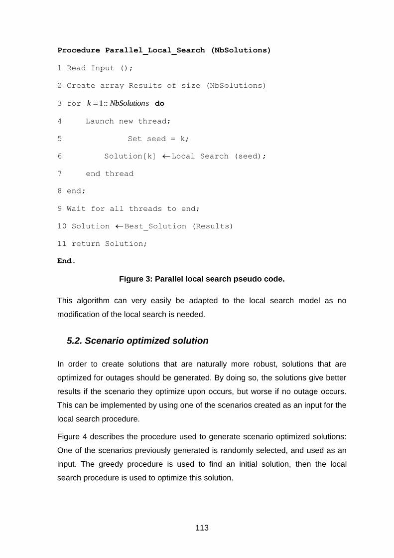
113

Procedure Parallel_Local_Search (NbSolutions)

1 Read Input ();

2 Create array Results of size (NbSolutions)

3 for sNbSolutionk ::1 do

4 Launch new thread;

5 Set seed = k;

6 Solution[k] Local Search (seed);

7 end thread

8 end;

9 Wait for all threads to end;

10 Solution Best_Solution (Results)

11 return Solution;

End.

Figure 3: Parallel local search pseudo code.

This algorithm can very easily be adapted to the local search model as no

modification of the local search is needed.

5.2. Scenario optimized solution

In order to create solutions that are naturally more robust, solutions that are

optimized for outages should be generated. By doing so, the solutions give better

results if the scenario they optimize upon occurs, but worse if no outage occurs.

This can be implemented by using one of the scenarios created as an input for the

local search procedure.

Figure 4 describes the procedure used to generate scenario optimized solutions:

One of the scenarios previously generated is randomly selected, and used as an

input. The greedy procedure is used to find an initial solution, then the local

search procedure is used to optimize this solution.

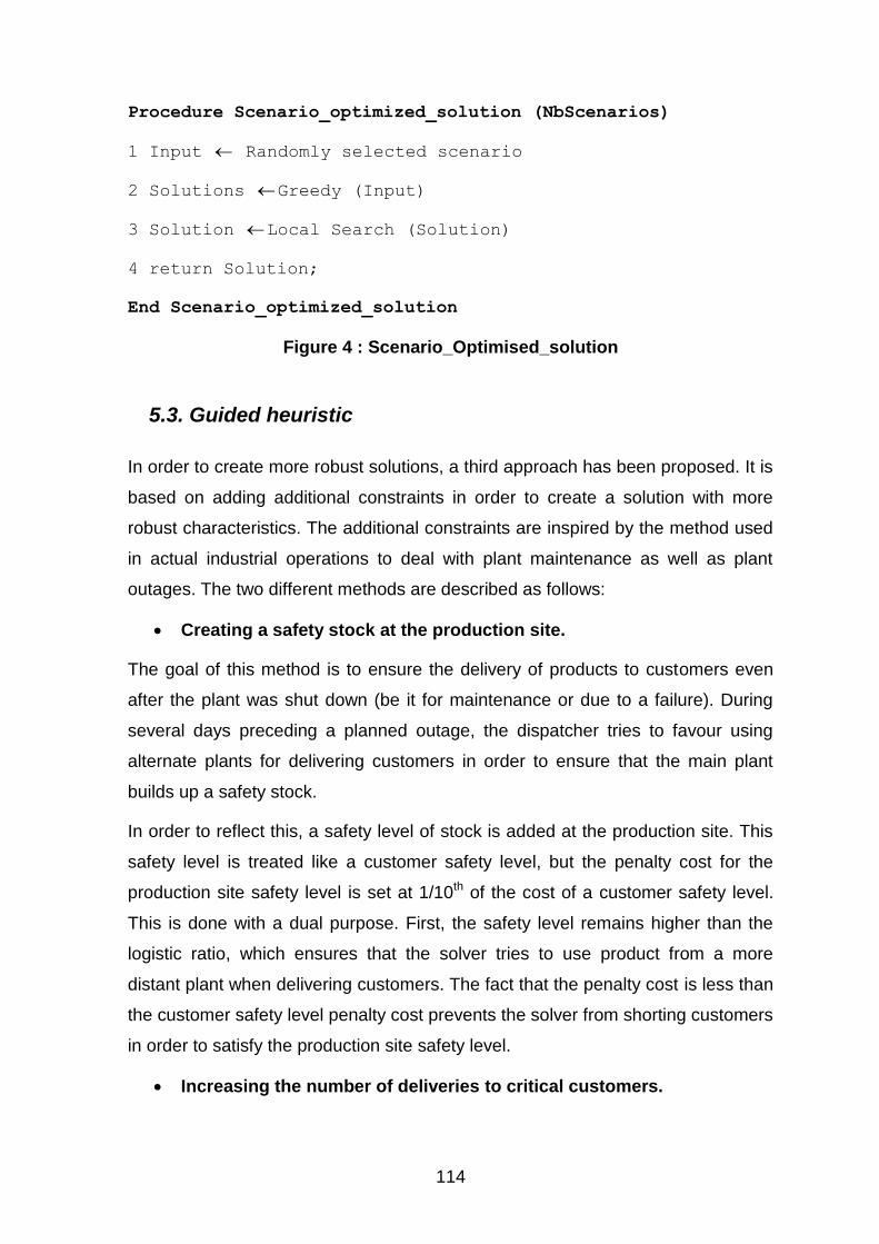
114

Procedure Scenario_optimized_solution (NbScenarios)

1 Input Randomly selected scenario

2 Solutions Greedy (Input)

3 Solution Local Search (Solution)

4 return Solution;

End Scenario_optimized_solution

Figure 4 : Scenario_Optimised_solution

5.3. Guided heuristic

In order to create more robust solutions, a third approach has been proposed. It is

based on adding additional constraints in order to create a solution with more

robust characteristics. The additional constraints are inspired by the method used

in actual industrial operations to deal with plant maintenance as well as plant

outages. The two different methods are described as follows:

Creating a safety stock at the production site.

The goal of this method is to ensure the delivery of products to customers even

after the plant was shut down (be it for maintenance or due to a failure). During

several days preceding a planned outage, the dispatcher tries to favour using

alternate plants for delivering customers in order to ensure that the main plant

builds up a safety stock.

In order to reflect this, a safety level of stock is added at the production site. This

safety level is treated like a customer safety level, but the penalty cost for the

production site safety level is set at 1/10th of the cost of a customer safety level.

This is done with a dual purpose. First, the safety level remains higher than the

logistic ratio, which ensures that the solver tries to use product from a more

distant plant when delivering customers. The fact that the penalty cost is less than

the customer safety level penalty cost prevents the solver from shorting customers

in order to satisfy the production site safety level.

Increasing the number of deliveries to critical customers.

115

The goal of this method is to make sure that critical customers do not run out of

product during production site maintenance or failure. When such a customer is at

risk, the number of deliveries to this customer is increased in order to make sure

that, when the production site stops, the customer would not be in need of an

urgent delivery.

To implement this, we increased the safety level of the critical customer(s) (i.e.,

the customers with the highest run out penalty cost) to one-half of the total

capacity of their gas storage tank.

6. EVALUATION OF ROBUSTNESS AND SOLUTION SELECTION

6.1. Evaluate all the solutions using robustness criteria

In this section we give a formal definition of the three possible criteria for the

reliability given by Kouvelis and Yu (1997). In order to compare the generated

solutions, we need to define a measure of reliability which takes into account the

cost of each solution applied on each scenario.

Let S be the set of all scenarios and A the set of feasible solutions. Let )(XFs be

the value of the objective function for solution X, where AX , under the scenario

s, where Ss . *

sF denotes the optimal value of the objective function F under the

scenario s.

Absolute robustness

The absolute robustness goal is to minimize the maximum cost among all possible

scenarios.

)))((max(min XFz sSsAX

A

(1)

The idea behind this notion of robustness is to optimize for the worst possible

scenario. However, this robustness gives no guarantee of the quality of the

solution in other cases.

Robust deviation

116

The goal of the robust deviation is to minimize the worst case deviation from

optimality among all feasible scenarios.

)))((max(min * XFFz ssSsAX

D

(2)

Relative robustness

Relative robustness minimizes the worst case percentage deviation from

optimality.

)))(

(max(min*

*

s

ss

SsAXR

F

FXFz

which is equivalent to ))

)((max(min

*

s

s

SsAXR

F

XFz

(3)

In our case, absolute robustness is a worst case optimisation and thus, is over

conservative. Therefore, we use the robust deviation and relative robustness

criteria. Preliminary tests showed that they give similar results, so we choose the

robust deviation method.

Note that these criteria originally require the knowledge of the optimal solution for

each scenario. In our case, as the inventory routing problem is NP-hard, we

cannot compute the value of the optimal solution in a reasonable amount of time.

Instead, we use the best known solution for the scenarios. The ‘optimized for

outage’ solution generation method helps to generate “good values” for the best

known solutions

6.2. Pareto optimality and solution selection

The criterion presented in section 4.4 allows us to compute the robustness of the

solutions. However, robustness has a price, and often the more robust solutions

will have a higher nominal cost. Thus a method is needed to select the best

solution that balances robustness and excess cost.

For each solution, we consider its nominal cost as well as its measure of

robustness (in this case: maximum deviation). We then fix a cost limit for the

robust solution. The limit is equal to the nominal cost of the original solution plus

10%.

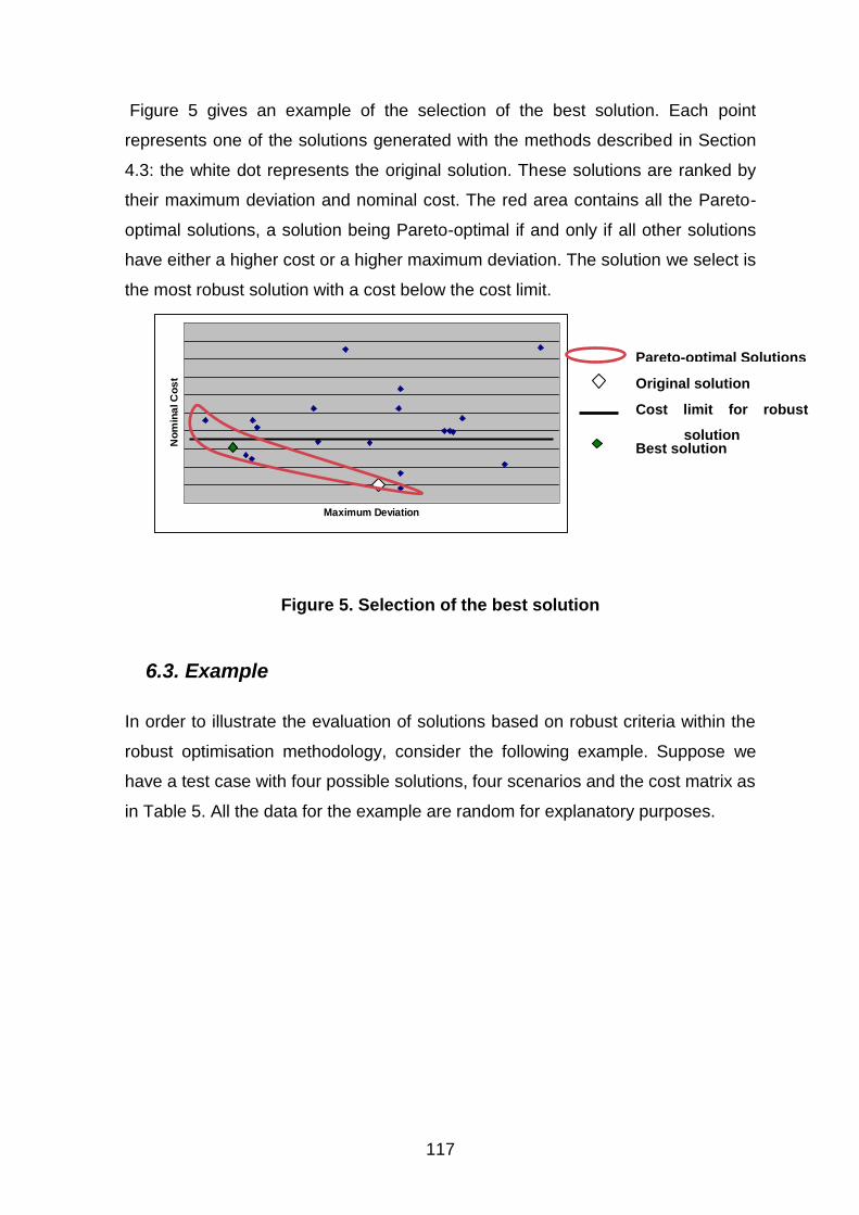
117

Figure 5 gives an example of the selection of the best solution. Each point

represents one of the solutions generated with the methods described in Section

4.3: the white dot represents the original solution. These solutions are ranked by

their maximum deviation and nominal cost. The red area contains all the Pareto-

optimal solutions, a solution being Pareto-optimal if and only if all other solutions

have either a higher cost or a higher maximum deviation. The solution we select is

the most robust solution with a cost below the cost limit.

Figure 5. Selection of the best solution

6.3. Example

In order to illustrate the evaluation of solutions based on robust criteria within the

robust optimisation methodology, consider the following example. Suppose we

have a test case with four possible solutions, four scenarios and the cost matrix as

in Table 5. All the data for the example are random for explanatory purposes.

Maximum Deviation

No

min

al C

os

t

Pareto-optimal Solutions

Original solution

Cost limit for robust

solution Best solution

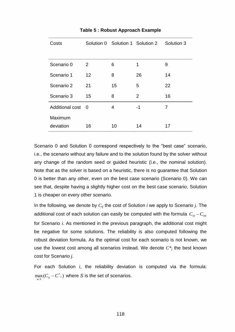
118

Table 5 : Robust Approach Example

Costs

Solution 0

Solution 1

Solution 2

Solution 3

Scenario 0 2 6 1 9

Scenario 1 12 8 26 14

Scenario 2 21 15 5 22

Scenario 3 15 8 2 16

Additional cost 0 4 -1 7

Maximum

deviation 16 10 14 17

Scenario 0 and Solution 0 correspond respectively to the “best case“ scenario,

i.e., the scenario without any failure and to the solution found by the solver without

any change of the random seed or guided heuristic (i.e., the nominal solution).

Note that as the solver is based on a heuristic, there is no guarantee that Solution

0 is better than any other, even on the best case scenario (Scenario 0). We can

see that, despite having a slightly higher cost on the best case scenario, Solution

1 is cheaper on every other scenario.

In the following, we denote by Cij the cost of Solution i we apply to Scenario j. The

additional cost of each solution can easily be computed with the formula 000 CCi

for Scenario i. As mentioned in the previous paragraph, the additional cost might

be negative for some solutions. The reliability is also computed following the

robust deviation formula. As the optimal cost for each scenario is not known, we

use the lowest cost among all scenarios instead. We denote C*j the best known

cost for Scenario j.

For each Solution i, the reliability deviation is computed via the formula:

)(max *sis

SsCC

where S is the set of scenarios.

119

In this example, we can see that the most reliable solution is Solution 1 with a

maximum deviation of 10. However, it does have an additional cost of 4. In this

example, the worst solution is Solution 4, with both the highest additional costand

the highest deviation. On the other hand, we can note that Solution 2, despite not

being as reliable as Solution 1, is better than Solution 0 with both a lower cost

when applied to the best case scenario, and a better robustness.

7. EVALUATION AND TESTING

In this section, we present how the robust methodology was tested as well as the

results obtained. Section 7.1 presents the 16 different real life test cases that were

used for evaluating the performance of the robustness methodology.

7.1. Test cases

16 different test cases were used for the evaluation of the robustness method. All

instances cover a 15-day horizon.

Note that the computation time needed does not only depends on the size of the

instance (i.e., the number of customers to be delivered), but also on its

composition and the difficulty to satisfy the constraints such as the compatibility of

the resources, the ratio between the quantity produced and the demand of the

customers.

Test cases “T” and “B” are based on real-life cases at Air Liquide. The “A” cases

are randomly generated instances. They cases are comprised of a set of sources

and customers as well as the available resources: drivers, trailers, and tractors.

The cases are detailed in Table 6.

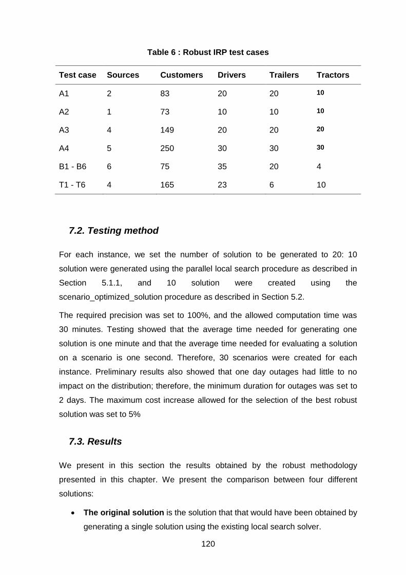
120

Table 6 : Robust IRP test cases

Test case Sources Customers Drivers Trailers Tractors

A1 2 83 20 20 10

A2 1 73 10 10 10

A3 4 149 20 20 20

A4 5 250 30 30 30

B1 - B6 6 75 35 20 4

T1 - T6 4 165 23 6 10

7.2. Testing method

For each instance, we set the number of solution to be generated to 20: 10

solution were generated using the parallel local search procedure as described in

Section 5.1.1, and 10 solution were created using the

scenario_optimized_solution procedure as described in Section 5.2.

The required precision was set to 100%, and the allowed computation time was

30 minutes. Testing showed that the average time needed for generating one

solution is one minute and that the average time needed for evaluating a solution

on a scenario is one second. Therefore, 30 scenarios were created for each

instance. Preliminary results also showed that one day outages had little to no

impact on the distribution; therefore, the minimum duration for outages was set to

2 days. The maximum cost increase allowed for the selection of the best robust

solution was set to 5%

7.3. Results

We present in this section the results obtained by the robust methodology

presented in this chapter. We present the comparison between four different

solutions:

The original solution is the solution that that would have been obtained by

generating a single solution using the existing local search solver.

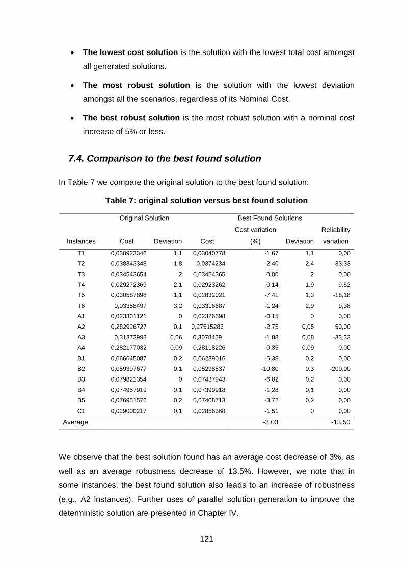
121

The lowest cost solution is the solution with the lowest total cost amongst

all generated solutions.

The most robust solution is the solution with the lowest deviation

amongst all the scenarios, regardless of its Nominal Cost.

The best robust solution is the most robust solution with a nominal cost

increase of 5% or less.

7.4. Comparison to the best found solution

In Table 7 we compare the original solution to the best found solution:

Table 7: original solution versus best found solution

Original Solution Best Found Solutions

Instances Cost Deviation Cost

Cost variation

(%) Deviation

Reliability

variation

T1 0,030923346 1,1 0,03040778 -1,67 1,1 0,00

T2 0,038343348 1,8 0,0374234 -2,40 2,4 -33,33

T3 0,034543654 2 0,03454365 0,00 2 0,00

T4 0,029272369 2,1 0,02923262 -0,14 1,9 9,52

T5 0,030587898 1,1 0,02832021 -7,41 1,3 -18,18

T6 0,03358497 3,2 0,03316687 -1,24 2,9 9,38

A1 0,023301121 0 0,02326698 -0,15 0 0,00

A2 0,282926727 0,1 0,27515283 -2,75 0,05 50,00

A3 0,31373998 0,06 0,3078429 -1,88 0,08 -33,33

A4 0,282177032 0,09 0,28118226 -0,35 0,09 0,00

B1 0,066645087 0,2 0,06239016 -6,38 0,2 0,00

B2 0,059397677 0,1 0,05298537 -10,80 0,3 -200,00

B3 0,079821354 0 0,07437943 -6,82 0,2 0,00

B4 0,074957919 0,1 0,07399918 -1,28 0,1 0,00

B5 0,076951576 0,2 0,07408713 -3,72 0,2 0,00

C1 0,029000217 0,1 0,02856368 -1,51 0 0,00

Average -3,03 -13,50

We observe that the best solution found has an average cost decrease of 3%, as

well as an average robustness decrease of 13.5%. However, we note that in

some instances, the best found solution also leads to an increase of robustness

(e.g., A2 instances). Further uses of parallel solution generation to improve the

deterministic solution are presented in Chapter IV.

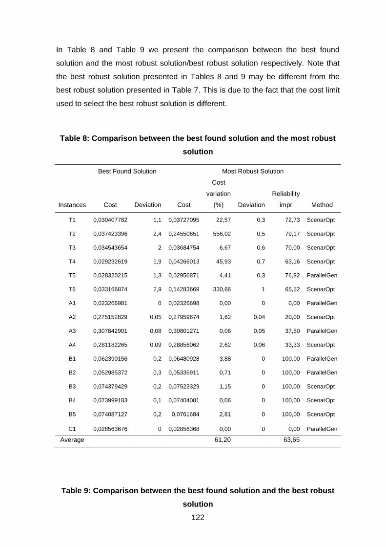
122

In Table 8 and Table 9 we present the comparison between the best found

solution and the most robust solution/best robust solution respectively. Note that

the best robust solution presented in Tables 8 and 9 may be different from the

best robust solution presented in Table 7. This is due to the fact that the cost limit

used to select the best robust solution is different.

Table 8: Comparison between the best found solution and the most robust

solution

Best Found Solution Most Robust Solution

Instances Cost Deviation Cost

Cost

variation

(%) Deviation

Reliability

impr Method

T1 0,030407782 1,1 0,03727095 22,57 0,3 72,73 ScenarOpt

T2 0,037423396 2,4 0,24550651 556,02 0,5 79,17 ScenarOpt

T3 0,034543654 2 0,03684754 6,67 0,6 70,00 ScenarOpt

T4 0,029232619 1,9 0,04266013 45,93 0,7 63,16 ScenarOpt

T5 0,028320215 1,3 0,02956871 4,41 0,3 76,92 ParallelGen

T6 0,033166874 2,9 0,14283669 330,66 1 65,52 ScenarOpt

A1 0,023266981 0 0,02326698 0,00 0 0,00 ParallelGen

A2 0,275152829 0,05 0,27959674 1,62 0,04 20,00 ScenarOpt

A3 0,307842901 0,08 0,30801271 0,06 0,05 37,50 ParallelGen

A4 0,281182265 0,09 0,28856062 2,62 0,06 33,33 ScenarOpt

B1 0,062390156 0,2 0,06480928 3,88 0 100,00 ParallelGen

B2 0,052985372 0,3 0,05335911 0,71 0 100,00 ParallelGen

B3 0,074379429 0,2 0,07523329 1,15 0 100,00 ScenarOpt

B4 0,073999183 0,1 0,07404081 0,06 0 100,00 ScenarOpt

B5 0,074087127 0,2 0,0761684 2,81 0 100,00 ScenarOpt

C1 0,028563676 0 0,02856368 0,00 0 0,00 ParallelGen

Average 61,20 63,65

Table 9: Comparison between the best found solution and the best robust

solution

123

Best Found Solution Best Robust Solution

Instances Cost Deviation Cost

Cost

variation

(%) Deviation

Reliability

impr Method

T1 0,030407782 1,1 0,03142384 3,34 0,7 36,36 ParallelGen

T2 0,037423396 2,4 0,03820777 2,10 1,2 50,00 ScenarOpt

T3 0,034543654 2 0,03619535 4,78 1,3 35,00 ParallelGen

T4 0,029232619 1,9 0,02923262 0,00 1,9 0,00 ScenarOpt

T5 0,028320215 1,3 0,02956871 4,41 0,3 76,92 ParallelGen

T6 0,033166874 2,9 0,03359295 1,28 2,2 24,14 ParallelGen

A1 0,023266981 0 0,02326698 0,00 0 0,00 ParallelGen

A2 0,275152829 0,05 0,27959674 1,62 0,04 20,00 ScenarOpt

A3 0,307842901 0,08 0,30801271 0,06 0,05 37,50 ParallelGen

A4 0,281182265 0,09 0,28856062 2,62 0,06 33,33 ScenarOpt

B1 0,062390156 0,2 0,06480928 3,88 0 100,00 ParallelGen

B2 0,052985372 0,3 0,05335911 0,71 0 100,00 ParallelGen

B3 0,074379429 0,2 0,07523329 1,15 0 0,00 ScenarOpt

B4 0,073999183 0,1 0,07404081 0,06 0 100,00 ScenarOpt

B5 0,074087127 0,2 0,0761684 2,81 0 100,00 ScenarOpt

C1 0,028563676 0 0,02856368 0,00 0 0,00 ParallelGen

Average 1,80 44,58

We can see that the results vary depending on the instance. In the case of the B

instances, the robust methodology manages to find solutions without any run outs,

even in the case of plant failure. However, in the case of the C4 instance, it was

not possible to improve the robustness of the initial solution. Also note that even if

the maximum nominal cost increase was set to 5%, most of the robust solutions

found have a lower cost increase. Overall, the robust methodology leads to a 45%

reliability increase, with less than a 2% cost increase. Also, we can clearly see

that each of the two solution generation methods found approximately 50% of the

best robust solutions, thus demonstrating that both are important for the

framework.

124

In the proposed framework, the time limit led to an evaluation of robustness based

on less than 20 scenarios. In order to further test the quality and the robustness of

the solutions found, the solutions where also evaluated over a set of 70 different

scenarios, randomly generated using a Monte Carlo method. The results can be

found in Table 10. Note that the last column indicates if the best robust solution is

the same as in results given in Table 9. Also, as the considered scenarios from

this test are different from the scenarios considered in Table 9 it is normal that the

deviation of the lowest cost solution differs from its previous value.

Table 10 : Result Quality Evaluation

Lowest

cost

solution Best Robust Solution

Instances Deviation Deviation

Reliability

impr

Cost

variation

(%)

Is

same

C1 10 5 50.00 8.75 Yes

C2 24 9 62.50 9.83 Yes

C3 20 7 65.00 6.67 Yes

C4 9 7 22.22 6.29 No

C5 8 1 87.50 4.41 Yes

C6 19 10 47.37 1.28 Yes

A1 4 2 50.00 2.57 No

A2 7 5 28.57 0.66 Yes

A3 9 3 66.67 0.38 Yes

B1 2 0 100.00 0.19 Yes

B2 1 0 100.00 1.15 Yes

B3 3 0 100.00 0.06 Yes

B4 1 0 100.00 1.67 Yes

Average 66.10 3.38

125

We note that in all but two cases, the best robust solution found using only 20

scenarios remains the best robust solution even when evaluated on 70 scenario.

However, Test case C4 has a more robust solution with 70 scenarios. However,

note that on instances A1, the most robust solution found using 20 scenarios

remains more robust than the lowest cost solution, even when evaluated on 70

scenarios. These results demonstrate that our scenario generation method is

highly effective at identifying robust solutions.

8. CONCLUSION

We propose a framework for robust decision making under uncertainty for the

inventory routing problem. We use a scenario-based approach and a min-max

criteria to select the best solution. To our knowledge, such an approach has not

been used before for the inventory routing problem under supply disruption. The

methodology includes a method to generate a set of representative scenarios.

This method takes into account both the allowed computation time and the

precision of the representation desired. We also present multiple ways of

generating feasible solutions. Lastly, we explain how to compute the robustness

of each solution, and how to select the solution with the best trade-off between

cost and robustness.

We applied our methodology to the logistic optimisation of Air Liquide bulk

distribution of liquid gas with uncertainties at the sources due to plant outages.

We show that the model of the discrete IRP can be extended in order to take into

account uncertainty aspects generated by plant outages. We then used a

scenario-based approach which allows us to optimize the distribution regarding

multiple possible future realization of the uncertainty variable.

We implemented the proposed framework which consists of an extended model

and robust methodology and showed that robust solutions with low costs can be

obtained for real-world test cases.

126

Results show that, using the robust methodology developed in this report, the

number of avoidable run outs due to plant outage are reduced by an average of

50% compared to the solutions found by the local search tool currently being

used, with a logistic cost increase of only 2%. This experimentation on a

particularly complex real world case shows the feasibility and effectiveness of our

approach. The methodology is generic and it can be applied to other IRP or more

general optimisation problems.

9. PUBLICATIONS

Preliminary results were presented in the IFORS 2011 and IESM 2011

international conferences. The scenario generation method was presented in the

2012 ILS international conference. A full journal paper has also been submitted to

the Transportation Research part B special issue on “Advances in Transportation

Reliability”.

127

Chapter IV: Inventory Routing - a GRASP

methodology

1. INTRODUCTION

The competition in local and global markets is pushing companies to look for

reductions in their logistic costs as they represent an important part of the final

cost of goods. To that aim, more centralized supply chain management systems

are needed and thus, a recent approach in seeking logistic cost reductions is to

consider the integration of transportation and inventory decisions.

For solving the IRP described in detail in the previous chapter, a heuristic

algorithm has been proposed by Benoist et al. (2011). We call this algorithm “the

original heuristic”. It combines a greedy construction algorithm (which we refer to

as “the greedy algorithm”) followed by a local search and is described in the next

section (referred to as “the local search” in this chapter).

128

In order to improve the solution quality of this “local search” for solving the rich

IRP, we propose two different designs of a GRASP (Greedy Randomized

Adaptative Search Procedure) framework for IRP in the context of a real-life

setting of bulk gas distribution. We imbed the “local search” heuristic within the

GRASP frameworks. The two GRASP methods are tested on 16 real-life test

cases and compared to the results provided by the initial “local search”. The

chapter is organized as follows: Section 2 describes the two GRASP

implementations we propose. Section 3 describes the methodology used for

testing as well as the test cases used. Section 4 presents the results and gives

some insight on the influence of computation time. Lastly, Section 5 concludes the

paper.

2. GRASP DESIGN AND IMPLEMENTATION METHODOLOGY

In this section, we describe the design of the GRASP, and its implementation. We

propose two different GRASP approaches which are based on the integration of

the specialized heuristic proposed by Benoist et al. (2011).

The GRASP algorithm, as described by Feo and Resende (1995), consists of

multiple iterations of two successive phases: a construction phase, in which an

initial solution is constructed, using a randomized greedy algorithm, and an

improvement phase, during which a local search algorithm is used to further

optimize the solution previously constructed.

As a first approach, we do not include the multi-start component of the GRASP

meta-heuristic. Instead, the construction phase is only run once before any

iteration. Then, during each iteration, the local search optimisation is performed

from the start using a different random seed. Thus, the final solutions found by

each iteration are different from one other.

The second approach includes the multi-start component as traditionally done

within a GRASP meta-heuristic. In the following sections, we describe the

algorithms used for each approach in detail.

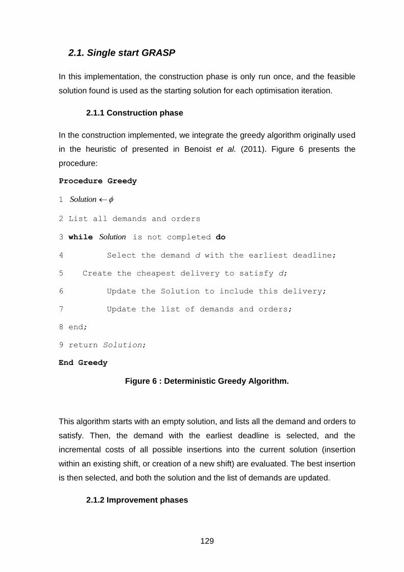
129

2.1. Single start GRASP

In this implementation, the construction phase is only run once, and the feasible

solution found is used as the starting solution for each optimisation iteration.

2.1.1 Construction phase

In the construction implemented, we integrate the greedy algorithm originally used

in the heuristic of presented in Benoist et al. (2011). Figure 6 presents the

procedure:

Procedure Greedy

1 Solution

2 List all demands and orders

3 while Solution is not completed do

4 Select the demand d with the earliest deadline;

5 Create the cheapest delivery to satisfy d;

6 Update the Solution to include this delivery;

7 Update the list of demands and orders;

8 end;

9 return Solution;

End Greedy

Figure 6 : Deterministic Greedy Algorithm.

This algorithm starts with an empty solution, and lists all the demand and orders to

satisfy. Then, the demand with the earliest deadline is selected, and the

incremental costs of all possible insertions into the current solution (insertion

within an existing shift, or creation of a new shift) are evaluated. The best insertion

is then selected, and both the solution and the list of demands are updated.

2.1.2 Improvement phases

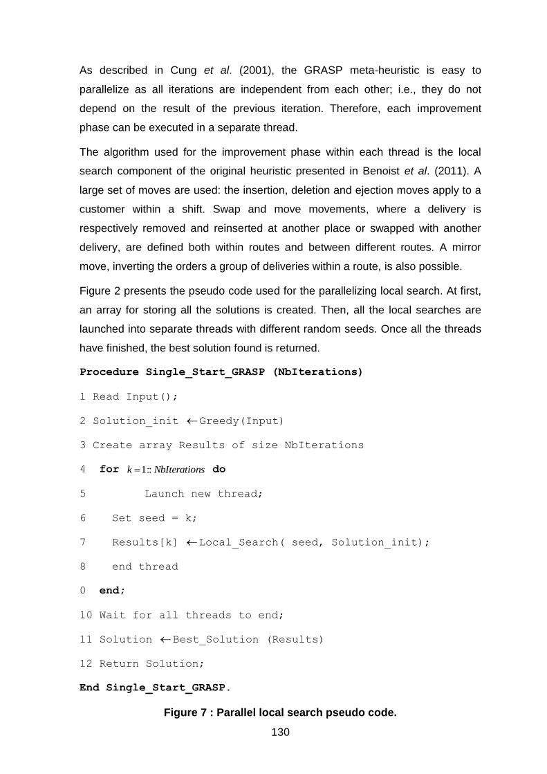
130

As described in Cung et al. (2001), the GRASP meta-heuristic is easy to

parallelize as all iterations are independent from each other; i.e., they do not

depend on the result of the previous iteration. Therefore, each improvement

phase can be executed in a separate thread.

The algorithm used for the improvement phase within each thread is the local

search component of the original heuristic presented in Benoist et al. (2011). A

large set of moves are used: the insertion, deletion and ejection moves apply to a

customer within a shift. Swap and move movements, where a delivery is

respectively removed and reinserted at another place or swapped with another

delivery, are defined both within routes and between different routes. A mirror

move, inverting the orders a group of deliveries within a route, is also possible.

Figure 2 presents the pseudo code used for the parallelizing local search. At first,

an array for storing all the solutions is created. Then, all the local searches are

launched into separate threads with different random seeds. Once all the threads

have finished, the best solution found is returned.

Procedure Single_Start_GRASP (NbIterations)

1 Read Input();

2 Solution_init Greedy(Input)

3 Create array Results of size NbIterations

4 for nsNbIteratiok ::1 do

5 Launch new thread;

6 Set seed = k;

7 Results[k] Local_Search( seed, Solution_init);

8 end thread

0 end;

10 Wait for all threads to end;

11 Solution Best_Solution (Results)

12 Return Solution;

End Single_Start_GRASP.

Figure 7 : Parallel local search pseudo code.

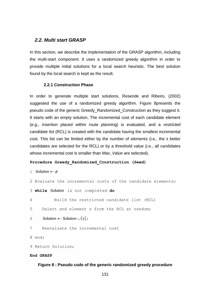
131

2.2. Multi start GRASP

In this section, we describe the implementation of the GRASP algorithm, including

the multi-start component. It uses a randomized greedy algorithm in order to

provide multiple initial solutions for a local search heuristic. The best solution

found by the local search is kept as the result.

2.2.1 Construction Phase

In order to generate multiple start solutions, Resende and Ribeiro, (2002)

suggested the use of a randomized greedy algorithm. Figure 8presents the

pseudo code of the generic Greedy_Randomized_Construction as they suggest it.

It starts with an empty solution. The incremental cost of each candidate element

(e.g., insertion placed within route planning) is evaluated, and a restricted

candidate list (RCL) is created with the candidate having the smallest incremental

cost. This list can be limited either by the number of elements (i.e., the k better

candidates are selected for the RCL) or by a threshold value (i.e., all candidates

whose incremental cost is smaller than Max_Value are selected).

Procedure Greedy_Randomized_Construction (Seed)

1 Solution

2 Evaluate the incremental costs of the candidate elements;

3 while Solution is not completed do

4 Build the restricted candidate list (RCL)

5 Select and element s from the RCL at random;

6 sSolutionSolution ;

7 Reevaluate the incremental cost

8 end;

9 Return Solution;

End GRASP

Figure 8 : Pseudo code of the generic randomized greedy procedure

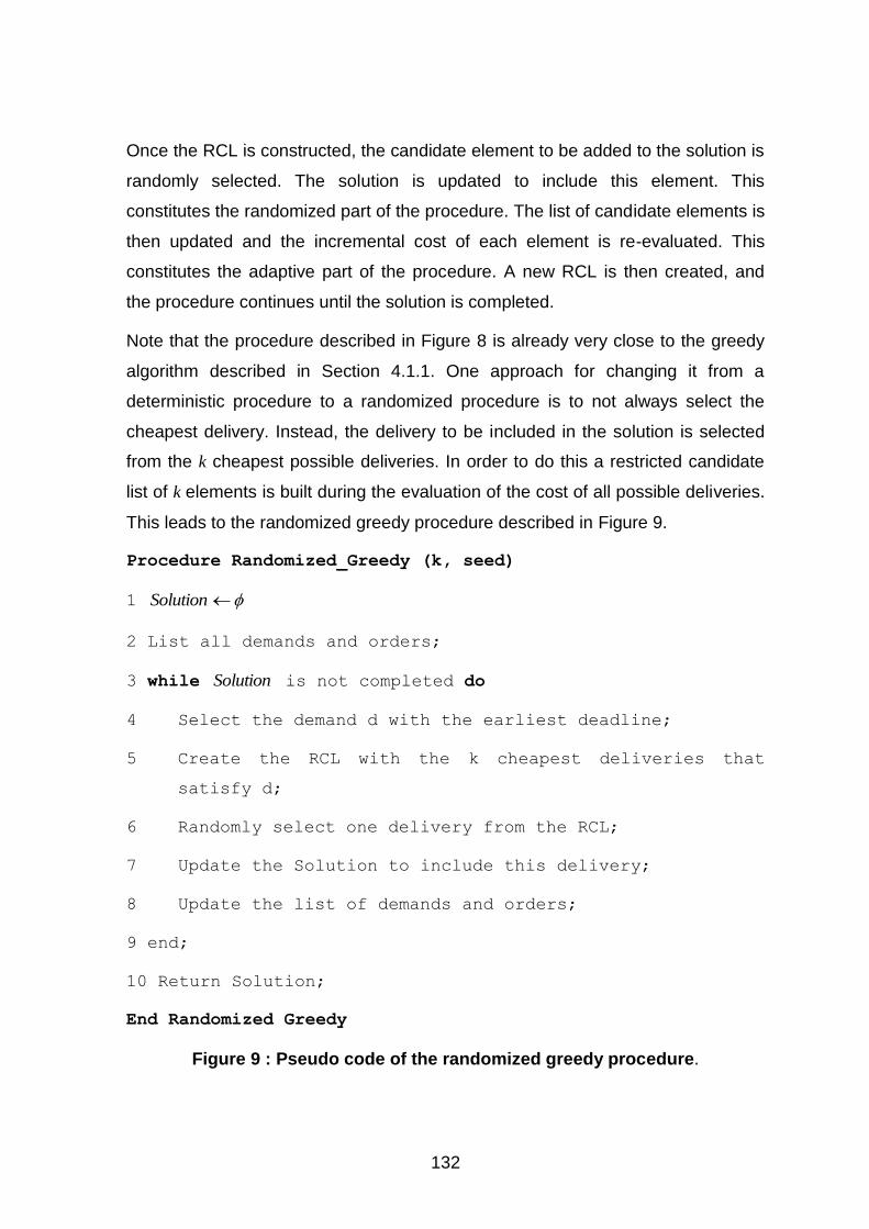
132

Once the RCL is constructed, the candidate element to be added to the solution is

randomly selected. The solution is updated to include this element. This

constitutes the randomized part of the procedure. The list of candidate elements is

then updated and the incremental cost of each element is re-evaluated. This

constitutes the adaptive part of the procedure. A new RCL is then created, and

the procedure continues until the solution is completed.

Note that the procedure described in Figure 8 is already very close to the greedy

algorithm described in Section 4.1.1. One approach for changing it from a

deterministic procedure to a randomized procedure is to not always select the

cheapest delivery. Instead, the delivery to be included in the solution is selected

from the k cheapest possible deliveries. In order to do this a restricted candidate

list of k elements is built during the evaluation of the cost of all possible deliveries.

This leads to the randomized greedy procedure described in Figure 9.

Procedure Randomized_Greedy (k, seed)

1 Solution

2 List all demands and orders;

3 while Solution is not completed do

4 Select the demand d with the earliest deadline;

5 Create the RCL with the k cheapest deliveries that

satisfy d;

6 Randomly select one delivery from the RCL;

7 Update the Solution to include this delivery;

8 Update the list of demands and orders;

9 end;

10 Return Solution;

End Randomized Greedy

Figure 9 : Pseudo code of the randomized greedy procedure.

133

2.2.2 Improvement phase

Unlike the single start GRASP described in Section 4.1.2 the multi-start GRASP

executes both the construction phase and the improvement phase during each

iteration of the algorithm. This creates different starting solutions for the

improvement phase, and thus can explore a larger range of the solution space.

One drawback of this method is that the improvement phase must compensate for

potentially worse starting solutions.

Figure 10 describes the overall multi-start GRASP procedure. For each of the

NBIteration iterations, a random initial solution is created using the randomized

greedy procedure. Then, this initial solution is optimized using the local search

procedure with each iteration being run in a separate thread. If the solution found

by the local search is better than the current best solution, the new solution found

is kept as the new best solution.

Procedure Multi_Start_GRASP (NbIterations)

1 Read Input ();

2 Create array Results of size NbIterations

3 for nsNbIteratiok ::1 do

4 Launch new thread;

5 Set seed = k;

6 Solution_init Randomized_Greedy (seed, Input)

7 Results[k] Local_Search (seed, Solution_init);

8 end thread

9 end;

10 Wait for all threads to end;

11 Solution Best_Solution (Results)

12 return Solution;

End Multi_Start_GRASP.

Figure 10: Pseudo Code for the GRASP meta-heuristic.

134

3. TESTING & RESULTS

In this section, we describe the methodology used to test and compare the

different approaches aforementioned in Section 2.

The algorithm is implemented in C# and tested on a 16-core; 8GB RAM computer

running Windows Server 2008. Testing was performed on 16 different instances

adapted from real-life data and three different heuristics were compared. The first

is based on the basic deterministic greedy and local search heuristic. The second

is the single start GRASP. Lastly, the third heuristic is the multi-start GRASP

methodology as described in Section 4.2

3.1. Testing methodology

The parameter with the most influence on the quality of the result is the

computation time. Before our study, a single run of the original heuristic algorithm

performed 4 million local search iterations and took an average of 264 seconds to

perform. Section 6 provides an example of how the local search can keep steadily

improving the solution until up to 7 minutes of computation time before getting

stuck in local optima. This also means that for both implementations, the time

needed for a single GRASP iteration would be over 4 minutes.

In order to show a fair comparison of all the three algorithms, we chose, after

preliminary testing, to use the following parameters for each algorithm:

16 million iterations for the local search.

20 iterations for the two GRASP implementations. Thus, each optimisation

phase of the GRASP performs 4 million local search iterations.

Note that the computation time needed for each algorithm is similar, the 16M-

iteration local search requiring an average of 1222 seconds to find a solution, and

the two 20-thread GRASP implementation needs an average of, respectively,

1290 and 1295 seconds to finish as shown in the results section of this chapter.

The original results heuristic results, obtained using 4 million local search

iterations, is used as a benchmark for comparing the other three methods.

3.2. Test instances

135

16 different test cases were used for the evaluation of the three methods. All

instances cover a 15-day horizon. Note that the computation time needed does

not only depend on the size of the test case (i.e., the number of customers to be

delivered), but also on its composition and the difficulty to satisfy the constraints

such as the compatibility of the resources, the ratio between the quantity

produced and the demand of the customers.

C area test cases

These real life test cases contain 4 sources and 165 customers. The resources

used to deliver products consist of 23 drivers, 6 trailers and 10 tractors. Data from

6 different time periods were used, resulting in 6 different instances.

B area test cases

These real life test cases consist of 6 sources and 75 customers. The resources

available for the deliveries are 35 drivers, 20 tractors and 4 trailers. Data from 5

different time periods were used resulting in 5 different instances

B_L performance test case

This real life test case is based on a 15-day horizon real-life test case. It consists

of 6 different sources and 175 customers. The resources available for the

deliveries are 35 drivers, 20 tractors and 12 trailers.

A1 performance test cases

This is a randomly generated instance that was initially created for performance

testing of the local search solver. It consists of 2 sources and 83 customers,

delivered by 20 drivers, 20 trailers and 10 tractors.

A2 performance test cases

This is a randomly generated instance that was initially created for performance

testing of local search solver. It consists of 1 source and 73 customers, delivered

by 10 drivers, 10 trailers and 10 tractors.

A3 performance test cases

This is a randomly generated instance that was initially created for performance

testing of the local search solver. It consists of 4 sources and 149 customers,

delivered by 20 drivers, 20 trailers and 20 tractors.

136

A4 performance test cases

This is a randomly generated instance that was initially created for performance

testing of the local search solver. It consists of 5 sources and 250 customers,

delivered by 30 drivers, 30 trailers and 30 tractors.

4. RESULTS OBTAINED

4.1. Overall results

Table 11 shows the comparison between 4 million local search iterations for the

original heuristic and 16 million local search iterations. The two first lines show the

value of the objective function and the computation time for the 4 million-iteration

local search for each instance. The last three lines show the value of the objective

function for the 16-million iteration heuristic, the improvement compared to the 4

million-iteration local search and the tested heuristic. We see that even with four

times the number of iterations and computation time, the results are only improved

by 1.66%.

Table 12 presents the results obtained using the single start GRASP

methodology. At the cost of a slightly longer computation time, we see that the

average improvement is significantly better than the improvement obtained by

simply increasing the number of iterations of the local search. The single start

GRASP obtains a 5.44% average improvement of the solution compared to the

heuristic.

Table 13: Local search vs. Multi Start GRASP presents the results obtained using

the multi-start GRASP methodology. The size of the restricted candidate list for

the randomized greedy procedure was set to 3. This allows finding good initial

solutions while still ensuring a high diversity amongst them. Tests were made with

a restricted candidate list of size 5, but this led to a significant deterioration of the

initial solution, which the local search was not able to overcome. With these

parameters, a 5.07% improvement of the objective function is obtained.

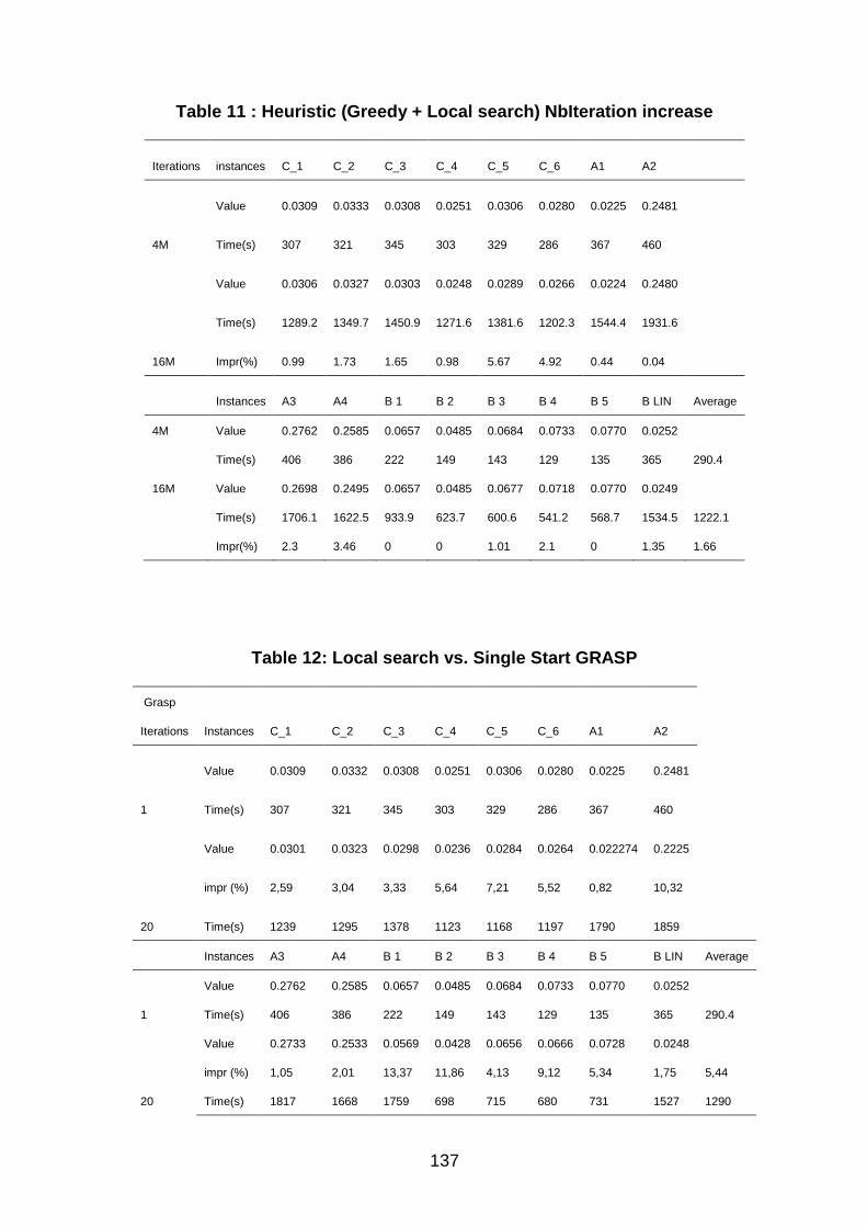
137

Table 11 : Heuristic (Greedy + Local search) NbIteration increase

Iterations instances C_1 C_2 C_3 C_4 C_5 C_6 A1 A2

4M

Value 0.0309 0.0333 0.0308 0.0251 0.0306 0.0280 0.0225 0.2481

Time(s) 307 321 345 303 329 286 367 460

16M

Value 0.0306 0.0327 0.0303 0.0248 0.0289 0.0266 0.0224 0.2480

Time(s) 1289.2 1349.7 1450.9 1271.6 1381.6 1202.3 1544.4 1931.6

Impr(%) 0.99 1.73 1.65 0.98 5.67 4.92 0.44 0.04

Instances A3 A4 B 1 B 2 B 3 B 4 B 5 B LIN Average

4M Value 0.2762 0.2585 0.0657 0.0485 0.0684 0.0733 0.0770 0.0252

Time(s) 406 386 222 149 143 129 135 365 290.4

16M Value 0.2698 0.2495 0.0657 0.0485 0.0677 0.0718 0.0770 0.0249

Time(s) 1706.1 1622.5 933.9 623.7 600.6 541.2 568.7 1534.5 1222.1

Impr(%) 2.3 3.46 0 0 1.01 2.1 0 1.35 1.66

Table 12: Local search vs. Single Start GRASP

Grasp

Iterations Instances C_1 C_2 C_3 C_4 C_5 C_6 A1 A2

1

Value 0.0309 0.0332 0.0308 0.0251 0.0306 0.0280 0.0225 0.2481

Time(s) 307 321 345 303 329 286 367 460

20

Value 0.0301 0.0323 0.0298 0.0236 0.0284 0.0264 0.022274 0.2225

impr (%) 2,59 3,04 3,33 5,64 7,21 5,52 0,82 10,32

Time(s) 1239 1295 1378 1123 1168 1197 1790 1859

Instances A3 A4 B 1 B 2 B 3 B 4 B 5 B LIN Average

1

Value 0.2762 0.2585 0.0657 0.0485 0.0684 0.0733 0.0770 0.0252

Time(s) 406 386 222 149 143 129 135 365 290.4

20

Value 0.2733 0.2533 0.0569 0.0428 0.0656 0.0666 0.0728 0.0248

impr (%) 1,05 2,01 13,37 11,86 4,13 9,12 5,34 1,75 5,44

Time(s) 1817 1668 1759 698 715 680 731 1527 1290

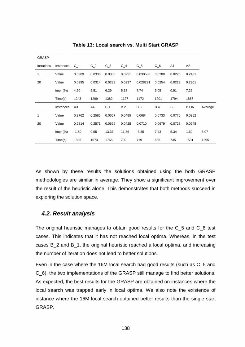
138

Table 13: Local search vs. Multi Start GRASP

GRASP

Iterations Instances C_1 C_2 C_3 C_4 C_5 C_6 A1 A2

1 Value 0.0309 0.0333 0.0308 0.0251 0.030588 0.0280 0.0225 0.2481

20

Value 0.0295 0.0314 0.0289 0.0237 0.028221 0.0254 0.0223 0.2301

impr (%) 4,60 5,51 6,29 5,38 7,74 9,05 0,91 7,26

Time(s) 1243 1299 1382 1127 1172 1201 1794 1867

Instances A3 A4 B 1 B 2 B 3 B 4 B 5 B LIN Average

1 Value 0.2762 0.2585 0.0657 0.0485 0.0684 0.0733 0.0770 0.0252

20

Value 0.2814 0.2571 0.0569 0.0428 0.0710 0.0679 0.0728 0.0248

impr (%) -1,89 0,55 13,37 11,86 -3,85 7,43 5,34 1,60 5,07

Time(s) 1825 1673 1765 702 719 685 735 1531 1295

As shown by these results the solutions obtained using the both GRASP

methodologies are similar in average. They show a significant improvement over

the result of the heuristic alone. This demonstrates that both methods succeed in

exploring the solution space.

4.2. Result analysis

The original heuristic manages to obtain good results for the C_5 and C_6 test

cases. This indicates that it has not reached local optima. Whereas, in the test

cases B_2 and B_1, the original heuristic reached a local optima, and increasing

the number of iteration does not lead to better solutions.

Even in the case where the 16M local search had good results (such as C_5 and

C_6), the two implementations of the GRASP still manage to find better solutions.

As expected, the best results for the GRASP are obtained on instances where the

local search was trapped early in local optima. We also note the existence of

instance where the 16M local search obtained better results than the single start

GRASP.

139

The multi-start GRASP methodology seems to be better than single-start for all

the C instances, with an average improvement of 6.5% in the logistic ratio,

whereas the single start GRASP has an average improvement of 4.5%. Due to

some particularity of the instances, the randomized greedy construction algorithm

is particularly effective at creating good initial solution for an efficient exploration

of the solution space. We note however that in the C_4 case, the single start

remains better that the multi-start.

In two different instance (A3 and B_LAR_3), the multi start GRASP methodology

only finds solutions worse than the original solution. This is due to the fact that the

local search cannot compensate for the deterioration of the original solution. We

see that on average, the single start heuristic seems to be yielding the best

results.

In the following section, we will detail the performance of the single start

compared to the original heuristic in terms of computation time.

4.3. Computation time sensitivity

In this section, we focus on two very different instances (C_4 and B1) and analyze

how the original heuristic and the single-start GRASP compares with different

values of computation time.

4.3.1 C_4 Test Case.

Figure 11 presents the global cost over time found by the local search, as well as

the global cost over time found by the parallel solution generation method. Note

that as it takes 5 minutes to generate a single solution; therefore,the solution

generation method does not give any results before the 5-minute mark. Also, as

the average solution generation time is close one minute (it takes 1290 seconds

to generate 20 solutions), the number of solutions generated is a good estimate of

the computation time.

In this case, we see that the local search converges in about 5 minutes, and then

does little to improve the solution. This is a good indicator that the local search is

trapped within local optima. On the other hand, by generating solutions in parallel,

we manage to find a better solution within those 5 minutes, and also keep finding

better solutions over time.

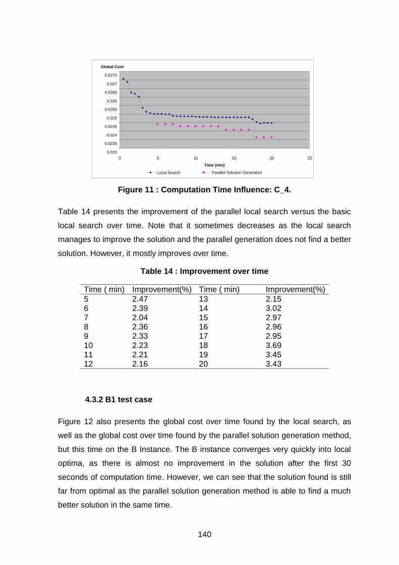
140

Figure 11 : Computation Time Influence: C_4.

Table 14 presents the improvement of the parallel local search versus the basic

local search over time. Note that it sometimes decreases as the local search

manages to improve the solution and the parallel generation does not find a better

solution. However, it mostly improves over time.

Table 14 : Improvement over time

Time ( min) Improvement(%) Time ( min) Improvement(%)

5 2.47 13 2.15 6 2.39 14 3.02 7 2.04 15 2.97 8 2.36 16 2.96 9 2.33 17 2.95 10 2.23 18 3.69 11 2.21 19 3.45 12 2.16 20 3.43

4.3.2 B1 test case

Figure 12 also presents the global cost over time found by the local search, as

well as the global cost over time found by the parallel solution generation method,

but this time on the B Instance. The B instance converges very quickly into local

optima, as there is almost no improvement in the solution after the first 30

seconds of computation time. However, we can see that the solution found is still

far from optimal as the parallel solution generation method is able to find a much

better solution in the same time.

0.023 0.0235 0.024

0.0245 0.025

0.0255 0.026

0.0265 0.027

0.0275

0 5 10 15 20 25 Time (min)

Global Cost

Parallel Solution Generation Local Search

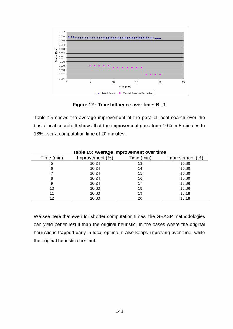
141

0.056

0.057

0.058

0.059

0.06

0.061

0.062

0.063

0.064

0.065

0.066

0.067

0 5 10 15 20 25

Time (min)

Glo

bal

Co

st

Local Search Parallel Solution Generation

Figure 12 : Time Influence over time: B _1

Table 15 shows the average improvement of the parallel local search over the

basic local search. It shows that the improvement goes from 10% in 5 minutes to

13% over a computation time of 20 minutes.

Table 15: Average Improvement over time

Time (min) Improvement (%) Time (min) Improvement (%) 5 10.24 13 10.80

6 10.24 14 10.80

7 10.24 15 10.80

8 10.24 16 10.80

9 10.24 17 13.36

10 10.80 18 13.36

11 10.80 19 13.18

12 10.80 20 13.18

We see here that even for shorter computation times, the GRASP methodologies

can yield better result than the original heuristic. In the cases where the original

heuristic is trapped early in local optima, it also keeps improving over time, while

the original heuristic does not.

142

5. CONCLUSIONS AND FUTURE WORK

In this paper we propose two versions of the GRASP (a single start and a multi-

start version) for the real-life IRP. Our procedures imbed an existing specialized

heuristic for this problem into a GRASP framework. We also use parallelization to

reduce the time needed to perform all GRASP iterations. We conducted extensive

testing on 16 data sets representative of real life data. We show that within

reasonable computation time (less than 25 minutes) we manage to reduce the

objective function value by 5.44% on average. This increase is much more

significant than letting the current heuristic run for an additional 20 minutes, which

only yields an average reduction of 1.6% in objective function value. Achieving

high performance in a limited amount of time is crucial in an industrial operations

context. The obtained improvement represents considerable cost saving for this

large-scale industrial problem.

Possible future work include testing different randomization methods for the

greedy algorithm, as well as looking at other known meta-heuristics such as

simulated annealing and/or tabu search.

6. PUBLICATIONS

The work presented in this chapter has been presented in the MOSIM 2012

international conference held in Bordeaux.

143

Chapter V: Production planning and

customer allocation under supply uncertainty

1. INTRODUCTION

The goal of the production planning and customer allocation problem is to

optimally allocate industrial gas product from production sources to bulk customer

in order to cover demand over time while subject to supply, production and

distribution constraints. The objective is to minimize total cost which includes

product, distribution and contractual costs.

The model takes into account many specificities of the Air Liquide (AL) supply

chain such as the following which were described in detail in the introduction

chapter.

Production, liquefaction, inventory balance and replenishment constraints

at AL sources, storage buffers and bulk customers (with given tank size

and product demand).

Depot specific road resources with capacity and speed.

144

Incoming contract to buy product with competitors.

The possibility of plants failures, modeled using a stochastic production

function.

We deal with plant failure uncertainty using a stochastic scenario based approach.

Several scenarios are created, each with an associated probability. We use a two-

stage stochastic approach to solve this problem with the first stage decision being

the decision taken prior to the knowledge of the failure, and the second stage

decision being the recovery action taken after the failure until the end of the time

horizon. Failing to deliver a customer due to a shortage of product leads to a

heavy penalty on the objective function. We minimize both the cost of the supply

chain and the expected recovery cost of all scenarios.

2. A TWO STAGE PROGRAMMING APPROACH

We address the sourcing problem under plant failure uncertainty and contractual

conditions, and propose a stochastic programming model for solving it. The

challenge is to design a model structure that can incorporate data related to

parameter uncertainty but still remain tractable. To that aim we propose a two-

stage stochastic programming model. In this section, we present the general

methodology we propose for solving the production planning and customer

allocation problem under uncertainty, how the model could be used to improve the

resilience/robustness of a supply chain as well as the modeling assumptions

made and the rational for these choices.

2.1. General Methodology.

As stated in the introduction, we propose a two-stage stochastic approach to the

problem. This stochastic approach is embedded within a global methodology. In

this section, we give an overview of the methodology used, as well as the results

we want to highlight. The methodology is divided into two mains steps. Figure 13

below presents the entire methodology.

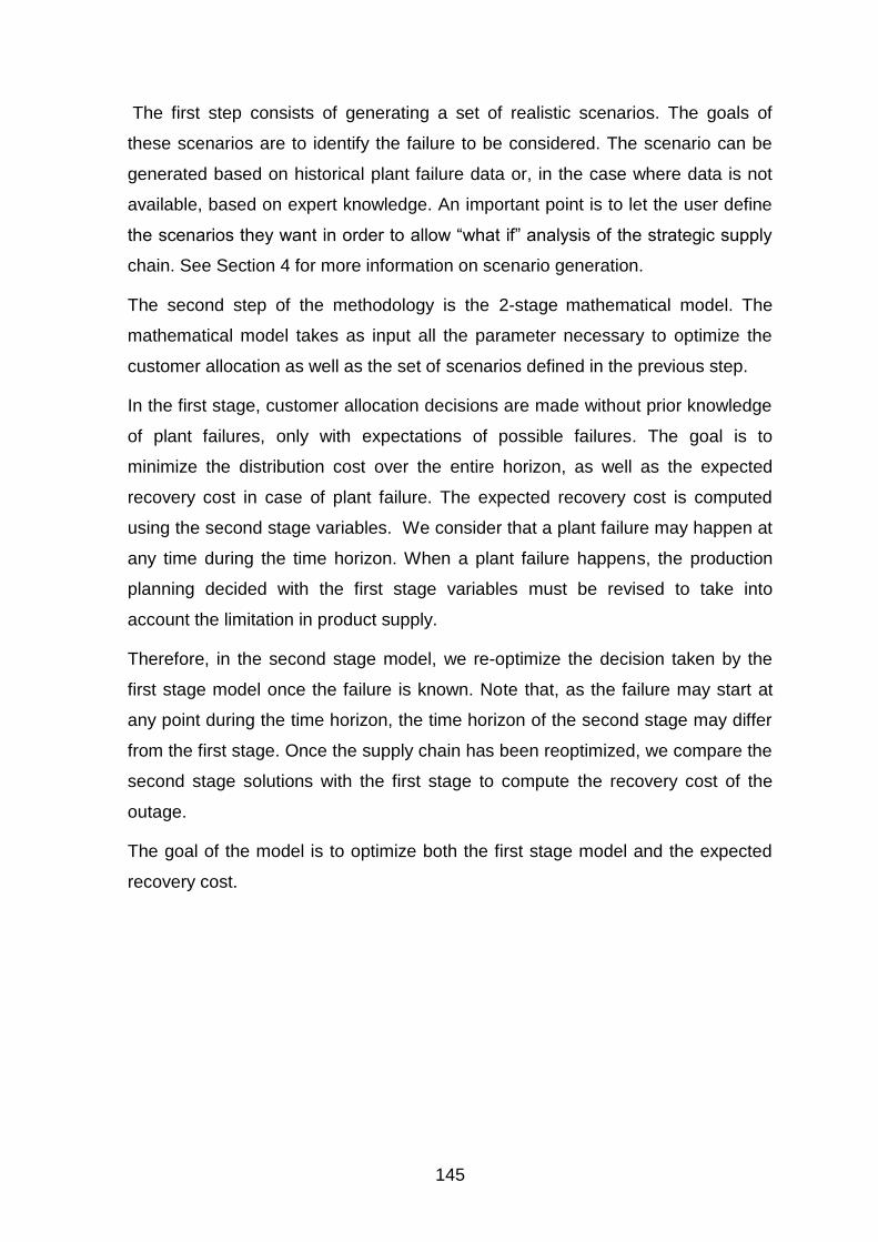
145

The first step consists of generating a set of realistic scenarios. The goals of

these scenarios are to identify the failure to be considered. The scenario can be

generated based on historical plant failure data or, in the case where data is not

available, based on expert knowledge. An important point is to let the user define

the scenarios they want in order to allow “what if” analysis of the strategic supply

chain. See Section 4 for more information on scenario generation.

The second step of the methodology is the 2-stage mathematical model. The

mathematical model takes as input all the parameter necessary to optimize the

customer allocation as well as the set of scenarios defined in the previous step.

In the first stage, customer allocation decisions are made without prior knowledge

of plant failures, only with expectations of possible failures. The goal is to

minimize the distribution cost over the entire horizon, as well as the expected

recovery cost in case of plant failure. The expected recovery cost is computed

using the second stage variables. We consider that a plant failure may happen at

any time during the time horizon. When a plant failure happens, the production

planning decided with the first stage variables must be revised to take into

account the limitation in product supply.

Therefore, in the second stage model, we re-optimize the decision taken by the

first stage model once the failure is known. Note that, as the failure may start at

any point during the time horizon, the time horizon of the second stage may differ

from the first stage. Once the supply chain has been reoptimized, we compare the

second stage solutions with the first stage to compute the recovery cost of the

outage.

The goal of the model is to optimize both the first stage model and the expected

recovery cost.

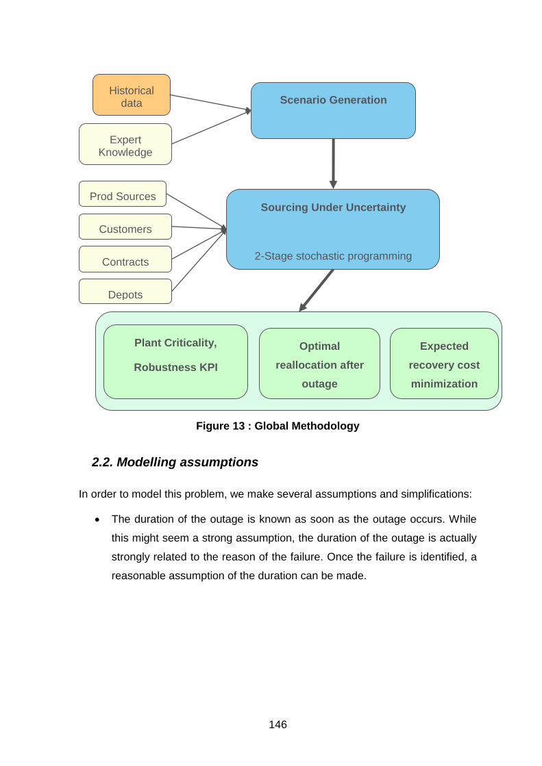
146

Figure 13 : Global Methodology

2.2. Modelling assumptions

In order to model this problem, we make several assumptions and simplifications:

The duration of the outage is known as soon as the outage occurs. While

this might seem a strong assumption, the duration of the outage is actually

strongly related to the reason of the failure. Once the failure is identified, a

reasonable assumption of the duration can be made.

Historical data

Expert Knowledge

Scenario Generation

Sourcing Under Uncertainty

2-Stage stochastic programming

Prod Sources

Customers

Contracts

Depots

Plant Criticality,

Robustness KPI

Optimal

reallocation after

outage

Expected

recovery cost

minimization

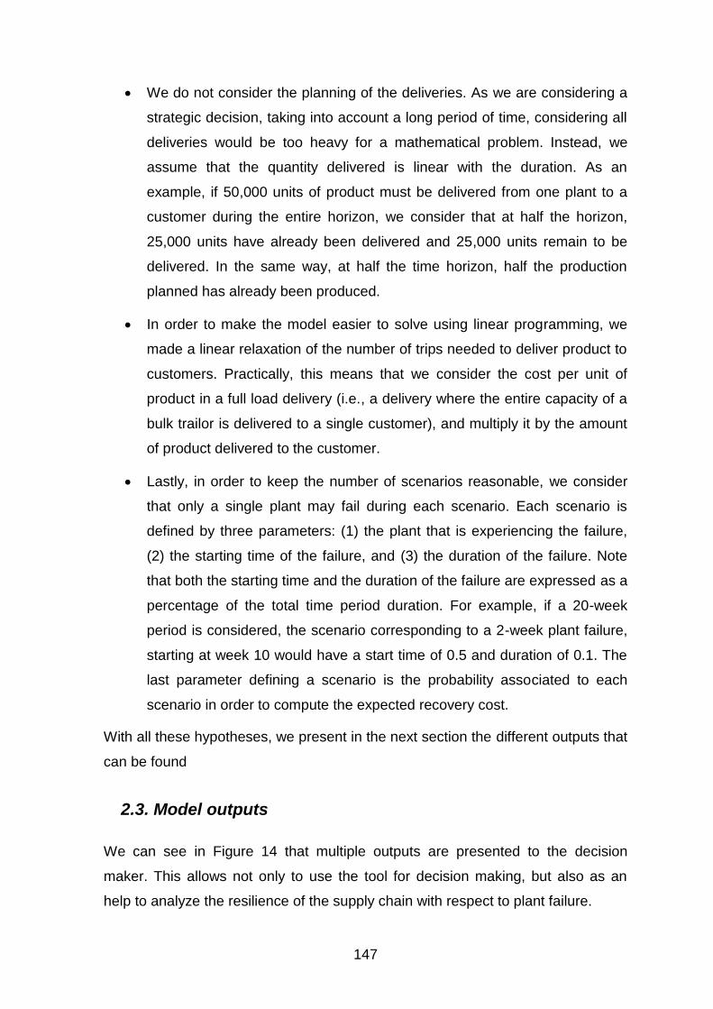
147

We do not consider the planning of the deliveries. As we are considering a

strategic decision, taking into account a long period of time, considering all

deliveries would be too heavy for a mathematical problem. Instead, we

assume that the quantity delivered is linear with the duration. As an

example, if 50,000 units of product must be delivered from one plant to a

customer during the entire horizon, we consider that at half the horizon,

25,000 units have already been delivered and 25,000 units remain to be

delivered. In the same way, at half the time horizon, half the production

planned has already been produced.

In order to make the model easier to solve using linear programming, we

made a linear relaxation of the number of trips needed to deliver product to

customers. Practically, this means that we consider the cost per unit of

product in a full load delivery (i.e., a delivery where the entire capacity of a

bulk trailor is delivered to a single customer), and multiply it by the amount

of product delivered to the customer.

Lastly, in order to keep the number of scenarios reasonable, we consider

that only a single plant may fail during each scenario. Each scenario is

defined by three parameters: (1) the plant that is experiencing the failure,

(2) the starting time of the failure, and (3) the duration of the failure. Note

that both the starting time and the duration of the failure are expressed as a

percentage of the total time period duration. For example, if a 20-week

period is considered, the scenario corresponding to a 2-week plant failure,

starting at week 10 would have a start time of 0.5 and duration of 0.1. The

last parameter defining a scenario is the probability associated to each

scenario in order to compute the expected recovery cost.

With all these hypotheses, we present in the next section the different outputs that

can be found

2.3. Model outputs

We can see in Figure 14 that multiple outputs are presented to the decision

maker. This allows not only to use the tool for decision making, but also as an

help to analyze the resilience of the supply chain with respect to plant failure.

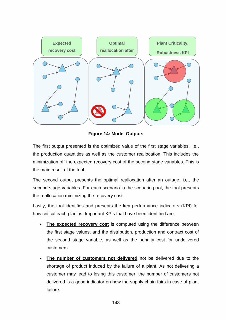
148

Figure 14: Model Outputs

The first output presented is the optimized value of the first stage variables, i.e.,

the production quantities as well as the customer reallocation. This includes the

minimization off the expected recovery cost of the second stage variables. This is

the main result of the tool.

The second output presents the optimal reallocation after an outage, i.e., the

second stage variables. For each scenario in the scenario pool, the tool presents

the reallocation minimizing the recovery cost.

Lastly, the tool identifies and presents the key performance indicators (KPI) for

how critical each plant is. Important KPIs that have been identified are:

The expected recovery cost is computed using the difference between

the first stage values, and the distribution, production and contract cost of

the second stage variable, as well as the penalty cost for undelivered

customers.

The number of customers not delivered not be delivered due to the

shortage of product induced by the failure of a plant. As not delivering a

customer may lead to losing this customer, the number of customers not

delivered is a good indicator on how the supply chain fairs in case of plant

failure.

Plant Criticality,

Robustness KPI

Optimal

reallocation after

outage

Expected

recovery cost

minimization

149

The quantity of product not delivered to customers due to the shortage

of product induced by the plant failure. This KPI is closely related to the

number of customer not delivered, but gives a more precise indication on

the amount of product that will be missing in case of plant failure.

In the next section we present the full mathematical model used for the

implementation and resolution of this problem.

3. MATHEMATICAL MODEL

In this section we detail the parameters and decision variables used in the model.

3.1. Input Parameters

The input parameters are listed in Table 16, auxiliary variables in Table 17, and

decision variables in Table 18.

Table 16 : Input Parameters

Sources parameters

S Set of AL production sources

S Set of source operated by competitors

Production parameters

r

sc Production cost per unit at source ALSs

v

sc Venting cost per unit at source ALSs

ss qq , Minimum and Maximum production level at source ALSs

Customer parameters

J Set of all customers

ju Demand at customer Jj

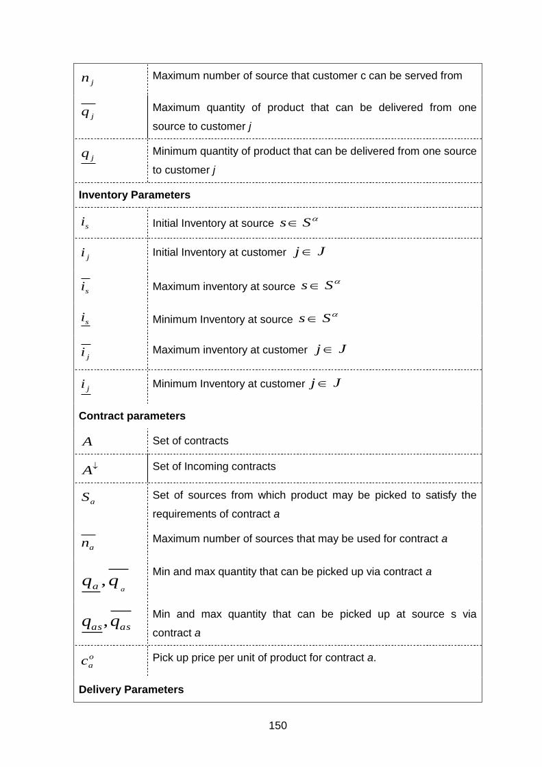
150

jn Maximum number of source that customer c can be served from

jq Maximum quantity of product that can be delivered from one

source to customer j

jq Minimum quantity of product that can be delivered from one source

to customer j

Inventory Parameters

si Initial Inventory at source Ss

ji Initial Inventory at customer Jj

si Maximum inventory at source Ss

si Minimum Inventory at source Ss

ji Maximum inventory at customer Jj

ji Minimum Inventory at customer Jj

Contract parameters

A Set of contracts

A Set of Incoming contracts

aS Set of sources from which product may be picked to satisfy the

requirements of contract a

an Maximum number of sources that may be used for contract a

aqqa ,

Min and max quantity that can be picked up via contract a

asas qq , Min and max quantity that can be picked up at source s via

contract a

o

ac Pick up price per unit of product for contract a.

Delivery Parameters

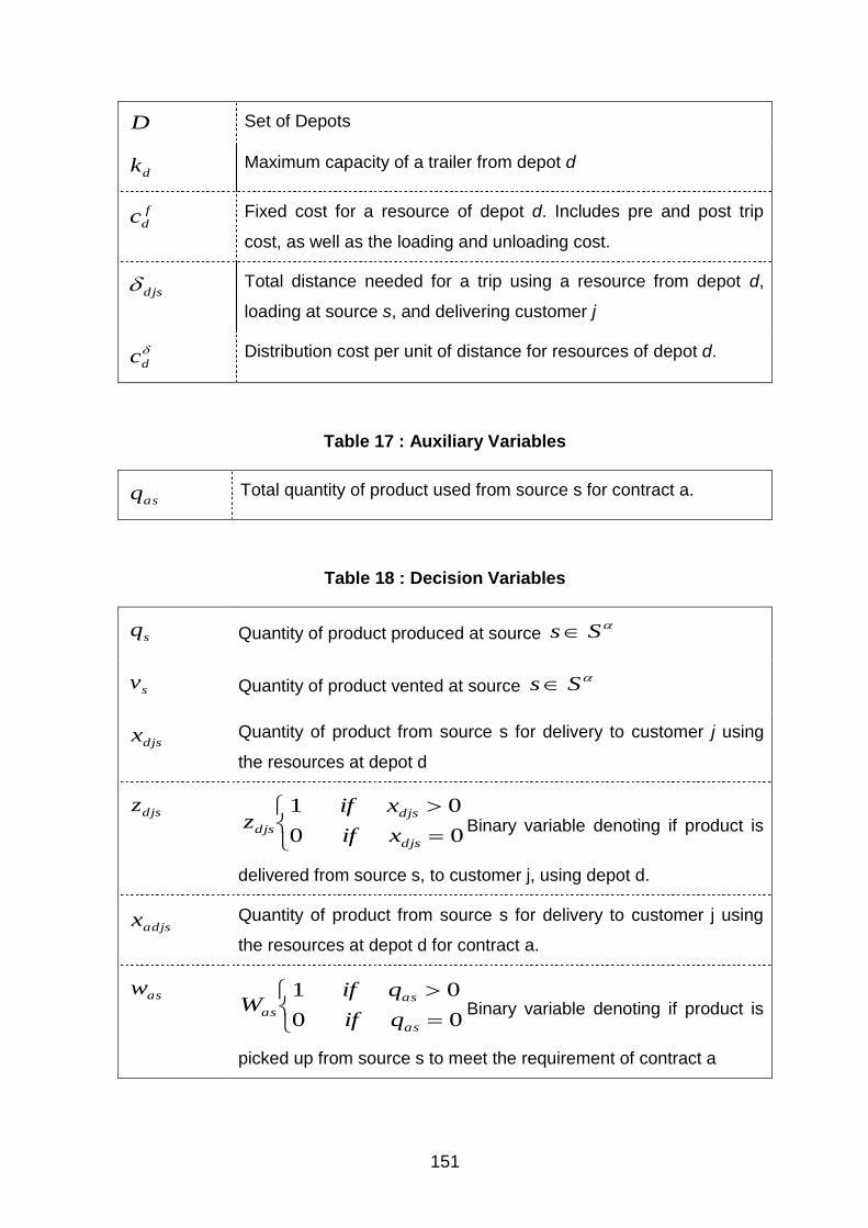
151

D Set of Depots

dk Maximum capacity of a trailer from depot d

f

dc Fixed cost for a resource of depot d. Includes pre and post trip

cost, as well as the loading and unloading cost.

djs Total distance needed for a trip using a resource from depot d,

loading at source s, and delivering customer j

dc Distribution cost per unit of distance for resources of depot d.

Table 17 : Auxiliary Variables

asq Total quantity of product used from source s for contract a.

Table 18 : Decision Variables

sq Quantity of product produced at source Ss

sv Quantity of product vented at source Ss

djsx Quantity of product from source s for delivery to customer j using

the resources at depot d

djsz

00

01

djs

djs

djs xif

xifz Binary variable denoting if product is

delivered from source s, to customer j, using depot d.

adjsx Quantity of product from source s for delivery to customer j using

the resources at depot d for contract a.

asw

00

01

as

as

asqif

qifW Binary variable denoting if product is

picked up from source s to meet the requirement of contract a

152

3.2. Allowed lists

The main difficulty of this model is the number of possible depot-customer-source

triplets for deliveries. In order to reduce the number of possibilities, and thus the

number of decision variables, a list of allowed triplet for deliveries is given as input

data.

Set of allowed depot-customer- source triplets for product delivery

Set of allowed depot-customer-source triplet for incoming contracts

3.3. Mathematical model

3.3.1 Objective

The objective of the model is the following:

eryCostE

qc

cvcq

cckxMin

E

R

Ss

as

Aa

o

a

v

ss

Ss

r

ss

djsd

sjd

f

dddjs

covRe

)(

))(/(),,(

The first term of the cost function represents the total delivery cost. For each trip

needed to satisfy the demand at customer j, a fixed cost as well as a distance cost

is counted. Note that the total number of trips needed is assumed to be an

integer. The second term represents the production and venting costs amongst all

production sources. Lastly, the third term takes into account the contract costs.

These three costs constitute the first stage objective function, or nominal cost.

This nominal cost will be abbreviated as NC in formulas that follow.

The expected recovery cost is computed using the second stage variables. See

section 3.6.6.

3.3.2 First stage constraints

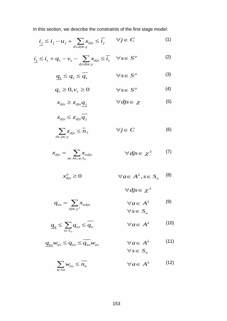
153

In this section, we describe the constraints of the first stage model:

j

djsds

djsjjj ixuii ,

Cj (1)

s

djsdj

djsssss ixvqii ,

Ss (2)

sss qqq Ss (3)

0,0 ss vq Ss (4)

jdjsdjs qzx

jdjsdjs qzx

djs (5)

j

jsds

djs nz ,

Cj

(6)

aSsAa

adjsdjs xx,

djs

(7)

0a

djsx aSsAa ,

djs

(8)

djs

adjsas xq

aSs

Aa

(9)

a

Ss

asa qqqa

Aa (10)

asasasasas wqqwq

aSs

Aa

(11)

Sas

aas nw Aa (12)

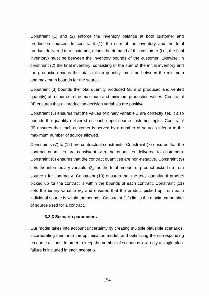
154

Constraint (1) and (2) enforce the inventory balance at both customer and

production sources. In constraint (1), the sum of the inventory and the total

product delivered to a customer, minus the demand of this customer (i.e., the final

inventory) must be between the inventory bounds of the customer. Likewise, in

constraint (2) the final inventory, consisting of the sum of the initial inventory and

the production minus the total pick-up quantity, must be between the minimum

and maximum bounds for the source.

Constraint (3) bounds the total quantity produced (sum of produced and vented

quantity) at a source to the maximum and minimum production values. Constraint

(4) ensures that all production decision variables are positive.

Constraint (5) ensures that the values of binary variable Z are correctly set. It also

bounds the quantity delivered on each depot-source-customer triplet. Constraint

(6) ensures that each customer is served by a number of sources inferior to the

maximum number of source allowed.

Constraints (7) to (12) are contractual constraints. Constraint (7) ensures that the

contract quantities are consistent with the quantities delivered to customers.

Constraint (8) ensures that the contract quantities are non-negative. Constraint (9)

sets the intermediary variable asq as the total amount of product picked up from

source s for contract a. Constraint (10) ensures that the total quantity of product

picked up for the contract is within the bounds of each contract. Constraint (11)

sets the binary variable was and ensures that the product picked up from each

individual source is within the bounds. Constraint (12) limits the maximum number

of source used for a contract.

3.3.3 Scenario parameters

Our model takes into account uncertainty by creating multiple plausible scenarios,

incorporating them into the optimisation model, and optimizing the corresponding

recourse actions. In order to keep the number of scenarios low, only a single plant

failure is included in each scenario.

155

Another assumption of our proposed model is that the plant failure occurs and is

rectified during the time period considered. In most two-stage stochastic models,

either the first stage and second stage decision are totally different (e.g. in the first

stage, facility location are decided, and the customer allocation is decided in the

second stage), or the first stage focuses on the next period, while the second

stage decisions concerns the future time periods. In our case, new decisions have

to be made in the middle of the time period.

The parameters defining each scenario can be found in Table 19.

For each scenario, a sourcing problem is solved in order to determine the optimal

recourse action. Therefore, new decisions variables are needed. These decision

variables are the same as the first stage variables, but are also indexed on

scenarios.

Table 19 : Scenario Parameters

Scenarios parameters

Set of scenarios

p Probability associated to scenario

Start of the plant failure for scenario in percentage of the time

horizon : 1,0

Duration of the plant failure for scenario in percentage of the

time horizon : 1,0

s Production plant experiencing the failure

Ss

Figure 15 illustrates an example of a scenario. It shows the state of plant s over

the entire time horizon H. The black part represents the down time of the plant. It

starts at time H* and last for a duration equal to H* .

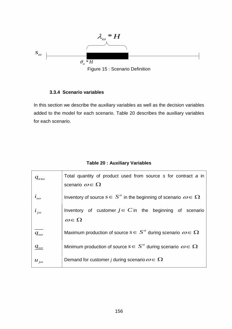
156

Figure 15 : Scenario Definition

3.3.4 Scenario variables

In this section we describe the auxiliary variables as well as the decision variables

added to the model for each scenario. Table 20 describes the auxiliary variables

for each scenario.

Table 20 : Auxiliary Variables

asq Total quantity of product used from source s for contract a in

scenario

si Inventory of sourceSs in the beginning of scenario

ji Inventory of customer Cj in the beginning of scenario

sq Maximum production of sourceSs during scenario

sq Minimum production of sourceSs during scenario

ju Demand for customer j during scenario

s

H*

H*

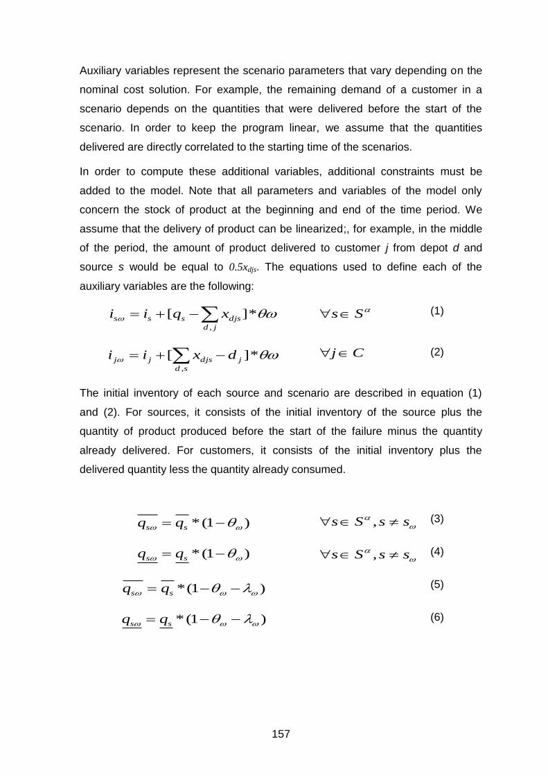
157

Auxiliary variables represent the scenario parameters that vary depending on the

nominal cost solution. For example, the remaining demand of a customer in a

scenario depends on the quantities that were delivered before the start of the

scenario. In order to keep the program linear, we assume that the quantities

delivered are directly correlated to the starting time of the scenarios.

In order to compute these additional variables, additional constraints must be

added to the model. Note that all parameters and variables of the model only

concern the stock of product at the beginning and end of the time period. We

assume that the delivery of product can be linearized;, for example, in the middle

of the period, the amount of product delivered to customer j from depot d and

source s would be equal to 0.5xdjs. The equations used to define each of the

auxiliary variables are the following:

*][,

jd

djssss xqii Ss (1)

*][,

sd

jdjsjj dxii Cj (2)

The initial inventory of each source and scenario are described in equation (1)

and (2). For sources, it consists of the initial inventory of the source plus the

quantity of product produced before the start of the failure minus the quantity

already delivered. For customers, it consists of the initial inventory plus the

delivered quantity less the quantity already consumed.

)1(* ss qq ssSs , (3)

)1(* ss qq ssSs , (4)

)1(* ss qq (5)

)1(* ss qq (6)

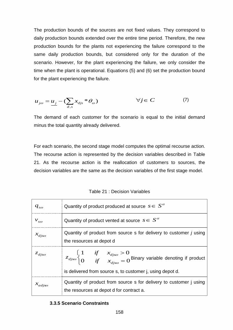
158

The production bounds of the sources are not fixed values. They correspond to

daily production bounds extended over the entire time period. Therefore, the new

production bounds for the plants not experiencing the failure correspond to the

same daily production bounds, but considered only for the duration of the

scenario. However, for the plant experiencing the failure, we only consider the

time when the plant is operational. Equations (5) and (6) set the production bound

for the plant experiencing the failure.

)*(,

sd

djsjj xuu Cj (7)

The demand of each customer for the scenario is equal to the initial demand

minus the total quantity already delivered.

For each scenario, the second stage model computes the optimal recourse action.

The recourse action is represented by the decision variables described in Table

21. As the recourse action is the reallocation of customers to sources, the

decision variables are the same as the decision variables of the first stage model.

Table 21 : Decision Variables

sq Quantity of product produced at source Ss

sv Quantity of product vented at source Ss

djsx Quantity of product from source s for delivery to customer j using

the resources at depot d

djsz

00

01

djs

djs

djs xif

xifz Binary variable denoting if product

is delivered from source s, to customer j, using depot d.

adjsx Quantity of product from source s for delivery to customer j using

the resources at depot d for contract a.

3.3.5 Scenario Constraints

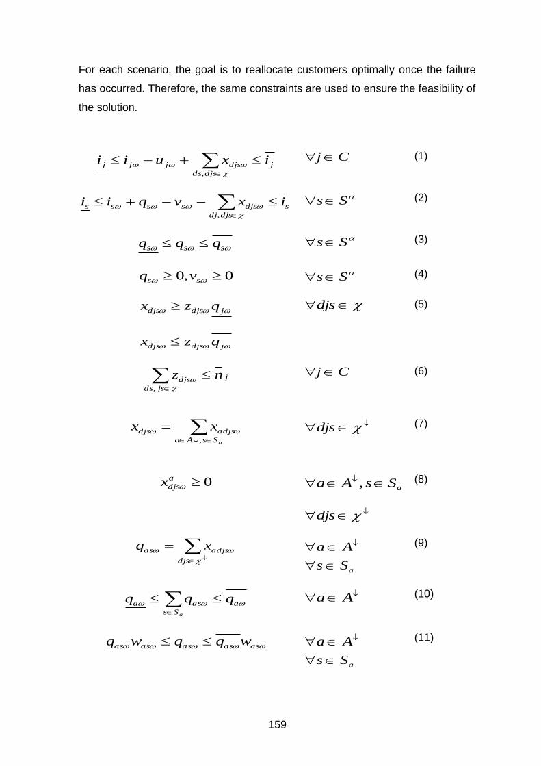
159

For each scenario, the goal is to reallocate customers optimally once the failure

has occurred. Therefore, the same constraints are used to ensure the feasibility of

the solution.

j

djsds

djsjjj ixuii

,

Cj (1)

s

djsdj

djsssss ixvqii

,

Ss (2)

sss qqq Ss (3)

0,0 ss vq Ss (4)

jdjsdjs qzx

jdjsdjs qzx

djs (5)

j

jsds

djs nz

,

Cj

(6)

aSsAa

adjsdjs xx,

djs

(7)

0a

djsx aSsAa ,

djs

(8)

djs

adjsas xq

aSs

Aa

(9)

a

Ss

asa qqqa

Aa (10)

asasasasas wqqwq

aSs

Aa

(11)

160

Sas

aas nw Aa (12)

As for the first stage model, constraints (1) and (2) ensure inventory balance at

both customer and sources. Constraints (3) and (4) are related to the production

and venting bounds of each source. Constraints (5) and (6) are the multi-sourcing

constraint, and constraint (7) to (12) are the contract-related constraints.

Preliminary testing showed that the model proposed in Section 3 had unwanted

behavior in the second stage scenarios. We noticed that on multiple cases, the

recovery cost was negative, meaning that the outage led to better results.

This is of course impossible in real life, and is the cause of the limitation to a

single plant outage per scenario. With our model, once an outage has occurred,

the optimal solution to minimize the cost would be to reduce the production of the

plants not impacted by the outage to the minimum quantity needed to satisfy

demand, thus leading to important savings on the production cost. The goal of the

nominal model is to set up a long term production and delivery plan. While it

seems reasonable that plants should be allowed to increase their production in

case of outage, reducing their production because the failure happened in another

plant does not reflect reality. Therefore, we added constraint (13) in order to

prevent production plants from reducing their production in the second stage.

ssw qq wssSs ,

(13)

3.3.6 Expected recovery cost computation

In order to compute the expected recovery cost, we define the scenario cost

SC , which includes the delivery, production and contract costs for

scenario .

E

R Ss

as

Aa

o

a

v

ss

Ss

r

ssdjsd

sjd

f

dddjs qccvcqcckxSC

)())(/(

),,(

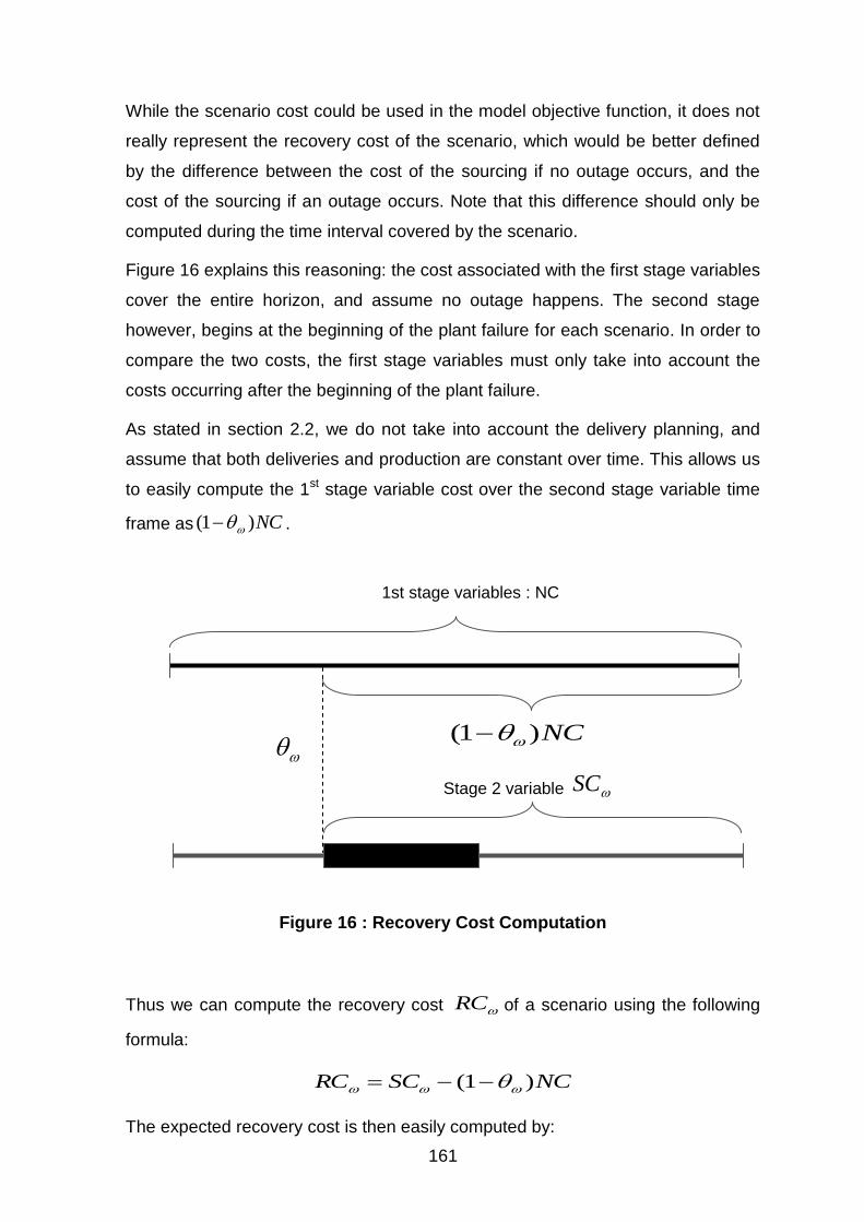
161

While the scenario cost could be used in the model objective function, it does not

really represent the recovery cost of the scenario, which would be better defined

by the difference between the cost of the sourcing if no outage occurs, and the

cost of the sourcing if an outage occurs. Note that this difference should only be

computed during the time interval covered by the scenario.

Figure 16 explains this reasoning: the cost associated with the first stage variables

cover the entire horizon, and assume no outage happens. The second stage

however, begins at the beginning of the plant failure for each scenario. In order to

compare the two costs, the first stage variables must only take into account the

costs occurring after the beginning of the plant failure.

As stated in section 2.2, we do not take into account the delivery planning, and

assume that both deliveries and production are constant over time. This allows us

to easily compute the 1st stage variable cost over the second stage variable time

frame as NC)1( .

Figure 16 : Recovery Cost Computation

Thus we can compute the recovery cost RC of a scenario using the following

formula:

NCSCRC )1(

The expected recovery cost is then easily computed by:

1st stage variables : NC

Stage 2 variable SC

NC)1(

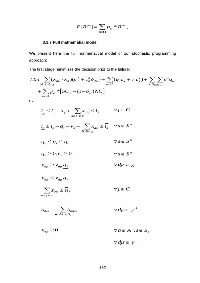
162

RCpRCE *][

3.3.7 Full mathematial model

We present here the full mathematical model of our stochastic programming

approach:

The first stage minimizes the decision prior to the failure:

NCSCp

qccvcqcckxMinE

R Ss

as

Aa

o

a

v

ss

Ss

r

ssdjsd

sjd

f

dddjs

)1(*

)())(/(),,(

s.c.

j

djsds

djsjjj ixuii ,

Cj

s

djsdj

djsssss ixvqii ,

Ss

sss qqq Ss

0,0 ss vq Ss

jdjsdjs qzx

jdjsdjs qzx

djs

j

jsds

djs nz ,

Cj

aSsAa

adjsdjs xx,

djs

0a

djsx aSsAa ,

djs

163

djs

adjsas xq

aSs

Aa

a

Ss

asa qqqa

Aa

asasasasas wqqwq

aSs

Aa

Sas

aas nw Aa

And the second stage minimizes the scenario cost for each scenario:

E

R Ss

as

Aa

o

a

v

ss

Ss

r

ssdjsd

sjd

f

dddjs qccvcqcckxMin

)())(/(

),,(

s.c

j

djsds

djsjjj ixuii

,

Cj

s

djsdj

djsssss ixvqii

,

Ss

sss qqq Ss

0,0 ss vq Ss

jdjsdjs qzx

jdjsdjs qzx

djs

j

jsds

djs nz

,

Cj

aSsAa

adjsdjs xx,

djs

0a

djsx aSsAa ,

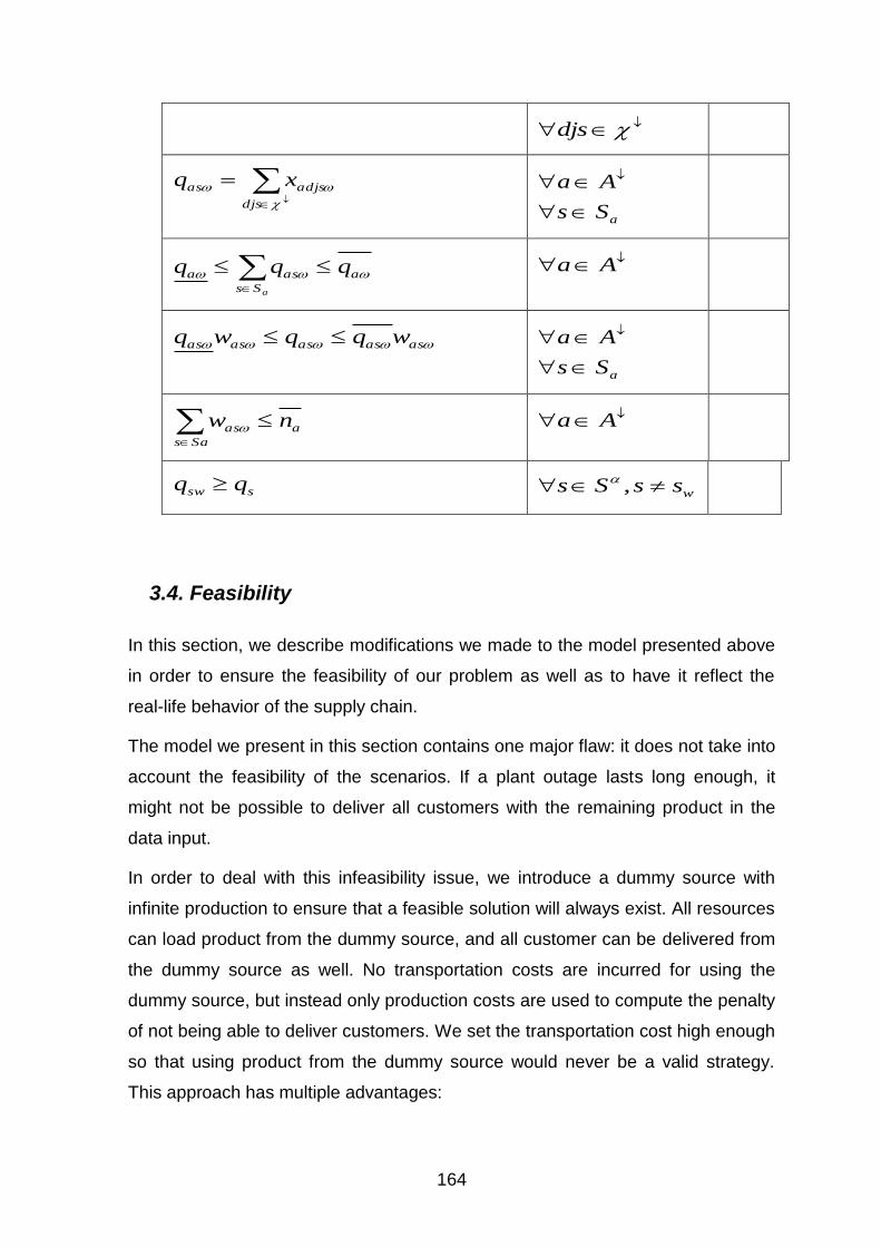
164

djs

djs

adjsas xq

aSs

Aa

a

Ss

asa qqqa

Aa

asasasasas wqqwq

aSs

Aa

Sas

aas nw Aa

ssw qq wssSs ,

3.4. Feasibility

In this section, we describe modifications we made to the model presented above

in order to ensure the feasibility of our problem as well as to have it reflect the

real-life behavior of the supply chain.

The model we present in this section contains one major flaw: it does not take into

account the feasibility of the scenarios. If a plant outage lasts long enough, it

might not be possible to deliver all customers with the remaining product in the

data input.

In order to deal with this infeasibility issue, we introduce a dummy source with

infinite production to ensure that a feasible solution will always exist. All resources

can load product from the dummy source, and all customer can be delivered from

the dummy source as well. No transportation costs are incurred for using the

dummy source, but instead only production costs are used to compute the penalty

of not being able to deliver customers. We set the transportation cost high enough

so that using product from the dummy source would never be a valid strategy.

This approach has multiple advantages:

165

The penalty for not delivering a customer is directly proportional to the

amount of product. This ensures that the model is always attempts to

deliver as much product as possible to every customer, and does not let

one customer go completely unserved in order to serve all others. This

choice was made in order to reflect the reality of distribution where a given

level of customer service must be maintained in order not to lose

customers.

In the case where the dummy source has to be use in any scenario, the

quantity of product delivered from the dummy source corresponds to the

quantity of product missing in order to be able to deliver all customers in

case of plant failure. This information is important in order to negotiate

future contracts.

Lastly, because each scenario only involves one plant failing, this model

also allows estimating how critical a plant is within the supply chain, i.e.,

the cost of a plant failing. This can be calculated by computing the average

scenario cost for each plant in the input data. This information allows

deciding which plant to focus on for maintenance, or if the production

capability of plants should be increased.

4. SCENARIO GENERATION

In this section, we describe the method used to generate scenarios for our

methodology, as well as how we compute the probability assigned to each one.

The goal of the scenario generation method is to create a set of scenarios

representing realistic failures that may happen. The computation depends heavily

on the amount and quality of available historical data. In a real life environment,

the data quality depends on the available plant outages that have been recorded.

Moreover, the scenario generation method is generic and takes into account that

some data could be unavailable. To that aim, we propose two different methods

for generating the scenarios.

166

The first uses the expert knowledge of the decision maker. As the tool

implementing this methodology is indented to be used by expert knowledge for

supply chain robustness analysis, we wanted to keep the possibility for the end

user defining the scenarios he wanted to use, and to assign the probabilities to

each of them.

The second scenario generation method is based on historical data.

In order to determine which scenarios to create and the assigned probabilities, the

following questions should be answered: What is the probability of any failure

happening? What is the probability of a specific plant to fail? What is the

probability of the failure being a specific duration? What is the probability for a

specific duration of an outage? For each of these questions, we explain how

historical data are used, and which default value is used in case no data are

availablein Sections 5.1, 5.2 and 5.3.

The scenario generation method is based on a scenario tree. Figure 17

describes an example of a scenarios tree that is considered. In this very simple

example, only two plants are examined by the generation method. Multiple

reasons could lead to this choice. Either there are only two plants within the input

data, or there are only two plants that are likely to fail during the time horizon.

For each plant, the same three scenarios are considered:

One scenario of duration 0.3, and start date 0.2

On scenario of duration 0.1 and start date 0.5

One scenario of duration 0.3 and start date 0.5

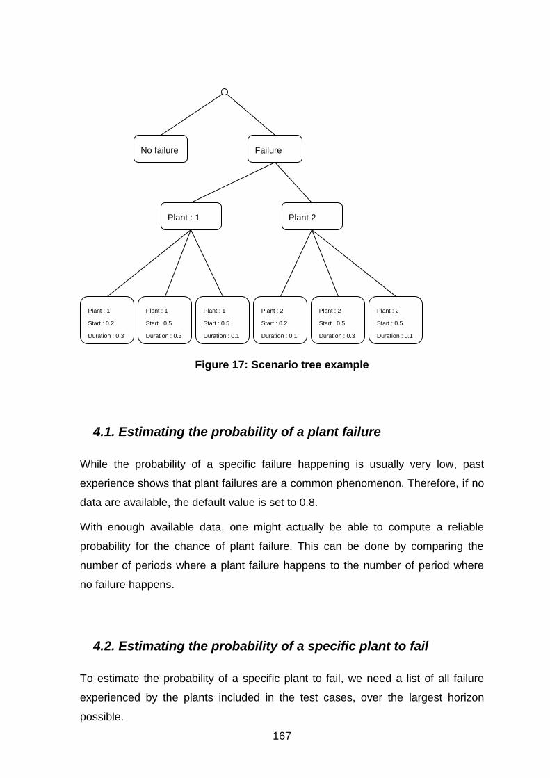
167

Figure 17: Scenario tree example

4.1. Estimating the probability of a plant failure

While the probability of a specific failure happening is usually very low, past

experience shows that plant failures are a common phenomenon. Therefore, if no

data are available, the default value is set to 0.8.

With enough available data, one might actually be able to compute a reliable

probability for the chance of plant failure. This can be done by comparing the

number of periods where a plant failure happens to the number of period where

no failure happens.

4.2. Estimating the probability of a specific plant to fail

To estimate the probability of a specific plant to fail, we need a list of all failure

experienced by the plants included in the test cases, over the largest horizon

possible.

No failure Failure

Plant : 1

Start : 0.2

Duration : 0.3

Plant : 2

Start : 0.5

Duration : 0.3

Plant : 1

Start : 0.5

Duration : 0.1

Plant : 1

Start : 0.5

Duration : 0.3

Plant : 2

Start : 0.2

Duration : 0.1

Plant : 2

Start : 0.5

Duration : 0.1

Plant : 1 Plant 2

168

If the data is available, then let sN be the number of failures experienced by

plant Ss , and S

sNN the total number of plant failures.

The probability of plant s to fail can then be approximated by:

N

Nsps

If no data is available, then the probability of a specific plant to fail is set by default

to:

Sps

1

As stated in section 5.1, the final tool allows these values to be modified in order

to be able to take into account expert knowledge of the supply chain.

4.3. Estimating the duration and start time of plant failures

The duration is the parameter with the greater impact on the distribution as it

directly affects the amount of product available for distribution. Start time has a

lesser impact, mainly due to the fact that seasonality is not taken into account.

This means that for the same duration, the amount of product missing will always

be the same, with no regard to the starting date of the scenario. However,

depending on the choices made in the first stage of the model, the impact of an

outage will still differ depending on the start date.

If no data is available, the scenario will be chosen with a duration ranging from 0.1

to 0.3, and a start date ranging from 0.1 to 0.6

5. IMPLEMENTATION & RESULTS

The model described in Section 3 has been implemented using C# .net 3.5, and

using CPLEX 12.2 to solve the problem. The model was implemented using ILOG

OPL (Optimisation Programming Language).

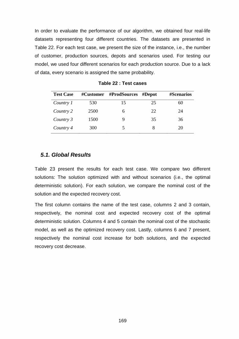
169

In order to evaluate the performance of our algorithm, we obtained four real-life

datasets representing four different countries. The datasets are presented in

Table 22. For each test case, we present the size of the instance, i.e., the number

of customer, production sources, depots and scenarios used. For testing our

model, we used four different scenarios for each production source. Due to a lack

of data, every scenario is assigned the same probability.

Table 22 : Test cases

Test Case #Customer #ProdSources #Depot #Scenarios

Country 1 530 15 25 60

Country 2 2500 6 22 24

Country 3 1500 9 35 36

Country 4 300 5 8 20

5.1. Global Results

Table 23 present the results for each test case. We compare two different

solutions: The solution optimized with and without scenarios (i.e., the optimal

deterministic solution). For each solution, we compare the nominal cost of the

solution and the expected recovery cost.

The first column contains the name of the test case, columns 2 and 3 contain,

respectively, the nominal cost and expected recovery cost of the optimal

deterministic solution. Columns 4 and 5 contain the nominal cost of the stochastic

model, as well as the optimized recovery cost. Lastly, columns 6 and 7 present,

respectively the nominal cost increase for both solutions, and the expected

recovery cost decrease.

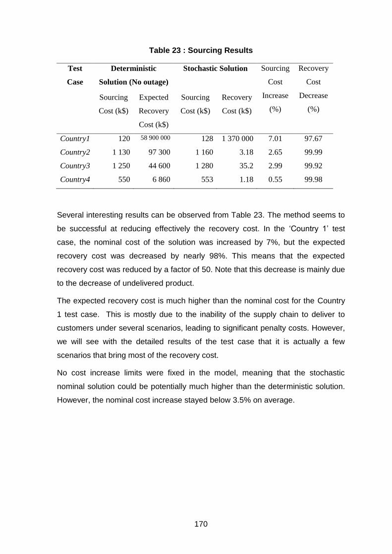
170

Table 23 : Sourcing Results

Test

Case

Deterministic

Solution (No outage)

Stochastic Solution Sourcing

Cost

Increase

(%)

Recovery

Cost

Decrease

(%)

Sourcing

Cost (k$)

Expected

Recovery

Cost (k$)

Sourcing

Cost (k$)

Recovery

Cost (k$)

Country1 120 58 900 000 128 1 370 000 7.01 97.67

Country2 1 130 97 300 1 160 3.18 2.65 99.99

Country3 1 250 44 600 1 280 35.2 2.99 99.92

Country4 550 6 860 553 1.18 0.55 99.98

Several interesting results can be observed from Table 23. The method seems to

be successful at reducing effectively the recovery cost. In the ‘Country 1’ test

case, the nominal cost of the solution was increased by 7%, but the expected

recovery cost was decreased by nearly 98%. This means that the expected

recovery cost was reduced by a factor of 50. Note that this decrease is mainly due

to the decrease of undelivered product.

The expected recovery cost is much higher than the nominal cost for the Country

1 test case. This is mostly due to the inability of the supply chain to deliver to

customers under several scenarios, leading to significant penalty costs. However,

we will see with the detailed results of the test case that it is actually a few

scenarios that bring most of the recovery cost.

No cost increase limits were fixed in the model, meaning that the stochastic

nominal solution could be potentially much higher than the deterministic solution.

However, the nominal cost increase stayed below 3.5% on average.

171

5.2. Detailed results

While Table 23 gives a global view of the results of the methodology we propose,

it does not show many important details. In this section, we focus on the Country 1

test case, and present multiple result tables extracted from the CPLEX solution.

Using these results, we show how we can deduce valuable information

concerning the resilience of the supply chain.

Table 24 presents the detailed results plan by plant for the Country 1 test case.

For each plant we present the average recovery cost, as well as the minimum and

maximum recovery cost. We also present the average number of customer not

delivered for any outage for each plant as well as the average quantity of product

missing from a full delivery to a customer. As stated in Section 2, a customer is

counted as not delivered if he is delivered any amount of product from the dummy

source in the final solution. The missing quantity of product corresponds to the

total quantity of product produced by the dummy source.

From Table 24 we can easily see that some plants are more robust than others in

the sense that a failure leads to less perturbation in the supply chain. Plants

2,8,9,10,14 and 15 all have average recovery cost less than 500. This likely

means that customers can easily be reallocated to a nearby plant.

However for plant 1,3,4,5,6,7,11,12 and 13, the recovery cost is extremely high.

One may note a clear link between the expected recovery cost and the average

missing quantity column. This shows that the main component of a high recovery

cost is the penalty for missing deliveries.

Furthermore, Plant 3 is the most critical plant in this test case, with an average of

26.75 customers not delivered, and nearly 3 million unit of unmet demand.

However, one scenario exists where the outage does not lead to any recovery

cost. This means that this plant has enough buffer to deliver customers through

shorter outages.

Most plant can continue delivering customer safely during short outages, as

shown by a low minimum recovery cost value. The only notable exception is Plant

1, whose minimum recovery cost is much higher than other plants. Thus any type

of failure on Plant 1 will lead to a major disruption in distribution.

172

Table 24: Detailed results for Country 1 case.

Plant

Expected

Recovery

Cost (k$) Min (k$) Max (k$)

Average not

delivered

customers

Average

missing

quantity (kg)

1 28 138 973.53 40 792 4.5 281382.763

2 0.03 0.0227 0.04314 0 0

3 292 728 0 437 615 26.75 2927281.6

4 1 452 0.0173 5 810 0.5 14524.95

5 6 585 0.0351 26 342 0.5 65856.625

6 5 665 0.0402 22 662 1 56655.675

7 125 0.0356 501.736 0.25 1254.2

8 0.042 0.0353 0.0515 0 0

9 0.041 0.0350 0.0546 0 0

10 0.042 0.0351 0.0565 0 0

11 1 512 0.0289 6050.15 2.75 15125.275

12 73.6 0.0351 294.51 0.25 736.15

13 6228.3 0.0350 12 214.35 1 62283.238

14 0.041 0.0351 0.0544 0 0

15 0.037 0.0306 0.0507 0 0

6. CONCLUSIONS AND FURTHER RESEARCH

We study a customer allocation problem where a set of customer must be

optimally allocated to a production source in order to satisfy their demand. We

also introduced uncertainty in the form of possible plant failures.

173

We propose a framework for stochastic decision making under uncertainty for the

production and allocation problem under supply uncertainty. The proposed

methodology consists of two main steps: firstly, it generates a set of realistic

scenarios, and secondly, it solves the model using a two-stage stochastic

approach. A unique point of our model is that the second stage deals with the

same decision variables within the same period as the first stage model

The goal of the scenarios is to identify the failures to be considered. The scenario

can be generated based on historical plant failure data or, in the case where data

is not available, based on expert knowledge. An important point is to let the user

define the scenarios they want, in order to allow sensitivity analysis of the

strategic supply chain.

The second step of the methodology is the mathematical model. The

mathematical model takes as input all the parameters necessary to optimize the

customer allocation as well as the set of scenarios defined in the previous step.

We applied our methodology to the production planning and customer allocation

faced by Air Liquide with uncertainties at the sources due to plant outages. Based

on four real-life test cases, we show how our approach proves to be efficient at

minimizing the product shortage in case of plant outage, while only leading to a

small cost increase if no outage occurs.

7. PUBLICATIONS

Preliminary results of the work presented in this chapter have been presented at

the ROADEF 2013 conference held in Troy, France. The full results will be

presented at the IESM 2013 conference, to be held in Rabat, Morocco.

174

Chapter VI: Conclusions

During my thesis we studied a complex bulk gas distribution supply chain and

proposed several solutions to deal with uncertainty, in particular the plant outages

where plants stops producing for extended periods of time.

The work presented in this thesis contains three major contributions. The first

contribution is a framework for robust decision making under uncertainty for the

inventory routing problem. This framework includes methods to generate a set of

probable scenarios, a set of routing schedules and a methodology to select the

most robust solution.

175

We applied our methodology to the bulk liquid gas distribution of Air Liquide with

uncertainty at the sources due to plant outages. We showed that the model of the

discrete IRP can be extended in order to take into account uncertainty aspects

generated by plant outages. Next we used a scenario-based approach which

allows us to optimize the distribution regarding multiple possible future realizations

of the uncertain variables. We also proposed different methods to generate those

scenarios. We implemented the proposed framework which consists of an

extended model and robust methodology and showed that robust solutions with

low cost can be obtained on several real-world test cases. Results show that

using the robust methodology developed in this thesis, the number of avoidable

run outs due to plant outage are reduced by an average of 50% compared to the

solution found by the rapid local search tool currently in use today with a logistic

cost increase of only 2%. This experimentation on a particularly complex real

world case shows the feasibility and effectiveness of our approach. The

methodology is generic and it can be applied to other IRP or more general

optimisation problems.

The second contribution is the improvement of the rapid local search heuristic by

imbedding it into a meta-heuristic. We proposed two versions of the GRASP, a

single start and a multi-start version, for the rich, real–life IRP. Our procedures

imbed an existing specialized heuristic for this problem. We also used

parallelization to reduce the time needed to perform all GRASP iterations. We

conducted extensive testing on 16 data sets representative of real-life data. We

show that within a reasonable computation time (i.e., less than 25 minutes) we

manage to reduce the objective function value by 5.44% on average. This

increase is much more significant than just letting the current heuristic run for 20

additional minutes, which only gives an average reduction of 1.6% in the objective

function value. Achieving high performance in a limited amount of time is crucial in

an industrial operations context. The obtained improvement represents

considerable cost saving for this large-scale industrial problem.

176

My third contribution studied a production planning and customer allocation

problem taking into account the possibility of plant outages. In order to make the

problem tractable in reasonable time, we assume all deliveries and production to

be linear over time, and thus only optimize the total amount produced and/or

delivered over the entire time horizon. In order to make this tool as useful as

possible within an industrial context, we not only focus on obtaining an optimized

solution, but also ensure that our tool is able to provide useful information for the

decision maker. This allows the tool to be used for supply chain analysis, for

example in ‘what if’ scenarios of sensitivity analysis. Examples of different outputs

that can be provided are: the optimized solution, the optimal recovery solution,

and important key performance indicators such as plant criticality. Plant criticality

is characterized by the average missing quantity to satisfy the entire customer set

and/or the number of customers not delivered. The methodology was tested on

several real-life test cases and shows that the recovery cost is decreased by at

least a factor of 50 while increasing the nominal sourcing cost by only 3.3% on

average. We also show more detailed results for one of the test cases which

demonstrates how some plants are critical in the supply chain while others can go

down with a relatively small impact on distribution.

The goal of thesis is to provide examples on how to take into account uncertainty,

with a focus on plant outage in the Air Liquide supply chain. The three

contributions made in this research thesis show how effectively both robust and

stochastic optimisation can be for including uncertainties within industrial

optimisation tools. The proposed methodologies are grounds for new research

and development projects aiming at releasing a fully operational tool used for

supply chain analysis and design.

177

Of course, further research can still be considered. This research only focuses on

a single uncertainty while the supply chain faces many. Some uncertainties are

closely related to supply uncertainty. These include on-site unit failure,

unexpected customer consumption (peaks or drops), or even the addition or

removal of customers. All of these uncertainties have a similar impact on the

supply chain as a plant failure, i.e., leading to shortage of product, and potentially

to undelivered customers. All these uncertainties could be treated in the same

way as plant outages. This, however, would lead to an increased number of

scenarios for both methods and thus to a longer computation time. Improving the

algorithm would be needed in order to keep the computation time reasonable.

More classic uncertainties could also be considered. Customer demand variation,

or travel time uncertainties are classical extensions of academic problems.

However, as lower impact uncertainties, they probably should be treated by new

methodologies rather than the methods presented in this research.

One of the main improvements that could be done to both supply uncertainty

methods presented would be to investigate identifying the ‘cost’ of not delivering a

customer. In the IRP, we assume that the cost is directly related to the run-out

cost. In the production planning and customer allocation we use an arbitrary value

to decide the balance between the first stage decisions and the expected recovery

cost of the scenario (this value is the total sum of the weight of the scenarios) in

the objective function. Both of these problems would benefit from being able to

identify more precisely the impact and importance of customer delivery. Note that

this may vary from customer to customer i.e., some customers may be more

important than others.

Lastly, future work will consist of extending the methodology developed in this

thesis to other supply chain problems encountered by Air Liquide. This includes

other bulk distribution problems such as facility location or fleet sizing. It could

also be extended to other distribution methods such as gas cylinder distribution.

178

Bibliography

[1] Abdelmaguid T.F., M.M. Dessouky, “A genetic algorithm approach to

the integrated inventory-distribution problem”, International Journal

of Production Research 44 (21) pp. 4445–4464, (2006)

[2] D. Adelman : “ A Price-Directed Approach to Stochastic Inventory

Problem” Operation Research 52, pp 499-514 (2004)

[3] Abdelmaguid T.F., M.M. Dessouky, F. Ofrdóñez : “Heuristic

approaches for the inventory routing distribution problem”

Computers Industrial Engineering 56, pp 1519-1534 , (2009)

[4] E.H. Aghezzaf : Robust Distribution Planning for supplier-managed

inventory agreements when demand rates and travel times are

stationary” Journal of the Operational Research Society 59 pp

1055-1065 (2008)

[5] Aissi H., Bazgan C., Vanderpooten D. : “Min-max and min-max

regret versions of combinatorial optimization problems: A survey”

European Journal of Operational Research 197 pp 427-438 (2009)

179

[6] Aloulou M.A, Kalaï.R, Vanderpooten D " Une nouvelle approche de

la robustesse : alpha-robustesse lexicographique " European

Working Group “Multiple Criteria Decision Aiding” Series 3 (2005)

[7] Andersson H., Hoff A., Christiansen M., Hasle G. Lokketangen A.:

“Industrial aspect and literature survey: Combined inventory

management and routing” Computer and Operation Research 37 pp

1515-1536 (2010)

[8] Archetti A., L. Bertazzi, A. Hertz, M.G. Speranza 2009: “A Hybrid

heuristic for an Inventory Routing Problem” INFORMS journal of

computing Accepted Paper.

[9] Averbackh I: “Minmax regret solution for minimax optimization

problem with uncertainty” Operation Research Letter 27 pp 57-65

(2000)

[10] Averbackh I: “On the complexity of a class of combinatorial

optimization problems with uncertainty” Mathematical Programming

A 90 pp 263-272 (2001)

[11] J.F. Bard, L. Huang, P. Jaillet, and M. Dror : « A Decomposition

Approach to the Inventory Routing Problem with Satellite Facilities

“Transportation Science, 32: pp 189-203, (1998).

[12] W. Bell, L. Dalberto, M. Fisher, A. Greenfield, R. Jaikumar, P. Kedia,

R. Mack P. Prutzman : “ Improving the Distribution of Industrial

Gases with an On-Line Computerized Routing and Scheduling

Optimizer” Interfaces 13, pp 4-23 (1983)

[13] Benoist T, Estellon B, Gardi F, Jeanjean A Recherche locale haute

performance pour l'optimisation de la distribution de gaz industriels

par camions-citernes. In Roadef'09, Nancy. (2009)

[14] Benoist T., Gardi F, JeanJean A.: “Randomized Local Search for

Real-Life Inventory Routing” Transportation Science, Vol. 45, No. 3,

Aug., pp. 381-398. (2011)

[15] Ben-Tal A, El Ghaoui L, Nemirovski A: Robust Optimization,

Princeton University Press, (2009)

180

[16] Ben-Tal A, Nemirovski A: “Robust solutions of uncertain linear

programs” Operation research Letters 25 pp 1-13 (1999)

[17] Ben-Tal A, Nemirovski A: “Robust solutions of Linear Programming

problems contaminated with uncertain data” Mathematical

Programming (series A) 88, pp 411-424 (2000).

[18] Ben-Tal A, Nemirovski A: “Robust Optimization – Methodology and

applications” Mathematical Programming (series B) 92, pp 453-480

(2002).

[19] Ben-Tal A, Boaz G, Shtern S.: “Robust multi echelon multi-period

inventory control” European Journal of Operational Research 199

pp 922-935 (2009)

[20] L. Bertazzi, M.G. Speranza : “Inventory control on sequences of links

with given transportation frequencies” International Journal of

Production Economics 59, Issues 1-3, pp 261-270 ( 1999 )

[21] L. Bertazzi, M.G. Speranza , W. Ukovich : “ Minimization of Logistic

cost with Given Frequency” Management Science 46, pp 973-988 (

2000 )

[22] L. Bertazzi, G. Paletta, M.G. Speranza : “Deterministic Order-Up-To

Level Policies in an Inventory Routing Problem” Transportation

Science 36, pp 119-132 (2002)

[23] L. Bertazzi, G. Paletta, M.G. Speranza : “Minimizing the Total Cost in

an Integrated Vendor managed Inventory System ” Journal of

heuristics 11, pp 393-419 (2005)

[24] L. Bertazzi, M.G. Speranza : “ Worst Case Analysis of the full load

policy in the single link problem” International Journal of Production

Economics 93-94 ,pp 217-224 ( 2005)

[25] L. Bertazzi, L.M.A Chann, M.G Speranza: “Analysis of Practical

policies for a single link Distribution system “ Naval Research

Logistics 54, pp 497-509 (2006)

181

[26] L. Bertazzi, M.W.P. Savelsbergh and M.G. Speranza: “Inventory

routing.” In: B.L. Golden, R. Raghavan and E.A. Wasil, Editors, The

vehicle routing problem: latest advances and challenges, Springer,

Berlin (2007).

[27] L. Bertazzi : “ Analysis of Direct Shipping Policies in an Inventory

Routing Problem with discrete Shipping times “ Management

Science 54, pp 748-762 ( 2008)

[28] Berk E. and Arreola-Risa A.: Note on “Future supply uncertainty in

EOQ models” Naval Research Logistics 41:129-132 (1994).

[29] Bertsimas D, Simchi-levi D, "A new generation of vehicle routing

research : robust algorithm addressing uncertainty " (1993)

[30] Bertsimas D, Sim M: "The Price Of Robustness" Operations

Research 52 pp35-53 (2004)

[31] Bertsimas D, Pachamanova D, Sim M : “Robust Linear optimization

under general norms” Operation Research Letters 32 pp 510-516

(2004)

[32] Bertsimas D, Thiele A : "A Robust Optimization Approach to Supply

Chain Management"(2004)

[33] Bertsimas D, Brown, Caramanis " Theory and applications of robust

Optimization" (2008)

[34] Birge J.R. and Louveaux F.: Introduction to Stochastic Programming,

Springer.(1997)

[35] Boudia M., M.A.O Louly, C.Prins 2006: “A reactive GRASP and pat

relinking for a combined production-distribution problem”

Computers and operation Research 34 pp. 3402-3419.

[36] Boudia M., Prins C.: “A memetic Algorithm with dynamic population

management for an integrated production-distribution problem”

European Journal of Operational research 195 pp: 703-715 (2007)

[37] Bundschuh M, Klabjan D, Thurston D.L: “Modeling robust and

reliable supply chain”

182

[38] A.M Campbell, L. Clarke, A. Kleywegt, M.W.P Salvesberg: “The

Inventory Routing Problem” in: Fleet Management and Logistics,

T.G. Crainic and G. Laporte (eds) pp 95-113, Kluwer, Boston (1998)

[39] A.M Campbell, M.W.P Savelsbergh: “Delivery Volume Optimization”

Transportation Science 38, pp 210–223. ( 2004 )

[40] A.M Campbell, M.W.P Savelsbergh: “A Decomposition approach for

the inventory routing problem” Transportation Science 38, pp 488–

502. (2004 )

[41] Chien T., A. Balakrihnan, R. Wong 1989: “An integrated inventory

allocation and vehicle routing problem” Transportation Science 23

pp 67-76

[42] Chopra S. and Sodhi M.S. Managing risk to avoid supply-chain

breakdown. MIT Sloan Management Review 46, 52-61.(2004)

[43] M. Christiansen : “ Decomposition of a combined inventory and time

constrained ship routing problem” Transportation Science 33 pp 3-

16 (1999)

[44] Christopher M. and Peck H.: “Building the Resilient Supply Chain”.

International Journal of Logistics Management 15, 2, 1-13. (2004)

[45] W. G. Cochran, Sampling Techniques. 3rd Edition, John Wiley &

Sons, New York, (1977).

[46] Cung V-D, S.L. Martins, C.C Ribeiro, C.Roucairol 2002: “Strategies

for the parallel implementation of Metaheuristics”, Essays and

Surveys in Metaheuristics, pp. 263-308, Kluwer Academic

Publisher.

[47] Darlington J, Pantelides C.C, Rustem B, Tanyi B.A.: “Decreasing the

sensitivity of open loop optimal solutions in decision making under

uncertainty” European Journal of Operational research 121 pp 343-

362 ( 2000)

[48] Dantzig G.B : “Linear Programming under Uncertainty” Management

Science 1, pp 197-206 (1955).

183

[49] Dejax P. 2001: "Stratégie et implantation et Implantation du Système

Logistique", ch.13 dans "La Maîtrise des Flux", J.-P. CAMPAGNE,

coordonnateur, Editions Hermès.

[50] De Kok A.G. et S.C. Graves edts. 2003, « Supply chain

management: design, coordination and operations », Handbooks in

Operations Research and Management Science, Vol.11, Elsevier,

765 pp.

[51] M. Dror, M. Ball, B. Golden: “Computational comparison of

algorithms for the inventory routing problem”. Annal of Operation

Research 4, pp 3-23, (1985)

[52] Durieux-Paris S, Genin P, Thierry C : « Prise de décision dans la

chaine logistique en monde incertain », Document de synthèse du

projet GDR MACS (2007)

[53] El-Ghaoui L, Lebret H. :”Robust solutions to least-square problems

to uncertain data matrixes” SIAM journal of matrix analysis and

applications 18 pp 1035-1064 (1997)

[54] El-Ghaoui L, Oustry F, Lebret H. “Robust Solutions to uncertain

semi-definite programs. SIAM journal of optimization (1998)

[55] Feo T.A., Resende M.G.C : “A probabilistic for a computationally

difficult set covering problem” Operation Research 8 pp 67-71

(1989)

[56] Feo T.A., Resende M.G.C: “Greedy randomized Adaptative Search

Procedures”. Journal of Global Optimization 6 pp 109-133 (1995)

[57] Festa P, M.G.C Resende 2001: GRASP an annotated bibliography.

Essays and Surveys in meta-heuristics Kluwer.

[58] Fisher M, A Greenfield, R. Jaikumar, P. Kedia : “Real-time

Scheduling of a Bulk Delivery Fleet: Practical Application of

Lagrangian Relaxation “ Technical Report, The Warton School,

University of Pennsylvannia, Department of Decision Sciences.

(1982)

184

[59] Geandreau M, Laporte G, Séguin R, “Stochastic Vehicle Routing”

European Journal of Operational Research 88 (1996)

[60] Golden B., A. Assad, R. Dahl 1984: “Analysis of a large scale vehicle

routing problem with an inventory component”, Large Scale

Systems 7 pp 181-190

[61] Grellier E, N. Brahimi, P.Dejax 2004: “GRASP for an Inventory

Routing Problem: Design and implementation.” Research Report,

Ecole des Mines de Nantes.

[62] Grossmann I.E, "Enterprise Wide Optimization : A New Frontier in

Process System Engineering" (2005)

[63] Gupta S.K, Rosenhead J. "Robustness in sequential investment

decisions". Management Science,15(2) , B18-B29,(1968)

[64] Guttierez G.J, Kouvelis.P "A robustness Approach to international

sourcing" Annals of Operations Research 59, pp 165-193 ( 1995)

[65] Guttierez G.J, Kouvelis.P, Kurawarwala.A " A Robustness Approach

to Uncapacitated Network Design Problems" European Journal of

Operation Research, pp 362-376, (1996)

[66] Heindricks K.B and Singhal V.R : “Associations between supply

chain glitches and operating performance” Management science;

51-5, pp 695-711, 2005

[67] P Jaillet, JR Bard, L Huang, M Dror: “Delivery cost approximations

for inventory routing problems in a rolling horizon framework.”

Transportation Science 36:33,pp 292-300, (2002)

[68] Kaplan S. and Garrick B.J : “On the Quantitative Definition of Risk”

Risk Analysis " Risk Analysis val 1, N°1, pp11-27

[69] Killmer K.A, Anandalingam G, Malcom S.A.: “Siting noxious facility

location under uncertainty” European Journal of Operation

Research 113 pp 596-607 (2001).

[70] Kleindorfer.P.R, Saad.G.H : “ Managing disruption risk in Supply

Chains” Production and operation management Vol 14 n°1, pp 53-

68 ( 2005)

185

[71] Kleywegt A.J, V.S. Nori, M.W. Savelsberg : “ The stochastic

inventory routing problem with direct deliveries” Transportation

Science 36, pp 94-118 (2002)

[72] Kleywegt A.J, V.S. Nori, M.W. Savelsberg : “ Dynamic programming

approximation for a stochastic inventory routing problem”

Transportation Science 38, pp 42-70 (2004)

[73] Kleywegt A.J, Shapiro A. : “ Stochastic Optimization” Handbook of

Industrial engineering : Technology and Operation Management,

Third Edition pp 2625-2649 (2007)

[74] Klibi W, Martel A, Guitouni A : “The design of robust value-creating

supply chain network : A critical review”, European Journal of

Operational Research 203, pp 283-293 (2010)

[75] Kouvelis.P and Yu G, Robust Discrete Optimization and its

Applications, Kluwer Academic Publisher (1997).

[76] Laguna M, Lino P, Perez A, Quintanilla S, Valls V,: “Minimizing

weighted tardiness of jobs with stochastic interruptions in parallel

machines” European journal of Operational Research 127 pp 444-

457, (2000)

[77] Lowe T.J, Wendel R.E, Hu G. : “Screening location strategies to

reduce exchange rate risk” European Journal of Operational

Research 136 ( 2002)

[78] Martel A, “The design of production distribution network : A

mathematical programming approach”, 2005

[79] Martel A, Klibi W. : “A reengineering methodology for supply chain

network operating under disruption”, forthcoming in Managing

Supply Disruption

[80] Mausser H.E, Laguna M. : “A heuristic to minimax absolute regret for

linear programs with interval objective function coefficients”

European Journal of Operational Research 117 pp 157-174

(1999a)

186

[81] Mausser H.E, Laguna M. : “A new mixed integer formulation for the

maximum regret problem” International Transaction on Operation

Research pp 398-403 (1999b)

[82] MirHassani S.A, Lucas C, Mitra G, Messina E, Poojari C.A.:

“Computational solution of capacity planning models under

uncertainty” Parallel Computing 26, pp 511-538, (2000)

[83] Mohamed Z.M. An integrated production-distribution model for a

multi-national company operating under varying exchange rates.

International Journal of Production Economics 58, 81-92.(1999)

[84] Moin N.H., S. Sahli, N.A.B Aziz: “An efficient hybrid genetic

algorithm for the multi-product multi period inventory routing

problem”, International Journal of Production Economics, Accepted

Paper (2010)

[85] Mulvey J.M, Vanderbei R.J, Zenios S.A,” Robust Optimization of

Large-Scale Systems” Operation Research, Vol43, 264-281 (1995)

[86] Mulvey J.M, Ruszczynski A.: “A new scenario method for large scale

stochastic optimization” Operation Research 43 pp 477-490 (1995)

[87] Norrman A, Jansson U : “Ericsson’s proactive supply chain risk

management approach after a serious sub-supplier accident”,

International Journal of Physical Distribution and Logistic

Management, Vol.34 N°4, pp 434-456 (2004)

[88] Oppen J.,A. Lokketangen, J. Desrosiers 2010: ”Solveing a rich

vehicle routing and inventory routing problem using column

generation” Computers and operation Research 37 pp. 1308-1317.

[89] Oke A, Gopalakrishnan M : “Managing disruption in supply chains :

A case study of a retail supply chain ”, International Journal of

Production Economics 118 , pp 168-175, (2009)

[90] Parlar M. and Berkin D. Future supply uncertainty in EOQ models.

Naval Research Logistics 38:107-121 (1991).

[91] Qi.L, Shen.Z-J, Snyder.L, The effect of supply disruption on supply

chain Design decisions. ( 2009 )

187

[92] Rao, S., & Goldsby, T. (2009). Supply chain risks: a review and

typology. The International Journal of Logistics Management,

20 (1), 97-123

[93] Resende M.G.C, C.C. Ribeiro 2002 : Greedy randomized Adaptive

Search Procedure. State of the Art Handbook in Metaheuristics,

F.Glover and G.Kochenberger, eds., Kluwer

[94] Resende M.G.C, C.C Ribeiro 2003: Greedy Randomized Adaptative

Search Procedures. Handbook of Metaheuristics 57 pp. 219-249

[95] Roy B "Robustesse de quoi, vis-à-vis de quoi, mais aussi robustesse

pourquoi en aide à la décision?” Newsletters of the European

Working Group" Multicriteria Aid for Decisions", number 6 in 3,

pages 1-6, (2002).

[96] Roy B “Robustness in operational research and decision aiding : A

multi faceted issue” (2008)

[97] Sabri E.H, Beamon B.M, “ A Multi-Objective Approach to

Simultaneous Strategic and Operational Planning in Supply Chain

Design” OMEGA Vol.28, pp 581-598, ( 2000)

[98] Saltelli, A., Tarantola S., Campolongo F. and Ratto: Sensitivity

Analysis in Practice: A Guide to Assessing Scientific Models. Wiley.

(2004)

[99] Savelsbergh M.W.P, J-H Song: “Inventory Routing with Continuous

moves”, Computers & Operation research 34, pp 1744-1763 (2006)

[100] Savelsbergh M.W.P and Song J.-H: “An Optimization Algorithm for

the Inventory Routing with Continuous Moves” Computers and

Operations Research 35 pp. 2266-2282 (2008)

[101] Santoso T, Ahmed S, Goetschalckx M, Shapiro A, “A stochastic

programming approach for supply chain network design under

uncertainty” European Journal of Operation Research 167, pp 96-

115, (2005)

[102] Sen S, Higle J.L: “An Introductory Tutorial on Stochastic Linear

Programming Model” Interfaces 29:2 pp 33-61 (1999)

188

[103] Shapiro A., 2003. Monte Carlo Sampling Methods, Chapter 6 in

Handbooks in OR. & MS. Vol.10, A. Ruszczynski, A. Shapiro

Editors, Elsevier, 2003.

[104] Shapiro A., 2007. Stochastic programming approach to optimization

under uncertainty. Mathematical Programming: Series A and B 112, 1,

183-220.

[105] Sheffi Y, Rice J.B Jr : “A supply Chain View of the resilient

Entreprise” MIT Sloan Management Review 47 N°1 (2005)

[106] Snyder L, Supply chain robustness and reliability: Models and

Algorithms, PhD thesis, Northwestern University (2003).

[107] Snyder L Daskin M , “Reliability Models for facility Location : the

Expected failure Cost Case” (2003)

[108] Snyder L “A note on the international sourcing algorithm of

Guttierez and Kouvelis”

[109] Snyder L: “Facility location under uncertainty : a review” (2006)

[110] Solyali O, Süral H.: “A branch and cut Algorithm Using a Strong

Formulation and an A Priori Tour Based Heuristic for an Inventory-

Routing Problem” Transportation Science 45 n° 3 pp. 335-345.

(2011)

[111] Solyali, O., J-F. Cordeau, Laporte G.: “Robust Inventory Routing

under Demand Uncertainty”. Submitted Paper. (2010)

[112] J-H. Song: “Inventory routing Investigation”, PhD thesis, School of

Industrial and Systems Engineering, Georgia Institute of

Technology. (2004)

[113] J-H. Song, M.W.P Savelsbergh: “Performance measurements for

Inventory Routing“, Transportation science 41, pp. 44-54 (2007)

[114] Soyster A.L: “Convex Programming with set-inclusive constraints

and applications to inexact linear programming” Operations

Research 21 pp 1154-1157 (1973)

189

[115] Speranza M.G and Ukovich W: “Minimizing Transportation and

Inventory Costs for Several Products on a Single Link” Operation

Research 42 pp 879-894 (1994)

[116] Tang C.S: “Robust strategies for mitigating supply chain

disruptions. International Journal of Logistics” Research and

Applications 9, 1, 33-45. (2006a)

[117] Tang C.S.:”Perspectives in supply chain risk management.

International Journal of Production Economics” 103, 451–488.

(2006b)

[118] Tang C.S. and Tomlin B., 2008. The power of flexibility for

mitigating supply chain risks. International Journal of Production

Economics 116, 12-27.

[119] Tang O, Nurmaya Musa S.: “Identifying risk issues and research

advancements in supply chain risk management” International

Journal of Production Economics 133, pp 25-34 (2010)

[120] Thun J.H, Hoenig D : “ An empirical analysis of supply chain risk

management in the German automotive industry”, International

Journal of Production Economics (2009), doi: 10.1016/j.ijpe

.2009.10.010

[121] Tomlin B.: “On the Value of Mitigation and Contingency Strategies

for Managing Supply Chain Disruption Risks” Management Science

52, 5, 639–657. (2006)

[122] Tragalis T.B, Mishina T, Foote B.L : “An interior point multiobjective

programming approach for production planning with uncertain

information” Computers & Industrial Engineering 37 pp 631-648

(1999).

[123] Van Hentenryck.P, Bent.R “Online stochastic optimization” , The

MIT Press, (2006)

[124] Vladimirou H, Zenios S.A: “Stochastic linear programs with

restricted recourse” European Journal of Operation Research 101

pp 177-192 (1997)

190

[125] Wagner S.M. and Bode C.: “An empirical investigation into supply

chain vulnerability”. Journal of purchasing and supply management

12, 301-312. (2006)

[126] Wagner S.M. and Bode C.:” An empirical examination of supply

chain performance along several dimensions of risk”. Journal of

business logistics 29, 1, 307-325.

[127] Yager Rr "Decision making using the minimization of regret"

International Journal of Approximate Reasoning 36, pp 109-128,

(2004)

[128] You.F, Wassik.J.M, Grossman.I.E "Risk management for a global

supply chain planning under uncertainty : Models And Algorithm"

(2008)

[129] You. F, Grossman I.E.: Integrated Multi Echelon Supply chain

design with inventories under uncertainty: MINLP Models,

Computational Strategies. AIChE Journal ( 2009)

[130] Yu C-S, Li H-L, “A robust optimization model for stochastic logistic

problem”, International Journal of Production economics 64, pp

385-397, (2000).

191

Annexe 1 : Publication List

International Conferences

H. Dubedout, P. Dejax, N. Neagu and T. Yeung, Tactical customer allocation under production plant outages for liquid gas distribution, to be presented at EURO-INFORMS Joint International Meeting, July 2013. H. Dubedout, P. Dejax, N. Neagu and T. Yeung, Production planning and customer allocation under supply uncertainty, conference of the 'Société Française de Recherche Opérationelle et Aide à la Décision' (ROADEF), Troyes, France, 2013. H. Dubedout, P. Dejax, N. Neagu and T. Yeung, Customer allocation and production optimization under plant outage, International Conference on Industrial Engineering and Systems Management (IESM), Rabat, Maroc, 2013. H. Dubedout, P. Dejax, N. Neagu and T. Yeung, A scenario generation method and robust optimization for a real-life bulk liquid gas distribution problem, International Conference on Information Systems, Logistics and Supply Chain (ILS), Quebec, Canada, 2012. H. Dubedout, P. Dejax, N. Neagu and T. Yeung, A Grasp for real life inventory routing problem (IRP): application to bulk liquified gas distribution, International Conference on Modeling, Optimization & Simulation (MOSIM), Bordeaux, France, 2012. H. Dubedout, V-D. Cung, P. Dejax, N. Neagu, and T. Yeung, Robust optimization of bulk gas distribution, International Conference on Industrial Engineering and Systems Management (IESM), Metz, France, 2011. H. Dubedout, P. Dejax, N. Neagu, and T. Yeung, Real life Inventory Routing Problem: modeling uncertainty with scenarios, International Conference of the International Federation of Operational Research Societies (IFORS), Melbourne, Australia, 2011. H. Dubedout, and N. Neagu, Robust optimization of bulk liquified gas distribution, (long abstract paper), Triennial Symposium on Transportation Analysis (TRISTAN VII), Tromsø, Norway, 2010.

192

Submitted and working papers

H. Dubedout, P. Dejax, N. Neagu, and T. Yeung, Robust optimization methodology: generic framework and application to inventory routing problem, submitted to Transportation Research Part B: Methodological, special issue "Advances in Transportation Reliability". H. Dubedout, P. Dejax, N. Neagu, and T. Yeung, Robust optimization methodology for the production planning and customer allocation problem, working paper.

Optimisation de chaine logistique et planning de distribution sous

incertitude d’approvisionnement

L4u L’Université Nantes Angers Le Mans

Supply chain design and distribution planning under supply

uncertainty

Hugues DUBEDOUT

193

Optimisation de chaine logistique et planning de di stribution sous incertitude d’approvisionnement

Résumé La distribution de liquide cryogénique en « vrac », ou parcamions citernes, est un cas particulier des problèmesd’optimisation logistique. Ces problèmes d’optimisation dechaines logistiques et/ou de transport sont habituellementtraités sous l’hypothèse que les données sont connues àl’avance et certaines. Or, la majorité des problèmesd’optimisation industriels se placent dans un contexteincertain. Mes travaux de recherche s’intéressent aussi bien aux méthodes d’optimisation robuste que stochastiques. Mes travaux portent sur deux problèmes distincts. Le premier est un problème de tournées de véhicules avec gestion des stocks. Je propose une méthodologie basée sur les méthodes d’optimisation robuste, représentant les pannes par des scénarios. Je montre qu’il est possible de trouver des solutions qui réduisent de manière significative l’impact des pannes d’usine sur la distribution. Je montre aussi comment la méthode proposée peut aussi être appliquée à la version déterministe du problème en utilisant la méthode GRASP, et ainsi améliorer significativement les résultats obtenu par l’algorithme en place. Le deuxième problème étudié concerne la planification de la production et d’affectation les clients. Je modélise ceproblème à l’aide de la technique d’optimisation stochastique avec recours. Le problème maître prend les décisions avant qu’une panne ce produise, tandis que les problèmes esclaves optimisent le retour à la normale après la panne. Le but est de minimiser le coût de la chaîne logistique. Les résultats présentés contiennent non seulement la solution optimale au problème stochastique, mais aussi des indicateurs clés de performance. Je montre qu’il est possible de trouver des solutions ou les pannes n’ont qu’un impact mineur. Mots-Clés : Chaîne Logistique, Supply chain, Gaz Cryogéniques,Tournées avec gestion des stocks, Incertitude, OptimisationRobuste, Optimisation Stochastique.

Abstract The distribution of liquid gazes (or cryogenic liquids) usingbulks and tractors is a particular aspect of a fret distributionsupply chain. Traditionally, these optimisation problems aretreated under certainty assumptions. However, a large partof real world optimisation problems are subject tosignificant uncertainties due to noisy, approximated orunknown objective functions, data and/or environmentparameters. In this research we investigate both robustand stochastic solutions. We study both an inventory routing problem (IRP) and aproduction planning and customer allocation problem.Thus, we present a robust methodology with an advancedscenario generation methodology. We show that withminimal cost increase, we can significantly reduce theimpact of the outage on the supply chain. We also showhow the solution generation used in this method can alsobe applied to the deterministic version of the problem tocreate an efficient GRASP and significantly improve theresults of the existing algorithm. The production planning and customer allocation problemaims at making tactical decisions over a longer timehorizon. We propose a single-period, two-stage stochasticmodel, where the first stage decisions represent the initialdecisions taken for the entire period, and the second stagerepresenting the recovery decision taken after an outage.We aim at making a tool that can be used both for decisionmaking and supply chain analysis. Therefore, we not onlypresent the optimized solution, but also key performanceindicators. We show on multiple real-life test cases that it isoften possible to find solutions where a plant outage hasonly a minimal impact. Keywords: Supply Chain, uncertainty, Robust Optimisation, Stochastic Optimisation

L’Université Nantes Angers Le Mans

Supply chain design and distribution planning under supply uncertainty

Hugues DUBEDOUT