
Optimisation and Integration of Variable Renewable Energy ...
140
Optimisation and Integration of Variable Renewable Energy Sources in Electricity Networks Wang Zhang Centre for Future Energy Networks, School of Electrical and Information Engineering, B.E M.E. The University of Sydney This dissertation is submitted for the degree of Doctor of Philosophy School of EIE June 2017
-
Upload
khangminh22 -
Category
Documents
-
view
1 -
download
0
Transcript of Optimisation and Integration of Variable Renewable Energy ...

Optimisation and Integration ofVariable Renewable Energy Sources in
Electricity Networks
Wang Zhang
Centre for Future Energy Networks, School of Electrical and InformationEngineering, B.E M.E.
The University of Sydney
This dissertation is submitted for the degree ofDoctor of Philosophy
School of EIE June 2017

I would like to dedicate this thesis to my loving family . . .

Declaration
I hereby declare that except where specific reference is made to the work of others, thecontents of this dissertation are original and have not been submitted in whole or in partfor consideration for any other degree or qualification at this or any other university. Thisdissertation is my own work and contains nothing that is the outcome of work done in collab-oration with others, except as specified in the text and acknowledgments. This dissertationcontains fewer than 60,000 words including appendices, bibliography, footnotes, tables andequations and has fewer than 150 figures.
Wang ZhangJune 2017

Thesis Authorship Attribution Statement
Chapter 2 of this thesis is published as [21]. I designed the study, formulated the model andsimulation, analysed the data and wrote the drafts of the manuscript.
Chapter 3 of this thesis is published as [58, 59]. I designed the study in [58] and co-designed the study in [59] with the co-authors, formulated the system model, conducted thesimulation, analysed the data and wrote the drafts of the manuscripts.
Chapter 4 of this thesis is published as [73, 74]. I designed the studies, formulated themodels and conducted the simulations, analysed the data sets and wrote the drafts of themanuscripts.
Chapter 5 of this thesis is published as [87]. I designed the studies, formulated the modelsand conducted the simulations, analysed the data sets and wrote the drafts of the manuscripts.
In addition to the statements above, in cases where I am not the corresponding authorof a published item, permission to include the published material has been granted by thecorresponding author.
Wang Zhang, February 2017.
As supervisor for the candidature upon which this thesis is based, I can confirm that theauthorship attribution statements above are correct.
Zhao Yang Dong, February 2017.

Acknowledgements
I would like to express my deepest appreciation and most sincere gratitude to my supervisorsProf. Zhao Yang Dong and Dr. Guo Chen. I would also like to express my sincere thanks toDr. Ke Meng and Dr. Yan Xu. They were exceptional mentors for me throughout my research.Moreover, I would also like to express my sincere appreciation to Prof. David John Hill forhis support and wisdom, and for giving me the opportunity to work with him. Furthermore,my most sincere gratitude and appreciation go to my parents, who have provided me withlove, support, and understanding throughout my life and especially throughout my PhD. Theresearch presented in this thesis would not have been possible without the contributions andsupport.
I would also like to express my thanks, to my cousin, for being supportive and a veryclose friend while we are both far away from family; to Mr.Zhuoyang Wang, for being anamazing colleague and for always having a different point of view; and to Susan, for beingthere and a true friend, and for the wonderful moments and adventures.
Furthermore, I would like to thank all members of the Centre for Future Energy Networksat the school of Electrical and Engineering, the University of Sydney, for being such adynamic team and for making being supportive and encouraging.
Finally, I would like to dedicate this thesis to my grandparents. I have been extremelyfortunate in my life to have grandparents who have shown me unconditional love and support,reminding me to be a person with an ambitious brain and a kind and warm heart.
Abstract
The growing penetration of renewable energy sources (RESs) into the electricity power gridis profitable from a sustainable point of view and provides economic benefit for long-termoperation. Nevertheless, balancing production and consumption is and will always be acrucial requirement for power system operation. However, the trend towards increasingrenewable energy penetration has raised concerns about the stability, reliability and securityof future electricity grids. The clearest observation in this regard is the intermittent nature ofrenewable generation sources [1], such as wind and solar generation. Moreover, the locationof renewable generation tends to be heavily defined by meteorological and geographicalconditions [2, 3], which makes the generation sites distant from load centres. These factsmake the analysis of electricity grid operation under both dynamic [4] and the steady statemore difficult, posing challenges in effectively integrating variable RESs into electricitynetworks.
The thesis reports on studies that were conducted to design efficient tools and algorithmsfor system operators, especially transmission system operators for reliable short-term systemoperation that accounts for intermittency and security requirements. In particular, the follow-ing points are addressed through chapters in this thesis: What are the impacts of renewablegeneration on the grid steady state operations? What are the existing modeling and solvingmethods, and why are they inadequate when modelling to account for intermittencies? Howcould a transmission system operator effectively coordinate conventional controllable gener-ators with various renewable sources with increasing penetration levels? What challengesand opportunities do new elements at different levels of the electricity network, such as net-worked microgrids, distributed renewable generations, and demand side management (DSM)present with regard to the steady state operation in transmission networks? Finally, whatis the requirement for computation efficiency and convergence of the algorithms? Overall,this thesis aims to provide an efficient tool for modeling and analyzing the steady state ofelectricity grids with a high penetration of RESs.
Initially, the impact of renewable generation on the steady state is studied in the opera-tion stage [5], in terms of the optimal dispatch decision-making process and load flow onan hourly basis. The problem is formulated into a security constraint optimal power flow
x
(SCOPF) problem, and the goal is to minimise the cost of operating the power system byidentifying the setpoints of the controllable components - for example generators, transform-ers, capacitor banks, etc. - within system limits for a reliable, secure and economic powersupply under uncertainties. In particular, different approaches to accounting for uncertaintiesbrought by random variables are studied in details, with discussions on the advantages anddisadvantages of each approach in the application of the optimal dispatch problems. Inaddition, the computation complexity of SCOPF is brought to an even higher level regardinguncertainties. Therefore, the first study also looks into strategies for solving such large-scalecomputationally expensive problems, where decomposition techniques are applied. Thesecond chapter subsequently presents a new and efficient approach to address the uncertainfactors that arise from load demand and renewable generation in power systems; this isdone using a robust SCOPF model. The proposed algorithm is then tested on a modifiedIEEE 14-bus system and IEEE 118-bus system, showing promising results to effectively andefficiently integrate RESs into the electricity power grid operation.
Then, based on the first study, more sophisticated modeling on the electricity network areinvestigated in the third and fourth chapters.
First, the behaviour of a meshed ac and high voltage direct current(HVDC) grid connect-ing large-scale offshore wind farms is studied in the scope of SCOPF. A hierarchical SCOPFmodel is proposed for a meshed ac/multi-terminal HVDC (MTDC) system with high windpenetration. Two interacting levels regulates the power flow in an MTDC grid according toreference signals from the high level. In this way, the proposed method utilises an MTDCsystem to provide support for the ac system by redistributing power flow across the entiregrid and reducing control costs. Second, the raising of microgrids in the distribution networkwarrants further attention.
Extending the previous studies, the fourth chapter explores the potential of using multiplemicrogrids to support the main grid’s security control. Corrective control is comparedwith the preventive control method, and employed to relieve post-contingency overflowsby effectively coordinating system generators and multiple microgrids. An incentive-basedmechanism is designed to encourage the microrgrids to actively cooperate with the main gridfor post-contingency recovery, which distinguishes the proposed method from the previousmodels by using a traditional centralised control method, such as direct load control. Ascenario-decomposition based approach is then developed to solve the proposed robustSCOPF problem. Numerical simulations on the IEEE14- and 118-bus systems demonstratethe effectiveness and efficiency of the proposed method.
Finally, the questions regarding to the computational efficiency and convergence analysisare addressed in chapter 5 and a DSM model in a real-time pricing environment is introduced.

xi
This model presents an alternative way of using flexibility in the demand side to compensatefor the uncertainties on the generation side. To start with, a summary of previous chapters isprovided in terms of reducing the calculation complexity. In particular, a linearised power flowmodel is adopted for optimal dispatch scheduling problems, while it is normally formulatedwith a quadratic objective function and linearised constraints. This clearly alleviates thecomputational burden by approximating the optimal power flow into a convex optimisationproblem, but it also neglects some system physical constraints, such as reactive power andvoltage limits. To overcome this disadvantage, two approaches are described in detail forcomputation efficiency improvement. First, the chapter introduces approach that applies a dcoptimal power flow model with an ac power flow N-1 contingency analysis security checkusing the Benders Decomposition is introduced, which is applied in the models in chapter3 and 4. The chapter also describes the details regarding effectiveness, merit, drawbacks,and limitations. Next, a fast-distributed dual gradient algorithm is proposed to accelerate theconvergence rate and overcome the possible non-convergence during the iteration process fornon-differentiable convex problem. The proposed algorithm is applied to a widely adoptedsocial welfare optimisation problem under a real-time pricing environment to demonstrate itseffectiveness.

Table of contents
List of figures xvii
List of tables xix
Nomenclature xxi
1 Introduction 11.1 Background and Motivation . . . . . . . . . . . . . . . . . . . . . . . . . 11.2 Contribution . . . . . . . . . . . . . . . . . . . . . . . . . . . . . . . . . . 31.3 Thesis Outline . . . . . . . . . . . . . . . . . . . . . . . . . . . . . . . . . 4
2 Integration of Renewable Energy Source into Optimal Generation Dispatch 72.1 Introduction . . . . . . . . . . . . . . . . . . . . . . . . . . . . . . . . . . 72.2 Optimal Power Flow Formulation . . . . . . . . . . . . . . . . . . . . . . 8
2.2.1 General Form of the Optimal Problem . . . . . . . . . . . . . . . . 82.2.2 Nonlinear Optimal Power Flow Formulation . . . . . . . . . . . . 92.2.3 Linearised Optimal Power Flow . . . . . . . . . . . . . . . . . . . 142.2.4 Random Variables and Uncertainties . . . . . . . . . . . . . . . . . 15
2.3 Probability OPF Formulation and Solutions . . . . . . . . . . . . . . . . . 152.3.1 Formulation and Solution Methods . . . . . . . . . . . . . . . . . 17
2.4 Security Constrained OPF . . . . . . . . . . . . . . . . . . . . . . . . . . 202.4.1 Security Constrained OPF General Form . . . . . . . . . . . . . . 202.4.2 Preventive Control versus Corrective Control . . . . . . . . . . . . 202.4.3 Improved Combined Control Strategy . . . . . . . . . . . . . . . . 21
2.5 Robust Security Constrained Optimal Power Flow Formulation and SolvingMethod . . . . . . . . . . . . . . . . . . . . . . . . . . . . . . . . . . . . 232.5.1 Robust Constraint Formulation using the Taguchi Orthogonal Array
Testing Technique . . . . . . . . . . . . . . . . . . . . . . . . . . 232.5.2 Robust SCOPF by Benders Decomposition . . . . . . . . . . . . . 31
xiv Table of contents
2.6 Numerical Simulation . . . . . . . . . . . . . . . . . . . . . . . . . . . . . 33
2.6.1 Simulation on the IEEE 14-bus System . . . . . . . . . . . . . . . 33
2.6.2 Simulation on the IEEE 118-Bus System . . . . . . . . . . . . . . 35
2.6.3 Discussion . . . . . . . . . . . . . . . . . . . . . . . . . . . . . . 36
2.7 Conclusion . . . . . . . . . . . . . . . . . . . . . . . . . . . . . . . . . . 36
3 Hierarchical SCOPF Considering Wind Energy Integration through Multi-TerminalVSC-HVDC Grids 393.1 Introduction . . . . . . . . . . . . . . . . . . . . . . . . . . . . . . . . . . 39
3.2 Combined Ac and Multi-Terminal HVDC Grids . . . . . . . . . . . . . . . 41
3.2.1 Ac versus Dc . . . . . . . . . . . . . . . . . . . . . . . . . . . . . 41
3.2.2 Operation Schemes . . . . . . . . . . . . . . . . . . . . . . . . . . 42
3.3 Hierarchical SCOPF Considering Wind Energy Integration through Multi-Terminal VSC-HVDC Grids . . . . . . . . . . . . . . . . . . . . . . . . . 43
3.3.1 Mixed HVAC and Multi-Terminal VSC-HVDC System Modelling . 43
3.3.2 Security Constrained Optimal Power Flow with Two Levels . . . . 44
3.3.3 Benders Decomposition for N-1 Contingency Analysis in the TwoLevel Framework . . . . . . . . . . . . . . . . . . . . . . . . . . . 48
3.3.4 SCOPF Framework for the Meshed Ac/MTDC Grids . . . . . . . . 51
3.4 Case Study . . . . . . . . . . . . . . . . . . . . . . . . . . . . . . . . . . 52
3.4.1 SCOPF Results . . . . . . . . . . . . . . . . . . . . . . . . . . . . 53
3.4.2 Redispatch Wind Generation in the MTDC System . . . . . . . . . 56
3.4.3 Analysis and Discussion . . . . . . . . . . . . . . . . . . . . . . . 56
3.5 Conclusion . . . . . . . . . . . . . . . . . . . . . . . . . . . . . . . . . . 58
4 Robust SCOPF Using Multiple Microgrids for Corrective Control under Un-certainties 614.1 Introduction . . . . . . . . . . . . . . . . . . . . . . . . . . . . . . . . . . 61
4.2 Post-Contingency Robust SCOPF with Multiple Microgrids . . . . . . . . . 64
4.2.1 Post-Contingency Robust SCOPF Formulating and ContingencyControl Categorising . . . . . . . . . . . . . . . . . . . . . . . . . 64
4.2.2 Incentive Based Post-Contingency Controls with Multiple MGs . . 66
4.3 Case Study . . . . . . . . . . . . . . . . . . . . . . . . . . . . . . . . . . 70
4.3.1 Robust Degree, Contingency Set Categorisation and Cost Calculation 70
4.3.2 Incentive of MG CC Simulation and Analysis . . . . . . . . . . . . 72
4.4 Conclusion . . . . . . . . . . . . . . . . . . . . . . . . . . . . . . . . . . 75
Table of contents xv
5 Computation Efficiency and Convergence Analysis 775.1 Problem Complexity Analysis of SCOPF Under Uncertainties and Its Solutions 785.2 Distributed Algorithms with Fast Convergence Rate Application in Real-
Time Pricing Strategy and Convex Relaxation . . . . . . . . . . . . . . . . 805.2.1 Background . . . . . . . . . . . . . . . . . . . . . . . . . . . . . . 815.2.2 Problem Formulation . . . . . . . . . . . . . . . . . . . . . . . . . 835.2.3 Fast Distributed Dual Gradient Algorithm . . . . . . . . . . . . . . 885.2.4 Numerical Simulation . . . . . . . . . . . . . . . . . . . . . . . . 92
5.3 Conclusion . . . . . . . . . . . . . . . . . . . . . . . . . . . . . . . . . . 94
6 Conclusion and Future Work 956.1 Conclusion . . . . . . . . . . . . . . . . . . . . . . . . . . . . . . . . . . 956.2 Future work . . . . . . . . . . . . . . . . . . . . . . . . . . . . . . . . . . 96
7 List of Publication 99
References 101
Appendix A Convergence analysis of the FDDGA used in Chapter 5 111
Appendix B Proof of Theorem 1, Proposition 1 and Theorem 3 115

List of figures
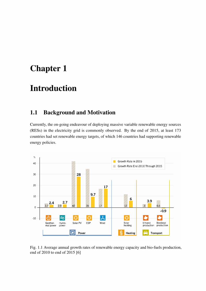
1.1 Average annual growth rates of renewable energy capacity and bio-fuelsproduction, end of 2010 to end of 2015 [6] . . . . . . . . . . . . . . . . . . 1
2.1 Computation flowchart of the robust SCOPF . . . . . . . . . . . . . . . . . 32
3.1 General configuration of an ac grid (left side) with an embedded VSC-MTDCsystem connected to the dc grid (right side) . . . . . . . . . . . . . . . . . 43
3.2 Single-line diagram of the offshore wind farm connected with a VSC-MTDCsystem . . . . . . . . . . . . . . . . . . . . . . . . . . . . . . . . . . . . . 47
3.3 Hierarchical system dispatch scheme for meshed ac/MTDC grids . . . . . . 523.4 Single-line diagram of the offshore wind farm connected with a VSC-MTDC
system . . . . . . . . . . . . . . . . . . . . . . . . . . . . . . . . . . . . . 533.5 Single-line diagram of the offshore wind farm connected with a VSC-MTDC
system . . . . . . . . . . . . . . . . . . . . . . . . . . . . . . . . . . . . . 54
4.1 Flowchart of the decomposition algorithm for SCOPF . . . . . . . . . . . . 664.2 MG architecture . . . . . . . . . . . . . . . . . . . . . . . . . . . . . . . . 674.3 A small household-sized MG . . . . . . . . . . . . . . . . . . . . . . . . . 674.4 IEEE 33-bus grid regarded as a whole MG . . . . . . . . . . . . . . . . . . 674.5 Process of post-contingency control with MGs . . . . . . . . . . . . . . . . 69
5.1 The duck chart, showing a deep midday drop in net load and a steep ramp-upstarting in the late afternoon and extending into evening peak load; the obser-vation of oversupply risks is attributable to variable generation resources[7] 82
5.2 Different computation times of sub-gradient projection method by usingdifferent time slots and step sizes . . . . . . . . . . . . . . . . . . . . . . . 86
5.3 The blue and red lines represent the information exchange, where users sendtheir own consumptions and the energy provider announces the price signal 87
5.4 Comparison between sub-gradient method and FDDGA when N=10 . . . . 92

xviii List of figures
5.5 Comparison between sub-gradient method and FDDGA when N=500 . . . 925.6 Comparison of number of iterations between the sub-gradient method and
the FDDGA with increasing user number N . . . . . . . . . . . . . . . . . 93

List of tables
2.1 L9(34) OA Array . . . . . . . . . . . . . . . . . . . . . . . . . . . . . . . 262.2 Results for the IEEE14-Bus System . . . . . . . . . . . . . . . . . . . . . 352.3 L8(27) OA for IEEE 118-Bus System . . . . . . . . . . . . . . . . . . . . 352.4 Results for the IEEE118-Bus System . . . . . . . . . . . . . . . . . . . . . 36
3.1 SCOPF Result for IEEE14-Bus System . . . . . . . . . . . . . . . . . . . 543.2 SCOPF Result for IEEE118-Bus System . . . . . . . . . . . . . . . . . . . 553.3 Centralised Scheme Simulation on Linearised SCOPF on IEEE 14-Bus System 553.4 Rescheduling Result Due to Wind Generation Deviation on IEEE 14-Bus
System . . . . . . . . . . . . . . . . . . . . . . . . . . . . . . . . . . . . . 563.5 Rescheduling Result Due to Wind Generation Deviation in the IEEE118-Bus
System . . . . . . . . . . . . . . . . . . . . . . . . . . . . . . . . . . . . . 56
4.1 IEEE 14-Bus System Robust SCOPF vs. Traditional SCOPF . . . . . . . . 714.2 IEEE14-Bus System Contingency Control and Cost . . . . . . . . . . . . . 714.3 IEEE118-Bus System Robust SCOPF vs. Traditional SCOPF . . . . . . . . 724.4 IEEE118-Bus System Contingency Control and Cost . . . . . . . . . . . . 734.5 IEEE14-Bus System With MG CC Cost for Each Corresponding Contingency
with Given Incentive Rate . . . . . . . . . . . . . . . . . . . . . . . . . . . 744.6 IEEE118-bus system with MG CC cost for each corresponding contingency
with given incentive rate . . . . . . . . . . . . . . . . . . . . . . . . . . . 74
5.1 Number of Variables for Several Types of Optimisation Problem Formulation 805.2 Computation Time for Both the Sub-gradient Method and the FDDGA.
Different User Numbers at Time Slot t=7 . . . . . . . . . . . . . . . . . . 94
Nomenclature
Functions
•+ Optimistic optimisation variable in confident interval
•− Pessimistic optimisation variable in confident interval
D(•) Dual problem
L (•) Lagrangian function of a given problem
µ(•) Mean value of normally distributed random variables
σ2(•) Variance of normally distributed random variables
• Optimistic optimisation variable in confident interval
f (•) Operation cost function for optimal power flow
pi(•), pt(•) Proximity functions for double smoothing techniques
Indices
c index of voltage source converters
i Bus number or from bus for a transmission line
j Bus number or to bus for a transmission line
k Index for contingency
l index for branches
m Iteration for the dc grid droop control
s Index for scenarios

xxii Nomenclature
Parameters
αm,i corrective control action cost coefficient for participated microgrid i
αg,i Redispatch cost coefficient for generator i
βw Scale parameter for Weibull distribution
∆uk Allowed deviation of control vector from pre-contingency to contingency k
ε Terminate criterion
η Robust degree
γ Step size for sub-gradient method
Λ Estimated upper bound for Lagrangian multiplier λ
B Admittance matrix of the grid
JDC Jacobian matrix for dc grid
pacvsc,k Vector of active power generation of all VSC on the ac side in contingency k
qacvsc,k Vector of reactive power generation of all VSC on the ac side in contingency k
Y Admittance matrix
idci j Upper limit for current rating on the dc line from bus i to bus j
ρk Probability of contingency k to occur
ρs Probability of scenario s to occur
σi, σt Convex parameters
τ TLDSCOPF Algorithm iteration termination criteria on pacvsc
θslack,θre f Voltage angle at the reference bus or slack bus
Ki,Ki Lower and upper limit for droop constant of VSC on dc bus i
ϕmini j ,ϕmax
i j Minimum and maximum voltage angle shift by voltage shift transformer betweenbus i and j

Nomenclature xxiii
ai,biandci Quadratic, linear and constant coefficients for quadratic cost function for genera-tion unit i
bi j Series susceptance between bus i and bus j
gi j Series conductance between bus i and bus j
H Power transfer distribution factors
kw Shape parameter for Weibull distribution
nb Number of Buses in the grid
ndcb Number of dc buses
ndcb Total number of dc buses in dc grid
ng Total number of generators in the grid
nk Number of contingencies
nm Number of microgrids
ns Number of scenarios
nϕ Number of the phase shifting transformers in the system
nrad Number of random variables in a system
ntr Number of the Tap changing transformers in the system
pdng,i, pup
g,i Ramp down and ramp up limits on generation unit i
pming,i , pcap
g,i Minimum and maximum active power generation of generation unit i
pmini j , pcap
i j Minimum and maximum active power flow from bus i to j
pdnm,i, pup
m,i Minimum and maximum adjustment on microgrid i
Prated Rated power for wind turbine
pac,maxvsc,c , pac,min
vsc,c Maximum and minimum active power generation rating of VSC c on the acside
pdc,re fvsc,i Reference value for active power generation of grid VSC on dc bus i in dc grid

xxiv Nomenclature
pρmax
w, j Most probable(forecast) active power generation on wind farm connected to the nodej
qming,i ,q
capg,i Minimum and maximum reactive power generation of generation unit i
qmini j ,qcap
i j Minimum and maximum reactive power flow from bus i to j
qac,maxvsc,c ,qac,min
vsc,c Maximum and minimum reactive power generation rating of VSC c on theac side
ri j Resistance of the dc lines from node i to node j
Tk Allowed post-contingency recovery time for contingency k
trmini j , trmax
i j Minimum and maximum voltage tap rate by voltage tapping transformer betweenbus i and j
V mini ,V max
i Minimum and maximum voltage magnitude on bus i
Vk Vector of all voltages of Ac buses in contingency k
vcin Cut in wind speed for wind power
vcout Cut out wind speed for wind power
Vde f ,i Predefined nominal voltage at bus i
vrated Rated wind velocity for wind turbine
Sets
Z System Z
N Set of users subscribed to an aggregator in the real time pricing model
SCK Sets of corrective controlled contingencies
SNK il Sets of Contingencies without solutions
SPK Sets of preventive controlled contingencies
Variables
∆p Vector of changes of active power injections on buses
∆pL Vector of changes of active power flow on branches

Nomenclature xxv
u Control vector for not considering any contingency
x State vector for not considering any contingency
λ t Lagrangian multiplier, often used to indicate the electricity rate of a given time slot t
λk Dual variables for problem k
λc,k Dual variable for pkvsc
λg,k Dual variable for pkg
θ Vector of voltage angles
ϕ Vector of Voltage angle shift
Idc Vector of current in dc grid
pd Vector of active power to loads on all buses
pg Vector of active power from conventional generation units on all buses
pL Vector of active power flow on all branches
pr Vector of active power from renewable generation units on all buses
p Vector of active power
pρmax
d Vector of the most probable load demand
pρmax
r Vector of the most probable renewable energy generation
pmaxH Vector of equivalent upper limit on active power flow for all branches in robust
formulation
pminH Vector of equivalent lower limit on active power flow for all branches in robust
formulation
q Vector of reactive power
r Vector of random variables
tr Vector of tap setting
u0 Control vector for pre-contingency

xxvi Nomenclature
uk Control vector for contingency k
u Control variable vector
Vdc Vector of voltage in dc grid
V Vector of voltage magnitudes
x0 State vector for pre-contingency
xk State vector for contingency k
x State variable vector
z Optimisation variable vector
ω Optimal value for sub-problems’ objective function
θi Voltage angle at bus textiti
θi j Voltage angle difference between node bus i and j
pmaxa,l Aggregated upper bound for branch l all loads and line flow
pmina,l Aggregated lower bound for branch l all loads and line flow
κ Lagrangian multiplier
ϕi j Voltage angle shift between node bus i and j
pi j Random active power flow from bus i to bus j
pr,i Random active power from renewable generation on bus i
ξ User’s consumption preference parameter
Ccc,m Corrective control cost by microgrids
Cm&gcc Corrective control cost by microgrids and generation units
CmESCC Total contingency control cost by microgrids
CbaseESCC Total contingency control cost without considering microgrids’ supports
Cpc,m Preventive control cost by microgrids
Cm&gpc Preventive control cost by microgrids and generation units

Nomenclature xxvii
Ki Droop constant of VSC on dc bus i
Lt Aggregated consumption in the real time pricing model in the time slot t
pi Active power injection on bus i
pd,i Active power demand on bus i
pg,i Active power generation at generator i
psg,i Active power generation of generation unit i in scenario s
pmaxh,l Equivalent upper limit on active power flow for branch l in robust formulation
pminh,l Equivalent lower limit on active power flow for branch l in robust formulation
pi j Active power flow from bus i to bus j
pdci j Power flow from node i to node j on the dc line
p(S)r,1 Testing scenario S generated from OA library for variable pr,1
pr,i Active power from renewable generation on bus i
pavsc,ic Active power generation on the ac side
pac,kvsc,i Active power generation of VSC in the ac grid on ac bus i in contingency k
qi Reactive power injection on bus i
qd,i reactive power demand on bus i
qi j Reactive power flow from bus i to bus j
qr,i reactive power from renewable generation on bus i
ri,k Slack variables for branch l in problem k
tri j Tap setting for tap changing transformers between bus i and j
v Wind velocity
Vi Voltage magnitude on bus textiti
V ac,ki Voltage on ac bus i in contingency k
V dci Voltage on node i in the dc grid
xti User i’s consumption in time slot t in the real time pricing model
Chapter 1
Introduction
1.1 Background and Motivation
Currently, the on-going endeavour of deploying massive variable renewable energy sources(RESs) in the electricity grid is commonly observed. By the end of 2015, at least 173countries had set renewable energy targets, of which 146 countries had supporting renewableenergy policies.
Fig. 1.1 Average annual growth rates of renewable energy capacity and bio-fuels production,end of 2010 to end of 2015 [6]
2 Introduction
To achieve these targets, the last decade saw a steady increase in the global demand forrenewable energy, with an overall 30% increase. According to the Renewables 2016 GlobalStatus Report [6], between 2004 to 2014 the installed capacity of RESs has experienced arapid growth globally, with 270 GW growth for wind power; up to 136 GW for photovoltaics;285 GW for wave and tidal power; and up to 49 GW for biomass. The growing penetrationof RESs into the electricity power grid is profitable from a sustainable point of view andprovides economic benefit for long-term operation. Reliable and secure energy supply isof high priority for modern society [8]; unfortunately, however, this has arisen becauseof concern about the trend towards increasing renewable energy penetration, due to theintermittent nature of renewable generation sources, such as wind and solar generation.
In addition, security requirements for the system to withstand contingencies also plays animportant role in supplying reliable and secure energy to the consumer. This becomes evenmore challenging with the reducing fraction of dispatchable generation sources in the gird.Moreover, the location of renewable generation tends to be heavily defined by meteorologicaland geographical conditions, which makes the generation sites distant from load centres.Therefore, cost-efficient operation strategies must be analysed anew and designed to accountfor the heterogeneous nature of large variable RESs, for improved reliability and security.While the main challenge is to maintain the balance between supply and demand, thischallenge can be further categorised according to controlled time scales, as follows:
1. Frequency and voltage regulation and stability [9]. Challenges are brought by thevariety of scattered RESs that create frequent power injections into the grid as wellas possible reversed power flows. This problem is mainly regarded as in distributionnetworks [10], in the time scale of milliseconds to a second.
2. Frequency inertia. Conventional electricity networks mainly rely on synchronousgenerators with large inertia that are capable of providing key support in frequencyand voltage stability. However, power electronics inverter-based distributed generationincluding RESs present a lack of frequency inertia. As a result, the stability of the gridand the quality of service might be affected as the voltage and frequency transient maybecome too large in a low mechanical inertia grid.
3. Reliable and secure optimal power flow problem. Although a relatively accurateforecast on load could be achieved by now, uncertainties brought by variable intermit-tent renewable sources normally induce a large-scale optimisation problem [11, 12],especially when security constraints are considered. Solution computation using a tradi-tionally formulated deterministic problem might not be valid when the real generationof RESs deviates from the predicted value. This type of computation is normally done
1.2 Contribution 3
in the minutes to hourly basis. Additionally, security and resilience of the electricitygrid normally require a fast response from the disptachable generation that has beenseen as a trend of reduction [13]. Therefore new and more efficient approaches need tobe explored considering all aforementioned transitions in the network [14].
4. Energy management system and scheduling. Unit commitment [15] is normallyadopted for day-ahead scheduling, where the uncertainties of the renewable generationcould have a continuous impact on optimal decision-making, which normally leads toa stochastic problem. With constraints such as minimum running and shut down timefor conventional large generators, the solution for long term scheduling could suffereven more due to the uncertain variables.
5. Long-term operation and planning [16, 17]. The integration of RESs also urges theelectricity network to experience a significant ongoing reconstruction and expansion inorder to accommodate the heterogeneous nature of these sources as well as dynamiccontrol and communication. Meanwhile, the grid also tends to be smaller, moreresilient and less interdependent. Moreover, the locations of generation that used to bedetermined by the load centre become more diverse and could be remotely off shore.
A potential solution to these challenges is to find an efficient framework that is able to accom-modate a high penetration level of RESs and is computationally efficient for operations invarious time domains. In particular, diverse approaches should be exhausted for uncertaintiesof modelling and handling that correspond to different types of optimisation problems. Inaddition, mathematical approaches such as approximation and decomposition techniquesare applied to the problem to alleviate the computational burden. Thus, this thesis aims toprovide an efficient tool for modelling and analysing the steady state of the electricity gridwith a high penetration of RESs. It aims to develop effective solving approaches so thatvariable RESs can be integrated smoothly into electricity networks.
1.2 Contribution
This PhD thesis presents the detailed steady-state modelling of the integration of renewableenergy generation into the network for future electricity network operations and optimi-sation. Its contributions lie in its effectiveness in considering the intermittent renewablegeneration into the operation modelling and in developing efficient solving techniques. Thesecontributions are summarised as follows:
• an efficient framework in modeling and optimising the electricity network operationby taking into account uncertainties, securities and new components;

4 Introduction
• comparison, identification and analysis of various approaches are thoroughly conductedin considering uncertainties in the optimisation problem, based on which a robustoptimal power flow approach is proposed for effectively considering random variables;
• in order to incorporate security measures against contingencies, the robust optimalpower flow is elevated into a robust SCOPF problem, using decomposition techniques;
• a hierarchical SCOPF is then proposed for a meshed ac and dc grid. A two-levelstructure is investigated to effectively coordinate the offshore renewable generationwith the in-land main grid optimal dispatch decision-making process;
• an incentive-based approach is designed and then tested to explore the potential ofnetworked microgrids in supporting the main grid’s security control actions in thepost-contingency control scenario under uncertainties;
• an extended investigation of computation efficiency, optimisation approximation andconvex relaxation is conducted. A semi-linearised SCOPF is proposed that could becomputed fast without the loss of power system physical limitations; and
• finally, an efficient framework that could be applied to non-convex optimisation prob-lems using distributed dual gradient algorithm is proposed to further alleviate thecomputation burden and to achieve better convergence.
1.3 Thesis Outline
Following this general introduction, this thesis is divided into the following chapters, includ-ing individual brief introductions.
Chapter 2 studies the impact of renewable generation on the steady state in theoperation stage, in terms of an optimal dispatch decision-making process on an hourly basis.It then introduces a framework to implement security requirements with uncertaintiesfor hourly operation, following a brief introduction of power flow modelling and optimalpower flow models. Different approaches for accounting for uncertainties caused by randomvariables are carefully examined. Finally, after analysing various approaches, the chapterpresents a new efficient approach to address the uncertain factors caused by load demand andrenewable generation in power systems via a robust SCOPF model.
Chapter 3 studies meshed ac and HVDC grid connecting large-scale offshore windfarms in the scope of SCOPF. It provides background information on HVDC systems andproposes a hierarchical SCOPF model for a meshed ac/multi-terminal HVDC (MTDC)system with high wind penetration.

1.3 Thesis Outline 5
In Chapter 4 multiple microgrids are investigated in supporting main grid’s securitycontrol. The chapter provides a detailed comparison of preventive control and correctivecontrol in contingency control strategies. An incentive-based mechanism is designed toencourage the microgrids to actively cooperate with the main grid for post-contingencyrecovery.
Chapter 5 addresses the computation efficiency and convergence analysis. It de-scribes concerns with regard to the computation efficiency and convergence in solving theSCOPF and analyses approaches used in proposed models. Furthermore, a double smoothingtechnique is introduced to improve the convergence performance in distributed optimisationin the DSM.
Chapter 6 presents conclusion and outlook draws the conclusion of this thesis andprovides some information on future research possibilities.
Chapter 7 comprises the list of publications.

Chapter 2
Integration of Renewable Energy Sourceinto Optimal Generation Dispatch
This chapter introduces an efficient framework to address both uncertain factors causedby load and renewable generation as well as security considerations in electricity networkoperations. To this end, the chapter first introduces the basic optimal power flow (OPF)principles by formulating a nonlinear optimisation problem and then simplifying it into alinearised OPF problem. Based on this, the chapter then introduces and compares variousapproaches to integrate random renewable sources generation into the OPF problem. Finally,it presents a robust SCOPF model [18], which consists of two steps. First, a robust OPFis realised through a minimum number of uncertainty scenarios selected from the Taguchiorthogonal array testing (TOAT) [19] method. Then, the security constraints are incorporatedinto the robust OPF using Benders Decomposition (BD) [20]. The obtained solution is robustagainst uncertain load and wind generation and secure against contingencies. The numericalsimulation demonstrates the solution’s effectiveness in accommodating RESs in hourly systemoperations. This chapter is based on [21].
2.1 Introduction
The challenges of integrating renewable generation sources into the electricity networkoperation exist at all different levels and in a range of time frames. The incorporation ofrenewable resources would significantly alter the traditional approach of economic dispatch.Moreover, the variability of renewable resources would require measures to accommodatefast generation changes. Although no short term marginal costs are associated with RESs,increased operational costs by utilizing other components in the grid to compensate for the
8 Integration of Renewable Energy Source into Optimal Generation Dispatch
resources’ intermittent nature would be incurred and need to be accounted for in the operationoptimisation.
OPF determines the optimal control variables of a power system with regard to a prede-fined objective function and certain constraints [22]. The core of the economically efficientand reliable electricity network operation relies heavily on the OPF problem. The mathemati-cal formulation of OPF was initially introduced in the 1960s [23] and was considered to bedifficult to solve. The problem is complex economically, electrically and computationally.The development of the OPF has significantly benefited from the evolution of optimisationtheory and computing technologies; an overview of the development can be found in [24]and [25].
Traditionally, the OPF problem only considers static physical and operating limits asthe constraints. To protect the system against credible contingencies, however, there is anincreasing interest in and necessity to take into account the security constraints correspondingto degraded conditions in the OPF, thus yielding SCOPF problems. The system therefore,gains immunity to the contingencies with a reasonable sacrifice of operation cost.
In recent years, with the increasing penetration of RESs, such as wind power, thesystem operating state tends to be more volatile and uncertain. Traditional deterministicSCOPF is able to determine the control variables of the system given information aboutload and non-controllable generation. However, given the intermittent nature of renewables,even with a highly accurate prediction of load and renewable resources, the solution oftraditional deterministic SCOPF may not be valid, which may lead to overflows or evensystem failure should the contingency in fact occur. Therefore, SCOPF that is capable ofadapting to uncertainties caused by the random load and renewable power injections hasbecome considerably important for maintaining system reliability.
2.2 Optimal Power Flow Formulation
2.2.1 General Form of the Optimal Problem
The OPF problem is an optimisation problem, whose general form is given as follows,

2.2 Optimal Power Flow Formulation 9
minimiseu
f (x,u) (2.1)
subject to
h(x,u) = 0 (2.2)
g(x,u)≤ 0. (2.3)
Equation (2.1) is the objective function, where x denotes a nx by 1 state vector, while udenotes the control vector in the size of nu by 1 control variable. Equation (2.2) represents theequality constraints, and (2.3) the inequality constraints, which restrict the optimal solutionspace. Normally, a variable vector z can be defined to denote the combined variables of statevariables x and control variables u with the length of nz shown below:
z =
[xu
](2.4)
2.2.2 Nonlinear Optimal Power Flow Formulation
Nonlinear OPF is also known as alternating current OPF(ACOPF), as it considers constraintson the variables related to the reactive power and voltages. This section first briefly introducedac power flow, followed by the objective function, control variables, and state variables.
Ac power flow modeling
The power flow problem is a steady state computation problem of voltage magnitude andphase angle at each bus in a given power system network. Detailed modeling of the ac systemcan be found in [26]. Here, the unified nodal power and power flow equations are given asfollows,

10 Integration of Renewable Energy Source into Optimal Generation Dispatch
pi =Vi
nb
∑j=1
Vj(gi j cos(θi −θ j)+bi j sin(θi −θ j) (2.5)
qi =Vi
nb
∑j=1
Vj(gi j sin(θi −θ j)−bi j cos(θi −θ j) (2.6)
pi j =(tri jVi)2gi j − (tri jVi)(tr jiVjgi j)cos(θi j +ϕi j −ϕ ji)
− (tri jVi)(tr jiVj)bi j sin(θi j +ϕi j −ϕ ji) (2.7)
qi j =(tri jVi)2(bi j +bsh
i j )− (tri jVi)(tr jiVjgi j)sin(θi j +ϕi j −ϕ ji)
+(tri jVi)(tr jiVj)bi j cos(θi j +ϕi j −ϕ ji) (2.8)
pi and qi are the real power and reactive power injections on the node i, while pi j and qi j
denote the real and reactive power flows from bus i and bus j. The system series conductance,the series susceptance and the shunt susceptance between node i and node j are denoted bygi j, bi j and bsh
i j respectively, while voltage angle difference and voltage angle shift betweennode i and j are denoted by θi j and ϕi j respectively. Vi,Vj are the voltage magnitudes of nodei and j. Finally, ti j is the controllable tap setting for tap changing transformers between nodesi and j.
Objective Function
Various objective functions could be formulated to achieve different goals, including minimis-ing generation cost, losses, total generation, and maximising market surplus. Some examplesare given in this section. The most widely used objective function for economical dispatchingis to minimise the generation cost, which is closely related to the cost coefficients of eachgenerator. The form of the objective function is normally in a quadratic model, shown below:
minimiseu
f (x,u) (2.9)
where
f (x,u) =ng
∑i=1
(ai p2g,i +bi pg,i + ci) (2.10)
2.2 Optimal Power Flow Formulation 11
To minimise the generation cost, the algorithm could minimise the quadratic cost modelin (2.10), where ai, bi and ci are the quadratic, linear and constant cost coefficients forgenerator i respectively. Therefore, (2.10) is normally the cost of conventional generatorswhose generation costs are the reflection of the fuel costs. While renewable generation isnormally considered to have very low marginal costs, these costs are not considered in (2.10).Another cost function that is commonly adopted is shown in (2.11), which minimises thetotal losses.
f (x,u) =nl
∑i=1
nl
∑j=1
gi j(V 2i +V 2
j −2ViVj cos(θi −θ j)) (2.11)
A similar approach to (2.11) is shown in (2.12), which minimises the total generation inthe grid, leading to the minimum overall losses.
f (x,u) =ng
∑i=1
pg,i (2.12)
Moreover, recent interests in regulating the voltage profile in the electricity network couldalso be achieved by reducing the difference between all of the node voltages to a predefinedprofile, for instance 1 p.u., as shown below,
f (x,u) =nb
∑i=1
(Vi −Vde f ,i)2 (2.13)
or
f (x,u) =nb
∑i=1
(Vi −1)2 (2.14)
Noticeably, the objective function of the OPF is variable and flexible. It could be an equationof control variables such as pg,i in (2.10), a function of the state variable Vi in (2.13), or afunction of both as in (2.11). Therefore, before the chapter proceeds to the constraint, thestate and control variables are defined in the next section.
Variables
The state variable vector x and the control variable vector u in the ACOPF problem can benormally defined as follows, and the parameters can vary depending on the operation model

12 Integration of Renewable Energy Source into Optimal Generation Dispatch
and market decisions.
u = [pT,qT, trT,ϕT]T (2.15)
Control variable vector u contains variables that can be controlled and alternated by thesystem operators. In general, the control variables can be determined to setpoints within theirlimits so that the objective function can be optimised. The first vector p in (2.15) includesa few sets of variables of pg,i ∀i = 1, ...,ng, poth,i ∀i = 1, ...,noth. pg,i normally refers to theconventional generator i whose generation setpoint can be determined and managed, whilepoth,i refers to any other sources that can be controlled in the electricity network for realpower injection, for example pac
vsc,i which denotes the power injection from a voltage sourceconverter [27] to the ac grid. On the other hand, RESs are normally treated as uncontrollablegenerations with uncertainties, and therefore output from renewable generations is notincluded in the control variable u. By adopting different approaches, the OPF could betransformed into various types of optimisation problems, which is explained in details laterin this chapter. The second vector q includes qg,i ∀i = 1, ...,ng, qsvc,i ∀i = 1, ...,nsvc. qg,i, andqoth,i ∀i = 1, ...,noth, where qg,i refers to all reactive power generation from generators, qsvc,i
denotes the reactive power compensation from the static var compensators and qoth,i is allother reactive power injection from controllable sources. The third element tr in vector uincludes all tapping transfers and tap ratios, while the last one ϕ contains all phase shiftingtransformers in the network. Their numbers are ntap and npha respectively.
x = [VT,θ T]T (2.16)
The state variables of the system include voltage magnitude vector V and voltage angle θ ,where V includes voltage magnitude Vi, ∀i = 1, ...,nb on each bus nb, and θ has the voltageangle θi, ∀i = 1, ...,nb on each bus.
Another set of variables, r ⊆ x, refers to random variables such as renewable generationpr,i ∀i = 1, ...,nres and real power and reactive power demand from load pd,i ∀i = 1, ...,nd
and qd,i ∀i = 1, ...,nd . For the deterministic OPF formulation, vector r becomes empty sincethe renewable energy generation and load can be treated as constant when the uncertaintiesare neglected. However, the deterministic approach becomes inadequate in handling decisionmaking in an OPF problem with a high penetration of RESs. Therefore, the complete set ofvariables in this thesis is the following,
2.2 Optimal Power Flow Formulation 13
z = [xT,uT,rT]T (2.17)
Constraints
There are two types of constraints in the formulated OPF problem: equality constraints andinequality constraints. The power balance equation is the first equality constraint that mustbe fulfilled for both real and reactive power balance, normally in the nodal balance equationfor each bus ∀i = 1, ...,nb:
pg,i − pd,i − pi + pr,i = 0 ∀i = 1, ...,nb (2.18)
qg,i −qd,i −qi +qr,i = 0 ∀i = 1, ...,nb (2.19)
It should be noted that all the variables in (2.18) are the power infeed on the bus i. If there isno generator on the bus i, then pg,i = 0. Another equality constraint is purely for the purposeof computation, where the reference voltage angle is defined and fixed at the reference value,normally zero, on the slack bus:
θslack = θre f = 0 (2.20)
The inequality sets normally correspond to the system operation limits on both controlvariables and state variables as follows:
pming,i ≤ pg,i ≤ pcap
g,i ∀i = 1, ...,ng (2.21)
qming,i ≤ qg,i ≤ qcap
g,i ∀i = 1, ...,ng (2.22)
V mini ≤Vi ≤V max
i ∀i = 1, ...,nb (2.23)
trmini j ≤ tri j ≤ trmax
i j ∀i, j = 1, ...,nb (2.24)
ϕmini j ≤ ϕi j ≤ ϕ
maxi j ∀i, j = 1, ...,nb (2.25)
pmini j ≤ pi j ≤ pcap
i j ∀i, j = 1, ...,nb (2.26)
qmini j ≤ qi j ≤ qcap
i j ∀i, j = 1, ...,nb (2.27)
(2.21) and (2.22) are the inequality constraints on the active power and reactive poweroutput for each generator. (2.24) and (2.25) are the tap ratio limits on the tap changing trans-
14 Integration of Renewable Energy Source into Optimal Generation Dispatch
formers and phase shifting operation range on the phase shifting transformers respectively.The last two inequality constraints (2.26) and (2.27) are the real and reactive power line flowlimits, and normally pmin
i j =−pcapi j , and therefore (2.26) is always written as:
−pcapi j ≤ pi j ≤ pcap
i j ∀i, j = 1, ...,nb (2.28)
2.2.3 Linearised Optimal Power Flow
The nonlinear OPF can represent the real system operation, especially when voltage andreactive power are concerned. However, it is nonlinear and non-convex and therefore difficultto solve and heavy in computation. Powerful solvers, Bonmin [28], CPLEX [29], Gurobi[30], IPOPT [31], KNITRO [32], etc., could be applied to solve the nonlinear OPF in aniterative manor, but the iteration might not converge in time and the global optimal is difficultto prove. In contrast, linearised OPF is an approximation of the nonlinear OPF. It is oftencalled dc OPF since it neglects the reactive power from the formulation. Linearised OPF hasgained its popularity among system operators for several reasons, among which the mostdistinct advantage that the linearised OPF can be solved efficiently with solutions that arereliable and non-iterative.
Objective Function, Variables and Constraints
In linearised OPF, objective function such as minimisation of operating cost (2.11) and totalgeneration (2.12) remain the same as in nonlinear OPF. However, since the reactive poweris neglected, voltage profile optimisation (2.13) cannot be formulated in dc OPF. With theassumption that the voltage at each node is 1.0 p.u., as well as the elimination of reactivepower in the control variable, the number of variables and system complexity are significantlyreduced. The variables explicitly become:
u = [pT,ϕT]T (2.29)
x = [θ ] (2.30)
Consequently both equality constraints and inequality constraints are modified, and onlythose associated with the variables in (2.29) and (2.30) remain. The power flow equation(2.7) is also simplified with assumptions, such as that voltage magnitudes are constant at 1.0p.u., the resistance of transmission line can be neglected, sinθ = θ , etc.. It is transformed

2.3 Probability OPF Formulation and Solutions 15
into:
pi j =−bi jθi j ∀i, j = 1,2, ...,nb (2.31)
The detailed process of the linearised power flow is investigated in a sufficient amount ofliterature -see [33] and [26] and it is therefore omitted in this thesis.
2.2.4 Random Variables and Uncertainties
As discussed in the previous sections, variable vector r includes random variables thatare caused by determinant renewable source generations and ever changing load demands.When the uncertainties of these random variables are considered, related constraints becomeequations containing random variables. In this thesis, • is used to denote random variables.Considering renewable generation uncertainties as well as uncertainties in load demand, in alinearised OPF, constraints (2.18) and (2.26) become probabilistic constraints as follows,
pg,i − pd,i − pi + pr,i = 0 ∀i = 1, ...,nb (2.32)
pmini j ≤ pi j ≤ pcap
i j ∀i, j = 1, ...,nb (2.33)
Normally, these uncertainties are captured using the probability density functions (PDF) [34]of the random variables, to obtain probabilistic characteristics. This requires presumptionsof the knowledge of PDFs of the random variables, which are sometimes difficult to obtain.Alternatively, robust optimisation offers another method to deal with random variables in theoptimisation problems with uncertainties.
2.3 Probability OPF Formulation and Solutions
A dc OPF model that aims to minimise the total cost can be summarised as follows, using theobjective function, equality constraints, and inequality constraints described in the previoussection:

16 Integration of Renewable Energy Source into Optimal Generation Dispatch
Objective:
minimiseng
∑i=1
(ai pg,i2 +bi pg,i + ci) (2.34)
Subject to:
p = Bθ = pg −pd +pr (2.35)
pgmin ≤ pg ≤ pg
cap (2.36)
pmini j ≤
θi −θ j
xi j≤ pmax
i j or pLmin ≤ pL ≤ pL
max (2.37)
Equations (2.35), (2.36) and (2.37) are the constraints (2.18), (2.21) and (2.26) in matrixform. Similarly, by replacing pr,pd and pL with the random variables pr, pd and pL, theprobabilistic problem is formulated as follows,
Objective:
minimiseng
∑i=1
(ai pg,i2 +bi pg,i + ci) (2.38)
Subject to:
p = Bθ = pg − pd + pr (2.39)
pming ≤ pg ≤ pcap
g (2.40)
pminL ≤ pL ≤ pmax
L (2.41)
Comparing the probabilistic formulations (2.38) to (2.41), the deterministic OPF formu-lations (2.34) to (2.37) take the traditional nonrenewable generation as controllable variable,while the renewables and loads are considered to be uncontrollable factors. The uncertaintieswithin the uncontrollable parameters represents difficulties into the optimisation problem,as the optimised result in one scenario might cause constraint violation in another. A fewdifferent approaches are given in the following sections for the solution of OPF with randomvariables.

2.3 Probability OPF Formulation and Solutions 17
2.3.1 Formulation and Solution Methods
Various studies on the OPF problem under uncertainties have been proposed in the literature;they can generally be classified into probabilistic [35–37], stochastic [38, 39], and robustapproaches [40, 41], depending on the way of integrating random variables into the problemformulation and computation process. The approaches can also be categorised according tothe techniques of realisation of the random variables uncertainties: namely the scenario-basedapproach and interval optimisation.
In general, probabilistic OPFs target small systems and their solutions are also normallyin the form of PDFs, and the system operators therefore need to further analyse these resultsto generate a short-term operation plan. Due to the stochastic nature of wind generation,stochastic OPF (S-OPF) has been widely used to accommodate uncertainties of both renew-ables and load in the optimal operation. Similarly to probability OPF (P-OPF), knowledge ofPDFs of random variables is required for S-OPF formulation. Various solving techniqueshave been used in S-OPFs to reduce the computation burden. Chance constraints [39, 42, 43]are often used in S-OPF to study the uncertainties of load and renewables. Robust optimisa-tion [44, 45] has also captured researchers’ attention for determining control strategies underuncertainties.
The most significant difference of robust OPF compared to P-OPF or S-OPF is that itonly requires the knowledge of the interval of variation of the random variables, but it is ableto yield a solution that is robust within an uncertainties range [46, 47]. Moreover, it yieldsa solution that is immune to the effect of uncertainties within the given range. In terms ofselecting solution approaches for formulated problems, the nscenario-based approach is themost straight forward method to uncertainty realisation [48–50]. With the knowledge of thePDFs of the random variables, the scenarios can be generated using sampling methods. TheMonte Carlo Simulation (MCS)[51] has been popularly adopted to test scenario generationsand is always used as a benchmark for solution accuracy. However, to ensure a full coverageof the probabilities, a large number of scenarios are normally generated, which can causemore computation burden, especially with large power system networks. In contrast, intervaloptimisation [52, 53] does not require the details of the PDFs of random parameters, andit is usually used in robust optimisation. In spite of having these merits, however, intervaloptimisation is argued to be conservative in certain circumstance. An overly wide confidenceinterval could lead to a narrowed solution region, resulting in the waste of system resourcesand losses of economic efficiency. On the other hand, an overly narrowed interval could losethe ability to represent significant probabilities.
18 Integration of Renewable Energy Source into Optimal Generation Dispatch
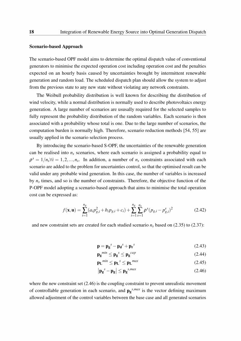
Scenario-based Approach
The scenario-based OPF model aims to determine the optimal dispatch value of conventionalgenerators to minimise the expected operation cost including operation cost and the penaltiesexpected on an hourly basis caused by uncertainties brought by intermittent renewablegeneration and random load. The scheduled dispatch plan should allow the system to adjustfrom the previous state to any new state without violating any network constraints.
The Weibull probability distribution is well known for describing the distribution ofwind velocity, while a normal distribution is normally used to describe photovoltaics energygeneration. A large number of scenarios are ususally required for the selected samples tofully represent the probability distribution of the random variables. Each scenario is thenassociated with a probability whose total is one. Due to the large number of scenarios, thecomputation burden is normally high. Therefore, scenario reduction methods [54, 55] areusually applied in the scenario selection process.
By introducing the scenario-based S-OPF, the uncertainties of the renewable generationcan be realised into ns scenarios, where each scenario is assigned a probability equal toρs = 1/ns∀i = 1,2, ...,ns. In addition, a number of ns constraints associated with eachscenario are added to the problem for uncertainties control, so that the optimised result can bevalid under any probable wind generation. In this case, the number of variables is increasedby ns times, and so is the number of constraints. Therefore, the objective function of theP-OPF model adopting a scenario-based approach that aims to minimise the total operationcost can be expressed as:
f (x,u) =ng
∑i=1
(ai p2g,i +bi pg,i + ci)+
ng
∑i=1
ns
∑s=1
ρs(pg,i − ps
g,i)2 (2.42)
and new constraint sets are created for each studied scenario ns based on (2.35) to (2.37):
p = pgs −pd
s +prs (2.43)
pgmin ≤ pg
s ≤ pgcap (2.44)
pLmin ≤ pL
s ≤ pLmax (2.45)∣∣pg
s −pg∣∣≤ pg
s,max (2.46)
where the new constraint set (2.46) is the coupling constraint to prevent unrealistic movementof controllable generation in each scenario, and pg
s,max is the vector defining maximumallowed adjustment of the control variables between the base case and all generated scenarios

2.3 Probability OPF Formulation and Solutions 19
in the allowed duration. It is clear that the scenario-based approach dramatically increasesproblem size and leads to long computation time, which makes it less suitable for frequencyOPF computation.
Interval-based Approach
The interval optimisation approach is another way to deal with uncertainties. Unlike thescenario-based approach, interval optimisation does not need explicit PDFs of random vari-ables. Instead, it selects the optimal intervals to represent the random variables so thatthe optimisation result can be valid with uncertainty to some extent. Another significantdifference is that in the interval-based approach, the cost raised by uncertain wind generationis not applied to the objective function in the form of penalty costs. Instead, the uncer-tainty is embodied in the operation cost interval and reflected in the increased operationcost. This implies that the model based on the interval optimisation usually exhausts allavailable RES instead of locating an optimally scheduled value. The problem derives thepower confidence interval on the power generation control variables, in this case [p−g,i, p+g,i],and its corresponding cost interval[∑
ngi=1(ai(p−g,i)
2 +bi p−g,i +ci),∑ngi=1(ai(p+g,i)
2 +bi p+g,i +ci)],according to the interval of renewable generation [p−r,i, p+r,i]. The unique feature of the intervaloptimisation is that it uses confidence interval numbers to describe uncertainty, withoutany presumptions on PDFs, and derives optimistic and pessimistic solutions to satisfy theoperational and economic requirements of power systems. Therefore, the objective functionof the interval-based OPF model can be expressed as:
f (x,u) =ng
∑i=1
(ai(p±g,i)2 +bi p±g,i + ci) (2.47)
and new constraint sets are created for each studied scenario ns based on (2.35) to (2.37):
p = pg±−pd
±+pr± (2.48)
pgmin ≤ pg
± ≤ pgcap (2.49)
pLmin ≤ pL
± ≤ pLmax (2.50)
pr± ∈ [pr
−,pr+] (2.51)
from (2.47) to (2.51), the optimised cost is closely related to [p−g,i, p+g,i], which is the confi-dence interval derived from given information in (2.51). The derivation of the representativeinterval on Pg,i can be subjective and difficult. Moreover, the optimised results tend to havemore value in analysis than in decision-making.
20 Integration of Renewable Energy Source into Optimal Generation Dispatch
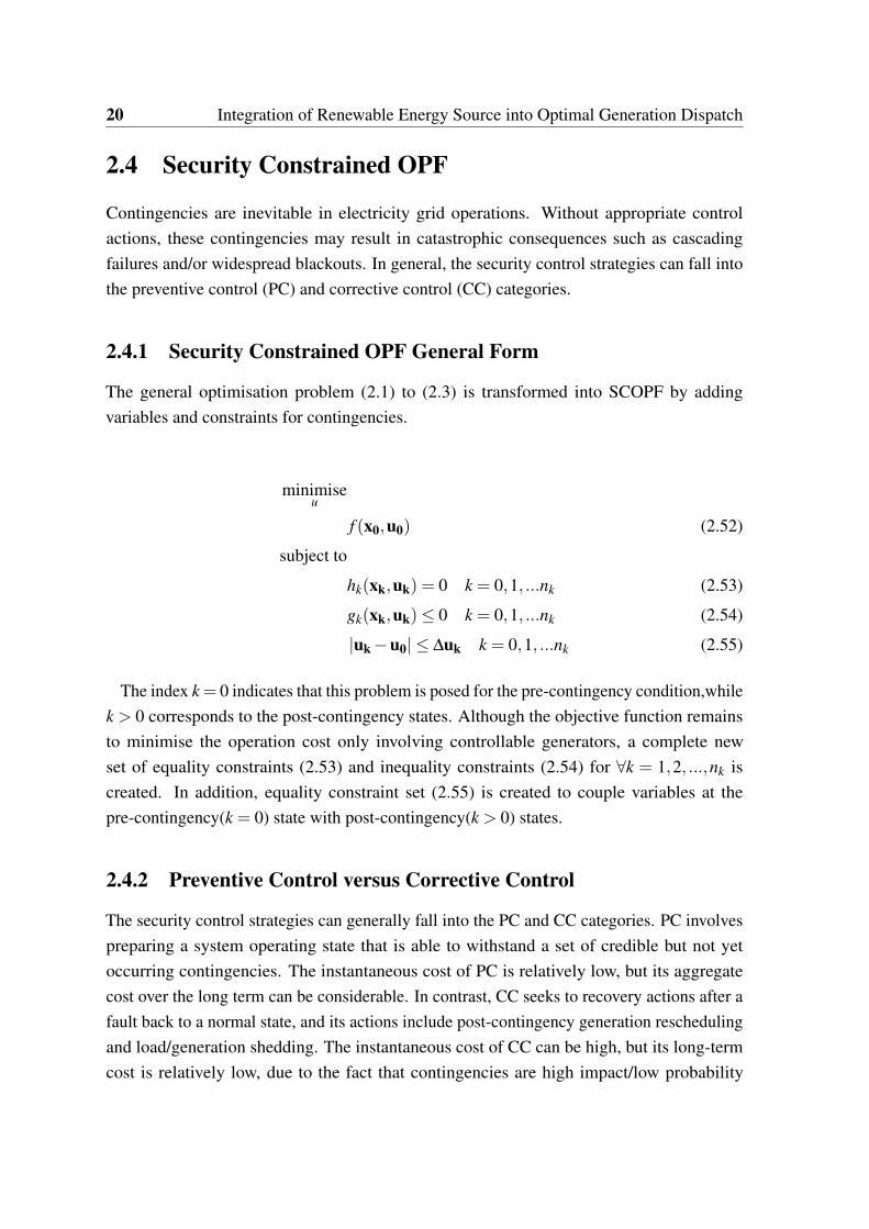
2.4 Security Constrained OPF
Contingencies are inevitable in electricity grid operations. Without appropriate controlactions, these contingencies may result in catastrophic consequences such as cascadingfailures and/or widespread blackouts. In general, the security control strategies can fall intothe preventive control (PC) and corrective control (CC) categories.
2.4.1 Security Constrained OPF General Form
The general optimisation problem (2.1) to (2.3) is transformed into SCOPF by addingvariables and constraints for contingencies.
minimiseu
f (x0,u0) (2.52)
subject to
hk(xk,uk) = 0 k = 0,1, ...nk (2.53)
gk(xk,uk)≤ 0 k = 0,1, ...nk (2.54)
|uk −u0| ≤ ∆uk k = 0,1, ...nk (2.55)
The index k = 0 indicates that this problem is posed for the pre-contingency condition,whilek > 0 corresponds to the post-contingency states. Although the objective function remainsto minimise the operation cost only involving controllable generators, a complete newset of equality constraints (2.53) and inequality constraints (2.54) for ∀k = 1,2, ...,nk iscreated. In addition, equality constraint set (2.55) is created to couple variables at thepre-contingency(k = 0) state with post-contingency(k > 0) states.
2.4.2 Preventive Control versus Corrective Control
The security control strategies can generally fall into the PC and CC categories. PC involvespreparing a system operating state that is able to withstand a set of credible but not yetoccurring contingencies. The instantaneous cost of PC is relatively low, but its aggregatecost over the long term can be considerable. In contrast, CC seeks to recovery actions after afault back to a normal state, and its actions include post-contingency generation reschedulingand load/generation shedding. The instantaneous cost of CC can be high, but its long-termcost is relatively low, due to the fact that contingencies are high impact/low probability
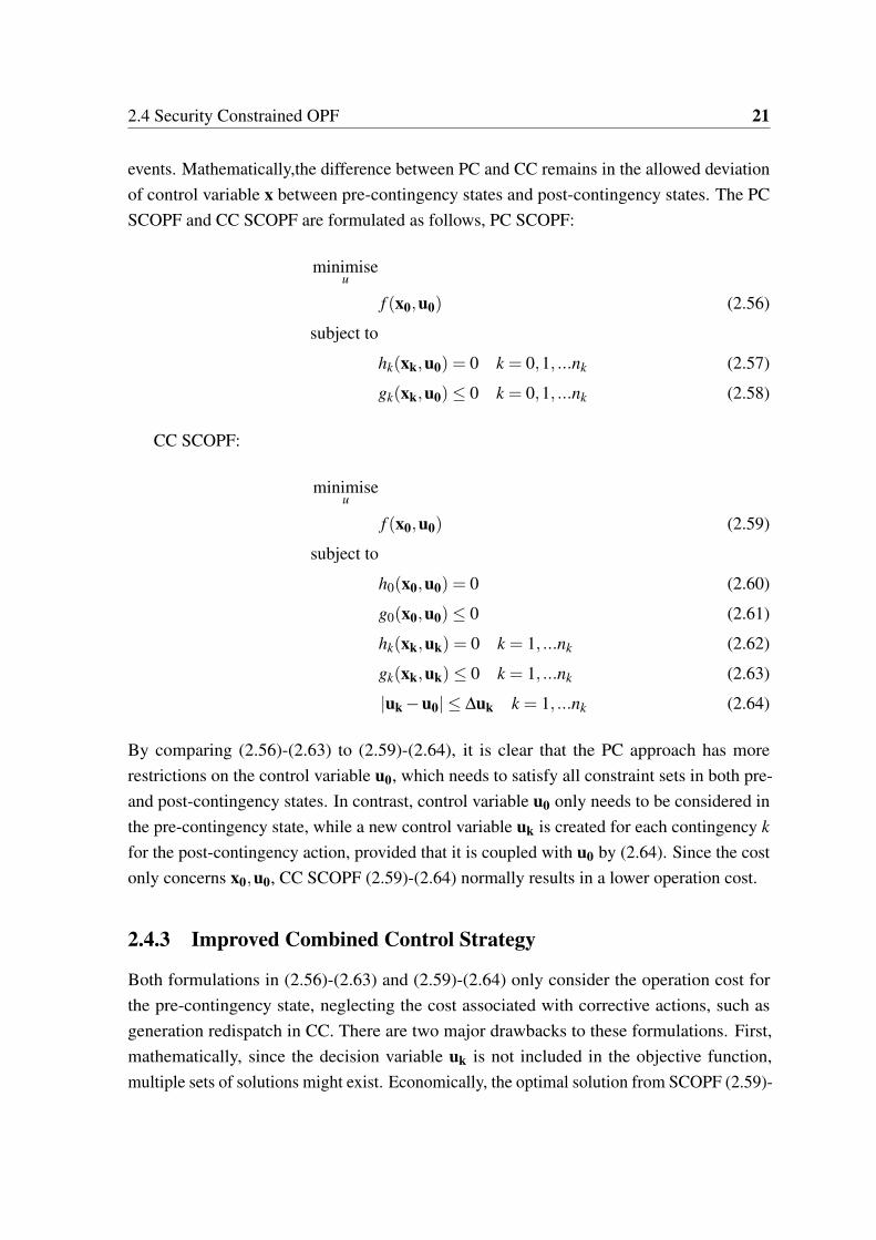
2.4 Security Constrained OPF 21
events. Mathematically,the difference between PC and CC remains in the allowed deviationof control variable x between pre-contingency states and post-contingency states. The PCSCOPF and CC SCOPF are formulated as follows, PC SCOPF:
minimiseu
f (x0,u0) (2.56)
subject to
hk(xk,u0) = 0 k = 0,1, ...nk (2.57)
gk(xk,u0)≤ 0 k = 0,1, ...nk (2.58)
CC SCOPF:
minimiseu
f (x0,u0) (2.59)
subject to
h0(x0,u0) = 0 (2.60)
g0(x0,u0)≤ 0 (2.61)
hk(xk,uk) = 0 k = 1, ...nk (2.62)
gk(xk,uk)≤ 0 k = 1, ...nk (2.63)
|uk −u0| ≤ ∆uk k = 1, ...nk (2.64)
By comparing (2.56)-(2.63) to (2.59)-(2.64), it is clear that the PC approach has morerestrictions on the control variable u0, which needs to satisfy all constraint sets in both pre-and post-contingency states. In contrast, control variable u0 only needs to be considered inthe pre-contingency state, while a new control variable uk is created for each contingency kfor the post-contingency action, provided that it is coupled with u0 by (2.64). Since the costonly concerns x0,u0, CC SCOPF (2.59)-(2.64) normally results in a lower operation cost.
2.4.3 Improved Combined Control Strategy
Both formulations in (2.56)-(2.63) and (2.59)-(2.64) only consider the operation cost forthe pre-contingency state, neglecting the cost associated with corrective actions, such asgeneration redispatch in CC. There are two major drawbacks to these formulations. First,mathematically, since the decision variable uk is not included in the objective function,multiple sets of solutions might exist. Economically, the optimal solution from SCOPF (2.59)-

22 Integration of Renewable Energy Source into Optimal Generation Dispatch
(2.64) might result in a considerable cost for post-contingency control actions. Therefore, itis crucial to incorporate the cost associated with corrective actions into the objective function,and a mixed preventive- and post-contingency control SCOPF is formulated as follows toachieve a minimised overall operation cost,
minimiseu
f (x,u)− f (x, u)+nk
∑k=1
ρkCk(x,u) (2.65)
subject to
h0(x,u) = 0 (2.66)
g0(x,u)≤ 0 (2.67)
hk(xk,uk) = 0 k = 1, ...nk (2.68)
gk(xk,uk)≤ 0 k = 1, ...nk (2.69)
|uk −u| ≤ ∆uk k = 1, ...nk (2.70)
The objective function (2.65) has two parts: the first element f (x,u)− f (x, u) measures thecost imposed by modified PC actions, while the other element ∑
nkk=1 ρkCk(x,u) is the sum
of CC costs. It is noticeable that x0 and u0 are replaced, since there is no longer a purelypreventive control action. Instead, x and u are the variable for calculating the operationcost, which is adjusted in a hybrid way considering both CC and PC actions. x, u representsthe optimal operating state determined by a conventional OPF solution without securityconsiderations. ρk corresponds to the probability of the contingency k and Ck(x,u) is theCC cost function of the contingency for the operating point x,u , normally modeled as aquadratic function of deviation on controllable variables, taking generation difference as anexample:
Ck(x,u) =ng
∑i=1
αg,i(pg,i − pkg,i)
2 (2.71)
∆uk is the vector defining maximal allowed adjustment of the control variables between thepre-contingency and the post-contingency state. Taking generation redispatch as an examplefor corrective generation rescheduling, ∆uk is the generation ramping rate in response tocontingency k in the allowed time.
2.5 Robust Security Constrained Optimal Power Flow Formulation and Solving Method 23
2.5 Robust Security Constrained Optimal Power Flow For-mulation and Solving Method
Traditional deterministic SCOPF introduced in section2.4 is able to determine the controlvariables of the system given information on load and non-controllable generation. However,given the intermittent nature of renewables, even with a highly accurate prediction of loadand renewable resources, the solution of traditional deterministic SCOPF may not be valid.Therefore, a SCOPF that is capable of adapting to uncertainties caused by the randomload and renewable power injections has become considerably important for maintainingsystem reliability. However, the work that has been done to incorporate the uncertaintiesinto SCOPF is limited. The major difficulty lies in a huge problem size caused by thecombination of the contingencies and variable uncertainties. After the introduction of P-OPF and SCOPF in sections2.3 and 2.4 respectively, the complexity of the SCOPF underuncertainties could be foreseen. Therefore, this section introduces a new efficient approach toaddress the uncertain factors caused by load demand and renewable generation in the powersystem, via a robust SCOPF model. The presented robust SCOPF algorithm is not onlycapable of satisfying the security requirements, but is also robust against uncertain renewablegeneration output and load demand. To get a balance between representativeness, economicefficiency and computation efficiency, a combination of scenario-based and interval-basedoptimisation method is used. This is achieved by adding the uncertainties directly back tothe OPF problem using TOAT for selecting a minimum number of representative uncertaintyscenarios. Moreover, security requirements are checked and satisfied by the using PC, tofortify the reliability of the network. The BD technique is employed to convert the originaloptimisation problem into a master problem corresponding to a base operation case and Nsub-problems each representing contingency scenarios. Finally the modified robust SCOPFcan be seen as a deterministic equivalent OPF model that considers the uncertainty andsecurity with high scalability.
2.5.1 Robust Constraint Formulation using the Taguchi OrthogonalArray Testing Technique
In the OPF formulation, the traditional nonrenewable generation is taken as controllable vari-able, and the renewables and loads are considered as uncontrollable factors. The uncertaintieswithin the uncontrollable parameters represent difficulties in the optimisation problem, as theoptimised result in one scenario might cause constraint violation in another. The presentedrobust OPF problem aims to minimise the cost of all conventional generation with the load
24 Integration of Renewable Energy Source into Optimal Generation Dispatch
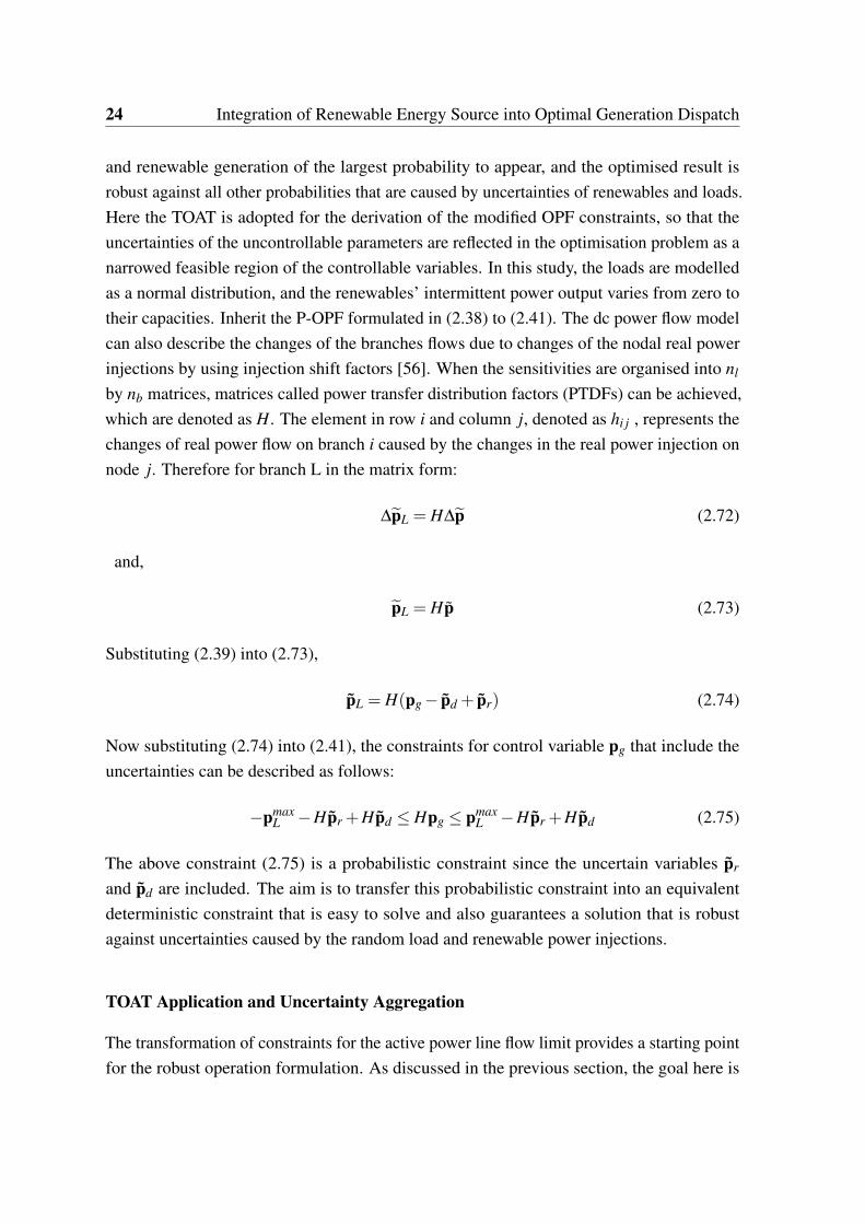
and renewable generation of the largest probability to appear, and the optimised result isrobust against all other probabilities that are caused by uncertainties of renewables and loads.Here the TOAT is adopted for the derivation of the modified OPF constraints, so that theuncertainties of the uncontrollable parameters are reflected in the optimisation problem as anarrowed feasible region of the controllable variables. In this study, the loads are modelledas a normal distribution, and the renewables’ intermittent power output varies from zero totheir capacities. Inherit the P-OPF formulated in (2.38) to (2.41). The dc power flow modelcan also describe the changes of the branches flows due to changes of the nodal real powerinjections by using injection shift factors [56]. When the sensitivities are organised into nl
by nb matrices, matrices called power transfer distribution factors (PTDFs) can be achieved,which are denoted as H. The element in row i and column j, denoted as hi j , represents thechanges of real power flow on branch i caused by the changes in the real power injection onnode j. Therefore for branch L in the matrix form:
∆pL = H∆p (2.72)
and,
pL = Hp (2.73)
Substituting (2.39) into (2.73),
pL = H(pg − pd + pr) (2.74)
Now substituting (2.74) into (2.41), the constraints for control variable pg that include theuncertainties can be described as follows:
−pmaxL −Hpr +Hpd ≤ Hpg ≤ pmax
L −Hpr +Hpd (2.75)
The above constraint (2.75) is a probabilistic constraint since the uncertain variables pr
and pd are included. The aim is to transfer this probabilistic constraint into an equivalentdeterministic constraint that is easy to solve and also guarantees a solution that is robustagainst uncertainties caused by the random load and renewable power injections.
TOAT Application and Uncertainty Aggregation
The transformation of constraints for the active power line flow limit provides a starting pointfor the robust operation formulation. As discussed in the previous section, the goal here is
2.5 Robust Security Constrained Optimal Power Flow Formulation and Solving Method 25
to transform this probabilistic constraint (2.75) into a deterministic equation. There are tworeasons for this:
• The first reason, as previously mentioned, is that the equivalent deterministic constraintis easy to solve and also guarantees a solution that is robust against uncertainties causedby the random load and renewable power injections.
• The second reason is that this approach can be well incorporated into the decompositiontechnique well, which is used later for security constraints formulation.
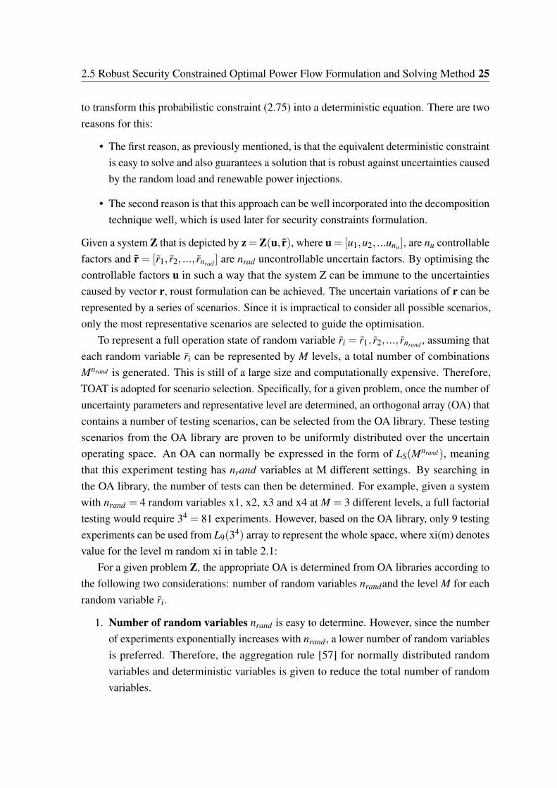
Given a system Z that is depicted by z=Z(u, r), where u= [u1,u2, ...unu], are nu controllablefactors and r = [r1, r2, ..., rnrad ] are nrad uncontrollable uncertain factors. By optimising thecontrollable factors u in such a way that the system Z can be immune to the uncertaintiescaused by vector r, roust formulation can be achieved. The uncertain variations of r can berepresented by a series of scenarios. Since it is impractical to consider all possible scenarios,only the most representative scenarios are selected to guide the optimisation.
To represent a full operation state of random variable ri = r1, r2, ..., rnrand , assuming thateach random variable ri can be represented by M levels, a total number of combinationsMnrand is generated. This is still of a large size and computationally expensive. Therefore,TOAT is adopted for scenario selection. Specifically, for a given problem, once the number ofuncertainty parameters and representative level are determined, an orthogonal array (OA) thatcontains a number of testing scenarios, can be selected from the OA library. These testingscenarios from the OA library are proven to be uniformly distributed over the uncertainoperating space. An OA can normally be expressed in the form of LS(Mnrand), meaningthat this experiment testing has nrand variables at M different settings. By searching inthe OA library, the number of tests can then be determined. For example, given a systemwith nrand = 4 random variables x1, x2, x3 and x4 at M = 3 different levels, a full factorialtesting would require 34 = 81 experiments. However, based on the OA library, only 9 testingexperiments can be used from L9(34) array to represent the whole space, where xi(m) denotesvalue for the level m random xi in table 2.1:
For a given problem Z, the appropriate OA is determined from OA libraries according tothe following two considerations: number of random variables nrandand the level M for eachrandom variable ri.
1. Number of random variables nrand is easy to determine. However, since the numberof experiments exponentially increases with nrand , a lower number of random variablesis preferred. Therefore, the aggregation rule [57] for normally distributed randomvariables and deterministic variables is given to reduce the total number of randomvariables.

26 Integration of Renewable Energy Source into Optimal Generation Dispatch
Table 2.1 L9(34) OA Array
Experimentnumber
Random variablex1
Random variablex2
Random variablex3
Random variablex4
1 x1(1) x2(1) x3(1) x4(1)2 x1(1) x2(2) x3(2) x4(2)3 x1(1) x2(3) x3(3) x4(3)4 x1(2) x2(1) x3(2) x4(3)5 x1(2) x2(2) x3(3) x4(1)6 x1(2) x2(3) x3(1) x4(2)7 x1(3) x2(1) x3(3) x4(2)8 x1(3) x2(2) x3(1) x4(3)9 x1(3) x2(3) x3(2) x4(1)
(a) If a random variable ri is normally distributed with mean µ(ri) and varianceσ2(ri), then a linear transformation r′ = ari +b is still a normal distribution withmean aµ(ri)+b and variance a2σ2(ri).
(b) If another random variable r j is normally distributed with mean µ(r j) and vari-ance σ2(r j),then a linear transformation r′′ = a1ri +a2r j is still a normal distri-bution with mean a1µ(ri)+a2µ(r j) and variance a2
1σ2(ri)+a22σ2(r j).
2. Number of levels M for each random variable. When designing testing experimentsfor the studied system Z, the number of levels M for each random variable ri and thevalue at each level need to be properly defined, so that the selected testing experimentscan cover the random space. Normally, if a random variable ri has a quadratic effect onZ, then M = 3 levels are selected for ri, and the corresponding values for these levels areµ(ri)−
√3/2σ(ri), µ(ri)+
√3/2σ(ri), and µ(ri) provided that ri is symmetrically
distributed. Moreover, if a random variable ri has a linear relation on Z, then M = 23levels are selected for ri, and the corresponding value for these levels are µ(ri)−σ(ri),µ(ri)+σ(ri), provided that ri is symmetrically distributed.
Transformation of Probabilistic Constraint by TOAT
Now looking back at (2.75), it is clear that both random variable vector pd and pr have alinear effect on (2.75). Therefore two levels are selected for pd and pr. By eliminating zeroelements in pg, pd and pr, the equation (2.75) can be transformed into:
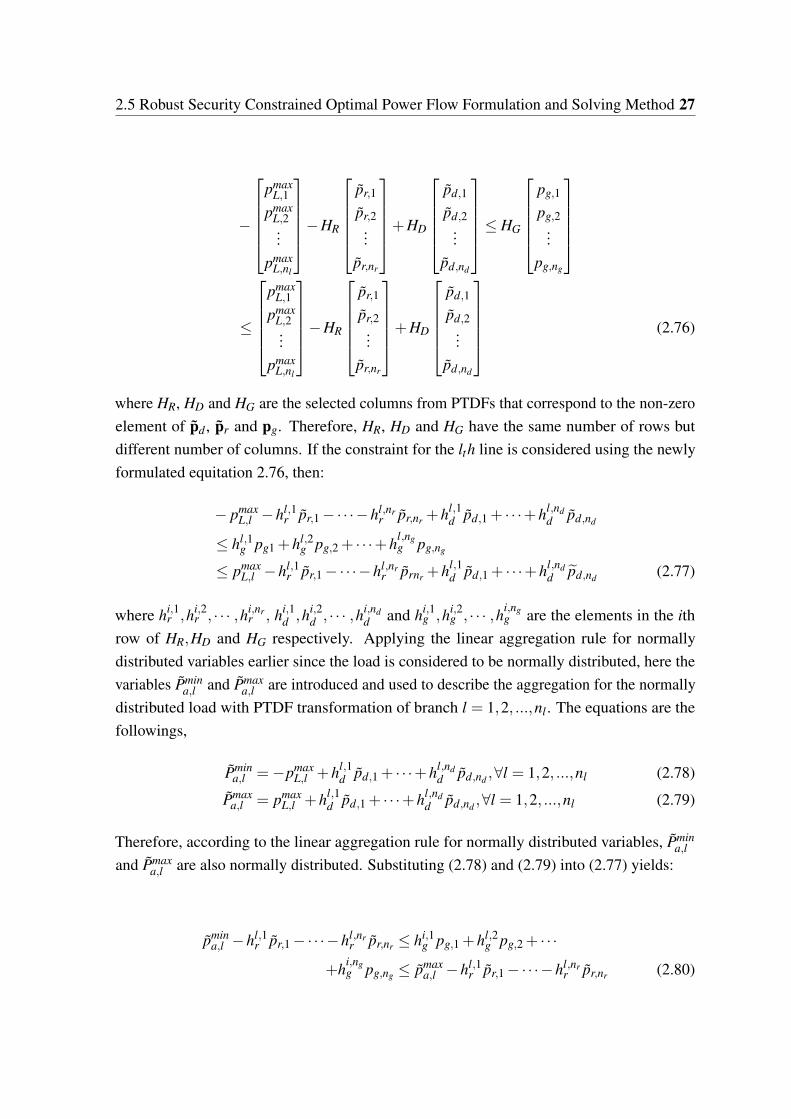
2.5 Robust Security Constrained Optimal Power Flow Formulation and Solving Method 27
−
pmax
L,1
pmaxL,2...
pmaxL,nl
−HR
pr,1
pr,2...
pr,nr
+HD
pd,1
pd,2...
pd,nd
≤ HG
pg,1
pg,2...
pg,ng
≤
pmax
L,1
pmaxL,2...
pmaxL,nl
−HR
pr,1
pr,2...
pr,nr
+HD
pd,1
pd,2...
pd,nd
(2.76)
where HR, HD and HG are the selected columns from PTDFs that correspond to the non-zeroelement of pd , pr and pg. Therefore, HR, HD and HG have the same number of rows butdifferent number of columns. If the constraint for the lth line is considered using the newlyformulated equitation 2.76, then:
− pmaxL,l −hl,1
r pr,1 −·· ·−hl,nrr pr,nr +hl,1
d pd,1 + · · ·+hl,ndd pd,nd
≤ hl,1g pg1 +hl,2
g pg,2 + · · ·+hl,ngg pg,ng
≤ pmaxL,l −hl,1
r pr,1 −·· ·−hl,nrr prnr +hl,1
d pd,1 + · · ·+hl,ndd pd,nd (2.77)
where hi,1r ,hi,2
r , · · · ,hi,nrr , hi,1
d ,hi,2d , · · · ,hi,nd
d and hi,1g ,hi,2
g , · · · ,hi,ngg are the elements in the ith
row of HR,HD and HG respectively. Applying the linear aggregation rule for normallydistributed variables earlier since the load is considered to be normally distributed, here thevariables Pmin
a,l and Pmaxa,l are introduced and used to describe the aggregation for the normally
distributed load with PTDF transformation of branch l = 1,2, ...,nl . The equations are thefollowings,
Pmina,l =−pmax
L,l +hl,1d pd,1 + · · ·+hl,nd
d pd,nd ,∀l = 1,2, ...,nl (2.78)
Pmaxa,l = pmax
L,l +hl,1d pd,1 + · · ·+hl,nd
d pd,nd ,∀l = 1,2, ...,nl (2.79)
Therefore, according to the linear aggregation rule for normally distributed variables, Pmina,l
and Pmaxa,l are also normally distributed. Substituting (2.78) and (2.79) into (2.77) yields:
pmina,l −hl,1
r pr,1 −·· ·−hl,nrr pr,nr ≤ hi,1
g pg,1 +hl,2g pg,2 + · · ·
+hi,ngg pg,ng ≤ pmax
a,l −hl,1r pr,1 −·· ·−hl,nr
r pr,nr (2.80)
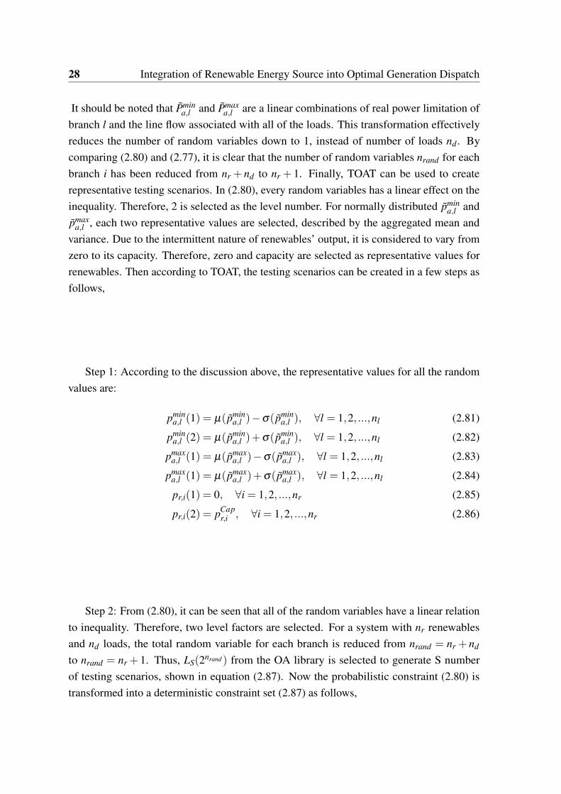
28 Integration of Renewable Energy Source into Optimal Generation Dispatch
It should be noted that Pmina,l and Pmax
a,l are a linear combinations of real power limitation ofbranch l and the line flow associated with all of the loads. This transformation effectivelyreduces the number of random variables down to 1, instead of number of loads nd . Bycomparing (2.80) and (2.77), it is clear that the number of random variables nrand for eachbranch i has been reduced from nr + nd to nr + 1. Finally, TOAT can be used to createrepresentative testing scenarios. In (2.80), every random variables has a linear effect on theinequality. Therefore, 2 is selected as the level number. For normally distributed pmin
a,l andpmax
a,l , each two representative values are selected, described by the aggregated mean andvariance. Due to the intermittent nature of renewables’ output, it is considered to vary fromzero to its capacity. Therefore, zero and capacity are selected as representative values forrenewables. Then according to TOAT, the testing scenarios can be created in a few steps asfollows,
Step 1: According to the discussion above, the representative values for all the randomvalues are:
pmina,l (1) = µ(pmin
a,l )−σ(pmina,l ), ∀l = 1,2, ...,nl (2.81)
pmina,l (2) = µ(pmin
a,l )+σ(pmina,l ), ∀l = 1,2, ...,nl (2.82)
pmaxa,l (1) = µ(pmax
a,l )−σ(pmaxa,l ), ∀l = 1,2, ...,nl (2.83)
pmaxa,l (1) = µ(pmax
a,l )+σ(pmaxa,l ), ∀l = 1,2, ...,nl (2.84)
pr,i(1) = 0, ∀i = 1,2, ...,nr (2.85)
pr,i(2) = pCapr,i , ∀i = 1,2, ...,nr (2.86)
Step 2: From (2.80), it can be seen that all of the random variables have a linear relationto inequality. Therefore, two level factors are selected. For a system with nr renewablesand nd loads, the total random variable for each branch is reduced from nrand = nr + nd
to nrand = nr + 1. Thus, LS(2nrand) from the OA library is selected to generate S numberof testing scenarios, shown in equation (2.87). Now the probabilistic constraint (2.80) istransformed into a deterministic constraint set (2.87) as follows,
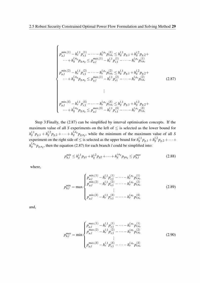
2.5 Robust Security Constrained Optimal Power Flow Formulation and Solving Method 29
pmin,(1)a,l −hl,1
r p(1)r,1 −·· ·−hl,nrr p(1)r,nr ≤ hl,1
g pg,1 +hi,2g pg,2+
· · ·+hl,ngg pg,ng ≤ pmax,(1)
a,l −hl,1r p(1)r,1 −·· ·−hl,nr
r p(1)r,nr
pmin,(2)a,l −hl,1
r p(2)r,1 −·· ·−hl,nrr p(2)r,nr ≤ hl,1
g pg,1 +hl,2g pg,2+
· · ·+hl,ngg pg,ng ≤ pmax,(1)
a,l −hl,1r p(2)r1 −·· ·−hl,nr
r p(2)r,nr
...
pmin,(S)a,l −hl,1
r p(S)r,1 −·· ·−hl,nrr p(S)r,nr ≤ hl,1
g pg,1 +hl,2g pg,2+
· · ·+hl,ngg pg,ng ≤ pmax,(S)
a,l −hl,1r p(S)r,1 −·· ·−hl,nr
r p(S)r,nr
(2.87)
Step 3:Finally, the (2.87) can be simplified by interval optimisation concepts. If themaximum value of all S experiments on the left of ≤ is selected as the lower bound forhl,1
g pg,1 + hl,2g pg,2 + · · ·+ hl,ng
g pg,ng , while the minimum of the maximum value of all Sexperiment on the right side of ≤ is selected as the upper bound for hl,1
g pg,1 +hl,2g pg,2 + · · ·+
hl,ngg pg,ng , then the equation (2.87) for each branch l could be simplified into:
pminh,l ≤ hi,1
g pg1 +hi,2g pg2 + · · ·+hi,ng
g pgng ≤ pmaxh,l (2.88)
where,
pminh,l = max
pmin,(1)
a,l −hl,1r p(1)r,1 −·· ·−hl,nr
r p(1)r,nr
pmin,(2)a,l −hl,1
r p(2)r,1 −·· ·−hl,nrr p(2)r,nr
...
pmin,(S)a,l −hl,1
r p(S)r,1 −·· ·−hl,nrr p(S)r,nr
(2.89)
and,
pmaxh,l = min
pmax,(1)
a,l −hl,1r p(1)r,1 −·· ·−hl,nr
r p(1)r,nr
pmax,(2)a,l −hl,1
r p(2)r,1 −·· ·−hi,nrr p(2)r,nr
...
pmax,(S)a,l −hl,1
r p(S)r,1 −·· ·−hl,nrr p(S)r,nr
(2.90)

30 Integration of Renewable Energy Source into Optimal Generation Dispatch
Thus, a robust constraint is created for the active power limitation for branch i. All of thetesting scenarios that were generated by TOAT are now simplified into two cases pmax
h,l andpmin
h,l . Applying this for all branches i = 1,2, ...,nl , the final constraint for HGpg in matrixform is achieved,
pminH ≤ HGpg ≤ pmax
H (2.91)
The inequality constraint (2.88) and (2.91) are deterministic constraints that are without anyrandom variables. Therefore, in three steps, the probabilistic constraint (2.75) is approximatedinto a deterministic constraint (2.91).
Robust OPF Transformation and Formulation
Finally, after the transformation according to constraint (2.41), the robust OPF is formulatedas follows,
Objective:
minimiseng
∑i=1
(ai pg,i2 +bi pg,i + ci) (2.92)
Subject to:
p = pg −pρmax
d +pρmax
r (2.93)
pming ≤ pg ≤ pcap
g (2.94)
pminH ≤ HGpg ≤ pmax
H (2.95)
where pρmax
d and pρmax
r are the most probable values for load and renewable generationrespectively, and generally forecast values can be used.
The above formulated OPF is an equivalent deterministic OPF that can be solved easily.Compare (2.92)-(2.95) to (2.34) and to (2.37), the most significant change is the considerationof constraint (2.95). Another noticeable change is the way in which the renewable generationoutput and load are considered in both problems. In (2.34) to (2.37), PR and PD are taken asdeterministic values, for instance as the most probable value. The optimised result p∗
g fromsuch formulation would most likely lead to overflows on branches, if there was an offsetbetween the real output and renewables from the predicted value. It should be noted that thesolution space from (2.95) is the common solution space from (2.37) for probable scenarios.
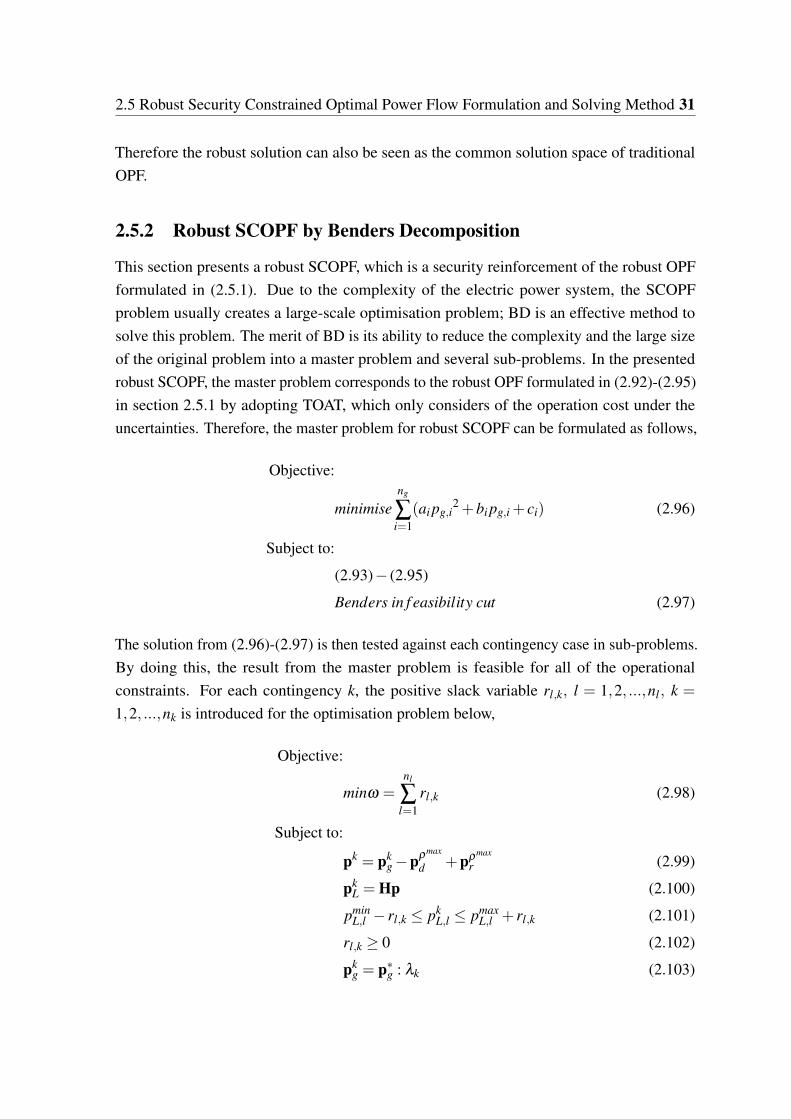
2.5 Robust Security Constrained Optimal Power Flow Formulation and Solving Method 31
Therefore the robust solution can also be seen as the common solution space of traditionalOPF.
2.5.2 Robust SCOPF by Benders Decomposition
This section presents a robust SCOPF, which is a security reinforcement of the robust OPFformulated in (2.5.1). Due to the complexity of the electric power system, the SCOPFproblem usually creates a large-scale optimisation problem; BD is an effective method tosolve this problem. The merit of BD is its ability to reduce the complexity and the large sizeof the original problem into a master problem and several sub-problems. In the presentedrobust SCOPF, the master problem corresponds to the robust OPF formulated in (2.92)-(2.95)in section 2.5.1 by adopting TOAT, which only considers of the operation cost under theuncertainties. Therefore, the master problem for robust SCOPF can be formulated as follows,
Objective:
minimiseng
∑i=1
(ai pg,i2 +bi pg,i + ci) (2.96)
Subject to:
(2.93)− (2.95)
Benders in f easibility cut (2.97)
The solution from (2.96)-(2.97) is then tested against each contingency case in sub-problems.By doing this, the result from the master problem is feasible for all of the operationalconstraints. For each contingency k, the positive slack variable rl,k, l = 1,2, ...,nl, k =
1,2, ...,nk is introduced for the optimisation problem below,
Objective:
minω =nl
∑l=1
rl,k (2.98)
Subject to:
pk = pkg −pρmax
d +pρmax
r (2.99)
pkL = Hp (2.100)
pminL,l − rl,k ≤ pk
L,l ≤ pmaxL,l + rl,k (2.101)
rl,k ≥ 0 (2.102)
pkg = p∗
g : λk (2.103)

32 Integration of Renewable Energy Source into Optimal Generation Dispatch
In the subproblem for each contingency, the Lagrangian coefficient λk and correspondingvalue pk
g are calculated. If ω > 0 , the Benders cut is formed according to the λk and addedback to the master problem (2.97). The sub-problem then is updated in each iteration whichleads to adjustments on the controllable variables in the master problem, until the procedureconverge. The Benders cut can be given as:
ω∗+λk(pg −p∗
g)≤ 0, (2.104)
The whole robust SCOPF computation is illustrated in figure 2.1 The above SCOPF formula-tion is based on the robust OPF formulated in section 2.5.1. Therefore, the robustness againstthe uncertain variables is first given from the master problem, and then tested against eachcontingency using N-1 contingency analysis, as shown in figure 2.1. Since the linearisedmodel is adopted to approximate the power flow model, the whole robust SCOPF is convexand able to converge efficiently. This chapter mainly focuses on the structure of robustSCOPF formulation, where only the PC action is considered for security control. Numericalsimulations are conducted on the modified IEEE 14-bus system and IEEE 118-bus system todemonstrate the effectiveness of the presented approach.
2.6 Numerical Simulation
The robust SCOPF model is verified on the modified IEEE 14-bus and IEEE 118-bus systems.The algorithm is programmed in MATLAB and the system data is from MATPOWERpackage. The simulations were carried out on a Intel Core I5 CPU at 3.20GHz with 4.00GBof RAM. The OPF and power flow are solved using the MATPOWER package. The result ofthe robustness SCOPF is compared tothe traditional OPF in terms of the robust degree andgeneration cost. The testing scenarios are generated by MCS with 50000 scenarios.
The interior point method is adopted to solve the OPF problem. The renewable resourcesare assumed as wind farms, installed in selected nodes. The Weibull distribution has beenused to describe the wind speed in various studies, usually with the parameters of usingβw = 11.0086 and kw=1.9622. For v > 0 the wind speed PDF model is as follows:
f (v,βw,kw) =kw
βw(
vβw
)kw−1e−v
βwkw
(2.105)
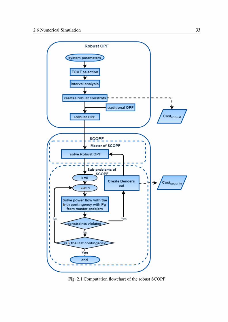
2.6 Numerical Simulation 33
Fig. 2.1 Computation flowchart of the robust SCOPF

34 Integration of Renewable Energy Source into Optimal Generation Dispatch
and the wind turbine power is simulated using:
pr =
prate(v− vci)/(vrate − vci) vci ≤ v ≤ vrate
prate vrate ≤ v ≤ vco
0 otherwise(2.106)
During the simulation, the load is treated as normally distributed with the mean value ofthe original load value from the given system, whose deviation is assume to be 5% of themean.
2.6.1 Simulation on the IEEE 14-bus System
This system consists of nb =14 buses, ng =5 generation units, nd =11 loads and nl =20branches; therefore the ‘N-1’ security checks contain k =25 scenarios. The traditionalgenerators are taken as controllable variables, whose generation limits and cost functions arethe default values from the MATPOWER case14. The maximum branch active power flowfor branches 1 and 7 are 80MW; for branches 3 and 6 are 50MW; for branches 17 to 20 are20 MW; and rest 40MW. Two wind farms (nr = 2) rated at 40MW are connected to bus 2and bus 3, respectively. The total number of uncertainties of this system is nran = nd +nr,which is 13. Applying the linear aggregation rule for normal distributed variables (2.78) and(2.79), the number of uncertainties is reduced to nr +1 = 3. Therefore L4(23) is selected,which leads to S = 4 scenarios, as follows,
L4(23) =
1 1 11 2 22 1 22 2 1
(2.107)
Therefore, taking the lower bound for example, four testing experiments can be constructedusing variables pmin
a,l , pr,1, and pr2, and each of two levels:
pmina,l (1) = µ(pmin
a,l )−σ(pmina,l ) (2.108)
pmina,l (2) = µ(pmin
a,l )+σ(pmina,l ) (2.109)
pr,1(1) = 0 (2.110)
pr,1(2) = 40MW (2.111)
pr,2(1) = 0 (2.112)
pr,2(2) = 40MW (2.113)

2.6 Numerical Simulation 35
Table 2.2 Results for the IEEE14-Bus System
RobustSCOPF
Cost (103$/h) 5.657Robust Degree (%) 99.47
No. Security Constraints for PC4(L4−5, L4−9L5−6, G4)
TraditionalOPF
Cost (103/h) 5.17Robust Degree(%) 4.48
and therefore the OA used to create the lower bound for branch i for the given simulation is:
L4(23) =
pmin
a,l (1) 0 0pmin
a,l (1) 40 40pmin
a,l (2) 0 40pmin
a,l (2) 40 0
(2.114)
The constraints (2.88) can then be created for robust OPF once the values of pminh,l and pmax
h,l
are determined.Next, 25 ‘N-1’ security tests are conducted in addition to the robust OPF, where Benders
infeasibility cuts are created as PCs if there is a violation of branch flow limits. The resultstested against 50000 MCS scenarios are shown in table 2.2. where the robust degree η isdefined as,
η =S f easible
S×100% (2.115)
where S f easible is the number of scenarios without violations, and S is the total number ofscenarios.
It can be observed that the minimum operation cost of robust OPF is higher than thatof traditional OPF by 487$/h, 84% of which is from the robust requirement and the restfrom the security constraints. However, the results demonstrate the significance of the robustdegree, as the solution from traditional OPF only has 4.48 % feasibility against uncertainties.
2.6.2 Simulation on the IEEE 118-Bus System
The IEEE 118-bus system consists of nb =118 buses, ng =54 generation units and nl =186branches, therefore the ‘N-1’ security checks contain k =240 scenarios. The maximumbranch active power flow limit from node 8 to node 9 and node 9 to node 10 is set as550MW; from node 8 to node 5 as 500MW; and for the rest as 280 MW. Five wind farms(nr = 5) rated at 200MW are connected to bus 16, bus 37, bus 48, bus 75 and bus 83
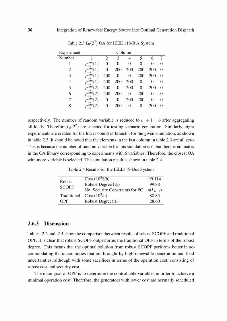
36 Integration of Renewable Energy Source into Optimal Generation Dispatch
Table 2.3 L8(27) OA for IEEE 118-Bus System
ExperimentNumber
Column1 2 3 4 5 6 7
1 pmina,l (1) 0 0 0 0 0 0
2 pmina,l (1) 0 200 200 200 200 0
3 pmina,l (1) 200 0 0 200 200 0
4 pmina,l (1) 200 200 200 0 0 0
5 pmina,l (2) 200 0 200 0 200 0
6 pmina,l (2) 200 200 0 200 0 0
7 pmina,l (2) 0 0 200 200 0 0
8 pmina,l (2) 0 200 0 0 200 0
respectively. The number of random variable is reduced to nr + 1 = 6 after aggregatingall loads. Therefore,L8(27) are selected for testing scenario generation. Similarly, eightexperiments are created for the lower bound of branch i for the given simulation, as shownin table 2.3. it should be noted that the elements in the last column in table 2.3 are all zero.This is because the number of random variable for this simulation is 6, but there is no matrixin the OA library corresponding to experiments with 6 variables. Therefore, the closest OAwith more variable is selected. The simulation result is shown in table 2.4.
Table 2.4 Results for the IEEE118-Bus System
RobustSCOPF
Cost (103$/h) 99.114Robust Degree (%) 99.88No. Security Constraints for PC 4(L4−5)
TraditionalOPF
Cost (103/h) 88.85Robust Degree(%) 28.60
2.6.3 Discussion
Tables 2.2 and 2.4 show the comparison between results of robust SCOPF and traditionalOPF. It is clear that robust SCOPF outperforms the traditional OPF in terms of the robustdegree. This means that the optimal solution from robust SCOPF performs better in ac-commodating the uncertainties that are brought by high renewable penetration and loaduncertainties, although with some sacrifices in terms of the operation cost, consisting ofrobust cost and security cost.
The main goal of OPF is to determine the controllable variables in order to achieve aminimal operation cost. Therefore, the generators with lower cost are normally scheduled

2.7 Conclusion 37
with higher output. However, constraints such as branch flow limit affect the results, so thatthe generator with the lowest cost does not normally operate at its full capacity. The presentedrobust SCOPF actually incorporates the uncertainties into the branch flow limitation usingPTDF and approaches such as scenario reduction and interval optimisation.
2.7 Conclusion
Using a robust SCOPF model, this chapter has presented a new efficient approach to addressthe uncertain factors caused by load demand and renewable generation in power system ispresented in this chapter, via a robust SCOPF model. The robust SCOPF algorithm is notonly capable of satisfying the security requirements, but is also robust against uncertainrenewable generation output and load demand. The algorithm is able to achieve a balancebetween representativeness, economic efficiency, and computation efficiency. Moreover, theuncertainties are incorporate into the OPF problem in such a way that the formulated modelcan be seen as a deterministic equivalent OPF model. Furthermore, the approach could bea useful tool to estimate the relative costs to secure a given system against uncertaintiesfrom RESs and load, costs to secure the system from contingencies, or both. The numericalsimulations have demonstrated the effectiveness of the presented algorithm. In addition, thecomputational burden can be further alleviated by facilitating the grid computation techniquessince the problems can easily be decomposed. In conclusion, this chapter has introduced ageneral framework to efficiently integrate the uncertainties from the RESs into a steady stateanalysis in the forms of SCOPF. However, a few more points need to be further analysed.First, the linearised OPF model in this chapter neglects some system operating constraintssuch as voltage and reactive power limits, which needs to be addressed in the followingchapters. Second, new large-scale RESs tend to be built remotely and expansion on existingtransmission network is worth considering in the modelling. Moreover, RESs exist in theelectricity grid in various forms and different levels. Therefore, it is also worth examiningrecent developments of RESs in sub-transmission systems and on the demand side. Finally,only PC is considered in the contingency control in this chapter, which is considered to beconservative in the long term. The following chapters investigate the competition betweenCC and PC actions as well.
Chapter 3
Hierarchical SCOPF Considering WindEnergy Integration throughMulti-Terminal VSC-HVDC Grids
This chapter discusses two topics. First, in addition to its intermittent nature, renewablegeneration is also affected by high meteorological and geographical impacts, which meansthat large-scale renewable generation farm away from load centres and expansion on existingtransmission are needed. High-voltage direct current (HVDC) transmission systems offerunique benefits in terms of economy, capacity and distance, and this is why HVDC has beenused as a new form to transmit power from off shore large-scale renewable energy generation.Therefore this chapter first examines the question of how an operation and control structureof a meshed ac and HVDC grid is designed and constructed. Second, it then discusses howto efficiently coordinates the offshore renewable generation into the inland ac electricity gridoperation, via a hierarchical SCOPF model considering large scale offshore wind energyintegration through multi-terminal voltage source converter-HVDC(VSC-HVDC) grids. Thischapter is based on [58, 59].
3.1 Introduction
With the development of large scale offshore wind farms and floating photovoltaics farms,MTDC systems have drawn significant attention in interconnecting the renewable energy tothe main ac grid. It is becoming increasingly important to consider the injection of the offshore renewable generation into the main ac power system in the economic operation. In themeantime requirements such as making the control strategies robust against the uncertainties

40Hierarchical SCOPF Considering Wind Energy Integration through Multi-Terminal
VSC-HVDC Grids
caused by the intermittency of renewables, have been considered to be of great significanceto the electricity network reliability.
Although HVDC technology has traditionally been restricted to the transmission of powerbetween two points on the ac grid, connecting wind farms through MTDC grids offersseveral advantages, such as increased reliability of power transmission, improved balanceservice across ac interconnections and reduced generation variability. Given that MTDCgrids offer unique capability in terms of regulating power flow, the meshed ac/HVDC systemscan be operated more flexibly and cost effectively. Currently, wind is treated as a negativeload, and supply is tailored to match the random demand [60]. Therefore, many technicalissues must be addressed [61, 62] to connect offshore wind farms using MTDC grids. Totake advantage of applying MTDC grids to support ac system operation and wind energyintegration, extensive research has been directed towards the modelling, control and operationof mixed ac/dc systems [63], in terms of system modelling, power flow modelling, windpower integration and optimal dispatching computation.
The previous chapter two introduced a framework to incorporate renewable energygeneration into the security constrained OPF with efficient computation approach. However,two aspects need further review. First, the renewable generation is assumed to be installedwithin the existing transmission infrastructure, and connected directly back to the electricitygrid, which is also assumed to be operated by the transmission system operators. In thischapter, this assumption is examined by modelling offshore wind farms that are connectedby VSCs. Each wind farm is operated by an individual energy plant owner, which wouldhave an effect on the problem formulation structure. Second, the chapter also examinesthe contingency control strategies. For simplicity, PC was the only strategy adopted inthe previous chapter, in contrast, the present chapter investigates how to coordinate CCeffectively with PC under the structure of SCOPF model considering large-scale offshorewind farms through a multi-terminal VSC-connected ac/HVDC system. Finally, although thedc power flow or linearised power flow model has its advantage in computation efficiency,neglecting constraints on variables such as voltage and reactive power might lead the solutionfrom linearised power flow model to be infeasible in real-world operations. This chapterdescribes the approach of using dc OPF combined with an ac power flow check via BD forimproved computation efficiency and better security.

3.2 Combined Ac and Multi-Terminal HVDC Grids 41
3.2 Combined Ac and Multi-Terminal HVDC Grids
3.2.1 Ac versus Dc
The devision between ac and dc systems began in the late 19th century, when it was notfeasible to integrate both systems with the technology available at the time. The ac systemdominated the industry for a long time, and it was not until the early 20th century that the dcsystem started to come back. The first commercial dc link was initially operated in 1954 toconnect the island of Gotland with mainland Sweden. This inspired much dc system researchand many projects. With the developmemnt of converter technologies, today numerousMTDC grid projects connecting offshore floating renewable generations are observed allaround the world. There has been offshore wind generation with an operating capacityof 3,813MW in total in relatively shallow waters around the United Kingdom, Germany,Denmark, Belgium and so on [64, 65]. Similar growth has also been seen in China, Canada,and the United States (US) in recent years.
One important concern associated with the deployment of offshore wind generation isthe cost of building the long distance of transmission lines to deliver the generated energy tothe load centres. In recent years, there has been an increasing interest in building MTDC[66–68] systems driven by the grid integration of remotely located wind energy. The totalcost of building dc cable connections is cheaper, with around 300-600 miles’ breakevendistance [69] for overhead lines. Therefore, HVDC systems are significantly beneficialfor large amount power transmission at large distances. However, existing transmissionsystems are HVAC dominant, and it is therefore crucial to study approaches to increase thetransmission efficiency of existing HVAC networks with newly added HVDC systems. Oneapproach is to find a proper modification of HVAC systems and connected remote renewablegenerations in the HVDC system through converters, so that this meshed interconnectioncan effectively share the diverse portfolio of intermittent resources and increase operationalflexibility. However expanding renewable energy such as wind power mainly from windresources poses a number of unique challenges because its generation output is inherentlyintermittent. Uncertainties raised by with RESs due to their intermittent nature threatenthe system’s reliable operation. As more wind resources are brought online, it is becomingincreasingly critical to consider the integration of offshore RESs into the economic operationof main grids. Therefore requirements such as making the control strategies robust againstthe uncertainties caused by the intermittency of renewables have been considered to be ofgreat significance to the electricity network reliability.
42Hierarchical SCOPF Considering Wind Energy Integration through Multi-Terminal
VSC-HVDC Grids
3.2.2 Operation Schemes
In general, HVDC systems connecting the offshore renewable generation are expansionson top of existing transmission systems. Normally, transmission systems operators areresponsible for operating the grids and coordinating with other adjacent transmission systems.The new HVDC transmission in the electricity grid not only provides power injections to theentire grid, but might also have a significant impact on the power flow directions in wholenetwork, causing difficulties in operation and the possibility of violating network constraints.A well-designed coordination strategy and a clearly defined responsibility for different typesof operators could be beneficial to reduce such risks.
Three operating schemes are introduced in [70] for a mixed HVAC-HVDC system. Theseare the supper independent system operator, the technology separated independent systemoperator and the geographically separated independent system operator. In this thesis, theoperating schemes are categorised into two types according to the information accessibilityof each system operator, namely centralised operation scheme and the distributed operationscheme. This in turn shapes the formulation of the system power flow problem.
Centralised Scheme
The centralised scheme requires that a system operator have the knowledge of the wholesystem, including both ac and HVDC systems. In this scenario, data are sent to a centralauthority that is able to conduct an optimisation based on all of the system’s requirementinformation. The control signal can then reach all components in the entire system.
The advantage of such a scheme is clear: since information over the entire ac and dcgrid is known, an optimisation problem can be easily formulated such as OPF problem tominimise operation costs, or to minimise overall losses. However, the drawback of such ascheme is the formulated problem size and complexity, especially when both uncertaintiesand security requirements are considered.
Distributed Scheme and Independent System Operator
Alternatively, different system operators can be responsible for ac and dc grids. For a newHVDC system, a new system operator can be organised so that it operates and controls theinformation of the HVDC system and only shares partial knowledge with the ac systemoperators for coordination purposes. In this case, the optimisation problem such as the OPFproblem needs to be carefully formulated, and the limitation on the control signals needs tobe addressed. The computation complexity is reduced and the solution is normally achievediteratively by using the repeated exchange of information.
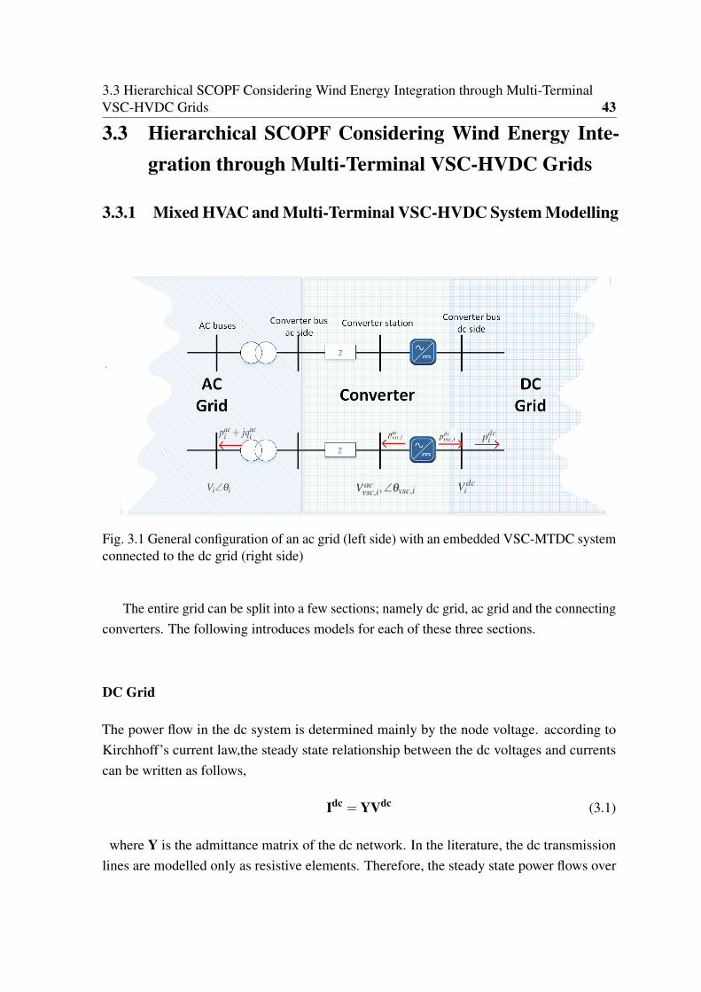
3.3 Hierarchical SCOPF Considering Wind Energy Integration through Multi-TerminalVSC-HVDC Grids 43
3.3 Hierarchical SCOPF Considering Wind Energy Inte-gration through Multi-Terminal VSC-HVDC Grids
3.3.1 Mixed HVAC and Multi-Terminal VSC-HVDC System Modelling
Fig. 3.1 General configuration of an ac grid (left side) with an embedded VSC-MTDC systemconnected to the dc grid (right side)
The entire grid can be split into a few sections; namely dc grid, ac grid and the connectingconverters. The following introduces models for each of these three sections.
DC Grid
The power flow in the dc system is determined mainly by the node voltage. according toKirchhoff’s current law,the steady state relationship between the dc voltages and currentscan be written as follows,
Idc = YVdc (3.1)
where Y is the admittance matrix of the dc network. In the literature, the dc transmissionlines are modelled only as resistive elements. Therefore, the steady state power flows over

44Hierarchical SCOPF Considering Wind Energy Integration through Multi-Terminal
VSC-HVDC Grids
the lines from node i and node j can be calculated as follows,
pdci j =
V dci −V dc
j
ri j(3.2)
where V dci and V dc
j are the voltage deviation from the reference bus and ri j denotes the lineresistance between node i and j. The active power injection on node i in the MTDC systemcan be written as,
pdci =V dc
i
ndcb
∑j=1
Yi jV dcj . (3.3)
and the active power flow on the branch from node i to node j is
pdci j =V dc
i Yi j(V dcj −V dc
i ) (3.4)
Ac System
The modelling of the ac system was described in Chapter 2, and is therefore not repeatedhere.
Converter Modelling
The VSC is modelled as an ac voltage source that is connected to a dc voltage source. Theconverter can be modelled by an ac side and a dc side. For the ac side, the active power pac
vsc,c
and reactive power qvsc,c can be controlled by controlling the voltage magnitude V acvsc,c and
the voltage angle θvsc,c. On the dc side, the voltage V dcvsc can be controlled within its limits to
control the power flow. For a lossless VSC, the power balance equation couples the ac anddc systems together, as follows:
pacvsc,c = ηt pdc
vsc,c,∀c = 1,2, ...,nvsc (3.5)
where ηt indicates transmission and conversion efficiency and thus for a system neglectslosses ηt = 1.

3.3 Hierarchical SCOPF Considering Wind Energy Integration through Multi-TerminalVSC-HVDC Grids 45
3.3.2 Security Constrained Optimal Power Flow with Two Levels
PC and CC SCOPF are two types of control strategies to deal with credible contingenciesto ensure that the system can either withstand or recover from faults. Although PC cansecure the system against all contingencies, the strategy is normally viewed as conservativein that it leads to a higher operational cost. Various approaches focus on CC actions toalleviate post-contingency overloads, such as generation redispatch and load curtailment.The objective of a SCOPF algorithm is to minimise the total generation cost in addition to thesecurity control cost, which includes both PC and CC costs. PC costs may be included in theSCOPF objective function during the initial scheduling stage. On the other hand, CC costsnormally refer to the expected costs, for they are probably related. Moreover, PC costs canbe predetermined using known information regarding generator cost coefficients, whereasCC costs vary with selected actions during the post-contingency period. A cost-efficientand readily available CC strategy, such as adopting MTDC to coordinate terminal powerinjections by redistributing wind power generated in the system, offers great potential forefficient CC actions. The operation scheme for the HVAC and MTDC system in this chapteradopts a distributed structure, as described in the previous section. The introduced schememakes use of the power flow control capability of MTDC grids to provide support for acsystems, so that the ac/dc system can be operated in a cost-effective way. A two-layerinteraction is designed for the SCOPF so that limited information is exchanged between twosystem operators. The hierarchical dispatch scheme is a particularly attractive method ofproblem decomposition as it provided a highly intuitive system redispatch architecture.
Security Constrained Optimal Power Flow in Ac System
The SCOPF in the ac system adopts the structure of (2.59)-(2.64), which promotes post-contingency control strategy. The control variables vector u and state variables vector v inthe SCOPF for the ac system are given as follows,
zk =
[uk
vk
](3.6)
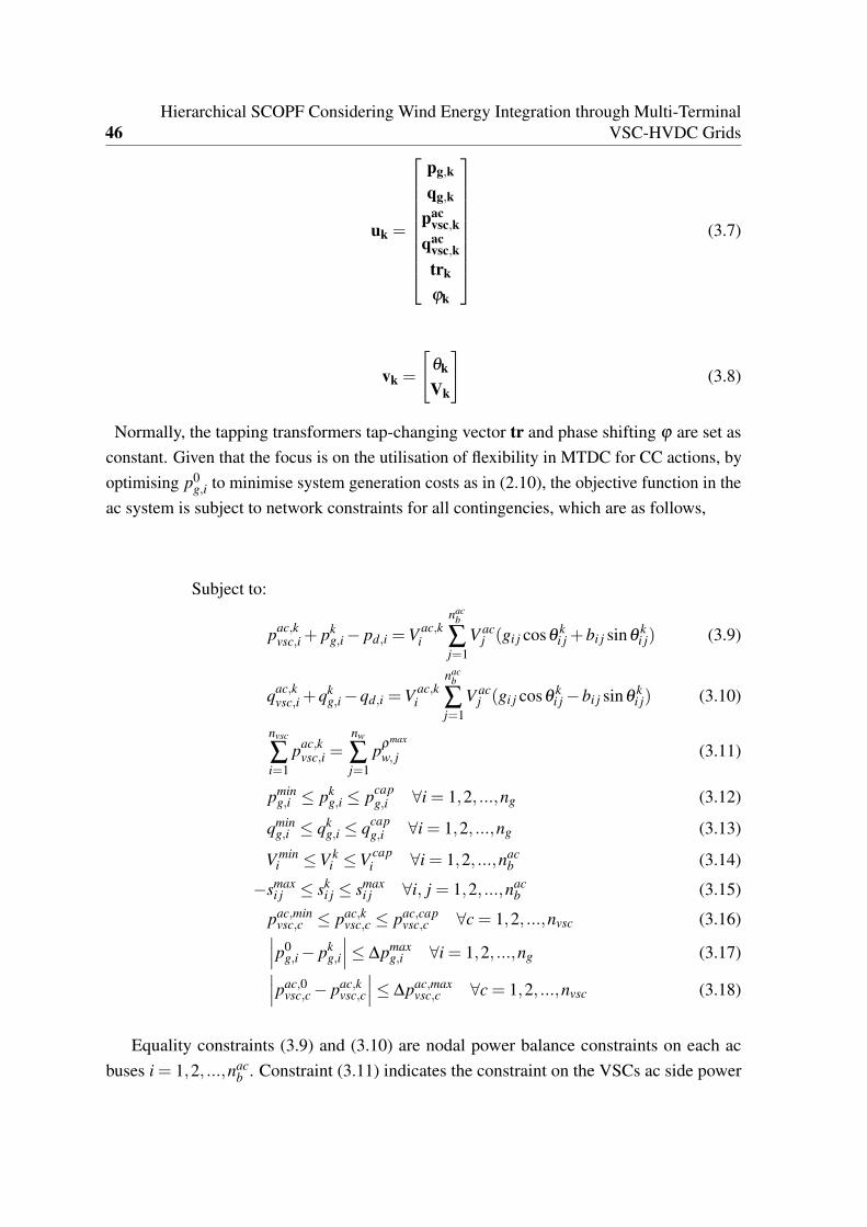
46Hierarchical SCOPF Considering Wind Energy Integration through Multi-Terminal
VSC-HVDC Grids
uk =
pg,k
qg,k
pacvsc,k
qacvsc,ktrk
ϕk
(3.7)
vk =
[θk
Vk
](3.8)
Normally, the tapping transformers tap-changing vector tr and phase shifting ϕ are set asconstant. Given that the focus is on the utilisation of flexibility in MTDC for CC actions, byoptimising p0
g,i to minimise system generation costs as in (2.10), the objective function in theac system is subject to network constraints for all contingencies, which are as follows,
Subject to:
pac,kvsc,i + pk
g,i − pd,i =V ac,ki
nacb
∑j=1
V acj (gi j cosθ
ki j +bi j sinθ
ki j) (3.9)
qac,kvsc,i +qk
g,i −qd,i =V ac,ki
nacb
∑j=1
V acj (gi j cosθ
ki j −bi j sinθ
ki j) (3.10)
nvsc
∑i=1
pac,kvsc,i =
nw
∑j=1
pρmax
w, j (3.11)
pming,i ≤ pk
g,i ≤ pcapg,i ∀i = 1,2, ...,ng (3.12)
qming,i ≤ qk
g,i ≤ qcapg,i ∀i = 1,2, ...,ng (3.13)
V mini ≤V k
i ≤V capi ∀i = 1,2, ...,nac
b (3.14)
−smaxi j ≤ sk
i j ≤ smaxi j ∀i, j = 1,2, ...,nac
b (3.15)
pac,minvsc,c ≤ pac,k
vsc,c ≤ pac,capvsc,c ∀c = 1,2, ...,nvsc (3.16)∣∣∣p0
g,i − pkg,i
∣∣∣≤ ∆pmaxg,i ∀i = 1,2, ...,ng (3.17)∣∣∣pac,0
vsc,c − pac,kvsc,c
∣∣∣≤ ∆pac,maxvsc,c ∀c = 1,2, ...,nvsc (3.18)
Equality constraints (3.9) and (3.10) are nodal power balance constraints on each acbuses i = 1,2, ...,nac
b . Constraint (3.11) indicates the constraint on the VSCs ac side power

3.3 Hierarchical SCOPF Considering Wind Energy Integration through Multi-TerminalVSC-HVDC Grids 47
injections, for which the sum of the power injection equals the forecast converter wind powergeneration delivered from the HVDC system to VSCs. pρmax
w, j denotes the most probablewind generation. The inequality constraints (3.12) to (3.16) are the operation limits on activepower generation limits, reactive generation limits, voltage limits, branch line flow limitsin the ac system, and VSCs’ power ratings, respectively. (3.17) and (3.18) are couplingconstraints on pk
g,i and pkvsc,c to avoid unrealistic movements in CC actions. (3.17) and (3.18)
correspond to coupling constraint (2.55). Normally, the problem can be considered a PC-CCSCOPF by selecting different ∆uk, where ∆u = Tkd∆uk/dt ∀k = 1,2, . . . ,nk. The couplingconstraint (2.55) indicates that the controllable variable u0 can be moved from u0 to uk
within bounds to satisfy the post-contingency constraints. Therefore, by setting ∆u = 0, theproblem becomes a pure PC-OPF. It should be noted that CC costs are not included in theobjective function, as post-contingency control variable uk is not included in the objectivefunction. Therefore, the formulated objective function can maximise the number of postcontingency control actions, and the ability of MTDC in post-contingency control can thenbe evaluated. Furthermore, as CC costs are incurred when contingency happens, there is aslight possibility that this approach may lead to a higher overall estimated control cost. Theformulation of the SCOPF in the ac grid is able to determine the optimised values of pac,0
g,i
and pac,0vsc,c using the given forecast information on remote wind farm generation, and pac,0
vsc,c isthe reference information announced to the HVDC system operator for OPF computation inthe HVDC system.
Optimal Power Flow in the Dc System
In this thesis, a distributed operation scheme is assumed, where the HVDC system is managedand operated by the HVDC system operator. Therefore, the ac system operation only haslimited information from the HVDC system operator to coordinaten the optimal dispatchdecision-making process. The HVDC system power dispatching is then regulates the powertransmitted to the VSC terminals by determining the converter dc sides’ droop gains with afixed active power set point, according to the reference power injection required from theac grid. Wind farms are assumed to be connected to the HVDC system with wind voltagesource converter (WVSC), which is regulated as a voltage source.
Assuming that the loss through WVSC is neglected and the power injected from thewind farm side is based on the real wind power generation, the active power from theWVSC injected into the MTDC grid pdc
i , i = 1,2, ...,nw equals to the wind power generationpw,i, i = 1,2, ...,nw. Then using dc voltage droop control, the active power flow at eachgrid-side voltage source converter(GVSC) pdc
i , i = nw +1,nw +2, ...,ndcb can be controlled
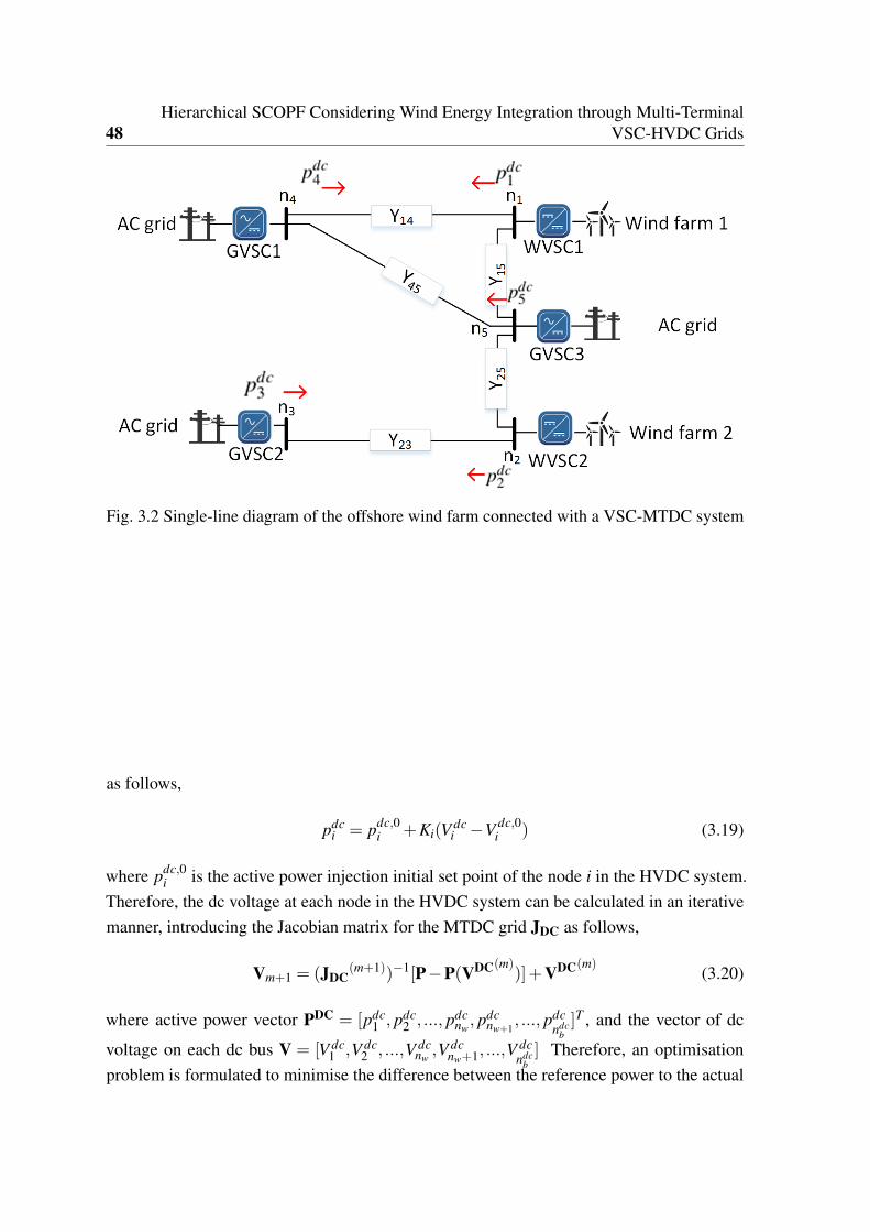
48Hierarchical SCOPF Considering Wind Energy Integration through Multi-Terminal
VSC-HVDC Grids
Fig. 3.2 Single-line diagram of the offshore wind farm connected with a VSC-MTDC system
as follows,
pdci = pdc,0
i +Ki(V dci −V dc,0
i ) (3.19)
where pdc,0i is the active power injection initial set point of the node i in the HVDC system.
Therefore, the dc voltage at each node in the HVDC system can be calculated in an iterativemanner, introducing the Jacobian matrix for the MTDC grid JDC as follows,
Vm+1 = (JDC(m+1))−1[P−P(VDC(m)
)]+VDC(m)(3.20)
where active power vector PDC = [pdc1 , pdc
2 , ..., pdcnw, pdc
nw+1, ..., pdc
ndcb]T , and the vector of dc
voltage on each dc bus V = [V dc1 ,V dc
2 , ...,V dcnw,V dc
nw+1, ...,Vdcndc
b] Therefore, an optimisation
problem is formulated to minimise the difference between the reference power to the actual

3.3 Hierarchical SCOPF Considering Wind Energy Integration through Multi-TerminalVSC-HVDC Grids 49
power injection at each MTDC GVSC terminal as follows,
Objective:
minimisendc
∑i=nw+1
∣∣∣pdcvsc,i − pdc,re f
vsc,i
∣∣∣ (3.21)
Subject to:
Ki ≤ Ki ≤ Ki (3.22)
Vi ≤Vi ≤Vi (3.23)
−idci j ≤ idc
i j ≤ idci j (3.24)
By optimising (3.24), the actual power output pdci can be set close to the required value,
within limitations on the droop constants (3.22), converter dc voltage level limits (3.23) andthe cable rating on the dc cables (3.24).
3.3.3 Benders Decomposition for N-1 Contingency Analysis in the TwoLevel Framework
In this study, both PC and CC are computed through BD as introduced in Chapter 2. Thisapproach has been successfully applied to take advantage of underlying problem structuresfor various optimisation problems. Master problem as base case k = 0:
Objective:
minimiseng
∑i=1
(ai(pac,0g,i )2 +bi p
ac,0g,i + ci) (3.25)
Subject to:
pac,0vsc,i + p0
g,i − pd,i = p0i ∀i = 1,2, ...,nac
b (3.26)nvsc
∑c=1
pac,0vsc,c =
nw
∑j=1
pρmax
w, j (3.27)
pming,i ≤ p0
g,i ≤ pcapg,i ∀i = 1,2, ...,ng (3.28)
−pmaxi j ≤ p0
i j ≤ pmaxi j ∀i, j = 1,2, ...,nac
b (3.29)
pac,minvsc,c ≤ pac,k
vsc,c ≤ pac,capvsc,c ∀i = c,2, ...,nvsc (3.30)
Benders in f easibility cut (3.31)
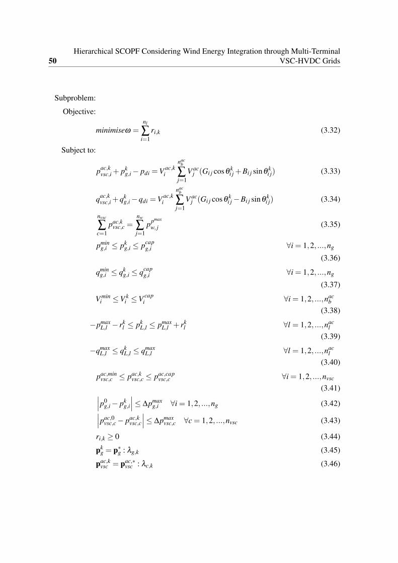
50Hierarchical SCOPF Considering Wind Energy Integration through Multi-Terminal
VSC-HVDC Grids
Subproblem:
Objective:
minimiseω =nl
∑i=1
ri,k (3.32)
Subject to:
pac,kvsc,i + pk
g,i − pdi =V ac,ki
nacb
∑j=1
V acj (Gi j cosθ
ki j +Bi j sinθ
ki j) (3.33)
qac,kvsc,i +qk
g,i −qdi =V ac,ki
nacb
∑j=1
V acj (Gi j cosθ
ki j −Bi j sinθ
ki j) (3.34)
nvsc
∑c=1
pac,kvsc,c =
nw
∑j=1
ppmax
w, j (3.35)
pming,i ≤ pk
g,i ≤ pcapg,i ∀i = 1,2, ...,ng
(3.36)
qming,i ≤ qk
g,i ≤ qcapg,i ∀i = 1,2, ...,ng
(3.37)
V mini ≤V k
i ≤V capi ∀i = 1,2, ...,nac
b
(3.38)
−pmaxL,l − rk
l ≤ pkL,l ≤ pmax
L,l + rkl ∀l = 1,2, ...,nac
l
(3.39)
−qmaxL,l ≤ qk
L,l ≤ qmaxL,l ∀l = 1,2, ...,nac
l
(3.40)
pac,minvsc,c ≤ pac,k
vsc,c ≤ pac,capvsc,c ∀i = 1,2, ...,nvsc
(3.41)∣∣∣p0g,i − pk
g,i
∣∣∣≤ ∆pmaxg,i ∀i = 1,2, ...,ng (3.42)∣∣∣pac,0
vsc,c − pac,kvsc,c
∣∣∣≤ ∆pmaxvsc,c ∀c = 1,2, ...,nvsc (3.43)
ri,k ≥ 0 (3.44)
pkg = p∗
g : λg,k (3.45)
pac,kvsc = pac,∗
vsc : λc,k (3.46)
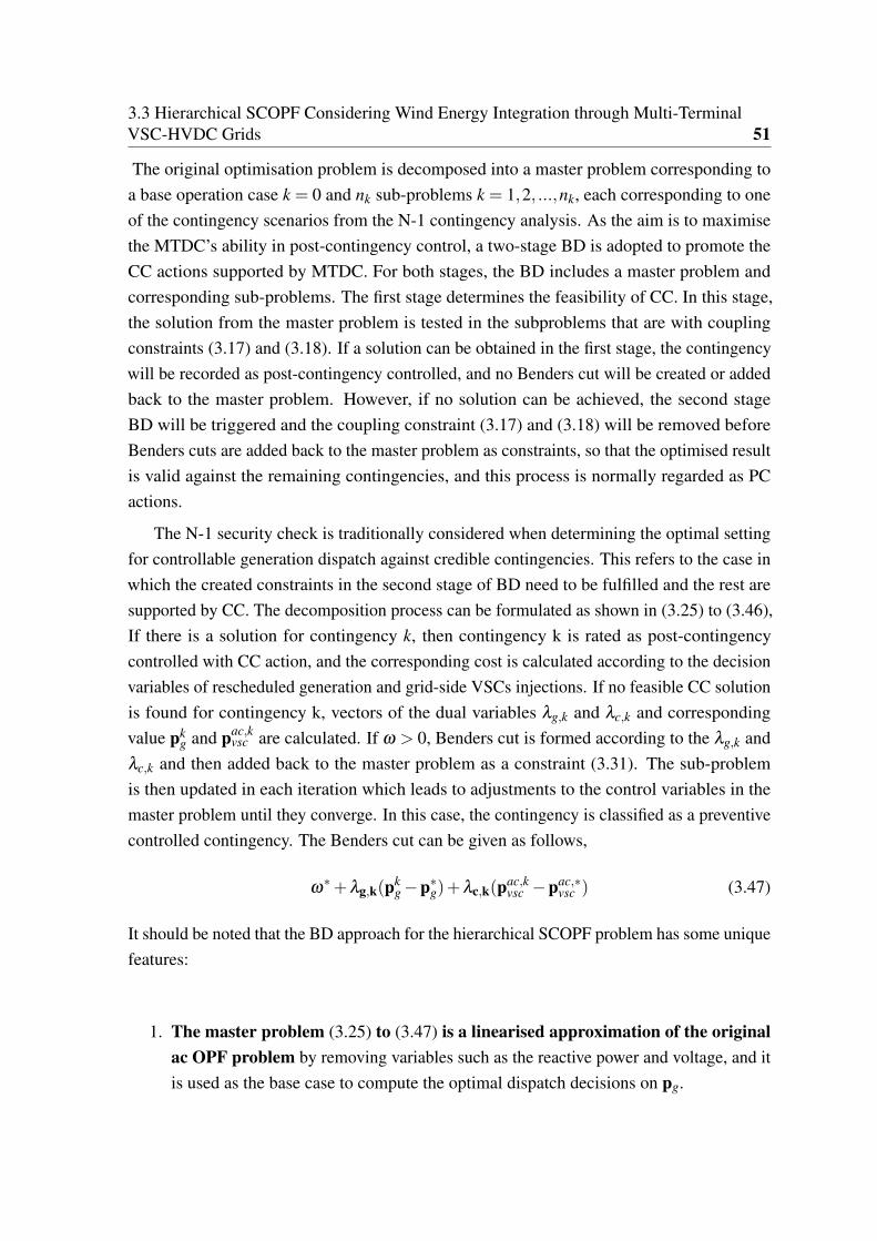
3.3 Hierarchical SCOPF Considering Wind Energy Integration through Multi-TerminalVSC-HVDC Grids 51
The original optimisation problem is decomposed into a master problem corresponding toa base operation case k = 0 and nk sub-problems k = 1,2, ...,nk, each corresponding to oneof the contingency scenarios from the N-1 contingency analysis. As the aim is to maximisethe MTDC’s ability in post-contingency control, a two-stage BD is adopted to promote theCC actions supported by MTDC. For both stages, the BD includes a master problem andcorresponding sub-problems. The first stage determines the feasibility of CC. In this stage,the solution from the master problem is tested in the subproblems that are with couplingconstraints (3.17) and (3.18). If a solution can be obtained in the first stage, the contingencywill be recorded as post-contingency controlled, and no Benders cut will be created or addedback to the master problem. However, if no solution can be achieved, the second stageBD will be triggered and the coupling constraint (3.17) and (3.18) will be removed beforeBenders cuts are added back to the master problem as constraints, so that the optimised resultis valid against the remaining contingencies, and this process is normally regarded as PCactions.
The N-1 security check is traditionally considered when determining the optimal settingfor controllable generation dispatch against credible contingencies. This refers to the case inwhich the created constraints in the second stage of BD need to be fulfilled and the rest aresupported by CC. The decomposition process can be formulated as shown in (3.25) to (3.46),If there is a solution for contingency k, then contingency k is rated as post-contingencycontrolled with CC action, and the corresponding cost is calculated according to the decisionvariables of rescheduled generation and grid-side VSCs injections. If no feasible CC solutionis found for contingency k, vectors of the dual variables λg,k and λc,k and correspondingvalue pk
g and pac,kvsc are calculated. If ω > 0, Benders cut is formed according to the λg,k and
λc,k and then added back to the master problem as a constraint (3.31). The sub-problemis then updated in each iteration which leads to adjustments to the control variables in themaster problem until they converge. In this case, the contingency is classified as a preventivecontrolled contingency. The Benders cut can be given as follows,
ω∗+λg,k(pk
g −p∗g)+λc,k(pac,k
vsc −pac,∗vsc ) (3.47)
It should be noted that the BD approach for the hierarchical SCOPF problem has some uniquefeatures:
1. The master problem (3.25) to (3.47) is a linearised approximation of the originalac OPF problem by removing variables such as the reactive power and voltage, and itis used as the base case to compute the optimal dispatch decisions on pg.

52Hierarchical SCOPF Considering Wind Energy Integration through Multi-Terminal
VSC-HVDC Grids
2. The reactive power and voltage are then checked in the subproblems based on thesolution of p∗
g from the master problem.
3. The master problem adopts a linearised power flow model for optimisation, whichis convex and easy to solve, while the solution is handed over to the subproblem asan input for the N-1 contingency analysis. A nonlinear power flow is adopted in thesubproblem, which attempts to find a feasible solution given the restriction on reactivepower generation and voltage limits. This process does not aim to further optimise thesystem, but is instead used as a feasibility check realised by the BD approach.
4. Although there are concerns that BD may fail to converge to either a global op-timal or a local optimal when applied to nonlinear SCOPF exist, the approach ofadopting a linearised OPF in the master problem that is convex helps to reduce suchrisk, and the computation experience with the ac power flow in the subproblems hasbeen encouraging. Moreover, convex relaxation [71, 72] techniques that are discussedin Chapter 5 could be applied to further alleviate such concerns.
5. In general, the additional security constraints introduced on top of the OPF prob-lem do lead to a more complicated optimisation problem since the solution needsto satisfy not only the system’s physical limits, but also all of the contingency cases,which poses challenges in real-time operation. However the computation time canbe alleviated by checking all contingencies at the same time, since all sub-problemsare not interdependent. Moreover, to further reduce the computation burden, thecontingency filter technique could be applied, which only includes the most severecontingencies into the feasibility check.
.
3.3.4 SCOPF Framework for the Meshed Ac/MTDC Grids
After introducing each part of the system, this section introduces the overall dispatch algo-rithm, which is able to make use of the power flow control capability of MTDC grids toprovide support for ac systems, so that the ac/dc system can be operated in a cost-effectiveway. The presented hierarchical dispatch scheme, where two layers interact, is a particularlyattractive method of problem decomposition, as the layers provide a highly intuitive systemredispatch architecture.
The two-layer BD SCOPF dispatch algorithm (TLDSCOPF algorithm)is described asfollows,
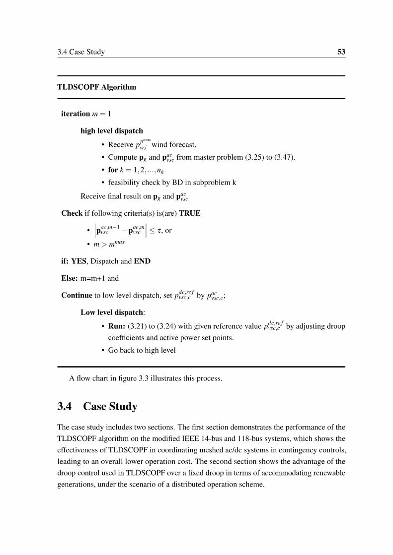
3.4 Case Study 53
TLDSCOPF Algorithm
iteration m = 1
high level dispatch
• Receive ppmax
w,i wind forecast.
• Compute pg and pacvsc from master problem (3.25) to (3.47).
• for k = 1,2, ...,nk
• feasibility check by BD in subproblem k
Receive final result on pg and pacvsc
Check if following criteria(s) is(are) TRUE
•∣∣∣pac,m−1
vsc −pac,mvsc
∣∣∣≤ τ , or
• m > mmax
if: YES, Dispatch and END
Else: m=m+1 and
Continue to low level dispatch, set pdc,re fvsc,c by pac
vsc,c;
Low level dispatch:
• Run: (3.21) to (3.24) with given reference value pdc,re fvsc,c by adjusting droop
coefficients and active power set points.
• Go back to high level
A flow chart in figure 3.3 illustrates this process.
3.4 Case Study
The case study includes two sections. The first section demonstrates the performance of theTLDSCOPF algorithm on the modified IEEE 14-bus and 118-bus systems, which shows theeffectiveness of TLDSCOPF in coordinating meshed ac/dc systems in contingency controls,leading to an overall lower operation cost. The second section shows the advantage of thedroop control used in TLDSCOPF over a fixed droop in terms of accommodating renewablegenerations, under the scenario of a distributed operation scheme.
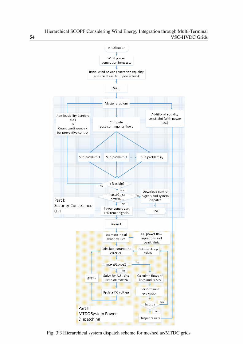
54Hierarchical SCOPF Considering Wind Energy Integration through Multi-Terminal
VSC-HVDC Grids
Fig. 3.3 Hierarchical system dispatch scheme for meshed ac/MTDC grids

3.4 Case Study 55
3.4.1 SCOPF Results
Integrating multiple wind farms into the MTDC grid allows for effective sharing of renewableresources and cost-effective electricity supply. Two modified meshed ac/dc systems, theIEEE 14-bus and the IEEE 118-bus systems, are used to demonstrate the presented strategy’sperformance. To quantitatively evaluate the performance of the presented method, theExpected Security Control Cost (ESCC) index is selected, given the probabilistic nature ofcontingencies, which can be expressed as follows,
ESCC =
CC Cost︷ ︸︸ ︷nk
∑k=1
ρk
ng
∑i=1
αg,i(pkg,i − p∗g,i)
2+
PC Cost︷ ︸︸ ︷ng
∑i=1
f (p∗g,i)− f (pg,i) (3.48)
where pg,i denotes the conventional OPF result for generator i without considering anysecurity constraints, and f (pg,i) is the associated OPF cost. (3.48) shows that the CC costis the sum of all probable post-contingency control costs, where ρk is the probability ofcontingency k, while the PC cost of a given state variable is the cost difference between OPFproblems with and without security constraints.
IEEE 14-Bus System
A ±400 kV five-terminal dc grid has been added to the system, which provides the intercon-nection of two wind farms to three buses at a benchmark ac system through VSC converters.The one-line diagram is shown in figure 3.4. The maximum power flow limits for branches 1and 7 are 80 MVA; for branches 3 and 6, 50 MVA; for branches 17-20, 20 MVA; and for therest 40 MVA. The two wind farms, each consisting of 30 Vestas 2 MW wind turbines, arelocated at bus 18 and bus 19.
In this study, a wind power generation overestimation scenario is selected to demonstratethe ability of the MTDC to coordinate with generator rescheduling in the CC stage, wherethe available wind power generation is 20% less than the estimated value. To accommodatethe base loading level, the load profile and unit parameters of the original system areadjusted accordingly. The rate of generator redispatch is set at $30/MW/h. In total, 25 N-1contingencies are analysed in this study, including loss of transmission lines l1, l2,..., l20 andgenerators G1, G2,...,G5. The simulation results are given in table 3.1.
IEEE 118-Bus System
A modified version of the IEEE 118-bus system is used, which contains three VSC convertersand a dc grid with five buses and four dc lines. Thus, the system consists of 123 buses, 54
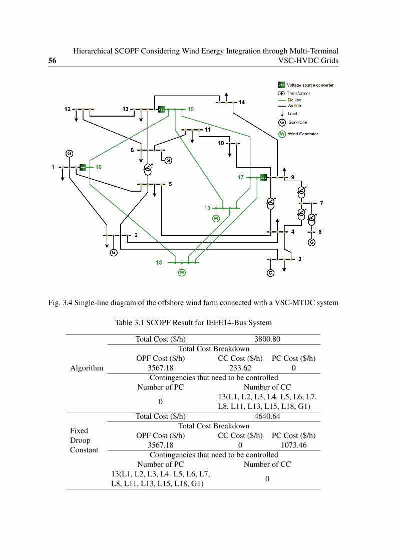
56Hierarchical SCOPF Considering Wind Energy Integration through Multi-Terminal
VSC-HVDC Grids
Fig. 3.4 Single-line diagram of the offshore wind farm connected with a VSC-MTDC system
Table 3.1 SCOPF Result for IEEE14-Bus System
Algorithm
Total Cost ($/h) 3800.80Total Cost Breakdown
OPF Cost ($/h) CC Cost ($/h) PC Cost ($/h)3567.18 233.62 0Contingencies that need to be controlled
Number of PC Number of CC
013(L1, L2, L3, L4. L5, L6, L7,L8, L11, L13, L15, L18, G1)
FixedDroopConstant
Total Cost ($/h) 4640.64Total Cost Breakdown
OPF Cost ($/h) CC Cost ($/h) PC Cost ($/h)3567.18 0 1073.46Contingencies that need to be controlled
Number of PC Number of CC13(L1, L2, L3, L4. L5, L6, L7,L8, L11, L13, L15, L18, G1) 0
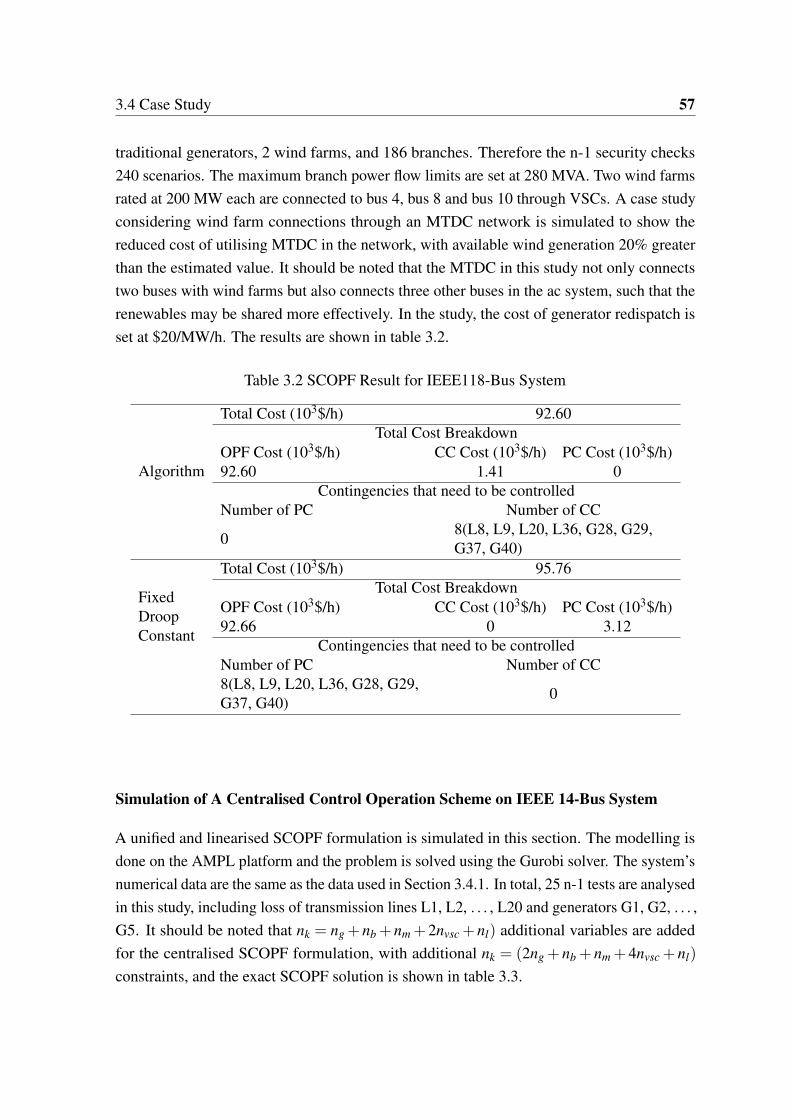
3.4 Case Study 57
traditional generators, 2 wind farms, and 186 branches. Therefore the n-1 security checks240 scenarios. The maximum branch power flow limits are set at 280 MVA. Two wind farmsrated at 200 MW each are connected to bus 4, bus 8 and bus 10 through VSCs. A case studyconsidering wind farm connections through an MTDC network is simulated to show thereduced cost of utilising MTDC in the network, with available wind generation 20% greaterthan the estimated value. It should be noted that the MTDC in this study not only connectstwo buses with wind farms but also connects three other buses in the ac system, such that therenewables may be shared more effectively. In the study, the cost of generator redispatch isset at $20/MW/h. The results are shown in table 3.2.
Table 3.2 SCOPF Result for IEEE118-Bus System
Algorithm
Total Cost (103$/h) 92.60Total Cost Breakdown
OPF Cost (103$/h) CC Cost (103$/h) PC Cost (103$/h)92.60 1.41 0
Contingencies that need to be controlledNumber of PC Number of CC
08(L8, L9, L20, L36, G28, G29,G37, G40)
FixedDroopConstant
Total Cost (103$/h) 95.76Total Cost Breakdown
OPF Cost (103$/h) CC Cost (103$/h) PC Cost (103$/h)92.66 0 3.12
Contingencies that need to be controlledNumber of PC Number of CC8(L8, L9, L20, L36, G28, G29,G37, G40) 0
Simulation of A Centralised Control Operation Scheme on IEEE 14-Bus System
A unified and linearised SCOPF formulation is simulated in this section. The modelling isdone on the AMPL platform and the problem is solved using the Gurobi solver. The system’snumerical data are the same as the data used in Section 3.4.1. In total, 25 n-1 tests are analysedin this study, including loss of transmission lines L1, L2, . . . , L20 and generators G1, G2, . . . ,G5. It should be noted that nk = ng +nb +nm +2nvsc +nl) additional variables are addedfor the centralised SCOPF formulation, with additional nk = (2ng + nb + nm + 4nvsc + nl)
constraints, and the exact SCOPF solution is shown in table 3.3.

58Hierarchical SCOPF Considering Wind Energy Integration through Multi-Terminal
VSC-HVDC Grids
Fig. 3.5 Single-line diagram of the offshore wind farm connected with a VSC-MTDC system
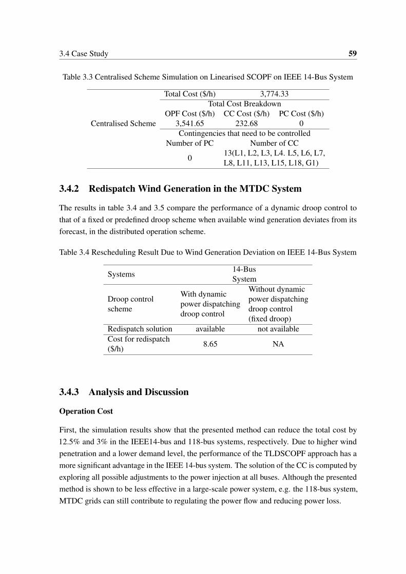
3.4 Case Study 59
Table 3.3 Centralised Scheme Simulation on Linearised SCOPF on IEEE 14-Bus System
Centralised Scheme
Total Cost ($/h) 3,774.33Total Cost Breakdown
OPF Cost ($/h) CC Cost ($/h) PC Cost ($/h)3,541.65 232.68 0Contingencies that need to be controlled
Number of PC Number of CC
013(L1, L2, L3, L4. L5, L6, L7,L8, L11, L13, L15, L18, G1)
3.4.2 Redispatch Wind Generation in the MTDC System
The results in table 3.4 and 3.5 compare the performance of a dynamic droop control tothat of a fixed or predefined droop scheme when available wind generation deviates from itsforecast, in the distributed operation scheme.
Table 3.4 Rescheduling Result Due to Wind Generation Deviation on IEEE 14-Bus System
Systems14-BusSystem
Droop controlscheme
With dynamicpower dispatchingdroop control
Without dynamicpower dispatchingdroop control(fixed droop)
Redispatch solution available not availableCost for redispatch($/h) 8.65 NA
3.4.3 Analysis and Discussion
Operation Cost
First, the simulation results show that the presented method can reduce the total cost by12.5% and 3% in the IEEE14-bus and 118-bus systems, respectively. Due to higher windpenetration and a lower demand level, the performance of the TLDSCOPF approach has amore significant advantage in the IEEE 14-bus system. The solution of the CC is computed byexploring all possible adjustments to the power injection at all buses. Although the presentedmethod is shown to be less effective in a large-scale power system, e.g. the 118-bus system,MTDC grids can still contribute to regulating the power flow and reducing power loss.

60Hierarchical SCOPF Considering Wind Energy Integration through Multi-Terminal
VSC-HVDC Grids
Table 3.5 Rescheduling Result Due to Wind Generation Deviation in the IEEE118-BusSystem
Systems118-BusSystem
Droop controlscheme
With dynamicpower dispatchingdroop control
Without dynamicpower dispatchingdroop control(fixed droop)
Redispatch solution available not availableCost for redispatch($/h) 77.1 NA
CC vs. PC
As shown in tables 3.1 and 3.2, with the TLDSCOPF approach, some pre-contingency actionscan be shifted to post-contingency control and the corresponding PC cost can be eliminated.Compared to CC, which relies solely on redispatching traditional generators, integratingwind energy through MTDC grids is economically efficient as there is no extra cost incurredby redistributing renewable units in the MTDC system.
Accommodating Intermittent Generation
Another advantage of adopting dynamic droop control when dealing with random generationfrom the off-shore wind farms in the MTDC system is observed in tables 3.4 and 3.5. Systemswith fixed or predefined droop constants have difficulty achieving a solution when facedwith variations in wind power generation. However, by optimising the droop values in thepresented method, MTDC grids can provide corrective support to ac systems by redistributingpower flow across grids, thereby reducing control costs. It should be noted that the CCcost and PC cost shown in the tables only consider the redispatching costs that are intendedto alleviate security constraint violations. The redispatching costs for covering losses ofgeneration that do not cause system constraint violations are not included.
Centralised Operation vs. Distributed Operation
To compare the adopted distributed operation scheme with a centralised one, a centralisedSCOPF is formulated and simulated. The computation results shown in tables 3.4 and 3.5 usethe solution from the previous SCOPF as the reference value, and the simulation only servesto mitigate the imbalance caused by the mismatch between forecast wind generation andreal wind generation in the allowed period. Also it should also be noted that the presented

3.5 Conclusion 61
algorithm does not need to consider the uncertainties of off-shore wind farm generation at theSCOPF stage. As shown in the tables 3.4 and 3.5, with fixed droop constants, the availablewind energy cannot be redistributed across the entire system, which leads to infeasiblesolutions in the initial OPF results. The presented method shows capability in accommodatingthe intermittence of the renewables even though randomness is not considered in the SCOPFstage, which could contribute to mitigating operational challenges.
When comparing the hierarchically distributed method with the centralised unifiedmethod, it is observed that both approaches have their own advantages and disadvantages.
1. In the hierarchical method, the mixed ac/dc system is decomposed into an ac sub-system and a multi-terminal dc subsystem, where each level is solved individuallyduring each step of the iterations. The structure of the problem becomes simpler, andcommunication and computation requirements are reduced compared to the unifiedapproach.
2. If the MTDC subsystem and the ac subsystem are owned and operated independentlyby different organisations, the hierarchical method provides more flexibility to systemoperations in terms of communication, computation, control, etc.
3. In practical situations, for a super-large-scale interconnected power system, the dispatchinterval may be insufficient for the computation time required for convergence in thepresented iterative algorithm. In such situations, the algorithm has to be terminatedprior to convergence. To allow intermediate termination, all iterates generated by thehierarchical method must be feasible system-wide.
4. The case study shows that, the results of the hierarchical method are almost identicalto these of the unified approach. In fact, sub-optimal inputs are allowed due tocomputational limits. As a result, the presented formulation, though sub-optimal,achieves desired operational objectives.
3.5 Conclusion
In this chapter, the SCOPF model has been extended to incorporate a dc grid with severalrenewable generations. Two operation schemes were introduced for system operators, and asystem redispatch scheme was proposed to facilitate wind power integration through MTDCgrids. Moreover, the contingency control strategy was extended: CC and PC were compared,and a hierarchical structure was employed to promote post-contingency control in the meshac/dc grid.

62Hierarchical SCOPF Considering Wind Energy Integration through Multi-Terminal
VSC-HVDC Grids
Through a hierarchical structure where two layers (the high level is a traditional SCOPFproblem and the low level is a dynamic MTDC grid power dispatching problem.) interact, anhighly intuitive system redispatch scheme can be achieved. This is advantageous comparedto other approaches in that it 1) takes advantage of MTDC grids’ power flow regulatingcapability, which ensures that the meshed ac/dc systems can be operated more flexibly andcost-effectively; 2) isolates ac and dc systems, which simplifies computation procedures;and 3) makes wind power integration technically and economically available for systemoperations, which indicates high potential for practical applications. Moreover, despitethe fact that an increasing number of MTDC systems will be commissioned in the future,the technology is still under development. Future work should focus on network topology,converter outage, and delayed information exchange, among others. Thus, the successfulimplementation of MTDC systems relies heavily on planning.
This chapter has also attempted to adopt a linearised OPF (dc-OPF) model and nonlinearpower flow (ac power flow) check in the n-1 contingency analysis via BD techniques. Suchan approach typically finds a dispatch solution from DC-OPF that does not violate anyconstraints in the ac power flow in contingencies. This has become a common practicewidely employed by system operators.
In the next chapter, the advantages and disadvantages of adopting post-contingencycontrols are studied in details, and these controls are compared to pre-contingency approaches.The chapter also introduces microgrids, which are another effective method for integrating ofRESs, and it presents an incentive-based mechanism to encourage the use of microgrids incontingency recovery supports.
Chapter 4
Robust SCOPF Using MultipleMicrogrids for Corrective Control underUncertainties
RESs penetrate the electricity networks at various levels and in all different forms. Afterintroducing concepts such as power flow models and OPF, Chapter 2 introduced a frameworkto incorporate intermittent renewable energy generation into the electricity network operationunder security consideration, via a robust SCOPF model, which adopts preventive control asthe security control strategy. Given the significant growth in microgrid (MG) deploymentsacross the world and appealing merits of CC strategies, this chapter explores the potential ofusing multiple MGs in supporting the main grid’s security control. CC is employed to relievepost-contingency overflows by effectively coordinating system generators and multiple MGs.In addition, an incentive based mechanism is designed to encourage the MGs to activelycooperate with the main grid for post-contingency recovery in order to enhance both thereliability of supply and the security of the connected power system. This chapter is basedon[73, 74].
4.1 Introduction
Power system operations require the system to stay within its security and economic con-straints, and the system operator consistently manages the system to achieve an optimalbalance in operations. Power blackouts are a serious problem, especially for modern soci-eties. During a blackout event in South Australia in 2016, thousands of households wereaffected due to an outage affecting an interstate connector. Pre-contingency control, which

64 Robust SCOPF Using Multiple Microgrids for Corrective Control under Uncertainties
was introduced in Chapter two, is generally regarded as conservative, since contingen-cies are high-risk/low-probability events. Therefore, reliable and economically efficientpost-contingencies have attracted enormous amount of research interest. Among all of theproposed elements, generation re-dispatch is the most direct method of post-contingencycontrol. Several solution techniques are proposed in [75] to solve CC problems by usinggeneration re-dispatch. The performance of the presented iterative approach is comparedto other techniques and claimed to be more computationally efficient. The authors in [76]presented an optimal coordination strategy between PC and CC so that the overall estimatedexpected security control cost is minimised. The proposed control strategy mainly focuseson steady state overflow security and solving post-contingency with generation re-dispatch.
These aforementioned security controls rely heavily on the traditional thermal generationre-dispatch. However, relying on generation re-dispatch only as CC actions is inadequate.First, the solution region of this approach is overly tightened by slow generators rampingrate in allowing time, which leads to a limited number of CC solutions. Moreover, due tothe complexity of electricity networks, the coupling constraint is normally not capped bythe generator with the slowest ramping, making it difficult to determine the feasibility ofthe CC without studying the electric network structure. Moreover, another concern is thatfrequent generator ramping could lead to an increased cycling cost and a reduced lifetimeof generators. To overcome these disadvantages, new elements with fast response, such asdistributed energy sources , energy storage [77] and DSM [78, 79], high voltage dc, andmulti-terminal high voltage dc grid [80] that was introduced in Chapter 3, have recently beenexplored for post contingency control actions.
Among various new methods, direct load control provides an equivalent approach topost-contingency control action, when others are not sufficient. It is usually used as a backupplan to avoid causing dramatic inconvenience for the electricity consumers. An approachusing voluntary load shedding to remove the overload after contingencies is proposed in[79]. The approach manages to seek the optimal point between security and operation costs.However, the paper only focuses on the feasibility of using the voluntary load reduction asCC actions, and neglects the design of a proper incentive mechanism. Apart from direct loadcontrol and load shedding, energy storage also shows potential in remedying the overflowcaused by contingencies. In [77], a CC strategy is proposed coordinating both bulk anddistributed energy storage for SCOPF. Different types of energy storage are selected and thenanalyzsed. However, the energy storage devices are still expensive for large-scale installation.Besides these strategies, other techniques, such as high voltage dc [81] and FACT devices[82], are also used in the application of control strategies in the SCOPF. However, due to the

4.1 Introduction 65
complex nature of electricity networks and the large size of the SCOPF problem, the existingstudies normally use only single method to achieve contingency control.
Moreover, these studies only aim to propose the feasible post-contingency control so-lutions without discussing on the cost or incentive associated with adopting such methods,thereby posing difficulties in real execution.
In the meantime, traditional deterministic SCOPF does not consider uncertainty, thusassuming that the load is deterministic and that all generations are controllable. However,large-scale RESs such as wind and solar power are integrated into today’s power grid. Variousmethods have been introduced to model the uncertainty into the problem, among whichrobust optimisation has gained popularity, as it does not require the details of the probabilitydistribution functions of random parameters.
However, uncertainties in load demand and renewable power generation for the securitycontrol are not systematically addressed. In addition, each element in the electricity networkis closely related, and it is unrealistic for system operator to make decisions regardingindividual components. These considerations motive the search for alternatives, such as usingmultiple MGs as CC actions in post-contingency recovery. Therefore, this chapter introducesa new model to illustrate and compute the incentives and costs of multi-MGs to participate inthe post-contingency control actions under uncertainty.
MG technology is recognised as a crucial platform for accommodating a high level ofrenewables, considering not only energy management but also instantaneous power. AnMG is a cluster of interconnected loads, distributed energy resources and storage withinclearly defined electrical boundaries that acts as a single controllable entity with regard tothe grid [83]. MGs are an attractive solution to facilitate the most efficient utilisation ofRESs, and they have enormous potential to enhance both the reliability of supply and thesecurity of the connected power system. MGs have seen a significant growth in industrialinvestments in the last decade. In the US, around 124 MGs were in operation by 2015, witha total capacity of 1,169 MWs [84]. It is expected that a higher number number of MGswill be deployed in future power systems. According to a report titled ’North AmericanMicrogrids 2015: Advancing Beyond Local Energy Optimization’, industry experts predictthat the nation-wide MG capacity in the US will exceed 2,850MW. Not only does thisincentivise a boom in the MG market, but also provides opportunities for MGs to supportgrid operations. In this Chapter, multiple MGs are integrated as an entity and connectedto the main ac transmission grid via substations as a collected controllable connection ofcontrollable demand, conventional demand, and energy storage. Furthermore, from the MGoperator’s point of view, as a whole, MGs are capable of acting as an entity that is able toprovide incentive based [85] post-contingency control action when needed.
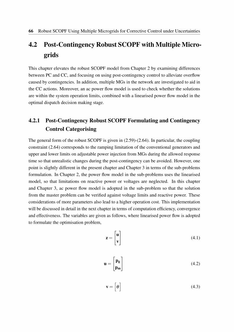
66 Robust SCOPF Using Multiple Microgrids for Corrective Control under Uncertainties
4.2 Post-Contingency Robust SCOPF with Multiple Micro-grids
This chapter elevates the robust SCOPF model from Chapter 2 by examining differencesbetween PC and CC, and focusing on using post-contingency control to alleviate overflowcaused by contingencies. In addition, multiple MGs in the network are investigated to aid inthe CC actions. Moreover, an ac power flow model is used to check whether the solutionsare within the system operation limits, combined with a linearised power flow model in theoptimal dispatch decision making stage.
4.2.1 Post-Contingency Robust SCOPF Formulating and ContingencyControl Categorising
The general form of the robust SCOPF is given in (2.59)-(2.64). In particular, the couplingconstraint (2.64) corresponds to the ramping limitation of the conventional generators andupper and lower limits on adjustable power injection from MGs during the allowed responsetime so that unrealistic changes during the post-contingency can be avoided. However, onepoint is slightly different in the present chapter and Chapter 3 in terms of the sub-problemsformulation. In Chapter 2, the power flow model in the sub-problems uses the linearisedmodel, so that limitations on reactive power or voltages are neglected. In this chapterand Chapter 3, ac power flow model is adopted in the sub-problem so that the solutionfrom the master problem can be verified against voltage limits and reactive power. Theseconsiderations of more parameters also lead to a higher operation cost. This implementationwill be discussed in detail in the next chapter in terms of computation efficiency, convergenceand effectiveness. The variables are given as follows, where linearised power flow is adoptedto formulate the optimisation problem,
z =
[uv
](4.1)
u =
[pg
pm
](4.2)
v =[θ
](4.3)
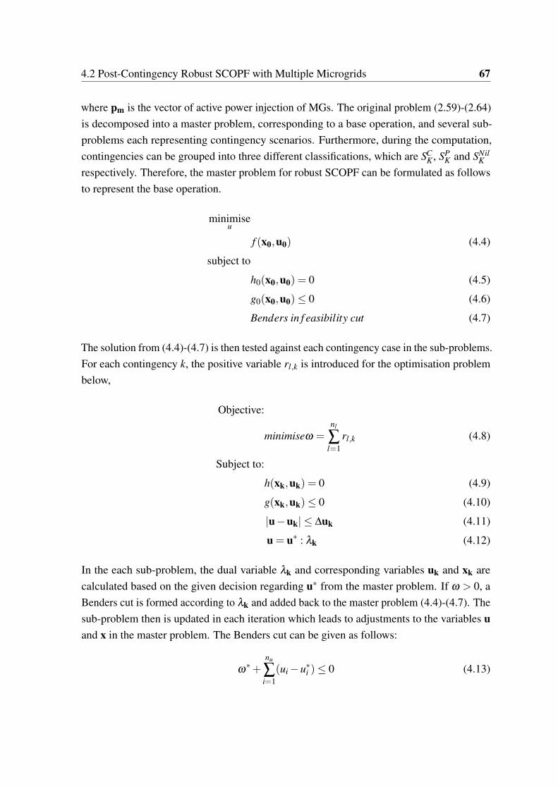
4.2 Post-Contingency Robust SCOPF with Multiple Microgrids 67
where pm is the vector of active power injection of MGs. The original problem (2.59)-(2.64)is decomposed into a master problem, corresponding to a base operation, and several sub-problems each representing contingency scenarios. Furthermore, during the computation,contingencies can be grouped into three different classifications, which are SC
K , SPK and SNil
K
respectively. Therefore, the master problem for robust SCOPF can be formulated as followsto represent the base operation.
minimiseu
f (x0,u0) (4.4)
subject to
h0(x0,u0) = 0 (4.5)
g0(x0,u0)≤ 0 (4.6)
Benders in f easibility cut (4.7)
The solution from (4.4)-(4.7) is then tested against each contingency case in the sub-problems.For each contingency k, the positive variable rl,k is introduced for the optimisation problembelow,
Objective:
minimiseω =nl
∑l=1
rl,k (4.8)
Subject to:
h(xk,uk) = 0 (4.9)
g(xk,uk)≤ 0 (4.10)
|u−uk| ≤ ∆uk (4.11)
u = u∗ : λk (4.12)
In the each sub-problem, the dual variable λk and corresponding variables uk and xk arecalculated based on the given decision regarding u∗ from the master problem. If ω > 0, aBenders cut is formed according to λk and added back to the master problem (4.4)-(4.7). Thesub-problem then is updated in each iteration which leads to adjustments to the variables uand x in the master problem. The Benders cut can be given as follows:
ω∗+
nu
∑i=1
(ui −u∗i )≤ 0 (4.13)

68 Robust SCOPF Using Multiple Microgrids for Corrective Control under Uncertainties
where nu is the number of control variables ui. The processes (4.4)-(4.13) are used not onlyto decompose a complex problem into several sub-problems for computational efficiency,but also to categorise different types of contingencies. The application of the BD into theSCOPF for contingency action determination is shown in flowchart in figure 4.1. As shownin Figure 4.1, the feasibility of SC
K is analysed first. If a feasible solution set (uk,xk) existsin the sub-problem k by taking the decision variable set (u0,x0) from the master problem,then the contingency k can be solved by CC, thus k ∈ Sc
k. If no feasible solution is found, theBenders cuts are created and taken into the master problem for PC solutions. As shown in(4.2), the control variables include two sets of vectors. Apart from conventional generationpg, the active power injections pm from multiple microgrids are taken into consideration ascontrol variables, where both positive and negative power injections can be made accordingto the requirements for the contingency control. Therefore, in MGs’ normal operation mode,each MG’s energy management system (EMS) optimises the schedule of the generation andconsumption within itself. If a contingency occurs, microgrids operators can offer supportto the upper-level grid to alleviate the overflow caused by contingencies. Mathematically,control variables pm are not considered in PC actions, and only in CC actions. Alternatively,pm can be treated in the same way as pd in the normal operation mode.
4.2.2 Incentive Based Post-Contingency Controls with Multiple MGs
In the post-contingency situation, the main grid system operator needs to take actions toresolve the overflow. As the active power flow on the transmission line can be seen as thecomposed contribution of each node injection [56], overflow caused by contingencies couldtraditionally be resolved by quickly changing the generation output. Various methods havebeen investigated for CC actions to replace relying solely on generation re-dispatch. In thissection, aggregated multiple MGs are used to support CC along with conventional generators.
MG Architecture
A typical MG architecture [86] is presented in figure 4.2, including the key componentsuncontrollable and flexible loads, dispatchable units (e.g. diesel generator), non-dispatchableunits (e.g. wind turbine and photovoltaics), and energy storage (e.g. batteries, fuel cells andelectric vehicles).
A centralised EMS control through the communication system by the MG controller isadopted to perform the optimal scheduling for the entire MG. In a normal operation state, aMG provides reliable power to loads, manages the renewable generations, and coordinatesall dispatchable units, flexible loads, and energy storage to achieve certain objectives, such as
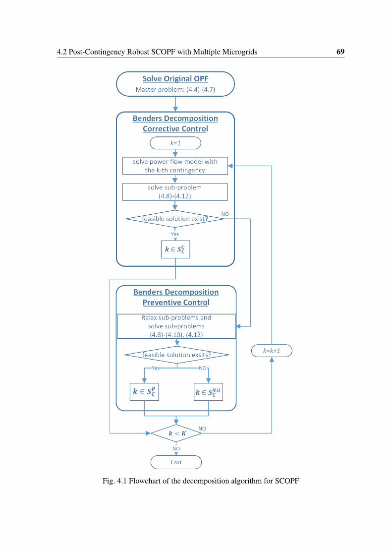
4.2 Post-Contingency Robust SCOPF with Multiple Microgrids 69
Fig. 4.1 Flowchart of the decomposition algorithm for SCOPF
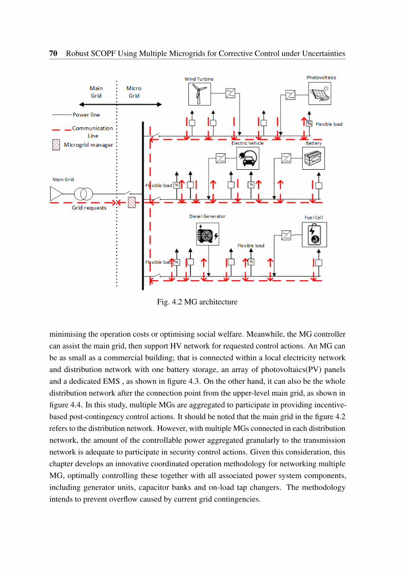
70 Robust SCOPF Using Multiple Microgrids for Corrective Control under Uncertainties
Fig. 4.2 MG architecture
minimising the operation costs or optimising social welfare. Meanwhile, the MG controllercan assist the main grid, then support HV network for requested control actions. An MG canbe as small as a commercial building; that is connected within a local electricity networkand distribution network with one battery storage, an array of photovoltaics(PV) panelsand a dedicated EMS , as shown in figure 4.3. On the other hand, it can also be the wholedistribution network after the connection point from the upper-level main grid, as shown infigure 4.4. In this study, multiple MGs are aggregated to participate in providing incentive-based post-contingency control actions. It should be noted that the main grid in the figure 4.2refers to the distribution network. However, with multiple MGs connected in each distributionnetwork, the amount of the controllable power aggregated granularly to the transmissionnetwork is adequate to participate in security control actions. Given this consideration, thischapter develops an innovative coordinated operation methodology for networking multipleMG, optimally controlling these together with all associated power system components,including generator units, capacitor banks and on-load tap changers. The methodologyintends to prevent overflow caused by current grid contingencies.

4.2 Post-Contingency Robust SCOPF with Multiple Microgrids 71
Fig. 4.3 A small household-sized MG
Fig. 4.4 IEEE 33-bus grid regarded as a whole MG
72 Robust SCOPF Using Multiple Microgrids for Corrective Control under Uncertainties
Incentive-Based MG Control Action
Aggregated multiple MGs provide a comprehensive yet sophisticated solution that is ableto provide both reductions and increments on the connected load when required from themain grid. The interaction of coordinating multiple MGs for post-contingency control withthe main grid is illustrated in figure 4.5, and its detailed mathematical model is given in thissection. As illustrated in figure 4.5, if a feasible solution is found, the contingency k ∈ SC
K ,otherwise k ∈ SP
K ∪SNilk . For k ∈ SC
K , the associated cost Ckcc is calculated, which is the sum of
the generators redispatch cost Ckcc,g and MGs control action cost Ck
cc,m for each contingencyk ∈ SC
K , defined as,
Ckcc,g = pk
ng
∑i=1
αg,i∆p2g,i (4.14)
Ckcc,m = pk
nm
∑i=1
αm,i∆p2m,i (4.15)
The ESCC of SCOPF considering MGs for CC action is denoted as CmESCC =Ccc,m +Cm
pc,where Ccc,m is the sum of each individual CC cost by MGs actions, and Cm
pc is the total costof all remaining credible contingencies can only be controlled by PC when using MGs forCC, as shown below,
Cm&gcc = ∑
k∈Sck
(Ckcc,g +Ck
cc,m) (4.16)
Cm&gpc =
ng
∑i=1
f (pg,i)− f (pg,i) (4.17)
where pg,i denotes the conventional OPF result for generator i without considering securityconstraints, and f (pg,i) is the OPF cost function, which can be in the form of (2.10). More-over, the main grid is able to compute the ESCC of securing all credible contingencies atthe generation dispatch stage, assuming that all MGs are at normal operation. In this case,only conventional generators are required for contingency controls, and all connected MGsare no allowed to participate. Therefore, from the main grid system operator’s perspective,the aggregated multiple MGs are treated as load. In this case, the cost associated withcontingency control can be easily computed by removing variable pm,i from control variableu, and the cost can be denoted as the base case scenario cost at Cbase
ESCC =Cbasecc +Cbase
pc .
From the main grid system operator’s perspective, the approach that has a lower totalESCC and more CC actions is preferred. In other words, if the Cm
ESCC ≤CbaseESCC, the main grid
system operator will accept the support from MGs and then coordinate the generators together
4.2 Post-Contingency Robust SCOPF with Multiple Microgrids 73
with MGs for post-contingency actions to achieve an overall lower contingency control cost.Regarding the MGs, when the contingency k occurs, the MG controller can determine theupper and lower limits of the power adjustment by checking the states of the available energystorage level, flexible demand, controllable generators and RESs. MGs can then provide post-contingency control actions by adjusting their power injection within the limit for contingencycontrol support and to be paid by the main grid system operator. In equations (4.14)-(4.17),the probability of contingencies ρk and cost coefficients of conventional generators αg,i
are both known by the main grid system operator. The algorithm then needs to iterate on(∆pg,i,∆pm,i) while updating the cost coefficient rm,i in each iteration, until the criterion ofCm
ESCC ≤CbaseESCC is satisfied.
It should be noted that the individual MG operator defines not only the upper and lowerbounds of power injection adjustments of MG i ∆pm,i but also the limits on αm,i. Thismeans that at certain stage of the iteration, any MG can refuse further reduction on the costcoefficients αm,i. Noticeably, compared to the direct load control method, the incentive-basedscheme includes economic aspects in its formulation. The scheme can dynamically lookinto the current situation and make the economically optimal solution based on the currentsituation. Moreover, the incentive-based scheme enables active participation of MGs in thecontingency control, and the burden of taking post-contingency control actions is sharedby almost all entities in the electricity networks. In addition, as shown in figure 4.5, ∆pm,i,which means that changes in power injection from MG i in the post contingency controlare computed by MG i. Therefore, the upper and lower limits on ∆pm,i do not need to beacknowledged by the upper level grid system operator. This makes the overall incentive-basedCC strategy computationally efficient.
The problem can be generalised into a quadratic problem with linear constraints asfollows, assuming that branch flow adjustment vector ∆pL,l is computed from the BDin SCOPF for any contingency k ∈ SC
K . Iterate on the problem (4.18)-(4.22) and update
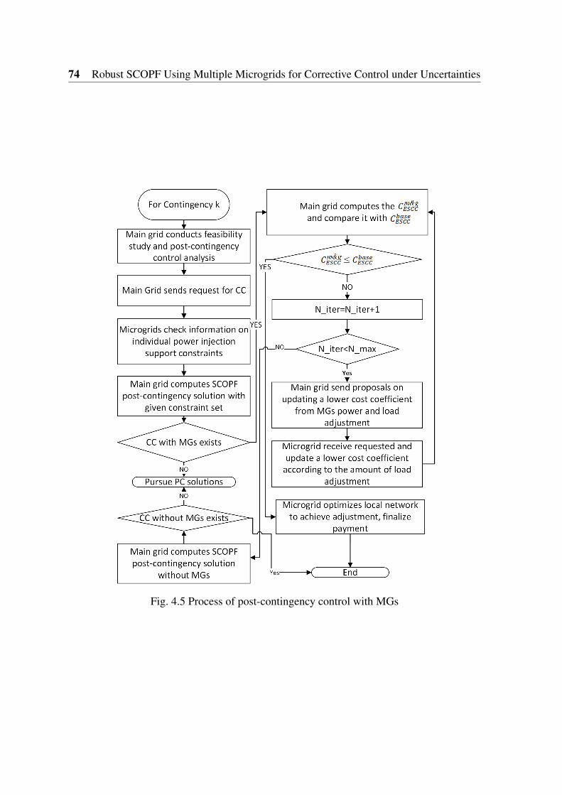
74 Robust SCOPF Using Multiple Microgrids for Corrective Control under Uncertainties
Fig. 4.5 Process of post-contingency control with MGs

4.3 Case Study 75
rm,i, ∀i = 1,2, ...,nm until criterion (4.23) is satisfied,
Objective:
minng
∑i=1
αg,i∆p2g,i +
nm
∑i=1
αm,i∆p2m,i (4.18)
Subject to:ng
∑i=1
∆pg,i +nm
∑i=1
∆pm,i = 0 (4.19)
H(∆pg +∆pm) = ∆pL (4.20)
pdng,i ≤ ∆pg,i ≤ pup
g,i ∀i = 1,2, ...,ng (4.21)
pdnm,i ≤ ∆pm,i ≤ pup
m,i ∀i = 1,2, ...,nm (4.22)
and the criteria is defined as follows,
CmESCC ≤Cbase
ESCC (4.23)
where CbaseESCC can be pre-determined by SCOPF analysis and αm,i, Cm
ESCC are updated duringeach iteration. Furthermore, pg and pm are vectors of ∆pg,i and ∆pm,i. ∆pg,i denotes thecontrol variable as generation ramping in the allowed time period, constrained by rampinglimits or generation reserve.
4.3 Case Study
The formulated SCOPF is tested on modified IEEE 14-bus and IEEE 118-bus systems. Thesimulation is divided into two sub-sections. Section 4.3.1 presents the simulation results interms of robust degree, contingency sets, and total SCOPF cost. Then based on the simulationresults in that section, the incentives and cost coefficients are simulated and determined forMGs to participate in the post-contingency control actions in section 4.3.2.
4.3.1 Robust Degree, Contingency Set Categorisation and Cost Calcu-lation
First, the results of traditional SCOPF and robust SCOPF with supports from MGs areverified and compared for the modified IEEE 14-bus and IEEE 118-bus systems, in termsof the robust degree and generation cost. The testing scenarios are generated by MCS with

76 Robust SCOPF Using Multiple Microgrids for Corrective Control under Uncertainties
50000 scenarios. The Weibull distribution is adopted for wind speed PDF, whose parametersare the same as those shown in Chapter 2.
IEEE 14-Bus System
The modified IEEE 14-bus system adopts the same configuration as in Chapter 2. Further-more, additional information for the simulation is described. To account for the probabilityeffect of the contingency in the problem, the probability of each contingency and the genera-tion ramping cost of each generator are assumed to be 1% and 30 $/MW/h, respectively. Theoriginal load buses in the IEEE14-bus system are modified into nodes connected to multipleMGs. The capacity of the aggregate flexible load in the MGs on load bus i ∈ nb is assumed tobe at 10% of the original load on bus i. Similarly, the capacity of the total dispatched energyunit is assumed to be at 10% of the original load and energy storage is 10% as well. First, therobust SCOPF and traditional SCOPF are compared in terms of operation cost and robustdegree, as shown in table 4.1.
Table 4.1 IEEE 14-Bus System Robust SCOPF vs. Traditional SCOPF
RobustSCOPF
Cost ($/h) 6067.01Robust Degree (%) 99.47
TraditionalSCOPF
Cost ($/h) 5947.11Robust Degree (%) 94.09
The SCOPF in table 4.1 has a higher cost compared with the SCOPF model in Chapter 2.This increase reflects making the solution more secure by considering more system constraints.Since the subproblems in this chapter adopt an ac power flow model, some solutions thatwere feasible with only linearised power flow become infeasible when constraints such asreactive power and voltage are taken into consideration.
The SCOPF simulation results are shown in table 4.2. The SCOPF without MG CCactions only relies on generation redispatch for post-contingency control. It is obvious thatnumber of contingencies that can be remedied by CC actions is much lower without MGsupport. Since the cost coefficients for generator redispatch are known by the system operator,the cost associated with CC actions without MGs can be determined, as shown in table 4.2,where the CC cost with MG support needs to be determined, taking the CC cost withoutMGs as a reference.
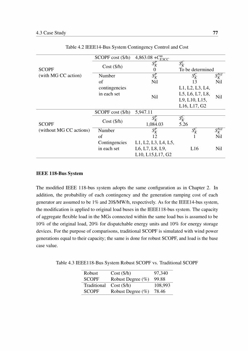
4.3 Case Study 77
Table 4.2 IEEE14-Bus System Contingency Control and Cost
SCOPF(with MG CC action)
SCOPF cost ($/h) 4,863.08 +CmESCC
Cost ($/h)SP
K SCK
0 To be determinedNumberofcontingenciesin each set
SPK SC
K SNilK
Nil 13 Nil
Nil
L1, L2, L3, L4,L5, L6, L7, L8,L9, L10, L15,L16, L17, G2
Nil
SCOPF(without MG CC actions)
SCOPF cost ($/h) 5,947.11
Cost ($/h)SP
K SCK
1,084.03 5.26NumberofContingenciesin each set
SPK SC
K SNilK
12 1 NilL1, L2, L3, L4, L5,L6, L7, L8, L9,L10, L15,L17, G2
L16 Nil
IEEE 118-Bus System
The modified IEEE 118-bus system adopts the same configuration as in Chapter 2. Inaddition, the probability of each contingency and the generation ramping cost of eachgenerator are assumed to be 1% and 20$/MW/h, respectively. As for the IEEE14-bus system,the modification is applied to original load buses in the IEEE118-bus system. The capacityof aggregate flexible load in the MGs connected within the same load bus is assumed to be10% of the original load, 20% for dispatchable energy units and 10% for energy storagedevices. For the purpose of comparisons, traditional SCOPF is simulated with wind powergenerations equal to their capacity; the same is done for robust SCOPF, and load is the basecase value.
Table 4.3 IEEE118-Bus System Robust SCOPF vs. Traditional SCOPF
RobustSCOPF
Cost ($/h) 97,340Robust Degree (%) 99.88
TraditionalSCOPF
Cost ($/h) 108,993Robust Degree (%) 78.46
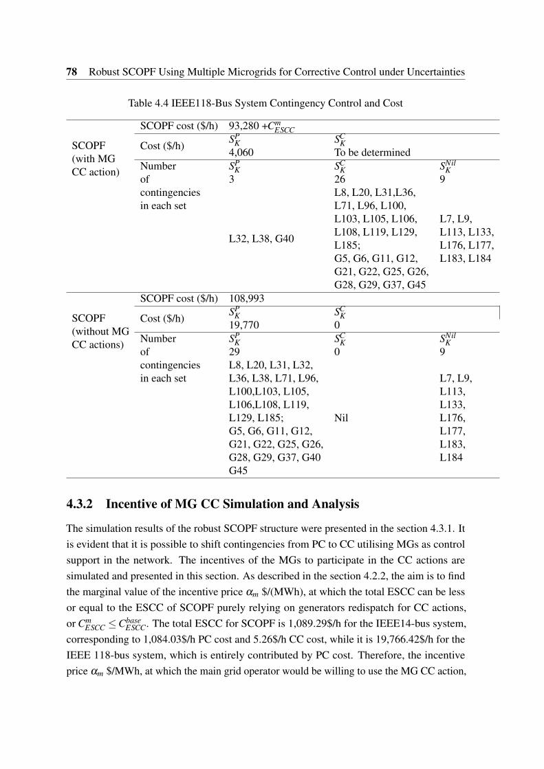
78 Robust SCOPF Using Multiple Microgrids for Corrective Control under Uncertainties
Table 4.4 IEEE118-Bus System Contingency Control and Cost
SCOPF(with MGCC action)
SCOPF cost ($/h) 93,280 +CmESCC
Cost ($/h)SP
K SCK
4,060 To be determinedNumberofcontingenciesin each set
SPK SC
K SNilK
3 26 9
L32, L38, G40
L8, L20, L31,L36,L71, L96, L100,L103, L105, L106,L108, L119, L129,L185;G5, G6, G11, G12,G21, G22, G25, G26,G28, G29, G37, G45
L7, L9,L113, L133,L176, L177,L183, L184
SCOPF(without MGCC actions)
SCOPF cost ($/h) 108,993
Cost ($/h)SP
K SCK
19,770 0Numberofcontingenciesin each set
SPK SC
K SNilK
29 0 9L8, L20, L31, L32,L36, L38, L71, L96,L100,L103, L105,L106,L108, L119,L129, L185;G5, G6, G11, G12,G21, G22, G25, G26,G28, G29, G37, G40G45
Nil
L7, L9,L113,L133,L176,L177,L183,L184
4.3.2 Incentive of MG CC Simulation and Analysis
The simulation results of the robust SCOPF structure were presented in the section 4.3.1. Itis evident that it is possible to shift contingencies from PC to CC utilising MGs as controlsupport in the network. The incentives of the MGs to participate in the CC actions aresimulated and presented in this section. As described in the section 4.2.2, the aim is to findthe marginal value of the incentive price αm $/(MWh), at which the total ESCC can be lessor equal to the ESCC of SCOPF purely relying on generators redispatch for CC actions,or Cm
ESCC ≤CbaseESCC. The total ESCC for SCOPF is 1,089.29$/h for the IEEE14-bus system,
corresponding to 1,084.03$/h PC cost and 5.26$/h CC cost, while it is 19,766.42$/h for theIEEE 118-bus system, which is entirely contributed by PC cost. Therefore, the incentiveprice αm $/MWh, at which the main grid operator would be willing to use the MG CC action,
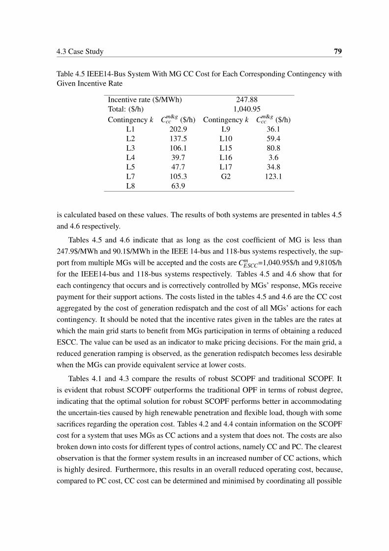
4.3 Case Study 79
Table 4.5 IEEE14-Bus System With MG CC Cost for Each Corresponding Contingency withGiven Incentive Rate
Incentive rate ($/MWh) 247.88Total: ($/h) 1,040.95Contingency k Cm&g
cc ($/h) Contingency k Cm&gcc ($/h)
L1 202.9 L9 36.1L2 137.5 L10 59.4L3 106.1 L15 80.8L4 39.7 L16 3.6L5 47.7 L17 34.8L7 105.3 G2 123.1L8 63.9
is calculated based on these values. The results of both systems are presented in tables 4.5and 4.6 respectively.
Tables 4.5 and 4.6 indicate that as long as the cost coefficient of MG is less than247.9$/MWh and 90.1$/MWh in the IEEE 14-bus and 118-bus systems respectively, the sup-port from multiple MGs will be accepted and the costs are Cm
ESCC=1,040.95$/h and 9,810$/hfor the IEEE14-bus and 118-bus systems respectively. Tables 4.5 and 4.6 show that foreach contingency that occurs and is correctively controlled by MGs’ response, MGs receivepayment for their support actions. The costs listed in the tables 4.5 and 4.6 are the CC costaggregated by the cost of generation redispatch and the cost of all MGs’ actions for eachcontingency. It should be noted that the incentive rates given in the tables are the rates atwhich the main grid starts to benefit from MGs participation in terms of obtaining a reducedESCC. The value can be used as an indicator to make pricing decisions. For the main grid, areduced generation ramping is observed, as the generation redispatch becomes less desirablewhen the MGs can provide equivalent service at lower costs.
Tables 4.1 and 4.3 compare the results of robust SCOPF and traditional SCOPF. Itis evident that robust SCOPF outperforms the traditional OPF in terms of robust degree,indicating that the optimal solution for robust SCOPF performs better in accommodatingthe uncertain-ties caused by high renewable penetration and flexible load, though with somesacrifices regarding the operation cost. Tables 4.2 and 4.4 contain information on the SCOPFcost for a system that uses MGs as CC actions and a system that does not. The costs are alsobroken down into costs for different types of control actions, namely CC and PC. The clearestobservation is that the former system results in an increased number of CC actions, whichis highly desired. Furthermore, this results in an overall reduced operating cost, because,compared to PC cost, CC cost can be determined and minimised by coordinating all possible
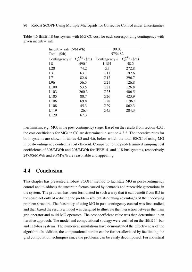
80 Robust SCOPF Using Multiple Microgrids for Corrective Control under Uncertainties
Table 4.6 IEEE118-bus system with MG CC cost for each corresponding contingency withgiven incentive rate
Incentive rate ($/MWh) 90.07Total: ($/h) 5754.82Contingency k Cm&g
cc ($/h) Contingency k Cm&gcc ($/h)
L8 490.1 L185 58.2L20 74.2 G5 272.8L31 63.1 G11 192.6L71 82.6 G12 296.7L96 56.5 G21 126.8L100 53.5 G21 126.8L103 260.3 G25 406.5L105 80.7 G26 423.9L106 69.8 G28 1196.1L108 45.3 G29 862.3L119 126.4 G45 204.3L129 67.3
mechanisms, e.g. MG, in the post-contingency stage. Based on the results from section 4.3.1,the cost coefficients for MGs in CC are determined in section 4.3.2. The incentive rates forboth systems are shown in tables 4.5 and 4.6, below which the total ESCC of using MGin post-contingency control is cost efficient. Compared to the predetermined ramping costcoefficients of 30$/MW/h and 20$/MW/h for IEEE14- and 118-bus systems, respectively,247.9$/MW/h and 90/MW/h are reasonable and appealing.
4.4 Conclusion
This chapter has presented a robust SCOPF method to facilitate MG in post-contingencycontrol and to address the uncertain factors caused by demands and renewable generations inthe system. The problem has been formulated in such a way that it can benefit from BD inthe sense not only of reducing the problem size but also taking advantages of the underlyingproblem structure. The feasibility of using MG in post-contingency control was first studied,and then based the results a model was designed to illustrate the interaction between the maingrid operator and multi-MG operators. The cost coefficient value was then determined in aniterative approach. The model and computational strategy were verified on the IEEE 14-busand 118-bus systems. The numerical simulations have demonstrated the effectiveness of thealgorithm. In addition, the computational burden can be further alleviated by facilitating thegrid computation techniques since the problems can be easily decomposed. For industrial

4.4 Conclusion 81
application, as a dispatch tool, the formulated robust SCOPF method can help the systemoperator to enhance the system security while optimising the system’s economic performanceunder large-scale intermittent renewable power integration and MG deployments.
Chapter 5
Computation Efficiency andConvergence Analysis
This chapter comprises two parts. The first concerns computation efficiency and conver-gence, which are of significant importance in the optimal dispatch decision-making process.However the SCOPF problem is normally computationally expensive if a full ac power flowmodel is implemented with large number of contingencies. Adding uncertainties to a complexproblem makes it more complicated. A bottleneck here is not only due to the large numberof variables and contingencies, but also to the scale of the problem by implementation ofthe uncertainties. Approaches can normally be exploited. First the issue can be tackledby applying decomposition techniques. Second, the computational burden can be eased byidentifying the most efficient method for uncertainties realisation. Finally, since SCOPF witha full ac power flow model is non-linear, and non-convex, an approximation can be madeso that the problem can be solved easily for global optimal. This chapter initially discussesthese approaches, some of which have been employed in this thesis, while others might bebeneficial in future implementation. Next, the second part discusses the issue of some convexoptimisation problems requiring further smoothing when a distributed algorithm is employed.Using demand side flexibility to compensate for the uncertainties caused by the generationside is another effective method to accommodate the growing fraction of RESs in the grid,and a DSM model using social welfare optimisation is demonstrated using a fast distributeddual gradient method to improve the convergence of the algorithm. This chapter is based on[21, 58, 59, 73, 87].

84 Computation Efficiency and Convergence Analysis
5.1 Problem Complexity Analysis of SCOPF Under Uncer-tainties and Its Solutions
The OPF problem is the essential part of the power system, which underlines variousapplications in economic dispatch, unit commitment, loss minimisation, voltage regulation,planning, etc. The basic structure and several types of formulation were introduced in Chapter2.
The SCOPF problem under uncertainties brings the scale of the OPF problem to aeven higher level. Its fundamental structure is generally non-convex and NP-hard, withan enormous number of constraints and variables. The difficulties in solving the SCOPFproblem can be summarised into the following three points.
1. The core of SCOPF is the ac OPF problem, which is nonconvex and NP-hard, and mayhave local solutions. Ongoing research on OPF solution techniques has been conducedfor as long as the OPF problem has existed [88–90]. Several techniques have beenapplied, such as successive quadratic programs, Lagrangian relaxation, the interiorpoints methods (IPM), and artificial intelligence. Although IPM has been widelyadopted in the power system analysis for its advantages in terms of good convergenceand robustness, when the scale of the problem becomes large, the method has difficultyto initialising a feasible solution, and the iteration can grow. Therefore, approximationand relaxation approaches have been proposed. The most popular approximation isthe DC-OPF model or linearised OPF model, introduced in Chapter 2. Althoughthe DC-OPF problem becomes convex and the constraints are linear, however, thedisadvantages in neglecting some system and engineering constraints make it lessadequate for certain tasks.
2. Another factor that makes the SCOPF under uncertainties a large-scaled problem isthe large amount of security constraints and variables in an N-1 contingency analysisfor security considerations. One approach to reduce the computation load is to applythe contingency filter techniques [91], since contingencies are low-probability/high-impact events. In this case, only the most severe contingencies are selected forstudy, so that the number of constraints and variables can be significantly reduced.However, determining the severity of a contingency for a given network can be arbitrary,applying the contingency filter therefore might avoid some high impact contingencies.Another approach is to apply the decomposition techniques so that the problem canbe decomposed into several sub-problems, which can be better underline the problemstructure and applied with parallel computation.
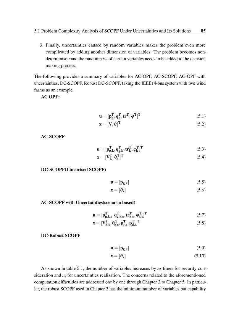
5.1 Problem Complexity Analysis of SCOPF Under Uncertainties and Its Solutions 85
3. Finally, uncertainties caused by random variables makes the problem even morecomplicated by adding another dimension of variables. The problem becomes non-deterministic and the randomness of certain variables needs to be added to the decisionmaking process.
The following provides a summary of variables for AC-OPF, AC-SCOPF, AC-OPF withuncertainties, DC-SCOPF, Robust DC-SCOPF, taking the IEEE14-bus system with two windfarms as an example.
AC OPF:
u = [pTg ,q
Tg , tr
T,ϕT]T (5.1)
x = [V,θ ]T (5.2)
AC-SCOPF
u = [pTg,k,q
Tg,k, tr
Tk ,ϕ
Tk ]
T (5.3)
x = [VTk ,θ
Tk ]
T (5.4)
DC-SCOPF(Linearised SCOPF)
u = [pg,k] (5.5)
x = [θk] (5.6)
AC-SCOPF with Uncertainties(scenario based)
u = [pTg,k,s,q
Tg,k,s, tr
Tk,s,ϕ
Tk,s]
T (5.7)
x = [VTk,s,θ
Tk,s,p
Tr,s,p
Td,s]
T (5.8)
DC-Robust SCOPF
u = [pg,k] (5.9)
x = [θk] (5.10)
As shown in table 5.1, the number of variables increases by nk times for security con-sideration and ns for uncertainties realisation. The concerns related to the aforementionedcomputation difficulties are addressed one by one through Chapter 2 to Chapter 5. In particu-lar, the robust SCOPF used in Chapter 2 has the minimum number of variables but capability

86 Computation Efficiency and Convergence Analysis
Table 5.1 Number of Variables for Several Types of Optimisation Problem Formulation
ACOPF
ACSCOPF
DCSCOPF
ACSCOPFUncertianties(scenario based)
DCRobustSCOPF
nu 2ng +ntr +nϕ nk(2ng +ntr +nϕ) nkng nkns(2ng +ntr +nϕ) nkngnx 2nb 2nknb nknb nkns(2nb +nr) nknb
to consider the uncertainties that is equavalent to that of DC-SCOPF with uncertainties usinga scenario based approach, which increased the number of variables by ns times. Furthermore,the whole problem is decomposed into a master and nk sub-problems, giving each problema number of ng control variables and nb state variables. In this way, the uncertainties andsecurities are addressed in a computationally efficient manner.
Chapter 3 extended the model by considering the ac power flow into the SCOPF problem.Instead of formulating a whole AC-SCOPF problem, BD is employed to take advantages theproblem structure, where a DC-OPF is used in the master problem for optimisation while acpower flow is used in the sub-problems for the N-1 contingency analysis for the constraintscheck.In this case, the problem can not only benefit from fast convergence by approximationin the OPF model, but can also check the solution solved from the approximated model withnetwork constraints that are normally neglected by the traditional linearised OPF model.
5.2 Distributed Algorithms with Fast Convergence RateApplication in Real-Time Pricing Strategy and ConvexRelaxation
Chapters 2 to 4 all examined the problems on the transmission or sub-transmission level inthe scope of SCOPF considering uncertainties, which the aim of introducing an efficient wayto integrate the large scaled renewable generation sources in the electricity operation, such asan hourly based OPF problem for economic dispatch. Various approaches were introduced toaccommodate the uncertainties brought by both load and renewable generation sources, anda robust formulation was introduced and demonstrated in the simulation.
On the other hand, ensuring flexibility on the demand side to compensate for the un-certainties on the generation side is an alternative approach to accommodate the increasingpenetration on RESs. This section introduces an optimal energy scheduling model in a realtime pricing (RTP) environment [92] for DSM, and two aspects are considered:

5.2 Distributed Algorithms with Fast Convergence Rate Application in Real-Time PricingStrategy and Convex Relaxation 87
1. The increasing penetration of distributed renewable sources in the electricity grid onthe demand side has been observed in many countries. Consumers are becoming’prosumers’ [93] and the traditional ’generation follows demand’ way of operation hasbeen challenged. With the advance of smart grid application, the end users have gainedmore control and flexibility regarding their electricity behaviours. Therefore, a DSMmodel is designed to study the feasibility of ’demand follows generation’ behaviourunder the RTP environment.
2. A social welfare model is used to simulate the consumers’ behaviours. Since someinformation on consumer consumption, such as upper and lower limit of consumptionin a certain time frame and individual consumption preference at each time slot, isonly known by the consumers, a centralised algorithm is not suitable in this case.Therefore, a distributed algorithm is applied to find the optimal solution. However, themodel is not strongly convex and therefore when the distributed algorithm is applied,the gradient method suffers from a slow convergence rate. A convex relaxation andsmoothing technique is introduced to improve the convergence, and the convergenceanalysis is provided.
5.2.1 Background
The increasing penetration of RESs has been evidently increasing the risk of reliable electric-ity grid operation. In recent years, the increasing pressure on the power grid has also beencaused by the rising peak load demand, which is partly due to the rapid growth in the useof air conditioners and other appliances, as well as the introduction of some new types ofdemand to the grid, e.g. plug-in electric vehicles (EVs). Moreover, the increasing amount ofrenewable generations is not always capable of providing support to reduce the peak load.This problem was observed back in 2013, when California’s grid operator CAISO releaseda report on how the growth of solar power was going to change the state’s energy balanceover the coming years. In this report, the famous ’duck curve’, shown in figure 5.1, drewenormous attention. This graph illustrates a deep drop in the net load around noon, which isdriven by a large amount of PV power injected into the grid, followed by a sharp ramp-upfrom the late afternoon until the early night time, when PV power fades as residents start tocome home from work and to consume electricity at the same time. It should also be notedthat peak demand occurs only a limited number of times per year. Thus, many new assetsare in fact idle and operated at a mere fraction of their capacity. For example, in the US,10%–20% of electricity costs are determined by peak demand summing up to only 100 hours
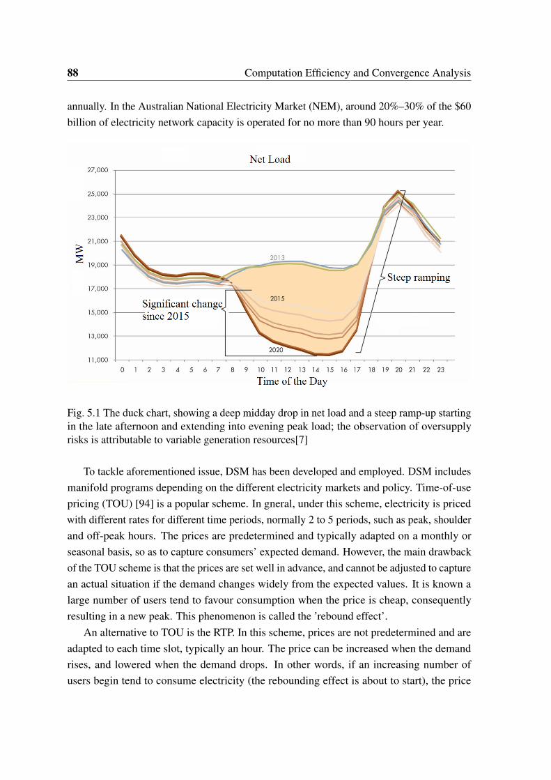
88 Computation Efficiency and Convergence Analysis
annually. In the Australian National Electricity Market (NEM), around 20%–30% of the $60billion of electricity network capacity is operated for no more than 90 hours per year.
Fig. 5.1 The duck chart, showing a deep midday drop in net load and a steep ramp-up startingin the late afternoon and extending into evening peak load; the observation of oversupplyrisks is attributable to variable generation resources[7]
To tackle aforementioned issue, DSM has been developed and employed. DSM includesmanifold programs depending on the different electricity markets and policy. Time-of-usepricing (TOU) [94] is a popular scheme. In gneral, under this scheme, electricity is pricedwith different rates for different time periods, normally 2 to 5 periods, such as peak, shoulderand off-peak hours. The prices are predetermined and typically adapted on a monthly orseasonal basis, so as to capture consumers’ expected demand. However, the main drawbackof the TOU scheme is that the prices are set well in advance, and cannot be adjusted to capturean actual situation if the demand changes widely from the expected values. It is known alarge number of users tend to favour consumption when the price is cheap, consequentlyresulting in a new peak. This phenomenon is called the ’rebound effect’.
An alternative to TOU is the RTP. In this scheme, prices are not predetermined and areadapted to each time slot, typically an hour. The price can be increased when the demandrises, and lowered when the demand drops. In other words, if an increasing number ofusers begin tend to consume electricity (the rebounding effect is about to start), the price

5.2 Distributed Algorithms with Fast Convergence Rate Application in Real-Time PricingStrategy and Convex Relaxation 89
will rise accordingly and thus mitigate the ’rebounding effect’. This scheme can reflect thecurrent conditions and effectively capture the actual demand. Therefore, the RTP scheme canovercome the disadvantage of TOU. Mohsenian-Rad et al. [92, 95, 96] proposed innovativemodels for RTP. Their models have received much attention and citations in the last severalyears. In general, these models aim to maximise the aggregated welfare for users whileminimising the cost for the energy provider through an optimal RTP strategy. Furthermore,based on Mohsenian-Rad et al’ models, some extended models have been proposed fordifferent applications. For sintance, Chai et al. extended this work to a two-level game modelgiven for multiple utility companies [97]. The authors argue that the equilibrium points canbe achieved in games formulated between users and utility companies through distributedalgorithms. A load scheduling strategy is proposed in [98], where the RESs and storages areinstalled. The problem is again solved in a distributed fashion. Study [99] extends the workby considering load uncertainty in the optimisation constraints. Similar schemes can also befound in [100, 101].
In general, these models [92, 95–101] are concave maximisation problem and can besolved by using the IPM in a centralised fashion to obtain global optimal solutions if allparameters are known to the energy provider. However, when these models are applied inpractice such as the optimal RTP problems, it is difficult to collect the parameters of allhouseholds due to privacy concerns. Moreover, when the user number is large, centralisedtechniques may not be feasible. Instead, a distributed sub-gradient algorithm is widelyapplied [92, 95–101]. This algorithm simulates the dynamic behaviours between users andthe energy provider, and finally converges to an equilibrium point. Furthermore, the smartgrid environment with two-way communication networks provides such a platform for thebi-directional information exchange between customers and the energy provider. In general,a one-day operation can be divided into several time slots. For example, a one-hour-basedtime slot is often adopted. The price for each time slot is computed in real-time and then hasto be announced at the beginning of each time slot. However, there are still some problemsthat require further discussion. For example, it is unknow that whether the equilibrium pointis unique or the same as the solution from the centralised algorithm (IPM). On the other hand,during the optimising process, although the distributed sub-gradient algorithm [102] is widelyused in many RTP models to achieve an optimal solution, this algorithm in fact suffers froma slow convergence and numeric sensitivity to the step size, or even from non-convergence.More specifically, the step size parameter in the distributed algorithm has a strong impacton the convergence rate. In practice, it is difficult to adapt the step size efficiently becauseoscillation occurs when the step size is big, while convergence becomes too slow when thestep size is small.

90 Computation Efficiency and Convergence Analysis
5.2.2 Problem Formulation
Let N denote the set of consumers who subscribe to an energy provider where N , N .A whole-day cycle is divided into T time slots, where T , T . On the customer side, theappliances are categorised into two types, deferrable and non-deferrable. For each useri ∈ N , let xt
i denote the user iu’s consumption in time slot t, where xti satisfies xt
i ≤ xti ≤ xt
i .
xti and xt
i denote the minimum and the maximum consumption in time slot t of user iu,respectively. The minimum consumption is the summation of all consumption from non-deferrable appliances. The maximum consumption represents the total consumption of allappliances. Denote set It
p,i = [xti,x
ti].
User’s Utility Function
Each user is assumed to behave independently to various prices and to have different pref-erences for energy demand. The concept of utility function U(x,ξ ) from microeconomicsis used to describe users’ different responses and represents the satisfaction obtained fromconsuming x amount of energy. Herein, ξ is a parameter specifying each user’s preferenceof each user and may vary in different time slots. In general, the following utility function iswidely adopted,
U(x,ξ ) =
{ξ x−αx2 i f 0 ≤ x ≤ ξ
α
ξ 2
2αi f x ≥ ξ
α
(5.11)
Provider’s Utility
The energy provider’s cost function Ct(Lt) describes the cost of providing Lt units of energyto its subscribers in time slot t. In general, the cost function should fulfil the propertiesdescribed below. Characteristics: The cost function is strictly convex and increases with theprovided capacity, for example the cost function that has been used for OPF throughout thisthesis:
C(L) = aL2 +bL+ c (5.12)
where a > 0,b ≥ 0andc ≥ 0. In the time slot t, denote set Jt = [Jmint ,Jmax
t ], where Jmint =
∑ni=1 xt
i and Jmaxt = ∑
niu=1 xt
i
5.2 Distributed Algorithms with Fast Convergence Rate Application in Real-Time PricingStrategy and Convex Relaxation 91
Objective Function Formulation
The interactions between the energy provider and its customers can be formulated as opti-misation problems in various models based on different scenarios. To identify the commonfeatures of these models, three typical models are reviewed briefly in the following. Ageneralised comprehensive model is then described.
For each time slot t, the objective is to maximise the sum of the utility functions of allusers and minimise the cost imposed on the energy provider. Mathematically, this can beexpressed as:
Objective:
maximiseN
∑iu=1
U(xti,ξ
ti )−Ct(Lt)
Subject to:xt
i
∑iu=1
= Lt
xti ∈ [xt
i,xti]
Lt ∈ [Jmint ,Jmax
t ] (5.13)
The constraint indicates that the aggregated load of all users should be equal to thegeneration of the energy provider at each time slot t. As mentioned in the introduction, theparameters xt
i , xti and ξ t
i are private information for each user. It is difficult for the energyprovider to solve this problem with a centralised algorithm. Alternatively, the primal problemcan be transformed into its dual problem. The Lagrangian function of problem (5.13) can bewritten as follows:
L (x,Lt ,λt) = sumi∈N (U(xt
i,ξti )−λ
txti)+λ
tLt −Ct(Lt) (5.14)
where λ t is the Lagrangian multiplier, often used to indicate the electricity rate of a giventime slot. Then the primal problem can be transformed into:
D(λ t) = maxL (x,Lt ,λt) (5.15)
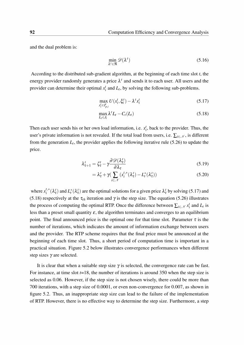
92 Computation Efficiency and Convergence Analysis
and the dual problem is:
minλ t∈ℜ
D(λ t) (5.16)
According to the distributed sub-gradient algorithm, at the beginning of each time slot t, theenergy provider randomly generates a price λ t and sends it to each user. All users and theprovider can determine their optimal xt
i and Lt , by solving the following sub-problems.
maxxt
i∈Itp,i
U(xti,ξ
ti )−λ
txti (5.17)
maxLt∈Jt
λtLt −Ct(Lt) (5.18)
Then each user sends his or her own load information, i.e. xti , back to the provider. Thus, the
user’s private information is not revealed. If the total load from users, i.e. ∑i∈N , is differentfrom the generation Lt , the provider applies the following iterative rule (5.26) to update theprice.
λtτ+1 = ζ
tτ − γ
∂D(λ tτ)
∂λτ
(5.19)
= λtτ + γ( ∑
i∈N
(xt,∗i (λ t
τ)−L∗t (λ
tτ)) (5.20)
where xt,∗i (λ t
τ) and L∗t (λ
tτ) are the optimal solutions for a given price λ t
τ by solving (5.17) and(5.18) respectively at the τth iteration and γ is the step size. The equation (5.26) illustratesthe process of computing the optimal RTP. Once the difference between ∑i∈N xt
i and Lt isless than a preset small quantity ε , the algorithm terminates and converges to an equilibriumpoint. The final announced price is the optimal one for that time slot. Parameter τ is thenumber of iterations, which indicates the amount of information exchange between usersand the provider. The RTP scheme requires that the final price must be announced at thebeginning of each time slot. Thus, a short period of computation time is important in apractical situation. Figure 5.2 below illustrates convergence performances when differentstep sizes γ are selected.
It is clear that when a suitable step size γ is selected, the convergence rate can be fast.For instance, at time slot t=18, the number of iterations is around 350 when the step size isselected as 0.06. However, if the step size is not chosen wisely, there could be more than700 iterations, with a step size of 0.0001, or even non-convergence for 0.007, as shown infigure 5.2. Thus, an inappropriate step size can lead to the failure of the implementationof RTP. However, there is no effective way to determine the step size. Furthermore, a step
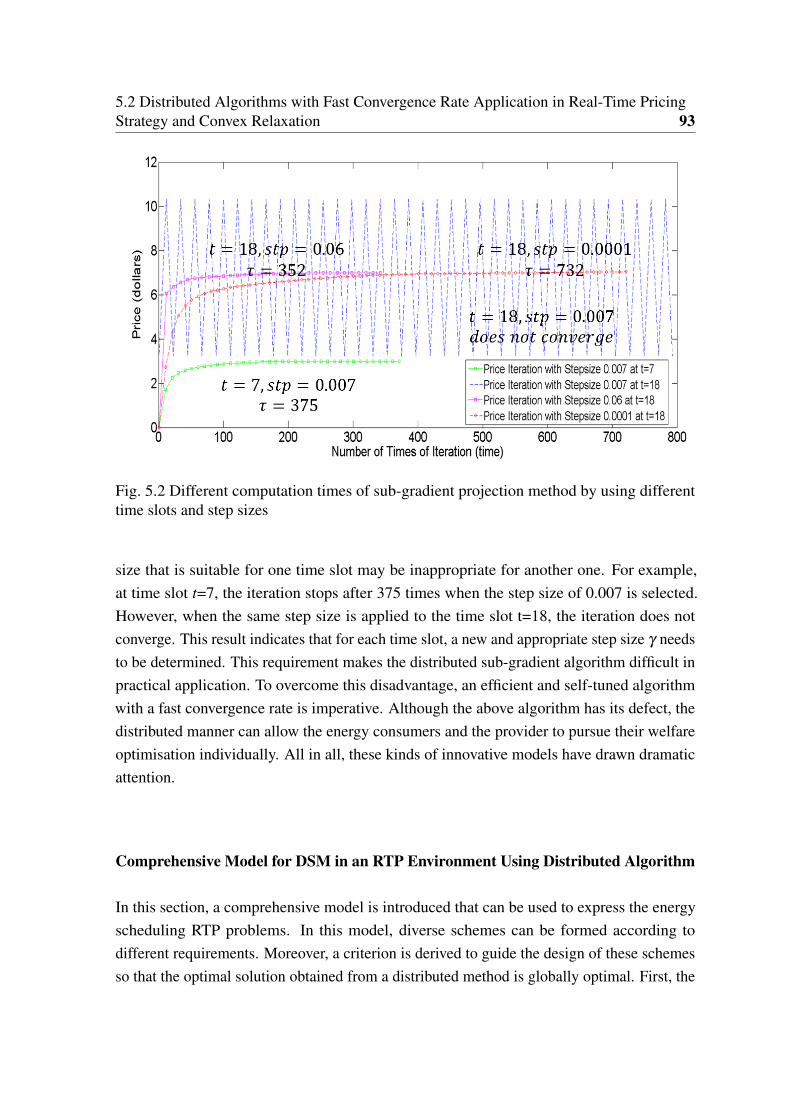
5.2 Distributed Algorithms with Fast Convergence Rate Application in Real-Time PricingStrategy and Convex Relaxation 93
Fig. 5.2 Different computation times of sub-gradient projection method by using differenttime slots and step sizes
size that is suitable for one time slot may be inappropriate for another one. For example,at time slot t=7, the iteration stops after 375 times when the step size of 0.007 is selected.However, when the same step size is applied to the time slot t=18, the iteration does notconverge. This result indicates that for each time slot, a new and appropriate step size γ needsto be determined. This requirement makes the distributed sub-gradient algorithm difficult inpractical application. To overcome this disadvantage, an efficient and self-tuned algorithmwith a fast convergence rate is imperative. Although the above algorithm has its defect, thedistributed manner can allow the energy consumers and the provider to pursue their welfareoptimisation individually. All in all, these kinds of innovative models have drawn dramaticattention.
Comprehensive Model for DSM in an RTP Environment Using Distributed Algorithm
In this section, a comprehensive model is introduced that can be used to express the energyscheduling RTP problems. In this model, diverse schemes can be formed according todifferent requirements. Moreover, a criterion is derived to guide the design of these schemesso that the optimal solution obtained from a distributed method is globally optimal. First, the

94 Computation Efficiency and Convergence Analysis
users’ welfare function can be defined as,
Wi(xti) =U(xt
i,ξti )−λ
txti (5.21)
and the energy provider’s welfare function is defined as,
W (Lt) = λtLt −Ct(Lt) (5.22)
Both Wi(xti) and W (Lt) are concave and coupled with the dynamic price signal λ t . Normally,
most energy scheduling problems can be generalised as different interactions among usersand the energy provider. Thus the process of a comprehensive model can be illustrated infigure 5.3. According to the presented comprehensive model, different energy scheduling
Fig. 5.3 The blue and red lines represent the information exchange, where users send theirown consumptions and the energy provider announces the price signal
schemes can be generated based on different problems by using the forms of (5.21) and(5.22). For example, by simply combining (5.21) and (5.22) to achieve social welfare, model(5.13) and its equivalent (5.14) can be formed. In general, no matter how these models aredesigned, the following criterion is provided, which is able to guarantee that the optimisationsolution achieved from a distributed method is equivalent to the optimal solution computedusing a centralised method.
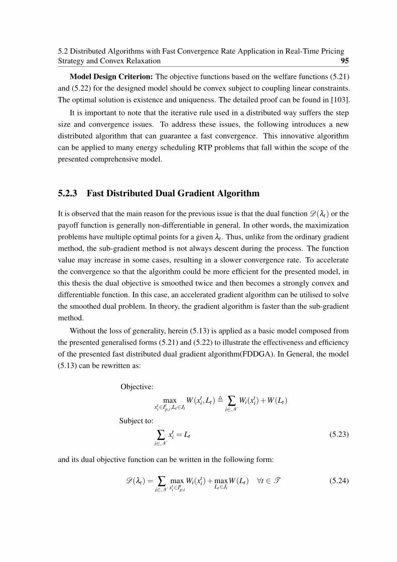
5.2 Distributed Algorithms with Fast Convergence Rate Application in Real-Time PricingStrategy and Convex Relaxation 95
Model Design Criterion: The objective functions based on the welfare functions (5.21)and (5.22) for the designed model should be convex subject to coupling linear constraints.The optimal solution is existence and uniqueness. The detailed proof can be found in [103].
It is important to note that the iterative rule used in a distributed way suffers the stepsize and convergence issues. To address these issues, the following introduces a newdistributed algorithm that can guarantee a fast convergence. This innovative algorithmcan be applied to many energy scheduling RTP problems that fall within the scope of thepresented comprehensive model.
5.2.3 Fast Distributed Dual Gradient Algorithm
It is observed that the main reason for the previous issue is that the dual function D(λt) or thepayoff function is generally non-differentiable in general. In other words, the maximizationproblems have multiple optimal points for a given λt . Thus, unlike from the ordinary gradientmethod, the sub-gradient method is not always descent during the process. The functionvalue may increase in some cases, resulting in a slower convergence rate. To acceleratethe convergence so that the algorithm could be more efficient for the presented model, inthis thesis the dual objective is smoothed twice and then becomes a strongly convex anddifferentiable function. In this case, an accelerated gradient algorithm can be utilised to solvethe smoothed dual problem. In theory, the gradient algorithm is faster than the sub-gradientmethod.
Without the loss of generality, herein (5.13) is applied as a basic model composed fromthe presented generalised forms (5.21) and (5.22) to illustrate the effectiveness and efficiencyof the presented fast distributed dual gradient algorithm(FDDGA). In General, the model(5.13) can be rewritten as:
Objective:
maxxt
i∈Itp,i,Lt∈Jt
W (xti,Lt), ∑
i∈N
Wi(xti)+W (Lt)
Subject to:
∑i∈N
xti = Lt (5.23)
and its dual objective function can be written in the following form:
D(λt) = ∑i∈N
maxxt
i∈Itp,i
Wi(xti)+max
Lt∈JtW (Lt) ∀t ∈ T (5.24)
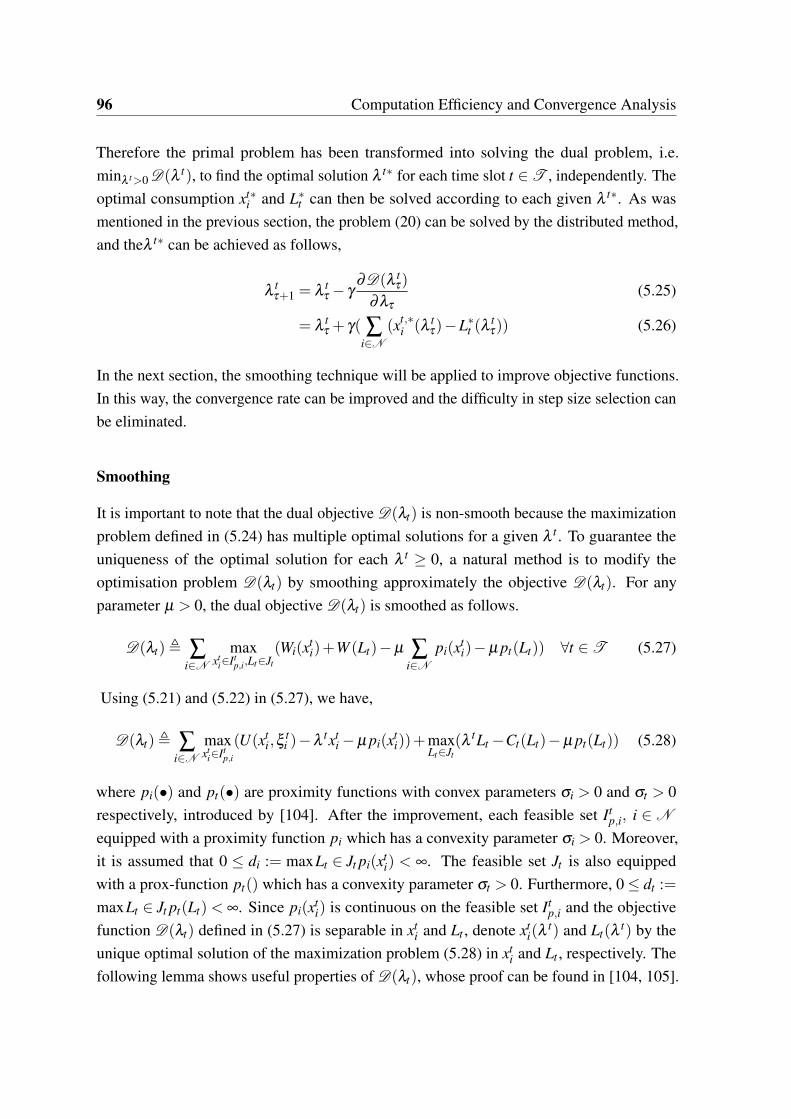
96 Computation Efficiency and Convergence Analysis
Therefore the primal problem has been transformed into solving the dual problem, i.e.minλ t>0 D(λ t), to find the optimal solution λ t∗ for each time slot t ∈ T , independently. Theoptimal consumption xt∗
i and L∗t can then be solved according to each given λ t∗. As was
mentioned in the previous section, the problem (20) can be solved by the distributed method,and theλ t∗ can be achieved as follows,
λtτ+1 = λ
tτ − γ
∂D(λ tτ)
∂λτ
(5.25)
= λtτ + γ( ∑
i∈N
(xt,∗i (λ t
τ)−L∗t (λ
tτ)) (5.26)
In the next section, the smoothing technique will be applied to improve objective functions.In this way, the convergence rate can be improved and the difficulty in step size selection canbe eliminated.
Smoothing
It is important to note that the dual objective D(λt) is non-smooth because the maximizationproblem defined in (5.24) has multiple optimal solutions for a given λ t . To guarantee theuniqueness of the optimal solution for each λ t ≥ 0, a natural method is to modify theoptimisation problem D(λt) by smoothing approximately the objective D(λt). For anyparameter µ > 0, the dual objective D(λt) is smoothed as follows.
D(λt), ∑i∈N
maxxt
i∈Itp,i,Lt∈Jt
(Wi(xti)+W (Lt)−µ ∑
i∈N
pi(xti)−µ pt(Lt)) ∀t ∈ T (5.27)
Using (5.21) and (5.22) in (5.27), we have,
D(λt), ∑i∈N
maxxt
i∈Itp,i
(U(xti,ξ
ti )−λ
txti −µ pi(xt
i))+maxLt∈Jt
(λ tLt −Ct(Lt)−µ pt(Lt)) (5.28)
where pi(•) and pt(•) are proximity functions with convex parameters σi > 0 and σt > 0respectively, introduced by [104]. After the improvement, each feasible set It
p,i, i ∈ N
equipped with a proximity function pi which has a convexity parameter σi > 0. Moreover,it is assumed that 0 ≤ di := maxLt ∈ Jt pi(xt
i) < ∞. The feasible set Jt is also equippedwith a prox-function pt() which has a convexity parameter σt > 0. Furthermore, 0 ≤ dt :=maxLt ∈ Jt pt(Lt)< ∞. Since pi(xt
i) is continuous on the feasible set Itp,i and the objective
function D(λt) defined in (5.27) is separable in xti and Lt , denote xt
i(λt) and Lt(λ
t) by theunique optimal solution of the maximization problem (5.28) in xt
i and Lt , respectively. Thefollowing lemma shows useful properties of D(λt), whose proof can be found in [104, 105].
5.2 Distributed Algorithms with Fast Convergence Rate Application in Real-Time PricingStrategy and Convex Relaxation 97
Lemma 1 The function D(λt) has the following properties:
1. D(λt) is convex and continuously differentiable on λ t > 0
2. Its gradient ▽Dµ(λt) =−(∑i∈N xt
i(λt)−Lt(λ t)) is Lipschitz-continuous with Lips-
chitz constant Lµ = ∑i∈N 1/(µσi)+1/(µσt); and
3. Dµ(λt)≤ D(λt)≤ Dµ(λt)+µ(∑i∈N di +dt), ∀λ ∈ ℜm+
Remark 1: If function W (Lt) defined in (5.22) is taken, there is no need to apply thesmoothing to W (•) in the function D(λt), since Ct(Lt) is strongly convex.
Second smoothing is applied to Dµ , which allows the use of a fast gradient method with agood convergence rate for the decrease of
∥∥▽Dµ(•)∥∥. Therefore, a strongly convex function
υ
2 ∥•∥2 to Dµ is simply added for a scalar υ > 0, which is a special case of prox-function. It
should be noted that the second smoothing is motivated by [104]. Thus we have the followingobjective function is obtained:
Dµ,υ(λt) := Dµ(λ
t)+υ
2
∥∥λt∥∥2 (5.29)
Similarly, the new dual objective function Dµ,υ(λt) has the following good properties [104].
Lemma 2: For the function Dµ,υ(λt),
1. Dµ,υ(λt) is υ-strongly convex and continuously differentiable on λ t ; and
2. Its gradient ▽Dµ,υ(λt) = ▽Dµ(λ
t) + υλ t is Lipschitz continuous with Lipschitzconstant Lµ,υ = Lµ +υ .
The section now focuses on solving the optimisation problem below
minλ t∈ℜ
Dµ,υ(λt) (5.30)
FDDGA
An FDDGA to solve the problem (5.30) is presented. The algorithm can be described asfollows:
FDDGA
Initialisation: Set λ t,0 = κt,0 =: 0 ∈ ℜ; and compute β =
√Lµ,υ−
√υ√
Lµ,υ+√
υ

98 Computation Efficiency and Convergence Analysis
iteration for τ ≤ 0, execute the following steps:
Step 1. Broadcast the price λ t,τ ,κt,τ
• Capacity update for energy provider
Lt,τ = argmaxLt∈Jt
W (Lt) = argmaxLt∈Jt
κt,τLt −Ct(Lt) (5.31)
• Load update of each user i ∈ N .
xt,τi = arg max
xt,τi ∈It
i
Wi(xti)−µ pi(xt
i)
= arg maxxt,τ
i ∈Iti
−κtxti −µ pi(xt
i) (5.32)
Step 2. Collect Lt,τ and xt,τi , ∀i ∈ N , and compute:
▽Dµ(κt,τ) =−( ∑i∈N
xti −Lt)+υκt,τ (5.33)
Piece update with two steps:
λt,τ+1 = κt,τ − 1
Lµ,υ▽Dµ,υ(κt,τ) (5.34)
κt,τ+1 = λt,τ +β (λ t,τ+1 −λ
t,τ) (5.35)
Step 3. If the given stopping criteria is satisfied, then terminate at τ:
1. Dual variables satisfies∣∣λ t,τ+1 −λ t,τ
∣∣≤ ε
2. Primal objective function value satisfies:
max
{maxi∈N
∣∣∣∣∣Wi(xt,τ+1i )−Wi(x
t,τi )
Wi(xt,τi )
∣∣∣∣∣ ,∣∣∣∣W (Lt,τ+1)−W (Lt,τ)
W (Lt,τ)
∣∣∣∣}
≤ ε; (5.36)
3. Primal feasibility satisfies∣∣∣∣∣ ∑i∈N
xt,τ+1i −Lt,τ+1
∣∣∣∣∣≤ ε (5.37)
5.2 Distributed Algorithms with Fast Convergence Rate Application in Real-Time PricingStrategy and Convex Relaxation 99
Terminate
Here Theorem 1 is provided; its convergence is given in AppendixTheorem 1:For any given accuracy ε > 0, let the sequence {λ t,τ}
τ≥0 and {xt,τ ,Lt,τ}t,τ be generatedby the FDDGA. Then a τ0 =O(1
εln 1
ε)> 0 exists such that for any τ > τ0, |W (xt,τ ,Lt,τ)−W ∗| ≤
5ε and∣∣∑i∈N xt,τ
i −Lt,τ∣∣≤ ε
Λ. That is, the iteration complexity of the FDDGA for achieving
a ε-optimal solution is O(1ε
ln 1ε)
5.2.4 Numerical Simulation
The FDDGA formulations were programmed in MATLAB. The simulations were carried outon an Intel Core I5 CPU running at 3.20 GHz with 4 GB of RAM. The numerical simulationhere serves to compare the performance of the presented algorithm with the previous dualsub-gradient algorithm for to solve the problems (5.24) and other similar problems that fallinto the generalised comprehensive model.
For numerical simulation, it is assumed that the standard utility function and the costfunction are adopted from (5.11) and (5.12) respectively. Choose the proximity functionpi(xt
i) =12 ∥xt
i∥2 with σi = 1 and L(µ,υ) as Lemma 2. Let µ = 1
3(∑i∈N di+dt)and υ = 2ε
2Λ2 ,where ε is the desired accuracy. Λ is an upper bound of the solution of the dual problem(5.24), and this simulation we uses Λ = λ t +∆0, where ∆0 is a small positive real number toguarantee that Λ is always larger than λ t . Both algorithms are terminated when all of thetermination conditions are satisfied at iteration τ +1 with required accuracy ε = 0.01.
This section provides several results of the numerical simulations to illustrate that theperformance of the convergence of the presented algorithm is superior to the widely adoptedsub-gradient method [92, 95–101]. Two kinds of analysis cases are examined.
Case 1
Figures 5.4 and 5.5 display the comparison results of the FDDGA and the sub-gradientmethod, showing the dynamic progress of iteration for achieving optimal values in a randomlyselected time slot. Two different group sizes are studied, i.e. N=10 and N=500.
As shown in figure 5.4, at the beginning of the iteration, the price signal (red line) is low.Therefore, the aggregated load (blue line) is high due to the cheap price while the optimisedgeneration is low. Clearly, the large gap between the aggregated load and the provided energyrequires further iterations. With the price signal increases, the difference between load andgeneration continues to decrease, until the termination criteria are met. By illustrating the
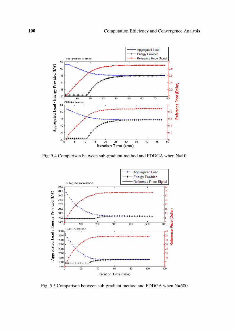
100 Computation Efficiency and Convergence Analysis
Fig. 5.4 Comparison between sub-gradient method and FDDGA when N=10
Fig. 5.5 Comparison between sub-gradient method and FDDGA when N=500
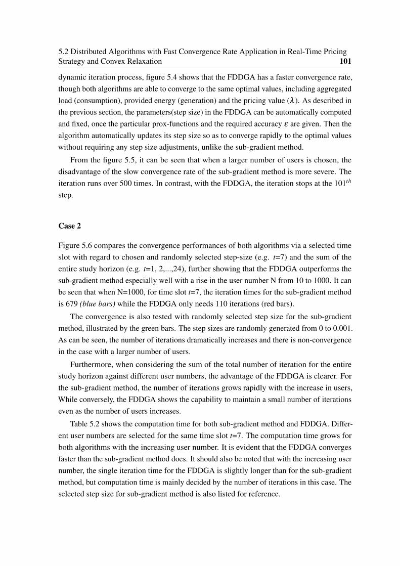
5.2 Distributed Algorithms with Fast Convergence Rate Application in Real-Time PricingStrategy and Convex Relaxation 101
dynamic iteration process, figure 5.4 shows that the FDDGA has a faster convergence rate,though both algorithms are able to converge to the same optimal values, including aggregatedload (consumption), provided energy (generation) and the pricing value (λ ). As described inthe previous section, the parameters(step size) in the FDDGA can be automatically computedand fixed, once the particular prox-functions and the required accuracy ε are given. Then thealgorithm automatically updates its step size so as to converge rapidly to the optimal valueswithout requiring any step size adjustments, unlike the sub-gradient method.
From the figure 5.5, it can be seen that when a larger number of users is chosen, thedisadvantage of the slow convergence rate of the sub-gradient method is more severe. Theiteration runs over 500 times. In contrast, with the FDDGA, the iteration stops at the 101th
step.
Case 2
Figure 5.6 compares the convergence performances of both algorithms via a selected timeslot with regard to chosen and randomly selected step-size (e.g. t=7) and the sum of theentire study horizon (e.g. t=1, 2,...,24), further showing that the FDDGA outperforms thesub-gradient method especially well with a rise in the user number N from 10 to 1000. It canbe seen that when N=1000, for time slot t=7, the iteration times for the sub-gradient methodis 679 (blue bars) while the FDDGA only needs 110 iterations (red bars).
The convergence is also tested with randomly selected step size for the sub-gradientmethod, illustrated by the green bars. The step sizes are randomly generated from 0 to 0.001.As can be seen, the number of iterations dramatically increases and there is non-convergencein the case with a larger number of users.
Furthermore, when considering the sum of the total number of iteration for the entirestudy horizon against different user numbers, the advantage of the FDDGA is clearer. Forthe sub-gradient method, the number of iterations grows rapidly with the increase in users,While conversely, the FDDGA shows the capability to maintain a small number of iterationseven as the number of users increases.
Table 5.2 shows the computation time for both sub-gradient method and FDDGA. Differ-ent user numbers are selected for the same time slot t=7. The computation time grows forboth algorithms with the increasing user number. It is evident that the FDDGA convergesfaster than the sub-gradient method does. It should also be noted that with the increasing usernumber, the single iteration time for the FDDGA is slightly longer than for the sub-gradientmethod, but computation time is mainly decided by the number of iterations in this case. Theselected step size for sub-gradient method is also listed for reference.

102 Computation Efficiency and Convergence Analysis
Fig. 5.6 Comparison of number of iterations between the sub-gradient method and theFDDGA with increasing user number N
Table 5.2 Computation Time for Both the Sub-gradient Method and the FDDGA. DifferentUser Numbers at Time Slot t=7
NFDDGA Sub-gradient Method
Computation Time(Seconds)
Computation Time(Seconds) Step Size
10 0.450 0.740 0.00220 0.790 12.52 0.0012450 0.851 4.052 0.00150
200 1.040 4.722 0.00089500 1.397 6.660 0.00069
1000 1.902 9.019 0.00030

5.3 Conclusion 103
As mentioned previously, the final price should be announced at the beginning of eachtime slot. The FDDGA with faster convergence rate can provide more efficient ways toobtain an optimal RTP and is more suitable for practical application.
5.3 Conclusion
This chapter has examined the complexity and the scale of the problem of SCOPF whenrandom energy generation is considered in the formulation. It discussed a few differentapproaches to reduce the computation burden, which were are applied throughout Chapter 2to 4 for demonstration.
This chapter has also investigated the use of DSM to compensate for the uncertaintiescaused by high fraction RESs generation in the grid. In particular, a distributed algorithm isrequired in this case, which is further smoothed by the FDDGA algorithm to improve theconvergence performance, so that the real-time computation can be ensured. The convergenceanalysis is provided in the appendix.

Chapter 6
Conclusion and Future Work
6.1 Conclusion
This thesis has presented several methods of power system operation and optimisation withthe ultimate goal of accommodating the ever-increasing level of penetration of RESs atall different levels of electricity grids. RESs such as PV and wind introduce additionaldifficulties, which in turn increase the complexity of operating and planning for the grid, andpose challenges in the reliable and secure operation and optimisation for system operators.Intermittency, randomness in generation, and spattered and remote locations of RESs alsorequire the grid expansion in both new transmission lines and larger line capacity. Traditionaloperation and optimisation models become inadequate both for handling the uncertaintiesand for finding a solution, a they are overwhelmed by the problem size and computationload. Designing an effective model to consider the randomness of uncertainties and securityrequirements, and proposing efficient methods to solve these problems could mitigate theseissues. For example, a generalised framework of robust SCOPF is introduced in Chapter 2.Moreover, realising that a meshed MTDC grid and an ac grid could coexist in the future grid,Chapter 3 investigated a hierarchical SCOPF model for offshore wind farm optimal dispatchoperation. Subsequently, Chapter 4 investigated the coordination of multiple microgrids inthe post-contingency recovery, in the scenarios with large renewable generation penetrationon both the transmission and MG levels. Finally, Chapter 5 examined the DSM, which isconsidered to be an alternative way to use the flexibility from the demand side to compensatefor the uncertainties caused by the generation side.
The problems and solutions considered in this thesis have raised an additional and crucialissue regard to computation efficiency as the optimisation problem becomes computationallyexpensive, especially when security and reliability requirements are considered. In particular,a nonlinear formulation of an OPF problem is employed, which is non-convex and NP-
106 Conclusion and Future Work
hard, and it becomes even more computationally expensive when the security constraints anduncertainties are involved. Therefore, a linearised model, also called a dc power flow model, isnormally adopted as an approximation to study the OPF, neglecting some network constraintsand physical losses. Another approach considered in this thesis to reduce the computationcomplexity is to apply decomposition techniques, on both linearised and nonlinear SCOPF,which functions well in parallel with the robust formulation developed to accommodateuncertainties brought by both load and RESs. The numerical simulations in each chapterhave demonstrated encouraging outcomes with regard to the tractability of the problem. Inaddition, a smoothing technique has been developed to be applied to the distributed algorithmwith a widely used gradient method to improve the convergence of the algorithm.
6.2 Future work
Since the penetration of RESs continues to increase in the electricity grid, some interestingresearch questions that could not be investigated in this thesis are discussed and formulatedhere as inspiration for future studies in mainly two aspects: modelling and computation.
Modelling
• Models for OPF and SCOPF considering uncertainties should be further devel-oped. Control strategies of multiple MGs should be investigated. It might be valuableto study and develop a concept of operational flexibility [106] to evaluate the capabilityof MGs to participate in system operations and the electricity market.
• Models of high or 100% power electronics-based grid with small or no inertianeed to be studied. An MG is a good candidate for a heavy inverter-based grid, whichfeatures high penetration of renewable sources and distributed generators, as wellas low inertia. A plug-and-play feature [107] with its enabler controller design andgranular integration into the grid might change the basic structure of the electricitygrid operation.
• Since there are few meshed MTDC systems in operation now, it would be of greatvalue to further investigate detailed models. This includes different converters,losses models, droop control strategies and different operation schemes.

6.2 Future work 107
Computation
• Relaxation and approximation could be applied to reduce the complexity of calcu-lating the SCOPF under uncertainties, apart from linearisation.
• Data-driven optimisation [108, 109], online algorithms [110] and machine learn-ing [111–113] could be more suitable techniques to deal with uncertainties broughtby renewable sources with advanced development in computation and communicationtechnologies.

Chapter 7
List of Publication
Journal paper
[1 ] W. Zhang, J. Li, G. Chen, Z. Y. Dong, and K. P. Wong. A comprehensive model withfast solver for optimal energy scheduling in rtp environment. IEEE Transactions onSmart Grid, PP(99):1–10, 2016.
[2 ] W. Zhang, Y. Xu, Z. Dong, and K. P. Wong. Robust security-constrained optimalpower flow using multiple microgrids for corrective control under uncertainty. IEEETransactions on Industrial Informatics, PP(99):1–1, 2016.
[3 ] W. Zhang, Y. Xu, K. Meng, and Z. Y. Dong. SCOPF using multi-microgrids forcorrective control in energy internet. Southern Power System Technology, PP(8):67–73,2016.
[4 ] K. Meng, W. Zhang, Y. Li, Z. Y. Dong, Z. Xu, K. P. Wong, and Y. Zheng. [submitted]Hierarchical scopf considering wind energy integration through multi-terminal vsc-hvdc grids. IEEE Transactions on Power Systems, 2016(submitted).
[5 ] B. Zeng, C. Li, G. Chen, and W. Zhang. Verhulst model of interval grey number basedon information decomposing and model combination. Journal of Applied Mathematics,2013.
110 List of Publication
Conference paper
[1 ] W. Zhang, Yan Xu, Zhao Yang Dong, Yijia Wang, and Rui Zhang. An efficientapproach for robust scopf considering load and renewable power uncertainties. In 2016Power Systems Computation Conference (PSCC), pages 1–7, June 2016.
[2 ] W. Zhang, G. Chen, Z. Dong, J. Li, and Z. Wu. An efficient algorithm for optimal re-altime pricing strategy in smart grid. In 2014 IEEE PES General Meeting | ConferenceExposition, pages 1–5, July 2014.
[3 ] W. Zhang, X. Yan, Z. Y. Dong, K. Meng, and R. Zhang. Robust opf considering loadand renewable power uncertainties in multi-terminal hvdc grids. In 2016 IEEE PESAsia-Pacific Power and Energy Engineering Conference (APPEEC),pages 24–27, Oct2016.
[4 ] W. Zhang, G. Chen, and Z. Y. Dong. Demand side management given distributedgeneration and storage: A comparison for different pricing and regulation scenarios.In 10th International Conference on Advances in Power System Control, Operation &Management, pages 29–34, November 2015.
[5 ] W. Zhang, G. Chen, Y. Su, Z. Dong, and J. Li. A dynamic game behavior: Demandside management based on utility maximization with renewable energy and storage in-tegration. In 2014 Australasian Universities Power Engineering Conference (AUPEC),pages 1–5, Sept 2014.
[6 ] R. Zhang, Y. Xu, W. Zhang, Z. Y. Dong, and Yu Zheng. Impact of dynamic loadmodels on transient stability-constrained optimal power flow. In 2016 IEEE PESAsia-Pacific Power and Energy Engineering Conference (APPEEC), pages 18–23, Oct2016.
[7 ] Z. Wang, W. Zhang, L. Zhang, G. Chen, Z. Dong, and T. Huang. Impact of differentpenetrations of renewable sources and demand side management on australian futuregrid. In 2015 First Workshop on Smart Grid and Renewable Energy (SGRE), pages1–6, March 2015.
References
[1] Thomas B Johansson. Renewable energy: sources for fuels and electricity. Islandpress, 1993.
[2] Gustav Resch, Anne Held, Thomas Faber, Christian Panzer, Felipe Toro, and ReinhardHaas. Potentials and prospects for renewable energies at global scale. Energy Policy,36(11):4048–4056, 2008.
[3] Walter Musial, Sandy Butterfield, Bonnie Ram, et al. Energy from offshore wind. InOffshore technology conference. Offshore Technology Conference, 2006.
[4] Y. Xu, Z. Y. Dong, Z. Xu, K. Meng, and K. P. Wong. An intelligent dynamic securityassessment framework for power systems with wind power. IEEE Transactions onIndustrial Informatics, 8(4):995–1003, Nov 2012.
[5] Z. Dong, K. P. Wong, K. Meng, F. Luo, F. Yao, and J. Zhao. Wind power impact onsystem operations and planning. In IEEE PES General Meeting, pages 1–5, July 2010.
[6] Renewables 2016 Global Status Report ren21. http://www.ren21.net/wp-content/uploads/2016/06/GSR_2016_Full_Report.pdf. Accessed: 2017-01-15.
[7] Paul Denholm, Matthew O’Connell, Gregory Brinkman, and Jennie Jorgenson. Over-generation from solar energy in california: A field guide to the duck chart. NationalRenewable Energy Laboratory, Tech. Rep. NREL/TP-6A20-65023, 2015.
[8] S. Taggart, G. James, Z. Dong, and C. Russell. The future of renewables linked by atransnational asian grid. Proceedings of the IEEE, 100(2):348–359, Feb 2012.
[9] Thierry Van Cutsem and Costas Vournas. Voltage stability of electric power systems,volume 441. Springer Science & Business Media, 1998.
[10] M. N. Kabir, Y. Mishra, G. Ledwich, Z. Y. Dong, and K. P. Wong. Coordinated controlof grid-connected photovoltaic reactive power and battery energy storage systems toimprove the voltage profile of a residential distribution feeder. IEEE Transactions onIndustrial Informatics, 10(2):967–977, May 2014.
[11] Raul Banos, Francisco Manzano-Agugliaro, FG Montoya, Consolacion Gil, AlfredoAlcayde, and Julio Gómez. Optimization methods applied to renewable and sustainableenergy: A review. Renewable and Sustainable Energy Reviews, 15(4):1753–1766,2011.
112 References
[12] Aoife M Foley, Paul G Leahy, Antonino Marvuglia, and Eamon J McKeogh. Currentmethods and advances in forecasting of wind power generation. Renewable Energy,37(1):1–8, 2012.
[13] J. Zhao, F. Wen, Y. Xue, Z. Y. Dong, and J. Xin. Power system stochastic economicdispatch considering uncertain outputs from plug-in electric vehicles and wind genera-tors. Dianli Xitong Zidonghua(Automation of Electric Power Systems), 34(20):22–29,2010.
[14] R. Zhang, Y. Xu, W. Zhang, Z. Y. Dong, and Y. Zheng. Impact of dynamic load modelson transient stability-constrained optimal power flow. In 2016 IEEE PES Asia-PacificPower and Energy Engineering Conference (APPEEC), pages 18–23, Oct 2016.
[15] Narayana Prasad Padhy. Unit commitment-a bibliographical survey. IEEE Transac-tions on power systems, 19(2):1196–1205, 2004.
[16] Z. Y. Dong, M. Lu, Z. Lu, and K. P. Wong. A differential evolution based methodfor power system planning. In 2006 IEEE International Conference on EvolutionaryComputation, pages 2699–2706, 2006.
[17] K. Meng, H. Yang, Z. Y. Dong, W. Guo, F. Wen, and Z. Xu. Flexible operationalplanning framework considering multiple wind energy forecasting service providers.IEEE Transactions on Sustainable Energy, 7(2):708–717, April 2016.
[18] A Monticelli, MVF Pereira, and S Granville. Security-constrained optimal power flowwith post-contingency corrective rescheduling. IEEE Transactions on Power Systems,2(1):175–180, 1987.
[19] KWOK-LEUNG TSUI. An overview of taguchi method and newly developed statisti-cal methods for robust design. IIE Transactions, 24(5):44–57, 1992.
[20] Antonio J Conejo, Enrique Castillo, Roberto Minguez, and Raquel Garcia-Bertrand.Decomposition techniques in mathematical programming: engineering and scienceapplications. Springer Science & Business Media, 2006.
[21] W. Zhang, Y. Xu, Z. Y. Dong, Y. Wang, and R. Zhang. An efficient approach for robustscopf considering load and renewable power uncertainties. In 2016 Power SystemsComputation Conference (PSCC), pages 1–7, June 2016.
[22] A.J. Wood and B.F. Wollenberg. Power Generation, Operation, and Control. AWiley-Interscience publication. Wiley, 1996.
[23] J Carpentier. Optimal power flows. International Journal of Electrical Power andEnergy Systems, 1(1):3 – 15, 1979.
[24] R. C. Burchett, H. H. Happ, D. R. Vierath, and K. A. Wirgau. Developments in optimalpower flow. IEEE Transactions on Power Apparatus and Systems, PAS-101(2):406–414, Feb 1982.
[25] M. Huneault and F. D. Galiana. A survey of the optimal power flow literature. IEEETransactions on Power Systems, 6(2):762–770, May 1991.
References 113
[26] P. Kundur, N.J. Balu, and M.G. Lauby. Power System Stability and Control. DiscussionPaper Series. McGraw-Hill Education, 1994.
[27] Jamal A Baroudi, Venkata Dinavahi, and Andrew M Knight. A review of powerconverter topologies for wind generators. Renewable energy, 32(14):2369–2385,2007.
[28] Bonmin (Basic Open-source Nonlinear Mixed INteger programming) p. belotti andp. bonami and c. d’ambrosio and etc. https://projects.coin-or.org/Bonmin. Accessed:2017-02-08.
[29] CPLEX Optimizer ibm. http://www-01.ibm.com/software/commerce/optimization/cplex-optimizer/index.html. Accessed: 2017-02-08.
[30] Inc. Gurobi Optimization. Gurobi optimizer reference manual, 2016.
[31] A. Wächter and L. T. Biegler. On the implementation of an interior-point filter line-search algorithm for large-scale nonlinear programming. Mathematical programming,106(1):25–57, 2006.
[32] R. H. Byrd, J. Nocedal, and R. A. Waltz. Knitro: An integrated package for nonlinearoptimization. In Large-scale nonlinear optimization, pages 35–59. Springer, 2006.
[33] X.F. Wang, Y. Song, and M. Irving. Modern Power Systems Analysis. Power electronicsand power systems. Springer US, 2010.
[34] Robert V Hogg and Allen T Craig. Introduction to mathematical statistics.(5"" edition).Upper Saddle River, New Jersey: Prentice Hall, 1995.
[35] M. Shukla and G. Radman. Optimal power flow using probabilistic load model. InProceedings of the Thirty-Seventh Southeastern Symposium on System Theory, 2005.SSST ’05., pages 439–442, March 2005.
[36] H. Ahmadi and H. Ghasemi. Probabilistic optimal power flow incorporating windpower using point estimate methods. In 2011 10th International Conference onEnvironment and Electrical Engineering, pages 1–5, May 2011.
[37] C. Wan, Z. Xu, P. Pinson, Z. Y. Dong, and K. P. Wong. Probabilistic forecasting ofwind power generation using extreme learning machine. IEEE Transactions on PowerSystems, 29(3):1033–1044, May 2014.
[38] T. Yong and R. H. Lasseter. Stochastic optimal power flow: formulation and solution.In 2000 Power Engineering Society Summer Meeting (Cat. No.00CH37134), volume 1,pages 237–242 vol. 1, 2000.
[39] G. Li and X. P. Zhang. Stochastic optimal power flow approach considering correlatedprobabilistic load and wind farm generation. In IET Conference on Reliability ofTransmission and Distribution Networks (RTDN 2011), pages 1–7, Nov 2011.
[40] Y. Zhang and G. B. Giannakis. Robust optimal power flow with wind integrationusing conditional value-at-risk. In 2013 IEEE International Conference on Smart GridCommunications (SmartGridComm), pages 654–659, Oct 2013.
114 References
[41] B. Chen, J. Wang, L. Wang, Y. He, and Z. Wang. Robust optimization for transmissionexpansion planning: Minimax cost vs. minimax regret. IEEE Transactions on PowerSystems, 29(6):3069–3077, Nov 2014.
[42] T. Summers, J. Warrington, M. Morari, and J. Lygeros. Stochastic optimal powerflow based on convex approximations of chance constraints. In 2014 Power SystemsComputation Conference, pages 1–7, Aug 2014.
[43] H. Zhang and P. Li. Probabilistic analysis for optimal power flow under uncertainty.IET Generation, Transmission Distribution, 4(5):553–561, May 2010.
[44] H. Yu and W. D. Rosehart. An optimal power flow algorithm to achieve robustoperation considering load and renewable generation uncertainties. IEEE Transactionson Power Systems, 27(4):1808–1817, Nov 2012.
[45] Dimitris Bertsimas, David B Brown, and Constantine Caramanis. Theory and applica-tions of robust optimization. SIAM review, 53(3):464–501, 2011.
[46] John M Mulvey, Robert J Vanderbei, and Stavros A Zenios. Robust optimization oflarge-scale systems. Operations research, 43(2):264–281, 1995.
[47] S. Marin and A. Garces. Robust optimal power flow in distribution systems with highpenetration of wind energy using a model-based evolutionary strategy. In 2014 IEEEPES Transmission Distribution Conference and Exposition - Latin America (PES TD-LA), pages 1–6, Sept 2014.
[48] B. Zou and Q. Xiao. Solving probabilistic optimal power flow problem using quasimonte carlo method and ninth-order polynomial normal transformation. IEEE Trans-actions on Power Systems, 29(1):300–306, Jan 2014.
[49] E. M. Constantinescu, V. M. Zavala, M. Rocklin, S. Lee, and M. Anitescu. Acomputational framework for uncertainty quantification and stochastic optimization inunit commitment with wind power generation. IEEE Transactions on Power Systems,26(1):431–441, Feb 2011.
[50] A. Alabdulwahab, A. Abusorrah, X. Zhang, and M. Shahidehpour. Coordination ofinterdependent natural gas and electricity infrastructures for firming the variability ofwind energy in stochastic day-ahead scheduling. IEEE Transactions on SustainableEnergy, 6(2):606–615, April 2015.
[51] Christopher Z Mooney. Monte carlo simulation, volume 116. Sage Publications, 1997.
[52] Z. Wang and F. L. Alvarado. Interval arithmetic in power flow analysis. IEEETransactions on Power Systems, 7(3):1341–1349, Aug 1992.
[53] P. Zhang and W. Li. Boundary analysis of distribution reliability and economicassessment. IEEE Transactions on Power Systems, 25(2):714–721, May 2010.
[54] J. M. Morales, S. Pineda, A. J. Conejo, and M. Carrion. Scenario reduction forfutures market trading in electricity markets. IEEE Transactions on Power Systems,24(2):878–888, May 2009.
References 115
[55] Z. Wang, B. Chen, J. Wang, and M. M. Begovic. Stochastic dg placement for conser-vation voltage reduction based on multiple replications procedure. IEEE Transactionson Power Delivery, 30(3):1039–1047, June 2015.
[56] R. D. Zimmerman, C. E. Murillo-Sanchez, and R. J. Thomas. Matpower: Steady-stateoperations, planning, and analysis tools for power systems research and education.IEEE Transactions on Power Systems, 26(1):12–19, Feb 2011.
[57] T.T. Soong. Fundamentals of Probability and Statistics for Engineers. Wiley, 2004.
[58] W. Zhang, Y. Xu, Z. Y. Dong, K. Meng, and R. Zhang. Robust opf considering loadand renewable power uncertainties in multi-terminal hvdc grids. In 2016 IEEE PESAsia-Pacific Power and Energy Engineering Conference (APPEEC), pages 24–27, Oct2016.
[59] K. Meng, W. Zhang, Y. Li, Z. Y. Dong, Z. Xu, K. P. Wong, and Y. Zheng. [submit-ted]hierarchical scopf considering wind energy integration through multi-terminalvsc-hvdc grids. IEEE Transactions on Power Systems, 2016.
[60] P. Pinson, C. Chevallier, and G. N. Kariniotakis. Trading wind generation from short-term probabilistic forecasts of wind power. IEEE Transactions on Power Systems,22(3):1148–1156, Aug 2007.
[61] Sandy Butterfield, Walt Musial, Jason Jonkman, Paul Sclavounos, and Libby Wayman.Engineering challenges for floating offshore wind turbines. In Copenhagen OffshoreWind Conference, Copenhagen, Denmark, pages 377–382. Citeseer, 2005.
[62] Iñigo Martinez de Alegría, Jon Andreu, José Luis Martín, Pedro Ibanez, José LuisVillate, and Haritza Camblong. Connection requirements for wind farms: A survey ontechnical requierements and regulation. Renewable and Sustainable Energy Reviews,11(8):1858–1872, 2007.
[63] J. Beerten, O. Gomis-Bellmunt, X. Guillaud, J. Rimez, A. van der Meer, and D. VanHertem. Modeling and control of hvdc grids: A key challenge for the future powersystem. In 2014 Power Systems Computation Conference, pages 1–21, Aug 2014.
[64] Anna J Wieczorek, Simona O Negro, Robert Harmsen, Gaston J Heimeriks, Lin Luo,and Marko P Hekkert. A review of the european offshore wind innovation system.Renewable and Sustainable Energy Reviews, 26:294–306, 2013.
[65] P. Bresesti, W. L. Kling, R. L. Hendriks, and R. Vailati. Hvdc connection of offshorewind farms to the transmission system. IEEE Transactions on Energy Conversion,22(1):37–43, March 2007.
[66] RJ Barthelmie and SC Pryor. Potential contribution of wind energy to climate changemitigation. Nature Climate Change, 4(8):684–688, 2014.
[67] Gene Russo. Renewable energy: Wind power tests the waters. Nature, 513(7519):478–480, 2014.
[68] Colin Macilwain. Supergrid. Nature, 468(7324):624–625, 2010.
116 References
[69] M Milligan, E Ela, J Hein, T Schneider, G Brinkman, and P Denholm. Renewableelectricity futures study bulk electric power systems: Operations and transmissionplanning. National Renewable Energy Laboratory (NREL), USA, Tech. Rep, 2012.
[70] E. Iggland, R. Wiget, S. Chatzivasileiadis, and G. Anderson. Multi-area dc-opf forhvac and hvdc grids. IEEE Transactions on Power Systems, 30(5):2450–2459, Sept2015.
[71] S. H. Low. Convex relaxation of optimal power flow x2014;part i: Formulations andequivalence. IEEE Transactions on Control of Network Systems, 1(1):15–27, March2014.
[72] S. H. Low. Convex relaxation of optimal power flow x2014;part ii: Exactness. IEEETransactions on Control of Network Systems, 1(2):177–189, June 2014.
[73] W. Zhang, Y. Xu, Z. Y. Dong, and K. P. Wong. Robust security-constrained optimalpower flow using multiple microgrids for corrective control under uncertainty. IEEETransactions on Industrial Informatics, PP(99):1–1, 2016.
[74] W. Zhang, Y. Xu, K. Meng, and Z. Y. Dong. Scopf using multi-microgrids forcorrective control in energy internet. Southern Power System Technology, 8:67–73,2016.
[75] F. Capitanescu and L. Wehenkel. A new iterative approach to the corrective security-constrained optimal power flow problem. IEEE Transactions on Power Systems,23(4):1533–1541, Nov 2008.
[76] Y. Xu, Z. Y. Dong, R. Zhang, K. P. Wong, and M. Lai. Solving preventive-correctivescopf by a hybrid computational strategy. IEEE Transactions on Power Systems,29(3):1345–1355, May 2014.
[77] S. Dong Y. Wen, C. Guo. Coordinated control of distributed and bulk energy storagefor alleviation of post-contingency overloads. Energies, 7(3):1599–1620, 2014.
[78] S. K., K. Ng, , and J. Zhong. Security-constrained dispatch with controllable loadsfor integrating stochastic wind energy. In 2012 3rd IEEE PES Innovative Smart GridTechnologies Europe (ISGT Europe), pages 1–8, Oct 2012.
[79] Florin Capitanescu. Enhanced risk-based {SCOPF} formulation balancing operationcost and expected voluntary load shedding. Electric Power Systems Research, 128:151– 155, 2015.
[80] J. Cao, W. Du, and H. F. Wang. An improved corrective security constrained opffor meshed ac/dc grids with multi-terminal vsc-hvdc. IEEE Transactions on PowerSystems, 31(1):485–495, Jan 2016.
[81] V. Saplamidis, R. Wiget, and G. Andersson. Security constrained optimal power flowfor mixed ac and multi-terminal hvdc grids. In 2015 IEEE Eindhoven PowerTech,pages 1–6, June 2015.

References 117
[82] A. Berizzi, M. Delfanti, P. Marannino, M. S. Pasquadibisceglie, and A. Silvestri.Enhanced security-constrained opf with facts devices. IEEE Transactions on PowerSystems, 20(3):1597–1605, Aug 2005.
[83] Alexis Kwasinski. A microgrid architecture with multiple-input dc/dc converters:applications, reliability, system operation, and control. ProQuest, 2007.
[84] Stephen Sewalk, Norm G Miller, Sunny Liston, and David Wenzhong Gao. Commer-cial buildings: Energy efficiency and reliability with electric, smart, and microgrids.
[85] N. H. Tran, C. T. Do, S. Ren, Z. Han, and C. S. Hong. Incentive mechanisms foreconomic and emergency demand responses of colocation datacenters. IEEE Journalon Selected Areas in Communications, 33(12):2892–2905, Dec 2015.
[86] P. Basak, A. K. Saha, S. Chowdhury, and S. P. Chowdhury. Microgrid: Controltechniques and modeling. In 2009 44th International Universities Power EngineeringConference (UPEC), pages 1–5, Sept 2009.
[87] W. Zhang, J. Li, G. Chen, Z. Y. Dong, and K. P. Wong. A comprehensive model withfast solver for optimal energy scheduling in rtp environment. IEEE Transactions onSmart Grid, PP(99):1–10, 2016.
[88] J. A. Momoh, R. Adapa, and M. E. El-Hawary. A review of selected optimal powerflow literature to 1993. i. nonlinear and quadratic programming approaches. IEEETransactions on Power Systems, 14(1):96–104, Feb 1999.
[89] J. A. Momoh, M. E. El-Hawary, and R. Adapa. A review of selected optimal powerflow literature to 1993. ii. newton, linear programming and interior point methods.IEEE Transactions on Power Systems, 14(1):105–111, Feb 1999.
[90] H. W. Dommel and W. F. Tinney. Optimal power flow solutions. IEEE Transactionson Power Apparatus and Systems, PAS-87(10):1866–1876, Oct 1968.
[91] Florin Capitanescu, JL Martinez Ramos, Patrick Panciatici, Daniel Kirschen,A Marano Marcolini, Ludovic Platbrood, and Louis Wehenkel. State-of-the-art,challenges, and future trends in security constrained optimal power flow. ElectricPower Systems Research, 81(8):1731–1741, 2011.
[92] P. Samadi, A. H. Mohsenian-Rad, R. Schober, V. W. S. Wong, and J. Jatskevich.Optimal real-time pricing algorithm based on utility maximization for smart grid. In2010 First IEEE International Conference on Smart Grid Communications, pages415–420, Oct 2010.
[93] I. Lampropoulos, G. M. A. Vanalme, and W. L. Kling. A methodology for modelingthe behavior of electricity prosumers within the smart grid. In 2010 IEEE PESInnovative Smart Grid Technologies Conference Europe (ISGT Europe), pages 1–8,Oct 2010.
[94] M. Parvania, M. Fotuhi-Firuzabad, and M. Shahidehpour. Optimal demand responseaggregation in wholesale electricity markets. IEEE Transactions on Smart Grid,4(4):1957–1965, Dec 2013.
118 References
[95] P. Samadi, H. Mohsenian-Rad, R. Schober, and V. W. S. Wong. Advanced demand sidemanagement for the future smart grid using mechanism design. IEEE Transactions onSmart Grid, 3(3):1170–1180, Sept 2012.
[96] A. H. Mohsenian-Rad, V. W. S. Wong, J. Jatskevich, R. Schober, and A. Leon-Garcia.Autonomous demand-side management based on game-theoretic energy consumptionscheduling for the future smart grid. IEEE Transactions on Smart Grid, 1(3):320–331,Dec 2010.
[97] B. Chai, J. Chen, Z. Yang, and Y. Zhang. Demand response management with multipleutility companies: A two-level game approach. IEEE Transactions on Smart Grid,5(2):722–731, March 2014.
[98] Y. Zhang, N. Gatsis, and G. B. Giannakis. Robust energy management for microgridswith high-penetration renewables. IEEE Transactions on Sustainable Energy, 4(4):944–953, Oct 2013.
[99] P. Tarasak. Optimal real-time pricing under load uncertainty based on utility max-imization for smart grid. In 2011 IEEE International Conference on Smart GridCommunications (SmartGridComm), pages 321–326, Oct 2011.
[100] S. Weckx, J. Driesen, and R. D’hulst. Optimal real-time pricing for unbalanceddistribution grids with network constraints. In 2013 IEEE Power Energy SocietyGeneral Meeting, pages 1–5, July 2013.
[101] M. Fathi and M. Gholami. Localized demand-side management in electric powersystems. In Iranian Conference on Smart Grids, pages 1–4, May 2012.
[102] Stephen Boyd, Lin Xiao, and Almir Mutapcic. Subgradient methods. lecture notes ofEE392o, Stanford University, Autumn Quarter, 2004, 2003.
[103] Antimo Barbato and Antonio Capone. Optimization models and methods for demand-side management of residential users: A survey. Energies, 7(9):5787–5824, 2014.
[104] Yu Nesterov. Smooth minimization of non-smooth functions. Mathematical program-ming, 103(1):127–152, 2005.
[105] Olivier Devolder, François Glineur, and Yurii Nesterov. Double smoothing tech-nique for large-scale linearly constrained convex optimization. SIAM Journal onOptimization, 22(2):702–727, 2012.
[106] Andreas Ulbig and Göran Andersson. On operational flexibility in power systems. InPower and Energy Society General Meeting, 2012 IEEE, pages 1–8. IEEE, 2012.
[107] Souvik Dasgupta, Shankar Narayan Mohan, Sanjib Kumar Sahoo, and Sanjib KumarPanda. A plug and play operational approach for implementation of an autonomous-micro-grid system. IEEE Transactions on Industrial Informatics, 8(3):615–629, 2012.
[108] Jung P Shim, Merrill Warkentin, James F Courtney, Daniel J Power, Ramesh Sharda,and Christer Carlsson. Past, present, and future of decision support technology.Decision support systems, 33(2):111–126, 2002.

References 119
[109] Erick Delage and Yinyu Ye. Distributionally robust optimization under momentuncertainty with application to data-driven problems. Operations research, 58(3):595–612, 2010.
[110] Shai Shalev-Shwartz et al. Online learning and online convex optimization. Founda-tions and Trends® in Machine Learning, 4(2):107–194, 2012.
[111] X. Chen, Z. Y. Dong, K. Meng, Y. Xu, K. P. Wong, and H. W. Ngan. Electricity priceforecasting with extreme learning machine and bootstrapping. IEEE Transactions onPower Systems, 27(4):2055–2062, Nov 2012.
[112] Christophe Andrieu, Nando De Freitas, Arnaud Doucet, and Michael I Jordan. Anintroduction to mcmc for machine learning. Machine learning, 50(1-2):5–43, 2003.
[113] Rui Zhang, Zhao Yang Dong, Yan Xu, Ke Meng, and Kit Po Wong. Short-term loadforecasting of australian national electricity market by an ensemble model of extremelearning machine. IET Generation, Transmission & Distribution, 7(4):391–397, 2013.
Appendix A
Convergence analysis of the FDDGAused in Chapter 5
Convergence analysis
In this section, the convergence analysis of the FDDGA introduced in Chapter 5 is provided.Firstly, denote λ t∗ as the unique optimal solution of the proposed twice smoothed dualproblem (5.30) and λ t∗ as an optimal solution of the dual problem (5.24). Then it gives:∥∥λ
t∗∥∥≤ Λ (A.1)
where Λ is an estimated upper bound for λ t∗.
The goal is to compute an approximate optimal solution for primal problem (5.23),defined as follows:
Definition 1.
For any given target accuracy ε > 0, if there exists non-negative constants c1,c2 suchthat:
∣∣W (xt , Lt)−W ∗∣∣≤ c1ε and
∣∣∣∣∣ ∑i∈N
xti − Lt
∣∣∣∣∣≤ c1ε (A.2)
then (xt , Lt) ∈ ℜN+1 is an ε-optimal feasible solution of primal problem (5.23).
Proposition 1. Let {λ t,τ}τ≥0 be the sequence of iterates generated by (5.31)-(5.35). Then
for all τ ≥ 0, it holds,
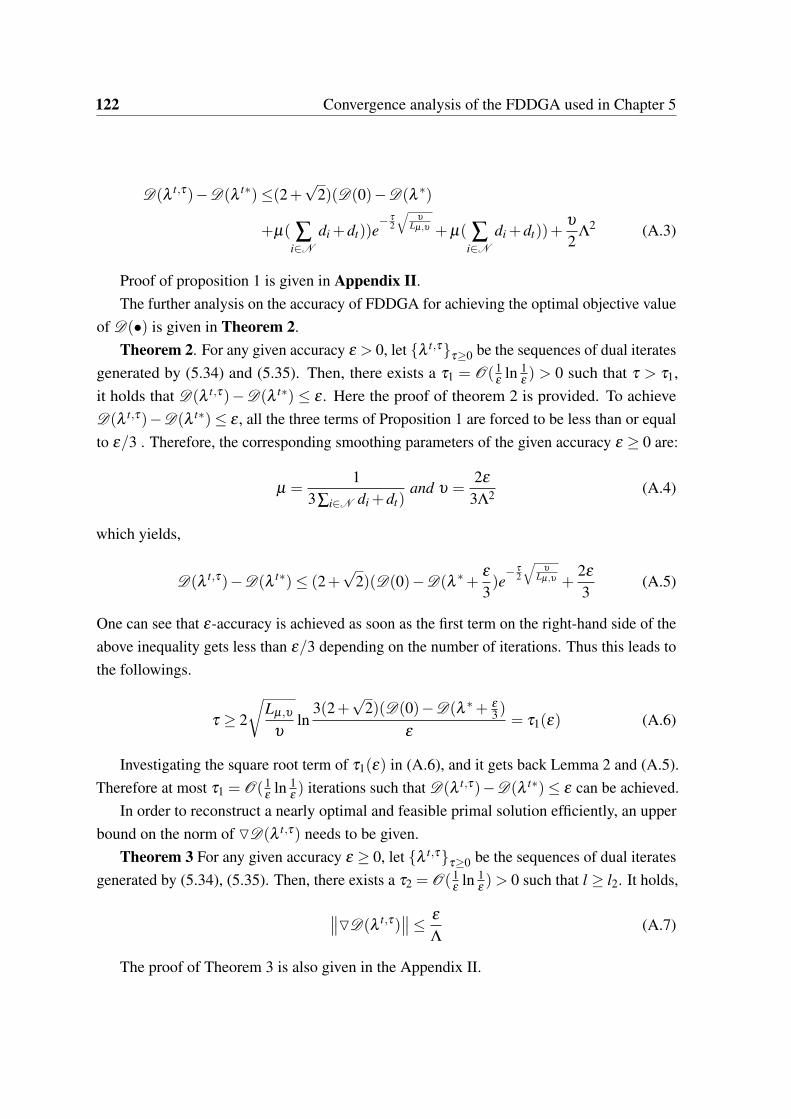
122 Convergence analysis of the FDDGA used in Chapter 5
D(λ t,τ)−D(λ t∗)≤(2+√
2)(D(0)−D(λ ∗)
+µ( ∑i∈N
di +dt))e− τ
2
√υ
Lµ,υ +µ( ∑i∈N
di +dt))+υ
2Λ
2 (A.3)
Proof of proposition 1 is given in Appendix II.The further analysis on the accuracy of FDDGA for achieving the optimal objective value
of D(•) is given in Theorem 2.Theorem 2. For any given accuracy ε > 0, let {λ t,τ}
τ≥0 be the sequences of dual iteratesgenerated by (5.34) and (5.35). Then, there exists a τ1 = O(1
εln 1
ε) > 0 such that τ > τ1,
it holds that D(λ t,τ)−D(λ t∗) ≤ ε . Here the proof of theorem 2 is provided. To achieveD(λ t,τ)−D(λ t∗)≤ ε , all the three terms of Proposition 1 are forced to be less than or equalto ε/3 . Therefore, the corresponding smoothing parameters of the given accuracy ε ≥ 0 are:
µ =1
3∑i∈N di +dt)and υ =
2ε
3Λ2 (A.4)
which yields,
D(λ t,τ)−D(λ t∗)≤ (2+√
2)(D(0)−D(λ ∗+ε
3)e
− τ
2
√υ
Lµ,υ +2ε
3(A.5)
One can see that ε-accuracy is achieved as soon as the first term on the right-hand side of theabove inequality gets less than ε/3 depending on the number of iterations. Thus this leads tothe followings.
τ ≥ 2
√Lµ,υ
υln
3(2+√
2)(D(0)−D(λ ∗+ ε
3)
ε= τ1(ε) (A.6)
Investigating the square root term of τ1(ε) in (A.6), and it gets back Lemma 2 and (A.5).Therefore at most τ1 = O(1
εln 1
ε) iterations such that D(λ t,τ)−D(λ t∗)≤ ε can be achieved.
In order to reconstruct a nearly optimal and feasible primal solution efficiently, an upperbound on the norm of ▽D(λ t,τ) needs to be given.
Theorem 3 For any given accuracy ε ≥ 0, let {λ t,τ}τ≥0 be the sequences of dual iterates
generated by (5.34), (5.35). Then, there exists a τ2 = O(1ε
ln 1ε)> 0 such that l ≥ l2. It holds,
∥∥▽D(λ t,τ)∥∥≤ ε
Λ(A.7)
The proof of Theorem 3 is also given in the Appendix II.
Appendix B
Proof of Theorem 1, Proposition 1 andTheorem 3
This section describe the proofs for theorem 1, proposition 1 and theorem 3 presented inChapter 5
Proof of Theorem 1
According to (5.28), (5.31) and (5.32), it gives,
Dµ(λt,τ) = ∑
i∈N
U(xt,τi ,ξ )−λ
t,τxt,τi −µ pi(x
t,τi )
+λt,τLt,τ −C(Lt,τ)−µ pt(Lt,τ) (B.1)
Noting that W ∗ = D∗ and ▽Dµ(λt,τ) =−[∑i∈N xt,τ
i −Lt,τ ], so,
W (xt,τi ,Lt,τ)−W ∗ = λ
t,τ▽Dµ(λt,τ)+ ∑
i∈N
µ pi(xt,τi )
+µ pt(Lt,τ)−Dµ(λt,τ)+D(λ t∗) (B.2)
Then, |D(λ t,τ)−D(λ t∗)≤ ε|. Therefore,∣∣W (xt,τi ,Lt,τ)−W ∗∣∣≤ ∥λt,τ∥
∥∥▽Dµ(λt,τ)
∥∥+2ε (B.3)

124 Proof of Theorem 1, Proposition 1 and Theorem 3
It holds,
∥λt,τ∥ ≤ Λ
√3ε(Dµ0−Dµ(λ t∗)) (B.4)
Due to the choice of l0 and the above estimates, the following could be obtained,∣∣W (xt,τi ,Lt,τ)−W ∗∣∣≤ (3−2
√2)ε +(2+
√2)ε ≤ 5ε (B.5)
Finally, it follows from (A.2) , Lemma1 and Theorem 3 that,∣∣∣∣∣ ∑i∈N
xt,τi −Lt,τ
∣∣∣∣∣= ∥∥▽Dµ(λt,τ)
∥∥≤ ε
Λ(B.6)
The proof of Theorem 1 is complete.
Proof of proposition 1
From (5.29), it gives Dµ(0)≤ D(0) and D(λ ∗)−µ(∑i∈N di +dt)≤ Dµ(λt∗), thus,
Dµ(0)−Dµ(λt∗)≤ D(0)−D(λ t∗)+µ( ∑
i∈N
di +dt) (B.7)
Since Dµ(λt∗)+ υ
2
∥∥∥λ t∗∥∥∥2
≤ Dµ(λt∗)+ υ
2 ∥λ t∗∥2, and and follows from the above in-
equality, (A.1) and due to Dµ,υ(λt,τ) = Dµ(λ
t,τ)+ υ
2 ∥λ t∗∥2, it leads to:
Dµ(λt,τ)−Dµ(λ
t∗)≤ (Dµ(0)−Dµ(λt∗))e
−τ
√υ
Lµ,υ +υ
2(∥∥∥λ
t∗∥∥∥2
−∥∥λ
t,τ∥∥2) (B.8)
Now it is estimated∥∥∥λ t∗
∥∥∥2−∥λ t,τ∥2 as follow,
∥∥∥λt∗∥∥∥2
−∥∥λ
t,τ∥∥2 ≤∥∥λ
t∗−λ t,τ∥∥(∥∥λ
t∗−λ t,τ∥∥+2
∥∥∥λt∗∥∥∥)
≤ 2+2√
2υ
(Dµ(0)−Dµ(λt∗))e
−τ
√υ
Lµ,υ (B.9)
Hence, combing with (B.7), (B.8) and (B.9) the desired result is achieved and thiscompletes the proof.

125
Proof of Theorem 3
From lemma 2, the following could be obtained,∥∥▽Dµ(λt,τ)
∥∥≤∥∥▽Dµ,υ(λ
t,τ)∥∥+υ
∥∥λt,τ∥∥ (B.10)
Moreover, noting that,
D(λ t∗)+υ
2
∥∥λt∗∥∥2 ≥ Dµ(λ
t∗)+υ
2
∥∥λt∗∥∥2
≥ D(λ t∗)−µ( ∑i∈N
di +dt)+υ
2
∥∥λt∗∥∥2 (B.11)
Combing with the previous estimates, it gives rise to,
∥∥▽Dµ(λt,τ)
∥∥≤ (√
Lµ,υ +√
υ)
√2(D(0)−D(λ t∗)+
ε
3)e
−τ
√υ
Lµ,υ +2√
2ε
3Λ(B.12)
For ε > 0 fixed, the first term of the above inequality decreases by the iteration counter τ .In order to ensure
∥∥▽Dµ(λt,τ)
∥∥≤ ε
Λ, the following is needed,
τ ≥ 2
√Lµ,υ
εln
3Λ(√
Lµ,υ +√
υ)√
2(D(0)−D(λ t∗)+ ε
3)
(3−2√
2)ε= τ2(ε) (B.13)
Note that τ2 = O(1ε
ln 1ε) and the proof is completed.