Erneuerbare Energien und Energieeffizienz Renewable ...

This paper examines a method to model plug-in electric vehicles as part of the power system and presents results for the contribution of plug-in electric vehicles to balance the fl uctuating electricity generation of renewable energy sources.

The scientifi c contribution includes:

■ A novel approach to characterizing fl uctuating generation. This allows the detailed comparison of results from energy analysis and is the basis to describe the eff ect of electricity from renewable energy sources and plug-in electric vehicles on the power system.

■ The characterization of mobile storage, which includes the description of mobility behavior using probabilities and battery discharging costs.

■ The introduction of an agent-based simulation approach, coupling energy markets and distributed grids using a price-based mechanism design.

■ The description of an agent with specifi c driving behavior, battery discharg-ing costs and optimization algorithm suitable for real plug-in vehicles and simulation models.

■ A case study for a 2030 scenario describing the contribution of plug-in electric vehicles to balance generation from renewable energy sources in California and Germany.

ISBN: 978-3-86219-460-5

Erneuerbare Energien und Energieeffi zienzRenewable Energies and Energy Effi ciency

David Dallinger

Erneuerbare Energien und Energieeffizienz

Renewable Energies and Energy Efficiency

Band 20 / Vol. 20

Herausgegeben von / Edited by Prof. Dr.-Ing. Jürgen Schmid, Universität Kassel

David DallingerDavid DallingerDavid DallingerDavid Dallinger

PlugPlugPlugPlug----in electric vehicles integrating fluctin electric vehicles integrating fluctin electric vehicles integrating fluctin electric vehicles integrating fluctuating renewable electricityuating renewable electricityuating renewable electricityuating renewable electricity

kasseluniversity

press

This work has been accepted by the faculty of Electrical Engineering and Computer Science of the

University of Kassel as a thesis for acquiring the academic degree of Doktor der Ingenieurwissenschaften

(Dr.-Ing.).

Supervisor: Prof. Dr.-Ing. Jürgen Schmid, Universität Kassel

Co-Supervisor: Prof. Dr. rer. pol. Martin Wietschel, Fraunhofer ISI

Defense day 7th December 2012

Bibliographic information published by Deutsche Nationalbibliothek

The Deutsche Nationalbibliothek lists this publication in the Deutsche Nationalbibliografie;

detailed bibliographic data is available in the Internet at http://dnb.d-nb.de.

Zugl.: Kassel, Univ., Diss. 2012

ISBN print: 978-3-86219-460-5

ISBN online: 978-3-86219-461-2

URN: http://nbn-resolving.de/urn:nbn:de:0002-34615

© 2013, kassel university press GmbH, Kassel

www.upress.uni-kassel.de

Cover design: Grafik Design Jörg Batschi

Printed in Germany

http://dnb.ddb.de/

„Die Praxis sollte das Ergebnis des

Nachdenkens sein, nicht umgekehrt“

Hermann Hesse (1877-1962)

ABSTRACT

I

Abstract This paper examines a method to model plug-in electric vehicles as part of the power system and presents results for the contribution of plug-in electric vehicles to balance the fluctuating electricity generation of renewable energy sources. To reduce emissions emitted by passenger vehicles and the dependence on oil, electric driving is discussed. The paper therefore analyses a situation assuming a high share of plug-in electric vehicles in Germany for 2030. To avoid an incising peak load due to electric vehicle charging and to use the load shifting and storage potential of vehicles’ batteries a mechanism to schedule charging or feeding back electricity is of high relevance. To implement such a mechanism and analyze the contribution of plug-in electric vehicles as a grid resource an agent- based simulation method is applied. Plug-in electric vehicles are modeled as independent agents controlled by a mechanism designed making use of the marginal cost- based electricity market model PowerACE. The method allows considering single vehicles and a very high degree of details in terms of smart charging profits, battery degradation and driving behavior. The simulation results show that fueling passenger vehicles with electricity allows a reduction of carbon dioxide emissions. The magnitude of emission reduction is relatively small unless the electricity is supplied by additionally installed renewable energy sources. A very important finding for Germany therefore is that electricity from renewable energy sources should be used to provide sustainable transportation. In terms of revenues from smart charging, values are in the range of 50 – 250 euros per year and rather depend on the yearly electricity consumption than on power or battery size. In conclusion, smart charging technology must be low cost and make use of existing components implemented in passenger vehicles. The grid integration performance of fluctuating electricity generation strongly depends on the generation pattern. A daily generation pattern results in a better grid integration performance because the available energy for load shifting also follows a daily pattern. For Germany, therefore, especially solar power can be balanced with storage of plug-in electric vehicles.

ZUSAMMENFASSUNG II

Zusammenfassung Im Rahmen dieser Arbeit wird untersucht, inwieweit netzgekoppelte Elektrofahrzeuge zum Ausgleich fluktuierender Elektrizitätserzeugung von erneuerbaren Energien beitragen können. Die Elektromobilität gilt als eine vielversprechende Option, um Emissionen im Verkehrssektor und die Abhängigkeit von fossilen Energieträgern zu senken. Dies gilt im Besonderen, wenn die erforderliche Elektrizität aus erneuerbaren Energiequellen stammt. In Deutschland und Europa ist im Bereich der erneuerbaren Energien vor allem der Ausbau von fluktuierenden Erzeugern wie Windturbinen und Photovoltaikanlagen geplant (Beurskens et al., 2011). Eine große Herausforderung dieser Ressourcen ist jedoch die Volatilität der von Sonneneinstrahlung und Windgeschwindigkeit abhängenden Erzeugung. Inwieweit Last- und Erzeugungsmanagement mittels Elektromobilität zu einer besseren Integration von erneuerbaren Energien beitragen kann, ist daher eine entscheidende Forschungsfrage. Die Arbeit gliedert sich wie folgt. Nach einer Einleitung zur wissenschaftlichen Fragestellung und deren Bedeutung (Kapitel 1) werden die Grundlagen zur Steuerung netzgekoppelter Fahrzeuge geschaffen (Kapitel 2). Darauf aufbauend wird die Methodik zur Charakterisierung der verwendeten Zeitreihen (Kapitel 3) und die Besonderheiten mobiler Speicher (Kapitel 4) thematisiert. Anschließend folgt das eigentliche Methodenkapitel (Kapitel 5), in dem das verwendete Simulationsmodell vorgestellt wird. Die Erstellung eines Zukunftsszenarios für das Jahr 2030 mit hohem Anteil erneuerbarer Energien und Elektrofahrzeugen definiert das Untersuchungsfeld der Arbeit (Kapitel 6). Die Ergebnisse (Kapitel 7) fokussieren auf die Möglichkeit zur Integration von erneuerbaren Energien, die mittels der in (Kapitel 3) festgelegten Charakterisierungsparameter quantifiziert werden. Außerdem werden marginale CO2-Emissionen (Kapitel 7.5) und mögliche Einsparungen durch das gesteuerte Laden (Kapitel 7.6) diskutiert. Die sich anschließende Sensitivitätsanalyse (Kapitel 7.7) rundet das Ergebniskapitel ab und zeigt die größten Unsicherheiten der Untersuchung auf. Abschließend werden in Kapitel 8 wichtige Schlussfolgerungen und der sich aus der Arbeit ergebenden weitere Forschungsbedarf aufgezeigt. Das Kernstück der Arbeit ist die in Kapitel 3, 4 und 5 entwickelte Methodik. Dies beinhaltet die Festlegung und Definition von Charakterisierungsparametern mit denen die Zeitreihen als wichtige Eingangsparameter und die Ergebnisse beschrieben werden. Dadurch wird es möglich, den Effekt von fluktuierenden Erzeugern auf das Energiesystem zu messen. Nur so kann anschließend quantifiziert werden, welchen Beitrag die Elektromobilität zur Integration leistet. Ein weiterer grundlegender methodischer Inhalt ist die Beschreibung von mobilen Speichern. Zur Bestimmung von Elektromobilitätsnutzern wurde ein Abfrageschema entwickelt (Biere, et al. 2009) und auf eine Mobilitätsstudie (MID, 2010) angewandt. Der so gefilterte Datensatz wird verwendet, um Wahrscheinlichkeiten für die Modellierung des Mobilitätsverhaltens abzuleiten. Nach wirtschaftlichen Gesichtspunkten zeichnen sich mögliche Nutzer von Elektrofahrzeugen durch eine hohe elektrische Fahrleistung aus. Höhere Anschaffungskosten von Elektrofahrzeugen müssen über die aufgrund der hohen Effizienz niedrigeren Betriebskosten amortisiert werden. Dies gelingt besonders im Fall

ZUSAMMENFASSUNG

III

von Nutzern, die in kleineren Gemeinden wohnen und täglich zur Arbeit pendeln.1 Städter sind in der Regel wesentlich weniger geeignet, weil sie oft nur ein Fahrzeug besitzen, die Lademöglichkeit unsicherer ist und die elektrische Fahrleistung trotz höheren Verbrauchs im Stadtverkehr nicht ausreicht, um die Anfangsinvestition in das Fahrzeug zu amortisieren. Durch die Filterung des Datensatzes wird erreicht, dass nur Fahrprofile von potentiellen Nutzern in die Modellierung einbezogen werden. Außerdem sind die Entladekosten ein wichtiger Einflussfaktor für die Bestimmung des Rückspeiseverhaltens von mobilen Speichern. Zur Quantifizierung der Entladekosten wurden zwei Ansätze in Abhängigkeit der Entladetiefe (Rosenkranz, 2003/2007) und des Energiedurchsatzes (Peterson et al., 2009) der Batterie untersucht. Bei der Entwicklung des Batteriealterungsmodells mussten viele Vereinfachungen getroffen werden. Beispielsweise wurden Temperatur und C-Rate2 sowie Abhängigkeiten zwischen Alterungsmechanismen vernachlässigt. Darüber hinaus ist heute aufgrund der hohen Entwicklungsdynamik nur sehr schwer abschätzbar, welche Batteriechemie sich zukünftig durchsetzt. Die generell für Lithium- Batterien entwickelten Ansätze erlauben daher nur eine sehr vereinfachte Darstellung der durch Alterung verursachten Entladekosten. Die Beschreibung der verwendeten Simulationsumgebung beginnt mit einem Überblick zum Agenten-basierten Strommarktmodell PowerACE (Sensfuß, 2007), das als Grundlage für die Modellierung verwendet wird. PowerACE bildet alle wichtigen Akteure der Angebots- und Nachfrageseite des Strommarkts in Deutschland ab und erlaubt es Grenzkosten-basierte Strompreise zu bestimmen. Für die Elektromobilität dient der Strompreis als Steuergröße, um das intelligente Lade- und Entladeverhalten der Fahrzeuge zu bestimmen. Im implementierten Steuerungsmechanismus werden einzelne Fahrzeuge einem Fahrzeug- Pool zugeordnet der wiederum in Fahrzeug- Gruppen unterteilt ist. Für Fahrzeug- Pools wird über eine Strompreisprognose ein spezifisches Preissignal ermittelt. Ausgehend von diesem Steuersignal wird auf der Gruppenebene ein variables Netzentgelt addiert, um die Situation im Verteilnetz abzubilden. Durch die fahrzeugspezifische Anpassung des variablen Netzentgelts in Abhängigkeit der Trafoauslastung und die Pool-spezifische Preisvorhersage wird eine gleichmäßige Verlagerung der Elektrizitätsnachfrage in Lasttäler erreicht. Dieser Steuerungsmechanismus erfordert eine uneinheitliche Tarifgestaltung, die in dieser Form heute aufgrund des Gleichheitsgedankens nicht rechtmäßig ist. Der verwendete iterative Prozess erlaubt jedoch eine sehr gute Steuerung der Fahrzeuge, ohne die individuellen Mobilitäts- und Batterieanforderungen zu vernachlässigen. Auf Fahrzeugebene wurde ein Software- Agent entwickelt, der in Zusammenarbeit mit dem Fraunhofer ISE in ein Versuchsfahrzeug implementiert wurde (Link, 2011).3 In PowerACE beinhaltet dieser Agent die Modellierung des Fahrverhaltens unter Verwendung der aus Mobilitätsstudien ermittelten Wahrscheinlichkeiten. Die einem spezifischen Fahrzeug zugewiesenen Fahrten ermöglichen die Ermittlung der Zeitperiode, die für das Erzeugungs- und Lastmanagement zur Verfügung steht sowie den Ausgangs- und erforderlichen Endzustand des Speichers. Über die entwickelten Funktionen zur Batteriealterung werden die Rückspeisekosten in Abhängigkeit des 1 Der Wirtschaftsverkehr wird in dieser Arbeit nicht betrachtet. Kleine Transporter weisen jedoch ein hohes Potential aufgrund der Fahrprofile und der guten Planbarkeit von Fahrten auf. Bei der Betrachtung von ganz Deutschland ist das Potential aufgrund der geringen Fahrzeugzahl im Vergleich zu privaten PKW jedoch relativ gering. 2 C- Rate: Lade- bzw. Entladerate definiert als Batteriekapazität (kWh) dividiert durch eine Stunde. 3 Siehe auch Anhang B.

ZUSAMMENFASSUNG IV

spezifischen Speicherzustands ermittelt. Der implementierte Optimierungsalgorithmus nutzt diese Informationen und das vom Steuerungsmechanismus bereitgestellte Preissignal, um einen optimalen Lade- und Entlade- Fahrplan zu ermitteln. Die Agenten-basierte Modellierung bietet in diesem Zusammenhang den Vorteil, dass individuelle Nutzerbedürfnisse wie das Mobilitätsverhalten oder die von der Entladetiefe bzw. dem vom spezifischen Speicherzustand abhängigen Rückspeisekosten abgebildet werden können. Außerdem können in zukünftigen Arbeiten Preissensitivitäten implementiert werden, um zu berücksichtigen, dass je Nutzer unterschiedliche Anreize zum Last- und Erzeugungsmanagement notwendig sind. Das Ergebniskapitel beginnt mit einer Auswertung der Verlagerungszeit bzw. der Zeitperiode zwischen zwei Wegen, über die das Lade- und Entlade- Verhalten optimiert werden kann. Diese zeigt, dass die Verlagerungszeiten über den Tag stark schwanken und vor allem nach dem letzten Weg lange Verlagerungsperioden möglich sind. Generell gilt, dass Elektrofahrzeuge nur als Kurzzeitspeicher mit Verlagerungszeiten im Bereich von wenigen Stunden bis Tagen eingesetzt werden können. Für die wirtschaftliche Nutzung der Fahrzeuge ist eine hohe Auslastung mit nahezu täglichen Fahrten vorteilhaft. Der Primärnutzen der Fahrzeuge, die Befriedigung des Mobilitätsverhaltens, reduziert demnach die Freiheitsgrade des Speichermanagements. Der Beitrag zur Integration von fluktuierenden Erzeugern durch die Elektromobilität wird anhand der entwickelten Charakterisierungsparameter gemessen und an zwei Fallstudien zum Lastmanagement untersucht. Dafür wurde für Kalifornien und Deutschland ein Szenario mit gleichem Anteil an fluktuierenden Erzeugern und Elektrofahrzeugen entwickelt und verglichen. Die Ergebnisse zeigen, dass die je nach Szenarien resultierende Fluktuation der Residuallast4 hohen Einfluss auf die Fähigkeit zur Integration hat. Für Kalifornien wird ein höherer Anteil an Sonnenenergie zugrunde gelegt. Außerdem schwankt dort die Windenergieerzeugung aufgrund des Temperaturunterschiedes zwischen Pazifik und Festland oft in einem täglichen Rhythmus. Der tägliche Rhythmus der resultierenden Residuallast begünstigt die Integration durch Elektrofahrzeuge deren zur Lastverlagerung verfügbare Energiemenge täglich durch Fahrten erneuert wird. In Deutschland wird die Windeinspeisung durch Tiefdruckgebiete bestimmt, die öfters zu längeren Perioden mit starker Windeinspeisung führen. Der durch die Elektromobilität integrierbare Überschussstrom, für Deutschland zwischen 50 % und 64 % und für Kalifornien von 73 %, zeigt die Eignung von Elektrofahrzeugen zur Integration von relativ regelmäßig schwankenden Erzeugern. Die Rückspeisung wurde ausschließlich für das Deutschland Szenario betrachtet, weil in diesem Anwendungsfall die notwendigen Informationen zum Kraftwerkspark für Kalifornien nicht verfügbar sind. Im Besonderen beim Ausgleich der Residuallastschwankungen wird durch die Rückspeisung eine Verbesserung gegenüber dem reinen Lastmanagement erreicht. Insgesamt wird die Residuallastschwankung um 38 % bis 43 % gegenüber dem Referenzszenario ohne Elektromobilität reduziert. Gegenüber dem reinen Lastmanagement werden weitere 12 % bis 18 % an Überschussstrom genutzt. Beim Vergleich der beiden Methoden zur Berechnung der Rückspeisungskosten auf Fahrzeugebene zeigt sich, dass der Speicherhub bei der Alterung basierend auf der Entladetiefe wesentlich geringer ist. Insgesamt wird öfters und mit geringerer Entladungstiefe zykliert. Für die gesamte Fahrzeugflotte resultiert dies in einer höheren rückgespeisten Energiemenge im Fall der energiebasierten

4 Die Residuallast ist die resultierende Last aus Systemlast minus fluktuierender Einspeisung.

ZUSAMMENFASSUNG

V

Berechnung der Entladekosten. Die Mengen des integrierten Überschussstroms weichen insgesamt jedoch nur um wenige Prozentpunkte voneinander ab. Zusätzlich zur Integrationsfähigkeit wurden Grenzemissionen sowie Einsparungen durch das intelligente Laden betrachtet. Die CO2-Grenzemissionen werden dabei stark vom Kraftwerkspark bestimmt. Beim Laden nach dem letzten Weg erhöht sich die Spitzenlast. Die Elektrizität wird in diesem Fall oft von Gasturbinen bereitgestellt, was zu vergleichsweise geringen Emissionen führt. Insgesamt stammen nur 1,8 % aus Überschussstrom von fluktuierenden erneuerbaren Energien. Durch die Lastverlagerung und die zusätzliche Rückspeisung wird dieser Anteil auf 8,1 % bzw. 10,4 % gesteigert. Die Gesamtbilanz verschlechtert sich beim zugrundegelegten Szenario jedoch von 100 g CO2/km für ungesteuertes Laden auf 113 bis 116 g CO2/km für das intelligente Laden. Ursache ist die durch die Lastverlagerung erhöhte Auslastung von Kraftwerken mit niedrigen Grenzkosten. Diese Kraftwerke sind bei gewählten Brennstoff- und CO2-Preisen meist Kohlekraftwerke mit hohen Emissionen. Der zusätzliche Verbrauch an Überschussstrom reicht nicht aus, um diese höheren Emissionen aus Kohlekraftwerken zu kompensieren. Daraus folgt, dass zusätzliche erneuerbare Energien erforderlich sind, um die Grenzemissionen der Elektromobilität zu verbessern. Für diesen Fall werden nur sehr wenige regelbare Kraftwerke benötigt bzw. gelingt bei der Betrachtung inklusive Rückspeisung sogar eine zusätzliche Verwendung von erneuerbaren Energien, die die Nachfrage der Elektromobilität übersteigt. Die mit Hilfe des Modells ermittelten Einsparungen durch intelligentes Laden gegenüber dem Laden nach dem letzen Weg liegen im Bereich von 50 - 250 Euro pro Fahrzeug und Jahr. Es zeigt sich, dass für reines Lastmanagement die Einsparungen linear mit dem jährlichen Elektrizitätsbedarf korrelieren. Die Batteriegröße, welche weitere Freiheitsgrade bei der Optimierung ermöglicht, hat beim reinen Lastmanagement keinen Einfluss. Bei Lastmanagement inklusive Rückspeisung zeigt sich im Gegensatz dazu, dass die Batteriegröße die Einsparungen durch intelligentes Laden beeinflusst. Größere Batterien ermöglichen höhere Einsparungen sind jedoch nicht über die Teilnahme am Elektrizitätsmarkt finanzierbar. Insgesamt sind die individuellen Einsparungen, die am Elektrizitätsmarkt erreichbar sind, jedoch sehr gering. Eine Steigerung der Anreize könnte über die Variabilisierung von heute fixen Kosten der Elektrizitätsversorgung, wie variable Netzentgelte, realisiert werden. In einer Sensitivitätsanalyse wurden die wesentlichen Eingangsparameter des Modells variiert. Besonders sensitiv sind Zeitreihen und Erzeugungsmix der fluktuierenden erneuerbaren Energien. Außerdem weisen Batteriegröße und -kosten eine erhöhte Sensitivität auf. Der Einfluss der Beladeinfrastruktur auf die Integration ist unerwartet gering. Eine hohe Verfügbarkeit von Infrastruktur erhöht den elektrischen Fahranteil und damit die verlagerbare Energiemenge. Die Verlagerungszeit an öffentlicher Infrastruktur, die meist während des Tages genutzt wird, ist aber kürzer als nach dem letzten Heimweg des Tages. Ist nur private Infrastruktur verfügbar führt dies dazu, dass zwar weniger Energie verlagert werden kann, die Verlagerungszeit aber ansteigt. Beide Effekte gleichen sich weitestgehend aus und begründen die geringe Sensitivität der Verfügbarkeit von Infrastruktur. Im Fall des ungesteuerten Ladens haben auch das Mobilitätsverhalten und die Netzanschlussleistung einen sehr hohen Einfluss. Während beim gesteuerten Laden beide Faktoren nur geringe Abweichungen zum Referenzfall bewirken. Wird das Mobilitätsverhalten nicht berücksichtigt bzw. stationäre Speicher modelliert zeigt sich der hohe Stellenwert der Lastverlagerung. Trotz der erhöhten Freiheitsgrade für das Speichermanagement wird durch stationäre Speicher ein insgesamt geringerer Beitrag zur Integration erneuerbarer Energien geleistet. Dieser Zusammenhang zeigt, dass der Nutzen durch die verlagerbare Energie höher ist als die

ZUSAMMENFASSUNG VI

durch das Mobilitätsverhalten verursachten Restriktionen. Die duale Speicher-verwendung erweist sich im Fall der Elektromobilität damit als ein Erfolgsfaktor. Das untersuchte Szenario für das Jahr 2030 weist Unsicherheiten bezüglich der verfügbaren Elektrofahrzeuge sowie den Annahmen zum Elektrizitätssystem aus. Die zu erreichende Penetration von Elektrofahrzeugen ist nach wirtschaftlichen Gesichtspunkten stark vom Preisen für Konkurrenzprodukte wie Öl oder Gas sowie der Batterietechnik abhängig. Aus heutiger Sicht erscheinen die politischen Ziele und das gewählte Penetrationsszenario als eher optimistisch. Inwieweit die diskutierten Preisanreize Nutzer motivieren am Lastmanagement teilzunehmen, wurde nicht explizit untersucht. Es wurde angenommen, dass Nutzer in jedem Fall auf das Steuersignal reagieren. Eine weitere Unsicherheit der Ergebnisse besteht daher darin, wie viele Nutzer tatsächlich zu einer Reaktion auf das Anreizsignal motiviert werden können. Zusammenfassend zeigt diese Arbeit, dass die Elektromobilität die Integration von erneuerbaren Energien fördern kann. Dabei ist die Elektromobilität ein Baustein, der im Zusammenspiel mit flexiblen Kraftwerken, anderen Speichertechnologien, der großflächigen Verteilung durch Netze und dem Lastmanagement mit anderen Verbrauchern einen hohen Anteil erneuerbarer Energien im Energiesystem ermöglicht.

TABLE OF CONTENTS VII

Table of contents

Abstract I

Zusammenfassung II

Acronyms and Abbreviations X

List of figures XI

List of tables XIII

1 Introduction 1 1.1 Background 1 1.2 Problem definition 1 1.3 Objective and procedure 2

2 Controlling grid-connected vehicles 3 2.1 Introduction 3 2.2 Grid-connected vehicles 3

2.2.1 Vehicle concepts 3 2.2.2 Current status 5 2.2.3 Total costs of ownership 5 2.2.4 Carbon dioxide emissions 6

2.3 Demand-side management 8 2.3.1 Framework conditions 8 2.3.2 Current status 10 2.3.3 Control mechanism 12 2.3.4 Control equipment 14 2.3.5 Revenue potential 16

2.4 Summary 17

3 Characteristics of fluctuating generation 18 3.1 Introduction 18 3.2 Method and input data 18 3.3 Evaluation criteria of energy fluctuation 21

3.3.1 Duration curve 21 3.3.2 Ramp rates 23 3.3.3 Interval availability 24

3.4 Evaluation of energy fluctuation 26 3.4.1 Total system load 26 3.4.2 Wind onshore 27 3.4.3 Wind offshore 28 3.4.4 Solar power 29

3.5 Summary 31

4 Characteristics of mobile storage 32 4.1 Introduction 32 4.2 Mobility behavior 32

4.2.1 Method and input data 32 4.2.2 Data preparation and filter criteria 33 4.2.3 Probabilities describing mobility behavior 36 4.2.4 Grid management time 38

4.3 Battery degradation 40 4.3.1 Discussion of modeling approaches and stress factors 40 4.3.2 Model based on the depth of discharge 42 4.3.3 Model based on energy throughput 43 4.3.4 Discharge costs 43

4.4 Summary 45

TABLE OF CONTENTS VIII

5 Simulation model 46 5.1 Introduction 46 5.2 Simulation approach 46

5.2.1 Model requirements 46 5.2.2 Existing model approaches 47 5.2.3 Modeling grid-connected vehicles 51

5.3 Basis of the model development 53 5.3.1 The PowerACE simulation model 53 5.3.2 Supply and demand time series 54 5.3.3 Supply bid 55 5.3.4 Market clearing 55 5.3.5 Merit-order effect 55

5.4 Model description 57 5.4.1 Layers of the simulation model 57 5.4.2 Multi-agent control approach 58 5.4.3 Demand-side management agent 60 5.4.4 Distribution grid agent 61 5.4.5 Device agent 63 5.4.6 Graph search optimization 63 5.4.7 Stochastic simulation of mobility behavior 64

5.5 Evaluation of multi-agent control mechanism 65 5.5.1 Distribution grid level 65 5.5.2 System level 66 5.5.3 Two-level control 67

5.6 Summary 68

6 Scenario definition 69 6.1 Introduction 69 6.2 Electricity sector 69 6.3 Vehicle sector 70 6.4 Distribution grid 72

7 Results 73 7.1 Introduction 73 7.2 Driving behavior 73

7.2.1 Average driving data 73 7.2.2 Grid management time 74 7.2.3 Evaluation of the stochastic simulation 75 7.2.4 Conclusions 76

7.3 Effect on the power system 77 7.3.1 Residual load 77 7.3.2 Last trip charging 78 7.3.1 Time-of-use tariff 79 7.3.2 Demand-side management 81 7.3.3 Conclusions 84

7.4 Vehicle-to-grid 87 7.4.1 Optimal power plant park 87 7.4.2 Price mark-up 88 7.4.3 Effect on the power system 90 7.4.4 Conclusions 92

7.5 Power plant utilization 93 7.5.1 GER 2030 scenario 93 7.5.2 Additional renewable energy 95 7.5.3 Conclusions 96

7.6 Revenues 97 7.6.1 Electricity price 97 7.6.2 Electricity costs 99 7.6.3 Conclusions 101

TABLE OF CONTENTS

IX

7.7 Sensitivity analysis 102 7.7.1 Time series 102 7.7.2 Grid connection power 103 7.7.3 Battery costs and size 105 7.7.4 Mobility behavior 107 7.7.5 Infrastructure 109 7.7.6 Share of fluctuating generation technology 110 7.7.7 Conclusions 112

7.8 Model limitations 113

8 Conclusions and outlook 114

Appendix XV A. Figures and Tables XV

A1. Vehicle charging behavior XV A2. Characteristics of fluctuating generation XVI A3. Mobility behavior XXI A4. Scenario definition XXVII A5. Results XXIX A6. Sensitivity analysis XXXIII

B. Field test XLIV C. Publications XLV

References XLVI

ACRONYMS AND ABBREVIATIONS X

Acronyms and Abbreviations ACE Agent-based Computational Economics

Ah Ampere-hour (used for weighted energy throughput based battery aging)

BEV Battery electric vehicle

BMU German Federal Ministry for the Environment, Nature Conservation and Nuclear Safety

CA California

CAISO California independent system operator

CCGT Combined cycle gas turbine

CO2 Carbon dioxide

CPP Critical peak pricing

DG Distribution grid

DoD Depth of discharge

DR Demand Response

DSM Demand-side management

EEX European Energy Exchange

GER Germany

GT Gas turbine

HEV Hybrid electric vehicle

I/C Interruptible/Curtailable

ICE Internal combustion engine

IPCC Intergovernmental Panel on Climate Change

IWES Fraunhofer Institute for Wind Energy and Energy System Technology

LT Last trip

MID Mobility in Germany (Mobilität in Deutschland)

MOP German Mobility Panel (Deutsches Mobilitätspanel)

Mup Price mark-up

NREL National Renewable Energy Laboratory

PEV Plug-in electric vehicle

PHEV Plug-in hybrid electric vehicles

PV Photovoltaics

RES Renewable energy sources

RES-E Electricity from renewable energy sources

RS Residual load

RTP Real-time prices

soc State of charge

ST Solar thermal

TCO Total costs of ownership

TOU Time-of-use

USABC U.S. Advanced Battery Consortium

V2G Vehicle-to-grid

WD Weekday

LIST OF FIGURES XI

List of figures Figure 2-1: Principal concept of plug-in electric vehicles ........................................................................ 3 Figure 2-2: Comparison of CO2 emissions by fuel and conversion technology ....................................... 7 Figure 2-3: Fluctuation of renewable generation ................................................................................... 10 Figure 2-4: Components for automated control of electric vehicles ...................................................... 15 Figure 2-5: Marginal versus total costs of different power plant options 2010 ...................................... 17 Figure 3-1: Duration curve of a wind turbine illustrating the characterization parameters used ........... 22 Figure 3-2: Sorted ramp rate for the German system load in 2008 ........................................................ 24 Figure 3-3: Average time availability for different sections of normalized power ................................ 25 Figure 3-4: Sorted duration curves of the total system load for Germany and California ..................... 26 Figure 3-5: Sorted duration curves for wind onshore ............................................................................. 27 Figure 3-6: Sorted duration curves for wind offshore ............................................................................ 29 Figure 3-7: Sorted ramp rates for solar generation in California and Germany ..................................... 30 Figure 4-1: Classification of the MID 2008 data set .............................................................................. 34 Figure 4-2: Classification of the MID 2008 data set implementing the filter criteria for PEV users ..... 35 Figure 4-3: Probability to start a trip on weekdays and Saturdays ......................................................... 37 Figure 4-4: Correlation between the average duration of a trip and the range of a trip ......................... 38 Figure 4-5: Grid management time of plug-in electric vehicles ............................................................. 39 Figure 4-6: Battery cycle life dependent on depth of discharge ............................................................. 42 Figure 4-7: Battery degradation costs .................................................................................................... 44 Figure 5-1: Principle structure of the PowerACE model ....................................................................... 53 Figure 5-2: Principle of the merit-order effect ....................................................................................... 56 Figure 5-3: Overview of the PowerACE extension to model grid-connected vehicles .......................... 57 Figure 5-4: Multi-agent control mechanism ........................................................................................... 59 Figure 5-5: Merit-order in the GER 2030 scenario and price forecast function of the pool agent ......... 61 Figure 5-6: Function between transformer utilization and variable grid fee .......................................... 62 Figure 5-7: Overview of the device agent .............................................................................................. 63 Figure 5-8: Stochastic simulation process of mobility behavior for one day ......................................... 65 Figure 5-9: Evaluation of the DG-agent ................................................................................................. 66 Figure 5-10: Evaluation of DSM-agent control ....................................................................................... 66 Figure 5-11: Load of plug-in electric vehicles charging applying demand-side management ................. 67 Figure 7-1: Location of vehicles ............................................................................................................ 74 Figure 7-2: Hourly average grid management time and energy demand of returning vehicles ............. 75 Figure 7-3: Energy demand of returning vehicles and grid management time on weekdays ................. 76 Figure 7-4: Cumulated frequency of residual load variation for different hours of the day ................... 78 Figure 7-5: Ramp rates for the CA 2030 scenario .................................................................................. 79 Figure 7-6: Electric vehicle load with time-of-use tariff control ............................................................ 80 Figure 7-7: Change in the residual load duration curve due to DSM for Germany ............................... 82 Figure 7-8: Change in the residual load duration curve due to DSM for California .............................. 82 Figure 7-9: Cumulated hourly reduction of negative residual energy for California and Germany ....... 83 Figure 7-10: Total costs of different power plant options 2030 and residual load ................................... 87 Figure 7-11: PowerACE market clearing price depending on the residual load ...................................... 89 Figure 7-12: V2G operation: depth of discharge versus energy throughput ............................................ 90 Figure 7-13: Change in the residual load duration curve due to V2G for Germany ................................ 91 Figure 7-14: Cumulated hourly reduction of negative residual energy due to V2G for Germany ........... 92 Figure 7-15: Source of electricity for plug-in electric vehicles in percent ............................................... 94 Figure 7-16: Change in electricity production while installing additional renewable energy sources ..... 95 Figure 7-17: Average electricity price for different charging strategies .................................................. 98 Figure 7-18: Frequency of maximum daily electricity price spread ........................................................ 99 Figure 7-19: Electric driving share for last trip and smart charging ...................................................... 100 Figure 7-20: Savings for smart charging compared to instant charging after each trip. ......................... 100 Figure 7-21: Operational expenditures for different charging strategies................................................ 101 Figure 7-22: Consumption of negative residual load and ramp rate factor for different time series ...... 103 Figure 7-23: Comparing results for varying grid connection power ...................................................... 104 Figure 7-24: Effect of grid connection power on the PEVs’ load curve for last trip charging ............... 105 Figure 7-25: Comparing results for varying battery costs ...................................................................... 105 Figure 7-26: Comparing results for different battery sizes .................................................................... 107 Figure 7-27: Comparing results for different mobility behavior ............................................................ 108 Figure 7-28: Sensitivity of infrastructure to negative load consumption and electric driving share ...... 109

LIST OF FIGURES XII

Figure 7-29: Negative residual load for different photovoltaic shares ................................................... 110 Figure 7-30: Comparing results varying the share of fluctuating generation technologies .................... 111 Figure A-1: Charging curve of Opel MERIVA battery electric test vehicle ......................................... XV Figure A-2: Cumulated availability of onshore wind generation for different hours of the day ........... XX Figure A-3: Clearing price at European Energy Exchange ................................................................... XX Figure A-4: Range probability MID 2008 ......................................................................................... XXVI Figure A-5: Probability for location (MID 2008) .............................................................................. XXVI Figure A-6: Transformer utilization winter season .......................................................................... XXVII Figure A-7: Transformer utilization spring and autumn .................................................................. XXVII Figure A-8: Transformer utilization summer season ........................................................................ XXVII Figure A-9: Hourly average grid management time ∆t on a Saturday .............................................. XXIX Figure A-10: Hourly average grid management time ∆t on a Sunday ................................................ XXIX Figure A-11: Probability system load versus residual load Germany 2030 .......................................... XXX Figure A-12: Probability last trip versus DSM charging Germany 2030 .............................................. XXX Figure A-13: Probability last trip versus V2G charging Germany 2030 ............................................... XXX Figure A-14: Probability system load versus residual load California 2030 ....................................... XXXI Figure A-15: Probability last trip versus DSM charging California 2030 ........................................... XXXI Figure A-16: Sorted ramp rates for scenario GER 2030 .................................................................... XXXII Figure A-17: Average electricity prices for different charging strategies .......................................... XXXII Figure A-18: Frequency of maximum daily electricity price spread .................................................. XXXII Figure A-19: PEVs load curve, hourly mean versus quarter hourly mean values. ............................. XXXV Figure A-20: Sorted load curve for PEVs last trip charging .............................................................. XXXV

LIST OF TABLES XIII

List of tables Table 2-1: Technical design of plug-in vehicles ..................................................................................... 4 Table 2-2: Additional investments for PEVs compared to a conventional vehicle ................................. 6 Table 2-3: Demand response applications in the residential sector ...................................................... 12 Table 3-1: Overview of the renewable energy input data ..................................................................... 19 Table 3-2: Installed capacity assumptions of CAISO data. .................................................................. 20 Table 3-3: Nomenclature duration curve parameter ............................................................................. 21 Table 3-4: Nomenclature ramp rate parameter ..................................................................................... 23 Table 3-5: Nomenclature interval availability parameter ..................................................................... 24 Table 3-6: Selected parameters used to characterize the load curve. .................................................... 27 Table 3-7: Selected parameters to characterize the wind onshore time series. ..................................... 28 Table 3-8: Selected parameters to characterize the interval availability of wind onshore time series. 28 Table 3-9: Selected parameters to characterize the wind offshore time series. .................................... 29 Table 3-10: Selected parameters to characterize the solar time series. ................................................... 30 Table 4-1: Overview of the main German mobility surveys ................................................................. 33 Table 4-2: Nomenclature of stochastic simulation parameters ............................................................. 36 Table 4-3: Probability to travel derived unfiltered versus filtered data set ........................................... 36 Table 4-4: Nomenclature of grid management time parameters ........................................................... 39 Table 4-5: Parameters for battery cycle life calculation ....................................................................... 42 Table 4-6: Parameters to calculate battery discharge costs ................................................................... 43 Table 5-1: Nomenclature PowerACE market model ............................................................................ 54 Table 5-2: Nomenclature PowerACE DSM-Agent .............................................................................. 58 Table 6-1: Intermittent generation and electricity demand for GER 2030 and CA 2030 ..................... 70 Table 6-2: Fuel and CO2 prices for the GER 2030 scenario ................................................................. 70 Table 6-3: Passenger vehicle types ....................................................................................................... 71 Table 6-4: Resulting power and energy values of the vehicle fleet scenarios ...................................... 71 Table 6-5: Battery degradation parameter ............................................................................................ 72 Table 7-1: Average yearly driving data ................................................................................................ 73 Table 7-2: Average grid management time for days of the week ......................................................... 75 Table 7-3: Average yearly driving data for one vehicle of a fleet of 1200 vehicles based on MOP..... 75 Table 7-4: Evaluation parameters, residual load for California versus Germany ................................. 77 Table 7-5: Evaluation parameter, last trip charging, California versus Germany ................................. 79 Table 7-6: Electric vehicle time-of-use tariff of Pacific Gas and Electric ............................................ 80 Table 7-7: Evaluation parameters, time-of-use, charging California versus Germany ......................... 81 Table 7-8: Evaluation parameters, demand-side management, charging California versus Germany .. 81 Table 7-9: Change of evaluation parameters for California and Germany ........................................... 83 Table 7-10: Capacity for the 2030 GER scenario ................................................................................... 88 Table 7-11: Energy and demand in case of vehicle-to-grid for Germany ............................................... 91 Table 7-12: V2G evaluation parameter GER 2008 ................................................................................. 92 Table 7-13: Energy balance for last trip and smart charging .................................................................. 94 Table 7-14: Energy and emission values for the scenario with additional renewable energy ................. 96 Table A-1: Duration curve parameters system load ........................................................................... XVI Table A-2: Duration curve parameters wind ...................................................................................... XVI Table A-3: Duration curve parameters solar ....................................................................................... XVI Table A-4: Ramp rate parameters system load ................................................................................... XVI Table A-5: Ramp rate parameters wind ............................................................................................. XVII Table A-6: Ramp rate parameters solar ............................................................................................. XVII Table A-7: Interval availability parameters for GER 2008 and CA ................................................. XVIII Table A-8: Interval availability parameters for GER 2007 ................................................................. XIX Table A-9: Interval availability parameters for GER 2009 ................................................................. XIX Table A-10: Sample size after determining PEV user .......................................................................... XXI Table A-11: User segments MID 2008 survey .................................................................................... XXII Table A-12: Filtered user segments MID 2008 survey ........................................................................ XXII Table A-13: Probability for start time MID 2008 ............................................................................... XXIII Table A-14: Probability for average trips per day MID 2008 ............................................................ XXIV Table A-15: Probability for the range MID 2008 .............................................................................. XXIV Table A-16: Probability for the location MID 2008 ............................................................................ XXV Table A-17: Agent scenario ............................................................................................................. XXVIII Table A-18: Standard deviation of grid management time for days of the week .............................. XXIX

LIST OF TABLES XIV

Table A-19: Duration curve parameters GER 2007 ......................................................................... XXXIII Table A-20: Ramp rate parameters GER 2007 ................................................................................ XXXIII Table A-21: Duration curve parameters GER 2007 IWES .............................................................. XXXIII Table A-22: Ramp rate parameters GER 2007 IWES...................................................................... XXXIII Table A-23: Duration curve parameters GER 2009 ........................................................................ XXXIV Table A-24: Ramp rate parameters GER 2009 ............................................................................... XXXIV Table A-25: Average electric driving share of vehicle fleet in dependence of connection power .. XXXVI Table A-26: Duration curve parameters last trip charging .............................................................. XXXVI Table A-27: Ramp rate parameters last trip charging ..................................................................... XXXVI Table A-28: Duration curve parameters demand-side management ............................................... XXXVI Table A-29: Ramp rate parameters demand-side management ....................................................... XXXVI Table A-30: Duration curve parameters vehicle-to-grid DoD battery aging and mark-up price ... XXXVII Table A-31: Ramp rate parameters vehicle-to-grid DoD battery aging and mark-up price ........... XXXVII Table A-32: Duration curve parameters vehicle-to-grid Ah battery aging and mark-up price ...... XXXVII Table A-33: Ramp rate parameters vehicle-to-grid Ah battery aging and mark-up price .............. XXXVII Table A-34: Duration curve parameters vehicle-to-grid DoD battery aging and mark-up price .. XXXVIII Table A-35: Ramp rate parameters vehicle-to-grid DoD battery aging and mark-up price .......... XXXVIII Table A-36: Duration curve parameters vehicle-to-grid Ah battery aging and mark-up price ..... XXXVIII Table A-37: Ramp rate parameters vehicle-to-grid Ah battery aging and mark-up price ............. XXXVIII Table A-38: Duration curve parameters battery size 15 kWh ......................................................... XXXIX Table A-39: Ramp rate parameters battery size 15 kWh ................................................................ XXXIX Table A-40: Duration curve parameters battery size 30 kWh ......................................................... XXXIX Table A-41: Ramp rate parameters battery size 30 kWh ................................................................ XXXIX Table A-42: Duration curve parameters deterministic MOP mobility behavior ..................................... XL Table A-43: Ramp rate parameters deterministic MOP mobility behavior ............................................ XL Table A-44: Duration curve parameters probability based MOP mobility behavior .............................. XL Table A-45: Ramp rate parameters probability based MOP mobility behavior ...................................... XL Table A-46: Duration curve parameters commuter scenario .................................................................. XL Table A-47: Ramp rate parameters commuter scenario .......................................................................... XL Table A-48: Duration curve parameters vehicle-to-grid DoD without mobility behavior ..................... XLI Table A-49: Ramp rate parameters vehicle-to-grid DoD without mobility behavior ............................ XLI Table A-50: Duration curve parameters vehicle-to-grid Ah without mobility behavior ........................ XLI Table A-51: Ramp rate parameters vehicle-to-grid Ah without mobility behavior ............................... XLI Table A-52: Duration curve parameters demand-side management .................................................... XLII Table A-53: Ramp rate parameters demand-side management ............................................................ XLII Table A-54: Duration curve parameters vehicle-to-grid DoD battery aging and mark-up price ......... XLII Table A-55: Ramp rate parameters vehicle-to-grid DoD battery aging and mark-up price ................. XLII Table A-56: Duration curve parameters vehicle-to-grid Ah battery aging and mark-up price ............ XLII Table A-57: Ramp rate parameters vehicle-to-grid Ah battery aging and mark-up price .................... XLII Table A-58: Duration curve parameters .............................................................................................. XLIII Table A-59: Ramp rate parameters ..................................................................................................... XLIII

INTRODUCTION

1

1 Introduction 1.1 Background The Intergovernmental Panel on Climate Change (IPCC) concludes that there is strong evidence that the observed climate change is being caused by carbon dioxide (CO2) and other greenhouse gas emissions caused by human activity (IPCC, 2007). Major emitters include the transportation (23 %) and electricity sectors (41 %) which together account for a total share of over 60 % of the worldwide energy-related CO2 emissions (IEA, 2008 p. 391). For both sectors, a rapid growth in energy use is expected to accompany the rising prosperity in developing countries. Low carbon energy conversion plays a key role in promoting this growth and reducing emissions in more developed countries. The low carbon intensity of electricity from renewable energy sources (RES-E) is one of the main measures to reduce CO2 emissions in the European energy strategy (EU, 2009a) and plays a globally important role as a mitigation instrument (Awerbuch, 2006; IPCC, 2011; Schmid et al., 2012). In the European Union, wind and solar are the fastest growing renewable energy sources (RES) for electricity generation. Electricity generation from biomass faces competition from the food and transportation sectors. Hydropower is already very well developed and the potentials to build additional capacities are limited in most of Europe. Therefore, it is expected that time-varying electricity generation will be expanded to reach the goals of the European Union (Beurskens et al., 2011). The problem here is that the grid integration of fluctuating RES-E generated by photovoltaic panels or wind turbines requires storage, demand response and/or wide distribution options in order to balance the variable electricity output. Plug-in electric vehicles (PEVs) could provide both storage and demand response. Further, PEVs convert electricity very efficiently and can significantly reduce emissions from passenger transportation if low carbon technologies are used to generate the electricity consumed by electric vehicles. The interaction between fluctuating RES-E and PEVs therefore represents a major research challenge to reach the CO2 reduction goals of the European Union and to minimize worldwide climate change. 1.2 Problem definition One of the main challenges associated with an electricity system featuring a high share of RES is the higher installed capacity and fluctuation in power (NERC, 2009; Parsons et al., 2004). Currently in Germany, there are 25 GW of installed photovoltaic power with a capacity factor of around 10 % (EEX, 2011). The simultaneous generation of these power plants reaches a maximum level of 70 % to 80 % and completely rises and declines within a time period of hours. To a lesser extent, the same applies to wind generation in Germany, which has an installed power of 30 GW and an average capacity factor between 20 % and 30 % (EEX, 2011). If even higher installed capacities of fluctuating generation are assumed, this results in a highly volatile residual load (RS) and demands a new way of thinking about the electricity system. Besides the fluctuating generation which determines the need for storage and demand-side management, the storage unit investigated here – plug-in hybrid vehicles – has limitations due to consumer mobility needs. The main purpose of PEVs is to meet the demand for mobility and not to function as a storage or load shifting device. When

INTRODUCTION 2

using PEVs to balance fluctuating generation, therefore, it is essential that they can be operated as storage units without user curtailment. The main challenge in this research paper is to account for fluctuating generation and the unique storage characteristics of mobile battery storage in a simulation environment which makes it possible to analyze future developments in the electricity system. 1.3 Objective and procedure The objective of this paper is to investigates how PEVs can help to balance the fluctuation of RES-E in Germany in order to establish an electricity system with a very high level of low carbon electricity generation. To investigate the contribution of PEVs to balancing the fluctuating generation output of RES, the procedure is as follows. First, basic information about plug-in electric vehicles and demand-side management is provided (Chapter 2). This clarifies the scenarios and methods used in this work. Then the characteristics of fluctuating generation (Chapter 3) and mobile storage (Chapter 4) are described. A parameter set is defined to describe time series and the initial and resulting situation of the power system. Generation fluctuates very individually for specific regions and years. Therefore, time series of three generation years are analyzed for Germany. To account for a region with RES-E and a load characteristic different to Germany, an additional case study is provided for California. This case study is done to put the results on a broader basis and be able to compare two electricity systems characteristic for northern and southern countries. California differs from Germany because of the cooling load in summer, which is distinctive for southern countries. The characteristic of RES-E also differs because of higher solar generation potential and thermal wind caused by temperature differences between the mainland and the Pacific Ocean. The storage and demand-side management potential of PEVs is determined by mobility behavior and by battery ageing costs in the case of vehicle-to-grid services. Chapter 4 provides information from different mobility surveys and defines probabilities to characterize the mobility behavior and the availability of PEV storage. In addition, a method to account for battery degradation is presented. The simulation model using the fluctuation of RES-E and the characteristics of mobile storage as input parameters is demonstrated in Chapter 5. The simulation approach combines automated demand response and vehicle-to-grid with an electricity market model. The electricity prices are modeled according to a marginal cost approach. Electric vehicles are included as distributed agents using price signals as the basis to determine their charging and vehicle-to-grid behavior. The framework of the analyzed electricity systems is presented in the section on scenarios (Chapter 6). Currently, fossil sources are mainly responsible for electricity generation and passenger vehicle fuels. To account for an electricity system with high RES-E share and PEV penetration, a future scenario is defined for 2030. This scenario distinguishes between Germany (GER) and California (CA), but keeps the relative number of vehicles and RES shares equal for comparison reasons. Finally, Chapter 7 presents the results which includes a sensitivity analysis and Chapter 8 the conclusions.

CONTROLLING GRID- CONNECTED VEHICLES

3

2 Controlling grid-connected vehicles 2.1 Introduction This chapter introduces grid-connected vehicles and demand-side management (DSM) as a method to control distributed devices and is structured in two main parts. The first part contains basic information about electric vehicles and the relevant parameters for the vehicle simulation. The second part provides background information on demand-side management and the chapter finishes with a summary of the discussed topics. 2.2 Grid-connected vehicles Vehicles using an electricity-based propulsion system are discussed in the context of alternative transportation to reduce emissions and improve vehicle efficiency. A grid-connected vehicle is defined as a vehicle able to charge a battery with electricity from the grid which is used as energy source to drive the propulsion system. The basic electric vehicle concepts and their current status in Germany are discussed in the next section. This paper focuses on private passenger transportation. Commercial light-duty vehicles on selected routes is another promising application for electric transport, but this is not considered here because of the relatively small vehicle fleet compared to private passenger vehicles.5 The additional investment needed for electric vehicles and batteries is provided. The cost structure of electric vehicles forms the basis for the assumptions made about possible users and underlines the vehicle specifications used. Finally, CO2 emissions are discussed as a major argument for analyzing the interaction of electric vehicle storage and RES. 2.2.1 Vehicle concepts This paper focuses on vehicles which convert electricity from an external power source into the kinetic energy used for driving. These vehicles are referred to as grid-connected vehicles or plug-in electric vehicles (PEVs). They include pure battery electric vehicles (BEVs) and plug-in hybrid electric vehicles (PHEVs)6 as shown in Figure 2-1.

Figure 2-1: Principal concept of plug-in electric vehicles

5 Commercial transport accounts for less than 10 % of all registered passenger vehicles in 2011. 6 PHEVs are further distinguished by parallel and serial drive train concepts. For the presented work, detailed drive train specification is not relevant. For further information on vehicle concepts see (Naunin, 2007).

CONTROLLING GRID- CONNECTED VEHICLES 4

A BEV uses a single propulsion system that mainly consists of a battery as storage, power electronics to convert electricity and an electric motor (Chan, 1993; Emadi, 2005). The battery is designed to store the total energy necessary to meet mobility needs. A plug-in hybrid electric vehicle combines an electric propulsion system with a second drive train. In the majority of the discussed cases, this comprises a conventional internal combustion engine (ICE), but could also be a fuel cell or a microturbine. PHEVs allow the combustion engine to be kept within the optimum speed range so that power is transmitted more efficiently. PHEVs can be designed with smaller battery storage but needing two propulsion systems results in increased complexity. BEVs and PHEVs both recuperate braking energy. The main advantage of an electric propulsion system is its high efficiency between 69 % and 88 % from tank to wheel.7 The energy density of the battery storage (150 – 250 Wh/kg)8 is about one hundred times smaller than gasoline. This results in a higher vehicle weight. The option of generating the electricity required for vehicles from different sources enables the diversification of fuels and reduces the reliance on oil. The specifications of the vehicles used in the following simulation of the power system are shown in Table 2-1.

Table 2-1: Technical design of plug-in vehicles

Technical data PHEV (25) PHEV (57) BEV (100) BEV (167)

Usable battery storage [kWh] 4.5 12 15 30 Battery depth of discharge [%] 80 80 80 80 Engine power [kW] 65 40 Electric motor power [kW] 40 60 66 100 Equivalent energy use [kWh/100 km, tank] 0.18 0.21 0.15 0.18 Electric range [km] 25 57 100 167

Two PHEV concepts are considered: The PHEV (25) with 25 km electric driving range accounts for a small to mid-size passenger vehicle.9 The bigger PHEV (57) can be characterized as typical mid-size sedan.10 The BEV concepts distinguish a 100 km (small sedan) and a 167 km (mid-size sedan) driving range. The specifications are based on own assumptions and research results from (Wietschel et al., 2008), (Biere et al., 2009), (Kley, 2011) and (Plötz et al., 2012). The studies rely on cost calculations and imply that the battery should be utilized as much as possible to recoup the higher investment of PEVs. Considering typical driving data results in a vehicle specification with a relatively small battery and favors PHEVs to account for the less frequent longer trips that do not justify a larger battery.11

7 Lithium-based battery: ηmin = 90 % and ηmax = 95 % (Vandenbossche et al., 2006) and (Schuster, 2009); Power electronics: ηmin = 92 % (Tang, 2009) with IGBTs at 3.2 kW and ηmax = 97 % Fraunhofer ISE prototype with silicon carbide transistors (SiC-JFETs); electric motor: asynchronous motor ηmin =90 % and permanent magnet motors ηmin = 95 % (Maggetto et al., 2000). 8 The value varies with the battery technology used, see (Kalhammer, 2007). For gasoline, the energy density is 11 - 12 kWh/kg. 9 The Prius plug-in hybrid provides 73 kW engine output and approximately 23 km electric range with a 4.4 kWh battery (Toyota, 2012). 10 The Chevrolet Volt or Opel Ampera provides 63 kW/111 KW engine/electric motor output, respectively, and approximately 60 km electric range with 16 kWh battery (Opel, 2012). 11 For research on the optimal design of PEVs, see (Shiau et al., 2010).


5

2.2.2 Current status A rising share of vehicles using electric engine assistance are being sold in Germany and across the world. Currently, these are mainly hybrid electric vehicles (HEVs) sold in the USA and in Japan with a share of 2–10 % of passenger car sales (DOE, 2012). In 2011, Germany had 42.3 million registered passenger vehicles. The total number of HEVs on German roads is 37 thousand, representing a 2011 market share of 2.8 % of newly registered vehicles. The number of 2011 registered PEVs is 2.3 thousand (KBA, 2012). The model range of PEVs available in Germany is low compared to conventional vehicles. Announcements of new models, however, have increased strongly since 2008.12 Today, electric vehicles in Germany are only used by a small minority of innovative individuals and in research projects. Despite this, the market share of PEVs is expected to grow in the future (Mock, 2011) due to government support,13 legislation to reduce vehicle emissions (see EU, 2009b14; CARB, 2012) and the expectation of rising oil prices (e.g. Aleklett et al., 2010). 2.2.3 Total costs of ownership The total costs of ownership (TCO) are an indicator for the economic success of alternative vehicles. A detailed TCO analysis in which the author was involved is available in (Wietschel et al., 2008 and Biere et al, 2009). In the following, additional investments are summarized for the vehicle concepts discussed to provide background information on the PEV types. The cost assumptions are based on (CONCAWE, 2008) referring to the year 2010+. The cost estimations are in line with (Thiel, 2010) and (Bandivadekar et al., 2008). Cost savings of the PEV design compared to the reference vehicle (77 kW)15 arise from downsizing the internal combustion engine and eliminating the standard alternator and starter. In case of BEVs, eliminating the fuel tank accounts for additional savings. Extra costs are caused by the electric motor, transmission and battery. Battery costs are adopted from (Kalhammer et al., 2007) and consider technology learning that could be achieved by 2030. In case of PHEVs, the power train also has to be adapted to account for the parallel or serial use of two transmission systems. The assumed additional investments are summarized in Table 2-2.

12 The website (UMBReLA, 2012) of the research project “Umweltbilanzen Elektromobilität” provides an overview of available and announced vehicles. 13 The German government has set the goal of at least 1 million PEVs on German roads in 2020 (BMBF, 2009). 14 The Regulation (EC) No. 443/2009 of April 23, 2009 (EU, 2009b.) setting emission performance standards for new passenger cars as part of the Community's integrated approach to reduce CO2 emissions from light-duty vehicles. 15 For details see (CONCAWE, 2008, p. 4).


Table 2-2: Additional investments for PEVs compared to a conventional vehicle16

Economic data PHEV (25) PHEV (57) BEV (100) BEV (167)

Alternative engine + transmission (downsizing)1 -257 € -794 € -2,541 € -2,541 €

Electric motor + modified transmission2 1,120 € 1,520 € 1,640 € 2,320 €

Power train and vehicle components3 2,442 € 1,503 €

Credit for standard alternator + starter + tank4 -300 € -300 € -450 € -450 €

Battery [euros/kWh]5 281 247 247 233

Battery 1,581 € 3,705 € 4,631 € 8,738 €

Additional investment compared to ICE (77 KW) 4,585 € 5,634 € 3,280 € 8,067 €

Note:1 33 euros/kW for BEV and 21.5 euros /kWmotor for PHEVs (downsizing); 2 Fixed cost 320 euros + 20 euros /kWmotor;

3 37.5 euros /kWengine; 4 300 euros for alternator and starter, 150 euros fuel tank; Source: Derived

from (CONCAWE, 2008);5 Derived from (Kalhammer, 2007), assumes a volume of >50k units per annum for 2020+.

The higher investment needed for PEVs can be compensated for by their lower operating costs, mainly due to the fuel savings made during electric driving. Under optimistic assumptions about battery cost reduction and battery lifetime, amortization periods between 3 and 10 years are possible (Wietschel et al., 2008). The development of gasoline and electricity prices are crucial for the TCO of PEVs. This includes uncertainty about taxation because of the high taxes on German gasoline. It can be concluded that increasing electrification of passenger transport is likely given the expectation of rising oil prices. 2.2.4 Carbon dioxide emissions The CO2 emissions of PEVs are strongly determined by the electricity generation source. The following discussion therefore focuses on the electricity generation mix for electric vehicles. The analysis does not consider the complete life cycle of electric vehicles including vehicle and battery production as well as recycling and transportation issues. A general literature analysis reveals that the emissions during the production of electric vehicles are higher than for conventional vehicles due to the materials and energy necessary to produce the battery (Helms et al., 2011; CONCAWE, 2007a; Burnham et al., 2006). The CO2 equivalent for combustion engine vehicles is in the range of 5200 kg CO2 per vehicle, whereas a PHEV accounts for 7200 kg CO2 per vehicle (TIAX LLC, 2007; Notter et al., 2009; Sørensen, 2004). The emissions per kilometer driven depend strongly on vehicle lifetime and driving range. For an vehicle with a life time of 12 years and 12,500 km driven per year the CO2 equivalent per km is 3.6 g for a conventional vehicle and 4.8 g for an PHEV. Figure 2-2 illustrates the estimates17 of the fuel and/or technology pathway averages of CO2 emissions of an electric drive train compared to conventional vehicles. A strong variation depending on the fuel used can be observed for the conversion of electricity. Fossil fuels, especially coal and lignite, do not considerably alter PEV emissions per kilometer relative to conventional vehicles. Only a very efficient conversion technology using combined cycle gas turbines and renewable energy sources18 such as wind and

16 The component costs assume a volume of >50k units per annum and are projected for 2010+. The reduction estimates through volume production for some of the key components could be very optimistic and it is uncertain how much and at what rate future costs will decline under different circumstances. 17 Values can vary in the range of 10 to 20 % because of assumptions about efficiency and emission factors. 18 Note: For wind and solar, the CO2 emissions of production and transport are included in Figure 2-2.


7

solar can reduce PEV emissions significantly. The wide span between lignite and wind also underlines the importance of the electricity source for the life cycle analysis. It can be concluded that RES-E is decisive for PEVs’ related emissions (further see Schmid et al., 2012).

Figure 2-2: Comparison of CO2 emissions by fuel and conversion technology

Assumptions: Efficiency: Gas turbine (GT) 37 %; combined cycle gas turbine (CCGT) 64.5 %; coal power plant 46.5 %; lignite power plant 45 %; electric drive train 90 %; diesel engine 0.32 %; gasoline engine 28 %; Energy use at the wheel 0.18 kWh/km; Emission factors [CO2 eq/kWh]: Gas 201.6; coal 352.8; lignite 399.6, oil 266.4; wind 21; solar 106; For literature on emission factors e.g. see (Lenzen, 2008). The CO2 emissions of PEVs related to the electricity consumed can be determined with the following methods:

Average emissions: To calculate the CO2 emissions from electricity consumption, the average of the total power plant park is used, including RES-E, nuclear and fossil sources. In this approach the CO2 emissions from electricity production are attributed equally to all consumers.

Marginal emissions: The marginal emissions account for the emissions of the additional consumption of electricity. Only the power plants utilized for the additional electricity demand are considered when calculating the CO2 emissions. The method is very precise in determining the total emissions of the power plant park, but different electricity consumers are treated differently.

Cap and trade: In the European CO2 emissions trading system, the total emissions are fixed by a cap. Assuming an unchanged cap and no exchange with other trading systems, additional electricity demand will not result in additional emissions. In this theoretical case, the CO2 emissions of PEVs would be zero.

In the work conducted, the marginal emission approach is applied because it allows the exact calculation of the PEVs’ CO2 emissions. The results are strongly influenced by the merit-order, which mainly depends on power plant efficiencies and fuel prices as well as the residual load curve to which the PEVs’ demand is added. Therefore, results are compared to average emissions. The marginal emissions resulting from PEVs’ electricity demand have been examined by various other studies (e.g. see Park et al., 2007; McCarthy et al., 2010; Sioshansi et al., 2011). However, power systems with a high share of RES-E have not yet been analyzed nor has how balancing RES-E could change the CO2 emissions of PEVs. Chapter 7.5 of this paper focuses on the interaction of RES-E and PEVs.


2.3 Demand-side management Demand-side management (DSM) is described as the active effort to modify electricity customers’ usage patterns (Eto, 1996). This includes regulatory measures to improve the efficiency of appliances. In this paper, the focus is on DSM intended to realize load shaping objectives, which is also referred to as “demand response” (DR) (DOE, 2006).19 Demand response is used to reduce the electricity demand in time periods with high wholesale electricity prices or when the system’s security is jeopardized. Besides load shifting, peak clipping and valley filling, the generation of small distributed units and vehicles feeding back power into the grid (vehicle-to-grid) are also considered in the context of DSM. The chapter is structured as follows. First, the framework conditions are discussed including the advantages of DSM in power systems with a large share of fluctuating generation. Then the current status in Germany and possible load management devices are described. The control strategies used for demand response and the necessary equipment make up sections 2.2.3 and 2.2.4. Finally, possible revenues are discussed. Chapter 2.3 is partly published in (Dallinger et al., 2012c). 2.3.1 Framework conditions Methods to control the demand-side of the electricity system have been a subject of discussion since the very beginning of electricity supply (Hausman et al., 1984). In the USA, DSM became more important due to least-cost planning in the 1970s, when utilities realized that demand-side technologies can be used to limit the installed capacity needed and to reduce overall system costs (Eto, 1996). Especially in areas where high loads occur only rarely, such as air conditioning in California,20 DSM has been successful in reducing the under-utilization of the standing capacity of power plants and increasing system security. In Germany, peak load reduction is not as relevant because of the different load duration curve,21 the high capacity installed22 and the better connections with neighboring countries.23 In northern Europe (France, Germany, Denmark), night storage heating controlled by a radio ripple signal was introduced during the sixties and seventies to increase the demand during night load valleys which resulted due to the enforced use of nuclear power plants (Quaschning et al., 1999). DR services are mainly used for operation scheduling – organized in day-ahead electricity markets - and system balancing - organized in the regulation reserve markets. Through these applications, DR enhances the elastic demand needed for electricity markets to function properly (Talukdar et al., 2005; Wellinghof et al. 2007), to increase the efficiency of electricity production and allow for higher system security (Andersen et al., 2006; DOE, 2006).

19 “Demand response is a tariff or program established to motivate changes in electric use by end-use customers in response to changes in the price of electricity over time, or to give incentive payments designed to induce lower electricity use at times of high market prices or when grid reliability is jeopardized.” (DOE, 2006) 20 See load duration curve for California and Germany in Figure 3-4 in Chapter 3 and compare the values of cfQ<0.8 in Table 3-6. 21 No summer peaks; peak load is during the winter and the utilization of peak load power is higher, see Figure 3-4, Chapter 3. 22 The total capacity of dispatchable power plants is 100 GW (BMWi, 2012) with a maximal peak load of approximately 80 GW. Note: Even the rapid nuclear phase-out of 8.4 GW after the Fukushima catastrophe in Japan has not caused critical shortages in the German power system. 23 Note that the electricity prices in Germany are higher partially due to the greater security of supply.


9

Barriers to residential demand response arise because revenues in electricity markets are determined by the energy that can be shifted to a later time period (energy arbitrage) and real-time adoption of power (system services). Both applications favor large customers because of less complex control as well as higher individual incentives. Other discussed DR barriers to the mass addition of small residential appliances are:

Efficiency gains stand in contrast to possible DR revenues. Especially in the residential sector, more efficient household devices reduce the demand available for load shifting.24 Potential revenues and the amortization time of smart grid technology are affected by efficiency gains and render the investments less attractive.

Almost all electricity markets are characterized by a oligopolistic structure with a dominant supply side. A higher price elasticity of demand reduces the revenues made during peak hours. Hence, there is only a low level of support from the dominant supply market players.

Customer stakeholder support is limited because of concerns about the impact on customer bills in the residential sector in the case of price-based incentives and because of low consumer acceptance of direct control and/or automation technology.

Changes to market rules and operation as well as regulatory policies are necessary to allow a higher share of DR services to participate in the markets.

Time-resolved energy consumption measures enable conclusions to be drawn regarding consumer habits and can therefore cause data security concerns.

Two current developments that are helping to tackle some of the main barriers are the mass use of communications technology in the residential sector and a rising share of fluctuating generation in power systems. The costs of communications technology are decreasing and high network availability allows more and more applications and participants to be included. Additionally, a higher degree of automation of DR devices and electricity billing is possible. In combination with heat or electricity storage technologies, this development can reduce consumer curtailment and DR participation efforts (Franz et al., 2006). In terms of power systems, the rising share of fluctuating generation with mostly prioritized dispatch reduces the residual load25 or energy to be produced by dispatchable power plants (see Figure 2-3). Thereby, the capacity credit (Ensslin et al., 2008) of fluctuating RES-E is lower and the dispatchable capacity required – to ensure system security on the same level – cannot be reduced to the same extent as the added capacity of fluctuating generation. This lead to a power system with a higher share of under-utilized peak capacity, volatility in electricity prices and the need for higher ramping capacities to stabilize the system (see Chapter 7.3.1 and Cappers et al., 2011). Under these conditions, DR could be an attractive alternative to limit the necessary peak capacity and reduce overall system costs.

24 In terms of heating, e.g. for a passive house with extremely low heating and/or cooling needs, fossil heating is likely to be replaced by electric heating, which increases the electricity demand and possible DR revenues. The total energy demand is still reduced which can reduce the overall DSM potential if combined heat and power is an included option. 25 Definition: The residual load is the remaining load for dispatchable power plants calculated by subtracting the fluctuating generation from RES from the load curve.


Figure 2-3: Fluctuation of renewable generation

Source: Own calculation, data basis (Nitsch et al., 2010) Lead Scenario A 2030; installed capacity: Wind onshore 37.8 GW; wind offshore 25 GW; photovoltaics 63 GW.

In Germany, the installed capacity of wind power and photovoltaic was 54 GW or 67.6 % of the annual peak load of approximately 80 GW by the end of 2011 (ENTSO-E, 2011). Until 2030, a further increase to 162 % of the annual peak load is expected (Nitsch et al., 2010). In other European countries, similar developments are anticipated supported by the European policy in order to reduce greenhouse gas emissions, increase supply security and stimulate innovative industries (e.g. Held, 2010; Beurskens et al., 2011). In conclusion, the increasing installed capacity of fluctuating generation and the decreasing costs of applying DR programs are very promising starting points for further research. 2.3.2 Current status The appliances available for DR can be assigned to the industry, tertiary and residential sectors (Klobasa, 2010). The potential of different DR technologies or processes is characterized by the energy available for load shifting, the positive or negative control power available and the length of time by which a process can be postponed – in the following referred to as the grid management time. Appliances which allow for the decoupling of demand and supply can be defined as follows.26

Process shifting appliances: Processes in the industry or residential sectors are postponed to a later time period. Typical examples include chlorine-alkali and aluminum electrolysis or electrical arc furnaces (industry sector) as well as dishwashers, washing machines and dryers (residential sector).

Demand reduction appliances: Demand reduction appliances are mostly limited to ornamental functionalities (Nestle, 2007). Typical examples include Christmas illuminations or water fountains. The demand of these appliances is not increased after the demand reduction.27

Storage appliances: An appliance coupled to a storage device allows load shifting without or only little curtailment (e.g. storage losses). Most common is the use of thermal storage in cooling devices (e.g. in the food retail sector) and electrical heaters (e.g. night storage heating or heat pump applications). This group also includes ventilation systems using the air inside a building as storage (Stadler, 2008) or PEVs using battery storage and generation from distributed, combined heat and power with thermal storage.

26 This definition follows (Nestle, 2007). 27 Referring to the type of customer load response defined in (DOE, 2006, p. 20), demand reduction appliances correspond to “foregoing”.


11

The potential for DR applications in Germany has been analyzed by (Stadler, 2005) for the residential sector and in general by (Klobasa, 2007). A virtual power plant28 is currently in use including DR industrial appliances (>1MW) that operate in the tertiary regulation reserve market (Steag, 2012). In the residential sector, 14 GW (Stadler, 2008) of night storage heating29 are currently in use with a yearly electricity demand of 15.4 TWh.30 The grid management time of typical night storage heating is 6-24 hours depending on the ambient temperature (see Stadler, 2005). For a single household, the energy needed is in the range of 9500 kWh/a and is mainly obtainable in winter. Because of their low efficiency, new night storage heaters have now been prohibited (EnEV, 2009, § 10a). New installations31 of electric heating systems are therefore mainly heat pumps. Because an ambient heat source is used, the energy required is two to three times lower than in the case of night storage heating. In 2010, the total power installed of heat pumps was 0.93 GW with an energy demand of 2.4 TWh (GZB, 2010). The grid management time depends on the thermal water storage and is in the same range as night storage heating. The DR potential from cooling applications is not widely used at present. Applications exist mainly in the tertiary and the residential sectors. Accessing big appliances in the tertiary sector is easier than single refrigerators in the residential sector (Klobasa, 2010). The potential of the different sectors is about 1.5 GW (tertiary sector) and 3 GW (residential sector). The grid management time ranges between a few minutes and up to 10 hours (Stadler, 2005). The DR demand varies with temperature and consumer behavior but is available throughout the entire year. A typical residential refrigerator uses 80 – 100 W of power with an annual energy demand of 120 – 250 kWh. As for electric heating, efficiency gains are expected that reduce the potential of existing cooling devices. Air conditioning in Germany is mostly used in the tertiary sector and not included in current DR programs. There is more than 5 GW power available but the shifting potential is heavily dependent on the ambient temperature (Klobasa, 2007). The grid management time is assumed to be relatively short (without curtailment of personal comfort) due to the limited heat storage capacity of many buildings. Especially California, with its huge demand for air conditioning, has a low shifting potential because of the generally poor insulation of buildings. Process shifting appliances in the industry sector account for 2.8 GW and 1350 GWh of shiftable load (Klobasa, 2007). Large industry consumers participate on the European Energy Exchange market (EEX) and in some cases on regulation reserve markets. Dishwashers, dryers and washing machines are typical process shifting appliances in the residential sector. The grid connection power is in the range of 1.81 GW with an annual energy demand of 3.1 TWh32 (Klobasa, 2007). The maximal grid management time is assumed to be one day but depends strongly on user preferences.

28 Including total generation capacities of 400 MW. 29 For technical details on night storage heating see (Moditz, 1975). In West and East Germany, 4.5 % and 2.2 % f the households, respectively, use night storage heating (RWI/forsa, 2011). 30 Note: The demand depends on the ambient temperature. 31 Approximately 30% of the heating systems installed in new buildings in 2011 use a heat pump. In 2000, this share was only 0.6 % of the heating systems and by 2008 heat pumps represented 18.5 % of heating systems installed in new buildings (GZB, 2010). 32 This equals 11 % (Geiger et al., 2005) of the total residential electricity demand of 141 TWh in 2010 (BMWi, 2012).


Table 2-3: Demand response applications in the residential sector

Device Power [kW]

Energy demand [kWh/a]

Grid management time [hours]8

Type of device

Refrigerator /freezer 0.08 – 0.1 1201 – 4272 0.1 – 4.2

Storage appliances

Freezer 0.08 – 0.14 2111 – 3752 0.1 – 2 Night storage heating 10 – 18 9902 1 6 – 24 Heating with heat pump 3 – 6 25814 – 3670 5 6 – 24 Electric vehicle 3.5 – 12 10006 – 40007 0 – 48 Washing machine 2 – 2.5 160 – 192 0 – 24 Process

shifting appliances

Dishwasher 2 – 2.5 230 – 467 0 – 24 Dryer 2.5 – 3.1 280 – 362 0 – 24

Note: 1 New device (manufacturer specifications); 2 four-person household (RWI/forsa, 2011); 3 Average 2006-2008 (RWI/forsa, 2011); 4 Coefficient Of Performance = 2.7 (GZB, 2010); 5 Power installed 0.93 GW; electricity demand 2.4 TWh (GZB, 2010); 6 PHEV: Range 10,000 km/a; 50 % el. Driving share; 7 20,000 km/a: 100 % el. Driving share; 8 Own estimations based on (Stadler, 2005) and (Klobasa, 2007).

Table 2-3. summarizes typical power and demand values for residential DR appliances and gives an estimate of the grid management time. Unlike other home appliances being discussed, PEVs use electric battery storages. Electric storages enable vehicle-to-grid (V2G) services (e.g. see Brooks et al., 2001 or Kempton et al., 2008) and long grid management times (see Chapter 7.2.2) with low storage losses in the case of lithium batteries, but are associated with significantly higher costs (see Chapter 2.2.3) than the thermal storages used by devices such as freezers and heat pumps. A typical German grid connection for a PEV is single-phase 220 volt with 16 ampere which results in a power of 3.5 kW. Three-phase connections with 12 kW are also available or could easily be installed in German households. The energy demand and the grid management time depend on mobility behavior (see Chapter 4.2). PEVs have high DSM potential because of the battery storage – enabling low curtailment of consumer behavior – and the higher electricity demand compared to other appliances. 2.3.3 Control mechanism Since the liberalization of the electricity market, prices have been the driving force for the dispatch decisions of power plants and storage devices. The order of magnitude of players operating on the supply side of the EEX does not allow typical consumers from the residential or tertiary sector to participate in the market. Trading costs and effort as well as the prequalification rules mean this is not feasible for residential consumers. Individual consumers are bundled by service providers who operate at the EEX. If DR is to be used, the question is how to control demand and small distributed generation within these consumer pools? Two possible approaches are discussed referred to as direct and indirect33 control. These approaches distinguish the parties taking the dispatch decision (Nestle, 2007; Chassin et al., 2008). In direct control, the decision is taken by the service providers on a system level and in indirect control, the decision is made by the consumers. Direct control or centralized optimal dispatch implies that a service provider can shut down or reduce loads and directly control distributed generation units. To do so, communication of the status and a signal to switch devices are necessary. This concept is traditionally used when utilities control a power plant portfolio, hydro pumped storage or very large demand from industry applications. Examples for the residential sector include the direct load control of water heaters (Ericson, 2009) and air

33 Also referred to as customer driven control.


13

conditioning loads in California. The advantages of direct control are prompt and predictable reactions in order to control signals. Drawbacks arise from reduced consumer acceptance in the case of controlling loads in private homes or vehicles and the communication and optimization efforts involved in controlling a large number of small storages or generation devices with varying consumer needs. Indirect control uses price signals to manage loads or generation units. The service provider sends price signals and the consumer (or an automatically controlled device programmed by the consumer) decides to either reduce or shift the load when the price is high, or to pay the higher price. The decision to participate in a specific event remains with the consumer. In this case, consumer acceptance should be higher than is the case for direct control (Valocchi, 2007). Disadvantages arise from the possibility of avalanche effects or simultaneous reactions to the signal (Schey et al., 2012; Dallinger et al., 2012a)34 and inherent forecasting errors due to the necessity to predict the reaction of consumers to different price signals. Another distinction made is between price-based and incentive-based DR, which describes how the change in consumer behavior is obtained (DOE, 2006, p.9). Price-based demand response options are the same as indirect control. Incentive-based options include direct control but also interruptible/curtailable (I/C)35 services or the participation on capacity or ancillary service markets. In cases of I/C and specific markets, the operation decision is made by the consumer. Incentive-based options excluding direct control are only offered to large industry customers and are therefore not considered in detail. Micro-level self-organizing systems or markets that bundle consumption are regarded as indirect control. The discussed price-based signals are time-of-use (TOU) rates,36 real-time prices (RTP)37 and critical peak pricing (CPP).38 Compared to incentive-based options, time-based retail rates account for the vast majority of DR offerings in the USA but have lower efficiency in peak load reduction39 (Cappers et al., 2010). Research projects40

34 Avalanche effects are electricity demand peaks caused by automated demand response which occur if several consumers start using electricity at the same time when rates are low; see (Ramchurn et al., 2011; Schneider et al., 2011). 35 “Interruptible/curtailable (I/C) service: programs integrated with the customer tariff that provide a rate discount or bill credit for agreeing to reduce load, typically to a pre-specified firm service level (FSL), during system contingencies. Customers that do not reduce load typically pay penalties in the form of very high electricity prices that come into effect during contingency events or may be removed from the program. Interruptible programs have traditionally been offered only to the largest industrial (or commercial) customers.” (DOE, 2006, p. 9). 36 “Time-of-use (TOU): a rate with different unit prices for usage during different blocks of time, usually defined for a 24-hour day. TOU rates reflect the average cost of generating and delivering power during those time periods. TOU rates often vary by time of day (e.g., peak vs. off-peak period), and by season and are typically pre-determined for a period of several months or years.” (DOE, 2006, p. 9). 37 “Real-time pricing (RTP): a rate in which the price for electricity typically fluctuates hourly reflecting changes in the wholesale price of electricity. RTP prices are typically known to customers on a day- ahead or hour-ahead basis.” (DOE, 2006, p. 9). 38 “Critical Peak Pricing (CPP): CPP rates include a pre-specified high rate for usage designated by the utility to be a critical peak period. CPP events may be triggered by system contingencies or high prices faced by the utility in procuring power in the wholesale market, depending on the program design. CPP rates may be super-imposed on either a TOU or time-invariant rate and are called on relatively short notice for a limited number of days and/or hours per year. CPP customers typically receive a price discount during non-CPP periods.” (DOE, 2006, p. 9). 39 The drop in demand is in the range of 13 – 20 % (Faruqui et al., 2009). 40 E.g. the GridWise project described in (Hammerstrom et al., 2007a; Hammerstrom, et al., 2007b) shows that automated DR significantly increases DR performance. The same conclusion is drawn from other projects such as DINAR (IWES, 2012) or the e-Energy model regions (e-Energy, 2012).


using real-time pricing showed that automated control of DR devices can improve the DR services from retail customers, but require low-cost standardized technology. Hourly prices in combination with smart devices represent an adequate tool to involve consumers in the electricity markets (Wolak, 2010). Since 2011, the German Energy Act (EnWG, 2012, §40, (5)) requires every retail supplier to provide a tariff reflecting the demand and supply situation in Germany. However, due to the expectation of time-of-use tariffs for electric heating, DR is currently rarely used in the German residential sector. Experiences with advanced DR technology mainly stem from research projects on new communication and information technology (e-Energy, 2012). The degree of control accuracy of price-based options is lower than direct control. Therefore direct control is better for units with a high system impact because of the higher relevance of forecasting errors.41 The time scale of control and notice requirements are lower for direct control. Time-based retail rates must be available in advance to allow for reactions. Hence, indirect control is better suited to (day-ahead) operation scheduling.42 System balancing requires higher accuracy and short notice times which favor direct control or self-organization (e.g. via frequency or voltage measurement by distributed devices). Direct control can best be applied to control problems with a manageable number of participants and individual constraints. Indirect control is preferable for an increasing number of individual objectives (e.g. Nestle, 2007; Chassin et al., 2008; Ma et al., 2010). Since consumer acceptance seems to be crucial for managing mobility-related systems and because of the high number of distributed devices with inherent objectives,43 an indirect energy management system is considered the most promising option to control mass applications with plug-in electric vehicles. 2.3.4 Control equipment A communication unit and a meter are the minimum requirements for a vehicle to be capable of automatically controlled smart charging (see Figure 2-4). In principle, these components can be installed in the car or directly at the grid connection. At present, the billing point of electricity is a meter installed at the grid connection with the exception of railway metering. Hence, each grid connection point is coupled to a contract with an energy supplier. As shown in Figure 7-1 (Chapter 7.2), charging at home is the most likely option for PEVs. The standing time and the energy demand at home is the highest. Therefore, a smart meter at home offers the individual consumer the biggest benefits. To extend the smart grid connection time, other meters could be installed at work or at different commercial and leisure locations. In unbundled electricity markets it is possible that each of these grid connections has a different supplier contract. The moving vehicle needs to adopt the grid connection contract and the electricity rate or smart grid service agreement at each connection. Another contract is necessary to share the revenues of smart grid services at public grid connections. Recent research projects have shown that billing customers at public charging stations with relatively low utilization comes at a very high cost (Kley et al., 2010). In addition, infrastructure at the

(Faruqui et al., 2009) and (Barbose et al., 2005) gives an overview of recent research in this direction in the US and France. For a field test on automated critical peak pricing see (Piette et al., 2006). 41 Note: It is not accurate here to refer to kW or MW to define the unit impact. In a micro-grid, a device with a power consumption of less than 1 kW can still have a high impact, whereas in a power system at the level of, e.g. Germany, the impact will be negligible. 42 See (DOE, 2006, p. 13). 43 Compared to a heating system the objectives of individual drivers are much more diverse (see Chapter 4).


15

grid connection and in the vehicle should provide the same functionality. For example, if the vehicle provides V2G, but the grid connection only allows unidirectional metering, only a reduced service can be offered and the utilization of the bidirectional components would be lower. Installing the meter and the communication unit in the PEVs makes the vehicles more independent of the available infrastructure. But in this case the electricity is metered twice and it is necessary to deduct the PEV’s electricity consumption from the regular electricity demand. From today’s perspective, off-board metering without special PEV billing is the easiest option. In the long term, however, onboard metering could guarantee a more efficient expansion of the infrastructure. Shorter vehicle life cycles also facilitate faster technology adoption and therefore favor the mobile metering concept. The components required for automated control are illustrated in Figure 2-4.

Figure 2-4: Components for automated control of electric vehicles

Note: PEV: Plug-in electric vehicle. Figure design by Jakob Zwick.

Looking at the costs for grid connections and smart grid services, power and real-time capability play an especially important role. Increasing the power increases the costs44 for circuit breakers, current protection, plugs, wiring and power electronics. Real-time capability only comes with permanent communication links and the need for reliable communication technology also costs more. For example, the price for a 22 kW mode 3 International Electrotechnical Commission standard 61851 plug is about 300 euros today.45 A regular household plug (about 3 kW), which is sufficient to charge a vehicle over night, costs less than 5 euros.46 The costs for control equipment are hard to quantify because it is not clear yet which equipment in vehicles could also be used for the control system. (Tomić et al., 2007) assumes 50 dollars for a meter and 100 dollars for the communication system. Costs of power inverters used in photovoltaic systems can be taken as a guideline for bidirectional V2G electronics. According to 44 Especially the step from 1-phase to 3-phase increases the costs. 45 Economies of scale could reduce the price in the future. Costs are expected to be about 100 euros. 46 A wall box (excluding smart charging) is offered by different suppliers for prices above 1000 euros.


(Meinhardt et al., 2007), power inverter costs are in the range of 0.15 to 0.2 euros/W in 2020. Costs for the billing process and providing a control signal are not yet clear. Especially in the near future, the author expects PEVs to use low power standard technology. In the medium term, it will be necessary to exploit synergies between components already available in the vehicle and smart grid applications and therefore move the meter into the vehicle. Car-PCs or smart phone processors are able to schedule charging depending on the electricity rate, or record meter data. Communication hardware will probably be available in vehicles by 2020. Transaction and charging inverters could be integrated in one device using the same power electronics. In this case, a bidirectional grid connection would come at a lower extra cost (AC Propulsion, 2003). In contrast, installing additional charging infrastructure with its own communications, processor, meter, circuit breaker and current protection does not seem to be the best approach in a world with rapidly evolving technologies and consumer needs. 2.3.5 Revenue potential PEVs with DR or V2G can generate revenues due to operation scheduling and system balancing. Classical operation scheduling takes place on the day-ahead and to a lesser extent intraday markets. System balancing uses regulation reserve markets to trade different services. Besides the common markets, PEV services could be used in the portfolios of network and system operators, utilities and micro grids47 (Momber et al., 2010). A detailed analysis of regulation reserve markets conducted by the author is available in (Dallinger et al., 2011). It is concluded here that revenues on regulation reserve markets are restricted because of driving behavior and current legislation. Furthermore, regulation reserve requires more sophisticated and expensive control than demand scheduling. The market volume is limited and does not account for mass participation of PEVs. In addition, generation from RES is mainly traded over the day-ahead market. This is why this paper focuses on the day-ahead electricity market. For additional research on regulation reserve see (Kempton et al., 2001; Kempton et al., 2005; Tomić et al., 2007; Andersson et al., 2010). The earning potential of smart grid devices on the electricity markets is determined by the spread between low and high prices over the load management time. Figure 2-5 illustrates possible spreads in electricity markets and compares the marginal and total electricity generation costs depending on the operating hours. The price spread between the base (a coal power plant η= 49 %) and the peak (a gas turbine η= 37.5 %) in Figure 2-5 is 44 euros/MWh. For electricity systems with a high share of fluctuating RES-E, the total generation costs of a power plant become more relevant for pricing. The difference between the total costs of a coal power plant with 6,000 hours of operation and a gas turbine with 500 hours of operation is about 130 euros/MWh (see Figure 2-5).

47 One example is the self-consumption of photovoltaic generation in terms of photovoltaics grid parity or under the current feed-in tariff in Germany that provides an extra subsidy for local consumption of photovoltaic generation.


17

Figure 2-5: Marginal versus total costs of different power plant options 2010

Assumptions: Gas turbine (GT): specific investment: 350 euros/KW, efficiency: 37.5 % ; combined cycle gas turbine (CCGT): specific investment: 750 euros/kW, efficiency: 59 %; gas price 27.1 euros/MWhtherm; coal power plant: specific investment: 20 euros/kW, efficiency: 49 %; coal price 12 euros/MWhtherm; CO2 price 15 euros/t; interest rate 10 %.

The total cost curves rise sharply at low operating hours. This shows the tendency for price peaks in high capacity electricity systems used to provide back-up power for fluctuating generation from RES. A recent study estimating revenues from energy arbitrage (Peterson et al., 2010), which includes battery degradation but not costs for smart grid technology, reports possible annual profits of 10 – 120 US dollars. For the base peak spread of 44 euros/MW and a PEV demand of 1000 – 4000 kWh/a, a theoretical load shifting revenue of 44 – 176 euros could be made. This implies no costs and perfect use of the base-peak spread. Hence, achievable DR revenues are lower and do not provide incentives. Rising fuel prices and a high share of fluctuating generation could accentuate the base-peak spread and result in higher revenues as discussed in Chapter 7.4.2. On a residential level, electricity prices also include additional components such as grid fees and service costs. Making these fixed price components more flexible could also cause greater price spreads. Today, however, flat retail rates, which do not provide load shifting incentives, are most common in Germany. 2.4 Summary Chapter 2 aimed to provide the basic knowledge needed to understand this thesis. Today, PEVs do not play an important role for transportation or DR. This is mainly because of their significantly higher costs and storage limitations. Overall, PEVs only offer cost advantages if their operating savings due to their lower fuel costs exceed the higher vehicle investment. PEVs are discussed as a promising option to reduce CO2 emissions in the transportation sector and balance RES-E in the future. This paper concentrates on PEVs as a device which could offer a mass application for DR with a high load shifting potential compared to other devices in the residential sector. Especially in combination with RES-E as the enabler for low PEVs’ emissions, the research question on how PEVs can contribute to integrate fluctuating supply is of highest relevance.

CHARACTERISTICS OF FLUCTUATING GENERATION 18

3 Characteristics of fluctuating generation 3.1 Introduction The residual load, which is defined as the system load curve minus the fluctuating generation, forms the starting point of analyzing the contribution of storage devices in electricity systems with a high share of RES-E. In contrast to the system load, the residual load is characterized by a non-recurring time-dependent demand. Because of the individual characteristics of fluctuating generation, it is important to specify the time series of RES-E used. Further, it is necessary to investigate different weather years to reduce the uncertainty associated with only analyzing one specific generation time series. As a result, three different weather years with specific RES generation are analyzed for Germany. Additionally, a case study for California is conducted. Both areas are leaders in green technology adoption but have different climate conditions and load behavior. In Germany, the focus is on wind power, including offshore, and on photovoltaic with a very low capacity factor. The load peak here occurs in winter. In California, solar power including photovoltaic and solar thermal is more important. In terms of wind energy, mainly onshore farms are discussed, offshore installations are not included. The load peak is sharper and occurs during the summer months. A comparison of these two states should deliver insights into the specific demand-side management capabilities of integrating RES-E into the grid. The next section introduces the time series used. Then, the criteria used to measure the effects of different charging strategies and compare time series of renewable generation technologies are defined. Finally, the time series used are discussed and characterized by applying the defined parameters. 3.2 Method and input data Hourly-resolved generation time series of RES representing the fluctuation in the investigated area are required as model input to analyze the contribution of PEVs as a grid resource. The transmission within the investigated area is not considered. Therefore, a single time series is used representing all the generation units of a specific RES. Compared to the generation output of a single site, combining data from several sites results in a smoothing effect48 (Holttinen, 2005). The energy output of the available data is scaled up to the assumed generation output in the scenario (see Chapter 5.3.2). This method relies on simplified assumptions that weather, site-specific and RES technology data can be used to describe future RES-E output with a higher installed capacity. Methodological weaknesses stem from limited weather data availability, technological change and changes in the geographic distribution of installation sites. Table 3-1 gives an overview of the time series used as input for the simulation as well as the data source, underlying weather years, and information about the method of data preparation as well as the scenario in which the time series are used.

48 The smoothing effect describes a reduction in standard variation when more turbines and a higher separation of the turbines are used to generate one time series. The smoothing effect of a specified area is limited.

CHARACTERISTICS OF FLUCTUATING GENERATION

19

Table 3-1: Overview of the renewable energy input data

Time series Scenario Method of data

preparation Weather

year Source

Wind onshore GER

GER 2030

Measured 2007/2008/ 2009

EEX, 2011

Wind offshore GER Measured Schubert, 2010/11

Wind offshore IWES GER Weather data (model) 2007 Lange, 2011

Photovoltaics GER Weather data (measured) 2007/2008/ 2009

Schubert, 2011

Load GER Measured ENTSO-E, 2011

Wind CA

CA 2030 Weather data (measured and model data)

CAISO, 2011 and NREL, 2009

Solar thermal CA 2005

Photovoltaics CA

Load CA Measured 2005 There are three different methods of generating RES-E time series. Measured data from areas with many well developed sites is of very high quality such as wind onshore generation in Germany. If such data is insufficient, additional time series can be generated from weather data (wind speed and irradiation) using weather models and weather data measured at weather stations. In general, measured weather data represents the characteristics of a specific site more accurately. However, such data is also prone to measurement errors and measuring stations are often not available in sufficient numbers. Measured energy data is available for wind onshore in Germany and the total system load. All other time series are taken from sources that use weather data to calculate the generation output of RES. The German photovoltaic (PV) time series are taken from (Schubert, 2011)49 and were created using irradiation data from over 750 metering stations (SoDa, 2011) spread all over Germany. To generate the time series of different weighted cell technologies, site categories as well as the different installation angles are taken into account. Diffuse and direct radiation, reflection and temperature-dependent efficiencies of modules and inverters are also included. The time series is considered to be of high quality because of the advanced method used and the large quantity of radiation measurement data considered. The German wind offshore time series 2007 – 2009 are also taken from (Schubert, 2010 and 2011). Data from up to 24 measurement stations50 (Meteomedia AG, 2009) at off- and near shore locations in the German North and Baltic Sea are considered. A multi turbine power curve (McLean, 2008) is used to calculate the power output with a hub height of ninety meters. The number of measurement stations considered is relatively low and includes near-shore measurement stations. Additionally, a 2007 weather data offshore time series from Fraunhofer Institute for Wind Energy and Energy System Technology (IWES, 2011) is used. To calculate the data, 50 wind speed time series from weather model data51 and common offshore turbine power curves52 with ninety meter hub height are used (Nitsch et al., 2010). Real offshore turbine output and measured wind speed data are limited and the real output of several wind parks is not known. Therefore, the data quality is considered to be

49 The used method refers to Quaschning, 2009, Klucher, 1979 and Vallo, M. et al., 2004. 50 2007: 21 stations; 2008: 24 stations; 2009: 19 stations 51 COSMO EU: spatial resolution 7 x 7km², temporal resolution 1 hour, height 68.8 m and 116.2 m, respectively. 52 Possible examples are Vestas V112, ENERCON E126 and AREVA M5000 (see Vestas, 2011, AREVA, 2011 and ENERCON, 2011)


adequate with the potential for improvements as soon as measured German offshore time series become available. The basis of the German onshore wind time series are quarter hourly measured data from the years 2006/07/08 from 18,685/19,460/20,301 installed turbines with a capacity at the end of the respective year53 of 20.622/22.247/23.903 GW (Bundesverband Windenergie e.V., 2011). The hourly data is published by national transmission system operators and the European Energy Exchange AG (EEX, 2011). The data quality is considered to be excellent because of the high diversity of turbines and sites. For a time series referring to a future scenario, the data underestimates the generation output because many older turbine types are installed (average turbine power is between 1.10 and 1.18 MW). The geographic distribution of the turbines is expected to be similar in the future. The time series for solar thermal, photovoltaics, load and wind output in California are taken from the California independent system operator (CAISO, 2011). The source distinguishes between different time series for photovoltaics and solar thermal (ST) (see Table 3-2). In this paper, the time series are aggregated and weighted by the installed capacity to obtain single time series for PV and ST.

Table 3-2: Installed capacity assumptions of CAISO data.

Technology Installed capacity [MW] Total photovoltaics (PV) 6,661 Large PV 3,527 Distribute PV 1,045 Customer Side PV 1,749 Out of State PV 340 Total solar thermal (ST) 4,458 Large Solar Thermal 4,058 Out of State ST 400 Wind 9,436 Source: (CAISO, 2011); Scenario: ”33 percent trajectory case”

The CA time series are generated using measured data from existing sites as well as weather data from numerical weather prediction models. For details on the CA time series for the total system load as well as wind, PV and ST generation, see (NREL 2009; Solar Anywhere, 2011; CPUC, 2012).

53 The average installed capacity is assumed to be 50 % of the total newly installed capacity plus the capacity already installed at the beginning of the year.


21

3.3 Evaluation criteria of energy fluctuation To describe the generation of intermittent RES-E and the resulting residual load, the following three types of criteria are distinguished:

Factors counting the available energy. These factors are the most common ones used but do not consider fluctuation and availability aspects. These factors are discussed and supplemented in Chapter 3.3.1.

The load change rate or the ramp rate. This factor describes the change in generation and load output between time steps. To compare different time series, the ramp rate factor as well as the mean and standard deviation of the ramp rate are considered in Chapter 3.3.2.

The interval availability is introduced to account for the average time intermittent power output is available (see Chapter 3.3.3). This factor is related to the capacity credit but takes different power levels into account.

These evaluation criteria are used to describe PEVs’ contribution to better integrating intermittent RES-E into the electricity grid (Chapter 7) and to characterize the input data. 3.3.1 Duration curve

Table 3-3: Nomenclature duration curve parameter

Parameter Unit

cfpos Capacity factor -

cfneg Capacity factor to characterize the negative residual load -

flh Full load hours h T Time period t Є T 8760 h/a t Time period of time step t Є {0…T} h E(t). Energy produced in a certain time period MWh

Prated Rated power MW

PMax Maximal power MW

PMin Minimal power MW

rcf0.8 Ratio between cfQ<0.8 and cfQ>=0.8 -

cfQ<0.8 Capacity factor for sorted power values smaller than the 0.8 quantile -

cfQ>=0.8 Capacity factor for sorted power values equal to and bigger than the 0.8 quantile - Index

t Time step - Q Quantile -

The energy produced by generation units is often described using the capacity factor cf or the full load hours flh respectively.

( )

*

T

t

rated

E tcf

P T and

( )T

t

rated

E tflh

P (3-1)

Both factors are related to the energy produced E(t) in a certain time period T. Prated is the rated power of a generation unit. In terms of the negative residual load, cfneg and cfy=0 are used to indicate the intercept of the duration curve with the y-axis. For fluctuating RES-E, part load (generation) operation dominates the duration curve (see Figure 3-1). Therefore, an additional factor, the capacity factor ratio rcf0.8, is introduced. to describe the energy production.


0.8

0.80.8

Qcf

Q

cfr

cf

(3-2)

rcf0.8 is defined as the ratio between the capacity factor cfQ<0.8 for sorted power values smaller than the 0.8 quantile and the capacity factor cfQ>=0.8 for sorted power values equal to and bigger than the 0.8 quantile. The normalized area under the curve in Figure 3-1 represents the capacity factor and the areas left and right of the 0.8 quantile represent cfQ>=0.8 and cfQ<0.8, respectively. In addition, the maximal and minimal power PMax and PMin (1 hourly mean) and the correlation between fluctuating RES-E and the total system load are used as indicators for aggregated time series.

Figure 3-1: Duration curve of a wind turbine illustrating the characterization parameters used

Source: Wind onshore turbine: (NREL, 2009), Pmax = 100 % = 10 MW; Note: cf: capacity factor; Q: quantile; CA: California; NREL: National Renewable Energy Laboratory.

The information value of the capacity factor and the full load hours serves to compare the energy production of different technologies and installation sites. The capacity factor ratio allows for a more detailed analysis of the energy availability. A rcf0.8 of 0.2 indicates that the energy generation over the total time period is the same. A rcf0.8 of 1 shows that, for 20 % of the time with the highest output, the energy production equals the output of the other 80 % in the time period. A capacity factor cfQ>=0.8 close to 20 % indicates a high share of full-load operation (e.g. photovoltaics CA). Hence, lower values indicate higher part-load operation (e.g. photovoltaics GER).


23

3.3.2 Ramp rates

Table 3-4: Nomenclature ramp rate parameter

Parameter Unit P(t) Mean power of time step MW rr Ramp rate - RR Total set of ramp rates rrf Ramp rate factor -

Ppeak Peak power MW

Prated Rated power MW T Total time period 8760 h/a t Time period of time step t Є {0…T} h σ standard deviation - μ mean value - Index

t Time step -

An important value to characterize the fluctuation of wind time series is the ramp rate (Sørensen et al., 2009; Gottschall et al., 2007).54 The ramp rate rr is defined as:

1 1( ) t t t t

rated peak

P P P Prr t or

P P

(3-3)

where P is the mean power (hourly mean power) and n the counting index of one time step t in the time period T.55 The values are normalized to the rated power Prated for generation technologies and the peak power Ppeak (1 hour mean) for the system load. A positive ramp rate reflects an increase in either generation or load. To quantify the ramp rate rr of different technologies and scenarios, the following parameters are introduced. The ramp rate factor rrf gives the area under the sorted ramp rate curve for positive rrfpos and negative rrfneg ramp rates (see Figure 3-2). The two areas are equal.56 The ramp rate factor allows a comparison of the overall ramping of duration curves. Using the trapezoid function approach, rrf is calculated using Equation 3-4.

1 1

1( ) ( ) 0.5t t t t

t

rrf t t rr rrT ;

0posrrf RR ; 0negrrf RR

(3-4)

In addition, the standard deviation σpos,neg, the mean value of rr μ pos,neg and the intersection value of xy=0 are applied to characterize the fluctuation. Figure 3-2 illustrates the different parameters used to describe the ramping of fluctuation based on the German system load.

54 The ramp rate is also described as power output increments. 55 In this paper, a time resolution of one hour is used, T = 8760 h. 56 rrfpos = rrfneg is true if t is high or the first and the last state of power are the same. For t = 8760-1 rrfpos = rrfneg with high accuracy.


Figure 3-2: Sorted ramp rate for the German system load in 2008

Source: Load GER: (EEX, 2011) load year 2008, Pmax = 100 % = 77.950 GW; Note: GER: Germany.

The ramp rate factor serves to compare the fluctuation of different technologies, installation sites and resulting load curves. The mean and standard deviation of the positive and negative ramp rates make it possible to characterize the irregularity of the fluctuation. An intersection with the y-axis higher than 50 % indicates a more frequent negative ramp rate with less variation (see Figure 3-2) and the reverse is true for an intersection smaller than 50 %. 3.3.3 Interval availability

Table 3-5: Nomenclature interval availability parameter

Parameter Unit

ΔPnormalized Delta of normalized power in a time series %

Pmin Minimum power MW

Pmax Maximum power MW

Ppeak Peak power of the load curve MW

Prated Rated power of installed capacity MW X Total number of events crossing section boundary - t Time period of time step h Cor Correlation % Index t Time step - x Number of events -

The energy parameters and the ramp rates do not describe for how long which fraction of fluctuating RES generation or residual load is available consecutively. To address this specific property, the average time availability t0-t4 of the specific power levels section 0-4 is investigated. The power levels are defined as a section of the normalized delta power value ΔPnormalized.

max min max min( ) - ( ) ( ) - ( )normalized

rated peak

P t P t P t P tP or

P P (3-5)


25

Note that ΔPnormalized depends on a specific time series. Hence, sections of photovoltaics and wind time series are different. The sections in detail are:

Section 0: 0 % < Pt <= 10 % Section 1: 10 % < Pt <= 30 % Section 2: 30 % < Pt <= 60 % Section 3: 60 % < Pt <= 90 % Section 4: 90 % < Pt <= 100 %

The average availability of a section tSec is defined as the average time of all time periods tt a section is available.

.

X

txSec

tt

X

(3-6)

The total number of events x in which a time series crosses a section boundary is X. Figure 3-3 illustrates the values used to quantify the time availability.

Figure 3-3: Average time availability for different sections of normalized power

Source: Time series (Wind onshore GER 2008): (EEX, 2011); Note: Sec: Scention, t: time.

The average time availability is applied to describe the reliability of a fluctuating energy source. The standard deviation of t is used for a more detailed assessment of average time availability. Related values in the literature are the capacity credit (Ensslin et al., 2008) and correlation (e.g. see Blarke et. al, 2008). Unlike the capacity credit, the average time availability also describes the mid and peak availability values. The correlation Cor is used to characterize the relation between the system load and supply from fluctuating generation.


3.4 Evaluation of energy fluctuation In the following, the time series used in the simulation are characterized using the parameters defined in Chapter 3-3. For Germany, the time series of 2008 are applied as the basis for the simulation because the generation output of wind in 2008 is roughly equal to the 10-year generation average. Besides the GER 2008 time series, the time series for CA 2005 are discussed in detail. All values are normalized to provide a basis for comparison. The detailed evaluation parameters for the different weather years of GER 2007 and GER 2009 as well as available wind data from Denmark are provided in the Appendix A2. 3.4.1 Total system load The total system load curve and its correlation with fluctuating generation from RES determine the residual load. Figure 3-4 shows the load duration curve for Germany and California. The differences occur due to individual consumer and industry demands. Air conditioning is the most obvious load; this is typical for California and other countries with a hot summer climate and the reason for the very steep CA system load curve within 10 % of the highest values. The parameter cfQ>=0.8 (14.3 % compared to 18 %) indicates that peak generation is needed for fewer hours in CA than in GER, where the value close to 20 % shows that a high load occurs for numerous hours over the year. The values for the capacity factor cf and the minimum power Pmin are also characteristic for the specific conditions in CA.

Figure 3-4: Sorted duration curves of the total system load for Germany and California

Source: GER: Germany (ENTSO-E, 2011) reference year 2008, Pmax = 100 % = 77.950 GW; CA: California (CAISO, 2011), reference year 2005, Pmax = 100 % = 63.545 GW.

In terms of the ramp rates, GER 2008 values yield a higher ramp rate factor (rrf 1.19 % compared to 1.05 %). Especially in the morning hours, a high ramping up is typical for Germany. In this context, Xy=56.40 % indicates that ramping down occurs more often in GER but is not as rapid as ramping up (μpos > μneg). In CA, ramping up is also faster than ramping down, but not as fast as in GER. The discussed parameters are summarized in Table 3-6.


27

Table 3-6: Selected parameters used to characterize the load curve.

Load GER 2008 Load CA 2005

cf 73.53% rrfpos 1.19% cf 54.58% rrfpos 1.05%

cfQ>=0.8 17.99% μ pos 2.74% cfQ>=0.8 14.27% μ pos 2.12%

rcf0.8 0.32 μ neg -2.12% rcf0.8 0.35 μ neg -2.07%

Pmin 44.70% xy=0 56.40% Pmin 36.29% xy=0 50.59% Source: Own calculation; data basis (EEX, 2011) and (CAISO, 2011). 3.4.2 Wind onshore Onshore wind is the fluctuating energy source with the highest installed capacity in Germany57 and worldwide. The available time series are very accurate and smoothing effects in areas with high installed capacity are well known (compare aggregated data with data of single turbines in Figure 3-5). Onshore wind time series for CA and GER indicate a similar peak mean power output Pmax of around 80 % (see Pmax in Table 3-7) of total installed capacity. The CA values of cfQ>=0.8 and rcf0.8 are higher than for GER, which demonstrates a higher availability of peak as well as off-peak generation hours.

Figure 3-5: Sorted duration curves for wind onshore

Source: SWK 4161 GER: (SWK, 2010); NREL 3568: (NREL, 2009); wind onshore CA: (CAISO, 2011); wind onshore GER: (ENTSO-E, 2011); Note: CA: California; NREL: National Renewable Energy Laboratory; GER: Germany; SWK: Stadtwerke Karlsruhe.

The CA time series also show a higher ramp rate factor rrf and mean ramp rates μ. The CA intersection with the x axis xy=0 is 47.14 %. Consequently, ramping down is more rapid (μneg > μpos) in California. Ramping down and up in GER shows similar values with xy=0 close to 50 %. The discussed parameters are summarized in Table 3-7.

57 The installed wind onshore capacity in Germany was about 30 GW at the end of 2011.


Table 3-7: Selected parameters to characterize the wind onshore time series.

Wind onshore GER 2008 Wind onshore CA 2005

cf 19.99% rrfpos 0.66% cf 28.88% rrfpos 1.25%

cfQ>=0.8 10.00% μ pos 1.34% cfQ>=0.8 10.58% μ pos 2.21%

rcf0.8 1.00 μ neg -1.30% rcf0.8 0.58 μ neg -2.63%

Pmin 0.56% xy=0 49.72% Pmin 2.02% xy=0 47.14%

Pmax 82.51% Pmax 80.75% Source: Own calculation data basis (EEX, 2011) and (CAISO, 2011). The interval availability of wind is heavily dependent on weather events. The standard deviation of the average interval availability time is very high, especially in section 1 (Quantile 10 – 30 %). In CA, the interval availability is higher (section 1-3) except for the peak hours (section 4). Hence, weather events with a long and high output are more likely for GER. Periods with a long absence of significant capacity are also more often and longer in GER (section 0). Analyzing the availability for different hours of the day shows a peak output during the evening (17 – 24 hour clock) in CA, whereas no clear trend is apparent for GER (see Appendix A2). The parameters for wind availability are summarized in Table 3.8.

Table 3-8: Selected parameters to characterize the interval availability of wind onshore time series.

Wind onshore GER 2008 Wind onshore CA 2005

Quantile % of peak

power Number of

events t mean

[h] tσ

[h] Quantile

% of peak power

Number of events

t mean [h]

tσ

[h]

Sec. 0 < 8.8 173 16.5 20.5 Sec. 0 < 9.9 122 6.6 7.2

Sec. 1 8.8 – 25.1 173 34.1 61.0 Sec. 1 9.9 – 25.6 122 64.9 127.8

Sec. 2 25.1 – 49.7 100 24.8 29.3 Sec. 2 25.6 – 49.2 267 16.7 19.3

Sec. 3 49.7 – 74.3 47 15.9 14.0 Sec. 3 49.2 – 72.9 168 6.7 6.1

Sec. 4 >74.3 16 6.1 3.8 Sec. 4 >72.9 2 3.0 0.0 Source: Own calculation; data basis (EEX, 2011) and (CAISO, 2011); Note: σ: standard deviation, t: time in hours.

3.4.3 Wind offshore For GER, offshore data from two different sources are available (wind offshore IWES 2007 and wind offshore GER 2007-2009), while offshore wind is not considered in the CA scenario (CAISO, 2011). The 2007 GER data uses different wind speed time series and methods to calculate the power output. Comparing the two data sets reveals significant differences (see Figure 3-6). This indicates possible uncertainty about real offshore time series for Germany and suggests limitations of the available weather data. German offshore wind generation is expected to produce large amounts of energy and have a higher nominal power availability than onshore wind. The IWES data set accounts for a higher energy output with a capacity factor of 48.4 % and a higher availability of nominal power (cfQ>=0.8 close to 20 %) compared to the wind offshore GER 2007/08 data set. The difference in Pmax results from the different turbine power


29

curves used.58 Offshore ramping is higher than onshore. Wind offshore GER 2007-2009 shows significantly higher ramping than the IWES time series. One possible explanation is the lower number of available measurement points in the GER 2007-2009 time series.

Figure 3-6: Sorted duration curves for wind offshore

Source: Wind onshore GER 2007 and 2008: Data set (Meteomedia AG, 2009), method (Schubert, 2010); wind onshore GER IWES 2007: (IWES, 2011); Note: GER: Germany; IWES: Fraunhofer Institute for Wind Energy and Energy System Technology.

In this thesis, the wind offshore GER 2008 time series are used since real data for offshore are not available. To account for the different data sets, a sensitivity analysis is carried out (see Chapter 7.7.1). The discussed parameters for wind offshore availability are summarized in Table 3-9.

Table 3-9: Selected parameters to characterize the wind offshore time series.

Wind offshore GER 2008 Wind offshore GER 2007 Wind offshore GER 2007 IWES

cf 40.65% rrfpos 1.61% cf 41.33% rrfpos 2.04% cf 48.42% rrfpos 0.95%

cfQ>=0.8 15.00% μ pos 3.21% cfQ>=0.8 14.87% μ pos 4.09% cfQ>=0.8 18.20% μ pos 2.64%

rcf0.8 0.58 μ neg -3.19% rcf0.8 0.56 μ neg -4.07% rcf0.8 0.60 μ neg -2.70%

Pmin 0.13% xy=0 49.86% Pmin 0.40% xy=0 49.79% Pmin 0.18% xy=0 49.86%

Pmax 85.93% Pmax 86.71% Pmax 96.45%

Source: Own calculation, data basis (EEX, 2011) and (IWES, 2011). 3.4.4 Solar power CA parameters for photovoltaics and solar thermal show very high energy output and availability of nominal power during the main hours of generation (indicated by a high cfQ>=0.8). The energy output in Germany is less than half that generated in California (cfCA PV = 24.7 % compared to cfGER PV = 10 %). The peak of simultaneous generation is 64.5 % of the nominal power in GER, whereas the CA time series show a much higher Pmax. Absolute ramping is also higher in CA (rrfGER,PV = 1.35; rrfCA,PV = 3.18; rrfCA,ST = 3.2) as are the CA average ramp rates (Figure 3-7). One possible explanation for this is the higher share of direct radiation in CA, which leads to simultaneous

58 The maximal power output is limited to 89 % in the Trade Wind turbine curve used for the wind offshore GER 2007 data set.


generation and a greater tendency towards very large installations as well as PV tracing systems. In terms of the solar thermal generation time series, the higher ramp rates also indicate the use of thermal storage. The solar thermal power plants are operated to maximize electricity output during peak hours.

Figure 3-7: Sorted ramp rates for solar generation in California and Germany

Source: Photovoltaics Germany (GER) 2008: Data set (SoDa, 2011), method (Schubert, 2011); solar thermal and photovoltaics California (CA): (CAISO, 2011).

Ramping down and ramping up are more evenly balanced for solar thermal generation than for photovoltaics. Photovoltaics shows a tendency to more rapid and greater ramping down for CA. The parameters used for solar availability are summarized in Table 3-10.

Table 3-10: Selected parameters to characterize the solar time series.

Photovoltaic GER 2008 Photovoltaic CA Solar Thermal CA

cf 10.02% rrfpos 1.35% cf 24.66% rrfpos 3.18% cf 25.81% rrfpos 3.20%

cfQ>=0.8 7.57% μ pos 4.36% cfQ>=0.8 15.45% μ pos 7.60% cfQ>=0.8 16.88% μ pos 10.79%

rcf0.8 3.10 μ neg -4.71% rcf0.8 1.68 μ neg -10.40% rcf0.8 1.89 μ neg -9.37%

Pmin 0.00% xy1=0 72.76% Pmin 0.00% xy1=0 69.76% Pmin 0.00% xy1=0 70.36%

Pmax 64.62% xy2=0 29.47% Pmax 98.42% xy2=0 30.61% Pmax 95.72% xy2=0 34.14%

Source: Own calculation data basis (Schubert, 2011), (SoDa, 2011) and (CAISO, 2011).


31

3.5 Summary This chapter described load and RES-E fluctuation as the main input parameters to the presented simulation model (Chapter 5). In detail the following points were considered:

The time series of fluctuating generation for German photovoltaics as well as wind on- and offshore and for Californian solar thermal, photovoltaics and wind onshore were introduced (Chapter 3.2)

A novel approach to characterizing the time series was defined in Chapter 3.3. This allows the comparison of data from similar studies and is the basis to describe the effect of RES-E and PEVs on the power system in detail.

In section 3.4, all time series were characterized using the defined parameters. Additional information on the time series is available in the Appendix A2.

Characterizing the time series shows that uncertainty can be high, especially for time series with limited real data such as offshore wind in Germany. This indicates the importance of clearly characterizing the data used to allow for a comparisons of different studies.

Describing time series for RES-E and the system load using evaluation parameters can become very complex if applied to analyze the fluctuation of time series. The parameters used to describe the fluctuating generation of RES (see Chapter 3.3.3) represent a first approach to compare different generation profiles and do not claim to be complete. Nevertheless, it seems insufficient to focus only on energy-related parameters such as the capacity factor to describe RES-E. Therefore, the applied method is of high scientific value for the presented work. The method described is partly published in (Dallinger et al., 2013).

CHARACTERISTICS OF MOBIL STORAGE 32

4 Characteristics of mobile storage 4.1 Introduction The contribution PEVs can make to balancing the power system is mainly determined by the technical vehicle configuration, the battery degradation and driver behavior. In terms of the technical configuration such as battery size and grid connection power, parameters are determined by the market penetration of specific PEVs. These parameters are estimated using cost calculations (see Chapter 2.2) and provided by scenarios (see Chapter 6.3). The major difference between stationary and mobile storage is mobility behavior and the acceptance of DSM by consumers with PEVs. Consumer acceptance is not included in this research because of the complexity of accounting for qualitative aspects in a simulation model. Hence, when characterizing mobile storage, my focus is on mobility behavior (Chapter 4.2) given by mobility surveys and battery degradation-related discharging costs as another main aspect to determine the storage operation (Chapter 4.3). 4.2 Mobility behavior This section characterizes the mobility behavior of typical PEVs users. Mobility behavior determines the parking time and location as well as the battery state of charge of vehicles being plugged back into the grid. These parameters are crucial for analyzing the contribution PEVs can make to balancing the fluctuating generation of RES and are therefore investigated in great detail in the following section. First, surveys investigating mobility behavior in Germany are discussed (see Chapter 4.2.1). Based on the information provided by such mobility surveys, possible PEVs’ users in terms of technical requirements and economic criteria are selected (see Chapter 4.2.2). The driving behavior of these users is then described using probabilities applied to model the driving behavior in the simulation model (see Chapter 4.2.3). Finally, the definition of the grid management time is presented in Chapter 4.2.4 as the most important parameter for DSM of PEVs. 4.2.1 Method and input data There are two main mobility surveys of private car owners in Germany: “Mobility in Germany” (MID) and “German Mobility Panel” (MOP). Both surveys focus on passenger cars. The MID survey was conducted in 2002 and again in 2008 with about 60,000 participants each time. MID is a longitudinal cross-sectional survey with a survey period of one year and interview periods of one day. The MOP survey has been realized annually since 1994. MOP data from 2002 until 2008 are used for this research. The MOP is a multi-day or cross-sectional survey recording a one week travel behavior diary. Table 4-1 gives the number of persons, households and cars involved as well as the reported trips for the discussed surveys.

CHARACTERISTICS OF MOBIL STORAGE

33

Table 4-1: Overview of the main German mobility surveys

MOP 2002-08 MID 2002 MID 2008

Report period One week One day

Persons participating 12,235 61,729 60,713

Households participating 6,958 15,380 21,063

Passenger car trips 298,008 66,114 94,151

Passenger cars participating 8,162 33,768 34,601

Source: Own calculation using data from German Mobility Panel (MOP, 2002-2008), Mobility in Germany (MID) 2002 (MID, 2003) and Mobility in Germany 2008 (MID, 2010).

The MOP data has the advantages of a high number of reported trips and weekly chains of trips. Information on the trip’s destination allows infrastructure aspects to be included. The number of persons, households and cars involved is lower than in MID. The MID data provides a wider spectrum of participants representing German mobility behavior. The MID reporting period of one year means the data are less dependent on weather conditions or holiday seasons affecting mobility behavior. Further, MID collects data on the annual driving distance which has been identified as the main parameter for determining the total costs of ownership and which is not available in the MOP survey. For these reasons, MID data is used to determine a user group particularly suited to PEVs. 4.2.2 Data preparation and filter criteria Analyzing the data sets of the different mobility surveys indicates that driving behavior is specific to the different user segments. The classification of the MID 2008 data set into the main driver’s professional activity and municipal size in Figure 4.1 shows for example that the segment representing the average yearly driving distance of full-time employees is much larger than homemakers or pensioners. In addition, Figure 4-1 provides the segment’s size as a percent of the total sample, representing all vehicle owners in Germany. The biggest user segment comprises full-time employees living in cities with 5,000 to < 20,000 inhabitants. Technical and economic filter criteria are defined to identify the most suitable users for PEVs.


Figure 4-1: Classification of the MID 2008 data set

Source: Own calculation using data from Mobility (MID) in Germany 2008 (MID, 2010); Note: The bubble size and the values in brackets represent the segment’s share of the total data set. The technical filter criteria consider the parking situation of passenger car users at home. A grid connection with minimal outlay for the public charging infrastructure requires a regular parking spot on private property or in close proximity to the user’s home. For the BEVs’ segments, additional queries on the availability of a second car in the household and of regular trips shorter than 90 km are implemented . An analysis of the total costs of ownership forms the basis of the economic filter criteria. Details of the TCO calculation for 2020 can be found in (Biere, et al. 2009).59 In addition to scenario parameters such as the expected fuel and the battery prices, the electric driving distance decisively influences the TCO of a PEV compared to a conventional diesel or gasoline vehicle. Users with a high electric driving share are able to recoup the higher PEV’s investment because of operating cost savings (see Chapter 2.2.3). Another parameter under investigation is the percentage of kilometers driven with an average speed under 45 km/h. This parameter is used to determine the inner-city driving share. Because of the low part-load efficiency of internal combustion engines and the possibility in electric motors to recuperate braking energy, PEV fuel savings are higher for inner-city driving. Hence, in segments with a high inner-city driving share, a lower electric driving distance is sufficient to compensate the higher investment. The results of selecting data to find potential PEV users are presented in Figure 4.2. Figure 4.2 indicates that, for most segments, the average km driven per year increase. The filtration results in an increase of the inner-city driving share only in a few segments such as part-time employees in cities with more than 500,000 inhabitants. From this, it can be concluded that, in most cases, the impact of the km driven per year is higher than the impact of the inner-city driving share. Hence, additional fuel savings from inner-city driving are not high enough to compensate the shorter distances of users living in cities.

59 For the data basis see CONCAWE (2007a) and CONCAWE (2007b).


35

Part-time employees living in cities with 20,000 to 50,000 inhabitants comprise a very specific segment, for which both characterization values decrease. This segment includes numerous BEV users driving the second car of a household. A shorter driving distance is needed for BEVs to be able to recoup the investment because all trips are driven in purely electric mode. For PHEVs, an electric driving share of 65 % is assumed (Biere, et al. 2009).

Figure 4-2: Classification of the MID 2008 data set implementing the filter criteria for PEV users

Source: Own calculation using data from Mobility in Germany (MID) 2008 (MID, 2010); Note: The bubble size and the values in brackets represent the segment’s share of the total data set. Transparent bubbles correspond to unfiltered MID 2008 classification as showen in Figure 4-1. As a result of applying the filters, full- and part-time employees gain shares at the expense of homemakers and pensioners. The same applies to the residents of small cities. The selected data set represents drivers who are suited to using a PEV under the assumptions of rising fuel prices, declining prices for batteries and current driving behavior. Possible changes in driving behavior due to electric mobility in the future, e.g. due to increased intermodal transport, are not considered. (Kley, 2011) shows that behavior changes are negligible between the data sets of MOP 1994 and MOP 2008 and conventional vehicles and a United Kingdom-based PEV trial (BMW Group, 2011) indicates that this finding could also be valid for the change in propulsion type. The used filter criteria mainly account for economic aspects. Recent studies have shown, however, that the economic performance is only one of many criteria – such as the limited driving range in BEVs or lifestyle and vehicle image – influencing a consumer’s decision to buy a vehicle. Please refer to Appendix A3 for additional information on the values behind Figure 4.1 and 4.2 and information about the data set size for the MOP and MID surveys after filtration.


4.2.3 Probabilities describing mobility behavior A stochastic process described by probability distributions is used to estimate driving behavior. Compared to a deterministic process using given data sets and dealing exclusively with one possible reality, a stochastic approach allows for the indeterminacy of driving behavior. A stochastic simulation approach as described in Chapter 5.4.7 is preferred because deterministic data result in simultaneousness and repetitive behavior, especially if data are limited and scaling up to a larger sample size is necessary. The stochastic process is simplified to six probability parameters which are defined and discussed in the following. The probabilities are derived from the filtered MID 2008 date set described in the previous section.

Table 4-2: Nomenclature of stochastic simulation parameters

Parameter Unit

Protravel Probability to travel with the vehicle on a certain day %

Travelday Boolean value driving / not driving true/false

Prostart Probability starting a trip %

Prorange Probability for a range class %

Proloc Probability location %

avtrip Average trips - km Range of a trip km

tdrive,m Duration of a trip or driving time min M Total number of trips - X Total number of participants - Index day Day of sample collection day Є {Sun, Sat, Mon, Fri, WD} - x Participant of the survey - m Trip Є { 0…M} - t Time step Є { 0…95} - k Range class Є { 0…20} - l Location class Є { 0…2} -

Distinct patterns of traveling behavior are observed on Fri, Sat, Sun, Mon and on other weekdays. Other weekdays (WD) are Tues, Wed and Thur and these were merged into one data set because driving behavior was found to be very similar on these days (day Є {Sun, Sat, Mon, Fri, WD}). The probability to travel with the vehicle on a certain day Protravel (day) is defined as:

day

travel

1Pro (day) = × Travel

X

dayxx

X (4-1)

where Travel is a Boolean value (true, false) indicating whether the respondent x is driving on a certain day. X represents the total number of participants. Table 4-3 shows the value of Protravel for the original and the filtered MID 2008 data. Compared to the unfiltered data, the probability to travel increases for the selected PEV user group for all days.

Table 4-3: Probability to travel derived unfiltered versus filtered data set

Protravel (day) Sun Sat WD Fri Mon

MID 2008 44.7% 59.7% 70.4% 69.8% 69.5%

MID 2008 with filter 47.7% 62.3% 75.5% 71.6% 73.5%


37

The probability for starting a trip Prostart on a specific day and time slot is given by:

day

start day,t1day

1Pro (day, t) = ×

Mm

M (4-2)

with Mday representing all trips on a specific day and mday,t a single trip started on a specific day and time t. t is an index out of 0 – 95, or a 15 minute time resolution during a day, respectively. Figure 4-3 gives the values of Prostart of the MID 2008 survey for the selected group of PEVs (see Chapter 4.2.2) on weekdays and Saturdays. For Prostart an accumulation of full and half-hour time steps is absorbed and equalized with a gliding average60.

Figure 4-3: Probability to start a trip on weekdays and Saturdays

Source: Own calculation using data from Mobility in Germany 2008 (MID, 2010) with filter criteria from Chapter 4.2.2

The probability of starting a trip also depends on the average trips per day avtrip(day) given by Equation 4-3.

daytrip

day

Mav day

X (4-3)

The different driving range values are classified in k element out of 0, 1, …, 20. The assignment between the range km and the range class k is given in the Appendix A3. The probability Prorange on a specific day for a range class k is given by Equation 4-4.

day

range day,k1day

1Pro (day, k) = ×

Mm

M

(4-4)

For the MID 2008 surveys the range was found not to be a time-dependent parameter. Hence, the probability for a trip with the range k is the same for all start time steps and a time discrimination is not necessary.61 The class specification and the used probabilities are given in the Appendix A3.62

60 The data set shows a high accumulation of full- and half- hours. The author suggests that this is determined by the survey methodology and does not represent real behavior. 61 In the MOP survey, longer trips are more likely in the morning hours. Therefore, Probrange should be a function of the day, range classification and time. 62 A function of Prorange(t) is not used because, for most hours of the day, the difference between the average Prorange of all hours of the day and specific hours is marginal. During the night hours 23 to 4, Prorange(t) (where trips are rare) deviations from the average values are found. Hence, in some specific cases, the use of Prorange(t) could make sense.


For all data used (MID and MOP), range and duration exhibit a linear correlation, which is shown for the MID 2008 survey in Figure 4-4.

Figure 4-4: Correlation between the average duration of a trip and the range of a trip

Source: Own calculation using data from Mobility in Germany (MID) 2008 (MID, 2010) with filter criteria from section 4.2.2

Taking this correlation into account, trip duration tdrive,m(k) is calculated according to Equation 4-5.

drive, mt ( ) 0.7211 k 5m k (4-5)

Including aspects related to the infrastructure in the simulation model requires additional probability values concerning the destination of a trip. To reduce possible trip destinations, data is classified into locations l private,63 work64 and public.65 Prolocation represents the probability of a trip ending at l out of 0…2 locations.

day

loc 1day

1Pro (day, t, ) = × (day, t, )

Ml m l

M (4-6)

Details on the probabilities used and the difference between the mobility surveys are shown in the Appendix A3. The method described is published in (Dallinger et al., 2012a) using data of the mobility survey MID 2002. The defined probabilities are applied as input parameters for the stochastic mobility behavior simulation approach presented in Chapter 5.4.7. To improve the stochastic simulation, combinatorial probabilities would be needed but this would greatly increase the complexity of the model and the effort for data preparation. 4.2.4 Grid management time The grid management time is used as an input parameter for the charging and discharging optimization. Chapter 7.2 discusses the resulting average grid management time of a vehicle fleet. In the following, the calculation of the grid management time is introduced on single vehicle level.

63 The way home; loop trips: from home to home. 64 Trip to the work place. 65 Shopping trips; leisure trips and service trips.


39

Table 4-4: Nomenclature of grid management time parameters

Parameter Unit Δt Grid management time h

tstart Start time of a trip h

treturn Return time of a trip h

tdrive Driving time h

tcharge Charging time until state of charge = 100 % h

tunc Uncertainty of the exact start and end time of a trip h

Δt,night Management time during the night h

Δt,day Management time during the day h M Total number of trips - Indices m Trip Є { 0…M} -

The limited availability of the PEV storage is the main difference compared to stationary storage units which are available 24 hours seven days a week. Hence, the mobility behavior defining the time available for load management and V2G is an important parameter when modeling PEV devices. In the following, the time between trip m and the following trip m+1 available for DSM is called “grid management time Δt”. Figure 4-5 illustrates the grid management time for a typical weekday.

Figure 4-5: Grid management time of plug-in electric vehicles

Source: Own calculation using data from Mobility in Germany 2002 (MID, 2003); Note: WD: Weekday.

Δt is defined as the time period between the start time of a trip tstart,m and the start time of the next tstart,m+1 minus the driving time tdrive,m and the charging time tcharge,m. To calculate tcharge,m, the nominal grid connection power is used. To consider the uncertainty of the exact start and end time, tunc,m can be included. At present, vehicle users do not schedule their driving behavior exactly. Hence, tunc can be used to describe the fact that some users prefer to charge immediately after arriving at a destination, do not like to charge at all because the state of charge (soc) is sufficient for all expected trips in the next days, or wish to have a soc of 100 % two hours before using the vehicle. Including this aspect the calculation of Δt for a specific trip m results in

, 1 , , arg , ,( ) ( )start m start m drive m ch e m unc mt m t t t t t (4-7)


For a more precise analysis, the grid management time is divided into the grid management at night Δt,night and during the day Δt,day. For data evaluation tunc is assumed to be zero. Δt,night is defined as the period between the return from the last trip treturn,lasttrip of one day and the start of the first trip tstart,firsttrip (of the next day).

, , arg ,( )night return lasttrip start firsttrip ch e lasttript t t t (4-8)

Δt,day is defined as the time period between the first and the last trip of a day minus the sum of the driving and charging times during the day.

, , , arg ,1 1( ) day dayM M

day return lasttrip start firsttrip drive m ch e mt t t t T (4-9)

The grid management time is affected by the availability of charging infrastructure and the grid connection power. Further, note that Δt can adopt negative values if the time period is too short to recharge the battery completely. 4.3 Battery degradation Information about the wear of vehicle batteries is needed as a decision-making aid for feeding back electricity into the grid. In this chapter, battery degradation is discussed with regard to finding a simplified approach to model battery wear and related discharging costs. In the following section lithium-ion batteries are addressed in general without distinguishing the broad variety of different lithium-ion battery chemistries and their specific characteristics. The battery degradation algorithms should be suitable for use in the multi-agent model PowerACE and for controlling the test vehicles in the related field (see Appendix B). 4.3.1 Discussion of modeling approaches and stress factors Battery ageing describes irreversible physical and chemical effects that reduce battery performance. The end-of-life of automotive batteries is defined as a nominal capacity fade of 80 % compared to the initial rated capacity (USABC, 1996). The capacity fade of lithium batteries is mainly influenced by the following stress factors (Ramadass et al., 2002; Smith et al., 2009; Sauer et al., 2008):

temperature cycles state-of-charge swing c-rate66 waiting periods soc in waiting periods.

The calendar life of batteries is mostly determined by thermal ageing. An increase in temperature augments the relative cell resistance over time and reduces the lifetime (Wright et al., 2002). The relevance of temperature for V2G is reduced if battery pre-cooling or heating is assumed before a V2G cycle is started. If conditions are too harsh, cycling could be restricted. During discharging it is assumed that the cooling system is able to keep the temperature within the defined levels. Hence, temperature-related calendar life is only an issue if no grid connection is available and does not apply to cycling under conditions that can be defined to limit battery ageing. 66 C- rate: Charge or discharge rate defined as the battery capacity (kWh) divided by 1h.


41

The c-rate or discharging and charging power affects ageing and influences cell temperature. For example in (Peterson et al., 2009), ageing factors are defined for specific c-rates. In terms of V2G cycles, the c-rate is very low compared to driving cycles. The rated power of a PEV motor ranges from 30 to 100 kW with correspondingly higher peak power, whereas the power used in a V2G cycle is in the range of 3 to 20 kW at a standard home grid connection. In terms of LiFePO4 cell chemistry, (Peterson et al., 2009) found that the capacity fading factor for driving (2.85 C-rate) is 2.2 times higher than for V2G (0.5 C-rate). The cycle life related to the depth of discharge (DoD) or soc-swing is described in various publications (e.g. Ning et al., 2004; Sarre et al. 2004) and given by battery manufacturers for batteries under test conditions. Most experts describe this relation as one of the main factors for cycle-based battery ageing, even if the influence of this factor seems to be rather low for LiFePO4 based chemistries (Peterson et al., 2009). The influence of the stress factors on battery ageing varies for different lithium-based battery chemistries. Furthermore, cell dimensions and system design play an important role for the lifetime (Smith et al., 2009). Modeling physical and chemical processes yields the most accurate information about battery ageing but also has the highest complexity (e.g. Sauer et al., 2008). Laboratory experiments are necessary to characterize each specific battery chemistry. This is not feasible for this research and algorithms are too complex to run in a vehicle-embedded system. Weighted energy throughput or ampere-hour (Ah) models are less complex and can be used as an accurate heuristic approach to determine battery ageing (Sauer et al., 2008). In this case detailed information about the effects of different stress factors is required. Because lithium-based battery chemistries are undergoing rapid development, the relevant information is not readily available and it is still unclear which will be the dominant materials used in the future so the definition of these factors is very complex. A related approach, which simply takes one stress factor into account, is the event-oriented ageing model or Wöhler curve (Sauer et al. 2008). This approach is used to determine the number of cycles of a battery as a function of the depth of discharge until the end of its lifetime. In terms of battery ageing, an exact detection is not possible because of the many interdependent stress factors. Furthermore, the factors are assumed to remain constant over the total capacity fade. For V2G cycles where it is possible to define cycling conditions (temperature, c-rate, waiting periods etc.), cycle life related to the depth of discharge seems to be adequate for modeling V2G in the electricity sector. In addition, this approach can be adapted to model degradation costs for future scenarios considering batteries with a better cycle life performance. To account for a lower influence of the DoD, a model based on the energy throughput with parameters published by (Peterson et al., 2009) is also used and compared to the common DoD functions.


4.3.2 Model based on the depth of discharge

Table 4-5: Parameters for battery cycle life calculation

Parameter Unit DoD Depth of discharge %

Ncycle Number of cycles - soc State-of-charge %

a, b Parameters of Ncycle function - According to (Rosenkranz, 2003/2007) and (Kalhammer, et al., 2007), battery degradation is influenced by the depth of discharge (see Figure 4-6). The cycle life Ncycle

dependent on the soc-swing referred as depth of discharge DoD can be described by Equation 4-10.

b

cycleN a DoD (4-10)

For a currently available Li-ion battery, parameters aSaft=1331 and bSaft=-1.825 are used. The parameters result from a trend line drawn from data given by (Kalhammer et al., 2007) for a high energy cell manufactured by the company Saft. In general, the performance of a single cell is better than the entire battery system because of non-uniform degradation. The cell performance is used in a simplified manner here. The U.S. Advanced Battery Consortium (USABC) goal is the basis for estimating the degradation of future battery systems (Pesaran et al., 2009). In this case the parameters result in aUSABC=2744 and bUSABC=-1.665. For this thesis, a very optimistic 2030 scenario was assumed with the parameters aScenario2030=4000 and bScenario2030=-1.632. Figure 4-6 summarizes the data used and shows the performance of a nickel-metal hydride (NiMH) battery and manufacturer values as a reference.

Figure 4-6: Battery cycle life dependent on depth of discharge

Source: U.S. Advanced Battery Consortium (USABC) goal trend line: Own calculation using data from (Peterson et al., 2009) for (DoD 70 %=5,000 cycles and DoD 3 %=1,000,000 cycles); Scenario2030: Own assumptions; NiMH: function Cycles=1515 DoD-0.65 (Rosenkranz, 2003); A123 System: According to (Peterson et. al, 2009); other data from (Kalhammer et al., 2007); Note: soc: state-of-charge; NiMH: Nickel–metal hydride battery.


43

The discussed model indicates the highest lifetime for a fully charged (100 % soc) battery without cycling. However, when considering calendar life, a soc of 100 % is the most demanding condition. This contraction indicates a weakness of the model. 4.3.3 Model based on energy throughput Furthermore, especially for A123 Systems batteries, cycle life and DoD do not seem to be appropriate approaches. Analyses from (Peterson et al., 2009) show that the most important factor for capacity fade of A123 Systems is the energy processed and not the DoD, which is used in the equations above. According to the A123 Systems website, a cycle life of 7,000 cycles for a capacity fade of 20 % is assumed. This results in a lifetime reduction of 0.0029 percent points per cycle. (Peterson et al., 2009) conclude that capacity fade per normalized Wh processed is 0.0062 percent points (maximum 2.85 C-rate) for driving and 0.0027 percent points (0.5 C-rate) for arbitrage. The disparity of the two values is caused by different C-rates for driving and for arbitrage cycling. 4.3.4 Discharge costs

Table 4-6: Parameters to calculate battery discharge costs

Parameter Unit

cdis Discharge costs ct/kWh

cdis,energy Discharge costs for one processed kWh ct

cdis,unit Discharge costs per discharge unit e.g. 1 % of soc ct/kWh

Cbat Costs for the battery ct/kWh

Ebat Usable energy of the battery kWh DoD Depth of discharge %

Ncycle Number of cycles -

To decide whether V2G options are profitable, the battery degradation costs per unit discharge are required. When the battery is discharged, the degradation costs are a function cdis (DoDstart, DoDend), which depends on the DoD at the start of the discharging (DoDstart), and the DoD at the end (DoDend). Additional parameters of the function are battery-specific parameters, the cost for the battery Cbat and the usable energy of the battery Ebat. The special case of regular charging and discharging up to a certain DoD is considered here, assuming that the degradation costs are equally distributed over all life cycles of the battery. In this case, the costs for one cycle, i.e. one discharge from DoDstart= 0 to DoDend = DoD, represent the total battery costs divided by the number of cycles.

(0, )( )bat

discycle

Cc DoD

N DoD (4-11)

The costs for one processed kWh illustrated in Figure 4-7 are given by Equation 4-12.

, (0, )( )

bat batdis energy

cycle

C DoD Ec DoD

N DoD

(4-12)

It follows that the general degradation costs are:

( , ) (0, ) (0, )dis start end dis end dis startc DoD DoD c DoD c DoD (4-13)

for end startDoD DoD


Then, the cost per discharge unit cdis_unit as a function of the DoD before the discharge is:

, ( ) ( , 1%)dis unit disc DoD c DoD DoD (4-14)

(0, 1%) (0, )dis disc DoD c DoD

( 1%) ( )

bat bat

cycle cycle

C C

N DoD N DoD

Figure 4-7 illustrates these specified discharge costs as a function of the DoD for the degradation functions described earlier, with specific investment costs of 247 euros per kWh of usable energy. The investment costs of bidirectional power electronics, charging equipment, metering and V2G efficiency losses are not included.

Figure 4-7: Battery degradation costs

Note: Investment 247 €/kWhusable energy for the battery system; costs caused by electricity losses due to V2G efficiencies are not included; soc: state-of-charge; USABC: U.S. Advanced Battery Consortium.

The cost calculation per energy unit discharged illustrates the necessary spread between base and peak price for feeding electricity back into the grid. With the model based on the depth of discharge, the cost function rises with increasing DoD rates. For USABC and scenario 2030 assumptions, the costs per kWh are between 2 and 9 ct. The model based on the energy processed with the A123 battery performance results in constant costs of about 4 ct per kWh. The costs for a full cycle with the Saft cell are about 18 ct per kWh. The presented method is published in (Link et al., 2010 and Dallinger et al., 2012).


45

4.4 Summary Chapter 4 considered the following issues and information necessary to model PEVs in the power system:

The main surveys on mobility behavior were introduced and compared with regard to their suitability for this thesis. The survey mobility in Germany 2008 is the most representative study available and is therefore used as the main source for modeling mobility behavior.

Because of PEVs’ higher investment costs and their lower operating costs compared with conventional vehicles, PEVs favor specific vehicle user segments. The most promising segments are full-time employees living in small towns with less than 100,000 inhabitants. Considering this issue as well as the required availability of private parking, filter criteria are defined to select potential PEV users from the MID survey representing the German average.

Probabilities were defined as input parameters to model driving behavior. The method used makes it easy to compare the data of different surveys using only six probability parameters and can be simply adapted to different driving behavior.

The grid management time is one of the main parameters to determine the contribution of PEVs as DR and V2G devices.

Battery ageing is analyzed for V2G services. DoD-specific discharge costs can be calculated using the battery investment and the two ageing parameters defined for different ageing assumptions.

In a critical appraisal of this section it should be mentioned that driving behavior could change in the future and may be heavily influenced by the use of electric vehicles. Furthermore, lithium batteries are a fast-developing research area and how batteries age is not fully understood so far. The introduced method does not account in detail for battery ageing and is very simplified. Further, it is assumed that V2G is only done if positive profits can be made and the investment in bidirectional power electronics is not taken into account.

SIMULATION MODEL 46

5 Simulation model 5.1 Introduction The following chapter describes the model used to analyze how a hypothetical PEV fleet could contribute to balancing fluctuating RES-E. The chapter starts with a discussion of simulation approaches and develops the approach used (Chapter 5.2). Next, the PowerACE model is introduced as the framework for this analysis (Chapter 5.3) and the further development of the model is described (Chapter 5.4). Finally, the control strategy used is evaluated (Chapter 5.5) and the chapter closes with a summary (Chapter 5.6). 5.2 Simulation approach The simulation model used to examine the role mobile storage can play in balancing residual load fluctuation focuses on the German power system in 2030. The research questions and model applications sparked by the main objective are:

How do specific DR control mechanisms and charging strategies affect PEV grid operation?

What generation portfolio would be used to produce the electricity for PEVs? What is the possible revenue from smart charging? How do price sensitivity and consumer behavior affect the results? To which extent will elastic demand affect the electricity prices and reduce

supply side market power? How many kilometers can be driven electrically with specific vehicle

configurations und charging strategies? How does a strategy to integrate RES-E on a system level affect the distribution

grid? What is the contribution of PEVs to balance RES-E compared to other DR

applications? Is it possible to adopt the research results for Germany to other power systems?

Possible applications of the approach developed include generating price signals to test real-life reactions to prices and modeling possible price schemes to test the effects on the grid. Not all of these research questions can be addressed in this work, but the model has to be suitable for a wider scope of research to guarantee its future prospects. In the following sections, the requirements for answering the research questions are specified first, then approaches to modeling PEV, power systems and markets as well as control mechanisms for distributed devices are discussed. Finally, the approach applied for modeling PEVs in the power system is introduced. 5.2.1 Model requirements The main goal of this thesis is to analyze the interaction of grid-connected electric vehicles and fluctuating renewable energy generation in the German power system. For this task it is essential to simulate the fluctuation characteristics of RES-E (see Chapter 3) and the specific requirements for using PEVs for DR and V2G (see

SIMULATION MODEL

47

Chapter 4). Additionally, the main players and components of the power system have to be taken into account. The key research issues are the following: Technical requirements: Electricity as a product with special storage and transportation characteristics means it is necessary to account for the technical restrictions of power plants, storage devices and transportation grids. A detailed analysis of the power plant dispatch67 that matches the total system demand must be made to calculate the DSM revenues and emissions of PEVs. Further, the specific fluctuation of RES-E has to be represented in the model. This fluctuation, which is dependent on time and season, has to be simulated over a longer time period (e.g. one year) with an adequate time resolution. There are a wide variety of grid-connected vehicles being discussed, which makes it necessary to take different vehicle specifications into account. Additionally, not only the power system but also the mobility needs of users are important. Aspects such as changes in the state of charge due to driving, the availability of different grid connections or user segments with specific behavior should also be included in the simulation environment. Economic requirements: The dispatch of the power plants and storage technologies have to mirror the demand and supply situation and follow the economic rules applied in today’s liberalized electricity markets. The model should be capable of including possible incentives for players to shift demand or feed-in electricity in order to calculate the value of load shifting and V2G. With respect to the diversity of different consumer groups, it might be useful to implement individual price sensitivities. Flexibility: Given the currently very low number of PEVs and the growing share of RES-E, the simulation model should be able to adapt to different RES and PEV scenarios and changing framework conditions. The charging strategy, vehicle specifications and battery degradation costs must also be adjustable. With regard to further research applications, accounting for other smart grid devices (e.g. heat pumps or combined heat and power) would be an additional useful feature. Feasibility requirements: The model should consider the electricity market with all its relevant players and technical restrictions as well as mobility behavior and vehicles interacting with the power system. It is obvious that simplifications are necessary to apply the simulation model with the given computing resources and time frame. Therefore, it is important achieve a good balance between the computational effort required and reliable modeling output. 5.2.2 Existing model approaches There is a wide range of different models concerning PEV. An overview of the available modeling approaches is given below, divided into related model approaches, power system models, which are the main focus, and indirect control approaches. The literature overview does not claim to be exhaustive and presents work regarded as the most relevant for this research.

Related model approaches

Models and model approaches are described in the following which either provide input parameters or utilize the results of a power system model.

67 For example, to account for marginal CO2 emissions or RES used for electric driving.

SIMULATION MODEL 48

Market penetration: The market diffusion of PEV and the possible vehicle configuration affect the available storage capacity and grid connection power of PEVs in a power system. The decision to buy any product is influenced by numerous social factors which are very complex to include in a simulation model. Therefore, many studies reduce decision-making to a discrete choice among different vehicle technologies based on the total costs of ownership (e.g. Biere et al., 2009). These simplified approaches can be extended by assumptions about learning rates for the different components used in alternative vehicles and penetration constraints in specific vehicle segments (Mock, 2011). Other approaches include modeling macroeconomic framework conditions using system dynamics (IWW, 2000; Christidis et al., 2003) or include conditional likelihood (Bass, 1969) and/or network externalities (Katz et al., 1985) as presented in (Becker, 2009). This thesis does not focus on modeling the market penetration of vehicles and the number of vehicles available in the power system is taken as an exogenous variable. Vehicle configuration: In terms of vehicle configuration, battery size and energy use are relevant when simulating PEVs in the power system. Vehicles converting electricity from an external source to kinetic energy can be configured in a variety of ways. These vehicles are not available on the mass market so the exact configurations that will be successful on the market are not yet known. Therefore – as was the case for market penetration – analyzing the total costs of ownership is used to predict feasible future vehicle configurations. Optimal battery size considering constraints due to infrastructure and deterministic driving behavior has been analyzed by (Kley, 2011) and (Plötz, 2012). The optimal PHEV design minimizing total costs, fuel consumption and emissions has been modeled by (Shiau et al., 2010). An analysis package for advanced vehicle modeling to investigate fuel economy is provided in (Markel et al., 2002). The level of detail in these models is very high and difficult to reproduce in a model focusing on the effects of PEVs in the power system. Therefore, vehicle configurations are taken as an exogenous variable as described in Chapter 2.2.1, taking into account the results of current research in this field. Mobility behavior: To account for mobility behavior deterministic data from surveys or traffic counts as well as traffic or trip models can be used. Methods to model mobility behavior mainly focus on specific street systems to reflecting expected traffic loads in rush hours (e.g. Cascetta et al., 1984). This is not suitable for the research on power systems, which focuses on standing vehicles. The exact driving routes are not relevant. The problem of PEVs’ availability can be analyzed with the method of event simulation (e.g. Banks et al., 2004; Zeigler et al., 2000). Applications accounting for the PEVs as resource in the power system are presented in (Fluhr et al., 2010). Most publications investigating PEVs in the power system use deterministic or average data. In this paper a stochastic simulation model is used (see Chapter 5.4.7). Long-term models for energy planning: Long-term models used for strategic planning such as PERSEUS (Gerbracht et al., 2010), PRIMES (PRIMES, 2011), MASSAGE (Schrattenholzer, 1981), TIMES (Loulou, 2008) or PowerACE-ResIvest (Held, 2010) supply information on the power plant mix, fuel prices or RES distribution in a future scenario (Pehnt et al., 2011). These models provide very valuable information for the research question tackled here but are beyond the scope of this thesis focusing on short-term effects. Therefore, a simplified approach is used to derive the new installations of conventional power plants (see chapter 7.4.1). Installed capacities of renewable energy plants and their respective generation are taken as exogenous parameters provided by scenarios and model results taken from the literature.

SIMULATION MODEL

49

Life cycle emission models: The results of the dispatch in the power system form the basis for characterizing the carbon intensity of the consumed electricity in the life cycle emission analysis. Examples for life cycle analysis models are GREET (Greenhouse gases, Regulated Emissions, and Energy use in Transportation, Burnham et al., 2006) and TREMOD (Transport Emission Model, Knörr et al., 2010). Only the direct CO2 emissions of electricity generation lie within the scope of this thesis (Chapter 7.5).

Power system and market models

Models of the power system and related markets are most relevant to analyze the research questions raised in this work. Due to the wide range of models dealing with the energy sector, the discussion here concentrates on models with an hourly or smaller time resolution and a one year time frame (short-term models) to account for the fluctuation of RES-E and PEV load. In general, models including PEVs can be distinguished into those with passive and those with active operation dispatch. Passive PEV operation accounts for load shifting through scenarios using a load or a generation profile that is not affected by the simulation model. In contrast, a model with active PEV operation uses an objective function to adopt the charging or discharging operation. In terms of driving behavior, the distinction is between static and dynamic. Static driving behavior in this context refers to average values taken to characterize a vehicle fleet as a whole, whereas dynamic driving behavior refers to studies using real driving data and a time-resolved availability of vehicles. Most basic models discussing PEVs in power systems can be characterized as simulation models without objective functions and with static driving behavior. The given load curve from a specific power system is matched with the expected PEV load and the resulting situation is analyzed in terms of peak load increase (Rahman et al., 1993; Hadley et al., 2009). The charging load profile is distinguished by scenarios, e.g. start charging after 8 pm or perfect valley filling68 and does not account for vehicle-specific driving profiles. Instead, the load profile represents a fleet of vehicles based on average values in terms of availability, energy used and connection power. A simulation model for California including PEVs and power plant dispatch is introduced by (McCarthy et al., 2010). The model is used to account for the marginal CO2 emissions of PEVs. The hourly resolved PEV demand is applied using scenarios and does not model dynamic demand. More sophisticated models account for detailed driving behavior using deterministic profiles tracked by the global positioning system or derived from mobility surveys (Parks et al., 2007). Nonetheless, the charging strategy remains passive and is based on different scenarios. To account for specific system impacts, the PEVs’ load simulation is coupled with unit commitment models for power systems (Wang et al., 2011), the total energy system including heat and transportation sector (Lund et al., 2008) or distribution grids (Green et al., 2011; Clement-Nyns et al., 2010; Markel et al., 2009). Simulation models including active operation dispatch can be classified as market equilibrium, single-firm optimization and simulation models (Ventosa et al., 2005). Single-firm optimization seeks an optimal decision (vector) for a market participant in a given situation, whereas in market equilibrium and simulation models, different players with different objective functions and/or restrictions are modeled. The main application for market equilibrium models in the energy sector is the interaction between demand

68 Valley filling describes the increase of demand in off-peak periods or load valleys. “Perfect” in this context refers to a social optimum with respect to minimizing electricity costs for the demand side.

SIMULATION MODEL 50

and supply players facilitating a clear formulation of equations (Green et al., 1992). POLES69 (POLES, 2006) is an example of a partial-equilibrium world model. A bottom-up equilibrium model including technical details often faces limitations concerning numerical tractability (Ventosa et al., 2005). The only published market equilibrium model including PEVs – which was found by the author – discusses distributed control (Ma et al., 2010) and introduces an algorithm for overnight valley filling of PEV demand (social optimum). The simulation covers one day and uses a homogeneous70 population. Similar approaches controlling devices in smart grids or the control of wireless devices (Huang, et al., 2003) are also discussed on a theoretical basis. The scope of formal equilibrium models is limited to broader applications that do not have the technical and behavioral details necessary for this thesis. Single-firm optimization models optimize an objective function under specific system constraints. (Sioshansi et al., 2009) introduces a single-firm optimization model for a power system including PEVs. The model solves a unit commitment problem and is capable of different objective functions such as the minimization of total system costs and emissions (Sioshansi et al., 2010; and Sioshansi et al., 2011). Because of the intractability of a year-long optimization horizon, the problem is solved in two simulation steps. An example focusing on buildings with distributed generation and exogenous, variable electricity tariffs is provided by (Momber et al., 2010). This model uses average vehicle availabilities but active operation dispatch to account for the minimization of energy costs or emissions. Other single-firm models addressing electricity markets include, e.g. (Anderson et al., 2002) and (Baıllo, 2002). In the context of liberalized electricity markets, the single-firm objective is not capable of player-specific optimization goals. Simulation models are used if the formal equilibrium framework of the analyzed system is too complex to be addressed with the usual market equilibrium models (Ventosa et al., 2005) or if the problems do not match a single equilibrium. In terms of electricity market models, (Otero-Novas et al., 2000) consider firms with different objective functions and different technical constraints. (Day et al., 2001) shows that simplified simulation models (considering a symmetric case) with nearly optimal supply functions obtain similar results to market equilibrium models. Because of the possibility to integrate asymmetric firms and more detailed technical constraints, simulation models can establish a more realistic framework. Agent-based71 modeling is a subarea of simulation models. Agent-based simulation is used in two fields relevant for this work, market or power system modeling (referred as Agent-based Computational Economics (ACE)) and in the context of distributed and indirect control (see Chapter 2.3.3 and the following section). In the context of electricity market modeling, bidding strategies and market design are investigated. For example (Bower et al., 2000) investigate market design, (Visudhiphan et al., 2001) analyze how market actors learn to maximize profits, and (Bunn et al., 2007) determine the effects of different power plant portfolios. Besides these theoretical research models, applied models are also used. For example, (Conzelmann et al., 2005) introduce an agent-based model covering different markets and physical layers representing the grid infrastructure. A model focusing on the German electricity market was introduced by

69 Prospective Outlook on Long-term Energy Systems. 70 All PEVs have the same battery size, grid connection power and state of charge at the beginning of the simulation. 71 The idea of agent- based system combines game theory, social sciences and software engineering. An Agent is defined as: “.... a computer system that is situated in some environment, and that is capable of autonomous action in this environment in order to meet its design objectives.” (Wooldridge, 2002).

SIMULATION MODEL

51

(Sensfuß, 2007). This particular model was used to calculate electricity prices and analyze the price effects of RES-E on the power system (Sensfuß et al., 2008). The high flexibility needed to account for individual behavior requires arguments for the specific behavior of agents and is the main drawback of agent-based modeling (Ventosa et al., 2005). To the author’s best knowledge, so far there has been no large-scale, agent-based power system simulation including PEVs. In addition to this section focusing on models including PEVs, a broader discussion including the principles of energy system modeling approaches can be found in (Sensfuß, 2007; Wietschel, 2000; Ventosa et al., 2005). For more details on models including RES and agent-based electricity market models, see (Connolly et al., 2010) and (Weidlich et al., 2008), respectively.

Distributed or indirect control

As outlined in Chapter 2.3.3, indirect control seems preferable for involving consumers in the power markets. In this section, approaches are discussed that consider automated demand response with indirect control. Most approaches integrate both the management of automated devices, referred to as mechanism design (Rosenschein et al., 1994), and the devices themselves that measure parameters of their environment and react to these measurements. All automated devices (including computer systems and mechanical systems) are referred to here as “agents”.72 It should be noted that the functionality of a basic software agent is equal to a simple controller, a concept which was well known long before (Woolridge, 2002) introduced agent-based programming. There is a huge selection of publications defining the term “agents” and only a few can be discussed here. (Schneider et al., 2011) defines an agent for a residential cooling system that receives a price signal, a 24 h rolling average price and the standard deviation of the price to generate a minimal cost operation schedule under temperature constraints. (Nestle, 2007) defines control algorithms for storage, process shifting and demand reduction appliances. PEVs’ agents are defined in (Link et al., 2010) and (Rotering et al., 2010). Autonomous PEVs’ frequency and voltage base control is discussed in (Peças Lopes et al., 2010). The theory and implementation of multi-agent systems are discussed in (McArthur et al., 2007a/b) and (Roche et al., 2010). (Kok et al., 2010) and (Akkermans et al., 2004) present a multi-agent coordination concept that is implemented by (Roossien, 2009) in a field test using different DR devices. Based on simulations, (Ramchurn et al., 2011; Fahrioglu et al., 2000) discuss the design of controls and incentives in smart grids. Design examples of indirect control mechanisms including PEVs are presented for congestion pricing (Fan, 2011; Wu et al., 2012) and managing a distributed grid energy hub (Galus et al., 2008). As far as the author is aware, there are no published studies of coupling automated DR using indirect or distributed control with a large-scale, agent-based power system simulation. 5.2.3 Modeling grid-connected vehicles Two principle models are suggested by the model requirements and simulation methods: a single-firm optimization and a multi-firm optimization model.73 This thesis applies a multi-firm, agent-based approach for the following reasons:

72 A simple example of a mechanical (e.g. cuckoo clock) or software agent (e.g. cell phone) is a clock timer that measures time and reacts when a specific time is reached. 73 Equilibrium models are not capable of the necessary level of detail.

SIMULATION MODEL 52

Due to the (still ongoing) liberalization of the electricity system, decision-making is affected by different players competing on electricity markets. The wholesale electricity price as well as prices for regulation reserve are generated by this competitive context. As a consequence, operating generation units no longer depends on centralized decisions, but rather on the decentralized decisions of multiple firms acting in a market (e.g. see Ventosa et al., 2005; Sensfuß, 2007; Weidlich et al., 2008). Hence, a multi-firm approach is a better fit to the framework conditions.

The detailed description of the supply side (e.g. unit commitment) requires the implementation of technical and economic constraints, leading to a complex optimization problem when solved on an hourly basis for one year. Including constraints that consider different driving behavior, vehicle specifications and consumer needs further increases complexity. This can result in intractability with the currently available computing resources.74

In a simplified approach, PEVs can be characterized as an elastic demand. However, a detailed analysis shows (see Chapter 4 and Chapter 7.2) that the availability of PEVs in the grid and individual constraints with respect to the required state of charge, vehicle specification, battery degradation, V2G capability and consumer behavior result in a very complex problem. A multi-agent system is one approach that can account for such complex interactions (Wooldridge, 1995/2002; Roche et al., 2010).

In practice, it is obviously extremely difficult to control multiple devices with individual requirements in a smart grid environment. Centralized control requires high volume real-time data exchange, which can be computationally intractable (Ma et al., 2010) or at least very difficult to solve. Furthermore, directly controlled charging by a utility or third party face resistance on the part of consumers. Therefore, distributed or indirect control is better suited to controlling large populations of distributed devices which act as independent agents.

Mixed Integer Linear Programming – mainly used in single optimization models to achieve reasonable computing time – cannot solve a non-linear function of battery degradation described by the depth of discharge (see Chapter 4.3). As a result, the objective function determining the unit commitment cannot include the defined input parameters for battery degradation. Hence, solving this function increases the complexity or creates the need for a linearization of functions describing battery ageing.

In terms of programming, an agent-based model allows object-oriented structures providing a higher flexibility and reduced susceptibility to errors. With regard to further research, it is then easy to implement additional smart grid agents such as heat pumps or combined heat and storage devices.

The applied approach combines a large-scale, agent-based power system model with indirect control of PEVs. The PEVs are programmed as individual agents controlled by a mechanism design framework that pools PEVs and interacts with the other parts of the power system model. The implemented agents do not account for learning capabilities. A stochastic model is used to determine the individual mobility behavior of each PEV agent. This very detailed approach was only feasible because the simulation model PowerACE (Sensfuß, 2007) was available in the research group the work is conducted in.

74 This problem occurred in the single-firm optimization presented by (Sioshansi et al, 2011).

SIMULATION MODEL

53

5.3 Basis of the model development The next section describes the PowerACE simulation model used as the basis for the simulation of PEVs in the power system. The contribution of the author in this chapter is limited to describing work mainly conducted by Frank Sensfuß.75 5.3.1 The PowerACE simulation model In the PowerACE model, agent behavior is implemented in terms of the strategic bidding of single power plants or power plant pools (see Genoese et al., 2012; Sensfuß, 2007). The model uses stepwise marginal cost functions and bid-based dispatch to match generation and load on an instantaneous basis. The regular electricity demand is inelastic and the clearing prices mainly result from the marginal generation costs of different power plants (perfect competition). In total, PowerACE considers about 1500 different power plants in Germany. Fluctuating energy generation is implemented using the time series introduced in Chapter 3. The dispatch is calculated on an hourly basis for an entire year. Imports and exports can be considered exogenously or using an extended European version of the model (Pfluger et al., 2012). Dispatch of pump storage and other storage technologies is optimized based on a price forecast. Grid restrictions can be considered using areas with limited transition capacity. PowerACE considers day-ahead electricity as well as regulation reserve markets. In this thesis, only the day-ahead market module is used. Table 5-1 gives the nomenclature of the section and Figure 5-1 provides an overview of the PowerACE model. Model details can be retrieved from (Sensfuß, 2007).

Figure 5-1: Principle structure of the PowerACE model

Source: PowerACE research group Fraunhofer ISI; Note: PowerACE Germany single market model.

75 The PowerACE simulation module was developed in a project sponsored by the "Volkswagen Stiftung" in cooperation with the University of Karlsruhe, the University of Mannheim and the Fraunhofer Institute for Systems and Innovation Research. PowerACE is a simulation model in the object-oriented programming language “Java”.

SIMULATION MODEL 54

Table 5-1: Nomenclature PowerACE market model

Parameter Unit D Energy demand (total system load) MWh S Energy supply (total generation) MWh dt Demand in time step t (average power) MW st Supply in time step t (average power) MW x Normalized time series %

R Number of renewable energy technologies (onshore wind, offshore wind, photovoltaics, solar thermal, biomass, hydropower, geothermal) -

Ki Generation capacity of power plant i MW ηi Efficiency of power plant i % pbid,i Bid price of power plant i euros/MWh zi Start-up costs of power plant i euros/MWh vi Number of unscheduled hours of power plant i - oi Operation and maintenance costs of power plant i euros/MWh pfuel,f Fuel price of fuel f euros/MWh pCO2 CO2 price euros/ t C02 ef CO2 emission factor of fuel f t C02/MWh mup Mark-up euros/MWh Index i Power plant Є of power plant database - f Fuel Є {gas, coal, lignite, oil, waste and nuclear} - t Time steps Є {0…hours of the year} - r Renewable energy technology Є {0…R} -

5.3.2 Supply and demand time series Normalized time series are used to characterize non-dispatchable demand (inelastic system load) and supply (see Chapter 3). The normalized, hourly resolved time series x for a RES technology r out of all renewable energy technologies R or the system load are multiplied by the assumed yearly energy generation S or demand D in the simulation scenario to calculate the supply s and demand d in the time step t.

,

,

( )( ) =

( ) =r r t

systemload t

s r t S x

d t D x

(5-1)

Geothermal generation is evenly distributed over all hours of the year as given by Equation 5-2.

1

( )( )8760hydropowerANDgeothermals r t S (5-2)

For hydropower run-of-river, the same function is used with a monthly adaptation. This approximation does not consider technological improvements or a changing distribution of renewable generation. The time series represents the characteristics of a specific load or weather year. Biomass is a dispatchable renewable energy source. However, due to the current RES-E legislation in Germany, biomass does not follow the supply and demand situation but feeds in nominal power 24 hours seven days a week. It is likely that in a power system with limited controllable generation available, biomass dispatch will have to account for the market situation. Therefore, in the scenario simulations, biomass generates power in time periods with high residual load. In this case, the total generation and the installed capacity is given as an input parameter and power is dispatched in the hours of the year with the highest residual load.

SIMULATION MODEL

55

5.3.3 Supply bid The necessary information of a power plant i is taken from a database covering the main (capacity > 10 MW) power plants available in Germany (Platts, 2010). For scenario simulations, power plants reaching the expected end of their technical lifetime are excluded from the data set. Newly installed power plants are introduced as exogenous input parameters.76 A bid point of a single power plant consists of the bid price pbid and the capacity Ki of the bid. The supply curve or merit-order represents all power plant bids for a specific hour. The supply curve changes daily because of the probabilistic availability of power plants (see Sensfuß, 2007, pp. 75-76). The bid price pbid is calculated according to marginal generation costs including fuel, expenditures for emission trading allowances, start-up, operation and maintenance costs.

2

ibid fuel,f co f up

1p (i)= (p +p e )+o +m

η ii

z

v (5-3)

In equation 5-3 η is the efficiency, pfuel is the price for fuel f, pCO2 is the price for CO2, ef the CO2 emission factor and o the operation and maintenance costs. Equation 5-3, including the start-up costs z divided by the number of unscheduled hours v, is added by the agent if peak load power plants are expected to be dispatched and deducted if base load power plants try to avoid an expected start-up operation (see Sensfuß, 2007, pp. 74-77). In this thesis, base load power plants (on the left-hand side of the merit-order) can place bids below their marginal costs including avoided start-up costs, and peak power plants (on the right-hand side of the merit-order) can place bids including start-up costs. The price mark-up mup is used to cover fixed costs, and applied only in hours of demand scarcity. Mark-up prices (Chapter 7.4.2) are used when considering V2G (Chapter 7.4 and 7.7) and consumer revenues (Chapter 7.6) and are assumed to be zero in all other simulation runs. Fluctuating RES-E is prioritized and their bids are placed with a price of zero. 5.3.4 Market clearing Market clearing uses a uniform price auction.77 All bid points of a time step t are sorted according to the bid price. Starting with the lowest pbid, capacity is subtracted from demand until the intersection with zero is reached. The market clearing price is determined by the last bid necessary to meet demand. The price is valid for the total quantity sold in the hour t. The price elasticity of the total system load is assumed to be zero. For details on market clearing see (Sensfuß, 2007, pp. 78-80). 5.3.5 Merit-order effect In a perfectly competitive market assuming bids based on variable costs, fluctuating RES-E affect the resulting clearing prices because of the merit-order effect (Sensfuß et al., 2008; Green et al., 2010; Sáenz de Miera et al., 2008). High RES generation shares lead to a high volatility of the residual load and market clearing prices. The merit-order effect describes the phenomenon that RES generation using a bid price of zero replaces bids of thermal power plants with higher variable costs. The reduction of the clearing price depends on the residual load and the merit-order

76 The model can be used in combination with long-term models of power plant parks such as PERSEUS (Gerbracht et al., 2010). 77 Electricity is a homogenous commodity.

SIMULATION MODEL 56

sequence affected by the residual load reduction. For the 2008 German electricity market, Figure 5-2 illustrates the principle of the merit-order effect.

Figure 5-2: Principle of the merit-order effect

Note: Merit-order of the power plants in Germany 2008 with and without the total installed capacity of wind (23,883 MW) and photovoltaics (6,019 MW); RES-E: Electricity from renewable energy sources.

In terms of the German electricity market with an installed capacity of 54 GW78 from fluctuating RES equaling 67.6 percent the of annual peak load79 by the end of 2011, the price reducing effect of RES-E can be observed by comparing the residual load and the EEX spot market prices (see Appendix A2; Nicolosi et al., 2009). Even negative prices are becoming increasingly common in the context of RES generation, oligopoly markets and the current subsidy system (Genoese et al., 2010). With regard to the future development of increased RES capacity in the power system, providing low capacity credit price bids including total costs (Chapter 7.4.2) and capacity markets are being debated. In the simulation approach used here, the effect of RES-E on the clearing price plays an important role in controlling the charging and discharging of PEVs to better integrate fluctuating generation.

78 Wind power: 27.2 GW installed end of 2010 (BMU, 2011) plus about 2 GW installed in 2011; Photovoltaics: 17.3 GW installed end of 2010 (BMU, 2011) plus about 7.5 GW installed in 2011 79 The annual peak load in Germany is 2008 76.8 GW; 2009 73.0; 2010 79.9 GW.

SIMULATION MODEL

57

5.4 Model description The following section describes the simulation model developed to analyze the contribution of PEVs to integrating RES-E. A principal overview of the model’s structure is provided, then the multi-agent control approach is presented and finally the agent functions are defined. Chapter 5.4 is partly published in (Dallinger et al., 2012d). 5.4.1 Layers of the simulation model The PowerACE model extension is constructed at three different levels (see Figure 5.3). At the system level, the demand-side management agents interact with the PowerACE market. The DSM-agents place supply and demand bids on the PowerACE market and represent the related demand of the assigned PEVs.

Figure 5-3: Overview of the PowerACE extension to model grid-connected vehicles

Note: Abbreviations see Table 4-2, Table 4-6 and Table 5-2. The distribution grid level is represented by the distribution grid (DG) agents used to control the device agents. The DG-agents also account for regionalization and grid restrictions. A device agent represents a single PEV with vehicle and storage specification as well as individual driving behavior. A DSM-agent bundles one or more DG-agents and the DG-agent bundles one or more device agents. The principal structure of the model is shown in Figure 5-3. Table 5-2 gives the nomenclature used in this chapter.

SIMULATION MODEL 58

Table 5-2: Nomenclature PowerACE DSM-Agent

Parameter Unit D Energy demand (total system load) MWh S Energy supply (total generation) MWh dt Demand in time step t (average power) MW st Supply in time step t (average power) MW

wt Operation (average power) wt=st+dt MW

wW Normalized transformer utilization % A Total number of demand-side management agents (DSM-Agent) -

Ga Total number of distribution grid agents (DG-Agents) from DSM-Agent a -

Ng Total number of devices agents from DG-Agents g -

Wg Nominal transformer power DG-Agent g MW R Number of renewable energy technologies - RS Residual load I Dispatchable power plants - T Time period 1/4h

soct State of charge for time step t % η Efficiency %

pt Price signal for time step t ct/kWh

Δpt Delta of price signal for time step t ct/kWh ag,cg Fixed parameter of grid fee function ct/kWh

cdis Discharge costs ct/kWh

Cbat Cost for the battery euros/kWh

Ebat Usable energy of the battery kWh P Grid connection power kW Δt Grid management time h t Time step 1/4h Z Vector space (Δtm, Ebat) - Index a Demand-side management agent Є {0…A} -

g Distribution grid agent Є {0…Ga} -

n Device agent Є {0…Ng} - t Time steps Є {0…hours of the year} - r Renewable energy technology Є {0… R} - i Power plant Є of power plant database -

m Trip of agent n Є {0… Mn} -

k Range class Є { 0…20} -

l Location class Є { 0…2} - season Season Є {winter, spring, summer, autumn} - day Day Є {Sun, Sat, Mon, Fri, WD} - WD Weekday Є {Tue, Wed, Thur} -

5.4.2 Multi-agent control approach Without central optimization, the question arises how to dispatch the grid-connected vehicles. In liberalized electricity systems – which are the guideline for agent-based simulations of the electricity market – the market or clearing prices determine the dispatch of power plants. In a single-firm optimization, vehicles would be dispatched according to an objective function with specific constraints from a central point collecting all the information. In practice, this means the vehicles would be controlled directly by a utility or service provider (see Chapter 2.3.3). Instead of direct control, distributed optimization of a multi-agent system is used here (see Chapter 5.2). The starting point is a single vehicle agent with the objective to reduce charging costs or make V2G profits. The goal of this single vehicle does not

SIMULATION MODEL

59

account for integrating RES-E or the best strategy to manage a vehicle pool. Therefore, a framework or mechanism design80 is necessary. Mechanism design is discussed in relation to Game Theory and applied to different, very individual cases. The presented control mechanism is designed to control the PEVs in the simulation software. In the model, the DSM-agent and DG-agent are used to control the dispatch of device agents using two feedback loops (see Figure5-4). The objective of all DSM-agents is to minimize the overall electricity costs for PEVs. The objective of the DG-agent is to avoid simultaneous activities of vehicle agents in the distribution grid. For the DSM-agents, it is assumed that all agents interact and place bids in the PowerACE market that accounts for DSM-agents’ optimality. Therefore, an iteration over all DSM-agents is performed (i.e. first feedback loop). The number of iteration steps is defined by the number of DSM-agents (discretization). In the second iteration, a DSM-agent a determines the operation wa,t of all device agents n assigned to the DSM-agent a. As a control signal, the DSM-agent generates a real time price signal pa,t (price forecast) knowing the operation wA,t of all the DSM-agent a who have already acted. To determine the operation of PEVs controlled by the DSM-agent, the DSM-agent a gives the price signal to the allocated DG-agents g. On the distribution grid level, a second iteration or feedback loop is conducted over all devices Ng (see Figure 5-4: feedback loop device-agents N). For every device, the operation wn,t is determined and known on the DG-level. The operation wn,t causes a change in the price signal which is considered by device-agent n+1. The change in the price signal Δpg,t accounts for the change in transformer utilization as variable grid fee.

Figure 5-4: Multi-agent control mechanism

Note: Abbreviations see Table 5-2. By adapting the price signal in the iteration process, an approximately optimal dispatch on system level is reached (e.g. see Weise, 2009) and distribution grid constraints are considered. The contribution to the grid integration of RES-E is considered using the

80 Mechanism design is used to ensure that the individual objective functions of agents result in solving a given problem, the social optimal dispatch of PEVs. In this paper, mechanism design is realized by DSM-agents (accounting for demand valley filling) and DG-agents (to limit transformer utilization).

SIMULATION MODEL 60

price reducing effect of RES-E on the control signal, as the price forecast accounts for the merit-order effect. The control mechanism is a theoretical construct for the simulation. For feasible market implementations using PEVs’ aggregator agents, see (Bessa et al., 2011; Gómez et al., 2011). In practice, the developed mechanism is not applicable due to the different treatments of agents in iterations. The two-stage process concept can be applied to smart grid applications in general and reduces the communication effort. The developed demand agent is used in a field test with 20 Volkswagen midsize sedan PHEVs (“TwinDrive”). For details see Appendix B. The introduced approach allows to combine a software agent embedded in a real vehicle with a power system model, facilitating the investigation of energy system scenarios. 5.4.3 Demand-side management agent An agent is defined as a perception and action subsystem (Wooldridge, 2002, p.34). This is a similar function as a feedback loop in control theory. The perception function is used to observe the environment. For the DSM-agent a the perception includes the calculation of the residual load dRS,t and an estimation of the operation wA,t of the DSM agents A. It is assumed that the demand of the DSM-agents 0 to (a-1) is known when pool a performs the price forecast. To account for the demand of the pool agents (a+1) to A, wA,t is calculated using Equation 5-4.

1

, ,01

a

A t a t

Aw w

a

(5-4)

The residual load dRS,t in GW is calculated as:

, , , ,

R

RS t system t A t r ttd d w s (5-5)

With dsystem,t as the total system load and sr,t as the supply time series of all renewable technologies R. The price forecast or control signal pa,t is calculated as a function of the residual load. In the heuristic approach, experiences with the clearing results of the PowerACE market are used for a polynomial function fitting between residual load and clearing price. The used function as well as the bit points (price / residual load) and the merit-order are given in Figure 5-5. The price pa,t in euros per MWh with dRS,t in GWh is calculated using Equation 5-6.81

3 2

, , , , ,( ) 0.0008 0.0922 5.0624 27.415a t RS t RS t RS t RS tp d d d d (5-6)

for dRS,t values greater than zero. For dRS,t equalling zero or below, a linear correlation is used.

, , ,( ) 27.415a t RS t RS tp d d (5-7)

This is necessary to detect the time intervals with the lowest residual load. A price forecast based on the marginal costs does not allow negative prices. All time steps with negative residual load would result in a price of zero making it impossible to estimate the best charging time period.

81 For pa,t in ct/kWh divide by 10.

SIMULATION MODEL

61

Figure 5-5: Merit-order in the GER 2030 scenario and price forecast function of the pool agent Simulated using the PowerACE model; fuel CO2 prices according to [19] Scenario A “deutlich”; installed convention generation capacities based on own estimations. Installed capacity: oil 0.7 GW; gas turbines 16.4 GW; combined gas and steam 10.2 (η = 45-59) and 25.6 GW (η = 60-65); coal 8.7 GW, lignite 9.2 GW; waste 0.9 GW.

The price forecast is forwarded to the group and device level, where the operation of the devices is determined for one day as described in Chapter 5.4.5. Perfect foresight of the device operation is assumed for the bid placed by the DSM-agents.

, ,

G N

a t n tg nw w (5-8)

The assumptions that the generation of intermittent RES-E and the demand are known is obviously not realistic for a real electricity market. Deterministic data are used here to reduce complexity and account for a theoretically optimal dispatch. Nonetheless the agent-based approach enables to include stochastic values in future work. 5.4.4 Distribution grid agent The action carried out by the DG-agent is to modify the control signal pa,t such that the transformer utilization is not violated at distribution grid level. The individual price signal pn,t for a device-agent is calculated by Equation 5-9.

, , , , ( )n t g t a t g tp p p p n (5-9)

The variable grid fee Δpg,t is specific to each device n and depends on the expected situation in the local network. To calculate this price component, two concepts have been developed which both assume that supply and demand in a local network are perfectly known in advance. The first concept includes a simulation of a detailed distribution grid. The approach introduced in (Rudion et al., 2006; Rost et al., 2006; Venkatesh, 2003) with algorithms to calculate the voltage for each bus of the network is implemented in the PowerACE model. The voltage variation due to PEVs’ demand and V2G operation is used as an indicator to generate a variable price component. This allows a very detailed analysis considering a specific position (indicated by a network bus) of the device in the network structure. The approach requires data on the distribution grid structure as well as on the local demand and supply situation. The second concept is a simplification of the first. It is assumed that a specific transformer capacity is available at the distribution grid level.

SIMULATION MODEL 62

In this case the value of the grid fee is correlated with the utilization. For the standard simulation, the second concept is used because this requires much lower computing resources and data. The results at the level of the German power system – which is the main focus of this research – are not affected by the concept used. The perception functionality of the DG-agents includes calculation of the transformer utilization with residential demand and the operation of device agents. The normalized transformer utilization wW without load and generation from PEVs is calculated according to Equation 5-10.

g,

, ( )( )=

Wt

g tW

g

d day seasonw ( 5-10)

dg,t(season)(day) is an exogenously given load profile of a household (BTU Cottbus, 2002) distinguished for different seasons and days (see Appendix A4). To calculate the individual price for a device n, Δpg,t is added to the pool price pa,t. The quadratic relation

2

g, ,( ) = ( )Wt g g t gp n a w c (5-11)

depending on transformer utilization determines the grid fee (see Figure 5-6).

Figure 5-6: Function between transformer utilization and variable grid fee

Note: PEVs: Plug-in elevtric vehicles; Abbreviations see Table 5-2. The constant parameter cg is assumed to be 0.5 ct/ kWh and ag is calculated by setting the sum of the variable grid fee to be equal to a constant grid fee of 1.38 ct/ kWh.82

2

, , tan ,( )T T W

g t g cons g g tt t gw p a w c (5-12)

For the next device, it is assumed that the operation of the devices 0 to (n-1) within the same group is known. The transformer utilization n >1 is calculated by Equation 5-13.

g,

1

,, 0( )( )

=Wt

n

n gg tW

g g

wd day seasonw

W

(5-13)

The price minimum of pn,t changes if Δpg,t is higher than the delta of pa,t between pa,min and the second cheapest price in the time series pa,t. This mechanism ensures an equal distribution of the PEVs’ demand in low price periods and accounts for the transformer utilization in a distribution network dominated by residential electricity demand (see Chapter 5.5.1).

82 This equals the share of costs for the RES and combined heat and power feed-in tariff in 2009.

SIMULATION MODEL

63

5.4.5 Device agent The device agent represents one vehicle with an individual driving behavior which performs a price-based optimization. Perception functions are detecting trips, real time prices and battery discharging costs. Actions are creating an optimized planned schedule wplan,t (see 5.4.6) and perform the charging and discharging operation wn,t. The devices in a group are called successively to simulate the quarter-hourly operation for t = 0-95 (see Figure 5-7). The simulation cycles through all the time steps for each device. The mobility behavior based on deterministic data or stochastic simulation is available for each device in advance. If a trip occurs (t=tm), the soc83 is reduced and the vehicle is not available for the duration tdrive,m. In terms of DSM and V2G, the optimization is started after a trip. The resulting charging schedule is the basis for the charging strategies DSM (wn,t=dn,t) and V2G (wn,t=dn,t+sn,t). Besides “smart” charging, “dumb” charging is also permitted after the last trip or instantly after the trip. After the loop over a one day time period, the operation wn,t and, in the case of smart charging additionally the planned operation wplan,t, is communicated to the DG-level.

Figure 5-7: Overview of the device agent

Note: Abbreviations see Table 4-6 and Table 5-2. 5.4.6 Graph search optimization To find the optimal charging dn,t and discharging sn,t schedule of a PEV within the grid management time Δtm,84 the shortest path algorithm approach of (Dijkstras, 1959) is used. Compared to a standard solver, this method allows a significant reduction in simulation time and high flexibility to integrate different battery degradation costs (Link et al., 2010 and Link, 2011). The implementation of the algorithm is explained below. 83 Here, the state of charge (soc) describes the usable battery capacity. The depth of discharge (DoD) is used to describe the total battery capacity. Hence, if the total battery capacity equals the usable battery capacity DoD equals the soc. 84 Δtm as calculated for the optimization does not include the charging time; see Equation 4-7.

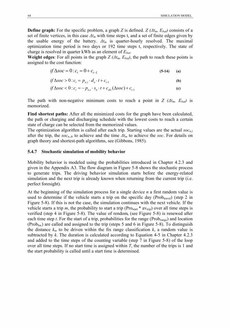
SIMULATION MODEL 64

Define graph: For the specific problem, a graph Z is defined. Z (Δtm, Ebat) consists of a set of finite vertices, in this case Δtm with time steps t, and a set of finite edges given by the usable energy of the battery. Δtm is quarter-hourly resolved. The maximal optimization time period is two days or 192 time steps t, respectively. The state of charge is resolved in quarter kWh as an element of Ebat. Weight edges: For all points in the graph Z (Δtm, Ebat), the path to reach these points is assigned to the cost function:

10 : 0t tif soc c c (5-14) (a)

, -10 : t n t n tif soc c p d t c (b)

, -10 : ( )t n t n dis tif soc c p s t c soc c

(c)

The path with non-negative minimum costs to reach a point in Z (Δtm, Ebat) is memorized. Find shortest paths: After all the minimized costs for the graph have been calculated, the path or charging and discharging schedule with the lowest costs to reach a certain state of charge can be selected from the memorized values. The optimization algorithm is called after each trip. Starting values are the actual socn,t after the trip, the socn,Δt to achieve and the time Δtm to achieve the soc. For details on graph theory and shortest-path algorithms, see (Gibbons, 1985). 5.4.7 Stochastic simulation of mobility behavior Mobility behavior is modeled using the probabilities introduced in Chapter 4.2.3 and given in the Appendix A3. The flow diagram in Figure 5-8 shows the stochastic process to generate trips. The driving behavior simulation starts before the energy-related simulation and the next trip is already known when returning from the current trip (i.e. perfect foresight). At the beginning of the simulation process for a single device n a first random value is used to determine if the vehicle starts a trip on the specific day (Probtravel) (step 2 in Figure 5-8). If this is not the case, the simulation continues with the next vehicle. If the vehicle starts a trip m, the probability to start a trip (Prostart * avtrip) over all time steps is verified (step 4 in Figure 5-8). The value of rendomt (see Figure 5-8) is renewed after each time step t. For the start of a trip, probabilities for the range (Probrange) and location (Probloc) are called and assigned to the trip (steps 5 and 6 in Figure 5-8). To distinguish the distance km to be driven within the fix range classification k, a random value is subtracted by k. The duration is calculated according to Equation 4-5 in Chapter 4.2.3 and added to the time steps of the counting variable (step 7 in Figure 5-8) of the loop over all time steps. If no start time is assigned within T, the number of the trips is 1 and the start probability is called until a start time is determined.

SIMULATION MODEL

65

Figure 5-8: Stochastic simulation process of mobility behavior for one day

Note: Abbreviations see Table 4-2; Random: Random number generated for time step t. 5.5 Evaluation of multi-agent control mechanism To explain how the load management mechanism of distribution grid and system level affect the simulation, two evaluation cases are conducted. In both cases one day of simulation is observed. It is assumed that vehicles do not drive and that the battery state of charge for all vehicles is zero at the beginning of the simulation. The German system load of a winter’s day is taken as the basis. Power and vehicle penetration correspond to the scenario GER defined in Chapter 6. The control mechanism is observed at the distribution grid level and then at the system level separately. Finally, the combined two-level control is discussed. 5.5.1 Distribution grid level To evaluate the DG-agent, the prices of DSM-agents pa,t are set to zero. Only the variable grid fee pg,t is used to control the devices. The transformer utilization with and without the demand of the device-agents is given in Figure 5-9. For the assumptions in Chapter 6.4, the increment of the increase in transformer utilization (see Chapter 5.4.4) per device agent is between 0.24 and 0.48 percent points with 4 kW and 8 kW grid connection power, respectively. With 401 vehicles assigned to a DG-agent – accounting for 401 iterations – the utilization is balanced at about 16 %. Hence, without any external influence, the DG-agent accounts for a distribution close to the optimum (see Figure 5-9).

SIMULATION MODEL 66

Figure 5-9: Evaluation of the DG-agent

Note: PEVs: Plug-in electric vehicles.

5.5.2 System level For the evaluation at system level, only the price signals of the DSM-agents account for the operation of the devices. Three cases are distinguished to show the effect of an increasing number of iterations and control signals. In the first case, one price is used to control all devices. In the second case, two different price signals are used, whereas 30 prices are applied in the third case. The results of the simulation are given in Figure 5-10.

Figure 5-10: Evaluation of DSM-agent control

Note: DSM: Demand-side management.

As expected, using only one price signal to control all devices results in a strong simultaneous reaction. Since no mobility behavior is taken into account and the storage is assumed to be empty at the beginning of the simulation, every device-agent has the same degree of operation freedom. Only the differences in total storage volume and grid connection power result in slightly different charging periods. Using two prices reduces the simultaneous peak but still does not allow the overnight load valley to be filled. With 30 iterations and control signals, a nearly optimal valley filling is reached. The mechanism provides similar results to a single-firm optimization or the algorithm introduced by (Ma et al., 2010) taking a Nash equilibrium into account. For all DSM-agents, the reaction to different prices is sufficient for load valley filling. The load of a single DSM-agent can still be simultaneous and therefore result in peaks in the distribution grid.

SIMULATION MODEL

67

5.5.3 Two-level control The two control mechanisms on the system level for all DSM-agents and on distribution grid level for DG-agents accomplish the goals of load valley filling – which equals low charging costs (social optimum for all PEVs) – and limiting the maximal power in the distribution grid, respectively. The goals of both agents are equal in a typical load situation with a load valley during the night and an increased load during the day. Assuming a strong fluctuation of the residual load can also result in contrary aims, for instance, if a high solar peak on the system level results in incentives for the DSM-agent to charge during the day. On DG level (in a case without any solar power installed), this incentive increases the transformer utilization in a time period when the utilization is expected to be high. In this case the variable grid fee would work against the price signal of the DSM-agent and restrict the transformer utilization. Including RES generation and using the combined load shifting mechanism of DSM-agent and DG-agent results in the load shifting given in Figure 5-11. The charging load inversely follows the residual load and therefore contributes to integrate fluctuating RES-E. The energy available depends on the driving behavior and is restricted by the grid connection power as well as the availability of vehicles. The mechanism considers the next trip using only the positive grid management time. If the time period between one trip and the next does not allow for load shifting (negative grid management time), charging starts instantly.

Figure 5-11: Load of plug-in electric vehicles charging applying demand-side management

Note: DSM: Demand-side management; PEVs: Plug-in electric vehicles.

SIMULATION MODEL 68

5.6 Summary Chapter 5 introduced a simulation approach for PEVs in a power system. The approach allows software agents to be included – in real life applications or smart grid field trials using price-based control – in a power system model. This is able to consider a much greater level of detail and more individual restrictions than common single-firm optimization models. Furthermore, the classical structure of smart grids as a multi-agent system is taken into account by the model, making a more realistic description of future power systems possible. The following issues were addressed:

The context of the research problem was outlined and related research fields discussed.

The PowerACE model serves as the simulation environment for this research. Main PowerACE functionalities and the equation framework were provided.

The detailed approach was formulated and explained. This represents the main scientific value of this thesis. This includes the description of the simulation agents, the optimization algorithm applied and the stochastic simulation of mobility behavior.

Two case studies were provided to evaluate and test the functionality of the developed simulation model.

Critical remarks: In order to consider a dispatch close to the optimum – in this first version of the model – agent behavior is reduced to clear technical requirements without strategic behavior or gaming and learning functionalities. Perfect foresight of the trips and the exclusion of consumer price sensitivity result in idealized dispatch behavior which best matches fluctuating generation. Power ACE can be applied to model different regions and transmission limitations between these regions but these are not considered in this thesis.

SCENARIO DEFINITION

69

6 Scenario definition 6.1 Introduction The scenarios include certain assumptions about the future. These are necessary because the framework conditions with regard to the market penetration of PEVs or the installed capacity of RES are not sufficient to answer the research question. In order to analyze the effect of fluctuating renewable energy generation from wind power and photovoltaics, as well as the contribution of PEVs towards balancing these RES-E, the author had to construct a scenario for 2030. In the following scenario, assumptions for Germany are presented which distinguish between the electricity sector and the vehicle sector. In addition, a sub-scenario for California is constructed to take the different fluctuation of RES-E there into account. This chapter is divided into sub-chapters which describe the assumptions about the electricity sector, the vehicle sector, and the distributed grid. 6.2 Electricity sector In order to investigate the contribution of PEVs to integrating RES-E into the grid, scenarios are defined based on surveys available in the literature. These scenarios are used to create an environment with very high RES penetration (necessary to reach the CO2 reduction goal of the German government). The main scenario used “GER 2030” refers to the “Lead Scenario 2010”, which was part of a survey investigating high RES penetration in Germany carried out on behalf of the German Federal Ministry for the Environment, Nature Conservation and Nuclear Safety (Nitsch et al., 2010). Other surveys of the German energy sector (dena-Netzstudie II 2010 in DENA, 2010) do not account for the time period until 2030 or provide a similar penetration scenario of RES (Energieszenarien 2011 in Schlesinger et al., 2011).85 The “Lead Scenario 2010” was selected because this study is best suited to investigating the effects of fluctuating generation. However, in order to enable scenario-independent general findings and conclusions to be drawn, a detailed analysis of the input parameters is made so that the effects of the scenario estimations are transparent. A sub-scenario for California “CA 2030” is used based on data from a 2020 CAISO study (CAISO, 2011) in order to consider the different load curve, RES technology composition and fluctuation characteristics in CA (see Chapter 3). The CA 2030 scenario is scaled to the same energy generation share of fluctuating RES-E as the GER 2030 scenario to enable comparability (see Table 6-1).

85 To some extent these studies are influenced by stakeholders. The “Lead Scenario 2010” is supported by policymakers and companies interested in high RES penetration and strong reduction of CO2 emissions.

SCENARIO DEFINITION 70

Table 6-1: Intermittent generation and electricity demand for GER 2030 and CA 2030

Scenario Wind

onshore Wind

offshore Photo-voltaics

Solar thermal

Share of fluctuating RES-E (peak load;

generation)

Total electricity demand (peak

load; generation) Unit

GER* Capacity 37.8 25 63 - 162.0% 77.8 GW

Generation 87 95 57 - 47.6% 502.1** TWh

CA*** Capacity 28.2 - 19.9 13.3 96.7% 63.5 GW

Generation 71.4 - 43.1 30.2 47.6% 303.8 TWh

Source: * Lead Scenario 2010 (Nitsch et al., 2010); ** Energiereport IV (Schulz et al., 2005); *** Proportion of technologies and fluctuation from (CAISO, 2011); The generation share of intermittent RES is scaled to 47.6 % and the same value of the Lead Scenario, 2010, respectively.

The hourly characteristics of RES generation and the load curve were already discussed in Chapter 3. 2008 is used as the reference year for the GER 2030 time series because the wind availability in this year is close to the 10 year average. Electricity imports and exports and storage technologies such as hydro pumped storage are not taken into account. To indicate the dispatchable supply side, the merit-order of power plants is generated using primary energy and CO2 prices from (Nitsch et al., 2010) as shown in Table 6-2. Assumptions about the power plant park are given in Chapter 7.4.1.

Table 6-2: Fuel and CO2 prices for the GER 2030 scenario

Oil Gas Coal Lignite CO2

Unit euros/MWhtherm euros/t

Price 58.68 49.68 23.4 3.8 52 Source: Lead Scenario 2010 (Nitsch et al., 2010);

6.3 Vehicle sector The penetration scenario for PEVs follows (METI, 2006), a study investigating a 100 % penetration of alternative vehicles (HEVs, PHEVs, BEVs and fuel cell vehicles) for Japan in 2050. The penetration of PHEVs and BEVs was adapted to the German market by specifying two electric vehicle concepts: PHEVs with 4.5 kWh or 12 kWh and BEVs with 15 kWh or 30 kWh usable battery storage (see Table 6-3 and Chapter 2). The assumptions with regard to the energy use of PEVs imply a reduction in weight as well as in air and rolling resistance compared to today’s vehicles (Moawad et al., 2009; Gonder et al., 2007; Santini et al., 2002).86 The values in Table 6-3 include the efficiency. For V2G, an efficiency of 94 % is assumed. The battery charging power is assumed to be constant over time.87 Total PHEV penetration in 2030 is 12 million or 24 % of the total passenger vehicle fleet, with a PEV share of over 80 %. This scenario is classified as optimistic (for further estimations, see Hadley et al., 2009; McCarthy et al., 2010; Becker, 2009; IEA, 2010). The political goal in Germany is to have at least 1 million PEVs in 2020 and 6 million PEVs in 2030 (BMBF, 2009). For the CA 2030

86 Values in the range of: weight 800 - 1400 kg, drag coefficient 0.2 - 0.26 and rolling resistance 0.0045 - 0.006. 87 For real batteries charging power is not linear see (Appendix A1).

SCENARIO DEFINITION

71

scenario (California Department of Transportation , 2005),88 the PEV’s share of the total fleet equals the GER scenario and results in a total PEV penetration of 6.8 million.89

Table 6-3: Passenger vehicle types

Device Type (km)*

Usable storage [kWh]

Grid connection

power [kW]

Equivalent energy use [kWhel/km] **

CA 2030 (6.7 million

PEVs)

GER 2030 (12 million

PEVs) 1 PHEV (25) 4.5 4 0.18 31.6% 31.6% 2 PHEV (57) 12 4 0.21 50.4% 50.4% 3 BEV (100) 15 8 0.15 13.9% 13.9% 4 BEV (167) 30 8 0.18 4.0% 4.0%

Comments: * In brackets: hypothetical driving range in km; ** at grid connection including: charging η = 98.5 %, lithium-based battery: η = 97 % and electric motor η = 95 % The allocation of the different vehicle types is given in Table 6-3. In total, 12 thousand PEVs are modeled for GER 2030, representing 12 million PEVs. Thus, the operation of one vehicle is scaled-up by a factor of 1,000. Table 6-4 summarizes the power and storage capacity of the resulting vehicle fleet for the two scenarios. A fleet of PEVs provides high power with a relatively low usable amount of battery storage. The power/energy ratio of the total fleet for CA 2030 and GER 2030 is 0.44. By comparison, German pumped storage plants provide 7.76 GW with a rated volume of 224.31 GWh (ratio: 0.035).

Table 6-4: Resulting power and energy values of the vehicle fleet scenarios

CA 2030 GER 2030

Type Vehicles

[thousand] Connection power [GW]

Storage capacity [GWh]

Vehicles [thousand]

Connection power [GW]

Storage capacity [GWh]

PHEV (25) 2,150 8.60 9.68 3,885 15.54 17.48PHEV (57) 3,430 13.72 41.16 6,585 26.34 79.02BEV (100) 945 7.56 14.18 1,230 9.84 18.45BEV (167) 275 2.20 8.25 300 2.40 9.00

Sum 6,800 32.08 73.26 12,000 54.12 123.95

In this thesis, it is assumed that the necessary infrastructure is always available. The sensitivity of this assumption is analyzed in Chapter 7.7.5. PEVs are plugged-in after each trip. The battery degradation parameters used are summarized in Table 6-5. For V2G, the two scenarios, the energy processed and the depth of discharge are distinguished. Both scenarios have optimistic assumptions on battery ageing and cost reduction.

88 Total passenger vehicles 28,320,000. 89 This assumption is similar to (Hadley et al., 2009) who suppose a penetration of 6.63 million PEVs.

SCENARIO DEFINITION 72

Table 6-5: Battery degradation parameter

Energy processed (Ah) Depth of discharge (DoD)

Type a b Cbat [euros/kWh] a b Cbat [euros/kWh]

PHEV (25) 7000 -1 281 4000 -1.632 281

PHEV (57) 7000 -1 247 4000 -1.632 247

BEV (100) 7000 -1 247 4000 -1.632 247

BEV (167) 7000 -1 233 4000 -1.632 233

6.4 Distribution grid A standard load profile of the residential sector is used to account for the distribution grid (see Appendix A4). The profile represents 100 households and is normalized assuming a 400 kVA transformer. This results in a relatively low utilized transformer with a minimum of 4.8 % and a maximum of 27.8 %. The vehicle demand is added depending on the vehicles assigned to the DG-agent and the transformer capacity per device-agent. For the standard scenario, with 401 vehicles assigned to a DG-agent and 4.52 kVA transformer capacity per vehicle, the normalized demand per vehicle (4 kW) is added by

, , ,, 4.

4.52 401g t g t g tn t

g g a g g

w d dw kW

W W W N W kW

(6-1)

Hence, the demand of one vehicle with a 4 kW grid connection accounts for a utilization increase of 0.24 percent points and all vehicles account for an increase of 100 %. The parameters ag and cg to calculate the variable grid fee are assumed to be 30.1390 and 0.5 ct/ kWh. Transmission limitations are not considered.

90 The value results from Equation 5-12.

RESULTS

73

7 Results 7.1 Introduction This chapter describes the results from the PowerACE DSM simulation model. First, the driving behavior generated using a stochastic simulation approach is discussed (Chapter 7.2). Next, the resulting residual load is presented for the scenarios CA and GER as well as the effects of last trip, TOU and DSM charging (Chapter 7.3). The power plant park and the effects of the V2G charging strategy are then discussed for the GER scenario (Chapter 7.4) followed by further power plant park utilization (Chapter 7.5) and smart charging revenues (Chapter 7.6). Finally, the sensitivities are analyzed for the main assumptions (Chapter 7.7). Each sub-chapter concludes with the main findings for that section. 7.2 Driving behavior Compared to stationary storage devices, the availability of PEVs as a grid resource is affected by the behavior of the vehicle user. This makes it harder to assess storage and load shifting. To analyze PEVs’ grid availability first, the average yearly driving behavior and the resulting PEVs’ electricity demand are discussed. Then the time period during which vehicles are available for smart grid services (DSM and V2G) and the energy demand of the vehicles when plugged back into the grid are described. Finally, the stochastic simulation of driving data is evaluated using deterministic data to validate the stochastic simulation approach. 7.2.1 Average driving data Average driving data only permit a rough characterization of the vehicle fleet. The values given in Table 7-1 represent an average of 10 simulations with probabilities from the MID 2008 mobility survey (see Chapter 4.2). Values can vary by up to percent points because of the stochastic method used. The yearly driving distance amounted to 15,298 km with 3.9 trips per day and 249 days of driving on average.

Table 7-1: Average yearly driving data

Days driving Total trips Total driving distance Trips per day Average km per trip

MID 2008 249 days 960 trips/a 15,298 km 3.9 trips 15.9 km

Source: Data basis (MID, 2010). Note: Average out of 12,000 vehicles.

The yearly electric driving pattern is affected by the charging strategy and the assumptions about infrastructure availability. For last trip charging, mainly infrastructure at home is available. In the case of smart charging, it is possible to charge when the vehicles are parked. The driving location is determined by the probabilities defined in Chapter 4.2.3 and available in the Appendix A3. Parking at home and at work occurs most often and the parking location is relatively easy to predict. Public parking for shopping or leisure activities is characterized by a high degree of diversity.

RESULTS 74

It is therefore more complex and cost-intensive to connect vehicles parking at these spots to the grid and the average parking time here is shorter, which reduces the grid management time. Consequently, from a smart grid perspective, home and work charging seem to be of primary interest. The PEV location results are presented in Figure 7-1.

Figure 7-1: Location of vehicles

Source: Data basis (MID, 2010).

The average electric driving share of last trip charging of the PEV fleet is 54 %, resulting in an average electricity consumption of 1594 kWh per year and PEV. In total, the PEV fleet’s demand is 19.1 TWh for GER 2030 and 10.8 TWh for CA 2030. For smart charging (TOU, DSM and V2G), the average electricity consumption here increases to 2061 kWh per vehicle with an electric driving share of 70 %. This increase is caused by the assumed greater availability of infrastructure. In total, the PEV fleet consumes 24.9 TWh for GER 2030 and 14.0 TWh for CA 2030, accounting for approximately 5 % of the total electricity demand. 7.2.2 Grid management time The resulting grid management time of the stochastic simulation using the probabilities of the MID 2008 mobility survey is described here. The grid management time ∆t depends on the return time of a trip (see Chapter 4.2.4). Figure 7-2 gives the energy returning to the grid and the ∆t for the quarter-hourly resolved simulation of a weekday. The average ∆t depending on arrival time decreases until noon and then starts to rise until midnight. The average ∆t for a weekday is 7.4 hours (see Table 7-2). Evaluating the grid management time separately for days and nights shows that ∆t day is much shorter than ∆t night. The average of ∆t day on a weekday is 1.8 hours per trip whereas ∆t night is 23.6 hours. The ∆t night value is strongly influenced by vehicles that do not drive on the next day(s). ∆t day can be negative if the time for recharging in a parking period is too low.91

91 Note: To a minor extent, the ∆t values depend on the grid connection power as defined in Chapter 6.2.

RESULTS

75

Figure 7-2: Hourly average grid management time and energy demand of returning vehicles

Source: Data basis (MID, 2010); Note: ∆t: Grid management time for the total average; ∆t day: trips during the day; ∆t night: the last trip of a day; Results for a weekday.

On Fridays and Saturdays, ∆t night increases because the probability to drive on the weekend is lower. ∆t day at weekends is in the same order of magnitude as weekdays (see Table 7-2). See Appendix A5 for the hourly shares for Saturdays and Sundays.

Table 7-2: Average grid management time for days of the week

Unit [h] Mon WD Fri Sat Sun

∆t 6.7 7.4 8.9 9.6 7.9

∆t day 1.8 1.8 1.8 1.7 1.9

∆t night 21.6 23.6 29.6 31.5 22.1

Source: Data basis (MID, 2010).

The wide diversity of mobility behavior causes a high standard deviation for all average values. The hourly standard deviation for ∆t can also be found in the Appendix A5. 7.2.3 Evaluation of the stochastic simulation In order to validate the concept of modeling mobility behavior, the stochastic simulation results are evaluated using deterministic data from the MOP survey. The weekly MOP driving profiles are randomly linked to a 365-day driving profile for 12,000 vehicles. The stochastic data result from a simulation as explained in Chapter 5.4.7 with probabilities drawn from the MOP data set rather than the MID survey. The average values from a simulation of 12,000 vehicles are summarized in Table 7-3 for total trips per year, days with a trip, average trips per day, total driving range and average range per trip of the fleet.

Table 7-3: Average yearly driving data for one vehicle of a fleet of 1200 vehicles based on MOP

Total trips per year and vehicle

Days with a trip

Average trips per day driving

Driving range per year [km]

Average range per trip [km]

Deterministic data 816.0 268.7 3.0 11,044.9 13.6

Stochastic data 823.6 268.0 3.1 11,113.8 13.5 Source: Data Basis: (MOP, 2002-2008).

RESULTS 76

The differences between the stochastic simulation and deterministic data were very low. This proves the high consistency in terms of yearly parameters. Besides the yearly driving data, the grid management time and the related energy demand of returning vehicles are used to compare the stochastic data with the deterministic data (see Figure 7-3). The data is evaluated over quarter hours of one day. For the energy demand of returning PEVs, the correlation between the two data sets is 96.69 %. The correlation is lower in terms of the average grid management time of a time step (49.41 %). During nighttime hours, values vary strongly because of the low frequency of trips. In the evening, differences of up to 8 hours occur. Vehicles not being driven the next day(s) strongly affect the average value. Excluding time steps with a low sample size (t < 20) results in a correlation of 83.71 % between the stochastic and deterministic approaches.

Figure 7-3: Energy demand of returning vehicles and grid management time on weekdays

Sorce: Data Basis: (MOP, 2002-2008); Note: Sample size 800,000 trips; correlation between grid management time t0-95 = 49.41 %, t20-95= 83.71 %; correlation between energy demand t0-95 = 96.69 %. Comparing the stochastic and deterministic data reveals that driving behavior is complex and very diverse. The simple modeling approach does not account for combinatorial probabilities (e.g. longer standing time after long trips). Especially for time-resolved values such as the grid management time, the approach does not necessarily provide realistic results for a single vehicle. But, as shown in Figure 7-3, results are very accurate for the total fleet. This proves that the probability-based approach is sufficient to model driving behavior for the research application of this thesis. 7.2.4 Conclusions The main findings from modeling driving behavior are:

Primary parking locations are at work and at home. The grid management time is highest after the last trip. But average grid

management time indicates load shifting and V2G potential even during the day. Compared to last trip charging, the electric driving share increases if several

charging processes are possible. Under the assumptions made, there was an increase from 54 % for last trip charging to 70 % for permanent infrastructure availability – which is assumed for TOU, DSM and V2G charging.

Comparing the stochastic simulation with the deterministic data set of the MOP survey shows that the method used is suitable.

RESULTS

77

7.3 Effect on the power system This chapter shows how the PEV load affects the power system in the CA 2030 and GER 2030 scenarios.92 First, the residual load is examined as a benchmark. Next, the effects on the residual load of different charging strategies are analyzed for the two scenarios. The main results are then summarized and discussed. Chapter 7.3 is partly published in (Dallinger et al., 2013). 7.3.1 Residual load In order to evaluate how PEVs can help to integrate RES-E into the grid, the remaining residual93 load is used as a benchmark. The assessment applies the parameters defined in Chapter 3.3. The most important parameters for the scenarios CA 2030 and GER 2030 are summarized in Table 7.4.

Table 7-4: Evaluation parameters, residual load for California versus Germany

RS GER 2030 RS CA 2030

cfpos 38.8 % rrfpos 2.03 % cfpos 28.9 % rrfpos 1.99 %

cfneg -0.285 % μ pos 4.39 % cfneg -0.278 % μ pos 4.38 %

cfy=0 3.2 % μ neg -3.76 % cfy=0 4.4 % μ neg -3.63 %

rcf0.8 0.51 xy=0 53.88 % rcf0.8 0.50 xy=0 54.70 %

Pmin -43.52 % CorRES-load 34.22 % Pmin -26.46 % CorRES-load 46.81 %

Pmax 90.36 % Pmax 71.69 %

In both scenarios, the very high RES penetration of 47.6 % has a strong effect on the remaining residual load duration curve (see Figures 7.7 and 7.8). The reduction of both the area under the curve and the capacity factor cfpos compared to the load duration curve indicate RES generation. Zero crossing of the residual duration curve is 3.2 % for GER and 4.4 % for CA. This means that RES generation exceeds electricity demand in 3.2 % and 4.4 % of the 8760 simulated hours for GER and CA, respectively. In total, the negative residual load (cfneg) for GER 2030 is -0.285 % and -0.278 % for CA 2030, or 1.95 TWh and 1.55 TWh in absolute values, respectively.94 During these time periods it is necessary to either distribute more electricity, or store it, or limit RES power or introduce DSM to keep the system balanced. The reduction in the maximal power value Pmax in CA 2030 to 72 % and in GER 2030 to 90 % shows that RES’s contribution to reducing the peak residual load is much higher in CA 2030 than in GER 2030 (see Table 7-4). This is due to the closer correlation between photovoltaic and solar thermal generation and the CA 2030 load curve. The higher negative peak Pmin for GER is caused by the high level of installed RES capacity, in total 162 % of the peak load (see Chapter 6.2). For CA 2030 and GER 2030, Pmin is in the middle of the day when wind and solar output occur simultaneously. Compared to GER, the lower installed RES capacity in CA results in fewer extreme RES power supply situations. There is a greater influence of solar generation in CA, and wind and solar strongly affect traditional peak load hours, particularly during the spring months when high cooling loads are not online. For high penetration of fluctuating RES, it will no longer be possible to make a clear distinction between base load during nighttime hours and peak load periods during the 92 The main findings of the chapter are published in (Dallinger et al., 2012c). 93 The residual load is defined as the total system load minus fluctuating RES generation. 94 Absolute value = relative value * 8760 * Pmax, absolute

RESULTS 78

day. This result is illustrated in Figure 7-4, which cumulates the frequency of different availability sections (see Chapter 3.3.3) over the hours of one day for the simulation period of one year. Peak hours (Sec. 3) during the night are likely for both scenarios. A peak residual load is most likely during the early evening. For CA 2030, a morning peak is also observed between 6 and 8 am caused by the characteristics of wind generation here. In CA, high generation from wind during morning hours is unlikely. Peak wind output occurs early evening (see Appendix A2). Very high peak hours (see Sec. 4 in Figure 7-4) accumulate between 5 and 9 pm. Noon is characterized by a high frequency of off-peak periods (see Sec. 1 in Figure 7-4). Obviously, a lack of solar generation still results in a peak load during the day, but the residual load is likely to be low. From a RES fluctuation point of view, it is easier to integrate RES-E into the grid in CA 2030 because of the higher load, RES-E correlation as well as lower RES capacity with equal energy output (installed capacity is 96.7 % of the peak load versus 162 % for GER 2030).

Figure 7-4: Cumulated frequency of residual load variation for different hours of the day

Note: CA 2030: Pmax,load = 63.55 GW, Pmax,RS = 45.55 GW, Pmin,RS = -16.81 GW, ΔPRS= 62.37 GW; GER 2030: Pmax,load = 77.95 GW, Pmax,RS = 70.44 GW, Pmin,RS = -33.92, ΔPRS= 104.36 GW.

Ramping is in the same range for both scenarios with a rrf around 2 %. Compared to the system load, an increase in total ramping is observed for the residual load (compare Table 7-4 and 3-6; GER 2030: rrf change from 1.19 % to 2.03 %; CA 2030: rrf change from 1.05 % to 1.99 %). Further, the intensity of the ramp rates indicated by μ increases due to the higher penetration of fluctuating RES generation. 7.3.2 Last trip charging Charging EVs immediately after returning from the last trip of the day affects the peak load. The simultaneousness of PEV charging is influenced by driving behavior and the grid connection power. The peak load increase resulting from uncontrolled charging is determined by the correlation of the initial load curve and PEV charging. For the CA 2030 scenario, this correlation is smaller than for GER 2030. For CA, the hourly mean load Pmax increases by about 7.7 percent points whereas, for GER 2030, the increase is

RESULTS

79

10.2 percent points (compare Pmax in Table 7-4 and Table 7-5). It should be noted that GER driving data is used here for CA. This could be one reason for the higher correlation of vehicle electricity demand and load curve in GER. For both scenarios there are only minor reductions in the time period with negative residual load (cfx=0), the negative peak (Pmin) and the amount of negative residual load (cfneg). The negative residual load consumed by PEV charging is 11.3 % for GER 2030 and 17.1 % for CA 2030.

Figure 7-5: Ramp rates for the CA 2030 scenario

Note: Pmax,load = 63.55 GW = 100 %; CA: California; PEVs: Plug-in electric vehicles

The effect of last trip charging on the ramp rates for CA 2030 is shown in Figure 7-5. The ramping increases largely due to the fluctuating generation (see system load versus residual load in Figure 7-5 and compare Table 7-4 with Table 7-5). The additional increase caused by charging PEVs is small. In conclusion, fluctuating RES-E have a much greater effect on the ramp rates than charging PEVs.

Table 7-5: Evaluation parameter, last trip charging, California versus Germany

RS + PEVs last trip charging GER 2030 RS + PEVs last trip charging CA 2030

cfpos 41.6% rrfpos 2.32% cfpos 30.8% rrfpos 2.20%

cfneg -0.253% μ pos 5.06% cfneg -0.230% μ pos 4.87%

cfy=0 3.00% μ neg -4.25% cfy=0 4.00% μ neg -4.00%

rcf0.8 0.52 xy=0 54.34% rcf0.8 0.52 xy=0 54.91%

Pmin -42.59% CorRES-load+PEV 27.63% Pmin -25.57% CorRES-load+PEV 40.20%

Pmax 100.59% Pmax 79.18%

7.3.1 Time-of-use tariff To evaluate the load management with time-of-use tariffs, a tariff of the utility (Pacific Gas and Electric, 2011) is implemented in the simulation as a control signal. The tariff structure follows the classical expectations about base and peak load in California and does not account for a high share of RES-E. Other TOU tariffs would provide similar results in terms of simultaneous PEV demand if analyzed with regard to automated control.

RESULTS 80

Table 7-6: Electric vehicle time-of-use tariff of Pacific Gas and Electric

Super Off Peak Off Peak Peak Off Peak

Time period Midnight – 5 am 5 am – 12 pm 12 pm – 6 pm 6 pm – Midnight

Rate 14.4 ct/kWh 16.7 ct/kWh 25.7 ct/kWh 16.7 ct/kWh Source: (Pacific Gas and Electric, 2011).

The tariff is divided into four time periods and three price levels (see Table 7-6). The Californian load curve and PEV penetration as defined in Chapter 6 serve as an example. The result of a one week simulation using the TOU tariff indicates two main price peaks (see Figure 7-6). After the first trip in the morning, PEVs’ agents manage to reload the battery in the off-peak period 5 am – 12 pm to avoid the peak rate starting at 12 pm. The recharge after the first trip is necessary to realize a high electric driving share. The second peak is observed before 5 am. This results from the applied optimization algorithm that selects the last possible time step to charge if the cost of several time steps is the same.95

Figure 7-6: Electric vehicle load with time-of-use tariff control

Source: time-of-use (TOU) tariff (Pacific Gas and Electric, 2011); load curve (CAISO, 2011); Note: Summer week in scenario CA 2030 (see Chapter 6).

Analyzing the evaluation parameter (see Table 7-7) shows that TOU rates do not significantly improve the contribution of PEVs as a grid resource compared to last trip charging. For CA 2030, a peak load reduction is observed (Pmax is reduced from 79 % to 74 %) and a possible consumption of 39 % of negative residual load versus 17 % in the case of last trip charging (compare cfneg in Tables 7-4, 7-5 and 7-7). Improvements are smaller with regard to Pmin and ramping.96 For GER 2030, parameter changes compared to last trip charging are in the same range as for CA values. Only the peak reduction is lower because the GER peak load occurs in the evening. The TOU rate used is designed to reduce peak load during the day.

95 In terms of battery ageing, using the last possible time step for recharging is not groundless because a high state of charge can reduce the calendar life. 96 Note: In CA, Pmin occurs during the day when the TOU rate is high and PEVs therefore avoid charging.

RESULTS

81

Table 7-7: Evaluation parameters, time-of-use, charging California versus Germany

RS + PEVs TOU charging GER 2030 RS + PEVs TOU charging CA 2030

cfpos 42.4 % rrfpos 2.35 % cfpos 31.3 % rrfpos 2.20 %

cfneg -0.191 % μ pos 4.49 % cfneg -0.170 % μ pos 4.37 %

cfy=0 2.20 % μ neg -4.88 % cfy=0 3.20 % μ neg -4.42 %

rcf0.8 0.49 xy=0 47.87 % rcf0.8 0.47 xy=0 49.72 %

Pmin -42.15 % CorRES-load+PEV 35.36 % Pmin -24.57 % CorRES-load+PEV 49.65 %

Pmax 98.50 % Pmax 74.40 %

The simultaneous reaction of automated agents and the changing requirements in terms of peak and off-peak hours due to RES-E (see Figure 7-4) indicate that smart grid control must provide more sophisticated solutions to reduce demand peaks and integrate fluctuating generation. 7.3.2 Demand-side management Simulating dynamic pricing with a distributed vehicle-based optimization (Chapter 5.4) illustrates the contribution of PEVs to balancing fluctuating RES-E using demand-side management. The evaluation parameters quantifying the effect of DSM smart charging are summarized in Table 7-8.

Table 7-8: Evaluation parameters, demand-side management, charging California versus Germany

RS + PEVs DSM charging GER 2030 RS + PEVs DSM charging CA 2030

cfpos 42.3% rrfpos 1.52% cfpos 31.2% rrfpos 1.70%

cfneg -0.102% μ pos 2.88% cfneg -0.076% μ pos 3.43%

cfy=0 1.40% μ neg -3.20% cfy=0 1.60% μ neg -3.33%

rcf0.8 0.48 xy=0 47.35% rcf0.8 0.46 xy=0 50.71%

Pmin -34.02% CorRES-load+PEV 44.50% Pmin -18.52% CorRES-load+PEV 56.56%

Pmax 91.93% Pmax 72.09%

The effect of controlled PEV charging on the residual load duration curve is shown for Germany and California in Figures 7-7 and 7-8, respectively.97 In both cases, it is possible to limit peak load and to increase consumption of the negative residual load. For GER 2030 about 64.0 % and for CA 2030 about 72.6 % of the negative residual load can be consumed (see Table 7-9, relative values cfneg). The time period with negative residual load is reduced by 158 hours (GER 2030) and 245 hours (CA 2030). The negative residual peak reduction is 7.4 GW for GER and 5.1 GW for CA (see Table 7-9 absolute change).

97 Additionally in the Appendix, Figure A-11 to A-15 show the probability of the residual load for the scenarios CA and GER.

RESULTS 82

Figure 7-7: Change in the residual load duration curve due to DSM for Germany

Note: DSM: Demand-side management; RES: Renewable energy sources; PEVs: Plug-in electric vehicles. In terms of ramping, a significant ramp rate factor reduction of 34.3 % is achieved for GER and 22.5 % for CA. In addition, the ramping mean and the standard deviation values are significantly lower.

Figure 7-8: Change in the residual load duration curve due to DSM for California

Note: DSM: Demand-side management; RES: Renewable energy sources; PEVs: Plug-in electric vehicles. PEVs make a greater contribution in CA 2030 than in GER to integrating RES-E in terms of negative residual load consumption and reducing peak load. This indicates that these two parameters are influenced by the RES generation characteristics and the resulting residual load, respectively. For GER 2030, RES generation and some hours with negative residual load are dominated by wind. The GER wind generation output is characterized by longer high production periods whereas generation tends to follow a rhythmic daily pattern for CA, especially during the spring and summer (see Appendix A2). A daily rhythm is preferable for RES-E grid integration using PEVs, because driving behavior also follows a daily pattern and does not permit long load shifting periods. Recharging the PEV’s battery is only possible if electricity has been consumed for driving. This effect is enhanced by the higher RES capacity required in GER 2030 to produce the same RES electricity output.

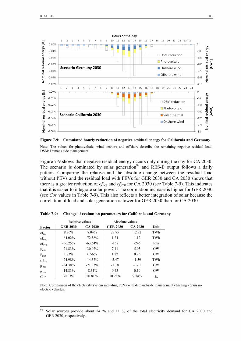
RESULTS

83

Figure 7-9: Cumulated hourly reduction of negative residual energy for California and Germany

Note: The values for photovoltaic, wind onshore and offshore describe the remaining negative residual load; DSM: Demans side management.

Figure 7-9 shows that negative residual energy occurs only during the day for CA 2030. The scenario is dominated by solar generation98 and RES-E output follows a daily pattern. Comparing the relative and the absolute change between the residual load without PEVs and the residual load with PEVs for GER 2030 and CA 2030 shows that there is a greater reduction of cfneg and cfy=0 for CA 2030 (see Table 7-9). This indicates that it is easier to integrate solar power. The correlation increase is higher for GER 2030 (see Cor values in Table 7-9). This also reflects a better integration of solar because the correlation of load and solar generation is lower for GER 2030 than for CA 2030.

Table 7-9: Change of evaluation parameters for California and Germany

Relative values Absolute values

Factor GER 2030 CA 2030 GER 2030 CA 2030 Unit

cfpos 8.96% 8.04% 23.75 12.92 TWh

cfneg -64.02% -72.58% 1.24 1.12 TWh

cfy=0 -56.25% -63.64% -158 -245 hour

Pmin -21.83% -30.02% 7.41 5.05 GW

Pmax 1.73% 0.56% 1.22 0.26 GW

rrfpos -24.98% -14.37% -3.47 -1.59 TWh

μ pos -34.38% -21.83% -1.18 -0.61 GW

μ neg -14.83% -8.31% 0.43 0.19 GW

Cor 30.03% 20.81% 10.28% 9.74% % Note: Comparison of the electricity system including PEVs with demand-side management charging versus no electric vehicles.

98 Solar sources provide about 24 % and 11 % of the total electricity demand for CA 2030 and GER 2030, respectively.

RESULTS 84

7.3.3 Conclusions Country-specific time series and installed capacities for solar and wind power were considered for the two case studies of Germany and California. Comparing these two shows that the resulting residual load is strongly affected by the assumptions concerning the installed capacity of renewable energy sources and by the time series used. The findings for Germany and California under the scenario assumptions made for 2030 with high shares of RES-E and PEVs are:

The capacity factors of wind and photovoltaics are lower in GER than in CA. Hence, a higher installed capacity is needed to generate the same amount of energy in Germany. For both countries, the energy produced from fluctuating RES represents 47 % of the total system load. The installed RES capacity as a percentage of the system peak load is 162 % for GER and 97 % for CA. The higher installed capacity results in more RES surplus generation or in more negative residual load situations in the GER scenario.

The ramping of the residual load is strongly influenced by RES generation.

Compared to the load curve without considering RES generation, ramping nearly doubles if fluctuating generation is included. This is true for both CA and GER. In terms of single time series, especially PV in CA has very high ramp rates. Possible reasons are the higher direct radiation in CA and the resulting system specifications (trekking systems, solar thermal power using storage, and concentration of installations to a specific region). In addition, the method of calculating the time series can influence the results. For GER, offshore wind shows higher ramp rates compared to onshore wind (see Chapter 3).

Besides the energy actually produced by a renewable energy technology, its

fluctuation plays an important role when evaluating the contribution of storage technologies to integrating RES-E into the grid. In terms of photovoltaics, the characteristics on sunny days are obviously very similar in both GER and CA. Taking the entire year into account, however, reveals an on/off characteristic for GER. In other words, days with almost no generation occur more often in GER, particularly during the winter, but also during the summer, albeit with reduced probability. Solar generation is much more reliable in CA and even for wind, generation here is characterized by a regular daily pattern for large periods of the year. In GER, there is a greater dependence on specific weather fronts for wind generation. To sum up, periods with very high wind velocities lasting several days and periods with almost no wind are more likely in GER than in CA.

In this context, besides the characteristics of the individual generation

technology, it is also very important to account for the overall outcome of the technology mix and the resulting residual load. The correlation between load and the expected output of total RES generation strongly affects the situation in a power system. A higher correlation is found between the expected RES generation and the load for CA than for GER. This is due to the daily pattern of generation in CA being a better match for the load curve, which also follows a daily pattern. In addition, the air conditioning load and solar generation, which dominate Californian summers, evidently have a high correlation.

RESULTS

85

The residual load in both simulation scenarios indicates a drastic change taking

place in the power system if renewable energies became a dominant generation source. In this case, peak hours at noon and during the early afternoon are unlikely. This time of the day is dominated by a low residual load. A high peak probability is observed during early evening and nighttime hours. For CA, the morning hours are also expected to have high residual loads. This does not mean that typical peak load events which follow the load curve are no longer possible. However, they are less likely and it will no longer be possible to describe the residual load for the entire year based on a few characteristic days.

To investigate the effect of grid-connected vehicles on the power system, three charging strategies were distinguished: charging after the last trip, TOU tariff based charging and demand-side management. In terms of last trip charging, the results presented here are similar to other published studies. Main findings are:

Last trip charging results in an increased peak demand of 9 percent points for Germany and 7 percent points for California.

Last trip charging increases the ramp rates in the power system. With the used

time increment of one hour, however, the increase is low compared to the effect of fluctuating generation. The ramp rate factor increases by 10 to 15 %.

Overall, PEVs only make a small contribution to balancing RES-E and only a

small proportion of surplus energy from RES or negative residual load can be consumed in the case of last trip charging.

TOU charging can be a first approach to reducing peak loads and promoting off-peak charging. If there is a regular residual load pattern, TOU rates can also help to integrate fluctuating RES-E. For non-recurring RES generation, TOU rates are not flexible enough and cannot effectively integrate fluctuating RES-E.

RESULTS 86

Previous studies have also analyzed DSM using grid-connected vehicle loads (e.g. Sioshansiet al., 2011; Wang et al., 2011). The PowerACE DSM model includes a detailed simulation of individual driving behavior and a control mechanism based on real-time pricing and distributed optimization from the perspective of vehicles acting as independent agents. In addition, a power systems with a high share of fluctuating RES-E is analysed. The results in detail are:

DSM is restricted by mobility behavior. If consumers maximize the electric range of their vehicles to recoup their initial investment, the peak load increases even with load management.

DSM reduces ramp rates by 25 % for GER and 14 % for CA. The surplus

electricity consumption from RES is 64 % of the total negative residual load for GER and 73 % for CA. The negative residual load peak is reduced by 22 % for GER and 30 % for CA.

Comparing CA and GER reveals that more effective use can be made of plug-in

electric vehicles as a grid resource in CA due to the characteristics of RES-E and the resulting residual load here. This is because grid-connected vehicle load shifting is only possible within a time period of several hours to one or two days. The daily pattern characterizing RES power generation in CA means it is easier to integrate.

The same argument applies when comparing photovoltaics and wind power with

each other. The daily pattern of photovoltaic generation favors the storage capabilities of plug-in electric vehicles if charging infrastructure is available where the vehicles are parked during the day.

This chapter highlights the importance of carefully considering load and renewable energy generation output when analyzing future power systems. A detailed description of RES-E time series, system load and residual load is recommended for a better understanding of research results.

RESULTS

87

7.4 Vehicle-to-grid The analysis of battery ageing in Chapter 4.3 indicated the price spreads necessary for V2G. Based on these findings, V2G contribution as a grid resource is discussed in the following. The chapter starts with the definition of the power plant park for GER 2030. Next, a price mark-up is introduced to account for the costs of underutilized power plants. Finally, the effects on the residual load are discussed. Chapter 7.4 is partly published in (Dallinger et al., 2012d). 7.4.1 Optimal power plant park Analyzing the charging strategies of last trip and DSM charging does not necessarily require information on the exact power plant park, if the price sensitivity of consumers is not considered. For V2G charging, the power plant park is essential regarding the decision to provide V2G. The arbitrage of energy is only economically valuable if the price spread within a defined time period is high enough. An approach focusing on Germany was used to account for the power plant park. Perfect foresight in the GER 2030 scenario is assumed and the time frame between 2010 and 2030 is not considered. Parameters which heavily influence the power plant park are fuel prices, the RES capacity and the total electricity demand and are defined by the scenario GER 2030 (see Chapter 6.2). The analysis focuses on three power plant options: gas turbines (GT), combined cycle gas turbines (CCGT) and coal power plants. Nuclear and carbon capture and storage are not considered.99 Figure 7-10 gives the total electricity generation costs of the power plant options depending on the utilization and the residual load for different charging scenarios.

Figure 7-10: Total costs of different power plant options 2030 and residual load

Assumptions: Gas turbine (GT): specific investment: 333 euros/kW, efficiency: 39 %; combined cycle gas turbine (CCGT): specific investment: 733 euros/kW efficiency: 60 %; gas price 49.68 euros/MWhtherm; coal power plant: specific investment: 1650 euros/kW efficiency: 50 %; coal price 23.4 euros/MWhtherm; CO2 price 52 euros/t; interest rate 10 %; Note: LT: Last trip; DSM: Demand-side management; V2G: Vehicle-to-grid.

Coal has the lowest total electricity generation costs for a utilization greater than 3363 hours. Between 1012 and 3363 hours, CCGT has the lowest costs. For utilization lower than 1012, GT is the optimal option to produce electricity in terms of costs. Switching between generation technologies producing at lowest costs yields the optimal generation

99 Neither technology is cost competitive with coal under the assumptions about investments as well as CO2 and fuel prices.

RESULTS 88

capacity. The lowest total cost switch between coal power plants and CCGT at 3363 hours of operation gives the base load or coal capacity needed of 24.3 GW. Changing from CCGT to GT takes place at 1012 hours of operation. The optimal CCGT capacity is 13.9 GW. The remaining GT capacity required to reach peak residual load (64.3 GW)100 is 26 GW. To account for system security, 10 % of overcapacity provided by GT are included.101 Power plants still available in 2030 and currently under construction are considered (BDEW, 2011). New installations and the total installed capacity in 2030 are given in Table 7-10.

Table 7-10: Capacity for the 2030 GER scenario

Power plant type

Min. utilization

[h]

Optimal capacity [MW]

Old capacity available in 2030 [MW]

Under construction 2010 [MW]

New installations

[MW]

Installed capacity 2030

[MW]

Oil 749 749

GT 0 26,03 4,023 28,438 32,461

CCGT 1010 13,942 9,54 1,038 3,364 13,942

Coal 3,368 24,314 3,081 6,933 4,361 14,375

Lignite 6,244 2,875 9,119

Waste 820 820

Total 64,28611 Total 71,46622 Note: 1 Equals peak load by PEVs last trip charging including dispatchable biomass generation; 2 Includes 10 % reserve provided by gas turbines; Available capacity from lignite and waste is assumed to reduce the necessary capacity of coal because of the lower marginal generation costs.

The different PEV charging strategies affect the residual load curve and therefore the resulting optimal power plant capacity. The sensitivity of the charging strategy (difference in the residual load between last trip and V2G charging) to optimal capacity is relatively low for the switching point between coal and CCGT (434 MW capacity delta).102 The switching point between GT and CCGT is affected more strongly by the charging strategy (2034 MW capacity delta). For both cases, the means of 217 and 1017 MW are used to calculate the optimal capacity. Furthermore, the efficiency of the power plant options affects the optimum. In this case, switching between CCGT and coal shows a higher sensitivity.103 The presented approach applies simplifications but provides a possible scenario for the power plant mix in 2030. In general, investment planning is associated with uncertainty and has high sensitivity to residual load and price development. The decision making is reduced to the total generation costs and does not account for strategic decisions in terms of the capacity planning of countries and utility firms. 7.4.2 Price mark-up The utilization of fossil power plants is reduced with a higher share of RES-E, which feed-in electricity with priority over fossil generation (see Chapter 7.3.1 and Figure 7-4). In this case, profit contributions are not high enough if bids are placed 100 This includes capacity from biomass (9.88 GW), geothermal (0.75 GW) and hydro (2.68 GW). 101 The availability of the different power plant options is 0.97 for lignite, 0.93 for coal and 0.99 for gas. 102 Note, that the base load capacity from lignite and coal exceeds this point. 103 The gradient is 4.31 MW/h at h = 3361 and 8.00 MW/h at h = 1012. A 1 % efficiency increase of CCGT compared to coal and GT changes the switching points h = 3361 to 3697 and h = 1012 to 983; the effect on the optimal capacity is +1400 MW and + 232 MW, respectively.

RESULTS

89

based solely on marginal generation costs. Therefore, a price mark-up is used that accounts for the lower utilization and includes depreciation on power plant investments. The mark-up calculation used has been developed by Fabio Genoese104 and proceeds as follows:

Forecast the expected utilization of a power plant and calculate the expected income in one year of operation.

If the power plant is not fully depreciated, a yearly annuity is calculated. The annuity includes fixed costs, the specific investment and capital costs.

Subtract the income from the annuity and allocate the result to the operating hours of the power plant.

The method accounts for the total electricity generation costs. The depreciation time period is 15 years for GT and 20 years for all other plants. An interest rate of 10 % and specific investments of 333 euros/kW for GT, 733 euros/kW CCGT and 1650 euros/kW for coal power plants are used. The supply clearing price for last trip charging including and excluding the mark-up for one year of operation is shown in Figure 7-11 in comparison to the merit-order and the bid points without mark-up.

Figure 7-11: PowerACE market clearing price depending on the residual load

To account for the mark-up of supply bids in the price forecast, the heuristic functions of DSM-agents are adapted to

4 3 2, , , , , ,p ( ) = 0.00001 0.001 +0.0024 4.6204 6.7877MarkUP

a t RS t RS t RS t RS t RS td d d d d

(7-1)

for dRS,t values greater than zero. For a dRS,t equal to zero or negative, a linear correlation is used.

, , ,p ( ) = 6.7877a t

MarkUPRS t RS td d (7-2)

For the calculation of V2G operation, both price forecast functions including and excluding the mark-up are considered using different scenarios.

104 Fabio Genoese is a member of the PowerACE work group at Fraunhofer ISI.

RESULTS 90

7.4.3 Effect on the power system Besides the price function and availability of vehicles, the method used to calculate the V2G costs also affects V2G operation. In Chapter 4.3, two methods were introduced to consider battery degradation: the energy processed (Ah) and the depth of discharge (DoD). Each method results in different V2G charging strategies. To illustrate the differences, Figure 7-12 shows the V2G operation of a stationary battery device (Storage: 30 kWh; grid connection 8 kW).

Figure 7-12: V2G operation: depth of discharge versus energy throughput

Assumptions: Storage size: 30 kWh; grid connection 8 kW; Note: V2G: Vehicle-to-grid.

The DoD-based method results in shallow cycles using smaller price spreads for energy arbitrage. Deep cycles are only conducted for very high price spreads (see upper panel of Figure 7-12). Full cycles are more likely for the method based on the energy processed (see lower panel of Figure 7-12). Compared to the DoD-based V2G, the total amount of energy shifted is larger, but the number of V2G operations is lower. Compared to the stationary storage operation shown in Figure 7-12, driving further increases the complexity of V2G operation. The optimization time frame in this case is only the grid management time between two trips. For V2G feeding back electricity, it is necessary to have high and low prices within the grid management time. For example, a vehicle arriving with an empty battery in the evening can be cheaply recharged overnight if prices are low. But the next period with high prices – based on today’s typical conditions – is most likely to occur around noon the next day. There is no high price period within the grid management time at night and vehicles will not use V2G. This effect is enhanced even more for the DoD-method because the soc is low when vehicles return from a trip. In this case, V2G comes at higher costs compared to a soc of 100 % and even higher price spreads are required.

RESULTS

91

The effect of V2G on the total power system is analyzed using the same parameters as for DSM and last trip charging but focuses on the GER 2030 scenario.105 Besides the charging strategies Ah and DoD, the simulation results with and without the price mark-up (Mup) are distinguished. The feed-back energy is higher with Ah V2G charging. Compared to the total electricity demand of 502 TWh, the feed-back energy varies between 0.8 % and 1.5 %. The V2G energy demand increases proportionately to the energy feedback to the grid (see Table 7-11). The higher price spread due to the mark-up nearly doubles the energy fed-back within the simulation time frame of one year.

Table 7-11: Energy and demand in case of vehicle-to-grid for Germany

Feed-back Demand

V2G [GWh] V2G relative EV2G/EGER V2G [GWh] V2G relative EV2G/EGER

V2G Ah -5,384 -0.788% -1.072% 29,730 4.354% 5.921% V2G DoD -4,152 -0.608% -0.827% 28,758 4.211% 5.728% V2G Mup Ah -9,927 -1.454% -1.977% 33,728 4.939% 6.717%

V2G Mup DoD -7,649 -1.120% -1.523% 31,879 4.669% 6.349% Note: Mup: Clearing prices include price mark-up; EV2G: Energy vehicle-to-grid; EGER: Energy demand Germany.

The peak system load Pmax is reduced by 1.2 percent points for DoD battery ageing compared to DSM charging. For V2G-based on Ah ageing, the reduction is about 0.6 percent points. With mark-up, the reduction is 1 to 2 percent points compared to DSM (compare Table 7-11 value Pmax). The increase of the minimal residual load is much greater (see Table 7-11 value Pmin). Compared to DSM charging (-33.96 %), V2G results in a Pmin value of -26.1 % and -28.2 % for Ah and DoD, respectively. The battery degradation for Ah and DoD is given by the specific battery chemistry so it is not possible to compare them exactly, but Ah shows the tendency to process more energy which results in a greater increase in the negative residual load to be consumed. For DoD-based ageing, a higher peak load reduction without mark-up is observed.

Figure 7-13: Change in the residual load duration curve due to V2G for Germany

Note: RES: Renewable energy sources; PEVs: Plug-in electric vehicles; V2G Ah: Vehicle-to-grid energy with weighted energy throughput based battery aging. Figure 7-13 shows the effect of V2G with DoD battery ageing on the cumulated negative residual load for one year of simulation. Compared to DSM (64.3 %), between 12.7 (V2G DoD) and 17.4 (V2G mark-up Ah) percent points negative residual energy 105 The CA 2030 scenario is not considered because of a lack of information on the power plant park.

RESULTS 92

can be used additionally (compare Table 7-12 value cfneg(RS)/cfneg(X)). There is a large reduction in the hours during which the residual load is negative (see value cfy=0 in Table 7-12). During nighttime hours the negative residual load is consumed almost completely. The remaining negative residual load occurs during the day between 10 am and 3 pm (see Figure 7-14).

Figure 7-14: Cumulated hourly reduction of negative residual energy due to V2G for Germany

Note: Simulation including mark-up prices and DoD based battery aging. The values for photovoltaic, wind onshore and offshore describe the remaining negative residual load; DSM: Demand-side management; V2G: Vehicle-to-grid.

V2G also enables a further reduction of the total ramping and mean ramp rates. In terms of ramping, Ah and DoD-based battery ageing are similar. All the values discussed are summarized in Table 7-12.

Table 7-12: V2G evaluation parameter GER 2008

Time series cfneg 1-(cfneg(PEVs)

/ cfneg) cfy=0 Pmin Pmax rrfpos μ pos μ neg xy=0

CorRES-

load+PEV

RS GER -0.285% 3.20% -43.52% 90.36% 2.03% 4.39% -3.76% 53.88% 34.22%LT -0.253% 11.60% 3.00% -42.59% 100.59% 2.32% 5.06% -4.25% 54.34% 27.63%

TOU -0.191% 23.95% 2.20% -42.15% 98.50% 2.35% 4.49% -4.88% 47.87% 35.36%DSM -0.102% 64.32% 1.40% -34.02% 91.93% 1.52% 2.88% -3.20% 47.35% 44.50%

V2G Ah -0.052% 81.75% 0.60% -26.11% 91.34% 1.34% 2.63% -2.70% 49.34% 52.37%V2G DoD -0.065% 77.03% 0.80% -28.23% 90.75% 1.36% 2.63% -2.77% 48.64% 49.89%V2G Ah Mup -0.051% 81.98% 0.60% -26.18% 89.93% 1.15% 2.28% -2.32% 49.49% 52.37%V2G DoD Mup -0.060% 78.75% 0.60% -27.48% 90.18% 1.20% 2.35% -2.41% 49.29% 49.89%

7.4.4 Conclusions Compared to DSM, additional assumptions were necessary for V2G about the power plant park, clearing prices and battery ageing. These increase the uncertainty of the results. For the German power plant park, the strong reduction of the residual load for the 2030 scenario favors the installation of GT for peak capacity as the most cost-efficient option in an underutilized power plant park. The higher share of underutilized standing capacity can result in clearing prices that are not sufficient to recoup power plant investment if marginal bid prices are assumed. Including a price mark-up to account for the total generation costs of power plants results in an increase of clearing prices of approximately 40 euros/MWh in peak hours. The mark-up increases price spreads. Hence, V2G energy arbitrage increases and leads to a better integration of RES-E. Compared to DSM, V2G provides a better integration of RES-E for all discussed evaluation parameters.

RESULTS

93

The two battery ageing models, energy processed Ah and depth of discharge, result in different V2G operation characteristics. For the DoD-based strategy, more shallow cycles are observed. More deep cycles result with Ah ageing and higher total feed-back energy over one year. For peak power reduction with low price spreads, V2G with Ah ageing performs better, whereas DoD-ageing gives better results with regard to negative peak load reduction. Compared to DSM, between 12.7 and 17.4 percent points of the negative residual load can be additionally consumed. Peak load reduction compared to DSM is between 0.6 and 2 percent points, or, in absolute values, between 0.5 GW and 1.6 GW. 7.5 Power plant utilization This chapter addresses the question of using power plants to produce the electricity for plug-in electric vehicles and the resulting CO2 emissions (Dallinger et al., 2012b).106 The method used accounts for the marginal electricity generation. CO2 emissions are calculated using the emission factors for fossil generation introduced in Chapter 2.2.4. The chapter is structured in two parts. The first part presents the results for the GER 2030 scenario and power plant park defined in Chapter 6 and 7.4.1. The second part defines an additional scenario where the energy from fluctuating RES is increased to equal the amount of energy consumed by the PEV fleet. This scenario is constructed to account for the argument that the electricity required to meet PEVs’ demand should be generated by additionally installed RES capacity in order to keep marginal emissions as low as possible. 7.5.1 GER 2030 scenario The following results are based on previously presented findings with the difference that they also include dispatchable generation from biomass as well as run-of-the-river and geothermal generation. The PEV’s marginal energy source is given by the differences in power plant generation between the simulations excluding und including PEVs. Table 7-13 shows the energy balance for the simulation excluding PEVs as well as last trip, DSM and V2G charging. In terms of generation, fossil and RES are distinguished as is the negative residual load. The reduction of the negative residual load between the scenarios including and excluding PEVs is due to the marginal electricity consumed by PEVs from RES. For last trip charging, this fraction is 0.36 TWh of 19.14 TWh total demand, and 2.03 TWh of 25.06 TWh total demand for demand-side management. In V2G, the negative residual load decreases still further due to PEVs’ consumption of 2.63 TWh. Compared to DSM, the total load increases because of energy losses due to V2G.107 PEVs’ marginal generation is dominated by fossil fuels with 18.79 TWh, 23.04 TWh and 22.76 TWh in the three charging cases.

106 The main findings of the chapter are published in (Dallinger et al., 2012b). 107 Note: An efficiency of 94 % is assumed for V2G, charging η = 98.5 %, Lithium-based battery: η = 97 % and discharging η = 98.5 %

RESULTS 94

Table 7-13: Energy balance for last trip and smart charging

Generation Load PEVs’ energy source

Unit [TWh] Fossil RES-E Neg. residual load1 Total PEVs Fossil RES-E

Excluding PEVs 179.33 325.15 -3.20 502.10

Last trip 198.24 325.15 -2.84 521.24 19.14 18.79 0.36

DSM 202.45 325.15 -1.17 527.16 25.06 23.04 2.03

V2G (DoD Mup) 202.17 325.15 -0.56 527.50 25.40 22.76 2.63 Note: 1 In addition to the wind and photovoltaic generation used in Chapter 7.3 and 7.4 to calculate the negative residual load, run-of-river power plants and geothermal are also included as non-dispatchable RES.

Fossil generation for last trip charging is dominated by gas as the primary energy source (see Figure 7-15). Smart charging (DSM and V2G) shifts demand to hours with lower marginal costs. In Germany, these hours typically feature marginal power plants with higher CO2 emissions such as coal or lignite. The fossil generation mix of PEVs using DSM and V2G is therefore dominated by coal (see Figure 7-15). DSM and V2G increase the share of RES-E (8.06 % and 10.35 % versus 1.85 % for last trip charging), reduce the peak load and balance the intermittency in the grid (see Chapter 7.3 and 7.4). Despite this, with the given power plant park, DSM and V2G also increase total CO2 emissions. The specific CO2 emissions for last trip charging are 495.32 g/kWh, 562.31 g/kWh for DSM and 575.50 g/kWh for V2G. The fraction of marginal RES generation is not large enough to compensate for the increase in the share of CO2-intensive base load power plants. Assuming an energy use of 0.2 kWh/km, the emissions per kilometer amount to 99.84 g/km for last trip, 113.49 g/km for DSM and 116.25 g/km for V2G charging. These values are only slightly better than today’s most efficient passenger cars with combustion engines.

Figure 7-15: Source of electricity for plug-in electric vehicles in percent

Note: DSM: Demand-side management; V2G: Vehicle-to-grid; DoD: Depth of Dischage based battery aging.

Taking the average instead of the marginal emissions results in CO2 emissions between 53.13 g/km for last trip and 54.44 g/km for V2G charging.108

108 The average CO2 emissions of the total power plant park are 265.56 g/kWh, 271.76 g/kWh and 271.55 g/kWh for last trip, DSM and V2G charging, respectively.

RESULTS

95

7.5.2 Additional renewable energy In order to reduce PEV emissions, the electricity needed could be provided by additionally installed RES.109 To account for this scenario, 19.12 TWh, 25.01 TWh and 25.34 of additional energy from fluctuating RES are assumed in the simulation for last trip charging and smart charging (DSM and V2G), respectively.110 However, even with additional RES-E, it is not possible to provide 100 percent of the power needed to drive renewably because the intermittent RES-E supply does not always match the residual load including PEVs’ demand.111 For last trip charging, 2.23 TWh or about 12 % of the electricity still have to be provided by conventional power plants. For DSM, only 0.35 TWh or less than 1 % of controllable power is needed. For V2G, the energy from fluctuating generation can be more than the amount needed for PEVs (see Table 7-14). For the scenario with additional RES-E it is not possible to unequivocally analyze the mix of electricity needed from controllable power plants because of two overlapping effects. First, the additional RES-E replaces controllable generation, and second, a small fraction of electricity from controllable power plants is still consumed by PEVs. The approach used does not allow these two effects to be analyzed separately. The change in electricity produced compared to the simulation without PEVs (see Figure 7-16) indicates that the additional RES-E mainly replaces coal (η 40-49) and lignite (η 40-49) with generation from gas-fired power plants. For DSM and V2G, a smaller amount of coal generation is replaced and additional electricity from lignite is consumed in the case of V2G.

Figure 7-16: Change in electricity production while installing additional renewable energy sources

Note: DSM: Demand-side management; V2G: Vehicle-to-grid; DoD: Depth of Dischage based battery aging.

The average emissions of the thermal power plants are 703.37 g/kWh for last trip charging, 714.46 g/kWh for DSM and 720.88 g/kWh for V2G. Emissions are lower for last trip and DSM charging compared to the simulation without PEVs (718.87 g/kWh). Assuming average emissions for fossil generation and zero emissions for RES-E results in CO2 emissions of 81.93 g/kWh for last trip charging and 10.10 g/kWh for DSM. For V2G, emissions for this specific case are negative (-22.14 g/kWh). Note that upstream emissions are not included, e.g. due to production and transport of wind turbines,

109 The German government has announced that the electricity for electric vehicles should come from additional RES (German Government, 2010). 110 Note, that RES-E values vary because of rounding errors (< 0.1TWh) and PEVs’ electricity demand varies because of the stochastic driving behavior simulation. 111 Note: The system is limited to Germany and exchange flows over the system’s borders are not taken into account.

RESULTS 96

photovoltaic modules or fossil fuels and power plants.112 The resulting CO2 emissions per kilometer driving distance for last trip charging and DSM are 16.39 and 2.02 g CO2/km, respectively.

Table 7-14: Energy and emission values for the scenario with additional renewable energy

Generation [TWh] PEVs energy source

[TWh] CO2 emissions

[g/kWh]

Fossil RES-E Neg. residual load Fossil RES-E Thermal Total averageExcluding PEVs 179.33 325.15 -3.20 718.87 256.76

Last trip 181.56 344.27 -5.23 2.23 16.91 703.37 245.00

DSM 179.69 350.15 -3.28 0.35 24.71 714.46 243.48

V2G 178.57 350.48 -2.08 -0.77 26.17 720.88 244.02 7.5.3 Conclusions This study investigates the utilization of thermal power plants and renewable energy sources including and excluding the electricity demand of plug-in electric vehicles in Germany. Compared to approaches which use the average CO2 emissions of the power plant park, the methods used here allow the electricity consumption of plug-in electric vehicles to be directly assigned to individual power plants and therefore provide much more accurate results. The European CO2 emission trading system is not considered by the simulation approach and, theoretically, would result in additional CO2 emissions of zero (see Chapter 2.2.4). The conclusions in detail are:

For the case study made, but also for other electricity systems, the CO2

emissions from the marginal power plants are higher than the average of the total power plant mix (McCarthy et al., 2010). More RES-E magnifies this effect because RES only very rarely function as marginal power plants.

On the one hand, smart charging or demand-side management can increase the share of RES acting as marginal power plants compared to “dumb or last trip charging. In the case study, it was possible to increase the share of RES-E from 1.85 % to 8.06 % for DSM and to 10.35 % for V2G. On the other hand, smart charging also results in a higher utilization of power plants with low marginal costs. In the case study this resulted in a higher utilization of coal and lignite which generate electricity with high CO2 emissions.

A higher utilization of base load power plants can be positive in terms of CO2 emissions if combined cycle gas turbines or combined heat and power are used (Sioshansi et al., 2011). However, the expected price spread between coal and gas as well as the installation of new power plants in the past (IEA, 2011) indicate that coal is more likely to be dispatched as the marginal power plant for smart charging PEVs in many power systems of the world.

For the case study, the positive effect in terms of higher RES utilization is not high enough to compensate for the higher utilization of CO2-intensive power plants and leads to an increase in emissions. In detail, electric driving results in 100 g CO2 equivalent per kilometer for last trip charging and 113 and 116 g CO2 equivalent per kilometer for DSM and V2G, respectively. This is only a minor emission reduction compared to conventional vehicles.

112 Including the RES mix of wind and photovoltaic generation results in CO2 emissions of 115.25 g/kWh for last trip charging and 53.80 g/kWh for DSM. Assumptions: wind 21 g CO2/kWh and 76.2 % share of fluctuating RES; PV 106 g CO2/kWh and 23.8 % share of fluctuating RES.

RESULTS

97

To improve the life cycle emissions of electric vehicles, governments, automotive companies and drivers are considering the installation of additional RES-E. This strategy would result in a significant reduction of CO2 emissions. In the case study, smart charging achieved a higher reduction than last trip charging (2 g for DSM versus 16 g CO2 equivalent per kilometer) if additional RES-E are installed because less controllable power is required for DSM charging. For V2G, emissions from energy production are negative because a small fraction of additional RES-E are included.

This chapter confirmed the importance of the electricity source for the life cycle emissions from plug-in electric vehicles and showed that, even in an environment with a very high share of RES-E, the marginal CO2 emissions for electric driving can still be very high. Significant emission reductions are possible if RES-E are used to power the electric vehicles. 7.6 Revenues The possible profits due to smart charging are mainly affected by the costs for infrastructure, the operation of a smart charging control system and battery ageing as well as revenues from system services, energy arbitrage or load shifting. As summarized in Chapter 2.3.5, at today’s costs and revenues, profits are only small or even negative. Future perspectives are characterized by high uncertainty about revenues and costs. Nevertheless, the following chapter reveals potential revenues on day-ahead energy markets which could act as consumer incentives. The chapter is structured as follows. First the PowerACE clearing prices and daily price spreads are discussed. Next, electricity costs are analyzed with respect to the electric driving share, yearly driving distance and charging strategy. Finally, a summary of the results is provided. 7.6.1 Electricity price The PowerACE clearing price is used to calculate the fleet average electricity price for a specific charging strategy. The clearing prices are multiplied by the fleet operation and average fleet prices are calculated. The marginal cost base peak spread between GT (152 euros/MWh) and a coal power plant (81.2 euros/MWh) is 71.6 euros/MWh for the GER 2030 scenario. Including RES with marginal costs of zero theoretically increases the spread to 152 euros/MWh.113 In contrast, the differences between the average prices of the charging strategies resulting from the simulation conducted here are much lower. Without mark-up, DSM and V2G are only 2.3 ct/kWh and 3.3 – 3.5 ct/kWh better, respectively, than last trip charging. Using the mark-up for power plant bid calculation increases the average spread to 4.5 and 7.0 – 7.5 ct/kWh (see Figure 7-17).

113 For the assumptions, see Figure 7-10.

RESULTS 98

Figure 7-17: Average electricity price for different charging strategies

Note: The PowerACE clearing price does not include taxes and other costs or profits that are not reflected in the day-ahead market as introduced in the PowerACE model. DSM: Demand-side management; V2G: vehicle-to-grid; Depth of discharge (DoD) and energy throughput (Ah) are used to account for battery ageing.

Comparing the theoretical spread with the price spread realized reveals that actually reachable spreads are much lower. There are two main reasons: First, last trip charging is not necessarily conducted in the time period with the highest price. Considering the frequency of the residual load quantile sections shown in Figure 7-4 indicates that early evening is the period with the highest residual load and therefore the highest prices. Despite this, residual load is low about 20 % of the evening period. Hence, the probability of high prices in the early evening is high but low prices are also possible. Second, the residual load fluctuation on most days does not result in a situation with a high and low residual load, which is necessary for a short-time storage to realize profits. The base and peak residual load depend on the RES-E fluctuation. For Germany – dominated by wind with event-based characteristics – longer periods with high or low residual load are typical. Photovoltaic generation correlates with the load, which buffers the base peak residual load spread. The frequency of the maximum obtainable price spreads over one day calculated by the PowerACE simulation is given in Figure 7-18. The average spread is 57 euros/MWh and 81 euros/MWh with and without mark-up price, respectively. Spreads over 100 euros/MWh are infrequent in the simulation without mark-up. Most daily spreads are within the range of 40 – 60 euros/MWh. The spread between DSM and last trip charging (see Figure 7-17) therefore seems reasonable considering that last trip charging is not exclusively realized in the hour with the highest prices and DSM with the lowest prices of one day. In the simulation including the mark-up price, maximal daily price spreads over 100 euros/MWh become more frequent. In particular, price spreads vary more compared to the simulation without mark-up and compared to values observed in the 2008 and 2009 EEX market (see Appendix A.5, Figure A 18).

RESULTS

99

Figure 7-18: Frequency of maximum daily electricity price spread

Note: PowerACE simulation results with charging strategy: Demand-side management (DSM); GER: Germany.

7.6.2 Electricity costs Beside the price spread, driving behavior, battery size and electric driving share all influence the savings due to smart charging. A higher yearly electricity demand increases the possible revenues of smart charging. For last trip charging, the electric driving share is lower compared to smart charging (include DSM and V2G). This is due to different infrastructure assumptions (see Chapter 7.2). Furthermore, battery size and yearly driving distance affect the yearly electricity consumption. Figure 7-19 shows the electric driving share over the yearly driving distance for the two assumptions made about charging opportunities. The variation at constant driving distance and charging strategy indicates the different electric driving share due to the different battery size in the various PEVs. The gain in driving share is clearly visible for a battery size of 4.5 kWh and 12 kWh, whereas this starts to decline again for larger batteries. Naturally, more frequent charging also increases the electric driving share. Because of more frequent longer trips, a higher yearly driving distance reduces the electric driving share. Hence, using average driving shares for the cost calculation results in overestimating the savings in operation expenditures for higher driving distances. 114

114 Note: A higher driving distance still reduces the total costs of ownership compared to gasoline vehicles. Therefore, the effects on the results (section 4.1.2) with criteria defined in (Biere et al., 2009) using average assumptions are small.

RESULTS 100

Figure 7-19: Electric driving share for last trip and smart charging

Note: Sample size 1203 vehicles; stochastic driving simulation and vehicles with different battery size (see section 6) cause variations even at constant yearly driving distances; Charging opportunities: Smart charging permanent available; Last trip charging (LT) only after the last trip. Electricity costs are a linear function of the electricity demand for DSM and last trip charging (for DSM see Figure 7-20). This is intuitive for last trip charging because no dispatch decision is possible. For DSM, a larger battery could facilitate a longer grid management time and therefore the opportunity for additional savings. However, additional DSM savings with a larger battery are not obtained with the batteries implemented and savings remain a function of the demand (see Appendix A5, Figure A-17). For V2G, savings are affected by battery size and electricity demand. A larger battery allows higher energy arbitrage which results in a higher income and reduces the average price paid per kWh. Figure 7-20 shows the savings for smart charging compared to the costs for last trip charging with the same electricity demand.

Figure 7-20: Savings for smart charging compared to instant charging after each trip.

Note: Electricity prices and driving behavior result from a PowerACE simulation with price mark-up and battery ageing based on depth of discharge; DSM: Demand-side management; V2G: Vehicle-to-grid; Numbers depict battery size in kWh.

RESULTS

101

For DSM, yearly savings are between 50 and 100 euros for PHEVs (25) with a 4.5 kWh battery. The PHEVs with a 12 kWh battery achieve savings between 100 and 120 euros. For the BEV, a higher efficiency is assumed. Therefore, the demand and savings of the BEV with a 15 kWh battery are lower than PHEVs’ (12 kWh) savings and demand. For V2G, savings are between 100 and 250 euros depending on battery size and yearly electricity demand. The costs for battery degradation are considered in this estimation, but additional costs – e.g. for smart charging equipment and the operation of PEVs pools – are not included and are expected to be disproportionately higher for V2G. 7.6.3 Conclusions This chapter indicated that PEVs can realize savings due to smart charging. Price spreads and savings due to demand response increase compared to today’s wholesale markets. However, revenues are still relatively low and do not encourage the high investments needed for the smart charging technology. Therefore – as pointed out in Chapter 2.3 – components available in the vehicles should be used to implement smart charging. The extra savings made by switching from DSM to V2G charging are lower than 50 euros/a for small batteries. Taking additional V2G investment for power electronics and uncertainty about the battery ageing into account indicates that DSM could be more attractive. Comparing the savings in operating costs due to electric driving with a gasoline vehicle and considering different battery sizes (influences the electric driving share) and charging strategies reveals that major savings can be achieved with electric driving (see Figure 7-21).

Figure 7-21: Operational expenditures for different charging strategies.

Assumptions: Electricity prices include PowerACE clearing prices plus a fixed price component of 15 ct/kWh. Gasoline vehicle: efficiency 5.8 l/100 km; gasoline price 1.8 euros/l; DSM: Demand-side management; V2G: vehicle-to-grid. The significance of the charging strategy used is small compared to the switch from gasoline to electricity. Hence, to maximize savings, consumers should first increase their electric driving share. In terms of revenues, smart charging only seems to be attractive if it does not restrict driving and additional investments are low.

RESULTS 102

The price calculation used implies a specific scenario. A different development of fuel or CO2 prices could affect the results and increase price spreads. The used mark-up takes costs from underutilized power plants into account, but strategic bidding behavior, which could also increase price spreads, is not included in the simulation. Further, wholesale prices only account for a fraction of about 25 % of today’s retail electricity prices in Germany. Hence, to enhance consumer incentives, fixed price components such as grid fees and taxes could also be changed to variable price components. Note: This also results in a price risk for consumers and could reduce the acceptance for RTP-based electricity rates. 7.7 Sensitivity analysis The results are associated with a high degree of uncertainty because the generation time series of fluctuating RES has such a large impact as do the assumptions on the development of the vehicle fleet and the electricity system. Therefore, a sensitivity analysis is key to ensure a broader basis of the results. First, RES generation time series are analyzed for additional weather years. Then, the grid connection power as well as battery size and costs are investigated. After this, mobility behavior and infrastructure aspects are examined to account for possible uncertainties. Finally, the share of each fluctuating generation technology in total fluctuating generation is varied to investigate the storage capability for specific RES technologies. 7.7.1 Time series The generation time series of fluctuating RES-E are affected by the specific weather conditions in a simulation reference year in terms of fluctuation and yearly generation. In the following, the analysis focuses on the fluctuation of RES-E. Therefore, the yearly energy generation and load are kept constant as defined in the GER 2030 scenario. This enables an exclusive analysis of the effect of the fluctuation characteristic. Data from two different sources is available for the offshore time series. The scenarios GER 2007 and GER 2007 (IWES) are distinguished to account for the two methods (Schubert, 2011 and IWES, 2011) used to generate the data (see Chapter 3.2). The ratio of 1-(cfneg(PEV)/cfneg(RS))

115 or the negative residual load consumed due to PEVs

charging and the ramp rate factor are used as the main indicators to describe the sensitivity of the different time series. The results vary between 8 % and 12 % for the negative residual load consumed (see Figure 7-22). In the case of smart charging, there is greater variation in the results for different reference years. The highest consumption of the negative residual load of about 64 % is possible with 2008 data whereas only 50 % of the negative residual load can be consumed by PEVs for the 2009 time series. For V2G, surplus RES-E consumption is between 63 % in 2009 and 82 % in 2008. For all smart charging cases the year 2008 results in the highest and 2009 in the lowest consumption of negative residual load. Comparing the GER 2007 and GER 2007 (IWES) results reveals that the method used to generate the offshore time series affects the negative residual load that can be consumed. The values range from 0.8 percent points for DSM to 2.7 and 3.7 percent points for V2G.

115 Here, PEV describes one of the charging strategies: last trip, DSM or V2G.

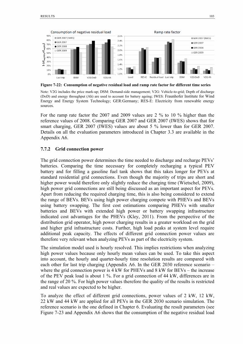
RESULTS

103

Figure 7-22: Consumption of negative residual load and ramp rate factor for different time series

Note: V2G includes the price mark-up; DSM: Demand-side management; V2G: Vehicle-to-grid; Depth of discharge (DoD) and energy throughput (Ah) are used to account for battery ageing; IWES: Fraunhofer Institute for Wind Energy and Energy System Technology; GER:Germany; RES-E: Electricity from renewable energy sources.

For the ramp rate factor the 2007 and 2009 values are 2 % to 10 % higher than the reference values of 2008. Comparing GER 2007 and GER 2007 (IWES) shows that for smart charging, GER 2007 (IWES) values are about 5 % lower than for GER 2007. Details on all the evaluation parameters introduced in Chapter 3.3 are available in the Appendix A6. 7.7.2 Grid connection power The grid connection power determines the time needed to discharge and recharge PEVs’ batteries. Comparing the time necessary for completely recharging a typical PEV battery and for filling a gasoline fuel tank shows that this takes longer for PEVs at standard residential grid connections. Even though the majority of trips are short and higher power would therefore only slightly reduce the charging time (Wietschel, 2009), high power grid connections are still being discussed as an important aspect for PEVs. Apart from reducing the required charging time, this is also being considered to extend the range of BEVs. BEVs using high power charging compete with PHEVs and BEVs using battery swapping. The first cost estimations comparing PHEVs with smaller batteries and BEVs with extended high power or battery swapping infrastructure indicated cost advantages for the PHEVs (Kley, 2011). From the perspective of the distribution grid operator, high power charging results in a greater workload on the grid and higher grid infrastructure costs. Further, high load peaks at system level require additional peak capacity. The effects of different grid connection power values are therefore very relevant when analyzing PEVs as part of the electricity system. The simulation model used is hourly resolved. This implies restrictions when analyzing high power values because only hourly mean values can be used. To take this aspect into account, the hourly and quarter-hourly time resolution results are compared with each other for last trip charging (Appendix A6. In the GER 2030 reference scenario – where the grid connection power is 4 kW for PHEVs and 8 kW for BEVs – the increase of the PEV peak load is about 1 %. For a grid connection of 44 kW, differences are in the range of 20 %. For high power values therefore the quality of the results is restricted and real values are expected to be higher. To analyze the effect of different grid connections, power values of 2 kW, 12 kW, 22 kW and 44 kW are applied for all PEVs in the GER 2030 scenario simulation. The reference scenario is the one defined in Chapter 6. Evaluating the result parameters (see Figure 7-23 and Appendix A6 shows that the consumption of the negative residual load

RESULTS 104

is only slightly affected by different power values. For DSM charging with 2 kW grid connection, the ratio of cfneg (PEV)116 to cfneg (RS)117 is reduced by 2 percent points compared to the reference case. For V2G, the reduction of the negative load consumption is 3.7 percent points for V2G with DoD battery ageing and 3 percent points for V2G Ah. If the grid connection power is changed stepwise from the reference case to 44 kW, the consumption of negative residual load remains the same or is only slightly increased. Considering that smart charging with a lower grid connection power of 2 kW reduces the electric driving share by about 1 percent points compared to the reference case118 means grid connection power can be rated as a parameter which only has a small influence on negative residual load consumption.

Figure 7-23: Comparing results for varying grid connection power

Note: V2G includes the price mark-up; DSM: Demand-side management; V2G: Vehicle-to-grid; Depth of discharge (DoD) and energy throughput (Ah) are used to account for battery ageing; The reference scenario uses a grid connection power of 4 kW for plug-in hybrid electric vehicles (PHEVs) and 8 kW for battery electric vehilces (BEVs) in average the grid connection power is 4.5 kW.

As a consequence of the method used, smart charging shows very low variations in peak load due to the changed grid connection power. For last trip charging, increasing power values also increases the peak load up to a charging power of 22 kW. For the 44 kW simulation, the maximum peak load declines compared to 22 kW. Note, the model is hourly resolved and uses hourly mean values. One reason for this reduction in peak load between 22 kW and 44 kW is that, besides the amplitude, power also affects the time course of the PEVs’ last trip charging curve. For last trip charging, a higher connection power directs the demand to shift to the return time of the trip as indicated in Figure 7-24. A low grid connection power widens the PEVs’ load curve. Hence, adding the PEVs’ load curve to the residual load can result in a lower peak load, even if charging power is increased.

116 Negative capacity factor including PEV demand. 117 Negative capacity factor for the residual load (RS) excluding PEV demand. 118 Detailed driving shares for the simulation are given in the Appendix A5.

RESULTS

105

Figure 7-24: Effect of grid connection power on the PEVs’ load curve for last trip charging

Note: The reference scenario uses a average grid connection power of 4.5 kW.

To sum up, a higher grid connection power (> 12 kW) does not increase the contribution PEVs can make to integrating RES-E in the GER 2030 scenario. This can be explained by the power to energy ratio of storage in the analyzed scenario and for PEVs in general. The high power does not allow the load management time or load shifting period to be significantly increased. The load shifting potential is not restricted by the power but by the energy available for load shifting and the battery size as shown in the following sections. 7.7.3 Battery costs and size The costs for mass-produced automotive lithium batteries are one of the most sensitive parameters for the total costs of ownership calculation (e.g. see Kley, 2011). Because of the relatively low production volume today and uncertainty about the precise technology in the future, there is a large bandwidth of cost development assumptions. Therefore, the assumed specific investments in batteries is adopted by plus and minus 20 % and 40 % in the GER 2030 reference case. The cost variation only affects the V2G charging case. Results on the electric driving share, the grid management time as well as last trip and DSM charging remain unchanged despite varying battery costs. Reducing the battery costs increases the share of negative residual load that can be consumed and reduces the ramp rate factor (see Figure 7-25). In terms of the negative residual load consumed, DoD ageing is more sensitive to both cost increases and decreases. The sensitivity to a cost increase is higher for DoD ageing than for Ah ageing with regard to ramping. On the contrary Ah battery ageing is more sensitive than DoD ageing to a cost decrease.

Figure 7-25: Comparing results for varying battery costs

Note: V2G includes the price mark-up (Mup); V2G: Vehicle-to-grid; Depth of discharge (DoD) and energy throughput (Ah) are used to account for battery ageing. The reference scenario uses a average battery price of 258 euros/kWh.

RESULTS 106

For DoD-based battery ageing, the energy fed back into the grid increases from 4.4 TWh in the reference case to 5.6 TWh and 7.1 TWh with a 20 % and 40 % cost reduction, respectively. For Ah with 6 TWh in the reference case, the same cost reduction results in 7.3 TWh and 8.7 TWh of electricity fed back to the grid. The sensitivity regarding the integration of RES-E is not very high but detectable and differs depending on the ageing method used to model PEVs’ batteries. The assumptions about battery size in the GER 2030 scenario are restrictive and small batteries in combination with PHEVs are favored. Nevertheless, vehicle concepts with bigger batteries are also part of the research discussion on PEVs. Consumer surveys indicate that the electric driving range and therefore the battery size are of great interest (Peters al., 2011). Varying the battery size therefore provides valuable results for this analysis compared to other research. To analyze the battery size variation, the total fleet is modeled with 15 kWh and additionally with 30 kWh of usable battery storage for all vehicles. In the reference case GER 2030, mainly 4.5 kWh (PHEV 25) and 12.5 kWh (PHEV 57) of usable storages are assumed. Battery size affects the electric driving share of PEVs. Especially for last trip charging, an increase in battery size increases the electric driving share. Compared to the reference case, the electric driving share of 53.7 % increases to 69.6 % with 15 kWh batteries and to 85.6 % with 30 kWh batteries. For smart charging or a full availability of infrastructure, the share increases from 70.3 % to 79.8 % and to 89.3 %, respectively. This affects the electricity demand of the PEV fleet and, in the case of smart charging, the electricity available for load shifting.119 As explained, bigger batteries can increase the negative residual load consumption for all charging strategies. Compared to DSM, V2G DoD charging results in a disproportionately large and V2G Ah in a disproportionately low increase (see Figure 7-26). In terms of DoD ageing, not only the battery size but also the battery cost function is affected by a change in battery size. The negative residual load consumption increases even more for V2G DoD due to the energy available at lower costs. The same tendency is observed for the smart charging ramp rate factor. The highest reduction with 17 % is observed for V2G DoD with 30 kWh batteries. For last trip charging, the ramp rate factor rises for both simulated cases. The reduction of the ramp rate factor for a 30 kWh battery compared to a 15 kWh battery could be caused by a higher diversity in the state of charge after the last trip. For a battery of 15 kWh, most batteries are empty after the last trip. Hence, the charging time is the same for many PEV agents. This causes high simultaneity in stopping the charging process. Overall, differences in the ramp rate factor for last trip charging are only in the range of 2 % compared to the reference values.

119 The PEVs’ demand for last trip charging is 19.2 TWh (reference), 24.8 TWh (15 kWh) and 30.5 TWh (30 kWh) and 25.0 TWh (reference), 28.8 TWh (15 kWh) and 32.3 TWh (30kWh) for smart charging.

RESULTS

107

Figure 7-26: Comparing results for different battery sizes

Note: V2G includes the price mark-up; DSM: Demand-side management; V2G: Vehicle-to-grid; Depth of discharge (DoD) and energy throughput (Ah) are used to account for battery ageing. Numbers depict battery size in kWh. The reference scenario uses a average battery sitze of 10.3 kWh.

The sensitivity of the battery size to the integration of RES-E is very high. Nevertheless, from an economic point of view, PEV types with smaller batteries are more likely (Plötz et al., 2012). Therefore, varying the battery size is considered to be less relevant compared to parameters such as RES-E time series. 7.7.4 Mobility behavior Drivers’ mobility behavior influences the availability of PEVs in the electricity grid. The typical mobility behavior of current vehicles was discussed in Chapter 4.2 and possible PEV users selected. This selection is based on economic and infrastructure aspects but only represents one possible scenario for the future. Therefore, the sensitivity of mobility behavior is also investigated using the following variations. As well as the reference scenario using filtered data of the MID survey, driving data is used from the MOP survey. For MOP data, deterministic and stochastic driving are distinguished. The stochastic data is implemented using probabilities as presented for the MID survey in Chapter 4.2.3 and Chapter 5.4.7. The MOP data used is unfiltered and therefore the electricity demand and yearly driving distance are smaller than for the MID data used. Additionally, a commuter and a stationary storage scenario are analyzed. For the commuter scenario on weekdays, a first trip starting in the morning at 7:30 am and a second trip in the late afternoon at 5:00 pm are assumed for all PEVs defined in the GER 2030 scenario. The driving distance is uniformly 30 km for each of the two trips. No PEV trips are assumed at weekends. No driving is assumed to occur in the stationary storage scenario. Here, only V2G charging is conducted. The number of PEVs equals the number of stationary storage devices with the battery size and grid connection power defined in the GER 2030 reference scenario.

RESULTS 108

Figure 7-27: Comparing results for different mobility behavior

Note: V2G and stationary storage includes the price mark-up; V2G: Vehicle-to-grid; Depth of discharge (DoD) and energy throughput (Ah) are used to account for battery ageing; MOP: German Mobility Panel;The reference scenario uses mobility behavior according to Mobility in Germany 2008 (MID, 2010). Analyzing the results reveals that the deterministic and stochastic MOP data are roughly the same for smart charging (see Figure 7-27). For last trip charging, the deviation is higher in electricity demand – 15.78 TWh for the deterministic and 16.43 TWh for the stochastic data – and the negative residual load consumed – 17.0 % for the deterministic and 15.4 % for the stochastic data. This indicates that the last trip for the stochastic data does not perfectly equal the last trip for the deterministic data. This is because the stochastic method used does not account for combinatorial probabilities in order to simplify the mobility simulation. Results for smart charging are not significantly affected. For the commuter scenario, last trip charging deviates significantly from the reference case. The electric driving share increases to 78.2 %. With a yearly driving distance of 15,180 km per vehicle, the total PEV fleet’s electricity demand amounts to 27.6 TWh. The negative residual load consumed is only 0.5 % and the ramp rate factor increases noticeably from 2.3 % to 3.7 %. Further, the simultaneous arrival time after the last trip results in a peak load of 151.65 % compared to the GER 2030 total system load. For smart charging, the electric driving share is 92.2 % and the electricity demand is about 32.6 TWh. For all smart charging strategies analyzed, the consumption of the negative residual load is slightly lower than in the reference case. The ramp rate factor remains in the same range as for the reference scenario. This shows the smart charging mechanism applied is efficient to avoid simultaneous actions of the vehicle fleet. The results for the stationary storage simulation are unexpected. One would expect that driving restricts the capability of PEVs to provide storage capacity for the electricity system. In contrast, the results indicate a lower consumption of negative residual load and higher ramp rates for stationary storage. For both V2G ageing assumptions, the restrictions due to mobility behavior are lower than the gains due to the demand available for load shifting. The energy fed back to the grid is 7.4 TWh and 7.3 TWh for V2G DoD and Ah, respectively. In the reference case, the energy fed back is 4.4 TWh for V2G DoD and 6.0 TWh for V2G Ah. This indicates that restrictions due to mobility behavior are higher for DoD-based battery ageing. The mobility behavior affects the contribution of PEVs to balancing fluctuating RES-E. Variations are not very high for smart charging and are mainly caused by the changing energy demand due to different mobility behavior. The commuter scenario is found to be highly sensitive for last trip charging because of the strong simultaneousness. Comparing stationary storage with PEV storage indicates that the value of the demand available for load shifting due to driving is higher than the V2G restrictions caused by mobility behavior.

RESULTS

109

7.7.5 Infrastructure Infrastructure is a very important aspect, especially in the case of BEVs. Public infrastructure is necessary for acceptance reasons, to convince consumers that running out of fuel is very unlikely (Peters et al., 2010) even though (Kley, 2011) shows that public infrastructure usually does not recoup its investment and that charging at home is favorable from an economic point of view. Constantly available infrastructure is assumed in the reference scenario GER 2030. Additional simulations with a charging opportunity at home and at work as well as only at home are conducted to account for the sensitivity of available infrastructure. Infrastructure is assumed to be available for last trip charging and plays no other role in this case. For smart charging, infrastructure availability affects the electric driving share.120 Because of the assumption that DSM and V2G are only possible if the parking time is greater than the charging time, the electric driving share is the same for DSM and V2G (see right side of Figure 7-28). The driving share varies slightly in general and for smart charging because of the simulation method. The electric driving share is about 70 % in the case of overall infrastructure availability and 66 % if only home charging is possible. One would expect that the reduced availability of infrastructure reduces electricity demand and that therefore the consumption of negative residual load is lower as well. But the opposite is true for DSM in the conducted simulation (see DSM values on the left side of Figure 7-28). The reason for the increase in the negative residual load consumed is the energy available in a load management period. Refilling the vehicle after each trip during the day reduces the energy demand after the last trip of the day. Because of the much higher grid management time after the last trip (see Chapter 7.2.2), a lower state of charge after the last trip can be of value for the grid integration of RES. Obviously, this would also result in higher gasoline use and higher operation expenditures. The reference case allows a better integration of the negative residual load for V2G. The higher availability of infrastructure increases the flexibility in managing PEV storage capabilities. If high price spreads are available, energy can be fed back to the grid and the electricity demand available to consume the negative residual load is higher.

Figure 7-28: Sensitivity of infrastructure to negative load consumption and electric driving share

Note: V2G includes the price mark-up; V2G: Vehicle-to-grid; Depth of discharge (DoD) and energy throughput (Ah) are used to account for battery ageing; The reference scenario uses permanent available charching infrastructure.

120 Note: It is assumed that vehicles plug-in after each trip to maximize the electric driving share and to therefore minimize operating expenditure.

RESULTS 110

In conclusion, infrastructure availability has a small effect on the negative residual load. The negative residual load that can be consumed varies between 64.2 % and 64.7 % for DSM and between 78.6 % and 76.8 % for V2G. 7.7.6 Share of fluctuating generation technology The fluctuation of RES-E is crucial for analyzing the contribution of storage devices in electricity systems with high shares of RES. The previously conducted analyses on the CA 2030 scenario and the GER 2030 scenario with different generation and load time series underline the importance of the resulting residual load for the dispatch of storage and PEVs. Besides the time series, the energy produced from different fluctuating generation technologies or the capacity installed also strongly affect the residual load curve. To account for this issue and to further investigate the effects of photovoltaic versus wind generation, the share of photovoltaic power in total fluctuating energy generation is varied. The energy produced from wind and photovoltaic is 239 TWh in the GER 2030 scenario. Keeping the total energy generation of fluctuating RES-E constant, the share of photovoltaics is varied between 0 % and 45 %. The results shown in Figure 7-29 indicate that the negative residual load is strongly affected by the composition of fluctuating generation technologies. Starting with a zero percent share of photovoltaic generation – here 239 TWh total fluctuating generation are provided by wind onshore and offshore – the negative residual load declines from 4.8 TWh to 1.9 TWh in the reference scenario GER 2030. For the reference scenario the share of PV is 24 % of the fluctuating electricity generation. Increasing this share to 45 % makes the negative residual load increase to 10.2 TWh. This indicates the limited capacity credit of photovoltaic generation.

Figure 7-29: Negative residual load for different photovoltaic shares

Note: RES-E PV 0.0 %: wind onshore 47.8 % offshore 52.2 %; RES-E PV 15.0 % : wind onshore 40.6 % offshore 44.4 %; Reference: PV 23.8 % wind onshore 36.4 % offshore 39.7 %; RES-E PV 30.0 %: wind onshore 33.5 % offshore 36.5 %; RES-E PV 45.0 %: wind onshore 26.3 % offshore 28.7 %. V2G includes the price mark-up; PV: Photovoltaic; RES: Renewable energy sources; V2G: Vehicle-to-grid; Depth of discharge (DoD) is used to account for battery ageing: PEVs: Plug-in electric vehilces. The remaining negative residual load and the percentages of negative residual load that can be consumed are presented in Figure 7-30. The highest percentage of negative residual load can be used for DSM in the reference scenario GER 2008. For V2G, the scenario with 30 % fluctuating PV generation enables the biggest integration of negative residual load with 82 %. In absolute values, the RES-E PV 45 % scenario with

RESULTS

111

the highest negative residual load allows the largest amount of fluctuating energy to be integrated. In this case more than 20 % of the PEV demand can be covered by RES-E.

Figure 7-30: Comparing results varying the share of fluctuating generation technologies

Note: RES-E PV 0.0 %: wind onshore 47.8 % offshore 52.2 %; RES-E PV 15.0 % : wind onshore 40.6 % offshore 44.4 %; Reference: PV 23.8 % wind onshore 36.4 % offshore 39.7 %; RES-E PV 30.0 %: wind onshore 33.5 % offshore 36.5 %; RES-E PV 45.0 %: wind onshore 26.3 % offshore 28.7 %. V2G includes the price mark-up; PV: Photovoltaic; RES: Renewable energy sources; V2G: Vehicle-to-grid; Depth of discharge (DoD) is used to account for battery ageing: PEVs: Plug-in electric vehilces. Scenarios with a higher share of photovoltaic generation result in a higher ramp rate factor of the residual load. For smart charging, ramp rate reduction increases with higher photovoltaic generation shares. This indicates a good capability of PEVs to reduce ramping caused by photovoltaic generation. From the perspective of the total electricity system, it is preferable to have a RES generation share which results in a low negative residual load. The reference scenario results in the lowest residual load under the time series and the total amount of RES-E assumed here.

RESULTS 112

7.7.7 Conclusions The analysis reveals that especially the RES generation time series and technology shares are highly sensitive. Battery size also has a strong influence on the contribution of PEVs to balancing fluctuating generation. The conclusions in detail are:

The consumption of the negative residual load varies strongly between different

weather years, by 14 % between 2008 and 2009. The grid connection power has a stronger effect on system load in the case of

last trip charging. Besides the increase in peak power, a shift of the load profile to the arrival time of the last trip can be observed. The sensitivity to grid connection power is of low relevance for smart charging.

Battery costs and size are most sensitive in DoD-based battery ageing. A 40 % cost increase reduces the negative residual load consumed by about 5 %, whereas a 40 % cost reduction increases the negative residual load consumption by 4 %. For the same cost variation, the ramp rate factor varies between minus 15 % and plus 10 %.

Increasing the battery size to 30 kWh for all PEVs in the vehicle fleet results in an increase in the negative residual load consumed, especially for V2G. V2G DoD allows for the maximum 12 % increase of negative residual load consumption. However, bigger batteries seem relatively unlikely from a cost perspective.

The sensitivity of mobility behavior is lower for smart charging. For last trip charging, uniform driving behavior as is expected for work commutes strongly increases ramp rates and the peak load of the PEV fleet.

Comparing stationary and mobile storage reveals that mobility behavior restricts V2G performance. But the gain in load shifting capability due to the electricity demand of electric driving is higher than these restrictions.

Comparing pervasive charging infrastructure with home charging only reduces the electric driving share by 4 percent points, from 70 % to 66 %. The infrastructure sensitivity to the negative residual load is low.

The negative residual load consumed varies between 40 % and 64 % for DSM and between 50 % and 82 % for V2G DoD depending on the generation technology mix. Together with the RES generation time series, the technology mix of fluctuating generation therefore has the highest influence on the negative residual load consumed.

The sensitivity analysis underlines the high importance of the RES technology mix and the weather years for the contribution PEVs’ batteries can make to balancing fluctuating generation.

RESULTS

113

7.8 Model limitations The PowerACE simulation model can only approximate the electricity market and power system. Assumptions have to be made to answer the research question, especially regarding the specifications and market penetration of plug-in electric vehicles as well as the installed capacity of fluctuating generation from solar and wind. Besides the scenario assumptions (Chapter 6), the simulation model faces the following main method-related limitations:

Perfect transmission is assumed within the investigated system. A detailed

simulation of the German electricity grid is beyond the scope of this thesis due to the high complexity and large amounts of data needed. In many cases, grid extensions or generation curtailments seem economically favorable compared to the installation of storage devices (DENA, 2010). The distribution grid is modeled by applying a simplified approach (Chapter 5.4) which is not able to account for the complexity and diversity of the German grid, but which can serve as a basis for further research.

The management mechanism for distributed devices applied in the simulation model does not account for the complexity and communication structure of smart grids. The approach further would involve retail electricity consumers being treated individually and receiving individual price signals.

The time resolution of the main model is hourly. Therefore, all presented results indicate hourly mean values. Especially in the case of peak power, this methodological restriction can lead to power values being underestimated.

The research focus here is on operation scheduling. Perfect foresight is assumed for mobility behavior, fluctuating generation and system load. In practice, this is obviously not the case and system balancing mechanisms are needed to continuously balance supply and demand. System balancing and forecast deviations are not considered.

For plug-in electric vehicles, it is assumed that vehicles are connected to the grid while parked. Furthermore the time between trips is known and used for demand-side management. Consumer acceptance of making the vehicle available and reacting to price incentives is not considered. Therefore, the results represent an idealized case.

CONCLUSIONS AND OUTLOOK 114

8 Conclusions and outlook The analysis conducted describes how fluctuating generation from renewable energy sources affects the load curve and how plug-in electric vehicles can be used to balance the resulting residual load. Further, marginal CO2 emissions and monetary benefit due to smart charging are discussed. An agent-based method was developed on the basis of the electricity market model PowerACE (Sensfuß, 2007) and applied to investigate a 2030 scenario for Germany and California. The PowerACE model provides a price signal as a basis to control the operation of plug-in electric vehicles. Automated demand response using one price as a control signal result in a high simultaneousness of operation because the objective function of all players is to minimize costs. This interrelation is observed in the simulation model while using time-of-use rates and in California where time-of-use prices are applied to control plug-in electric vehicles at present (Schey et al., 2012). Therefore, individual price perspectives and variable grid fees were used to overcome the problem of simultaneous reaction in the simulation. In current practice different treatment of retail customers is not possible. However, the applied control mechanism considers the overall electricity market and distribution grid aspects and allows to achieve an operation of flexible demand close to the social optimum. 121 Vehicles are simulated as agents considering individual driving behavior and battery discharging costs. Driving behavior defines the main smart charging optimization parameters, the time period between trips and the energy taken from the storage. To model driving behavior, trips are generated using probabilities drawn from a mobility survey (MID 2010) and adjusted to account for particularities of electric vehicle users (Biere et al., 2009). This allows to assign an individual driving behavior data set to each vehicle agent participating in the simulation. Small deterministic data sets or average driving behavior applied for a large fleet of vehicles can result in simultaneous charging operation and is therefore not suited to model the operation of electric vehicle fleets. Considering battery degradation is of high relevance to model vehicle-to-grid but faces uncertainties caused by the high complexity of battery aging processes. To calculate the discharging costs, two different simplified approaches, considering energy throughput-based aging (Peterson et al., 2009) and depth of discharge-based aging (Rosenkranz, 2003) are applied. Depth of discharge-based aging results in swallow cycling and a lower amount of energy fed back to the grid compared to the energy throughput method. Further depth of discharge-based aging increases the complexity of the optimization algorithms because the state of charge affects discharging costs. To account for depth of discharge-based battery aging therefore a graph search optimization algorithm scheduling the charging and discharging behavior is applied. Within the framework of a research project the algorithm to schedule the charging operation of vehicle agents within the simulation is also implemented in a Volkswagen Golf Variant “TwinDrive” plug-in hybrid electric vehicle. This enables to test smart grid software applications in a simulation environment and to investigate how smart grid applications affect the power system and the electricity market. Vice versa, the value of a specific smart grid application and the interrelation with other applications can be analyzed with the introduced simulation model. This proves a main advantage of agent-based simulation, which permits a customized approach and allows to solve a complex problem while including control algorithms implemented in real smart grid applications. 121 The multi-agent simulation do not allow for a mathematical provable optimum.

CONCLUSIONS AND OUTLOOK

115

Investigating the contribution of plug-in vehicles integrating fluctuating generation requires measures to describe the initial and the resulting situation of the power system. The high diversity of time-resolved generation requires parameters which go beyond the energy production per year or the base and peak power. A novel set of parameters– defined in this thesis – enables a more precise description of the load duration curve, ramp rates and fluctuation. Analyzing scenarios for both the German and Californian power system indicated that it is still difficult to capture fluctuation with a few significant parameters. Nevertheless, the introduced method does allow a more detailed characterization and comparison of electricity system scenarios and provides a good basis for energy analyses of high levels of fluctuating generation. Three main evaluation parameters were observed to quantify plug-in electric vehicles’ contribution to balancing fluctuating generation: the change in the minimum residual load, the percentage of negative residual load that can be consumed, and the reduction of residual load ramp rates. For all three aspects, plug-in electric vehicles make a positive contribution to improving the grid integration of electricity from fluctuating renewable energy sources. For demand-side management in the 2030 scenario for Germany, the minimum residual load is reduced by 22 % or 7.4 GW; 64 % or 1.2 TWh of the negative residual load can be consumed and the ramp rate factor is reduced by 25 %. Including vehicle-to-grid services allows better grid integration than demand response only. Here, for the same scenario with depth of discharge-based battery aging, the minimum negative residual load is reduced by 37 % or 12.6 GW; 79 % or 1.5 TWh of the negative residual load can be consumed and the ramp rate factor is reduced by 41 %. However, because of disproportionately higher costs for vehicle-to-grid and high uncertainty regarding battery ageing, demand shifting is still expected to be the more promising mid-term charging strategy. The life cycle CO2 emissions from plug-in electric vehicles are mainly determined by the electricity source. Applying average CO2 emissions of the total power plant mix results in a significant CO2 reduction compared to vehicles using fossil fuels. This is caused by the high level of renewable generation assumed in the simulation scenario. Analyzing the precise emission increase due to the additional demand indicates that for Germany marginal CO2 emissions are higher than the total average. Fluctuating generation only acts as a marginal power plant, if supply exceeds regular demand and the residual load therefore is negative. This was the case in 3.2 % of the yearly simulation period for wind and solar generation in the analyzed scenario. Even if plug-in electric vehicles consume more electricity during these hours, it is not enough to compensate for the marginal generation by fossil power plants during the rest of the year. Hence, due to methodology, marginal emissions are likely to be higher than average emissions. A higher level of renewable generation enhances this effect. The installation of additional renewable energy sources therefore is necessary to guarantee a significant reduction of CO2 emissions while using plug-in electric vehicles. A high level of non-dispatchable generation with very low marginal operation costs affects the functionality of electricity markets. The price-reducing effects caused by fluctuating generation and underutilized capacity of conventional power plants leads to a financing gap of controllable peak capacity. Therefore, market bids including price mark-ups to account for the total costs to operate a power plant are likely. This can increase the price spreads on future electricity markets and therefore provide incentives for demand response and storage. For the 2030 scenario, revenues from demand response and vehicle-to-grid for a single consumer are found to be between 50 and 250 euros per year. It remains to be investigated, however, if these still relatively low

CONCLUSIONS AND OUTLOOK 116

incentives will suffice to entice consumers into smart charging. To overcome this problem, making invariable electricity price components122 more flexible could be one way to boost smart grid revenues in the future. The presented results are highly sensitive to the fluctuation of solar and wind generation time series. For California, the solar capacity credit is much higher than for Germany because of the strong correlation with air conditioning loads. This effect reduces the necessary peak power capacity and also the need for demand response in California. In contrast, for Germany the need for peak power capacity is increasing in the applied scenario. Also, the contribution that plug-in electric vehicles can make as a grid resource is affected by the fluctuation of renewable electricity generation. The share of the negative residual load consumed varies between 40 % in Germany with 2009 weather data and 73 % in California. The reliable daily pattern of solar and to a lesser extend of wind generation in California favors the grid integration with plug-in electric vehicles acting as a short-term storage. In contrast, high wind generation in Germany is likely to occur for several days in a row. Due to the daily driving pattern, the limited load shifting capacity of plug-in electric vehicle is less suited to balance longer periods of high wind generation output. Hence, for Germany, plug-in electric vehicles are better suited to balance the fluctuation of photovoltaic generation. Parameters such as the grid connection power or infrastructure availability are less relevant for the storage capabilities of plug-in electric vehicles. A higher grid connection power only marginally increases the ability to integrate fluctuating generation. In most cases, the standing time after a trip is sufficient to recharge the battery even with a standard power connection. The availability of infrastructure affects the electric driving share and consequently the electricity demand. Nevertheless, due to the low grid management and shorter parking times in public places, a better availability of infrastructure does not necessarily result in better load management capabilities. Comparing stationary and mobile storage reveals that mobility behavior restricts vehicle-to-grid performance. However, the gain in load shifting capability due to the electricity demand of electric driving is higher than these restrictions. This reveals that the dual use of the storage option is the key feature of smart grid devices. Plug-in electric vehicles are not suitable for long-term storage or to store high amounts of energy. To be able to manage very high levels of renewable electricity generation therefore will require a portfolio of flexible conventional generation, new transmission lines, long-term storage applications and additional demand-side options. Suggestions for further research mainly arise from limitations of the simulation model (see Chapter 7.8). Including more details in terms of transmission and distribution grids as well as expanding the observed system to the level of the European network would be valuable developments. Further research is needed in terms of distributed load management mechanisms for price-based automated demand response applicable to the mass market and including consumer acceptance. Distribution grid monitoring and the allocation of reactive power are possible services plug-in electric vehicles can provide to improve grid management. Besides plug-in electric vehicles, additional smart grid devices, transmission networks, flexible generation units and other short- and long-term storage options are required to guarantee a functional electricity system with a high share of fluctuating generation. It is therefore vital that future research considers the interaction, peculiarity and economic competitiveness of different instruments for integrating fluctuating renewable energy sources. 122 Invariable electricity price components of retail electricity prices are grid fees or cost subsidy shares caused by renewable energy sources.

APPENDIX A

XV

Appendix

A. Figures and Tables

A1. Vehicle charging behavior

Figure A-1: Charging curve of Opel MERIVA battery electric test vehicle

Source: Opel, 2010; Note: Battery size 16 kWh; soc: state-of-charge

APPENDIX A XVI

A2. Characteristics of fluctuating generation

Table A-1: Duration curve parameters system load

Time series flh cf cfQ<0.8 cfQ>=0.8 rcf0.8 Ph,min Ph,max Load GER 2007 (ENTSO-E) 6336 72.33% 54.58% 17.81% 0.33 42.93% 100.00%

Load GER 2008 (ENTSO-E) 6441 73.53% 55.54% 17.99% 0.32 44.70% 100.00%

Load GER 2009 (ENTSO-E) 6300 71.92% 53.83% 18.08% 0.34 39.72% 100.00%

Load CA 2005 (CAISO) 4781 54.58% 40.31% 14.27% 0.35 36.29% 100.00% Source: Own calculation data basis (ENTSO-E, 2011) and (CAISO, 2011)

Table A-2: Duration curve parameters wind

Time series flh cf cfQ<0.8 cfQ>=0.8 rcf0.8 Pmin Pmax

Onshore GER 2007 (EEX) 1845 21.06% 95.58% 10.77% 0.10 0.59% 85.43% Onshore GER 2008 (EEX) 1751 19.99% 100.00% 10.00% 0.10 0.56% 82.51% Onshore GER 2009 (EEX) 1521 17.36% 91.93% 9.04% 0.08 0.32% 83.64% Onshore CA 2005 (CAISO) 2530 28.88% 18.30% 10.58% 0.58 2.02% 80.75% Onshore DK-West 2010 (energinet.dk) 2145 24.48% 12.82% 11.66% 0.91 0.01% 90.82% Onshore DK-East 2010 (energinet.dk) 2186 24.95% 11.83% 13.13% 1.11 0.00% 97.77%

Offshore GER 2007 (ISI) 3620 41.33% 26.46% 14.87% 0.56 0.40% 86.71% Offshore GER 2008 (ISI) 3561 40.65% 25.65% 15.00% 0.58 0.13% 85.93%

Offshore GER 2009 (ISI) 3484 39.77% 24.71% 15.06% 0.61 1.08% 88.04%

Offshore GER 2007 (IWES) 4241 48.42% 30.22% 18.20% 0.60 0.18% 96.45%

Onshore turbine 3568 CA 2006 (NREL) 3484 39.77% 20.16% 19.61% 97.26% 0.00% 100.00% Offshore turbine 1295 CA 2006 (NREL) 3472 39.64% 20.85% 12.29% 57.82% 0.00% 100.00% Onshore turbine 4161 GER 2008 (SWK) 1703 19.44% 7.14% 12.29% 172.06% 0.00% 100.00%

Source: Own calculation data basis (EEX, 2011), (CAISO, 2011), (energinet.dk. 2011), (NREL, 2009), (SWK, 2010) and (IWES, 2011)

Table A-3: Duration curve parameters solar

Time series flh cf cfQ<0.8 cfQ>=0.8 rcf0.8 Ph,max Photovoltaics GER 2007 (ISI) 913 10.42% 2.31% 8.10% 3.50 67.08%

Photovoltaics GER 2008 (ISI) 878 10.02% 2.44% 7.57% 3.10 64.62%

Photovoltaics GER 2009 (ISI) 865 9.88% 2.08% 7.80% 3.75 70.87%

Photovoltaics CA 2005 (CAISO) 2160 24.66% 9.21% 15.45% 1.68 98.42%

Solar thermal CA 2005 (CAISO) 2261 25.81% 8.93% 16.88% 1.89 95.72%

Photovoltaic single installation GER 2008 (SWK) 1097 12.52% 2.50% 10.01% 4.00 82.30% Source: Own calculation data basis (Schubert, 2011), (SWK, 2010) and (CAISO, 2011)

Table A-4: Ramp rate parameters system load

Time series rrfpos μ pos σpos μ neg σneg xy=0

Load GER 2007 (ENTSO-E) 1.271% 2.96% 2.65% -2.23% 1.69% 57.00%

Load GER 2008 (ENTSO-E) 1.19% 2.74% 2.51% -2.12% 1.59% 56.40%

Load GER 2009 (ENTSO-E) 1.32% 3.04% 2.87% -2.32% 1.79% 56.72%

Load CA 2005 (CAISO) 1.05% 2.12% 1.60% -2.07% 1.83% 50.59% Source: Own calculation data basis (ENTSO-E, 2011) and (CAISO, 2011)

APPENDIX A

XVII

Table A-5: Ramp rate parameters wind

Time series rrfpos μ pos σpos μ neg σneg xy=0

Onshore GER 2007 (EEX) 0.69% 1.39% 1.42% -1.36% 1.43% 50.67% Onshore GER 2008 (EEX) 0.66% 1.34% 1.38% -1.30% 1.37% 50.76% Onshore GER 2009 (EEX) 0.64% 1.30% 1.32% -1.25% 1.27% 50.84% Onshore CA 2005 (CAISO) 1.25% 2.35% 2.21% -2.63% 2.77% 47.14% Onshore DK-West 2010 (energinet.dk) 0.98% 1.98% 1.98% -1.92% 1.94% 50.43% Onshore DK-East 2010 (energinet.dk) 1.30% 2.69% 3.16% -2.51% 2.93% 51.17% Offshore GER 2007 (ISI) 2.04% 4.09% 3.87% -4.07% 3.60% 50.15% Offshore GER 2008 (ISI) 1.61% 3.21% 3.01% -3.19% 2.91% 50.75% Offshore GER 2009 (ISI) 1.59% 3.22% 3.01% -3.11% 2.89% 50.75% Offshore GER 2007 (IWES) 1.52% 3.17% 3.60% -2.95% 3.26% 49.80% Onshore turbine 3568 CA 2006 (NREL) 3.81% 8.70% 11.94% -8.22% 11.40% 46.2% Offshore turbine 1295 CA 2006 (NREL) 2.64% 5.74% 7.84% -5.67% 7.12% 46.7% Onshore turbine 4161 GER 2008 (SWK) 2.72% 6.74% 7.79% -6.36% 6.73% 40.8%

Source: Own calculation data basis (EEX, 2011), (CAISO, 2011), (energinet.dk. 2011), (NREL, 2009), (SWK, 2010) and (IWES, 2011)

Table A-6: Ramp rate parameters solar

Time series rrfpos μ pos σpos μ neg σneg xy1=0 xy2=0

Photovoltaics GER 2007 (ISI) 1.42% 5.22% 4.77% -5.01% 4.37% 72.63% 29.24%



Photovoltaics CA 2005 (CAISO) 3.18% 10.52% 7.60% -10.40% 7.72% 69.76% 30.61%

Solar thermal CA 2005 (CAISO) 3.20% 10.79% 12.98% -9.37% 12.92% 70.36% 34.14%

Photovoltaic single installation GER 2008 (SWK) 2.75% 9.35% 9.44% -9.10% 8.68% 70.7% 28.7% Source: Own calculation data basis (ENTSO-E, 2011), (SWK, 2010) and (CAISO, 2011)

APPENDIX A XVIII

Table A-7: Interval availability parameters for GER 2008 and CA

Sec 0 Sec 1

Time series yQ-0.1 yQ-0.3 Counts tmean tσ tmax yQ-0.3 yQ-0.6 Counts tmean tσ tmax Wind onshore GER 0.6% 8.8% 173 20.5 16.5 134 8.8% 25.1% 173 34.1 61.0 620

Wind offshore GER 0.1% 8.7% 103 7.7 8.4 35 8.7% 25.9% 103 77.2 138.8 982

Photovoltaic GER 0.0% 6.3% 347 16.3 10.1 166 6.3% 18.9% 342 8.6 3.2 13

RES GER 0.5% 11.3% 167 7.5 5.6 38 11.3% 32.9% 167 44.9 83.2 622

Load GER 44.7% 50.2% 30 3.9 2.0 8 50.2% 61.3% 30 286.0 653.9 2900

RS GER -

43.5% -30.1% 2 4.0 2.8 6 -30.1% -3.4% 50 4.0 2.3 10

Wind onshore CA 2.0% 9.9% 122 6.6 7.2 42 9.9% 25.6% 122 64.9 127.8 794

Solar thermal CA 0.0% 9.6% 229 15.2 5.2 44 9.6% 28.7% 266 9.8 2.4 12

Photovoltaic CA 0.0% 9.8% 365 13.3 1.5 17 9.8% 29.5% 325 10.7 1.6 13

RES CA 1.2% 8.4% 170 6.4 5.0 17 8.4% 22.7% 170 45.0 106.2 886

Load CA 36.3% 42.7% 240 4.5 2.0 11 42.7% 55.4% 240 31.9 118.1 1822

RS CA -

26.5% -16.6% 5 2.6 1.9 6 -16.6% 3.0% 5 3.6 1.5 6

Sec 2 Sec 3

Time series yQ-0.3 yQ-0.6 Counts tmean tσ tmax yQ-0.6 yQ-0.9 Counts tmean tσ tmax

Wind onshore GER 25.1% 49.7% 100 24.8 29.3 131 49.7% 74.3% 47 15.9 14.0 58

Wind offshore GER 25.9% 51.6% 214 27.1 50.6 511 51.6% 77.3% 195 16.0 19.5 88

Photovoltaic GER 18.9% 37.9% 266 7.3 2.7 11 37.9% 56.8% 149 5.0 2.0 8

RES GER 32.9% 65.4% 271 16.0 21.4 144 65.4% 97.8% 134 6.0 4.8 33

Load GER 61.3% 77.9% 283 24.6 35.0 162 77.9% 94.5% 280 13.1 4.7 19

RS GER -3.4% 36.8% 50 166.7 185.4 718 36.8% 77.0% 338 14.1 22.2 140

Wind onshore CA 25.6% 49.3% 267 16.7 19.3 132 49.3% 72.9% 168 6.7 6.1 41

Solar thermal CA 28.7% 57.4% 131 7.1 2.8 11 57.4% 86.1% 194 6.3 2.2 9

Photovoltaic CA 29.5% 59.1% 360 8.7 1.9 11 59.1% 88.6% 304 6.0 1.5 8

RES CA 22.7% 44.2% 370 10.9 9.5 117 44.2% 72.9% 271 6.5 2.3 11

Load CA 55.4% 74.5% 412 9.2 5.7 20 74.5% 93.6% 66 8.2 3.7 13

RS CA 3.0% 32.4% 105 76.8 203.2 1651 32.4% 61.9% 480 8.1 9.8 117 Sec 4

Time series yQ-0.9 yQ-1 Counts tmean tσ tmax Wind onshore GER 74.3% 86% 16 6.1 3.8 17

Wind offshore GER 77.3% 83% 131 4.5 4.7 26

Photovoltaic GER 56.8% 63% 24 2.8 0.9 4

RES GER 2008 97.8% 109% 7 3.0 1.2 4

Load GER 2008 94.5% 100% 60 2.0 1.1 5

RS GER 2008 77.0% 90% 62 3.1 2.6 14

Wind onshore CA 72.9% 81% 2 3.0 0.0 3

Solar thermal CA 86.1% 96% 175 4.6 2.6 8

Photovoltaic CA 88.6% 98% 80 2.2 1.0 4

RES CA 72.9% 73% 21 3.2 1.8 6

Load CA 93.6% 100% 13 2.8 1.2 5

RS CA 61.9% 71.7% 19 2.5 1.0 4

Note: CA: California base year of time series 2005; GER: Germany reference year of time series 2008; Source: Own calculation data basis (EEX, 2011), (CAISO, 2011), (Schubert, 2011)

APPENDIX A

XIX

Table A-8: Interval availability parameters for GER 2007

Sec 0 Sec 1

Time series yQ-0 yQ-0.1 Counts tmean tσ tmax yQ-0.1 yQ-0.3 Counts tmean tσ tmax

Wind onshore 0.6% 9.1% 151 18.0 25.1 189 9.1% 26.0% 152 39.8 63.9 528

Wind offshore 0.4% 9.0% 158 4.8 4.4 23 9.0% 26.3% 160 49.9 85.4 519

Wind offshore IWES 0.2% 9.8% 135 9.1 10.5 86 9.8% 29.1% 136 55.3 80.5 527

Photovoltaic 0.0% 6.7% 340 16.4 8.6 117 6.7% 20.1% 343 8.5 3.5 13

RES 0.8% 12.2% 193 7.6 7.3 70 12.2% 35.0% 194 37.6 67.0 528

Load 42.9% 48.6% 32 4.3 2.1 8 48.6% 60.1% 32 265.2 601.2 2738

RS -43.3% -30.0% 7 3.0 1.8 6 -30.0% -3.3% 60 5.5 4.4 20Sec 2 Sec 3


Wind onshore 26.0% 51.5% 109 23.7 33.1 197 51.5% 76.9% 54 14.4 17.6 109

Wind offshore 26.3% 52.2% 246 23.3 34.7 198 52.2% 78.1% 248 13.4 15.5 119

Wind offshore IWES 29.1% 57.9% 161 34.5 48.1 315 57.9% 86.8% 166 22.3 25.9 140

Photovoltaic 20.1% 20.1% 239 7.7 2.6 11 20.1% 60.4% 157 5.4 1.9 8

RES 35.0% 69.2% 275 13.9 18.9 189 69.2% 103.4% 100 7.6 10.9 101

Load 60.1% 77.2% 293 23.6 34.8 166 77.2% 94.3% 289 12.5 5.0 19

RS -3.3% 36.6% 59 141.1 263.5 1743 36.6% 76.6% 295 16.6 29.8 366Sec 4

Time series yQ-0.9 yQ-1 Counts tmean tσ tmax

Wind onshore 76.9% 85.4% 14 4.9 3.8 12

Wind offshore 78.1% 86.7% 151 2.4 2.0 11

Wind offshore IWES 86.8% 96.5% 126 12.5 14.0 79

Photovoltaic 60.4% 67.1% 42 2.5 0.9 4

RES 103.4% 114.8% 5 2.2 1.8 5

Load 94.3% 100.0% 45 2.2 1.8 12

RS 76.6% 89.9% 51 4.3 3.6 15 Source: Own calculation data basis (EEX, 2011) and (Schubert, 2011)

Table A-9: Interval availability parameters for GER 2009

Sec 0 Sec 1

Time series yQ-0 yQ-0.1 Counts tmean tσ tmax yQ-0.1 yQ-0.3 Counts tmean tσ tmax

Wind onshore 0.3% 8.7% 166 18.1 22.0 162 8.7% 25.3% 165 34.5 40.9 207

Wind offshore 1.1% 9.8% 123 7.0 8.4 46 9.8% 27.2% 123 63.7 80.5 344

Photovoltaic 0.0% 7.1% 329 17.7 14.3 165 7.1% 21.3% 335 8.4 3.3 13

RES 2.1% 13.2% 175 8.6 7.2 55 13.2% 35.5% 174 41.3 48.6 335

Load 39.7% 45.7% 30 3.8 2.1 8 45.7% 57.8% 30 183.6 428 2400

RS -38.4% -24.8% 12 3.7 1.5 6 -24.8% 2.3% 78 4.5 3.5 25Sec 2 Sec 3


Wind onshore 25.3% 50.3% 108 18.3 23.7 185 50.3% 75.3% 33 12.5 11.0 43

Wind offshore 27.2% 53.3% 206 25.8 31.3 182 53.3% 79.3% 182 15.5 19.0 124

Photovoltaic 21.3% 21.3% 233 7.4 2.5 11 21.3% 63.8% 122 5.0 1.8 7

RES 35.5% 68.9% 259 15.1 20.1 193 68.9% 102.4% 114 5.6 4.5 38

Load 57.8% 75.9% 267 26.6 40.9 314 75.9% 94.0% 307 12.2 5.6 20

RS 2.3% 43.1% 78 104.7 176.8 933 43.1% 83.8% 296 12.8 18.0 131Sec 4

Time series yQ-0.9 yQ-1 Counts tmean tσ tmax

Wind onshore 75.3% 83.6% 4 6.8 1.3 8

Wind offshore 79.3% 88.0% 120 3.3 2.6 12

Photovoltaic 63.8% 70.9% 32 2.2 0.8 4

RES 102.4% 113.5% 3 3.7 2.3 5

Load 94.0% 100.0% 110 2.8 2.0 12

RS 83.8% 97.3% 31 4.6 4.1 14 Source: Own calculation data basis (EEX, 2011) and (Schubert, 2011)

APPENDIX A XX

Figure A-2: Cumulated availability of onshore wind generation for different hours of the day

Note: California 2030: Pmax,load = 28.23 GW, Pmax =22.79 GW, Pmin = 0.57 GW, ΔP= 22.22 GW Germany 2030: Pinstalled = 37.8 GW, Pmax = 31.19 GW, Pmin = 0.21, ΔP= 30.98 GW; Sec: Section: P: Power.

Figure A-3: Clearing price at European Energy Exchange

Source: (EEX, 2011).

APPENDIX A

XXI

A3. Mobility behavior

Table A-10: Sample size after determining PEV user

Source: Own calculation using data from German Mobility Panel (MOP, 2002-2008), Mobility in Germany (MID) 2002 (MID, 2003) and Mobility in Germany 2008 (MID, 2010). Note: 1Assignment of persons to vehicles is not possible in a one-to-one way with MOP data sets. Therefore, only data sets are used where number of vehicles equals the number of persons and where the number of vehicles equals 1.This assumption allows an indirect assignment.

MOP 2002-08 1 MID 2002 MID 2008

Filter criteria - parking available

parking available and economically

attractive -

parking available and economically

attractive

Report period One week One day

Persons participating

12,235 3,550 61,729 6,451 60,713 8,289

Households participating

6,958 2,104 15,380 5,244 21,063 5,346

Passenger car trips 298,008 87,939 66,114 20,132 94,151 22,138

Passenger cars participating

8,162 2,913 33,768 8,994 34,601 9,436

AP

PE

ND

IX A

X

XII

Tab

le A

-11:

U

ser

segm

ents

MID

200

8 su

rvey

M

un

icip

al s

ize

Pro

fess

ion

al a

ctiv

itie

s

> 5

00.0

00

100.

000

to <

500

.000

50

.000

to <

100

.000

20

.000

to <

50.

000

5.00

0 to

< 2

0.00

0 <

5.0

00 in

habi

tant

s

1 2

3 1

2 3

1 2

3 1

2 3

1 2

3 1

2 3

Seg

men

t sh

are

Ful

l-ti

me

empl

oyee

s

5.2%

38

%

15,5

92

5.

9%32

%15

,785

3.

6%37

%16

,035

10

.1%

31

%16

,712

13

.8%

30%

16,7

74

9.4%

27%

17,1

89

47

.9%

P

art-

tim

e em

ploy

ees

2.

1%

43%

13

,505

2.

3%35

%13

,808

1.6%

31%

14,7

054.

8%

43%

14,1

836.

3%43

%14

,649

3.9%

36%

14,9

04

20.9

%

Pen

sion

ers

3.

2%

46%

10

,647

3.

2%54

%10

,984

1.7%

42%

10,8

754.

4%

43%

11,1

045.

6%43

%11

,445

3.0%

43%

11,3

27

21.0

%

Hom

emak

er

1.1%

60

%

12,4

70

1.

2%48

%12

,248

0.

8%38

%11

,583

2.

2%

38%

12,9

00

3.1%

36%

13,1

04

1.8%

41%

14,1

77

10

.2%

Mun

icip

al s

egm

ent s

hare

11

.5%

12.6

%

7.5%

21

.5%

28.8

%

18.2

%

S

ourc

e: D

ata

basi

s: (

MID

, 201

0); N

ote:

1: S

hare

of

pass

enge

r ca

rs; 2

: Sha

re o

f km

dri

ven

with

ave

rage

spe

ed <

45

km/h

; 3: Y

earl

y dr

ivin

g di

stan

ce k

m/a

. T

able

A-1

2:

Fil

tere

d u

ser

segm

ents

MID

200

8 su

rvey

M

un

icip

al s

ize

Pro

fess

ion

al a

ctiv

itie

s

> 5

00.0

00

100.

000

to <

500

.000

50

.000

to <

100

.000

20

.000

to <

50.

000

5.00

0 to

< 2

0.00

0 <

5.0

00 in

habi

tant

s

1 2

3 1

2 3

1 2

3 1

2 3

1 2

3 1

2 3

Seg

men

t sh

are

Ful

l-ti

me

empl

oyee

s

5.6%

22

%

18,5

62

5.

5%22

%20

,728

4.

3%16

%18

,093

10

.8%

26

%19

,792

14

.7%

11%

21,1

17

10.5

%14

%20

,652

51.3

%

Par

t-ti

me

empl

oyee

s

2.6%

49

%

16,0

57

2.4%

2%16

,277

1.0%

49%

11,5

126.

5%

13%

13,0

048.

3%18

%17

,320

4.0%

11%

18,4

02

24.8

%

Pen

sion

ers

1.

8%

7%

13,5

75

2.8%

15%

13,0

711.

9%39

%14

,244

4.8%

6%

14,7

825.

1%29

%14

,782

3.1%

17%

13,9

69

19.6

%

Hom

emak

er

1.0%

11

%

14,4

89

0.

4%67

%12

,012

0.

0%0%

0

1.0%

33

%17

,320

1.

2%48

%13

,004

0.

7%49

%15

,756

4.3%

Mun

icip

al s

egm

ent s

hare

10

.9%

11.2

%

7.2%

23

.2%

29.4

%

18.2

%

S

ourc

e: D

ata

basi

s: (

MID

, 201

0); N

ote:

1: S

hare

of

pass

enge

r ca

rs; 2

: Sha

re o

f km

dri

ven

with

ave

rage

spe

ed <

45

km/h

; 3: Y

earl

y dr

ivin

g di

stan

ce k

m/a

.

APPENDIX A

XXIII

Table A-13: Probability for start time MID 2008

Time t Mon WD Fri Sat Sun 0 0.00116 0.00088 0.00237 0.00233 0.00258 1 0.00116 0.00063 0.00164 0.00157 0.00248 2 0.00104 0.00052 0.00138 0.00151 0.00258 3 0.00073 0.00033 0.00099 0.00144 0.00220 4 0.00055 0.00031 0.00092 0.00144 0.00220 5 0.00043 0.00027 0.00059 0.00103 0.00248 6 0.00037 0.00029 0.00066 0.00116 0.00258 7 0.00043 0.00021 0.00079 0.00089 0.00239 8 0.00049 0.00031 0.00079 0.00096 0.00229 9 0.00055 0.00029 0.00059 0.00082 0.00229

10 0.00073 0.00033 0.00072 0.00096 0.00201 11 0.00067 0.00031 0.00066 0.00096 0.00191 12 0.00067 0.00033 0.00053 0.00096 0.00201 13 0.00073 0.00023 0.00059 0.00075 0.00210 14 0.00073 0.00025 0.00059 0.00110 0.00220 15 0.00073 0.00036 0.00059 0.00096 0.00220 16 0.00073 0.00057 0.00072 0.00096 0.00220 17 0.00104 0.00071 0.00092 0.00096 0.00229 18 0.00184 0.00149 0.00138 0.00130 0.00239 19 0.00263 0.00222 0.00204 0.00116 0.00277 20 0.00386 0.00358 0.00289 0.00157 0.00325 21 0.00484 0.00408 0.00361 0.00164 0.00325 22 0.00643 0.00574 0.00473 0.00233 0.00344 23 0.00692 0.00641 0.00565 0.00233 0.00344 24 0.00870 0.00869 0.00776 0.00301 0.00325 25 0.00980 0.00965 0.00887 0.00308 0.00287 26 0.01298 0.01298 0.01222 0.00377 0.00344 27 0.01464 0.01396 0.01314 0.00377 0.00334 28 0.01862 0.01769 0.01623 0.00472 0.00411 29 0.01904 0.01804 0.01630 0.00493 0.00430 30 0.02015 0.01976 0.01768 0.00787 0.00535 31 0.01800 0.01806 0.01525 0.00931 0.00516 32 0.01721 0.01865 0.01591 0.01198 0.00707 33 0.01359 0.01624 0.01354 0.01226 0.00745 34 0.01415 0.01622 0.01413 0.01684 0.01079 35 0.01225 0.01381 0.01275 0.01616 0.01203 36 0.01347 0.01451 0.01413 0.01883 0.01500 37 0.01304 0.01327 0.01288 0.01869 0.01576 38 0.01415 0.01480 0.01564 0.02499 0.01910 39 0.01243 0.01342 0.01466 0.02280 0.01719 40 0.01341 0.01490 0.01610 0.02547 0.01891 41 0.01182 0.01379 0.01525 0.02355 0.01843 42 0.01286 0.01545 0.01709 0.02766 0.01977 43 0.01219 0.01289 0.01393 0.02328 0.01748 44 0.01396 0.01402 0.01551 0.02595 0.01987 45 0.01353 0.01300 0.01413 0.02396 0.01824 46 0.01647 0.01526 0.01597 0.02759 0.02044 47 0.01543 0.01373 0.01545 0.02260 0.01815 48 0.01739 0.01591 0.01735 0.02424 0.01891 49 0.01666 0.01495 0.01617 0.02109 0.01643 50 0.01898 0.01706 0.01952 0.02301 0.01939 51 0.01653 0.01467 0.01748 0.01924 0.01566 52 0.01690 0.01499 0.01781 0.02054 0.01834 53 0.01574 0.01304 0.01591 0.01773 0.01710 54 0.01727 0.01570 0.01788 0.02102 0.02168 55 0.01433 0.01323 0.01485 0.01849 0.01834 56 0.01611 0.01482 0.01794 0.01992 0.02178 57 0.01519 0.01442 0.01663 0.01808 0.01920 58 0.01715 0.01783 0.02116 0.02034 0.02340 59 0.01464 0.01587 0.01873 0.01602 0.01891 60 0.01647 0.01792 0.02070 0.01684 0.02101 61 0.01574 0.01700 0.01840 0.01390 0.01786 62 0.01966 0.02137 0.02241 0.01678 0.02073 63 0.01733 0.01875 0.01853 0.01417 0.01624 64 0.02051 0.02135 0.02057 0.01678 0.01777 65 0.01972 0.02026 0.01821 0.01486 0.01576 66 0.02358 0.02453 0.02116 0.01883 0.01929 67 0.02119 0.02116 0.01781 0.01671 0.01662 68 0.02321 0.02277 0.01906 0.01897 0.01824 69 0.02070 0.02028 0.01669 0.01588 0.01652 70 0.02333 0.02271 0.01899 0.01794 0.02025 71 0.01868 0.01863 0.01538 0.01390 0.01662 72 0.01972 0.01938 0.01623 0.01472 0.01834 73 0.01739 0.01718 0.01453 0.01143 0.01614 74 0.01813 0.01846 0.01689 0.01280 0.01786 75 0.01476 0.01501 0.01387 0.01020 0.01328 76 0.01445 0.01482 0.01374 0.01116 0.01442 77 0.01157 0.01245 0.01124 0.00856 0.01165 78 0.01115 0.01245 0.01209 0.00972 0.01337 79 0.00857 0.00936 0.00854 0.00719 0.01079 80 0.00784 0.00879 0.00868 0.00739 0.01117 81 0.00643 0.00707 0.00730 0.00541 0.00917 82 0.00637 0.00693 0.00703 0.00589 0.00917 83 0.00545 0.00536 0.00480 0.00411 0.00697 84 0.00545 0.00525 0.00453 0.00479 0.00697 85 0.00508 0.00460 0.00342 0.00363 0.00573 86 0.00533 0.00511 0.00414 0.00431 0.00630 87 0.00441 0.00419 0.00375 0.00356 0.00525 88 0.00398 0.00444 0.00434 0.00397 0.00535 89 0.00343 0.00377 0.00414 0.00329 0.00468 90 0.00325 0.00370 0.00473 0.00404 0.00468 91 0.00245 0.00257 0.00355 0.00315 0.00353 92 0.00202 0.00232 0.00388 0.00336 0.00344 93 0.00159 0.00165 0.00302 0.00301 0.00287 94 0.00165 0.00147 0.00302 0.00288 0.00315 95 0.00116 0.00096 0.00230 0.00199 0.00267

Sample size 3043 9555 3266 2921 2094 Source: Data basis: (MID, 2010).

APPENDIX A XXIV

Table A-14: Probability for average trips per day MID 2008

Source: Data basis: (MID, 2010).

Table A-15: Probability for the range MID 2008

Range classification range km k Mon WD Fri Sat Sun

< 2 km 2 km 0 0.2101 0.2099 0.2257 0.2386 0.1544

2 to < 4 km 4 km 1 0.3839 0.3747 0.3929 0.4035 0.3234

4 to < 6 km 6 km 2 0.4915 0.4981 0.5063 0.5278 0.4404

6 to < 8 km 8 km 3 0.5735 0.5736 0.5772 0.6212 0.5316

8 to < 10 km 10 km 4 0.6394 0.6375 0.6390 0.6857 0.5895

10 to < 12.5 km 12.5 km 5 0.7054 0.7000 0.6848 0.7239 0.6573

12.5 to < 15 km 15 km 6 0.7388 0.7444 0.7401 0.7667 0.7053

15 to < 17.5 km 17.5 km 7 0.7675 0.7815 0.7771 0.7982 0.7368

17.5 to < 20 km 20 km 8 0.8019 0.8203 0.8181 0.8227 0.7725

20 to < 25 km 25 km 9 0.8502 0.8692 0.8565 0.8581 0.8193

25 to < 30 km 30 km 10 0.8940 0.8934 0.8890 0.8881 0.8591

30 to < 35 km 35 km 11 0.9180 0.9183 0.9114 0.9094 0.8749

25 to < 40 km 40 km 12 0.9344 0.9391 0.9291 0.9253 0.8871

40 to < 45 km 45 km 13 0.9479 0.9483 0.9403 0.9370 0.8988

45 to < 50 km 50 km 14 0.9574 0.9572 0.9515 0.9480 0.9129

50 to < 60 km 60 km 15 0.9662 0.9667 0.9613 0.9547 0.9246

60 to < 70 km 70 km 16 0.9751 0.9753 0.9681 0.9628 0.9357

70 to < 100 km 100 km 17 0.9845 0.9868 0.9803 0.9773 0.9550

10 to < 150 km 150 km 18 0.9890 0.9907 0.9885 0.9837 0.9702

15 to < 300 km 300km 19 0.9962 0.9958 0.9939 0.9933 0.9848

< 300 km 1000 km 20 1 1 1 1 1

Sample size 3266 9555 3043 2921 2094

Source: Data basis: (MID, 2010); Note: Cumulative data.

Day Sun Sat WD Fri Mon

avtrip 3.41 3.83 3.95 4.01 4.11

APPENDIX A

XXV

Table A-16: Probability for the location MID 2008

Weekday Weekend

Time t Home l=0 Work l=1 Public l=2 Home l=0 Work l=1 Public l=2

0 1 1 1 0.793103 0.793103 11 1 1 1 0.8 0.8444444 1 2 1 1 1 0.916667 0.916667 13 1 1 1 0.869565 0.9130433 14 0.999162 0.999999521 1 0.794118 0.8529415 15 0.999162 0.999999521 1 1 1 16 0.999162 0.999999521 1 0.888889 0.888889 17 0.999162 0.999999521 1 0.916667 0.916667 1 8 0.999162 0.999999521 1 0.846154 0.846154 19 0.999162 0.999999521 1 0.85 0.85 110 0.999162 0.999999521 1 0.625 0.6666667 111 0.999162 1.000000223 1 0.833333 0.833333 112 0.998325 1.00000004 1 0.727273 0.727273 113 0.998325 1.00000004 1 0.8 0.8 1 14 0.998325 1.00000004 1 0.545455 0.545455 115 0.998325 1.00000004 1 0.714286 0.714286 116 0.998325 1.00000004 1 0.666667 0.666667 117 0.997483 0.99999978 1 0.545455 0.818182 118 0.996644 0.9999997 1 0.75 0.75 119 0.994971 1.00000034 1 0.214286 0.714286 1 20 0.994966 0.99999956 1 0.4 0.9 121 0.992418 1.00000014 1 0.0909091 1.0000001 122 0.983939 0.9991546 1 0.368421 1 123 0.977966 0.9974575 1 0.102564 0.846154 124 0.966102 0.9966105 1 0.258065 0.83871 125 0.941831 0.9940124 1 0.425 0.825 1 26 0.92381 0.9930741 1 0.277778 0.638889 127 0.899827 0.9930913 1 0.272727 0.659091 128 0.875755 0.987921 1 0.290323 0.419355 129 0.835366 0.981707 1 0.225 0.475 130 0.788879 0.97046 1 0.305263 0.442105 131 0.748686 0.965849 1 0.191304 0.408695 1 32 0.703345 0.958627 1 0.22449 0.3129254 133 0.654545 0.942857 1 0.244681 0.3031916 134 0.626298 0.934256 1 0.256522 0.3434785 135 0.597403 0.917749 1 0.288066 0.3868314 136 0.570312 0.901041 1 0.222222 0.2516338 137 0.549479 0.887153 1 0.24058 0.266667 1 38 0.529922 0.86817 1 0.261456 0.2884102 139 0.515935 0.855298 1 0.221918 0.2684933 140 0.507785 0.851211 1 0.228758 0.2418299 141 0.488851 0.830189 1 0.251244 0.2636818 142 0.486231 0.832186 1 0.298387 0.3252687 143 0.480587 0.828301 1 0.344304 0.3670888 1 44 0.473322 0.818417 1 0.389362 0.4042556 145 0.475745 0.817022 1 0.388747 0.4015347 146 0.482553 0.822979 1 0.413395 0.4318708 147 0.497861 0.839178 1 0.453083 0.4638069 148 0.511548 0.850299 1 0.454965 0.4688218 149 0.517477 0.845695 1 0.489855 0.4927536 1 50 0.53271 0.853016 1 0.478495 0.4973122 151 0.549743 0.858491 1 0.487365 0.5126358 152 0.560684 0.853846 1 0.436261 0.4730882 153 0.564516 0.854839 1 0.375427 0.4232086 154 0.568627 0.859335 1 0.465625 0.49375 155 0.575342 0.861301 1 0.392727 0.4218179 1 56 0.575214 0.862393 1 0.378082 0.3863012 157 0.567869 0.85567 1 0.388732 0.3915489 158 0.555363 0.841695 1 0.371968 0.3854451 159 0.556314 0.826792 1 0.343558 0.3650304 160 0.548552 0.810903 1 0.351706 0.3569553 161 0.545611 0.797762 1 0.369427 0.3726117 1 62 0.561102 0.801205 1 0.455658 0.4617742 163 0.566494 0.791019 1 0.465217 0.4695648 164 0.572294 0.793939 1 0.472973 0.4763514 165 0.578856 0.784229 1 0.474265 0.4963238 166 0.581315 0.774222 1 0.578571 0.5821424 167 0.610333 0.78021 1 0.532203 0.552542 1 68 0.62511 0.769974 1 0.563686 0.5826562 169 0.638112 0.772727 1 0.619217 0.6298932 170 0.651264 0.77245 1 0.617363 0.6688099 171 0.679965 0.788378 1 0.516605 0.5535054 172 0.698344 0.7890153 1 0.602941 0.6088234 173 0.699656 0.7839933 1 0.577465 0.5950706 1 74 0.718346 0.7932814 1 0.650735 0.6654409 175 0.74525 0.8074262 1 0.561644 0.5662102 176 0.766234 0.8216453 1 0.619048 0.626374 177 0.774385 0.8201865 1 0.60804 0.6130651 178 0.782423 0.8242319 1 0.60262 0.6157204 179 0.788136 0.8313563 1 0.532895 0.5394739 1 80 0.787361 0.8257897 1 0.577381 0.5892858 181 0.786678 0.8237775 1 0.651852 0.6666668 182 0.809483 0.8425059 1 0.723214 0.7321426 183 0.824873 0.8510997 1 0.835821 0.8805971 184 0.841216 0.8665538 1 0.734177 0.7594935 185 0.85151 0.8733221 1 0.65 0.7333333 1 86 0.867003 0.8863633 1 0.765625 0.796875 187 0.888889 0.9074075 1 0.701492 0.7611935 188 0.904882 0.91835 1 0.779221 0.779221 189 0.922045 0.9321037 1 0.83871 0.854839 190 0.940536 0.9505863 1 0.744444 0.7555551 191 0.962312 0.96733713 1 0.849057 0.8679249 192 0.973109 0.97563001 1 0.811594 0.811594 1 93 0.975 0.97666667 1 0.818182 0.8363638 194 0.982485 0.982485 1 0.887097 0.887097 195 1 1 1 0.923077 0.923077 1


APPENDIX A XXVI

Figure A-4: Range probability MID 2008

Source: Data basis: (MID, 2010);

Figure A-5: Probability for location (MID 2008)


APPENDIX A

XXVII

A4. Scenario definition

Figure A-6: Transformer utilization winter season

Source: Load profile (BTC Cottbus, 2007)

Figure A-7: Transformer utilization spring and autumn


Figure A-8: Transformer utilization summer season


APPENDIX A XXVIII

Table A-17: Agent scenario

DSM-agent

Distribution grid-agent

Device-agent Sum devices

Grid power [MW]

Capacity [MWh] PHEV (25) PHEV (57) BEV (100) BEV (167)

1 1 129 220 41 11 401 1.812 4.16552 1 130 219 41 11 401 1.812 4.1583 1 129 220 41 11 401 1.812 4.16554 1 130 219 41 11 401 1.812 4.1585 1 129 220 41 11 401 1.812 4.16556 1 130 219 41 11 401 1.812 4.1587 1 129 220 41 11 401 1.812 4.16558 1 130 219 41 11 401 1.812 4.1589 1 129 220 41 11 401 1.812 4.1655

10 1 130 219 41 11 401 1.812 4.15811 1 129 220 41 11 401 1.812 4.165512 1 130 219 41 11 401 1.812 4.15813 1 129 220 41 11 401 1.812 4.165514 1 130 219 41 11 401 1.812 4.15815 1 129 220 41 11 401 1.812 4.165516 1 130 219 41 11 401 1.812 4.15817 1 129 220 41 11 401 1.812 4.165518 1 130 219 41 11 401 1.812 4.15819 1 129 220 41 11 401 1.812 4.165520 1 130 219 41 11 401 1.812 4.15821 1 129 220 41 11 401 1.812 4.165522 1 130 219 41 11 401 1.812 4.15823 1 129 220 41 11 401 1.812 4.165524 1 130 219 41 11 401 1.812 4.15825 1 129 220 41 11 401 1.812 4.165526 1 130 219 41 11 401 1.812 4.15827 1 129 220 41 11 401 1.812 4.165528 1 130 219 41 11 401 1.812 4.15829 1 129 220 41 11 401 1.812 4.165530 1 130 219 41 11 401 1.812 4.158

APPENDIX A

XXIX

A5. Results

Figure A-9: Hourly average grid management time ∆t on a Saturday

Note: Grid management time for trips during the day (∆t day) and the last trip of a day (∆t night) Source: Data basis of mobility survey (MID, 2010).

Figure A-10: Hourly average grid management time ∆t on a Sunday

Note: Grid management time for trips during the day (∆t day) and the last trip of a day (∆t night) Source: Data basis of mobility survey (MID, 2010).

Table A-18: Standard deviation of grid management time for days of the week

Unit [h] Mon WD Fri Sat Sun

σ ∆t 12.2 17.3 17.3 17.1 13.8

σ ∆t day 2.8 21.8 21.8 2.9 3.6

σ ∆t night 16.8 20.5 24.0 20.6 18.0

Source: Data basis of mobility survey (MID, 2010).

APPENDIX A XXX

Figure A-11: Probability system load versus residual load Germany 2030

Figure A-12: Probability last trip versus DSM charging Germany 2030

PEVs: Plug-in electric vehicle; DSM: Demand-side management.

Figure A-13: Probability last trip versus V2G charging Germany 2030

PEVs: Plug-in electric vehicle; DSM: Demand-side management. V2G: Vehicel-to-grid; V2G includes the price mark-up; Depth of discharge (DoD) is used to account for battery ageing.

APPENDIX A

XXXI

Figure A-14: Probability system load versus residual load California 2030

Figure A-15: Probability last trip versus DSM charging California 2030

Note: PEVs: Plug-in electric vehicle; DSM: Demand-side management.

APPENDIX A XXXII

Figure A-16: Sorted ramp rates for scenario GER 2030

Note: RS: residual load; DSM: demand-side management, V2G: vehicle-to-grid; V2G includes the price mark-up; Eenergy throughput (Ah) is used to account for battery ageing.

Figure A-17: Average electricity prices for different charging strategies

Note: DSM: Demand-side management: V2G: Vehicle-to-grid; Depth of discharge (DoD) is used to account for battery ageing.

Figure A-18: Frequency of maximum daily electricity price spread

Source: (EEX, 2011) Note: EEX: European Energy Exchange market.

APPENDIX A

XXXIII

A6. Sensitivity analysis Time series

Table A-19: Duration curve parameters GER 2007

Time series cfpos cfneg 1-(cfneg(PEVs)/cfneg cfQ<0.8 cfQ>=0.8 rcf0.8 Ph,min Ph,max cfy=0

Load 72.3% 54.6% 17.8% 32.7% 42.9% 100.0%

RES 34.4% 21.6% 12.9% 0.60 1.12% 102.72%

RS 38.2% -0.324% 25.0% 13.2% 0.53 -43.50% 89.61% 3.20%

LT 40.9% -0.283% 12.53% 26.9% 14.1% 0.52 -42.55% 97.61% 2.80%

DSM 41.6% -0.133% 58.88% 28.0% 13.7% 0.49 -33.04% 92.37% 1.20%

V2G Ah Mup 41.6% -0.082% 74.64% 28.3% 13.3% 0.47 -28.98% 91.38% 0.80%

V2G DoD Mup 41.6% -0.093% 71.25% 28.2% 13.4% 0.47 -30.98% 90.94% 1.00%

Table A-20: Ramp rate parameters GER 2007

Time series rrfpos μ pos σpos μ neg σneg xy=0 rrmax rrmin

Load GER 1.271% 2.96% 2.65% -2.23% 1.69% 57.00% 13.33% -8.91%

RES GER 1.69% 3.42% 3.34% -3.34% 3.37% 50.68% 18.95% -20.49%

RS GER 2.09% 4.49% 3.68% -3.91% 2.81% 53.43% 22.77% -18.92%

LT GER 2.36% 5.12% 4.10% -4.37% 2.95% 53.88% 25.35% -18.83%

DSM GER 1.55% 2.90% 3.58% -3.30% 2.81% 46.65% 21.69% -17.84%

V2G Ah Mup 1.21% 2.40% 2.99% -2.38% 2.27% 50.10% 22.23% -14.63%

V2G DoD Mup 1.24% 2.44% 3.12% -2.50% 2.37% 49.29% 26.62% -20.09%

Table A-21: Duration curve parameters GER 2007 IWES


Load 72.3% 54.6% 17.8% 32.7% 42.9% 100.0%

RES 34.4% 21.4% 13.0% 0.61 0.76% 104.61%

RS 38.3% -0.347% 25.0% 13.3% 0.53 -36.79% 91.64% 3.80%

LT 41.0% -0.309% 10.95% 26.8% 14.2% 0.53 -35.62% 100.29% 3.40%

DSM 41.7% -0.145% 58.07% 27.8% 13.8% 0.50 -25.30% 94.36% 1.80%

V2G Ah Mup 41.7% -0.101% 70.92% 28.2% 13.5% 0.48 -21.38% 93.66% 1.00%

V2G DoD Mup 41.7% -0.109% 68.55% 28.1% 13.6% 0.48 -22.60% 92.67% 1.20%

Table A-22: Ramp rate parameters GER 2007 IWES


Load GER 1.271% 2.96% 2.65% -2.23% 1.69% 57.00% 13.33% -8.91%

RES GER 1.51% 3.09% 3.16% -2.98% 3.02% 51.07% 17.14% -17.48%

RS GER 1.96% 4.22% 3.48% -3.63% 2.60% 53.67% 20.17% -15.96%

LT GER 2.23% 4.86% 3.89% -4.12% 2.78% 54.08% 22.72% -15.88%

DSM GER 1.47% 2.77% 3.40% -3.10% 2.65% 47.04% 17.91% -14.18%

V2G Ah Mup 1.13% 2.23% 2.84% -2.29% 2.16% 49.18% 18.71% -12.54%

V2G DoD Mup 1.17% 2.28% 2.96% -2.39% 2.24% 48.61% 19.44% -12.70%

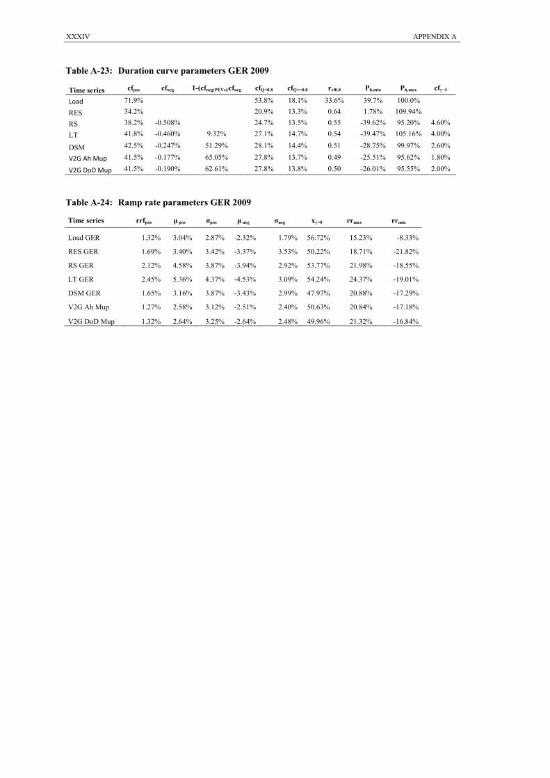
APPENDIX A XXXIV

Table A-23: Duration curve parameters GER 2009


Load 71.9% 53.8% 18.1% 33.6% 39.7% 100.0%

RES 34.2% 20.9% 13.3% 0.64 1.78% 109.94%

RS 38.2% -0.508% 24.7% 13.5% 0.55 -39.62% 95.20% 4.60%

LT 41.8% -0.460% 9.32% 27.1% 14.7% 0.54 -39.47% 105.16% 4.00%

DSM 42.5% -0.247% 51.29% 28.1% 14.4% 0.51 -28.75% 99.97% 2.60%

V2G Ah Mup 41.5% -0.177% 65.05% 27.8% 13.7% 0.49 -25.51% 95.62% 1.80%

V2G DoD Mup 41.5% -0.190% 62.61% 27.8% 13.8% 0.50 -26.01% 95.55% 2.00%

Table A-24: Ramp rate parameters GER 2009


Load GER 1.32% 3.04% 2.87% -2.32% 1.79% 56.72% 15.23% -8.33%

RES GER 1.69% 3.40% 3.42% -3.37% 3.53% 50.22% 18.71% -21.82%

RS GER 2.12% 4.58% 3.87% -3.94% 2.92% 53.77% 21.98% -18.55%

LT GER 2.45% 5.36% 4.37% -4.53% 3.09% 54.24% 24.37% -19.01%

DSM GER 1.65% 3.16% 3.87% -3.43% 2.99% 47.97% 20.88% -17.29%

V2G Ah Mup 1.27% 2.58% 3.12% -2.51% 2.40% 50.63% 20.84% -17.18%

V2G DoD Mup 1.32% 2.64% 3.25% -2.64% 2.48% 49.96% 21.32% -16.84%

APPENDIX A

XXXV

Grid connection power

Figure A-19: PEVs load curve, hourly mean versus quarter hourly mean values.

Source: Own calculation, probabilities obtained from the data basis (MID 2008, 2010); Note: The reference scenario uses a average grid connection power of 4.5 kW.

Figure A-20: Sorted load curve for PEVs last trip charging

Source: Own calculation, probabilities obtained from the data basis (MID 2008, 2010); Note: The reference scenario uses a average grid connection power of 4.5 kW.

APPENDIX A XXXVI

Table A-25: Average electric driving share of vehicle fleet in dependence of connection power

Last Trip DSM V2G DoD Mup V2G Ah Mup

Power Electric driving share

Energy use for driving [kWh/a]

Electric driving share






2 kW 53.66% 2963 69.02% 2973 69.05% 2970 69.08% 2961

Reference 53.73% 2966 70.26% 2969 70.33% 2962 70.32% 2965

12 kW 53.75% 2965 70.92% 2970 70.84% 2971 70.87% 2964

22 kW 53.79% 2964 70.77% 2973 70.97% 2958 70.86% 2966

44 kW 53.76% 2965 70.78% 2968 70.86% 2968 70.83% 2970 Note: Reference: GER 2030 scenario as defined in chapter 6 with grid connection power between 4 kW and 8 kW. Sample size 12,000 vehicles.

Table A-26: Duration curve parameters last trip charging

Scenarios cfpos cfneg 1-(cfneg(PEVs)/cfneg cfQ<0.8 cfQ>=0.8 rcf0.8 Ph,min Ph,max cfy=0

2 kW 41.34% -0.2544% 10.64% 27.56% 14.03% 50.90% 97.49% -42.83% 2.80%

Reference 41.34% -0.2517% 11.60% 27.44% 14.15% 51.55% 100.44% -42.56% 3.00%

12 kW 41.34% -0.2484% 12.75% 27.41% 14.17% 51.71% 102.66% -42.20% 2.80%

22 kW 41.34% -0.2470% 13.23% 27.40% 14.18% 51.74% 104.24% -42.21% 2.80%

44 kW 41.34% -0.2469% 13.27% 27.40% 14.18% 51.76% 102.74% -42.29% 2.80%

Table A-27: Ramp rate parameters last trip charging

Scenario rrfpos μ pos σpos μ neg σneg xy=0 rrmax rrmin

2 kW 2.21% 4.87% 3.89% -4.01% 2.75% 54.84% 29.51% -19.15%

Reference 2.32% 5.04% 4.01% -4.27% 2.87% 54.12% 29.78% -19.17%

12 kW 2.36% 5.09% 4.09% -4.37% 2.98% 53.80% 31.68% -18.90%

22 kW 2.37% 5.09% 4.12% -4.39% 3.03% 53.68% 29.74% -19.00%

44 kW 2.37% 5.10% 4.13% -4.41% 3.04% 53.64% 30.10% -19.27%

Table A-28: Duration curve parameters demand-side management

Scenario cfpos cfneg 1-(cfneg(PEVs)/cfneg cfQ<0.8 cfQ>=0.8 rcf0.8 Ph,min Ph,max cfy=0

2 kW 42.20% -0.1024% 64.02% 28.57% 13.72% 48.02% 91.93% -34.02% 1.40%

Reference 42.21% -0.0970% 65.94% 28.58% 13.72% 48.02% 91.91% -34.03% 1.20%

12 kW 42.21% -0.0970% 65.91% 28.58% 13.72% 48.01% 91.84% -33.95% 1.20%

22 kW 42.24% -0.0970% 65.93% 28.61% 13.72% 47.95% 91.55% -33.45% 1.20%

44 kW 42.22% -0.0994% 65.08% 28.60% 13.72% 47.98% 91.53% -33.35% 1.40%

Table A-29: Ramp rate parameters demand-side management


2 kW 1.55% 2.96% 3.41% -3.24% 2.65% 47.72% 27.52% -17.51%

Reference 1.52% 2.88% 3.43% -3.19% 2.64% 47.38% 27.44% -17.74%

12 kW 1.50% 2.86% 3.42% -3.10% 2.62% 47.93% 27.72% -17.62%

22 kW 1.49% 2.84% 3.40% -3.08% 2.61% 47.93% 27.42% -17.33%

44 kW 1.48% 2.83% 3.39% -3.07% 2.60% 47.89% 27.66% -17.38%

APPENDIX A

XXXVII

Table A-30: Duration curve parameters vehicle-to-grid DoD battery aging and mark-up price


2 kW 42.18% -0.0716% 74.87% 28.76% 13.49% 46.89% 90.13% -29.57% 0.80%

Reference 42.25% -0.0611% 78.56% 28.85% 13.46% 46.65% 90.14% -27.42% 0.80%

12 kW 42.29% -0.0585% 79.44% 28.90% 13.44% 46.51% 90.06% -27.06% 0.60%

22 kW 42.28% -0.0590% 79.27% 28.89% 13.44% 46.50% 90.13% -27.06% 0.60%

44 kW 42.28% -0.0583% 79.52% 28.90% 13.43% 46.47% 90.14% -26.96% 0.60%

Table A-31: Ramp rate parameters vehicle-to-grid DoD battery aging and mark-up price


2 kW 1.2514% 2.44% 3.08% -2.54% 2.35% 49.01% 22.79% -15.68%

Reference 1.1966% 2.35% 3.00% -2.42% 2.27% 49.24% 22.90% -15.34%

12 kW 1.1652% 2.31% 2.93% -2.33% 2.20% 49.74% 22.36% -14.62%

22 kW 1.1624% 2.30% 2.93% -2.33% 2.19% 49.63% 22.19% -14.80%

44 kW 1.1567% 2.29% 2.92% -2.31% 2.18% 49.72% 22.27% -15.14%

Table A-32: Duration curve parameters vehicle-to-grid Ah battery aging and mark-up price


2 kW 42.19% -0.0595% 79.10% 28.81% 13.42% 46.58% 90.05% -28.28% 0.80%

Reference 42.27% -0.0509% 82.11% 28.93% 13.37% 46.22% 89.87% -26.20% 0.60%

12 kW 42.30% -0.0488% 82.85% 28.98% 13.35% 46.07% 89.84% -25.61% 0.60%

22 kW 42.30% -0.0478% 83.23% 28.99% 13.35% 46.03% 89.79% -25.51% 0.60%

44 kW 42.31% -0.0475% 83.31% 29.01% 13.34% 45.99% 89.81% -25.53% 0.60%

Table A-33: Ramp rate parameters vehicle-to-grid Ah battery aging and mark-up price


2 kW 1.2291% 2.42% 2.97% -2.49% 2.27% 49.22% 19.31% -15.03%

Reference 1.1527% 2.28% 2.86% -2.31% 2.18% 49.64% 19.79% -14.69%

12 kW 1.1230% 2.23% 2.80% -2.25% 2.11% 49.78% 19.32% -13.48%

22 kW 1.1114% 2.23% 2.77% -2.21% 2.09% 50.13% 19.14% -14.24%

44 kW 1.1035% 2.22% 2.76% -2.19% 2.07% 50.29% 18.75% -14.58%

APPENDIX A XXXVIII

Battery costs


Scenario cfpos cfneg 1-(cfneg(PEVs)/cfneg) cfQ<0.8 cfQ>=0.8 rcf0.8 Ph,max Ph,min cfy=0

V2G DoD +20 42.24% -0.07% 76.90% 28.80% 13.50% 46.87% 90.40% -28.39% 0.80%

V2G DoD +40 42.23% -0.07% 74.97% 28.76% 13.54% 47.06% 90.48% -29.28% 0.80%

V2G DoD -20 42.26% -0.06% 80.13% 28.90% 13.41% 46.38% 89.91% -26.65% 0.60%

V2G DoD -40 42.27% -0.05% 81.78% 28.98% 13.35% 46.06% 89.30% -26.18% 0.60%



V2G DoD +20 1.24% 2.44% 3.10% -2.51% 2.34% 49.25% 24.33% -15.95%

V2G DoD +40 1.28% 2.51% 3.17% -2.59% 2.41% 49.12% 25.73% -16.04%

V2G DoD -20 1.14% 2.23% 2.87% -2.30% 2.19% 49.21% 21.14% -14.35%

V2G DoD -40 1.07% 2.09% 2.71% -2.16% 2.09% 49.06% 19.84% -14.00%



V2G Ah +20 42.25% -0.05% 28.89% 13.42% 46.46% 90.30% -26.11% 0.60% 81.32%

V2G Ah +40 42.24% -0.06% 28.84% 13.46% 46.68% 91.19% -26.08% 0.60% 80.31%

V2G Ah -20 42.27% -0.05% 28.99% 13.33% 45.99% 89.31% -25.91% 0.60% 83.28%

V2G Ah -40 42.29% -0.04% 29.05% 13.28% 45.73% 88.50% -25.83% 0.60% 84.27%



V2G Ah +20 1.21% 2.39% 2.96% -2.43% 2.25% 49.51% 20.62% -13.91%

V2G Ah +40 1.26% 2.47% 3.04% -2.54% 2.31% 49.23% 21.53% -14.22%

V2G Ah -20 1.09% 2.16% 2.74% -2.19% 2.11% 49.56% 19.41% -15.84%

V2G Ah -40 1.02% 2.01% 2.60% -2.07% 2.04% 49.31% 19.26% -16.06%

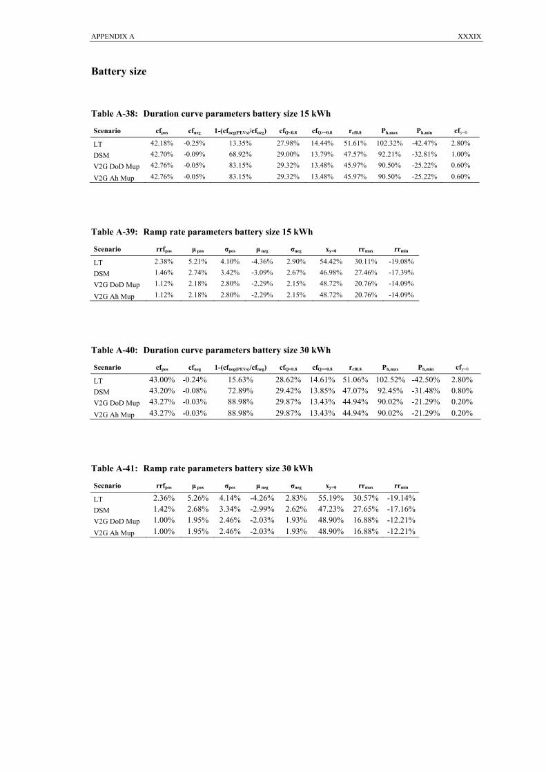
APPENDIX A

XXXIX

Battery size

Table A-38: Duration curve parameters battery size 15 kWh


LT 42.18% -0.25% 13.35% 27.98% 14.44% 51.61% 102.32% -42.47% 2.80%

DSM 42.70% -0.09% 68.92% 29.00% 13.79% 47.57% 92.21% -32.81% 1.00%

V2G DoD Mup 42.76% -0.05% 83.15% 29.32% 13.48% 45.97% 90.50% -25.22% 0.60%

V2G Ah Mup 42.76% -0.05% 83.15% 29.32% 13.48% 45.97% 90.50% -25.22% 0.60%

Table A-39: Ramp rate parameters battery size 15 kWh


LT 2.38% 5.21% 4.10% -4.36% 2.90% 54.42% 30.11% -19.08%

DSM 1.46% 2.74% 3.42% -3.09% 2.67% 46.98% 27.46% -17.39%

V2G DoD Mup 1.12% 2.18% 2.80% -2.29% 2.15% 48.72% 20.76% -14.09%

V2G Ah Mup 1.12% 2.18% 2.80% -2.29% 2.15% 48.72% 20.76% -14.09%

Table A-40: Duration curve parameters battery size 30 kWh


LT 43.00% -0.24% 15.63% 28.62% 14.61% 51.06% 102.52% -42.50% 2.80%

DSM 43.20% -0.08% 72.89% 29.42% 13.85% 47.07% 92.45% -31.48% 0.80%

V2G DoD Mup 43.27% -0.03% 88.98% 29.87% 13.43% 44.94% 90.02% -21.29% 0.20%

V2G Ah Mup 43.27% -0.03% 88.98% 29.87% 13.43% 44.94% 90.02% -21.29% 0.20%

Table A-41: Ramp rate parameters battery size 30 kWh


LT 2.36% 5.26% 4.14% -4.26% 2.83% 55.19% 30.57% -19.14%

DSM 1.42% 2.68% 3.34% -2.99% 2.62% 47.23% 27.65% -17.16%

V2G DoD Mup 1.00% 1.95% 2.46% -2.03% 1.93% 48.90% 16.88% -12.21%

V2G Ah Mup 1.00% 1.95% 2.46% -2.03% 1.93% 48.90% 16.88% -12.21%

APPENDIX A XL

Mobility behavior

Table A-42: Duration curve parameters deterministic MOP mobility behavior

Scenario cfpos cfneg 1-

(cfneg(PEVs)/cfneg) cfQ<0.8 cfQ>=0.8 rcf0.8 Ph,max Ph,min cfy=0

LT 40.85% -0.24% 17.01% 27.19% 13.89% 51.06% 98.31% -41.95% 2.80%

DSM 41.42% -0.11% 60.81% 27.98% 13.54% 48.40% 91.30% -34.29% 1.60%

V2G DoD Mup 41.47% -0.07% 77.09% 28.27% 13.27% 46.93% 88.76% -27.72% 0.80%

V2G Ah Mup 41.48% -0.05% 80.99% 28.34% 13.19% 46.55% 88.77% -26.18% 0.60%

Table A-43: Ramp rate parameters deterministic MOP mobility behavior


LT 2.20% 4.82% 3.83% -4.04% 2.81% 54.44% 28.46% -19.21%

DSM 1.52% 2.96% 3.49% -3.09% 2.72% 48.85% 27.73% -18.39%

V2G DoD Mup

1.18% 2.37% 2.96% -2.35% 2.25% 50.17% 22.91% -15.80%

V2G Ah Mup 1.15% 2.33% 2.84% -2.27% 2.16% 50.70% 19.87% -13.43%

Table A-44: Duration curve parameters probability based MOP mobility behavior


LT 40.94% -0.24% 15.37% 27.22% 13.97% 51.32% 99.44% -42.13% 2.80%

DSM 41.40% -0.12% 59.31% 27.96% 13.56% 48.49% 90.89% -34.76% 1.60%

V2G DoD 41.45% -0.07% 75.45% 28.24% 13.28% 47.02% 88.96% -27.76% 0.80%

V2G Ah 41.46% -0.06% 80.16% 28.31% 13.20% 46.64% 88.67% -26.31% 0.80%

Table A-45: Ramp rate parameters probability based MOP mobility behavior


LT 2.25% 4.91% 3.89% -4.14% 2.85% 54.25% 28.76% -18.98%

DSM 1.55% 2.98% 3.50% -3.18% 2.69% 48.35% 27.76% -17.85%

V2G DoD 1.18% 2.37% 2.96% -2.35% 2.25% 50.17% 22.91% -15.80%

V2G Ah 1.15% 2.33% 2.84% -2.27% 2.16% 50.70% 19.87% -13.43%

Table A-46: Duration curve parameters commuter scenario


LT 42.58% -0.2833% 0.48% 29.37% 14.05% 47.84% 95.88% -32.70% 1.40%

DSM 43.31% -0.1118% 60.75% 29.43% 13.96% 47.44% 94.44% -29.21% 1.00%

V2G DoD Mup 43.32% -0.0806% 71.69% 29.47% 13.92% 47.22% 94.02% -26.54% 0.80%

V2G Ah Mup 43.33% -0.0633% 77.76% 26.65% 16.22% 60.86% 151.65% -43.52% 3.20%

Table A-47: Ramp rate parameters commuter scenario


LT 1.33% 2.67% 3.89% -2.64% 2.74% 50.21% 37.95% -25.37%

DSM 1.18% 2.36% 3.66% -2.32% 2.60% 50.39% 37.25% -24.33%

V2G DoD Mup 1.14% 2.31% 3.57% -2.21% 2.58% 51.04% 36.89% -24.54%

V2G Ah Mup 3.66% 8.62% 13.32% -6.36% 7.57% 57.55% 63.01% -38.19%

APPENDIX A

XLI

Table A-48: Duration curve parameters vehicle-to-grid DoD without mobility behavior



V2G 2 kW 38.60% -0.1069% 62.46% 25.98% 12.73% 49.00% 84.91% -33.32% 1.40%

V2G reference 38.60% -0.1037% 63.59% 25.98% 12.72% 48.97% 84.90% -32.45% 1.40%

V2G 12 kW 38.60% -0.1029% 63.87% 25.98% 12.72% 48.95% 84.92% -32.42% 1.40%

V2G 22 kW 38.60% -0.1036% 63.60% 25.98% 12.72% 48.95% 84.91% -32.43% 1.40%

Table A-49: Ramp rate parameters vehicle-to-grid DoD without mobility behavior


V2G 2 kW 1.42% 2.99% 3.14% -2.67% 2.42% 52.86% 24.87% -18.69%

V2G reference 1.41% 2.98% 3.13% -2.65% 2.41% 52.92% 24.75% -18.33%

V2G 12 kW 1.41% 2.98% 3.13% -2.64% 2.40% 52.97% 24.44% -18.42%

V2G 22 kW 1.41% 2.99% 3.12% -2.64% 2.40% 53.10% 24.58% -18.31%

Table A-50: Duration curve parameters vehicle-to-grid Ah without mobility behavior



V2G 2 kW 38.60% -0.0990% 65.24% 25.98% 12.72% 48.95% 87.43% -31.95% 1.20%

V2G reference 38.60% -0.0987% 65.33% 25.98% 12.71% 48.93% 87.27% -31.81% 1.20%

V2G 12 kW 38.60% -0.0987% 65.34% 25.99% 12.71% 48.89% 87.23% -31.85% 1.20%

V2G 22 kW 38.61% -0.0979% 65.60% 25.99% 12.70% 48.88% 87.18% -31.75% 1.20%

Table A-51: Ramp rate parameters vehicle-to-grid Ah without mobility behavior


V2G 2 kW 1.49% 3.20% 3.08% -2.78% 2.34% 53.56% 20.72% -15.56%

V2G reference 1.48% 3.19% 3.07% -2.76% 2.34% 53.54% 21.51% -15.30%

V2G 12 kW 1.48% 3.18% 3.05% -2.75% 2.33% 53.57% 21.47% -15.01%

V2G 22 kW 1.47% 3.16% 3.05% -2.75% 2.32% 53.50% 21.42% -14.99%

Note: V2G scenarios include mark-up prices

APPENDIX A XLII

Infrastructure

Table A-52: Duration curve parameters demand-side management


Permanent available 42.21% -0.1017% 64.29% 28.58% 13.72% 48.00% 91.91% -33.87% 1.40%

Home + work 42.10% -0.1021% 64.15% 28.51% 13.69% 48.02% 91.74% -33.82% 1.40%

Home 41.98% -0.1004% 64.74% 28.43% 13.64% 47.97% 91.83% -33.48% 1.20%

Table A-53: Ramp rate parameters demand-side management


Permanent available 1.50% 2.82% 3.47% -3.17% 2.68% 47.03% 27.68% -17.38%

Home + work 1.51% 2.83% 3.49% -3.18% 2.69% 47.07% 28.01% -17.53%

Home 1.52% 2.84% 3.49% -3.24% 2.72% 46.67% 27.99% -17.65%




Home + work 42.13% -0.0660% 76.83% 28.75% 13.44% 46.76% 89.94% -28.22% 0.80%

Home 42.01% -0.0660% 76.80% 28.66% 13.42% 46.82% 89.11% -28.34% 0.80%




Home + work 1.22% 2.37% 3.03% -2.48% 2.30% 48.90% 23.73% -15.41%

Home 1.25% 2.42% 3.07% -2.54% 2.36% 48.82% 23.73% -15.82%




Home + work 42.14% -0.0545% 80.84% 28.83% 13.36% 46.33% 89.58% -27.13% 0.60%

Home 42.03% -0.0545% 80.84% 28.74% 13.34% 46.39% 89.58% -27.22% 0.60%




Home + work 1.17% 2.30% 2.89% -2.37% 2.21% 49.21% 21.01% -14.68%

Home 1.19% 2.34% 2.93% -2.42% 2.27% 49.04% 21.16% -14.73%

APPENDIX A

XLIII

Share of fluctuating generation technology

Table A-58: Duration curve parameters



RS-PV 0% 38.54% -0.697% 25.06% 14.16% 56.50% 90.71% -51.46% 6.40%

DSM RES-PV 0% 42.20% -0.427% 38.79% 27.76% 14.87% 53.56% 92.58% -31.54% 4.20%

V2GDoD RES-PV 0% 42.24% -0.348% 50.10% 27.98% 14.61% 52.21% 90.86% -29.34% 3.80%

RS-PV 15% 38.54% -0.286% 25.56% 13.26% 51.87% 89.87% -32.16% 3.40%

DSM RES-PV 15% 42.21% -0.132% 53.97% 28.47% 13.86% 48.70% 91.64% -24.85% 1.80%

V2GDoD RES-PV 15% 42.24% -0.087% 69.41% 28.66% 13.66% 47.65% 90.51% -20.40% 1.40%

RS-PV 30% 38.54% -0.429% 25.72% 13.24% 51.47% 90.71% -51.46% 4.20%

DSM RES-PV 30% 42.20% -0.159% 63.03% 28.62% 13.73% 47.97% 92.25% -40.75% 2.00%

V2GDoD RES-PV 30% 42.26% -0.077% 81.99% 28.92% 13.41% 46.37% 90.01% -33.65% 1.00%

RS-PV 45% 38.54% -1.499% 26.47% 13.57% 51.27% 91.55% -70.82% 9.20%

DSM RES-PV 45% 42.21% -0.763% 49.07% 28.99% 14.00% 48.29% 93.04% -58.68% 6.00%

V2GDoD RES-PV 45% 42.30% -0.389% 74.03% 29.19% 13.51% 46.28% 90.14% -49.29% 3.80%


Table A-59: Ramp rate parameters


RS-PV 0% 1.64% 3.46% 2.92% -3.11% 2.40% 52.68% 18.13% -16.86%

DSM RES-PV 0% 1.23% 2.24% 3.09% -2.70% 2.59% 45.29% 19.01% -17.42%

V2GDoD RES-PV 0% 1.03% 1.93% 2.83% -2.18% 2.27% 46.93% 18.78% -15.65%

RS-PV 15% 1.75% 3.78% 3.03% -3.25% 2.33% 53.70% 24.47% -14.48%

DSM RES-PV 15% 1.25% 2.28% 2.97% -2.73% 2.43% 45.48% 23.83% -14.09%

V2GDoD RES-PV 15% 1.02% 1.95% 2.63% -2.14% 2.10% 47.65% 18.75% -12.56%

RS-PV 30% 2.26% 4.91% 4.09% -4.17% 3.27% 54.09% 30.82% -22.63%

DSM RES-PV 30% 1.72% 3.28% 3.96% -3.56% 3.09% 47.93% 30.06% -21.04%

V2GDoD RES-PV 30% 1.34% 2.66% 3.36% -2.67% 2.61% 49.90% 25.53% -18.19%

RS-PV 45% 2.87% 6.26% 5.65% -5.28% 4.98% 54.21% 37.16% -30.92%

DSM RES-PV 45% 1.72% 4.52% 5.48% -4.64% 4.71% 49.29% 36.33% -30.52%

V2GDoD RES-PV 45% 1.34% 3.44% 4.57% -3.34% 3.97% 50.70% 33.30% -26.24%


APPENDIX B XLIV

B. Field test

The price-based control of PEVs as introduced in Chapter 2 and Chapter 5 is applied in the field test “Flottenversuch Elektromobilität” (BMU, 2009; E.ON AG, 2012 and Volkswagen AG, 2011). The Flottenversuch Elektromobilität is a project funded by the German Federal Ministry for the Environment, Nature Conservation and Nuclear Safety (BMU) with Volkswagen AG and E.ON Energie AG as the main industry partners.123 As one task within the subproject AP1 under E.ON AG leadership a on-board meter was developed and implemented in 20 Golf Variant “TwinDrive” plug-in hybrid electric vehicles. Details on the technical specification are available in (Link, 2011, Chapter 5.3). The depth of discharge-based battery cost calculation (see Chapter 4.3.4) and the optimization algorithm (see Chapter 5.4.6) were implemented in the Volkswagen vehicles and the PowerACE DSM simulation environment. The tariff used in the field was generated with the PowerACE simulation model including variable grid fees for a 2030 scenario124 and gives incentives for the grid integration of fluctuating generation units (see Chapter 5.3.5). This shows a valuable application of the simulation model in a research project. The application of the methods in the field test and the simulation environment provides evidence on the technical feasibility and practical relevance of this work.

123 Further partners are GAIA Akkumulatorenwerke GmbH, Evonik Litarion GmbH, ifeu - Institut für Energie- und Umweltforschung Heidelberg GmbH, Westfälische Wilhelms-Universität Münster Fraunhofer ISiT - Fraunhofer Institut für Siliziumtechnologie. 124 Note: The scenario introduced in Chapter 6 is not consistent with the scenarios of the Flottenversuch Elektromobilität.

APPENDIX C

XLV

C. Publications

Publication Status Chapter Dallinger, D, and M Wietschel. 2012a. Grid integration of intermittent renewable energy sources using price-responsive plug-in electric vehicles. Renewable and Sustainable Energy Review 16 (5): 3370–3382.

Published Chapter 4

and 5

Biere, D, D Dallinger and M Wietschel. 2009. Ökonomische Analyse der Erstnutzer von Elektrofahrzeugen. Zeitschrift für Energiewirtschaft.

Published Chapter 4

Dallinger, D, D Krampe and B Pfluger. 2012d. Electric Vehicles in a Smart Grid Environment. In: Smart Grid Infrastructure & Networking. Edited by K Iniewski.

Published Chapter 2

Dallinger, D, G Schubert and M Wietschel. 2013. Integration of intermittent renewable power supply using grid-connected vehicles - a 2030 case study for California and Germany. Applied Energy 104: 666–682.

Published Chapter 3, 6

and 7

Dallinger, D, J Link, M Büttner. 2012e. Smart Grid Agent: Plug-In Electric Vehicle. Submitted to IEEE Transactions on Smart Grid.

Submitted Chapter 4, 5

and 7

Dallinger, D, D Krampe and M Wietschel. 2011. Vehicle-to-grid regulation based on a dynamic simulation of mobility behavior. IEEE Transactions on Smart Grid.

Published -

Kley, F, M Wietschel, D Dallinger. 2012. Evaluation of European Electric Vehicle Support Schemes. In: Governance on Innovation towards Sustainability: The global transport sector. Edited by M Nilsson, K Hillman, A Rickne and T Magnusson.

Published -

Kley, F, C Lerch, and D Dallinger. 2011 . New business models for electric cars - a holistic approach. Energy Policy.

Published -

Pehnt, M, H Helms, U Lambrecht, D Dallinger, M Wietschel, H Heinrichs, R Kohrs, J Link, S Trommer, T Pollok and P Behrens. 2011. Elektroautos in einer von erneuerbaren Energien geprägten Energiewirtschaft, Zeitschrift für Energiewirtschaft.

Published -

Beer, S, T Gómez, D Dallinger, I Momber, M Marnay, M Stadler and J Lai. 2010. Economic Analysis of Used Electric Vehicle Batteries Integrated into Commercial Building Microgrids. IEEE Transactions on Smart Grid.

Published -

REFERENCES XLVI

References AC Propulsion. 2003. “Development and Evaluation of a Plug-in HEV with Vehicle-to-Grid Power

Flow.” Accessed November 11, 2011. http://www.acpropulsion.com/icat01-2_v2gplugin.pdf.

Akkermans, JM, and J Schreinemakers. 2004. “Microeconomic distributed control: Theory and

application of multi-agent electronic markets.” In Proceedings of CRIS (ii): 1-8. Accessed

March 31, 2012. http://www.see.asso.fr/clubs_techniques/se/xmedia/Club_Tech_SE-2001-

2008/2004/CRIS-Grenoble-10-04/S8/s8-a1.pdf.

Aleklett, K, M Höök, K Jakobsson, M Lardelli, S Snowden, and B Söderbergh. 2010. The Peak of the

Oil Age – Analyzing the world oil production Reference Scenario in World Energy Outlook

2008. Energy Policy 38 (3): 1398-1414.

Andersen, FM, SG Jensen, and HV Larsen. 2006. “Analyses of demand response in Denmark.” Risø

National Laboratory Ea Energy Analyses RAM-løse edb Risø-R-1565(EN) (October).

Accessed March 31, 2012. http://www.ea-energianalyse.dk/reports/511_Analyses_of

_Demand_Response_in_Denmark.pdf.

Anderson, EJ, and AB Philpott. 2002. Optimal offer curve construction in electricity markets.

Mathematics of Operations Research 27 (1): 82-100.

Andersson, S-L, AK Elofsson, MD Galus, L Göransson, S Karlsson, F Johnsson, and G Andersson.

2010. Plug-in hybrid electric vehicles as regulating power providers: Case studies of Sweden

and Germany. Energy Policy 38 (6): 2751-2762.

AREVA. 2011. “M5000 technical data.” Accessed July 11, 2011. http://www.areva-wind.com/

fileadmin/infomaterial/AREVAwind_TechnicalData.pdf.

Awerbuch, S. 2006. Portfolio-Based Electricity Generation Planning: Policy Implications For

Renewables And Energy Security. Mitigation and Adaptation Strategies for Global Change 11

(3): 693-710.

Baıllo, A. “A methodology to develop optimal schedules and offering strategies for a generation

company operating in a short- term electricity market.” Dissertation, ICAI, Universidad

Pontificia Comillas, Madrid, 2002.

Bandivadekar, A, K Bodek, L Cheah, and C Evans. 2008. “On the road in 2035, Reducing

Transportation’s Petroleum Consumption and GHG Emissions.” Report Laboratory for Energy

and the Environment Massachusetts Institute of Technology. Accessed March 31, 2012.

http://scholar.google.com/scholar?hl=en&btnG=Search&q=intitle:On+the+Road+in+2035#1.

Banks, J, J Carson, BL Nelson, and D Nicol. 2004. Discrete-Event System Simulation, Fourth Edition.

Prentice Hall.

Barbose, G, C Goldman, R Bharvirkar, N Hopper, M Ting, and B Neenan. 2005. “Real Time Pricing as

a Default or Optional Service for C&I Customers: A Comparative Analysis of Eight Case

Studies.” Lawrence Berkeley National Laboratory, Berkeley. LBNL-57661. Prepared for

California Energy Commission. Accessed March 31, 2012. http://eetd.lbl.gov/ea/ems/

reports/57661.pdf.

REFERENCES

XLVII

Bartels, M, C Gatzen, D Lindenberger, F Müsgens, M Peek, A Seeliger, D Steuber, R Wissen, P Hofer,

A Kirchner, J Scheelhaase, and M Schlesinger. 2005. “Energiereport IV: Die Entwicklung der

Energiemärkte bis zum Jahr2030 - Energiewirtschaftliche Referenzprognose.“ Institute of

Energy Economics, University of Cologne. Accessed July 11, 2011. http://www.prognos.

com/fileadmin/pdf/Energiereport%20IV_Kurzfassung_d.pdf.

Bass, FM. 1969. A New Product Growth for Model Consumer Durables. Management Sci. 15(5) 215-

227.

BDEW: German Association of Energy and Water Industries. 2011. “51 Kraftwerke bis 2019 geplant.”

Anlage zur Presseinformation, Bundesverband der Energie- und Wasserwirtschaft e.V. (April):

1-4. Accessed March 31, 2012. http://www.bdew.de/internet.nsf/id/28A564757298E630C125

786800297145/$file/110404 Anlage zur PM Hannover_Kraftwerksliste.pdf.

Becker, TA. 2009. “Electric Vehicles in the United States A New Model with Forecasts to 2030.”

Center for Entrepreneurship & Technology at the University of California, Berkeley. Accessed

March 31, 2012. http://cet.berkeley.edu/dl/CET_Technical%20Brief_EconomicModel2030_f.

pdf.

Bessa, RJ, and MA Matos. 2011. Economic and technical management of an aggregation agent for

electric vehicles: a literature survey. Euro. Trans. Electr. Power. doi: 10.1002/etep.565.

Beurskens, L W M, M Hekkenberg, P Vethman. 2011. „Renewable Energy Projections as Published in

the National Renewable Energy Action Plans of the European Member States“ Energy research

Centre of the Netherlands ECN-E--10-069 Accessed March 31, 2012.

http://www.ecn.nl/docs/library/report/2010/e10069.pdf.

Biere, D, D Dallinger, and M Wietschel. 2009. Ökonomische Analyse der Erstnutzer von

Elektrofahrzeugen, Zeitschrift für Energiewirtschaft 33 (2): 173-181.

Blarke, MB, and H. Lund. 2008. The effectiveness of storage and relocation options in renewable

energy systems. Renewable Energy 33 (7): 1499-1507.

BMBF: Federal Ministry of Education and Research. 2009. Nationaler Entwicklungsplan

Elektromobilität der Bundesregierung. Accessed March 31, 2012. http://www.bmbf.de/

pubRD/nationaler_entwicklungsplan_elektromobilitaet.pdf.

BMU: Federal Ministry for the Environment, Nature Conservation and Nuclear Safety. 2009.

“Flottenversuch Elektromobilität” Accessed March 31, 2012. http://www.bmu-

klimaschutzinitiative.de/de/projekte_nki?p=3&d=310.

BMW Group. 2011. “Fully charged Mini publishes results of UK’s most in-depth electric vehicle trial”.

Accessed March 31, 2012. https://www.press.bmwgroup.com/pressclub/p/gb/pressDetail.html?

outputChannelId=8&id=T0118820EN_GB&left_menu_item=node__2310.

BMWi: Federal Ministry of Economics and Technology. 2012. 1 “Gesamtausgabe der Energiedaten -

Datensammlung des BMWi.“ Accessed March 31, 2012. http://www.bmwi.de/BMWi/

Redaktion/Binaer/energie-daten-gesamt,property=blob,bereich=bmwi,sprache=de,rwb=true.xls.

Bower, J, and D Bunn. 2000. Model-based comparisons of pool and bilateral markets for electricity.

Energy Journal 21 (3): 1-29.

REFERENCES XLVIII

Brooks, A, T Gage, and AC Propulsion. 2001. “Integration of Electric Drive Vehicles with the Electric

Power Grid -- a New Value Stream Description of Value-Added functions.” Paper presented at

18th Electric Vehicle Symposium (EVS-18), Berlin, Oktober 20-24, 2001.

BTU Cottbus: Brandenburgische Technische Universität Cottbus. 2002. “Standard residential load

profile”

Bundesverband Windenergie e.V. 2011. “Statistic: Installed wind capacity in Germany”. Accessed

March 31, 2012. http://www.wind-energie.de/infocenter/statistiken/deutschland/installierte

windenergieleistung-deutschland.

Bunn, DW, and FS Oliveira. 2007. “Agent-based analysis of technological diversification and

specialization in electricity markets.” European Journal of Operational Research 181 (3): 1265-

1278.

Burnham, A, M Wang, and Y Wu. 2006. “Development and Applications of GREET 2.7. The

Transportation Vehicle Cycle Model.” Argonne National Laboratory Argonne National

Laboratory, Energy Systems Division, ANL/ESD/06-5. (Nov). Accessed March 31, 2012.

http://www.transportation.anl.gov/pdfs/TA/378. pdf.

CAISO: California Independent System Operator. 2011. 1 “33 percent trajectory case - preliminary new

scenarios: File ‘One-Minute Data for Load, Wind and Solar’ (3/14/2011 07:44) and ‘Step 1

Assumptions, Forecast Errors and Renewable Profiles’ (3/11/2011 15:23). Accessed October

24, 2011. http://www.caiso.com/Documents/33%20percent%20trajectory%20case%20-

%20preliminary%20new%20scenarios.

California Department of Transportation. 2005. “California Motor Vehicle Stock, Travel and Fuel

Forecast.” Accessed March 31, 2012. http://www.dot.ca.gov/hq/tsip/smb/documents/mvstaff/

mvstaff05.pdf.

Cappers, P, A Mills, C Goldman, R Wiser, and JH Eto. 2011. “Mass Market Demand Response and

Variable Generation Integration Issues: A Scoping Study.” Lawrence Berkeley National

Laboratory, Environmental Energy Technologies Division, LBNL-5063E. Prepared for the

Office of Electricity Delivery and Energy Reliability U.S. Department of Energy, Accessed

March 31, 2012. http://eetd.lbl.gov/ea/emp/reports/lbnl-5063e.pdf.

Cappers, P, C Goldman, and D Kathan. 2010. “Demand response in U.S. electricity markets: Empirical

evidence.” Energy 35 (4): 1526-1535.

CARB: California Air Resources Board. 2012. “Low Carbon Fuel Standard Program.”, Accessed March

31, 2012. http://www.arb.ca.gov/fuels/lcfs/lcfs.htm.

Cascetta, E. 1984. Estimation of trip matrices from traffic counts and survey data: A generalized least

squares estimator. Transportation Research 18B (415): 289-299.

Chan, CC. 1993. An overview of electric vehicle technology. Proceedings of the IEEE 81 (9): 1202-

1213.

Chassin, DP, and L Kiesling. 2008. Decentralized coordination through digital technology, dynamic

pricing, and customer-driven control: The gridwise testbed demonstration project. The

Electricity Journal 21 (8): 51-59.

REFERENCES

XLIX

Christidis, P, I Hidalgo, and A Soria. 2003. “The IPTS Transport technologies model.” European

Commission Joint Research Centre (DG JRC) Institute for Prospective Technological Studies,

EUR 20762 EN. Accessed March 31, 2012. http://ftp.jrc.es/EURdoc/eur20762en.pdf.

Clement-Nyns, K, E Haesen, and J Driesen. 2010. The impact of charging plug-in hybrid electric

vehicles on a residential distribution grid. IEEE Transactions on Power Systems 25 (1): 371-

380.

CONCAWE: Conservation of Clean Air and Water in Europe. 2007a. “Well-to-Wheels analysis of

future automotive fuels and powertrains in the European context WELL-TO-TANK Report

Version 2c.” Concawe, European Council for Automotive R&D, Institute for Environment and

Sustainability of the EU Commission’s Joint Research Centre. Accessed July 11, 2011.

http://ies.jrc.ec.europa.eu/uploads/media/WTT_Report_010307.pdf.

CONCAWE: Conservation of Clean Air and Water in Europe. 2007b. “WTW Appendix 1: Summary of

WTW Energy and GHG Balances.” Concawe, European Council for Automotive R&D,

Institute for Environment and Sustainability of the EU Commission’s Joint Research Centre.

Accessed July 11, 2011. http://iet.jrc.ec.europa.eu/sites/about-jec/files/documents/

WTW_App_1_010307.pdf.

CONCAWE: Conservation of Clean Air and Water in Europe. 2008. “Vehicle retail price estimation.

Well-to-Wheels analysis of future automotive fuels and powertrains in the European context

TANK-TO-WHEELS Report Version 3., October 2008 TTW, TTW APPENDIX 1.” Concawe,

European Council for Automotive R&D, Institute for Environment and Sustainability of the EU

Commission’s Joint Research Centre. Accessed March 31, 2012. http://iet.jrc.ec.europa.eu/

sites/about-jec/files/documents/V3.1_TTW_App_1_07102008.pdf.

Connolly, D, H Lund, BV Mathiesen, and M Leahy. 2010. A review of computer tools for analysing the

integration of renewable energy into various energy systems. Applied Energy 87 (4): 1059-

1082.

Conzelmann, G, G Boyd, and V Koritarov. 2005. “Multi-agent power market simulation using

EMCAS.” Paper presented at Power Engineering Society General Meeting, San Francisco, June

12-16, 2005.

CPUC: California Public Utilities Commission. 2012. “Renewable Integration Workshops.” Accessed

March 31, 2012. http://www.cpuc.ca.gov/PUC/energy/Renewables/100824_workshop.htm.

Dallinger, D, and M Wietschel. 2012a. Grid integration of intermittent renewable energy sources using

price-responsive plug-in electric vehicles. Renewable and Sustainable Energy Review 16 (5):

3370-3382.

Dallinger, D, D Krampe and M Wietschel. 2011. Vehicle-to-Grid Regulation Reserves Based on a

Dynamic Simulation of Mobility Behavior, IEEE Transactions on Smart Grid 2 (2).

Dallinger, D, M Wietschel, and DJ Santini. 2012b. Effect of demand response on the marginal

electricity used by plug-in electric vehicles. Paper presented at 26th Electric Vehicle

Symposium (EVS-26), Los Angeles, May 6-9, 2012.

REFERENCES L

Dallinger, D, G Schubert and M Wietschel. 2013. Integration of intermittent renewable power supply

using grid-connected vehicles - a 2030 case study for California and Germany. Applied Energy

104: 666–682.

Dallinger, D, D Krampe and B Pfluger. 2012c. Electric Vehicles in a Smart Grid Environment. In:

Network Innovations for Smart Grids. Edited by K Iniewski.

Dallinger, D, J Link, M Büttner and M Wietschel. 2012d. Smart Grid Agent: Plug-In Electric Vehicle.

Submitted to IEEE Transactions on Smart Grid.

Day, C, and D Bunn. 2001. Divestiture of generation assets in the electricity pool of England and Wales:

a computational approach to analyzing market power. Journal of Regulatory Economics 19 (2):

123-141.

DENA: Deutsche Energie-Agentur GmbH: Kohler, S, A-C Agricola, and H Seidl. 2010. 1 dena-

Netzstudie II: Integration erneuerbarer Energien in die deutsche Stromversorgung im Zeitraum

2015 – 2020 mit Ausblick 2025. Accessed July 11, 2011. http://www.dena.de/fileadmin/

user_upload/Download/Dokumente/Studien___Umfragen/Endbericht_dena-Netzstudie_II.pdf.

Dijkstra, EW. 1959. A note on two problems in connexion with graphs. Numerische Mathematik 1 (1):

269-271.

DOE: U.S. Department of Energy. 2006. “Benefits of Demand Response in Electricity Markets and

Recommendations for Achieving Them. Response.” Accessed March 31, 2012.

http://eetd.lbl.gov/ea/EMP/reports/congress-1252d.pdf.

DOE: US Department of Energy. 2012. “The Alternative Fuels and Advanced Vehicles Data Center,

Data, Analysis, and Trends.” Accessed November 11, 2011. http://www.afdc.energy.gov/afdc/

data/vehicles.html#afv_hev.

E.ON AG. 2012. “Flottenversuch Elektromobilität” Accessed March 31, 2012.

http://www.eon.com/de/business-areas/sales/mobility/e-mobility/vw-fleet-test.html.

e-Energy. 2012. “Research support program of the Federal Ministry of Economics and Technology

(BMWi).” Accessed March 31, 2012. http://www.e-energy.de/de/index.php.

EEX: European Energy Exchange. 2011. „Transparency in Energy Markets - Gesetzliche

Veröffentlichungspflichten der Übertragungsnetzbetreiber. European Energy Exchange AG -

Transparenzplattform.” Accessed July 11, 2011. http://www.transparency.eex.com/de/.

Emadi, A, K Rajashekara, SS Williamson, and SM Lukic. 2005. Topological Overview of Hybrid

Electric and Fuel Cell Vehicular Power System Architectures and Configurations. IEEE

Transactions on Vehicular Technology 54 (3): 763-770.

ENERCON. 2011. „ENERCON Wind energy converters - Product overview.” Accessed July 11, 2011.

http://www.enercon.de/p/downloads/EN_Productoverview_0710.pdf.

energinet.dk. 2011. “Download of market data, Production and consumption, time series: DK-West:

Wind power production, DK-East: Wind power production.”, Accessed March 31, 2012.

http://www.energinet.dk/EN/El/Engrosmarked/Udtraek-af-markedsdata/Sider/default.aspx.

REFERENCES

LI

EnEV. 2009. “Verordnung über energiesparenden Wärmeschutz und energiesparende Anlagentechnik

bei Gebäuden ( Energieeinsparverordnung - EnEV ).” German Federal Ministry of Economics

and Technology: 1-42. Accessed March 31, 2012. http://www.enev-online.org/

enev_2009_volltext/index.htm.

Ensslin, C, M Milligan, H Holttinen, M O’Malley, and A Keane. 2008. “Current methods to calculate

capacity credit of wind power, IEA collaboration.” Paper presented at IEEE Power and Energy

Society General Meeting - Conversion and Delivery of Electrical Energy in the 21st Century ,

Pittsburgh, July 20-24, 2008.

ENTSO-E: European Network of Transmission System Operators for Electricity. 2011. “Hourly load

values of all countries for a specific month”, Accessed July 11, 2011.

https://www.entsoe.eu/db-query/consumption/mhlv-all-countries-for-a-specific-month/.

EnWG: Energiewirtschaftsgesetz. 2012. 1 “Gesetz über die Elektrizitäts- und Gasversorgung” Accessed

March 31, 2012. http://www.gesetze-im-internet.de/enwg_2005/

Ericson, T. 2009. Direct load control of residential water heaters. Energy Policy 37 (9): 3502-3512.

Eto, J. 1996. “The past, present, and future of US utility demand-side management programs.”

Lawrence Berkeley National Laboratory, Environmental Energy Technologies Division,

LBLN-39931. Accessed March 31, 2012. http://www.osti.gov/bridge/product.biblio.jsp?

osti_id=491537.

EU: European Union. 2009a. Directive 2009/28/EC. On the promotion of the use of energy from

renewable sources and amending and subsequently repealing Directives 2001/77/EC and

2003/30/EC. EN. Official Journal of the European Union L 140/16 EN Accessed March 31,

2012. http://eur-lex.europa.eu/LexUriServ/LexUriServ.do?uri=CELEX:32009L0028:EN:NOT

EU: European Union. 2009b. Regulation (EC) No 443/2009. Setting emission performance standards for

new passenger cars as part of the Community’s integrated approach to reduce CO2 emissions

from light-duty vehicles. Official Journal of the European Union L140/1: 1-15. 1 Accessed

March 31, 2012. http://eur-lex.europa.eu/LexUriServ/LexUriServ.do?uri=OJ:L:2009:

140:0001:0015:EN:pdf.

Fahrioglu, M. 2000. Designing incentive compatible contracts for effective demand management. Power

Systems, IEEE Transactions 15 (4): 1255-1260.

Fan, Z. 2011. “Distributed charging of PHEVs in a smart grid.” Paper presented at IEEE Second

International Conference on Smart Grid Communications, Brussels, October 17 - 20, 2011.

Faruqui, A, and S Sergici. 2009. “Household response to dynamic pricing of electricity–a survey of the

experimental evidence.” The Brattle Group. Accessed March 31, 2012.

http://www.science.smith.edu/~jcardell/Readings/uGrid/House DemandResp Experience.pdf.

Fluhr, J, and KH Ahlert. 2010. “A stochastic model for simulating the availability of electric vehicles for

services to the power grid.” Paper presented at 43rd Hawaii International Conference on

System Sciences (HICSS), Honolulu, January 5-10, 2010.

REFERENCES LII

Franz, O, M Wissner, F Büllingen, C-I Gries, C Cremer, M Klobasa, F Sensfuß, and others. 2006.

“Potenziale der Informations- und zur Optimierung der Energie- versorgung und des Energie-

verbrauchs ( eEnergy ).” wik-Consult - Fraunhofer Gesellschaft, 1 Prepared for the German

Federal Ministry of Economics and Technology. Accessed March 31, 2012. http://www.e-

energy.de/documents/Studie_Potenziale_Langfassung.pdf.

Galus, M., and G. Andersson. 2008. Demand Management of Grid Connected Plug-In Hybrid Electric

Vehicles (PHEV). 2008 IEEE Energy 2030 Conference (November): 1-8.

Geiger B, M Nickel, and F Wittke. 2005. Energieverbrauch in Deutschland - Daten, Fakten,

Kommentare. BWK- Das Energie-Fachmagazin, 1/2: 48.

Genoese F, M Genoese, and M Wietschel. 2010. “In Occurrence of negative prices on the German spot

market for electricity and their influence on balancing power markets.” Paper presented at 7th

International Conference on the European Energy Market (EEM), Madrid, June 23-25, 2010.

Genoese, F, M Genoese, M Wietschel. 2012. Medium-term Flexibility Options in a Power Plant

Portfolio - Energy Storage Units vs. Thermal Units. In: 9th International Conferenceon the

European Energy Market (EEM). Florence, Italy.

Gerbracht, H, and D Most. 2010. Impacts of plug-in electric vehicles on Germany’s power plant

portfolio-A model based approach. Energy Market (EEM), 2010: 1-7.

German Government. 2010. “Regierungsprogramm Elektromobilität.” Accessed March 31, 2012.

http://www.bmbf.de/pubRD/programm_elektromobilitaet.pdf.

Gibbons, A. 1985. Algorithmic Graph Theory. Cambridge University Press. pp. 5–6.

ISBN 0-521-28881-9.

Gómez, SRT, I Momber, MR Abbad, and AS Miralles. 2011. Regulatory framework and business

models for charging plug-in electric vehicles: Infrastructure, agents, and commercial

relationships. Energy Policy 39 (10): 6360-6375.

Gonder, J, and A Simpson. 2007. Measuring and Reporting Fuel Economy of Plug-In Hybrid Electric

Vehicles. The World Electric Vehicle Association Journal 1.

Gottschall, J, and J Peinke. 2007. Stochastic modelling of a wind turbine’s power output with special

respect to turbulent dynamics. Journal of Physics: Conference Series 75: 012045.

Green, RC, and N Vasilakos. 2010. Market behaviour with large amounts of intermittent generation.

Energy Policy 38 (7): 3211-3220.

Green, RC, L Wang, and M Alam. 2011. The impact of plug-in hybrid electric vehicles on distribution

networks: a review and outlook. Renewable and Sustainable Energy Reviews 15: 544e53.

Green, RJ, and DM Newbery. 1992. Competition in the British electricity spot market. Journal of

Political Economy 100 (5): 929-953.

GZB: GeothermieZentrum Bochum 2010. “Studie Analyse des deutschen Wärmepumpenmarktes

Bestandsaufnahme und Trends.” Bochum University of Applied Sciences. Accessed March 31,

2012. http://www.geothermie-zentrum.de/fileadmin/media/geothermiezentrum/Projekte/WP-

Studie/Abschlussbericht_WP-Marktstudie_Mar2010.pdf.

REFERENCES

LIII

Hadley, SW, and A Tsvetkova. 2009. Potential Impacts of Plug-in Hybrid Electric Vehicles on Regional

Power Generation. The Electricity Journal 22 (10) : 56-68.

Hammerstrom, DJ, J Brous, T Oliver, DP Chassin, GR Horst, R Kajfasz, P Michie, and others. 2007a.

“Pacific Northwest GridWise TM Testbed Demonstration Projects Part II . Grid Friendly TM

Appliance Project.” Pacific Northwest National Laboratory, PNNL-17079. Accessed March 31,

2012. http://www.centerpointenergy.com/staticfiles/CNP/Common/SiteAssets/doc/gfa_project_

final_report_pnnl17079.pdf.

Hammerstrom, DJ, R Ambrosio, TA Carlon, JG Desteese, R Kajfasz, and RG Pratt. 2007b. “Pacific

Northwest GridWise TM Testbed Demonstration Projects Part I . Olympic Peninsula Project.”

Pacific Northwest National Laboratory, PNNL-17167. Accessed March 31, 2012.

http://www2.econ.iastate.edu/tesfatsi/OlympicPeninsulaProject.FinalReport_pnnl17167.pdf.

Hausman, W, and J Neufeld. 1984. Time-of-day pricing in the U.S. electric power industry at the turn of

the century. The RAND Journal of Economics 15 (1): 116-26.

Held, AM. “Modelling the future development of renewable energy technologies in the European

electricity sector using agent-based simulation.” Dissertation, Karlsruhe Institute of

Technology, Karlsruhe, 2010.

Helms, H, M Pehnt, U Lambrecht and A Liebich. 2010. Electric vehicle and plug-in hybrid energy

efficiency and life cycle emissions, 18th International Symposium Transport and Air Pollution,

Retrieved: 11 July 2011, http://www.ifeu.de/verkehrundumwelt/pdf/Helms%20et%20al.%20%

282010%29%20Electric%20vehicles%20%28TAP%20conference%20paper%29%20final.pdf.

Holttinen, H. 2005. Hourly Wind Power Variations in the Nordic Countries. Wind Energy Volume 8 (2):

173-195.

Huang, M, PE Caines, and RP Malhame. 2003. “Individual and mass behaviour in large population

stochastic wireless power control problems: centralized and Nash equilibrium solutions.” Paper

presented at 42nd IEEE Conference on 1 Decision and Control, Maui, December 9-12, 2003.

IEA: International Energy Agency. 2008. “World energy outlook 2008” Accessed March 31, 2012.

http://www.worldenergyoutlook.org/media/weowebsite/2008-1994/WEO2008.pdf.

IEA: International Energy Agency. 2010. “Energy Technology Perspectives 2010, Scenarios &

Strategies to 2050.” OECD/IEA, 2010 International Energy Agency. Accessed March 31, 2012.

http://www.iea.org/Textbase/nppdf/free/2010/etp2010_part1.pdf.

IEA: International Energy Agency. 2011. “World energy outlook 2011” Accessed March 31, 2012.

http://www.iea.org/weo/.

IPCC: Intergovernmental Panel on Climate Change. 2007. “Climate Change 2007: Synthesis Report”

Prepared by Bernstein, L, P Bosch, O Canziani, Z Chen, R Christ, O Davidson, W Hare and

others. Accessed March 31, 2012. http://www.ipcc.ch/pdf/assessment-

report/ar4/syr/ar4_syr.pdf.

REFERENCES LIV

IPCC: Intergovernmental Panel on Climate Change. 2011. “IPCC Special Report - Renewable Energy

Sources and Climate Change Mitigation.” Prepared by Working Group III of the IPCC:

Edenhofer, O, R Pichs-Madruga, Y Sokona, K Seyboth, S Kadner, T Zwickel, P Eickemeier,

and others. Cambridge University Press, Cambridge, United Kingdom and New York, NY,

USA, 1075 pp. Accessed March 31, 2012. http://srren.ipcc-wg3.de/report/IPCC_SRREN_

Full_Report.pdf.

IWES: Fraunhofer Institute for Wind Energy and Energy System Technology. 2012. „DINAR -

Dezentrale regenerative Energieversorgungsanlagen: Technische und wirtschaftliche

Integration in den Netzbetrieb und Anpassung von Rahmenbedingungen“. Accessed March 31,

2012. http://www.iset.uni-kassel.de/pls/w3isetdad/www_iset_new.main_page?p_name=

7231004&p_lang=ger.

IWES: Fraunhofer Institute for Wind Energy and Energy System Technology. 2011. „Time series

offshore wind.“ Obtained from Dr. Bernhard Lange, Head of the Department Energy

Meteorology and System Integration, October 27, 2011.

IWW: Institute for Economic Policy and Economic Research. 2000. “ASTRA - Assessment of Transport

Strategies.” University of Karlsruhe, Project funded by the European Commission under the

Transport RTD Programme of the 4th framework programme: 1-48. Accessed March 31,

2012. http://www.astra-model.eu/doc/ASTRA-Final_Report.pdf.

Kalhammer, FR, BM Kopf, DH Swan, VP Roan, and MP Walsh. 2007. “Status and prospects for zero

emissions vehicle technology”, Report of the ARB Independent Expert Panel 2007. Prepared

for State of California Air Resources Board Sacramento, California. Accessed July 11, 2011.

www.arb.ca.gov/msprog/zevprog/zevreview/zev_panel_report.pdf.

Katz, ML and C Shapiro. 1985. Network Externalities, Competition, and Compatibility. The American

Economic Review 75 (3): 424-440.

KBA: Kraftfahrt-Bundesamt. 2012. „Statistiken Fahrzeugbestand“ Accessed July 11, 2012.

http://www.kba.de/cln_033/nn_125264/DE/Statistik/statistik__node.html?__nnn=true.

Kempton, W, and J Tomić. 2005. Vehicle-to-grid power implementation: From stabilizing the grid to

supporting large-scale renewable energy. Journal of Power Sources 144 (1) : 280-294.

Kempton, W, J Tomić, S Letendre, A Brooks, and T Lipman. 2001. “Vehicle-to-grid power: battery,

hybrid, and fuel cell vehicles as resources for distributed electric power in California.” , UC

Davis, Institute of Transportation Studies, UCD-ITS-RR-01-03. Accessed March 31, 2012.

http://escholarship.org/uc/item/0qp6s4mb.pdf.

Kempton, W, V Udo, K Huber, and K Komara. 2008. “A test of vehicle-to-grid (V2G) for energy

storage and frequency regulation in the PJM system.” Accessed March 31, 2012.

http://www.udel.edu/V2G/resources/test-v2g-in-pjm-jan09.pdf.

Kley, F, D Dallinger, and M Wietschel. 2010. “Assessment of future EV charging infrastructure”. Paper

presented at International Advanced Mobility Forum, Geneva, March 9-10, 2010.

Kley, F. “Ladeinfrastrukturen für Elektrofahrzeuge Entwicklung und Bewertung einer Ausbaustrategie

auf Basis des Fahrverhaltens.” Dissertation, Karlsruhe Institute of Technology (KIT), Karlsruhe

2011.

REFERENCES

LV

Klobasa, M. 2010. Analysis of demand response and wind integration in Germany’s electricity market.

IET Renewable Power Generation 4 (1): 55-63.

Klobasa, M. 2007. “Dynamische Simulation eines Lastmanagements und Integration von Windenergie

in ein Elektrizitätsnetz auf Landesebene unter regelungstechnischen und

Kostengesichtspunkten“ Dissertation, (17324), Eidgenössische Technische Hochschule (ETH)

(2007).

Klucher, TM. 1979. Evaluation of models to predict insolation on tilted surfaces. Solar Energy 23 (2):

111-114.

Knörr, W, F Kutzner, U Lambrecht, and A Schacht. 2010. “TREMOD, Fortschreibung und Erweiterung

” Daten- und Rechenmodell : Energieverbrauch und Schadstoffemissionen des motorisierten

Verkehrs in Deutschland 1960-2030.” Institut für Energie- und Umweltforschung Heidelberg

GmbH, FKZ 3707 45 101. Accessed March 31, 2012. http://www.ifeu.de/verkehrundumwelt

/pdf/IFEU%282010%29_TREMOD_%20Endbericht_FKZ%203707%20100326.pdf.

Kok, JK, and MJJ Scheepers. “Intelligence in electricity networks for embedding renewables and

distributed generation.” In Intelligent Infrastructures, Intelligent Systems, Control and

Automation: Science and Engineering Volume 42 edited by Negenborn, RR, Z Lukszo, and H

Hellendoorn, Springer, 2010.

Lenzen, M. 2008. Life cycle energy and greenhouse gas emissions of nuclear energy: A review. Energy

Conversion and Management 49: 2178-2199.

Link, J, M Büttner, D Dallinger, and J Richter. 2010. “Optimisation Algorithms for the Charge Dispatch

of Plug-in Vehicles based on Variable Tariffs.” Working paper sustainability and innovation

No. S3/2010. Accessed July 11, 2011. http://econstor.eu/bitstream/10419/36697/

1/623961075.pdf.

Link, J. “Elektromobilität und erneuerbare Energien : Lokal optimierter Einsatz von netzgekoppelten

Fahrzeugen.” Dissertation., Department of Electrical Engineering and Information Technology,

Technical University Dortmund, Dortmund, 2011.

Loulou, R, and M Labriet. 2008. ETSAP-TIAM: the TIMES integrated assessment model Part I: Model

structure. In Computational Management Science 5 (1): 10.1007/s10287-007-0046-z

Lund, H, and W Kempton. 2008. Integration of renewable energy into the transport and electricity

sectors through V2G. Energy Policy 36 (9): 3578-3587.

Ma, Z, D Callaway, and I Hiskens. 2010. “Decentralized Charging Control for Large Populations of

Plug-in Electric Vehicles : Application of the Nash Certainty Equivalence Principle.” Paper

presented at IEEE International Conference on Control Applications, Yokohama, September 8-

10.

Maggetto, PG, and J Van Mierlo. 2000. “Electric and Electric Hybrid Vehicle Technology: A survey.”

Paper presented at IEE Seminar on Electric, Hybrid and Fuel Cell Vehicles (Ref. No.

2000/050), IEE Seminar, April 11.

Markel, T, A Brooker, T Hendricks, V Johnson, K Kelly, B Kramer, M O’Keefe, S Sprik, and K Wipke.

2002. ADVISOR: a systems analysis tool for advanced vehicle modeling. Journal of Power

Sources 110 (2): 255-266.

REFERENCES LVI

Markel, T, M Kuss, and P Denholm. 2009. “Communication and control of electric drive vehicles

supporting renewable.”, Paper presented at 5th IEEE Vehicle Power and Propulsion Conference

(VPPC'09), Dearborn, September 7-11, 2009.

McArthur, SDJ, and EM Davidson. 2007a. Multi-Agent Systems for Power Engineering Applications —

Part I : Concepts , Approaches , and Technical Challenges. Power Systems 22 (4): 1743-1752.

McArthur, SDJ, and EM Davidson. 2007b. Multi-Agent Systems for Power Engineering Applications

— Part II : Technologies , Standards , and Tools for Building Multi-agent Systems. Power

Systems 22 (4): 1753-1759.

McCarthy, R, and C Yang. 2010. Determining marginal electricity for near-term plug-in and fuel cell

vehicle demands in California: Impacts on vehicle greenhouse gas emissions. Journal of Power

Sources 195 (7): 2099-2109.

McLean, JR, G Hassan, and Partners Ltd. 2008. “Trade Wind WP 2.6 - Equivalent Wind Power

Curves.” Accessed July 11, 2011. http://www.trade-wind.eu/fileadmin/documents/publications/

D2.4_Equivalent_Wind_Power_Curves_11914bt02c.pdf.

Meinhardt, M, A Engler, and B Burger. 2007. “PV-Systemtechnik – Motor der Kostenreduktion für die

photovoltaische Stromerzeugung.” Presentation at FVS BSW-Solar, Hannover, September 26-

27, 2007. Accessed March 31, 2012. http://www.fv-sonnenenergie.de/fileadmin/publikationen/

tmp_vortraege_jt2007/th2007_15_meinhardt.pdf.

Meteomedia AG. 2009. Meteorologischer Datensatz. Gais, Schweiz.

METI: Ministry of Economy, Trade and Industry. 2006. “Strategic Technology Roadmap (Energy

Sector) - Energy Technology Vision 2100”. Accessed March 31, 2012. http://www.iae.or.jp/

2100/main.pdf.

MID: Mobility in Germany 2002. 2003. Project handling: Institute for Applied Social Science Research

(infas) and the Institute of Transport Research of the German Aerospace Center (DLR) on

behalf of the Federal Ministry of Transport, Building and Urban Affairs. Accessed July 11,

2011. http://www.mobilitaet-in-deutschland.de/engl%202008/index.htm.

MID: Mobility in Germany 2008. 2010. Project handling: Institute for Applied Social Science Research

(infas) and the Institute of Transport Research of the German Aerospace Center (DLR) on

behalf of the Federal Ministry of Transport, Building and Urban Affairs. Accessed July 11,

2011. http://www.mobilitaet-in-deutschland.de/engl%202008/index.htm.

Moawad, A, G Singh, S Hagspiel, M Fellah, and A Rousseau. 2009. “Impact of Real World Drive

Cycles on PHEV Fuel Efficiency and Cost for Different Powertrain and Battery

Characteristics.” Paper presented at 24th Electric Vehicle Symposium (EVS-24), Stavanger,

May 13-16, 2009.

Mock, P. 2011. “Development of a scenario model for simulation of future market shares and CO2

emissions of vehicles (VECTOR21).” Simulation. Accessed March 31, 2012. http://elib.uni-

stuttgart.de/opus/volltexte/2011/5845/.

Moditz, H. Elektrische Raumheizung: energiewirtschaftliche und technische Grundlagen. Vienna:

Springer, 1975, ISBN: 3211812806.

REFERENCES

LVII

Momber, I, T Gómez, G Venkataramanan, M Stadler, S Beer, J Lai, C Marnay, and V Battaglia. 2010.

“Plug-in Electric Vehicle Interactions with a Small Office Building : An Economic Analysis

using DER-CAM.” Paper presented at IEE Power and Energy Society General Meeting,

Minneapolis, July 25-29, 2010.

MOP: German Mobility Panel. 2002-2008. “Project handling: Institute for Transport Studies of the

University of Karlsruhe”, 1 Accessed July 11, 2011. http://www.dlr.de/cs/en/desktopdefault

.aspx / tabid-704/1238_read-2294/.

Naunin, D. Hybrid-, Batterie- und Brennstoffzellen-Elektrofahrzeuge (4. Ed.), Renningen: expert-

Verlag, 2007.

NERC: North American Electric Reliability Corporation. 2009. “Accommodating High Levels of

Variable Generation: Special Report.” Accessed March 31, 2012. http://www.nerc.com/docs/

pc/ ivgtf/ IVGTF_Outline_Report_040708.pdf.

Nestle, D. „Energiemanagement in der Niederspannungsversorgung mittels dezentraler Entscheidung. -

Konzept, Algorithmen, Kommunikation und Simulation.“ Disseration, Institute of Energy

Engineering. Department of Efficient Energy Conversion. University of Kassel, Kassel, 2007.

Nicolosi, M, and M Fürsch. 2009. The Impact of an increasing share of RES-E on the Conventional

Power Market – The Example of Germany. ZfE Zeitschrift für Energiewirtschaft 03/2009.

Ning, G, and BN Popov. 2004. Cycle Life Modeling of Lithium-Ion Batteries. Journal of The

Electrochemical Society 151 (10): A1584.

Nitsch, J, T Pregger, Y Scholz, T Naegler, M Sterner, N Gerhardt, A Von Oehsen, C Pape, Y Saint-

Drenan, and B Wenzel. 2010. „Langfristszenarien und Strategien für den Ausbau der

erneuerbaren Energien in Deutschland bei Berücksichtigung der Entwicklung in Europa und

global.“ Deutsches Zentrum für Luft- und Raumfahrt, Fraunhofer Institut für Windenergie und

Energiesystemtechnik, Ingenieurbüro für neue Energien, vol. BMU - FKZ0, Accessed

November 11, 2011. http://www.erneuerbare-energien.de/inhalt/47034/40870/.

Notter, D, M Gauch, R Widmer, A Stamp, HJ Althaus, and P Wäger. 2009. “LCA of Li-Ion batteries for

electric vehicles.” Empa – Swiss Federal Laboratories for Materials Testing and Research TSL

Technology and Society Lab, Dübendorf.

NREL: National Renewable Energy Laboratory. 2009. “Western Wind Resources Dataset.” Accessed

July 11, 2011. http://www.nrel.gov/wind/westernwind.

Opel. 2010. “Opel Meriva log file” Obtained from Alexander von Kropff, November 29, 2010.

Opel. 2012. “Ampera Spezifikation.” Accessed July 11, 2011. http://www.opel.de/fahrzeuge/modelle/

personenwagen/ampera/spezifikationen/antriebssystem.html.

Otero-Novas, I, C Meseguer, C Batlle, and JJ Alba. 2000. A simulation model for a competitive

generation market. IEEE Transactions on Power Systems 15 (1): 250-256.

Pacific Gas and Electric. 2011. “Electric vehicle time of the use tariff”. Accessed July 11, 2011.

http://sdge.com/clean-energy/electric-vehicles/electric-vehicles.

REFERENCES LVIII

Parks, K, P Denholm, and T Markel. 2007. “Costs and Emissions Associated with Plug-In Hybrid

Electric Vehicle Charging in the Xcel Energy Colorado Service Territory Costs and Emissions

Associated with Plug-In Hybrid Electric Vehicle Charging in the Xcel Energy Colorado Service

Territory.” Technical Report. NREL/TP-640-41410. Accessed March 31, 2012.

http://www.nrel.gov/docs/fy07osti/41410.pdf

Parsons, B, M Milligan, B Zavadil, D Brooks, B Kirby, K Dragoon, and J Caldwell. 2004. Grid impacts

of wind power: a summary of recent studies in the United States. Wind Energy 7 (2): 87-108.

Peças Lopes, JA, SA Polenz, CL Moreira, and R Cherkaoui. 2010. Identification of control and

management strategies for LV unbalanced microgrids with plugged-in electric vehicles.

Electric Power Systems Research 80 (8): 898-906.

Pehnt, M, H Helms, U Lambrecht, D Dallinger, M Wietschel, H Heinrichs, R Kohrs, J Link, S

Trommer, T Pollok, and P Behrens. 2011. Elektroautos in einer von erneuerbaren Energien

geprägten Energiewirtschaft. Zeitschrift für Energiewirtschaft, 03/2011: 221-234.

Pesaran, AA, T Markel, HS Tataria, and D Howell. 2009. “Battery requirements for plug-in hybrid

electric vehicles – analysis and rationale.” Paper presented at 23rd Electric Vehicle Symposium

(EVS-23), Anaheim, December 2-5, 2007. Accessed July 11, 2011. http://www.spinnovation.

com/sn/Batteries/Battery_Requirements_for_Plug-In_Hybrid_Electric_Vehicles_-

_Analysis_and_Rational.pdf.

Peters, A, and E Dütschke. 2010. “Zur Nutzerakzeptanz von Elektromobilität Analyse aus

Expertensicht“ Fraunhofer Institute for Systems and Innovation Research. Accessed March

31,2012. http://www.elektromobilitaet.fraunhofer.de/Images/FSEM_Ergebnisbericht_Expert-

eninterviews_tcm243-66462.pdf

Peterson, SB, J Apt, and JF Whitacre. 2009. Lithium-ion battery cell degradation resulting from realistic

vehicle and vehicle-to-grid utilization, Journal of Power Sources 195 (8): 2385-2392.

Peterson, SB, JF Whitacre, and J Apt. 2010. The economics of using plug-in hybrid electric vehicle

battery packs for grid storage. Journal of Power Sources 195 (8): 2377-2384.

Pfluger, B, M Wietschel. 2012. Impact of Renewable Energies on Investments in Conventional Power

Generation Technologies and Infrastructures from a Long-term Least-cost Perspective. In: 9th

International Conference on the European Energy Market (EEM). Florence, Italy.

Piette, MA, D Watson, N Motegi, S Kiliccote, and P Xu. 2006. “Automated Critical Peak Pricing Field

Test: Program Description and Results.” Ernest Orlando Lawrence Berkeley National

Laboratory, Environmental Energy Technologies Division, LBNL-59351 (April). Accessed

February 23, 2008. http://drrc.lbl.gov/system/files/59351.pdf

Platts. 2010. “World Electric Power Plants Database.” Accessed March 31, 2012.

http://www.platts.com/Products/worldelectricpowerplantsdatabase/Overview.

Plötz, P, F Kley, and T Gnann. 2012. Optimal Battery Sizes for Plug-In-Hybrid Electric Vehicles. Paper

presented at 26th Electric Vehicle Symposium (EVS-26), Los Angeles, May 6-9, 2012.

REFERENCES

LIX

POLES, description by Kitous, A. 2006. “Prospective Outlook on Long-term Energy Systems - A World

Energy Mode-.” Accessed March 31, 2012. http://www.eie.gov.tr/turkce/en_tasarrufu/

uetm/twinning/sunular/hafta_02/5_POLES_description.pdf.

PRIMES. 2011. “The PRIMES Model”. Institute of Communication and Computer Systems of the

National Technical University of Athens. Accessed March 31, 2012.

http://www.e3mlab.ntua.gr/e3mlab/index.php?option=com_content&view=category&id=35&It

emid=80&lang=en.

Quaschning, V, and R Hanitsch. 1999. Lastmanagement einer zukünftigen Energieversorgung e

Integration regenerativer Energien in die Elektrizitätsversorgung. BWK e Brennstoff Wärme

Kraft: 64-67.

Quaschning, V. Regenerative Energiesysteme: Technologie - Berechnung – Simulation, 6 st edition.

München: Hanser Fachbuch, 2009, ISBN: 978-3-446-42151-5.

Rahman, S, and GB Shrestha. 1993. An investigation into the impact of electric vehicle load on the

electric utility distribution system. IEEE Transactions on Power Delivery 8 (2): 591-597.

Ramadass, P, B Haran, RWhite, and BN Popov. 2002. Capacity fade of Sony 18650 cells cycled at

elevated temperatures Part I . Cycling performance. Journal of Power Sources 112: 606-613.

Ramchurn, S, P Vytelingum, and A Rogers. 2011. “Agent-based control for decentralised demand side

management in the smart grid.” Paper presented at Proc. of 10th Int. Conf. on Autonomous

Agents and Multiagent Systems – Innovative Applications Track (AA- MAS), Taipei, , 02 –

May 06, 2011.

Roche, R, B Blunier, A Miraoui, V Hilaire, and A Koukam. 2010. “Multi-agent systems for grid energy

management: A short review.” Paper presented at IECON 2010 - 36th Annual Conference on

IEEE Industrial Electronics Society, Phoenix, November 7-10, 2010.

Roossien, B. 2009. “Field-test upscaling of multi-agent coordination in the electricity grid.” Paper

presented at 20th International Conference and Exhibition on Electricity Distribution (CIRED)

- Part 1, Prague, June 8-11, 2009.

Rosenkranz, CA, U Köhler, and JL Liska. 2007. “Modern battery systems for plug-in hybrid electric

vehicles.” Paper presented at 23rd Electric Vehicle Symposium (EVS-23), Anaheim, December

2-5, 2007.

Rosenkranz, K. 2003. “Deep-Cycle Batteries for Plug-in Hybrid Application”, Paper presented at 20th

Electric Vehicle Symposium (EVS-20), Plug-In Hybrid Vehicle Workshop, Long Beach,

November 15-19, 2003.

Rosenschein, JS, and G Zlotkin. Ruels of Encounter: Designing conventions for automated negotiation

among computers. Cambridge: MIT Press, 1994, ISBN 0-262-18159-2.

Rost, A, and B Venkatesh. 2006. “Distribution system with distributed generation load flow.” Paper

presented at Large Engineering Systems Conference on Power Engineering, Halifax, July 26-

28, 2006.

Rotering, N. 2010. Optimal charge control of plug-in hybrid electric vehicles in deregulated electricity

markets. IEEE Transactions on Power Systems 26 (3): 1021-1029.

REFERENCES LX

Rudion, K, ZA Styczynski, and N Hatziargyriou. 2006. “Development of benchmarks for low and

medium voltage distribution networks with high penetration of dispersed generation.” CIGRE

Report. Accessed March 31, 2012. http://users.ntua.gr/stpapath/Paper_2.61.pdf.

RWI/forsa, 2011. “Erhebung des Energieverbrauchs der privaten Haushalte für die Jahre 2006-2008.”

Rheinisch-Westfälisches Institut für Wirtschaftsforschung (RWI) forsa Gesellschaft für

Sozialforschung und statistische Analysen mbH, Forschungsprojekt Nr. 54/09 des

Bundesministeriums für Wirtschaft und Technologie, BMWi. Accessed March 31, 2012.

ttp://www.bmwi.de/Dateien/BMWi/PDF/bericht-erhebung-des-energieverbrauchs-private-

haushalte-2006-2008,property=pdf,bereich=bmwi,sprache=de,rwb=true.pdf.

Sáenz de Miera, G, P del Río González, and I Vizcaíno. 2008. Analysing the impact of renewable

electricity support schemes on power prices: The case of wind electricity in Spain. Energy

Policy 36 (9): 3345-3359.

Santini, DJ, AD Vyas, and JL Anderson. 2002. “Fuel Economy Improvement via Hybridization vs .

Vehicle Performance Level.” SAE Technical Paper 2002-01-1901.

Sarre, G, P Blanchard, and M Broussely. 2004. Aging of lithium-ion batteries. Journal of Power Sources

127 (1-2) : 65-71.

Sauer, DU, and H Wenzl. 2008. Comparison of different approaches for lifetime prediction of

electrochemical systems—Using lead-acid batteries as example. Journal of Power Sources 176

(2): 534-546.

Schey, S, D Scoffield and J Smart. 2012. A First Look at the Impact of Electric Vehicle Charging on the

Electric Grid in The EV Project. Paper presented at 26th Electric Vehicle Symposium (EVS-

26), Los Angeles, May 6-9, 2012.

Schlesinger, M, and others. 2011. “Energieszenarien 2011: Projekt Nr. 12/10 des Bundesministeriums

für Wirtschaft und Technologie.” Accessed July 11, 2011. http://www.prognos.com/fileadmin/

pdf/publikationsdatenbank/11_08_12_Energieszenarien_2011.pdf.

Schmid, J, and M Günther. 2012. Efficiency gains in the future energy system Increase energy

efficiency by direct electricity. BWK - Das Energie-Fachmagazin 64, No. 9.

Schneider, KP, and JC Fuller. 2011. “Analysis of distribution level residential demand response.” Power

Systems Conference and Exposition (PSCE), 2011 IEEE/PES: 1-6.

http://ieeexplore.ieee.org/xpls/abs_all.jsp?arnumber=5772572.

Schrattenholzer, L. 1981. “The energy supply model message.” International Institute for Applied

Systems Analysis, Laxenburg, Austria (December).

Schubert, G. “Modellierung der Stromeinspeisung aus Windenergie für ein europäisches Strom.“

Seminar Paper, Fraunhofer ISI and University of Flensburg, 2010.

Schubert, G. “Modellierung der stündlichen regionalen Photovoltaik- und Windstromeinspeisung in

Europa auf Basis meteorologischer Daten.” Master’s Thesis, Fraunhofer ISI and University of

Flensburg. 2011.

REFERENCES

LXI

Schulz, W, M Bartels, C Gatzen, D Lindenberger, and F Müsgens. 2005. “Energiereport IV–Die

Entwicklung der Energiemärkte bis zum Jahr 2030, Energiewirtschaftliche Referenzprognose.”

EWI/Prognose. Accessed July 11, 2011. http://www.prognos.com/fileadmin/

pdf/Energiereport%20IV_Kurzfassung_d.pdf.

Schuster, A. 2009. “Eigenschaften heutiger Batterie- und Wasserstoffspeichersysteme für eine

nachhaltige elektrische Mobilität.” Paper presented at Internationale Energiewirtschaftstagung

at Technical University Vienna, February 11-13, 2009.

Sensfuß, F, M Ragwitz, and M Genoese. 2008. The merit-order effect: A detailed analysis of the price

effect of renewable electricity generation on spot market prices in Germany. Energy Policy 36

(8): 3086-3094.

Sensfuß, F. “Assessment of the impact of renewable electricity generation on the German electricity

sector - An agent-based simulation approach.” Dissertation, Karlsruhe Institute of Technology,

Karlsruhe, 2007.

Shiau, CSN, SB Peterson, and JJ Michalek. 2010. Optimal Plug-In Hybrid Electric Vehicle Design and

Allocation for Minimum Life Cycle Cost, Petroleum Consumption, and Greenhouse Gas

Emissions. J. Mech. Des. 132 (9): 91013.

Sioshansi, R, and J Miller. 2011. Plug-in hybrid electric vehicles can be clean and economical in dirty

power systems. Energy Policy 39 (10): 6151-6161.

Sioshansi, R, and P Denholm. 2009. Emissions impacts and benefits of plug-in hybrid electric vehicles

and vehicle-to-grid services. Environmental Science & Technology 43 (4): 1199-204.

Sioshansi, R, and P Denholm. 2010. The Value of Plug-In Hybrid Electric Vehicles as Grid Resources.

The Energy Journal 31 (3): 1-22.

Smith, K, GH Kim, and A Pesaran. 2009. “Modeling of Nonuniform Degradation in Large-Format Li-

ion Batteries.” Poster at National Renewable Energy Laboratory. Accessed July 11, 2011.

http://www.nrel.gov/vehiclesandfuels/energystorage/pdfs/46041.pdf.

SoDa. 2011. “Solar irradiation data from HC3hourDNI.

Solar Anywhere. 2011. “Satellite solar irradiance data.” Accessed July 11, 2011.

https://www.solaranywhere.com/Public/About.aspx.

Sørensen, B. 2004. “Total life-cycle assessment of PEM fuel cell car” Roskilde University Energy and

Environment Group. Accessed March 31, 2012. http://ptech.pcd.go.th/p2/userfiles/consult/

5/LCA%209.pdf

Sørensen, P, P Pinson, NA Cutululis, H Madsen, LE Jensen, J Hjerrild, MH Donovan, JR Kristoffersen,

and A Vigueras-Rodríguez. 2009. “Power fluctuations from large wind farms - Final report.”

Risø National Laboratory for Sustainable Energy, Risø-R-1711(EN). Accessed July 11, 2011.

http://130.226.56.153/rispubl/reports/ris-r-1711.pdf.

Stadler, I. “Demand Response – Nichtelektrische Speicher für Elektrizitätsversorgungssysteme mit

hohem Anteil erneuerbarer Energien.“ Habilitation, University of Kassel, Kassel, 2005.

Stadler, I. 2008. Power grid balancing of energy systems with high renewable energy penetration by

demand response, Utilities Policy 16: 90e98.

REFERENCES LXII

Steag 2012. “Virtual control power plant: Services” Accessed March 31, 2012. http://power-saar.steag-

saarenergie.de/en/index.php?jump=http%3A//power-saar.steag-

saarenergie.de/en/02_Leistungen/03_Leistungen.php

SWK: Stadtwerke Karlsruhe GmbH. 2010. “Time series of wind and solar generation.” Obtained from

Dr. Ing. Thomas Schnepf, Stabsstelle Strategische Planung, October 28, 2010.

Talukdar, S, T Mount, S Oren, and others. 2005.” Software Agents for Market Design and Analysis,

Final Project Report.” Power Systems Engineering Research Center. Accessed March 31, 2012.

http://www.pserc.wisc.edu/Talukdar_BiddingAgents_M6_PSERC_ExecSummary.pdf.

Tang, L. 2009. “A low-cost, digitally-controlled charger for plug-in hybrid electric vehicles.” Paper

presented at IEEE Energy Conversion Congress and Exposition, San Jose, September 20-24,

2009.

Thiel, C, A Perujo, and A Mercier. 2010. Cost and CO2 aspects of future vehicle options in Europe

under new energy policy scenarios. Energy Policy 38 (11): 7142-7151.

TIAX LLC. 2007. “Full Fuel Cycle Assessment Tank To Wheels Emissions and Energy Consumption.”

Consultant Report (Draft) for California Energy Commission prepared by Stefan Unnasch and

Michael Chan Cupertino, California Contract No. 600-02-003. Accessed March 31, 2012.

http://www.energy.ca.gov/2007publications/CEC-600-2007-003/CEC-600-2007-003-D.pdf.

Tomić, J, and W Kempton. 2007. Using fleets of electric-drive vehicles for grid support. Journal of

Power Sources 168 (2): 459-468.

Toyota. 2012. “Prius-plug-in technology.” Accessed July 11, 2011. http://www.toyota.com/upcoming-

vehicles/prius-plug-in/technology.html.

UMBReLA: Environmental balances for electric mobility. 2012. „Market overview.” Research Project

of Institute for Energy and Environmental Research (IFEU), Heidelberg. Accessed March 31,

2012. http://www.emobil-umwelt.de/index.php?option=com_content&view=article&id=89&

Itemid=93.

USABC: U.S. Advanced Battery Consortium. 1996. “Electric vehicle battery test procedure manual.”

Accessed July 11, 2011. http://avt.inel.gov/battery/pdf/usabc_manual_rev2.pdf.

Vallo, M, J Hoff, O Von Bodungen, S Andritschke. 2004. “Hochschule Osnabrück - Labor für Physik

und Solartechnik Sunrise Sonnenstandberechnung offline (sunset)“ Accessed March 31, 2012.

http://131.173.116.141/PV-Anlage/sunset/sunset.html.

Valocchi, M, A Schurr, J Juliano, and E Nelson. 2007. “Plugging in the consumer.” IBM Global

Business Services. Accessed March 31, 2012. http://www-05.ibm.com/de/energy/pdf/plugging-

in-the-consumer.pdf.

Vandenbossche, P, F Vergels, J Vanmierlo, J Matheys, and W Vanautenboer. 2006. SUBAT: An

assessment of sustainable battery technology. Journal of Power Sources 162 (2): 913-919.

Venkatesh, B. 2003. Data structure for radial distribution system load flow analysis. IEE Proceedings

Transmission and Distribution 150 (1): 101-106.

REFERENCES

LXIII

Ventosa, M, A Baillo, A Ramos, and M Rivier. 2005. Electricity market modeling trends. Energy Policy

33 (7): 897-913.

Vestas. 2011. “Product information V112 3.0 MW OFFSHORE.” Accessed July 11, 2011.

http://nozebra.ipapercms.dk/Vestas/Communication/Productbrochure/V11230MW/V11230MW

OffshoreUK/.

Visudhiphan, P, P Skantze and M Ilic. 2001. Dynamic investment in electricity markets and its impact

on system reliability. Working paper MIT_EL 01.

Volkswagen AG. 2011. “Flottenversuch Elektromobilität” Accessed March 31, 2012.

http://www.volkswagenag.com/content/vwcorp/info_center/de/news/2011/06/Flottenversuch_E

lektromobilitaet_in_Berlin.html.

Wang, J, C Liu, D Ton, Y Zhou, J Kim, and A Vyas. 2011. Impact of plug-in hybrid electric vehicles on

power systems with demand response and wind power. Energy Policy 39 (7): 4016-4021.

Weidlich, A, and D Veit. 2008. A critical survey of agent-based wholesale electricity market models.

Energy Economics 30 (4): 1728-1759.

Weise, T. 2009. “Global Optimization Algorithms – Theory and Application –”. Electronic book.

Accessed March 31, 2012. http://www.it-weise.de/projects/book.pdf.

Wellinghof, J, and DL Morenoff. 2007. Recognizing the importance of demand response: the second

half of the wholesale electric market equation. Energy Law Journal 28 (2): 389–419.

Wietschel, M, and D Dallinger. 2008. Quo Vadis Elektromobilität? Energiewirtschaftliche Tagesfragen

58 (12): 8-16.

Wietschel, M. “Produktion und Energie: Planung und Steuerung industrieller Energie- und Stoffströme.“

Habilitation, University of Karlsruhe, Karlsruhe, 2000.

Wietschel, M, F Kley und D Dallinger. 2009. „Eine Bewertung der Ladeinfrastruktur für

Elektrofahrzeuge“ Zeitschrift für die gesamte Wertschöpfungskette Automobilwirtschaft,

12 (3): 33-41.

Wolak, FA. 2010. “An Experimental Comparison of Critical Peak and Hourly Pricing: The Power Cents

DC Program.” Department of Economics Stanford University. Accessed July 11, 2011.

http://sedc-coalition.eu/wp-content/uploads/2011/06/Wolak-10-03-15-PowerCentsDC-

Paper.pdf

Wooldridge, M, and NR Jennings. 1995. Intelligent Agents: Theory and Practice. Knowledge

Engineering Review, 10 (2): 115-152.

Wooldridge, M. An Introduction to MultiAgent Systems -1st edition, Chichester: John Wiley & Sons,

2002.

Wright, RB, CG Motloch, and JR Belt. 2002. Calendar-and cycle-life studies of advanced technology

development program generation 1 lithium-ion batteries. Journal of Power 110: 445-470.

Wu, C, H Mohsenian-Rad, and J Huang. 2012. Vehicle-to-aggregator interaction game. IEEE

Transactions on Smart Grid 3(1): 434-442.

Zeigler, B, H Praehofer, and TG Kim. Theory of modeling and simulation: integrating discrete event and

continuous complex dynamic systems. Vol.2. Academic Press, 2000.

ACKNOWLEDGEMENTS LXIV

Acknowledgements The research presented in this thesis was carried out in the Competence Center Energy Technology and Energy Systems at the Fraunhofer Institute for Systems and Innovation Research ISI in Karlsruhe. I am very grateful to Professor Jürgen Schmid for supervising and supporting this work. His outstanding enthusiasm and knowledge was a great help and the basis for my motivation doing science in the field of renewable energies. Professor Martin Wietschel did excellent work while supervising my thesis at Fraunhofer ISI. His way of thinking positive and getting things done have been a great lesson for life. My sincere thanks also go to Chris Marnay for offering me the opportunity of working in his group at Lawrence Berkeley National Laboratory as well as Danilo Santini and Tomás Gómez for letting me working on diverse international projects. Benjamin Pfluger, Fabio Genoese, Jochen Link, Niklas Hartmann, Fabian Kley and all other PhD candidates working with me provided refreshing insights, critical questions and an ironic common sense. There were many people who supported me, for which I would like to thank them:

Professor Harald Bradke and Professor Martin Braun, co-referees in my disputation.

All scientific assistants I worked with especially Ilan Momber, Daniel Krampe and David Biere.

Gillian Bowman-Köhler for proofreading the essential parts of this thesis.

All reviewers that provided valuable comments and suggestions to my publications.

I am deeply grateful to my family for their enduring support and encouragement throughout the duration of my entire studies. Finally, I would like to thank Kristin Kiesow for going with me through all the ups and downs of a PhD’s life and for her loving support and understanding.

Schriftenreihe Erneuerbare Energien und Energieeffizienz Renewable Energies and Energy Efficiency Herausgegeben von / Edited by Prof. Dr.-Ing. Jürgen Schmid, Universität Kassel http://www.uni-kassel.de/upress

Band 1: The Influence of Modelling Accuracy on the Determination of Wind Power

Capacity Effects and Balancing Needs (2007), ISBN 978-3-89958-248-2 Cornel Ensslin

Band 2: The Way to Competitiveness of PV – An Experience Curve and Break-even Analysis (2006), ISBN 978-3-89958-241-3 Martin Staffhorst

Band 3 Smart Electricity Networks based on large integration of Renewable Sources and Distributed Generation (2007), ISBN 978-3-89958-257-4 Manuel Sánchez Jiménez

Band 4 Large-scale integration of wind power in the Russian power supply: analysis, issues, strategy (2007), ISBN 978-3-89958-339-7 Alexander Badelin

Band 5 Lastmanagement – Nutzung der thermischen Kapazität von Gebäuden als nichtelektrischer Energiespeicher in elektrischen Versorgungsnetzen (2008), ISBN 978-3-89958-356-4 Aleksandra Saša Bukvic-Schäfer

Band 6 Mini-Grid System for Rural Electrification in the Great Mekong Sub Regional Countries (2008), ISBN 978-3-89958-364-9 Tawatchai Suwannakum

Band 7 Energiemanagement in der Niederspannungsversorgung mittels dezentra-ler Entscheidung - Konzept, Algorithmen, Kommunikation und Simulation (2008), ISBN 978-3-89958-390-8 David Nestle

Band 8 Development and Modelling of a Thermophotovoltaic System (2008), ISBN 978-3-89958-375-5 Giovanni Mattarolo

Band 9 Energiekonditionierung in Niederspannungsnetzen unter besonderer Be-rücksichtigung der Integration verteilter Energieerzeuger in schwachen Netzausläufern (2008), ISBN 978-3-89958-377-9 Jörg Jahn

Band 10 Provision of Ancillary Services by Distributed Generators. Technological and Economic Perspective (2009), ISBN 978-3-89958-638-1 Martin Braun

Band 11 Optimum Utilization of Renewable Energy for Electrification of Small Islands in Developing Countries (2009), ISBN 978-3-89958-694-7 Indradip Mitra

Band 12 Regelung und Optimierung eines Brennstoffzellensystems für die Hausenergieversorgung (2009), ISBN 978-3-89958-696-1 Björn Eide

Band 13 Netzschutz für elektrische Energieversorgungssysteme mit hohem Anteil dezentraler Stromerzeugungsanlagen (2009), ISBN 978-3-89958-778-4 Andrey Shustov

Band 14 Bioenergy and renewable power methane in integrated 100% renewable energy systems. Limiting global warming by transforming energy systems (2010), ISBN 978-3-89958-798-2 Sterner, Michael

Band 15 Role of Grids for Electricity and Water Supply with Decreasing Costs for Photovoltaics (2010), ISBN 978-3-89958-958-0 Bhandari, Ramchandra

Band 16 Betrieb eines übergeordneten dezentral entscheidenden Energiemanagements im elektrischen Verteilnetz (2010), ISBN 978-3-86219-008-9 Ringelstein, Jan

Band 17 Grid and Market Integration of Large-Scale Wind Farms using Advanced Wind Power Forecasting: Technical and Energy Economic Aspects (2011), ISBN 978-3-86219-030-0 Cali, Ümit

Band 18 Ein Beitrag zur mathematischen Charakterisierung von Photovoltaik-Dünnschichttechnologien auf Basis realer I/U-Kennlinien (2011), ISBN 978-3-86219-054-6 Glotzbach, Thomas

Band 19 Herausforderungen und Lösungen für eine regenerative Elektrizitäts-versorgung Deutschlands, ISBN 978-3-86219-186-4 Reinhard Mackensen

This paper examines a method to model plug-in electric vehicles as part of the power system and presents results for the contribution of plug-in electric vehicles to balance the fl uctuating electricity generation of renewable energy sources.

The scientifi c contribution includes:

■ A novel approach to characterizing fl uctuating generation. This allows the detailed comparison of results from energy analysis and is the basis to describe the eff ect of electricity from renewable energy sources and plug-in electric vehicles on the power system.

■ The characterization of mobile storage, which includes the description of mobility behavior using probabilities and battery discharging costs.

■ The introduction of an agent-based simulation approach, coupling energy markets and distributed grids using a price-based mechanism design.

■ The description of an agent with specifi c driving behavior, battery discharg-ing costs and optimization algorithm suitable for real plug-in vehicles and simulation models.

■ A case study for a 2030 scenario describing the contribution of plug-in electric vehicles to balance generation from renewable energy sources in California and Germany.

ISBN: 978-3-86219-460-5

Erneuerbare Energien und Energieeffi zienzRenewable Energies and Energy Effi ciency

David Dallinger

Erneuerbare Energien und Energieeffizienz Renewable ...

Documents

Transcript of Erneuerbare Energien und Energieeffizienz Renewable ...