T

35 Prediction of renewable resources potential

levision, internet,

io; television first,

I. Zisos, D.I. Tseles, A.I. DounisTechnological Educational Institute of Piraeus, Department of Automation, 250 P. Ralli & Thivon Str., Egaleo, 122 44 Greece, giannisz@teipir.gr, dtsel@teipir.gr, aidounis@otenet.gr

AbstractIn this paper, we present forecasting systems for meteorological parameters using soft computing methodologies. The basic philosophy o f the soft computing techniques for forecasting is that they build prediction systems from input-output patterns directly without using any prior information. Conventional model-free prediction approaches are neural networks, fuzzy models and neuro fuzzy models. Another technique for solving prediction tasks is the combination o f several such predictors and is called committee machine. These prediction techniques are called global predictors. The main advantage o f these systems is that they do not require any prior knowledge of the characteristics o f the input time-series in order to predict their future values. Here, we develop the fuzzy predictor (FP), neural network predictor (NNP), Adaptive neural fuzzy inference system-predictor (ANFISP), and committee machine-predictor (CMP). The considered forecasting systems are implemented in MATLAB. The comparison and the evaluation both o f the systems are done according to their predictions, using several statistical estimators.

35.1 Introduction

The weather forecasting affects the lives and the decisions of a large group of people in modern societies. Especially, the prediction of meteorological variables such as temperature, solar radiation, relative humidity, wind speed and rainfall etc is very important for many reasons. For example, the fishing industry depends on and expects early information in order to avoid severe weather phenomena at sea and to cut down on fuel consumption. The usefulness of the forecasting is important for agricultural areas, airports, regions that use renewable energy resources such as wind generators, greenhouses, etc. Forecasting with 100% accuracy may be impossible, but we can do our best to reduce forecasting errors. To solve forecasting problems, many researchers haveproposed many different models or methods I'-2-8’1013!. For the prediction of future behavior of a system based on knowledge regarding its previous behavior is one of the essential objectives of science There are two basic approaches to prediction: model-based approach and nonparametric method. Model-based approach assumes that sufficient prior information is available with which one can construct an accurate statistical mathematical model for prediction. Nonparametric approach on the other hand attempts to analyze a sequence of

of SynEnergy I Proceedings of SynEnergy Forum-1 337

measurements produced by a physical system to predict its future behavior. Two issues with important priority must be addressed in forecasting systems. First, the data sampling and second the number of data which should be used for inputs. In most applications these issues are settled empirically.In this paper we represent model free forecasting systems such as fuzzy predictor, neural predictor, neuro-fuzzy predictor and committee machine. These systems are trained by input-output patterns. The fuzzy predictor is a fuzzy predictive model (Wang-Mendel method) which learns an input-output mapping |n’12L The WM method was one of the first methods to design fuzzy systems from data. The WM method gives accurate prediction and at the same time is easy to explain to the nonexpert.The method has been applied to a variety of problems '3’4,91. The neural network predictor is a multilayer preceptor neural network (MLP) ',,A’7,141. The neuro-fuzzy predictor is designed based on the adaptive neuro-fuzzy inference system (ANFIS) |I4L Another technique for solving prediction tasks is the combination of several predictors that is called committee machine. The purposed committee machine is a static structure. In this technique the predictors are combined by means of a mechanism (ANFIS) that does not involve the input signal. The mechanism (ANFIS) is trained by the output data of predictors.The paper is organised as follows. Section 2 presents the methodology for timeseries prediction. In section 3 we describe the structure of model-free forecasting systems. Section 4 presents the data analysis (temperature and solar radiation time series). Simulation results and the comparison of prediction schemes are then discussed in section 5. Conclusions are made in the final section.

35.2 Time series prediction

Time series is a stochastic process where the time index takes on a finite or countable infinite set of values. These values usually constitute measurements of variables of a physical system obtained on specific time delays which might be hours, days, months or years. Time series analysis includes three basic problems: Prediction, Modeling, and Characterization.The one that concerns this paper is the prediction problem. Time series prediction is defined as a method depicting past time series values to future ones. The method is based on the hypothesis that the change of the values follows a specific model which is called latent model.The time series model can be considered as a black box which makes no effort to retrieve the coefficients which affect its behavior. Inputs of the model are the past values until the time instance t and output is the prediction of the model at the time instance t+p.

338 Proceedings of SynEnergy Forum-1Pr°ceedings of SynEner

figure 1. Basicstructu

35.3 The modcl-fre,

35.3.1 Fuzzy Predicts

The WM’s method fi one-pass operation i computational time. ‘

The main advan

• In many ca

• The cost ol explanatory

It constitutes on> results in a smoot suitable for the n< The methodology

1. Pre-process2. Decide the i

3. Separate the

4. Create a glo

5. Use the trait time k, appl; output y(k +

6. Evaluate the

. Two issues with ita sampling and tions these issues

predictor, neural is are trained by 1 (Wang-Mendel is one of the first te prediction and

ietwork predictor ozzy predictor is IS) ,l41. Another tors that is called tructure. In this IS) that does not ; output data of

> systems. Section xtk-1) — ►OTj

’is:

St)Simulation results x(k-2>— ► *00

Conclusions are wl- 1 ) .....»irtO Forecasting Q>U

CL.System v ( k + p )

O£4x (k + p )

x(k-m )— ►k

CL v ( k - m )O

a -

The main advantages of the time series prediction model are:

• In many cases we need to identify what happens, not why it happens.

• The cost of the model is least in comparison with other categories of models like theexplanatory model.

It constitutes one of the most frequently used preprocessing methods. Normalizing data results in a smoothing time series, as the values are limited in a specific range. It is also very suitable for the neural and neuro-fuzzy systems which use activation functions.The methodology used to design a predictor is summarized as follows *5':

1. Pre-process data.

Decide the m lag values.

Separate the actual data set into a training data set and a test data set.

Create a global predictor based on the architectures that follow in the next sections.

Use the training data set to train the predictor. The training proceeds as follows. At time k, apply x(k - 1), x(k - 2), ...,x(k - m) to the predictor. Take the prediction output y(k + p). Calculate the output errors (criteria evaluation).

Evaluate the performance of the trained predictor with the test data set.6.

to or countable f variables of a days, months or

Modeling, and

diction is defined I is based on the h is called latent

effort to retrieve st values until the mce t+p.

x (k + p ) = f ( x ( k ) . x ( k - 1) x (k - «;))

Figure 1. Basic structure o f the forecasting system.

35.3 The model-free forecasting systems

35.3.1 Fuzzy Predictor (FP)

The WM’s method for prediction system design presents three characteristics: simplicity, a one-pass operation on the numerical input-output pairs to extract the rules and fast computational time. Suppose we are given N input-output samples:

SynEnergy Forum-1 Proceedings o f SynEnergy Forum-1 339

is fi

Pi ar M th

Pl­an at nei sigi fun byproa Leve with

35.3 ■

ANI auto based Sugenc functi

35.3.4

Anothe

Proceed

where x. are inputs, M is the number of the inputs and y is the output. This method consists of the following five steps.

1st step: Divide the input and output spaces into fuzzy regions

We consider that the input x. and the outputy lie in the domain intervals [x. | min, x; | m J and [ymm, y ] respectively. We divide each interval into 2z + 1 fuzzy regions and assign each region a symmetrical triangular fuzzy set. Of course, other shapes of membership functions are possible.

2nd step: Data-generated fuzzy rules

From the training set, take the mth numerical data pair

for each data pair calculate their respective membership grades in the attributed fuzzy sets. Next, choose for each variable their highest membership degree from the respective grades. Now, a rule from the m training pair is obtained:

Rm: IFx” is A " AND ... AND x™ is A™ THEN f is C

where A™ and C"' are fuzzy sets that attributed in the condition and conclusion parts of the rule and m is the index of the rule. Especially, we define k( i = 1,..., M) fuzzy sets, A| , q=1, ,1. for each input x. where lg represents the number of membership functions in theoutput space. The fuzzy set A™ is one of the A9- ’s. Generally, in real applications we give, in the fuzzy sets linguistic names, like "big", "very positive", etc.

3rd step: Assign a degree to each rule

As there are usually many data pairs and therefore many rules generated, there is high probability of conflict. That is, rules which have the same IF part and a different THEN part. To resolve this problem is to assign a truth degree (TD) to each rule and accept only the rule that has the largest truth degree. We use the following product strategy:

TD ” ' = ( x i '1) . . . . / / , . « > ) f , c . ( / - » )

4th step: Create a combined fuzzy rule base

The maximum number of rules that can be generated is 1, • 12 •... • 1M. From the 3rd step the reduction of the number of rules is achieved. The generated rules determine a combined fuzzy rule base.

5th step: Determine a mapping based on the combined fuzzy rule base

Determine the overall continuous fuzzy predictive model. Using the combined rule base with K fuzzy rules in the form (7), the product inference engine, the singleton fuzzifier and the center-average defuzzifier, the following fuzzy system is obtained |n|:

v = / W = ^ r - i r ! ----

z < n v * »y=1 <=1

where y', is the centre of d . The output variable y is based on the inputs ( x,, x2, x M).

35.3.2 Neural Network Predictor (NNP)

A neural network is a massively parallel distributed processor made up of simple processing units, which has a natural propensity for storing experiential knowledge and making it available for use.Neural networks are characterized by several parameters. These are, the activation functions used in every layer nodes, network different architectures, and the learning processes that are used. The most commonly used activation functions are linear, sigmoid and hyperbolic tangent activation functions.Multilayer networks have been applied successfully to solve diverse problems by training them in a supervised manner with a highly popular algorithm known as error back- propagation algorithm. Two kinds of signals are identified in this network: function signals and error signals. A function signal propagates forward through the network, and emerges at the output end of the network as an output signal. An error signal originates at an output neuron of the network and propagates backward through the network. It is called an error signal because its computation by every neuron of the network involves an error-dependent function. The target of the process is to train network weights with input-output patterns, by reducing the error signal of the output node, for every training epoch. The training process objective is to adapt the parameters in order to minimize the cost function. A Levenberg-Marquardt (LM) is a fast training algorithm for networks with moderate size, with the ability of memory reduction for use when the training data set is large.

35.3.3 Adaptive Neural Fuzzy Inference System-Prcdictor (ANFISP)

ANFIS stands for Adaptive Neural Fuzzy Inference System. ANFIS is a technique for automatically tuning (Backpropagation algorithm) Sugeno-type fuzzy inference system based on some collection of input-output data. The ANFIS predictor uses firstorder Sugeno-type systems, single output derived by weighted defuzzification, and membership function type that is a generalized bell curve (MATLAB).

35.3.4 Committee Machines-Predictors (CMP)

Another method for solving forecasting tasks is the combination of neural network

Proceedings of SynEnergy Forum-1 341

predictors called committee machine |6’8). The proposed committee machine is a static structure. In this technique the predictors are combined by means of a mechanism that does not involve the input signal. The outputs of four different predictors are nonlinearly combined to produce an optimum prediction. Here, the nonlinear mechanism is the neuro- fuzzy system ANFIS which is trained by the output data from predictors.

InputvectorX(n)

NNP2

NNP3

NNP4Z.(n)

Figure 2. A typical architecture o f a committee machine based on static structure.

For simplicity, the NNP will be referred to as IL-HL-OL network, corresponding to the number of nodes in each layer (IL: input layer, HL: Hidden layer, and OL: Output layer). In iteration (time step) n, the nth training example is presented to the network. The symbol Z((n) refers to the prediction signal appearing at the output of NNR. The symbol Y(n) refers to the final prediction at iteration n.

35.4 Solar Radiation and Temperature Time series

It must be mentioned that the meteorological data used come from the Greek NationalObservatory, of Athens.

35.4.1 Solar Radiation

The data obtained were hourly measurements for the period 1981-2000 and were measured in Watt / m2. After observing the data, it is obvious that apart from the logical values, there are some data that are equal to -99.9. They constitute measurement errors and have to be replaced. The object is to create the mean daily solar radiation time series without error measurements in order to use it in the prediction systems. The process used in order to create the time series described is the following:

1. Replacement -99.9 values with zeros

2. Computation of the average of non-zero hourly values for every 24 hours for all theyears.

Figu

35.4.

Tradrequinormequal

IS a static rn that does nonlinearly s the neuro-

9S of SynEnergy Forum - 1

k t m a m t k

’• & f ■-fi *”-i ■: *4 &£■:■

t \ 1 '><.}■ ■ ■ 'V ’. Kj*'4 &'nv.V*• ;v; v''V‘ '

'

' ' ’ - O ' -

£ -r,'-V - -ra ■ <•> , ..• : ■-£.•* - f . i ’ ■*.. f r - .'. • >•'- ' s . 5 . V 1. ' •’ •- '

35.4.2 Temperature

1 The temperature d a t a o b t a i n e d a r e for the period 1981-2003 and are measured in C \ They also contain e r ro r m e a s u r e m e n t s equal to -99.9 that have to be eliminated. The object is to create the mean, m a x i m u m a n d m inimum daily temperature t.me series without the error measurements. T h e p r o c e s s u s e d is the same as before, differing in the fact that in the temperature time s e r i e s w e a r e co n cern ed with zero and negative values m contrast with the

Isolar time series w h e r e w e c a r e a b o u t the positive non- zero values of solar radiation.

The mean d a i l y v a lu e s o f the lime series that are equal to zero are replaced from the average o f t h e p r e v io u s an d next values if they are non-zeros or else from first

previous n o n - z e r o v a lu e .

Mean daily s o la r r a d i a t i o n Mean daily temperature

anding to the Output layer). i. The symbol symbol Y(n)

reek National g | | S M ^ 3* Tune plots o f A thens's d a ily m e a n solar radiation and temperature.

ere measured I values, there yjj nd have to be T | without error d in order to

for all the

35.4.3 Normalization

■ u se linear or logarithmic scaling essentially. These Traditional normalization t e c h n i q u e s ^ estjmates of maximum and minimum values of

quire the designer to s u p p ly P r^ c t l C . n e u r a i n e t w o r k p e r f o r m a n c e . The normalization prmalized variables so as to i m p r o v equation typically used is:

y Ymin X max Xmjn(y ~ y ■)'•'max -'min'

m x e [xmin> xmJ and y e f y m ). y . ^ J - H ere’ x is the original data value and y is the ondingnormalized v a r ia b le . I n t h i s study ym|n = 0.1 and ymax = 0.9.

35.4.4 Statistical estimators

The performance of the forecasting models was evaluated according to criteria: Mean Square Error (MSE), Absolute Mean Error (AME) and Correlation Coefficient (q), as follows:

M S E ( * * ) - * * ) ) 'n w

A M E = - y \ v ( k ) - y ( k ) ) \n *-i

p _______j r - l _______________________

J x o w - y y ■ Z W ) “ >o!V it-i w

- 1 < P < + 1

The y(k) is the actual value for time k, y(k) is the predicted value (model output) for the time k and n is the number of test data used for prediction and y, y are the mean of actual and predicted values, respectively. The first criterion measures the average error for all points. Correlation coefficient q (Pearson’s formula) measures how well the predicted values correlate with the actual values. Clearly, a correlation coefficient value closer to positive unity means better forecasting.

35.5 Simulation results

35.5.1 Prediction results with FP

For the global prediction scheme we split the collected data into two categories. The training set consists of the temperature of the first seventeen years (1981-1997), while the test set includes the remaining six years (1998-2003). The choice of four inputs to form the WM method is case-dependent. It is an open question as to how to select the optimal number of data points.For the numerical fuzzy approach 138 rules were obtained. In the table of comparison the computational time has also been recorded. The training time for WM’s method is 32.366sec for the Pentium M 1,7GHz, 512 MB RAM. Figure 3 depicts the results of fuzzy model for training data 1981 to 1997.

344 Proceedings of SynEnergy Forum-1

RwU (black) and Pred cled {red) data for WM (1981-199?) Real (black) and Predicted (red) data forWM (1997)

3 criteria: Mean ^efficient (q), as

I output) for the e mean of actual age error for all ell the predicted it value closer to 1

) categories. The 1-1997), while the ^ nputs to form the . elect the optimal

3f c o m p a riso n theethod is 32366sec . . ^ g if fuzzy model for | | | g ^

M m S

SynEnergy

m m

p o o o ^ o o oSamp tea

(a)

Figure 4. The training results o f daily mean temperatures 1981 to 1997for fuzzy predictive model. The curves represent the actual and predicted values versus samples.

P redictor Fuzzy' model (WM)Inputs T(k-1) T(k-2) T(k-6) T(k-7)

M fs 9 7 *7i 5

O utput T(k)M fs 15

A N DM ethod

Product

Im plication ProductA ggregation SumD efuzzifier Centroid

R ules 13SResults Train Test

C om putationTim e

32.366 sec 2.063 sec

A M E 1.385728 1.447687M SE 3.066376 3.375785

P 0.971563 0.972925M axim um

E rror(absolute)

8.736815 8.198800

-

Table 1. Non normalized data.

35.5.2 Prediction results with NNP

The main object is to create many different structures of neural network predictors, and train and test them with the meteorological data available in order to conclude the best and more efficient topology for forecasting solar radiation and temperature.

Proceedings o f SynEnergy Forum -1 345

Initially it is appropriate to split the data to training and test data. There is no fixed theoretical model clarifying what percentage of the whole data should be the training or the test data. Usually test data constitute a 20 to 30 percent of the overall data. Therefore, concerning the solar radiation data, they were split in four parts, one consisting of 5 years, while the temperature data were split in three parts of 8 years of data each. The question is which part of the data could be used as test data in order to constitute a characteristic sample of the measurements. This is because there may be a part of data that during the training process can cause local minima which essentially is a destruction of the predictions. In order to solve this problem, multifold cross-validation has been utilized.After implementing this method it was obvious that any part of data could be used as test data, as the test error was almost the same for every part. So, it was decided that for the solar radiation the training data are the data of the years 1981 to 1995 and the test data are the data of the years 1996 to 2000. For the temperature the training data are the data of the years 1981 to 1995 and the test data are the 1996 to 2003 data.The next step is to decide the main structure of the neural network predictors. The main question is the number of hidden layers used firstly, and the number of nodes secondly in order to avoid huge complexity and the overfitting problem. For the meteorological time series used in this study, one hidden layer is appropriate and sufficient. The following cases of structures of neural networks have been created and simulated: Inputs: 2,3,5,7 previous daily measurements for the 12 different time series created (real and normalized data), Number of hidden layers: 1, Number of nodes of hidden layer: 2,3,5,10,15, Output: 1 (One day prediction), Activation Functions used in neurons: Hidden layer: sigmoid, linear, Output layer: linear |14lAfter having trained and tested all the different cases and structures of neural networks with the different in normalization and type meteorological time-series, they have been compared according to the above error criteria in order to result in the most suitable neural predictors’ structure for every different time-series.

• In the beginning, the best four neural networks for every different type of normalization were chosen.

• Next, the best four neural network predictors for every different type of meteorological time-series in order to use them in more complex systems like neural network committee machines were chosen.

• Finally, the best neural network predictor for every different time-series in order to be able to compare its results with ANFIS was chosen.

The optimum neural network predictors for every different time-series are introduced:

1. Daily mean solar radiation: 5-15-1, normalized in the range 0.1-0.9, using sigmoid activation function.

Proceedings o f SynEnergy Forum-1

[able 2. Daily mean temperature.

N euralN etw ork

A ctiva tionfunction

MSE AME P

5-15-1 Sigm oid 0.010896 0.078213 0.81751

Table 3. Daily mean Solar radiation.

The following figures, 5 and 6 the graphs present: Time plot, error plot, and scatter plot.

10 fixed ig or the erefore,5 years, estion is icteristic iring the dictions.

,d as test it for the data are

ita of the

rhe main condly in >ical time /ing cases previous

:ed data), it: 1 (One id, linear,

vorks with iave been ble neural

t type of

t type of like neural

order to be

•duced: ng sigmoid

rgyForuPt-1

Figure 5. Prediction results o f daily mean temperature with NN (5-10-1).

Proceedings o f SynEnergy Forum-1

2. Daily mean temperature: 5-10-1, normalized in the range 0.1-0.9, using sigmoid activation function.

N euralN etw ork

5-10-1

A ctiva tionfunction

Sigmoid i ---------------------------

0.000801

Procee

Figure 6. The prediction results o f daily mean solar radiation with N N (5-15-1).

35.5.3 Prediction results with ANFISP

For the training and testing of data a first Sugeno type system consisting of 7 inputs was created. The combination of fuzzy logic with neural networks proved to have very good results in the daily mean solar radiation and temperature forecasting.

Fest M e asu rem en t-P red tc fton w ith AN FIS M s e = 9 183 R m se=3.G 304 A n te = 2 .6 2 1 3 p=G.S76&8 Nder-G . 15011

5 -1 5 -1

Hea&iiemerttsPredations

1033 1065 1090 10S6 HOD f 105 1110 1115 1120 1125

Number of samples

Test Messyrement-Pred^bon wtft ANFIS Mse=9.163 Rmse*303S4 Ame=29213 p*2.S78£G Nd«=0J5S11

Figure 8. Prediction results o f temperature with ANFIS for a small sample

500

T est M eas-ureirent-PrediCtjon with ANFIS

¥se=7543.572 Rmse=6-5 .6-537 Ane=64 2335 p=0 S1305 Ndei=022346------- 1--------1--------1------- 1--------1------- 1--- T------- 1..........1

Measurements

1

i . v - iT

fei% ‘ w ri54 -: X&&&M7&Si?i tt-vvwi*. H -

fc-nmwBI E.

Test Measurernen^Predictioo with ANFIS Mse=7543.572 Rmse=aa.S537 Ane=S4 3365 p=0.313C5 Nda=0 2234e

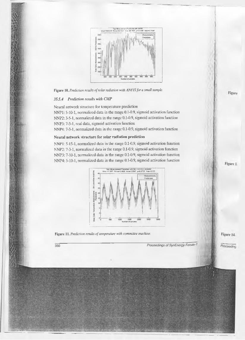
Figure 10. Prediction results o f solar radiation with ANFIS for a small sample.

35.5.4 Prediction results with CMP

Neural network structure for temperature prediction NNP1: 5-10-1, normalized data in the range 0.1-0.9, sigmoid activation function NNP2: 3-5-1, normalized data in the range 0.1-0.9, sigmoid activation function NNP3: 7-3-1, real data, sigmoid activation functionNNP4: 7-3-1, normalized data in the range 0.1-0.9, sigmoid activation function

Neural network structure for solar radiation prediction

NNP1: 5-15-1, normalized data in the range 0.1-0.9, sigmoid activation function NNP2: 7-3-1, normalized data in the range 0.1-0.9, sigmoid activation function NNP3: 7-10-1, normalized data in the range 0.1-0.9, sigmoid activation function NNP4: 5-10-1, normalized data in the range 0.1-0.9, sigmoid activation function

Test W*asu-rement-Pred t t i « i wrth 5m committee machine U s e - 12.1 P77 Rmse= 3.4625 Ame=3.0flv? p=0.87757 Nde*=C.173

Number o f sampies

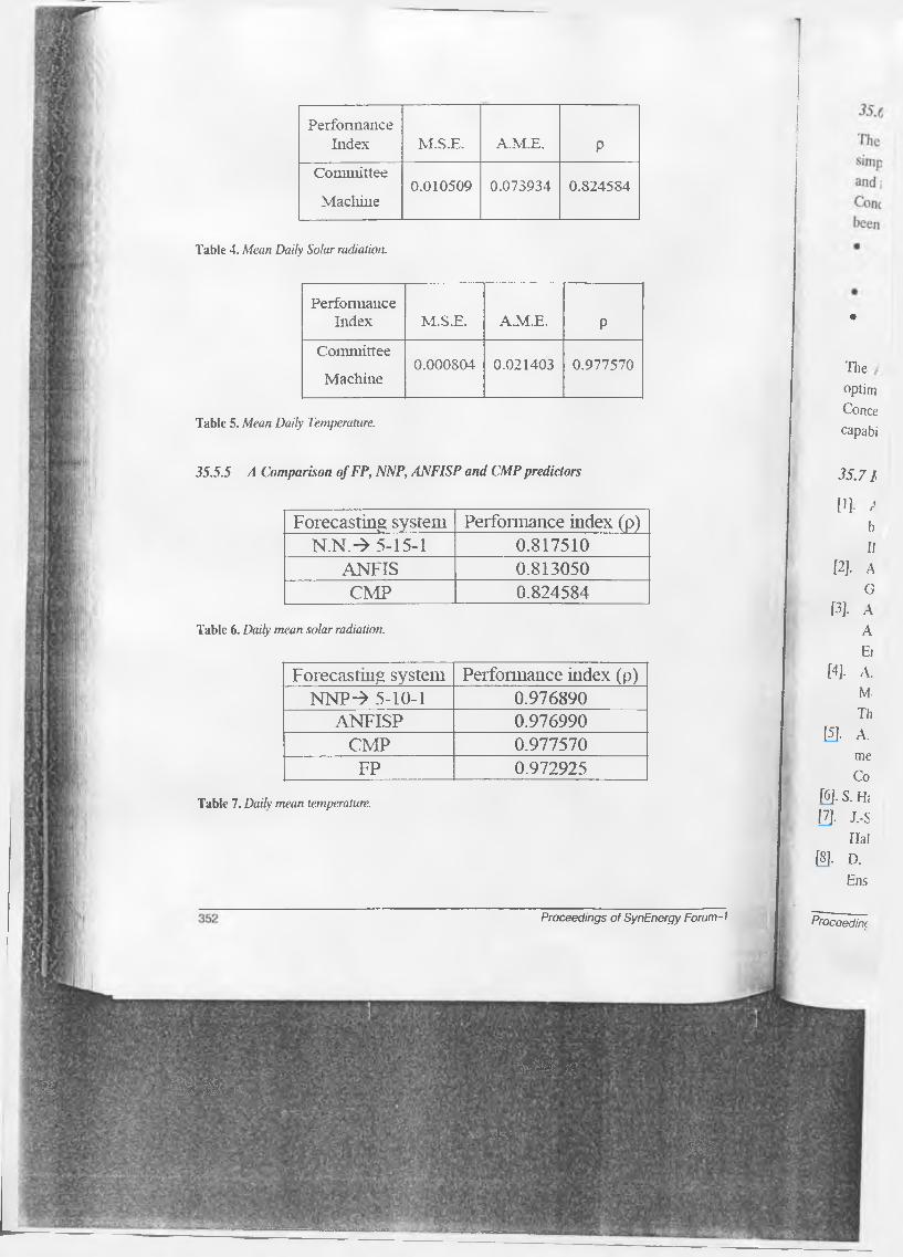
Figure 11. Prediction results o f temperature with committee machine.

Proceedings o f S y n E n e r g y Forum-1

.■Mm

Test Measurers entPredictioe with 5 rh committee machine Mse=l2. <377 Rrase=3<925 Ame=3.3097 {>=0 37757 Ndei=S.17J

Measurements

“ redictions

----------

h 'I'.\

! ; a

• W

W \ i

V

1D3S 10*5 I OS© 1395 HOC 11*35 1113 1115 1120 1125 Number e>: samples

Test Measurement-Prediction wrr. 5th committee machine

Number o f sampies

"s s l MeasurememPte-actioc with 5th convn&ee machine Mse=7t32.148 Rnse=«4.45£ Arr,e=30.9C77 6*2.82458 Ndei=0.2!725

Nu t te r erf samptes

Figure 12. Prediction results o f temperature with committee machine for a small sample.

Figure 13. Prediction results o f solar radiation with committee machine.

Figure 14. Prediction results o f solar radiation with committee machine for a small sample.

Proceedings of SynEnergy Forum-1

. .

h ? « .v .f i s ■ m - m ' > ■ ■ :

*&’‘*o: ■.

m

- toV

•

TheoptimConcecapabi

35.7 /

[1] b II

[2], A G

[3], A A Ei

[4], A. M< Th

[5], A. me Co

[6], S. H;[7], J.-S

Hal[8], D.

Ens

Proceeding

Forecasting system Performance index (p)N.N .-> 5-15-1 0.817510

ANFIS 0.813050CMP 0.824584

PerformanceIndex M.S.E. A.M.E. P

Committee

Machine0.010509 0.073934 0.S24584

PerformanceIndex M.S.E. A.M.E. P

Committee

Machine0.000804 0.021403 0.977570

Forecasting system Performance index (p)NNP-* 5-10-1 0.976890

ANFISP 0.976990

Proceedings of SynEnergy Forum-1

CMPFP

0.9775700.972925

Table 4. Mean Daily Solar radiation.

Table 5. Mean Daily Temperature.

35.5.5 A Comparison o f FP, NNP, ANFISP and CMP predictors

Table 6. Daily mean solar radiation.

Table 7. Daily mean temperature.

35.6 Conclusions

The WM’s method for prediction system presents three important characteristics: simplicity, a one-pass operation on the numerical input-output pairs to find proper rules, and fast computational time. The FP has a good predictive capability.Concerning neural networks that were created and simulated the below conclusions have been excluded:

• The best type of normalization proved to be the one in region 0.1-0.9 in combination with sigmoid activation function in the hidden layer nodes.

• Most suitable choice of inputs is 5 or 7 previous day’s data.

• The number of nodes used in the hidden layer depends on the type and the complexity of the time series, and on the number of inputs.

The ANFISP model proved satisfactory on global prediction and which approaches of optimum neural predictors’ results.Concerning the committee machine predictor, it proved to have a greater predictive capability than other forecasting models.

35.7 References

[1], A. F. Atiya, S. M. El-Shoura, S. 1. Shaheen and M. S. El-Sherif, "A comparison between neural-network forecasting techniques-case study: river flow forecasting", IEEE Tran, on Neural Networks, vol. 10, no. 2, pp. 402-409, 1999.

[2], A. Bardossy and L. Duckstein, "Fuzzy Rule-Based Modeling with Applications to Geophysical, Biological and Engineering Systems", CRC, 1995.

[3]. A. I. Dounis, D. L. Tseles, D. Belis, M. Daratsianakis, "Neuro-Fuzzy Network for Ambient Temperature Prediction", Neties’ 97 European Conference of Networking Entities, Ancona, 1-3 Oct. 1997.

[4], A. I. Dounis, B. Brachos, B. Stathouliss, D. L. Tseles, Neuro-Fuzzy Logic System for Mean Daily Solar Radiation, 2nd Conference Automation and Technology, Thessalonica 2-3 October, 1998, pp. 194-199.

[5]. A. I. Dounis, G. Nikolaou, D. Piromalis and D. L. Tseles, "Model free predictors for meteorological parameters forecasting: a review", 1st International Scientific Conference on Information Technology and Quality, Athens 5-6 June, 2004, A.2.3.

[6], S. Haykin, "Neural Networks-A comprehensive foundation", Prentice Hall, 1999.[7], J.-S. R. Jang, C.-T. Sun, E. Mizutani, "Neuro-Fuzzy and Soft Computing", Prentice

Hall, 1996.[8]. D. Kim and C. Kim, "Forecasting Time Series with Genetic Fuzzy Predictor

Ensemble", IEEE Tr. on Fuzzy Systems, vol. 5, no. 4, pp. 523-535, 1997.

________3rgy Forum-1 j Proceedings of SynEnergy Forum-1 353

II

IS.,

[9]. A. Mountis, G. Levermore, "Weather prediction for feedforward control working on the summer data", 5th Conference on Technology and Automation, Thessalonici, Greece, 15-16 October, 2005.

[10]. Riordan, B. K. Hansen, "A fuzzy case-based system for weather prediction", Engineering Intelligent Systems, vol. 10, no. 3, pp. 139-146, 2000.

[11]. L. X. Wang, "Adaptive Fuzzy Systems and Control Design and Stability Analysis", PTR Prcntice-Hall, 1994.

[12]. L. X. Wang, "The WM Method Completed: A Flexible Fuzzy System Approach to Data Mining", IEEE on FS, vol. 11, no. 6, pp. 768-782, 2003.

[13]. A. S. Weigend, N. A. Gershenfeld, "Time Series Prediction: Forecasting the Future and Understanding the Past" Massachusetts: Addison-Wesley Pub., 1994.

[14]. J. Zisos, A. I. Dounis, G. Nikolaou, G. Stavrakakis, D. Tseles, "Forecasting Temperature and Solar Radiation: An Application of Neural Networks and Neuro- Fuzzy Techniques", 1st International Scientific Conference, Tripoli, eRA, 16-17 Sept., Tripoli, 2006.

36 Optim technc

E. Charami1, S1 Dpt of En:

Macedonia,2 Dpt of Elect

Dpt of Enj Macedonia,

4 Centre for Greece, Tel:

Abstract The provision oj world. Areas an expected to incre, problems especic The reasons ofti water managem< a possible solutu known and effii Energy Sources, economical com\ This paper prese Osmosis (RO) y (CRES) in Kerc desalination Um correlation betwe Unit could produ

354 Proceedings of SynEnergy F o ru rr tA

36.1 Introductii

During the last c systems have be desalination unit production from it with fresh wate2001, p 74).

| Proceedings o f Syi