OPTIMAL INVENTORY POLICIES IN SERIAL SUPPLY ...

iii

OPTIMAL INVENTORY POLICIES IN

SERIAL SUPPLY CHAINS

MULTI-ECHELON INVENTORY MANAGEMENT:

A CASE STUDY IN THE PORCELAIN INDUSTRY

Nuri Mert ONUR

ABSTRACT

In the first chapter, we have summarized the basics of supply chain

management. Integration along the Supply Chain and Natures of Supply Chain

Management problems observed.

In the second chapter, models and potential problems in inventory

management have been studied. Chapter II describes a review of the most important

contributions in lot sizing problems for single and multi-stage of reorder cycle time

models, including some approaches with the power of two restrictions, and the

application of the algorithms.

In the last chapter, the results of the empirical study carried out in Yıldız

Porcelain Factory have been presented. To carry out all the necessary calculations to

assess the required values, we have prepared a visual basic macro through using the

properties of the excel microsoft office program.

In the emprical study the principal objective is to find a solution to the

problem of determining the total costs in multi-stage serial systems in the production

process of porcelain substances using the Szendrovits, Andrew Z. algorithm

approach, satisfying the power of two restrictions. Other secondary objective is to

determine the effectiveness of the power of two approach, comparing the results

obtained in the dissertation prepared by Faik Başaran in 1993. The algorithm

developed is based on the assumption of a multi-stage serial system.

iv

ÖZ

Birinci bölümde, tedarik zincir yönetimi konusunun tanımı ve

özellikleri anlatılmıştır.Tedarik zinciri ve tedarik zincir yönetimindeki

karşılaşılan problemler incelenmiştir.

İkinci bölümde, envanter yönetimindeki modeller ve potansiyel

problemler gösterilmiştir.Ayrıca ikinci bölümde yeniden sipariş verme süresi

modellerinde ikinin kuvveti algoritmasını içerecek şekilde tek ve çok

kademe için kısımlara ayırma problemleri incelenmiştir.

Son Bölümde, Porselen Sanayii alanında uygulanan çalışmanın

sonuçları gösterilmiştir.Sonuçlara ulaşmak için Yıldız Porselen

Fabrikasından Faik Başaran tarafından alınan veriler mikrosoft ofis programı

olan excel’de visual basic bilgisayar dilinde makro yazılarak uygulanmış ve

sonuçlar ortaya konulmuştur.

Yapılan uygulama çalışmasının birincil amacı ikinin kuvveti

algoritmasını Andrew Z. Szendrovits’in algoritmasını kapsayacak şekilde

çok kademeli seri sistem olan porselen sanayii örneğinde uygulayıp toplam

maliyetleri bulmaktır.İkincil amaç ikinin kuvveti algoritmasına göre bulunan

değerleri 1993 yılında İstanbul’da Faik Başaran tarafından hazırlanmış

doktora tezindeki değerlerle karşılaştırıp algoritmanın efektifliğini ortaya

çıkarmaktır.Uygulanan algoritma çok kademeli seri sistem için

tasarlanmıştır.

v

Acknowledgments

It gives me great pleasure to acknowledge the many people who have

contributed to the development of this thesis.

I am especially grateful to Prof.Dr.Güneş Gençyılmaz. In the past three years,

I have benefitted from his valuable advices, expertises and directions. I have truly

appreciated his unwavering patience, especially as I tried to manage my conflicting

responsibilities at İstanbul Kültür University. Without his never-ending support

and encouragement, this thesis would not have been possible. His encouragement

and guidance have made this research a rewarding experience.

I would like to extend my sincere gratitude to my advisor Assistant Prof. Faik

Başaran for providing constant inspiration and guidance throughout the course of this

Research. I gratefully acknowledge my indebtedness to him for his time and patience.

I am especially indebted to Assistant Prof. Gülsüm Savcı Gökgöz for her

continuing support throughout the development of this thesis.

I would like to thank Prof. Dr. Tülin Aktin, Assistant Prof. Rıfat Özdemir and

Assistant Prof. Ufuk Kula. Their suggestions have also improved this thesis.

Many thanks go to each of my colleagues in the department of Business

Administration and Industrial Engineering at İstanbul Kültür University for his and

her support and encouragement. I have been very fortunate to be able to work on

such challenging problems with such a great group of people. A special thanks goes

to each Teaching Assistants Erol Muzır, Halis Sak and M.Taha Bilişik for reviewing

this study, and their valuable suggestions.

Special thanks goes to my friends Kemal-Emel Demircan and Mete Gülaçtı

for their continuing encouragement and support.

vi

Sincere thanks go to my parents, who taught me the proper attitude

toward life. They always remind me of the importance of perseverance, health,

and happiness. I found these attitudes are very beneficial in pursuing my degree

and maintaining a good balance between work and family. From my early years at

İstanbul University, to these past years, I have been perpetually "busy" and have

asked my family to sacrifice a lot. I am truly grateful that they have supported me,

and enabled me to excel in my studies as a result.

Finally, I would like to thank my fiance, Ayşegül, a soulmate and a forever,

faithful presence in my life. Her constant love supported me in overcoming many

obstacles and frustrations in these years. I especially thank her for enduring countless

lonely hours when I struggled by myself. One thing worth nothing is that she always

shows high interest in my work. I therefore owe my deepest thanks to her.

vii

TABLE OF CONTENTS

ABSTRACT .......................................................................................................... iii

ÖZ.......................................................................................................................... iv

LIST OF TABLES..................................................................................................x

LIST OF FIGURES.............................................................................................. xi

ABBREVIATIONS.............................................................................................. xii

INTRODUCTION ..................................................................................................1

1. CONCEPTUAL FRAMEWORK...................................................................2

1.1. Supply Chain Management........................................................................2

1.1.1. Basics of Supply Chain Management.................................................2

1.1.1.1. Definition of Supply Chain Management ...................................4

1.1.1.2. Integration along the Supply Chain ............................................5

1.1.1.3. Natures of Supply Chain Management Problems........................6

1.1.1.4. Important Issues in Efficient Supply Chain Planning..................9

1.1.1.5. Push-based versus Pull-based Supply Chain.............................10

1.1.1.5.1. Push-based Supply Chain System..........................................10

1.1.1.5.2. Pull-based Supply Chain System ............................................11

2. MODELS AND POTENTIAL PROBLEMS IN INVENTORY

MANAGEMENT ..................................................................................................13

2.1. Lot Sizing Problems and Models as a Remedy to Lot Sizing Problems....13

2.1.1. Single Stage Models ........................................................................13

2.1.2. Multi-Stage Models .........................................................................15

2.2. Types of Inventory Models......................................................................18

2.2.1. The Basic EOQ Model.....................................................................21

2.2.1.1. Multiple Items EOQ Models ....................................................22

2.2.1.2. Resource Constrained Multiple Items EOQ Models .................22

viii

2.2.1.3. EOQ For Multiple Items With One Constraint .........................22

2.2.1.4. EOQ For Multiple Items With Two Constraint.........................26

2.2.2. Dynamic Lot Sizing Models ............................................................30

2.2.2.1. Example For Dynamic Lot Sizing Models................................30

2.2.2.1.1. Period Order Quantity ...........................................................31

2.2.2.1.2. Fixed Period Demand............................................................32

2.2.2.1.3. Lot For Lot Rule (L4L) .........................................................34

2.2.2.1.4. Silver-Meal Method ..............................................................35

2.2.2.1.5. Wagner-Whitin Algorithm ....................................................37

2.2.3. The Model by Crowston, Wagner, and Williams..............................43

2.2.3.1. Simple Extensions of the Model...............................................43

2.2.4. Reorder Cycle Time Problems .........................................................44

2.2.5. Power – of – two Policy...................................................................47

3. EMPIRICAL STUDY ...................................................................................49

3.1. Purpose & Scope Of The Study ...............................................................49

3.1.1. Purpose............................................................................................49

3.1.2. Scope...............................................................................................49

3.2. History of Porcelain.................................................................................50

3.3. Kinds of Porcelain ...................................................................................54

3.4. History of Yıldız Porcelain Factory ..............................................................55

3.5. Production Structure Studied ........................................................................56

3.6. Information of Production Structure .............................................................64

3.7. Methodology................................................................................................98

3.8. Problem Definition.......................................................................................98

3.9. Maxwell and Muckstadt Approach ...............................................................98

3.10. Implementation of the Empirical Study ....................................................101

Large Brimmed Soup Bowl .......................................................................110

LBSB Lid..................................................................................................111

ix

Brimmed Regular Plate ∅29 cm...............................................................112



Brimmed Hollow Plate ∅21 cm ................................................................115

Brimmed Oval Plate ∅35 cm ....................................................................116

Brimmed Oval Plate ∅21 cm ....................................................................117

Large Brimmed Compote Bowl.................................................................118

Brimmed Compote Bowl...........................................................................119

Brimmed Creamer.....................................................................................120

Brimmed Creamer Saucer .........................................................................121

Brimmed Salt Shaker.................................................................................122

Brimmed Lemon Plate...............................................................................123

CONCLUSION ...................................................................................................125

REFERENCES ...................................................................................................127

x

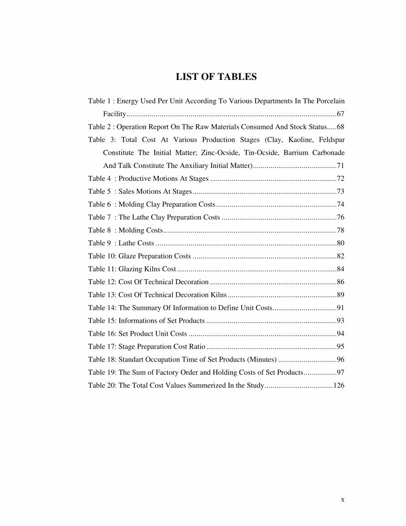
LIST OF TABLES

Table 1 : Energy Used Per Unit According To Various Departments In The Porcelain

Facility............................................................................................................67

Table 2 : Operation Report On The Raw Materials Consumed And Stock Status.....68

Table 3: Total Cost At Various Production Stages (Clay, Kaoline, Feldspar

Constitute The Initial Matter; Zinc-Ocside, Tin-Ocside, Barrium Carbonade

And Talk Constitute The Anxiliary Initial Matter)...........................................71

Table 4 : Productive Motions At Stages .................................................................72

Table 5 : Sales Motions At Stages..........................................................................73

Table 6 : Molding Clay Preparation Costs..............................................................74

Table 7 : The Lathe Clay Preparation Costs ...........................................................76

Table 8 : Molding Costs.........................................................................................78

Table 9 : Lathe Costs .............................................................................................80

Table 10: Glaze Preparation Costs ..........................................................................82

Table 11: Glazing Kilns Cost ..................................................................................84

Table 12: Cost Of Technical Decoration .................................................................86

Table 13: Cost Of Technical Decoration Kilns ........................................................89

Table 14: The Summary Of Information to Define Unit Costs.................................91

Table 15: Informations of Set Products ...................................................................93

Table 16: Set Product Unit Costs ............................................................................94

Table 17: Stage Preparation Cost Ratio ...................................................................95

Table 18: Standart Occupation Time of Set Products (Minutes) ..............................96

Table 19: The Sum of Factory Order and Holding Costs of Set Products.................97

Table 20: The Total Cost Values Summerized In the Study...................................126

xi

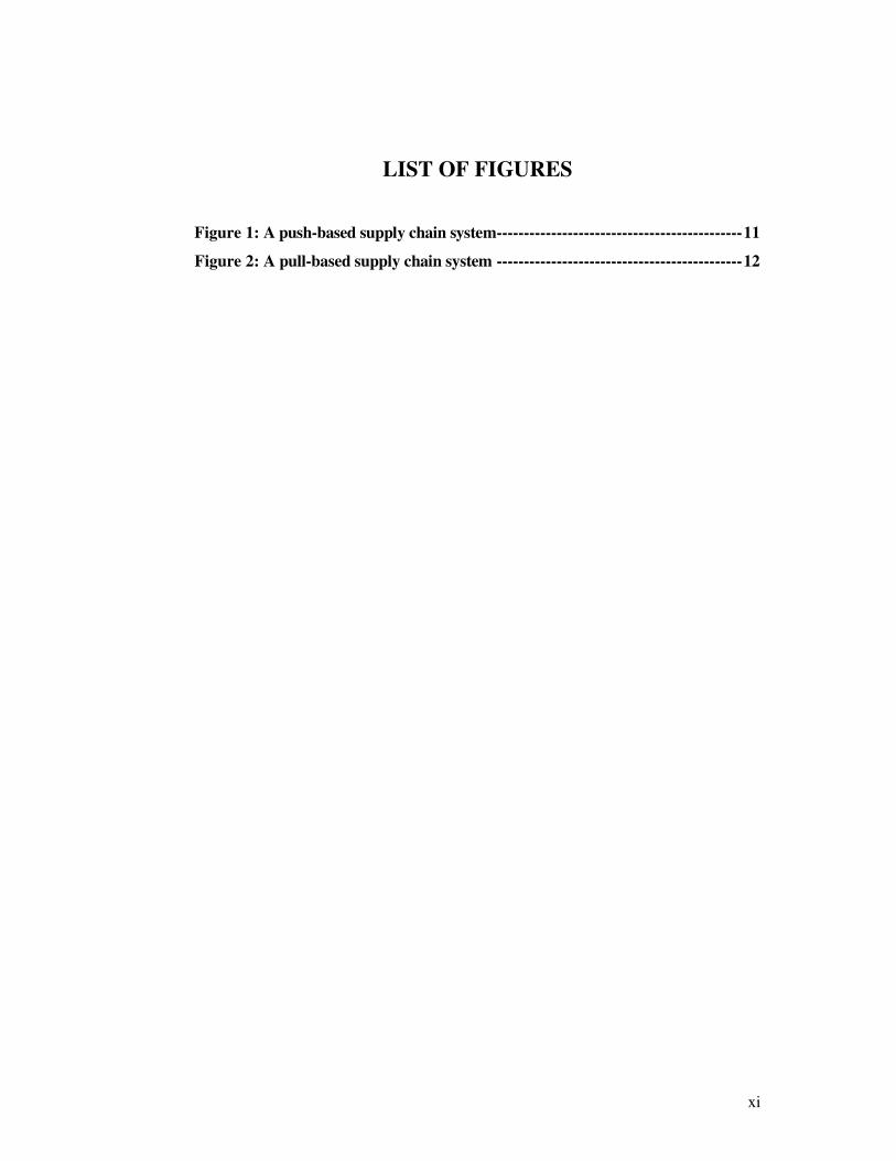
LIST OF FIGURES

Figure 1: A push-based supply chain system---------------------------------------------11

Figure 2: A pull-based supply chain system ---------------------------------------------12

xii

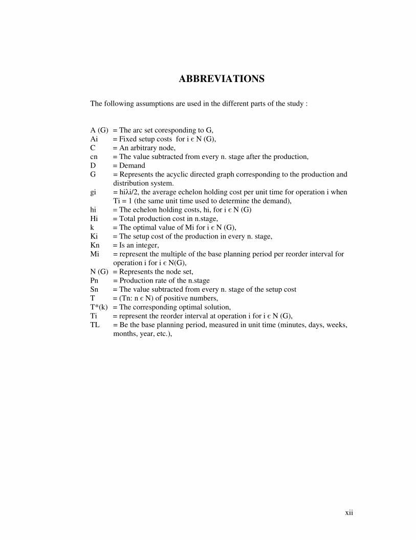
ABBREVIATIONS

The following assumptions are used in the different parts of the study : A (G) = The arc set coresponding to G, Ai = Fixed setup costs for i є N (G), C = An arbitrary node, cn = The value subtracted from every n. stage after the production, D = Demand G = Represents the acyclic directed graph corresponding to the production and

distribution system. gi = hiλi/2, the average echelon holding cost per unit time for operation i when

Ti = 1 (the same unit time used to determine the demand), hi = The echelon holding costs, hi, for i є N (G) Hi = Total production cost in n.stage, k = The optimal value of Mi for i є N (G), Ki = The setup cost of the production in every n. stage, Kn = Is an integer, Mi = represent the multiple of the base planning period per reorder interval for

operation i for i є N(G), N (G) = Represents the node set, Pn = Production rate of the n.stage Sn = The value subtracted from every n. stage of the setup cost T = (Tn: n є N) of positive numbers, T*(k) = The corresponding optimal solution, Ti = represent the reorder interval at operation i for i є N (G), TL = Be the base planning period, measured in unit time (minutes, days, weeks,

months, year, etc.),

1

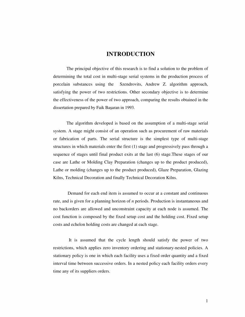
INTRODUCTION

The principal objective of this research is to find a solution to the problem of

determining the total cost in multi-stage serial systems in the production process of

porcelain substances using the Szendrovits, Andrew Z. algorithm approach,

satisfying the power of two restrictions. Other secondary objective is to determine

the effectiveness of the power of two approach, comparing the results obtained in the

dissertation prepared by Faik Başaran in 1993.

The algorithm developed is based on the assumption of a multi-stage serial

system. A stage might consist of an operation such as procurement of raw materials

or fabrication of parts. The serial structure is the simplest type of multi-stage

structures in which materials enter the first (1) stage and progressively pass through a

sequence of stages until final product exits at the last (6) stage.These stages of our

case are Lathe or Molding Clay Preparation (changes up to the product produced),

Lathe or molding (changes up to the product produced), Glaze Preparation, Glazing

Kilns, Technical Decoration and finally Technical Decoration Kilns.

Demand for each end item is assumed to occur at a constant and continuous

rate, and is given for a planning horizon of n periods. Production is instantaneous and

no backorders are allowed and unconstraint capacity at each node is assumed. The

cost function is composed by the fixed setup cost and the holding cost. Fixed setup

costs and echelon holding costs are changed at each stage.

It is assumed that the cycle length should satisfy the power of two

restrictions, which applies zero inventory ordering and stationary-nested policies. A

stationary policy is one in which each facility uses a fixed order quantity and a fixed

interval time between successive orders. In a nested policy each facility orders every

time any of its suppliers orders.

2

The organization of the document is as follows. Chapter II describes a review

of the most important contributions in lot sizing problems for single and multi-stage

models, for reorder cycle time models, including some approaches with the power of

two restrictions, and the application of the algorithms. In the last chapter, the results

of an empirical study carried out in Yıldız Porcelain Factory have been presented.

1. CONCEPTUAL FRAMEWORK

1.1. Supply Chain Management

In the past few years, interest in supply chain management has grown dramatically.

This interest has forced many firms to adjust and analyze their supply chains. In most

cases, however, this has been done based on experience and intuition; very few

analytical models or design tools have been used in this process. In this chapter, we

summarize the basics of supply chain management.

1.1.1. Basics of Supply Chain Management

An accelerating trend toward globalization marked the latter half of the

twentieth century and the beginning of the present one. It is common to see a

company design, produce and distribute products through a global network to

provide the best customer service at the lowest price. Coordination throughout the

entire logistical system must be planned and managed, because of the impact in costs

that it represents to the companies and their opportunity to compete in today’s global

market.

The central issue in the supply chain performance is the inventory

management. Inventories are present at every stage of the supply chain as raw

materials to finished goods. The inventory acts as a buffer against any uncertainty,

but holding inventory is costly and runs the risk of product deterioration and

obsolescence. The focus of inventory problems traditionally has been on lot size

determination. Supply occurs in discrete batches or lots and items proceeds through a

3

sequence of stages. The issue of the lot sizing is to determine how large these lots

should be trying to find the best balance between fixed costs and inventory holding

costs. Ford Harris in 1915 introduced the classic Economic Lot Size Model which

serves as reference for many other research studies.

Therefore, the lot sizing problem can be formulated as the problem of

determining the reorder interval time, because of a functional relationship between

the lot size and the manufacturing cycle time. Due to the fact that this problem is

continuous and that the reorder optimal interval can take any positive real value, is

often impractical to implement it. This is referred to a discrete problem imposing the

restriction that the reorder interval can take only positive integer values. Maxwell and

Muckstadt (1985) explain the advantages of formulating the problem in terms of

reorder intervals rather than in terms of lot sizes. They establish three principal

reasons for this: (1) the experience that production planning is more naturally

centered around the frequency of production because it dictates the numbers of set-

ups, the requests for tooling and fixtures, and the demands on the material handling

system, (2) the mathematical representation of the model is simplified, and (3) from a

scheduling point of view it is often practical to keep reorder intervals constant in the

face of minor changes to demand forecasts and to adjust lot sizes accordingly.

A special case is given by considering the discrete problem with the power of

two restrictions in which the reorder interval is constraint to be not only integer, but

also a power of two. The power-of-two policy was developed by Roundy (1985). It

considers the problem of determining the reorder interval instead of the reorder

quantity and has the advantage of an easy implementation, even if the system is very

complex and it is known that the cost of the optimal solution for the discrete problem

using the power-of-two solution of a continuous problem is within about 6% of the

cost of the optimal solution of the continuous problem without those restrictions.

Implementing power of two policies makes production scheduling easier, and

ensures that production cycles regenerate as frequently as possible, so that inventory

imbalances that in practice can be easily corrected. Although considerable research

has been devoted to traditional methods of search, optimization using such methods

4

is not that efficient, particularly in finding a solution for very complex search space.

Furthermore, significant less attention has been paid to stochastic search and

optimization techniques like genetic algorithms. Khouja, Michalewicz and Wilmot

(1998) presented a genetic algorithm for solving the Economic Lot Size Scheduling

Problem finding better solutions than the iterative dynamic programming approach.

Genetic algorithms have been employed to solve optimization problems across all

disciplines and interests, obtaining global optimal or near optimal solutions in

complex search spaces. Their simplicity permits their use to solve difficult problems,

showing an important reduction in the computational time.

1.1.1.1. Definition of Supply Chain Management

Supply chain management or logistics management refers to the management of

the flow of goods from points-of-origin to points-of-consumption. In the past, a

variety of names have been used according to Lambert and Stock (1993):

Physical distribution Materials Management

Distribution Materials logistics management

Distribution engineering Logistics

Business logistics Quick-response systems

Marketing logistics Industrial logistics

Distribution logistics

Nowadays, supply chain management and logistics management seem to be the

most widely accepted term. The Council of Logistics Management, one of the largest

and most prestigious groups of logistics professionals, provides the excellent definition

of logistics management as following:

"Logistics management is the process of planning, implementing and controlling

the efficient, cost effective flow and storage of raw material, in-process inventory,

finished goods, and related information from point-of-origin to point-of-consumptionfor

the purpose of conforming to customer requirements."

5

Supply chain management or logistics management is a vital part of a firm's

operation. Logistics is the third-largest source of cost of doing business for a typical

firm after manufacturing and marketing. Efficient and effective management of the

logistics function can have a substantial impact. Logistics cost is reduced, profitability

is improved, and the level of customer service is increased. There are a number of key

factors in supply chains, Arnold and Chapman (2000):

- A supply chain includes all activities and processes to supply a product or

service to an end customer.

- Any number of companies can be linked in the supply chain.

- A customer can be a supplier to another customer so the total chain can have

a number of supplier/customer relationships.

- While the distribution system can be direct from supplier to customer, it can

contain a number of intermediaries (distributors) such as wholesalers,

warehouses, and retailers.

- Product or services usually flow from supplier to customer and design

and demand information usually flows from customer to supplier.

1.1.1.2. Integration along the Supply Chain

Basically, the integrated supply chain management concept refers to

administering all supply chain activities as an integrated system. Integrating all

distribution-related activities in the supply chain as mentioned in the previous section

can reduce total operating costs of a company. Without this integrated approach, the

costs to satisfy customer demand and expectations will be higher. A company must

make a decision that coordinates all set of activities within the supply chain or business

interfaces. The following are the list of critical business interfaces within the supply

chain.

- Supplier-purchasing

- Purchasing-production

- Production-marketing

6

- Marketing-distribution

- Distribution-intermediary (wholesaler and/or retailer)

- Intermediary-customer/end-user

These business interfaces must be considered as a whole since uncoordinated

decisions involving these activities could cause a build up of inventory along the supply

chain. Now, the decisions of purchasing are not only concerning about the low per unit

costs for raw material, but also need to consider the production to achieve the lowest

per-unit production costs. All decisions within the business interfaces must be made

under the same goal, which is minimize the inventory holding costs and logistics costs

or total operating costs of the firm. Management should strive to minimize the total

operating costs rather than the cost of each activity. Attempts to reduce the cost of

individual activities may lead to increased total costs. For example, consolidating

finished goods inventory in a small number of distribution centers will reduce

inventory carrying costs and warehousing costs but may lead to an increase in freight

expense or a lower sales volume. On the other hand, savings associated with large

volume purchases may increase the inventory carrying costs. So, reductions in one cost

may lead to increase in the costs of other activities. Effective supply chain

management can be accompolished only by viewing logistics as an integrated system,

and also minimizing its total operating cost subject to the company's customer service

objectives.

1.1.1.3. Natures of Supply Chain Management Problems

Generally supply chain management problems involve the decision on how

products are to move through the supply and distribution channels, and at the

operational level, this includes decision on how to fill a recently received customer

order, how to respond to a temporary transportation rate reduction, and also how to

route the current customer orders. Each day the supply chain system operates to move

the products smoothly and efficiently through the channel. Basically the planning in

supply chain management can be divided into four major decision areas: customer

7

service standards, distribution network configuration, inventory policy or deployment,

and transportation system selection and routing.

Customer service standards: The design of supply chain system greatly affects

the level of customer service. Conversely, the level of customer service to be provided

definitely impacts the design of supply chain systems. High levels of service normally

use decentralized inventories at several locations and the use of, sometime, more

expensive forms of transportations. Low levels of service generally require the use of

less expensive forms of transportations and allow centralized inventories at few

locations. It is known that high levels of service equates to high logistics costs. So, the

first priority in supply chain planning must be the proper setting of customer service

levels. Ballou (1999) suggests that effective supply chain planning should start with a

survey of customer service needs and desires.

Distribution network configuration: Distribution network decision involves how

to place the stocking points and the sourcing points in the supply chain system. This

also includes the number, location, and size of the facilities and assigning market

demands to each facility. Generally distribution network problem includes all product

movements and associated costs starting from plants/suppliers all the way to end

customers. Finding the minimum assignment cost is the ultimate goal of distribution

network planning. The following are the key questions in distribution network

problem:

- What are the best number, location, and size of stocking points?

- Which plants/suppliers should serve which stocking points/facilities?

- Which products should be shipped directly from plants/suppliers to

customers and which should be transshipped through the warehousing

system?

Inventory policy: In general two strategies, push inventory and pull inventory are

involved in managing inventory throughout a supply chain. The push inventory

8

strategy refers to a make-to-stock policy while a pull inventory policy refers to a

demand-drive policy. More details on the push and pull inventory policies will be

presented again in a later section. An effective inventory policy tries to reduce the

number of stocking points throughout the supply chain system. This will reduce the

amount of inventory carried in the system including the safety stocks. However, the

cost reduction associated with inventory consolidation is in trade-off with higher

transportation costs. With fewer stocking points, smaller outbound shipment sizes with

higher shipping charges must be weighed against larger shipment sizes of inbound

goods that travel through longer distances to the marketplace. Therefore, the

distribution network decision must be sensitive to the inventory deployment and control

policies used. This indicates that inventory policy directly affects the distribution

network decision and the whole supply chain planning. The following are common

questions related to inventory policy:

- What turnover ratio should be maintained?

- Which products should be maintained at which stocking points?

- What level of product availability should be maintained in inventory?

- Which method of inventory control is best?

- Should push or pull inventory strategies be used?

Transport selection and routing: Transportation selection and routing decisions

directly affect the supply chain decisions. The number, size and location of stocking

points depend on the transportation policies of the company as much as inventory

policies. As the number of stocking points increases, fewer customers will be assigned to

any one point, the mode of transportation may change and this will affect the

transportation cost. The following are questions related to the transportation system

selection and routing:

- Which customers should be served out of which stocking points?

- Which transportation types, truckload (TL) or less than truckload (LTL),

should be assigned to which customers?

- Which modes of transportation, Rail, Truck, Air, Water, or Pipeline, should

be used?

9

1.1.1.4. Important Issues in Efficient Supply Chain Planning

Cost trade-offs: Supply chain planning needs to balance all conflicting costs such

as transportation costs versus inventory costs, production costs versus distribution

costs, and ultimately customer service costs versus all supply chain costs. All issues in

the supply chain must be considered as a whole to avoid any suboptimal plans. Both

facility location and distribution issues must be addressed at the same time, since output

of facilities location decision is the input to the distribution system and are

economically related to one another.

Consolidation: Consolidation happens when small shipments are consolidated to

form a large shipment to gain the economies of scale. For example, two or more

customer orders might be combined with other customer orders received at other time

periods to form a large shipment if possible. Consolidation strategy will lower average

per-unit shipping costs. This also avoids shipping small quantities of items over long

distances at high per-unit transport rate. In general, the concept of consolidation will

be useful when the quantities shipped are small.

Postponement: The key idea of postponement is "to ship as much as you can as

far as you can before committing to the end product." The final product processing

and distribution are delayed until a customer order is received. This is done to avoid

increasing total inventory level throughout the company logistics network and the

possibility of obsolete stocks. Postponement can be classified into five types;

Labeling, Packaging, Assembly, Manufacturing, and Time.

Mixed strategy: A mixed strategy allows an optimal strategy to be established

for separate product groups. Usually mixed strategy leads to lower costs than a single

or global strategy. In general, single strategies can benefit from economies of scales

and administrative simplicity however they ineffectively perform when the product

groups vary in terms of cube, weight, order size, sales volume, and customer service

requirements. Examples of a mixed strategy include using of some public warehousing

along with privately owned space, shipping product directly from the plants along with

10

from the warehouses, and filling customer order from a single warehouse along with

instances of shipping from multiple warehouses for some products.

1.1.1.5. Push-based versus Pull-based Supply Chain

Supply chain or logistics systems are normally categorized as push-based or

pull-based systems. In a push-based supply chain system, long-term forecasts are used

to determine a firm's production. On the other hand, in a pull-based supply chain

system, production is demand driven, and therefore is directly related to actual

customer demands instead of a forecast. With actual demands, a firm can decrease

inventory both at the retail and the manufacturing levels and also decrease the

variability in the system due to lead-time reduction. A significant reduction in system

inventory level and costs make a pull-based system more superior to a push-based

system. The trend today is toward pull-based system even though it is more difficult to

implement than a push-based system. The succeeding sections summarize key concepts

of these two supply chain systems.

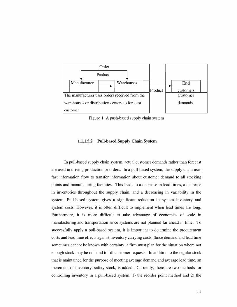
1.1.1.5.1. Push-based Supply Chain System

In a push-based supply chain system, production decisions are based on long-

term forecasts. Orders from the retailer's warehouses are used to forecast customer

demand. This system is appropriate where production or purchase quantities exceed the

short-term requirements of the inventories. However, a firm may have the problem of

overstocking or excess inventory. The excess inventory could become obsolete,

damaged, or nonfunctional because of age. High inventory leads to high inventory cost.

A push-based system also produces larger and more variable production batches and

this can impact the customer service levels, since the system has the inability to meet

changing demand patterns. Moreover, a push-based supply chain increases

transportation costs, heightens inventory levels and heightens manufacturing costs, due

to inability to meet or react to changing market conditions. Figure 1.1 shows a push-

based system.

11

Order

Product

End

Manufacturer

Warehouses

Product customers The manufacturer uses orders received from the

warehouses or distribution centers to forecast

customer

Customer

demands

Figure 1: A push-based supply chain system

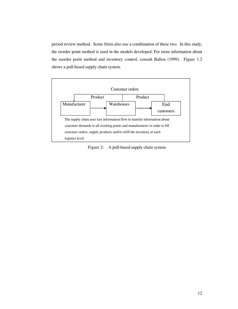
1.1.1.5.2. Pull-based Supply Chain System

In pull-based supply chain system, actual customer demands rather than forecast

are used in driving production or orders. In a pull-based system, the supply chain uses

fast information flow to transfer information about customer demand to all stocking

points and manufacturing facilities. This leads to a decrease in lead times, a decrease

in inventories throughout the supply chain, and a decreasing in variability in the

system. Pull-based system gives a significant reduction in system inventory and

system costs. However, it is often difficult to implement when lead times are long.

Furthermore, it is more difficult to take advantage of economies of scale in

manufacturing and transportation since systems are not planned far ahead in time. To

successfully apply a pull-based system, it is important to determine the procurement

costs and lead time effects against inventory carrying costs. Since demand and lead time

sometimes cannot be known with certainty, a firm must plan for the situation where not

enough stock may be on hand to fill customer requests. In addition to the regular stock

that is maintained for the purpose of meeting average demand and average lead time, an

increment of inventory, safety stock, is added. Currently, there are two methods for

controlling inventory in a pull-based system; 1) the reorder point method and 2) the

12

period review method. Some firms also use a combination of these two. In this study,

the reorder point method is used in the models developed. For more information about

the reorder point method and inventory control, consult Ballou (1999). Figure 1.2

shows a pull-based supply chain system.

Customer orders

Product Product

End Manufacturer

Warehouses

customers

The supply chain uses fast information flow to transfer information about

customer demands to all stocking points and manufacturers in order to fill

customer orders, supply products and/or refill the inventory at each

logistics level.

Figure 2: A pull-based supply chain system

13

2. MODELS AND POTENTIAL PROBLEMS IN

INVENTORY MANAGEMENT

Inventory problems have been studied for many years. This review describes

some of the most important contributions in this field. It includes methods used to

solve single and multi-stage lot sizing problems. For multi-stage systems, some

models are shown that deal with special cases like capacity constraint and joined

setup costs. Finally, it is presented some algorithms applications that can be

considered as previous work in lot sizing problems.

2.1. Lot Sizing Problems and Models as a Remedy to Lot Sizing Problems

2.1.1. Single Stage Models

For many years the main focus of the inventory theory has been in the lot size

determination. Many authors try to solve the single stage problem. The classic

Economic Lot Size Model, introduced by Ford Harris in 1915, is a very basic model

that considered a warehouse facing constant demand for a single item. It assumes

constant fixed cost, instantaneous batch delivery following a deterministic lead time,

all replenishment orders are for the same quantity and no shortages are allowed. The

total cost per time TC (Q), is composed by ordering cost, product purchase cost and

inventory holding cost.

TC (Q) = ordering cost + purchased cost + inventory holding cost

TC (Q) = AD / Q + CD + hQ / 2 (Equation 1.1)

Based on the cycle inventory level over time, the inventory level decreased

constantly from the order quantity size (Q) to zero each cycle, and averages Q/2. The

process repeats each time Q units are sold (every T=Q/D), integrating over this cycle

length it can be found the average inventory, I.

14

Q/D

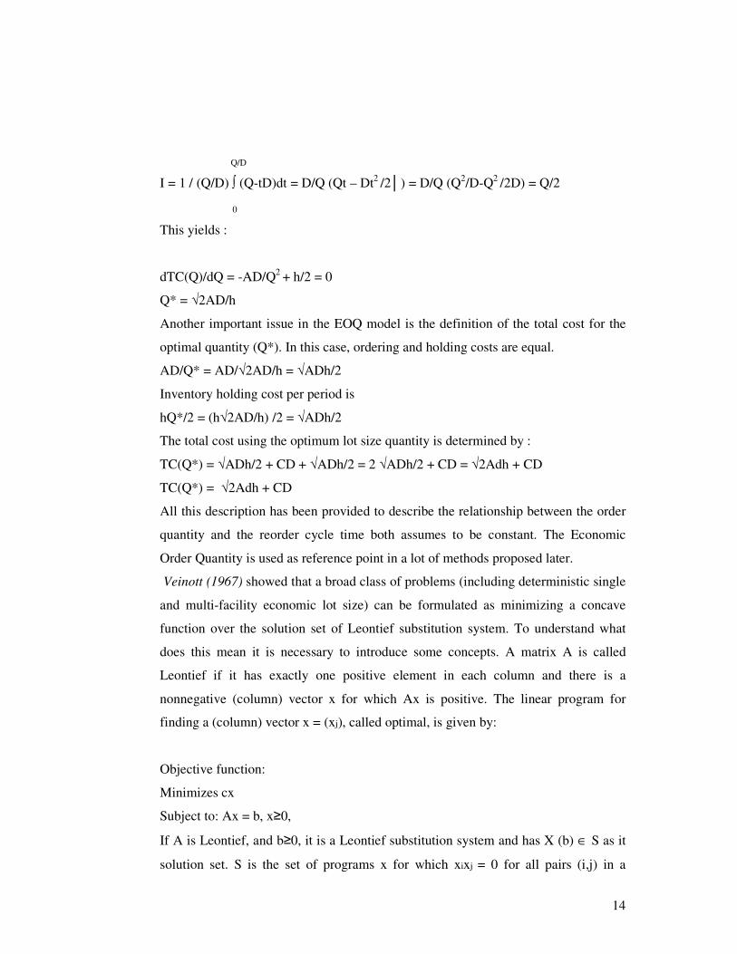
I = 1 / (Q/D) ∫ (Q-tD)dt = D/Q (Qt – Dt2 /2│) = D/Q (Q2/D-Q2 /2D) = Q/2

0

This yields :

dTC(Q)/dQ = -AD/Q2 + h/2 = 0

Q* = √2AD/h

Another important issue in the EOQ model is the definition of the total cost for the

optimal quantity (Q*). In this case, ordering and holding costs are equal.

AD/Q* = AD/√2AD/h = √ADh/2

Inventory holding cost per period is

hQ*/2 = (h√2AD/h) /2 = √ADh/2

The total cost using the optimum lot size quantity is determined by :

TC(Q*) = √ADh/2 + CD + √ADh/2 = 2 √ADh/2 + CD = √2Adh + CD

TC(Q*) = √2Adh + CD

All this description has been provided to describe the relationship between the order

quantity and the reorder cycle time both assumes to be constant. The Economic

Order Quantity is used as reference point in a lot of methods proposed later.

Veinott (1967) showed that a broad class of problems (including deterministic single

and multi-facility economic lot size) can be formulated as minimizing a concave

function over the solution set of Leontief substitution system. To understand what

does this mean it is necessary to introduce some concepts. A matrix A is called

Leontief if it has exactly one positive element in each column and there is a

nonnegative (column) vector x for which Ax is positive. The linear program for

finding a (column) vector x = (xj), called optimal, is given by:

Objective function:

Minimizes cx

Subject to: Ax = b, x≥0,

If A is Leontief, and b≥0, it is a Leontief substitution system and has X (b) ∈ S as it

solution set. S is the set of programs x for which xixj = 0 for all pairs (i,j) in a

15

specified set. In applications it is often appropriate to impose additional restrictions

of the form xixj = 0, for example in production problems if it is possible to produce

only one product in each period.

Leontief substitution systems seem to provide a natural setting for studying

inventory models with concave costs. Their applications are on single and multi-

facility lot size problem, lot-size-smoothing and warehousing models. Their

algorithms required a computational effort that increases algebraically with the size

of the problem instead of exponentially.

2.1.2. Multi-Stage Models

Multi-echelon inventory systems can be used to optimize the deployment of

inventory in a supply chain. Multi-stage manufacturing situations (raw materials,

components, subassemblies, assemblies) are conceptually very similar to multi-

echelon inventory systems. Multi-echelon models examine the entire system,

searching better solutions for the entire chain, not each stage independently. This

coordination has the advantage of given better global solutions. In the multi-stage

systems there have been a lot of contributions in serial, assembly, distribution,

general and some special structures.

Clark and Scarf (1960) introduced the echelon stock concept which permits

some very convenient mathematical simplifications. They define the echelon stock of

echelon j (in general multi-echelon system) as the number of units in the system that

are at, or have passed through, echelon j but have as yet not been specifically

committed to outside customers. They considered the problem of determining

optimal purchasing quantities in a multi-stage serial and distribution models. Echelon

j stock may often be considered to be the facility j value-added inventory. The Clark-

Scarf model allows stochastic demand and convex holding costs, but setup costs are

assumed to be associated with no more than two facilities.

16

Crowston, Wagner and Henshaw (1972) made a comparison of exact and

heuristics routines for lot size determination in multi-stage assembly systems. They

concluded that economic lot sizes in multi-stage assembly systems can be determined

by dynamic programming for problems of moderate size, while heuristic search

routines appear to be promising for large problems. Using these results Crowston,

Wagner and Williams (1973) present a model for multi-stage assembly systems to

compute a set of optimal lot sizes so that the lot size at each facility is a positive

integer multiple of the lot size at its successor facility. It is important to mention that

they considered the serial system as a special case of the assembly system. Their

model assumes constant continuous final demand, instantaneous production at each

stage and infinite planning horizon.

A few years later, Williams (1982) proved that the well known theorem by

Crowston, Wagner and Williams (1973) shows to be defective. The theorem

establishes that an optimal solution to the batch size determination problem for

multi-echelon production/inventory assembly structures is characterized by a set of

lot sizes, such that the lot size at each stage must be an integer multiple of the lot size

at its successor stage. The theorem proved to be defective at the point that results

were extended from two level systems to more general assembly systems.

Schwarz (1973) deals with a one-warehouse n-retailer deterministic

inventory system with known demands. As a conclusion, he shows that the form of

the optimal policy can be very complex for more than four retailers and he argues for

restricting attention to a simpler class of strategies (where each location’s order

quantity does not change with time) and develops an effective heuristic for finding

good solutions.

Schwarz and Schrage (1975) make use of the myopic strategy. Myopic

policies optimize a given objective function with respect to any two stages and

ignore multi-stage interaction effects. Optimal and near optimal policies were

proposed for multi-echelon production/inventory assembly systems under continuous

review with constant demand over and infinite planning horizon. Schwarz and

17

Schrage model was widely used as a standard among the multi-stage

production/inventory models.

Szendrovits (1981) presented a comment on the optimality in Schwarz and

Schrage model, considering that their restrictions could be helpful to facilitate

analytical tractability, but do not necessarily lead to optimal inventory policies as

claimed by the authors. Szendrovits showed that a lower cost solution could be

obtained in sample problems when the integrality constraint was violated. The

example provided a lower cost solution by permitting two lots at a given stage to

provide the total input for the three lots at its successor stages.

Later, Blackburn and Millen (1985) proposed simple cost modifications to

improve the global optimality of the Schwarz and Schrage procedure. The

effectiveness of these alternative modifications was tested through a series of

simulation experiments. A new formulation of the lot sizing problem in multi-stage

assembly systems which leads to an effective optimization algorithm was proposed

by Afentakis, Gavish and Karmarkar (1984). The problem was reformulated in terms

of echelon stock which simplifies it decomposition by a Lagrangean relaxation

method. A Branch and Bound algorithm which uses the bounds obtained by the

relaxation was developed and tested.

A significant amount of work in this area has focused on evaluating the

performance of the proposed techniques. Blackburn and Millen (1985) examined

seven different heuristic algorithms, six combination of methods and four cost

modification procedures. A series of simulation experiments was conducted and it

was concluded that the combination methods when used with some of the cost

modifications result in enhanced performance in comparison to other sequential

approaches. Axsäter (1986) analyzed the applicability in practice of some standard

lot sizing problems and the way in which some adjustments can be considered.

Assumptions in lot sizing models and the extent to which these assumptions are valid

in practical situations are discussed.

18

A branch-and-bound based algorithm for optimal lot sizing of products with

a complex product structure was proposed by Afentakis and Gavish (1986). It

assumed unconstraint production facilities and suggested that the formulation of the

lot sizing problem in terms of its echelon stock, and the use of Lagrangean

relaxation, seems to yield efficient algorithms. Afentakis (1987) developed an

improved heuristic method for the dynamic lot-sizing problem in multi-stage

production systems. This is a generalization of the single stage Wagner-Within

algorithm, and attempts to optimize over all stages simultaneously, while building

the production plans in a forward manner.

Billington, Blackburn, Maes, Millen, and Wassenhove (1994) examined the

performance of heuristics found effective for the capacitated multiple-product, single

stage problem in multi-stage settings. This study is one of the most comprehensive in

terms of the number of methods examined and the conditions under which they were

examined. The single-stage heuristics are: Dixon/Silver (1981), Lambrecht and

Vanderveken (1979), the Dogramaci, Panayiotopoulos and Adam (1981), and

different versions of the ABC heuristics of Maes and Van Wassenhove (1986). These

heuristics are altered in two ways: (1) they allow the inclusion of the cost

modification procedures developed by Blackburn and Millen, and (2) the feasibility

routines have been modified to work in multi-stage environments. Both

modifications attempt to coordinate decisions made across stages concerning lot

sizes.

2.2. Types of Inventory Models

Inventory models come in all shapes, sizes, colors and varieties. In general,

the assumptions that one makes about three key variables determines the essential

structure of the model.These variables are demand, costs, and physical aspects of the

system.

19

A. Demand: The assumptions that one makes about demand are usually the

most important in determining the complexity of the model.

a. Deterministic and stationary: The simplest assumption is that the demand

is constant and known.These are really two different assumptions: one, that the

demand is not anticipated to change, and the other is that the demand can be

predicted in advance.The simple EOQ model is based on constant and known

demand.

b. Deterministic and time varying: .Changes in demand may be systematic or

unsystematic.Systematic changes are those that can be forecasted in advance.Lot

sizing under time varying demand patterns is a problem that arises in the context of

manufacturing final products from components and raw materials.

c. Uncertain: We use the term uncertainty to mean that the distribution of

demand is known, but the exact values of the demand cannot be predicted in

advance.In most contexts, this means that there is a history of past observations from

which to estimate the form of the demand distribution and the values of the

parameters.In some situations, such as with new products, the demand uncertainty

could be assumed but some estimate of the probability distribution would be

reguired.

d. Unknown: In this case even the distribution of the demand is unknown.The

traditional approach in this case has been to assume some form of a distribution for

the demand and update the parameter estimates using Bayes rule each time a new

observation becomes available.

B. Costs: Since the objective is to minimize costs, the assumptions one makes

about the cost structure are also important in determining the complexity of the

model

20

a. Averaging versus discounting: When the time value of Money is

considered, costs must be discounted rather than averaged.

b. Structure of the order cost: The assumptions that one makes about the

order cost function can make a substantial differencein the complexity of the

resulting model.

c. Time varying costs: Most inverntory models assume that costs are time

invariant.Time varying costs can often be included without increasing the

complexity of the analysis.

d. Penalty costs: Most stochastic, and many deterministic models, include a

specifıc penalty, p , for not being able to satisfy a demand when it occurs.In many

circumstances p can be difficult to estimate. For that reason, n many systems one

substitutes a servise level for p.The service level is the acceptable proportion of

demands filled from stock, or the acceptable proportion of order cycles in which all

demand is satisfied.

C. Other distinguishing physical aspects: Invertory models are also

distinguished by the assumptions made about various aspects of the timing and

logistics of the model. Some of these include:

a. Lead time assumptions: The lead time is defined as the amount of time

that elapses from the point that a replenishment order is placed until it arrives.The

lead time is a very important quantity in in inventory analysis; it is a measure of the

system response time.The simplest assumption is that the lead time is zero.This is, of

course, anallyticall expedient but not very realistic in practice.It makes sense only if

the time required for replenishment is short compared with the time between reorder

decisions.

21

The most common assumption is that the lead time is a fixed constant.The

analysis is much more complicated if the lead time is assumed to be a random

variable.Issues such as order crossing (that is, orders not arriving in the same

sequence that they were placed), and independence must be considered.

b. Backordering assumptions: Assumptions are required about the way that

the system reacts when demand exceeds supply.The simplest and most common

assumption is that all exceeds demand is backordered.Backordered demand is

represented by a negative inventory level.The other extreme is that all excess demand

is lost.This latter case, known as lot sales, is most common in retailing environments.

Mixtures of backordering and lost sales have also been explored.Various

alternatives exist for mixture models.One is that a fixed fraction of demands is

backordered and a fixed lost.Another is that customers are villing to wait a fixed time

time for their orders to be filled.

c. The review process: Continuous review means that the level of inventory

is known at all times.This has also been referred to as transactions reporting because

it means that each demand transaction is recorded as it occurs.Modern supermarkets

with scanning devices at the checkout counter are an example of this sort of system (

assuming, of course, that the devices are connected to the computer used for stock

replenishment decisions).

d. Changes which occur in the inventory during storage: Traditional

inventory theory assumes that the inventory items do not change character while they

are in stock.

2.2.1. The Basic EOQ Model

The assumptions of the basic EOQ model are :

1. Demand is known with certainty and fixed at λ units time.

22

2. Shortages are not permitted.

3. Lead time for delivery is instantaneous.

4. There is no time discounting of Money. The objective is to minimize

average costs per unit time over an infinite time horizon.

5. Costs include K per order, and h per unit held per unit time.

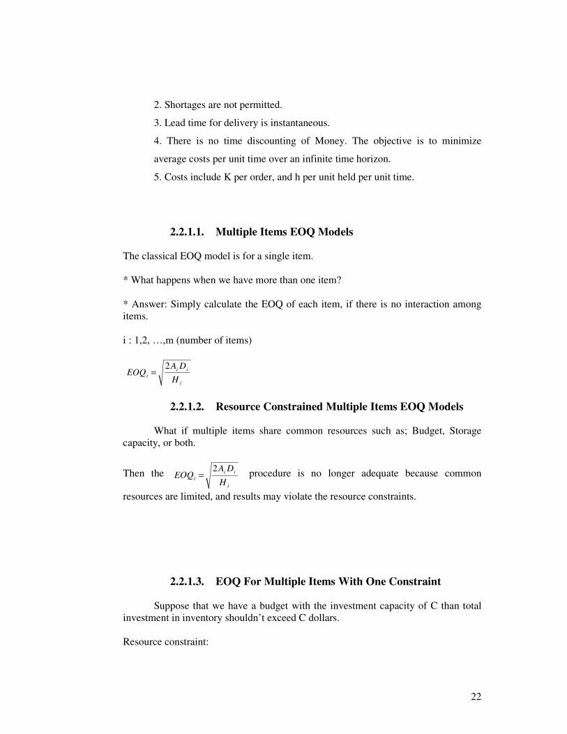
2.2.1.1. Multiple Items EOQ Models The classical EOQ model is for a single item. * What happens when we have more than one item? * Answer: Simply calculate the EOQ of each item, if there is no interaction among items. i : 1,2, …,m (number of items)

i

ii

iH

DAEOQ

2=

2.2.1.2. Resource Constrained Multiple Items EOQ Models

What if multiple items share common resources such as; Budget, Storage

capacity, or both.

Then the i

ii

iH

DAEOQ

2= procedure is no longer adequate because common

resources are limited, and results may violate the resource constraints.

2.2.1.3. EOQ For Multiple Items With One Constraint

Suppose that we have a budget with the investment capacity of C than total investment in inventory shouldn’t exceed C dollars. Resource constraint:

23

CQc i

m

i

i ≤∑=1

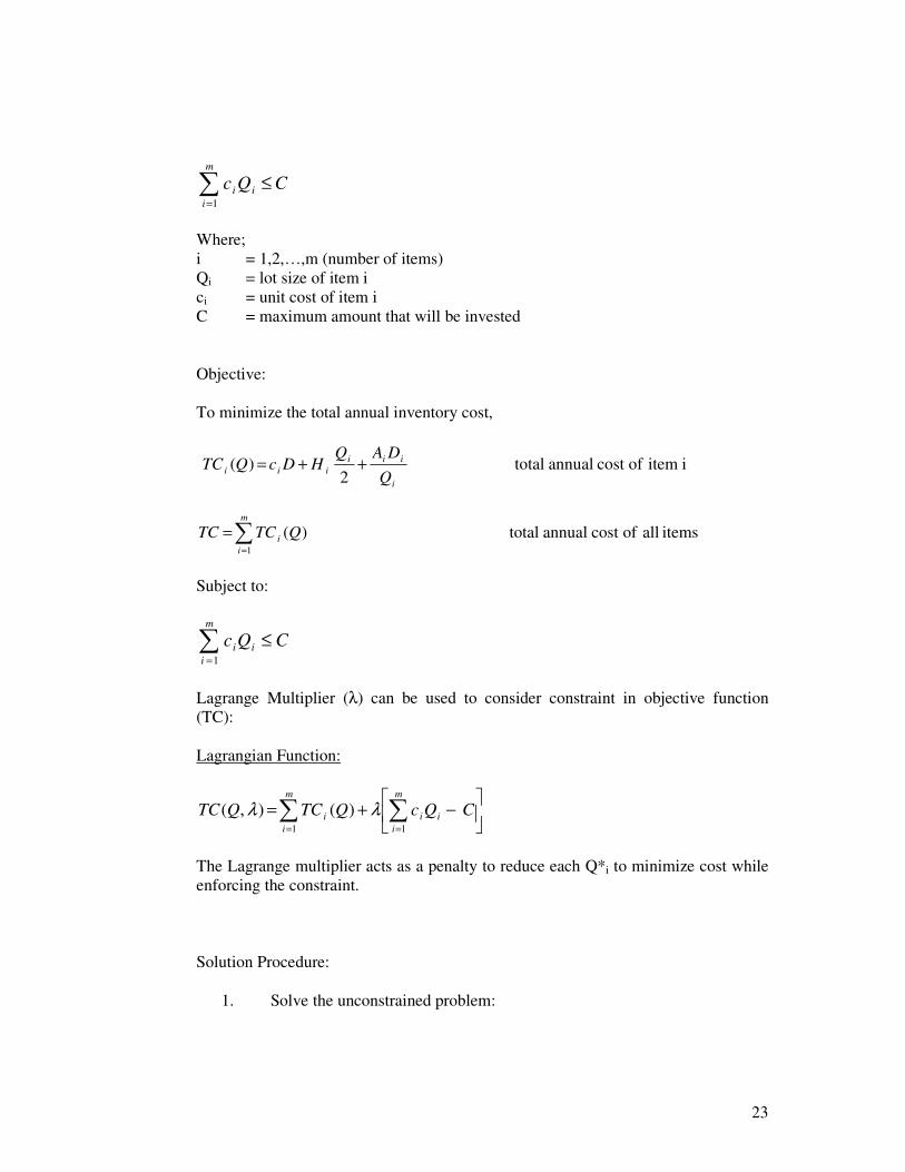
Where; i = 1,2,…,m (number of items) Qi = lot size of item i ci = unit cost of item i C = maximum amount that will be invested Objective: To minimize the total annual inventory cost,

i item ofcost annual total2

)(i

iii

iiiQ

DAQHDcQTC ++=

items all ofcost annual total)(1∑

=

=m

i

i QTCTC

Subject to:

CQc i

m

i

i ≤∑=1

Lagrange Multiplier (λ) can be used to consider constraint in objective function (TC): Lagrangian Function:

−+= ∑∑

==

CQcQTCQTC i

m

i

i

m

i

i

11

)(),( λλ

The Lagrange multiplier acts as a penalty to reduce each Q*i to minimize cost while enforcing the constraint. Solution Procedure:

1. Solve the unconstrained problem:

24

Find: i

ii

iH

DAEOQ

2= for i = 1,2,..,m

If the constraint is satisfied this solution is the optimal one. 2. If this is not the case, set TC(Q, λ).

−+= ∑∑

==

CQcQTCQTC i

m

i

i

m

i

i

11

)(),( λλ

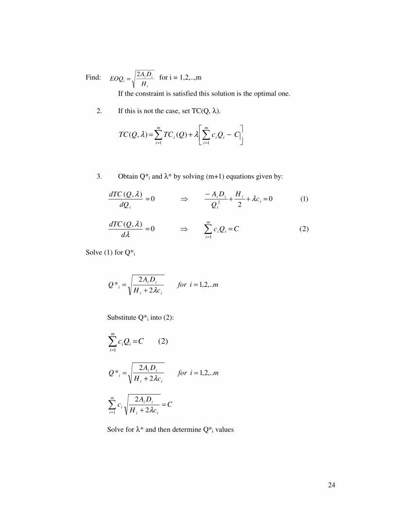
3. Obtain Q*i and λ* by solving (m+1) equations given by:

)1(02

0),(

2=++

−⇒= i

i

i

ii

i

cH

Q

DA

dQ

QdTCλ

λ

)2(0),(

1

CQcd

QdTCi

m

i

i =⇒= ∑=λ

λ

Solve (1) for Q*i

miforcH

DAQ

ii

ii

i ,..2,12

2* =

+=

λ

Substitute Q*i into (2):

)2(1

CQc i

m

i

i =∑=

miforcH

DAQ

ii

ii

i ,..2,12

2* =

+=

λ

CcH

DAc

ii

iim

i

i =+

∑= λ2

2

1

Solve for λ* and then determine Q*i values

25

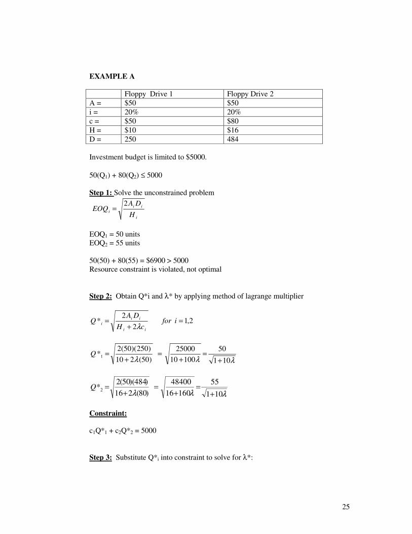
EXAMPLE A Floppy Drive 1 Floppy Drive 2 A = $50 $50 i = 20% 20% c = $50 $80 H = $10 $16 D = 250 484 Investment budget is limited to $5000. 50(Q1) + 80(Q2) ≤ 5000 Step 1: Solve the unconstrained problem

i

ii

iH

DAEOQ

2=

EOQ1 = 50 units EOQ2 = 55 units 50(50) + 80(55) = $6900 > 5000 Resource constraint is violated, not optimal Step 2: Obtain Q*i and λ* by applying method of lagrange multiplier

2,12

2* =

+= ifor

cH

DAQ

ii

ii

iλ

λλλ 101

50

10010

25000

)50(210

)250)(50(2*1

+=

+=

+=Q

λλλ 101

55

16016

48400

)80(216

)484)(50(2*2

+=

+=

+=Q

Constraint: c1Q*1 + c2Q*2 = 5000 Step 3: Substitute Q*i into constraint to solve for λ*:

26

λλ 101

55*

101

50* 21

+=

+= QQ

Constraint: c1Q*1 + c2Q*2 = 5000

5000101

5580

101

5050 =

++

+ λλ

38.11015000101

6900=+⇒=

+λ

λ

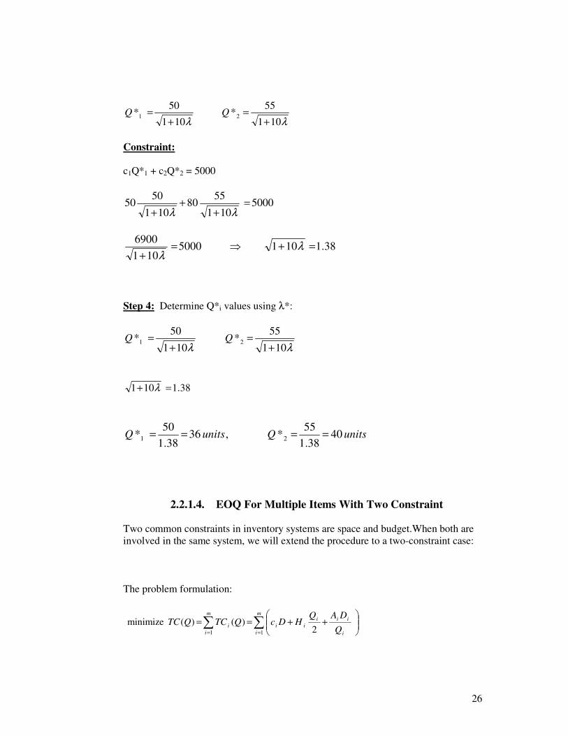
Step 4: Determine Q*i values using λ*:

λλ 101

55*

101

50* 21

+=

+= QQ

38.1101 =+ λ

unitsQunitsQ 4038.1

55*,36

38.1

50* 21 ====

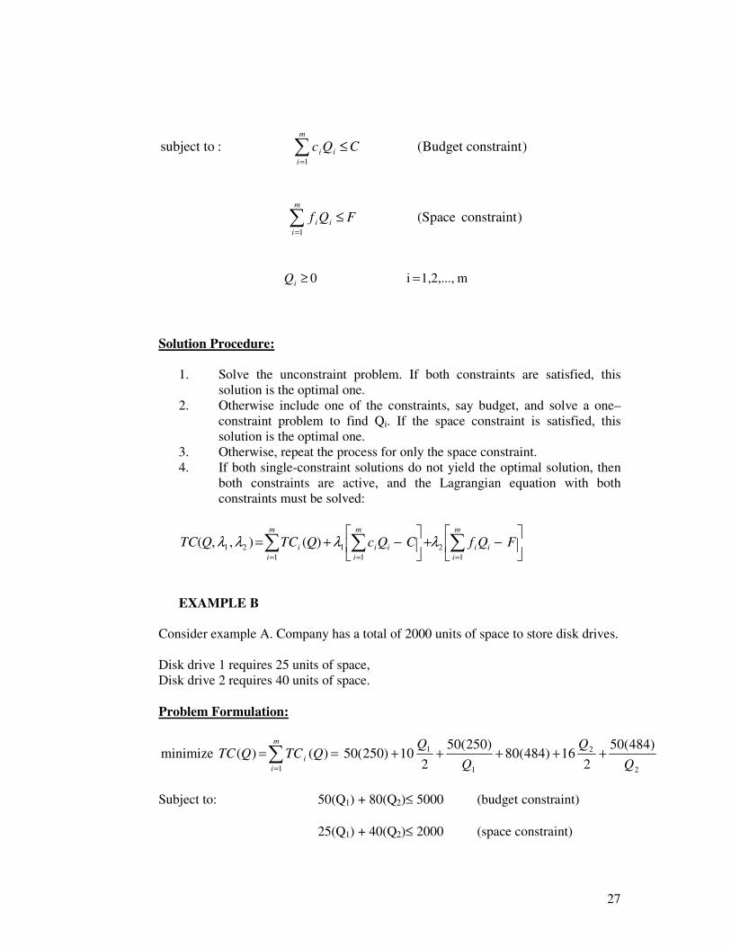
2.2.1.4. EOQ For Multiple Items With Two Constraint Two common constraints in inventory systems are space and budget.When both are involved in the same system, we will extend the procedure to a two-constraint case: The problem formulation:

∑ ∑= =

++==

m

i

m

i i

iii

iiiQ

DAQHDcQTCQTC

1 1 2)()(minimize

27

)constraintBudget (:subject to1

CQc i

m

i

i ≤∑=

)constraint (Space1

FQf i

m

i

i ≤∑=

m1,2,...,i0 =≥iQ

Solution Procedure:

1. Solve the unconstraint problem. If both constraints are satisfied, this solution is the optimal one.

2. Otherwise include one of the constraints, say budget, and solve a one–constraint problem to find Qi. If the space constraint is satisfied, this solution is the optimal one.

3. Otherwise, repeat the process for only the space constraint. 4. If both single-constraint solutions do not yield the optimal solution, then

both constraints are active, and the Lagrangian equation with both constraints must be solved:

−+

−+= ∑∑∑

===

FQfCQcQTCQTC i

m

i

ii

m

i

i

m

i

i

12

11

121 )(),,( λλλλ

EXAMPLE B

Consider example A. Company has a total of 2000 units of space to store disk drives. Disk drive 1 requires 25 units of space, Disk drive 2 requires 40 units of space. Problem Formulation:

∑=

+++++==m

i

iQ

Q

Q

QQTCQTC

1 2

2

1

1 )484(50

216)484(80

)250(50

210)250(50)()(minimize

Subject to: 50(Q1) + 80(Q2)≤ 5000 (budget constraint) 25(Q1) + 40(Q2)≤ 2000 (space constraint)

28

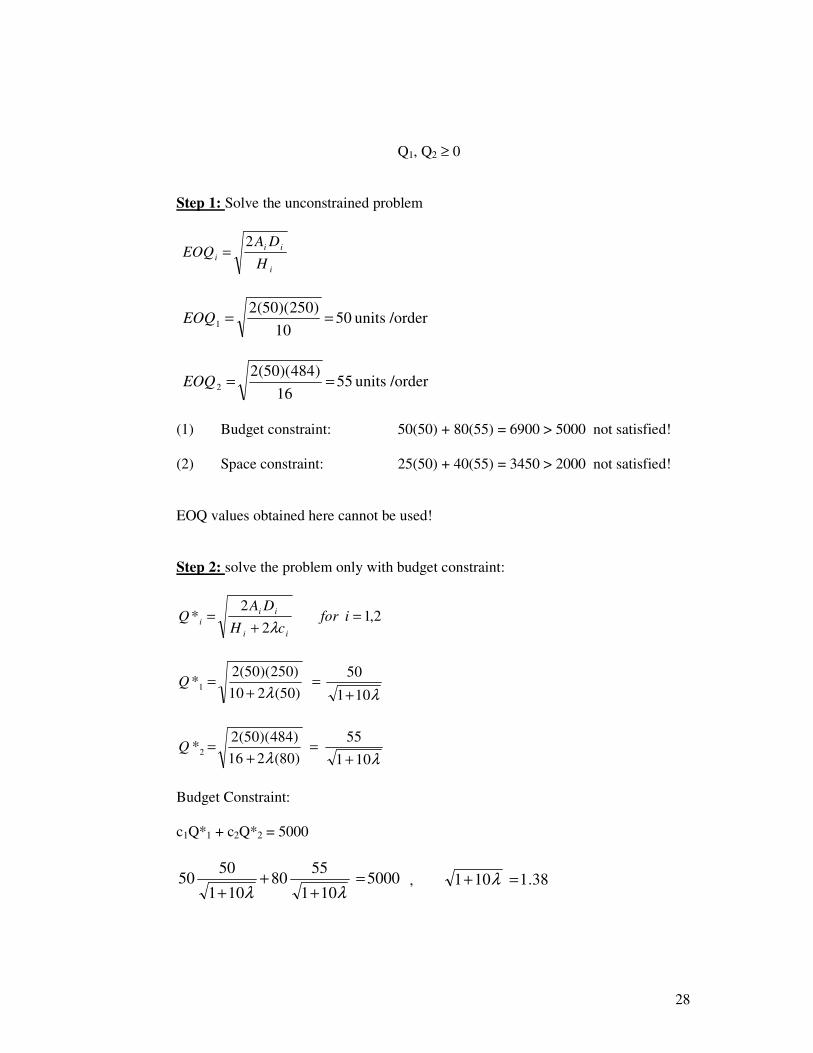
Q1, Q2 ≥ 0 Step 1: Solve the unconstrained problem

i

ii

iH

DAEOQ

2=

/orderunits5010

)250)(50(21 ==EOQ

/orderunits5516

)484)(50(22 ==EOQ

(1) Budget constraint: 50(50) + 80(55) = 6900 > 5000 not satisfied! (2) Space constraint: 25(50) + 40(55) = 3450 > 2000 not satisfied! EOQ values obtained here cannot be used! Step 2: solve the problem only with budget constraint:

2,12

2* =

+= ifor

cH

DAQ

ii

ii

iλ

λλ 101

50

)50(210

)250)(50(2*1

+=

+=Q

λλ 101

55

)80(216

)484)(50(2*2

+=

+=Q

Budget Constraint: c1Q*1 + c2Q*2 = 5000

5000101

5580

101

5050 =

++

+ λλ , 38.1101 =+ λ

29

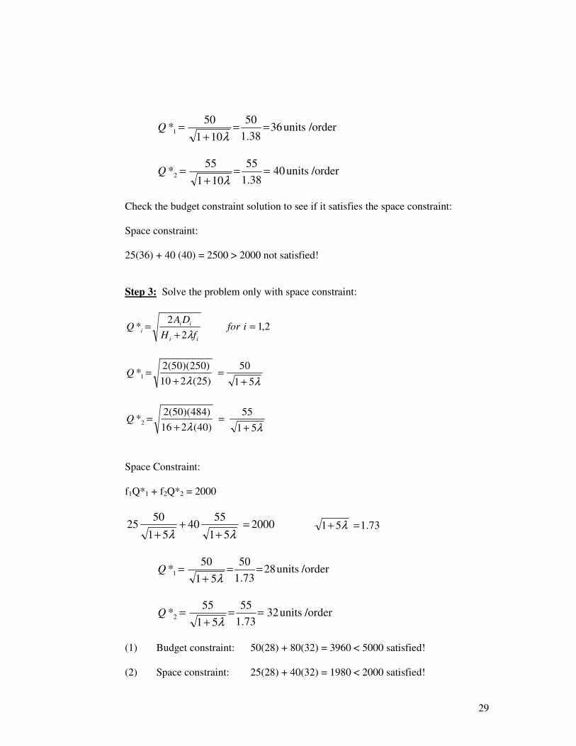
/orderunits3638.1

50

101

50*1 ==

+=

λQ

/orderunits4038.1

55

101

55*2 ==

+=

λQ

Check the budget constraint solution to see if it satisfies the space constraint: Space constraint: 25(36) + 40 (40) = 2500 > 2000 not satisfied! Step 3: Solve the problem only with space constraint:

2,12

2* =

+= ifor

fH

DAQ

ii

iii

λ

λλ 51

50

)25(210

)250)(50(2*1

+=

+=Q

λλ 51

55

)40(216

)484)(50(2*2

+=

+=Q

Space Constraint: f1Q*1 + f2Q*2 = 2000

200051

5540

51

5025 =

++

+ λλ 73.151 =+ λ

/orderunits2873.1

50

51

50*1 ==

+=

λQ

/orderunits3273.1

55

51

55*2 ==

+=

λQ

(1) Budget constraint: 50(28) + 80(32) = 3960 < 5000 satisfied! (2) Space constraint: 25(28) + 40(32) = 1980 < 2000 satisfied!

30

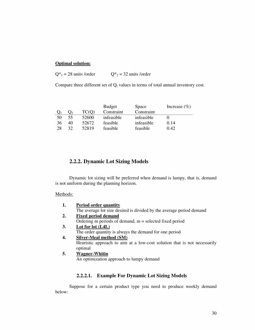
Optimal solution: Q*1 = 28 units /order Q*2 = 32 units /order Compare three different set of Qi values in terms of total annual inventory cost.

Q1 Q2 TC(Q) Budget Constraint

Space Constraint

Increase (%)

50 55 52600 infeasible infeasible 0 36 40 52672 feasible infeasible 0.14 28 32 52819 feasible feasible 0.42

2.2.2. Dynamic Lot Sizing Models

Dynamic lot sizing will be preferred when demand is lumpy, that is, demand is not uniform during the planning horizon. Methods:

1. Period order quantity The average lot size desired is divided by the average period demand

2. Fixed period demand Ordering m periods of demand, m = selected fixed period

3. Lot for lot (L4L) The order quantity is always the demand for one period

4. Silver-Meal method (SM) Heuristic approach to aim at a low-cost solution that is not necessarily optimal

5. Wagner-Whitin An optimization approach to lumpy demand

2.2.2.1. Example For Dynamic Lot Sizing Models

Suppose for a certain product type you need to produce weekly demand below:

31

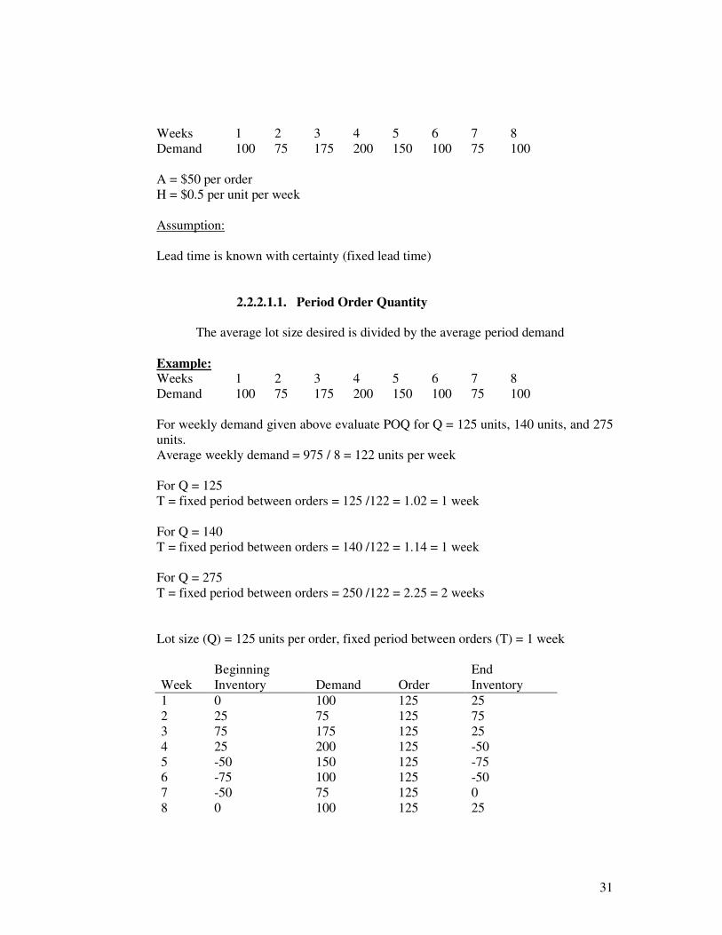
Weeks 1 2 3 4 5 6 7 8 Demand 100 75 175 200 150 100 75 100 A = $50 per order H = $0.5 per unit per week Assumption: Lead time is known with certainty (fixed lead time)

2.2.2.1.1. Period Order Quantity

The average lot size desired is divided by the average period demand Example: Weeks 1 2 3 4 5 6 7 8 Demand 100 75 175 200 150 100 75 100 For weekly demand given above evaluate POQ for Q = 125 units, 140 units, and 275 units. Average weekly demand = 975 / 8 = 122 units per week For Q = 125 T = fixed period between orders = 125 /122 = 1.02 = 1 week For Q = 140 T = fixed period between orders = 140 /122 = 1.14 = 1 week For Q = 275 T = fixed period between orders = 250 /122 = 2.25 = 2 weeks Lot size (Q) = 125 units per order, fixed period between orders (T) = 1 week

Week Beginning Inventory Demand Order

End Inventory

1 0 100 125 25 2 25 75 125 75 3 75 175 125 25 4 25 200 125 -50 5 -50 150 125 -75 6 -75 100 125 -50 7 -50 75 125 0 8 0 100 125 25

32

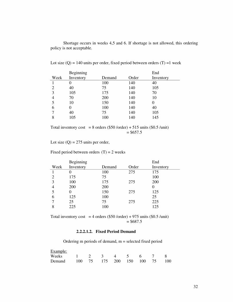
Shortage occurs in weeks 4,5 and 6. If shortage is not allowed, this ordering policy is not acceptable. Lot size (Q) = 140 units per order, fixed period between orders (T) =1 week


End Inventory

1 0 100 140 40 2 40 75 140 105 3 105 175 140 70 4 70 200 140 10 5 10 150 140 0 6 0 100 140 40 7 40 75 140 105 8 105 100 140 145

Total inventory cost = 8 orders ($50 /order) + 515 units ($0.5 /unit) = $657.5 Lot size (Q) = 275 units per order, Fixed period between orders (T) = 2 weeks


End Inventory

1 0 100 275 175 2 175 75 100 3 100 175 275 200 4 200 200 0 5 0 150 275 125 6 125 100 25 7 25 75 275 225 8 225 100 125

Total inventory cost = 4 orders ($50 /order) + 975 units ($0.5 /unit) = $687.5

2.2.2.1.2. Fixed Period Demand

Ordering m periods of demand, m = selected fixed period Example: Weeks 1 2 3 4 5 6 7 8 Demand 100 75 175 200 150 100 75 100

33

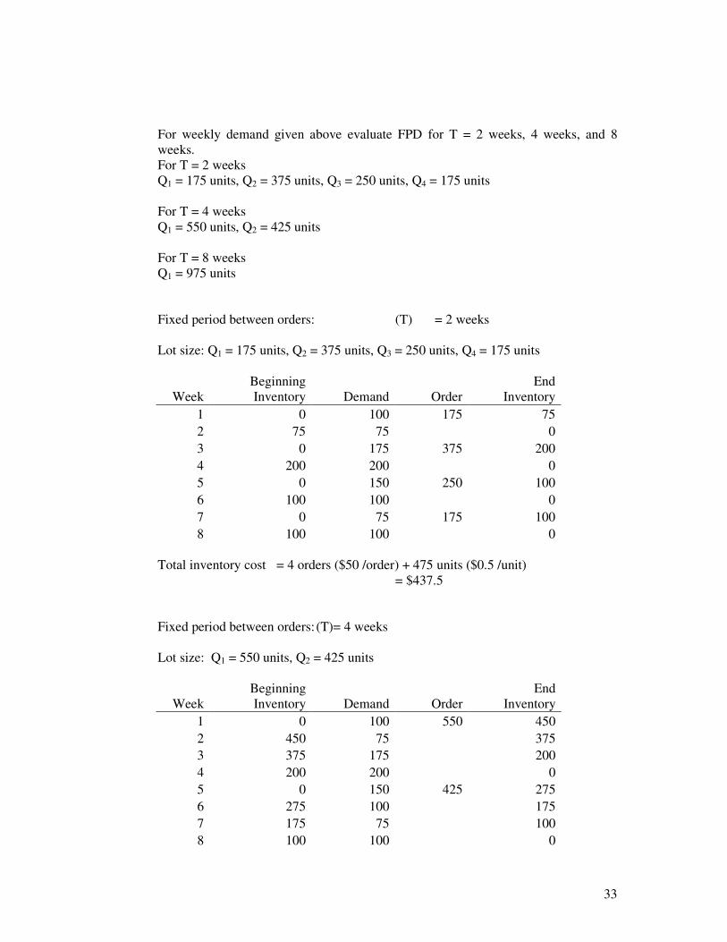
For weekly demand given above evaluate FPD for T = 2 weeks, 4 weeks, and 8 weeks. For T = 2 weeks Q1 = 175 units, Q2 = 375 units, Q3 = 250 units, Q4 = 175 units For T = 4 weeks Q1 = 550 units, Q2 = 425 units For T = 8 weeks Q1 = 975 units Fixed period between orders: (T) = 2 weeks Lot size: Q1 = 175 units, Q2 = 375 units, Q3 = 250 units, Q4 = 175 units


End Inventory

1 0 100 175 75 2 75 75 0 3 0 175 375 200 4 200 200 0 5 0 150 250 100 6 100 100 0 7 0 75 175 100 8 100 100 0

Total inventory cost = 4 orders ($50 /order) + 475 units ($0.5 /unit) = $437.5 Fixed period between orders: (T)= 4 weeks Lot size: Q1 = 550 units, Q2 = 425 units


End Inventory

1 0 100 550 450 2 450 75 375 3 375 175 200 4 200 200 0 5 0 150 425 275 6 275 100 175 7 175 75 100 8 100 100 0

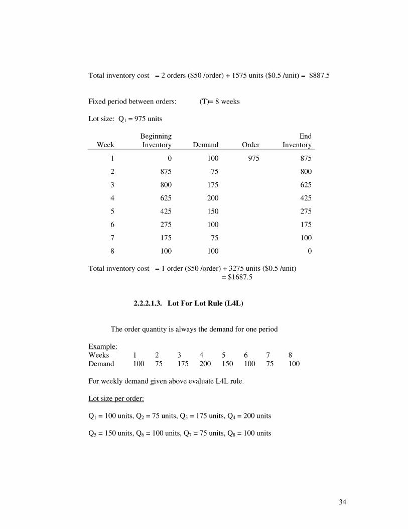
34

Total inventory cost = 2 orders ($50 /order) + 1575 units ($0.5 /unit) = $887.5 Fixed period between orders: (T)= 8 weeks Lot size: Q1 = 975 units


End Inventory

1 0 100 975 875

2 875 75 800

3 800 175 625

4 625 200 425

5 425 150 275

6 275 100 175

7 175 75 100

8 100 100 0 Total inventory cost = 1 order ($50 /order) + 3275 units ($0.5 /unit) = $1687.5

2.2.2.1.3. Lot For Lot Rule (L4L)

The order quantity is always the demand for one period Example: Weeks 1 2 3 4 5 6 7 8 Demand 100 75 175 200 150 100 75 100 For weekly demand given above evaluate L4L rule. Lot size per order: Q1 = 100 units, Q2 = 75 units, Q3 = 175 units, Q4 = 200 units Q5 = 150 units, Q6 = 100 units, Q7 = 75 units, Q8 = 100 units

35

Total

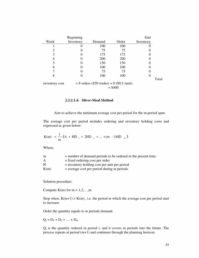
inventory cost = 8 orders ($50 /order) + 0 ($0.5 /unit) = $400

2.2.2.1.4. Silver-Meal Method

Aim to achieve the minimum average cost per period for the m-period span. The average cost per period includes ordering and inventory holding costs and expressed as given below:

( )m21 1)HD -(m... 2HD HD A m

1 K(m) ++++=

Where; m = number of demand periods to be ordered in the present time. A = fixed ordering cost per order H = inventory holding cost per unit per period K(m) = average cost per period during m periods Solution procedure: Compute K(m) for m = 1,2,…,m Stop when, K(m+1) > K(m) , i.e. the period in which the average cost per period start to increase. Order the quantity equals to m periods demand. Qi = D1 + D2 + … + Dm Qi is the quantity ordered in period i, and it covers m periods into the future. The process repeats at period (m+1) and continues through the planning horizon.


End Inventory

1 0 100 100 0 2 0 75 75 0 3 0 175 175 0 4 0 200 200 0 5 0 150 150 0 6 0 100 100 0 7 0 75 75 0 8 0 100 100 0

36

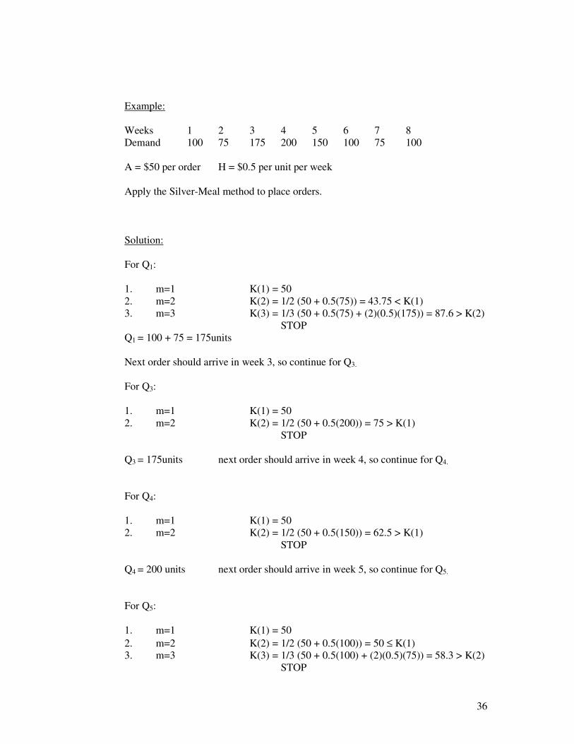
Example: Weeks 1 2 3 4 5 6 7 8 Demand 100 75 175 200 150 100 75 100 A = $50 per order H = $0.5 per unit per week Apply the Silver-Meal method to place orders. Solution: For Q1: 1. m=1 K(1) = 50 2. m=2 K(2) = 1/2 (50 + 0.5(75)) = 43.75 < K(1) 3. m=3 K(3) = 1/3 (50 + 0.5(75) + (2)(0.5)(175)) = 87.6 > K(2) STOP Q1 = 100 + 75 = 175units Next order should arrive in week 3, so continue for Q3. For Q3: 1. m=1 K(1) = 50 2. m=2 K(2) = 1/2 (50 + 0.5(200)) = 75 > K(1) STOP Q3 = 175units next order should arrive in week 4, so continue for Q4. For Q4: 1. m=1 K(1) = 50 2. m=2 K(2) = 1/2 (50 + 0.5(150)) = 62.5 > K(1) STOP Q4 = 200 units next order should arrive in week 5, so continue for Q5. For Q5: 1. m=1 K(1) = 50 2. m=2 K(2) = 1/2 (50 + 0.5(100)) = 50 ≤ K(1) 3. m=3 K(3) = 1/3 (50 + 0.5(100) + (2)(0.5)(75)) = 58.3 > K(2) STOP

37

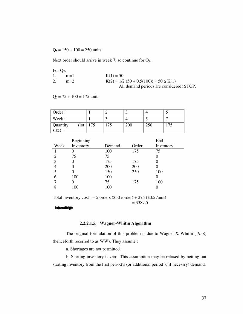
Q5 = 150 + 100 = 250 units Next order should arrive in week 7, so continue for Q7. For Q7: 1. m=1 K(1) = 50 2. m=2 K(2) = 1/2 (50 + 0.5(100)) = 50 ≤ K(1) All demand periods are considered! STOP. Q7 = 75 + 100 = 175 units Order : 1 2 3 4 5

Week : 1 3 4 5 7

Quantity (lot size) :

175 175 200 250 175


End Inventory

1 0 100 175 75 2 75 75 0 3 0 175 175 0 4 0 200 200 0 5 0 150 250 100 6 100 100 0 7 0 75 175 100 8 100 100 0

Total inventory cost = 5 orders ($50 /order) + 275 ($0.5 /unit) = $387.5 In the first chapter, we have summarized the basics of supply chain

2.2.2.1.5. Wagner-Whitin Algorithm

The original formulation of this problem is due to Wagner & Whitin [1958]

(henceforth recerred to as WW). They assume :

a. Shortages are not permitted.

b. Starting inventory is zero. This assumption may be relaxed by netting out

starting inventory from the fırst period’s (or additional period’s, if necessry) demand.

38

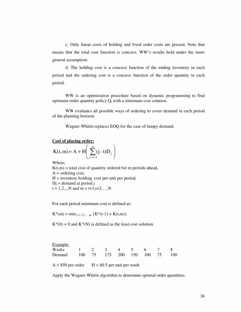
c. Only linear costs of holding and fixed order costs are present. Note that

means that the total cost function is concave. WW’s results hold under the more

general assumption:

d. The holding cost is a concave function of the ending inventory in each

period and the ordering cost is a concave function of the order quantity in each

period.

WW is an optimization procedure based on dynamic programming to find

optimum order quantity policy Qi with a minimum cost solution.

WW evaluates all possible ways of ordering to cover demand in each period of the planning horizon.

Wagner-Whitin replaces EOQ for the case of lumpy demand.

Cost of placing order:

+= ∑

+=

m

1jt)D-(jH A m)K(t,

tj

Where; K(t,m) = total cost of quantity ordered for m periods ahead, A = ordering cost, H = inventory holding cost per unit per period, Dj = demand at period j t = 1,2,..,N and m = t+1,t+2,…,N For each period minimum cost is defined as: K*(m) = min t = 1,2,…,m {K*(t-1) + K(t,m)} K*(0) = 0 and K*(N) is defined as the least cost solution. Example: Weeks 1 2 3 4 5 6 7 8 Demand 100 75 175 200 150 100 75 100 A = $50 per order H = $0.5 per unit per week Apply the Wagner-Whitin algorithm to determine optimal order quantities.

39

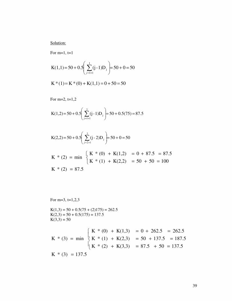
Solution: For m=1, t=1

50 0 50 1)D-(j5.0 50 K(1,1)1

11j =+=

+= ∑

+=j

50 50 0 K(1,1) (0)*K (1)*K =+=+=

For m=2, t=1,2

87.5 0.5(75) 50 1)D-(j5.0 50 K(1,2)2

11j =+=

+= ∑

+=j

50 0 50 2)D-(j5.0 50 K(2,2)2

12j =+=

+= ∑

+=j

87.5 (2)*K

100 50 50 K(2,2) (1)*K

87.5 87.5 0 K(1,2) (0)*Kmin (2)*K

=

=+=+

=+=+=

For m=3, t=1,2,3 K(1,3) = 50 + 0.5(75 + (2)175) = 262.5 K(2,3) = 50 + 0.5(175) = 137.5 K(3,3) = 50

137.5 (3)*K

137.5 50 87.5 K(3,3) (2)*K

187.5 137.5 50 K(2,3) (1)*K

262.5 262.5 0 K(1,3) (0)*K

min(3)*K

=

=+=+

=+=+

=+=+

=

40

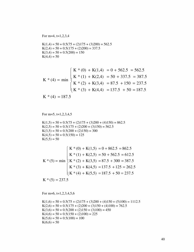
For m=4, t=1,2,3,4 K(1,4) = 50 + 0.5(75 + (2)175 + (3)200) = 562.5 K(2,4) = 50 + 0.5(175 + (2)200) = 337.5 K(3,4) = 50 + 0.5(200) = 150 K(4,4) = 50

187.5 (4)*K

187.5 50 137.5 K(4,4) (3)*K

237.5 150 87.5 K(3,4) (2)*K

387.5 337.5 50 K(2,4) (1)*K

562.5 562.5 0 K(1,4) (0)*K

min(4)*K

=

=+=+

=+=+

=+=+

=+=+

=

For m=5, t=1,2,3,4,5 K(1,5) = 50 + 0.5(75 + (2)175 + (3)200 + (4)150) = 862.5 K(2,5) = 50 + 0.5(175 + (2)200 + (3)150) = 562.5 K(3,5) = 50 + 0.5(200 + (2)150) = 300 K(4,5) = 50 + 0.5(150) = 125 K(5,5) = 50

237.5 (5)*K

237.5 50 187.5 K(5,5) (4)*K

262.5 125 137.5 K(4,5) (3)*K

387.5 300 87.5 K(3,5) (2)*K

612.5 562.5 50 K(2,5) (1)*K

862.5 862.5 0 K(1,5) (0)*K

min(5)*K

=

=+=+

=+=+

=+=+

=+=+

=+=+

=

For m=6, t=1,2,3,4,5,6 K(1,6) = 50 + 0.5(75 + (2)175 + (3)200 + (4)150 + (5)100) = 1112.5 K(2,6) = 50 + 0.5(175 + (2)200 + (3)150 + (4)100) = 762.5 K(3,6) = 50 + 0.5(200 + (2)150 + (3)100) = 450 K(4,6) = 50 + 0.5(150 + (2)100) = 225 K(5,6) = 50 + 0.5(100) = 100 K(6,6) = 50

41

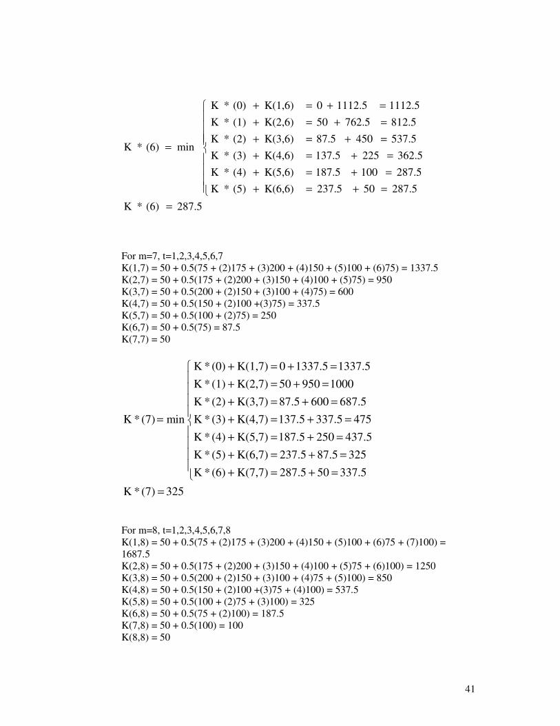
287.5 (6)*K

287.5 50 237.5 K(6,6) (5)*K

287.5 100 187.5 K(5,6) (4)*K

362.5 225 137.5 K(4,6) (3)*K

537.5 450 87.5 K(3,6) (2)*K

812.5 762.5 50 K(2,6) (1)*K

1112.5 1112.5 0 K(1,6) (0)*K

min(6)*K

=

=+=+

=+=+

=+=+

=+=+

=+=+

=+=+

=

For m=7, t=1,2,3,4,5,6,7 K(1,7) = 50 + 0.5(75 + (2)175 + (3)200 + (4)150 + (5)100 + (6)75) = 1337.5 K(2,7) = 50 + 0.5(175 + (2)200 + (3)150 + (4)100 + (5)75) = 950 K(3,7) = 50 + 0.5(200 + (2)150 + (3)100 + (4)75) = 600 K(4,7) = 50 + 0.5(150 + (2)100 +(3)75) = 337.5 K(5,7) = 50 + 0.5(100 + (2)75) = 250 K(6,7) = 50 + 0.5(75) = 87.5 K(7,7) = 50

325 (7)*K

337.5 50 287.5 K(7,7) (6)*K

325 87.5 237.5 K(6,7) (5)*K

437.5 250 187.5 K(5,7) (4)*K

475 337.5 137.5 K(4,7) (3)*K

687.5 600 87.5 K(3,7) (2)*K

1000 950 50 K(2,7) (1)*K

1337.5 1337.5 0 K(1,7) (0)*K

min(7)*K

=

=+=+

=+=+

=+=+

=+=+

=+=+

=+=+

=+=+

=

For m=8, t=1,2,3,4,5,6,7,8 K(1,8) = 50 + 0.5(75 + (2)175 + (3)200 + (4)150 + (5)100 + (6)75 + (7)100) = 1687.5 K(2,8) = 50 + 0.5(175 + (2)200 + (3)150 + (4)100 + (5)75 + (6)100) = 1250 K(3,8) = 50 + 0.5(200 + (2)150 + (3)100 + (4)75 + (5)100) = 850 K(4,8) = 50 + 0.5(150 + (2)100 +(3)75 + (4)100) = 537.5 K(5,8) = 50 + 0.5(100 + (2)75 + (3)100) = 325 K(6,8) = 50 + 0.5(75 + (2)100) = 187.5 K(7,8) = 50 + 0.5(100) = 100 K(8,8) = 50

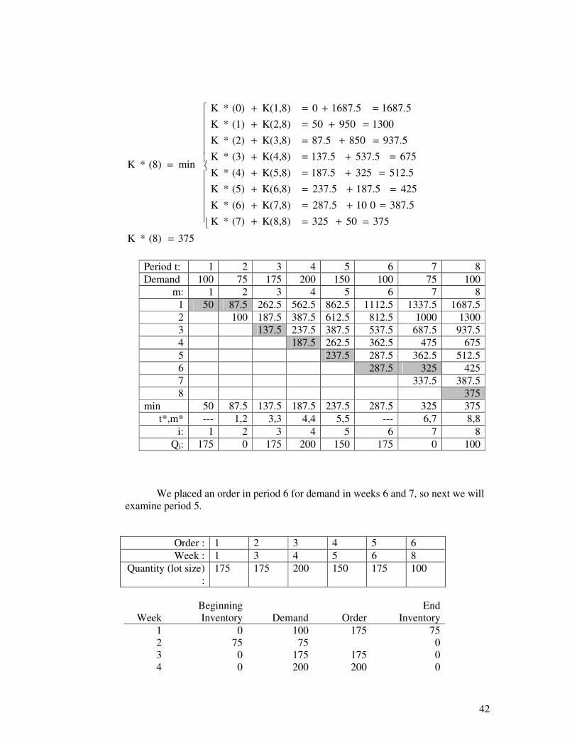
42

375 (8)*K

375 50 325 K(8,8) (7)*K

387.5 010 287.5 K(7,8) (6)*K

425 187.5 237.5 K(6,8) (5)*K

512.5 325 187.5 K(5,8) (4)*K

675 537.5 137.5 K(4,8) (3)*K

937.5 850 87.5 K(3,8) (2)*K

1300 950 50 K(2,8) (1)*K

1687.5 1687.5 0 K(1,8) (0)*K

min(8)*K

=

=+=+

=+=+

=+=+

=+=+

=+=+

=+=+

=+=+

=+=+

=

We placed an order in period 6 for demand in weeks 6 and 7, so next we will examine period 5.

Order : 1 2 3 4 5 6 Week : 1 3 4 5 6 8

Quantity (lot size) :

175 175 200 150 175 100


End Inventory

1 0 100 175 75 2 75 75 0 3 0 175 175 0 4 0 200 200 0

Period t: 1 2 3 4 5 6 7 8 Demand 100 75 175 200 150 100 75 100 m: 1 2 3 4 5 6 7 8

1 50 87.5 262.5 562.5 862.5 1112.5 1337.5 1687.5 2 100 187.5 387.5 612.5 812.5 1000 1300 3 137.5 237.5 387.5 537.5 687.5 937.5 4 187.5 262.5 362.5 475 675 5 237.5 287.5 362.5 512.5 6 287.5 325 425 7 337.5 387.5 8 375 min 50 87.5 137.5 187.5 237.5 287.5 325 375 t*,m* --- 1,2 3,3 4,4 5,5 --- 6,7 8,8 i: 1 2 3 4 5 6 7 8 Qi: 175 0 175 200 150 175 0 100

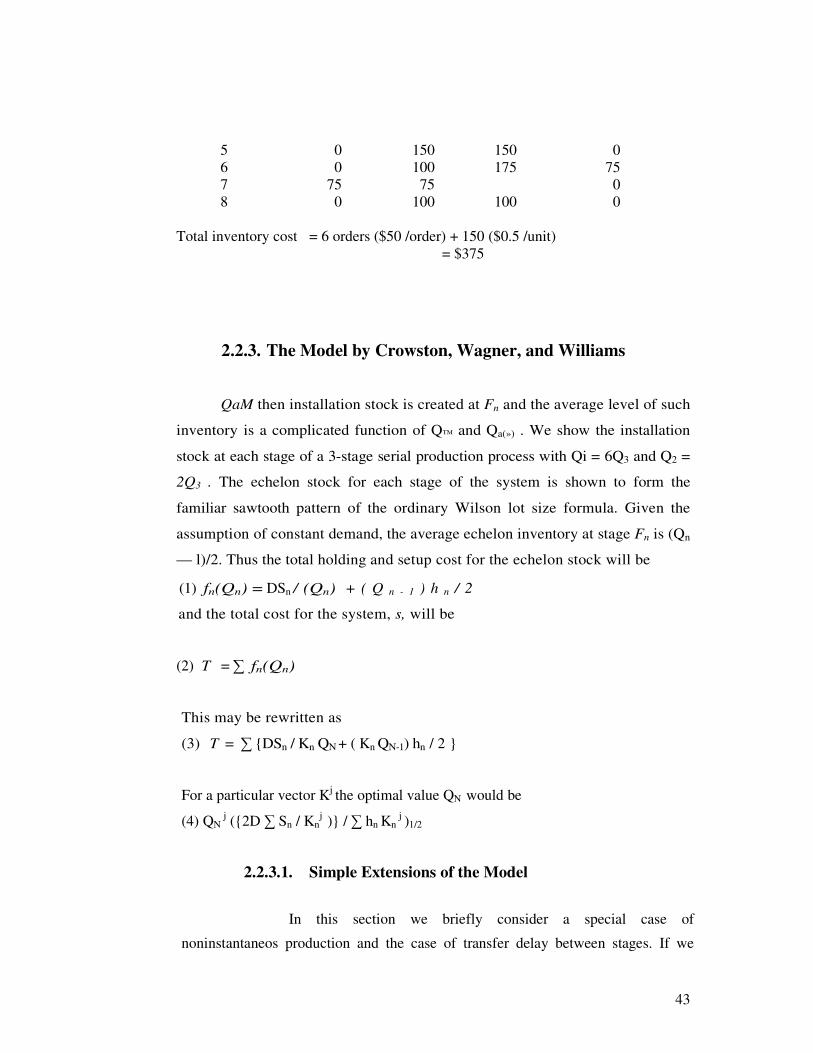
43

5 0 150 150 0 6 0 100 175 75 7 75 75 0 8 0 100 100 0

Total inventory cost = 6 orders ($50 /order) + 150 ($0.5 /unit) = $375

2.2.3. The Model by Crowston, Wagner, and Williams

QaM then installation stock is created at Fn and the average level of such

inventory is a complicated function of Q™ and Qa(») . We show the installation

stock at each stage of a 3-stage serial production process with Qi = 6Q3 and Q2 =

2Q3 . The echelon stock for each stage of the system is shown to form the

familiar sawtooth pattern of the ordinary Wilson lot size formula. Given the

assumption of constant demand, the average echelon inventory at stage Fn is (Qn

— l)/2. Thus the total holding and setup cost for the echelon stock will be

(1) fn(Qn) = DSn / (Qn) + ( Q n - 1 ) h n / 2

and the total cost for the system, s, will be

(2) T = ∑ fn(Qn)

This may be rewritten as

(3) T = ∑ {DSn / Kn QN + ( Kn QN-1) hn / 2 }

For a particular vector Kj the optimal value QN would be

(4) QN j ({2D ∑ Sn / Kn

j )} / ∑ hn Kn j )1/2

2.2.3.1. Simple Extensions of the Model

In this section we briefly consider a special case of

noninstantaneos production and the case of transfer delay between stages. If we

44

assume production rate pn at Fn and given pn ≥ p0n then the result of theorem 1

applies.

(5) TCn = DSn / Kn Qn +[( Kn Qn – 1) / 2 ] [ 1- D / pn ] hn

(2DS*/Hn)m. This implies the carrying cost of a unit of in-process inventory of Fn is

a function of the total value of its components. Our model indicates that this results in

double-counting. Finally, we would suggest that if heuristic decision rules are con-

structed for the more complicated case of multiple successors, incremental holding

costs are again appropriate.

2.2.4. Reorder Cycle Time Problems

Based on the traditional Economic Order Quantity model showed before, the

time between two consecutive orders, called reorder interval, is constant and

proportional to the order quantity. The lot sizing problem can be formulated as the

determination of the reorder cycle interval. T=Q/D, and ignoring the production cost

(because it won’t affect for the comparison), the optimum reorder interval can be

derived. As mentioned before, this problem is continuous and the reorder optimal

interval can take any positive real value. However, their solution presents some

difficulties. This is the reason to solve it as a discrete problem, imposing the

restriction that the reorder interval can take only positive integer values.

There are several reasons to formulate the lot sizing model in terms of reorder

intervals as described before. A lot of authors have been developing new techniques

to solve the problem in terms of this point of view; some of the most important are

mentioned here.

Elmaghraby (1978) analyzed the economic lot scheduling problem (ELSP),

which arises from the desire to accommodate the cyclical production pattern when

several products are made on a single facility. This work reviews the contributions to

the problem, and extends the analysis in four directions: (1) offers an improved

45

analytical approach based on dynamic programming. It tries to guarantee feasibility

at the outset, by imposing some constraints on the cycle times, then to optimize the

individual cycle duration subject to the imposed constraint. The solution obtained in

this manner is feasible and optimal over its set of solutions; (2) a test of feasibility of

a given set of parameters, through an integer linear programming formulation; (3) a

systematic procedure for escape from infeasibility, when the set of parameters were

judge infeasible; and (4) a procedure for the determination of a basic period for a

given set of multipliers to achieve a feasible schedule.

Szendrovits (1975) presented the functional relationship between the

production lot size, the manufacturing cycle time and the average process inventory

in a production system, and illustrated the resulting effect on the conventional

Economic Lot Quantity model. He treats the manufacturing cycle time as a function

of the lot size in a multistage production system. This model was called the economic

production quantity (EPQ). This study challenges the widely accepted doctrine of the

efficiency of long production runs.

Roundy (1985) introduced two simple policies called q-optimal integer-ratio

and optimal power-of-two, which are proved to be 94% and 98% effective. The

effectiveness

of a policy is 100% times the ratio of the minimum of the average cost over all

policies to the average cost of the policy in question. Both policies are very efficient

and their most important advantage is the flexibility it allows in choosing the order

intervals to correspond to easily-implemented time periods.

The power-of-two policy is a special case of the discrete problem for

determining the reorder cycle time, in which the reorder interval is constraint to be

not only integer, but also a multiple of two. It allows us to obtain an extremely

efficient algorithm which produces a policy having an average cost within 2% of the

minimum possible. Mitchell (1987) extended Roundy’s results for the backlogging

problem, obtaining a 98% effective policy for the backlogging problem in O (N log

N) time.

46

Maxwell and Muckstadt (1985) presented an algorithm that can be used to

find consistent and realistic reorder intervals for each item in large-scale production

distribution systems. Attention was restricted to policies that are nested, stationary,

and a power-of-two multiple of a base planning period. The model that results from

the assumptions is an integer nonlinear programming problem. It was showed that

the solution to this problem is similar to that of the economic lot size problem with a

modified echelon holding cost for an operation, to reflect the precedence constraints

of the production-distribution system.

Roundy (1986) studied a multi-product multi-stage production inventory

system in continuous time. In process and finished goods were referred to as

products and inventories of a single item held at different locations were treated as

different products. External demand can occur for any or all of the products at a

constant, product-dependent rate. In the new policy defined by Roundy each product

uses a stationary interval of time between successive orders, and the ratio of the order

intervals of any two products is an integer power of two. The effectiveness of an

optimal power-of-two policy is at least 98%. The algorithm is efficient for very large

systems.

Jackson, Maxwell and Muckstadt (1988) had reviewed the Maxwell and

Muckstadt (1985) model, proving a useful invariance property of the optimal

partition of such systems, and used these results as the basis for algorithms to solve a

capacitated version of the Maxwell-Muckstadt model. They suggest that the

algorithm perform well in cases characterized by many operations per work center,

however this reasoning was based on limited argument and experience with practical

examples. This approach can be effectively used to establish reorder intervals in

many industrial environments.

The power-of-two policy has been extended to solve more complex

problems, showing that it maintains it effectiveness. One of the major complications

in managing multi-item inventory systems stems from the fact that various

47

components, in particular, setup costs, are often jointly incurred between several

distinct items. It is presented two cases with joint setup costs were power-of-two

policy were applied successfully.

Jackson, Maxwell and Muckstadt (1985) presented an efficient procedure

for the joint replenishment problem under the restriction that the reorder intervals

must be power of two times a based period length. To solve the joint replenishment

problem requires answering two questions: (1) what is the optimal time between

major setups? , and (2) what is the optimal reorder interval for each item. They

demonstrate by analytic means rather than experimentation that the worst case

performance is within 6% of optimality. The performance bound is more than

adequate given the typical errors in estimates of the setup costs, the holding costs,

and the demand rate.

Federgruen and Zheng (1992) extended the results obtained by Roundy

(1985) to a general joint setup cost structure. The joint cost structure often reflects

economies of scale which invoke the need for careful coordination of the items

replenishment strategies, and the joint replenishment problem is the most multi-item

inventory model with joint setup costs. They derived two efficient algorithms to

compute an optimal power-of-two policy. The problem of determining the optimal

power-of-two policy can be formulated as a nonlinear mixed integer program.

Federgruen, Zheng and Queyranne (1992) generalized Roundy’s results.

They considered a production-distribution network represented by a general directed

acyclic network showing that the power-of-two policies are close to optimal in a

general class of

production-distribution networks with general joint setup costs.

2.2.5. Power – of – two Policy

The power-of-two policy has been used in industry for many years, and

extensive research studies on the efficiency of this restriction have been done. Based

48

on that, the present approach includes the power of two restrictions. The new

approach is compared with the methodology for the implementation of the power-of-

two policy, presented Maxwell and Muckstadt (1985) as a nonlinear integer problem.

One of the main contributions of this research is a methodology that could be easily

implemented particularly in industrial applications, and that could be used to develop

future studies including additional restrictions as capacity constraints.

It is shown that several research studies have been done for many years

focusing in lot size determination for single stage systems like the classic Economic

Lot Size Model by Harry Ford, and multi-stage inventory systems as Clark and Scarf

(1960), Afentakis and Gavish (1986) and Schwarz (1973). Some applications for

multi-stage models make use of a myopic strategy were the objective function is

optimized based on any two stages, as done by Schwarz and Schrage (1975).

After the formulation of the lot sizing problem as the problem of

determining the reorder cycle time, a lot of authors have been developed new

techniques, like Elmaghraby (1978) who proposed an analytical approach based on

dynamic programming. Moreover, Roundy (1985) introduced two policies called q-

optimal integer-ratio and optimal power-of-two, which are proved to be 94% and

98% effective. The power-of-two policy is a special case of a discrete problem for

determining the reorder cycle time, in which the reorder interval is constraint to be

not only integer, but also a power of two. Consequently, Maxwell and Muckstadt

(1985), Roundy (1986) and Federgruen and Zheng (1992), proved the advantages of

this policy applying it to problems with additional restrictions.

The next chapter describes algorithm developed to solve a problem of

determining the reorder cycle time determination in multi-stage serial system,

considering the power-of-two restrictions.

49

3. EMPIRICAL STUDY

3.1. Purpose & Scope Of The Study

3.1.1. Purpose

The principal objective of this research is to find a solution to the problem of

determining the total cost in multi-stage serial systems in the production process of

porcelain substances using the Szendrovits, Andrew Z. algorithm approach,

satisfying the power of two restrictions. Other secondary objective is:

To determine the effectiveness of the power of two approach, comparing the results

obtained in the dissertation prepared by Faik Başaran in 1993.

3.1.2. Scope

The algorithm developed is based on the assumption of a multi-stage serial

system. A stage might consist of an operation such as procurement of raw materials

or fabrication of parts. The serial structure is the simplest type of multi-stage

structures in which materials enter the first (1) stage and progressively pass through a

sequence of stages until final product exits at the last (6) stage.These stages of our

case are Lathe or Molding Clay Preparation (changes up to the product produced),

Lathe or molding (changes up to the product produced), Glaze Preparation, Glazing

Kilns, Technical Decoration and finally Technical Decoration Kilns.

Demand for each end item is assumed to occur at a constant and continuous

rate, and is given for a planning horizon of n periods. Production is instantaneous and

no backorders are allowed and unconstraint capacity at each node is assumed. The

cost function is composed by the fixed setup cost and the holding cost. Fixed setup

costs and echelon holding costs are changed at each stage.

50

It is assumed that the cycle length should satisfy the power of two

restrictions, which applies zero inventory ordering and stationary-nested policies. A

stationary policy is one in which each facility uses a fixed order quantity and a fixed

interval time between successive orders. In a nested policy each facility orders every

time any of its suppliers orders.

The organization of the document is as follows. Chapter II describes a review

of the most important contributions in lot sizing problems for single and multi-stage

models, for reorder cycle time models, including some approaches with the power of

two restrictions, and the application of the algorithms. In the last chapter, the results

of an empirical study carried out in Yıldız Porcelain Factory have been presented.

3.2. History of Porcelain

Porcelain is a type of hard semi-translucent ceramic generally fired at a

higher temperature than glazed earthenware, or stoneware pottery. It is white, but

mildly translucent and can be decorated to provide colour.Porcelain, pronounced

POUR suhlihn, is a type of ceramics highly valued for its beauty and strength. It is

often called china, or chinaware, because it was first made in China. Porcelain is

characterized by whiteness, a delicate appearance, and translucence (ağabeylity to let

light through). Because it is the hardest ceramic product, porcelein is used for

electrical insulators and laboratory equipment. However, porcelain is known

primarily as a material for high-quality vases and tableware, as well as for figurines

and other decorative objects. The type of porcelain that is used for such purposes

produces a bell-like ring when struck.

Porcelain differs from other types of ceramics in its ingredients and in the

process by which it is produced. Two common types of ceramics--earthenware and

stoneware—are made from a single natural clay, which is then fired (baked). In many

cases, the object is coated with a glassy substance called glaze. Firing at a low

temperature produces earthenware, a porous material. Earthenware can be made

51

waterproof by glazing. Firing at a high temperature produces stoneware, a hard,

heavy material. Stonewareis nonporous without glazing.

Unlike earthenware and stoneware, porcelain is basically made from a

mixture of two ingredients-kaolin and petuntse. Kaolin is a pure white clay that

forms when the mineral feldspar breaks down. Petuntse is a type of feldspar found

only in China. It is ground to a fine powder and mixed with kaolin. This mixture is

fired at temperatures from about 2280_F (1250_C) to 2640_F (1450_C). At these

extreme temperatures, the petuntse vitrifies that is, it melts together and forms a

nonporous, natural glass. The kaolin, which is highly resistant to heat, does not melt

and therefore allows the item to hold its shape. The process is complete when the

petuntse fuses itself to the kaolin. The Chinese probably made the first true porcelein

during the Tang dynasty (618-907). The techniques for combining the proper

ingredients and firing the mixture at extremely high temperatures gradually

developed out of the manufacture of stoneware. During the Song dynasty (960-

1279), Chinese emperors started royal factories to produce porcelain for their

palaces. Since the 1300’s, most Chinese porcelain has been made in the city of

Jingdezhen.

For centuries, the Chinese made the world’s finest porcelain. Collectors

regard many porcelain bowls and vases produced during the Ming dynasty (1368-

1644) and Qing dynasty (1644-1912) as artistic treasures.Porcelain makers perfected

a famous blue and white underglazed porcelain during the Ming period.Painting over

the glaze with enamel colors also became a common decorating technique at this

time. During the Qing period, the Chinese developed a great variety of patterns and

colors and exported porcelain objects to Europe in increasing numbers. By the

1100’s, the secret of making porcelain had spread to Korea and to Japan in the

1500’s. Workers in these countries also created beautiful porcelain objects. A

Japanese porcelain called Kakiemon was first produced during the 1600’s. It features

simple designs on a white background. Another well-known Japanese porcelain

called Imari ware, or Arita, is famous for its dense decorations in deep blue and red.

52

European porcelain; as early as the 1100’s, traders brought Chinese porcelain

to Europe, where it became greatly admired. However, it was so rare and expensive

that only wealthy people could afford it. As trade with the Orient grew during the

1600’s, porcelain became popular with the general public. The custom of drinking

tea, coffee, and chocolate became widespread and created a huge demand for

porcelain cups and saucers. European manufacturers responded by trying to make

hard-paste porcelain themselves, but for a long time they failed to discover the secret.

Nevertheless, some of their experiments resulted in beautiful soft-paste porcelain.

The first European soft-paste porcelain was produced in Florence, Italy, about 1575.

By the 1700’s, porcelain manufactured in many parts of Europe was starting to

compete with Chinese porcelain. France, Germany, Italy, and England became the

major centers for European porcelain production.

French porcelain; France became famous during the 1700's as the leading

producer of soft-paste porcelain. The first factories were established at Rouen, St.

Cloud, Lille,and Chantilly. The most celebrated type of soft-paste porcelain was first

produced at Vincennes in 1738. In 1756, the factory was moved to the town of

Sevres. Its soft-paste porcelain became known as Sevres. The earliest Sevres had

graceful shapes and soft colors. Sevres pieces produced from 1750 to 1770 were

decorated with brilliant colors and heavy gilding. Many of these pieces had richly

colored backgrounds and white panels painted with birds, flowers, landscapes, or

people. Sevres is also noted for its fine figurines of biscuit (unglazed porcelain).

Beginning in 1771, a hard-paste porcelain industry developed near Limoges, where

kaolin deposits had been discovered. By the 1800's, Limoges had become one of the

largest porcelain centers in Europe. An American named David Haviland opened a

porcelain factory at Limoges in 1842 to make tableware for the American market.

Haviland porcelain features soft colors that blend together and small floral patterns.

German porcelain; A German chemist named Johann Friedrich Bottger

discovered the secret of making hard-paste porcelain in 1708 or 1709. This discovery

led to the establishment of a porcelain factory in Meissen in 1710. Meissen porcelain

is sometimes called Dresden because Bottger first worked near the city. For nearly a

53

century, it surpassed in quality all other hard-paste porcelain made in Europe. The

great success of Meissen porcelain can be partly attributed to the fine artists who

decorated it. They painted the wares with an amazing variety of colors and designs.

Johann Horoldt (or Herold), who became chief painter in 1720, produced beautiful

Chinese and Japanese as well as European designs. Johann Kandler, who worked

from about 1730 to 1770, is famous for his exquisite figures of animals and people.

Political disorder in Germany and competition from Sevres porcelain drove the

Meissen factory into decline during the late 1700's. It continued to operate but did

not make wares of the same artistic quality.

English porcelain; England is well known as the center for the production of

bone china. Before the invention of bone china, the English manufactured fine soft-

paste porcelain at Chelsea, Bow, and Derby. Most of this English porcelain was

styled after Oriental and Continental designs. Worcester porcelain, first produced in

1751, is one of the oldest and best English porcelains. During its early years, the

Worcester factory produced soft-paste porcelain, much of it decorated with Chinese

designs in blue underglaze. Since the 1760's, it has manufactured bone china in a

wide variety of colors and patterns. Josiah Spode developed a bone china paste that

became the standard English paste in 1800. Spode china featured a large number of

designs but was especially noted for its exotic birds. Most of the famous English

Wedgwood ware is not porcelain at all, but earthenware or stoneware. Nevertheless,

its classical Greek figures and reliefs became enormously popular and had a great

influence on porcelain designs throughout Europe.

Modern porcelain; Technical advances enabled the porcelain industry to

produce porcelain in large quantities. Today, extensive porcelain making is carried

out in the United States, Europe, and Japan. Some notable examples of fine

contemporary porcelain are American Lenox, German Rosenthal, and Japanese

Noritake.

54

3.3. Kinds of Porcelain

There are three main kinds of porcelain: (1) hard-paste porcelain, (2) soft-

paste porcelain, and (3) bone china. The differences between these types of porcelain

are based on the material from which they are made. This material is called the body

orpaste.

Hard-paste porcelain, which is sometimes called true porcelain or natural

porcelain, has always been the model and ideal of porcelain makers. It is the type of

porcelain first developed by the Chinese from kaolin and petuntse. Hard-paste

porcelain resists melting far better than other kinds of porcelain. For this reason, it

can be fired at higher temperatures. These hot temperatures cause the body and the

glaze to become one. When hard-paste porcelain is broken, it is approximatelly

impossible to distinguish the body from the glaze.

The proportions of kaolin and petuntse in hard-paste porcelain may vary. The

porcelain is said to be severe if the percentage of kaolin is high, and mild if the

percentage of kaolin is low. Most collectors of porcelain prefer mild porcelain

because of its mellow, satiny appearance. In comparison, severe porcelain may seem

harshandcold.

Soft-paste porcelain, sometimes called artificial porcelain, was developed in

Europe in an attempt to imitate Chinese hard-paste porcelain. Experimenters used a

wide variety of materials in their efforts to produce a substance that was hard, white,

and translucent. They eventually developed soft-paste porcelain by using mixtures of

fine clay and glasslike substances. These materials melt at the high temperatures used

in making hard-paste porcelain. For this reason, soft-paste porcelain is fired at lower

temperatures and does not completely vitrify--that is, it remains somewhat porous.

Breaking a piece of soft-paste porcelain reveals a grainy body covered with a glassy

layer of glaze.Although soft-paste porcelain was invented in imitation of true

porcelain, it has merits of its own. Most of it is creamy in tone, and some people

55

prefer this color to pure white. In addition, the colors used to decorate it merge with

the glaze to produce a soft, silky effect that appeals to many collectors.

Bone china is basically made by adding bone ash (burned animal bones) to

kaolin and petuntse. English porcelain makers discovered this combination of

ingredients about 1750, and England still produces nearly all the world’s bone

china.Though not as hard as true porcelain, bone china is more durable than soft-

paste porcelain. The bone ash greatly increases the translucence of the porcelain.

(http://www.artistictile.net/pages/Info/Info_tile1.html)

3.4. History of Yıldız Porcelain Factory

Sultan Abdulhamid II established YıIdız Porcelain Factory in 1890 at the

suggestion of the French ambassador M. Paul Cambon. Known at that time as the

Imperial Porcelain Factory, it was established to meet the interior decoration needs of

the Ottoman Palace. At this time there was a high demand for porcelain from both

the court and the wealthy classes, as a result of which large quantities of porcelain

were imported from European countries at high prices. This economic consideration

must have been the crucial factor in the decision to open a local factory. The Imperial

Porcelain Factory was built on a flat area in Yildiz Palace Park at the personal

instigation of the sultan. Experts from the Sevres and Limoges factories in France

assisted in setting up the factory, and the latest European technology, including

porcelain moulds, were imported. Trial production at the factory began in 1892 but

two years later the great earthquake of 1894 caused serious damage to the building.

The same year it was repaired by chief palace architect Raimondo d'Aronco, and

production recommenced. From 1894 onwards in addition to vases, wall plates and

other primarily decorative objects, wash basins, writing sets, dinner, tea and coffee

services, plates for visiting cards, lidded bowls, dishes, jugs for asure, bonbon dishes

in the form of water melons, and other items for daily use also began to be produced.

The main subjects of the designs were portraits of the sultans, panoramas of Istanbul,

figures of women and children, mythological and allegorical scenes, arabesque

scrollwork, floriate patterns and rococo style country scenes. The decorators included

56

well known painters such as Hazret-i ,Sehriyari Ali Ragip, Enderuni Abdurrahman,

Omer Adil, A. Nicot, E. Narcice, L Avergne, and Tharet. Consequently the Imperial

Porcelain Factory, whose primary purpose was to produce decorative porcelain for

the palace and court circles, also played a significant role in the development of

Turkish art. After sultan Abdulhamid 11 was deposed in 1909 production at the

factory was stopped until 1911, when its former administrators persuaded the

government to reopen it. During the War of Independence this factory produced

ceramic insulators for linking telegraph wires. It was closed down again in 1920, and

in 1936 was liquidated. In 1957 the state textile and ceramics conglomerate

Sumerbank reopened the factory. Since 1995 Yildiz Porcelain Factory has been a

museum-factory operating under the auspices of the Department of National Palaces.

As well as producing ware in traditional designs with the object of keeping the art of

Turkish porcelain alive, the factory produces limited edition reproductions of

originals in "the National Palaces Porcelain Collection".

This factory made a key contribution to the synthesis between European and

Turkish art. Production here has continued uninterrupted, and its high quality

products have helped to preserve the art of Turkish porcelain and acquaint people all

over the world with its traditional designs.

Today the Yıldız Porcelain Factory produces both items in modern designs

and reproductions of its exquisite early ware, so that the public can enjoy the art of a

bygone age in their homes as well as in museums. (www.basbakanlik.gov.tr)

3.5. Production Structure Studied

Quartz, feldspar and kaoline, which are the raw materials used in making

porcelain, are brougth to the facility in large quantities as 15-20 tonne blocks and go

through various tests so as to be determined whether they are homogeneous and

whether they meet the required physical and chemical qualities. The raw materials

found to have feasible qualities are mixed in required proportions and ground to very

fine particles and cleaned from iron with magnets. The vacuumed pugs are measured

57

to be 20 mms in diameter.While some part of the the clay which has rested for two

months has gained formable quality is sliced in required thickness to be used over the

lathe, water is added to the rest to obtain casting material.after the formation through

casting or the lathe the handles are fixed to the product. Until this process , the extra

residue can be recycled. Biscuit product taken from the lathe are taken into drying

compartments where they are dried with air ventiation of 45 oC. Casting material is

dried in room temperature so as to achieve stable solid thickness. Although during

the first drying a certain hardness is achieved, a biscuit firing in a kiln of about 900-

1200 C is also necessary so that the china would not crack durin the glazing stage.

Although glazing is applied through dipping the product into a large tank, spraying is

also used with larger products.Opaque, glossy or translucent glazed products go

trough a second firing for 16 hours in a 1500 oC kiln.

After the glazing stage the product has achieved a water proof quality. China,

gastronomically and hygienically very practical, is used in hotels as well as in homes,

and the products used in hotels are washed in industrial dishwashers so more durable

products against scratches, cracks and hits have been developed. Most importantly

these products are thicker than home chinaware.

Of the products with no decorations, the ones with no foults such as

deformation, cracks and fingerprints are graded as first quality while the ones with

acceptable foults are graded as second quality and the ones with surface cracks,

chamot and deformations are considered as loss.These products are destroyed as they

are impossible to recycle. Enamels which are applied over the glazing, are open to

outside effects and are transferred onto the plate from paper on which the decoration

is printed through screen painting technique. The decoration is expected to resist at

least 350 washings. The decorated product is fired in the tunnel kiln for 4 hours

which makes the enamel unite with the glazing. The elegant enamel has become the

chinaware’s most visible quality. Then, the product fresh from the kiln is inspected

for the final time, wrapped and marketed.

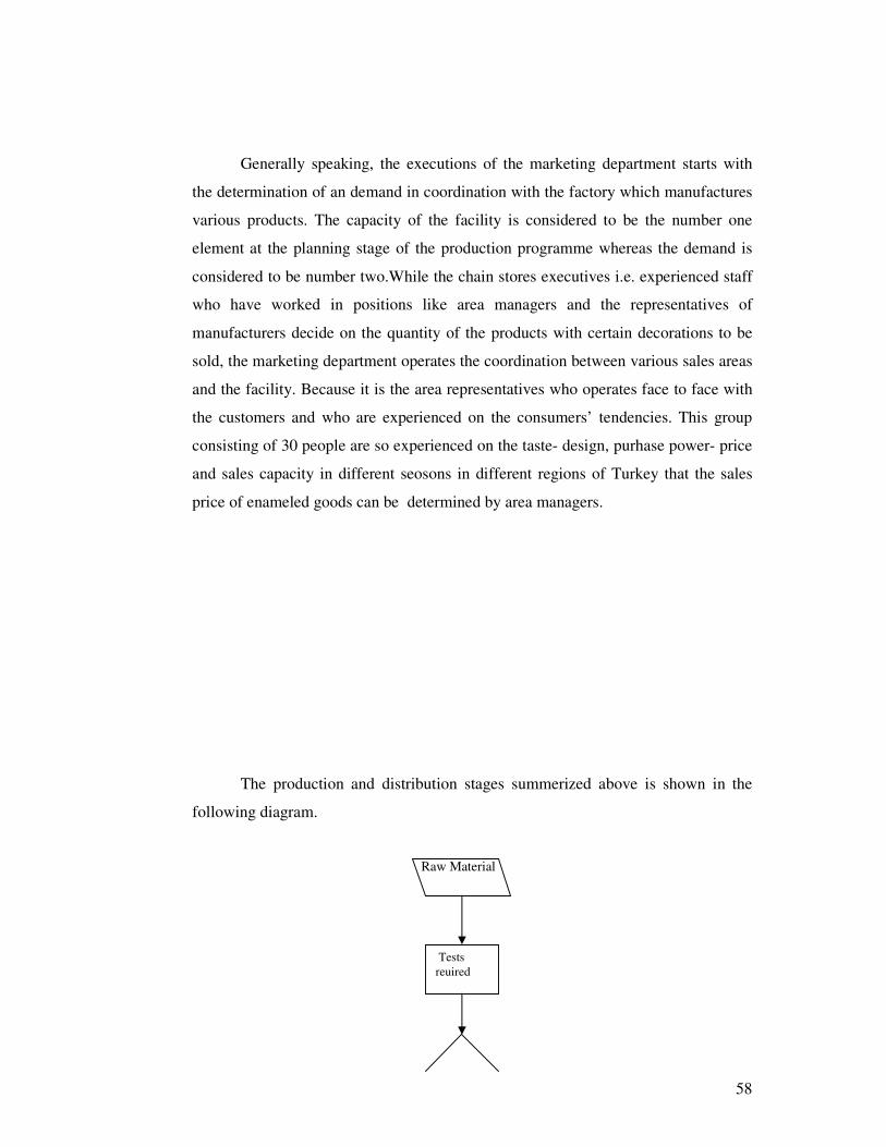
58

Generally speaking, the executions of the marketing department starts with

the determination of an demand in coordination with the factory which manufactures

various products. The capacity of the facility is considered to be the number one

element at the planning stage of the production programme whereas the demand is

considered to be number two.While the chain stores executives i.e. experienced staff

who have worked in positions like area managers and the representatives of

manufacturers decide on the quantity of the products with certain decorations to be

sold, the marketing department operates the coordination between various sales areas

and the facility. Because it is the area representatives who operates face to face with

the customers and who are experienced on the consumers’ tendencies. This group

consisting of 30 people are so experienced on the taste- design, purhase power- price

and sales capacity in different seosons in different regions of Turkey that the sales

price of enameled goods can be determined by area managers.

The production and distribution stages summerized above is shown in the

following diagram.

Raw Material

Tests reuired

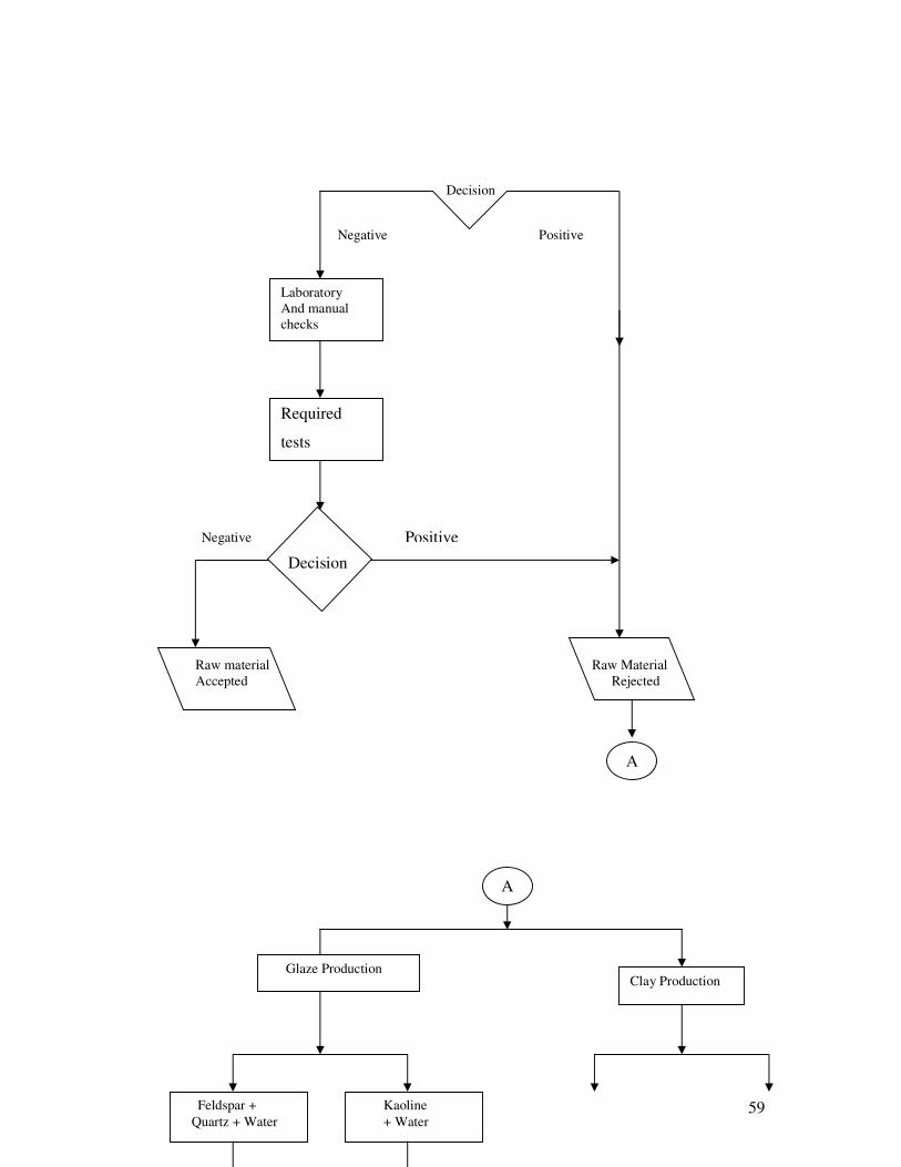
59

Decision

Negative Positive

Negative

Raw material Raw Material Accepted Rejected

Laboratory And manual checks

Required

tests

A

Decision

Positive

A

Clay Production Glaze Production

Kaoline + Water

Feldspar + Quartz + Water

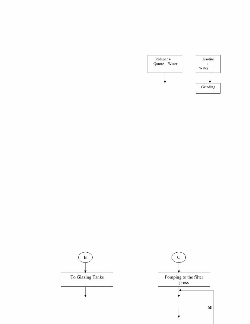
60

Kaoline + Water

Feldspar + Quartz + Water

Grinding

B

To Glazing Tanks

C

Pomping to the filter press

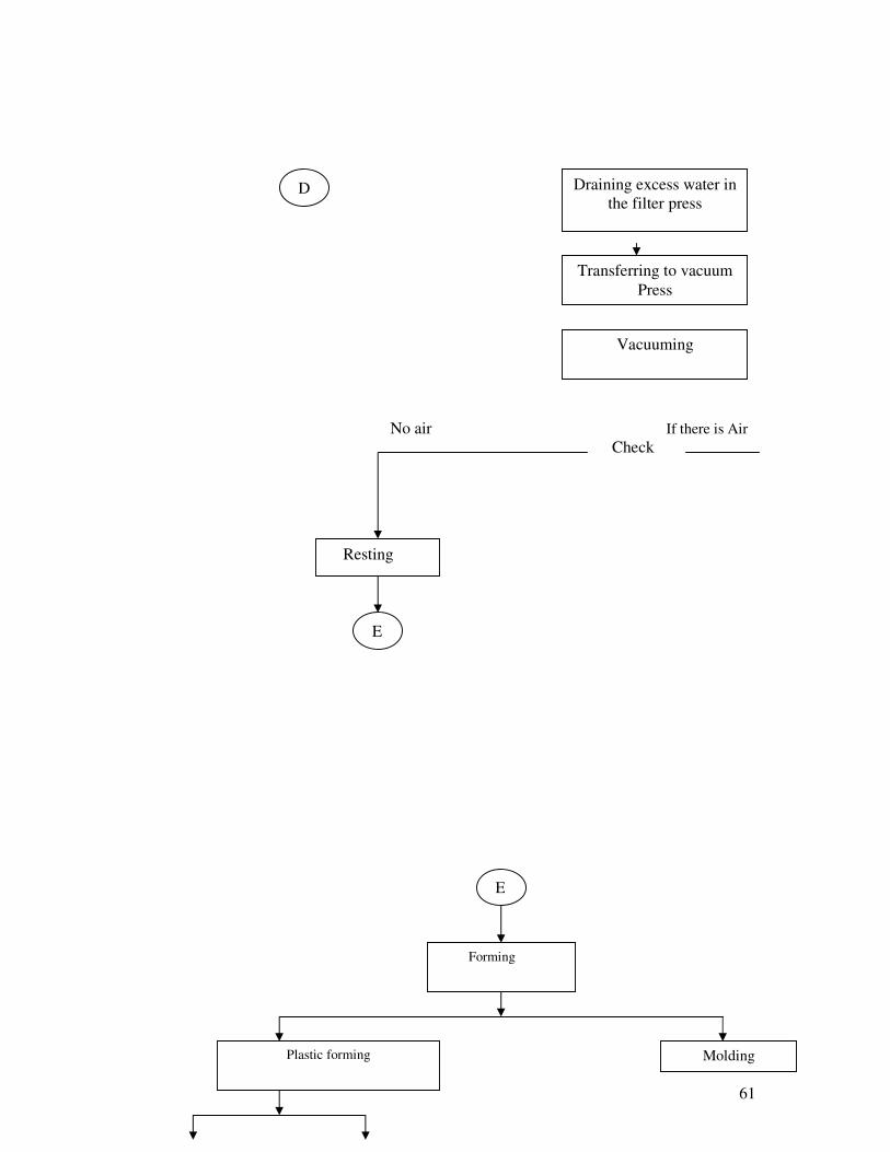
61

No air If there is Air Check

D Draining excess water in the filter press

Transferring to vacuum Press

Vacuuming

Resting

E

E

Forming

Plastic forming

Molding

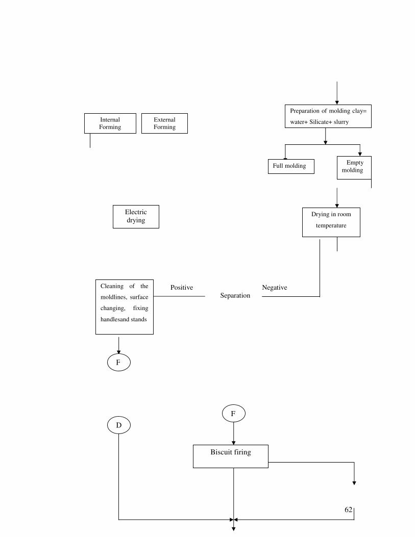
62

Positive Negative Separation

External Forming

Internal Forming

Preparation of molding clay=

water+ Silicate+ slurry

Empty molding

Full molding

Electric drying

Drying in room

temperature

Cleaning of the

moldlines, surface

changing, fixing

handlesand stands

F

D

Biscuit firing

F

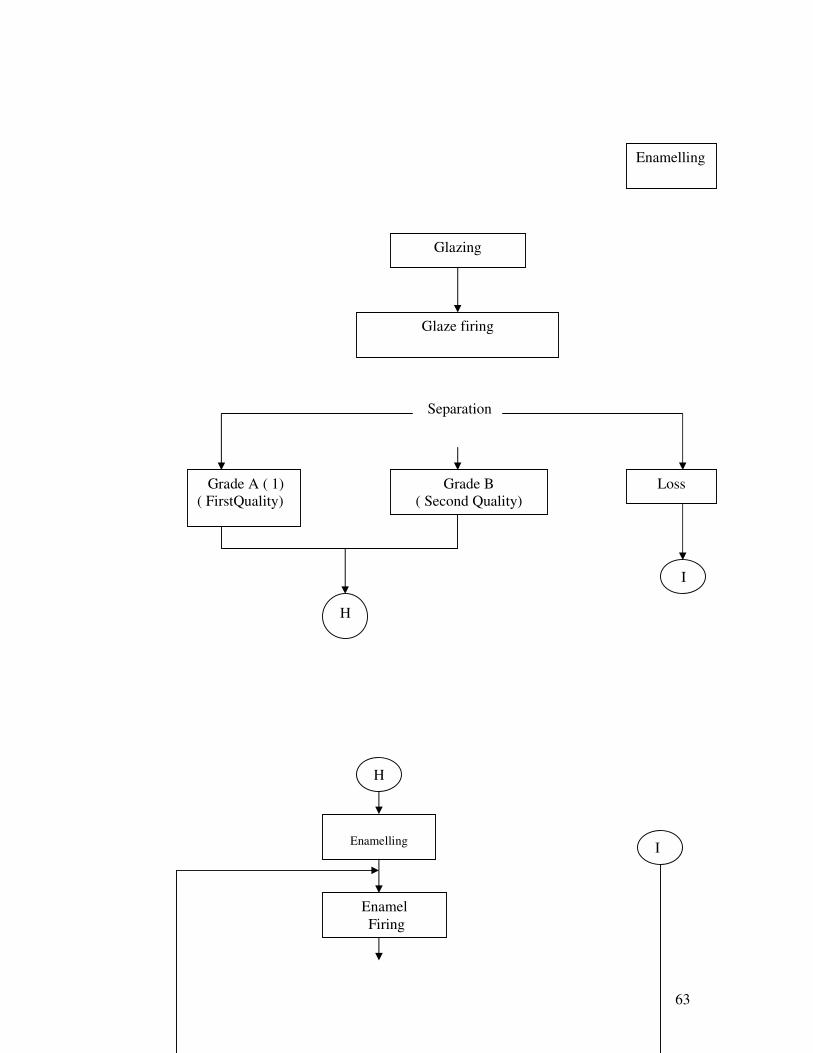
63

Separation

Enamelling

Glaze firing

Glazing

Grade B ( Second Quality)

Grade A ( 1) ( FirstQuality)

Loss

H

I

H

Enamelling

Enamel Firing

I

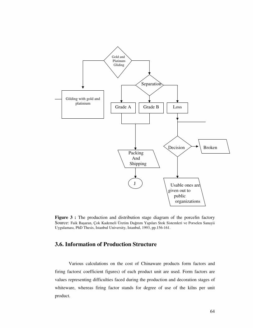
64

Gold and Platinum Gliding

Separation

Decision Broken Packing And Shipping Usable ones are given out to public organizations Figure 3 : The production and distribution stage diagram of the porcelin factory Source: Faik Başaran, Çok Kademeli Üretim Dağıtım Yapıları Stok Sistemleri ve Porselen Sanayii Uygulaması, PhD Thesis, Istanbul University, Istanbul, 1993, pp.156-161.

3.6. Information of Production Structure

Various calculations on the cost of Chinaware products form factors and

firing factors( coefficient figures) of each product unit are used. Form factors are

values representing difficulties faced during the production and decoration stages of

whiteware, whereas firing factor stands for degree of use of the kilns per unit

product.

Gilding with gold and

platinium Grade A

Grade B

Loss

J

65

For the form factor, each product is given the value of 1 then for the products

exceeding 30 cm in diameter another value of 0.5 is added for each extra 5 cm.

Weight is the key element on the determination of the difficulty factor and after 5

kgs, 0.1 per 5 kg unit, and after 25 kgs 0.2 is added to the calculation. For the

products which takes more than 60 minutes to molda figure of 0.1 is added to the

forming factor for each 30 minute period. With non fixing formings should the

product weight less than 1.5 kgs, the forming factor is directly calculated as 1. If

handles etc are to be fixed to the body or the lids another 0.25 is added for each piece

fixed.

With the plates, forming factor after 15 cm at the biscuit stage a figure of 0.5

for each 5 cm, and after 25 cms 1 per 5 cm is added to the initial factor 1. When

calculating the forming factors of bowls, should the product at the biscuit stage is

less than 5 cm in diameter the forming factor is considered 1, as the diameter

increases another 0.2 is added for each 5 cm.

While calculating the volumes of the products going into the kilns used in the

determination of their firing factors, the products are to roughly resemble a cyllinder

or a rectangular prism. Before the volumes are calculated, the size of the product at

the biscuit stage is increased 1.5 cm. At this stage if the heigth of the product is less

than 6 cm, the heigth is accepted as 6 cm. Products reaching 6 to 10 cm in height

with the additions are taken as 10 cm. However, with the products exceeding 10 cm

without the 1.5 cm addition, the value found with the addition is the base.

Additionally, with stacked neatly firings number of shelves and the shell heights

should be taken into consideration. The structure of the product and glazing show

differences when they are loaded on op of each other. For instance larger products

such as kettles and vases should be piled in the kiln with cake plates taking extra care

so as to protect the decoration and cake plates should be put in the kiln with cups so

that different combinations help to make best use of the kiln capacity. For this reason

although certain rules are tried to follow to calculate the firing factor, the result is

gained with a certain approximation.

66

Valume of the Prism

Firing Factor = ------------------------------

1OOO*k

k in this formula stands for the number of layers. 1000 stands for the

divident as 1 firing factor is given 1000 cm3 volume.

In the following section cost records of the porcelain facility where the

application study is performed. The records used here are the records for compote

and cake sets out of 300 different items. In the facility where the production lasts 24

hours, the kilns are never turned off so glazing and decoration kilns are operated in

three shifts.In the other departments a workday consists of 8 hours and when

necessary the employees work overtime even at the weekends.

When calculating the unit costs, total costs of a department within a period and total

weights of firing-forming factors determining the property of the production activity

are considered.

Items like power, machinery, construction maintenance and spare parts costs

have been used as setup costs of various departments. Management of the facilities,

and items such as main labour costs, indirect materials, superstructure maintenance,

and amortization constitude the fixed costs. Seasonal cost ratio of holding cost is

determined %10 of the total production cost at various stages.Chinaware (porcelain)

does not lose its quality in time so once the product is produced and placed in the

warehouse it only requires the lighting and protection services enabling us to use the

factors such as the crackability of the product and the change in the trends.

Data from both the marketing department of the production facility and

marketing company of the holding have been used to calculate unit cost figures. To

calculate the costs of the sets amount and cost ratio of different decorations, the

records of the household appliances department of the corporation have been

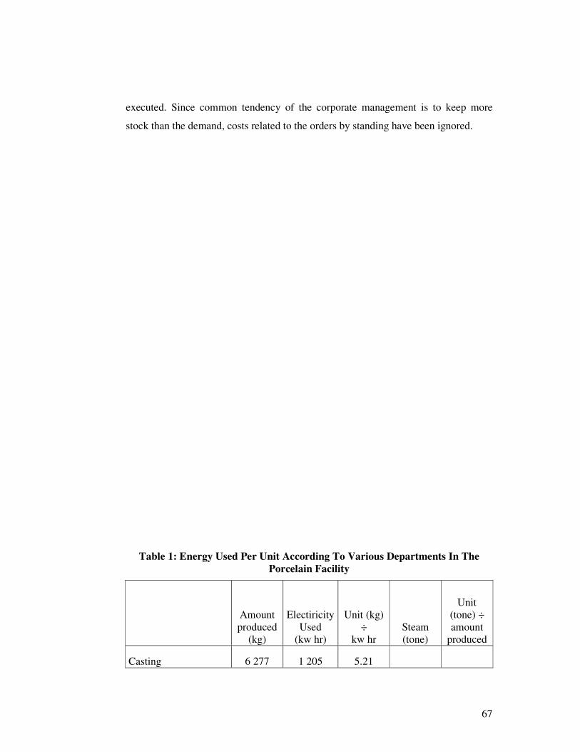
67

executed. Since common tendency of the corporate management is to keep more

stock than the demand, costs related to the orders by standing have been ignored.

Table 1: Energy Used Per Unit According To Various Departments In The Porcelain Facility

Amount produced

(kg)

Electiricity Used

(kw hr)

Unit (kg) ÷

kw hr Steam (tone)

Unit (tone) ÷ amount

produced

Casting 6 277 1 205 5.21

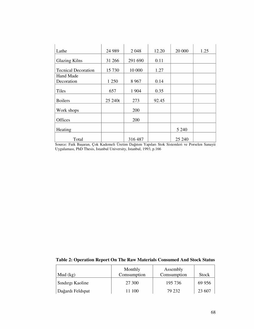
68

Lathe 24 989 2 048 12.20 20 000 1.25

Glazing Kilns 31 266 291 690 0.11

Tecnical Decoration 15 730 10 000 1.27 Hand Made Decoration 1 250 8 967 0.14

Tiles 657 1 904 0.35

Boilers 25 240t 273 92.45

Work shops 200

Offices 200

Heating 5 240

Total 316 487 25 240 Source: Faik Başaran, Çok Kademeli Üretim Dağıtım Yapıları Stok Sistemleri ve Porselen Sanayii Uygulaması, PhD Thesis, Istanbul University, Istanbul, 1993, p.166

Table 2: Operation Report On The Raw Materials Consumed And Stock Status

Mud (kg) Monthly

Comsumption Assembly

Comsumption Stock

Sındırgı Kaoline 27 300 195 736 69 956

Dağardı Feldspat 11 100 79 232 23 607

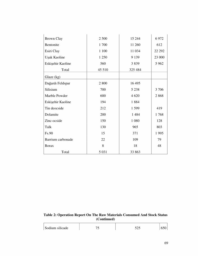
69

Brown Clay 2 500 15 244 6 972

Bentonite 1 700 11 260 612

Esiri Clay 1 100 11 034 22 292

Uşak Kaoline 1 250 9 139 23 000

Eskişehir Kaoline 560 3 839 5 962

Total 45 510 325 484

Glaze (kg)

Dağardı Feldspar 2 800 16 495

Silisium 700 5 238 3 706

Marble Powder 600 4 620 2 868

Eskişehir Kaoline 194 1 884

Tin deocside 212 1 599 419

Dolamite 200 1 484 1 768

Zinc-ocside 150 1 080 128

Talk 130 965 803

Fs.90 15 371 1 995

Barrium carbonade 22 109 79

Borax 8 18 48

Total 5 031 33 863

Table 2: Operation Report On The Raw Materials Consumed And Stock Status (Continued)

Sodium silicade 75 525 650

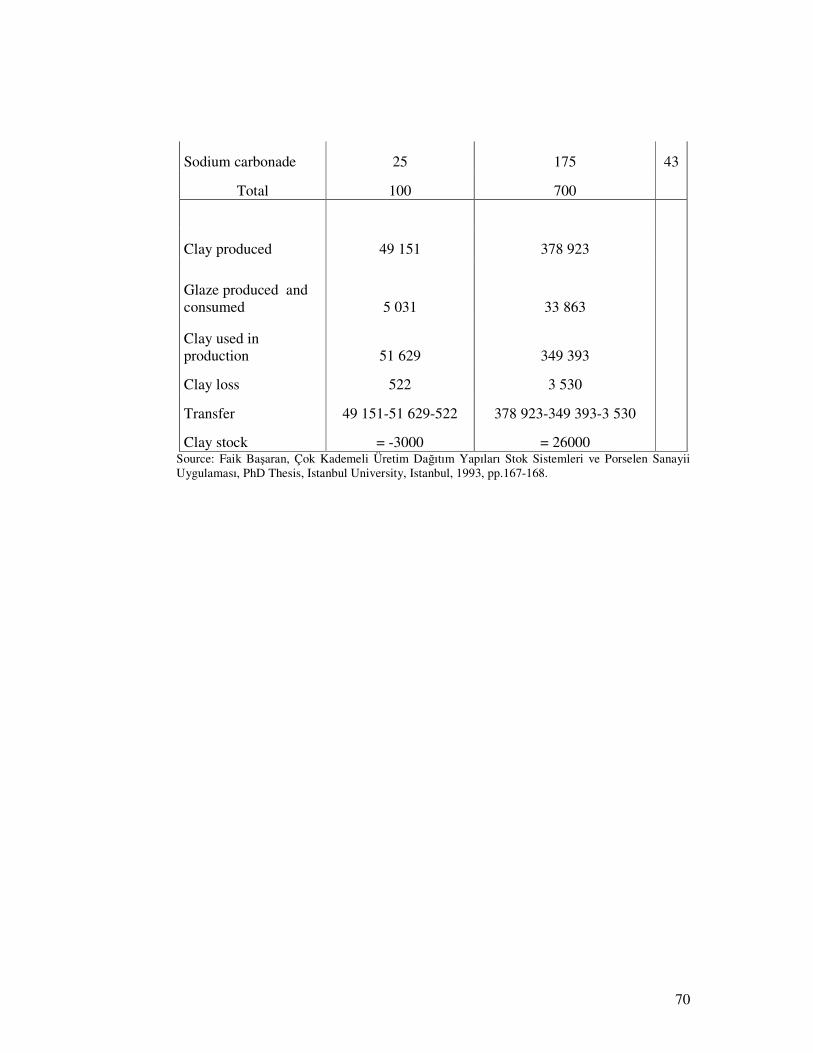
70

Sodium carbonade 25 175 43

Total 100 700

Clay produced 49 151 378 923

Glaze produced and consumed 5 031 33 863

Clay used in production 51 629 349 393

Clay loss 522 3 530

Transfer 49 151-51 629-522 378 923-349 393-3 530

Clay stock = -3000 = 26000 Source: Faik Başaran, Çok Kademeli Üretim Dağıtım Yapıları Stok Sistemleri ve Porselen Sanayii Uygulaması, PhD Thesis, Istanbul University, Istanbul, 1993, pp.167-168.

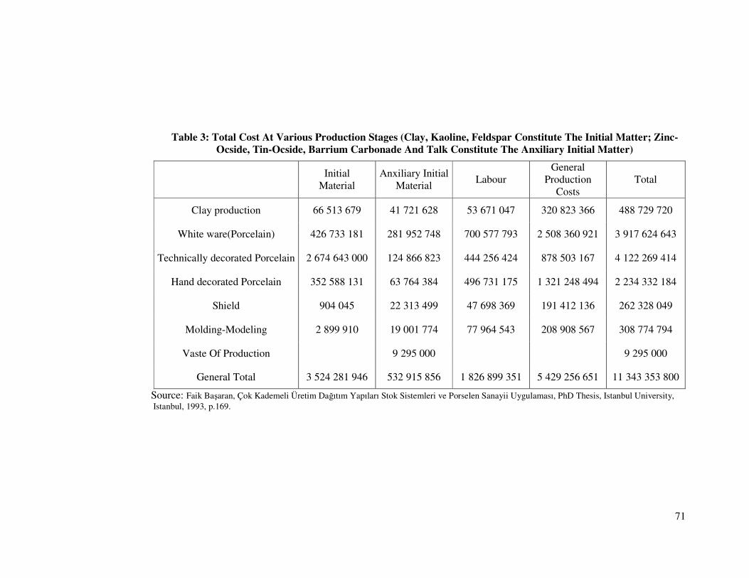
71

Table 3: Total Cost At Various Production Stages (Clay, Kaoline, Feldspar Constitute The Initial Matter; Zinc-Ocside, Tin-Ocside, Barrium Carbonade And Talk Constitute The Anxiliary Initial Matter)

Initial

Material Anxiliary Initial

Material Labour

General Production

Costs Total

Clay production 66 513 679 41 721 628 53 671 047 320 823 366 488 729 720

White ware(Porcelain) 426 733 181 281 952 748 700 577 793 2 508 360 921 3 917 624 643

Technically decorated Porcelain 2 674 643 000 124 866 823 444 256 424 878 503 167 4 122 269 414

Hand decorated Porcelain 352 588 131 63 764 384 496 731 175 1 321 248 494 2 234 332 184

Shield 904 045 22 313 499 47 698 369 191 412 136 262 328 049

Molding-Modeling 2 899 910 19 001 774 77 964 543 208 908 567 308 774 794

Vaste Of Production 9 295 000 9 295 000

General Total 3 524 281 946 532 915 856 1 826 899 351 5 429 256 651 11 343 353 800

Source: Faik Başaran, Çok Kademeli Üretim Dağıtım Yapıları Stok Sistemleri ve Porselen Sanayii Uygulaması, PhD Thesis, Istanbul University, Istanbul, 1993, p.169.

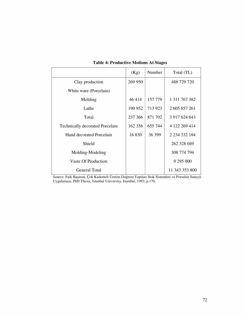
72

Table 4: Productive Motions At Stages

(Kg) Number Total (TL)

Clay production 269 950 488 729 720

White ware (Porcelain)

Molding 46 414 157 779 1 311 767 382

Lathe 190 952 713 923 2 605 857 261

Total 237 366 871 702 3 917 624 643

Technically decorated Porcelain 162 356 655 744 4 122 269 414

Hand decorated Porcelain 16 830 36 399 2 234 332 184

Shield 262 328 049

Molding-Modeling 308 774 794

Vaste Of Production 9 295 000

General Total 11 343 353 800


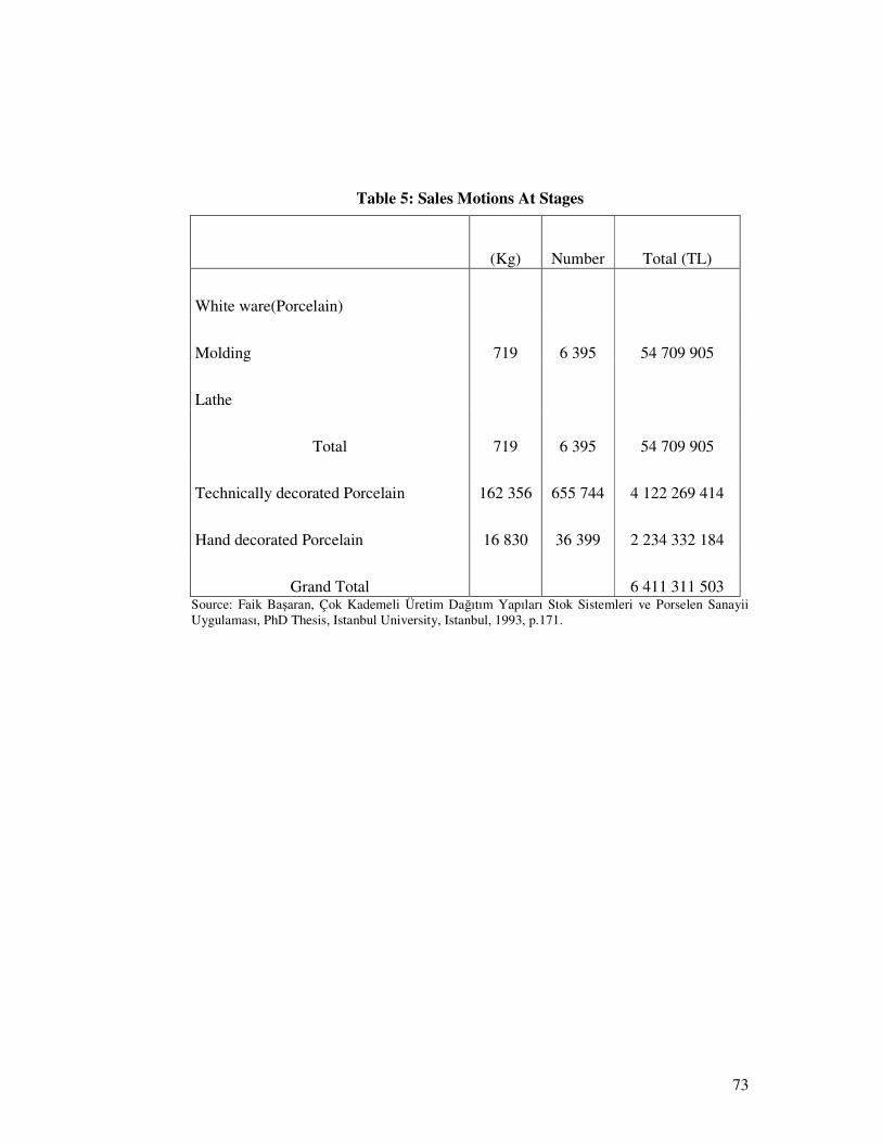
73

Table 5: Sales Motions At Stages

(Kg) Number Total (TL)

White ware(Porcelain)

Molding 719 6 395 54 709 905

Lathe

Total 719 6 395 54 709 905

Technically decorated Porcelain 162 356 655 744 4 122 269 414

Hand decorated Porcelain 16 830 36 399 2 234 332 184

Grand Total 6 411 311 503 Source: Faik Başaran, Çok Kademeli Üretim Dağıtım Yapıları Stok Sistemleri ve Porselen Sanayii Uygulaması, PhD Thesis, Istanbul University, Istanbul, 1993, p.171.

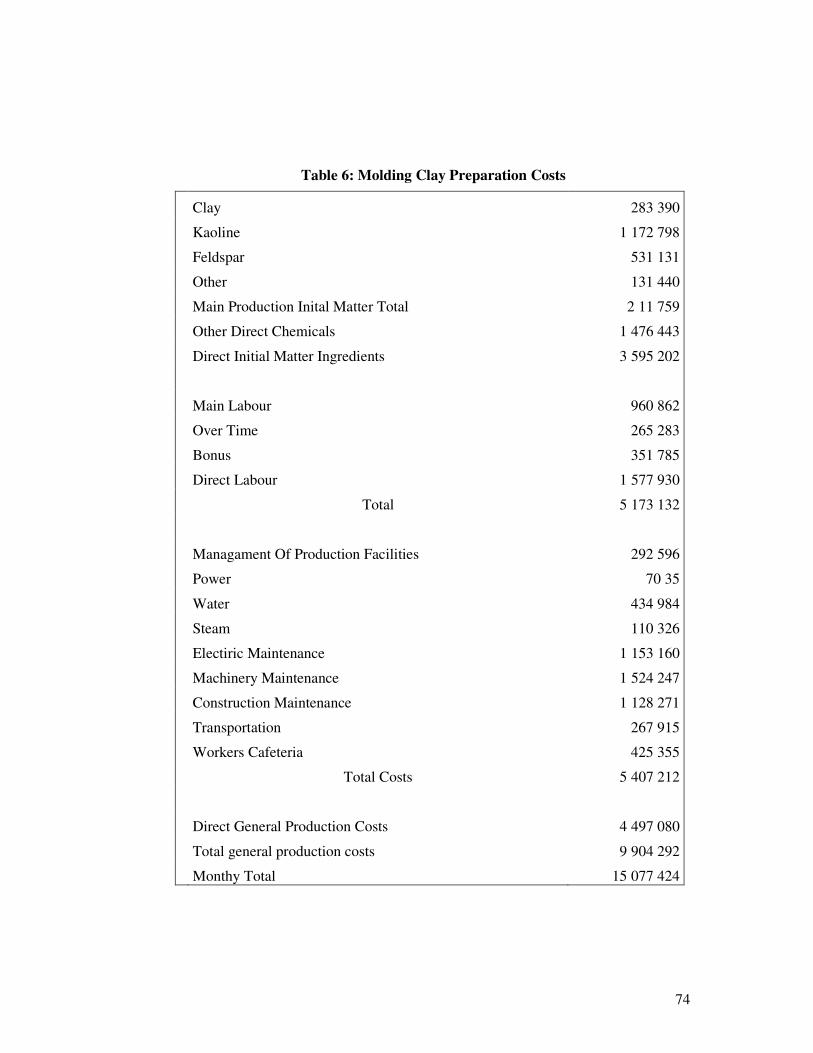
74

Table 6: Molding Clay Preparation Costs

Clay 283 390

Kaoline 1 172 798

Feldspar 531 131

Other 131 440

Main Production Inital Matter Total 2 11 759

Other Direct Chemicals 1 476 443

Direct Initial Matter Ingredients 3 595 202

Main Labour 960 862

Over Time 265 283

Bonus 351 785

Direct Labour 1 577 930

Total 5 173 132

Managament Of Production Facilities 292 596

Power 70 35

Water 434 984

Steam 110 326

Electiric Maintenance 1 153 160

Machinery Maintenance 1 524 247

Construction Maintenance 1 128 271

Transportation 267 915

Workers Cafeteria 425 355

Total Costs 5 407 212

Direct General Production Costs 4 497 080

Total general production costs 9 904 292

Monthy Total 15 077 424

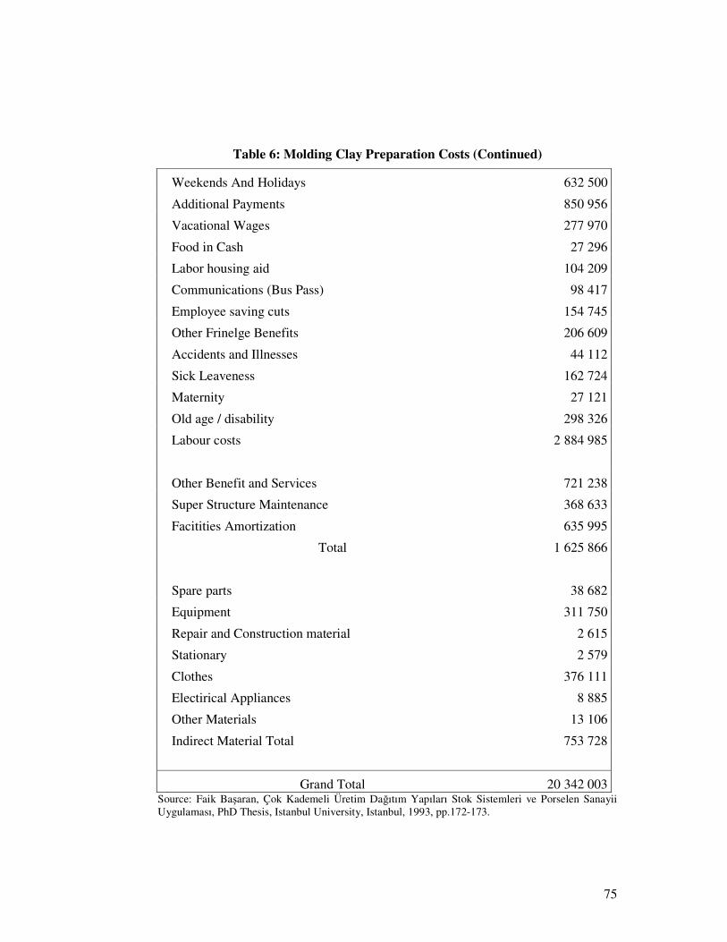
75

Table 6: Molding Clay Preparation Costs (Continued)

Weekends And Holidays 632 500

Additional Payments 850 956

Vacational Wages 277 970

Food in Cash 27 296

Labor housing aid 104 209

Communications (Bus Pass) 98 417

Employee saving cuts 154 745

Other Frinelge Benefits 206 609

Accidents and Illnesses 44 112

Sick Leaveness 162 724

Maternity 27 121

Old age / disability 298 326

Labour costs 2 884 985

Other Benefit and Services 721 238

Super Structure Maintenance 368 633

Facitities Amortization 635 995

Total 1 625 866

Spare parts 38 682

Equipment 311 750

Repair and Construction material 2 615

Stationary 2 579

Clothes 376 111

Electirical Appliances 8 885

Other Materials 13 106

Indirect Material Total 753 728

Grand Total 20 342 003 Source: Faik Başaran, Çok Kademeli Üretim Dağıtım Yapıları Stok Sistemleri ve Porselen Sanayii Uygulaması, PhD Thesis, Istanbul University, Istanbul, 1993, pp.172-173.

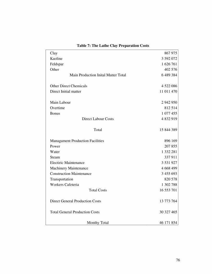
76

Table 7: The Lathe Clay Preparation Costs

Clay 867 975

Kaoline 3 592 072

Feldspar 1 626 761

Other 402 576


Other Direct Chemicals 4 522 086

Direct Initial matter 11 011 470

Main Labour 2 942 950

Overtime 812 514

Bonus 1 077 455

Direct Labour Costs 4 832 919

Total 15 844 389

Managament Production Facilities 896 169

Power 207 855

Water 1 332 281

Steam 337 911



Construction Maintenance 3 455 693


Workers Cafeteria 1 302 788



Total General Production Costs 30 327 465


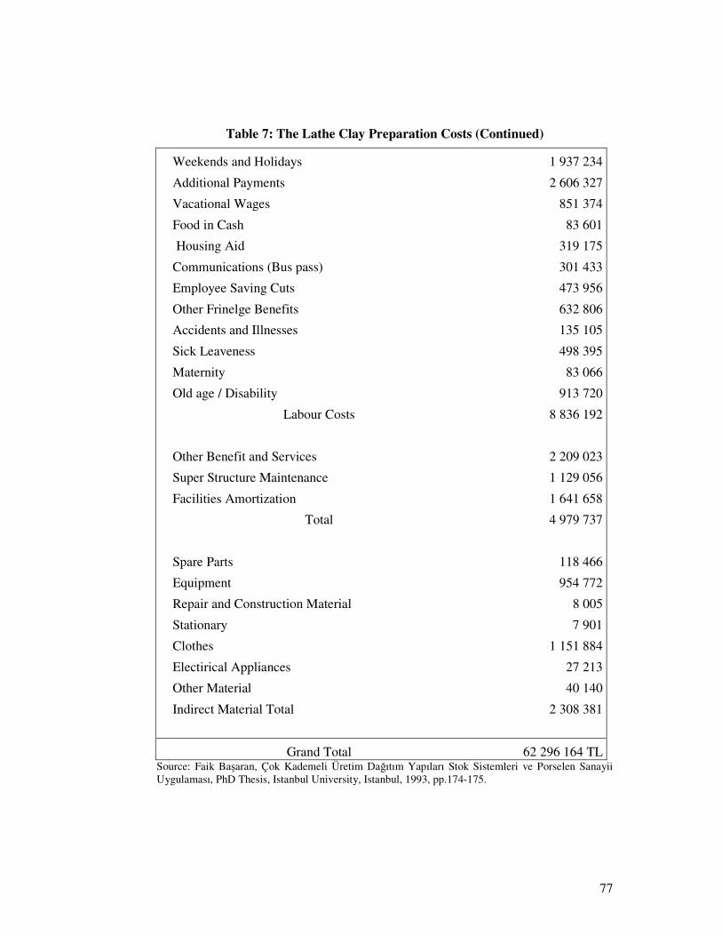
77

Table 7: The Lathe Clay Preparation Costs (Continued)

Weekends and Holidays 1 937 234

Additional Payments 2 606 327


Food in Cash 83 601

Housing Aid 319 175

Communications (Bus pass) 301 433

Employee Saving Cuts 473 956

Other Frinelge Benefits 632 806


Sick Leaveness 498 395

Maternity 83 066

Old age / Disability 913 720

Labour Costs 8 836 192

Other Benefit and Services 2 209 023

Super Structure Maintenance 1 129 056

Facilities Amortization 1 641 658

Total 4 979 737

Spare Parts 118 466

Equipment 954 772

Repair and Construction Material 8 005

Stationary 7 901

Clothes 1 151 884


Other Material 40 140

Indirect Material Total 2 308 381

Grand Total 62 296 164 TL Source: Faik Başaran, Çok Kademeli Üretim Dağıtım Yapıları Stok Sistemleri ve Porselen Sanayii Uygulaması, PhD Thesis, Istanbul University, Istanbul, 1993, pp.174-175.

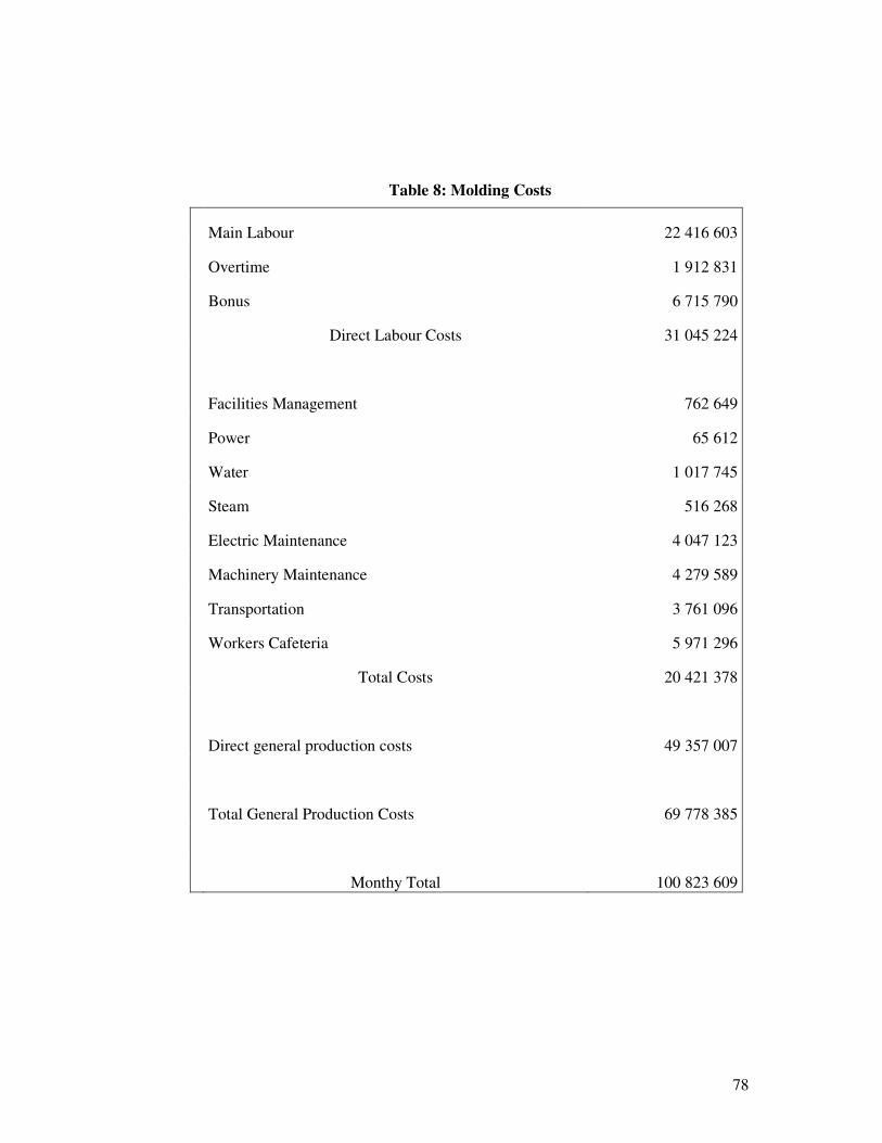
78

Table 8: Molding Costs


Overtime 1 912 831

Bonus 6 715 790

Direct Labour Costs 31 045 224

Facilities Management 762 649

Power 65 612

Water 1 017 745

Steam 516 268

Electric Maintenance 4 047 123


Transportation 3 761 096



Direct general production costs 49 357 007



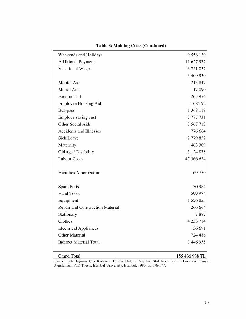
79

Table 8: Molding Costs (Continued)


Additional Payment 11 627 977

Vacational Wages 3 751 037

3 409 930

Marital Aid 213 847

Mortal Aid 17 090

Food in Cash 265 956

Employee Housing Aid 1 684 92

Bus-pass 1 348 119

Employe saving cust 2 777 731

Other Social Aids 3 567 712


Sick Leave 2 779 852

Maternity 463 309

Old age / Disability 5 124 878



Spare Parts 30 984

Hand Tools 599 974

Equipment 1 526 855


Stationary 7 887

Clothes 4 253 714





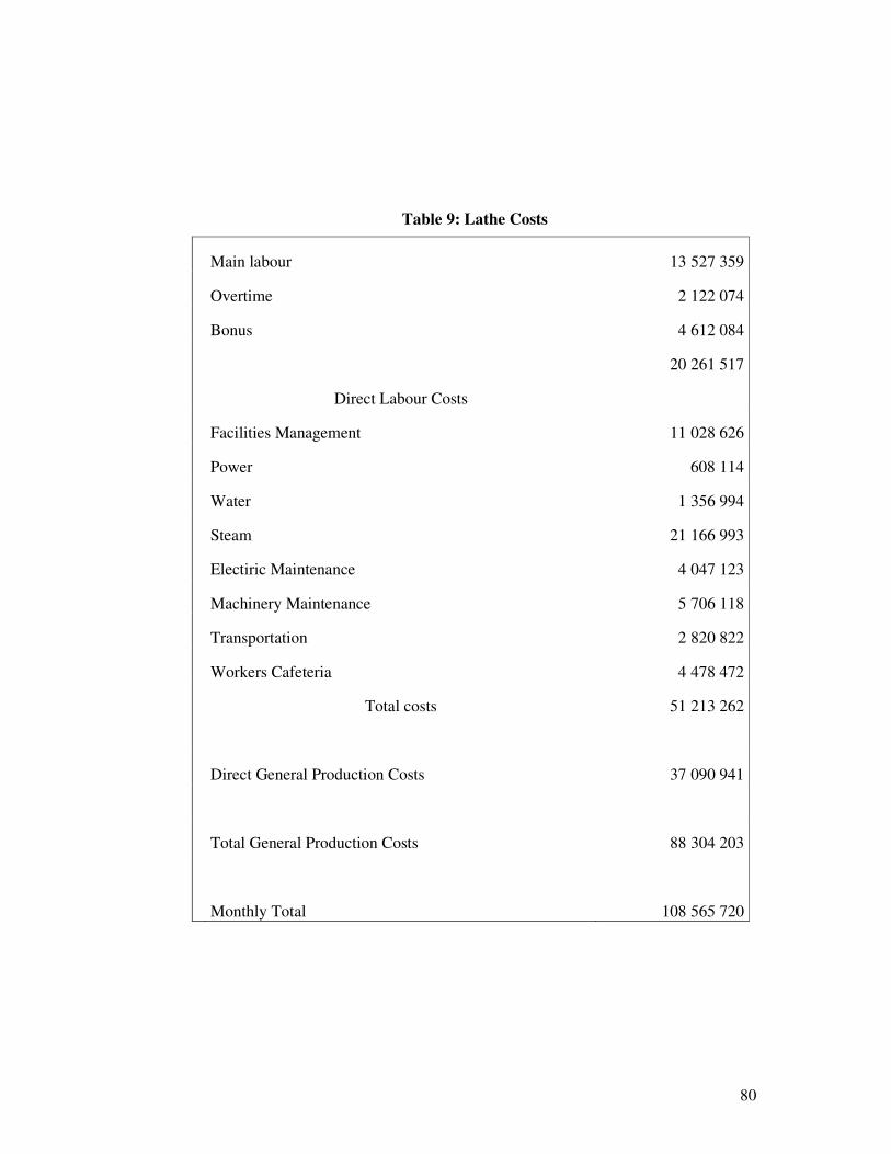
80

Table 9: Lathe Costs

Main labour 13 527 359

Overtime 2 122 074

Bonus 4 612 084

20 261 517

Direct Labour Costs

Facilities Management 11 028 626

Power 608 114

Water 1 356 994

Steam 21 166 993





Total costs 51 213 262



Monthly Total 108 565 720

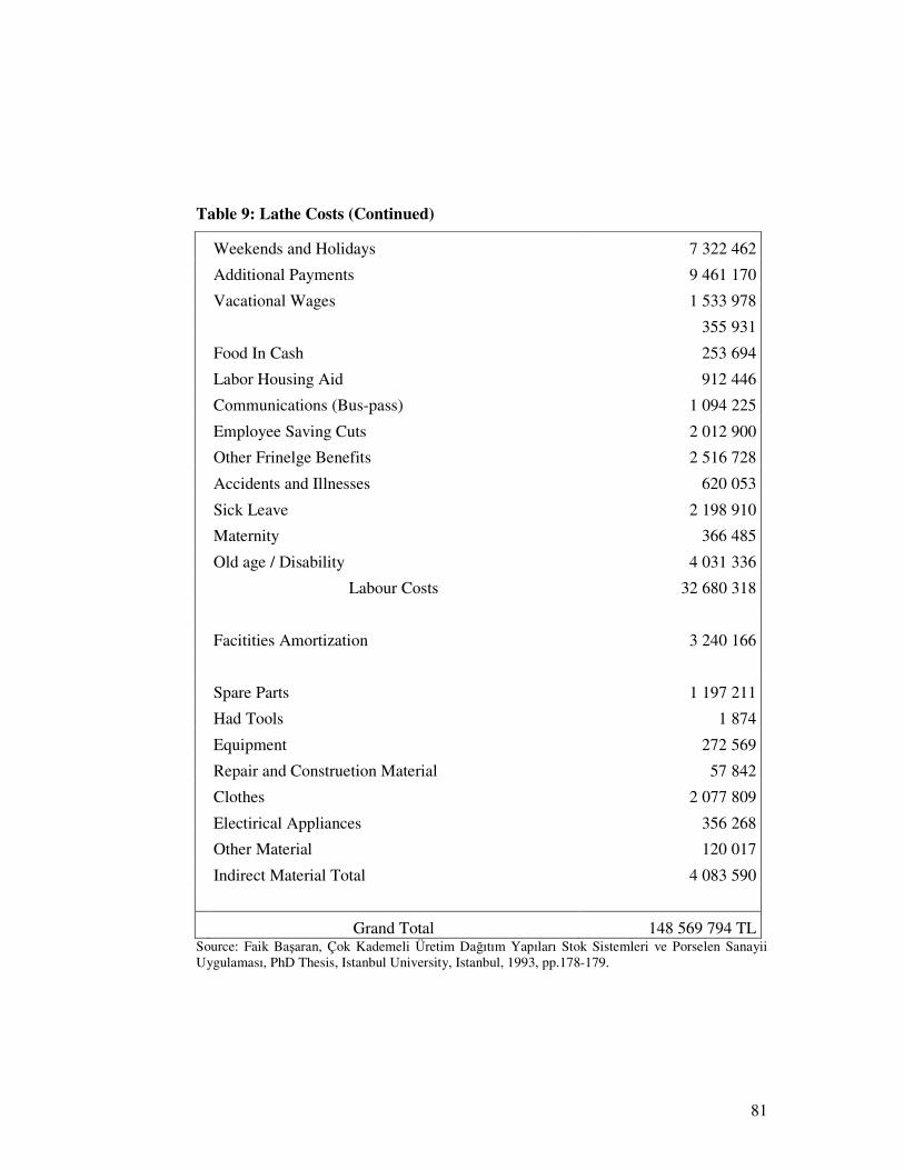
81

Table 9: Lathe Costs (Continued)




355 931

Food In Cash 253 694

Labor Housing Aid 912 446

Communications (Bus-pass) 1 094 225

Employee Saving Cuts 2 012 900

Other Frinelge Benefits 2 516 728



Maternity 366 485



Facitities Amortization 3 240 166

Spare Parts 1 197 211

Had Tools 1 874

Equipment 272 569

Repair and Construetion Material 57 842

Clothes 2 077 809





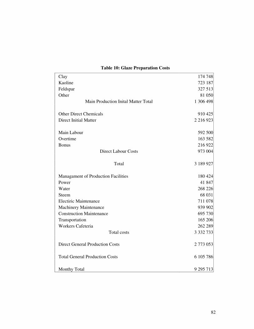
82

Table 10: Glaze Preparation Costs

Clay 174 748

Kaoline 723 187

Feldspar 327 513

Other 81 050


Other Direct Chemicals 910 425

Direct Initial Matter 2 216 923

Main Labour 592 500

Overtime 163 582

Bonus 216 922

Direct Labour Costs 973 004

Total 3 189 927

Managament of Production Facilities 180 424

Power 41 847

Water 268 226

Steem 68 031

Electiric Maintenance 711 078

Machinery Maintenance 939 902

Construction Maintenance 695 730


Workers Cafeteria 262 289





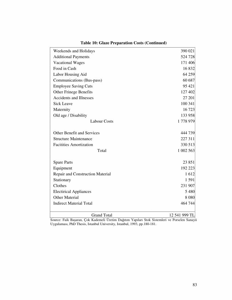
83

Table 10: Glaze Preparation Costs (Continued)

Weekends and Holidays 390 021

Additional Payments 524 728


Food in Cash 16 832

Labor Housing Aid 64 259

Communications (Bus-pass) 60 687

Employee Saving Cuts 95 421

Other Frinege Benefits 127 402


Sick Leave 100 341

Maternity 16 723

Old age / Disability 133 958


Other Benefit and Services 444 739

Structure Maintenance 227 311


Total 1 002 563

Spare Parts 23 851

Equipment 192 223


Stationary 1 591

Clothes 231 907



Indirect Material Total 464 744


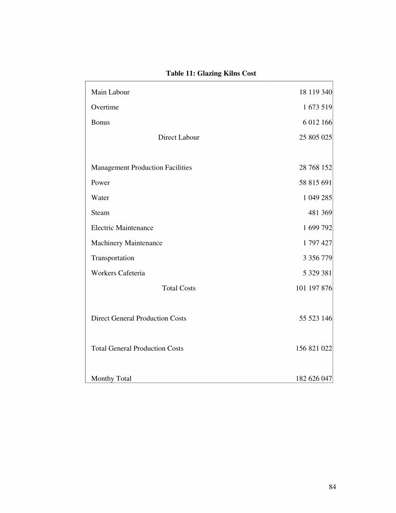
84

Table 11: Glazing Kilns Cost


Overtime 1 673 519

Bonus 6 012 166


Management Production Facilities 28 768 152

Power 58 815 691

Water 1 049 285

Steam 481 369

Electric Maintenance 1 699 792








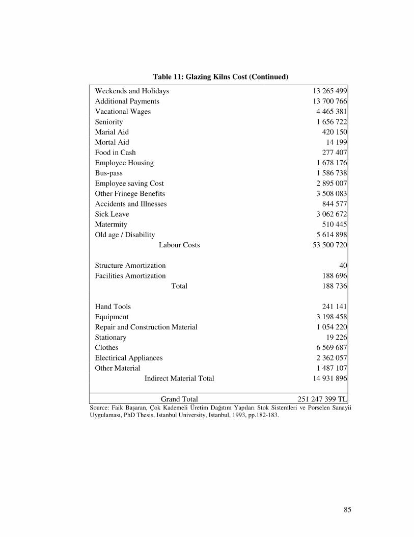
85

Table 11: Glazing Kilns Cost (Continued)




Seniority 1 656 722

Marial Aid 420 150

Mortal Aid 14 199


Employee Housing 1 678 176

Bus-pass 1 586 738

Employee saving Cost 2 895 007

Other Frinege Benefits 3 508 083



Matermity 510 445



Structure Amortization 40

Facilities Amortization 188 696

Total 188 736

Hand Tools 241 141

Equipment 3 198 458

Repair and Construction Material 1 054 220

Stationary 19 226

Clothes 6 569 687

Electirical Appliances 2 362 057

Other Material 1 487 107



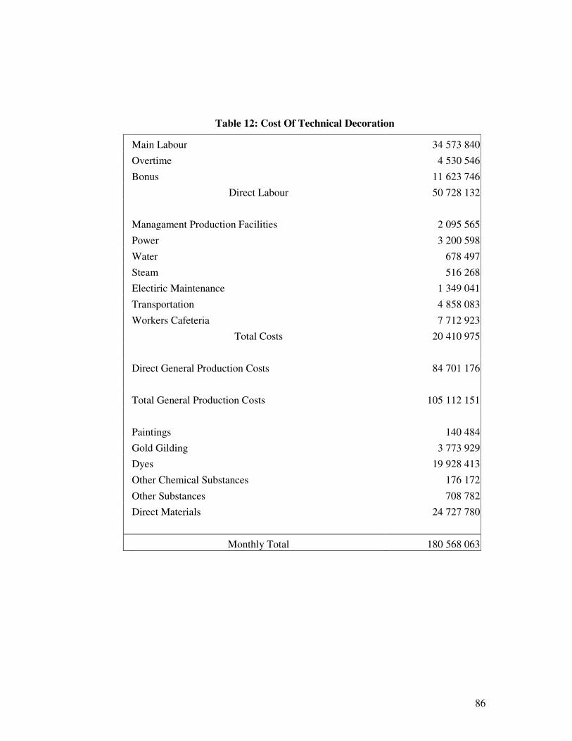
86

Table 12: Cost Of Technical Decoration


Overtime 4 530 546

Bonus 11 623 746


Managament Production Facilities 2 095 565

Power 3 200 598

Water 678 497

Steam 516 268







Paintings 140 484

Gold Gilding 3 773 929

Dyes 19 928 413

Other Chemical Substances 176 172

Other Substances 708 782

Direct Materials 24 727 780

Monthly Total 180 568 063

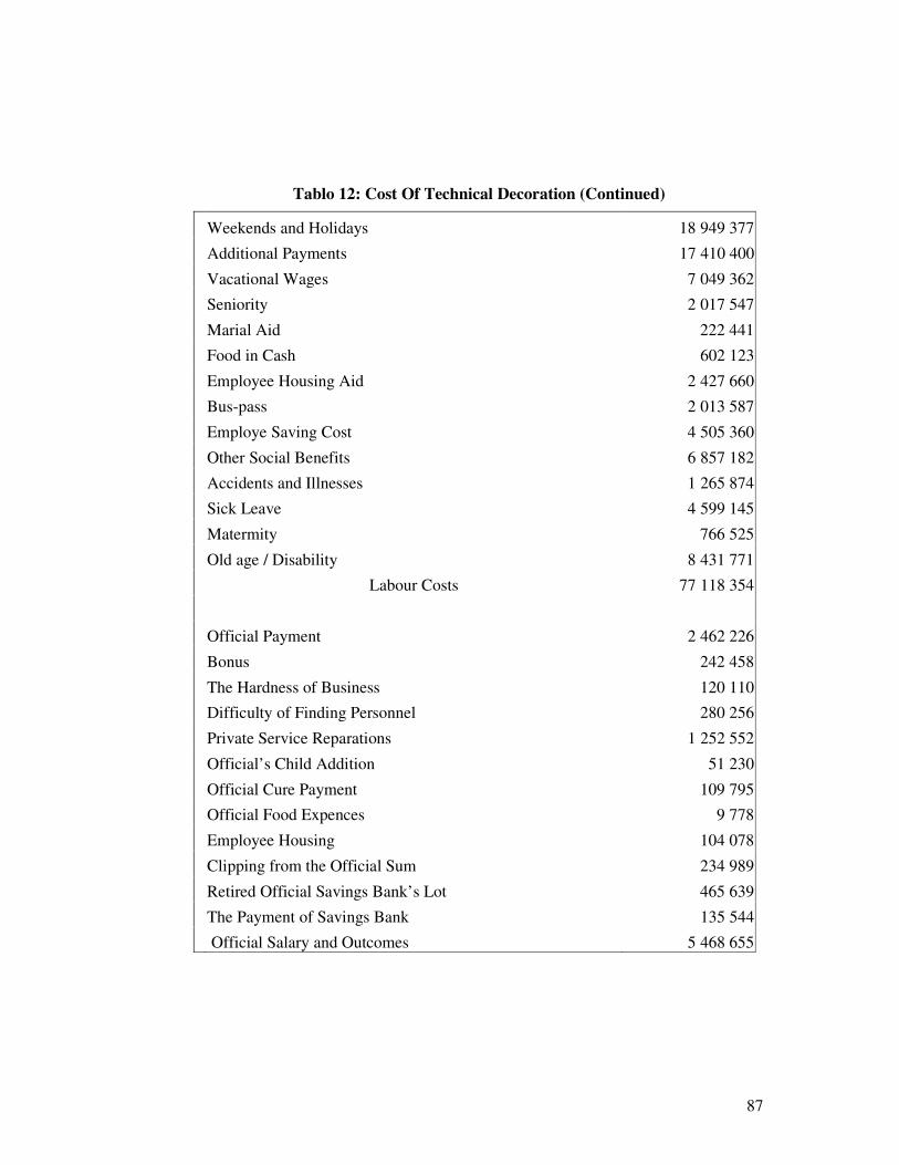
87

Tablo 12: Cost Of Technical Decoration (Continued)




Seniority 2 017 547

Marial Aid 222 441


Employee Housing Aid 2 427 660

Bus-pass 2 013 587

Employe Saving Cost 4 505 360

Other Social Benefits 6 857 182

Accidents and Illnesses 1 265 874


Matermity 766 525



Official Payment 2 462 226

Bonus 242 458

The Hardness of Business 120 110

Difficulty of Finding Personnel 280 256

Private Service Reparations 1 252 552

Official’s Child Addition 51 230

Official Cure Payment 109 795

Official Food Expences 9 778

Employee Housing 104 078

Clipping from the Official Sum 234 989

Retired Official Savings Bank’s Lot 465 639

The Payment of Savings Bank 135 544

Official Salary and Outcomes 5 468 655

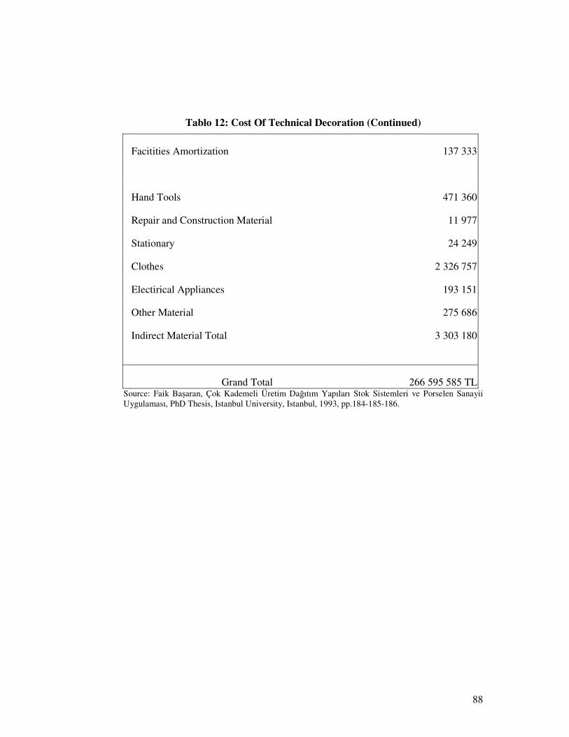
88

Tablo 12: Cost Of Technical Decoration (Continued)


Hand Tools 471 360


Stationary 24 249

Clothes 2 326 757




Grand Total 266 595 585 TL Source: Faik Başaran, Çok Kademeli Üretim Dağıtım Yapıları Stok Sistemleri ve Porselen Sanayii Uygulaması, PhD Thesis, Istanbul University, Istanbul, 1993, pp.184-185-186.

89

Table 13: Cost Of Technical Decoration Kilns

Main labour 10 641 517

Over time 982 861

Bonus 3 530 954


Managament Production Facilities 16 895 582

Power 34 542 549

Water 616 247

Steam 282 708

Electiric Maintenance 998 290

Machinery maintenance 1 055 632


Workers cafeteria 3 129 954


Direct general production costs 32 608 832

Total general production costs 92 101 235

Monthy total 107 256 567

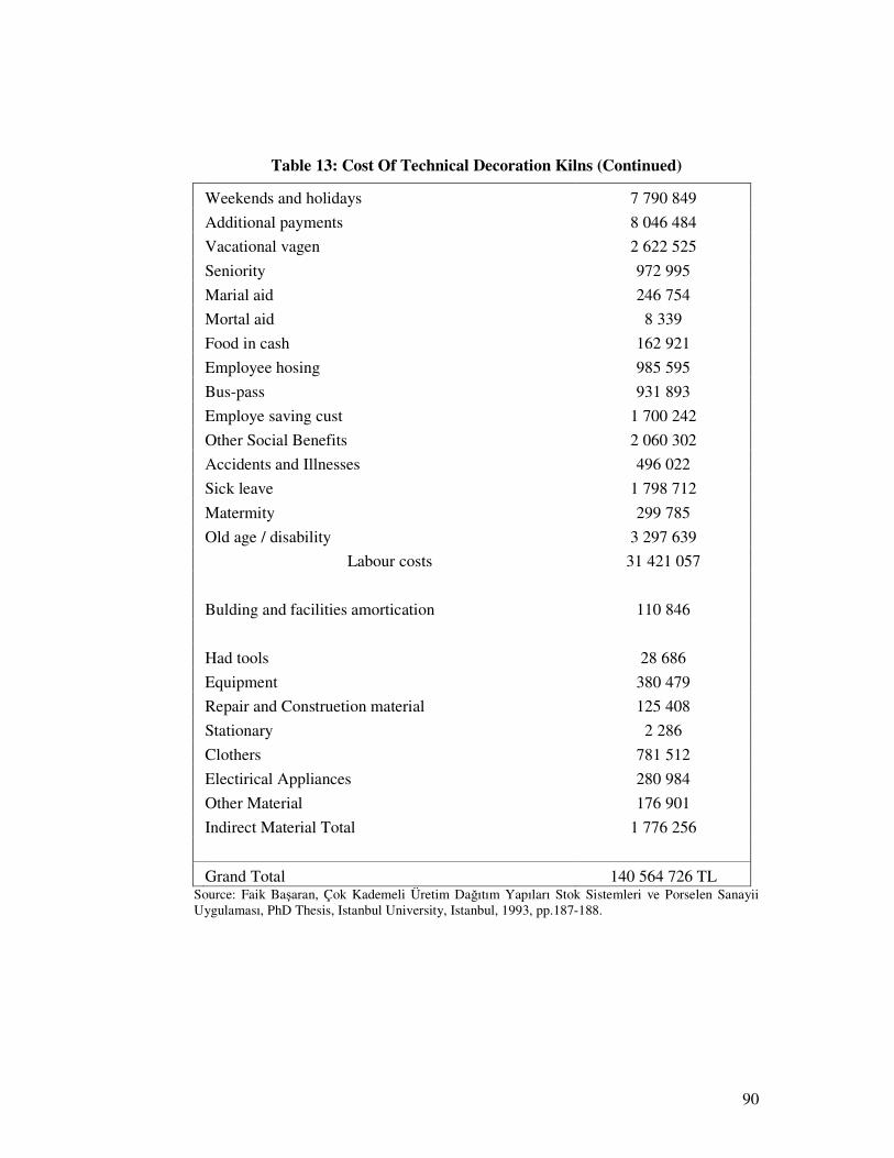
90

Table 13: Cost Of Technical Decoration Kilns (Continued)

Weekends and holidays 7 790 849

Additional payments 8 046 484

Vacational vagen 2 622 525

Seniority 972 995

Marial aid 246 754

Mortal aid 8 339

Food in cash 162 921

Employee hosing 985 595

Bus-pass 931 893

Employe saving cust 1 700 242

Other Social Benefits 2 060 302


Sick leave 1 798 712

Matermity 299 785

Old age / disability 3 297 639

Labour costs 31 421 057

Bulding and facilities amortication 110 846

Had tools 28 686

Equipment 380 479

Repair and Construetion material 125 408

Stationary 2 286

Clothers 781 512





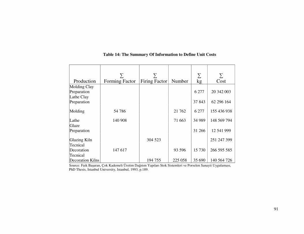
91

Table 14: The Summary Of Information to Define Unit Costs


Production ∑

Forming Factor ∑

Firing Factor Number ∑ kg

∑ Cost

Molding Clay Preparation 6 277 20 342 003 Lathe Clay Preparation 37 843 62 296 164

Molding 54 786 21 762 6 277 155 436 938

Lathe 140 908 71 663 34 989 148 569 794 Glaze Preparation 31 266 12 541 999

Glazing Kiln 304 523 251 247 399 Tecnical Decoration 147 617 93 596 15 730 266 595 585 Tecnical Decoration Kilns 194 755 225 058 35 690 140 564 726

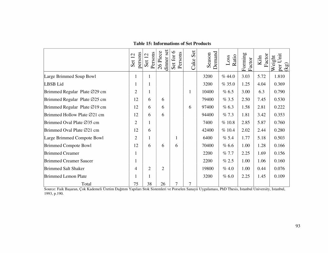
93

Table 15: Informations of Set Products

Din

ner

Set

12

pers

ons

Din

ner

Set

12

Per

sons

26

Pie

ce

dinn

er s

et

Com

post

e S

et f

or 6

P

erso

ns

Cak

e S

et

Sea

son

Dem

and

Los

s R

atio

For

min

g F

acto

r

Kil

n F

acto

r W

eigh

t pe

r U

nit

(kg)

Large Brimmed Soup Bowl 1 1 3200 % 44.0 3.03 5.72 1.810

LBSB Lid 1 1 3200 % 35.0 1.25 4.04 0.369

Brimmed Regular Plate ∅29 cm 2 1 1 10400 % 6.5 3.00 6.3 0.790

Brimmed Regular Plate ∅25 cm 12 6 6 79400 % 3.5 2.50 7.45 0.530

Brimmed Regular Plate ∅19 cm 12 6 6 6 97400 % 6.3 1.58 2.81 0.222

Brimmed Hollow Plate ∅21 cm 12 6 6 94400 % 7.3 1.81 3.42 0.353

Brimmed Oval Plate ∅35 cm 2 1 7400 % 10.8 2.85 5.87 0.760

Brimmed Oval Plate ∅21 cm 12 6 42400 % 10.4 2.02 2.44 0.280

Large Brimmed Compote Bowl 2 1 1 6400 % 5.4 1.77 5.18 0.503

Brimmed Compote Bowl 12 6 6 6 70400 % 6.6 1.00 1.28 0.166

Brimmed Creamer 1 2200 % 7.7 2.25 1.69 0.156

Brimmed Creamer Saucer 1 2200 % 2.5 1.00 1.06 0.160

Brimmed Salt Shaker 4 2 2 19800 % 4.0 1.00 0.44 0.076

Brimmed Lemon Plate 1 1 3200 % 6.0 2.25 1.45 0.109

Total 75 38 26 7 7 Source: Faik Başaran, Çok Kademeli Üretim Dağıtım Yapıları Stok Sistemleri ve Porselen Sanayii Uygulaması, PhD Thesis, Istanbul University, Istanbul, 1993, p.190.

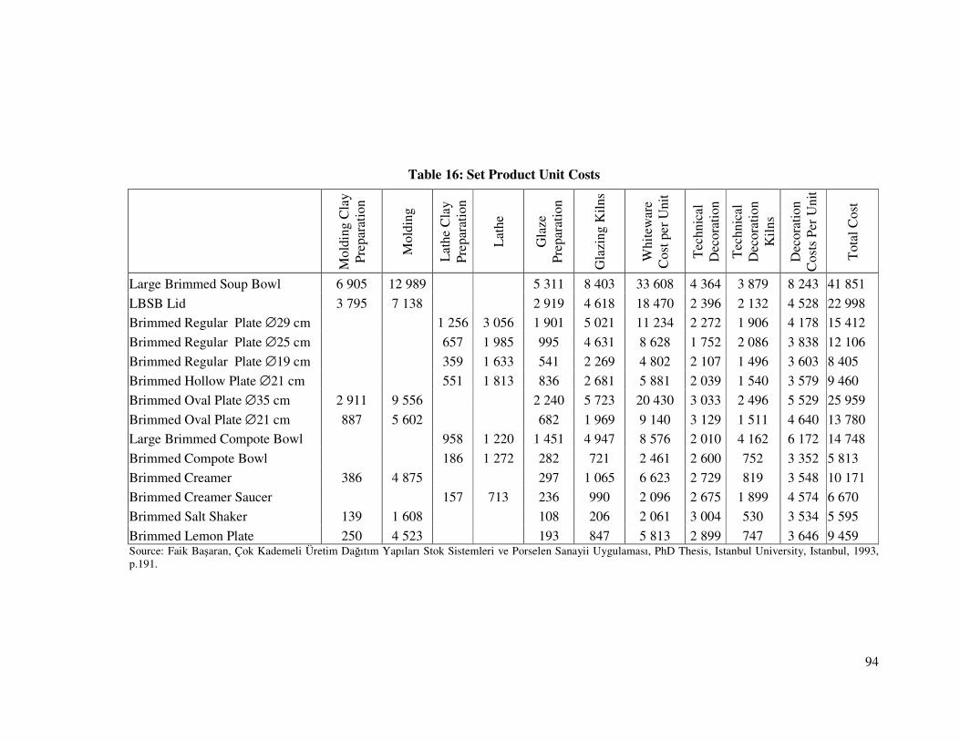
94

Table 16: Set Product Unit Costs

Mol

ding

Cla

y P

repa

rati

on

Mol

ding

Lat

he C

lay

Pre

para

tion

Lat

he

Gla

ze

Pre

para

tion

Gla

zing

Kil

ns

Whi

tew

are

Cos

t per

Uni

t

Tec

hnic

al

Dec

orat

ion

Tec

hnic

al

Dec

orat

ion

Kil

ns

Dec

orat

ion

Cos

ts P

er U

nit

Tot

al C

ost

Large Brimmed Soup Bowl 6 905 12 989 5 311 8 403 33 608 4 364 3 879 8 243 41 851

LBSB Lid 3 795 7 138 2 919 4 618 18 470 2 396 2 132 4 528 22 998

Brimmed Regular Plate ∅29 cm 1 256 3 056 1 901 5 021 11 234 2 272 1 906 4 178 15 412

Brimmed Regular Plate ∅25 cm 657 1 985 995 4 631 8 628 1 752 2 086 3 838 12 106

Brimmed Regular Plate ∅19 cm 359 1 633 541 2 269 4 802 2 107 1 496 3 603 8 405

Brimmed Hollow Plate ∅21 cm 551 1 813 836 2 681 5 881 2 039 1 540 3 579 9 460

Brimmed Oval Plate ∅35 cm 2 911 9 556 2 240 5 723 20 430 3 033 2 496 5 529 25 959

Brimmed Oval Plate ∅21 cm 887 5 602 682 1 969 9 140 3 129 1 511 4 640 13 780

Large Brimmed Compote Bowl 958 1 220 1 451 4 947 8 576 2 010 4 162 6 172 14 748

Brimmed Compote Bowl 186 1 272 282 721 2 461 2 600 752 3 352 5 813

Brimmed Creamer 386 4 875 297 1 065 6 623 2 729 819 3 548 10 171

Brimmed Creamer Saucer 157 713 236 990 2 096 2 675 1 899 4 574 6 670

Brimmed Salt Shaker 139 1 608 108 206 2 061 3 004 530 3 534 5 595

Brimmed Lemon Plate 250 4 523 193 847 5 813 2 899 747 3 646 9 459 Source: Faik Başaran, Çok Kademeli Üretim Dağıtım Yapıları Stok Sistemleri ve Porselen Sanayii Uygulaması, PhD Thesis, Istanbul University, Istanbul, 1993, p.191.

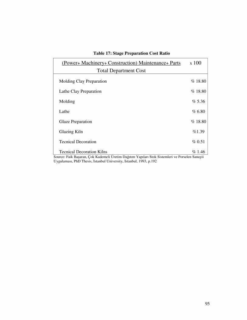
95

Table 17: Stage Preparation Cost Ratio

(Power+ Machinery+ Construction) Maintenance+ Parts x 100

Total Department Cost

Molding Clay Preparation % 18.80

Lathe Clay Preparation % 18.80

Molding % 5.36

Lathe % 6.80

Glaze Preparation % 18.80

Glazing Kiln %1.39

Tecnical Decoration % 0.51

Tecnical Decoration Kilns % 1.46 Source: Faik Başaran, Çok Kademeli Üretim Dağıtım Yapıları Stok Sistemleri ve Porselen Sanayii Uygulaması, PhD Thesis, Istanbul University, Istanbul, 1993, p.192

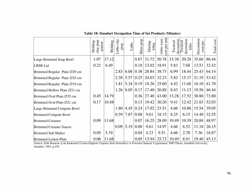
96

Table 18: Standart Occupation Time of Set Products (Minutes)

Mol

ding

cl

ay p

rep

arat

ion

Mol

ding

Lat

he c

lay

prep

Lat

he

Bla

re p

rep

Gla

zing

ki

lng

whi

te w

are

cost

per

uni

t

Tec

nica

l de

cora

tion

T

ecni

cal

deco

rati

on

kiln

s

Dec

orat

ion

cost

per

Tot

al c

ost

Large Brimmed Soup Bowl 1.07 17.12 0.87 31.72 50.78 15.38 20.28 35.66 86.44

LBSB Lid 0.22 6.49 0.18 12.02 18.91 5.83 7.68 13.51 32.42

Brimmed Regular Plate ∅29 cm 2.83 6.68 0.38 28.84 38.73 6.99 18.44 25.43 64.14



Brimmed Hollow Plate ∅21 cm 1.26 8.05 0.17 17.40 26.88 8.43 11.13 19.56 46.44

Brimmed Oval Plate ∅35 cm 0.45 14.79 0.36 27.40 43.00 13.28 17.52 30.80 73.80

Brimmed Oval Plate ∅21 cm 0.17 10.48 0.13 19.42 30.20 9.41 12.42 21.83 52.03

Large Brimmed Compote Bowl 1.80 4.45 0.24 17.02 23.51 4.66 10.88 15.54 39.05

Brimmed Compote Bowl 0.59 7.87 0.08 9.61 18.15 8.25 6.15 14.40 32.55

Brimmed Creamer 0.09 11.68 0.07 16.25 28.09 10.49 10.39 20.88 48.97

Brimmed Creamer Saucer 0.09 5.19 0.08 9.61 14.97 4.66 6.52 11.18 26.15

Brimmed Salt Shaker 0.05 5.19 0.04 4.23 9.51 4.66 2.70 7.36 16.87

Brimmed Lemon Plate 0.06 11.68 0.05 13.94 25.73 10.49 8.91 19.40 45.13 Source: Faik Başaran, Çok Kademeli Üretim Dağıtım Yapıları Stok Sistemleri ve Porselen Sanayii Uygulaması, PhD Thesis, Istanbul University, Istanbul, 1993, p.193.

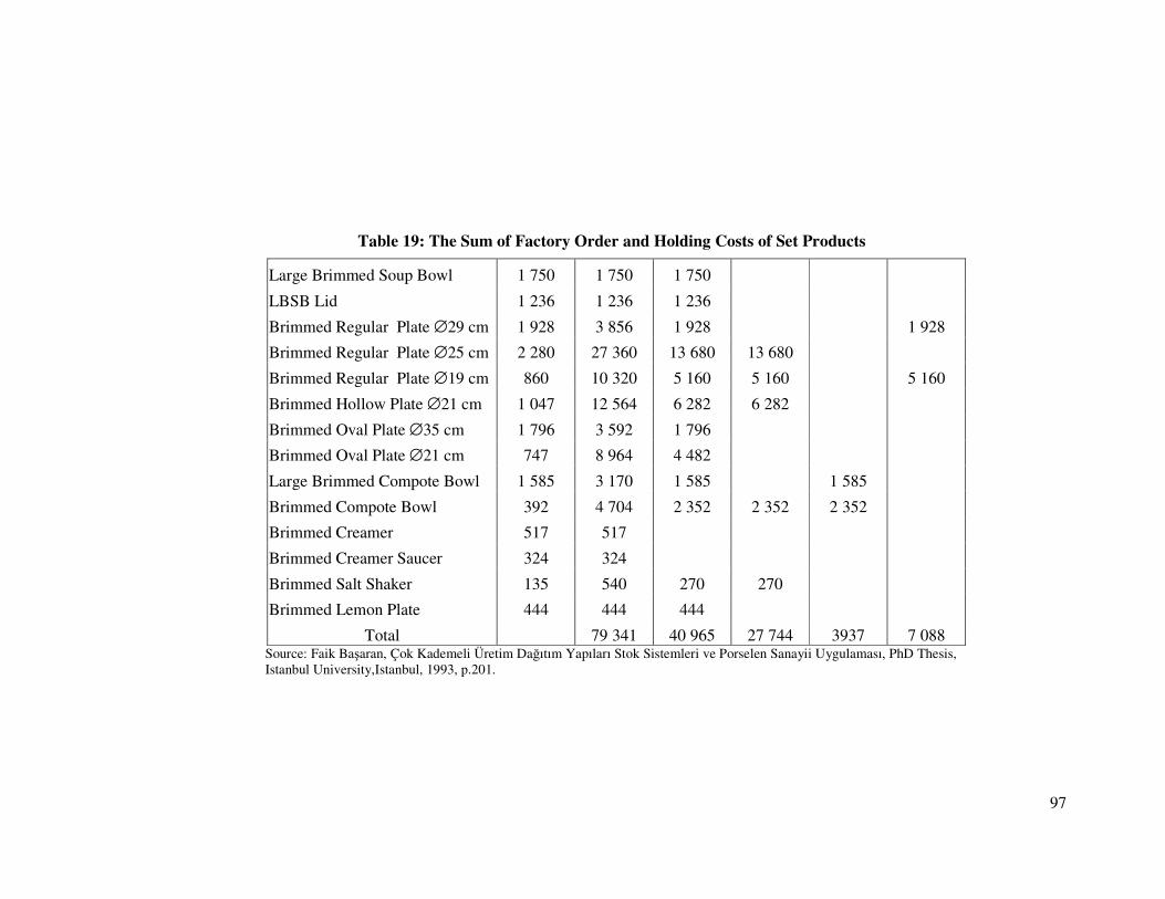
97

Table 19: The Sum of Factory Order and Holding Costs of Set Products

Large Brimmed Soup Bowl 1 750 1 750 1 750

LBSB Lid 1 236 1 236 1 236

Brimmed Regular Plate ∅29 cm 1 928 3 856 1 928 1 928

Brimmed Regular Plate ∅25 cm 2 280 27 360 13 680 13 680

Brimmed Regular Plate ∅19 cm 860 10 320 5 160 5 160 5 160

Brimmed Hollow Plate ∅21 cm 1 047 12 564 6 282 6 282

Brimmed Oval Plate ∅35 cm 1 796 3 592 1 796

Brimmed Oval Plate ∅21 cm 747 8 964 4 482

Large Brimmed Compote Bowl 1 585 3 170 1 585 1 585

Brimmed Compote Bowl 392 4 704 2 352 2 352 2 352

Brimmed Creamer 517 517

Brimmed Creamer Saucer 324 324

Brimmed Salt Shaker 135 540 270 270

Brimmed Lemon Plate 444 444 444

Total 79 341 40 965 27 744 3937 7 088 Source: Faik Başaran, Çok Kademeli Üretim Dağıtım Yapıları Stok Sistemleri ve Porselen Sanayii Uygulaması, PhD Thesis, Istanbul University,Istanbul, 1993, p.201.

98

3.7. Methodology

The methodology used in the present work includes three major tasks: (1)

development of the algorithm to solve the proposed problem, (2) measurement of the

effectiveness of the algorithm, and (3) models are programmed through using the

computer program of Excel to build a macro using visual basic codes.

To satisfy the objectives of this research, it is necessary to follow some steps

described in detail next. The first part of this section is the problem definition, trying

to clearly establish the restrictions considered. Next, two ways to solve the proposed

problem are presented: (1) the optimal power-of-two policy formulated as a

nonlinear integer-programming problem, proposed by Maxwell and Muckstadt

(1985); and (2) the algorithm approach using the power-of-two restrictions. These

models are programmed through using the computer program of Excel to build a

macro using visual basic codes . The codes built are available in Appendix A.

The algorithm approach and the optimal power-of-two methodology,

Maxwell andMuckstadt (1985), other methods cased in the dissertation of Faik

Başaran are compared to define the effectiveness of the algorithms.

3.8. Problem Definition

An algorithm to determine the reorder cycle time in multi-stage serial system

is developed. Demand for each end item is assumed to occur at a constant and

continuous rate. Production is instantaneous and no backorders are allowed. Fixed

setup costs and echelon holding costs are changed at each stage. The capacity at each

node is unconstraint.

3.9. Maxwell and Muckstadt Approach

A power-of-two policy, as described by Roundy (1986), is a sequence

T = (Tn: n є N) of positive numbers with the following three properties. First, orders

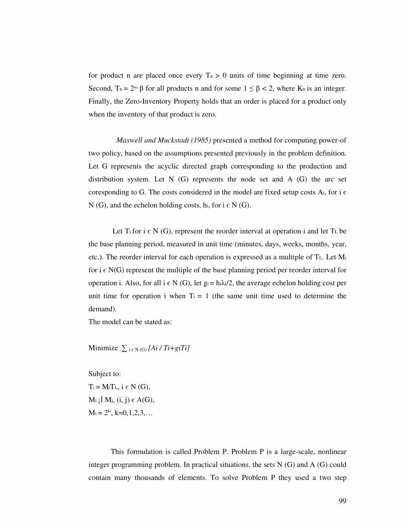
99

for product n are placed once every Tn > 0 units of time beginning at time zero.

Second, Tn = 2Kn β for all products n and for some 1 ≤ β < 2, where Kn is an integer.

Finally, the Zero-Inventory Property holds that an order is placed for a product only

when the inventory of that product is zero.

Maxwell and Muckstadt (1985) presented a method for computing power-of

two policy, based on the assumptions presented previously in the problem definition.

Let G represents the acyclic directed graph corresponding to the production and

distribution system. Let N (G) represents the node set and A (G) the arc set

coresponding to G. The costs considered in the model are fixed setup costs Ai, for i є

N (G), and the echelon holding costs, hi, for i є N (G).

Let Ti for i є N (G), represent the reorder interval at operation i and let TL be

the base planning period, measured in unit time (minutes, days, weeks, months, year,

etc.). The reorder interval for each operation is expressed as a multiple of TL. Let Mi

for i є N(G) represent the multiple of the base planning period per reorder interval for

operation i. Also, for all i є N (G), let gi = hiλi/2, the average echelon holding cost per

unit time for operation i when Ti = 1 (the same unit time used to determine the

demand).

The model can be stated as:

Minimize ∑ i є N (G) [Ai / Ti+giTi]

Subject to:

Ti = MiTL, i є N (G),

Mi ¡İ Mj, (i, j) є A(G),

Mi = 2ki, k=0,1,2,3,…

This formulation is called Problem P. Problem P is a large-scale, nonlinear

integer programming problem. In practical situations, the sets N (G) and A (G) could

contain many thousands of elements. To solve Problem P they used a two step

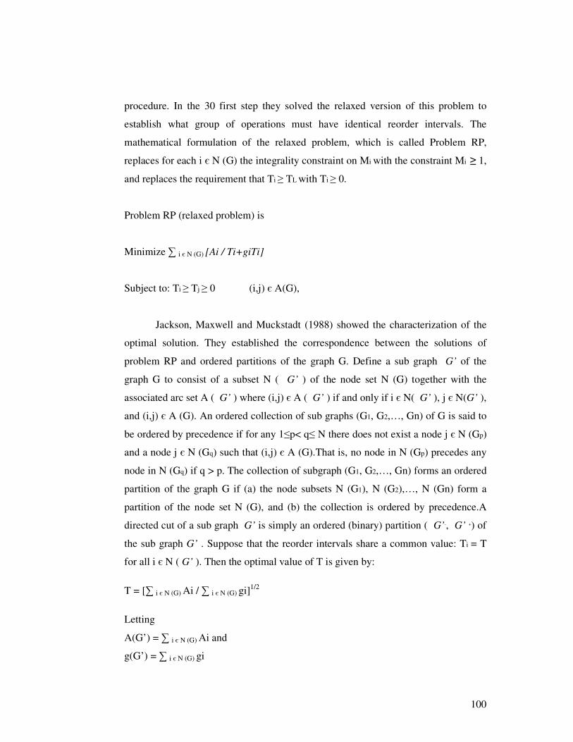
100

procedure. In the 30 first step they solved the relaxed version of this problem to

establish what group of operations must have identical reorder intervals. The

mathematical formulation of the relaxed problem, which is called Problem RP,

replaces for each i є N (G) the integrality constraint on Mi with the constraint Mi ≥ 1,

and replaces the requirement that Ti ≥ TL with Ti ≥ 0.

Problem RP (relaxed problem) is

Minimize ∑ i є N (G) [Ai / Ti+giTi]

Subject to: Ti ≥ Tj ≥ 0 (i,j) є A(G),

Jackson, Maxwell and Muckstadt (1988) showed the characterization of the

optimal solution. They established the correspondence between the solutions of

problem RP and ordered partitions of the graph G. Define a sub graph G’ of the

graph G to consist of a subset N ( G’ ) of the node set N (G) together with the

associated arc set A ( G’ ) where (i,j) є A ( G’ ) if and only if i є N( G’ ), j є N(G’ ),

and (i,j) є A (G). An ordered collection of sub graphs (G1, G2,…, Gn) of G is said to

be ordered by precedence if for any 1≤p< q≤ N there does not exist a node j є N (Gp)

and a node j є N (Gq) such that (i,j) є A (G).That is, no node in N (Gp) precedes any

node in N (Gq) if q > p. The collection of subgraph (G1, G2,…, Gn) forms an ordered

partition of the graph G if (a) the node subsets N (G1), N (G2),…, N (Gn) form a

partition of the node set N (G), and (b) the collection is ordered by precedence.A

directed cut of a sub graph G’ is simply an ordered (binary) partition ( G’-, G’ +) of

the sub graph G’ . Suppose that the reorder intervals share a common value: Ti = T

for all i є N ( G’ ). Then the optimal value of T is given by:

T = [∑ i є N (G) Ai / ∑ i є N (G) gi]1/2

Letting

A(G’) = ∑ i є N (G) Ai and

g(G’) = ∑ i є N (G) gi

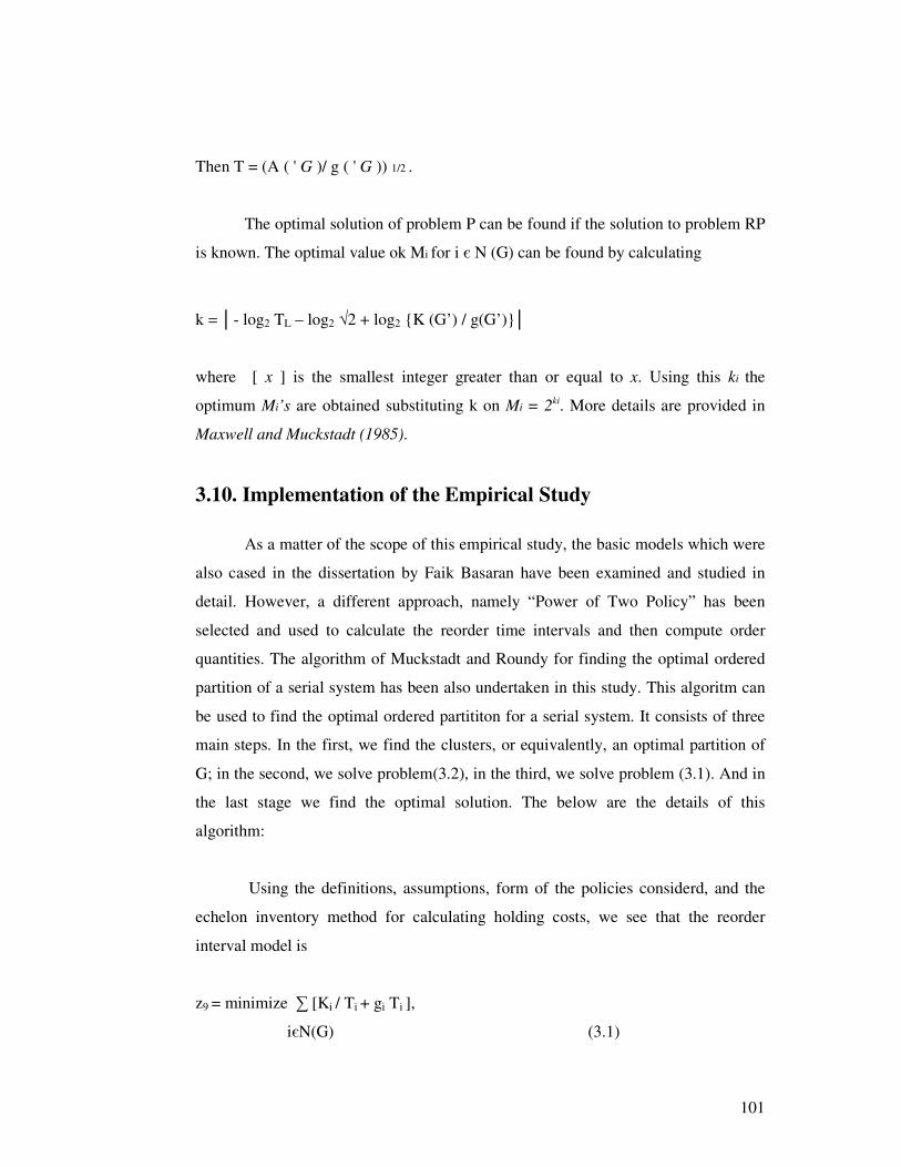
101

Then T = (A ( ' G )/ g ( ' G )) 1/2 .

The optimal solution of problem P can be found if the solution to problem RP

is known. The optimal value ok Mi for i є N (G) can be found by calculating

k = │- log2 TL – log2 √2 + log2 {K (G’) / g(G’)}│

where [ x ] is the smallest integer greater than or equal to x. Using this ki the

optimum Mi’s are obtained substituting k on Mi = 2ki. More details are provided in

Maxwell and Muckstadt (1985).

3.10. Implementation of the Empirical Study

As a matter of the scope of this empirical study, the basic models which were

also cased in the dissertation by Faik Basaran have been examined and studied in

detail. However, a different approach, namely “Power of Two Policy” has been

selected and used to calculate the reorder time intervals and then compute order

quantities. The algorithm of Muckstadt and Roundy for finding the optimal ordered

partition of a serial system has been also undertaken in this study. This algoritm can

be used to find the optimal ordered partititon for a serial system. It consists of three

main steps. In the first, we find the clusters, or equivalently, an optimal partition of

G; in the second, we solve problem(3.2), in the third, we solve problem (3.1). And in

the last stage we find the optimal solution. The below are the details of this

algorithm:

Using the definitions, assumptions, form of the policies considerd, and the

echelon inventory method for calculating holding costs, we see that the reorder

interval model is

z9 = minimize ∑ [Ki / Ti + gi Ti ],

iєN(G) (3.1)

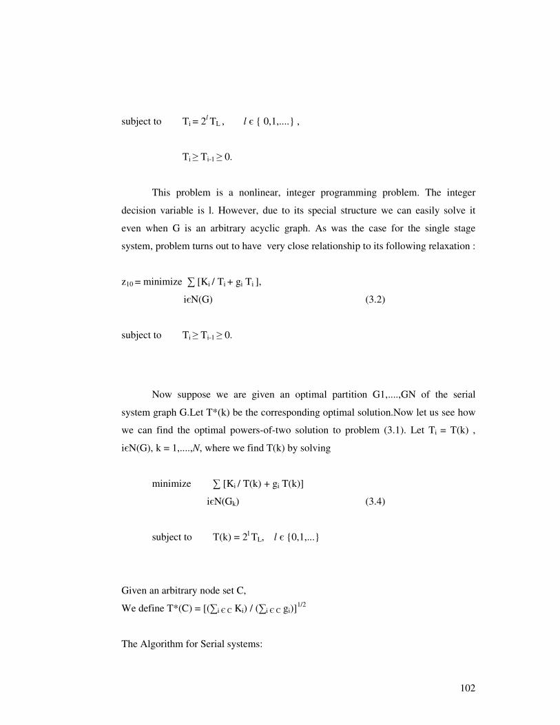
102

subject to Ti = 2l TL , l є { 0,1,....} ,

Ti ≥ Ti-1 ≥ 0.

This problem is a nonlinear, integer programming problem. The integer

decision variable is l. However, due to its special structure we can easily solve it

even when G is an arbitrary acyclic graph. As was the case for the single stage

system, problem turns out to have very close relationship to its following relaxation :

z10 = minimize ∑ [Ki / Ti + gi Ti ],

iєN(G) (3.2)

subject to Ti ≥ Ti-1 ≥ 0.

Now suppose we are given an optimal partition G1,....,GN of the serial

system graph G.Let T*(k) be the corresponding optimal solution.Now let us see how

we can find the optimal powers-of-two solution to problem (3.1). Let Ti = T(k) ,

iєN(G), k = 1,....,N, where we find T(k) by solving

minimize ∑ [Ki / T(k) + gi T(k)]

iєN(Gk) (3.4)

subject to T(k) = 2l TL, l є {0,1,...}

Given an arbitrary node set C,

We define T*(C) = [(∑i Є C Ki) / (∑i Є C gi)]1/2

The Algorithm for Serial systems:

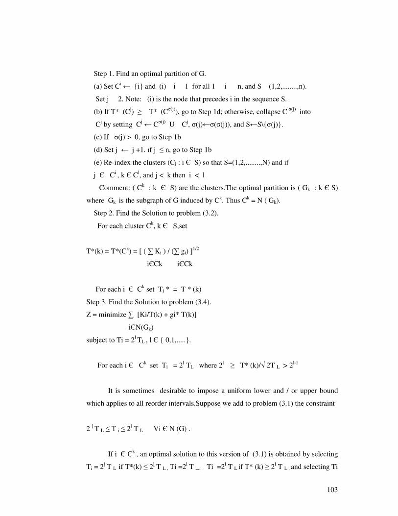
103

Step 1. Find an optimal partition of G.

(a) Set Ci ← {i} and (i) i 1 for all 1 i n, and S (1,2,........,n).

Set j 2. Note: (i) is the node that precedes i in the sequence S.

(b) If T* (Cj) ≥ T* (Cσ(j)), go to Step 1d; otherwise, collapse C σ(j) into

Cj by setting Cj ← Cσ(j) U Cj, σ(j)←σ(σ(j)), and S←S\{σ(j)}.

(c) If σ(j) > 0, go to Step 1b

(d) Set j ← j +1. ıf j ≤ n, go to Step 1b

(e) Re-index the clusters (Ci : i Є S) so that S=(1,2,........,N) and if

j Є Ci , k Є Cl, and j < k then i < l

Comment: ( Ck : k Є S) are the clusters.The optimal partition is ( Gk : k Є S)

where Gk is the subgraph of G induced by Ck. Thus Ck = N ( Gk).

Step 2. Find the Solution to problem (3.2).

For each cluster Ck, k Є S,set

T*(k) = T*(Ck) = [ ( ∑ Ki ) / (∑ gi) ]1/2

iЄCk iЄCk

For each i Є Ck set Ti * = T * (k)

Step 3. Find the Solution to problem (3.4).

Z = minimize ∑ [Ki/T(k) + gi* T(k)]

iЄN(Gk)

subject to Ti = 2l TL , l Є { 0,1,.....}.

For each i Є Ck set Ti = 2l TL where 2l ≥ T* (k)/√ 2T L > 2l-1

It is sometimes desirable to impose a uniform lower and / or upper bound

which applies to all reorder intervals.Suppose we add to problem (3.1) the constraint

2 l T L ≤ T i ≤ 2l T L Vi Є N (G) .

If i Є Ck , an optimal solution to this version of (3.1) is obtained by selecting

Ti = 2l T L if T*(k) ≤ 2l T L , Ti =2l T _, Ti =2l T L if T* (k) ≥ 2l T L , and selecting Ti

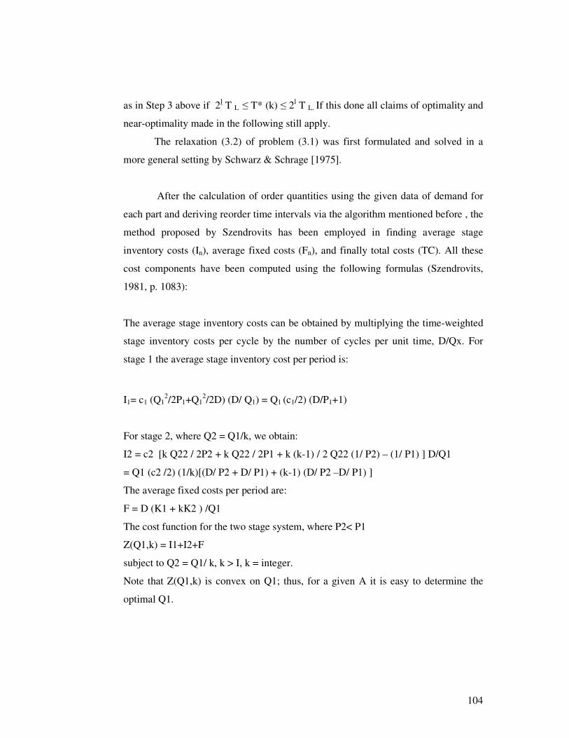
104

as in Step 3 above if 2l T L ≤ T* (k) ≤ 2l T L. If this done all claims of optimality and

near-optimality made in the following still apply.

The relaxation (3.2) of problem (3.1) was first formulated and solved in a

more general setting by Schwarz & Schrage [1975].

After the calculation of order quantities using the given data of demand for

each part and deriving reorder time intervals via the algorithm mentioned before , the

method proposed by Szendrovits has been employed in finding average stage

inventory costs (In), average fixed costs (Fn), and finally total costs (TC). All these

cost components have been computed using the following formulas (Szendrovits,

1981, p. 1083):

The average stage inventory costs can be obtained by multiplying the time-weighted

stage inventory costs per cycle by the number of cycles per unit time, D/Qx. For

stage 1 the average stage inventory cost per period is:

I1= c1 (Q12/2P1+Q1

2/2D) (D/ Q1) = Q1 (c1/2) (D/P1+1)

For stage 2, where Q2 = Q1/k, we obtain:

I2 = c2 [k Q22 / 2P2 + k Q22 / 2P1 + k (k-1) / 2 Q22 (1/ P2) – (1/ P1) ] D/Q1

= Q1 (c2 /2) (1/k)[(D/ P2 + D/ P1) + (k-1) (D/ P2 –D/ P1) ]

The average fixed costs per period are:

F = D (K1 + kK2 ) /Q1

The cost function for the two stage system, where P2< P1

Z(Q1,k) = I1+I2+F

subject to Q2 = Q1/ k, k > I, k = integer.

Note that Z(Q1,k) is convex on Q1; thus, for a given A it is easy to determine the

optimal Q1.

105

To carry out all the necessary calculations to assess the required values, I

have prepared a visual basic macro through using the properties of the excel

program. This replication of the algorithm on the excel has given the below results:

Sub test()

Dim Demand As Double

Dim MaxQ As Double

Dim CI(1 To 6) As Double

Dim F As Double

Dim TotalCost As Double

Dim p(1 To 6) As Double

Dim M(1 To 6) As Double

Dim K(1 To 6) As Double

Dim S(1 To 6) As Double

Dim Q(1 To 6) As Double

Dim H(1 To 6) As Double

Dim T(1 To 6) As Double

Dim TPrime(1 To 6) As Double

Dim C(1 To 6) As Double

Dim sigma(1 To 6) As Double

Dim C1, C2, C3, C4, C5, C6 As Double

Dim Constant As Double

Dim SumK, SumH As Double

Dim I, j, n As Integer

Demand = Cells(3, 3)

For I = 1 To 6

106

C(I) = I

Next

For I = 1 To 6

sigma(I) = I - 1

Next

Constant = Cells(3, 5)

For I = 1 To 6

p(I) = Cells(5 + I, 7)

Next

For I = 1 To 6

S(I) = Cells(5 + I, 4)

Next

For I = 1 To 6

K(I) = Cells(5 + I, 2)

Next

For I = 1 To 6

H(I) = Cells(5 + I, 3)

Next

For I = 1 To 6

T(I) = Constant * Application.Power(K(I) / H(I), 0.5)

Next

For j = 2 To 6

If (T(C(j)) < T(C(sigma(j)))) Then

'do nothing

107

Else

sigma(j) = sigma(j - 1)

C(j) = C(j - 1)

SumK = 0

SumH = 0

For n = C(j) To j

SumK = SumK + K(n)

SumH = SumH + H(n)

Next

For n = C(j) To j

T(n) = Constant * Application.Power(SumK / SumH, 0.5)

Next

End If

Next

For I = 1 To 6

Cells(15 + I, 6) = C(I)

Cells(15 + I, 7) = T(I)

Next

For I = 1 To 6

For n = 0 To 100

If (T(I) < Application.Power(2, n)) Then

TPrime(I) = Application.Power(2, n)

Cells(15 + I, 8) = Application.Power(2, n)

108

n = 100

End If

Next

Next

For I = 1 To 6

Q(I) = Demand * TPrime(I)

Cells(23 + I, 7) = Q(I)

Next

MaxQ = 0

For I = 1 To 6

If (Q(I) > MaxQ) Then

MaxQ = Q(I)

End If

Next

For I = 1 To 6

M(I) = Application.Round(Q(I) / Q(6), 0)

Cells(23 + I, 8) = M(I)

Next

For I = 1 To 5

If (p(I + 1) >= p(I)) Then

CI(I) = Q(6) * H(I) / 2 * 1 / M(I) * (Demand * 250 / p(I) + Demand * 250 / p(I

+ 1) + (M(I) - 1) * Demand * 250 * (1 / p(I) - 1 / p(I + 1)))

Else

CI(I) = Q(6) * H(I) / 2 * 1 / M(I) * (Demand * 250 / p(I) + Demand * 250 / p(I

+ 1))

End If

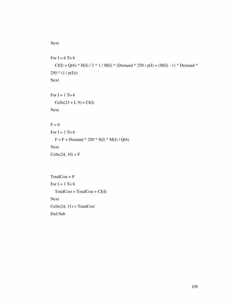
109

Next

For I = 6 To 6

CI(I) = Q(6) * H(I) / 2 * 1 / M(I) * (Demand * 250 / p(I) + (M(I) - 1) * Demand *

250 * (1 / p(I)))

Next

For I = 1 To 6

Cells(23 + I, 9) = CI(I)

Next

F = 0

For I = 1 To 6

F = F + Demand * 250 * S(I) * M(I) / Q(6)

Next

Cells(24, 10) = F

TotalCost = F

For I = 1 To 6

TotalCost = TotalCost + CI(I)

Next

Cells(24, 11) = TotalCost

End Sub

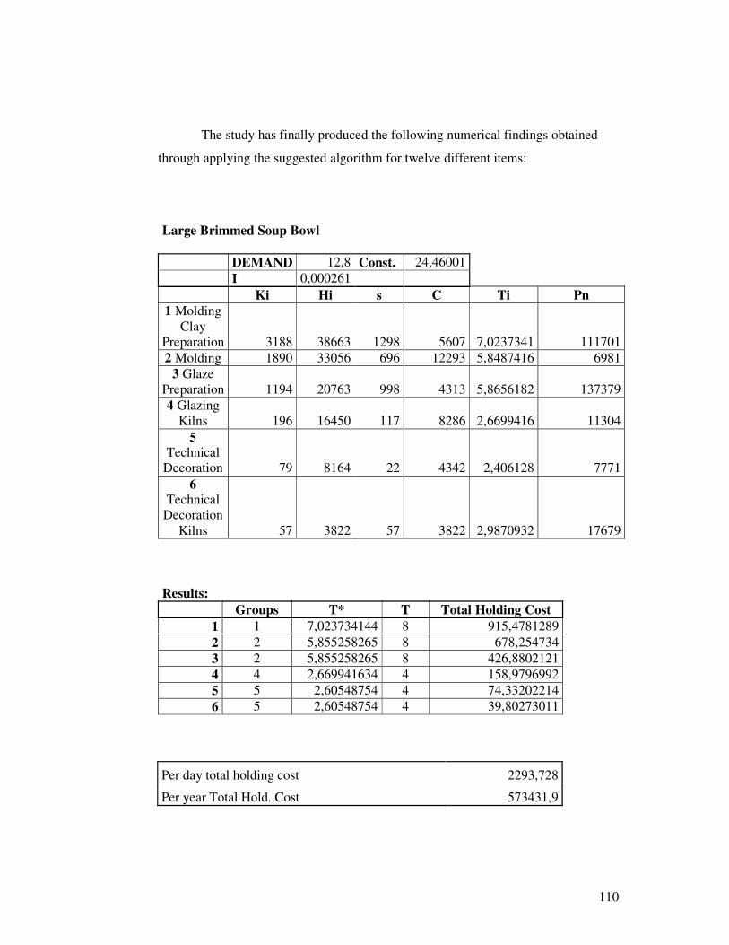
110

The study has finally produced the following numerical findings obtained

through applying the suggested algorithm for twelve different items:

Large Brimmed Soup Bowl DEMAND 12,8 Const. 24,46001 I 0,000261

Ki Hi s C Ti Pn 1 Molding

Clay Preparation 3188 38663 1298 5607 7,0237341 111701 2 Molding 1890 33056 696 12293 5,8487416 6981

3 Glaze Preparation 1194 20763 998 4313 5,8656182 137379 4 Glazing

Kilns 196 16450 117 8286 2,6699416 11304 5

Technical Decoration 79 8164 22 4342 2,406128 7771

6 Technical

Decoration Kilns 57 3822 57 3822 2,9870932 17679

Results: Groups T* T Total Holding Cost

1 1 7,023734144 8 915,4781289 2 2 5,855258265 8 678,254734 3 2 5,855258265 8 426,8802121 4 4 2,669941634 4 158,9796992 5 5 2,60548754 4 74,33202214 6 5 2,60548754 4 39,80273011

Per day total holding cost 2293,728

Per year Total Hold. Cost 573431,9

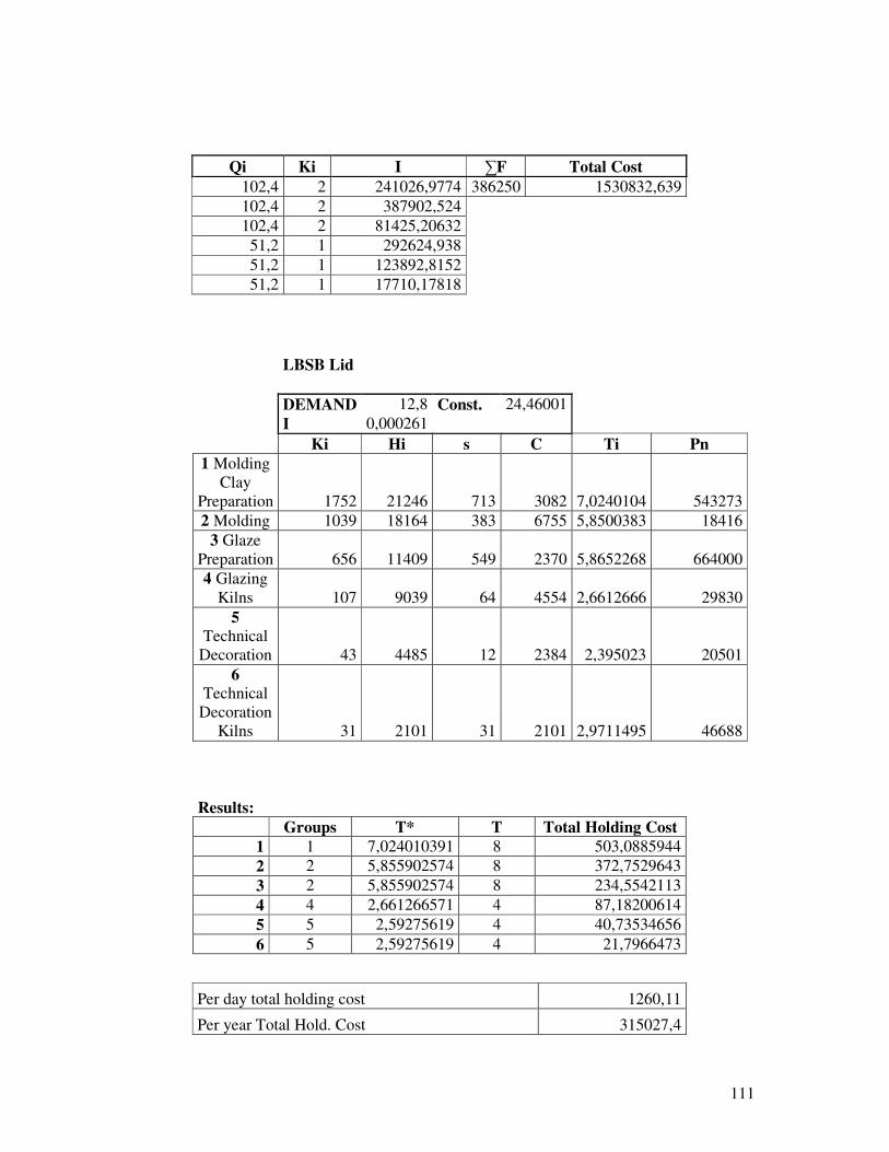
111

Qi Ki I ∑F Total Cost 102,4 2 241026,9774 386250 1530832,639 102,4 2 387902,524 102,4 2 81425,20632 51,2 1 292624,938 51,2 1 123892,8152 51,2 1 17710,17818

LBSB Lid DEMAND 12,8 Const. 24,46001 I 0,000261 Ki Hi s C Ti Pn 1 Molding



Kilns 107 9039 64 4554 2,6612666 29830 5


6 Technical



1 1 7,024010391 8 503,0885944 2 2 5,855902574 8 372,7529643 3 2 5,855902574 8 234,5542113 4 4 2,661266571 4 87,18200614 5 5 2,59275619 4 40,73534656 6 5 2,59275619 4 21,7966473



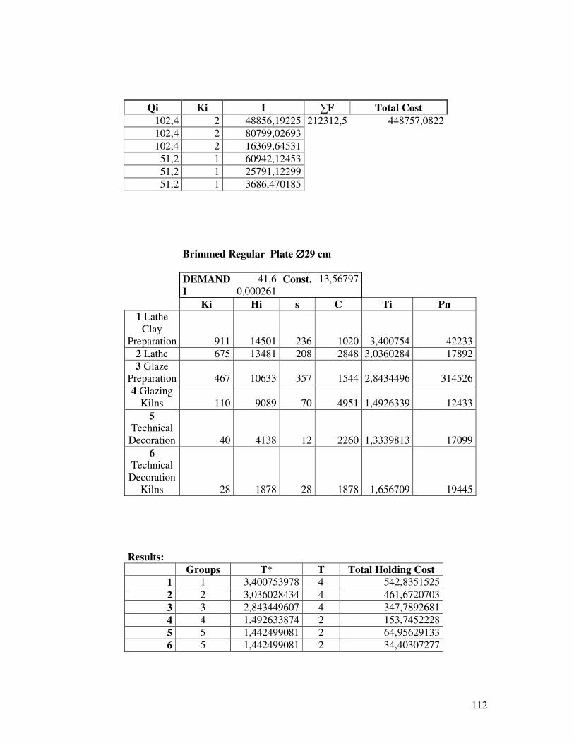
112

Qi Ki I ∑F Total Cost 102,4 2 48856,19225 212312,5 448757,0822 102,4 2 80799,02693 102,4 2 16369,64531 51,2 1 60942,12453 51,2 1 25791,12299 51,2 1 3686,470185

Brimmed Regular Plate ∅∅∅∅29 cm DEMAND 41,6 Const. 13,56797 I 0,000261 Ki Hi s C Ti Pn

1 Lathe Clay

Preparation 911 14501 236 1020 3,400754 42233 2 Lathe 675 13481 208 2848 3,0360284 17892 3 Glaze

Preparation 467 10633 357 1544 2,8434496 314526 4 Glazing

Kilns 110 9089 70 4951 1,4926339 12433 5


6 Technical



1 1 3,400753978 4 542,8351525 2 2 3,036028434 4 461,6720703 3 3 2,843449607 4 347,7892681 4 4 1,492633874 2 153,7452228 5 5 1,442499081 2 64,95629133 6 5 1,442499081 2 34,40307277

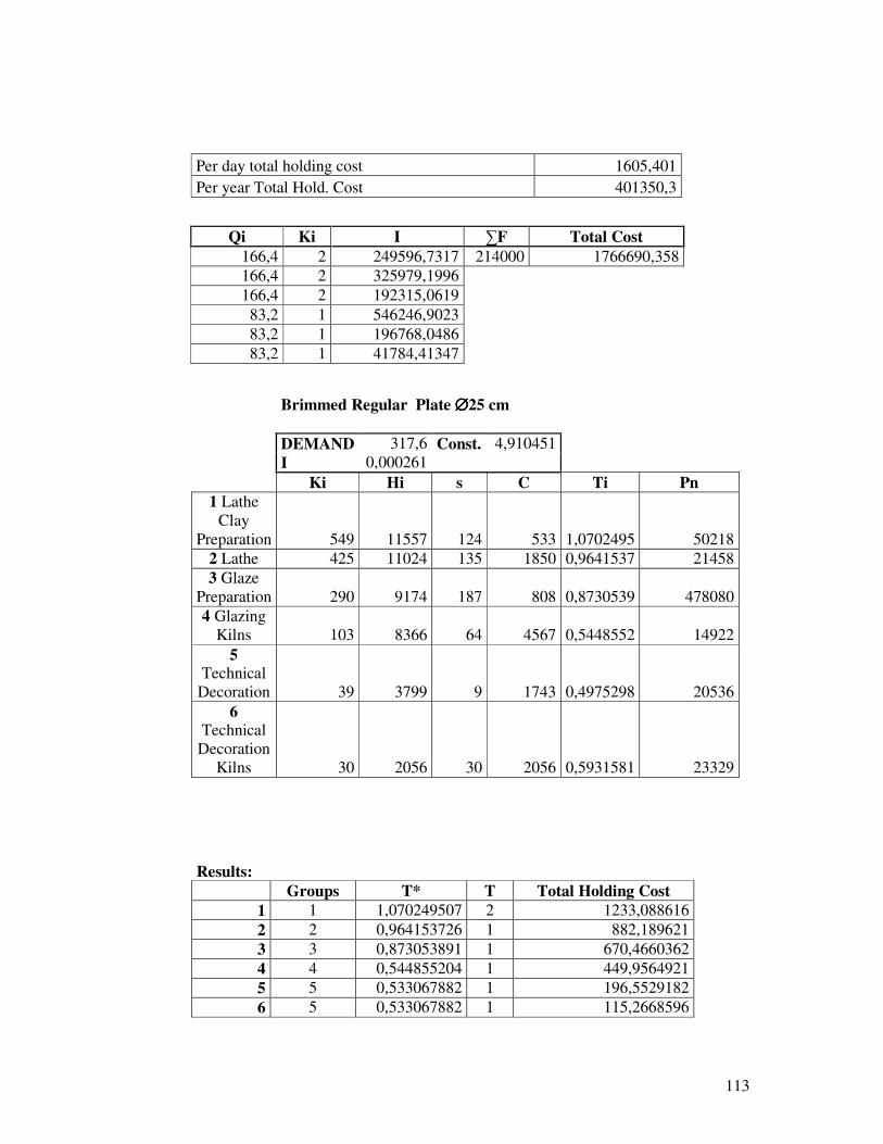
113





1 Lathe Clay



Kilns 103 8366 64 4567 0,5448552 14922 5


6 Technical



1 1 1,070249507 2 1233,088616 2 2 0,964153726 1 882,189621 3 3 0,873053891 1 670,4660362 4 4 0,544855204 1 449,9564921 5 5 0,533067882 1 196,5529182 6 5 0,533067882 1 115,2668596

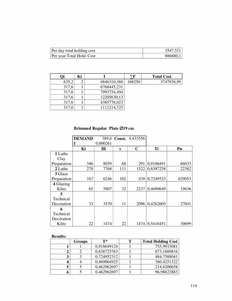
114

Per day total holding cost 3547,521 Per year Total Hold. Cost 886880,1



1 Lathe Clay



Kilns 65 5807 32 2237 0,4690649 19636 5


6 Technical



1 1 0,918649124 1 755,9933081 2 2 0,838725763 1 673,1889834 3 3 0,724952312 1 484,7588041 4 4 0,469064925 1 360,4251322 5 5 0,462962697 1 214,6200658 6 5 0,462962697 1 96,98822883

115



Brimmed Hollow Plate ∅∅∅∅21 cm DEMAND 377,6 Const. 4,503453 I 0,000261 Ki Hi s C Ti Pn

1 Lathe Clay



Kilns 70 6190 37 2644 0,478905 20607 5


6 Technical



1 1 1,011131476 2 1115,117828 2 2 0,910685002 1 772,0186815 3 3 0,818675598 1 565,689838 4 4 0,478904999 1 375,2103795 5 5 0,473626207 1 207,8426504 6 5 0,473626207 1 97,79873114

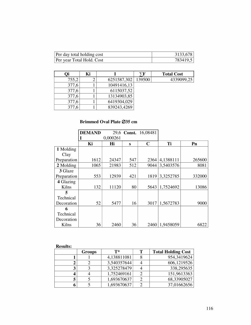
116



Brimmed Oval Plate ∅∅∅∅35 cm DEMAND 29,6 Const. 16,08481 I 0,000261 Ki Hi s C Ti Pn 1 Molding



Kilns 132 11120 80 5643 1,7524692 13086 5


6 Technical



1 1 4,138811081 8 954,3419624 2 2 3,540357644 4 606,1219526 3 3 3,325278479 4 338,295635 4 4 1,752469161 2 151,9613363 5 5 1,693670637 2 68,33905027 6 5 1,693670637 2 37,01662656

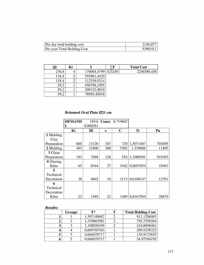
117

Per day total holding cost 2156,077 Per year Total Holding Cost 539019,1


Brimmed Oval Plate ∅∅∅∅21 cm DEMAND 169,6 Const. 6,719682 I 0,000261 Ki Hi s C Ti Pn 1 Molding



Kilns 65 6544 27 1942 0,6697054 18463 5


6 Technical



1 1 1,507140687 2 911,1206963 2 2 1,339865982 2 795,7299264 3 3 1,108050109 2 410,8898401 4 4 0,669705363 1 209,9258322 5 5 0,666929717 1 139,9175855 6 5 0,666929717 1 54,97594195

118

Per day total holding cost 2522,56 Per year Total Hold. Cost 630640

Qi Ki I ∑F Total Cost 339,2 2 2101642,475 313750 1.221.790 339,2 2 3909201,929 339,2 2 705018,4481 169,6 1 3126928,922 169,6 1 1875919,055 169,6 1 185442,6491

Large Brimmed Compote Bowl DEMAND 25,6 Const. 17,29584 I 0,000261 Ki Hi s C Ti Pn

1 Lathe Clay



Kilns 140 10979 69 4878 1,9530992 21067 5


6 Technical



1 1 3,790854537 4 357,1622282 2 2 3,34083238 4 301,7592852 3 3 3,187891287 4 265,8060125 4 4 1,953099238 2 143,4022564 5 5 1,967369758 2 76,2894313 6 5 1,967369758 2 57,9180393

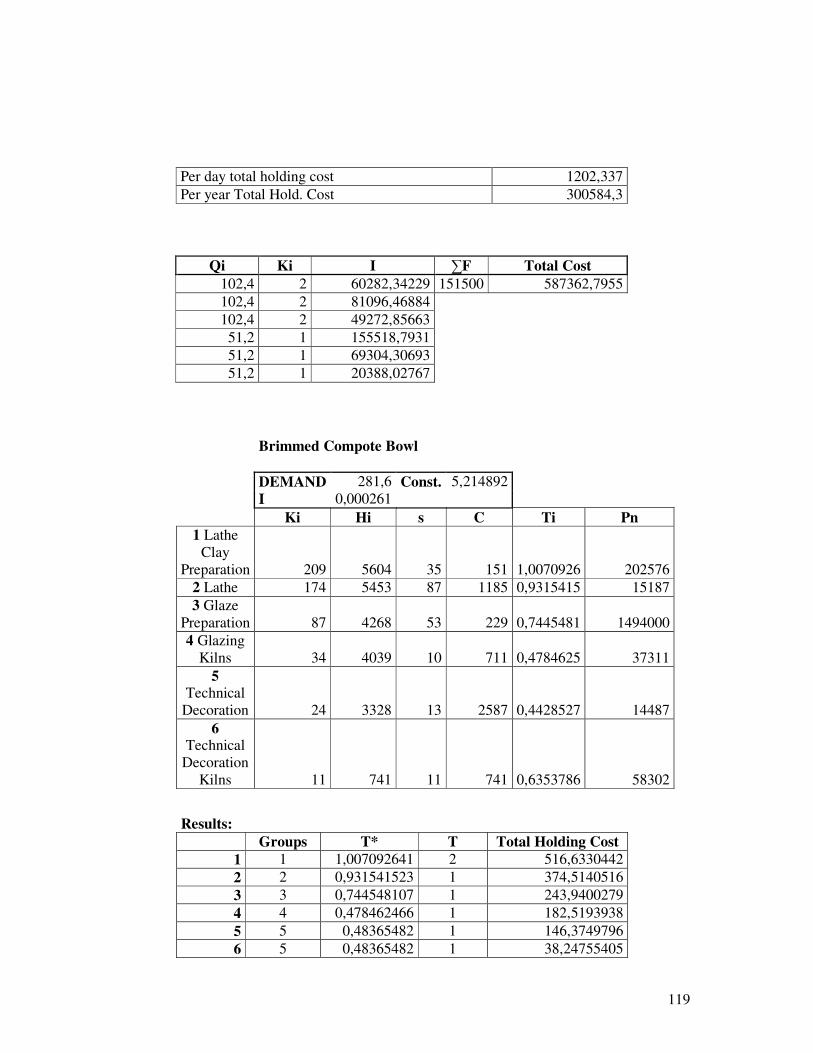
119



Brimmed Compote Bowl DEMAND 281,6 Const. 5,214892 I 0,000261 Ki Hi s C Ti Pn

1 Lathe Clay



Kilns 34 4039 10 711 0,4784625 37311 5


6 Technical



1 1 1,007092641 2 516,6330442 2 2 0,931541523 1 374,5140516 3 3 0,744548107 1 243,9400279 4 4 0,478462466 1 182,5193938 5 5 0,48365482 1 146,3749796 6 5 0,48365482 1 38,24755405

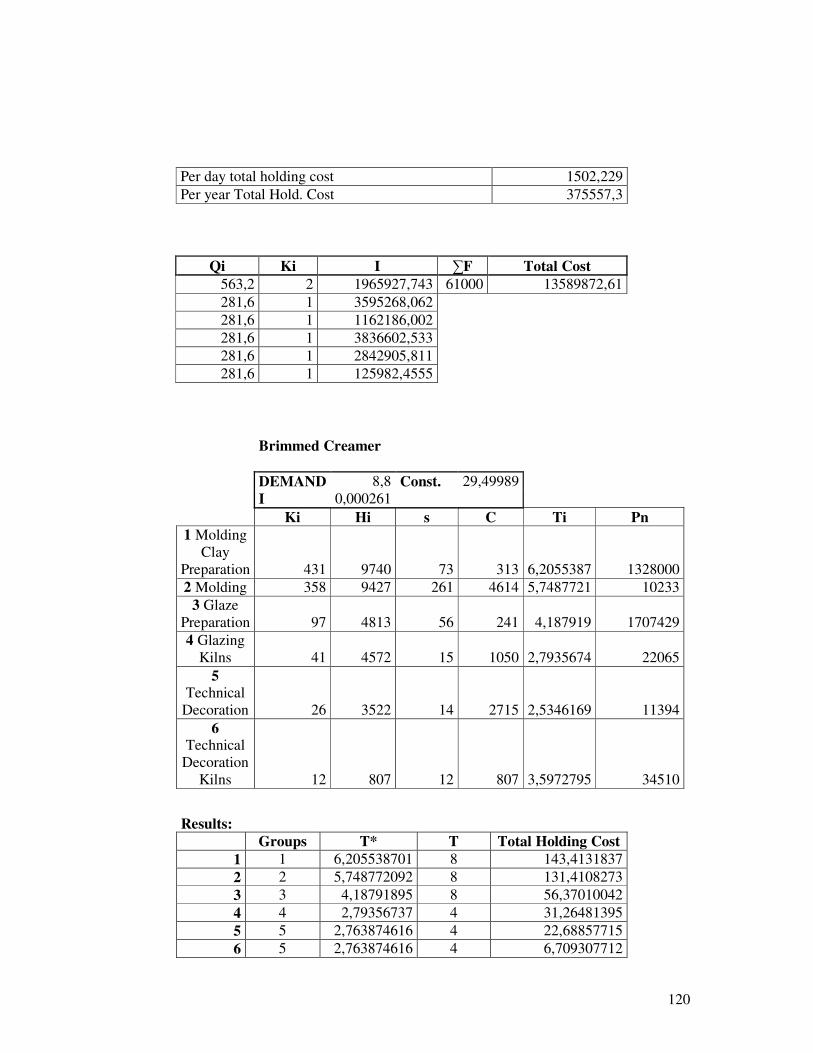
120



Brimmed Creamer DEMAND 8,8 Const. 29,49989 I 0,000261 Ki Hi s C Ti Pn 1 Molding



Kilns 41 4572 15 1050 2,7935674 22065 5


6 Technical



1 1 6,205538701 8 143,4131837 2 2 5,748772092 8 131,4108273 3 3 4,18791895 8 56,37010042 4 4 2,79356737 4 31,26481395 5 5 2,763874616 4 22,68857715 6 5 2,763874616 4 6,709307712

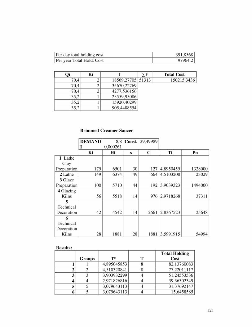
121



Brimmed Creamer Saucer DEMAND 8,8 Const. 29,49989 I 0,000261 Ki Hi s C Ti Pn

1 Lathe Clay



Kilns 56 5518 14 976 2,9718268 37311 5


6 Technical


Results:

Groups T* T Total Holding

Cost 1 1 4,895045853 8 82,13760083 2 2 4,510320841 8 77,22011117 3 3 3,903932299 4 51,24553536 4 4 2,971826816 4 39,36302349 5 5 3,079643113 4 31,37692147 6 5 3,079643113 4 15,6458585

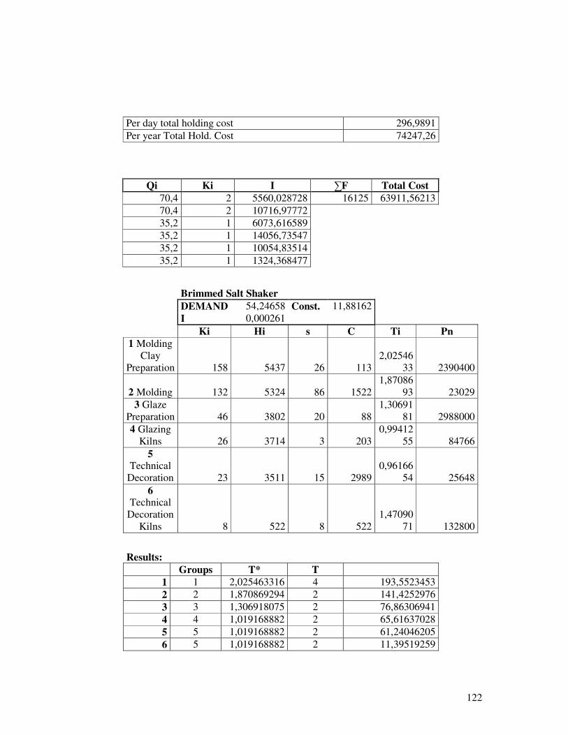
122



Brimmed Salt Shaker DEMAND 54,24658 Const. 11,88162 I 0,000261 Ki Hi s C Ti Pn 1 Molding

Clay Preparation 158 5437 26 113

2,0254633 2390400

2 Molding 132 5324 86 1522 1,87086

93 23029 3 Glaze

Preparation 46 3802 20 88 1,30691

81 2988000 4 Glazing

Kilns 26 3714 3 203 0,99412

55 84766 5

Technical Decoration 23 3511 15 2989

0,9616654 25648

6 Technical

Decoration Kilns 8 522 8 522

1,4709071 132800

Results: Groups T* T

1 1 2,025463316 4 193,5523453 2 2 1,870869294 2 141,4252976 3 3 1,306918075 2 76,86306941 4 4 1,019168882 2 65,61637028 5 5 1,019168882 2 61,24046205 6 5 1,019168882 2 11,39519259

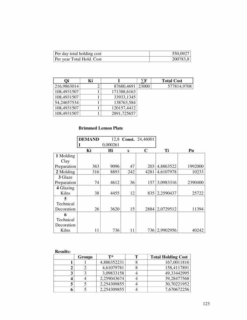
123



Brimmed Lemon Plate DEMAND 12,8 Const. 24,46001 I 0,000261 Ki Hi s C Ti Pn 1 Molding



Kilns 38 4455 12 835 2,2590437 25722 5


6 Technical



1 1 4,886352231 8 167,0011816 2 2 4,61079781 8 158,4117891 3 3 3,09833158 4 49,33442995 4 4 2,259043674 4 39,28477568 5 5 2,254309855 4 30,70221952 6 5 2,254309855 4 7,670672256

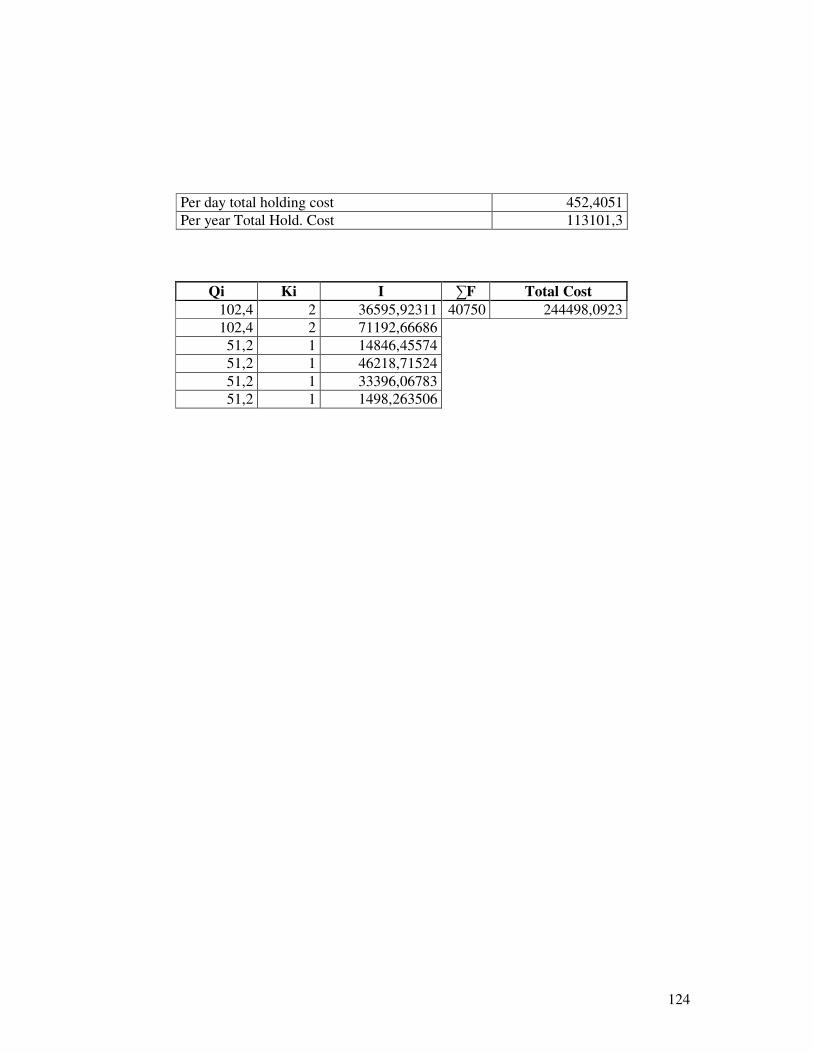
124



125

CONCLUSION

The main contribution of this research is the development of the algorithm

approach to determine the reorder cycle time in multi-stage serial system,

considering the power of two restrictions.

The algorithm developed shows to be effective, because it provides solutions

in costs Optimal solutions are obtained 75 percent of the time for small problems.

The algorithm programmed in excel (macro in visual basic) and using a Pentium 4,

provides solutions in less than one second for small problems.

The algorithm is conducted to measure the ability to provide solutions of the

same quality in different problems instances. The experiment shows that algorithm

gives very accurate solutions, comparing the results obtained in the other algorithms.

A comparison between power of two algorithm and another heuristics

developed in this area.The total cost values obtained in the study are summarized in

the accompanying table.

As it can be seen from the table, the existing method (method 5) which has

been used in the factory is not effective.It is the worsth method since the total cost

has the highest value.The method 3 (Peterson and Silver’s) is also not effective.It is

the second worsth method in all.It has the second highest total cost value. On the

other hand the other four methods, method 1, method 2, method 4 and our main

method (method 6) have total cost values approximatelly near to each other.

17.699.188 ≤ 17.933.825 ≤ 18.238.911 ≤ 22.042.954 ≤ 80.751.763 ≤ 270.166.199.

The method 4 is the most effective method with having the least total cost value

while the others having a bigger total cost value.Only finding the total cost of the

Brimmed Oval Plate ∅21 cm, our method power of two policy is the best effective

one since it has the smallest total cost value.

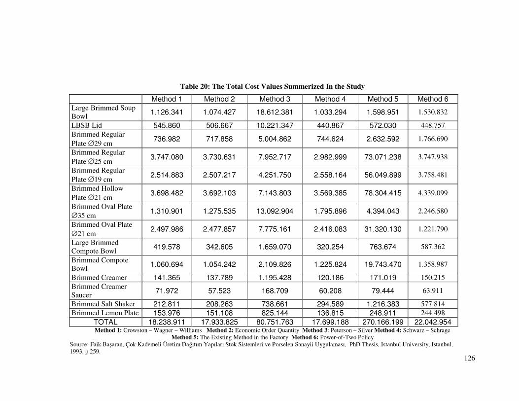
126

Table 20: The Total Cost Values Summerized In the Study

Method 1 Method 2 Method 3 Method 4 Method 5 Method 6

Large Brimmed Soup Bowl

1.126.341 1.074.427 18.612.381 1.033.294 1.598.951 1.530.832

LBSB Lid 545.860 506.667 10.221.347 440.867 572.030 448.757

Brimmed Regular Plate ∅29 cm

736.982 717.858 5.004.862 744.624 2.632.592 1.766.690


3.747.080 3.730.631 7.952.717 2.982.999 73.071.238 3.747.938


2.514.883 2.507.217 4.251.750 2.558.164 56.049.899 3.758.481

Brimmed Hollow Plate ∅21 cm

3.698.482 3.692.103 7.143.803 3.569.385 78.304.415 4.339.099

Brimmed Oval Plate ∅35 cm

1.310.901 1.275.535 13.092.904 1.795.896 4.394.043 2.246.580

Brimmed Oval Plate ∅21 cm

2.497.986 2.477.857 7.775.161 2.416.083 31.320.130 1.221.790

Large Brimmed Compote Bowl

419.578 342.605 1.659.070 320.254 763.674 587.362

Brimmed Compote Bowl

1.060.694 1.054.242 2.109.826 1.225.824 19.743.470 1.358.987

Brimmed Creamer 141.365 137.789 1.195.428 120.186 171.019 150.215

Brimmed Creamer Saucer

71.972 57.523 168.709 60.208 79.444 63.911

Brimmed Salt Shaker 212.811 208.263 738.661 294.589 1.216.383 577.814

Brimmed Lemon Plate 153.976 151.108 825.144 136.815 248.911 244.498

TOTAL 18.238.911 17.933.825 80.751.763 17.699.188 270.166.199 22.042.954

Method 1: Crowston – Wagner – Williams Method 2: Economic Order Quantity Method 3: Peterson – Silver Method 4: Schwarz – Schrage Method 5: The Existing Method in the Factory Method 6: Power-of-Two Policy


127

REFERENCES

Axsäter, Sven, “Evaluation of Lot-Sizing Techniques”, International Journal Of

Production Research, 24 (1), 1986, 51-57.

Axsäter, Sven, “Note: Optimal Policies for Serial Inventory Systems under Fill Rate

Constraints”, Management Science, Vol. 49, No. 2, 2003, pp. 247 – 253.

Başaran, Faik, “Çok Kademeli Üretim Dağıtım Yapıları Stok Sistemleri ve Porselen

Sanayii Uygulaması”, Unpublished Dissertation of Doctorate, Istanbul University,

Istanbul, 1993

Blackburn, Joseph D. and Millen, Robert A., “An Evaluation of Heuristic

Performance in Multi-stage Lot-Sizing Systems”, International Journal of

Production Research, 23 (5), 1985, 857-866.

Blackburn, Joseph D. and Millen, Robert A., “Improved Heuristics for Multi-stage

Requirements Planning Systems”, Management Science, 28 (1), January 1982, 44-

56.

Boyaci, Tamer and Gallego, Guillermo, “Serial Production / Distribution Systems

Under Service Constraints”, Manufacturing & Sevice Operations Management, Vol.

3, No. 1, 2001 pp. 43 – 50.

Cehn, Fangruo, “Optimal Policies for Multi-Echelon Inventory Problems with Batch

Ordering”, Operations Research, Vol. 48, No. 3, 2000, pp. 376 – 389.

Clark, Andrew J. and Scarf, Herbert, “Optimal Policies for a Multi-Echelon

Inventory Problem”, Management Science, 23, 1960, 475-490.

128

Crowston, Wallace B.; Wagner, Michael and Williams, Jack F., “Economic Lot Size

Determination in Multi-stage Assembly Systems”, Management Science, 19 (5),

January 1973, 517-527.

Dixon, P. S. and Silver, E. A., “A Heuristic Solution Procedure for the Multi-item

Single-level, Limited Capacity, Lot Sizing Problem”, Journal of Operations

Management, 2 (1), October 1981, 23-29.

Federgruen, Awi and Zheng, Yu-Sheng, “The Joint Replenishment Problem with

General Joint Cost Structures”, Operations Research, 40 (2), March-April 1992, 384-

403.

Federgruen, Awi; Queyranne, M. and Zheng, Yu-Sheng, “Simple Power-of-two

Policies are Close to Optimal in a General Class of Production/ Distribution

Networks with General Joint Setup Costs”, Mathematics of Operations Research, 17

(4), November 1992, 951-963.

IOMA, “Improving Logistics and Supply Chain Management”, Inventory

Management Report., 2003, Issue 03 – 10, www.ioma.com.

Jackson, Peter L.; Maxwell, William L. and Muckstadt, John A., “Determining

Optimal Reorder Intervals in Capacitated Production/ Distribution Systems”

Management Science, 34 (8), August 1988, 938-958.

Jackson, Peter L.; Maxwell, William L. and Muckstadt, John A., “The Joint

Replenishment Problem with Power-of-two Restrictions”, AIIE Transactions, 17 (1),

March 1985, 25-32.

Maxwell, William L. and Muckstadt, John A., “Establishing Consistent and Realistic

reorder Intervals in Production/ Distribution Systems”, Operations Research, 33 (6),

November-December 1985,1316-1341.

129

Roundy, Robin, “A 98% Effective Lot Sizing Rule for a Multi-product, Multistage

Production/ Inventory System”, Mathematics of Operations Research, 11 (4),

November 1986, 699-727.

Roundy, Robin, “A 98% Effective Integer-Ratio Lot Sizing for One-Warehouse

Multi-Retailer Systems”, Management Science, 31 (11), November 1985, 1416-1430.

Schwarz, Leroy B., “A Simple Continuous Review Deterministic One-Warehouse

N-Retailer Inventory Problem”, Management Science, 19 (5), Januar 1973, 555-565.

Sun, Daning and Queyranne, Maurice, “Production and Inventory Model Using Net

Present Value”, Operations Research, Vol. 50, No. 3, 2002, pp. 528 – 537.

Schwarz, Leroy B. and Schrage, Linus, “Optimal and System Myopic Policies for

Multi-Echelon Production/ Inventory Assembly Systems”, Management Science, 21

(11), July 1975,1285-1294.

Szendrovits, Andrew Z., “Comments on the Optimality in Optimal and System

Myopic Policies for Multi-Echelon Production/ Inventory Assembly Systems”,

Management Science, 27 (9), September 1981,1081-1087.

Szendrovits, Andrew Z., “Manufacturing Cycle Time Determination for a Multistage

Economic Production Quantity Model”, Management Science, 22 (3), November

1975, 298-308.

Veinott, Arthur F. Jr., “Minimum Concave-Cost Solution of Leontief Substitution

Models of Multi-Facility Inventory Systems”, Operations Research, 17 (2), 1967,

262-291.

Williams, Jack F., “On the Optimality of Integer Lot Size Ratios in “Economic Lot

Size Determination in Multi-stage Assembly Systems”, Management Science, 28

(11), November 1982,1341-1349.

130

Zipkin, Paul H., Foundations of Inventory Management, McGraw-Hill, United States

of America, 2000.

Electronic Sources:

http://www.artistictile.net/pages/Info/Info_tile1.html

www.basbakanlik.gov.tr

OPTIMAL INVENTORY POLICIES IN SERIAL SUPPLY ...

Documents

Transcript of OPTIMAL INVENTORY POLICIES IN SERIAL SUPPLY ...