Electronic copy available at: http://ssrn.com/abstract=1126044Electronic copy available at: http://ssrn.com/abstract=1126044

PRODUCTION AND OPERATIONS MANAGEMENT Vol. 8, No. 2, Summer 1999

Printed in U.S.A.

OPTIMALITY OF STATE-DEPENDENT (s, S) POLICIES IN INVENTORY MODELS WITH MARKOV-

MODULATED DEMAND AND LOST SALES*

FENG CHENG AND SURESH P. SETH1 IBM Thomas J. Watson Research Center, Yorktown Heights, New York 10598, USA

School of Management, University of Texas at Dallas, Richardson, Texas 75083, USA

Markov-modulated processes have been used in stochastic inventory models with setup costs for modeling demand under the influence of uncertain environmental factors, such as fluctuating economic and market conditions. The analyses of these models have been carried out in the literature only under the assumption that unsatisfied demand is fully backlogged. The lost sales situation occurs in many retail establishments such as department stores and supermarkets. We use the analysis of the Markovian demand model with backlogging to analyze the lost sales case; in particular, we establish the optimality of an (s , S) -type policy under fairly general conditions. (DYNAMIC INVENTORY MODEL; MARKOV CHAIN; (s, S) POLICY; LOST SALES)

1. Introduction

In the literature of stochastic inventory models, there are two different assumptions about the excess demand unfilled from existing inventories: the backlog assumption and the lost sales assumption. The former is more popular in the literature partly because historically the inventory studies started with spare parts inventory management problems in military applications, where the backlog assumption is realistic. However, in many other business situations, it is quite often that demand that cannot be satisfied on time is lost. This is particularly true in a competitive business environment. For example, in many retail establishments, such as a supermarket or a department store, a customer chooses a competitive brand or goes to another store if his/her preferred brand is out of stock.

In the presence of fixed ordering costs in inventory models under either assumption, an important issue has been to establish the optimality of (s, S) -type policies. While there are many classical and recent papers dealing with this issue in the backlog case, only Veinott ( 1966), Shreve ( 1976), and Bensoussan, Crouhy, and Proth ( 1983), to our knowledge, have considered the lost sales case explicitly. This is perhaps because the proofs of the results in the lost sales case are usually more complicated than those in the backlog case. Shreve and Bensoussan, Crouhy, and Proth establish the optimality of an

* Received February 1996; revisions received November 1996, October 1997, and September 1998; accepted September 1998.

183 1059-1478/99/0802/183$1.25

Copyright 0 1999, Production and Operations Management Society

Electronic copy available at: http://ssrn.com/abstract=1126044Electronic copy available at: http://ssrn.com/abstract=1126044

184 FENG CHENG AND SURESH P. SETH1

(s, S)-type policy by using the concept of K-convexity. Veinott ( 1966) provides a dif- ferent proof for the optimality of (s, S) -type policies in the lost sales case. His proof is based on a different set of assumptions which neither implies nor is implied by those used in Shreve and Bensoussan, Crouhy, and Proth. It should be noted that all these results are obtained under the condition of zero lead time.

Many efforts have been made to incorporate various realistic features in inventory models. However, most of them are carried out under the backlog assumption. One such feature is that of Markovian demand, which has been considered by Karlin and Fabens ( 1959), Song and Zipkin ( 1993), Sethi and Cheng ( 1993, 1997), Cheng and Sethi ( 1998 ) , Ozekici and Parlar ( 1998 ) , Beyer and Setbi ( 1997 ) , and Beyer, Sethi, and Taksar ( 1998). Without exception, they all use the backlog assumption in their analyses. As a natural extension of and a flexible alternative to independent demands considered in the bulk of the classical inventory literature, Markovian demands can model demands that are dependent on randomly changing economic and market conditions. As the lost sales sit- uation is often the case in competitive markets, it is interesting and worthwhile to extend the Markovian demand model to incorporate the lost sales case.

This paper is written as an extension of Sethi and Cheng (1997) with the lost sales assumption as the important point of departure. The plan of the paper is as follows. In Section 2, we formulate our basic lost sales model with Markovian demands, provide the dynamic programming equations, and state the existence results. In Section 3, we present a new K-convexity result associated with the cost functions in the lost sales case and then show that state-dependent (s, S) policies are optimal for our Markovian demand model formulated under a set of less restrictive assumptions than those in the independent de- mand models of Shreve and Bensoussan, Crouhy, and Proth. In Section 4, we discuss extensions that incorporate various realistic features and constraints, such as supply un- certainty, service levels, and storage capacities. An infinite horizon stationary model is also presented. We conclude the paper with some remarks in Section 5.

2. Model Formulation

Consider an inventory problem over a finite horizon (0, N) = { 0, 1, 2, . . . , N } . The demand in each period is assumed to be a random variable defined on a given probability space and not necessarily identically distributed. To precisely define the demand process, we consider a finite collection of demand states labeled i E Z = { 1, 2, . . . , L } and let ik denote the demand state observed at the beginning of the ktb period. We assume that ik, k E (0, N), is a Markov chain over Z with the transition matrix P = { pU} . Thus,

0 zzpij 5 1, i E I, FEZ, and lip,= 1, i E I. j=l

Let the nonnegative random variable & denote the demand at the end of a given period k~(0,N- l)= {O,l,..., N - 1 } . Demand & in period k depends on the demand state ik in that period and has the probability density function +i,k( *) for the demand state ik = i. We assume that

E (& ik = i) = jrn Z4i,k(Z)dZ 5 M < ~0, kE(O,N- l), i E I. (2.1) 0

At the beginning of period k, an order uk 2 0 is placed with the knowledge that the demand state is ik and that the quantity uk will be delivered at the end of period k, but before the period k demand & materializes. If the on-hand inventory xk at the beginning of period k plus the amount uk delivered in period k exceeds the demand, i.e., if xk + uk 2 &, then the demand is met, and the remaining inventory is carried over to the next

OPTIMALITY OF STATE-DEPENDENT POLICIES 185

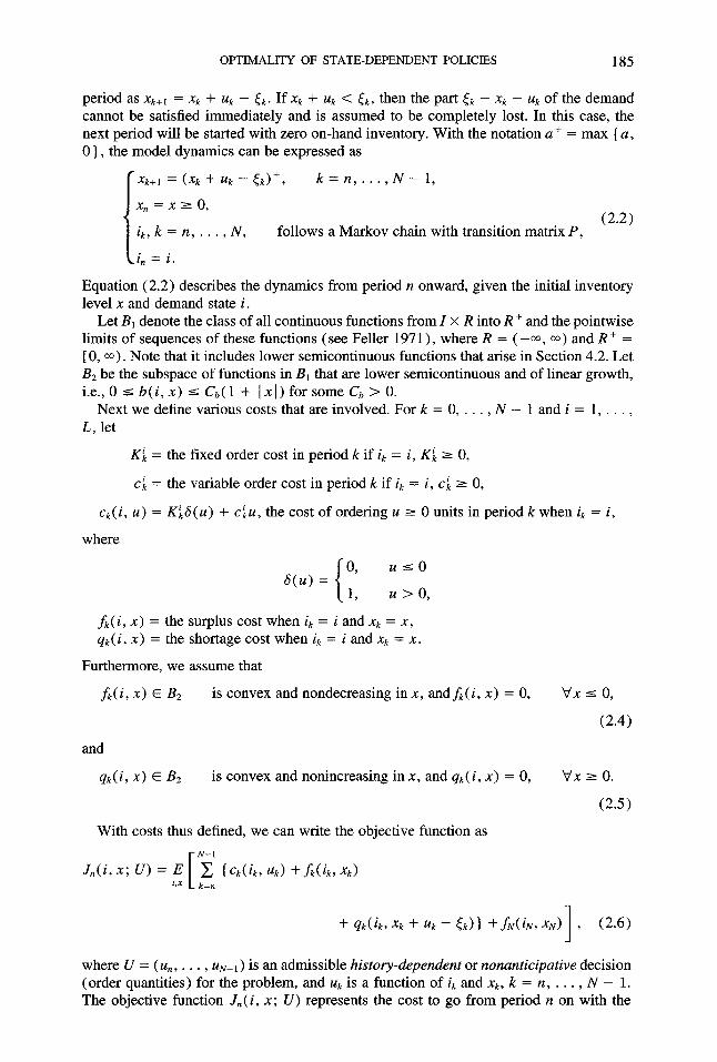
period as &+, = xk + uk - Eke If & + U& < <k, then the part & - xk - uk Of the demand cannot be satisfied immediately and is assumed to be completely lost. In this case, the next period will be started with zero on-hand inventory. With the notation a+ = max { a, 0)) the model dynamics can be expressed as

I

xk+l = (xk + uk - <k>+, k = n, . . . ) N - 1,

x, = x 2 0,

ik, k = n, . . . , N, follows a Markov chain with transition matrix P, (2.2)

i, = i.

Equation (2.2) describes the dynamics from period n onward, given the initial inventory level x and demand state i.

Let Bi denote the class of all continuous functions from Z X R into R+ and the pointwise limits of sequences of these functions (see Feller 197 1) , where R = ( --co, ~0) and R + = [ 0, ~0). Note that it includes lower semicontinuous functions that arise in Section 4.2. Let B2 be the subspace of functions in B, that are lower semicontinuous and of linear growth, i.e., 0 I b(i, x) 5 C,(l + 1 xl) for some C, > 0.

Next we define various costs that are involved. For k = 0, . . . , N - 1 and i = 1, . . . , L, let

K6 = the fixed order cost in period k if ik = i, K: 2 0,

CL = the variable order cost in period k if ik = i, ci 2 0,

ck(i, U) = KiS(u) + ciu, the cost of ordering u 2 0 units in period k when ik = i,

where

0, US0 S(u) =

1, u > 0,

fk( i, x) = the surplus cost when ik = i and xk = x, qk( i, x) = the shortage cost when ik = i and xk = x.

Furthermore, we assume that

fk(i, X) E & is convex and nondecreasing in x, andf,( i, x) = 0,

and

qk(ir X) E & is convex and nonincreasing in x, and qk( i, x) = 0,

With costs thus defined, we can write the objective function as

N-l

tjx I 0,

(2.4)

vxro.

(2.5)

+ qk(ik, xk + uk - Sk)} +fN(irV, xN) , 1 (2.6)

where U = (u,, . . . , UN- I ) is an admissible history-dependent or nonanticipative decision (order quantities) for the problem, and uk is a function of ik and xk, k = n, . . . , N - 1. The objective function .Zn( i, x; U) represents the cost to go from period n on with the

186 FENG CHENG AND SURESH P. SETH1

initial conditions being i and x under the decision U. With U denoting the class of all admissible decisions, we can define the value function v,( i, x) for the problem over (n, N) as

u,(i,x) = inf J,(i,x; U). (2.7) UEI

The dynamic programming equations for the model are defined for n = 0, 1, . . . , N - landi= 1,2,...,Las

un(i, X) =f,(i, x) + inf {c,(i, u) + E[qn(i, x + 2.4 LIZ=0

and

- En> + un+t(in+l, (x - u - &)+)I& = i]}. (2.8)

+(i,x) =fN(i,x), i = 1,2,. . . , L. (2.9)

The results establishing the existence of an optimal feedback policy are similar to those in the backlog case treated in Sethi and Cheng ( 1993), and Beyer, Sethi, and Taksar (1998).

THEOREM 2.1 The dynamic programming Equations (2.8) and (2.9) dejine a sequence offunctions u, (i, x) in Bz. Moreover, there exists afunction z& (i, x) in B1, which provides the injimum in (2.8)foranyx. Set l? = (Co, fi,, . . . , i&-, ) , then l? is an optimal decision for the problem Jo( i, x, U). Moreover,

uo(i, x) = min Jo(i, x; U). (2.10) LIE?1

In simpler words, the theorem, called a verification theorem, means that there exists a policy in the class of all admissible (or history-dependent) policies, whose objective function value equals the value function defined by (2.7), and there is a Markov (or feedback) policy which gives the same objective function value.

3. Optimality of (s , S) Policies

The optimality of (s, S)-type policies has been established for stochastic inventory models with various conditions on demand and cost functions. A key concept used in proving the optimality of (s, S) policies for standard models in the literature is K-convexity of a function, which was first utilized by Scarf ( 1960). Discussions about some useful properties of K-convex functions can be found in Bertsekas (1976) and Bensoussan, Crouhy, and Proth ( 1983).

Sethi and Cheng ( 1993, 1997) extended the definition of K-convexity to include func- tions defined on convex subsets of the real line. They generalized the existing results on the properties of K-convex functions, which allow for less restrictive assumptions and more realistic features arising in inventory models. Using these generalized results, they established the optimality of state-dependent (s, S) policies in Markovian demand inven- tory models for the full backlog case.

However, in the lost sales case the truncation due to lost sales requires the conditions enforcing the K-convexity to be reexamined. Moreover, new conditions need to be intro- duced in order to establish the optimality of (s, S) policies for the lost sales case.

3.1. Preliminaries

The next subsection is devoted to proving the optimality of (s, S) policies for the lost sales case. To facilitate the proof, we provide the following proposition as a preliminary result. In comparison to the similar results in Shreve ( 1976) and Bensoussan, Crouhy,

OPTIMALITY OF STATE-DEPENDENT POLICIES 187

and Proth ( 1983 ) , our optimality proof is presented not only for a more general case but also in a simpler manner.

PROPOSITION 3.1 Let

H(x) = q(x) + g(x’>. (3.1)

Zf q(x) is convex and nonincreasing with q(x) = 0, Vx 2 0, g(x) is K-convex, and q’-(O) 5 g’+(O), where

g’+(o) = iii g g(x) and q’-(O) = iii 2 q(x),

then H(x) is K-convex. Proof. Clearly, we have H(x) = q(x) + g(0) for x < 0 and H(x) = g(x) for x 2 0.

We need to verify that

K + H(y + z) - H(y) + z H(Y) - WY - b)

b 1 2 0, t/z 2 0, b > 0, y, (3.2)

in the following four cases: (a) 0 5 y - b < y I y + z, (b) y - b < y 5 y + z < 0, (c)y - b < 0 5 y 5 y + z, and (d) y - b < y < 0 5 y + z. The proofs in cases (a) and (b) are obvious from the definition of H(x).

In case (c), we have from (3.1) that

K + H(y + z) = K + g(y + z),

and

H(y) + z Hb’) - H(Y - b) b

= g(y) + z g(Y) - g(o) - q(y - b) b

Since q(y - b) s 0 and y 5 b, we have

K + g(y + z) 2 g(y) + z g(y) - g(o) Y

~ g(y) + z g(Y) - g(O) - dy - b) b

Therefore, (3.2) holds in case (c). In case (d), the definition of H(x) implies that

K + H(y + z> = K + g(y + z>,

and

H(Y) + z H(Y) - H(Y - b)

b = q(y) + g(0) + z q(y) - g(y - b).

From the K-convexity of g(x), we know that for 0 5 w I y + z,

K + g(y + z) 2 g(w) + (y + z - w) g(w) - g(O) W

Letting w + 0, we have

K + H(y + z) 2 g(0) + (Y + z)g’+(O).

188 FENG CHENG AND SURESH P. SETH1

Since

g’+(o) 2 4’-(o) 2 q’(y) 2 q(y) - ;(y - b, )

and

Ye?‘(Y) 2 4(Y), vy 5 0,

we obtain

K + H(y + z) 2 g(O) + (y + z)q’(Y) = g(0) + q(Y) + Z 4(Y) - dY - b)

b ’

This validates (3.2) for case (d). c3

3.2. Proof of the Optima&y of (s, S) Policies

The following theorem can now be proved without the assumptions on the growth rate of the shortage cost made in Bensoussan, Crouhy, and Proth ( 1983) and Shreve ( 1976) ; see Remark 4.2 in Sethi and Cheng (1997) for a discussion.

THEOREM 3.1. Assume for each i, j, and n, i = 1, . . . , L, j = 1, . . . , L, and n = 1, . . . ) N- 1,

K; 2 K;,, = i pijK’,,, 2 0, (3.1) j=l

and

(3.2)

q;-(i, 0) 5JAZl(i, 0) - ci,+,. (3.3)

Then there exists a sequence si, Sf, with 0 I st 5 St, n = 0, . . . , N - 1 and i = 1, . . . , L, such that the feedback policy

i

s; - x, z&(i, x) =

for x < s:

0, forx 2 sf (3.4)

is optimal. Remark 3.1. Assumption (3.2) means that either the unit ordering cost ci > 0 or the

expected holding cost Efn+l(in+l, x - En) --t +m as x -+ ~0, or both. It rules out such unrealistic trivial cases as the one with ci = 0 and fn( i, x) = 0, x 2 0, for each i and n, which implies ordering an infinite amount whenever an order is placed. The condition generalizes the usual assumptions made by Scarf ( 1960) and others that the unit inventory carrying cost h > 0. Furthermore, we need not impose a condition like (3.2) on the lost sales side assumed in Bensoussan, Crouhy, and Proth (1983) and Bertsekas (1976).

Remark 3.2. Assumption (3.3) means that the marginal shortage cost in one period is larger than or equal to the expected unit ordering cost less the expected marginal inventory holding cost in any state of the next period. If this condition does not hold, that is, if -qL-(i, 0) < Ft+l - 7Lz1 (i, 0) for some i, a speculative retailer may find it attractive to meet a smaller part of the demand in period n than is possible from the available stock, carry the leftover inventories to period n + 1, and order a little less as a result in period n + 1 with the expectation that he will be better off. Thus, Assumption (3.3) rules out this kind of speculation on the part of the retailer. But such a speculative behavior is not allowed in our formulation of the dynamics (2.2) in any case, since the demand in any period must be satisfied to the extent of the availability of inventories. This suggests that

OPTIMALITY OF STATE-DEPENDENT POLICIES 189

it might be possible to prove Theorem 3.1 without (3.3). Moreover, our proof relies on the K-convexity of the value function, whereas this property is only a sufficient condition and not a necessary condition for the optimality of an (s, S) policy.

Proof of Theorem 3.1. We can rewrite (2.8) as

u,(i, x) = &(i, x) - c:x + inf {KaS(y - x) + cky + E[qn(i, y - En) Y=X

+ %+l(in+l, (y - In)‘>Iin = ill, x 22 0,

= f,(i, x) - c;x + H,(i, x), x 2 0,

where for x 2 0,

(3.5)

H,(i, x) = inf [KiS(y - x) + Z,(i, y)], (3.6) y~xszo

.G(i,x) = CfJ + E[q,(i,x - En> + Un+l(kl+l, tx - &l>+>Iin = il. (3.7)

Note that u, (i, x) is defined for x E R + = [ 0, 03). In view of Proposition 4.2 in Sethi and Cheng ( 1997) with A = 0 and B = +a, we need only to prove that

1

Z,( i, x) is lower semicontinuous and K$convex on R+, and (3.8)

Z,(i,x)-++masx++w.

This is because with (3.6), (3.8), and Propositions 4.1 (ii) and 4.2(iii) in Sethi and Cheng (1997), we can conclude v,(i, x) to be Kb-convex on R+. Since uN(i, x) in (2.9) is convex by definition of fj,( i, x), thus Z+, (i, x) is convex, and the proof of the theorem follows from an induction argument beginning with the premise that Z,,, (i, x) is KA+l-convex on R+.

With regards to (3.8), note that 2, E Bz since v, E B2. Furthermore, using the fact that u,+r 2 fn+l 2 0 in (3.7)) q,,( i, x) is nonincreasing in x and Assumption (3.2), we have

Z,(i,x)=rc~x+q,(i,O) + E[f,+,(i,+,,(x-J,)+)Ii,=i]++w,asx++w.

Finally, to prove the K’convexity of Z, on R”, let us define

Qnti, x> = qnti, xl + C,+l(i, x+1, (3.9)

where

V,+lti,x) = E[u,+~ti,+~,x)IL = il = ZpPiivn+l(j,x). j=l

Thus, we have

Z,(i,x) = c:x + E [Qn(i,x - &)li, = i] = c:x + s - en<’ 17 x - CMi,,+*(E>4.

0

In view of (2.1), (2.3), and Proposition 4.1 in Sethi and Cheng ( 1997), it is sufficient to show that Q,(i, x) is @i+,-convex on R, if Z,+,(i, x) is Kb+l-convex on R+ for each i, i = 1, . . . , L.

First, we note that if Z,+,(i, x) is KL+l-convex on R+, then V,+l(i, x) is Ki+,-convex for x E R+ on account of Proposition 4.2(ii) in Sethi and Cheng (1997) and (2.3). To this end, according to Proposition 3.1, we need to verify that

q:-(i, 0) 5 VAzl(i, 0).

From the Ki,, -convexity of Z,+l(j, x) on R+ and Proposition 4.2 in Sethi and Cheng (1997), there exist ~j,+~ and S j,,,, Sh+, 2 s’,+r 2 0, such that

190 FENG CHENG AND SURESH P. SETH1

%,l(j, x> =fn+l(jv x) - c ‘,+1x + Ki,+l + Zn+l(j, Si,+,), ifx < si+i,

Zn+l(j, xl, ifx 2 sj,+,.

Thus, we have

vLZ* (i9 0) = i PijUL-El (j, 0) = 2 Pijff AIl(jv 0) - c j,,,] =JL&(i, 0) - c;+1. j=l j=l

This completes the proof. 13 Theorem 3.1 extends the analysis obtained in Sethi and Cheng ( 1997) to the lost sales

case with zero lead time and additional minor restrictions on the cost structure. In the backlog case, the mathematical analysis based on the zero lead time assumption can be extended easily to the nonzero lead time case by replacing the inventory level with the inventory position, which is the sum of the inventory on hand and amounts on order. But the relationship between the inventory position and the inventory on hand and amounts on order is not straightforward in the lost sales case. Therefore, we cannot claim that the same results will hold for the lost sales case with nonzero lead time.

4. Extensions

The model formulated and analyzed in Sections 2 and 3 can be extended to incorporate some additional constraints and realistic features that arise often in practice. It can be shown that (s, S)-type policies continue to remain optimal for the extended models. In the following, we briefly describe the new features in some of these extensions. Interested readers are referred to Cheng ( 1996) for details.

Supply Uncertainty

We shall model supply uncertainty by replacing the demand state i with a demand/ supply state i = (id, i”), where id denotes the demand state and i” denotes the supply state; see also Ozekici and Parlar ( 1998). We also redefine Z to denote the set of all possible demand/supply states. Let rk be a random variable representing the availability of the supply in period k. If the supply is available in period k, then rk = 1; otherwise, rk = 0. Therefore, the inventory balance equations are given by

xkil = (xk + rk’uk - tk)+, k E (n, N- 1).

We further assume that the probability of supply being available in period k with the demand/supply state i is Rki, i.e.,

Pr(rk = 1 1 ik = i) = Rki, k E (0, N, i E I, OsRkis 1.

Storage and Service Constraints

Following Sethi and Cheng ( 1997), we let B < CO be the storage capacity and Ah be the marginal service level in period k with demand state i as in Section 2. Thus, the inventory level is restricted by the lower bound Ai and the upper bound B such that

A: 5 & + uk 5 B. (4.1)

The Infinite Horizon Problem

For practical reasons, we shall limit our discussion to the stationary discounted infinite horizon case, see Beyer and Sethi ( 1998) for the problem with average cost criterion. Let us assume that the given data for the problem are independent of time. Thus,

fk(i, x) =f(& x>, qk(i, x) = q(i, x), 4i.k = +iv

and

OPTIMALITY OF STATE-DEPENDENT POLICIES 191

ck(i, u) = KS(u) + c'zz, i E I, k = 0, 1, 2, . . . .

It is important to observe that the fixed ordering cost K is independent of the state i as well, so that Assumption ( 3.1) holds. The dynamic programming equations become

u(i, X) =f(i, x) + inf .J . [

c(z, u) + E q(i, x + u - [')

+a~pyu(j,(~+zz-<i)+) , 11 i E I, (4.2) j=l

where cx is a given discount factor, 0 < (Y < 1, Ei is a random variable with density function 43 i( .), and u (i, X) is the value function in any period with the initial inventory x and the demand state i.

The optimality of (s , S) -type policies for each of the above extended models can be established in a way similar to that in Sethi and Cheng ( 1997) with appropriate modifi- cations for the lost sales situation. It should be noted that for the infinite horizon problem, the optimal policy parameters S’ and si are dependent only on the demand state i and not on time.

5. Concluding Remarks

This paper extends the Markovian demand models to incorporate the case in which any unsatisfied demand is lost rather than backlogged. Our treatment of this case is without some of the assumptions on the growth rate of the cost functions made in the literature. It is shown that like many classical stochastic inventory models, the extended model exhibits optimality of (s, S) policies.

A computational study based on the models in this paper can be found in Cheng ( 1996). The “optimal” (s, S) policies independent of the demand state, i.e., the state-independent (s, S) policies imposed by Karlin and Fabens ( 1959)) are also computed. The numerical results show how much better the performance of the state-dependent (s, S) policies is compared to that of the state-independent (s, S) policies.’

’ This research was supported in part by NSERC grant A4619 and Canadian Center for Marketing Information Technologies. The authors thank Dirk Beyer, Vinay Kanetkar, Dmitry Krass, the three anonymous referees, and the Area Editor handling the paper for their comments on the paper. The authors would also like to thank IBM Research Division and the University of Texas at Dallas for the support provided during the revision of this paper.

References

BENSOUSSAN, A., M. CROUHY AND J. PROTH ( 1983), Mathematical Theory of Production Planning, North- Holland, Amsterdam.

BERTSEKAS, D. (1976), Dynamic Programming and Stochastic Control, Academic Press, New York. BEYER, D. AND S. P. SETHI ( 1997)) “Average Cost Optimality in Inventory Models with Markovian Demand,”

Journal of Optimization Theory and Applications, 92, 3, 497-526. - ( 1999)) “Average Cost Optimality of (s, S) -type policies in Inventory Models with Markovian Demand

and Lost Sales,” forthcoming. ~- , AND M. TAKSAR (1998), “Inventory Models with Markovian Demands and Cost Functions

of Polynomial Growth,” Journal of Optimization Theory and Application, 98, 2, 281-323. CHENG, F. ( 1996), “Inventoty Models with Markovian Demands,” Doctoral Dissertation, University of Toronto. - AND S. P. SETHI (1999), “A Periodic Review Inventory with Demands Influenced by Promotions,”

Management Science, forthcoming. FELLER, W. (1971)) An Introduction to Probability Theory and Its Application, Vol. II, 2nd Edition, Wiley,

New York. KARLIN, S., AND H. SCARF (1958)) “Inventory Models of the Arrow-Harris-Marschak Type with Time Lag”

in Studies in Mathematical Theory of Inventory and Production, K. J. Arrow, S. Karlin, and H. Scarf (eds.), Stanford University Press, Stanford, CA, 155-178.

192 FENG CHENG AND SURESH P. SETH1

- AND A. FABENS (1959)) “The (s, S) Inventory Model under Markovian Demand Process” in Marhe- matical Methods in the Social Sciences, Stanford University Press, Stanford, CA.

OZEKICI, S. AND PARLAR, M. (1998), “Inventory Models with Unreliable Suppliers in Random Environments,” Annals of Operations Research, forthcoming.

SCARF, H. (1960), “The Optimality of (S, s) Policies in the Dynamic Inventory” in Mathematical Methods in Social Sciences, .I. Arrow, S. Karlin, and P. Suppes (eds.), Stanford University Press, Stanford, CA.

SETHI, S. P. AND F. CHENG (1993), “Optimality of (s, S) Policies in Inventory Models with Markovian Demand Processes,” C’MIT Working Paper, University of Toronto.

- AND ~ ( 1997), “Optimality of (s, S) Policies in Inventory Models with Markovian Demand Processes,” Operations Research, 45, 6, 931-939.

SHREVE, S. E. (1976), “Abbreviated proof [in the lost sales case], ” in Dynamic Programming and Stochastic Control, D. P. Bertsekas, Academic Press, New York, 105-106.

SONG, J.-S. AND P. ZIPKIN (1993), “Inventory Control in a Fluctuating Demand Environment,” Operations Research, 41, 2,351-370.

VEINOTT, A. JR. ( 1966), “On the Optimality of (s, S) Inventory Policies: New Conditions and a New Proof,” SIAM J. Appl. Math., 14, 1067-1083.

Feng Cheng received his PH.D. in Operations Management from the University of Toronto in 1996. He also holds a Master degree (Engineering) from Tsinghua University and a Bachelor degree (Engineering) from Northern Jiaotong University. After completing his PH.D., he joined IBM Re- search Division as a postdoctoral researcher. His areas of research include production planning, inventory control, and stochastic processes. He is currently an Operations Research specialist in IBM Supply Chain Optimization Practice, an IBM consulting organization providing consultation, edu- cation, system development and integration services to clients in the area of supply chain simulation and optimization. He has published in a number of the internationally renowned journals including Production and Operations Management, Operations Research, and Management Science. He is a member of INFORMS.

Suresh P. Sethi is Professor of Operations Management at the University of Texas at Dallas. He has published three books and over 200 papers on operations management, economics and finance, marketing, operations research and optimal control. Journals include Management Science, Opera- tions Research, Mathematics of Operations Research, Journal of Economic Theory, Economic The- ory, Mathematical Finance, Journal of Economic Dynamics and Control, Journal of Financial and Quantitative Analysis, Biometrics, SIAM Journal of Control and Optimization, IEEE Transactions on Automatic Control, AIIE Transactions, Journal of Optimization Theory and Applications, Ad- vances in Applied Probability, Annals of Applied Probability, International Journal of Flexible Manufacturing Systems, and the FMS Magazine. Sethi’s contributions to knowledge have been recognized by honors that include Connaught Senior Research Fellow, Award of Merit of the Ca- nadian Operational Research Society, Honorary Professor at Zhejiang University of Technology, and Fellow of the Royal Society of Canada.