INVENTORY MANAGEMENT - mpbou
216
M.B.A. (MM) Second Year INVENTORY MANAGEMENT MADHYA PRADESH BHOJ (OPEN) UNIVERSITY - BHOPAL
-
Upload
khangminh22 -
Category
Documents
-
view
1 -
download
0
Transcript of INVENTORY MANAGEMENT - mpbou

M.B.A. (MM) Second Year
INVENTORY MANAGEMENT
MADHYA PRADESH BHOJ (OPEN) UNIVERSITY - BHOPAL

COURSE WRITER
Upendra Kachru, Sr. Professor, FORE School of Management, New DelhiUnits (1-5)
Vikas® is the registered trademark of Vikas® Publishing House Pvt. Ltd.
VIKAS® PUBLISHING HOUSE PVT. LTD.E-28, Sector-8, Noida - 201301 (UP)Phone: 0120-4078900 Fax: 0120-4078999Regd. Office: A-27, 2nd Floor, Mohan Co-operative Industrial Estate, New Delhi 1100 44 Website: www.vikaspublishing.com Email: [email protected]
All rights reserved. No part of this publication which is material protected by this copyright noticemay be reproduced or transmitted or utilized or stored in any form or by any means now known orhereinafter invented, electronic, digital or mechanical, including photocopying, scanning, recordingor by any information storage or retrieval system, without prior written permission from the Registrar,Madhya Pradesh Bhoj (Open) University, Bhopal
Information contained in this book has been published by VIKAS® Publishing House Pvt. Ltd. and hasbeen obtained by its Authors from sources believed to be reliable and are correct to the best of theirknowledge. However, the Madhya Pradesh Bhoj (Open) University, Bhopal, Publisher and its Authorsshall in no event be liable for any errors, omissions or damages arising out of use of this informationand specifically disclaim any implied warranties or merchantability or fitness for any particular use.
Copyright © Reserved, Madhya Pradesh Bhoj (Open) University, Bhopal
Published by Registrar, MP Bhoj (open) University, Bhopal in 2020
Reviewer Committee
1. Dr. Roopali BajajProfessorV.N.S. College, Bhopal (M.P.)
2. Dr. Lila SimonAssociate ProfessorB.S.S. College, Bhopal (M.P.)
Advisory Committee
1. Dr. Jayant SonwalkarHon’ble Vice ChancellorMadhya Pradesh Bhoj (Open) University,Bhopal (M.P.)
2. Dr. L.S. SolankiRegistrarMadhya Pradesh Bhoj (Open) University,Bhopal (M.P.)
3. Dr. Ratan SuryavanshiDirectorMadhya Pradesh Bhoj (Open) University,Bhopal (M.P.)
4. Dr. Roopali BajajProfessorV.N.S. College, Bhopal (M.P.)
5. Dr. Lila SimonAssociate ProfessorB.S.S. College, Bhopal (M.P.)
6. Dr. Archna NemaProfessorBansal College, Bhopal (M.P.)
3. Dr. Archna NemaProfessorBansal College, Bhopal (M.P.)

SYLLABI-BOOK MAPPING TABLEInventory Management
Unit-1: Introduction to InventoryManagement(Pages 3-25)
Unit-2: Strategic InventoryManagement
(Pages 27-48)
Unit-3: Inventory Control Techniques(Pages 49-88)
Unit-4: Inventory Models(Pages 89-131)
Unit-5: Material RequirementPlanning Systems(Pages 133-206)
Unit IInventory Management: Inventory concept; need for inventory;types of inventory, functions, use; Dependent and IndependentDemand, Responsibility for inventory management.
Unit IIStrategic Inventory Management: Objectives and Importanceof the inventory management function in reference to Profitability,Strategy, customer satisfaction and Competitive Advantage.
Unit IIIInventory Control Techniques: Inventory classification and itsuse in controlling inventory, Setup time and inventory control, safetystock determination considering service level. Strategies to increaseInventory Turns Reduce throughput time, Reduce WIP, eliminatewaste, and reduce inventory level in service and manufacturingorganizations.
Unit IVInventory Models: Inventory models – Fixed Order Versus FixedInterval systems, Developing Special Quantity Discount Models –Inventory Model for Manufactured Items – Economic Lot Sizewhen Stock Replenishment is instantaneous – Non-instantaneousReplenishment Models – Inventory Models with uncertainty –Probabilistic Inventory Models – Models with Service Levels andSafety Stock
Unit VMaterial Requirement Planning Systems (MRP): Meaning.purpose and advantage or MRP. Data Requirements andManagement Files and Database Updating Inventory Records Billof Materials, types of BOM. Modular BOM. Master ProductionSchedules - meaning, objectives process. Managing MPS inventoryrecords, lot sizing, process of MRP, and output of MRP.Introduction to MRPH systems. Using Distribution ResourcePlanning to manage inventories in multiple locations.


INTRODUCTION 1
UNIT 1 INTRODUCTION TO INVENTORY MANAGEMENT 3-25
1.0 Introduction1.1 Objectives1.2 Inventory: Concept, Need and Types1.3 Functions and Use of Inventory1.4 Inventory Costs1.5 Dependent and Independent Demand1.6 Responsibility for Inventory Mangement1.7 Answers to ‘Check Your Progress’1.8 Summary1.9 Key Terms
1.10 Self-Assessment Questions and Exercises1.11 Further Reading
UNIT 2 STRATEGIC INVENTORY MANAGEMENT 27-48
2.0 Introduction2.1 Objectives2.2 Forecasting – A strategic Tool
2.2.1 Developing a Model2.2.2 Accuracy and Validation Assessments2.2.3 Collaborative Forecasting
2.3 Objectives and Importance of Inventory Management Functions in Reference to Profitability, Strategy,Customer Satisfaction and Competitive Advantage
2.4 Answers to ‘Check Your Progress’2.5 Summary2.6 Key Terms2.7 Self-Assessment Questions and Exercises2.8 Further Reading
UNIT 3 INVENTORY CONTROL TECHNIQUES 49-88
3.0 Introduction3.1 Objectives3.2 Inventory Classification and its use in Controlling Inventory3.3 Standardization and Variety Reduction
3.3.1 Standardization3.3.2 Variety Reduction
3.4 Setup time and inventory control3.5 Safety Stocks Determination Considering Service Level3.6 Strategies to Reduce Inventory Levels in Service and Manufacturing Organizations
3.6.1 Eliminate Waste and Reduce WIP3.6.2 Increase Inventory Turns3.6.3 Reduce Throughput Time
CONTENTS

3.7 Answers to ‘Check Your Progress’3.8 Summary3.9 Key Terms
3.10 Self-Assessment Questions and Exercises3.11 Further Reading
UNIT 4 INVENTORY MODELS 89-131
4.0 Introduction4.1 Objectives4.2 Elementary Inventory Models and Stock Levels
4.2.1 Fixed Order Versus Fixed Interval Systems4.3 Fixed-Order Quantity Model (Classic Model)
4.3.1 Economic Order Quantity4.3.2 Sensitivity Analysis
4.4 Advanced Deterministic EOQ Models4.4.1 Developing Special Quantity Discount Models or Price-break Model4.4.2 Backordering Inventory Model4.4.3 Reorder Point Model with Variable Demand4.4.4 Model with Specified Service Levels and Safety Stock
4.5 EPQ and Fixed-Time Period Models4.5.1 Economic Production Quantity Model4.5.2 Fixed-Time Period Systems4.5.3 Fixed-Time Period Model with Safety Stock
4.6 Single-Period Inventory Problem-Probabilistic Inventory Models4.7 Inventory Models with Uncertainty4.8 Answers to ‘Check Your Progress’4.9 Summary
4.10 Key Terms4.11 Self-Assessment Questions and Exercises4.12 Further Reading
UNIT 5 MATERIAL REQUIREMENT PLANNING SYSTEMS 133-206
5.0 Introduction5.1 Objectives5.2 Material Requirement Planning System—Meaning, Purpose and Advantage5.3 Files and Databases – Data Requirements and Management
5.3.1 File Organization and Access5.3.2 Complete Record
5.4 Updating Inventory Records5.4.1 Transaction Types and Effects
5.5 Bills of Material-Types5.5.1 Bill of Material Structuring5.5.2 Transient Sub-assemblies5.5.3 Product Model Designations
5.6 Modularization of Bills of Material5.6.1 Modularization Technique5.6.2 Pseudo Bills of Material5.6.3 Manufacturing Bills of Material
5.7 Master Production Schedules – Meaning and Objective

5.8 Managing Master Production Scheduling Inventory Records5.8.1 Lot Sizing5.8.2 Data Integrity5.8.3 Engineering Change Control5.8.4 Process of MRP5.8.5 Output of Mrp
5.9 Introduction to MRPII Systems5.10 Using Distribution Resource Planning to Manage Inventories in Multiple Locations5.11 Answers to ‘Check Your Progress’5.12 Summary5.13 Key Terms5.14 Self-Assessment Questions and Exercises5.15 Further Reading


Introduction
NOTES
Self - LearningMaterial 1
INTRODUCTION
Inventory is a major cost in the supply chain and a key element in improvingcustomer service and enhancing customer satisfaction. High inventory at retail outletsmay help in making goods easily available to customers and result in growth insales, but it can also increase costs and bring down profitability. Having the rightamount of inventory to meet customer requirements is critical. Inventorymanagement is about two things: not running out and not having too much.
In today’s competitive markets, companies are required to determinecustomer requirements and meet their expectations consistently. With the likelihoodof customer requirements and expectations increasing over time, companies mustconstantly strive to improve their operations. Companies today have the opportunityto adopt a combination of proven supply chain inventory practices and a newgeneration of inventory optimization technology. Recognizing this need, world-class companies are reducing inventory levels across their organization, whilesimultaneously improving service levels and productivity. They are doing this notonly by planning their manufacturing activities but also by reducing their work-in-progress. All of these factors impact the ability of the organization to respondadequately to the needs of the customer and maintain the required service levels;they result in increased inventory levels.
This book, Inventory Management, has been written in the Self-InstructionalMode (SIM) wherein each unit begins with an Introduction to the topic followedby an outline of the Objectives. The detailed content is then presented in a simpleand an organized manner, interspersed with Check Your Progress questions totest the understanding of the students. A Summary along with a list of Key Termsand a set of Self-Assessment Questions and Exercises is also provided at the endof each unit for effective recapitulation.


Introduction to InventoryManagement
NOTES
Self - LearningMaterial 3
UNIT 1 INTRODUCTION TOINVENTORY MANAGEMENT
Structure
1.0 Introduction1.1 Objectives1.2 Inventory: Concept, Need and Types1.3 Functions and Use of Inventory1.4 Inventory Costs1.5 Dependent and Independent Demand1.6 Responsibility for Inventory Mangement1.7 Answers to ‘Check Your Progress’1.8 Summary1.9 Key Terms
1.10 Self-Assessment Questions and Exercises1.11 Further Reading
1.0 INTRODUCTION
Inventories are materials and supplies carried on hand either for sale or to providematerial or supplies to the production process. They provide a buffer against thedifferences in demand rates and production rates. Inventory management involvesthe control of current assets being procured or produced in the normal course ofthe company’s operations, i.e., ‘how many’ parts, pieces, components, raw materialand finished goods the firm should hold and when should it replenish the stock.What should be the trigger points for action?
The aim of having inventories is to give an organization the freedom todistinguish its processes of purchasing, manufacturing and marketing of its mainproducts. Inventories not only separate processes, but also reduce chances ofproduction shortages. For example, manufacturing often produce goods withhundreds or even thousands of components. If any of these components are notavailable on time, the entire production operation can be halted. This would meana heavy loss to the firm. To shun initiating a production run and later realizing thescarcity of an important raw material or other constituent, organizations maintaininventories.
The primary objective of effective inventory management is to reduce thetotal expenses—direct and indirect—which are related with retaining these assets.However, the importance of inventory management to the company is based onthe extent of investment in inventory. As the value of the inventory goes up, thecriticality of the function in inventory management help an organization to come upto or exceed customers’ expectations of product availability while maximizing netprofits or minimizing costs. If shortages can disrupt planned marketing andmanufacturing operations, overstocked inventories can create their own problems.

Introduction to InventoryManagement
NOTES
Self - Learning4 Material
Overstocking increases cost and reduces profitability through added warehousing,working capital requirements, interest costs, deterioration, insurance, taxes andobsolescence.
In this unit, you will learn the concepts and functions of inventory. Inventoryplanning is critical to manufacturing as well as marketing. Raw material shortagescan shut down a manufacturing line or modify a production schedule, which, inturn, will introduce added expense and potential for finished goods shortages.Likewise, with commitment to a particular inventory assortment, marketing mayfind that sales and customer satisfaction both fall. In this unit, you will also understandthe impact of independent and dependent demand on planning for optimal inventory.
1.1 OBJECTIVES
After going through this unit, you will be able to:
Understand the concept of inventory
Describe the functions of an inventory and its various types and use
Analyse the costs associated with inventories
Explain dependent and independent demand and its impact on thedetermination and control of inventories
Describe the role of inventory planners
1.2 INVENTORY: CONCEPT, NEED ANDTYPES
The term inventory means any stock of direct or indirect material (raw materialsor finished items or both) stocked in order to meet the expected and unexpecteddemand in the future. A basic purpose of inventory management is to controlinventory by managing the flows of materials. It sets policies and controls to monitorlevels of inventory and determines what levels should be maintained, when stocksshould be replenished, and how large orders should be.
Inventory is a stock of materials used to satisfy customer demand or supportproduction of goods or services. The study of inventories is necessary because itis an organizational asset; it needs to be acquired, allocated and controlled. Allorganizations have an inventory and it can be a sizable asset. Inventories influencesales and revenue generation. They impact customer relations and influenceproduction and operations costs. Large amounts of inventory reduce ROI asinventory constitutes a cost and is frequently the largest single expenditure of thefirm. Excesses of inventories can result in bankruptcy.
By convention, inventory generally refers to items that contribute to or becomepart of an enterprise’s output. The most commonly identified types of inventoryare:

Introduction to InventoryManagement
NOTES
Self - LearningMaterial 5
1. Raw Materials Inventory: These are parts and raw materials obtainedfrom suppliers that are used in the production process. Examples of thistype of inventory are steel sections and sheet metal used in fabrication shops,and raw materials such as rayon, acetate, cotton gin and dyes used in thetextile industry.
2. Work-in-Process (WIP) Inventory: This constitutes partly finished parts,components, sub-assemblies or modules that have been started into theproduction process but not finished. For example in a fabrication shop,these may be cut steel sections or pressed parts, and in a textile unit, thesemay be plied yarn or raw woven fabric.
3. Finished Goods Inventory: This constitutes finished product or end-items.These products are ready for delivery to the customer. Examples of finishedgoods are the common items you find in your retail store like packagedsoaps, tea, shirts, pants, etc.
4. Replacement Parts Inventory: This constitutes maintenance parts meantto replace other parts in machinery or equipment, either the company’sown or its customers’.
5. Supplies Inventory: These are parts or materials that are used to supportthe production process, but are not usually a component of the product.These could be stationery used by the company and lubricants and coolantsused to run the machines, etc.
6. Transportation (pipeline) Inventory: These are items that are in thedistribution system but are in the process of being shipped from suppliers orto customers.
Though the description above focuses on manufacturing inventory,wholesalers and retailers have corresponding inventory types. These exhibitdifferent risks depending upon a firm’s position in the distribution channel. If anindividual enterprise plans to operate at more than one level of the distributionchannel, it must be prepared to assume additional inventory risk.
Manufacturing: Manufacturing inventory is typically classified into raw materials,finished products, component parts, supplies and work-in-process. Independenceof workstations is desirable in intermittent processes and on assembly lines aswell. As the time that it takes to do identical operations varies from one unit to thenext, inventory allows management to reduce the number of setups. This results inbetter performance.
In the case of seasonal items, any fluctuation in demand can be met, ifpossible, by either changing the rate of production or with inventories. If thefluctuation in demand is met by changing the rate of production, one has to takeinto account the different costs. The cost of increasing production and employmentlevel involves employment and training; additional staff and service activities; addedshifts; and overtime costs. On the other hand, the cost of decreasing productionand employment level involves unemployment compensation costs; other employeecosts; staff, clerical and services activities; and idle time costs. By maintaininginventories, the average output can be made fairly stable. The use of seasonalinventories can often give a better balance of these costs.

Introduction to InventoryManagement
NOTES
Self - Learning6 Material
In addition, the firm also has to have in-services inventory. This generallyrefers to finished goods, the tangible goods that must often be transferred towarehouses in close proximity to wholesalers and retailers to be sold, and thesupplies necessary to administer the service.
For a manufacturer, inventory risk has a long-term dimension. Althoughretailers or wholesalers have a wider product line than a manufacturer, themanufacturer’s inventory com-mitment is relatively deep and of long duration.
Wholesale: The wholesaler purchases large quantities from manufacturers andsells small quantities to retailers. He provides the capability to provide retailcustomers with assorted merchandise from different manufacturers in smallerquantities. Expansion of product lines has increased the width and inventory risk.Where products are seasonal, the wholesaler has to take an inventory position farin advance of selling.
Wholesaler risk exposure is narrower but deeper and of longer durationthan that of retailers.
Retail: For a retailer, inventory management is fundamentally a matter of buyingand selling. The retailer purchases a wide variety of products and markets them.The prime emphasis in retailing is on inventory turnover and direct productprofitability. Turnover measures inventory velocity and is calculated as the ratio ofannual sales divided by average inventory.
Although retailers take risks on a variety of products, the position on anysingle product is not deep. This does not mean that their risk is lesser; due to thevariety of merchandise, the risk is wider. A typical supermarket, for example,carries more than 10,000 SKUs. The variety of merchandise reflects the risk ofthe retailer.
Total Inventory
Supplies Raw Materials/ Components
In-process Goods Finished Goods
Fig. 1.1 Total Inventory
The total inventory held is additive in nature as shown in Figure 1.1. Theinventory constitutes supplies, raw materials, components, in-process goods andfinished goods. The dotted lines in Figure 1.1 show how raw materials andcomponents are converted to in-process goods and how in-process goods areconverted to finished goods. At each stage, the conversion process adds value tothe inventory, increasing the costs associated with holding inventory.
Introduction to InventoryManagement
NOTES
Self - LearningMaterial 7
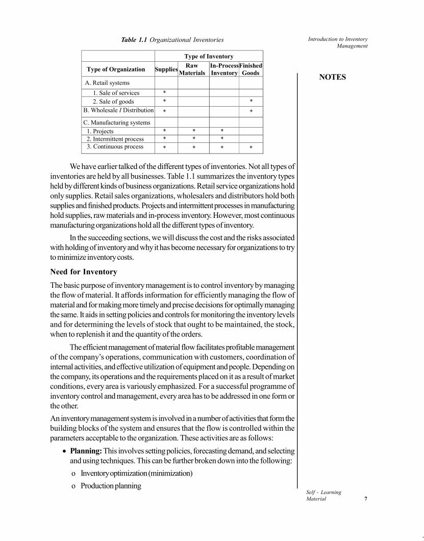
Table 1.1 Organizational Inventories
Type of Inventory
Type of Organization Supplies Raw
Materials In-ProcessInventory
Finished Goods
A. Retail systems
1. Sale of services * 2. Sale of goods * *
B. Wholesale I Distribution * *
C. Manufacturing systems 1. Projects * * * 2. Intermittent process * * * 3. Continuous process * * * *
We have earlier talked of the different types of inventories. Not all types ofinventories are held by all businesses. Table 1.1 summarizes the inventory typesheld by different kinds of business organizations. Retail service organizations holdonly supplies. Retail sales organizations, wholesalers and distributors hold bothsupplies and finished products. Projects and intermittent processes in manufacturinghold supplies, raw materials and in-process inventory. However, most continuousmanufacturing organizations hold all the different types of inventory.
In the succeeding sections, we will discuss the cost and the risks associatedwith holding of inventory and why it has become necessary for organizations to tryto minimize inventory costs.
Need for Inventory
The basic purpose of inventory management is to control inventory by managingthe flow of material. It affords information for efficiently managing the flow ofmaterial and for making more timely and precise decisions for optimally managingthe same. It aids in setting policies and controls for monitoring the inventory levelsand for determining the levels of stock that ought to be maintained, the stock,when to replenish it and the quantity of the orders.
The efficient management of material flow facilitates profitable managementof the company’s operations, communication with customers, coordination ofinternal activities, and effective utilization of equipment and people. Depending onthe company, its operations and the requirements placed on it as a result of marketconditions, every area is variously emphasized. For a successful programme ofinventory control and management, every area has to be addressed in one form orthe other.
An inventory management system is involved in a number of activities that form thebuilding blocks of the system and ensures that the flow is controlled within theparameters acceptable to the organization. These activities are as follows:
Planning: This involves setting policies, forecasting demand, and selectingand using techniques. This can be further broken down into the following:
o Inventory optimization (minimization)
o Production planning

Introduction to InventoryManagement
NOTES
Self - Learning8 Material
o Sales and operations planning
o Sales forecasting or demand management
Acquisition: Inventory is constantly in the process of being acquired,dispersed and re-acquired. Acquisition relates to the action taken on ordersor replacements, which may either be positive or negative. It is associatedwith the quantity of the order, the timing of the receipts, and the reschedulingof inventories.
Stock keeping: This refers to the functions related to accounting forinventories. It may be integrated or merged with the planning process insome cases.
Disposition: This relates to the disbursement or distribution of inventoryafter it has been received. Inventory may be disbursed to the in-housedemand source, the processing facility, the warehouse or store. In addition,it also includes the disposal of obsolete items and scrap.
Inventory, though a large part of it may be an idle resource, comprises thephysical stock of goods that is kept by an enterprise for meeting its businessobjectives in the future. As a result of this, a significant percentage of the assets ofmany firms get tied up in inventories. This could range from 35 per cent to over 50per cent of the total capital utilized in a typical firm. Holding inventory, also representsa risk and a cost to the firm. Effective inventory management is therefore critical tothe firm.
Check Your Progress
1. Define inventory.
2. Identify any two types of inventories.
3. What is the basic purpose of an inventory?
1.3 FUNCTIONS AND USE OF INVENTORY
Formulating an inventory policy requires understanding the inventory’s role in thefirm. Though inventory is an idle resource and adds to the risk of the firm, it isnevertheless essential to keep some inventory in order to promote smooth andefficient running of business. The ultimate function of inventory is to provide timeutility, guard against discontinuity and uncertainty, and provide economic advantage.
If the demand for the product is known precisely, it may be possible (thoughnot necessarily economical) to produce the product in a quantity to exactly meetthe demand. However, in the real world this does not happen and inventoriesbecome essential. Inventories also permit production planning for smoother flowand lower- cost operation through larger lot-size production. They allow a bufferwhen delays occur.

Introduction to InventoryManagement
NOTES
Self - LearningMaterial 9
These delays can be for a variety of reasons: a normal variation in shippingtime, a shortage of material at the vendor’s plant, an unexpected strike in any partof the supply chain, a lost order, a climatic catastrophe like a hurricane or floods,or perhaps a shipment of incorrect or defective materials.
As a result, a significant percentage of assets of firms get tied up ininventories. This figure could range from 35 per cent to over 50 per cent of thetotal capital utilized in a typical firm. Holding of inventory, therefore, also reflects atype of risk to the firm. These are risks related to capital investment, cash flowand the potential for obsolescence of the inventory.
The inventory decision gets further complicated due to the differentrelationships between the inventory and the objectives of different functionaldepartments. These conflicting objectives are reflected in the contradictoryviewpoints of different parts of the organization.
Table 1.2 Conflicting Organizational Objectives
Area Typical Response
Marketing / Sales
I can't sell from an empty wagon. I can't keep our customers if we continue to stock-out and there is not sufficient product variety.
Production If I can produce larger lot sizes, I can reduce per unit cost and functional efficiency.
Purchasing I can reduce per unit cost if I buy quantities in bulk.
Warehousing I am out of space. I can't fit anything else in the building.
Finance Where am I going to get the funds to pay for the inventory? The levels should be lower.
The responses in Table 1.2 place the focus on the functional significance ofinventory for different departments in the organization:
Marketing would like to have a large inventory so that customer service canbe improved and sales can increase.
Production would like to minimize setup costs and increase workerproductivity by having large production runs adding on to the in-process inventory(work-in-progress and finished goods).
Purchasing can bring down prices by buying in bulk and obtaining quantitydiscounts. Stores or warehousing has storage constraints in storing and movinglarge quantities of stock.
However, the bottom line is equally important. All these requirements canbe met at a cost. Larger inventories mean more capital investment, lower cashflows, idle inventory and lower profitability.
All this is evident in Table 1.3. The whole picture of inventory becomesclear when seen in the context of the different functional objectives of departmentswithin the organization.

Introduction to InventoryManagement
NOTES
Self - Learning10 Material
Table 1.3 Functional Significance of Inventory
Functional Area
Functional Responsibility Inventory Goal Inventory Inclination
Marketing Sell the Product Maximize customer service High
Production Make the Product Efficient lot sizes High
Purchasing Buy required materials Low cost per unit High
Finance Provide working capital Efficient use of capital Low
Engineering Design the product Avoid obsolescence Low
As will be apparent from Table 1.3, some functional areas find inventorydesirable, while others do not. What is important to note is that both the inclinationto hold inventory and the inventory goals of the different functions are significantlydifferent.
The functionality of inventory becomes clear only when it is considered inlight of all the factors—quality, customer service and economic factors, i.e. fromthe viewpoints of purchasing, manufacturing, sales and finance. Inventory build-up is important as it is meant to permit them to meet their functional objectives.
Some of these objectives are as follows:
1. To protect against unpredictable variations (fluctuations) in demand andsupply
2. To take advantage of price discounts by bulk purchases
3. To take advantage of batches and longer production run
4. To provide flexibility to allow changes in production plans in view of changesin demands, etc.
5. To facilitate intermittent production
To maintain independence of operations, the supply of materials at a workcentre allows flexibility in operations. Inventory can be used, among other things,to promote sales by reducing customers’ waiting time; to improve workperformance by reducing the number of setups; or to protect employment levelsby minimizing the cost of changing the rate of production.
Consider the case of an enterprise that does not have any inventory. Clearly,as soon as the enterprise receives a sales order, it will have to order for rawmaterials to complete the order. This will keep the customers waiting. It is quitepossible that sales are lost. Also, the enterprise may have to pay a high price forsome other reasons.
The major issue in inventory decisions is how to reconcile the differencesbetween the different functional requirements of the different parts of theorganization and the goals of the organization as a whole. No matter what theviewpoint of each department is or what each function desires, in the ultimateanalysis, effective inventory management has to provide an economic advantagethat is essential to organizational competitiveness.

Introduction to InventoryManagement
NOTES
Self - LearningMaterial 11
Broadly speaking, the functions of inventory have been shown in Figure1.2. Raw materials flow in from the supplier and finally are sold to the customer.During the process of providing goods to the customer, the inventory is requiredfor use, transformation and distribution. A part of the inventory is in transit connectingthe different transformation and distribution activities.
In-transit
In-transit
Supplier
Raw Materials
Customer
Use
Idle
Incomplete Transformation
Sale
Finished Goods
Idle
In-transit
Fig. 1.2 Functions of Inventory
Inventory, though an idle resource, comprises physical stock of goods that is keptby an enterprise for future purposes. Functional inventory categories are:
Working stock Safety stock Anticipation stock Pipeline stock Decoupling stock Psychic stock
The build-up of inventory takes place at different points during the flowfrom the supplier to the final customer. It is desirable to maintain inventories inorder to provide time utility, guard against discontinuity and uncertainty, enhancestability of production, protect employment levels and provide economic advantageto the organization. However, excessive inventory is a drain to the profitability ofthe organization and is reflected in the costs. This is discussed in the next section.
Check Your Progress
4. List any three objectives of inventory.
5. Name two functional inventory categories.
6. Why does the marketing department need an inventory?
1.4 INVENTORY COSTS
The heart of inventory decisions lies in the identification of inventory costs andoptimizing the costs relative to the operations of the organization. As inventory is anecessary but idle resource, inventory costs in manufacturing need to be minimized.

Introduction to InventoryManagement
NOTES
Self - Learning12 Material
Large holdings of inventory also cause long cycle times, which may not be desirable.
CB
COST
A
D
TIMEMaterialsAcquisition
ProductShipment
FinishedGoods
Manufacturing Cycle Time
Throughput Time
OA = material costAB = labour costBC = factory overheadOC = total product cost
RawMaterial
storagefabrication storage
subassembly
storage
assembly
storage
Work-in-Progress
Fig. 1.3 Cost of Inventory with Time
The total inventory held is additive in nature. Raw materials are convertedto finished goods through a number of incremental processes. Regardless of theoperating process, all production costs incurred during a particular period to thejobs or products produced during that time period are assigned to the inventory.These processes also add to the cost of inventory held by the organization.Therefore, the cost of inventory increases with time as shown in Figure 1.3.
What are the costs identified with inventories? The costs generally associatedwith inventories are shown in Figure 1.4, and each component of this cost isdescribed below.
Holding (or carrying) costs: It costs money to hold inventory. Such costs arecalled inventory holding costs or carrying costs. This broad category includes thecosts for:
Storage facilities
Handling
Insurance
Pilferage
Breakage
Obsolescence
Depreciation
Taxes

Introduction to InventoryManagement
NOTES
Self - LearningMaterial 13
600
500
400
300
200
100
0 200 400 600 800 1000
EOQProcurement Costs
Stock-out Costs
Carying CostsTotal Inventory Costs
MinimumTotal Inventory
Costs
Cos
t of
Sto
ckin
g a
Mat
eria
l (R
s)
Total Inventory
Fig. 1.4 Total Inventory Costs
As can be seen from Figure 1.4, holding costs are shown as a straight line.These costs increase proportionately with the increase in the inventory level.Obviously, if the holding costs are high, the organization should try to carry lowerinventory and frequently replenish the stock.
Though holding costs are represented by a straight line, there are somefixed and variable costs of holding inventory, i.e. some of the costs will not changeby increase or decrease in inventory levels, while some costs are dependent onthe levels of inventory held. The general breakdown for inventory holding costshas been shown in Table 1.4.
Table 1.4 Fixed and Variable Holding Costs
Fixed costs Variable cost
Capital costs of warehouse or store
Cost of operating the warehouse or store
Personnel costs
Cost of capital in inventory
Insurance on inventory value
Losses due to obsolescence, theft, spoilage
Cost of renting warehouse or storage space
Capital costs and costs of operating a warehouse, including personnel, are
fixed, but costs such as interest costs of capital held in inventory are variable. Thereason why the cost curve for holding inventory is a straight line is that thecontribution of the variable costs in the total holding costs is much greater than thatof the fixed costs.
Ordering Costs/ Setup (or production change) costs: Although it costs moneyto hold inventory, it also, unfortunately, costs money to replenish inventory, eitherthrough the purchase cycle or through the manufacturing cycle.
Inventory Ordering Costs: The costs that are incurred in the purchase cycle arecalled procurement costs or inventory ordering costs. Ordering costs have twocomponents:

Introduction to InventoryManagement
NOTES
Self - Learning14 Material
(a) One component that is relatively fixed, and
(b) Another component that will vary.
Table 1.5 Fixed and Variable Ordering Costs
Fixed costs Variable costs
Staffing costs (payroll, benefits, etc.)
Fixed costs on IT systems
Office rental and equipment costs
Fixed costs of Vendor Development
Shipping costs
Cost of placing and order (phone, postage, order forms)
Running costs of IT systems
Receiving and inspection costs
Variable costs of Vendor Development
The fixed and variable components of the ordering or procurement costsare shown in Table 1.5. Referring back to Figure 1.4, it will be seen that inventoryordering costs decrease increasingly with the increase in inventory. This can beexplained if we are able to clearly differentiate between those ordering costs thatdo not change much and those that are incurred each time an order is placed.
One major component of cost associated with inventory is the cost ofreplenishing it. If an organization orders a part or raw material from an outsidesupplier, and places orders for the part or raw material with the supplier threetimes per year instead of six times per year, the costs to the organization thatwould change are variable costs, and probably not the fixed costs.
There are costs incurred in maintaining and updating the information system,developing vendors, evaluating capabilities of vendors. Ordering costs also includeall the details, such as counting items and calculating order quantities. The costsassociated with maintaining the system needed to track orders are also included inordering costs. This includes phone calls, typing, postage, and so on.
Though vendor development is an ongoing process, it is also a very expensiveprocess. With a good vendor base, it is possible to enter into longer-termrelationships to supply needs for perhaps the entire year. This changes the ‘when’to ‘how many to order’ and brings about a reduction both in the complexity andcosts of ordering.
Clearly, the fixed costs related to procurement or order placement aresignificantly greater than the variable costs associated with placing orders.
Setup (or production change) costs: In the case of sub-assemblies or finishedproducts that may be produced in-house, the costs associated with changing overequipment from producing one item to producing another is usually referred to assetup costs.
Ordering costs are incurred in the purchase cycle, while setup costs areincurred in the manufacturing cycle. Therefore, in Figure 1.4 the setup cost isactually represented by the inventory ordering costs. These two costs are consideredto be exclusive.

Introduction to InventoryManagement
NOTES
Self - LearningMaterial 15
Setup costs reflect the costs involved in obtaining the necessary materials,arranging specific equipment setups, filling out the required papers, appropriatelycharging time and materials and moving out the previous stock of materials inmaking each different product. If there were no costs or loss of time associated inchanging form one product to another, many small lots would be produced,permitting reduction in inventory levels and resultant savings in costs.
Shortage or Stock-out costs: When the stock of an item is depleted, an order forthat item must either wait until the stock is replenished or be cancelled. There is atrade-off between carrying stock to satisfy demand and the costs resulting fromstock-out. The costs that are incurred as result of running out of stock are knownas stock-out or shortage costs.
Understanding the cost of a stock-out is critical to the implementation ofany inventory model. Unless these costs are known, the organization cannot balancethe costs (and risk) of holding inventory with the loss of profits when an item is outof stock.
For a retailer, the costs include both the lost profits from the immediateorder because of cancellations, and the long-run costs if stock-outs reduce thelikelihood of future orders. For a manufacturer, these include loss of productionas well as capacity. In addition, the ultimate consequence is that sales of goodsmay be lost, and finally customers can be lost.
If the unfulfilled demand for the items can be satisfied at a later date(backorder case), in this case costs of backorders are assumed to vary directlywith the shortage quantity (in rupee value) and the cost involved in the additionaltime required to fulfill the backorder ( /year).
However, if the unfulfilled demand is lost, the cost of shortages is assumedto vary directly with the shortage quantity ( /unit shortage). When this is related tothe total cost of inventory, the cost decreases increasingly with the increase ininventory, as this cost is relatively fixed with respect to the value of the inventory.Check out Figure 1.4 again, you will see that this relationship is clearly visible.
Frequently, the assumed shortage cost is a little more than a guess, althoughit is usually possible to specify a range of such costs.
1.5 DEPENDENT AND INDEPENDENTDEMAND
The risk of carrying additional inventory depends on the nature of the demand.Each type of demand carries with it a different type of risk. Moreover, this adds tothe cost and quantum of inventory held by the organization.
For example, marketing experts hold Edsel designed by Ford Motor Co.as a supreme example of corporate America’s failure to understand the nature ofconsumer demand. Edsel was created as an automobile that would meet consumer

Introduction to InventoryManagement
NOTES
Self - Learning16 Material
demands for a new generation of Americans. It was the hot new car that everybodywas talking about. It turned out to be a major failure. The company sufferedgreatly because it did not consider the risks associated with getting the figureswrong.
Inventory items can be divided into two main types: Independent demand,and dependent demand items. In inventory management it is important to distinguishbetween dependent and independent demand.
An item has independent demand when we cannot control it or tie it directlyto another item’s demand. The Ford example was an example of independentdemand. Though Ford tried to manipulate demand through pricing incentives andother marketing efforts, Edsel failed. As the results of the Edsel show, the firm cantry to predict or influence independent demand, but independent demand for theproduct is ultimately determined by the marketplace.
In order to predict independent demand, firms use different types offorecasting methods. Forecasting looks at the marketplace to determine how muchof the product the consumers want.
In forecasting, both the accuracy of data as well as the method is important.It is not only important to know where the data comes from but also if it is useful.There are many different applications to consider when deciding which method isthe best. Not only is the input important but also the quality of the output. Feedbackon the output creates the ability to go back and correct any errors that might havebeen made during the initial input of data. The first item to look at is differentmethods used in different situations.
Manufacturing requirements are primarily derived from dependent demand,while retailing requirements depend on independent demand. Dependent demandis by far the most common type of demand. An item has dependent demandwhen the demand for an item is controlled directly, or tied to the production ofsomething else. Continuing with the Edsel example, let us suppose Ford decidedto manufacture 15,000 units of the automobile for the first year based on a forecastof independent demand. Based on this forecast, Ford knew exactly how manysteering wheels are needed and when. This is because the demand for these itemsis dependent on the production schedule of 15,000 automobiles for the year. Thesteering wheels are dependent demand items because:
The firm controls their demand through the production schedule; and
Their demand is tied to the production of automobiles.
Dependent demand in a manufacturing unit is based on the sub-assemblies,components, or raw materials that are part of the BOM for the end items. Thedemand for these items is indirect or comes from the finished products demand,when we explode the BOM (Bills of Materials). A BOM ‘explosion’ is referred toan assembly or sub-assembly when broken down into its individual componentsand parts.

Introduction to InventoryManagement
NOTES
Self - LearningMaterial 17
1.5.1 Material Planning
Inventory systems are predicated on whether demand is derived from an end itemor is related to the item itself. Because independent demand is uncertain, extrainventory needs to be carried to reduce the risk of stocking out.
To determine the quantities of independent item that must be produced,firms usually use a variety of techniques, including customer surveys and forecasting.However, a balance is sometimes difficult to obtain because of the difficulty inestimating stock-out costs, as was discussed in the last section. It is generallydifficult to accurately estimate lost profits, the effects of lost customers or latenesspenalties.
An analysis of inventory is useful to determine the level of stocks. Analysis ofinventory is carried out through a number of models for stock keeping decisionsthat specify:
1. The time for ordering the items.
2. The size of the order.
3. Quantity to be ordered.
Economic Order Quantity (EOQ) models, due to their simplicity andversatility, are often used for material planning when independent demand is themost important issue. EOQ models are simple models, which base their decisionson the historic data to arrive at average consumption for a given period. Given theaverage lead-time for the item, it is possible to calculate the quantity that needs tobe maintained in inventory until the material is replenished. Once the quantity reachesthat level, an order is placed based on the Economic Order Quantity.
EOQ is a simple technique that works. There are a number of variants of thetechnique, mainly differing in the quantity that is ordered or on the timing of theorder. The assumptions of these models are:
The demand is fairly regular.
The supplier supplies the material within the lead-time.
The material is available relatively easily in the market.
The material is delivered as a single package.
These models work well for planning inventories, only when the aboveassumptions are true. However, the question is: how many of these assumptionsare true and for how many items? We will be discussing this and studying suchmodels in subsequent units in this book.
Materials Requirement Planning (MRP) considers both independentdemand and dependent demand. It uses the basic principle that external demandis generally independent and internal demand is generally dependent. It gets theindependent demand and calculates the total demand by working downwards atthe highest level of the Bill of Materials after deducting on-hand quantities. Oncethis is done for high- level items, as explained in the earlier section, the bills of

Introduction to InventoryManagement
NOTES
Self - Learning18 Material
material are exploded to calculate the components required. This process isrepeated further down the levels till the raw material requirements are arrived at.
Independent Demand
Dependent Demand Dependent Demand
Activity Activity
On HandInventory
On HandInventory
Activity
Fig. 1.5 Independent and Dependent Demand in MRP Models
1.5.2 Managing Independent Demand
It must be remembered that inventory is costly and large amounts are generallyundesirable. As inventory can have a significant impact on a company’s productivityas well as delivery time, different methods have to be found to reduce inventory.One approach is to reduce the risks associated with inventory. If risks are reduced,inventory levels can also be reduced.
It has been found that the risks due to independent demand can be reducedthrough process design. Process design can minimize the risk if we reduce demanduncertainty of independent demand by positioning the process from the push–pullpoint of view. What is the push–pull view?
Push–Pull View to Modulate Independent Demand: Processes can bedivided into two categories depending on whether they are executed in responseto a customer order or in anticipation of customer orders: pull processes and pushprocesses. Pull processes are initiated by customer order, whereas push processesare initiated and performed in anticipation of customer orders. In other words, inpush processes independent demand has a high level of uncertainty, while in pullprocesses demand uncertainty is low as the process is initiated on the demandbeing known.
Figure 1.6 shows graphically the push–pull system in a retail network. Itcan be clearly seen from the dotted arrow in Figure 1.6, which represents the pullprocess, that the manufacturing and replenishment cycle is initiated when customerdemand is known with certainty, i.e. it is executed after the customer order arrives.Whereas for a push process, represented by the solid arrows, demand is notknown and must be forecast, as the customer order is yet to arrive.

Introduction to InventoryManagement
NOTES
Self - LearningMaterial 19
Customer order Cycle
ProcurementManufacturingReplenishment Cycle
CustomerOrderArrives
PULLPROCESS
Customer Order Cycle
Replenishment andManufacturing Cycle
PUSHPROCESS
Procurement Cycle
Customer
Retailer
Manufacturer
Supplier
Fig. 1.6 Push–Pull Processes for a Retail Network
Based on the criterion of how they relate to the customer order, pull processesare referred to as reactive processes because they react to customer demand.Push processes are referred to as speculative processes because they respond tothe forecast rather than actual demand.
Many processes combine both push and pull systems. The push–pullboundary in a supply chain separates push processes from pull processes.
A push–pull view of demand is very useful when considering inventory build-up. However, the systems to manage inventory in these two types of processesdiffer significantly. Inventory levels in push processes need to cater to theuncertainties in the demand forecast, while inventory for pull processes is dependenton the customer order only and therefore safety stock that is meant to cater todemand uncertainties is significantly reduced.
A push process can become a pull process if the responsibility for certainprocesses can be passed onto a different stage of the supply chain, and makingthis transfer is possible. For example, computer makers such as Dell are movingto a pull system of dependent demand, where computers are built-to-order (BTO)and components can be obtained on short notice. In Dell’s case, it takes them anaverage of 15 minutes to get the components as they use this in conjunction with avendor-managed-inventory (VMI) arrangement.
One clear conclusion in studying these two processes is that a supply chainthat has fewer stages and more pull processes has a significant impact on inventoryreduction. Manufacturers are moving from a production push environment whichis largely focused on production efficiency with large safety stocks to consumerpull environment which is focused on meeting expected consumer demand with aminimum inventory requirement.
The Push–Pull View has become very popular in modulating independentdemand, as organizations using it find that it helps in reducing the ‘unwantedinventory’ and improves the number of times the inventory turns over, i.e. ‘inventoryturns’. Both of these are measures of good inventory management.
Demand Management: Demand management describes the process of influencingthe volume or consumption of the product or service through management decisions.It is another technique available to the organization to reduce the uncertainty ofindependent demand. For example, air conditioner and refrigerator manufacturers

Introduction to InventoryManagement
NOTES
Self - Learning20 Material
offer discounts for their products in winter, when the demand for the productsfalls. Electricity tariffs in India are designed on slabs based on consumption. Theidea is to provide incentive for reducing the consumption of electricity.
The objective of such exercises of demand management is to helporganizations use their resources and production capacity more effectively. As thedemand for a particular product is high during the peak time, the costs are alsohigh. Many organizations avoid this situation by offering price incentives or usepromotional strategies so that customers make purchases before or after traditionalperiods of peak demand.
The idea is to shift demand or to spread demand more evenly without losingthe custom. Telephone companies the world over provide special offers for callsmade during late hours or at night. For instance, MTNL offered a 50 per centdiscount for calls made after 10.00 p.m. but before 6.00 a.m.
The same principle is involved when doctors and other professionals requireprior appointments to meet their patients and clients.
Both these concepts are very important in controlling the uncertaintyassociated with independent demand and are commonly used by organizations toreduce the negative impact due to the nature of the different types of demand.
1.6 RESPONSIBILITY FOR INVENTORYMANGEMENT
Inventory controllers are responsible for planning and controlling a specific groupof items. People performing these tasks are known as inventory analysts. Theirprimary responsibilities relate to execution of the plan. In doing so, their primaryactivities include the following:
1. Release orders for production.
2. Send requisitions to purchasing.
3. Change order and requisition quantities, or cancel them.
4. Reschedule open shop orders.
5. Request changes in open purchase order timing.
6. Approve requests for unplanned stock disbursements
In addition to the activities listed here which relate to execution, the inventoryanalysts also are responsible for activities related to the inventory files. Theirnomenclature originates from this. In order to maintain inventory files they arecharged with:
1. Handling engineering changes in bills of material of items under their control
2. Monitoring inventory for inactivity or obsolescence, and recommendingdisposition
3. Investigating and correcting errors in inventory records
4. Participating in analyses of cycle inventory counts

Introduction to InventoryManagement
NOTES
Self - LearningMaterial 21
5. Analysing discrepancies in item requirements and coverage, and takingappropriate corrective actions
6. Requesting changes in master production schedules
MRP is a powerful tool for inventory controllers, who interact continuouslywith MRP, receive its principal outputs, and take action based on the data itsupplies. They extract from its files data needed for analyses and supply data tokeep it current. Most of these tasks are routine and self-explanatory. Theresponsibility for inventory management is best explained in the context of MRP‘action notice’, as given below:
Releasing planned orders
MRP ‘action notices’ relate to transactions on planned and released orders. Thesecontinually modify inventory status data, and provide directions to the action thatneeds to be taken. The principal actions signalled by MRP ‘action notices’ are thefollowing:
1. Release the planned orders
2. Expedite the released orders
3. Delay the released orders
4. Cancel the released orders
All of these action notices involve either the timing of orders, or changingquantities.
Table 1.6 Planned Order Mature for Release
Lead Time: 2 Period
11 12 13 14
Gross Requirements 200 200
Scheduled Receipts 100
On Hand 120 120 20 20 – 180
Planned-order Releases 180 Action Bucket
Releasing of planned orders takes place when MRP generates a messagerecommending ‘release the order’. Orders are ready for release when a quantityappears in the current-period bucket. This is shown in Table 1.6.
The quantity appears as a result of offsetting for lead time in the requirementsexplosion or by passage of time, gradually bringing a planned-order release towardthe current period, called the actual bucket. MRP tests the contents of this bucket,and ensures that these actions are limited to:
1. Releasing orders in the right quantity at the right time, or
2. Rescheduling the due dates of open orders as required, making them coincidewith the dates of actual need
In both cases, MRP suggests both the quantity and the timing of planned-order releases. When the planned order shown in Table 1.6 is released, thetransaction changes the status of the item as shown in Table 1.7. Both open ordersare now scheduled with the correct due dates.

Introduction to InventoryManagement
NOTES
Self - Learning22 Material
Table 1.7 Planned Order Release
Period
11 12 13 14
Gross Requirements 200 200
Scheduled Receipts 100 180 +180
On Hand 120 120 20 20 0
Planned-order Releases 0 –180
Inventory controllers may override MRP by holding orders back if startingwork centres cannot handle them, or releasing orders early to level load at differentwork centres, e.g., for input/output control, or increasing order quantities if aparent needs more. MRP also monitors the validity of all open-order due datesconstantly. Inventory planners review these recommendations and decide whetherto execute them. They may also change quantities if amounts of available rawmaterial or components are not enough to make the full quantity planned. Makingchanges is difficult once work has begun, but splitting these into two or moresublots with different schedules is easier. Reducing quantities rather than delayingorder release is always preferable, though additional set-ups can reduce the capacityavailable, which often is the reason to split orders in the first place. Experiencedplanners have to balance the advantages and disadvantages.
Releasing planned-purchase orders is simpler for two reasons: first, nocomponent materials are involved and second, planners are less concerned withlevel-loading suppliers’ facilities.
Preproduction time is the time required to prepare paperwork (purchaseand stores requisitions, shop order packets, etc.) and to check the availability oftooling, test equipment, process specifications, and other resources. This forms asignificant element of lead time. This MRP can be programmed to signal the timeto begin such actions through an additional powerful action notice: ‘prepare torelease’. MRP does this by using its forward visibility of planned orders, eliminatingthis element from planned lead times, making them much shorter.
Check Your Progress
7. What are inventory ordering costs?
8. Who are responsible for planning and controlling a specific group ofitems?
1.7 ANSWERS TO ‘CHECK YOUR PROGRESS’
1. Inventory is a stock of materials used to satisfy customer demand or supportproduction of goods or services.
2. Raw material inventory and WIP inventory.
3. The basic purpose of inventory management is to control inventory bymanaging the flow of material.

Introduction to InventoryManagement
NOTES
Self - LearningMaterial 23
4. Three of the objectives are as follows:
(i) To protect against unpredictable variations (fluctuations) in demandand supply
(ii) To take advantage of price discounts by bulk purchases
(iii) To take advantage of batches and longer production run
5. Functional inventory categories are:
Working stock
Safety stock
6. Marketing would like to have a large inventory so that customer service canbe improved and sales can increase.
7. The costs that are incurred in the purchase cycle are called procurementcosts or inventory ordering costs.
8. Inventory controllers are responsible for planning and controlling a specificgroup of items.
1.8 SUMMARY
The term inventory means any quantity of direct or indirect materials (rawmaterials or finished items or both) stocked in order to meet an expectedand unexpected demand in the future. Formulating inventory policy requiresunderstanding the inventory’s role in the firm.
Though inventory is an idle resource and adds to the risk of the firm, it isalso essential to keep some inventory to enable smooth and efficient runningof business.
The function of inventory is to provide time utility, guard against discontinuityand uncertainty and provide economic advantage. Some of the reasonswhy this build-up is important are protection against unpredictable variations(fluctuations) in demand and supply, deriving advantage of price discountsby bulk purchases and longer production runs.
In addition, inventory provides the flexibility to allow changes in productionplans in view of changes in demands and to facilitate intermittent production.In view of the quality, customer service and economic factors—from theviewpoints of purchasing, manufacturing, sales and finance—effectiveinventory management is essential for organizational competitiveness.
The core of inventory decisions lies in the identification of inventory costsand optimizing the costs relative to the operations of the organization: Whenshould items be ordered, how large the order should be and ‘when’ and‘how many to deliver.’
The following costs are generally associated with inventories: Holding (orcarrying) costs, Cost of ordering, Setup (or production change) costs andShortage or Stock-out costs.

Introduction to InventoryManagement
NOTES
Self - Learning24 Material
Inventory items can be divided into two main types: Independent demandand dependent demand items. An item has independent demand whenwe cannot control it or tie it directly to another item’s demand. An item hasdependent demand when the demand for an item is controlled directly ortied to the production of something else.
Since independent demand is uncertain, extra inventory needs to be carriedto reduce the risk of stocking out. The analysis of inventory is carried outthrough a number of models. Some of these are the EOQ model and theMRP model.
Independent demand can also be modulated by the type of process theorganization uses. Pull processes are initiated by customer order, whereaspush processes are initiated and performed in anticipation of customers’orders. A supply chain that has fewer stages and more pull processes has asignificant impact on inventory reduction.
The role of inventory controllers is performed by those who are responsiblefor planning and controlling a specific group of items. Their primary activitiesinclude: (a) Releasing orders for production, (b) Sending requisitions topurchasing, (c) Changing order and requisition quantities, or cancel them,and (d) Rescheduling open shop orders, (e) Requesting changes in open-purchase order timing, (f) Approving requests for unplanned stockdisbursements.
1.9 KEY TERMS
Inventory: It refers to the stock of direct or indirect material (raw materialsor finished items or both) that are maintained in order to meet the expectedand unexpected demand in the future.
Retailer: It refers to a person or business that purchases a wide variety ofproducts and markets them.
Production Rate: It is the number of units manufactured over a period oftime.
1.10 SELF-ASSESSMENT QUESTIONS ANDEXERCISES
Short-Answer Questions
1. List the most commonly identified types of inventory.
2. Outline the common factors on which the levels of inventory depend.
3. Write a short note on Economic Order Quantity (EOQ).
4. Briefly state Materials Requirement Planning (MRP).

Introduction to InventoryManagement
NOTES
Self - LearningMaterial 25
5. ‘Inventory controllers are responsible for planning and controlling a specificgroup of items. Their primary responsibilities relate to execution of the plan.’How do inventory planners fulfill this role?
Long-Answer Questions
1. Examine the role of inventory in an organization. Explain the impact it hason different functions in the organization.
2. Inventory is costly and large quantities are generally undesirable as this canhave a significant impact on a company’s productivity, delivery time andprofitability. Discuss with examples.
3. ‘Independent demand increases a firm’s risk to meet the expectations ofthe market place.’ Discuss the merits of the statement and provide an exampleto illustrate your answer.
1.11 FURTHER READING
Zipkin, Paul Herbert. 2000. Foundations of Inventory Management. New Delhi:McGraw Hill.
Orlicky, Joseph and George Plossl. 1994. Orlicky’s Material RequirementPlanning. New Delhi: McGraw-Hill.
Seetharama L Narsimhan, Dennis WMcLeavy, Peter J Billington. 1994. ProductionPlanning and Inventory Control. New Delhi: Prentice Hall of India PvtLtd.
J. R. Tony Arnold, Stephen N. Chapman. 2007. Introduction to MaterialsManagement. New Delhi: Prentice Hall.
Richard J. Tersine.1982. Principles of Inventory and Materials Management.New Delhi: Prentice Hall.


Strategic InventoryManagement
NOTES
Self - LearningMaterial 27
UNIT 2 STRATEGIC INVENTORYMANAGEMENT
Structure
2.0 Introduction2.1 Objectives2.2 Forecasting – A strategic Tool
2.2.1 Developing a Model2.2.2 Accuracy and Validation Assessments2.2.3 Collaborative Forecasting
2.3 Objectives and Importance of Inventory Management Functions in Referenceto Profitability, Strategy, Customer Satisfaction and Competitive Advantage
2.4 Answers to ‘Check Your Progress’2.5 Summary2.6 Key Terms2.7 Self-Assessment Questions and Exercises2.8 Further Reading
2.0 INTRODUCTION
In the previous unit, you studied the basic concepts of inventories to understand itsfunctionality. In this unit, you will learn how forecasting is used as a strategic toolfor decision making for a long term. Forecasting of demand levels is vital to a firmas a whole, as it provides the basic inputs for planning and control of all functionalareas, including the supply chain. Demand levels and their timings greatly affectcapacity levels, financial needs and general structure of the business. Each functionalarea has its special forecasting problems. Supply chain forecasting concerns thespatial as well as variation of demand with time, the extent of its variability and itsdegree of randomness. Planning and controlling supply chain activities requireaccurate estimates of the product and service volumes to be handled by the chain.These estimates are typically in the form of forecasts and predictions. Supplychain professionals often finds it necessary to take it upon themselves to produceforecasts for short-term planning, such as inventory control, order sizing, or transportscheduling.
In this unit, you will also understand the objectives and importance ofinventory management with reference to profitability, strategy, customer satisfactionand competitive advantage for a firm.
2.1 OBJECTIVES
After going through this unit, you will be able to:
Understand how forecasting is used as a tool for strategic decision making
Discuss the objectives and importance of inventory management with referenceto profitability, strategy, customer satisfaction and competitive advantage

Strategic InventoryManagement
NOTES
Self - Learning28 Material
2.2 FORECASTING – A STRATEGIC TOOL
In business and economics, forecasting has various meanings. There are two distinctquantities involved in forecasting—a forecast and a prediction. A prediction is abroader concept. It is an estimate of a future event achieved through subjectiveconsiderations other than just past data; this subjective consideration need notoccur in any pre-determined way.
In supply chain management, we adopt a rather specific definition of aforecast, which is given below:
A forecast is an estimate of a future event achieved by systematicallycombining and casting forward in a pre-determined way data about the past.
An analysis of the factors that influence future values determines how futurevalues are estimated. One way to characterize different kinds of forecasting canbe based on how far into the future they focus. Detailed forecasts for individualitems are generally short-term forecasting. Such forecasts are used to plan short-run decisions which are used for inventory control, order sizing, or transportscheduling, etc. Aggregate product demand forecasts are medium-term forecastsused to plan for capacity, location and layout over a much longer time span. Long-term forecasts are used for strategic decision-making.
The supply chain has both space and time dimensions. That is, the supplychain professional must know where demand volume will take place as well aswhen it will take place. Spatial location of demand is needed to plan warehouselocations, balance inventory levels across the supply chain network andgeographically allocate transportation resources.
Demand forecasting estimates the quantity of a service or a product that consumerswill purchase. Demand forecasting entails techniques including informal as well asquantitative methods, such as the use of current or historical sales data from testmarkets. Demand forecasting can be used to:
Make pricing decisions
Assess future capacity requirements
Make decisions on whether to enter a new market
Forecasting sales is different from forecasting demand. There is debate indemand-planning literature on how to represent and measure historical demand,as historical demand outlines the basis of forecasting. The main question is whetherone should use the history of outbound shipments or customer orders or acombination of the two as proxy for the demand.
The effect that inventory levels have on sales is known as stock effect. Inthe severe cases of stockouts, demand is not converted to sales owing to a lack ofavailability. Also, demand is left unexploited when item sales go down as a resultof poor display location etc.
Market response effect: Market response effect is the effect of marketevents beyond or within the control of a retailer. An item’s demand could rise if acompetitor increases the price or if one advertises the item in a proper manner.

Strategic InventoryManagement
NOTES
Self - LearningMaterial 29
The consequent increase in sales reflects a change in demand due to consumersresponding to stimuli that has the potential to bring about additional sales.Notwithstanding the stimuli, these forces have to be managed aptly within thedemand forecast.
Here, demand forecasting makes use of techniques in causal modelling.Demand forecast modelling takes into account the size of the market and marketshare dynamics versus competitors, and its effect on firm demand over a certaintime period. In the manufacturer to retailer model, promotional events are used.
Demand forecasting methods are not 100 per cent accurate. A combinationof forecasts improves accuracy and brings down the potential for large errors.
The following are some of the general considerations in demand forecasting:
Demand forecasting factors
Forecasting purposes
Demand determinants
Forecasts’ length
New products’ forecasting demand
Good forecasting method criteria
Presentation of forecast to the management
Role of macro-level forecasting in demand forecasts
Recent trends in demand forecasting
Demand control or management
Accurate demand forecasting is imperative for an organization to producethe necessary quantities at the right time and cater to, well in advance, the differentfactors of production— equipment, raw materials, labour, machine accessories,etc.
Demand forecasting can be categorized into short-term and long-term forecasting.The purposes of both these types of forecasting are listed below:
Purposes of short-term forecasting
Appropriate scheduling of production
Reducing costs of buying raw materials
Determining appropriate price policy
Setting sales targets and establishing controls and incentives
Coming up with appropriate promotional and advertising campaigns
Forecasting short-term financial requirements
Purposes of long-term forecasting
Planning a new unit or expanding an existing unit
Planning long-term financial requirements
Planning manpower requirements

Strategic InventoryManagement
NOTES
Self - Learning30 Material
Short-term forecasts can be up to 12 months long; medium-term forecastscan be 1 to 3 years long; and long-term forecasts are usually 3 to 10 years long.
Recent trends in demand forecasting
1. Firms are giving more importance to demand forecasting than they did tenyears ago.
2. Forecasting necessitates close cooperation and consultation with variousspecialists; thus, team spirit is stronger.
3. Data and information gathering tools facilitate better quality of forecasting.
4. New products’ forecasting is still in its formative years.
5. Forecasts are generally broken down in monthly forecasts.
6. In spite of the obvious advancements in technology, demand forecasting isfar from accurate.
7. The value of personal feel has been accepted.
8. Top-down approach is more popular than bottom-up approach.
2.2.1 Developing a Model
The uncertainty of the future and unpredictability of the course of environmentalforces that determine events impacts all organizations. To reduce this uncertainty,you need to find the right balance between having what your customers want andthe cost of carrying that inventory. If you are short on demand, you could havebackorders, cancellations and unsatisfied customers. But if you overstock theproduct, you waste time, money and space.
This solution lies in generating predictions that are precise and accurate. Inorder to reduce uncertainty, the organization has to be able to anticipate demandbefore it happens and prepare for what is ahead. It has to find the means tounderstand how environmental forces will impact its business.
Not all factors will be relevant to every organization. Environmental forcesthat are important to one organization may not be important to another. A small–scale or medium scale manufacturer may be interested in demand in the localmarket, governmental plans in infrastructure development, cost and availability ofpower, etc. in his own geographical area. On the other hand, a manufacturer oftobacco products would like relevant information on the decline in tobacco useover the past few years that will ensure that the forecast for those products issensible.
Analysis of the environmental forces has three goals:
Forecasting
Modelling
Characterization
The ‘logical order’ in which these three goals are to be tackled depends onthe objective of the organization. Often, modelling and forecasting proceed in aniterative way; however, there is no ‘logical order’ in the broadest sense. The processof forecasting and decision making is shown in Figure 2.1.

Strategic InventoryManagement
NOTES
Self - LearningMaterial 31
TheDecisionMaker
Decisions4
Action6
Forecasts3
Interaction5
Resources2
Performance1
Fig. 2.1 Forecasting and Decision-making
Forecasting is the start of any planning activity. Forecasting systems generallyprovide three pieces of information:
(1) Indications of whether a product market is static or dynamic (i.e. growth ordecline after seasonal adjustment)
(2) The best forecast in the next n periods(3) The forecast range within which the actual value is expected to fall
Therefore, the main purpose of forecasting is to estimate the occurrence,timing or magnitude of future events. Forecasting is not precise because of theinteraction between many factors or environmental forces that lead to the events.The effect of these interactions is increased uncertainty. This often leads to indecision.Is this an oxymoron? It need not be so. We must remember that indecision anddelays are the parents of failure. In order to avoid indecision and delays in decisionmaking, we need to use forecasting which can play a pivotal role in assisting decisionmaking.
Interactions among the different environmental forces generally follow certainlogical rules. This makes it possible to use mathematical functions to represent thecause-and-effect relationship among inputs, resources, forecasts and the outcome.The relationships are captured in a model which reflects how these environmentalforces impact the future. There should be no compromise in the quality of themodel.The model establishes a link between planning, controlling systems and the forecastsnecessary for planning, scheduling and controlling the system for an efficient output.Models reflect the realization of the uncertainty in forecasting and reflect the levelof sophistication and accuracy required for effective decision making. Therefore,in building a model, it is essential that the model provides satisfaction on these twocritical questions:
1. Is the model adequate?2. Is the model stable?
This also means that the model should reflect the objectives of themanagement. For example, the type of model that will be adequate for short-termforecasts may not be adequate for long-term forecasts. In order that the modelforecasts are stable, it will have to reflect and compensate for the actual performance.This is done by developing a model so that the forecast is an iterative process,which means the forecasts are updated so as to form a feedback loop to correctthe original forecast.

Strategic InventoryManagement
NOTES
Self - Learning32 Material
ModelSpecification
Past Data &ManagerialJudgement
Model Estimation
Is theModel
Adequate?no
Model Building
Forecasting
Fig. 2.2 Modelling and Forecasting
Figure 2.2 highlights the systematic development and the relationship betweenmodelling and forecasting and highlights the relationship between the model andthe forecast.
Even simple business problems require good models. For example, yourboss calls you. He wants you to make a sales forecast for the next two years forthe major products manufactured and marketed by your organization. At firstglance, this seems to be a very easy exercise. In a static world, perhaps, you cantake last year’s sales figures and add an appropriate internal growth to thesefigures and arrive at the projections.
But the world is dynamic. Things change and any projection should considerthe changes that have taken place and the changes that are expected in the businessenvironment. You know that the figures you give your boss will be used to determinethe resources of your department. Therefore, you would like the figures to reflectthe real situation on the ground.
Knowing that it is more important for organizations to grow their marketshare rather than just try to protect the sales volumes, the model should reflect thisreality. First you need to identify outside factors that have an impact on the forecast.If the historical growth of the market was 5 per cent and it is projected to grow at10 per cent, your historical sales figures will not be a good guide for the future, asthis would result in a reduction of the market share. So, if you need to protect yourmarket share, you need different forecasting models to determine the parameterswithin which you will operate.
Let us use some more examples. Assume DHL has reports that two newproducts competing with their product line are being introduced in the marketwithin the next six months. These new products are based on a new generation oftechnology that makes it possible to reduce costs by at least 10 per cent comparedto the current technology. What impact will this have on DHL?
If DHL wants to compete on price, perhaps DHL needs to look internallyat their costing, their competencies and other performance parameters. If DHL

Strategic InventoryManagement
NOTES
Self - LearningMaterial 33
decides to stay in the business activity, they may require value chain analysis toassess their competitiveness. In order to compete on product differentiation basis,they need to look at their product development capabilities and competencies andtheir advertising and marketing strategies to determine their ability to protect theirmarket share, etc.
Suppose airfreight industry sources believe that the government is planningto tax export consignments: what happens then? The problem becomes even morecomplex. Assume that currently, export consignments account for 20 per cent ofDHL sales. We will have to determine their impact on sales targets. We needforecasting models to help us build the operational and demand data under thechanged conditions.
So far we have only looked at the present-day environment and seen thecomplexity of factors that can have an influence on the growth and profitability ofan organization. Over a period, the importance of different components ofenvironmental forces can change. As the pace of change is increasing, anorganization will need to look to the future with a greater amount of forethought.
Even though modern forecasting packages are very powerful, they requireconsistent historical data. Many companies lack such data creating the need forgeneration of data. Also, sometimes an expert’s experience and knowledge of themarketplace may be superior to the forecasting techniques that could be used.For instance, the effect of future events, such as the launch of new products cannotbe deduced from historical data. Therefore, a combination of systems which usemathematical prediction and expert opinion may be required for such applications.
2.2.2 Accuracy and Validation Assessments
All models need to be validated and verified. Validation is concerned with thequestion, ‘Are we building the right system?’ Verification, on the other hand, seeksto answer the question, ‘Are we building the system right?’
Since validation is used for the purpose of establishing a model’s credibility,it is important that the method used for validation is itself credible. Features of timeseries, which might be revealed by examining its graph with the forecast valuesand the residual behaviour, condition forecasting modelling.
An effective approach to modelling forecasting validation is to hold out aspecific number of data points for estimation validation (i.e. estimation period) anda specific number of data points for forecasting accuracy (i.e. validation period).The data, which is not held out, is used to estimate the parameters of the model.The model is then tested on the data in the validation period, and if the results aresatisfactory, forecasts are generated beyond the end of the estimation and validationperiods.
A good model should have small error measures in both the estimation andvalidation periods and its validation period statistics should be similar to its ownestimation period statistics.
Holding data out for validation purposes is probably the single most importantdiagnostic test of a model: it gives the best indication of the accuracy that can beexpected when forecasting the future. It is a rule that one should hold out at least20 per cent of data for validation purposes.

Strategic InventoryManagement
NOTES
Self - Learning34 Material
A note of caution: Though forecasting is an important component of strategicand operational planning, we should not immerse ourselves in the techniques offorecasting and lose track of the reasons for forecasting.
2.2.3 Collaborative Forecasting
Collaborative forecasting is based on the concept of supply chain management.Collaborative Planning, Forecasting and Replenishment (CPFR) is a business modelthat takes a holistic approach to supply chain management and information exchangeamong trading partners. It uses common metrics, standard language and firmagreements to improve supply chain efficiencies for all participants. In other words,collaborative forecasting is based on considering the entire supply chain orpartnerships as a single unit and the sharing of information between the links in thechain. The objective is to collectively, as members of the supply chain, meet theneeds of the final consumer. This is accomplished by supplying the right product atthe right place, right time and right price to the customer.
According to the Roundtable held at the University of Denver in May 2002, theCPFR Overview Committee developed target objectives of business benefits usingCPRF. These are shown below:
Increased in-stock at shelf 5–8 per cent
Reduced average network inventory10 per cent
Increased sales 8–10 per cent
Reduced operating expense 1–2 per cent
Reduced cost of goods 3–4 per cent
Reduced lead-time/cycle-time 25–30 per cent
Decreased account receivables 8–10 per cent
Reduced forecast error +/– 20 per cent (six weeks out) and +/– 30 percent (twelve weeks out)
To successfully implement a supply chain management strategy, forecastingalong with demand planning, are key factors. Bringing down investments in inventoryand enhancing customer service levels is directly connected to the level of accuracyand efficiency with which this demand is forecast and is communicated up anddown the supply chain.
Though accurate and effective forecasting is an elusive target, manycompanies are now using an approach of collaborative forecasting. Collaborativeforecasting involves the entire supply chain to participate in decisions about demand.This demand involves gathering forecasting information both internally and externallyand is used to drive the activities of the supply chain. Collaborative forecastingovercomes some of the inherent problems with traditional forecasting. It is a methodby which enterprise-wide knowledge is unified into a forecast more accurate thana traditional forecast and has the support of the entire supply chain. The objectiveis to be able to provide the best and most timely predictions of demand.
The need for collaborative forecasting arises due to increasing competitionand the requirement that manufacturers in a supply chain must synchronize operationsto derive the benefits of collaboration. Understocking as well as overstocking of

Strategic InventoryManagement
NOTES
Self - LearningMaterial 35
inventory, both cause problems and decrease a manufacturer’s competitiveness.Collaborative forecasting can help eliminate excess inventory and at the same timesupport the supply chain management initiative of the participating companies.
Business Model - Generic
Distributor BusinessDevelopment Activities
Develop Front-EndAgreement
Create JointBusiness Plan
1.
2.
3.
4.
5.
6.
DistributorException Triggers
Distributor DecisionSupport Data
Ex
ception
Criteria
POS Data
Create SalesForecast
Identify Exceptions ForSales Forecast
Resolve/Collaborate OnException Items
Create Order Forecast
ConsumerUpdated Data for
Exception ItemsLongTerm Short
Term
Retail Store
7.
8.
Identify Exceptions forOrder Forecast
Order ForecastFrozen Forecast
ManufacturerDecision Support Data
ManufacturerMaterials &ProductionPlanning
ManufacturerException Triggers
ProduceProduct
Order Filling/Shipment Execution
Order Generation9.
10.Distributor ReceivingProduct
Order Filling Feedback
Replen
ishm
entF
orecasting
Exception C
riteriaP
lanning
Manufacturer BusinessDevelopment Activities
Distributor Activities Either/Joint Activities Manufacturer Activities
Fig. 2.3 CPFR Model
The collaborative approach is a deviation from tradition and requiresmembers to make significant changes in the ways they worked in the past. Thechanges in working methods often result in resistance issues. If participants do notactually change their behaviour, the effort that goes into creating an improvedforecast process will generally not produce the best results. In addition to changingold work habits, the collaborative process also demands more work for many ofthe participants. Participants who were previously not involved with the forecastingprocess often may view the process as extra work.
However, results do not come in immediately. It takes time to put the systemin place and get results from it. There is a learning curve for participants, systemsand sub-systems have to be developed and process decisions have to be madebefore results come in. All of these issues combine to make a change to collaborativeforecasting as a challenge to each of the organizations in the entire supply chain.
In the collaborative forecasting environment, the information is current andmore accurate as companies supplement statistical information with informationgathered directly from the customer, the market and other sources. This

Strategic InventoryManagement
NOTES
Self - Learning36 Material
supplemental information reduces the uncertainty that exists in the forecast andtherefore minimizes the inventory carried as the need for inventory to coveruncertainty is reduced.
The driving premise of CPFR is that all supply chain participants develop asynchronized forecast. A company can collaborate with numerous other supplynetwork members both upstream and downstream in the supply network. Everyparticipant in a CPFR process—supplier, manufacturer, distributor, retailer—canview and amend forecast data to optimize the process from end to end. Essentially,CPFR puts an end to guesswork in forecasting. It means that manufacturers andretailers share their plans with detailed knowledge of each others’ assumptionsand constraints.
The first CPFR exercise was undertaken by Wal-Mart and Warner-Lambertfor Listerine products. They used special CPFR software to exchange forecasts.Supportive data, such as past sales trends, promotion plans and even the weather,were transferred in an iterative fashion. This allowed them to develop a singleforecast based on their original forecasts. The results were gratifying. Listerinesales increased, the ûll rates improved and there was a significant reduction ofinventory investment. There are many other successful examples of CPRF.Heineken, USA employs CPFR and has successfully cut its order-cycle time. It isextending its program and is currently providing collaborative planning andreplenishment software to its top 100 distributors.
As technology becomes faster and smarter and as the willingness of supplychains to share information increases, companies will benefit as inventory willincreasingly be replaced with information. There is a hope that the forecastingfunction may become dramatically different than it is today.
Check Your Progress
1. What is a forecast?
2. Define ‘collaborative planning, forecasting and replenishment’.
2.3 OBJECTIVES AND IMPORTANCE OFINVENTORY MANAGEMENT FUNCTIONSIN REFERENCE TO PROFITABILITY,STRATEGY, CUSTOMER SATISFACTIONAND COMPETITIVE ADVANTAGE
Inventory management has an important impact on manufacturing cost, inventorycarrying cost, replenishment lead times in the supply chain, transportation cost withinthe supply chain, labour costs associated with shipping and receiving, and the levelof product availability which may results in more stock outs, and lower profitability.
Where inventory is not properly managed it may result in increasesmanufacturing cost, increases inventory cost, increases replenishment lead timesin the supply chain, increases transportation cost within the supply chain, increases

Strategic InventoryManagement
NOTES
Self - LearningMaterial 37
labor costs associated with shipping and receiving, hurts the level of productavailability and results in more stock outs, and lower profitability.
Reducing on-hand inventory levels through strategic and controlled processis a key to our improvement goals and also improving competitive position intarget markets.
Inventory management systems are designed to monitor product availability,determine purchasing schedules and cycle out obsolete or unsold products. Theavailability of products is just one way in which an inventory management systemattempts to create customer satisfaction. Good inventory management implies thatit is easy to fulfill any customer’s order. One should be aware of the special ordersthat sell on occasion and it is prudent to have those products available in a limitedquantity to keep your inventory costs down and to develop a positive reputationfor quickly filling special orders.
Inventory management helps to maintain customer satisfaction when it comesto product returns. When product is returned because it is damaged but still underwarranty, it can be changed instantly. A good and well-designed inventorymanagement system also helps in saving quick procurement costs and such savingscan be passed to clients in the form of lower pricing.
Inventory is stored in a warehouse or other storage facility before it is usedto fill customer orders. The efficiency with which this inventory is stored directlyaffects a firm’s profitability. What is the reason for this? It is because receivingmaterial as well as processing and filling customer orders are costs of doing business.While a single warehouse cost factor might not have a significant effect on thefirm’s profitability, the total extra cost a firm incurs from having inefficient warehouseoperations can have a significant effect on overall firm’s profitability.
The impact of inventory management on different performance measures issummarized in Table 2.1.
Table 2.1 Impact of Inventory Management on Supply Chain Performance
Performance Measure Impact of Inventory Management
Manufacturing cost Increases
Inventory cost Increases
Replenishment lead time Increases
Transportation cost Increases
Shipping and receiving cost Increases
Level of product availability Decreases
Profitability Decreases
Indicative of the effect of poor inventory strategies are excessive inventories,low customer service levels, inaccurate and untimely capacity planning, lost income,increased transportation costs and ineffective production scheduling.
In addition to it the effect on performance, poor inventory strategies also hurtrelationships between different stages of the supply chain. Blame for increases ininventory or poor customer service etc. is bandied around. Each stage assigns blame

Strategic InventoryManagement
NOTES
Self - Learning38 Material
to other stages of the supply chain because each stage feels it is doing its best. Thisleads to a loss of trust in the supply chain members and makes coordination effortsbetween members who supply to the company more difficult to execute.
In the changed circumstances of today’s highly competitive marketplace,competitive advantage is provided by inventory management basically as a resultin the integration of supply chain management systems. Poor inventory managementmoves a supply chain away from the efficient frontier by increasing cost anddecreasing responsiveness. A lack of coordination impacts performance.
The fundamental challenge today is for supply chains to achieve coordinationin spite of multiple ownership and increased product variety. This has been thesubject of significant debate and discussion. As organizations seek to developpartnerships and more effective information links with trading partners, internalprocesses become interlinked and span the traditional boundaries of firms.
Now let us see how purchasing is used as a multi pronged technique toolfor strategic advantage. A study by McKinsey found that after pricing, reducingpurchasing costs is the most powerful way to improve shareholder returns. A 10per cent decrease in material cost improves the returns by 22 per cent, while thesame reduction in labour costs or increase in market share, increases returns by16 and 17 per cent, respectively. The McKinsey results are shown in Figure 2.4.
Percent
10% Improvement in...
Pricing
Purchased materials/services
Market share/volume
Labor expenses
Other expenses
Food assets
Working capital assets
Increased returns by...
30
22
17
16
11
11
11
Fig. 2.4 Purchasing as a Performance Leveller
What are the implications of the McKinsey study? The message is veryclear, though purchasing has strategic importance under all circumstances, whenthe market is highly competitive, purchasing becomes a critical function. It providesthe highest leverage to the profitability of the firm.
Materials management views the purchasing/supply organization as theintegrating mechanism in the internal and external exchanges of the firm.
Marketing strategies of suppliers shape purchasing strategies of buyers andvice versa. Within the context of interactive buyer-seller relationship, purchasingexceeds buying as marketing exceeds selling.
From systems theory and total quality viewpoints, every purchase is also asale and a part of the value-creation process. Suppliers have the ability to enhancethis value, because they can deliver technology, knowledge, products or servicequality that will beat competitors.

Strategic InventoryManagement
NOTES
Self - LearningMaterial 39
These argument lead us to the conclusion that purchasing can be seen linking theinternal and external exchange functions of the organization. Simply put, it means:
Every purchase is also a sale. The focus is on internal exchange, you aresupplying an internal customer and purchasing decisions. This also contributeto marketing and organizational goals.
Purchasing is more than buying: The focus is on external exchange, i.e.there are complex exchange relationships with suppliers in markets. Thecore idea is that profits are best achieved through provision of competitiveproducts that give customers satisfaction, and purchasing has a major rolein this.
Purchasing activities involve management and combination of internal/external andupstream/downstream supply chain. Integrated into the customer-employer-supplierchain. The contemporary concept of purchasing is shown in Figure 2.5. As will beapparent from the figure, there are three primary functions of modern materialmanagement:
Strategic procurement, i.e. aligning procurement tasks and suppliers’performance with the corporate and business strategies of the firm.
Supplier-base management, i.e. managing the structure and culture of supplierrelationship that is denominated in strategic purchasing.
Develop a lean supply organization by energizing organizational teams throughflexible structures and responsive information systems.
For the effective contribution of purchasing function to the goals and strategiesof the organization, it is essential for its practitioners to become completely.
Suppliers Purchasing Internal customers
and marketing
External exchange/supply
Purchasingsupply
organisation
Internal exchange/supply
Lean supplyorganisation
Supplier-basemanagement
Strategicprocurement
Fig. 2.5 Purchasing in the Modern Materials Management Context
This concept means modifying the association with suppliers besides anotherkind of internal relationship between supply and the other functional areas. Inorder to accomplish this successfully, companies have to bring in five major conceptsinto the functioning of the purchase department, which reflect the basiccharacteristics of purchasing in the materials context:

Strategic InventoryManagement
NOTES
Self - Learning40 Material
Horizontal integrated perspective: The first requirement is that purchasing hasto transform from a traditional vertical, stand-alone process to a horizontal,integrated one. A purchasing department that functions as a separate unit, restrictedto cutting purchase orders, expediting parts, and trying to wring price concessionsfrom suppliers, fails to give the best results. The concept of purchasing in thesupply chain is that of a horizontal, integrated process. As purchasing controlsand/or influences nearly three-quarters of the costs, it has to manage both internaland external relationships effectively. This is a change that has to be led andsupported by the top management.
Internally, it needs to function upfront as equal associates with sales,engineering, and manufacturing in product design, strategic planning, etc. With thecooperation of user groups purchasing is better qualified to evaluate the non-priceelements of total cost. For example, in the case of a well-known automobilepurchasing found that engineers were specifying different types of fasteners fordifferent products, when one common fastener would have been sufficient. Bystandardizing the part, the company was able to make saving in excess of 1crore.
Externally, it needs to work with suppliers in the supply chain. Companies,as diverse as Toyota, Honda, Ford, Harley-Davidson, Detroit Diesel, Black &Decker, Yamazaki Mazak, Motorola, Bose, and Xerox; the identified strategicsignificance of maximizing their supply management processes. They are developingeffective new ways for their internal functions to work together with suppliers inoptimizing product design, development, manufacture, and distribution. Suchimprovements have enabled some to slash their development times by as much as40 per cent, increase inventory turns from six to over 50 a year, and reduce thecost of purchased materials by between 15 and 35 per cent.
Total cost of ownership (TCO): Purchasing has to move from a price focus toa total cost focus. Best-practice companies comprehend and quantify the totalcost of ownership (TCO). TCO is the actual price of any purchase which includeshidden extras. Traditional purchasing focused exclusively on price reductions. Theresult was that costs popped up elsewhere, e.g. by using lower quality raw materialsor by buying in bulk. In the first case, often, results in increased product failure. Inthe second case, goods can become obsolete. Both eventualities affect overallexpenditure.
The best approach is to work across functions to quantify important elementssuch as warehousing expenses, field failure, freight and the cost of poor forecasting,and to include these in the TCO. Only clear nation of the TCO can enable acompany to take reasonable decisions, definite that price reductions in a singlearea certain that price reductions in one area will not simply appear as increasessomewhere else. Companies that do not track the TCO, moreover, risk leaving asmuch as half of the potential cost savings—those unrelated to price—on the table.
Improved skills: Given the complexities and challenges the supply chain faces,purchasing has to convert itself from low-skilled to best-skilled people. Purchasingneeds the company’s best and brightest people, especially, as its contribution tothe improvement of shareholder returns is significant.

Strategic InventoryManagement
NOTES
Self - LearningMaterial 41
Efforts made by organizations to generate strategic alliances, preferredsuppliers, single source and partnering types of arrangement with suppliers torelease benefits and create synergies, are not achievable in the standard armslength, competitive, non-trusting mode.
Cooperative agreements with suppliers require far greater top managementand inter-functional contact within the purchasing organization as well as acrossthe peer functions in the supplier’s organization. Getting more from suppliers willrequire an internally different approach and skill set.
Use of innovative tools: Purchasing needs to change its traditional approach. Ithas to abandon standard approaches in favour of using innovative tools. Manyprogressive firms have discovered traditional bidding and administrative tools tobe insufficient to generate and manage supplier networks, and had to develop newones.
Some examples of the use of innovative tools by companies that have extractedthe most from reconfiguring the supply chain are as follows:
1. Linear performance pricing helps manufacturers and suppliers quantify thelink between function and cost for large capital items or for unique andinfrequently purchased items.
2. Partnership performance contracts are used to identify and quantify value-creation opportunities and to ensure they are fairly distributed betweenpartners.
3. Lean production diagnostics help suppliers identify where and how theycan improve performance.
4. Electronic market making and online bidding are applied to obtain the lowestpossible cost.
A new study of leading European businesses by benchmarking specialistPIMS Associates and the Chartered Institute of Purchasing and Supply (CIPS)reveals that an effective purchasing strategy can add up to 4 per cent of sales valueor 30 per cent to profitability. With such possibilities, it is not surprising that manycompanies are now training their purchasing personnel in the use of differentanalytical tools, reflecting the degree of skill needed to set up and run a suppliernetwork.
Information and insight: Finally, purchasing has to have the ability to convertdata into insight. Good decisions are made with the right information. Often,purchasing departments depend on data—much of it incomplete—about whattheir company buys. Their actual requirement is established facts and insight inthree primary domains: TCO, supply markets, and supplier economics.
Understanding supply markets helps a company determine, among otherthings, how much leverage it has over suppliers. TCO ensures new business isawarded to suppliers at the right total cost. Comprehending supply markets enablesa company decide how much leverage it has over suppliers. And analysing suppliereconomics helps determine where a supplier might be extracting disproportionateprofits, or running losses. With this knowledge, purchasing helps achieve continuousimprovement and a competitive advantage.

Strategic InventoryManagement
NOTES
Self - Learning42 Material
Information technology has made it feasible to create a computer networkfor handling activities, such as, purchasing, billing, and payment. The developmentof Electronic Data Interchange (EDI) provides links beyond organizationalboundaries between buyers, sellers, and between companies performing similarfunctions, through automated computer-to-computer exchange of standardcommercial documents. The economics of EDI are so inducing that it has at afixed rate all over the world while it is being utilized by both manufacturing andservice industries. It is estimated that more than 150,000 companies worldwidewere involved with EDI by 2000.
With a knowledge base the firm can establish yardsticks by which to judgepurchasing performance. Purchasing departments frequently make independentsavings estimates that have little trustworthiness with other departments. However,improvements in purchasing can quickly boost productivity and profits.
Effective purchasing is not just about price (short term) but about totalcost of acquisition (long-term value).
Professional procurement teams that base their expertise on negotiationand transaction skills alone are not sufficient to implement an effectiveprocurement approach.
Applying a strategic approach to a poorly purchased good or servicegenerates a saving of between 20 per cent and 40 per cent in expenditure.
There is a clear correlation between purchasing effectiveness and relativemarket prices paid. Transactional purchasing leads to 102 per cent ofmarket price while advanced techniques achieve 98.5 per cent - a savingof 3.5 per cent.
Close relationships with suppliers restrict price rises to below marketnorms.
An effective purchasing strategy improves the quality of the supplier’sservice in terms of product, delivery, response times and customer serviceas well as price.
Centralized Purchasing
The current trend is towards purchasing centralization for the vital materials wherefirms can take advantage of economies of scale and other benefits. Centralizedpurchasing is a purchasing department where the firm’s corporate office makesthe purchasing decisions, inclusive of order quantity, pricing policy, contracting,negotiations and supplier selection and evaluation.
This type of organization is typical in situations where organizations that have chosento develop a truly strategic purchasing function. Typically, such organizations gothrough a four-stage process:
1. Get the basics right: Getting the basics right reducing the time spent oninterfering on an exception basis in everyday functions. It also resolvescomplaints about purchasing efficiency and responsiveness. If the everydayprocesses work well, purchasing will have the time to take a more strategicapproach.

Strategic InventoryManagement
NOTES
Self - LearningMaterial 43
2. Use short-term cross-functional project teams to develop purchasingstrategies: A cross-functional approach encourages thinking about issuesfurther upstream, such as material specification, strategic make/buy analysis,etc.
3. Develop the supporting organizational infrastructure: Companiesgenerally focus on five elements of organizational support for strategicpurchasing: leadership, organizational structure, people development,performance measurement, and information systems. Organizationalmodifications characteristically include the establishment of a corporate-wide purchasing leadership group. Other changes include the upgrading ofthe skills of the purchasing organization, the establishment of relevantperformance measures, and the development of a centre-led structure thatincludes regular cross-functional project teams.
4. Build world-class suppliers: First, companies develop an estimate of‘should be’ cost. Difference of more than 5 percent, pinpoint areas of thesupplier’s business that do not meet world-class standards. You have totake an interest in their suppliers’ manufacturing processes, even to the pointof assessing a supplier’s suppliers. Stabilizing internal company processesand having full time vendor development teams leads to the development ofbetter supplier networks.
Over the last few decades, global sourcing has grown significantly due tomany factors, such as improvement of communication and transportationtechnologies, the reduction of international trade barriers, and deregulation ofthe transportation industry. More and more firms are expanding their supplybases to participate in global sourcing.
The advantages of centralized purchasing are many, under thesecircumstances. However, this type of structure requires a number of skill sets andpurchasing expertise. Also, while centralized purchasing may result in lower costsand better negotiating power, the centralized system may also be too rigid andeven infeasible for large, multi-unit organizations consisting of several unrelatedbusiness operations.
In addition, centralized purchasing gives a competitive advantage when theskill levels of the purchasing organization are high. It is essential for purchasing towork in a close manse with the internal operations of the organization besidescustomers and suppliers in order to make sure that prospects to gain a competitiveedge in explored to its maximum. Collaborative relationships need a more integratedway of working than in times past and additional skills to incorporate activities
Supplier coordination
Supplier development
Supplier market research
Cost analysis
Sourcing strategy formulation
Benchmarking and
Outsourcing decisions

Strategic InventoryManagement
NOTES
Self - Learning44 Material
The combination of internal business functions and processes, i.e. internalco-operation between marketing, operations, finance, human resources,engineering, accounting and management information systems, is a tough challengefor many organizations. The issue is further complicated in purchasing functionswhere the expectation from then is to not only integrate with other internal functions,but also to align with their supply chain activities. This they means that need excellentsoft skills to get the external customer recognized as an additional member of theteam.
The transition to strategic purchasing implies finding people with the skills todesign, build, and manage a supplier network. From low-skilled job, the purchasingjob has changed to one that requires the best-skilled people in the organization.
Check Your Progress
3. Define ‘purchase’ in the context of systems theory and total quality.
4. What do purchasing activities involve?
5. What does TCO mean?
6. How does linear performance pricing help manufacturers and suppliers?
2.4 ANSWERS TO ‘CHECK YOUR PROGRESS’
1. A forecast is an estimate of a future event achieved by systematicallycombining and casting forward in a pre-determined way data about thepast.
2. Collaborative Planning, Forecasting and Replenishment (CPFR) is a businessmodel that takes a holistic approach to supply chain management andinformation exchange among trading partners.
3. From systems theory and total quality viewpoints, every purchase is also asale and a part of the value-creation process. Suppliers have the ability toenhance this value, because they can deliver technology, knowledge,products or service quality that will beat competitors.
4. Purchasing activities involve management and combination of internal/externaland upstream/downstream supply chain.
5. TCO (total cost of ownership) is the actual price of any purchase whichincludes hidden extras.
6. Linear performance pricing helps manufacturers and suppliers quantify thelink between function and cost for large capital items or for unique andinfrequently purchased items.
2.5 SUMMARY
In business and economics, forecasting has various meanings. There aretwo distinct quantities involved in forecasting, a forecast and a prediction. Aprediction is a broader concept. It is an estimate of a future event achieved

Strategic InventoryManagement
NOTES
Self - LearningMaterial 45
through subjective considerations other than just past data; this subjectiveconsideration need not occur in any pre-determined way.
A forecast is an estimate of a future event achieved by systematicallycombining and casting forward in a pre-determined way data about thepast.
Demand forecasting estimates the quantity of a service or a product thatconsumers will purchase. Demand forecasting entails techniques includinginformal as well as quantitative methods, such as the use of current orhistorical sales data from test markets.
Demand forecasting can be used to:
o Make pricing decisions
o Assess future capacity requirements
o Make decisions on whether to enter a new market
Forecasting sales is different from forecasting demand. There is debate indemand-planning literature on how to represent and measure historicaldemand, as historical demand outlines the basis of forecasting. The mainquestion is whether one should use the history of outbound shipments orcustomer orders or a combination of the two as proxy for the demand.
Demand forecasting methods are not 100 per cent accurate. A combinationof forecasts improves accuracy and brings down the potential for largeerrors.
The following are some of the general considerations in demand forecasting:
o Demand forecasting factors
o Forecasting purposes
o Demand determinants
o Forecasts’ length
o New products’ forecasting demand
o Good forecasting method criteria
o Presentation of forecast to the management
o Role of macro-level forecasting in demand forecasts
o Recent trends in demand forecasting
o Demand control or management
Purposes of short-term forecasting include the following:
o Appropriate scheduling of production include the following
o Reducing costs of buying raw materials
o Determining appropriate price policy
o Setting sales targets and establishing controls and incentives
o Coming up with appropriate promotional and advertising campaigns
o Forecasting short-term financial requirements

Strategic InventoryManagement
NOTES
Self - Learning46 Material
Purposes of long-term forecasting are as follows:
o Planning a new unit or expanding an existing unit
o Planning long-term financial requirements
o Planning manpower requirements
Short-term forecasts can be up to 12 months long; medium-term forecastscan be 1 to 3 years long; and long-term forecasts are usually 3 to 10 yearslong.
The uncertainty of the future and unpredictability of the course ofenvironmental forces that determine events impacts all organizations. Toreduce this uncertainty, you need to find the right balance between havingwhat your customers want and the cost of carrying that inventory. If you areshort on demand, you could have backorders, cancellations and unsatisfiedcustomers. But if you overstock the product, you waste time, money andspace.
Forecasting is the start of any planning activity. Forecasting systems generallyprovide three pieces of information:
(1) Indications of whether a product market is static or dynamic (i.e.growth or decline after seasonal adjustment)
(2) The best forecast in the next n periods
(3) The forecast range within which the actual value is expected to fall
Collaborative forecasting is based on the concept of supply chainmanagement. Collaborative Planning, Forecasting and Replenishment(CPFR®) is a business model that takes a holistic approach to supply chainmanagement and information exchange among trading partners.
Collaborative forecasting uses common metrics, standard language and firmagreements to improve supply chain efficiencies for all participants. In otherwords, collaborative forecasting is based on considering the entire supplychain or partnerships as a single unit and the sharing of information betweenthe links in the chain.
The objective of collaborative forecasting is to collectively, as members ofthe supply chain, meet the needs of the final consumer. This is accomplishedby supplying the right product at the right place, right time and right price tothe customer.
Inventory management has an important impact on manufacturing cost,inventory carrying cost, replenishment lead times in the supply chain,transportation cost within the supply chain, labour costs associated withshipping and receiving, and the level of product availability which may resultsin more stock outs, and lower profitability.
Inventory management systems are designed to monitor product availability,determine purchasing schedules and cycle out obsolete or unsold products.The availability of products is just one way in which an inventory managementsystem attempts to create customer satisfaction. Good inventory managementimplies that it is easy to fulfill any customer’s order.
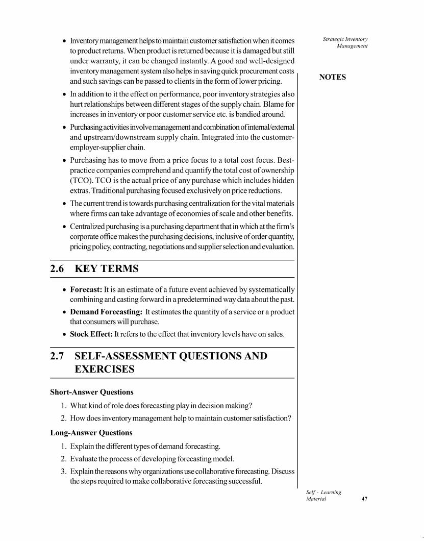
Strategic InventoryManagement
NOTES
Self - LearningMaterial 47
Inventory management helps to maintain customer satisfaction when it comesto product returns. When product is returned because it is damaged but stillunder warranty, it can be changed instantly. A good and well-designedinventory management system also helps in saving quick procurement costsand such savings can be passed to clients in the form of lower pricing.
In addition to it the effect on performance, poor inventory strategies alsohurt relationships between different stages of the supply chain. Blame forincreases in inventory or poor customer service etc. is bandied around.
Purchasing activities involve management and combination of internal/externaland upstream/downstream supply chain. Integrated into the customer-employer-supplier chain.
Purchasing has to move from a price focus to a total cost focus. Best-practice companies comprehend and quantify the total cost of ownership(TCO). TCO is the actual price of any purchase which includes hiddenextras. Traditional purchasing focused exclusively on price reductions.
The current trend is towards purchasing centralization for the vital materialswhere firms can take advantage of economies of scale and other benefits.
Centralized purchasing is a purchasing department that in which at the firm’scorporate office makes the purchasing decisions, inclusive of order quantity,pricing policy, contracting, negotiations and supplier selection and evaluation.
2.6 KEY TERMS
Forecast: It is an estimate of a future event achieved by systematicallycombining and casting forward in a predetermined way data about the past.
Demand Forecasting: It estimates the quantity of a service or a productthat consumers will purchase.
Stock Effect: It refers to the effect that inventory levels have on sales.
2.7 SELF-ASSESSMENT QUESTIONS ANDEXERCISES
Short-Answer Questions
1. What kind of role does forecasting play in decision making?
2. How does inventory management help to maintain customer satisfaction?
Long-Answer Questions
1. Explain the different types of demand forecasting.
2. Evaluate the process of developing forecasting model.
3. Explain the reasons why organizations use collaborative forecasting. Discussthe steps required to make collaborative forecasting successful.

Strategic InventoryManagement
NOTES
Self - Learning48 Material
2.8 FURTHER READING
Zipkin, Paul Herbert. 2000. Foundations of Inventory Management. New Delhi:McGraw Hill.
Orlicky, Joseph and George Plossl. 1994. Orlicky’s Material RequirementPlanning. New Delhi: McGraw-Hill.
Seetharama L Narsimhan, Dennis WMcLeavy, Peter J Billington. 1994.Production Planning and Inventory Control. New Delhi: Prentice Hallof India Pvt Ltd.
J. R. Tony Arnold, Stephen N. Chapman. 2007. Introduction to MaterialsManagement. New Delhi: Prentice Hall.
Richard J. Tersine.1982. Principles of Inventory and Materials Management.New Delhi: Prentice Hall.

Inventory ControlTechniques
NOTES
Self - LearningMaterial 49
UNIT 3 INVENTORY CONTROLTECHNIQUES
Structure
3.0 Introduction3.1 Objectives3.2 Inventory Classification and its use in Controlling Inventory3.3 Standardization and Variety Reduction
3.3.1 Standardization3.3.2 Variety Reduction
3.4 Setup time and inventory control3.5 Safety Stocks Determination Considering Service Level3.6 Strategies to Reduce Inventory Levels in Service and Manufacturing
Organizations3.6.1 Eliminate Waste and Reduce WIP3.6.2 Increase Inventory Turns3.6.3 Reduce Throughput Time
3.7 Answers to ‘Check Your Progress’3.8 Summary3.9 Key Terms
3.10 Self-Assessment Questions and Exercises3.11 Further Reading
3.0 INTRODUCTION
It is useful to visualize the inventory of a medium-sized business organization. Theinventory would comprise thousands of items, each item with different usage, price,lead-time and specifications. This makes planning and coordination extremelydifficult, if not impossible. There could be different procurement and technicalproblems associated with different items and many a time the firm has to deal withthe inability of the entire chain of suppliers to respond promptly.
As the number of departments and users increases, different types of issuesarise. For example, an electric company had as many as 118 names for a simplescrew with a width of 3/8 inches and length of 6 inches, depending upon the typeof usage and the department using the screw. This type of issue would finally resultin confusion and tend to duplicate ordering or result in overstocking.
In order to escape this quagmire, many selective inventory managementtechniques are based on a thorough analysis of the items that constitute the inventory.It is often prudent to classify inventory so as to improve response time and bringthe relevant issues within the capability of the supply chain partners.
The use of class systems makes the effort to manage inventory more effectiveand efficient than if the organization managed each individual item independently.In this unit, we will study some of the classifications that facilitate the process ofimproving the management of inventory.

Inventory ControlTechniques
NOTES
Self - Learning50 Material
In this unit, we will touch upon the concept of variety reduction andstandardization as they are closely related to inventory control, and in fact, itencourages standardization. Though standardization and variety reduction areoften considered as independent areas of study, in reality, variety reduction isa subset of standardization. Both these areas have intersections with inventorycontrol at a number of points. Variety reduction and standardization reduce theefforts required in controlling inventory and at the same time enhance reliability,flexibility and responsiveness of a firm at a lower inventory cost.
Standardization and variety reduction of materials result in the replacementof several materials/components by a single component with all the functionalitiesof the materials/components it replaces. These results in reduced purchasing costs,lower inventory control requirements, lower inventory levels, and inventory costs.Surveys show that materials standardization is a popular cost reduction strategy inmost firms. Similarly, standardization of procedures, i.e., pre-set procedures andreference materials, processes result in lower inventory levels, improved quality,and supplier delivery performance. It also makes it easier to exchange information,which makes the exercise of inventory control easier. Therefore, it is not surprisingthat professionals rank standardization and variety control very high in terms ofprojected future strategic decision-making.
We will also discuss the setup time, safety stock and the strategies that areused to reduce inventory levels in service and manufacturing organizations.
3.1 OBJECTIVES
After going through this unit, you will be able to:
Understand inventory classification and its usefulness
Discuss the reference of standardization and variety reduction
Describe the concept of setup time and inventory control
Explain safety stocks determination considering service level
Evaluate strategies to reduce inventory levels
3.2 INVENTORY CLASSIFICATION AND ITSUSE IN CONTROLLING INVENTORY
Recent industry reports show that inventory costs as a per cent of total logisticscosts are increasing. Despite this rise, many organizations have not taken fulladvantage of ways to lower inventory costs. Much of the cost in inventories is dueto:
Too much of wrong stuff
Not enough of right stuff
Unawareness of obsolete material
High shrinkage rate

Inventory ControlTechniques
NOTES
Self - LearningMaterial 51
Low turnover rate
Excessive expediting/staging
Ineffective scheduling
The control systems can also be classified depending on their characteristics. Basedon characteristics, there can be different types of systems. The most common arethe following:
Classification models
Periodic review (fixed-order period)
Two–bin system
Perpetual or continuous review (fixed-order quantity)
Modified control systems
MRP and DRP systems and
Fair share allocation
Classification Models
Material items can be classified based upon their commercial importance, demandpatterns (regular, sporadic, etc.) and supply reliability (of both raw material suppliersand own manufacturing), sources of supply, and modes of handing.
However, the most popular classification method used, especially in smalland medium firms, is ABC classification. This analysis is based on the historicalstock levels recorded for the different items. The components that are easiest tocontrol are characterized by high use and low inventories.
As the ABC classification method is generally used in most firms for inventorycontrol, it is based on usage and cost of the inventory item. The system of controlof this model is described below:
Controls For Class ‘A’ Items: All Class ‘A’ items require close control. However,where stock-out costs are high, special attention is required. Raw materials thatare used continuously, in extremely high volume, are often purchased at rates thatmatch usage rates. Contracts are often executed with vendors, with penalty clauses,for the continuous supply of these materials. Buffer stocks that provide excellentservice levels are justified for such items.
Where purchase of inventory items is not guided by either economicalquantities or cycles, the items need careful monitoring. It is possible to achievesignificant savings by changing the rate of flow periodically as demand and inventorypositions change. Minimum supplies should be ensured to guard against demandfluctuations and possible interruptions of supply.
For the balance of Class ‘A’ items, normally reports are generated on aweekly basis, to provide the necessary close surveillance over inventory levels.Close surveillance reduces the risk of a prolonged stock out. Depending upon theinventory system used, time-triggered or event-triggered orders are released.
Controls for Class ‘B’ Items: These items are generally monitored and controlledby a computer-based exception reporting system. Periodic review by the
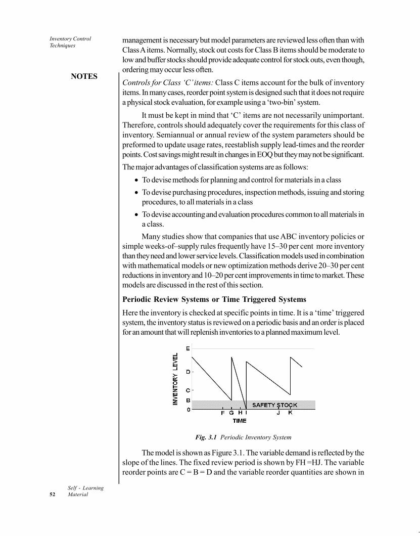
Inventory ControlTechniques
NOTES
Self - Learning52 Material
management is necessary but model parameters are reviewed less often than withClass A items. Normally, stock out costs for Class B items should be moderate tolow and buffer stocks should provide adequate control for stock outs, even though,ordering may occur less often.
Controls for Class ‘C’ items: Class C items account for the bulk of inventoryitems. In many cases, reorder point system is designed such that it does not requirea physical stock evaluation, for example using a ‘two-bin’ system.
It must be kept in mind that ‘C’ items are not necessarily unimportant.Therefore, controls should adequately cover the requirements for this class ofinventory. Semiannual or annual review of the system parameters should bepreformed to update usage rates, reestablish supply lead-times and the reorderpoints. Cost savings might result in changes in EOQ but they may not be significant.
The major advantages of classification systems are as follows:
To devise methods for planning and control for materials in a class
To devise purchasing procedures, inspection methods, issuing and storingprocedures, to all materials in a class
To devise accounting and evaluation procedures common to all materials ina class.
Many studies show that companies that use ABC inventory policies orsimple weeks-of–supply rules frequently have 15–30 per cent more inventorythan they need and lower service levels. Classification models used in combinationwith mathematical models or new optimization methods derive 20–30 per centreductions in inventory and 10–20 per cent improvements in time to market. Thesemodels are discussed in the rest of this section.
Periodic Review Systems or Time Triggered Systems
Here the inventory is checked at specific points in time. It is a ‘time’ triggeredsystem, the inventory status is reviewed on a periodic basis and an order is placedfor an amount that will replenish inventories to a planned maximum level.
Fig. 3.1 Periodic Inventory System
The model is shown as Figure 3.1. The variable demand is reflected by theslope of the lines. The fixed review period is shown by FH =HJ. The variablereorder points are C = B = D and the variable reorder quantities are shown in

Inventory ControlTechniques
NOTES
Self - LearningMaterial 53
Figure 3.1. You will see that E–C¹ E–B¹ E–D. Similarly, the lead-times are variableas FG¹ HI¹ JK. The reorder quantity is E, the inventory level at review period.
The reorder quantity, therefore, varies from one review period to the next.The economic reorder cycle would then be EOQ/R, where R is the annualrequirement: for example, if EOQ = 10,000 units and annual requirements areR=120,000 units, then the economic cycle would be 10,000/120,000 = 1/12 or 1month.
The safety stock is OB. Safety stock needs to buffer also against uncertaintyin demand over each period. The long planning interval with its associated demandvariation causes more safety stock to be held than in other systems.
Some other advantages of this system are:
Sometimes makes operating efficiencies possible by reviewing the status ofall items at the same time
Fewer orders are placed
Purchase discounts more likely
Lower shipping and freight costs
The periodic system had more appeal in pre-computer days because itdoes not require continuous inventory records. Inventory holding costs are usuallyhigher than those associated with the continuous review system.
Two-bin Policy
The two-bin policy can be seen as a variant of the reorder point reorder methodwhere no demand forecast is needed and the inventory level does not have to bemonitored continuously. This system makes stores clerks happy because no fancyrecord keeping is needed. They merely open the second bin and place an order. Itis usually adopted for inexpensive, fast-moving items. In classification models, thispolicy is often used for ‘C’ category items.
It works like this: the inventory is physically separated into two bins, one ofwhich contains an amount equal to the reorder inventory level. Stock is drawnfrom the first bin. For each item, action is triggered when inventories in the bin getsempty, the inventory has fallen to the reorder point Q, an order is placed for Qunits. Stock is now drawn from the second bin. And, the cycle is repeated.
Continuous Review Systems or Event Triggered Systems
These are generally fixed quantity systems. In these systems, we know the inventoryheld at all times. A perpetual review system controls inventory by reviewing thesystem daily to determine replenishment needs. It compares the sum of the inventoryon-hand and on-order to establish the reorder point.
This is the most robust policy and is optimal under the greatest number ofconditions. When inventory falls to B, an order is placed. The fixed reorder quantityis AC and the lead-time (DE = FG= HI) is also fixed. However, the time betweenorders is variable as you will see that DF < FH. The only uncertainty is the magnitudeof demand during the lead-time. The parameters that define a reorder quantitysystem are ‘Q’, the fixed amount ordered at one time and reorder point.

Inventory ControlTechniques
NOTES
Self - Learning54 Material
Fig. 3.2 Perpetual Inventory System
The model is shown as Figure 3.2. In this case also, the demand is variable whichis reflected in the slope of the lines. This is a complex system and its complexityincreases as the operations become larger. It requires accurate accountability andlarge computing power. Computer aided systems are normally used for properimplementation. Despite its complexity, the advantages of perpetual systems are:
Efficient, meaningful order size
Safety stock need for lead-time only
Relatively insensitive to forecast and parameter errors
Less attention on slow moving items
Some disadvantages arise out of this:
Clerks may set order quantities
Lot sizes, reorder points, and safety stocks must be revised
Delays in posting transactions
Errors and mistakes in transactions
High freight and transportation charges
Fewer chances for dollar value discounts
These systems require the inventory level to be under sufficiently closesurveillance so that notice can be given when the reorder point has been reached.
Material Requirement Planning (MRP)
Material requirement planning (MRP) is appropriate when inventory planning isprimarily required for items with dependent demand or for determining inventoryrequirements in a multiple plant/warehouse environment.
MRP methods use a common information base to coordinate inventoryrequirements across multiple locations or across different stages in the value-addedchain. Planning activities may occur at the plant to coordinate inventory allocationand delivery to multiple distribution centers or to coordinate inventory requirementsacross multiple channel partners, such as manufacturers and retailers.
There are a number of proven strategies that will provide payoff in theinventory area, both in customer service and in financial terms. Some of these

Inventory ControlTechniques
NOTES
Self - LearningMaterial 55
strategies involve having fewer inventories while others involve owning less of theinventory you have. MRP and information technology solutions have been able toprovide solutions, not only for inventory management but also for aggregateplanning, material requirement planning and operations scheduling.
MRP is a three-step process:
(i) identifying the requirements and setting the basic parameters
(ii) running the planning
(iii) implementing the MRP. If all the three are synchronized well, the MRP runwill give accurate results which can be implemented.
Distribution Requirements Planning (DRP): DRP is defined as distributionrequirements planning, which includes determining labour, equipment, andwarehouse space requirements.
DRP is usually used with an MRP system, although most DRP models aremore comprehensive than stand-alone MRP models and can scheduletransportation. The underlying rationale for DRP is to more accurately forecastdemand and then use that information to develop delivery schedules. This way,distribution firms can minimize inbound inventory by using MRP in conjunctionwith other schedules.
DRP may be used for both distribution and manufacturing. In manufacturing,DRP will work directly with MRP. There are some constraints to the use of DRPsystems.
First, DRP systems require accurate and coordinated forecasts for eachdistribution center. The forecast is necessary to direct the flow of goods throughthe distribution channel with forecasts for each distribution center and SKU aswell as adequate lead-time to allow product movement. Forecast error can be asignificant concern when forecasts are used to guide inventory-planning systems.
Second, DRP requires consistent and reliable performance cycles formovement between distribution facilities. Variable performance cycles areaccommodated through safety lead-times but performance-cycle uncertaintyreduces planning system effectiveness.
Fair Share Allocation: Fair share allocation is a simplified inventory managementplanning method that provides each distribution facility with an equitable or ‘fairshare’ of available inventory from a common source, such as a plant warehouse.
The first step is to establish business rules that prioritize locations or customersand define fair share logic. Using fair share allocation rules, the planner determinesthe amount of inventory that can be allocated to each distribution center from theavailable inventory at the plant warehouse.
The limitation of this system is that while it coordinates inventory levelsacross multiple sites, fair share allocation does not consider site-specific factors,such as differences in performance-cycle time, economic order quantity or safetystock requirements. Fair share allocation methods are, therefore, limited in theirability to manage multistage inventories.

Inventory ControlTechniques
NOTES
Self - Learning56 Material
Modified Control or Optional Replenishment Systems
Control systems sometimes combine regular review cycles and order points. Insuch systems, stock levels are reviewed on a periodic basis but orders are placedonly when inventories have fallen to a pre-determined reorder level. Such systemscombine the advantages of ‘event’ triggered and ‘time’ triggered review systems.These have the lowest total costs. Regardless of which technique or solution oneemploys, there are two important issues in inventory control: order quantity andorder timing.
Choice of System
The proper choice of control systems is extremely important. Proactive inventorymanagement practices make a measurable difference in operations and reduce ininventory costs. In addition, they significantly impact the burden due to:
Ever-increasing storage space needs
Slow-moving materials
Disposition of scrap, obsolete, and surplus materials
Transaction recording errors
Misplaced materials
However, in order to be effective, the inventory control system should providesatisfactory answers to three questions:
1. How often should the assessment of stock on hand be made?
2. When should a replenishment order be placed?
3. What should be the size of the replenishment order?
The answers to these questions should determine the system used to controlinventory.
The following facts describe the important differences that determine thechoice of the system that should be used.
1. Perpetual systems are expensive to operate and maintain but if economicallyjustified, provide the best control parameters.
2. Periodic systems require less manpower to control compared to perpetualsystems. In perpetual systems, each item must be counted as it is issued ordemanded. In periodic systems, physical inventory count is taken only atthe end of the period. This system is especially good for fast moving rawmaterials and supplies.
3. Periodic systems require less calculating time than perpetual systems. In theevent triggered system, each issue or demand from stock must be recordedand accounted for. Systemic costs, i.e. the costs of running the system aregenerally less with the time-triggered system.
4. Periodic systems may require more buffer stock to protect against uncertaindemand and lead-time. The reorder time is often non-optimal as it is fixedeither weekly or monthly and not based solely on economics, resulting inhigher physical inventory costs.

Inventory ControlTechniques
NOTES
Self - LearningMaterial 57
5. Periodic systems run the risk in more stock outs when unusually highfluctuation in demand occurs. When one or successive periods of unusuallylarge demand occur, perpetual systems can react more quickly because itkeeps track of net inventory with each unit demanded.
6. Materials Requirement Planning is based on several assumptions. Whenthose assumptions are incorrect, you can have more problems controllingthe system than even if you do manually. While MRP approaches to inventorymanagement offer significant benefits, there are some constraints to theireffectiveness, primarily based on the assumptions made in these models:
o Capacity is infinite: It assumes that we can produce anything as longas we have material at the right time. This is a major flaw. In amanufacturing set up, capacity is a constraint most of the times andcapacity is always finite. Having enough material at the right time is noguarantee that schedule can be met without any delay.
o Lead-times are constant: MRP systems are based on lead-timesschedules that are either forward scheduling or backward scheduling.The major assumption here is lead-times are constant. Are the lead-times really constant? How frequently are they reviewed to validatewhether the lead-times are still valid? How much of safety is loaded intothese lead-times? What are the basic assumptions with which they wereinitialized? Answers to some of these questions are necessary as lead-times have a cascading effect as the material gets converted from rawmaterial to finished products.
o Accurate stock status/on order status: MRP accuracy depends onaccuracy of stock status. Therefore, the assumption is the perpetualinventory status matches with the actual on hand quantity: for example,if the purchase orders’ due dates get modified over phone or fax and thesystem does not get updated. The problem gets compounded becauseof the pegging used in MRP calculations.
7. MRP starts with independent demand for the end products. If there isuncertainty, there should be a provision for incorporating that uncertaintyinto the planning.
8. The MRP response time is a measure of how quickly the shop floor canimplement changes and update the transactional data. It is not always easyfor the firm or the entire chain of suppliers to respond to MRPrecommendations promptly. Therefore, it is often prudent not to plan for allmaterials through MRP. Response time should dictate how frequently youshould run MRP and how many items should be included for planning run.Each change or response is also a cost to the company and needs to betaken into account.
Check Your Progress
1. What are the ways of classifying material?
2. State one advantage of the classification system.

Inventory ControlTechniques
NOTES
Self - Learning58 Material
3.3 STANDARDIZATION AND VARIETYREDUCTION
Technical standards in all their forms are means to codify technology for a society.The first technical standard that we know of was a reference standard—a commonnumber system. Using a number system, civilization defined units of weight andmeasure (unit standards) as early as 3500 BC. These standards were consideredso important that their definitions were kept secure with a primary authority suchas the king or a temple by 3000 BC.
These standards of weight and measure played a significant part in thedevelopment of early civilization. It created a reliable form of income for the rulersby providing the weights and measures that were used for taxation. In a sense, thisdevelopment assisted in the rise of the first great city states of Babylon and Egypt.
Table 3.1 shows the history of the evolution of standards. The next standardsto evolve were similarity and methodology standards. Both types of standardsdefine common properties. Similarity standards describe similar physicalrelationships and provide the definition of the minimal admissible attributes of adevice while methodology standards describe similar procedures.
Table 3.1 History of the Evolution of Standards
Historical Periods Agrarian Industrial Information Strata of Standards
Units and reference Similarity and methodology
Compatibility and Etiquette
New Technology Weights and measures
Powered machines Telephony Computers
New Com-munications
Trade routes Mechanized transport
Electronic Wireless
New Value System Land as property Patents for invention
Public utilities Branded IDs
A unit standard like, say, a gallon, may define the carrying capacity of a
container, and a similarity standard would define how similar in construction onecontainer is to the next. This concept offers significant economic advantage inmanufacturing as well as distribution, selling and using. Economists describe thisas increasing ‘externalities.’ Similarity standards emerged during the IndustrialRevolution and were used to codify the results of repetitive processes.
In the early nineteenth century, from the growing use of mechanized process,a new concept of interchangeability emerged. This turned out to be an extremelypowerful tool. Interchangeability of parts was originally conceived by Eli Whitneyfor the rapid assembly of guns. His use of standard parts enabled his firm to gaina competitive advantage in its bid for an army rifle contract.
By the mid-nineteenth century, machine tools and measuring devices hadprogressed sufficiently and it was possible to create a drawing (specification) andmachine parts to match. By using these specifications, multiple companies couldmanufacturer interchangeable parts.
In 1904, Baltimore’s business district was burnt to the ground. Washington,New York and Philadelphia all tried to come to Baltimore’s rescue. However,

Inventory ControlTechniques
NOTES
Self - LearningMaterial 59
when their pumping equipment arrived in Baltimore, the rescuers had to stand byhelplessly. There was no way to connect the different-sized hose couplings toBaltimore’s fire hydrants. Baltimore was lost for the lack of standard fire hosecouplings. Sadly, this was a lesson that was learnt too late, but it helped spread theconcept of standardization into other areas, such as railways; all train tracks ornuts and bolts were made interchangeable. The objective of standardization herewas variety reduction.
The result of this focus on variety reduction became the beginning of thesystems for standardization that are in use today. Engineering standards, forexample, specify properties of materials, fits and tolerances and drafting practices.Product standards provide details of the attributes of manufactured items that areembodied in formulas, descriptions, drawings or models. All these ultimately alsoresult in variety reduction. In other words, variety reduction is a subset ofstandardization.
Now even products that do not need any form of interchangeability havesimilarity requirements (public and private) for safety, usage, environment, shipping,etc. Examples include the standards for emergency exit signs, motor vehicle speedlimits, the definition and marking of specific plastics for recycling or thetransportation of hazardous goods.
The evolution of standardization continued with compatibility standards.Compatibility standards define a relationship between two or more dissimilar things.Compatibility of dissimilar parts or systems may seem to be related to theinterchangeability of similar parts and systems but it is distinct: for example, theplug and socket are not similar but they may be locally compatible. Similarly,remote compatibility standards are used to define the interface or protocol standardsbetween communications devices or systems.
In industry, the development and application of standards made it possibleto manufacture a large volume of interchangeable parts. Henry Ford’s assemblylines were made possible by improved manufacturing processes that allowedunskilled workers to quickly attach standard parts to standard cars.
The adoption of standards makes it easier for firms to communicate withtheir suppliers. Standards are also used within industries to prevent conflict andduplication of effort. Governmental departments, trade associations and technicalassociations help to set standards within industries; these are coordinated andpromoted by organizations, such as the American National Standards Institute(ANSI) and the International Organization for Standardization (ISO).
Etiquettes are a new form of standards made possible by the advances incommunication technology. They combine the concepts of variety reduction andcompatibility in a unique manner such that standards on basic communications canbe implemented and yet allow for proprietary communications technology.Examples of etiquettes used to negotiate with remote systems include theInternational Telecommunications Union (ITU) V.8 used by telephone modems.
Etiquettes simplify the process of maintaining compatibility between systems.Compatibility may be considered in three dimensions:

Inventory ControlTechniques
NOTES
Self - Learning60 Material
Over time: forward or backward (in time) compatibility
Across space: remote and multi-user compatibility
Through matter: conversion using a separate interworking system
Using etiquettes, separate systems can operate in different ways to findcompatible modes of operation. Etiquette standards create new ways to implement,control and add value to communication systems: for example, Ricoh a facsimilemachine manufacturer, offered proprietary higher speed G3 facsimile to itscorporate customers. Then, years later, higher speed operation similar to whatRicoh pioneered was included in the G3 facsimile standard. In this manner,companies can add value yet support compatible communications or interfaces.
Etiquette has many other diverse applications: for example, in marketing,market segmentation via etiquette can be applied to the sales channel, allowingindividual dealers and distributors to automatically poll their specific customers’equipment for usage billing which is a common practice in the copier market.Distribution networks and supply chains can also use etiquettes for problem analysisand maintenance support, automatic ordering of parts and components, etc.
Standards are emerging as a discipline of their own and have become anintrinsic and vital part of the fabric of society. They are reducing uncertainty andvariability inherent in most products and processes. It has the disadvantage ofdiscouraging innovation and could also mean a reduction in the focus on theindividual’s skills, competencies and behaviour.
Despite this limitation, standards are creating a great impact on society, asmechanisms for optimizing economic use of scarce resources. It makes it possiblefor the same task performed by different people to give the same result. It iscreating new technologies and value systems, new paradigms (etiquettes) andnew insights in product development, processes, and communication systems andin management.
It is reducing the differences in the ways people work, organize themselvesand perform their tasks. It helps seamless communication any where under thesun, ultimately leading to a world that is more integrated and globalized.
3.3.1 Standardization
The term standardization can have several meanings depending on its context.Commonly it is considered to be a universally agreed-upon set of guidelines forinteroperability. Standards make it possible to reduce variations in the same tasksperformed by different people; to acquire the best way of carrying out a processand document it in detail. Products, production or service processes and activitiesbecome a routine with well-defined boundaries.
A standard is defined as ‘a model or general agreement of rule establishedby authority, consensus or custom, created and used by various levels of interest’.
Today, many organizations with worldwide operations are interested instandardization of their processes and operations. There are many benefits of itand these benefits are mainly from its power to provide for the basis of similarityand consistency in operations, processes and procedures. Consistency increases

Inventory ControlTechniques
NOTES
Self - LearningMaterial 61
efficiency. It also makes process control easier and creates a positive perceptionof service or product quality.
Standards can be de facto or de jure. De facto is a Latin expression thatmeans ‘in practice’ but it is not spelt out by law. De jure is an expression thatmeans ‘based on law’, as contrasted with de facto. This means standards arefollowed for convenience or they are used because of legally binding contractsand documents.
There are different types of standards. Standards can be based on productdescriptions, methods of tests, codes of practice, etc. However, the best way toclassify standards, based on the most significant difference in the different types ofstandards, is:
1. Publicly available standards: They are, for example, a standard producedby a trade association that may be used by any organization.
2. Private standards: They are not public but are based on the specificrequirements of the organization that developed them.
Publicly Available Standards
When one talks of publicly available standards, the most important category isInternational Standards. These standards generally, deal with establishing agreementon uniform identifications for definite characteristics of quality, design, performance,quantity, service and so on.
The primary authority that produces such standards is the InternationalOrganization of Standards Organization (ISO). The ISO has as its members thenational standards bodies comprising countries all over the world. The standardsthat they develop are applied to products, processes or services. A well-known‘process’ standard is the ISO 9000 series which provides a framework for effectivemanagement of organizations.
In addition to the standards developed and maintained by the ISO, amongthe publicly available standards, are many worldwide standards developed by, forexample, the World Wide Web Consortium (W3C) which is the main internationalstandards organization for the World Wide Web; the International Electro-technicalCommission (IEC); the Universal Postal Union (UPU); Society of AutomotiveEngineers (SAU); Society of Mechanical Engineers (SME) and many others.
Regional standards bodies also have been developing standards on the samelines as ISO. One example is the standards known as European Standards. Theyare produced by CEN, the European Committee for Standardization whosemembers are the national standards bodies of European Union countries. ThoughEuropean Standards have been framed by CEN they have also been adopted asBritish Standards by the British government.
In addition, each country or economy has a single recognized NationalStandards Body (NSB). India has the Bureau of Indian Standards (BIS). Thebureau is involved in the development of technical standards (popularly known asIndian Standards), product quality and management system certifications andconsumer affairs. It brings together and coordinates with various interested groups

Inventory ControlTechniques
NOTES
Self - Learning62 Material
like manufacturers, consumers, technical experts, testing personnel and otherinterested parties to prepare standards known as Indian Standards (IS).
These standards are considered as legal documents in India and relate to a widerange of subjects including:
Product Specifications
Methods of Test
Codes of Practices
Guidelines
Terminologies
Glossaries
Basic Standards
So far, BIS has formulated over 17,000 standards in different areas. Oneinteresting standard is the Hallmarking of gold jewellery, launched on 11 April2000, intended to ensure that the consumer gets gold jewellery of the puritydeclared. The Government of India requested for this standard as India is thelargest consumer of gold and the purchaser of gold jewellery. Though this particularscheme is voluntary in nature, it is meant to protect the common consumer. Thecertification is equivalent to the International Standard (ISO 9202:1991-Jewellery–Fineness of Precious Metal Alloys) issued by ISO.
Formal standards, such as Indian, European or international standards, varyin the strength of their provisions: for example, they may specify requirements forthe features or characteristics of a product, or simply recommend the best way ofdoing something. To support these different standards, many evaluation bodieshave also come up; for example, Quality Council of India (QCI) has been set upas an Autonomous body by the Government of India to establish and operateNational Accreditation Structure for conformity assessment bodies.
Some of the bodies certified by QCI provide different services includingtesting, certification, inspection or calibration services for organizations wantingtheir product or service to comply with international, European or Indian Standards.This facilitates and provides support to the standardization process as bothbusinesses and government agencies often have to follow official standards whichare often a prerequisite for doing business in certain markets, with certain companies,or within certain consortia.
Specifications: The basis on which these evaluation bodies check the complianceof products and services is by ensuring that the products and services meet thespecifications laid out. What, then, are ‘specifications’?
Similarity standards, methodology standards, compatibility standards andetiquette standards need to be tested on a common platform. A specification is atype of a standard that tests these standards and provides a platform so that theycan be compared and related to objects. In other words, specification is a standardthat is applied to objects to see if they fit our needs. In essence, a specification isa function which has a clear responsibility to identify an object that satisfies it andto combine with other specifications in various ways that will support that basicresponsibility.

Inventory ControlTechniques
NOTES
Self - LearningMaterial 63
According to ASTM, ‘A specification is an explicit set of requirements tobe satisfied by a material, product, or service’.
In engineering, manufacturing and business, it is vital for suppliers, purchasersand users of materials, products or services to understand and agree upon allrequirements for the successful completion of the transaction. A specificationprovides the necessary details about the specific requirements. It communicateswhat is required in terms of different standards that are applicable. It also establishesthe different standards against which inspections, tests and quality checks are tobe made. It also establishes the intangible services that are to be provided, likewarranty, maintenance and support.
Imagine a shipping company that moves various kinds of goods around theworld. It has a cargo of meat that it wants to put in a container. Not all containerswould be suitable for such a cargo. To hold meat, a container must be refrigeratedand must be clean enough to safely store food. The specification calls for thecontainer to be able to store goods at less than -4°C and meet the sanitaryrequirements for storage of food. If the shipping company wants to move thecargo of meat safely to its destination, it needs to check the cargo’s storagespecification to ensure that the container meets the specifications.
Generally, specifications are public standards that may be written by governmentagencies, standards organizations (ISO, ASTM, IEC, UPU, etc.), tradeassociations, corporations, and others. They include a number of criteria thatencompass:
Descriptive title and scope of the specification
Date of last effective revision and revision designation
Person, office, or agency responsible for questions on the specification,updates, and deviations
The significance or importance of the specification and its intended use
Terminology and definitions to clarify the meanings of the specification
Test methods for measuring all specified characteristics
Material requirements: physical, mechanical, electrical, chemical, etc.;Targets and tolerances
Performance requirements; Targets and tolerances
Workmanship
Certifications required
Safety considerations and requirements
Environmental considerations and requirements
Quality requirements, sampling (statistics), inspections, acceptance criteria
Person, office, or agency responsible for enforcement of the specification
Completion and delivery
Provisions for rejection, re-inspection, rehearing, corrective measures

Inventory ControlTechniques
NOTES
Self - Learning64 Material
Specifications are important both in the procurement of raw materials anddefining the finished products. However, a specification does not necessarily provethe product to be correct. It is the people who use the item (engineers, tradeunions, etc.) or specify the specifications (building codes, government, industry,etc.) who have the responsibility to consider the available specifications to specifythe correct one. They need to validate the suitability of the specification. Evenwhen the specifications are right, it is essential to enforce compliance and use theitem correctly.
Private standards
Private standards enable companies to minimize uncertainty and variability in theirprocesses. By using standardization processes, organizations create for themselvesmany options to improve their competitiveness. Some of the types of privatestandards that are found in most manufacturing organizations and are commonlyused are given below:
Raw Materials Standardization: Most raw materials, such as bar stock, steeland other metal tubes, sheet metal, moldings/castings, hardware and evenprogrammable chips, etc. can be standardized. The standards used by firms areoften different from the national standards, and may be based on internationalstandards, company specific standards or standards adopted from some othernation.
The idea behind such standards for raw materials is to make processesflexible enough to make different products without any setup to change materials,fixturing mechanisms or cutting tools: for example, Tata Motors used DIN standardsfor some of their critical sheet metal products. The use of this standard was basedon the process and tooling that was being used to form the chassis for the Tatatruck.
Process Standardization: Producing goods and services on a consistent basis iscrucial for businesses in today’s competitive environment. Consistent quality meansrepeated and more customers. This can be achieved through standardization ofprocesses.
Most statistical controls on quality are based on standardization ofprocesses. Process controls must be in place for an effective Quality managementsystem, such as Total Quality Management. Such a system facilitates theorganization to keep actual production within the desired tolerances.
Concurrent engineering of products and processes ensure that processesare actually specified by the design team. They can cause significant harm if theyare left to chance or ‘to be determined later’. However, the process capability ofmaterials and products needs to be compatible with the specified engineeringtolerances.
Processes must be coordinated such that all parts and products can be builtwith minimum setup changes and eliminate unnecessary movement of materials;for example, such as practised in flexible manufacturing.

Inventory ControlTechniques
NOTES
Self - LearningMaterial 65
Process standardization is often a complex process. Process documentationfor each firm is generally unique because of the conglomeration of different processesand activities. It becomes more difficult as the level of detail increases. Nevertheless,each firm has to create this documentation for competitive advantage.
Product/Component Standardization: A large number of buying firms preparetheir own specifications suited to their specific products. By preparing their ownspecifications, they do not have to pay premium prices of brand name items. Theycan often create specifications that avoid the use of patented, copyrighted andproprietary products. By doing so, they broaden the field of competition as itallows all manufacturers capable of meeting the firm’s specifications as potentialsuppliers.
Describing requirements entails some risk. It means the company assumescomplete responsibility for the performance of the item. It also means specialinspection procedures which may add to the cost. A firm’s own specifications,however, will save time and money when the design calls for items that are closeto industry standards. Special dimensions, tolerances or features should be designedas additions or alterations to standard parts.
Tool Standardization: Tooling costs for most mechanical industries can beextremely large. Standardization determines how many different tools are requiredfor assembly, alignment, calibration, testing, repair and service. Most suchorganizations have company-wide tool standardization programmes. Theseprogrammes work with people in manufacturing/service to determine toolpreferences, analyse tools used for existing products, prioritize usage histories todetermine ‘standard tooling’. They then issue common tool lists with commonparts lists which are used to bring down costs.
Feature Standardization: ‘Features’ are any geometry that requires a separatetool like a drill, ream, grind, lap, hole punch, bend radii and cutting tool bit formachine tools. These tools as well as the processes need to be standardized.Hard questions need to be asked before finalizing standardization: for example,‘Why do you need to lap the part?’ or ‘Can grinding provide the end resultrequired?’
Standardization is carried out using the same procedures as toolstandardization.
The standardization options we have described above embrace at leastfour levels of standardization: compatibility, interchangeability, commonality andreference.
In supply chain management, standardization refers to approaches for increasingthe commonality of the part, the process, or the product. Standardization helpspart suppliers rationalize their product lines and allows them to:
Reduce their overhead costs and subsidies, which allows them to be morecost competitive
Improve their operational flexibility, resulting in better delivery
Simplify their supply chain management

Inventory ControlTechniques
NOTES
Self - Learning66 Material
Private standards are used by many firms especially to deal with such thingsas operating practices, procedures and systems, e.g., standardization of purchasingprocedures or job standardization. Like standardization of materials, thestandardization of procedures, e.g. purchasing, can also be a potential point ofcost savings for companies; and standardization of jobs has been found to bepositively related to the perception of efficiency, productivity and service quality.
Developing a Standardization Programme
A standardization programme can be approached in various ways but because somany departments and suppliers are affected by standards decisions, the benefitsof standardization cannot be fully realized without involving cross-functional teamswith internal members from different departments, e.g. supply management,marketing, quality and engineering. In addition to internal members, the exercisebecomes more beneficial if relevant suppliers are also included in the team.
Inputs are obtained from all user departments and relevant suppliers andthe standards team typically is charged with the responsibility of reconcilingdifferences between them and making the final standards decisions.
However, it must be kept in mind that specification writing is a professionaltrade with its own professional designations such as ‘CCS’ which means ‘CertifiedConstruction Specifier’. It is always advantageous to have such an expert on theteam. Such an approach helps in the standardization programme.
Advantages of Standardization
There are many benefits of standardization. All the advantages accrue from thefact that standardization enables organizations to minimize uncertainty and variability.It provides for consistency. Consistency increases efficiency. It also enables easierprocess control.
Arising from these basic characteristics, standardization of products andmanufacturing inputs, help a firm in many ways. Some of the advantages are givenbelow:
Reduced Inventory Items: Standardization implies reducing unnecessaryvarieties and determining the most economical sizes, grades, shapes, colours,types of parts, etc.
Lower Product Costs: Economies of scale occur when product designcosts are spread over a large volume. Very often, a standard component ina product provides the same functionality without paying for new engineeringwork and customization.
Lower Purchasing Costs: Purchasing costs are reduced through purchasingleverage. There is also a reduction in inventory cost and savings in storagespace requirements.
Lower Overheads: Standardized products often justify investments in moreefficient production processes. Higher-volume production systems result inoverhead cost reduction. It also allows a process to use less skilledemployees, though this often reflects in reduced flexibility.

Inventory ControlTechniques
NOTES
Self - LearningMaterial 67
Lower Inventory Costs: It forms a basis for inventory analysis and resultsin reduction of inventory through identification of surplus and non-productiveitems and slow-moving items. It also provides the basis for classification ofitems, thereby helping inventory control.
Quicker Product Design: Standardized product interfaces often reduceproduct design periods as have been demonstrated in personal computerdesigns. Manufacturers have benefited by industry standards that define theprotocol that must exist between each module.
Enhanced Product Flexibility Capabilities: Standardized features thatuse standard interfaces permit designers to enhance their offerings withoutrisking incompatibility as long as they stay within the specified parameters.It eliminates a large number of setups, simplifies internal logistics and resultsin inventory reduction.
Quality: Standardization has a positive impact on product quality. Itencourages the concept of continuous improvement and permits reductionin the number of vendors.
Delivery: Standard products may create economies of scale intransportation. Inventories of standard products can also be placed at sitesnear customers to facilitate a rapid response to any order, often providing acompetitive advantage with time-conscious customers.
Responsiveness: Standard end products enable manufacturers to use‘Make- to-stock’ market orientations, thereby decoupling manufacturingdecisions from market transactions. Dell Computers has taken advantageof standardization to redesign its supply chain and operate on a Build-to-order basis with remarkable results.
It also makes it easier for the organization to use the pull system for itssupply chain. It can work on quicker deliveries from vendors. There is amarked improvement in parts availability.
Simplified Value Comparisons: Standardized goods help consumers toshop for the best price or product performance. It helps in evolving bettermeans of communication about the product. People can easily compare thecost of a 60-watt Philips bulb with a Laxman & Sylvania bulb. It alsoprovides consumer protection as the performance standards are oftenregulated.
Standardization does not only provide advantages to business but is sopowerful a concept, as the advantages mentioned show, that it finds use in allwalks of life. Examples include formalization of judicial procedure in court andestablishing uniform criteria for diagnosing disease, etc. Standardization providesa framework for the effective management of organizations whatever be the functionsit may carry out.
3.3.2 Variety Reduction
Variety reduction is a form of standardization. Therefore, precisely separating thetwo terms is as difficult as separating research from development and mechanization

Inventory ControlTechniques
NOTES
Self - Learning68 Material
from automation. Both have evolved from the concept of similarity and areconcerned with the elimination of unnecessary diversity in any sphere of companyoperations.
Standardization is most commonly used in the sense of reducing a series ofitems all serving the same purpose to one item or a very few items; e.g., all inter-office memoranda to be written on A4 paper. Variety reduction is widely interpretedas a reduction in a range of items all serving the same or similar purposes byremoving the least profitable and those with least user appeal. There is a wideoverlap between this technique and standardization.
The difference between the two techniques is brought about when oneconsiders the way in which they are applied. Variety reduction, though it can beemployed on any aspect of company operations, is in practice usually restrictedto three areas: the product range, the raw materials list and stocks of engineeringspares.
In practice, standardization is increasingly identified with public domain,while variety reduction still remains within the internal domain of organizations.This led to some new techniques that have become popular today. Some of theseare discussed in the rest of this sub section.
Use of Standard Parts: Designing the product using standard parts is one methodof variety reduction. This is often adopted by many manufacturing organizations.
Fig. 3.3 Standard and Custom-built Components
As you can see from Figure 3.3, standard components require little or no toolingand processing. However, in such products it is essential to ensure and take extracare so that:
The product functions so as to perform as intended.
Reliability is ensured so that the product will perform consistently.
The product is maintainable so that maintenance is economical.
The product is safe so that it will perform with minimal hazard to the userand the environment.
The production process is simple so that the product can be produced atthe intended costs and volumes.

Inventory ControlTechniques
NOTES
Self - LearningMaterial 69
Modular Designs: Another way to reduce variety in customized products is touse modular designs. In the fashion world, this is called mix-and-match clothing.In manufacturing, assemble to order systems allow the customer to specify a needand then either the customer or the vendor selects pre-engineered sub-assembliesto meet a customer’s need. The product then is either assembled or shipped as akit to the customer. This is the system that Dell uses. A wider variety of end productoptions is possible but within certain limits.
The single-platform product architecture used by Maruti Udyog Ltd. (MUL)for launching the Maruti 800, Omni and Gypsy in 1984–85 was based on a modulardesign concept. Basic modules were integrated to create three different productswith a high degree of commonality of parts. Writing on the product architecture,the General Manager of MUL in his note referred to earlier wrote:
It is possible for us to find a product which can, with necessary engineeringinputs, with a high degree of parts commonality, cater to the demands of thethree demand segments identified earlier. This vehicle, I am defining as a UniversalVehicle…e logic of this type of conversion of a sedan to the Universal Vehicle isthe use of mass production technology in the manufacture of aggregates, so asto minimize the cost of built-up products….
If the objectives for 1987–98, are laid down to capture 50 per cent of the car, jeepand light commercial vehicle market and defense requirements, the domesticsales will be of the order of 70,500 units, including spare parts requirements.With a focus on this type of volume, the project becomes economically viable.
The key to successful product development is to know what features orparts of the end product need to be customized to meet the expectations of thetarget customers.
Simplification: Another process that is commonly used by organizations is thesimplification process. Some authorities consider simplification as an integral partof standardization. Simplification is an outcome of standardization.
Simplification involves reduction in the number of standard items in use by afirm in its product design and what it carries in its inventory. The latter is exemplifiedby an electrical company which had 56 different names for a standard M3 bolt, 3inches in diameter and 6 inches in length. The same bolt was used for severaldifferent applications and it was classified differently depending upon the departmentand the application. This resulted in excessive inventories and shortages of thesame item.
By simplifying the nomenclature, the company was able to save moneyprimarily from reduced inventory investment, more competitive prices, greaterquantity discounts and reduced ordering and handling costs. These savings accruedbecause fewer different items had to be handled and controlled and the quantitiesbecame much larger. In addition, there was much lower stock but fewer shortagesfor the item.
There are a number of principles on which simplification is based. Theseprinciples are shown in Table 3.2.

Inventory ControlTechniques
NOTES
Self - Learning70 Material
Table 3.2 Principles of Simplification
Reduction Reduction means to reduce an application to its essentials. This principle is applicable to all aspects of application design: Reduce the functionality (goals) Reduce the structural and navigational complexity Reduce the interface (screen) complexity
Integration The principle of integration stresses the importance of integrating simple, elementary tasks into a coherent framework.
Prioritizing Prioritizing means that applications should focus on the essential tasks and not try to serve a multitude of, possibly diverse, goals. This includes optimization with respect to the important aspects of a task.
In essence, making variety reduction techniques simple or simpler should
finally result in a solution that reduces the complexity or extent of the part, reducesthe fundamental parts or makes it easier to process the part. This can be achievedthrough reduction, integration and prioritization.
Check Your Progress
3. Define a standard.
4. What do you mean by simplification?
3.4 SETUP TIME AND INVENTORY CONTROL
In just-in-time systems, there is an attempt to decrease setup times as a part ofinventory control. Since setup activities add no marketable form, fit, or function tothe product, they are by definition non-value adding. This decreases the cost perorder, encourages more and smaller orders, and thus decreases the EOQ. It alsolessens or eliminates inventory for ‘changeover’ time.
The JIT (just-in-time) tool involved in decreasing setup times is called SMED(single-minute exchange of dies). By reducing setup time toward SMED, moresetups can be completed each day. In the SMED process, some operations thatare done during setup are completed prior to setup, and other functions are ofteneliminated entirely. And some functions are simply streamlined. Decreases in setuptime of 50 per cent or better are common in JIT systems compared to conventionalsystems.
Setup time reduction impact adds to inventory control techniques in that itadds to the ability of the firm to meet deadlines, adjust to uncontrollable demandand increases the throughput in the organization.
Another way to look at a JIT is as manufacturing system that is focused toenhance product quality and productivity by eliminating waste, often from alloperations. This is done by adopting a practice of manufacturing in small lots.Small lot sizes contribute to higher productivity in a firm through lower levels ofinventory and scrap, high product quality, lower inspection costs, increased flexibilityand earlier detection of defects. This issue is applicable both to the internal processesof the organization as well as the supply chain.

Inventory ControlTechniques
NOTES
Self - LearningMaterial 71
The idea of JIT is to create a ‘pull’ system in the production processes. Thishas to be justified in terms of the setup cost, as it involves frequent setups. In orderto reduce setup time, we have to examine if we can simplify the process from thepoint of view of setting up and changing over. There are two types of setup timespossible.
The internal setup time is the time scheduled for setting up the process ormachine when it is not running production.
The external setup time is the setup time that occurs during the functioningof a process or machine.
In JIT, the goal is to decrease the needed setup time resulting in machinedowntime. The premise is that in processes, during production by machinery,complete utilization of the operation does not occur neither is it fully occupied.Consequently, it is possible for the operator to carry out certain setup tasks whenthe process or machine is functioning, with respect to the process and the machinery.
Setup time is also directly associated with production lot sizes. The reductionin setup times results in a reduction of lot sizes. To ensure that production is notdisrupted problems must be identified and sorted out and the quality must beextremely high. Reduction in lot sizes leads to a decrease in the total time taken tomanufacture lead-time in a geometric manner, specifically during the involvementof more than one operation in the process.
Because of what has been said earlier and for other reasons, manufacturers seemany benefits when setup reduction is implemented. Some of the benefits are asfollow:
Short span of lead times
Reduction of wastage of material
Less faults
Less inventory
More need for less space
More productivity
Greater flexibility
Increased capacity
Reducing batch sizes also forces problems out into the open. Quality problemsare often the first to surface. Several factors are responsible for errors within anorganization. Nevertheless, it is possible to prevent nearly all of these errors, in caseindividuals endeavour to find out the time of occurrence of problems, determine rootcauses, and subsequently take appropriate corrective actions. In the case of traditionalmanufacturing, the lots are large so a few defective units cause fewer problemsbecause they may be placed aside and the next unit used. This is not true when thelot size is small. A defective unit will cause disruption in the production process. Thisdiscovery is actually advantageous and allows problems to be solved.
Setting marks, or poka-yokes mechanisms, determine the starting point forsettings. A poka-yoke is an error-proofing device. It is used as the key to SetupTime Reduction projects. The technique lies in revisiting the setup functions from

Inventory ControlTechniques
NOTES
Self - Learning72 Material
time-to-time in order to review the results from the earlier project, also to decreasethe setup time repeatedly. This is done by analysing the setup process, break itdown into identifiable elements, and differentiate between elements of the setupthat are internal and external. Then you will find ways to decrease setup times inthe operation. It is possible to complete certain functions before setup which areperformed when the setup is happening. Other functions can be completelyremoved, while certain functions only require streamlining them. Reduction in setuptime of 50 per cent or more are general.
MACHINESMATERIALS
WAREHOUSE
DIE SHELF
Fig. 3.4 Layout of Plastic Assembly Factory
For example, the layout of a ten-machine department producing plasticassemblies is shown in Figure 3.4. The machines are located close to one another,the material or dies are stored at the other end of the hall. One operator runs onemachine. Three large equally sized lots are presently produced by an individualoperator/machine per day at the rate of five units per minute. The operator has tocarry out one setup at the beginning of the shift and two other setups for thedifferent lots during the remainder of the shift. The initial setup time was 100 minutesand these activities are carried out when the machine is not running.
The department sets up a project with the objective to reduce the setuptime. As all of the activity times were internal to the setup, the methodology usedwas to eliminate or reduce all internal setup activities. Though it is not possible forcertain activities such as ‘Remove Die’ to be carried out during the machine’srunning status, it is possible for several activities to be carried out during themachine’s running status either before or after the setup takes place.
The improvement team documented the project. Some of the observationsof the team are given below and form an excellent illustration of the poka-yokemechanism:
The ‘clean around machine’ activity can take place while the machine isrunning before the setup.
Paperwork for the previous lot could be delayed until after the machine hasbeen restarted on the next production lot.
The dies were stored on a shelf in the opposite corner of the department,by relocating the shelf to a more central location; the distance traveled couldbe reduced and also the time required for the activity.
Also, the trips to return the die from the previous lot and the trip to obtainthe die for the next lot could be split up. Procuring the die for the subsequentproduction lot will be carried out before the setup, and returning the diefrom the previous production lot will be done past production.

Inventory ControlTechniques
NOTES
Self - LearningMaterial 73
Obtaining the die for the next lot and preheating it, could be carried outduring the machines running condition before the setup, so the machine will not bestopped while this takes place.
By restructuring and redesigning the process and the workplace, the SetupTime Reduction Project, was able to show dramatic results. The internal setuptime was reduced from 100 minutes to 23 minutes. As the setup took place threetimes per machine per shift, the total daily savings in machine run time was 6930minutes per day. Based on the existing production rate, the department could nowruns 34,650 additional units per production day.
Table 3.3 Operations of the Plastic Assembly Factory
Operation Before Setup Operation After SetupChanges Time Changes Time
1. Stop Machine * 1. Clean Area Around 5 mins.Machine
2. Clean Area Around 5 mins. 2. Find and Obtain Tools 1 mins.Machine
3. Fill Out Paperwork For 4 mins. 3. Obtain Die for Next 2 mins.Previous Lot Lot from Shelf
4. Return Material From 10 mins. 4. Pre Heat Die for 22 mins.Previous Lot Next lot
5. Find And Obtain Tools 3 mins. 5. Obtain Die for Next 3 mins.Lot from Staging
6. Remove Die For Previous 7 mins. 6. Stop Machine *Lot From Machine
7. Clean Inside Die 2 mins. 7. Remove Die from 6 mins.Machine for next lot
8. Return Die/Obtain Die 8 mins. 8. Clean Inside Die 2 mins.For Next Lot
9. Pre-Heat Die For Next 22 mins 9. Install Die into MachineLot for Next Lot 8 mins.
10. Install Die For Next 9 mins. 10. Make adjustments 1 mins.Lot Into Machine
11. Make Adjustments 2 mins. 11. Feed material for 3 mins.next Lot
12. Locate & Obtain 16 mins. 12. Make ten test 2 mins.Material For Next Lot Widgets
13. Feed Material For 3 mins. 13. Check Dimensions for 1 mins.Next Lot ten time widgets
14. Make Thirty Test 6 mins. 14. Start machine *Widgets
15. Check Dimensions 3 mins. 15. Stage unused material 3 mins.On Thirty Test Widgets from Previous Lot
16. Start Machine * 16. Return die from 2 mins.Lot to shelf previous
17. Fill out paper work 4 mins.for Previous Lot
Total External Time For Setup 0 mins. Total External Time For Setup42 mins.
Total Internal Time For Setup 100 mins. Total Internal Time For Setup23 mins.

Inventory ControlTechniques
NOTES
Self - Learning74 Material
The company stopped operations on Saturdays and saved the overtimeassociated with the operators, the supervisor, and the support departments. Thecompany was also able to ship the last orders of the week on Friday midnightinstead of Monday morning. Average inventories were reduced and customerswere more satisfied with earlier shipments.
3.5 SAFETY STOCKS DETERMINATIONCONSIDERING SERVICE LEVEL
The newspaper seller’s dilemma provides an insight into the concept of servicelevel and safety stocks. Although we use marginal analysis to provide an estimateof the stock-out risk, in practice it is often difficult to determine the cost of stock-outs (or marginal loss). This may also include intangibles, such as the loss of customergoodwill or the cost of potential delays to other part of the system.
In some cases, the customers may be willing to wait if the response time isreasonable. The purpose of safety stock is to cover the random variations in demandor lead-time. Though the safety stock concept is not intended to cover all thevariations during that period, the amount of variation covered by the safety stockdepends on the desired stock-out risk or the customer service level.
When not all costs are available or the penalty for a stock-out is not available,a common alternative is to specify the customer service level. It refers to theprobability that the firm can meet the demand of a customer. In competitiveenvironments, under normal circumstances, firms often choose to keep stock-outs as small as possible to lower the probability of losing customers to competitors.
It is not the same in the case of perishables or dated items, such asnewspapers. Here the firm may lower its customer’s service level because theremay not be any demand for the newspapers at the end of the day. Even in suchcases, it is important for a firm to specify the service levels so that an appropriatelevel of safety stock is maintained to retain customers. These calculations alsoform a starting point to determine the amount of investment required to carrythose safety stocks determined by the service level.
As the firm gains experience and is able to collect more data, it may decide tochange safety stock levels to match the demand patterns of individual items. Basedon these arguments, service level can be classified in two different ways:
Order Service level
Unit Service level
Order Service Level (OSL): Order service level (OSL) is information onthe proportion of cycles that the customer demand was satisfied. Though it doesnot tell us exactly how many units were short or not filled during any cycle, it is anindicator of the number of stock-outs during a specified period. The order stock-out risk (OSOR) specifies the quantity of units unfilled or short during that period.Therefore,
OSL = 1 – OSOR

Inventory ControlTechniques
NOTES
Self - LearningMaterial 75
In the newspaper seller’s problem, we know that order has to be placed 52times during the year. The order service level represents the probability of havinga stock-out during the placement of an order. In the case of the newspaper problemthere are 52 cycles or orders during the year. Suppose that OSL = 0.95 and n ofthe cycles per year = 52. Then customer demand will be satisfied during 49 cycleson an average, whereas during 3 cycles on an average we can expect a stock-out.
The order stock-out risk in many production situations can create seriousproblems. This is especially true if shortages occur during an operation, where thesucceeding operation cannot be performed without completing the previousoperation. In such a case, regardless of the quantity of items available, the remainingoperations come to a halt. Therefore, the order service level or the order stock-out risk is a very appropriate measure in a manufacturing environment.
Unit Service Level (USL) and Unit Stock-out Risk (USOR): Unit service level(USL) indicates the percentage of units of demand filled in any period of time andthe unit stock-out risk (USOR) specifies the quantity of units unfilled or shortduring that period. Therefore, similar to the OSL relationship:
USL = 1 – USOR … (3.1)
As the unit service level and unit stock-out risk provides data on the exactquantities of units of customer demand filled or unfilled during each cycle or duringany time period, it is a measure that is commonly used in many consumer goodsapplications.
Suppose the annual demand in the case of the newspaper problem is 5200units, as on an average we sell 100 papers with a standard deviation of 10 papersand the USL is 0.90. Then, we can expect 5200 * 0.90 or 4680 units of demandwill be filled during the year. We can also expect 520 newspapers of stock-outduring the year. Or, we can expect we will not be able to supply newspapers to 10customers in each order cycle.
Service level is often measured by stock availability, but could also bemeasured by order cycle time or consistency of cycle time. For example, wecould have a customer service objective of 99 per cent stock availability. There isan exponential relationship between the inventory and service levels. By increasingstock levels, we generally provide higher service levels to our customers. But, atsome point, large increases in inventory yield relatively small gains in customerservice.
Unit Service Safety Stock
The unit service safety stock is the per cent unit service level that answers thequestion of what percentage of units demanded can be supplied from stock. Thisis sometimes also called the fill rate. It is the mirror reflection of the stock-outrate and specifies the percentage of units demanded that cannot be supplied fromstock and consequently it can become either lost sales or backorders.

Inventory ControlTechniques
NOTES
Self - Learning76 Material
Number of Days
?
200
Inve
ntor
y
0
–25
R
X = 200L
{
Fig. 3.5 EOQ with USL
Figure 3.5 shows the problem. The ‘y-axis shows the inventory and the x-axis shows the time elapsed. We need to find out that with a per cent order servicelevel of 0.90 and a lead-time MAD of 20 units, what would be the per cent unitservice level?
This can be answered by calculating the stock-out rate first and convertingthe stock-out per cent to the per cent unit service level. Tables are available thatgive us the expected number of stock-outs (gk) on the unit normal distribution.For demand less than the reorder point, the stock-out quantity is zero; for demandlevels more than the reorder point, the stock-out quantity is demand minus thereorder point.
In the problem, we have been discussing, L = 1.25 MADL = 1.25 * 20 = 25.The reorder point was calculated using 1.28 standard deviations to provide a 90per cent order service level. From the tables g(1.28) is given as 0.047. The formulato arrive at USOR is given below:
USOR = σL * g(k) / Q … (3.2)
And the Unit Service Level can be expressed as:
USL = 1 – σL * g(k) / Q … (3.3)
Hence, USOR = σL * g(1.28) / Q
Or g(1.28) = Q * USOR / σLOr 0.047 = 900 * USOR / 25 — from tables
Or USOR = 0.047 * 25 / 900 = 0.001
And USL = 1.0 – 0.001 = 0.999
Therefore, the associated service level (USL) is 99.9 per cent.
Backorders or Lost Sale Costs
As most inventory managers will do, ours has specified a 99 per cent service levelwithout explicitly considering stock-out costs. Because we already have holdingcost estimates, we can now derive the implicit or imputed stock-out costs thatthe inventory manager used intuitively. Our analysis will distinguish between the

Inventory ControlTechniques
NOTES
Self - LearningMaterial 77
backorder and the lost sales case. The analysis is important in its own right, becauseit will allow us to specify safety stocks when we are provided with stock-out costestimates but no desired service levels.
At this point, it is worth noting that increasing the safety stock level by onemore unit has the same effect as adding one more unit to the reorder point. Therefore,adding one unit to R is analogous to increasing SS by one additional unit.
Also when backorders are involved, raising the reorder point by one unitwill also cost because we will hold the unit for almost the entire cycle regardless ofwhether or not it is used to satisfy demand. If we do not add the unit to the reorderpoint, we suffer a backorder penalty per unit which includes expediting costs,extra paperwork, ill-will, etc. with a probability SOR. Balancing these marginalcosts gives:
Per cycle marginal cost of adding 1 unit to R = per cycle marginal cost ofnot adding 1 unit to R.
H(Q/D = OSOR (p)
OSOR = HQ/pD
Or p = HQ/OSOR * D
We must determine ë, the imputed backorder cost, given the unit servicelevel.
ServiceLevel
OrderQuantity (Q)
ECQ
Set by Management
EPQ
Per Cycle
Per Units Demanded
Per Unit
Per Outage
Per Unit
Per Outage
ReorderPoint (B)
KnownStockout
Cost
Lost Sale
Backorder
FOSS
Fig. 3.6 Framework for Multi-period Inventory Models
The normative framework for all these types of problems is shown in Figure3.6 which is self explanatory and summarizes the problems explained above.
Check Your Progress
5. List any two benefits of setup reduction.
6. Name the two ways in which service level is classified.

Inventory ControlTechniques
NOTES
Self - Learning78 Material
3.6 STRATEGIES TO REDUCE INVENTORYLEVELS IN SERVICE ANDMANUFACTURING ORGANIZATIONS
There are numerous models to determine optimal inventory holding. The standardresults of these models provide a framework for identifying the determinants ofinventory levels in practice. Some apply to specific types of inventory - raw materials,work-in-process (WIP), or finished goods. However, as the requirements forthese three types of inventory are often interrelated, making this distinction indetermining optimal inventory holding is generally not necessary.
It should be kept in mind that overall performance of the inventorymanagement system depends upon the cooperative efforts of the memberorganizations in the supply chain. It is important to determine if all the supply chainmember organizations are truly committed to improving the performance of thesupply chain. Cooperation is a critical factor in determining supply chain performanceand a cooperative philosophy is the key to the success of inventory managementinitiative.
Optimum levels of inventory generally depend upon the cycle time, or by reducingcycle times it is possible to reduce the requirements to hold inventories. The greaterthe time between the receipt of an order and supplying it to the customer, the largeris the quantum of inventory that is held at different parts of the organization and atdifferent stages of processing. Therefore, a major thrust in good inventory managementstrategy is generally centered around cycle time reduction. Likewise, there are othersstrategies that are used to reduce the inventory levels in service and manufacturingorganizations. They are:
(a) Reduce WIP
(b) Eliminate waste
(c) Increase Inventory turns
(d) Reduce throughput time
We will now understand how the four strategies are used to reduce inventorylevels.
Finished goods consist of productive and non-productive inventories. Elementsthat are related to the cycle time have been shown to have a significant contributionto the non-productive inventory in Figure 3.7. These include:
Orders in temporary storage
Orders waiting to be worked
Orders under inspection
Orders in transit, etc.
As is apparent, these also contribute to the levels of inventory and are non-productive assets that impact both the profitability and cash flow of the firm.

Inventory ControlTechniques
NOTES
Self - LearningMaterial 79
Inputs
Unreleased Orders Backlog
In-ProcessInventory
Nonproductive
Productive
Outputs
Finished Goods
Orders Being Worked
Orders Being Inspected
Orders Waiting to be Worked
Orders in Transit
Orders in Temporary Storage
Fig. 3.7 Factors Contributing to Increased Finished Goods Inventory
Therefore, an essential aspect of reducing non-productive finished goodsinventory is reduction of throughput time; more efficient physical flow of parts,from the point of supply, through the factory and shipment through distributionchannels. All these lead to decreased turn around time and reduction in the costs.
3.6.1 Eliminate Waste and Reduce WIP
Another category of non-productive inventory includes excess and surplus stock.Surplus stock comprises the items with no demand in the foreseeable future, andexcess stock contains those items whose current supply exceeds current demand.Surplus and remaining stock of unsold goods is a problem that is often unavoidable.In an increasingly fast-paced world of products and technology, many companiesare stuck with unsold products and service items. This is often an important inventorymanagement problem, especially in a project context and in the context of sparepart items.
The starting point for reducing finished goods inventory is the segmentationinto productive and non-productive categories. The priority in reducing stock mustfirst be focused on reducing unproductive stock. The first area that needs to beexamined is the inventory which should not be carried (surplus and excess). Notonly does this immediately improve cash flow but it also achieves inventory reductionwith a minimum impact on customer service levels.
3.6.2 Increase Inventory Turns
Inventory turnover analysis is often used to identify surplus and excess inventory.A relatively low turnover indicates the stock is idle or essentially dormant. Wholesaleand retail organizations might use ‘gross profit margin times the inventory turnoverfor a given time period’ to locate slow-moving or ‘dead’ items. Once surplus andexcess inventory items are identified, disposal action of waste can proceed.
Though there are opportunities to dispose of some of the stock, the marginalsalvage value of such stock is often based on the total weight and mass instead ofthe specific obtainable value for each product. The number of advertisements inthe media reflects the seriousness of the issue relating to excess and surplus stock.

Inventory ControlTechniques
NOTES
Self - Learning80 Material
The next step is to examine how cycle time can be reduced to minimizenon-productive inventory. Cycle time has important implications for both thefinancial and the economic performance of a business organization. As mentionedearlier, the correlation of procurement lead-time and the frequency of raw materialsdelivery and manufacturing lead-times with the inventory level of manufacturingplants finally determine the inventory levels of finished goods. If cycle times arehigh, companies pay for this either in inventory carrying costs or by losing capacityto changeovers.
Stock may be held in different forms depending on either the product or theindustry. The traditional balance is one between raw material and finished productstocks. Appropriate levels can vary with changing conditions and strategies, sothey must be monitored and controlled by manage-ment. Unexpected shortagesand excesses indicate a failure of the inventory control mechanisms or planningmechanisms that maintain or establish stock levels.
The solution lies in either building finished goods inventory in order to shipon-time (JIT approach), or reduce lot sizes and do more changeovers. Reducinglot sizes has often been found to be the best solution to lower holding costs as itcan provide for higher inventory rotation, but without triggering substantial stock-outs and backorders, caused by demand peaks and/or lead-time delays.
An example of using inventory turns, i.e. lower cycle times successfully toreduce finished goods inventory levels has been demonstrated by the motor vehiclemanufacturing industry in Canada. Its inventory turns ratio is 299.36, i.e.manufacturers keep in an average a little more than a day’s worth of finishedgoods. The scope for improvement in cycle time can be gauged from thecomparative figure for India, which is 22.5 turns.
In general, supply chain inventories have been declining significantly in allparts of the world. This is also true for finished goods inventory. The US Departmentof Commerce data on inventory sales ratio in the US, shown in Figure 3.8 is anindicator. There has been a steady decline in the ratio between 1991 and 2000.
Year
Per
cent
Source: U.S. Department of Commerce
1991 1992 1993 1994 1995 1996 1997 1998 1999 2000
1.60
1.55
1.50
1.45
1.40
1.35
1.30
1.25
Fig. 3.8 Inventory Sales Ratio

Inventory ControlTechniques
NOTES
Self - LearningMaterial 81
Though the inventory profiles for raw materials and finished goods are similar,finished goods have additional dimensions that complicate the situation and constrainthe ability of the company in reducing these inventories. This is because the goodshave to travel from the manufacturer to the customer. The route the finished goodstake depends on the type of organization. The way the company organizes thisfunction reflects the level of control it has on these channels and also determinesthe ability of the firm to cope with the levels of finished goods inventory.
As already explained, manufacturing organizations deal with all the threeinventory types (raw materials, WIP and finished goods), while pure wholesaleand retail organizations deal predominantly with finished goods. Vertically integratedorganizations perform more than one function; they may manufacture, distributeand retail their products to the ultimate consumer. Other organizations distributeand retail while others only retail.
3.6.3 Reduce Throughput Time
Throughput time reduction minimizes the time required to take a product or servicefrom concept to delivery. It is applicable on the factory floor and in non-manufacturing areas as well. Customer lead-time refers to the time span betweencustomer ordering and customer receipt. Manufacturing lead-time refers to thetime span from material availability at the first processing operation to completionat the last operation.
In many manufacturing plants, less than 10 per cent of the total manufacturinglead- time is spent actually manufacturing the product. And less than 5 per cent oftotal customer lead-time is spent in the production process. The cumulative cycletimes of the processes in the value stream are the theoretical limit to how much wecan reduce lead-times, without investing in different equipment.
Clearly, there is ample opportunity to reduce lead-times in most organizations.Reducing lead-times doesn’t involve speeding up equipment to cut the cycle timesor getting plant personnel to work faster. What it does involve is the rapid fulfilmentof customer orders and the rapid transformation of raw materials into qualityproducts in the shortest amount of time possible.
Table 3.4 Lead-time Data of Plastics Assembly Factory
Activity Total Days %
Processing 3 7.5
In- transit 5 1.3
Setup/ changeover 5 1.3
In queue 30 75.0
On hold waiting for materials 4 10.0
On- hold quality 2 5.0
Total 40 100.1
The lead-time analysis for the product line at a plastics plant is shown inTable 3.4. As can be seen, the actual production accounts for only 7.5 per cent ofthe total manufacturing lead-time. As in most plants, the largest contributor tolead-time is queue time—the time product is sitting idle waiting to be processed atthe next operation.
Inventory ControlTechniques
NOTES
Self - Learning82 Material
This non-productive lead-time results in tying up cash without adding value andcauses unnecessary customer waiting. The approach to this problem is:
Measure current lead-times and set improvement targets
Change the organization from a functional orientation to a product orientation
Cross-train plant personnel within cells in a number of operations for greaterflexibility
Empower work cells and teams to take ownership for the entire value stream
Continually reduce batch sizes between work centres
Institute local scheduling between work cells
By employing these principles, many world-class manufacturers have shrunklead- time by 50–80 per cent, gained market share, improved profitability andincreased employee morale.
One of the most common applications of lead-time reduction is new productdevelopment. Companies can gain strategic advantages over the competition.Companies that practice JIT with shorter lead-times can bring a concept to thehands of the consumer while the competition was still developing it.
For example, partnerships, concurrent engineering and outsourcing of newproduct development processes have allowed most automobile companies toshorten their lead-times for new models to eighteen months or less, whereas earliera sixty- month development lead-time was not uncommon for most automobilecompanies.
As the examples in this section have shown, when implemented correctly,JIT can lead to dramatic improvements in a manufacturing organization’s return oninvestment, quality and efficiency.
Check Your Progress
7. List four strategies that are used to reduce inventory.
8. What does customer lead-time refer to?
3.7 ANSWERS TO ‘CHECK YOUR PROGRESS’
1. Material items can be classified based upon their commercial importance,demand patterns (regular, sporadic, etc.) and supply reliability (of both rawmaterial suppliers and own manufacturing), sources of supply, modes ofhanding.
2. One of the major advantage of classification systems is:
To devise methods for planning and control for materials in a class
3. A standard is defined as ‘a model or general agreement of rule establishedby authority, consensus or custom, created and used by various levels ofinterest.’

Inventory ControlTechniques
NOTES
Self - LearningMaterial 83
4. Simplification involves reduction in the number of standard items in use by afirm in its product design and what it carries in its inventory.
5. Two benefits of setup reduction are:
Short span of lead times
Reduction of wastage of material
6. Service level can be classified in two different ways:
Order Service level
Unit Service level
7. The four strategies that are used to reduce inventory levels are:
Reduce WIP
Eliminate waste
Increase Inventory turns
Reduce throughput time
8. Customer lead-time refers to the time span between customer ordering andcustomer receipt.
3.8 SUMMARY
Material items can be classified based upon their commercial importance,demand patterns (regular, sporadic, etc.) and supply reliability (of both rawmaterial suppliers and own manufacturing), sources of supply, modes ofhanding, etc.
The components that are easiest to control are characterized by high useand low inventories.
As the ABC classification method is generally used in most firms for inventorycontrol, it is based on usage and cost of the inventory item.
Controls For Class ‘A’ Items: All Class ‘A’ items require close control.However, where stock-out costs are high, special attention is required.Raw materials that are used continuously, in extremely high volume, areoften purchased at rates that match usage rates. Contracts are often executedwith vendors, with penalty clauses, for the continuous supply of thesematerials. Buffer stocks that provide excellent service levels are justified forsuch items.
Controls for Class ‘B’ Items: These items are generally monitored andcontrolled by a computer-based exception reporting system. Periodic reviewby the management is necessary but model parameters are reviewed lessoften than with Class A items. Normally, stock out costs for Class B itemsshould be moderate to low and buffer stocks should provide adequate controlfor stock outs, even though, ordering may occur less often.
Controls for Class ‘C’ items: Class C items account for the bulk of inventoryitems. In many cases, reorder point system is designed such that it does notrequire a physical stock evaluation, for example using a ‘two-bin’ system.

Inventory ControlTechniques
NOTES
Self - Learning84 Material
The major advantages of classification systems are as follows:
o To devise methods for planning and control for materials in a class
o To devise purchasing procedures, inspection methods, issuing and storingprocedures, to all materials in a class
o To devise accounting and evaluation procedures common to all materialsin a class.
Periodic Review Systems or Time Triggered Systems: Here the inventory ischecked at specific points in time. It is a ‘time’ triggered system, the inventorystatus is reviewed on a periodic basis and an order is placed for an amountthat will replenish inventories to a planned maximum level.
Some advantages of periodic review system are:
o Sometimes makes operating efficiencies possible by reviewing the statusof all items at the same time
o Fewer orders are placed
o Purchase discounts more likely
o Lower shipping and freight costs
The two-bin policy can be seen as a variant of the reorder point reordermethod where no demand forecast is needed and the inventory level doesnot have to be monitored continuously.
Continuous Review Systems or Event Triggered Systems: These are generallyfixed quantity systems. In these systems, we know the inventory held at alltimes. A perpetual review system controls inventory by reviewing the systemdaily to determine replenishment needs. It compares the sum of the inventoryon-hand and on-order to establish the reorder point.
Despite its complexity, the advantages of perpetual systems are:
o Efficient, meaningful order size
o Safety stock need for lead-time only
o Relatively insensitive to forecast and parameter errors
o Less attention on slow moving items
Some disadvantages arise out of perpetual systems:
o Clerks may set order quantities
o Lot sizes, reorder points, and safety stocks must be revised
o Delays in posting transactions
o Errors and mistakes in transactions
o High freight and transportation charges
o Fewer chances for dollar value discounts
Material Requirement Planning is appropriate when inventory planning isprimarily required for items with dependent demand or for determininginventory requirements in a multiple plant/warehouse environment.
Inventory ControlTechniques
NOTES
Self - LearningMaterial 85
MRP is a three-step process:(i) identifying the requirements and setting the basic parameters(ii) running the planning(iii) implementing the MRP. If all the three are synchronized well, the MRP
run will give accurate results which can be implemented.
Distribution Requirements Planning (DRP): DRP is defined as DistributionRequirements Planning, which includes determining labour, equipment, andwarehouse space requirements. DRP is usually used with an MRP system,although most DRP models are more comprehensive than stand-alone MRPmodels and can schedule transportation. The underlying rationale for DRPis to more accurately forecast demand and then use that information todevelop delivery schedules. This way, distribution firms can minimize inboundinventory by using MRP in conjunction with other schedules.
Control systems sometimes combine regular review cycles and order points.In such systems, stock levels are reviewed on a periodic basis but ordersare placed only when inventories have fallen to a pre-determined reorderlevel. Such systems combine the advantages of ‘event’ triggered and ‘time’triggered review systems. These have the lowest total costs. Regardless ofwhich technique or solution one employs, there are two important issues ininventory control: order quantity and order timing.
The proper choice of control systems is extremely important. Proactiveinventory management practices make a measurable difference in operationsand reduce in inventory costs. In addition, they significantly impact the burdendue to:
o Ever-increasing storage space needs
o Slow-moving materials
o Disposition of scrap, obsolete, and surplus materials
o Transaction recording errors
o Misplaced materials
In order to be effective, the inventory control system should providesatisfactory answers to three questions:
1. How often should the assessment of stock on hand be made?2. When should a replenishment order be placed?3. What should be the size of the replenishment order?
The answers to these questions should determine the system used to controlinventory.
Standardization and variety reduction of materials result in the replacementof several materials/components by a single component with all thefunctionalities of the materials/components it replaces. These results inreduced purchasing costs, lower inventory control requirements, lowerinventory levels, and inventory costs.

Inventory ControlTechniques
NOTES
Self - Learning86 Material
Surveys show that materials standardization is a popular cost reductionstrategy in most firms. Similarly, standardization of procedures, i.e., pre-setprocedures and reference materials, processes, etc. result in lower inventorylevels, improved quality, and supplier delivery performance. It also makesit easier to exchange information, which makes the exercise of inventorycontrol easier.
The term standardization can have several meanings depending on its context.Commonly it is considered to be a universally agreed-upon set of guidelinesfor interoperability. Standards make it possible to reduce variations in thesame tasks performed by different people; to acquire the best way of carryingout a process and document it in detail. Products, production or serviceprocesses and activities become a routine with well-defined boundaries.
A standard is defined as ‘a model or general agreement of rule establishedby authority, consensus or custom, created and used by various levels ofinterest.’
Variety reduction is a form of standardization. Therefore, precisely separatingthe two terms is as difficult as separating research from development andmechanization from automation. Both have evolved from the concept ofsimilarity and are concerned with the elimination of unnecessary diversity inany sphere of company operations.
In Just-in-Time systems, there is an attempt to decrease setup times as apart of inventory control. Since setup activities add no marketable form, fit,or function to the product, they are by definition non-value adding.
Service level can be classified in two different ways:
o Order Service level
o Unit Service level
Order Service Level (OSL): Order service level (OSL) is information onthe proportion of cycles that the customer demand was satisfied. Though itdoes not tell us exactly how many units were short or not filled during anycycle, it is an indicator of the number of stock-outs during a specified period.
Unit Service Level (USL) and Unit Stock-out Risk (USOR): Unit servicelevel (USL) indicates the percentage of units of demand filled in any periodof time and the unit stock-out risk (USOR) specifies the quantity of unitsunfilled or short during that period.
The unit service safety stock is the per cent unit service level that answersthe question of what percentage of units demanded can be supplied fromstock. This is sometimes also called the fill rate. It is the mirror reflection ofthe stock-out rate and specifies the percentage of units demanded thatcannot be supplied from stock and consequently it can become either lostsales or backorders.
As most inventory managers will do, ours has specified a 99 per cent servicelevel without explicitly considering stock-out costs. Because we alreadyhave holding cost estimates, we can now derive the implicit or imputedstock-out costs that the inventory manager used intuitively.

Inventory ControlTechniques
NOTES
Self - LearningMaterial 87
There are numerous models to determine optimal inventory holding. Thestandard results of these models provide a framework for identifying thedeterminants of inventory levels in practice. Some apply to specific types ofinventory - raw materials, work-in-process (WIP), or finished goods.
Strategies that are used to reduce the inventory levels in service andmanufacturing organizations. They are:
(a) Reduce w-i-p(b) Eliminate waste(c) Increase inventory turns(d) Reduce throughput time
3.9 KEY TERMS
ABC Classification: This analysis is based on the historical stock levelsrecorded for the different items.
Two-bin Policy: The two-bin policy can be seen as a variant of the reorderpoint reorder method where no demand forecast is needed and the inventorylevel does not have to be monitored continuously.
Distribution Requirements Planning (DRP): Distribution requirementsplanning includes determining labour, equipment, and warehouse spacerequirements.
Standard: This is defined as ‘a model or general agreement of rule establishedby authority, consensus or custom, created and used by various levels ofinterest.’
3.10 SELF-ASSESSMENT QUESTIONS ANDEXERCISES
Short-Answer Questions
1. What are the questions that inventory control system should answer in orderto be effective?
2. What is the basis on which compliance of products and services arechecked?
3. List the different strata of standardization that have evolved over time.
4. What are international standards?
5. List the different benefits of standardization.
6. Define the term variety reduction.
Long-Answer Questions
1. Describe the various inventory classification models.
2. Explain the difference between variety reduction and standardization.
3. Describe the tool used for setup time reduction.
4. Explain the strategies used to reduce inventory levels.

Inventory ControlTechniques
NOTES
Self - Learning88 Material
3.11 FURTHER READING
Zipkin, Paul Herbert. 2000. Foundations of Inventory Management. New Delhi:McGraw Hill.
Orlicky, Joseph and George Plossl. 1994. Orlicky’s Material RequirementPlanning. New Delhi: McGraw-Hill.
Seetharama L Narsimhan, Dennis WMcLeavy, Peter J Billington. 1994.Production Planning and Inventory Control. New Delhi: Prentice Hallof India Pvt Ltd.
J. R. Tony Arnold, Stephen N. Chapman. 2007. Introduction to MaterialsManagement. New Delhi: Prentice Hall.
Richard J. Tersine.1982. Principles of Inventory and Materials Management.New Delhi: Prentice Hall.

Inventory Models
NOTES
Self - LearningMaterial 89
UNIT 4 INVENTORY MODELS
Structure
4.0 Introduction4.1 Objectives4.2 Elementary Inventory Models and Stock Levels
4.2.1 Fixed Order Versus Fixed Interval Systems4.3 Fixed-Order Quantity Model (Classic Model)
4.3.1 Economic Order Quantity4.3.2 Sensitivity Analysis
4.4 Advanced Deterministic EOQ Models4.4.1 Developing Special Quantity Discount Models or Price-break Model4.4.2 Backordering Inventory Model4.4.3 Reorder Point Model with Variable Demand4.4.4 Model with Specified Service Levels and Safety Stock
4.5 EPQ and Fixed-Time Period Models4.5.1 Economic Production Quantity Model4.5.2 Fixed-Time Period Systems4.5.3 Fixed-Time Period Model with Safety Stock
4.6 Single-Period Inventory Problem-Probabilistic Inventory Models4.7 Inventory Models with Uncertainty4.8 Answers to ‘Check Your Progress’4.9 Summary
4.10 Key Terms4.11 Self-Assessment Questions and Exercises4.12 Further Reading
4.0 INTRODUCTION
Inventory is a major source of cost in the supply chain and also the basis forimproving customer service and enhancing customer satisfaction, for example,high inventory at retail outlets may help in making the goods easily available tocustomers and also result in a growth in sales, but it will also increase costs andbring down profitability. These two major issues in conflict with each other need tobe resolved in order to optimize the inventory carried by an organization.
Excess inventory is a cost burden to an organization in terms of capital tiedup, the cost of obsolescence and the cost of servicing products in the supplychain. However, having the right amount of inventory to meet customerrequirements is critical. Inventory management is about two things: not running outand not having too much.
Essentially, inventory is a reserve system to prevent stock-outs. However,as important as it is to prevent such a stock-out, you also do not want to hold onto too much inventory because holding costs can become a major encumbrance.So, how do you balance the two and what is the right amount? More importantly,when should you reorder to prevent a stock-out? The answer to this can bedetermined by obtaining and using appropriate inventory models in decision-making.Such inventory models assume that demands are constant and known. An accuratedemand forecast can result in optimized operations.

Inventory Models
NOTES
Self - Learning90 Material
However, there is another face to this problem. In reality demand is nevercertain. It occurs with some probability. We know that inventory decisions arehigh-risk and high-impact operations. Inventory exists in the supply chain becauseof a mismatch between supply and demand. Therefore, there are inventory modelsthat take risk or probability into account.
In many of these cases, the development of a mathematical model and thesubsequent determination of an ‘optimal order quantity’ are employed, usuallymaking specific assumptions regarding demand distribution, cost functions andperformance measure. Even though under these circumstances EOQ modelsbecome more complex, yet they find application. This is because of the simplecharacteristics of forecasting systems and inventory trade-offs.
In this unit, we will discuss some simple inventory models for arriving atbasic inventory decision rules.
4.1 OBJECTIVES
After going through this unit, you will be able to:
Explain elementary inventory models and stock levels
Discuss the fixed -order quality model and advanced deterministic EOQ model
Interpret EPQ and fixed time period models
Understand non-instantaneous replenishment models
Describe the inventory models under risk and uncertainty
Discuss probabilistic inventory models
Explain safety stocks and how they relate to the level of service
4.2 ELEMENTARY INVENTORY MODELS ANDSTOCK LEVELS
What is the need for inventory models? The answer lies in the nature of inventoryitself. As you can see in Figure 4.1, inventory consists of raw materials which formthe inputs. These are converted by a firm, and the processes generate in-processgoods and finished goods. In the process, the firm makes a large investment ininventory.
Inputs
Outpus
TotalInventory
Level
Raw MaterialsSupplies
In-Process Goods
Finished Goods
Fig. 4.1 Movement of Inventory in a Firm

Inventory Models
NOTES
Self - LearningMaterial 91
World-class production facilities are characterized by their relentless effortsto increase productivity and quality while reducing costs. Towards this end, inventorymodels have the major objective of minimizing the total inventory cost and tobalance the economics of large orders or large production runs against the cost ofholding inventory and the cost of going short.
Inventory management is concerned with matching supply with demand.The central problem is to find the amount to be produced or purchased in order tomaximize the total expected profit, or minimize the total expected cost. The questionof how much to order is determined by inventory models.
Inventory models analyse fluctuations in stock; starting from basicassumptions, they obtain bounds between which the stock varies. In order to dothis, inventory models start with the inventory cycle. The inventory cycle beginswith the receipt of an order. Consider an inventory process involving one item,with the initial stock equal to Q, a positive real number. During regular time intervalsthe stock decreases because of demand. Units are withdrawn and when theinventory is depleted more material is ordered from the supplier. The suppliertakes some time to deliver the order. This time is represented by ‘T’, thereplenishment lead-time. This completes an inventory cycle.
At the beginning of the performance cycle, stock is at the maximum level,‘Q’. At the end of the cycle, the stock reaches zero and order is received by thefirm again. The average inventory is ‘Q/2’. This completes the performance cycle.The cycle is reflected in Figure 4.2 below.
Time T T
Inve
nto
ry L
eve
l
‘Q
’
Average Inventory (Q/2)
Q
Fig. 4.2 Typical Inventory Cycle
Inventory management attempts to provide the framework necessary toreduce the cycle time of the inventory cycle. A shorter cycle time brings down theaverage inventory as well as the lead-time for replenishment. Inventory modelsare optimization models that attempt to reduce cycle times and at the same timeensure that an item will be available on an ongoing basis throughout the year.
A successful example of use of inventory models in bringing down both theaverage inventory and cycle time was demonstrated by the Mahindra Group. Thecompany faced tough competition after the introduction of economic reforms inthe country in the 1990s. Managing its inventory was necessary for the companyto sustain its margin. The company decided to streamline its business processesby introducing scientific inventory practices to reduce the cost of inventory. In a

Inventory Models
NOTES
Self - Learning92 Material
period of three years, the company was able to reduce its inventory level by morethan 50 per cent and bring down the replenishment lead-time to 19 days comparedto 52 days prior to implementation of the start of the program. By using inventorycontrol techniques, the company was able to improve their margins and profitability.
How do inventory models optimize the costs associated with investing ininventory and minimize the costs over the performance cycle? How do you basethe inventory policy and at the same time achieve the service level desired? Inventorymodels try to provide answers.
4.2.1 Fixed Order Versus Fixed Interval Systems
There are two general types of systems and these can be distinguished on thebasis of the ordering criteria. The models of these two systems are;
(a) Fixed-order Quantity Models (also called the Economic Order Quantitymodels).
(b) Fixed-time Period Models (also referred to as the Periodic System or P-models).
The basic difference between the two systems is that the fixed-order quantitymodels are ‘event triggered’ and fixed-time period models are ‘time triggered’. Inother words, at an identified level of the stock, the fixed-order quantity modelinitiates an order. This event may take place at any time, depending on the demandfor the items considered. In contrast, the fixed-time period models review thestocks at time intervals that are fixed and orders are placed at the end of pre-determined time periods. In these models, only the passage of time triggers action.
Table 4.1 makes a comparison of the two systems and brings out thesignificant differences.
Table 4.1 Differences between Fixed-order Quantity andFixed-time Period Models
Feature Fixed-order quantity model Fixed-time period model
Order quantity The same amount ordered each time Quantity varies each time order is placed
When to place order?
Reorder point when inventory position dips to a pre-determined level
Reorder when the review period arrives
Record keeping Each time a withdrawal or addition is made
Counted only at review period
Size of inventory Less than fixed-time period model Larger than fixed-order quantity model
Time to maintain Higher due to perpetual record keeping
Type of items Higher-priced, critical or important items
The models that emanate from this system are for perpetual systems that requirecontinual monitoring of inventory. Every time a withdrawal from inventory or anaddition to inventory is made, records must be updated. Generally, fixed-orderquantity models are favoured when:
Items are more expensive because the average inventory is lower.
Items are critical, e.g. repair parts, because there is closer monitoring andtherefore, quicker response to potential stock-out.

Inventory Models
NOTES
Self - LearningMaterial 93
These models are similar to batch processing systems; counting takes placeonly at the review period. The fixed-time period models require a larger averageinventory because they must also protect against stock-out during the review period;while the fixed-order quantity mode has no review period.
These differences and the nature of operations tend to influence the choiceof the inventory system that is more appropriate.
Check Your Progress
1. What do inventory models analyse?
2. Name the two types of inventory models.
4.3 FIXED-ORDER QUANTITY MODEL(CLASSIC MODEL)
In this section we will consider the fixed-order quantity models, i.e. inventorymodels in which demand is assumed to be fixed and completely pre-determined.The heart of inventory analysis resides in the identification of relevant costs. Thebasic approach to determining fixed-order sizes are the Economic Order Quantity(EOQ) models. The basic EOQ model is concerned primarily with the cost ofordering and the cost of holding inventory.
Stock Available
Demand Occurs(units withdrawn)
Determine Stock Position(on hand + on order – backorders)
Is Stock Position Reorder Point?<
yes
Issue Replenishment Order
no
stock receipt
Fig. 4.3 Fixed-order Quantity System
The principle on which the fixed-order quantity system operates is shown inFigure 4.3. The model examines the stock position to determine when to orderinventory. It does this by determining the economic quantity to be ordered basedon a number of decision parameters which include demand, the cost of orderingand the cost of holding inventory. This, in turn, determines the reorder point. Whenthe stock reaches the reorder point, a replenishment order is issued to bring thestock within pre-determined limits.
However, in order to obtain the economic order quantity or determine the optimumreorder point, a number of assumptions are made in all such models. The basicassumptions in simple EOQ fixed-order quantity models are as follows:
(i) The rate of demand for the item is deterministic and is a constant ‘D’ unitsper annum independent of time.
(ii) Production rate is infinite, i.e. production is instantaneous.

Inventory Models
NOTES
Self - Learning94 Material
(iii) Shortages are not allowed.
(iv) Lead-time is zero or constant and it is independent of both demand as wellas the quantity ordered.
(v) The entire quantity is delivered as a single package (or produced in a singlerun).
The Classical EOQ model is a simple mathematical model. The formula, forarriving at the economic quantity, uses a number of notations. These notationsmay be different in different texts. The notations that we have used in this text are,therefore, given below:
Q – Lot sizeS – Set-up cost or Ordering ( /year)D – Annual DemandP – Unit Price ( /unit)H – Holding or Carrying cost per Unit ( /Unit)F – Inventory Carrying Charges Factor
Q* – Economic Order quantity (to be determined)
a b c d e f
INVENTORY
Q
B
TIME
Fig. 4.4 Classical EOQ Model
The classical EOQ model is shown in Figure 4.4. The y-axis plots the quantityand the x-axis plots time. Here Q is the order quantity, B is the reorder point andab = cd = ef which reflect the lead-times. The relationships, shown in terms of the‘inventory level’ vs. ‘time’, reflect the model depicted in Figure 4.4.
The objective of the model is to minimize the average annual variable costs,and it provides a solution to the problem of determining when an order should beplaced and how much should be ordered. The EOQ model does this by attemptingto minimize total annual costs by varying the order quantity or lot size.
COST
TC(Q)
TVC (Q)HQ/2
DS/Q
Q*
ORDER QUANTITY (Q)
Fig. 4.5 Annual Inventory Cost

Inventory Models
NOTES
Self - LearningMaterial 95
The relationships between holding costs, ordering costs and the total inventorycost are shown in Figure 4.5. From Figure 4.5 it is obvious that based on ourassumption that the inventory is consumed at uniform rate and since the maximuminventory level is Q, the average inventory will be half the maximum inventory, i.e.Q/2.
Cycle inventory is the average stock held by the firm. Hence, the averageinventory holding cost will be the cost incurred in holding the average inventory.This can be written as:
Holding Cost = HQ/2 = FPQ/2
The ordering cost will decrease as order size increases. This follows as fora given annual demand, the larger the order size, the fewer the orders needed.Ordering cost will, therefore, depend on the demand, order size and orderingcost. It is commonly assumed that ordering costs are relatively independent of thesize of the order. This can be represented by:
Ordering Cost = DS/Q.
The total annual costs have a fixed and a variable component. The purchasecost of the inventory is fixed and the costs associated with ordering and holdingthe inventory are variable. The total cost is a summation of the variable and fixedcosts. We will, in this text, generally calculate total costs using the variable costs.When calculated in this way, it is called ‘TVC’ or the total variable cost.
The relationship between total cost (TC) and TVC is as follows:
TVC(Q) = TC(Q) + PD … (4.1)
This does not change any of the results because if the price P and annualdemand D were included, the only effect it would have is to raise the total costcurve. This is shown in Figure 4.5.
TVC when Q units are ordered each time is the sum of the holding andordering costs:
TVC(Q) = DS/Q + HQ/2 …(4.2)
Solved Example 4.1
Novelty Ltd. carries a wide assortment of items for its customers. One item,Gaylook, is very popular. Desirous of keeping its inventory under control, a decisionis taken to order only the optimal economic quantity, for this item, each time. Youhave the following information. Make your recommendations:
Annual demand : 1,60,000 units
Price per unit : 20
Carrying cost : 1 per unit or 5 per cent per rupee of inventoryvalue
Cost per order : 50

Inventory Models
NOTES
Self - Learning96 Material
Determine the optimal economic quantity by developing the following table:
Size of order 1 10 20 40 80 100
No. of orders
Average inventory
Carrying costs
Order costs
Total costs
Answer
Let us look at the problem using a tabular approach. We know the requirement,carrying cost and ordering cost. These have been appropriated in the table below.
Appropriation of Requirement and Costs:
Order per year Lot size Average inventory
Carrying cost (Re 1)
Ordering cost (Rs 50 per
order)
Total cost per year
1 1,60,000 80,000 80,000 50 80,000
10 16,000 8000 8000 500 8500
40 8000 4000 4000 1000 5000
80 4000 2000 2000 2000 4000
100 2000 2000 1000 4000 5000
1600 800 800 5000 5800
The optimum quantity (lot size) for this item is 4000 units.
4.3.1 Economic Order Quantity
The optimum quantity (lot size) that we have calculated in the problem aboveusing a tabular approach is called the Economic Order Quantity (EOQ). Theorder quantity at which the total cost is minimum (Q*) can mathematically beexpressed as:
As TVC(Q) = DS/Q + HQ/2
Differentiating the Equation
dTVC(Q)/dQ = – C R/Q2 + H/2 = 0
Q = Q* = (2DS/H) = (2DS/FP) = EOQ ... (4.3)
This equation is known as the EOQ formula. From this formula, the optimaltime between orders can be derived.
T Q* = D/Q = D/”(2DS/H) = (DH/2S)
The Minimum Total Annual Cost (TC) of holding inventory is given by theformula:
TVC(Q) = DS/Q + HQ/2
If Q = Q*, then:
TVC(Q*) = DS/Q* + HQ*/2

Inventory Models
NOTES
Self - LearningMaterial 97
= DSQ*/Q*Q* + HQ*/2
= DSQ */(2DS/H) + HQ*/2)
= HQ*2 + HQ*/2
TVC(Q*) = HQ* ...(4.4)
In the above discussion, we considered that lead-time is zero. However, ifthe lead-time is constant, the above results can also be used without any modification.
If the lead-time is say constant (ab = cd = ef) and equal to L, then duringlead-time, the consumption is L*D units. This means, order will have to be releasedfor quantity Q*, the new order will arrive exactly after time period ‘L’ at whichtime inventory level will be zero and the system will repeat itself.
The inventory level at which the order is released is known as reorder level asshown in Figure 4.4. It can be mathematically expressed by the equation:
Reorder Level (B in Figure 4.4) = RB = LD …(4.5)Where, L is given in years and ‘D’ is the annual demand.
Let us work out an example to understand the EOQ Model and all that hasbeen said earlier in this section on fixed-order quantity policies:
A company, ABC Ltd., for one of its class ‘A’ items, placed 8 orders each fora lot of 150 numbers, in a year. Given that the ordering cost is 5400.00, theinventory holding cost is 40 per cent and the cost per unit is 40.00. Find out if thecompany is making a loss in not using the EOQ Model for order quantity policies.
What are your recommendations for ordering the item in the future? Andwhat should be the reorder level, if the lead-time to deliver the item is 6 months?
D = Annual demand = 8*150 = 1200 units
P = Unit purchase cost = 40.00
S = Ordering Cost = 5400.00
F = Holding Cost = 40 per cent
Using the Economic Order Equation:
Q* = (2DS/H) = (2DS/FP) = EOQ
= (2 *5400*1200)/(0.40*40) = 900 units
Minimum Total Annual Cost: TVC(Q*) = FPQ*
= 900*0.40*40
= 14,400.00
The Total Annual Cost under the present system = TVC(Q) = DS/Q + HQ/2
= (1200*5400/150 + 0.40*40*150/2)
= (43,800 + 1200) = 45,000.00
The loss to the company = 45,000 – 14,400 = 30,600
Reorder Level: RB = L*D = (6/12)* 1200 = 600 units
The company should place orders for economic lot sizes of 900 units in eachorder. It should have a reorder level at 600 units.

Inventory Models
NOTES
Self - Learning98 Material
4.3.2 Sensitivity Analysis
Sensitivity analysis is an analysis method that is used to identify how much variationsin the input values for a given variable will impact the results for a mathematicalmodel. It studies how various sources of uncertainty in a mathematical modelcontribute to the model’s overall uncertainty. This technique is used within specificboundaries that depend on one or more input variables. The method can be helpfulin different situations, including forecasting or predicting as well as identifying whereimprovements or adjustments need to be made in a process.
A credible sensitivity analysis typically has five steps:i. Identify key cost drivers, ground rules, and assumptions for sensitivity
testing;ii. Re-estimate the total cost by choosing one of these cost drivers to
vary between two set amounts; for example, maximum and minimumor performance thresholds;
iii. Document the results;iv. Repeat 2 and 3 until all factors identified in step 1 have been tested
independently;v. Evaluate the results to determine which drivers affect the cost estimate
most.
Based on this discussion, let us now see how sensitivity analysis is used ininventory control. In the models that we have discussed in this section, we haveassumed as if various parameters used, such as annual demand D, inventory carryingcharges factor H, ordering or set-up cost S, are known. In real-life situations, thevalue that is used is often an estimate which may be different than real value due toa number of factors. Due to practical reasons, it is important to test the results ofthe EOQ model and find how sensitive the results are to the changes in variousparameters.
The sensitivity can be explored in various ways. Let us assume that theestimated values of parameters differ from ‘true’ values by some factor ‘X’. Theaverage inventory will be XQ*Q/2. The estimated holding cost is XH *H and theestimated ordering cost is XS*HQ/2. The estimated purchasing cost is XP*DP.Then the Q sensitivity of D, S, and H can be given as follows:
Q* = (2DS/H)
Q* = (2DS XDXS )/ HXH = Q* (XDXS/XH)
(Q – Q*)/Q* = {Q* [ (XDXS/XH) ] – Q*}/Q*
= [ (XDXS/XH)] – 1 = Order Quantity Error Fraction … (4.6)
Similarly, the sensitivity of the total variable costs can be determined. TVC(Q)sensitivity of D, S and H is given by:
[(TVC(Q) – TVC(Q*)/TVC(Q*)] = [ (XDXSXH) ] – 1 =
TVC Error Fraction …(4.7)
And TVC(Q) sensitivity of Q is given by:
[(TVC(Q) – TVC(Q*))/TVC(Q*)] = (XQ – 1)2/2 XQ …(4.8)
TVC(Q)/TVC(Q*) = ½ [Q*/Q + Q/Q*] …(4.9)

Inventory Models
NOTES
Self - LearningMaterial 99
Figure 4.6 shows that the EOQ model is not so sensitive to the errors on thehigher or lower side of demand estimation. To examine the sensitivity of the coststo the errors in estimation of parameters, let us consider an example where theestimates of ‘S’, ‘H’ and ‘P’ are correct, i.e. they all correspond to the ‘true’value. This means, XQ = XH = XS = 1. However, the estimate of demand turnsout to be 50 per cent higher than the true demand, i.e. ‘XD = 1.5’.
2.5
2.0
1.5
1.25
1.0
00.5 1.0 1.5 2.0 2.5
Q/Q
TC
/TC
Fig. 4.6 Inventory Sensitivity1
Now putting these values into the equation, we can find the ratio of actualcost to ‘true’ cost for this case.
(TVC(Q) – TVC(Q*)/TVC(Q*) = (1.5*1*1) –1 = 1.22 – 1 = 0.22
If the same example is considered, and we assume that demand is 50 percent on the lower side of true demand, then ‘XD = 0.5’. We already know thatXQ = XH = XS = 1 as before. Therefore, we get,
(TVC(Q) – TVC(Q*)/TVC(Q*) = (0.5*1*1) –1 = 0.71 – 1 = – 0.29
The results show that if the estimate of demand is 50 per cent on the highside of the ‘true’ value of demand, the increase in cost over the ‘true’ optimal costis only 22.0 per cent and if estimated demand is 50 per cent on the lower side,then the increase in cost over the ‘true’ optimal cost will be 29.00 per cent. This isalso reflected in Figure 4.6.
Since XD, XS and XH appear in ratio in Q*, any error in the numerator ordenominator of the same magnitude and direction will cancel each other out, whereaserrors in the opposite direction will be magnified. Therefore, it will be advantageousto overestimate XH, if XD and XS are likely to be overestimated and underestimateXH, if XD and XS are likely to be underestimated.
We can see from the mathematical derivations of the EOQ equations that:
1. For similar magnitudes, overestimation is preferable to underestimation ofparameters.
2. If ‘XD’ and ‘XS’ are likely to be overestimated, then it is better tooverestimate XS since errors cancel out when they are in the same direction.
3. In general, the total cost is not very sensitive to errors in estimation ofparameters.

Inventory Models
NOTES
Self - Learning100 Material
Solved Example 4.2
A manufacturer of rubber boots, Nalanda Rubber, has to supply his customers600 units of his product per year. Shortages are not allowed and the inventorycarrying cost amount to 0.60 per unit per year. The setup cost per run is 80.Find:
(i) The Economic Order Quantity
(ii) The minimum average yearly cost
(iii) The optimum number of orders per year
(iv) The optimum period of supply per optimum order
(v) The increase in the total cost associated with ordering 20 per cent morethan EOQ
Answer
We are given:
D = Total number of unit supplied per unit time period = 600 units
S = Setup cost per run = 80
H = Inventory carrying cost per unit per year = 0.60
(i) Economic order quantity is given by:
EOQ = Q* = (2DS /H)
= [(2 x 600 x 80) /0.60] = 400 units
(ii) Minimum average yearly cost is given by:
T* = (D * S)/Q* + (Q* * H)/2
= (600 × 80)/400 + (400 × 0.60)/2 = 240
(iii) The optimum number of orders per year is:
N* = D/Q* = 600/400 = 3/2
(iv) The optimum period of supply per optimum order is
T* = 1/N* = 1/(3/2) = 2/3
(v) Ordering 20 per cent higher than EOQ:
Ordering quantity = (120 × 400)/100 = 480 units
With Q* = 400 and Q = 480,
The ratio k = Q/QEOQ = 480/400 = 1.2
We have TQ/T* = [(1/k + k)/2]
= (1/1.2 + 1.2)/2 = 61/60
Thus, the cost would increase by 1/60th
Or 240 × 1/60 = 4

Inventory Models
NOTES
Self - LearningMaterial 101
The table below provides a summary of the formulae on errors and sensitivitydiscussed in this section:
Error Fraction Error Factor Formula
Order quantity
(Q - Q*)/Q*
XD, XS, XH / 1D S HX X X
Total variable cost
(TVC(Q) – TVC(Q*))/ TVC(Q*)
XD, XS, XH
/ 1D S HX X X
Total variable cost
(TVC(Q) – TVC(Q*))/ TVC(Q*)
XQ (XQ – 1)2/2 XQ
TVC(Q)/TVC(Q*) ½ [Q*/Q + Q/Q*]
Check Your Progress
3. What does the basic EOQ model deal with?
4. List any two assumptions of the EOQ model.
4.4 ADVANCED DETERMINISTIC EOQMODELS
The classical model is a simple representation of the inventory optimization problem.In real life, as mentioned earlier, the demand for the product is not known precisely,prices are not fixed. In order to make EOQ models more realistic, models thatconsider some of these factors have been developed. In this section, we will discussthe following models:
Quantity discounts or price-break model
Backordering inventory model
Reorder point model with variable demand
Model with specified service levels
4.4.1 Developing Special Quantity Discount Models orPrice-break Model
Each of us has purchased goods in larger quantities than we immediately need sothat we could pay a lower unit price. The basic EOQ model does not involvepurchasing cost in arriving at a decision on the order size. This is because the price isthe same for all order sizes: for example, a Classic cigarette sold from an openpacket will cost 3.50 each. If purchased as a packet of 20, it would cost 65.00.However, if you buy a carton of 10 packets it will only cost 600.00. To determinethe optimal quantity of cigarettes you want to buy, the model simply solves for theeconomic order quantity for each price and at the point of price change.

Inventory Models
NOTES
Self - Learning102 Material
COST
U1 U2
PDDSQ
HQ2
TC(Q)
ORDER QUANTITY (Q)
Fig. 4.7 Quantity Discounts: Price Breaks are given at Quantities U1 and U
2
Figure 4.7 describes this type of situation. The cost is shown on the y-axisand the order quantity (Q) is shown on the x-axis. There are two price breaks orpoints where the firm can qualify for volume discounts. These are at U1 and U2.This is reflected in changes in both the total purchasing cost as well as the holdingcost. This modified simple lot-size model is called the quantity volume case orprice-break model.
When quantity discounts are offered, demand is certain, delivery isinstantaneous (no stock-outs) and item cost varies with volume ordered, there is adiscrete or steep change rather than a per-unit change and a separate U-shapedtotal cost curve for each unit price.
The general procedure for determining the order quantity starts by checkingthe lowest cost curve for an optimal Q*. If that is unsuccessful, each higher costcurve is systematically checked until the optimal Q* is found. The total cost foreach feasible economic order quantity and price-break order quantity is tabulatedand the Q that leads to the minimum cost is the optimal order size or the Q* for thegiven item. Figure 4.8 represents this concept.
Start Calculate the EOQfor the lowest unit cost
Is the EOQvalid?
Yes Selct the EOQ asthe order quantity
NoIs the EOQvalid?
Yes
Calculate the EOQfor the next higher unit cost
No
Calculate the total cost for the valid EOQand all larger price-break quantities
Select the order quantity with thelowest total cost
Fig. 4.8 Cost-break Model Logic
If the holding costs of the company are based on a percentage of unit prices,the largest order quantity which is also the lowest unit price, is solved first. The Q*
that is determined should be valid. If it is not, the next largest order quantity is

Inventory Models
NOTES
Self - LearningMaterial 103
examined till a feasible solution is found. The cost of this Q* is compared to thecost of using the order quantity at the price break and the lowest cost determinesthe Q*.
Let us use an example to illustrate this. Escorps Ltd. uses lubricating fluidfor its machine shop. About 800 gallon bottles of the fluid is required annually.Ordering costs are 160, carrying cost is 40 per bottle. The price offered bythe supplier is 200 per bottle if the order is less than 50 bottles, for 50 to 100bottles the price is 180 per bottle and it is 160 if the order is more than 100bottles. Determine the optimal order quantity and the total cost.
For the 3 options, A, B and C, shown in Figure 4.9, the manufacturer offersprice discounts: for items ‘A’ and ‘B’ at quantities equal to or greater than ‘Q
A‘
and ‘QB’ and for item ‘C’ for a quantity greater than ‘Q
C’. The average annual
variable costs are reflected by the curves ‘AA’, ‘BB’ and ‘CC’. The decision rule
is that you order the quantity with the lowest cost.
This problem is worked out numerically below. First, compute the commonEOQ:
Q* = (2DS/H) = EOQ
= (2*800*160/40) = 40*2 = 80
80 bottles can be bought at 180 per bottle. The total cost to purchase800 bottles a year at the rate of 80 bottles per order will be:
TC (Q*) = HQ* + PD
Where, PD is the purchase cost
= 40*80 + 180*800 = 3200 + 1,44,000 = 1,47,200
Ave
rage
an
nua
l var
iab
le c
osts
B
A Q = 0-49
B
C
Q = 50-100
Q > 100
QAQB QC Quantity
Fig. 4.9 Escorps Ltd.
As a lower cost range exists, this must be checked also, i.e. 100 bottles at 160. Take the Q value that is closest to the Q* value.
The Total annual cost at the lower price would be= TC (Q) = DS/Q + HQ/2 + PD
= 800*160/100 + 40*100/2 + 160*800
= 1280 + 2000 + 1,28,000 = 1,31,280

Inventory Models
NOTES
Self - Learning104 Material
Therefore, because the lowest total cost is obtained when the order quantityis 100, this is the overall optimal order quantity.
Solved Example 4.3
Notebooks Ltd. sells discounted office supplies over the Internet. One popularproduct sold is legal-size notepads which are ordered by many law firms. It offersthe following quantity discount structure, based on the quantity ordered:
1. 1–19 dozens @ 21.95 per dozen
2. 20–99 @ 19.95 per dozen
3. 100–199 @ 18.95 per dozen
4. 200+ @ 17.95 per dozen
Harvansh & Sons, a law firm, would like to purchase legal notepads toorder using the EOQ model for quantity discounts. Its ordering cost is 35 perorder, its demand in the coming year is for 1500 dozen notepads and its annualcarrying cost rate is 40 per cent of acquisition cost.
a. How many dozen notepads should ABC order each time?
b. What would be the resulting total inventory cost per year (ordering pluscarrying plus materials)?
c. How many orders/year should be expected?
d. What is the expected maximum inventory level of notepads?
e. If ABC has only enough storage space for 150 dozen notepads, how manyshould it order each time?
Answer:
D = 1500 dozens per year
S = 35 per order
H = FP = 0.40(P) carrying cost per year per dozen
Q* = (2DS/H) = (2DS/FP) = EOQ
First, compute the EOQ at each acquisition cost level:
For P = 21.95
Q*1 = 2DS/FP = 2 * 1500 * 35/(40 * 21.95) = 109 Doz.
For P = 19.95
Q*2 = 2DS/FP = 2 * 1500 * 35/(40 * 19.95) = 115 Doz.
For P = 18.95
Q*3 = 2DS/FP = 2 * 1500 * 35/(40 * 18.95) = 118 Doz.
For P = 17.95
Q*4 = 2DS/FP = 2 * 1500 * 35/(40 * 17.95) = 115 Doz.
The EOQ is feasible only when the value of P is 18.95. Next, check thetotal inventory cost for 118 dozens @ 18.95 and for 200 dozens @ 17.95:
TC = TVC + DP = HQ/2 + SD/Q + DP
For 118 dozens @ 18.95:

Inventory Models
NOTES
Self - LearningMaterial 105
TC = 0.40 * 18.95 * 118/2 + 35 * 1500/118 + 1500 *18.95
= 447.22 + 444.92 + 28,425.00
= 29,317.14
For 200 dozens @ 17.95:
TC = 0.40(17.95)(200)/2 + 35(1500)/200 + 1500(17.95)
= 718.00 + 262.50 + 26,925.00
= 27,905.50
a. As there is a saving in ordering 200 dozens at a cost of 17.95 for eachdozen, Harvansh & Sons should order 200 dozen notepads.
b. TC = 27,905.50
c. Orders per year:
D/Q*4 = 1500/200 = 7.5 orders per year
d. Maximum inventory level of notepads Q = 200 dozens
e. If the maximum inventory level cannot exceed 150 dozens, then the cost of 17.95 per dozen would not be allowed since 200 dozens cannot be
stored. In this case, the best order quantity would be 118 dozens at 18.95 per dozen.
4.4.2 Backordering Inventory Model
This model considers the situation when backorders are allowed, i.e. stock-out isallowed for some period in the system. In case of shortage, the demand is assumedto reflect as a backorder and is not lost. The model assumes three costs, unlikethe earlier model that assumed only the first two costs shown below:
1. Ordering or setup cost
2. Inventory holding cost
3. Shortage or stock-out cost
This model is shown in Figure 4.9. The model adjusts the backorders withthe inventory and based on that, it determines the reorder point.
No
Yes
Waiting for demand
Demand occurs, unitswithdrawn frominventory or backorder
Is position Reorder point?<
Issue an order forexactly 'Q' units
Fig. 4.10 Reorder Point Model

Inventory Models
NOTES
Self - Learning106 Material
The shortage cost is denoted by K rupees per Re short per unit time, i.e. //Year. The total average annual cost (TVC) can be written as,
TVC= Ordering cost +Inventory holding cost + Cost of backorders
If, K is the penalty for shortage of 1 unit per year
t1 is the stock replenishment time for zero inventory = Q – J/D
t2 is the backlog time = J/D, where
‘J’ is the backorder quantity
Then the average inventory and stock-out can be derived using Figure 4.10.
INV
EN
TO
RY
LE
VE
L
Q
t1
t3
t2
J
TIME
Fig. 4.11 EOQ Model with Backorders
TVC(Q,J) = R/J [ S + (H(Q – J) t1/2) + KJ t2/2]
= D/Q[ S + (H(Q – J)2/2D) + KJ2/2D substituting for t1 and t
2
= [SD/Q + (H(Q – J)2/2Q) + KJ2/2Q
= [SD/Q + (H(Q2 – 2JQ + J2)/2Q) + KJ2/2Q
= SD/Q + HQ/2 – HJ + HJ2/2Q + KJ2/2Q
Or dTVC(Q,J)/dQ = – SD/Q2 + H/2 – HJ2/2Q2 + KJ2/2 Q2
= H/2 – 1/Q2 [SD – (H + K) J2/2] = 0
Or Q*2 = 2SD/H + (H + K) J2/2
Or dTVC(Q,J)/dJ = –H + HJ/Q + KJ/Q
Or –H + (H + K) J/Q = 0
J* = HQ*/(H + K) ... (4.10)
Therefore, Q* = 2SD/H * (H + K)/K ...(4.11)
And similarly it can be proven that:
TVC(Q*,J*) = K J* …
(4.12)
If shortages are not allowed, then K =
The equation for EOQ will be reduced to: Q = Q* = (2DS/H). This is thesame equation that we had derived earlier, i.e. optimal order quantity for the EOQmodel.
Let us try to understand this model with a simple problem. ABC Ltd.manufactures office products. One of its products is staplers meant for office use.

Inventory Models
NOTES
Self - LearningMaterial 107
The daily production is uniform at 50 units. It is estimated that the setup costs forthe assembly line is 360. The production cost is 12 and carrying cost is 5. Ifthe shortage cost is 20 per stapler per day, find the optimal production size.
Given
Daily requirement, D = 50
Carrying Cost, H = 5
Shortage Cost, K = 20 per day
Production Cost, = 12 per unit
Setup Cost, S = 360
EOQ = Q* = 2SD/H * (H + K)/K = 2*360*50/5 * * (5 + 20)/20
= 720 * 5/4 = 60/2 = 30 units
Let us try another exercise to demonstrate the EOQ model. The demandfor an item is equal to 600 units per year. The per unit cost of the item is 50 andthe cost of placing an order is 5. The inventory carrying cost is 20 per cent ofinventory per annum and the cost of shortage is 1 per unit per month. Find theoptimum ordering quantity if stock-outs are permitted. If stock-outs are notpermitted what would be the loss to the company?
D = 600 units P = 50.00
S = 5.00 per order F = 20 per cent per annum
K = 12 per annum
Q* = 2SD/FP * (FP + K)/K
= 2*5*600/0.2*50 * (0.2*50 + 12)/12 = 600*22/12
= 1100 = 33.16, Say 36 units
Max. Number of backorders = J* = FPQ/(FP + K)
= 33* (0.20*50/((0.20*50) +12) = 15 units
Total Annual Cost (with backorders permitted) = TVC(Q*,J*) = K J*
= 12*15 = 180
If stock-outs and backorders are not permitted, the Total Annual Cost is:
TVC(Q) = FPQ = 0.2*50 * 36 = 360
Therefore, additional cost when backordering is not allowed = 360.00 –180.00 = 180.00
4.4.3 Reorder Point Model with Variable Demand
We will now examine a moderately complex quantity/reorder point model in whichlead-time does not vary, but demand does. In this model, we take into account thepossibility of a stock-out. The model establishes buffer stocks that adequatelyprotect service to customers when demand is uncertain.

Inventory Models
NOTES
Self - Learning108 Material
Qu
anti
ty
L1L2
ExpectedDemand
Buffer
RO
Fig. 4.12 Variable Demand with Constant Lead-time Model
Figure 4.12 has quantity represented on the Y-axis and time on the X-axis.The lead-time is constant, i.e. L1 = L2. The expected demand is variable. This isreflected in the change in the quantities on the y-axis. You can also see from Figure4.11 that the expected lead-time demand ‘u’ plus the buffer stock ‘B’ equals thereorder level Ro.
Second, we also know that the lead-time ‘L’ is constant, which is anassumption for the model. And, the buffer stock is a function of the variation indemand ‘óu‘ and the protection level specified to maintain the confidence level,i.e. ‘z’.
Let us now look at the basic formulae. The notations that are used in themodel are given below:
µ = Demand during lead-time, a random variable
σu = Standard deviation of demand during lead-time
µ = Expected demand during lead-time
d¯ = Expected average daily demand
σ d = Standard deviation of expected daily demand
D¯ = Expected annual demand
B = Buffer stock
L = Lead-time
z = Number of standard deviations needed for a specified confidencelevel
As we know that the buffer stock is a function of the variation in demand‘óu‘ and the protection level specified, therefore, the expected lead-time demandequals expected demand times lead-time:
Ro = µ ̄ * B and ‘B’ is ‘z* σ u’ for the specified service level
And µ ̄ = d¯* L,
Therefore,
R* = d¯* L + z* σ u…(4.13)

Inventory Models
NOTES
Self - LearningMaterial 109
The order quantity is simply the simple lot-size formula with expected annualdemand substituted for annual demand:
Q = Q* = (2D¯S/H) = EOQ…(4.14)
Generally, average demand is used for this model regardless of the distributionof the demand function. Let us use an example to illustrate the model.
Solved Example 4.4
A part used to repair machines has a normally distributed monthly demand with amean of 65.0 and a standard deviation of 5.2. If lead-time is so predictable that itcan be considered a constant 0.25 month and the service level is 90 per cent:
a. What is the order point?
b. What is the safety stock level?
Answer:
Order Point = R* = d¯* L + z*σu = 0.25(65) = 16.25 parts + z*suWhere d¯ = monthly demand
su = L (σd) 2 = 0.25 (5.2)2 = 2.60 parts
The graph below depicts the problem.
R* = d¯* L + z(σ d) = 16.25 + 1.28(2.60) = 19.58 parts
Service Risk10%
R*
The safety stock level is
‘B’ = ‘z*σu’
= 1.28 * 2.6
= 3.33 parts
4.4.4 Model with Specified Service Levels and Safety Stock
Look closely at the first cycle in figure above, there are several relationships thatcan be imputed. One such is the service level. This is commonly judged based onthe probability of fulfillment capability from current stock. This probability or itemfill rate is referred to as the service level. For a single item, can be defined as
Expected number of units out of stock annuallyService Level 1
Total Annual Demand
The service level is expressed as a value between 0 and 1.

Inventory Models
NOTES
Self - Learning110 Material
If we want to provide a 90 per cent assurance of being able to meet customerdemand until the new shipment is received, there is a cost involved. Since a targetservice level is typically specified, the task is to control the expected number ofstock-out units. This will reflect in higher levels of average inventory than thereotherwise would have been. This cost is critical and optimized with the expectedstock-out costs.
Computation for controlling the service level for single items is easy. Theexpected stock-out cost, a key calculation in the total inventory cost, is the expectedprobability of a stock-out times the stock-out costs that are incurred regardless ofthe number of units short. The complementary cumulative function can also beused to set buffer stocks for the allowable number of stock-outs per year. Theexpected number of stock-outs for a demand level is found by multiplying thenumber of orders in a year (D/Q) times the probability of a stock-out.
However, the probability of filling the customer order completely whencustomers request more than one item at a time, can be more complex than single-item service levels. Let us suppose that five items requested on an order whereeach item has a fill rate of 0.90, that is, only a 10 per cent chance of the item notbeing in stock. Filling the entire order without any item being out of stock wouldbe given by the probability shown below:
0.90 × 0.90 × 0.90 × 0.90 × 0.90 = 0.59
The probability of filling the order completely in this case is less than theindividual item probabilities.
When there is a mixture of items, the service level is then more properlyexpressed as a weighted average fill rate (WAFR). The WAFR is found bymultiplying the probability with which each combination of items appears on theorder by the probability of filling the order completely, given the number of itemson the order. If a target WAFR is specified, then the fill rates for each item must beadjusted to achieve this desired WAFR.
4.5 EPQ AND FIXED-TIME PERIOD MODELS
In manufacturing firms, the batch mode of production is widely used on the shopfloor. Even in assembly operations, much of the work is done in batches. Whileunits are being added to inventory (causing it to grow), other units are being takenout of inventory (causing it to diminish). Models that reflect this type of inventorysystem are called Economic Production Quantity (EPQ) Models.
We have earlier discussed the principles used in fixed-order quantity modelswhich are basically ‘event triggered’. These models are commonly used in retailmerchandising segment. These types of models are described in this section.
4.5.1 Economic Production Quantity Model
Economic Production Quantity Models find common application in batch processes.The reason that batch processes are used in certain instances is that the capacity to

Inventory Models
NOTES
Self - LearningMaterial 111
produce a part exceeds the part’s usage or demand rate. Also, even in assemblyplants, except for the final assembly, firms very seldom invest in specialized equipmentto manufacture each and every single part. Under such circumstances, items areperiodically produced in batches or lots instead of being produced continually.
Figure 4.13 illustrates the EPQ model. It shows how inventory is affected byperiodically producing a batch of a particular item. The slope of inventoryaccumulation is not vertical, as it was in the simple lot-size model. This is the casebecause the entire order is not received at one time. As long as production continues,inventory will continue to grow and shrink. The quantity represented on the Y-axisand time on the X-axis. ‘p’ reflects the production rate and ‘r’ the rate at whichthe inventory is consumed.
QU
AN
TIT
Y (
Q)
Q1
B
Q
p – r
p
–r
O tp
t1
TIME
Fig. 4.13 EPQ Model
In such operations, during the production phase of the cycle, inventory buildsup at a rate equal to the difference between production and usage rates. In assemblylines also when the order is placed, the supplier begins producing units which aresupplied continuously to the purchaser.
For example, if the daily production rate is 50 units and the daily usage rateis 20 units, inventory will build up at the rate of 50 – 20 = 30 units per day. As longas production occurs, the inventory level will continue to build. When productionceases, the inventory level will begin to decrease till it reaches a minimum. Theinventory cycle is repeated in the EPQ model as the process keeps repeatingitself.
The simplest EPQ model is the single item model. This model has assumptions thatare similar to those of the EOQ model except that instead of orders received in asingle delivery, units are received incrementally during production. The assumptionsof the simple EPQ model are:
1. There is only one item involved.
2. Annual demand is known.
3. Usage is continuous and production is periodical.
4. The usage rate is constant.
5. The production rate is constant.
6. Lead-time does not vary.
7. There are no quantity discounts.

Inventory Models
NOTES
Self - Learning112 Material
There can be two alternatives, i.e. the component is bought out as in thecase of Just-in-Time (JIT) production or the firm makes the component. If thefirm makes the part, there is no ordering cost. However, there will be setup costs.Setup costs are similar to ordering costs as they are independent of the lot size.During the production phase of the cycle, inventory builds up at a rate equal to thedifference between production and usage rates.
In this model, the following symbols have been used:
‘p’ is the production rate
‘r’ is the withdrawal rate
‘tp‘ is the average inventory, i.e. tp = Q/p
Max Inventory = tp (p - r)
= Q (p – r)/p substituting the value of tpTVC(Q) = Setup + Holding Cost
= DS/Q + HQ (p –r)/2p
dTVC (Q)/dQ = – DS/Q2 + H (p – r)/2p
EPQ = Q* = [(2DSp/H (p – r)] ... (4.15)
TVC(Q*) = HQ* (p – r)/p … (4.16)
Similarly, we can work out the relationship of the EPQ model with backordering.The formulae are given below:
Q* = [(2DSp/H (p – r)]* (H + K)/K … (4.17)
J* = HQ*(p – r)/(H + K) p...(4.18)
TVC(Q*,J*) = KJ* ...(4.19)
This example should illustrate this model. Messrs. Saluja Industriesmanufactures specialty hardware. One of its hardware items has an annualconsumption of 12,000 units. The ordering cost is 40 per unit and the unit costof the item is 3.00. The inventory holding cost is assumed to be 20 per cent ofthe average value of the inventory. The inventory consumption rate is 30 units perday while the arrival rate is 40 units per day. Find the economic production quantityand the total inventory cost.
The EPQ is given by:
Q* = [(2DSp/H (p – r)]
and TVC(Q*) = HQ* (p – r)/p
Where: D = 12,000
S = 40
F = 0.20
H = FP = 0.20*3 = 0.60 per unit
p = 40 units
r = 30 units

Inventory Models
NOTES
Self - LearningMaterial 113
Therefore, Q* = [(2*12000*30*40/0.6(40 – 30)]
= 28800000/6 = 48000 H2190 units
TVC(Q*) = 0.6*2190 (40 -30)/40 = 328.50
EPQ models are also available for multiple items, but these advanced modelsare beyond the scope of this book.
4.5.2 Fixed-Time Period Systems
In many retail merchandising systems, a fixed-time period system is used. Salespeople make routine visits to customers and take orders for their complete line ofproducts. Inventory, therefore, is counted only at particular times, such as everyweek or every month or when the supplier’s visit is due. Sometimes, this is alsoresorted to in order to combine orders to save transportation costs.
Stock Available
Demand Occurs
Is Stock > Demand?
Backorder/Lost Sale
Yes
no
yes
Has Review Period Arrived?
Determine Stock Position(on hand + on order – backorders)
Computer Order Quantity(max. stock – stock position)
Issue Replenishment Order
no
Fig. 4.14 Fixed-time Period Model System
The way in which a fixed-time period quantity system works is shown inFigure 4.14. Fixed-time period models generate order quantities that vary fromperiod to period, depending on the usage rates. They generally require a higherlevel of safety stock than fixed-order quantity systems. They also require continualtracking of inventory on hand and replenishing stock instantaneously when thereorder point is reached.
The risk associated with this system is that it is possible that some large demandwill draw the stock down to zero right after an order is placed. There is no remedyfor such a situation and the condition could go unnoticed until the next review period.Even after placement of new orders, the item may still take time to arrive.
This highlights the high probability of being out of stock throughout the entirereview period and order lead-time. Safety stock, therefore, is an extremely importantrequirement for these systems and is used to effectively protect against the highprobability of stock-outs.

Inventory Models
NOTES
Self - Learning114 Material
For simple inventory models, we assume that future demand is known withcertainty. Here we can use the same logic that we have used in deriving the formulaefor the basic inventory control model, to determine Q*. This value is used todetermine the time interval.
L L L LTTT
TIME
QU
AN
TIT
YO
E
Fig. 4.15 Fixed-time Period Model
Figure 4.15 shows the fixed-time period model. The quantity is representedon the Y-axis and time on the X-axis. ‘E’ is the outer limit for inventory holding.The fixed time at which inventory is replenished is shown as ‘T’ and the lead-timeis shown as ‘L’.
To derive the economic order quantity, the notations used in this model are asfollows:
Q = Quantity to be ordered
T = Number of days between reviews
L = Lead-time in days (time between placing an order and receiving it)
D = Forecast average daily demand
H = Holding or Carrying Cost
F = Inventory Carrying Charges Factor
P = Unit Price
Figure 4.16 shows the annual inventory costs for this model.
Total Annual Cost = Order + Holding Cost
TVC(T) = S/T + DFPT/2
dTVC(T)/dT = –S/T2 + DFP
T* = 2S/DFP … (4.20)
EOQ = Q* = (2S/PF) … (4.21)

Inventory Models
NOTES
Self - LearningMaterial 115
COST
TVC(T)
DFPT2
PD
STT
T*
Fig. 4.16 Annual Inventory Costs
Generally, demand may vary from day to day as well as from period toperiod. Demand ‘D’ can be forecast and revised in each review period if desiredor the yearly average may be used if appropriate.
4.5.3 Fixed-Time Period Model with Safety Stock
In the fixed-time period model with safety stock, reorders are placed at thetime of review ‘T’ and the safety stock has to be a function of the level of servicedesired and lead-time. Here,
z = Number of standard deviations for a specified service probability
σT + L = Standard deviation of demand over the review and lead-time
I = Current inventory level (which includes items on order)
The value of ‘z’ is dependent on the probability of stocking out. Accordingly, thequantity that must be reordered is:
Safety Stock = z* σ T + L … (4.22)
The model has the same features as Figure 4.16. We are, in this caseconsidering a fixed-time period system with a review cycle of ‘T’ and constantlead-time of ‘L’. Demand is assumed to be normally distributed and randomlydistributed about a mean ‘D’.
The required order quantity is the sum of the expected demand during thelead-time and the inventory target less the inventory currently on hand. The quantityto order ‘Q’ is given by the relationship:
Order Quantity = Average demand over the Lead Period + safety stock– Inventory currently on hand
Or Q = D*(T + L) + z* σT + L – I …(4.23)
In fixed-time period models, it is essential that ‘safety stock’ is a considerationin model building. Safety stocks also reflect the service level. If we want to providea 95 per cent assurance of being able to meet customer demand until the newshipment is received, there is a cost involved as the value of ‘z’ will be higher. Thiswill reflect in higher levels of average inventory than they otherwise would havebeen. This cost is critical and is optimized with the expected stock-out costs.
The expected stock-out cost, a key calculation in the total inventory cost isthe expected probability of a stock-out times the stock-out costs that are incurred
Inventory Models
NOTES
Self - Learning116 Material
regardless of the number of units short. The complementary cumulative functioncan also be used to set buffer stocks for the allowable number of stock-outs peryear. The expected number of stock-outs for a demand level is found by multiplyingthe number of orders in a year (D/Q) times the probability of a stock-out.
Let us assume a problem.
Solved Example 4.5
A company wants to use a fixed-order period for ordering a particular inventoryitem that is purchased for 180 per unit. The annual demand for the product is15,000 units. The ordering cost is 800 per order. The annual carrying cost rateis 35 per cent of the acquisition cost. The expected demand during lead-time is200 units and the upper inventory target is 700 units.
a. How often should the product be ordered?
b. What is the annual total inventory cost that should be expected?
c. If the company is going to place an order now and the current inventorylevel is 248 units, what should be the order quantity?
Answer:
a. D = 15,000 units per year
S = 800 per order
H = FP = 0.35(180) = 63 carrying cost per year perunit held
T = 2S/DFP = 2 * 800/15000 * 0.35 * 180 = 0.14115years
= 0.04115 * 365 = 15.02 days
b. TC = FPDT/2 + S/T
= (0.35 * 180 * 15,000 * 0.04115/2) + 800/.04115
= 19,443.38 + 19,441.07
= 38,884.45
c. Order Quantity = Inventory Target + Expected Demand during Lead-time – Demand during Lead Period
Q = 700 + 200 – 248
= 652 units
4.6 SINGLE-PERIOD INVENTORY PROBLEM-PROBABILISTIC INVENTORY MODELS
The single-period inventory problem can be summarized as follows: A single quantitycan be made for delivery of an item before the beginning of a period representingthe duration of some planning horizon. There is uncertainty regarding the totaldemand for the item over the period. There is no opportunity of placing anysubsequent orders during the period. Units remaining at the end of the period are
Inventory Models
NOTES
Self - LearningMaterial 117
disposed of at some (possibly negative) value and unsatisfied demand results in ashortage cost. Such problems are associated with the inventory of an item havingone or more of the following characteristics:
Becomes obsolete quickly, e.g. newspapers, fashion goods, etc.
Spoils quickly, e.g. fruit, vegetables, etc.
Seasonal goods where a second order during the season is difficult.
Stocked only once, e.g. spare parts for a single production run of products.
Its future is uncertain beyond the planning horizon
It should be understood that given all the rigidities and disequilibria thatexist in the short run, uncertainty tends to lower optimal production.
A simple example of this type of problem is the florist’s problem. Considera florist stationed outside a 5-star hotel. Every morning the wholesaler’s truckcomes to him and he has to decide how many flowers to buy. If he does not haveenough flowers in the stand, some customers will not be able to purchase flowersand the florist will lose the profit associated with these sales. On the other hand, ifhe stocks too many flowers he will not be able to sell them the next day, as theywill get spoilt. He will have paid for flowers, lowering profit for the day.
Actually, this is a very common type of problem for all products that areperishable or have very low shelf lives. This includes both goods as well as services.A simple way to think about this is to consider how much risk we are willing totake for running out of inventory.
In addition to these types of problems, some problems owing to the verylarge cost of setting up an order have the characteristics of the single-period inventoryproblem. An example is the design decision on the capacity of, say, manufacturingplants and the lot size decision for items produced to tight quality controlspecifications. These types of problems can also be considered as single-periodinventory problems.
In the Single-period Inventory Model, the approach used assumes unitsthat cannot be carried over to a subsequent period without penalty. There is afinite-length (1- period) planning horizon. Marginal analysis is used to determineorder quantity.
The classical case illustrated in most texts is the ‘newspaper seller’s dilemma’.Let’s take the example where the newspaper vendor has collected data over afew months that show that on each Sunday, on an average, 100 papers were soldwith a standard deviation of 10 papers. With this data, it is possible for ournewspaper vendor to state a service rate that he feels is acceptable to him. Forexample, the newspaper vendor might want to be 90 per cent sure of not runningout of newspapers each Sunday.
If we assume a normal distribution and the newspaper vendor stocks exactly100 papers each Sunday morning and the risk of stock running out at 50 per cent.The demand would be expected to be less than 100 newspapers, 50 per cent ofthe time and greater than 100, the other 50 per cent. To be 90 per cent sure of notstocking out, he needs to carry a few more papers. From the ‘normal distribution

Inventory Models
NOTES
Self - Learning118 Material
curve’, we know that we need to have additional papers to cover 1.282 standarddeviations, in order to ensure that the newspaper vendor is 90 per cent sure of notstocking out.
If past sales do not exist, then a managerial estimation of the demanddistribution can also be modelled by a cumulative probability distribution, or asuitable theoretical probability distribution.
If we know the potential profit and loss associated with stocking either toomany or too few papers on the stand, we can calculate the optimal stocking levelusing marginal analysis. The optimal stocking level occurs at the point where theexpected benefits derived from carrying the next unit are less than the expectedcosts for that unit. This can be mathematically expressed as is given below:
If Co = Cost per unit of demand,
Cu = Cost per unit of demand overestimated,
And
The probability that the unit will be sold is ‘p’; The expected marginal costequation can be represented as:
p (Co) (1-p)Cu
Here (1 – p) is the probability of the newspaper not being sold. Solving for p,we obtain
p [Cu / (Co +Cu)] … (4.24)
This equation states that we should continue to increase the size of the orderso long as the probability of selling what we order is equal to or less than the ratioCu/ (Co+Cu).
Applying this equation to our example, we can also derive a minimumacceptable probability of selling the Qth newspaper. Let us assume in this examplethat the cost of the newspaper is 2.00 and the salvage value of the unsoldnewspapers is 0.50:
Therefore, Cu is 1.50
And Co = 2.00
p [Cu / (Co +Cu)] = 1.50 / (2.00 + 1.50) = 1.5/3.5 = 0.43
This means that the newspaper boy should buy more newspapers as longas he has a 43 per cent or better chance of selling the newspaper. Hence, aknowledgeable newspaper boy should review his buying decision. If he wants toraise the marginal profit on a newspaper, he should be willing to accept a higherstock-out risk.
A quick way to find the exact number of standard deviations needed for agiven probability of stocking out is provided by Microsoft Excel. Press insert andyou will find ‘functions’. Click on ‘function’ and select the category ‘statistical’.You can then use the NORMSINV (probability) function to get the answer.NORMSINV returns the inverse of the standard normal cumulative distribution.
In this case, i.e. ‘newspaper seller’s dilemma’, (NORMISINV (.90)) =1.281552.
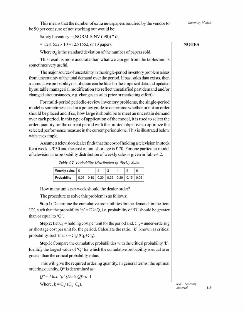
Inventory Models
NOTES
Self - LearningMaterial 119
This means that the number of extra newspapers required by the vendor tobe 90 per cent sure of not stocking out would be:
Safety Inventory = (NORMISINV (.90)) * σs
= 1.281552 x 10 = 12.81552, or 13 papers.
Where σs is the standard deviation of the number of papers sold.
This result is more accurate than what we can get from the tables and issometimes very useful.
The major source of uncertainty in the single-period inventory problem arisesfrom uncertainty of the total demand over the period. If past sales data exists, thena cumulative probability distribution can be fitted to the empirical data and updatedby suitable managerial modification (to reflect unsatisfied past demand and/orchanged circumstances, e.g. changes in sales price or marketing effort).
For multi-period periodic-review inventory problems, the single-periodmodel is sometimes used in a policy guide to determine whether or not an ordershould be placed and if so, how large it should be to meet an uncertain demandover each period. In this type of application of the model, it is used to select theorder quantity for the current period with the limited objective to optimize theselected performance measure in the current period alone. This is illustrated belowwith an example.
Assume a television dealer finds that the cost of holding a television in stockfor a week is 30 and the cost of unit shortage is 70. For one particular modelof television, the probability distribution of weekly sales is given in Table 4.2.
Table 4.2 Probability Distribution of Weekly Sales
Weekly sales 0 1 2 3 4 5 6
Probability 0.05 0.10 0.20 0.25 0.20 0.15 0.05
How many units per week should the dealer order?
The procedure to solve this problem is as follows:
Step 1: Determine the cumulative probabilities for the demand for the item‘D’, such that the probability ‘p’ = D Q, i.e. probability of ‘D’ should be greaterthan or equal to ‘Q’.
Step 2: Let Ch= holding cost per unit for the period and, Cb = under-orderingor shortage cost per unit for the period. Calculate the ratio, ‘k’, known as criticalprobability, such that k = Ch/ (Ch+Cb).
Step 3: Compare the cumulative probabilities with the critical probability ‘k’.Identify the largest value of ‘Q’ for which the cumulative probability is equal to orgreater than the critical probability value.
This will give the required ordering quantity. In general terms, the optimalordering quantity, Q* is determined as:
Q*= Max. ‘p’ (De Q)>k–1
Where, k = Ch/ (Ch+Cb).

Inventory Models
NOTES
Self - Learning120 Material
In our example, the results are shown in Table 4.3. Comparing the cumulativeprobabilities with ‘k’, we find that the maximum value of ‘Q’ where ‘p’ (D Q)> kis ‘4’.
Table 4.3 Critical Probability and Order Quantity
Demand (in units) Prob. that demand will
be at this level
Prob. that demand will be at
this level or greater P(d>Q)
1 0.15 1.00>0.30
1 0.10 0.95>0.30
2 0.10 0.85>0.30
3 0.25 0.65>0.30
4 0.20 0.40>0.30
5 0.15 0.20>0.30
6 0.05 0.05
In this example, the optimum policy is to stock 4 units. In case of continuousdistributions, a similar method can also be used.
A similar logic and approach can be used in the case when lead-times areprobabilistic. Such problem types are encountered more frequently for costly spareparts, perishable goods, seasonal items like in fashions and room heaters, air-conditioners, etc. These types of problems will be covered in the next section.
4.7 INVENTORY MODELS WITH UNCERTAINTY
In today’s growing global supply chains, there is uncertainty in demand, in costs,in lead-time and in supplied quantity. The risks of supply disruptions continue togrow, but through efficient use of inventory and robust system design, those riskscan be effectively mitigated. Though it is generally believed that demand variabilityinduces avoidance of stock-outs by increasing safety stock levels, the relationshipbetween demand uncertainty and inventory levels is still empirical.
However, inventory models with uncertainty have been developed that canbe used to determine how much inventory should be kept on stock, what servicelevels should be met and how to design inventory layout. Such models considerthat risks have geometrically-distributed probabilities and demand to be eitherdeterministic or normally distributed.
Figure 4.17 shows the relationship between working stock and safety stock,where demand is uncertain. In the figure Ss represents safety stock. B is the reorderpoint and working stock is shown as the difference between the total stock andsafety stock.
QU
AN
TIT
Y
TIME
Safety Stock
WorkingStock
WorkingStock
Q + Ss
Ss
B
Fig. 4.17 Working Stock and Safety Stock

Inventory Models
NOTES
Self - LearningMaterial 121
In reorder point models with risk, the probability distribution of demandduring the lead-time is an important characteristic in inventory management. Wecan, generally, assume the lead-time demand as a normal distribution as shown inFigure 4.18. The y-axis shows the frequency of occurrence, i.e. the probabilityand the x-axis shows the demand during lead-time.
The different relationships shown in Figure 4.17 are reflected in Figure 4.18also. The reason that we can represent the inventory model shown in Figure 4.17with the distribution shown in Figure 4.18 is because of the central limit theorem.Suppose, we repeat an experiment many times, where the lead-time demand is ‘M’and ‘Mi’ is the result of the ith experiment. In general, we won’t know what thedistribution of ‘Mi’ is and it may be discrete or continuous. The central limit theoremsays that the distribution of the average of Mi’s is normal.
SAFETYSTOCK
REORDER POINT
PRO
BA
BIL
ITY
P(M
)
DEMAND DURING LEAD TIME (M)
O B
PROBABILITY OFA STOCKOUT,p (M > B)
Fig. 4.18 Realistic Lead-time Demand
Using these concepts, we can tackle problems with constant lead-time andvariable demand. Data has been provided in Table 4.4 to illustrate such a problem.In the problem, it is assumed that the weekly demand is variable and the lead-timeis constant at 2 weeks.
Table 4.4 Calculation of Lead-time Demand
Demand first week (D)
Probability p(D)
Demand second week (D)
Probability p(D)
Lead-time
demand (col. 1) (col. 3)
(M)
Probability (col. 2) (col. 4) p(M)
1 0.60 1 3 4
0.60 0.30 0.10
2 4 5
0.36 0.18 0.06
3 0.30 1 3 4
0.60 0.30 0.10
4 6 7
0.18 0.09 0.03
4 0.10 1 3 4
0.60 0.30 0.10
5 7 8
0.06 0.03 0.01
In the basic data in Table 4.4, columns 1 to 3 are used to calculate the lead-time demand and the probability of lead-time demand, which are given in columns5 and 6. The lead-time demand and probability of lead-time demand obtained inTable 4.4 have been rearranged in Table 4.5 to obtain the distribution.

Inventory Models
NOTES
Self - Learning122 Material
Table 4.5 Lead-time Demand and Probability
Lead-time demand (M)
Probability P(M)
0 0 1 0 2 0.36 3 0 4 0.36 5 0.12 6 0.09 7 0.06 8 0.01
Total 1.00
We have worked out the example of constant lead-time and variable demandabove. A reasonable approximation method for determining model parameters isto use the EOQ model to solve the order size. The time between orders is thensimply the order quantity divided by annual demand. The standard deviation ofdemand during the order interval is found by determining the daily standard deviationof demand and multiplying by the square root of the length of the order interval.Different relationships emerge when there is:
(a) Variable demand and constant lead-time
(b) Constant demand with variable lead-time
(c) Variable demand with variable lead-time
Each of these relationships is shown below. The notations that are used are asfollows:
B = Reorder point in units.
M = Lead-time demand in units (a random variable).
f (M) = Probability density function of lead-time demand.
p (M) = Probability of a lead-time demand of M units.
L = Expected lead-time
Lm = Maximum lead-time
= Standard deviation of lead-time demand
Q = Lot size
S = Setup cost or Ordering Cost ( /year)
Ss = Safety Stock
D = Annual Demand
P = Unit Price ( /unit)
H = Holding or Carrying cost per Unit ( /Unit)
F = Inventory Carrying Charges Factor
Q* = Economic Order quantity (to be determined)

Inventory Models
NOTES
Self - LearningMaterial 123
P(M>B)
J
WLTIME
QU
AN
TIT
Y
Q + Ss
BJ
–W0
Ss
Fig. 4.19 Inventory Risk: Variable Demand and Constant Lead-time
The relationships that emerge when demand is variable and lead-time is constantare as shown in Figure 4.19. The figure shows the relationships that are givenbelow:
B – SS = expected lead-time demand
B – J = minimum lead-time demand
B + W = maximum lead-time demand
p(M>B) = probability of a stock-out
P(M>B)
QU
AN
TIT
Y
Q + Ss
BJ
–W
0 Ss
LM
TIME
Fig. 4.20 Inventory Risk: Variable Demand and Variable Lead-time
The relationships when there is a constant demand with variable lead-timeare shown in Figure 4.20. The relationships that emerge from this configurationare given below:
p (M > B) = probability of a stock-out
B – S = expected lead-time demand
B + W = maximum lead-time demand
The lot order size is given by the expression:
Q* = 2DS / H … (4.25)
And the reorder point is given by:
B = M + Ss … (4.26)
When both demand and lead-times are probabilistic, the basic procedurefor finding operating doctrines is a convergence procedure. This is a directed trialand error method. For the quantity/reorder point model, the order quantity iscomputed assuming constant demand. Then the reorder point is calculated usingthe computed order quantity. This value is then used to recalculate the order quantity

Inventory Models
NOTES
Self - Learning124 Material
and recalculate the reorder point. Eventually, the order quantity and the reorderpoint converge at their optimal values. The example of ABC Ltd. illustrates themethod.
ABC Ltd. for one of its class ‘A’ items, has an ordering cost of 5400.00,the inventory holding cost is 40 per cent and the cost per unit is 40.00.
D = Annual demand = 8*150 = 1200 units
P = Unit purchase cost = 40.00
S = Ordering Cost = 5400.00
F = Holding Cost = 40%
The lead-time to deliver the item is 10 days. The lead-time demand is givenin Table 4.6 below.
Table 4.6 Lead-time Demand
Lead-time demand (M)
Probability P(M) Lead-time demand (M)
Probability P(M)
0 0 1 0 2 0.36 3 0 4 0.36 5 0.12 6 0.09 7 0.06 8 0.01 Total 1.00
What is the lowest cost reorder point if the stock-out cost is 5 per unit?
Using the Economic Order Equation:
Q* = (2DS/H) = (2DS/FP) = EOQ
= (2 *5400*1200)/(0.40*40) = 900 units.
Reorder Level: RB = L*D = (10/365) * 1200 33 units
Let us now determine the lowest cost reorder point.
B = 34 E (M > B) = or
= (34 - 33) * 0.36 + (34 - 33) * 0.00 + (34 - 33) * 0.36 + (34 - 33) *
0.12 + (34 - 33) * 0.09 + (34 - 33) * 0.06 + (34 - 33) * 0.01
= 1 unit
8
(M - 33) p (M) 1 + 1
Mmax
(M - B) p (M) M=B + 1
TCS = Holding Cost + Stock-out Cost
= (B - M) H + SCS E (M>B)/ Q
TCS = (34 - 33) * 1 + 5400 * 2 * 1/ 900
= 1 + 12 = Rs 13.00
B = 35 E (M > B) =
= (35 - 33) * 0.36 + (35 - 33) * 0.12 + (35 - 33) * 0.09 + (35 - 33) *
0.06 + (35 - 33) * 0.01
= 1.28 units
8
(M - 33) p (M) 2 + 1

Inventory Models
NOTES
Self - LearningMaterial 125
TCS = (35 - 33) * 1 + 5400 * 2 * 1.28/ 900
= 2 + 15.36 = Rs 17.36
B = 36 E (M > B) =
= (36 - 33) * 0.12 + (36 - 33) * 0.09 + (36 - 33) * 0.06 +
(36 - 33) * 0.01
= 1.12 units
8
(M - 33) p (M) 4 + 1
TCS = (36 - 33) * 1 + 5400 * 2 * 1.12/ 900
= 4 + 13.44 = Rs 17.44
B = 37 E (M > B) =
= (37 - 33) * 0.09 + (37 - 33) * 0.06 + (37 - 33) * 0.01
= 0.80 units
8
(M - 33) p (M) 5 + 1
TCS = (37 - 33) * 1 + 5400 * 2 * 0.80/ 900
= 5 + 9.60 = Rs 14.60
B = 38 E (M > B) =
= (38 - 33) * 0.06 + (38 - 33) * 0.01
= 0.42 units
8
(M - 33) p (M) 6 + 1
TCS = (38 - 33) * 1 + 5400 * 2 * 0.42/ 900
= 6 + 5.04 = Rs 11.04
B = 39 E (M > B) =
= (39 - 33) * 0.01 = 0.07 units
TCS = (39 - 33) * 1 + 5400 * 2 * 0.07/ 900
= 7 + 0.84 = Rs 7.84
8
(M - 33) p (M) 7 + 1
Therefore, the lowest cost of reorder point is 39 units with an expectedannual cost of safety stock of 7.84.
In the example that we worked out above and in this section, we haveconsidered the single-period inventory problem when there is a fixed order orsetup cost including the point at which the marginal revenue of an additional unit ofinitial inventory just equals the marginal cost of a unit of inventory.
Table 4.7 shows certain statistical relationships and formulae that can beused for continuous and discrete distributions. These formulae summarize thematerial provided in this section.

Inventory Models
NOTES
Self - Learning126 Material
Table 4.7 Some Statistical Relationships
Variable Continuous Distributions Discrete
Distributions
Mean Lead-Time0
Mf(M)dM
Mmax
M=0
Mp(M)
Demand M
Lead-Time Demand2(M – M) f(M)dM
Mma
M=0
p(M)Variance s2
Probability of aB
f(M)dM
Mmax
M=B+1
p(M)Stock-out p(M > B)
Expected Stock-outB
(M – B) f(M)dM
Mmax
M=B+1
(M – B)p(M)
The inventory models analysed represent a small subset of the inventorymodels. Other models including infinite horizon models, continuous review andperiodic review models are outside the scope of this book.
Check Your Progress
5. List the assumptions of a backordering inventory model.
6. List any two assumptions of the simple EPQ model.
4.8 ANSWERS TO ‘CHECK YOUR PROGRESS’
1. Inventory models analyse fluctuations in stock.
2. The two types of inventory models are:(a) Fixed-order Quantity Models (also called the Economic Order
Quantity models).(b) Fixed-time Period Models (also referred to as the Periodic System
or P-models).
3. The basic EOQ model is concerned primarily with the cost of ordering andthe cost of holding inventory.
4. The two assumptions in simple EOQ fixed-order quantity models are:(i) The rate of demand for the item is deterministic and is a constant ‘D’
units per annum independent of time.(ii) Production rate is infinite, i.e. production is instantaneous.
5. A backordering inventory model assumes only two costs:(i) Ordering or setup cost(ii) Inventory holding cost

Inventory Models
NOTES
Self - LearningMaterial 127
6. The assumptions of the simple EPQ model are:(i) There is only one item involved.(ii) Annual demand is known.
4.9 SUMMARY
Inventory management is concerned with matching supply with demand.The central problem is to find the amount to be produced or purchased inorder to maximize the total expected profit, or minimize the total expectedcost. The question of how much to order is determined by inventory models.
Inventory models analyse fluctuations in stock; starting from basicassumptions, they obtain bounds between which the stock varies. In orderto do this, inventory models start with the inventory cycle. The inventorycycle begins with the receipt of an order.
Inventory management attempts to provide the framework necessary toreduce the cycle time of the inventory cycle. A shorter cycle time bringsdown the average inventory as well as the lead-time for replenishment.Inventory models are optimization models that attempt to reduce cycle timesand at the same time ensure that an item will be available on an ongoingbasis throughout the year.
There are two general types of systems and these can be distinguished onthe basis of the ordering criteria. The models of these two systems are;
(a) Fixed-order Quantity Models (also called the Economic OrderQuantity models).
(b) Fixed-time Period Models (also referred to as the Periodic System orP-models).
The basic difference between the two systems is that the fixed-order quantitymodels are ‘event triggered’ and fixed-time period models are ‘timetriggered’. In other words, at an identified level of the stock, the fixed-order quantity model initiates an order. This event may take place at anytime, depending on the demand for the items considered. In contrast, thefixed-time period models review the stocks at time intervals that are fixedand orders are placed at the end of pre-determined time periods. In thesemodels, only the passage of time triggers action.
Generally, fixed-order quantity models are favoured when:
o Items are more expensive because the average inventory is lower.
o Items are critical, e.g. repair parts, because there is closer monitoringand therefore, quicker response to potential stock-out.
The basic assumptions in simple EOQ fixed-order quantity models are asfollows:
o The rate of demand for the item is deterministic and is a constant ‘D’units per annum independent of time.
o Production rate is infinite, i.e. production is instantaneous.
Inventory Models
NOTES
Self - Learning128 Material
o Shortages are not allowed.
o Lead-time is zero or constant and it is independent of both demand aswell as the quantity ordered.
o The entire quantity is delivered as a single package (or produced in asingle run).
Cycle inventory is the average stock held by the firm. Hence, the averageinventory holding cost will be the cost incurred in holding the averageinventory.
The ordering cost will decrease as order size increases. This follows as fora given annual demand, the larger the order size, the fewer the orders needed.Ordering cost will, therefore, depend on the demand, order size and orderingcost. It is commonly assumed that ordering costs are relatively independentof the size of the order.
When quantity discounts are offered, demand is certain, delivery isinstantaneous (no stock-outs) and item cost varies with volume ordered,there is a discrete or steep change rather than a per-unit change and aseparate U-shaped total cost curve for each unit price.
Computation for controlling the service level for single items is easy. Theexpected stock-out cost, a key calculation in the total inventory cost, is theexpected probability of a stock-out times the stock-out costs that are incurredregardless of the number of units short.
When there is a mixture of items, the service level is then more properlyexpressed as a weighted average fill rate (WAFR).
The WAFR is found by multiplying the probability with which eachcombination of items appears on the order by the probability of filling theorder completely, given the number of items on the order.
In many retail merchandising systems, a fixed-time period system is used.Sales people make routine visits to customers and take orders for theircomplete line of products.
Inventory, therefore, is counted only at particular times, such as every weekor every month or when the supplier’s visit is due. Sometimes, this is alsoresorted to in order to combine orders to save transportation costs.
In today’s growing global supply chains, there is uncertainty in demand, incosts, in lead-time and in supplied quantity. The risks of supply disruptionscontinue to grow, but through efficient use of inventory and robust systemdesign, those risks can be effectively mitigated. Though it is generally believedthat demand variability induces avoidance of stock-outs by increasing safetystock levels, the relationship between demand uncertainty and inventorylevels is still empirical.
As the unit service level and unit stock-out risk provides data on the exactquantities of units of customer demand filled or unfilled during each cycle orduring any time period, it is a measure that is commonly used in manyconsumer goods applications.

Inventory Models
NOTES
Self - LearningMaterial 129
Service level is often measured by stock availability, but could also bemeasured by order cycle time or consistency of cycle time. For example,we could have a customer service objective of 99 per cent stock availability.
There is an exponential relationship between the inventory and service levels.By increasing stock levels, we generally provide higher service levels to ourcustomers. But, at some point, large increases in inventory yield relativelysmall gains in customer service.
4.10 KEY TERMS
Fixed-Order Quantity Model: It refers to inventory models in whichdemand is assumed to be fixed and completely pre-determined.
Economic Production Quantity (EPQ) models: These are models withinventory systems where other units are taken out of inventory (causing it todiminish) while some are added to the inventory (causing it to grow).
Fixed-Time Period Models: These are models that generate orderquantities that vary from period to period, depending on the usage rates.
Multi-period Model: These are model for multi-period problems wherethe approach is to maximize the expected utility of the income cash flow.
4.11 SELF-ASSESSMENT QUESTIONS ANDEXERCISES
Short-Answer Questions
1. Write a short note on fixed-order quantity model.
2. What is a price-break model?
3. List the three costs that backorder Inventory model assumes.
4. Write a short note on fixed-time period systems.
5. Write a short note on single-period inventory problem.
6. What is order service level?
7. What is multi-period model?
Long-Answer Questions
1. Explain the EOQ model of inventory with its simplifying assumptions.
2. Nuvyug Industries Ltd. has an annual requirement of 5000 pieces of brakecylinders for its popular brand of golf carts. Each brake cylinder has a carryingcost of 25 per unit per year. The ordering cost per order is 800. Calculatethe total inventory cost for the following values of number of orders: 5, 10, 20and 25. Plot the various costs with respect to these orders on a graph and useit to find the EOQ.

Inventory Models
NOTES
Self - Learning130 Material
3. Imperial Exports runs a carpet discount store in Lucknow. The companystocks export rejected carpets in its warehouse and sells it through anadjoining showroom. The store keeps several brands and styles of carpetsin stock; however, its biggest seller is the ‘Badohi Fine Quality’ carpet.Imperial Exports wants to determine the optimal order size and total inventorycost for this brand of carpet, given an estimated annual demand of 1,00,000metres of carpet, an annual carrying cost of 7.50 per metre and an orderingcost of 1500.
4. Hindustan Unilever Ltd. is the manufacturer of Surf detergent powder. A 100g pack is priced at 30 for its suppliers. One of its suppliers purchases16,000 packs per annum. The supplier incurs an ordering cost of 350.00per order and has a carrying cost of 12 per cent of the inventory value. HULoffers discounts for the following range of bulk purchases to its suppliers: 0.5per cent for 3000–6999 units, 0.75 per cent for 7000–9999 units and 1 percent for 10,000 and more units. Which discount option should the supplierchoose? What is the EOQ in this case?
5. Examine the cost of uncertainty in demand during lead-time.
6. A part used to repair machines has a normally distributed monthly demandwith a mean of 65.0 and a standard deviation of 5.2. If the lead-time is sopredictable that it can be considered a constant 0.25 month and the servicelevel is 90 per cent:
a. What is the order point?b. What is the safety stock level?
7. An auto dealership has experienced the following historical demands duringlead-times for Logan wide-bodied automobiles.
Actual DDLT # of Occurrences Actual DDLT # of Occurrences 7 2 12 6 8 6 13 11 9 4 14 9
10 8 15 3 11 7 16 1
This data covers the dealership’s past 57 orders. The replenishment lead-time is five days to receive an order of automobiles.
a. Compute the order point using a 90 per cent service level.b. Compute the expected demand during lead-time.c. What is the effective level of safety stock resulting from this order
point?
8. A part has a normally distributed monthly demand with a mean of 65.0 anda standard deviation of 5.2. If lead-time is so predictable that it can beconsidered a constant 0.25 month and the service level is 90 per cent:
a. What is the order point?b. What is the safety stock level?

Inventory Models
NOTES
Self - LearningMaterial 131
9. A company uses a fixed order period for ordering a forging that is purchasedfor 180 per unit. The annual demand for the forging is 15,000 units. Theordering cost is 800 per order. The annual carrying cost rate is 35 percent of the acquisition cost. The expected demand during lead-time is 200units and the upper inventory target is 700 units.
a. How often should the forging be ordered?b. What is the annual total inventory cost that should be expected?c. If the company is going to place an order now and the current inventory
level is 248 units, what should be the order quantity?
10. What is the cost of uncertainty in demand during lead-time?
4.12 FURTHER READING
Zipkin, Paul Herbert. 2000. Foundations of Inventory Management. New Delhi:McGraw Hill.
Orlicky, Joseph and George Plossl. 1994. Orlicky’s Material RequirementPlanning. New Delhi: McGraw-Hill.
Seetharama L Narsimhan, Dennis WMcLeavy, Peter J Billington. 1994. ProductionPlanning and Inventory Control. New Delhi: Prentice Hall of India PvtLtd.
J. R. Tony Arnold, Stephen N. Chapman. 2007. Introduction to MaterialsManagement. New Delhi: Prentice Hall.
Richard J. Tersine.1982. Principles of Inventory and Materials Management.New Delhi: Prentice Hall.


Material RequirementPlanning Systems
NOTES
Self - LearningMaterial 133
UNIT 5 MATERIAL REQUIREMENTPLANNING SYSTEMS
Structure
5.0 Introduction5.1 Objectives5.2 Material Requirement Planning System—Meaning, Purpose and Advantage5.3 Files and Databases – Data Requirements and Management
5.3.1 File Organization and Access5.3.2 Complete Record
5.4 Updating Inventory Records5.4.1 Transaction Types and Effects
5.5 Bills of Material-Types5.5.1 Bill of Material Structuring5.5.2 Transient Sub-assemblies5.5.3 Product Model Designations
5.6 Modularization of Bills of Material5.6.1 Modularization Technique5.6.2 Pseudo Bills of Material5.6.3 Manufacturing Bills of Material
5.7 Master Production Schedules – Meaning and Objective5.8 Managing Master Production Scheduling Inventory Records
5.8.1 Lot Sizing5.8.2 Data Integrity5.8.3 Engineering Change Control5.8.4 Process of MRP5.8.5 Output of Mrp
5.9 Introduction to MRPII Systems5.10 Using Distribution Resource Planning to Manage Inventories in Multiple
Locations5.11 Answers to ‘Check Your Progress’5.12 Summary5.13 Key Terms5.14 Self-Assessment Questions and Exercises5.15 Further Reading
5.0 INTRODUCTION
Companies must be able to plan for their material requirements in the best possibleway. They must know what items they require. They must also know how much isrequired at a time, and finally when the quantities are required to meet demand.This is what Material Requirements Planning (MRP) does.
The business environment requires an enterprise to have good processes andsystems which should be able to adjust to changes in this environment. These changesmay be with respect to technological innovations, government policies, interest rates,competition, changing customer perception or any other force of change. Companiesneed to differentiate themselves from other players in the market. It is often thisdifference that separates a successful company from one that is not. Companies use

Material RequirementPlanning Systems
NOTES
Self - Learning134 Material
various means to differentiate themselves. However, to do so they need the rightinformation—at the right time—to make the right decisions so that:
The products that are going to be produced conform to the requirements ofthe market and the designs should anticipate and accommodate thecustomer’s future needs.
The marketing department, which keeps an eye on the trends and needs ofthe market, should give relevant information to the production departmentso that they are in a position to make periodic and relevant changes to theproducts.
The demand–supply factor in the market should be analysed for properproduction planning and there should be some system that can helpmanagements to take strategic decisions.
The organization should have a good system of managing its vendors, whichincludes parameters of quality, price and delivery schedules.
Competitive advantage starts from sourcing the right raw material at theright time. Differentiation is achieved when companies control the types andquantities of materials they purchase, plan which products are to be produced andin what quantities.
In this unit, you will learn about the concept of material requirement planning.You will study about data requirements and management of data for MRP systems.Here, you will first understand the requirements for files and database required forMRP programmes. The unit will describe the updating of inventory records thatconstitute an important part in the functionality of MRP programmes. You will alsolearn about the bills of material (BoM). You will examine the modularization ofBoMs and manufacturing BoM. You will learn about Master Production Schedulesand the ‘rough-cut capacity plan’ as a part of Master Production Schedulingconcepts. These are the outcomes of the aggregate plan. Finally, the unit will touchupon the MRPII Systems and discover the idea behind Distribution ResourcePlanning.
5.1 OBJECTIVES
After going through this unit, you will be able to:
Understand how files and databases can be created and organized foreffective use in MRP
Understand the importance of bills of material and how they are structured
Discuss master production schedules
Explain Managing Master Production Scheduling
Understand the concept of MRPII Systems
Describe distribution resource planning

Material RequirementPlanning Systems
NOTES
Self - LearningMaterial 135
5.2 MATERIAL REQUIREMENT PLANNINGSYSTEM—MEANING, PURPOSE ANDADVANTAGE
Material planning systems try to optimize operations by ensuring that materials arealways available to meet production requirements, but stocks are not more thanwhat is necessary, at any given time. MRP modules take the guesswork out ofpurchasing by automatically calculating material requirements and coordinatingpurchase orders and production orders for timely receipt. Unrealistic manufacturingplans can be easily identified, which may arise when there is not enough time tomanufacture an intermediate for a target production date or if a vendor is unlikelyto deliver materials by the time they are required.
These systems are often described as MRP I and MRP II systems. MRP Istands for materials requirement planning and MRP II for manufacturing resourceplanning. MRP I and MRP II are tools that have been developed to helporganizations determine precisely when and how much material to purchase andprocess. The solutions provided by these systems are based upon a time-phasedanalysis of sales orders, production orders, current inventory and forecasts.
MRP is a set of logical planning techniques related to the manufacturingenvironment. It is a network-scheduling concept which integrates company-wideinformation to plan manufacturing activities. The function of a material requirementplanning is to translate the master production schedule into detailed componentmaterial requirements and orders, based on inventory.
The MRP system has at its heart four relevant questions which allow thederivation of the fundamental shortage equation. These are:
(1) What are we going to make?(2) What does it take to make it?(3) What have we got?(4) What do we have to get?
These are the basics of MRP. The system determines item by item what isto be processed and when, as well as what is to be manufactured and when. Thisis based on order priorities and available capacities.
Purpose of MRP system
MRP is offered as a standard software and its purpose is:
To use the master production schedule to determine the end productrequirements and break these down into component parts and sub-assembliesto create a materials plan
To show time-phased requirements for releasing materials and receivingmaterials that enable the MPS to be implemented
Specify when production and purchase orders must be placed for eachpart and sub-assembly to complete the products on schedule.

Material RequirementPlanning Systems
NOTES
Self - Learning136 Material
Figure 5.1 shows the MRP system, identifying the input–output relationships. Itshows that in the process of planning, the MRP system allocates existing inventorieson hand to the items to be manufactured. And based on gross requirements, itreevaluates the validity of the timing of any outstanding orders. The systemestablishes a schedule of planned orders for each item, including orders, if any, tobe released immediately plus orders scheduled for release at specific future dates.Planned order quantities are computed using any of several lot-sizing rules.
InventoryStatusRecord
Bill ofMaterials(BOM)
Independent ItemDemand
Master ProductionSchedule (MPS)
Inventory OrderAction
Priority Integrity
PerformanceControl
Priority Planning
Planned-OrderSchedule
ExceptionReports
Inventoryrecord
MRPSystem
To CapacityRequirementsPlanning (CRP)
Fig. 5.1 MRP System
Material Requirement Planning (MRP) was developed as a concept that questionedmany of the existing concepts and techniques of inventory management. Thesetechniques were built on order point (OP) concepts or the stock replenishmentconcept. MRP proponents argued the validity, relevance and ability of thereplenishment concept to meet the requirements for production inventories. Theyraised questions about the following commonly accepted ideas:
1. The concept of stock replenishment2. All techniques involving reorder points3. Square-root economic order quantities4. Classification of inventory by function5. Aggregate inventory management concepts6. Controls based on ABC inventory classification
Programmes based on reorder point techniques made false assumptions aboutboth demand and supply environments, misinterpreted observed demandbehaviour, could not determine the specific timing of future demands, and lackedthe ability to re-plan. Stock replenishment was carried out through methods thatincluded statistical order points, min-max, two-bin and periodic review techniques.Forecasts of demand were explicitly or implicitly used during replenishment leadtime and safety stock was provided to compensate for the fluctuations in demand.

Material RequirementPlanning Systems
NOTES
Self - LearningMaterial 137
According to the MRP concept, the term stock replenishment also meansrestoration of inventory to its previous state – but this is not always right. Productioninventories handled in this manner may be found to be in conflict with one of thefollowing three basic management objectives:
1. High customer service for high sales revenue
2. Low inventory for high return on investment
3. Low costs for high profits
Stock replenishment attempts to have inventory items in stock at all times,while the ideal is to have inventory items availability at the time of need, not sooneror later. The need for individual production inventory items can be better determinedthrough the use of modern, computer-assisted MRP programmes, so thatundesirable and wasteful practices can be avoided.
Development of MRP
MRP was originally introduced in the 1960s, when material requirements andmaterial planning were done manually. Calculations were made to determine theresource requirements of a production run based on sales forecasts. Thesecalculations were developed into simple computer programmes by somemanufacturing companies. These were custom software programmes that ran onmainframe computers. They were simple programmes that calculated the rawmaterial needed to produce products and the machine and labour time needed forthe job. Sometimes, they would also calculate the parts to be ordered. Let us tryto understand the concept with the help of an example.
Suppose a material requirements plan has to be developed by ABCManufacturing to produce precipitators over a six month period. Assume that thelead time between the release of a particular order to the shop floor and itsproduction is two months. 200 precipitators are currently lying in stock with thecompany. It has been forecasted that the customer demand is likely to be 100precipitators in the first month, 80 in the third month, and 175 in the fifth month.This data is tabulated in Table 5.1.
Table 5.1 Forecast and Inventory for Precipitators
Month Month Month Month Month Month1 2 3 4 5 6
Demand 100 0 80 0 175 0
Inventory 200
Order ? ? ? ? ? ?
There are 200 precipitators initially available, so if the company uses these formeeting the demand of 100 in the first month, there would be 200–100 = 100precipitators left in hand at the end of the first month. Clearly, some moreprecipitators will have to be ordered for meeting the forecasted future demand.Conceptually, therefore, two related decisions need to be made regarding ordering:
Quantity: How much is to be ordered
Timing: When it is to be ordered
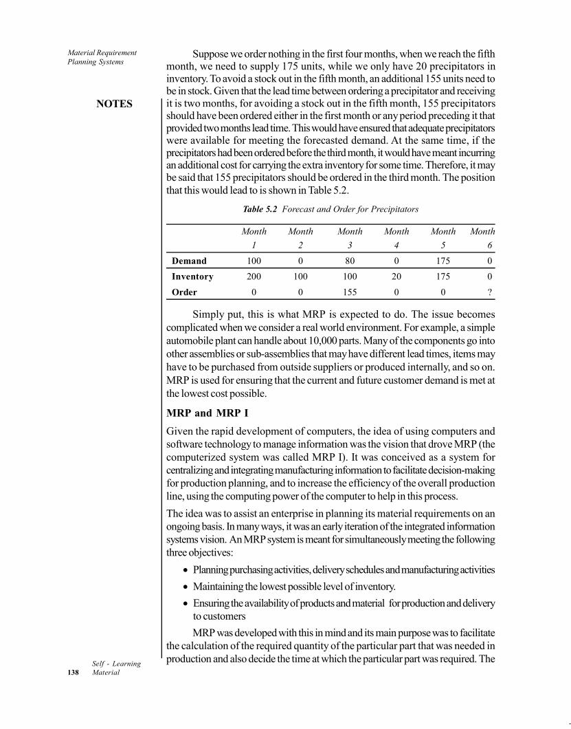
Material RequirementPlanning Systems
NOTES
Self - Learning138 Material
Suppose we order nothing in the first four months, when we reach the fifthmonth, we need to supply 175 units, while we only have 20 precipitators ininventory. To avoid a stock out in the fifth month, an additional 155 units need tobe in stock. Given that the lead time between ordering a precipitator and receivingit is two months, for avoiding a stock out in the fifth month, 155 precipitatorsshould have been ordered either in the first month or any period preceding it thatprovided two months lead time. This would have ensured that adequate precipitatorswere available for meeting the forecasted demand. At the same time, if theprecipitators had been ordered before the third month, it would have meant incurringan additional cost for carrying the extra inventory for some time. Therefore, it maybe said that 155 precipitators should be ordered in the third month. The positionthat this would lead to is shown in Table 5.2.
Table 5.2 Forecast and Order for Precipitators
Month Month Month Month Month Month
1 2 3 4 5 6
Demand 100 0 80 0 175 0
Inventory 200 100 100 20 175 0
Order 0 0 155 0 0 ?
Simply put, this is what MRP is expected to do. The issue becomescomplicated when we consider a real world environment. For example, a simpleautomobile plant can handle about 10,000 parts. Many of the components go intoother assemblies or sub-assemblies that may have different lead times, items mayhave to be purchased from outside suppliers or produced internally, and so on.MRP is used for ensuring that the current and future customer demand is met atthe lowest cost possible.
MRP and MRP I
Given the rapid development of computers, the idea of using computers andsoftware technology to manage information was the vision that drove MRP (thecomputerized system was called MRP I). It was conceived as a system forcentralizing and integrating manufacturing information to facilitate decision-makingfor production planning, and to increase the efficiency of the overall productionline, using the computing power of the computer to help in this process.
The idea was to assist an enterprise in planning its material requirements on anongoing basis. In many ways, it was an early iteration of the integrated informationsystems vision. An MRP system is meant for simultaneously meeting the followingthree objectives:
Planning purchasing activities, delivery schedules and manufacturing activities
Maintaining the lowest possible level of inventory.
Ensuring the availability of products and material for production and deliveryto customers
MRP was developed with this in mind and its main purpose was to facilitatethe calculation of the required quantity of the particular part that was needed inproduction and also decide the time at which the particular part was required. The

Material RequirementPlanning Systems
NOTES
Self - LearningMaterial 139
task of MRP is to create an optimum inventory system. MRP calculations arebased on dependent demand, that is, they assume that the demand is known.
To determine the requirements, MRP uses three inputs. One of the majorinputs required by the system is the Master Production Schedule, which is a list ofthe end products that are to be produced, the quantity of each product that has tobe produced and the time at which the products have to be ready for shipment.Another major input is the Bill of Material (BoM) File. BoM lists the componentparts and the subassembly that make up each product. The third major input is theInventory Record File, which is a computerized inventory system used to maintainrecords of items in the master files, including raw material, components assembliesand BoM.
The structure of a typical MRP system is shown in Figure 5.2. The functionof MRP is to translate the master production schedule into detailed componentmaterial requirements and orders, based on inventory. The system determines,item-by-item, what is to be processed and when, as well as what is to bemanufactured and when. This is based on order priorities and available capacities.As the purpose of manufacturing inventory is to satisfy production requirements,the production plan is the source of demand and thus demand is seen asdeterministic.
CustomerOrder
SalesForecast
Master ProductSchedule
EngineeringChanges
Bills ofMaterial File MRP Processor Inventory Record
File
InventoryTransactions
Service PartsEquipment
OutputReports
Fig. 5.2 Structure of the MRP System
These inputs are converted into two main outputs, namely planned orderreleases and reschedule notices. In the process of planning, the MRP systemallocates the existing inventories in hand to the items to be manufactured; andbased on the gross requirements, it reevaluates the validity of the timing of anyoutstanding orders. The system establishes a schedule of planned orders for eachitem, including orders, if any, to be released immediately along with the ordersscheduled for release at specific future dates.
Planned order quantities are computed from the schedule using any of theseveral lot sizing or priority rules. These lot sizing rules determine the manner of

Material RequirementPlanning Systems
NOTES
Self - Learning140 Material
calculating the required quantity of the particular part and the timing at which theparticular part is required.
Order point versus MRP
There are two ways in which inventories can be managed in an organization. Oneis the material requirement method and the other is the order point technique.
MRP refers to a time-phased replenishment approach in which inventorystatus is reviewed and new shipment plans are generated periodically. The demandis treated as dependent demand and the requirements are worked out based onthe master schedule.
Time-phased logic is employed for anticipating requirements for upstreaminventory echelons, while forecasting is employed for anticipating requirements atthe independent demand level (or echelon). Therefore, planned lead times andinventory status are made use of for timing order releases so that inventory can beminimized and at the same time, excessive shortfalls can be avoided. Becauseinventories are planned throughout the supply chain, they have their basis inanticipated demand.
Opposed to MRP, demand is treated by order point systems at all echelons in thesupply chain as independent. The theory makes five basic assumptions. These areas follows:
1. Independent demand can be forecasted with reasonable accuracy.
2. Forecasts normally account for all demands.
3. Safety stocks protect against forecast errors and unexpected events.
4. Demand will be fairly uniform in the short-term and will constitute a fractionof the reorder quantities.
5. It is desirable to replenish inventories when they are depleted below theorder point quantity.
There is a popular saying that forecasts will be wrong. Forecasts of demandfor components are mostly derived from each item’s past usage and determineonly the average amount of demand expected in the future, not the time of specificdemands. Order point attempts to protect users against forecast errors and otherunexpected occurrences by adding a cushion called safety stock. It uses economicorder quantity computation to specify the size of the replenishment order. Howwell order point inventory planning works depends on how closely the assumptionsrelate to the actual situations in the inventory.
The order point assumption of fairly uniform usage in small increments isvery often not valid in many manufacturing environments. Requirements forcomponents of products occurs in discrete ‘lumps’ caused by parent order lotsizes. This is often a problem that has to be tackled in order point systems.
The general practice in this system is to decentralize control and independentlyreview the inventory at every stage. Based on such constant review, the firm mustplace orders as soon as the inventory falls below the reorder point. In case theinventory falls to zero, it is also necessary to take backorders into account when

Material RequirementPlanning Systems
NOTES
Self - LearningMaterial 141
new orders are placed. The basis for calculating reorder points is the demand thatis expected during expected replenishment times (actual lead times)
Table 5.3 Comparison of MRP and the Order Point System
Attribute MRP Order Point
Demand Dependent Independent
Order philosophy Requirements Replenishment
Deals with Products Parts
Forecast Based on master schedule Based on past demand
Control concept Control all items ABC
Looks at Future Past
Order dates Complete Start
Objectives Meet manufacturing needs Meet customer needs
Lot sizing Discrete EOQ
Re-planning Yes No
Demand pattern Lumpy, but predictable Random
Future orders Shows everything in the horizon No, except in fixed time models
Types of inventory Work in process and raw material Finished goods and spare parts
Table 5.3 offers a detailed comparison of the two systems. MRP systemsare usually deemed proactive. Some of the benefits offered by MRP are compatibilitywith other supply chain systems such as transportation planning and DRP, enhancedcustomer service and inventory reduction. MRP works better than conventionalorder point systems in cases where supply chain integration is viable.
Order point systems, on the other hand, are deemed reactive, because ofthe lack of mechanisms for anticipating demand changes and because averageinformation is often used by them for making replenishment decisions. It is this thatsometimes results in inadequate performance in situations where demand tends tobe highly fluctuating.
Given that the basis for the MRP system is the concept of centralized planningand control that has its basis in global inventory and order information, theenvironment in which it works best is when there is fluctuation in demand with timeand demand and replenishment times are uncertain. It is believed that this superiorperformance results from the ability of MRP to anticipate demand changes in thesupply chain on the basis of forecast information and to anticipate futurerequirements and release time-phased orders accordingly.
At the same time, it must be remembered that there are certain disadvantagesto MRP as well. Some of these disadvantages include high implementation costs,the necessity data to be accessible throughout the supply chain and highly uncertainenvironments resulting from system nervousness.
A comparatively extensive and complex software information system isrequired by MRP. Communication between the central planning function and theseveral nodes of the distribution network or supply chain is necessary, which maybe difficult to achieve when independent enterprises control the network nodes.

Material RequirementPlanning Systems
NOTES
Self - Learning142 Material
When order point systems are used, relatively lesser information coordinationis required. Implementation becomes a lot easier when only inventory and theorder information local to the upstream replenishment loop are used. When seenfrom the perspective of control logic and planning, the advantages of systems mayget eroded by such issues of operation and implementation.
Inputs from master production schedule
In a typical manufacturing environment, MPS specifies the quantity of each finishedproduct required in each planning period; it is a set of time-phased requirementsfor end items. The firm, however, also needs a set of time-phased requirementsfor the parts and raw materials that make up those end items. Therefore, MRP isa production planning and control technique in which MPS is used to createproduction and purchase orders for lower-level components. In the 1970s,manufacturers began to use techniques such as MRP in recognition of theimportance of the distinction between independent and dependent demand items.
The inputs to the MRP system come from the MPS. MPS expresses theoverall production plan and the span of time covered by it is termed the planninghorizon. The planning horizon of the MPS usually covers a time span large enoughto contain recurring requirements for a given end item.
In the development of lot requirements, component inventories are allocatedaccording to the sequence of all the end item lots. The sequence of end item lotsaffects both the quantities and the timing of requirements in an MRP system. MRPdeals with this through level-by- level and time-phasing techniques.
A change in end item lot sequence affects not only the timing but also thequantities of requirements. This may create a severe problem because the sequenceof the lots of all products in MPS normally keeps changing. This needs to be keptin mind.
Bills of materials
In determining the net requirements for a low-level inventory item, the quantitythat exists under its own identity as well as any quantities existing as (consumed)components of parent items must be accounted for. The product structure is takenfrom the bill of materials. Net requirements are developed by allocating (reallocating)quantities in inventory to the quantities of gross requirements, in a level-by-levelprocess. The downward progression form one product level to another is calledan explosion. The bill of material file guides the explosion process.
Inventory order actions
In addition to MPS, MRP also requires following information to determine theinventory order actions:
a. Orders for components originating from sources external to the plant usingthe system
b. The forecasts for items subject to independent demand
The inventory record file is used to obtain information on the status data requiredfor determination of size and timing of planned orders namely, item lead-time,safety stock (if any), scrap allowances, lot-sizing algorithms, etc.

Material RequirementPlanning Systems
NOTES
Self - LearningMaterial 143
The product structure file (bill of materials) contains information onrelationships of components and assemblies that are necessary to do an MRP.Some areas of special concern are the product structure, the lot-sizing and theitem lead-times. These are discussed below:
Lot Sizing: Lot-sizing techniques in MRP are meant to determine plannedorder quantities. Lot sizing is also another reason why the top-to-bottom, level-by-level procedure must be followed. For an MRP to be able to carry out acomplete explosion, lot-sizing algorithms must be incorporated into the computerprogram that controls the requirement computation.
Lot-sizing techniques can be categorized into those that generate fixed,repetitively ordered quantities and those that generate varying orderquantities.
The factors that are generally considered in the design of such techniquesinclude:
o Variability of demand
o Length of the planning horizon
o Size of the planning period
o Ratio of setup and unit costs
In the more commonly used procedures described below, the first twoprocedures are demand-rate oriented and the others are discrete lot-sizingtechniques.
Fixed order quantity (FOQ): The fixed order quantity policy maintains thesame order quantity each time an order is issued. This may be specified for anyitem under an MRP system but in practice is limited to a few items with highordering cost. However, this rule is also used when quantity discounts, truckloadcapacity or minimum purchase quantities are specified by suppliers. During thesteel control regime in the 1970s, steel could only be ordered in wagon loads.
Economic order quantity (EOQ): This model is a demand rate-orientedmodel and will be discussed in detail in the next unit. This technique is unsuited todiscrete, discontinuous, non-uniform demand situations and is generally used forcontinuous and assembly-line type operations only.
Fixed period requirements (FPR): This is a converse technique to theFOQ; the user specifies how many periods of coverage every planned order shouldprovide. The ordering interval is specified and the quantity is allowed to vary.
Period order quantity (POQ): It is the modified EOQ for use in discretedemand situation. Using the schedule to know the future net requirements, EOQ iscomputed. Based on this, the number of orders per year to be placed is determined.Similar to FPR, the ordering interval is computed and supplies are orderedaccordingly. A potential difficulty with discontinuous net requirements could betheir distribution. In case, where for several periods (coinciding with orderinginterval) there are zero requirements, a pre-determined order interval would proveinoperative.
Lot-for-lot ordering (L4L): It is the simplest of all the different procedures,though it is a special case of POQ. It provides period-by-period coverage of net

Material RequirementPlanning Systems
NOTES
Self - Learning144 Material
requirements and the planned order quantity always equals the quantity of netrequirements being covered. The projected on-hand inventory is combined withthe new order so that it will equal zero at the end of each period. This techniqueminimizes inventory-carrying cost and is suitable for expensive items, purchasedor manufactured, with highly discontinuous demand.
Least unit cost (LUC): In this technique, the lot size as well as the orderinginterval are allowed to vary. The setup plus inventory carrying cost per unit iscalculated and the requirements to be covered by the order are based upon theleast ‘unit cost’. This may turn out to be larger than required in the planning period.The criteria still remains the lot size with the least unit cost. The main drawback ofthe technique is that it considers only one lot at a time.
Least total cost (LTC): This technique is based on the rationale that sumof the setup and inventory carrying costs (total cost) for all lots within the planninghorizon should be minimized. For items using this criterion, the two costs shouldbe as equal as possible. The order quantities, at which the setup cost per unit andthe carrying cost per unit are most nearly equal, are selected. The measure of theleast total cost is the Economic Part Period (EPP). This is the cost of one unit ofthe item carried in inventory for one period and follows logically from the assumptionthat the carrying cost of the inventory item should equal the setup cost.
EPP = Setup Cost / Inventory Cost per Unit per Period
This procedure allows the lot size and the ordering interval to vary withtime, depending upon inventory carrying costs. The technique is generally biasedtoward larger order quantities. However, its major drawback is the assumptionthat least cost occurs when setup cost and inventory costs are equal.
Wagner–Whitin Algorithm (W–W Method): This algorithm is a dynamicprogramming approach to determine optional lot sizes, in discrete, discontinuousand non-uniform demand situations. The technique minimizes the combined (total)cost of setup and of carrying inventory and is normally used as a standard formeasuring relative effectiveness of other discrete lot-sizing techniques. However,in the real world, there is little evidence that with changing requirements and planninghorizons, a dynamic programming approach will guarantee optimality.
In recent years, however, several more advanced techniques are availablefor determining dynamic optimal lot sizes. The main disadvantages of thesetechniques including W–W method are
(i) They require sophisticated software, e.g. sophisticated ERP softwareto be effective.
(ii) As the techniques deal with dynamic programming, they are difficultfor the average MRP user to understand.
A re-computation of a parent planned order quantity will often mean thatcomponent item open orders have to be rescheduled, in addition to recomputingand/or retiming planned orders. There is some merit in ‘freezing’ an order quantityonce established and only changing its timing as required by changing netrequirements.

Material RequirementPlanning Systems
NOTES
Self - LearningMaterial 145
The planned order quantity determined by any of the lot-sizing techniques issubject to certain adjustments dictated by practical consideration, such as:
(i) Warehousing and limitations(ii) Scrap allowances(iii) Multiple usages(iv) Raw materials wastage and cutting factors(v) Coiling constraints in the case of some raw materials
In some cases, there is a clear direction: for example, where there aresignificant setup costs, POQ, LTC or LUC could provide satisfactory results.However, there does not appear to be one best lot-sizing algorithm that could beselected for a given manufacturing environment for a class of items, in most cases,even for a single specific item.
Item lead-times: The individual inventory item lead-times determine thetiming of release of orders and schedules. If the lead-time for manufacturing acomponent or a part is variable, then stock-outs could occur if a batch is notscheduled for production sufficiently in advance of actual requirements. The effectof item lead-time is solved by time-phasing. Positioning the planned order releaseahead of the time of the net requirements is called setting the lead-time. The timingof requirements is calculated and deliveries determined by the lead-times suppliedto the MRP system. The requirements are derived from the explosion of the bill ofmaterials and data used in aligning the requirements and planned order dates.
Computation of requirements is complicated by the factors we havediscussed earlier. One is the structure of the product, containing severalmanufacturing levels of materials, component parts and sub-assemblies. The secondis lot sizing, i.e. the ordering of inventory items in quantities exceeding netrequirements, for reasons of economy or convenience. Very often thesecomplications arise because of multiple requirements for an inventory item due tocommonality, i.e. usage in the manufacture of a number of other items, multiplerequirements for an inventory item due to its recurrence on several levels of agiven end items and the recurrence of requirements within a time span across alarge planning horizon.
Other complicating factors relate to the different individual lead-times ofinventory items that make up the product with provisions made for safety lead-times, safety stocks and buffer stocks. These are discussed below.
Safety lead-time: Suppose that 10 per cent of the time a shop is behindschedule and 5 per cent of the time it is ahead of the schedule. Now in this situation,if management desires that stock-outs should not occur even 1 per cent of thetime, then it will need to hold inventory to meet both these possibilities. This wouldresult in higher inventory holding costs. The determination of lead-time should,therefore, balance the cost of holding inventory and cost of stock-outs. Attemptsshould also be made to reduce the variability in lead-time by proper schedulingand coordinated production control systems.
Safety stock: In some situations, sales forecast errors, customer orderchanges, production variability in upstream departments, adjustment for rejects,

Material RequirementPlanning Systems
NOTES
Self - Learning146 Material
scraps and the like make it necessary to provide for safety stock. This is neededto guard against such variability. Safety stock is determined by considering thecost of stock-outs and cost of holding excess inventories. Once a safety stocklevel is determined, the lot- size policies can be modified to start production whennet requirements fall to the level of the safety stock.
Buffer stocks in requirements systems: Though dependent items are notsubject to the kinds of random variations in demand that characterize primaryproduct demand, buffer stocks in requirements systems are designed to absorbrandom variations in the supply schedule. The time required for processing ordersthrough the system often varies due to factors as delays, breakdowns, rejections,scrap and plan changes. In addition, the actual quantity delivered from productionis variable because of scrap.
Buffer stocks due to the compounding effects of inflated sales forecasts,pessimistic production lead-times and incorrect ordering, could produce very largeraw material and work-in-process inventories. This defeats the primary purposeof MRP systems. Efforts are required in identifying, isolating and correcting thecauses of these variations so that buffer stocks can be kept at a minimum just toabsorb variations in supply time and in the quantity actually delivered.
Priority planning and priority integrity
The beauty of the MRP process lies in its ability to accomplish priority planningthrough rescheduling demand. MRP uses a number of rules to assign work to theresources (schedule) in the model. These rules could be very simple, such as:
Select the task that is due the soonest (earliest due date)
Select the task that requires the least amount of time to complete (shortestprocessing time)
Select the task that requires the least amount of setup time or cleanup timeor travel time
In the real world, it is usually the case that the rules are not very simple. Thesecould also be very complex, such as:
Select the task that is due the soonest unless there are any tasks to becompleted for Customer A, in which case all tasks for Customer A shouldbe completed first.
Select the task that uses the same tooling, has the same colour and thesame due date as the last task completed by a particular resource.
Select the task that allows the resource used to be completed or preparedfor another task by a certain time.
Select the resource that best meets all skill requirements to complete thespecific task (i.e. allocate repairmen to service calls where each service callwill require a certain skill set and the repairman will have that skill set).
Complex rules are very often just a combination of or exceptions to simplerules. These combinations and exceptions make planning and scheduling of a difficulttask. Scheduling models can be broadly classified into two categories: continuousor intermittent conversion processes. A continuous or assembly type system is

Material RequirementPlanning Systems
NOTES
Self - LearningMaterial 147
one where a large number or indefinite numbers of homogenous units are produced.On the other hand, an intermittent system produces a variety of products eitherone at a time or in batches. Some processes have the characteristics of both thesetypes of systems; they are neither strictly continuous nor intermittent.
Capacity requirement planning
As the master schedule is developed, rough-cut capacity planning is used to checkcapacity requirements against capacity availability. But rough-cut capacity planningdoes not take into account lead-time offsetting or the amount ahead of timecomponent parts must be made to meet the master schedule for the end items.MRP forms the basis for detailed capacity calculations.
The output of the MRP system indicates what component items will have tobe produced and when and this output can, therefore, be converted into thecapacities required to produce these items. The explosion of the MPS results indetails on machine load, or workload projections. The MRP then compares thiswith available departmental and work centre capacities to answer such questionas relating to overtime work, inter-departmental transfer of work/people, sub-contracting of work, starting new shifts, hiring more manpower, etc.
This exercise by using the routing sheet which indicates the sequence ofmachines or work centres a part must go through during processing and the labourstandards, makes it possible to determine capacity requirements at each operation.
The total capacity requirements placed on a work centre during a giventime period are called load. The output of capacity requirements planning (CRP)is usually in the form of load report, or load profile which is a graphical representationof the load on each work centre by time period. This report provides visibility intothe future and is based on valid order priorities. Hence, it facilitates capacityrequirement planning by providing essential inputs for the capacity requirementplanning system to function effectively.
Check Your Progress
1. List three objectives of the MRP System.
2. State one disadvantage of MRP.
5.3 FILES AND DATABASES – DATAREQUIREMENTS AND MANAGEMENT
Data is the lifeblood of an organization and a valuable enterprise asset. It providesthe foundation on which companies base critical and everyday business decisions.Competitive success, to a large extent, depends on optimized, integrated datamanagement functions so that decision-makers can access quality data to operateconfidently in a high-performance environment.
Integrated data management is a term that has come up with the use ofcomputers for handling data. Before computer-based integrated planning andcontrol systems became available, departments and functional groups in

Material RequirementPlanning Systems
NOTES
Self - Learning148 Material
manufacturing companies maintained their own manual files, organized to suit theirparticular needs. Such files included a considerable amount of data duplication.For example, a typical inventory record contained the part number, item description,its use, standard cost, purchase-order quantity, etc. All or some of these recordshad to be duplicated wherever the information was required to be used again,e.g., in engineering drawings, purchasing records, production planning, stores,billing records, etc.
With the introduction of computers in business operations, management ofdata systems started as a sub-discipline of computer science. It has now maturedinto a major field of management. It is used to eliminate or minimize data duplication,redundancy, different file ’versions’, and different update cycles and optimizingfile access and economy of use.
Data is known by many names. Databases consist of one or more datafiles, and activities relating to them are known as file management, data management,and database management. Data management comprises all the disciplines relatedto managing data as a valuable resource. It is defined as the development andexecution of architectures, policies, practices and procedures that properly managethe full data life cycle needs of an enterprise.
What is true for the business is equally relevant to MRP. All MRP systemsused today, are based on computer programmes. Computer files constitute thefoundation on which the MRP structure is built. Foundations determine thesoundness and utility of any structure. Just as the best machines cannot producehigh-quality goods from defective raw materials, MRP cannot produce soundresults unless the computer files that form the structure provides consistent, stableand high quality information.
Dealing with and managing of data is crucial to ensure the proper workingof the system. It is a major part of the implementation strategy in MRP. Lackof a sound foundation is a primary reason why many MRP programmes installedin industry have failed to live up to expectations. Therefore, file data quality andintegrity underlies effective operation of MRP. This means that the file data hasto be accurate, timely, and accessible.
Quality lies in these attributes of file-record data, which have to be demonstratedin the two classes of data on which computer programmes operate:
Data input by transactions
Data in files
In addition to accuracy, timeliness, and accessibility, data needs to be efficientlyorganized. This means that duplication of data has to be minimized. Many of theserequirements are conflicting. The first issue in data management is: how can thesedifferent objectives be reconciled. Data file management functions consist of:
1. File creation
2. File organization
3. File access
4. File updating (transaction processing)

Material RequirementPlanning Systems
NOTES
Self - LearningMaterial 149
5. File maintenance (changes and corrections)
6. Inquiry capability
7. Report generation
The first issue in data management is to remove the inefficiencies in thetraditional manual systems which formed the historical basis of recording data.The main problem in the traditional system was record or data file duplication.
The dilemma is that files when they are duplicated are self-sufficient foreach application’s use; user access is fast and economical. However, the cost ofstorage and maintenance is excessive. On the other hand, if all duplication iseliminated either several files must be accessed to retrieve a full set of data requiredfor a given application, or files must be consolidated and will contain more data. Inthis case, sequential processing is less efficient, and random access processingrequires multiple accessing for selective data retrieval.
The dilemma can be resolved by determining the way in which data files canbe organized, such that there is an optimal balance of both the advantages and thedisadvantages. The problem is to organize the data file such that it is not ’owned‘by any one business function using the file contents, but by everyone who finds ormay find the data useful now or in the future.
There is a conflict in resolving this issue. The problem is that in addition tofunctional departments, different applications also use the common file data.Database objective called application independence comes into play here.Application independence implies that changes in application programmes (likeMRP) should not cause reorganization of the database, because reorganizing thedatabase is a major and costly undertaking.
In order to solve this issue, the goal of organizing the database should bethat it should be independent of applications for which it is used, i.e., the databaseshould be common and serve all applications and subsystems. This has to be forthe current applications as well as for the applications that may be required in thefuture. As the future is equally important, the number, nature and frequency ofapplications are not fixed, and it becomes more difficult to tailor file organizationto optimize the overall efficiency without a trade-off.
This is a technical system problem that in practice is solved by compromisesbetween the conflicting objectives. How best to meet the requirements of efficiencyin storage, file maintenance, and data retrieval, therefore, depends upon the natureand type of compromises made. Different database software packages haveadopted different approaches to this solution.
What, however, is common is the principle that when files become part of asystem database, they have to serve as a common base for multiple applications.They can no longer ’belong’ to individual departments or individual functions wherethe data originate or is generated.
5.3.1 File Organization and Access
A data file is a set of records, each consisting of a number of fields of relevantdata. Each record has a data element that serves as its identification. This is called

Material RequirementPlanning Systems
NOTES
Self - Learning150 Material
the key by which the record is found in the file. An example is the part number inan inventory record file. Each file is organized in the sequence of its key numbers.
File organization and file access problems arise when some data other than thekey is to be retrieved. Accessing such data directly, in their own right, is not possiblebecause the data is identified through the key only. It must be accessed indirectly,through one of the following:
1. A file scan
2. A separately maintained index
3. A linked record or chain
The problem and some solutions can be illustrated using a simple example.
At the start of each class the teacher takes the attendance. The ‘attendance register’is a set of records of names. Each of these records may have at least five fields:
Student’s Name
Student’s Roll Number
Subject
Section
Date
The file could be organized in a number of ways; however, an alphabeticalsequence is generally common. Envision this file residing in computer random-access storage and pretend to be a computer programme retrieving data. To learnthe roll number of a student with the name Nirmal Tiwari, you would knowapproximately where to look for the name, perhaps somewhere towards the endof the list. Starting from there, we can conduct a file scan forward or backwarduntil the desired record has been located.
The logic of this technique can be programmed for computers by setting upa subsidiary record or index. The index, in this case, the range of storage addresses(names) for each page of the attendance register, would be the reference. Thisindex would be consulted first, and therefore the subsequent scan would be limited.But the name, the key itself, is not a problem to find directly in computer systems.There are a number of techniques available for minimizing the scans or evenaccessing the record directly.
If we were to want additional data or seek other information, which cannotbe directly accessed from the key itself, there might be a problem. Problems arisewhen we seek data such as:
1. Which of the students is specializing in marketing?
2. Whose roll number is PGP 2 – 06 - 1379?
3. What are all the names of those who do not stay in the hostels?
The college may provide a second list that answers Question 1. The namesmay be arranged according to the student’s specialization. Computers makeduplication unnecessary; in them, the specialization file would contain only thestorage addresses of the specializations but no names, student’s roll no., or section,since these can be extracted from name-key records. Such record linkages are

Material RequirementPlanning Systems
NOTES
Self - LearningMaterial 151
called chaining; the contents of one record are linked to the location of another.This will be described in more detail later.
If Question 1 was frequent, an index to specializations could be constructed.This would create another small subsidiary file but would limit the file search time.Question 3 could be solved similarly. Obviously, more extensive indices limit thesearch time, but at the expense of storing a larger number of subsidiary files. Thisis also true for data files that serve multiple applications, or files for unspecifiedfuture applications. In all cases, file organization and data retrieval problems arecommon and constant, involving a trade-off between the economy of file storageand efficiency of data retrieval.
In some cases, the problems of data retrieval may be more complex. If youconsider the Georgian calendar, months have uneven number of days, the patternof holidays is irregular, and therefore, it is difficult to distinguish workdays fromothers. The normal calendar would result in total confusion, if it had to answer anyquestions relating to scheduling. This type of problem has to be handled by convertingthe data file system into a form amenable to the logic of the computer system.
Good file maintenance is extremely difficult; rarely are adequate resources allocatedfor this function. There are many changes, and some of these affect literally hundredsof records. People not related to manufacturing processes do not realize howmany components must be planned and controlled for even simple products. Amatchbox, for example, has over fourteen component parts and materials:
Cardboard
Soft wood
Ammonium phosphate
Tapioca flour-paste
Sulphur
Red amorphous phosphorous
Hot paraffin wax
Antimony trisulfide
Potassium chlorate
Bichromate of potash
Powdered glass
Inert fillers
Animal glue
Labels
Customer preferences require different types of matchboxes. There can bewood, wax or cardboard matchboxes. Then there are different types of kitchenmatches, drawing room matchboxes, hotel and commercial matchboxes,presentation matchboxes, etc. The number of varieties can be extensive.
To give an example, a typical sequence of operations for manufacturingwooden-stick matches includes debarking the logs, cutting the logs into shortlengths, peeling of the short lengths, chopping to match lengths, operations related

Material RequirementPlanning Systems
NOTES
Self - Learning152 Material
to treating the matchsticks, operations related to forming the match heads,operations relating to formation of the box, treating the sides for the striking strip,and packaging the matches. Manufacturing a matchbox requires about four hundredand forty different operations, some manual and some by machines.
If a simple product like a matchbox is really not so simple when it comes tomanufacturing, imagine the complexity involved in complex products. MRP has toschedule and monitor operations. In addition, data on processing has to bemaintained. The bills of material, for each of the product varieties, have to bedeveloped and maintained. All of these data files have to be rigorously accurate ifMRP is to function properly.
All computer-based systems require effective file maintenance. Computermanufacturers and software suppliers have invested heavily in the development offile management programmes (database software) to help users cope with theproblem of maintaining file integrity. Their use requires adequate, competent staffing.Errors resulting from economizing on file maintenance may not show up immediatelybut will eventually prove very costly in impaired system effectiveness.
5.3.2 Complete Record
An MRP programme has a set of logically linked item inventory records coupledwith programmes that accept data to maintain these records up-to-date. Eachrecord consists of three portions or segments: item master data (header), inventorystatus, and subsidiary data. A full item inventory record consists of:
1. Item master data segment
Item identity
Item characteristics
Planning factors
Safety stocks
Pointers to other files
2. Inventory status segment
Gross requirements
o Control balance or past-due fields
o Time-phased data fields
o Totals
Scheduled receipts
o Control balance or past-due fields
o Time-phased data fields
o Totals
On-hand inventoryo Current on-hand fieldso Allocated on-hand fields

Material RequirementPlanning Systems
NOTES
Self - LearningMaterial 153
o Projected on-hand fieldso Totals (ending inventory or net requirements)
Planned-order releaseso Control balance or past-due fieldso Time-phased data fieldso Totals
3. Subsidiary data segment
Order detailso External requirementso Open (shop and purchase) orderso Released portion of blanket orderso Blanket order detail and historyo Other (user’s choice)
Records of pending actiono Purchase requisitions outstandingo Purchase order changes requested (quantity, due date)o Material requisitions outstandingo Shop order changes requested (rescheduled due dates)o Planned (shop) orders held up, material shortageso Shipment of items requested (requisition, etc.)o Other (user’s choice)
Counters, accumulatorso Usages to dateo Scrap (or vendor rejects) to dateo Details of demand historyo Forecast errors, by periodo Other (user’s choice)
Tracking recordso Firm-planned orderso Unused scrap allowances, by open shop ordero Engineering change actions takeno Orders held up, pending engineering changeo Orders held up, raw material substitutiono Other interventions by inventory planner
These types of data are collectively termed the logical records (data logicallyrelated) as against the physical records (in computer storage) in possibly differentformats and different locations. Data constituting logical records are not necessarilystored together; some may not be stored at all, but recreated in the computer’smemory when needed for computation and/or display.

Material RequirementPlanning Systems
NOTES
Self - Learning154 Material
Table 5.4 Record of an Inventory Item
ITEM MASTERDATA SEMENT
INVENTORYSTATUS SEGMENT
SUBSIDIARYDATA SEGMENT
Part No. Description Lead Time Std. Cost Safety Stock
Class
etc.
TotalsPeriod
Last Year's UsageCycleSetup
PointersCutting DataScrep Allowance
Order Quantity
Allocated ControlBalance 1 2 3 4 5 6
Gross Requirements
Scheduled Receipts
On Hand 120
Planned Order Releases
Order Details
Pending Action
Counters
Keeping Track
A separate time-phased record is established and maintained for every inventoryitem. Each record has the three segments as shown in Table 5.4. The inventorystatus segment is the middle segment which is either reconstructed periodically orkept up-to-date continuously. The horizontal format for recording and displayingtime-phased inventory status data consists of four rows of time-buckets:
1. Gross requirements
2. Scheduled receipts (open orders)
3. On-hand (current and projected by period)
4. Planned-order releases
This format accommodates all information essential for the proper handling ofstatus data for MRP. It shows inventory status in the summary form. However, theformat can also be expanded to provide more detail and information.
A number of optional fields are often incorporated. An example is theinventory status segment of the record which may include a field labelled ’Allocatedon hand’. Another optional field is ’Past due‘. Another optional field in the statussegment of the inventory record is a ’total‘ bucket which appears at the end ofeach row. It is used for reconciliation purposes or validity checks.
Check Your Progress
3. What do you mean by Data Management?
4. Name the two classes of data on which computer programmes operate.
5.4 UPDATING INVENTORY RECORDS
Any event that changes the inventory status is called an inventory transaction.Inventory status data is maintained by processing (posting) inventory transactionsto item inventory records. Inventory transactions modify the inventory status ofitems to reflect its true status. Unless the records are maintained and transactionsupdated properly, the inventory records in the MRP programme will be incorrectand the MRP will become ineffective. Therefore, proper updating of inventoryrecords is crucial.
Material RequirementPlanning Systems
NOTES
Self - LearningMaterial 155
There are several types of entries that are required for the programme to processand update inventory records. These are as follows:
1. Inventory transactions
2. User-controlled exceptions to regular processing logic
3. Pseudo-transactions
4. Final assembly schedule entries
5. Error-correction entries
6. File-maintenance entries
An inventory transaction may report a normal or planned event, such as a stockreceipt, or an unexpected event. The unexpected event could be a stock return.While both may have the same physical effect, the processing logic for unexpectedevent must be modified to provide correct results. When a transaction updates thecomponent-item status, it may also cause subsidiary records to be effected andon processing, can affect multiple inventory records.
Normal MRP logic can be overridden through user-controlled exceptions.This option is used when human judgement is required to evaluate and solveproblems. These commands include ‘hold’. This command prevents a plannedorder from being issued. A second is the ‘scrap’ command. This is used to avoidthe release of a new order if its quantity is smaller than the scrap allowance of anexisting open order. A third is ‘firm planned order’ command, which freezes aplanned order in place.
Reports of events that do not affect inventory status but are posted to thesubsidiary data segment of the record are called pseudo-transactions. These arecontrived transactions. Examples are purchase requisition issue or recording asubcontractor’s work order. These are termed as pseudo-transactions because,in the first case, the status will be affected only upon the release of the purchaseorder and in the second case, inventory status will change only on receipt of thematerial from the work order.
Final assembly schedule entries are used when end products are assembledto order or the end products have several customer options and do not appearin the master production schedule. It is also used in Just-in-Time. A day’s orshift’s end-item production is translated into high-level components consumed,and this total is entered into each component’s inventory records in lieu ofindividual stock disbursement transactions. This is also called backflushing.However, this practice requires care and should be done only when the processinglead times are short, bills of material highly accurate, and tight discipline existsin reporting end-item production promptly and accurately.
Error-correction entries are used to correct errors. Generally, they do notaffect the real status of the inventory as they are distinguished by special transactioncodes. For example, an order for item A is released but MRP reports it erroneouslyas item B. The error to B is corrected with an entry that reverses the previoustransaction. This is used in lieu of an order-cancellation transaction. The effect onB’s data is the same, but the distinction is made to keep proper records of thecauses of transactions.

Material RequirementPlanning Systems
NOTES
Self - Learning156 Material
File maintenance entries update the item master data. It changes attributesin the item inventory record. Examples of such changes are description, standardcost, or ABC classification, or lead time, or scrap allowance, etc. Filemaintenance entries do not affect inventory status and do not trigger the standardMRP replanning process.
5.4.1 Transaction Types and Effects
There are two types of transactions:
(a) External inventory transactions, and
(b) Internal transactions.
External inventory transactions are reported in the system. Internaltransactions are generated by the MRP system itself. These transactions can havedifferent impacts on the MRP system, which can be categorized into three differentclasses;
(a) External transactions affecting one record;(b) External transactions affecting multiple records,(c) Internal transactions affecting multiple records.
Several different transaction types will affect inventory status the same way; forexample, a stock receipt of an overrun on a production order, a customer return,and an upward inventory adjustment resulting from a physical count will all increasethe quantity on hand and reduce the net requirements. Each of the ten transactionsin the following list has only one effect on item inventory status. These are describedas follows:
1. External transactions affecting one record
Changes in gross requirements: It results when transactions reporting increases,reduces, or cancels a demand for an external item. This changes the quantity andeither increases or reduces the contents of one or more gross requirements buckets.An example is in the interplant transfers of components. The timing of a grossrequirement is changed by reducing the quantity in the original bucket and increasingthe quantity in the new bucket and the projected on-hand and planned-orderreleases are recomputed.
Change in scheduled receipts: When the quantity in an open order is increased,reduced, cancelled or rescheduled, it involves reducing the contents of one bucketand increasing that of another. This could be due to a purchase order increase, asupplier’s overshipment, and a change in the order due date. Rescheduling, in thiscase also, necessitates re-computing the projected on-hand and planned-orderreleases.
Shortage in scheduled receipts: This is caused by a full or partial stock receiptof material ordered. Unless the delivery is premature, neither the projected on-hand nor the planned-order schedules are re-computed. This applies to a plannedreceipt for which an order has been placed previously, but does not apply to thequantity of an overrun or overdelivery.

Material RequirementPlanning Systems
NOTES
Self - LearningMaterial 157
Change in the quantity on hand: This is the result of transactions that increaseor reduce the quantity on hand without affecting any open orders. Stock returns,overdeliveries, inventory adjustments, and unplanned disbursements can makesuch changes in the quantity on hand. Here, you have to re-compute projectedon-hand and planned-order releases.
Reduction in the quantity on hand or reduction in gross requirements:These results from a disbursement or shipment of an external service part or interplantorder. These have no secondary effects on the other status data in the record.
Reduced quantity on hand or reduced quantity allocated: It is a normaloccurrence due to planned disbursement of a component against a parent order.As material requisitions or picking lists are filled, the reporting transactions reducethe item quantities on hand and allocated.
2. External transactions affecting multiple records
Changed quantity of planned-order release: These changes occur when theplanner, in order to solve a problem, changes the quantity or timing of a plannedorder. The recurrence of this problem is avoided by ’freezing’ this change so thatthe MRP system will not re-compute or reposition this planned order the next timenet requirements change. The transaction reporting this intervention to the systemis the firm planned order that affects more than one record. The change in theplanned-order schedule affects the gross requirements of all components ofmanufactured items and causes their status to be re-computed. This type of changeis not applicable to purchased items unless the customer supplies material to thesupplier.
Reduction in quantity of planned-order release or increase in scheduledreceipts in parent records: This action is initiated when a planned order is released.The transaction converts this action into an open order (scheduled receipt) in theparent item’s inventory record. This transaction changes component records sothat the gross requirements are reduced and the allocated quantities are increased.
Increased quantity of planned-order release and reduction in scheduledreceipts in the parent record: This increases the gross requirements and reducesthe quantity allocated in component records and nullifies a previous under-releasetransaction. This happens when inventory planners decide to cancel or change aprevious release of an order.
3. Internal transactions affecting multiple records
Changes in the quantity of planned-order release in the parent record and changesin the quantity of gross requirements in the component record: This is the onlyinternal transaction affecting multiple records. It is caused by MRP replanning,which changes a parent planned-order schedule, requiring different grossrequirements of component items. The change is carried out by the system internallyin the requirements planning explosion.
There are almost no limits to the number of different transaction types thatmay be used; they have only a limited number of effects on inventory status as has

Material RequirementPlanning Systems
NOTES
Self - Learning158 Material
been described earlier. MRP programme designers and users are free to create,without limit any number and type of transaction sets best suited to their needs.
5.5 BILLS OF MATERIAL-TYPES
The bills of material (BoM) form the heart of the MRP system and are theframework on which the entire planning process depends. The BoM defines therelationships of assemblies (parent items) and their components. In a MRP system,the major roles of the BoM are:
a. Specifying how products are built, including added sub-assemblies (options)and semi-finished items
b. Scheduling and assembly of products, sub-assemblies and components
c. Identifying optional product features for improved forecasting
d. Making order entry simple and easy by specifying customer requirementsaccurately, including options
e. Stating the MPS in the fewest possible number of items
f. Planning subassembly priorities
g. Product costing
h. Efficient computer file storage and file maintenance
These functions focus on the key role of the BoM in MRP. The BoM mustbe accurate and up to date for its outputs to be used effectively. All requirementsare processed by the MRP software depending on the data available from theBoM. Errors in the BoM can disrupt the MRP system and in its wake createmanufacturing bottlenecks, scheduling problems, and shortages and excess ofinventories.
Types
The following are the different types of Bill of Material (BOM):
Assembly Bill of Materials
Configurable BOM
Single-Level BOM
Multi-Level BOM
Engineering Bill of Materials (EBOM)
Manufacturing Bill of Materials (MBOM)
Service BOM
Sales BOM
Among these, the following are the important types of BOM.
Engineering Bill of Materials (EBOM)
Manufacturing Bill of Materials (MBOM)

Material RequirementPlanning Systems
NOTES
Self - LearningMaterial 159
5.5.1 Bill of Material Structuring
The term bill of material structure refers to the arrangement of parents andcomponents within the BoM file. In order to be useful for MRP, the BoM must beunambiguous and structured properly. MRP software uses the structure to organize,load, maintain and retrieve BoM records. MRP does not have a role in creatingthe structure; which is basically a function of design engineering.
Though the bill of materials is provided by design engineering, it describesproducts and the way they are put together. This is called the Engineering BoM.Design engineers are concerned primarily with functions of components andproducts and basically use this as a basis for assigning part numbers. Other functionsoften create additional part numbers and different structuring to make their workeasier. An example is added part numbers for spare parts made separately fromcomponents used in production.
The BoM, in the form of the manufacturing BoM or the engineering BoM,are not best suited for MRP functions. It has to be restructured to make it moreamenable to the planning and scheduling process, without affecting the integrity ofproduct specifications and permitting modifications complying with engineeringchanges. The severity of the restructuring problem varies from company tocompany, depending on the complexity of its products and the nature of its business.
BoM restructuring is necessary so that the BoM clearly assists in theassignment of item identities to (a) eliminate ambiguity, (b) define levels ofmanufacture, and (c) handle transient sub-assemblies. It should also be able toeasily handle product model designations, pseudo bills of material and effectivelyinterface with order entry.
MRP requires BoMs in which each item to be planned must be uniquelyidentified. One part number must not identify two or more different items. The samesubassembly number must not be used for two or more different sets of components.Special care must be taken when a product is redesigned, so that the assemblies andsub-assemblies are given a new BoM, even though the form, fit and function may bethe same. Similar care has to be taken in the case of spare parts.
MRP requires unique identities for every item it plans, for each obtained bypurchase orders on suppliers, for each made on work in a manufacturing facility,and for every item to be carried in inventory. Considerations of file organization,maintenance, and data retrieval are very important because of the masses of dataencountered in even small manufacturing companies.
Bills of material should reflect, through their level structure, materialmovements into and out of stock, not necessarily into a stockroom but into a stateof completion. When a fabricated part or a subassembly is completed, it isconsidered to be ’on hand‘ until withdrawn as a component of an order for aparent. MRP assumes that each inventory item under its control goes into and outof stock, and also assumes that the BoM accurately reflects this.
Planning BoMs must specify not only the composition of a parent, but alsothe process stages in its manufacture. BoM product structure levels must defineeach step in the buildup of the product so that MRP can establish, using plannedlead times, the timing of order releases and completion. Even when operations are

Material RequirementPlanning Systems
NOTES
Self - Learning160 Material
minor, assigning separate identities to parts that go through these minor operationsis essential. In other words, items must have separate identities if their order prioritiesare to be planned by MRP and if they are to be identified in stock.
5.5.2 Transient Sub-assemblies
Transient sub-assemblies, also called phantom items, are intermediate productsthat never see a stockroom, i.e., they are manufactured and immediately consumedin the assembly of the parent items. Therefore, theoretically, the need to identifytransient sub-assemblies in BoMs should not be necessary. However, in practice,it becomes necessary as there are often overruns in production, customer returnsor spare-part demand for such assemblies. As these cannot be ruled out, transientsub-assemblies must be identified separately and their inventory status maintained.
In most assembly lines, a number of sub-assemblies feed the main assemblyline directly. In this example, the sub-assembly is treated similarly to other sub-assemblies moving in and out of stock. The receipts and disbursements are reportedusing artificial transactions to update the phased inventory records. This is aproblem, as the transactions for transient sub-assemblies need to be reportedcontinuously to maintain inventory records up to date. Such transactions, unrelatedto the actual movement of materials, are difficult to record accurately usingconventional means. Using the phantom bill technique the transactions related towork-in-process orders do not have to be reported and posted. The transactionis treated with the lead time as zero, the lot sizing is lot-for-lot, and the BoMrecord is coded showing component B as phantom.
The difference in processing a transaction using the regular MRP logic andthe phantom bill logic is illustrated by this example. Say, assembly A has a transientsubassembly B as one of its components, and part C is a component of B. Item B,the phantom, is sandwiched between A, its parent, and C, its component.
Table 5.5 Transient Assembly B, its Parent and Component
Component – Part A Period 1 Period 2 Period 3 Period 4
Scheduled Receipts
On-hand
Planned-order Release 40
Component – Part B
Gross Requirements 40
Allocated
Scheduled Receipts
On-hand 8 – 32 – 32
Planned-order Release 32
Component – Part B
Gross Requirements 32
Allocated
Scheduled ReceiptsOn-hand 50 18 18

Material RequirementPlanning Systems
NOTES
Self - LearningMaterial 161
Table 5.5 shows inventory status of items A, B and C. The zero-lead-timeon B places the planned-order release for 32 pieces of the transient assembly inthe same period as the net requirement, and this in turn puts the requirement for 32of component C in the same period. Using regular MRP logic the first transactionwould be shown as given in Table 5.6.
Table 5.6 Update following Release of Order for Item A
Component – Part A Period 1 Period 2
Scheduled Receipts 40
On-hand
Planned-order Release 0
Component – Part B
Gross Requirements
Allocated 40
Scheduled Receipts
On-hand 8 – 32 – 32
Planned-order Release 32
Component – Part B
Gross Requirements 32
Allocated
Scheduled Receipts
On-hand 50 18 18
In the absence of the phantom code for B, the MRP logic updates recordsof items A and B while the record for C is unchanged.
Following the release of order for item B, the regular MRP logic, updatesC’s record as is shown in Table 5.7.
Table 5.7 Update following Release of Order for Item B
Component – Part A Period 1 Period 2
Scheduled Receipts 40
On-hand
Planned-order Release 0
Component – Part B
Gross Requirements
Allocated 40
Scheduled Receipts 32
On-hand 8 0 0
Planned-order Release 0
Component – Part B
Gross Requirements 0
Allocated 32
Scheduled Receipts
On-hand 50 18 18

Material RequirementPlanning Systems
NOTES
Self - Learning162 Material
By the use of the phantom technique, all three records would be updated inone step. This is shown in the following table.
Table 5.8 Update using Phantom Technique
Component – Part A Period 1 Period 2
Scheduled Receipts 40
On-hand
Planned-order Release
Component – Part B
Gross Requirements
Allocated 0
Scheduled Receipts 8
On-hand 8 0 0
Planned-order Release 0
Component – Part B
Gross Requirements 0
Allocated 32
Scheduled Receipts
On-hand 50 18 18
The phantom bill technique reduces gross requirements for C (as though Cwere a direct component of A). The 8 units of B in stock (perhaps from a previousoverrun) are applied by allocation to help meet the gross requirements for A; theremainder of 32 units is allocated to C. the phantom logic is nothing more than adifferent treatment of allocation combined with zero lead time and lot-for-lotordering.
The phantom BoM technique is most useful with net change MRPprogrammes. In regenerative MRP, not posting transactions to phantom recordsto cover assembly activities may be worthwhile but is not crucial, because aplanned-order release does not update the component gross requirements. Hence,the problem of rebalancing (realigning) the planned order and gross requirementsdata of the three records does not arise.
5.5.3 Product Model Designations
Product lines usually consist of a number of models, often in families of similarproducts. Marketing or salespeople normally think of products and forecast salesin specific models. However, products normally have many optional features.Customer selection of these options creates a large number of possible optioncombinations in specific models. Under these circumstances, though model numbersmay be unique identifiers, yet they may not be adequate for material requirementsplanning, because they fail to provide complete product definition.

Material RequirementPlanning Systems
NOTES
Self - LearningMaterial 163
Consider a model of a simple desktop computer. If it is offered with a RAMof 256 Kb, 512 Kb, 1 Mb and 2 Mb, there will be 4 options for the same model.If it is offered with a DVD player, a CD player and a CD writer, the number ofoptions now becomes 12 (4 × 3). The family of optional features is a multiplicationof the number of options for each particular feature, and if 5 options are offered, itis possible to build 408 (4 × 3 × 3 × 6 × 2 = 408) desktop computers with no twoidentical; each would have a unique configuration of optional features. A completeset of model designations would contain 408 different configurations.
Final assembly schedules are part of the execution process, defining thecomponents needed to build what customers have ordered. These configurationshave to be specifically identified for MRP as they are essential and provide thecomplete information on model options required for planning purposes. In additionto initial planning, the execution phase of manufacturing will also require thesedetails for final assembly scheduling, production, and shipping for despatchingwhat customers have ordered.
In addition, these details will define the unique configuration of the end productand the specific modules required to build the products customers want. The specificdetails of options desired by customers must be provided for customer-orderentry, pricing and for proper delivery.
In the planning phase, attempts to forecast demand for the multitude ofmodels and the corresponding options offered, make forecasting impossible inmost cases. On the one hand, developing master production schedules and settingup bills of material can lead to a great waste of effort, as many of these optionsmay never be exercised by the customers. On the other hand, reducing the numberof options or limiting the combinations of options would alienate customers as itwould limit their choices. MRP finds a solution to this dilemma through modularbill of materials.
Check Your Progress
5. Name the two types of transactions in databases.
6. Why is it necessary to identify transient sub-assemblies?
7. What does the term bill of material structure refer to?
5.6 MODULARIZATION OF BILLS OFMATERIAL
In order to improve the quality of forecasting and simplify master productionscheduling, it is possible to plan for sets of parts, assemblies or sub-assemblies,commonly called modules. These modules can be combined in different ways toarrive at the right combination of models and options. The modules describe setsof components for product functions, options, attachments, or common use inmany products which together, in different combinations, result in the offering ofproduct models and their options.

Material RequirementPlanning Systems
NOTES
Self - Learning164 Material
In modularizing the bills of material, the end-item bills of material are rearrangedgrouping components into useful sets, with two different objectives:
1. Disentangling combinations of optional product features
2. Segregating components common to many parents from those unique toone parent or peculiar to some function
In the PC example it is possible to set up and store a bill of material for eachof the 204 different PCs. If a few design improvements and engineering changesare made this could add myriad additional bills. For example, if the design engineersat marketing department’s request add an option of 4.5 inch disc drive, the numberof possible option combinations doubles from 408 to 916. Many of the possibleconfigurations may never be sold during the life of the product; their BoM wouldnever be used. Developing valid master production schedules for so many modelsis impossible. If the manufacturer produces 300 PCs per month, how many ofwhich of the 408 options will make up the 300? Therefore, this approach is neitherpractical nor necessary.
The solution that is used is to neglect, in the planning phase, end productshaving combinations of options and attachments; forecast and plan each of theirtop-level components separately. In the example, if the production rate is 300PCs per month, each month schedules 300 sets of components common to allmodels in a BoM for this module.
There are four RAM options. The past demand has averaged 75 per cent 1 Mband 20 per cent 2 Mb RAM. Using this as the criterion, a monthly schedule of 225and 60 units, respectively, is reasonable. These may be good averages, but customerorders in any one month are unlikely to break down exactly that way; some safetystock would be desirable. The best way to plan safety stock if desirable in MRPis at the master production schedule level. Each type of RAM option could be’overplanned’ based on past variations in actual orders, adding say 25 to eachMPS only in the first period to avoid distorting capacity requirements. This approachcould be followed for other optional features. This would require setting up only19 BoMs and developing 19 MPS as follows:
Basic PC : 1
RAM : 4
DVD/CD : 3
Option C : 3
Option D : 6
AMD processor/ Intel : 2
Total 19
This total compares with 408 if each PC configuration had its own BoM. Ifthe engineers add the option of 4.5 inch disc drive, instead of doubling the numberof bills, it would add only one BoM to the file. Therefore, the total would nowcome to 17 instead of 916. The modular structure significantly reduces the amountof computation required in handling models and options. This is why MRP uses a

Material RequirementPlanning Systems
NOTES
Self - LearningMaterial 165
modular structure. There are some issues that need to be kept in mind beforerestructuring BoMs for modularity.
The first is the practice of some manufacturers to work on the BoMs coveringa few of the models already built, then using this configurations to adapt the BoMto other models by adding and subtracting components to account for configurationdifferences. Such an approach may be satisfactory for many uses of BoMs, butnot for MRP.
The second is the percentage bills of material. This is sometimes used tominimize the number of MPS. For example in the example earlier, the BoM for theparent PC would show both RAM options with a quantity per assembly of 0.75for 1 Mb and 0.20 for 2 Mb. This approach again is not suited to MRP as it isdifficult to make valid delivery promises on percentage BoMs. The problems withpercentage BoMs outweigh the advantages.
5.6.1 Modularization Technique
The technique of restructuring end-product BoM into a modular format can beillustrated using the PC example, simplified to only two models and two optionalfeatures. Customers can choose only AMD processor or Intel processor, and 1MB RAM or 2 MB RAM. Figure 5.3 shows 2 BoMs; the first combines IntelProcessor and the second, AMD Processor, and so on. In the figure, the end-product model numbers (1001, 1002) are on Level 0 of their respective BoM.Level-l components may also be assemblies, but their components are omitted forsimplicity.
Computer with Intel Processor
Computer with AMD Processor
Intel 1001 AMD -1002
C 41
A 13
C 41
L 40 L 40
A 13
B 31 B 28
D 41 D 45
Fig. 5.3 Bills of Material for Two PC Models
Restructuring these bills of material involves grouping Level-l componentsinto logical modules. For example, A13 is common to both models and would beassigned to the ‘common’ group. C41 and L40 are also common. B 28 is found inthe Intel Model, not with the AMD Model, etc. The remaining Level-l componentitems are similarly assigned to groups, as shown in Figure 5.4. The Level-lcomponents, B28, D41, B31, and D45, remain unassigned; each is used withonly one of the option combinations.

Material RequirementPlanning Systems
NOTES
Self - Learning166 Material
B 31 D 45
Intel 1001
C 41
A 13 C 41 L 40
L 40
A 13
B 28 D 41
Common to both Computer Models
For Computer with AMD Processor only
For Computer with Intel Processor only
Fig. 5.4 Level-1 Component Items
For the sub-assemblies or components not assigned, the process is carriedone step further, as shown in Figure 5.5, looking at their Level-2 components andassigning them to options. This operation is carried out at all levels till all componentsare grouped under the proper options. Generally, the practice is that expensivecombinations have separate modules, but inexpensive components can be assignedto more than one module. This treatment is not applicable for single parts usedwith combination of options.
B 31 D 45
BC 41
BL 70
B 28 D 41
DC 21
DC 91 DL 70
BC 41 BC 41
BA 05 DM 81
BL 70
Level 2
Level 1
Fig. 5.5 Breakdown of Unassigned Level 1 Items
When a product BoM is being modularized, each assembly, subassembly, or moduleis assigned to one or the other of these two schedules:
1. To the master production schedule, by making it part of the planning BoM
2. To the final assembly schedule, by putting it in the manufacturing BoM whenneeded for execution
In the modularizing example, the level items were assigned to different optiongroups. Many of those items are assemblies and probably contain commoncomponents. In the example, we have worked on BC 41 which is common to B28, D 41 and B 31. As mentioned earlier, forecast errors on options and modelsmake it reasonable to use safety stock. The requirements for common items willbe overstated, if there is safety stock assigned to each one of them. There is a risk

Material RequirementPlanning Systems
NOTES
Self - LearningMaterial 167
that the safety stocks will be included in the different options and models. Suchparts must be segregated in order to avoid overplanning. Overplanning models,options and suboptions can result in pyramiding inventory, which has to be avoidedat all costs.
BoM modularization often is a difficult and tedious task. The difficultyincreases when products become complex, or are designed as ’integrated‘assemblies (non-modular design), and when they involve a number of optionalfeatures. Therefore, judgement is often needed in deciding what should bemodularized and what should not. This is particularly true as the attempt to segregatecommon or semi-common parts is often very difficult. Excessive modularizationshould be avoided; if a little is good, a lot is not necessarily better.
One must understand the objectives of modularization, and base decisionson this. The principal objective of BoM in MRP programmes is to define thecomponent items required to produce the end items in the MPS.
In addition to these advantages, lack of modularization in product design(called integrated design), where option combinations cannot be disentangledand options within options exist, also result in higher investment in safety stock.The logic for this has been explained earlier. Therefore, the objective of a modularBoM is also to reduce the inventory and make production scheduling easier.
Modularization is of great help to sort out option combinations, and tosegregate the common from the unique components to reduce inventory. Forexample, the exercise we have carried out in the PC example, would result in 4BoMs that would describe items unique to the Intel model and the AMD modeland items common to both models. If we were increase the number of models to3, one additional BoM would be added, and if we were to increase another option,one more BoM would be added. In a conventional approach, 2 additional BoMswould be required in the first case, and 3 additional BoMs would be added in thesecond case. The multitude of possible combinations of options requires a verylarge number of bills of material, 916 in the PC example. Modularization reducedthis number to 19.
In real life situations, products have a much larger number of items to forecast,master-schedule, and maintain BoMs. Therefore, a principle of modularization is:
Forecasts and master schedules improve inversely as the number of enditems involved.
The modular BoM, therefore, determines the correct Level in the originalBoM at which to forecast end or Level-0 products and the master schedule ofend items. It is used to improve flexibility of production with a minimum investmentin component materials inventory, while simultaneously offering a wide choice ofproducts, and giving better delivery service to customers. Modular bills of materialhelp to achieve all of these goals. This advantage increases for the product as thenumber of models and options increase.
5.6.2 Pseudo Bills of Material
The objective of modularization is to have the smallest possible number of items toforecast and plan for in the master-schedule. A technique of creating pseudo bills

Material RequirementPlanning Systems
NOTES
Self - Learning168 Material
of material, also called superbills or S-bills is often used to meet this objective.Pseudo bills are artificial entities created solely to facilitate planning by reducingthe number of items to be planned.
When there are two or more modules associated with each individual option,these could be combined in pseudo bills, assigning an artificial parent identity. Theitems they represent will never be assembled. With S-bills, forecasting and master-scheduling options become simpler. These pseudo bill numbers are represented inthe master production schedule, and MRP will explode the MPS requirementsutilizing the S-bills in the BoM file.
Another useful pseudo bill is the kit number or K-number. Where thereare many small, loose parts on Level-1 in the product structure this becomes anice way to treat the items. The objective with K-bills and S-bills is the same: toassign a single new identity code to sets of items that constitute a logical planninggroup and employing the format of a BoM, to relate such items to an MPSrequirement. Such items are usually fasteners and hardware items, or packagingmaterial used in assembling major product units.
It is often impractical to deal with such items individually on the MPS Level.MRP users find K-bills which put these parts into an imaginary grouping with apart number to identify it, as a convenient way to treat the group as an end item formaster scheduling. K-numbers may be used to advantage within a modular BoMto streamline material requisitioning, or they may replace the modular bit.
Where modular BoM exist, each generic code has one or moreplanning BoM number counterparts, and the generic-to-specific conversion canbe made by using decision tables or inverted bills of material, which is anothertype of pseudo bill.
Artificial BoM such as option modules, S-bills and K-bills represent asuperstructure in the bill-of-material file that requires proper maintenance. Theyoften increase the difficulty, labour, and cost of BoM file maintenance, but theextra effort and cost is worthwhile when they are used properly. They ultimatelyresult in an improvement in planning by simplifying forecasting, master-schedulingand other MRP procedures.
5.6.3 Manufacturing Bills of Material
A manufacturing bill of materials reflects the product as planned by manufacturingengineering. It is also referred to as the ’as manufactured’, ’as built‘ or ’as ordered‘BoM. It generally differs from an engineering bill of material as it is structured toreflect how an end item is manufactured on the shop floor. It not only provides alist of the parts and materials, but also documents and tools required in themanufacture of a product.
Manufacturing bills, called M-bills, are coded to distinguish them fromplanning bills that MRP uses exclusively. M-bill items can be components of endproducts or of other M-items. It supports execution of final assembly schedulesrather than support MPS. M-bills are not involved in planning, they are intendedfor use in execution.

Material RequirementPlanning Systems
NOTES
Self - LearningMaterial 169
Planning defines the resources needed to support the plans; execution assignsavailable resources to produce what customers have ordered.
Level-0 products, those relating to customer orders, are rarely used in massscheduling, i.e., in the planning BoM. Instead, Level-l and Level-2 modulesassociated with individual options are promoted to end item status in the MPS.Activities of entering customer orders and managing order backlogs, called orderentry, are external to MRP. Order entry is one of the drivers of the executionphase and normally interfaces with final assembly scheduling only. BoM for Level-0 products and other sub-assemblies, excluded from planning BoM, are neededin execution. Parts have to be requisitioned, ordered, scheduled and assembled.Also, final assembly schedules may be assembled and shipped in smaller lots.
In addition to the difference between the planning BoM and the M-bill,another area is the difference between the engineering BoM and the M-bill. Let uslook at an example to understand the issues.
ABC Ltd makes the front end of an industrial truck. The manufacturingprocess requires using various parts to make a frame and fan assembly in parallel.These two sub-assemblies are then brought together with additional parts for thefront end to be completed. These three activities are carried out in three separatedepartments.
Engineering created separate drawings for the frame, fan and final assemblywhere the same digits (number) were used to identify the drawing as the part andthe drawing number. The bill structure had levels for a frame and a fan subassemblygoing into the final assembly. However, the fan and frame sub-assemblies werequickly consumed after being produced; therefore, manufacturing did not needthese part numbers in the bill structure. These are excess levels and make the billmore complex than needed. This brought in the need for a separate, manufacturingbill database to leave out the fan and frame assembly.
When assemblies require numerous parts that are used all at once, and areused at different final assembly areas, manufacturing has some legitimate reasonsto ask for a separate BoM. This was discussed in the section on ‘phantom bills fortransient sub-assemblies’. In addition, the manufacturing BOM includes materialthat is contained in drawing notes and typically also includes an indicator of whethermanufacturing intends on buying or making the indicated material.
To make customer orders understandable to planning, production andother people, and to enable order entry and other computer programmes tointeract, an order entry editing process needs to be a part of the MRP programmeto translate customer orders into BoM data. Specifying options during orderentry directs bill processor programmes to call out appropriate planning BoMand construct M-bills for individual end products.
Properly structured bills of material are the key to using MRP effectively inany type of manufacturing. Proper linkages between the different types of BoMare vital for ensuring realistic master production schedules and accurate data, andthat plants build, ship, and invoice customers for the specific products they haveordered, and also that the needs of the manufacturing planning and control aremet.

Material RequirementPlanning Systems
NOTES
Self - Learning170 Material
Check Your Progress
8. What is the function of a BoM?
9. Which are the two schedules to which the modularized BoM is assigned?
5.7 MASTER PRODUCTION SCHEDULES –MEANING AND OBJECTIVE
Aggregate figures for individual periods over the planning horizon often fail toprovide enough specific information to support production planning. Operationsmanagers need precise information about what the firm expects of them. Theyneed to know specific demands like the specifications and sizes of steel to buy, thetypes of beer and container sizes to make in a brewery, and so on. Shop-floorworkers need detailed plans to achieve their goals. MPS provides this information.In other words, MPS serves the following purposes:
It meets the demand for individual products in the product group. At thislevel of planning, product groups are disaggregated into individual products.
It shows when incoming sales orders can be scheduled into production.
It also shows when each shipment can be scheduled for delivery.
It also takes into account current backlogs so that production and deliveryschedules are realistic.
It generates the amounts and dates of specific items to be produced.
The question now arises is - what exactly is a master production schedule?A master production schedule (MPS) is a vital component of planning and controlin manufacturing. MPS is the programme accepted by management whichauthorizes the actions on the shop floor in manufacturing products or in the case ofservice organizations, serving the customers.
These are in essence planning devices—they are statements of what can andshould be made, means of balancing customers’ needs against the manufacturingcapabilities. They form the basis for coordinating the activities of different functionalareas involved in the execution of the outputs and measuring their performance.However, it should be made clear at the beginning that MPS are not execution tools.
Every manufacturing company or plant has overall plans of production; itwould be difficult to conceive of a plant operating without them. When planningfor material requirements, the creation and maintenance of formal MPS areprerequisites. Very often, these manufacturing plans may not be expressed in anexplicit form, i.e., in a formal set of numbers, but in any manufacturing operation,the sum total of what a plant is committed to produce at any point in time isimplicitly the equivalent to an MPS.
MPS can be defined as the overall plans of production of a manufacturingunit.
MPS is not a forecast. A forecast represents estimates of demand fromoutside sources, whereas a MPS is a plan. It constitutes the plans of internal

Material RequirementPlanning Systems
NOTES
Self - LearningMaterial 171
production. A clear distinction exists between developing forecasts and setting upschedules of production, despite the fact that in some cases the two may be identicalin content. Forecasts of all external demands are technically a part of the MPS,though they may not be listed in the formal MPS files. While forecasting attemptsto predict when products will leave inventory, MPS plans when they will enterinventory.
MPS represents the most important plan in the resource management system.Effective schedules can improve on-time delivery, reduce inventory, cut lead timeand improve the utilization of resources.
MPS defines the current and future (forecasted) resource requirements basedon current and forecasted customer orders. In the real world, a manufacturingsystem with only a fair degree of complexity might process components throughseven or eight manufacturing stages, including fabrication operations and assemblingsteps that join numerous parts into subassemblies. The process would probablybe integrated with parts purchased from outside vendors. The final-assembly planwould combine numerous internally manufactured components, purchasedcomponents and subassemblies into end products for the customers.
Completing these orders is the goal; MPS provides the production targetsfor reaching that goal. In doing so, it takes into account the technical requirementsof the task and the available capacity, and matches it with the forecasted demand.Everything else in the planning system works from MPS. MPS drives MRP, whichin turn, develops plans for all the components with dependent requirements. Theresult is a set of purchasing and manufacturing orders with start and due dates, anda list of the minimum quantities of inventory required to satisfy MPS.
MPS focusses on sales and marketing’s best guess of the future need for products.This best guess is then passed to the next planning function, namely the next MRPrun. MPS assumes certain ideal characteristics about the imperfect world ofproduction and the plant floor:
Infinite resources (machine capacity and labour) are always available anddo not change.
Material resources will arrive as scheduled in the right quantities. Anyvariances, or missed incoming shipments, will be expedited manually untilthe next MRP run.
Customer orders and products have the same priority. MRP aggregatesdemand (customer orders) into lots and outputs.
Lead times (production and material delivery) are fixed or proportional tolot sizes.
Scheduling to meet planning requirements.
MPS are statements to specify how many specific items will be made andwhere they will be made. ‘Items’ in MPS are always identified as the end items,i.e., the items that are defined as highest level entities. End items may be products,major assemblies, planning modules, groups of components covered by pseudobills of material, or even individual parts used at the highest level in the productstructure or subject to demand from sources external to the plant. It does not

Material RequirementPlanning Systems
NOTES
Self - Learning172 Material
relate to a component of any parent in BoM used by MRP for explodingrequirements. Orders are inputs to the execution phase, i.e., the MRP, and are notentered into MPS.
PLANNING HORIZON
MonthProduct
Moist # 35
Moist # 45
Moist # 55
A
50
M J J A S O N O J F M A M J
606050
75 60 50
50
80100
200 200 150 150 100 100 100 150 150 200 250 250 250 250
Firm Flex Unrestricted
Motor 3848
Motor 4002
Degm 12- 305
End Items
End Items
16 17 18 19
Fig. 5.6 Master Production Schedules
The MPS format normally is a matrix which lists the end items vertically andquantities of each item horizontally in periods. This is shown in Figure 5.6. Thefigure is typical of MPS for families of end items having numerous models. Themeaning of the quantities in relation to the timing indicated is fixed by the users.Different users use different conventions. They may represent:
End-item availability
Start of end-item production
End-item components availability
Depending on which convention is adopted, the interface between the masterproduction schedule and the MRP system will vary. However, it is necessary thatthe time periods of MPS must be identical to those of MRP. Generally, for productionplanning purposes, a week is the most common time period used. This means thatsales forecasts and production plans, used by management and marketing, whichare generally stated in months or quarters, must be translated into weekly figuresfor specific end-item numbers. This relationship is also shown in Figure 5.7.
The time period spanned by the MPS is termed as the planning horizon ortime fences. MPS often needs to be revised to respond to significant changes inthe mix of new customer orders or to serious unplanned developments inprocurement and manufacturing. In order to do so and not create problems in thesupply chain, the time fences or the planning horizon is generally divided into firm,flexible and unrestricted portions.
Figure 5.5 shows three time fences. The first time fence permits productmodel changes, provided the required components are available. During the secondtime fence, changes are avoided, though minor changes may still be permitted.The last fence before actual production takes place is strictly frozen, i.e., no changesare allowed during this time. This firm portion is equal to the cumulative (procurement

Material RequirementPlanning Systems
NOTES
Self - LearningMaterial 173
and manufacturing) lead time. It represents quantities of end items for whichcomponent materials have been procured and work begun on some of them.
The frequency of updating or revising the MPS is usually related to theforecasting cycle. This may be on a weekly or monthly basis. The review periodmust be balanced against keeping the planning process effective and makingcountless changes in order schedules.
Rough-cut Capacity Planning
The process of translating aggregate plans into plans for individual products iscalled desegregation. To generate the necessary details, planners disaggregate thehigher-level production plans and transform them into a more detailed schedule. Atrial master schedule is developed. This is called rough-cut capacity planning.The objective is to determine whether approximately enough capacity will beavailable to meet the MPS, without laying undue emphasis on developing exactfigures.
Although the master production schedule relates primarily to production, italso has significant direct implications for both marketing and finance. This is becauseit becomes an agreement between marketing and manufacturing that defines theexecution activities of the operations management system over the short-term.This agreement is particularly important in make-to-order systems since it reflectsthe firm’s commitment to deliver products by the dates promised to customers.The schedule determines whether or not the demand is met. The ability of theorganization to meet demand has certain marketing implications as well.
Similarly, production generates significant costs in labour and material, oftenreaching nearly 60 per cent of the total cash outlays. Consequently, both marketingand finance must not just be aware of the master schedule, but must also give ittheir approval.
With the present age’s emphasis on eliminating functional barriers, manyprogressive organizations have formed inter-functional teams with representativesfrom the concerned departments working together to develop a master schedulethat meets the needs of the organization. This also promotes cooperation becauseface-to-face discussions can help each functional representative in understandingthe constraints and problems faced by the other functional areas better, and thuswork out an optimal plan following discussion.
The rough-cut capacity plan gives details about the quantities and timing ofthe planned production of a product. The method relies primarily on historicalaccounting information to determine the number of standard hours required per unitof each product. With experience, by trying various combinations, the schedulercan hope to meet product demand, avoid excessive production set-up costs,maintain appropriate aggregate inventory levels, and do all of this within plannedcapacity levels.

Material RequirementPlanning Systems
NOTES
Self - Learning174 Material
Fig. 5.7 Rough-cut capacity plan
Figure 5.7 shows an example of a rough-cut capacity plan. The upperportion shows that the aggregate production plan hopes to make 1,200, 800 and600 two-litre bottles of soda over the three-month planning horizon. To plan thework, the operations manager needs a week-by-week schedule that specifieswhat flavours to make and when.
The production schedule shown in the bottom half of Figure 5.7 providesthis information. It tells workers on the shop floor how much of each flavour tomake in each period, or time frame. After deciding which production-planningstrategy best suits their firm, planners can then determine the resource needs overthe planning horizon.
The rough-cut capacity plan provides three outputs. The outputs that aregenerated by this process are the master production schedule (MPS), the timefences (setting various time intervals for commitments), and the available-to-promiseinventory (the number of units the sales personnel can commit to the customers),which is based on the projected in-hand inventory (inventory available for the nextplanning period).
Master production schedule (MPS): The master production scheduleprovides details about the quantities and delivery timings of a product,but not the production plan, for example, if according to the masterschedule, 1,200 cars of a particular model are to be delivered to thecustomer in the first week and 1,000 cars of the model are already instock, then only 200 units have to be produced in this week. On theother hand, if there are 1,500 units of this model of the car in the inventory,there may be no requirement for any production in the first week.
MPS not only gives details about the quantities and timing of the plannedproduction of a product, it also takes into account the inventory statusof the product in a given time period.
Available-to-promise inventory: It is necessary for sales personnelto know the available-to-promise inventory, which gives them informationon the maximum number of units of the product that they can commit tocustomers in a given time period. The available-to-promise inventory isthe difference between the inventory available from the previous periodand the customer orders booked.

Material RequirementPlanning Systems
NOTES
Self - LearningMaterial 175
Apart from the first period in which the initial inventory is available fromthe previous week, available-to-promise inventory is found for only thoseperiods in which an MPS value is scheduled.
Time fences: This expresses the span of time covered by the overallproduction plan. It is known as the planning horizon or the time fence.Time fences of MPS usually cover a time span large enough to containrecurring requirements for a given end item. They regulate changes inMPS. Time fences are commitments of the pattern of changes that cantake place in MPS over time. They are, therefore, projections that helpthe production process in gearing itself to meet its commitments. Thisinformation is usually shared with supply chain partners to help themplan their production processes and supply requirements on time. Thishelps in reducing costs and in forging better relationships with the membersof the supply chain.
The connect between BoM and MPS
The MPS end items are placed at the top of the hierarchy while planning bills ofmaterial. The MRP system assumes that the MPS understands the ‘part numbers’,i.e., the inventory item numbers that uniquely identify specific material, componentparts, subassemblies and items. It also assumes that each inventory item isunambiguously identified through a unique code (part number).
The link between MPS and the component BoM is called the schedule interface.The type of interface can be decided by the firm. Depending on the conventionschosen, there are three options for choosing what the quantities represent:
1. End-item gross requirements
2. End-item production requirements
3. End-item planned orders
The option chosen must be dearly defined and understood by all if MRP isto function satisfactorily. In Figure 5.6 (rough-cut capacity plan), what does thequantity of 200 Cherry Cola in period 1 mean? The three choices are: grossrequirement, production requirement, or planned order to be released to makeCherry Cola.
Table 5.9 MPS Interface: Gross Requirements
Cherry Cola Period
Lead Time: 1 1 2 3 4 5 6
Gross requirements 200 200 200
Scheduled receipts 100
In-hand 120 120 20 –180 –180 –380 –380
Planned order releases 180 200
If MPS represents gross requirements, the gross requirements schedules ofthe end-item (Cherry Cola) records and processing will be standard, as shown inTable 5.9. MRP will deduct the in-hand and on-order (Scheduled receipts)

Material RequirementPlanning Systems
NOTES
Self - Learning176 Material
quantities, and show that 180 bottles of Cherry Cola in period 2 and 200 CherryCola bottles in period 4 need to be available in the first five periods. This optionrepresents a requirements plan needed to begin end-item production.
The second option could be the end-item production requirements. Thispresupposes that the demand for each end item has been adjusted against theinventory in-hand. In this case, the MPS will be represented by Table 5.10.
Table 5.10 MPS Interface: Production Requirements
Cherry Cola Period
Lead Time: 1 1 2 3 4 5 6
Gross requirements 200 200 200
Scheduled receipts 100
In-hand 120 –100 –100 –300
Planned order releases 100 200
The third option treats MPS as a schedule of the planned order releases.MPS will, in this case, plan the requirements to produce the end items if still desirablewhen the scheduled time comes. These calculations are shown in Table 5.11.
Table 5.11 MPS Interface: Production Requirements
Cherry Cola Period
Lead Time: 1 1 2 3 4 5 6
Gross requirements 200
Scheduled receipts 100
In-hand 120
Planned order releases 100 200 200 200
In the development of lot requirements, component inventories are allocatedaccording to the sequence of all the end item lots. The sequence of the end itemlots affects both the quantity and the timing of requirements in an MRP system.MRP deals with this through level-by-level and time phasing techniques.
A change in the end item lot sequence affects not only the timing but also thequantity of requirements. This may create severe problems because the sequenceof the lots of all the products in the MPS normally keeps changing. This needs tobe kept in mind.
Check Your Progress
10. Define MPS.
11. What is the link between MPS and the component BoM known as?

Material RequirementPlanning Systems
NOTES
Self - LearningMaterial 177
5.8 MANAGING MASTER PRODUCTIONSCHEDULING INVENTORY RECORDS
All MRP systems have a common objective, which is to provide direction inmanaging inventories and planning production. MRP converts a time-phased MPSinto the gross requirements of components, showing them as discrete perioddemands for each individual item in the bill of materials. From these grossrequirements, it subtracts the ‘on-hand’ inventories and releases orders to meetthe production requirements in a time-phased manner.
Some data is essential so that MRP can accurately compute net requirements foreach inventory item, time-phase them, and determine the proper timing. Theessential data utilized in planning new order actions are:
1. Item identity number (part number)
2. Order quantity recommended (lot size)
3. Date of recommended order release (start date)
4. Date of indicated order completion (due date)
Planned orders cover both procurement (purchase orders) and production (shoporders). New order action for purchased items usually is taken in two steps:
Sending purchase requisitions to the supply group
Placing purchase orders with suppliers
A recent trend is the used of open-ended orders. Here, the planningdepartment has planner-buyers, who place individual purchase orders (actually,releases against open orders placed by purchasing) directly with suppliers.
In addition to new order actions, MRP reviews the production schedule on acontinuous basis, and if necessary recommends revisions to previously releasedorders. The actions at the review phase are limited to:
1. Increase in order quantities
2. Decrease in order quantities
3. Cancellation of orders
4. Advancing order due dates
5. Deferring order due dates
6. Suspension of orders (indefinite deferment)
MRP is not capable of planning for safety stock because the calculation of netrequirements with safety stock views it as another requirement. Therefore, theprogramme has to be specially controlled (or modified manually) in cases wheresafety stock is essential. This problem can be handled in two ways:
(a) Add to the net requirements
(b) Pre-deduct from on-hand inventory before MRP begins time-phasing thegross requirements

Material RequirementPlanning Systems
NOTES
Self - Learning178 Material
The second option is normally preferred and commonly used.
MRP has to time-phase both the gross and net requirements. Time phasingof requirements is carried out to cover planned orders. The order quantities eitherare made to match the net requirements or are calculated using one of the severallot-sizing techniques.
Coverage of net requirements is only in part through planned future orders,since the netting process includes ‘on-order‘ amounts. The MRP system has tocalculate the requirements and re-evaluate the timing of released orders, takingthis into consideration. The timing of planned order releases is determined and theinformation is stored or printed out for future order action. The need for reschedulingthese orders, forward or backward in time, if required for coverage of netrequirements, is also an output of the calculations.
The prerequisites and assumptions raises the question, if some prerequisitescannot be provided or if some assumptions are invalid, can MRP be used effectively?In other words, what is the applicability of MRP to different types of manufacturingbusinesses?
The answer is that MRP represents sound planning practices valid in alltypes of manufacturing. Some exceptions can be handled by changes to standardMRP programmes. These programmes uniquely identify inventory items or a billof material such that MRP becomes capable of handling the exceptions. In addition,integrity of file data should be maintained under these special conditions. Thetechnique used here is to create ‘phantom’ or ‘pseudo’ bills of material, as hasbeen discussed earlier. The principle is similar to fictitious stocking, spaced deliveryof components during long assemblies and excess issues.
Since the beginning, MRP has been used successfully in many diversebusinesses, which included cables and wires, furniture and packaged spices, etc.This shows the wide applicability criteria that have sometimes been obscured.The principal criterion of MRP applicability is the existence of MPS to which rawmaterial procurement, fabrication, and sub-assembly activities are geared.
Application of MRP is generally better in discrete order as contrasted tocontinuous processing and repetitive manufacturing. Where specific batch ordersexist and complex processes are used, MRP is more useful. Nevertheless, MRPcan be used in simple, continuous, even one-piece products effectively; sometimes,you may need to use some modifications.
Inventory Records
The first companies to develop and use MRP were manufacturers of complexassembled products, involving extensive procurement and fabrication requirementsand many components with large numbers of orders in production simultaneously.This environment represents the most severe inventory management and productionplanning problems. MRP, as it used computers, made it feasible to tackle suchproblems in a simpler manner.
However, for MRP to work, the inventory records of thousands and thousands ofcomponents, sub-assemblies, and assemblies has to be known correctly and in

Material RequirementPlanning Systems
NOTES
Self - LearningMaterial 179
proper time. This is facilitated by the inventory status file. It answers the followingquestions:
1. What do we have now?
2. What do we need in which periods?
3. What must we do to meet these requirements?
As should be clear from these questions, Inventory status file indicates howmuch inventory is on hand or on order. In the retail business, an inventory item isoften designated as a stock keeping unit (SKU). These SKUs are treated in thesame manner as any other inventory item. A manufacturing inventory is defined asconsisting of the following:
1. Raw materials in stock
2. Semi-finished component parts in stock
3. Finished component parts in stock
4. Sub-assemblies in stock
5. Component parts in process
6. Sub-assemblies in process
Table 5.12 MRP Record of Rubber Hose
Item: X123
Description: Rubber Hose
Lot Size: 100 units
Lead Time: 2 Weeks
Week 1 2 3 4 5 6 7 8
Gross Requirements 150 100 120 150
Scheduled Receipts 200
Projected On-hand Inventory 150 50 200 80 200
Planned Receipts
Planned-order Releases
The MRP record for an inventory item is shown in Table 5.12. The inventoryrecord divides the future into time periods called time buckets. Generally, firmsuse weekly time buckets, although other time periods could as easily be used. Theinventory record shows an item’s lot-size policy, lead time, and various time-phaseddata.
The time-phased information contained in the inventory record consists of:
1. Gross requirements
2. Scheduled receipts
3. Projected on-hand inventory
4. Planned receipts
5. Planned-order releases
In order for MRP to work, accurate inventory records must be keptmeticulously. In the case of materials that come in continuous form (rolls of sheetmetal, etc.), the standard planning procedures are modified and the system that

Material RequirementPlanning Systems
NOTES
Self - Learning180 Material
can handle such inventory items properly is adopted. For most companies, theaccuracy requires continually updating inventory records as items are withdrawnor added. Many companies now automate the function of tracking inventory itemsusing bar codes. These are similar to the Universal Product Codes (UPCs) yousee on many items at departmental stores. This is done so that mistakes can beminimized.
The purpose of inventory record is to keep track of inventory levels andcomponent replenishment needs. In case this is not done properly, it can createmajor discontinuities in the system. For example, BPCL undertook a majorprogramme which envisaged creating a comprehensive MRP implementation systemfor their entire operations. They started the programme at their refinery, WadilubLubricants Plant and the Lubs C&F Agency at Pune. At their Wadilub plant,container suppliers used to directly dispatch containers to the third-party blenderswithout making goods receipt (GR) and goods issue (GI) documents. This createdproblems for BPCL, as the system would not physically receive because it did nothave any issues for such materials. The entire system of documentation had to beenforced as accuracy could only be maintained with the necessary documentationcompleted at both ends of each transaction, and registered into the system.
The simplest inventory records provide the accurate status of quantities on handand released orders. The sum of these two is called available. The action that isneeded is determined by comparing requirements to status, scheduling plannedorders when the available total is zero, or upon depletion of this total to somepredetermined minimum, at which time action will be taken to meet the anticipatedfuture needs. The classic perpetual inventory control equation sums up inventorystatus:
Quantity Available = X = A + B – C
Here, A = Quantity on hand
B = Quantity on order
C = Quantity required
If X is positive, there is some quantity available for future requirements: if it isnegative, an impending shortage may occur because of inadequate coverage. Theobjective should be to keep the value of X equal to or above zero at all times.MRP attempts to do this by placing an order (increasing the value of B) wheneverX approaches zero or is negative. Three additional bits of information are requiredto preclude shortages:
1. Information on timing
2. Order lead times and other information to organize inventories and orders
3. Planned (future) coverage
For example, the status might be as follows:
On hand = 180
On order = 120
Required = 200
X = 180 + 120 – 200 = 100

Material RequirementPlanning Systems
NOTES
Self - LearningMaterial 181
The data would indicate that there is no need to order new material. However,if the material on order is due on the 1 January, and you need material for year-endproduction by 15 December, there will be a shortage of 20 units. So you need toimmediately release orders for at least 20 units to be supplied before 15 December.However, if the order lead time is not sufficient, the shortage cannot be avoided.MRP overcomes such shortcomings by adding planned-order data and by time-phasing all status data. The classic equation is modified to become:
Available = X = A + B + D – C
Here, D equals a quantity planned for future order release.
Though item attributes such as cost, volume of usage, or continuity of demandare irrelevant to MRP, this raises the question whether or not C-category itemsthat are low-cost and numerous, deserve the full MRP treatment. MRP arguablyprocesses large volumes of data at very low cost, but this is the least of the costsinvolved. People must maintain files, review MRP outputs, make decisions, andtake action. This often negates the potential gains from MRP treatment of low-value items.
MRP is better for control of high-value A-items and medium-value B-items.Simpler techniques for C-items can handle them well outside MRP. This isparticularly true of items with common usage, those quickly and inexpensivelypurchased or produced, and inexpensive, rugged items with long shelf life.
MRP is probably the most comprehensive approach to manufacturinginventory and other ‘dependent demand’ inventory management systems. However,a major problem with MRP systems is the integrity of the data. If there are anyerrors in the inventory data, the bill of materials, or the master production schedule,then the output data will also be incorrect. Another major problem with MRPsystems is that it assumes that this ’lead time’ in manufacturing will be the sameeach time the item is made, without regard to the quantity being made, or otheritems being made simultaneously in the factory.
Also, MRP and scheduling have been going through a lot of change in theprevious two decades. This is because manufacturers are increasingly subject tomassive pressures to drive down costs and increase the efficiency. Companies arelooking at new ways to do this and controlling inventory costs. These pressures,to drive down costs and increase the efficiency, often invalidate the traditionalMRP approaches. Therefore, looking at alternative and more modern conceptsof planning and scheduling is often the option with the highest potential.
Moreover, companies struggling to serve their customers using purelytraditional MRP methodology are often unable to meet the demands for agility andresponsiveness that consumers at the end of the supply chain request. To makethings worse, with product lifecycles decreasing, it means that manufacturing anddistribution are increasing in complexity. For the manufacturer, this translates intoa need to better manage customer demands and expectations, and to respondaccordingly.
Gary Barton, partner at Deloitte Touche Consulting Group (San Francisco,CA), explains that the MPS assumes static requirements and it schedules existingcapacity. ‘But, it’s not enough for marketing and sales to give us a plan of demand

Material RequirementPlanning Systems
NOTES
Self - Learning182 Material
once a month and then for us to cycle through the traditional requirements planningeach week. By the middle of the week, the requirements plan that we put in placeis usually busted. Our ability to predict is only so good.’
New systems to overcome these limitations are being developed. MRP hasaccordingly being redefined. The new concept is MRP II; it stands forManufacturing Resource Planning. We will study about this in a subsequentsection of this unit. MRP II and Enterprise Resource Planning (ERP), which isbased on MRP II are the results of this massive effort. Both MRP II and ERP areconcerned with the manufacturing aspects of the expanded model. These obviouslyinclude both conventional material requirements planning and scheduling, but thesystems have also been integrated into purchasing functions, sales-order processing,costing, accounts receivable and payable and general ledger, providing a singleplatform for meeting the diverse planning requirements of manufacturing enterprises.
5.8.1 Lot Sizing
The lot size is the amount produced for each machine set-up. There are a numberof lot-sizing methods, which determine the order quantities or the size of the lotusing different yardsticks. Lot size directly affects inventory and scheduling. InMRP, Lot-for-Lot models are generally used. This approach orders only thequantity required to cover the period’s demand. Because of the manner in whichthe lot size is calculated, no remnants remain. Due to this also, the lot size quantityvaries with each order.
Whatever be the method used, the basic impacts on inventory cost and itscontrol are undisputed. Small lots reduce variability in the system and smoothproduction. Small lots also enhance quality in many ways. Small lots reduce cycletime. Work-in-Progress (WIP) is proportional to cycle time. Therefore, by reducingthe cycle time, the firm also reduces the inventory.
30 Day Average Demand200
150
100
50
0
ON
HA
ND
IN
VE
NT
OR
Y
Time
Fig. 5.8 Impact of Lot Size on Inventory
Figure 5.8 shows the relationship between lot size and inventory. In thefigure, it has been assumed that the average demand for the component is 40 unitsper day based on a 30-day average demand. As the graph shows, a lot size of 20units generates an average inventory of 15 units. If the lot size is increased to 75units, the characteristics of the inventory curve changes significantly. Now the

Material RequirementPlanning Systems
NOTES
Self - LearningMaterial 183
average inventory is 93 units, and there are also wide fluctuations in inventorylevels.
The lower dotted line and the upper dotted line show this difference. Thereis a 600 per cent increase in the average inventory level, nearly twice the percentageincrease of the lot size. The actual inventory, however, could be much larger thanthat shown in the figure because of a number of reasons including the uncertaintyof fluctuations, the difficulty of correcting a stockout and the need for coping withother contingencies.
The effects of small lots differ somewhat between Make to Order(MTO) and Make-to-Stock (MTS) environments, but they are important in eithersituation. MTO is a pull process, while MTS is a push process. Push processesare processes in a supply chain initiated and performed in anticipation of customerorders. Pull processes are processes in a supply chain initiated by a customerorder.
In MTO environments, the ability to make smaller lots economically makesit practical to accept smaller orders, which helps in marketing and operationalflexibility. In an MTS environment, small lots translate directly to smallerinventories. It is particularly beneficial in this type of environment as inventorycarrying costs are sometimes significant.
In high clock-speed industries, i.e., such as fashion or technology markets,obsolete inventory may make the difference between profit and loss. Clock-speeddefines how fast a firm or parts of a firm must respond to change, to competitivethreats, and to other organizational challenges.
In high clock-speed environments, smaller lots often enable conversion fromMTS to MTO. Many factories that deliver to their customers in MTO operateintermediate processes in MTS; thereby, they are able to further reduce theirinventory by converting a push process into a pull process.
In many production situations, especially, where set-up times are large andare a constraint on manufacturing, larger lot sizes become an important consideration.Larger lots cause fewer set-up changes. To maximize the throughput, many firmsselect a lot size as large as possible.
Sometimes, firms prefer to use large lot sizes or orders due to the total leadtime. Long lead times generally result in higher costs associated with higher work-in-process inventory. In addition, they tend to be associated with increaseduncertainty about requirements, larger safety stocks and worsened due dateperformance.
To counteract the negative effects of the long lead times, the remedy is toexplore ways to reduce the set-up time. This is the approach used in just-in-time(JIT) systems. With set-up reduction, lot-for-lot ordering is gaining popularity inMRP applications. This is because a lot-for-lot order is an immediate copy of theMPS and a direct reflection of demand forecasts. Since all levels of MRP plansare based on MPS, the accuracy of MRP is enhanced, as its correctness is highlydependent on the accuracy of demand forecasting.

Material RequirementPlanning Systems
NOTES
Self - Learning184 Material
5.8.2 Data Integrity
Data integrity is an important prerequisite for an MRP system. The bill of materiallists the components and their requirements for a given product and also reflectsthe way the product is actually made—in steps from raw material to componentpart to sub-assembly to assembly to final product.
The bill of materials should be reviewed to ascertain its data integrity for purposesof MRP. The following checklist will help in spotting its structural deficiencies. Thebill of materials should:
1. Forecast optional product features
2. Permit the MPS to be stated in the fewest possible number of end items
3. Lend it to planning of sub-assembly priorities
4. Permit easy order entry via bill of material numbers
5. Be usable for purposes of final assembly scheduling
6. Provide the basis for product costing
7. Be geared to efficient computer file storage and file maintenance
Data integrity also means that the assumptions regarding inventories are met in allrespects, i.e.,
Lead times for all inventory items are known
All receipts and issues are reportable
Components and materials are discretely disbursed and used
The process is independent
The database must be tested for integrity to ensure that this is true for allinventory items
File data must be accurate, complete and up to date, if the MRP system isto prove successful or even useful
Good management requires clear assignment of responsibility for the BoMto be accurate.
A precondition for the system’s effective operation is file data integritypertaining to inventory status data and to bill of materials data. To reconcile inventoryrecords and correct errors, many companies using MRP also employ what iscalled cycle counting. Using this method, a physical count of each part is made atleast once during its replenishment cycle, which is the period between orders toreplenish inventory.
5.8.3 Engineering Change Control
The number of engineering changes released can be very large. Changes can becaused by a number of reasons. For example, failure of products to function properly,customer preferences, competitors’ innovations, materials and processimprovements, cost reductions, and many other factors cause engineering changesto take place. Changes fall into two broad categories:
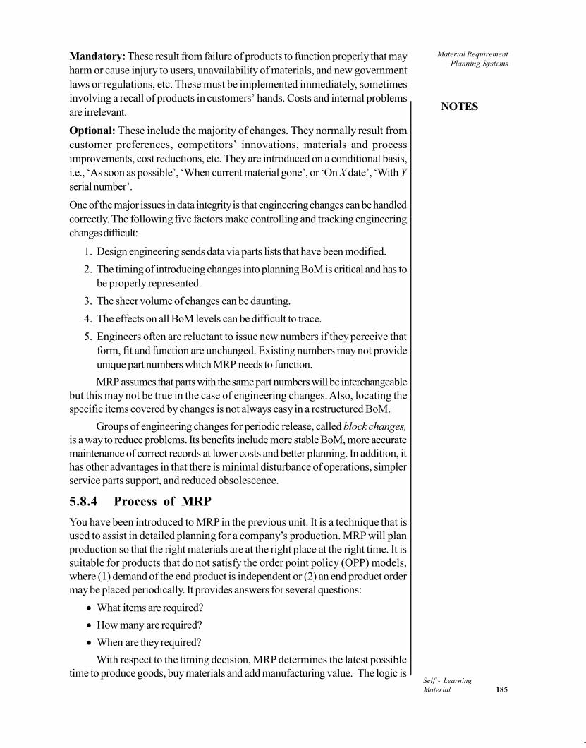
Material RequirementPlanning Systems
NOTES
Self - LearningMaterial 185
Mandatory: These result from failure of products to function properly that mayharm or cause injury to users, unavailability of materials, and new governmentlaws or regulations, etc. These must be implemented immediately, sometimesinvolving a recall of products in customers’ hands. Costs and internal problemsare irrelevant.
Optional: These include the majority of changes. They normally result fromcustomer preferences, competitors’ innovations, materials and processimprovements, cost reductions, etc. They are introduced on a conditional basis,i.e., ‘As soon as possible’, ‘When current material gone’, or ‘On X date’, ‘With Yserial number’.
One of the major issues in data integrity is that engineering changes can be handledcorrectly. The following five factors make controlling and tracking engineeringchanges difficult:
1. Design engineering sends data via parts lists that have been modified.
2. The timing of introducing changes into planning BoM is critical and has tobe properly represented.
3. The sheer volume of changes can be daunting.
4. The effects on all BoM levels can be difficult to trace.
5. Engineers often are reluctant to issue new numbers if they perceive thatform, fit and function are unchanged. Existing numbers may not provideunique part numbers which MRP needs to function.
MRP assumes that parts with the same part numbers will be interchangeablebut this may not be true in the case of engineering changes. Also, locating thespecific items covered by changes is not always easy in a restructured BoM.
Groups of engineering changes for periodic release, called block changes,is a way to reduce problems. Its benefits include more stable BoM, more accuratemaintenance of correct records at lower costs and better planning. In addition, ithas other advantages in that there is minimal disturbance of operations, simplerservice parts support, and reduced obsolescence.
5.8.4 Process of MRP
You have been introduced to MRP in the previous unit. It is a technique that isused to assist in detailed planning for a company’s production. MRP will planproduction so that the right materials are at the right place at the right time. It issuitable for products that do not satisfy the order point policy (OPP) models,where (1) demand of the end product is independent or (2) an end product ordermay be placed periodically. It provides answers for several questions:
What items are required?
How many are required?
When are they required?
With respect to the timing decision, MRP determines the latest possibletime to produce goods, buy materials and add manufacturing value. The logic is

Material RequirementPlanning Systems
NOTES
Self - Learning186 Material
to order as late as possible, but without the risk of a stockout. The driving principlein MRP is never order before you need to, never plan to stockout. Proper materialrequirements planning can keep cash in the firm and still fulfil all production demands.
In order to meet the requirements that the principle above imposes, there are anumber of assumptions that are fundamental to all MRP models. In addition, thereare also prerequisites that ensure that the assumptions provide the necessaryoptimum outputs. These are discussed as follows:
Prerequisites: MRP is the single most powerful tool in guiding inventory planning,purchase management and production control. MRP is easy to operate and addsdramatically to profits.
However, in order to develop an MRP model that works, there are someprerequisites. The principal prerequisites for a standard MRP system are as follows.
1. A master production schedule exists and can be stated in the bill of materialsform.
2. All inventory items are uniquely identified.
3. A bill of material exists at the time of planning.
4. Inventory records contain data on the status of every item.
5. Data integrity is maintained, file data is accurate, complete, and up-to-date.
The importance of these requirements needs to be emphasized in view ofthe implementation problems that MRP systems often face.
Assumptions: In addition, in building MRP models process independence ofmanufactured items is ensured by certain requirements regarding inventories. TheMRP system models make a number of assumptions, some explicit and someimplicit. It assumes that:
Every inventory item moves into and out of stock, i.e., there will be reportablereceipts, following which the item will be in an ‘on-hand’ state and willeventually be disbursed to support an order for an item into which it ismerged. This dictates the need for tracking and recording the movement ofitems into and out of stores.
Lead times for all inventory items are known and can be supplied to thesystem, at least as estimates. Planned lead times are supplied by plannersand normally have fixed values, but these can be changed. More than onevalue cannot be used simultaneously for an item, but a programmemodification can be made to alert planners to orders coming up for releasein some predetermined time period. Lead times of individual items are usedin calculating the timing of release dates from scheduled completion datesfor planned orders. MRP assumes that a component-item order must becompleted, at the latest, in the period containing the parent-item requirementthat needs it.
All components of an assembly must be available at the time an order forthat assembly is to be released to the factory. It is assumed that all componentsof an assembly are needed at the time an assembly order is released. This isbecause as the assembly lead time is relatively short, all the components will

Material RequirementPlanning Systems
NOTES
Self - LearningMaterial 187
be needed simultaneously. In cases of significant exceptions to this rule,where it may take several weeks to assemble a unit and expensivecomponents are required over this period, standard MRP procedures needto be modified.
Components and materials are discretely disbursed and used. For example,if 100 units of a component are required for a given work or assemblyorder, MRP expects that exactly 100 units will be disbursed and used. Inthe case of materials that come in continuous form (rolls of sheet metal,etc.) the standard planning procedures are modified and the system adoptedto handle such inventory items properly. There is a problem in MRP inrecognizing that excess material issued may still be available for use in otherorders but is no longer in the normal stock area. Making adjustments isquite complicated.
The process is independent, i.e., a manufacturing order for any given inventoryitem can be started and completed on its own and not be contingent on theexistence or progress, of some other order for completing the process.Thus, ‘mating part’ relationships and set-up dependencies do not fit thescheme of MRP. The common solution to this problem is to include ‘runwith’ codes in each items’ records. Lot-sizing techniques are often modifiedto ensure that items in such families come up for ordering at about the sametime.
The requirement of independence is basic to the development of the MRPsystem and has to be incorporated in the inventory items in the records. Theassumption of process independence means that any given inventory item can bestarted and completed on its own and not be contingent on the existence or progress,of some other order for completing the process. Thus, ‘mating part’ relationshipsand ‘set-up dependencies’ in a manufacturing order are not acceptable in theinventory records. Any exception requires system modification. Clever applicationsof lot sizing are often used to tackle this issue.
5.8.5 Output of MRP
MRP is basically a planning tool. It coordinates orders within the plant and fromoutside, i.e., both purchase orders and jobs. It focuses on scheduling purchaseorders and jobs to satisfy the material requirements generated by external demand.In doing so, MRP programmes operate on three separate levels:
1. Planning and controlling inventories
2. Planning open-order priorities
3. Providing inputs to capacity requirements planning
Operating at three levels is necessary because MRP programmes requireboth production and inventory information in order to produce their primary outputs.The outputs are schedules or plans for orders, both released and pending, andidentifying orders that are to be expedited or de-expedited.
MRP computes the schedules of what should be started into the line basedon demand. It takes action when supply exceeds demand by rescheduling orcancelling planned orders. In addition, it also generates messages suggesting de-

Material RequirementPlanning Systems
NOTES
Self - Learning188 Material
expediting or cancelling open orders. However, if demand exceeds supply, thenMRP reschedules or creates planned orders and generates messages suggestingwhere orders should be expedited, or it creates new orders. With these outputs, itspecifies the actions to be taken currently and in the future to maintain an efficientproduction/inventory management system.
When MRP programmes are properly designed, implemented and used, theyoperate on these different levels to make MRP a highly effective tool formanufacturing inventory management. The effectiveness of MRP follows from thebenefits that accrue from its actions. Some of the benefits are as follows:
1. Inventory investment can be held to a minimum.
2. Planning is change-sensitive and reactive.
3. MRP provides future data on an item-by-item basis.
4. Inventory control is proactive, not reactive.
5. Order quantities are related to requirements.
6. MRP focuses on the timing of requirements and order actions.
It deals with two basic dimensions of production control: quantity and timing.The system determines the appropriate production quantities of all types of items– from the final products that are sold to the inputs that are purchased as rawmaterial. Production timing is determined to ensure that order due dates are met.
Because MRP is a push system, its focus is on timing. This enables it to dowhat none of the earlier inventory management systems could do. It generatesoutputs that serve as valid inputs for other manufacturing logistics programmes,including purchasing, scheduling at the shop floor level, despatching and activitycontrol, and capacity requirements planning.
MRP triggers activities and can be viewed as the upstream system ofmanufacturing activities. It is involved in the procurement of material and theirconversion into a shippable product. This assists it in planning operations inproduction. It is only after inventory planning initiates purchase requisitions andshop orders that procurement and manufacturing can be carried out.
The principal outputs of inventory planning are purchase requisitions andshop orders, each calling for a specific quantity of some item by a date. Theefficacy of MRP depends on its ability to suggest ordering the right items in theright quantities at the right time for delivery on the right date. To make this happen,it issues action calls according to a detailed time-phased plan that it develops.
It keeps this plan up-to-date by re-evaluating and revising the plan periodicallyin response to changes in the environment. It continuously monitors and adjusts allthe open-order due dates, automatically reacting to the changes in the environment.When MRP provides sound inputs with valid capacity constraints, downstreamplanning and execution programmes can function effectively; if the outputs are notsound, it has a negative impact on downstream planning and execution.
A major criticism of MRP programmes is that they ignore capacity constraintsand often plan the production of items for which capacity is inadequate. This criticismis based on a partial understanding of the basic function of MRP programmes. MRPanswers the question, ‘what should be produced to support MPS?’ MRP experts

Material RequirementPlanning Systems
NOTES
Self - LearningMaterial 189
believe that programmes can be designed to answer either the question of what canbe produced with the existing capacity or what should be produced to supportMPS. If programmes try to do too much by answering both the questions, thecomplexity of the logic defeats the very purpose for which MRP has been created.
As MRP is designed to show what has to be done in order to execute theMPS plan, it implicitly trusts MPS. The capacity planned is based on the capacityconstraints in the MPS. The validity of the outputs from MRP, therefore, isdetermined to a large degree by the MPS contents. In other words, invalid MPSguarantee invalid MRP outputs.
In addition, as has been discussed earlier, invalid MRP outputs can also becaused by bad data in BoM, inventory, lead time and activity-reporting files. Itneeds to be emphasized very strongly that the success of MRP depends both onthe validity of the MPS as well as the quality of the data it uses.
5.9 INTRODUCTION TO MRPII SYSTEMS
MRP is an essential element of sound planning and control and an integral part ofthe process of improving manufacturing capabilities. The logic of MRP is based onthe fundamental logic of manufacturing. MRP, as the central technique in the coresystem, provides the industry the tools in creating world-class performance. Inthat sense, there is no substitute for MRP.
As the purpose of manufacturing inventory is to satisfy productionrequirements, the production plan is the source of demand, and therefore, MRP isan integral part of manufacturing. Specifically, the function of an MRP is to translatethe master production schedule into detailed component material requirementsand orders, based on the inventory. The system determines item by item, what isto be processed and when, as well as what is to be manufactured and when. Thisis based on order priorities and available capacities.
Supplier-customer relations are changing radically and rapidly. Instead oftransactional, antagonistic arm’s length, and formal dealings, both parties are seeingthe benefits of collaboration and alliances. Relationships are increasingly transformingto long-term partnership arrangements. This is reflected in the numbers of suppliersfor each class of materials being drastically reduced; buyers certify a single sourcefor many categories, examining closely the supplier’s operations and capability ofclose teamwork. Contracts are signed covering long periods, specifying aggregatedemands on the supplier’s capacity for families of similar items, and setting priceson individual items. Orders are released at the contract rate for individual itemsand delivered in small quantities in short lead times.
These developments have had their impact on MRP. As a matter of fact,MRP has— to a large degree—made many of these developments possible. Thegrowth of computer capabilities to handle material requirements has made it easyfor organizations to look at the entire flow of both the incoming materials and theoutgoing finished goods as a system. MRP planners have, through the MRP logicand the developments in IT, made it possible to handle all communications with
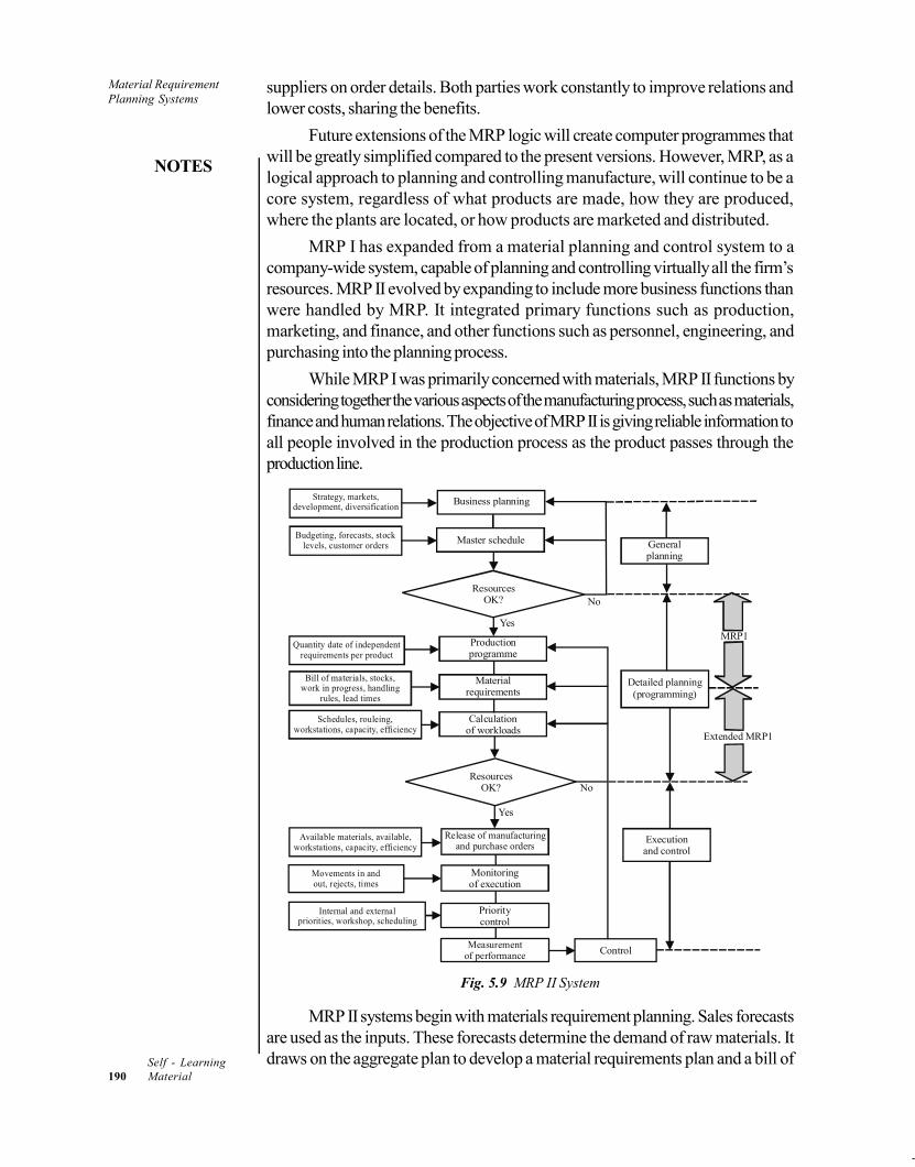
Material RequirementPlanning Systems
NOTES
Self - Learning190 Material
suppliers on order details. Both parties work constantly to improve relations andlower costs, sharing the benefits.
Future extensions of the MRP logic will create computer programmes thatwill be greatly simplified compared to the present versions. However, MRP, as alogical approach to planning and controlling manufacture, will continue to be acore system, regardless of what products are made, how they are produced,where the plants are located, or how products are marketed and distributed.
MRP I has expanded from a material planning and control system to acompany-wide system, capable of planning and controlling virtually all the firm’sresources. MRP II evolved by expanding to include more business functions thanwere handled by MRP. It integrated primary functions such as production,marketing, and finance, and other functions such as personnel, engineering, andpurchasing into the planning process.
While MRP I was primarily concerned with materials, MRP II functions byconsidering together the various aspects of the manufacturing process, such as materials,finance and human relations. The objective of MRP II is giving reliable information toall people involved in the production process as the product passes through theproduction line.
Strategy, markets,development, diversification
Business planning
Budgeting, forecasts, stocklevels, customer orders
Quantity date of independentrequirements per product
Bill of materials, stocks,work in progress, handling
rules, lead times
Schedules, rouleing,workstations, capacity, efficiency
Available materials, available,workstations, capacity, efficiency
Movements in andout, rejects, times
Internal and externalpriorities, workshop, scheduling
Master schedule
ResourcesOK?
Generalplanning
No
Yes
Productionprogramme
Materialrequirements
Calculationof workloads
ResourcesOK?
Detailed planning(programming)
No
Yes
Release of manufacturingand purchase orders
Monitoringof execution
Prioritycontrol
Measurementof performance Control
Executionand control
Extended MRP1
MRP1
Fig. 5.9 MRP II System
MRP II systems begin with materials requirement planning. Sales forecastsare used as the inputs. These forecasts determine the demand of raw materials. Itdraws on the aggregate plan to develop a material requirements plan and a bill of

Material RequirementPlanning Systems
NOTES
Self - LearningMaterial 191
materials for each product, and a set of time-phased shop orders providing alabour and machine schedule. For accounting and finance, it provides data aboutthe cost of production, including machine time, labour time, materials used, andfinal production numbers. An overview of MRP II is provided in Figure 5.9
Almost every MRP II system is modular in construction. It has three levels:
Planning— MRP, CRP
Execution— Process modelling, inventory, logistics
Analysis—Costing, financial payables, receivables, ledger systems
The extended applications of MRP II depend upon the modules chosen by theorganization. Characteristic basic modules in an MRP II system are:
Master Production Scheduling (MPS)
Item Master Data (Technical Data)
Bill of Materials (BOM) (Technical Data)
Production Resources Data (Manufacturing Technical Data)
Inventories and Orders (Inventory Control)
Purchasing Management
Material Requirements Planning (MRP)
Shop Floor Control (SFC)
Capacity Requirements Planning (CRP)
Standard Costing (Cost Control)
Cost Reporting/Management (Cost Control)
Distribution Resource Planning (DRP)
Data generated from all of these modules are utilized together by theMRP II in arriving at the result or information. Since MRP II is a free softwaresystem without any proprietary issues, it can be modified according to individualorganization requirement. Thus, it is also available now as purchased/licensed orin-house software.
The benefits of this type of system affect both marketing and logistics. The majormarketing benefits are:
1. Improved service levels to increase on-time deliveries
2. Improved and more effective promotional and new-product introductionplans
3. Improved ability to anticipate shortages
4. Improved inventory coordination with other enterprise functions
5. Enhanced ability to offer customers a coordinated inventory managementservice
The major logistics benefits are:
1. Reduced distribution centre freight costs due to coordinated shipments
2. Reduced inventory levels

Material RequirementPlanning Systems
NOTES
Self - Learning192 Material
3. Decreased warehouse space requirements (because of inventory reductions)
4. Reduced customer freight cost as a result of fewer backorders
5. Improved coordination between logistics and manufacturing
6. Enhanced budgeting capability, since DRP can effectively simulate inventoryand transportation requirements under multiple planning scenarios
Today, most manufacturing industries are equipped with MRP II systems.Up till 1998, around 70 per cent of Fortune 1000 companies had installed MRP IIsoftware systems. By 1999, this number had increased to 90 percent. However,the requirements of different industries may be different and systems have to becustomized to these requirements. For instance, some industries such aspharmaceuticals or food need specialized functions, e.g., lot traceability in regulatedmanufacturing. Other industries may not need complex materials planning.
MRP logic has also extended to managing finished inventories and distribution.Distribution involves a number of activities centred on the physical flow of goodsand information. The distribution system, therefore, is the physical link betweensuppliers and customers. This system is known as Distribution Requirement Planning(DRP) and is used for planning of distribution networks.
Traditional MRP, DRP, DRP II and MRP II applications evolved into present-day ERP, which is more capable of meeting manufacturers’ challenges in thegeneration of value chain. Thus, a key difference between MRP II and ERP is thatwhile MRP II has traditionally focused on the planning and scheduling of internalresources, ERP strives to plan and schedule supplier resources as well, based onthe dynamic customer demands and schedules.
Implementation Benefits
The benefits associated with the successful implementation of MRP I, MRP II,ERP, DRP I and DRP II systems can be measured both in terms of enhancedperformances and user satisfaction. Some of the benefits are as follows:
Increased information on which to base decisions
Better ability to meet volume/product changes
Better cost estimation
Reduced ‘expediting’ costs and delivery lead times
Better capacity planning and production scheduling, increasing throughputand ability to meet delivery promises
Reduced manpower costs by reduction of overtime
Better product customization
Improved coordination between functions, especially with finance, marketingand sales departments
Improved product quality and scrap reduction

Material RequirementPlanning Systems
NOTES
Self - LearningMaterial 193
Table 5.13 summarizes a study on the adoption of new technology-supportedinventory initiative of world class companies, conducted by the Aberdeen Groupin 2004. It shows that 10-17 per cent of the companies surveyed reported greaterthan 20 per cent improvements in key cost and service metrics from their inventoryinitiatives.
More and more companies are trying to reduce inventory across the totalextended supply chain, while a lesser number are trying to minimize their costs bypushing inventory responsibilities to their suppliers or monitoring and managinginventory at a local level. 38 per cent companies try to minimize inventory at thelocal level, but compared to firms that try to reduce inventory across the supplychain, they are half as likely to have below-average inventory carrying costs astheir industry peers.
Table 5.13 Impact of Technology-Supported Inventory Control Processes
ReducedInventoryCarrying Costs
ReducedInventoryObsolescenceCosts
Reduced LeadTimes toCustomers
Increased Per-fect Order %(On Time andComplete) toCustomers
0-5%Improvement
6-10%Improvement
11-12%Improvement
More than 20%Improvement
26% 34% 40% 37%
38% 32% 28% 26%
26% 18% *5% 2*%
10% 15% *7% 14
* Percentage of respondents achieving improvement level from their latest supply than inventory initiative
The benefits in using MRP I, MRP II and ERP systems for throughputplanning, cost information (inventory), time performance (i.e., lead times) andorganizational achievements (i.e., coordination), finally result in improvedproductivity and lower costs for the entire supply chain.
However, there are some essential requirements for all these systems toprovide benefits. These include a realistic and accurate forecast, an accurateincoming and ongoing unit demand schedule, an accurate inventory control systemand an accurate bill of materials, timely generation of exception and reschedulingreports, and finally the human element— employees must be properly educated,receptive and committed to the system in order to fully realize the potential of theinvestment.
Check Your Progress
12. What is a lot size?
13. How has MRP II evolved from MRP I?

Material RequirementPlanning Systems
NOTES
Self - Learning194 Material
5.10 USING DISTRIBUTION RESOURCEPLANNING TO MANAGE INVENTORIES INMULTIPLE LOCATIONS
There are three structures that combine to form the distribution channel from themanufacturer to the customer. The structure at one end of the channel is themanufacturer. The manufacturer is responsible for the development and productionof products goods. The end structure is the retailer who sells goods and servicesdirectly to the customer. In between the two lies, a process called distribution,which originates at the manufacturer’s end and connects to the retailer.
Distribution involves a number of activities centered on the physical flow of goodsand information. The distribution system, therefore, is the physical link betweensuppliers and customers. One of the major issues in controlling finished goodsinventory is an optimal distribution network that is intelligently designed to minimizecosts by providing the customer the right goods, in the right quantity, at the rightplace, and at right time. In order to meet the customer and service requirementssuccessfully, the distribution system can have several distinct levels. Inventory maybe maintained for distribution to customers in all or any combination of theselevels:
Supplier’s facility/ factory
In transit
Regional warehouses
Distribution centers/ depots, and
Customer’s facility/ retailers
These levels of a typical distribution chain are shown in Figure 5.10, which showsthe flow of finished goods through these levels. The figure illustrates a very simpleand basic distribution network.
In transit
Fig. 5.10 Finished Goods Distribution Network
The factory supplies the finished goods to the regional warehouses. Thesemay be owned by the manufacturer or by its distributors. The distributors, in turn,send the finished goods to the depots, which they may run themselves or are run

Material RequirementPlanning Systems
NOTES
Self - LearningMaterial 195
by the wholesalers. Distributors and wholesalers provide goods to differentcategories of retailers.
The different categories of retailers are differentiated on how they combinedifferent decisions regarding location, assortment, selection of target markets, etc.In descending order of product support, the retail outlets are turnkey, specialtyshops, discount shops, and mail order. The retail decision, therefore, entails atrade-off between price and service.
Turnkey operations obtain finished goods from an assemble-to-orderproducer. It delivers material to the user, sets it up, and ensures it is workingproperly. A specialty shop is a retailer of one type of item, such as men’s or women’sclothing, sporting goods, jewelry, and so on. A discount shop is a retailer carryinga very broad line of products that competes by offering lower prices. For itemsthat are small enough to be mailed or shipped by common carrier, mail order is anincreasingly popular alternative.
In real life distribution networks are quite complex. For example, HindustanUnilever Ltd. (HUL) is the market leader in the detergent and soap industry. HULhas about 130 brands and over 1,200 SKUs in its portfolio and 7,000 stockistsfilling up shelves in over one million retail outlets. HUL has 100 factories, 13 salesbranches and 121 warehouse depots, along with 93 third-party manufacturingsites, all of which constitute its distribution network. Each of these entities providesHUL with data that is used in the company’s planning the distribution system aswell as the flow of its products to the customer.
Distribution systems store large amounts of materials for rapid delivery to acustomer to buffer inflexible production systems that were incapable of makingthe swift adjustments required to keep pace with rapidly changing customer needs.Each of the above may receive finished goods from a central or regional warehouse.Therefore, considering the extensive distribution network that is characteristic ofall finished goods, the distribution between stocking points within the distributionchain becomes a critical decision variable.
An optimal policy to manage finished goods allows companies to achievehigher profitability levels. In general terms, policies should be aimed at loweringthe holding costs through higher inventory rotation, but without triggering substantialstock-outs and backorders, caused by demand peaks and/or lead time delays.An organization must choose distribution outlets and design the field support system.The distribution system choice affects several inventory and product support issues.
Finished goods inventory is finally a trade-off between inventory costs andschedule stability, once the decisions on the distribution network are firmed up.Therefore, the goal of finished goods inventory is to manage inventory levels so asto minimize costs deriving from holding inventory and from adjustment to the masterproduction schedule (MPS) to prevent stock-outs.
As mentioned previously, as the number of distribution points increase, thereis an increase in the average inventory held by the firm. The firm has little controlon the inventory in transit, but safety stock can be reduced if the correspondingun-certainty in supply is reduced. This mean that demand variability is a keydeterminant of safety stock. To achieve a high customer service level stock mustbe held as a buffer against this variability in demand. Therefore, inventory

Material RequirementPlanning Systems
NOTES
Self - Learning196 Material
management becomes a struggle to minimize investment in inventory while fillingevery customer order on time. This places a premium on the use of accuratedemand forecasting techniques.
In real life applications, demand distribution is a priori, that is, it seldomknown accurately. Customer demand for finished goods is variable andunpredictable. In FMCG, the situation is further complicated by frequent salespromotions which are commonplace. Often, the information flows do not providesufficient advance warning of a promotion, thus causing further difficulties with aplanned buildup of stock. These increase the variability in demand thus makingprediction much more difficult.
It is highly important for companies to increase service levels withoutincreasing inventory investment. Because the amount of inventory needed to meetservice levels is directly related to lead times and variability, reducing lead timesand supply chain variability is also highly important.
The problem of variable demand is compounded by the fact that there isusually a variable lead time associated with delivery from production. A big costin production is lost production due to resetting machines and changing products.Consequently, in most production shops, reducing manufacturing costs is achievedby planning long production runs which minimize changeover time. This enhancesthe variable lead time associated with delivery from production. Often, productiondoes not provide sufficient advance warning of scheduled maintenance. Therefore,matching finished goods quantities becomes difficult. Goods arrive in larger orsmaller than requested quantities and in a sequence that may not match the salesforecast.
In addition, the uncertainty of the future and unpredictability demand andlead time, and the lack of precision in forecasting need to be resolved. This is notonly a cost but also a risk to the firm. In order to reduce the uncertainty, theorganization has to realize that these uncertainties exist and also find means tounderstand how their impact on the business can be minimized.
The most commonly used method is an extended application of MRPsystems. This method is known as Distribution Requirement Planning (DRP). Thistechnique is used for planning of distribution networks. DRP emerged as a majortool during the 1970s. By the 1980s DRP had become a standard approach forplanning and controlling distribution logistics activities. The concept was extendedto embrace all business functions in the supply channel renamed distribution resourceplanning (DRP II). DRP II is widely used not just for inventory and logistics, buta number of other functions required to minimize inventories.
Distribution resource planning provides a framework for determining the need toreplenish inventory by:
Linking market requirements with manufacturing and demand management
Relating current inventory positions and demand forecasts to productionscheduling, and
Matching material supply to manufacturing demand, and customer demandto product supply

Material RequirementPlanning Systems
NOTES
Self - LearningMaterial 197
The logic of DRP very closely resembles the logic of MRP systems. Distributionnetworks in the retail business consist of a network of outlets, distribution centersand warehouses. Regional warehouses are fed by a national distribution center,and the regional centers feed the regional outlets, and these feed the distributionchains at the local level. However, DRP needs the following information:
Demand in a future time period.
Scheduled receipts at the beginning of a time period.
Safety stock requirement for a period.
On-hand inventory at the beginning of a period.
By thinking of each level in the distribution network as a level in a bill ofmaterials, the gross requirements are first calculated. Orders or forecasted demand,or some combination of both are used to arrive at the numbers. If orders are used,orders placed by the distribution points will generate gross requirements at thedifferent levels in the network, from local to regional and finally national. Thisstructure is captured in the DRP for determining finished goods requirement.
The scheduled receipts are the goods the distributor expects to receivefrom orders that already have been released. On-hand inventory balance constitutesthe goods that already are received and entered into inventory. By subtractingscheduled receipts and on-hand inventory from gross requirements the programmedetermines the net requirements. Based upon the distributor’s lot-sizing policyand receiving behavior, planned order receipts and capacity planning are generated.
You define all nodes in the network including plants, distribution centers(DCs), warehouses, and stock transfer points. You set up the material masterrecord for each node. In MRP 4 of the material master record, you must definethe deployment strategy for each material (the fair and push distribution options)as well as deployment horizon (push horizon). For the push horizon, you need toenter the number of days for which the system considers the available to deploy(ATD) quantity and any additional quantity produced. Any quantity producedbeyond the push horizon is not considered in the deployment calculation.
You create a forecast for each DC, for example, sales forecast, and transferthe forecasted data to Demand Management. The system creates independentrequirements. You can then perform a DRP run in each DC and in each supplyingplant. The DRP run considers the quota arrangements defined in the network,available stock, sales orders, and independent requirements.
The DRP run in the DCs creates releases for stock transport requisitions inthe supplying plants and planned orders for production. These are then convertedto production orders for manufacturing.
Table 5.14 describes some of the important DRP key figures. How these keyfigures are calculated is given below:
Independent requirements are calculated for each distribution center usingstatistical forecasting. The programme has a tool for this. Alternatively, youcan manually create the independent requirements.

Material RequirementPlanning Systems
NOTES
Self - Learning198 Material
Sales orders are obtained from the sales force.
The demand fence in the MRP is defined by the user. The demand fence isrepresented in days and indicates the time during which certain demandtypes contribute to the demand key figure. Beyond the demand horizon,the maximum value of the sales order and the forecast is taken as the demand.
For the selection of demand types within the demand fence, you define achecking group and a checking rule for the demand key figures.
The system calculates the on-hand stock using the initial stock (stock of theprevious day) plus the in transit stock of the current day minus the demandof the current day.
The system calculates the target stock level by taking the sum of the forecastwithin the safety time (in this example, three days) plus the safety stock forthe current day.
The system calculates the safety stock automatically and stores it in thematerial master record.
Table 5.14 DRP Key Figures
The system calculates the replenishment orders by adding the target stocklevel to the demand and subtracting the initial stock. As should be apparent, DRPenables the user to set certain inventory control parameters (like a safety stock)and calculate the time-phased inventory requirements.
DRP is usually used with an MRP system, although most DRP models aremore comprehensive than stand-alone MRP models and can scheduletransportation. The underlying rationale for DRP is to more accurately forecastdemand and then use that information to develop delivery schedules. This way,distribution firms can minimize inbound inventory by using MRP in conjunctionwith other schedules.
For example, Hindustan Lever (HUL) ERP module includes a distributionresource planning (DRP) module which integrates manufacturing and distributionoperations. Distribution centers give the demand to the factories. The DRP modulehelps Lever to compute demand dynamically based on daily sales orders. Forwardsales orders likewise provide the basis for a dynamic calculation of inventorynorms at the company’s regional and local distribution centers.

Material RequirementPlanning Systems
NOTES
Self - LearningMaterial 199
The system has helped HUL workflow automation of the supply chain. Ithandles exceptions involving dispatching, a wide range of truck capacities, lead-time variances, and changes in both demand and sourcing. These have helped itminimize inventory levels.
The planning cycle of HUL used to be monthly, and this has now becomedaily. The improved planning has resulted in significant inventory reduction. Forexample, the stock levels in the detergent business alone dropped from 105,000tons to less than 55,000 tons. Measured in days, stock levels fell from six weeksof sales to less than three weeks. The volume of finished goods languishing indistribution centers fell from three weeks to less than one week. In the factories,HUL now keeps a one-day inventory, while at the buffer depot it is four to fivedays. Supplier inventory levels are at three days, down from the previous sevendays.
DRP calculates requirements into the future by taking current inventory,adding shipments that are already on the way, and subtracting expected demand.Whenever the projected inventory drops below the desired safety stock level, itcalculates the desired shipment date from the plant based on the desired arrivaltime.
This simple replenishment and shipment logic of traditional DRP are oftennot sufficient in the real world situation. Firstly, DRP ignores costs. Secondly,limitations of the real world exist that prevent the ideal plan from becoming reality.For example, plants have limited production capacity, warehouses have limitedfloor space, shipping docks can only unload a certain number of trucks per hour,and truck availability may limit the timely movement of product. Finally, the problemof distribution is much more complicated than reflected in most DRP modules.Due to these limitations and constraints, DRP often produces non-feasible plans.New systems using dynamic distribution logic are being developed to overcomethese shortcomings.
Check Your Progress
14. What is the manufacturer responsible for?
15. How does distribution resource planning replenish the inventory?
5.11 ANSWERS TO ‘CHECK YOUR PROGRESS’
1. An MRP system is meant for simultaneously meeting the following threeobjectives:
Planning purchasing activities, delivery schedules and manufacturingactivities
Maintaining the lowest possible level of inventory.
Ensuring the availability of products and material for production anddelivery to customers
2. Disadvantage of MRP includes high implementation costs.

Material RequirementPlanning Systems
NOTES
Self - Learning200 Material
3. Data management is defined as the development and execution ofarchitectures, policies, practices and procedures that properly manage thefull data life cycle needs of an enterprise.
4. The two classes of data on which computer programmes operate are:i. Data input by transactionsii. Data in files
5. There are two types of transactions: (a) external inventory transactions,and (b) internal transactions.
6. This is necessary as there are often overruns in production, customer returnsor spare-part demands for such assemblies, none of which can be ruledout.
7. The term bill of material structure refers to the arrangement of parentsand components within the BoM file.
8. BoM is the framework on which the entire planning process of the MRPdepends.
9. The two schedules to which the modularized BoM is assigned are:(a) The master production schedule, by making it part of the planning
BoM(b) The final assembly schedule, by putting it in the manufacturing BoM
when needed for execution
10. MPS can be defined as the overall plans of production of amanufacturing unit.
11. The link between MPS and the component BOM is known as scheduleinterface.
12. Lot size is the amount produced for each machine set-up.
13. MRP II evolved by expanding to include more business functions than werehandled by MRP. It integrated primary functions such as production,marketing, and finance, and other functions such as personnel, engineering,and purchasing into the planning process.
14. The manufacturer is responsible for the development and production ofgoods.
15. Distribution resource planning provides a framework for determining theneed to replenish inventory by:
i. Linking market requirements with manufacturing and demandmanagement
ii. Relating current inventory positions and demand forecasts toproduction scheduling, and
iii. Matching material supply to manufacturing demand, and customerdemand to product supply

Material RequirementPlanning Systems
NOTES
Self - LearningMaterial 201
5.12 SUMMARY
Given the rapid development of computers, the idea of using computersand software technology to manage information was the vision that droveMRP (the computerized system was called MRP I).
It was conceived as a system for centralizing and integrating manufacturinginformation to facilitate decision-making for production planning, and toincrease the efficiency of the overall production line, using the computingpower of the computer to help in this process.
An MRP system is meant for simultaneously meeting the following threeobjectives:
o Planning purchasing activities, delivery schedules and manufacturingactivities
o Maintaining the lowest possible level of inventory.
o Ensuring the availability of products and material for production anddelivery to customers
MRP systems are usually deemed proactive. Some of the benefits offeredby MRP are compatibility with other supply chain systems such astransportation planning and DRP, enhanced customer service and inventoryreduction. MRP works better than conventional order point systems in caseswhere supply chain integration is viable.
Order point systems are deemed reactive, because of the lack of mechanismsfor anticipating demand changes and because average information is oftenused by them for making replenishment decisions. It is this that sometimesresults in inadequate performance in situations where demand tends to behighly fluctuating.
It is believed that this superior performance results from the ability of MRPto anticipate demand changes in the supply chain on the basis of forecastinformation and to anticipate future requirements and release time-phasedorders accordingly.
It must be remembered that there are certain disadvantages to MRP. Someof these disadvantages include high implementation costs, the necessity datato be accessible throughout the supply chain and highly uncertainenvironments resulting from system nervousness.
Data is the lifeblood of an organization and a valuable enterprise asset. Itprovides the foundation on which companies base critical and everydaybusiness decisions. Competitive success, to a large extent, depends onoptimized, integrated data management functions so that decision-makers canaccess quality data to operate confidently in a high-performance environment.
With the introduction of computers in business operations, management ofdata systems started as a sub-discipline of computer science. It has now

Material RequirementPlanning Systems
NOTES
Self - Learning202 Material
matured into a major field of management. It is used to eliminate or minimizedata duplication, redundancy, different file ’versions’, and different updatecycles and optimizing file access and economy of use.
Quality lies in these attributes of file-record data, which have to bedemonstrated in the two classes of data on which computer programmesoperate:
o Data input by transactions
o Data in files
Data file management functions consist of:
o File creation
o File organization
o File access
o File updating (transaction processing)
o File maintenance (changes and corrections)
o Inquiry capability
o Report generation
There are several types of entries that are required for the programme toprocess and update inventory records. These are as follows:
o Inventory transactions
o User-controlled exceptions to regular processing logic
o Pseudo-transactions
o Final assembly schedule entries
o Error-correction entries
o File-maintenance entries
There are two types of transactions:(a) External inventory transactions, and(b) Internal transactions.
External inventory transactions are reported in the system. Internaltransactions are generated by the MRP system itself.
These transactions can have different impacts on the MRP system, whichcan be categorized into three different classes;
(a) External transactions affecting one record;(b) External transactions affecting multiple records,(c) Internal transactions affecting multiple records.
The bills of material (BoM) form the heart of the MRP system and are theframework on which the entire planning process depends. The BoMdefines the relationships of assemblies (parent items) and their components.
In a MRP system, the major roles of the BoM are as follows:a. Specifying how products are built, including added sub-assemblies
(options) and semi-finished items

Material RequirementPlanning Systems
NOTES
Self - LearningMaterial 203
b. Scheduling and assembly of products, sub-assemblies and componentsc. Identifying optional product features for improved forecastingd. Making order entry simple and easy by specifying customer
requirements accurately, including optionse. Stating the MPS in the fewest possible number of items
f. Planning subassembly priorities
g. Product costing
h. Efficient computer file storage and file maintenance
The term bill of material structure refers to the arrangement of parentsand components within the BoM file. In order to be useful for MRP, theBoM must be unambiguous and structured properly. MRP software usesthe structure to organize, load, maintain and retrieve BoM records. MRPdoes not have a role in creating the structure; which is basically a function ofdesign engineering.
In modularizing the bills of material, the end-item bills of material arerearranged grouping components into useful sets, with two differentobjectives:
1. Disentangling combinations of optional product features
2. Segregating components common to many parents from those uniqueto one parent or peculiar to some function
The objective of modularization is to have the smallest possible number ofitems to forecast and plan for in the master-schedule. A technique of creatingpseudo bills of material, also called superbills or S-bills is often used tomeet this objective. Pseudo bills are artificial entities created solely to facilitateplanning by reducing the number of items to be planned.
MPS serves the following purposes:
o It meets the demand for individual products in the product group. At thislevel of planning, product groups are disaggregated into individualproducts.
o It shows when incoming sales orders can be scheduled into production.
o It also shows when each shipment can be scheduled for delivery.
o It also takes into account current backlogs so that production and deliveryschedules are realistic.
o It generates the amounts and dates of specific items to be produced.
o MPS can be defined as the overall plans of production of amanufacturing unit.
o MPS represents the most important plan in the resource managementsystem. Effective schedules can improve on-time delivery, reduceinventory, cut lead time and improve the utilization of resources.
The process of translating aggregate plans into plans for individual productsis called desegregation. To generate the necessary details, planners

Material RequirementPlanning Systems
NOTES
Self - Learning204 Material
disaggregate the higher-level production plans and transform them into amore detailed schedule. A trial master schedule is developed. This is calledrough-cut capacity planning. The objective is to determine whetherapproximately enough capacity will be available to meet the MPS, withoutlaying undue emphasis on developing exact figures.
The link between MPS and the component BoM is called the scheduleinterface. The type of interface can be decided by the firm. Depending onthe conventions chosen, there are three options for choosing what thequantities represent:
o End-item gross requirements
o End-item production requirements
o End-item planned orders
The time-phased information contained in the inventory record consists of:
o Gross requirements
o Scheduled receipts
o Projected on-hand inventory
o Planned receipts
o Planned-order releases
The lot size is the amount produced for each machine set-up. There are anumber of lot-sizing methods, which determine the order quantities or thesize of the lot using different yardsticks. Lot size directly affects inventoryand scheduling.
MRP is basically a planning tool. It coordinates orders within the plant andfrom outside, i.e., both purchase orders and jobs. It focuses on schedulingpurchase orders and jobs to satisfy the material requirements generated byexternal demand. In doing so, MRP programmes operate on three separatelevels:
1. Planning and controlling inventories2. Planning open-order priorities3. Providing inputs to capacity requirements planning
MRP is an essential element of sound planning and control and an integralpart of the process of improving manufacturing capabilities. The logic ofMRP is based on the fundamental logic of manufacturing. MRP, as thecentral technique in the core system, provides the industry the tools increating world-class performance. In that sense, there is no substitute forMRP.
MRP II systems begin with materials requirement planning. Sales forecastsare used as the inputs. These forecasts determine the demand of raw materials.It draws on the aggregate plan to develop a material requirements plan anda bill of materials for each product, and a set of time-phased shop ordersproviding a labour and machine schedule.

Material RequirementPlanning Systems
NOTES
Self - LearningMaterial 205
Distribution resource planning provides a framework for determining theneed to replenish inventory by:
o Linking market requirements with manufacturing and demandmanagement
o Relating current inventory positions and demand forecasts to productionscheduling
o Matching material supply to manufacturing demand, and customerdemand to product supply
DRP is usually used with an MRP system, although most DRP models aremore comprehensive than stand-alone MRP models and can scheduletransportation. The underlying rationale for DRP is to more accuratelyforecast demand and then use that information to develop delivery schedules.This way, distribution firms can minimize inbound inventory by using MRPin conjunction with other schedules.
5.13 KEY TERMS
Data File: It is a set of records consisting of a number of fields of relevantdata.
Inventory Transaction: It refers to an event that changes the inventorystatus.
Bill of Materials Structure: It refers to the arrangement of parents andcomponents within the BoM file.
Phantom Items: These are intermediate products that never see thestockroom, i.e., they are manufactured and immediately consumed in theassembly of the parent items.
Pseudo Bills: These are artificial entities created solely to facilitate planningby reducing the number of items to be planned.
5.14 SELF-ASSESSMENT QUESTIONS ANDEXERCISES
Short-Answer Questions
1. What does the term material requirement planning mean?
2. State two advantages and two disadvantages of MRP.
3. Outline the difference between BoM and the M-bill.
4. What are some issues to be kept in mind before restructuring BoMs formodularity?
5. Write a short note on the pseudo bills of material.
6. How can the outputs of MRP be made useful?

Material RequirementPlanning Systems
NOTES
Self - Learning206 Material
7. What is a time-phased record? How are separate time-phased recordsestablished and maintained for every inventory item in MRP?
Long-Answer Questions
1. Write a detailed note on the manufacturing bills of material.
2. Explain modularization technique in detail.
4. Describe the ways a firm remove the inefficiencies in the traditional manualsystems which formed the historical basis of recording data in MRP systems.
5. ‘Unless the records are maintained and transactions updated properly, theinventory records in the MRP programme will be incorrect and MRP willbecome ineffective.’ Discuss with examples for different types of transactions.
6. How can modules in a modular BoM be combined in different ways toarrive at the right combination of models and options? Explain with anexample.
7. Discuss the structure of the bill of materials.
5.15 FURTHER READING
Zipkin, Paul Herbert. 2000. Foundations of Inventory Management. New Delhi:McGraw Hill.
Orlicky, Joseph and George Plossl. 1994. Orlicky’s Material RequirementPlanning. New Delhi: McGraw-Hill.
Seetharama L Narsimhan, Dennis WMcLeavy, Peter J Billington. 1994.Production Planning and Inventory Control. New Delhi: Prentice Hallof India Pvt Ltd.
J. R. Tony Arnold, Stephen N. Chapman. 2007. Introduction to MaterialsManagement. New Delhi: Prentice Hall.
Richard J. Tersine.1982. Principles of Inventory and Materials Management.New Delhi: Prentice Hall.

NOTES

NOTES