Optimal Control of Wave Energy Converters

Michigan Technological University Michigan Technological University

Digital Commons @ Michigan Tech Digital Commons @ Michigan Tech

Dissertations, Master's Theses and Master's Reports

2018

Optimal Control of Wave Energy Converters Optimal Control of Wave Energy Converters

Shangyan Zou MICHIGAN TECHNOLOGICAL UNIVERSITY, [email protected]

Copyright 2018 Shangyan Zou

Recommended Citation Recommended Citation Zou, Shangyan, "Optimal Control of Wave Energy Converters", Open Access Dissertation, Michigan Technological University, 2018. https://doi.org/10.37099/mtu.dc.etdr/702

Follow this and additional works at: https://digitalcommons.mtu.edu/etdr

Part of the Ocean Engineering Commons

http://www.mtu.edu/

http://www.mtu.edu/

https://digitalcommons.mtu.edu/

https://digitalcommons.mtu.edu/etdr

https://doi.org/10.37099/mtu.dc.etdr/702

https://digitalcommons.mtu.edu/etdr?utm_source=digitalcommons.mtu.edu%2Fetdr%2F702&utm_medium=PDF&utm_campaign=PDFCoverPages

http://network.bepress.com/hgg/discipline/302?utm_source=digitalcommons.mtu.edu%2Fetdr%2F702&utm_medium=PDF&utm_campaign=PDFCoverPages

OPTIMAL CONTROL OF WAVE ENERGY CONVERTERS

By

Shangyan Zou

A DISSERTATION

Submitted in partial fulfillment of the requirements for the degree of

DOCTOR OF PHILOSOPHY

In Mechanical Engineering-Engineering Mechanics

MICHIGAN TECHNOLOGICAL UNIVERSITY

2018

© 2018 Shangyan Zou

This dissertation has been approved in partial fulfillment of the requirements for

the Degree of DOCTOR OF PHILOSOPHY in Mechanical Engineering-Engineering

Mechanics.

Department of Mechanical Engineering-Engineering Mechanics

Dissertation Advisor: Dr. Ossama Abdelkhalik

Committee Member: Dr. Rush D. Robinett

Committee Member: Dr. Nina Mahmoudian

Committee Member: Dr. Wayne W. Weaver

Department Chair: Dr. William W. Predebon

Dedication

To my mother, father, and wife

Without your love, support, and encouragement, I would neither be who I am nor

would this work be what it is today.

To grandmother and grandfather

Who always believe me and expect me in completing this work.

To my advisor and teachers

Who guide, support and encourage me with your knowledge, patience, and quality.

To my colleagues and friends

Who help me and enrich my life.

Contents

List of Figures . . . . . . . . . . . . . . . . . . . . . . . . . . . . . . . . . xiii

List of Tables . . . . . . . . . . . . . . . . . . . . . . . . . . . . . . . . . . xvii

Preface . . . . . . . . . . . . . . . . . . . . . . . . . . . . . . . . . . . . . . xix

Acknowledgments . . . . . . . . . . . . . . . . . . . . . . . . . . . . . . . xxi

Definitions . . . . . . . . . . . . . . . . . . . . . . . . . . . . . . . . . . . . xxiii

Nomenclature . . . . . . . . . . . . . . . . . . . . . . . . . . . . . . . . . . xxv

Abstract . . . . . . . . . . . . . . . . . . . . . . . . . . . . . . . . . . . . . xxxv

1 Introduction . . . . . . . . . . . . . . . . . . . . . . . . . . . . . . . . . 1

1.1 Overview . . . . . . . . . . . . . . . . . . . . . . . . . . . . . . . . . 1

1.2 Optimal control of single-degree-of-freedom WEC . . . . . . . . . . 2

1.3 Optimal control of single body multi-degree-of-freedom WEC . . . . 4

1.4 Optimal control of the WEC array . . . . . . . . . . . . . . . . . . 5

1.4.1 The WEC array modeling and layout optimization . . . . . 5

vii

1.4.2 The optimal control of the WEC array . . . . . . . . . . . . 7

1.5 The Power take-off units . . . . . . . . . . . . . . . . . . . . . . . . 8

1.5.1 General Review . . . . . . . . . . . . . . . . . . . . . . . . . 8

1.5.2 Air Turbines . . . . . . . . . . . . . . . . . . . . . . . . . . . 8

1.5.3 Hydro Turbines . . . . . . . . . . . . . . . . . . . . . . . . . 9

1.5.4 Direct Drive system . . . . . . . . . . . . . . . . . . . . . . . 9

1.5.5 The hydraulic system . . . . . . . . . . . . . . . . . . . . . . 10

1.5.5.1 Constant pressure configuration . . . . . . . . . . . 11

1.5.5.2 Variable pressure . . . . . . . . . . . . . . . . . . . 12

1.5.5.3 Variable - Constant pressure . . . . . . . . . . . . . 13

2 Modeling of the Wave Energy Converters . . . . . . . . . . . . . . 14

2.1 Wave Model . . . . . . . . . . . . . . . . . . . . . . . . . . . . . . . 15

2.2 Single Body Heaving Wave Energy Converter . . . . . . . . . . . . 16

2.2.1 The Wave Excitation Force . . . . . . . . . . . . . . . . . . 18

2.2.1.1 The Wave Excitation Force: Pressure Accumulation 19

2.2.2 The Hydrostatic Restoring Force . . . . . . . . . . . . . . . 20

2.2.3 The Radiation Force . . . . . . . . . . . . . . . . . . . . . . 21

2.3 Single Body Pitching Wave Energy Converter . . . . . . . . . . . . 22

2.4 Single Body Three-Degree-of-Freedom WEC . . . . . . . . . . . . . 26

2.5 Wave Energy Converters Array . . . . . . . . . . . . . . . . . . . . 31

2.5.1 The WEC array surrogate model . . . . . . . . . . . . . . . 33

viii

2.5.2 The model identification . . . . . . . . . . . . . . . . . . . . 37

3 Optimal Control of Wave Energy Converters: Unconstrained con-

trol . . . . . . . . . . . . . . . . . . . . . . . . . . . . . . . . . . . . . . 39

3.1 Singular Arc Controller . . . . . . . . . . . . . . . . . . . . . . . . . 40

3.1.1 Singular Arc Controller for the Simplified WEC Models . . . 40

3.1.2 Singular Arc Control for the WEC Models with Radiation

States . . . . . . . . . . . . . . . . . . . . . . . . . . . . . . 43

3.2 Simple Model Control . . . . . . . . . . . . . . . . . . . . . . . . . 46

4 Optimal Control of Wave Energy Converters: Constrained con-

trol . . . . . . . . . . . . . . . . . . . . . . . . . . . . . . . . . . . . . . 49

4.1 Shape-Based Approach . . . . . . . . . . . . . . . . . . . . . . . . . 50

4.1.1 Shape-Based Approach for Simplified WEC Model . . . . . . 51

4.1.2 Shape-Based Approach for Higher-Order Model WEC Optimal

Control . . . . . . . . . . . . . . . . . . . . . . . . . . . . . 54

4.2 Pseudospectral Optimal Control . . . . . . . . . . . . . . . . . . . . 57

4.2.1 System Approximation Using Fourier Series . . . . . . . . . 57

4.2.2 Control Optimization for Linear Time-Invariant WECs . . . 63

4.2.3 Control Optimization for Linear Time-Varying WECs . . . . 64

4.3 Linear Quadratic Gaussian Optimal Control . . . . . . . . . . . . . 67

4.3.1 The LQ control law . . . . . . . . . . . . . . . . . . . . . . . 67

4.4 Collective Control of WEC array . . . . . . . . . . . . . . . . . . . 72

ix

5 Wave Estimation for WEC control . . . . . . . . . . . . . . . . . . . 76

5.1 Kalman Filter . . . . . . . . . . . . . . . . . . . . . . . . . . . . . . 77

5.1.1 Kalman Filter with the measurements of the total wave pres-

sure . . . . . . . . . . . . . . . . . . . . . . . . . . . . . . . 77

5.1.1.1 Initialization of The Kalman Filter States . . . . . 80

5.1.1.2 Simulation results . . . . . . . . . . . . . . . . . . 81

5.2 Extended Kalman Filter . . . . . . . . . . . . . . . . . . . . . . . . 85

5.2.1 Extended Kalman Filter for Singular Arc Controller . . . . . 85

5.2.1.1 Dynamic model of the Extended Kalman Filter . . 85

5.2.1.2 WEC measurements model . . . . . . . . . . . . . 87

5.2.1.3 The Jacobian Matrices . . . . . . . . . . . . . . . . 88

5.2.1.4 The EKF Process . . . . . . . . . . . . . . . . . . . 91

5.2.1.5 Pseudo Measurement . . . . . . . . . . . . . . . . . 93


5.2.2 Extended Kalman Filter for Linear Quadratic Gaussian Con-

troller . . . . . . . . . . . . . . . . . . . . . . . . . . . . . . 96

5.2.2.1 The Jacobian Matrices . . . . . . . . . . . . . . . . 100


5.3 Consensus estimation for the WEC array . . . . . . . . . . . . . . . 104

5.3.1 The Continuous-Discrete Kalman-Consensus Filter . . . . . 106

5.3.2 Simulation results . . . . . . . . . . . . . . . . . . . . . . . . 108

x

5.3.2.1 Test Case 1 . . . . . . . . . . . . . . . . . . . . . . 109

5.3.2.2 Test Case 2 . . . . . . . . . . . . . . . . . . . . . . 115

6 Power Take Off Constraints . . . . . . . . . . . . . . . . . . . . . . . 119

6.1 Modeling of The Discrete Displacement Hydraulic Power Take-Off

unit . . . . . . . . . . . . . . . . . . . . . . . . . . . . . . . . . . . 120

6.1.1 The Hydraulic Cylinder . . . . . . . . . . . . . . . . . . . . 121

6.1.2 The Hoses . . . . . . . . . . . . . . . . . . . . . . . . . . . . 123

6.1.3 The Directional Valves . . . . . . . . . . . . . . . . . . . . . 125

6.1.4 The Pressure Accumulators . . . . . . . . . . . . . . . . . . 126

6.1.5 The Hydraulic Motor . . . . . . . . . . . . . . . . . . . . . . 127

6.2 Numerical Validation . . . . . . . . . . . . . . . . . . . . . . . . . . 129

6.2.1 The Control Algorithm . . . . . . . . . . . . . . . . . . . . . 129

6.2.1.1 The Buoy Control Method . . . . . . . . . . . . . . 129

6.2.2 The Force-Shifting Algorithm . . . . . . . . . . . . . . . . . 132

6.2.3 Simulation Tool . . . . . . . . . . . . . . . . . . . . . . . . . 134

6.2.3.1 The System Losses . . . . . . . . . . . . . . . . . . 137

6.2.4 Simulation Results . . . . . . . . . . . . . . . . . . . . . . . 137

6.2.5 Discussion . . . . . . . . . . . . . . . . . . . . . . . . . . . . 147

7 Conclusion . . . . . . . . . . . . . . . . . . . . . . . . . . . . . . . . . . 152

7.1 Future work . . . . . . . . . . . . . . . . . . . . . . . . . . . . . . . 156

xi

References . . . . . . . . . . . . . . . . . . . . . . . . . . . . . . . . . . . . 157

A Proof of Existence . . . . . . . . . . . . . . . . . . . . . . . . . . . . . 197

A.1 Stability of The CD-KCF . . . . . . . . . . . . . . . . . . . . . . . 197

B Letters of Permission . . . . . . . . . . . . . . . . . . . . . . . . . . . 205

xii

List of Figures

1.1 General layout for a hydraulic power take-off (PTO). . . . . . . . . 11

2.1 The wave elevation . . . . . . . . . . . . . . . . . . . . . . . . . . . . 16

2.2 The geometry of a heaving point absorber . . . . . . . . . . . . . . 17

2.3 The geometry of the Wavestar absorber. . . . . . . . . . . . . . . . 22

2.4 The frequency response of the dynamics of the Wavestar absorber. . 25

2.5 Geometry of a 3-DoF cylindrical Buoy; MWL is the mean water level[1] 26

2.6 The layout of the WEC array . . . . . . . . . . . . . . . . . . . . . 31

2.7 The layout of the WEC array surrogate model . . . . . . . . . . . . 35

2.8 The connection between body 1 and body 2 . . . . . . . . . . . . . 37

4.1 SB parameters definitions . . . . . . . . . . . . . . . . . . . . . . . 56

4.2 The framework diagram of the logic of the control [1] . . . . . . . . . . 66

5.1 Geometry of the buoy used in the numerical simulations in this paper. 82

5.2 Comparison between the SMC, the SA, the RL and the PD in terms

of harvested energy. The SMC performance is close to the ideal SA. 83

xiii

5.3 The Control force using SMC and the displacement of the buoy. No

constraints on the control and the displacement are assumed. . . . . 84

5.4 The series expansion for the force F on the buoy is a good approxima-

tion for the true force for the linear force test case . . . . . . . . . . 84

5.5 Schematic of the Sandia experimental WEC with locations of pressure

transducers . . . . . . . . . . . . . . . . . . . . . . . . . . . . . . . 95

5.6 The extracted energy using SA control and EKF . . . . . . . . . . . 95

5.7 The estimation of the system responses, the control effort and the

estimation of the excitation force . . . . . . . . . . . . . . . . . . . 96

5.8 The convergence of the estimated states. . . . . . . . . . . . . . . . 97

5.9 The flow chart of LQG optimal controller . . . . . . . . . . . . . . . . 98

5.10 The energy extracted by the LQG controller. . . . . . . . . . . . . . 104

5.11 The control force . . . . . . . . . . . . . . . . . . . . . . . . . . . . . 105

5.12 The pitch rotation and pitch velocity. . . . . . . . . . . . . . . . . . 105

5.13 The distribution of the buoys in the wave farm . . . . . . . . . . . . 109

5.14 The average percent estimation error and the disagreement of the ex-

citation force . . . . . . . . . . . . . . . . . . . . . . . . . . . . . . 114


citation force using 30 frequencies . . . . . . . . . . . . . . . . . . . 116


citation force using 200 frequencies . . . . . . . . . . . . . . . . . . 117

xiv

5.17 Estimation error and Disagreement obtained with different number of

frequencies using the CD-KCF . . . . . . . . . . . . . . . . . . . . . 118

6.1 The layout of the Discrete Displacement Cylinder (DDC) hydraulic

system. . . . . . . . . . . . . . . . . . . . . . . . . . . . . . . . . . . 121

6.2 When accounting for displacement constraints, some unconstrained

methods harvest less energy. PD: proportional-derivative; SA: singu-

lar arc; PDC3: proportional-derivative complex conjugate control; SB:

shape-based; MPC: model predictive control; PS: pseudo-spectral. 133

6.3 An example for all discrete possible values for a PTO force. . . . . . 133

6.4 The Simulink model of the wave energy conversion system. . . . . . 135

6.5 The Simulink model of the hydraulic PTO system. . . . . . . . . . 136

6.6 The pressure loss of the hose which has a 1-m length and 3.81× 10−2

m diameter with different flow rates across the hose. . . . . . . . . . 139

6.7 The flow loss of the generator. . . . . . . . . . . . . . . . . . . . . . 139

6.8 The friction force of the cylinder with different velocities when the

cylinder force is 100 kN. . . . . . . . . . . . . . . . . . . . . . . . . 140

6.10 The power extracted by the actuator and the generator and the gen-

erator speed . . . . . . . . . . . . . . . . . . . . . . . . . . . . . . . 145

6.9 The energy extracted accounting for displacement and force con-

straints, including the hydraulic system dynamics model. . . . . . . 145

6.11 The rotational angle and the angular velocity . . . . . . . . . . . . 146

xv

6.12 The cylinder force and the PTO torque . . . . . . . . . . . . . . . . 147

6.13 The pressure of the accumulator and the chamber . . . . . . . . . . 147

B.1 The permission letter of reusing the paper [2]. . . . . . . . . . . . . 206



B.4 The permission letter of reusing the paper [5]. (1) . . . . . . . . . . 209








B.12 The permission letter of reusing the paper [8] . . . . . . . . . . . . 215

xvi

List of Tables

2.1 Model parameters for the Wavestar. . . . . . . . . . . . . . . . . . . 25

6.1 The data used in the simulation of the overall WEC system. . . . . 142

6.2 Capacity requirement of the controllers without hydraulic system. . 149

6.3 Capacity requirement of the controllers with hydraulic system. . . . 150

xvii

Preface

Chapter 1 provides the introduction of this dissertation with a detailed survey of the

literature. Chapter 2 presents the model of the interaction between the wave and the

single body heaving device, the single body pitching device, the single body three

degrees of freedoms device and the Wave Energy Converters array. Chapter 3 intro-

duces the development of the unconstrained controller, which includes the Singular

Arc control and the Simple Model Control. Chapter 4 proposes the constrained con-

trol development which includes the Pseudospectral optimal control, Linear Quadratic

optimal control, and the Collective Control. The state and wave estimation are intro-

duced in Chapter 5, which includes the Kalman Filter, Extended Kalman Filter, and

the Kalman-consensus Filter. Chapter 6 presents the development of the hydraulic

power take-off system. The materials of Chapter 2, 3, 4, 5 and 6 are published as

references [1, 2, 3, 4, 5, 6, 7, 8, 9]. The contents of Chapter 1 include part of the

literature review of those articles.

xix

Acknowledgments

I would like to express my sincere gratitude to all those who have supported me,

helped me, and inspired me during my doctoral program at Michigan Technological

University.

First of all, I would like to thank my advisor, Dr. Ossama Abdelkhalik. Thank you

for giving me the opportunity to join your research group and pursue a Ph.D. Your

guidance, support, and encouragement played a significant role in completing this

work. I learned not only the knowledge but also personal qualities from you.

Second, I am grateful to Dr. Bo Chen, Dr. Lyon B. King, Dr. Rush Robinett,

Dr. Umesh Korde and all the instructors and professors who provided advice and

supported me when I am struggled with some problem.

Third, my gratitude also goes to my parents and grandparents. Thank you for edu-

cating me since childhood and encouraging me to explore the unknowns. You have

taught me to be confident, hard-working, and gave me the harbor that I can rely on.

Next, I would like to thank my wife Xin He. Thank you for your support and company.

Thank you for your understanding of my interest in academia, and supporting me as

I continue my career.

xxi

Finally, I would like to thank all my colleagues and friends who have helped me and

enriched my life in my doctoral program.

xxii

Definitions

BEM Boundary Element Method

CCC Complex Conjugate Control

CWR Capture Width Ratio

DDC Discrete Displacement Cylinder

DoF Degrees of Freedom

FK Froude-Krylov

FSA Force Shifting Algorithm

GA Genetic Algorithm

JONSWAP Joint North Sea Wave Observation Project

LQG Linear Quadratic Gaussian

MPC Model Predictive Control

NLP Non Linear Programming

OWC Oscillating Water Column

PD Proportional-derivative control

PID Proportional Integral Derivative

PM Pierson-Moskowitz

PMP Pontryagins Minimum Principle

PS Pseudospectral

PTO Power Take Off

RL Resistive Loading control

SA Singular Arc

SB Shape-based

SMC Simple Model Control

SPMG Synchronous Permanent Magnet Generator

SUMT Sequential Unconstrained Minimization Techniques

WEC Wave Energy Converter

xxiv

Nomenclature

The variables and parameters used in this dissertation are summarized in the Nomen-

clature. The scalars, vectors, and matrices are denoted as a different format. Ad-

ditionally, the superscription c denotes the variables and parameters of the coupled

(surge-pitch) motion, the h denotes the variables and parameters of the heave motion.

Nomenclature Chapter 1 - 5

A Frequency dependent added mass (kg)

A1 Transformed state penalty matrix

Ae,Be,Ce Excitation force matrices

Apz Coupling force between different masses (N)

Ar,Br,Cr,Dr Radiation force matrices

As Surface area (m2)

B Frequency dependent radiation damping (N.s.m−1)

B1 Transformed control penalty matrix of the coupled motion

Bm Damping coefficient of the resistive loading control (N.s.m−1)

Bv Viscous damping coefficient (N.s.m−1)

c Artificial damping coefficient (N.s.m−1)

cd Vertical distance from the COG to sensor’s cell (m)

clin Linearized radiation damping coefficient (N.s.m−1)

xxv

Cg Consensus gain

C External Force matrix of the coupled motion

D Distance between the floater and the water surface (m)

Dmax Maximum allowable displacement (m)

Dφ Derivative matrix

D−1φ Integration matrix

E Extracted wave energy

F System matrix

F System Jacobian matrix

F1 Transformed system matrix

Fd Diffraction force (N)

Fe Excitation force (N)

Few Excitation force coefficient (N.m−1)

FFK Froude-Krylov force (N)

Fr Radiation force (N)

Fs Hydrostatic force (N)

FT Total wave force without infinity mass (N)

FTs Surface integration of the total wave force (N)

FT Pseudo measurement of FT (N)

FTs Measurement of FTs (N)

g Gravitational acceleration on earth (m.s−2)

xxvi

g(x) Inequality constraint function

G Weight matrix of the process noise

Gu Control force weight matrix

h Water depth (m)

hcog Height of the center of gravity to the bottom of the cylinder (m)

heq Vertical distance between the floater and the artificial mass (m)

hex Excitation impulse response function

hr Radiation impulse response function

H Hamiltonian

Hm Output Jacobian matrix

Hp Length of prediction horizon (s)

Hs Significant wave height (m)

J Objective function

Jr Moment of inertia of the rigid body (kg.m2)

J∞ Added moment of inertia at infinity frequency (kg.m2)

k Artificial stiffness coefficient (N.m−1)

k Unit directional vector along z direction

k State of the auxiliary equation

K Hydrostatic stiffness coefficient (N.m−1)

Kd Derivative control gain

Kg Kalman gain

xxvii

Kmoor Mooring stiffness (N.m−1)

Kres Hydrostatic restoring stiffness coefficient (N.m.rad−1)

Kp Proportional control gain

L Horizontal distance between the floater and the artificial mass (m)

m Total mass (kg)

mr Rigid body mass (kg)

m∞ Added mass at infinity frequency (kg)

~n Normal direction of the surface

Ncw Integer number of control updates

Nf Number of Fourier terms

NH Integer length of prediction horizon

p Pressure measured by pressure sensors (Pa)

P0 Power produced by individual floater (W)

Parray Total power produced by the WEC array (W)

P Estimation error covariance matrix

q Interaction factor

Q State penalty matrix

Qp Process noise covariance matrix

r Position of the floater in the WEC array (m)

rg Weight of external penalty function

Rc Radius of a cylinder (m)

xxviii

R Control penalty matrix

Rs Radius of a sphere (m)

S(ω) Wave spectrum density (m2.s.rad−1)

S State of the Riccati equation

Tend Total simulation time (s)

u Control force (N)

umax Maximum control capacity (N)

U1 Transformed control force

v Measurement noise

ve Velocity of the excitation force (m.s−1)

vh Heave velocity of the floater (m.s−1)

vp Pitch velocity of the floater (rad.s−1)

vs Surge velocity of the floater (m.s−1)

V Volume of the displaced water (m3)

W Weight of objective matrix

x Surge displacement (m)

xCB x coordinate of the center of buoyancy (m)

z Heave displacement (m)

z Measurement of the heave displacement (m)

zCB z coordinate of the center of buoyancy (m)

zmax Maximum allowable heave displacement (m)

xxix

α0 Initial angle between the connector/arm and the horizontal axis (rad)

β Wave direction (o)

ε instantaneous change of the angle α (rad)

η(ω) Wave elevation (m)

θ Pitch rotation (rad)

ρ Density of water (kg.m−3)

τe Excitation torque (N.m)

τew Excitation torque coefficient (N)

τG Torque due to the gravity (N.m)

τPTO Power take off torque (N.m)

τr Radiation torque (N.m)

τs Hydrostatic restoring torque (N.m)

φ(ω) Random phase shift (rad)

~φ Basis function vector

φ Basis function matrix

χ Wave number (rad.m−1)

Ψ(x) Disagreement

ω0 Fundamental frequency (rad.s−1)

ωn nth wave frequency (rad.s−1)

ωp Peak frequency of the wave (rad.s−1)

xxx

Nomenclature Chapter 6

Ahose Area of the hose (m2)

Av Instantaneous opening area of the valve (m2)

A0 Maximum opening area of the valve(m2)

A1 Piston area of chamber 1 (m2)




Cd Valve discharge coefficient

CQ1 Flow loss coefficient of the hydraulic motor (m3.s−1.Pa−1)

Cv Gas specific heat at constant volume (J.(kg.K)−1)

dhose Diameter of the hose (m)

Dc Characteristic dimension of the buoy (m)

DM Total hydraulic motor displacement (m3)

Dw Hydraulic motor displacement (m3)

Fc Force applied by the cylinder (N)

Ffric Friction force of the cylinder (N)

Fref Reference control force (N)

kgen Number of generators

lhose Length of the hose (m)

pacc Pressure in the accumulator (Pa)

xxxi

pavg,exp Expected average power output (W)

pA1 Pressure in chamber 1 (Pa)




pf Pressure drop across the hose (Pa)

pH Pressure of the high pressure accumulator (Pa)

pL Pressure of the low pressure accumulator (Pa)

pζ Pressure drop of the fitting (Pa)

pλ Pressure drop across a straight pipe/hose (Pa)

Pactuator Actuator power extraction (W)

Pave Average extracted power (W)

Pgen Generator power output (W)

PM Motor power output (W)

Pw Wave energy transport (W.m−1)

Qacc Inlet flow to the accumulator (m3.s−1)

QA1 Inlet flow to chamber 1 (m3.s−1)




Qin Inlet flow of the hose (m3.s−1)

xxxii

Qout Outlet flow of the hose (m3.s−1)

Rgas Ideal gas constant (kg.m2)

Re Reynold’s number

tv Valve opening and closing time (s)

Tgas Gas temperature (K)

Tw Hydraulic accumulator wall temperature (K)

uv Valve opening and closing signal

vc Instantaneous piston velocity (m.s−1)

vout Velocity of the outlet flow of the hose (m.s−1)

Va0 Accumulator size (m3)

Vext Accumulator external volume of the pipeline (m3)

Vg Accumulator gas volume (m3)

V0,A1 External volume of the connecting hose to chamber 1 (m3)




xc Instantaneous stroke of the cylinder (m)

xc,max Maximum stroke of the cylinder(m)

β(p) Effective bulk modulus of the fluid(Pa)

ζ Fitting loss coefficient

ηc Cylinder efficiency

xxxiii

ηout Electricity generation efficiency

ν Kinematic viscosity of the fluid (m2.s−1)

τa Accumulator thermal time constant (s)

ψ Motor speed control coefficient

ωM Angular velocity of the hydraulic motor (rad.s−1)

xxxiv

Abstract

In this dissertation, we address the optimal control of the Wave Energy Converters.

The Wave Energy Converters introduced in this study can be categorized as the single

body heaving device, the single body pitching device, the single body three degrees

of freedoms device, and the Wave Energy Converters array. Different types of Wave

Energy Converters are modeled mathematically, and different optimal controls are

developed for them. The objective of the optimal controllers is to maximize the energy

extraction with and without the motion and control constraints. The development

of the unconstrained control is first introduced which includes the implementation of

the Singular Arc control and the Simple Model Control. The constrained optimal

control is then introduced which contains the Shape-based approach, Pseudospectral

control, the Linear Quadratic Gaussian optimal control, and the Collective Control.

The wave estimation is also discussed since it is required by the controllers. Several

estimators are implemented, such as the Kalman Filter, the Extended Kalman Filter,

and the Kalman-Consensus Filter. They can be applied for estimating the system

states and the wave excitation force/wave excitation force field. Last, the controllers

are validated with the Discrete Displacement Hydraulic system which is the Power

Take-off unit of the Wave Energy Converter.

xxxv

The simulation results show that the proposed optimal controllers can maximize the

energy absorption when the wave estimation is accurate. The performance of the

unconstrained controllers is close to the theoretical maximum (Complex Conjugate

Control). Furthermore, the energy extraction is optimized and the constraints are

satisfied by applying the constrained controllers. However, when the proposed con-

trollers are further validated with the hydraulic system, they extract less energy than

a simple Proportional-derivative control. This indicates the dynamics of the Power

take-off unit needs to be considered in designing the control to obtain the robustness.

xxxvi

Chapter 1

Introduction

1.1 Overview

Wave energy is one of the reliable renewable energy sources such as solar and wind

energy. Different wave energy conversion concepts are proposed based on the dif-

ferent mechanism of energy absorbing, different water depth and different locations

of the device (shoreline, near-shore, offshore) [10]. There are three main wave en-

ergy extraction concepts [10]: oscillating water column devices [11], oscillating body

systems [12], and overtopping converters. In details, the single-body heaving buoys,

two-body heaving systems, fully submerged heaving systems, and pitching devices can

1

be considered as the oscillating body systems. In a typical heaving buoy (point ab-

sorber) system, the energy extraction results from the oscillating movement of a single

body reacting against a fixed frame of reference (the sea bottom or a bottom-fixed

structure). In one typical configuration of these Wave Energy Converters (WECs),

hydraulic cylinders are attached to the floating body. When the float moves due to

heave the hydraulic cylinders drive hydraulic motors which in turn drive a generator

[13]. This type of WECs extracts the wave heave energy. There are other types of

WECs that extract surge energy [14]. Moreover, there are types of WECs extract

wave energy from the pitch motion [15], for instance, the WaveStar buoy. The mech-

anisms that translate the motion of oscillating bodies in water into useful electrical

energy are usually called Power take-off (PTO) systems.

1.2 Optimal control of single-degree-of-freedom

WEC

The research of the wave energy conversion and optimal control starts from the middle

of the 1970s [16, 17]. For the Single-Degree-Of-Freedom (S-DoF) WEC, the classical

work about wave energy is to construct the wave model as a spring-mass-damper

system.

mx+ clinx+Kx = Fe + u (1.1)

2

There are many control strategies that already have been developed [18] [19] [20] for

the single degree of freedom WEC. Reference [21] proposes a linear quadratic gaus-

sian controller. The model predictive control method is addressed in reference [22].

In reference [23], pseudo-spectral (PS) method has been applied. In reference [5], a

shape based method is developed. Reference [24] develops a multi-resonant feedback

controller which is the time domain implementation of the Complex Conjugate Con-

trol [25]. In [26], the dynamic programming has was for maximizing energy capture.

The optimal control can be analyzed using the Pontryagin minimum principle in time

domain [27], or using resonant conditions in the frequency domain. The objective of

the control is usually to maximize the extracted energy. The optimal solution com-

puted within the context of the optimal control theory was developed in [2] for a

S-DoF WEC.

Consider handling the constraints of the wave energy conversion problem specifically,

there are several engineering implemented controllers applies discontinuous control for

the wave energy conversion. The latching control is one example of a discontinuous

control. Solving a continuous system with discontinuous control is known as the

discontinuous system control [28]. In general, the discontinuity can happen in either

the system or the control. Several controllers are developed which include the Bang-

Bang control [29], the on-off control [30], the feedback controller [31] and the sliding

mode control [32]. Although some of those controllers are not developed on a WEC

problem, it is inspiring for exploring the advantage of the discontinuous control for

3

the WEC continuous system.

1.3 Optimal control of single body multi-degree-

of-freedom WEC

Several references have motivated the use of a multiple degrees-of-freedom (multi-

DoF) WEC as opposed to a single-mode WEC. Evans [33] extended the results of

two-dimensional WECs to bodies in channels and accounts for the body orientation

on the energy harvesting. In fact, reference [34] points out that the power that can be

extracted from a mode that is antisymmetric to the wave (such as pitch and surge)

is twice as much as that can be extracted from a mode that is symmetric (such as

heave). One of the references that recently studied the pitchsurge power conversion is

Reference [35]. Yavuz [35] models the pitchsurge motions assuming no heave motion;

hence, there is no effect from the heave motion on the pitchsurge power conversion.

The mathematical model used in reference [35] for the motions in these 2-DoF WECs

is coupled through mass and damping only; there is no coupling in the stiffness.

However, it has been observed that floating structures can be subject to parametric

instability arising from variations of the pitch restoring coefficient [36]. The reference

describes an experimental heaving buoy for which the parametric excitation causes

the pitch motion to grow resulting in instability. A harmonic balance approach is

4

implemented to cancel this parametric resonance and results of tank experiments are

presented. Reference [37] investigated experimentally the performance of a surge-

heave-pitch WEC for the Edinburgh Duck, on a rig that allowed the duck to move

in the 3-DoF. The controller in this experiment optimized the spring and damping

coefficients in each of the three modes, in addition to the product of the nod angle and

velocity, which is a nonlinear term that changes with the change of linear damping

due to the duck rotation.

As will be detailed in this dissertation, the equations of motion for a 3-DoF WEC

have a second-order term that causes the heave motion to parametrically excite the

pitch mode; and the pitch and surge motions are coupled. For relatively large heave

motions, which would be needed for higher energy harvesting, it is not possible to

neglect this parametric excitation term. Rather, the controller should be designed to

leverage this nonlinear phenomenon for optimum energy harvesting.

1.4 Optimal control of the WEC array

1.4.1 The WEC array modeling and layout optimization

The study of the dynamics of systems of interacting bodies also started in the 1970s’

when people start to explore the wave energy conversion. Reference [38] applies the

5

linear wave theory to solve the interaction between multiple bodies which can be

considered as the first investigation of the WEC array. The interaction factor q is

defined in terms of the power generated by the WEC array (Parray) and the power

generated by the isolated buoys (P0).

q =ParrayNP0

(1.2)

Later, as shown in references [39, 40], the configuration of the WEC array can signif-

icantly improve the power extraction. The subsequent study of the hydrodynamics

of the WEC array is presented in references [41, 42, 43, 44]. Due to the complexity

of solving the WEC array problem analytically, the semi-analytical approach is de-

veloped. There are four main semi-analytical approaches: the point absorber method

[38, 45], the plane wave method [46, 47], the multiple scattering method [42, 48], the

direct matrix method [49, 50, 51, 52]. Based on the research conducted on the hydro-

dynamics of the WEC array, the layout optimization is explored in terms of the energy

extraction. There are three main approaches for the layout optimization. The first

one is the selected optimization [53, 53, 54, 55, 56] which studies the performance of

particular configuration of the WEC array. The second approach optimizes the spac-

ing of the buoys by applying the local optimization method [57]. The last approach

applies the global optimization to optimize the WEC array layout for maximizing the

energy absorption [51, 58, 59].

6

1.4.2 The optimal control of the WEC array

Due to the complexity of the hydrodynamics of the WEC array, several references

[56, 60, 61, 62, 63] applies the BEM resource to evaluate the performance of the

controller which only applies a simple control law. Several controllers have been

developed recently thanks to the numerical modeling of the WEC array and the

improved capacity of the computer. The coordinated control (global control) is de-

veloped in reference [64]. The performance of the controller is compared with the

independent control where a significant improvement is found. The global control is

also studied in reference [65] which concludes we can obtain constructive interaction

between buoys with proper control. Reference [66] introduces the decentralized model

predictive control for a WEC array which has the triangular configuration. Refer-

ence [67] also studies the model predictive control by neglecting the cross interaction

between floaters in the array. The control in-formed optimization is proposed in [68]

for the array layout optimization. The reference concludes a 40% improvement of the

energy extraction can be achieved with the knowledge of the control applied in the

optimization.

7

1.5 The Power take-off units

1.5.1 General Review

Different classes of PTO units are reviewed in this section. The first research on the

PTO unit is presented in reference [69] which tests the phase latching control with

the hydraulic PTO experimentally. Later, the first theoretical model of the hydraulic

system is developed in reference [70]. Although references [71, 72] points out that the

hydraulic system is most suitable for wave energy conversion, different types of PTO

units has their different advantages and disadvantages. There are four main categories

of the PTO units: the air turbine, the water turbine, the direct drive system and the

hydraulic system [73].

1.5.2 Air Turbines

The air turbine is usually applied in the oscillating water columns. There are three

main categories of air turbines: the Wells turbine, the Impulse turbine, and the

Denniss-Auld turbine. The Wells turbine is the most popular turbine due to its

simplicity and economy which is most studied among different turbines [74, 75, 76,

77, 78, 79, 80, 81, 82, 83, 84]. It is later improved in terms of the efficiency, starting

8

characteristic and noise level [85, 86, 87, 88, 89, 90, 91]. The impulse turbine is

studied in references [92, 93, 94] which is found to have a better performance than

the Wells Turbine. Reference [85, 95, 96] study the other types of air turbines.

1.5.3 Hydro Turbines

The hydro turbine is applied for power generation for many decades. Although the

hydro turbines have no water shortage problem, do not require a return pipe, and no

damage to the environment [74], the energy extraction with hydro turbines require a

sufficient head.

1.5.4 Direct Drive system

The direct drive system is also popular for the point absorber WEC. The direct

drive system can also be categorized as the direct mechanical drive system and the

direct electrical drive system. For the direct mechanical drive system, reference [97]

introduces a direct driven rotary wave energy point absorber. Later reference [98]

points out that the direct drive rotary system is more suitable for a high power level

system, and the synchronous permanent magnetic linear generator (SPMG) is more

suitable for a low power level system. A suboptimal controller is developed for a

9

slider-crank WEC in reference [99].

References [100, 101, 102] present the direct electrical drive PTO unit which has no

requirement of the intermediate mechanical devices by combining the linear electrical

generator with the WEC directly. The direct electrical drive PTO is found to have

a good performance in terms of the energy conversion efficiency of a surge WEC in

reference [103]. Additionally, as shown in reference [104], the global energy conversion

efficiency can be improved by considering the electrical losses in designing the control.

References [105, 106] develop the passive tunning control and the reactive control

respectively with the direct drive system to maximize the energy extraction.

1.5.5 The hydraulic system

This section presents a review of hydraulic PTO units. Figure 1.1 is a general layout

for a typical hydraulic PTO. The hydraulic system is composed of the actuator, the

valve, the accumulators and the motor. The motion of the buoy will compress/de-

compress the chamber of the actuator and transfer the wave power to the hydraulic

system. All the hydraulic systems can be categorized into three main groups: the

constant-pressure, the variable-pressure, and the constantvariable pressure hydraulic

systems [107, 108].

10

1.5.5.1 Constant pressure configuration

The first configuration is constructed with a low-pressure (LP) accumulator and a

high-pressure (HP) accumulator. This type of hydraulic system can be achieved with

a simple mechanism, and the control level is low.

Figure 1.1: General layout for a hydraulic power take-off (PTO).

The typical configuration of a constant-pressure hydraulic system is presented in de-

tail in [109, 110], using phase control. Control of the constant-pressure hydraulic sys-

tem is achieved by implementing auxiliary accumulators in [111]. The latching and

declutching controls are demonstrated in [112] using a constant-pressure hydraulic

system. Additionally, a declutching control is presented in [113] for controlling a hy-

draulic PTO by switching on and off using a by-pass valve. The method is also tested

with the SEAREV WEC with an even higher energy absorption. A detailed image of

a single acting hydraulic PTO system with the phase control is presented in [70, 114].

11

The hydraulic system implemented in SEAREV is presented in [115]. In [116], a novel

model of the hydraulic PTO of the Pelamis WEC is developed, with the ability to

apply reactive power for impedance matching. In [117], a double-action WEC with an

inverse pendulum is proposed. The authors of [117] report that a double-action PTO

can supply the output power in each wave period without large instantaneous fluc-

tuating power. A double-acting hydraulic cylinder array is developed in [118], where

the model is found to be adaptive to different sea states to achieve higher energy ex-

traction. The authors of [119] present the optimization of a hydraulic PTO of a WEC

for an irregular wave where optimal damping is achieved by altering the displacement

of the variable-displacement hydraulic motor. The authors of [120] present the design

and testing of a hybrid WEC that obtains higher energy absorption than a single os-

cillating body with a hydraulic PTO. A discrete-displacement hydraulic PTO system

is studied in [15] for the Wavestar WEC. An energy conversion efficiency of 70% is

achieved. Additionally, adjustment of the force applied by the PTO is accomplished

through implementing multiple chambers.

1.5.5.2 Variable pressure

A variable-pressure hydraulic system is suggested in [121, 122, 123]. In this situation,

the piston is connected directly to a hydraulic motor. This system can achieve better

12

controllability, but the fluctuation of the output power is not negligible. Two hy-

draulic PTO systems are compared in [124], where constant-pressure hydraulic PTO

and variable-pressure hydraulic PTO systems are compared. It was shown that a

variable-pressure hydraulic PTO system would have a higher efficiency. The variable-

pressure approach was also investigated in [125], where the hydraulic motor is used in

order to remove the accumulator and control the output using the generator directly.

A comparison between a constant-pressure system and a variable-pressure system

was conducted in [126]; validation was conducted using AMEsim and demonstrated a

good agreement. Power smoothing was achieved in [127] by means of energy storage.

1.5.5.3 Variable - Constant pressure

The variable–constant pressure hydraulic system is constructed with two parts: the

variable pressure part and the constant pressure part. The variable pressure part is

accomplished by a hydraulic transformer. A generic oil hydraulic PTO system, ap-

plied to different WECs, is introduced in [128]. The authors of [129] developed a PID

controller, with the reactive power supplied by the hydraulic transformer (working as

a pump). A suboptimal control is suggested in [129] for practical implementation in

terms of the efficiency of the PTO.

13

Chapter 2

Modeling of the Wave Energy

Converters

Energy can be extracted from the wave based on the interaction between the absorbers

and the wave. Accordingly, it is essential to describe the interaction mathematically

for the controller design. The model of the WEC varies for different configurations

which include the freedom of motion, nonlinear effect, interaction with other absorbers

and so on. Hence this chapter introduces the modeling of the WEC and focuses on

discussing several configurations in details. The model of the ocean wave is first

introduced in Section 2.1. Section 2.2 introduces the model of a single-degree-of-

freedom heaving WEC which is the most classical configuration in the research of

WEC. The model of the WaveStar, a pitching WEC, is developed in Section 2.3.

14

Further, the model of a three-degree-of-freedom WEC which includes the surge, heave,

and pitch motion is discussed in Section 2.4. The following section (Section 2.5)

extend the work to the study of the model of the WEC array.

2.1 Wave Model

Ocean waves can be viewed as the irregular wave. The irregular wave is the super-

position of multiple regular waves with different amplitude, frequency and random

phase shift. To describe the irregular wave, the wave spectrum is applied. There

are several commonly used wave spectrum, for instance, the Joint North Sea Wave

Observation Project (JONSWAP) spectrum, the Pierson-Moskowitz (PM) Spectrum,

the Bretschneider spectrum and so on. In this dissertation, the Bretschneider spec-

trum is mostly applied. The spectral density of the Bretschneider spectrum can be

expressed as:

S(ω) =5

16

ω4p

ω5H2s e−5ω4

p/(4ω4) (2.1)

where ωp is the peak frequency, and Hs is the significant height of the wave. Those

two quantities are the essential parameters of the ocean wave spectrum. Figure. 2.1

presents the frequency dependent wave elevation of a Bretschneider wave which has

a significant height of 1m and a peak period of 9s.

The reason to select the Bretschneider spectrum is that it is a more conservative choice

15

Figure 2.1: The wave elevation

by considering the power absorption estimation. The JONSWAP spectrum, which is

frequently applied, has a narrow frequency band. However, the Bretschneider spec-

trum has a wider frequency band which makes the energy extraction more difficult.

Consequently, the Bretschneider spectrum is applied to prevent the overestimation of

the energy extraction.

2.2 Single Body Heaving Wave Energy Converter

The most studied WEC model is the single body heaving WEC. This section also

introduces the modeling of a heaving point absorber. The geometry of the WEC is

depicted in Figure. 2.2.

The x denotes the surge direction, z denotes the heave direction. The dynamics of

16

Figure 2.2: The geometry of a heaving point absorber

the wave and buoy interaction can be described as:

mrz = Fe + Fr + Fs + u (2.2)

where in the equation mr represents the rigid body mass of the point absorber. Fe

denotes the wave excitation force which comes from the incoming wave. The excita-

tion force is the summation of the Froude-Krylov (FK) force and the diffraction force

(Fe = FFK + Fd). It can be precisely calculated by the surface integration of the

pressure on the wet surface. Fr represents the radiation force which is generated by

the radiated wave. Fs is the hydrostatic restoring force which results from the gravity

and buoyancy. u is the control force. The equation can be further expanded which

follows the Cummin’s equation [130]:

mz = Fe + u−Kz −∫ t

0

hr(τ)z(t− τ)dτ (2.3)

where in the equation m = mr+m∞ indicates the total mass which is the summation

of the rigid body mass and the added mass at the infinity frequency. K is the

17

hydrostatic stiffness coefficient. hr is the radiation impulse response function. The

energy extracted over the time interval [0, T ] from the wave energy converter can be

computed as:

E = −∫ T

0

{u(t)z(t)}dt (2.4)

2.2.1 The Wave Excitation Force

The excitation force is the force from the incoming wave acting on the floater which

can be expressed by the summation of independent wave components:

Fe =N∑n=1

<(Few(ωn)η(ωn)ei(−ωnt+φ(ωn))) (2.5)

where Few is the frequency dependent excitation force coefficients which can be com-

puted by the Boundary Elements Method (BEM) softwares. For instance, WAMIT

[131], Nemoh [132], Ansys AQWA [133]. η(ωn) presents the frequency dependent

wave elevation which is dependent on different wave spectrum. φ(ωn) is the random

phase shift in the time domain of particular frequency ωn. The excitation force also

can be presented by the convolution:

Fe =

∫ ∞−∞

hex(t− τ)η(τ)dτ (2.6)

18

where hex(t) is the excitation impulse response function, and η(t) is the time domain

wave elevation.

2.2.1.1 The Wave Excitation Force: Pressure Accumulation

To precisely compute the wave excitation force, the pressure accumulation can be

applied. As mentioned before, the excitation force has two components: the Froude

Krylov (FK) force and the diffraction force. However, for low frequencies, the diffrac-

tion forces are small compared to the Froude Krylov force [25]. In this section we

will neglect the diffraction forces and hence the excitation force refers to the Froude

Krylov force. The excitation force is modeled as the integration of the excitation

pressure over the wet buoy surface. The excitation pressure distribution on the buoy

surface is computed using the potential flow theory as follows. The surface is divided

into a grid of cells, each cell is assumed to have uniform pressure over its area. Each

cell is identified by two indices j and k; the index j determines the vertical position of

a cell and k denotes the surface number in a certain vertical position j. The excitation

force is then computed as [134]:

Fe =∑j

∑k

As,jk~njkk

ℵ∑n=1

(ρgη(ωn)

cosh(χn(z + zj,k + h))

cosh(χnh)cos(χnxj,k − wnt+ φn)

)(2.7)

19

where As,jk is the surface area of the cell #jk. ηn is the wave amplitude at frequency

ωn, χn is the wave number, χn = 2π/λn where λn is the wavelength associated with

the frequency ωn. The vector ~njk is the normal to the surface #jk, k is the downward

unit vector which is [0; 0;−1], h is the mean water level height, xj,k and zj,k denotes

the coordinate of the cell #jk. χn has to satisfy the dispersion relation:

ω2n = gχn tanh(hχn) (2.8)

2.2.2 The Hydrostatic Restoring Force

The hydrostatic restoring force is a spring-like force which is composed by the gravity

and buoyancy. When the buoy is partially submerged in the water, the hydrostatic

force can be expressed as:

Fs = −Kz (2.9)

where K is the hydrostatic stiffness coefficient. Normally, for a heaving cylindrical

WEC, the hydrostatic coefficient can be approximated as:

K = ρgπR2c (2.10)

20

where r is the radius of the surface at the bottom of the cylinder. Moreover the

hydrostatic force also can be evaluated by the surface integration as:

Fs =∑j

∑k

As,jk~njkk(−ρg(z + zj,k)) (2.11)

2.2.3 The Radiation Force

The radiation force, Fr, is due to the the radiated wave from the moving float. It can

be modeled as [130]:

Fr(t) = −m∞z(t)−∫ t

0

hr(τ)z(t− τ)dτ (2.12)

Instead of evaluating the convolution, a state space model can be applied to simplify

the calculation of the radiation force [135]:

~xr = Ar~xr + Brv

Fr = Cr~xr (2.13)

where v is the heaving velocity of the WEC, ~xr is the radiation state vector. The Ar,

Br and Cr are the radiation matrices which can be obtained by approximating the

21

Figure 2.3: The geometry of the Wavestar absorber.

impulse response function hr(t) in the Laplace domain Hr(s) as follows [136]:

Hr(s) =pns

n + pn−1sn−1 + ...p1s+ p0

qmsm + qm−1sm−1 + ...q1s+ q0(2.14)

where n < m. The radiation matrices then can be identified based on the transfer

function.

2.3 Single Body Pitching Wave Energy Converter

In this section, the dynamic model of the single body pitching WEC is introduced.

The pitching WEC is referred to the WaveStar absorber [112]. The floater has a single

degree of freedom motion which is the pitch rotation. The geometry of the proposed

absorber is depicted in Figure 2.3.

22

The WEC dynamic model can be described based on linear wave theory by Equa-

tions (2.15) to (2.22):

Jrθ = τe + τs + τr − τG − τPTO (2.15)

where Jr is the moment of inertia of the rigid body. θ is the pitch rotation of the

floater. τe is the wave excitation torque acting on the buoy, τs is the restoring mo-

mentum, τr is the radiation torque, and τG is the torque caused by the gravity. τPTO

is the PTO torque. The equation of motion can be further expanded as:

θ =1

J(τe − τPTO −Kresθ − hr ∗ θ) (2.16)

where J = Jr + J∞ is the total moment of inertia and J∞ is the moment of added

mass at infinite frequency, Kres is the coefficient of the hydro-static restoring torque,

and hr is the radiation impulse response function. In Equation (2.16), the radiation

torque is expanded as:

τr = −J∞θ − τr (2.17)

τr = hr ∗ θ (2.18)

The ∗ operation is the convolution between the impulse response function and the

23

angular velocity θ which can be approximated by a state space model as:

~xr = Ar~xr + Brθ (2.19)

τr = Cr~xr + Drθ (2.20)

Since the excitation torque can be expressed by the convolution between the impulse

response function and the wave elevation (τe = hex ∗ η). The convolution can be

approximated by a state space model as:

~xe = Ae~xe + Beη (2.21)

τe = Ce~xe (2.22)

where Ae, Be, and Ce are the excitation matrices which are identified from the

excitation impulse response function. The parameters of the floater are listed in

Table 2.1. The viscous damping is not considered in the proposed dynamic model

because it is assumed to be negligible based on linear wave theory. In this designed

study the extreme wave motion will not be achieved due to the limited capacity of

the PTO unit. As a result, the small wave assumption can be held. The frequency

response of the proposed WEC dynamic model without control is shown in Figure

2.4.

24

Figure 2.4: The frequency response of the dynamics of the Wavestarabsorber.

Table 2.1Model parameters for the Wavestar.

Symbol Value Unit

J 3.8× 106 kg m2

Kres 14× 106 Nm/rad

The transfer function Hr(s)

(b0, b1, ..., b5) (0.01, 1.44, 62.4, 816, 1310, 144)× 104

(a0, a1, ..., a5) (0.001, 0.0906, 1.67, 6.31, 13.3, 9.18)

The transfer function Hex(s)

(b0, b1) (5.4, 270)× 104

(a0, a1, ..., a4) (0.036, 0.39, 1.5, 2.6, 1.6)

25

2.4 Single Body Three-Degree-of-Freedom WEC

Consider a cylindrical buoy has the heave, pitch and surge motion with base radius

Rc, and a mass mr. The geometry of the floater is plotted in Figure. 2.5.

Figure 2.5: Geometry of a 3-DoF cylindrical Buoy; MWL is the meanwater level[1]

where d1, d3, and θ5 denotes the surge x, heave z and pitch θ motion respectively.

hcog is the height of the center of gravity from the base. G represents the center of

gravity and B represents the center of buoyancy of the floater. Assuming a body

fixed coordinate system located at the buoy’s center of gravity. The pitch restoring

moment is:

τs = −ρgV xCB (2.23)

where xCB is the x-coordinate of the center of buoyancy, and V is the submerged

26

volume which can be computed as:

V = πR2c

(hcog +

z

cos(θ)

)(2.24)

The coordinates of the center of buoyancy are:

xCB =sin(θ)

(R2ccos(θ)

2 +R2c + 4h2cogcos(θ)

2 + 8hcogzcos(θ) + 4z2)

8cos(θ) (z + hcogcos(θ))(2.25)

zCB =

(R2ccos(θ)

2 −R2c + 4h2cogcos(θ)


8 (z + hcogcos(θ))(2.26)

The resulting pitch restoring moment is:

τs = −πρgR2csin(θ)

(hcog +

z

cos(θ)

)(R2ccos(θ)

2 +R2c + 4h2cogcos(θ)


8cos(θ) (z + hcogcos(θ))(2.27)

Linearizing Eq. (2.27) using Taylor expansion to a first order, we get:

τs ≈−πρgR2

c

4

(R2c + 2h2cog + 4hcogz + 2z2

)θ (2.28)

The heave restoring force is:

Fs = ρgπR2c

(z

cos(θ)− z0

)≈ ρgπR2

c

(z

(1 +

θ2

2

)− z0

)(2.29)

27

where z0 is the vertical position of the center of gravity at equilibrium, for θ = 0. The

system equations of motion are then:

(mr +m11

∞)x+m15

∞θ +Bv1x+Kmoorx = F 1e + F 1

r + u1 (2.30)(mr +m33

∞)z +Bv3z + ρgπR2

c

(z

(1 +

θ2

2

)− z0

)= F 3

e + F 3r + u3 (2.31)

(Jr + J55

∞)θ + J51

∞ x+Bv5θ +πρgR2

c

4

(R2c + 2h2cog + 4hcogz + 2z2

)θ = F 5

e + F 5r + u5

(2.32)

The radiation forces can be expressed as:

F 1r = −hr,11 ∗ x− hr,15 ∗ θ

F 3r = −hr,33 ∗ z

F 5r = −hr,51 ∗ x− hr,55 ∗ θ

where hr,ij are the radiation impulse response functions. Eqs. (2.30)– (2.32) are cou-

pled and nonlinear. If we linearize Eq. (2.31), the heave equation becomes linear and

decoupled from the surge-pitch equations. If we linearize the surge-pitch equations

assuming the higher order terms z × θ and z2 × θ are small, we get a coupled system

of equations of the form:

m~x+ C~x+ K~x = ~Fe + ~Fr + ~u (2.33)

28

where the excitation force vector ~Fe = [F 1e , F

3e , F

5e ]T , the control force vector ~u =

[u1 , u3 , u5]T , the matrix m is:

m =

mr +m11∞ m15

∞

J51∞ Jr + J55

∞

(2.34)

the matrix C is:

C =

Bv1 0

0 Bv5

(2.35)

and the matrix K is:

K =

Kmoor 0

0 Kres

(2.36)

where Kmoor is the mooring stiffness in surge direction. Kres is a time-varying stiffness

in pitch direction which has a constant part and a time varying part: Kres = Kc +

Kp(t). The expression for Kc and Kp(t) is:

Kc =πρgR2

c

4

(R2c + 2h2cog

)(2.37)

Kp(t) = πρgR2chcogz (2.38)

Thus the pitch-surge system of equations are coupled linear time varying, and the

29

heave model is an uncoupled linear time invariant equation. The problem is more

challenging than S-DoF WECs due to this coupled motion. The heave motion also

influences the surge and pitch motion and it is independent of the other two modes

itself. A similar problem is found in mechanical vibrations. The excitation from heave

motion in coupled motion is called the parametric excitation. For the single degree

of freedom, this parametric excitation phenomenon is modeled through Mathieu’s

equation. The analysis of the system with parametric exciting starts from the 1990s

[137] [138]. Researchers work on the S-DoF WECs with single frequency parametric

exciting term has found that the energy harvested from the parametrically excited

system is much more than non-parametric excited [139] [140] and the stability is also

discussed by [141] [142] [143]. Then the problem has been expanded to the single

degree of freedom with the multi-frequency parametric exciting system recently. The

analysis of the system excited by the multi-frequency parametric excitation terms

has been done by [144] [145] [146], although there is no controller included for energy

harvesting. In our problem, the coupled motion can be considered as a two-degree-

of-freedom (2-DoF) motion with the multi-frequency parametrically excited system,

and the main purpose of designing the controller is to maximize the energy capture.

30

Figure 2.6: The layout of the WEC array

2.5 Wave Energy Converters Array

The dynamic model of the WEC array is presented in this section. The WEC array

has three spherical Wave Energy Converters which has 2m radius. The three buoys

have a triangular layout which is shown in Fig. 2.6.

The positions of those three bodies expressed in the global coordinates are (0, 5),

(5, 0) and (0, −5) respectively. The wave direction of the wave farm is 0o. The

dynamics of the WEC array can be described as:

~z = m−1(~Fe + ~u−K~z −Cr~xr)

~xr = Ar~xr + Br~v (2.39)

31

where the ~z is the heave displacement of the three bodies respectively. The total mass

m = mr + m∞ can be expressed by the summation of the rigid body mass and the

added mass. The rigid body mass and the added mass are written as:

mr =

mr,11 0 0

0 mr,22 0

0 0 mr,33

(2.40)

m∞ =

m∞,11 m∞,12 m∞,13

m∞,21 m∞,22 m∞,23

m∞,31 m∞,32 m∞,33

(2.41)

Additionally, K represents the hydrostatic coefficients.

K =

K11 0 0

0 K22 0

0 0 K33

(2.42)

The ~xr is the radiation state vector, and Ar, Br and Cr are the radiation matrices

which can be identified from the radiation damping Bij and the added mass Aij of

the ith body influenced by the motion of the jth body. The construction of the total

radiation matrices is introduced in reference [147]. The ~Fe = [Fe,1, Fe,2, Fe,3]T is the

32

vector of the incoming wave excitation force which can be expressed as:

Fe,i(t) =∑n

<(Few,i(ωn)η(ωn)ei(−ωnt+φn)) (2.43)

where Few,i(ωn), i = 1, 2, 3 is the frequency domain excitation force coefficient which

takes the position of the floater in the array into consideration. The ~u = [u1, u2, u3]T

is the control force vector.

2.5.1 The WEC array surrogate model

The hydrodynamics of the floaters in the WEC array are coupled. Hence, to avoid the

evaluation of the complex hydrodynamics, the details of the surrogate model which

is identical to the hydrodynamic model is proposed in reference [148]. The surrogate

model applies mechanical elements which includes the spring, damper and masses to

33

approximate the hydrodynamics behavior. The model can be expressed as:

x1 = x4 x2 = x5 x3 = x6

x4 =1

m1

(Fe,1 + Apz1 −K11x1 + u1)

x5 =1

m2

(Fe,2 + Apz2 −K22x2 + u2)

x6 =1

m3

(Fe,3 + Apz3 −K33x3 + u3)

x7 = x10 x8 = x11 x9 = x12

x10 =1

m4

(Apz4 −mr,4g)

x11 =1

m5

(Apz5 −mr,5g)

x12 =1

m6

(Apz6 −mr,6g) (2.44)

where x1, x2 and x3 represents the displacement of the three bodies respectively.

x4, x5 and x6 are the velocities of the three buoys. Further, x7, x8 and x9 are the

displacement of the three artificial masses. The x10, x11 and x12 are the velocities of

the three artificial masses. We can denote three floaters and artificial masses in the

WEC array as shown in Fig. 2.7.

The mi = mr,i + m∞,i, i = 1, 2..., 6 represents the total mass of the ith body, where

mr,i is the rigid body mass and m∞,i is the added mass. The added mass of the three

bodies can be obtained from WAMIT, while the added mass of the artificial masses

can be computed by m∞,i = ρ13πR3

s,i, i = 4, 5, 6. The Fe,i is the excitation force of the

34

Figure 2.7: The layout of the WEC array surrogate model

ith body which is described in Eq. (2.43). The hydrodynamics coupling are described

by the internal forces of the Surrogate model:

35

Apz1 = −k14(z1 − z4) sin(α0 + ε14)− c14(v1 − v4) sin(α0 + ε14)

− k16(z1 − z6) sin(α0 + ε16)− c16(v1 − v6) sin(α0 + ε16) (2.45)





Apz4 = k14(z1 − z4) sin(α0 + ε14) + c14(v1 − v4) sin(α0 + ε14)

+ k24(z2 − z4) sin(α0 + ε24) + c24(v2 − v4) sin(α0 + ε24) (2.48)





where

εij =zi − zj√

L2 + h2eq cos(α0)(2.51)

where kij and cij represent the artificial stiffness and damping between the ith and

36

jth body. The α0 is the initial angle between the spring-damper connector and the

horizontal axis. The εij describes the instantaneous change of the angle α which is

denoted in Fig. 2.8.

Figure 2.8: The connection between body 1 and body 2

The proposed surrogate model will replace the hydrodynamic model to simulate the

hydrodynamic behavior and predict the energy absorption of the wave farm.

2.5.2 The model identification

To approximate the hydrodynamic model of the WEC array accurately, the parame-

ters of the surrogate model need to be identified properly. The unknown parameters

of the surrogate model of the three body WEC array are:

P =[k14, k16, k24, k25, k35, k36, c14, c16, c24, c25, c35, c36,

mr,4, mr,5, mr,6, Rs,4, Rs,5, Rs,6] (2.52)

37

Since the wave direction in this paper is 0o, the system response of the buoy 1 and

buoy 3 are identical. The spring, damper and artificial masses are symmetric about

the x axis. Hence, the variables need to be identified can be reduced to:

P = [k14, k24, k16, c14, c24, c16, mr,4, mr,6, Rs,4, Rs,6] (2.53)

The objective function of the system identification is set up as:

Minimize : J =3∑i=1

eTi ei (2.54)

i = 1, 2, 3 (2.55)

where ei represents the approximation error of the displacement of the ith body:

ei = zi − zi (2.56)

where zi is the displacement propagated based on the surrogate model and ~zi is

the displacement of the ith body which is obtained from the AQWA simulation. The

Genetic Algorithm [149] is applied for the system identification to identify the optimal

parameters of the Surrogate model.

38

Chapter 3

Optimal Control of Wave Energy

Converters: Unconstrained control

Based on the dynamic model of the buoy and wave interaction introduced in the last

chapter, the controller needs to be designed for different WECs. The essential part

of the wave energy conversion is the design of the controller since the control force

is the external force that will extract energy from the ocean. There is a significant

effort made by the researchers on developing the controllers to maximize the energy

capture. In this dissertation, the proposed controllers also aim at absorbing the

maximum energy. In this chapter, the proposed controllers only consider the energy

extraction regardless of the constraint on the displacement, velocity, and control

capacity. Section 3.1 introduces the Singular Arc controller which is developed based

39

on the optimal control theory. The Simple Model Control is introduced in Section

3.2 which is designed based on the knowledge of the total wave force. The total wave

force combines all the wave force acting on the floater which provides the benefit that

the people working with wave energy conversion do not require a background of each

wave force.

3.1 Singular Arc Controller

The Singular Arc (SA) controller is developed based on the optimal control theory.

The Singular Arc means when we solve optimal control of the wave energy conversion,

the singularity will happen. However, the controller is still solvable.

3.1.1 Singular Arc Controller for the Simplified WEC Mod-

els

In this section, the SA controller is derived for a heaving point absorber with simplified

WEC model. The simplified WEC model has a frequency-independent radiation force.

Hence the model presented in Eq. (2.3) will be modified as:

mz = (Fe + u−Kz − clinz) (3.1)

40

The simplified WEC model can be presented in a state space format as:

x1 = x2 , x3 = 1

x2 =1

m(Fe(x3) + u−Kz − clinx2) (3.2)

where c denotes the linearized radiation damping. The optimal control then can be

solved for the simplified WEC model. Assuming no limits on the control value, the

optimal control problem is then defined as:

Min : J((x(t), u(t)) =

∫ tf

0

{u(t)x2(t)}dt (3.3)

Subject to : Equations (3.2)

The Hamiltonian [27] in this problem is defined as:

H(x1, x2, x3, u, λ1, λ2, λ3) = ux2 + λ1x2 +λ2m

(Fe(x3) + u− clinx2 −Kx1) + λ3 (3.4)

41

where ~λ = [λ1, λ2, λ3]T are Lagrange multipliers. The necessary conditions for opti-

mality show that the optimal solution (x∗1,x∗2,x∗3,u∗,λ∗1,λ

∗2,λ∗3) should satisfy the Euler-

Langrange equations:

∂H

∂λ= x

∂H

∂x= −λ

∂H

∂u= 0 (3.5)

Evaluating the Hamiltonian partial derivatives in Eq. (3.5), we find that the optimal

trajectory should satisfy the motion constraints in (3.2) in addition to:

λ1 =K

mλ2 , , x2 +

λ2m

= 0 (3.6)

λ2 = −λ1 +clinmλ2 − u (3.7)

λ3 = − 1

m

∂Fe(x3)

∂x3λ2 (3.8)

Since the Hamiltonian H is linear in the control u, The optimality conditions (3.6)-

(3.8) do not yield an expression for u, which means that the solution is a singular arc

control. For this singular arc, it is possible to show that the optimal control is given

by [150]:

u =m

2clin

∂Fe(x3)

∂x3+ clinx2 +Kx1 − Fe(x3) (3.9)

42

If we consider a limitation on the control force, the Pontryagin’s Minimum Principal

can be applied to determine the optimal switching condition between the SA controller

and the saturation.

u =

usa,∂H∂u

= 0;

γ, ∂H∂u

< 0;

−γ, ∂H∂u

> 0;

(3.10)

where γ is the maximum available control level, and usa is the SA control defined in

Eq. (3.9).

3.1.2 Singular Arc Control for the WEC Models with Radi-

ation States

Let us consider the dynamics described in Eq. (2.3) without simplification where

the radiation force is dependent on the frequency which can be expressed by a state

space model (Eq. (2.13)). The system model can then be represented by a state space

43

format as:

x1 = x2 (3.11)

x2 =1

m(Fe(x3)−Cr~xr −Kx1 + u) (3.12)

x3 = 1 (3.13)

~xr = Ar~xr + Brx2 (3.14)

Define ~x = [x1, x2, x3, ~xr] as the state vector. The cost function is the same as that

defined in Eq. (3.3). The Hamiltonian in this case is defined as:

H = ux2 + λ1x2 +λ2m

(Fe(x3)−Cr~xr −Kx1 + u) + λ3 + ~λr(Ar~xr + Brx2) (3.15)

where ~λr ∈ R1∗nr are the costate associated with the radiation states. The optimality

conditions are also derived from Eq. (3.5):

λ1 =K

mλ2 (3.16)

λ2 = −λ1 − u− ~λrBr (3.17)

λ3 = −λ2m

∂Fext(x3)

∂x3(3.18)

~λr =λ2m

Cr − ~λrAr (3.19)

x2+λ2m

= 0 (3.20)

44

The optimality conditions in Eqs. (3.11)–(3.14) and (3.16)–(3.20) can be solved for

the control u(t). One way to solve these equations is to use Laplace transform to

convert this system of differential equations to a system of algebraic equations in the

S domain; this derivation is detailed in reference [2]. The obtained optimal control

force in the S domain, U(s), is of the form U(s) = U1(s) + U2(s) where:

U1(s) =N1(s)

D1(s)

N1(s) = (ms2 + (Cr(sI + Ar)−1Br −Bv)s+K)Fe(s)

D1(s) = s(Cr(sI−Ar)−1Br −Cr(sI + Ar)

−1Br + 2Bv) (3.21)

U2(s) =N2(s)

D2(s)

N2(s) =((λ20 + ~λr0(sI + Ar)

−1Br

)s− λ10

)(ms2 + (Cr(sI−Ar)

−1Br +Bv)s+K)

D2(s) = s2(Cr(sI−Ar)−1Br −Cr(sI + Ar)

−1Br + 2Bv) (3.22)

The U2(s) is a transient term that depends only on the initial values of the co-states

and is independent from the excitation force. So, for the steady state solution, the

U2(s) term will be dropped, and U(s) = U1(s). The inverse Laplace of the U1(s) term

depends on the size and values of the radiation matrices, which would vary depending

on the desired level of accuracy. In general, the inverse Laplace transform of U1(s)

will have harmonic terms and exponential terms. All exponential terms are dropped

when considering the steady state solution.

45

3.2 Simple Model Control

Consider the system dynamics described in Eq. (2.3). The wave forces acting on

the floater can be combined as a total force. This section, a Simple-Model-Control

(SMC) is proposed for a heaving point absorber based on the total wave force. Since

the total wave force is composed by the excitation force, hydrostatic force, radiation

force (velocity dependent part). The system dynamics can be expressed based on the

total force as:

(mr +m∞)z = FT (z, z, t) + u (3.23)

Note that the total force FT (z, z, t) is assumed a function of time, buoy position, and

buoy velocity. Although, the dependency of the total force is determined, the explicit

format of the total force is assumed to be unknown. The dependence on time is

intuitive since part of this force is due to the wave pressure on the buoy surface, and

the wave pressure is time dependent. The buoy position determines the hydrostatic

force, and hence the force FT should be function of the position z. Also, the buoy

velocity creates waves which affects the force on the buoy, and hence FT is made also

function of z. Let the state vector ~x = [x1, x2, x3]T and m = mr +m∞, the dynamic

46

model in Eq. (3.23) can be written in the state space form:

x1 = x2

x2 =1

m(FT (x1, x2, x3) + u)

x3 = 1 (3.24)

where the x1 and x2 represent the position and velocity of the buoy respectively, x3

represents the time t. Since the objective is to maximize the harvested energy, the

cost function is the same as defined in Eq. (3.3). The Hamiltonian can be written as:

H(x1, x2, x3, FT , λ1, λ2, λ3) = ux2 + λ1x2 +λ2m

(FT + u) + λ3 (3.25)

The necessary conditions for optimality are shown in Eq. (3.5). By evaluating those

partial derivatives, we find that the the optimal trajectory should satisfy the motion

constraints in (3.24) in addition to:

λ1 = −∂H∂x1

= −λ2m

∂FT∂x1

(3.26)

λ2 = −∂H∂x2

= −u− λ1 −λ2m

∂FT∂x2

(3.27)

λ3 = − 1

m

∂FT (x3)

∂x3λ2 (3.28)

∂H

∂u= x2 +

λ2m

= 0 (3.29)

47

The optimal control force can be solved by solving the system dynamics and the

optimality conditions simultaneously [3]:

u∗ = mx2

∂FT

∂x1− FT − ∂FT

∂x2FT/m− x2 ddt

∂FT

∂x2∂FT

∂x2

(3.30)

where u∗ denotes the optimal control. To implement this control law in time domain,

we need to compute FT , FT , x2,∂FT

∂x1and ∂FT

∂x2. These calculations are discussed

in Section 5.1.1. The equation of the optimal controller also indicates the SMC is

adaptive to different format of the total force which means it is adaptive to different

dynamics or different nonlinearities.

48

Chapter 4

Optimal Control of Wave Energy

Converters: Constrained control

In the last section, we discussed the optimal control without considering the constraint

on the displacement, velocity, and control capacity. However, in the real ocean, those

physical constraints usually existed. Hence, to develop a more realistic controller

which takes the constraints into consideration is necessary. Section 4.1 presents the

development of the Shape-Based controller. The proposed controller assumes the

trajectory of the velocity and solves the control and energy by applying the system

dynamics. The trajectory of the velocity will be adjusted to satisfy the constraint

on the displacement and control. Section 4.2 presents the Pseudospectral optimal

49

control which approximates the dynamics with series expansion. The optimal con-

trol can then be solved numerically with the consideration of the constraints. The

Linear Quadratic Gaussian Optimal Control is introduced in Section 4.3. The LQG

controller implements the constraints by applying the penalty function to the state

vector and the control force. Finally, the development of the controller is extended

to the array of WECs. Section 4.4 derives the Collective Control for the WEC ar-

ray. The controller applies the Proportional-Derivative control law where the control

coefficients are optimized based on the overall performance of the WEC array by

satisfying the constraints.

4.1 Shape-Based Approach

This Shape-Based (SB) controller is developed in this section. The velocity of the

floater is approximated by series expansion. The position, acceleration, control forces

are computed based on the system dynamics based on the knowledge of the excitation

force. The velocity profile will then be optimized in terms of the energy extraction and

constraints. The following Section 4.1.1 derives the SB controller with the simplified

WEC model. The controller is further derived based on the higher-order WEC model

in Section 4.1.2.

50

4.1.1 Shape-Based Approach for Simplified WEC Model

The equation of motion of a single body heaving point absorber is presented in

Eq. (2.3). However, in this section, the SB concept is first explained here for the

simplified dynamic model of a heaving point absorber which can be written as [26]:

~x =

x1x2

=

0 −K

1m

−1m

(clin +Bv)

x1x2

+

Kclinm

ve +

0

−1m

u (4.1)

where m is the total mass of the float including the radiation added mass. clin is the

hydrodynamic damping of the float, Bv is the coefficient of the friction force acting

on the float. K is the hydrostatic stiffness. x1 and x2 represent the spring force and

the velocity of the float respectively. ve is the vertical velocity of the wave and u is

the control force. The distance between the floater and the water surface impacts

the linearity of the model above. When the distance D exceeds the limitation, the

buoyancy force gets smaller due to a smaller cross section of the buoy at the water

level. Hence the spring force x1 is constrained as:

x1 =

Kknon

(Dmax(knon − 1) +D) if D > Dmax

KD if |D| ≤ Dmax

Kknon

(Dmax(1− knon) +D) if D < −Dmax

(4.2)

51

where knon is a nonlinearity coefficient, Dmax is the maximum allowable displacement

and is set as a given constraint, and D is computed as:

D(t) =

∫ t

0

(ve(τ)− vh(τ)) dτ (4.3)

where vh is the second state x2. The Shape-Based (SB) approach assumes a Fourier

series representation for the buoy velocity (vh ≡ x2) with unknown Fourier coefficients.

vh(t, a0, · · · , aN , b1, · · · , bN) =a02

+ ΣNf

n=1

(an cos

(nπ

Hp

t

)+ bn sin

(nπ

Hp

t

))(4.4)

where Hp is the time interval over which the objective function will be optimized, and

it is assumed that we have a model for the wave velocity over this horizon Hp, Nf is

the number of Fourier terms and it is a design parameter. The SB approach seeks

to optimize the Fourier coefficients so that the extracted energy of the horizon Hp is

maximum. The frequencies in the Fourier expansion in Eq. (4.4) can be extracted

from the predicted excitation force so that the frequencies in the velocity Fourier

expansion match the frequencies in the predicted excitation force, ωn, n = 1, · · · , Nf .

Hence the velocity can be written as:

vh(t, a0, · · · , aN , b1, · · · , bN) =a02

+ ΣNf

n=1 (an cos (ωnt) + bn sin (ωnt)) (4.5)

52

For a given buoy velocity representation, the derivative of the velocity vh(t) can be

evaluated analytically. Given a model for the wave vertical velocity, ve(t), the vertical

displacement between the float and the water surface is computed based on Eq. (4.3).

The spring force x1 then can be computed based on Eq. (4.2). Resultantly, the control

force can be computed by applying Eq. (4.1):

u(t, a0, · · · , aN , b1, · · · , bN) = x1(t)− (clin +Bv)vh(t) + clinve(t)−mvh(t) (4.6)

The optimal control problem can then be formulated as follows:

Max E(t) = −∫ T0u(t)x2(t)dt, Subject to:

1. |u| ≤ umax,

2. |D| ≤ Dmax

3. The equations of motion defined in Eq. (4.1).

The design variables are the Fourier coefficients a0, an, and bn, ∀n = 1 · · ·Nf . The

optimization algorithm used to solve this optimization problem is the interior point

method [151]. The optimization process requires an initial guess for the coefficients.

A good initial guess for the coefficients is one that is close to the optimal solution

so that the computational cost of the optimization process is small. A good initial

guess can be obtained using the available wave predication; the Fourier coefficients

53

are initialized such that the velocity matches the wave vertical velocity. To do that,

the predicted wave velocity is expanded using Fourier series as follows:

ve(t) =c02

+ ΣNf

n=1

(cn cos

(nπTt)

+ dn sin(nπTt))

(4.7)

In Eq. (4.7), the coefficients c0, cn, and dn can be computed given the prediction for

ve(t). These coefficients are used as initial guess for the coefficients a0, an, and bn,

respectively, ∀n = 1 · · ·Nf .

4.1.2 Shape-Based Approach for Higher-Order Model WEC

Optimal Control

For the performance model described in Eq. (2.3), the SB approach still approxi-

mates the buoy velocity using Fourier series as described in the last section. The

optimization design variables are still the Fourier coefficients in the velocity Fourier

expansion. For a given shape of the velocity (given a set of the design variables), the

control force and the objective function (extracted energy) are evaluated as follows.

The vector of radiation states ~xr can be propagated in time over the Horizon Hp using

the velocity profile, as described in Eq. (2.13). The history of the radiation states is

then used along with the history of the velocity over Hp to compute the control force

54

using Eq. (2.3):

u = (mr +m∞)x2 − Fe + Cr~xr +Kx1 +Bvx2 (4.8)

where x2 is the derivative of the velocity which can be computed analytically by

taking the derivative for the velocity Fourier expansion. Once the input control u

is computed over the horizon Hp it is used to propagate the whole system over the

horizon Hp using Eq. (2.3), and the corresponding extracted energy is computed using

Eq. 2.4. This completes the evaluation of the control and the corresponding energy

at any time step; this process is repeated as the simulation marches in time.

As a way to save on the computational cost, it is possible to take advantage of the

fact that at each time a control command is needed we compute the control over

a horizon Hp starting at that time. In other words, at a given time step, the SB

approach computes the required control at each time step over Hp. This control

history is stored and is used to save on the computational time. This control history

is used at subsequent time steps without updating the control. This saving on the

computational effort reduces the optimality of the solution since a control predicted

at a previous time step is suboptimal. To implement this concept, we define the

number of time steps in which new control calculations are not needed as the integer

parameter CtrlInteg. The following parameters are also defined:

NH : an integer that represents the Horizon length in units of wave period

55

Figure 4.1: SB parameters definitions

Ncw : an integer that determines the number of control updates in one wave period

Nf : the number of Fourier terms

Figure 4.1 is an illustration that shows these parameters. Algorithm 1 shows an

outline for the SB algorithm. The variable t is the time, Tend is the end of simulation

time. As can be seen from the above presentation, the SB method can be considered

as a particular form of the model predictive control with a different parameterization

than the standard piecewise constant input trajectory used in the literature [23].

Algorithm 1 Outline for the SB Algorithm

for all t ∈ 0, ..., T end doif t < CtrlInteg steps of time then

Use the wave perdition data to compute buoy velocity over the time horizonOptimize the Fourier coefficients for maximum energy extraction over the timehorizonSave the computed control for the future CtrlInteg time steps

end ifApply control at current time t

end for

56

4.2 Pseudospectral Optimal Control

The Pseudospectral (PS) optimal control is introduced in this section. The proposed

approach solves the control numerically by approximating the states and the control

force with series expansion. The controller is derived for a single body 3-degree-

of-freedom (surge, heave, pitch) WEC. Two cases will be investigated, the first case

considers the linear dynamics without parametric excitation. The second case includes

the parametric excitation.

4.2.1 System Approximation Using Fourier Series

The control forces and the states each is approximated by a linear combination of the

basis functions, φk(t). For the WEC problem, and due to the periodicity nature of the

wave, it is intuitive to select a Fourier series to be the basis functions. A truncated

Fourier Series that has zero mean is used with Nf terms. Since we have both sine and

cosine functions, Nf is an even number and is equal to twice the number of cosine (or

sine) functions in the Fourier series. The vector of basis functions is:

~Φ(t) = [cos(w0t), sin(w0t), ..., cos(Nf

2w0t), sin(

Nf

2w0t)] (4.9)

57

where w0 = 2π/Tend is the fundamental frequency, Tend represents the total simulation

time. The states and the controller can be approximated using ~Φ(t) as follows:

xi(t) =

N/2∑k=1

xcik cos(kw0t) + xsik sin(kw0t) = ~Φ(t)xi (4.10)

uj(t) =

N/2∑k=1

ucjk cos(kw0t) + usjk sin(kw0t) = ~Φ(t)uj (4.11)

where in the above two equations, i is the state index, and j is the control index. In

Eq. (4.10) xcik/xsik denotes the kth coefficient of cosine/sine term of basis function for

ith state. In Eq. (4.11) ucjk/usjk denotes the kth coefficient of cosine/sine term of basis

function for jth control. The Fourier coefficients (or weight vectors) are grouped as

follows:

xi(t) = [xci1, xsi1, x

ci2, x

si2, ..., x

c

iNf2

, xsiNf2

]T (4.12)

uj(t) = [ucj1, usj1, u

cj2, u

sj2, ..., u

c

jNf2

, usjNf2

]T (4.13)

In the problem the variables need to be optimized are the velocity of surge motion

vs(t), the velocity of pitch rotation vp(t), the controller in surge direction us(t) and

58

the controller in pitch direction up(t). So we have i = 1, 2 j = 1, 2:

vs(t) ≈ x1(t) = ~Φ(t)x1 (4.14)

vp(t) ≈ x2(t) = ~Φ(t)x2 (4.15)

us(t) ≈ u1(t) = ~Φ(t)u1 (4.16)

up(t) ≈ u2(t) = ~Φ(t)u2 (4.17)

The main advantage of selecting the Fourier Series to be the basis function is that

we can compute the derivative and integration of the approximation easier than the

other orthogonal polynomials. The differentiation of the approximated states can be

expressed as:

xi = ~Φ(t)xi = ~Φ(t)Dφxi (4.18)

Because the basis function is the only time dependent term of the approximated states,

and for a zero-mean Fourier Series, the derivative can be conveniently expressed as

a matrix Dφ ∈ RN×N . The matrix is block diagonal, where each block Dkφ can be

expressed as:

Dkφ =

0 kω0

−kω0 0

(4.19)

where the matrix Dφ is invertible, and its inverse is the matrix used to compute the

integration of a state. The integration matrix is still block diagonal. Each block of

59

integration matrix can be written as:

D−kφ =

0 − 1kω0

1kω0

0

(4.20)

This state approximation can be used to approximate all other quantities that are

functions of the states. The viscous damping in the surge direction F sb can be ex-

pressed as:

F sb = Bv,11vs = Bv,11

~Φ(t)x1 (4.21)

The hydrostatic force Fs can be expressed as:

Fs = K11z = K11~Φ(t)xz = K11

~Φ(t)D−1φ x1 (4.22)

The radiation forces can also be approximated using this Fourier series representation

for the states eliminating the need for convolution integral evaluation. The radiation

force in the surge mode can be written as:

F 1r =

∫ ∞−∞

hr,11(t− τ)xN1 (τ)dτ +

∫ ∞−∞

hr,15(t− τ)xN2 (τ)dτ

= F 11r + F 15

r (4.23)

60

where each of the above two terms can be approximated as [152]:

F 11r = (hr,11 ∗ ~Φ(t))x1 = ~Φ(t)(Gr,11 −m11

∞Dφ)x1 (4.24)

F 15r = (hr,15 ∗ ~Φ(t))x2 = ~Φ(t)(Gr,15 −m15

∞Dφ)x2 (4.25)

where m∞ denotes the added mass at infinite frequency. The matrix Gr ∈ RN×N is

block diagonal, the k-th block is:

Gr,k =

B(kω0) kω0A(kω0)

−kω0A(kω0) B(kω0)

(4.26)

The excitation force can also approximated by Fourier Series.

F 1e ≈ ~Φ(t)e1 (4.27)

F 5e ≈ ~Φ(t)e2 (4.28)

61

Substituting these approximated forces and states in the system’s dynamics Eq.

(2.33), we get:

r1 = ((mr +m11∞)~ΦDφ +Bv,1

~Φ +K11~ΦD−1φ + hr,11 ∗ ~Φ)x1

− ~Φe1 − ~Φ~u1 + (m15∞~ΦDφ + hr,15 ∗ ~Φ)x2 (4.29)

r2 = ((Jr + J55∞ )ΦDφ +Bv,5

~Φ +K55~ΦD−1φ + hr,55 ∗ ~Φ)x2

− ~Φe2 − ~Φ~u2 + (J51∞~ΦDφ + hr,51 ∗ ~Φ)x1 (4.30)

where r1 and r2 are residuals due to the approximation. In the Galerkin method, the

residuals are orthogonal to the basis function. That is:

< r1, φj > = 0 (4.31)

< r2, φj > = 0 (4.32)

where j = 1, ..., N . This implies that the residuals vanish at all the collocation points.

62

4.2.2 Control Optimization for Linear Time-Invariant WECs

The objective of the proposed controller is to maximize the energy conversion of the

surge and pitch mode. Hence the objective function can be expressed as:

J =

∫ T

0

~uT~vdt =T

2(u1x1 + u2x2) (4.33)

So the optimal control problem is to minimize Eq. (4.33) subject to Eqs. (4.29)

(4.30). For the system dynamics described in Eq. (2.33) with constant pitch stiffness

Kres = Const, the equation of motion can be written in matrix form as:

Fd,11 Fd,12

Fd,21 Fd,22

x1x2

=

u1u2

+

e1e2

(4.34)

where Fd,ij are given as a block diagonal matrix. The kth block is:

Fkd,ij =

Dkij Mk

ij

−Mkij Dk

ij

(4.35)

where i, j = 1, 2 and

Dkij = Bij(kω0) +Bv,ij

Mkij = kω0(mr,ij + Aij(kω0))−Kij/(kω0)

63

where Aij(kω0) denotes the added mass at kth frequency of ith mode due to jth

mode. It is possible to solve for the optimal control analytically [23] by setting the

partial derivative of J with respect to the control to zero; that is ∂J∂u

= 0. Hence, the

expression of the optimal control is:

u∗ = −(F−1d + F−Td )−1F−1d e (4.36)

4.2.3 Control Optimization for Linear Time-Varying WECs

When the pitch stiffness is a function of the heave amplitude, the pitch stiffness

term Kres has a time-varying term Kp(t). This is usually referred to as parametric

excitation since the heave motion excites the pitch motion, which is coupled with

the surge. Then the system becomes a time-varying system. This affects the second

constraint Eq. (4.30) which becomes as follows in a Linear Time-Varying WEC:

r2 = ((Jr + J55∞ )~ΦDφ +Bv,55

~Φ + (Kc +Kp)~ΦD−1φ + hr,55 ∗ ~Φ)x2

− ~Φe2 − ~Φu2 + (J51∞~ΦDφ + hr,51 ∗ ~Φ)x1 (4.37)

The time-varying stiffness can be approximated as:

Kp(t) = ~Φ(t)s (4.38)

64

So the r2 residual can be expressed as:

r2 = ((Jr + J55∞ )~ΦDφ +Bv,55

~Φ +Kc~ΦD−1φ + ~Φs~ΦD−1φ + hr,55 ∗ ~Φ)x2

− ~Φe2 − ~Φu2 + (J51∞~ΦDφ + hr,51 ∗ ~Φ)x1 (4.39)

The r1 residual remains the same. The residuals can be discretized at collocation

points:

rj1 = ((mr +m11∞)~ΦjDφ +Bv,11

~Φj +K11~ΦjD

−1φ + hr,11 ∗ ~Φj)x1

− ~Φj e1 − ~Φju1 + (m15∞~ΦjDφ + hr,15 ∗ ~Φj)x2 (4.40)

rj2 = ((Jr + J55∞ )~ΦjDφ +Bv,55

~Φj +Kc~ΦjD

−1φ + ~Φj s~ΦjD

−1φ + hr,55 ∗ ~Φj)x2

− ~Φj e2 − ~Φju2 + (J51∞~ΦjDφ + hr,51 ∗ ~Φj)x1 (4.41)

where ~Φj = ~Φ(tj), the nodes tj are uniformly spaced between 0 and Tend:

tj = jδt with δt = Tend/(N − 1) and j = 0, ..., N − 1 (4.42)

The objective function will be the same as the time-invariant system in Eq. (4.33). To

solve for the control, a Nonlinear Programming (NLP) approach will be implemented.

The NLP is then to minimize Eq. (4.33), subject to Eqs. (4.40) and (4.41), which

have a total of 2N equality constraints.

65

To further explain the logic of the controller, a framework diagram is included in

Figure. 4.2. In the figure, the switch is on when we need to compute the control

history over the prediction horizon. The switch is off when the time is between the

beginning of the prediction horizon and the end. When the switch is off the controller

will be extracted from the control history directly and feed to the dynamics system.

When the time reaches the end of the prediction horizon, the switch is on again to

compute the control history of the next prediction horizon.

Figure 4.2: The framework diagram of the logic of the control [1]

66

4.3 Linear Quadratic Gaussian Optimal Control

Another classical control, the Linear Quadratic Gaussian (LQG) optimal control will

be implemented here for a single body 3-degree-of-freedom WEC. The controller

aims at absorbing the maximum energy within the constraints. The constraints are

implemented in the cost function as penalty functions. Further, the optimal control

problem is split into two parts. The first part is the LQ optimal controller which

computes the control assuming the availability of the estimated states; this part

requires, as input, the wave prediction and the estimation of the states. The second

part is an LQ optimal estimator which generates the estimation and prediction. Only

the control strategy will be discussed in this section. The estimator will be introduced

in Section 5.2.2.

4.3.1 The LQ control law

As mentioned before, for a 3-dof WEC, the heave motion is uncoupled from the other

two modes. Hence, the heave motion can be controlled by the SA controller [2]. The

control for the coupled surge-pitch modes will be designed using a time-varying Linear

Quadratic Gaussian optimal control approach. The objective is set to maximize the

energy over the simulation time period within the state and control constraints; hence

67

we can write the objective function as:

Minimize J =

∫ Tend

0

((xc)TQcxc + (uc)TWcxc +1

2(uc)TRcuc)dt (4.43)

The Lagrangian for surge-pitch motion then can be defined as:

Lc = (xc)TQcxc + (uc)TWcxc +1

2(uc)TRcuc (4.44)

where Qc and Rc are the state and control penalty matrix respectively. xc is the

state vector of the coupled system. uc is the control vector of the coupled motion.

Further, the matrices Wc and Rc are selected as:

Wc =

02×2

I2×2

0nr×2

(4.45)

Rc =

εr,1 0

0 εr,5

(4.46)

The Lagrangian can be transformed to the following convex format:

Lc =1

2(xc)T (Qc −Wc(Rc)−1(Wc)T )xc+

1

2(uc + (Rc)−1(Wc)Txc)TRc(uc + (Rc)−1(Wc)Txc) (4.47)

68

If we do not included any constraint for the states of surge and pitch, the state penalty

matrix is set as Qc = 0. Let us define Ac1 = (Qc −Wc(Rc)−1(Wc)T ), Bc

1 = Rc and

Uc1 = (uc + (Rc)−1(Wc)Txc). The system dynamics described in Eq. (2.33) can be

compacted in a state space format as:

xc(t) = Fc(t)xc(t) + Gc(t)uc(t) + cc(t) (4.48)

where

Fc(t) =

02×2 I2×2 02×nr

−m−1K −m−1C −m−1Cr

0nr×2 Br Ar

(4.49)

Gc =

02×2

m−1

0nr×2

(4.50)

cc(t) =

02×2

m−1

0nr×2

F 1

e

F 5e

(4.51)

The dynamics can also be transformed to the format based on the new controller Uc1:

xc(t) = Fc1(t)x

c(t) + Gc(t)Uc1(t) + cc(t) (4.52)

69

where Fc1(t) = Fc(t)−Gc(Rc)−1(Wc)T . Hence the Hamiltonian can be defined as:

H =1

2(xc)TAc

1xc +

1

2(Uc

1)TBc

1Uc1 + λc(Fc

1(t)xc(t) + Gc(t)Uc

1(t) + cc(t)) (4.53)

Applying the necessary conditions for optimality, we get:

λc

= −∂H∂xc≡ −Ac

1xc − (Fc

1(t))Tλc (4.54)

∂H

∂Uc1

≡ Bc1U

c1 + Gcλc = 0 (4.55)

∂H

∂λci= xci (4.56)

Hence, based on Eq. (4.55), the optimal control law is:

Uc1∗ = −(Bc

1)−1(Gc)Tλc (4.57)

which requires evaluation of the costates. This system is inhomogeneous due to the

excitation force (cc(t) in Eq. (4.52)), then the costate is assumed in the form [153]:

λc = Scxc + kc (4.58)

where the term kc is added due to the inhomogeneity of the system. Taking the

derivative for Eq. (4.58) and solving Eq. (4.52), (4.54), (4.57) and (4.58) together, we

70

obtain the Riccati and the auxiliary equations as:

Sc + ScFc1(t) + Fc

1(t)TSc − ScGc(Bc

1)−1(Gc)TSc + Ac

1 = 0 (4.59)

kc + Fc1(t)

Tkc − ScGc(Bc1)−1(Gc)Tkc + Sccc(t) = 0 (4.60)

Since there is no constraint on the final conditions, then the final conditions of the

Riccati and Auxiliary equations are Sc(tf ) = 0, kc(tf ) = 0. These two equations can

be propagated backward to get the time history of the optimal feedback gain. Then

the optimal control is:

Uc1∗ = −(Bc

1)−1(Gc)T (Sc(t)xc(t) + kc(t)) (4.61)

Finally the expression of the control force can be obtained after transforming back

Uc1∗ to get:

uc∗ = −((Bc1)−1(Gc)TSc(t) + (Bc

1)−1(Wc)T )xc(t)− (Bc

1)−1(Gc)Tkc(t) (4.62)

A similar approach can be developed for the heave control to get:

uh∗

= −((Bh1 )−1(Gh)TSh(t) + (Bh

1 )−1(Wh)T )xh(t)− (Bh1 )−1(Gh)Tkh(t) (4.63)

71

where

Wh =

0

1

0

(4.64)

Bh1 = Rh = εr,3 (4.65)

4.4 Collective Control of WEC array

The control development is finally extended to the WEC array. To obtain a overall

maximum energy extracted from the WEC array, the collective control is proposed

in this section. The controller applies the PD feedback control law which can be

expressed as:

~u = −Kp~z −Kd~vh (4.66)

72

where Kp and Kd are the feedback gains of the controller. The PD control gains

matrices take the form of:

Kp =

Kp,11 0 0

0 Kp,22 0

0 0 Kp,33

(4.67)

Kd =

Kd,11 Kd,12 Kd,13

Kd,21 Kd,22 Kd,23

Kd,31 Kd,32 Kd,33

(4.68)

To have the maximum energy absorption and satisfy the constraints, the control

feedback gains need to be optimized. The objective function can be expressed as:

Minimize : J =∑i

∫ T

0

uivh,idt (4.69)

Sub to : | zi | −zmax 6 0

| ui | −umax 6 0

i = 1, 2, 3 (4.70)

where the variables of the optimization are:

~x = [Kp,11, Kp,22, Kp,33, Kd,11, Kd,12, Kd,13

, Kd,21, Kd,22, Kd,23, Kd,31, Kd,32, Kd,33] (4.71)

73

The ui and vi can be obtained by the propagation of the Surrogate model which

is described in Eq. (2.44). The zmax is the maximum displacement of the floaters

in the wave farm and umax is the maximum control capacity. The constraint on

the control force is dependent on the capacity of the device, it is a hard constraint.

Hence, the control force is saturated by the control limitation in the simulation. The

constraint on the displacement is implemented as an exterior penalty function in the

cost function. The original cost function can be transformed as:

Minimize : J = −E +1

2rg

3∑i=1

(max(0, gi))2 (4.72)

i = 1, 2, 3 (4.73)

where gi represents the inequality constraints:

gi =| zi | −zmax (4.74)

And the control force is saturated by the maximum control force umax. The weight of

the penalty function can be identified iteratively by applying the Sequential Uncon-

strained Minimization Techniques (SUMT) [154]. The details of the SUMT algorithm

are summarized in Algorithm. 2.

The parameters of the SUMT need to be carefully selected to guarantee the optimality

and the efficiency of the optimization.

74

Algorithm 2 The SUMT algorithm with the exterior penalty function

1: Initialization: Choose ~x0 (Initial guess of the optimization variable)Ns (Number of SUMT iterations)Nu (Number of Sequential Quadratic Programming iterations)εi’s (Stopping criteria)rg (Weight of the penalty function)cg (scaling multiplier for rg)

2: while q 6 Ns and ∆J2 > ε1 and ∆~xT∆~x > ε2 do3: Call Sequential Quadratic Programming to minimize J(~xq, rqg)

Output: ~xq∗

4: Compute the stopping criteria∆J = J(~xq, rqg)− J(~xq−1, rq−1g )

∆~x = ~xq∗ − ~x(q−1)∗5: Update the states and parameters

q = q + 1rqg = cgr

q−1g

~xq = ~x(q−1)∗

6: end while

75

Chapter 5

Wave Estimation for WEC control

The wave estimation and forecasting are required by the optimal controller. Hence it is

necessary to provide the development of the estimator. There are several estimation

techniques can be applied for wave estimation. Section 5.1 presents the Kalman

Filter. The developed sequential estimator does not require a large data collection.

The extended Kalman Filter (EKF) is introduced in Section 5.2 for a system has

nonlinear dynamics. The EKF linearize the nonlinear system dynamics with the first

order approximation. The last Section 5.3 presents the derivation and development

of the consensus estimator for the estimation of the WEC array. The communication

technology is applied to improve the wave estimation and forecasting.

76

5.1 Kalman Filter

The sequential estimator Kalman Filter is implemented for the wave estimation. In

the wave energy conversion problem, the measurements (ex, position, velocity) col-

lected is discrete, however, the system behaves continuously. Hence the continuous-

discrete Kalman Filter is developed for different models. In this section, the details of

the implementation of the Kalman Filter for the Simple Model Control is introduced.

5.1.1 Kalman Filter with the measurements of the total wave

pressure

In this section, the Kalman Filter is designed for a heaving point absorber with the

measurements of the total wave pressure acting on the floater. It is assumed that

we measure the buoy position x1, its velocity x2, and also the total pressure using

multiple pressure sensors on the buoy surface, as detailed in reference [4]. The surface

pressure can then be used to compute the total force FTs. Let xi be the measurement

of xi and FTs be the measurement of FTs. The measurement FTs is then added to

the quantity m∞ ˙x2 to obtain FT as a pseudo-measurement. These measurements will

also be used to estimate the quantities FT , ∂FT/∂x1 and ∂FT/∂x2 which are required

by the SMC controller.

77

Since we need to estimate the derivatives of the force FT with respect to time and

the states, it is convenient to approximate the force FT using a series expansion. This

way, it is possible to compute approximate expressions for the derivatives once the

coefficients of the polynomial are determined. Moreover, it is possible to compute

approximate expressions for the control force and the harvested energy analytically.

Toward that end, it is assumed that the following series expansion approximates the

force FT :

FT = a1x1 + a2x2 + b1x31 + b2sign(x2)x

22 +

N∑n=1

(cn cos(ωnt) + dn sin(ωnt)) (5.1)

The above series expansion is selected intuitively and in a general form. Higher order

terms can be added to the polynomial terms if needed. While this series expansion is

suitable for 1-DoF point absorbers, it is straightforward to write similar expansions

for other types of WECs or extend it to account for multi-DoF WECs.

The coefficients in the Eq. (5.1) are estimated using a Kalman filter such that the

square error between FT and FT is minimized. The frequencies ωn,∀n, are assumed

fixed and equally spaced in a particular range. This assumption enables the use of a

linear Kalman filter. If desired, these frequencies could be appended to the Kalman

filter state vector to be estimated; in such case, an extended Kalman filter would be

needed for the resulting nonlinear system. If we use a sufficiently large number of

frequencies, the assumption of fixed frequencies provides reasonable accuracy.

78

The Kalman filter uses the measurements to update the estimates of the coefficients

in FT sequentially in time. The state vector of the Kalman filter is selected as:

~x = [a1, a2, b1, b2, c1, · · · , cN , d1, · · · , dN ]T (5.2)

The dynamic equation of the Kalman filter is:

˙~x = ~0 (5.3)

where ~0 is a vector which components are all zeros. The coefficiensts ~x are assumed to

be constant in the dynamic model; yet they can be updated based on measurements

in the Kalman update step. Each measurement is simulated as a zero mean white

noise added to its true signal. The Kalman filter output equation is:

y = FT = a1x1 + a2x2 + b1x31 + b2sign(x2)x

22 +

N∑n=1

(cn cos(ωnt) + dn sin(ωnt)) (5.4)

The process of implementing the Kalman filter in this dissertation is standard and

is not presented; reference [155] presents the details on the process of linear Kalman

filters. At each time step, the partial derivatives of FT can be evaluated by taking

79

the derivatives of Eq. (5.1), and using the estimated states as follows:

∂FT∂t

=∑

(−cnωn sin(ωnt) + dnωn cos(ωnt))

∂FT∂x1

= a1 + 3b1x21

∂FT∂x2

= a2 + 2b2sign(x2)x2 ,d

dt

∂FT∂x2

= 2b2sign(x2) ˙x2

(5.5)

These partial derivatives are substituted in Eq. (3.30) to compute the control force.

As a result, the proposed control force only requires the current states which can be

obtained from the state estimation by using Kalman Filter. The wave prediction is

not required for the SMC controller.

5.1.1.1 Initialization of The Kalman Filter States

The initial conditions of the state vector ~x0 dictate the effectiveness of the Kalman

filter in estimating the coefficients. In this problem, in particular, there are multiple

local solutions that the Kalman filter can converge to that are not the true values of

the coefficients. Hence, it is critical to have a good initial guess for the coefficients.

In this study, the initial guess values are obtained via an optimization process that

is here described. First, measurements are collected over some period, called the

initialization period T0. In the simulations conducted in Section 5.1.1.2, T0 = 100

seconds and measurements are collected every ∆t = 0.05 seconds. The optimization

80

problem is to find the vector ~x0 that minimizes the function:

J =

ND∑i=1

‖FT(~x0, x1(i∆t), x2(i∆t), i∆t

)− FT (i∆t)‖2 (5.6)

where ND is the number of data points. A sequential quadratic programming algo-

rithm was used to solve this optimization problem. It is noted here that this process

works even when sea state changes over time. This is because data are collected

continuously and used to update the estimate of the coefficients ~x via the Kalman

update step. In the simulations conducted, data collected over 100 s are used for this

update step. Hence the introduced initialization of the Kalman Filter is adaptive to

the changing environment using the collected data.

5.1.1.2 Simulation results

The simulation results are presented in this section. The performance of the SMC

controller with Kalman Filter is shown. The numerical testing was conducted using

the buoy shown in Figure 5.1. The dynamic model applied in the WEC plant in the

simulation is the Cummins’ equation (Eq. (2.3)), although the controller is derived

based on the simple model by defining a total force. A Bretschneider wave is realized

using 200 frequencies equally spaced in the range 0 − 4 rad/s. The significant wave

height is 0.3 m, and the peak period is 7 s. The hydrodynamic and hydrostatic forces

81

Figure 5.1: Geometry of the buoy used in the numerical simulations inthis paper.

on the buoy are simulated using force coefficients that are computed using Nemoh

[132]. These forces, in addition to the viscous damping force, are considered as data

that simulates the force measurements FTs. These forces are also used to propagate

the buoy motion and generate simulated measurements for the buoy position and

velocity. The derivative of the measured velocity is computed at each time step

and is used to compute the force FT . The numerical parameters used to generate

the data are as follows: the mass of the buoy is 4.637 × 103 kg, the stiffness of

hydrostatic force is 4.437 × 104 N/m, and the viscous damping coefficient is 6.1525

Nm/s. The effectiveness of the proposed control system is assessed by comparing the

harvested energy obtained using the proposed SMC to the optimal harvested energy as

computed by the singular arc control (SA) [2]. The SA is computed assuming perfect

measurements (noise free measurements) so that we can use the harvested energy from

SA as a reference. Figure 5.2 shows the harvested energy over 10 minutes. In the

82

Figure 5.2: Comparison between the SMC, the SA, the RL and the PD interms of harvested energy. The SMC performance is close to the ideal SA.

first 100 seconds, no control was applied; rather only measurements were collected

and used to initialize the Kalman filter. Three different controls are presented in

Figure 5.2. The SA is the maximum energy curve computed using the singular arc

control. The SMC line is the energy harvested using SMC. The RL line is the energy

harvested using the resistive loading control: u = −Bmx2. Finally, the PD line is

the energy extracted using the Proportional Derivative control u = −Kpx1 −Kdx2.

The feedback gain of the RL and PD controllers are optimized in terms of energy

extraction. As can be seen in Figure 5.2, the harvested energy using the SMC is

very close to the optimal one, and it is significantly larger than the RL harvested

energy. The control force produced using the SMC is shown in Figure 5.3, and the

displacement of the buoy over time is shown in the same figure. To emphasize the

accuracy of the assumed force series expansion in Eq. (5.1) when the actual forces on

the buoy are linear, Figure 5.4 shows both the true and the approximate forces on

the buoy surface.

83

Figure 5.3: The Control force using SMC and the displacement of thebuoy. No constraints on the control and the displacement are assumed.

Figure 5.4: The series expansion for the force F on the buoy is a goodapproximation for the true force for the linear force test case

84

5.2 Extended Kalman Filter

The Extended Kalman Filter is introduced in this section. The EKF is usually applied

for a nonlinear system and applies the first order approximation. The details of im-

plementing the EKF for the SA controller and the LQG controller will be introduced

in the following sections.

5.2.1 Extended Kalman Filter for Singular Arc Controller

The EKF will be first combined with the SA controller for wave and state estimation

of a heaving point absorber. The nonlinearity happened in computing the excita-

tion force when the surface integration is applied. In this case, the pressure will be

measured by the pressure sensors.

5.2.1.1 Dynamic model of the Extended Kalman Filter

Define the state vector ~x of the estimation as:

~x = [x1, x2, ~xr, ~η, ~ω, ~φ]T (5.7)

85

where ηi is the wave amplitude at frequency ωi, and φi is the phase associated with

ωi. Further, ηi, ωi, φi are the elements of the ~η, ~ω and ~φ. The EKF estimates the

most N dominating frequencies in the wave, where N is a design variable. The heave

dynamic equations in terms of the state vector ~x can be written as:

x1 = x2 (5.8)

(mr +m∞)x2 = FT + u (5.9)

~η = ~0 (5.10)

~ω = ~0 (5.11)

~φ = ~0 (5.12)

where Eq. (5.9) is similar to Eq. (2.3), except Eq. (5.9) considers the viscous damping

force. The FT is the total wave force including the excitation force, radiation force,

hydrostatic force and the viscous damping force. The excitation force is computed

based on Eq. (2.7). The radiation force can be evaluated by the state space model

(Eq. (2.13)). The hydrostatic force is computed based on Eq. (2.11). The viscous

damping can be expressed by a linear damping force:

Fv = −Bvx2 (5.13)

86

5.2.1.2 WEC measurements model

The radiation force on the buoy is mainly a function of the buoy motion and hence

it can be computed in real time. The hydrostatic force is also a function of the

buoy position and hence it can be computed as a function of the buoy state. The

excitation force, on the other hand, is a function of the buoy motion as well as the

wave potential field. That means we need to know the wave and its potential field

in order to compute the excitation force so that we can compute the control force

u(t). Hence, measurements are collected to estimate the excitation force. Typically,

buoy position is measured. The buoy position, however, is a result of the interaction

of the wave with the buoy body and hence it is not a direct measurement of the

excitation force. Sensing the pressure at a few points on the buoy surface provides

measurements that are more direct to the excitation force.

In this analysis, it is assumed that the measurements are: the position of the buoy,

the pressure values at N points distributed on the buoy surface. The pressure is

measured using pressure sensors which locations are known. Hence the output model

for this system is constructed as follows:

~y ≡ [x1, p1, p2, · · · , pN ]T = [hm,1(~x), hm,2(~x), · · · , hm,N+1(~x)]T (5.14)

87

where the pressure at a cell of vertical distance cd,j from the center of gravity is:

pj =ℵ∑n=1

ρgηncosh(χn(x1 + cd,j + h))

cosh(χnh)cos(−ωnt+ φn)− ρg(x1 + cd,j)−

Bvx2As− Cr~xr

As

(5.15)

where As is the total surface area of the buoy. The first term in Eq (5.15) is the

excitation pressure; the last term is the radiation pressure; the second term is the

hydrostatic pressure, and the third term is the viscous damping pressure. The mea-

surements are related to the output model through Eq. (5.16).

y = ~y + ~v(t) (5.16)

where ~v(t) is the vector of sensors noises.

5.2.1.3 The Jacobian Matrices

To implement the EKF, we need to compute the partial derivatives of the functions

in the dynamic model (from Eq. (5.8) to Eq. (5.12)) with respect to the state vector

defined in Eq. (5.7). These derivatives are collected in the Jacobian matrix F . Note

that the pressure on a vertical surface does not contribute to the heave motion. In

this analysis where we focus on the heave motion, the cells on non-vertical surfaces

will be referred to as heave-effective cells. Assuming that the pressure sensors that are

88

on heave-effective cells are always submerged in the water then F can be computed

as shown in Eq. (5.17), where:

F =

0 1 0 0 0 0

∂FT

∂x1

∂FT

∂x2

∂FT

∂~xr

∂FT

∂~η∂FT

∂~ω∂FT

∂~φ

0 ∂Fr

∂x2∂Fr

∂~xr0 0 0

0 0 0 0 0 0

0 0 0 0 0 0

0 0 0 0 0 0

(5.17)

where

∂FT∂x1

=1

m

∑j

∑k

As,jk~njkk{∑n

[ρgηn

sinh(χn(x1 + zj,k + h))χncosh(χnh)

cos(χnxj,k − ωnt+ φn)

]− ρg

}(5.18)

∂FT∂x2

= − 1

mBvisc (5.19)

∂FT∂~xr

= − 1

mCr

T (5.20)

∂FT∂ηn

=1

m

∑j

∑k

As,jk~njkkρgcosh(χn(x1 + zj,k + h))

cosh(χnh)cos(χnxj,k − ωnt+ φn) (5.21)

∂FT∂ωn

=1

m

∑j

∑k

tAs,jk~njkkρgηncosh(χn(x1 + zj,k + h))

cosh(χnh)sin(χnxj,k−ωnt+φn) (5.22)

89

∂FT∂φn

= − 1

m

∑j

∑k

As,jk~njkkρgηncosh(χn(x1 + zj,k + h))

cosh(χnh)sin(χnxj,k − ωnt+ φn)

(5.23)

∀n = 1 · · ·N

The Jacobian matrix, Hm, of the output equations is evaluated as follows.

Hm(j, i) =∂hm,j∂~x(i)

(5.24)

where for j = 1:

∂hm,1∂~x(1)

= 1,∂hm,1∂~x(l)

= 0,∀l = 2, ..., N + 1 (5.25)

where for j = 2, 3, · · · , N + 1, we can write the following gradient functions for each

frequency n ∈ {1, · · · , N}:

∂hm,j∂ηn

= ρgcosh(χn(x1 + zj,k + h))

cosh(χnh)cos(−ωnt+ φn) (5.26)

∂hm,j∂ωn

= ρgηncosh(χn(x1 + zj,k + h))

cosh(χnh)t sin(−ωnt+ φn) (5.27)

∂hm,j∂φn

= −ρgηncosh(χn(x1 + zj,k + h))

cosh(χnh)sin(−ωnt+ φn) (5.28)

90

For j = 2, 3, · · · , N + 1, we can write the following gradient functions with respect to

the heave position:

∂hm,j∂x1

=∑n

ρgηnsinh(χn(x1 + zj,k + h))χn

cosh(χnh)cos(−ωnt+ φn)− ρg (5.29)

∂hm,j∂x2

= −BviscAs

(5.30)

∂hm,j∂~xr

= −Cr

As(5.31)

5.2.1.4 The EKF Process

The WEC system under consideration is a continuous system while the measurements

are collected at discrete points. Hence a continuous-discrete Extended Kalman Filter

will be implemented [155]. Associated with the estimated state vector ~x(t) is the

matrix P(t) which is the covariance of the state error vector. The covariance matrix

propagates in time according to the Riccati equation:

P(t) = F (~x(t), t)P(t) + P(t)F T (~x(t), t) + G(t)Qp(t)GT (t) (5.32)

At each measurement time a Kalman gain is computed using Eq. (5.33).

Kg,k = P−k HTm,k(~x

−k )[Hm,k(~x

−k )P−k HT

m,k(x−k ) + Rk

]−1(5.33)

91

The process of the continuous-discrete EKF implemented on the WEC system is here

briefed:

1. Propagate the current state using Eqs. (5.8) to (5.12) to the next measurement

time k; the resulting state is ~x −k

2. Propagate the covariance matrix to the next measurement time k using the

Riccati equation (5.32). The resulting covariance is P−k

3. Compute the Kalman Gain using Eq. (5.33).

4. Update the state ~x −k using: ~x +k = ~x −k + Kg,k[~ym,k − ~y(~x −k )]

5. Update the covariance P−k using: P+k = [I−Kg,kHm,k(~x

−k )]P−k

6. The current state is ~x +k and the current covariance is P+

k . Go to step 1).

The EKF needs to be initialized with initial guesses for the state vector and the

covariance, ~x(0) and P0, respectively. This EKF generates an estimate for the state

vector ~x at each time step k. Using the estimated state vector, ~x, an estimate for the

excitation force Fe can be computed using Eq. (2.7), where the states x1, ωn, φn, and

ηn are replaced by their estimates.

92

5.2.1.5 Pseudo Measurement

The velocity is not being measured in the problem. Preliminary simulation results

show that the estimated excitation force converges to the true excitation force with

reasonable accuracy after a transient period. In this transient period, the estimates

of the amplitudes, frequencies, and phases deviate away before they converge to their

true signals. Aiming at eliminating this deviation in the initial phase and improving

the estimation accuracy, a pseudo-velocity measurement is added. The pseudo veloc-

ity measurement is generated by taking the derivative of the position, capitalizing on

the available very accurate position sensors. This pseudo measurement is appended

to the measurements vector and is handled as other measurements. The new output

model is:

~y ≡ [x1, x2, p1, p2, · · · , pN ]T = [hm,1(~x), hm,2(~x), · · · , hm,N+2(~x)]T (5.34)

93


The simulation results are presented in this section. Figure. 5.5 presents the floater

(Sandia experimental buoy) applied in the simulation and the location of the pres-

sure sensors. The device has a mass of 858.4kg, a volume of 0.8578m3, and a di-

agonal inertia matrix of [83.9320, 83.9320, 137.5252]kg.m2. The wave applied has a

Bretschneider wave spectrum with totally 32 frequencies. It is assumed that there

are 8 pressure sensors on one quadrant of the buoy surface at different heights.

Figure. 5.6 shows the energy absorbed using a complex conjugate control assuming

perfect knowledge of the excitation force (ideal CCC in Figure. 5.6), the energy ab-

sorbed using a SA control assuming perfect knowledge of the excitation force (ideal

SA in Figure. 5.6), and the energy absorbed using SA control assuming noisy measure-

ments and using the EKF to estimate the excitation force (Real SA in Figure. 5.6).

The energy harvested using the baseline resistive loading control based on the esti-

mated buoy states (Real RL) is also shown in Figure. 5.6. The energy of the ideal

CCC matches that of the ideal SA, which highlights the effectiveness of the SA con-

trol. As expected, the real SA produces lower energy harvesting due to the presence

of measurements noises and model uncertainties, which result in errors in estimating

the excitation force. Yet, the energy harvested using the real SA is high compared to

the energy harvested using the real RL control.

94

Figure 5.5: Schematic of the Sandia experimental WEC with locations ofpressure transducers

Figure 5.6: The extracted energy using SA control and EKF

The corresponding system response (ex, position, velocity), the control force and the

excitation force are shown in Figure. 5.7. From the figures, we can tell that the

estimated position matches the true one. The error in velocity estimation is also

very small. The estimation of the excitation force is accurate. Figure. 5.8 shows

the convergence of the estimated states, the wave frequency, and the wave amplitude

respectively.

95

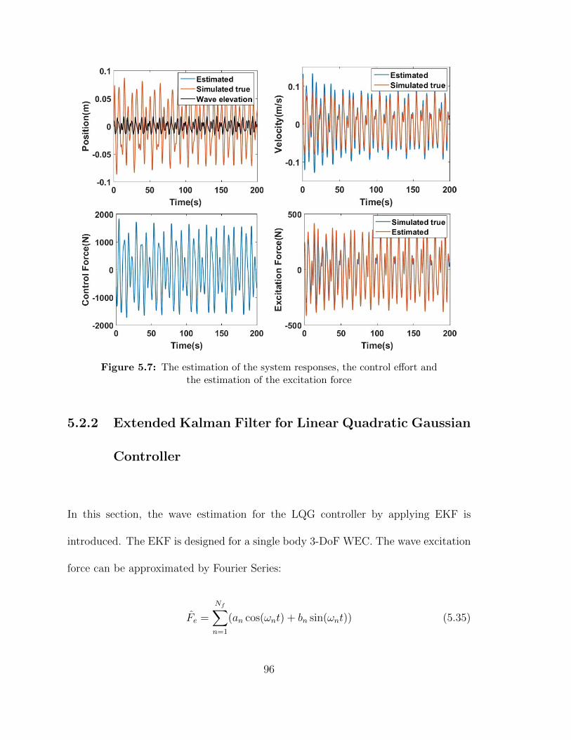
Figure 5.7: The estimation of the system responses, the control effort andthe estimation of the excitation force

5.2.2 Extended Kalman Filter for Linear Quadratic Gaussian

Controller

In this section, the wave estimation for the LQG controller by applying EKF is

introduced. The EKF is designed for a single body 3-DoF WEC. The wave excitation

force can be approximated by Fourier Series:

Fe =

Nf∑n=1

(an cos(ωnt) + bn sin(ωnt)) (5.35)

96

Figure 5.8: The convergence of the estimated states.

where Nf represents the number of Fourier terms used to approximate the excitation

force. Since in this problem the surge-pitch motion is excited by heave motion, two

Kalman filters are built to estimate the states: one for the coupled motion (surge

and pitch), and one for the heave motion. Although we can combine those two

Kalman filters into one, separating them reduces the computational cost. They are

still coupled because the heave motion excites the surge and pitch motion. The

current estimate of heave displacement is fed into a Kalman filter to estimate the

states of surge and pitch motions.

In Fig. 5.9, the Kalman Filter 1 estimates the states of heave motion. The state

vectors for Kalman Filter 1 and Kalman Filter 2 are:

~xh = [z, z, ~x3r, ~a3, ~b3, ~ω3]T (5.36)

~xc = [x, θ, x, θ, ~xcr, ~a1, ~b1, ~a5, ~b5, ~ω1, ~ω5]T (5.37)

97

Figure 5.9: The flow chart of LQG optimal controller

where ~aj, ~bj, and ~ωj represent the coefficients and frequencies of cosine and sine

functions, respectively, in the excitation force Fourier expansion. The superscript

of those parameters j can be 1, 3 and 5 which denotes the surge, heave and pitch

motions respectively. The subscript h denotes the states of the heave motion, and

the subscript c denotes the states of the coupled motion.

The equations of motion of the dynamic system described in Eq. (2.33) and Eq. (2.31)

can be written as a state space model. The detailed state space representation of

Eq. (2.33) is presented in Section 4.3. Hence, in this section, we will mainly introduce

the state space expression of Eq. (2.31). Let the first part of the states of Kalman

Filter 1 be ~xh = [d3, d3, ~x3r]T . Hence the equation of motion of the heave motion can

98

be written as:

~xh(t) = Fh(t)~xh(t) + Gh(t)u3(t) + ch(t) (5.38)

where

Fh(t) =

0 1 0

− 1m3K33 − 1

m3Bv,3 − 1m3 C

3r

0 B3r A3

r

(5.39)

Gh =

0

1m3

0

(5.40)

ch(t) =

0

1m3

0

F3e (5.41)

The Fe represents the estimation of excitation force. In this dissertation, a short-term

prediction for excitation force will be needed to compute the control. The sea states

are assumed to be steady within this short prediction period. Hence, the dynamics

99

of the states for estimating the excitation force are:

~a = ~0 (5.42)

~b = ~0 (5.43)

~ω = ~0 (5.44)

where ~a = [~a1, ~a3, ~a5]T , ~b = [~b1, ~b3, ~b5]T , ~ω = [~ω1, ~ω3, ~ω5]T .

5.2.2.1 The Jacobian Matrices

To implement the Extended Kalman Filter, we need to construct the Jacobian matri-

ces from the nonlinear system. The partial derivatives are computed for Eq. (5.38),

Eq. (4.48) and Eqs. (5.42) to (5.44). To write the partial derivatives in matrix format,

the following matrices are defined:

φc =

φ1c φ1

s 0 0

0 0 φ5c φ5

s

(5.45)

φh =

[φ3c φ3

s

](5.46)

Dcφ =

D1 0

0 D5

(5.47)

Dhφ = D3 (5.48)

100

where

φjc =

[cos(ωj1t)... cos(ωjnt)

]φjs =

[sin(ωj1t)... sin(ωjnt)

]j = 1, 3, 5 (5.49)

where D1, D3 and D5 are row vectors of size n. The kth component of the Dj vector

can be expressed as:

Djk = −ajk sin(ωjkt)t+ bjk cos(ωjkt)t (5.50)

where j = 1, 3, 5 and k = 1, ..., n. The Jacobian matrix can then be written in the

form:

F c(t) =

Fc(t)

0 0 0 0 0 0

m−1φc m−1Dcφ

0 0 0 0 0 0

0 0

...

0 0

(5.51)

In this study, it is assumed that the displacement and velocity will be measured for

each of the surge, pitch and heave motions. For the coupled motion we can write the

101

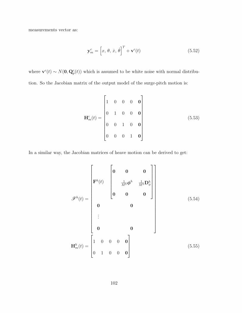
measurements vector as:

ycm =[x, θ, x, θ

]T+ vc(t) (5.52)

where vc(t) ∼ N(0,Qcp(t)) which is assumed to be white noise with normal distribu-

tion. So the Jacobian matrix of the output model of the surge-pitch motion is:

Hcm(t) =

1 0 0 0 0

0 1 0 0 0

0 0 1 0 0

0 0 0 1 0

(5.53)

In a similar way, the Jacobian matrices of heave motion can be derived to get:

F h(t) =

Fh(t)

0 0 0

1M3φ

h 1M3 D

hφ

0 0 0

0 0

...

0 0

(5.54)

Hhm(t) =

1 0 0 0 0

0 1 0 0 0

(5.55)

102

where, the output model of the heave motion is:

yhm = [z, z]T + vh(t), (5.56)

and the vh(t) ∼ N(0,Qhp(t)) is the measurement noise of heave motion which is also

assumed to be white noise.

As indicated in Fig. 5.9, two Kalman Filters are implemented to generate estimation.

The procedure of updating the estimation is the same as introduced in Section 5.2.1.4.

Once the estimation of the states at a current time is available, Eq. (5.35) can be

used for predicting the excitation force for a future short period.


In this section, the performance of the LQG controller is presented. The total simu-

lation time is 200s. The motion is constrained; the constraint for the surge is 1m, for

the heave is 0.2m, and for the pitch is 1rad. The wave applied in the simulation has

a Bretschneider wave spectrum. The absorbed energy is shown in Figure. 5.10. The

first figure compares between the energy absorption using the LQG controller and

energy absorption using the LQ controller. The latter represents the ideal situation

when we assume we have perfect knowledge of the wave. As can be seen in Fig. 5.10,

the energy captured by the LQG controller is around 61.6% of the energy captured

103

Figure 5.10: The energy extracted by the LQG controller.

by the LQ controller. The second figure shows the energy extracted from the surge,

heave, and pitch mode respectively. From the figure, we can tell the total energy is

3.56 times the energy captured by heave motion only. Note that it can be shown that

the maximum ratio between the total energy and heave energy is 3 when the system

is linear (without parametric excitation) and in the absence of viscous damping. The

control force is presented in Fig. 5.11; the maximum control force is around 20kN.

Fig. 5.12 shows the pitch rotation and the pitch velocity. As can be seen in Fig. 5.12,

the pitch rotation is within the specified constraints.

5.3 Consensus estimation for the WEC array

The consensus estimation is implemented in this section for the estimation of the

wave field in the WEC array. The consensus estimation applies the communication

technology to improve the performance of the estimation. The developed estimator

104

Figure 5.11: The control force

Figure 5.12: The pitch rotation and pitch velocity.

is extended from the discrete KCF developed in [156]. Then the derivation of the

proposed Continuous-Discrete KCF is presented. Since most of the variables in the

mathematical derivations and models are in the vector or matrix format, the different

denotations for the scalar, vector, and matrix are neglected except a real number is

included.

105

5.3.1 The Continuous-Discrete Kalman-Consensus Filter

When we have a continuous dynamic system and discrete measurements, a

Continuous-Discrete Kalman-Consensus Filter becomes necessary. The continuous

dynamics of each agent of the WEC array is described in Eq. (2.3), since the coupling

between different agents is neglected. The dynamics can be presented in a state space

format as:

~xi = F~xi + Guui + Gwi (5.57)

~ym,i = Hm,i~xi + ~vi (5.58)

where ~xi is the state of the ith agent, ui is the control input and ~ym,i is the mea-

surement output. The wi and ~vi are the process noise and measurement noise of ith

agent, respectively. The F is the system matrix, Gu is the control matrix, G is the

process noise gain matrix and Hm,i is the output matrix. The proposed CD-KCF

106

model can be summarized as:

˙~xi = F~xi + Guui

Pi(t) = F(t)Pi(t) + Pi(t)FT (t) + G(t)Qp(t)G

T (t)

~x +k,i = ~x −k,i + Kg,k,i(~ym,k,i −Hm,k,i~x

−k,i) + Cg,k,i

∑Ni

(~x −k,j − ~x−k,i)

P+k,i = (I−Kg,k,iHm,k,i)P

−k,i

Kg,k,i = P−k,iHTm,k,i(Rk,i + Hm,k,iP

−k,iH

Tm,k,i)

−1 (5.59)

where ~xi is the states of the estimation of the ith agent. ~ym,k,i is the measurements of

the kth stage of the ith agent. P is the error covariance matrix of the state estimation,

Qp is the process noise covariance matrix, R is the measurement noise covariance

matrix. Kg,k,i is the Kalman gain and Cg,k,i is the consensus gain. Algorithm. 3

shows the process of the CD-KCF. Furthermore, the stability of the proposed CD-

KCF is shown in Appendix. A.

Algorithm 3 Continuous-Discrete Kalman-Consensus Filter: a Continuous-Discreteobserver with a consensus term.

1: Initialization: Pi = Pi,0, ~xi = ~xi,02: while new data exists do3: Compute the Kalman Gain


−k,iH

Tm,k,i)

−1

4: Update the current estimation based on consensus law~x +k,i = ~x −k,i + Kg,k,i(~ym,k,i −Hm,k,i~x

−k,i) + Cg,k,i

∑Ni

(~x −k,j − ~x−k,i)


−k,i

5: Propagate the estimation˙~xi = F~xi + GuuiPi(t) = F(t)Pi(t) + Pi(t)F

T (t) + G(t)Qp(t)GT (t)

6: end while

107

5.3.2 Simulation results

In this section, the simulation results are presented to validate the performance of

the proposed estimator for different cases. The measured states are only subset of

the estimated states. The first case is designed to test the proposed CD-KCF for the

WEC array interacts with regular wave. The second test case apply the CD-KCF for

the WEC array interacts with the irregular wave. The performance of the regular

Kalman Filter (KF) is also presented to compare it to the performance of the CD-

KCF. To analyze the performance of the CD-KCF and KF, the following quantities

are defined. The disagreement among the array is defined as:

Ψ(~x) = (N∑i=1

~δ2i )12 (5.60)

The above equation can be further expanded to be: Ψ(~x) = (∑N

i=1

∑Mj=1

~δ2i,j)12 , if

the basis vectors are orthogonal, where M is the number of elements in the ~δi vector.

Additionally, ~δi = ~xi−¯~x, where

¯~x represents the average estimation which is computed

as¯~x = 1

N

∑i ~xi.

108

5.3.2.1 Test Case 1

The first test case is the estimation of the position and velocity of each buoy in a wave

farm, in addition to the excitation force field using the CD-KCF. Practically, the esti-

mated quantities are required by the controller. By applying the proposed estimator,

a better energy extraction is expected if the more precise information is provided.

Additionally, since the CD-KCF estimates in a distributed fashion, the wave farm

will have a more stable performance even if the data collection and communication

of some agents collapse. In this case, the wave farm has 16 buoys; only the heave

motion is considered for each of them. The interaction between buoys is neglected

in this section. The direction of the incoming wave β is 20o, where β represents the

angle between the wave propagation direction and the x axis. The distribution of the

buoys is shown in Fig. 5.13.

Figure 5.13: The distribution of the buoys in the wave farm

109

For observing the excitation force field, we need to introduce the expression of the

excitation force field. The excitation force is function of the wave elevation; the wave

elevation field can be expressed as [157, 158]:

η(t) =Nw∑j=1

<(η(ωj)ei(χjr−ωjt+φj)) (5.61)

where Nw is the total number of frequencies, η(ωj) is the wave elevation at frequency

ωj, φj is the random time domain phase shift of particular frequency ωj, kj is the

wave number which can be computed as χ = ω2/g, where the deep water assumption

is applied. The position r is expressed as:

r = x cos(β) + y sin(β) (5.62)

The excitation force field can be expressed as:

Fe(t) =∑j

<(Few(ωj)η(ωj)ei(χjr−ωjt+φj)) (5.63)

where Fe(ωj) is the frequency domain excitation force coefficient. The system dy-

namics of each agent is described in Eq. (2.3). However, the radiation damping is

approximated with a linear damping force as:

Fr = clinzi (5.64)

110

where zi is the heave displacement of each agent. There is no control force included

in the simulation (u = 0), only free motion is considered. Additionally:

Fe,i(t) =∑j

<(Few(ωj)η(ωj)ei(χjri−ωjt+φj)) (5.65)

Consequently, the state space model of the unforced and uncoupled wave farm can

be expressed as:

x1,i = x2,i (5.66)

x2,i =1

m(Fe,i(t)−Kx1,i − clinx2,i) (5.67)

To estimate the excitation force, a Fourier Series approximation for the excitation

force is used:

Fe,i(t) ≈Nf∑j=1

aj cos(χjri − ωjt) + bj sin(χjri − ωjt) (5.68)

≈ φ(ri, t)[~a, ~b]T (5.69)

where Nf is the number of Fourier terms in the approximation, φ(ri, t) =

[cos(~θi), sin(~θi)] and ~θi = ~χri − ~ωt. Hence, the dynamics of the estimator can be

111

expressed as:

˙x1,i = x2,i (5.70)

˙x2,i =1

m(φ(ri, t)[~a, ~b]

T −Kx1,i − clinx2,i) (5.71)

˙~a = 0Nf×1 (5.72)

˙~b = 0Nf×1 (5.73)

The differential equations can be written in a state space form as˙~x = Fi~x, where

~x = [x1,i, x2,i, ~a, ~b]Tand:

Fi =

0 1 01×Nf 01×Nf

−Km

− cm

cos(~θi)m

sin(~θi)m

0Nf×1 0Nf×1 0Nf×Nf 0Nf×Nf

0Nf×1 0Nf×1 0Nf×Nf 0Nf×Nf

(5.74)

where the estimated quantities are the position, velocity of each agent and the un-

known coefficients of the wave field which are generally required by the controller.

Although the unknown coefficients are unmeasurable, the position and velocity are

measurable. Additionally, for more realistic case, the WEC system becomes more

stochastic (ex, nonlinear effect). Consequently, it is appropriate to select Kalman

filter to develop consensus estimation of the wave field. The dynamics of the coeffi-

cients ~a and ~b are 0 which means they are not propagated. However, they are not fixed

112

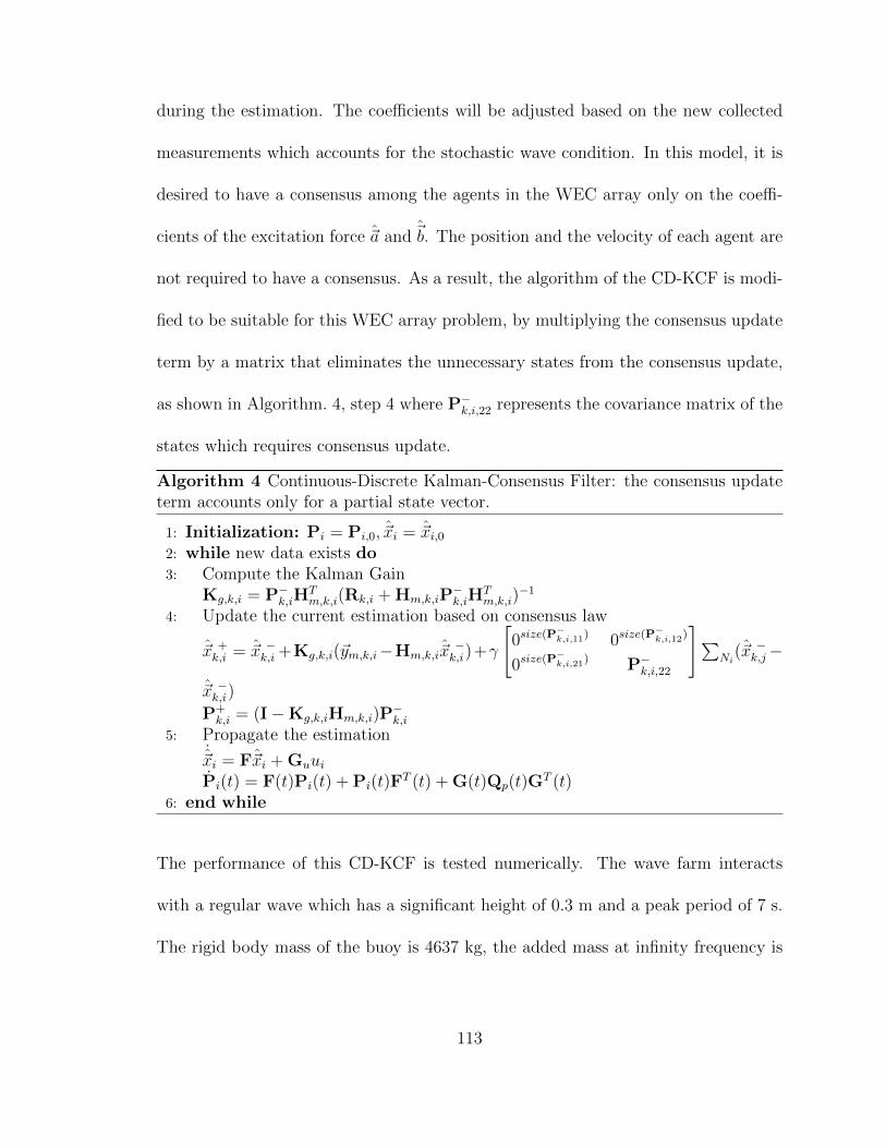
during the estimation. The coefficients will be adjusted based on the new collected

measurements which accounts for the stochastic wave condition. In this model, it is

desired to have a consensus among the agents in the WEC array only on the coeffi-

cients of the excitation force ~a and ~b. The position and the velocity of each agent are

not required to have a consensus. As a result, the algorithm of the CD-KCF is modi-

fied to be suitable for this WEC array problem, by multiplying the consensus update

term by a matrix that eliminates the unnecessary states from the consensus update,

as shown in Algorithm. 4, step 4 where P−k,i,22 represents the covariance matrix of the

states which requires consensus update.

Algorithm 4 Continuous-Discrete Kalman-Consensus Filter: the consensus updateterm accounts only for a partial state vector.

1: Initialization: Pi = Pi,0, ~xi = ~xi,02: while new data exists do3: Compute the Kalman Gain


−k,iH

Tm,k,i)

−1

4: Update the current estimation based on consensus law

~x +k,i = ~x −k,i +Kg,k,i(~ym,k,i−Hm,k,i~x

−k,i)+γ

[0size(P

−k,i,11) 0size(P

−k,i,12)

0size(P−k,i,21) P−k,i,22

]∑Ni

(~x −k,j−

~x −k,i)


−k,i

5: Propagate the estimation˙~xi = F~xi + GuuiPi(t) = F(t)Pi(t) + Pi(t)F

T (t) + G(t)Qp(t)GT (t)

6: end while

The performance of this CD-KCF is tested numerically. The wave farm interacts

with a regular wave which has a significant height of 0.3 m and a peak period of 7 s.

The rigid body mass of the buoy is 4637 kg, the added mass at infinity frequency is

113

Figure 5.14: The average percent estimation error and the disagreementof the excitation force

2702kg, the hydrostatic stiffness is 4.44× 104 N.m−1 and the linear damping is 1064

N.s.m−1. Fig. 5.14 shows the average percent estimation error of the excitation force

of all the agents, which is defined as

ee = (∑i

| Fe,i − Fe,i |max | Fe,i |

)/N (5.75)

As shown in Fig. 5.14, the estimation error of the CD-KCF has slightly better con-

vergence compared to the standard KF. The disagreement of the estimation is also

shown in the figure. The states of the estimation for the WEC array contains the

position, velocity and the coefficients a and b. Since the agents in the WEC array only

have consensus on the coefficients which represents the wave field. The disagreement

is computed only based on the coefficients. The disagreement of the CD-KCF con-

verges significantly faster than the KF which means all the agents reach a consensus

quickly in this case. The computational cost of the CD-KCF is 263.37s which is less

than the standard KF which takes 268.38s.

114

5.3.2.2 Test Case 2

The second test case presents the estimation of the position, velocity, and the exci-

tation force field in a wave array that is subject to an irregular wave. The irregular

wave has the Bretschneider wave spectrum. The significant height of the wave is 0.3

m and the peak period is 7 s. The total number of frequencies of the wave field is as-

sumed 200 ranging from 0.1 rad.s−1 to 4 rad.s−1. The initial guess for the coefficients

is assumed of the form:

~ai = αi(~ae cos(φ)−~be sin(φ)) (5.76)

~bi = αi(−~ae sin(φ)−~be cos(φ)) (5.77)

where αi is a random weight on the initial guess for different agents, ~ae =

<(Fe(ω)η(ω)) and ~be = =(Fe(ω)η(ω)). Two different simulations are presented in

this section. The first simulation assumes less number of frequencies in the estimator

while the true model is simulated using 200 frequencies. Specifically, 30 different fre-

quencies are assumed in the CD-KCF model, which means the state vector includes

30 a and b coefficients. The main reason for using fewer frequencies in the estimation

model is the computational cost. The computational cost of the CD-KCF is 1493.13s

compared to 1560.40s of the standard KF. The CD-KCF is slightly faster than the

standard KF. The average percent estimation error of the excitation force is shown

115

Figure 5.15: The average percent estimation error and the disagreementof the excitation force using 30 frequencies

in Fig. 5.15. The CD-KCF converges slightly faster than the KF; the performance

of both filters is nearly the same in terms of the estimation error. The second fig-

ure in Fig. 5.15 shows the disagreement in the estimation of the two filters on the

coefficients. The CD-KCF has a significantly better agreement than the KF.

To study the impact of the number of frequencies in the estimator model on the

results, the simulation is extended to estimate the true excitation force using 200

frequencies in the estimator model. The estimation error of CD-KCF and KF is

shown in the first figure in Fig. 5.16. The CD-KCF has a better performance both

in terms of the convergence speed and estimation error. As shown in the second

figure in Fig. 5.16, the disagreement of the estimation on the coefficients converges

significantly faster in the case of the CD-KCF.

The percent estimation error converges to about 25% as shown in Fig. 5.15 when using

only 30 frequencies in the estimator model, whereas it converges to about 0% when

116

Figure 5.16: The average percent estimation error and the disagreementof the excitation force using 200 frequencies

using 200 frequencies, as shown in Fig. 5.16. This is expected since the estimation with

less number of frequencies cannot fully capture the true wave spectrum. To highlight

the impact of the number of frequencies on the estimation performance, Fig. 5.17 show

simulations using 30, 100, and 200 frequencies in the estimator model of the CD-KCF.

Both the estimation error and the disagreement significantly improved by increasing

the number of frequencies. Moreover, from the figures regarding the estimation error,

we can tell that the required time to obtain reasonable low-level error is less than 40s.

Typically, the sample time of the ocean observation is around 15-30mins within which

the sea state is reasonably described [159]. Apparently, the converging time of the

developed estimator is significantly less than the sample time. Additionally, based on

the wave conditions applied in references [160, 161], we can consider an even faster

wave dynamics where the sea state changes around 120s. It is still much larger than

40s. Hence, the proposed estimator is able to catch the constantly changing wave.

117

Figure 5.17: Estimation error and Disagreement obtained with differentnumber of frequencies using the CD-KCF

118

Chapter 6

Power Take Off Constraints

This Chapter introduces the Power take-off constraints of the WEC. In previous

chapters, the optimal control and the optimal estimation are proposed for the WEC.

Although some of them consider the constraint on the displacement and the control

force. The realistic performance of the controller with the Power take-off (PTO)

unit implemented is not validated. Among the different categories of PTO units,

the hydraulic system and direct drive system are mainly applied for WEC control.

Section 6.1 introduces the modeling of the discrete displacement hydraulic PTO. The

details of the dynamics of the hydraulic cylinder, hoses, directional valves, pressure

accumulators and the hydraulic motor are presented in this section. Section 6.2

presents the numerical validation on the proposed system. The control algorithms

that will be applied to the hydraulic system and the simulation tool are introduced

119

first. The simulation results are then presented.

6.1 Modeling of The Discrete Displacement Hy-

draulic Power Take-Off unit

In this dissertation, the Discrete Displacement Cylinder (DDC) hydraulic system is

used to apply the PTO torque. A simplified illustration for this system is shown in

Figure 6.1. More details about the DDC hydraulic system can be found in [15]. As

shown in Figure 6.1, the DDC hydraulic system is mainly composed of the actua-

tor/cylinder, the manifold valves, the manifold accumulators, and the generator. The

PTO torque is computed in the Equation (6.1) as the product of the cylinder force

and the moment arm:

τPTO = Fcl1 (6.1)

where the moment arm can be expressed by Equation (6.2):

l1 =l2l3 sin(θ − α0)

xc + l4(6.2)

xc = −l4 +√−2l2l3 cos(θ − α0) + (l22 + l23) (6.3)

120

Figure 6.1: The layout of the Discrete Displacement Cylinder (DDC)hydraulic system.

6.1.1 The Hydraulic Cylinder

The actuator force Fc is generated by the hydraulic cylinder and can be computed by

Equations (6.4) and (6.5):

Fc = −pA1A1 + pA2A2− pA3A3 + pA4A4 (6.4)

Fc = Fc − Ffric (6.5)

where pAi is the pressure of the ith chamber and Ai is the area of the piston. Ffric is

the cylinder friction force. The dynamics of the chamber pressure can be described

121

by flow continuity Equations (6.6) to (6.9):

pA1 =β(pA1)

A1(xc,max − xc) + V0,A1(QA1 − vcA1) (6.6)

pA2 =β(pA2)

A2xc + V0,A2(QA2 + vcA2) (6.7)

pA3 =β(pA3)

A3(xc,max − xc) + V0,A3(QA3 − vcA3) (6.8)

pA4 =β(pA4)

A4xc + V0,A4(QA4 + vcA4) (6.9)

where V0,A1, V0,A2, V0,A3, and V0,A4 are the volumes of the connecting hoses of different

chambers. xc,max is the maximum stroke of the cylinder. xc and vc are the position

and velocity of the piston, respectively, which are defined positive down. β(pAi) is

the effective bulk modulus of the fluid based on different pressures, and is assumed

to be constant in this study. Additionally, QAi is the flow from the connecting hose

to the ith chamber. The cylinder friction is expressed by Equation (6.10):

Ffric =

tanh(afvc) | Fc | (1− ηc), if Fcvc > 0

tanh(afvc) | Fc | ( 1ηc− 1) otherwise

(6.10)

where a is the coefficient used to smooth the friction curve versus velocity. ηc is a

constant efficiency of the cylinder.

122

6.1.2 The Hoses

The hoses connected between the cylinder and the manifold valves are modeled by

Equations (6.11) and (6.12) which refer to [15]:

Qout =(p1 − p2)Ahose − pf (Qout)Ahose

ρlhose(6.11)

p1 =(Qin −Qout)β

Ahoselhose(6.12)

where Qin and Qout are the fluid flows in and out of the hose, and p1 and p2 are the

pressures of the inlet and outlet of the hose, respectively. Ahose is the area of the

hose, lhose is the length of the hose, ρ is the fluid density, and pf (Qout) is the pressure

drop across the hose. The pressure drop across a straight pipe/hose can be modeled

by the equation:

pλ =0.3164lhoseρ

2Re0.25dhose

Qout | Qout |(0.25d2hoseπ)2

(0.5 + 0.5 tanh(2300−Re

100))

+128νρlhoseQout

πd4hose(0.5 + 0.5 tanh(

−2300 +Re

100)) (6.13)

where ν is the kinematic viscosity of the fluid. Re represents the Reynold number

which can be computed by Equation (6.14):

Re =voutdhose

ν(6.14)

123

Equation (6.13) combines the pressure loss of the laminar flow and the turbulent

flow by the hyperbolic-tangent expression. Consequently, a continuous transition of

the pressure loss between the laminar and turbulent flow can be created. When the

Reynold number is less than 2200, (0.5 + 0.5 tanh(2300−Re100

)) is close to zero, which

means the pressure drop is contributed by the laminar flow. On the other hand, when

the Reynold number is greater than 2400, (0.5 + 0.5 tanh(−2300+Re100

)) is close to zero,

which means the pressure drop is contributed by the turbulent flow. Another source

of pressure drop is the fitting loss, which can be computed by Equation (6.15):

pζ = ζρ

2Qout | Qout |

1

(0.25d2hoseπ)2(6.15)

where ζ is the friction coefficient for a given fitting type. Finally, the total resistance

in the hose with n line pieces and m fittings can be computed by Equation (6.16):

pf (Qout) = pλ,1(Qout) + ...+ pλ,n(Qout) + pζ,1(Qout) + ...+ pζ,m(Qout) (6.16)

In this dissertation, the pressure loss of the hoses is modeled by the Equation (6.17):

pf (Qout) = pλ(Qout) + pζ,M(Qout) + pζ,C(Qout) (6.17)

where pζ,M represents the fitting resistance which considers the internal pressure drops

in the manifold and pζ,C represents the cylinder inlet loss.

124

6.1.3 The Directional Valves

The two-way two-position directional valves are used in this model. The flow across

the valve can be described by the following orifice Equation (6.18):

Qv = sign(∆p)CdAv(α)

√2

ρ| ∆p | (6.18)

where ∆p is the pressure difference cross the valve, Cd is the discharge coefficient,

and Av(α) is the opening area which can be computed by Equations (6.19)–(6.21):

Av(α) = αA0 (6.19)

α =

1tv, if uv = 1

− 1tv, if uv = 0

(6.20)

0 6 α 6 1 (6.21)

where A0 is the maximum opening area of the valve. In this paper, a total of eight

valves are used to control the actuator force. The tv represents the opening and

closing time of the valve. The shifting algorithm of the valve applied in this paper

can be further improved [162] to reduce the pressure oscillations and improve the

energy efficiency. Moreover, the different opening time has a significant impact on

the cylinder pressure [163]. The opening time tv is selected to be 30 ms in this paper

125

to avoid the cavitation or pressure spikes and to have a relatively fast response to the

reference control command. Since the focus of this paper is to examine the controllers’

performance practically, the influence of different opening times is not investigated in

this paper.

6.1.4 The Pressure Accumulators

The accumulators in the DDC system are used as pressure sources and also for en-

ergy storage. The dynamics of the pressure accumulator can be modeled with the

Equations (6.22)–(6.24) [15]:

pacc =

Qacc + 1

1+RgasCv

VgTgas

1τa

(Tw − Tgas)Va0−Vg+Vext

β+ 1

1+RgasCv

Vgpacc

(6.22)

Vg = −Qacc + paccVa0 − Vg + Vext

β(6.23)

Tgas =1

τa(Tw − Tgas)−

RgasTgasCvVg

Vg (6.24)

where pacc is the pressure of the accumulator, Qacc is the inlet flow to the accumulator,

Rgas is the ideal gas constant, Cv is the gas specific heat at constant volume, Tw is

the wall temperature, τa is the thermal time constant, β is the bulk modulus of the

fluid in the pipeline volume Vext, Va0 is the size of the accumulator, Vg is the gas

volume, and Tgas is the gas temperature. Hence the state of the accumulator contains

126

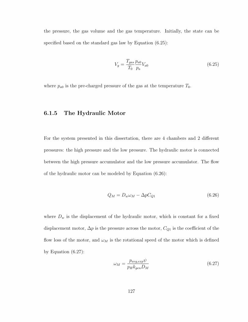
the pressure, the gas volume and the gas temperature. Initially, the state can be

specified based on the standard gas law by Equation (6.25):

Vg =TgasT0

pa0paVa0 (6.25)

where pa0 is the pre-charged pressure of the gas at the temperature T0.

6.1.5 The Hydraulic Motor

For the system presented in this dissertation, there are 4 chambers and 2 different

pressures: the high pressure and the low pressure. The hydraulic motor is connected

between the high pressure accumulator and the low pressure accumulator. The flow

of the hydraulic motor can be modeled by Equation (6.26):

QM = DwωM −∆pCQ1 (6.26)

where Dw is the displacement of the hydraulic motor, which is constant for a fixed

displacement motor, ∆p is the pressure across the motor, CQ1 is the coefficient of the

flow loss of the motor, and ωM is the rotational speed of the motor which is defined

by Equation (6.27):

ωM =pavg,expψ

pHkgenDM

(6.27)

127

where pavg,exp is the expected average power output, pH is the pressure of the high

pressure accumulator, kgen is the number of generators, DM is the total motor dis-

placement, and ψ is a coefficient for the motor speed control to prevent the high

pressure from depletion or saturation which is formulated by Equations (6.28) and

(6.29):

k =4

(pH,max − pH,min)(6.28)

ψ =

k(pH − pH,min), if pH > pH,min

0, otherwise

(6.29)

To achieve the desired motor speed introduced in Equation (6.27), the generator

torque control needs to be included. In this paper, the generator and inverter are

not modeled and the desired motor speed is assumed achievable. The power in the

hydraulic motor can be computed by Equation (6.30):

PM = ∆pQM (6.30)

This completes the modeling of DDC hydraulic system; the control algorithm is in-

troduced in the next section.

128

6.2 Numerical Validation

6.2.1 The Control Algorithm

Two parts will be presented in this section: the control method for the buoy and the

force-shifting algorithm for controlling the valves. The control method for controlling

the buoy computes a reference value for the control force at each time step. This

reference control force is then used as an input to the PTO, and the actual control

force that results from the PTO is computed using the force-shifting algorithm. Each

of the two parts is detailed below.

6.2.1.1 The Buoy Control Method

Several control methods will be tested in this paper using a simulator that simulates

the PTO unit. Some of these controller were originally developed for heave control.

It is relatively straightforward, however, to extend a control method from the heave

motion to the pitch motion. For example, the singular arc (SA) control method [2]

can be used to compute the control torque by the following Equation (6.31):

τPTO(s) =N(s)

D(s)(6.31)

129

where:

N(s) = (Js2 + (Cr(sI + Ar)−1Br −Dr)s+K)τe(s)

D(s) = s(Cr(sI + Ar)−1Br − Cr(sI − Ar)−1Br − 2Dr) (6.32)

where the excitation torque can be expressed as Fourier series expansion by Equa-

tion (6.33):

τe =n∑i=1

<(τew(ωi)η(ωi)ei(−ωit+φi)) (6.33)

An inverse Laplace transformation is then applied to the SA control to obtain the

control in the time domain. The required information to compute the control is

the time t, the excitation torque coefficient τew, the wave frequency vector ~ω and

the time domain phase shift vector ~φ. A reference control method is the feedback

proportional-derivative (PD) control. The PD control takes the form of Equation

(6.34):

τPTO = Kpθ +Kdθ (6.34)

where Kp is the proportional gain and Kd is the derivative gain. In addition to the

above two control methods, simulated with the hydraulic system are model predictive

control (MPC) [164], shape-based (SB) control [5], proportional-derivative complex

conjugate control (PDC3) [24], and pseudo-spectral (PS) control [165]. Each one of

these methods is well documented in the literature, so the details of each control

methods are avoided in this section.

130

In the original developments, the SA control and the PDC3 control compute a con-

trol force that is equivalent to the complex conjugate control (C3), and hence the

maximum possible harvested energy in the linear domain. However, the C3 does not

account for constraints on the buoy displacement. In fact, since the C3 criterion is to

resonate the buoy with the excitation force, the motion of the buoy always violates

displacement constraints when controlled using the SA and PDC3 controls. On the

other hand, the MPC, SB, and PS control methods compute a control force in an

optimal sense, taking displacement constraints into account. Figure 6.2 shows a sim-

ulation for 5 min for the above six control methods when a constraint on the buoy

displacement is assumed. The simulation parameters are detailed in Section 6.2.3.

This simulation does not account for the PTO dynamics and is here presented to

highlight the impact of including the PTO into the simulations in Section 6.2.3.

As can be seen from Figure 6.2, among the six control methods, the MPC and PD

controls performed best, then the SB method, then the PS, and then the PDC3

and SA methods. The two methods (SA and PDC3) that perform best without dis-

placement constraints actually have the poorest performance when accounting for the

constraints.

131

6.2.2 The Force-Shifting Algorithm

The force-shifting algorithm (FSA) is introduced in this section. The FSA used in

this paper is described by Equation (6.35):

{Fc(t) = ~F [k] | k = arg min | Fref (t)− ~F [k] |} (6.35)

where Fref is the reference control force (computed for instance using one of the six

control methods described above), and ~F is the vector of the possible discrete values

for the force. With different permutations of valve openings, it is possible to produce

different levels of constant forces, as shown in Figure 6.3, where it is assumed that

pH = 200 bar and pL = 20 bar. The FSA selects the discrete force level that is closest

to the reference control force. It is noted here that the discrete force changes over

time due to the fluctuation of the pressures in the accumulators.

132

Figure 6.2: When accounting for displacement constraints, someunconstrained methods harvest less energy. PD: proportional-derivative;

SA: singular arc; PDC3: proportional-derivative complex conjugate control;SB: shape-based; MPC: model predictive control; PS: pseudo-spectral.

Figure 6.3: An example for all discrete possible values for a PTO force.

133

6.2.3 Simulation Tool

A tool for simulating the dynamics of the WEC including the motion dynamics,

the hydrodynamic/hydrostatic force calculations, and the PTO hardware model was

developed in MathWorks Simulink®. The detailed Simulink model of the wave energy

conversion system is shown in Figure 6.4. The Plant block simulates the dynamics

of the buoy. The PTO block simulates all the equations of the valves, hoses, and

accumulators. As can be seen in Figure 6.4, the excitation force is an input that is

computed outside the Plant block. The control force command is computed in the

block ‘Control Command’. Despite the name, six different controllers were tested in

the ‘Control Command’ block. A detailed Simulink model of the hydraulic system is

shown in Figure 6.5, this model is inside the PTO block in Figure 6.4. The parameters

of the dynamic model of the WaveStar used in the simulations in this dissertation are

listed in Table 2.1.

134

Figure 6.4: The Simulink model of the wave energy conversion system.

135

Figure 6.5: The Simulink model of the hydraulic PTO system.

The irregular waves are simulated in this study using the stochastic Pierson–

Moskowitz (PM) spectrum. The wave used in the simulation has a significant height

of 1.75 m and a peak period 5.57 s. With regard to the significant height and peak

period applied in the simulation, they are selected from the validated wave climate

in [112, 166] for the Wavestar C5. The proper range so that the wave for C5 can

have major energy absorption is with a significant height from 0.5 m to 3 m and peak

period from 2 s to 7 s. The wave climate applied in this study is in the middle of the

range to avoid losing generality.

136

6.2.3.1 The System Losses

The system losses are computed in this study. The system losses include the pressure

loss of the hoses, the flow loss of the generator, and the friction of the cylinder.

The pressure loss is shown in Figure 6.6, in which the vertical line represents the

transition between the laminar flow and the turbulent flow when the Reynold number

is Re = 2300, for each of the two possible directions of the fluid flow. The amount of

the flow loss and the friction force of the cylinder are shown in Figures 6.7 and 6.8.

All the system parameters used in the simulations are listed in Table 6.1.

6.2.4 Simulation Results

The above Simulink tool is used to simulate the performance of the above six control

methods. The energy extracted by those methods is shown in Figure 6.9. In this

simulation, there are limitations on the maximum stroke and the maximum control

force. In addition, the PTO dynamics are simulated. The maximum control force

in the cylinder in the simulations presented in this paper is assumed to be 215 kN.

The maximum allowable displacement in the simulations presented in this paper is

assumed to be 1.2 m. As can be seen in Figure 6.9, the MPC and PD control

methods harvest the highest energy level compared to the other methods. The SB

137

method comes next. The SA, PDC3, and PS control methods come next, and the

three of them perform about the same. For further analysis of the performance of the

controllers, the capture width ratio (CWR) is evaluated:

CWR =PaveDPw

(6.36)

where Pave is the average power extraction of the buoy, Pw is the wave energy trans-

port, and D is the characteristic dimension of the buoy. The CWRs of the MPC,

PD, SB, SA, PDC3, and PS controllers are 51.21%, 50.92%, 44.68%, 37.60%, 37.14%,

and 36.86% respectively. According to the [166], the CWR of the performance of

the floater with the applied wave ranges from 40% to 50%. Hence, the performance

of the proposed controllers is in the reasonable range in terms of energy extraction.

Comparing Figure 6.9 to Figure 6.2 we can see that by including the PTO model,

the performance of the SA method improves slightly, while the performance of the

PS degrades slightly, and as a result, the three methods PS, SA, and PDC3 perform

about the same. The performance of the MPC, PD, and SB control methods actually

slightly improve when the PTO model is included.

138

Figure 6.6: The pressure loss of the hose which has a 1-m length and3.81× 10−2 m diameter with different flow rates across the hose.

Figure 6.7: The flow loss of the generator.

139

Figure 6.8: The friction force of the cylinder with different velocitieswhen the cylinder force is 100 kN.

Another important result to examine is the output mechanical power at the actuator

and the output power from the generator. These two quantities are compared in the

first part of Figure 6.10. From the figure, we can tell that the power absorbed in

the generator side is much smoother than the power extracted by the actuator. The

hydraulic accumulators act as a power capacitor for energy storage, resulting in this

relatively smooth power profile at the generator output. As can be seen in the figure

also, the actuator power includes reactive power; these are the times at which the

actuator power is negative. At these times, the PTO actually pumps power into the

ocean through the actuator. The generator output power does not have any reactive

power, confirming that all the reactive power come from the accumulators.

140

The efficiency of the system is defined by Equation (6.37):

ηout =Pgen

Pactuator(6.37)

The efficiency depends on the control method. For example, in this test case, the

efficiency of the SB controller is 80.15%, for the MPC it is 72.58%, for the PS it is

67.34%, for the SA it is 64.36%, and for the PD controller it is 71.76%, over 300 s.

In the context of comparing the performance of different control methods, it is im-

portant to highlight one significant difference between them that emanates from the

theory behind each control method. Each of the MPC, SB, and PS control methods

requires wave prediction. That is, wave information (or excitation force) is needed

over a future horizon at each time step in the simulation. In the simulations in this

paper, this future horizon is assumed to be 0.6 s for the SB and MPC control methods

and is assumed to be 60 s for the PS control. Wave prediction is assumed perfect

in these simulations. Non-perfect wave prediction would affect the results obtained

using these methods. The PD, SA, and PDC3 control methods do not need future

wave prediction.

This simulation tool also provides detailed operation information that is useful for

characterizing different components in the system. For example, the generator speed

is computed in the simulation and is shown in the second part of Figure 6.10. As

141

shown in the figure, the speed is oscillating around 1200 RPM.

Table 6.1The data used in the simulation of the overall WEC system.

Symbol Value Unit

Length of the arms

l2 3 m

l3 2.6 m

l4 1.6 m

Length of the hoses C2M

lA1 1 m

lA2 1 m

lA3 1 m

lA4 1 m

Diameter of the hoses C2M

dA1 1.5 in

dA2 1.5 in

dA3 1.5 in

dA4 1.5 in

Maximum stroke

xc,max 3 m

Area of the chambers

142

A1 113.4× 10−4 m2

A2 32.55× 10−4 m2

A3 80.85× 10−4 m2

A4 162.75× 10−4 m2

Max Area of the valves

A01 1.6× 10−4 m2

A02 1.6× 10−4 m2

A03 1.6× 10−4 m2

A04 1.6× 10−4 m2

Accumulator size

Va0 100× 10−3 m3

Pressure drop coef

ζM 1.3

ζC 1

Specific time constant S

τl 23 s

τh 34 s

Initial pressure of the accumulators

pa,l 20 bar

pa,h 130 bar

143

Initial angle

α0 1.0821 rad

Control parameters

K −9.16× 106 Nm/rad

B 4.4× 106 Nms/rad

Valve opening time

tv 30× 10−3 s

Wall temperature

Tw 50 oC

Ideal gas constant

R 276 J/kg/K

Gas specific heat at constant volume

Cv 760 J/kg/K

Motor displacement

Dw 100 cc/rev

Flow loss coefficient

CQ1 5.4× 10−12 m3/s/Pa

Fluid bulk modulus

β 1.5× 109 Pa

144

Figure 6.10: The power extracted by the actuator and the generator andthe generator speed

Figure 6.9: The energy extracted accounting for displacement and forceconstraints, including the hydraulic system dynamics model.

To present detailed plots for the response of the buoy, only one control method is se-

lected as a sample to avoid excessive figures in the paper. The SB method is selected

here to present the detailed WEC response in this section. The angular displacement

of the buoy is shown in the first part in Figure 6.11; the maximum angular displace-

ment is about 10 degrees and it is below 5 degrees most of the time. The angular

145

Figure 6.11: The rotational angle and the angular velocity

velocity of the buoy is shown in the second part in Figure 6.11. The cylinder force

and the PTO torque are shown in Figures 6.12, respectively. Both the reference and

actual values are plotted in each of the two figures. As can be seen in Figure 6.12,

the control force is below the force limit of 215 kN. The accumulator pressure is

shown in Figure 6.13. The high pressure is oscillating around 100 bar, while the low

pressure is stable around 20 bar. The chamber pressure is also shown in Figure 6.13.

Significant fluctuations can be observed when the hydraulic system is extracting en-

ergy. This is necessary to be able to track the reference control command effectively.

However, those fluctuations may be reduced by increasing the valve opening area or

including relief valves.

146

Figure 6.12: The cylinder force and the PTO torque

Figure 6.13: The pressure of the accumulator and the chamber

6.2.5 Discussion

In this study, different recent control methods are tested using a simulation tool that

simulates a hydraulic PTO system. In a theoretical test (where PTO is assumed to

track the reference control command ideally and in the absence of all constraints,)

the SA controller has the best performance in terms of energy extraction. However,

the performance of the SA controller with the hydraulic system model included is

147

the poorest among the tested six control methods. To get more insight into this

phenomenon, consider Table 6.2 that presents data for three controllers (SA, PD,

and PDC3) in the theoretical test case. As can be seen in Table 6.2, the energy

extracted by the PD controller in this theoretical test is about 60% of that of the SA

controller. However, the buoy maximum displacement associated with the SA control

is significantly greater than that of the PD control (almost three times higher) which

makes it more difficult to achieve. Similarly, the maximum control force required by

the SA control is significantly greater than that of the PD control, which means a

PTO might not be able to track the command force at all times when using a SA

control, while it is more likely to track a command force generated using a PD control.

The data of the PDC3 control in Table 6.2 also highlights that the PDC3 control

in this test case generates about the same level of average power, but in a higher

displacement range and with higher force capability. This indicates that including a

model for the PTO would result in favorable performance for the PD control compared

to the PDC3. To highlight the impact of the PTO model on the performance of

the different control strategies, consider Table 6.3. The data are presented for all

the six control methods. As can be seen from Table 6.3, all the control methods

reached the maximum possible control capacity allowable by the PTO. Since this

maximum control force is well below that needed by the SA in Table 6.2, the amount

of harvested energy in this practical case is significantly less than that computed in

the theoretical case (13.49 kW compared to 35.11 kW in average power). The drop

148

in energy harvested using the PD control, however, is less since the maximum force

needed theoretically was as high as that of the SA. The displacement of the PDC3

reached the maximum displacement allowable by the WEC (1.2 m.) This is expected

since the PDC3 tends to increase the displacement and hence it would reach a limit

imposed by the WEC system.

Table 6.2Capacity requirement of the controllers without hydraulic system.

Symbol Value Unit

The SA controller

FPTO,max 3705 kN

xc,max − xc,min 3.2 m

Pave 35.11 kW

The PD controller

FPTO,max 1119 kN


Pave 21.00 kW

The PDC3 controller

FPTO,max 1404 kN


Pave 21.08 kW

149

Table 6.3Capacity requirement of the controllers with hydraulic system.

Symbol Value Unit

The SA controller

FPTO,max 215 kN


Pave 13.49 kW

The PD controller

FPTO,max 215 kN


Pave 18.26 kW

The PDC3 controller

FPTO,max 215 kN


Pave 13.32 kW

The SB controller

FPTO,max 215 kN


Pave 16.02 kW

The MPC controller

FPTO,max 215 kN

150


Pave 18.37 kW

The PS controller

FPTO,max 215 kN


Pave 13.22 kW

151

Chapter 7

Conclusion

The optimal control of the Wave Energy Converters is presented in this dissertation.

The proposed controllers aim at absorbing the maximum wave energy. Several con-

trollers are derived without considering the constraints on the displacement, velocity

and the control force. However, most of the controllers consider the constraints with-

out losing the optimality in terms of the energy extraction. The wave estimation is

required for the controller, several wave estimation techniques are introduced. Fur-

ther, the novel consensus estimator is developed for the estimation of the wave field

in the WEC array by applying the timely communication technology. To further

validate the performance of the controller, the hydraulic Power Take off unit is im-

plemented to examine the controllers. The focus of this dissertation is on developing

and validating optimal controllers.

152

The first part of this dissertation is regarding the development and validation of the

optimal controllers for the single body WEC. The single body WEC, in this study, can

be categorized as the single body heaving WEC and the single body pitching WEC.

The controllers developed for these two systems have similar derivation and format

since they are all single-degree-of-freedom. The single body WEC has relatively simple

dynamics, hence it is convenient for the control design. The Singular Arc control

(Section 3.1), the Simple Model Control (Section 3.2) and the Shape-based control

(Section 4.1) are proposed for the single body WEC. The SA control and SMC control

are derived based on the optimal control theory without considering the motion and

control constraints. Both controllers require the wave estimation, specifically, the

performance of the SA controller relies on the goodness of the estimation of the

excitation force. On the other hand, the performance of the SMC control relies on

the estimation of the total wave force acting on the floater. The simulation results

of the SA controller is presented in Section 5.1. The results show that when the SA

controller has perfect knowledge of the wave, the energy extracted by the SA controller

is the same as the Complex Conjugate Controller. That confirms the SA controller is a

time domain implementation of the Complex Conjugate Control. Further, the energy

extracted by the SA controller with wave estimation is still close to the Complex

Conjugate Controller. Section 5.2.1 shows the simulation results of the SMC. When

there is an accurate estimation of the total wave force, the energy extracted by the

SMC controller can be very close to the Ideal SA controller which is simulated based

153

on perfect knowledge of the wave.

Considering the constrained optimal control developed for the single body WEC. The

SB controller is derived by assuming the trajectory of the velocity of the buoy and

solve the coefficients of the velocity profile by optimization. It can be considered as a

numerical optimal control. The SB controller is further validated with the hydraulic

system which is shown in Section 6.2.4. The performance of the SB controller is worse

than the PD and MPC controller, however, it is better than the PDC3, PS and SA

controller. Hence it has a good robustness with the complex dynamics.

The second part of this dissertation presents the control design for the single body

three-degree-of-freedom WEC. The three-degree-of-freedom WEC moves in the surge,

heave and pitch mode. The heave motion is proven to be independent of the other two

modes when the motion is small. Hence, the control design can be separated as the

control design for the heave motion (1-DoF) and for the surge-pitch coupled motion

(2-DoF). The Pseudospectral optimal control and the Linear Quadratic Gaussian op-

timal control are implemented for the 3-DoF system. Although those two controllers

both require the wave estimation, only the performance with wave estimation of the

LQG controller is discussed in this dissertation. The simulation results of the LQG

controller is shown in Section 5.2.2. The results show that with a good accuracy of

the estimation, the LQG controller can extract the major amount of energy of the

LQ controller which assumes the perfect knowledge of the wave. Additionally, the

154

energy extracted from the three modes is significantly higher than 3 times the heave-

only mode due to the parametric excitation. That also indicates with the proper

controller, the nonlinearity of the wave energy conversion problem can be utilized to

generate more energy. The PS control is validated with the hydraulic system pre-

sented in Section 6.2.4. The performance of the PS controller is worse than the other

optimal controllers which indicate the PS controller is hard to be adaptive to complex

dynamics.

Based on the simulation results shown in Section 6.2.4. We can also point out the

PD control and the MPC control has the best performance. However, to implement

the MPC control, the wave prediction is required and it is relatively computational

expensive than the PD control. Although the optimal controls are derived based on

maximizing the energy capture, the PD control is very simple to be implemented and

is very robust. Additionally, most of the optimal controllers, although shows a good

performance theoretically (without real PTO implementation), they are not robust

when they are implemented with the PTO unit. That does not mean the optimal

control are always worse than the PD control. That indicates the optimal control

needs to be solved by considering the dynamics not only of the wave-buoy interaction

but also of the wave estimation unit and PTO unit.

In the last, we discuss the Collective Control and the consensus estimation of the WEC

array. The Collective Controller applies the PD feedback control law, where the PD

155

feedback control gains are optimized in terms of energy extraction and constraints.

The Consensus estimation of the WEC array applies the communication technology

to improve the estimation. The simulation results show a significant improvement

of the accuracy of the estimation and the disagreement among all the agents in the

WEC array.

7.1 Future work

Regarding the research of the WEC array, the Collective Control is only preliminarily

constructed for the WEC array. Additionally, the Consensus estimation of the wave

field is only validated for an uncoupled, unforced WEC array. Hence, the future work

will focus on the development of the controllers, estimators and PTO units of the

WEC array.

First, the Collective control needs to be further optimized to have a robust perfor-

mance. Second, the consensus estimation needs to be extended to a coupled, forced

WEC array. Finally, the PTO units need to be considered in the control design. So

that we can validate our controllers through a realistic wave to wire model.

156

References

[1] O. Abdelkhalik, S. Zou, R. Robinett, G. Bacelli, D. Wilson, and R. Coe, “Con-

trol of three degrees-of-freedom wave energy converters using pseudo-spectral

methods.” Journal of Dynamic Systems, Measurement, and Control, vol. 140(7),

no. 9, pp. 074 501–074 501–9, 2018.

[2] S. Zou, O. Abdelkhalik, R. Robinett, G. Bacelli, and D. Wilson, “Optimal

control of wave energy converters,” Renewable energy, vol. 103, pp. 217–225,

2017.

[3] O. Abdelkhalik and S. Zou, “Control of wave energy converters using a simple

dynamic model,” IEEE Transactions on Sustainable Energy, 2018.

[4] O. Abdelkhalik, S. Zou, R. Robinett, G. Bacelli, and D. Wilson, “Estimation

of excitation forces for wave energy converters control using pressure measure-

ments,” International Journal of Control, vol. 90, no. 8, pp. 1793–1805, 2017.

[5] O. Abdelkhalik, R. Robinett, S. Zou, G. Bacelli, R. Coe, D. Bull, D. Wilson,

157

and U. Korde, “On the control design of wave energy converters with wave

prediction,” Journal of Ocean Engineering and Marine Energy, vol. 2, no. 4,

pp. 473–483, 2016.

[6] S. Zou and O. Abdelkhalik, “Control of wave energy converters with discrete

displacement hydraulic power take-off units,” Journal of Marine Science and

Engineering, vol. 6, no. 2, p. 31, 2018.

[7] ——, “Time-varying linear quadratic gaussian optimal control for three-degree-

of-freedom wave energy converters.” Renewable Energy, under review.

[8] ——, “Consensus estimation in arrays of wave energy converters,” IEEE Trans-

actions on Sustainable Energy, 2018.

[9] O. Abdelkhalik and S. Zou, “The collective control of the wec array surrogate

model,” draft.

[10] F. d. O. Antonio, “Wave energy utilization: A review of the technologies,”

Renewable and sustainable energy reviews, vol. 14, no. 3, pp. 899–918, 2010.

[11] M.-F. Hsieh, I.-H. Lin, D. G. Dorrell, M.-J. Hsieh, and C.-C. Lin, “Development

of a wave energy converter using a two chamber oscillating water column,” IEEE

Transactions on Sustainable Energy, vol. 3, no. 3, pp. 482–497, 2012.

[12] A. Sproul and N. Weise, “Analysis of a wave front parallel wec prototype,”

IEEE Transactions on Sustainable Energy, vol. 4, no. 6, pp. 1183–1189, 2015.

158

[13] J. Falnes, “A review of wave-energy extraction,” Marine structures, vol. 20,

no. 4, pp. 185–201, 2007.

[14] E. Renzi and F. Dias, “Hydrodynamics of the oscillating wave surge converter

in the open ocean,” European Journal of Mechanics-B/Fluids, vol. 41, pp. 1–10,

2013.

[15] R. H. Hansen, M. M. Kramer, and E. Vidal, “Discrete displacement hydraulic

power take-off system for the wavestar wave energy converter,” Energies, vol. 6,

no. 8, pp. 4001–4044, 2013.

[16] K. Budal and J. Falnes, “Optimum operation of improved wave-power con-

verter,” Mar. Sci. Commun.;(United States), vol. 3, no. 2, 1977.

[17] S. H. Salter, “Power conversion systems for ducks.” IEE’Future Energy Con-

cepts’ Conference, 1979.

[18] U. A. Korde, “On control approaches for efficient primary energy conversion in

irregular waves,” in OCEANS’98 Conference Proceedings, vol. 3. IEEE, 1998,

pp. 1427–1431.

[19] F. Fusco and J. V. Ringwood, “Hierarchical robust control of oscillating wave en-

ergy converters with uncertain dynamics,” IEEE Trans. Sustain. Energy, vol. 5,

no. 3, pp. 958–966, 2014.

159

[20] J. V. Ringwood, G. Bacelli, and F. Fusco, “Energy-maximizing control of wave-

energy converters: The development of control system technology to optimize

their operation,” IEEE Control Systems, vol. 34, no. 5, pp. 30–55, 2014.

[21] J. Scruggs, S. Lattanzio, A. Taflanidis, and I. Cassidy, “Optimal causal control

of a wave energy converter in a random sea,” Applied Ocean Research, vol. 42,

pp. 1–15, 2013.

[22] G. Li and M. R. Belmont, “Model predictive control of a sea wave energy

converter: a convex approach,” IFAC Proceedings Volumes, vol. 47, no. 3, pp.

11 987–11 992, 2014.

[23] G. Bacelli and J. V. Ringwood, “Numerical optimal control of wave energy

converters,” IEEE Trans. Sustain. Energy, vol. 6, no. 2, pp. 294–302, 2015.

[24] J. Song, O. Abdelkhalik, R. Robinett, G. Bacelli, D. Wilson, and U. Korde,

“Multi-resonant feedback control of heave wave energy converters,” Ocean En-

gineering, vol. 127, pp. 269–278, 2016.

[25] J. Falnes, Ocean waves and oscillating systems: linear interactions including

wave-energy extraction. Cambridge university press, 2002.

[26] G. Li, G. Weiss, M. Mueller, S. Townley, and M. R. Belmont, “Wave energy

converter control by wave prediction and dynamic programming,” Renewable

Energy, vol. 48, pp. 392–403, 2012.

160

[27] A. E. Bryson, Applied optimal control: optimization, estimation and control.

Routledge, 2018.

[28] J. Cortes, “Discontinuous dynamical systems,” IEEE Control Systems, vol. 28,

no. 3, 2008.

[29] A. A. Agrachev and Y. Sachkov, Control theory from the geometric viewpoint.

Springer Science & Business Media, 2013, vol. 87.

[30] S. Bennett, A history of control engineering, 1930-1955. IET, 1993, no. 47.

[31] B. Brogliato, “Nonsmooth impact mechanicsmodels, dynamics and control,

ser,” Lecture Notes in Control and Information Sciences. London: Springer,

vol. 220, 1996.

[32] V. I. Utkin, Sliding modes in control and optimization. Springer Science &

Business Media, 2013.

[33] D. Evans, “Some theoretical aspects of three-dimensional wave-energy ab-

sorbers,” in Proceedings of the first symposium on wave energy utilization,

Chalmers University of Technology, Gothenburg, Sweden, 1979, pp. 77–106.

[34] M. French and R. Bracewell, “Ps frog a point-absorber wave energy converter

working in a pitch/surge mode,” in Fifth International Conference on Energy

Options: The Role of Alternatives in the World Energy Scene, University of

161

Reading, Reading, UK. http://citeseerx. ist. psu. edu/viewdoc/download. Cite-

seer, 1987.

[35] H. Yavuz, “On control of a pitching and surging wave energy converter,” Inter-

national journal of green energy, vol. 8, no. 5, pp. 555–584, 2011.

[36] C. Villegas and H. van der Schaaf, “Implementation of a pitch stability control

for a wave energy converter,” in Proc. 10th Euro. Wave and Tidal Energy Conf.

Southampton, UK, 2011.

[37] H. E. Young and J. Pollock, “Variable coefficient control of a wave-energy de-

vice,” The University of Edinburgh, Tech. Rep., 1985.

[38] K. Budal, “Theory for absorption of wave power by a system of interacting

bodies,” Journal of Ship Research, vol. 21, no. 4, 1977.

[39] J. Falnes and K. Budal, “Wave-power absorption by parallel rows of interacting

oscillating bodies,” Applied Ocean Research, vol. 4, no. 4, pp. 194–207, 1982.

[40] G. Thomas and D. Evans, “Arrays of three-dimensional wave-energy absorbers,”

Journal of Fluid Mechanics, vol. 108, pp. 67–88, 1981.

[41] P. McIver, “Some hydrodynamic aspects of arrays of wave-energy devices,”

Applied Ocean Research, vol. 16, no. 2, pp. 61–69, 1994.

162

[42] S. Mavrakos and P. Koumoutsakos, “Hydrodynamic interaction among vertical

axisymmetric bodies restrained in waves,” Applied Ocean Research, vol. 9, no. 3,

pp. 128–140, 1987.

[43] H. Kagemoto and D. K. Yue, “Interactions among multiple three-dimensional

bodies in water waves: an exact algebraic method,” Journal of Fluid mechanics,

vol. 166, pp. 189–209, 1986.

[44] T. Kinoshita, W. Bao, and S. Sunahara, “The hydrodynamic forces acting on

a cylinder array oscillating in waves and current,” Journal of Marine Science

and Technology, vol. 2, no. 3, pp. 135–147, 1997.

[45] D. Evans, “Some analytic results for two and three dimensional wave-energy

absorbers,” Power from sea waves, pp. 213–249, 1980.

[46] M. Simon, “Multiple scattering in arrays of axisymmetric wave-energy devices.

part 1. a matrix method using a plane-wave approximation,” Journal of Fluid

Mechanics, vol. 120, pp. 1–25, 1982.

[47] B. F. M. Child, “On the configuration of arrays of floating wave energy con-

verters,” 2011.

[48] S. Mavrakos, “Hydrodynamic coefficients for groups of interacting vertical ax-

isymmetric bodies,” Ocean Engineering, vol. 18, no. 5, pp. 485–515, 1991.

163

[49] B. Child and V. Venugopal, “Interaction of waves with an array of floating wave

energy devices,” in Proceedings of the 7th European Wave and Tidal Energy

Conference, Porto, Portugal, 2007.

[50] ——, “Modification of power characteristics in an array of floating wave energy

devices,” in Proceedings of the 8th European Wave and Tidal Energy Confer-

ence, Uppsala, Sweden, 2009, pp. 309–318.

[51] ——, “Optimal configurations of wave energy device arrays,” Ocean Engineer-

ing, vol. 37, no. 16, pp. 1402–1417, 2010.

[52] ——, “Non-optimal tuning of wave energy device arrays,” in 2nd International

conference on Ocean Energy (ICOE), 2008, pp. 15–17.

[53] H. Wolgamot, P. Taylor, and R. E. Taylor, “The interaction factor and direc-

tionality in wave energy arrays,” Ocean Engineering, vol. 47, pp. 65–73, 2012.

[54] P. C. Vicente, F. d. O. Antonio, L. M. Gato, and P. A. Justino, “Dynamics of

arrays of floating point-absorber wave energy converters with inter-body and

bottom slack-mooring connections,” Applied Ocean Research, vol. 31, no. 4, pp.

267–281, 2009.

[55] M. Folley and T. Whittaker, “The effect of sub-optimal control and the spectral

wave climate on the performance of wave energy converter arrays,” Applied

Ocean Research, vol. 31, no. 4, pp. 260–266, 2009.

164

[56] B. Borgarino, A. Babarit, and P. Ferrant, “Impact of wave interactions effects

on energy absorption in large arrays of wave energy converters,” Ocean Engi-

neering, vol. 41, pp. 79–88, 2012.

[57] C. Fitzgerald and G. Thomas, “A preliminary study on the optimal formation

of an array of wave power devices,” in Proceedings of the 7th European Wave

and Tidal Energy Conference, Porto, Portugal, 2007, pp. 11–14.

[58] D. Sarkar, E. Contal, N. Vayatis, and F. Dias, “Prediction and optimization of

wave energy converter arrays using a machine learning approach,” Renewable

Energy, vol. 97, pp. 504–517, 2016.

[59] E. Jansson, “Multi-buoy wave energy converter: Electrical power smoothening

from array configuration,” 2016.

[60] P. Justino and A. Clement, “Hydrodynamic performance for small arrays of

submerged spheres,” in 5th European Wave Energy Conference, 2003.

[61] P. Ricci, J.-B. Saulnier, and A. Falcao, “Point-absorber arrays: a configuration

study off the portuguese west-coast,” in Proceedings of 7th European Wave and

Tidal Energy Conference, Porto, Portugal, September, 2007, pp. 11–13.

[62] B. Borgarino, A. Babarit, and P. Ferrant, “Impact of long separating distance

between interacting wave energy converters on the overall energy extraction of

a dense array.” in 9th European Wave and Tidal Energy Conference, 2011.

165

[63] J. Cruz, R. Sykes, P. Siddorn, and R. E. Taylor, “Estimating the loads and

energy yield of arrays of wave energy converters under realistic seas,” IET

Renewable Power Generation, vol. 4, no. 6, pp. 488–497, 2010.

[64] G. Bacelli, P. Balitsky, and J. V. Ringwood, “Coordinated control of arrays of

wave energy devicesbenefits over independent control,” IEEE Transactions on

Sustainable Energy, vol. 4, no. 4, pp. 1091–1099, 2013.

[65] P. Balitsky, “Modelling controlled arrays of wave energy converters,” Ph.D.

dissertation, National University, 2013.

[66] D. Oetinger, M. E. Magana, and O. Sawodny, “Decentralized model predictive

control for wave energy converter arrays,” IEEE Transactions on Sustainable

Energy, vol. 5, no. 4, pp. 1099–1107, 2014.

[67] M. Starrett, R. So, T. K. Brekken, and A. McCall, “Increasing power capture

from multibody wave energy conversion systems using model predictive con-

trol,” in Technologies for Sustainability (SusTech), 2015 IEEE Conference on.

IEEE, 2015, pp. 20–26.

[68] P. B. Garcia-Rosa, G. Bacelli, and J. V. Ringwood, “Control-informed optimal

array layout for wave farms,” IEEE Transactions on Sustainable Energy, vol. 6,

no. 2, pp. 575–582, 2015.

[69] K. Budal, “Model experiment with a phase-controlled point absorber,” in 2nd

166

International Symposium on Wave and Tidal Energy, Cambridge, UK, 23-25

September 1981, 1981, pp. 191–206.

[70] H. Eidsmoen, “Simulation of a slack-moored heaving-buoy wave-energy con-

verter with phase control,” 1996.

[71] B. Drew, A. R. Plummer, and M. N. Sahinkaya, “A review of wave energy

converter technology,” 2009.

[72] P. Ricci, J. Lopez, M. Santos, J. Villate, P. Ruiz-Minguela, F. Salcedo, and

A. d. O. Falcao, “Control strategies for a simple point-absorber connected to

a hydraulic power take-off,” in Proceedings of 8th European Wave and Tidal

Energy Conference, Uppsala, Sweden, 2009, pp. 7–10.

[73] A. Tetu, “Power take-off systems for wecs,” in Handbook of Ocean Wave Energy.

Springer, 2017, pp. 203–220.

[74] S. H. Salter, J. Taylor, and N. Caldwell, “Power conversion mechanisms for

wave energy,” Proceedings of the Institution of Mechanical Engineers, Part M:

Journal of Engineering for the Maritime Environment, vol. 216, no. 1, pp. 1–27,

2002.

[75] U. A. Korde, “A power take-off mechanism for maximizing the performance

of an oscillating water column wave energy device,” Applied ocean research,

vol. 13, no. 2, pp. 75–81, 1991.

167

[76] L. Gato and A. d. O. Falcao, “Aerodynamics of the wells turbine,” International

Journal of Mechanical Sciences, vol. 30, no. 6, pp. 383–395, 1988.

[77] L. Gato et al., “Performance of the wells turbine with a double row of guide

vanes,” JSME international journal. Ser. 2, Fluids engineering, heat transfer,

power, combustion, thermophysical properties, vol. 33, no. 2, pp. 265–271, 1990.

[78] M. Inoue, K. Kaneko, and T. Setoguchi, “Studies on wells turbine for wave

power generator: Part 3; effect of guide vanes,” Bulletin of JSME, vol. 28, no.

243, pp. 1986–1991, 1985.

[79] M. Inoue, K. Kaneko, T. Setoguchi, and S. Raghunathan, “Simulation of start-

ing characteristics of the wells turbine,” in 4th Joint Fluid Mechanics, Plasma

Dynamics and Lasers Conference, 1986, p. 1122.

[80] K. Kaneko, T. Setoguchi, and M. Inoue, “Performance of wells turbine in oscil-

lating flow,” Proc Current Practices and New Tech in Ocean Eng, pp. 447–452,

1986.

[81] S. Raghunathan, “The wells air turbine for wave energy conversion,” Progress

in Aerospace Sciences, vol. 31, no. 4, pp. 335–386, 1995.

[82] S. Raghunathan and C. Tan, “Performance of the wells turbine at starting,”

Journal of Energy, vol. 6, no. 6, pp. 430–431, 1982.

168

[83] M. Inoue, K. Kaneko, and T. Setoguchi, “Determination of optimum geome-

try of wells turbine rotor for wave power generator–part ii: considerations for

practical use,” Proc curr pract new tech Ocean Engg, vol. 2, pp. 441–446, 1986.

[84] T. Setoguchi, M. Takao, K. Kaneko, M. Inoue et al., “Effect of guide vanes on

the performance of a wells turbine for wave energy conversion,” International

Journal of Offshore and Polar Engineering, vol. 8, no. 02, 1998.

[85] M. Inoue, K. Kaneko, T. Setoguchi, and H. Hamakawa, “Air turbine with self-

pitch-controlled blades for wave power generator (estimation of performance by

model testing),” JSME international journal. Ser. 2, Fluids engineering, heat

transfer, power, combustion, thermophysical properties, vol. 32, no. 1, pp. 19–24,

1989.

[86] M. Katsuhara, F. Kitamura, K. Kajiwara, and Y. Ohta, “Characteristics of

air turbines for wave activated generator used as light beacon,” in Proceedings

of 2nd symposium on wave energy utilization in Japan, JAMSTEC, 1987, pp.

83–91.

[87] T. Kim, T. Setoguchi, K. Kaneko, and M. Takao, “The optimization of blade

pitch settings of an air turbine using self-pitch-controlled blades for wave power

conversion,” Journal of solar energy engineering, vol. 123, no. 4, pp. 382–386,

2001.

169

[88] D. Richards and F. B. Weiskopf, “Studies with, and testing of the mccormick

pneumatic wave energy turbine with some comments on pwecs systems,” in

Utilization of Ocean WavesWave to Energy Conversion. ASCE, 1986, pp.

80–102.

[89] M. McCormick, J. Rehak, and B. Williams, “An experimental study of a bidi-

rectional radial turbine for pneumatic wave energy conversion,” in OCEANS’92.

Mastering the Oceans Through Technology. Proceedings., vol. 2. IEEE, 1992,

pp. 866–870.

[90] T. Setoguchi, K. Kaneko, H. Maeda, T. Kim, M. Inoue et al., “Impulse turbine

with self-pitch-controlled guide vanes for wave power conversion: performance

of mono-vane type,” International Journal of Offshore and Polar Engineering,

vol. 3, no. 01, 1993.

[91] T. Setoguchi, M. Takao, Y. Kinoue, K. Kaneko, S. Santhakumar, M. Inoue

et al., “Study on an impulse turbine for wave energy conversion,” in The Ninth

International Offshore and Polar Engineering Conference. International Soci-

ety of Offshore and Polar Engineers, 1999.

[92] M. Takao and T. Setoguchi, “Air turbines for wave energy conversion,” Inter-

national Journal of Rotating Machinery, vol. 2012, 2012.

[93] S. Santhakumar, “Report of workshop on turbine for ocean energy application,”

Indian Institute of Technology, Madras, India, 1996.

170

[94] S. Santhakumar, V. Jayashankar, M. Atmanand, A. Pathak, M. Ravindran,

T. Setoguchi, M. Takao, K. Kaneko et al., “Performance of an impulse turbine

based wave energy plant,” in The Eighth International Offshore and Polar En-

gineering Conference. International Society of Offshore and Polar Engineers,

1998.

[95] T. Setoguchi, S. Santhakumar, M. Takao, T. Kim, and K. Kaneko, “A perfor-

mance study of a radial turbine for wave energy conversion,” Proceedings of the

Institution of Mechanical Engineers, Part A: Journal of Power and Energy, vol.

216, no. 1, pp. 15–22, 2002.

[96] M. Takao, Y. Fujioka, and T. Setoguchi, “Effect of pitch-controlled guide vanes

on the performance of a radial turbine for wave energy conversion,” Ocean

engineering, vol. 32, no. 17, pp. 2079–2087, 2005.

[97] K. Rhinefrank, J. Prudell, and A. Schacher, “Development and characterization

of a novel direct drive rotary wave energy point absorber mts-ieee oceans con-

ference proceedings,” in OCEANS 2009, MTS/IEEE Biloxi-Marine Technology

for Our Future: Global and Local Challenges. IEEE, 2009, pp. 1–5.

[98] K. Rhinefrank, A. Schacher, J. Prudell, T. K. Brekken, C. Stillinger, J. Z. Yen,

S. G. Ernst, A. von Jouanne, E. Amon, R. Paasch et al., “Comparison of direct-

drive power takeoff systems for ocean wave energy applications,” IEEE Journal

of Oceanic Engineering, vol. 37, no. 1, pp. 35–44, 2012.

171

[99] Y. Sang, A suboptimal control strategy for a slider crank wave energy converter

power take-off system. Western Carolina University, 2015.

[100] N. Baker and M. A. Mueller, “Direct drive wave energy converters,” Rev. Energ.

Ren.: Power Engineering, vol. 1, pp. 1–7, 2001.

[101] M. Mueller, “Electrical generators for direct drive wave energy converters,”

IEE Proceedings-generation, transmission and distribution, vol. 149, no. 4, pp.

446–456, 2002.

[102] N. Baker, M. Mueller, and P. Brooking, “Electrical power conversion in direct

drive wave energy converters,” in Proceedings of the European Wave Energy

Conference, Cork, Ireland, 2003, pp. 197–204.

[103] E. Enferad, D. Nazarpour, S. Golshannavaz, and F. Aminifar, “Direct drive

surge wave energy converter with grid integration functionality,” International

Transactions on Electrical Energy Systems, vol. 26, no. 5, pp. 1066–1084, 2016.

[104] T. Kovaltchouk, B. Multon, H. B. Ahmed, J. Aubry, F. Rongere, and A. Glu-

mineau, “Influence of control strategy on the global efficiency of a direct wave

energy converter with electric power take-off,” in Ecological Vehicles and Re-

newable Energies (EVER), 2013 8th International Conference and Exhibition

on. IEEE, 2013, pp. 1–10.

[105] H. Mendonca and S. Martinez, “A resistance emulation approach to optimize

172

the wave energy harvesting for a direct drive point absorber,” IEEE Transac-

tions on Sustainable Energy, vol. 7, no. 1, pp. 3–11, 2016.

[106] J. K.-H. Shek, D. E. Macpherson, M. A. Mueller, and J. Xiang, “Reaction force

control of a linear electrical generator for direct drive wave energy conversion,”

IET renewable power generation, vol. 1, no. 1, pp. 17–24, 2007.

[107] F. Ferri and P. Kracht, “Implementation of a hydraulic power take-off for wave

energy applications,” Recuperado de http://www. sdwed. civil. aau. dk/digita-

lAssets/97/97533 d4, vol. 7, 2013.

[108] A. Plummer and C. Cargo, “Power transmissions for wave energy converters:

a review,” in 8th International Fluid Power Conference (IFK). University of

Bath, 2012.

[109] F. d. O. Antonio, “Modelling and control of oscillating-body wave energy con-

verters with hydraulic power take-off and gas accumulator,” Ocean engineering,

vol. 34, no. 14, pp. 2021–2032, 2007.

[110] F. d. O. Antonio, “Phase control through load control of oscillating-body wave

energy converters with hydraulic pto system,” Ocean Engineering, vol. 35, no. 3,

pp. 358–366, 2008.

[111] P. Ricci, J. Lopez, M. Santos, P. Ruiz-Minguela, J. Villate, F. Salcedo et al.,

“Control strategies for a wave energy converter connected to a hydraulic power

take-off,” IET renewable power generation, vol. 5, no. 3, pp. 234–244, 2011.

173

[112] R. H. Hansen, Design and control of the powertake-off system for a

wave energy converter with multiple absorbers. Videnbasen for Aal-

borg UniversitetVBN, Aalborg UniversitetAalborg University, Det Teknisk-

Naturvidenskabelige FakultetThe Faculty of Engineering and Science.

[113] A. Babarit, M. Guglielmi, and A. H. Clement, “Declutching control of a wave

energy converter,” Ocean Engineering, vol. 36, no. 12, pp. 1015–1024, 2009.

[114] H. Eidsmoen, “Tight-moored amplitude-limited heaving-buoy wave-energy con-

verter with phase control,” Applied Ocean Research, vol. 20, no. 3, pp. 157–161,

1998.

[115] C. Josset, A. Babarit, and A. Clement, “A wave-to-wire model of the searev

wave energy converter,” Proceedings of the institution of mechanical engineers,

Part M: Journal of Engineering for the Maritime Environment, vol. 221, no. 2,

pp. 81–93, 2007.

[116] R. Henderson, “Design, simulation, and testing of a novel hydraulic power take-

off system for the pelamis wave energy converter,” Renewable energy, vol. 31,

no. 2, pp. 271–283, 2006.

[117] D. Zhang, W. Li, Y. Ying, H. Zhao, Y. Lin, and J. Bao, “Wave energy converter

of inverse pendulum with double action power take off,” Proceedings of the

Institution of Mechanical Engineers, Part C: Journal of Mechanical Engineering

Science, vol. 227, no. 11, pp. 2416–2427, 2013.

174

[118] J. C. Antolın-Urbaneja, A. Cortes, I. Cabanes, P. Estensoro, J. Lasa, and

M. Marcos, “Modeling innovative power take-off based on double-acting hy-

draulic cylinders array for wave energy conversion,” Energies, vol. 8, no. 3, pp.

2230–2267, 2015.

[119] C. Cargo, A. Hillis, and A. Plummer, “Optimisation and control of a hydraulic

power take-off unit for a wave energy converter in irregular waves,” Proceed-

ings of the Institution of Mechanical Engineers, Part A: Journal of Power and

Energy, vol. 228, no. 4, pp. 462–479, 2014.

[120] K. Sun, W. Ge, L. Luo, H. Liang, C. Xu, J. Leng, Z. Yuan, and H. Huang, “Re-

search on the hydraulic power take-off unit of a hybrid wave energy converter,”

in OCEANS 2016-Shanghai. IEEE, 2016, pp. 1–4.

[121] R. H. Hansen, T. O. Andersen, and H. C. Pedersen, “Model based design of effi-

cient power take-off systems for wave energy converters,” in 12th Scandinavian

International Conference on Fluid Power, SICFP 2011. Tampere University

Press, 2011, pp. 35–49.

[122] Y. Kamizuru, Development of hydrostatic drive trains for wave energy convert-

ers. Shaker, 2014.

[123] J. Hals, R. Taghipour, and T. Moan, “Dynamics of a force-compensated two-

body wave energy converter in heave with hydraulic power take-off subject to

175

phase control,” in Proceedings of the 7th European Wave and Tidal Energy

Conference, Porto, Portugal, 2007, pp. 11–14.

[124] R. Costello, J. Ringwood, and J. Weber, “Comparison of two alternative hy-

draulic pto concepts for wave energy conversion,” in Proceedings of the 9th

European wave and tidal energy conference (EWTEC). School of Civil Engi-

neering and the Environment, University of Southampton, 2011.

[125] Y. Kamizuru, M. Liermann, and H. Murrenhoff, “Simulation of an ocean wave

energy converter using hydraulic transmission.”

[126] M. Penalba, N. P. Sell, A. J. Hillis, and J. V. Ringwood, “Validating a wave-

to-wire model for a wave energy converterpart i: The hydraulic transmission

system,” Energies, vol. 10, no. 7, p. 977, 2017.

[127] K. Schlemmer, F. Fuchshumer, N. Bohmer, R. Costello, and C. Villegas, “De-

sign and control of a hydraulic power take-off for an axi-symmetric heaving

point absorber,” in Proceedings of the Nineth European Wave and Tidal Energy

Conference, Southampton, 2011.

[128] J. F. Gaspar, M. Calvario, M. Kamarlouei, and C. G. Soares, “Power take-off

concept for wave energy converters based on oil-hydraulic transformer units,”

Renewable Energy, vol. 86, pp. 1232–1246, 2016.

176

[129] E. V. Sanchez, R. H. Hansen, and M. M. Kramer, “Control performance assess-

ment and design of optimal control to harvest ocean energy,” IEEE Journal of

Oceanic Engineering, vol. 40, no. 1, pp. 15–26, 2015.

[130] W. Cummins, “The impulse response function and ship motions,” David Taylor

Model Basin Washington DC, Tech. Rep., 1962.

[131] C. Lee, WAMIT Theory Manual, ser. Report (Massachusetts Institute of

Technology. Department of Ocean Engineering). Massachusetts Institute of

Technology, Department of Ocean Engineering, 1995. [Online]. Available:

http://books.google.com/books?id=fWKGHAAACAAJ

[132] A. Babarit and G. Delhommeau, “Theoretical and numerical aspects of the

open source BEM solver NEMOH,” in 11th European Wave and Tidal Energy

Conference (EWTEC2015), ser. Proceedings of the 11th European Wave and

Tidal Energy Conference, Nantes, France, Sep. 2015. [Online]. Available:

https://hal.archives-ouvertes.fr/hal-01198800

[133] I. ANSYS, “Ansys aqwa v14. 0,” URL www. ansys. com, 2014.

[134] H. Krogstad and Ø. Arntsen, “Linear wave theory,” Norwegian University of

Science and Technology, Trondheim, 2000.

[135] Z. Yu and J. Falnes, “State-space modelling of a vertical cylinder in heave,”

Applied Ocean Research, vol. 17, no. 5, pp. 265–275, 1995.

177

http://books.google.com/books?id=fWKGHAAACAAJ

https://hal.archives-ouvertes.fr/hal-01198800

[136] T. Perez and T. I. Fossen, “A matlab toolbox for parametric identification of

radiation-force models of ships and offshore structures,” 2009.

[137] K. Szabelski, “The vibrations of self-excited system with parametric excitation

and non-symmetric elasticity characteristic,” Journal of Theoretical and Applied

Mechanics, vol. 29, no. 1, pp. 57–81, 1991.

[138] M. Clifford and S. Bishop, “Locating oscillatory orbits of the parametrically-

excited pendulum,” The ANZIAM Journal, vol. 37, no. 3, pp. 309–319, 1996.

[139] F. Dohnal and B. Mace, “Amplification of damping of a cantilever beam by

parametric excitation,” Proc 9th MOVIC, 2008.

[140] P. H. Nguyen and J. H. Ginsberg, “Vibration control using parametric excita-

tion,” Journal of Vibration and Acoustics, vol. 123, no. 3, pp. 359–364, 2001.

[141] E. I. Butikov, “Parametric excitation of a linear oscillator,” European Journal

of Physics, vol. 25, no. 4, p. 535, 2004.

[142] B. Zaghari, M. Ghandchi Tehrani, and E. Rustighi, “Mechanical modelling of

a vibration energy harvester with time-varying stiffness,” 2014.

[143] B. Zaghari, G. Tehrani, and E. Rustighi, “Energy harvesting using parametric

excitation,” 2014.

178

[144] B. Sahoo, L. Panda, and G. Pohit, “Two-frequency parametric excitation and

internal resonance of a moving viscoelastic beam,” Nonlinear Dynamics, vol. 82,

no. 4, pp. 1721–1742, 2015.

[145] A. Sofroniou and S. Bishop, “Dynamics of a parametrically excited system with

two forcing terms,” Mathematics, vol. 2, no. 3, pp. 172–195, 2014.

[146] A. El-Bassiouny and M. Eissa, “Resonance of non-linear systems subjected

to multi-parametrically excited structures:(comparison between two methods,

response and stability),” Physica Scripta, vol. 70, no. 2-3, p. 101, 2004.

[147] R. G. Coe and D. L. Bull, “Nonlinear time-domain performance model for a

wave energy converter in three dimensions,” in Oceans-St. John’s, 2014. IEEE,

2014, pp. 1–10.

[148] S. Darwish and O. Abdelkhalik, “Approximate surrogate models of wave energy

conversion arrays using mechanical elements,” Applied Ocean Research, under

review.

[149] A. Chipperfield and P. Fleming, “The matlab genetic algorithm toolbox,” 1995.

[150] P. Kasturi and P. Dupont, “Constrained optimal control of vibration dampers,”

Journal of Sound and vibration, vol. 215, no. 3, pp. 499–509, 1998.

[151] A. Forsgren, P. E. Gill, and M. H. Wright, “Interior methods for nonlinear

optimization,” SIAM review, vol. 44, no. 4, pp. 525–597, 2002.

179

[152] G. Bacelli, “Optimal control of wave energy converters,” Ph.D. dissertation,

National University of Ireland Maynooth, 2014.

[153] V. Garber, “Optimum intercept laws for accelerating targets.” AIAA Journal,

vol. 6, no. 11, pp. 2196–2198, 1968.

[154] P. Venkataraman, Applied optimization with MATLAB programming. John

Wiley & Sons, 2009.

[155] J. L. Crassidis and J. L. Junkins, Optimal Estimation of Dynamic Systems.

CHAPMAN&HALL/CRC, 2004.

[156] R. Olfati-Saber, “Kalman-consensus filter: Optimality, stability, and perfor-

mance,” in Decision and Control, 2009 held jointly with the 2009 28th Chinese

Control Conference. CDC/CCC 2009. Proceedings of the 48th IEEE Conference

on. IEEE, 2009, pp. 7036–7042.

[157] M. Folley, Numerical Modelling of Wave Energy Converters: State-of-the-Art

Techniques for Single Devices and Arrays. Academic Press, 2016.

[158] R. Salmon, “Introduction to ocean waves,” Scripps Inst. of Oceanogr., Univ. of

Calif., San Diego.[Available at http://www-pord. ucsd. edu/rsalmon/111. text-

book. pdf, from SIO 111/Physics 111 Textbook, http://www-pord. ucsd. edu/r-

salmon/waves. html.], 2014.

[159] A. Pecher and J. P. Kofoed, Handbook of Ocean Wave Energy. Springer, 2017.

180

[160] H.-N. Nguyen and P. Tona, “Wave excitation force estimation for wave energy

converters of the point-absorber type,” IEEE Transactions on Control Systems

Technology, 2017.

[161] C. Cargo, A. Hillis, and A. Plummer, “Strategies for active tuning of wave

energy converter hydraulic power take-off mechanisms,” Renewable Energy,

vol. 94, pp. 32–47, 2016.

[162] A. H. Hansen and H. C. Pedersen, “Reducing pressure oscillations in discrete

fluid power systems,” Proceedings of the Institution of Mechanical Engineers,

Part I: Journal of Systems and Control Engineering, vol. 230, no. 10, pp. 1093–

1105, 2016.

[163] R. H. Hansen, T. O. Andersen, H. C. Pedersen, and A. H. Hansen, “Control of

a 420 kn discrete displacement cylinder drive for the wavestar wave energy con-

verter,” in Proceedings of the ASME/BATH 2014 Symposium on Fluid Power

and Motion Control, Bath, UK, 2014, pp. 10–12.

[164] J. Hals, J. Falnes, and T. Moan, “Constrained optimal control of a heaving buoy

wave-energy converter,” Journal of Offshore Mechanics and Arctic Engineering,

vol. 133, no. 1, pp. 1–15, 2011.

[165] D. R. Herber and J. T. Allison, “Wave energy extraction maximization in irreg-

ular ocean waves using pseudospectral methods,” in ASME 2013 International

Design Engineering Technical Conferences and Computers and Information in

181

Engineering Conference. American Society of Mechanical Engineers, 2013, pp.

V03AT03A018–V03AT03A018.

[166] M. Kramer, L. Marquis, and P. Frigaard, “Performance evaluation of the waves-

tar prototype,” in EWTEC Conference-Proceedings. Citeseer, 2011.

[167] G. Takacs et al., “Basics of vibration dynamics,” in Model Predictive Vibration

Control. Springer, 2012, pp. 25–64.

[168] W. J. Palm, Mechanical vibration. John Wiley Hoboken, NJ, 2007.

[169] J. Falnes, “Wave-energy conversion through relative motion between two single-

mode oscillating bodies,” Journal of Offshore Mechanics and Arctic Engineer-

ing, vol. 121, no. 1, pp. 32–38, 1999.

[170] S. Olaya, J.-M. Bourgeot, and M. Benbouzid, “Optimal control for a self-

reacting point absorber: A one-body equivalent model approach,” in IEEE

PEAC 2014. IEEE, 2014, pp. 332–337.

[171] O. Abdelkhalik, S. Zou, R. Robinett, and U. Korde, “Time-varying linear

quadratic gaussian optimal control for three-degree-of-freedom wave energy con-

verters,” in 12th European Wave and Tidal Energy Conference (EWTEC 2017),

2018.

[172] J. Falnes and P. M. Lillebekken, “Budal’s latching-controlled-buoy type wave-

power plant,” 2003.

182

[173] G. Nolan, M. O Cathain, J. Murtagh, and J. Ringwood, “Modelling and sim-

ulation of the power take-off system for a hinge-barge wave-energy converter,”

2003.

[174] I. Istif, A. Sagirli, and K. Kutlu, “Bond graph modeling and position control of

an electrohydraulic elevator,” in Proceedings of ESDA: 6th Biennial Conference

on Engineering Systems Design and Analysis, Istanbul, Turkey, 2002.

[175] J. P. Kofoed, P. Frigaard, E. Friis-Madsen, and H. C. Sørensen, “Prototype

testing of the wave energy converter wave dragon,” Renewable energy, vol. 31,

no. 2, pp. 181–189, 2006.

[176] T. Yoshida, M. Sanada, S. Morimoto, and Y. Inoue, “Study of flywheel energy

storage system for power leveling of wave power generation system,” in Electri-

cal Machines and Systems (ICEMS), 2012 15th International Conference on.

IEEE, 2012, pp. 1–5.

[177] W. Sheng, R. Alcorn, and A. Lewis, “Assessment of primary energy conversions

of oscillating water columns. ii. power take-off and validations,” Journal of

Renewable and Sustainable Energy, vol. 6, no. 5, p. 053114, 2014.

[178] V. Jayashankar, S. Anand, T. Geetha, S. Santhakumar, V. J. Kumar, M. Ravin-

dran, T. Setoguchi, M. Takao, K. Toyota, and S. Nagata, “A twin unidirectional

impulse turbine topology for owc based wave energy plants,” Renewable Energy,

vol. 34, no. 3, pp. 692–698, 2009.

183

[179] K. Mala, J. Jayaraj, V. Jayashankar, T. Muruganandam, S. Santhakumar,

M. Ravindran, M. Takao, T. Setoguchi, K. Toyota, and S. Nagata, “A twin

unidirectional impulse turbine topology for owc based wave energy plants–

experimental validation and scaling,” Renewable energy, vol. 36, no. 1, pp.

307–314, 2011.

[180] A. Serena, M. Molinas, and I. Cobo, “Design of a direct drive wave energy

conversion system for the seaquest concept,” Energy Procedia, vol. 20, pp. 271–

280, 2012.

[181] S. Salter and C. Lin, “The sloped ips wave energy converter,” in 2nd European

Wave Energy Conference, Lisbon, Portugal, November, 1995, pp. 337–344.

[182] S. Salter and C.-P. Lin, “Wide tank efficiency measurements on a model of

the sloped ips buoy,” in Proceedings of 3rd European Wave Energy Conference,

1998, pp. 200–6.

[183] P. Brooking and M. Mueller, “Power conditioning of the output from a linear

vernier hybrid permanent magnet generator for use in direct drive wave energy

converters,” IEE Proceedings-Generation, Transmission and Distribution, vol.

152, no. 5, pp. 673–681, 2005.

[184] Y. Sang, H. B. Karayaka, Y. Yan, and J. Z. Zhang, “Resonance control strategy

for a slider crank wec power take-off system,” in Oceans-St. John’s, 2014. IEEE,

2014, pp. 1–8.

184

[185] Y. Sang, H. B. Karayaka, Y. Yan, J. Z. Zhang, E. Muljadi, and Y.-H. Yu,

“Energy extraction from a slider-crank wave energy converter under irregular

wave conditions,” in OCEANS’15 MTS/IEEE Washington. IEEE, 2015, pp.

1–7.

[186] O. Keysan, A. McDonald, M. Mueller, R. Doherty, and M. Hamilton, “C-gen,

a lightweight direct drive generator for marine energy converters,” 2010.

[187] N. Hodgins, A. McDonald, J. Shek, O. Keysan, and M. Mueller, “Current and

future developments of the c-gen lightweight direct drive generator for wave &

tidal energy.”

[188] E. Tedeschi, M. Molinas, M. Carraro, and P. Mattavelli, “Analysis of power

extraction from irregular waves by all-electric power take off,” in Energy Con-

version Congress and Exposition (ECCE), 2010 IEEE. IEEE, 2010, pp. 2370–

2377.

[189] F. d. O. Antonio, P. A. Justino, J. C. Henriques, and J. M. Andre, “Reactive

versus latching phase control of a two-body heaving wave energy converter,” in

Control Conference (ECC), 2009 European. IEEE, 2009, pp. 3731–3736.

[190] G. Bacelli, J. V. Ringwood, and J.-C. Gilloteaux, “A control system for a

self-reacting point absorber wave energy converter subject to constraints,” Pro-

ceedings of 18th IFAC World Congress, vol. 44, no. 1, pp. 11 387–11 392, 2011.

185

[191] Y. Kamizuru, L. Verdegem, P. Erhart, C. Langenstein, L. Andren, M. Lenßen,

and H. Murrenhoff, “Efficient power take-offs for ocean energy conversion,”

in Proceedings of the 4th International Conference on Ocean Energy, Dublin,

Ireland, vol. 1719, 2012, p. 18.

[192] J. Lasa, J. C. Antolin, C. Angulo, P. Estensoro, M. Santos, and P. Ricci, “De-

sign, construction and testing of a hydraulic power take-off for wave energy

converters,” Energies, vol. 5, no. 6, pp. 2030–2052, 2012.

[193] G. Bacelli, J.-C. Gilloteaux, and J. Ringwood, “State space model of a hydraulic

power take off unit for wave energy conversion employing bondgraphs.” WREC,

2008.

[194] Y. You-Guan, G. Guo-fang, and H. Guo-Liang, “Simulation technique of

amesim and its application in hydraulic system [j],” Hydraulics Pneumatics

& Seals, vol. 3, pp. 28–31, 2005.

[195] C. J. Taylor, M. Stables, P. Cross, K. Gunn, and G. A. Aggidis, “Linear and

non–linear control of a power take–off simulation for wave energy conversion,”

2009.

[196] H. Engja and J. Hals, “Modelling and simulation of sea wavepower conversion

systems,” in 7th European Wave and Tidal Energy Conference-EWTEC, 2007.

186

[197] D. C. Karnopp, D. L. Margolis, and R. C. Rosenberg, System dynamics: mod-

eling, simulation, and control of mechatronic systems. John Wiley & Sons,

2012.

[198] J. F. Gaspar, M. Kamarlouei, A. Sinha, H. Xu, M. Calvario, F.-X. Fay, E. Rob-

les, and C. G. Soares, “Analysis of electrical drive speed control limitations of

a power take-off system for wave energy converters,” Renewable Energy, 2017.

[199] J. Gaspar, M. Calvario, and C. G. Soares, “Pump and gas accumulator based

phase control of wave energy converters,” Renewable Energies Offshore, pp.

295–303, 2015.

[200] J. F. Gaspar, M. Kamarlouei, A. Sinha, H. Xu, M. Calvario, F.-X. Fay, E. Rob-

les, and C. G. Soares, “Speed control of oil-hydraulic power take-off system for

oscillating body type wave energy converters,” Renewable Energy, vol. 97, pp.

769–783, 2016.

[201] R. H. Hansen, A. Hansen, and T. O. Andersen, “Simulation of utilisation of

pressure propagation for increased efficiency of secondary controlled discrete

displacement cylinders,” in Applied Mechanics and Materials, vol. 233. Trans

Tech Publ, 2012, pp. 3–6.

[202] R. H. Hansen, T. O. Andersen, and H. C. Perdersen, “Analysis of discrete pres-

sure level systems for wave energy converters,” in Fluid Power and Mechatronics

(FPM), 2011 International Conference on. IEEE, 2011, pp. 552–558.

187

[203] K. Rhinefrank, A. F. Yokochi, A. von Jouanne, M. Dittrich, and E. Agamloh,

“Magnetic helical screw drive,” Apr. 8 2009, uS Patent App. 12/420,720.

[204] J. Shek, D. Macpherson, and M. Mueller, “Phase and amplitude control of a

linear generator for wave energy conversion,” 2008.

[205] A. Sinha, D. Karmakar, and C. Guedes Soares, “Effect of floater shapes on the

power take-off of wave energy converters,” Guedes Soares C (ed.) Renewable

Energies Offshore. London: Taylor & Francis Group, pp. 375–382, 2015.

[206] S. Pakdelian and H. A. Toliyat, “Dynamic modeling of the trans-rotary mag-

netic gear for the point-absorbing wave energy conversion systems,” in Energy

Conversion Congress and Exposition (ECCE), 2014 IEEE. IEEE, 2014, pp.

3163–3170.

[207] R. H. Hansen, T. O. Andersen, and H. C. Pedersen, “Determining required

valve performance for discrete control of pto cylinders for wave energy,” in

ASME 2012 6th International Conference on Energy Sustainability & 10th Fuel

Cell Science, Engineering and Technology Conference. American Society of

Mechanical Engineers, 2012, pp. 565–578.

[208] R. N. F. P. KIN, “Wave star energy,” 2004.

[209] C. Guedes Soares, J. Bhattacharjee, M. Tello, and L. Pietra, “Review and

classification of wave energy converters,” Maritime engineering and technology,

pp. 585–594, 2012.

188

[210] M. Ohkusu, “On the heaving motion of two circular cylinders on the surface of

a fluid,” Reports of Research Institute for Applied Mechanics, vol. 17, no. 58,

pp. 167–185, 1969.

[211] ——, “Wave action on groups of vertical circular cylinders,” Journal of the

Society of Naval Architects of Japan, vol. 1972, no. 131, pp. 53–64, 1972.

[212] ——, “Hydrodynamic forces on multiple cylinders in waves,” in Int. Symp. on

the Dynamics of Marine Vehicles and Structures in Waves, 1974, 1974.

[213] G. De Backer, M. Vantorre, and J. De Rouck, “Wave energy absorption by

point absorber arrays,” 2011.

[214] C. M. Linton and P. McIver, Handbook of mathematical techniques for

wave/structure interactions. CRC Press, 2001.

[215] C. Linton and D. Evans, “The interaction of waves with arrays of vertical cir-

cular cylinders,” Journal of Fluid Mechanics, vol. 215, pp. 549–569, 1990.

[216] S. Mavrakos and P. McIver, “Comparison of methods for computing hydrody-

namic characteristics of arrays of wave power devices,” Applied Ocean Research,

vol. 19, no. 5-6, pp. 283–291, 1997.

[217] B. Borgarino, A. Babarit, P. Ferrant et al., “Extension of free-surface green’s

function multipole expansion for infinite water depth case,” International Jour-

nal of Offshore and Polar Engineering, vol. 21, no. 03, 2011.

189

[218] A. Babarit, “Impact of long separating distances on the energy production of

two interacting wave energy converters,” Ocean Engineering, vol. 37, no. 8, pp.

718–729, 2010.

[219] R. Taghipour, T. Moan et al., “Efficient frequency-domain analysis of dynamic

response for the multi-body wave energy converter in multi-directional wave,”

in The Eighteenth International Offshore and Polar Engineering Conference.

International Society of Offshore and Polar Engineers, 2008.

[220] M. Folley and T. Whittaker, “The adequacy of phase-averaged models for mod-

elling wave farms,” in ASME 2011 30th International Conference on Ocean,

Offshore and Arctic Engineering. American Society of Mechanical Engineers,

2011, pp. 663–671.

[221] A. Alexandre, T. Stallard, and P. Stansby, “Transformation of wave spectra

across a line of wave devices,” in Proceedings of the 8th European Wave and

Tidal Energy Conference, Uppsala, Sweden, vol. 710, 2009.

[222] J. A. Oskamp and H. T. Ozkan-Haller, “Wave predictions at the site of a wave

energy conversion array,” Coastal Engineering Proceedings, vol. 1, no. 32, p. 39,

2011.

[223] N. Booij, R. Ris, and L. H. Holthuijsen, “A third-generation wave model for

coastal regions: 1. model description and validation,” Journal of geophysical

research: Oceans, vol. 104, no. C4, pp. 7649–7666, 1999.

190

[224] C. Wang and G. Wu, “Interactions between fully nonlinear water waves and

cylinder arrays in a wave tank,” Ocean Engineering, vol. 37, no. 4, pp. 400–417,

2010.

[225] C. Yang, R. Lohner, and S. C. Yim, “Development of a cfd simulation method

for extreme wave and structure interactions,” in ASME 2005 24th International

Conference on Offshore Mechanics and Arctic Engineering. American Society

of Mechanical Engineers, 2005, pp. 951–963.

[226] E. B. Agamloh, A. K. Wallace, and A. Von Jouanne, “Application of fluid–

structure interaction simulation of an ocean wave energy extraction device,”

Renewable Energy, vol. 33, no. 4, pp. 748–757, 2008.

[227] M. A. Bhinder, A. Babarit, L. Gentaz, and P. Ferrant, “Assessment of viscous

damping via 3d-cfd modelling of a floating wave energy device,” in Proceedings

of the 9th European Wave and Tidal Energy Conference, Southampton, UK,

2011.

[228] S. Bellew and T. Stallard, “Linear modelling of wave device arrays and com-

parison to experimental and second order models.”

[229] S. Weller, T. Stallard, and P. Stansby, “Experimental measurements of irreg-

ular wave interaction factors in closely spaced arrays,” IET renewable power

generation, vol. 4, no. 6, pp. 628–637, 2010.

191

[230] E. Lejerskog, H. Gravrakmo, A. Savin, E. Stromstedt, S. Tyrberg, K. Haikonen,

R. Krishna, C. Bostrom, M. Rahm, R. Ekstrom et al., “Lysekil research site,

sweden: A status update,” in 9th European Wave and Tidal Energy Conference,

Southampton, UK, 5-9 September 2011, 2011.

[231] E. Tedeschi, M. Santos, P. Ricci, M. Molinas, and J. Villate, “Control strate-

gies for the grid integration of wave energy converters at the biscay marine

energy platform,” in Proceedings of the European Wave and Tidal Energy Con-

ference,(EWTEC2011), Southampton, UK, vol. 59, 2011.

[232] M. Molinas, O. Skjervheim, B. Sørby, P. Andreasen, S. Lundberg, and T. Unde-

land, “Power smoothing by aggregation of wave energy converters for minimiz-

ing electrical energy storage requirements,” in Proceedings of the 7th European

Wave and Tidal Energy Conference, 2007, pp. 3–8.

[233] D. OSullivan and G. Dalton, “Challenges in the grid connection of wave energy

devices,” in 8th European wave and tidal energy conference. Uppsala, Sweden,

2009.

[234] F. Sharkey, E. Bannon, M. Conlon, and K. Gaughan, “Dynamic electrical rat-

ings and the economics of capacity factor for wave energy converter arrays,”

2011.

192

[235] P. Ricci, A. Rico, P. Ruiz-Minguela, F. Boscolo, and J. Villate, “Design, mod-

elling and analysis of an integrated mooring system for wave energy arrays,” in

Proceedings of the 4th International Conference on Ocean Energy, vol. 17, 2012.

[236] O. Langhamer, “Wave energy conversion and the marine environment: Colo-

nization patterns and habitat dynamics,” Ph.D. dissertation, Acta Universitatis

Upsaliensis, 2009.

[237] A. De Andres, R. Guanche, L. Meneses, C. Vidal, and I. Losada, “Factors that

influence array layout on wave energy farms,” Ocean Engineering, vol. 82, pp.

32–41, 2014.

[238] W. Chen, F. Gao, X. Meng, and J. Fu, “Design of the wave energy converter

array to achieve constructive effects,” Ocean Engineering, vol. 124, pp. 13–20,

2016.

[239] A. Babarit, “On the park effect in arrays of oscillating wave energy converters,”

Renewable Energy, vol. 58, pp. 68–78, 2013.

[240] B. Robertson, C. Hiles, E. Luczko, and B. Buckham, “Quantifying wave power

and wave energy converter array production potential,” International Journal

of Marine Energy, vol. 14, pp. 143–160, 2016.

[241] C. Greenwood, D. Christie, V. Venugopal, J. Morrison, and A. Vogler, “Mod-

elling performance of a small array of wave energy converters: Comparison of

spectral and boussinesq models,” Energy, vol. 113, pp. 258–266, 2016.

193

[242] J. Wu, S. Shekh, N. Y. Sergiienko, B. S. Cazzolato, B. Ding, F. Neumann,

and M. Wagner, “Fast and effective optimisation of arrays of submerged wave

energy converters,” in Proceedings of the 2016 on Genetic and Evolutionary

Computation Conference. ACM, 2016, pp. 1045–1052.

[243] C. Jones, J. Magalen, and J. Roberts, “Wave energy converter (wec) array

effects on wave, current, and sediment circulation: Monteray bay, ca.”

[244] J. M. Hamrick, A three-dimensional environmental fluid dynamics computer

code: Theoretical and computational aspects. Virginia Institute of Marine

Science, College of William and Mary, 1992.

[245] M. C. Haller, A. Porter, P. Lenee-Bluhm, K. Rhinefrank, E. Hammagren,

T. Ozkan-Haller, and D. Newborn, “Laboratory observation of waves in the

vicinity of wec-arrays,” Oregon Wave Energy Trust, Tech. Rep., 2011.

[246] J. Newman, “Wave effects on multiple bodies.”

[247] C. J. Sharp, “Wave energy converter array optimization: Array economic anal-

ysis and preliminary results of a genetic algorithm approach introducing cost

factors,” Ph.D. dissertation, 2015.

[248] A. J. Nambiar, D. I. Forehand, M. M. Kramer, R. H. Hansen, and D. M. Ingram,

“Effects of hydrodynamic interactions and control within a point absorber array

on electrical output,” International Journal of Marine Energy, vol. 9, pp. 20–40,

2015.

194

[249] D. I. Forehand, A. E. Kiprakis, A. J. Nambiar, and A. R. Wallace, “A fully cou-

pled wave-to-wire model of an array of wave energy converters,” IEEE Trans-

actions on Sustainable Energy, vol. 7, no. 1, pp. 118–128, 2016.

[250] M. Mosher, “A new methodology for frequency domain analysis of wave energy

converters with periodically varying physical parameters,” Ph.D. dissertation,

University of Victoria, 2012.

[251] J. Engstrom, M. Eriksson, M. Goteman, J. Isberg, and M. Leijon, “Performance

of large arrays of point absorbing direct-driven wave energy converters,” Journal

of Applied Physics, vol. 114, no. 20, p. 204502, 2013.

[252] L. B. Hernandez and J. M. E. Alzola, “Hydrodynamic interaction of ocean wave

energy point absorbers,” 2016.

[253] G. S. Asgeirsson, “Hydrodynamic investigation of wavepower buoys,” 2013.

[254] M. Bankestad, “Modeling, simulation and dynamic control of a wave energy

converter,” 2013.

[255] J. C. McNatt, V. Venugopal, and D. Forehand, “The cylindrical wave field of

wave energy converters,” International Journal of Marine Energy, vol. 3, pp.

e26–e39, 2013.

195

[256] ——, “A novel method for deriving the diffraction transfer matrix and its appli-

cation to multi-body interactions in water waves,” Ocean Engineering, vol. 94,

pp. 173–185, 2015.

[257] A. Babarit, B. Borgarino, P. Ferrant, and A. Clement, “Assessment of the influ-

ence of the distance between two wave energy converters on energy production,”

IET renewable power generation, vol. 4, no. 6, pp. 592–601, 2010.

[258] R. Olfati-Saber and R. M. Murray, “Consensus problems in networks of agents

with switching topology and time-delays,” IEEE Transactions on automatic

control, vol. 49, no. 9, pp. 1520–1533, 2004.

196

Appendix A

Proof of Existence

A.1 Stability of The CD-KCF

In this section, the stability of the CD-KCF is proved based on a Lyapunov-like

stability analysis. Since most of the variables in the mathematical derivations and

models are in the vector or matrix format, the different denotations for the scalar,

vector, and matrix are neglected except a real number is included.

Proposition 1. Consider a Continuous-discrete Kalman-Consensus Filter with the

estimation model in Eq. (5.59), and let Cg,i = γPi. Suppose γ > 0 is sufficiently small

197

and the covariance matrix Pi is positive definite and is bounded:

β1I 6 Pi 6 β2I (A.1)

Then the collective dynamics of the estimation error ei = xi − xi is globally asymp-

totically stable.

Proof. Assume a globally positive definite Lyapunov function V (e) =∑N

i=1 eTi P−1i ei.

The differential between the true dynamics (without noise) and the estimator dynam-

ics gives the dynamics of the estimation error:

ei = Fei (A.2)

The update of the estimation is:

x+k,i = x−k,i +Kg,k,i(yk,i −Hm,k,ix−k,i) + Cg,k,i

∑Ni

(x−k,j − x−k,i) (A.3)

For the true system, we have x+k,i = x−k,i. Hence, the update of the error is:

e+k,i = [I −Kg,k,iHm,k,i]e−k,i + Cg,i

N∑j=1

(e−k,j − e−k,i) (A.4)

198

The derivative of the Lyapunov function can be computed as:

V =N∑i=1

eTi P−1i ei + eTi P

−1i ei + eTi P

−1i ei (A.5)

=N∑i=1

eTi P−1i ei + eTi P

−1i ei − eTi (P−1i PiP

−1i )ei (A.6)

Using the propagation model of the covariance matrix and Eq. (A.2), we get:

V =N∑i=1

eTi FTP−1i ei + eTi P

−1i Fei−

eTi (P−1i (F (t)Pi(t) + Pi(t)FT (t) +Gi(t)Qp(t)G

Ti (t))P−1i )ei (A.7)

= −eTi P−1i Gi(t)Qp(t)GTi (t)P−1i ei 6 0 (A.8)

At any time t = tk, since V < 0 ∀e ∈ Rn \ {0}, we have:

V (tk+1)− 6 V (tk)

+ (A.9)

where the equality only holds when the estimation error ei = 0. For t = tk+1, the

Lyapunov function is:

V (tk+1)− =

N∑i=1

(e−k+1,i)T (P−k+1,i)

−1e−k+1,i (A.10)

V (tk+1)+ =

N∑i=1

(e+k+1,i)T (P+

k+1,i)−1e+k+1,i (A.11)

To make the notation simple, the tk and k will be dropped in the rest of the derivation.

199

If we substitute Eq. (A.4) into Eq. (A.11), and let Mi = I −Kg,iHm,i then:

V + =∑i

(Mie−i + Cg,i

∑j

(e−j − e−i ))T (P−i )−1M−1i

(Mie−i + Cg,i

∑j

(e−j − e−i )) (A.12)

=∑i

((e−i )TMTi (P−i )−1e−i +

γ(e−i )TMTi (P−i )−1M−1

i P−i∑j

(e−j − e−i )+

γ∑j

(e−j − e−i )T e−i +

γ2∑j

(e−j − e−i )TM−1i P−i

∑j

(e−j − e−i )) (A.13)

The second term can be simplified by applying the update law of the covariance

matrix:

Ta2 = γ(e−i )TMTi (P−i )−1M−1

i P−i∑j

(e−j − e−i )

= γ(e−i )T (P−i )−1(P−i )TMTi (P−i )−1M−1

i P−i∑j

(e−j − e−i ) (A.14)

= γ(e−i )T (P−i )−1P+i (P−i )−1M−1

i P−i∑j

(e−j − e−i ) (A.15)

= γ(e−i )T (P−i )−1P+i (P+

i )−1P−i∑j

(e−j − e−i ) (A.16)

= γ(e−i )T∑j

(e−j − e−i ) (A.17)

200

Hence:

V + =∑i

((e−i )TMTi (P−i )−1e−i +

2γ(e−i )T∑j

(e−j − e−i )+

γ2∑j

(e−j − e−i )TM−1i P−i

∑j

(e−j − e−i )) (A.18)

= V − −∑i

(e−i )T (Kg,iHm,i)T (P−i )−1e−i +

∑i

2γ(e−i )T∑j

(e−j − e−i )+

∑i

γ2∑j

(e−j − e−i )TP−i (P+i )−1P−i

∑j

(e−j − e−i ) (A.19)

Since the covariance matrix is bounded, hence:

V + 6 V − −∑i


2γ∑i

(e−i )T∑j

(e−j − e−i )+

γ2β22

β1

∑i

∑j

(e−j − e−i )T∑j

(e−j − e−i ) (A.20)

The second term can be proved to be negative definite by substituting the Kalman

201

Gain:

∀e ∈ Rn \ {0}

Tb2 = −∑i

(e−i )T (Kg,iHm,i)T (P−i )−1e−i (A.21)

= −∑i

(e−i )THTm,iK

Tg,i(P

−i )−1e−i (A.22)

= −∑i

(e−i )THTm,i(Ri +Hm,iP

−i H

Tm,i)

−THm,ie−i < 0 (A.23)

To solve for the last two terms in Eq. (A.20), let us define a quadratic function which

is similar to the disagreement function [258] as:

ΦG =∑i

∑j

(ej − ei)T∑j

(ej − ei) (A.24)

The ΦG is a positive definite function. Since:

∑i

∑j

eTj∑j

(ej − ei) (A.25)

=∑i

∑j

eTj∑j

ej −∑i

∑j

eTj∑j

ei (A.26)

= N∑j

eTj∑j

ej −N∑j

eTj∑i

ei = 0 (A.27)

202

The disagreement function can be simplified as:

ΦG = N∑i

−eTi∑j

(ej − ei) > 0 (A.28)

So we define:

L =∑i

eTi∑j

(ej − ei) 6 0 (A.29)

Hence, Eq. (A.20) can be further simplified as:

V + 6 V − −∑i


2γL+γ2β2

2

β1ΦG (A.30)

Since ΦG = −NL, then:

V + 6 V − −∑i


2γL− γ2β22N

β1L (A.31)

Since the second term is negative definite, then to guarantee the summation of the

last two terms is still negative definite the following condition should be satisfied:

2γ − γ2β22N

β1> 0 (A.32)

203

Hence we can solve:

γ 62β1β22N

(A.33)

We define γ 6 2β1β22N

, if 0 < γ 6 γ, then V + < V − ∀e ∈ Rn \ {0} which means

δV = V + − V − < 0 ∀e ∈ Rn \ {0}. Recall Eq. (A.9), we can write:

V (tk+1)+ 6 V (tk+1)

− 6 V (tk)+ (A.34)

where the equality only holds when the estimation error ei converges to 0. As time

goes to infinity (t → ∞), the Lyapunov function will asymptotically converge to

zero (V (e) → 0) for 0 < γ 6 γ which also indicates xi → x (reach the consensus).

Moreover, since both the update δV and the derivative V of the Lyapunov function is

globally negative definite. Hence the error dynamics is globally asymptotically stable.

This completes the proof.

204

Appendix B

Letters of Permission

In this chapter, the permission letters from the journals for approving the reuse of

the materials in the papers are listed.

1. The permission letter is shown in Figure. B.1 for using the paper from the Journal

of Renewable Energy, Elsevier.

2. The permission letter is shown in Figure. B.2 for using the paper from IEEE

Transactions on Sustainable Energy.

Copyright ©2018 IEEE, Reprinted, with permission, from O. Abdelkhalik, S. Zou,

”Control of Wave Energy Converters Using A Simple Dynamic Model,” IEEE Trans-

actions on Sustainable Energy, 2018.

205

Figure B.1: The permission letter of reusing the paper [2].

3. The permission letter is shown in Figure. B.3 for using the paper from International

Journal of Control, Taylor & Francis.

4. The permission letter is shown in Figure. B.4, B.5 and B.6 for using the paper

from Journal of Ocean Engineering and Marine Energy, Springer Nature.

5. The permission letter is shown in Figure. B.7 for using the paper from the Journal

of Marine Science and Engineering, MDPI.

6. The permission letter is shown in Figure. B.8 and B.9 for using the paper from

the Journal of Dynamic Systems, Measurement, and Control, ASME.

206


207


7. The permission letter is shown in Figure. B.10 and B.11 for using the paper from

the Journal of Renewable Energy, Elsevier.

8. The permission letter is shown in Figure. B.12 for using the paper from IEEE

Transactions on Sustainable Energy.

Copyright ©2018 IEEE, Reprinted, with permission, from S. Zou, O. Abdelkhalik,

”Consensus Estimation in Arrays of Wave Energy Converters,” IEEE Transactions

on Sustainable Energy, 2018.

9. Since the content of the article listed below applied in this dissertation is a draft,

the authors retain the copyright of the draft [9].

208

Figure B.4: The permission letter of reusing the paper [5]. (1)

209


210


211



212



213


214

Figure B.12: The permission letter of reusing the paper [8]

215

Optimal Control of Wave Energy Converters

Documents

Transcript of Optimal Control of Wave Energy Converters