1

Wave climate simulation for southern region of the South China Sea 2

3

by 4

5

6

Ali Mirazei, Fredolin Tangang, Liew Juneng, Muzneena Ahmad Mustapha, Research Centre for 7

Tropical Climate Change System (IKLIM), Faculty of Science and Technology, National University of 8

Malaysia, Bangi, Selangor, Malaysia 9

10

Mohd Lokman Husain, Mohd Fadzil Akhir, Institute of Oceanography and Environment, Universiti 11

Malaysia Terengganu, Kuala Terengganu, Malaysia 12

13

Corresponding Author: Fredolin Tangang, Research Centre for Tropical Climate Change System 14

(IKLIM), Faculty of Science and Technology, National University of Malaysia, 43000 Bangi, Selangor, 15

Malaysia (tangang@ukm.my).

16

17

18

19

20

21

22

23

Abstract 24

25

This study investigates long-term variability and wave characteristic trends in the southern region of 26

the South China Sea (SCS). We implemented the state-of-the art WAVEWATCH III spectral wave 27

model to simulate a 31-year wave hindcast. The simulation results were used to assess the inter-annual 28

variability and long-term changes in the SCS wave climate for the period 1979 to 2009. The model was 29

forced with Climate Forecast System Reanalysis (CFSR) winds and validated against altimeter data 30

and limited available measurements from an Acoustic Wave and Current (AWAC) recorder located 31

offshore of Terengganu, Malaysia. The mean annual significant wave height and peak wave period 32

indicate the occurrence of higher wave heights and wave periods in the central SCS and lower in the 33

Sunda shelf region. Consistent with wind patterns, the wave direction also shows southeasterly 34

(northwesterly) waves during the summer (winter) monsoon. This detailed hindcast demonstrates 35

strong inter-annual variability of wave heights, especially during the winter months in the SCS. 36

Significant wave height correlated negatively with Niño3.4 index during winter, spring and autumn 37

seasons but became positive in the summer monsoon. Such correlations correspond well with surface 38

wind anomalies over the SCS during El Nino events. During El Niño Modoki, the summer time 39

positive correlation extends northeastwards to cover the entire domain. Although significant positive 40

trends were found at 95% confidence levels during May, July and September, there is significant 41

negative trend in December covering the Sunda shelf region; however, the trend appears to be largely 42

influenced by large El Niño signals. 43

44

Keywords: South China Sea, WAVEWATCH IIITM

, significant wave height, Niño3.4, El Niño Modoki. 45

46

1 Introduction 47

48

Climate change is recognised as a major environmental issue influencing natural and human 49

systems. Coastal areas are most affected by a range of hazards connected with climate change, such as 50

increasing inundation due to storms and sea level rise resulting in coastal erosion. Moreover, increased 51

storminess changes the characteristics of waves. Surface ocean waves are formed when winds blow 52

across the water surface transferring their energy to the water. As surface winds over the ocean might 53

be changing both in strength and patterns due to climate change, ocean waves could be affected by 54

anthropogenic forcing of the climate system [Wang et al., 2004]. Ocean wave and storm surge 55

characteristics of the future climate are also expected to be different from that of the present [Mori et 56

al., 2010]. In assessing the impact of changes in waves on coastal and offshore environments, it is 57

crucial to understand the spatial and temporal variability of the wave climate. Long-term changes in 58

wave characteristics can modify the profile of the coast and the shape of sandy beaches through 59

changes in nearshore circulation and sediment transport characteristics [Wright et al., 1991; Bosserelle 60

et al., 2012]. Understanding the present wave climate is important in the context of assessing the long-61

term and future changes of waves associated with anthropogenic forcing. Recent studies on several 62

climate change scenarios suggested shifts of storm tracks and an increase of storm frequency and 63

hence, changes in the wave characteristics [IPCC, 2007]. Moreover, investigating the present wave 64

climate would provide valuable information on the possible impact of waves to coastal zones, such as 65

coastal flooding, inundation and erosion. 66

67

A combination of data analysis, including statistical and numerical modelling has been 68

employed to assess the present wave climate. In this study, a numerical wave model was used to 69

understand the long-term changes and spatial variability of waves in the southern region of the South 70

China Sea (SCS). A number of studies have employed numerical wave models to simulate ocean 71

surface wave characteristics in coastal areas with emphasis on long-term extreme wave climate impacts 72

[Lionello and Sanna, 2005; Music and Nickovic, 2008; Panchang et al., 2008; Cuchiara et al., 2009; 73

Hemer et al., 2010]. Swail et al. [1999] used a global spectral ocean wave model for two long-term (40 74

years) wave hindcasts to analyse the trends and variability of changes in waves. Regionally, Bosserelle 75

et al. [2012] implemented a third generation spectral wave model (WAVEWATCH III) with a 40-year 76

simulation to quantify the inter-annual variability and longer-term changes in the wave climate around 77

Western Australia. In other investigations, numerical wave models have been used to predict the future 78

wave climate under various global warming emission scenarios [Wang et al., 2004; Wang and Swail, 79

2006; Kriezi and Broman, 2008; Mori et al., 2010; Brown et al., 2012; Zacharioudaki et al., 2011]. 80

81

The SCS is a semi-enclosed marginal sea located in the western Pacific and covers an area from 82

the Malacca Straits including Singapore, to the Straits of Taiwan (Fig. 1). Monsoon winds and synoptic 83

systems, such as fronts and tropical cyclones dominate the SCS weather and climate [Chu et al., 1999; 84

Chu et al., 2000]. The SCS is an important natural resource for the surrounding nations in terms of: oil 85

and gas production, tourism and recreation, commerce, navigation and fisheries [Salahuddin and 86

Curtis, 2011]. However, the information on potential long-term changes of wave properties in the SCS 87

is fragmented and incomplete. It appears that long-term wave characteristics in the SCS have not been 88

recorded systematically. The number of studies on waves and their characteristics are limited and only 89

cover a short period of time [Qi et al., 2010; Chu et al., 2004; Chunxia et al., 2008; Jiang et al., 2010]. 90

As climate change is becoming more imminent, there is a need to assess the future wave climate in the 91

SCS under various greenhouse gasses emission scenarios and thus, the basis for such as assessment is 92

the understanding of the present wave climate. This research seeks to quantify the changes in wave 93

climate and variability in the southern extent of the SCS over the past 31 years. 94

95

The rest of this paper is organised as follows: The data set and methodology used in this study 96

and the model setup and validation are all described in Section 2. The results, followed by a detailed 97

discussion, are given in Section 3 and Section 4 concludes the paper. 98

99

2 Data and Method 100

101

2.1 Atmospheric data 102

103

Reliable and accurate global high-resolution (both temporally and spatially) surface wind data 104

are crucial for driving ocean wave models. The availability of such data is limited and restricted to only 105

small regions that have comprehensive marine observation networks. However, there are several 106

reanalysis wind products available, including those of the National Centres for Environmental 107

Prediction (NCEP) and the European Centre for Medium-Range Weather Forecasts (ECMWF). Climate 108

Forecast System Reanalysis (CFSR) is an NCEP product based on a high-resolution global coupled 109

atmosphere-ocean-land surface-sea ice system with a resolution of ~38 km (T382) and temporal 110

coverage of 31 years from 1979 to 2009 [Saha et al., 2010]. The CFSR data are a blended product of 111

conventional and satellite observations and available at an hourly time resolution in tropical regions. A 112

comparison with the QuickSCAT climatology for a period between September 1999 to October 2009 113

indicated smaller errors for the CFSR compared with the NCEP/NCAR reanalysis (R1) and 114

NCEP/DOE reanalysis (R2) [Xue et al., 2010]. 115

116

2.2 Wave model setup 117

118

This study employs WAVEWATCH IIITM

(WW3), which is an operational third generation 119

wave model from NCEP/NOAA [Tolman, 2002 2009]. WW3 has been widely validated against global 120

network buoys and altimeter data [Tolman, 2002; Bidlot et al., 2007; Hanson et al., 2009; Chawla et al., 121

2009]. The main physics of WW3 is mostly based on the WAM model [WAMDI group, 1988] but 122

subsequent improvement on its physics for shallow waters increases the model’s ability to simulate 123

shallow water processes, such as refraction and shoaling. In areas where the swell is generated nearby, 124

WW3 captures the wave height variability better than WAM [Padilla-Hernadez et al., 2004; NCEP, 125

2006]. WW3 also uses sub-grids to better resolve islands in the simulation for improved estimation of 126

refraction and wave energy reduction due to depth-induced breaking and obstructions blocking 127

[Tolman, 2009]. 128

129

A multi-grid WW3, which is a mosaic of grids with two-way exchange of information, was 130

implemented to simulate the wave characteristics in the southern SCS (Fig. 1) from 1979 to 2009. The 131

outer computational domain M1, covers the entire SCS and parts of the adjacent seas from 90° to 145° 132

E and 10° S to 45° N with 0.3 × 0.3° spatial grid resolution. Two nested domains of M2 and M3 with 133

computational grids of medium (0.25 × 0.25°) and fine (0.15 × 0.15°) resolutions, respectively, are 134

embedded within M1 to assess wave parameters approaching the southern extent of the SCS coastlines. 135

The use of high spatial resolution (e.g., M3 at 0.15° resolution) is expected to resolve well the 136

underlying bathymetry for the M3 domain, which is large enough to also properly account for the swell 137

components. 138

139

To better resolve the islands and shoals in the computation, the three computational grids are 140

embedded with an obstacle grid that is generated as described by Chawla and Tolman [2007]. The 141

bathymetric data was obtained from the ETOPO2 (NGDC, 2006) at 2-minute resolution (≈0.033°) (Fig. 142

1). The WW3 model automatically interpolates the forcing data in both space and time using a 143

quadratic scheme proportional to every grid resolution. As the SCS is located in a tropical area, no ice 144

coverage is used in the computation. 145

146

Different configurations of the model were examined to produce wave parameters. For input 147

and dissipation, the Tolman-Chalikov (TC) parameterisation was used because it performed better than 148

WAM4 in simulating wave parameters for the SCS [Tolman, 2009]. The TC approach also reduces 149

computation time. Additionally, all domains were set based on shallow water physics with default 150

values. 151

152

2.3 Model validation 153

154

The results of the WW3 model were validated with satellite altimeter data and limited three-155

month Acoustic Wave and Current (AWAC) directional wave data recorded nearshore at Terengganu 156

(102.92° E and 5.5° N) (Fig. 2a). The AWAC wave measurements are available in two-hourly intervals 157

covering a period from Jan-Apr 2009 and were provided by the Institute of Oceanography and 158

Environment (INOS), University Malaysia, Terengganu. The TOPEX/Poseidon (1992 to 2005) and 159

JASON (2005 to present) data for the SCS were obtained from the French Research Institute for 160

Exploration of the Sea (Ifremer). Figure 2b shows the sixteen satellite tracks considered in this study. 161

The altimeter data are available in high-resolution and are averaged every 5 records along each track 162

yearly and compared with simulated data that are interpolated along their appropriate tracks. However, 163

the altimeter data have limitations, especially with data sparseness, because the satellite only returns to 164

the same point after 10 days or more and only the sea surface directly below the satellite is measured. 165

166

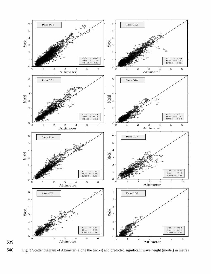
Chu et al. [2004] validated the WW3 model against TOPEX/Poseidon wave measurements in 167

the SCS and they found good agreement between the simulated and observed data. Figures 3 and 4 168

represent scatter plots of simulated versus altimeter significant wave height (SWH) for all selected 169

tracks. The computed statistics for the entire year of 2009, including the coefficient of determination 170

(C.D.), bias and root mean square error (RMSE) are displayed. Generally, based on the scatter plots, 171

the model performed reasonably well in simulating the SWH. For most tracks, the simulated SWH 172

matches the observed with C.D. ranges between 0.8–0.9 and averaged RMSEs of 0.35 m. For these 173

tracks, the range of bias is between -0.1 to 0.1 m. The model underestimated the SWH in the Malacca 174

Straits and Gulf of Thailand (Passes 001 and 166) with smaller C.D.s of 0.66 and 0.59, respectively. In 175

the case of Malacca Straits, insufficient model resolution reduces its performance. In addition, higher 176

resolution of wind forcing is also required to capture wave characteristics in such a narrow water 177

channel. Moreover, the wave characteristics can be influenced by strong tidal currents, especially along 178

Peninsular Malaysia, the Gulf of Thailand and the west coast of Borneo [Fang et al., 1999]; however, 179

tidal effects were not included in the simulation. 180

181

In addition to satellite altimetry data, the model was also validated against a three-month record of 182

nearshore wave measurements at Terengganu (Fig. 5). The measurements were carried out using a 183

Nortek acoustic Doppler profiler and directional wave gauge (AWAC) for a period of Jan-Apr 2009. 184

Figure 4 shows the time series comparison of SWH and mean wave period between the model and 185

AWAC data. The comparison shows the reasonable ability of the model to reproduce the wave 186

parameters in the location with C.D. values of 0.96 and 0.98 for HS and TM, respectively. For Hs, the 187

C.D. (RMSE) value of 0.96 (0.22 m) is generally larger (smaller) compared with the value based on the 188

satellite tracks. 189

190

Due to the nearshore location of the AWAC, the insufficient resolution of the model resulted in 191

an underestimation of the wave height. On the other hand, short-lived local winds could also be a 192

reason why the model did not accurately reproduce short period waves in some regions [Bosserelle et 193

al., 2012]. In addition, the complexity of topography and existence of islands could cause refraction 194

and blocking of waves, which leads to an underestimation of wave heights and wave periods nearshore 195

and in coastal areas. 196

197

2.4 Analysis methods 198

199

The WW3 model has been set to output several parameters at 3-hourly intervals for the 31-year 200

hindcast. These outputs comprised three main wave parameters: the significant wave height, peak wave 201

period and mean wave direction. These parameters were used to investigate the inter-annual variability 202

and long-term changes of the wave climate in the southern SCS. Seasonal mean significant wave 203

heights were determined by combining: the Dec-Jan-Feb (DJF) monthly mean for winter, Mar-Apr-204

May (MAM) for spring, Jun-Jul-Aug (JJA) for summer and Sep-Oct-Nov (SON) for autumn. 205

Simulated parameters were averaged annually and identified as the mean annual wave height (Hs), peak 206

wave period (Tp) and mean wave direction (MWD). Moreover, the mean annual of the 99th

(H99) and 207

90th

(H90) percentiles of wave height, which are known as the largest 1% and 10% of the parameters, 208

respectively, were also calculated. To compute the annual mean wave direction, the mean wave 209

direction was first split into meridional and zonal components and averaged separately and then 210

recombined. Inter-annual variability of Hs was determined by calculating the standard deviation of the 211

monthly mean values of Hs. 212

213

Trends in the time series of Hs, Tp, MWD and H90were computed for each grid point of the M3 214

domain. The trend analysis of the year-grouped wave height climate was made by the linear least 215

square fitting of time series of Hs and H90, while the p-values of correlation were computed to 216

determine the significance of the trend. Additionally, trends in monthly wave height were computed to 217

identify the significance of changes during every month. Trends at 95% confidence (p-value < 0.05) 218

were considered statistically significant. The relationship between wave height variability and El Nino-219

Southern Oscillation (ENSO) was also investigated by correlating ENSO indices (Nino 3.4 and El Nino 220

Modoki) with Hs. 221

222

3 Results and discussion 223

224

The maximum Hs features prominently in the central region of the SCS (Fig. 6) where winds 225

can increase from 5 knots to over 40 knots in a matter of hours during the monsoon seasons. Hs 226

decreases gradually in the northeast-southwest direction towards the Sunda shelf where the values are 227

relatively lower. In the southern region of the SCS and in the Gulf of Thailand, Hs ranges from 0.5 to 1 228

m. The lower values of Hs in the Gulf of Thailand might be due to shadowing effects of Indo-China. In 229

the coastal region along Peninsular Malaysia and the west coast of Borneo, Hs values were lower than 230

0.5 m. The reduction of Hs in these regions could be due to complex bathymetry and insufficient model 231

resolution. The bathymetry in the SCS (Fig. 1) plays an important role because large amounts of wave 232

energy, generated in the central parts of the SCS, is reduced due to apparent differences of topography 233

between the Sunda shelf and the central SCS. On Sunda shelf, the gradual depth reduction allows the 234

swell to travel to coastal regions of Peninsular Malaysia with no sudden bathymetric interaction, except 235

in areas where islands are located. However, along the offshore region of Borneo, sudden reductions in 236

depth reduce the wave energy impact on coastal areas due to breaking and refraction. Moreover, this 237

region might still be influenced by extreme waves generated by typhoons tracking over the central and 238

northern regions of the SCS. However, whether they are accurately resolved in the CFSR winds is 239

beyond the scope of this paper. 240

241

The spatial pattern of the 99th

(not shown) and 90th

percentiles (Fig. 7) resembles Hs with the 242

maximum values reaching 4 m in the central SCS. Along the coast of Vietnam, H90 can reach as high as 243

3 m. However, these values reduce to between 1–2 m in the Gulf of Thailand and southern regions of 244

the SCS (Fig. 7). The obstruction effects of several islands in the southern region of the SCS were well 245

resolved. The existence of multiple islands in southern regions of the SCS obstructs wave propagations 246

resulting in a reduction of Hs and H90. In addition, the tides and surges change the mean water depth 247

and current fields [Wolf and Prandle, 1999]; therefore, lower Hs in the coastal areas could also be 248

associated with tidal currents, which were not included in the simulation. Figure 8 depicts the seasonal 249

changes of the mean Hs. Of the seasons, the winter monsoon has the highest mean Hs, ranging from 2 250

m in the southern part of the SCS to 3 m in the central region (Fig. 8). In comparison, the values are 251

much lower during JJA. This obvious contrast is because of higher intensity winds during the winter 252

monsoon. The MAM (SON) transitional season has a similar spatial pattern to that of the summer 253

(winter). 254

255

The mean peak wave period Tp, has high values in the central SCS (>12° N) and decreases 256

slightly towards the Sunda shelf and coastal region of Borneo (Fig. 9). Similar to the mean Hs, the Tp 257

values decrease while the waves travel towards the Gulf of Thailand due to the shadowing of Indo-258

China. Moreover, the reduction of Tp in southern regions of the study domain is due to the presence of 259

several islands, which prevent waves with longer wavelengths from propagating into this area. This 260

explains why the largest values of T90 (not shown) are simulated at the offshore Riau Islands. Along the 261

eastern coast of Peninsular Malaysia, Tp has an almost constant value of 6.5 s. However, T90 reaches 262

around 9 s along Peninsular Malaysia coasts. 263

264

The MWD is predominantly influenced by the monsoonal winds over this region. Starting 265

around November, the Siberian High pushes the airflow around an anticyclone that carries air from 266

Siberia across China and out over the SCS during the northeast monsoon (DJF). The mean MWD is 267

predominantly northeasterly during DJF and MAM (Fig. 10). However, the mean MWD in the Gulf of 268

Thailand becomes more southerly in the shadow of the Indo-China region. During the SON transitional 269

season, the mean MWD gradually becomes westerly in the central SCS and turns southward along 270

Peninsular Malaysia. At the beginning of the summer monsoon (JJA), the wind over the SCS becomes 271

predominantly south-southwesterly [Lau et al., 1998]. Therefore, as we expected, the MWD becomes 272

southwesterly starting late May and reverts back to northeasterly around mid-September. 273

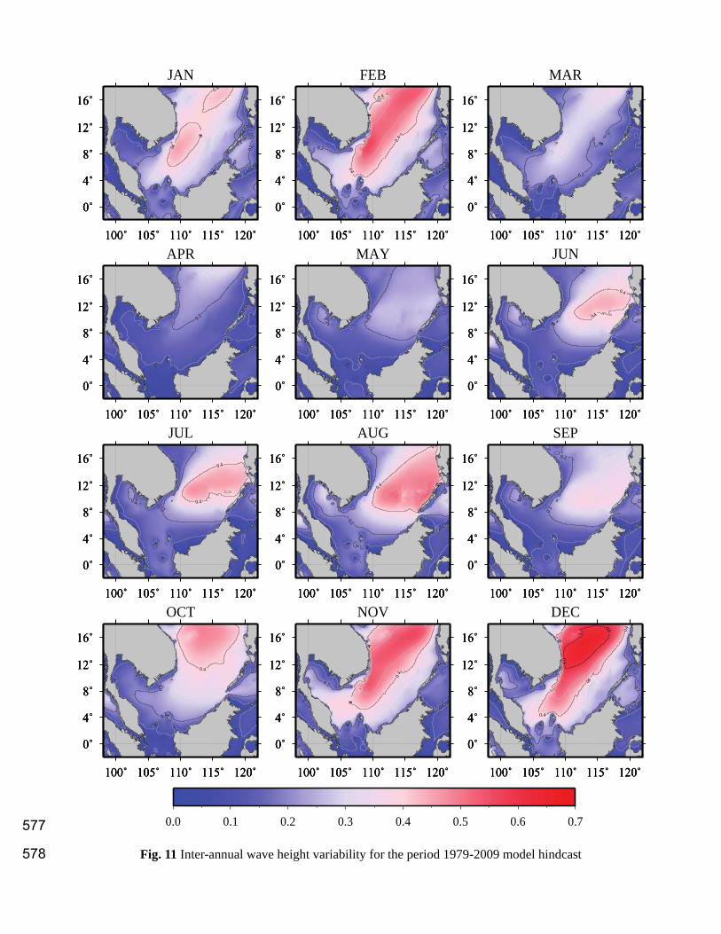
274

The standard deviation of the individual monthly mean significant wave heights was used to 275

measure the inter-annual variability of each corresponding month. The inter-annual variability of 276

significant wave height in the southern sector of the SCS is greatest during the winter months, 277

especially December. The elongated area of high standard deviation extends from the north, in the 278

northeasterly-southeasterly direction, to south along the coastal region of Peninsular Malaysia (Fig. 279

11). The high inter-annual variability observed in December could be forced by coherent large 280

phenomena, such as the El Nino – Southern Oscillation (ENSO). Juneng and Tangang [2005] indicated 281

that the anomalous low-level winds over the SCS are largely modulated by ENSO, particularly during 282

winter. Moreover, since the mid-1980s, there has been a tendency for maximum warming to occur at 283

the central equatorial Pacific Ocean resulting in a different event known as El Nino Modoki [Ashok et 284

al., 2007; Weng et al., 2007, 2009; Ashok and Yamagata, 2009], which generates a different response 285

over the SCS [Feng et al., 2010]. The El Nino Modoki occurrences are represented by the El-Niño 286

Modoki (EMI) index [Ashok et al., 2007]; hence, it is of interest to investigate further the relationship 287

between wave climates in the SCS and these phenomena. 288

289

The mean values of significant wave height for each season were correlated with the Niño 3.4 290

and El-Niño Modoki (EMI) climate indices. The correlation between the Niño 3.4 and mean Hs 291

demonstrate significant values in the central sector (>12° N) of the SCS during the winter (DJF). This 292

is consistent with the work of Juneng and Tangang [2005], which indicated weaker winter monsoon 293

winds over the SCS during El Nino. Weaker winds correspond to weaker waves and lower significant 294

wave heights. However, in summertime (JJA), positive correlation values are observed for the entire 295

southern SCS and become significant in the offshore region of Peninsular Malaysia and the Karimata 296

Straits (Fig. 12). Juneng and Tangang [2005] indicated strengthening of summer monsoonal winds over 297

the southern region of the SCS during El Nino years. Furthermore, Hs in the Gulf of Thailand exhibits 298

positive correlation with Niño 3.4, except during SON (when there is a negative correlation). Similarly, 299

in the Celebes Sea region, the correlation values are positive in all seasons except SON. The strong 300

ENSO signals in the wave climate in this sea could be due to its open connection with the western 301

Pacific Ocean, which allows the swell from the Pacific Ocean to easily penetrate the area. In contrast 302

with this, the relationship is weaker in the Sulu Sea due to the blocking effect of the Philippines group 303

of islands. 304

305

Figure 13 indicates the correlation values between Hs and the EMI. During SON, DJF and 306

MAM, the correlation values are weaker compared with the conventional El Nino. Moreover, in the 307

winter season, the significant negative correlation can only be found over the northern region of the 308

study domain. In the southern region, Hs correlates only weakly but positively with EMI. This could be 309

associated with the existence of the anomalous cyclonic circulation over the eastern Peninsular 310

Malaysia during El Nino Modoki [Feng et al., 2010]. This cyclonic circulation strengthens the winter 311

monsoonal winds over this region during El Nino Modoki and hence, enhances the wave height. 312

During transitional seasons (i.e., SON and MAM), the relationship between Hs and EMI is non-313

significant for almost the entire study domain. However, in summer, the area that has positive and 314

significant correlation expands northward to cover the entire domain, except for the northern region of 315

the Vietnamese coast. The differences of correlation strength and spatial distribution between Nino3.4 316

and EMI are attributed to the changes in the low level wind field over the SCS during El Nino Modoki, 317

which are associated with the westward shifting of the anomalous anti-cyclonic circulation over the 318

western north Pacific region [Feng et al., 2010]. 319

320

Long-term trends in the surface wind influences the Hs trend [Young, 1999; Young et al., 2011; 321

Bosserelle et al., 2012]. Over the SCS, Juneng and Tangang [2010] indicated that the zonal wind has 322

increased significantly over a period from 1962-2007. However, if a period from 1979 to 2007 were to 323

be considered, the trend might not be as prominent [Juneng and Tangang, 2010, Figure 2f]. In the 324

present study, we quantified the long-term changes of trend in the time series of Hs from 1979 to 2009 325

by a monthly mean trend analysis. Figure 14 depicts a spatial distribution of significant trends of Hs at 326

the 95% statistical confidence level with areas of non-significant changes shaded with dots. Generally, 327

increasing positive trends of Hs are found to be significant in the central region of the SCS during May, 328

July and September (Fig. 14). In contrast, significant negative trends of Hs dominate the southern 329

region of the SCS during December. In other months, the trends are non-significant. We investigated 330

further these trends by examining the time series of three box-areas, as indicated in Figure 2. Figure 15 331

shows the time series of the 90th

percentiles of Hs for the three areas during July and December. For 332

comparison, the corresponding time series of the ERA-INTERIM are also shown. As expected, the 333

modelled 90th

percentiles of Hs are higher than those of the ERA-INTERIM due to the WW3 finer grid-334

resolution. Moreover, the two time series are also mostly in phase with respect to the inter-annual 335

variability. However, the modelled fluctuations are greater during winter, especially in conjunction with 336

the 1997/98 El Nino. The large inter-annual fluctuations and relatively short record could be the reason 337

why most of the trends of the modelled 90th

percentiles of Hs are not significant. 338

339

4 Conclusions 340

341

A third generation wave model (WW3) was applied to the simulation of wave climate in the 342

southern extent of the SCS during the 31-year period from 1979 to 2009. The outputs were well 343

validated against available is situ and altimeter data and hence, the computed wave characteristics from 344

the model outputs provide reasonable estimates of wave climate in the region in the absence of long-345

term wave observations. The spatial distribution of the modelled seasonal mean Hs (and H90) indicates 346

higher values in the northern region of the study domain, which decrease southwestwards. In the most 347

southern regions, lower amplitudes of Hs are associated with shadowing, island blocking and 348

refraction. Seasonally, the values are higher during winter (DJF) and lower during summer (JJA) and 349

spring (MAM). Also, the results demonstrate strong inter-annual variability, especially during the 350

winter months. The mean Hs correlates negatively with the Nino3.4 index for almost the entire region 351

during winter, spring and autumn seasons. However, the correlation sign reverses during the summer 352

monsoon. During El Nino Modoki, the positive correlation during summer extends northeastwards to 353

cover almost the entire domain. The trend analysis indicates positive and negative long-term trends of 354

mean Hs depending on the month and location. However, the long-term trends could be masked by the 355

large inter-annual variability. 356

357

Acknowledgements 358

359

This research is funded by the grants of MOHE LRGS/TD/2011/UKM/PG/01, MOSTI Science fund 360

04-01-02-SF0747 and Universiti Kebangsaan Malaysia DIP-2012-020. 361

362

363

364

365

366

367

References: 368

369

Ashok, K., S. K. Behera, S. A. Rao, H. Y. Weng, and T. Yamagata (2007), El Nino Modoki and its 370

possible teleconnection, J. Geophys. Res., 112(C11007), doi:10.1029/2006JC003798. 371

372

Ashok, K., and T. Yamagata (2009), The EL Niño with a difference, Nature, 461, 481–484, 373

doi:10.1038/461481a. 374

375

Bidlot, J. R., J. G. Li, P. Wittmann, M. Faucher, H. S. Chen, J. M. Lefevre, T. Bruns, D. Greenslade, F. 376

Ardhuin, N. Kohno, S. Park and M. Gomez (2007), Inter-comparison of operational wave forecasting 377

systems, paper presented at 10th

International workshop on wave hindcasting and forecasting, Oahu, 378

Hawaii. 379

380

Bosserelle, C., C. B. Pattiaratchi, and I. Haigh (2012), Inter-annual variability and longer-term changes 381

in the wave climate of Western Australia between 1970 and 2009, Ocean Dyn., 62:63–76, 382

doi:10.1007/s10236-011-0487-3. 383

384

Brown, J. M., J. Wolf, and A. J. Souza (2012), Past to future extreme events in Liverpool Bay: model 385

projections from 1960-2100, Climate Change, 111:365–391, doi:10.1007/s10584-011-0145-2. 386

387

Chawla, A., and H. L. Tolman (2007), Automated grid generation for WAVEWATCH III, 388

NOAA/NWS/NCEP/OMB, Technical Note 254. 389

390

Chawla, A., H. L. Tolman, J. L. Lanson, E.-M. Devaliere, and V. M. Gerald (2009), Validation of a 391

Multi-Grid WAVEWATCH IIITM

modeling system, NOAA/MMAB Contribution no. 281. 392

393

Chu, P. C., Y. Qi, Y. Chen, P. Shi, and Q. Mao (2004), South China Sea wind-wave characteristics. Part 394

I: Validation of Wavewatch-III using TOPEX/Poseidon data, Journal of Atmospheric and Oceanic 395

Technology, 21(11):1718–1733, doi:10.1175/JTECH1661.1. 396

397

Chu, P. C., S. Lu, and W. T. Liu (1999), Uncertainty of South China Sea prediction using NSCAT and 398

National Centers for Environmental Prediction winds during tropical storm Ernie, 1996, J. Geophys. 399

Res., 104(C5), 11,273–11,289, doi:10.1029/1998JC900046. 400

401

Chu, P. C., J. M. Veneziano, C. Fan, M. J. Carron, and W. T. Liu (2000), Response of the South China 402

Sea to Tropical Cyclone Ernie 1996, J. Geophys. Res., 105(C6), 13,991–14,009, 403

doi:10.1029/2000JC900035. 404

405

Cuchiara, D. C., E. H. Fernandes, J. C. Strauch, J. C. Winterwerp, and L. J. Calliari (2009), 406

Determination of the wave climate for southern Brazilian shelf, Continental Shelf Research, 29:545–407

555, doi:10.1016/j.csr.2008.09.025. 408

409

Chunxia, L., Y. Qi, and J. Liang (2008), The effect of sea waves on Typhon Imodo, 2nd

CAWCR 410

Modelling Workshop 2008, High Resolution Modelling, Nov. 25-28 Australia. 411

412

Fang, G., Y.-K. Kwok, K. Yu, and Y. Zhu (1999), Numerical simulation of principal tidal constituents in 413

the South China Sea, Gulf of Tonkin and Gulf of Thailand, Continental Shelf Research, 19(7):845–869, 414

doi:10.1016/s0278-4343(99)00002-3. 415

416

Feng, M., M. J. McPhaden, and T. Lee (2010), Decadal variability of the Pacific subtropical cells and 417

their influence on the southeast Indian Ocean, Geophys. Res. Lett., 37:L09606, 418

doi:10.1029/2010GL042796. 419

420

Hanson, J. L., B.A. Tracy, H. L. Tolma, and D. R. Scott (2009), Pacific hindcast performance of three 421

numerical wave model, J. Atmos. Oceanic Technol., 26:1614–1633. 422

423

Hemer, M. A., J. A. Church, and J. R. Hunter (2010), Variability and trends in the directional wave 424

climate of the southern hemisphere, Int.J. Climatol, 30:475–491, doi:10.1002/joc.1900. 425

426

IPCC AR4 (2007), Climate change 2007, Fourth assessment report of the intergovernmental panel on 427

climate change, Cambridge University Press, Cambridge. 428

429

Jiang, L. F., Z. X. Zhang, and Y. Q. Qi (2010), Simulation of SWAN and WAVEWATCH III in 430

Northern South China Sea, 20th

International Offshore and Polar Engineering Conference, Beijing, 431

China, June 20–25, 2010. 432

433

Juneng, L., and F. T. Tangang (2005), Evolution of ENSO-related rainfall anomalies in Southeast Asia 434

region and its relationship with atmosphere-ocean variations in Indo-Pacific sector, Clim. Dyn., 435

25:337–350, doi:10.1077/s00382-005-0031-6. 436

437

Juneng, L., F. T. Tangang (2010), Long-term trends of winter monsoon synoptic circulations over the 438

maritime continent: 1962-2007, Atmos. Sci. Lett., 11(3): 199–203, doi:10.100/asl.272. 439

440

Kriiezi, E. E., and B. Broman (2008), Past and future wave climate in the Baltic Sea produced by the 441

SWAN model with forcing from the regional climate model RCA of the Rossby Center, In: IEEE/OES 442

US/EU-Baltic International Symposium (ed.), Tallinn, Estonia, 27-29 May 2008, pp 360–366. 443

444

Lau, K.-M., H.-T. Wu, and S. Yang (1998), Hydrologic processes associated with the first transition of 445

the Asian Summer Monsoon: A pilot satellite study, Bull. Am. Meteorol. Soc., 79:1871–1882. 446

447

Lionello, P., and A. Sanna (2005), Mediterranean wave climate variability and its links with NAO and 448

Indian Monsoon, Clim Dyn, 25:611–623, doi:10.1007/s00382-005-0025-4. 449

450

Mori, N., T. Yasuda, H. Mase, T. Tom, Y. Oku (2010), Projection of extreme wave climate change 451

under global warming, Hydrol Res Lett, 4:15–19. 452

453

Music, S., and S. Nikovic (2008), 44-year wave hindcast for the Eastern Mediterranean, Coastal 454

Engineering, 55:872–880, doi:10.1016/j.coastaleng.2008.02.024. 455

456

NCEP (2006), National Center for Environmental Prediction, Washington DC., available at 457

http://polar.ncep.noaa.gov/waves. 458

459

NGDC (2006), National Geophysical Data Center, available at 460

http://ngdc.noaa.gov/mgg/global/etopo2.html. 461

462

Padilla-Hernandez, R., W. Perrie, B. Toulany, P. C. Smith, W. Zhang, and S. Jimenez-Hernandez 463

(2004), Intercomparison of modern operational wave models, In: 8th

International workshop on wave 464

hindcasting and forecasting, North Shore, Oahu, Hawaii. 465

466

Panchang, V. G., C. Jeong, and D. Li (2008), Wave climatology in coastal Maine for aquaculture and 467

other applications, Estuaries and Coast: J. CERF, 31:289–299, doi:10.1007/s12237-007-9016-5. 468

469

Qi, Y. Q., Z. X. Zhang, and P. SHI (2010), Extreme wind, wave and current in deep water of South 470

China Sea, Int. J. Offshore and Polar Engineering, Vol.20, No.1, pp:18–23. 471

472

Saha S., S. Moorthi, H.-L. Pan, X. Wu, J. Wang, S. Nadiga, P. Tripp, R. Kistler, J. Woollen, D. 473

Behringer, H. Liu, D. Stokes, R. Grumbine, G. Gayno, J. Wang, Y.-T. Hou, H. Chuang, H.-M. H. Juang, 474

J. Sela, M. Iredell, R. Treadon, D. Kleist, P. van Delst, D. Keyser, J. Derber, M. Ek, J. Meng, H. Wei, R. 475

Yang, S. Lord, H. van den Dool, A. Kumar, W. Wang, C. Long, M. Chelliah, Y. Xue, B. Huang, J.-K. 476

Schemm, W. Ebisuzaki, R. Lin, P. Xie, M. Chen, S. Zhou, W. Higginsz, C.-Z. Zou, Q. Liu, Y. Chen, Y. 477

Han, L. Cucurull, R. W. Reynolds, G. Rutledge, and M. Goldberg (2010), The NCEP climate forecast 478

system reanalysis, Bull Amer Meteor Soc., 91:1015–1057. 479

480

Salahuddin, A., and S. Curtis (2011), Climate extremes in Malaysia and the equatorial South China 481

Sea, Global and Planetary Change, 78:83–91, doi:10.1016/j.gloplacha.2011.05.001. 482

483

Swail, V. R., A. T. Cox, and V. J. Cardone (1999), Analysis of wave climate trends and variability, 484

WMO Workshop on Advances in Marine Climatology (CLIMAR99), 8-15 September 1999, 485

Vancouver, B.C., p. 245–256. 486

487

Tolman, H. L. (2002), Validation of WAVEWATCH III version 1.15 for a global domain, 488

NCEP/NOAA/NWS, National Center for Environmental Prediction, Technical note 213, Washington. 489

490

Tolman, H. L. (2009), User manual and system documentation of WAVEWATCH III TM version 3.14, 491

NOAA/NWS/NCEP/MMAB Technical Note 276 492

493

WAMDI (1988), The WAM model – a third generation ocean wave prediction model, J Phys 494

Oceanogr., 18:1775–1810. 495

496

Wang, X. L., F. W. Zwiers, and V. R. Swail (2004), North Atlantic ocean wave climate change 497

scenarios for the Twenty-First century, J. Climate, doi:10.1175/1520–0442. 498

499

Wang, X. L., and V. R. Swail (2006), Trends of Atlantic wave extremes as simulated in a 40-yr wave 500

hindcast using kinematically reanalyzed wind fields, J. Clim., 15:1020–1035, doi:10.1175/1520-501

0442(2002)015<1020:TOAWEA>2.0.CO;2. 502

503

Weng, H., K. Ashok, S. K. Behera, S. A. Rao, and T. Yamagata (2007), Impacts of recent El Niño 504

Modoki on dry/wet conditions in the Pacific Rim during boreal summer, Clim. Dyn., 29:113–129, 505

doi:10.1007/s00382-007-0234-0. 506

507

Weng, H., S. K. Behera, and T. Yamagata 2009, Anomalous winter climate conditions in the Pacific rim 508

during recent El Niño Modoki and El Niño events, Clim. Dyn., 29:113–129, doi:10.1007/s00382-008-509

0394-6. 510

511

Wolf, J., and D. Prandle (1999), Some observation of wave-current interaction, Coastal Engineering 37, 512

471–485. 513

514

Wright, L. D., J. D. Boon, S. C. Kim, and J. H. List (1991), Modes of cross-shore sediment transport on 515

the shoreface of the Middle Atlantic Bight, Marine Geology, 96:19–51, doi:10.1016/0025-516

3227(91)90200-N. 517

518

Xue, Y., B. Huang, Z.-Z. Hu, A. Kumar, C. Wen, D. Behringer, and S. Nadiga (2010), An assessment of 519

oceanic variability in the NCEP climate forecast system reanalysis, Clim. Dyn., doi:10.1007/s00382-520

010-0954-4. 521

522

Young, I. R. (1999), Seasonal variability of the global ocean wind and wave climate, Int. J. Climatol., 523

19:931–950. 524

525

Young, I. R., S. Zieger, and A. V. Babanin (2011), Global trends in wind speed and wave height, 526

Science, doi:10.1126/science.1197219. 527

528

Zacharioudaki, A., S. Pan, and D. Simmonds (2011), Future wave climate over the west-European shelf 529

seas, Ocean Dyn., 61:807–827, doi:10.1007/s10236-011-0395-6. 530

531

90˚ 95˚ 100˚ 105˚ 110˚ 115˚ 120˚ 125˚ 130˚ 135˚ 140˚ 145˚

−10˚

−5˚

0˚

5˚

10˚

15˚

20˚

25˚

30˚

35˚

40˚

45˚

90˚ 95˚ 100˚ 105˚ 110˚ 115˚ 120˚ 125˚ 130˚ 135˚ 140˚ 145˚

−10˚

−5˚

0˚

5˚

10˚

15˚

20˚

25˚

30˚

35˚

40˚

45˚

90˚ 95˚ 100˚ 105˚ 110˚ 115˚ 120˚ 125˚ 130˚ 135˚ 140˚ 145˚

−10˚

−5˚

0˚

5˚

10˚

15˚

20˚

25˚

30˚

35˚

40˚

45˚

−8000

−6000

−4000

−2000

0

2000

4000

6000

8000

(m)

Μ2 = 0.25° × 0.25°

Μ1 = 0.31° × 0.31°

Μ3 = 0.15° × 0.15°

532

Fig. 1 Bathymetry and definition for three mosaic nested computational domains 533

534

535

100˚ 104˚ 108˚ 112˚ 116˚ 120˚

0˚

4˚

8˚

12˚

16˚

100˚ 104˚ 108˚ 112˚ 116˚ 120˚

0˚

4˚

8˚

12˚

16˚ South China Sea

Gulf of Thailand

Malacc

a Strait

Vietnam

Combodia

Laos

Thailand

Philip

pines

Singapore

Sabah

Sarawak

Indonesia

BruneiPeninsular

Malaysia

Sumatra

Celebes Sea

Sulu Sea

Kepulauan RiauPal

awan

Island

Tioman IslandJemaja Islands

Siantan Islands

a

c

b

Terengganu

AWAC

100˚ 104˚ 108˚ 112˚ 116˚ 120˚

0˚

4˚

8˚

12˚

16˚

100˚ 104˚ 108˚ 112˚ 116˚ 120˚

0˚

4˚

8˚

12˚

16˚

100˚ 104˚ 108˚ 112˚ 116˚ 120˚

0˚

4˚

8˚

12˚

16˚

100˚ 104˚ 108˚ 112˚ 116˚ 120˚

0˚

4˚

8˚

12˚

16˚

100˚ 104˚ 108˚ 112˚ 116˚ 120˚

0˚

4˚

8˚

12˚

16˚

100˚ 104˚ 108˚ 112˚ 116˚ 120˚

0˚

4˚

8˚

12˚

16˚

100˚ 104˚ 108˚ 112˚ 116˚ 120˚

0˚

4˚

8˚

12˚

16˚

100˚ 104˚ 108˚ 112˚ 116˚ 120˚

0˚

4˚

8˚

12˚

16˚

100˚ 104˚ 108˚ 112˚ 116˚ 120˚

0˚

4˚

8˚

12˚

16˚

100˚ 104˚ 108˚ 112˚ 116˚ 120˚

0˚

4˚

8˚

12˚

16˚

100˚ 104˚ 108˚ 112˚ 116˚ 120˚

0˚

4˚

8˚

12˚

16˚

100˚ 104˚ 108˚ 112˚ 116˚ 120˚

0˚

4˚

8˚

12˚

16˚

100˚ 105˚ 110˚ 115˚ 120˚

0˚

4˚

8˚

12˚

16˚

153 229 051 127

077001 203

038 114 190

012

216

140064

100˚ 105˚ 110˚ 115˚ 120˚

0˚

4˚

8˚

12˚

16˚

Karimata Strait

536

Fig. 2 The area of focus of this study (left) and the coverage of Topex satellite tracks in the SCS (right) 537

538

0

1

2

3

4

5

6M

odel

0 1 2 3 4 5 6

Altimeter

Pass 038

C.D. = 0.85

Bias = 0.09

RMSE = 0.36

0

1

2

3

4

5

6

Mod

el

0 1 2 3 4 5 6

Altimeter

Pass 012

C.D. = 0.86

Bias = −0.05

RMSE = 0.32

0

1

2

3

4

5

6

Mod

el

0 1 2 3 4 5 6

Altimeter

Pass 051

C.D. = 0.89

Bias = 0.12

RMSE = 0.35

0

1

2

3

4

5

6

Mod

el

0 1 2 3 4 5 6

Altimeter

Pass 064

C.D. = 0.81

Bias = −0.09

RMSE = 0.28

0

1

2

3

4

5

6

Mod

el

0 1 2 3 4 5 6

Altimeter

Pass 114

C.D. = 0.89

Bias = 0.16

RMSE = 0.38

0

1

2

3

4

5

6

Mod

el

0 1 2 3 4 5 6

Altimeter

Pass 127

C.D. = 0.72

Bias = −0.10

RMSE = 0.44

0

1

2

3

4

5

6

Mod

el

0 1 2 3 4 5 6

Altimeter

Pass 077

C.D. = 0.87

Bias = −0.04

RMSE = 0.30

0

1

2

3

4

5

6

Mod

el

0 1 2 3 4 5 6

Altimeter

Pass 166

C.D. = 0.59

Bias = −0.12

RMSE = 0.35

539

Fig. 3 Scatter diagram of Altimeter (along the tracks) and predicted significant wave height (model) in metres 540

541

0

1

2

3

4

5

6

Mod

el

0 1 2 3 4 5 6

Altimeter

Pass 190

C.D. = 0.93

Bias = 0.03

RMSE = 0.35

0

1

2

3

4

5

6

Mod

el

0 1 2 3 4 5 6

Altimeter

Pass 242

C.D. = 0.73

Bias = −0.07

RMSE = 0.27

0

1

2

3

4

5

6

Mod

el

0 1 2 3 4 5 6

Altimeter

Pass 216

C.D. = 0.88

Bias = 0.03

RMSE = 0.37

0

1

2

3

4

5

6

Mod

el

0 1 2 3 4 5 6

Altimeter

Pass 229

C.D. = 0.90

Bias = 0.02

RMSE = 0.36

0

1

2

3

4

5

6

Mod

el

0 1 2 3 4 5 6

Altimeter

Pass 179

C.D. = 0.65

Bias = −0.12

RMSE = 0.27

0

1

2

3

4

5

6

Mod

el

0 1 2 3 4 5 6

Altimeter

Pass 001

C.D. = 0.66

Bias = −0.14

RMSE = 0.37

0

1

2

3

4

5

6

Mod

el

0 1 2 3 4 5 6

Altimeter

Pass 203

C.D. = 0.81

Bias = −0.10

RMSE = 0.31

0

1

2

3

4

5

6

Mod

el

0 1 2 3 4 5 6

Altimeter

Pass 153

C.D. = 0.87

Bias = 0.08

RMSE = 0.40

542

Fig. 4 Same as Fig. 3 except for different tracks 543

0

1

2

3

Sig

nif

ican

t w

av

e h

eig

ht

(m)

0 200 400 600 800 1000

Two hourly record

0

1

2

3

Sig

nif

ican

t w

av

e h

eig

ht

(m)

0 200 400 600 800 1000

Two hourly records

C.D. = 0.96

Bias = 0.13

RMSE = 0.22

−− Model

−− AWAC

0

2

4

6

8

Mean

wav

e p

eri

od (

s)

0 200 400 600 800 1000

Two hourly record

0

2

4

6

8

Mean

wav

e p

eri

od (

s)

0 200 400 600 800 1000

Two hourly records

C.D. = 0.98

Bias = 0.28

RMSE = 0.75

−− Model

−− AWAC

544

545

Fig. 5 Comparison between modelled and measured (AWAC) significant wave height and mean wave period 546

during the period Jan-Mar 2009 547

548

549

100˚ 104˚ 108˚ 112˚ 116˚ 120˚

0˚

4˚

8˚

12˚

16˚

100˚ 104˚ 108˚ 112˚ 116˚ 120˚

0˚

4˚

8˚

12˚

16˚

100˚ 104˚ 108˚ 112˚ 116˚ 120˚

0˚

4˚

8˚

12˚

16˚

0.9

0.9

0.9 0.91.

2

1.2 1.2

1.2

1.2

1.5

1.51.5

1.5

1.8

1.8

1.8

0

1

2

(m)

550

Fig. 6 Mean significant wave height for the period 1979-2009 model hindcast 551

552

100˚ 104˚ 108˚ 112˚ 116˚ 120˚

0˚

4˚

8˚

12˚

16˚

100˚ 104˚ 108˚ 112˚ 116˚ 120˚

0˚

4˚

8˚

12˚

16˚

100˚ 104˚ 108˚ 112˚ 116˚ 120˚

0˚

4˚

8˚

12˚

16˚

4

4

4

4

4

5

5

66

1

2

3

4

5

6

7

(m)

553

Fig. 7 Mean 90th percentile wave height for the period 1979-2009 model hindcast 554

555

100˚ 105˚ 110˚ 115˚ 120˚

0˚

4˚

8˚

12˚

16˚

DJF

100˚ 105˚ 110˚ 115˚ 120˚

0˚

4˚

8˚

12˚

16˚

1

1.5

1.5

2

2

2.5

2.5

100˚ 105˚ 110˚ 115˚ 120˚

0˚

4˚

8˚

12˚

16˚

MAM

100˚ 105˚ 110˚ 115˚ 120˚

0˚

4˚

8˚

12˚

16˚

1

1

100˚ 105˚ 110˚ 115˚ 120˚

0˚

4˚

8˚

12˚

16˚

JJA

100˚ 105˚ 110˚ 115˚ 120˚

0˚

4˚

8˚

12˚

16˚

1

1.5

100˚ 105˚ 110˚ 115˚ 120˚

0˚

4˚

8˚

12˚

16˚

SON

100˚ 105˚ 110˚ 115˚ 120˚

0˚

4˚

8˚

12˚

16˚

1

1.5

1.5

2

0 1 2 3

m

556

Fig. 8 Seasonal mean wave height variability for the period 1979-2009 model hindcast 557

558

559

560

561

562

563

564

565

566

567

568

569

100˚ 104˚ 108˚ 112˚ 116˚ 120˚

0˚

4˚

8˚

12˚

16˚

100˚ 104˚ 108˚ 112˚ 116˚ 120˚

0˚

4˚

8˚

12˚

16˚

100˚ 104˚ 108˚ 112˚ 116˚ 120˚

0˚

4˚

8˚

12˚

16˚

4

4

4

5

5

5

5

6

6

6

6

7

7

7

0

1

2

3

4

5

6

7

8

(s)

570

Fig. 9 Mean peak wave period Tp, for the period 1979-2009 model hindcast 571

572

573

100˚ 105˚ 110˚ 115˚ 120˚

0˚

4˚

8˚

12˚

16˚

DJF

100˚ 105˚ 110˚ 115˚ 120˚

0˚

4˚

8˚

12˚

16˚

100˚ 105˚ 110˚ 115˚ 120˚

0˚

4˚

8˚

12˚

16˚

MAM

100˚ 105˚ 110˚ 115˚ 120˚

0˚

4˚

8˚

12˚

16˚

100˚ 105˚ 110˚ 115˚ 120˚

0˚

4˚

8˚

12˚

16˚

JJA

100˚ 105˚ 110˚ 115˚ 120˚

0˚

4˚

8˚

12˚

16˚

100˚ 105˚ 110˚ 115˚ 120˚

0˚

4˚

8˚

12˚

16˚

SON

100˚ 105˚ 110˚ 115˚ 120˚

0˚

4˚

8˚

12˚

16˚

0 60 120 180 240 300 360

deg

574

Fig. 10 Mean MWD variability for the period 1979-2009 model hindcast 575

576

100˚ 105˚ 110˚ 115˚ 120˚

0˚

4˚

8˚

12˚

16˚

JAN

100˚ 105˚ 110˚ 115˚ 120˚

0˚

4˚

8˚

12˚

16˚

0.2

0.20.

2

0.2

0.4

0.4

0.4

100˚ 105˚ 110˚ 115˚ 120˚

0˚

4˚

8˚

12˚

16˚

100˚ 105˚ 110˚ 115˚ 120˚

0˚

4˚

8˚

12˚

16˚

FEB

100˚ 105˚ 110˚ 115˚ 120˚

0˚

4˚

8˚

12˚

16˚

0.2

0.2

0.2

0.2

0.4

0.40.4

0.4

100˚ 105˚ 110˚ 115˚ 120˚

0˚

4˚

8˚

12˚

16˚

100˚ 105˚ 110˚ 115˚ 120˚

0˚

4˚

8˚

12˚

16˚

MAR

100˚ 105˚ 110˚ 115˚ 120˚

0˚

4˚

8˚

12˚

16˚

0.2

0.2

0.2

0.2

100˚ 105˚ 110˚ 115˚ 120˚

0˚

4˚

8˚

12˚

16˚

100˚ 105˚ 110˚ 115˚ 120˚

0˚

4˚

8˚

12˚

16˚

APR

100˚ 105˚ 110˚ 115˚ 120˚

0˚

4˚

8˚

12˚

16˚

0.2

0.2

100˚ 105˚ 110˚ 115˚ 120˚

0˚

4˚

8˚

12˚

16˚

100˚ 105˚ 110˚ 115˚ 120˚

0˚

4˚

8˚

12˚

16˚

MAY

100˚ 105˚ 110˚ 115˚ 120˚

0˚

4˚

8˚

12˚

16˚

0.20.2

100˚ 105˚ 110˚ 115˚ 120˚

0˚

4˚

8˚

12˚

16˚

100˚ 105˚ 110˚ 115˚ 120˚

0˚

4˚

8˚

12˚

16˚

JUN

100˚ 105˚ 110˚ 115˚ 120˚

0˚

4˚

8˚

12˚

16˚

0.2

0.2

0.4

0.4

100˚ 105˚ 110˚ 115˚ 120˚

0˚

4˚

8˚

12˚

16˚

100˚ 105˚ 110˚ 115˚ 120˚

0˚

4˚

8˚

12˚

16˚

JUL

100˚ 105˚ 110˚ 115˚ 120˚

0˚

4˚

8˚

12˚

16˚

0.2

0.2

0.4

0.4

100˚ 105˚ 110˚ 115˚ 120˚

0˚

4˚

8˚

12˚

16˚

100˚ 105˚ 110˚ 115˚ 120˚

0˚

4˚

8˚

12˚

16˚

AUG

100˚ 105˚ 110˚ 115˚ 120˚

0˚

4˚

8˚

12˚

16˚

0.2

0.20.

4

0.4

100˚ 105˚ 110˚ 115˚ 120˚

0˚

4˚

8˚

12˚

16˚

100˚ 105˚ 110˚ 115˚ 120˚

0˚

4˚

8˚

12˚

16˚

SEP

100˚ 105˚ 110˚ 115˚ 120˚

0˚

4˚

8˚

12˚

16˚

0.2

0.2

0.2

100˚ 105˚ 110˚ 115˚ 120˚

0˚

4˚

8˚

12˚

16˚

100˚ 105˚ 110˚ 115˚ 120˚

0˚

4˚

8˚

12˚

16˚

OCT

100˚ 105˚ 110˚ 115˚ 120˚

0˚

4˚

8˚

12˚

16˚

0.2

0.2

0.4

100˚ 105˚ 110˚ 115˚ 120˚

0˚

4˚

8˚

12˚

16˚

100˚ 105˚ 110˚ 115˚ 120˚

0˚

4˚

8˚

12˚

16˚

NOV

100˚ 105˚ 110˚ 115˚ 120˚

0˚

4˚

8˚

12˚

16˚

0.2

0.4

0.4

0.4

100˚ 105˚ 110˚ 115˚ 120˚

0˚

4˚

8˚

12˚

16˚

100˚ 105˚ 110˚ 115˚ 120˚

0˚

4˚

8˚

12˚

16˚

DEC

100˚ 105˚ 110˚ 115˚ 120˚

0˚

4˚

8˚

12˚

16˚

0.2

0. 2

0.2

0.4

0.4

0.40.6

0.6

100˚ 105˚ 110˚ 115˚ 120˚

0˚

4˚

8˚

12˚

16˚

0.0 0.1 0.2 0.3 0.4 0.5 0.6 0.7 577

Fig. 11 Inter-annual wave height variability for the period 1979-2009 model hindcast 578

579

100˚ 105˚ 110˚ 115˚ 120˚

0˚

4˚

8˚

12˚

16˚

100˚ 105˚ 110˚ 115˚ 120˚

0˚

4˚

8˚

12˚

16˚

DJF

100˚ 105˚ 110˚ 115˚ 120˚

0˚

4˚

8˚

12˚

16˚

100˚ 105˚ 110˚ 115˚ 120˚

0˚

4˚

8˚

12˚

16˚

100˚ 105˚ 110˚ 115˚ 120˚

0˚

4˚

8˚

12˚

16˚

MAM

100˚ 105˚ 110˚ 115˚ 120˚

0˚

4˚

8˚

12˚

16˚

100˚ 105˚ 110˚ 115˚ 120˚

0˚

4˚

8˚

12˚

16˚

100˚ 105˚ 110˚ 115˚ 120˚

0˚

4˚

8˚

12˚

16˚

JJA

100˚ 105˚ 110˚ 115˚ 120˚

0˚

4˚

8˚

12˚

16˚

100˚ 105˚ 110˚ 115˚ 120˚

0˚

4˚

8˚

12˚

16˚

100˚ 105˚ 110˚ 115˚ 120˚

0˚

4˚

8˚

12˚

16˚

SON

100˚ 105˚ 110˚ 115˚ 120˚

0˚

4˚

8˚

12˚

16˚

−0.5 −0.4 −0.3 −0.2 −0.1 0.0 0.1 0.2 0.3 0.4 0.5

Correlation

580

Fig. 12 Correlation of seasonal mean HS with Niño 3.4 for winter (DJF); Spring (MAM); Summer (JJA) and 581

Autumn (SON) at 90% confidence level. Dotted shading shows non-significant correlations at 90% confidence 582

level 583

584

100˚ 105˚ 110˚ 115˚ 120˚

0˚

4˚

8˚

12˚

16˚

100˚ 105˚ 110˚ 115˚ 120˚

0˚

4˚

8˚

12˚

16˚

DJF

100˚ 105˚ 110˚ 115˚ 120˚

0˚

4˚

8˚

12˚

16˚

100˚ 105˚ 110˚ 115˚ 120˚

0˚

4˚

8˚

12˚

16˚

100˚ 105˚ 110˚ 115˚ 120˚

0˚

4˚

8˚

12˚

16˚

MAM

100˚ 105˚ 110˚ 115˚ 120˚

0˚

4˚

8˚

12˚

16˚

100˚ 105˚ 110˚ 115˚ 120˚

0˚

4˚

8˚

12˚

16˚

100˚ 105˚ 110˚ 115˚ 120˚

0˚

4˚

8˚

12˚

16˚

JJA

100˚ 105˚ 110˚ 115˚ 120˚

0˚

4˚

8˚

12˚

16˚

100˚ 105˚ 110˚ 115˚ 120˚

0˚

4˚

8˚

12˚

16˚

100˚ 105˚ 110˚ 115˚ 120˚

0˚

4˚

8˚

12˚

16˚

SON

100˚ 105˚ 110˚ 115˚ 120˚

0˚

4˚

8˚

12˚

16˚

−0.5 −0.4 −0.3 −0.2 −0.1 0.0 0.1 0.2 0.3 0.4 0.5

Correlation

585

Fig. 13 Correlation of seasonal mean HS with El-Niño Modoki (EMI) for winter (DJF); Spring (MAM); Summer 586

(JJA) and Autumn (SON) at 90% confidence level. Dotted shading shows non-significant correlations at 90% 587

confidence level 588

589

100˚ 105˚ 110˚ 115˚ 120˚

0˚

4˚

8˚

12˚

16˚

100˚ 105˚ 110˚ 115˚ 120˚

0˚

4˚

8˚

12˚

16˚

100˚ 105˚ 110˚ 115˚ 120˚

0˚

4˚

8˚

12˚

16˚

JAN

100˚ 105˚ 110˚ 115˚ 120˚

0˚

4˚

8˚

12˚

16˚

100˚ 105˚ 110˚ 115˚ 120˚

0˚

4˚

8˚

12˚

16˚

FEB

100˚ 105˚ 110˚ 115˚ 120˚

0˚

4˚

8˚

12˚

16˚

100˚ 105˚ 110˚ 115˚ 120˚

0˚

4˚

8˚

12˚

16˚

100˚ 105˚ 110˚ 115˚ 120˚

0˚

4˚

8˚

12˚

16˚

MAR

100˚ 105˚ 110˚ 115˚ 120˚

0˚

4˚

8˚

12˚

16˚

100˚ 105˚ 110˚ 115˚ 120˚

0˚

4˚

8˚

12˚

16˚

100˚ 105˚ 110˚ 115˚ 120˚

0˚

4˚

8˚

12˚

16˚

APR

100˚ 105˚ 110˚ 115˚ 120˚

0˚

4˚

8˚

12˚

16˚

100˚ 105˚ 110˚ 115˚ 120˚

0˚

4˚

8˚

12˚

16˚

100˚ 105˚ 110˚ 115˚ 120˚

0˚

4˚

8˚

12˚

16˚

MAY

100˚ 105˚ 110˚ 115˚ 120˚

0˚

4˚

8˚

12˚

16˚

100˚ 105˚ 110˚ 115˚ 120˚

0˚

4˚

8˚

12˚

16˚

100˚ 105˚ 110˚ 115˚ 120˚

0˚

4˚

8˚

12˚

16˚

JUN

100˚ 105˚ 110˚ 115˚ 120˚

0˚

4˚

8˚

12˚

16˚

100˚ 105˚ 110˚ 115˚ 120˚

0˚

4˚

8˚

12˚

16˚

100˚ 105˚ 110˚ 115˚ 120˚

0˚

4˚

8˚

12˚

16˚

JUL

100˚ 105˚ 110˚ 115˚ 120˚

0˚

4˚

8˚

12˚

16˚

100˚ 105˚ 110˚ 115˚ 120˚

0˚

4˚

8˚

12˚

16˚

100˚ 105˚ 110˚ 115˚ 120˚

0˚

4˚

8˚

12˚

16˚

AUG

100˚ 105˚ 110˚ 115˚ 120˚

0˚

4˚

8˚

12˚

16˚

100˚ 105˚ 110˚ 115˚ 120˚

0˚

4˚

8˚

12˚

16˚

100˚ 105˚ 110˚ 115˚ 120˚

0˚

4˚

8˚

12˚

16˚

SEP

100˚ 105˚ 110˚ 115˚ 120˚

0˚

4˚

8˚

12˚

16˚

100˚ 105˚ 110˚ 115˚ 120˚

0˚

4˚

8˚

12˚

16˚

100˚ 105˚ 110˚ 115˚ 120˚

0˚

4˚

8˚

12˚

16˚

OCT

100˚ 105˚ 110˚ 115˚ 120˚

0˚

4˚

8˚

12˚

16˚

100˚ 105˚ 110˚ 115˚ 120˚

0˚

4˚

8˚

12˚

16˚

100˚ 105˚ 110˚ 115˚ 120˚

0˚

4˚

8˚

12˚

16˚

NOV

100˚ 105˚ 110˚ 115˚ 120˚

0˚

4˚

8˚

12˚

16˚

100˚ 105˚ 110˚ 115˚ 120˚

0˚

4˚

8˚

12˚

16˚

100˚ 105˚ 110˚ 115˚ 120˚

0˚

4˚

8˚

12˚

16˚

DEC

100˚ 105˚ 110˚ 115˚ 120˚

0˚

4˚

8˚

12˚

16˚

−0.020 −0.015 −0.010 −0.005 0.000 0.005 0.010 0.015 0.020

m/year

590

Fig. 14 Trend in monthly mean wave height for the period 1979-2009 for each month of year. Significant trends 591

at 90% confidence level are bounded by a solid red line. Dotted shading shows non-significant trends at 90% 592

confidence 593

level594

1

2

3

4

5

6

7

Sig

nif

ican

t w

ave

hei

gh

t (m

)

1980 1984 1988 1992 1996 2000 2004 2008

a (Winter)

0

1

2

3

4

Sig

nif

ican

t w

ave

hei

gh

t (m

)

1980 1984 1988 1992 1996 2000 2004 2008

a (Summer)

1

2

3

4

5

6

7

Sig

nif

ican

t w

ave

hei

gh

t (m

)

1980 1984 1988 1992 1996 2000 2004 2008

b (Winter)

0

1

2

3

4

Sig

nif

ican

t w

ave

hei

gh

t (m

)

1980 1984 1988 1992 1996 2000 2004 2008

b (Summer)

1

2

3

4

5

6

7

Sig

nif

ican

t w

ave

hei

gh

t (m

)

1980 1984 1988 1992 1996 2000 2004 2008

c (Winter)

0

1

2

3

4

Sig

nif

ican

t w

ave

hei

gh

t (m

)

1980 1984 1988 1992 1996 2000 2004 2008

c (Summer)

595

Fig 15. Comparison of averaged 90th percentile of significant wave height in 3 bounded areas (a, b and c) during 596

December and July between ERA-INTERIM (blue line) and model (red line) 597

598

599