Operation of HVDC converters for transformer inrush current ...
211
Operation of HVDC converters for transformer inrush current reduction Zahra Solh Joukhah ADVERTIMENT La consulta d’aquesta tesi queda condicionada a l’acceptació de les següents condicions d'ús: La difusió d’aquesta tesi per mitjà del repositori institucional UPCommons (http://upcommons.upc.edu/tesis) i el repositori cooperatiu TDX ( http://www.tdx.cat/ ) ha estat autoritzada pels titulars dels drets de propietat intel·lectual únicament per a usos privats emmarcats en activitats d’investigació i docència. No s’autoritza la seva reproducció amb finalitats de lucre ni la seva difusió i posada a disposició des d’un lloc aliè al servei UPCommons o TDX. No s’autoritza la presentació del seu contingut en una finestra o marc aliè a UPCommons (framing). Aquesta reserva de drets afecta tant al resum de presentació de la tesi com als seus continguts. En la utilització o cita de parts de la tesi és obligat indicar el nom de la persona autora. ADVERTENCIA La consulta de esta tesis queda condicionada a la aceptación de las siguientes condiciones de uso: La difusión de esta tesis por medio del repositorio institucional UPCommons (http://upcommons.upc.edu/tesis) y el repositorio cooperativo TDR (http://www.tdx.cat/?locale- attribute=es) ha sido autorizada por los titulares de los derechos de propiedad intelectual únicamente para usos privados enmarcados en actividades de investigación y docencia. No se autoriza su reproducción con finalidades de lucro ni su difusión y puesta a disposición desde un sitio ajeno al servicio UPCommons No se autoriza la presentación de su contenido en una ventana o marco ajeno a UPCommons (framing). Esta reserva de derechos afecta tanto al resumen de presentación de la tesis como a sus contenidos. En la utilización o cita de partes de la tesis es obligado indicar el nombre de la persona autora. WARNING On having consulted this thesis you’re accepting the following use conditions: Spreading this thesis by the institutional repository UPCommons (http://upcommons.upc.edu/tesis) and the cooperative repository TDX (http://www.tdx.cat/?locale- attribute=en) has been authorized by the titular of the intellectual property rights only for private uses placed in investigation and teaching activities. Reproduction with lucrative aims is not authorized neither its spreading nor availability from a site foreign to the UPCommons service. Introducing its content in a window or frame foreign to the UPCommons service is not authorized (framing). These rights affect to the presentation summary of the thesis as well as to its contents. In the using or citation of parts of the thesis it’s obliged to indicate the name of the author.
-
Upload
khangminh22 -
Category
Documents
-
view
0 -
download
0
Transcript of Operation of HVDC converters for transformer inrush current ...

Operation of HVDC converters for transformer inrush current reduction
Zahra Solh Joukhah
ADVERTIMENT La consulta d’aquesta tesi queda condicionada a l’acceptació de les següents condicions d'ús: La difusió d’aquesta tesi per mitjà del r e p o s i t o r i i n s t i t u c i o n a l UPCommons (http://upcommons.upc.edu/tesis) i el repositori cooperatiu TDX ( h t t p : / / w w w . t d x . c a t / ) ha estat autoritzada pels titulars dels drets de propietat intel·lectual únicament per a usos privats emmarcats en activitats d’investigació i docència. No s’autoritza la seva reproducció amb finalitats de lucre ni la seva difusió i posada a disposició des d’un lloc aliè al servei UPCommons o TDX. No s’autoritza la presentació del seu contingut en una finestra o marc aliè a UPCommons (framing). Aquesta reserva de drets afecta tant al resum de presentació de la tesi com als seus continguts. En la utilització o cita de parts de la tesi és obligat indicar el nom de la persona autora.
ADVERTENCIA La consulta de esta tesis queda condicionada a la aceptación de las siguientes condiciones de uso: La difusión de esta tesis por medio del repositorio institucional UPCommons (http://upcommons.upc.edu/tesis) y el repositorio cooperativo TDR (http://www.tdx.cat/?locale-attribute=es) ha sido autorizada por los titulares de los derechos de propiedad intelectual únicamente para usos privados enmarcados en actividades de investigación y docencia. No se autoriza su reproducción con finalidades de lucro ni su difusión y puesta a disposición desde un sitio ajeno al servicio UPCommons No se autoriza la presentación de su contenido en una ventana o marco ajeno a UPCommons (framing). Esta reserva de derechos afecta tanto al resumen de presentación de la tesis como a sus contenidos. En la utilización o cita de partes de la tesis es obligado indicar el nombre de la persona autora.
WARNING On having consulted this thesis you’re accepting the following use conditions: Spreading this thesis by the i n s t i t u t i o n a l r e p o s i t o r y UPCommons (http://upcommons.upc.edu/tesis) and the cooperative repository TDX (http://www.tdx.cat/?locale-attribute=en) has been authorized by the titular of the intellectual property rights only for private uses placed in investigation and teaching activities. Reproduction with lucrative aims is not authorized neither its spreading nor availability from a site foreign to the UPCommons service. Introducing its content in a window or frame foreign to the UPCommons service is not authorized (framing). These rights affect to the presentation summary of the thesis as well as to its contents. In the using or citation of parts of the thesis it’s obliged to indicate the name of the author.

Universitat Politecnica de Catalunya
Departament d’Enginyeria Electrica
Doctoral Thesis
Operation of HVDC convertersfor transformer inrush current
reduction
Autor: Zahra Solh Joukhah
Directors: Andreas SumperAgustı Egea-Alvarez
Tutor: Oriol Gomis-Bellmunt
Barcelona, September 2017

Universitat Politecnica de CatalunyaDepartament d’Enginyeria ElectricaCentre d’Innovacio Tecnologica en Convertidors Estatics i AccionamentAv. Diagonal, 647. Pl. 208028 Barcelona
Copyright c© Zahra Solh Joukhah, 2017
Impres a BarcelonaPrimera impressio, September 2017

Acta de calificación de tesis doctoral Curso académico:2016-2017
Nombre y apellidos Zahra Solh Joukhah
Programa de doctorado Doctorat en Enginyeria Elèctrica
Unidad estructural responsable del programa
Resolución del Tribunal Reunido el Tribunal designado a tal efecto, el doctorando / la doctoranda expone el tema de la su tesis doctoral
titulada __ Operation of power Systems including Multi-Terminal HVDC grids.
Acabada la lectura y después de dar respuesta a las cuestiones formuladas por los miembros titulares del
tribunal, éste otorga la calificación:
NO APTO APROBADO NOTABLE SOBRESALIENTE
(Nombre, apellidos y firma) Presidente/a
(Nombre, apellidos y firma) Secretario/a
(Nombre, apellidos y firma) Vocal
(Nombre, apellidos y firma) Vocal
(Nombre, apellidos y firma) Vocal
______________________, _______ de __________________ de _______________
El resultado del escrutinio de los votos emitidos por los miembros titulares del tribunal, efectuado por la Escuela
de Doctorado, a instancia de la Comisión de Doctorado de la UPC, otorga la MENCIÓN CUM LAUDE:
SÍ NO
(Nombre, apellidos y firma) Presidente de la Comisión Permanente de la Escuela de Doctorado
(Nombre, apellidos y firma) Secretario de la Comisión Permanente de la Escuela de Doctorado
Barcelona a _______ de ____________________ de __________


To Hadi, Kimia, Mehdi, Arash, Kourosh and Elahewho have shared in all my joys and sorrows, my trials,
failures and achievements; and whose lovecourage and devotion have been the
strength of my striving,this thesis is affectionately dedicated.
i

ii

Acknowledgements
I wish to express my acknowledgement to my PhD supervisors: Dr.AndreasSumper, Dr.Agusti Egea-Alvarez and Dr.Oriol Gomis-Bellmunt for the thoughtful guidance and support of this work. Their suggestions and comments, inmany technical discussions have essentially contributed to the success of thiswork.
Furthermore, thanks to Toni Sudria, Roberto, Montesinos and Samuel Gal-ceran for their help and valuable advice. I also would like to thank my col-leagues at CITCEA-UPC, Monica Aragues, Ingrid Munne, Edu Prieto, EduBullich, Pau Lloret, Francesc Girbau, Rodrigo Teixeira, Pol Olivella, RicardFerrer, Joan Sau, Paco, Muhammad Raza, Ana Cabrera, Abel, Kevin, CarlosCollados, Joan Marc, Collados, Quim, Andreu and Gerard for their supportand the enjoyable moments shared while working/learning.
Finally and most important, I would like to thank my parents, husband, broth-ers and sister for their support, encouragement, patience and understandingto reach my wishes over the last years.
Afsaneh(Zahra)

iv

Abstract
The present PhD thesis deals with transformer inrush current in offshoregrids including offshore wind farms and High Voltage Direct Current (HVDC)transmission systems. The inrush phenomenon during transformers energiza-tion or recovery after the fault clearance is one of important concerns in off-shore systems which can threaten the security and reliability of the HVDCgrid operation as well as the wind farms function. Hence, the behaviour ofwind turbines, Voltage Source Converters (VSC) and transformer under thenormal operation and the inrush transient mode is analyzed.For inrush current reduction in the procedure of the offshore wind farmsstart-up and integration into the onshore AC grid, a technique based on Volt-age Ramping Strategy (VRS) is proposed and its performance is comparedwith the operation of system without consideration of this approach. Thenew methodology which is simple, cost-effective ensures minimization oftransformer inrush current in the offshore systems and the enhancementof power quality and the reliability of grid under the transformer energizingcondition. The mentioned method can develop much lower inrush currentsaccording to the slower voltage ramp slopes.Concerning the recovery inrush current, the operation of the offshore grid es-pecially transformers is analyzed under the fault and the system restorationmodes. The recovery inrush transient of transformers can cause tripping theHVDC and wind farms converters as well as disturbing the HVDC powertransmission. A voltage control design based on VRS is proposed in HVDCconverter to recover all the transformers in offshore grid with lower inrushcurrents. The control system proposed can assure the correct performanceof the converters in HVDC system and in wind farm and also the robuststability of the offshore grid.

vi

Resumen
Esta tesis doctoral estudia las corrientes de energizacion de transformadoresde parques eolicos marinos con aerogeneradores con convertidores en fuentede tension (VSC) de plena potencia conectados a traves de una conexionde Alta Tension en Corriente Continua (HVDC). Las corrientes de ener-gizacion pueden disminuir la fiabilidad de la transmision electrica debido adisparos intempestivos de las protecciones durante la puesta en marcha orecuperacion de una falta.Para la mitigacion de las corrientes de energizacion durante la puesta enmarcha del parque esta tesis propone una nueva estrategia basada en incre-mentar la tension aplicada por el convertidor del parque eolico en forma derampa (VRS). Este metodo persigue energizar el parque eolico con el menorcoste y maxima fiabilidad. La tesis analiza diferentes escenarios y diferentesrampas.Otro momento en que las corrientes de energizacion pueden dar lugar a undisparo intempestivo de las protecciones es durante la recuperacion de unafalta en la red de alterna del parque eolico marino. Esta tesis extiende laestrategia VRS, utilizada durante la puesta en marcha del convertidor delparque, para los escenarios de recuperacion de una falta.

viii

Contents
List of Figures xv
List of Tables xxi
Nomenclature xxiii
1 Introduction 11.1 Context . . . . . . . . . . . . . . . . . . . . . . . . . . . . . . 11.2 objectives and scope . . . . . . . . . . . . . . . . . . . . . . . 41.3 Thesis outline . . . . . . . . . . . . . . . . . . . . . . . . . . . 6
2 Offshore grid structure for wind power plants 92.1 Introduction . . . . . . . . . . . . . . . . . . . . . . . . . . . . 92.2 Wind turbine . . . . . . . . . . . . . . . . . . . . . . . . . . . 10
2.2.1 Wind turbine components . . . . . . . . . . . . . . . . 102.2.2 Wind turbine classification . . . . . . . . . . . . . . . 12
2.2.2.1 Fixed-speed wind turbine . . . . . . . . . . . 132.2.2.2 Limited-speed wind turbine . . . . . . . . . . 142.2.2.3 Variable-speed wind turbine with partial-scale
converter . . . . . . . . . . . . . . . . . . . . 142.2.2.4 Variable-speed wind turbine with full-scale
converter . . . . . . . . . . . . . . . . . . . . 152.3 Offshore collection grid layouts . . . . . . . . . . . . . . . . . 16
2.3.1 Radial . . . . . . . . . . . . . . . . . . . . . . . . . . . 162.3.2 Ring . . . . . . . . . . . . . . . . . . . . . . . . . . . . 172.3.3 Star . . . . . . . . . . . . . . . . . . . . . . . . . . . . 18
2.4 Power transformer . . . . . . . . . . . . . . . . . . . . . . . . 192.5 Converter . . . . . . . . . . . . . . . . . . . . . . . . . . . . . 20
2.5.1 Line Commutated Converter . . . . . . . . . . . . . . 202.5.2 Voltage Source Converter . . . . . . . . . . . . . . . . 22
2.6 HVDC grid for offshore wind power transmission and appliedtopologies . . . . . . . . . . . . . . . . . . . . . . . . . . . . . 232.6.1 Point-to-point HVDC topology . . . . . . . . . . . . . 25
ix

Contents
2.6.2 Multi-terminal HVDC topology . . . . . . . . . . . . . 25
2.7 Summary . . . . . . . . . . . . . . . . . . . . . . . . . . . . . 27
3 VSC converter modeling and control 293.1 Introduction . . . . . . . . . . . . . . . . . . . . . . . . . . . . 29
3.2 Average model of a VSC converter . . . . . . . . . . . . . . . 30
3.3 Models of AC grid coupling filter . . . . . . . . . . . . . . . . 31
3.3.1 Inductive coupling filter (L) . . . . . . . . . . . . . . . 31
3.3.2 Inductive-capacitive coupling filter (LC) . . . . . . . . 32
3.4 DC grid Modeling . . . . . . . . . . . . . . . . . . . . . . . . 33
3.4.1 Back-to-back grid model . . . . . . . . . . . . . . . . . 34
3.4.2 Point-to-point grid model . . . . . . . . . . . . . . . . 35
3.4.3 Multi-terminal grid model (three-terminal) . . . . . . 35
3.5 Converter control design . . . . . . . . . . . . . . . . . . . . . 37
3.5.1 Converter current control (Inner loop) . . . . . . . . . 38
3.5.2 Phase Locked Loop . . . . . . . . . . . . . . . . . . . . 42
3.5.3 Current limiter . . . . . . . . . . . . . . . . . . . . . . 43
3.5.4 Voltage Controlled Oscillator (VCO) . . . . . . . . . . 44
3.5.5 AC voltage control for offshore grids . . . . . . . . . . 44
3.5.6 AC voltage control for onshore AC grids . . . . . . . . 47
3.5.7 DC bus voltage control . . . . . . . . . . . . . . . . . 49
3.5.8 Constant power controller . . . . . . . . . . . . . . . . 51
3.6 Control systems for AC fault condition . . . . . . . . . . . . . 51
3.6.1 DC chopper . . . . . . . . . . . . . . . . . . . . . . . . 52
3.6.2 Wind farm power reduction by controlling HVDC con-verter . . . . . . . . . . . . . . . . . . . . . . . . . . . 54
3.7 Summary . . . . . . . . . . . . . . . . . . . . . . . . . . . . . 54
4 Modeling and control of a wind turbine equipped with full powerconverter 574.1 Introduction . . . . . . . . . . . . . . . . . . . . . . . . . . . . 57
4.2 Variable-speed wind turbine with full power converter . . . . 58
4.3 Simplified model of a full power converter wind turbine . . . 59
4.3.1 Aerodynamic model of the wind turbine . . . . . . . . 61
4.4 Control system of full power converter wind turbine . . . . . 62
4.5 Simulation results . . . . . . . . . . . . . . . . . . . . . . . . 63
5 Transformer inrush current in HVDC systems 675.1 Introduction . . . . . . . . . . . . . . . . . . . . . . . . . . . . 67
x

Contents
5.2 Transformers inrush current . . . . . . . . . . . . . . . . . . . 695.2.1 Effects of different factors on inrush current . . . . . . 705.2.2 Magnitude, waveform and time period of inrush current 725.2.3 Inrush current harmonics . . . . . . . . . . . . . . . . 73
5.3 Impacts of transformer inrush current on the HVDC system . 735.4 Reduction strategies of transformer inrush current . . . . . . 74
5.4.1 Pre-insertion resistor strategy . . . . . . . . . . . . . . 745.4.2 Controlled switching strategy . . . . . . . . . . . . . . 755.4.3 Neutral resistor with sequential switching strategy: . . 765.4.4 Residual flux reduction strategy . . . . . . . . . . . . 775.4.5 Prefluxing strategy . . . . . . . . . . . . . . . . . . . . 77
5.5 No application of inrush current reduction strategies on HVDCsystems . . . . . . . . . . . . . . . . . . . . . . . . . . . . . . 78
5.6 Dynamic model of transformer . . . . . . . . . . . . . . . . . 785.6.1 Modeling of transformer primary winding . . . . . . . 805.6.2 Modeling of the iron core . . . . . . . . . . . . . . . . 815.6.3 Modeling of transformer secondary winding . . . . . . 88
5.7 Simulation results . . . . . . . . . . . . . . . . . . . . . . . . 895.7.1 Worst-case scenario of inrush current . . . . . . . . . . 89
5.8 Summary . . . . . . . . . . . . . . . . . . . . . . . . . . . . . 96
6 Energization inrush current reduction by proposed voltage ramp-ing strategy during start-up and integration of offshore wind farm 996.1 Introduction . . . . . . . . . . . . . . . . . . . . . . . . . . . . 996.2 Analyzed system . . . . . . . . . . . . . . . . . . . . . . . . . 1006.3 Start-up procedure of an offshore wind farm along with inrush
current reduction . . . . . . . . . . . . . . . . . . . . . . . . . 1026.3.1 Step 1: Start-up of offshore converter . . . . . . . . . . 1026.3.2 Step 2: Energization of HVDC transformer . . . . . . 1046.3.3 Step 3: Energization of offshore AC busbar and feeder 1046.3.4 Step 4: Smooth start-up of the wind turbine . . . . . . 104
6.4 Proposed Voltage Ramping Strategy (VRS) for inrush currentdecrement . . . . . . . . . . . . . . . . . . . . . . . . . . . . . 1066.4.1 Advantages of the proposed voltage ramping strategy 109
6.5 Simulation . . . . . . . . . . . . . . . . . . . . . . . . . . . . . 1096.5.1 Case study 1: HVDC transformer energization with-
out the voltage ramping strategy . . . . . . . . . . . . 1106.5.2 Case study 2: Decrement of HVDC transformer inrush
current using VRS and start-up of the offshore grid . . 1116.6 Summary . . . . . . . . . . . . . . . . . . . . . . . . . . . . . 119
xi

Contents
7 Recovery inrush current reduction of offshore transformers usingproposed voltage ramping strategy 1217.1 Introduction . . . . . . . . . . . . . . . . . . . . . . . . . . . . 121
7.2 Effect of the voltage sag on the grid side converter of offshorewind turbine . . . . . . . . . . . . . . . . . . . . . . . . . . . 122
7.3 Recovery inrush current reduction process of transformers . . 123
7.3.1 Stage 1: Detection of the fault occurrence time (ti) . . 125
7.3.2 Stage 2: Computation of the voltage sag magnitude . 125
7.3.3 Stage 3: Fault ride-through and operation of protec-tion devices . . . . . . . . . . . . . . . . . . . . . . . . 126
7.3.4 Stage 4: Detection of the fault clearance time (tf ) . . 126
7.3.5 Stage 5: Voltage recovery and inrush current diminution127
7.4 Proposed control system based on VRS . . . . . . . . . . . . 128
7.5 Simulation results . . . . . . . . . . . . . . . . . . . . . . . . 130
7.5.1 Recovery of transformers without using VRS . . . . . 133
7.5.2 Recovery of transformers using VRS . . . . . . . . . . 138
7.6 Summary . . . . . . . . . . . . . . . . . . . . . . . . . . . . . 143
8 Conclusions 1458.1 Contributions . . . . . . . . . . . . . . . . . . . . . . . . . . . 145
8.2 Future Work . . . . . . . . . . . . . . . . . . . . . . . . . . . 147
Bibliography 149
A Synchronous reference frame and Droop controller 163A.1 Park transformation . . . . . . . . . . . . . . . . . . . . . . . 163
A.2 Instantaneous power theory in the synchronous reference frame164
A.3 Droop controller design . . . . . . . . . . . . . . . . . . . . . 166
B Magnetic characteristics 169B.1 Introduction . . . . . . . . . . . . . . . . . . . . . . . . . . . . 169
B.2 The B −H curve . . . . . . . . . . . . . . . . . . . . . . . . . 169
B.3 Residual flux . . . . . . . . . . . . . . . . . . . . . . . . . . . 171
B.4 Saturation flux . . . . . . . . . . . . . . . . . . . . . . . . . . 173
C Parameters calculation of the transformer equivalent circuit 175C.1 Introduction . . . . . . . . . . . . . . . . . . . . . . . . . . . . 175
C.2 Voltage and current at the primary and secondary Windings . 175
C.3 Winding resistances and the leakage inductances . . . . . . . 176
C.4 Characteristics of the core . . . . . . . . . . . . . . . . . . . . 176
xii

Contents
D Calculation of Flux offset impacting on recovery inrush current 179
xiii

xiv

List of Figures
2.1 Topology of an offshore grid. . . . . . . . . . . . . . . . . . . 9
2.2 The basic elements of a horizontal-axis wind turbine. . . . . . 11
2.3 Fixed-speed wind turbine with SCIG generator. . . . . . . . . 13
2.4 Limited variable-speed wind turbine with WRIG generator. . 14
2.5 Variable-speed wind turbine with DFIG generator. . . . . . . 15
2.6 Variable-speed wind turbine with direct drive PMSG generator. 15
2.7 Scheme of the radial collection configuration. . . . . . . . . . 17
2.8 Representation of single-sided ring collection configuration. . 18
2.9 Representation of double-sided ring collection configuration. . 18
2.10 Star collection configuration. . . . . . . . . . . . . . . . . . . 19
2.11 Line commutated converter topology. . . . . . . . . . . . . . . 21
2.12 Scheme of a 2-level 3-phase VSC. . . . . . . . . . . . . . . . . 22
2.13 Schematic of a half-bridge module and a cascaded configuration. 24
2.14 Schematic of a full-bridge module and a cascaded configuration. 24
2.15 Offshore wind power transmission through point-to-point HVDCtopology. . . . . . . . . . . . . . . . . . . . . . . . . . . . . . . 25
2.16 Offshore wind power transmission through multi-terminal HVDCtopology. . . . . . . . . . . . . . . . . . . . . . . . . . . . . . . 26
3.1 Average equivalent circuit of a two-level VSC converter. . . . 30
3.2 Model of the VSC converter connection to the AC grid througha L coupling filter. . . . . . . . . . . . . . . . . . . . . . . . . 31
3.3 Model of the converter connection to the offshore load througha LC coupling filter. . . . . . . . . . . . . . . . . . . . . . . . 32
3.4 Back-to-back converter DC grid model. . . . . . . . . . . . . 34
3.5 The point-to-point system representation for a DC grid analysis. 35
3.6 Three-terminal DC grid model. . . . . . . . . . . . . . . . . . 36
3.7 Control block diagram of converter current. . . . . . . . . . . 39
3.8 Current limiting strategies. . . . . . . . . . . . . . . . . . . . 43
3.9 Voltage and current controller scheme for the converter con-nected to an offshore load through a LC filter. . . . . . . . . . 47
xv

List of Figures
3.10 Scheme of the AC voltage controller implemention with a in-ner control loop for a VSC interfaced with the main AC gridthrough a L filter. . . . . . . . . . . . . . . . . . . . . . . . . 48
3.11 DC voltage control structure in a converter connected to theAC grid through a L filter (by using PI regulator design). . . 50
3.12 Constant power control and current and voltage control struc-tures of a converter connected to the AC grid by means of aL coupling filter. . . . . . . . . . . . . . . . . . . . . . . . . . 52
3.13 Scheme of a DC chopper. . . . . . . . . . . . . . . . . . . . . 53
4.1 General scheme of a wind turbine equipped with full powerconverter. . . . . . . . . . . . . . . . . . . . . . . . . . . . . . 58
4.2 Block diagram of simplified model of wind turbine equippedwith full power converter. . . . . . . . . . . . . . . . . . . . . 59
4.3 The simplified model of wind turbines electrical and mechan-ical systems. . . . . . . . . . . . . . . . . . . . . . . . . . . . . 60
4.4 Control scheme of the wind turbine. . . . . . . . . . . . . . . 63
4.5 The performance of the simplified model for various windspeeds. . . . . . . . . . . . . . . . . . . . . . . . . . . . . . . . 65
4.6 Evaluation of the current of GSC converter and DC voltage. . 66
5.1 Inrush current waveform for one phase of the HVDC trans-former. . . . . . . . . . . . . . . . . . . . . . . . . . . . . . . . 72
5.2 Scheme of neutral resistor with sequential switching strategy [1]. 76
5.3 Prefluxing device [2]. . . . . . . . . . . . . . . . . . . . . . . . 77
5.4 T-equivalent circuit model of a two-winding transformer. . . . 79
5.5 Electric circuit diagram of a three-phase two-winding trans-former with a Y to ground-∆ connection [3]. . . . . . . . . . . 80
5.6 Block diagram for the transformer primary windings. . . . . . 81
5.7 Equivalent model of a nonlinear inductor. . . . . . . . . . . . 82
5.8 Block diagram of the magnetizing current. . . . . . . . . . . . 83
5.9 Equivalent electric circuit for a Y-∆ transformer [3]. . . . . . 84
5.10 Magnetizing characteristic curve of a transformer. . . . . . . . 86
5.11 Two slope saturation curve. . . . . . . . . . . . . . . . . . . . 87
5.12 Block diagram for the transformer secondary windings. . . . . 88
5.13 Single-line diagram of the case study. . . . . . . . . . . . . . . 89
5.14 Inrush current and voltage of a transformer under worst con-dition. (a) The applied voltage at the transformer primaryside. (b) Inrush current of a transformer for time duration15s. (c) Inrush current for time duration 0.7s. . . . . . . . . . 91
xvi
List of Figures
5.15 Simulation results of transformer inrush current for each phaseduring energization. (a) Inrush current of phase-a. (b) Zoomedof inrush current for phase-a. (c) Inrush current of phase-b. (d) Zoomed of inrush current for phase-b. (e) Inrush cur-rent of phase-c. (f) Zoomed of inrush current for phase-c. . . 92
5.16 Secondary voltage and current waveforms of transformer dur-ing the energization. (a) The simulated voltage for 0.4s. (b) Thesimulated current for 0.4s. . . . . . . . . . . . . . . . . . . . . 93
5.17 Total flux of transformer for each phase. . . . . . . . . . . . . 94
5.18 Currents of core loss, core saturation and excitation branchesfor each phase. . . . . . . . . . . . . . . . . . . . . . . . . . . 95
5.19 Comparison between inrush current of phase-a and delta cur-rent. . . . . . . . . . . . . . . . . . . . . . . . . . . . . . . . . 96
5.20 Harmonic content present in inrush current of: (a) Phase-a. (b) Phase-b. (c) Phase-c. . . . . . . . . . . . . . . . . . . . 97
6.1 Single-line diagram of the system under study. . . . . . . . . 101
6.2 Flowchart of the offshore wind farm start-up procedure. . . . 103
6.3 Transformer voltage ramp characteristic curve. . . . . . . . . 107
6.4 Proposed control structure for the offshore converter. . . . . . 108
6.5 Simulation results of HVDC transformer switching-in withoutusing voltage ramping strategy. (a) Voltage at the high volt-age side of HVDC transformer. (b) Inrush current of trans-former. (c) Zoomed of inrush current for phase-a. (d) Zoomedof inrush current for phase-b. (e) Zoomed of inrush currentfor phase-c. . . . . . . . . . . . . . . . . . . . . . . . . . . . . 110
6.6 Simulation results of HVDC transformer energization with us-ing voltage ramping strategy. (a) AC voltage of transformershigh voltage side. (b) Inrush current of transformer. (c) Zoomedof inrush current for phase-a. (d) Zoomed of inrush currentfor phase-b. (e) Zoomed of inrush current for phase-c. . . . . 112
6.7 Peak inrush current reduction versus the different ramp times(for phase-a,b and c). . . . . . . . . . . . . . . . . . . . . . . 113
6.8 Simulation results for offshore platform during the wind tur-bines start-up process. . . . . . . . . . . . . . . . . . . . . . . 114
6.9 AC current of offshore feeder for phases-a, b and c. . . . . . . 115
6.10 Voltage and current of MV side of WTT1 during start-upprocedure of the offshore grid. . . . . . . . . . . . . . . . . . . 116
xvii

List of Figures
6.11 Inrush current of the first wind turbines transformer duringenergization. (a) Three-phase inrush current. (b) The sim-ulated inrush current of phase-a. (c) The simulated inrushcurrent of phase-b. (d) The simulated inrush current of phase-c.117
6.12 Voltage and current of WTT1 LV side during start-up proce-dure of the offshore grid. . . . . . . . . . . . . . . . . . . . . . 118
6.13 Voltage and current of grid side converter (GSC1) in the firstwind turbine (WT1) after closing switch S3 . . . . . . . . . . 119
7.1 Flowchart of the voltage recovery procedure and reduction oftransformer inrush current. . . . . . . . . . . . . . . . . . . . 124
7.2 Block diagram of fault detection. . . . . . . . . . . . . . . . . 125
7.3 Block diagram of measurement system of voltage sag. . . . . 126
7.4 Block diagram of fault clearance time detection. . . . . . . . . 127
7.5 The proposed control block diagram of offshore HVDC con-verter for recovery inrush current reduction. . . . . . . . . . . 129
7.6 Schematic diagram of the simulated offshore grid during thevoltage recovery. . . . . . . . . . . . . . . . . . . . . . . . . . 131
7.7 Influence of the fault and voltage recovery on HVDC trans-formers behavior. (a) Primary side voltage. (b) Inrush current. 133
7.8 Inrush current of different phases of HVDC transformer dur-ing fault and voltage recovery cases in system without VRS. . 134
7.9 Simulation results for wind turbine 1 under fault and recov-ery conditions. (a): Transformers primary voltage of the windturbine. (b): Transformers primary current waveform of thewind turbine. (c): DC voltage of the wind turbnine. (d): Ac-tive power injection of the wind turine. . . . . . . . . . . . . . 135
7.10 Simulation results for wind turbine 2 under fault and recov-ery conditions. (a): Transformers primary voltage of the windturbine. (b): Transformers primary current waveform of thewind turbine. (c): DC voltage of the wind turbnine. (d): Ac-tive power injection of the wind turine. . . . . . . . . . . . . . 136
7.11 Simulation results for wind turbine 3 under fault and recov-ery conditions. (a): Transformers primary voltage of the windturbine. (b): Transformers primary current waveform of thewind turbine. (c): DC voltage of the wind turbnine. (d): Ac-tive power injection of the wind turine. . . . . . . . . . . . . . 137
7.12 Voltage and current at high voltage terminal of HVDC trans-former (tramp =15 s) . . . . . . . . . . . . . . . . . . . . . . . 139
xviii

List of Figures
7.13 Inrush current of different phases for HVDC transformer tramp =15 s . . . . . . . . . . . . . . . . . . . . . . . . . . . . . . . . 140
7.14 Primary voltage and inrush current of transformer in eachwind turbine under fault and recovery conditions . . . . . . . 141
7.15 AC and DC voltages, active power and current of the firstwind turbines converter during fault and recovery conditions 142
7.16 Variation of the peak inrush current of the HVDC transformerversus different time periods of ramp (for phase-a) . . . . . . 143
A.1 Scheme of the DC voltage droop control in a converter linkedto the main AC grid through L coupling filter. . . . . . . . . 166
B.1 B-H curve. . . . . . . . . . . . . . . . . . . . . . . . . . . . . . 169B.2 Piecewise linear B-H curve. . . . . . . . . . . . . . . . . . . . 171B.3 Hysteresis loop. . . . . . . . . . . . . . . . . . . . . . . . . . . 172B.4 Magnetic flux and inrush current during core saturation. . . . 173
xix

xx

List of Tables
4.1 Wind turbine characteristic parameters . . . . . . . . . . . . 64
5.1 Transformer specification per phase . . . . . . . . . . . . . . . 90
6.1 Comparison of peak inrush currents for two cases. . . . . . . 1116.2 The value of overvoltage at transformer high voltage side of
each wind turbine. . . . . . . . . . . . . . . . . . . . . . . . . 116
7.1 Parameters of the simulated scenarios . . . . . . . . . . . . . 132
xxi

xxii

Nomenclature
CITCEA Centre d’Innovacio en Convertidors Estatics i AccionamentsUPC Universitat Politecnica de CatalunyaAC Alternating CurrentDC Direct CurrentHV High VoltageHF High FrequencyDFIG Doubly Fed Induction GeneratorPMSG Permanent Magnet Synchronous GenratorHVAC High Voltage Alternating CurrentHVDC High Voltage Direct CurrentLCC Line Commuted ConverterVSC Voltage Source ConverterMTDC Multi-Terminal HVDCVRS Voltage Ramping StrategyWT Wind TurbineSCIG Squirrel Cage Induction GenratorWRIG Wound Rotor Induction GeneratorWRSG Wound Rotor Synchronous GeneratorCSC Current Source ConverterIGBT Insulated-Gate Bipolar TransistorMOSFET Metal-Oxide-Semiconductor Field-Effect TransistorMMC Modular Multilevel ConvertersPWM Pulse Width ModulationGRT General Ring TopologyST Star TopologySGRT Star with a General Ring TopologyWFRT Wind Farm Ring TopologySSRT Substations Ring TopologyPLL Phase Locked LoopPCC Point of Common Coupling
xxiii

List of Tables
IMC Internal Model ControlPI Proportional-Integral ControllerVCO Voltage Controlled OscillatorLQG Linear-Quadratic-GaussianMSC Machine Side ConverterGSC Grid Side ConverterSTC Saturable Transformer Component modelCB Circuit BreakerWTT Wind Turbines TransformerFRT Fault Ride-ThroughFCTD Fault Clearance Time Detection
xxiv

Chapter 1
Introduction
1.1 Context
Over the past decades, the most prevalent energy sources applied for elec-tricity generation were fossil fuels, falling or flowing water and nuclear fis-sion. The main disadvantages of using sources such as fossil fuels and nuclearfission are harmful environmental effects, limitation of fossil sources, the nu-clear risk issue and some countries dependency on other countries for theseimportant sources [4, 5]. Due to the increasing concerns for these difficul-ties, renewable energy resources are used for satisfying rising need for elec-tricity. Nowadays, these electrical sources play a key role in the electricityindustry.
In recent years, energy policies have been built up for Europe Union whichits use would allow for the possibility of improving the EUs energy effi-ciency by 20%, decreasing CO2 and greenhouse gas emissions by 20% andincreasing 20 percent of renewable energy sources in EU energy mix [6]. Infact, these targets would lead to increment of energy security, reduction ofclimate change, environmental pollution mitigation, renewable energy mar-ket development and economic benefits.
One of the most important non-polluting and sustainable electricity gen-eration technologies from renewable energy sources is power plants basedon wind. These plants can be located in the situations of onshore or off-shore. Due to the lack of proper onshore wind sites, the expansion in windpower further has been proceeded towards offshore wind power plants duringlast few years.
The offshore wind farms offer significant advantages in comparison withthe onshore concepts, such as having stronger and steadier wind speeds inthe marine plants, lower installation limitations, higher service life and their
1

Chapter 1 Introduction
compatibility with environment [7]. However, these systems are more expen-sive than onshore technologies [8].
Focusing on wind turbine of offshore wind farms, two distinguished tech-nologies are being mounted which include: Doubly Fed Induction Generator(DFIG) and Permanent Magnet Synchronous Generator (PMSG). Nowa-days, for maintenance costs reduction of the offshore wind turbines, the ten-dency of wind turbine manufacturers is rather to install PMSG. Althoughthe PMSG type has many constructive options, the direct-driven PMSGwith full rated power converter is the most interesting concept presented foroffshore wind turbines [4]. The important advantage of this configuration isthat the generator is entirely decoupled from the AC power system throughfull power converters. This feature contrasts with the DFIG in which thestator is directly linked to the AC network. Therefore, this leads in turn to alower sensitivity of the generator against grid fluctuations. In addition, thistopology can operate under different modes of AC power system, due to itsimplementation with modern approaches.
Moving on offshore wind systems, there are engineering challenges related tothe transfer of power produced by offshore wind farms into the mainland Al-ternating Current (AC) power systems. Various transmission systems havebeen proposed to solve these challenges which High Voltage AlternatingCurrent (HVAC) is one of the possible solutions. In terms of economic is-sues, this technology is not cost-effective for long transmission distances over100 km from the shore [9]. The reason of this fact is that the power trans-mission using HVAC technology can cause a considerable reactive power inthe conductors as well as high power losses which makes the requirement forthe compensation devices installation possible [9, 10, 11]. Therefore, HighVoltage Direct Current (HVDC) transmission systems have been attractingmuch attention for integration of the large-scale wind farms far away fromthe shore into the AC power network [12]. These HVDC technologies actuallyallow to transmit higher electrical power over longer distances, interconnectthe asynchronous systems and transfer the submarine and underground ca-bles [4, 13]. However, these systems have drawbacks compared to AC systemsincluding higher investment costs, and higher losses in short distances [14].
Initially, Line Commutated Converter (LCC) based on HVDC was the mostprevalent technology to achieve the abovementioned aim [15]. However, withthe development of power electronic devices and the emersion of modernpower converters, the HVDC technology based on Voltage Sourced Con-
2

1.1 Context
verters (VSC-HVDC) became a convenient option for transferring offshorewind power into the onshore power grids. In the offshore applications, theVSC converters have a better performance than the LCC converters thanksto their numerous features, such as compact filters, independent active andreactive power regulation, steady control of AC voltage, no commutationfailure and black-start ability [15]. However, the main disadvantage of thistechnology is high losses of converter due to switching [11].
The first topology applied for offshore DC transmission networks is point-to-point HVDC links. These offshore HVDC grids are used for direct connectionof an offshore converter station into a main AC power grid. A Multi-TerminalHVDC (MTDC) system is a newfound solution which several large offshorewind farms can be interfaced into various onshore AC networks. Howev-er, these meshed DC grids contain technical challenges related to control [16]and protection [15] issues.
To adapt the voltage of the offshore converter station and the voltage ofthe offshore wind farm platform, a power transformer is applied. During thestart-up procedure of the offshore wind farm and the voltage recovery pro-cess of the offshore grid, the power transformer will experience a high inrushcurrent due to the sudden enhancement of AC voltage across the transformerwinding [17, 18]. The manifestation of this transient current has adverse ef-fects on the offshore power network, such as tripping of VSC and disturbancein HVDC system operation. Hence, the reduction of these inrush currentshas grown in importance. Over the previous decades, various techniques havebeen suggested in order to decrease the current to the minimum possible lev-el. Nevertheless, as far as the author of the thesis knows, there is a researchfor the reduction of the transformer inrush current in HVDC systems thatcan be found in literature [19]. Therefore, there is still much research to bedone in this topic. Hence, this thesis will propose a new Voltage RampingStrategy (VRS) for inrush current diminution in offshore grids, based onthe gradual increase of the voltage employed in the transformers primarywinding.The main goal of this thesis is to ensure the correct behavior of the HVDCconverter in the cases of energization and restoration of the offshore gridstransformers, taking into account the proposed technique in the HVDC con-verter. In this direction, the studies developed can be classified in the twocategories below:
• Operation and control of offshore HVDC converters for reduction of
3

Chapter 1 Introduction
transformers energization inrush current.
• Operation and control of HVDC converter for recovery inrush currentdecrement of the offshore transformers.
1.2 objectives and scope
• Explain the main components applied to the offshore grids,their topology and integration. A detailed description of windturbine types is presented. Also, the offshore collection grid structuresand different converter topologies are analyzed. In addition, the HVDCtransmission system for interconnection between offshore wind powerplants and onshore AC grid is discussed. This study reveals the trendtowards the utilization of variable-speed wind turbines equipped witha full power converter and two-level VSC based HVDC transmissionsystems.
• Present a dynamic model and different control schemes for aVSC, ensuring the optimal performance of the converter andthe stability of the HVDC transmission grid. The goal of this lit-erature is to represent an average model for converter in order to studythe dynamic response of converter at low frequencies. Representationsof AC grid filters and DC link of power converter are also presented todesign various control systems for the VSC converter. The controllersconsidered are based on the vector control strategy and ensure bet-ter performance of the converter under different operating modes. Inaddition, this work analyzes the Phase Locked Loop (PLL), currentloop and the AC and DC voltage loop dynamics for the control systemdesign.
• Study a simplified model and a control system for variablespeed wind turbine equipped with full power converter toinvestigate its behaviour in case of transformer inrush tran-sient. To reflect the dynamic behavior of wind turbines under differ-ent wind speeds, a simplified model is presented. This simplificationcompounds all the models related to the turbine, the drive train, thegenerator and the machine side converter. Also, the DC bus and thecontrollers of the mentioned wind turbine are modeled. The DC bus
4

1.2 objectives and scope
voltage regulation assuring the stability of the system is supported bythe converter at the offshore wind turbine grid side.
• Analyze the transformer inrush current phenomenon in theHVDC systems (disadvantages, effective parameters, etc.), in-vestigate various solutions for inrush transient decrement anddesign a model for transformer considering the non-linearcharacteristics of the magnetic core. Inrush transient of the trans-former is caused by a sudden variation of the transformer voltageduring energization and restoration conditions. This transient phe-nomenon can result in the tripping of the HVDC converter due to thecurrent saturation and, consequently, disturbing of the HVDC systemoperation. Over the last decades, several methodologies based on theinsertion of a resistor, controlled switching and variation of residualflux were employed to limit this high inrush current. The applicationof the mentioned technologies to the HVDC systems is not convenientdue to costly, high losses, low reliability and requirement of knowledgeof the core residual flux. Furthermore, to analyze the inrush current ofthe transformer, a T-equivalent circuit model is designed. The trans-former behavior in case of core saturation can be approximated bymeans of this dynamic model. Also, this model is validated using sim-ulation for worst-case scenario of the inrush currents.
• Design a new strategy to reduce inrush current of HVDCtransformer during the start-up and integration of the off-shore wind farm into the onshore AC system. The design ofthe proposed reduction method is based on the ramping of the voltagein the high voltage terminal of HVDC transformer. The implementa-tion of the mentioned approach is carried out in the control systemof the offshore converter. The procedure of the offshore wind farmstart-up and integration is analyzed, based on this process, the off-shore converter can also provide a smooth start-up for offshore windfarm. Moreover, this reduction design can be confirmed by a compari-son between the performance of the system with considered techniqueand its performance without this approach.
• Design a voltage ramping strategy-based control system forrecovery inrush current diminution of offshore transformers.
5

Chapter 1 Introduction
The emersion of transformers recovery inrush currents in offshore gridscan influence the operation of available converters. To minimize thesetransient currents during grid recovery, a voltage control scheme isdesigned based on Voltage Ramping Strategy (VRS). The proposedcontrol strategy needs a process to reflect the voltage drops due to thefault occurred, as well as to create the considered ramp for the systemvoltage restoration. Furthermore, the proposed scheme is comparedto the control system without this new strategy in order to show theachievement of lower inrush currents in the offshore grids.
1.3 Thesis outline
This PhD represents a novel technique for transformer inrush current re-duction during start-up and integration of an offshore wind farm into theonshore AC grid and during the recovery of offshore grid after fault clear-ance. Further information of each of the chapters of this thesis is includedbelow:
• Chapter 2 explains the structure of the offshore grid in wind powerplants. All sectors of the grid including the wind turbine, collectiongrid, transformer, converter and HVDC system are discussed in detail.
• Chapter 3 presents an average model for converter as well as modelsfor AC grid coupling filter including inductive and inductive-capacitive,and for DC grid with back-to-back, point-to-point and multi-terminalconfigurations. Moreover, different control schemes for power convert-er are elaborated.
• Chapter 4 describes a simplified model and a control design for a fullpower converter wind turbine in offshore grid. Finally, a simulation iscarried out to validate the referred representation.
• Chapter 5 deals with the transient inrush current of transformers inHVDC systems as well as some technologies for restriction of this highcurrent. Furthermore, a dynamic model is presented to analyze trans-
6

1.3 Thesis outline
formers behavior in the case of core saturation.
• Chapter 6 explains a voltage ramping strategy for decrement of theHVDC transformer inrush current during process of the start-up andintegration of an offshore wind farm into the main AC system.
• Chapter 7 presents a control system developed to diminish the recov-ery inrush current of the entire transformers available in the offshoregrid, considering a framework for the voltage restoration.
• Chapter 8 draws the results and Conclusions of this thesis.
7

8

Chapter 2
Offshore grid structure for windpower plants
Explanation of offshore grid structure for a better analysis of the model andcontrol of components applied to the grid is the objective of this chapter.
2.1 Introduction
Offshore wind power plants are one of the fastest-growing renewable energygeneration plants in the last few years [20]. This is due to the fact that theseoffshore technologies offer better characteristics compared to the onshorewind farms [7]. On the other hand, there are stronger and steadier windresources in offshore wind power plants which in turn lead to generate morepower. Furthermore, this technology makes the installation of larger windturbines possible due to that the limitations of the wind turbine installationare fewer [4, 7].
DC
AC
AC
DC
DC
Ca
ble
HVDC transmission
system
ConverterWT
Converter1
23
4
5
Collection
grid
TransformerAC grid
Figure 2.1: Topology of an offshore grid.
9

Chapter 2 Offshore grids structure
The structure of an offshore grid for a wind power plant, composed of WindTurbines (WTs), an offshore collection grid, a power transformer, powerconverters, as well as a HVDC power transmission system for connection ofoffshore wind farm into onshore AC grid is described to better understandthe roles of each of these components. Figure 2.1 depicts the topology of theoffshore grid. In fact, this picture summarizes the offshore grids fundamen-tal components whose modeling and control system will be studied in thisthesis. First, the wind turbine components and technologies with variable-speed wind turbines 1© are briefly summarized. Second, the possible layoutsof offshore collection grid 2© are presented. Here, an AC collection grid ispresented for collecting the power generated by the wind turbines. Third, thefocus is on transformer 3© which provides the voltage adaptation betweenthe converter of the HVDC system and the collection grid. Fourth, a briefoverview of Line Commutated Converter and Voltage Source Converter 4©is provided. In this section, the advantages of VSC over LCC are highlight-ed. The last section discusses two different types of HVDC transmission sys-tem 5© for connection of offshore wind farms to the AC power networks. Itshould be mentioned that this chapter has adopted the HVDC connectionfor offshore grid.
2.2 Wind turbine
All wind turbines operate in the way to extract the kinetic energy avail-able in the wind and then, convert this energy into the electric power. Inthe past two decades, the development of the wind power capacity had anincreasing trend. For example, a wind turbine had a power capacity of 300kW in the 1980´s. A decade later, the wind turbine capacity had increasedto 1500 kW. Nowadays, the biggest wind turbines for offshore wind farmscan be built with an electric power capacity of more than 8 MW [4]. In thefuture, the wind turbine power capacity for offshore applications is expectedto reach 20 MW [21]. The main parts of a wind turbine and its differenttopologies are studied in this section.
2.2.1 Wind turbine components
Nowadays, the majority of the modern large wind turbines mounted world-wide include the horizontal-axis turbines with three blade rotors. This sec-tion focuses on the details regarding the important elements inside wind tur-bine. Figure 2.2 demonstrates a typical design of this horizontal-axis windturbine [4].
10

2.2 Wind turbine
1
1
2
3
45
68
9
7
10
11
12
13
14
15
16
1.Hub2.Blade3.Pitch system4.Bearings5.Low speed shaft6.Gearbox7.High speed shaft8.Bearings9.Brake10.Generator11.Nacelle12.Yaw system13.Tower14.Converter15.Transformer16.Switchgear
Figure 2.2: The basic elements of a horizontal-axis wind turbine.
11

Chapter 2 Offshore grids structure
The wind turbine system consists of a rotor which is usually incorporat-ed into the hub, the blades and the mechanical shaft. The reason why theblades are mounted on the rotor hub through mechanical joints is to extractthe wind energy. Using this shaft, the incoming power is transmitted intothe generator. Moreover, a pitch mechanism which varies the angle of bladesis located in the rotor hub and allows for the power captured from wind tobe restricted. Thus, this action results in keeping the generator below itspower margin. Furthermore, for the limitation of the generator speed duringits function, mechanical brakes which are safety mechanisms are embed-ded [4]. A gearbox is commonly implemented in the wind turbines in orderto adapt the radial rotating speed of the rotor hub to the high rotating speedof the machine rotor. This gearbox can be eliminated in some wind turbinesdepending on the generator type. In fact, when the generator can adjust therotor speed to its electrical speed, the machine is connected to the turbinewithout the gearbox [4].The wind turbine generators which are linked directly to the output shaftof the gearbox are employed to transform the mechanical energy into elec-trical energy. There are various types of these machines, including inductionor synchronous generators. In addition, the power converters are designedin wind turbines to attain maximum efficiency and reliability. Thus, theseconverters can be interfaced with the stator or rotor terminals of generatorsdependent on the topology of turbine and the type of generator applied. Typ-ically, the wind turbines contain a step-up transformer to match voltage levelfor interconnections [4].In terms of distribution of components inside the wind turbine, the genera-tor and gearbox are installed within the nacelle, whereas the other elementsof the wind turbine such as the converter or the transformer can be housedeither inside the tower or the nacelle [4].Both the offshore and onshore wind turbines include the parts referredabove, however their support layout is different. On the other hand, theoffshore structure providing the support system of the wind turbine is basedon a structure joined to the sea bed or relying on buoyancy or ballast meth-ods, whilst onshore structures are mounted on a conventional concrete base-ment [4].
2.2.2 Wind turbine classification
The most significant wind turbine types are categorized in this chapter asfixed-speed wind turbine, limited-speed wind turbine, variable-speed withpartial-scale converter and variable-speed with full-scale converter [4]. A
12

2.2 Wind turbine
brief description of each of these wind turbine technologies is presented hereand the variable-speed wind turbine with full-scale converter has been se-lected to investigate the offshore grid for this thesis.
2.2.2.1 Fixed-speed wind turbine
Fixed-speed wind turbine was the most convenient type of these machinesduring 80s and 90s [4]. In this type of wind turbines, a three-bladed rotor isgenerally connected to a Squirrel Cage Induction Generator (SCIG) througha multiple-stage gearbox, as illustrated in Figure 2.3.
Gearbox Soft starterSCIG TransformerWind
turbine
Reactive
compensation
Figure 2.3: Fixed-speed wind turbine with SCIG generator.
Furthermore, the stator of the SCIG is directly coupled to the electricalnetwork through a transformer. The applied SCIG makes the turbine workat constant speed [22].During normal operating condition, capacitor banks are generally needed toestablish reactive power support for SCIG, so as to be able to magnetize thegenerator. In addition, in order to avoid the inrush current during the ma-chines start-up and connection to the AC grid, a thyristor-based soft-starteris employed in these wind turbines [4, 23]. Moreover, the passive or activestall and pitch systems are used to govern the aerodynamic power [22].The significant benefits of this wind turbine technology include its robuststructure, the relatively low costs of production and simple control [4]. How-ever, the drawbacks are suboptimal energy extraction from the wind, requir-ing reactive power supply for the induction generators, fault ride-throughrequirement and high mechanical stress, which lead to the use of the othertopologies [4].
13

Chapter 2 Offshore grids structure
2.2.2.2 Limited-speed wind turbine
The limited variable-speed wind turbine which typically includes a WoundRotor Induction Generator (WRIG) with a variable rotor resistance wassuggested during the 90s [4]. This technology can attain a limited range ofspeed variation using a variable resistance connected in series with the rotorwinding of the generator. Thus, the speed can be changed with the variationof the resistor level [4]. Also, in order to control the reactive power and lim-it the aerodynamic power in such machine, the capacitor banks and pitchcontrol are usually implemented [22].
Gearbox Soft starterWRIG TransformerWind
turbine
Reactive
compensation
Figure 2.4: Limited variable-speed wind turbine with WRIG generator.
In general, this concept could remove the lack of variable speed with en-hancement of the aerodynamic efficiency. However, these wind turbines havedrawbacks similar to those of fixed-speed concept for the large turbines [4]. Asketch of this type of wind turbines is shown in Figure 2.4.
2.2.2.3 Variable-speed wind turbine with partial-scale converter
This category of wind turbines is used to increase the operational efficiencyof wind turbines. These wind turbines are equipped with a WRIG generatorin which the stator winding is directly linked to the AC network and therotor winding is interfaced with the AC system via a partial-scale powerconverter. Therefore, the generator of the aforementioned wind turbine isintroduced as a Doubly Fed Induction Generator (DFIG) due to the factthat both the rotor and the stator have the ability of power injection intothe AC system [24]. Also, the power converter can independently regulatethe real and reactive power in a wide speed range (typically from -40%to +30% [4]). This action in turn results in optimum wind energy cap-ture. Hence, the application of this wind turbine type is very effective atsites in which wind oscillations are highly severe [24].The partial-scale power converter consists of two back-to-back voltage source
14

2.2 Wind turbine
converters connected through a DC link [24]. The converter at the grid sidecan be regulated to support the reactive power and also enhance the windturbines fault ride-through capability [4]. Typical configuration of such asystem is shown in Figure 2.5.
Gearbox WRIG TransformerWind
turbine
Grid
filters
VSC back-to-back
converter
Crow bar
Figure 2.5: Variable-speed wind turbine with DFIG generator.
Nevertheless, this technology has various disadvantages. For instance, thepresence of slip rings for power capture from the DFIGs rotor can result ingenerator operation failures [24, 25]. In addition, the direct connection ofthe generators stator into the grid can increase the complexity of managingan appropriate ride through operation under grid fault condition [24, 25].
2.2.2.4 Variable-speed wind turbine with full-scale converter
This type of wind turbines is capable of maximizing the power extracted fromwind [4]. Thus, the generators of this concept operate at the variable speedin order to achieve this maximum power. There are different generator typesfor implementation in this wind turbine topology such as Permanent MagnetSynchronous Generator (PMSG), SCIG and Wound Rotor Synchronous
TransformerWind
turbine
Grid
filters
VSC back-to-back
converter
C+
Figure 2.6: Variable-speed wind turbine with direct drive PMSG generator.
15

Chapter 2 Offshore grids structure
Generator (WRSG) [4, 26]. In this thesis, the variable-speed wind turbinewith full power converter which includes a direct drive PMSG generator isstudied. The configuration of this wind turbine type is depicted in Figure2.6.The synchronous generator of this wind turbine produces variable volt-age/frequency due to its changeable operating speed [27]. Hence, this ma-chine needs to be entirely decoupled from the constant-frequency AC grid.For this reason, the full power converters are used to link the stator of thegenerator with the AC network [27]. The application of these power con-verters allows for the connection between the rotor of the generators andthe wind turbine to be done without a gearbox [24]. The power transmissioninto the grid, DC voltage control and grid voltage/frequency support [24]can be provided through an appropriate control system at the grid side con-verter. In addition, this converter enables the combination of ride-throughtechniques [4]. The DC link of the power converters is generally equippedwith a DC chopper which allows to bypass excessive currents during theperformance [4]. A pitch control system is usually applied to restrict aero-dynamic speed during the fault.
2.3 Offshore collection grid layouts
The location of the wind turbines within an offshore wind farm will bespecified according to the speed, direction and the turbulence intensity ofthe wind. Therefore, in order to maximize the wind power extraction, thelayout of the offshore collection grid should be optimized considering theforegoing parameters.A collection grid of AC offshore wind farms can be constructed based onthree different connection layouts: radial, ring and star [25, 28, 29]. Thesedesigns are explained in detail in this section and the offshore wind farmgrid with radial configuration is studied in this thesis.
2.3.1 Radial
The radial collection system rows the wind turbines inside one feeder ina string topology. Figure 2.7 depicts the radial collection scheme. In thisconfiguration, two factors, the nominal power of machines and the capacityof cables, have an important impact on the determination of the maximumnumber of wind turbines that can be installed in one feeder.Although this collection topology is the cheapest, the most straightforwardand prevalent, it contains difficulties in terms of reliability. On the other
16

2.3 Offshore collection grid layouts
hand, when a fault takes place in the interface cable between the first windturbine and the hub of the feeder, the total power produced by the rest ofthe wind turbines in the feeder is wasted [4, 29, 30].
Substation
platform
AC Export cable
Figure 2.7: Scheme of the radial collection configuration.
2.3.2 Ring
The ring connection grid is achieved by improving the reliability of the radialconfiguration. Hence, this design is more expensive than the radial collec-tion system. The ring collection system can be also classified based on howthe formation of ring. Thus, single-sided, double-sided and multi-ring arethree possible ring schemes. In all ring topologies, extra cables are joinedto provide redundant paths for the power flow in a feeder. Therefore, in asingle-sided ring scheme, the outermost wind turbine within the feeder isinterfaced with the collector hub through an interface cable, whilst in thedouble-sided configuration, the redundant cable couples two feeders in par-allel together [4, 30, 31]. The schematics of two ring designs are shown inFigures 2.8 and 2.9. The main disadvantage of the double-sided system isthe oversizing of some cables for the bidirectional power flow in the cablefault mode [4].
17

Chapter 2 Offshore grids structure
Substation
platform
AC Export cable
Figure 2.8: Representation of single-sided ring collection configuration.
Substation
platform
AC Export cable
Figure 2.9: Representation of double-sided ring collection configuration.
2.3.3 Star
Using the star topology, the rating of cables joining the wind turbines andcollector point can be attenuated and the reliability of the system can beimproved. Thus, the common connection point is generally positioned in themiddle of all wind turbines situation. Figure 2.10 illustrates the star collec-tion configuration.
18

2.4 Power transformer
Substation
platform
AC Export cable
Figure 2.10: Star collection configuration.
In the case of a cable failure, only one wind turbine will be lost and thus, thereliability of the system is enhanced. Therefore, this can be regarded as anadvantage of the star design. Nevertheless, the high cost and the losses ofcables are its drawbacks which are due to the longer lengths of cables andthe application of lower voltage ratings for coupling wind turbines in thissystem [30, 31, 32].
2.4 Power transformer
The operation of power transformers settled in offshore substations is tomatch the voltage of the offshore collection grid and of the offshore convert-er of HVDC grid. In fact, these transformers, increase the voltage level ofthe inner-array cable (typically from 10-36 kV to 110-200 kV), so as to mini-mize the electrical losses associated to the export cable [33]. In addition, thevoltage control can be achieved by alternating the transformer winding ratio(transformer tap changer).The design of offshore transformers is virtually similar to the one of thetransformers used in onshore AC networks. The difference between themis that the aim of minimizing the maintenance and harmful effects of themarine surroundings are considered in the offshore transformer design. For
19

Chapter 2 Offshore grids structure
instance, corrosion matters are taken into account in order to ensure theprotection of the offshore environment. Transformers are commonly con-structed with copper windings wrapped around laminated iron cores. Tocool the system, these parts of the offshore transformer are digged into theoil [4, 33].
2.5 Converter
The power converter is one of the most important components required forthe HVDC system of an offshore grid. It has the ability of converting electri-cal energy from AC into DC or vice versa. Generally, there are two differenttypes of configuration for converters used in HVDC grids. This classificationis determined based on the converter operation principles. Therefore, thetopology that requires an AC system to operate is called Line CommutatedConverter (LCC) and further topology which is self-commutated employsVoltage Source Converter (VSC). The utilization of VSC in high voltageDC systems of offshore grids is prevalent. The reason for this is that theproper operating facilities for offshore systems such as black-start capabilityand independent active and reactive power regulation can be provided bymeans of this technology [15]. This section will present a brief descriptionof VSC converters in offshore grids as well as of the LCC converters used inthe HVDC transmission systems.
2.5.1 Line Commutated Converter
The construction of a Line Commutated Converter (LCC) is based on theimplementation of the thyristor switches in Current Source Converters (C-SCs) configuration [4]. The thyristors which are bistable switches can betriggered with a gate pulse once in a half cycle [34]. However, the switching-off of these switching devices will take place when the current passes throughthe zero [4]. Thereby, this causes to restrict the controlling ability of LCCconverters [21]. As such, LCCs need a relatively powerful AC voltage sourcefor the commutation of the thyristors [35]. This technology is facing to lackof black start capability and therefore, it requires an auxiliary start-up sys-tem in offshore wind power plants or in very weak grids [36].However, LCC is a mature technology which enables efficiency, reliable andcost-effective power transmission for multiple utilizations. Hence, it can beemployed for transferring power over several hundreds of MW [37]. More-over, LCCs are capable of withstanding short-circuits, since DC inductorshave the capability of the current limitation under fault condition [38]. In
20

2.5 Converter
L
L
AC side
AC side
DC side
DC side
(a) 6-pulse (b) 12-pulse
Figure 2.11: Line commutated converter topology.
addition, this thyristor-based technology renders small number of switchingsso that low switching losses can be resulted [21].The basic building block utilized for LCC converters is a 6-pulse bridge inwhich six thyristor valves are placed. These thyristor type valves of LCCconverter have to fulfill the functions as: conducting high current (up to5 kA), blocking high voltage (up to 8.5 kV ), governing the DC voltagethrough the firing angle, connecting AC and DC sides and transmitting athigher voltage levels [4, 21]. As such, the power transmission by means ofLCC can be performed up to 7200 MW at a DC voltage level of ±800 kV,whereas the VSC is able to transfer up to 1000 MW at ±320 kV [21].Furthermore, various thyristors are usually connected in series to ensure theachievement of desired high voltages. Therefore, in case of a single thyris-tor failure, the whole HVDC circuit is not disabled. As a consequence, theredundancy can be foreseen. Most of the classical HVDC topologies employ12-pulse LCCs in order to cancel the harmonics with orders of 5,7,17,etc [4].The commutation of line-commutated converters is based on the currenttransmission from one branch of the converter to another which takes placethanks to a synchronized firing sequence of the thyristor valves. The commu-tation normally acts with AC system voltage source. Therefore, the short-circuit capacity of the AC system needed for LCC commutation is almosttwice the rating of the converter [35]. Figure 2.11 shows the scheme of the
21

Chapter 2 Offshore grids structure
6-pulse and 12-pulse series LCC converters.
2.5.2 Voltage Source Converter
Self-commutated voltage source converters are developed on the basis ofpower electronic devices. The switching elements in VSCs are Insulated GateBipolar Transistors (IGBT) which contains the controllability characteristicof MOSFET and also feature of the BJT reliability [4]. Therefore, these de-vices do not commutate with frequency in the AC network. Thus, the riskof commutation failure can be eliminated,since an AC grid is not required.The operation of turning-off and turning-on in IGBTs allows for greatercontrollability and switching symmetry than the LCCs, which leads to aquicker power flow control. The VSC technology enables controlling activeand reactive power independently so that the need for costly reactive pow-er compensators is removed [4]. Another feature of VSC is the decrease inthe generation of harmonics thanks to a larger number of switching opera-tions [21]. Also, the short-circuit capacity control of AC grid is not requiredin this technology [4]. An additional advantage is its black start capability.The converter topologies in VSC-HVDC are commonly divided into threegroups: two-level converter, three-level converter and Modular MultilevelConverter (MMC). A VSC converter allows for the generation of a sinusoidalAC voltage from a constant DC voltage in an inverter mode and it can carryout the inverse process of this conversion in a rectifier mode. Hence, theutilization of a Pulse Width Modulation (PWM) technique is efficient forthe switching of the IGBTs. The reason for this is that the PWM makes theswitching devices produce an almost sinusoidal wave at a certain frequen-cy [4]. Figure 2.12 shows the scheme of a two-level voltage source converter.
Figure 2.12: Scheme of a 2-level 3-phase VSC.
22

2.6 HVDC grid for offshore wind power transmission and applied topologies
Focusing on the higher level VSC converters, the harmonic distortions of theoutput voltage as well as the number of switchings can be reduced throughthese technologies. Therefore, power losses associated with the switching canbe significantly reduced with this topology, compared to the VSC-HVDCsystems including two-level converters [4].Modular Multilevel Converter topology was suggested by Prof. Rainer Mar-quardt in 2003 and worlds first implementation of this concept was in theTrans Bay Cable project [4]. In this project, two converter stations intercon-nected together through a transmission line with a voltage level of 200 kVand a length of 88 km were equipped with MMC converters of 400 MW [4].Multilevel converters are constructed via a series connection of multiplesub-modules in order to maximize the output voltage level of the convert-er [21]. This concept can be built according to two different configurationswhich are half-bridge and full-bridge.In MMC topologies, each module includes the semiconductor switches anda DC capacitor independently. For this reason, this technology has a con-siderable advantage compared to the two-level and three-level VSC con-cepts, which is the inexistence of a connection of the common capacitor inthe converters DC link [21]. This renders the MMC suitable for applicationsof high-power and high voltage.The benefits of MMC concept are small switching losses and a low level ofHF-noise in comparison with two-level converter topology, which in turn arerelated to the low switching frequency[4].Furthermore, the switching operation of modules in MMC allows for theformation of multiple small voltage steps in order to create step-wise ACwaveforms of the output voltage [4]. Therefore, the large voltage steps cor-responding to the PWM operation can be diminished by using this con-cept. Figures 2.13 and 2.14 show the schematics of the MMC with topologiesof half-bridge and full-bridge modules, respectively.
2.6 HVDC grid for offshore wind power transmissionand applied topologies
To transfer offshore wind power, HVDC grids in which one or multiple large-scale offshore wind power plants are integrated into onshore electric powersystems are applied. Offshore HVDC links can be divided into two mainconfigurations depending on the locations of wind farms and onshore ACsubstations, flexibility, redundancy and reliability of power transmission and
23

Chapter 2 Offshore grids structure
PM1
PM2
PMn
PMn
PM2
PM1
S1
S2
D1
D2
+
-
PM
L
L
L
L
+Udc
-Udc
(b)
(a)
Figure 2.13: Schematic of a half-bridge module and a cascaded configuration.
PM1
PM2
PMn
PMn
PM2
PM1
L
L
L
L
+Udc
-Udc
(b)
(a)
S1
S2
D1
D2
+
-
PM
S3
S4
D3
D4
Figure 2.14: Schematic of a full-bridge module and a cascaded configuration.
eventual costs of transmission cables and devices [4], which can be point-to-point (PPT) and multi-terminal HVDC links. The foregoing topologies arediscussed below in greater detail.
24
2.6 HVDC grid for offshore wind power transmission and applied topologies
2.6.1 Point-to-point HVDC topology
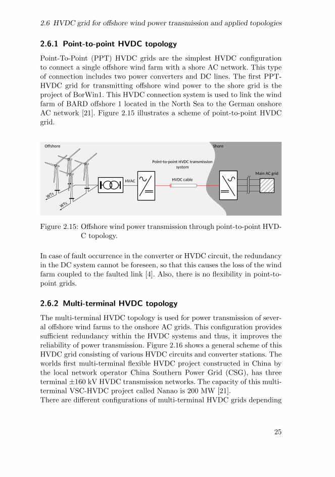
Point-To-Point (PPT) HVDC grids are the simplest HVDC configurationto connect a single offshore wind farm with a shore AC network. This typeof connection includes two power converters and DC lines. The first PPT-HVDC grid for transmitting offshore wind power to the shore grid is theproject of BorWin1. This HVDC connection system is used to link the windfarm of BARD offshore 1 located in the North Sea to the German onshoreAC network [21]. Figure 2.15 illustrates a scheme of point-to-point HVDCgrid.
Main AC grid
Point-to-point HVDC transmission
system
HVDC cableHVAC
ShoreOffshore
Figure 2.15: Offshore wind power transmission through point-to-point HVD-C topology.
In case of fault occurrence in the converter or HVDC circuit, the redundancyin the DC system cannot be foreseen, so that this causes the loss of the windfarm coupled to the faulted link [4]. Also, there is no flexibility in point-to-point grids.
2.6.2 Multi-terminal HVDC topology
The multi-terminal HVDC topology is used for power transmission of sever-al offshore wind farms to the onshore AC grids. This configuration providessufficient redundancy within the HVDC systems and thus, it improves thereliability of power transmission. Figure 2.16 shows a general scheme of thisHVDC grid consisting of various HVDC circuits and converter stations. Theworlds first multi-terminal flexible HVDC project constructed in China bythe local network operator China Southern Power Grid (CSG), has threeterminal ±160 kV HVDC transmission networks. The capacity of this multi-terminal VSC-HVDC project called Nanao is 200 MW [21].There are different configurations of multi-terminal HVDC grids depending
25

Chapter 2 Offshore grids structure
on the number and capacity of HVDC links, maximum loss of power, flexi-bility, redundancy, number of HVDC circuit breakers and fast communica-tions [15, 4].
Main AC grid
Multi-terminal HVDC
transmission system
HVAC
ShoreOffshore
Main AC grid
HVAC
Figure 2.16: Offshore wind power transmission through multi-terminalHVDC topology.
These topologies are the General Ring Topology (GRT), the Star Topology(ST), the Star with a General Ring Topology (SGRT), the Wind farm RingTopology (WFRT) and the Substations Ring Topology (SSRT) [4].The common feature of all multi-terminal HVDC grid configurations is flex-ibility, since the bidirectional power flow is possible in case of failure in thesegrids. However, some differences can be found between these configurationssuch as [4]:
• The implementation of ST and SGRT topologies with an offshore plat-form.
• The requirement for fast communication in the GRT, WFRT and SSRTtopologies to attune the protection devices.
• The need for a number of HVDC circuit breakers equal to the numberof wind farms or AC grids for WFRT and SSRT topologies and anumber of circuit breakers equal to the total number of wind farmsand onshore AC substations for GRT, ST and SGRT configurations.
26

2.7 Summary
2.7 Summary
This chapter has introduced the offshore grid structure to be implemented indifferent scenarios such as inrush current reduction of transformers availablein offshore systems during start-up and integration of offshore wind farmsor during system restoration after fault clearance. Hence, all the main com-ponents of the abovementioned grid have been described in detail in orderto enable us to better understand and analyze these scenarios.
27

28

Chapter 3
VSC converter modeling and control
To analyze the HVDC converter behavior in the offshore grids, modelingof the voltage source converter, modeling of the AC and DC grids of theconverter as well as different control systems of converters have been studied.
3.1 Introduction
The VSC-HVDC transmission technology is used in offshore grids to con-nect the offshore wind farms to the main AC grids. The VSC converter ofhigh voltage DC systems plays a significant role in transferring the powerwithin the offshore grid. Therefore, in order to better understand the dy-namic characteristics of converters, an averaged model of power converter ispresented. In addition, different representations of AC and DC grids of con-verters are included. Based on these models, several control schemes of thepower converter are introduced in order to ensure the optimal converter per-formance and stability of HVDC systems under various conditions. Controlstructures of converters are designed on the basis of a basic vector controlstrategy including a voltage control loop and an AC current control loop. Thedesign of these controllers is accomplished based on the dynamic equationsof the power converter as well as the applications of the control system.This chapter is organized as follows: an averaged model is described in Sec-tion 3.2. In Section 3.3, models of AC grid coupling filters including inductivecoupling filter and inductive-capacitive filter are presented. Section 3.4 dis-cusses the modeling of DC grids for back-to-back, point-to-point and multi-terminal configurations. Thereafter, the inner and outer control loops and aPhase Locked Loop (PLL) method to synchronize the system with the ACgrid are analyzed in Section 3.5. Finally, a study of the converter controlsystems under the fault condition is presented in Section 3.6. It should bementioned that all the information of this chapter is referred to [39, 40].
29

Chapter 3 VSC converter modeling and control
3.2 Average model of a VSC converter
To scheme the VSC converter control strategies and analyze the HVDC sys-tem, an average model of the power converter is considered. This simplifiedequivalent representation that shows the average dynamic behavior of a con-verter at low-frequencies is achieved by decoupling the converter AC and DCsections as shown in Figure 3.1.
Vcab
Vcbc
Vcac
VSC
IDCm
VSC
IDCm
DC
Vcan
Vcbn
Vccn
AC
C E C E
Figure 3.1: Average equivalent circuit of a two-level VSC converter.
In this average model, the converter AC side is represented by three ACvoltage sources, whereas the converter DC side is modeled as a controllablecurrent source. By neglecting losses in the voltage source converter, the ac-tive power on the AC side becomes identical to the power exchanged at theconverter DC side [41, 42] i.e.
PAC = PDC = EIDCm (3.1)
and therefore, the DC current of the source can be calculated based on thepower balance at the AC and DC side of the converter, i.e. [39]
IDCm =PACE
(3.2)
where PAC is the active power at the AC side, PDC is the power at theDC side of the converter, E is the DC side voltage and IDCm is the currentinjected in the DC side of the converter.
30

3.3 Models of AC grid coupling filter
3.3 Models of AC grid coupling filter
To decrease high-frequency harmonics in AC current, limit short-circuit cur-rents, avoid variations of the current polarity in IGBT and independentlycontrol the active and reactive powers by regulating the current [43], an ACcoupling filter between the AC grid and the AC side of the VSC converter isneeded. For HVDC applications, the most common filters are inductance fil-ters (L). However, inductance and capacitor filters (LC) are used for voltageregulation when the converter is interfaced with an offshore grid includingoffshore load or offshore wind farm. The models of AC coupling filters aredescribed in the following subsections.
3.3.1 Inductive coupling filter (L)
The L filter allows for the connection of the VSC converter to the ACgrid. The schematic diagram of the VSC connection to the AC system bymeans of a L filter is sketched in Figure 3.2.
Rc
vzabc
PCCLc
vcabc
icabc
VSC
L filter
E
Figure 3.2: Model of the VSC converter connection to the AC grid througha L coupling filter.
According to the average model of the VSC converter, as illustrated in Figure3.1, and assuming a balanced three-phase grid, differential equations at theAC side of the VSC converter under the stationary frame can be described as
Lcdicadt = vza − vca −Rcica
Lcdicbdt = vzb − vcb −Rcicb
Lcdiccdt = vzc − vcc −Rcicc
(3.3)
31
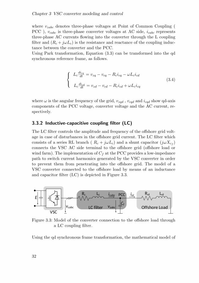
Chapter 3 VSC converter modeling and control
where vzabc denotes three-phase voltages at Point of Common Coupling (PCC ), vcabc is three-phase converter voltages at AC side, icabc representsthree-phase AC currents flowing into the converter through the L couplingfilter and (Rc + jωLc) is the resistance and reactance of the coupling induc-tance between the converter and the PCC.Using Park transformation, Equation (3.3) can be transformed into the qdsynchronous reference frame, as follows.
Lcdicqdt = vzq − vcq −Rcicq − ωLcicd
Lcdicddt = vzd − vcd −Rcicd + ωLcicq
(3.4)
where ω is the angular frequency of the grid, vzqd , vcqd and icqd show qd-axiscomponents of the PCC voltage, converter voltage and the AC current, re-spectively.
3.3.2 Inductive-capacitive coupling filter (LC)
The LC filter controls the amplitude and frequency of the offshore grid volt-age in case of disturbances in the offshore grid current. The LC filter whichconsists of a series RL branch ( Rc + jωLc) and a shunt capacitor (jωXcf )connects the VSC AC side terminal to the offshore grid (offshore load orwind farm). The implementation of Cf at the PCC provides a low-impedancepath to switch current harmonics generated by the VSC converter in orderto prevent them from penetrating into the offshore grid. The model of aVSC converter connected to the offshore load by means of an inductanceand capacitor filter (LC) is depicted in Figure 3.3.
Rc
vzabc
PCCLc
vcabc
icabc
VSC
LC filter
E
CfOffshore Load
Rol Loliol
Figure 3.3: Model of the converter connection to the offshore load througha LC coupling filter.
Using the qd synchronous frame transformation, the mathematical model of
32

3.4 DC grid Modeling
Figure 3.3 can be expressed as:
Lcdicqdt
= vcq − vzq −Rcicq − ωLcicd (3.5)
Lcdicddt
= vcd − vzd −Rcicd + ωLcicq (3.6)
where ω is the nominal frequency of the power system, icqd is qd-axis compo-nents of the AC current flowing from the converter to the PCC, vzqd refers tothe voltages at the PCC and vcqd are the voltages applied by the converterin the synchronous reference frame.Also, according to state-space equations, dynamics of offshore load voltagein qd synchronous frame can be defined as follows
Cfdvzqdt
= ωCfvzd + icq − iolq (3.7)
Cfdvzddt
= −ωCfvzq + icd − iold (3.8)
where iolqd indicates the currents flowing through the offshore load (Rol +jωLol) in qd synchronous frame. Moreover, the dynamic model of the off-shore load composed of a series RL branch is written as
Loldiolqdt
= vzq −Roliolq − ωLoliold (3.9)
Loldiolddt
= vzd −Roliold + ωLoliolq (3.10)
where Rol and Lol are the resistance and inductance of the offshore load.
3.4 DC grid Modeling
The classification of the DC grids that exist among the converter stationsof HVDC transmission systems is established on the basis of the situationand operation of the converter stations. Thus, DC grid configurations canbe divided into three main groups: back-to-back, point-to-point and multi-terminal grids.The cables in the DC grid connecting two or more converter stations arerepresented by π-equivalent circuits in which the capacitor at each terminalis equal to the summation of the whole capacitors joined in parallel at thatend [44].
33

Chapter 3 VSC converter modeling and control
3.4.1 Back-to-back grid model
The HVDC back-to-back structure is a common configuration used to con-nect two asynchronous AC systems, operating at various frequencies, througha DC grid. Two VSC converters of this configuration are located at the samestation and thus, there is no transmission of power with a DC grid over along distance. The schematic diagram of a back-to-back system is shown inFigure 3.4.
VSC2
E1
IDCm
C1
IDCl
IDC
VSC1DC grid
Figure 3.4: Back-to-back converter DC grid model.
applying the Kirchhoffs laws to analyze the DC circuit, the following expres-sions are obtained
IDC = IDCm − IDCl (3.11)
dE1
dt=
1
C1IDC (3.12)
where E1 is the DC voltage, C1 is the capacity of DC capacitor, IDCm isthe current coming from the DC side of VSC1, IDC is the current flowingthrough the DC bus capacitor and IDCl is the current flowing through theDC side of VSC2.Substituting for IDC in Equation (3.12), based on Equation (3.11), thederivative of the DC voltage can be expressed as a function of the cur-rent from both converters as:
dE1
dt=
1
C1(IDCm − IDCl) (3.13)
34

3.4 DC grid Modeling
3.4.2 Point-to-point grid model
The point-to-point system is used to connect two AC systems like an offshorewind farm and an onshore AC grid. This type of system is composed of twoconverter stations that are interfaced by means of a DC transmission line(cable or overhead line). The typical schematic of the point-to-point systemis depicted in Figure 3.5.
VSC2
E1
IDCm1
C1
IDCl
VSC1
R1 L1 C2E2
IDCm2
DC grid
Figure 3.5: The point-to-point system representation for a DC grid analysis.
The DC link differential equations describing the dynamic behavior of thepoint-to-point HVDC grid can be expressed as follows
dE1
dt=
1
C1(IDCm1 − IDCl) (3.14)
dE2
dt=
1
C2(IDCl − IDCm2) (3.15)
dIDCldt
=1
L1(E1 − E2 −R1IDCl) (3.16)
where E1 and E2 are the voltages of equivalent capacitors, C1 and C2 are theequivalent capacitances at both sides of the DC grid, IDCm1 and IDCm2 arethe currents flowing through the converters, IDCl is the current flowingthrough the DC cable and R1 and L1 are the resistance and inductanceof the DC cable.
3.4.3 Multi-terminal grid model (three-terminal)
The multi-terminal HVDC configuration contains more than two HVDCconverter stations which are geographically separated and linked throughDC transmission lines. The scheme of a three-terminal grid, studied in thisthesis, is depicted in Figure 3.6.
35

Chapter 3 VSC converter modeling and control
VSC2
E1
IDCm1
C1
IDCl1
VSC1
R1 L1
C2E2
IDCm2
VSC3
IDCl2
C3 E3IDC3
IDC1 IDC2
R2
L2
DC grid
IDCm3
Figure 3.6: Three-terminal DC grid model.
The differential relations of the three-terminal grid shown in Figure 3.6 canbe obtained based on circuit laws, as
dE1
dt=
1
C1IDC1 (3.17)
dE2
dt=
1
C2IDC2 (3.18)
dE3
dt=
1
C3IDC3, (3.19)
dIDCl1dt
=1
L1(E1 − E2 −R1IDCl1) (3.20)
dIDCl2dt
=1
L2(E1 − E3 −R2IDCl2) (3.21)
and also, the following expressions
IDC1 = IDCm1 − IDCl1 − IDCl2 (3.22)
IDC2 = IDCl1 − IDCm2 (3.23)
36

3.5 Converter control design
IDC3 = IDCl2 + IDCm3 (3.24)
Substituting for Equations (3.22) to (3.24) in (3.17) to (3.19) and reorganiz-ing the differential equations of the DC grid, the state-space representationcan be obtained in the following form.
dx3t
dt= A3tx3t +B3tu3t (3.25)
For the three-terminal grid, the state vector (x) including the currents inthe inductors and the voltages in the capacitors and the input vector (u) arecharacterized
x3t =[E1 E2 E3 IDCl1 IDCl2
]T(3.26)
u3t =[IDCm1 IDCm2 IDCm3
]T(3.27)
and the matrices in the state-space model are defined as
A3t =
0 0 0 −1
C1
−1C1
0 0 0 1C2
0
0 0 0 0 1C3
1L1
−1L1
0 −R1L1
01L2
0 −1L2
0 −R2L2
(3.28)
B3t =
1C1
0 0
0 −1C2
0
0 0 1C3
0 0 00 0 0
(3.29)
3.5 Converter control design
The control strategy implemented in the converters of this thesis is basedon the classic vector control [45, 46, 47]. The aforementioned control systemenables controlling the active and reactive powers independently as well as
37
Chapter 3 VSC converter modeling and control
limiting current. This control strategy can be classified in two groups: lowerlevel controller and higher level controller. The lower level controller knownas current control loop or inner loop is responsible for regulating the q- andd-axis components of the AC current. Moreover, the higher level controllernamed as voltage control loop or outer loop is used for the production ofthe current reference components, i∗cq and i∗cd, in order to inject to the in-ner loop. Depending on the HVDC converter application in the thesis, theouter loop is determined on the basis of the DC and AC voltage controlsystems. Namely,
• The DC voltage control scheme is employed for converters linking theDC systems to the main AC networks. The DC voltage controller gov-erns the HVDC grid voltage to ensure power balance and DC systemstability. Thus, in applications in which i∗cq is provided by the DC volt-age controller, the other current component, i∗cd, results from an ACvoltage controller in order to be capable of regulating AC voltage atthe PCC.
• When the power converter is connected to offshore wind farm, theAC voltage controller is applied to the converter in order to generatea stable voltage at the AC busbar of the offshore wind farm plat-form. Therefore, the goal of this control system in this case is to pro-vide both current components of the converter, i∗cqd for inner controlloop. The fact is that the AC voltage control system is the sole con-troller available in outer loop.
A detailed description of the inner and the outer controllers is presentedin the next subsections. Note that the control systems based on the vectorcontrol method are designed in the synchronous reference frame, defined bythe grid angle obtained through a Phase Locked Loop (PLL) system. For thisreason, the currents and voltages measured at the AC side are transformedinto q-and d-components through park transformation.
3.5.1 Converter current control (Inner loop)
The inner current control based on vector control strategy is designed totrack the current references obtained by the outer controller in a definedtime and to generate voltage references for injecting to the VSC convert-er. Therefore, the systems active and reactive powers can be independentlycontrolled under these circumstances. Figure 3.7 shows the structure of thisinner loop controller.
38

3.5 Converter control design
Rc
vzabc
PCCLc
vcabc
icabc
VSC
E
vzd
vzabc
Kpll(s)
T( )vzqd
T( )
icabc
icqd1s
PLL
vcabc
-
-
+
+
icq-
+
++
vcq
vzq
vcd
vzd
icq
*
icd
*
Kilq(s)
Kild(s)
Lc
Lc
Vo
lta
ge
mo
du
lati
on
icd
Inner Loop
Control System
-
+
0vzd*
-
ucq
- ucd
Figure 3.7: Control block diagram of converter current.
According to Subsection 3.3.1, the mathematical model describing the ACside current dynamics of the converter flowing through a L coupling filter, isas follows [39]
Lcd
dt
[icqicd
]=
[−Rc −ωLcωLc −Rc
] [icqicd
]+
[vzq − vcqvzd − vcd
](3.30)
Due to the existence of ωLc terms in Equation (3.30), dynamics of icq andicd are coupled to each other. This coupling can result in an adverse traceon the efficiency of the current control loops. For this reason, an approachof the decoupling and independent control of q and d components of currentis employed to avoid this drawback. In addition, the decoupling of the q−
39

Chapter 3 VSC converter modeling and control
and d−axes needs a feed-forward technique in order to inject the ωLcicd andωLcicq signals into the q- and d-axis control loops when icq and icd are regu-lated to control the active power and reactive power, respectively. Thus, thecross coupling between q and d axes is compensated using feed-forward sig-nals. Hence, two new control signals (ucq,ucd) are introduced here[
ucqucd
]=
[0 −ωLcωLc 0
] [icqicd
]+
[vzq − vcqvzd − vcd
](3.31)
where ucq and ucd indicate the outputs of two current loop controllers, icqdrepresents the qd-axis components of the current flowing at the AC side ofthe converter, vcqd is the qd-axis components of the voltage generated bythe converter, vzqd is the qd-axis components of the voltage at PCC and Lcis the inductance of the coupling filter.According to the resulting control signals in Equation (3.31) and assum-ing the d-axis component of the voltage on the AC side is equal to zero(vzd = 0), the desired fundamental components of the VSC AC voltage inthe qd frame are computed as below.[
vcqvcd
]=
[0 −ωLcωLc 0
] [icqicd
]+
[vzq0
]−[ucqucd
](3.32)
Therefore, substituting Equation (3.32) into Equation (3.30), two decou-pled first-order linear systems can be deduced as[
ucqucd
]=
[Rc 00 Rc
] [icqicd
]+ Lc
d
dt
[icqicd
](3.33)
By transforming the previous equations through Laplace, transfer functionsbetween the currents flowing through the coupling filter and voltages of thecurrent controller are obtained as
icq =1
Lcs+Rcucq (3.34)
icd =1
Lcs+Rcucd (3.35)
where s is the Laplace operator.Based on Equations (3.34) and (3.35), the q−and d−axis variables of the
40

3.5 Converter control design
converters AC current (icq,icd) can be regulated by ucq and ucd, respective-ly. Moreover, by applying the Internal Model Control (IMC) technique [48,49], the transfer functions of the controller, Kilq(s) and Kild(s), can be de-signed as
Kilq(s) = Kild(s) =Kp−ils+Ki−il
s(3.36)
where Kilq(s) and Kild(s) are simple proportional-integral regulators allow-ing for tracking references and Kp−il and Ki−il represent proportional andintegral gains, respectively. Hence, these gains are defined as
Kp−il =Lcτil
(3.37)
Ki−il =Rcτil
(3.38)
where τil is the resulting control closed loop time constant which is selecteddepending on the requirements of the application and the converters switch-ing frequency. It is typically considered to be a number of times faster thanthe switching frequency of the VSC in order to track current references fromsome milliseconds to tens of milliseconds depending on the application [39].It should be noted that ucq and ucd are the output of two proportional-integral (PI) regulators available in the converters current control system. Ad-ditionally, the q and d-axes PI regulators, Kilq(s) and Kild(s), process theerror between the reference current and its actual value, i.e. ecqd = i∗cqd −icqd and then provide ucqd. Hence, the VSC inner controller generates vcqand vcd which, in turn, control icq and icd in accordance with Equation(3.30). Consequently, based on these descriptions, the state-space model ofthe VSC current controller can be deduced as
dxildt
= Biluil (3.39)
yil = Cilxil +Diluil (3.40)
where the inputs, outputs and state variables are
xil =[eicq eicd
]T(3.41)
uil =[i∗cq i∗cd icq icd vzq vzd
]T(3.42)
41
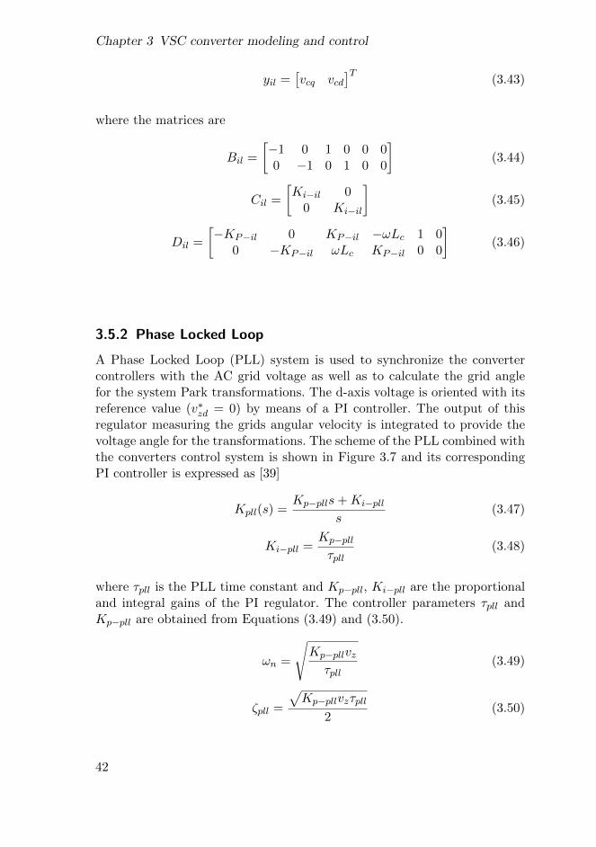
Chapter 3 VSC converter modeling and control
yil =[vcq vcd
]T(3.43)
where the matrices are
Bil =
[−1 0 1 0 0 00 −1 0 1 0 0
](3.44)
Cil =
[Ki−il 0
0 Ki−il
](3.45)
Dil =
[−KP−il 0 KP−il −ωLc 1 0
0 −KP−il ωLc KP−il 0 0
](3.46)
3.5.2 Phase Locked Loop
A Phase Locked Loop (PLL) system is used to synchronize the convertercontrollers with the AC grid voltage as well as to calculate the grid anglefor the system Park transformations. The d-axis voltage is oriented with itsreference value (v∗zd = 0) by means of a PI controller. The output of thisregulator measuring the grids angular velocity is integrated to provide thevoltage angle for the transformations. The scheme of the PLL combined withthe converters control system is shown in Figure 3.7 and its correspondingPI controller is expressed as [39]
Kpll(s) =Kp−plls+Ki−pll
s(3.47)
Ki−pll =Kp−pllτpll
(3.48)
where τpll is the PLL time constant and Kp−pll, Ki−pll are the proportionaland integral gains of the PI regulator. The controller parameters τpll andKp−pll are obtained from Equations (3.49) and (3.50).
ωn =
√Kp−pllvzτpll
(3.49)
ζpll =
√Kp−pllvzτpll
2(3.50)
42

3.5 Converter control design
where ζpll is damping ratio, ωn is the electrical angular velocity and vz isthe AC grid voltage magnitude.
3.5.3 Current limiter
The current of the converter can be enhanced to a given maximum value de-termined by the thermal limits of the converter [36, 42]. The current limitercompares the current value computed from the active and reactive refer-ence currents with the maximum permitted magnitude. When it exceedsthe rated current of the converter, the magnitude of the reference current islimited. The current limit is defined as
|Imaxc | =√
(i∗cq)2 + (i∗cd)
2 (3.51)
The current limiter implemented in the VSC control system can be achievedin several ways depending on the priorities between the active and reactivepowers. Three different possible strategies for the restriction of the referencecurrent, shown in Figure 3.8, are described below.
icq,ref
icq
*
icd=icd,ref
*
Ic
icd,ref
i cq=i cq,ref
icd
**
icd,ref icd
*
icq
*
icq,ref
(a) (b) (c)
Icmax
Icmax
Icmax
Ic Ic
Figure 3.8: Current limiting strategies.
• Reactive power priority (i∗cd): The converter will give this priority tothe reactive current reference to keep the AC voltage when the currentlimit is exceeded. Under these circumstances, the d-axis current willbe maintained and q-axis current will be reduced, as shown in Fig-ure 3.8 (a). This strategy is generally selected when the converter islinked to a weak grid or employed to supply an offshore load.
43

Chapter 3 VSC converter modeling and control
• Active power priority (i∗cq): When the converter is connected to a stronggrid, priority is normally given to the delivery of active power. Con-sequently, the q-axis current will keep constant and the d-axis currentwill decrease, as illustrated in Figure 3.8 (b).
• limiting the current in both axes proportionally and maintaining thepower factor constant (Figure 3.8 (c)).
3.5.4 Voltage Controlled Oscillator (VCO)
In the offshore load in which the frequency is not imposed by the AC systemor in offshore wind farms in start-up mode, frequency control is a chal-lenge. In order to overcome this issue, the Voltage Controlled Oscillator(VCO) is used instead of the PLL in the converter station supplying powerto the offshore load or energizing the offshore grid. The output of VCO whichresults from the integration of the nominal frequency of the power systemis used to transform voltages and currents from stationary into synchronousreference frame and vice verse [50]. Figure 3.9 shows the scheme of the VCOintegrated in the VSC control system.
3.5.5 AC voltage control for offshore grids
The aim of the AC voltage controller is to generate an AC voltage withconstant amplitude and frequency (vzabc) for the offshore grids includingwind farms and load. This voltage control loop is composed of two com-pensators, a decoupling feed-forward compensation and a load compensat-ing feed-forward in order to ensure uninterrupted and balanced voltage atthe offshore grid terminal and also to fulfill a pre-specified dynamic perfor-mance [50].The AC voltage controller strategy is defined according to the load voltagedynamic model, described in Subsection 3.3.2, in order to facilitate the con-trol design.
Cfdvzqdt
= ωCfvzd + icq − iolq (3.52)
Cfdvzddt
= −ωCfvzq + icd − iold (3.53)
The previous relations show that the q and d-axis components of the offshoreterminal voltage, vzq and vzd, are regulated on the basis of the AC currents
44

3.5 Converter control design
in the qd synchronous frame, icq and icd, and they are coupled to each oth-er. Also, the effects of offshore grid currents are taken into considerationin these expressions. Hence, to eliminate the coupling between the q andd-axis components of offshore terminal voltage, a decoupling feed-forwardcompensation approach is applied. This technique is designed in a similarway to the one employed to decouple q- and d-axis current components, (icqand icd), in the AC current controller system.Moreover, the control process is developed by means of a further feed-forwardmechanism to compensate the impacts of the offshore grid current. For thisreason, the offshore grid current values in the qd synchronous frame, iolq andiold, are added to the AC current references.The AC currents in the synchronous frame can be written as follows [50]
icq = ucq + iolq − ωCfvzd (3.54)
icd = ucd + iold + ωCfvzq (3.55)
where ucq and ucd denote the output of the voltage controllers.Arranging the previous functions and substituting those in Equations (3.52)and (3.53), the following relations can be deduced
Cfdvzqdt
= ucq (3.56)
Cfdvzddt
= ucd (3.57)
Applying Laplace transformation to Equations (3.56) and (3.57), two decou-pled d−and q−axis closed loop transfer functions are obtained
vzq(s) =1
Cfsucq (3.58)
vzd(s) =1
Cfsucd (3.59)
These equations illustrate that vzq and vzd are independently regulated byucq and ucd.Considering the symmetrical optimum method, two PI compensators gener-ating two independent outputs of ucq and ucd can be designed. Therefore, the
45

Chapter 3 VSC converter modeling and control
PI compensators are
Kol(s) =kp−ols+ ki−ol
s= k
s+ n
s(3.60)
Kp−ol = k, Ki−ol = nKp−ol (3.61)
where Kp−ol and Ki−ol are the proportional and integral control gains. Inaddition, the controller parameters, n and Kp−ol, are calculated based onEquations (3.62), (3.63) and (3.64).
δm−ol = sin−1(1− nτol1 + nτol
) (3.62)
ωol =√nτ−1
ol (3.63)
kp−ol = ωol Cf (3.64)
where δm−ol, ωol and τol denote phase margin, crossover frequency and timeconstant, respectively. It should be noted that the symmetrical optimumtechnique has disadvantages in case of offshore grid disturbances, such asload disconnection [51]. Therefore, LQG optimization procedure is appro-priate to achieve a better disturbance rejection and also a faster dynamicresponse [51]. In other words, this methodology is selected in order to en-sure the optimum regulation and stability of the closed-loop system whichare the important design objectives of the voltage controller [51, 50]. TheLQG compensators are defined as [52]
Kol(s) = k1As3 +Bs2 + Cs+D
Es3 + Fs2 +Gs+H(3.65)
It should be noted that two LQG compensators in the qd synchronous frameprocess the error between the offshore voltage reference and its actual val-ue, (eq = v∗zq − vzq, ed = v∗zd − vzd), and then provide ucq and ucd. There-fore, icq and icd are constructed based on Equations (3.54) and (3.55) andare delivered to the corresponding q and d-axis current control loops.Finally, the AC voltage control loop of the converter station connected tothe offshore grid can be designed as follows
icq = iolq − ωCfvzd +Kol(s)(v∗zq − vzq) (3.66)
icd = iold + ωCfvzq +Kol(s)(v∗zd − vzd) (3.67)
46

3.5 Converter control design
Figure 3.9 depicts the control scheme of a converter linked to the offshoreload through a LC filter. Note that one assumption adopted in the ACvoltage controller of this thesis is that the q and d-axis components of voltageare, (vzq, vzd)=(vzn, 0). The vzn is the nominal value of offshore terminalvoltage.
Ɵ
vcabc
Vo
lta
ge
mo
du
lati
on -
-
+
+
icq-
+
++
vcqvzq
vcd
vzd
icq*
icd
*
Kilq(s)
Kild(s)
Lc
Lcicd
Inner Loop
-
-
+
+
+
-
+
+++
vzqiolq
*
iold
*
Kol(s)
Kol(s)
Cf
Cf
Outer Loop
vzd
vzq
vzd
icqd
VCO
vzabc
vzqd
1s
T(Ɵ)
T(Ɵ)
T(Ɵ)
icabc
iolabciolqdƟ
Control System
Rc
vzabc
PCCLc
vcabc
icabc
VSC
E
Cf
Rol Loliol
--
ucq
ucd
eq
ed
Figure 3.9: Voltage and current controller scheme for the converter connect-ed to an offshore load through a LC filter.
3.5.6 AC voltage control for onshore AC grids
To control the AC grid voltage magnitude with its reference value, the ACvoltage controller is handled in the converter station. This controller enablesgeneration of reactive power in order to adjust the AC grid voltage. The fore-
47

Chapter 3 VSC converter modeling and control
going controller comprises a PI regulator to be able to annul steady stateerrors. Figure 3.10 pictures the scheme of the AC voltage control in the con-verter linked into the AC grid by means of a L filter.
Rc
vzabc
PCCLc
vcabc
icabc
VSC
E
vzd
vzabc
Kpll(s)
T( )vzqd
T( )
icabc
icqd1s
PLL
vcabc
Vo
lta
ge
mo
du
lati
on
Control System
-
+
0vzd*
-
-
+
+
icq-
+
++
vcqvzq
vcd
vzd
icq
*
icd
*
Kilq(s)
Kild(s)
Lc
Lcicd
Inner Loop
--
-
+
vzq
Q23
AC Voltage Control
*
vzq
vzq
Kv(s)
Figure 3.10: Scheme of the AC voltage controller implemention with a in-ner control loop for a VSC interfaced with the main AC gridthrough a L filter.
Due to the reactive current is associated with reactive power, as seen inFigure 3.10, the voltage of AC system can be controlled by d-axis referencecurrent. The d-axis component of current reference can be calculated usingthe PI controller as
i∗cd =2
3vzqKv(s)(v
∗zq − vzq)︸ ︷︷ ︸Q
(3.68)
48

3.5 Converter control design
where Kv is specified as
Kv(s) =kp−vs+ ki−v
s(3.69)
where kp−v and ki−v are the proportional and integral gains of voltage con-troller.
3.5.7 DC bus voltage control
The objectives of the DC voltage controller are the regulation of the DC volt-age in the HVDC grid to ensure DC grid voltage stability and the balancebetween the DC grid power and the power supplied to the AC grid. Thisvoltage controller operating in outer control loop generates the active cur-rent, i∗cq, for AC current control loop. In turn, changing this current allowsfor the control of the DC voltage. There are several methodologies employedfor DC voltage regulation, among which the droop controller and the PI con-troller are the most common methods. The PI controller is a simple methodallowing for the regulation of output current. The foregoing technique is im-plemented in this thesis and further details are explained in the followingsubsection. Also, the description of the droop controller can be found in Ap-pendix A.To control the DC bus voltage by means of the AC current reference, i∗cq, theoutput of the DC voltage regulator, i∗DCl, is transformed into the active pow-er reference value.
P ∗ = E1I∗DCl (3.70)
where E1 is the DC voltage at the converter and I∗DCl is the reference valueof the current flowing from the dc side of the converter.Substituting Equation (3.70) in the Equation (A.12) of Appendix A andrearranging the obtained relation, the current injected to the AC currentcontroller of the converter can be defined as
i∗cq =2
3vzqE1I
∗DCl (3.71)
• PI controller design:
The PI-based DC voltage regulator is mostly implemented in HVDC grids
49

Chapter 3 VSC converter modeling and control
to control DC voltage at a stable level. The controller scheme for the back-to-back converter linked to the AC grid through an L filter is depicted inFigure 3.11.
Rc
vzabc
PCCLc
vcabc
icabc
VSC
E1
vcabc
Vo
lta
ge
mo
du
lati
on
Control System
-
-
+
+
icq-
+
++
vcqvzq
vcd
vzd
Kilq(s)
Kild(s)
Lc
Lcicd
Inner Loop
--
IDClIDCm
C1
icq
*
23
DC Voltage Control
E1
IDCm
-
+
Kdc(s)E1
*
E1
IDCIDCl +
-
vzq
OuterLoop
vzd
vzabc
Kpll(s)
T( )vzqd
T( )
icabc
icqd1s
PLL
-
+
0vzd*
icd*
23
-
+
vzq
Q*
vzq
vzq
Kv(s)
Figure 3.11: DC voltage control structure in a converter connected to theAC grid through a L filter (by using PI regulator design).
The DC bus dynamics as defined in Subsection 3.4.1 are
dE1
dt=
1
C1(IDCm − IDCl) (3.72)
The (IDCm − IDCl) in Equation (3.72) can be also replaced by the currentflowing through the capacitor, IDC , and consequently, the PI controller out-put can be computed as
IDC = C1dE1
dt(3.73)
50

3.6 Control systems for AC fault condition
Transformation of Equation (3.73) into Laplace domain results in a trans-fer function between the controlled current and the DC bus voltage as follows
E1(s) =1
C1sIDC(s) (3.74)
To achieve a satisfactory performance of the system, a controller with anintegrator, such as a PI controller, is used as
Kdc(s) = Kp−dc +Ki−dcs
(3.75)
where the constants of the PI controller can be computed as
Kp−dc = 2C1ξdcωdc (3.76)
Ki−dc = C1ω2dc (3.77)
where ξdc is the desired damping factor of the DC voltage controller and ωdc isthe desired angular velocity of the voltage controller. Note that the stablesystem response can be ensured when the DC voltage controller is designedto have a much slower response than the current regulator [39]. Hence, theDC current flowing through the converter ,IDCl, can be considered to beidentical to the reference, I∗DCl [53].
3.5.8 Constant power controller
The purpose of constant active power transmission to the HVDC grid canbe attained by employing a constant active power controller in the converterstation. This controller, as shown in Figure 3.12, is formulated on the basisof the instantaneous power theory as
i∗cq =2
3vzqP ∗ (3.78)
3.6 Control systems for AC fault condition
When an AC grid fault takes place, all the generated power cannot be ex-ported to the AC grid due to the saturation of the converter current limit. Insuch condition, the power that cannot be supplied to the AC system is
51

Chapter 3 VSC converter modeling and control
Rc
vzabc
PCCLc
vcabc
icabc
VSC
E
vcabc
Vo
lta
ge
mo
du
lati
on
Control System
-
-
+
+
icq
-
+
++
vcqvzq
vcd
vzd
Kilq(s)
Kild(s)
Lc
Lcicd
Inner Loop
--
-
+
vzq
Q
*
vzq
vzq
Kv(s)
OuterLoop
vzd
vzabc
Kpll(s)
T( )vzqd
T( )
icabc
icqd1s
PLL
-
+
0vzd*
icd
*
23
icq
*
vzq
P23
*
Constant power control
Figure 3.12: Constant power control and current and voltage control struc-tures of a converter connected to the AC grid by means of a Lcoupling filter.
stored in the capacitors, and the DC voltage increases rapidly. Consequent-ly, controlling the DC voltage will be a priority and this is accomplishedby dissipating power in chopper resistors, or by reducing part of the windfarm power. In the first case, a DC chopper is employed to dissipate theadditional power in a resistor during the voltage sag. The second solutionis implemented by reducing the power generated by the wind farm in or-der to restore power balance in the HVDC grid. These two approaches areexplained in more detail in next Subsections.
3.6.1 DC chopper
During short contingencies, the DC chopper prevents the DC voltage en-hancement beyond a maximum permitted value. The reason for this incre-
52

3.6 Control systems for AC fault condition
ment is the power imbalance in the HVDC grid. The DC chopper comprisingpower electronic switches and resistors is installed in the DC voltage control-ling converter stations. Moreover, it can be modeled as a voltage controlleddirect current source, the value of which can be defined as
I∗dc−chopper = kdc−chopperE2 − Emin2
Emax2 − Emin2
(3.79)
where I∗dc−chopper is the current injected by the current source, E2 is the DC
voltage, Emax2 and Emin2 are the upper and lower thresholds of the DC voltagein terminals of the converter and kdc−chopper is a gain chosen on the basis ofthe nominal capacity of the DC chopper and DC voltage, namely, Sn/E2 [54].Figure 3.13 illustrates the scheme of a DC chopper.
VSC2
E2E1
R1 L1
Idc-chopper
VSC1
DC chopper
-
+E2
minE2
minmaxE2E2 -
1
1
0
Figure 3.13: Scheme of a DC chopper.
where α is the duty cycle and is issued for transistors controlling the DCchopper. Once the value of E2 is equal to Emin2 , α becomes zero and whenthe E2=Emax2 , the value of α is to 1. Actually, the DC chopper operateslinearly.when the DC voltage exceeds of the pre-defined threshold, the DC chopperdissipates the amount of current flowing in the DC grid which prevents inturn all the active power from being transmitted to the AC grid. The mainadvantages of this technique are that the output power of the wind farms
53

Chapter 3 VSC converter modeling and control
remains constant during the fault and the system remains stable in case offault.
3.6.2 Wind farm power reduction by controlling HVDC converter
HVDC converters connected to the wind farm are adjusted to transfer allthe power generated by wind farm to the HVDC grid. When a long faultoccurs (e.g. the disconnection of a line) and the DC voltage reaches the al-lowable limit, Emax1 , the operating mode of the converter at the wind farmside is switched to power reduction mode. In this case, the converter enablescontrolling the DC voltage by decreasing power injection [55]. This actioncan be implemented using a variation of the wind farm power reference. Itshould be noted that power dissipation through the DC chopper is not pos-sible due to the overheating of the resistors. The power reduction controllaw is stated accordingly through the following expression
P redwf = P ∗wf − kk(Emax1 − E1)︸ ︷︷ ︸
P
(3.80)
kk = E1kdroop (3.81)
where P redwf is the reduced power of the wind farm, P ∗wf is the wind farm
power reference, E1 is the DC voltage, Emax1 and kdroop are control con-stants to be chosen in the control system design, so that the stability andperformance are guaranteed under any possible conditions.The previous relation indicates that the power reduction approach utilizesa droop characteristic for the injected power decrement.
3.7 Summary
In this chapter, the average model of the VSC converter, AC grid couplingfilter models and DC grid models have been studied. Also, a control schemebased on a two-level cascaded control system (inner and outer control loops)has been explained. Three possible control modes for outer loop have beenrepresented: the AC voltage control mode, the DC voltage control mode andthe constant power control mode. One technique for DC voltage regulationincluding a PI controller has been analyzed. In order to create a stablevoltage for offshore grids as well as to keep AC voltage constant under normaland abnormal conditions, two different AC voltage control strategies have
54

3.7 Summary
been presented. It is pointed out that inner current loop is a fundamentalto any control systems.
55

56

Chapter 4
Modeling and control of a windturbine equipped with full powerconverter
The scopes of this chapter comprise the description of a dynamic simplifiedmodel for the full power converter wind turbine of an offshore grid and theexplanation of a control scheme. Finally, a simulation to test the employedmodel will be also carried out in this chapter.
4.1 Introduction
A variable-speed wind turbine equipped with a full power converter as well asa control scheme for the wind turbine will be modeled in this chapter. Thesimplified model is presented in order to reflect the dynamic response ofthe wind turbine to different incoming winds. The models of turbine, drivetrain, generator and Machine Side Converter, MSC, are represented togetherin this simplification, while the mathematical description associated with theDC bus of the wind turbine is separately discussed. Note that the equivalentscheme of the wind turbine converter at the grid side is the same model ofconverter in the HVDC transmission system. The control systems used forwind turbines can be classified in two groups of electrical and mechanicalcontrollers. The control system of the MSC and GSC converters forms theelectrical controller of the wind turbine, whereas the pitch control systemand DC chopper of the wind turbine develop the mechanical controller. Thecontrol scheme of the Grid Side Converter, GSC, is used for the regulationof DC bus voltage.Therefore, this study is organized as follows: Section 4.2 briefly describes thewind turbine with full power converter. Section 4.3 focuses on the simplifiedmodel of the wind turbine. Section 4.4 discusses the control scheme of thiswind turbine system. Finally, the simulation results are presented in Section
57

Chapter 4 Modeling and control of a wind turbine
4.5 in order to confirm the validity of the model and control design.
4.2 Variable-speed wind turbine with full powerconverter
PMSG wind turbines equipped with full power converter are increasinglyemployed in the industry due to their features. In this wind turbine tech-nology, the generator and AC system is decoupled through power convert-ers, to reduce the effect of a grid fault on the generator. In addition, themachine side converter makes the generator operates within a wider speedrange. Hence, power extraction from the wind can be maximized. Further-more, the converter at the grid side can meet the requirements of gridcodes. Therefore, the reactive power support can be supplied, especiallyunder fault condition, and the wind turbine can withstand the AC systemfaults [4, 56].
PMSG
Wind
turbine
MSC GSC
Offshore
collection
grid
AC
DC
DC
AC
Transformer
WTT
DC
ch
op
pe
r
Control system
Rch
-wt
EWT
iDCm
CWT
iDClFilter
LW
iW
vr
ich
vpvw
Figure 4.1: General scheme of a wind turbine equipped with full power con-verter.
A conceptual schematic of the full-scale converter wind turbine is illustratedin Figure 4.1. The wind turbine captures the power from the wind kinet-ic energy. Then, the extracted power is transmitted through a shaft into aPMSG direct driven generator. This generator, which produces the electri-cal power, is interconnected to the AC power system through a full powerconverter. In this type of generator, the excitation is provided by means ofthe permanent magnets. Therefore, excitation losses can be considerably di-minished [4]. Also, the lack of slip rings is an advantage that results in lowmaintenance of these machines [56]. Thereby, PMSG generators can be usedfor offshore applications.
58

4.3 Simplified model of a full power converter wind turbine
The full-scaled power converters linked to the stator windings of the gener-ator are based on the insulated gate bipolar transistors (IGBTs) technolo-gy. These converters make the generator speed to be fully decoupled fromthe constant-frequency AC system. Also, the capacity of converters is con-sidered to be identical to or larger than the nominal generator power.The converter of the generator side injects the current into the DC circuit inorder to charge the DC capacitor. The grid side converter, which is interfacedinto the AC power grid (collection grid) through a transformer, controls theDC bus voltage. The transformer of the wind turbine steps up the outputvoltage of the grid side converter to the voltage of the offshore collectiongrid. Under operating condition, a DC chopper is applied to bypass thevoltage sages [4]. To limit the power extracted from wind, a pitch controlsystem is embedded.
4.3 Simplified model of a full power converter windturbine
In order to represent the wind turbine dynamic behavior during offshoregrid simulations, design the control system and facilitate the study of thewind turbine, which presentes numerous mechanical complexities, a simpli-fied model is considered in this thesis. This dynamic representation appliedto wind turbines equipped with full power converter is divided into threemain parts, as shown in Figure 4.2. The first one is related to the dynamicmodel of the mechanical and electrical systems of the wind turbine, includingturbine aerodynamic, pitch system, drive train, generator and the machineside converter. The second and the third part refer to the modeling of thegrid side converter and the DC link of the wind turbine. The wind turbineconverter at the offshore collection grid side can be modeled by the same
Pit
ch s
yst
em
Dri
ve
tra
in
Ge
ne
rato
r
Tu
rbin
e
MSC
con
vert
er
Model of mechanical and electrical
systems of wind turbine Wind turbine DC grid
EWT
EWT
iDCm
EWT
vwind
GSC converter
EWT-
+
*
PIi*1
τil s+1ich icWT
iPm Pe
Figure 4.2: Block diagram of simplified model of wind turbine equipped withfull power converter.
59

Chapter 4 Modeling and control of a wind turbine
representation of the HVDC system converter, included in Subsection 3.3.1of Chapter 3. The model of the electrical and mechanical systems of thewind turbine is expanded in detail below.The dynamic simplified representation of the electrical and mechanical sys-tems, indicated in Figure 4.3, is presented in order to show the variationsof power captured by the wind turbine according to the variations in theincoming wind speed. For this purpose, the turbine aerodynamics are rep-resented by a power-wind speed curve, so that the mechanical power of thewind turbine can be changed depending on the speed of incoming wind. Fur-ther description regarding the aerodynamic model can be found in Subsec-tion 4.3.1. For higher wind speeds, the extracted power can be diminishedthrough a pitch control system. In fact, the mechanical power reduction canbe accomplished by filtering the difference between the captured mechani-cal power and the power reference. Henceforth, the power controlled by thepitch system is smoothed thanks to the dynamics of the mechanical andelectrical systems. These systems, containing the drive train and genera-tor, allow to transfer the mechanical power into the generator and convertit into electrical power. Therefore, their simplified model is composed of adynamic 1
JWT s+1 corresponding to the rotor inertia and a dynamic 1τeles+1
corresponding to the electrical system. The JWT and τele are inertia andelectrical time constants for the wind turbine, respectively [40].
vwind
P* -+
1
ps+1
+
-
1JWTs+1
1
eles+1
Pm
Inertia Electrical
system
Pe
EWT
iDCmP
vwind
Pitch systemAerodynamics Drive train Generator
Power
converter
Figure 4.3: The simplified model of wind turbines electrical and mechanicalsystems.
Finally, the electrical power obtained from the generator can be divided bythe DC bus voltage in order to inject current into the DC link of the con-verter, according to Equation (4.1). Thus, the generator side converter canbe modeled.
iDCm =PeEWT
(4.1)
60

4.3 Simplified model of a full power converter wind turbine
Moreover, the dynamic model of the wind turbine DC link shown in Figure4.2 can be defined as
dEWT
dt=[
1CWT
− 1CWT
− 1CWT
] iDCmEWTRch−wt
iDCl
(4.2)
where EWT is voltage of DC bus, CWT is the capacitor of wind turbine DCbus, iDCm is DC current injected by the machine side converter, iDCl is thecurrent through the DC side of the GSC converter and Rch−wt shows theresistance of DC chopper in DC bus.
4.3.1 Aerodynamic model of the wind turbine
The mechanical power generated, Pm, depends on a power coefficient, Cp, andkinetic energy in the air passing across an area swept by rotor blades, Pwind[57]. In fact, the value of this extracted aerodynamic power can be calculatedas [57]
Pm = CpPwind =1
2CpρAv
3wind (4.3)
where ρ is the air density, A is the area swept by the rotor blades and vwindis the wind speed. The power coefficient Cp which is a function of the tipspeed ratio λ and the blade pitch angle ϑ can be achieved as
Cp(λ, ϑ) = c1(c21
Λ− c3ϑ− c4ϑ
c5 − c6)e−c71Λ (4.4)
where [c1...c9] are the wind turbine power coefficients and Λ is defined as
1
Λ=
1
λ+ c8ϑ− c9
1 + ϑ3(4.5)
The relation between the rotational speed of the wind turbine ωt and theaverage wind speed can be described as the tip speed ratio λ
λ =ωtR
vwind(4.6)
where R is the turbine radius.
61

Chapter 4 Modeling and control of a wind turbine
Through the differentiation from Equation (4.4) and solution of its roots, thecomputation of the maximum efficiency of a wind turbine is possible. For thesake of facility, the pitch angle of blades is considered as a constant valueof ϑ=0. Therefore, the optimal value of the power coefficient Coptp can bededuced as follows
Coptp =c1c2e
− c6c7+c2c2
c7(4.7)
Moreover, the optimum tip speed ratio for the calculation of Coptp is
λopt =1
c9 + c6c2
+ 1c7
(4.8)
Therefore, in order to maximize the energy extraction from the wind, thetip speed ratio should be kept at λopt.
4.4 Control system of full power converter windturbine
To regulate a wind turbine, two controller types are required: the mechanicaland the electrical control system. Each of the power converters of the windturbine, MSC and GSC, contains a classic vector control that acts as theelectrical controller. The structure of the GSC control, as shown in Figure4.4, consists of an inner loop and an outer loop. The outer loop comprisesonly a DC voltage controller and is responsible for DC bus voltage regula-tion. This voltage loop is controlled by means of a proportional-integral (PI)regulator and provides the current reference for the inner current controlloop. The AC voltage controller is eliminated in the outer loop of the windturbine GSC converter in order to avoid the confluence of the aforemen-tioned controllers operation with that of the AC voltage control system ofthe offshore HVDC converter [37]. Moreover, to orient the control systemwith grid voltage, a Phase Locked Loop (PLL) is used in the GSC. In thepower converter of the machine side, only DC current is injected to the DClink, corresponding to the power generated by the wind turbine and the DCbus voltage. The mechanical control of the wind turbine includes a pitchsystem. This control system diminishes the power captured from the windwhen the power is above the nominal level. The pitch system has the slowdynamics. Hence, a DC chopper is implemented in the wind turbine in or-der to dissipate the power in case that power reduction through the pitch
62

4.5 Simulation results
EWT
Inner loop
DC voltage loop
T( )iW
T( )
T( )PLL
vr
iW
T( )-1vW vW AC
system
vW
vr iW
DC
system
=0
EWT*
iDCl
iDCm
GSC
Converter
EWT Pe
MSC
Converter
GSC control system
Mechanical and
electrical systems
vwind
P*MSC system
abcabc
abc*abc*qd
iW*d q
iW*
vrqd
qd
abc
abc
Figure 4.4: Control scheme of the wind turbine.
controller is not possible. Further details about the DC chopper, DC voltagecontroller and inner loop can be found in Chapter 3.
4.5 Simulation results
To evaluate the performance of the simplified model and the wind turbinecontrol system, a simulation is carried out using MATLAB/SIMULINK soft-ware. The scheme of the simulated system is shown in Figure 4.3. The char-acteristic parameters of the wind turbine used in this simulation have beenpresented in Table 4.1. The wind turbine considered is based on Areva M5000model.Figures 4.5 (a)-(d) show the wind speed, the mechanical power, the mechan-ical power controlled by the pitch controller and the electrical power, respec-tively. It can be seen that the mechanical power varies along with changesin wind speed. Also, this power extracted by the turbine can be limitedthrough a pitch system, when it exceeds the nominal value, as illustrated inFigure 4.5 (c). The electrical power generated by means of the machine thatreflects the wind speed variations and dynamic behavior of the drive trainand PMSG is indicated in Figure 4.5 (d).
63

Chapter 4 Modeling and control of a wind turbine
Table 4.1: Wind turbine characteristic parameters
Parameter Value Units Description
R 58 m Turbine baldes radiusρ 1.225 kg/m3 Air density
JWT 1.7 s Inertia time constantϑ 0 Pitch angle of rotor bladesτele 0.01 s Electrical time constantτp 0.17 s Pitch time constant
ωnom 14.8 min−1 Nominal speed
c1 0.5 1c2 116 1c3 0.4 1c4 0 1c5 0 1 Cp function parametersc6 5 1c7 21 1c8 0.08 1c9 0.035 1
λopt 0.411 1 Optimum tip-speed ratio
Coptp 8 1 Optimum power coefficientPWT 5 MW Nominal power of wind turbinevr/ vp 3.3/33 kV Nominal transformer voltagePconv 5.6 MVA Nominal converter powerEWT 6 kV Nominal DC voltage
64

4.5 Simulation results
4 6 8 10 12 14 16 18 20 22 24 2610
11
12
13
14
Time [s]
v w [
m/s
]
(a) Wind speed
4 6 8 10 12 14 16 18 20 22 24 262
3
4
5
6
7
Time [s]
P mec
[M
W]
(b) Mechanical power
4 6 8 10 12 14 16 18 20 22 24 262
3
4
5
6
7
Time [s]
P mec
−pi
tch [M
W]
(c) Mechanical power controlled by pitch
4 6 8 10 12 14 16 18 20 22 24 262
3
4
5
6
7
Time [s]
P elec
[MW
]
(d) Electrical power
Figure 4.5: The performance of the simplified model for various wind speeds.
65

Chapter 4 Modeling and control of a wind turbine
As shown in Figures 4.6 (a) and (b), the DC bus voltage is stable due tothe utilization of the DC voltage controller in GSC, whereas the AC currentvalue of GSC varies on the basis of the produced power.
4 6 8 10 12 14 16 18 20 22 24 260.9
1
1.1
1.2
1.3
Time [s]
Cur
rent
[kA
]
(a)
4 6 8 10 12 14 16 18 20 22 24 265.9
5.95
6
6.05
6.1
Time [s]
DC
vol
tage
[kV
]
(b)
Figure 4.6: Evaluation of the current of GSC converter and DC voltage.
66

Chapter 5
Transformer inrush current in HVDCsystems
This chapter will describe the state of the art of transformers inrush cur-rent, the impact of the inrush current phenomenon on the HVDC system, thetechniques applied for inrush current limitation and the requirement fora novel reduction strategy in HVDC transmission systems. Finally, it willpresent a transformer model considering magnetic core effects for inrushcurrent investigation.
5.1 Introduction
The security and reliability of the offshore HVDC grid in operation un-der different condition is important. One of the challenges related to powertransmission in HVDC systems is transformers inrush current during ener-gization and restoration after fault removal. Tripping the HVDC converterand disturbing HVDC power transfer can be the outcome of these high in-rush currents [58, 59]. Transient magnetizing currents or the selfsame mag-netizing inrush currents are generated by the iron core saturation of thetransformer. These currents are one of the significant abnormalities in trans-formers as well as their amplitudes are generally several times the nominalcurrent. The first inrush current was observed by Ferranti when commis-sioning the Deptford to London 11 kV link in 1890 [60]. For more than 100years, these transformer inrush currents have caused some difficulties, suchas the malfunction of protective relays and power quality reduction of thenetwork [17, 60]. Hence, knowledge of transformers behavior under normaloperation and transient cases is a requirement for the reliable and stableperformance of transformers protection devices [61, 62]. Thus, the possibil-ity of achieving this knowledge could be provided by transformer modelingwhich is a vast topic. Therefore, in order to study inrush transient behaviorof transformers during the energization and recovery modes, some represen-
67

Chapter 5 Inrush current
tations have been proposed.These models used for transformers transient are classified as: Matrix model(BCTRAN model), Saturable Transformer Component (STC) model,Topology-based model (Duality based model and Geometric model), Mod-el based on a T-equivalent circuit and Model based on a π-equivalent cir-cuit [63, 64].These models deal with the main problems, such as, the lack of informationabout parameters, modeling of hysteretic iron-core, modeling of windinglosses, adequate modeling of transformers behavior in complete saturationand determination of the residual fluxes in order to investigate inrush tran-sients. In this chapter, a simplified model of a three-phase transformer ispresented to show the non-linear behavior of transformers under transientcondition. The suggested dynamic model, which is based on a T-equivalentcircuit, represents in detail the non-linear magnetic core. In fact, an ap-propriate representation for the nonlinearity of the magnetizing branch isproposed in which the saturation characteristics of the core are estimatedby means of a piecewise linearization method. Based on this model, thenon-linear differential equations defining the transient behavior of the mag-netizing branch can be solved easily, and finally, yield results in reasonablesimulations.Furthermore, due to the importance of the power grids reliability and stabil-ity in the electric industry, transformer inrush current reduction has attract-ed researchers attentions. Over the past decades, many techniques for trans-former inrush current control have been proposed, based on the idea that themagnetizing current is dependent on various operating conditions [65]. How-ever, the application of these techniques in HVDC transmission systems hasdrawbacks such as high costs, high losses and slight reliability [66, 67, 68, 69,70]. Moreover, the reduction of the transformer inrush current in HVDC sys-tems using a pre-insertion resistor has been suggested in Literature [19]. Thismethod, applied for the inrush current decrement in the energization pro-cedure of the doubly-fed induction generator offshore wind farms connectedto Modular Multilevel Converter (MMC)-HVDC system, has disadvantagessuch as high costs and losses. Therefore, due to the importance of HVDCoperation during the inrush transient period, a better scheme is needed toovercome these problems. Therefore, this thesis proposes a strategy basedon transformers voltage ramping in order to minimize the inrush currentwithin the energization and restoration of transformer and improve powerquality.
68

5.2 Transformers inrush current
5.2 Transformers inrush current
In power systems, transformers manifest themselves as non-linear elementsdue to the magnetizing characteristics of the iron core during the tran-sients. For this reason, the inrush transients can take place and endangerthe HVDC system operation. These inrush currents are generally catego-rized into three different groups: recovery inrush current, sympathetic in-rush current and energization inrush current. The recovery inrush currenttakes place when the transformers voltage is restored after removal of short-circuit in the system. The sympathetic inrush can occur when two or moretransformers are operated in parallel. In addition, the energization inrushcurrent is the most common form of inrush current [71] and results from theswitching-on of a transformer which has been previously de-energized. Thiscurrent, including the highest current magnitudes, is analyzed in detail be-low.Transformers energization in offshore power systems usually results fromconnecting a HVDC converter to a transformer under the no-load condi-tion. When energization occurs, the voltage across the high voltage windingof the transformer will experience an abrupt change. Therefore, a magneticflux in the core equal to the integral of the induced voltage is created [17, 18]and is added to the residual flux. A brief description of the residual flux hasbeen provided in Appendix B.When the polarity of residual flux is in the direction of flux produced af-ter transformers switching, the whole flux can exceed the saturation kneepoint of the iron core. Therefore, the transformers core will be driven intothe saturation region and the transformer winding will operate as a windingwith an air-core. Consequently, the inductance of the transformer windingis rapidly reduced to the percentage of its normal value and hysteresis andeddy losses will also be negligible. Due to flux saturation in the magneticcore, the transformer will draw a large magnetizing current from the sup-plying network to be able to maintain the magnetic flux in the core. Thiscurrent is known as energization inrush current [66, 72].This energization inrush current rises suddenly to its maximum level in thefirst half cycle after the transformers switching-on and thereupon, it fadesslowly [73]. Each cycle of this current is also composed of a steady-statecomponent and a transient component. The first one is governed by theused voltage and air-core impedance of the excited winding and the secondone derives from the saturation of transformers core [72].
69

Chapter 5 Inrush current
5.2.1 Effects of different factors on inrush current
During the energization of the no-load power transformer, the magnitude,waveform and time duration of the magnetizing inrush current drawn bythe transformer are generally influenced by parameters of the power net-work supplying the transformer and by the characteristics of the trans-formers design (i.e., the structure of transformers and magnetic effects oftransformer core) [60, 74]. These two factors are the phase angle of appliedvoltage at the moment of the transformers energization (i.e., switching an-gle), the impedance of the power system [65, 75], transformers size, corematerial, winding connections in three-phase transformers [65, 75] and themagnitude and polarity of the residual flux stored in the transformer coreat the instant of energization, φr, [60, 66, 67, 76, 68, 77].Depending on the combination of the foregoing parameters, the worst-casescenario of inrush current can take place. This case includes the highest peakcurrent which will usually appear in the first period after the transformersmagnetization [78]. Hence, these mentioned parameters are briefly describedin the following sections.
A: Switching angle:One of the important parameters determining the amplitude of the peak in-rush current is the point on the voltage wave at the moment of transformersswitching-on or the switching angle β [66, 77, 79]. This switching angle canbe obtained based on Equation (5.1) [79]
β = arccos
[imaxi− φr − φsat
φn− 1
](5.1)
i =vm√
R2 + (ωLsat)2(5.2)
where imax indicates the peak inrush current, i states the amplitude of thesteady-state current for the saturated transformer, vm is the magnitude ofthe source voltage, Lsat is the winding inductance during the saturation, R isDC resistance of the energized high voltage winding, φn is the nominal fluxof the winding, φsat and φr are the saturation flux and residual flux, respec-tively. The description of the fluxes can be found in Appendix B.When the energization of the transformer takes place at the zero point onthe voltage wave (β = 0) and the transformer has positive residual flux, the
70

5.2 Transformers inrush current
maximum inrush current will be reached in the high voltage winding. There-fore, this can be called as the worst-case scenario in the energization of thetransformer [75, 80].In addition, the transformers energization at a maximum point on the ap-plied voltage waveform (β = 90) leads to the minimum inrush current [1,75].
B: Impedance of the supply circuit:During energization, impedance between the transformer and the supplysource affects the amplitude of the voltage at the transformers terminals.Hence, the magnitude of the peak inrush current is influenced by this sourceimpedance. Namely, an increment in the source impedance leads to a reduc-tion in the peak inrush current [81].
C: Transformer power (MVA):The magnitude of the peak inrush current depends on the MVA size of thetransformer. On the other hand, small power transformers provide higheramplitude of peak inrush current compared to larger transformers with thesame core material [75].
D: Core material:A transformer core saturated during the inrush phenomenon is constructedfrom laminations. These laminations are thin strips of high-grade electricalsteel and are electrically isolated by a thin coating of insulation. The fluxdensity of the steel, the design of the core and the connection method usedfor the laminations to create the core section influence the magnitude andduration of the magnetizing inrush current.Over the last few decades, there have been some changes in transformers de-sign [75]. Nowadays, some transformers are designed using high-permeability(High-B) electrical steel (e.g. H & D materials) in order to provide moreconsistent grain orientation. This feature in turn results in a greater satura-tion flux density, a bigger linear portion of the magnetization characteristiccurve and a smaller level of residual flux density in comparison with theconventional grain-oriented electrical steel type materials (e.g. R materi-al) [75]. Therefore, transformers with these core materials, namely moderntransformers, have lower magnetizing inrush currents [75].
E: Residual flux:The residual flux within the transformers core causes changes in the inrushcurrent changes. The level of this flux that remains in the transformers core
71
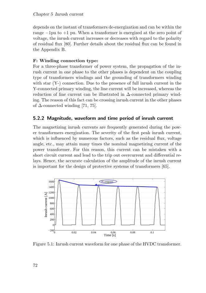
Chapter 5 Inrush current
depends on the instant of transformers de-energization and can be within therange −1pu to +1 pu. When a transformer is energized at the zero point ofvoltage, the inrush current increases or decreases with regard to the polarityof residual flux [80]. Further details about the residual flux can be found inthe Appendix B.
F: Winding connection type:For a three-phase transformer of power system, the propagation of the in-rush current in one phase to the other phases is dependent on the couplingtype of transformers windings and the grounding of transformers windingwith star (Y-) connection. Due to the presence of full inrush current in theY-connected primary winding, the line current will be increased, whereas thereduction of line current can be illustrated in ∆-connected primary wind-ing. The reason of this fact can be crossing inrush current in the other phasesof ∆-connected winding [71, 75].
5.2.2 Magnitude, waveform and time period of inrush current
The magnetizing inrush currents are frequently generated during the pow-er transformers energization. The severity of the first peak inrush current,which is influenced by numerous factors, such as the residual flux, voltageangle, etc., may attain many times the nominal magnetizing current of thepower transformer. For this reason, this current can be mistaken with ashort circuit current and lead to the trip out overcurrent and differential re-lays. Hence, the accurate calculation of the amplitude of the inrush currentis important for the design of protective systems of transformers [65].
0 0.02 0.04 0.06 0.08 0.1−200
0
200
400
600
800
1000
1200
1400
1600
Time [s]
Inru
sh c
urre
nt [A
]
DC component
Figure 5.1: Inrush current waveform for one phase of the HVDC transformer.
72

5.3 Impacts of transformer inrush current on the HVDC system
The waveform of the magnetizing inrush current is non-symmetrical. Forthis reason, this current has high order harmonics and DC component whichmakes power quality decrease [60]. A typical inrush current waveform is il-lustrated in Figure 5.1. The DC component and even harmonics of differentmagnitudes can be easily seen. It should be noted that the DC componentand the current waveform decrease along with time.The magnitude of inrush current is not a constant quantity, but it changeswith time and decays slowly after several minutes [81, 82]. Therefore, thiscurrent can take along time to reach its steady-state value. The attenuationtime of inrush current depends on the impedance of the circuit including theimpedance of the system connected to the transformer, as well as that of thetransformers winding and magnetizing impedance [81]. Due to the nonlineareffect of transformer magnetization inductance, the calculation of the decayrate using a L/R time constant is very difficult.
5.2.3 Inrush current harmonics
The transformer is a harmonic current source. The energization of the trans-former will produce a magnetizing inrush current which includes all harmoniccomponents and a DC component [60]. The harmonics of the transformerinrush current generally decay when this current fades to the steady-statemode [60]. The second harmonic content of this current is a significant orderof harmonics and is also dependent upon the magnetizing characteristic ofthe core. In fact, its value becomes higher when the saturation flux densi-ty, Bsat, is smaller. Moreover, current corresponding to the second harmonicorder is usually applied to distinguish inrush currents of power transformerfrom fault currents, so as to restrain the operation of the transformer differ-ential protection during energization.
5.3 Impacts of transformer inrush current on theHVDC system
Transformer inrush transient can influence the operation of the HVDC trans-mission system and threaten the stability of this grid. In fact, the functionof the HVDC converter can be interrupted through converter protectiondue to current saturation as well as transition of the HVDC power can bedelayed. Moreover, this large transient current, which is rich in terms ofharmonic content and contains a high direct current component, can resultin the unexpected tripping of the transformers protective devices and con-
73

Chapter 5 Inrush current
sequently, it can lead to failure of the transformers energization or recoveryoperation.Furthermore, insulation failures in power transformers which are energizedunder no-load condition or are restored after fault clearance are hazardouseffects of the inrush current [66]. In addition, the presence of drastic elec-tromagnetic stresses provided by the magnetizing inrush current alleviatespower transformers life time [68].
5.4 Reduction strategies of transformer inrush current
Considerable inrush current in the power transformer can occur due to themagnetic saturation resulting from a sudden change in the transformersvoltage. In order to limit the magnetizing inrush current magnitude, severaltechnologies have been rendered by researchers, which can be classified as:pre-insertion resistor, controlled switching, neutral resistor with sequentialswitching, reduction of residual flux and prefluxing [67].The most prevalent techniques among them are controlled switching and pre-insertion resistors. However, the transformer controlled switching methodneeds the value of residual flux in transformer core, it is more econom-ical and reliable than the pre-insertion resistors [83]. The reason is thatthe pre-insertion resistor method needs to install large resistors [84]. There-fore, the present section will explain the available technologies for inrushcurrent diminution.
5.4.1 Pre-insertion resistor strategy
One old method for the reduction of the energization transients in trans-formers is the pre-insertion resistor scheme. In fact, this technique is basedon the temporary insertion of a relatively large resistor in series with thecircuit when the transformer is switched on. Consequently, using this strat-egy, voltage collapse can take place across the pre-insertion resistor and thedecrement of transformer windings voltage and the core flux can also resultfrom this [85]. Finally, the inrush current can be decreased.Although this technique is simple and leads to inrush current reduction, ithas two disadvantages: the excessive loss and the considerable cost to up-grade the breakers [17, 69, 70].
74

5.4 Reduction strategies of transformer inrush current
5.4.2 Controlled switching strategy
Controlled switching technology is mainly designed to decrease transformerinrush currents at the moment of energization and to prevent power qualitydegradation. This much more flexible method switches on the transformer atthe optimal point on the voltage waveform to be able to suppress transientinrush currents [86].If the appropriate time for transformer energization is at the peak of thevoltage waveform, reduction of the transient flux caused by the transformercore and consequently inrush current are certain. However, transformer ener-gization at the zero point on the voltage waveform can lead to the generationof a peak inrush current [69].Therefore, there are three various strategies for controlled energization ofthe transformer that are discussed below. In these techniques, the closinginstants of circuit breaker poles are controlled and performed in an adequatesequence [66, 68].
A: Rapid closing strategy:The function of this methodology is to close one phase first and then theother two phases during a quarter cycle to minimize the inrush current andto improve power quality in the power system. The main shortcomings ofthis approach are the need for residual flux information in all phases andthe independent regulation of circuit breakers, which are necessary to fulfillthis closing process [66, 68].
B: Delayed closing strategy:This closing technique implies to energize one phase in the beginning and todelay the switching of the two remnant phases 2-3 cycles later. The require-ments of this strategy are the data of the residual flux just in one phase andthe independent control of circuit breaker [66, 68].
C: Three phase simultaneous closing strategy:This strategy has proved to reduce the magnetizing current by simulta-neously closing all phases at a proper polarity and amplitude of residualflux. Thus, the information regarding the residual flux of all phases is im-portant in this method.The application of this strategy is limited to cases where the residual fluxesare equal to zero in one phase and have high values in the other two withopposite polarities [66, 68].
75

Chapter 5 Inrush current
5.4.3 Neutral resistor with sequential switching strategy:
A proposed approach for reduction in the inrush current is sequential ener-gization with a neutral resistor, as shown in Figure 5.2. This method involvesa combination of a grounding resistor at the neutral point of the energizingtransformer and a sequential switching strategy [1, 87]. The basic princi-ple for the restriction of the inrush current in the referred technique is theestablishment of some damping in the inrush currents by means of the neu-tral resistor. The reason for this is the unbalanced flow of these currents indifferent phases. Hence, in this method, each of the transformer phases issequentially switched on and the neutral resistor will be connected in se-ries with the switched phase. Thereby, the reduction of the induced voltageacross the energized winding occurs. Consequently, it can be stated that theperformance of the proposed technique is similar to that of the pre-insertionresistor technique [1, 87]. In view of the fact that the diminution in trans-former transient current is a function of the size of the neutral resistor, anappropriate choice of this resistance value can considerably decrease the peakinrush current [1, 87].
Figure 5.2: Scheme of neutral resistor with sequential switching strategy [1].
Compared to the pre-insertion resistor scheme, its simplicity and much morecost-effective, due to the existence of only one resistor, are the main advan-tages of this technique. However, the proper selection of the resistor sizefor optimal operation has not been completely solved and this methodol-ogy is limited to star grounded connected transformers and some specificnon-earthed star connections [1, 87].
76

5.4 Reduction strategies of transformer inrush current
5.4.4 Residual flux reduction strategy
The phenomenon of transformer inrush current can be mitigated via thereduction of the residual flux in the core of the transformer. This impliesthat the magnitude of the residual flux in the transformer is one of the mainparameters affecting the inrush current amplitude. Therefore, decreasing theamount of residual flux can reduce this current. The value of residual fluxcan be decreased using a capacitor mounted on the primary side of thetransformer or using a low-power ultra-low-frequency voltage source [81].
5.4.5 Prefluxing strategy
Another strategy for inrush current reduction is the regulation of the trans-former residual flux at a high amplitude and desired polarity and then, thetransformer energization at an optimal point on the system voltage wave inaccordance with the polarity of the residual flux. Hence, this process is calledpre-fluxing technique [66, 2]. On the other hand, the pre-fluxing techniqueis implemented to feed some DC flux first, before transformers switching-on, so as to make inrush current reduction possible with closing circuitsbreakers [66, 2].
Cpf Vcap Lm
To primary conductor
Line isolator
+
-
Line isolator
To ground connection
Figure 5.3: Prefluxing device [2].
The main benefit of this scheme over the other decrement schemes is thatthe pre-fluxing device (capacitor) adjusts the transformer flux to the desiredvalue and consequently, it can make the transformer residual flux informa-tion unnecessary. The pre-fluxing device, which has a simple construction,only acts within the isolation term and afterwards, it is disconnected fromthe AC network according to energization. This results in another advantage
77

Chapter 5 Inrush current
over the methodology of the pre-insertion resistors [66]. Figure 5.3 illustratesthe prefluxing device.
5.5 No application of inrush current reductionstrategies on HVDC systems
The mentioned techniques for inrush current minimization depend on factorssuch as the switching instant of the Circuit Breaker (CB), data or compu-tation of the residual flux in the transformer core, installation of large resis-tances, the connection type of the winding, the appropriate choice of resistorsize and the model for CBs switching control. Therefore, the application ofthese schemes for inrush current reduction in HVDC systems entails highercosts, higher losses and more complexity.Hence, due to the importance of the correct operation of the HVDC transmis-sion system, especially the power converter, during energization and restora-tion of the power transformer as well as the economic and technical issues ofthe system, a simpler, highly efficient and more cost-effective technique tolimit inrush current is required. This thesis proposes a new method calledVoltage Ramping Strategy (VRS). The implementation of this proposedmethod is easier due to the fact that information of transformer parame-ters is not needed. In addition, the basic principle of this approach is thecreation and regulation of ramp in the voltage across the transformers wind-ing connected the power converter. Therefore, this strategy is implementedin the AC voltage controller of the HVDC converter in order to achievelower inrush current and ensure that there is no interruption of the HVDCconverter during inrush transient.
5.6 Dynamic model of transformer
The most common representation for a three-phase two-winding transformerwhich had been proposed by Steinmetz in 1897 is model based on a T-equivalent electric circuit [63].This classical transient representation that considers winding connections(e.g., Y-Y or Y-∆) and transformer losses is applicable to transformer tran-sient studies. In other words, the transformer behavior during the energiza-tion of its iron core can be modeled by using a T-equivalent circuit. Sincethree-phase transformers applied in HVDC transmission systems are com-monly constructed through three single-phase transformers with Y-connec-tion on its primary side and the inrush current in each of the phases is
78

5.6 Dynamic model of transformer
different [88], the T-model is represented by the composition of three sep-arate single-phase units containing the efficacy of the magnetic core satu-ration [89]. In addition, the saturation of the core is modelled by a currentsource in this scheme [73]. The topology for electrical equivalent circuit of atwo-winding transformer is illustrated in Figure 5.4.
Rpj Lpj
vpj
Primary winding
Rmj
iexcj
Lmj
iRmj iLmj
ipj
Iron core
esj
Ideal Transformer
epj
RsjLsj
vsj
isj
Secondary
winding
Figure 5.4: T-equivalent circuit model of a two-winding transformer.
In order to establish the T-model for a single-phase transformer, two maincomponents, windings and the iron core, must be considered. Therefore, thewinding resistances and leakage inductances, are defined for the transformerprimary and secondary windings. The iron core behavior can be also modeledby means of a parallel excitation branch which is a parallel combination of alinear magnetizing resistance and a non-linear inductance, Rmj and Lmj , re-spectively [63, 90, 91].The Rmj and Lmj indicate the core losses and the magnetic core satura-tion. Consequently, the iron core presents the non-linear behavior duringthe analysis of the transformer transients [91].A model of three-phase two-winding transformer with a Y to ground- ∆connection can be derived from the electric circuit diagram shown in Figure5.5.
79

Chapter 5 Inrush current
iRma
epa
Lma
Rma
iLma
iRmb
epb
Lmb
Rmb
iLmb
iRmc
Lmc
Rmc
iLmc
epc
vpaRpa Lpa
Rpb Lpb
Rpc Lpc
vpb
vpc
ipa
ipb
ipc
Y-connection -connection
esa
esb
esc
isaRsaLsa
RsbLsb
RscLsc
isb
isc
vsa
vsb
vsc
Figure 5.5: Electric circuit diagram of a three-phase two-winding trans-former with a Y to ground-∆ connection [3].
5.6.1 Modeling of transformer primary winding
For the transformer primary windings, Rpj and Lpj present the winding re-sistance and leakage inductance for each of the transformer phases. Theseresistances and leakage inductances are linear [90]. The state equation de-scribing the primary side of a three-phase transformer in Figure 5.4 can beexpressed as follows [3]:
vpj − epj = Rpjipj + Lpjdipjdt
(5.3)
where j denotes the corresponding phase, vpj and epj show the primaryterminals voltage and the voltage induced in the primary winding, respec-tively. The epj differs from vpj due to the voltage drop across the windingresistance and the leakage reactance and it also lags the main flux by 90. Theipj represents the current in the primary windings.Applying Laplace transform to Equation (5.3), the following formula can bewritten.
ipj =1
sLpj[vpj − epj −Rpjipj ] (5.4)
Based on Equation (5.4), a block diagram for the transformer primary sidecan be shown in Figure 5.6.
80

5.6 Dynamic model of transformer
ipjvpj +
-
1
sLpj
epjRpj
+
-
Figure 5.6: Block diagram for the transformer primary windings.
Furthermore, according to the equivalent circuit of Figure 5.4, the current ofthe primary side, ipj , will consist of the excitation branch current, iexcj , plusthe current component of the secondary winding, isj , [90]. So,
ipj = isj + iexcj (5.5)
5.6.2 Modeling of the iron core
Power transformer modeling considering iron core effects is an important is-sue to analyze the inrush current transients during transformer exciting andrecovery. The reason for this is that the flux in the magnetic core reachesthe limit of the saturation flux and consequently, leads to the saturation ofthe core. Then, this saturation influences the magnetizing current and final-ly, concludes to occur the inrush current. Hence, the transformer model musttake into account the effect of the core saturation at the time of transformerenergization and recovery. This is not enough for the model of the core, theconsideration of the core losses composed of hysteresis and eddy-currentlosses is also required. In general, the representation of the transformer willbe more practical due to the implementation of these impacts, however itbecomes more wrapped [91].Therefore, the iron core presents a non-linear behavior during the trans-former transients due to the effects of saturation and losses of the trans-former core. Hence, the non-linear operation of the core can be modeled inthree methods: [92]
a) Linear resistor and nonlinear inductor.
b) Nonlinear resistor and nonlinear inductor.
c) Linear resistor and nonlinear hysteresis inductor.
In order to study inrush current transient, the method (a), which includesnon-linear inductance (Lm) and linear resistance (Rm), is more commonly
81

Chapter 5 Inrush current
applied to model the non-linear iron core of transformer, due to its simplici-ty. In this method, the Rm and Lm are the core losses and the magnetic coresaturation, respectively [92]. Moreover, the core model, as shown in Figure5.4, is interfaced with a point of the T-equivalent circuit that the integral ofthe voltage is identical to the flux of the core [91].According to Figure 5.4, current in the excitation branch, iexcj , is computedas follows [90]:
iexcj = iRmj + iLmj (5.6)
where iRmj and iLmj denote the core losses and magnetizing currents, re-spectively.In the representation of the transformer core, the magnetizing branch in-dicating core saturation can be modeled by a current source [60, 73], asillustrated in Figure 5.7. The magnetizing current presented by this currentsource depends on the total flux of the transformer core. In general, the total
iRmjiLmj
Lmj Rmjepj(t)
iexcj
iLmj
iRmj iexcj
j(t)> sat(t)
j(t)
rj(t)
1s
epj(t)++
j(t)< sat(t)1Lnon-sat
1Lsat
iLmj
If ++
Figure 5.7: Equivalent model of a nonlinear inductor.
flux, φj , results from the sum of the integral of the induced voltage across themagnetizing branch, epj(t), and the residual flux remained in the core, φrj , [3].
82

5.6 Dynamic model of transformer
Thus,
φj(t) =
∫epj(t)dt+ φrj (5.7)
In addition, the mentioned flux can be obtained based on the following ex-pression [93]
φj(t) = LmjiLmj(t) (5.8)
Substituting for φj(t) in Equation (5.7), based on Equation (5.8) and takingLaplace, the following relation can be deduced for the magnetizing current.
iLmj(s) =1
Lmj[1
sepj + φrj ] (5.9)
where Lmj shows the magnetizing inductance. The magnetizing current isin time phase with its associated flux to excite the core. The block diagramof magnetizing current is shown in Figure 5.8.
iLmjepj +1
s+
1
Lmj
rj
Figure 5.8: Block diagram of the magnetizing current.
For transformers with connection of Y-Y, the current of the magnetizingbranch in each phase, iLmj , can be obtained through the reduction of thecomponent of the core loss current, iRmj , from the primary winding cur-rent, ipj , on the basis of Equations (5.5) and (5.6). Thus,
iLmj = ipj − iRmj (5.10)
It should be noted that in transformers with configuration of Y-Y, the cur-rent in the secondary windings is equal to zero [90].The theorem of the magnetizing branch current in Y-∆ connected trans-formers is quite different. Figure 5.9 shows the equivalent electric circuit ofa Y-∆ connected transformer which is excited from the star side.
83

Chapter 5 Inrush current
Rma
iexca
Lma
iRma iLma
LpaRpaipa
+
-
RsaLsa idelta
Rmb
iexcb
Lmb
iRmb iLmb
LpbRpbipb
vpb
+
-
RsbLsb idelta
Rmc
iexcc
Lmc
iRmc iLmc
LpcRpcipc
vpc
+
-
RscLsc idelta
Primary winding Core Secondary winding
vpa
Figure 5.9: Equivalent electric circuit for a Y-∆ transformer [3].
84

5.6 Dynamic model of transformer
Under no-load normal operation state, the transformer secondary terminals,which are in delta configuration, are not connected to the load. Therefore, theinduced voltages across the windings with delta connection become almostbalanced and the delta winding current can be considered zero [90].However, when the three-phase transformer is energized, an unbalance mayarise in the induced voltage. This implies that a high voltage collapse willtake place in the leakage impedance of the primary winding. Hence, the un-balance of induced voltage results in the creation of a current in the deltawinding [90].Based on the T-equivalent circuit and supposing the secondary windingswith delta connection, the computation of magnetizing current is as fol-lows [90]:
iLmj = ipj − iRmj − idelta (5.11)
The current of delta winding, idelta, is related to the rate of flux changing.
A: Modeling of non-linear inductance:Changing the non-linear magnetizing inductance, Lm, shows the essentialfeature of the iron core during the transformer energization and restora-tion, namely saturation and non-saturation of the transformer core [93]. Thisinductance can be defined using the curve of magnetizing characteristic, mag-netic flux versus magnetizing current, (φ − i). The slopes of this magneticcurve represent the core magnetic inductance at the non-saturation and sat-uration modes [60, 73, 78, 93, 94].Figure 5.10 shows the curve of magnetizing characteristic. During the steadyoperation of transformer, no saturation occurs in the magnetic core, namelyφ<φsat, and the value of magnetizing current is low. Thus, in this mode, thecore magnetizing inductance is located in the linear segment of the magne-tizing characteristic curve and its content becomes equal to a stable value,Lnonsat [93].However, when a transformer is switched on, the core flux exceeds the satu-ration flux, namely φ>φsat. Hence, the transformer core is driven into satura-tion and the inrush current will be generated, which results in the variation ofthe magnetizing inductance. On the other hand, the periodic saturation andnon-saturation conditions of iron core in the transformer appear during theinrush current phenomenon. Therefore, the core saturation and the severenon-linear of the core lead to the variation of the magnetizing inductance of
85
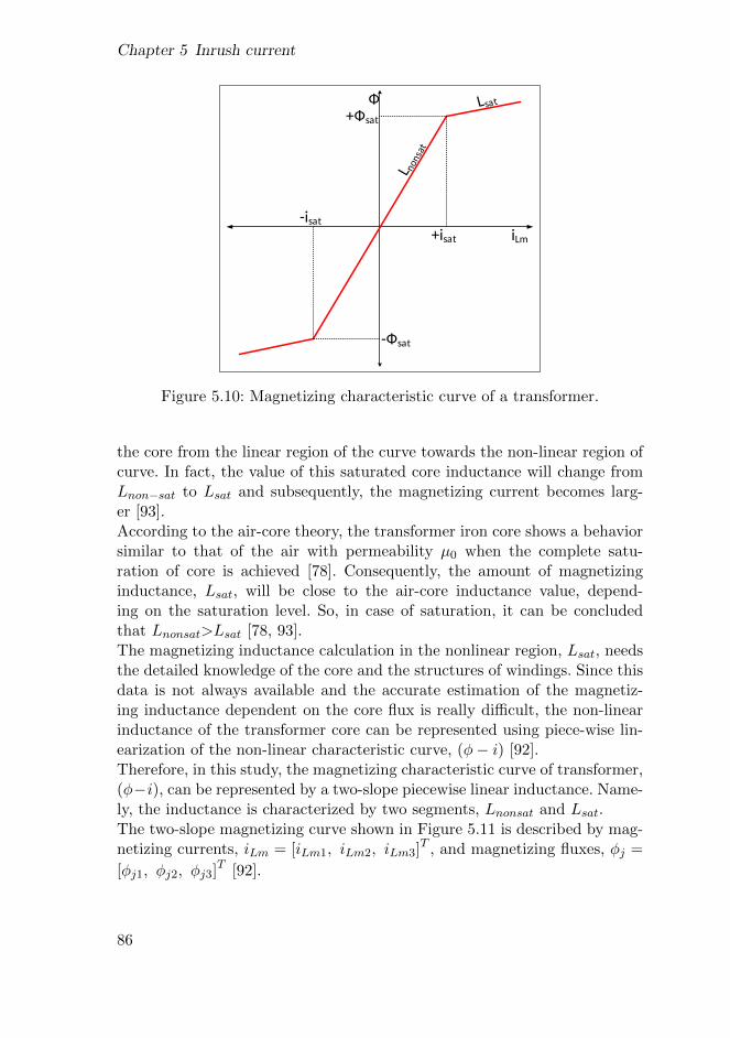
Chapter 5 Inrush current
+isat iLm
-isat
-Фsat
+Фsat
Ф
Figure 5.10: Magnetizing characteristic curve of a transformer.
the core from the linear region of the curve towards the non-linear region ofcurve. In fact, the value of this saturated core inductance will change fromLnon−sat to Lsat and subsequently, the magnetizing current becomes larg-er [93].According to the air-core theory, the transformer iron core shows a behaviorsimilar to that of the air with permeability µ0 when the complete satu-ration of core is achieved [78]. Consequently, the amount of magnetizinginductance, Lsat, will be close to the air-core inductance value, depend-ing on the saturation level. So, in case of saturation, it can be concludedthat Lnonsat>Lsat [78, 93].The magnetizing inductance calculation in the nonlinear region, Lsat, needsthe detailed knowledge of the core and the structures of windings. Since thisdata is not always available and the accurate estimation of the magnetiz-ing inductance dependent on the core flux is really difficult, the non-linearinductance of the transformer core can be represented using piece-wise lin-earization of the non-linear characteristic curve, (φ− i) [92].Therefore, in this study, the magnetizing characteristic curve of transformer,(φ−i), can be represented by a two-slope piecewise linear inductance. Name-ly, the inductance is characterized by two segments, Lnonsat and Lsat.The two-slope magnetizing curve shown in Figure 5.11 is described by mag-netizing currents, iLm = [iLm1, iLm2, iLm3]T , and magnetizing fluxes, φj =
[φj1, φj2, φj3]T [92].
86

5.6 Dynamic model of transformer
Ф j1
i Lm1 i Lm2 i Lm3
Ф j2
Ф j3
Ф j
i Lm
Figure 5.11: Two slope saturation curve.
This model of magnetizing inductance based on piecewise linearization ofthe non-linear characteristic curve is adequate to regulate the state-spaceexpressions showing the transient behavior of the transformer during exci-tation or restoration.The equation for magnetization inductance of the Kth (k = 1, 2) linear seg-ment of the foregoing curve is as the following: [92]
Lmk =dφ
diLm=
φk+1 − φkiLmk+1 − iLmk
(5.12)
This Equation (5.12) is contingent on the situation of the operating regionand its value is identical to the slope of the Kth linear segment of the mag-netizing curve [92].In order to determine the φk in Equation (5.12), the following formula isapplied:
φk =vkω
(5.13)
where ω is the angular frequency.
87

Chapter 5 Inrush current
B: Modeling of linear resistor:In order to model of the Hysteresis and eddy-current losses of the magneticcore, a linear resistance, Rmj , is considered [91]. In fact, this resistance isindicated with a fixed amount computed at the fundamental frequency ofthe induced voltage [90]. The Equation (5.14) can be used to calculate thislinear component.
Rmj =epjiRmj
(5.14)
where Rmj represents the linear resistance and iRmj shows the eddy-currentof the respective phase.
5.6.3 Modeling of transformer secondary winding
Figure 5.4 shows that the transformer secondary windings are only com-posed of the resistance, Rsj , and the leakage inductance, Lsj , at each phase.According to the equivalent circuit of Figure 5.4, the generalized analyticalexpression for the transformer secondary winding can be deduced as
esj − vsj = Rsjisj + Lsjdisjdt
(5.15)
where vsj and esj are the voltage at the secondary winding terminal and theinduced voltage in the secondary side by ideal transformer, respectively. Sim-ilar to the primary side of the transformer, the applied voltage, vsj , differsfrom esj , in the voltage drop across the resistance and the leakage inductanceof the secondary winding, represented in Figure 5.4. The isj represents thesecondary winding current.
isj1
s Lsj
Rsj
esj+
-
+
-
vsj
Figure 5.12: Block diagram for the transformer secondary windings.
Taking the Laplace transform from both sides of Equation (5.15), the Equa-tion (5.16) and the block diagram of Figure 5.12 can be obtained.
88
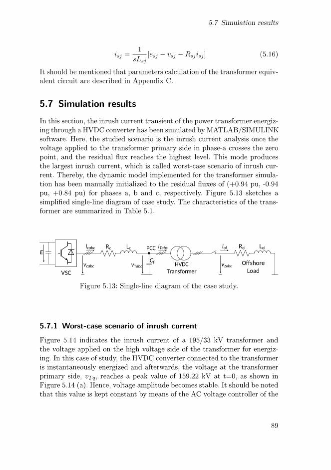
5.7 Simulation results
isj =1
sLsj[esj − vsj −Rsjisj ] (5.16)
It should be mentioned that parameters calculation of the transformer equiv-alent circuit are described in Appendix C.
5.7 Simulation results
In this section, the inrush current transient of the power transformer energiz-ing through a HVDC converter has been simulated by MATLAB/SIMULINKsoftware. Here, the studied scenario is the inrush current analysis once thevoltage applied to the transformer primary side in phase-a crosses the zeropoint, and the residual flux reaches the highest level. This mode producesthe largest inrush current, which is called worst-case scenario of inrush cur-rent. Thereby, the dynamic model implemented for the transformer simula-tion has been manually initialized to the residual fluxes of (+0.94 pu, -0.94pu, +0.84 pu) for phases a, b and c, respectively. Figure 5.13 sketches asimplified single-line diagram of case study. The characteristics of the trans-former are summarized in Table 5.1.
HVDC
Transformer
Rc
vTabc
PCCLc
vcabc
icabc
VSC
E
Cf Offshore
Load
Rol LolioliTabc
vzabc
Figure 5.13: Single-line diagram of the case study.
5.7.1 Worst-case scenario of inrush current
Figure 5.14 indicates the inrush current of a 195/33 kV transformer andthe voltage applied on the high voltage side of the transformer for energiz-ing. In this case of study, the HVDC converter connected to the transformeris instantaneously energized and afterwards, the voltage at the transformerprimary side, vTq, reaches a peak value of 159.22 kV at t=0, as shown inFigure 5.14 (a). Hence, voltage amplitude becomes stable. It should be notedthat this value is kept constant by means of the AC voltage controller of the
89

Chapter 5 Inrush current
Table 5.1: Transformer specification per phase
Parameter Value Unit
Nominal voltage 195/33 kV
Nominal current 1036.3/6123.4 A
Nominal power 350 MVA
Frequency 50 Hz
Rp/Rs 0.326/0.028 Ω
Lp/Ls 0.0484/0.0041 H
Rm 54321 Ω
Connection Ynd11 -
φsat ≈1.25φn pu
φr ≈(+0.94, -0.94, +0.84)φn pu
converter.The inrush current waveforms measured on the high voltage terminal ofthe three-phase transformer are shown in Figure 5.14 (b). Regarding Fig-ure 5.14 (b), it is obvious that inrush currents are higher than the ratedcurrents. Moreover, it can be deduced that the shape and magnitude of theinrush currents depend on the voltage at the connection instant as well asthe assumed amount of residual flux. Also, the zoomed plot of inrush currentcan be observed for a duration of 0.7s in Figure 5.14 (c).In Figure 5.15, the magnetizing inrush currents, their zoomed view and theenvelope of inrush current peaks are displayed for each of the transformerphases. These plots illustrate that the inrush current takes place when thetransformer is magnetized to its nominal voltage ( 195 kV) through instan-taneous switching of the VSC.Initially, it is assumed that the residual fluxes in the core contain the max-imum values, (+0.94 pu, -0.94 pu, +0.84 pu) for phases a, b and c, respec-tively and the transformer is energized at the instant that the voltage ofphase-a is crossing the zero. Thus, the inrush currents obtained from MAT-LAB simulation are considered as a worst-case scenario. It should be noted
90

5.7 Simulation results
2 4 6 8 10 12 140
100
200
(a)
Vo
lta
ge
[kV
]
v
Tqv
Td
0 5 10 15−1000
010002000
(b)
Cu
rre
nt
[A
]
ITa
ITb
ITc
0 0.1 0.2 0.3 0.4 0.5 0.6 0.7−1000
010002000
(c) Time [s]
Cu
rre
nt
[A
]
ITa
ITb
ITc
Figure 5.14: Inrush current and voltage of a transformer under worst con-dition. (a) The applied voltage at the transformer primaryside. (b) Inrush current of a transformer for time duration15s. (c) Inrush current for time duration 0.7s.
that the steady-state case will appear after a long time.As shown in Figure 5.15, the highest peak inrush current is related to phase-a, the value of which reaches 1654.2 A in 4 millisecond after switching inphase-a. This implies that a high value of residual flux and the switchingat the instant when voltage passes through zero influence the magnitude ofinrush current. The maximum values of inrush current for the other phas-es, b and c are -824.52 A and -829.72 A, in accordance with the Figure 5.15.Moreover, two other conclusions can be stated corresponding to the Figure5.15. The first one is that the inrush current waveforms include large andlong lasting DC components. The second one is that the time necessary forthe inrush current to drop to 50 % of its maximum value (τ50%) is approxi-mately 1.065s, 1.065s and 1.07s for phases a, b and c, respectively.
91

Chapter 5 Inrush current
0 5 10 150
500
1000
1500
(a)
Inru
sh c
urre
nt
[A
]
ITa
DC component of ITa
0 0.1 0.2 0.3 0.4 0.5 0.6 0.7 0.8 0.9 10
500
1000
1500
(b)
Inru
sh c
urre
nt
[A
]
ITa
DC component of ITa
0 5 10 15−1000
−500
0
(c)
Inru
sh c
urre
nt
[A
]
ITb
DC component of ITb
0 0.1 0.2 0.3 0.4 0.5 0.6 0.7 0.8 0.9 1−1000
−500
0
(d)
Inru
sh c
urre
nt
[A
]
ITb
DC component of ITb
0 5 10 15−1000
−500
0
(e)
Inru
sh c
urre
nt
[A
]
ITc
DC component of ITc
0 0.1 0.2 0.3 0.4 0.5 0.6 0.7 0.8 0.9 1−1000
−500
0
(f) Time [s]
Inru
sh c
urre
nt
[A
]
ITc
DC component of ITc
Figure 5.15: Simulation results of transformer inrush current for each phaseduring energization. (a) Inrush current of phase-a. (b) Zoomedof inrush current for phase-a. (c) Inrush current of phase-b. (d) Zoomed of inrush current for phase-b. (e) Inrush currentof phase-c. (f) Zoomed of inrush current for phase-c.
92

5.7 Simulation results
The voltage waveform at the transformer secondary side during energiza-tion is demonstrated in Figure 5.16 (a). It can be observed that the voltagelevel has been changed from 159.22 kV to 26.944 kV through transformerrelation. As shown in Figure 5.16 (a), there are small transients on the waveshape of the secondary voltage that are caused by the inrush current phe-nomenon which took place at the transformer primary terminal. It shouldbe noted that these transients can be mitigated by inrush current reductiontechniques.The secondary current waveform of a three-phase transformer is also illus-trated in Figure 5.16 (b). Current in each phase is approximately equal tozero, because the transformer is energized in no-load condition. Moreover,small fluctuations in the current waveforms can be seen due to the inrushtransients.
0 0.05 0.1 0.15 0.2 0.25 0.3 0.35 0.4
−20
0
20
Time [s] (b)
Vol
tage
[kV
]
VTa
(secondary)
VTb
(secondary)
VTc
(secondary)
0 0.05 0.1 0.15 0.2 0.25 0.3 0.35 0.4
−0.2
0
0.2
Time [s]
Cur
rent
[A]
ITa
(secondary)
ITb
(secondary)
ITc
(secondary)
(a)
Figure 5.16: Secondary voltage and current waveforms of transformer duringthe energization. (a) The simulated voltage for 0.4s. (b) Thesimulated current for 0.4s.
The total flux of the magnetic core for each phase during the first 50 cyclesis plotted in Figure 5.17. It can be seen that the total fluxes generated by theexcitation of the no-load transformer start from the residual fluxes 476.39wb, -476.39 wb, 425.71 wb for phases a, b and c, respectively.
93

Chapter 5 Inrush current
0 0.1 0.2 0.3 0.4 0.5 0.6 0.7 0.8 0.9 1−600
−400
−200
0
200
400
600
800
Time [s]
φ a [wb]
0 0.1 0.2 0.3 0.4 0.5 0.6 0.7 0.8 0.9 1−600
−400
−200
0
200
400
600
800
Time [s]
φ b [wb]
0 0.1 0.2 0.3 0.4 0.5 0.6 0.7 0.8 0.9 1−600
−400
−200
0
200
400
600
800
Time [s]
φ c [wb]
Figure 5.17: Total flux of transformer for each phase.
The currents of core loss, core saturation and excitation branches for eachphase (iRm, iLm and iexc) are represented in Figure 5.18. As shown, whenthe transformer is energized, the whole current passes through the core sat-uration branch, whereas a quite low current flows through the core lossbranch. Therefore, the excitation current will be almost the same as thecurrent of the core saturation branch. It should be noted that the flown
94

5.7 Simulation results
current in the excitation branch can be neglected during the steady-statecondition.
0 0.2 0.4−4−2
024
(d)
Cu
rre
nt
[A
]
IRma
0 0.2 0.4−4−2
024
(e)
IRmb
0 0.2 0.4−4−2
024
(f)
IRmc
0 0.2 0.40
50010001500
(g)
Cu
rre
nt
[A
]
ILma
0 0.2 0.4−800−600−400−200
0
(h)
ILmb
0 0.2 0.4−800−600−400−200
0
(i)
ILmc
0 0.2 0.40
50010001500
Time [s]
Cu
rre
nt
[A
]
Iexca
0 0.2 0.4−800−600−400−200
0
Time [s]
Iexcb
0 0.2 0.4−800−600−400−200
0
Time [s]
Iexcc
(c)(b)(a)
Figure 5.18: Currents of core loss, core saturation and excitation branchesfor each phase.
Since the windings of the transformer on the primary and secondary termi-nals are connected as Y − ∆, third-harmonic currents circulate within thedelta winding of the transformer. However, these currents, known as deltacurrents, are preventing the flowing in the supply line. Figure 5.19 shows acomparison between inrush and delta currents of an energizing transformer.The harmonic contents variations of the transformers transient inrush cur-rent with time for each phase are illustrated in Figure 5.20. The inrushcurrent of transformer includes all the harmonic components such as funda-mental, second, third, fourth, fifth, etc. and a DC component. These harmon-ic contents were obtained by means of a Discrete Time Fourier Transform(DTFT). Figure 5.20 shows that, the most significant harmonic componentsare fundamental and 2th order harmonics. For phase-a, their peak values are
95

Chapter 5 Inrush current
0 0.02 0.04 0.06 0.08 0.1 0.120
200
400
600
800
1000
1200
1400
1600
Time [s]
Cur
rent
[A
]
ITa
Ideltaa
Figure 5.19: Comparison between inrush current of phase-a and delta cur-rent.
665 A and 452 A, respectively. The fifth harmonic current has a maximumvalue of nearly 61 A, nearly 7.5 times smaller than the second harmonic andnearly 10.5 times smaller than the fundamental component. These harmon-ics decay when the inrush current decays toward the steady-state mode. Asshown in Figure 5.20, harmonics with higher orders of 3 have discontinu-ities. In other words, the peak values of these harmonics reduce to zero andthen, increase again.
5.8 Summary
Transformer inrush current is a transient response to the magnetization thatcan exceed the nominal value of the transformer current and may be as in-tense as a short-circuit current. This transient inrush current, which is richin terms of harmonics, has undesirable effects on the HVDC network. Animportant drawback of this inrush current in HVDC systems can be thedisconnection of power converter, which can lead in turn to the interruptionof the operation of the HVDC system. Consequently, the reduction of thiscurrent has become a main issue in the modern power industry.Some technologies to limitat inrush current have been presented in this chap-ter. The application of these techniques in HVDC systems entails difficultiessuch as, requirement for the knowledge of residual flux, physical space re-quirements, low reliability and high costs. Therefore, this thesis will propose
96

5.8 Summary
−1 0 1 2 3 4 5 6 7 8 9 100
0.5
(a)
Cu
rre
nt
[K
A]
fundamental second third forth fifth sixth
−1 0 1 2 3 4 5 6 7 8 9 100
0.2
0.4
(b)
Cu
rre
nt
[K
A]
fundamental second third forth fifth sixth
−1 0 1 2 3 4 5 6 7 8 9 100
0.2
0.4
(c) Time [s]
Cu
rre
nt
[K
A]
fundamental second third forth fifth sixth
Figure 5.20: Harmonic content present in inrush current of: (a) Phase-a. (b) Phase-b. (c) Phase-c.
a novel approach in the next chapters which allows for the minimization ofthe inrush current of the transformer during the system start-up and restora-tion after fault clearance. Simulations have been carried out in order to showthe worst-case scenario of inrush current.
97

98

Chapter 6
Energization inrush current reductionby proposed voltage ramping strategyduring start-up and integration ofoffshore wind farm
The main scopes for this chapter are to develop a strategy for HVDC trans-former inrush current reduction and control the offshore platform voltage, inorder to provide a smooth start-up for offshore wind farm through the pow-er converter of the HVDC transmission system. In addition, analysis of thestart-up procedure of the offshore wind farm as well as a comparison betweenthe performance of the proposed design and that of the system without thereduction approach can be mentioned as further objectives.
6.1 Introduction
The start-up of offshore wind farms through the HVDC systems in a stableand smooth mode is a significant issue. To achieve this target, there is theHVDC technology based on the Voltage Source Converter (VSC). In fact, theself-commutated VSC system can interconnect to the passive grid thanks toits black start capability and it can also generate a stable AC voltage atthe offshore wind farm platform for start-up. This is due to the fact thatthe power electronic devices are utilized in VSCs. Therefore, VSC-basedHVDC systems can facilitate the start-up of offshore wind farms and theirintegration into the onshore AC systems [95].Furthermore, to coordinate the start-up of the VSC-HVDC system and theoffshore wind farm system, a start-up procedure should be developed forthe whole system. During the start-up process, transformers available in thepower system, especially the HVDC transformer, will be switched-in and
99

Chapter 6 Energization inrush current reduction of HVDC transformer
their energization often leads to the appearance of a large inrush current inthe power grid. These currents containing harmonics can cause the dynamicovervoltages that lead to system instability. On the other hand, the voltagequality of Offshore Platform (OP) may be affected by the inrush currentof the transformer in the HVDC system and the protection devices maybe tripped. Hence, the existence of a method is essential for energizationinrush current reduction of the transformer. A research work [19] has beencarried out in the field of transformers inrush current minimization beforethe energization of doubly-fed induction generator offshore wind farms.This chapter proposes a strategy, which is applied in the control system ofoffshore converter in the VSC-HVDC grid, to limit the inrush current duringthe transformer energization in the start-up process and also to improvevoltage quality at offshore platform. This method is called Voltage RampingStrategy (VRS) and is performed only for inrush current reduction of HVDCtransformer.This study is organized as follows: Section 6.2 describes the configurationof the offshore wind farm connected to the VSC-HVDC system, Section 6.3analyzes the procedure of offshore system start-up and Section 6.4 introducesthe proposed system. Simulation results are represented in Section 6.5 toprove the validity of the proposed method and finally, Section 6.6 draws theconclusions.
6.2 Analyzed system
The system under study contains a VSC-HVDC power converter interfacedwith an offshore wind farm through an interface RLC filter and a powertransformer in Yg/∆ connection. The RLC filter composed of a series RLbranch and a shunt capacitor (cf ) allows for the regulation of the HVDCtransformer and offshore platform voltages. The power converter, called off-shore converter, maintains stable voltage at the offshore platform. Figure 6.1shows a simplified schematic diagram of the offshore wind farm connectedto the offshore converter during the start-up condition.The collection system for offshore wind farm is comprised several radialstrings which collect wind turbines power and deliver it to the offshore plat-form. The radial strings are equipped with a number of wind turbines con-nected to each other by submarine cables and injecting the power into a33 kV offshore feeder [96]. This chapter takes into account only four windturbines from one string in order to facilitate the research on the offshorewind
100
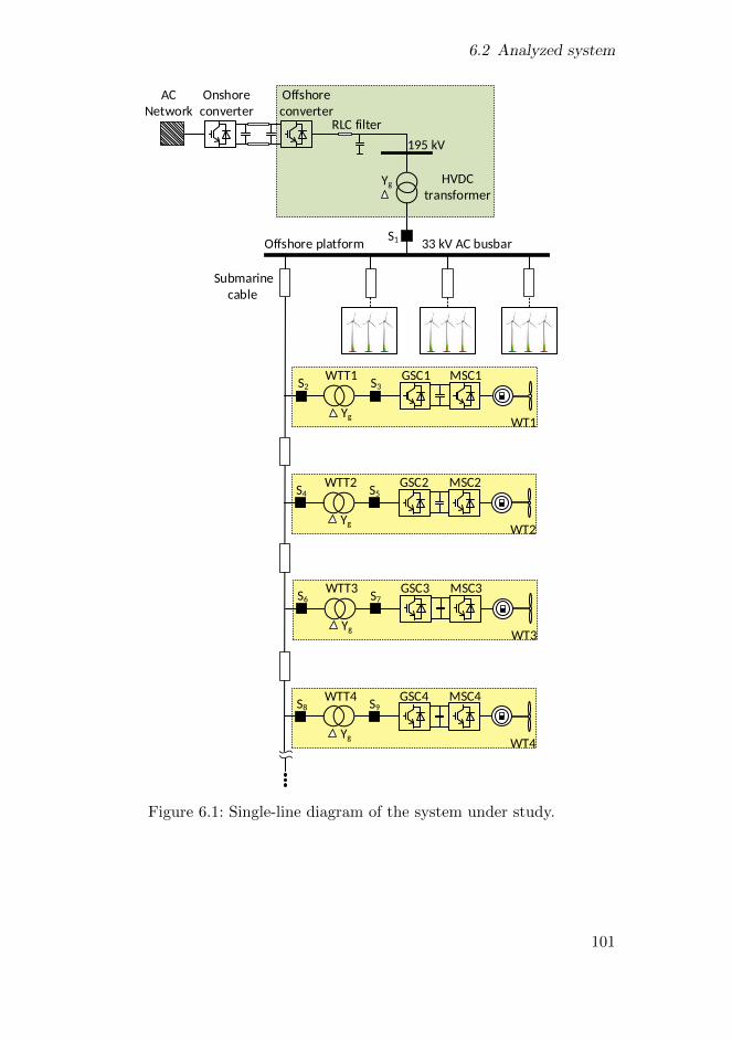
6.2 Analyzed system
HVDC
transformer
195 kV
Yg
AC
Network
Offshore
converter
Onshore
converterRLC filter
Submarine
cable
Offshore platform 33 kV AC busbarS1
WTT1
YgWT1
WTT4
YgWT4
S2 S3
S4
S8 S9
GSC1 MSC1
GSC4 MSC4
WTT2
YgWT2
S5
GSC2 MSC2
WTT3
YgWT3
S7
GSC3 MSC3
S4
S6
Figure 6.1: Single-line diagram of the system under study.
101

Chapter 6 Energization inrush current reduction of HVDC transformer
farm start-up.Each wind turbine is presented as a Permanent Magnetic Synchronous Gen-erator (PMSG, 5 MW) connected to a step-up transformer of 3.3/33 kV viathe back-to-back converters (5.6 MVA). The wind turbines step-up trans-former (WTT) is required to transform the generator voltage into the voltageof the offshore feeder. The back-to-back converters are employed to allowfor the active power transmission under wind turbines start-up and nor-mal operating conditions. The wind turbines converter that is confrontedwith the offshore grid is called Grid Side Converter (GSC) and the powerconverter faced with the electrical machine is called Machine Side Converter(MSC). The GSC is equipped with a DC-chopper that limits the DC voltageand dissipates the power that cannot be fed under AC fault condition [40].
6.3 Start-up procedure of an offshore wind farm alongwith inrush current reduction
The successful start-up of the offshore wind farm, its integration into an ACpower network and the reduction of the HVDC transformer inrush currentduring the start-up can be achieved by means of the following process. Al-so, the flowchart of Figure 6.2 presents the sequential steps of this procedure.
6.3.1 Step 1: Start-up of offshore converter
To start-up the offshore wind farm and integrate it with AC grid, the ener-gization of the offshore power converter in the HVDC transmission systemis the first step. As the onshore converter is energized and the capacitorsof DC link will be charged, the offshore converter will be able to operateunder this DC voltage. Hence, the control system of offshore converter isactivated to establish a stable nominal voltage at the HVDC transformerterminals as well as at the AC busbar of the offshore wind farm platformafter closing switch S1. The offshore converters controller actually providesthe constant reference voltage in the AC busbar for energizing the offshorewind farm [95, 97].In other words, when the offshore converter is energized in the beginning ofthe offshore grid start-up procedure, the converter AC side is faced with anopen circuit and consequently, the active and reactive powers of the convert-er are close to zero [97]. In fact, the reason is that the offshore wind farmbehaves like a passive load [98].
102

6.3 Start-up procedure of an offshore wind farm along with inrush current reduction
N=1
Energization of the wind turbine transformer
Voltage stabilization
???
YES
NO
Synchronization of GSC of wind turbine with AC grid
Pre-charge of DC link through rectifier
Control system for GSC of wind turbine: ON
Disconnection of pre-charge circuit
Control system for MSC of wind turbine: ON
Integration of wind turbine and power transmission to
the AC grid
NO
YES
EWT = EWT
???
N=N+1 N=Total number of wind turbines of a
feeder ???
NO
END
YES
Integration of offshore wind farm to the AC network, transmission of power and reduction of the HVDC
transformer inrush current
N is the number of wind turbine
Closing switch before Trf (S2)
Closing switch after Trf (S3)
Step
4: E
ner
giza
tion
of
off
shor
e w
ind
far
m
START
Closing the switch S1
Generation of a 33 kV voltage at offshore
platform and feeder
Energization of HVDC Transformer with
minimum inrush currentusing Voltage Ramping
Strategy (VRS)
Voltage stabilization
???
YES
NO
Start-up of the offshore converter
Step
3: E
ner
giza
tion
of
off
shor
e A
C b
usb
ar
St
ep 2
Step
1
*
Figure 6.2: Flowchart of the offshore wind farm start-up procedure.
103
Chapter 6 Energization inrush current reduction of HVDC transformer
6.3.2 Step 2: Energization of HVDC transformer
The HVDC transformer is energized under no-load condition through theoffshore converter. Once the offshore converter controller is activated, anabrupt voltage will induce across the high voltage terminal of HVDC trans-former. This sudden increment of the transformer voltage may lead to trans-former core saturation mode and consequently, the transformer will draw alarge magnetizing current from the supplying network. This considerablecurrent is named energization inrush current and its magnitude can reachseveral times the HVDC transformer rated current. Thus, the HVDC trans-former connected to the offshore converter is started-up along with largeinrush current, so that this current can affect the power quality of the off-shore system and it also results in the inadvertent operation of protectivedevices. Thus, in order to energize the transformer with the minimum valueof inrush current, a technique is required to design the control system ofthe offshore converter. For this reason, a new method, called Voltage Ramp-ing Strategy (VRS), is introduced in this chapter (Section 6.4). The mainobjective of the proposed VRS is to restrict the HVDC transformer inrushtransience before offshore wind farm start-up. Also, this strategy is employedonly when the no-load transformer is being switched in.
6.3.3 Step 3: Energization of offshore AC busbar and feeder
After the transformer is energized and the voltage reaches the rated lev-el, switch S1 is closed to energize the AC busbar of the offshore wind farmplatform. This implies that the offshore feeder will be switched on this way.
6.3.4 Step 4: Smooth start-up of the wind turbine
The first step of the wind turbine start-up is closing switch S2 after theenergization of the whole offshore feeder. Hence, the grid voltage suddenlyexerted to the high voltage terminal of the transformer can lead to the sat-uration of the transformer core. Therefore, an inrush current can be drawnby means of the wind turbine transformer. The inrush current amplitude ofthe transformer is much lower than that of HVDC transformer. This indi-cates that the voltage level and reactance of the wind turbine transformeris lower in comparison with the HVDC transformer. After transformer ener-gization and once the transformer voltage has reached the nominal level, thepre-charge of the wind turbines DC link can be started. This step is accom-plished by a pre-charge circuit consisting of an uncontrolled diode rectifierin series with a resistor, R. The control block diagram of the aforementioned
104

6.3 Start-up procedure of an offshore wind farm along with inrush current reduction
circuit is schematically illustrated in Figure 6.4. The operation procedure be-gins by closing switch Sdc1, followed by the connection of resistor, R, to theDC link in order to constrain the inrush current derived from pre-chargingthe DC link. The reason for using the resistor is that it is in charge of defin-ing the DC link charge current and time constant. However, when the DClink is pre-charged and the DC voltage has reached the specified value, theresistor, R, is bypassed by closing Sdc2 [99, 100].With regard to the approach of DC voltage to the pre-defined threshold, thesynchronization of the grid side converters voltage with the AC system volt-age can take place. This synchronization is made by applying a PLL inthe grid side converter system. Under such circumstance, the grid side con-verter system is oriented to the grid voltage. Once the synchronization isattained, the grid side converter can be connected to the wind turbine trans-former by closing switch S3. At this moment, the controller of the grid sideconverter will be automatically activated to govern the DC voltage and toensure the power balance of the wind turbine system [101]. When the DCvoltage is tuned to normal operational value, the circuit of the DC link pre-charge can be disconnected by opening switch Sdc1 [99, 100]. During thisoperation mode, the grid side converter behaves as a rectifier and the powerflowing is performed from the AC side to the DC side. In other words, nopower can be transmitted to the AC grid until this step. Since the oscillationscaused by the grid side converters connection to the grid disappear and thevoltage of GSC is stabilized, the MSC is activated and then, power balancingin the DC link will take place. Therefore, the integration of the wind turbineinto the AC grid is fully accomplished by connecting MSC to the system. Asa consequence, the offshore converter can absorb the total power generatedby the wind turbine and transmit it to the AC power system through theHVDC link. Further details regarding the control of the machine and gridside converters of the wind turbine can be found in Chapter 4.In the start-up sequence of an offshore wind farm, the energization of eachwind turbine is carried out only when the switching on and integration of theprevious wind turbine is finished. In other words, when the first wind tur-bine (N=1) is started-up, the energization process of the second wind turbine(N=N+1) begins in a way similar to that of the previous wind turbine. Thiscycle continues to energize the entire wind turbines of one feeder. There-fore, in this case, the offshore wind farm is integrated into the AC grid andthe active power generated by the wind farm is transmitted to the AC powernetwork [98]. Finally, the offshore wind farm start-up and the minimizationof HVDC transformer inrush current can be achieved by means of the fore-going procedure, as shown in Figure 6.2. Also, it should be mentioned that
105

Chapter 6 Energization inrush current reduction of HVDC transformer
the DC link voltage of the wind turbine, in this study, is assumed to becharged.
6.4 Proposed Voltage Ramping Strategy (VRS) forinrush current decrement
To limit inrush current when the no-load transformer is energized by the off-shore converter, the voltage ramping strategy is proposed. This methodologyis performed by gradual increment of voltage on the high voltage terminalof the HVDC transformer from zero to nominal level. In fact, the inrushcurrent reduction of the HVDC transformer is achieved by means of thegeneration of a ramp in the transformer voltage amplitude. Hence, this im-plies that the flux of the transformer being energized will not exceed thesaturated knee-point of (φ− I) curve discussed in Chapter 5. Therefore, us-ing this strategy, the peak inrush current can be minimized depending on theduration of the voltage ramp or the slopes value of the voltage ramp. Actu-ally, enhancement of the period of ramp or reduction of voltage ramp slopecan decrease the transformer inrush current amplitude.The estimation of the ramp slope rate SV RS is obtained based on the divisionof deviation of the transformer peak voltage amplitude (vT = vTm) from itsinitial value (vT = 0) to the desired duration for ramp tramp. Namely, thecalculation of voltage ramp can be achieved based on Equation (6.1).
SV RS =∆vTtramp
=vTm − 0
tend − tstart(6.1)
where tstart and tend are instants of the ramp starting and finishing, respec-tively. Also, the characteristic curve of voltage ramp is illustrated in Figure6.3.Figure 6.4 depicts a VRS-based control structure for the offshore convert-er system that largely overcomes the aforementioned difficulties during theoffshore grid start-up. Figure 6.4 shows that the assumption adopted in thismethod is (v∗Tq, v
∗Td) = (v∗Tq, 0), where VRS is implemented for the q−axis
component of the transformer reference voltage, v∗Tq. Hence, v∗Tq is adjustedbased on the given ramp to ensure the reduction of the current. The controlsystem of the offshore converter in Figure 6.4, as outlined in Chapter 3, com-prises an inner current control loop and an outer voltage control loop. Toperform the diminution of the peak inrush current under the transformerenergization condition as well as to regulate the amplitude, frequency and
106

6.4 Proposed Voltage Ramping Strategy (VRS) for inrush current decrement
vTm
tstart t
vT
tend
Figure 6.3: Transformer voltage ramp characteristic curve.
phase angle of the transformer voltage after the switching-in, Equations (6.2)and (6.3) are utilized for outer voltage loop.
i∗cq = kolq(s)(v∗Tq − vTq)− ωcfvTd + iTq (6.2)
i∗cd = kold(s)(v∗Td − vTd) + ωcfvTq + iTd (6.3)
where i∗cqd represents the qd-axis components of the reference current forthe offshore converter, v∗Tqd shows the qd-axis reference voltage componentsof the transformer, iTqd and vTqd denote the qd-axis components of the ACcurrent and voltage at high voltage side of HVDC transformer.Based on Equations (6.2) and (6.3), the transformer voltage in the qd frameis compared to the output signals of VRS, then the error signal is pro-cessed by compensators in qd frame, kolqd(s). Finally, with adding voltagedecoupling feed-forward compensations (ωcfvTd and ωcfvTq) and currentfeed-forward compensations (iTq and iTd), the command of current in qdframe (i∗cq and i∗cd) is issued for the corresponding q− and d−axes currentcontrol loop. Thus, the two outputs of the inner current control loop, asshown in Figure 6.4, can control i∗cq and i∗cd according to
vcq = kilq(s)(i∗cq − icq)− ωLicd + vTq (6.4)
vcd = kild(s)(i∗cd − icd) + ωLicq + vTd (6.5)
where vcqd is voltage at the offshore converter AC side, kilqd presents twosimple proportional-integral regulators and icqd is the qd-axis current com-ponents of offshore converter.
107

Chapter 6 Energization inrush current reduction of HVDC transformer
+
-
v Tq
v Td
Ko
ld(s
)
i Tq i Tdu
Tq
uT
dv T
d*
v Tq*
+
-
Cf
c f
Ko
lq(S
)
++
-
+++
i ca
bc
i Ta
bc
VT
ab
c
Off
sho
re c
on
ve
rte
r
Rc+
jXLc
T(
)
VC
Oω
Voltage modulation
v ca
bc
T(
)T
()
i cq
i cd
c f
Dev
elo
pe
d O
ute
r C
on
tro
l Lo
op
Vca
bc
HV
DC
Tra
nsf
orm
er
S3
S1
v wa
bc
S2
PLL
T(
)
GSC
1
Sd
c1
+
i wq
-+
EW
T1
-+
*
PI E
i wq
*
EW
T1
L w
i wd=
0
*
-K
d(S
) L w
Kq(s
)
v rd
++ +
v wd
++
v wq
v rq
-
Voltage modulationS
ub
ma
rin
e
cab
leW
TT
1
Re
ctif
ier
R
v rq
v ra
bc
v rd
Sd
c2
i wa
bc
P
v win
d
v win
d
0
Pm
ax
MSC
1
EW
T1
Pe
le
1τ
ele
s+
1
i dc
1
J WT
s+1
1
EW
T1
Rw+
jXLw
i wd
*
i cq
- -
+ +i cq
i cd
Kil
q(S
)
Kil
d(s
)
L c L c
+
-
+
++ +v T
q
v Td
*
Inn
er
Co
ntr
ol L
oo
p
v cd
v cq
i cd
Co
ntr
ol S
yst
em
of
Off
sho
re
Co
nve
rte
r
v
v Tq*
v Tm
t ra
mp
t
v Tq*
v T
=0
v Td*
v Tm
t ra
mp
t
v Td*
Vo
lta
ge
Ra
mp
ing
Str
ate
gy
(VR
S)
v T
v wa
bc
v pa
bc
i op
ab
c
v op
ab
c
i pa
bc
i ra
bc
Figure 6.4: Proposed control structure for the offshore converter.
108

6.5 Simulation
6.4.1 Advantages of the proposed voltage ramping strategy
The most significant benefits of the proposed technique are the considerabledecrement of transformer inrush current, accurate operation of HVDC con-verter during energizing condition and high power quality. In addition, thisstrategy ensures much lower inrush currents for slower ramps. The other ad-vantages of this method are cost-effective and straightforward implementa-tion in the voltage regulator of offshore converter connected to transformer.
6.5 Simulation
In order to validate the proposed reduction strategy and perform the start-up of offshore grid, two case studies have been simulated using MATLAB/Simulink package. The system comprises an offshore wind farm of four windturbines and a voltage source converter of HVDC transmission system. Windturbines based on PMSG are supposed to encounter the same wind pro-file. Transformers are modeled according to the T-equivalent circuit.The first case simulates the HVDC transformers behavior during energiza-tion without applying the voltage ramping strategy for inrush current re-striction. This will imply, in turn, that there is a high peak of current in thehigh voltage side of the transformer. The second case analyzes the effectsof the proposed strategy on the inrush current of the HVDC transformeras well as the sequences of the start-up of the whole offshore system. Thevoltage ramp starts at t=0 s and its duration takes into account 100 s. Thecharacteristic parameters utilized in the simulation are:
• HVDC transformer parameters: Yg/∆, 195/33 kV, S=350 MVA, R=0.003 pu, L=0.14 pu, φr=(+0.94,-0.94,+0.84) pu, φsat=1.25 pu.
• Wind turbine transformer parameters: ∆/Yg, 33/3.3 kV, S=5.56 MVA, R=0.006 pu, L=0.06 pu, φsat=1.1 pu, φr= (+0.8,-0.8,0) pu.
• PMSG parameters: Vn=3.3 kV, Pn=5.26 MW, PF grid=0.9 inductive.
• Offshore HVDC converter parameters: Vac=195 kV, Sn=350 MVA,Rc=1.6296 Ω, Lc=51.9 mH, cf=2.93 µF.
• Wind tubine parameters: ρ=1,225 Kg/m3,R=58 m, nnominal=14.8min−1
, Pn=5 MW, EWT=6 kV, cdc=1400 µF,RWT=0.0235 Ω, LWT=0.75 mH,ϑpitch=0, JWT=1.7 s, τele=0.01 s, c1=0.5, c2=116, c3=0.4, c4=0, c5=0,c6=5, c7=21, c8=0.08, c9=0.035.
109

Chapter 6 Energization inrush current reduction of HVDC transformer
• Submarine cable parameters: R=0.06 Ω/km, L=0.36 mH/km, c=0.26 µF/km, d=2.8 km.
6.5.1 Case study 1: HVDC transformer energization without thevoltage ramping strategy
In this case, the HVDC transformer is switched in through an offshore powerconverter without employing the inrush transient reduction method, VRS.Therefore, as observed in Figure 6.5 (b), a high inrush current is drawn bythe HVDC transformer, which is due to the sudden energizing by the offshoreconverter (shown in Figure 6.5 (a)). The amplitude of this inrush current forphases a, b and c is +1654.36 A, -824.55 A and -829.8 A, respectively. Thevalue of peak inrush current for phase-a is 1.6 times higher than the nominal
1 2 3 4 5 6 7 8 9 100
100
200
Vo
lta
ge
[
kV
]
(a)
VTq
0 1 2 3 4 5 6 7 8 9 10−1000
0
1000
2000
Cu
rre
nt
[A
]
(b)
ITa
ITb
ITc
0 0.1 0.20
1000
2000
Time [s]
Cu
rre
nt
[A]
(c)
ITa
0 0.1 0.2−800−600−400−200
0
Time [s]
(d)
0 0.1 0.2−800−600−400−200
0
Time [s]
(e)
ITb
ITc
Figure 6.5: Simulation results of HVDC transformer switching-in withoutusing voltage ramping strategy. (a) Voltage at the high volt-age side of HVDC transformer. (b) Inrush current of trans-former. (c) Zoomed of inrush current for phase-a. (d) Zoomedof inrush current for phase-b. (e) Zoomed of inrush current forphase-c.
110

6.5 Simulation
current value of the transformer. Here, the offshore platform is not discon-nected during transformer switching. However, as soon as the inrush currentdecays, the offshore platform is energized and consequently, the start-up ofthe offshore wind farm will begin. The worst case scenario of residual flux(+94%, -94%, +84%) was implemented in the transformer in order to beenergized.
6.5.2 Case study 2: Decrement of HVDC transformer inrushcurrent using VRS and start-up of the offshore grid
A. Energizing of the HVDC transformer by VRS:
This mode simulates the start-up of the HVDC transformer with the im-plementation of the voltage ramping strategy in the offshore converter. Inthis case, the voltage is ramped up from zero to the peak value (159.22 kV)with a ramping time (tramp) of 100 s, as shown in Figure 6.6 (a). Depend-ing on the duration of the ramp, the reduction amount of inrush currentchanges. As illustrated in Figure 6.6 (b), the inrush current, correspondingto tramp=100 s, is considerably decreased.The comparison between the values of the peak inrush current magnitude ofthe transformer in energization cases with and without using the proposedstrategy will reveal the significant influence of this method, as it can be seenin Figures 6.6 (c)-(e) as well as in Table 6.1.
Table 6.1: Comparison of peak inrush currents for two cases.
Magnitude of inrush Phase-A Phase-B Phase-C
current (A) (A) (A)
Without VRS 1654.34 824.55 829.8
With VRS 100.423 125.1 169.3
The results obtained from Table 6.1 show that the largest decrease in thetransformers inrush current appears in phase-a. On the other hand, thedegradation of current for phases a, b and c is nearly 93.93%, 84.83%, 79.6%.Moreover, it can be observed in Figures 6.6 (b)-(d) that the steady-state case
111

Chapter 6 Energization inrush current reduction of HVDC transformer
0 50 100 150 200 250−200
0200
(a)
Vo
lta
ge
[kV
]
0 50 100 150 200 250−200
0
200(b)
Cu
rre
nt
[A
]
0 10 20 30 40 50 60 70 80 90 100 110−200
0
200(c)
Cu
rre
nt
[A
]
0 10 20 30 40 50 60 70 80 90 100 110−200
0
200(d)
Cu
rre
nt
[A
]
0 10 20 30 40 50 60 70 80 90 100 110−200
0
200(e)
Time [s]
Cu
rre
nt
[A
]
Figure 6.6: Simulation results of HVDC transformer energization with us-ing voltage ramping strategy. (a) AC voltage of transformershigh voltage side. (b) Inrush current of transformer. (c) Zoomedof inrush current for phase-a. (d) Zoomed of inrush current forphase-b. (e) Zoomed of inrush current for phase-c.
112

6.5 Simulation
of the transformer is almost reached at t=140 s and the switching operationof offshore platform is accomplished by closing S1 at this moment. There-after, the wind turbines prior connected to the switching into the offshoregrid establish small effects on the steady-state condition of HVDC trans-former.Figure 6.7 shows the reduction of the peak inrush current for different phasesof the HVDC transformer when the duration of the voltage ramp (tramp) isincreasing. As can be observed in Figure 6.7, in the beginning, the trans-former is excited in the instant t=0 s and the phase-a of the transformerhas the highest value of peak inrush current (1654.34 A). Afterwards, thetransformer is switched on by the voltage ramping strategy, and tramp isconsidered as 10 seconds. This time becomes identical to the slope of thevoltage ramp, SV RS = 15.922 kV/s. In Figure 6.7, it can be observed thatthe ramp time increases to 100 seconds or the slope is decreased to a lowervalue, SV RS = 1.5922 kV/s. Therefore, as illustrated in Figure 6.7, increas-ing the duration or decreasing the slope of the voltage ramp leads effectivelyto a peak current reduction. In fact, the proposed voltage ramping strategyprovides a more appropriate response in case of voltage ramps with slowerslope. Hence, the optimal selection of the voltage ramp slope can significant-ly decrease peak magnetizing currents. In addition, the peak inrush currentreduction for phases b and c are represented in Figure 6.7.
0 10 20 30 40 50 60 70 80 90 1000
500
1000
1500
2000
Ramp time [s]
Pea
k in
rush
cur
rent
[A]
Phase−a Phase−b Phase−c
Figure 6.7: Peak inrush current reduction versus the different ramp times(for phase-a,b and c).
113

Chapter 6 Energization inrush current reduction of HVDC transformer
B. Start-up of the offshore platform and feeder:
Figure 6.8 indicates the voltage and current of the offshore platform dur-ing offshore grids start-up. As it can be seen, points (1) to (5) are the mainoperation steps. Actually, point (1) shows the energizing of the offshore plat-form and feeder by means of the power converter and closing switch S1 att=140 s. However, in this mode, a 33 kV voltage is provided at the off-shore platform (AC busbar) and the entire feeder composed of three parallelsubmarine cables, the value of current is almost zero. When the voltage be-comes entirely stable, the consecutive start-up and integration of each ofthe four first wind turbines can be performed corresponding to points (2) to(5). These points show the performance of the first wind turbine from thefeeder till the last one, respectively.
140 160 180 200 220 240 260−50
0
50
Time [s]
Vo
lta
ge
[kV
]
Vopa
Vopb
Vopc
140 160 180 200 220 240 260
−500
0
500
Time [s]
Cu
rre
nt
[A]
Iopa
Iopb
Iopc
(2)(1) (4) (5)(3)
Figure 6.8: Simulation results for offshore platform during the wind turbinesstart-up process.
As shown in Figure 6.8, in spite of the inrush transient existence in thecurrent of the offshore feeder, slight deviations from sinusoidal waveform ofvoltage are observed. These are due to the harmonics generated by wind tur-bines transformers. Furthermore, an enhancement in peak inrush currents
114

6.5 Simulation
at the moment of wind turbines transformer energization can be seen in thetotal current of the offshore feeder which entirely conflicts with the values ofthe peak inrush currents of each wind turbine. This is due to the fact thatthe current of the offshore feeder results from the sum of the currents of thewhole wind turbines. Figure 6.9 represents the current of the offshore feederfor different phases a, b and c.
140 160 180 200 220 240 260
−500
0
500
Time [s]
Cu
rre
nt
[A
]
Ia
140 160 180 200 220 240 260
−500
0
500
Time [s]
Cu
rre
nt
[A
]
Ib
140 160 180 200 220 240 260
−500
0
500
Time [s]
Cu
rre
nt
[A
]
Ic
170AWT1:193.2A
202.43A
WT3:274AWT4:
−265.6AWT1: WT2: WT3:
−363AWT4:−414A
WT2: WT3:310.55A
204.5A
−282A
167.7A 380AWT4:WT1:
WT2:
Figure 6.9: AC current of offshore feeder for phases-a, b and c.
Maximum AC overvoltage due to transformer energization in each windturbine is presented in Table 6.2.
115

Chapter 6 Energization inrush current reduction of HVDC transformer
Table 6.2: The value of overvoltage at transformer high voltage side of eachwind turbine.
Wind turbine 1 2 3 4
Overvoltage (%) 16.54 8.64 7.3 6.1
C. Start-up of the first offshore wind turbine:
At the beginning of the first wind turbine start-up, all converters of thewind turbine (GSC1 and MSC1) are blocked and there is voltage stability atthe offshore platform. Nevertheless, there are no voltages at the wind tur-bine and DC link of converters. When the first wind turbine (WT1) basedon PMSG is started-up by closing S2 at the moment of t = 145 s, a 33 kV
140 160 180 200 220 240 260
−20
0
20
Time [s]
Vo
lta
ge
[kV
]
Vpa
Vpb
Vpc
140 160 180 200 220 240 260
−200
0
200
Time [s]
Cu
rre
nt
[A]
Ipa
Ipb
Ipc
Figure 6.10: Voltage and current of MV side of WTT1 during start-up pro-cedure of the offshore grid.
116

6.5 Simulation
voltage is generated across the MV and LV terminals of the transformer. Onthe other hand, this voltage in turn results in the inrush current occurrenceat the transformer MV side, as indicated in Figure 6.10, and this current isdamped around t = 163 s. In addition, it can be noticed in Figure 6.10 thatthis inrush current including harmonics leads to the overvoltage phenomenain the 33 kV voltage of the transformer and the offshore feeder during theenergizing of the transformer.
145 145.5 146 146.5 147 147.5 148
−200
0
200
Cu
rre
nt
[A
] (a)
Ipa
Ipb
Ipc
145 145.1 145.2 145.3 145.4 145.5 145.6−100
0100200
Cu
rre
nt
[A
]
(b)
Ipa
145 145.1 145.2 145.3 145.4 145.5 145.6−100
0100200
Cu
rre
nt
[A
]
(c)
Ipb
145 145.1 145.2 145.3 145.4 145.5 145.6−300−200−100
0100
Time [s]
Cu
rre
nt
[A
] (d)
Ipc
Figure 6.11: Inrush current of the first wind turbines transformer duringenergization. (a) Three-phase inrush current. (b) The simulatedinrush current of phase-a. (c) The simulated inrush current ofphase-b. (d) The simulated inrush current of phase-c.
The simulation result for the transformer inrush current of the wind turbineat the beginning of the feeder and also zoomed current for each of the phas-es are shown in Figure 6.11. The peak current magnitude for phases a, band c are +200.4 A, +196.6 A, -271.4 A, respectively. Furthermore, in Fig-
117
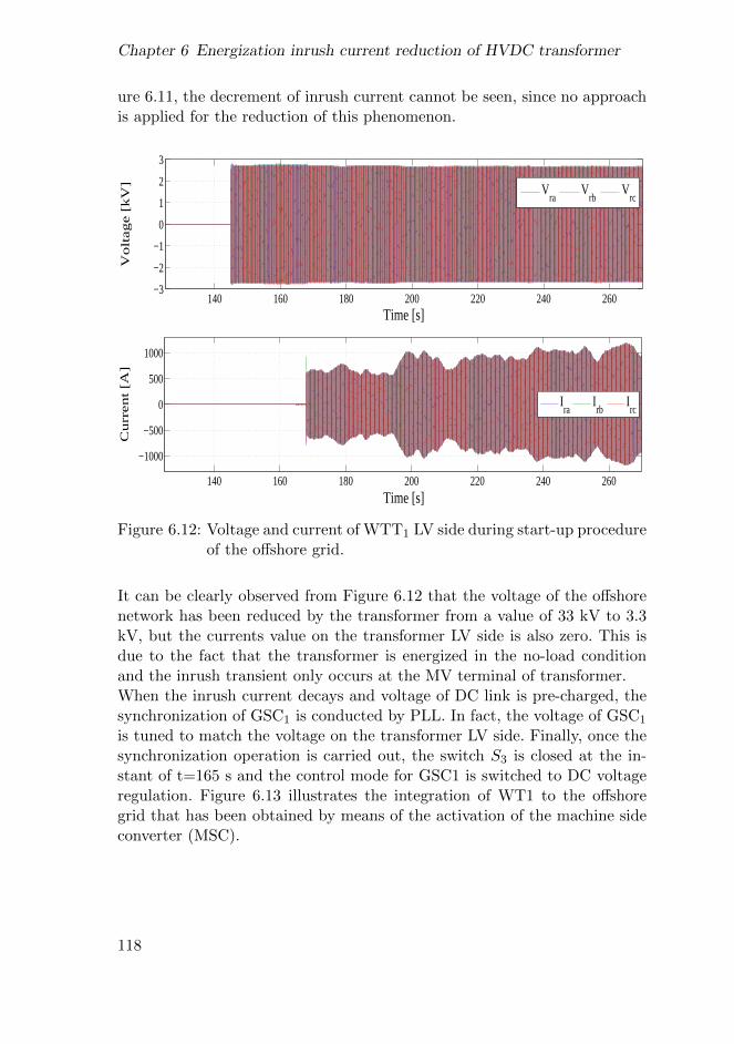
Chapter 6 Energization inrush current reduction of HVDC transformer
ure 6.11, the decrement of inrush current cannot be seen, since no approachis applied for the reduction of this phenomenon.
140 160 180 200 220 240 260−3
−2
−1
0
1
2
3
Time [s]
Vo
lta
ge
[kV
]
Vra
Vrb
Vrc
140 160 180 200 220 240 260
−1000
−500
0
500
1000
Time [s]
Cu
rre
nt [A
]
Ira
Irb
Irc
Figure 6.12: Voltage and current of WTT1 LV side during start-up procedureof the offshore grid.
It can be clearly observed from Figure 6.12 that the voltage of the offshorenetwork has been reduced by the transformer from a value of 33 kV to 3.3kV, but the currents value on the transformer LV side is also zero. This isdue to the fact that the transformer is energized in the no-load conditionand the inrush transient only occurs at the MV terminal of transformer.When the inrush current decays and voltage of DC link is pre-charged, thesynchronization of GSC1 is conducted by PLL. In fact, the voltage of GSC1
is tuned to match the voltage on the transformer LV side. Finally, once thesynchronization operation is carried out, the switch S3 is closed at the in-stant of t=165 s and the control mode for GSC1 is switched to DC voltageregulation. Figure 6.13 illustrates the integration of WT1 to the offshoregrid that has been obtained by means of the activation of the machine sideconverter (MSC).
118
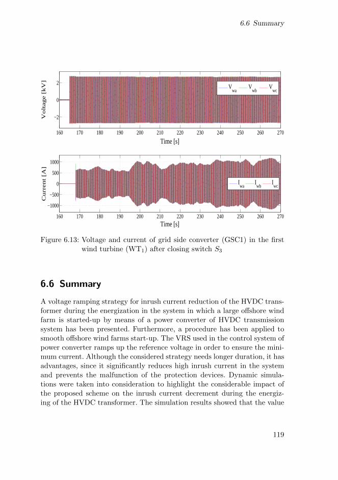
6.6 Summary
160 170 180 190 200 210 220 230 240 250 260 270
−2
0
2
Time [s]
Vo
lta
ge
[kV
]
Vwa
Vwb
Vwc
160 170 180 190 200 210 220 230 240 250 260 270
−1000
−500
0
500
1000
Time [s]
Cu
rre
nt
[A]
Iwa
Iwb
Iwc
Figure 6.13: Voltage and current of grid side converter (GSC1) in the firstwind turbine (WT1) after closing switch S3
6.6 Summary
A voltage ramping strategy for inrush current reduction of the HVDC trans-former during the energization in the system in which a large offshore windfarm is started-up by means of a power converter of HVDC transmissionsystem has been presented. Furthermore, a procedure has been applied tosmooth offshore wind farms start-up. The VRS used in the control system ofpower converter ramps up the reference voltage in order to ensure the mini-mum current. Although the considered strategy needs longer duration, it hasadvantages, since it significantly reduces high inrush current in the systemand prevents the malfunction of the protection devices. Dynamic simula-tions were taken into consideration to highlight the considerable impact ofthe proposed scheme on the inrush current decrement during the energiz-ing of the HVDC transformer. The simulation results showed that the value
119

Chapter 6 Energization inrush current reduction of HVDC transformer
of inrush current due to the transformer switching operation is much lowerthan the rated current value of the transformer and that the smooth start-upof the offshore grid has been performed as designed.
120

Chapter 7
Recovery inrush current reduction ofoffshore transformers using proposedvoltage ramping strategy
This chapter analyzes the recovery inrush current reduction procedure oftransformers in offshore grids and designs a new control system in orderto minimize inrush currents under fault recovery condition. The design ofthis control system is based on the voltage ramping strategy. Moreover, tovalidate the proposed system, a comparison between the operation of theproposed controller and that of the control system without the reductionstrategy has been carried out.
7.1 Introduction
This chapter presents a recovery inrush current reduction technique for allthe transformers available in the offshore grid, including HVDC and windfarm transformers. These transformers are exposed to AC faults. The mostsevere AC fault is a symmetrical three-phase short circuit that leads to theappearance of voltage sags on the power grids, which results in power qualityproblems. Voltage sags are short duration voltage drops [102] that can causemagnetic flux deviations in the core of transformers. Therefore, transform-ers will have a DC component of magnetic flux, called flux offset, during thevoltage sag period [103, 104, 105].When the system fault is cleared and the voltage will rapidly restore to itsnominal level, the total magnetic flux of the transformer becomes higherthan the flux value in the steady-state condition. This fact is due to thesame flux offset available in the transformer core. Hence, this over flux inthe core may provoke that the transformer in the offshore grid is driven intothe saturation mode and consequently, it will lead to high non-sinusoidalexcitation current occurrence in the high voltage side of transformers in the
121

Chapter 7 Recovery inrush current reduction by VRS
offshore grid [103, 104, 106]. The probability of such inrush transients ishigh during voltage recovery due to the slow decay of magnetic flux devi-ations [107]. Therefore, transformer inrush currents resulting from voltagerecovery after fault occurrence can be introduced as one of the challengesconcerning power quality.These recovery inrush currents can have adverse effects on the functioningof the offshore power systems and its components, such as: mechanical andelectrical stress on the transformer, bad operation of protection systems, har-monic overvoltages and instability issues [106].In addition, the performance of offshore grid converters can be affected bysaturation characteristics of transformers under fault and recovery condi-tions. On the other hand, the converter might be tripped by this type ofcurrent and consequently, the operation of HVDC transmission system andoffshore wind farm can be disturbed. Hereby, the reduction of these inrushcurrents has been a serious concern.Therefore, a Voltage Ramping Strategy (VRS) in which voltage is graduallyramped up from the voltage sag level to the nominal value is introduced inthis chapter. This reduction method assures the decrement of transformersinrush currents during the recovery of grids voltage. The verification of theoperation of the referred approach is also shown in some simulations.
7.2 Effect of the voltage sag on the grid sideconverter of offshore wind turbine
The main objective of the control system in the grid side converter of eachoffshore wind turbine is to inject the generated power into the grid. Toachieve this purpose, it is necessary to keep the DC voltage nearly sta-ble, by means of a DC voltage regulator. When a three-phase short circuitfault occurs in the AC grid, it results in the serve voltage sags on the ACterminals of the power converters in each wind turbine. Under these cir-cumstances, the current limitation imposed by the thermal characteristicsof the converter is reached and therefore, the incoming power which can betransmitted from one side to the other is restricted in proportion to the ACvoltage sag [108]. Thereby, the DC capacitor will be charged by the surpluspower and then the DC voltage will increase rapidly which may lead to theactivation of the overvoltage protection. On the other hand, the incrementof DC voltage can reflect the power imbalance of the DC link [109, 37].In order to mitigate the DC overvoltage at the DC bus as well as avoid thedisconnection of the protection devices of the converters in the grid, a DC
122

7.3 Recovery inrush current reduction process of transformers
chopper where the excess of power is dissipated is employed at the DC sideof converters in the wind power system. Namely, the DC voltage exceedingthe maximum permitted voltage is reduced to ensure balanced power. Thepower reduction achieved by means of the DC Chopper can be analyticallydescribed as [40]
P redwind = Pwind(1 + kr(EDC − EWTmin)) (7.1)
where Pwind is the wind turbine power, P redwind is the reduced wind turbinepower, EDC is DC voltage and kr can be selected as
kr =1
EWTmax − EWT
min
(7.2)
where EWTmax and EWT
min indicate the upper and lower thresholds of DC voltagein terminals of the wind turbine converters. The control action kr(EDC −EWTmin) is saturated in order not to exceed the power.
Grid side converters in wind turbines are also responsible for grid voltagesupport using AC voltage controllers during the grid fault. However, whena wind farm is integrated with an AC grid through HVDC transmissionsystems, it is better to devitalize the AC voltage support in the grid sideconverters of the wind turbines. The reason for this is to avoid control con-fluence with the offshore HVDC converter [37].Finally, as the fault is cleared and the system voltage is restored to thepre-fault level, the incoming power transmission to the AC grid will in-crease. Hence, the power system is brought back to the normal condition.
7.3 Recovery inrush current reduction process oftransformers
When an AC fault takes place in the offshore grid, a voltage sag appearsin system. After a defined duration, the fault is cleared and the voltage ofthe power system increases suddenly to its nominal value. Then, this abruptchange leads to the appearance of high inrush currents in all the trans-formers available in the offshore grid. The presence of these currents canresult in severe drawbacks in the offshore grids. Therefore, the decrement oftransformer inrush current is essential for the optimal performance of thesystem. Thereby, a framework is considered to restore the grid voltage by
123

Chapter 7 Recovery inrush current reduction by VRS
means of the proposed approach and to reduce inrush transient of trans-formers, as shown in Figure 7.1. Thus, several functions associated withthe determination of the fault occurrence instant and the fault clearancetime, the definition of the voltage sag magnitude as well as the evaluation ofthe fault ride-through have been addressed in this flowchart to achieve thereferred objectives. Further details regarding all these steps are presented inthe following subsections.
START
Voltage sag
measurement
Fault detection
Fault clearance
time detection
Voltage recovery by means of VRS
and Inrush current reduction
END
Fault ride-through
(FRT) and Switches
disconnection of
faulty wind turbine
Input data
- The q and d components of HVDC transformer voltage at the HV terminal (vTq and vTd)
- Rated voltage of HVDC transformer (vTrated
)
- Rated current of HVDC converter (icrated
) - The q and d components of HVDC converter current (icq and icd) - Threshold value
Sta
ge
1S
tag
e 2
Sta
ge
3S
tag
e 4
Sta
ge
5
Input data
- Magnitude of voltage sag (ΔvTqd)
- Rated voltage of HVDC transformer (vTrated
) at HV terminal
- Rated current of HVDC converter (icrated
) - The q and d components of HVDC converter current (icq and icd) - Threshold value
Figure 7.1: Flowchart of the voltage recovery procedure and reduction oftransformer inrush current.
124

7.3 Recovery inrush current reduction process of transformers
7.3.1 Stage 1: Detection of the fault occurrence time (ti)
The first step in the procedure of voltage restoration and transformer inrushcurrent reduction is to gain the instant in which the fault happens in theoffshore wind farm integrated with a HVDC converter. Figure 7.2 illustratesa block diagram of the fault detection scheme. Figure 7.2 shows that thefunction of fault detection is obtained from the comparison of the voltageamplitude at the high-voltage terminal of the HVDC transformer (vT ) witha threshold (around 90% of its corresponding rated value (vratedT )), as wellas from the comparison of the magnitude of the current in the AC terminalof the HVDC converter (ic) with a threshold (around 90% of rated current(iratedc )). Thus, whenever the value of vT is less than the threshold and theamplitude of ic is higher than its threshold, the AC fault is indicated anda signal 1 (or signal of Fault Detection (sFD)) is issued. In this thesis, thevoltage and current thresholds are considered to be 90%.Moreover, to compute vT and ic, which contain the q and d components
of voltage and current, the equations (√v2Tq + v2
Td) and (√i2cq + i2cd) are
applied, respectively.
&
vT SFD
01
0.9
Comparison
vT
rated
vTd
vTq<+
2vTd
2vTq
ic
Comparison
>+ 2icd
2icq
icqicd
icrated
Figure 7.2: Block diagram of fault detection.
7.3.2 Stage 2: Computation of the voltage sag magnitude
When the fault incidence is detected as explained in the previous subsec-tion, the amplitude of the voltage which drops to the lower levels is evaluat-ed. In fact, each component of vTqd is separately compared with that of the
125

Chapter 7 Recovery inrush current reduction by VRS
saturation limit and then, the obtained signal is filtered by the zero-orderhold and moving average functions, as it can be seen in Figure 7.3. Thesefunctions are used to obtain the voltage drop during the fault interval.
(Fig
7.2
)
s FD
vTqd
+
-
Zero-Order
Hold Moving Average
Filter
vTqd1n PM-i
i=0
n-1
Figure 7.3: Block diagram of measurement system of voltage sag.
7.3.3 Stage 3: Fault ride-through and operation of protectiondevices
If the measured voltage level meets the Fault Ride Through (FRT) require-ments of the wind turbine [110], the wind turbine stays connected to theoffshore system for a specific period of time under grid fault. Otherwise, thefaulty wind turbine can be disconnected from the power system because ofthe tripping of the protection devices and hereupon, the isolation of the faultfrom the grid will take place. The instant in which the fault is cleared bymeans of the switch disconnection is also called tf .Furthermore, in the case of AC fault at a wind turbine, the other wind tur-bines will experience a sudden voltage drop. However, these wind turbinesand their generators also remain connected to the power system. It is worthemphasizing that the generators of the wind turbines are under the load inthese circumstances.
7.3.4 Stage 4: Detection of the fault clearance time (tf)
Figure 7.4 depicts the block diagram of the fault clearance time detec-tion. This block compares the amplitude of the AC current of the HVDC
converter (ic), calculated according to equation√i2cq + i2cd, with its thresh-
old (90% of iratedc ) and also, a comparison between the absolute value of
126

7.3 Recovery inrush current reduction process of transformers
voltage sag magnitude (|∆vTqd|) with the threshold of the HVDC trans-former voltage at the high voltage terminal (10% of vratedT ), as well as withthe nominal value of the HVDC transformer voltage (vratedT ) will accom-plish. Once the ic is smaller than the threshold and the absolute value of∆vTqd is higher than the threshold of vratedT and smaller than vratedT , namely0.1vratedT < |∆vTqd| ≤ vratedT , the instant of fault removal is determined and asignal 1 (or signal of the Fault Clearance Time Detection (sFCTD)) is gen-erated.
&
icrated
Comparison
Absolute
value
Comparison&
icComparison
| vTqd|
<
vTqd
0.1vTrated
Input 1
+
2icd
2icq <
0.9
icq
icd
Input 2
sFCTD
01
(Fig 7.3)
01
Figure 7.4: Block diagram of fault clearance time detection.
7.3.5 Stage 5: Voltage recovery and inrush current diminution
When the protection devices operate and the three-phase switches of thefaulty section are opened for isolation (at instant tf ), the voltage recoverywill take place and the AC grid voltage will return to its nominal level.In the new grid formed after the isolation of the faulty wind turbine, thevoltage restoration of all the wind turbines will be accomplished at the sametime. This implies that all the transformers which increase the low-levelvoltages generated at the wind turbine to the medium voltage used in thecollection grid of the wind farm are simultaneously recovered with the HVDCtransformer, which enhances the collection grid voltage to the transmission-level voltage.In addition, the voltage recovery of transformers generates huge inrush cur-rents at the instant of their restoration to the grid, due to the transformercore saturation. Thus, in order to reduce these transformer inrush transients
127

Chapter 7 Recovery inrush current reduction by VRS
during fault recovery, a soft recovery method of voltage is required. There-by, this chapter proposes a voltage control system based on the VoltageRamping Strategy to ensure the inrush current decrement as well as toguarantee the simultaneous restoration of all the transformers available inthe offshore grid after fault removal. The advanced control system is handledin the offshore HVDC converter system and further details will be presentedin Section 7.4.
7.4 Proposed control system based on VRS
The purpose of the proposed control system is to regulate voltage amplitudeand frequency under normal operation, as well as to restore the voltage tothe nominal level under grid recovery condition so as to ensure the reduc-tion of inrush transients and the stability of the system. The design of theproposed controller for the HVDC converter is illustrated in Figure 7.5.As shown in Figure 7.5, the control structure for the HVDC converter isbased on the vector control method including a lower level control (innerloop) and an upper level control (AC voltage loop). The inner loop is re-sponsible for the regulation of the qd components of the current via thecoupling filter and the voltage loop is in charge of the control of the ACvoltage amplitude at the high voltage side of the transformer. The controlis almost similar to the one utilized in the power injection system for theoffshore load [51] but it allows for the control of i∗cd by (v∗Td+ vTd−vTd) andi∗cq by (v∗Tq + vTq − vTq), as shown in Figure 7.5. Therefore, the performanceof this developed voltage loop not only depends on the amplitudes of thetransformer voltage, vTqd, and HVDC transformers current, iTqd, but alsodepends on the amount of voltage sag and the ramp rate imposed to obtainthe minimum inrush current. As a matter of fact, the qd components valueof the voltage drop including the ramp at the fault clearance instant is vTqd.With regard to Figure 7.5, the qd components of the HVDC converter cur-rent reference, i∗cq and i∗cd, are determined as
i∗cq = iTq − ωcfvTd + kolq(s)(v∗Tq + vTq − vTq) (7.3)
i∗cd = iTd + ωcfvTq + kold(s)(v∗Td + vTd − vTd) (7.4)
where vTq and vTd are the two new control inputs.
128

7.4 Proposed control system based on VRS
Cable 1 Cable 2 Cable 3E
vTabcvcabc
icabc iTabc
Offshore HVDC
converterHVDC converter
transformer
vcq
vcabc
icabc
iTabc
vTabcvTqd
iTqd
icqd
0
Inner loop
T( )-1
vcd
VCO
T( )
icqd vTqd
Voltage Loop
Voltage ramp system Advanced voltage
control system
+
+
*
vTd
vTq
*
+
vTd^
+
vTq^
vTqd^
vTq~
vTd~
Kold(S)
cf
cf
+uTd
+uTq +
+
-
vTd
vTq
-
vTqd
Kolq(S)
iTd
+
+
*
-
icq iTq
+
vTqd
1
vTqd
icq
d
sFCTD
icra
ted
vT
rate
d
Fault clearance
time detection(Fig 7.4)
Ramp Rate
vTqd
t1sxo 1
sFCTD
icd*
Control System of HVDC Converter
MSC GSC Fault
EWTvrabcvwabc
iwabc
Pelec
iDC
Pmec
DivisionEWT
vwind
+-
Electrical
system
Inertia
Pitch
controller
P
*
P
vwind
DC voltage
loop
vwqd
vwabc
EWT
EWT
*
vrqd
iwqd iwabc
vrabc
T( )
-1
Inner
loopiwqd
* T(
)
vrabcPLL
Offshore wind turbine
(Fig 7.3)
Measurement
system of
voltage sag
(Fig 7.3)
sF
Dv
Tq
d
Fault detection(Fig 7.2)
vT
qd
Rc Lc
Rw Lw
vpabc
Figure 7.5: The proposed control block diagram of offshore HVDC converterfor recovery inrush current reduction.
129

Chapter 7 Recovery inrush current reduction by VRS
As the fault takes place, these components, vTq and vTd, can change theset-points of voltage, v∗Tq and v∗Td, and also construct a voltage ramp at theinstant in which the fault is cleared, tf .To perform set-points variations, the magnitude of the voltage sag, namely∆vTqd, is immediately calculated after fault detection, as described in Sub-section 7.3.2. Thus, the obtained content, ∆vTqd, is gradually ramped up tozero at the moment in which the fault clearance is indicated by the signalof the Fault Clearance Time Detection, sFCTD, as shown in Figure 7.5. Thevoltage ramp rate is commonly tuned according to the division of the voltagesag value, ∆vTqd, into the voltage recovery duration, ∆t = tr − tf , so as toachieve the lowest inrush currents. It should be noted that the tr is the timeat which the initial condition is reached.The conclusion of this analysis is the new inputs of the voltage control sys-tem, vTqd. Moreover, Figure 7.5 shows that uTq and uTd are the output oftwo independent compensators. Namely,
uTq = kolq(s)(vTq − vTq) (7.5)
uTd = kold(s)(vTd − vTd) (7.6)
where vTq = v∗Tq + vTq and vTd = v∗Td + vTd. The compensators kolq(s) andkold(s), are obtained on the basis of the LQG optimization procedure dis-cussed in Chapter 3. When the control signals uTq and uTd are provided, thecomponents i∗cq and i∗cd are built according to Equations (7.3) and (7.4) andrendered to the corresponding inner loop controllers.The most significant advantages of the aforementioned method are recoveryinrush current reduction, system stability and the avoidance of the trip ofthe HVDC converter and protection relays of the transformer.
7.5 Simulation results
In this section, simulation studies have been carried out to evaluate theperformance of the advanced control system under symmetrical three-phasefault condition and voltage recovery process with MATLAB/Simulink. Thestudied system consists of a HVDC converter connected to a cluster of windturbines, as illustrated in Figure 7.6. In this section, simulation results forthe first three wind turbines of the cluster are analyzed. Three different sce-narios have been considered. The first one analyzes the inrush currents of
130

7.5 Simulation results
HVDC
transformer
Cable 1
Cab
le 2
Cab
le 3
Fault
Offshore HVDC
converter
WTT1
WTT2
WTT3
PMSG
PMSG
PMSG
Figure 7.6: Schematic diagram of the simulated offshore grid during the volt-age recovery.
all the transformers available in the power system without implementingthe developed method. The second one simulates the behavior of all thetransformers using the proposed technique which has considerable impacton the reduction of inrush currents magnitude. The third one analyzes theeffect of different durations of voltage ramp on the transformer inrush tran-sients.In the referred cases, an approximately 85% voltage sag with a durationof 300 ms is applied at the middle point between connection of the secondwind turbine transformer and offshore gird at instant t = 150 s. Figure 7.6illustrates the schematic diagram of the simulated network. The parametershave been summarized in Table 7.1. It should be noted that in system op-eration under the recovery process, WT 1 and WT 3 remain also connectedto the offshore grid, whereas the second turbine WT 2 is disconnected at theinstant of fault clearance, t = 150.3 s.
131

Chapter 7 Recovery inrush current reduction by VRS
Table 7.1: Parameters of the simulated scenarios
parameter value unit
PMSG nominal power (Pn) 5 [MW]
PMSG nominal voltage (Vn) 3.3 [kV]
WT inertia time constant (JWT ) 1.7 [s]
WT electrical time constant (τele) 0.01 [s]
WT pitch time constant (τpitch) 0.17 [s]
WT nominal DC voltage (EWT ) ± 3 [kV]
WT lower DC voltage level (EminWT ) 6.18 [kV]
WT upper DC voltage level (EmaxWT ) 6.48 [kV]
WT DC capacitor (CWT ) 1.4 [mF]
WT transformers (∆/Yg) nominal power (Pn) 5.56 [MVA]
WT transformers nominal voltage (Vp/Vs) 33/3.3 [kV]
WT transformers resistance/inductance (R/L) 0.006/0.06 [pu]
WT transformers magnetization resistance (Rm) 500 [pu]
WT transformers saturation flux (Φsat) 1.1 [pu]
WT transformers residual flux (Φrj) (+0.8,-0.8,0) [pu]
Submarine cable resistance (RCS) 0.06 [Ω/km]
Submarine cable inductance (LCS) 0.36 [mH/km]
Submarine cable capacitor (CCS) 0.26 [µF/km]
Submarine cable 1 length 1 [km]
Submarine cable 2 length 0.7 [km]
Submarine cable 3 length 0.7 [km]
HVDC transformers (Yg/∆) nominal power (Pn) 350 [MVA]
HVDC transformers nominal voltage (VHV /VLV ) 195/33 [kV]
HVDC transformers resistance/inductance (R/L) 0.003/0.14 [pu]
HVDC transformers magnetization resistance (Rm) 500 [pu]
HVDC transformers saturation flux (Φsat) 1.25 [pu]
HVDC transformers residual flux (Φrj) (+0.94,-0.94,+0.84) [pu]
HVDC converters nominal power (Pn) 350 [MVA]
HVDC converters nominal voltage (Vn) 195 [kV]
(X/R) 10 [pu]
132

7.5 Simulation results
7.5.1 Recovery of transformers without using VRS
In this case, there is no reduction technique for recovery inrush currents, i.e.,the transformer inrush current is considerable and can affect the operationof protection devices. The voltage and current of the HVDC transformer be-fore, during and after the fault are shown in Figure 7.7. From Figure 7.7, itcan be deduced that fault causes a voltage sag of around 64% in the voltageof the transformer primary side at t = 150 s. It is worth noting that an over-current is generated due to the fault occurrence and thereafter it is limitedby the HVDC converter.
149.6 149.8 150 150.2 150.4 150.6 150.8 151 151.2 151.4−500
0
500
(a)
Vol
tage
[kV
]
149.8 150 150.2 150.4 150.6 150.8 151 151.2 151.4
−2000
0
2000
(b)
Time [s]
Cur
rent
[A]
Figure 7.7: Influence of the fault and voltage recovery on HVDC transform-ers behavior. (a) Primary side voltage. (b) Inrush current.
As shown in Figure 7.7 (a), the voltage is recovered to the nominal value, i.e.,there is no time delay for the voltage restoration to this level after three-phase fault removal. In other words, according to Figure 7.7 (b), a largetransient current is drawn by the transformer at the instant of fault re-moval, which is a consequence of the transformer core saturation caused bythe sudden voltage increment.The inrush currents of the different phases of the HVDC transformer in thesystem without VRS are shown in Figures 7.8 (a), (c) and (e) and zoomedat the voltage recovery instant in Figures 7.8 (b), (d) and (f). As it can beconcluded from these figures, the inrush current magnitude in phase-c forthe HVDC transformer is higher than those in the two other phases. In other
133

Chapter 7 Recovery inrush current reduction by VRS
words, the maximum inrush current of phases a, b and c are +715 A, +1090A, -1325 A, respectively.
150 151 152 153 154 155 156 157
−2000
0
2000
I Ta [A
]
(a)
150.4 150.45 150.5 150.55 150.6 150.65
−1000
0
1000
I Ta [A
]
(b)
150 151 152 153 154 155 156 157
−2000
0
2000
I Tb [A
]
(c)
150.4 150.45 150.5 150.55 150.6 150.65
−1000
0
1000
I Tb [A
]
(d)
150 151 152 153 154 155 156 157
−2000
0
2000
Time [s]
I Tc [A
]
(e)
150.4 150.45 150.5 150.55 150.6 150.65
−1000
0
1000
Time [s]
I Tc [A
](f)
Figure 7.8: Inrush current of different phases of HVDC transformer duringfault and voltage recovery cases in system without VRS.
Figures 7.9, 7.10 and 7.11 (a) indicate that the primary voltage of each windturbine transformer drops when the three-phase fault occurs at the secondwind turbine. Thereby, the amount of each voltage sag is nearly 85%. Afterthat, fault removal is performed by means of the disconnection of the faultywind turbine from the offshore grid at t = 150.3 s. In this case, the otherwind turbines keep also connected to the offshore system.In Figure 7.10 (a), it can be clearly observed that the transformer primaryvoltage of the second wind turbine will be zero after fault removal whereasthe voltages of the two other wind turbine transformers are quickly restoredto the nominal value, vpn = 33 kV, as seen in Figures 7.9 and 7.11 (a).Consequently, from Figures 7.9, 7.10 and 7.11 (b), it can be deduced thattransformers of WT 1 and WT 3 experience high inrush currents due to thetransformer core saturation. Transformer inrush currents of the first andthird wind turbines in phases a, b and c have the values -340 A, +466 Aand +282 A, respectively. It should be also noted that the current under the
134

7.5 Simulation results
150 150.5 151 151.5 152 152.5
−100
0
100
(a)
Vol
tage
[kV
]
150 150.5 151 151.5 152 152.5−500
0
500(b)
Cur
rent
[A]
150 150.5 151 151.5 152 152.54
5
6
7(c)
DC
vol
tage
[kV
]
150 150.5 151 151.5 152 152.5−10
0
10
20
(d)
Time [s]
Pow
er [M
W]
Figure 7.9: Simulation results for wind turbine 1 under fault and recoveryconditions. (a): Transformers primary voltage of the wind tur-bine. (b): Transformers primary current waveform of the windturbine. (c): DC voltage of the wind turbnine. (d): Active powerinjection of the wind turine.
135

Chapter 7 Recovery inrush current reduction by VRS
150 150.5 151 151.5 152 152.5
−100
0
100
(a)
Vol
tage
[kV
]
150 150.5 151 151.5 152 152.5−500
0
500(b)
Cur
rent
[A]
150 150.5 151 151.5 152 152.54
5
6
7(c)
DC
vol
tage
[kV
]
150 150.5 151 151.5 152 152.5−10
0
10
20
(d)
Time [s]
Pow
er [M
W]
Figure 7.10: Simulation results for wind turbine 2 under fault and recoveryconditions. (a): Transformers primary voltage of the wind tur-bine. (b): Transformers primary current waveform of the windturbine. (c): DC voltage of the wind turbnine. (d): Active powerinjection of the wind turine.
136

7.5 Simulation results
150 150.5 151 151.5 152 152.5
−100
0
100
(a)
Vol
tage
[kV
]
150 150.5 151 151.5 152 152.5−500
0
500(b)
Cur
rent
[A]
150 150.5 151 151.5 152 152.54
5
6
7(c)
DC
vol
tage
[kV
]
150 150.5 151 151.5 152 152.5−10
0
10
20
(d)
Time [s]
Pow
er [M
W]
Figure 7.11: Simulation results for wind turbine 3 under fault and recoveryconditions. (a): Transformers primary voltage of the wind tur-bine. (b): Transformers primary current waveform of the windturbine. (c): DC voltage of the wind turbnine. (d): Active powerinjection of the wind turine.
137

Chapter 7 Recovery inrush current reduction by VRS
fault condition is equal to the rated current of each wind turbines convert-er. As shown in Figures 7.9, 7.10 and 7.11 (c) and (d), during the fault, theactive power cannot be completely injected into the offshore grid by eachwind turbine, in which results in the increment of the DC link voltage. Onthe other hand, the DC voltage exceeds the specified threshold during thefault and therefore, the DC chopper is activated to reduce this voltage andalso ensure an adequate power reduction. After fault removal, the DC volt-age returns to the nominal level and active power is restored quickly. Asillustrated, the DC voltage and active power experience oscillations duringvoltage recovery.
7.5.2 Recovery of transformers using VRS
In order to alleviate inrush currents, a VRS for recovery after fault has beenimplemented in the voltage control system of the HVDC converter. A similarthree-phase AC fault of 300 s duration is applied to the second wind turbineas in the previous case. In this method, as soon as the fault is removed, thevoltage of the offshore grid gradually ramps up to the nominal value tobe able to reduce high currents. Therefore, this voltage ramping techniquedoes not allow for the voltage to return to normal condition suddenly anddecreases the saturation probability of transformers core. The method hasbeen simulated and the results are presented below.Figure 7.12 shows the three-phase voltage and current of HVDC transformerfor a system with VRS. From this Figure, it can be deduced that a 15 sdelay has been taken into account for the voltage to be recovered to the rat-ed value after fault clearance. Therefore, currents variations in the HVDCtransformer, as observed in Figure 7.12 (b), are associated with this rampfor voltage recovery.In this case study, the recovery of voltage is slower than in the case with-out VRS, as illustrated in Figure 7.12 (a), regardless of the magnitude ofvoltage sag. On the other hand, in accordance with Figure 7.12 (a), it takeslonger time for voltages of different phases to attain nominal values whereasin Figure 7.7 (a), the voltages are restored very quickly. Also, comparison ofFigure 7.12 (b) and Figure 7.7 (b) indicates that inrush currents of the HVD-C transformer in a system with VRS are much lower than those in a systemwithout VRS. Thus, it can be mentioned that the VRS with tramp = 15 scan reduce the inrush current to nearly 1/3 of the value of inrush currentsin the system without VRS during voltage recovery.
138
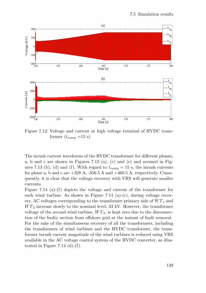
7.5 Simulation results
150 155 160 165 170 175 180−200
−100
0
100
200
Time [s]
Vo
lta
ge
[kV
](a)
vTa
vTb
vTc
150 155 160 165 170 175 180−2000
−1000
0
1000
2000
Time [s]
Cu
rre
nt [A
]
(b)
ITa
ITb
ITc
Figure 7.12: Voltage and current at high voltage terminal of HVDC trans-former (tramp =15 s)
The inrush current waveforms of the HVDC transformer for different phases,a, b and c are shown in Figures 7.13 (a), (c) and (e) and zoomed in Fig-ures 7.13 (b), (d) and (f). With regard to tramp = 15 s, the inrush currentsfor phase a, b and c are +228 A, -356.5 A and +460.5 A, respectively. Conse-quently, it is clear that the voltage recovery with VRS will generate smallercurrents.Figure 7.14 (a)-(f) depicts the voltage and current of the transformer foreach wind turbine. As shown in Figure 7.14 (a)-(c), during voltage recov-ery, AC voltages corresponding to the transformer primary side of WT 1 andWT 2 increase slowly to the nominal level, 33 kV. However, the transformervoltage of the second wind turbine, WT 2, is kept zero due to the disconnec-tion of the faulty section from offshore grid at the instant of fault removal.For the sake of the simultaneous recovery of all the transformers, includingthe transformers of wind turbines and the HVDC transformer, the trans-former inrush current magnitude of the wind turbines is reduced using VRSavailable in the AC voltage control system of the HVDC converter, as illus-trated in Figure 7.14 (d)-(f).
139

Chapter 7 Recovery inrush current reduction by VRS
150 160 170 180
−10000
1000
Time [s]
Cu
rre
nt [A
] (a)
ITa
164.92 164.94 164.96 164.98 165−500
0
500
Time [s]
Cu
rre
nt [A
] (b)
ITa
150 160 170 180
−10000
1000
Time [s]
Cu
rre
nt [A
] (c)
ITb
164.92 164.94 164.96 164.98 165−500
0
500
Time [s]
Cu
rre
nt [A
] (d)
ITb
150 160 170 180
−10000
1000
Time [s]
Cu
rre
nt [A
] (e)
ITc
164.92 164.94 164.96 164.98 165−500
0
500
Time [s]
Cu
rre
nt [A
] (f)
ITc
Figure 7.13: Inrush current of different phases for HVDC transformertramp = 15 s
By comparing the case with VRS and the previous one without VRS (i.e., Fig-ures 7.14 (d) and (f) with Figures 7.9 and 7.11 (b)), it can be observed thatthe transformer inrush current of each of the wind turbines in the differentphases, a, b and c was reduced by 53.2%, 64% and 48.3%, respectively.The dynamic performance of the active power and DC voltage in the firstwind turbine (WT 1) under fault and voltage recovery conditions is sketchedin Figure 7.15 (b) and (d). In order to better realize these shapes, the plotsof AC voltage and current of the grid side converter are also shown in Fig-ures 7.15 (a) and (c).When the fault is simulated at the second offshore wind turbine, the DCchopper of the wind turbine is activated to control the DC voltage and toreduce the active power injection, as observed in Figure 7.15 (b) and (d). Theoperation of the DC chopper protection is included based on the overvoltageof the DC link capacitor of the wind turbine.
140

7.5 Simulation results
150 160 170−50
0
50
Time [s]
Vol
tage
[kV
](a)
150 160 170−50
0
50
Time [s]V
olta
ge [k
V]
(b)
150 160 170−50
0
50
Time [s]
Vol
tage
[kV
]
(c)
150 160 170−200
−100
0
100
200
Time [s]
Cur
rent
[A]
(d)
150 160 170−200
−100
0
100
200
Time [s]
Cur
rent
[A]
(e)
150 160 170−200
−100
0
100
200
Time [s]
Cur
rent
[A]
(f)
WT3
WT3
WT2
WT2
WT1
WT1
Figure 7.14: Primary voltage and inrush current of transformer in each windturbine under fault and recovery conditions
Once the system is restored and the DC overvoltage of the full power con-verter wind turbine comes back to the nominal level, all the power injectionis also recovered. It is worth emphasizing that these restorations to the nor-mal conditions are accomplished through a ramp, as can be seen in Figures7.15 (b) and (d).Finally, Figure 7.16 shows the reduction of the peak recovery inrush currentof the HVDC transformer (in phase-a) for different time periods of ramp.
141

Chapter 7 Recovery inrush current reduction by VRS
150 160 170 180 190 200 210 220−4000
−2000
0
2000
4000
(a)
Time [s]
Vol
tage
[V]
150 160 170 180 190 200 210 220−10
0
10
20(b)
Time [s]
Act
ive
pow
er [M
W]
150 160 170 180 190 200 210 220−2000
−1000
0
1000
2000(c)
Time [s]
Cur
rent
[A]
150 160 170 180 190 200 210 2205
5.5
6
6.5
7(d)
Time [s]
DC
vol
tage
[kV
]
Figure 7.15: AC and DC voltages, active power and current of the first windturbines converter during fault and recovery conditions
142

7.6 Summary
0 10 20 30 40 50 60100
200
300
400
500
600
700
800
Ramp time [s]
Peak
inru
sh c
urre
nt [
A]
Figure 7.16: Variation of the peak inrush current of the HVDC transformerversus different time periods of ramp (for phase-a)
7.6 Summary
This chapter has introduced an inrush current reduction technique for off-shore transformers during system recovery. This voltage ramping strategycan be designed to guarantee the inrush current decline of transformersavailable in the offshore grid, including HVDC and wind turbines trans-formers, under system restoration mode and to ensure a robust stability. Theproposed method can be implemented in the AC voltage control system ofthe HVDC converter which is based on a conventional vector control systemand can gradually increase the grid voltage to the nominal level. The methodhas been tested under three scenarios, the simulation results of which showthe validity of this approach for recovery inrush current reduction.
143

144

Chapter 8
Conclusions
Several studies to improve the operation of offshore grids under inrush tran-sient condition of the transformer have been presented in this thesis. Thischapter explains the main conclusions drawn throughout the thesis and italso contains lines of research for future work.
8.1 Contributions
The contributions are detailed per chapter.
• Chapter 2 analyzed the structure of an offshore grid and the ex-istence of different configurations in offshore wind farms as well asdifferent types of wind turbines, power converters and HVDC trans-mission systems. This structure makes voltage control of the offshorewind farm grid possible through the HVDC converter and also theaccurate analysis of the models and controllers used for each of theoffshore components in the next chapters.
• Chapter 3 addressed the dynamic model and different control schemesfor the voltage source converter of the HVDC transmission system. Thedesign of the control systems has been produced considering the dy-namics of the AC and DC grids of the converter, the current and thevoltage control loops, PLL and VCO. Once the HVDC converter isconnected to the offshore wind farm, by applying the voltage and cur-rent control mechanisms, HVDC system stability and power balanceunder different operating conditions can be achieved.
• Chapter 4 presented the simplified model and the control design forthe variable-speed wind turbine. The generator of the wind turbineis totally decoupled from the offshore wind turbine grid through full
145

Chapter 8 Conclusions
power converters. The scheme of the control system is based on the ba-sic vector control method. The model applied has been tested throughsimulations and the results have proved the ability of the model toreflect variations in the power extracted by the turbine dependent onthe alterations in the incoming wind. The wind turbine model can beused in offshore transformer inrush current reduction studies and itcan provide a highly accurate estimate of the wind turbine dynamicresponse.
• Chapter 5 analyzed extensively the inrush transient phenomenonduring transformers energization in offshore HVDC grids. Under in-rush current condition, the HVDC converter might be tripped and theperformance of HVDC transmission grid might be disturbed. Thus, theinrush current reduction of the transformer in offshore HVDC systemsis an important issue. Several techniques to decrease the inrush tran-sient of the transformer in a power system have been presented. Theanalyzed strategies cannot ensure the correct performance of HVDCgrids in case of inrush transient due to their complexity, high losses andcosts, the requirement for residual flux information and bigger phys-ical spaces. Therefore, a new method has been proposed in this thesiswhich allows to minimize high inrush currents and to operate correct-ly the HVDC converter under such condition. The transformer modelhas been designed to estimate the dynamic behavior of transform-ers whenever the transformer core is driven into saturation mode. Therepresentation of the transformer has been tested through simulations.
• Chapter 6 proposed a voltage ramping strategy to reduce the ener-gization inrush current of the HVDC transformer during the processof offshore wind farms start-up and integration into the onshore ACgrid. This method is based on the ramping of the voltage in the highvoltage terminal of the transformer connected to the HVDC convert-er. The ramped voltage ensures minimum energization inrush currentin the offshore grid. The proposed strategy can provide much lowerinrush currents when the voltage ramp slope is slower. The other ad-vantages of the considered technique are no tripping of the HVDCconverter under the transformer energization mode, simplicity, cost-effective and easy implementation in the HVDC converters controlsystem. The performance of this methodology has been validated by
146

8.2 Future Work
means of dynamic simulations.
• Finally, Chapter 7 proposed a voltage control system based on VRSfor the HVDC converter to restore all the transformers in the offshoregrid after fault recovery with minimum inrush currents. The consideredcontrol system has been developed on the basis of the conventional vec-tor control system and has made the grid voltage to increase accordingto a ramp. For this reason, a system voltage recovery procedure hasbeen presented in order to achieve the voltage sag derived from thefault occurrence and to then implement a desired voltage ramp for therestoration of the grid voltage. The selection of lower voltage rampslopes can lead to the appearance of smaller inrush currents in the off-shore grid. The control system proposed can ensure the safe operationof the converters available in the HVDC system and in wind turbinesand consequently, the stability of the offshore grid. The validation ofthe concept has been confirmed by means of simulations and the per-formance of the control system with and without the new strategy hasbeen compared, this comparison showed that the proposed method candiminish inrush current.
8.2 Future Work
Inrush current under transformers energizing and recovery conditions is animportant challenge in power grids. This transient in HVDC systems is a newtopic and therefore, there is much research to do in the field of inrush currentreduction in these grids. The work developed in this thesis has propoundedseveral research lines for future work. Given this, the future research linescan be the following:
• Analysis of inrush current in MMC-HVDC systems.
• Study of the start-up and integration of the offshore wind farm intothe onshore AC system through MMC converters.
• Practical implementation of the transformers energization inrush cur-rent reduction methodology explained in Chapter 6.
• Design a VRS-based controller in MMC converters of the offshore gridto reduce HVDC transformer inrush currents during the start-up pro-cedure of offshore wind farms.
147

Chapter 8 Conclusions
• Practical implementation of the VRS-based voltage control system ofthe HVDC converter under transformers voltage recovery conditionexplained in Chapter 7.
• Analysis of the control system based on the voltage ramping strate-gy to decrease transformers recovery inrush current in offshore gridsincluding MMC converters.
• Comparison of the VRS strategy behavior in offshore grids with MMCconverters and VSC converters.
148
Bibliography
[1] S. Abdulsalam and W. Xu, “A sequential phase energization methodfor transformer inrush current reduction part I: Transient performanceand practical considerations,” IEEE Transactions on Power Delivery,vol. 22, no. 1, pp. 208–216, Jan 2007. xvi, 71, 76, 172
[2] D. Taylor, J. Law, B. Johnson, and N. Fischer, “Single-phase trans-former inrush current reduction using prefluxing,” IEEE Transactionson Power Delivery, vol. 27, no. 1, pp. 245–252, Jan 2012. xvi, 77
[3] J. Faiz and S. Saffari, “Inrush current modeling in a single-phase trans-former,” IEEE Transactions on Magnetics, vol. 46, no. 2, pp. 578–581,Feb 2010. xvi, 80, 82, 84
[4] D. Van Hertem, O. Gomis-Bellmunt, and J. Liang, HVDC Grids: Foroffshore and supergrid of the future. John Wiley & Sons, 2016, vol. 51.1, 2, 9, 10, 12, 13, 14, 15, 16, 17, 20, 21, 22, 23, 24, 25, 26, 58, 59
[5] J.G.Slootweg, “Wind power: Modelling and impact on power systemdynamics,” in PhD thesis, Delft University of Technology, 2003. 1
[6] European Commission, Communication from the commission to theEuropean Council and the European Parliament-An energy policy forEurope. Commission of the European Communities, 2007. 1
[7] R. Swart, C. Coppens, H. Gordijn, M. Piek, P. Ruyssenaars, J. Schran-der, P. de Smet, M. Hoogwijk, M. Papalexandrou, E. de Visser et al.,Europe’s onshore and offshore wind energy potential: An assessmentof environmental and economic constraints. European EnvironmentAgency, 2009. 2, 9
[8] Energy Agency and Group of Eight, Wind energy technology roadmap.International Energy Agency, 2013. 2
[9] N. B. Negra, J. Todorovic, and T. Ackermann, “Loss evaluation of H-VAC and HVDC transmission solutions for large offshore wind farms,”Electric power systems research, vol. 76, no. 11, pp. 916–927, 2006. 2
149

Bibliography
[10] T. Halder, “Comparative study of HVDC and HVAC for a bulk powertransmission,” in 2013 International Conference on Power, Energyand Control (ICPEC), Feb 2013, pp. 139–144. 2
[11] P. Bresesti, W. L. Kling, R. L. Hendriks, and R. Vailati, “HVDCconnection of offshore wind farms to the transmission system,” IEEETransactions on Energy Conversion, vol. 22, no. 1, pp. 37–43, March2007. 2, 3
[12] T. Ackermann, “Transmission systems for offshore wind farms,” IEEEPower Engineering Review, vol. 22, no. 12, pp. 23–27, Dec 2002. 2
[13] M. H. Okba, M. H. Saied, M. Z. Mostafa, and T. M. Abdel-Moneim,“High voltage direct current transmission - a review, part I,” 2012IEEE Energytech, pp. 1–7, May 2012. 2
[14] T. Ackermann, “Transmission systems for offshore wind farms,” WindPower in Power Systems, pp. 479–504, 2005. 2
[15] O. Gomis-Bellmunt, J. Liang, J. Ekanayake, R. King, and N. Jenk-ins, “Topologies of multiterminal HVDC-VSC transmission for largeoffshore wind farms,” Electric Power Systems Research, vol. 81, no. 2,pp. 271–281, 2011. 2, 3, 20, 26
[16] J. Liang, O. Gomis-Bellmunt, J. Ekanayake, and N. Jenkins, “Controlof multi-terminal VSC-HVDC transmission for offshore wind power,”in 2009 13th European Conference on Power Electronics and Applica-tions, Sept 2009, pp. 1–10. 3
[17] M. T. Hagh and M. Valizadeh, “Analysis and comparative study oftransient inrush current reduction methods,” in 2007 InternationalPower Engineering Conference (IPEC 2007), 2007. 3, 67, 69, 74
[18] J. P. Bowles, “Overvoltages in HVDC transmission systems causedby transformer magnetizing inrush currents,” IEEE Transactions onPower Apparatus and Systems, no. 2, pp. 487–495, 1974. 3, 69
[19] L. Cai and Z. Fan, “Doubly-fed induction generator offshore wind far-m with VSC-HVDC grid connection: Start-up procedure,” in Interna-tional Conference on Renewable Power Generation (RPG 2015), Oct2015, pp. 1–6. 3, 68, 100
[20] EWEA, The European Offshore Wind Industry–Key Trends and S-tatistics 2013. European Wind Energy Association, 2014. 9
150

Bibliography
[21] Monica Aragues Penalba, “Operation and control of transmission sys-tems for onshore wind power plants,” in PhD thesis, Universitat Po-litecnica de Catalunya,Barcelona, February 2016. 10, 20, 21, 22, 23,25
[22] J. Fortmann, Modeling of Wind Turbines with Doubly Fed GeneratorSystem. Springer, 2014. 13, 14
[23] M.Stiebler, Wind Energy Systems for Electric Power Generation.Springer, 2008. 13
[24] V. Vittal and R. Ayyanar, Grid Integration and Dynamic Impact ofWind Energy. Springer, 2012. 14, 15, 16
[25] T. Ackermann, Wind power in power systems. John Wiley & Sons,2005. 15, 16
[26] E. Ahmed Masmoudi, Z. Zhu, and J. Hu, “Electrical machines andpower-electronic systems for high-power wind energy generation appli-cations: Part I–market penetration, current technology and advancedmachine systems,” International journal for computation and math-ematics in electrical and electronic engineering (COMPEL), vol. 32,no. 1, pp. 7–33, 2012. 16
[27] M. Sathyajith, Wind Energy: Fundamentals, Resource Analysis andEconomics. Springer, 2006. 16
[28] Thomas Haugsten Hansen, “Offshore wind farm layouts: Performancecomparison for a 540 MW offshore wind farm,” in Master thesis sub-mitted to University of NTNU, Department of electric Power Engi-neering, 2009. 16
[29] S. Lumbreras and A. Ramos, “Offshore wind farm electrical design: areview,” wind Energy, vol. 16, no. 3, pp. 459–473, 2013. 16, 17
[30] A. Sannino, H. Breder, and E. K. Nielsen, “Reliability of collectiongrids for large offshore wind parks,” in 2006 International Conferenceon Probabilistic Methods Applied to Power Systems, June 2006, pp.1–6. 17, 19
[31] M. Damen, P. Bauer, S. de Haan, and J. Pierik, “Steady state electricaldesign, power performance and economic modeling of offshore windfarms,” EPE Journal, vol. 16, no. 4, pp. 44–49, 2006. 17, 19
151

Bibliography
[32] M. A. Parker and O. Anaya-Lara, “Cost and losses associated withoffshore wind farm collection networks which centralise the turbinepower electronic converters,” IET Renewable Power Generation, vol. 7,no. 4, pp. 390–400, July 2013. 19
[33] Roy Maclean, “Electrical system design for the proposed one gigawattbeatrice offshore wind farm,” in Master thesis, University of Strath-clyde, 2004. 19, 20
[34] X. Zhang, C. Rehtanz, and B. Pal, Flexible AC Transmission Systems:Modelling and Control. Springer, 2012. 20
[35] M. P. Bahrman and B. K. Johnson, “The ABCs of HVDC transmissiontechnologies,” IEEE Power and Energy Magazine, vol. 5, no. 2, pp.32–44, March 2007. 20, 21
[36] Silvio Miguel Fragoso Rodrigues, “Dynamic modeling and control ofVSC-based multi-terminal DC networks,” in PhD thesis, UniversidadeTecnica de Lisboa, December 2011. 20, 43
[37] H. Liu and Z. Chen, “Fault ride-through and grid support of per-manent magnet synchronous generator-based wind farms with HVACand VSC-HVDC transmission systems,” in 2012 IEEE InternationalEnergy Conference and Exhibition (ENERGYCON), Sept 2012, pp.769–773. 20, 62, 122, 123
[38] N. Flourentzou, V. G. Agelidis, and G. D. Demetriades, “VSC-basedHVDC power transmission systems: An overview,” IEEE Transactionson Power Electronics, vol. 24, no. 3, pp. 592–602, March 2009. 20
[39] A. Egea-Alvarez, A. Junyent-Ferre, and O. Gomis-Bellmunt, “Ac-tive and reactive power control of grid connected distributed gener-ation systems,” in Modeling and control of sustainable power systems.Springer, 2012, pp. 47–81. 29, 30, 39, 41, 42, 51
[40] Agusti. Egea- Alvarez, “Multiterminal HVDC transmission systemsfor offshore wind,” in PhD thesis, Universitat Politecnica de Catalun-ya,Barcelona, July 2014. 29, 60, 102, 123
[41] G. Zhang, Z. Xu, and Y. Cai, “An equivalent model for simulatingVSC based HVDC,” in 2001 IEEE/PES Transmission and Distribu-tion Conference and Exposition, vol. 1, 2001, pp. 20–24. 30
152

Bibliography
[42] Christian Ismunandar, “Control of multi-terminal VSC-HVDC for off-shore wind power integration,” in PhD thesis, Delft University of Tech-nology, August 2010. 30, 43
[43] Silvio Miguel Fragoso Rodrigues, “Dynamic modeling and control ofVSC-based multi-terminal DC networks,” in PhD thesis, Universi-idade Tecnica de Lisboa, December 2011. 31
[44] E. Prieto-Araujo, A. Egea-Alvarez, S. Fekriasl, and O. Gomis-Bellmunt, “DC voltage droop control design for multi-terminal hvdcsystems considering AC and DC grid dynamics,” in 2016 IEEE Pow-er and Energy Society General Meeting (PESGM), July 2016, pp. 1–1.33
[45] A. Lindberg and L. Lindberg, “Inner current loop for large voltagelow switching frequency,” in Fifth International Conference on PowerElectronics and Variable-Speed Drives, Oct 1994, pp. 217–222. 37
[46] S. Cole and R. Belmans, “A proposal for standard VSC-HVDC dynam-ic models in power system stability studies,” Electric Power SystemsResearch, vol. 81, no. 4, pp. 967–973, 2011. 37
[47] L. Zhang and H. P. Nee, “Multivariable feedback design of VSC-HVDCconnected to weak ac systems,” 2009 IEEE Bucharest PowerTech, pp.1–8, June 2009. 37
[48] L. Harnefors and H. P. Nee, “Model-based current control of AC ma-chines using the internal model control method,” IEEE Transactionson Industry Applications, vol. 34, no. 1, pp. 133–141, Jan 1998. 41
[49] J. Morren and S. W. H. de Haan, “Ridethrough of wind turbines withdoubly-fed induction generator during a voltage dip,” IEEE Transac-tions on Energy Conversion, vol. 20, no. 2, pp. 435–441, June 2005.41
[50] A. Yazdani and R. Iravani, Voltage-sourced converters in power sys-tems: modeling, control, and applications. John Wiley & Sons, 2010.44, 45, 46
[51] Z. Solhjoukhah, A. Egea-Alvarez, and O. Gomis-Bellmunt, “Voltagecontrol of offshore load connected to a multi-terminal HVDC trans-mission system,” in 11th IET International Conference on AC and DCPower Transmission, Feb 2015, pp. 1–9. 46, 128
153

Bibliography
[52] Q. b. Jin, S. b. Ren, and L. Quan, “LQG optimum controller designand simulation base on inter model control theory,” in 2009 IEEE In-ternational Conference on Intelligent Computing and Intelligent Sys-tems, vol. 3, Nov 2009, pp. 62–65. 46
[53] E. Prieto-Araujo, F. D. Bianchi, A. Junyent-Ferre, and O. Gomis-Bellmunt, “Methodology for droop control dynamic analysis of mul-titerminal VSC-HVDC grids for offshore wind farms,” IEEE Trans-actions on Power Delivery, vol. 26, no. 4, pp. 2476–2485, Oct 2011.51
[54] C. Nentwig, J. Haubrock, R. H. Renner, and D. V. Hertem, “Appli-cation of DC choppers in HVDC grids,” in 2016 IEEE InternationalEnergy Conference (ENERGYCON), April 2016, pp. 1–5. 53
[55] O. Gomis-Bellmunt, J. Liang, J. Ekanayake, and N. Jenkins, “Voltage–current characteristics of multiterminal HVDC-VSC for offshore windfarms,” Electric Power Systems Research, vol. 81, no. 2, pp. 440–450,2011. 54
[56] Abram Perdana, “Dynamic models of wind turbines,” in PhD thesis,Chalmers University of Technology, May 2008. 58
[57] Adria Junyent-Ferre, “Control of power electronic converters for theoperation of wind generation systems under grid disturbances,” in PhDthesis, Universitat Politecnica de Catalunya, Barcelona, May 2011. 61
[58] L. Peng, W. Ye, W. Yuting, H. Haosheng, and Y. Yubo, “Character-istic and influence analysis on the inrush current of HVDC convert-er transformer,” in 2014 International Conference on Power SystemTechnology (POWERCON), Oct 2014, pp. 281–286. 67
[59] Z. Hong-yue, “Thinking of converter connection-transformer differen-tial protection’s magnetizing inrush current judgement,” Power Sys-tem Protection and Control, vol. 39, no. 20, pp. 151–154, 2011. 67
[60] R. Turner, K. S. Smith et al., “Transformer inrush currents,” IEEEIndustry Applications Magazine, vol. 16, no. 5, pp. 14–19, 2010. 67,70, 73, 82, 85, 171
[61] G. Ning, W. Aiyuan, W. Jie, L. Haitao, and R. Zhong, “Analysisand reduction of magnetizing inrush current for switch-on unloaded
154

Bibliography
transformer,” in 2013 2nd International Symposium on Instrumenta-tion and Measurement, Sensor Network and Automation (IMSNA),Dec 2013, pp. 1022–1026. 67
[62] M. Rahman and A. Gangopadhyay, “Digital simulation of magnetizinginrush currents in three-phase transformers,” IEEE Transactions onPower Delivery, vol. 1, no. 4, pp. 235–242, Oct 1986. 67
[63] F. de Leon, A. Farazmand, and P. Joseph, “Comparing the T and piequivalent circuits for the calculation of transformer inrush currents,”IEEE Transactions on Power Delivery, vol. 27, no. 4, pp. 2390–2398,Oct 2012. 68, 78, 79
[64] N.Chiesa, Hoidalen, Lambert, and Martinez, “Calculation of inrushcurrents–benchmarking of transformer models,” in IPST Conference,Delft, 2011. 68
[65] JR.M.Holmukhe and K.D.Deshpande, “Power transformer inrush cur-rents and its effects on protective relays,” i-cost electronics cenferenceProceeding, 2011. 68, 70, 72
[66] S. Kumar, K. Kant, D. Tiwari, S. Bhil, S. Wagh et al., “Preflux-ing technique to mitigate inrush current of three-phase power trans-former,” in Asia-Pacific International Symposium and Exhibition onElectromagnetic Compatibility: APEMC, 2013, p. 207. 68, 69, 70, 74,75, 77, 78
[67] R. Ekstrom, S. Apelfrojd, and M. Leijon, “Transformer magnetizinginrush currents using a directly coupled voltage-source inverter,” ISRNElectronics, vol. 2013, 2013. 68, 70, 74
[68] S. D. Bole, “Mitigation of inrush current in transformer,” Interna-tional Journal of Innovative Technology and Exploring Engineering(IJITEE), pp. 2278–3075. 68, 70, 74, 75, 174
[69] M. Wani, K. Kurundkar, and M. P. Bhawalkar, “Use of power electron-ic converters to suppress transformer inrush current,” in 2012 IEEEInternational Conference on Power Electronics, Drives and EnergySystems (PEDES), Dec 2012, pp. 1–5. 68, 74, 75
[70] A. Rasic, G. Herold, and U. Krebs, “Fast connection /reconnectionof the VSC to the power network,” in 2007 European Conference onPower Electronics and Applications, Sept 2007, pp. 1–8. 68, 74, 172
155

Bibliography
[71] Zoran Gajic, “Differential protection methodology for arbitrary three-phase power transformers,” in 9th IET International Conference onDevelopments in Power System Protection (DPSP 2008), March 2008,pp. 44–49. 69, 72
[72] J. Holcomb, “Distribution transformer magnetizing inrush current,”Transactions of the American Institute of Electrical Engineers. PartIII: Power Apparatus and Systems, vol. 80, no. 3, pp. 697–702, April1961. 69
[73] A. Tokit and G. tumberger, Wind Farm Transformer Inrush Studies.Manitoba HVDC Research Centre Inc. 69, 79, 82, 85, 175
[74] G. Wojtasiewicz, G. Komarzyniec, T. Janowski, S. Kozak, J. Kozak,M. Majka, and B. Kondratowicz-Kucewicz, “Inrush current of super-conducting transformer,” IEEE Transactions on Applied Superconduc-tivity, vol. 23, no. 3, pp. 5 500 304–5 500 304, June 2013. 70, 174
[75] R. S. Girgis and E. G. Tenyenhuis, “Characteristics of inrush currentof present designs of power transformers,” in 2007 IEEE Power Engi-neering Society General Meeting, June 2007, pp. 1–6. 70, 71, 72
[76] F. Asghar and K. Basu, “Reduction of three-phase transformer mag-netizing inrush current by use of point-on-wave switching,” in 2009IEEE Student Conference on Research and Development (SCOReD),Nov 2009, pp. 368–370. 70
[77] Nilesh Deokar, Harpreet Singh, “Mitigation and analysis of three-phase transformer magnetizing inrush current by using point-on-waveswitching method,” International Journal of Emerging Technology andAdvanced Engineering, vol. 4, 2014. 70
[78] N. Chiesa, B. Mork, and H. Hoidalen, “Transformer model for in-rush current calculations: Simulations, measurements and sensitivityanalysis,” IEEE Transactions on Power Delivery, vol. 25, no. 4, pp.2599–2608, Oct 2010. 70, 85, 86, 175
[79] M. Yazdani-Asrami, A. Yousefi-Talouki, and M. Mirzaie, “Assessmentof inrush current for power transformers by three-dimensional rep-resentation,” Research Journal of Applied Sciences, Engineering andTechnology, vol. 4, no. 5, pp. 533–538, 2012. 70
156

Bibliography
[80] J. Wang and R. Hamilton, “Analysis of transformer inrush current andcomparison of harmonic restraint methods in transformer protection,”in 2008 61st Annual Conference for Protective Relay Engineers, April2008, pp. 142–169. 71, 72, 170, 171
[81] L. Blume, G. Camilli, S. Farnham, and H. Peterson, “Transformermagnetizing inrush currents and influence on system operation,”Transactions of the American Institute of Electrical Engineers, vol. 63,no. 6, pp. 366–375, June 1944. 71, 73, 77
[82] S. K. Agasti, R. Naresh, and N. Ghosh, “Investigation of various affect-ing factors and reduction technique of transformer magnetizing inrushcurrent,” in 2016 International Conference on Computation of Power,Energy Information and Commuincation (ICCPEIC), April 2016, pp.307–310. 73
[83] Aaliyaa Mohammad, Hadya Mohammad, “Modelling of an inrush cur-rent using matlab,” International Journal of Electrical Electronics En-gineering Advanced Research, vol. 1, 2013. 74
[84] Nicola Chiesa, “Power transformer modeling for inrush current calcu-lation,” in PhD thesis, University of NTNU, 2010. 74
[85] JINSHENG PENG, “Assessment of transformer energisation tran-sients and their impacts on power systems,” in PhD thesis, Universityof Manchester, 2013. 74
[86] A. Ebner, “Transient transformer inrush currents due to closing time-and residual flux measurement-deviations if controlled switching isused,” unpublished, 2007. 75, 171, 172
[87] Sami G.Abdulsalam and Wilsun Xu, “Analytical study of transformerinrush current transients and its applications,” in International Con-ference on Power Systems Transients (IPST05), 2005, pp. 140–145.76
[88] R. Yacamini and A. Abu-Nasser, “Transformer inrush currents andtheir associated overvoltages in HVDC schemes,” IEE Proceedings C- Generation, Transmission and Distribution, vol. 133, no. 6, pp. 353–358, September 1986. 79
[89] G. Tsourakis, I. Milis, and J. Prousalidis, “Transformer sympathet-ic inrush: A case study,” in 8th Mediterranean Conference on Pow-
157

Bibliography
er Generation, Transmission, Distribution and Energy Conversion(MEDPOWER 2012), Oct 2012, pp. 1–5. 79
[90] S. Abdulsalam, W. Xu, W. Neves, and X. Liu, “Estimation of trans-former saturation characteristics from inrush current waveforms,”IEEE Transactions on Power Delivery, vol. 21, no. 1, pp. 170–177,Jan 2006. 79, 80, 81, 82, 83, 85, 88, 175
[91] S. Javadi, B. Vahidi, and S. H. Hosseinian, “Three phase transformermodeling with consideration the core effect,” in 2008 InternationalConference on Electrical Machines and Systems, Oct 2008, pp. 4375–4378. 79, 81, 82, 88
[92] A. Tokic, I. Uglesic, and G. Stumberger, “Simulations of transformerinrush current by using BDF-based numerical methods,” MathematicalProblems in Engineering, vol. 2013, 2013. 81, 82, 86, 87
[93] G. Baoming, A. de Almeida, Z. Qionglin, and W. Xiangheng, “An e-quivalent instantaneous inductance-based technique for discriminationbetween inrush current and internal faults in power transformers,”IEEE Transactions on Power Delivery, vol. 20, no. 4, pp. 2473–2482,Oct 2005. 83, 85, 86
[94] Shin-Der Chen and Ray-Lee Lin and Chih-Kun Cheng, “Magnetizinginrush model of transformers based on structure parameters,” IEEETransactions on Power Delivery, vol. 20, no. 3, pp. 1947–1954, July2005. 85
[95] P. Wang, Z. Li, X. P. Zhang, and P. F. Coventry, “Start-up sequencesof an offshore integrated MMC MTDC system,” in 11th IET Interna-tional Conference on AC and DC Power Transmission,, Feb 2015, pp.1–7. 99, 102
[96] I. Arana, A. Hernandez, G. Thumm, and J. Holboell, “Energizationof wind turbine transformers with an auxiliary generator in a largeoffshore wind farm during islanded operation,” IEEE Transactions onPower Delivery, vol. 26, no. 4, pp. 2792–2800, Oct 2011. 100
[97] L. Xiang and H. Min-xiao, “Direct virtual power control of VSC-HVDC for starting up of offshore wind farm,” in 2013 IEEE PESAsia-Pacific Power and Energy Engineering Conference (APPEEC),Dec 2013, pp. 1–6. 102
158

Bibliography
[98] W. Li, Y. Kang, G. Tang, and M. Kong, “Start-up and integration ofDFIG-based wind farm using modular multilevel VSC-HVDC trans-mission system,” in 2014 IEEE Applied Power Electronics Conferenceand Exposition (APEC 2014), March 2014, pp. 358–365. 102, 105
[99] J. A. Cortajarena, J. D. Marcos, P. Alvarez, F. J. Vicandi, and P. Alko-rta, “Start up and control of a DFIG wind turbine test rig,” in 37thAnnual Conference on IEEE Industrial Electronics Society, Nov 2011,pp. 2030–2035. 105
[100] J. Da Silva, R. De Oliveira, S. Silva, B. Rabelo, W. Hofmann et al., “Adiscussion about a start-up procedure of a doubly-fed induction gener-ator system,” in Nordic Workshop on Power and Industrial Electronics(NORPIE/2008). Helsinki University of Technology, 2008. 105
[101] L. Xu, L. Yao, and C. Sasse, “Grid integration of large DFIG-basedwind farms using VSC transmission,” IEEE Transactions on PowerSystems, vol. 22, no. 3, pp. 976–984, Aug 2007. 105
[102] Mojtaba Khederzadeh, “Mitigation of the impact of transformer in-rush current on voltage sag by TCSC,” Electric Power Systems Re-search, vol. 80, no. 9, pp. 1049–1055, 2010. 121
[103] J. Pedra, L. Sainz, F. Corcoles, and L. Guasch, “Symmetrical andunsymmetrical voltage sag effects on three-phase transformers,” IEEETransactions on Power Delivery, vol. 20, no. 2, pp. 1683–1691, April2005. 121, 122, 179, 180
[104] L. Guasch, F. Corcoles, J. Pedra, and L. Sainz, “Effects of symmetricalvoltage sags on three-phase three-legged transformers,” IEEE Trans-actions on Power Delivery, vol. 19, no. 2, pp. 875–883, April 2004.121, 122, 180, 181
[105] S. Chou, C. Lee, H. Ko, and P. Cheng, “A low-voltage ride-throughmethod with transformer flux compensation capability of renewablepower grid-side converters,” IEEE Transactions on Power Electronics,vol. 29, no. 4, pp. 1710–1719, April 2014. 121, 181
[106] J. Vaheeshan, M. Barnes, and R. Shuttleworth, “Dynamic analysis of amodular multilevel converter based VSC-HVDC system incorporatingtransformer magnetisation characteristics,” in 11th IET InternationalConference on AC and DC Power Transmission,, Feb 2015, pp. 1–9.122
159

Bibliography
[107] H. Chen, H.Ko, and P. Cheng, “An inrush current mitigation methodfor the grid-connected converters in the low-voltage ride-through op-eration,” in 2013 IEEE Energy Conversion Congress and Exposition(ECCE), Sept 2013, pp. 1717–1724. 122
[108] Y. Wang, X. Su, and X. Han, “Fault ride-through control of the windfarm integrated with VSC-HVDC,” in 2013 International Conferenceon Electrical Machines and Systems (ICEMS), Oct 2013, pp. 267–272.122
[109] S. Shilpa Mishra, Sandeep Shukla, “Performance analysis and limi-tations of grid connected DFIG wind turbine under voltage sag and3-phase fault,” in International Journal of Engineering Research andDevelopment, Sept 2013, pp. 1717–1724. 122
[110] M. Mohseni, S.Islam, and M. Masoum, “Impacts of symmetrical andasymmetrical voltage sags on DFIG-based wind turbines consideringphase-angle jump, voltage recovery, and sag parameters,” IEEE Trans-actions on Power Electronics, vol. 26, no. 5, pp. 1587–1598, May 2011.126
[111] U.A.Bakshi and V.Bakshi, Magnetic Circuits and Transformers.Technical Publications, 2008. 169
[112] R. Yacamini and H. Bronzeado, “Transformer inrush calculations usinga coupled electromagnetic model,” IEE Proceedings-Science, Measure-ment and Technology, vol. 141, no. 6, pp. 491–498, 1994. 170
[113] Y. Husianycia and M. Rioual, “Determination of the residual fluxeswhen de-energizing a power transformer / comparison with on-sitetests,” in 2005 IEEE Power Engineering Society General Meeting,June 2005, pp. 449–454. 171
[114] W. Ge, Y. Wang, Z. Zhao, X. Yang, and Y. Li, “Residual flux in theclosed magnetic core of a power transformer,” IEEE Transactions onApplied Superconductivity, vol. 24, no. 3, pp. 1–4, June 2014. 171, 172
[115] M. Vanti, S. Bertoli, S. Cabral, A. Gerent, and P. Kuo, “Semianalyticsolution for a simple model of inrush currents in transformers,” IEEETransactions on Magnetics, vol. 44, no. 6, pp. 1270–1273, June 2008.172
160

Bibliography
[116] M. Rioual and C. Sicre, “Energization of a no-load transformer forpower restoration purposes: sensitivity to parameters,” in 2000 IEEEPower Engineering Society Summer Meeting, vol. 2, 2000, pp. 892–895.172
[117] D. Taylor, N. Fischer, J. Law, and B. Johnson, “Using labVIEW tomeasure transformer residual flux for inrush current reduction,” in2009 North American Power Symposium (NAPS). IEEE, 2009, pp.1–6. 173, 174
[118] Y. Tao, W. Man-fang, R. Zhen, and C. Ka-wing, “Simulation studyof impact of transformer excitation inrush current on oil-fired thermalplants as black-start sources,” in 2005 IEEE/PES Transmission andDistribution Conference and Exhibition: Asia and Pacific, 2005, pp.1–4. 174, 179
[119] L. Prikler, G. Banfai, G. Ban, and P. Becker, “Reducing the mag-netizing inrush current by means of controlled energization and de-energization of large power transformers,” Electric power systems re-search, vol. 76. 174
161

162

Appendix A
Synchronous reference frame andDroop controller
A.1 Park transformation
To enable the control scheme of a three-phase converter system and pro-vide a simpler structure, the system variables such as currents and voltagesrequire to become constant values in steady state. Therefore, under suchcondition, the rejection of disturbances and tracking the reference signals bymeans of the PI and other regulators will be possible. Hence, a Park trans-formation known as synchronous reference frame is applied to achieve thefixed quantities. Note that the Park transformation synthesizes the Clarketransformation and a rotation.The transformation of the xabc vector to a qd0 frame with angle θ is char-acterized as:
xqd0 = T (θ)xabc (A.1)
where xabc is a vector with the three-phase quantities in the stationary frameand xqd0 is a vector with the transformed quantities in the qd0 frame.The Park transformation matrix T (θ) is defined as
T (θ) =2
3
cos(θ) cos(θ − 2π
3 ) cos(θ + 2π3 )
sin(θ) sin(θ − 2π3 ) sin(θ + 2π
3 )
12
12
12
(A.2)
Since the matrix T (θ) is invertible, the inverse transformation can be ob-tained as
163

Appendix A Synchronous reference frame and Droop controller
xabc = T−1(θ)xqd0 (A.3)
with
T−1(θ) =
cos(θ) sin(θ) 1
cos(θ − 2π3 ) sin(θ − 2π
3 ) 1
cos(θ + 2π3 ) sin(θ + 2π
3 ) 1
(A.4)
In present thesis, the q-and d-axes deal with the active and reactive pow-ers, respectively.
A.2 Instantaneous power theory in the synchronousreference frame
A sinusoidal three-phase signal, xabc(t), can be presented as
xabc(t) =√
2X
cos(ωt+ ϕx)
cos(ωt+ ϕx − 2π3 )
cos(ωt+ ϕx + 2π3 )
(A.5)
Using the Park transformation matrix, T (θ), for a general signal, xabc(t), andreplacing θ = ωt+ ϕ, a xqd0(t) signal can be derived as
xqd0(t) = T (ωt+ ϕ)xabc =√
2X
cos(ϕx − ϕ)
− sin(ϕx − ϕ)
0
(A.6)
The voltage and current in synchronous reference can be expressed in the
164

A.2 Instantaneous power theory in the synchronous reference frame
conventional phasor form, namley
Vqd =1√2
(vq − jvd) (A.7)
Iqd =1√2
(iq − jid) (A.8)
Thus, the three-phase power can be concluded as
S = P + jQ = 3VqdIqd = 3(1√2
(vq − jvd))(1√2
(iq − jid)) (A.9)
As a result, the instantaneous active and reactive powers can be representedas functions of the instantaneous voltages and currents as
P =3
2(vqiq + vdid) (A.10)
Q =3
2(vqid − vdiq) (A.11)
And considering the system voltage is aligned with the q-axis and the vd =0, the active and reactive powers can be simplified as follows
P =3
2vqiq (A.12)
Q =3
2vqid (A.13)
From previous equations, it can be deduced that the active and reactivepowers can be independently regulated by the active current and reactivecurrent, iq and id, respectively.
165

Appendix A Synchronous reference frame and Droop controller
A.3 Droop controller design
At high DC voltages, the converter keeps the voltage approximately fixed bya proportional control law, so-called droop control. There are several droopimplementations in order to achieve the control of the DC voltage. The cur-rent and power based droop controls are the most prevalent type of thesecontrollers.
Rc
vzabc
PCCLc
vcabc
icabc
VSC
E1
vcabc
Vo
lta
ge
mo
du
lati
on
Control System
-
-
+
+
icqicq-
+
++
vcqvzq
vcd
vzd
Kilq(s)
Kild(s)
Lc
Lcicd
Inner Loop
--
-
+
vzq
Q
*
vzq
vzq
Kv(s)
IDClIDCm
C1
OuterLoop
vzd
vzabc
Kpll(s)
T( )vzqd
T( )
icabc
icqd1s
PLL
-
+
0vzd*
icq*
E1
-
+
E1
vzq
IDCl
*KDroopE12
3
DC Voltage Control
*
icd
*
23
Figure A.1: Scheme of the DC voltage droop control in a converter linked tothe main AC grid through L coupling filter.
In this study, the current based control is used to regulate the DC currentbased on the DC voltage. The reasons are that the mentioned method re-flects linear control behavior as well as the droop scheme is associated withthe dynamics of the DC system.Furthermore, the droop design is according to the calculation of the DC
166

A.3 Droop controller design
current extracted by the converter.
i∗DCl = kdroop(E1 − E∗1) (A.14)
Where i∗DCl denotes the DC current reference of the converter, E∗1 and E1
represent the reference and actual values of converter DC voltage, respec-tively. The kdroop is the proportional coefficient which depends on the designof control system.The scheme of a DC voltage droop controller is sketched in Figure A.1.
167

168

Appendix B
Magnetic characteristics
B.1 Introduction
This appendix presents a summary of the magnetic characteristics of trans-former core such as B −H curve, residual flux and saturation flux in orderto realize the inrush transient phenomenon.
B.2 The B −H curve
For magnetic material of transformer core, there is a relationship betweenthe magnetic flux density (B) and the magnetic field strength (H) whichcan be represented as a graph [111]. The mentioned graph is called magne-tization curve or B −H curve.
Saturation
O H(AT/m)
Knee point
Instep
B (Wb/m2)
C
A
+Br
-Br
D
J
E
F
I
G
Figure B.1: B-H curve.
The above nonlinear B −H curve illustrates a hysteresis loop which consistsof some portions as: [111]OACD:
169

Appendix B Magnetic characteristics
• Initial segment (O-A): In this portion, the amount of flux densitydoes not rapidly increase for the low values of the magnetic fieldstrength. This section can be shown by curve OA. The point A iscalled as instep.
• Middle segment (A-C): In this section, when H enhances, the B in-creases quickly. This is almost straight line curve. At point C, it startsbending again. The point C in which this segment bends is called asknee point.
• Saturation segment (C-D):After the knee point, rate of increment in B decreases drastically andthe slope dB
dH in this portion becomes a air-core inductance.Eventually, the curve becomes parallel to H axis indicating that anyincrease in H is not going to cause any variation in B. This area isknown as saturation region.
D-E: In this part, current is reduced to zero, but core can not be completelydemagnetized. OE represents the residual magnetism and residual flux den-sity (Br).E-F: The current is reversed and increased in the reversed direction to getcomplete demagnetization of the core.F-G: In the FG region, the current is increased in reversed direction till sat-uration in opposite direction is achieved.G-I: Here, the current is reduced to zero but again flux density lags and corecan not be completely demagnetized. OI represents residual flux density inother direction i.e. −Br.I-J: The current is again reversed and increase till complete demagnetizationis achieved.J-D: In this region, the current is again increased in original direction tillsaturation is reached.It should be noted that the nonlinear B −H curve can be represented as apiece-wise linear curve, as shown in Figure B.2 [112].To convert the (B −H) curve to a (φ− i) curve, two equations are appliedas follows [80]
I =d
NH (B.1)
170

B.3 Residual flux
+Bsat
B
H
-Bsat
Figure B.2: Piecewise linear B-H curve.
φ = BA (B.2)
Where I represents the magnetizing current, N is the number of turns perphase, d shows the mean length of the winding, φ is the flux and A is thecross-sectional area of the core.The amount of A is dependent on the situation of the magnetic flux density(B) relative to the saturation point of the B −H curve [80, 86].According to Equations (B.1) and (B.2), it can be concluded that the vari-ations of B and H lead to the changing of the flux and magnetizing cur-rent, respectively.Moreover, the (φ− i) characteristic curve of the transformer core is providedby the manufacturer [86].
B.3 Residual flux
At the instant of transformer disconnection from a supply source, a certainamount of flux will remain in the magnetic core which is called residual flux(Φr) [60]. In fact, the reason of its occurrence is the remanent magnetizationof the core after the transformer de-energization [113].The existence of residual flux, as initial magnetic flux left in the core, rep-resents one of the hysteresis characteristics of the core. This flux is a vectorwith direction and numerical value [114]. Figure B.3 illustrates a hysteresis
171

Appendix B Magnetic characteristics
curve for a core driven into the saturation. In this figure, ±Φr shows theresidual flux when the transformer is de-energized and Subsequently, thecurrent is interrupted.
+ r
i
- r
Figure B.3: Hysteresis loop.
The direct measurements of the residual flux in the transformer core are noteasy, therefore, several indirect techniques are available in order to approxi-mate it [70, 114]. The most well-known method for obtaining the residual fluxis based on the integration of the winding voltage during the de-energizationprocess. [70, 115, 116].Hence, the residual flux can be calculated by the following equation at thetime of transformer de-energization, tde−energization [86].
φr =1
N
∫v(t)dt (B.3)
using v(t) = v0 sin(ω0t) in the Equation (B.3), it can be deduced that [86]
φr = −φ0 cos(ω0tde−energization) (B.4)
Due to the presence of DC component, the estimation of residual flux byusing this approach is hardly fulfilled.The residual flux magnitude for power transformers is usually in the rangeof 70 to 100 % of the nominal magnetic flux [1].
0.7(p.u.) 〈|φr| 〈1(p.u)(B.5)
It is noticeable that the magnitude and polarity of residual flux in the trans-former core influences on the peak inrush current [114]. Hence, the study
172

B.4 Saturation flux
of residual flux has a considerable importance in the investigation of inrushcurrent.For the three-phase transformer energization in this chapter, it is assumedthat the Φr includes the values of +94, -94 and +84 % of the magnetizingflux in the first, second and third limbs of transformer, respectively.
B.4 Saturation flux
Figure B.4 illustrates how the magnitude of the inrush current are related tothe residual flux and the angle of the system voltage at the time of switchingon.
+ r
t
Iinrush
i
2 m + r
m
V
t
Energization
Voltage
Total flux
Prospective flux
Inrush current
Figure B.4: Magnetic flux and inrush current during core saturation.
As shown in Figure B.4, a no-load transformer with a positive residual fluxis energized at the positive zero crossing of the sinusoidal voltage.At this instant, the prospective flux has the peak value with a 90 electricaldegree delay and also it is the same direction with the residual flux. Thementioned prospective flux will circulate within the transformer core understeady-state conditions and its value is obtained by the integral of the en-ergized voltage. Therefore, a total flux in the magnetic core of transformerwhich is sum of the prospective flux and the residual flux is generated andfollows the residual flux and attains its highest amplitude with a 180 elec-trical degrees delay [117].The total flux of the magnetic core during the first period of energization
173

Appendix B Magnetic characteristics
can be mathematically characterized by [117]
φ(t) =1
N
∫v(t)dt+ φr (B.6)
solving of the Equation (B.6) and substituting v = vm sin(ωt + θ) andφm = vm
Nω , the total flux can be deduced as follows [118]
φ = −φm cos(ωt+ θ) + φm cos(θ) + φr (B.7)
where vm is peak value of the applied primary voltage, θ is the phase angleof voltage at switching instant, φm is the peak value of magnetic flux, φr isthe transformers residual flux and N is the number of turns in the primarywinding [117].Once transformer is switched on at the positive zero crossing of the sinu-soidal voltage, e.g. θ = 0, and the direction of prospective flux is equal withthat of the residual flux and also ωt = π, the highest magnitude of the totalflux becomes [74, 68]
φ = 2φm + φr (B.8)
Consequently, at this level of flux, the magnetic core is fully saturated andhence, a high unsymmetrical magnetizing current corresponding to this to-tal flux is drawn by the primary winding to be able to support this valueof flux [117]. In this condition, the instantaneous inductance of the magnet-ic core is very low and equal to the air-core inductance of the transformerwinding [119].However, when the transformer is energized at the peak value of voltage, namely θ = π/2, the transient flux and the inrush current will reduce, becausethe value of prospective flux is zero. Therefore, the value of total flux be-comes φm + φr [74].
174

Appendix C
Parameters calculation of thetransformer equivalent circuit
C.1 Introduction
In order to use the T-equivalent circuit, the determination of its parametersis necessary. Hence, these specifications can be estimated from transformergeometry or from measurements of the open-circuit and short-circuit tests.Due to the manufacturers of power transformers do not usually prepare thedesign and construction information of transformers, the parameters can bederived from these tests [78]. The winding resistances and leakage induc-tances of the transformer equivalent circuit can be obtained based on theshort circuit tests. Also, the magnetizing reactance and the resistance repre-senting losses in the transformer core can be calculated through open circuittests [73, 90].In this study, due to the lack of information of open-circuit and short-circuittests for transformer with power 350 MVA and voltage 195/33 kVA andalso, the lack of the transformer geometry, the parameters are defined ac-cording to the following sections.
C.2 Voltage and current at the primary and secondaryWindings
The nominal currents of primary and secondary windings are obtained basedon the Equation (C.1)
In =S√
3 vL−L(C.1)
where vL−L shows the line voltage at the primary or secondary side and Sis the power of three-phase transformer. Also, in the windings with structure
175

Appendix C Calculation of equivalent circuit parameters
of star
vphase =vL−L√
3and Iphase = IL−L (C.2)
and in the delta connected windings
vphase = vL−L and Iphase =IL−L√
3(C.3)
C.3 Winding resistances and the leakage inductances
In the three-phase transformers, the base impedance for the primary andsecondary windings with configurations star, Y , and delta, ∆ is defined as
ZbY =v2L−LS
(C.4)
Zb∆ = 3v2L−LS
(C.5)
Based on the base impedance and the topology of windings (Y or ∆), theleakage inductance and resistance of both windings are calculated as
X =Uk100
Zb(Y/∆) (C.6)
L =X
ω(C.7)
R =UR100
Zb(Y/∆) (C.8)
where ω is the angular frequency. It should be noted that UR and UK inthe primary and secondary windings are identical.
C.4 Characteristics of the core
The magnetizing curve used in the saturation model of the transformercore can be approximated based on the fluxes and currents produced at thetransformer primary winding during energization. These fluxes and currentsare required for obtaining the magnetizing inductance and are as follows
φ = φpu. φb (C.9)
imag = ipu. ib (C.10)
176

C.4 Characteristics of the core
where the base of flux and current are computed as follows
φb =√
2vp,phaseω
(C.11)
ib =√
2S
vp,phase(C.12)
where S is the power for single phase transformer and vp,phase is the phasevoltage at the primary side. In this chapter, we assume that φpu = [0, 1.25, 1.45]pu and ipu = [0, 0.0012, 1] pu.The value of core losses resistance is based on the nominal power of three-phase transformer and the voltage of the primary winding, which is definedas
Rm = Rm,puv2L−LS
(C.13)
It should be noted that Rm,pu=500 pu is applied in the Equation (C.13) inorder to generate 0.2 of active loss at rated voltage.
177

178

Appendix D
Calculation of Flux offset impactingon recovery inrush current
Analytical calculation of DC component of total magnetic flux when thevoltage returns to the pre-fault value is determined in this section. This DCcomponent is the main reason of the transformer recovery inrush currentgeneration. Hence, in order to obtain this factor, the total flux of the mag-netic core, φj , which is sinusoidal, is characterized according to the followingequations [103, 118].
φj(t) = φrj +1
N
∫ t
0vj(t)dt
= φrj −vmjNω
sin(θj − π/2) +vmjNω
sin(ωt+ θj − π/2)
= φrj + φmj cos(θj)︸ ︷︷ ︸≡φj,dc
−φmj cos(ωt+ θj)︸ ︷︷ ︸≡φj,steady−state
(D.1)
where φrj represents the residual value of the magnetic flux, vj = vmj sin(ωt+θj), vmj is peak value of the voltage applied to the transformer, θj is thephase angle of voltage, φmj is the peak value of magnetic flux and N is thenumber of turns in the primary winding.In the steady-state operation of transformer, the DC component of totalflux ,φj,dc, is zero. Namely, the following condition is correct for the initialflux, as the mean value of the transformer flux is zero.
φmj cos(θj) + φrj = 0 (D.2)
and accordingly, the equation of total flux in the steady-state can be de-duced as
φ = −φmj cos(ωt+ θj) =vmjNω
sin(ωt+ θj − π/2) (D.3)
179

Appendix D Calculation of Flux offset
supposing the voltage sag occurrence in the system, the voltage applied tothe transformer for conditions: before, during and after the sag can be ex-pressed as [103, 104]
vj =
vj(t) = vmj sin(ωt+ θj) 0 ≤ t ≤ ti
vj,sag(t) = vmj,sag sin(ωt+ θj,sag) ti ≤ t ≤ tfvj(t) = vmj sin(ωt+ θj) tf ≤ t
(D.4)
where pre- and post-sag voltages are equal to the peak voltage value (vmj).Also, vj,sag represents the value of voltage during sag.According to the Equation (D.1), the magnetic flux of transformer can beobtained at any instant even when the voltage varies under the sag. There-fore, the flux after the fault clearance can be defined as follows [103]
φj(t) = φrj +1
N
∫ ti
0vj(t)dt+
1
N
∫ tf
ti
vj,sag(t)dt+1
N
∫ t
tf
vj(t)dt (D.5)
where sag takes place between time interval [ti, tf ]. These instants indicatethe occurence time and the finish time of voltage sag, respectively. Consid-ering the following equation [103].
1
N
∫ t
0vj(t)dt =
1
N
∫ ti
0vj(t)dt+
1
N
∫ tf
ti
vj(t)dt+1
N
∫ t
tf
vj(t)dt
⇒ 1
N
∫ t
0vj(t)dt−
1
N
∫ tf
ti
vj(t)dt =1
N
∫ ti
0vj(t)dt+
1
N
∫ t
tf
vj(t)dt (D.6)
and substituting this equation in the expression (D.5), the post-sag flux canbe written as
φj(t) = φrj +1
N
∫ t
0vj(t)dt+
1
N
∫ tf
ti
(vj,sag(t)− vj(t))dt (D.7)
where the two first terms are identical to the terms of the flux formula inthe steady-state case of transformer. Therefore, the total magnetic flux asthe voltage returns to the nominal value can be defined by additional DC
180

magnetic flux to the steady-state flux.
φj(t) = −φmj cos(ωt+ θj) + φj,dc (D.8)
Hence, the DC component of the transformer total magnetic flux which is aconstant component can be determined as follows
φj,dc(t) =1
N
∫ tf
ti
(vj,sag(t)− vj(t))dt (D.9)
where the magnetic flux deviation (φj,dc) represents the flux disturbance in-duced by the grid voltage sag, vj and vj,sag indicate the transformer voltagein the normal and sag conditions, respectively. The value of this DC compo-nent of flux ,φj,dc, is not null when the voltage is recovered. As a result, themagnitude of total flux will be high under this situation and the transformersaturation phenomenon can easily take place.Eventually, with assumptions vj,sag = hvj , ∆t = tf − ti and ψi = ωti + θjand substituting in the previous equation, the value of constant flux can beconcluded as
φj,dc(t) =1
N
∫ tf
ti
(h− 1)vj(t)dt
=
√2(h− 1)vmj
Nω
[sin(ωtf + θj − π/2)− sin(ωti + θj − π/2)
]=
2√
2(1− h)vmjNω
[cos(ψi+ω∆t
2 − π/2). sin(−ω∆t2 )
](D.10)
where h is the magnitude of voltage sag [104, 105].
181

182