,Vo,,,v,ear Analyris. Theory. Methods & Apphcorrons. Vol. 8. No. 1, pp. 17-38. 1984. 036?-546)(/U %3.00+ .OO

Prmted in Great Britam 0 1984 Pergamon Press Ltd.

ON THE MATHEMATICAL PROBLEM OF LINEAR AND NON- LINEAR HYDRODYNAMIC STABILITY WITH COMPLETELY

PERTURBED DATA*

FABIO Rosso

Istituto di Matematica “R. Caccioppoli”. Universita di Napoli, Via Mezzocannone 8, 80134 Napoli. Italia

(Receiued 10 December 1982)

Key words and phrases: Hydrodynamic stability, boundary disturbances. method of linear stability. Serrin’s method.

1. INTRODUCTION

AN INCREDIBLE number of papers have been devoted so far to the problem of stability of solutions to the Navier-Stokes equations when disturbances to the initial data only are supposed to cause instabilities. On the contrary, as far as we know, only two papers (see [l]. [2]) have dealt with the same problem when also disturbances both to the boundary data and to the body force are taken into account; the results of these latter papers are confined, however, to laminar flows and to particular spatial geometries.

Within any typical experiment it is practically impossible to control all the data with arbitrary precision; therefore it is of both theoretical and practical interest to investigate the general problem of linear and nonlinear hydrodynamic stability with completely perturbed data. In particular it is extremely interesting to see whether or not the range of stability? becomes, in the general case, smaller than that determined by disturbances to the initial data only. Although one intuitively expects an affirmative answer, we shall show that the range remains the same, independently of the size of the data in the case of linear stability; the same holds in the fully nonlinear case provided only that either boundary disturbances are not “too large” or they are sufficiently regular.

Our approach to the mathematical problem is the natural and direct generalization (at least in principle) both of the so-called “method of linear stability” and of the variational method, suggested for the first time by Serrin [3], for studying nonlinear hydrodynamic stability. Both methods have been not only fruitfully and extensively employed in applications, but are also deeply related to each other [4], [5], [6], [7].

To be a little more precise, let us denote with u the velocity of a (steady or unsteady) basic motion m occurring in a two or three-dimensional bounded region, and with Re > 0 the Reynolds number of m. Let moreover uo, ur, andfbe, respectively, disturbances to the initial and boundary value of u and to the body force. Let also 9(q) be the real part of the first eigenvalue q of the linear operator related to the problem of linear stability (see Section 4)

* Preliminary drafts of this research were communicated by the author during the Meeting “Waves and Stability in Continuous Media” (Catania, Italy, November 1981) and at the “Fifth Canadian Symposium on Fluid Dynamics” (Windsor, Canada, June 1982). within the framework of activities of the G.N.F.M. of the Italian C.N.R.

t That is, the interval of the real positive line allowed to the Reynolds number of the basic flow for this remains stable.

17

18 F. Rosso

when ur = f= 0 identically. Let finally R;’ =sup R;‘(t), where R;‘(t) is the maximum of the

energy functional (see Sections 3 and 5) occurring in Serrin’s method when ur =f= 0. It is

well known [3], [5], [6], that, when ur = f = 0, the hypothesis 5R(u1) > 0 is sufficient for m to be asymptotically linearly stable in the mean, while the hypothesis Re < R, is sufficient for m to be unconditionally asymptotically stable in the mean. In any case all disturbances decay exponentially in time.

In the present paper we shall prove, among other things, that the same conditions on %(a,) and Re are sufficient for m to be, respectively, linearly and nonlinearly asymptotically stable in the mean also when or and f do not vanish identically. The nonlinear stability is conditioned or not according to the regularity of boundary disturbances in the sense that, roughly speaking, “regularity acts in favour of stability”. Moreover, as far as the asymptotic stability is concerned, the order of time decay is, just as when Ur =f= 0, of exponential type.

It should be pointed out that, for proving asymptotic stability, we have to require the boundary disturbances to be unsteady. In this connection, we prove, in full generality, that the time decay to zero (in suitable norms) of disturbances to the boundary data and to the body force is a sufficient condition for asymptotic stability. This result extends the validity of a similar one proved in [l], [2] in special cases.* However, we also succeed in proving asymptotic stability when disturbances to the body force are not, a priori, requested to decay in time to zero.

The present paper should be considered, however, as a produce of a first approach to the problem in the title. In fact we leave open, for example, the problem of testing quantitatively our results in concrete cases. This involves numerical computation and might be the object of a specific research. Similarly, we leave to future investigations the problem of validity of the linearization principle, the case when m occurs in an unbounded domain. and the case when pointwise norms, instead of the L2-norm, are employed for measuring the size of disturbances [4], [6], [23].

The contents of the paper are the following: after some preliminaries (Section 2), we point out (Section 3) two possible ways to take the boundary data into account. This is made by considering suitable “lifts” of them inside the region where m occurs; however, the main purpose here is to avoid any extra condition on these lifts, which could not be deduced from specified functional properties of the boundary data themselves. In Section 4 we extend the “method of linear stability” to the case of completely perturbed data. The fully nonlinear case is developed in Sections 5 and 6, respectively, for steady and unsteady boundary disturbances. In these sections we prove various theorems of stability in the mean. Finally we investigate in Section 7 the basic problem of the attractivity of u when unsteady boundary disturbances are present: after stating a general criterion of attractivity, we prove the main results of the present paper concerning both conditioned and unconditioned asymptotic stability in the mean for completely perturbed data.

2. PRELIMINARIES

Throughout the paper, Q will be an open bounded set of R”’ (N = 2, 3). Its boundary I

* It is worth noting that (see [2]), at least for some functional classes, disturbances to the boundary data bus to decay to zero, as t goes to infinity. in order to get asymptotic stability. However, in [2] an example is also given of boundary disturbances which do nor decay to zero but for which the basic motion is asymptotically stable.

The mathematical problem of linear and nonlinear hydrodynamic stability 19

is an (N - 1)-dimensional manifold of class CL uniformly (see [8, p. 67]), and Q is locally located on one side of I?.

Let {v, p} be a classical solution of the Navier-Stokes initial-boundary value problem (i.b.v.p.)

I

a,v+Rev.Vv=-Vp+Av+F

V.v=O

v=vr 0nI

v(0) = v0 in 52,

where p is the pressure and F the body force. If f, u,- and u. are disturbances to F, vr and v0 respectively, a new motion will take place in Q; assuming this latter to be also a Navier- Stokes flow, the difference motion, say {v, J-C}, will be governed by the following i.b.v.p.:

I

a,u + Re((u + v) . Vu + U. Vu) = -VJ-C + Au + f

v.u=o (1)

u = ur onr

u(O) = u. in Q.

The data are requested to obey the compatibility conditions

J ur. n do, V . u. = 0 (n = the outward unit normal to I). (2) r

In the sequel, instead of considering (l), we shall deal, as a rule, with its homogeneous version, i.e.

a,w+Re((w+v).Vw+w.Vv)=-Vir+Aw+f*

v.w=o

w=O 0nI

w(0) = w. in 52,

(3)

where w = u - 4, 4 is a suitable (to be specified later) divergence-free lift of u inside Q and

f*=f--~,~+A+Re(~~Vw+~~V~+w~V~+v~V~+~~Vv),

i WU = u0 - 4(O). (4)

Let us now denote with C;(Q) the whole set of C”-differentiable scalar functions of compact support in Q and with 9(Q) the subset of [Cr(Q)12v of divergence-free vector-valued functions. In order to describe our results appropriately, we need the following function spaces.

(a) X(Q) is the completion of 9?(Q) in L’(R); we denote with (. , .) and / . I2 the standard Hilbert product and the related norm respectively.

(b) H”J’(Q) (real s 2 0, real p 3 1) is the completion of [C”(Q)]” with respect to the norm

20 F. Rosso

where [s] = max{integer k/k s s}, 11 . Il,s~,p;n is the usual Sobolev norm of order ([s], p), and LY, 1~~1, D” are the standard multi-index notations usually employed when partial derivatives occur. We also denote with H”- ‘b.“(r) and with /I * IIs_ lip.p;r respectively, the trace space associated with H”+(Q) and its norm (see [8], [9]> [lo] for example).

(c) If X is a Banach space, then LP(O, T, X) denotes the space of all Lebesgue measurable functions g:(O, r) + X with finite norm

1 (1’ ld%dr)“p, if p E [l, 00) (I .Ix = X-norm)

(d) PV;,:.,(Qr) (real s, r 2 0, realp 2 l), where Qr = G x (0, T), is the anisotropic Sobolev space defined as the completion of [Cm(Q7)lN with respect to the norm

kh.rp;Q~: = (~TI~gliL Q dt + bT ,$” ll~:glIi.,: R dt

+ T IId”&> - d%w I&: R dt, dt2),/p, It* - t,l’+P(‘-[rl)

The corresponding space w~:>,z(~r), where CT = I X (0, T), is defined, by means of standard arguments (see [8]-[14] for example), starting from a differentiable atlas of local charts on ET; its norm is denoted with /I . lls.r~pizr.

To simplify our notations we shall write 11 . IIs:... instead of II . lls,2;.. , and / . lpi.,. instead of

Ho!J;; a$ally: when identifications are clear from the context, the labels “;g”, ‘.;I”. ;Cr will be dropped as a rule.

3. CHOICES OF THE LIFT c#~ AND SOME REMARKS ON THE ENERGY FUNCTIONAL

Let us first suppose ur = r+(x). In this case one can choose +(x) as the unique solution in H”J’(Q) of the stationary Stokes problem

i

-A4+Vc=O

0.4=0 (5)

4 = r+(x) on I.

In fact, if we assume

ur E H m-l’yr) (integer in 2 1, real p > 1) (6)

a theorem due to Cattabriga [15] states, under condition (2)i, that problem (5) has one and only one solution 4 in H”.P(Q) such that

II 4llrn,P s Cll4m-l/p,P (7)

where C(m, p, Q) is a positive constant. There is another way to obtain a lift of u,-(x) based on the following result (see [16, p. 4701);

for any 6 > 0 there exists a linear continuous mapping Ud from

H3’z,2(I-): = [J/E H312,2(r)/L i,b. n da = 0)

The mathematical problem of linear and nonlinear hydrodynamic stability 21

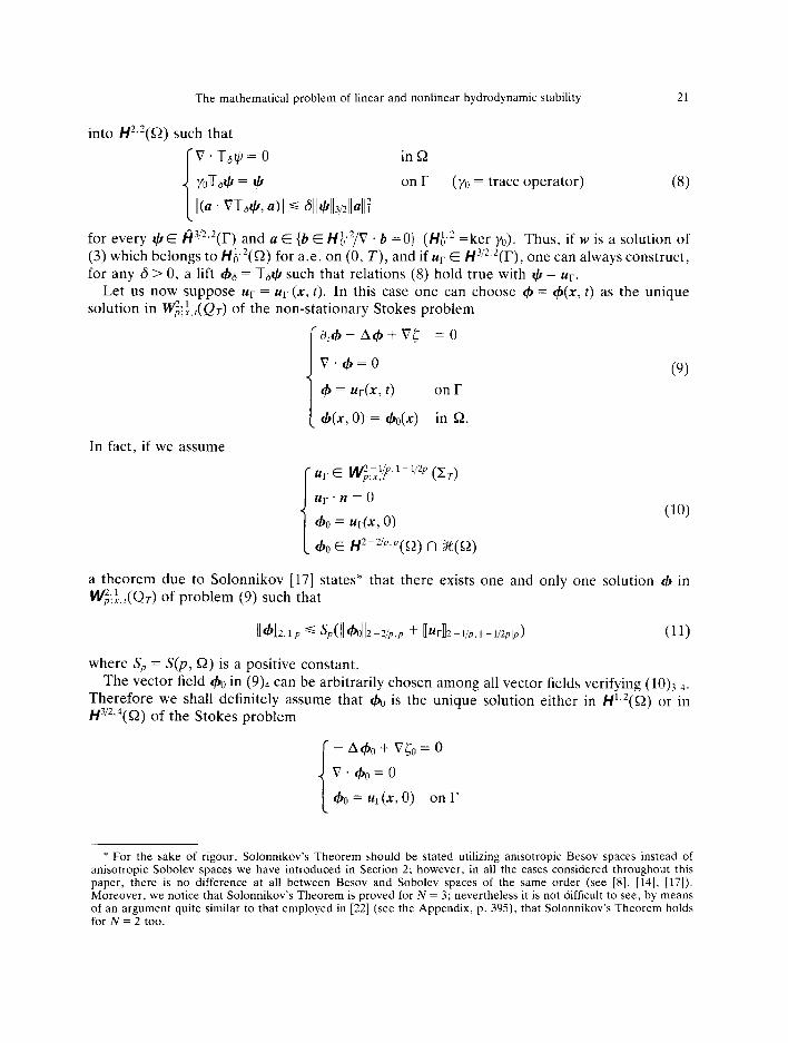
into H2.‘(sZ) such that

1

V.-n-&= 0 in R

YoT& = 4 on I (y. = trace operator) (8)

I@ . V~&(l, a> I =s ~114M4:

for every 4 E fi3i2,2(I) and a E {b E H&‘/V . b = 0} ( HA,2 - -ker ~0). Thus, if w is a solution of

(3) which belongs to H/,.‘(n) for a.e. on (0, T), and if ur E H 3’2.2(r), one can always construct. for any 6 > 0, a lift 4~ = U& such that relations (8) hold true with 4 = ur.

Let us now suppose ur = ur (x, t). In this case one can choose 4 = 4(x, t) as the unique solution in W$f;.,(Qr) of the non-stationary Stokes problem

r&4-A4+Vj =0

v.c#J=o i (9)

I 4 = ur(x, t> on I

4(X> 0) = 40(x) in !2.

In fact. if we assume

a theorem due to Solonnikov [17] states* that there exists one and only one solution 4 in

bl&,,(Q~) of problem (9) such that

(11)

where S, = S(p, S2) is a positive constant.

The vector field 40 in (9)4 can be arbitrarily chosen among all vector fields verifying (10)3.+ Therefore we shall definitely assume that 40 is the unique solution either in H’,2(~) or in

H3’2,4(R) of the Stokes problem

!

-A40+V~o=0

v.40=0

40 = w(x, 0) on r

* For the sake of rigour, Solonnikov’s Theorem should be stated utilizing anisotropic Besov spaces instead of anisotropic Sobolev spaces we have introduced in Section 2; however, in all the cases considered throughout this paper, there is no difference at all between Besov and Sobolev spaces of the same order (see [g], [14]. [17]). Moreover, we notice that Solonnikov’s Theorem is proved for N = 3; nevertheless it is not difficult to see. by means of an argument quite similar to that employed in [22] (see the Appendix, p. 395), that Solonnikov’s Theorem holds for N = 2 too.

22 F. Rosso

subject to, respectively, the following assumptions:

1

either ur(x, 0) E H1’2,2(IJ

or +-, 0) E H~-(N+~)/~N.~N/(N+Z)(~), (12)

In fact, via Cattabriga’s Theorem and a well known embedding result for fractional order Sobolev spaces (see [8, theorem 7.58, p. 218]), we have, respectively,

ll~olli c wr(o)ll1/2

ll ‘hh2.4 s KlI(40/12,4N/(N+2) s K1C2/lU~(0)/12-(hi+2)/4N,4N/(N-2)

(13)

where C1 = C(1,2, Q), C2 = C(2,4N/(N + 2), Q), and K1(Q) is an embedding constant. Since throughout the paper we will utilize estimate (11) only for either p = 2 or p = 4, the

above remarks show that [+lhllp can be completely dominated by means of suitable norms of ur(x, 0) and ur(x, t).

Also when ur = ur(x, t) one can consider a second possibility to construct a lift 4(x, t) of the boundary data. This follows from the fact that if ur E H 3i2,2(r) a.e. on (0, T), then there

always exists, for any 6 > 0, a lift +6(t) = Ua~r(t) such that relations (8) remain valid a.e. on

(0, 0 In Sections 5 and 6 we shall deal with the energy functional

F,(w) = _ (w. vu, w) IVwli

where a could be either u or 4. To apply Serrin’s criterion of the energy theory of hydrodynamic stability [3] we need to know, first of all, what kind of assumptions one has to impose on a in order for F, to remain bounded along solutions of problem (3). In this connection it is very easy to see that F, is bounded in H’,2(Q) if

i

u E L”(Q) if u = D(X),

D E L”(0, x; L”(Q)) if u = u(x, t). (14)

In fact, I(w . Vu, w) = - (w . VW, u)l s P (ess suplul)IV I2 w 2 w h ere P(Q) > 0 denotes Poincare’s constant. As far as Fb is concerned, the subject is a little more complicated since we desire to get the boundedness of F& by means of suitable hypotheses on ur only.

To this aim, let us first suppose 4 = 4(x).

LEMMA 1. If ZQ- E H’/*.*(r), then, F+ is bounded in H’.2(Q).

Proof. In fact, via Sobolev’s and Poincare’s inequalities [18], [19], bearing in mind the Sobolev embedding H’,2-+ L4, we have

I(w ’ oh w) = - (w ’ vw, +)I s l+14lw14Ivw(Z

=z Wztl~IId(2 (N~1)/41WI~(2N-2)IvWl~/4)lvW12 (15)

S k2C~P1”2N-2’2’*‘~1”4~~*y/~~/~~VW~~

where K*(Q) > 0 is an embedding constant. If Ur E H3’2.2(IY), then F+, is not only bounded in H1,2(!2) but also as small as we want. In

‘The mathematical problem of linear and nonlinear hydrodynamic stability 23

fact, because of (8)3, we have

Let us now suppose 4 = 4)(x, t).

LEMMA 2. If ur EWE;,‘&&) and ur(O) E H - 2 (,y,2)/4N.4~~~(N+2)(r), then Fd is bounded in

W(Q).

Proof. Let us set dt) = [c/J[, (real p 3 2) and notice that

therefore

Moreover, from (11) and (13)2, we have

If the right-hand side of (17) is finite, we have CY, il aELP(O, a). As a consequence aE

L"(0, 30) and

Thus we get

which proves that F6 is bounded in H’~2(Q). If Uy E L”(0, rn. H312.2(Ij), then F&, is not only bounded in H’,‘(R) but also as small as we

want. This follow8 immediately from (16). The above remarks allow us to say that, under suitable hypotheses for ur, the variational

problem

R,‘(t) = :z; F,(w), (19)

where V={H,~'(Q),Q . w = 0}, is properly posed. In fact, if F, is bounded, the same proof as in [20] applies to get the existence of the maximum. Moreover it turns out that R;’ = sup R-‘(t) is finite. 120

24 F. Rosso

4.THEOREMS OFLINEAR STABILITY

Throughout this section we shall suppose v = v(x) and (14)i to be satisfied. We shall also suppose Vu E L”( 52).

When ur = f = 0 one says, by definition, that v is linearly stable iff 3!(s) > 0, where % means “the real part of” and q is the first eigenvalue of the linear operator IL of X(S2) to itself defined by

a E D(L) and La = b @ (G(v, a), b) = (g, b) Vb E V,

where

G(v, a) = Re(v * Va + a - Vu) + Au.

From classical results [4], [21] concerning [I , it follows that the above definition is well- posed. Moreover, by means of the arguments developed in [4] (see also [6]) it can be proved that

a(q) > 0 3 1~1~ c AIu& exp( - kt), Vt z= 0 (20)

(where A, k are suitable positive constants independent of u), for all solutions of the following (linearized) Navier-Stokes i.b.v.p.:

1

a,u + G(v, u) = - VX

v.u=o

u=o on I

u(0)=uO inR.

The above is, in short, the core of the so-called “method of linear stability” in classical hydrodynamics.

In the following two theorems we shall extend the validity of (20) to the case of non- vanishing disturbances to the body force and the boundary data. In fact, if one defines

0”; = max { (~01~,ll4/1~~, Ia Ifi: dt} 0

Di"' = Imix I& I~ur(o)l/1/2, bd3/2,3/4~2;L >

we have the following.

THEOREM 1. Let u. E X(Q), f E L*(O, 00; L2(Q)), and

ur E /fl’*,*(I) if ur = ur(x),

[ur. n = 0 in E,, ur E W~$,3/“(C,), Ur(0) E kW2(r) if Uy = Ur(X, t)].

Then, if 9?(q) > 0, for any E > 0 there exists 6, > 0 such that

The mathematical problem of linear and nonlinear hydrodynamic stability 25

for any solution u of the following (linearized) Navier-Stokes i.b.v.p.:

a,u + G(u, u) = - Vrr + f

V.u=O

u = uy 0nI

u(0)=uO inn.

Proof. Let us consider the homogeneous version of (21), i.e.

I

a,w + G(u, w) = - Vn+f*

v.w=o

w=o on I

w(0) = wg in 52,

(22)

where w = u - 4, w. = u. - 4(O), and f * = f - d,#~ + Ac$ - Re(v . 04 + C#J. Vu). It is known (see [4], [21]) that, under the hypotheses made here for Q and u, [I has a countable set of eigenvalues {cJ~}, each of finite multiplicity, which can cluster only at infinity. A lemma due to Sattinger ([4, p. 8081) states that, for a sufficiently large n,

q&r, a)] z= (l/2) l Vu 12’ Vu E M,(Q) n I/, (23)

where M,(Q) is the invariant subspace of IL related to {a,+ 1, a,+~, . . .}. As in the proof of theorem 4.1 of [4], we split w as follows:

w=w,+w,,w,EM,I(~),EM,(R)n v.

One easily sees that

I(&, %>I c cllwll:

I(h,w)l 4w112lw*/2 (24)

I(lw2, WI>1 4w112lw212.

We shall now deduce a number of a priori estimates for solutions of (22), which lead, by means of standard arguments,? to the proof of theorem 1. To this aim, take the L*-product of (22)i with w. From (23) (24), it follows

;lwl? + ch$ e+122+ GIfti+ c7/vd@ (25)

where 2 =f* - A+. Always following the proof of theorem 4.1 in [4], one immediately convinces himself that

1~112’ c ~8 exp(-W) I WI(O) 12’ + ~9 exp(-WI ‘exp(W(l .fW Ii + IV@) Ii) k (26)

t As is well-known, a proof based only on a priori estimates is quite formal; however it is easy to apply one of the classical methods usually employed to prove an existence theorem (for example the Faedc+Galerkin’s method) to obtain a rigorous proof of solutions of (22) with the properties requested in the statement of theorem 1.

26 F. Rosso

where y is any number in (0, %?(a,)). Thus, from (25) and (26), we get

$lwli + 4422 s cl0 exp(-2yl) Iw0li + cl1 exP(-W)

x o’exp(2Y~)(lf(s) Ii + lV46) I:> do I + cglj/; + c,1vg := II + I* + 13 + I+

Inequality (27) in turn implies

(27)

4

IwItS Iwol:exp(-ti) + exp(-vt) I

‘exp(vs) ,FrI,(s) ds, (28) 0

for any v E (0, cd). Let us now set 5-, = exp(-ti) Ji, exp(vs) Z,(S) ds; it is easily seen that 9, -+ 0 exponentially as t--, m. To examine the behaviour of 92.93, and Y-4, we distinguish steady from unsteady boundary disturbances. In the former case we have

so that

IfI: + lW2 c IfI: + Cl2 IM:, (29)

+ cl1 exp( - vt) I

’ exp( vs) exp( -2ys) I

‘exp(2yE) If(C) i:Gds 0 0 (30)

since C#J = 4(x). In the latter case we have

I fl: + lWl22 =z lfl: + IMI: + 4 Tw>

so that

I f

T2 S cl8 exp( - vf) 0

exp(vs) exp(-2vs) I~‘exp(2~E)Cf(E~ 122 J

(31)

(32)

(33)

The mathematical problem of linear and nonlinear hydrodynamic stability

(If(s) 1: + Ii

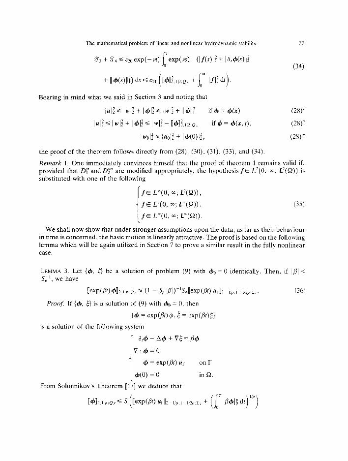
Bearing in mind what we said in Section 3 and noting that

1422~ lwlif 141ic lwlS+ IIM if 4 = 4(x)

lul2’ C I+ + 141: c Iwl: + bbk 2:Qx if+=c$(x,t).

IwolZ s l4lZ + ltmi,

27

(34)

(28)’

(28)”

(28)“’

the proof of the theorem follows directly from (28), (30), (31), (33), and (34).

Remark 1. One immediately convinces himself that the proof of theorem 1 remains valid if.

provided that 0s’ and D 2”” are modified appropriately, the hypothesis fE L’(O, =; f’(Q)) is

substituted with one of the following

1

fE L”(O, “; L2(Q)) >

fE L2(0, m; L”(Q)) > (35)

fE L”(0, cc; L”(Q)).

We shall now show that under stronger assumptions upon the data, as far as their behaviour in time is concerned, the basic motion is linearly attractive. The proof is based on the following lemma which will be again utilized in Section 7 to prove a similar result in the fully nonlinear case.

LEMMA 3. Let (4, c} be a solution of problem (9) with 40 = 0 identically. Then. if l/j < S;‘, we have

nexp(~t)dd2.11p:QT s (1 - ~,I/W’~,Uexp(P~) ~d-~~p.~-~~2p5T. (36)

Proof. If (4, E} IS a solution of (9) with & = 0, then

(4 = exp(Bt) 6 E = exp(LM

is a solution of the following system

i

&4-A++Vg=P4

v*l$=o

4 = exp(Pt) UY on I-

4(O) =‘O in R.

From Solonnikov’s Theorem [17] we deduce that

bb~2.11P:QT UexpW ~rn2-llp.l-IIZp.xr + (~Tb-Wl; dtj I”)

28 F. Rosso

the lemma follows.

THEOREM 2. Let u0 E X(Q), ur = ur(x, t) and ?%(a,) > 0. Then, if ~(0) = 0 identically and

there exists BE (0, SF’) such that

ur. n = OinC,, exp(@)fE L’(O, m; r’(Q)), exp(@) ur E W~f;Y(Zx),

the conclusion of theorem 1 holds and moreover, there exists p > 0 such that

Iu122CMexp(-~~)Vt~O,

where M is a positive constant depending only upon Q and the data.

Proof. Bearing in mind the proof of theorem 1, we have

(37)

TTz G cl8 exp( - vr) /‘exp((v - 2Y)s) 1 (lexp(yE)f(E) I: 0

+ I adexp(yEl NC)> 12’ + J lb(E) 12’ + Ilexp(yE) 4(C) II?> dE do

d c22 (i oxlexp(~)fl~d~+ Uexp(ur)~n~.1,2:(I.)(exp(-2~) - exp(-4),

53 + 9-,S czOexp(-vt) o’(~exp(2-1r6)f(s)~$+ Ia,(exp(2~‘vs)+((s))IZ I

+ 4~‘~I+(s)lZ + Ilexp(2-'vs)4(s)IIf) ds

s c23 ii oi lexpW14fl:dt+ Iexp(2_l~~)~~lli,~,:,g.) q-4.

Notice now that exp@)fE L2(0, cc; L2(Q)) and exp@t)ur E H@J::‘~(C~) for every BE [0, B]. Moreover, because of the choice made in Section 3 as far as the term & occurring in (11) is concerned, the hypothesis ~(0) = 0 allows us to apply lemma 3. Thus, for fi = min(2-‘v, y, /3), we have

Since, as we said in the proof of theorem 1, 5-1 C c25/wol$ exp(-2yt), inequality (28) implies

IwIt< Mexp(-Pt) Vt 2 0.

Finally recall that I u I$ S/W 1; + 1413; by employing the same arguments as in the proof of lemma 2 to the function w(t) = lexppt)+12, one shows that w, d/dt o E L2(0, ~0). Since H’.2 (0, m)-+ Lm(O, a) and

The mathematical problem of linear and nonlinear hydrodynamic stability 29

we deduce

I+(t) 1: s (1 - &> I WG Uexp(Bt) 4,1~2:~ exp(- PC) and the proof of theorem 2 is complete.

Remark 2. The proof of theorem 2 remains valid if the hypothesis exp(@) f~ L*(O, x; L2(Q)) is substituted with one of the following:

1

exp(PWE L”(O, 00; L*(Q)),

expW.fE L*(O, co; Lx(Q)>,

exp(@)fE Lm(O, co; L”(Q)).

Theorems 1 and 2 extend, as we have already said at the beginning of this section, the validity of the “method of linear stability” to the case of non-vanishing f and ur.*

5. THEOREMS OF NONLINEAR STABILITY FOR STEADY BOUNDARY DISTURBANCES

Throughout this section we suppose u = ur(x), while u might be time dependent or not and has to verify only properties (14).

In this and subsequent sections we shall extend the variational formulation, due to Serrin [3], of the “Energy Method” to the problem of stability with completely perturbed data. The core of Serrin’s criterion is stated by the following proposition: let Re < R, or, equivalently (see [5], [6], [7]), let p1 > 0, where pl is the first (real) eigenvalue of the linear self-adjoint operator IL, defined by

aED(L,,) and ~a=g~Re(a~Vu,b)+(Va,Vb)=(g,b),‘Jb~ V.

Then any solution of (1) with f = ur = 0 is unconditionally asymptotically stable and

/ul2GBlu&exp(k(Re-R,)t),W’tO(k=const.>O). (38)

To investigate the general problem, we start from the so-called “Energy Identity”: which one gets immediately from (3)1 taking its scalar product with w in L2(R):

(1/2)~iwi$+ /Vw/%l -ReF,(w) -R@,(w)) =(Lw) +(f,w>+ (A4 w), (39)

where

h,,:= -Re(+*Vw+ +.V++ vsV~$+ @*Vu).

* When ur = f = 0 identically, it can be seen [6] that 1 u 1 *+ 0 implies 3(s) > 0, which provides a criterion for nonlinear instability. We do not know, at present, if the same result remains valid when ur and f do not vanish identically.

t For the sake of precision, it should be said that the formal argument employed in this paper leads to an Energy Identify while the Faedo-Galerkin’s method should produce an Energy Inequality only. In fact, the solutions to problem (1) that we deal with throughout the paper are of Hopf type (see [7], [18] for details).

30 F. Rosso

Notice that, for y, q > 0, we have.

(W w) zz (l/(21’)) IV+lt + (Y/2) 1Vw1k

(A w) c (l/(27?)) If I$ + WY4 I VW It (40)

(h, w) c (@/2> IV48 + (~~*/(~~~)(~~~~~~pI~1*1~~122 + ld.4. From (39) and (40) it follows that

(1/2)~lw~~+lVw~~(l-(y/2)-~P2-ReF,(w)-ReP~(w)) (41)

G (l/(277)) lfl3 + (N?Y) + W(2r) ess supl~l*) lV#l2’ + Re*/CW 1414. Let us now prove the following

THEOREM 3. Let u. E ‘X(Q),fE L*(O, 03; L*(Q)) and

Icy E H'@+-)*

Then, if Re < R, and

I(~r((r,~ < G1(l - r)(l - ReR;‘)Re-’ (t E (0, 1)) with Gr = (l/2)K;‘C;1P-11(2N-2)2(1-N)/4, f or any E > 0 there exists 6, > 0 such that

D~‘<S,*lul*<E VrE [O, Tl,

for any finite T > 0.

(42)

(43)

Proof. From the proof of lemma 1 it follows that

I& =S W’11~rll1/2;

thus, if we choose (y/2) = VP* = (r/2)(1 - ReR;‘) with arbitrary rE (0, l), we have

MI := 1 - (y/2) - VP* - ReR;’ - ReF+(w) 3 1 - ReR;l - y- Re(2G1)-1~lu~~~lp

For y= $1 - ReR;‘), one obtains, from (42), that MI is positive and, from (41), that

$wlZ + P*A,Ivwl; s czs(lfl3 + lw45 + I4Ii> (44)

where we have set A, = 2P-‘(1 - r) (1 - ReR;‘). From (44) it follows that

I rlVw/:dl6 c26

0 (ia lfl: dt + T1hll?/2 + Wrll;f2 + 1 wol:) (45)

145~ lw~Iiexp(-W + ~25ev(-W [exp(b)(f(s)ll

+ lV4+) lZ + l+(s) 14) dt 6 I wol? exp(-W (46)

+ c27 ( J’,m IfI; dt + 1t41$2 + lldf,2).

The mathematical problem of linear and nonlinear hydrodynamic stability 31

From (44) and (45) we deduce that w E Lm(O, T; X(Q)) fl L’(O, T; W(Q)) for any finite T > 0, and, in particular, that (43) is satisfied (recall inequalities (28)‘, (28)“‘).

The restriction imposed to the size of (l~r11~‘~ in theorem 3 can be removed; but then, as we shall see in the next two results, either the range of stability becomes smaller (at least in principle), or ur has to be chosen more regular than in theorem 3. In fact we have

PROPOSITION 1. Let uo E X(Q),fE L’(O, ~4; r2(Q)) and

Ur E H1’2,2(I.).

Let moreover 4(x) be the unique solution of problem (5) inside Q. Then, if Re < (R;l + R ;‘)-‘, for any E > 0 there exists 6, > 0 such that (43) holds true:

Proof In Section 3 we have seen that the variational problem R ;’ =max F+,(w) is well-

posed if ur EHv2,‘(@). Thus we have V

A41 2 1 - Re(R;’ + R ;‘) - (y/2) - qP2.

If y =2@ = ~(1 - Re(R;’ + R $.‘)), if will be Ml > o and the same proof of theorem 3 applies.

Remark 3. It is almost evident that the restriction of the range of stability is effective only if R, (a = u, 4) is positive. In this connection it should be explicitly pointed out that R, could be calculated via the same variational argument which holds for R,. In fact r$ is uniquely determined by ur and problem (5) can always be handled by means of suitable numerical techniques (see [16, Chapter I]).

Let us now define

THEOREM 4. Let ug E X(Q),fE L2(0, m; L2(Q)) and

Ur E H3’2’2(r).

Then, if Re < R;‘, for any E > 0, there exists 6, > 0 such that

D;‘<&*lzl2<& Vt E [0, T]

for any finite T > 0.

Proof. We choose now 4~ = Tsur (see Section 3). From (8)3 it follows that

F4s(W) s dWll3/2

(47)

with arbitrary 6 > 0. As a consequence, bearing in mind the proof of theorem 3, we have, for y= 2qP2 = ~(1 - ReR;‘),

Ml 2 (1 - t)(l - ReR;l) - 6ReIIu&p

We can always choose 6 = (2Re)-‘(1 - z)(l - ReR;‘)IIu&j~, so that Ml turns out to be

32 F. Ross0

positive without any restriction on JIu~~~~/~. From this stage on the same proof as in theorem 3 applies.

Remark 4. The reader can easily convince himself that, D/‘(i = 1, 2) being modified appro- priately, the statement of remark 1 remains valid for theorems 3 and 4 and proposition 1.

To conclude this section, we wish to emphasize that, when ur = ur(x), it is not physically reasonable to look for conditions upon the data which ensure the attractivity of u as t goes to infinity. A rigorous proof of this fact has been given, in our knowledge, only in particular one-dimensional cases (see footnote on p. 18); it does not seem a simple matter to see whether or not this result extends to more general situations.

6. THEOREMS OF NONLINEAR STABILITY FOR UNSTEADY BOUNDARY DISTURBANCES

Throughout this section we suppose ur = ur(x, t), while u is as in the previous section. Let us define

DY = max{ DY, 11 ur(O) 11 - 2 (N-2)/4N,4Nl(N+2)> bd7/4,7/8~4:d

We shall now prove some results of simple stability, leaving the subsequent Section 7 to the problem of the attractivity of U.

THEOREM 5. Let u. E X(Q),fE L2(0, 00; L2(S2)), and

i

Q(O) E H 1/‘2.2 I- n H2-(“+2)/4N.4N/(N+2)(r),

( )

Uy E W~&~‘4(L) n Wj~::‘*(C,).

Ur’PZ=O inC,.

Then, if Re < R, and

where

A(ur(O), ur) <(l/2)(1 - z)(l - ReRi’) (zE (0, l)),

A := ReS42(N-1)‘4p1’(2N-2)(K1C211ur(0) 112-(~+2)/4~,4~/(~+2) + it~d7/4,7/8~4;z,)~

for any E > 0 there exists 6, > 0 such that

DZUn<h+/u/2<~, VtaO.

Proof. Since now 4 = 4(x, t), the “Energy Identity” is the following

(1/2)$wli + IVwl$(l - ReF,(w) - ReDF.+(w)) (f, 4 + (L, 4 + (A4 w),

where h,, = h,, + a,+. Notice that, for any V> 0,

(h,,, w) s (h,,, w) + (2v)-‘iG#l; + (vp2/2) lvwl;,

(48)

(49)

(50)

33 The mathematical problem of linear and nonlinear hydrodynamic stability

so that, from (40) and (50), we obtain

(lIz)%lw~3+lVw/i(l-(y/2)- VP*-(vP’/2)-ReF,(w) -ReF6(w))

G (l/211) lfli + ((1/2Y) + (Re*/2r) esssupIu/*) IV+li + (Re*/2q)!dl~ (51)

+ (1/2v) IWI: =s c*s(lfl: + p+t: + / 41: + lb#l:>.

In agreement with the choices suggested in Section 3 (see lemma 2 and inequality (18)), for 4Pi = 2P*v = y= t(1 - ReR;‘) and arbitrary rE (0, l), we have

M2:= 1 - (y/2) - (VP’) - (vP*/2) - ReF,(w) - ReFb(w) ~(1 - r)(l - ReR;‘) -A. (52)

Thus. from (48), it follows that M2 is positive; as a consequence, from (11) and (13), we

obtain

Therefore (28)“‘, the

+ IVd+)lS + l#+)li + lh4Q)IS) do s Iw0122exp(-&4 (54)

+ c32 ci

om IfI; dt + 11 W(O) II;/2 + b&/2,3/4~2;I,

+ )iUr(O)ii42-(N+2)/4N,4Nl(N+2) + bd~/4,7/814;~, i

w E L"(0, co; X(Q)) l-l P(O, cc; W(Q)); bearing in mind inequalities (28)‘, (28)“, proof of theorem 5 is complete.

As in Section 5 we can prove

PROPOSITION 2. Let u. E X(Q), fE L2(0, 00; r*(Q)), and

*r(O) E /.//W(r) n Hz-(N+*)/4N,4N/(N+*)(r),

ur . it = 0 in IZ,, ur E W~~~~~i4(C,) n lIl@;~‘8(C,).

Let moreover 4(x, t) be the unique solution of problem (9) inside Q. Then, if Re < (R;l + R s’) -‘, for any E > 0 there exists 6, > 0 such that (49) holds true.

Proof. The result follows by combining the arguments developed in the proof of proposition 1 and the proof of theorem 5.

34 F. Rosso

The statement of remark 3 remains obviously valid also here. Again as in Section 5, when one deals with more regular boundary disturbances, the

restriction to the size of boundary data stated by (48) can be removed without affecting the range of stability allowed by theorem 5. In fact, let us define

THEOREM 6. Let u. E X(Q), fE L2(0, cc; f2(Q)), ur(0) E /+3/2,2(I) and

ur E P(o, w; Hs’*qI-)) fl P(0, “; N2J(I)) ;

let, moreover, ur be strongly differentiable in H3”,*(I) with respect to t E (0, m) and

a,ur E ~~(0, to; H3’*,*(r)). Then, if Re < R,, for any E > 0 there exists 6, > 0 such that

D~U”<&~IUI~<E vtao.

Proof. The structure of the proof is the same as for theorem 4; therefore we outline only the differences. We have now

M2 3 (1 - r)(l - ReR,‘) - 6Re ll~r(13/2

z (1 - r)(l - ReR;‘) - 6Re ess sup l~~~l/s,~.

Let us now set a(t) = /I z&. W e h ave cuE L2(0, m) f’ L4(0, xi) and IIcf1~~r)13/2 E L’(0, ~0). With an argument employed many times throughout this paper one sees that / d/dt (Y/ G I( ar~r(13/2 and

;S,s,;U II urll3/* s =P o

(j-x IIurll$2 + Ibturll:,2 dt) “*. (56)

Since the right-hand side of (56) is finite, we can always choose 6 so small that M2 turns out to be positive without any restriction on the size of Il~rll3/2. Thus, in the usual way, we get

lwli d lw013exp(-&t) + c34q-&t) ~‘exp(&s)(lf(s)li

+ 1 Vh&> I: + 1 h(s) i: + /&d&) I;) dt.

Since UG is linear and continuous from H3’2,2(I) into p(Q), we have

11 46112 s K3 II k(l3/2

(58)

where K3 > 0 is an embedding constant. Moreover, since ur is strongly differentiable in H”*(r), we have U& = &U,. In fact

I/ a,48 - Taa4rII2 s /ii 11 he’( 4b(t + A) - +6(t)) - Ua~rUrll2

The mathematical problem of linear and nonlinear hydrodynamic stability 35

d K3 trnO I)h-‘(ur(t + h) - z+(t)) - ~iz4-l13/2 = 0.

as a consequence we have

Finally

)u):Slwl:+ Ic#+~\Z~IWIS+ esssup)/u&

IWOII~ luoIZ+ I#@)l:~ IQI: + II~rmIlk*> and the proof is complete.

Define now

The following result is alternative to theorem 6: its proof can be easily obtained, by slight modifications, from that of theorem 6 and is therefore omitted.

PROPOSITION 3. Let u. E X(Q),fE L2(0, x; c(Q)), ~~(0) E H”>‘“,‘(I). and

ur E L”(0, w; H”‘*,z(I-)).

Let, moreover. ur be strongly differentiable in H”‘*.‘(I) with respect to t E (0. x) and let

a,ur E L”(0, “; @‘(I-)).

Then, if Re < R,. for any E > 0 there exists 6, > 0 such that

for any finite T > 0.

Df”<6,+llulz<~ Vt E [O, T]

Remark 5. We wish to point out explicitly that theorem 5 is essentially different from both theorem 6 and proposition 3. In fact the former does nor require the existence of the first time-derivative of ur(x, t) since the fractional order involved for the time variable is always less than one.

Remark 6. The reader can easily convince himself that, Dy (i = 2, 3, 4) being modified appropriately, what we said in remark 1 applies as well for theorems 5 and 6 and propositions 2 and 3.

36 F. Rosso

7.THEOREMSOFNONLINEARASYMPTOTICSTABILITYFORUNSTEADY BOUNDARYDISTURBANCES

Throughout this section ur and u will be as in the previous one. The results proved in Section 6 imply, in a very direct way, the attractivity of ZJ. To see this,

let us begin, first of all, with the following sufficient criterion for asymptotic stability:

PROPOSITION 4. Let all the assumptions of theorem 6 be verified. Then, if Re < R, and if

!iE (If(t)/* + Ilur(r)//3/2 + liarur@)113/2) = O,

the basic motion u is unconditionally asymptotically stable, i.e. for any choice of D3Un we have

lim ju(t)Jz = 0. I--tee

Proof. Bearing in mind the proof of theorem 6, define

Y(t) : = I,’ exp(h> (If@> Ii + /Ids) lIZi2 + II e(s) lib + II ~94s> II!121 ds.

Since Y(t) is an increasing function of t, there exists lim Y(t) = m; if m < 00 the theorem is r-x

obvious. If m = x we have

Remark 7. Proposition 4 generalizes a similar result given in [l], [2] for particular laminar flows.

We shall now prove two theorems of asymptotic stability which do not require, a priori, the decay to zero of disturbances to the body force as t goes to infinity. Further, the first theorem does not require the existence of a,ur but the attractivity of u is conditioned; the second theorem does require the existence of ~3,ur but the attractivity of D is uncondirioned. This circumstance seems to indicate, in agreement with our physical intuition, that “regularity acts in favour of stability”.

THEOREM 7. Let all the assumptions of theorem 5 be satisfied. Let moreover ~~(0) = 0 identically in Q and let /3 E (0, min{ SF1, Srl}) such that

exp(@)f E L2(0, a; r2(Q)),

exp(@) ILL E W@$‘“(Cs) n WI~;7’8(2m).

Then, if Re < R,, the basic motion u is conditionally asymptotically stable and

luI2 c Mexp(-Pt) vtso,

where 0 = min(4-‘A,, /3) and M is a positive constant depending only upon Q and the data.

Proof. The structure of the proof is similar to that of theorem 2. We outline only some

The mathematical problem of linear and nonlinear hydrodynamic stability 37

differences: from (54) we have, in particular,

lwlZ< IwajZexp(-h,t) + c31exp(-44 0f(lexp(2-1b).f(s)li I

+ / (exp(2-‘A$) 4(s)) It + I exp(4-‘A$s) 4(s) Ii + I &(ed2-‘h) 4(s)> II + 4-‘A2,1 exp(2_lA,s) 4(s) 1:) d.s S / w0 1: exp( -Ad)

+ ~37 exp(-W ii

Oz lexp(2~l&t)fl: dt + lIexp(2-‘Ad) rbll$112:~~

+ llexp(4~1W dG,1~4;p, . 1

Bearing in mind lemma 3 and the proof of theorem 2, we deduce that

Iwl: c Iw&exp(-&t) + ~37exp(-W is

oz bpfWl:dt

where D = min{4-‘h,, /3}. Finally, to prove that I u I2 decays as required, one proceeds as in the last part of the proof of theorem 2.

THEOREM 8. Let all the assumptions of theorem 6 be satisfied. Assume also

exp(2P’&t)fE L*(O, m; L*(Q)),

Then, if Re < R,, the basic motion u is unconditionally asymptotically stable and

/uIZ G Mexp(-2-‘&t) vt 2 0

where A, = 2Pe2(1 - r) (1 - ReR;‘), t is any number in (0, 1) and M is a positive constant depending only upon Q and the data.

Proof. The result follows easily from inequality (58) as far as the decay of / w 12 is concerned. To see that also (u(~ goes to zero exponentially, it suffices to show that 1 &I2 does so. Nevertheless, by an argument already employed in this paper (see lemma 2 and theorem 2), we have

exp(W /hlZ =5 K3 exp(W llell$2

and the proof is complete.

exp(&t) ll~rll$~ + exp(Q) ll~mllhdt< M)3

38 F. Rosso

REFERENCES

1. GALDI G. P., Su un criteria di stabilita non lineare in presenza di perturbazioni iniziali e al contorno e la sua applicazione a due classi di moti magnetoidrodinamici, Boll. Un. mat. ital. 8, 336-354 (1973).

2. RENNO P., Sulla stabilita asintotica in presenza di perturbazioni al contorno per una classe di moti magneto- idrodinamici. Rc. Accad. Sci. jis. mat. Napoli 41, 435-468 (1974).

3. SERRIN J., On the stability of viscous fluid motions, Archs ration. Mech. Analysis 3, 1-13 (1959). 4. SAT-~INGER D. H., The mathematical problem of hvdrodvnamic stability, J. Math. Mech. 19. 797-813 (1970). 5. JOSEPH D. D., Srability of Fluid Motions I, II, Springer, Berlin (1976): 6. GALDI G. P.. Introduzione alla teoria della stabilita in fluidodinamica, lectures held at the V School of Math.

Phys. of the G. N. F. M. of the Italian C. N. R., Ravello-Montecatini, Italy (1980). 7. Rosso F.. Pointwise unconditional attractivity of solutions to the Navier-Stokes equations, Reu. Rottmaine Math.

pures appl. (to appear). 8. ADAMS R. A.. Soboleu Spaces, Academic Press, New York (1975). 9. SLOBODECKI~ 1.. N.. Generalized Sobolev spaces and their applications to boundary problems for partial differential

equations, Leningrad Gos. Ped. Inst. Ufen. Zap. 197, 54-112 (1958) (in Russian), Am. math. Sot. Transl. 57, 207-275 (1966) (in English).

10. USPENSKli S. V., Imbedding theorems for generalized Sobolev classes W;, Sib. mat. Zh. 3, 418-445 (1962) (in Russian), Am. math. Sot. Transl. 90, 45-79 (1970) (in English).

11. USPENSKIi S. V.. Properties of I+‘;-classes with a fractional derivative on differentiable manifolds. D&l. Akad. Nuuk. SSSR 132, 60-62 (1960) (in Russian), Soviet Math. 1, 495-497 (1960) (in English).

12. IL‘IN V. P.. The properties of some classes of differentiable functions of several variables defined in an n- dimensional region, Trudy Mat. Inst. V.A. Steklova 66, 227-363 (1962) (in Russian), Am. math. Sot. Transl. 81. 91-256 (1969) (in English).

13. AVANTAGGIATI A. & TROISI M.. Spazi di Sobolev con peso e problemi ellittici in un angolo I, Annali Mat. pura appl. 95, 361-408 (1973).

14. MlRAND.4 C., Istifuzioni di Anahsi Funzionale Lineare I, Unione Matematica Italiana, Gubbio (1978). 15. CA-~TABRIGA L.. Su un problema al contorno relativo al sistema di equazioni di Stokes. Rc. Semin. mat. Uniu.

Padoua 31. 308-340 (1961). 16. TEMAM R.. Navier-Stokes Equations: Theory and Numerical Analysis, North-Holland, Amsterdam. revised

edition (1979). 17. SOLONNIKOV V. A., Estimates of the solutions of a non-stationary linearized system of Navier-Stokes equations,

Trudy Mat. Inst. V.A. Steklooa 70, 213-317 (1964) (in Russian), Am. math. Sot. Transl. 75. I-116 (1968) (in Enghsh).

18. SERRIS .I.. The initial value problem for the Navier-Stokes equations, in Non-Linear Problems (Edited by R. E. LANGER) Univ. of Wisconsin Press (1963).

19. LADYZHENSKAJA 0. A., The Mathematical Theory of Viscous Incompressible Flow, Gordon & Breach, New York (1969).

20. RIONERO S., Metodi variazionali per la stabilita asintotica in media in magnetoidrodinamica. Ann& Mat. pura appl. 78, 339-364 (1968).

21. PRODI G., Teoremi di tipo locale per il sistema di Navier-Stokes e stabilita delle soluzioni stazionarie, Rc. Semin. mat. Univ. Padova 32. 374-397 (1962).

22. GERHARDT C.. LP-estimates for solutions of the instationary Navier-Stokes equations in dimension two, Pacific .I. Math. 79. 375-398 (1978).

23. Rosso F.. Variational‘methods for pointwise stability of viscous fluid motions, Archs ration. Mech. Analysis (to appear).