International Journal of Pure and Applied Mathematics————————————————————————–Volume 73 No. 4 2011, 451-470

NUMERICAL METHOD FOR SINGULARLY PERTURBED

DIFFERENTIAL-DIFFERENCE EQUATIONS

WITH TURNING POINT

Pratima Rai1, Kapil K. Sharma2 §

1, 2Department of MathematicsCenter for Advance Study in Mathematics

Panjab UniversityChandigarh, 160014, INDIA

Abstract: In this paper, we present a numerical method to solve boundaryvalue problems for singularly perturbed differential-difference equations withturning point. A singularly perturbed differential-difference equation is a dif-ferential equation in which the highest order derivative is multiplied by a smallparameter and involving at least one delay term . The points of the domainwhere the coefficient of the convection term in the singularly perturbed dif-ferential equation vanishes are known as the turning points. The solution ofsuch type of differential equations exhibits boundary layer(s) or interior layer(s)depending upon the nature of the convection and the reaction term. In the de-velopment of numerical scheme for singularly perturbed differential-differenceequations with turning point, we use a scheme based on El-Mistikawy Werleexponential finite difference scheme [21]. Some a priori estimates have beenestablished to prove the convergence and stability of the proposed scheme.

AMS Subject Classification: 65L12, 34K26, 34K28Key Words: singular perturbations, differential-difference equations, turningpoint, interior layer, fitted operator methods ODE

Received: July 3, 2011 c© 2011 Academic Publications, Ltd.§Correspondence author

452 P. Rai, K.K. Sharma

1. Introduction

We consider singularly perturbed differential-difference equations with turningpoint. A singularly perturbed differential-difference equation is a differentialequation in which the highest order derivative is multiplied by a small parame-ter and involving at least one delay term. The arguments for small delay prob-lems are found throughout the literature on epidemics and population wherethese small shifts play important role in the mathematical modeling of variouspractical phenomena, for example, in the study of variational problems in con-trol theory where problems are complicated by the effect of time delays in signaltransmission [7], in the study of bistable devices [13], evolutionary biology [19],description of human pupil light reflex [2], a variety of models of physiologicalprocesses or diseases [9] and [12]. They are also satisfied by the moments of thetime of first exit of temporally homogeneous Markov processes [9] governingsuch phenomena as the time between impulses of a nerve cell and the persis-tence times of populations with large random fluctuations. Turning point isa point of the domain where the coefficient of the convection term vanishes.The solution of such type of differential equations exhibits boundary layer(s) orinterior layer(s) depending upon the nature of the convection and the reactionterm.

Lange and Miura initiate the asymptotic study of boundary value problemsfor singularly perturbed differential-difference equations [3], [5], [6] and [4] anddiscuss the case of small as well as large delay. Kadalbajoo and Sharma [14],[15], [16], [17] and [18] initiate the numerical approach to study further the effectof small and large delay as well as advance on the layer behavior of the solu-tion. Patidar and Sharma [10] consider second order linear singularly perturbeddifferential-difference equations having delay in the differentiated term wherethe coefficient of the first order term is either positive or negative throughoutthe domain. But, there is no literature till date for the case when a(x) vanishesor changes sign in the domain for such type of differential equations. In thispaper, we initiate the numerical study of singularly perturbed differential- dif-ference equation with turning points which can result in boundary or interiorlayer depending upon the value of coefficients.

We consider the singularly perturbed differential-difference equation havingan isolated turning point at x = 0:

−εy′′(x)− a(x)y′(x− δ) + b(x)y(x) = f(x), on Ω = (−1, 1) (1.1)

y(x) = φ(x), on − δ − 1 ≤ x ≤ −1,y(1) = γ.

(1.2)

NUMERICAL METHOD FOR SINGULARLY PERTURBED... 453

where ε is a constant such that 0 < ε≪ 1, a(x) is assumed to be in C2[−1, 1],b(x) and f(x) are required to be in C1[−1, 1], δ = o(ε) such that (ε−δa(x)) > 0for all x ∈ [−1, 1], γ is a positive constant and

a(0) = 0, a′(0) > 0. (1.3)

In order to exclude the so called resonance cases we require

b(x) ≥ b0 > 0 ∀ x ∈ [−1, 1]. (1.4)

We also impose following restriction so as to ensure that there are no otherturning points in the interval [−1, 1]

|a′(x)| ≥ |a′(0)/2| for − 1 ≤ x ≤ 1. (1.5)

Under condition (1.3)-(1.5) the solution of (1.1)-(1.2) has an internal layer atx = 0. The bounds on the behavior of y(x) near the turning point dependspecifically on ε and on the characteristic parameter β

β = b(x)/a′(x) |x=0 (1.6)

and there exists constants βl, βs such that

βl ≤ |β| ≤ βs. (1.7)

If β < 0, y(x) is “smooth” near x = 0; on the other hand if β > 0, then, thereis in general an “interior layer” at x = 0, nature of which depends upon thevalue of β.

Abrahamsson [11] proves estimates on the analytical solution and discussesthe nature of the solution of the singularly perturbed turning point problems.Further, the author proves results concerning non-uniform convergence of thedifference schemes for such type of problems. Berger et al. [1] prove analyticalresults for the bounds on the derivatives of such problems where β is an integerin addition to the non -integral case. Using these bounds it is shown thatmodified version of El Mistikawy Werle scheme give by the author is uniformlyconvergent of the order hmin(β,1). Farrell [20] gives necessary and sufficientcondition for uniform convergence of a difference scheme for such problems.

There are two kind of ε-uniform finite difference schemes which have smalltruncation error in the layer region(s). The first are the fitted operator meth-ods which comprise specially designed finite difference operators on standardmeshes; the second are the fitted mesh methods which comprises standard finite

454 P. Rai, K.K. Sharma

difference operators on specially designed meshes. In this paper, we will adoptfitted operator approach.

The objective of this paper is to present a numerical approach to solvesingularly perturbed differential-difference equations with turning point. Inthis approach, we first approximate the shifted term by Taylor series and then,apply a difference scheme, provided shifts are of o(ε). The scheme used here isbased on El Mistikawy Werle exponential finite

2. Some a Priori Estimates

Taking Taylor series expansion of the term y′(x− δ) in equation (1.1), we have

y′(x− δ) ≈ y′(x)− δy′′(x). (2.1)

Using this approximation in (1.1), we get

Lε(u) ≡ −(ε− δa(x))u′′(x)− a(x)u′(x) + b(x)u(x) = f(x),u(−1) = φ(−1), u(1) = γ.

(2.2)

Here u is approximation to y(x). Now, we establish some a priori estimatesabout the solution and its derivatives for the singularly perturbed differential-difference equations with turning point. For a given function g(x) ∈ Ck[−1, 1],||g||k denote Σk

i=0max−1≤x≤1|gi(x)|, where gi(x) denote ith derivative of g. Let

Cε(x) = ε− δa(x). Hence after we will use Cε as constant part of Cε(x) whena(x) depends on x (since δ is of o(ε) and a(x) is bounded therefore Cε = o(ε)).

Lemma 2.1. (Continuous Maximum Principle) Let Ψ(x) be any suffi-ciently smooth function satisfying Ψ(−1) ≥ 0 and Ψ(1) ≥ 0. Then, LεΨ(x) ≥ 0for all x ∈ (−1, 1) implies that Ψ(x) ≥ 0 for all x ∈ [−1, 1].

Proof. Let q be such that Ψ(q) = minx∈[−1,1]Ψ(x). Let us assume thatΨ(q) < 0. Clearly q /∈ −1, 1. Since, q is point of minima therefore Ψ′(q) = 0and Ψ′′(q) > 0.

Now,

LεΨ(q) = −(ε− δa(q))Ψ′′(q)− a(q)Ψ′(q) + b(q)Ψ(q),= −(ε− δa(q))Ψ′′(q) + b(q)Ψ(q),< 0.

which is a contradiction. This follows that Ψ(q) ≥ 0 and therefore Ψ(x) ≥0 ∀x ∈ [−1, 1].

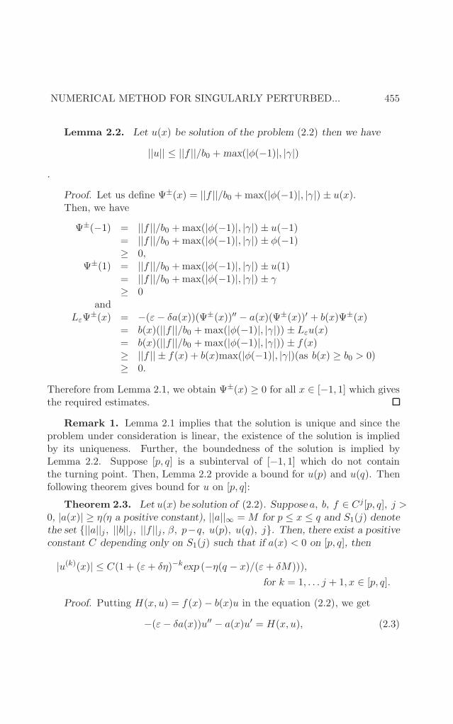
NUMERICAL METHOD FOR SINGULARLY PERTURBED... 455

Lemma 2.2. Let u(x) be solution of the problem (2.2) then we have

||u|| ≤ ||f ||/b0 +max(|φ(−1)|, |γ|)

.

Proof. Let us define Ψ±(x) = ||f ||/b0 +max(|φ(−1)|, |γ|) ± u(x).Then, we have

Ψ±(−1) = ||f ||/b0 +max(|φ(−1)|, |γ|) ± u(−1)= ||f ||/b0 +max(|φ(−1)|, |γ|) ± φ(−1)≥ 0,

Ψ±(1) = ||f ||/b0 +max(|φ(−1)|, |γ|) ± u(1)= ||f ||/b0 +max(|φ(−1)|, |γ|) ± γ≥ 0

andLεΨ

±(x) = −(ε− δa(x))(Ψ±(x))′′ − a(x)(Ψ±(x))′ + b(x)Ψ±(x)= b(x)(||f ||/b0 +max(|φ(−1)|, |γ|)) ± Lεu(x)= b(x)(||f ||/b0 +max(|φ(−1)|, |γ|)) ± f(x)≥ ||f || ± f(x) + b(x)max(|φ(−1)|, |γ|)(as b(x) ≥ b0 > 0)≥ 0.

Therefore from Lemma 2.1, we obtain Ψ±(x) ≥ 0 for all x ∈ [−1, 1] which givesthe required estimates.

Remark 1. Lemma 2.1 implies that the solution is unique and since theproblem under consideration is linear, the existence of the solution is impliedby its uniqueness. Further, the boundedness of the solution is implied byLemma 2.2. Suppose [p, q] is a subinterval of [−1, 1] which do not containthe turning point. Then, Lemma 2.2 provide a bound for u(p) and u(q). Thenfollowing theorem gives bound for u on [p, q]:

Theorem 2.3. Let u(x) be solution of (2.2). Suppose a, b, f ∈ Cj[p, q], j >0, |a(x)| ≥ η(η a positive constant), ||a||∞ =M for p ≤ x ≤ q and S1(j) denotethe set ||a||j , ||b||j , ||f ||j , β, p−q, u(p), u(q), j. Then, there exist a positiveconstant C depending only on S1(j) such that if a(x) < 0 on [p, q], then

|u(k)(x)| ≤ C(1 + (ε+ δη)−kexp (−η(q − x)/(ε + δM))),

for k = 1, . . . j + 1, x ∈ [p, q].

Proof. Putting H(x, u) = f(x)− b(x)u in the equation (2.2), we get

−(ε− δa(x))u′′ − a(x)u′ = H(x, u), (2.3)

456 P. Rai, K.K. Sharma

putting a(x) = −k(x) in the above equation and integrating it twice usingintegrating factor, we obtain

u(x) = ub(x) +K1 +K2

∫ q

xexp

(

−

∫ q

t

k(α)

ε+ δk(α)dα

)

dt, x ≤ t, (2.4)

where

ub(x) = −

∫ q

xz(t)dt, z(x) =

∫ q

x

H(t, u)

ε+ δk(t)exp

(

−

∫ t

x

k(α)

ε+ δk(α)dα

)

dt,

here constants K1 and K2 may depend upon ε. Now

0 < η < k(α) ≤ ||k|| =M for α ∈ (p, q)

⇒ ε < ε+ δη < ε+ δk(α) ≤ ε+ δM (because k(x) > 0)

⇒ exp

(

−

∫ t

x

k(α)

εdα

)

< exp

(

−

∫ t

x

k(α)

ε+ δηdα

)

< exp

(

−

∫ t

x

k(α)

ε+ δk(α)dα

)

≤ exp

(

−

∫ t

x

k(α)

ε+ δMdα

)

Let K(x) =∫ xp a(t)dt. Then, bounds on u implied by Lemma 2.2 leads to

|z(x)| ≤ Cε+δη

∫ qx exp

(

−∫ tx

k(α)ε+δk(α)dα

)

dt

≤ Cε+δη

∫ qx exp

(

−∫ tx

k(α)ε+δM dα

)

dt

= Cε+δη

∫ qx exp

(

− 1ε+δM (K(t)−K(x))

)

dt,

applying the inequality

exp[

−(ε+ δM)−1(K(t)−K(x))]

≤ exp[

−η(t− x)(ε+ δM)−1]

x ≤ t

we obtain

|z(x)| ≤ C(ε+ δη)−1

∫ q

xexp

(

−(ε+ δM)−1η(t− x))

dt ≤ C. (2.5)

Hence, |ub(p)| ≤ C. The boundary condition u(q) = d2 implies that K1 = d2.One can also see that u′(q) = −K2. Now u(p) = d1 gives

K2

∫ q

pexp

(

−

∫ q

t

k(α)

ε+ δk(α)dα

)

dt = −ub(p) + d1 − d2 (2.6)

NUMERICAL METHOD FOR SINGULARLY PERTURBED... 457

and we have

∫ qp exp

(

−∫ qt

k(α)ε+δk(α)dα

)

dt ≥∫ qp exp

(

−∫ qt

k(α)ε+δηdα

)

dt

≥∫ qp exp

(

−K(q)−K(t)ε+δη

)

dt

≥∫ qp exp

(

−M(q−t)ε+δη

)

dt

≥ C(ε+ δη)

Using this in (2.6), we have |K2| ≤ C(ε+ δη)−1.Now

u′(x) = z(x)−K2 exp

(

−

∫ q

x

k(α)

ε+ δk(α)dα

)

implies that

|u′(x)| ≤ |z(x)|+K2

∣

∣

∣exp

(

−∫ qx

k(α)ε+δk(α)dα

)∣

∣

∣

≤ C(

1 + (ε+ δη)−1exp(

−∫ qx

k(α)ε+δk(α)dα

))

≤ C(

1 + (ε+ δη)−1exp(

− 1ε+δM

∫ qx k(α)dα

))

≤ C(

1 + (ε+ δη)−1exp(

− 1ε+δM [K(q)−K(x)]

))

≤ C(

1 + (ε+ δη)−1exp(

−η(q−x)ε+δM

))

(2.7)

The bound for u(i)(x) for i > 1 follows by induction on i and repeated differ-entiation.

Thus, for a(x) < 0 we have boundary layer at the right end of the intervaland the derivatives of the solution are bounded. In the similar way we canobtain bound for the case a(x) > 0, i.e, boundary layer occurs at the left endof the interval.

Remark 2. Let [p1, q1] be a subinterval of [−1, 1] contained in an in-terval (p, q) such that [p, q] contains none of the points −1, 1, 0. Assumef, a, b are in Cm[−1, 1] with m a positive integer and let S2(m) denote the set||a||m, ||b||m, ||f ||m, minp≤x≤q|a(x)|, q − p, q − q1, p1 − p, b0,|φ(−1)|, |γ|. Then, there is a constant C depending only on S2(m) such that

|u(k)(x)| ≤ C for i = 1, ...,m + 1, p1 ≤ x ≤ q1. (2.8)

Theorem 2.3 and Remark 2 reduce the matter of a priori estimates foru(x) to producing bounds on the derivatives of u(x) in a neighbourhood of theturning point.

458 P. Rai, K.K. Sharma

Theorem 2.4. Assume (1.3-1.6), β < 0, a, b, f be in Cm[−1, 1] with ma positive integer and define

S4(m) = ||a||m, ||b||m, ||f ||m, βs, b0, |φ(−1)|, |γ|, m.

Then, there exist a constant C depending only on S4(m) such that

|u(k)(x)| ≤ C, for k = 1, . . . ,m, and |x| ≤ 1/2.

Proof. Using mean value theorem, (1.5) and (1.7), we get

|a(x)| = |a(x)− a(0)| = |x||ax(ζ)| ≥ |x||ax(0)|/2 ≥ .5|x|b0/βs. (2.9)

Remark 2 implies that |u(k)(±1/2)| ≤ C1 for k = 1, ...,m where C1 dependsonly on S4(m) and differentiating (2.2) once and putting z = u′, we get

−(ε− δa(x))z′′(x) + (δax − a(x))z′(x) + (b(x)− a′(x))z(x) = f ′(x)− b′(x)u(x).

This equation has same form as (2.2). As solution of (2.2) is bounded, thereforewe obtain

|z(x)| = |u′(x)| ≤ C.

Now, for k = 2, ...,m, differentiating (2.2) k times, we get the equation satisfiedby z(x) ≡ u(k)(x) as

−(ε− δa(x))z′′(x)− (−kδax+a(x))z′(x)+ (kδa′′(x)+ b(x)−ka′(x))z(x) = r(x)

where r(x) depends on u(x), u′(x), ..., u(k)(x) and at most kth order derivativeof a, b and f . Applying Lemma 2.2 with b replaced by (kδa′′(x)+b(x)−ka′(x))and using inductive argument we obtain the desired bounds.

For β > 0, there is an internal layer at the turning point whose naturedepends upon the value of β. Theorem 2.4 provides bound on the derivativesfor the case β < 0, so we are left with finding the bounds on the derivatives ofthe solution to the case ((1.3)-(1.6)) along with β > 0. We now state a resultfor the case β > 0.

Theorem 2.5. Let β = m + λ where m is a positive integer and βl <|λ| < βs. In addition, let ((1.3)-(1.6)) along with β > 0 and a(x), b(x), f(x) ∈Cm+k[−1, 1] where k ≥ 2. Then, there exist a constant C depending only onS5(m+ k) such that the solution u(x)of (2.2) satisfies

|u(i)(x)| ≤ C, for − 1 ≤ x ≤ 1, and i = 1, . . . ,m,

NUMERICAL METHOD FOR SINGULARLY PERTURBED... 459

|u(i)(x)| ≤ C(|x|+ C1/2ε )λ−iI(x,Cε, λ),

for − 1 ≤ x ≤ 1, and i = m+ 1, . . . ,m+ k + 1,

where

S5(m) = ||a||2, ||b||1, ||f ||1, b0, βl, βs, |φ(−1)|, |γ|, ||a||m, ||b||m, ||f ||m, m,

and I(x,Cε, λ) ≡∫ cx2+Cε

s(−λ−1)/2ds, c > 2.

Proof. The proof same as in Berger et al. [1], just replace ε by Cε which isconstant part of Cε(x) = ε− δa(x).

Remark 3. If β > 1 then above theorem holds whereas if β < 0 then wecan take λ = β and still above result holds good. Therefore in correspondingsections we take λ = β as proving the result for β > 1 is then straightforward.

3. Numerical Scheme

We construct a scheme based on exponential scheme of El-Mistikawy and Werle[21] to approximate the solution u(x) of (2.2). Let uniform partition of theinterval [−1, 1] be given by xi = −1+ ih for i = 0, 1, . . . , n, where h = 2/n. Letuh denote discrete approximation to the solution u of (2.2). Let gi denotes g(xi)for any function g defined on this mesh. In this scheme, we replace (2.2) bypiecewise constant coefficient approximating differential equation. The solutionuh of the problem

Lhuh ≡ −(ε− δA(x))(uh)′′(x)−A(x)(uh)′(x) +B(x)uh(x) = F (x),

uh(−1) = u(−1) = φ(−1), uh(1) = u(1) = γ,(3.1)

is used as approximation to the solution u(x). Here, A, B, F are constants ineach subinterval (xi−1, xi), 1 ≤ i ≤ n, but their value can vary from interval tointerval. Here, A, B, F satisfy the inequality

|A(x)− a(x)|+ |B(x)− b(x)|+ |F (x)− f(x)| ≤ Ch,

for x ∈ X ′ = ∪ni=1(xi−1, xi) (3.2)

andB(x) ≥ b0, for x ∈ X ′ = ∪n

i=1(xi−1, xi), (3.3)

where C depends only on ||a||1, ||b||1, ||f ||1, A(x) = (ai−1 + ai)/2, B(x) =(bi−1 + bi)/2 and F (x) = (fi−1 + fi)/2, on (xi−1, xi) for each i. Problem (3.1)

460 P. Rai, K.K. Sharma

has a unique solution for the above choice of coefficients and at each interiorgrid point, x has following tridiagonal relationship

− (ε− δAi)h−2(r−i u

hi−1 + rciu

hi + r+i u

hi+1) = s−i fi−1 + scifi + s+i fi+1,

1 ≤ i ≤ n− 1, (3.4)

where

r−i = exp(ni)/g(ni − ki), r+i = exp(−ki+1)/g(ni+1 − ki+1),rci = r1i + r2i ,r1i = −ni − 1/g(ni − ki), r2i = ni+1 − 1/g(ni+1 − ki+1),s−i = g(ni)vi − exp(ni)g(−ki)vi,s+i = g(−ki+1)vi+1 − exp(−ki+1)g(ni+1)vi+1,sci = s−i + s+i ,

vi = 1/2 [1− exp(ni − ki)]−1 , i = 0 (1) n− 1

g(w) = (exp(w) − 1)/w, with g(0) ≡ 1.

(3.5)

Here, ni = hni and ki = hki where ni, ki denotes the the negative and positiveroots of

−(ε− δA(i))w2 −A(i)w +B(i) = 0, respectively.

In the above equation A(i), Bi denote the value of A(x), B(x) on (xi−1, xi),respectively.

We will use comparison function argument to derive the error estimate. Forthis, we require following Lemma:

Lemma 3.1. Consider operator Lhw(x) = −(ε−δA(x))w′′(x)−A(x)w′(x)+B(x)w(x), where (ε− δA(x)), A(x) and B(x) are constants on each subinterval(xi−1, xi), i = 1, ..., n. Suppose w(x) is in C1[−1, 1], w(x) restricted to [xi−1, xi]is in C2[xi−1, xi] for each i, w(−1) ≥ 0, w(1) ≥ 0, and Lw(x) ≥ 0 for all x inX ′. Then w(x) ≥ 0 for −1 ≤ x ≤ 1.

Proof. Let x0 be a point in (−1, 1) at which w attains its minimum. Ifw(x0) > 0 then nothing to prove. Hence, suppose w(x0) < 0. Then w′(x0) = 0and w′′(x0) > 0. Now

Lhw(x0) = −(ε− δA(x0))w′′(x0)−A(x0)w

′(x0) +Bw(x0).

Using (3.3) and the fact that ε − δA(x0) > 0, we get Lw(x0) < 0 which iscontradiction. Hence w(x0) > 0. Since x0 is chosen arbitrarily, this result holdsfor all x ∈ [−1, 1] and hence w(x) > 0 for −1 ≤ x ≤ 1.

NUMERICAL METHOD FOR SINGULARLY PERTURBED... 461

Let e(x) ≡ uh(x)− u(x), then we get

Lhe(x) = δ(A(x) − a(x))e′′(x) + F (x)− f(x) + (A(x) − a(x))e′(x)+(b(x)−B(x))e(x) ≡ G(x), x ∈ X ′,

(3.6)

e(−1) = 0, e(+1) = 0. (3.7)

We choose suitable comparison function ψ in C2[−1, 1] such that

ψ(±1) ≥ 0 and Lhψ(x) ≥ |G(x)| for x ∈ X ′ (3.8)

Then applying Lemma 2.3 and barrier function w(x) = ψ(x) ± e(x) we get

|e(x)| ≤ ψ(x) for − 1 ≤ x ≤ 1. (3.9)

We use a priori estimates to bound G(x) and choose ψ(x) suitably so thatit satisfies (3.8) thus yielding the error estimate. We state following Lemmaswhich we require in deriving error estimate:

Lemma 3.2. There is a positive constant c2 depending only on βl and βssuch that for ε in [0, 1] and βl < |β| < βs

(x2 + Cε)(β−1)/2I(x,Cε, β) ≥ c2 for − 1 ≤ x ≤ 1

where I(x,Cε, β) ≡∫ cx2+Cε

s−(β+1)

2 .

Proof.

Let φ(z) = zβ−12 I(x,Cε, β) where z = (x2 + Cε)

= zβ−12

∫ 4z s

−β−12 ds

= zβ−12

[

2s1−β2

1−β

]4

z

⇒ φ(z) = 21−β4

1−β

2 zβ−12 − 2

1−β

⇒ φ′(z) = −41−β

2 zβ−32 < 0.

Hence φ(x2 + Cε) ≥ φ(2) ≥ c2 for |x| ≤ 1, βl ≤ |β| ≤ βs.

For deriving error estimates for the case β > 0 we define following compar-ison function

φ(x, c) = (c2x2 +Cε)(β−1)/2I(cx,Cε, β). (3.10)

where c is constant such that c ∈ (0, 1]. Above Lemma shows that for c = 1,φ(x, c) is bounded below.

462 P. Rai, K.K. Sharma

Lemma 3.3. [2] For any c in (0, 1], φ′(x, c) < 0 for 0 < x ≤ 1, and hence if0 < c1 < c2 ≤ 1 and |x| ≤ 1, then φ(x, c1) ≥ φ(x, c2). Assuming the hypothesisof theorem 2.5, there are positive constants c < 1 and C3 depending only onS5(1) such that

Lhφ(x, c) ≥ C3φ(x, c) for x ∈ X ′. (3.11)

Theorem 3.4. Assuming conditions (1.3)-(1.6) and (3.2)-(3.3) be satisfiedand β > 0. Suppose A(x) ≥ 0 for x ≥ 0 and A(x) ≤ 0 for x ≤ 0. Then, thereare positive constants c and C1 depending only on S5(1) such that for u thesolution of (2.2) and uh the solution of (3.2)

|uh(x)− u(x)| ≤ C1hφ(x, c) for − 1 ≤ x ≤ 1 (3.12)

Proof. Using Lemma 3.3 we get above estimate as an immediate conse-quence of (3.6), (3.3), Lemma 2.2, and Theorem 2.5. The above bounds on theerror given by (3.12) suffers large growth when |x| < h, β ≤ 1 and ε− δA(x) =Cε(x) is small. In order to prevent loss of accuracy when (ε − δA(x)) ≪ h,|x| < h, and β < 1, we require that |A(x)| ≤ M |x|, ∀x ∈ X ′, where M is aconstant independent of h and ε. This condition is satisfied by modifying thechoice of A(x) near the turning point. If there is a mesh point xi coincidingwith the turning point x = 0, we put A(x) = 0 on (xi−1, xi+1). If the turningpoint is in the interior of (xi, xi+1) then A(x) = a(xi) on (xi−1, xi), A(x) = 0on (xi, xi+1), and A(x) = a(xi+1) on (xi+1, xi+2).

Theorem 3.5. Let the above conditions (1.3)-(1.6) and (3.2)-(3.3) be sat-isfied and β > 0. Let |A(x)| ≤ C4|x|. Then, there is a constant C5 independentof Cε and h and depending only on C4 and S5(1) such that

|uh(x)− u(x)| ≤ C5hφ(h, c) for |x| ≤ 1. (3.13)

Proof. Using (3.2), (3.6)-(3.9), and choosing ψ a large constant, it is suf-ficient to prove that G(x) in (3.6) is bounded by Chφ(h, c). By Lemma 3.3,we know that φ(x, c) is a decreasing function for x > 0, so we only need toprove the latter for x ∈ X ′ with 0 ≤ x ≤ h and the case x < 0 can be provedsymmetrically. For proving g(x) to be bounded by Chφ(h, c) it is sufficient toprove that

|A(x)− a(x)|φ(x, c) ≤ Chφ(h, c) for x ∈ X ′ with 0 ≤ x ≤ h,

which reduces to proving

xφ(x, c) ≤ Chφ(h, c) for 0 ≤ x ≤ h.

NUMERICAL METHOD FOR SINGULARLY PERTURBED... 463

By using mean value theorem and denoting xφ(x, c) = t(x), we get

xφ(x, c) = t(x)= t(h)− (h− x)tx(ξ)= hφ(h, c) − (h− x)[φ(ξ, c) + ξφx(ξ, c)].

Now, we combine terms in ξφx(ξ, c) containing I(cξ, Cε, β) with φ(ξ, c). Itcan be easily verified that for ξ in (0, h) φ(ξ, c) + ξφx(ξ, c) ≥ −2 and hence,xφ(x, c) ≤ hφ(h, c) + ch. This along with Lemma 3.2 gives us desired estimate.

Now from Theorem 3.4, we get O(h) accuracy away from the turning pointfor any β in βl, βs, and (3.13) yields

||uh(xi)− ui|| ≤M1(hβ + h), for β 6= 1,

||uh(xi)− ui|| ≤M2h ln6

ch2, for β = 1,

where M1 and M2 are constants independent of h and Cε.

4. Test Examples and Numerical Experiments

In this section we present some numerical examples in support of the theoreticalresults and to show the effect of shift on the solutions. In the following examplesx = 1/2 is taken as turning point. Since exact solutions are not known for theproblems given below, we use double mesh principle to calculate maximumerrors(denoted by En,ε) [8]:

En,ε = max0≤j≤n|(uh)nj − (uh)n2j |, En = max0<ε<1En,ε.

Example 4.1 Consider the problem

−εy′′ + 2(1− 2x)y′(x− δ) + 4y = 0, on x ∈ (0, 1)

with y(x) = 1 on − δ ≤ x ≤ 0, y(1) = 1

Example 4.2 Consider the problem

−εy′′ + 2(1 − 2x)y′(x− δ) + 4y = 4(1− 4x), on x ∈ (0, 1)

with y(x) = 1 on − δ ≤ x ≤ 0, y(1) = 1.

464 P. Rai, K.K. Sharma

0 0.2 0.4 0.6 0.8 10.2

0.3

0.4

0.5

0.6

0.7

0.8

0.9

1

1.1

1.2

x

num

eric

al s

olut

ion

..delta=0− delta=.025−− delta=.04

Figure 1: The numerical solution for example 1 (ε = .1,)

0 0.2 0.4 0.6 0.8 1−1

−0.5

0

0.5

1

1.5

x

num

eric

al s

olut

ion

−− delta=0.0− delta=0.025... delta=0.04

Figure 2: The numerical solution for example 2 (ε = .1,)

NUMERICAL METHOD FOR SINGULARLY PERTURBED... 465

ε ↓ n → 32 64 128 256 512 1024

1 1.716e − 4 4.436e − 5 1.127e − 5 2.839e − 6 7.125e − 7 1.785e − 7

2−2

6.284e − 4 1.695e − 4 4.403e − 5 1.122e − 5 2.833e − 6 7.12e − 7

2−4

1.948e − 3 5.910e − 4 1.640e − 4 4.33e − 5 1.113e − 5 2.821e − 6

2−6

3.63e − 3 1.475e − 3 5.047e − 4 1.508e − 4 4.146e − 5 1.089e − 5

2−8

3.987e − 3 1.952e − 3 9.168e − 4 3.733e − 4 1.272e − 4 3.789e − 5

2−10

7.147e − 3 1.979e − 3 9.814e − 4 4.866e − 4 2.297e − 4 9.359e − 5

2−12

5.562e − 3 3.583e − 3 9.837e − 4 4.898e − 4 2.444e − 4 1.215e − 4

2−14

4.045e − 3 2.778e − 3 1.794e − 3 4.908e − 4 2.446e − 4 1.222e − 4

2−16

4.045e − 3 1.986e − 3 1.388e − 3 8.975e − 4 2.460e − 4 1.222e − 4

2−18

4.046e − 3 1.986e − 3 9.844e − 4 6.938e − 4 4.489e − 4 1.232e − 4

2−20

4.046e − 3 1.986e − 3 9.844e − 4 4.902e − 4 3.468e − 4 2.245e − 4

Table 1: Maxmimum pointwise error (En,ε) for δ = 0 for Example 1

ε ↓, n → 32 64 128 256 512 1024

1 3.223e − 4 8.58e − 5 2.215e − 5 5.629e − 6 1.419e − 6 3.562e − 7

2−2

1.126e − 3 3.194e − 4 8.538e − 5 2.21e − 5 5.622e − 6 1.418e − 6

2−4

2.857e − 3 9.864e − 4 2.975e − 4 8.230e − 5 2.169e − 5 5.569e − 6

2−6

3.898e − 3 1.819e − 3 7.403e − 4 2.53e − 4 7.551e − 5 2.075e − 5

2−8

4.078e − 3 1.971e − 3 9.73e − 4 4.585e − 4 1.868e − 4 6.366e − 5

2−10

7.146e − 3 2.007e − 3 9.865e − 4 4.893e − 4 2.431e − 4 1.148e − 4

2−12

5.561e − 3 3.583e − 3 9.91e − 4 4.92e − 4 2.446e − 4 1.221e − 4

2−14

4.172e − 3 2.778e − 3 1.794e − 3 4.92e − 4 2.450e − 4 1.223e − 4

2−16

4.173e − 3 2.017e − 3 1.388e − 3 8.974e − 4 2.460e − 4 1.223e − 4

2−18

4.173e − 3 2.017e − 3 9.921e − 4 6.938e − 4 4.489e − 4 1.232e − 4

2−20

4.174e − 3 2.017e − 3 9.922e − 4 4.921e − 4 3.468e − 4 2.245e − 4

Table 2: Maximum pointwise error (En,ε) for δ = ε/4 for Example 1

466 P. Rai, K.K. Sharma

ε ↓ n → 32 64 128 256 512 1024

1 6.779e − 4 1.957e − 4 5.282e − 5 1.374e − 5 3.504e − 6 8.850e − 7

2−2

2.086e − 3 6.727e − 4 1.947e − 4 5.266e − 5 1.372e − 5 3.501e − 6

2−4

3.657e − 3 1.566e − 3 5.688e − 4 1.78e − 4 5.023e − 5 1.339e − 5

2−6

3.969e − 3 1.949e − 3 9.388e − 4 4.04e − 4 1.457e − 4 4.513e − 5

2−8

4.097e − 3 1.977e − 3 9.804e − 4 4.876e − 4 2.363e − 4 1.018e − 4

2−10

7.144e − 3 2.015e − 3 9.864e − 4 4.897e − 4 2.444e − 4 1.219e − 4

2−12

5.562e − 3 3.583e − 3 9.933e − 4 4.921e − 4 2.446e − 4 1.222e − 4

2−14

4.217e − 3 2.778e − 3 1.794e − 3 4.926e − 4 2.451e − 4 1.223e − 4

2−16

4.218e − 3 2.027e − 3 1.388e − 3 8.974e − 4 2.460e − 4 1.223e − 4

2−18

4.218e − 3 2.028e − 3 9.948e − 4 6.938e − 4 4.488e − 4 1.232e − 4

2−20

4.218e − 3 2.028e − 3 9.948e − 4 4.928e − 4 3.468e − 4 2.245e − 4

Table 3: Maximum pointwise error (En,ε) for δ = 2ε/5 for Example 1

ε ↓ n → 32 64 128 256 512 1024

1 2.203e − 3 5.726e − 4 1.459e − 4 3.684e − 5 9.254e − 6 2.319e − 6

2−2

8.165e − 3 2.202e − 3 5.722e − 4 1.459e − 4 3.683e − 5 9.25e − 6

2−4

2.533e − 2 7.683e − 3 2.132e − 3 5.628e − 4 1.447e − 4 3.667e − 5

2−6

4.720e − 2 1.918e − 2 6.561e − 3 1.960e − 3 5.340e − 4 1.415e − 4

2−8

5.173e − 2 2.537e − 2 1.192e − 2 4.853e − 3 1.654e − 3 4.926e − 4

2−10

5.222e − 2 2.571e − 2 1.276e − 2 6.325e − 3 2.986e − 3 1.217e − 3

2−12

5.235e − 2 2.577e − 2 1.278e − 2 6.368e − 3 3.178e − 3 1.580e − 3

2−14

5.238e − 2 2.578e − 2 1.279e − 2 6.371e − 3 3.179e − 3 1.588e − 3

2−16

5.239e − 2 2.579e − 2 1.279e − 2 7.309e − 3 3.180e − 3 1.588e − 3

2−18

5.239e − 2 2.579e − 2 1.279e − 2 6.372e − 3 4.127e − 3 1.588e − 3

2−20

5.239e − 2 2.579e − 2 1.279e − 2 6.372e − 3 3.339e − 3 2.300e − 3

Table 4: Maximum pointwise error (En,ε) for δ = 0.0 for Example 2

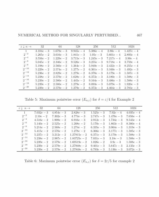
NUMERICAL METHOD FOR SINGULARLY PERTURBED... 467

ε ↓ n → 32 64 128 256 512 1024

1 3.104e − 3 1.679e − 3 9.945e − 4 5.386e − 4 2.80e − 4 1.427e − 4

2−2

1.265e − 2 3.616e − 3 1.841e − 3 1.05e − 3 5.601e − 4 2.893e − 4

2−4

3.556e − 2 1.229e − 2 3.715e − 3 1.245e − 3 7.217e − 4 3.90e − 4

2−6

5.045e − 2 2.346e − 2 9.526e − 3 3.255e − 3 9.718e − 4 3.759e − 4

2−8

5.198e − 2 2.560e − 2 1.264e − 2 5.949e − 3 2.422e − 3 8.255e − 4

2−10

5.229e − 2 2.574e − 2 1.277e − 2 6.361e − 3 3.160e − 3 1.492e − 3

2−12

5.236e − 2 2.829e − 2 1.279e − 2 6.370e − 3 3.179e − 3 1.587e − 3

2−14

5.238e − 2 2.579e − 2 1.628e − 2 6.372e − 3 3.180e − 3 1.588e − 3

2−16

5.239e − 2 2.580e − 2 1.445e − 2 9.164e − 3 3.486e − 3 1.588e − 3

2−18

5.239e − 2 2.580e − 2 1.279e − 2 8.093e − 3 5.079e − 3 1.920e − 3

2−20

5.239e − 2 2.579e − 2 1.279e − 2 6.372e − 3 4.464e − 3 2.783e − 3

Table 5: Maximum pointwise error (En,ε) for δ = ε/4 for Example 2

ε ↓ n → 32 64 128 256 512 1024

1 7.032e − 3 4.854e − 3 2.828e − 3 1.525e − 3 7.92e − 4 4.035e − 4

2−2

2.10e − 2 7.302e − 3 4.774e − 3 2.747e − 3 1.476e − 3 7.656e − 4

2−4

4.516e − 2 1.909e − 2 6.916e − 3 2.912e − 3 1.734e − 3 9.543e − 4

2−6

5.140e − 2 2.525e − 2 1.208e − 2 5.170e − 3 1.863e − 3 8.380e − 4

2−8

5.214e − 2 2.568e − 2 1.274e − 2 6.335e − 3 3.064e − 3 1.319e − 3

2−10

5.415e − 2 2.576e − 2 1.278e − 2 6.366e − 3 3.177e − 3 1.585e − 3

2−12

5.237e − 2 3.212e − 2 1.27915e − 2 6.371e − 3 3.179e − 3 1.588e − 3

2−14

5.238e − 2 2.987e − 2 1.83725e − 2 7.031e − 3 3.18e − 3 1.588e − 3

2−16

5.239e − 2 2.579e − 2 1.69519e − 2 1.026e − 2 3.9e − 3 1.588e − 3

2−18

5.239e − 2 2.579e − 2 1.27948e − 2 9.401e − 3 5.647e − 3 2.133e − 3

2−20

5.239e − 2 2.579e − 2 1.27948e − 2 6.793e − 3 5.136e − 3 3.072e − 3

Table 6: Maximum pointwise error (En,ε) for δ = 2ε/5 for example 2

468 P. Rai, K.K. Sharma

5. Conclusion and Discussion

A two point boundary value problem for a second-order singularly perturbeddifferential-difference equation with turning point is considered. We developa numerical scheme based on El-Mistikawy Werle exponential finite differencescheme [21] to solve such type of differential equations. The proposed numericalmethod is analyzed for consistency, stability, and convergence. The numericalresults are tabulated in the tables 1− 6 for the considered examples to supportthe predicted theory. The graphs of the solutions of the considered examplesfor different values of delay are plotted in fig 1− 2 to examine the questions onthe effect of delay on the interior layer behavior of the solution. It can be seenthat as the value of delay argument increases, graph gets more steeper.

Acknowledgments

The first author acknowledges the Council of Scientific and Industrial Research,New Delhi, India for providing financial support.

References

[1] A.E. Berger, Houde Han, R.B. Kellogg, A priori estimates and analysis ofa numerical method for a turning point problem, Mathematics of Compu-

tation, 42, No. 166 (1984), 465-492.

[2] A. Longtin, J. Milton, Complex oscillations and chaos in human pupillight reflex with mixed and delayed feedback, Mathematical Biosciences,90 (1988), 183-199.

[3] C.G. Lange, R.M. Miura, Singular perturbation analysis of boundary valueproblems for differential-difference equations, SIAM J. Appl. Math., 42

(1982), 502-531.

[4] C.G. Lange, R.M. Miura, Singular perturbation analysis of boundary valueproblems for differential-difference equations, III. Turning point problems,SIAM J. Appl. Math., 45 (1985), 708-734.

[5] C.G. Lange, R.M. Miura, Singular perturbation analysis of boundary valueproblems for differential-difference equations, V. Small shifts with layerbehavior, SIAM J. Appl. Math., 54 (1994), 249-272.

NUMERICAL METHOD FOR SINGULARLY PERTURBED... 469

[6] C.G. Lange, R.M. Miura, Singular perturbation analysis of boundary valueproblems for differential-difference equations, VI. Small shifts with rapidoscillations, SIAM J. Appl. Math., 54 (1994), 273-283.

[7] E.L. Els’gol’ts, Qualitative methods in mathematical analysis, Transla-

tions of Mathematical Monographs, 12, American Mathematical Society,Providence, RI (1964).

[8] E.P. Doolan, J.J.H. Miller, W.H.A. Schilders, Uniform Numerical Methods

for Problems with Initial and Boundary Layers, Boole Press, Dublin (1980).

[9] H.C. Tuckwell, On the first exit time problem for temporally homogeneousMarkov processes, J. Appl. Prob., 13 (1976), 39-48.

[10] K.C. Patidar, K.K. Sharma, ε-Uniformly convergent non-standard finitedifference methods for singularly perturbed differential difference equationwith small delay, Appl. Math. Comput., 175 (2006), 864-890.

[11] L.R Abrahamsson, A priori estimates for solution of singular perturbationswith a turning point, Stud. Appl. Math., 56 (1977), 51-69.

[12] M.C. Mackey, L. Glass, Oscillations and chaos in physiological controlsystems, Science, 197 (1977), 287-289.

[13] M.W. Derstine, H.M. Gibbs, D.L. Kaplan, Bifurcation gap in a hybridoptical system, Physics Review A, 26 (1982), 3720-3722.

[14] M.K. Kadalbajoo, K.K. Sharma, Numerical analysis of boundary-valueproblems for singularly-perturbed differential-difference equations withsmall shifts of mixed type, J. Optim. Theory Appl., 115, No. 1 (2002),145-163.

[15] M.K. Kadalbajoo, K.K. Sharma, Numerical analysis of boundary valueproblem for singularly perturbed delay differential equations with layerbehavior, Appl. Math. Comput., 151, No. 1 (2004), 11-28.

[16] M.K. Kadalbajoo, K.K. Sharma, An exponentially fitted finite differ-ence scheme for solving boundary-value problems for singularly-perturbeddifferential-difference equations: Small shifts of mixed type with layer be-havior, J. Comput. Anal. Appl., 8, No. 2 (2006), 151-171.

[17] M.K. Kadalbajoo, K.K. Sharma, Parameter-uniform fitted mesh methodfor singularly perturbed delay differential equations with layer behavior,Electron. Trans. Numer. Anal., 23 (2006), 180-201.

470 P. Rai, K.K. Sharma

[18] M.K. Kadalbajoo, K.K. Sharma, Numerical analysis of boundary-valueproblems for singularly perturbed differential-difference equations: Smallshifts of mixed type with rapid oscillations, Comm. Numer. Methods En-

grg., 20 (2004), 167-182.

[19] M. Wazewska-Czyzewska, A. Lasota, Mathematical models of the red cellsystem, Mat. Stos., 6 (1976), 25-40.

[20] P.A. Farrell, Sufficient conditions for the uniform convergence of a differ-ence scheme for a singularly perturbed turning point problem, SIAM J.

Numer. Anal., 25, No. 3 (1988), 618-643.

[21] T.M. El-Mistikawy, M.J. Werle, Numerical method for boundary layerswith blowing – The exponential box scheme, AIAA J., 16 (1978), 749-751.