numerical method for singularly perturbed third order ordinary ...
26
J. Appl. Math. & Informatics Vol. 35(2017), No. 3 - 4, pp. 277 - 302 https://doi.org/10.14317/jami.2017.277 NUMERICAL METHOD FOR SINGULARLY PERTURBED THIRD ORDER ORDINARY DIFFERENTIAL EQUATIONS OF REACTION-DIFFUSION TYPE J. CHRISTY ROJA AND A. TAMILSELVAN * Abstract. In this paper, we have proposed a numerical method for Singu- larly Perturbed Boundary Value Problems (SPBVPs) of reaction-diffusion type of third order Ordinary Differential Equations (ODEs). The SPBVP is reduced into a weakly coupled system of one first order and one second order ODEs, one without the parameter and the other with the parameter ε multiplying the highest derivative subject to suitable initial and bound- ary conditions, respectively. The numerical method combines boundary value technique, asymptotic expansion approximation, shooting method and finite difference scheme. The weakly coupled system is decoupled by replacing one of the unknowns by its zero-order asymptotic expansion. Fi- nally the present numerical method is applied to the decoupled system. In order to get a numerical solution for the derivative of the solution, the do- main is divided into three regions namely two inner regions and one outer region. The Shooting method is applied to two inner regions whereas for the outer region, standard finite difference (FD) scheme is applied. Neces- sary error estimates are derived for the method. Computational efficiency and accuracy are verified through numerical examples. The method is easy to implement and suitable for parallel computing. The main advantage of this method is that due to decoupling the system, the computation time is very much reduced. AMS Mathematics Subject Classification : AMS 65l10 CR G1.7. Key words and phrases : Third order singularly perturbed problems; Bound- ary value technique; Asymptotic expansion approximation; Shooting method; Parallel computation. 1. Introduction The numerical treatment of Singularly Perturbed Problems (SPPs) has received significant attention in recent years. These problems arise frequently Received March 5, 2016. Revised October 12, 2016. Accepted February 24, 2017. ∗ Corresponding author. c ⃝ 2017 Korean SIGCAM and KSCAM. 277
-
Upload
khangminh22 -
Category
Documents
-
view
2 -
download
0
Transcript of numerical method for singularly perturbed third order ordinary ...

J. Appl. Math. & Informatics Vol. 35(2017), No. 3 - 4, pp. 277 - 302https://doi.org/10.14317/jami.2017.277
NUMERICAL METHOD FOR SINGULARLY PERTURBED
THIRD ORDER ORDINARY DIFFERENTIAL EQUATIONS OF
REACTION-DIFFUSION TYPE
J. CHRISTY ROJA AND A. TAMILSELVAN∗
Abstract. In this paper, we have proposed a numerical method for Singu-larly Perturbed Boundary Value Problems (SPBVPs) of reaction-diffusiontype of third order Ordinary Differential Equations (ODEs). The SPBVPis reduced into a weakly coupled system of one first order and one second
order ODEs, one without the parameter and the other with the parameterε multiplying the highest derivative subject to suitable initial and bound-ary conditions, respectively. The numerical method combines boundary
value technique, asymptotic expansion approximation, shooting methodand finite difference scheme. The weakly coupled system is decoupled byreplacing one of the unknowns by its zero-order asymptotic expansion. Fi-nally the present numerical method is applied to the decoupled system. In
order to get a numerical solution for the derivative of the solution, the do-main is divided into three regions namely two inner regions and one outerregion. The Shooting method is applied to two inner regions whereas forthe outer region, standard finite difference (FD) scheme is applied. Neces-
sary error estimates are derived for the method. Computational efficiencyand accuracy are verified through numerical examples. The method is easyto implement and suitable for parallel computing. The main advantage ofthis method is that due to decoupling the system, the computation time is
very much reduced.
AMS Mathematics Subject Classification : AMS 65l10 CR G1.7.Key words and phrases : Third order singularly perturbed problems; Bound-ary value technique; Asymptotic expansion approximation; Shooting method;
Parallel computation.
1. Introduction
The numerical treatment of Singularly Perturbed Problems (SPPs) hasreceived significant attention in recent years. These problems arise frequently
Received March 5, 2016. Revised October 12, 2016. Accepted February 24, 2017.∗Corresponding author.
c⃝ 2017 Korean SIGCAM and KSCAM.
277

278 J.Christy Roja and A.Tamilselvan
in fluid dynamics, elasticity, chemical reactor theory and many other appliedareas. For long decades, a good number of research papers have been appearingin the field :’Numerical methods for singularly perturbed second order ordinarydifferential equations’, but only few authors have developed numerical methodsfor singularly perturbed higher order differential equations.
Analytical treatment of SPBVPs for the higher order non-linear ODEswhich have important applications in fluid dynamics is available in ([3],[7],[17],[24],[30]). O’Malley [18] discussed the existence, uniqueness and asymptotic esti-mates of the solution of higher order SPBVPs of the form
ε(m−n)y(m) + α1(x)y(m−1) + ...+ αm(x)y+ β(x)y(n) + β1(x)y
(n−1)
+....+ βn(x)y = 0,
on the interval Ω = [0, 1] and the boundary conditions
y(λi)(0) = li, i = 1, 2, ..., r, y(λi)(1) = li, i = r + 1, ...,m,
with the assumption that β(x) = 0, m > n and the coefficients are realand infinitely differentiable throughout Ω. In [19], the author discussed theasymptotic solutions of linear scalar equations of higher order.
Niederdrenk and Yserentant [17] have considered a convection-diffusiontype equation and constructed a difference scheme on a variable mesh and de-rived conditions equivalent to stability of the discrete problem under certainassumptions.
Howes [4] established the existence and comparison results on certain bound-ary value problems for nth order scalar nonlinear differential equations and theirsystem analogues. He also applied this theory to several classes of singularlyperturbed boundary value problems of higher order.
Michal Feckan [7] discussed the existence and asymptotic estimates solu-tions of SPBVPs of the type
ε2y(n) = f(x, y, ..., y(n−3), y(n−2)), n ≥ 3,
By = 0, Ly = 0, x ∈ Ω = (0, 1),
where L is a linear two-point boundary value condition for derivatives upto or-der (n − 3) and B has one of the following forms: i) y(n−2)(0) = y(n−2)(1) =0, ii) y(n−2)(0) = y(n−1)(1) = 0, iii) y(n−1)(0) = y(n−2)(1) = 0. Further-more, he used an approach based on fixed point theory, Leray-Schauder degreetheory and the implicit function theorem to show the existence of the solutionand to investigate the asymptotic behaviour of the solution of the above BVP. In[8], Feckan considered singularly perturbed higher order ODEs and he has alsoestablished lower bounds of the number of parameters for which these equationspossess a solution.
Gartland [3] considered the numerical approximation of differential opera-
tors of the form Lεu = εu(m)+∑m−1
ν=0 aνu(ν) with out turning points. He showed
that the uniform stability of the discrete boundary value problem follows from

Numerical method for singularly perturbed third order ODEs 279
uniform stability of an associated discrete initial value problem and uniform con-sistency of the scheme. He has also proved that the uniform consistency requiresexponential fitting or a special grid or both. Further, he has shown that a fam-ily of finite difference schemes based on an exponentially graded mesh and localpolynomial basis functions are of arbitrarily high uniform order of convergence.
In [24], an iterative method is described. Further, if the order of the equa-tion is even, then a Finite Element Method (FEM) based on standard Cm−1
splines on a Shishkin mesh is reported in [31]. Also Semper [25], Roos [23]and O’Malley [19] have considered fourth-order equation and applied a standardFEM. In [24, 30], a FEM for convection and reaction type problems is described.In [31, 30], Sun and Stynes presented FEMs on Shishkin meshes on higher-orderelliptic two point BVPs.
Motivated by the works of O’Malley, Zhao Weili, Howes and Feckan [4,5, 7, 8, 18, 19, 38, 39], Shanthi and Ramanujam [26, 27, 28, 29] developedvarious computational methods for solving SPPs for fourth order ODEs subjectto different types of boundary conditions.
Only very few authors have developed numerical methods for singularlyperturbed third order ordinary differential equations, that too on the analyticalbehavior of the solution.
Zhao Weili [38] has considered a more general class of third order non-linearSPBVPs and discussed the existence, uniqueness of the solution and obtainedasymptotic estimates using the theory of the differential inequalities.
In [5], Howes presented a study on the boundary and interior layer phenom-ena exhibited by solutions of singularly perturbed third order boundary valueproblems which govern the motion of thin liquid films subject to viscous, capil-lary and gravitational forces and are of the form εy′′′ = f(y)y′ + g(x, y), a <x < b, y(a, ε) = A, y′(a, ε) = C, y(b, ε) = B. The precise conditions specify-ing where and when the third order derivative terms in the differential equationsthat can be neglected were derived and improved estimates for the actual solu-tions in terms of solutions of the lower order models were constructed. He alsopresented a technique for replacing a third order problem with an asymptoticallyequivalent second order one that may have wider applicability.
Nayfeh [15] presented perturbation techniques to find the asymptotic ex-pansion solution for the third order problem considered in Howes [5]. Infact ZhaoWeili [38] has derived results on third order non-linear SPPs using differentialinequality theorems.
Based on the work of O’Malley, Zhao Weili, Howes and Feckan [4, 5, 7, 8,18, 19, 38, 39], Valarmathi and Ramanujam [32, 33, 34, 35] developed variousnumerical methods for solving SPPs for third order ODEs subject to differenttypes of boundary conditions. Roberts [22] has suggested a method for findingsolution for third order singularly perturbed ODEs.
The fundamental idea used in this method is the Boundary Value Technique(BVT) discussed by many authors for second order, third order and fourth orderODEs [21, 32, 27] in which the authors divided the interval [0, 1] into two

280 J.Christy Roja and A.Tamilselvan
subintervals namely [0, kε] and [kε, 1] where kε is taken as the approximatewidth of the boundary layer. In the inner region [0, kε] they applied an EFFDscheme of [1] and a classical finite difference scheme for the outer region [kε, 1].They also presented error estimates for the numerical solution. This BVT givesan excellant portrait of the solution, especially within the boundary layers whichcan be seen in [27, 32].
Following the Boundary Value Technique (BVT) of Roberts [22], Vigo-Aguiar [37], Valarmathi [32] and using the basic idea underlying the methodsuggested in Khuri [40, 41], Jayakumar [6] and Natesan [10, 16] we in the presentpaper, suggest a new computational method which makes use of the zero orderasymptotic expansion approximation, BVT and Shooting method to obtain anumerical solution for the derivative of SPBVPs for third order ODEs of reaction-diffusion type of the form:
−εy′′′(x) + b(x)y′(x) + c(x)y(x) = f(x), x ∈ Ω, (1)
y(0) = p, y′′(0) = q, y′′(1) = r. (2)
where 0 < ε ≪ 1, b(x), c(x) are sufficiently smooth functions satisfying thefollowing conditions:
b(x) ≥ β, β > 0, (3)
0 ≥ c(x) ≥ −γ, γ > 0, (4)
β − 2γ ≥ γ′, for some γ′ > 0. (5)
with Ω = (0, 1), Ω0 = (0, 1], Ω = [0, 1] and y ∈ C(3)(Ω)∩C(2)(Ω). Since theproblem (1)-(2) is of singularly perturbed in nature, classical numerical methods,in general, fail to provide good approximate solution. In order to get a numericalsolution for the derivative of the solution of SPBVPs (1)-(2) numerically, wedivide the interval [0, 1] into three subintervals [0, τ ], [τ, 1− τ ] and [1− τ, 1].
Two inner region problems respectively defined in the intervals [0, τ ], [1−τ, 1] are solved by shooting method and the boundary value problem (BVP)corresponding to the outer region is solved based on the standard finite differencescheme. It is quite natural to take τ and 1 − τ as the width of the boundarylayers which can be obtained or estimated [9]. The problems defined in theintervals [0, τ ], [τ, 1−τ ] and [1−τ, 1] are independent of each other. Therefore,these problems can be solved simultaneously, that is more suitable for parallelcomputing.
This method is easy to implement, and further, we could give a full-fledgedtheory (consistency, stability, convergence and error estimates) for the same. InSection 2 some analytical results for the SPBVPs (1)-(2) are presented. Section3 deals with derivative estimates of derivative of the solution. In Section 4 someanalytical and numerical results are derived for auxiliary second order SPBVPsof reaction-diffusion type and description of the numerical method is also given.The error estimates for the method are discussed in detail in Section 5. Section

Numerical method for singularly perturbed third order ODEs 281
6 deals with non-linear problems. Numerical examples are presented in Section7. Conclusions are drawn in the last section.
Through out this paper, we use C, with or without subscript to denote ageneric positive constant, which is independent of N and ε. We use h1 andh3 for mesh sizes for the innner region problems and h2 for mesh size forthe outer region problem. We define ||.|| of w = (w1, w2)
T ∈ R2 as ||w|| =max|w1|, |w2| .
2. Preliminaries
The SPBVPs (1)-(2) can be transformed into an equivalent weakly coupledsystem of the form:
P1y(x) ≡ y′1(x)− y2(x) = 0, x ∈ Ω0,
P2y(x) ≡ −εy′′2 (x) + b(x)y2(x) + c(x)y1(x) = f(x), x ∈ Ω,(6)
y1(0) = p, y′2(0) = q, y′2(1) = r, (7)
where y = (y1, y2)T , b(x), c(x), f(x) are sufficiently smooth functions sat-
isfying the above conditions (3)-(5). This transformation makes it possible toestablish the maximum principle theorems and stability results for the contin-uous problem. In this section, we present a maximum principle for the aboveproblem. Using this, a stability result is derived. Further, an asymptotic expan-sion approximation is constructed for the solution and a theorem is presented toestablish its accuracy.
Remark 2.1. The solution of the problem (6)-(7) exhibits twin boundary layersof width O(
√ε) occur at x = 0 and at x = 1 which are less severe because the
boundary conditions are prescribed for the derivative of the solution [24]. Thecondition (3) says that the problem (6)-(7) is a non-turning point problem. Thecondition (4) is known as the quasi-monotonicity condition [24]. The maximumprinciple for the above problem (6)-(7) can be established using the conditions(3)-(5).
2.1. Maximum Principle and Stability Result.
Theorem 2.1. (Maximum Principle).Consider the SPBVPs (6)-(7). Lety1(0) ≥ 0, y′2(0) ≥ 0 and y′2(1) ≥ 0. Then P1y(x) ≥ 0 for x ∈ Ω0 andP2y(x) ≥ 0 for x ∈ Ω implies that y(x) ≥ 0 for all x ∈ Ω.
Proof. Define the test functions s(x) = (s1(x), s2(x))T by
s1(x) =1
2+ ηx2 + x, s2(x) = 1 + ηx, x ∈ Ω and 0 < η ≪ 1/2.
Clearly, s1(0) > 0, s′2(0) > 0, s′2(1) > 0.We can easily prove that P1s > 0 for x ∈ Ω0 and P2s > 0 for x ∈ Ω .

282 J.Christy Roja and A.Tamilselvan
Assume that the theorem is not true. We define
ξ = max
maxx∈Ω
(−y1s1
)(x), max
x∈Ω
(−y2s2
)(x)
.
Then, ξ > 0. Also (y1 + ξs1)(x) ≥ 0 and (y2 + ξs2)(x) ≥ 0 for x ∈ Ω.Furthermore, there exists a point, x0 ∈ Ω such that
(y1 + ξs1)(x0) = 0 for x0 ∈ Ω0 or (y2 + ξs2)(x0) = 0 for x0 ∈ Ω.
Case 1: (y1 + ξs1)(x0) = 0 for x0 ∈ Ω0.This implies that y1 + ξs1 attains its minimum at x = x0.Then,
0 < P1(y + ξs)(x0) = (y1 + ξs1)′(x0)− (y2 + ξs2)(x0) ≤ 0,
which is a contradiction.Case 2: (y2 + ξs2)(x0) = 0 for x0 ∈ Ω.This implies that y2 + ξs2 attains its minimum at x = x0.Then,
0 < P2(y+ξs)(x0) = −ε(y2+ξs2)′′(x0)+b(x)(y2+ξs2)(x0)+c(x)(y1+ξs1)(x0) ≤ 0,
which is a contradiction.Hence it can be concluded that y(x) ≥ 0, ∀x ∈ Ω. Lemma 2.2. (Stability Result).If y(x) is the solution of the SPBVPs (6)-(7)then
||y(x)|| ≤ Cmax|y1(0)|, |y′2(0)|, |y′2(1)|, maxx∈Ω0
|P1y(x)|, maxx∈Ω
|P2y(x)|,
∀x ∈ Ω.
Proof.
Set M = Cmax|y1(0)|, |y′2(0)|, |y′2(1)|, maxx∈Ω0
|P1y(x)|, maxx∈Ω
|P2y(x)|.
Defining two barrier functions w±(x) = (w±1 (x), w
±2 (x))
T by
w±1 (x) = [
1
2+ ηx2 + x]M ± y1(x) and w±
2 (x) = (1 + ηx)M ± y2(x).
We have
P1w±(x) = w±
1′(x)− w±
2 (x) =Mηx± P1y(x) ≥ 0 and
P2w±(x) = −εw±
2′′(x) + b(x)w±
2 (x) + c(x)w±1 (x),
≥M(β − 2γ)± P2y(x) ≥Mγ′ ± P2y(x) ≥ 0,
by a proper choice of the constant C. Furthermore, we have
w±1 (0) =M/2± y1(0) ≥ 0, w±′
2 (0) =Mη ± y′2(0) ≥ 0,
w±2
′(1) =Mη ± y′2(1) ≥ 0,
by a proper choice of constant C. Applying Theorem 2.1 to the barrier functionsw±(x), we get the desired result.

Numerical method for singularly perturbed third order ODEs 283
2.2. Asymptotic Expansion Approximation. We use an asymptotic ex-pansion solution of the SPBVPs (6)-(7) in the form
y(x, ε) = u0(x) + v0(x) + w0(x) +√ε(u1(x) + v1(x) + w1(x)) +O(ε).
By using the method of stretching variable [14] we can get a zero order asymp-totic expansion approximation of (6)-(7) in the form yas = u0(x)+ v0(x)+ w0(x)where u0(x) = (u01(x), u02(x))
T is the solution of the reduced problem of theBVP (6)-(7) given by
u′01(x)− u02(x) = 0,
b(x)u02(x) + c(x)u01(x) = f(x),
u01(0) = p.
(8)
v0(x) = (v01(x), v02(x))T is the left layer correction term that satisfies
v′01(x)− v02(x) = 0,
−εv′′
02(x) + b(0)v02(x) = 0(9)
and v0(x) is given byv01(x) = (−C1
√ε exp(−x
√b(0)/ε))/
√b(0),
v02(x) = C1 exp(−x√b(0)/ε).
(10)
w0(x) = (w01(x), w02(x))T is the right layer correction term that satisfiesw′
01(x)− w02(x) = 0,
−εw′′
02(x) + b(1)w02(x) = 0(11)
and w0(x) is given byw01(x) = (C2
√ε exp(−(1− x)
√b(1)/ε))/
√b(1),
w02(x) = C2 exp(−(1− x)√b(1)/ε).
(12)
Note that
C1 = [(q − u′02(0))− (r − u′02(1)) exp(−√b(1)/ε)]/D,
C2 = [−(q − u′02(0)) exp(−√b(0)/ε) + (r − u′02(1))]/D,
where, D = [1− exp(−(√b(0) +
√b(1))/
√ε)]. The following theorem gives the
error bound for the difference between the solution of the SPBVPs (6)-(7) andits zero order asymptotic expansion approximation.
Theorem 2.3. The zero order asymptotic expansion approximation yas = u0(x)+v0(x) + w0(x) of the solution y(x) of the SPBVPs (6)-(7) defined by (8)-(12)satisfies the inequality
||y(x)− yas(x)|| ≤ C√ε, ∀x ∈ Ω.
284 J.Christy Roja and A.Tamilselvan
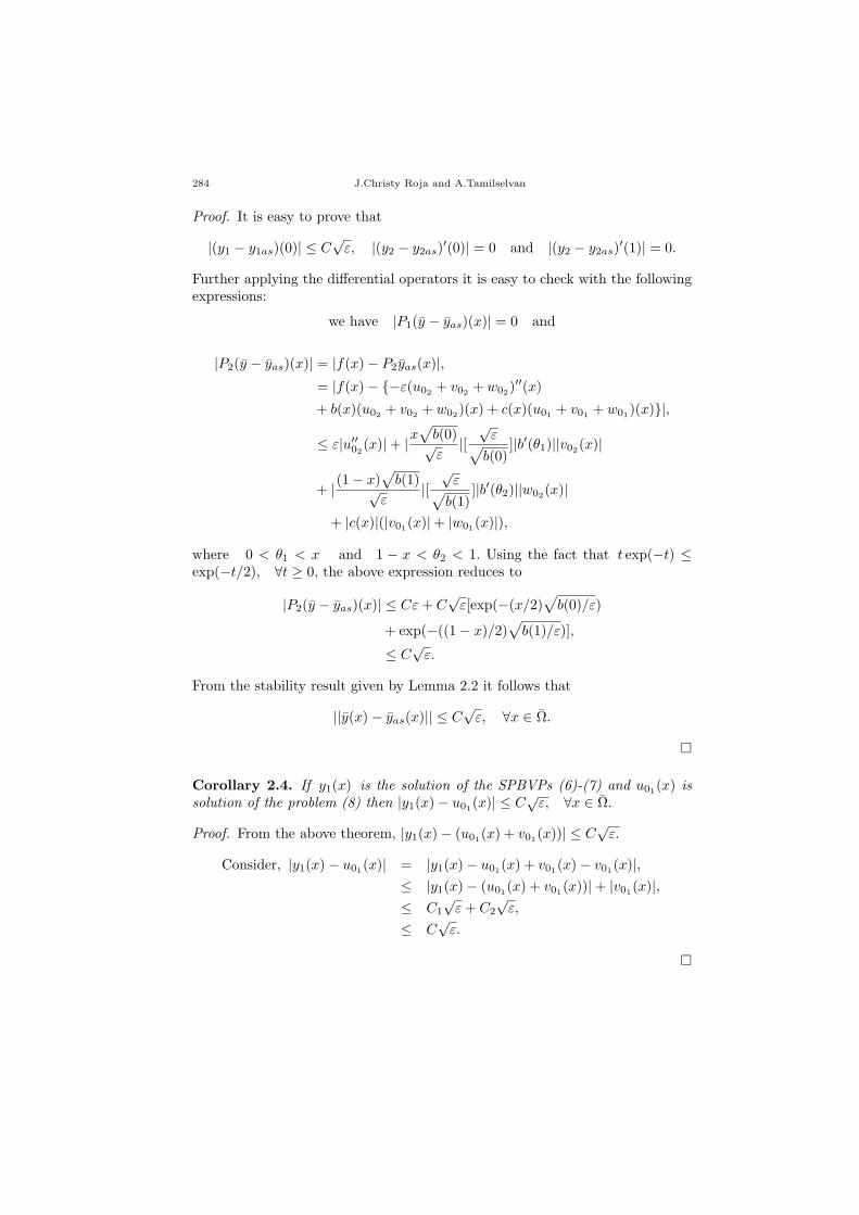
Proof. It is easy to prove that
|(y1 − y1as)(0)| ≤ C√ε, |(y2 − y2as)
′(0)| = 0 and |(y2 − y2as)′(1)| = 0.
Further applying the differential operators it is easy to check with the followingexpressions:
we have |P1(y − yas)(x)| = 0 and
|P2(y − yas)(x)| = |f(x)− P2yas(x)|,= |f(x)− −ε(u02 + v02 + w02)
′′(x)
+ b(x)(u02 + v02 + w02)(x) + c(x)(u01 + v01 + w01)(x)|,
≤ ε|u′′02(x)|+ |x√b(0)√ε
|[√ε√b(0)
]|b′(θ1)||v02(x)|
+ |(1− x)
√b(1)√
ε|[
√ε√b(1)
]|b′(θ2)||w02(x)|
+ |c(x)|(|v01(x)|+ |w01(x)|),
where 0 < θ1 < x and 1 − x < θ2 < 1. Using the fact that t exp(−t) ≤exp(−t/2), ∀t ≥ 0, the above expression reduces to
|P2(y − yas)(x)| ≤ Cε+ C√ε[exp(−(x/2)
√b(0)/ε)
+ exp(−((1− x)/2)√b(1)/ε)],
≤ C√ε.
From the stability result given by Lemma 2.2 it follows that
||y(x)− yas(x)|| ≤ C√ε, ∀x ∈ Ω.
Corollary 2.4. If y1(x) is the solution of the SPBVPs (6)-(7) and u01(x) issolution of the problem (8) then |y1(x)− u01(x)| ≤ C
√ε, ∀x ∈ Ω.
Proof. From the above theorem, |y1(x)− (u01(x) + v01(x))| ≤ C√ε.
Consider, |y1(x)− u01(x)| = |y1(x)− u01(x) + v01(x)− v01(x)|,≤ |y1(x)− (u01(x) + v01(x))|+ |v01(x)|,≤ C1
√ε+ C2
√ε,
≤ C√ε.

Numerical method for singularly perturbed third order ODEs 285
3. Estimates of derivatives
Theorem 3.1. Let y(x) be the solution of the SPBVPs (6)-(7). Then y2(x)satisfy
|y(k)2 (x)| ≤ C(1 + ε−(k/2)e(x, β)) (13)
for 0 ≤ k ≤ 3, where, e(x, β) = e−x√
β/ε + e−(1−x)√
β/ε, x ∈ Ω.
Proof. Consider the BVP
εy′′2 (x) + b(x)y2(x) + c(x)y1(x) = f(x), y′2(0) = q, y′2(1) = r.
Rewrite this BVP as
εy′′2 (x) + b(x)y2(x) = f(x)− c(x)y1(x), y′2(0) = q, y′2(1) = r.
Then, y1 ∈ C(2)(Ω) and using the procedure adopted in [12] we have |y(k)2 (x)| ≤C(1 + ε−(k/2)e(x, β)), as required.
4. Some analytical and numerical results for second order SPBVPs
We present some results for the following SPBVPs which are needed for therest of the paper. Consider the auxiliary second order SPBVPs
Ly⋆2(x) ≡ −εy⋆′′
2 (x) + b(x)y⋆2(x) = f(x)− c(x)u01(x), x ∈ Ω, (14)
B0y⋆2(0) ≡ y⋆
′
2 (0) = q, B1y⋆2(1) ≡ y⋆
′
2 (1) = r, (15)
where u01(x) is defined as in (8), b(x) and f(x) are sufficiently smooth andb(x) ≥ β, β > 0, 0 ≥ c(x) ≥ −γ, γ > 0.
4.1. Analytical Results.
Theorem 4.1. (Maximum Principle).Consider the SPBVPs (14)-(15). Lety⋆2(x) be a smooth function satisfying B0y
⋆2(0) ≥ 0 , B1y
⋆2(1) ≥ 0 and Ly⋆2(x) ≥
0 for x ∈ Ω. Then, y⋆2(x) ≥ 0, ∀x ∈ Ω.
Proof. Please refer [1].
Lemma 4.2. If y⋆2(x) is the solution of the SPBVPs (14)-(15) then
|y⋆2(x)| ≤ Cmax|B0y⋆2(0)|, |B1y
⋆2(1)|, max
x∈Ω|Ly⋆2(x)|, ∀x ∈ Ω.
Proof. Define the barrier functions ψ±(x) as
ψ±(x) = A′(1 + η′x)± y⋆2(x), x ∈ Ω,
where A′ = Cmax|B0y⋆2(0)|, |B1y
⋆2(1)|, max
x∈Ω|Ly⋆2(x)| and 0 < η′ ≪ 1/2.
It is easy to check that B0ψ±(0) ≥ 0, B1ψ
±(1) ≥ 0 and Lψ±(x) ≥ 0 for aproper choice of the constant C. Applying Theorem 4.1 to ψ±(x), the requiredstability bound is obtained.
286 J.Christy Roja and A.Tamilselvan
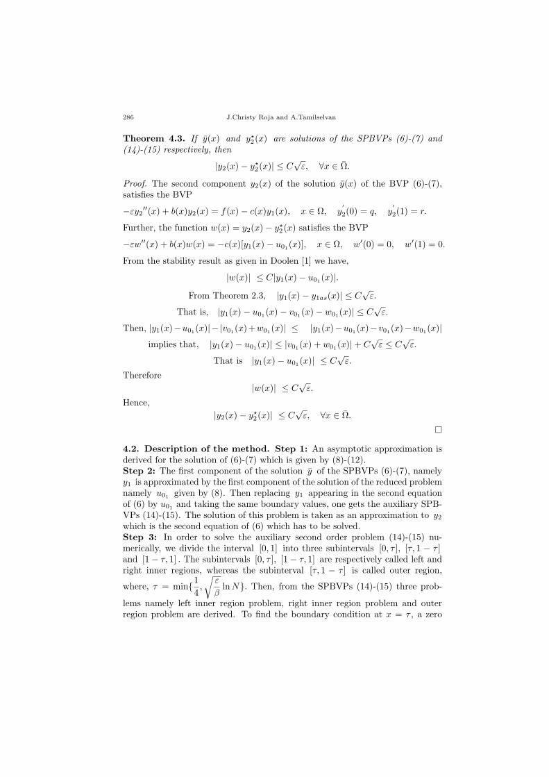
Theorem 4.3. If y(x) and y⋆2(x) are solutions of the SPBVPs (6)-(7) and(14)-(15) respectively, then
|y2(x)− y⋆2(x)| ≤ C√ε, ∀x ∈ Ω.
Proof. The second component y2(x) of the solution y(x) of the BVP (6)-(7),satisfies the BVP
−εy2′′(x) + b(x)y2(x) = f(x)− c(x)y1(x), x ∈ Ω, y′
2(0) = q, y′
2(1) = r.
Further, the function w(x) = y2(x)− y⋆2(x) satisfies the BVP
−εw′′(x) + b(x)w(x) = −c(x)[y1(x)− u01(x)], x ∈ Ω, w′(0) = 0, w′(1) = 0.
From the stability result as given in Doolen [1] we have,
|w(x)| ≤ C|y1(x)− u01(x)|.
From Theorem 2.3, |y1(x)− y1as(x)| ≤ C√ε.
That is, |y1(x)− u01(x)− v01(x)− w01(x)| ≤ C√ε.
Then, |y1(x)−u01(x)|− |v01(x)+w01(x)| ≤ |y1(x)−u01(x)−v01(x)−w01(x)|
implies that, |y1(x)− u01(x)| ≤ |v01(x) + w01(x)|+ C√ε ≤ C
√ε.
That is |y1(x)− u01(x)| ≤ C√ε.
Therefore
|w(x)| ≤ C√ε.
Hence,
|y2(x)− y⋆2(x)| ≤ C√ε, ∀x ∈ Ω.
4.2. Description of the method. Step 1: An asymptotic approximation isderived for the solution of (6)-(7) which is given by (8)-(12).Step 2: The first component of the solution y of the SPBVPs (6)-(7), namelyy1 is approximated by the first component of the solution of the reduced problemnamely u01 given by (8). Then replacing y1 appearing in the second equationof (6) by u01 and taking the same boundary values, one gets the auxiliary SPB-VPs (14)-(15). The solution of this problem is taken as an approximation to y2which is the second equation of (6) which has to be solved.Step 3: In order to solve the auxiliary second order problem (14)-(15) nu-merically, we divide the interval [0, 1] into three subintervals [0, τ ], [τ, 1 − τ ]and [1− τ, 1] . The subintervals [0, τ ], [1− τ, 1] are respectively called left andright inner regions, whereas the subinterval [τ, 1 − τ ] is called outer region,
where, τ = min14,
√ε
βlnN. Then, from the SPBVPs (14)-(15) three prob-
lems namely left inner region problem, right inner region problem and outerregion problem are derived. To find the boundary condition at x = τ , a zero

Numerical method for singularly perturbed third order ODEs 287
order asymptotic expansion is used.The left inner region problem for (14)-(15) is given by
εy′′
2 (x)− b(x)y2(x) = f(x) + c(x)u01(x), x ∈ (0, τ),
−y′2(0) = q, y2(τ) = u02(τ) + v02(τ) + w02(τ).(16)
The outer region problem for (14)-(15) is given byεy
′′
2 (x)− b(x)y2(x) = f(x) + c(x)u01(x), x ∈ (τ, 1− τ),
y2(τ) = u02(τ) + v02(τ) + w02(τ),
y2(1− τ) = u02(1− τ) + v02(1− τ) + w02(1− τ).
(17)
The right inner region problem for (14)-(15) is given byεy
′′
2 (x)− b(x)y2(x) = f(x) + c(x)u01(x), x ∈ (1− τ, 1),
y2(1− τ) = u02(1− τ) + v02(1− τ) + w02(1− τ), y′2(1) = r.(18)
Step 4: The left inner region problem (16) is solved by the Shooting methodusing the initial conditions y2(0) = u02(0)+ v02(0)+w02(0), y′2(0) = q . Here,Shooting method in the sense that BVP (16) is replaced by the IVP (19) on theinterval [0, τ ].Step 5: The right inner region problem (18) is solved by the Shooting methodusing the initial conditions y2(1) = u02(1)+v02(1)+w02(1), y′2(1) = r . Here,Shooting method in the sense that BVP (18) is replaced by the IVP (22) on theinterval [τ, 1].Step 6: The outer region problem (17) subject to boundary conditions y2(τ) =u02(τ) + v02(τ) + w02(τ), y2(1 − τ) = u02(1 − τ) + v02(1 − τ) + w02(1 − τ) issolved by standard FD scheme.Step 7: After solving both the inner region problems and the outer regionproblem, we combine their solutions to obtain an approximate solution y2 forthe derivative of the original problem (1)-(2) over the interval Ω.
4.3. Numerical Schemes.
4.3.1. Left Inner Region Problem. Using Step 4 for the BVP (16), we getthe following IVP
−εy′′
2 (x) + b(x)y2(x) = f(x)− c(x)u01(x), x ∈ (0, τ ],
y2(0) = q = u02(0) + v02(0) + w02(0), y′
2(0) = q.(19)
This IVP is equivalent to the following system:P ∗1 y
∗ ≡ y∗′
1 (x)− y∗2(x) = 0,
P ∗2 y
∗ ≡ −εy∗2 ′(x) + b(x)y∗1(x) = f∗(x), x ∈ (0, τ ],
y∗1(0) = q, y∗2(0) = q.
(20)
where f∗(x) = f(x)− c(x)u01(x), u01(x) is defined as in (8), y∗ = (y∗1 , y∗2)
T ,b(x) ≥ β, β > 0, 0 ≥ c(x) ≥ −γ, γ > 0.
288 J.Christy Roja and A.Tamilselvan
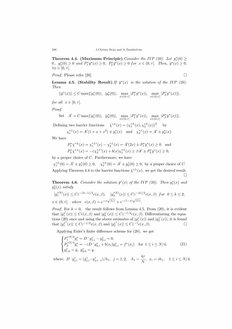
Theorem 4.4. (Maximum Principle).Consider the IVP (20). Let y∗1(0) ≥0 , y∗2(0) ≥ 0 and P ∗
1 y∗(x) ≥ 0, P ∗
2 y∗(x) ≥ 0 for x ∈ (0, τ ]. Then, y∗(x) ≥ 0,
∀x ∈ [0, τ ].
Proof. Please refer [20].
Lemma 4.5. (Stability Result).If y∗(x) is the solution of the IVP (20).Then
||y∗(x)|| ≤ Cmax|y∗1(0)|, |y∗2(0)|, maxx∈(0,τ ]
|P ∗1 y
∗(x)|, maxx∈(0,τ ]
|P ∗2 y
∗(x)|,
for all x ∈ [0, τ ].
Proof.
Set A′ = Cmax|y∗1(0)|, |y∗2(0)|, maxx∈(0,τ ]
|P ∗1 y
∗(x)|, maxx∈(0,τ ]
|P ∗2 y
∗(x)|.
Defining two barrier functions χ∗±(x) = (χ∗±1 (x), χ∗±
2 (x))T by
χ∗±1 (x) = A′(1 + x+ x2)± y∗1(x) and χ∗±
2 (x) = A′ ± y∗2(x).
We have
P ∗1 χ
∗±(x) = χ∗±1
′(x)− χ∗±2 (x) = A′(2x)± P ∗
1 y∗(x) ≥ 0 and
P ∗2 χ
∗±(x) = −εχ∗±2
′(x) + b(x)χ∗±1 (x) ≥ βA′ ± P ∗
2 y∗(x) ≥ 0,
by a proper choice of C. Furthermore, we have
χ∗±1 (0) = A′ ± y∗1(0) ≥ 0, χ∗±
2 (0) = A′ ± y∗2(0) ≥ 0, by a proper choice of C.
Applying Theorem 4.4 to the barrier functions χ∗±(x), we get the desired result.
Theorem 4.6. Consider the solution y∗(x) of the IVP (20). Then y∗1(x) andy∗2(x) satisfy
|y∗(k)1 (x)| ≤ Cε−(k−1)/2e(x, β), |y∗(k)2 (x)| ≤ Cε−(k)/2e(x, β) for 0 ≤ k ≤ 2,
x ∈ (0, τ ], where e(x, β) = e−x√
β/ε + e−(1−x)√
β/ε.
Proof. For k = 0, the result follows from Lemma 4.5. From (20), it is evident
that |y∗′
1 (x)| ≤ Ce(x, β) and |y∗′
2 (x)| ≤ Cε−1/2e(x, β). Differentiating the equa-
tions (20) once and using the above estimates of |y∗′
1 (x)| and |y∗′
2 (x)|, it is foundthat |y∗′′
1 (x)| ≤ Cε−1/2e(x, β) and |y∗′′
2 (x)| ≤ Cε−1e(x, β).
Applying Euler’s finite difference scheme for (20), we getP
∗N/41 y∗i = D−y∗1,i − y∗2,i = 0,
P∗N/42 y∗i = −εD−y∗2,i + b(xi)y
∗1,i = f∗(xi) for 1 ≤ i ≤ N/4,
y∗1,0 = q, y∗2,0 = q,
(21)
where, D−y∗j,i = (y∗j,i−y∗j,i−1)/h1, j = 1, 2, h1 =4τ
N, xi = ih1, 1 ≤ i ≤ N/4.
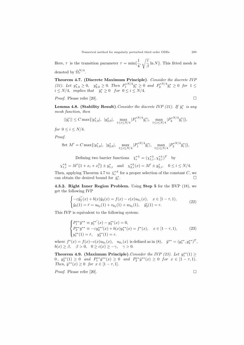
Numerical method for singularly perturbed third order ODEs 289
Here, τ is the transition parameter τ = min14,
√ε
βlnN. This fitted mesh is
denoted by ΩN/4τ .
Theorem 4.7. (Discrete Maximum Principle). Consider the discrete IVP
(21). Let y∗1,0 ≥ 0, y∗2,0 ≥ 0. Then P∗N/41 y∗i ≥ 0 and P
∗N/42 y∗i ≥ 0 for 1 ≤
i ≤ N/4, implies that y∗i ≥ 0 for 0 ≤ i ≤ N/4.
Proof. Please refer [20].
Lemma 4.8. (Stability Result).Consider the discrete IVP (21). If y∗i is anymesh function, then
||y∗i || ≤ Cmax|y∗1,0|, |y∗2,0|, max1≤i≤N/4
|P ∗N/41 y∗i |, max
1≤i≤N/4|P ∗N/4
2 y∗i |,
for 0 ≤ i ≤ N/4.
Proof.
Set M ′ = Cmax|y∗1,0|, |y∗2,0|, max1≤i≤N/4
|P ∗N/41 y∗i |, max
1≤i≤N/4|P ∗N/4
2 y∗i |,
Defining two barrier functions χ∗±i = (χ∗±
1,i , χ∗±2,i )
T by
χ∗±1,i =M ′1 + xi + x2i ± y∗1,i and χ∗±
2,i (x) =M ′ ± y∗2,i, 0 ≤ i ≤ N/4.
Then, applying Theorem 4.7 to χ∗±i for a proper selection of the constant C, we
can obtain the desired bound for y∗i .
4.3.2. Right Inner Region Problem. Using Step 5 for the BVP (18), weget the following IVP
−εy′′
2 (x) + b(x)y2(x) = f(x)− c(x)u01(x), x ∈ [1− τ, 1),
y2(1) = r = u02(1) + v02(1) + w02(1), y′2(1) = r.(22)
This IVP is equivalent to the following system:P ∗∗1 y∗∗ ≡ y∗∗
′
1 (x)− y∗∗2 (x) = 0,
P ∗∗2 y∗∗ ≡ −εy∗∗2 ′(x) + b(x)y∗∗1 (x) = f∗(x), x ∈ [1− τ, 1),
y∗∗1 (1) = r, y∗∗2 (1) = r.
(23)
where f∗(x) = f(x)−c(x)u01(x), u01(x) is defined as in (8), y∗∗ = (y∗∗1 , y∗∗2 )T ,b(x) ≥ β, β > 0, 0 ≥ c(x) ≥ −γ, γ > 0.
Theorem 4.9. (Maximum Principle).Consider the IVP (23). Let y∗∗1 (1) ≥0 , y∗∗2 (1) ≥ 0 and P ∗∗
1 y∗∗(x) ≥ 0 and P ∗∗2 y∗∗(x) ≥ 0 for x ∈ [1 − τ, 1).
Then, y∗∗(x) ≥ 0 for x ∈ [1− τ, 1].
Proof. Please refer [20].

290 J.Christy Roja and A.Tamilselvan
Lemma 4.10. (Stability Result).If y∗∗(x) is the solution of the IVP (23).Then,
||y∗∗(x)|| ≤ Cmax|y∗∗1 (1)|, |y∗∗2 (1)|, maxx∈[1−τ,1)
|P ∗∗1 y∗∗(x)|, max
x∈[1−τ,1)|P ∗∗
2 y∗∗(x)|,
∀x ∈ [1− τ, 1].
Proof.
Set A′′ = Cmax|y∗∗1 (1)|, |y∗∗2 (1)|, maxx∈[1−τ,1)
|P ∗∗1 y∗∗(x)|, max
x∈[1−τ,1)|P ∗∗
2 y∗∗(x)|.
Defining two barrier functions χ∗∗±(x) = (χ∗∗±1 (x), χ∗∗±
2 (x))T by
χ∗∗±1 (x) = A′′(1 + 2x)± y∗∗1 (x) and χ∗∗±
2 (x) = A′′ ± y∗∗2 (x).
We have
P ∗∗1 χ∗∗±(x) = χ∗∗±
1′(x)− χ∗∗±
2 (x) = A′′ ± P ∗∗1 y∗∗(x) ≥ 0 and
P ∗∗2 χ∗∗±(x) = −εχ∗∗±
2′(x) + b(x)χ∗∗±
1 (x) ≥ βA′′ ± P ∗∗2 y∗∗(x) ≥ 0,
by a proper choice of C. Furthermore, we have
χ∗∗±1 (1) = 3A′′ ± y∗∗1 (1) ≥ 0, χ∗∗±
2 (1) = A′′ ± y∗∗2 (1) ≥ 0,
by a proper choice of C. Applying Theorem 4.9 to the barrier functions χ∗∗±(x),we get the desired result.
Theorem 4.11. Consider the solution y∗∗(x) of the IVP (23). Then y∗∗1 (x)and y∗∗2 (x) satisfy
|y∗∗(k)1 (x)| ≤ Cε−(k−1)/2e(x, β), |y∗∗(k)2 (x)| ≤ Cε−(k/2)e(x, β)
for 0 ≤ k ≤ 2, x ∈ [1− τ, 1), where e(x, β) = e−x√
β/ε + e−(1−x)√
β/ε.
Proof. Proof is similar as Theorem 4.6.
Applying Euler’s finite difference scheme for (23), we getP
∗∗N/41 y∗∗ ≡ D+y∗∗1,i − y∗∗2,i = 0,
P∗∗N/42 y∗∗ ≡ −εD+y∗∗2,i + b(xi)y
∗∗1,i = f∗(xi) for 0 ≤ i ≤ N/4− 1,
y∗∗1,N/4 = r, y∗∗2,N/4 = r.
(24)
where, D+yj,i = (yj,i+1 − yj,i)/h3, j = 1, 2, h3 =4τ
N, xi = (1− τ) + ih3,
0 ≤ i ≤ N/4 − 1. Here, τ is the transition parameter defined as before. This
fitted mesh is denoted by ΩN/4τ .
Theorem 4.12. (Discrete Maximum Principle). Consider the discrete IVP
(24). Let y∗∗1,N/4 ≥ 0, y∗∗2,N/4 ≥ 0. Then P∗∗N/41 y∗∗i ≥ 0 and P
∗∗N/42 y∗∗i ≥
0 for 0 ≤ i ≤ N/4− 1 implies that y∗∗i ≥ 0 for 0 ≤ i ≤ N/4.
Proof. Please refer [20].

Numerical method for singularly perturbed third order ODEs 291
Lemma 4.13. (Stability Result).Consider the discrete IVP (24). If y∗∗i isany mesh function, then
||y∗∗i || ≤ Cmax|y∗∗1,N/4|, |y∗∗2,N/4|, max
0≤i≤N/4−1|P ∗∗N/4
1 y∗∗i | max0≤i≤N/4−1
|P ∗∗N/42 y∗∗i |,
for 0 ≤ i ≤ N/4.
Proof.
Set A′′ = Cmax|y∗∗1,N/4|, |y∗∗2,N/4|, max
0≤i≤N/4−1|P ∗∗N/4
1 y∗∗i |, max0≤i≤N/4−1
|P ∗∗N/42 y∗∗i |,
Defining the barrier functions χ∗∗±i = (χ∗∗±
1,i , χ∗∗±2,i )T by
χ∗∗±1,i = A′′1 + 2xi ± y∗∗1,i and χ∗∗±
2,i (x) = A′′ ± y∗∗2,i for 0 ≤ i ≤ N/4.
Applying Theorem 4.12 to χ∗∗±i for a proper selection of the constant C, we
can obtain the desired bounds for y∗∗i .
4.3.3. Outer Region Problem. The outer region problem for (14)-(15) isgiven by
Ly2(x) =
−εy′′
2 (x) + b(x)y2(x) = f(x)− c(x)u01(x), x ∈ (τ, 1− τ),
B0y2(0) = y2(τ) = u02(τ) + v02(τ) + w02(τ) = q∗,
B0y2(1) = y2(1− τ) = u02(1− τ) + v02(1− τ) + w02(1− τ) = r∗,
(25)
where b(x) and f(x) are sufficiently smooth and b(x) ≥ β, β > 0, 0 ≥c(x) ≥ −γ, γ > 0.
Theorem 4.14. (Maximum Principle).Consider the BVP (25). Let y2(x)be a smooth function satisfying B0y2(0) ≥ 0, B1y2(1) ≥ 0 and Ly2(x) ≥0 for x ∈ (τ, 1− τ). Then, y2(x) ≥ 0 for x ∈ [τ, 1− τ ].
Proof. Please refer [1].
Lemma 4.15. (Stability result).If y2(x) is the solution of the BVP (25) then
|y2(x)| ≤ Cmax|B0y2(0)|+ |B1y2(1)|+ maxx∈(τ,1−τ)
|Ly2(x)|, ∀x ∈ [τ, 1− τ ].
Proof. [1].
To solve this BVP, we apply standard FD scheme defined byLN/2y2,i := −εδ2y2,i + b(xi)y2,i = f(xi)− c(xi)u01(xi), 1 ≤ i ≤ N/2− 1,
BN/20 y2,0 = y2,0 = q∗, B
N/21 y2,N = y2,N/2 = r∗,
(26)
where δ2y2,i = (y2,i+1 − 2y2,i + y2,i−1)/h22, xi = τ + ih2 and h2 = 2(1 −
2τ)/N, 1 ≤ i ≤ N/2− 1.

292 J.Christy Roja and A.Tamilselvan
Theorem 4.16. (Discrete Maximum Principle).Consider the discrete BVP
(26). If BN/20 y2,0 ≥ 0, B
N/21 y2,N/2 ≥ 0 and LN/2y2,i ≥ 0 for 1 ≤ i ≤ N/2−1.
Then y2,i ≥ 0 for 1 ≤ i ≤ N/2.
Proof. Please refer [1].
Lemma 4.17. (Discrete Stability Result).If y2,i is the solution of the BVP(26) then
|y2,i| ≤ Cmax|BN/20 y2,0|+|BN/2
1 y2,N/2|+ max1≤i≤N/2−1
|LN/2y2,i|, for 0 ≤ i ≤ N/2.
Proof. Please refer [1].
5. Error Estimates
In this section, we derive error estimates for the solution of (14)-(15).
5.1. Inner region problems. In order to derive error estimate for thesolution of the inner region problems we prove the following theorems.
Error estimates for Left Inner Region Problem.
Theorem 5.1. Let y∗ = (y∗1 , y2∗)T and y∗i = (y∗1,i, y
∗2,i)
T be, respectively, thesolutions of (20) and (21). Then,
||y∗(xi)− y∗i || ≤ CN−1 lnN for 0 ≤ i ≤ N/4, xi ∈ ΩN/4τ .
Proof. From Lemma 4.1 in [9] and Theorem 4.6 it is clear that for each i, the
consistency errors due to y∗ with P∗N/41 and P
∗N/42 are bounded as given below.
|P ∗N/41 (y∗(xi)− y∗i )| = |(D− −D)y∗1(xi)|,
=h12|y∗
′′
1 (t)|,
=h12√εe(x, β), (27)
and |P ∗N/42 (y∗(xi)− y∗i )| = ε|(D− −D)y∗2(xi)|,
=εh12
|y∗′′
2 (t)|,
=h12e(x, β), (28)
for some point t satisfying, xi−1 ≤ t ≤ xi, where e(x, β) = e−x√
β/ε+e−(1−x)√
β/ε.
Since τ = min14,
√ε
βlnN, the argument is considered for two cases τ =
1
4
and τ =
√ε
βlnN separately.
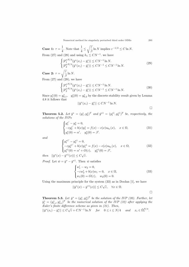
Numerical method for singularly perturbed third order ODEs 293
Case 1: τ =1
4. Note that
1
4≤
√ε
βlnN implies ε−1/2 ≤ C lnN.
From (27) and (28) and using h1 ≤ CN−1. we have|P ∗N/4
1 (y∗(xi)− y∗i )| ≤ CN−1 lnN.
|P ∗N/42 (y∗(xi)− y∗i )| ≤ CN−1 ≤ CN−1 lnN.
(29)
Case 2: τ =
√ε
βlnN .
From (27) and (28), we have|P ∗N/4
1 (y∗(xi)− y∗i )| ≤ CN−1 lnN.
|P ∗N/42 (y∗(xi)− y∗i )| ≤ CN−1 ≤ CN−1 lnN.
(30)
Since y∗1(0) = y∗0,1, y∗2(0) = y∗0,2 by the discrete stability result given by Lemma4.8 it follows that
||y∗(xi)− y∗i || ≤ CN−1 lnN.
Theorem 5.2. Let y∗ = (y∗1 , y∗2)
T and y∗1 = (y∗11 , y∗12 )T be, respectively, the
solutions of the IVPsy∗
′
1 − y∗2 = 0,
−εy∗′
2 + b(x)y∗1 = f(x)− c(x)u01(x), x ∈ Ω,
y∗1(0) = α′, y∗2(0) = β′.
(31)
and y∗1
′
1 − y∗12 = 0,
−εy∗1′2 + b(x)y∗11 = f(x)− c(x)u01(x), x ∈ Ω,
y∗11 (0) = α′ +O(ε), y∗12 (0) = β′,
(32)
then ||y∗(x)− y∗1(x)|| ≤ C√ε.
Proof. Let w = y∗ − y∗1. Then w satisfiesw′
1 − w2 = 0,
−εw′2 + b(x)w1 = 0, x ∈ Ω,
w1(0) = O(ε), w2(0) = 0.
(33)
Using the maximum principle for the system (33) as in Doolan [1], we have
||y∗(x)− y∗1(x)|| ≤ C√ε, ∀x ∈ Ω.
Theorem 5.3. Let y∗ = (y∗1 , y∗2)
T be the solution of the IVP (20). Further, lety∗i = (y∗1,i, y
∗2,i)
T be the numerical solution of the IVP (32) after applying theEuler’s finite difference scheme as given in (21). Then,
||y∗(xi)− y∗i || ≤ C√ε+ CN−1 lnN for 0 ≤ i ≤ N/4 and xi ∈ Ω
N/4τ .

294 J.Christy Roja and A.Tamilselvan
Proof. From Theorem 5.1, ||y∗1(xi)− y∗i || ≤ CN−1 lnN.From Theorem 5.2, ||y∗(xi)− y∗1(xi)|| ≤ C
√ε.
Using these estimates in the inequality,
||y∗(xi)− y∗i || ≤ ||y∗(xi)− y∗1(xi)||+ ||y∗1(xi)− y∗i ||,
where y∗1(x) is the solution of the system (32), this theorem gets proved.
The SPBVPs (14)-(15) is equivalent to the following IVP−εy′′2 (x) + b(x)y2(x) = f(x)− c(x)u01(x), x ∈ Ω,
y2(0) = q∗, y′2(0) = q,(34)
where q∗ is the asymptotic value of the solution of the BVP (14)-(15) at x = 0.Because of uniqueness of the solutions of the IVP (34) and the BVP (14)-(15), wehave the following result on the error estimate for the left inner region problem.
Theorem 5.4. Let y⋆2(xi) be the solution of the BVP (14)-(15). Further, lety∗i = (y∗1,i, y
∗2,i)
T be the numerical solution of the IVP (21). Then,
|y⋆2(xi)− y∗1,i| ≤ C√ε+ CN−1 lnN for 0 ≤ i ≤ N/4, xi ∈ ΩN/4
τ .
Proof. Consider the inequality
|y⋆2(xi)− y∗1,i| ≤ |y⋆2(xi)− y∗11 (xi)|+ |y∗11 (xi)− y∗1,i|,
where y∗11 (x) is the solution of the system (32). The proof follows from Theorem5.2 and Theorem 5.3.
Theorem 5.5. Let y be the solution of the BVP (6)-(7) and let y∗i = (y∗1,i, y∗2,i)
T
be the numerical solution of the IVP (21). Then,
|y2(xi)− y∗1,i| ≤ C√ε+ CN−1 lnN for 0 ≤ i ≤ N/4, xi ∈ ΩN/4
τ .
Proof. Consider the inequality,
|y2(xi)− y∗1,i| ≤ |y2(xi)− y⋆2(xi)|+ |y⋆2(xi)− y∗1,i|,
where y⋆2(x) is the solution of the BVP(14)-(15). The proof follows from Theo-rem 4.3 and Theorem 5.4.
Error estimates for Right Inner Region Problem.
Theorem 5.6. Let y∗∗ = (y∗∗1 , y∗∗2 )T and y∗∗i = (y∗∗1,i, y∗∗2,i)
T be, respectively,the solutions of (23) and (24). Then,
||y∗∗(xi)− y∗∗i || ≤ CN−1 lnN for 0 ≤ i ≤ N/4, xi ∈ ΩN/4τ .
Proof. Proof is similar as Theorem 5.1.

Numerical method for singularly perturbed third order ODEs 295
Theorem 5.7. Let y∗∗∗ = (y∗∗1 , y∗∗2 )T and y∗∗1 = (y∗∗11 , y∗∗12 )T be, respectively,the solutions of the IVPs
y∗∗′
1 − y∗∗2 = 0,
−εy∗∗′
2 + b(x)y∗∗1 = f(x)− c(x)u01(x), x ∈ Ω,
y∗∗1 (1) = α′′, y∗∗2 (1) = β′′(35)
and y∗∗1
′
1 − y∗∗12 = 0,
−εy∗∗1′2 + b(x)y∗∗11 = f(x)− c(x)u01(x), x ∈ Ω,
y∗∗11 (1) = α′′ +O(ε), y∗∗12 (1) = β′′(36)
then, ||y∗∗(x)− y∗∗1(x)|| ≤ C√ε.
Proof. Proof is similar as Theorem 5.2.
Theorem 5.8. Let y∗∗ = (y∗∗1 , y∗∗2 )T be the solution of the IVP (35). Further,let y∗∗i = (y∗∗1,i, y
∗∗2,i)
T be the numerical solution of the IVP (36) after applyingthe Euler’s finite difference scheme as given in (24). Then,
||y∗∗(xi)− y∗∗i || ≤ C√ε+ CN−1 lnN for 0 ≤ i ≤ N/4 and xi ∈ ΩN/4
τ .
Proof. From Theorem 5.7, ||y∗∗(xi)− y∗∗1(xi)|| ≤ C√ε.
From Theorem 5.6, ||y∗∗1(xi)− y∗∗i || ≤ CN−1 lnN.Using these estimates in the inequality,
||y∗∗(xi)− y∗∗i || ≤ ||y∗∗(xi)− y∗∗1(xi)||+ ||y∗∗1(xi)− y∗∗i ||,
where y∗∗1(x) is the solution of the system (36), this theorem gets proved.
The BVP (14)-(15) is equivalent to the following IVP−εy′′2 (x) + b(x)y2(x) = f(x)− c(x)u01(x), x ∈ Ω,
y2(1) = r∗, y′2(1) = r,(37)
where r∗ is the asymptotic value of the solution of the BVP (14)-(15) at x = 1.Because of uniqueness of the solution of the IVP (37) and the BVP (14)-(15), wehave the following result on the error estimate for the right inner region problem.
Theorem 5.9. Let y⋆2(xi) be the solution of the BVP (14)-(15). Further, lety∗∗i = (y∗∗1,i, y
∗∗2,i)
T be the numerical solution of the IVP (24). Then,
|y⋆2(xi)− y∗∗1,i| ≤ C√ε+ CN−1 lnN for 0 ≤ i ≤ N/4, xi ∈ ΩN/4
τ .
Proof. Consider the inequality
|y⋆2(xi)− y∗∗1,i| ≤ |y⋆2(xi)− y∗∗11 (xi)|+ |y∗∗11 (xi)− y∗∗1,i|,
where y∗∗11 (x) is the solution of the BVP (36). The proof follows from Theorem5.7 and Theorem 5.8.

296 J.Christy Roja and A.Tamilselvan
Theorem 5.10. Let y be the solution of the BVP (6)-(7) and let y∗∗i = (y∗∗1,i, y∗∗2,i)
T ,be the numerical solution of the IVP (24). Then,
|y2(xi)− y∗∗1,i| ≤ C√ε+ CN−1 lnN for 0 ≤ i ≤ N/4, xi ∈ ΩN/4
τ .
Proof. Consider the inequality,
|y2(xi)− y∗∗1,i| ≤ |y2(xi)− y⋆2(xi)|+ |y⋆2(xi)− y∗∗1,i|,
where y⋆2(x) is the solution of the system (14)-(15). The proof follows fromTheorem 4.3 and Theorem 5.9.
5.2. Outer Region Problem. Adopting the method of analysis provided in[2] the following theorems can be proved.
Theorem 5.11. Let y2(xi) be the solution of the BVP (25) and the solutiony2,i of the BVP (26) satisfy
|y2(xi)− y2,i| ≤ CN−1 lnN for 0 ≤ i ≤ N/2, xi ∈ ΩN/2τ
Proof. Please refer [2].
Theorem 5.12. Let y⋆2(xi) be the solution of the BVP (14)-(15) and y2,i bethe numerical solution of the BVP (25) after applying the standard FD schemeas given in (26). Then,
|y⋆2(xi)− y2,i| ≤ C√ε+ CN−1 lnN for 0 ≤ i ≤ N/2, xi ∈ ΩN/2
τ .
Proof. From Theorem 4.3, |y⋆2(xi)− y2(xi)| ≤ C√ε.
From Theorem 5.11, |y2(xi)− y2,i| ≤ CN−1 lnN.Using these estimates in the inequality,
|y⋆2(xi)− y2,i| ≤ |y⋆2(xi)− y2(xi)|+ |y2(xi)− y2,i|,
where y2(xi) is the solution of the BVP (25), this theorem gets proved.
Theorem 5.13. Let y be the solution of the BVP (6)-(7) and y2,i be thenumerical approximation obtained for y2(xi) from the BVP (25) after applyingthe standard FD scheme as given in (26). Then,
|y2(xi)− y2,i| ≤ C√ε+ CN−1 lnN for 0 ≤ i ≤ N/2, xi ∈ ΩN/2
τ .
Proof. From Theorem 4.3, |y2(xi)− y⋆2(xi)| ≤ C√ε,
From Theorem 5.12, |y⋆2(xi)− y2,i| ≤ CN−1 lnN.Using these estimates in the inequality,
|y2(xi)− y2,i| ≤ |y2(xi)− y⋆2(xi)|+ |y⋆2(xi)− y2,i|,
where y⋆2(xi) is the solution of the BVP (14)-(15), this theorem gets proved.
Numerical method for singularly perturbed third order ODEs 297
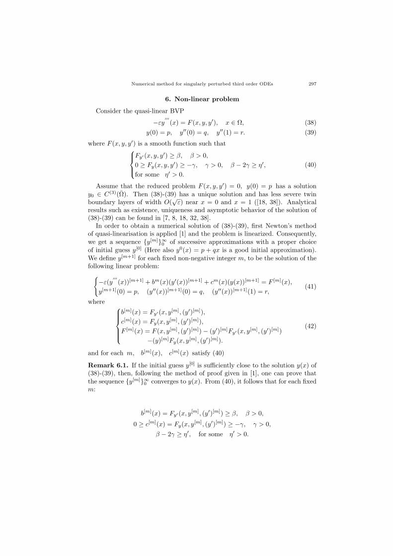
6. Non-linear problem
Consider the quasi-linear BVP
−εy′′′(x) = F (x, y, y′), x ∈ Ω, (38)
y(0) = p, y′′(0) = q, y′′(1) = r. (39)
where F (x, y, y′) is a smooth function such thatFy′(x, y, y′) ≥ β, β > 0,
0 ≥ Fy(x, y, y′) ≥ −γ, γ > 0, β − 2γ ≥ η′,
for some η′ > 0.
(40)
Assume that the reduced problem F (x, y, y′) = 0, y(0) = p has a solutiony0 ∈ C(3)(Ω). Then (38)-(39) has a unique solution and has less severe twinboundary layers of width O(
√ε) near x = 0 and x = 1 ([18, 38]). Analytical
results such as existence, uniqueness and asymptotic behavior of the solution of(38)-(39) can be found in [7, 8, 18, 32, 38].
In order to obtain a numerical solution of (38)-(39), first Newton’s methodof quasi-linearisation is applied [1] and the problem is linearized. Consequently,we get a sequence y[m]∞0 of successive approximations with a proper choiceof initial guess y[0] (Here also y0(x) = p + qx is a good initial approximation).We define y[m+1] for each fixed non-negative integer m, to be the solution of thefollowing linear problem:
−ε(y′′′(x))[m+1] + bm(x)(y′(x))[m+1] + cm(x)(y(x))[m+1] = F [m](x),
y[m+1](0) = p, (y′′(x))[m+1](0) = q, (y′′(x))[m+1](1) = r,(41)
where b[m](x) = Fy′(x, y[m], (y′)[m]),
c[m](x) = Fy(x, y[m], (y′)[m]),
F [m](x) = F (x, y[m], (y′)[m])− (y′)[m]Fy′(x, y[m], (y′)[m])
−(y)[m]Fy(x, y[m], (y′)[m]).
(42)
and for each m, b[m](x), c[m](x) satisfy (40)
Remark 6.1. If the initial guess y[0] is sufficiently close to the solution y(x) of(38)-(39), then, following the method of proof given in [1], one can prove thatthe sequence y[m]∞0 converges to y(x). From (40), it follows that for each fixedm:
b[m](x) = Fy′(x, y[m], (y′)[m]) ≥ β, β > 0,
0 ≥ c[m](x) = Fy(x, y[m], (y′)[m]) ≥ −γ, γ > 0,
β − 2γ ≥ η′, for some η′ > 0.
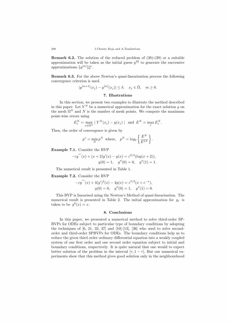
298 J.Christy Roja and A.Tamilselvan
Remark 6.2. The solution of the reduced problem of (38)-(39) or a suitableapproximation will be taken as the initial guess y[0] to generate the successiveapproximations y[m]∞0 .
Remark 6.3. For the above Newton’s quasi-linearisation process the followingconvergence criterion is used.
|y[m+1](xj)− y[m](xj)| ≤ δ, xj ∈ Ω, m ≥ 0.
7. Illustrations
In this section, we present two examples to illustrate the method describedin this paper. Let Y N be a numerical approximation for the exact solution y onthe mesh ΩN and N is the number of mesh points. We compute the maximumpoint-wise errors using
ENε = max
x∈ΩN| Y N (xj)− y(xj) | and EN = max
εEN
ε .
Then, the order of convergence is given by
p∗ = minN
pN where, pN = log2
EN
E2N
.
Example 7.1. Consider the BVP
−εy′′′(x) + (x+ 2)y′(x)− y(x) = ε3/4(log(x+ 2)),
y(0) = 1, y′′(0) = 0, y′′(1) = 1.
The numerical result is presented in Table 1.
Example 7.2. Consider the BVP
−εy′′′(x) + 4(y′)2(x)− 4y(x) = ε5/2(x+ e−x),
y(0) = 0, y′′(0) = 1, y′′(1) = 0.
This BVP is linearised using the Newton’s Method of quasi-linearisation. Thenumerical result is presented in Table 2. The initial approximation for y1 istaken to be y0(x) = x.
8. Conclusions
In this paper, we presented a numerical method to solve third-order SP-BVPs for ODEs subject to particular type of boundary conditions by adoptingthe techniques of [6, 21, 32, 37] and [10]-[13], [36] who used to solve second-order and third-order SPBVPs for ODEs. The boundary conditions help us toreduce the given third order ordinary differential equation into a weakly coupledsystem of one first order and one second order equation subject to initial andboundary conditions, respectively. It is quite natural that one would to expectbetter solution of the problem in the interval [τ, 1 − τ ]. But our numerical ex-periments show that this method gives good solution only in the neighbourhood

Numerical method for singularly perturbed third order ODEs 299
Table 1. Maximum pointwise errors ENε , EN and p∗for the
Example 7.1.
ε Number of mesh points N64 128 256 512 1024
2−6 7.8320e-006 4.1259e-006 4.0088e-006 3.7689e-007 2.1038e-007
2−7 3.8882e-006 2.8736e-006 1.8870e-007 1.2494e-007 1.7760e-007
2−8 1.9941e-006 1.5318e-006 6.5349e-007 5.8470e-007 1.4380e-007
2−9 9.5705e-007 7.2589e-007 4.8175e-008 2.8835e-008 1.7690e-008
2−10 4.7452e-008 3.6795e-008 2.4587e-008 1.5368e-008 8.4450e-008
2−6 3.3552e-004 1.6376e-004 8.2380e-005 4.1690e-005 2.1345e-005
2−7 1.6276e-004 8.1380e-005 4.0690e-005 2.0345e-005 1.0173e-005
2−8 8.1380e-005 4.0690e-005 2.0345e-005 1.0173e-005 5.0863e-006
2−9 4.0690e-005 2.0345e-005 1.0173e-005 5.0863e-006 2.5431e-006
2−10 2.0345e-005 1.0173e-005 5.0863e-006 2.5431e-006 1.2716e-006
2−6 7.7913e-006 6.5522e-006 4.6232e-006 3.7669e-006 2.6242e-006
2−7 7.3962e-006 6.5065e-006 4.3068e-006 2.6232e-006 1.3118e-006
2−8 6.9758e-007 5.8787e-007 2.1533e-007 1.3118e-007 6.5589e-007
2−9 6.4879e-007 4.9389e-007 1.0767e-007 6.5589e-008 3.2795e-008
2−10 5.7440e-008 4.6944e-008 4.3843e-008 3.2895e-008 1.3697e-008
EN 3.3552e-004 1.6376e-004 8.2380e-005 4.1690e-005 2.1345e-005
p 1.0348e+000 9.9122e-001 9.8259e-001 p∗9.6580e-001
The order of convergence=9.6580e-001CPU time(sec.)=7.4219e+000
of x = 0 and x = 1. Of course, an approximate solution can be improved bytaking better approximate initial condition as said in Section 4. This is thereason for taking the solution of the IVP only in the interval [0, τ ]. In [32], bothinner and outer region problems are BVPs, whereas in our case the inner regionproblem is an IVP and the outer region problem is a BVP. Naturally IVPs canbe treated more easily compared with BVPs. Though the present method yieldsalmost the same order of convergence as given in [32], the method produces verygood reduction on the maximum-pointwise error compared with [32]. The mainadvantage of this paper is that due to decoupling the system, the size of thematrix to be inverted is reduced from 2N − 1 to N − 1. This results in a goodreduction of the computation time. Error estimates derived in Section 5 showfirst order convergence. Our numerical experiments show that this method givesgood approximate solution especially with in the boundary layer regions whichcan be seen from the numerical results presented in Table 1 and Table 2. In allthe tables the numerical results appearing in the rows 1-5 and 11-15 correspondto the left and right boundary layers, respectively. The rest of the rows namely6-10 correspond to the outer region.

300 J.Christy Roja and A.Tamilselvan
Table 2. Maximum pointwise errors ENε , EN and p∗ for the
Example 7.2.
ε Number of mesh points N64 128 256 512 1024
2−6 8.1361e-007 6.1746e-007 4.1030e-007 8.4383e-007 4.4263e-007
2−7 4.0181e-007 3.1373e-007 2.1014e-007 1.2291e-007 7.1810e-008
2−8 2.1090e-007 1.5186e-007 1.1007e-007 6.1956e-008 3.5415e-008
2−9 1.1045e-007 7.5933e-008 5.1036e-008 3.1478e-008 1.7712e-008
2−10 5.1225e-008 3.7967e-008 2.5118e-008 2.5039e-008 1.8522e-008
2−6 1.2877e-004 6.6463e-005 3.3757e-005 1.7010e-005 0.9080e-005
2−7 6.9374e-005 1.1627e-005 9.0215e-00 2.5499e-007 3.4951e-007
2−8 4.5921e-007 1.7017e-007 2.8588e-008 2.2584e-008 1.5193e-008
2−9 6.5193e-008 5.5193e-008 4.5193e-008 3.0816e-008 2.6496e-008
2−10 5.6496e-008 4.0496e-008 3.6496e-008 2.6496e-008 1.7611e-008
2−6 2.9596e-004 1.6452e-004 9.1354e-005 5.0554e-005 2.7827e-005
2−7 6.4798e-006 5.2259e-007 4.5679e-007 2.7827e-007 1.3914e-007
2−8 6.3991e-007 4.1131e-007 2.2841e-007 1.3915e-007 1.9569e-008
2−9 6.2095e-007 4.0565e-007 3.1420e-007 6.9568e-008 5.4784e-008
2−10 5.8497e-008 5.0282e-008 4.7099e-008 3.4784e-008 1.7392e-008
EN 1.2877e-004 6.6463e-005 3.3757e-005 1.7010e-005 0.9080e-005
p 9.5417e-001 9.7736e-001 9.8880e-001 p∗9.0562e-001
The order of convergence= 9.0562e-001
CPUtime(sec.) =1.1781e+001
References
1. E.P. Doolan, J.J.H. Miller and W.H.A. Schilders, Uniform numerical methods for problemswith initial and boundary layers, Boole Press, Dublin, Ireland, 1980.
2. P.A. Farrell, A.F. Hegarty, J.J.H. Miller, E. O’Riordan and G.I. Shishkin, Robust compu-
tational techniques for boundary layers, Chapman and Hall/CRC, Raton, Florida, USA,Boca, 2000.
3. E.C. Gartland, Graded mesh difference schemes for singularly perturbed two-point bound-ary value problems, Mathematics of Computation 51 (1988).
4. F.A. Howes, Differential inequalities of higher order and the asymptotic solution of thenonlinear boundary value problems, SIAM, Journal of Math. Anal. 13 (1982), 61-80.
5. F.A. Howes, The asymptotic solution of a class of third order boundary value problemarising in the theory of thin film flow, SIAM, J.Appli.Math. 43 (1983), 993-1004.
6. J. Jayakumar and N. Ramanujam, A numerical method for singular perturbation problemsarising in chemical reactor theory, Comp.Math.Applic. 27 (1994), 83-99.
7. Michal Feckan, Singularly perturbed higher order boundary value problems, Journal ofdifferential equations 111 (1994), 79-102.
8. Michal Feckan, Parametrized singularly perturbed boundary value problems, Journal ofMathematical Analysis and Applications 188 (1994), 426-435.
9. J.J.H. Miller, E. O’Riordan and G.I. Shishkin, Fitted numerical methods for singularlyperturbed problems. Error estimates in the maximum norm for linear problems in one and
two dimensions, World Scientific, Singapore, 1996.10. S. Natesan and N. Ramanujam, A shooting method for singularly perturbed one-
dimensional reaction-diffusion neumann problems, Intern.J.Computer Math. 72 (1997),
383-393.11. S. Natesan, J. Jayakumar and J. Vigo-Aguiar, Parameter uniform numerical method for
singularly perturbed turning point problems exhibiting boundary Layers, Journal of Com-putational and Applied Mathematics 158 (2003), 121-134.
Numerical method for singularly perturbed third order ODEs 301
12. S. Natesan, Booster method for singularly perturbed Robin problems-II, Intern.J.ComputerMath. 78 (1997), 141-152.
13. S. Natesan, J. Vigo-Aguiar and N. Ramanujam, A numerical algorithm for singular pertur-
bation problems exhibiting weak boundary layers, Journal of Computers and Mathematicswith Applications 45 (2003), 469-479.
14. A.H. Nayfeh, Introduction to perturbation methods, John Wiley and Sons, New York, 1981.15. A.H. Nayfeh, Problems in perturbation methods, Wiley Interscience, New York, 1985.
16. S. Natesan and N. Ramanujam, A Shooting method for singularly perturbation problemsarising in chemical reactor theory, Intern.J.Computer Math. 70 (1997), 251-262.
17. K. Niederdrenk and H. Yserentant, The uniform stability of singularly perturbed discreteand continuous boundary value problems, Numer.Math. 41 (1983), 223-253.
18. R.E. O’Malley, Introduction to singular perturbations, Academic Press, New York, 1974.19. R.E. O’Malley, Singular perturbation methods for ordinary differntial equation, Springer-
verlag, New York, 1991.20. N. Ramanujam and U. N. Srivastava, Singularly perturbed initial value problems for non-
linear differential systems, Indian J. Pure and Appl.Math. 11 (1980), 98-113.21. S.M. Roberts, A boundary value technique for singular perturbation problems,
J.Math.Anal.Appl. 87 (1982), 489-508.22. S.M. Roberts, Further examples of the boundary value technique in singular perturbation
problems, Journal of Mathematical Analysis and Applications 133 (1988), 411-436.23. H.G. Roos, M. Stynes, A uniformly convergent discretization method for a fourth order
singular perturbation problem, Bonner Math.schriften 228 (1991), 30-40.
24. H.G. Roos, M. Stynes, and L. Tobiska, Numerical methods for singularly perturbed differ-ential equations, Convection-diffusion and flow problems, Springer-Verlag, 1996.
25. B. Sember, Locking in finite element approximation of long thin extensible beam, IMA,J.Numerical.Anal. 14 (1994), 97-109.
26. V. Shanthi and N. Ramanujam, Computational methods for reaction-diffusion problemsfor fourth order ordinary differentional equations with a small parameter at the highestderivative, Applied Mathematics and Computation 147 (2004), 97-113.
27. V. Shanthi and N.Ramanujam, A boundary value technique for boundary value problems
for singularly perturbed fourth-order ordinary differential equations, Computers and Math-ematics 47 (2004), 1673-1688.
28. V. Shanthi and N. Ramanujam, Asymptotic numerical fitted mesh method for singularlyperturbed fourth order ordinary differential equations of convection-diffusion type, Applied
Mathematics and computation 133 (2002), 559-579.29. V. Shanthi and N. Ramanujam, Asymptotic numerical method for boundary value problems
for singularly perturbed fourth order ordinary differential equations with a weak interiorlayer, Applied Mathematics and computation 172 (2006), 252-266.
30. G. Sun, M. Stynes, Finite element methods for singularly perturbed higher order el-liptic two-point boundary value problems I : Reaction-diffusion type problem, IMA,J.Numeri.Anal. 15 (1995), 117-139.
31. G. Sun, M. Stynes, Finite element methods for singularly perturbed higher order el-liptic two-point boundary value problems II : convection-diffusion type problem, IMA,J.Numeri.Anal. 15 (1995), 197-219.
32. S. Valarmathi and N. Ramanujam, Boundary value technique for finding numerical solu-
tion to boundary value problems for third order singularly perturbed ordinary differentialequations, Intern. J. Computer Math. 79 (2002), 747-763.
33. S. Valarmathi and N. Ramanujam, An asymptotic numerical method for singularly per-turbed third order ordinary differential equations of convection-diffusion type, Computers
and Mathematics with Applications 44 (2002), 693-710.

302 J.Christy Roja and A.Tamilselvan
34. S. Valarmathi and N. Ramanujam, An asymptotic numerical fitted mesh method for sin-gularly perturbed third order ordinary differential equations of reaction-diffusion type, Ap-plied Mathematics and computation 132 (2002), 87-104.
35. S. Valarmathi and N. Ramanujam, A computational method for solving boundary valueproblems for third -order singularly perturbed ordinary differential equation, AppliedMathematics and computation 129 (2007), 345-373.
36. J. Vigo-Aguiar and S. Natesan, An efficient numerical method for singular perturbation
problems, Journal of Computational and Applied Mathematics 192 (2006), 132-141.37. J. Vigo-Aguiar and S. Natesan, A parallel boundary value technique for singularly perturbed
two-point boundary problems, The Journal of Super computing 27 (2004), 195-206.38. Zhao Weili, Singular perturbations of boundary value problems for a class of third order
non-linear ordinary differential equations, Journal Differential equations 88 (1990), 265-278.
39. Zhao Weili, Singular perturbations for third order non-linear boundary value problem,Non-linear Analysis, Theory, Methods and applications, 1994.
40. S.A. Khuri, A.Sayfy, Self adjoint singularly perturbed second order two point boundaryproblems: A patching approach, Applied Mathematical Modelling 38 (2014), 2901-2914.
41. S.A. Khuri, Ali Sayfy, The boundary layer problem: A fourth-order collocation approach,Computers and Mathematics with Applications 64 (2012), 2089-2099.
J. Christy Roja has been working Assistant professor in St.Joseph’s college since 2009.
Her research interests include numerical analysis and singularly perturbed differential equa-tions.
Department of Mathematics, St.Joseph’s college, Tiruchirappalli, Tamilnadu, India.e-mail: [email protected]
A. Tamilselvan has been rendering his service in Bharathidasan University since Decem-ber 1999. He is currently Associate professor and Head in Bharathidasan University. Hisresearch interests are numerical analysis and singularly perturbed differential equations.
Department of Mathematics, Bharathidasan University, Tiruchirappalli, Tamilnadu, India.
e-mail: [email protected]