ε-Uniformly convergent non-standard finite difference methods for singularly perturbed differential...
27
e-Uniformly convergent non-standard finite difference methods for singularly perturbed differential difference equations with small delay Kailash C. Patidar a, * , Kapil K. Sharma b a Department of Mathematics and Applied Mathematics, University of Pretoria, Pretoria 0002, South Africa b Department of Mathematics, Panjab University, Chandigarh 160 014, India Dedicated to Prof. J.M.-S. Lubuma on the occasion of his 50th Birthday Abstract Non-standard finite difference methods (NSFDMs), now-a-days, are playing an important role in solving the real life problems governed by ODEs and/or by PDEs. Many differential models of sciences and engineerings for which the existing methodol- ogies do not give reliable results, these NSFDMs are solving them competitively. To this end, in this paper we consider, second order, linear, singularly perturbed differential dif- ference equations. Using the second of the five non-standard modeling rules of Mickens [R.E. Mickens, Nonstandard Finite Difference Models of Differential Equations, World Scientific, Singapore, 1994], the new finite difference methods are obtained for the par- ticular cases of these problems. This rule suggests us to replace the denominator func- tion of the classical second order derivative with a positive function derived systematically in such a way that it captures most of the significant properties of the 0096-3003/$ - see front matter Ó 2005 Elsevier Inc. All rights reserved. doi:10.1016/j.amc.2005.08.006 * Corresponding author. E-mail addresses: [email protected] (K.C. Patidar), [email protected] (K.K. Sharma). Applied Mathematics and Computation 175 (2006) 864–890 www.elsevier.com/locate/amc
-
Upload
independent -
Category
Documents
-
view
0 -
download
0
Transcript of ε-Uniformly convergent non-standard finite difference methods for singularly perturbed differential...

Applied Mathematics and Computation 175 (2006) 864–890
www.elsevier.com/locate/amc
e-Uniformly convergent non-standardfinite difference methods for singularly
perturbed differential differenceequations with small delay
Kailash C. Patidar a,*, Kapil K. Sharma b
a Department of Mathematics and Applied Mathematics, University of Pretoria,
Pretoria 0002, South Africab Department of Mathematics, Panjab University, Chandigarh 160 014, India
Dedicated to Prof. J.M.-S. Lubuma on the occasion of his 50th Birthday
Abstract
Non-standard finite difference methods (NSFDMs), now-a-days, are playing animportant role in solving the real life problems governed by ODEs and/or by PDEs.Many differential models of sciences and engineerings for which the existing methodol-ogies do not give reliable results, these NSFDMs are solving them competitively. To thisend, in this paper we consider, second order, linear, singularly perturbed differential dif-ference equations. Using the second of the five non-standard modeling rules of Mickens[R.E. Mickens, Nonstandard Finite Difference Models of Differential Equations, WorldScientific, Singapore, 1994], the new finite difference methods are obtained for the par-ticular cases of these problems. This rule suggests us to replace the denominator func-tion of the classical second order derivative with a positive function derivedsystematically in such a way that it captures most of the significant properties of the
0096-3003/$ - see front matter � 2005 Elsevier Inc. All rights reserved.doi:10.1016/j.amc.2005.08.006
* Corresponding author.E-mail addresses: [email protected] (K.C. Patidar), [email protected] (K.K. Sharma).

K.C. Patidar, K.K. Sharma / Appl. Math. Comput. 175 (2006) 864–890 865
governing differential equation(s). Both theoretically and numerically, we show thatthese NSFDMs are e-uniformly convergent.� 2005 Elsevier Inc. All rights reserved.
Keywords: Non-standard finite difference methods; Differential difference equations; Singularperturbations; Boundary value problems
1. Introduction
Consider the singularly perturbed differential difference equation
ey 00ðxÞ þ aðxÞy0ðx� dÞ þ bðxÞyðxÞ on X ¼ ð0; 1Þ; ð1:1Þ
under the interval and boundary conditions
yðxÞ ¼ /ðxÞ; on � d 6 x 6 0;
yð1Þ ¼ c.ð1:2Þ
where baðxÞ; bðxÞ 6 �h < 0 and f(x) are sufficiently smooth functions, 0 < e� 1and d = o(e) such that ðe� dbaðxÞÞ > 0 for all x 2 [0, 1]. Furthermore, c and hare positive constants.
Such problems arise frequently in the mathematical modeling of variouspractical phenomena, for example, in, the study of bistable devices [5], varia-tional problems in control theory and first exit time problems in the modelingof the determination of expected time for the generation of action potential innerve cells by random synaptic inputs in dendrites [11], description of thehuman pupil-light reflex [13], a variety of models for physiological processesor diseases [14,29], evolutionary biology [29], etc.
The determination of the expected time for the generation of action potentialsin nerve cells by random synaptic inputs in the dendrites can be modeled as afirst-exit time problem. In Stein�s model [27,28], the distribution representinginputs is taken as a Poisson process with exponential decay. If in addition, thereare inputs that can be modeled as a Wiener process with variance parameter rand drift parameter l, then the problem for expected first-exit time y, given ini-tial membrane potential x 2 (x1,x2), can be formulated as a general boundaryvalue problem for the linear second order differential difference equation [11]
r2
2y00ðxÞ þ ðl� xÞy0ðxÞ þ kEyðxþ aEÞ þ kI yðx� aIÞ � ðkE þ kIÞyðxÞ ¼ �1;
where the values x = x1 and x2 correspond to the inhibitory reversal potentialand to the threshold value of membrane potential for action potential genera-tion, respectively. Here y is the expected first-exit time and the first order deriv-ative term �xy 0(x) corresponds to exponential decay between synaptic inputs.

866 K.C. Patidar, K.K. Sharma / Appl. Math. Comput. 175 (2006) 864–890
The undifferentiated terms correspond to excitatory and inhibitory synaptic in-puts, modeled as a Poisson process with mean rates kE and kI, respectively, andproduce jumps in the membrane potential of amounts aE and aI, which aresmall quantities and could depend on the voltage. The boundary condition is
yðxÞ � 0; x 62 ðx1; x2Þ.This biological problem motivates the study of boundary value problems for
singularly perturbed differential difference equations with delay as well asadvance, which was initiated by Lange and Miura [11,12], where they intro-duced the new terminology ‘‘negative shift’’ for ‘‘delay’’ and ‘‘positive shift’’for ‘‘advance’’.
It is well known that classical methods, fail to provide reliable numericalresults for such problems (in the sense that the parameter e and the mesh sizeh cannot vary independently). There are essentially two strategies to designschemes which have small truncation errors inside the layer region(s). The firstapproach which forms the class of fitted mesh methods consists in choosing afine mesh in the layer region(s). The second approach is in the context of thefitted operator methods in which the mesh remains uniform and the differenceschemes reflect the qualitative behavior of the solution(s) inside the layerregion(s). A nice discussion using one or both of the above strategies can befound in Miller et al. [20].
The work contained in this paper falls under the second category. We usethe non-standard finite difference methods originally developed by Mickensfor some other problems. Since his outstanding works in the mid-1980�s, thenon-standard approach has shown a great potential in designing the reliableschemes that preserve significant properties of the solutions of differential mod-els in sciences and engineerings. Few of the most recent works in this directioninclude [1–4,7,10,15–19,22,23,26] and the references therein. However, inter-ested readers can find further references in first author�s survey article on thesemethods [24]. To the best knowledge of the authors, the idea of these NSFDMshas not been implemented for the singularly perturbed differential differenceequations so far. Furthermore, the work considered in our paper is almostindependent of the works in these references and thus provides further founda-tions in this area. It is to be noted that though the title of the paper [25]contains the word non-standard difference equation but these are not thenon-standard equation in the sense of Mickens.
Before we proceed, we first give a revised version (suitable in the presentcontext) of the definition of the non-standard finite difference method (giveninitially in [15] and reformulated in [1]) as follows:
Definition 1.1. A difference equation to determine approximate solutions yj tothe solution y(x) of the problem (1.1) is called a non-standard finite differencemethod if at least one of the following conditions is met:

K.C. Patidar, K.K. Sharma / Appl. Math. Comput. 175 (2006) 864–890 867
1. The classical denominator h or h2 of the discrete first or second order deriv-ative is replaced by a nonnegative function / such that
/ðzÞ ¼ zþOðz2Þ or /ðzÞ ¼ z2 þOðz3Þ as 0 < z! 0. ð1:3Þ
2. Nonlinear terms that occur in the differential equation are approximated ina nonlocal way.
The power of the non-standard finite difference methods is measured viaqualitative stability as depicted below [1].
Definition 1.2. A difference equation in yj is called qualitatively stable withrespect to some property P of the differential Eq. (1.1) or of its solutionwhenever the discrete equation or its solution replicates the property P for anyvalue of h.
Mickens [15] set five rules for the constructions of the discrete models thathave the capability to replicate the properties of the exact solution. Definition1.1 retains only two of these rules. The first rule is essential in that the quali-tative behavior of the exact solution is reflected by the denominator function/. However, we do not need the second rule in this paper as we are dealing withlinear problems only. The other rules are expressed in terms of Definition 1.2.For example, the schemes under consideration in this paper are stable withrespect to the order of the differential equation(s), they do satisfy minimum(maximum) principles, uniform stability estimate(s), etc.
In this paper, we consider the boundary value problems for a class of singu-larly perturbed differential difference equations where there is a small delay inthe convection term. The objective of the present work is to present some uni-formly convergent numerical schemes for such problems.
The paper is organized as follows. In Section 2, we derive some a priori resultsfor the particular cases of problem (1.1). Section 3 is devoted to the constructionof some exact and non-standard finite difference schemes for the problemsresulting from (1.1). In Section 4, we analyze these non-standard schemes forconvergence. Several numerical examples are given in Section 5. Discussionon the results as well as further research plans are indicated in Section 6.
1.1. Notations and terminology
Most of the notations and symbols we employ are fairly standard. However,to avoid notational complexities, we omit subscripted e, e.g., from ye and so on.The subscripted L and R are reserved for terms referring to the layers at Left
and Right ends. Further, throughout the paper, M will denote a positive con-stant which may take different values in different equations (inequalities) but isalways independent of e and the mesh size h.

868 K.C. Patidar, K.K. Sharma / Appl. Math. Comput. 175 (2006) 864–890
2. Some a priori estimates
Taking the Tailor series expansion of the term y 0(x � d) in Eq. (1.1), we have
y 0ðx� dÞ � y 0ðxÞ � dy00ðxÞ. ð2:1Þ
Using (2.1) in (1.1) and (1.2), we get
ðe� dbaðxÞÞy 00ðxÞ þ baðxÞy0ðxÞ þ bðxÞyðxÞ � f ðxÞ;yð0Þ � /ð0Þ; yð1Þ � c.
ð2:2Þ
Since (2.2) is an approximate version of (1.1) and (1.2), we use a different nota-tion (u(x)) for the solution of this approximate equation. Thus (2.2) is equiva-lent to
ðe� dbaðxÞÞu00ðxÞ þ baðxÞu0ðxÞ þ bðxÞuðxÞ ¼ f ðxÞ;uð0Þ ¼ /ð0Þ; uð1Þ ¼ c.
ð2:3Þ
Consider a(x) P a > 0 for "x 2 [0, 1] then depending on the value of the func-tion baðxÞ three different possibility can occur for dbaðxÞ < e:
baðxÞ ¼ aðxÞ ) Boundary layer at left end;baðxÞ ¼ �aðxÞ ) Boundary layer at right end;baðxÞ changes sign in ½0; 1�) Layer occurs in the turning point region.
9>>>=>>>; ð2:4Þ
In this paper, we deal with the first two cases mentioned in (2.4). The third caseis being considered elsewhere.
We establish now some a priori results about the solutions and their deriv-atives for the problems corresponding to above two cases.
2.1. A priori estimates when the layer is on the left side
In this case the problem (1.1) leads to
LLu � ðe� daðxÞÞu00ðxÞ þ aðxÞu0ðxÞ þ bðxÞuðxÞ ¼ f ðxÞ;uð0Þ ¼ /ð0Þ; uð1Þ ¼ c.
ð2:5Þ
Under the assumptions made on the coefficient functions, the operator LL
satisfies:
Lemma 2.1 (Continuous minimum principle). Assume that p(x) is any suffi-ciently smooth function satisfying p(0) P 0 and p(1) P 0. Then LLpðxÞ 6 0 for
all x 2 (0,1) implies that p(x) P 0 for all x 2 [0,1].

K.C. Patidar, K.K. Sharma / Appl. Math. Comput. 175 (2006) 864–890 869
Proof. Let x* be such that p(x*) = minx 2 [0, 1]p(x) and assume that p(x*) < 0.Clearly x* 62 {0,1}, therefore p 0(x*) 6 0 and p00(x*) 6 0. Furthermore,
LLpðx�Þ ¼ ðe� daðx�ÞÞp00ðx�Þ þ aðx�Þp0ðx�Þ þ bðx�Þpðx�Þ > 0;
which is a contradiction. It follows that p(x 0) P 0 and thus p(x) P 0"x 2 [0, 1]. h
Moreover,
Lemma 2.2. Let u(x) be the solution of the problem (2.5), then we have
kuk 6 h�1kf k þmaxðj/0j; jcjÞ.
Proof. We construct two barrier functions p± defined by
p�ðxÞ ¼ h�1kf k þmaxðj/0j; jcjÞ � uðxÞ.Then we have
p�ð0Þ ¼ h�1kf k þmaxðj/0j; jcjÞ � uð0Þ¼ h�1kf k þmaxðj/0j; jcjÞ � /0 P 0;
p�ð1Þ ¼ h�1kf k þmaxðj/0j; jcjÞ � uð1Þ¼ h�1kf k þmaxðj/0j; jcjÞ � c P 0
and
LLp�ðxÞ ¼ ðe� daðxÞÞðp�ðxÞÞ00 þ aðxÞðp�ðxÞÞ0 þ bðxÞp�ðxÞ¼ bðxÞðh�1kf k þmaxðj/0j; jcjÞÞ �LLuðxÞ¼ bðxÞ½h�1kf k þmaxðj/0j; jcjÞ� � f ðxÞ6 ð�kf k � f ðxÞÞ þ bðxÞmaxðj/0j; jcjÞ as bðxÞ 6 �h < 0
) bðxÞh�16 �1 6 0; since kf k 6 f ðxÞ.
Therefore, from Lemma 2.1, we obtain p±(x) P 0 for all x 2 [0,1], which givesthe required estimate. h
Lemma 2.1 implies that the solution is unique and since the problem underconsideration is linear, the existence of the solution is implied by its uniqueness.Further, the boundedness of the solution is implied by Lemma 2.2.
It is easy to prove that
Lemma 2.3. The solution u(x) of the constant coefficients problem corresponding
to (2.5) satisfies
juðxÞj 6 M 1þ exp � axCL;e
� �� �
870 K.C. Patidar, K.K. Sharma / Appl. Math. Comput. 175 (2006) 864–890
and
juðkÞðxÞj 6 MðCL;eÞ�k exp � axCL;e
� �; 8k P 1.
where CL,e = e � ad.
This result is useful in proving the following Lemma:
Lemma 2.4. The solution u(x) of (2.5) admits the decomposition
uðxÞ :¼ vL;e;dðxÞ þ wL;e;dðxÞ � vL;eðxÞ þ wL;eðxÞ ðasddependson eÞwhere the regular (smooth) component vL,e(x)(� ur(x)) satisfies
vL;eðxÞj j 6 M 1þ exp � axCL;e
� �� �;
vðkÞL;eðxÞ��� ��� 6 M 1þ ðCL;eÞ2�k exp � ax
CL;e
� �� �; 8k P 1
and the singular component wL,e(x)(� us (x)) satisfies
wðkÞL;eðxÞ��� ��� 6 MðCL;eÞ�k exp � ax
CL;e
� �; 8k P 0.
Proof. Plugging the three term asymptotic expansion for vL,e(x), viz.,
vL;eðxÞ ¼ v0ðxÞ þ CL;ev1ðxÞ þ ðCL;eÞ2v2ðxÞ ð2:6Þ
into Eq. (2.5), we obtain the relations
aðxÞv00ðxÞ þ bðxÞv0ðxÞ ¼ f ðxÞ; v0ð1Þ ¼ uð1Þ;
aðxÞv01ðxÞ þ bðxÞv1ðxÞ ¼ �v000ðxÞ; v1ð1Þ ¼ 0;
v002ðxÞ ¼ 0; v2ð0Þ ¼ 0; v2ð1Þ ¼ 0;
LLvL;e ¼ f ; vL;eð0Þ ¼ v0ð0Þ þ CL;ev1ð0Þ; vL;eð1Þ ¼ uð1Þ ð2:7Þ
and
LLwL;e ¼ 0; wL;eð0Þ ¼ uð0Þ � vL;eð0Þ; wL;eð1Þ ¼ 0. ð2:8Þ
Since v0 and v1 are independent of CL,e, we obtain
jvðkÞi ðxÞj 6 M ; 8k P 0 and i ¼ 0; 1. ð2:9Þ

K.C. Patidar, K.K. Sharma / Appl. Math. Comput. 175 (2006) 864–890 871
Lemma 2.3 then implies
jv2ðxÞj 6 M 1þ exp � axCL;e
� �� �ð2:10Þ
and
jvðkÞ2 ðxÞj 6 MðCL;eÞ�k exp � axCL;e
� �; 8k P 1. ð2:11Þ
Using (2.9), (2.10) and (2.11) into (2.6) and the equations which are obtainedvia the successive differentiation of (2.6), we will get the desired bounds onthe smooth component.
To obtain the bounds on the singular components wL,e, consider two barrierfunctions g± defined by
g�ðxÞ ¼ ðjuð0Þj þ jvL;eð0ÞjÞ expð�ax=CL;eÞ � wL;eðxÞ.Clearly, g±(0) and g±(1) are non-negative. Further, LLwL;e ¼ 0 implies thatLLg� 6 0. Therefore, Lemma 2.1 implies that g± P 0 which gives
jwL;eðxÞj 6 M exp � axCL;e
� �; where M ¼ ðjuð0Þj þ jvL;eð0ÞjÞ. ð2:12Þ
Now to find the bound on the derivatives of wL,e(x), we introduce
/ðxÞ ¼R x
0expð�AðtÞ=CL;eÞdtR 1
0expð�AðtÞ=CL;eÞdt
; where AðxÞ ¼Z x
0
aðsÞds. ð2:13Þ
Clearly, /(0) = 0, /(1) and x 2 [0,1]) / (x) 6 1. Furthermore, LL/ðxÞ 6 0.Therefore, from Lemma 2.1, we have /(x) P 0. Thus 0 6 /(x) 6 1.
We write wL,e(x) as
wL;eðxÞ ¼ c1/ðxÞ þ c2ð1� /ðxÞÞ.
Using (2.8) and the above values of /(x) at 0 and 1, we get c1 = 0,c2 = u(0) � vL,e(0). This implies that
wL;eðxÞ ¼ ðuð0Þ � vL;eð0ÞÞð1� /ðxÞÞ ð2:14Þ
and therefore,
jw0L;eðxÞj 6 M j/0ðxÞj; where M ¼ uð0Þ � vL;eð0Þ. ð2:15Þ
Eq. (2.13) then implies that
jw0L;eðxÞj 6 MðCL;eÞ�1 exp � axCL;e
� �. ð2:16Þ
872 K.C. Patidar, K.K. Sharma / Appl. Math. Comput. 175 (2006) 864–890
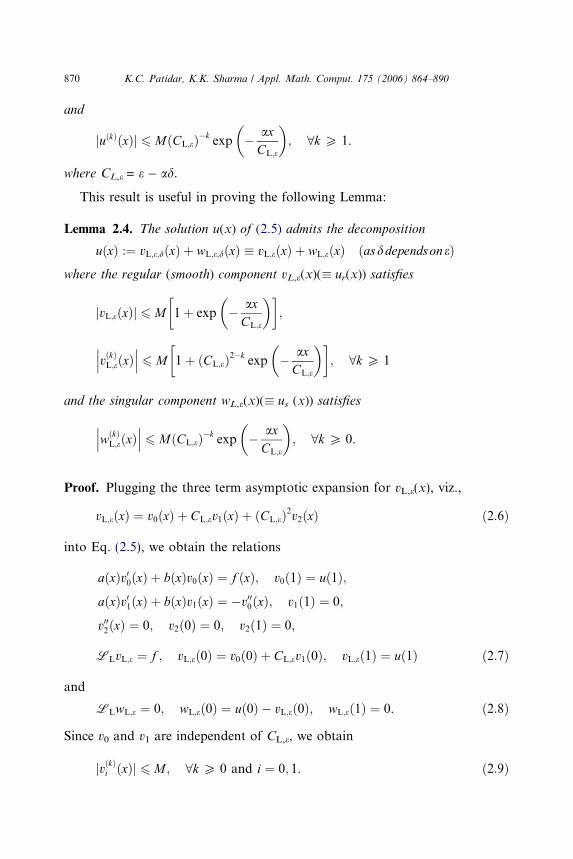
Now using the relation w00L;eðxÞ ¼ �ðaðxÞw0L;exþ wL;eðxÞÞ=CL;e, the bounds onw00L;e can be obtained via (2.12) and (2.16). Finally, the successive differentiationin (2.8) and the use of the bounds on the derivatives obtained at each earliersteps gives the desired bounds on wðkÞL;eðxÞ. This completes the proof. h
2.2. A priori estimates when the layer is on the right side
In this case the problem (1.1) leads to
LRu � �ðeþ daðxÞÞu00ðxÞ þ aðxÞu0ðxÞ þ b�ðxÞuðxÞ ¼ f �ðxÞ;uð0Þ ¼ /ð0Þ; uð1Þ ¼ c;
ð2:17Þ
where b*(x) = �b(x) and f*(x) = �f(x).Unlike the differential operator LL, here the differential operator LR satis-
fies the continuous maximum principle which is stated in
Lemma 2.5 (Continuous maximum principle). Assume that p(x) is any suffi-ciently smooth function satisfying p(0) P 0 and p(1) P 0. Then LRpðxÞP 0 for
all x 2 (0,1) implies that p(x) P 0 for all x 2 [0,1].
Proof. Again the proof is by contradiction. Let x* be such that pðx�Þ ¼minx2�XpðxÞ and assume that p(x*) < 0. Clearly x* 62 (0,1), therefore p 0(x*) = 0and p 0 0(x*) P 0. Further,
LRpðx�Þ ¼ �ðeþ daðx�ÞÞp00ðx�Þ þ aðx�Þp0ðx�Þ þ bðx�Þpðx�Þ 6 0;
which is a contradiction. It follows that p(x*) P 0 and thus p(x) P 08x 2 �X. h
We state the following results without proofs (because in this case theboundary layer will be at the right end of the interval, therefore, by transform-ing x to 1�x and proceeding in the similar manner one can easily get theproofs):
Lemma 2.6. The solution u(x) of the constant coefficients problem correspondingto (2.17) satisfies
juðxÞj 6 M 1þ exp � að1� xÞCR;e
� �� �and
juðkÞðxÞj 6 MðCR;eÞ�k exp � að1� xÞCR;e
� �; 8k P 1.
where CR,e = (e + ad).

K.C. Patidar, K.K. Sharma / Appl. Math. Comput. 175 (2006) 864–890 873
Lemma 2.7. The solution u(x) of (2.17) admits the decomposition
uðxÞ :¼ vR;e;dðxÞ þ wR;e;dðxÞ � vR;eðxÞ þ wR;eðxÞ;where the regular (smooth) component vR,e(x)(�ur(x)) satisfies
vR;eðxÞj j 6 M 1þ exp � að1� xÞCR;e
� �� �;
vðkÞR;eðxÞ��� ��� 6 M 1þ ðCR;eÞ2�k exp � að1� xÞ
CR;e
� �� �; 8k P 1.
and the singular component wR;eðxÞð� usðxÞÞ satisfies����wðkÞR;eðxÞ���� 6 MðCR;eÞ�k exp � að1� xÞ
CR;e
� �; 8k P 0.
Remark 2.8. With Ce = CL,e (and similarly in the other case CR,e), the firstconsequence of the above Lemmas is the fact that
juj � uj�1j ¼Z xj
xj�1
u0ðtÞdt
���������� 6 M
Z xj
xj�1
1þ exp �at=Ceð ÞCe
� �dt
����������
6 Mðxj � xj�1Þ;
meaning that the difference between the values of the exact solution at two suc-cessive grid points does not grow unboundedly.
3. Non-standard finite difference methods
The construction of the NSFDMs depends in general on the knowledge ofthe corresponding exact finite difference methods. Therefore, in this section,first we develop some exact schemes which will then be used to derive thenon-standard schemes.
We denote by n, a positive integer and let the interval [0, 1] be divided into n
equal parts through the nodes xm = mh, m = 0(1)n where h = 1/n is the meshsize.
3.1. Exact schemes
Assume that a(x), b(x) and f(x) in (2.5) and (2.17) are constants (denotedrespectively by a, b and f) throughout the interval [0, 1]. (Though a = a in sucha situation, we still prefer to use lowercase c in the definition of CL,e and CR,e.Thus we have (e � da) = cL,e and (e � da) = cR,e.)
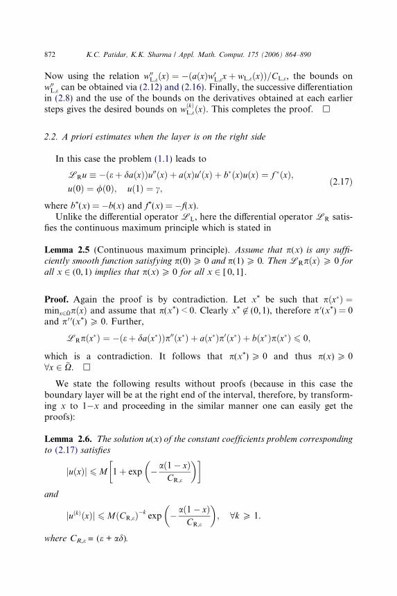
874 K.C. Patidar, K.K. Sharma / Appl. Math. Comput. 175 (2006) 864–890
We denote the approximate solution to u(x) at the grid points xj0s by m0js.When f = 0, the theory of finite difference methods yields the following exactfinite difference schemes
� exp þ ah2cL;e
� �mmþ1 þ 2 cosh
hffiffiffiffiffiffiffiffiffiffiffiffiffiffiffiffiffiffiffiffiffiffia2 � 4bcL;e
p2cL;e
!mm
� exp � ah2cL;e
� �mm�1 ¼ 0 ð3:1Þ
and
� exp � ah2cR;e
� �mmþ1 þ 2 cosh
hffiffiffiffiffiffiffiffiffiffiffiffiffiffiffiffiffiffiffiffiffiffiffiffia2 þ 4b�cR;e
p2cR;e
!mm
� exp þ ah2cR;e
� �mm�1 ¼ 0. ð3:2Þ
These schemes are exact in the sense that they preserve most of the essentialproperties of the corresponding differential equations and therefore solvesthe problems exactly. (A major advantage of having an exact difference schemefor a differential equation is that questions related to the usual considerationsof consistency, stability and convergence [8,9,21] do not arise.)
For the reasons, to be mentioned shortly in next subsection, we require theexact schemes for some reduced cases. To this end, the exact schemes corre-sponding to the problems (with constants a and f)
ðe� daÞu00ðxÞ þ au0ðxÞ ¼ f
and
�ðeþ daÞu00ðxÞ þ au0ðxÞ ¼ f �
can easily be deduced from the schemes (3.1) and (3.2) and are given by
cL;emjþ1 � 2mj þ mj�1
w2þ aj
mjþ1 � mj
h¼ fj ð3:3Þ
and
�cR;emjþ1 � 2mj þ mjþ1
f2þ aj
mj � mj�1
h¼ f �j ; ð3:4Þ
where
w2 ¼ hcL;e
aexp
ahcL;e
� �� 1
� �and f2 ¼ hcR;e
aexp
ahcR;e
� �� 1
� �.
K.C. Patidar, K.K. Sharma / Appl. Math. Comput. 175 (2006) 864–890 875
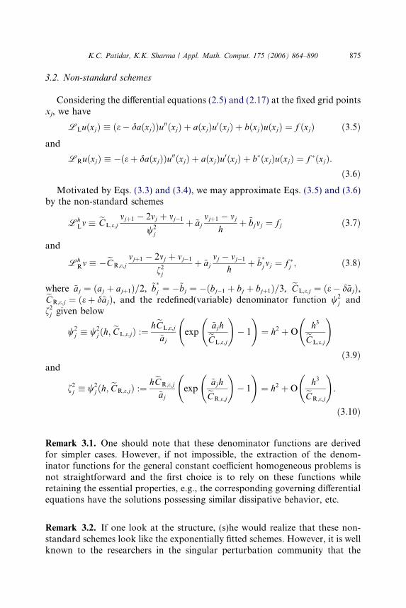
3.2. Non-standard schemes
Considering the differential equations (2.5) and (2.17) at the fixed grid pointsxj, we have
LLuðxjÞ � ðe� daðxjÞÞu00ðxjÞ þ aðxjÞu0ðxjÞ þ bðxjÞuðxjÞ ¼ f ðxjÞ ð3:5Þand
LRuðxjÞ � �ðeþ daðxjÞÞu00ðxjÞ þ aðxjÞu0ðxjÞ þ b�ðxjÞuðxjÞ ¼ f �ðxjÞ.ð3:6Þ
Motivated by Eqs. (3.3) and (3.4), we may approximate Eqs. (3.5) and (3.6)by the non-standard schemes
LhLm � eCL;e;j
mjþ1 � 2mj þ mj�1
w2j
þ ~ajmjþ1 � mj
hþ ~bjmj ¼ fj ð3:7Þ
and
LhRm � �eCR;e;j
mjþ1 � 2mj þ mj�1
f2j
þ ~ajmj � mj�1
hþ ~b
�j mj ¼ f �j ; ð3:8Þ
where ~aj ¼ ðaj þ ajþ1Þ=2, ~b�j ¼ �~bj ¼ �ðbj�1 þ bj þ bjþ1Þ=3, eCL;e;j ¼ ðe� d~ajÞ,eCR;e;j ¼ ðeþ d~ajÞ, and the redefined(variable) denominator function w2
j andf2
j given below
w2j � w2
j ðh; eCL;e;jÞ :¼ heCL;e;j
~ajexp
~ajheCL;e;j
!� 1
!¼ h2 þO
h3eCL;e;j
!ð3:9Þ
and
f2j � w2
j ðh; eCR;e;jÞ :¼ heCR;e;j
~ajexp
~ajheCR;e;j
!� 1
!¼ h2 þO
h3eCR;e;j
!.
ð3:10Þ
Remark 3.1. One should note that these denominator functions are derived
for simpler cases. However, if not impossible, the extraction of the denom-inator functions for the general constant coefficient homogeneous problems isnot straightforward and the first choice is to rely on these functions whileretaining the essential properties, e.g., the corresponding governing differentialequations have the solutions possessing similar dissipative behavior, etc.Remark 3.2. If one look at the structure, (s)he would realize that these non-standard schemes look like the exponentially fitted schemes. However, it is wellknown to the researchers in the singular perturbation community that the
876 K.C. Patidar, K.K. Sharma / Appl. Math. Comput. 175 (2006) 864–890
exponentially fitted schemes are not easily extendable for singularly perturbedPDEs whereas these NSFDMs do. Since such extension is beyond the scope ofthis paper, authors dealing them separately.
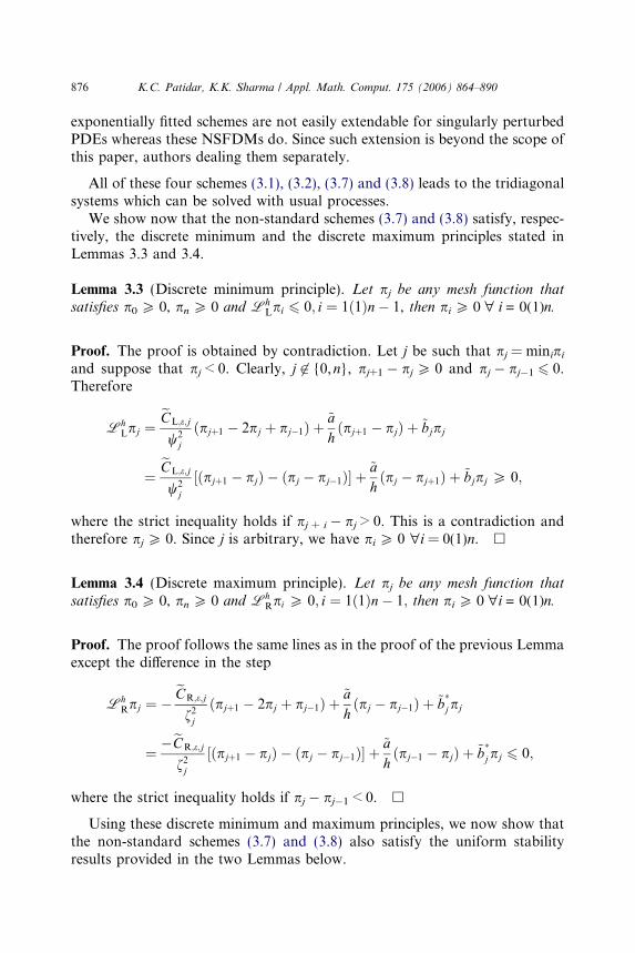
All of these four schemes (3.1), (3.2), (3.7) and (3.8) leads to the tridiagonalsystems which can be solved with usual processes.
We show now that the non-standard schemes (3.7) and (3.8) satisfy, respec-tively, the discrete minimum and the discrete maximum principles stated inLemmas 3.3 and 3.4.
Lemma 3.3 (Discrete minimum principle). Let pj be any mesh function thatsatisfies p0 P 0, pn P 0 and Lh
Lpi 6 0; i ¼ 1ð1Þn� 1, then pi P 0 " i = 0(1)n.
Proof. The proof is obtained by contradiction. Let j be such that pj = minipi
and suppose that pj < 0. Clearly, j 62 {0,n}, pj+1 � pj P 0 and pj � pj�1 6 0.Therefore
LhLpj ¼
eCL;e;j
w2j
ðpjþ1 � 2pj þ pj�1Þ þ~ahðpjþ1 � pjÞ þ ~bjpj
¼eCL;e;j
w2j
½ðpjþ1 � pjÞ � ðpj � pj�1Þ� þ~ahðpj � pjþ1Þ þ ~bjpj P 0;
where the strict inequality holds if pj + i � pj > 0. This is a contradiction andtherefore pj P 0. Since j is arbitrary, we have pi P 0 "i = 0(1)n. h
Lemma 3.4 (Discrete maximum principle). Let pj be any mesh function that
satisfies p0 P 0, pn P 0 and LhRpi P 0; i ¼ 1ð1Þn� 1; then pi P 0 "i = 0(1)n.
Proof. The proof follows the same lines as in the proof of the previous Lemmaexcept the difference in the step
LhRpj ¼ �
eCR;e;j
f2j
ðpjþ1 � 2pj þ pj�1Þ þ~ahðpj � pj�1Þ þ ~b
�j pj
¼ �eCR;e;j
f2j
½ðpjþ1 � pjÞ � ðpj � pj�1Þ� þ~ahðpj�1 � pjÞ þ ~b
�j pj 6 0;
where the strict inequality holds if pj � pj�1 < 0. h
Using these discrete minimum and maximum principles, we now show thatthe non-standard schemes (3.7) and (3.8) also satisfy the uniform stabilityresults provided in the two Lemmas below.
K.C. Patidar, K.K. Sharma / Appl. Math. Comput. 175 (2006) 864–890 877
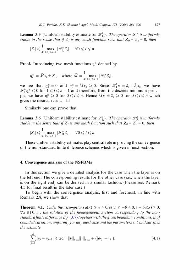
Lemma 3.5 (Uniform stability estimate for LhL). The operator Lh
L is uniformly
stable in the sense that if Zi is any mesh function such that Z0 = Zn = 0, then
jZij 61
amax
16j6n�1jLh
LZjj; 80 6 i 6 n.
Proof. Introducing two mesh functions g�i defined by
g�i ¼ eM xi � Zi; where eM ¼ 1
amax
16j6n�1jLh
LZjj;
we see that g�0 ¼ 0 and g�n ¼ eM xn P 0. Since LhLxi ¼ ~ai þ ~bixi, we have
LhLg�i 6 0 for 1 6 i 6 n � 1 and therefore, from the discrete minimum princi-
ple, we have g�i P 0 for 0 6 i 6 n. Hence eM xi � Zi P 0 for 0 6 i 6 n whichgives the desired result. h
Similarly one can prove that
Lemma 3.6 (Uniform stability estimate for LhR). The operator Lh
R is uniformly
stable in the sense that if Zi is any mesh function such that Z0 = Zn = 0, then
jZij 61
amax
16j6n�1jLh
RZjj; 80 6 i 6 n.
These uniform stability estimates play central role in proving the convergenceof the non-standard finite difference schemes which is given in next section.
4. Convergence analysis of the NSFDMs
In this section we give a detailed analysis for the case when the layer is onthe left end. The corresponding results for the other case (i.e., when the layeris on the right end) can be derived in a similar fashion. (Please see, Remark4.5 for final result in the later case.)
To begin with the convergence analysis, first and foremost, in line withRemark 2.8, we show that
Theorem 4.1. Under the assumptions a(x) P a > 0, b(x) 6 �h < 0, e � da(x) > 0,
"x 2 [0,1], the solution of the homogeneous system corresponding to the non-standard finite difference Eq. (3.7) together with the given boundary conditions, is of
bounded variation, uniformly for any mesh size and the parameters e, d and satisfies
the estimateXn
j¼1
jmj � mj�1j 6 2C�1kbkh;1kmkh;1 þ ðj/0j þ jcjÞ; ð4:1Þ

878 K.C. Patidar, K.K. Sharma / Appl. Math. Comput. 175 (2006) 864–890
where C = a or kakh,1. Here k.kh,1 is the discrete l1 norm given by
kxkh;1 ¼ max06i6n
jxij.
Proof. Consider the mesh function pj = mj � mj�1. The homogeneous part of(3.7) then leads to
eCL;e;j
w2j
ðpjþ1 � pjÞ þeajpjþ1
hþ ebjmj ¼ 0. ð4:2Þ
To replace the coefficients e� eaj and eaj involved in the above equation, wego for the choices:
e� deaj P e� dkakh;1; if pjþ1 � pj P 0;
0 < e� deaj < e� da; if pjþ1 � pj < 0;eaj P a > 0; if pjþ1 P 0;
0 < eaj 6 kakh;1; if pjþ1 < 0.
Further, w2� will represent w2
j with these choices in eaj.These choices lead us to choose K as
K ¼ð1þ aw2
�=hðe� daÞÞ�1; if pjþ1 � pj < 0; pjþ1 P 0;
ð1þ kakh;1w2�=hðe� dkakh;1ÞÞ
�1; if pjþ1 � pj P 0; pjþ1 < 0.
(ð4:3Þ
A simple rearrangement of the terms, followed by taking modulus and the useof triangle inequality yields:
jpjþ1j 6 Kjpjj þ ð1� KÞ hC2
C; ð4:4Þ
where C2 = kbkh,1kmkh,1 and C = a or kakh,1 depending upon the two situa-tions considered on p0js.
Changing j to j � 1 successively, we obtain
jpjj 6 Kjpj�1j þ ð1�KÞhC2
C
6 K jpj�2j þ ð1�KÞhC2
C
� ����� ����þ ð1�KÞhC2
C¼ K2 jpj�2j �
hC2
C
� �þ hC2
C
..
.
6 AKj�1 þ hC2
C; where Ajp1j �
hC2
C.
ð4:5Þ

K.C. Patidar, K.K. Sharma / Appl. Math. Comput. 175 (2006) 864–890 879
This implies thatXn
j¼1
jpjj 6 A1� Kn
1� K
� �þ C2
Cas K < 1 and nh ¼ 1. ð4:6Þ
Now from (4.2) and (4.4), we have
pjþ1 6 Kpj �ð1� KÞhebjmj
C. ð4:7Þ
Summing up for j = 1,2, . . . ,n � 1 and using m0 = /0, mp = c, we obtain
�p1 6 �Kpn þ ð1� KÞð/0 � cÞ � ð1� KÞhC
Xn�1
j¼1
ebjmj.
) jp1j 6 Kjpnj þ ð1� KÞðj/0j þ jcjÞ þð1� KÞh
C
Xn�1
j¼1
jebjjjmjj;
6 Kjpnj þ ð1� KÞðj/0j þ jcjÞ þð1� KÞC2
Cas ðn� 1Þh 6 1.
ð4:8ÞThus from (4.5), we obtain
Aþ hC2
C6 K AKn�1 þ hC2
C
� �þ ð1� KÞðj/0j þ jcjÞ þ
ð1� KÞC2
C
) Að1� KnÞ 6 ð1� KÞð1� hÞC2
Cþ ð1� KÞðj/0j þ jcjÞ;
which gives
Að1� KnÞ
1� K6
C2
Cþ ðj/0j þ jcjÞ as 1� h < 1. ð4:9Þ
The proof is accomplished then by using (4.9) in (4.6). h
Very often during the analysis, one encounters with the exponential termsinvolving e divided by the power functions in e which are always the main causeof worry. For their careful consideration while proving the e-uniform conver-gence, we prove
Lemma 4.2. For h not sufficiently small and for all k 2 Iþ, we have
lime!0
max16j6n�1
expð�Mxj=eÞek
¼ 0 and lime!0
max16j6n�1
expð�Mð1� xjÞ=eÞek
¼ 0;
where xj = jh, h = 1/n, "j = 1(1)n � 1.
Proof. Consider the partition
½0; 1� :¼ f0 ¼ x0 < x1 < x2 < < xn�1 < xn ¼ 1g.

880 K.C. Patidar, K.K. Sharma / Appl. Math. Comput. 175 (2006) 864–890
Clearly, for the interior grid points, we have
max16j6n�1
expð�Mxj=eÞek
6expð�Mxj=eÞ
ek¼ expð�Mh=eÞ
ek
and
max16j6n�1
expð�Mð1� xjÞ=eÞek
6expð�Mð1� xn�1Þ=eÞ
ek¼ expð�Mh=eÞ
ek.
(as x1 = h, 1 � xn�1 = 1 � (n � 1)h = h).An application of L�Hospital�s rule then leads to
lime!0
expð�Mh=eÞek
¼ limpð¼1=eÞ!1
pk
expðMhpÞ � limp!1
k!
ðMhÞk expðMhpÞ¼ 0;
which completes the proof. h
Now at the grid point xj, we consider a mesh function as uj�mj and observethat
jLhLðuj � mjÞj 6 Mhðu0ðnj
2Þ þ u00ðnj3ÞÞ þMh2ðuðnj
1Þ þ uð4Þðnj4ÞÞ; ð4:10Þ
where xj < nji < xjþ1; i ¼ 1; 2; 3; 4.
Denoting the smooth and singular components of the numerical solution bymr and ms, respectively, and using Lemma 2.4, we obtain
jLhLður
j � mrjÞj 6 M hþ h2
exp �anj4=eCL;e;j
� eCL;e;j
0@ 1A ð4:11Þ
and
jLhLðus
j � msjÞj 6 M hþ h2
exp �anj4=eCL;e;j
� ðeCL;e;jÞ3
0@ 1A. ð4:12Þ
Combining the two and considering the dominant parts, we get
jLhLðuj � mjÞj 6 M hþ h2
exp �anj4=eCL;e;j
� ðeCL;e;jÞ3
0@ 1A. ð4:13Þ
Using Lemma 3.5, we obtain
max16j6n�1
juj � mjj 6 M hþ max16j6n�1
h2exp �axj=eCL;e
� ðeCL;eÞ3
0@ 1A; ð4:14Þ
where eCL;e ¼ minjeCL;e;j.

K.C. Patidar, K.K. Sharma / Appl. Math. Comput. 175 (2006) 864–890 881
Finally, using Lemma 4.2, we obtain the main result:
Theorem 4.3. Assuming that a(x), b(x) and f(x) are sufficiently smooth so that
u(x) 2 C4[0,1], the non-standard finite difference method (3.7) is first order e-uniformly convergent in the sense that the numerical solution m of the problems
(2.5) obtained via (3.7) (with m0 = u(0), mn = u(1)) satisfies the error estimate
sup0<e61
max06j6n
juj � mjj 6 Mh. ð4:15Þ
Remark 4.4. It should be noted from (4.14) that for a fixed (but not very smalle) we do achieve second order convergence (though not e-uniform) which canbe seen in the tabular results. However, when e is very very small, one can seethe e-uniform numerical results in confirmation with the outcomes stated inTheorem 4.3.
Remark 4.5. The case when we have the layer in the vicinity of the right endthe interval, the difference operator Lh
R in the non-standard finite differencemethod (3.8) satisfies (as is shown earlier) the discrete maximum principle. Italso satisfies the uniform stability estimate and therefore by changing the roleof x through 1 � x, we see that (3.8) solves the problems (2.17) with the similarerror estimate as given in Theorem 4.3.
5. Test examples and numerical results
In this section we present some numerical results corresponding to constantor variable coefficient problems (with d = 0.5e) having different layerbehaviors.
Example 5.1. Consider the problem
ey 00ðxÞ þ y0ðx� dÞ � yðxÞ ¼ 0 with yðxÞ ¼ 1; �d 6 x 6 0; yð1Þ ¼ 1.
The exact solution of problem (2.5) with coefficient functions obtained fromabove equation is given by
uðxÞ ¼ ð1� expðm2ÞÞ expðm1xÞ � ð1� expðm1ÞÞ expðm2xÞexpðm1Þ � expðm2Þ
;
where
m1 ¼�1þ
ffiffiffiffiffiffiffiffiffiffiffiffiffiffiffiffiffiffiffiffiffiffiffiffiffi1þ 4ðe� dÞ
p2ðe� dÞ and m2 ¼
�1�ffiffiffiffiffiffiffiffiffiffiffiffiffiffiffiffiffiffiffiffiffiffiffiffiffi1þ 4ðe� dÞ
p2ðe� dÞ .

882 K.C. Patidar, K.K. Sharma / Appl. Math. Comput. 175 (2006) 864–890
Property. Layer occurs near the left end of the interval.
Example 5.2. Consider the problem
ey 00ðxÞ � expð�xÞy 0ðx� dÞ � xyðxÞ ¼ 0 with yðxÞ ¼ 1;
� d 6 x 6 0; yð1Þ ¼ 1.
Exact solution: not known.
Property. Layer occurs near the left end of the interval.
Example 5.3. Consider the problem
ey 00ðxÞ � y0ðx� dÞ � yðxÞ ¼ 0 with yðxÞ ¼ 1; �d 6 x 6 0; yð1Þ ¼ �1.
The exact solution of problem (2.17) with coefficient functions obtained fromabove equation is given by
uðxÞ ¼ �ð1þ expðm2ÞÞ expðm1xÞ þ ð1þ expðm1ÞÞ expðm2xÞexpðm1Þ � expðm2Þ
;
where
m1 ¼1þ
ffiffiffiffiffiffiffiffiffiffiffiffiffiffiffiffiffiffiffiffiffiffiffiffiffi1þ 4ðeþ dÞ
p2ðeþ dÞ and m2 ¼
1�ffiffiffiffiffiffiffiffiffiffiffiffiffiffiffiffiffiffiffiffiffiffiffiffiffi1þ 4ðeþ dÞ
p2ðeþ dÞ .
Property. Layer occurs near the right end of the interval.
Example 5.4. Consider the problem
ey 00ðxÞ � ð1þ xÞy 0ðx� dÞ � expð�xÞyðxÞ ¼ 0 with yðxÞ ¼ 1;
� d 6 x 6 0; yð1Þ ¼ �1.
Exact solution: not known.
Property. Layer occurs near the right end of the interval.
Example 5.5. Consider the problem
ey 00ðxÞ � ð1þ xÞy 0ðx� dÞ � expð�xÞyðxÞ ¼ 1 with yðxÞ ¼ 1;
� d 6 x 6 0; yð1Þ ¼ �1.
K.C. Patidar, K.K. Sharma / Appl. Math. Comput. 175 (2006) 864–890 883
Exact solution: not known.
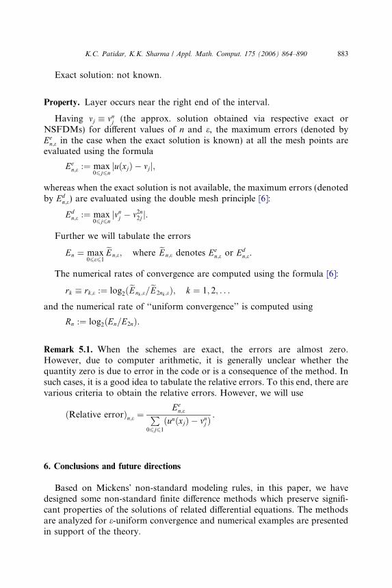
Property. Layer occurs near the right end of the interval.
Having mj � mnj (the approx. solution obtained via respective exact or
NSFDMs) for different values of n and e, the maximum errors (denoted byEe
n;e in the case when the exact solution is known) at all the mesh points areevaluated using the formula
Een;e :¼ max
06j6njuðxjÞ � mjj;
whereas when the exact solution is not available, the maximum errors (denotedby Ed
n;e) are evaluated using the double mesh principle [6]:
Edn;e :¼ max
06j6njmn
j � m2n2j j.
Further we will tabulate the errors
En ¼ max06e61
eEn;e; where eEn;e denotes Een;e or Ed
n;e.
The numerical rates of convergence are computed using the formula [6]:
rk � rk;e :¼ log2ðeEnk ;e=eE2nk ;eÞ; k ¼ 1; 2; . . .
and the numerical rate of ‘‘uniform convergence’’ is computed using
Rn :¼ log2ðEn=E2nÞ.
Remark 5.1. When the schemes are exact, the errors are almost zero.
However, due to computer arithmetic, it is generally unclear whether thequantity zero is due to error in the code or is a consequence of the method. Insuch cases, it is a good idea to tabulate the relative errors. To this end, there arevarious criteria to obtain the relative errors. However, we will useðRelative errorÞn;e ¼Ee
n;eP06j61
ðunðxjÞ � mnj Þ
.
6. Conclusions and future directions
Based on Mickens� non-standard modeling rules, in this paper, we havedesigned some non-standard finite difference methods which preserve signifi-cant properties of the solutions of related differential equations. The methodsare analyzed for e-uniform convergence and numerical examples are presentedin support of the theory.

884 K.C. Patidar, K.K. Sharma / Appl. Math. Comput. 175 (2006) 864–890
It is to be noted that in the construction of w and f in Section 3, we haveassumed that a(x) and b(x) are constant. So when we really have the constanta(x) and b(x) then we will have exact schemes. One also expects excellent numer-ical solutions in such cases (see, e.g., the results presented in Table 1). However,in view of the Remark 5.1 it is important to check whether the errors follow thesame pattern. Taking this fact into account, we have presented the relative errorsin Tables 2 and 7 using the criteria mentioned in Remark 5.1. One can see that theerrors in other tables, Tables 3–6 and 8–11 (where the results are given forvariable coefficient problems) increase initially when e starts decreasing and then
Table 1Results for Example 5.1 (maximum errors: using (3.1))
e n = 32 n = 64 n = 128 n = 256 n = 512 n = 1024
2�1 0.59E�14 0.13E�14 0.38E�13 0.33E�12 0.24E�11 0.69E�112�2 0.56E�15 0.23E�13 0.16E�12 0.27E�12 0.13E�12 0.19E�112�3 0.23E�14 0.19E�14 0.40E�13 0.13E�13 0.12E�11 0.59E�112�4 0.83E�15 0.15E�14 0.12E�13 0.18E�13 0.18E�12 0.18E�112�13 0.25E�12 0.25E�12 0.25E�12 0.25E�12 0.23E�12 0.24E�122�14 0.53E�13 0.51E�13 0.52E�13 0.54E�13 0.54E�13 0.12E�12
Table 2Results for Example 5.1 (relative errors: using (3.1))
e n = 32 n = 64 n = 128 n = 256 n = 512 n = 1024
2�1 0.48E�01 0.28E�01 0.12E�01 0.58E�02 0.29E�02 0.14E�022�2 0.56E�01 0.23E�01 0.11E�01 0.57E�02 0.32E�02 0.14E�022�3 0.44E�01 0.28E�01 0.12E�01 0.65E�02 0.28E�02 0.14E�022�4 0.54E�01 0.24E�01 0.12E�01 0.66E�02 0.26E�02 0.13E�022�13 0.44E�01 0.22E�01 0.11E�01 0.55E�02 0.27E�02 0.14E�022�14 0.44E�01 0.22E�01 0.11E�01 0.54E�02 0.27E�02 0.14E�02
Table 3Results for Example 5.1 (maximum errors: using (3.7))
e n = 16 n = 32 n = 64 n = 128 n = 256 n = 512
2�1 0.31E�03 0.77E�04 0.19E�04 0.48E�05 0.12E�05 0.30E�062�2 0.75E�03 0.19E�03 0.47E�04 0.12E�04 0.30E�05 0.74E�062�10 0.11E�01 0.55E�02 0.27E�02 0.13E�02 0.54E�03 0.19E�032�15 0.11E�01 0.57E�02 0.28E�02 0.14E�02 0.71E�03 0.35E�0310�9 0.11E�01 0.57E�02 0.29E�02 0.14E�02 0.72E�03 0.36E�0310�10 0.11E�01 0.57E�02 0.29E�02 0.14E�02 0.72E�03 0.36E�0310�11 0.11E�01 0.57E�02 0.29E�02 0.14E�02 0.72E�03 0.36E�0310�12 0.11E�01 0.57E�02 0.29E�02 0.14E�02 0.72E�03 0.36E�0310�13 0.11E�01 0.57E�02 0.29E�02 0.14E�02 0.72E�03 0.36E�03
En 0.11E�01 0.57E�02 0.29E�02 0.14E�02 0.72E�03 0.36E�03

Table 4Results for Example 5.1 (rates of convergence: using (3.7)) nk = 16 · 2k�1, k = 1(1)5
e r1 r2 r3 r4 r5
2�1 0.20E + 01 0.20E + 01 0.20E + 01 0.20E + 01 0.20E + 012�2 0.20E + 01 0.20E + 01 0.20E + 01 0.20E + 01 0.20E + 012�10 0.97E + 00 0.99E + 00 0.99E + 00 0.10E + 01 0.13E + 012�15 0.97E + 00 0.99E + 00 0.99E + 00 0.10E + 01 0.10E + 0110�9 0.97E + 00 0.99E + 00 0.99E + 00 0.10E + 01 0.10E + 0110�10 0.97E + 00 0.99E + 00 0.99E + 00 0.10E + 01 0.10E + 0110�11 0.97E + 00 0.99E + 00 0.99E + 00 0.10E + 01 0.10E + 0110�12 0.97E + 00 0.99E + 00 0.99E + 00 0.10E + 01 0.10E + 01
Rn 0.97E + 00 0.99E + 00 0.99E + 00 0.10E + 01 0.10E + 01
Table 5Results for Example 5.2 (maximum errors: using (3.7))
e n = 16 n = 32 n = 64 n = 128 n = 256 n = 512
2�1 0.18E�02 0.84E�03 0.41E�03 0.20E�03 0.10E�03 0.50E�042�4 0.79E�02 0.34E�02 0.14E�02 0.60E�03 0.28E�03 0.13E�032�8 0.18E�01 0.76E�02 0.23E�02 0.68E�03 0.43E�03 0.21E�032�15 0.18E�01 0.93E�02 0.47E�02 0.24E�02 0.12E�02 0.59E�0310�9 0.18E�01 0.93E�02 0.47E�02 0.24E�02 0.12E�02 0.59E�0310�10 0.18E�01 0.93E�02 0.47E�02 0.24E�02 0.12E�02 0.59E�0310�11 0.18E�01 0.93E�02 0.47E�02 0.24E�02 0.12E�02 0.59E�0310�12 0.18E�01 0.93E�02 0.47E�02 0.24E�02 0.12E�02 0.59E�0310�13 0.18E�01 0.93E�02 0.47E�02 0.24E�02 0.12E�02 0.59E�03
En 0.18E�01 0.93E�02 0.47E�02 0.24E�02 0.12E�02 0.59E�03
Table 6Results for Example 5.2 (rates of convergence: using (3.7)) nk = 16 · 2k�1, k = 1(1)5
e r1 r2 r3 r4 r5
2�1 0.11E + 01 0.10E + 01 0.10E + 01 0.10E + 01 0.10E + 012�2 0.11E + 01 0.11E + 01 0.10E + 01 0.10E + 01 0.10E + 012�4 0.12E + 01 0.13E + 01 0.12E + 01 0.11E + 01 0.11E + 012�8 0.12E + 01 0.17E + 01 0.17E + 01 0.68E + 00 0.99E + 002�15 0.97E + 00 0.99E + 00 0.99E + 00 0.10E + 01 0.10E + 0110�9 0.97E + 00 0.99E + 00 0.99E + 00 0.10E + 01 0.10E + 0110�10 0.97E + 00 0.99E + 00 0.99E + 00 0.10E + 01 0.10E + 0110�11 0.97E + 00 0.99E + 00 0.99E + 00 0.10E + 01 0.10E + 0110�12 0.97E + 00 0.99E + 00 0.99E + 00 0.10E + 01 0.10E + 0110�13 0.97E + 00 0.99E + 00 0.99E + 00 0.10E + 01 0.10E + 01
Rn 0.97E + 00 0.99E + 00 0.99E + 00 0.10E + 01 0.10E + 01
K.C. Patidar, K.K. Sharma / Appl. Math. Comput. 175 (2006) 864–890 885

Table 7Results for Example 5.3 (relative errors: using (3.2))
e n = 32 n = 64 n = 128 n = 256 n = 512 n = 1024
2�1 0.46E�01 0.23E�01 0.12E�01 0.58E�02 0.29E�02 0.14E�022�2 0.45E�01 0.22E�01 0.11E�01 0.56E�02 0.28E�02 0.14E�022�3 0.42E�01 0.21E�01 0.10E�01 0.52E�02 0.26E�02 0.13E�022�4 0.37E�01 0.18E�01 0.92E�02 0.46E�02 0.23E�02 0.11E�022�5 0.34E�01 0.17E�01 0.86E�02 0.43E�02 0.21E�02 0.11E�022�6 0.34E�01 0.17E�01 0.84E�02 0.42E�02 0.21E�02 0.11E�022�7 0.34E�01 0.17E�01 0.84E�02 0.42E�02 0.21E�02 0.10E�022�8 0.34E�01 0.17E�01 0.84E�02 0.42E�02 0.21E�02 0.11E�022�9 0.34E�01 0.17E�01 0.84E�02 0.42E�02 0.21E�02 0.11E�022�10 0.34E�01 0.17E�01 0.85E�02 0.42E�02 0.21E�02 0.11E�02
Table 8Results for Example 5.4 (maximum errors: using (3.8))
e n = 16 n = 32 n = 64 n = 128 n = 256 n = 512
2�1 0.21E�02 0.11E�02 0.55E�03 0.28E�03 0.14E�03 0.69E�042�4 0.65E�02 0.29E�02 0.14E�02 0.68E�03 0.33E�03 0.17E�032�5 0.10E�01 0.44E�02 0.20E�02 0.92E�03 0.45E�03 0.22E�032�6 0.15E�01 0.60E�02 0.25E�02 0.11E�02 0.52E�03 0.25E�032�7 0.19E�01 0.81E�02 0.32E�02 0.13E�02 0.59E�03 0.28E�032�8 0.20E�01 0.10E�01 0.43E�02 0.17E�02 0.69E�03 0.31E�032�9 0.20E�01 0.10E�01 0.52E�02 0.22E�02 0.86E�03 0.35E�032�10 0.20E�01 0.10E�01 0.54E�02 0.26E�02 0.11E�02 0.43E�032�11 0.20E�01 0.10E�01 0.54E�02 0.28E�02 0.13E�02 0.55E�032�12 0.20E�01 0.10E�01 0.54E�02 0.28E�02 0.14E�02 0.66E�032�13 0.20E�01 0.10E�01 0.54E�02 0.28E�02 0.14E�02 0.70E�032�14 0.20E�01 0.10E�01 0.54E�02 0.28E�02 0.14E�02 0.70E�032�15 0.20E�01 0.10E�01 0.54E�02 0.28E�02 0.14E�02 0.70E�0310�9 0.20E�01 0.10E�01 0.54E�02 0.28E�02 0.14E�02 0.70E�0310�10 0.20E�01 0.10E�01 0.54E�02 0.28E�02 0.14E�02 0.70E�0310�11 0.20E�01 0.10E�01 0.54E�02 0.28E�02 0.14E�02 0.70E�0310�12 0.20E�01 0.10E�01 0.54E�02 0.28E�02 0.14E�02 0.70E�0310�13 0.20E�01 0.10E�01 0.54E�02 0.28E�02 0.14E�02 0.70E�03
En 0.20E�01 0.10E�01 0.54E�02 0.28E�02 0.14E�02 0.70E�03
886 K.C. Patidar, K.K. Sharma / Appl. Math. Comput. 175 (2006) 864–890
remain constant so essentially they show some e dependence. (It is not uncom-mon and can be seen in many papers on singular perturbations showing uniformconvergence). However, the errors that we have presented in Tables 2 and 7 areclearly e-independent showing the exactness of the method.
It is interesting to note that we have provided the analysis for the problemsarising from the (1.1) via the expansion of the term y(x � d). Though it doesnot directly imply that the solution of the reduced problems is near the solutionof (1.1), such problems are still worth investigating as they provide us more
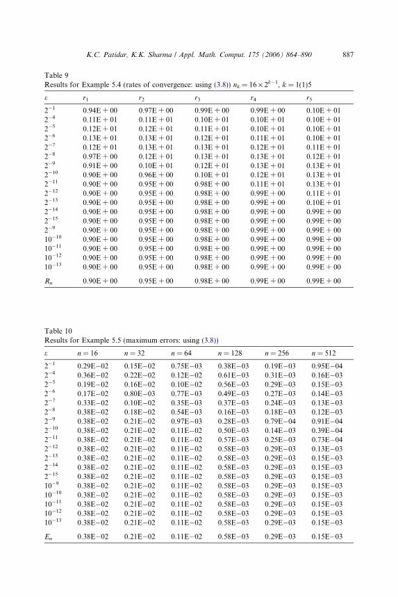
Table 9Results for Example 5.4 (rates of convergence: using (3.8)) nk = 16 · 2k�1, k = 1(1)5
e r1 r2 r3 r4 r5
2�1 0.94E + 00 0.97E + 00 0.99E + 00 0.99E + 00 0.10E + 012�4 0.11E + 01 0.11E + 01 0.10E + 01 0.10E + 01 0.10E + 012�5 0.12E + 01 0.12E + 01 0.11E + 01 0.10E + 01 0.10E + 012�6 0.13E + 01 0.13E + 01 0.12E + 01 0.11E + 01 0.10E + 012�7 0.12E + 01 0.13E + 01 0.13E + 01 0.12E + 01 0.11E + 012�8 0.97E + 00 0.12E + 01 0.13E + 01 0.13E + 01 0.12E + 012�9 0.91E + 00 0.10E + 01 0.12E + 01 0.13E + 01 0.13E + 012�10 0.90E + 00 0.96E + 00 0.10E + 01 0.12E + 01 0.13E + 012�11 0.90E + 00 0.95E + 00 0.98E + 00 0.11E + 01 0.13E + 012�12 0.90E + 00 0.95E + 00 0.98E + 00 0.99E + 00 0.11E + 012�13 0.90E + 00 0.95E + 00 0.98E + 00 0.99E + 00 0.10E + 012�14 0.90E + 00 0.95E + 00 0.98E + 00 0.99E + 00 0.99E + 002�15 0.90E + 00 0.95E + 00 0.98E + 00 0.99E + 00 0.99E + 002�9 0.90E + 00 0.95E + 00 0.98E + 00 0.99E + 00 0.99E + 0010�10 0.90E + 00 0.95E + 00 0.98E + 00 0.99E + 00 0.99E + 0010�11 0.90E + 00 0.95E + 00 0.98E + 00 0.99E + 00 0.99E + 0010�12 0.90E + 00 0.95E + 00 0.98E + 00 0.99E + 00 0.99E + 0010�13 0.90E + 00 0.95E + 00 0.98E + 00 0.99E + 00 0.99E + 00
Rn 0.90E + 00 0.95E + 00 0.98E + 00 0.99E + 00 0.99E + 00
Table 10Results for Example 5.5 (maximum errors: using (3.8))
e n = 16 n = 32 n = 64 n = 128 n = 256 n = 512
2�1 0.29E�02 0.15E�02 0.75E�03 0.38E�03 0.19E�03 0.95E�042�4 0.36E�02 0.22E�02 0.12E�02 0.61E�03 0.31E�03 0.16E�032�5 0.19E�02 0.16E�02 0.10E�02 0.56E�03 0.29E�03 0.15E�032�6 0.17E�02 0.80E�03 0.77E�03 0.49E�03 0.27E�03 0.14E�032�7 0.33E�02 0.10E�02 0.35E�03 0.37E�03 0.24E�03 0.13E�032�8 0.38E�02 0.18E�02 0.54E�03 0.16E�03 0.18E�03 0.12E�032�9 0.38E�02 0.21E�02 0.97E�03 0.28E�03 0.79E�04 0.91E�042�10 0.38E�02 0.21E�02 0.11E�02 0.50E�03 0.14E�03 0.39E�042�11 0.38E�02 0.21E�02 0.11E�02 0.57E�03 0.25E�03 0.73E�042�12 0.38E�02 0.21E�02 0.11E�02 0.58E�03 0.29E�03 0.13E�032�13 0.38E�02 0.21E�02 0.11E�02 0.58E�03 0.29E�03 0.15E�032�14 0.38E�02 0.21E�02 0.11E�02 0.58E�03 0.29E�03 0.15E�032�15 0.38E�02 0.21E�02 0.11E�02 0.58E�03 0.29E�03 0.15E�0310�9 0.38E�02 0.21E�02 0.11E�02 0.58E�03 0.29E�03 0.15E�0310�10 0.38E�02 0.21E�02 0.11E�02 0.58E�03 0.29E�03 0.15E�0310�11 0.38E�02 0.21E�02 0.11E�02 0.58E�03 0.29E�03 0.15E�0310�12 0.38E�02 0.21E�02 0.11E�02 0.58E�03 0.29E�03 0.15E�0310�13 0.38E�02 0.21E�02 0.11E�02 0.58E�03 0.29E�03 0.15E�03
En 0.38E�02 0.21E�02 0.11E�02 0.58E�03 0.29E�03 0.15E�03
K.C. Patidar, K.K. Sharma / Appl. Math. Comput. 175 (2006) 864–890 887
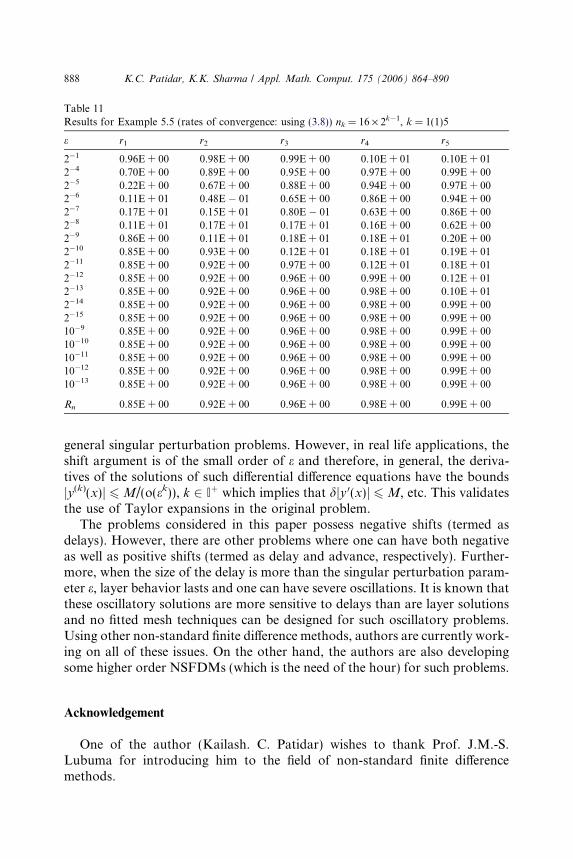
Table 11Results for Example 5.5 (rates of convergence: using (3.8)) nk = 16 · 2k�1, k = 1(1)5
e r1 r2 r3 r4 r5
2�1 0.96E + 00 0.98E + 00 0.99E + 00 0.10E + 01 0.10E + 012�4 0.70E + 00 0.89E + 00 0.95E + 00 0.97E + 00 0.99E + 002�5 0.22E + 00 0.67E + 00 0.88E + 00 0.94E + 00 0.97E + 002�6 0.11E + 01 0.48E � 01 0.65E + 00 0.86E + 00 0.94E + 002�7 0.17E + 01 0.15E + 01 0.80E � 01 0.63E + 00 0.86E + 002�8 0.11E + 01 0.17E + 01 0.17E + 01 0.16E + 00 0.62E + 002�9 0.86E + 00 0.11E + 01 0.18E + 01 0.18E + 01 0.20E + 002�10 0.85E + 00 0.93E + 00 0.12E + 01 0.18E + 01 0.19E + 012�11 0.85E + 00 0.92E + 00 0.97E + 00 0.12E + 01 0.18E + 012�12 0.85E + 00 0.92E + 00 0.96E + 00 0.99E + 00 0.12E + 012�13 0.85E + 00 0.92E + 00 0.96E + 00 0.98E + 00 0.10E + 012�14 0.85E + 00 0.92E + 00 0.96E + 00 0.98E + 00 0.99E + 002�15 0.85E + 00 0.92E + 00 0.96E + 00 0.98E + 00 0.99E + 0010�9 0.85E + 00 0.92E + 00 0.96E + 00 0.98E + 00 0.99E + 0010�10 0.85E + 00 0.92E + 00 0.96E + 00 0.98E + 00 0.99E + 0010�11 0.85E + 00 0.92E + 00 0.96E + 00 0.98E + 00 0.99E + 0010�12 0.85E + 00 0.92E + 00 0.96E + 00 0.98E + 00 0.99E + 0010�13 0.85E + 00 0.92E + 00 0.96E + 00 0.98E + 00 0.99E + 00
Rn 0.85E + 00 0.92E + 00 0.96E + 00 0.98E + 00 0.99E + 00
888 K.C. Patidar, K.K. Sharma / Appl. Math. Comput. 175 (2006) 864–890
general singular perturbation problems. However, in real life applications, theshift argument is of the small order of e and therefore, in general, the deriva-tives of the solutions of such differential difference equations have the boundsjy(k)(x)j 6M/(o(ek)), k 2 Iþ which implies that djy 0(x)j 6M, etc. This validatesthe use of Taylor expansions in the original problem.
The problems considered in this paper possess negative shifts (termed asdelays). However, there are other problems where one can have both negativeas well as positive shifts (termed as delay and advance, respectively). Further-more, when the size of the delay is more than the singular perturbation param-eter e, layer behavior lasts and one can have severe oscillations. It is known thatthese oscillatory solutions are more sensitive to delays than are layer solutionsand no fitted mesh techniques can be designed for such oscillatory problems.Using other non-standard finite difference methods, authors are currently work-ing on all of these issues. On the other hand, the authors are also developingsome higher order NSFDMs (which is the need of the hour) for such problems.
Acknowledgement
One of the author (Kailash. C. Patidar) wishes to thank Prof. J.M.-S.Lubuma for introducing him to the field of non-standard finite differencemethods.
K.C. Patidar, K.K. Sharma / Appl. Math. Comput. 175 (2006) 864–890 889
References
[1] R. Anguelov, J.M.-S. Lubuma, Contributions to the mathematics of the nonstandard finitedifference method and applications, Numerical Methods for Partial Differential Equations 17(2001) 518–543.
[2] R. Anguelov, J.M.-S. Lubuma, S.K. Mahudu, Qualitatively stable finite difference schemes foradvection–reaction equations, Journal of Computational and Applied Mathematics 158 (1)(2003) 19–30.
[3] R. Anguelov, J.M.-S. Lubuma, Nonstandard finite difference method by nonlocal approxi-mation, Mathematics and Computers in Simulation 61 (3–6) (2003) 465–475.
[4] J.B. Cole, S. Banerjee, Applications of nonstandard finite difference models to computationalelectromagnetics, Journal of Difference Equations and Applications 9 (12) (2003) 1099–1112.
[5] M.W. Derstine, H.M. Gibbs, D.L. Kaplan, Bifurcation gap in a hybrid optical system, PhysicsReview A 26 (1982) 3720–3722.
[6] E.P. Doolan, J.J.H. Miller, W.H.A. Schilders, Uniform Numerical Methods for Problems withInitial and Boundary Layer, Boole Press, Dublin, 1980.
[7] H. Al-Kahby, F. Dannan, S. Elaydi, Non-standard discretization methods for some biologicalmodels, in: R.E. Mickens (Ed.), Applications of Nonstandard Finite Difference Schemes,World Scientific, Singapore, 2000, pp. 155–180.
[8] F.B. Hilderbrand, Finite Difference Equations and Simulations, Prentice-Hall, Engle-woodCliffs, NJ, 1968.
[9] M.K. Jain, Numerical Solution of Differential Equations, John Wiley & Sons, New York, 1984.[10] P.M. Jordan, A nonstandard finite difference scheme for nonlinear heat transfer in a thin finite
rod, Journal of Difference Equations and Applications 9 (11) (2003) 1015–1021.[11] C.G. Lange, R.M. Miura, Singular perturbation analysis of boundary-value problems for
differential difference equations.V. Small shifts with layer behavior, SIAM Journal on AppliedMathematics 54 (1994) 249–272.
[12] C.G. Lange, R.M. Miura, Singular perturbation analysis of boundary-value problems fordifferential difference equations. VI. Small shifts with rapid oscillations, SIAM Journal onApplied Mathematics 54 (1994) 273–283.
[13] A. Longtin, J. Milton, Complex oscillations in the human pupil light reflex with mixed anddelayed feedback, Mathematical Biosciences 90 (1988) 183–199.
[14] M.C. Mackey, L. Glass, Oscillations and chaos in physiological control systems, Science 197(1977) 287–289.
[15] R.E. Mickens, Nonstandard Finite Difference Models of Differential Equations, WorldScientific, Singapore, 1994.
[16] R.E. Mickens (Ed.), Applications of Nonstandard Finite Difference Schemes, World Scientific,Singapore, 2000.
[17] R.E. Mickens, A.B. Gumel, Numerical study of a non-standard finite difference scheme for thevan der pol equation, Journal of Sound and Vibration 250 (5) (2002) 955–963.
[18] R.E. Mickens, A.B. Gumel, Construction and analysis of a non-standard finite difference schemefor the Burgers–Fisher equation, Journal of Sound and Vibration 257 (4) (2002) 791–797.
[19] R.E. Mickens, A non-standard finite difference scheme for the equations modelling stellarstructure, Journal of Sound and Vibration 265 (5) (2003) 1116–1120.
[20] J.J.H. Miller, E. O�Riordan, G.I. Shishkin, Fitted Numerical Methods for SingularPerturbation Problems, World Scientific, Singapore, 1996.
[21] A.R. Mitchell, D.F. Griffiths, Finite Difference Methods in Partial Differential Equations,Wiley, New York, 1980.
[22] S.M. Moghadas, M.E. Alexander, B.D. Corbett, A.B. Gumel, A positivity-preservingMickens-type discretization of an epidemic model, Journal of Difference Equations andApplications 9 (11) (2003) 1037–1051.

890 K.C. Patidar, K.K. Sharma / Appl. Math. Comput. 175 (2006) 864–890
[23] S.M. Moghadas, M.E. Alexander, B.D. Corbett, A non-standard numerical scheme for ageneralized Gause-type predator–prey model, Physica D: Nonlinear Phenomena 188 (1-2)(2004) 134–151.
[24] K.C. Patidar, On the use of non-standard finite difference methods, Journal of DifferenceEquations and Applications, in press.
[25] J.I. Ramos, C.M. Garcıa-Lopez, Nonstandard finite difference equations for ODEs and 1-DPDEs based on piecewise linearization, Applied Mathematics and Computation 86 (1) (1997)11–36.
[26] R.J. Spiteri, M.C. MacLachlan, An efficient non-standard finite difference scheme for an ionicmodel of cardiac action potentials, Journal of Difference Equations and Applications 9 (12)(2003) 1069–1081.
[27] R.B. Stein, A theoretical analysis of neuronal variability, Biophysical Journal 5 (1965) 173–194.
[28] R.B. Stein, Some models of neuronal variability, Biophysical Journal 7 (1967) 37–68.[29] M. Wazewska-Czyzewska, A. Lasota, Mathematical models of the red cell system, Mat. Stos. 6
(1976) 25–40.