European Journal of Control (2010)1:54–69

# 2010 EUCADOI:10.3166/EJC.16.54–69

H2=H1 Control of Singularly Perturbed Systems: The State

Feedback Case

Kanti B. Datta1,�, Aparajita RaiChaudhuri2,��

1Department of Electrical Engineering, IIT Kharagpur, Kharagpur-721302, India;2Department of Electrical Engineering, B.E.S.U, Howrah-711103, India

The design of a mixed H2=H1 linear state variable

feedback (LSVF) suboptimal controller for a continuous-

time singularly perturbed system using reduced order

slow and fast subsystems is described. It is shown that

the designed controller based on reduced order models

and the corresponding performance index (PI) both

are Oð�Þ close to those synthesized using the full order

system. Each of the three algebraic matrix equations to

be sequentially solved in our study, contains three

matrix variables coupled in them. Two of these

equations can be made independent of the matrix gain

variable under mild restrictions.

Keywords: Singularly perturbed systems, H2=H1

control, optimal control, robust control

1. Introduction

In robust control problemwith parameter uncertainties

to have a reasonable performance level guaranteed, we

define performance measures as H2 or H1 norm cri-

teria. For parameter uncertainties one can at best

minimize one of themkeeping a constraint on the other.

Such approaches are referred to as constrained optimal

control problem (COCP). In H1-COCP, an H2 per-

formance is minimized simultaneously imposing a

constraint on the H1 norm. These problems go by the

name of mixed H2=H1 control. There exists a number

of different formulations of these latter problems. To

understand this, letTziwi, i ¼ 0; 1 denote the closed-loop

transfer functions from the exogenous input wi to the

controlled output zi. The H1-COCP is to find an

internally stabilizing controller which minimizes

kTz0w0k2 while maintaining kTz1w1

k1 < �: A controller

that solves this problem will ensure that the closed-loop

system is robustly stable to all finite gain stable per-

turbations �, interconnected to the system by

w1 ¼ �z1, such that k�k � 1=� where the k�k is the

induced operator norm obtained by taking L2½0;1Þnorms on w1 and z1. Currently no analytical solution to

this problem is available. However, the convex pro-

gramming approach of Boyd et al. [3] offers a feasible

numerical alternative for the solvability of H1-COCP.

A closely related problem was studied by Bernstein and

Haddad, in which they have considered w ¼ w0 ¼ w1

and established necessary conditions to minimize an

upper bound of kTz0wk2 subject to the constraint

kTz1wk1 < �: These conditions are later found to be

sufficient also by Yeh et al. [22], [2]. In the equalized

case, z0 ¼ z1, w0 ¼ w1 the problem of Bernstein and

Haddad is equivalent to themaximum entropy problem

investigated byMustafa andGlover [16]. In this case the

optimal controller is the so-called central controller.

In [7], another version of mixed H2=H1 problem is

studied for a system in which the signal w0 is assumed

to be white noise while w1 is a signal with bounded

power. This problem is equivalent to the dual of the

problem in [2].

*Correspondence to: K.B. Datta, E-mail: attadbitnak@yahoo.com**E-mail: sgaparajita@gmail.com

Received 9 July 2008; Accepted 26 August 2009Recommended by J.C. Geromel, E.F. Camacho

Rotea and Khargonekar [20] parameterized the

set of all internally stabilizing LSVF controllers K

(in such cases we call K is admissible) for the

unconstrainedH2-optimal control problem: inf kTz0w0f

ðKÞk2 : K is admissibleg, and derived necessary and

sufficient conditions such that a controller in the above

set also satisfies kTz1w1k1 < 1. These conditions

involve two algebraic Riccati equations and a coupling

condition. On the other hand, Khargonekar and

Rotea [11] focused on the mixed H2=H1 control

problem as formulated by Bernstein and Haddad [2]

and developed a design procedure for a static state-

feedback gain controller by solving a finite-dimen-

sional convex programming problem over a bounded

set of real matrices.

In [14], a state-feedback mixed H2=H1 control

problem is solved via the solution of an associated

Nash game involving the two cost functions with w0 ¼w1 ¼ w and leads to a central state-feedback controller

as inminimumentropy problem ofMustafa andGlover

[16]. Moreover, in [14], it is assumed that the worst case

disturbance w�ðt; xÞ can be generated by a linear,

memoryless feedback strategy which is slightly restrict-

ive but necessary for a unique Nash equilibrium.

On the other hand, the H2-COCP for continuous

systems is excellently addressed in [8, 9, 19].

Based on a Riccati equation approach, Petersen and

McFarlane [19] developed a construction procedure

for an optimal state feedback quadratic guaranteed

cost control. Using the quadratic stabilizability

framework, Garcia et al. [8] studied theH2 guaranteed

cost control for singularly perturbed uncertain sys-

tems and showed how to construct a quadratic sta-

bilizing composite control minimizing an upper bound

on the H2 norm of a certain transfer matrix.

The high frequency phenomena and parameter

variations in a dynamical system can be handled by

considering a singularly perturbed uncertain model of

Kokotovic et al. [12]. In this case, the slow subsystem

takes into account low frequency uncertainties and the

fast dynamics describes the neglected high-frequency

part of the system. Important investigations into un-

certain singularly perturbed systems are made in [4, 5,

15]. In [5], the control of uncertain systems which

exhibit time-scale separation is studied by translating

the problem into a two-frequency scale decomposition

for H1 disk problems. A robust stabilizing composite

control for singularly perturbed systems with time-

varying uncertainties is developed in [4]. In [5], a

composite controller is designed with the objective to

guarantee stability of the uncertain system by the

construction of an appropriate Lyapunov function. In

these papers, no optimality properties have been

associated with these controllers. In [17, 18], optim-

ality through an H1 criterion is proposed under per-

fect state measurements for a well-knownmodel. In [1]

it is established that the mixed H2=H1 control prob-

lem is completely solved if a condition on the rank of

the input matrix is assumed. In [6], H1-COCP is

studied for a discrete singularly perturbed system and

a mixed H2=H1 suboptimal linear state-feedback

controller is designed based on reduced order models.

From above it appears thatH2=H1 optimization for a

continuous-time singularly perturbed system still

remains an unsolved problem.

The objective of the present paper is, therefore, to

design a mixed H2=H1 linear state variable feedback

(LSVF) suboptimal controller for a continuous-time

singularly perturbed system based on reduced order

slow and fast subsystems which are defined inde-

pendent of the small singular perturbation parameter

�. For the full-order case, our problem is to minimize

an upper bound of kTz0wk2 subject to the constraint

kTz1wk1 < � as in [2]. In the discrete-time case, see [6],

a weaker version of this problem is solved by assuming

that z0 ¼ z1, giving rise to a LSVF central controller.

The slow and fast subsystems introduced for our pres-

ent investigation are considerably different from those

used in quadratic regulator theory of Kokotovic et al.

[12]. The designed slow and fast LSVF gains are com-

bined to produce a composite feedback for the full-

order system with an approach quite different from

Kokotovic et al. [12]. The composite feedback gain and

also the corresponding quadratic performance index

(PI) are Oð�Þ close to the gain designed with full-order

system and the corresponding value of PI.

2. The Full-Order Problem

The singularly perturbed systems under consideration

is described by,

_xðtÞ ¼ AxðtÞ þ B1wðtÞ þ B2uðtÞ; ð1Þ

z1ðtÞ ¼ C1xðtÞ þD1uðtÞ ð2Þ

z0ðtÞ ¼ S1xðtÞ þ S2uðtÞ ð3Þ

xðtÞ ¼x1ðtÞ

x2ðtÞ

� �; A ¼

A11 A12

A21

�

A22

�

24

35;

B1 ¼B11

B21

�

24

35;B2 ¼

B12

B22

�

24

35; C1 ¼ ½C11 C12�

S1 ¼ ½S11 S12�;

and � > 0 is a small parameter, x1 2 Rn1 , x2 2 Rn2 ,

w 2 Rm1 is the disturbance input withE½wðtÞw0ðtÞ� ¼ I,

H2=H1 Control of SPS with LSVF 55

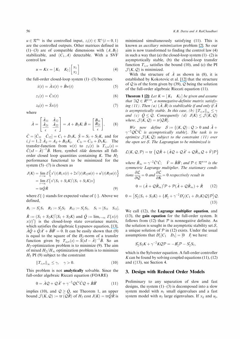
u 2 Rm2 is the controlled input, ziðtÞ 2 Rriði ¼ 0; 1Þare the controlled outputs. Other matrices defined in

(1)–(3) are of compatible dimensions with ðA;B2Þstabilizable, and ðC1;AÞ detectable. With a SVF

control law

u ¼ Kx ¼ K1 K2½ �x1x2

� �ð4Þ

the full-order closed-loop system (1)–(3) becomes

_xðtÞ ¼ ~AxðtÞ þ ~BwðtÞ ð5Þ

z1ðtÞ ¼ ~CxðtÞ ð6Þ

z0ðtÞ ¼ ~SxðtÞ ð7Þ

where

~A ¼

~A11~A12

~A21

�

~A22

�

24

35 ¼ Aþ B2K; ~B ¼

B11B21

�

" #; ð8Þ

~C ¼ ½ ~C11~C12� ¼ C1 þD1K, ~S ¼ S1 þ S2K, and for

i; j ¼ 1; 2 ~Aij ¼ Aij þ Bi2Kj; ~C1i ¼ C1i þD1Ki: The

transfer-function from wðtÞ to z1ðtÞ is Tz1wðsÞ ¼~CðsI� ~AÞ�1 ~B: Here, symbol tilde denotes all full-

order closed loop quantities containing K. The H2

performance functional to be minimized for the

system (5)–(7) is chosen as

JðKÞ ¼ limt!1

E

nx0ðtÞR1xðtÞ þ 2x0ðtÞR12uðtÞ þ u0ðtÞR2uðtÞ

o¼ lim

t!1E x0ðS1 þ S2KÞ

0ðS1 þ S2KÞx� �

¼ tr ~Q ~R ð9Þ

where Ef�g stands for expected value of f�g. Above we

defined,

R1 :¼ S01S1 R2 :¼ S0

2S2 R12 :¼ S01S2; S1 ¼ ½S11 S12�;

~R :¼ ðS1 þ S2KÞ0ðS1 þ S2KÞ and ~Q :¼ limt!1 E xðtÞf

xðtÞ0g is the closed-loop state covariance matrix,

which satisfies the algebraic Lyapunov equation, [13],~A ~Qþ ~Q ~A0 þ ~B ~B0 ¼ 0: It can be easily shown that (9)

is equal to the square of the H2-norm of a transfer

function given by Tz0wðsÞ ¼~SðsI� ~AÞ�1 ~B: So an

H2-optimization problem is to minimize (9). The aim

of mixedH2=H1 optimization problem is to minimize

H2 PI (9) subject to the constraint

kTz1wk1 � �; � > 0: ð10Þ

This problem is not analytically solvable. Since the

full-order algebraic Riccati equation (FOARE)

0 ¼ ~AQþQ ~A0 þ ��2Q ~C0 ~CQþ ~B ~B0 ð11Þ

implies (10), and Q � ~Q, see Theorem 1, an upper

bound J ðK;QÞ :¼ tr ðQ ~RÞ of H2 cost JðKÞ ¼ tr ~Q ~R is

minimized simultaneously satisfying (11). This is

known as auxiliary minimization problem [2]. So our

aim is now transformed to finding the control law (4)

in such a way that (a) the closed-loop system (1)–(2) is

asymptotically stable, (b) the closed-loop transfer

function Tz1w satisfies the bound (10), and (c) the PI

J ðK;QÞ is minimized.

With the structure of ~A as shown in (8), it is

established by Kokotovic et al. [12] that the structure

of Q is of the form given by (39),Q being the solution

of the full-order algebraic Riccati equation (11).

Theorem 1 [2]: Let K ¼ K1 K2½ � be given and assume

that 9Q 2 Rn�n, a nonnegative-definite matrix satisfy-

ing (11). Then (a) ð ~A; ~BÞ is stabilizable if and only if ~A

is asymptotically stable. In this case, (b) kTz1wk1 � �and (c) ~Q � Q: Consequently (d) JðKÞ � J ðK;QÞwhere, J ðK;QÞ ¼ tr½Q ~R�.

We now define S :¼ fðK;QÞ : Q > 0 and ~Aþ��2Q~C0 ~C is asymptotically stable}. The task is to

optimize J ðK;QÞ subject to the constraint (11) over

the open set S. The Lagrangian to be minimized is

LðK;Q;PÞ ¼ tr Q ~Rþ ð ~AQþQ ~A0 þQ ~R1Qþ ~VÞP� �

where ~R1 ¼ ��2 ~C0 ~C; ~V ¼ ~B ~B0; and P 2 Rn�n is the

symmetric Lagrange multiplier. The stationary condi-

tions@L

@Q¼ 0 and

@L

@K¼ 0 respectively result in

0 ¼ ð ~AþQ ~R1Þ0P þ Pð ~AþQ ~R1Þ þ ~R ð12Þ

0 ¼ S02ðS1 þ S2KÞ þ fB0

2 þ ��2D01ðC1 þD1KÞQgP

� �Q:

ð13Þ

We call (12), the Lagrange multiplier equation, and

(13), the gain equation for the full-order system. It

follows from (12) that P is nonnegative definite. As

the solution is sought in the asymptotic stability set S,

a unique solution of P in (12) exists. Under the usual

assumptions that D01½C1 D1� ¼ ½0 I� we have:

S02S2Kþ ��2KQP ¼ �B0

2P � S02S1;

which is the Sylvester equation. A full-order controller

K can be found by solving coupled equations (11), (12)

and ({13), see Section 4.

3. Design with Reduced Order Models

Preliminary to any separation of slow and fast

designs, the system (1)–(3) is decomposed into a slow

system model with n1 small eigenvalues and a fast

system model with n2 large eigenvalues. If xij and uj,

56 K.B. Datta and A RaiChaudhuri

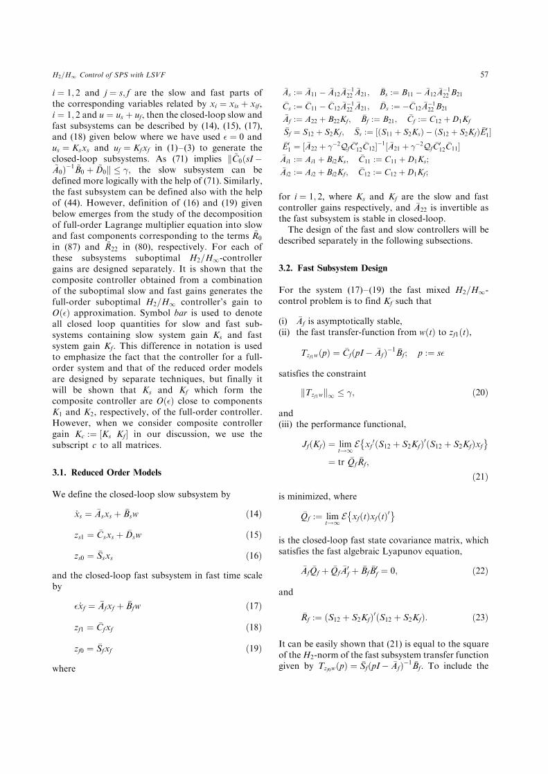
i ¼ 1; 2 and j ¼ s; f are the slow and fast parts of

the corresponding variables related by xi ¼ xis þ xif,

i ¼ 1; 2 and u ¼ us þ uf, then the closed-loop slow and

fast subsystems can be described by (14), (15), (17),

and (18) given below where we have used � ¼ 0 and

us ¼ Ksxs and uf ¼ Kfxf in (1)–(3) to generate the

closed-loop subsystems. As (71) implies k ~C0ðsI�~A0Þ

�1 ~B0 þ ~D0k � �; the slow subsystem can be

defined more logically with the help of (71). Similarly,

the fast subsystem can be defined also with the help

of (44). However, definition of (16) and (19) given

below emerges from the study of the decomposition

of full-order Lagrange multiplier equation into slow

and fast components corresponding to the terms ~R0

in (87) and ~R22 in (80), respectively. For each of

these subsystems suboptimal H2=H1-controller

gains are designed separately. It is shown that the

composite controller obtained from a combination

of the suboptimal slow and fast gains generates the

full-order suboptimal H2=H1 controller’s gain to

Oð�Þ approximation. Symbol bar is used to denote

all closed loop quantities for slow and fast sub-

systems containing slow system gain Ks and fast

system gain Kf. This difference in notation is used

to emphasize the fact that the controller for a full-

order system and that of the reduced order models

are designed by separate techniques, but finally it

will be shown that Ks and Kf which form the

composite controller are Oð�Þ close to components

K1 and K2, respectively, of the full-order controller.

However, when we consider composite controller

gain Kc :¼ ½Ks Kf� in our discussion, we use the

subscript c to all matrices.

3.1. Reduced Order Models

We define the closed-loop slow subsystem by

_xs ¼ �Asxs þ �Bsw ð14Þ

zs1 ¼ �Csxs þ �Dsw ð15Þ

zs0 ¼ �Ssxs ð16Þ

and the closed-loop fast subsystem in fast time scale

by

� _xf ¼ �Afxf þ �Bfw ð17Þ

zf1 ¼ �Cfxf ð18Þ

zf0 ¼ �Sfxf ð19Þ

where

�As :¼ �A11 � �A12�A�122

�A21; �Bs :¼ B11 � �A12�A�122 B21

�Cs :¼ �C11 � �C12�A�122

�A21; �Ds :¼ � �C12�A�122 B21

�Af :¼ A22 þ B22Kf; �Bf :¼ B21; �Cf :¼ C12 þD1Kf

�Sf ¼ S12 þ S2Kf; �Ss :¼ ½ðS11 þ S2KsÞ � ðS12 þ S2KfÞ �E01�

�E01 ¼ ½ �A22 þ ��2Qf

�C012�C12�

�1½ �A21 þ ��2Qf�C012�C11�

�Ai1 :¼ Ai1 þ Bi2Ks; �C11 :¼ C11 þD1Ks;

�Ai2 :¼ Ai2 þ Bi2Kf; �C12 :¼ C12 þD1Kf;

for i ¼ 1; 2, where Ks and Kf are the slow and fast

controller gains respectively, and �A22 is invertible as

the fast subsystem is stable in closed-loop.

The design of the fast and slow controllers will be

described separately in the following subsections.

3.2. Fast Subsystem Design

For the system (17)–(19) the fast mixed H2=H1-

control problem is to find Kf such that

(i) �Af is asymptotically stable,

(ii) the fast transfer-function from wðtÞ to zf1ðtÞ,

Tzf1wðpÞ ¼�CfðpI� �AfÞ

�1 �Bf; p :¼ s�

satisfies the constraint

kTzf1wk1 � �; ð20Þ

and

(iii) the performance functional,

JfðKfÞ ¼ limt!1

E xf0ðS12 þ S2KfÞ

0ðS12 þ S2KfÞxf� �

¼ tr �Qf�Rf;

ð21Þ

is minimized, where

�Qf :¼ limt!1

E xfðtÞxfðtÞ0� �

is the closed-loop fast state covariance matrix, which

satisfies the fast algebraic Lyapunov equation,

�Af�Qf þ �Qf

�A0f þ

�Bf�B0f ¼ 0; ð22Þ

and

�Rf :¼ ðS12 þ S2KfÞ0ðS12 þ S2KfÞ: ð23Þ

It can be easily shown that (21) is equal to the square

of theH2-norm of the fast subsystem transfer function

given by Tzf0wðpÞ ¼�SfðpI� �AfÞ

�1 �Bf. To include the

H2=H1 Control of SPS with LSVF 57

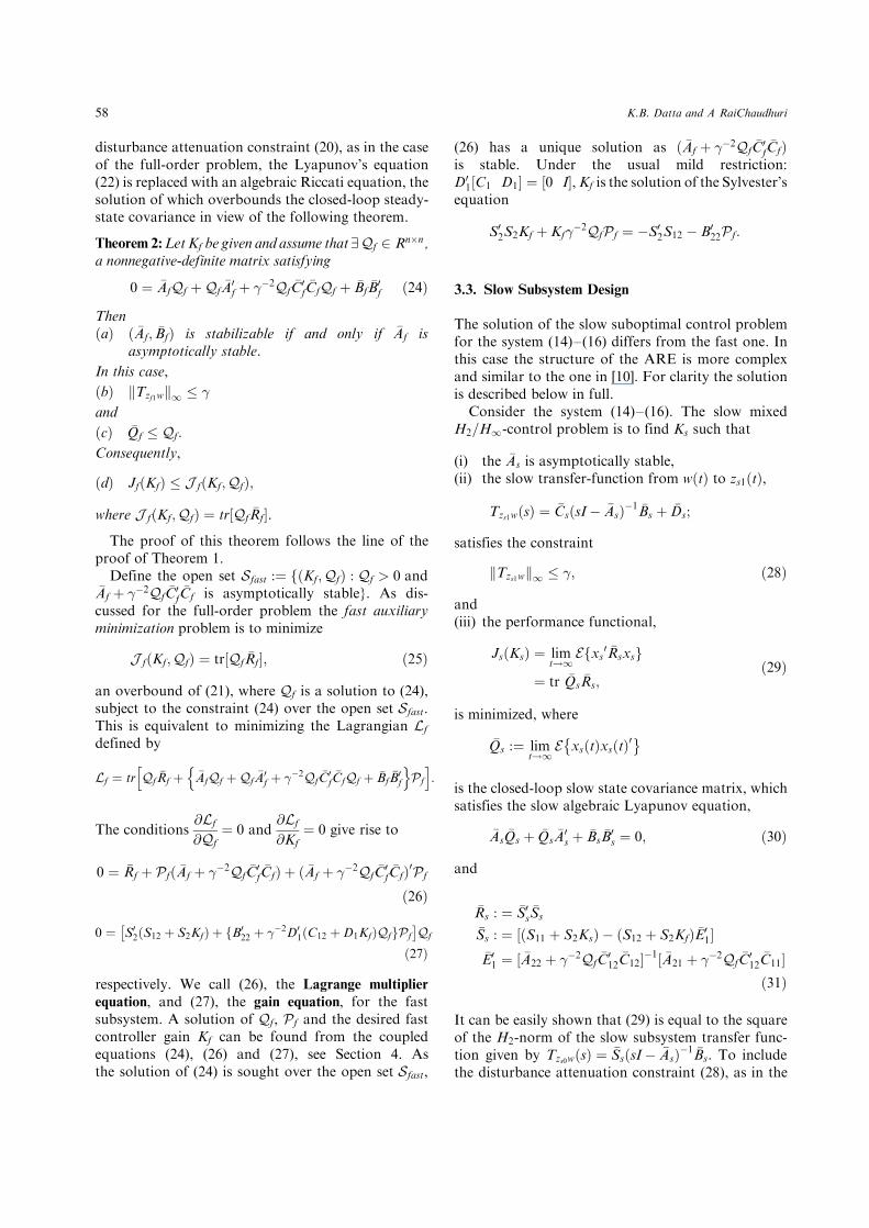
disturbance attenuation constraint (20), as in the case

of the full-order problem, the Lyapunov’s equation

(22) is replaced with an algebraic Riccati equation, the

solution of which overbounds the closed-loop steady-

state covariance in view of the following theorem.

Theorem 2:Let Kf be given and assume that9Qf 2 Rn�n,

a nonnegative-definite matrix satisfying

0 ¼ �AfQf þQf�A0f þ ��2Qf

�C0f�CfQf þ �Bf

�B0f ð24Þ

Then

ðaÞ ð �Af; �BfÞ is stabilizable if and only if �Af is

asymptotically stable.

In this case,

ðbÞ kTzf1wk1 � �

and

ðcÞ �Qf � Qf:

Consequently,

ðdÞ JfðKfÞ � J fðKf;QfÞ;

where J fðKf;QfÞ ¼ tr½Qf�Rf�.

The proof of this theorem follows the line of the

proof of Theorem 1.

Define the open set Sfast :¼ fðKf;QfÞ : Qf > 0 and�Af þ ��2Qf

�C0f�Cf is asymptotically stable}. As dis-

cussed for the full-order problem the fast auxiliary

minimization problem is to minimize

J fðKf;QfÞ ¼ tr½Qf�Rf�; ð25Þ

an overbound of (21), where Qf is a solution to (24),

subject to the constraint (24) over the open set Sfast.

This is equivalent to minimizing the Lagrangian Lf

defined by

Lf ¼ tr Qf�Rf þ �AfQf þQf

�A0f þ ��2Qf

�C0f�CfQf þ �Bf

�B0f

n oPf

h i:

The conditions@Lf

@Qf

¼ 0 and@Lf

@Kf

¼ 0 give rise to

0 ¼ �Rf þ Pfð �Af þ ��2Qf�C0f�CfÞ þ ð �Af þ ��2Qf

�C0f�CfÞ

0Pf

ð26Þ

0 ¼ S02ðS12 þ S2KfÞ þ fB0

22 þ ��2D01ðC12 þD1KfÞQfgPf

� �Qf

ð27Þ

respectively. We call (26), the Lagrange multiplier

equation, and (27), the gain equation, for the fast

subsystem. A solution of Qf, Pf and the desired fast

controller gain Kf can be found from the coupled

equations (24), (26) and (27), see Section 4. As

the solution of (24) is sought over the open set Sfast,

(26) has a unique solution as ð �Af þ ��2Qf�C0f�CfÞ

is stable. Under the usual mild restriction:

D01½C1 D1� ¼ ½0 I�,Kf is the solution of the Sylvester’s

equation

S02S2Kf þ Kf�

�2QfPf ¼ �S02S12 � B0

22Pf:

3.3. Slow Subsystem Design

The solution of the slow suboptimal control problem

for the system (14)–(16) differs from the fast one. In

this case the structure of the ARE is more complex

and similar to the one in [10]. For clarity the solution

is described below in full.

Consider the system (14)–(16). The slow mixed

H2=H1-control problem is to find Ks such that

(i) the �As is asymptotically stable,

(ii) the slow transfer-function from wðtÞ to zs1ðtÞ,

Tzs1wðsÞ ¼�CsðsI� �AsÞ

�1 �Bs þ �Ds;

satisfies the constraint

kTzs1wk1 � �; ð28Þ

and

(iii) the performance functional,

JsðKsÞ ¼ limt!1

E xs0 �Rsxsf g

¼ tr �Qs�Rs;

ð29Þ

is minimized, where

�Qs :¼ limt!1

E xsðtÞxsðtÞ0� �

is the closed-loop slow state covariance matrix, which

satisfies the slow algebraic Lyapunov equation,

�As�Qs þ �Qs

�A0s þ

�Bs�B0s ¼ 0; ð30Þ

and

�Rs : ¼ �S0s�Ss

�Ss : ¼ ½ðS11 þ S2KsÞ � ðS12 þ S2KfÞ �E01�

�E01 ¼ ½ �A22 þ ��2Qf

�C012�C12�

�1½ �A21 þ ��2Qf�C012�C11�

ð31Þ

It can be easily shown that (29) is equal to the square

of the H2-norm of the slow subsystem transfer func-

tion given by Tzs0wðsÞ ¼�SsðsI� �AsÞ

�1 �Bs. To include

the disturbance attenuation constraint (28), as in the

58 K.B. Datta and A RaiChaudhuri

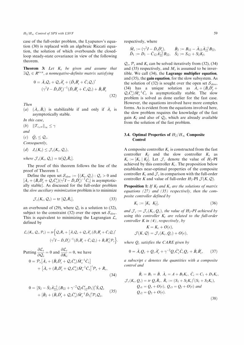
case of the full-order problem, the Lyapunov’s equa-

tion (30) is replaced with an algebraic Riccati equa-

tion, the solution of which overbounds the closed-

loop steady-state covariance in view of the following

theorem.

Theorem 3: Let Ks be given and assume that

9Qs 2 Rn�n, a nonnegative-definite matrix satisfying

0 ¼ �AsQs þQs�A0s þ ð �Ds

�B0s þ

�CsQsÞ0

ð�2I� �Ds�D0sÞ

�1ð �Ds�B0s þ

�CsQsÞ þ �Bs�B0s

ð32Þ

Then

ðaÞ ð �As; �BsÞ is stabilizable if and only if �As is

asymptotically stable.

In this case,

ðbÞ kTzs1wk1 � �

and

ðcÞ �Qs � Qs:

Consequently,

ðdÞ JsðKsÞ � J sðKs;QsÞ;

where J sðKs;QsÞ ¼ tr½Qs�Rs�.

The proof of this theorem follows the line of the

proof of Theorem 1.

Define the open set Sslow :¼ fðKs;QsÞ : Qs > 0 and

½ �As þ ð �Bs�D0s þQs

�C0sÞð�

2I� �Ds�D0sÞ

�1 �Cs� is asymptotic-

ally stable}. As discussed for the full-order problem

the slow auxiliary minimization problem is to minimize

J sðKs;QsÞ ¼ tr Qs�Rs½ �; ð33Þ

an overbound of (29), where Qs is a solution to (32),

subject to the constraint (32) over the open set Sslow.

This is equivalent to minimizing the Lagrangian Ls

defined by

LsðKs;Qs;PsÞ ¼ trnQs

�Rs þ��AsQs þQs

�A0s:ð

�Ds�B0s þ

�CsQsÞ0

ð�2I� �Ds�D0sÞ

�1ð �Ds�B0s þ

�CsQsÞ þ �Bs�B0s

�Ps

o:

Putting@Ls

@Qs

¼ 0 and@Ls

@Ks

¼ 0, we have

0 ¼ Ps�As þ ð �Bs

�D0s þQs

�C0sÞ

�M�1s

�Cs

� �þ �As þ ð �Bs

�D0s þQs

�C0sÞ

�M�1s

�Cs

� �0Ps þ �Rs;

ð34Þ

0 ¼ ½S2 � �S2�A�122�ðB22 þ ��2Qf

�C012D1Þ�

0 �SsQs

þ ½ �B2 þ ð �Bs�D0s þQs

�C0sÞ

�M�1s

�D1�0PsQs;

ð35Þ

respectively, where

�Ms :¼ ð�2I� �Ds�D0sÞ;

�B2 :¼ B12 � �A12�A�122 B22;

�D1 :¼ D1 � �C12�A�122 B22; �S2 :¼ S12 þ S2Kf;

Qs, Ps and Ks can be solved iteratively from (32), (34)

and (35) respectively, and Ms is assumed to be inver-

tible. We call (34), the Lagrange multiplier equation,

and (35), the gain equation, for the slow subsystem. As

the solution of (32) is sought over the open set Sslow,

(34) has a unique solution as �As þ ð �Bs�D0s þ

Qs�C0sÞ

�M�1s

�Cs is asymptotically stable. The slow

problem is solved as done earlier for the fast case.

However, the equations involved have more complex

forms. As is evident from the equations involved here,

the slow problem requires the knowledge of the fast

gain Kf and also of Qf, which are already available

from the solution of the fast problem.

3.4. Optimal Properties of H2=H1 Composite

Control

A composite controller Kc is constructed from the fast

controller Kf and the slow controller Ks as

Kc :¼ ½Ks j Kf�. Let J c denote the value of H2-PI

achieved by this controller Kc. The proposition below

establishes near-optimal properties of the composite

controllerKc and J c in comparison with the full-order

controller K and value of full-order H2-PI J ðK;QÞ.

Proposition 1: If Kf and Ks are the solutions of matrix

equations (27) and (35) respectively, then the com-

posite controller defined by

Kc :¼ ½Ks Kf�; ð36Þ

and J c :¼ J cðKc;QcÞ, the value of H2-PI achieved by

using this controller Kc are related to the full-order

controller K in (4), respectively, by

K ¼ Kc þOð�Þ;

J ðK;QÞ ¼ J cðKc;QcÞ þOð�Þ;

where Qc satisfies the CARE given by

0 ¼ ~AcQc þQc~A0c þ ��2Qc

~C0c~CcQc þ ~Bc

~B0c; ð37Þ

a subscript c denotes the quantities with a composite

control and

~Bc ¼ B1 ¼ ~B; ~Ac ¼ Aþ B2Kc; ~Cc ¼ C1 þD1Kc;

J cðKc;QcÞ ¼ tr Qc~Rc; ~Rc :¼ ðS1 þ S2KcÞ

0ðS1 þ S2KcÞ;

Qc1 ¼ Qs þOð�Þ; Qc3 ¼ Qf þOð�Þ and

Qc2 ¼ Q2 þOð�Þ:

ð38Þ

H2=H1 Control of SPS with LSVF 59

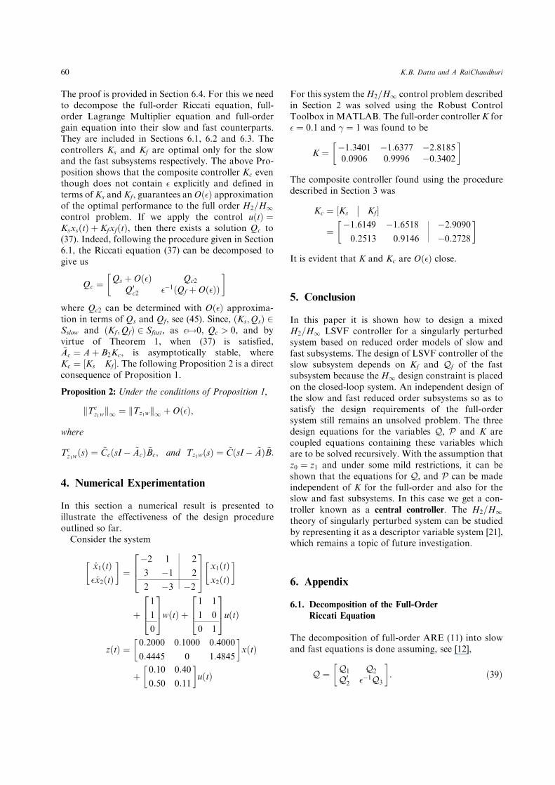
The proof is provided in Section 6.4. For this we need

to decompose the full-order Riccati equation, full-

order Lagrange Multiplier equation and full-order

gain equation into their slow and fast counterparts.

They are included in Sections 6.1, 6.2 and 6.3. The

controllers Ks and Kf are optimal only for the slow

and the fast subsystems respectively. The above Pro-

position shows that the composite controller Kc even

though does not contain � explicitly and defined in

terms ofKs and Kf, guarantees anOð�Þ approximation

of the optimal performance to the full order H2=H1

control problem. If we apply the control uðtÞ ¼KsxsðtÞ þ KfxfðtÞ, then there exists a solution Qc to

(37). Indeed, following the procedure given in Section

6.1, the Riccati equation (37) can be decomposed to

give us

Qc ¼Qs þOð�Þ Qc2

Q0c2 ��1ðQf þOð�ÞÞ

� �

where Qc2 can be determined with Oð�Þ approxima-

tion in terms of Qs and Qf, see (45). Since, ðKs;QsÞ 2Sslow and ðKf;QfÞ 2 Sfast, as � 7!0; Qc > 0, and by

virtue of Theorem 1, when (37) is satisfied,~Ac ¼ Aþ B2Kc, is asymptotically stable, where

Kc ¼ ½Ks Kf�. The following Proposition 2 is a direct

consequence of Proposition 1.

Proposition 2: Under the conditions of Proposition 1,

kTcz1w

k1 ¼ kTz1wk1 þOð�Þ;

where

Tcz1w

ðsÞ ¼ ~CcðsI� ~AcÞ ~Bc; and Tz1wðsÞ ¼~CðsI� ~AÞ ~B:

4. Numerical Experimentation

In this section a numerical result is presented to

illustrate the effectiveness of the design procedure

outlined so far.

Consider the system

_x1ðtÞ

� _x2ðtÞ

� �¼

�2 1 2

3 �1 2

2 �3 �2

264

375 x1ðtÞ

x2ðtÞ

� �

þ

1

1

0

264

375wðtÞ þ

1 1

1 0

0 1

264

375uðtÞ

zðtÞ ¼0:2000 0:1000 0:4000

0:4445 0 1:4845

� �xðtÞ

þ0:10 0:40

0:50 0:11

� �uðtÞ

For this system theH2=H1 control problem described

in Section 2 was solved using the Robust Control

Toolbox in MATLAB. The full-order controllerK for

� ¼ 0:1 and � ¼ 1 was found to be

K ¼�1:3401 �1:6377 �2:81850:0906 0:9996 �0:3402

� �

The composite controller found using the procedure

described in Section 3 was

Kc ¼ ½Ks Kf�

¼�1:6149 �1:6518 �2:9090

0:2513 0:9146 �0:2728

� �

It is evident that K and Kc are Oð�Þ close.

5. Conclusion

In this paper it is shown how to design a mixed

H2=H1 LSVF controller for a singularly perturbed

system based on reduced order models of slow and

fast subsystems. The design of LSVF controller of the

slow subsystem depends on Kf and Qf of the fast

subsystem because the H1 design constraint is placed

on the closed-loop system. An independent design of

the slow and fast reduced order subsystems so as to

satisfy the design requirements of the full-order

system still remains an unsolved problem. The three

design equations for the variables Q, P and K are

coupled equations containing these variables which

are to be solved recursively. With the assumption that

z0 ¼ z1 and under some mild restrictions, it can be

shown that the equations for Q, and P can be made

independent of K for the full-order and also for the

slow and fast subsystems. In this case we get a con-

troller known as a central controller. The H2=H1

theory of singularly perturbed system can be studied

by representing it as a descriptor variable system [21],

which remains a topic of future investigation.

6. Appendix

6.1. Decomposition of the Full-Order

Riccati Equation

The decomposition of full-order ARE (11) into slow

and fast equations is done assuming, see [12],

Q ¼Q1 Q2

Q02 ��1Q3

� �: ð39Þ

60 K.B. Datta and A RaiChaudhuri

Substituting from (39), the terms of (11) are now

simplified separately as shown below:

~AQ ¼~A11

~A12

��1 ~A21 ��1 ~A22

" #Q1 Q2

Q02 ��1Q3

� �

¼~A11Q1 þ ~A12Q

02

~A11Q2 þ ��1 ~A12Q3

��1ð ~A21Q1 þ ~A22Q02Þ ��2ð� ~A21Q2 þ ~A22Q3Þ

" #

ð40Þ

~B ~B0 ¼B11

��1B21

� �B011 ��1B0

21

� �

¼B11B

011 ��1B11B

021

��1B21B011 ��2B21B

021

" # ð41Þ

��2Q ~C0 ~CQ ¼ ��2Q1 Q2

Q02 ��1Q3

� �~C011

~C012

" #

~C11~C12

� � Q1 Q2

Q02 ��1Q3

� �

¼ ��2 Q1~C011 þQ2

~C012

Q02~C011 þ ��1Q3

~C012

" #

½ ~C11Q1 þ ~C12Q02

~C11Q2 þ ��1 ~C12Q3�

Writing the elements of (11) in the form of separate

equations with Oð�Þ approximation we have

ðiÞ 0 ¼ ð ~A11 þ ��2Q2~C012~C11ÞQ1

þQ1ð ~A11 þ ��2Q2~C012~C11Þ

0

þ ~A12Q02 þQ2

~A012 þ ��2½Q1

~C011~C11Q1

þQ2~C012~C12Q

02� þ B11B

011

ð42Þ

ðiiÞ 0 ¼ ~A12Q3 þQ1~A021 þQ2

~A022 þ B11B

021

þ ��2ðQ1~C011 þQ2

~C012Þ

~C12Q3 þOð�Þð43Þ

ðiiiÞ 0 ¼ ~A22Q3 þQ3~A022 þ B21B

021

þ ��2Q3~C012~C12Q3 þOð�Þ

ð44Þ

Afterwards (44) will turn out to be the algebraic

Riccati equation for designing suboptimal H2=H1

controller for the fast subsystem to Oð�Þ approxima-

tion. However, in the process of decomposition of

Lagrange’s multiplier equation and the gain equation

into slow-fast components, we will need some of the

intermediate steps in the process of derivation of (71).

With this hindsight, we take pain to give a sketch of

the derivation of (71) for the benefit of the readers.

From (43), solving for Q2 we get

�Q2 ¼ Q1E1 þ E2 þOð�Þ; ð45Þ

where

E1 :¼ ð ~A021 þ ��2 ~C0

11~C12Q3Þ ~A

0�1

22� ð46Þ

E2 :¼ ð ~A12Q3 þ B11B021Þ

~A0�1

22� ð47Þ

~A22� :¼ ~A22 þ ��2Q3~C012~C12

¼ ðIþ ��2Q3~C012~C12

~A�122 Þ

~A22:ð48Þ

Substituting (45) forQ2 in (42) and simplifying, we are

led to an equation with Q2 removed as

0 ¼ AQ1 þQ1A0 þQ1UQ1 þ B0BþOð�Þ ð49Þ

where

A :¼ ~A11 � ~A12E01 � ��2E2

~C012~C11

þ ��2E2~C012~C12E

01

ð50Þ

U ¼ ��2C0C ð51Þ

B0B :¼ � ~A12E02 � E2

~A012 þ B11B

011

þ ��2E2~C012~C12E

02

ð52Þ

C :¼ ~C11 � ~C12E01 ð53Þ

Making use of (46), we have

C0 ¼ ~C011½I� ��2 ~C12Q3

~A0�122�

~C012� �

~A021~A0�1

22�~C012:

Defining the bracketed term by H and simplifying

with the help of (48) we have

H :¼ I� ��2 ~C12Q3~A0�122�

~C012

¼ I� ��2 ~C12Q3~A0�122 ðIþ ��2 ~C0

12~C12Q3

~A0�122 Þ�1Þ�1 ~C0

12

¼ ðIþ ��2 ~C12Q3~A0�122

~C012Þ

�1

ð54Þ

It is not difficult to show that

~A�122� :¼ ð ~A22 þ ��2Q3

~C012~C12Þ

�1

¼ ~A�122 ½I� ��2Q3

~C012~C12ð ~A22 þ ��2Q3

~C012~C12Þ

�1�

¼ ~A�122 ½I� ��2Q3

~C012H

0 ~C12~A�122 �

ð55Þ

H2=H1 Control of SPS with LSVF 61

~C11Q1 þ ~C12Q02 ¼ CQ1 � ~C12E

02 ð56Þ

In view of this simplification in (54), C0 becomes

C0 ¼ ~C011½Iþ ��2 ~C12Q3

~A0�122

~C012�

�1

� ~A021~A0�1

22 ½Iþ ��2 ~C012~C12Q3

~A0�122 ��1 ~C 0

12

¼ ~C00H;

where

~C0 :¼ ~C11 � ~C12~A�122

~A21

With this simplification, U takes the form

U ¼ ��2 ~C00HH0 ~C0:

Now, with the help of (44) we can write

ðHH0Þ�1 ¼ ½Iþ ��2 ~C12~A�122 Q3

~C012�½Iþ ��2 ~C12Q3

~A0�122

~C012�

¼ Iþ ��2 ~C12~A�122 ½

~A22Q3 þQ3~A022

þ ��2Q3~C012~C12Q3� ~A

0�122

~C012

¼ I� ��2 ~C12~A�122 B21B

021~A0�122

~C012;

¼ I� ��2 ~D0~D00

¼: ��2 ~M0

ð57Þ

where

~D0 :¼ � ~C12~A�122 B21; ~M0 :¼ �2I� ~D0

~D00: ð58Þ

This gives us

U ¼ ��2C0C ¼ ~C00~M�10

~C0 ð59Þ

To simplify the expression for A we will use the fol-

lowing relations which are direct outcomes of (46),

(48) and (54):

E1 ¼ ð ~A021 þ ��2 ~C0

11~C12Q3 � ��2E1

~C012~C12Q3Þ ~A

0�1

22

ð60Þ

~C12~A�1

22� ¼ H0 ~C12~A�1

22 ð61Þ

~C12Q3~A0�1

22� ¼ H ~C12Q3~A0�1

22 ð62Þ

Substituting the expressions from (47)–(48), (60)

in (50) and simplifying with (44), (53) and (61), we

obtain

A ¼ ~A11 � ~A12~A�122 ð

~A21 þ ��2Q3~C012~C11

� ��2Q3~C012~C12E

01Þ � ��2E2

~C012ð

~C11 � ~C12E01Þ

¼ ~A0 � ��2ð ~A12~A�122 Q3 þ E2g ~C

012C

¼ ~A0 � ��2½ ~A12~A�122 Q3 þ ð ~A12Q3 þ B11B

021Þ

ð ~A022 þ ��2 ~C0

12~C12Q3Þ

�1� ~C012C

¼ ~A0 � ��2½ ~A12~A�122 fQ3ð ~A

022 þ ��2 ~C0

12~C12Q3Þ

þ ~A22Q3g þ B11B021�ð

~A022 þ ��2 ~C0

12~C12Q3Þ

�1 ~C012C

¼ ~A0 þ ��2 ~B0~D00HC

¼ ~A0 þ ~B0~D00~M�10

~C0

ð63Þ

where

~A0 :¼ ~A11 � ~A12~A�122

~A21;

~B0 :¼ ~B11 � ~A12~A�122

~B21; ~C0 :¼ ~C11 � ~C12~A�122

~A21

ð64Þ

To simplify B0B, we write E2 with the help of (47) and

(48) in the form

E2 ¼ ð ~A12Q3 þ B11B021 � ��2E2

~C012~C12Q3Þ ~A

0�122

ð65Þ

Inserting this expression for E2 in (52)

B0B ¼ B11B011 �

~A12~A�122 ð

~A12Q3 þ B11B021

� ��2E2~C012~C12Q3Þ

0 � ð ~A12Q3 þ B11B021

� ��2E2~C012~C12Q3Þ ~A

0�122

~A012 þ ��2E2

~C012~C12E

02

ð66Þ

With the help of (44), the second and fifth terms in

(66) can be written as

� ~A12~A�122 ðQ3

~A022 þ

~A22Q3Þ ~A0�122

~A012

¼ ~A12~A�122 ðB21B

021 þ ��2Q3

~C012~C12Q3Þ ~A

0�122

~A012

Hence,

B0B ¼ B11B011 �

~A12~A�122 ðB11B

021Þ

0 � ðB11B021Þ

~A0�122

~A012

þ ð ~A12~A�122 B21Þð ~A12

~A�122 B21Þ

0

þ ��2 ~A12~A�122 ðE2

~C012~C12Q3Þ

0

þ ��2ðE2~C012~C12Q3Þ ~A

0�122

~A012

þ ��2E2~C012~C12E

02~A12

~A�122 Q3

~C012~C12Q3

~A0�122

~A012

¼ ðB11 � ~A12~A�122 B21ÞðB11 � ~A12

~A�122 B21Þ

0

þ ��2ðE2 þ ~A12~A�122 Q3Þ ~C

012~C12ðE2 þ ~A12

~A�122 Q3Þ

ð67Þ

62 K.B. Datta and A RaiChaudhuri

Now,

E2 þ ~A12~A�122 Q3

¼ ð ~A12Q3 þ B11B021Þð

~A22 þ ��2 ~C012~C12Q3Þ

�1 ~A12~A�122 Q3

¼ ½ ~A12~A�122 f

~A22Q3 þQ3ð ~A0�122 þ ��2 ~C0

12~C12Q3Þg

þ B11B021�ð

~A22 þ ��2 ~C012~C12Q3Þ

�1

¼ ~A12~A�122 B11B

021 þ B11B

021Þð

~A22 þ ��2 ~C012~C12Q3Þ

�1

¼ ~B0B021ð

~A22 þ ��2 ~C012~C12Q3Þ

�1

ð68Þ

So,

ðE2 þ ~A12~A�122 Q3Þ ~C

012

¼ ~B0B021~A0�122

~C012ðIþ ��2 ~C12Q3

~A0�122

~C012Þ

�1

¼ � ~B0~D00H

ð69Þ

Consequently, we have,

B0B ¼ ~B0~B00 þ ��2 ~B0

~D00HH0 ~D0

~B00

¼ ~B0½Iþ ~D00~M�10

~D0� ~B00

ð70Þ

We shall now replace (63)–(70) in (49) to obtain the

following Riccati equation in Q1 which has now been

made free from Q3. However, it contains K1 and K2.

0 ¼ ð ~A0 þ ~B0~D00~M�10

~C0ÞQ1 þQ1ð ~A0 þ ~B0~D00~M�10

~C0Þ0

þQ1~C00~M�10

~C0Q1 þ ~B0½Iþ ~D00~M�10

~D0� ~B00 þOð�Þ;

which after minor simplification finally reduces to

0 ¼ ~A0Q1 þQ1~A00 þ ð ~D0

~B00 þ

~C0Q1Þ0 ~M�1

0

ð ~D0~B00 þ

~C0Q1Þ þ ~B0~B00 þOð�Þ:

ð71Þ

6.2. Decomposition of the Lagrange Multiplier

Equation

The Lagrange multiplier equation (12), which is in fact

a Lyapunov equation, is reproduced below

0 ¼ ð ~AþQ ~R1Þ0P þ Pð ~AþQ ~R1Þ þ ~R; ð72Þ

and has now to be decomposed into slow and fast

subsystem components as done for algebraic Riccati

equation (11) in the last section. It should be noted

that all through Oð�Þ approximation is used wherever

necessary. The structure of P is assumed to be of the

form, see [12],

P ¼P1 �P2

�P02 �P3

� �:

Proceeding with simplification of the terms in (72) we

have successively,

where we define,

A11 :¼ ~A11 þ ��2ðQ1~C011 þQ2

~C012Þ

~C11

A21 :¼ ~A21 þ ��2Q3~C012~C11;

A12 :¼ ~A12 þ ��2ðQ1~C011 þQ2

~C012Þ

~C12;

A22 :¼ ~A22 þ ��2Q3~C012~C12;

ð74Þ

so that,

Pð ~AþQ ~R1Þ ¼P1 �P2

�P02 �P3

� �A11 A12

��1A21 ��1A22

� �

¼P1A11 þ P2A21 P1A12 þ P2A22

P3A21 þOð�Þ P3A22 þOð�Þ

� �:

ð75Þ

Also,

~R ¼ ðS1 þ S2KÞ0ðS1 þ S2KÞ

¼ S11 þ S2K1 S12 þ S2K2½ �0

S11 þ S2K1 S12 þ S2K2½ �

¼~S01~S1

~S01~S2

~S02~S1

~S02~S2

" #

¼:~R11

~R12

~R0

12~R22

" #ð76Þ

where

~S1 :¼ ðS11 þ S2K1Þ; ~S2 :¼ ðS12 þ S2K2Þ;

~R11 :¼ ~S01~S1; ~R12 :¼ ~S0

1~S2;

~R0

12 :¼~S02~S1; ~R22 :¼ ~S0

2~S2:

ð77Þ

ð ~AþQ ~R1Þ ¼~A11 þ ��2ðQ1

~C011 þQ2

~C012Þ

~C11~A12 þ ��2ðQ1

~C011 þQ2

~C012Þ

~C12

��1ð ~A21 þ ��2Q3~C012~C11Þ þOð1Þ ��1ð ~A22 þ ��2Q3

~C012~C12Þ þOð1Þ

� �: ð73Þ

H2=H1 Control of SPS with LSVF 63

Using (75) and (76) in (72), the elements in the

resultant matrix are respectively:

0 ¼ ~R11 þ P1A11 þ P2A21 þA011P1 þA

021P

02 þOð�Þ

ð78Þ

0 ¼ ~R12 þ P1A12 þ P2A22 þA021P3 þOð�Þ

ð79Þ

0 ¼ ~R22 þ P3A22 þA022P3 þOð�Þ ð80Þ

It will be shown later that equation (80) is similar to

the Lagrange multiplier equation for a properly

defined fast subsystem of (1)–(3). We will now use

(79) and (80) to eliminate P2 and P3 from (78).

Solving (79) for P2 we get,

P2 ¼ P1X1 þ X2 þOð�Þ; ð81Þ

where

X1 ¼ �A12A�122 ; X2 ¼ �ð ~R12 þA

021P3ÞA

�122 ð82Þ

Substituting P2 from (81) into (78) gives us

0 ¼ ~R11 þ P1A11 þA011P1 þ ðP1X1 þ X2ÞA21

þA021ðP1X1 þ X2Þ

0 þOð�Þ

¼ ~S01~S1 þ P1A0 þA

00P1 þ X2A21 þ ðX2A21Þ

0

ð83Þ

where

A0 :¼ A11 þ X1A21:

Equation (83) contains P3 in X2 but P2 is eliminated.

The terms containing P3 may be simplified as shown

below. We have using (80),

~S01~S1 þ X2A21 þA

021X

02

¼ ~S01~S1 � ð~S0

1~S2 þA

021P3ÞA

�122 A21

�A021A

0�122 ð~S0

2~S1 þ P3A21Þ

¼ ~S01~S1 � ~S0

1~S2A

�122 A21 �A

021A

0�122

~S02~S1

þA021A

0�122

~S02~S2A

�122 A21

¼ ð~S1 � ~S2A�122 A21Þ

0ð~S1 � ~S2A�122 A21Þ:

With the above simplification (83) transforms to

0 ¼ P1A0 þA0P1 þ ð~S1 � ~S2A�122 A21Þ

0

ð~S1 � ~S2A�122 A21Þ þOð�Þ;

ð84Þ

in which P2 and P3 have been eliminated. We

will now remove Q2 and Q3 from A0 in (84)

using (43)–(44). Comparing (46) and (74), it is obvious

that

E01 ¼ A

�122 A21

So, making substitutions from (45) and (50) we

have

A0 ¼ A11 �A12A�122 A21

¼ ~A11 þ ��2ðQ1~C011 þQ2

~C012Þ

~C11

� f ~A12 þ ��2ðQ1~C011 þQ2

~C012Þ

~C12gE01

¼ ~A11 � ~A12E01 þ ��2ðQ1

~C011 þQ2

~C012Þð

~C11 � ~C12E01Þ

¼ ~A11 � ~A12E01 � ��2E2

~C012ð

~C11 � ~C12E01Þ

þ ��2Q1ð ~C11 � ~C12E01Þ

0ð ~C11 � ~C12E01Þ

¼ Aþ ��2Q1C0C;

ð85Þ

in which A and C are given in (63) and (53), see also

(59).

Putting (85) in (84), the equation for P1 is

0 ¼ P1ðAþ ��2Q1C0CÞ þ ðAþ ��2Q1C

0CÞ0P1

þ ð~S1 � ~S2A�122 A21Þ

0ð~S1 � ~S2A�122 A21Þ þOð�Þ;

ð86Þ

which after substitution from (63) for A and from (59)

for C0C finally reduces to

0 ¼ P1½ ~A0 þ ð ~B0~D00 þQ1

~C00Þ

~M�10

~C0�

þ ½ ~A0 þ ð ~B0~D00 þQ1

~C00Þ

~M�10

~C0�0P1

þ ~R0 þOð�Þ;

ð87Þ

where ~R0 ¼ ð~S1 � ~S2A�122 A21Þ

0ð~S1 � ~S2A�122 A21Þ,which

is similar to �Rs in which K1;K2 and Q3 are now

replaced with Ks;Kf and Qf respectively. The above

equation will be shown in a subsequent section to

represent the Lagrange multiplier equation of a

properly defined slow subsystem of (1)–(3).

6.3. Decomposition of the Gain Equation

The full-order controller gain K satisfies

0 ¼ S02ðS1 þ S2KÞQþ ½B0

2 þ ��2D01ðC1 þD1KÞQ�PQ;

ð88Þ

which will be decomposed into two parts, one

approximating K1, the controller’s gain for slow

64 K.B. Datta and A RaiChaudhuri

subsystem and the other K2, the controller’s gain for

fast subsystem. Simplifying the individual terms of

(88) we have,

ðIÞ S02S1Q ¼ S0

2 S11 S12½ �Q1 Q2

Q02 ��1Q3

� �

¼ S02 S11Q1 þ S12Q

02 S11Q2 þ

1

�S12Q3�

�

ðIIÞ S02S2KQ ¼ S0

2S2 K1Q1 þ K2Q02

�K1Q2 þ ��1K2Q3

�

ðIIIÞ B02PQ ¼ B0

12

1

�B022

� �P1 �P2

�P02 �P3

� �Q1 Q2

Q02 ��1Q3

� �¼ B0

12P1Q1 þ B022ðP

02Q1 þ P3Q

02Þ

�þOð�Þ ��1B0

22P3Q3 þOð1Þ�

ðIVÞ ��2D01ðC1 þD1KÞQPQ

¼ ��2 D01f

~C11Q1P1Q1 þ ~C12ðQ02P1Q1

�þQ3P

02Q1 þQ3P3Q

02Þg;

��1D01~C12Q3P3Q3 þOð1Þ�

From the terms (I)–(IV) simplified above, assembling

together ð1; 2Þ elements, we have

0 ¼ ½S02ðS12 þ S2K2Þ þ fB0

22 þ ��2D01ðC12

þD1K2ÞQ3gP3�Q3 þOð�Þ;ð89Þ

which turns out to be the controller’s gain for the fast

subsystem described by (27) to Oð�Þ approximation.

On the other hand, the (1,1)-elements lead to

0 ¼ S02ðS11Q1 þ S12Q

02Þ þ S0

2S2ðK1Q1 þ K2Q02Þ

þ ðB022P3 þ ��2D0

1~C12Q3P3ÞQ

02

þ ½B012 þ ��2D0

1ð~C11Q1 þ ~C12Q

02Þ�P1Q1

þ ðB022 þ ��2D0

1~C12Q3ÞP

02Q1 þOð�Þ;

ð90Þ

which will be shown to be the controller’s gain for the

slow subsystem described by (35) to Oð�Þ approx-

imation. Now, the various terms of (90) is rewritten

by setting

�Q2 ¼ Q1E1 þ E2 þOð�Þ;

P2 ¼ P1X1 þ X2 þOð�Þ

as defined in (45) and (81) in the following way toOð�Þapproximation:

ðAÞ S02ðS11Q1 þ S12Q

02Þ þ S0

2S2ðK1Q1 þ K2Q02Þ

ðBÞ ðB022P3 þ ��2D0

1~C12Q3P3ÞQ

02

¼ �ðB022P3 þ ��2D0

1~C12Q3P3ÞE

01Q1

� ðB022P3 þ ��2D0

1~C12Q3P3ÞE

02

ðCÞ ½B012 þ ��2D0

1ð~C11Q1 þ ~C12Q

02Þ�P1Q1

¼ B012P1Q1 þ ��2D0

1CQ1P1Q1

� ��2D01~C12E

02P1Q1

ðDÞ ðB022 þ ��2D0

1~C12Q3ÞP

02Q1

¼ ðB022 þ ��2D0

1~C12Q3ÞX

01P1Q1

þ ðB022 þ ��2D0

1~C12Q3ÞX

02Q1;

where in (C) we have used C ¼ ~C11 � ~C12E01 from (53).

IfQ is struck out from the right hand side of (88), then

the coefficient of Q02 in (A) and all terms contained in

(B) will not appear in the (1,1) term. These terms are,

in fact, eliminated if (89) is valid after Q3 is removed.

However, in the coefficient of Q02 in (A) and terms in

(B) will cause a simplification while simplifying coef-

ficients of Q1,P1Q1, and Q1P1Q1. The various terms

in (A), (B), (C), and (D) are now simplified consider-

ing the coefficients of Q1,P1Q1, and Q1P1Q1 suc-

cessively.

6.3.1. (I) Coefficients of Q1

Stacking together the terms in (A), (B), and the coef-

ficient of Q1 in (D), we have

S02~S1Q1 � S0

2~S2ðE

01Q1 þ E0

2Þ

� ðB022P3 þ ��2D0

1~C12Q3P3ÞE

01Q1

� ðB022P3 þ ��2D0

1~C12Q3P3ÞE

02

� ðB022 þ ��2D0

1~C12Q3Þ ~A

0�122�½

~S02~S1 þ P3A21�Q1

Taking into account (80) : 0 ¼ ~R22 þ P3A22 þA

022P3 þOð�Þ we see that the coefficient of E0

2 is Oð�Þ,and hence the above expression becomes

H2=H1 Control of SPS with LSVF 65

S02ð~S1 � ~S2E

01ÞQ1 � ðB 0

22 þ ��2D01~C12Q3Þ

½P3A�122 A21 þA

0�122 ð~S0

2~S1 þ P3A21Þ�Q1

¼ S02ð~S1 � ~S2E

01ÞQ1 � ðB 0

22 þ ��2D01~C12Q3Þ

½A0�122 ðA0

22P3 þ P3A22ÞA�122 A21 þA

0�122

~S02~S1�Q1

¼ ½S 02 � ðB 0

22 þ ��2D01~C12Q3ÞA

0�122

~S02�ð

~S1 � ~S2E01ÞQ1

ð91Þ

6.3.2. (II) Coefficients of P1Q1

The terms in the coefficient of P1Q1 are

B 012 � ��2D0

1~C12E

02 þ ðB0

22 þ ��2D01~C12Q3ÞX

01:

Now, observing that ~A11� ¼ A22, substituting for X1

from (82) and for Q2 from (45), simplifying with (53),

(61), (62) and (55) we have,

B 012 þ B 0

22X01

¼ B012 � B 0

22~A0�122�½

~A012�

�2 ~C 012f

~C11Q1 � ~C12ðE01Q1 þ E 0

2Þg�

¼ B012 � B 0

22ðI� ��2 ~A0�122

~C 012H

~C12Q3Þ ~A0�122

~A012

� ��2B 022~A0�122�

~C 012ðH

0 ~C 00Q1 � ~C12E

02Þ

The coefficient of Q1 above is, in fact, a coefficient of

Q1P1Q1 , and so transferring it to be included in (III),

we have

B 012 þ B 0

22X01 � coefficient of Q1

¼ ~B02 þ ��2B0

22~A0�122

~C012H

~C12Q3~A0�122

~A012

þ ��2B022~A0�122

~C012HH0 ~C12

~A�122 ðQ3

~A012 þ B21B

011Þ

¼ ~B02 þ ��2B0

22~A0�122

~C012M

�10

~C12~A�122

½ ~A22Q3 þ ��2Q3~C012~C12Q3 þQ3

~A022�

~A0�122

~A012

þ ��2B022~A0�122

~C012HH0 ~C12

~A�122 B21B

011

¼ ~B02 þ B0

22~A0�122

~C012M

�10

~C12~A�122 B21ðB

011 � B0

11~A0�122

~A012Þ

¼ ~B02 � B0

22~A0�122

~C012M

�10

~D0~B00;

where ~B2 ¼ B12 � ~A12~A�122 B22. The remaining terms

are

��2D01~C12ðQ3X

01 � E 0

2Þ

¼ ��2D 01~C12½Q3

~A0�122�f

~A012 þ ��2 ~C0

12ð~C11Q1

þ ~C12Q02Þg þ E 0

2�

¼ ��2D01~C12½Q3

~A0�122�f

~A012 þ ��2 ~C0

12ð~C11 � ~C12E

01ÞQ1

� ��2 ~C012~C12E

02g þ E 0

2�

So

��2D01~C12ðQ3X

01 � E 0

2Þ � coefficient of Q1

¼ ��2D01~C12½Q3

~A0�122�

~A012 � f��2Q3

~A0�122�

~C 012~C12 � IgE 0

2�

¼ ��2D01½H

~C12Q3~A0�122

~A012 � f��2H ~C12Q3

~A0�122

~C 012~C12

� ~C12g ~A0�122�ðQ3

~A012 þ B21B

011Þ�

¼ ��2D01½H

~C12Q3~A0�122

~A012 þHH0 ~A�1

22 ðQ3~A012 þ B21B

011Þ�

¼ ��2D01HH0½ðIþ ��2 ~C12

~A�122 Q3

~C12~C012Þ

~C12Q3~A0�122

~A012 þ

~C12~A�122 Q3

~A012 þ

~C12~A�122 B21B

011�

¼ ��2D01HH0½ ~C12

~A�122 ð

~A22Q3 þ ��2Q3~C 012~C12Q3

þQ3~A022Þ

~A0�122

~A012 þ

~C12~A�122 B21B

011�

¼ ���2D01HH0 ~C12

~A�122 B21ðB

011 � B0

21~A0�122

~A 012Þ

¼ D01M

�10

~D0~B00

ð92Þ

6.3.3. (III) Coefficients of Q1P1Q1

Simplification of coefficients of Q1P1Q1 appending

those obtained from (II) gives us

��2½D01ðI�

~C12Q3~A0�122�

~C012Þ � B0

22~A0�122�

~C012�C

¼ ��2½D01ðI�H ~C12Q3

~A0�122

~C012Þ � B0

22~A0�122

~C012H�C

¼ ��2½D01H� B0

22~A0�122

~C012H�C

¼ ~D01M

�10

~C0

ð93Þ

Hence, combining the terms in (91)–(93), the (1,1)-

element in the full-order gain equation, with~S0 ¼ ð~S1 � ~S2E

01Þ, becomes

0 ¼ ½S2 � ~S2A�122 ðB22 þ ��2Q3

~C012D1Þ�

0 ~S0Q1

þ ½ ~B2 þ ð ~B0~D00 þQ1

~C00ÞM

�10

~D1�0P1Q1 þOð�Þ;

ð94Þ

which turns out to be the controller’s gain for the slow

subsystem described by (35) to Oð�Þ approximation.

6.4. Proof of Proposition 1

The set of equations (44), (87) and (89) respectively

closely approximate the fast system equations (24),

(26) and (27). Hence it follows that

K2 ¼ Kf þOð�Þ:

Similarly the set of equations (71), (80) and (94)

respectively are close approximations of (32), (34) and

(35). So,

K1 ¼ Ks þOð�Þ:

66 K.B. Datta and A RaiChaudhuri

Hence, K ¼ Kc þOð�Þ. With the composite controller

Kc, the closed-loop system becomes

_xðtÞ ¼ ~AcxðtÞ þ ~BcwðtÞ;

z1ðtÞ ¼ ~CcxðtÞ;

where

~Ac ¼~Ac11

~Ac12

��1 ~Ac21 ��1 ~Ac22

" #

~Acij ¼ Aij þ Bi2Kcj; ~Bc ¼ B1;

~Cc ¼ ½ ~Cc11~Cc12� ¼ C1 þD1Kc; ~Cc1i ¼ C1i þD1Kci

Kc1 ¼ Ks; Kc2 ¼ Kf; ~Ac22 ¼ �Af; B21 ¼ �Bf; ~Cc12 ¼ �Cf:

Since Qc satisfies (37), proceeding as in Section 6.1

for the decomposition of ARE we have

0 ¼ ~AcsQc1 þQc1~A0cs þ ð ~Dcs

~B0cs þ

~CcsQc1Þ0

~M�1cs ð

~Dcs~B0cs þ

~CcsQc1Þ þ ~Bcs~B0cs þOð�Þ;

ð95Þ

0 ¼ ~Ac22Qc3 þQc3~A0c22 þ ��2Qc3

~C0c12

~Cc12Qc3

þ B21B021 þOð�Þ;

ð96Þ

where

~Acs :¼ ~Ac11 � ~Ac12~A�1c22

~Ac21;

~Bcs :¼ ~B11 � ~Ac12~A�1c22

~B21;

~Ccs :¼ ~Cc11 � ~Cc12~A�1c22

~Ac21

~Dcs :¼� ~Cc12~A�1c22B21;

~Mcs :¼ �2 � ~Dcs~D0cs

As ~Ac22 ¼ �Af; B21 ¼ �Bf; ~Cc12 ¼ �Cf, it follows from

(24) and (96) that Qc3 ¼ Qf þOð�Þ. Similarly, com-

paring (32) and (95) we haveQc1 ¼ Qs þOð�Þ. Also as

in Section 6.1, see (45), we can show

Qc2 ¼ Qc1E1ðKf; Qc3Þ þ E2ðKs;Kf;Qc3Þ þOð�Þ;

where E1ðKf;Qc3Þ is obtained replacing K2 and Q3 in

E1 with Kf and Qc3 and E2ðKs, Kf;Qc3Þ is obtained

replacing K1;K2;Q3 in E2 with Ks;Kf, and Qc3 using

(46) and (47) respectively. This argument shows

that Qc2 ¼ Q2 þOð�Þ. To show that J ðK;QÞ ¼J cðKc;QcÞþ Oð�Þ, we note that, since K ¼ Kc þOð�Þ,we have ~C ¼ ~Cc þOð�Þ, and ~A ¼ ~Ac þOð�Þ in view of

(5), (6) and (38). Now, (37) can be written as,

0 ¼ ð ~Ac þ ��2Qc~C0c~CcÞQc þQcð ~Ac þ ��2Qc

~C0c~CcÞ

0

� ��2QcðQc~C0c~CcÞ

0 þ ~Bc~B0c:

ð97Þ

Writing (11) in the form

0 ¼ ð ~Ac þ ��2Qc~C0c~CcÞQþQð ~Ac þ ��2Qc

~C0c~CcÞ

0

þ ��2Q ~C0c~CcQþ ~Bc

~B0c � ��2Qc

~C0c~CcQ

� ��2QðQc~C0c~CcÞ

0 þOð�Þ;

ð98Þ

we have, subtracting (98) from (97)

0 ¼ ð ~Ac þ ��2Qc~C0c~CcÞðQc �QÞ

þ ðQc �QÞð ~Ac þ ��2Qc~C0c~CcÞ

0

� ��2ðQc �QÞ ~C0c~CcðQc �QÞ þOð�Þ:

ð99Þ

By implicit function theorem, it can be shown that

Qc in (37) possesses a power series at � ¼ 0 represented

by

Qc ¼Qc1 Qc2

Q0c2 ��1Qc3

� �þX1i¼1

�i

i!

QðiÞc1 Q

ðiÞc2

QðiÞ0

c2 ��1QðiÞc3

" #

ð100Þ

and so also Q. The representation of Q is the same

as Qc but replacing Qc with Q in (100). Thus V :¼Qc �Q can be expanded as

V ¼V1 V2

V02 ��1V3

� �þX1i¼1

�i

i!

VðiÞ1 V

ðiÞ2

VðiÞ2

0��1V

ðiÞ3

" #;

ð101Þ

which satisfies in view of (99),

0 ¼ ð ~Ac þ ��2Qc~C0c~CcÞVþ Vð ~Ac þ ��2Qc

~C0c~CcÞ

0

� ��2V ~C0c~CcVþOð�Þ:

ð102Þ

Putting (101) into (102) and simplifying, the zero

order term for the (2,2) block element in the resulting

matrix equation obtained by putting � ¼ 0 becomes

0 ¼ ð ~Ac22 þ ��2Qc3~C0c12

~Cc12ÞV3

þ V3ð ~Ac22 þ ��2Qc3~C0c12

~Cc12Þ0

� ��2V3~C0c12

~Cc12V3:

ð103Þ

Assuming that ð �Af; �BfÞ is stabilizable and ð �Af; �CfÞ is

detectable, it follows from (24) that �Af þ ��2Qf�C0f�Cf is

stable. Since, �Af ¼ ~Ac22; �Cf ¼ ~Cc12 and Qc3 ¼ Qf, so~Ac22 þ ��2Qc3

~C0c12

~Cc12 is stable and ð ~Ac22; ~Cc12Þ is

detectable, which implies that the solution of the

above equation (103) gives rise to V3 ¼ 0. In view of

H2=H1 Control of SPS with LSVF 67

this, the (1,2) and (1,1) elements in (102) at � ¼ 0 are

respectively given by

0 ¼V2ð ~Ac22 þ ��2Qc3~C0c12

~Cc12Þ0

þ V1ð ~Ac21 þ ��2Qc3~C 0c12

~Cc11Þ0

0 ¼ ½ ~Ac11 þ ��2ðQc1~C 0c11 þQc2

~C 0c12Þ

~Cc11�V1

þ ½ ~Ac12 þ ��2ðQc1~C 0c11 þQc2

~C 0c12Þ

~Cc12�V02

þ V1½ ~Ac11 þ ��2ðQc1~C 0c11 þQc2

~C 0c12Þ

~Cc11�0

þ V2½ ~Ac12 þ ��2ðQc1~C 0c11 þQc2

~C 0c12Þ

~Cc12�0

� ��2½ðV1~C 0c11 þ V2

~C 0c12Þ

~Cc11V1

þ ðV1~C 0c11 þ V2

~C 0c12Þ

~Cc12V02�:

With the help of first equation eliminatingV2 from the

second equation, left coefficient of V1 becomes,

Cc ¼ ~Ac11 � ~Ac12E0c1 � ��2Ec2

~C 0c12ð

~Cc11 � ~Cc12E0c1Þ

0�

þ ��2Qc1ð ~Cc11 � ~Cc12E0c1Þ

0ð ~Cc11 � ~Cc12E0c1Þ

¼ Ac þ ��2Qc1CcC0c

¼ ~Acs þ ð ~Bcs~D0cs þQc1

~C 0csÞ

~M�1cs

~Ccs

where we have used the notations,

Ac :¼ ~Ac11 � ~Ac12E0c1 � ��2Ec2

~C0c12ð

~Cc11 � ~Cc12E0c1Þ

0

Cc :¼ ~Cc11 � ~Cc12E0c1; �Qc2 ¼ Qc1Ec1 þ Ec2 þOð�Þ;

Ec1 :¼ ð ~A0c21 þ ��2 ~C0

c11~Cc12Qc3Þð ~Ac22 þ ��2Qc3

~C0c12

~Cc12Þ0�1;

Ec2 :¼ ð ~Ac12Qc3 þ B11B021Þð

~Ac22 þ ��2Qc3~C0c12

~Cc12Þ0�1;

which follows from the observation that the decom-

position of (37) will generate similar equations as

given in Section 6.1 inserting only an additional sub-

script c in the variables. Simplifying other terms, the

(1,1) element finally becomes

0 ¼ CcV1 þ V1C0c � V1

~C0cs~M�1cs

~CcsV1:

Since Cc is stable, and ð ~Acs; ~CcsÞ is detectable, which

follow from the property of the slow-subsystem, the

solution of the above equation gives rise to V1 ¼ 0,

and consequently, V2 ¼ 0. Now, the first order term

for the (2,2) block element obtained from (101) and

(102) with V1 ¼ 0 ;V2 ¼ 0 and V3 ¼ 0 is

0 ¼ ð ~Ac22 þ ��2Qc3~C0c12

~Cc12ÞVð1Þ3

þ Vð1Þ3 ð ~Ac22 þ ��2Qc3

~C0c12

~Cc12Þ0

� ��2Vð1Þ3

~C0c12

~Cc12Vð1Þ3 þOð�Þ;

which is of the same form as (103) except for the Oð�Þ

term. Arguing similarly we have, Vð1Þ3 ¼ Oð�Þ: Thus

it is evident that V ¼ Qc �Q ¼ Oð�Þ: Hence,

J ðK;QÞ � J cðKc;QcÞ ¼ tr½ðQ�QcÞ ~B ~B0� ¼ Oð�Þ:

References

1. Blanchini F, Colaneri P, Pellegrino FA. Simultaneousperformance achievement via compensator blending.Automatica 2008; 44(1): 1–14

2. Bernstein DS, Haddad WM. LQG Control with anH1

performance bound: A Riccati equation approach.IEEE Trans Autom Control 1989; AC-34: 293–305

3. Boyd S, El Ghaoui L, Feron E, Balakrishnan V. LinearMatrix Inequalities in System and Control Theory,vol. 15. SIAM Studies in Applied Mathematics,Philadelphia, 1994

4. Chen YH, Chen JS. Robust composite control forsingularly perturbed systems with time varying uncer-tainties. J Dyn Syst Meas Control 1995; 117(4): 445–452

5. Corless M, Garofalo F, Glielmo L. New results incomposite control of singularly perturbed uncertainlinear system. Automatica 1993; 29(2): 387–400

6. Datta KB, RaiChaudhuri A.H2/H1 control of discretesingularly perturbed systems: the state feedback case.Automatica 2002; 38: 1791–1797

7. Doyle J, Zhou K, Glover K, Bodenheimer B. MixedH2

and H1 performance objectives II: Optimal Control.IEEE Trans Autom Control 1994; AC-39: 1575–1587

8. Garcia G, Daafouz J, Bernusson J. H2 guaranteed costcontrol for singularly perturbed uncertain systems.IEEE Trans Autom Control 1998; 43: 1323–1329

9. Geromel JC, Peres PLD, Souza SR.H2 guaranteed costcontrol for uncertain continuous-time linear systems.Syst Control Lett 1992; 19: 23–27

10. Haddad WM, Bernstein DS. Generalised Riccati equa-tions for the full and reduced-order mixed-normH2/H1

standard problem. Syst Control Lett 1992; 14: 185–19711. Khargonekar PP, Rotea MA. Mixed H2/H1 control:

A convex optimization approach. IEEE Trans AutomControl 1991; AC-36: 824–837

12. Kokotovic PV, Khalil HK, O’Reilly J. SingularPerturbation Methods in Control: Analysis and Design.Academic Press, 1986

13. Kwakernaak H, Sivan R. Linear Optimal controlSystems. Wiley-Interscience, 1972

14. Limebeer DJN, Anderson BDO, Handel B. A Nashgame approach to mixed H2/H1 control. IEEE TransAutom Control 1994; 39: 69–82

15. Luse DW, Khalil HK. Frequency-scale decompositionof H1 disk problems. SIAM J Control Optim 1989; 27:814–835

16. Mustafa D, Glover K.Minimum Entrophy H1 Control.Springer-Verlag, 1990

17. Pan Z, Basar T. H1-optimal control for singularlyperturbed systems-part I: Perfect state measurements.Automatica 1993; 29: 401–423

18. Pan Z, Basar T. H1-optimal control for singularlyperturbed systems-part II: Imperfect state measurements.IEEE Trans Autom Control 1994; AC-39: 280–299

68 K.B. Datta and A RaiChaudhuri

19. Petersen IR, McFarlane DC. Optimal guaranteed costcontrol and filtering for uncertain linear systems. IEEETrans Autom Control 1994; AC-39(9): 1971–1977

20. Rotea MA, Khargonekar PP. H2 optimal control withan H1 constraint: The state feedback case. Automatica1991; 27: 307–316

21. Takaba K, Katayama T.H2 output feedback control fordescriptor systems, Automatica 1998; 34(7): 841–850

22. Yeh H-H, Banda SS, Bor-Chin C. Necessary andsufficient conditions for mixed H2 and H1 optimalcontrol. IEEE Trans Autom Control 1992; AC-37(3):355–358

H2=H1 Control of SPS with LSVF 69