Modeling Polyethylene Fractionation Using the Perturbed-Chain Statistical Associating Fluid Theory...

Modeling Polyethylene Fractionation Using the Perturbed-ChainStatistical Associating Fluid Theory Equation of State

Eric L. Cheluget,*,† Costas P. Bokis,‡,§ Leigh Wardhaugh,† Chau-Chyun Chen,‡ andJohn Fisher†

NOVA Chemicals Corporation, NOVA Research & Technology Center, 2928-16 Street N.E.,Calgary, Alberta, Canada T2E 7K7, and Aspen Technology, Inc., Ten Canal Park,Cambridge, Massachusetts 02141

This paper illustrates how polymer fractionation can be characterized using the perturbed chainversion of the statistical associating fluid theory equation of state, a computationally efficientalgorithm, and pseudocomponents. We reparametrize the PC-SAFT equation of state and proposean efficient method of generating pseudocomponents to describe polydisperse polymer molecularweight distributions from the results of size exclusion chromatography analysis by numericalintegration. We perform rigorous phase equilibrium calculations to investigate the effects oftemperature, pressure, and feed composition on polyethylene fractionation. In these calculations,the polyethylene molecular weight distribution is treated as an ensemble of pseudocomponentsconsisting of chemical homologues of varying size. The simulation results are compared withplant data from an industrial solution polymerization process using cyclohexane as the solventto demonstrate the applicability of the method to an industrial situation. The results indicateversatile representation of the polymer polydispersivity as well as accurate prediction of theliquid-liquid, vapor-liquid, and fluid-liquid fractionation process.

1. Introduction

In this investigation, we examine several factorsinfluencing the phase behavior of polyethylene (PE)produced by the solution process. This process is mainlyused to manufacture high-density and linear low-densitypolyethylene (HDPE and LLDPE, respectively). In poly-olefin solution polymerization processes, ethylene ispolymerized in a solvent medium such as cyclohexane.1,2

The monomer, comonomer, and catalyst are dissolvedin solvent and simultaneously injected into the reactor,where polymerization takes place under adiabatic con-ditions. Downstream of the reactor, the process streamis heated and discharged through a pressure let-downvalve into a vapor-liquid flash unit. Prior to thepressure let-down, the polymer-containing process streamtemperature sometimes exceeds its lower critical solu-tion temperature3 (LCST) value, resulting in the forma-tion of two liquid-like phases, between which thepolymer is fractionated. One of the phases is rich inpolymer, while the other is mostly solvent. If thetemperature is a few degrees above the critical temper-ature of the solvent, then the solvent-rich phase issupercritical, and the solubility of polymer in this phaseis a function of pressure.4 This phase separation phe-nomenon might be undesirable because the phasecontaining most of the polymer usually has a highviscosity, which might cause difficulties in controllingthe process. This type of LCST-driven liquid-liquidphase separation has been experimentally characterizedfor several solvents in the laboratory.5-7 The thermo-

dynamic driving force for the phase separation in thesesystems is the difference between the thermal expansionof the solvent and polymer as the solvent approachesits critical point, the so-called free volume effect.8

In the vapor-liquid flash separator unit operatingbelow the critical point of the solvent, most of theunreacted ethylene and comonomer, such as 1-buteneor 1-octene, as well as a significant portion of thesolvent, leave as vapor. The liquid stream leaving thisunit is a concentrated solution of polymer in solvent,with a small amount of monomer and comonomer.Depending on the operating conditions of this unit, low-molecular-weight oligomers of the polymer might leavewith the vapor stream. This happens because, atintermediate and high pressures, polymer componentsat the low end of the molecular weight distribution(MWD) curve are appreciably soluble in the gaseoussolvent and are extracted from the resin product in theliquid.1 This fractionation might or might not be desir-able, depending on the product being produced; at anyrate, it is advantageous for process engineers to identifythe degree of fractionation at a given temperature andpressure. Whereas recent calculations utilizing theSanchez-Lacombe equation of state9 have identified theexistence and mapped the boundaries of a three-phaseliquid-liquid-vapor (VLL) coexistence region in similarsystems containing polydisperse polyethylene,10 solvent,and some residual monomer, this phenomenon, whichis restricted to a fairly narrow pressure range, is notinvestigated in this study and will be the subject offuture calculations. This is because the investigation ofthis important region of the phase diagram requiresmultiphase equilibrium calculations involving a mini-mum of three simultaneously present phases. A typicalphase diagram for a quasibinary polydisperse polymer-solvent system with a small amount of ethylene isshown in Figure 1. The locations of the LCST curve aswell as the VLL, LL, and VL regions are shown in the

* Author to whom correspondence should be addressed:E-mail [email protected]. Tel.: (403) 250-4535. Fax:(403) 250-0621.

† NOVA Chemicals Corporation.‡ Aspen Technology, Inc.§ Current address: Exxon Mobil Research and Engineering,

3225 Gallows Road 7A-1730, Fairfax, VA 22037-0001.

968 Ind. Eng. Chem. Res. 2002, 41, 968-988

10.1021/ie010287o CCC: $22.00 © 2002 American Chemical SocietyPublished on Web 09/22/2001

diagram. Note that, below the solvent’s critical temper-ature, the polymer-dilute phase in the LL region is aliquid, whereas slightly above the critical temperature,it is a fluid phase (FL). Hence, accurate modeling ofthese systems requires calculation of vapor-liquidequilibria (VLE), liquid-liquid equilibria (LLE), fluid-liquid equilibria (FLE), and vapor-liquid-liquid equi-libria (VLLE). Additionally, the precipitation tempera-ture of polymer in solution is an important variable, andits determination requires solid-liquid equilibriumcalculations (SLE). This study examines all but thelatter two of these equilibria.

Although polymers produced in the solution processare usually copolymers of ethylene with either 1-butene,1-octene, or possibly 1-hexene, the present study modelsall polyethylene as linear polyethylene, and no accountis taken of the degree of branching. The phase behaviorof polyethylene is affected by the degree of branching11-14

although, for hydrocarbon solvents with six and morecarbon atoms, this effect is of minor importance.15

In this study, we couple a rigorous thermodynamicmodel based on statistical mechanics with an efficientcomputer algorithm16 and the use of pseudocomponentsto investigate liquid-liquid and vapor-liquid polymerfractionation in the polyethylene solution process. Ini-tially, a brief description of the perturbed-chain statisti-cal associating fluid theory (PC-SAFT) equation of state(EOS) is given. This is followed by a description of howthe values of parameters in the PC-SAFT EOS weredetermined. The next section examines the use ofpseudocomponents for characterizing the compositionof polydisperse polymer. Results of calculations per-formed to investigate the effects of operating parameterssuch as temperature and pressure on the degree offractionation in liquid-liquid and liquid-vapor systemsare then reported. The final section of the paper isdevoted to the application of the fractionation model toa vapor-liquid separator in an actual plant, withmodeling results being compared to plant data.

2. The Perturbed-Chain Statistical AssociatingFluid Theory Equation of State

The PC-SAFT EOS17 is an improved form of theoriginal SAFT EOS.18-20 Over the past 10 years, therehave been many modifications of the now-ubiquitousSAFT EOS. Some of modifications have resulted in areduction in the complexity of the equation21 withaccompanying improvements in its accuracy. Othershave improved the accuracy of the EOS in the near-critical region.22-24 Yet others have generalized the basisof the model.25,26 In this study, we use the PC-SAFTmodification, which distinguishes itself in that thedispersion term, described below, is based on the realproperties of n-alkanes, allowing the equation to betterrepresent data for hydrocarbon fluids.

The original SAFT EOS is based on the perturbationtheory of classical statistical mechanics27,28 where theunknown properties of a real fluid are obtained as aperturbation of the properties of a model system forwhich molecular properties can be calculated. In theSAFT EOS, the reference fluid is a chain of hardspheres. In this approach, the Helmholtz energy of thesystem, A, is given by

where Aid, Ahc, and Apert are the ideal gas, hard-spherechain, and perturbation contributions to the Helmholtzenergy, respectively. In the original SAFT EOS, theproperties of real interacting chain fluids were obtainedas sums of terms accounting for ideal gas behavior, Aid;the repulsive energy of noninteracting hard-spheres, theenergy of forming chains from these spheres throughcovalent bonding, and the energy of forming clusters(associations) via, say, hydrogen bonding, with all threeconstituting Ahc; and the attractive (dispersion) energydue to interactions between isolated spheres (based onthe real behavior of argon), Apert ) Adisp. The systemsexamined in this study do not exhibit association, and

Figure 1. Illustration of the phase behavior of a polymer solution displaying LCST behavior. This curve is typical of a 5-15 wt %polydisperse polyethylene solution with a small amount of ethylene present. The arrows represent the solution polymerization processtrajectory.

A ) Aid + Ahc + Apert (1)

Ind. Eng. Chem. Res., Vol. 41, No. 5, 2002 969

hence, this term is ignored. Details on the hard-sphere,chain connectivity, and association models used in SAFTcan be found in papers by Chapman et al.18 and Huangand Radosz.19,20 These same models are used in PC-SAFT to calculate the Ahc contribution.

The difference between the two equations (SAFT andPC-SAFT) lies in the perturbation, or dispersion, term,which, instead of being based on the properties ofargon,29 a fluid consisting of single spheres, is based onactual bonded-sphere “chain” fluid behavior. The per-turbation contribution is obtained from Barker andHenderson’s second-order perturbation theory as a sumof first- (A1) and second- (A2) order terms

The Barker and Henderson theory was applied to asystem of chain molecules interacting via a square-wellpotential using Chiew’s30 expression for the radialdistribution function of interacting hard chains. Theresulting two integrals of the radial distribution functionin A1 and A2 were approximated using a temperature-independent power series ranging to sixth order inreduced segment density and dependent on the numberof segments in the molecule. The constants in this serieswere determined by fitting pure-component data forn-alkanes. First, the integrals were fully evaluated forLennard-Jones chains, and n-alkane vapor pressure anddensity data were regressed to obtain the values of threepure-compound parameters m, σ, and ε/k (the segmentnumber, segment diameter, and reduced interactionenergy, respectively). Once this was done, the constantsin the polynomial expressions for the integrals wereevaluated for n-alkanes from methane to triacontaneusing vapor pressure and liquid, vapor, and supercriticaldensity data. Hence, the PC-SAFT equation reproducesn-alkane data very accurately.

For applications to other fluids, the constants in theexpressions for the integrals are set to the valuesoptimized for n-alkanes and, hence, are assumed to beuniversal for all compounds. The values of the otherthree pure-compound parameters, that is, the segmentnumber m, the segment diameter σ, and the reducedinteraction energy ε/k, are then fit to pure-compounddata for the compound of interest. The EOS wasextended to mixtures using the usual one-fluid mixingrules with a binary interaction parameter kij to correctthe segment-segment interaction energies of unlikechains. Comparison to the original SAFT equation ofstate reveals improvement for both mixtures of smallcomponents and polymer solutions.17 The followingsection describes the approach taken in determining thevalues of the pure-compound parameters for the com-pounds of interest in this study.

The PC-SAFT EOS was implemented in the PolymersPlus process simulation package. The fractionationcalculations described in this study, some of whichutilize hundreds of pseudocomponents were, however,performed using a versatile and efficient phase equi-librium computation code supplied by Aspen Technol-ogy. The code was originally developed at the TechnicalUniversity of Berlin under the direction of ProfessorsW. Arlt and G. Sadowski. The code accepts the composi-tion in the form of discrete weight fractions correspond-ing to polymer pseudocomponents and conventionalcomponents.

3. Determination of Values of Parameters in thePC-SAFT EOS

Pure-Compound Parameters. Parametrization ofthe EOS is an important aspect of phase equilibriamodeling, if accurate predictions are to be made. Thecompounds of interest here are ethylene, cyclohexane,1-butene, and polyethylene. Although Gross and Sad-owski17 have determined pure-compound parameters formany compounds, including those above, there are othercompounds of interest that do not have listed param-eters. As a result, a standardized method for determin-ing the values of pure-compound parameters for con-ventional components with the PC-SAFT EOS wasdeveloped and used to determine new values of param-eters as part of this study. For these conventionalcomponents, as in Gross and Sadowski,17 vapor pres-sures and saturated liquid density data were used todetermine the values of parameters. To determine thevalues of parameters on an even basis, these data wereused in the temperature range 0.5 < TR < 1.0, whereTR is the reduced temperature, even for the case ofethylene, which is supercritical under normal industrialconditions. Initial studies with a few compounds in-volved multiproperty regression in which saturatedliquid, and in some cases supercritical, heat capacitieswere used to determine the values of the parameters.This had only a small impact on the accuracy and wasnot deemed necessary. The vapor pressure “data” wereactually the predictions of an accurate extended Antoineequation available in Polymers Plus, whereas thesaturated liquid density data were obtained from theDesign Institute for Physical Property Data (DIPPR)compilation.31 The optimal values of the parametersdetermined by this method are listed in Table 1.

Figure 2 compares the PC-SAFT vapor pressurecorrelation with experimental data for 1-butene. Asreported by Gross and Sadowski,17 the PC-SAFT EOSis able to correlate vapor pressures accurately. Thetrend is similar for other compounds. Figure 3 comparesthe predicted and experimental saturated liquid densi-ties for cyclohexane. Values are also calculated at higherpressures and compared with the Aalto and Keskinen32

model, which predicts liquid densities to 8000 bar andTR ) 0.995. Accurate liquid and vapor densities areoften required for the conversion of flow rates from avolumetric to a mass basis in operating plants. Valuesof parameters determined using saturation data aregood for predicting compressed liquid densities to about300 bar; above this pressure, the accuracy begins todeteriorate. Improvements in the accuracy of the high-pressure data could probably be made by including thesedata in the parameter regression. As a matter of fact,if liquid density data for a compound are scarce, theCOSTALD liquid density model16 could be used withina simulator to generate data, as with the extendedAntoine equation. A similar trend was observed for theother compounds, including ethylene. Because the criti-cal temperature of ethylene is only 9.2 °C, the prediction

Table 1. Pure-Component Parameter Values Used forConventional Components in the PC-SAFT EOSa

parameter ethylene 1-butene cyclohexane polyethylene

MW 28.05 56.11 84.16m 1.5399 2.3000 2.4694 m/MW ) 2.63 × 10-2

σ 3.4470 3.6392 3.8679 4.0218ε/k 180.68 221.27 282.29 252.0

a Polyethylene parameter values were determined by Gross.34

Adisp

RT)

A1

RT+

A2

RT(2)

970 Ind. Eng. Chem. Res., Vol. 41, No. 5, 2002

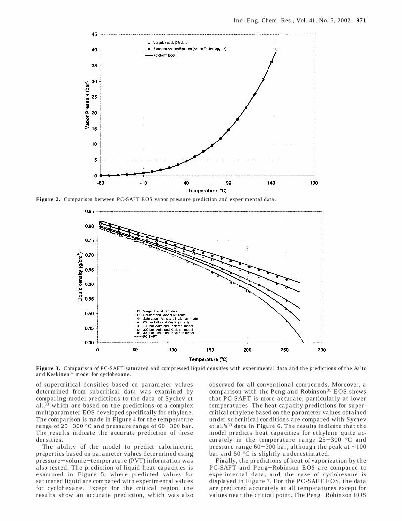
of supercritical densities based on parameter valuesdetermined from subcritical data was examined bycomparing model predictions to the data of Sychev etal.,33 which are based on the predictions of a complexmultiparameter EOS developed specifically for ethylene.The comparison is made in Figure 4 for the temperaturerange of 25-300 °C and pressure range of 60-300 bar.The results indicate the accurate prediction of thesedensities.

The ability of the model to predict calorimetricproperties based on parameter values determined usingpressure-volume-temperature (PVT) information wasalso tested. The prediction of liquid heat capacities isexamined in Figure 5, where predicted values forsaturated liquid are compared with experimental valuesfor cyclohexane. Except for the critical region, theresults show an accurate prediction, which was also

observed for all conventional compounds. Moreover, acomparison with the Peng and Robinson35 EOS showsthat PC-SAFT is more accurate, particularly at lowertemperatures. The heat capacity predictions for super-critical ethylene based on the parameter values obtainedunder subcritical conditions are compared with Sychevet al.’s33 data in Figure 6. The results indicate that themodel predicts heat capacities for ethylene quite ac-curately in the temperature range 25-300 °C andpressure range 60-300 bar, although the peak at ∼100bar and 50 °C is slightly underestimated.

Finally, the predictions of heat of vaporization by thePC-SAFT and Peng-Robinson EOS are compared toexperimental data, and the case of cyclohexane isdisplayed in Figure 7. For the PC-SAFT EOS, the dataare predicted accurately at all temperatures except forvalues near the critical point. The Peng-Robinson EOS

Figure 2. Comparison between PC-SAFT EOS vapor pressure prediction and experimental data.

Figure 3. Comparison of PC-SAFT saturated and compressed liquid densities with experimental data and the predictions of the Aaltoand Keskinen32 model for cyclohexane.


predicts accurate values in the critical region and lessaccurate values at low temperatures. This behavior wasalso observed for other conventional compounds. Theaccuracy of the heat of vaporization and heat capacityat high temperature is intimately tied to the locationof the vapor-liquid critical point predicted by theequation of state (at which point the heat of vaporizationvanishes and the heat capacity diverges). This temper-ature is often overpredicted by both the original SAFTEOS and the PC-SAFT EOS (and all other unrescaledmean-field EOSs) when parameterized in the mannerdescribed here.22 The discrepancy between the PC-SAFTEOS-predicted critical temperature and the true valueis, however, smaller than typical of the original SAFTEOS. This error could be eliminated by rescaling theequation to better predict the true critical point.24,36

In terms of the pure-compound parameters for poly-ethylene, experience with the original SAFT EOSindicates that the EOS can represent the PVT data ofmolten polymers accurately. As with other EOSs, suchas the original SAFT EOS and the Sanchez-LacombeEOS,9 however, the use of polymer pure-compoundparameter values determined from PVT data oftenresults in poor representations of binary or quasibinaryphase equilibria between the polymer and low-molecu-lar-weight solutes. For example, Koak et al.37 using theoriginal SAFT EOS found that they had to adjust thevalue of the energy parameter to obtain a reasonablefit to binary polyethylene-ethylene FLE cloud-pointdata. Calculations performed by Gross34 indicate thatthe PC-SAFT EOS suffers from the same deficiency andthat the use of values of parameters determined from

Figure 4. Comparison of PC-SAFT predictions and Sychev et al.33 supercritical ethylene density data.

Figure 5. Comparison of experimental data and PC-SAFT predictions of the saturated liquid heat capacity for cyclohexane.


molten polymer PVT data alone does not result in goodrepresentations of binary phase equilibrium data forpolyethylene-ethylene. Gross obtained a set of pure-compound parameters for polyethylene by adjusting thevalue of the energy parameter and the binary interac-tion parameter to simultaneously fit molten polymerPVT data38 and cloud-point data collected in the poly-disperse polyethylene-ethylene FLE study of de Looset al.39

The density values for molten polymer predicted bythe PC-SAFT EOS using Gross’s parameter values arecompared with experimental data for LDPE in Figure8. The fit is worse when compared for HDPE40 orLLDPE.41 The data are not well represented by theparameter values at high pressure. Because the moltenpolymer is relatively incompressible, however, the over-all error is relatively small and introduces little error

in the solution for low (<20%) polymer solutions. In anycase, commercial solution polymerization plants producea range of products ranging from high- to very low-density polyethylene so that the question of moltenpolymer density in relation to LLE or FLE behavior is,in a sense, poorly defined. Determination of the param-eter values directly from polymer PVT data yieldsexcellent correlations, as shown, for example, in Figure9 for HDPE. Similar results are obtained for LLDPEand LDPE. Prediction of binary polyethylene-ethylenephase equilibria using the PVT-optimized parametervalues is, however, poor, and as a result, the valuesoptimized by Gross were used in this study, althoughthe binary interaction parameter value was readjusted,as described in the next section. If one is interested invery accurate predictions of fluid volumetric behavior,then it might be expedient to use PC-SAFT with two

Figure 6. Comparison of PC-SAFT predictions and Sychev et al.33 supercritical ethylene heat capacity data.

Figure 7. Comparison of PC-SAFT and Peng-Robinson EOS predictions of the heat of vaporization and experimental data for cyclohexane.


sets of parameters, one set being used for polymersolution phase behavior and the other for polymersolution density predictions, if these calculations areperformed independently.

Flash separation units in solution polymerization aretypically operated in an adiabatic manner, and designcalculations require an enthalpy balance. As discussedearlier, the heat capacities predicted by PC-SAFT forconventional components are accurate. For polyethyleneusing the Gross parameter values, it was found that theheat capacity was slightly in error. To correct for this,the approach taken by Orbey et al.42 was followed. Inthis approach, the ideal gas heat capacity (Cp

ig) isadjusted to give the correct heat capacity (Cp) as

where the right-most term is obtained from the PC-SAFT EOS and is a function of temperature andpressure, whereas the ideal gas heat capacity is afunction of temperature only and, in this study, isassumed to be linearly dependent on temperature(measured in Kelvin)

Experimental values of the heat capacity of moltenpolyethylene were used to regress optimal values of C0

ig

and C1ig so as to fit the data using eq 3. The regression

yielded values of C0ig ) 1.666 kJ kg-1 K-1 and C1

ig )3.663 × 10-3 kg-1 K-2. The fit of the experimental datais displayed in Figure 10, which shows that adjustingthe ideal gas constants is an effective way of getting thePC-SAFT EOS to give accurate heat capacities when

Figure 8. Comparison of PC-SAFT predictions of the density of molten LDPE with Gross34 parameters and experimental data.38

Figure 9. PC-SAFT correlation of molten HDPE PVT data.38 The optimal parameters are m/MW ) 0.048 051 03, σ ) 3.260 959 63, ε/k) 237.235, where MW is the molecular weight of polyethylene.

Cp ) Cpig + T∫0

P ∂2v

∂T2dP (3)

Cpig ) C0

ig + C1igT (4)


the other pure-compound parameter values have beenoptimized to yield a compromise between PVT and LLEor FLE data.

Binary Interaction Parameters. Binary vapor-liquid equilibrium (VLE) data for ethylene-1-butene inthe temperature range 20-101 °C were used to deter-mine the value of kij in the PC-SAFT EOS. Figure 11shows a comparison between predicted and experimen-tal values of the bubble and dew points for this system.Overall, the VLE fit is accurate. A similar fit of VLEdata was performed for the ethylene-cyclohexane sys-tem, and the results obtained are similar to those forthe previous system, as shown in Figure 12. Some ofthe data from the Miller43 reference, at low temperature,were rejected as they were shown to be inconsistent withthe higher-temperature data and the low-concentrationdata of Pacheco et al.44 The elimination was based onan examination of the magnitude of kij obtained by

separately fitting data at each temperature for theisothermal data subsets.

Previous studies9 have used the data of de Loos etal.39 to determine values of binary interaction param-eters for the Sanchez-Lacombe EOS. These data consistof phase boundary information (isopleths and isothermswith critical points) for several polydisperse polyethyl-ene samples with ethylene in the temperature range of130-170 °C. Data for two of these polymers, denotedPE1 and PE7, have been used in several studies. Koaket al.37 fit these data using the original SAFT EOS. Tofit the data, it was necessary to simultaneously fit thevalues of the polymer energy parameter and kij and tointroduce a linear temperature dependence of kij, withdifferent constants valid for each polymer. These dataare modeled in the next section of this paper.

In this study, the values of kij for linear polyethylene-ethylene are determined using polyethylene-ethylene

Figure 10. Comparison of PC-SAFT predicted heat capacity with experimental data for molten polyethylene.

Figure 11. Comparison of VLE experimental data (Laugier et al.45) and PC-SAFT correlation for the ethylene-1-butene system.


cloud-point data measured by Chun Chan et al.14 Thepolymer used is a standard sample obtained from theNational Institute of Standards and Technology, NISTSRM 1483, which has a value of Mh W ) 32 × 103 and isnarrowly distributed, having a polydispersity index of1.11. This is a suitable system for use in determiningkij because the narrow molecular weight distributionallows the polymer to be treated as monodisperse,effectively decoupling the polymer segment-solventmolecule interaction energy problem from that of thepolymer MWD characterization. In this case, the poly-mer was assumed to be a discrete component with amolecular weight of 32 × 103. Initial calculations usingkij ) 0.0404, a value suggested by Gross34 based on thede Loos et al.39 data, showed reasonable predictions forintermediate temperatures but poor reproduction of thecloud points at 130 and 180 °C. This is partly due tothe value being determined using an independent dataset but is also due to the use of a different set of ethylenepure-compound parameters. On the basis of this resultand the experience of Koak et al.,37 the kij value wasmade a linear function of temperature by fitting the 130and 170 °C isotherms. The resulting relationship islisted in Table 2, and the data fit is displayed in Figures13 and 14.

Figure 13 shows the PC-SAFT predictions of the ChunChan et al.14 isotherms and indicates a fair reproductionof the data. In this figure, the filled symbols representtransitions at concentrations below the critical value,termed “dew-point” transitions, while the open symbolsrepresent “bubble-point” transitions, to the right of thecritical concentration. Hence, the critical point lies at apolymer concentration of ∼8 wt %, while the modelpredicts values of ∼6 wt %. In general, the EOS

predictions yield cloud-point curves that are too narrow,a phenomenon typical of mean-field models, with thediscrepancy between the experimental data and themodel predictions increasing at higher polymer concen-trations; unfortunately, no data are available for poly-mer concentrations higher than 15 wt %. This phenom-enon has also been observed when the PC-SAFT EOSis applied to monodisperse polyethylene-n-hexane sys-tems.48 Figure 14 shows isopleths calculated for 10 and15 wt % polymer including extrapolations to hightemperature. Attempts to calculate isopleths at 5 and7.5 wt %, in the vicinity of the critical region, resultedin convergence difficulties. Although the 10 wt %isopleth shows an accurate correlation with the experi-mental data, the 15 wt % does not, for the reasonexplained above. With the use of the linear kij temper-ature dependence, the extrapolation to high tempera-ture appears to be reasonable.

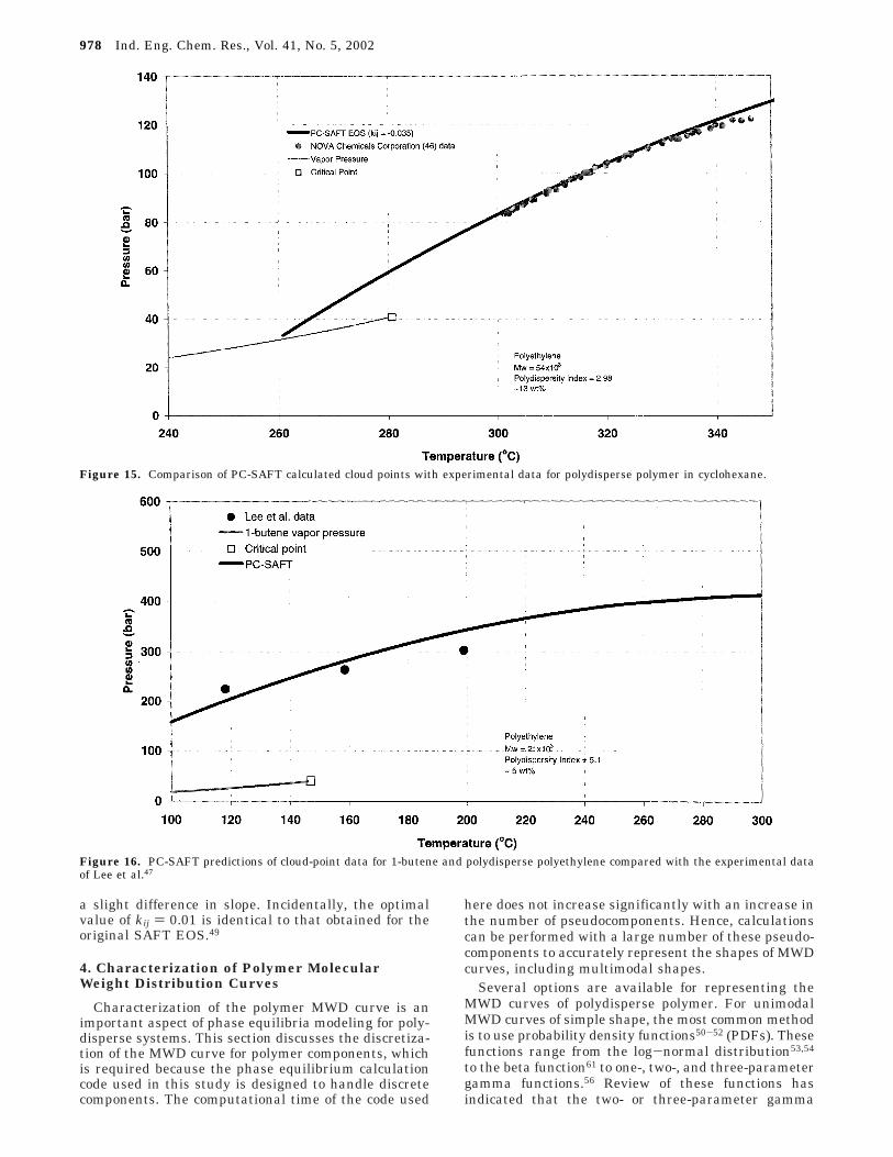
The value of the interaction parameter betweenpolyethylene and cyclohexane was determined by fittingcloud-point data for a solution of polydisperse polyeth-ylene in cyclohexane. The polyethylene sample used inthis study had a weight-average molecular weight of 54× 103 and a polydispersity index of 2.98. The MWDcurve of this resin determined by size exclusion chro-matography (SEC) was discretized into 50 pseudocom-ponents using the methods described in the next section.All pseudocomponents were assumed to have the samevalue of kij with cyclohexane. The predictions of themodel are compared to data in Figure 15. The experi-mental data were digitized from a hand-drawn semi-logarithmic plot and are based on a linear interpolationof some experimental points. In addition, there is someuncertainty regarding the actual polymer concentration

Figure 12. Comparison of PC-SAFT calculated and experimental vapor-liquid equilibria for ethylene-cyclohexane.

Table 2. PC-SAFT Binary Interaction Parameter Values

system kij data reference

ethylene-1-butene 0.00983 Laugier et al.45

ethylene-cyclohexane 0.034815 Miller43 and Pacheco et al.44

cyclohexane-polyethylene -0.035 NOVA Chemicals Corporation46

ethylene-polyethylene 0.03464 + 1.9 × 10-5(T/K) Chun Chan et al.14

1-butene-polyethylene 0.01 Lee et al.47


used, although the best estimate is 13 wt %. The PC-SAFT EOS accurately correlates the data. Initial at-tempts to estimate the value of kij using low-pressureVLE data, i.e., using experimentally determined (byinverse gas chromatography) values of the Henry’sconstant for cyclohexane at infinite dilution in themolten polymer, yielded a kij value of the wrong signand magnitude, resulting in predictions of UCST be-havior instead of the expected LCST behavior.

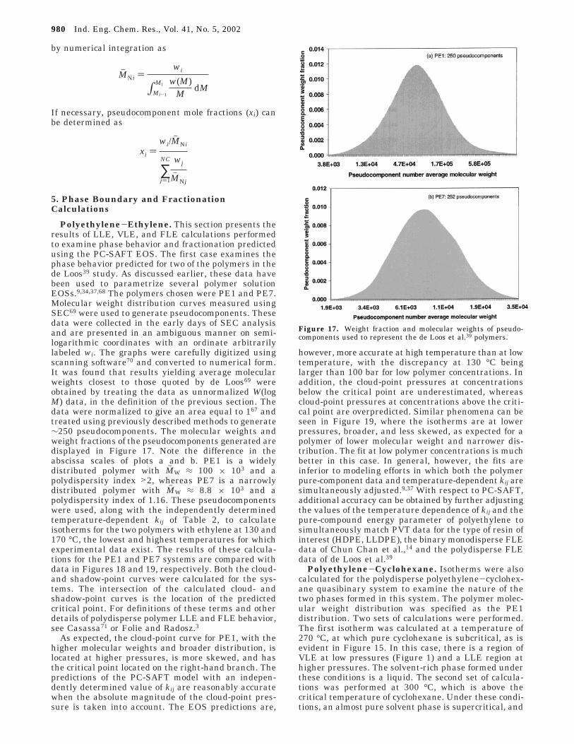
The value of kij between 1-butene and polyethylenewas obtained using data collected by Lee et al.,47 whomeasured the cloud point of a 5 wt % solution of apolydisperse polyethylene sample in 1-butene. Thepolymer had a number-average molecular weight of 21× 103 and a polydispersity index of 5.1. In the absenceof further characterization information regarding thispolymer, the data were fitted to the following shiftedtwo-parameter gamma function, with the lowest mo-

lecular weight (γ) assumed to be 1000 [see the nextsection for the definition of w(M)]

Using the specified molecular weight and polydipersityindex, the values of the two parameters R and â weredetermined and used to generate w(M) values, whichwere then used in the method described in the nextsection to generate 70 pseudocomponents. The pseudo-components were assumed to have the same interactionparameter with 1-butene (and to not interact amongthemselves). The value of kij was adjusted to fit theexperimentally determined isopleth, and the best fitobtained is shown in Figure 16. The PC-SAFT EOSreproduces the data reasonably well, although there is

Figure 13. Comparison of PC-SAFT calculated and experimental isotherms for the polyethylene-ethylene system of Chun Chan et al.14

The filled symbols represent dew-point transitions, and the open symbols represent bubble-point transitions.

Figure 14. PC-SAFT calculated isopleths for the polyethylene-ethylene compared with Chun Chan et al.14 data.

w(M) )(M - γ)R-1

âRΓ(R)exp[- M - γ

â ] γ e M e ∞


a slight difference in slope. Incidentally, the optimalvalue of kij ) 0.01 is identical to that obtained for theoriginal SAFT EOS.49

4. Characterization of Polymer MolecularWeight Distribution Curves

Characterization of the polymer MWD curve is animportant aspect of phase equilibria modeling for poly-disperse systems. This section discusses the discretiza-tion of the MWD curve for polymer components, whichis required because the phase equilibrium calculationcode used in this study is designed to handle discretecomponents. The computational time of the code used

here does not increase significantly with an increase inthe number of pseudocomponents. Hence, calculationscan be performed with a large number of these pseudo-components to accurately represent the shapes of MWDcurves, including multimodal shapes.

Several options are available for representing theMWD curves of polydisperse polymer. For unimodalMWD curves of simple shape, the most common methodis to use probability density functions50-52 (PDFs). Thesefunctions range from the log-normal distribution53,54

to the beta function61 to one-, two-, and three-parametergamma functions.56 Review of these functions hasindicated that the two- or three-parameter gamma

Figure 15. Comparison of PC-SAFT calculated cloud points with experimental data for polydisperse polymer in cyclohexane.

Figure 16. PC-SAFT predictions of cloud-point data for 1-butene and polydisperse polyethylene compared with the experimental dataof Lee et al.47


functions are the most versatile and reliable for use withpolymer MWD curves.48 For some polymers, this ap-proach provides a connection between the MWD curveand simplified kinetic schemes describing the polymer-ization process.50 In polyethylene production, the so-called Schultz-Flory distribution (a one-parametergamma function) has been used to identify the numberand relative activity of Ziegler-Natta catalytic sitespresent during polymerization.57 A variety of methodsfor calculating phase equilibria that directly utilizePDFs exist,58 including so-called “continuous thermo-dynamics” approaches.59,60 Although effective for specificmodels and systems, in general, these methods sufferfrom the drawback of being intimately tied to specificPDFs. The main disadvantage of using PDFs to repre-sent MWD curves, however, is their restriction to simpleunimodal shapes; representation of multimodal distri-butions requires deconvolution of a MWD curve into asubset of PDF distributions,57 complicating the problem.Many polyethylene solution polymerization processesinvolve more than one reactor in series or use multisitecatalysts, often resulting in multimodal MWD curves.

Pseudocomponents can be generated from PDFs usingtwo general methods. One method matches the mo-ments of the distribution to those of the pseudocompo-nents to be determined.56 This method is not suitablefor generating large numbers of pseudocomponents, asthe numerical magnitude of the moments increasesexponentially with the number of pseudocomponents,leading to numerical difficulties,48 particularly for di-vergent PDFs such as the log-normal distribution. Thesecond method uses values of parameters in the PDFto determine pseudocomponents by numerical quadra-ture,55,61 optimizing integral properties of the PDFs. Thequadrature scheme chosen depends on the PDF inquestion, and this method is useful for efficientlydetermining small numbers of pseudocomponents foruse in phase equilibria calculations where a detailedshape of the MWD curve is not required, such as inphase boundary calculations for polydisperse polymer.62

For solution polymerization applications, this would beapplicable if one were only interested in the location ofthe cloud point and not in fractionation. This is some-times the case, and schemes for generating quadraturepseudocomponents from the three-parameter gammafunction56 have been developed.48

The ultimate goal of solution polymerization simula-tion is to model the process from monomer introductionthrough to the final solid resin product, with enoughdetail regarding the MWD curve and branch distribu-tion for product scientists to infer the physical propertiesof the resin being made. Flash calculations yieldingresults at this level of detail require the use of severalhundred pseudocomponents, which is 2 orders of mag-nitude larger than the number required for thermody-namic and numerical convergence of unimodal distri-bution problems.56,62 They also require the use of aphase equilibrium code utilizing an efficient calculationmethod (such as, say, that described by Jog et al.63). Theapproach taken in this study is to generate largenumbers of pseudocomponents by direct numericalintegration of the MWD curve resulting from the SECanalysis. Such analyses are now routinely used tocharacterize the products being made in industrialplants. Ultimately, the results of process simulationswill have to be re-expressed in the form of SEC curvessthis is difficult, if not impossible to do when PDFs or

PDF-generated pseudocomponents are used in thecalculations.

Typically, the results of SEC analysis are expressedas the rate of change of the polymer weight fraction withthe logarithm of the molecular weight, log M, that is,dW(M)/(d log M) ≡ W(log M). These results usuallycontain 400-800 data points and are normalized to givean area under the curve of 1, i.e.

with MH and ML representing the largest and smallestmolecular weights in the sample, respectively. Size-exclusion chromatography data in the form of W(log M)are not convenient for the generation of pseudocompo-nents, because of the logarithmic scale, and can beconverted to reflect the change in weight fraction withchange in molecular weight via the transformation

This transformation preserves the normalization condi-tion, so that

The transformation changes the shape of the SECcurve (even when plotted on a logarithmic scale) andyields very small values of w(M) at high molecularweight as a result of the division by M. In many cases,a bimodal W(log M) curve is converted into a unimodalw(M) curve, as observed previously by Friedman.64

Scatter in the original W(log M) data at low molecularweight is amplified by the transformation, possiblyaffecting calculated values of the number-average mo-lecular weight, Mh N, as mole numbers are very sensitiveto this region of the curve. Scatter in the data can bereduced by either numerically smoothing the originalW(log M) data or the transformed w(M) data usingeither B-spline or least-squares routines.65-67 It is,however, numerically difficult to smooth the w(M) databecause of the very small magnitude of w(M) values athigh molecular weight, and hence W(log M), data arerecommended. Experience indicates that nonuniformrational B splines65 are suitable for most problemsencountered so far.

Numerical integration of the above data is mostconveniently performed by combining a smoothingprocedure that represents the data using piecewise low-order polynomials, such as B-SPLINES,65 with anintegration routine. Several such routines exist in theIMSL package of Fortran subroutines66 or TableCurve2D software.67 Smoothed W(log M) data are output atequally spaced (logarithmically) molecular weight in-tervals. The weight fraction of pseudocomponent i, wi,with molecular weight in the range Mi-1 to Mi, isobtained as

where the integral is evaluated numerically. As a resultof approximations in the spline representation andround-off error, the weight fractions determined aboveshould be normalized. The number-average molecularweight (Mh Ni) of pseudocomponent i is also determined

∫log ML

log MH W(log M) d log M ) 1

dW(M)dM

≡ w(M) ) 1ln(10) M

dW(M)d log M

∫ML

MH w(M) dM ) 1

wi ) ∫Mi-1

Mi w(M) dM


by numerical integration as

If necessary, pseudocomponent mole fractions (xi) canbe determined as

5. Phase Boundary and FractionationCalculations

Polyethylene-Ethylene. This section presents theresults of LLE, VLE, and FLE calculations performedto examine phase behavior and fractionation predictedusing the PC-SAFT EOS. The first case examines thephase behavior predicted for two of the polymers in thede Loos39 study. As discussed earlier, these data havebeen used to parametrize several polymer solutionEOSs.9,34,37,68 The polymers chosen were PE1 and PE7.Molecular weight distribution curves measured usingSEC69 were used to generate pseudocomponents. Thesedata were collected in the early days of SEC analysisand are presented in an ambiguous manner on semi-logarithmic coordinates with an ordinate arbitrarilylabeled wi. The graphs were carefully digitized usingscanning software70 and converted to numerical form.It was found that results yielding average molecularweights closest to those quoted by de Loos69 wereobtained by treating the data as unnormalized W(logM) data, in the definition of the previous section. Thedata were normalized to give an area equal to 167 andtreated using previously described methods to generate∼250 pseudocomponents. The molecular weights andweight fractions of the pseudocomponents generated aredisplayed in Figure 17. Note the difference in theabscissa scales of plots a and b. PE1 is a widelydistributed polymer with Mh W ≈ 100 × 103 and apolydispersity index >2, whereas PE7 is a narrowlydistributed polymer with Mh W ≈ 8.8 × 103 and apolydispersity index of 1.16. These pseudocomponentswere used, along with the independently determinedtemperature-dependent kij of Table 2, to calculateisotherms for the two polymers with ethylene at 130 and170 °C, the lowest and highest temperatures for whichexperimental data exist. The results of these calcula-tions for the PE1 and PE7 systems are compared withdata in Figures 18 and 19, respectively. Both the cloud-and shadow-point curves were calculated for the sys-tems. The intersection of the calculated cloud- andshadow-point curves is the location of the predictedcritical point. For definitions of these terms and otherdetails of polydisperse polymer LLE and FLE behavior,see Casassa71 or Folie and Radosz.3

As expected, the cloud-point curve for PE1, with thehigher molecular weights and broader distribution, islocated at higher pressures, is more skewed, and hasthe critical point located on the right-hand branch. Thepredictions of the PC-SAFT model with an indepen-dently determined value of kij are reasonably accuratewhen the absolute magnitude of the cloud-point pres-sure is taken into account. The EOS predictions are,

however, more accurate at high temperature than at lowtemperature, with the discrepancy at 130 °C beinglarger than 100 bar for low polymer concentrations. Inaddition, the cloud-point pressures at concentrationsbelow the critical point are underestimated, whereascloud-point pressures at concentrations above the criti-cal point are overpredicted. Similar phenomena can beseen in Figure 19, where the isotherms are at lowerpressures, broader, and less skewed, as expected for apolymer of lower molecular weight and narrower dis-tribution. The fit at low polymer concentrations is muchbetter in this case. In general, however, the fits areinferior to modeling efforts in which both the polymerpure-component data and temperature-dependent kij aresimultaneously adjusted.9,37 With respect to PC-SAFT,additional accuracy can be obtained by further adjustingthe values of the temperature dependence of kij and thepure-compound energy parameter of polyethylene tosimultaneously match PVT data for the type of resin ofinterest (HDPE, LLDPE), the binary monodisperse FLEdata of Chun Chan et al.,14 and the polydisperse FLEdata of de Loos et al.39

Polyethylene-Cyclohexane. Isotherms were alsocalculated for the polydisperse polyethylene-cyclohex-ane quasibinary system to examine the nature of thetwo phases formed in this system. The polymer molec-ular weight distribution was specified as the PE1distribution. Two sets of calculations were performed.The first isotherm was calculated at a temperature of270 °C, at which pure cyclohexane is subcritical, as isevident in Figure 15. In this case, there is a region ofVLE at low pressures (Figure 1) and a LLE region athigher pressures. The solvent-rich phase formed underthese conditions is a liquid. The second set of calcula-tions was performed at 300 °C, which is above thecritical temperature of cyclohexane. Under these condi-tions, an almost pure solvent phase is supercritical, and

Mh Ni )wi

∫Mi-1

Mi w(M)M

dM

xi )wi/Mh Ni

∑j)1

NC wj

Mh Nj

Figure 17. Weight fraction and molecular weights of pseudo-components used to represent the de Loos et al.39 polymers.


hence, this situation corresponds to FLE. Unfortunately,there are no cyclohexane data with which to comparethe results of the calculations.

The results of both sets of calculations are displayedin Figure 20, and they indicate that, once the pressurefalls below the cloud-point pressure, the incipientsolvent-rich phase contains virtually no polymer, re-gardless of the pressure and temperature and regardlesof whether the solvent-rich phase is supercritical orsubcritical. For the 270 °C calculation, the light-phasepolymer concentration does not change much as thesecond phase is converted from liquid to vapor with alowering of pressure. The line separating the LLE andVLE regions is drawn as an invariant pressure line,which is only the case for true binary systems composedof mondisperse polymer and solvent (because of Gibbs

phase rule); in reality, there is a (very) small three-phase region here for broadly distributed polymer. Ifethylene, 1-butene, or 1-octene is present, then thisthree-phase region is large, sometimes greater than 10bar.10 For subcritical conditions (270 °C), there is asharp kink separating the VLE and LLE regions, andfor the case of FLE at 300 °C, there is still a kink,although diffuse. Compared to the ethylene-polyeth-ylene case, the differences between the cloud- andshadow-point curves are not as pronounced, althoughthe precipitation threshold (maximum in the cloud-pointcurve) is located at very low concentrations, below 1%for PE1, and the critical point is located on the right-hand branch at about 3 wt % or so. The shapes of thecalculated cloud-point curves are very similar to thosemeasured for LLDPE in n-hexane by de Loos et al.15

Figure 18. Comparison between experimental (de Loos et al.39) and PC-SAFT calculated isotherms for the ethylene-polyethylene (PE1)system at 130 and 170 °C.

Figure 19. Experimental (de Loos et al.39) and PC-SAFT calculated isotherms for the ethylene-polyethylene (PE7) system at 130 and170 °C.


The next section examines polyethylene MWD curvesin equilibrated liquid and vapor phases.

Polyethylene-1-Butene. A similar set of calcula-tions was performed for the 1-butene-polyethylenebinary system, with isotherms being obtained at sub-and supercritical conditions relative to the critical pointof 1-butene. The calculations were performed at 130 and200 °C (see Figure 16). As with cyclohexane, PE1 waschosen, because it has a high molecular weight andbroad distribution, to emphasize the effects of polydis-persity. The results of the calculations are displayed inFigure 21. Because the 1-butene molecule is smaller,the isotherms are located at higher pressures as a resultof greater molecular size asymmetry in the system.Otherwise, the trends are very similar to those in thecyclohexane case, and the general conclusions remain

the same. The LLE and FLE regions are larger, how-ever, because of the increased density difference be-tween 1-butene and polyethylene.

Fractionation in an Industrial Process. Thissection describes the modeling of polyethylene fraction-ation in the flash unit of a plant producing polymerusing the SCLAIRTECH process.2 The unit effectsvapor-liquid separation of subcritical solvent and re-sidual monomer and comonomer from polymer. Theinitial case modeled involves operation of this unit at267 °C and 33 bar. The feed contains 16.32 wt %polyethylene, 1.66 wt % ethylene, and 5.7 wt % 1-butene.Samples of polymer leaving in the liquid stream fromthis unit and of “grease”, consisting of low-molecular-weight oligomeric material dissolved in the vapor, werecollected at a plant during normal operation. These

Figure 20. PC-SAFT calculated isotherms for PE-cyclohexane at sub- and supercritical temperatures (for pure cyclohexane).

Figure 21. PC-SAFT calculated isotherms for PE-1-butene at sub- and supercritical temperatures (for pure 1-butene).


samples were analyzed using SEC to determine MWDcurves. Using the results of the SEC analysis and amaterial balance, the MWD curve of material enteringthe flash unit was reconstructed. This reconstructioninvolved some assumptions regarding the materialbalance, particularly the flow rates of the components,because of lack of plant measurements and difficultieswith sampling and analytical techniques. Nonetheless,it represents the first attempt at experimentally char-acterizing fractionation in an operating plant. Materialdown to very low molecular weight, on the order of thesolvent’s, was also included to investigate the effects offractionation at low molecular weight. This distributionwas discretized to yield ∼250 pseudocomponents usingthe techniques described previously and treated as thepolymer feed in fixed-temperature and -pressure flashcalculations.

Table 3 compares the results of the flash calculationswith plant data. Considering the uncertainty in ac-curately measuring mass flow rates at the plant, it isapparent that the PC-SAFT modeling provides a rea-sonable prediction of the data. The predicted vaporfraction is 68 wt %. Figure 22 shows a comparisonbetween calculated and measured MWD curves for thegrease and resin. There is some scatter in the recon-structed original feed distribution, and this is reflectedin the vapor phase distribution. The plant data repre-sent pseudocomponents generated from SEC data usingnumerical integration techniques. The PC-SAFT calcu-lations provide an accurate characterization of thefractionation process, although there is some error inthe middle molecular weight range, as is evident froma comparison of the calculated and measured average

molecular weights listed in Table 4. The main discrep-ancy is in the number-average molecular weight, whichis sensitive to the low-molecular-weight end of the SECdata.

Additional calculations were performed with thissystem to examine the effect of pressure and tempera-ture on the molecular weight distribution of the polymerin the light phase. First, the LL boundary for the feedsystem going into the flash unit was calculated, asdisplayed in Figure 23. Also shown is the LL boundaryfor a quasibinary solution of polymer in cyclohexane atthe same polymer concentration. The effect of thepresence of 1-butene and ethylene is to increase the sizeof the LLE region (by ∼40 bar) and to raise the bubblepoint, or vapor pressure line.

A flash calculation was performed at 84 bar, less than1 bar into the LLE region, and the results of the overallLLE splits were very similar to the VLE case at 33 bar,with the only significant change being that the lightliquid phase now contains 0.77 wt % polyethylene(versus 0.05 wt % for VLE at 33 bar, Table 4). In thisregion, the solubility of the polymer is increased by thehigher pressure. The molecular weight distributions inthe feed, liquid, and vapor phases are shown in Figure24. The increased pressure results in the dissolution ofhigher-molecular-weight material in the light phase, sothat the number- and weight-average molecular weightsincrease to 786 and 2320, respectively. Additionalcalculations indicate that the nature of the light phasedoes not change significantly as it changes from a liquid

Figure 22. Results of plant flash simulation with the PC-SAFT calculated MWD curve of the liquid and vapor phases compared to plantdata in terms of pseudocomponents.

Table 3. Overall Results of the Flash Calculation

liquid composition(wt %)

vapor composition(wt %)

compound plantPC-SAFTcalculated plant

PC-SAFTcalculated

polyethylene 44.62 50.8 0.25 0.05ethylene 0.74 0.21 2.18 2.341-butene 4.48 1.44 6.41 7.72cyclohexane 50.15 47.6 91.39 89.9

Table 4. Polymer Molecular Weight Averages inEquilibrated Liquid and Vapor Phases

liquid phase vapor phase

molecularweight average

plantdataa

PC-SAFTcalculated

plantdatab

PC-SAFTcalculated

MN 13 200 11 323 140 164MW 126 000 126 592 170 190MZ 695 800 710 230 220 222polydispersityindex

9.6 11.2 1.21 1.16

a Based on resin SEC analysis. b Based on grease SEC analysis.


to a vapor phase, which occurs at a pressure of ap-proximately 55 bar for this mixture. Similarly, thedifference in going from the LLE region to the FLEregion is not dramatic.

A set of flash calculations was performed with the feeddescribed above to examine in detail the behavior of theequilibrated phases as the pressure is lowered from thecloud-point value of ∼84.5 bar to pressures as low as 1bar in the VL region. As the pressure falls below thecloud-point value, the new liquid phase generatedcontains very little polymer, <1 wt %, as shown on theright-hand side of Figure 25. This figure displays overallpolymer concentrations in equilibrated phases in LL andVL regions as a function of pressure at 267 °C. As thepressure is lowered further into the two-phase region,the polymer concentration in the light phase drops from∼0.77 to ∼0.1 wt %, as the system enters the three-

phase VLL region at ∼ 53 bar. Experience shows thata two-phase code such as the one used in this studycannot be used to reliably determine the pressure atwhich vapor is formed in this type of system containingethylene and 1-butene because, in reality, this is theedge of a VLL region.72 A code capable of handling threesimultaneous phases at equilibrium is required, so thisregion is shown schematically in this and subsequentfigures; future studies will examine this region in detail.

As expected, the polymer concentration in the heavyphase increases as the pressure is lowered in the LLregion, as a result of removal of solvent to form increas-ing amounts of the light phase. At low pressures, in theVL region, the polymer concentration increases withdecreasing pressure, in a seemingly counterintuitivemanner. This type of behavior has been observed incalculations of solubilities of solids and fluids in super-

Figure 23. Effect of ethylene and 1-butene on LL phase boundary of polydisperse polymer in cyclohexane.

Figure 24. MWD curves in equilibrated LL phase at 267 °C and 84 bar.


critical solvents73 and is attributed to the vapor pressureof the polymer influencing the solubility at low pres-sures. The experimental polyethylene-ethylene frac-tionation study of Spahl and Luft74 did not observe thisphenomenon, although the solvent was supercritical andthey did not perform experiments at low pressures. InFigure 25, the polyethylene concentration increasesfrom a value of ∼0.05 wt % at 47 bar to 0.12 wt % at 1bar. Figure 26 shows changes in the number-averagemolecular weight of polymer in equilibrated phases asthe pressure is lowered through the LL and VL regions.The trends are similar to those observed with the overallpolymer concentration, with the average polymer mo-lecular weight in the light phase decreasing withdecreasing pressure in the LL region and increasing

with decreasing pressure in the VL region. Whereas thelight-phase polymer average molecular weight changesby an order of magnitude over the pressure range, theheavy phase values are relatively insensitive to pres-sure, as this phase contains the nonvolatile high-molecular-weight polymer homologues.

Figure 27 displays the percentage of the total massin the light phase as a function of pressure. As thepressure is decreased, the total fraction of the feed inthe light phase increases from a value of zero at thecloud-point pressure to ∼40 wt % as the VLL boundaryis approached. This figure shows that the fraction of thelight phase increases to ∼84 wt % at 1 bar pressure, atwhich point all of the light components have beenvaporized, leaving behind only the heavy ends of the

Figure 25. Polymer concentration in equilibrated phases as a function of pressure for VLE and LLE at 267 °C.

Figure 26. Changes in polymer number-average molecular weight in equilibrated phases as a function of pressure for VLE and LLE at267 °C.


molten polymer. Figure 28 shows accompanying changesin the mass densities of the equilibrated phases, il-lustrating the change in the density of the light phaseas it is transformed from liquid to vapor, with its densitybeing halved by a small drop in pressure.

6. Conclusions

When parameterized using the appropriate experi-mental data, the PC-SAFT EOS provides accuratevalues of PVT, VLE, LLE, FLE, and calorimetricproperties for pure components and fluid mixtures.However, the model still suffers from an inability topredict accurate polymer-ethylene fluid-liquid phasebehavior based on pure-component polymer propertiesoptimized using molten polymer PVT data only. Im-provements could be made also by rescaling the equa-

tion to correctly predict vapor-liquid critical points andhandle copolymer systems. This would improve theaccuracy of the calorimetric properties.

Accurate process simulation of flash units in themultireactor solution polymerization industry requiresan accurate description of the MWD curve, which isgenerally not provided by probability density functionsor pseudocomponents generated using these functions.Large numbers of pseudocomponents can be efficientlygenerated by numerical integration from generic MWDcurves of any shape measured using SEC .

The PC-SAFT EOS is able to accurately predict VLE,LLE, and FLE fractionation of polydisperse polyethylenesolutions when coupled with an efficient phase equilib-rium calculation code and large numbers of pseudo-components. The simulation of an industrial flash

Figure 27. Distribution of mass between phases as a function of pressure in the two-phase region at 267 °C.

Figure 28. Behavior of phase mass densities as a function of pressure for VLE and LLE at 267 °C.


separation process using this combination results inaccurate predictions in a reasonable amount of time.The one weakness of the code is the inability to handlethe simultaneous presence of three phases, VLL, aphenomenon that does occur in practice. In addition,more plant data are needed to build a database reflect-ing VLE and LLE for resins with MWD curves ofmultimodal shapes.

Acknowledgment

The authors express their gratitude to A. Stojcevskiand other colleagues at NOVA Chemicals Corporationfor collecting and analyzing the plant phase equilibriumdata and to Dr. J. Gross and Professors W. Arlt and G.Sadowski of the Technical University of Berlin forproviding unpublished values of some PC-SAFT EOSparameters, as well as the computational code used toperform some of the calculations described in this study.One of the authors (E.L.C.) has also benefited fromdiscussions with Professor R. A. Heidemann of theUniversity of Calgary.

Literature Cited

(1) Johnson, E. D. Separation of Linear Polyethylene. U.S.Patent 2,857,369, 1958.

(2) Elvers, B.; Hawkins, S.; Schulz, G., Editors. Ullmann’sEncyclopedia of Industrial Chemistry; VCH Publishers: New York,1992; Vol. A21: Plastics, Properties and Testing to PolyvinylCompounds.

(3) Folie, B.; Radosz, M. Phase Equilibria in High-PressurePolyethylene Technology. Ind. Eng. Chem. Res. 1995, 34, 1501.

(4) McHugh, M. A.; Krukonis, V. J. Supercritical Fluid Extrac-tion, 2nd ed.; Butterworth-Heinemann: Stoneham, MA, 1994.

(5) Ehrlich, P.; Kurpen, J. J. Phase Equilibria of Polymer-Solvent Systems at High Pressures near Their Critical Loci:Polyethylene with n-Alkanes. J. Polym. Sci.: Part A 1963, 1, 3217.

(6) McHugh, M. A.; Guckes, T. L. Separating Polymer Solutionswith Supercritical Fluids. Macromolecules 1985, 18, 674.

(7) Irani, C.; Cozewith, C. Lower Critical Solution TemperatureBehavior of Ethylene Propylene Copolymers in MulticomponentSolvents. J. Appl. Polym. Sci. 1986, 31, 1879.

(8) Patterson, D. Role of Free Volume Changes in PolymerSolution Thermodynamics. J. Polym. Sci.: Part C 1968, 16, 3379.

(9) Gauter, K.; Heidemann, R. A. Modeling Polyethylene-Solvent Mixtures with the Sanchez-Lacombe Equation. Presentedat the 14th Symposium on Thermophysical Properties, Boulder,CO, June 2000.

(10) Gauter, K.; Heidemann, R. A. A Versatile Formulation ofPolymer-Solvent Phase Equilibrium Calculations. Presented atthe Ninth International Conference on Properties and PhaseEquilibria for Product and Process Design, Kurashiki, Japan, May2001.

(11) Hasch, B. M.; Lee, S.-H.; McHugh, M. A.; Watkins, J. J.;Krukonis, V. J. The Effect of Backbone Structure on the CloudPoint Behaviour of Polyethylene-Ethane and Polyethylene-Propane Mixtures. Polymer 1993, 34, 2554.

(12) Chen, S.-J.; Banaszak, M.; Radosz, M. Phase Behavior ofPoly(ethylene-1-butene) in Subcritical and Supercritical Pro-pane: Ethyl Branches Reduce Segment Energy and EnhanceMiscibility. Macromolecules 1995, 28, 1812.

(13) Chen, A.-Q.; Radosz, M. Phase Equilibria of Dilute Poly-(ethylene-co-1-butene) Solutions in Ethylene, 1-Butene, and1-Butene + Ethylene. J. Chem. Eng. Data 1999, 44, 854.

(14) Chun Chan, A. K.; Adidharma, H.; Radosz, M. Fluid-Liquid Transitions of Poly(ethylene-co-octene-1) in SupercriticalEthylene Solutions. Ind. Eng. Chem. Res. 2000, 39, 4370.

(15) de Loos, Th. W.; Graaf, L. J.; de Swaan Arons, J. Liquid-Liquid Phase Separation in Linear Low-Density Polyethylene-Solvent Systems. Fluid Phase Equilib. 1996, 117, 40.

(16) Aspen Technology. Aspen Plus Reference Manual, version10; Aspen Technology, Cambridge, MA, 1998; Volume 2: PhysicalProperty Methods and Models.

(17) Gross, J.; Sadowski, G. Perturbed-Chain SAFT: An Equa-tion of State Based on a Perturbation Theory for Chain Molecules.Ind. Eng. Chem. Res. 2001, 40, 1244.

(18) Chapman, W. G.; Gubbins, K. E.; Jackson, G.; Radosz, M.New Reference Equation of State for Associating Liquids. Ind. Eng.Chem. Res. 1990, 29, 1709.

(19) Huang, S. H.; Radosz, M. Equation of State for Small,Large, Polydisperse, and Associating Molecules. Ind. Eng. Chem.Res. 1990, 29, 2284.

(20) Huang, S. H.; Radosz, M. Equation of State for Small,Large, Polydisperse, and Associating Molecules: Extension toMixtures. Ind. Eng. Chem. Res. 1991, 30, 1994.

(21) Fu, Y.-H.; Sandler, S. I. A Simplified SAFT Equation ofState for Associating Compounds and Mixtures. Ind. Eng. Chem.Res. 1995, 34, 1897.

(22) Pfohl, O.; Brunner, G. 2. Use of BACK to Modify SAFT inOrder to Enable Density and Phase Equilibrium CalculationsConnected to Gas-Extraction Processes. Ind. Eng. Chem. Res.1998, 37, 2966.

(23) McCabe, C.; Galindo, A.; Gil-Villegas, A.; Jackson, G.Predicting the High-Pressure Phase Equilibria of Binary Mixturesof n-Alkanes Using the SAFT-VR Approach. Int. J. Thermophys.1998, 19, 1511.

(24) McCabe, C.; Jackson, G. SAFT-VR Modelling of the PhaseEquilibrium of Long-Chain n-Alkanes. Phys. Chem. Chem. Phys.1999, 1, 2057.

(25) Gil-Villegas, A.; Galindo, A.; Whitehead, P. J.; Mills, S. J.;Jackson, G. Statistical Associating Fluid Theory for Chain Mol-ecules with Attractive Potentials of Variable Range. J. Chem. Phys.1997, 106, 4168.

(26) Blas, F. J.; Vega, L. F. Prediction of Binary and TernaryDiagrams Using the Statistical Associating Fluid Theory (SAFT)Equation of State. Ind. Eng. Chem. Res. 1998, 37, 660.

(27) Barker, J. A.; Henderson, D. Perturbation Theory andEquation of State for Fluids. II. A Successful Theory for Liquids.J. Chem. Phys. 1967, 47, 4714.

(28) Boublik, T. In Equations of State for Fluids and FluidMixtures, Sengers, J. V., Kayser, R. F., Peters, C. J., White, H. J.,Eds.; Elsevier Science, New York, 2000.

(29) Chen, S. S.; Kreglewski, A. Applications of the Augmentedvan der Waals Theory of Fluids. I. Pure Fluids. Ber. Bunsen-Ges.Phys. Chem. 1977, 81, 1048.

(30) Chiew, Y. C. Percus-Yevick Integral Equation Theory forAthermal Hard-Sphere Chains. II. Average Intermolecular Cor-relation Functions. Mol. Phys. 1991, 73, 359.

(31) Daubert, T. E.; Danner, R. P. Physical and ThermodynamicProperties of Pure Chemicals, Data Compilation; Design Institutefor Physical Property Data, American Institute of ChemicalEngineers, Hemisphere Publishing: New York, 1989.

(32) Aalto, M. M.; Keskinen, K. I. Liquid Densities at HighPressures. Fluid Phase Equilib. 1999, 166, 183.

(33) Sychev, V. V.; Vasserman, A. A.; Golovsky, E. A.; Kozlov,A. D.; Spiridonov, G. A.; Tsymarny, V. A. Thermodynamic Proper-ties of Ethylene; Hemisphere Publishing Corporation, New York,1987.

(34) Gross, J. Technical University of Berlin, Berlin, Germany.Private communication, 2001.

(35) Peng, D. Y.; Robinson, D. B. A New Two-Constant Equa-tion of State. Ind. Eng. Chem. Fundam. 1976, 15, 59.

(36) Jiang, J.; Prausnitz, J. M. Critical Temepratures andPressures for Hydrocarbon Mixtures from an Equation of Statewith Renormalization-Group Theory Corrections. Fluid PhaseEquilib. 2000, 169, 127.

(37) Koak, N.; Visser, R. M.; de Loos, Th. W. High-PressurePhase Behavior of the Systems Polyethylene + Ethylene andPolybutene + 1-Butene. Fluid Phase Equilib. 1999, 158-160, 835.

(38) Olabisi, O.; Simha, R. Pressure-Volume-TemperatureStudies of Amorphous and Crystallizable Polymers. I. Experimen-tal. Macromolecules 1975, 8, 206.

(39) de Loos, T. W.; Poot, W.; Diepen, G. A. M. Fluid PhaseEquilibria in the System Polyethylene + Ethylene. 1. Systems ofLinear Polyethylene + Ethylene at High Pressure. Macromolecules1983, 16, 111.

(40) Danner, R. P.; High, M. S. Handbook of Polymer SolutionThermodynamics; Design Institute for Physical Property Data,American Institute of Chemical Engineers, American Institute ofChemical Engineers, New York, 1993.

(41) Beret, S.; Prausnitz, J. M. Densities of Liquid Polymersat High Pressure. Pressure-Volume-Temperature Measurements


for Polyethylene, Polyisobutylene, Poly(viny acetate), and Poly-(dimethylsiloxane) to 1 kbar. Macromolecules 1975, 8, 536.

(42) Orbey, H.; Bokis, C. P.; Chen, C.-C. Equation of StateModeling of Phase Equilibrium in the Low-Density PolyethyleneProcess: The Sanchez-Lacombe, Statistical Associating FluidTheory, and Polymer Soave-Redlich-Kwong Equations of State.Ind. Eng. Chem. Res. 1998, 37, 4481.

(43) Miller, S. A. In Ethylene and Its Industrial Derivatives;Miller, S. A., Ed.; Ernest Benn Limited: London, 1969. Thisreference contains data from Russian references: Zhuze, V.;Zhurba, V. K. Bull. Acad. Sci. USSR., Div Chem. Sci. 1960, 335.

(44) Pacheco, C. R. N.; Ferreira Filho, J. P.; Uller, A. M. C. InProceedings of the World Congress III of Chemical Engineering,Tokyo, Japan, 1986.

(45) Laugier, S.; Richon, D.; Renon, H. Ethylene + OlefinBinary Systems: Vapor-Liquid Equilibrium Experimental Dataand Modeling. J. Chem. Eng. Data 1994, 39, 388.

(46) NOVA Chemicals Corporation, Calgary, Alberta, Canada.Internal data, 2001.

(47) Lee, S.-H.; LoStracco, M. A.; Hasch, B. M.; McHugh, M.A. Solubility of Poly(ethylene-co-acrylic acid) in Low MolecularWeight Hydrocarbons and Dimethyl Ether. Effect of CopolymerConcentration, Solvent Quality, and Copolymer Molecular Weight.J. Phys. Chem. 1994, 98, 4055.

(48) Cheluget, E. L. NOVA Chemicals Corporation, Calgary,Alberta, Canada. Unpublished results.

(49) Hasch, B. M.; Lee S.-H.; McHugh, M. A. Strengths andLimitations of SAFT for Calculating Polar Copolymer-SolventPhase Behavior. J. Appl. Polym. Sci. 1996, 59, 1107.

(50) Peebles, L. H., Jr. Molecular Weight Distributions inPolymers; Interscience Publishers: New York, 1971.

(51) Ratzsch, M. T.; Kehlen, H.; Tschersich, L.; Wolf, B. A.Application of Continuous Thermodynamics to Polymer Fraction-ation. Pure Appl. Chem. 1991, 63, 1511.

(52) Phoenix, A. V.; Heidemann, R. A. An Algorithm forDetermining Cloud and Shadow Curves Using Continuous Ther-modynamics. Fluid Phase Equilib. 1999, 158-160, 643.

(53) Kotliar, A. M. A Critical Evaluation of MathematicalMolecular Weight Distribution Models Proposed for Real PolymerDistributions. I. Effects of a Low Molecular Weight Cut-Off Value.J. Polym. Sci.: Part A 1964, 2, 4303.

(54) Kotliar, A. M. A Critical Evaluation of MathematicalMolecular Weight Distribution Models Proposed for Real PolymerDistributions. II. Effects of a High Molecular Weight Cut-OffValue. J. Polym. Sci.: Part A 1964, 2, 4327.

(55) Cotterman, R. L.; Prausnitz, J. M. Flash Calculations forContinuous or Semicontinuous Mixtures Using an Equation ofState. Ind. Eng. Chem. Process Des. Dev. 1985, 24, 434.

(56) Tork, T.; Sadowski, G.; Arlt, W.; de Haan, A.; Krooshof,G. Modelling of High-Pressure Phase Equilibria Using the Sako-Wu-Prausnitz Equation of State II. Vapor-Liquid Equilibria inPolyolefin Systems. Fluid Phase Equilib. 1999, 163, 79.

(57) Soares, J. B. P.; Kim, J. D.; Rempel, G. L. Analysis andControl of the Molecular Weight and Chemical CompositionDistributions of Polyolefins Made with Metallocene and Ziegler-Natta Catalysts. Ind. Eng. Chem. Res. 1997, 36, 1144.

(58) Solc, K. Cloud-Point Curves of Polymers with Logarithmic-Normal Distribution of Molecular Weight. Macromolecules 1975,8, 819.

(59) Ratzch, M.; Kehlen, H. Continuous Thermodynamics ofPolymer Systems. Prog. Polym. Sci. 1989, 14, 1.

(60) Choi, J. J.; Bae, Y. C. Liquid-Liquid Equilibria of Poly-disperse Polymer Systems: Applicability of Continuous Thermo-dynamics. Fluid Phase Equilib. 1999, 157, 213.

(61) Radosz, M.; Cotterman, R. L.; Prausnitz, J. M. PhaseEquilibria in Supercritical Propane Systems for Separation ofContinuous Oil Mixtures. Ind. Eng. Chem. Res. 1987, 26, 731.

(62) Koak, N.; Heidemann, R. A. Phase Boundary Calculationsfor Solutions of a Polydisperse Polymer. Ind. Eng. Chem. Res., inpress.

(63) Jog, P. K.; Chapman, W. G.; Gupta, S. K.; Swindoll, R. D.Modeling of Liquid-Liquid Phase Separation in Linear Low-Density Polyethylene-Solvent Systems Using the SAFT Equationof State. Ind. Eng. Chem. Res. 2001, 40, xxxxx.

(64) Friedman, E. M. Modality of Molecular Distributions.Polym. Eng. Sci. 1990, 30, 569.

(65) de Boor, C. A Practical Guide to Splines; Springer-Verlag:New York, 1978.

(66) IMSL Inc. IMSL Math/Library Users Manual; IMSLInc.: Houston, Texas, 1991.

(67) Jandel Scientific. TableCurve 2D: Automated Curve Fitting& Equation Discovery: User’s Manual; AISN Software Inc.:Chicago, IL, 1996.

(68) de Loos, T. W.; Lichtenthaler, RN.; Diepen, G. A. M. FluidPhase Equilibria in the System Polyethylene + Ethylene. 2.Calculation of Cloud Point Curves for Systems of Linear Polyeth-ylene + Ethylene. Macromolecules, 1983, 16, 117.

(69) de Loos, Th. W. Evenwichten Tussen Fluide Fasen inSystemen van Lineair Polyetheen en Etheen. Ph.D. Dissertation,Delft University, Delft, The Nethrelands, 1981.

(70) Silk Scientific. UN-SCAN-IT Version 5.0. User’s Manualfor Windows; Silk Scientific: Oren, UT, 1998.

(71) Casassa, E. F. Phase Equilibrium in Polymer Solutions.In Fractionation of Synthetic Polymers; Tung, LH., Ed.; MarcellDekker: New York, 1977; Chapter 1.

(72) Heidemann, R. A. The University of Calgary, Calgary,Alberta, Canada. Private communication, 2000

(73) Schultze, C.; Donohue, M. D. Equation of State Calcula-tions of Supercritical Fluid Behavior: Effects of Size and Interac-tion Energy. Fluid Phase Equilib. 1996, 116, 465.

(74) Spahl, R.; Luft, G. Fractionation Phenomena in theSeparation of Ethylene-Polyethylene Mixtures. Angew. Makro-mol. Chemie 1983, 115, 87 (English translation of the Germanpaper).

(75) Vargaftik, N. B.; Vinogradov, Y. K.; Yargin, V. S. Handbookof Physical Properties of Liquids and Gases, 3rd Augmented andRevised ed.; Begell House, Inc.: New York, 1996.

(76) Parks, G. S.; Huffman, H. M.; Thomas, S. B. Thermal Dataon Organic Compounds VI. The Heat Capacities, Entropies andFree Energies of Some Saturated, Non-Benzenoid Hydrocarbons.J. Am. Chem. Soc. 1930, 52, 1032.

(77) San Jose, J. L.; Mellinger, G.; Reid, R. C. Measurement ofthe Isobaric Heat Capacity of Liquids and Certain Mixtures abovethe Normal Boiling Point. J. Chem. Eng. Data 1976, 21, 414.

(78) Gaur, U.; Wunderlich, B. Heat Capacity and Other Ther-modynamic Properties of Linear Macromolecules. II. Polyethylene.J. Phys. Chem. Ref. Data 1981, 10, 119.

Received for review March 30, 2001Revised manuscript received May 30, 2001

Accepted June 4, 2001

IE010287O


Modeling Polyethylene Fractionation Using the Perturbed-Chain Statistical Associating Fluid Theory...

Documents

Transcript of Modeling Polyethylene Fractionation Using the Perturbed-Chain Statistical Associating Fluid Theory...