B-splines with artificial viscosity for solving singularly perturbed boundary value problems

Mathematical and Computer Modelling 52 (2010) 654–666

Contents lists available at ScienceDirect

Mathematical and Computer Modelling

journal homepage: www.elsevier.com/locate/mcm

B-splines with artificial viscosity for solving singularly perturbedboundary value problemsMohan K. Kadalbajoo, Puneet Arora ∗,1Department of Mathematics and Statistics, I.I.T., Kanpur 208016, India

a r t i c l e i n f o

Article history:Received 23 March 2009Received in revised form 16 April 2010Accepted 20 April 2010

Keywords:Singular perturbationB-splinesCollocation methodArtificial viscosityDiscrete invariant imbedding

a b s t r a c t

In this paper, we propose a method for the numerical solution of singularly perturbedtwo-point boundary-value problems (BVPs). The artificial viscosity has been introducedto capture the exponential features of the exact solution on a uniform mesh and then theB-spline collocation method leads to a tridiagonal linear system. The analysis is done on auniform mesh, which permits its extension to the case of adaptive meshes which may beused to improve the solution. An error estimate for the numerical scheme so constructedis established. The design of an artificial viscosity parameter is confirmed to be a crucialingredient for simulating the solution of the problem. Known test problems have beenstudied to demonstrate the accuracy of themethod. Results shownby themethod are foundto be in good agreement with the exact solution.

© 2010 Elsevier Ltd. All rights reserved.

1. Introduction

In the field of singularly perturbed differential equation, the computation of its solution has been a great challenge and isof great importance due to the versatility of such equations in themathematicalmodelling of processes in various applicationfields. They provide the best simulation of observed phenomena and hence the numerical approximation of such equationshas been of growing interest.We consider the following singularly perturbed two-point boundary value problems

Lεu ≡ εu′′(x)+ a(x)u′(x)+ b(x)u(x) = f (x), where 0 < x < 1, (1.1)

subject to

u(0) = α, u(1) = β, α, β ∈ R, (1.2)

where 0 < ε 1 is a small positive parameter and a(x), b(x) ≤ −b∗ < 0 and f (x) are sufficiently continuouslydifferentiable functions.The problem has three possibilities depending on the values of a(x):

(1) a(x) ≥ a∗ > 0⇒ Boundary layer at left end.(2) a(x) ≤ −a∗ < 0⇒ Boundary layer at right end.(3) a(x) changes sign in [0, 1] ⇒ Layer occurs at the turning point of the region depending on the sign of a(x)

where a∗, b∗ are positive constants. This paper deals with the first two cases, the third being considered elsewhere.

∗ Corresponding author.E-mail addresses: [email protected] (M.K. Kadalbajoo), [email protected] (P. Arora).

1 CSIR Research Scholar.

0895-7177/$ – see front matter© 2010 Elsevier Ltd. All rights reserved.doi:10.1016/j.mcm.2010.04.012

http://www.elsevier.com/locate/mcm

http://www.elsevier.com/locate/mcm

mailto:[email protected]

mailto:[email protected]

http://dx.doi.org/10.1016/j.mcm.2010.04.012

M.K. Kadalbajoo, P. Arora / Mathematical and Computer Modelling 52 (2010) 654–666 655

This class of problemspossess boundary layers, i.e. regions of rapid change in the solutionnear one of the boundary points.They are also important inmany branches of engineering and applied science. They find their application in fluidmechanics,quantum mechanics, optimal control, chemical-reactor theory, aerodynamics, reaction–diffusion process, geophysics etc.There is a wide class of asymptotic expansion methods available for solving the above type problems. But there can bedifficulties in applying these asymptotic expansion methods, such as finding the appropriate asymptotic expansions in theinner and outer regions, which are not routine exercises but require skill, insight and experimentation. The numericaltreatment of singularly perturbed problems present some major computational difficulties and in recent years a largenumber of special-purpose methods [1] have been proposed to provide accurate numerical solutions. The presence of thesingular perturbation parameter ε leads to occurrences of wild oscillations in the computed solutions using classical finitedifferences and finite element methods with piecewise polynomial basis functions. Several difficulties are experienced insolving the singular perturbation problems using standard numerical methods with a uniform mesh. The need to resolvethe boundary layers has motivated the use of nonuniform meshes, where the majority of the mesh points are placed in fasttransition zones. Therefore, in order to overcome these drawbacks associated with classical methods, we have used a thirdapproach, namely the B-spline collocation method using artificial viscosity. In this method, we replace the perturbationparameter ε affecting the highest derivative by artificial viscosity η(x, ε). The artificial viscosity is then determined usingthe two-variable method and the corresponding collocation scheme for the boundary layer problem.This type of problem has been intensively studied analytically [2–4] and it is known that its solution generally has a

multiscale character; i.e. it features regions called ‘‘boundary layers’’ where the solution varies rapidly. Away from theboundary layers, the solution is approximately determined by neglecting the εu′′ term in (1.1) and perhaps one or bothof the boundary conditions (1.2). Pearson [5] was perhaps the first one who tried to solve numerically SPPs of the type (1.1)subject to Dirichlet type boundary conditions. Doolen et al. [6] have presented various exponentially fitted finite differenceschemes for both initial and boundary layer problems which are uniformly convergent in ε. Flaherty and Mathon [7] gavethe concept of polynomial and tension splines. Aziz and Jain [8] analyzed the problem using adaptive splines. Surla andStojanovic [9] have proposed a spline in the tension method for the singularly perturbed boundary value problem. Thereare, however, several finite difference methods [10,11] and methods based on singular perturbation theory [12] that donot require h/ε to be small. Many authors [13–15] used finite element techniques to tackle such problems. Liu and Gu [16]have proposedmany variants ofmeshless schemes for convection-dominated one and two dimensional problems. Sakai andUsmani [17] gave a new concept of B-spline in terms of hyperbolic and trigonometric splines which are different from theearlier ones. They have shown that the hyperbolic and trigonometric B-splines are characterized by a convolution of somespecial exponential functions and a characteristic function on the interval [0, 1].The paper is structured as follows. In Section 2, we have given a brief description of the derivation for the B-spline

collocation method. The artificial viscosity parameter, which is a crucial ingredient for simulating the solution of theproblem, has been designed in Section 3. In Section 4, stability has been discussed and in Section 5we derive convergence ofthe B-spline collocationmethod. In Section 6, numerical results and graphs with discussions are presented and comparisonsare made with other solutions. Finally, a summary of the main conclusions is given at the end of the paper in Section 7.Now, we give some a priori results about the solutions and their derivatives for the problem.

1.1. A priori estimates, when the layer is on left side

Under these conditions, the operator Lε admits the following continuous minimum principle:

Lemma 1 ([18] Continuous Minimum Principle). Suppose φ(x) be any smooth function satisfying φ(0) ≥ 0, φ(1) ≥ 0. Let Lεbe the operator as in (1.1) then Lεφ(x) ≤ 0, ∀ 0 < x < 1 implies that φ(x) ≥ 0, ∀ 0 ≤ x ≤ 1.

Lemma 2 ([18] Stability Estimate). Let u(x) be the solution of the given problem (1.1), then we have

‖u(x)‖∞ ≤ b∗−1‖f ‖ +max(|u(0)|, |u(1)|).

Lemma 3 ([18]). The solution u(x) and its successive derivatives corresponding to (1.1)–(1.2) satisfy

|u(i)(x)| ≤ C[1+ ε−i exp

(−a∗xε

)], ∀ i ≥ 0. (1.3)

Theorem 1. Let u(x) be the solution of the boundary-value problem (1.1)–(1.2) and let u(x) has the decomposition formu(x) = vε(x)+ wε(x). Then for sufficiently small ε; the regular (smooth) component satisfies

|v(i)ε (x)| ≤ C[1+ ε2−i exp

(−a∗xε

)], ∀ i ≥ 0 (1.4)

656 M.K. Kadalbajoo, P. Arora / Mathematical and Computer Modelling 52 (2010) 654–666

and the singular component satisfies

|w(i)ε (x)| ≤ C[ε−i exp

(−a∗xε

)], ∀ i ≥ 0. (1.5)

Proof. Taking an asymptotic expansion for vε(x), it can be written as

vε(x) = v0(x)+ εv1(x)+ ε2v2(x), (1.6)

where v0(x), v1(x), v2(x) are defined to be the solutions of the problems

a(x)v′0(x)+ b(x)v0(x) = f (x), v0(1) = u(1),a(x)v′1(x)+ b(x)v1(x) = −v

′′

0 (x), v1(1) = 0,v′′2 (x) = 0, v2(0) = 0, v2(1) = 0.

Thus the regular component vε(x) is the solution of

Lεvε(x) = f (x), vε(0) = v0(0)+ εv1(0), vε(1) = u(1), (1.7)

and hence the singular componentwε(x) is the solution of the homogeneous problem

Lεwε(x) = 0, wε(0) = u(0)− vε(0), wε(1) = 0. (1.8)

Since v(0) and v(1) are independent of ε, we have

|v(i)j (x)| ≤ C, ∀ i ≥ 0 and j = 0, 1.

By Lemma 3, we have

|v(i)2 (x)| ≤ C[1+ ε

−i exp(−a∗x/ε)], ∀ i ≥ 0.

Plugging the above bounds into Eq. (1.6) and the equations obtained by successive differentiation, we get the desired boundson the regular component.Now to obtain the required bounds on the singular component wε and its derivatives, we use the two barrier functions

ψ± defined by

ψ±(x) = ±wε(x)+ (|u(0)| + |vε(0)|) exp(−a∗xε

). (1.9)

Since ψ±(0) ≥ 0, ψ±(1) ≥ 0, and Lεψ±(x) ≤ 0 as Lεwε(x) = 0, therefore by virtue of the minimum principle, we haveψ±(x) ≥ 0. It also follows

|wε(x)| ≤ C exp(−a∗xε

), where C = (|u(0)| + |vε(0)|).

We introduce σ(x) to find the required bounds on the derivatives of the singular componentwε(x)

σ (x) =

∫ x0 exp

(−∫ t0a(s)εds)dt∫ 1

0 exp(−∫ t0a(s)εds)dt.

Then we have σ(0) = 0, σ (1) = 1 and x ∈ [0, 1] ⇒ σ(x) ≤ 1. Evoking the minimum principle, we have 0 ≤ σ(x) ≤ 1 asLεσ(x) ≤ 0. Rewritingwε(x) as

wε(x) = c1σ(x)+ c2(1− σ(x)).

Using Eq. (1.8) and the values of σ(x)with some manipulations give

wε(x) = (u(0)− vε(0))(1− σ(x)).

It implies that

|w′ε(x)| ≤ C | σ′(x)|, where C = u(0)− vε(0)

and therefore,

|w′ε(x)| ≤Cεexp

(−a∗xε

).


Table 1Cubic B-spline basis and its derivative function values at nodal points.

xi−2 xi−1 xi xi+1 xi+2

Bi(x) 0 1 4 1 0B′i(x) 0 3

h 0 −3h 0

B′′i (x) 0 6h2

−12h2

6h2

0

The estimate for w′′ε can be easily obtained from the differential equation and the bounds on wε and w′ε . One good

consequence of the above lemmas is

|ui − ui−1| =

∣∣∣∣∣∫ xi

xi−1u′(s)ds

∣∣∣∣∣ ≤ C∣∣∣∣∣∫ xi

xi−1

(1+

1εexp

(−a∗sε

))ds

∣∣∣∣∣≤ C(xi − xi−1),

i.e. the difference between two consecutive values of the exact solution does not grow unboundedly. In the case when theboundary layer forms at the right end of the interval, therefore, taking the transformation x → 1 − x. The proofs can bederived in a similar fashion as the previous one.

2. Description of the B-spline collocation method

In this section, we formulate a highly accurate B-spline collocation method for the two-point boundary value problems.For this purpose, we redefine the problem by introducing the artificial viscosity, which will be determined later. We rewritethe problem (1.1) as

Lεu ≡ η(x, ε)u′′(x)+ a(x)u′(x)+ b(x)u(x) = f (x), where 0 < x < 1, (2.1)

with boundary conditions

u(0) = α, u(1) = β, α, β ∈ R, (2.2)

where the coefficients a(x), b(x) and f (x) are sufficiently smooth functions. An approximate solution of the boundary valueproblem (2.1)–(2.2) is obtained by using the B-spline collocation method as described below. We define L2[0, 1] as a vectorspace of all the square integrable functions on [0, 1] and X is a linear subspace of L2[0, 1]. We divide the finite intervalΩ = [0, 1] into N subintervals by the set of N + 1 nodal points xi, i = (0, 1, . . . ,N) and∆x = h = xi+1 − xi, where h is theuniform spacing. The cubic B-splines are constructed for the partitionΠ of equally spaced nodes using four fictitious nodes(x−2, x−1, xN+1, xN+2) such that (Π : x−2 < x−1 < 0 = x0 < x1 < · · · < xN−1 < xN = 1 < xN+1 < xN+2). The cubicB-splines are defined by

Bi(x) =∆4Fx(xi−1)h3

, (2.3)

where

Fx(xi) = (xi − x)3+ =(xi − x)3, when x ≤ xi0, when xi ≤ x,

which on simplification gives

Bi(x) =1h3

(xi+2 − x)3, if x ∈ [xi+1, xi+2](xi+2 − x)3 − 4(xi+1 − x)3, if x ∈ [xi, xi+1](xi+2 − x)3 − 4(xi+1 − x)3 + 6(xi − x)3, if x ∈ [xi−1, xi](xi+2 − x)3 − 4(xi+1 − x)3 + 6(xi − x)3 − 4(xi−1 − x)3, if x ∈ [xi−2, xi−1]0, otherwise.

(2.4)

Suppose Λ = B−1, B0, . . . , BN+1 and let B3(Π) = span Λ. Since each Bi is piecewise cubic and is non-zero over fourconsecutive sub-intervals and vanishes otherwise, each sub-interval [xi, xi+1] contains fragments of four cubic B-splines.The functions Λ are linearly independent on [0, 1], thus B3(Π) is (N + 3) dimensional (see [19]). Each basis function istwice continuously differentiable and using splines (2.4), the nodal values and its derivatives at the nodes x can be given byTable 1.Let Lε be a linear operator whose domain is X and whose range is also in X . LetΛ be a linearly independent subset of X .

We seek an approximation U(x) ∈ B3(Π) to the solution u(x), which uses these cubic B-splines

U(x) =N+1∑i=−1

γiBi(x), (2.5)


where the γi’s are unknown scalars referred to as degrees of freedom. We determine the degrees of freedom γi’s and thusthe approximation to the solution of the BVP, by enforcing U(x) to satisfy the conditions:

LεU(xi) = f (xi), 0 ≤ xi ≤ N, (2.6)

and

U(x0) = α, U(xN) = β. (2.7)

Substituting the approximation (2.5) in the above equation, with some manipulation, leads to

(6ηi − 3aih+ bih2)γi−1 + (−12ηi + 4bih2)γi + (6ηi + 3aih+ bih2)γi+1 = h2fi, 0 ≤ i ≤ N, (2.8)

where η(xi) = ηi, a(xi) = ai, b(xi) = bi and f (xi) = fi. The given boundary conditions become

γ−1 + 4γ0 + γ1 = α (2.9)

and

γN−1 + 4γN + γN+1 = β. (2.10)

Eqs. (2.8) gives a system of N + 1 equations with N + 3 unknowns ΓN = (γ−1, γ0, . . . , γN+1). The two boundary conditions(2.9)–(2.10) together with N + 1 equations are then sufficient to solve for unknown ΓN . Now eliminating γ−1 from the firstequation of (2.8) and (2.9) and similarly γN+1 from the last equation of (2.8) and (2.10), we have

(−36η0 + 12a0h)γ0 + (6ha0)γ1 = f0h2 − α(6η0 − 3a0h+ b0h2) (2.11)

and

(−6haN)γN−1 + (−36ηN − 12aNh)γN = fNh2 − β(6ηN + 3aNh+ bNh2). (2.12)

Thematrix problem associatedwith Eq. (2.8) is a tridiagonal algebraic system and the solution of this tridiagonal system canbe easily obtained by using an efficient and stablemethod called ‘‘Discrete Invariant Imbedding’’. The three-term recurrencerelationship for the spline approximation can be written as

Aiγi+1 − Biγi + Ciγi−1 = Di, i = 1, 2, . . . ,N − 1, (2.13)

where

Ai = (6ηi + 3aih+ bih2), Bi = (12ηi − 4bih2),Ci = (6ηi − 3aih+ bih2), Di = h2fi.

We seek a difference relation of the form

γi = Wiγi+1 + Ti, (2.14)

whereWi, Ti corresponding toW (xi) and T (xi) are to be determined. By using relation (2.14) in (2.13), we find the recurrencerelations forWi, Ti, i = 1, 2, . . . ,N − 1,

Wi =Ai

Bi − CiWi−1(2.15)

and

Ti =CiTi−1 − DiBi − CiWi−1

. (2.16)

To start the iteration process of the above recurrence relation, initial values ofW0, T0 can be obtained from Eq. (2.11). Withthese initial values, we compute sequentiallyWi, Ti for i = 1, 2, . . . ,N−1 from Eqs. (2.15) and (2.16) in the forward processand then obtain γi in the backward process from Eqs. (2.14) using γN = TN .

3. Design of the artificial viscosity

3.1. When the layer is on left side

Using the two-variable method [4] of singular perturbations for the boundary value problem (1.1)–(1.2) with a(x) > 0,it can be shown that the solution can be expressed as:

u(x) = u0(x)+a(0)a(x)

(α − u0(0)) exp(−

∫ x

0

(a2(s)− εb(s))dsεa(s)

)+ O(ε), (3.1)


where

u0(x) = exp(∫ 1

x

b(s)a(s)ds)[β −

∫ 1

x

f (s)a(s)

exp(−

∫ 1

s

b(ξ)a(ξ)

dξ)ds]

is the solution of the reduced problem

a(x)u′0(x)+ b(x)u0(x) = f (x), u0(1) = β.

Taking the expansion for a(x) and b(x) about point ‘‘0’’ by Taylor’s series and retaining the first terms, we get

u(x) = u0(x)+ (α − u0(0)) exp(−(a2(0)− εb(0))x

εa(0)

)+ O(ε). (3.2)

Eqs. (2.8) and (3.2) at the nodal point xi are given by(6ηi

h− 3ai + bih

)γi−1 +

(−12

ηi

h+ 4bih

)γi +

(6ηi

h+ 3ai + bih

)γi+1 = hfi

and

γi−1 + 4γi + γi+1 = u0(ih)+ (α − u0(0)) exp(−(a2(0)− εb(0))ih

εa(0)

)+ O(ε).

In the limiting case as h→ 0, it gives

limh→0

ηi

h=a(0)2

γi−1 − γi+1

γi−1 − 2γi + γi+1(3.3)

and

γi−1 + 4γi + γi+1 = limh→0u0(ih)+ (α − u0(0)) exp

(−(a2(0)− εb(0))iρ

a(0)

), (3.4)

where ρ = hε. Similarly, evaluating the values of limh→0

ηih at the nodal points xi−1, xi, xi+1 and adding in the proportion 1,

4, 1 respectively and eliminating γ ′i s using Eq. (3.4), we define

ηi = η(xi) =εa(xi)ρ2

coth((a2(xi)− εb(xi))ρ

2a(xi)

). (3.5)

Since limx→0 x coth x = 1, x coth x = 1+ x2/3+ O(x4), we have

|x coth x− 1| ≤ Cx2 for x ≤ 1.

Also, limx→∞ coth x = 1, we have

|x coth x− 1| ≤ Cx for x ≥ 1.

Hence,

|x coth x− 1| ≤ Cx2

1+ xfor x ≥ 0, (3.6)

⇒ |ηi − ε| ≤ Ch2

ε + h. (3.7)

4. Stability

We will now show that the method is computationally stable. By stability we mean the effect of an error made in onestage of the calculation is not propagated into larger errors at latter stages of the computation. Let us now examine therecurrence relation given by (2.13). Suppose a small error τi has been made in the calculation ofWi, then we have

Wi = Wi + τi, (4.1)

and we are actually calculating

Wi =Ai

Bi − CiWi−1. (4.2)


From Eqs. (2.15) and (4.2), we have

τi =Ai

Bi − Ci(Wi−1 + τi−1)−

AiBi − CiWi−1

= AiCiτi−1[Bi − Ci(Wi−1 + τi−1)]−1[Bi − CiWi−1]−1

= W 2iCiAiτi−1, (4.3)

under the assumption that initially the error is small.Then from the definitions of Ai, Bi and Ci with the assumption that b(x) < 0 it can be shown that |Bi| > |Ai| + |Ci|,

∀ i = 1, 2, . . . ,N − 1. From the initial condition ofW0, it is clear that |W0| < 1. From Eq. (2.15)

W1 =A1

B1 − C1W0⇒ |W1| < 1, since |W0| < 1.

Successively it follows that |Wi| < 1 for i = 0, 1, . . . ,N − 1. Then it follows from Eq. (4.3) that

|τi| = |Wi|2|Ci||Ai||τi−1|

< |τi−1|. (4.4)

Suppose a small error τi has been made in the calculation of Ti, then we have

Ti = Ti + τi. (4.5)

Similar arguments give

τi = WiCiAiτi−1. (4.6)

Making use of the condition |Wi| < 1 for i = 0, 1, . . . ,N − 1 it follows that

|τi| = |Wi||Ci||Ai||τi−1|

< |τi−1| (4.7)

and thus the recurrence relations (2.15) and (2.16) are stable. Hence, we conclude that the discrete invariant imbeddingalgorithm is computationally stable. Finally, the convergence of the discrete invariant imbedding algorithm is ensured bythe condition |Wi| < 1 ∀ i = 0, 1, . . . ,N − 1.

5. Proof of the convergence

The following lemma gives the properties of the B-splines which are important for the proof.

Lemma 4. The B-splines set Λ = B−1, B0, . . . , BN+1 defined in Eq. (2.4) satisfy the inequality

N+1∑i=−1

|Bi(x)| ≤ 10, 0 ≤ x ≤ 1. (5.1)

Proof. We have,∣∣∣∣∣N+1∑i=−1

Bi(x)

∣∣∣∣∣ ≤ N+1∑i=−1

|Bi(x)|.

For any nodal value xi, we have

N+1∑i=−1

|Bi(x)| = |Bi−1(x)| + |Bi(x)| + |Bi+1(x)| = 6 < 10.

Also we have

|Bi(x)| ≤ 4, and |Bi+1(x)| ≤ 4, for x ∈ [xi, xi+1].


Similarly

|Bi−1(x)| ≤ 1, and |Bi+2(x)| ≤ 1, for x ∈ [xi, xi+1].

Thus for any point x ∈ [xi, xi+1]we have

N+1∑i=−1

|Bi(x)| = |Bi−1(x)| + |Bi(x)| + |Bi+1(x)| + |Bi+2(x)| ≤ 10.

This completes the lemma.

Theorem 2. The collocation approximation U(x) from the space B3(Π) to the solution u(x) of the boundary value prob-lem (1.1)–(1.2) exists. Further, if f ∈ C2[0, 1], then

‖u(x)− U(x)‖ ≤ Mh2

ε + h, (5.2)

for h sufficiently small and M is a positive constant (independent of ε).

Proof. We estimate the error using the triangle inequality

|u(x)− U(x)| ≤ |u(x)− SN(x)| + |SN(x)− U(x)| (5.3)

where SN is a unique spline from B3(Π) interpolating the solution u(x) of our boundary value problem (1.1)–(1.2). Iff (x) ∈ C2[0, 1] and u(x) ∈ C4[0, 1] then it follows from the De Boor–Hall error estimates [20] that

‖Di(u− SN)‖ ≤ mih4−imaxΩ

|u(4)|, i = 0, 1, 2, (5.4)

wheremi’s are independent of h and N . Let SN(x) ∈ B3(Π), then

SN(x) =N+1∑i=−1

λiBi(x). (5.5)

Now the collocating conditions are LεU(xi) = Lεu(xi) = f (xi). Also let LεSN(xi) = fn(xi) ∀ i = 0, 1, . . . ,N with boundaryconditions SN(x0) = α, SN(xN) = β . It is immediate from the estimate (5.4) that

|LεU(xi)− LεSN(xi)| = |Lεu(xi)− LεSN(xi)|≤ |ηi − ε||u(2)(x)| + (|ηi|m2h2 + ‖a‖m1h3 + ‖b‖m0h4)|u(4)(x)|.

Now from Lemma 3, the estimate (3.7) and using the argument that since ε 1 and ε−k exp(−a∗x/ε)→ 0 as ε → 0 ∀x ∈Ω and k ∈ I+, we easily obtain the following estimate

|LεU(xi)− LεSN(xi)| ≤ Mh2

ε + h. (5.6)

Using the recurrence relationship (2.13) the ith co-ordinate of Lε(U(xi)− SN(xi)) can be written as

(−36η0 + 12ha0)δ0 + (6ha0)δ1 = ξ0, (5.7)

(6ηi − 3aih+ bih2)δi−1 + (−12ηi + 4bih2)δi + (6ηi + 3aih+ bih2)δi+1 = ξi, i = 1(1)N − 1, (5.8)

(−6haN)δN−1 + (−36ηN − 12haN)δN = ξN , (5.9)

where

ξi = h2[f (xi)− fn(xi)], ∀ i = 0, 1, . . . ,N (5.10)

and

δi = γi − λi, ∀ i = −1, 0, . . . ,N + 1. (5.11)

The above recurrence relation represents a matrix system Aδ = ξ . It is evident from inequality (5.6) that

|ξi| = h2|f (xi)− fn(xi)| ≤ Mh4

ε + h. (5.12)

It is observed that the coefficient matrix A is strictly diagonally dominant as they satisfy the following relations:

|ai,i| − (|ai,i−1| + |ai,i+1|) = −6b(xi)h2 > 0 with b(xi) ≤ −b∗ < 0.


The above diagonal dominant property for smaller values of h implies

‖A−1‖∞ ≤1

6b∗h2. (5.13)

Using the relation (5.12), (5.13) and the matrix value δ = A−1ξ , we obtain

|δi| ≤ Mh2

ε + h, 0 ≤ i ≤ N. (5.14)

Now to estimate |δ−1| and |δN+1|, we use the boundary conditions (2.9) and (2.10) and we have

|δ−1| ≤ Mh2

ε + h, |δN+1| ≤ M

h2

ε + h, (5.15)

where M is a positive constant, which may take different values in different equations\inequalities, but is alwaysindependent of h and ε.The above inequality together with Lemma 4 enables us to estimate |U(x) − SN(x)|, hence |u(x) − U(x)|. Similarly, one

can obtain error estimates for the smooth and singular components of the solution. In particular

U(x)− SN(x) =N+1∑i=−1

δiBi(x),

‖U(x)− SN(x)‖ ≤ Mh2

ε + h. (5.16)

But ‖u(x)− SN(x)‖ ≤ Mh4. Combining the triangle inequality with the above results, we have

‖u(x)− U(x)‖ ≤ Mh2

ε + h. (5.17)

6. Numerical results

In this section, we shall present the results of some numerical experiments and compare the actual performance withthe theoretical results for the schemes discussed above. We solved five problems for various values of ε and N on uniformmeshes.

Example 1. Consider the following homogeneous singular perturbation problem from [21].

εu′′ + u′ − u = 0, (6.1)

subject to

u(0) = 1, u(1) = 1.

Its exact solution is given by

u(x) =(em2 − 1)em1x + (1− em1)em2x

em2 − em1, (6.2)

where

m1 =−1+

√1+ 4ε2ε

and m2 =−1−

√1+ 4ε2ε

.

Example 2. Here, we consider the following variable coefficient singular perturbation problem fromKevorkian and Cole [2],

εu′′ +(1−

x2

)u′ −

12u = 0, (6.3)

subject to

u(0) = 0, u(1) = 1.

Its exact solution is chosen to be a uniformly valid approximation which is obtained by the method given by Nayfeh [22],

u(x) =12− x

−12e−(x−x

2/4)/ε . (6.4)


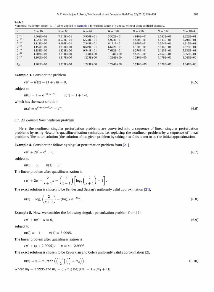
Table 2Numerical maximum errors (EN, ε ) when applied to Example 1 for various values of ε and N , without using artificial viscosity.

ε N = 16 N = 32 N = 64 N = 128 N = 256 N = 512 N = 1024

2−12 9.408E−01 7.414E−01 5.966E−01 5.562E−01 4.910E−01 3.792E−01 2.222E−012−13 1.026E+00 8.572E−01 6.558E−01 5.923E−01 5.570E−01 4.913E−01 3.794E−012−14 1.111E+00 9.495E−01 7.545E−01 6.171E−01 5.930E−01 5.574E−01 4.915E−012−15 1.157E+00 1.033E+00 8.649E−01 6.672E−01 6.120E−01 5.934E−01 5.576E−012−16 1.181E+00 1.121E+00 9.541E−01 7.612E−01 6.276E−01 6.123E−01 5.936E−012−20 1.204E+00 1.211E+00 1.198E+00 1.128E+00 9.575E−01 7.662E−01 6.356E−012−25 1.206E+00 1.217E+00 1.223E+00 1.224E+00 1.216E+00 1.179E+00 1.041E+00

EN 1.206E+00 1.217E+00 1.223E+00 1.224E+00 1.216E+00 1.179E+00 1.041E+00

Example 3. Consider the problem

εu′′ − u′(x)− (1+ ε)u = 0, (6.5)

subject to

u(0) = 1+ e−(1+ε)/ε, u(1) = 1+ 1/e,

which has the exact solution

u(x) = e(1+ε)(x−1)/ε + e−x. (6.6)

6.1. An example from nonlinear problems

Here, the nonlinear singular perturbation problems are converted into a sequence of linear singular perturbationproblems by using Newton’s quasilinearization technique, i.e. replacing the nonlinear problem by a sequence of linearproblems. The outer solution (the solution of the given problem by taking ε = 0) is taken to be the initial approximation.

Example 4. Consider the following singular perturbation problem from [21]

εu′′ + 2u′ + eu = 0, (6.7)

subject to

u(0) = 0, u(1) = 0.

The linear problem after quasilinearization is

εu′′ + 2u′ +2x+ 1

u =(2x+ 1

)[loge

(2x+ 1

)− 1

].

The exact solution is chosen to be Bender and Orszag’s uniformly valid approximation [21],

u(x) = loge

(2x+ 1

)− (loge 2)e

−2x/ε . (6.8)

Example 5. Now, we consider the following singular perturbation problem from [2],

εu′′ + uu′ − u = 0, (6.9)

subject to

u(0) = −1, u(1) = 3.9995.

The linear problem after quasilinearization is

εu′′ + (x+ 2.9995)u′ − u = x+ 2.9995.

The exact solution is chosen to be Kevorkian and Cole’s uniformly valid approximation [2],

u(x) = x+m1 tanh((m12

) ( xε+m2

)), (6.10)

wherem1 = 2.9995 andm2 = (1/m1) loge[(m1 − 1)/(m1 + 1)].


0 0.1 0.2 0.3 0.4 0.5 0.6 0.7 0.8 0.9 1

Exact solutionNum. sol. without viscosityNum. sol. with viscosity

0 0.1 0.2 0.3 0.4 0.5 0.6 0.7 0.8 0.9 10

0.1

0.2

0.3

0.4

0.5

0.6

0.7

0.8

0.9

1


0

0.2

0.4

0.6

0.8

1

1.2

1.4a b

Fig. 1. Exact and numerical solution profiles of (a) Example 2 for ε = 10−3 and N = 100 and (b) Example 3 for ε = 12−2 and N = 40.



a b

0 0.1 0.2 0.3 0.4 0.5 0.6 0.7 0.8 0.9 1 0 0.1 0.2 0.3 0.4 0.5 0.6 0.7 0.8 0.9 10

0.1

0.2

0.3

0.4

0.5

0.6

0.7

0.8

0.9

1

–1

0

1

2

3

4

5

Fig. 2. Exact and numerical solution profiles of (a) Example 4 for ε = 2−8 and N = 128 and (b) Example 5 for ε = 2−8 and N = 64.

Having the approximate solution obtained via B-splines for different values of N and ε, the maximum errors denoted byEN, ε at all the mesh points are evaluated. Further we will tabulate the maximum error for the scheme as

EN = max0≤ε≤1

EN, ε .

The experimental order of convergence (EOC) (presented in Tables 3 and 5) is computed using the formula:

ON, ε = log2(EN, ε/E2N, ε), (6.11)

The computed results are displayed in the Tables 1–6, for modest values of ε and N . It is observed that the computedresults using artificial viscosity show greater agreement with the exact solution as the mesh size is refined. For ε h thescheme gives first order convergence, which can be seen from estimate (5.2) and clearly reflects the tabular results too.In order to show the physical behaviour of the given problem, we give plots (Figs. 1 and 2) of the computed solutions for

different values of ε and N . The efficiency and the accuracy of the artificial viscosity over other schemes can be seen fromthe tables. The computed solution without using viscosity oscillates in the boundary layer regions for smaller ε. To controlthese disturbances, we use artificial viscosity and the results are far better than those without using viscosity.

7. Conclusions

In this paper, we have presented a B-spline collocation method for the numerical solution of the singularly perturbedboundary value problem. The artificial viscosity is exponentially stretchedwithin the boundary layers and this is responsiblefor improved accuracy compared to the related uniform scheme. These methods can be closely related to Galerkin methods,and hence to finite-element methods, as they are much easier and more efficient for computing. In comparison to FEM,the collocation matrix involves no integrations or numerical quadrature for complicated values of a(x) and b(x), andhence reduces the operation count. Also, collocation with B-splines leads to banded matrices as opposed to full matricesusing polynomials, trigonometric functions and other well-known nonpiecewise approximates. Example calculations werepresented to demonstrate the efficacy of the artificial viscosity scheme.


Table 3Numerical maximum errors (EN, ε ) and experimental order of convergence (EOC), when applied to Example 1 for various values of ε and N , using artificialviscosity.

ε N = 16 N = 32 N = 64 N = 128 N = 256 N = 512 N = 1024

2−12 1.085E−02 5.530E−03 2.754E−03 1.340E−03 6.269E−04 2.692E−04 9.640E−050.9723 1.0058 1.0393 1.0959 1.2196 1.4816 1.7862

2−13 1.089E−02 5.574E−03 2.798E−03 1.385E−03 6.718E−04 3.139E−04 1.347E−040.9662 0.9943 1.0145 1.0438 1.0977 1.2206 1.4817

2−14 1.091E−02 5.597E−03 2.821E−03 1.407E−03 6.942E−04 3.363E−04 1.571E−040.9629 0.9884 1.0036 1.0192 1.0456 1.0981 1.2211

2−15 1.092E−02 5.608E−03 2.832E−03 1.418E−03 7.054E−04 3.476E−04 1.683E−040.9614 0.9857 0.9980 1.0073 1.0210 1.0464 1.0992

2−16 1.093E−02 5.614E−03 2.838E−03 1.424E−03 7.110E−04 3.532E−04 1.739E−040.9612 0.9842 0.9949 1.0020 1.0094 1.0222 1.0469

2−20 1.093E−02 5.619E−03 2.843E−03 1.429E−03 7.163E−04 3.584E−04 1.792E−040.9599 0.9829 0.9924 0.9964 0.9990 1.0000 1.0027

2−25 1.093E−02 5.619E−03 2.843E−03 1.429E−03 7.166E−04 3.588E−04 1.795E−040.9599 0.9829 0.9924 0.9958 0.9980 0.9992 0.9997

EN 1.093E−02 5.619E−03 2.843E−03 1.429E−03 7.166E−04 3.588E−04 1.795E−04

Table 4Comparison of numerical solution of the present method with Kevorkian and Cole’s method, when applied to Example 2 for N = 200 and various valuesof ε.

x Present method Kevorkian and Cole’s solution [2]ε = 2−4 ε = 2−6 ε = 2−10 ε = 2−4 ε = 2−6 ε = 2−10

0.01 0.0848 0.2451 0.5038 0.0763 0.2384 0.50250.02 0.1568 0.3743 0.5063 0.1414 0.3651 0.50510.03 0.2180 0.4430 0.5089 0.1971 0.4332 0.50760.05 0.3143 0.5007 0.5141 0.2859 0.4916 0.51280.1 0.4566 0.5331 0.5276 0.4212 0.5253 0.52630.2 0.5641 0.5630 0.5568 0.5316 0.5556 0.55560.5 0.6896 0.6733 0.6678 0.6662 0.6667 0.66670.9 0.9174 0.9115 0.9095 0.9091 0.9091 0.9091

Table 5Numerical maximum errors (EN, ε ) and experimental order of convergence (EOC), when applied to Example 3 for various values of ε and N , using artificialviscosity.

ε N = 16 N = 32 N = 64 N = 128 N = 256 N = 512 N = 1024

2−12 1.088E−02 5.541E−03 2.757E−03 1.341E−03 6.272E−04 2.693E−04 9.642E−050.9735 1.0070 1.0398 1.0963 1.2197 1.4818 1.4896

2−13 1.093E−02 5.585E−03 2.801E−03 1.385E−03 6.720E−04 3.140E−04 1.347E−040.9687 0.9956 1.0161 1.0434 1.0977 1.2210 1.4814

2−14 1.095E−02 5.607E−03 2.823E−03 1.408E−03 6.944E−04 3.364E−04 1.571E−040.9656 0.9900 1.0036 1.0198 1.0456 1.0985 1.2211

2−15 1.096E−02 5.618E−03 2.835E−03 1.419E−03 7.056E−04 3.476E−04 1.683E−040.9641 0.9867 0.9985 1.0080 1.0214 1.0464 1.0992

2−16 1.097E−02 5.623E−03 2.840E−03 1.425E−03 7.112E−04 3.532E−04 1.739E−040.9642 0.9854 0.9949 1.0026 1.0098 1.0222 1.0467

2−20 1.097E−02 5.628E−03 2.845E−03 1.430E−03 7.165E−04 3.585E−04 1.792E−040.9629 0.9842 0.9924 0.9970 0.9990 1.0004 1.0026

2−25 1.097E−02 5.629E−03 2.846E−03 1.430E−03 7.168E−04 3.588E−04 1.795E−040.9626 0.9839 0.9929 0.9964 0.9984 0.9992 0.9995

EN 1.097E−02 5.629E−03 2.846E−03 1.430E−03 7.168E−04 3.588E−04 1.795E−04

Table 6Comparison of numerical solution of the present method with Bender and Orszag’s method, when applied to Example 4 for N = 300 and various values ofε.

x Present method Bender and Orszag’s solution [21]ε = 2−5 ε = 2−6 ε = 2−10 ε = 2−5 ε = 2−6 ε = 2−10

0.01 0.3154 0.4905 0.6843 0.3177 0.4905 0.68320.03 0.5646 0.6529 0.6647 0.5620 0.6487 0.66360.05 0.6228 0.6481 0.6454 0.6161 0.6432 0.64440.1 0.6054 0.6023 0.5987 0.5967 0.5978 0.59780.5 0.2908 0.2892 0.2880 0.2877 0.2877 0.28770.9 0.0517 0.0515 0.0513 0.0513 0.0513 0.0513


Acknowledgements

The second author wishes to acknowledge Council of Scientific and Industrial Research (CSIR), India for the financial aid(grant aid no. P-81 101) provided.

References

[1] M.K. Kadalbajoo, K.C. Patidar, A survey of numerical techniques for solving singularly perturbed ordinary differential equations, Applied Mathematicsand Computation 131 (2002) 299–320.

[2] J. Kevorkian, J.D. Cole, Perturbation Methods in Applied Mathematics, Springer-Verlag, New York, 1981.[3] W. Eckhaus, Matched Asymptotic Expansions and Singular Perturbations, in: North-Holland Mathematics Studies, vol. 6, North-Holland, Amsterdam,1973.

[4] R.E. O’Malley Jr., Introduction to Singular Perturbation, Academic Press, New York, 1979.[5] C.E. Pearson, On a differential equation of boundary layer type, Journal of Mathematical Physics 47 (1968) 134–154.[6] E.P. Doolan, J.J.H. Miller, W.H.A. Schilders, Uniform Numerical Methods for Problems with Initial and Boundary Layers, Boole Press, Dublin, 1980.[7] J.E. Flaherty, W. Mathon, Collocation with polynomial and tension splines for singularly-perturbed boundary value problems, SIAM Journal onScientific and Statistical Computing 1 (2) (1980) 260–289.

[8] M.K. Jain, T. Aziz, Numerical solution of stiff and convection diffusion equations using adaptive spline function approximation, Applied MathematicalModelling 7 (1983) 57–62.

[9] K. Surla,M. Stojanovic, Solving singularly perturbed boundary-value problems by spline in tension, Journal of Computational andAppliedMathematics24 (1988) 355–363.

[10] L.R. Abrahamson, H.B. Keller, H.O. Kreiss, Difference approximations for singular perturbations of systems of ordinary differential equations,Numerische Mathematik 22 (1974) 367–391.

[11] A.E. Berger, J.M. Solomon, M. Ciment, Higher order accurate tridiagonal difference methods for diffusion convection equations, in: Proceedings of theThird IMACS Conference on Computer Methods for Partial Differential Equations, Lehigh University, 1979.

[12] J.E. Flaherty, R.E. O’Malley Jr., The numerical solution of boundary value problems for stiff differential equations, Mathematics of Computation 31(1977) 66–93.

[13] E. O’Riordan, M. Stynes, A uniformly accurate finite element method for a singularly perturbed one-dimensional reaction–diffusion problem,Mathematics of Computation 47 (1986) 555–570.

[14] M. Stynes, E. O’Riordan, A finite element method for a singularly perturbed boundary value problem, Numerische Mathematik 50 (1986) 1–15.[15] A.H. Schatz, L.B.Wahlbin, On the finite elementmethod for singularly perturbed reaction–diffusion problems in two and one dimensions,Mathematics

of Computation 40 (161) (1983) 47–89.[16] G.R. Liu, Y.T. Gu, Meshless techniques for convection dominated problems, Computational Mechanics 38 (2) (2006) 171–182.[17] M. Sakai, R.A. Usmani, A class of simple exponential B-splines and their applications to numerical solution to singular perturbation problems,

Numerische Mathematik 65 (1989) 493–500.[18] J.J.H. Miller, E. O’Riordan, G.I. Shishkin, Fitted Numerical Methods for Singular Perturbation Problems, World Scientific, Singapore, 1996.[19] P.M. Prenter, Splines and Variational Methods, John Wiley & Sons Inc., New York, 1989.[20] C.A. Hall, On error bounds for spline interpolation, Journal of Approximation Theory 1 (1968) 209–218.[21] C.M. Bender, S.A. Orsazag, Advanced Mathematical Methods for Scientists and Engineers, McGraw-Hill, New York, 1978.[22] A.H. Nayfeh, Perturbation Methods, Wiley, New York, 1979.

B-splines with artificial viscosity for solving singularly perturbed boundary value problems

Documents

Transcript of B-splines with artificial viscosity for solving singularly perturbed boundary value problems