On the General Interpretation of First-Order Quantifiers

G. Aldo AntonelliUniversity of California, Davis

antonelli@ucdavis.edu

27 July 2013

Abstract

While second-order quantifiers have long been known to admit non-standard, or “general” inter-

pretations, first-order quantifiers (when properly viewed as predicates of predicates) also allow a

kind of interpretation that does not presuppose the full power-set of that interpretation’s first-order

domain. This paper explores some of the consequences of such “general” interpretations for (unary)

first-order quantifiers in a general setting, emphasizing the effects of imposing various further con-

straints that the interpretation is to satisfy.

1 Introduction

It has been known since Henkin (1950) that second-order quantifiers admit of interpretations on which

they are taken to range over some collection of subsets of the domain, a collection that possibly falls

short of the full power set. To capture these interpretations formally, Henkin introduced the notion of

a general model for second-order logic. A general model M supplies, besides an interpretation function

I for the extra-logical constants, also a sequence (D1, D2, . . .), where D1 is a non-empty domain of

objects, and each Dn+1 is a collection of n-place relations over D1 (by identifying subsets of D1 with

the corresponding sets of 1-tuples, we can assume that D2 ⊆ P (D1)). On Henkin’s account, D1 is the

range for the first-order variables, whereas each Dn+1 provides the range for second-order relational

variables whose values are n-place relations over D1. In order for the all the instances of the second-

order comprehension schema to be satisfied, Henkin also assumed each domain Dn+1 to be closed

under Boolean operations (intersection and complement, say) as well to contain all relations R that can

be obtained as projections of relations S ∈ Dn+2 (see Enderton 2009, Henkin 1996).

Many thanks to John Baldwin, Claude Laflamme, and Albert Visser for helpful comments. I am grateful to the referees fortheir useful criticisms, and especially for pointing me to the question of decidability, as well as to parts of the literature withwhich I was not previously familiar, notably Thomason and Johnson (1969), Bruce (1978), Väänänen (1978), López-Escobar(1991), and Andréka et al. (1998).

1

There is an asymmetry in Henkin’s semantics between the first- and the second-order case, which

becomes evident from the more abstract point of view of the theory of generalized quantifiers intro-

duced by Mostowski (1957), Lindström (1966) and Montague (1974). According to the theory, a

first-order quantifier Q is a predicate over the power set of the first-order domain D1: for example, the

first-order existential quantifier “there is at least one” denotes the collection of all non-empty subsets of

D1, and the quantifier “there exist exactly k” denotes the collection of all k-membered subsets. A quan-

tifier behaves precisely as such a predicate: when applied to a formula ϕ, the quantifier Q returns value

“true” precisely when the extension of ϕ in D1 falls under Q. The asymmetry in Henkin’s semantics lies

in the fact that whereas the determination of semantic values for the second-order quantifiers requires

the specification of various second-order domains, the meaning of the first-order quantifiers is assumed

to be fixed by the specification of a single first-order domain. In other words, there is an implicit bias in

Henkin’s semantics towards the standard interpretations of first-order quantifiers, according to which

they are construed as predicates over the full power set of D1. But it is in fact clear that just specifying

a domain of objects underdetermines the semantics of first-order quantifiers.

Symmetry can be restored by extending the general semantics to the first-order case. Once first-

order quantifiers are conceived as second-order predicates, it becomes apparent that it is indeed possi-

ble to develop a general, non-standard semantics on which they are interpreted as predicates ranging

— not over the full power set of the first-order domain — but over some collection of subsets. For

instance, the first-order existential quantifier ∃ can come to denote, on such a semantics, a collection

of non-empty subsets that may well be short of the collection of all non-empty subsets.

The possibility of such general interpretations is both technically interesting and philosophically

relevant. This paper is concerned with the former aspect, by presenting a rigorous formal account of

the basic technical notions underpinning the general interpretation of first-order quantifiers, while the

philosophical implications are developed in a parallel paper (Antonelli forthcoming). We will consider a

first-order languageL comprising, besides predicate symbols, also any number of first-order quantifiers

Q (some of which might or might not be the ordinary quantifiers ∃ and ∀). Models for such a language

will have the form (D1, D2, I) providing, in addition to an interpretation I for the predicates, two

distinct domains: a first-order domain D1 of objects and a second-order domain D2 of subsets of D1.

It is important to keep in mind that both D1 and D2 are only needed for the interpretation of first-

order notions — a point emphasized by the similar notation adopted for each. The domain D2 is only

“second-order” in the sense that it is comprised of subsets of D1, but no truly second-order notions are

involved.

Furthermore, we restrict ourselves to the case of quantifiers that are both unary and monadic, i.e.,

quantifiers that, just like ∃ and ∀, take exactly one formula as argument, binding a unique specific

variable in that formula (other variables may occur free, but are treated as parameters). This fact

explains why, in contrast to Henkin’s semantics for second-order logic, general models need only supply

the two domains D1 and D2, instead of the multiple domains Dn for n > 0. Such domains would

2

be needed were we to extend the framework to the fully general case of quantifiers that are n-ary

(applying to n formulas) and k-adic (simultaneously binding k variables), and quantifiers such as the

non-linear quantifiers of Henkin (1961) require more complex still non-standard models (see López-

Escobar 1991).

Equally crucial is the restriction throughout to a purely relational language L , i.e., a language with

any number of predicate symbols of any number of arguments (including the identity predicate.=),

but no individual constants or function symbols. This allows us to focus on the modal properties of

the quantifiers, which include way they interact with Boolean connectives. As an example consider

the K schema for the ordinary universal quantifier: ∀x(ϕ → ψ)→ (∀xϕ → ∀xψ). One way to read

the K schema is as stating that the universal quantifier is preserved by supersets: if (commuting the

antecedents) ∀ applies to ϕ, and ψ is a superset of ϕ, then ∀ applies to ψ as well. As such, the K

schema expresses a form of monotonicity that might in principle pertain to other quantifiers as well

(such as, for instance, “there are at least three”). But it is of course accidental that “ψ is a superset of

ϕ” can be expressed using the same quantifier ∀ that is being claimed to be monotonic, a fact that does

not generalize to other monotonic quantifiers (such as Q1 mentioned below).

It is also intuitively clear why the presence of singular terms would interfere with a proper un-

derstanding of general semantics: singular terms are unconstrained in their taking denotations in D1,

thereby giving access to the “dark corners” of the first-order domain where the light of the quantifiers

does not shine (i.e., less figuratively, allowing reference to objects that fall outside the range of the quan-

tifiers). Of course a case can be made that some quantifiers are essentially characterized by the way

they interact with singular terms, for instance in the schema of universal instantiation, ∀xϕ→ ϕ[t/x].

In interpreting the schema as asserting that instantiation holds throughout the range of applicability of

the quantifiers, we again reveal a bias in favor of the standard interpretation. We wil see that perhaps

a better way to express this fact — that quantifiers instantiate over their range — is by using the more

broadly valid schema ∀x(∀yϕ[y/x]→ ϕ).The central result of our investigations is that each model M is equivalent to its “hull,” i.e., the

model having the same first-order domain and the same interpretation of the predicates as M, but in

which the second-order domain is only comprised of those subsets definable in M. Philosophically,

such “lean” interpretations not only point to the fact the standard interpretations of first-order logic

“overshoot the target” in some informal but substantial sense, but also provide a possible criterion of

demarcation between genuinely first-order and genuinely second-order notions. They also play a promi-

nent technical role in establishing the correspondence between the “logical” properties of models (the

schema therein satisfied) and the “algebraic” properties (the various closure conditions characterizing

the second-order domain). For instance, in the case of the existential quantifier, we show that there is

a connection between the class of general interpretations satisfying a certain closure condition and the

outer-domain models of free logic (thereby showing that the set of validities for the class in question is

axiomatizable). Another prominent application will deal with the case of quantifiers expressing large

3

properties, i.e., those quantifiers that denote a filter over the second-order domain.

It appears that the idea of providing non-standard interpretation for the first-order quantifiers,

even in a generalized setting, first made its appearance with Thomason and Johnson (1969). Arguably,

Thomason and Johnson were the first to combine the generalized viewpoint (consideration of quanti-

fiers other than ∃ and ∀) with the non-standard approach (consideration of models that in some way

or other “liberalize” the interpretation of the quantifiers). Their approach is both more and less general

than the present one. It is more general in that they consider ordinary first-order logic augmented

with quantifier variables (while the present approach deals with quantifier constants): accordingly they

consider what formulas Qxϕ(x) are valid under all interpretations of the quantifier variable Q. As it

turns out, doing so introduces intrinsically higher-order features in the semantics, as shown by Väänä-

nen (1978) (improving upon previous results of Yasuhara (1969)). But the approach of Thomason and

Johnson is also less general than the present one in that they restrict themselves to quantifiers that

satisfy a form of permutation invariance, and moreover (as mentioned) only in the context of logics

extending ordinary first-order logic. The ordinary ∃ and ∀ are required to express invariance under

permutation, but in their absence the logic of quantifier variables becomes much weaker — decidable,

in fact (see Anapolitanos and Väänänen 1981). The notion of permutation invariance is also used by

Thomason and Johnson to identify a class of non-standard models, by allowing models in which the

interpretations of the quantifier variables are not required to be invariant under all permutations, but

just those in a given collection. In contrast, below we will consider a logic with quantifier constants,

which are not necessarily permutation invariant, and without assuming that the ordinary quantifiers

are available in the language. (Although Väänänen (1978) shows how, over first-order logic, quantifier

variables are equivalent to an equi-cardinality quantifier constant, this result does not extend to other

constants and depends on the availability of ∃ and ∀.) Non-standard models for the logic presented

below will not be obtained by weakening some invariance condition, but by keeping the meaning of

each quantifier fixed while varying the second-order domain to which it is applied.

Another prominent tradition that is relevant to our project is the one originating with Keisler’s clas-

sic (1970), which employs a non-standard semantics for the first-order quantifier constant Q1 (“there

exist uncountably many”), in order to show that the set of validities of such a quantifier (now on the

standard interpretation) can be recursively axiomatized. In particular, Keisler introduces countable

non-standard structures for the language with the quantifier Q1: so-called “weak models” in which the

quantifier is reinterpreted to apply to countable, definable subsets of the domain (ω1 iterations of an

omitting types construction are then deployed to blow up such subsets to uncountable size while keep-

ing the remaining subsets countable). What is relevant for our purposes is that Keisler’s weak-model

semantics is quite different from the one offered here both in inspiration and execution. In the first

place Keisler presupposes the ordinary quantifiers ∃ and ∀, which are needed to provide the required

axiomatization for Q1 (to express that Q1 is monotonic, for instance); whether these quantifiers are

present or not can make a substantial difference, as we learn from Anapolitanos and Väänänen (1981).

4

But perhaps most importantly, on Keisler’s weak models the meaning of the quantifier Q1 differs from

the meaning it has in the standard case: on such interpretations, “uncountably many” comes to denote

collections of subsets of the domain that are, in fact, countable. In contrast, we expend some effort

below to make sure that we compare the behavior of the same quantifier on the standard vs. the non-

standard interpretations. Such a task is complicated by the fact that we do not have (to the best of our

knowledge) a completely general criterion for when a quantifier Q over a domain D1 is the same as a

quantifier Q′ over D′1. But we do have answers in some cases: for instance if, say, Q = ∃, then we can

say that in each case the quantifier applies to all and only the non-empty subsets of the interpretation’s

second-order domain. In a slightly more general setting, in our case we can compare quantifiers Q and

Q′ over (D1, D2) and (D′1, D′2) if D1 ⊆ D′1 and similarly D2 ⊆ D′1 for the corresponding second-order

domains.

2 Basic Semantic Notions

Definition 2.1 Let s be a relational and quantificational signature, comprised of predicate symbols

P1, P2, . . ., of varying number of arguments, and unary monadic quantifier symbols Q1,Q2, . . . applying

to a formula and binding one variable.

Definition 2.2 The language determined by the signature s is the smallest set L (s) of formulas such

that:

1. If P is a k-place predicate symbol in s and x1, . . . , xk are variables then P x1 . . . xk is in L (s).2. If x and y are variables, then x

.= y is in L (s).

3. if ϕ and ψ are in L (s), then so are ¬ϕ and ϕ→ψ.

4. If Q is a unary quantifier symbol in s, ϕ is a formula in L (s), and x is a variable, then Qxϕ is in

L (s).The notions of free and bound occurrences of variables are defined as usual. When we want to make

the (finitely many) quantifier symbols of the language explicit, we write L (Q1, . . . ,Qn).

Definition 2.2 could, in principle, be easily generalized to arbitrary k-adic, n-ary quantifiers.

Definition 2.3 A model for a signature s is a triple M = (D1, D2, I), where D1 and D2 are both non-

empty, with D2 ⊆ P (D1), and I is a function assigning an interpretation I(P) = PM to each predicate

symbol P in the signature.

Definition 2.4 A model M= (D1, D2, I) is standard if D2 =P (D), and it is replete if D1 ∈ D2.

We will often be comparing models M= (D1, D2, I) and M′ = (D1, D′2, I) that differ at most in their

second-order domain, but are otherwise the same.

Definition 2.5 A monadic, first-order, unary quantifier is a function Q assigning a predicate Q(D1)

over P (D1) to each non-empty domain D1.

By a slight abuse of language, we use the same symbol Q for both the quantifier symbol in the

5

signature s and the function assigning the predicate Q(D1) to each domain D1. According to the

definition, for example, the quantifier ∃ is a function that assigns to each domain D1 a predicate over

P (D1), denoted by ∃(D1), which is true of a subset X ⊆ D1 if and only if X 6= ∅. Similarly, the

quantifier ∀ provides a predicate ∀(D1) which is true of X if and only if X = D1. Many other quantifiers

play an important role, for instance ∃! (“there is exactly one”) and Qα (“there exist at least ℵα” — so

that Q0 is the infinity quantifier, Q1 is Keisler’s quantifier, etc.); see Peters and Westerståhl (2006) for a

comprehensive treatment.

Just like ∃ and ∀ are dual of each other in standard first-order logic, the notion can be extended to

any unary quantifier.

Definition 2.6 For any quantifier Q, the dual of Q is the quantifier Qd such that for any domain D1

and X ⊆ D1: X ∈Qd(D1) if and only if D1 \ X /∈Q(D1).

Definition 2.7 Given a model M = (D1, D2, I) for the signature s, let QM = Q(D1) ∩ D2 denote

the restriction of Q(D1) to D2. The predicate QM is the interpretation assigned by the model to the

quantifier symbol Q.

Definition (2.7) provides a way to view quantifiers as constant across domains. We can say that

QM is the same quantifier as QM′because they are the restrictions of the same quantifier Q to different

domains. We now proceed with the notion of satisfaction, which generalizes the ordinary notion of

satisfaction for first-order languages.

Definition 2.8 An assignment s of objects from D1 to the variables is a function such that s(x) ∈ D1 for

each variable x . If d ∈ D1, then s[d/x] is the assignment such that s[d/x](x) = d and s[d/x](y) = s(y)

if y is a variable other than x . We say that s[d/x] results from shifting s at x .

Notation 2.1 If x = x1, . . . , xn is a sequence of variables and d = d1, . . . , dn a sequence members of

D1, the multiple shift s[d1/x1, . . . , dn/xn] = s[d1/x1], . . . , [dn/xn] is sometimes denoted by s[x/d], or even

s[x i/di].

Definition 2.9 We define satisfaction of a formula ϕ in L (s), by an assignment s of objects in D1 to

the variables, in a model M= (D1, D2, I), by recursion on ϕ:

M, s |= P x1 . . . xk iff ⟨s(x1), . . . , s(xk)⟩ ∈ PM;

M, s |= x.= y iff s(x) = s(y);

M, s |= ¬ϕ iff M, s 6|= ϕ;

M, s |= ϕ→ψ iff M, s 6|= ϕ or M, s |=ψ;

M, s |=Qxϕ iff {d ∈ D1 : M, s[d/x] |= ϕ} ∈QM.

In ordinary first-order logic it is customary to handle formulas with free variables the same as their

universal closure. But of course in the more general case, where quantifiers other than ∃ and ∀ might

or might not be present, special arrangements must be made.

6

Definition 2.10 If ϕ is a formula (with zero or more free variables) then we say that ϕ is true in

M, written M |= ϕ, if and only if M, s |= ϕ for every assignment s. Moreover, two models are L (s)-equivalent if the same L (s)-sentences are true in each.

It is convenient to introduce a notation for the extension of formula in a model, relative to a subset

of its free variables and an assignment. We consider the general case of a formula with free variables

x1, . . . xn and parameters instantiating the variable y1, . . . ym.

Definition 2.11 Where x= x1, . . . , xn and y= y1, . . . , ym are vectors of variables, M is a model, ϕ(x,y)

a formula, and s an assignment, then:

JϕKMs,x = {⟨d1, . . . dn⟩ ∈ Dn1 : M, s[d1/x1, . . . , dn/xn] |= ϕ}.

The values s(y1), . . . , s(ym) function as parameters in the previous definition. Using this notation

the satisfaction clause for the quantifier in Definition 2.9 becomes:

M, s |=Qxϕ iff JϕKMs,x ∈QM,

where we identify a subset X ⊂ D1 with the set X 1 of its 1-tuples, as already pointed out. If the model

is understood, we drop the superscript from JϕKMs,x .

Remark 2.1 A central theme in the paper is the possibility of imposing certain further restrictions on

the second-order domain D2 of a model. For instance, consider that the inference,

Qx(ϕ(x)∧ψ(x))Qxϕ(x)

which is validated by both ∃ and ∀ on their standard interpretations (but not, for instance, by ∃!). Such

an inference is not validated by those same quantifiers over general models. But it is of course valid

over the class of models M= (D1, D2, I) in which D2 is closed under ⊆, in the sense that if X ∈ D2 and

X ⊆ Y , then also Y ∈ D2. This follows since in every M:

Jϕ(x)∧ψ(x)Ks,x ⊆ Jϕ(x)Ks,x .

This observation will play a central role in Section 6. Notice that there are two considerations at work

here, i.e., whether the quantifier Q monotonic (which both ∃ and ∀ are), and whether the second-order

domain D2 of any given model is closed under supersets. And so, accordingly, there are two possible

sources of the failure of the inference above.

Definition 2.12 A general model M = (D1, D2, I) is closed under duals if and only if for any quantifier

Q in the signature s:

M, s |=Qd xϕ(x)⇐⇒M, s |= ¬Qx¬ϕ(x).

7

Remark 2.2 General models are not necessarily closed under duals. Let M be a non-replete general

model, i.e., such that D1 /∈ D2. Then M |= ¬∃x¬(x .= x) (indeed, this formula is true in every general

model), but M 6|= ∀x(x.= x). Conversely, if M is replete, then M |= ∀x(x

.= x). More generally

∀x(x.= x) is valid in any models in which D2 is non-empty and satisfies the closure under supersets

condition mentioned in Remark 2.1. (Notice also that in our counter-example the failure of duality is

due to the second-order domain’s being non-standard and is not due to the specific properties of the

quantifier Q.

We close this section by briefly taking up the issue of permutation invariance, which according

to a tradition going back to Tarski (1986), is regarded as the proper criterion demarcating logical

notions, including quantifiers. Cardinality quantifiers such as “there exists,” “exactly three,” etc. are all

permutation invariant.

Definition 2.13 A quantifier Q over a model M = (D1, D2, I) is permutation invariant if and only if,

for any permutation π of D1 and subset A ∈ D2, it holds that A ∈ QM ⇐⇒ π[A] ∈ QM, where π[A] is

the point-wise image of A under π.

Permutation invariance might fail in the context of general models. However, there are, again, two

sources of such failures for a quantifier Q over a domain D1: (a) the predicate Q(D1) might apply to

some subsets but not to their images under permutation; or (b) the underlying domain D2 itself might

not be closed under permutation. As to (a), some quantifiers lack invariance even on the standard

interpretation: consider for instance so-called “Montagovian” quantifiers of the form Qa(D1) = {X ⊆D1 : a ∈ X }. But it is equally clear that consideration of general interpretations in (b) allows for failure

of invariance even for those quantifiers that are invariant on the standard interpretation (such as ∃).

Permutation invariance (or its failure) will not concern us further here, but if one were interested on

pursuing such a notion as a criterion of logicality in the Tarskian tradition, then it appears that the

relevant test is whether a quantifier fails to be invariant on second-order domains that are themselves

closed under permutations (or p-closed, in the terminology of Antonelli 2010).

3 The Hull Theorem

One of the main insights that can be gleaned from consideration of general models for the first-order

quantifiers is that in some sense, as mentioned, they overshoot their target, in that there are much

leaner models, whose second-order domain is only comprised of the definable subsets, to which they

are equivalent. Here are the relevant notions.

Definition 3.1 A n-place relation R⊆ Dn1 is definable (from parameters) in a model M= (D1, D2, I) if

and only if there is a formula ϕ(x,y) and an assignment s such that R = JϕKMs,x (where x is an n-tuple

of free variables, and y is a sequence of parameters whose denotation is fixed by the assignment).

Remark 3.1 In Definition 3.1, the notation ϕ(x,y) indicates that any free variables in ϕ other than

8

the parameters are among x = x1, . . . , xn, but these variables can occur in ϕ in any particular order.

It follows as a result of such a convention that if a binary relation R is definable, for instance, so is its

converse. This kind of built-in manipulation of the variables will be important in the proof of Theorem

4.2.

Definition 3.2 Given a model M= (D1, D2, I), the hull H(M) of M is the collection of the parameter-

definable members of D2: H(M) = {X ∈ D2 : X is definable from parameters}.

If M is standard, then H(M) is just the collection of all parameter-definable subsets of D1, but if

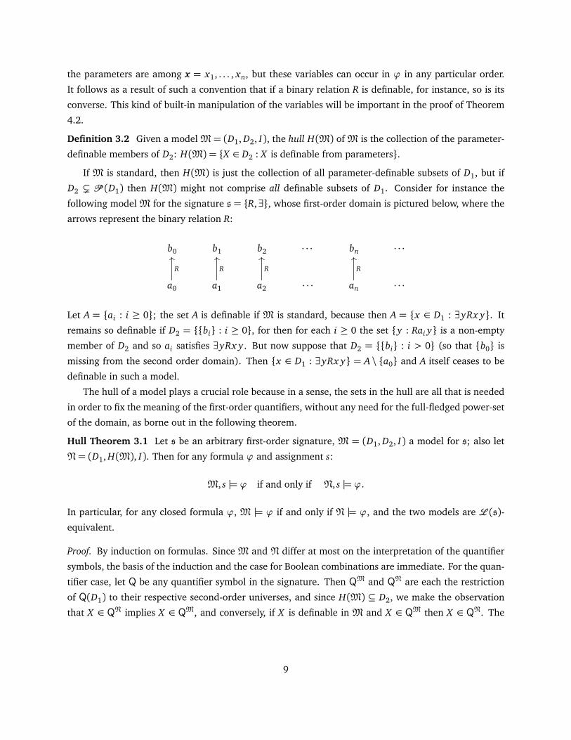
D2 ( P (D1) then H(M) might not comprise all definable subsets of D1. Consider for instance the

following model M for the signature s = {R,∃}, whose first-order domain is pictured below, where the

arrows represent the binary relation R:

b0 b1 b2 · · · bn · · ·

a0 a1 a2 · · · an · · ·

R R R R

Let A = {ai : i ≥ 0}; the set A is definable if M is standard, because then A = {x ∈ D1 : ∃yRx y}. It

remains so definable if D2 = {{bi} : i ≥ 0}, for then for each i ≥ 0 the set {y : Rai y} is a non-empty

member of D2 and so ai satisfies ∃yRx y . But now suppose that D2 = {{bi} : i > 0} (so that {b0} is

missing from the second order domain). Then {x ∈ D1 : ∃yRx y} = A \ {a0} and A itself ceases to be

definable in such a model.

The hull of a model plays a crucial role because in a sense, the sets in the hull are all that is needed

in order to fix the meaning of the first-order quantifiers, without any need for the full-fledged power-set

of the domain, as borne out in the following theorem.

Hull Theorem 3.1 Let s be an arbitrary first-order signature, M = (D1, D2, I) a model for s; also let

N= (D1, H(M), I). Then for any formula ϕ and assignment s:

M, s |= ϕ if and only if N, s |= ϕ.

In particular, for any closed formula ϕ, M |= ϕ if and only if N |= ϕ, and the two models are L (s)-equivalent.

Proof. By induction on formulas. Since M and N differ at most on the interpretation of the quantifier

symbols, the basis of the induction and the case for Boolean combinations are immediate. For the quan-

tifier case, let Q be any quantifier symbol in the signature. Then QM and QN are each the restriction

of Q(D1) to their respective second-order universes, and since H(M) ⊆ D2, we make the observation

that X ∈ QN implies X ∈ QM, and conversely, if X is definable in M and X ∈ QM then X ∈ QN. The

9

inductive step then is as follows:

M, s |=Qxϕ ⇐⇒ JϕKMs,x ∈QM, def. satisfaction;

⇐⇒ JϕKMs,x ∈QM ∩H(M), def. hull;

⇐⇒ JϕKNs,x ∈QM ∩H(M), ind. hypothesis;

⇐⇒ JϕKNs,x ∈QN, previous observation;

⇐⇒ N, s |=Qxϕ, def. satisfaction.

Although we have proved the theorem in general for any model M, it is perhaps most interesting to

consider the case where M = (D1,P (D), I) is standard. Then the model N = (D1, H(M), I) is equiva-

lent to it, thereby showing that the full power set is not needed to fix the meaning of the quantifiers. In

fact, the hull construction provides a sort of reflective equilibrium, in that its iteration does not produce

any new definable sets.

Corollary 3.1 If M= (D1, D2, I) and M′ = (D1, H(M), I), then H(M) = H(M′).

Proof. Suppose X ∈ H(M) is definable in M; then X ∈ D2 and there are a formula ϕ(x ,y) (where y is

a vector of variables) and an assignment s such that X = JϕKMs,x. Since X ∈ H(M), and it belongs to the

second-order domain of M′; we need to show that X is also definable in M′, for then X ∈ H(M′). We

argue as follows: for every d ∈ D1:

d ∈ X ⇐⇒M, s[d/x] |= ϕ, X definable;

⇐⇒M′, s[d/x] |= ϕ, Theorem 3.1.

For the converse implication, if X ∈ H(M′), then also X ∈ D2, since H(M′) ⊆ H(M) ⊆ D2. Then, by

the argument just given, using Theorem 3.1, X is definable in M, so that X ∈ H(M).

Definition 3.3 A model M= (D1, D2, I) is H-closed if and only if H(M)⊆ D2.

By the previous Corollary 3.1, every model is elementarily equivalent to an H-closed model. The

fact that each model is elementarily equivalent to its hull has both philosophical and logical ramifi-

cations. Note that the situation is significantly different in the case of second-order logic, where the

introduction of first-order definable subsets results in new values for the second-order parameters, so

that the construction needs to be iterated transfinitely in order to reach a fixed point. And so for in-

stance, restricting the second-order quantifiers to range over the first-order definable subsets in the

standard model N of arithmetic, results in a model of a theory, ACA0, which is much weaker than full

second-order arithmetic.

Remark on Demarcation 3.2 A notion’s invariance under restriction to first-order definable subsets,

“hull-invariance” (as we might call it) can be used as a criterion of demarcation of genuinely first-order

notions from second-order ones.

10

The Hull Theorem also has a converse of sorts.

Theorem 3.2 Suppose M= (D1, D2, I) is H-closed and M∗ = (D1, D∗2, I) is a model such that D2 ⊆ D∗2(but is otherwise the same as M). Then for any assignment s and formula ϕ:

M, s |= ϕ if and only if M∗, s |= ϕ.

Proof. By induction of ϕ. Since the two models differ only in their second-order domain the basis is

immediate and the Boolean cases follow immediately from the inductive hypothesis. For the quantifier

case:

M, s |=Qxϕ =⇒ JϕKMs,x ∈Q(D1)∩ D2, def. satisfaction, QM

=⇒ JϕKM∗

s,x ∈Q(D1)∩ D2, ind. hyp.

=⇒ JϕKM∗

s,x ∈Q(D1)∩ D∗2, D2 ⊆ D∗2=⇒ M∗, s |=Qxϕ. def. satisfaction, QM∗

Conversely:

M∗, s |=Qxϕ =⇒ JϕKM∗

s,x ∈Q(D1)∩ D∗2, def. satisfaction, QM∗

=⇒ JϕKMs,x ∈Q(D1)∩ D∗2, ind. hyp.

=⇒ JϕKMs,x ∈Q(D1)∩ D2, D2 is H-closed

=⇒ M, s |=Qxϕ. def. satisfaction, QM

In particular, by Theorem 3.2, any H-closed model M= (D1, D2, I) is L (s)-equivalent to the corre-

sponding standard model M∗ = (D1,P (D1), I). Thus we obtain a reduction of the decision problem of

L (s) on the standard interpretation to that of L (s) interpreted over H-closed models.

Corollary 3.2 For each L (s)-sentence ϕ, the following are equivalent:

(a) ϕ is valid in the class of standard models for L (s);(b) ϕ is valid in the class of H-closed models for L (s);(c) ϕ is valid in the class of those models M for L (s) whose domain is precisely H(M).

4 Building hulls from below

As regards the construction of hulls, it might be objected that such a construction still relies on the

notion of satisfaction in the original model, so that we cannot convincingly claim to have dispensed

with the full power-set of D1. Consider again the case of a standard M; in order to define the hull of M

we still need to use the notion of satisfaction in M, which makes use of the quantifiers in their standard

interpretation. But the objection can be circumvented, by giving a construction of H(M) “from below,”

11

without going through the notion of satisfaction in M. As in other cases, although we are interested in

the case where M is standard, the definition is general. We start by identifying a set of Gödel operations

on sets of n-tuples.

Definition 4.1 (Gödel operations). Given a signature s and domain D1, for each n let [D1]n be the

set of all n-place relations over D1, i.e., [D1]n = P (Dn1). For any domain D1, and D2 ⊆ P (D1), define

the following Gödel operations F0, . . . , F6, Fa (for a ∈ D1), and FQ (for Q a quantifier symbol in the

signature) on⋃

n>0[D1]n:

F0(X , Y ) = X × Y, cartesian prod.;

F1(X , Y ) = X ∩ Y, intersection;

F2(X ) = {⟨x1, . . . , xn⟩ : ⟨x1, . . . , xn⟩ /∈ X }, complement;

F3(X ) = {⟨x2, x1 . . . , xn⟩ : ⟨x1, x2 . . . , xn⟩ ∈ X }, permute head;

F4(X ) = {⟨x1, x1, . . . , xn⟩ : ⟨x1, . . . , xn⟩ ∈ X }, duplicate head;

F5(X ) = {⟨x1, . . . , xn⟩ : ⟨x1, x1, . . . , xn⟩ ∈ X }, collapse head;

F6(X ) = {⟨xn, x1, . . . , xn−1⟩ : ⟨x1, . . . , xn⟩ ∈ X }, rotate;

Fa(X ) = {⟨x1, . . . , xn⟩ : ⟨a, x1, . . . , xn⟩ ∈ X }, parametrize;

FQ(X ) = {⟨x1, . . . , xn⟩ : {y : ⟨y, x1, . . . , xn⟩ ∈ X } ∈Q(D1)∩ D2} Q-project.

Gödel operations as a tool for the analysis of definability have been around since Gödel (1940),

where they where used to provide a finite axiomatization of ZFC. There are important differences

between the set-theoretic case and the present setting: obviously the presence of the operations Fa,

needed to handle parameters, gives an infinite set of operations, but also the operation FQ generalizes

Gödel’s projection function, which is used to represent the existential quantifier.

Definition 4.2 Given a model M = (D1, D2, I), we say that an n-place relation R over D1, with n ≥ 1

is constructible in M if it can be obtained by repeated application of F0, . . . , F6, Fa, FQ to the relations

PM and D1 (which we identify with {⟨x⟩ : x ∈ D1}). We say that a set X ⊆ D1 is constructible if its

point-wise image under the 1-tuple operation, X 1, is constructible.

In general, we will, without further notice, identify a set X ⊆ D1 with X 1, including the case where

X = D1.

Remark 4.1 The identity relation d= {⟨x , x⟩ : x ∈ D1} can be obtained as F4(D1).

Definition 4.3 Given M= (D1, D2, I), let L(M) be the collection of all constructible subsets of D1. We

also say that the model M itself is constructible if D2 = L(M).

Our next task is to show that H(M) = L(M), thereby showing that the set of all definable subsets of

D1 can be obtained from below by means of the Gödel operations. To this end, we begin with a special

12

case.

Lemma 4.1 Suppose R⊆P (Dn1) is definable by a quantifier-free, parameter-free formula in M. Then

R is constructible in M.

Proof. Suppose that R is definable by a quantifier-free, parameter-free formula in the model M =

(D1, D2, I). We need to show that R is constructible. We consider a representative example. Let

ϕ(x , y, z) be the formula

P x x ∧¬P x y ∧ z 6= x;

we show how the relation {⟨x , y, z⟩ : ϕ(x , y, z)} ⊆ D31 can be obtained by repeated applications of

the Gödel operations to D1 and PM. Since in this case we have no parameters, the assignment is

irrelevant and we declutter notation by dropping any mention of the assignment s altogether. With this

understanding, we proceed to define the following relations S1, . . . , S10 over D1:

S1 = {⟨x , x⟩ : P x x}= d∩ PM;

S2 = {⟨x⟩ : P x x}= F5(S1);

S3 = {⟨x , y, z⟩ : P x x}= S2× D1× D1;

S4 = {⟨x , y⟩ : ¬P x y}= F2(PM);

S5 = {⟨x , y, z⟩ : ¬P x y}= S4× D1;

S6 = {⟨x , y, z⟩ : P x x ∧¬P x y}= S3 ∩ S5;

S7 = {⟨z, x⟩ : z 6= x}= F2(d);

S8 = {⟨z, x , y⟩ : z 6= x}= S7× D1;

S9 = {⟨x , y, z⟩ : z 6= x}= F6(F6(S8));

S10 = {⟨x , y, z⟩ : P x x ∧¬P x y ∧ z 6= x}= S6 ∩ S9;

= {⟨x , y, z⟩ : ϕ(x , y, z)}.

Lemma 4.2 Suppose the relation R ∈ [D1]n+m is definable in M = (D1, D2, I) by a parameter-free

formula ϕ(y1, . . . , yn, x1, . . . , xm). If R is constructible, then so is the relation S defined by fixing the

first n arguments of ϕ with parameters a1, . . . , an ∈ D: where s is an assignment such that s(yi) = ai ,

S = {⟨d1, . . . , dm⟩ : M, s[d1/x1 . . . dm/xm] |= ϕ}.

Proof. If R is constructible, then so is

S = Fan(· · · Fa1

(R) · · · ) = {⟨x1, . . . , xm⟩ : ⟨a1, . . . , an, x1, . . . , xm, ⟩ ∈ R}.

Theorem 4.1 Suppose R⊆P (Dn1) is definable in M. Then R is constructible in M.

13

Proof. Fix a model M and assignment s. We proceed by induction on the number q of nested quantifiers

in a formula ϕ(x1, . . . , xm) defining R. In view of Lemma 4.2 we can assume ϕ to be parameter-free.

If q = 0 we invoke Lemma 4.1. So suppose q > 0 and without loss of generality assume that ϕ has

the form Qyψ(y, x1, . . . , xn) (if not, successively apply the argument to each maximal subformula of

ϕ that does have this form). Notice also that by repeated application of rotation and permutation (F3

and F6) we can also assume that the variable of quantification y occurs first. By inductive hypothesis,

since ψ has fewer nested quantifiers, there is a constructible relation S over D1 such that

S = {⟨b, a1, . . . , an⟩ : M, s[b/y, ai/x i] |=ψ(y, x1, . . . , xn)}.

Then we have:

FQ(S) = {⟨a1, . . . , an⟩ : {a : ⟨a, a1, . . . , an⟩ ∈ S} ∈Q(D1)∩ D2}, def. FQ;

= {⟨a1, . . . , an⟩ : {a : M, s[b/y, ai/x i] |=ψ} ∈QM}, deff. S,QM;

= {⟨a1, . . . , an⟩ : {a : M, s[ai/x i][b/y] |=ψ} ∈QM}, y distinct from x i;

= {⟨a1, . . . , an⟩ : M, s[ai/x i] |=Qyψ}, def. satisfaction.

Theorem 4.2 Suppose R⊆P (Dn1) is constructible in M. Then R is definable in M (from parameters).

Proof. By induction on the number of iterations of the Gödel operations: D1 is definable by x.= x and

PM is definable by P x1 . . . xn. Based on the definitions of F0 . . . , F6, Fa and FQ we show that the result

of their application to definable relations is again definable.

• Suppose X , Y ⊆ D1 are definable by ϕ(x) and ψ(y); then F0(X , Y ) = X × Y is definable by

ϕ(x)∧ψ(y).• Suppose X , Y ⊆ Dn

1 are definable by ϕ(x) and ψ(x); then F1(X , Y ) = X ∩ Y is definable by

ϕ(x)∧ψ(x).• If X is definable by ϕ then F2(X ) is definable by ¬ϕ.

• F3 is the first of the operations whose definability depends on the details of the definition of JϕKs,x

(see Remark 3.1). Suppose X ⊆ Dn1 is definable by ϕ, then:

X = {⟨d1, . . . dn⟩ ∈ Dn1 : M, s[d1/x1, . . . , dn/xn] |= ϕ};

it follows that F3(X ) is also definable as {⟨d2, d1, . . . dn⟩ ∈ Dn1 : M, s[d1/x1, . . . , dn/xn] |= ϕ}.

• Suppose X is definable by ϕ(x1, . . . , xn); then F4(X ) is definable by the formula

x0.= x1 ∧ϕ(x1, . . . , xn).

14

• Suppose X ⊆ Dn+11 is definable by ϕ(x0, x1, . . . xn); then:

F5(X ) = {⟨d1, . . . , dn⟩ ∈ Dn1 : M, s[d1/x0, d1/x1 . . . , dn/xn] |= ϕ}.

• Suppose X ⊆ Dn1 is definable by ϕ(x1, . . . , xn), then:

F6(X ) = {⟨dn, d1, . . . , dn−1⟩ ∈ Dn1 : M, s[d1/x1 . . . , dn/xn] |= ϕ}.

• Suppose X ⊆ Dn+11 is definable by ϕ(x0, x1, . . . xn); then:

Fa(X ) = {⟨d1, . . . , dn⟩ ∈ Dn1 : M, s[a/x0, d1/x1 . . . , dn/xn] |= ϕ}.

• Finally, observe that if X ⊆ Dn+11 is defined by ϕ(y, x1, . . . , xn), then FQ(X ) is obviously defined

by Qyϕ(y, x1, . . . , xn).

Remark 4.2 It might seem that in the proof of Theorem 4.2 the details of the definition of JϕKs,x might

be avoided by introducing extra bound variables. So for instance, if ϕ(x1, x2, . . . , xn) defines X ⊆ Dn,

then F3(X ), permuting the first two elements of each n-tuple, is defined as the set of those n-tuples

x1, x2, . . . xn such that:

∃y∃z[y .= x1 ∧ z

.= x2 ∧ϕ(z, y, . . . , xn)].

But of course this only works if not only that ∃ is available in the signature, but also that it receives a

standard interpretation.

Corollary 4.1 H(M) = L(M) for each model M.

Proof. By Theorems 4.1 and 4.2.

5 Outer-Domain Models for the Existential Quantifier

In this section we consider general models for L (∃), the language whose signature contains the only

quantifier symbol is ∃ denoting the ordinary existential quantifier. We know from Corollary 3.2 that the

set of L (∃)-formulas that are valid over H-closed models is the same as the set of validities of classical

first-order logic. On the other hand, the logic determined by the class of all general models appears to

be quite weak indeed (we plan to investigate the issue of its decidability elsewhere). In this section we

investigate closure conditions on the second-order domains of models that fall short of H-closure while

still giving an expressive logic.

In particular, we will identify a property of general models for L (∃) such that each model having

such a property turns out to be equivalent to an outer-domain model of the sort developed for the

semantics of positive free logic by Leblanc and Thomason (1968), and vice versa. Since the outer-

domain models give rise to an axiomatizable set of validities, the same holds for the general models

15

with the property in question. It should be noted that in both cases the quantifier ∃ selects, in any

model, the non-empty members of the second-order domain, and so it is constant across models of the

two classes.

Definition 5.1 An outer-domain model I = (D, O, I) provides an interpretation I for the predicate

symbols, a non-empty outer domain O, and a possibly empty inner domain D ⊆ O. The interpretation

I(P) = PI is a relation over the outer domain O, i.e., where P is a k-place predicate symbol then

PI ⊆ Ok.

Truth in an outer-domain model is defined by restricting the quantifier ∃ to range over the inner

domain I .

Definition 5.2 Given an outer-domain model I = (D, O, I) and an assignment s of objects in O to the

variables, satisfaction is defined in the usual way for atomic formulas and Boolean combinations, while

for the quantifier case:

I, s |= ∃xϕ⇐⇒ for some d ∈ D : I, s[d/x] |= ϕ.

Remark 5.1 Notice that on the definition, ¬∃x¬ϕ is satisfied in I by s if and only JϕKs,x ⊇ D, which

gives the right truth condition for ∀ when the quantifier is construed to range over the inner domain

D. In this sense, inner-outer domain models satisfy the duality of ∀ and ∃ and so we can use ∀xϕ as

an abbreviation for ¬∃x¬ϕ.

One connection between outer-domain models and general models is easily uncovered.

Theorem 5.1 Let I = (D, O, I) be an outer-domain model, and let M = (D1, D2, I) be defined in such

a way that D1 = O and D2 = {X ⊆ O : X ∩ D 6=∅} (retaining the same interpretation function I). Then

for any assignment s of objects from D1 = O to the variables and any formula ϕ:

I, s |= ϕ⇐⇒M, s |= ϕ.

Proof. By induction on formulas. Since I and M have the same first-order domain and agree on the

interpretation of the predicates, the only non-trivial case is the one for the existential quantifier:

I, s |= ∃xϕ⇐⇒ for some d ∈ D : I, s[d/x] |= ϕ, def. satisfaction;

⇐⇒ for some d ∈ D : M, s[d/x] |= ϕ, ind. hypothesis;

⇐⇒ JϕKMs,x ∩ D 6=∅, re-writing;

⇐⇒ JϕKMs,x ∈ D2, def. M;

⇐⇒M, s |= ∃xϕ, def. satisfaction.

The converse of Theorem 5.1 fails in the general case, that is, it is not true that for any general model

M there is an equivalent outer-domain model I. This follows from Remark 2.1, since the inference

from ∃x(ϕ(x)∧ψ(x)) to ∃xϕ(x) is valid over outer-domain models but not over general models. The

16

inference is valid, of course, over models whose second-order domain is closed under supersets, and

in fact it only requires closure under supersets of non-empty members of D2, i.e., models such that

∅ 6= X ⊆ Y and X ∈ D2 imply Y ∈ D2. There is, however, a more general condition on general models

that gives full equivalence to outer-domain models.

Definition 5.3 A general model M= (D1, D2) is closed under (non-empty) overlaps if and only if X ∈ D2

and Y ∩ X 6=∅ imply Y ∈ D2.

Theorem 5.2 Let M = (D1, D2, I) be a general model closed under overlaps. We define an outer-

domain model I= (D, O, I) by putting O = D1 and letting D be obtained by selecting a (not necessarily

distinct) object d from each non-empty X ∈ D2. As to the interpretation function I , we just set PI = PM

for each predicate P in the signature. Then for any assignment s of objects from the common domain

D1 = O of I and M to the variables and any formula ϕ:

I, s |= ϕ⇐⇒M, s |= ϕ.

Proof. By induction on formulas. As before, since the two models differ only in the interpretation of

the quantifiers, we deal with that case only. We treat the two halves of the biconditional separately, as

the argument is somewhat different for each. For the direct implication:

I, s |= ∃xϕ =⇒ for some d ∈ D : I, s[d/x] |= ϕ, def. satisfaction;

=⇒ for some d ∈ D : M, s[d/x] |= ϕ, ind. hypothesis;

=⇒ for some X ∈ D2 : JϕKMs,x ∩ X 6=∅, def. D;

=⇒ JϕKMs,x ∈ D2 & JϕKMs,x 6=∅, overlap-closure;

=⇒M, s |= ∃xϕ, deff. satisfaction, ∃.

Conversely:

M, s |= ∃xϕ =⇒ JϕKMs,x ∈ D2 & JϕKMs,x 6=∅, def. satisfaction;

=⇒ JϕKMs,x ∩ D 6=∅, def. D;

=⇒ for some d ∈ D : M, s[d/x] |= ϕ, re-writing;

=⇒ for some d ∈ D : I, s[d/x] |= ϕ, ind. hypothesis;

=⇒ I, s |= ∃xϕ, def. satisfaction.

Thus we see that the class of formulas valid over all overlap-closed general models (in the language

with ∃ as the only quantifier) coincides with the class of formulas valid over outer-domain models.

Theorem 5.3 (Leblanc and Thomason 1968) The class of formulas valid over outer-domain models

can be axiomatized by the (universal closures of the) following schemas (where ∀ is defined in terms

17

of ∃ and negation):

• All propositional tautologies;

• Identity axioms: x.= x and x

.= y → (ϕ→ ϕ[x/y]);

• The K schema: ∀x(ϕ→ψ)→ (∀xϕ→∀xψ);

• Restricted universal instantiation: ∀x(∀xϕ→ ϕ);• Vacuous quantification: ϕ→∀xϕ, when x is not free in ϕ;

• The permutation principle: ∀x∀yϕ→∀y∀xϕ.

It follows that the class of formulas valid in the class of overlap-closed general models is axiomati-

zable as well.

6 Filters as Generalized Universals

While in the previous section we considered the behavior of one quantifier ∃ over different kinds of

models, here we compare different quantifiers over models essentially of the same kind. In particular,

we are interested in comparing the ordinary universal quantifier ∀ interpreted over standard models

with a quantifier Q interpreted over the class of models M such that QM is a filter. This is essentially

different from the results of the previous section, where we compared a single quantifier (constant

across models) over different classes of structures. Here, we are re-interpreting the quantifier, with

the aim of identifying precisely which algebraic properties of filters give us the well known principles

axiomatizing the universal quantifier in first-order logic. It should also be noted that interpretations for

the quantifier over filters can be found in the literature, likely making their first appearance with Slom-

son (1967), and continuing, e.g., with Keisler (1970), Bruce (1978) (in the dual form using ideals),

and Veloso (2000).

A filter F over a set X is standardly defined as a family of non-empty subsets of X that is closed

under supersets and binary intersections (occasionally one finds the further condition that F itself may

not be empty, but we will not, for the present purposes, rule out this limiting case). Filters can be

characterized as representing “large” properties:

• The empty set is not large;

• If A is large and A⊆ B then B is large;

• if A and B are large then A∩ B is large.

An example we will be using in the proof of Theorem 6.2 is the Fréchet filter of the co-finite subsets of

N. In this section we are going to investigate the logical properties of quantifiers that denote filters.

Definition 6.1 A quantifier Q is a filter on a model M= (D1, D2, I) if and only if the following hold:

F0. ∅ /∈QM;

F1. If A, B ∈QM then A∩ B ∈QM.

F2. If A∈QM and A⊆ B ∈ D2, then B ∈QM.

18

Notice the mention of D2 in condition F2; when M is standard, this is just the ordinary definition of a

filter.

We will see that the class of models M such that Q is a filter on M is in fact elementary, modulo the

taking of hulls. The proof will provide an example of how the Hull Theorem 3.1 can be used to show

how certain classes of models are axiomatizable.

Definition 6.2 FIL =�

ϕ ∈ L (Q) : for all M�

M is H-closed & Q a filter on M=⇒M |= ϕ�

.

Definition 6.3 Let δ1 and δ2 be the following sentence and schema:

δ1: ¬Qx¬(x .= x);

δ2: Qx(ϕ ∧ψ)↔ (Qxϕ ∧Qxψ).

Definition 6.4 ∆ =�

ϕ ∈ L (Q) : for all M�

M |= δ1 ∧ δ2 =⇒M |= ϕ�

, where of course M |= δ2 is

construed as a statement about all instances of δ2.

Whereas ∆ represents a class of formulas that are validated by a logical condition, FIL represents a

class of formulas validated by an algebraic condition.

Proposition 6.1 ∆⊆ FIL.

Proof. Assume θ ∈∆ and Q is a filter on the H-closed model M. We wish to show that M |= θ , and so

it suffices to prove that M |= δ1 ∧δ2. We take each up in turn:

• If M, s |=Qx¬(x .= x), for arbitrary s, then ∅ ∈QM, against assumption. So M, s |= δ1.

• Suppose M, s |= Qx(ϕ ∧ψ), for an arbitrary s. Also Jϕ ∧ψKs,x ⊆ JϕKs,x , and since M is H-

closed, JϕKs,x ∈ D2. Since Q is a filter on M, JϕKs,x ∈ QM, whence M, s |= Qxϕ. Similarly and

symmetrically M, s |= Qxψ. For the converse implication, assume M, s |= Qxϕ ∧Qxψ, so that

both JϕKs,x ∈ QM and JψKs,x ∈ QM. By hypothesis, JϕKs,x ∩ JψKs,x = Jϕ ∧ψKs,x ∈ QM, so that

M, s |=Qx(ϕ ∧ψ).

Proposition 6.2 FIL ⊆∆.

Proof. Assume θ ∈ FIL. To show θ ∈ ∆ suppose M = (D1, D2, I) is a model of δ1 and δ2; we wish to

show that M |= θ , and this in turn will follow if M is equivalent to some H-closed model of θ .

Let N = (D1, H(M), I); by Corolloary 3.1, H(N) = H(M) so N is H-closed. And by the Hull

Theorem 3.1, N is equivalent to M, so N |= δ1 ∧δ2 as well. The desired conclusion N |= θ will follow

if we can show that Q is a filter on N, which we do next.

F0. Since for any s we have N, s |= ¬Qx¬(x .= x), which is δ1, by definition of satisfaction ∅ /∈QN.

F1. Assume A, B ∈ QN; since N is constructible, there are formulas ϕ(x ,y) and ψ(x ,z), possibly

involving parameters y and z, and an assignment s such that A = JϕKs,x and B = JψKs,x . By

definition of satisfaction again N, s |=Qxϕ and N, s |=Qxψ, so by δ2 also N, s |=Qx(ϕ ∧ψ). It

follows that A∩ B = Jϕ ∧ψKs,x ∈QN, as desired.

F2. Suppose A∈QN and A⊆ B ∈ H(M) = H(N). Then there are formulas ϕ(x ,y) andψ(x ,z) and an

assignment s such that JϕKs,x = A, and JψKs,x = B. We also have N, s |=Qxϕ and JϕKs,x ⊆ JψKs,x .

19

From the latter, JϕKs,x = Jϕ ∧ψKs,x , so that N, s |=Qx(ϕ ∧ψ). But now by δ2 also N, s |=Qxψ,

so that B = JψKs,x ∈QN, as desired.

Theorem 6.1 FIL =∆.

Proof. By Propositions 6.1 and 6.2.

This shows that the class of H-closed models M forL (Q) such that Q is a filter on M is elementary,

and in fact axiomatized by δ1 and the single schema δ2. Of course both δ1 and δ2 become theorems

of ordinary first-order logic upon a change of notation replacing Q by ∀. This is no accident.

Definition 6.5 FOL =�

ϕ ∈ L (∀) : for all M�

M is standard =⇒M |= ϕ�

, where ∀ is the quantifier

such that X ∈ ∀(D1) if and only if X = D1, for any model M= (D1, D2, I).

Definition 6.6 If ϕ ∈ L (Q) then ϕ∀ is the result of writing ∀ in place of each occurrence of Q. If

Θ⊆L (Q), then Θ∀ = {ϕ∀ : ϕ ∈Θ}.

Theorem 6.2 FIL∀ ( FOL, where the inclusion is proper.

Proof. To see that if ϕ ∈ FIL then ϕ∀ is a theorem of ordinary first-order logic, suffices to remark that

if M = (D1,P (D1), I) is standard then it is H-closed, and moreover ∀(D1) = {D1} is a filter on M, so

M |= ϕ∀. To see that the inclusion is proper we need to exhibit a formula ϕ /∈ FIL such that ϕ∀ ∈ FOL.

Consider the formula:

(∗) QxQyRx y →QyQxRx y.

When re-writing Q as ∀ we obtain ∀x∀yRx y → ∀y∀xRx y , which is in FOL. But consider the model

N = (N,P (N), I) for L (Q) with one 2-place predicate symbol R. Assume that I(R) is the < relation

over N, and the quantifier QN is the Fréchet filter of the co-finite subsets of N. The model N, being

standard, is obviously H-closed. However, (∗) is false in N, since its antecedent “there are co-finitely

many x such that there are co-finitely many y > x” holds in N while the consequent, “there are co-

finitely many y ’s such that there are co-finitely many x < y” does not (this counter-example is due to

T. Forster and simplifies the author’s original proof).

Although FIL∀ is properly contained in first-order logic, several principles of first-order logic are

either already in FIL∀, or can be recovered by assuming that the first-order domain D1 of a model M

itself is a member of QM. We start with the K axiom of first-order logic, already mentioned at the

beginning.

Definition 6.7 Let K(Q) be the schema: Qx(ϕ→ψ)→ (Qxϕ→Qxψ).

Proposition 6.3 K(Q) ∈ FIL.

Proof. Assume M = (D1, D2, I) is H-closed and Q is a filter on M. To show that K(Q) is true in M,

suppose that M, s |=Qx(ϕ→ψ) and M, s |=Qxϕ for an arbitrary assignment s. From the latter, since

20

JϕKs,x ⊆ Jϕ ∨ψKs,x and Jϕ ∨ψKs,x ∈ D2 by H-closure, we have M, s |= Qx(ϕ ∨ψ). From the former,

M, s |=Qx(¬ϕ ∨ψ) and by the intersection property of filters

M, s |=Qx�

(¬ϕ ∨ψ)∧ (ϕ ∨ψ)�

,

i.e., J�

(¬ϕ ∨ψ)∧ (ϕ ∨ψ)�

Ks,x ∈ QM. But J((¬ϕ ∨ψ)∧ (ϕ ∨ψ)�

Ks,x = J(¬ϕ ∧ϕ)∨ψKs,x = JψKs,x , so

M, s |=Qxψ as desired.

A fundamental principle governing ∀ is universal instantiation: ∀xϕ→ ϕ, (assuming a substitution

rule allowing for the further replacement of the free occurrences of x in the consequent by some term t

as long as t is free for x in ϕ). In ordinary first-order logic, open formulas are treated on a par as their

universal closures. Accordingly, universal instantiation is in fact equivalent to ∀x(∀xϕ → ϕ), which

states that universal quantifiers can be validly instantiated by elements of the domain over which they

range. And it is in this form that we show that the corresponding principle for L (Q) is valid over

models M whose first-order domain is itself among the members of QM.

Proposition 6.4 The schema Qx(Qxϕ→ ϕ) is true in any model M= (D1, D2, I) such that D1 ∈QM.

Proof. Let s be an arbitrary assignment in M; we distinguish two cases:

(a) M, s |= Qxϕ. Then JQxϕ → ϕKs,x = JϕKs,x by propositional logic, and the hypothesis gives

M, s |=Qx(Qxϕ→ ϕ), as desired.

(b) M, s 6|= Qxϕ. Then JQxϕ → ϕKs,x = D1 by propositional logic and D1 ∈ QM by assumption, so

that again M, s |=Qx(Qxϕ→ ϕ).

Proposition 6.5 The schema ϕ → Qxϕ, with x not free in ϕ, is true in any model M = (D1, D2, I)

such that D1 ∈QM.

Proof. Assume M, s |= ϕ.

M, s |=Qxϕ⇐⇒ {d ∈ D1 : M, s[d/x] |= ϕ} ∈QM, Def. 2.9;

⇐⇒ {d ∈ D1 : M, s |= ϕ} ∈QM, x not free in ϕ;

⇐⇒ D1 ∈QM By the assumption.

Clearly Propositions 6.4 and 6.5 also follow under the assumption that Q is a non-empty filter on a

replete model M, for then D1 ∈ QM by monotonicity. Observe as well that the condition D1 ∈ QM is

equivalent to M |=Qx(x.= x).

We have seen that FIL is properly contained in first-order logic. Now we show that at least one

natural way of strengthening FIL by considering ultrafilters (a suggestion due to Claude LaFlamme)

takes us out of FOL: while filters represent large properties, ultrafilters behave more like truth. The

argument also provides another illustration of how the Hull Theorem 3.1 allows to turn satisfaction of

a schema into an algebraic property.

21

Ultrafilters are maximal filters, i.e., filters F on X such that for every A ⊆ X , either A ∈ F or

(X \ A) ∈ F . An equivalent characterization of ultrafilters, the one we will be using below, states that

if A, B ⊆ X and A∪ B ∈ F , then either A ∈ F or B ∈ F . It’s easy to see that this implies maximality,

at least in the case of non-empty filters, for then A∪ (X \ A) = X ∈ F , whence A ∈ F or (X \ A) ∈ F .

Conversely, if A∪ B ∈ F but neither A∈ F nor B ∈ F then maximality gives (X \ A) ∈ F and (X \ B) ∈ F .

By the intersection property, (X \A)∩ (X \ B) = (X \ (A∪ B)) ∈ F and by the intersection property again

(A∪ B)∩ (X \ (A∪ B)) =∅ ∈ F , a contradiction. We use this alternative characterization below.

Definition 6.8 A quantifier Q is an ultrafilter on a model M= (D1, D2, I) if and only of Q is a filter on

M and moreover:

F3. If A, B ∈ D2 and A∪ B ∈QM then either A∈QM or B ∈QM.

Again, as in Definition 6.1, in the case in which M is standard this gives the ordinary notion of ultrafilter.

Definition 6.9 UFIL =�

ϕ ∈ L (Q) : for all M�

M is H-closed & Q an ultrafilter on M=⇒M |= ϕ�

.

Definition 6.10 Let δ3 be the following schema:

δ3: Qx(ϕ ∨ψ)↔ (Qxϕ ∨Qxψ).

And define ∆∗ =�

ϕ ∈ L (Q) : for all M�

M |= δ1 ∧ δ2 ∧ δ3 =⇒M |= ϕ�

, where δ1 and δ2 are as in

Definition 6.3.

We wish to show that UFIL = ∆∗, from which it will follow that UFIL∀ 6⊆ FOL, since ∀ does not

distribute over disjunction.

Proposition 6.6 ∆∗ ⊆ UFIL.

Proof. Suppose θ ∈∆∗ and M = (D1, D2, I) is H-closed and Q is an ultrafilter on M. In order to show

that M |= θ it suffices to show that M |= δ1 ∧δ2 ∧δ3.

M |= δ1∧δ2 follows just as in the proof of Proposition 6.1. For δ3 suppose that M, s |=Qx(ϕ∨ψ).Then Jϕ ∨ψKs,x ∈ QM and since M is H-closed, both JϕKs,x ∈ D2 and JψKs,x ∈ D2. Since Q is an

ultrafilter, either JϕKs,x ∈QM or JψKs,x ∈QM, whence either M, s |=Qxϕ or M, s |=Qxψ.

For the converse, suppose M, s |= Qxϕ; then JϕKs,x ∈ QM and JϕKs,x ⊆ Jϕ ∨ψKs,x ∈ D2 by H-

closure. By monotonicity Jϕ ∨ψKs,x ∈ QM, so that M, s |= Qx(ϕ ∨ψ). The case for Qxψ is exactly

similar.

Proposition 6.7 UFIL ⊆∆∗.

Proof. Suppose that θ ∈ UFIL and M |= δ1∧δ2∧δ3 for M= (D1, D2, I).. In order to show that M |= θit suffices to show that N |= θ for some H-closed N equivalent to M.

Let N= (D1, H(M), I); since N is equivalent to M, also N |= δ1 ∧δ2 ∧δ3. Since H(N) = H(M) by

Corollary 3.1, it follows that N is H-closed. We show that Q is an ultrafilter on N, from which it will

follow that N |= θ , as desired.

Since N |= δ1 ∧ δ2 it follows that Q is a filter on N, just as in the proof of Proposition 6.2. To see

that N satisfies F3, suppose A, B ∈ H(M) and A∪ B ∈ QM. Then there are formulas ϕ and ψ and an

22

assignment s such that A= JϕKs,x and B = JψKs,x and N, s |= Qx(ϕ ∨ψ). By δ3 either N, s |= Qxϕ or

N, s |=Qxψ, whence either A∈QN or B ∈QN, as desired.

7 Compactness and Saturation

In this brief section we consider another correspondence between logical and algebraic (or, in this case,

topological) properties of models.

Definition 7.1 For a unary quantifier Q, a model M = (D1, D2) is called Q-compact if the following

condition holds: For any collection C ⊆ D2, if every finite sub-collection of C has intersection in QM,

then also⋂

C ∈QM.

If M is ∃-compact, then QM is compact in the usual topological sense: if C ⊆ QM has empty

intersection then there is finite sub-collection of C that also has empty intersection.

Definition 7.2 A model M is countably Q-saturated if and only if for any collection Φ(x; y1, . . . , yn) of

formulas in the free variable x and the finitely many parameters y: if for any formulasϕ1(x ,y), . . . ,ϕn(x ,y)

in Φ(x ,y) and assignment s,

M, s |=Qx�

ϕ1(x ,y)∧ . . .∧ϕn(x ,y)�

,

then M, s |=Qx∧

Φ(x ,y).

The notion of ∃-saturation is just the ordinary model-theoretic notion. Notice the restriction to sets

of parameters of cardinality strictly less than ℵ0.

Proposition 7.1 If M is Q-compact then it is countably Q-saturated.

Proof. The consequent is almost a re-writing of the antecedent. Let M be Q-compact and s an assign-

ment. Assume that for any finite subset {ϕ1, . . . ,ϕn} of Φ:

M, s |=Qx�

ϕ1(x ,y)∧ . . .∧ϕn(x ,y)�

,

and let C = {JϕKs,x : ϕ ∈ Φ}. Then any finite subset of C has intersection in QM, when by hypothesis⋂

C ∈QM, i.e., M, s |=Qx∧

Φ(x ,y).

Notice that the argument goes through also without the restriction to finite sets of parameters in

the definition of saturation. In ordinary first-order model theory, no model of infinite cardinality κ can

be saturated with respect to all sets of parameters of cardinality ≤ κ. For instance, for κ = ℵ0, all

finite sets of formulas ¬(x .= dn) are jointly satisfiable in a model with domain d0, d1, . . ., but there is

no d that satisfies all of them simultaneously. But the argument just given relies on the model being

standard. In the present setting, either some formula ¬(x .= dn) will not have an extension in D2 (as

pointed out by John Baldwin), so the model will not be H-closed, or M will not be ∃-compact.

23

Definition 7.3 A model M = (D1, D2, I) is Q-saturated (simpliciter) if it is saturated with respect to

sets of parameter of cardinality ≤ |D1|.

This allows us to give a converse of sorts to Proposition 7.1.

Proposition 7.2 If M is Q-saturated and constructible, the M is Q-saturated.

Proof. M = (D1, D2, I) being constructible means that D2 = H(M) (see Definition 4.3 and Corollary

4.1). Therefore, if C ⊆ QM, there is a set Φ(x ,y) of formulas in infinitely parameters y = y1, y2, . . .

such that C = {Jϕ(x ,y)Kx ,s : ϕ ∈ Φ} (of course each ϕ ∈ Φ contains only finitely many parameters). If

every finite subcollection of C has intersection in QM then, by saturation, so does C .

8 Concluding Remark

Just like in the case of second- and higher-order logic, non-standard interpretations for the quanti-

fiers are quite interesting both from a philosophical and a logico-mathematical point of view in the

first-order case as well. Philosophically, first-order quantifiers such as ∃ and ∀ have been interpreted

as carrying the ontological commitments of formalized (or formalizable) theories, as announced in

Quine’s famous dictum that “to be is to be the value of a variable” (see Quine 1948). But the possibility

of non-standard interpretations reveals that being the value of a variable is at best a sufficient, but not

necessary condition for ontological commitment. In fact, it is perhaps the characteristic feature of the

kind of non-interpretations presented here that there can be formulas φ(x) that are satisfiable in a

model, without the corresponding existential generalization ∃xϕ(x) being true (because the extension

JϕKx might not be a member of the second-order domain). In such a case the object a ∈ D1 satisfying

ϕ can be regarded as “lying beyond the reach” of the first order quantifiers, a fact that, as a conse-

quence of some of our results, might be transparent to users of the language so interpreted. Hence

much caution needs to be exercised when attempting to extract ontological commitments of theories

from a semantical analysis of the quantifiers. These philosophical issues are further investigated in An-

tonelli (forthcoming). From a logico-mathematical point of view, non-standard interpretations reveal

the possibility that interesting logical systems might be obtained by appropriately placing restrictions

on the second-order domains of models. We have seen examples of this in the case of overlap-closed

models and models over which the quantifier is a filter. Especially the latter provide clear instances of

how the Hull Theorem can be used to develop a “correspondence theory” relating logical and algebraic

properties of models.

References

D. Anapolitanos and J. Väänänen, Decidability of some logics with free quantifier variables, Zeitschrift

für mathematische Logik und Grundlagen der Mathematik, 27:17–22, 1981.

24

H. Andréka, I. Németi, and J. van Benthem, Modal languages and bounded fragments of predicate

logic, Journal of Philosophical Logic, 27(3):217–274, 1998, ISSN 0022-3611, URL http://dx.doi.org/10.1023/A:1004275029985.

G. A. Antonelli, Notions of invariance for abstraction principles, Philosophia Mathematica, 18(3):

276–92, 2010.

G. A. Antonelli, Life on the range: Quine’s thesis and semantic indeterminacy, in A. Torza, editor,

Quantifiers, Quantifiers, Quantifiers, Springer, forthcoming.

K. B. Bruce, Ideal models and some not so ideal problems in the model theory of L(Q), The Journal

of Symbolic Logic, 43(2):pp. 304–321, 1978, ISSN 00224812, URL http://www.jstor.org/stable/2272829.

H. Enderton, Second-order and higher-order logic, in E. Zalta, editor, Stanford Encyclopedia of Philoso-

phy, Stanford University, 2009, URL: http://plato.stanford.edu.

K. Gödel, The Consistency of the Axiom of Choice and the Generalized Continuum Hypothesis with the

Axioms of Set Theory, volume 3 of Annals of Mathematics Studies, Princeton University Press, 1940.

L. Henkin, Completeness in the theory of types, Journal of Symbolic Logic, 15(2):81–91, 1950.

L. Henkin, Some remarks on infinitely long formulas, in Infinistic Methods. Proccedings of the Symposium

on the Foundations of Mathematics, Warsaw 2–9 September 1959, pages 167–183, Pergamon Press,

1961.

L. Henkin, The discovery of my completeness proofs, Bulletin of Symbolic Logic, 2(2):127–158, 1996.

H. J. Keisler, Logic with quantifier “there exist uncountably many”, Annals of Mathematical Logic, 1:

1–93, 1970.

H. Leblanc and R. H. Thomason, Completeness theorems for some presupposition-free logics, Funda-

menta Mathematicæ, 62:125–54, 1968.

P. Lindström, First-order predicate logic with generalized quantifiers, Theoria, 32:186–95, 1966.

E. G. K. López-Escobar, Formalizing a non-linear Henkin quantifier, Fundamenta Mathematicae, 138

(2):83–101, 1991.

R. Montague, English as a formal language, in R.H. Thomason, editor, Formal Philosophy, Yale Univer-

sity Press, 1974, originally published 1969.

A. Mostowski, On a generalization of quantifiers, Fundamenta Mathematicæ, 44:12–36, 1957.

S. Peters and D. Westerståhl, Quantifiers in Logic and Language, Oxford University Press, 2006, 560 pp.

25

W. V. O. Quine, On what there is, Review of Metaphysics, 2(5):21–38, 1948.

A.B. Slomson, Some Problems in Mathematical Logic, PhD thesis, Oxford University, 1967, URL http://books.google.com/books?id=-VaQtgAACAAJ.

A. Tarski, What are logical notions?, History and Philosophy of Logic, 7:143–154, 1986, original text

1966; edited (with an introduction) by John Corcoran.

R. H. Thomason and D. R. Johnson, Predicate calculus with free quantifier variables, The Journal of

Symbolic Logic, 34(1):pp. 1–7, 1969, ISSN 00224812, URL http://www.jstor.org/stable/2270973.

P. A. S. Veloso, On the power of ultrafilter logic, Bulletin of the Section of Logic, 29:89–97, 2000.

J. Väänänen, Remarks on free quantifier variables, in Jaakko Hintikka, Ilkka Niiniluoto, and Esa

Saarinen, editors, Essays on Mathematical and Philosophical Logic, volume 122 of Synthese Library,

pages 267–272, Springer Netherlands, 1978, ISBN 978-94-009-9827-8, URL http://dx.doi.org/10.1007/978-94-009-9825-4_13.

M. Yasuhara, Incompleteness of Lp languages, Fundamenta Mathematicae, 66:147–52, 1969.

26