Graph representation for asymptotic expansion in homogenisation of nonlinear first-order equations

Nenad Antonic & Kresimir Burazin

Graph representation for asymptotic expansion

in homogenisation of nonlinear first-order equations

Abstract

Homogenisation of a linear transport equation leads to an integro-differential equa-tion with the differential part of the same type as the starting equation. The (nonperi-odic) homogenisation of semilinear transport equations is open.

In order to pinpoint technical difficulties, as a first step in that direction, followingthe approach of Tartar we consider an ordinary differential equation with an oscillatingcoefficient a:

u′ + au2 = f

u(0) = v

instead, and expand the solution in terms of a small parameter (the size of oscillationsin a). The crucial observation we made is a correspondence between multiple inte-grals representing the terms in asymptotic expansion of the solution and certain graphs,which allows easy manipulation of otherwise highly complicated expressions, and leadsto efficient computation of the terms in expansion.

Keywords: Homogenisation, memory effects, nonlinear equationsMathematics subject classification: 35B27, 05C90

Department of Mathematics Department of MathematicsUniversity of Zagreb University of OsijekBijenicka cesta 30 Trg Ljudevita Gaja 6Zagreb, Croatia Osijek, [email protected] [email protected]

This work is supported in part by the Croatian MZT through projects 037 015 and 037 101. Part of this

research was carried out while the authors enjoyed the hospitality of Max-Planck Institut fur Mathematik in den

Naturwissenschaften in Leipzig.

17th November 2005


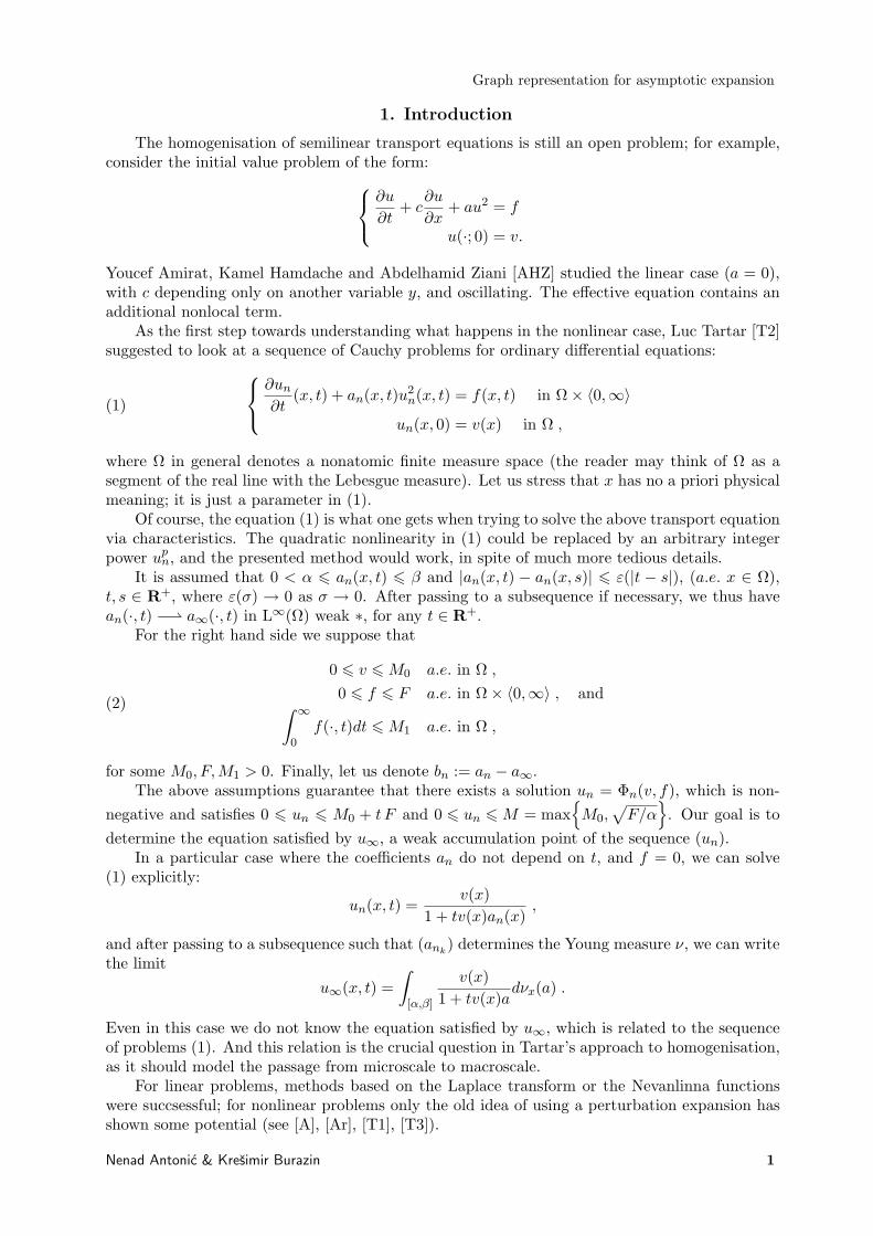
1. Introduction

The homogenisation of semilinear transport equations is still an open problem; for example,consider the initial value problem of the form:

∂u

∂t+ c

∂u

∂x+ au2 = f

u(·; 0) = v.

Youcef Amirat, Kamel Hamdache and Abdelhamid Ziani [AHZ] studied the linear case (a = 0),with c depending only on another variable y, and oscillating. The effective equation contains anadditional nonlocal term.

As the first step towards understanding what happens in the nonlinear case, Luc Tartar [T2]suggested to look at a sequence of Cauchy problems for ordinary differential equations:

(1)

∂un

∂t(x, t) + an(x, t)u2

n(x, t) = f(x, t) in Ω× 〈0,∞〉un(x, 0) = v(x) in Ω ,

where Ω in general denotes a nonatomic finite measure space (the reader may think of Ω as asegment of the real line with the Lebesgue measure). Let us stress that x has no a priori physicalmeaning; it is just a parameter in (1).

Of course, the equation (1) is what one gets when trying to solve the above transport equationvia characteristics. The quadratic nonlinearity in (1) could be replaced by an arbitrary integerpower up

n, and the presented method would work, in spite of much more tedious details.It is assumed that 0 < α 6 an(x, t) 6 β and |an(x, t) − an(x, s)| 6 ε(|t − s|), (a.e. x ∈ Ω),

t, s ∈ R+, where ε(σ) → 0 as σ → 0. After passing to a subsequence if necessary, we thus havean(·, t) − a∞(·, t) in L∞(Ω) weak ∗, for any t ∈ R+.

For the right hand side we suppose that

(2)

0 6 v 6 M0 a.e. in Ω ,

0 6 f 6 F a.e. in Ω× 〈0,∞〉 , and∫ ∞

0f(·, t)dt 6 M1 a.e. in Ω ,

for some M0, F, M1 > 0. Finally, let us denote bn := an − a∞.The above assumptions guarantee that there exists a solution un = Φn(v, f), which is non-

negative and satisfies 0 6 un 6 M0 + t F and 0 6 un 6 M = max

M0,√

F/α

. Our goal is todetermine the equation satisfied by u∞, a weak accumulation point of the sequence (un).

In a particular case where the coefficients an do not depend on t, and f = 0, we can solve(1) explicitly:

un(x, t) =v(x)

1 + tv(x)an(x),

and after passing to a subsequence such that (ank) determines the Young measure ν, we can write

the limitu∞(x, t) =

∫

[α,β]

v(x)1 + tv(x)a

dνx(a) .

Even in this case we do not know the equation satisfied by u∞, which is related to the sequenceof problems (1). And this relation is the crucial question in Tartar’s approach to homogenisation,as it should model the passage from microscale to macroscale.

For linear problems, methods based on the Laplace transform or the Nevanlinna functionswere succsessful; for nonlinear problems only the old idea of using a perturbation expansion hasshown some potential (see [A], [Ar], [T1], [T3]).

Nenad Antonic & Kresimir Burazin 1


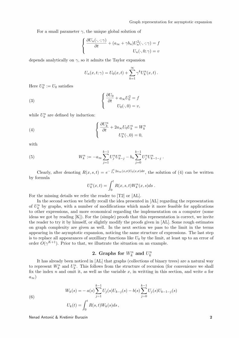
For a small parameter γ, the unique global solution of

∂Un(·, ·; γ)∂t

+ (a∞ + γbn)U2n(·, ·; γ) = f

Un(·, 0; γ) = v

depends analytically on γ, so it admits the Taylor expansion

Un(x, t; γ) = U0(x, t) +∞∑

k=1

γkUnk (x, t) .

Here Un0 := U0 satisfies

(3)

∂U0

∂t+ a∞U2

0 = f

U0(·, 0) = v,

while Unk are defined by induction:

(4)

∂Unk

∂t+ 2a∞U0U

nk = Wn

k

Unk (·, 0) = 0,

with

(5) Wnk := −a∞

k−1∑

j=1

Unj Un

k−j − bn

k−1∑

j=0

Unj Un

k−1−j .

Clearly, after denoting R(x, s, t) = e−R t

s 2a∞(x,σ)U0(x,σ)dσ, the solution of (4) can be writtenby formula

Unk (x, t) =

∫ t

0R(x, s, t)Wn

k (x, s)ds .

For the missing details we refer the reader to [T2] or [AL].In the second section we briefly recall the idea presented in [AL] regarding the representation

of Unk by graphs, with a number of modifications which made it more feasible for applications

to other expressions, and more economical regarding the implementation on a computer (someideas we got by reading [K]). For the (simple) proofs that this representation is correct, we invitethe reader to try it by himself, or slightly modify the proofs given in [AL]. Some rough estimateson graph complexity are given as well. In the next section we pass to the limit in the termsappearing in the asymptotic expansion, noticing the same structure of expressions. The last stepis to replace all appearances of auxilliary functions like U0 by the limit, at least up to an error oforder O(γK+1). Prior to that, we illustrate the situation on an example.

2. Graphs for Wnk and Un

k

It has already been noticed in [AL] that graphs (collections of binary trees) are a natural wayto represent Wn

k and Unk . This follows from the structure of recursion (for convenience we shall

fix the index n and omit it, as well as the variable x, in writting in this section, and write a fora∞)

(6)Wk(s) =− a(s)

k−1∑

j=1

Uj(s)Uk−j(s)− b(s)k−1∑

j=0

Uj(s)Uk−1−j(s)

Uk(t) =∫ t

0R(s, t)Wk(s)ds ,



where U0 is given as the unique solution of equation (3). Then the graph for W1(s) = −b(s)U20 (s)

is −1s

The formal rule is that a black circle in a vertex denotes function b in appropriate variable, and ifthe vertex has got no children, then there is U2

0 in appropriate variable. We write the coefficientat top (or left) of the tree. The graph for

U1(t) =∫ t

0R(s, t)W1(s)ds = −

∫ t

0R(s, t)b(s)U2

0 (s)ds

is −1t

s

In general, the edge |ts will denote∫ t0 R(s, t)F (s)ds, where F (s) is the formula represented by sub-

tree whose root is the vertex in variable s. For representing W2(s) = −a(s)U21 (s)−2b(s)U0(s)U1(s)

we use two binary trees, each of them representing one of the terms in the above equality. Thefirst term, that is

−a(s)(∫ s

0R(s1, s)b(s1)U2

0 (s1)ds1

)(∫ s

0R(s2, s)b(s2)U2

0 (s2)ds2

),

we write as −1s

s1 s2

Here the empty circle stands for function a(s) (this is another general rule), and the fact thattwo graphs for U1 are connected in a new vertex represents the term U2

1 . So, the rule is that aproduct of type UiUj we represent by a tree such that subtrees of the root are graphs for Ui andUj . From recursive relation (6) it is obvious that such type of product always comes either withfunction a or b as a factor, and that determines whether we have empty or black circle in the rootvertex.

The second term in the expression for W2(s) is 2b(s)U0(s)∫ s0 R(s1, s)b(s1)U2

0 (s1)ds1 and thecorresponding graph is

2s

s1

where we have applied the rule for products described above. Since the graph for U0 is simplya single vertex, the root does not have two children, but only one. The rule is that if we havevertex with black or empty circle, and if it has only one child, then we assume that there is U0

in appropriate variable as the second child. Now, using a binary tree for each term in recursionfor Wk, and using the additivity of integral we can inductively draw graphs for each Wk and Uk.Before we do that let us make one simplification. Note that we can omit variables in vertices,because they are inner variables of integration (and only the root variable is visible). With this,the graphs for U1, U2 and U3 are (these graphs are a streamlined version of graphs in [AL]):

U1 :−1

U2 :2 −1



U3 :−4 2 −1 4 −2

Remark. We wrote a program and ran it on a personal computer which calculated and drew graphs forUk and Wk. For k = 13 the run took one second and 100 MB of RAM was used. If we denote the numberof different graphs appearing in Uk by n(k), while the total number of graphs is m(k), then for the firstten graphs we have

k 1 2 3 4 5 6 7 8 9 10

m(k) 1 3 13 67 381 2307 14589 95235 636925 4341763

n(k) 1 2 5 15 48 166 596 2221 8472 32995

The table was computed using recursive formulae for m(k) and n(k) (which can easily be obtained from(6); in particular, we take m(0) := n(0) := 1):

m(k) =k−1∑

j=1

m(j)m(k − j) +k−1∑

j=0

m(j)m(k − 1− j)

n(k) =[ k−1

2 ]∑

j=1

n(j)n(k − j) +[ k−2

2 ]∑

j=0

n(j)n(k − 1− j) +n([k

2 ])(n([k2 ]) + 1)

2.

Here [r] := maxn ∈ Z : n 6 r denotes the largest integer function. Using Maple we checked that n(k+1)n(k)

is between 4 and 5 for k ∈ 11..5000, and that it always grows. From this we guess that the number ofdifferent binary trees grows exponentially in k.

Another interesting fact (the proof is immediate) is that all coefficients are powers of 2, while theirsum is (−1)k. We note that in graphs for Wk the number of vertices varies from k to 2k − 1.

Because of the exponential growth of the number of component graphs (n(k) in the Remark),it is more convenient not to distribute products. Let us introduce some modifications and try todo some further simplifications. Note that expressions for Wk differ only in one integral from theexpressions for Uk. So, the graphs for W1,W2 and W3 are:

W1 :-1

W2 :2 -1

W3 :-4 2 -1 4 -2

Now let us try to avoid such large numbers of trees: to this end we introduce a new rule thata horizontal line is the sign for a sum. The graphs for W2,W3 and W4 thus become:

W2 :

• •

•

•



W3 :•

• •

•

• •

•

•

•

• •

•

•

W4 :

• •

•

•

• •

•

•

• •

• •

•

• •

•

•

•

• •

•

•

•

•

• •

•

•

•

•

• •

•

• •

•

•

•

• •

•

•

Note that we did not write any coefficients in these graphs. From the recursion (6) it is clear thateach term but one appears twice. So, one term in the sum has coefficient −1 while all others have−2. The rule is to write the one with −1 as the first term in summation, and the correspondingvertex as the one connected with its parent, or if there is no parent, as the first (leftmost) vertexon the top horizontal line. For example, if we explicitly write down all coefficients in the graphfor W3, it will look like this:

W3 :-1•

-1• -1•

-2

-1• -1

-1• -1•

-2•

-1•

-2•

-1

-1• -1•

-2•

-1•

The coefficients are then multiplied as the vertices enter into products.By using this representation for graphs in a computer program, we save on memory, but

automatic drawing becomes highly nontrivial.

Remark. The asymptotic expansion

Un(x, t; γ) = U0(x, t) +∞∑

k=1

γkUnk (x, t)

in general converges only for small γ, while we are interested in the case γ = 1. Before proceeding further,we would like to show that the whole expansion converges in ordinary sense for γ = 1, at least with someadditional assumptions.

Let us prove that the above series converges for |γ| 6 1, at least for |t| < ρ, for some small ρ > 0. Inorder to do that, we assume that additional estimates (uniformly in x, t and n) are valid: α 6 a∞ 6 β,|bn| 6 β − α, 0 6 U0 6 M and 0 6 R 6 1. (For simplicity, we drop the index n in writing below.) Using(5) we can get

|W1| 6 (β − α)M2 and |U1| 6 (β − α)M2t ,

and inductively

|Uk| 6 Mσkk−1∑

j=0

ck,jτj ,

where σ := (β − α)Mt, τ := βMt and ck,j are some coefficients. Taking βM 6 1, and ρ = 1/2, we obtainan absolutely convergent series.



Indeed, this convergence follows by noting that the numbers u0 := 1, u1 := 1, and inductively:

wk :=k−1∑

j=1

ujuk−j +k−1∑

j=0

ujuk−j−1

uk :=wk

k,

satisfy uk 6 2k−1 for k ∈ N, while∑k−1

j=0 ck,j 6 uk.

3. Passing to the limit

Next we would like to describe an accumulation point of the sequence (un). Note that fora fixed x, using the (strong) L1 topology for v and f (as L∞ is not separable), and for M0, Fgiven, the restriction of Φn to the set of v, f satisfying (2) is Lipschitz continuous with values inL∞(〈0,∞〉), the Lipschitz bound depending only on M0, F, α and β. Using this we can extract asubsequence such that for each v, f satisfying (2), k ∈ N and s1, . . . , sk ∈ R+

(7)Φn(v, f) − u∞ = Φ∞(v, f) L∞ weak ∗

bn(·, s1) · · · bn(·, sk) − Mk(·, s1, . . . , sk) L∞ weak ∗ .

This allows us to pass to the limit (as n →∞) in equation (4), thus obtaining:

(8)

∂U∞k

∂t+ 2a∞U0U

∞k = W∞

k

U∞k (·, 0) = 0.

The recurrence relations (6) are still valid for n = ∞ if we replace the product bn(·, s1) · · ·bn(·, sk) by the appropriate weak limit Mk(·, s1, . . . , sk). For example:

Wn2 (s) = 2bn(s)U0(s)

∫ s

0R(s1, s)bn(s1)U2

0 (s1)ds1

− a∞(s)∫ s

0

∫ s

0R(s1, s)R(s2, s)bn(s1)bn(s2)U2

0 (s1)U20 (s2)ds1ds2 ,

whileW∞

2 (s) = 2U0(s)∫ s

0R(s1, s)M2(s1, s)U2

0 (s1)ds1

− a∞(s)∫ s

0

∫ s

0R(s1, s)R(s2, s)M2(s1, s2)U2

0 (s1)U20 (s2)ds1ds2 .

Note that, in general, the expressions for weak limits W∞k and U∞

k of sequences (Wnk ) and (Un

k )are formally the same as expressions for Wn

k and Unk , the only difference being that in W∞

k and U∞k

we have Mj(·, s1, s2, ..., sj) instead of the product bn(·, s1)bn(·, s2) · · · bn(·, sj) in each summationterm. So, from the graphs for Wn

k and Unk we can easily read their weak limits.

Thus we choose to represent W∞k and U∞

k by the same graphs as Wnk and Un

k .However, as we want to use graphs for manipulating such expressions, one difficulty does

arise: if we want to multiply, say U∞1 by U∞

1 and a∞, we would expect the graph to be

On the other hand, following the rules described in Section 2 and the convention adopted above,this graph describes:

a∞(t)∫ t

0

∫ t

0R(s, t)U2

0 (s)R(s1, t)U20 (s1)M2(s, s1)dsds1 ,



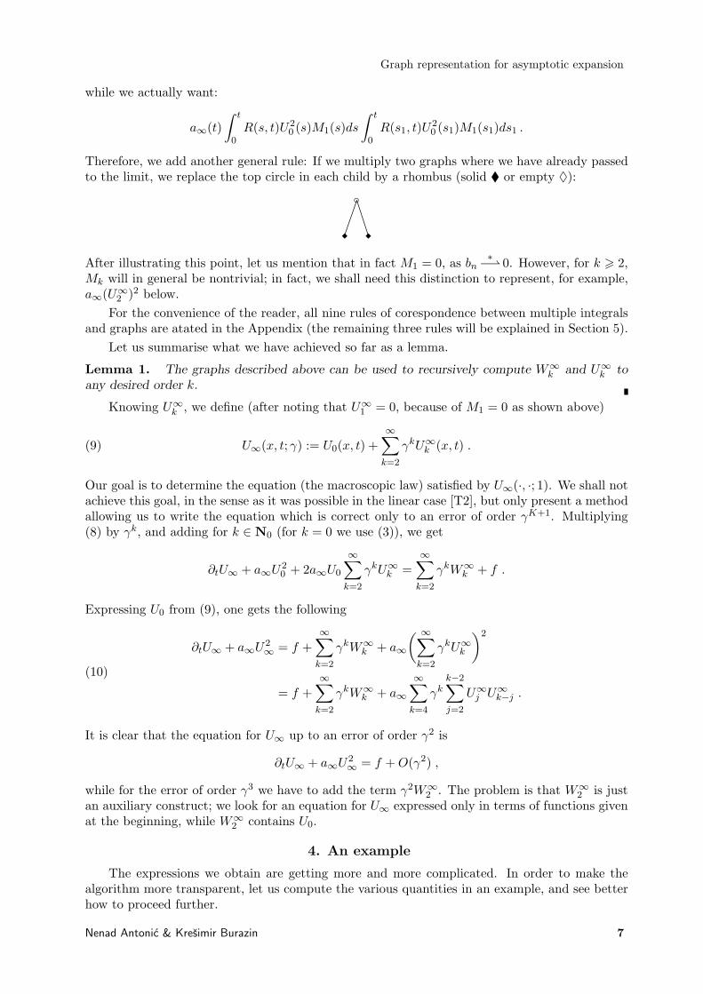
while we actually want:

a∞(t)∫ t

0R(s, t)U2

0 (s)M1(s)ds

∫ t

0R(s1, t)U2

0 (s1)M1(s1)ds1 .

Therefore, we add another general rule: If we multiply two graphs where we have already passedto the limit, we replace the top circle in each child by a rhombus (solid ¨ or empty ♦):

After illustrating this point, let us mention that in fact M1 = 0, as bn∗− 0. However, for k > 2,

Mk will in general be nontrivial; in fact, we shall need this distinction to represent, for example,a∞(U∞

2 )2 below.For the convenience of the reader, all nine rules of corespondence between multiple integrals

and graphs are atated in the Appendix (the remaining three rules will be explained in Section 5).Let us summarise what we have achieved so far as a lemma.

Lemma 1. The graphs described above can be used to recursively compute W∞k and U∞

k toany desired order k.

Knowing U∞k , we define (after noting that U∞

1 = 0, because of M1 = 0 as shown above)

(9) U∞(x, t; γ) := U0(x, t) +∞∑

k=2

γkU∞k (x, t) .

Our goal is to determine the equation (the macroscopic law) satisfied by U∞(·, ·; 1). We shall notachieve this goal, in the sense as it was possible in the linear case [T2], but only present a methodallowing us to write the equation which is correct only to an error of order γK+1. Multiplying(8) by γk, and adding for k ∈ N0 (for k = 0 we use (3)), we get

∂tU∞ + a∞U20 + 2a∞U0

∞∑

k=2

γkU∞k =

∞∑

k=2

γkW∞k + f .

Expressing U0 from (9), one gets the following

(10)

∂tU∞ + a∞U2∞ = f +

∞∑

k=2

γkW∞k + a∞

( ∞∑

k=2

γkU∞k

)2

= f +∞∑

k=2

γkW∞k + a∞

∞∑

k=4

γkk−2∑

j=2

U∞j U∞

k−j .

It is clear that the equation for U∞ up to an error of order γ2 is

∂tU∞ + a∞U2∞ = f + O(γ2) ,

while for the error of order γ3 we have to add the term γ2W∞2 . The problem is that W∞

2 is justan auxiliary construct; we look for an equation for U∞ expressed only in terms of functions givenat the beginning, while W∞

2 contains U0.

4. An example

The expressions we obtain are getting more and more complicated. In order to make thealgorithm more transparent, let us compute the various quantities in an example, and see betterhow to proceed further.



As it was mentioned in the Introduction, if we take an independent of t and f = 0, wecan solve each Cauchy problem (1) explicitly. To specify the example, we take x ∈ Ω := [0, 1](the Lebesgue measure assumed) and an(x) := a(nx), where a = 1

2χ[0, 12〉 + 3

2χ[ 12,1〉 on [0, 1〉,

and extended periodically to R+0 . Thus we have an

∗− 1, and the whole sequence determines ahomogeneous (independent of x) Young measure ν = 1

2δ 12

+ 12δ 3

2.

Further, we take v = 1, and the sequence of Cauchy problems (1) reads:

∂un

∂t(x, t) + an(x)u2

n(x, t) = 0

un(x, 0) = 1 .

We have 0 < 12 6 an 6 3

2 , and

un(x, t) =1

1 + tan(x).

Passing to the limit we get

u∞(t) =∫

11 + ta

dν(a) =1 + t

(1 + 12 t)(1 + 3

2 t),

while for bn = an − 1 we have bn∗− 0, or for higher powers k

(11) bkn

∗−

0 , k odd12k , k even .

The Cauchy problem (3) for U0 reduces to

∂U0

∂t+ U2

0 = 0

U0(·, 0) = 1,

and the solution is independent of x: U0(t) = 11+t . This gives:

R(s, t) = e−2R t

sdσ

1+σ =(

1 + s

1 + t

)2

,

and then Wn1 (s) = − 1

1+t and Un1 (t) = − t

(1+t)2. For Wn

k and Unk we get simple expressions (the

dependence on x is only through bn) as well:

Lemma 2.

Wnk (s) = bk

n(−1)k

[ksk−1

(1 + s)k+1− (k − 1)sk

(1 + s)k+2

]

Unk (t) = bk

n(−1)k tk

(1 + t)k+1.

Dem. By induction, from (6) we get:

Wnk (s) = −

k−1∑

j=1

(−tbn)k

(1 + t)k+2−

k−1∑

j=0

(−tbn)k−1

(1 + t)k+1= bk

n(−1)k

[ksk−1

(1 + s)k+1− (k − 1)sk

(1 + s)k+2

],

and then by integration we get the required expression for Unk .

Q.E.D.



Thus we are able to compute the functions Un:

Un(t; γ) =1

1 + t

∞∑

k=0

(−γtbn

1 + t

)k

=1

1 + t + γbnt,

the equality being uniformly valid for |γ| < 2− ε, for any ε > 0.After passing to the limit in n, we have for even k:

W∞k (s) =

12k

[ksk−1

(1 + s)k+1− (k − 1)sk

(1 + s)k+2

]

U∞k (t) =

12k

tk

(1 + t)k+1,

while for odd k we get noughts, by (11). Thus

U∞(t; γ) =1

1 + t

∞∑

l=0

(γ2t2

4(1 + t)2

)l

=1 + t

(1 + t)2 − γ2t2/4,

which, for γ = 1, coincides with u∞ computed above as the limit of un.The final task is, of course, to determine the right equation satisfied by u∞ = U∞(·; 1), or, in

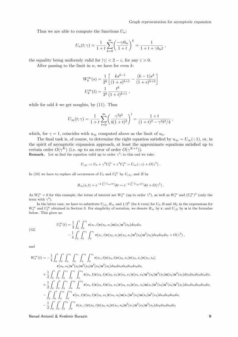
the spirit of asymptotic expansion approach, at least the approximate equations satisfied up tocertain order O(γK) (i.e. up to an error of order O(γK+1)).Remark. Let us find the equation valid up to order γ4; to this end we take:

U(4) := U0 + γ2U∞2 + γ4U∞4 = U∞(·; γ) + O(γ5) .

In (10) we have to replace all occurences of U0 and U∞k by U(4), and R by

R∞(s, t) = e−2R t

sU∞(σ)dσ = e−2

R ts

U(4)(σ)dσ + O(γ5) .

As W∞3 = 0 for this example, the terms of interest are W∞

2 (up to order γ2), as well as W∞4 and (U∞2 )2 (only the

term with γ0).

In the latter case, we have to substitute U(4), R∞ and 1/2k (for k even) for U0, R and Mk in the expressions forW∞

4 and U∞2 obtained in Section 3. For simplicity of notation, we denote R∞ by r, and U(4) by u in the formulaebelow. This gives us:

(12)

U∞2 (t) =1

2

Z t

0

Z s1

0

r(s1, t)r(s2, s1)u(s1)u2(s2)ds2ds1

− 1

4

Z t

0

Z s1

0

Z s1

0

r(s1, t)r(s2, s1)r(s3, s1)u2(s2)u

2(s3)ds3ds2ds1 + O(γ2) ,

and

W∞4 (t) = −1

4

Z t

0

Z t

0

Z s1

0

Z s1

0

Z s4

0

Z s4

0

r(s1, t)r(s4, t)r(s2, s1)r(s3, s1)r(s5, s4)

r(s6, s4)u2(s2)u

2(s3)u2(s5)u

2(s6)ds6ds5ds3ds2ds4ds1

+1

2

Z t

0

Z t

0

Z s1

0

Z s1

0

Z s4

0

r(s1, t)r(s4, t)r(s2, s1)r(s3, s1)r(s5, s4)u2(s2)u

2(s3)u(s4)u2(s5)ds5ds3ds2ds4ds1

+1

2

Z t

0

Z t

0

Z s1

0

Z s3

0

Z s3

0

r(s1, t)r(s3, t)r(s2, s1)r(s4, s3)r(s5, s3)u(s1)u2(s2)u

2(s4)u2(s5)ds5ds4ds2ds3ds1

−Z t

0

Z t

0

Z s1

0

Z s3

0

r(s1, t)r(s3, t)r(s2, s1)r(s4, s3)u(s1)u2(s2)u(s3)u

2(s4)ds4ds2ds3ds1

− 1

2

Z t

0

Z t

0

Z s2

0

Z s2

0

r(s1, t)r(s2, t)r(s3, s2)r(s4, s2)u2(s1)u

2(s3)u2(s4)ds4ds3ds2ds1



−Z t

0

Z t

0

Z s2

0

Z s2

0

Z s4

0

Z s4

0


r(s6, s4)u2(s1)u

2(s3)u2(s5)u

2(s6)ds6ds5ds4ds3ds2ds1

+ 2

Z t

0

Z t

0

Z s2

0

Z s2

0

Z s4

0

r(s1, t)r(s2, t)r(s3, s2)r(s4, s2)r(s5, s4)u2(s1)u


+

Z t

0

Z t

0

Z s2

0

Z s3

0

Z s3

0

r(s1, t)r(s2, t)r(s3, s2)r(s4, s3)r(s5, s3)u2(s1)u(s2)u


− 2

Z t

0

Z t

0

Z s2

0

Z s3

0

r(s1, t)r(s2, t)r(s3, s2)r(s4, s3)u2(s1)u(s2)u(s3)u

2(s4)ds4ds3ds2ds1

− 1

2

Z t

0

Z t

0

Z s2

0

Z s2

0



+

Z t

0

Z t

0

Z s2

0

r(s1, t)r(s2, t)r(s3, s2)u2(s1)u(s2)u

2(s3)ds3ds2ds1

+1

2

Z t

0

Z s1

0

Z s1

0

r(s1, t)r(s2, s1)r(s3, s1)u(t)u2(s2)u2(s3)ds3ds2ds1

+

Z t

0

Z s1

0

Z s1

0

Z s3

0

Z s3

0

r(s1, t)r(s2, s1)r(s3, s1)r(s4, s3)r(s5, s3)u(t)u2(s2)u2(s4)u

2(s5)ds5ds4ds3ds2ds1

− 2

Z t

0

Z s1

0

Z s1

0

Z s3

0

r(s1, t)r(s2, s1)r(s3, s1)r(s4, s3)u(t)u2(s2)u(s3)u2(s4)ds4ds3ds2ds1

−Z t

0

Z s1

0

Z s2

0

Z s2

0

r(s1, t)r(s2, s1)r(s3, s2)r(s4, s2)u(t)u(s1)u2(s3)u

2(s4)ds4ds3ds2ds1

+ 2

Z t

0

Z s1

0

Z s2

0

r(s1, t)r(s2, s1)r(s3, s2)u(t)u(s1)u(s2)u2(s3)ds3ds2ds1 + O(γ2)

For W∞2 we have to first replace U0 and R by U(4) − γ2U∞2 and R∞ + γ2R∞Q2, where Q2(s, t) := 2

R t

sU∞2 (σ)dσ;

and in the next step replace U∞2 by (12). This gives (with the same notational simplification as above)

W∞2 (t) =

1

2

Z t

0

r(s1, t)u(t)u2(s1)ds1

+1

4

Z t

0

Z t

0

r(s1, t)r(s2, t)u2(s1)u

2(s2)ds1ds2

− 1

4γ2

Z t

0

Z t

0

Z s2

0

r(s1, t)r(s2, t)r(s3, s2)u2(s1)u(s2)u

2(s3)ds3ds2ds1

+1

8γ2

Z t

0

Z t

0

Z s2

0

Z s2

0



− 1

2γ2

Z t

0

Z s1

0

Z s2

0

r(s1, t)r(s2, s1)r(s3, s2)u(t)u(s1)u(s2)u2(s3)ds3ds2ds1

+1

4γ2

Z t

0

Z s1

0

Z s2

0

Z s2

0

r(s1, t)r(s2, s1)r(s3, s2)r(s4, s2)u(s1)u2(s3)u

2(s4)ds4ds3ds2ds1

+1

2γ2

Z t

0

Z t

s1

Z s2

0

Z s3

0

r(s1, t)r(s3, s2)r(s4, s3)u(t)u2(s1)u(s3)u2(s4)ds4ds3ds2ds1

− 1

4γ2

Z t

0

Z t

s1

Z s2

0

Z s3

0

Z s3

0

r(s1, t)r(s3, s2)r(s4, s3)r(s5, s3)u(t)u2(s1)u2(s4)u

2(s5)ds5ds4ds3ds2ds1

− 1

2γ2

Z t

0

Z t

0

Z s2

0

Z s3

0

r(s1, t)r(s2, t)r(s3, s2)r(s4, s3)u2(s1)u(s2)u(s3)u

2(s4)ds4ds3ds2ds1

+1

4γ2

Z t

0

Z t

0

Z s2

0

Z s3

0

Z s3

0

r(s1, t)r(s2, t)r(s3, s2)r(s4, s3)r(s5, s3)u2(s1)u(s2)u


+1

4γ2

Z t

0

Z t

0

Z t

s1

Z s3

0

Z s4

0



− 1

8γ2

Z t

0

Z t

0

Z t

s1

Z s3

0

Z s4

0

Z s4

0


u2(s1)u2(s2)u

2(s5)u2(s6)ds6ds5ds4ds3ds2ds1 + O(γ4) ,

and putting all this together we get an approximation of the equation for u∞, correct up to order γ4. Besides the

unknown u∞, this equation involves only arithmetic operations, exponential function, integrals and derivatives (it

is a complicated integro-differential equation for u∞).



Even in this simplified example, it is clear that the classical mathematical notation for inte-grals, sums and products is useless for such expressions, even for relatively small powers of γ. Inthe next section we shall describe a much better notation, and rules of manipulation. However,any practical calculations should better be left to computers.

5. Substitutions for the asymptotic expansion

Our immediate goal is to obtain an equation for U∞ that is correct up to γK for some givenK. In order to do that we need to replace U0 in the equation

(10) ∂tU∞ + a∞U2∞ = f +

∞∑

k=2

γkW∞k + a∞

∞∑

k=4

γkk−2∑

j=2

U∞j U∞

k−j

by U∞ − ∑∞k=2 γkU∞

k . Unfortunately, U0 appears also in R in a way that is more difficult tohandle. First we define:

Qk(s, t) :=2∫ t

sa∞(σ)U∞

k (σ)dσ ,

R∞(s, t) :=e−2R t

s a∞(σ)U∞(σ)dσ ,

and then note that (for simplicity we omit the variables in writting)

(13)

R = R∞eP∞

k=2 γkQk

= R∞

(1 +

∞∑

m=1

1m!

( ∞∑

k=2

γkQk

)m)

= R∞

(1 +

∞∑

l=2

γl

[l/2]∑

m=1

∑α2+···+αl−2m+2=m

Pl−2m+2i=2

iαi=l

1α2! · · ·αl−2m+2!

Qα22 · · ·Qαl−2m+2

l−2m+2

),

where αi ∈ N0. Thus, in order to get a correct equation for U∞ we need to replace R by the aboveexpression. Since U∞

k (as well as Qk) contains U0 (and R) we will have to repeat this procedurea sufficient number of times. Note that with each replacement of U0 and R we achieve thatauxilary functions appear in the equation with a higher power of γ than before the replacements.This ensures that after finitely many replacements we obtain an equation for U∞ such that theterms appearing with γk, for k 6 K, do not contain U0. It is also clear that our equation isgoing to be complicated for manipulation (as the number of multiple integrals increases witheach replacement), and for this reason we would like to write an equation for U∞ with the aideof graphs. This task is not going to be trivial, as it will be clear from the algorithm described inthe next section.

We note that taking into account the terms of order up to γ3 (the same is true if we areinterested in the terms of order up to γ2), it is enough to replace U0 by U∞ and R by R∞ in theexpressions for W∞

2 and W∞3 . Other corrections can be included in O(γ4) term. And these terms

can be computed using the graphs described above. The first case was computed in [T2], and thesecond (using an earlier version of graphs presented here) in [AL]. It is clear that by includingthe terms with higher powers of γ we change nothing to lower order terms.

How to represent the correction of order γ4, or higher? Clearly, we have to adjust our graphsto incorporate representation of Qk, which allways appears in an integral (as Qk is part of thesubstitution for R which is in the integrand), and which is a function of two variables, the upperand lower bound of mentioned integral. In a way, Qk should be attached to a pair of computed



vertices, or better, to the edge connecting them. For example, the graph

t•

s•2¦

-1

-1• -1•

-2•

-1•

describes∫ t

0R(s, t)Q2(s, t)M2(s, t)U0(t)U2

0 (s)ds =∫ t

0R(s, t)2

∫ t

sa∞(σ)U∞

2 (σ)dσM2(s, t)U0(t)U20 (s)ds .

In particular, the red edge and its subgraph describe Q2(s, t). More precisely, this means thatwe multiply 2a∞ by U∞

2 , take the integral from s to t, and multiply the integrand over [0, t](integration in s) by this integral. The graph representation of Qk we get by replacing the graphfor U∞

2 by the graph for U∞k in the figure representing Q2.

The rule is that an edge (red coloured above) connected to a pair of computed vertices(actually, to the edge connecting them) contains an integral without R with bounds being thevariables (which we will not draw in the future as they are inner variables of integration) thatbelong to given vertices.

Aditional adjustments should be made in order to represent multiple products of Qk appearingin expresion (13) for R. A new rule states that if a certain number of graphs is connected in onevertex, then the integrals generated by them are multiplied. Additionally, if a product appearsimmediately after a red coloured edge, then each factor contains this red integral and the vertexbelow it. For example, the graph

•

•86¦

-1

-1• -1•

-2•

-1•

-1

-1• -1•

-2•

-1•

-1

-1• -1•

-2•

-1•

represents

∫ t

0R(s, t)

13!

(Q2(s, t))3M2(s, t)U0(t)U20 (s)ds =

=∫ t

0R(s, t)

13!

(2

∫ t

sa∞(σ)U∞

2 (σ)dσ)3

M2(s, t)U0(t)U20 (s)ds ,

of which the red edge and its subgraph stands for 13!Q2Q2Q2. At this point we have a necessary

tool (the graphs) for describing an equation correct up to γK .

6. Details of the substitution

Next we want to describe an algorithm for systematic replacement of U0 and R in the ex-pressions.

In order to obtain an equation correct up to the terms with γK , we need W∞k and U∞

kcorrect up to order γK−k. Let us denote by W∞

k,N , U∞k,N , Qk,N and RN such N -correct expressions



obtained form W∞k , U∞

k , Qk and R, where the terms up to γN contain only known functions, orthe unknown U∞.

Let us describe how to choose functions with this property. We use the definitions (we donot write the variable x, and for RN we suppress all variables):

RN := R∞

(1 +

N∑

l=2

γl

[l/2]∑

m=1

∑α2+···+αl−2m+2=m

Pl−2m+2i=2

iαi=l

1α2! · · ·αl−2m+2!

Qα22,N−l · · ·Q

αl−2m+2

l−2m+2,N−l

)

U∞k,N (t) :=

∫ t

0RN (s, t)W∞

k,N (s) ds

Qk,N (s, t) := 2∫ t

sa∞(σ)U∞

k,N (σ) dσ .

Let us note that if we were to know W∞k,N , these definitions would not be recursive, as RN does

not depend on U∞k,N , but only on Qk,i, for i 6 N − 2. How to define W∞

k,N?We take W∞

k , and replace all occurences of R by RN , and U0 by

U∞ −N∑

i=2

γiU∞i,N−i .

Let us look into the details for the first few steps. Starting with W∞k , we get

0. W∞k,0 by replacing U0 by U∞ and R by R0 = R∞; and calculate U∞

k,0, Qk,0;1. W∞

k,1 by replacing U0 by U∞ and R by R1 = R∞; and calculate U∞k,1, Qk,1;

2. W∞k,2 by replacing U0 by U∞ − γ2U∞

2,0 and R by R2 = R∞(1 + γ2Q2,0); and calculate U∞k,2,

Qk,2;3. W∞

k,3 by replacing U0 by U∞− γ2U∞2,1− γ3U∞

3,0 and R by R3 = R∞(1 + γ2Q2,1 + γ3Q3,0); andcalculate U∞

k,3, Qk,3;4. W∞

k,4 by replacing U0 by U∞ − γ2U∞2,2 − γ3U∞

3,1 − γ4U∞4,0 and R by R4 = R∞(1 + γ2Q2,2 +

γ3Q3,1 + γ4Q4,0 + 12!γ

4Q22,0); and calculate U∞

k,4, Qk,4.As W∞

k,N clearly depends only on other terms of correctness at most N − 2, this definition isgood. Using induction we can easily prove

Lemma 3. In the above defined W∞k,N , U∞

k,N , Qk,N and RN , no term of order γi, for i 6 N ,contains any auxiliary functions.

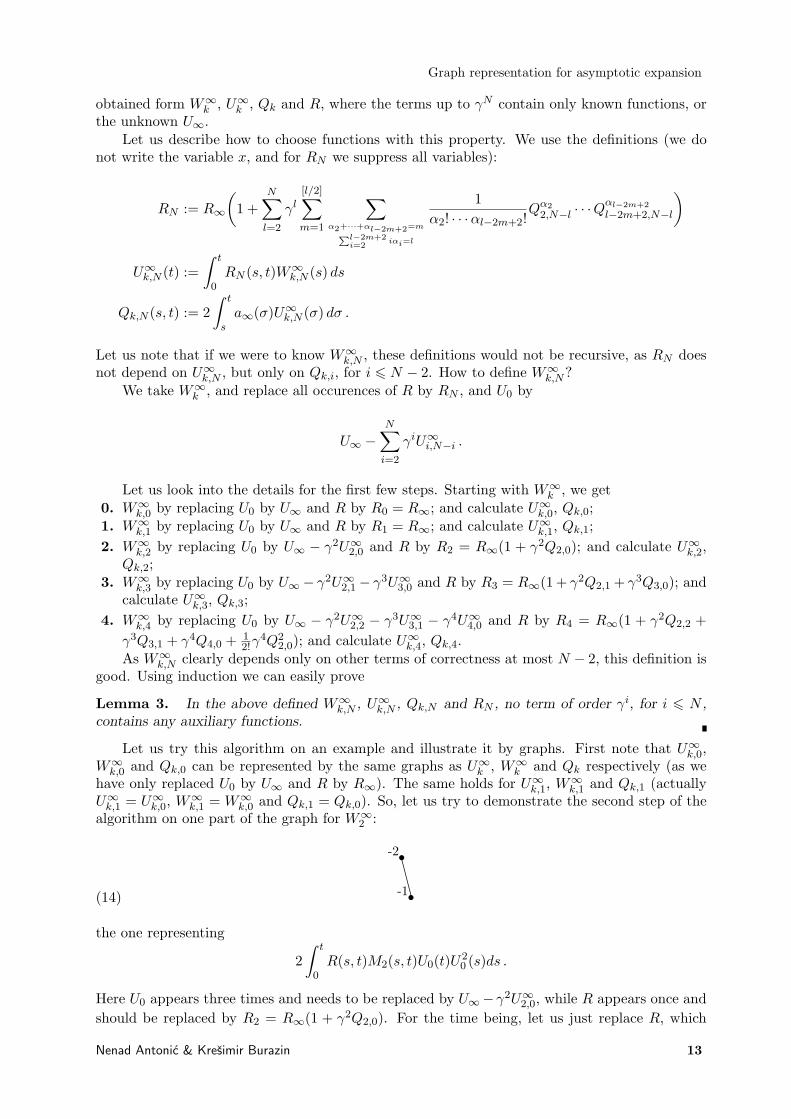
Let us try this algorithm on an example and illustrate it by graphs. First note that U∞k,0,

W∞k,0 and Qk,0 can be represented by the same graphs as U∞

k , W∞k and Qk respectively (as we

have only replaced U0 by U∞ and R by R∞). The same holds for U∞k,1, W∞

k,1 and Qk,1 (actuallyU∞

k,1 = U∞k,0, W∞

k,1 = W∞k,0 and Qk,1 = Qk,0). So, let us try to demonstrate the second step of the

algorithm on one part of the graph for W∞2 :

(14)

-2•

-1•

the one representing

2∫ t

0R(s, t)M2(s, t)U0(t)U2

0 (s)ds .

Here U0 appears three times and needs to be replaced by U∞− γ2U∞2,0, while R appears once and

should be replaced by R2 = R∞(1 + γ2Q2,0). For the time being, let us just replace R, which



gives

(15)2

∫ t

0

(R∞(s, t)(1 + γ2Q2,0(s, t))

)M2(s, t)U0(t)U2

0 (s)ds =

= 2γ2

∫ t

0R∞(s, t)Q2,0(s, t)M2(s, t)U0(t)U2

0 (s)ds+2∫ t

0R∞(s, t)M2(s, t)U0(t)U2

0 (s)ds ,

and we represent it by-2•

-1•? 2 2¦

-1

-1• -1•

-2•

-1•The star (?) in a vertex stands for R∞, and the integral (edge) that connects a vertex denoted bystar to its parent edge does not apply to this vertex, but only to the terms that are on the samesummation line with it (if there are any). Also, such a vertex with a star will never have anychildren, but we do not assume that there are two U0 in the appropriate variable. After partialdistribution of multiplication over addition, the above graph becomes

-2•

-1•2 2¦

-1

-1• -1•

-2•

-1•

-2•

-1•?

The first part in summation represents the first term in the right hand side of (15), while thesecond part stands for the second term. Note that since we have replaced all R’s in the graph(14) (actually, there was only one R there) and therefore only R∞ can appear in the above graph,we can omit writing stars for R∞ and draw the above graph as

-2•

-1•2 2¦

-1

-1• -1•

-2•

-1•

-2•

-1•

Therefore, such a vertex denoted by a star will be used only in this intermediary step while doingreplacements, and after performing the complete distribution in order to eliminate higher orderterms and write an approximate equation for U∞, we will not need it any more. However, wewill use it in replacements of U0 in a similar way. The general rule is (as it is used only in anintermediary step, it is not written in the Appendix):

The star (?) in a vertex stands for U∞ or R∞, depending whether it is connected to a vertexor an edge, and the integral (edge) that connects such a vertex to its parent vertex (or parentedge) does not apply to this vertex, but only to terms that are on the same summation line with



it (if there are any). We assume that there is U∞ instead of U0 in the appropriate vertex, andR∞ instead of R in the appropriate edge. Also, such a vertex will never have any children, butwe do not assume that there are two U0 in the appropriate variable.

Now, if we make all needed replacements of U0 and R in (14) we get

-2•

?2¦

-1• -1•

2 2

-1•

-1•

?2¦

-1• -1•

2 2

-1•

? 2¦

-1• -1•

2 2

-1•

? 2 2¦

-1

-1• -1•

-2•

-1•

For all terms of W∞2,2 we get a representation:

-1

-1•

?2¦

-1•-1•

2 2

-1•

? 2¦

-1•-1•

2 2

-1•

?2 2¦

-1

-1•-1•

-2•

-1•

-1•

?2¦

-1•-1•

2 2

-1•

? 2¦

-1•-1•

2 2

-1•

? 2 2¦

-1

-1•-1•

-2•

-1•

-2•

?2¦

-1•-1•

2 2

-1•

-1•

?2¦

-1•-1•

2 2

-1•

? 2¦

-1•-1•

2 2

-1•

? 2 2¦

-1

-1•-1•

-2•

-1•

Note that after distributing, there will be some terms with powers 4 and higher present. Theseterms are not of interest for us, as the purpose of calculating W∞

2,2 is to get all second (andlower) order terms that can be derived from W∞

2 . Thus, distributing the products over sums,eliminating the terms with powers greater than 2, and using symmetries, we get

-1

• •

0 2

• •¦

• •

-4 2

• •

¦

• •

6 2

• •

•

-4 2

• ¦

•

•

•

2 2

•

•

•

2•

•

4 2•

•¦

• •

4 2•

•

¦

• •

-8 2•

•

•

2 2•

¦

• •

•

-4 2•

•

•

The above graph represents all second order terms which can be derived from W∞2 .

7. The equation correct to any order K

Theorem 1. The graphs described above can be used to compute equation for U∞ that iscorrect to any desired order K.

Dem.From (10) we easily get

∂tU∞ + a∞U2∞ = f + LK + O(γK+1) ,

where

LK =K∑

k=2

γkW∞k,K−k + a∞

K∑

k=4

γkk−2∑

j=2

U∞j,K−kU

∞k−j,K−k .



Note that LK contains terms with powers of γ that are higher than K. There is only one step tothe required equation

∂tU∞ + a∞U2∞ = f + LK ,

where LK = LK +O(γK+1), and LK does not contain the terms with powers of γ higher than K.For given LK , in order to truncate the terms with higher powers, it is enough to distribute

the products over sums, and then just drop the terms with powers of γ higher than K.Q.E.D.

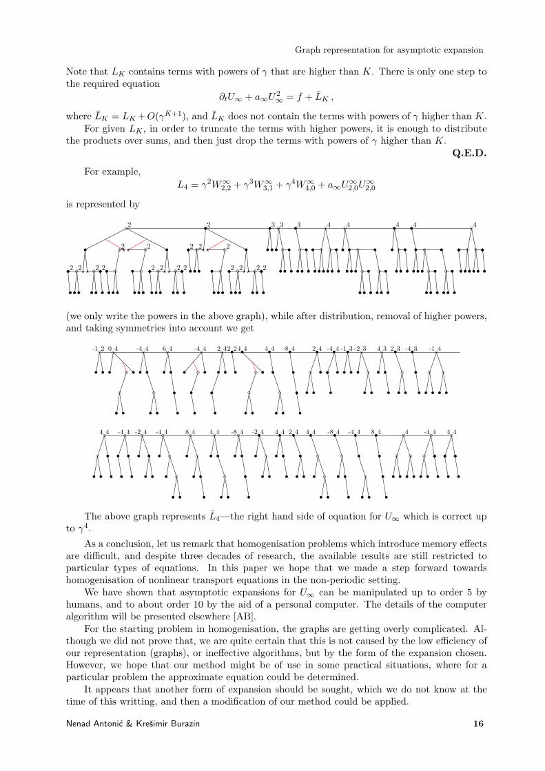
For example,L4 = γ2W∞

2,2 + γ3W∞3,1 + γ4W∞

4,0 + a∞U∞2,0U

∞2,0

is represented by

2

•

?2¦

••

2

•

? 2¦

••

2

•

?2¦

••

•

•

•

?2¦

••

2

•

? 2¦

••

2

•

? 2¦

••

•

•

2•

?2¦

••

2

•

•

?2¦

••

2

•

? 2¦

••

2

•

? 2¦

••

•

•

3•

••

3

•

••

•

•

3•

••

•

•

4

••

•

•

••

•

•

4

• •

••

•

••

•

•

•

••

•

•

4•

•

••

•

•

4•

•

••

•

••

•

•

•

••

•

•

4

¦

•••

¦

•• •

(we only write the powers in the above graph), while after distribution, removal of higher powers,and taking symmetries into account we get

-1 2

• •

0 4

• •¦

• •

-4 4

• •

¦

• •

6 4

• •

•

-4 4

• ¦

•

•

•

2 4

•

•

•

2 2•

•

4 4•

•¦

• •

4 4•

•

¦

• •

-8 4•

•

•

2 4•

¦

• •

•

-4 4•

•

•

-1 3•

• •

-2 3

•

• •

4 3

• •

•

2 3•

• •

-4 3•

•

•

-1 4

• •

• •

4 4

• •

•

•

-4 4

•

•

•

•

-2 4

• •

• •

-4 4

•

•

• •

8 4

•

• •

•

4 4

• •

• •

-8 4

• •

•

•

-2 4•

•

• •

4 4•

• •

•

2 4•

•

• •

4 4•

•

• •

-8 4•

• •

•

-4 4•

•

• •

8 4•

•

•

•

4

¦

• •

¦

• •

-4 4

¦

• • •

4 4

• •

The above graph represents L4—the right hand side of equation for U∞ which is correct upto γ4.

As a conclusion, let us remark that homogenisation problems which introduce memory effectsare difficult, and despite three decades of research, the available results are still restricted toparticular types of equations. In this paper we hope that we made a step forward towardshomogenisation of nonlinear transport equations in the non-periodic setting.

We have shown that asymptotic expansions for U∞ can be manipulated up to order 5 byhumans, and to about order 10 by the aid of a personal computer. The details of the computeralgorithm will be presented elsewhere [AB].

For the starting problem in homogenisation, the graphs are getting overly complicated. Al-though we did not prove that, we are quite certain that this is not caused by the low efficiency ofour representation (graphs), or ineffective algorithms, but by the form of the expansion chosen.However, we hope that our method might be of use in some practical situations, where for aparticular problem the approximate equation could be determined.

It appears that another form of expansion should be sought, which we do not know at thetime of this writting, and then a modification of our method could be applied.



Appendix

For the correspondence between multiple integrals and the graphs we use the following rules:1. A black circle in a vertex denotes function b in an appropriate variable; if the vertex has no

children, there is U20 in the appropriate variable; the coefficient is given at the top (left) of

the vertex (if there is no coefficient in the vertex, we take it to be 1).2. An empty circle stands for function a, the rest being the same as in 1.3. The edge |ts denotes

∫ t0 R(s, t)F (s)ds, where F (s) is the formula represented by the subtree.

4. A product of type UiUj we represent by a tree such that the subtrees of the root are graphsfor Ui and Uj .

5. If we have a vertex with a solid or empty circle, and if it has only one child, we assume thatthere is U0 in the appropriate variable as the second child.

6. If we have already (separately) passed to the limit in subtrees of some graph presenting aproduct, then instead of circles (solid or empty) we would write rhombi in the leading childvertices.

7. A red edge conected to the edge conecting a pair of vertices contains an integral without R,with the bounds being the variables that belong to given vertices.

8. If a certain number of graphs is connected in one vertex, then the integrals generated bythem are multiplied.

9. If a product appears immediately after a red coloured edge then each factor contains this redintegral and the vertex below it.

Note: The explicit writting of the variables in vertices can be ommited, as they are dummyvariables of integration, and only the root variable is important in the result.

Acknowledgements: The authors wish to thank Professor Luc Tartar for numerous inspiringdiscussions.

References[Ar] Radjesvarane Alexandre: Some results in homogenisation tackling memory effects,

Asymptotic Analysis 15 (1997) 229–259.[AHZ] Youcef Amirat, Kamel Hamdache, Abdelhamid Ziani: Etude d’une equation de trans-

port a memoire, Comptes Rendus de l’Academie des sciences Paris, Serie I 311 (1990) 685–688.

[A] Nenad Antonic: Memory effects in homogenisation: linear second-order equations, Archivefor Rational Mechanics and Analysis 125 (1993) 1–24.

[AB] Nenad Antonic, Kresimir Burazin: Computational aspects of graph representation ofasymptotic expansions in homogenisation, in preparation

[AL] Nenad Antonic, Martin Lazar: Computation of power-series expansions in homogenisa-tion of nonlinear equations, in Applied Mathematics and Computation, pp. 69–80, M. Roginaet al. (eds.), Deptartment of Mathematics, Zagreb, 2001.

[K] Donald E. Knuth: The Stanford Graphbase: A Platform for Combinatorial Computing,ACM Press and Addison-Wesley, 1993.

[T1] Luc Tartar: Nonlocal effects induced by homogenization, in Partial differential equationsand the calculus of variations vol. II, pp. 925–938, F. Colombini et al. (eds.), Birkhauser,1989.

[T2] Luc Tartar: Memory effects in homogenization, Archive for Rational Mechanics and Anal-ysis 111 (1990) 121–133.

[T3] Luc Tartar: Mathematical tools for studying oscillations and concentrations: from Youngmeasures to H-measures and their variants, in Multiscale problems in science and technology,pp. 1–84, N. Antonic et al. (eds.), Springer, 2002.


Graph representation for asymptotic expansion in homogenisation of nonlinear first-order equations

Documents

Transcript of Graph representation for asymptotic expansion in homogenisation of nonlinear first-order equations