A wave equation associated with mixed nonhomogeneous conditions: Global existence and asymptotic...

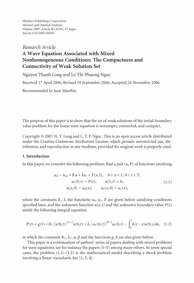
Hindawi Publishing CorporationAbstract and Applied AnalysisVolume 2007, Article ID 20295, 17 pagesdoi:10.1155/2007/20295

Research ArticleA Wave Equation Associated with MixedNonhomogeneous Conditions: The Compactness andConnectivity of Weak Solution Set

Nguyen Thanh Long and Le Thi Phuong Ngoc

Received 17 April 2006; Revised 19 September 2006; Accepted 24 November 2006

Recommended by Jean Mawhin

The purpose of this paper is to show that the set of weak solutions of the initial-boundaryvalue problem for the linear wave equation is nonempty, connected, and compact.

Copyright © 2007 N. T. Long and L. T. P. Ngoc. This is an open access article distributedunder the Creative Commons Attribution License, which permits unrestricted use, dis-tribution, and reproduction in any medium, provided the original work is properly cited.

1. Introduction

In this paper, we consider the following problem: find a pair (u,P) of functions satisfying

utt −uxx +Ku+ λut = F(x, t), 0 < x < 1, 0 < t < T ,

ux(0, t)= P(t), u(1, t)= 0,

u(x,0)= u0(x), ut(x,0)= u1(x),

(1.1)

where the constants K , λ, the functions u0, u1, F are given before satisfying conditionsspecified later, and the unknown function u(x, t) and the unknown boundary value P(t)satisfy the following integral equation:

P(t)= g(t) +K1∣∣u(0, t)

∣∣α−2

u(0, t) + λ1∣∣ut(0, t)

∣∣β−2

ut(0, t)−∫ t

0k(t− s)u(0,s)ds, (1.2)

in which the constants K1, λ1, α, β and the functions g, k are also given before.This paper is a continuation of authors’ series of papers dealing with mixed problems

for wave equations; see for instance the papers [1–5] among many others. In some specialcases, the problem (1.1)-(1.2) is the mathematical model describing a shock probleminvolving a linear viscoelastic bar [1, 2, 4].

2 Abstract and Applied Analysis

In [5], under conditions (u0,u1)∈H1×L2, F ∈ L2(QT), g,k ∈H1(0,T), K ∈R, λ,K1

≥ 0, λ1 > 0, α, β ≥ 2, Long and Giai have proved a theorem of global existence anduniqueness of a weak solution (u,P) of (1.1)-(1.2). The proof is based on a Galerkinmethod associated to a priori estimates, weak convergence, and compactness techniques.Furthermore, the asymptotic behavior of the solution (u,P) as λ1 → 0+ and an asymp-totic expansion of the solution (u,P) of (1.1)-(1.2) up to order N + 1/2 have been estab-lished.

The purpose of this paper is to develop some aspects related to the article [5]. Weshow here that the set of solutions of (1.1)-(1.2) is nonempty and satisfies the classicalHukuhara-Kneser property, that is, the set of solutions is a compact connected set in anappropriate function space. Such structure of the solutions set for differential equationswas studied in [6–10], we mention here [8–10] for Hukuhara-Kneser property and [6, 7]for Rδ-structure. It is well known that the “Rδ” results are really stronger than classicalKneser-type theorems, see [6, 7]. An important application of the above structures is thatthe existence of two different solutions implies the existence of a continuum of differentsolutions.

It is similar to the structure theorem in [8–10], a topological approach to provingconnectivity of the solution set of operator equations was invented by Krasnosel’skii andPerov, one of the theorems in this paper is closely related to the following theorem.

Theorem 1.1 [11]. Let (E,| · |) be a real Banach space, let D be a bounded open subsetof E with boundary ∂D, closure D, and let T : D→ E be a completely continuous operator.Assume that T satisfies the following conditions.

(i) T has no fixed points on ∂D and γ(I −T ,D) �= 0.(ii) For each ε > 0, there is a completely continuous operator Tε such that |Tε(x)−T(x)|

< ε, for all x ∈D, and such that for each h with |h| < ε, the equation x = Tε(x) + hhas at most one solution in D.

Then the set of fixed points of T is nonempty, compact, and connected.

The proof of the above theorem can be found in [11, Theorem 48.2]. We note thatcondition (i) is equivalent to the following condition.

(̃i) T has no fixed points on ∂D and deg(I −T ,D,0) �= 0.Because of this, if a completely continuous operator T is defined on D and has no fixedpoints on ∂D, then the rotation γ(I −T ,D) coincides with the Leray-Schauder degree ofI −T on D with respect to the origin, see [11, Section 20.2].

Deimling also studied the compactness and connectivity of the set of all fixed points,these theorems are given in [12, page 212].

Applying Theorem 1.1, using the same methods as in [5, 13], we consider the structureof the solution set of (1.1)-(1.2). The paper consists of three sections and the main results,in the case 1 < α, β ≤ 2, will be presented in Sections 2, 3. We end the paper by a remarkabout the similar result to the one above in the cases 1 < α < 2, β ≥ 2 or 1 < β < 2, α≥ 2.In our argument, the topological degree theory of compact vector fields and the followingtheorem will be used.

Theorem 1.2 [12, page 53]. Let E, F be Banach spaces, let D be an open subset of E, andlet f : D→ F be continuous. Then for each ε > 0, there is a mapping fε : D→ F that is locally

N. T. Long and L. T. P. Ngoc 3

Lipschitz such that

∣∣ f (x)− fε(x)

∣∣ < ε, ∀x ∈D, (1.3)

and fε(D) is a subset of the closed convex hull of f (D).

2. Existence of weak solution

Put Ω= (0,1), QT =Ω× (0,T), T > 0. We omit the definitions of usual function spaces:Cm(Ω), Lp(Ω), Wm,p(Ω). We denote Wm,p =Wm,p(Ω), Lp =W0,p(Ω), Hm =Wm,2(Ω),1≤ p ≤∞, m= 0,1, . . . .

The norm in L2 is denoted by ‖ · ‖. We also denote by 〈·,·〉 the scalar product in L2

or pair of dual scalar products of a continuous linear functional with an element of afunction space. We denote by ‖ · ‖X the norm of a Banach space X and by X ′ the dualspace of X . We denote by Lp(0,T ;X), 1≤ p ≤∞, the Banach space of the real functionsu : (0,T)→ X measurable, such that

‖u‖Lp(0,T ;X) =(∫ T

0

∥∥u(t)

∥∥pXdt

)1/p

<∞ for 1≤ p <∞,

‖u‖L∞(0,T ;X) = esssup0<t<T

∥∥u(t)

∥∥X for p =∞.

(2.1)

Let u(t),u′(t) = ut(t), u′′(t) = utt(t), ux(t), uxx(t) denote u(x, t), (∂u/∂t)(x, t),(∂2u/∂t2)(x, t), (∂u/∂x)(x, t), (∂2u/∂x2)(x, t), respectively. We put

V = {v ∈H1(0,1) : v(1)= 0}

,

a(u,v)=∫ 1

0

∂u

∂x

∂v

∂xdx.

(2.2)

Then V is a closed subspace of H1 and on V , ‖v‖H1 and ‖v‖V =√

a(v,v)= ‖vx‖ are twoequivalent norms. We have the following lemma.

Lemma 2.1. The imbedding V↩C0([0,1]) is compact and

‖v‖C0([0,1]) ≤ ‖v‖V ∀v ∈V. (2.3)

The proof is straightforward and we omit the details.We make the following assumptions:(H1) u0 ∈V and u1 ∈ L2,(H2) F ∈ L2(QT),(H3) g,k ∈H1(0,T),(H4) K ∈R, λ,K1 ≥ 0, λ1 > 0,(H5) 1 < α≤ 2, 1 < β ≤ 2.


Theorem 2.2. Let (H1)–(H5) hold. Let T > 0. Then the problem (1.1)-(1.2) has at least oneweak solution (u,P) such that

u∈ L∞(0,T ;V), ut ∈ L∞(

0,T ;L2),

u(0,·)∈W1,β(0,T), P ∈ Lβ′(0,T), β′ = β

β− 1.

(2.4)

Proof of Theorem 2.2. The proof consists of Steps 1–3.

Step 1 (the Galerkin approximation). Let {wj} be a denumerable base of V . Find theapproximate solution of problem (1.1)-(1.2) in the form

um(t)=m∑

j=1

cmj(t)wj , (2.5)

where the coefficient functions cmj satisfy the system of ordinary differential equations⟨

u′′m(t),wi⟩

+⟨

umx(t),wix⟩

+Pm(t)wi(0) +⟨

Kum(t) + λu′m(t),wi⟩

= ⟨F(t),wi⟩

, 1≤ i≤m,(2.6)

Pm(t)= g(t) +K1Hα(

um(0, t))

+ λ1Hβ(

u′m(0, t))−

∫ t

0k(t− s)um(0,s)ds, (2.7)

where Hr(z)= |z|r−2z, r ∈ {α,β},

um(0)= u0m =m∑

j=1

αmjwj −→ u0 strongly in H1,

u′m(0)= u1m =m∑

j=1

βmjwj −→ u1 strongly in L2.

(2.8)

Equation (2.6) is rewritten in the form

m∑

j=1

⟨

wj ,wi⟩(

c′′mj(t) + λc′mj(t))

+m∑

j=1

[⟨

wjx,wix⟩

+K⟨

wj ,wi⟩]

cmj(t)

+P[

cm,c′m]

(t)wi(0)= ⟨F(t),wi⟩

, 1≤ i≤m,

(2.9)

where

P[

cm,c′m]

(t)= g(t)−∫ t

0k(t− s)

m∑

j=1

cj(s)wj(0)ds+ P̃[

cm,c′m]

(t),

P̃ :R2m −→R, P̃[y,z]= K1Hα

( m∑

j=1

yjwj(0)

)

+ λ1Hβ

( m∑

j=1

zjwj(0)

)

.

(2.10)

Integrating (2.9) with respect to the time variable from 0 to t, we get

m∑

j=1

bi j(

cmj(t)eλt)′

(t) +Ami[

cm,c′m]

(t)=Ψmi(t), 1≤ i≤m, (2.11)


where

Ami[

cm,c′m]

(t)= eλt[ m∑

j=1

μi j

∫ t

0cmj(s)ds+wi(0)

∫ t

0P[

cm,c′m]

(s)ds

]

,

Ψmi(t)= eλt[ m∑

j=1

bi j(

βmj + λαmj)

+∫ t

0

⟨

F(s),wi⟩

(s)ds

]

,

bi j =⟨

wj ,wi⟩

, μi j =⟨

wjx,wix⟩

+K⟨

wj ,wi⟩

.

(2.12)

Integrating again (2.11), we obtain

m∑

j=1

bi jcmj(t) + e−λt∫ t

0Ami

[

cm,c′m]

(r)dr = Ψ̃mi(t), 1≤ i≤m, (2.13)

where

Ψ̃mi(t)= e−λt[ m∑

j=1

bi jαmj +∫ t

0Ψmi(r)dr

]

. (2.14)

Let B = (bi j), with bi j = 〈wj ,wi〉. Then B is invertible. Hence, it follows from (2.13) that

cm(t)=−B−1Dm[

cm,c′m]

(t) +B−1Ψ̃m(t)≡ (Ucm)

m(t), (2.15)

where

cm(t)= (cm1(t), . . . ,cmm(t))

,(

Ucm)

m(t)= ((Ucm)

m1(t), . . . ,(

Ucm)

mm(t))

,

Ψ̃m(t)= (Ψ̃m1(t), . . . ,Ψ̃mm(t))

,

Dm[

cm,c′m]

(t)= (Dm1[

cm,c′m]

(t), . . . ,Dmm[

cm,c′m]

(t))

,

Dmi[

cm,c′m]

(t)= e−λt∫ t

0Ami

[

cm,c′m]

(r)dr, 1≤ i≤m.

(2.16)

Omitting the index m, the system (2.15)-(2.16) is rewritten in the form

c =Uc, (2.17)

we note more that for 1≤ i≤m,

(Uc)i(t)=−B−1Di[c,c′](t) +B−1Ψ̃i(t),

Di[c,c′](t)= e−λt∫ t

0Ai[c,c′](r)dr,

Ψ̃i(t)= e−λt[ m∑

j=1

bi jαj +∫ t

0Ψi(r)dr

]

,

Ψi(t)= eλt[ m∑

j=1

bi j(

βj + λαj)

+∫ t

0

⟨

F(s),wi⟩

(s)ds

]

.

(2.18)


For Tm > 0, M > 0 which are chosen later, we put

S= {c ∈ C1([0,Tm]

;Rm)

: ‖c‖1 ≤M}

,

‖c‖1 = ‖c‖0 +‖c′‖0, ‖c‖0 = sup0≤t≤Tm

|c(t)|1, |c(t)|1 =m∑

i=1

∣∣ci(t)

∣∣.

(2.19)

Clearly, S is a closed convex and bounded subset of the Banach space Y = C1([0,Tm];Rm).Consider the operator U : S→ Y .

(a) At first, we choose Tm > 0, M > 0 such that U maps S into itself. Notice that sinceΨ(t) ∈ C0([0,Tm];Rm),Ψ̃(t) ∈ Y , so A[c,c′](t),D[c,c′](t) ∈ Y , for all c ∈ Y . Then, by(2.18), we have

(Uc)′i (t)=−B−1D′i [c,c′](t) +B−1Ψ̃′i (t), 1≤ i≤m,

D′i [c,c′](t)=−λe−λt

∫ t

0Ai[c,c′](r)dr + e−λtAi[c,c′](t),

Ψ̃′i (t)=−λe−λt[ m∑

j=1

bi jαj +∫ t

0Ψi(r)dr

]

+ e−λtΨi(t).

(2.20)

This implies that U : Y → Y . Let c ∈ S. We deduce from (2.18) and (2.20) that

∣∣(Uc)(t)

∣∣

1 ≤∥∥B−1

∥∥[∣∣D[c,c′](t)

∣∣

1 +∣∣Ψ̃(t)

∣∣

1

]

,∣∣(Uc)′(t)

∣∣

1 ≤∥∥B−1

∥∥[∣∣D′[c,c′](t)

∣∣

1 +∣∣Ψ̃′(t)

∣∣

1

]

,

∣∣D[c,c′](t)

∣∣

1 ≤∫ t

0

∣∣A[c,c′](r)

∣∣

1dr ≤ Tm

∥∥A[c,c′]

∥∥

0,∣∣D′[c,c′](t)

∣∣

1 ≤(

λTm + 1)∥∥A[c,c′]

∥∥

0.

(2.21)

On the other hand, by (2.12),

m∑

i=1

∣∣Ai[c,c′](t)

∣∣≤ eλt

[

μ̃∫ t

0

∣∣c(s)

∣∣

1ds+ w̃∫ t

0g(s)ds+Tm

m∑

i=1

N1i(M) +N2i(M)

]

, (2.22)

where

μ̃=max

{ m∑

j=1

μi j , 1≤ i≤m

}

, w̃ =m∑

i=1

wi(0),

N1i(M)= ‖k‖L1(0,T) sup

{∣∣∣∣wi(0)

m∑

j=1

yjwj(0)∣∣∣∣, ‖y‖Rm ≤M

}

, 1≤ i≤m,

N2i(M)= sup{∣∣wi(0)P̃[y,z]

∣∣, ‖y‖Rm ≤M, ‖z‖Rm ≤M

}

, 1≤ i≤m.

(2.23)


This implies that

∥∥A[c,c′]

∥∥

0 ≤ eλTm

[

μ̃TmM +Tmw̃‖g‖L∞(0,T) +Tm

m∑

i=1

N1i(M) +N2i(M)

]

≤ TmeλTm

[

μ̃M + w̃‖g‖L∞(0,T) +m∑

i=1

N1i(M) +N2i(M)

]

≡ TmeλTmξ(M,T).

(2.24)

Combining (2.21), (2.24), we get

‖Uc‖0 ≤∥∥B−1

∥∥[

T2me

λTmξ(M,T) +‖Ψ̃‖0∗]

,∥∥(Uc)′

∥∥

0 ≤∥∥B−1

∥∥[(

λTm + 1)

TmeλTmξ(M,T) +‖Ψ̃′‖0∗

]

,(2.25)

so

‖Uc‖1 ≤[

(λ+ 1)Tm + 1]

TmeλTmξ(M,T)

∥∥B−1

∥∥+‖Ψ̃‖1∗

∥∥B−1

∥∥, (2.26)

where

‖Ψ̃‖1∗ = ‖Ψ̃‖0∗ +‖Ψ̃′‖0∗ = sup0≤t≤T

∣∣Ψ̃(t)

∣∣

1 + sup0≤t≤T

∣∣Ψ̃′(t)

∣∣

1. (2.27)

Choosing M > 0 and Tm > 0 such that

M > 2‖Ψ̃‖1∗∥∥B−1

∥∥,

[

(λ+ 1)Tm + 1]

TmeλTmξ(M,T)

∥∥B−1

∥∥≤ 1

2M. (2.28)

Hence, ‖Uc‖1 <M for all c ∈ S, this means that US⊂ S.(b) Next, we show that U : S→ Y is continuous. Let c,d ∈ S, we have

(Uc)i(t)− (Ud)i(t)=−B−1[Di[c,c′](t)−Di[d,d′](t)]

, 1≤ i≤m, (2.29)

Di[c,c′](t)−Di[d,d′](t)= e−λt∫ t

0

[

Ai[c,c′](r)−Ai[d,d′](r)]

dr, 1≤ i≤m, (2.30)

Ai[c,c′](t)−Ai[d,d′](t)= eλtm∑

j=1

μi j

∫ t

0

[(

cj −dj)

(s)]

ds

+wi(0)eλt∫ t

0

[

P[c,c′](s)−P[d,d′](s)]

ds,

(2.31)

P[c,c′](t)−P[d,d′](t)=−∫ t

0k(t− s)

m∑

j=1

[

cj −dj]

(s)wj(0)ds+ P̃[c,c′](t)− P̃[d,d′](t).

(2.32)


Using the inequality ‖x|p−1x−|y|p−1y| ≤ |x− y|p, for all x, y ∈R, and for all p ∈ (0,1),we have

P̃[c,c′](t)− P̃[d,d′](t)≤ K1

∣∣∣∣∣

m∑

j=1

(

cj −dj)

(t)wj(0)

∣∣∣∣∣

α−1

+ λ1

∣∣∣∣∣

m∑

j=1

(

c′j −d′j)

(t)wj(0)

∣∣∣∣∣

β−1

.

(2.33)

Thus, there exists a constant ρ1 = ρ1(k,w̃,K1,λ1) > 0 such that

sup0≤t≤Tm

∣∣P[c,c′](t)−P[d,d′](t)

∣∣≤ ρ1

(

‖c−d‖0 +‖c−d‖α−10 +‖c′ −d′‖β−1

0

)

, (2.34)

so

∥∥A[c,c′]−A[d,d′]

∥∥

0

≤ eλTmTmμ̃‖c−d‖0 + eλTmTmw̃ρ1

(

‖c−d‖0 +‖c−d‖α−10 +‖c′ −d′‖β−1

0

)

,(2.35)

then

‖Uc−Ud‖0

≤ eλTmT2mμ̃∥∥B−1

∥∥‖c−d‖0 + eλTmT2

mw̃ρ1∥∥B−1

∥∥

(

‖c−d‖0 +‖c−d‖α−10 +‖c′ −d′‖β−1

0

)

.

(2.36)

Similarly, we also obtain from the equalities

(Uc)′i (t)− (Ud)′i (t)=−B−1[D′i [c,c′](t)−D′i [d,d′](t)

]

,

D′i [c,c′](t)−D′i [d,d′](t)=−λe−λt

∫ t

0

[

Ai[c,c′](r)−Ai[d,d′](r)]

dr

+ e−λt[

Ai[c,c′](t)−Ai[d,d′](t)]

(2.37)

that

∥∥(Uc)′ − (Ud)′

∥∥

0

≤ ∥∥B−1∥∥(

λTm + 1)

eλTmTmμ̃‖c−d‖0

+∥∥B−1

∥∥(

λTm + 1)

eλTmTmw̃ρ1

(

‖c−d‖0 +‖c−d‖α−10 +‖c′ −d′‖β−1

0

)

.

(2.38)

Thus, the estimates (2.36) and (2.38) show that U : S→ Y is continuous.


(c) Now, we show that U(S) is relatively compact in Y . Let c ∈ S, t, t′ ∈ [0,Tm]. From(2.18), we have

(Uc)i(t)− (Uc)i(t′)

=−B−1[Di[c,c′](t)−Di[c,c′](t′)]

+B−1[Ψ̃i(t)− Ψ̃i(t′)]

, 1≤ i≤m,(2.39)

Di[c,c′](t)−Di[c,c′](t′)

= (e−λt − e−λt′)∫ t

0Ai[c,c′](r)dr− e−λt

′∫ t′

tAi[c,c′](r)dr

= (− λe−λt0)

(t− t′)∫ t

0Ai[c,c′](r)dr− e−λt

′∫ t′

tAi[c,c′](r)dr, 1≤ i≤m,

(2.40)

Ψ̃i(t)− Ψ̃i(t′)=(− λe−λt0

)

(t− t′)m∑

j=1

bi jαj

+(− λe−λt0

)

(t− t′)∫ t

0Ψi(r)dr− e−λt

′∫ t′

tΨi(r)dr, 1≤ i≤m,

(2.41)

where t0 ∈ (t, t′) or t0 ∈ (t′, t). Then,∣∣D[c,c′](t)−D

[

c,c′](t′)∣∣

1 ≤(

λTm + 1)∥∥A[c,c′]

∥∥

0|t− t′|,∣∣Ψ̃(t)− Ψ̃(t′)

∣∣

1 ≤m∑

i=1

m∑

j=1

∣∣bi jαj

∣∣λ|t− t′|+

(

λTm + 1)‖Ψ‖0∗|t− t′|, (2.42)

where

‖Ψ‖0∗ = sup0≤t≤T

∣∣Ψ(t)

∣∣

1. (2.43)

From (2.39) and (2.42), we deduce that there exists a constant θ1 independent of c, t, t′

such that

∣∣Uc(t)−Uc(t′)

∣∣

1 ≤ θ1|t− t′|. (2.44)

Similarly, by (2.20), there exists a constant θ2 independent of c, t, t′ such that

∣∣(Uc)′(t)− (Uc)′(t′)

∣∣

1 ≤ θ2|t− t′|. (2.45)

It follows from US ⊂ S and the estimates (2.44), (2.45) that the set US is uniformlybounded and equicontinuous in the Banach space Y with respect to the norm ‖ · ‖1.Applying Arezela-Ascoli theorem, US is relatively compact in Y .

By the Schauder fixed point theorem, U has a fixed point c = (c1, . . . ,cm)∈ S. This im-plies that the system (2.6)–(2.8) has a solution (um(t),Pm(t)) with um(t)=∑m

j=1 cmj(t)wj

on [0,Tm]. By the same technique as in the proof of [5, Theorem 1], we can prove thefollowing steps, let us omit here.

Step 2 (a priori estimates). These estimates allow one to take Tm = T for all m.


Step 3 (limiting process). There exists a subsequence of sequences {(um,Pm)}, still de-noted by {(um,Pm)}, such that {(um,Pm)} converges to (u,P) which is the weak solutionof the problem. Theorem 2.2 is proved. �

3. Structure of weak solution set

In this section, we only consider the set of weak solutions which are obtained by theGalerkin method as above. Notations and norms will be the same as in Section 2.

Theorem 3.1. Let (H1)–(H5) hold. Let T > 0. Then the set of weak solutions (u,P) to theproblem (1.1)-(1.2) such that

u∈ L∞(0,T ;V), ut ∈ L∞(

0,T ;L2),

u(0,·)∈W1,β(0,T), P ∈ Lβ′(0,T), β′ = β

β− 1,

(3.1)

is compact and connected.

Proof of the Theorem 3.1. The proof consists of Steps 4–6.

Step 4. The set of fixed points c of the operator U : S→ Y is nonempty, compact, and con-nected, where S= {c ∈ C1([0,Tm];Rm) : ‖c‖1 ≤M} defined as in Theorem 2.2. Clearly, Sis the closure of the open convex, and the bounded subset

S= {c ∈ C1([0,Tm]

;Rm)

: ‖c‖1 <M}

, (3.2)

with M > 0, Tm > 0 will be chosen later. �

Proof of Step 4. (i) At first, we have

P̃ :R2m −→R,

P̃[y,z]= K1Hα

( m∑

j=1

yjwj(0)

)

+ λ1Hβ

( m∑

j=1

zjwj(0)

) (3.3)

is continuous, so for all ε > 0, by Theorem 1.2, there exists a mapping P̃ε : R2m → R thatis locally a Lipschitz approximation of P̃ such that

∣∣P̃[y,z]− P̃ε[y,z]

∣∣ <

ε

η, ∀y,z ∈Rm, (3.4)

where η > 0 may be chosen such that ε/η is as small as we wish. Clearly, P̃ε is continuous.


(ii) Next, we define the following operators.Let Uε : S→ Y be defined as follows: for every c ∈ S, 1≤ i≤m,

(

Uεc)

i(t)=−B−1Dεi[c,c′](t) +B−1Ψ̃i(t),

Dεi[c,c′](t)= e−λt∫ t

0Aεi[c,c′](r)dr,

Aεi[c,c′](t)= eλt[ m∑

j=1

μi j

∫ t

0cj(s)ds+wi(0)

∫ t

0Pε[c,c′](s)ds

]

,

Pε[c,c′](t)= g(t)−∫ t

0k(t− s)

m∑

j=1

cj(s)wj(0)ds+ P̃ε[c,c′](t).

(3.5)

For every 0≤ ζ ≤ 1, let

Vζ : S−→ Y c �−→Vζ(c) (3.6)

be defined by

(

Vζc)

i(t)=−ζB−1Di[c,c′](t) +B−1Ψ̃i(t), 1≤ i≤m. (3.7)

We put

Nε2i(M)= sup

{∣∣wi(0)P̃ε[y,z]

∣∣, ‖y‖Rm ≤M, ‖z‖Rm ≤M

}

, 1≤ i≤m,

ξε(M,T)= μ̃M + w̃‖g‖L∞(0,T) +m∑

i=1

N1i(M) +Nε2i(M), 1≤ i≤m,

(3.8)

and choose M > 0, Tm > 0 such that

M > 2‖Ψ̃‖1∗∥∥B−1

∥∥, Tm

[

(λ+ 1)Tm + 1]

eλTmξ(M,T)∥∥B−1

∥∥≤ 1

2M,

Tm[

(λ+ 1)Tm + 1]

eλTmξε(M,T)∥∥B−1

∥∥≤ 1

2M.

(3.9)

Analysis similar to that in the proof of Theorem 2.2 (Step 1) shows that U , Vζ : S→ Y arecompletely continuous. Furthermore, since

‖Uc‖1 <M, ‖Vζc‖1 <M, ∀c ∈ S, ∀ζ ∈ [0,1], (3.10)

the operators U , Vζ (Vζ =U when ζ = 1) have no fixed points on ∂S. This means that

0 /∈ (I −Vζ)

∂S. (3.11)

We can show that Uε : S→ Y is completely continuous. Let us only give the main ideas ofthe proof as follows.

(a) Replacing P̃ by P̃ε in the definition of operator U : S→ Y , we obtain the operatorUε : S→ Y . The mapping P̃ε is continuous, so we can define ξε(M,T) as in (3.8). By thatand by M, Tm are chosen as above, the operator Uε maps S into itself.


(b) For each c ∈ S, for any ε̃ > 0, there exists δ > 0 such that for all d in S,

‖c−d‖1 < δ =⇒ ∥∥Uεc−Uεd∥∥

1 < ε̃. (3.12)

Indeed, since P̃ε : R2m → R is continuous, P̃ε is continuous uniformly in the set [−2M,2M]2m. It follows that, with ε̃ > 0 as above, there exists δ1 > 0 such that for all (y1,z1),(y2,z2)∈ [−2M,2M]2m,

∥∥y1− y2

∥∥Rm < δ1

∥∥z1− z2

∥∥Rm < δ1

=⇒∣∣∣P̃ε[

y1,z1]− P̃ε

[

y2,z2]∣∣∣ <

ε̃

3η̃, (3.13)

where η̃ > 0 is large enough. Therefore, if δ > 0 is small enough (only depending on δ1),then

∣∣Pε[c,c′](t)−Pε[d,d′](t)

∣∣≤ ρ2‖c−d‖0 +

ε̃

6η̃, (3.14)

for all t ∈ [0,Tm], where ρ2 = ρ2(k,w̃) is a positive constant. Thus,

∥∥Aε[c,c′]−Aε[d,d′]

∥∥

0 ≤ eλTmTmμ̃‖c−d‖0 + eλTmTmw̃(

ρ2‖c−d‖0 +ε̃

6η̃

)

, (3.15)

so

∥∥Uεc−Uεd

∥∥

0 ≤ eλTmT2mμ̃∥∥B−1

∥∥‖c−d‖0 + eλTmT2

mw̃∥∥B−1

∥∥

(

ρ2‖c−d‖0 +ε̃

6η̃

)

. (3.16)

Similarly, we get

∥∥(

Uεc)′ − (Uεd

)′∥∥

0 ≤∥∥B−1

∥∥(

λTm + 1)

eλTmTmμ̃‖c−d‖0

+∥∥B−1

∥∥(

λTm + 1)

eλTmTmw̃(

ρ2‖c−d‖0 +ε̃

6η̃

)

.(3.17)

By η̃ is large enough, the estimates (3.16) and (3.17) show that (3.12) holds.Hence, Uε : S→ Y is continuous.(c) A similar argument to the one above for U(S) can be used to show that Uε(S) is

bounded and equicontinuous with respect to the norm ‖ · ‖1. Then Uε : S→ Y is com-pletely continuous. Furthermore, by (2.29)–(2.31), (3.5), for all c ∈ S, 1≤ i≤m, we have

(Uc)i(t)−(

Uεc)

i(t)=−B−1[Di[c,c′](t)−Dεi[c,c′](t)]

,

Di[c,c′](t)−Dεi[c,c′](t)= e−λt∫ t

0

[

Ai[c,c′](r)−Aεi[c,c′](r)]

dr,

Ai[c,c′](t)−Aεi[c,c′](t)=wi(0)eλt∫ t

0

[

P[c,c′](s)−Pε[c,c′](s)]

ds,

P[c,c′](t)−Pε[c,c′](t)= P̃[c,c′](t)− P̃ε[c,c′](t),

(3.18)


consequently

∣∣Uc(t)−Uεc(t)

∣∣

1 ≤∥∥B−1

∥∥T2

mw̃eλTm

ε

η, (3.19)

this implies that

∥∥Uc−Uεc

∥∥

0 <ε

2, (3.20)

when η is large enough.Similarly, we deduce from (2.37) and (3.5) that

∥∥(Uc)′ − (Uεc

)′∥∥

0 <ε

2, ∀c ∈ S. (3.21)

From (3.20), (3.21), we have

∥∥Uc−Uεc

∥∥

1 < ε, ∀c ∈ S. (3.22)

(iii) We now prove that for each h with ‖h‖1 < ε, the equation

c =Uεc+h (3.23)

has at most one solution on S. The proof is as follows.Let c = (c1, . . . ,cm), d = (d1, . . . ,dm) be two solutions of (3.23). We need to prove that

c(t)= d(t) ∀t ∈ [0,Tm]

. (3.24)

It is easy to see that

c(0)= d(0)= B−1Ψ̃i(0) +h(0). (3.25)

Put

γ = sup{

σ ∈ [0,Tm]

: c(t)= d(t)∀t ∈ [0,σ]}

. (3.26)

Clearly, by (3.25), γ ≥ 0. Then 0≤ γ ≤ Tm. In order to get γ = Tm, we suppose by contra-diction that γ < Tm. For all i= 1,m, for all t ∈ [0,Tm], we have

ci(t)−di(t)=(

Uεc)

i(t)−(

Uεd)

i(t)=−B−1[Dεi[c,c′](t)−Dεi[d,d′](t)]

,

Dεi[c,c′](t)−Dεi[d,d′](t)= e−λt∫ t

0

[

Aεi[c,c′](r)−Aεi[d,d′](r)]

dr,

c′i (t)−d′i (t)=(

Uεc)′i (t)−

(

Uεd)′i (t)=−B−1[D′εi[c,c

′](t)−D′εi[d,d′](t)]

,

D′εi[c,c′](t)−D′εi[d,d′](t)=−λe−λt

∫ t

0

[

Aεi[c,c′](r)−Aεi[d,d′](r)]

dr

+ e−λt[

Aεi[c,c′](t)−Aεi[d,d′](t)]

.

(3.27)


Hence, for all t ∈ [0,Tm],

∣∣c(t)−d(t)

∣∣

1 +∣∣c′(t)−d′(t)

∣∣

1 ≤∥∥B−1

∥∥(1 + λ)

∫ t

0

∣∣Aε[c,c′](r)−Aε[d,d′](r)

∣∣

1dr

+∣∣Aε[c,c′](t)−Aε[d,d′](t)

∣∣

1,(3.28)

in which

∣∣Aε[c,c′](t)−Aε[d,d′](t)

∣∣

1

≤ eλtμ̃∫ t

0

∣∣c(s)−d(s)

∣∣

1ds+ eλTmw̃∫ t

0

∣∣Pε[c,c′](s)−Pε[d,d′](s)

∣∣ds,

∣∣Pε[c,c′](t)−Pε[d,d′](t)

∣∣

≤∫ t

0

∣∣∣∣k(t− s)

m∑

j=1

[

cj(s)−dj(s)]

wj(0)∣∣∣∣ds+

∣∣P̃ε[c,c′](t)− P̃ε[d,d′](t)

∣∣

≤ ‖k‖L∞(0,T)w̃∫ t

0

∣∣c(s)−d(s)

∣∣

1ds+∣∣P̃ε[c,c′](t)− P̃ε[d,d′](t)

∣∣.

(3.29)

Since P̃ε : R2m → R is locally Lipschitz, with c(γ) = d(γ) ∈ Rm and c′(γ) = d′(γ) ∈ Rm,there exist a ball B̃ in R2m of radius r > 0 centered at (c(γ),c′(γ)) and L > 0 such that

∣∣P̃ε[

y1,z1]− P̃ε[

y2,z2]∣∣≤ L

(∣∣y1− y2

∣∣

1 +∣∣z1− z2

∣∣

1

)

,

∀(y1,z1)

,(

y2,z2)∈ B̃.

(3.30)

On the other hand, the functions c(t), d(t), c′(t), d′(t) are continuous on [0,Tm], andso are they at γ. Then, with r > 0 as above, there exists δ′ > 0 such that (c(t),c′(t)) and(d(t),d′(t)) belong to B̃, for all t ∈ [γ,γ+ δ′]⊂ [0,Tm]. This means that

∣∣P̃ε[c,c′](t)− P̃ε[d,d′](t)

∣∣≤ Lφ(t), ∀t ∈ [γ,γ+ δ′]⊂ [0,Tm

]

, (3.31)

where

φ(t)= ∣∣c(t)−d(t)∣∣

1 +∣∣c′(t)−d′(t)

∣∣

1. (3.32)

Combining (3.29)–(3.31), note that c(t) = d(t) for all t ∈ [0,γ], we deduce that there


exists a positive constant K1(Tm) (only depending on Tm) such that

∣∣Aε[c,c′](t)−Aε[d,d′](t)

∣∣

1

≤ eλTmμ̃∫ t

0

∣∣c(s)−d(s)

∣∣

1ds

+ eλTmw̃∫ t

0

∣∣P̃ε[c,c′](s)− P̃ε[d,d′](s)

∣∣ds

+ eλTmw̃2‖k‖L∞(0,T)

∫ t

0dτ∫ τ

0

∣∣c(s)−d(s)

∣∣

1ds≤ eλTmμ̃∫ t

0φ(s)ds

+ eλTmw̃L∫ t

0φ(s)ds+ eλTmw̃2‖k‖L∞(0,T)Tm

∫ t

0φ(s)ds

≤ K1(

Tm)∫ t

0φ(s)ds, ∀t ∈ [0,γ+ δ′].

(3.33)

By (3.28), (3.31), for all t ∈ [0,γ+ δ′], we have

φ(t)≤ ∥∥B−1∥∥(1 + λ)K1

(

Tm)∫ t

0dτ∫ τ

0φ(s)ds+K1

(

Tm)∫ t

0φ(s)ds

≤ ∥∥B−1∥∥(1 + λ)TmK1

(

Tm)∫ t

0φ(s)ds+K1

(

Tm)∫ t

0φ(s)ds

≤ K2(

Tm)∫ t

0φ(s)ds,

(3.34)

where K2(Tm) = ‖B−1‖(1 + λ)TmK1(Tm) + K1(Tm). Applying the Gronwall lemma, wehave φ(t)= 0 for all t ∈ [0,γ+ δ′]. Thus

c(t)= d(t), ∀t ∈ [0,γ+ δ′]. (3.35)

This gives a contradiction with choosing γ as (3.26). So (3.24) follows.(iv) Finally, it remains to show that

deg(

I −U ,S,0) �= 0. (3.36)

The family of the compact operators Vζ satisfies condition (3.11), applying the homotopyinvariance property of the degree, we obtain that deg(I −Vζ ,S,0) does not depend on λ.This implies that

deg(

I −V1,S,0)= deg

(

I −V0,S,0)

, (3.37)

where I −V1 = I −U and V0 is the constant mapping, since

(

V0c)

i(t)= B−1Ψ̃i(t), ∀c ∈ S, ∀t ∈ [0,Tm]

, ∀i= 1,m. (3.38)

Thus deg(I −U ,S,0)= deg(I −V0,S,0)= 1. This shows that (3.36) holds.Combining (3.11), (3.22), (3.23), (3.36), and applying Theorem 1.1, Step 4 is proved.


Step 5. The set of the solutions (um,Pm) is nonempty, compact, and connected.We obtain this result since the mapping in which for each cm = (cm1, . . . ,cmm) is corre-

sponding with um such that um(t)=∑mj=1 cmj(t)wj is continuous.

Step 6. The set of the weak solutions (u,P) which exist by passing the solutions (um,Pm)to the limit is nonempty, compact, and connected.

We also have this result since the mapping in which for each (um,Pm) is correspondingwith the weak solution (u,P) is continuous.

Theorem 3.1 is proved completely. �

Remark 3.2. By the definition of the operator

P̃ :R2m −→R,

P̃[y,z]= K1Hα

( m∑

j=1

yjwj(0)

)

+ λ1Hβ

( m∑

j=1

zjwj(0)

)

,(3.39)

and the inequalities

∣∣Hβ(x)−Hβ(y)

∣∣≤ |x− y|β−1, ∀x, y ∈R, ∀β ∈ (1,2),

∣∣Hα(x)−Hα(y)

∣∣≤ (α− 1)Rα−2|x− y|, ∀x, y ∈ [−R,R], ∀R > 0, ∀α≥ 2,

(3.40)

in the same manner, it may be concluded that Theorem 3.1 also holds in the cases 1 < α <2, β ≥ 2 or 1 < β < 2, α≥ 2.

Acknowledgments

The authors wish to express their sincere thanks to Professor Jean Mawhin and the refer-ees for their helpful suggestions and comments.

References

[1] N. T. An and N. D. Trieu, “Shock between absolutely solid body and elastic bar with the elas-tic viscous frictional resistance at the side,” Journal of Mechanics, National Center for ScientificResearch of Vietnam, vol. 13, no. 2, pp. 1–7, 1991.

[2] M. Bergounioux, N. T. Long, and A. P. N. Dinh, “Mathematical model for a shock probleminvolving a linear viscoelastic bar,” Nonlinear Analysis. Theory, Methods & Applications, vol. 43,no. 5, pp. 547–561, 2001.

[3] N. T. Long and T. N. Diem, “On the nonlinear wave equation utt −uxx = f (x, t,u,ux ,ut) associ-ated with the mixed homogeneous conditions,” Nonlinear Analysis. Theory, Methods & Applica-tions, vol. 29, no. 11, pp. 1217–1230, 1997.

[4] N. T. Long, L. V. Ut, and N. T. T. Truc, “On a shock problem involving a linear viscoelastic bar,”Nonlinear Analysis. Theory, Methods & Applications, vol. 63, no. 2, pp. 198–224, 2005.

[5] N. T. Long and V. G. Giai, “A wave equation associated with mixed nonhomogeneous conditions:global existence and asymptotic expansion of solutions,” Nonlinear Analysis. Theory, Methods &Applications, vol. 66, no. 7, pp. 1526–1546, 2007.

[6] M. E. Ballotti, “Aronszajn’s theorem for a parabolic partial differential equation,” NonlinearAnalysis. Theory, Methods & Applications, vol. 9, no. 11, pp. 1183–1187, 1985.


[7] K. Czarnowski, “Structure of the set of solutions of an initial-boundary value problem for aparabolic partial differential equation in an unbounded domain,” Nonlinear Analysis. Theory,Methods & Applications, vol. 27, no. 6, pp. 723–729, 1996.

[8] J. J. Nieto, “Hukuhara-Kneser property for a nonlinear Dirichlet problem,” Journal of Mathe-matical Analysis and Applications, vol. 128, no. 1, pp. 57–63, 1987.

[9] P. C. Talaga, “The Hukuhara-Kneser property for parabolic systems with nonlinear boundaryconditions,” Journal of Mathematical Analysis and Applications, vol. 79, no. 2, pp. 461–488, 1981.

[10] P. C. Talaga, “The Hukuhara-Kneser property for quasilinear parabolic equations,” NonlinearAnalysis. Theory, Methods & Applications, vol. 12, no. 3, pp. 231–245, 1988.

[11] M. A. Krasnosel’skiı̆ and P. P. Zabreı̆ko, Geometrical Methods of Nonlinear Analysis, vol. 263 ofFundamental Principles of Mathematical Sciences, Springer, Berlin, Germany, 1984.

[12] K. Deimling, Nonlinear Functional Analysis, Springer, Berlin, Germany, 1985.[13] L. H. Hoa and L. T. P. Ngoc, “The connectivity and compactness of solution set of an integral

equation and weak solution set of an initial-boundary value problem,” Demonstratio Mathemat-ica, vol. 39, no. 2, pp. 357–376, 2006.

Nguyen Thanh Long: Department of Mathematics and Computer Science,University of Natural Science, Vietnam National University Ho Chi Minh City,227 Nguyen Van Cu Street, Dist. 5, Ho Chi Minh City, VietnamEmail address: [email protected]

Le Thi Phuong Ngoc: Nha Trang Educational College, 01 Nguyen Chanh Street,Nha Trang City, VietnamEmail address: [email protected]

mailto:[email protected]

mailto:[email protected]

Submit your manuscripts athttp://www.hindawi.com

Hindawi Publishing Corporationhttp://www.hindawi.com Volume 2014

MathematicsJournal of


Mathematical Problems in Engineering

Hindawi Publishing Corporationhttp://www.hindawi.com

Differential EquationsInternational Journal of

Volume 2014

Applied MathematicsJournal of


Probability and StatisticsHindawi Publishing Corporationhttp://www.hindawi.com Volume 2014

Journal of


Mathematical PhysicsAdvances in

Complex AnalysisJournal of


OptimizationJournal of


CombinatoricsHindawi Publishing Corporationhttp://www.hindawi.com Volume 2014

International Journal of


Operations ResearchAdvances in

Journal of


Function Spaces

Abstract and Applied AnalysisHindawi Publishing Corporationhttp://www.hindawi.com Volume 2014

International Journal of Mathematics and Mathematical Sciences


The Scientific World JournalHindawi Publishing Corporation http://www.hindawi.com Volume 2014


Algebra

Discrete Dynamics in Nature and Society



Decision SciencesAdvances in

Discrete MathematicsJournal of

Hindawi Publishing Corporationhttp://www.hindawi.com

Volume 2014 Hindawi Publishing Corporationhttp://www.hindawi.com Volume 2014

Stochastic AnalysisInternational Journal of

A wave equation associated with mixed nonhomogeneous conditions: Global existence and asymptotic...

Documents

Transcript of A wave equation associated with mixed nonhomogeneous conditions: Global existence and asymptotic...