Asymptotic behavior for the Vlasov-Poisson equations with ...

Asymptotic behavior for the Vlasov-Poisson equations with

strong external curved magnetic field. Part I : well prepared

initial conditions

Mihaı BOSTAN ∗

(December 15, 2020)

Abstract

The subject matter of this paper concerns the magnetic confinement. We focus on theasymptotic behavior of the three dimensional Vlasov-Poisson system with strong externalmagnetic field. We investigate second order approximations, when taking into accountthe curvature of the magnetic lines. The study relies on multi-scale analysis and allows usto determine a regular reformulation for the Vlasov-Poisson equations with well preparedinitial conditions, when the magnetic field becomes large.

Keywords: Vlasov-Poisson system, averaging, homogenization.

AMS classification: 35Q75, 78A35, 82D10.

1 Introduction

We denote by f = f(t, x, v) the density of a population of charged particles of mass m, chargeq, depending on time t, position x and velocity v. We consider the Vlasov-Poisson equations,with a strong external non vanishing magnetic field

Bε(x) = Bε(x)e(x), Bε(x) =B(x)

ε, |e(x)| = 1, x ∈ R3

where ε > 0 is a small parameter. In the three dimensional setting the Vlasov equation writes

∂tfε + v · ∇xf ε +

q

m{E[f ε(t)](x) + v ∧Bε(x)} · ∇vf ε = 0, (t, x, v) ∈ R+ × R3 × R3. (1)

The electric field E[f ε(t)] = −∇xΦ[f ε(t)] derives from the potential

Φ[f ε(t)](x) =q

4πε0

∫R3

∫R3

f ε(t, x′, v′)

|x− x′|dv′dx′ (2)

which satisfies the Poisson equation

−∆xΦ[f ε(t)] =q

ε0

∫R3

f ε(t, x, v) dv, (t, x) ∈ R+ × R3

∗Aix Marseille Universite, CNRS, Centrale Marseille, I2M, Marseille France, Centre de Mathematiqueset Informatique, UMR 7373, 39 rue Frederic Joliot Curie, 13453 Marseille Cedex 13 France. E-mail :[email protected].

1

whose fundamental solution is z → 14π|z| , z ∈ R3 \ {0}. Here ε0 represents the electric permit-

tivity. For any particle density f = f(x, v), the notation E[f ] stands for the Poisson electricfield

E[f ](x) =q

4πε0

∫R3

∫R3

f(x′, v′)x− x′

|x− x′|3dv′dx′ (3)

and ρ[f ], j[f ] are the charge and current densities respectively

ρ[f ] = q

∫R3

f(·, v) dv, j[f ] = q

∫R3

f(·, v)v dv.

The above system is supplemented by the initial condition

f ε(0, x, v) = fin(x, v), (x, v) ∈ R3 × R3. (4)

We are interested in the asymptotic behavior of the problem (1), (3), (4) when ε goes to 0.This study is motivated by the analysis of tokamak plasmas. The main application concernsthe energy production through thermonuclear fusion, which can be achieved by plasma con-finement at high temperatures and pressures. We concentrate on magnetic confinement. Thestrength of the magnetic field allows to hold the plasma without physical contact with thematerial surface. Under the action of magnetic fields, the charged particles rotate aroundthe magnetic lines. The radius of this circular motion, which is called the Larmor radius, isproportional to the inverse of the strength of the magnetic field. Therefore strong magneticfields guarantee good confinement properties. But strong magnetic fields introduce also highcyclotronic frequencies, corresponding to small periods of rotation of the particles around themagnetic lines, leading to instabilities, when simulating numerically such regimes. We areface to a multi-scale problem and a theoretical study is required for handle the Vlasov-Poissonsystem perturbed by a strong external magnetic field.

The theoretical study of kinetic equations with strong magnetic field led naturally tothe guiding-center theory, which consists in the asymptotic behavior of the charged particledynamics under slowly varying magnetic fields, on the typical gyroradius length. For suchmagnetic fields, the dynamics inherits the features of the motion under uniform magneticfields : some motion invariants become adiabatic invariants [35, 27], the drifts across thefield lines, due to the magnetic gradient and magnetic curvature are small [1, 40, 41]. Manyworks concentrated on the development of a Hamiltonian theory for the guiding-center motion[34, 27]. In [36, 37, 16, 15, 26] the authors used the Lie transform perturbation theory fornon canonical Hamiltonian mechanics. For the variational derivation of non linear gyrokineticVlasov-Maxwell equations based on Lagrangian and Hamiltonian perturbation methods, werefer to [14].

Very recently, rigorous results for gyrokinetics based on variational averaging have beenestablished in [44]. In particular, the author investigates the error estimates for the gyroki-netic approximations of the Vlasov equation. For the mathematical analysis of the gyrokineticapproximation of the Vlasov-Poisson equations, we refer to [13, 30, 47, 48, 39].

The notion of two-scale convergence, introduced in [2, 42], is another tool allowing thetreatment of the Vlasov equation with strong external magnetic field. Mathematical resultswere obtained in [23, 24, 25]. The setting of uniform magnetic fields is particularly welladapted for using the two-scale convergence, the fast variable being related to the fast periodiccyclotronic motion.

In this study we follow the averaging techniques [5]. The main idea consists in separatingthe slow and fast time scales of the problems, and eliminating the fast oscillations by averagingover the characteristic time of the fast motion. The motion equations of a charged particleunder the action of a given electro-magnetic field (E = E(t, x),Bε = Bε(x)e(x)) are

dXε

dt= V ε(t),

dV ε

dt=

q

mE(t,Xε(t)) + ωεc(X

ε(t))V ε(t) ∧ e(Xε(t)) (5)

2

where ωεc(x) = qBε(x)m is the cyclotronic frequency. When the magnetic field is strong Bε(x) =

B(x)ε , a high frequency appears ωεc(x) = qB(x)

mε = ωc(x)ε , justifying the evolution with respect

to two time variables, t and s = t/ε. We are searching for

Xε(t) = X(t, t/ε) + εX1(t, t/ε) + ..., V ε(t) = V (t, t/ε) + εV 1(t, t/ε) + ... . (6)

Combining (5), (6) yields at the dominant order

∂sX = 0, ∂sV = ωc(X)V (t, s) ∧ e(X) (7)

and at the next one∂tX + ∂sX

1 = V (t, s) (8)

∂tV +∂sV1 =

q

mE(t,X)+(∇xωc(X) ·X1)V ∧e(X)+ωc(X)V 1∧e(X)+ωc(X)V ∧∂xe(X)X1.

(9)The position remains constant along the fast dynamics X = X(t). It is easily seen that thefast dynamics possesses other invariants : R(t) = |V ∧ e(X)|, Z(t) = V · e(X). We separatethe two time scales, that is, we identify a slow dynamics given by (X,R,Z), looking for theslow time variations of these quantities. Thanks to (7), we know that the orthogonal velocityrotates in the plan orthogonal to the magnetic lines. Averaging with respect to s the equation(8) leads to

dX

dt=ωc(X(t))

2π

∫ 2πωc(X)

0V (t, s) ds = Z(t)e(X(t)).

The equation (8) also writes

∂s

(X1 +

V (t, s) ∧ e(X(t))

ωc(X(t))

)= 0. (10)

Up to a second order term, during a cyclotronic period, the charged particle describes a circleof center X1 + (V ∧ e(X))/ωc(X), radius εR(t)/|ωc(X)|, in the plan orthogonal to e(X(t))

Xε(t) ≈ X(t) + εX1(t, t/ε) = X(t) + ε

(X1 +

V (t, t/ε) ∧ e(X(t))

ωc(X(t))

)− εV (t, t/ε) ∧ e(X(t))

ωc(X(t)).

The slow time variations of the parallel velocity Z come by averaging the parallel componentin (9). Thanks to the invariance (10), one gets

dZ

dt=

q

mE(t,X(t))·e(X(t))−ωc

2π

∫ 2πωc

0V ∧∂xe(V ∧e) ds·e =

q

mE(t,X(t))·e(X(t))+

R2(t)

2divxe

see [8] for more details. Taking the scalar product by V in (9) and observing, by integrationby parts, that the average of (ωc(X)V 1 ∧ e(X)− ∂sV 1) · V vanishes, we obtain

1

2

d

dt(R2 + Z2) =

q

mE(t,X(t)) · e(X(t)) Z(t)

and thereforedR

dt= −Z(t)R(t)

2divxe(X(t)).

Introducing the magnetic moment µ(x, v) = m|v∧e(x)|22B(x) , thanks to divx(Be) = 0, we obtain

the well known system of characteristics in the phase space given by position, parallel velocityand magnetic moment [33, 29, 15]

dX

dt= Z(t)e(X(t)),

dZ

dt=qE(t,X(t))− µ∇xB(X(t))

m· e(X(t)),

dµ

dt= 0.

3

The previous system corresponds to a transport equation in the phase space (x, z, µ), whosesolution describes the behavior of (f ε)ε>0 when ε ↘ 0. In other words, averaging appliesas well at the transport operator level. Using an Ansatz for the particle densities (f ε)ε>0,we identify the model satisfied by the dominant particle density in that Ansatz and analyzethe error estimate with respect to the particle densities (f ε)ε>0. These arguments are wellunderstood now and led to many formal asymptotic models, associated to different regimes.The convergence and the error estimates were studied as well, see [8] for a first order erroranalysis in the setting of the Vlasov equation with three dimensional general strong magneticfield. The same work presents also a formal derivation, based on averaging, of a second orderapproximation, which emphasizes the well known drifts across the magnetic field lines. Forthe first order approximation and error analysis of the two dimensional Vlasov-Poisson systemwith strong magnetic field, we refer to [7, 10]. Very recently, a second order approximationwas studied in [21] for the three dimensional non linear (and also linear) Vlasov equation,with general strong magnetic field. The authors consider a self-consistent electric field givenby the convolution of the charge density by a smooth given vector field in W 3,∞. The analysisis performed in the setting of well prepared initial conditions.

The present work concentrates on the non linear Vlasov-Poisson system with strong mag-netic field. We justify rigorously the second order approximation for three dimensional generalstrong magnetic fields, when considering well prepared initial conditions. To the best of ourknowledge, a rigorous proof for second order estimates has not been reported yet, in thesetting of the Vlasov-Poisson system, with general three dimensional magnetic field. Ourapproach relies on averaging, and combines standard results on first order and second orderelliptic operators.

To any transport operator, whose characteristic flow preserves the Lebesgue measure, itis possible to associate an average operator, along this characteristic flow, thanks to vonNeumann’s ergodic mean theorem [45]. It happens that the above mentionned average op-erator coincides with the orthogonal projection over the subspace of functions which are leftinvariant along the characteristic flow. For the main properties of the average operators werefer to [6]. The average operators are very useful tools when analyzing the Vlasov-Poissonsystem with strong external magnetic field in different regimes, like the guiding center ap-proximation, or the finite Larmor radius regime [8, 9, 11]. Moreover it is possible to handlethe multi-scale analysis of general linear first order PDEs and to perform a complete erroranalysis [12]. The averaging techniques also play a central role when constructing uniformlyaccurate methods for oscillatory evolution problems [17, 18, 19, 20, 31]. Theoretical andnumerical results for the Vlasov-Maxwell system with strong magnetic field were obtained in[22].

The derivation of the second order approximation follows by averaging techniques, bytaking advantage of the invariants of the cyclotronic motion. The computations simplify whena complete family of functional independent invariants is available for the fast dynamics. Theexpression of the average operator simplifies as well, when the characteristic flow is periodic.This is not the case in the general three dimensional framework, but after performing asuitable change of coordinates, the fast dynamics can be reduced to a periodic motion, witha complete family of functional independent invariants, as emphasized in the present work.We investigate the properties of the second order approximation for (1), (3), see Section 6.Following the same lines as in the proof of Theorem 2.1, we establish the well posedness ofthe second order approximation for (1), (3). For any k ∈ N, the notation Ckb stands for ktimes continuously differentiable functions, whose all partial derivatives, up to order k, arebounded. For any smooth vector field ξ : R3 → R3, the notation ∂xξ stands for the Jacobianmatrix field. The notation ωεc = ωc

ε = qBmε represents the cyclotronic frequency.

4

Theorem 1.1Consider a non negative, smooth, compactly supported initial particle density fin ∈ C1

c (R3 ×R3) and a smooth magnetic field Bε = B

ε ∈ C2b (R3) such that infx∈R3 |Bε(x)| = Bε

0 > 0 (that

is Bε0 = B0

ε , infx∈R3 |B(x)| = B0 > 0), divxBε = 0. For any T > 0, there is εT > 0 such that

for 0 < ε ≤ εT there exists a unique particle density fε ∈ C1c ([0, T ]×R3×R3), whose Poisson

electric field belongs to C1([0, T ]× R3)

E[fε(t)](x) =q

4πε0

∫R3

∫R3

fε(t, x′, v′)

x− x′

|x− x′|3dv′dx′, (t, x) ∈ R+ × R3

satisfying

∂tfε + c[(v · e)e] · ∇x,v fε +q

m(E[ιεfε] · e)e · ∇vfε + divxe

v ∧ (e ∧ v)

2· ∇vfε (11)

+ c[ vεD[fε] ] · ∇x,vfε +(v · e)ωεc

((∂xee ∧ e) ·

∇xωεcωεc

)v ∧ (e ∧ v)

2· ∇vfε

+ (v · e)(vε∧D[fε] · ∂xee)e · ∇vfε +

(vε∧D[fε] ·

∇xωεcωεc

)v − (v · e)e

2· ∇vfε = 0

andfε(0, x, v) = fin(x, v), (x, v) ∈ R3 × R3

where

ιε = 1 + (v · e) e · rotxe

ωεc, vεD = vε∧D + vεGD + vεCD

vε∧D[fε] =E[fε] ∧ e

Bε, vεGD = −m|v ∧ e|

2

2qBε

∇xBε ∧ eBε

, vεCD = −m(v · e)2

qBε∂xee ∧ e

and for any vector field ξ · ∇x, the notation c[ξ] · ∇x,v stands for the vector field

c[ξ] · ∇x,v = ξ · ∇x + (∂xeξ ⊗ e− e⊗ ∂xeξ)v · ∇v.

If the initial particle density fin satisfies (v ∧ e) · ∇vfin = 0 then, at any time t ∈ [0, T ], theparticle density fε(t) satisfies (v∧e)·∇vfε(t) = 0. Moreover, if for some integer k ≥ 2 we havefin ∈ Ckc (R3×R3),Bε ∈ Ck+1(R3), then fε ∈ Ck([0, T ]×R3×R3) and E[fε] ∈ Ck([0, T ]×R3).

Notice that the advection along the parallel velocity and parallel electric field enter the model(11) as O(1) terms. The advections along the electric cross field drift, magnetic gradient driftand magnetic curvature drift appear as O(ε) terms, as usual. All the other contributions,except for the last one in (11) are due to the curvature of the magnetic lines. Clearly, nonneglecting the curvature of the magnetic lines leads to many corrections with respect to themodel with straight magnetic lines.

When the initial conditions are well prepared, we prove that the solutions of the previousmodel allow us to approximate the solutions of the Vlasov-Poisson system (1), (3) up to asecond order term with respect to ε. We point out that performing the error analysis inthe general three dimensional framework is far from obvious, most of the time the authorsconsidering the two dimensional setting, with uniform magnetic field. The present methodprovides a complete rigorous error analysis for any three dimensional magnetic field shape.By well prepared initial conditions we understand

Definition 1.1A family (gε)0<ε≤1 ⊂ C1

c (R3 × R3) is said well prepared if

sup0<ε≤1

‖(v ∧ e) · ∇v gε‖L2(R3×R3)

ε2< +∞, sup

0<ε≤1

‖c0[gε] · ∇x,v(gε − 〈gε〉)‖L2(R3×R3)

ε< +∞

5

where c0[f ] · ∇x,v = (v · e)e · ∇x + qm(E[f ] · e)e · ∇v − [v ∧ ∂xe(v ∧ e)] · ∇v and the notation 〈·〉

stands for the average along the characteristic flow of the vector field ωc(x) (v ∧ e(x)) · ∇v,see Proposition 3.1.

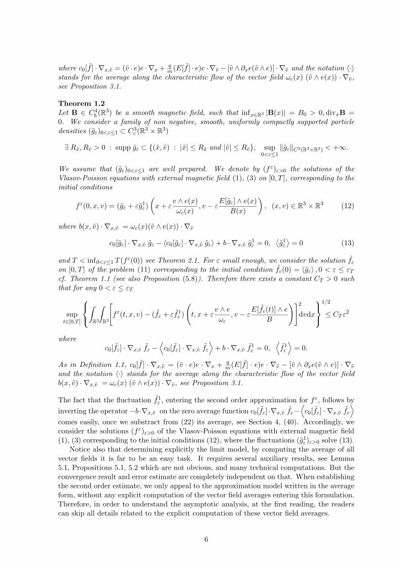
Theorem 1.2Let B ∈ C4

b (R3) be a smooth magnetic field, such that infx∈R3 |B(x)| = B0 > 0,divxB =0. We consider a family of non negative, smooth, uniformly compactly supported particledensities (gε)0<ε≤1 ⊂ C3

c (R3 × R3)

∃ Rx, Rv > 0 : supp gε ⊂ {(x, v) : |x| ≤ Rx and |v| ≤ Rv}, sup0<ε≤1

‖gε‖C3(R3×R3) < +∞.

We assume that (gε)0<ε≤1 are well prepared. We denote by (f ε)ε>0 the solutions of theVlasov-Poisson equations with external magnetic field (1), (3) on [0, T ], corresponding to theinitial conditions

f ε(0, x, v) = (gε + εg1ε)

(x+ ε

v ∧ e(x)

ωc(x), v − εE[gε] ∧ e(x)

B(x)

), (x, v) ∈ R3 × R3 (12)

where b(x, v) · ∇x,v = ωc(x)(v ∧ e(x)) · ∇v

c0[gε] · ∇x,v gε − 〈c0[gε] · ∇x,v gε〉+ b · ∇x,v g1ε = 0,⟨g1ε⟩

= 0 (13)

and T < inf0<ε≤1 T (f ε(0)) see Theorem 2.1. For ε small enough, we consider the solution fεon [0, T ] of the problem (11) corresponding to the initial condition fε(0) = 〈gε〉 , 0 < ε ≤ εTcf. Theorem 1.1 (see also Proposition (5.8)). Therefore there exists a constant CT > 0 suchthat for any 0 < ε ≤ εT

supt∈[0,T ]

∫R3

∫R3

[f ε(t, x, v)− (fε + εf1ε )

(t, x+ ε

v ∧ eωc

, v − εE[fε(t)] ∧ eB

)]2dvdx

1/2

≤ CT ε2

wherec0[fε] · ∇x,v fε −

⟨c0[fε] · ∇x,v fε

⟩+ b · ∇x,v f1ε = 0,

⟨f1ε

⟩= 0.

As in Definition 1.1, c0[f ] · ∇x,v = (v · e)e · ∇x + qm(E[f ] · e)e · ∇v − [v ∧ ∂xe(v ∧ e)] · ∇v

and the notation 〈·〉 stands for the average along the characteristic flow of the vector fieldb(x, v) · ∇x,v = ωc(x) (v ∧ e(x)) · ∇v, see Proposition 3.1.

The fact that the fluctuation f1ε , entering the second order approximation for f ε, follows by

inverting the operator −b·∇x,v on the zero average function c0[fε]·∇x,v fε−⟨c0[fε] · ∇x,v fε

⟩comes easily, once we substract from (22) its average, see Section 4, (40). Accordingly, weconsider the solutions (f ε)ε>0 of the Vlasov-Poisson equations with external magnetic field(1), (3) corresponding to the initial conditions (12), where the fluctuations (g1ε)ε>0 solve (13).

Notice also that determining explicitly the limit model, by computing the average of allvector fields it is far to be an easy task. It requires several auxiliary results, see Lemma5.1, Propositions 5.1, 5.2 which are not obvious, and many technical computations. But theconvergence result and error estimate are completely independent on that. When establishingthe second order estimate, we only appeal to the approximation model written in the averageform, without any explicit computation of the vector field averages entering this formulation.Therefore, in order to understand the asymptotic analysis, at the first reading, the readerscan skip all details related to the explicit computation of these vector field averages.

6

Our paper is organized as follows. In Section 2 we discuss the well posedness of theVlasov-Poisson problem with external magnetic field. We indicate uniform estimates withrespect to the magnetic field. The average operators, together with their main properties areintroduced in Section 3. The second order approximation of the Vlasov-Poisson problem isderived in Sections 4, 5. The error estimate relies on the construction of a corrector term.The well posedness of the limit model is discussed in Section 6.

2 Classical solutions for the Vlasov-Poisson problem with ex-ternal magnetic field

The Vlasov-Poisson equations are now well understood. We refer to [3] for weak solutions, andto [49, 38, 43] for strong solutions. For studying the Vlasov-Poisson equations with externalmagnetic field we can adapt the arguments in [38, 46]. Motivated by the asymptotic behaviorwhen the magnetic field becomes strong, we are looking for classical solutions, satisfyinguniform bounds with respect to the magnetic field. At least locally in time such solutionsexist, see Appendix A for the main lines of the proof.

Theorem 2.1Consider a non negative, smooth, compactly supported initial particle density fin ∈ C1

c (R3 ×R3) such that

supp fin ⊂ {(x, v) ∈ R3 × R3 : |x| ≤ Rinx , |v| ≤ Rin

v }and a smooth magnetic field B ∈ C1

b (R3). Let T < T (fin) := mε0

q2Rinv (12π)1/3‖fin‖

1/3

L1 ‖fin‖2/3L∞

.

There is a unique particle density f ∈ C1c ([0, T ] × R3 × R3), whose Poisson electric field is

smooth E[f ] ∈ C1([0, T ]× R3), satisfying

∂tf + v · ∇xf +q

m(E[f(t)] + v ∧B) · ∇vf = 0, (t, x, v) ∈ [0, T ]× R3 × R3 (14)

E[f(t)](x) =q

4πε0

∫R3

∫R3

f(t, x′, v′)x− x′

|x− x′|3dv′dx′, (t, x) ∈ [0, T ]× R3 (15)

f(0, x, v) = fin(x, v), (x, v) ∈ R3 × R3. (16)

The bound for the L∞ norm of the Poisson electric field E[f ] and the size of the supportof the particle density f are not depending on the magnetic field. Moreover, if for someinteger k ≥ 2 we have fin ∈ Ckc (R3 × R3),B ∈ Ckb (R3), then f ∈ Ck([0, T ] × R3 × R3) andE[f ] ∈ Ck([0, T ]× R3).

Remark 2.11. The solution constructed in Theorem 2.1 preserves the particle number and the total energy

d

dt

∫R3

∫R3

f(t, x, v) dvdx = 0, t ∈ [0, T ]

d

dt

{∫R3

∫R3

m|v|2

2f(t, x, v) dvdx+

1

8πε0

∫R3

∫R3

ρ[f(t)](x)ρ[f(t)](x′)

|x− x′|dx′dx

}= 0.

2. We have the following balance for the total momentum

d

dt

∫R3

∫R3

f(t, x, v)mv dvdx− q∫R3

∫R3

f(t, x, v)v ∧B dvdx =

∫R3

ρ[f(t)]E[f(t)] dx

= ε0

∫R3

1supp ρ[f(t)] divxE[f(t)] E[f(t)] dx

= ε0

∫R3

1supp ρ[f(t)] divx

(E[f(t)]⊗ E[f(t)]− |E[f(t)]|2

2I3

)dx = 0.

7

When the magnetic field is uniform, we obtain the conservation of the parallel momentum

d

dt

∫R3

∫R3

f(t, x, v)m(v · e) dvdx = 0

andd

dt

∫R3

∫R3

f(t, x, v)m(v ∧ e) dvdx =qB

m

(∫R3

∫R3

f(t, x, v)m(v ∧ e) dvdx

)∧ e

saying that the orthogonal momentum rotates at the cyclotronic frequency ωc = qBm∫

R3

∫R3

f(t, x, v)m(v ∧ e) dvdx = cos(ωct)

∫R3

∫R3

fin(x, v)m(v ∧ e) dvdx

+ sin(ωct)

∫R3

∫R3

fin(x, v)m(v ∧ e) ∧ e dvdx, t ∈ [0, T ].

3 Average operators and main properties

We intend to investigate the asymptotic behavior of the particle densities (f ε)ε>0 satisfying(1), (3), (4) when ε > 0 becomes small. We assume that the initial particle density and theexternal magnetic field Bε = B

ε e are smooth

fin ≥ 0, fin ∈ C1c (R3 × R3), B = Be ∈ C1

b (R3)

and let us consider T < T (fin). Under the above assumptions, we know by Theorem 2.1that there exists εT > 0 such that for every 0 < ε ≤ εT , there is a unique strong solutionf ε ∈ C1

c ([0, T ]×R3×R3), Eε := E[f ε] ∈ C1([0, T ]×R3) for the Vlasov-Poisson problem withexternal magnetic field Bε = B

ε e. As noticed in the proof of Theorem 2.1, we have uniformestimates with respect to ε for the L∞ norm of the electric field Eε and the size of the supportof the particle density f ε. Let us denote by (Xε, V ε)(t; t0, x, v) the characteristics associatedto (1)

dXε

dt=V ε(t; t0, x, v),

dV ε

dt=q

m[Eε(t,Xε(t; t0, x, v)) + V ε(t; t0, x, v) ∧Bε(Xε(t; t0, x, v))]

(17)Xε(t0; t0, x, v) = x, V ε(t0; t0, x, v) = v.

The strong external magnetic field induces a large cyclotronic frequency ωεc = qBε/m =ωc/ε, ωc = qB/m, and thus a fast dynamics. We are looking for quantities which are leftinvariant with respect to this fast motion. By direct computations we obtain

d

dt

[Xε(t) + ε

V ε(t) ∧ e(Xε(t))

ωc(Xε(t))

]= (V ε(t) · e(Xε(t)) e(Xε(t)) + ε

Eε(t,Xε(t))

B(Xε(t))∧ e(Xε(t))

+ εV ε(t) ∧ ∂xe(Xε(t))V ε(t)

ωc(Xε(t))− ε (∇xωc(Xε(t)) · V ε(t))

V ε(t) ∧ e(Xε(t))

ω2c (X

ε(t))

saying that the variations of x+εv∧e(x)ωc(x), along the characteristic flow (17), over one cyclotronic

period, is very small. Notice that the electro-magnetic force writes

q

mEε(t, x) +

ωcεv ∧ e(x) =

q

m(Eε(t, x) · e(x)) e(x) +

ωc(x)

ε

(v − εE

ε(t, x) ∧ e(x)

B(x)

)∧ e(x)

and therefore we introduce the relative velocity with respect to the electric cross field drift

v = v − εEε(t, x) ∧ e(x)

B(x). (18)

8

Accordingly, at any time t ∈ R+, we consider the new particle density

f ε(t, x, v) = f ε(t, x, v + ε

E[f ε(t)](x) ∧ e(x)

B(x)

), (x, v) ∈ R3 × R3. (19)

It is easily seen that the particle densities f ε, f ε have the same charge density

ρ[f ε(t)] = q

∫R3

f ε(t, ·, v) dv = q

∫R3

f ε(t, ·, v) dv = ρ[f ε(t)], t ∈ R+

implying that the Poisson electric fields corresponding to f ε, f ε coincide

E[f ε(t)] = E[f ε(t)], t ∈ [0, T ].

Therefore we can use the same notation Eε(t) for denoting them. We assume that themagnetic field satisfies

B0 := infx∈R3

|B(x)| > 0 or equivalently ω0 := infx∈R3

|ωc(x)| > 0 (20)

and therefore (18), (19) are well defined. Notice that the particle densities (f ε)ε>0 are smooth,f ε ∈ C1

c ([0, T ] × R3 × R3) and uniformly compactly supported with respect to ε (use theuniform bound for the electric fields (Eε)ε and the hypothesis (20)). Appealing to the chainrule leads to the following problem in the phase space (x, v)

∂tfε +

(v + ε

Eε ∧ eB

)· ∇xf ε − ε

[∂tE

ε ∧ eB

+ ∂x

(Eε ∧ eB

)(v + ε

Eε ∧ eB

)]· ∇vf ε

+[ωcεv ∧ e+

q

m(Eε · e) e

]· ∇vf ε = 0, (t, x, v) ∈ [0, T ]× R3 × R3 (21)

f ε(0, x, v) = fin

(x, v + ε

E[fin](x) ∧ e(x)

B(x)

), (x, v) ∈ R3 × R3.

We are looking for a representation formula for the time derivative of the electric field Eε, interms of the particle density f ε. Thanks to the continuity equation

∂tρ[f ε] + divxj[fε] = 0

we write

∂tE[f ε] =1

4πε0

∫R3

∂tρ[f ε(t)](x− x′) x′

|x′|3dx′

= − 1

4πε0

∫R3

divxj[fε](x− x′) x′

|x′|3dx′

= − 1

4πε0divx

∫R3

x′

|x′|3⊗ j[f ε(t)](x− x′) dx′

= − 1

4πε0divx

∫R3

x− x′

|x− x′|3⊗(j[f ε(t)](x′) + ερ[f ε(t)](x′)

Eε(t, x′) ∧ e(x′)B(x′)

)dx′.

We introduce as well the new Larmor center x = x + ε v∧e(x)ωc(x), which is a second order

approximation of the Larmor center x+εv∧e(x)ωc(x). The idea will be to decompose the transport

field in the Vlasov equation in such a way that x remains invariant with respect to the fastdynamics. We will distinguish between the orthogonal and parallel directions, taking as

9

reference direction the magnetic line passing through the new Larmor center x, that is e(x)(which is left invariant with respect to the fast dynamics)

v = [v − (v · e(x))e(x)] + (v · e(x))e(x).

Finally the Vlasov equation (21) writes

∂tfε+cε[f ε(t)]·∇x,v f ε+εaε[f ε(t)]·∇x,v f ε+

bε

ε·∇x,v f ε = 0, (t, x, v) ∈ [0, T ]×R3×R3 (22)

where the autonomous vector field bε

ε · ∇x,v is given by

bε

ε· ∇x,v = [v − (v · e(x)) e(x) + εAεx(x, v)] · ∇x +

ωc(x)

ε(v ∧ e(x)) · ∇v

and for any particle density f , aε[f ] · ∇x,v , cε[f ] · ∇x,v stand for the vector fields

aε[f ] · ∇x,v =

(E[f ] ∧ e

B−Aεx

)· ∇x +

[−∂x

(E[f ] ∧ e

B

)(v + ε

E[f ] ∧ eB

)(23)

+1

4πε0Bdivx

∫R3

x− x′

|x− x′|3⊗

(j[f ] + ερ[f ]

E[f ] ∧ eB

)(x′) dx′ ∧ e(x)

]· ∇v

cε[f ] · ∇x,v = (v · e(x)) e(x) · ∇x +

[ωc(x)v ∧ e(x)− e(x)

ε+

q

m(E[f ] · e(x)) e(x)

]· ∇v

=

[q

m(E[f ] · e(x)) e(x)− ωcv ∧

∫ 1

0∂xe

(x+ εs

v ∧ e(x)

ωc(x)

)v ∧ e(x)

ωc(x)ds

]· ∇v

+ (v · e(x)) e(x) · ∇x. (24)

The vector field Aεx(x, v) ·∇x will be determined by imposing that the Larmor center x is leftinvariant by the fast dynamics

bε · ∇x,v(x+ ε

v ∧ e(x)

ωc(x)

)= 0.

After some computations, the above condition writes[I3 + ε∂x

(v ∧ eωc

)]Aεx(x, v) = −∂x

(v ∧ eωc

)[v − (v · e(x)) e(x)]− e(x)− e(x)

ε∧ (v ∧ e(x))

and therefore Aεx(x, v) is well defined for a.a. (x, v) ∈ R3×R3. Notice that for ε small enough,that is

ε

∥∥∥∥∂x( v ∧ eωc

)∥∥∥∥L∞

< 1

the vector field Aεx is well defined on R3 × R3. In particular Aεx is well defined if

ε|v|(‖∂xe‖L∞

ω0+‖∇xωc‖L∞

ω20

)< 1.

Remark 3.1The vector field in the Vlasov equation (22) is divergence free

divx,v

(cε[f ] + εaε[f ] +

bε

ε

)= εdivx

(E[f ] ∧ e

B

)− εdivv

[∂x

(E[f ] ∧ e

B

)v

]= 0.

10

We intend to study the asymptotic behavior of (22), when ε goes to 0 by averaging with

respect to the flow of the fast dynamics generated by the advection field bε(x,v)ε · ∇x,v cf.

[6, 8, 10, 11, 12]. In order to do that, we concentrate on the main properties of this flow. Asin the two dimensional framework, we establish the periodicity of the fast dynamics.

Proposition 3.1Let B ∈ C1

b (R3) verifying (20) and e ∈ C2b (R3). We denote by (Xε(s;x, v), Vε(s;x, v)) the

characteristic flow of the autonomous vector field bε(x, v) · ∇x,vdXε

ds= ε[I3 − e(Xε(s;x, v))⊗ e(Xε(s;x, v))]Vε(s;x, v) + ε2Aεx(Xε(s;x, v), Vε(s;x, v))

dVε

ds= ωc(X

ε(s;x, v)) Vε(s;x, v) ∧ e(Xε(s;x, v))

Xε(0;x, v) = x, Vε(0;x, v) = v

(using the notation Xε(s;x, v) = Xε(s;x, v) + εVε(s;x, v) ∧ e(Xε(s;x, v))/ωc(Xε(s;x, v)))and

by (X(s;x, v), V(s;x, v)) the characteristic flow of the autonomous vector field b(x, v) ·∇x,v =ωc(x) (v ∧ e(x)) · ∇v

dX

ds= 0,

dV

ds= ωc(X(s;x, v)) V(s;x, v) ∧ e(X(s;x, v)), X(0;x, v) = x, V(0;x, v) = v.

1. For any (x, v) ∈ R3 × R3 and ε > 0 such that



ω20

)< 1 (25)

the characteristic s→ (Xε, Vε)(s;x, v) is periodic, with smallest period Sε(x, v) > 0.

2. For any (x, v) ∈ R3 × R3 and ε > 0 such that



ω20

)≤ 1

2

we have

|Xε(s;x, v)− X(s;x, v)| = |Xε(s;x, v)− x| ≤ ε2|v|ω0

, s ∈ R

2π

‖ωc‖L∞≤ Sε(x, v) ≤ 2π

ω0,

2π

‖ωc‖L∞≤ S(x, v) :=

2π

|ωc(x)|≤ 2π

ω0

|Sε(x, v)− S(x, v)| ≤ ε‖∇ωc‖L∞4π|v|ω30

,

|Vε(s;x, v)− V(s;x, v)| ≤ ε|v|2(

5‖∂xe‖L∞

ω0+ 4π

‖∇xωc‖L∞ω20

), s ∈

[0,

2π

ω0

]and

|Aεx(x, v)| ≤ 4|v|2(‖∂xe‖L∞


ω20

)

|Aεx(x, v)−Ax(x, v)| ≤ ε|v|3[

7

(‖∂xe‖L∞


ω20

)2

+1

2

‖∂2xe‖L∞ω20

]where

Ax(x, v) = −∂x(v ∧ e(x)

ωc(x)

)[v − (v · e(x)) e(x)]− ∂xe

v ∧ e(x)

ωc(x)∧ (v ∧ e(x)).

In particular, when ∇xωc = 0, we have Sε(x, v) = S(x, v) = 2π/|ωc|.

11

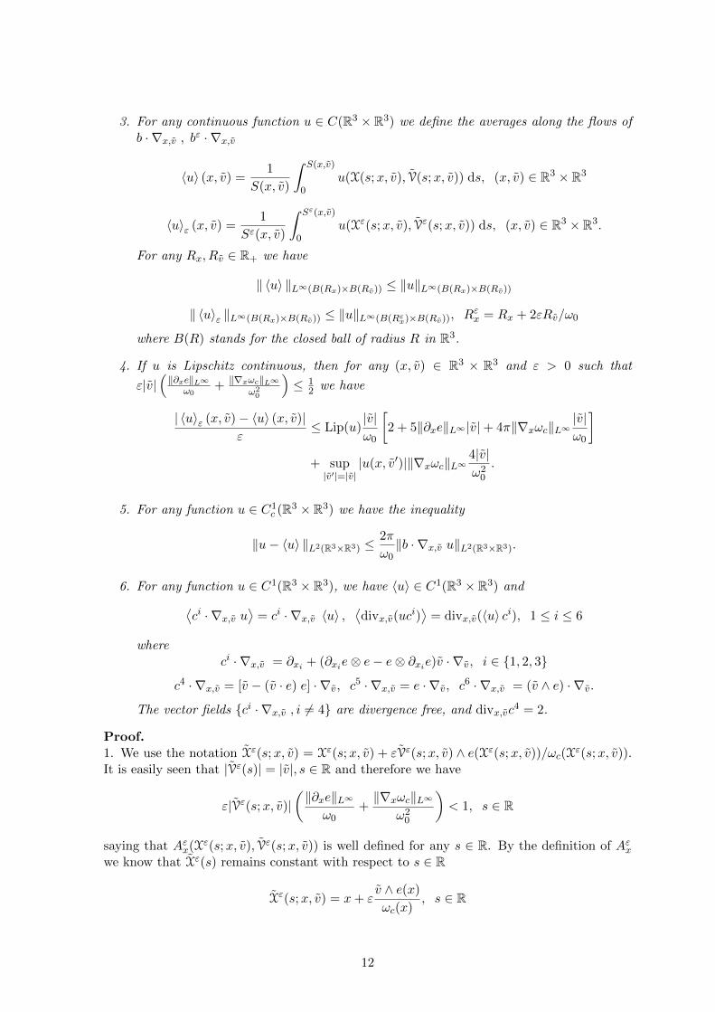
3. For any continuous function u ∈ C(R3 × R3) we define the averages along the flows ofb · ∇x,v , bε · ∇x,v

〈u〉 (x, v) =1

S(x, v)

∫ S(x,v)

0u(X(s;x, v), V(s;x, v)) ds, (x, v) ∈ R3 × R3

〈u〉ε (x, v) =1

Sε(x, v)

∫ Sε(x,v)

0u(Xε(s;x, v), Vε(s;x, v)) ds, (x, v) ∈ R3 × R3.

For any Rx, Rv ∈ R+ we have

‖ 〈u〉 ‖L∞(B(Rx)×B(Rv)) ≤ ‖u‖L∞(B(Rx)×B(Rv))

‖ 〈u〉ε ‖L∞(B(Rx)×B(Rv)) ≤ ‖u‖L∞(B(Rεx)×B(Rv)), Rεx = Rx + 2εRv/ω0

where B(R) stands for the closed ball of radius R in R3.

4. If u is Lipschitz continuous, then for any (x, v) ∈ R3 × R3 and ε > 0 such that


ω0+ ‖∇xωc‖L∞

ω20

)≤ 1

2 we have

| 〈u〉ε (x, v)− 〈u〉 (x, v)|ε

≤ Lip(u)|v|ω0

[2 + 5‖∂xe‖L∞ |v|+ 4π‖∇xωc‖L∞

|v|ω0

]+ sup|v′|=|v|

|u(x, v′)|‖∇xωc‖L∞4|v|ω20

.

5. For any function u ∈ C1c (R3 × R3) we have the inequality

‖u− 〈u〉 ‖L2(R3×R3) ≤2π

ω0‖b · ∇x,v u‖L2(R3×R3).

6. For any function u ∈ C1(R3 × R3), we have 〈u〉 ∈ C1(R3 × R3) and⟨ci · ∇x,v u

⟩= ci · ∇x,v 〈u〉 ,

⟨divx,v(uc

i)⟩

= divx,v(〈u〉 ci), 1 ≤ i ≤ 6

whereci · ∇x,v = ∂xi + (∂xie⊗ e− e⊗ ∂xie)v · ∇v, i ∈ {1, 2, 3}

c4 · ∇x,v = [v − (v · e) e] · ∇v, c5 · ∇x,v = e · ∇v, c6 · ∇x,v = (v ∧ e) · ∇v.

The vector fields {ci · ∇x,v , i 6= 4} are divergence free, and divx,vc4 = 2.

Proof.1. We use the notation Xε(s;x, v) = Xε(s;x, v) + εVε(s;x, v) ∧ e(Xε(s;x, v))/ωc(X

ε(s;x, v)).It is easily seen that |Vε(s)| = |v|, s ∈ R and therefore we have

ε|Vε(s;x, v)|(‖∂xe‖L∞


ω20

)< 1, s ∈ R

saying that Aεx(Xε(s;x, v), Vε(s;x, v)) is well defined for any s ∈ R. By the definition of Aεxwe know that Xε(s) remains constant with respect to s ∈ R

Xε(s;x, v) = x+ εv ∧ e(x)

ωc(x), s ∈ R

12

implying that the parallel velocity is left invariant

d

ds

(Vε(s) · e(Xε(s))

)= 0, s ∈ R

and that the orthogonal velocity rotates around e(x)

Vε(s;x, v) = R(−∫ s

0ωc(X

ε(σ;x, v)) dσ, e(x)

)v, s ∈ R.

Here the notation R(θ, e) stands for the rotation of angle θ around the axis e

R(θ, e)ξ = cos θ(I3 − e⊗ e)ξ − sin θ(ξ ∧ e) + (ξ · e) e, ξ ∈ R3.

As ωc has constant sign, there is a unique Sε(x, v) > 0 such that

sgn ωc

∫ Sε(x,v)

0ωc(X

ε(σ;x, v)) dσ =

∫ Sε(x,v)

0|ωc(Xε(σ;x, v))| dσ = 2π

and therefore Vε(Sε(x, v);x, v) = v. We claim that Xε(Sε(x, v);x, v) = x. It is enough to usethe invariance of the Larmor center

Xε(Sε) + εVε(Sε) ∧ e(Xε(Sε))

ωc(Xε(Sε))= x+ ε

v ∧ e(x)

ωc(x)

and to observe that

|Xε(Sε)− x| = ε

∣∣∣∣ v ∧ e(x)

ωc(x)− v ∧ e(Xε(Sε))

ωc(Xε(Sε))

∣∣∣∣≤ ε|v|

∣∣∣∣ e(Xε(Sε))ωc(Xε(Sε))− e(x)

ωc(x)

∣∣∣∣≤ ε|v|

∥∥∥∥∂x( e

ωc

)∥∥∥∥L∞|Xε(Sε)− x|

≤ ε|v|(‖∂xe‖L∞


ω20

)|Xε(Sε)− x|.

Our conclusion follows by (25).2. By the definition of the vector field Aεx(x, v) · ∇x, we deduce

|Aεx(x, v)| ≤∥∥∥∥∂x( v ∧ eωc

)∥∥∥∥L∞|v|+ ‖∂xe‖L∞

|v|2

ω0+ ε

∥∥∥∥∂x( v ∧ eωc

)∥∥∥∥L∞|Aεx(x, v)|

≤ 2|v|2(‖∂xe‖L∞


ω20

)+ ε|v|

(‖∂xe‖L∞


ω20

)|Aεx(x, v)|

≤ 2|v|2(‖∂xe‖L∞


ω20

)+|Aεx(x, v)|

2

implying that

|Aεx(x, v)| ≤ 4|v|2(‖∂xe‖L∞


ω20

).

Notice that∣∣∣∣[I3 + ε∂x

(v ∧ e(x)

ωc(x)

)]Aεx(x, v)−Ax(x, v)

∣∣∣∣ ≤ 2

∥∥∥∥∂x( v ∧ e(x)

ωc(x)

)∥∥∥∥L∞

ε‖∂xe‖L∞|v|2

ω0

+ ε‖∂xe‖2L∞|v|3

ω20

+ |v|∣∣∣∣e(x)− e(x)

ε− ∂xe(x)

v ∧ e(x)

ωc(x)

∣∣∣∣≤ ε

(3‖∂xe‖L∞

ω0+ 2‖∇xωc‖L∞

ω20

)‖∂xe‖L∞

ω0|v|3 +

ε

2

‖∂xe2‖L∞ω20

|v|3

13

and therefore

|Aεx(x, v)−Ax(x, v)| ≤∣∣∣∣[I3 + ε∂x

(v ∧ e(x)

ωc(x)

)]Aεx(x, v)−Ax(x, v)

∣∣∣∣+ ε|v|

(‖∂xe‖L∞


ω20

)|Aεx(x, v)|

≤ 7ε|v|3(‖∂xe‖L∞


ω20

)2

+ε‖∂2xe‖L∞

2ω20

|v|3.

The invariances of x and |v| yield

|Xε(s)− x| =

∣∣∣∣∣ε v ∧ e(x)

ωc(x)− ε V

ε(s) ∧ e(Xε(s))ωc(Xε(s))

∣∣∣∣∣ ≤ ε2|v|ω0

, s ∈ R.

It is easily seen that 2π/‖ωc‖L∞ ≤ Sε(x, v) ≤ 2π/ω0. Notice that we have

|ωc(x)| − ‖∇xωc‖L∞2ε|v|ω0≤ |ωc(Xε(σ))| ≤ |ωc(x)|+ ‖∇xωc‖L∞

2ε|v|ω0

.

Averaging with respect to σ ∈ [0, Sε(x, v)], we obtain

|ωc(x)| − ‖∇xωc‖L∞2ε|v|ω0≤ 2π

Sε(x, v)≤ |ωc(x)|+ ‖∇xωc‖L∞

2ε|v|ω0

.

Thanks to the formula |ωc(x)| = 2πS(x,v) , we deduce

2π

∣∣∣∣ 1

Sε(x, v)− 1

S(x, v)

∣∣∣∣ ≤ ε‖∇xωc‖L∞ 2|v|ω0

and

|Sε(x, v)− S(x, v)| = Sε(x, v)S(x, v)

∣∣∣∣ 1

Sε(x, v)− 1

S(x, v)

∣∣∣∣ ≤ ε‖∇xωc‖L∞ 4π|v|ω30

.

It remains to compare the velocities Vε(s;x, v), V(s;x, v). We will use the inequality

‖R(θ, e)−R(θ′, e′)‖ ≤ |θ − θ′|+ 5|e− e′|, θ, θ′ ∈ R, |e| = |e′| = 1.

For any s ∈ [0, 2π/ω0] we write

|(Vε − V)(s;x, v)| =∣∣∣∣R(−∫ s

0ωc(X

ε(σ)) dσ, e(x)

)v −R

(−∫ s

0ωc(X(σ)) dσ, e(x)

)v

∣∣∣∣≤[∫ s

0|ωc(Xε(σ))− ωc(X(σ))| dσ + 5|e(x)− e(x)|

]|v|

≤(

2π

ω0‖∇xωc‖L∞

2ε|v|ω0

+ 5‖∂xe‖L∞ε|v|ω0

)|v|

= ε|v|2(

5‖∂xe‖L∞

ω0+ 4π


).

3. It is a direct consequence of the invariances X(s;x, v) = x, |V(s;x, v)| = |v|

Xε(s;x, v) + εVε(s;x, v) ∧ e(Xε(s;x, v))

ωc(Xε(s;x, v))= x+ ε

v ∧ e(x)

ωc(x), |Vε(s;x, v)| = |v|.

14

4. It is a direct consequence of the previous statements. We have

| 〈u〉ε (x, v)− 〈u〉 (x, v)| ≤ 1

Sε(x, v)

∫ Sε(x,v)

0|u(Xε(s), Vε(s))− u(X(s), V(s))| ds

+

∣∣∣∣ 1

Sε(x, v)− 1

S(x, v)

∣∣∣∣ ∫ Sε(x,v)

0|u(X(s), V(s))| ds+

1

S(x, v)

∣∣∣∣∣∫ Sε(x,v)

S(x,v)|u(X(s), V(s))| ds

∣∣∣∣∣Our conclusion follows by noticing that

1

Sε(x, v)

∫ Sε(x,v)

0|u(Xε(s), Vε(s))− u(X(s), V(s))| ds ≤ Lip(u)

sup0≤s≤2π/ω0

(|Xε(s)− X(s)|+ |Vε(s)− V(s)|

)≤ εLip(u)

|v|ω0

[2 + 5‖∂xe‖L∞ |v|+ 4π


|v|]

and ∣∣∣∣ 1

Sε(x, v)− 1

S(x, v)

∣∣∣∣ ∫ Sε(x,v)

0|u(X(s), V(s))| ds+

1

S(x, v)

∣∣∣∣∣∫ Sε(x,v)

S(x,v)|u(X(s), V(s))| ds

∣∣∣∣∣≤ 4ε|v| sup

|v′|=|v||u(x, v′)|‖∇xωc‖L

∞

ω20

.

5. For any (x, v) ∈ R3 × R3

〈u〉 (x, v)− u(x, v) =1

S(x, v)

∫ S(x,v)

0[u(X(s;x, v), V(s;x, v))− u(x, v)] ds

=1

S(x, v)

∫ S(x,v)

0

∫ s

0

d

dσu(X(σ;x, v), V(σ;x, v)) dσds

=1

S(x, v)

∫ S(x,v)

0

∫ s

0(b · ∇u)(X(σ;x, v), V(σ;x, v)) dσds

=1

2π

∫ 2π

0

∫ θ|ωc(x)|

0(b · ∇u)(X(σ;x, v), V(σ;x, v)) dσdθ

implying that

| 〈u〉 (x, v)− u(x, v)| ≤ 1

2π

∫ 2π

0

∫ 2πω0

0|(b · ∇u)(X(σ;x, v), V(σ;x, v))| dσdθ

=

∫ 2πω0

0|(b · ∇u)(X(σ;x, v), V(σ;x, v))| dσ.

Taking into account that (x, v) → (X(σ;x, v), V(σ;x, v)) is measure preserving, it is easilyseen that

‖ 〈u〉 − u‖L2 ≤∫ 2π

ω0

0‖(b · ∇u)(X(σ; ·, ·), V(σ; ·, ·))‖L2 dσ =

2π

ω0‖b · ∇u‖L2 .

6. For any (x, v) ∈ R3 × R3 we have

〈u〉 (x, v) =1

2π

∫ 2π

0u(x,R(−θ, e(x))v) dθ

=1

2π

∫ 2π

0u(x, cos θ(v − (v · e(x))e(x) + sin θ(v ∧ e(x)) + (v · e(x))e(x)) dθ

15

and therefore 〈u〉 ∈ C1(R3 × R3), provided that e ∈ C1(R3). By direct computations wecheck that all the vector fields (ci · ∇x,v )1≤i≤6 are in involution with respect to (v ∧ e) · ∇v,see Remark 3.2 for a more general result. Thanks to the commutation between the flowsof ci · ∇x,v and (v ∧ e) · ∇v, we deduce easily that the average operator along the flow of(v ∧ e) · ∇v commutes with the flow of ci · ∇x,v , and thus with ci · ∇x,v , for 1 ≤ i ≤ 6. Itremains to observe that the average along the flow of (v ∧ e) · ∇v coincides with the averagealong the flow of ωc(v ∧ e) · ∇v. The divergences of the vector fields (ci · ∇x,v )1≤i≤6 areconstant along the flow of b · ∇x,v , implying that

divx,v(〈u〉 ci) = ci · ∇x,v 〈u〉+ 〈u〉divx,vci

=⟨ci · ∇x,v u

⟩+⟨u divx,vc

i⟩

=⟨divx,v(uc

i)⟩, 1 ≤ i ≤ 6.

Remark 3.2For further developments, notice that for any vector field ξ(x) · ∇x, the vector field

c[ξ] · ∇x,v = ξ(x) · ∇x + v ∧ (∂xeξ ∧ e) · ∇v = ξ(x) · ∇x + (∂xeξ ⊗ e− e⊗ ∂xeξ)v · ∇v

is in involution with respect to (v ∧ e) · ∇v. For justifying that, it is convenient to use, forany a ∈ R3, the notation M [a], standing for the matrix of the linear application v ∈ R3 →a ∧ v ∈ R3. We appeal to the formulae

M [a]M [b] = b⊗ a− (a · b)I3, M [a ∧ b] = b⊗ a− a⊗ b, a, b ∈ R3.

The commutator between (v ∧ e) · ∇v and c[ξ] · ∇x,v writes

(v ∧ e) · ∇v(ξ(x), v ∧ (∂xeξ ∧ e))− [ξ · ∇x + v ∧ (∂xeξ ∧ e) · ∇v](0, v ∧ e)= (0,−M [∂xeξ ∧ e](v ∧ e)−M [v]∂xeξ −M [e]M [∂xeξ ∧ e]v).

We are done provided that

M [∂xeξ ∧ e]M [e] +M [∂xeξ]−M [e]M [∂xeξ ∧ e] = 0.

Indeed, we have

M [e]M [∂xeξ ∧ e]−M [∂xeξ ∧ e]M [e] = (∂xeξ ∧ e)⊗ e− e⊗ (∂xeξ ∧ e)= M [e ∧ (∂xeξ ∧ e)] = M [∂xeξ]

Notice that the periods S, Sε are left invariant along the flows of b·∇x,v , bε ·∇x,v respectively,as well as the averages 〈u〉 , 〈u〉ε. If u is a C1 function, we have

〈b · ∇x,v u〉 (x, v) =1

S(x, v)

∫ S(x,v)

0

d

dsu(X(s), V(s)) ds = 0, (x, v) ∈ R3 × R3

and similarly 〈bε · ∇x,v u〉ε = 0.We introduce the application T ε : R3 × R3 → R3 × R3, given by

T ε(x, v) =

(x+ ε

v ∧ e(x)

ωc(x), v

), (x, v) ∈ R3 × R3.

16

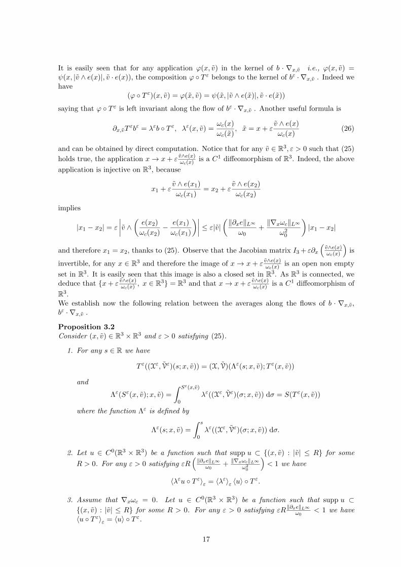
It is easily seen that for any application ϕ(x, v) in the kernel of b · ∇x,v i.e., ϕ(x, v) =ψ(x, |v ∧ e(x)|, v · e(x)), the composition ϕ ◦ T ε belongs to the kernel of bε · ∇x,v . Indeed wehave

(ϕ ◦ T ε)(x, v) = ϕ(x, v) = ψ(x, |v ∧ e(x)|, v · e(x))

saying that ϕ ◦ T ε is left invariant along the flow of bε · ∇x,v . Another useful formula is

∂x,vTεbε = λεb ◦ T ε, λε(x, v) =

ωc(x)

ωc(x), x = x+ ε

v ∧ e(x)

ωc(x)(26)

and can be obtained by direct computation. Notice that for any v ∈ R3, ε > 0 such that (25)

holds true, the application x→ x+ ε v∧e(x)ωc(x)is a C1 diffeomorphism of R3. Indeed, the above

application is injective on R3, because

x1 + εv ∧ e(x1)ωc(x1)

= x2 + εv ∧ e(x2)ωc(x2)

implies

|x1 − x2| = ε

∣∣∣∣v ∧ ( e(x2)

ωc(x2)− e(x1)

ωc(x1)

)∣∣∣∣ ≤ ε|v|(‖∂xe‖L∞ω0+‖∇xωc‖L∞

ω20

)|x1 − x2|

and therefore x1 = x2, thanks to (25). Observe that the Jacobian matrix I3 + ε∂x

(v∧e(x)ωc(x)

)is

invertible, for any x ∈ R3 and therefore the image of x→ x+ ε v∧e(x)ωc(x)is an open non empty

set in R3. It is easily seen that this image is also a closed set in R3. As R3 is connected, wededuce that {x+ ε v∧e(x)ωc(x)

, x ∈ R3} = R3 and that x→ x+ ε v∧e(x)ωc(x)is a C1 diffeomorphism of

R3.We establish now the following relation between the averages along the flows of b · ∇x,v,bε · ∇x,v .

Proposition 3.2Consider (x, v) ∈ R3 × R3 and ε > 0 satisfying (25).

1. For any s ∈ R we have

T ε((Xε, Vε)(s;x, v)) = (X, V)(Λε(s;x, v);T ε(x, v))

and

Λε(Sε(x, v);x, v) =

∫ Sε(x,v)

0λε((Xε, Vε)(σ;x, v)) dσ = S(T ε(x, v))

where the function Λε is defined by

Λε(s;x, v) =

∫ s

0λε((Xε, Vε)(σ;x, v)) dσ.

2. Let u ∈ C0(R3 × R3) be a function such that supp u ⊂ {(x, v) : |v| ≤ R} for some

R > 0. For any ε > 0 satisfying εR(‖∂xe‖L∞


ω20

)< 1 we have

〈λεu ◦ T ε〉ε = 〈λε〉ε 〈u〉 ◦ Tε.

3. Assume that ∇xωc = 0. Let u ∈ C0(R3 × R3) be a function such that supp u ⊂{(x, v) : |v| ≤ R} for some R > 0. For any ε > 0 satisfying εR ‖∂xe‖L

∞ω0

< 1 we have〈u ◦ T ε〉ε = 〈u〉 ◦ T ε.

17

Proof.1. As Aεx(x, v) is well defined for any (x, v) ∈ R3 × R3 and ε > 0 satisfying (25), and since|Vε(s;x, v)| = |v|, we deduce that (Xε(s;x, v), Vε(s;x, v)) exists for any s ∈ R. Let us considerΛε(s;x, v) =

∫ s0 λ

ε((Xε, Vε)(σ;x, v)) dσ, s ∈ R and γε(s;x, v) = T ε(Xε(s;x, v), Vε(s;x, v)).Observe, thanks to (26), that

dγε

ds= ∂T ε(Xε(s;x, v), Vε(s;x, v))bε(Xε(s;x, v), Vε(s;x, v))

= λε(Xε(s;x, v), Vε(s;x, v))b(T ε(Xε(s;x, v), Vε(s;x, v)))

=dΛε

ds(s;x, v)b(γε(s;x, v)).

Notice also that

d

ds(X, V)(Λε(s;x, v);T ε(x, v)) =

dΛε

ds(s;x, v)b((X, V)(Λε(s;x, v);T ε(x, v))).

Since γε(s;x, v) and (X, V)(Λε(s;x, v);T ε(x, v)) coincide at s = 0

γε(0;x, v) = T ε(x, v) = (X, V)(0;T ε(x, v))

we deduce that

T ε(Xε(s;x, v), Vε(s;x, v)) = γε(s;x, v) = (X, V)(Λε(s;x, v);T ε(x, v)), s ∈ R. (27)

Recall that Xε(s;x, v) = x, s ∈ R and∫ Sε(x,v)0 |ωc(Xε(σ;x, v))| dσ = 2π. Therefore we obtain

Λε(Sε(x, v);x, v) =

∫ Sε(x,v)

0

ωc(Xε(σ;x, v))

ωc(Xε(σ;x, v))dσ =

1

|ωc(x)|

∫ Sε(x,v)

0|ωc(Xε(σ;x, v))| dσ

=2π

|ωc(x)|= S(T ε(x, v)).

2. Consider first (x, v) ∈ R3×R3 such that |v| > R. Obviously we have |V(s;x, v)| = |v| > R

and 〈u〉 (x, v) = 1S(x,v)

∫ S(x,v)0 u(X(s;x, v), V(s;x, v)) ds = 0. Similarly we have |Vε(s;x, v)| =

|v| > R and

〈λεu ◦ T ε〉ε =1

Sε(x, v)

∫ Sε(x,v)

0λε((Xε, Vε)(s;x, v))u(Xε(s;x, v), Vε(s;x, v)) ds = 0

where Xε = Xε + ε Vε∧e(Xε)ωc(Xε)

. Therefore our conclusion holds true in this case. Consider now

|v| ≤ R. Thanks to the first statement, we can write

〈λεu ◦ T ε〉ε (x, v) =1

Sε(x, v)

∫ Sε(x,v)

0λε((Xε, Vε)(s;x, v))u(Xε(s;x, v), Vε(s;x, v)) ds

=1

Sε(x, v)

∫ Sε(x,v)

0

d

dsΛε(s;x, v)u((X, V)(Λε(s;x, v);T ε(x, v))) ds

=1

Sε(x, v)

∫ S(T ε(x,v))

0u((X, V)(σ;T ε(x, v))) dσ

=1

Sε(x, v)

∫ Sε(x,v)

0λε((Xε, Vε)(σ;x, v)) dσ 〈u〉 (T ε(x, v))

= (〈λε〉ε 〈u〉 ◦ Tε) (x, v).

3. It comes from the points 1. and 2. with λε = 1.

18

Remark 3.3The conclusions of the second and third statement in Proposition 3.2 remain valid for |v| ≤R, εR

(‖∂xe‖L∞


ω20

)< 1 if u ∈ C0(R3 × R3).

When establishing the convergence toward the limit model, we need to introduce a correctorterm. More exactly, we need to invert the operator (v ∧ e(x)) · ∇v on the set of zero averagefunctions. We will use the following result.

Proposition 3.3Let z ∈ C0(R3 × R3) be a continuous function, of zero average

〈z〉 (x, v) =1

2π

∫ 2π

0z (x,R(−θ, e(x))v) dθ = 0, (x, v) ∈ R3 × R3.

1. There is a unique continuous function u of zero average whose derivative along the flowof (v ∧ e(x)) · ∇v is z

(v ∧ e(x)) · ∇vu = z(x, v), (x, v) ∈ R3 × R3.

If z is bounded, so is u, and

‖u‖C0(B(Rx)×B(Rv)) ≤ π‖z‖C0(B(Rx)×B(Rv)), for any Rx, Rv > 0.

If supp z ⊂ B(Rx)×B(Rv), then supp u ⊂ B(Rx)×B(Rv).

2. If z is of class C1, then so is u and we have for any Rx, Rv > 0

‖∇vu‖C0(B(Rx)×B(Rv)) ≤ π√

3‖∇vz‖C0(B(Rx)×B(Rv))

‖∇xu‖C0(B(Rx)×B(Rv)) ≤ C(‖∇xz‖C0(B(Rx)×B(Rv)) +Rv‖∇vz‖C0(B(Rx)×B(Rv))

)for some constant C depending on ‖∂xe‖L∞.

Proof.1. It is easily seen that

u(x, v) =1

2π

∫ 2π

0(θ − 2π)z(x,R(−θ, e(x))v) dθ, (x, v) ∈ R3 × R3.

2. We appeal to the vector fields (ci · ∇x,v )1≤i≤6 which are in involution with (v ∧ e) · ∇v,see the last statement in Proposition 3.1, Remark 3.2. We have

(v ∧ e(x)) · ∇v(ci · ∇x,v u) = ci · ∇x,v z⟨ci · ∇x,v z

⟩= ci · ∇x,v 〈z〉 = 0,

⟨ci · ∇x,v u

⟩= ci · ∇x,v 〈u〉 = 0.

As before, we have

(ci·∇x,v u)(x, v) =1

2π

∫ 2π

0(θ−2π)(ci·∇x,v z)(x,R(−θ, e(x))v) dθ, (x, v) ∈ R3×R3, 1 ≤ i ≤ 6.

Since |v ∧ e(x)| is left invariant by the flow of (v ∧ e(x)) · ∇v, we also have for any (x, v) suchthat v ∧ e(x) 6= 0

(ci · ∇x,v u)(x, v)

|v ∧ e(x)|=

1

2π

∫ 2π

0(θ − 2π)

(ci · ∇x,v z| · ∧ e|

)(x,R(−θ, e(x))v) dθ, i ∈ {4, 6}.

19

We deduce that for any (x, v) ∈ B(Rx)×B(Rv) such that v ∧ e(x) 6= 0

|(ci · ∇x,v u)(x, v)||v ∧ e(x)|

≤ π‖∇vz‖C0(B(Rx)×B(Rv), i ∈ {4, 6}.

We also have for any (x, v) ∈ B(Rx)×B(Rv)

|(e ·∇vu)(x, v)| = |(c5 ·∇x,v u)(x, v)| ≤ π‖c5 ·∇x,v z‖C0(B(Rx)×B(Rv) ≤ π‖∇vz‖C0(B(Rx)×B(Rv).

We obtain, for any (x, v) ∈ B(Rx)×B(Rv) such that v ∧ e(x) 6= 0

|∇vu(x, v)|2 =|(c4 · ∇x,v u)(x, v)|2

|v ∧ e(x)|2+ |(c5 · ∇x,v u)(x, v)|2 +

|(c6 · ∇x,v u)(x, v)|2

|v ∧ e(x)|2

≤ 3π2‖∇vz‖2C0(B(Rx)×B(Rv).

As u is C1 (because z is assumed C1), we deduce

‖∇vu‖C0(B(Rx)×B(Rv) ≤ π√

3‖∇vz‖C0(B(Rx)×B(Rv)).

The estimate for ‖∇xu‖C0(B(Rx)×B(Rv)) follows immediately, using the fields ci · ∇x,v , i ∈{1, 2, 3}

‖ci · ∇x,v u‖C0(B(Rx)×B(Rv)) ≤ π‖ci · ∇x,v z‖C0(B(Rx)×B(Rv)), i ∈ {1, 2, 3}

and the previous estimate for ‖∇vu‖C0(B(Rx)×B(Rv)).

4 The limit model and convergence result

We concentrate now on the formal derivation of the limit model in (22), as ε goes to 0. Weexpect that the solution of (22) writes

f ε = fε ◦ T ε + ελεf1ε ◦ T ε + ε2f2ε ◦ T ε + . . . (28)

where b · ∇x,v fε = 0,⟨f1ε

⟩= 0. The idea is to split the contributions at any order into

average and fluctuation. As fε ∈ ker b · ∇x,v , we know that fε ◦ T ε ∈ ker bε · ∇x,v and thus⟨fε ◦ T ε

⟩ε

= fε ◦ T ε. By Proposition 3.2 we also have⟨λεf1ε ◦ T ε

⟩ε

= 〈λε〉ε⟨f1ε

⟩◦ T ε = 0

and therefore ⟨f ε⟩ε

= fε ◦ T ε +O(ε2), f ε −⟨f ε⟩ε

= ελεf1ε ◦ T ε +O(ε2).

Accordingly, at the leading order, the particle density f ε has no fluctuation (provided that theinitial condition will be well prepared) and the averages at the orders 1, ε combine togetherin fε ◦ T ε. For any smooth compactly supported particle density f = f(x, v) we introducethe notations, motivated by (23), (24)

a[f ] · ∇x,v =

(E[f ] ∧ e

B−Ax(x, v)

)· ∇x − ∂x

(E[f ] ∧ e

B

)v · ∇v

+1

4πε0B

[divx

∫R3

x− x′

|x− x′|3⊗ j[f ](x′) dx′ ∧ e(x)

]· ∇v

c0[f ] · ∇x,v = (v · e) e · ∇x +q

m(E[f ] · e) e · ∇v − [v ∧ ∂xe(v ∧ e)] · ∇v (29)

20

c1[f ] · ∇x,v = limε↘0

∂T εcε[f ◦ T ε]− λε(x, v)(c0[f ] ◦ T ε)ε

· ∇x,v . (30)

The last notation is justified by the expansion

cε[f ◦ T ε] · ∇x,v (f ◦ T ε) = λε(x, v)(c0[f ] · ∇x,v f) ◦ T ε + ε(c1[f ] · ∇x,v f) ◦ T ε +O(ε2) (31)

for any smooth particle density f , which will be used in the sequel. The expression for thevector field c1[f ] · ∇x,v follows by straightforward computations, see Proposition 5.6, usingthe definition

cε[f ] · ∇x,v = (v · e(x)) e(x) · ∇x +q

m(E[f ] · e(x)) e(x) · ∇v − ωc(x)v ∧ e(x)− e(x)

ε· ∇v.

Taking the average of (22) along the flow (Xε, Vε) yields

∂t

⟨f ε(t)

⟩ε

+⟨cε[f ε(t)] · ∇x,v f ε(t)

⟩ε

+ ε⟨aε[f ε(t)] · ∇x,v f ε(t)

⟩ε

= 0. (32)

Motivated by (28), we have

∂t

⟨f ε⟩ε

= (∂tfε) ◦ T ε +O(ε2).

For the contribution of the term εaε[f ε] · ∇x,v f ε observe that

aε[f ε] · ∇x,v f ε = a[f ε] · ∇x,v f ε +O(ε) (33)

= a[fε ◦ T ε] · ∇x,v (fε ◦ T ε) +O(ε)

= λε(a[fε] · ∇x,v fε) ◦ T ε +O(ε).

It remains to analyze the contribution of cε[f ε] · ∇x,v f ε. Since⟨f1ε

⟩= 0, we have ρ[f1ε ] =

0, E[f1ε ] = 0, E[λεf1ε ◦ T ε] = O(ε) and therefore

cε[f ε] · ∇x,vf ε = cε[fε ◦ T ε + ελεf1ε ◦ T ε] · ∇x,v (fε ◦ T ε + ελεf1ε ◦ T ε) +O(ε2) (34)

= cε[fε ◦ T ε] · ∇x,v (fε ◦ T ε) + εcε[fε ◦ T ε] · ∇x,v (λεf1ε ◦ T ε) +O(ε2)

= λε(c0[fε] · ∇x,v fε) ◦ T ε + ελε(c1[fε] · ∇x,v fε) ◦ T ε

+ ελε(c0[fε] · ∇x,v f1ε ) ◦ T ε +O(ε2).

Thanks to the second statement in Proposition 3.2, we have

ε⟨aε[f ε] · ∇x,v f ε

⟩ε

= ε⟨λε(a[fε] · ∇x,v fε) ◦ T ε +O(ε)

⟩ε

(35)

= ε 〈λε〉ε⟨a[fε] · ∇x,v fε

⟩◦ T ε +O(ε2)

= ε⟨a[fε] · ∇x,v fε

⟩◦ T ε +O(ε2)

and ⟨cε[f ε] · ∇x,v f ε

⟩ε

=⟨λε(c0[fε] · ∇x,v fε) ◦ T ε

⟩ε

+ ε⟨λε(c1[fε] · ∇x,v fε) ◦ T ε

⟩ε

(36)

+ ε⟨λε(c0[fε] · ∇x,v f1ε ) ◦ T ε

⟩ε

+O(ε2)

= 〈λε〉ε⟨c0[fε] · ∇x,v fε

⟩◦ T ε + ε 〈λε〉ε


⟩◦ T ε

+ ε 〈λε〉ε⟨c0[fε] · ∇x,v f1ε

⟩◦ T ε +O(ε2)

=⟨c0[fε] · ∇x,v fε

⟩◦ T ε + ε


⟩◦ T ε

+ ε⟨c0[fε] · ∇x,v f1ε

⟩◦ T ε +O(ε2)

21

where in the last equality we have used the relation 〈λε〉ε = 1 +O(ε2). By combining (32),(35), (36) and keeping all the terms up to the second order, we find the following model forthe particle density fε

∂tfε +⟨c0[fε] · ∇x,v fε

⟩+ ε⟨

(a[fε] + c1[fε]) · ∇x,v fε⟩

+ ε⟨c0[fε] · ∇x,v f1ε

⟩= 0, b ·∇fε = 0.

(37)We need another equation for the fluctuation f1ε . Replacing in (22) the expressions in (33),(34) yields

∂tfε ◦ T ε + ελε(∂tf1ε ◦ T ε) + λε(c0[fε] · ∇x,v fε) ◦ T ε + ελε((a[fε] + c1[fε]) · ∇x,v fε) ◦ T ε

+ ελε(c0[fε] · ∇x,v f1ε ) ◦ T ε +bε

ε· ∇x,v (fε ◦ T ε + ελεf1ε ◦ T ε + ε2f2ε ◦ T ε) = O(ε2).

(38)

Taking the difference between (38) and (37) (after composition with T ε) leads to

ελε(∂tf1ε ◦ T ε) + λε(c0[fε] · ∇x,v fε) ◦ T ε −


⟩◦ T ε

+ ελε(a[fε] + c1[fε]) · ∇x,v fε) ◦ T ε − ε⟨

(a[fε] + c1[fε]) · ∇x,v fε⟩◦ T ε

+ ελε(c0[fε] · ∇x,v f1ε ) ◦ T ε − ε⟨c0[fε] · ∇x,v f1ε

⟩◦ T ε

+ bε · ∇x,v (λεf1ε ◦ T ε + εf2ε ◦ T ε) = O(ε2)

because fε ◦ T ε ∈ ker bε · ∇x,v . As λε = 1 +O(ε), the previous equation also writes

ε∂tf1ε ◦ T ε + λε

(c0[fε] · ∇x,v fε −


⟩)◦ T ε + (λε − 1)


⟩◦ T ε

+ ε(

(a[fε] + c1[fε]) · ∇x,v fε −⟨

(a[fε] + c1[fε]) · ∇x,v fε⟩)◦ T ε (39)

+ ε(c0[fε] · ∇x,v f1ε −

⟨c0[fε] · ∇x,v f1ε

⟩)◦ T ε

+ bε · ∇x,v[f1ε ◦ T ε − ε

v ∧ e(x)

ωc(x)· ∇xωc(x)

ωc(x)f1ε ◦ T ε + εf2ε ◦ T ε

]= O(ε2).

Notice that by (26) we have

bε · ∇x,v (f1ε ◦ T ε) = bε · t∂T ε(∇x,v f1ε ) ◦ T ε = λε(b · ∇x,v f1ε ) ◦ T ε

and

εbε · ∇x,v(f2ε ◦ T ε −

v ∧ e(x)

ωc(x)· ∇xωc(x)

ωc(x)f1ε ◦ T ε

)= εbε · ∇x,v

[(f2ε −

v ∧ e(x)

ωc(x)· ∇xωc(x)

ωc(x)f1ε

)◦ T ε

]= ελε

[b · ∇

(f2ε −

v ∧ e(x)

ωc(x)· ∇xωc(x)

ωc(x)f1ε

)]◦ T ε.

The equality (39) suggests that the fluctuation f1ε satisfies the problem

c0[fε] · ∇x,v fε −⟨c0[fε] · ∇x,v fε

⟩+ b · ∇x,v f1ε = 0,

⟨f1ε

⟩= 0. (40)

22

Moreover, considering the contributions of order ε in (39) leads to the definition of thecorrector f2ε

∂tf1ε −

v ∧ e(x)

ωc(x)· ∇xωc(x)

ωc(x)


⟩+ (a[fε] + c1[fε]) · ∇x,v fε (41)

−⟨

(a[fε] + c1[fε]) · ∇x,v fε⟩

+ c0[fε] · ∇x,v f1ε −⟨c0[fε] · ∇x,v f1ε

⟩+ b · ∇x,v

(f2ε −

v ∧ e(x)

ωc(x)· ∇xωc(x)

ωc(x)f1ε

)= 0.

We have obtained the limit model (37), (40), to be supplemented by an initial condition.The well posedness of this model will be established in Section 6. We will discuss the ex-istence/uniqueness of smooth solutions on any time interval [0, T ], if ε is small enough cf.Theorem 1.1. Notice that (37), (40) is a regular reformulation of the Vlasov-Poisson systemwith strong external magnetic field. Indeed, replacing ε by 0 in (37) leads to the zero ordermodel

∂tf0 +⟨

(v · e) e · ∇xf0 +q

m(E[f0] · e) e · ∇vf0 − [v ∧ (∂xe(v ∧ e)] · ∇vf0

⟩= 0, b · ∇f0 = 0.

We are ready now to establish rigorously the second order approximation f ε = fε ◦ T ε +ελεf1ε ◦ T ε +O(ε2).

Proof. (of Theorem 1.2)Clearly we have

supε>0{‖ρ[gε]‖L1(R3) + ‖ρ[gε]‖L∞(R3)} < +∞.

By Proposition 3.3 we obtain supp (g1ε) ⊂ {(x, v) ∈ R3 × R3 : |x| ≤ Rx, |v| ≤ Rv} and it iseasily seen that

supp f ε(0) ⊂{

(x, v) ∈ R3 × R3 : |v| ≤ Rεv := Rv + ε‖E[gε]‖L∞

B0, |x| ≤ Rεx := Rx + ε

Rεvω0

}.

Therefore the particle densities (f ε(0))0<ε≤1 are uniformly compactly supported and we havesupε>0‖f ε(0)‖C2(R3×R3) < +∞. Notice that inf

ε>0T (f ε(0)) > 0, see Theorem 2.1, and thus we

can pick a time 0 < T < infε>0

T (f ε(0)). By Theorem 2.1 we know that (f ε)ε are uniformly

compactly supported in [0, T ]× R3 × R3 and

supt∈[0,T ]

[‖f ε(t)‖C2(R3×R3) + ‖∂tf ε(t)‖C1(R3×R3) + ‖E[f ε(t)]‖C2(R3)

]< +∞, ε > 0.

We deduce that (f ε)ε are uniformly compactly supported in [0, T ]× R3 × R3 and

supt∈[0,T ]

[‖f ε(t)‖C2(R3×R3) + ‖∂tf ε(t)‖C1(R3×R3)

]< +∞, ε > 0.

The particle densities (〈gε〉)ε are uniformly compactly supported in R3×R3, we have supε>0‖ 〈gε〉 ‖C3(R3×R3) <

+∞, and therefore we know by Theorem 1.1 that the particle densities (fε)ε are uniformlycompactly supported in [0, T ]× R3 × R3 and

supε>0,t∈[0,T ]

[‖fε(t)‖C3(R3×R3) + ‖∂tfε(t)‖C2(R3×R3) + ‖E[fε(t)]‖C3(R3)

]< +∞.

23

Clearly we have c0[fε] · ∇x,v fε,⟨c0[fε] · ∇x,v fε

⟩∈ C2

c (R3 × R3) and by Proposition 3.3

applied to

c0[fε] · ∇x,v fεωc

−


ωc

⟩+ (v ∧ e) · ∇vf1ε = 0,

⟨f1ε

⟩= 0

we deduce that f1ε (t) ∈ C2c (R3 × R3). We also have ∂t(c0[fε] · ∇x,v fε), ∂t


⟩∈

C1c (R3 × R3) and by appealing one more time to Proposition 3.3 (noticing that

⟨∂tf

1ε

⟩=

∂t

⟨f1ε

⟩= 0), we obtain ∂tf

1ε (t) ∈ C1

c (R3 × R3) and

supε>0,t∈[0,T ]

[‖f1ε (t)‖C2(R3×R3) + ‖∂tf1ε (t)‖C1(R3×R3)

]< +∞.

Finally we define the corrector f2ε by solving (41). More exactly we define f2ε = v∧e(x)ωc(x)

·∇xωcωc(x)

f1ε + uε, where 〈uε〉 = 0 and

∂tf1ε −

v ∧ e(x)

ωc(x)· ∇xωcωc(x)


⟩+ (a[fε] + c1[fε]) · ∇x,v fε

−⟨

(a[fε] + c1[fε]) · ∇x,v fε⟩

+ c0[fε] · ∇x,v f1ε −⟨c0[fε] · ∇x,v f1ε

⟩+ b · ∇x,v uε = 0.

Thanks to Proposition 3.3, see also the expression of the field c1[fε] · ∇x,v cf. Proposition5.6, it is easily seen that

supε>0,t∈[0,T ]

[‖uε(t)‖C1(R3×R3) + ‖∂tuε(t)‖C0(R3×R3)] < +∞

which implies

supε>0,t∈[0,T ]

[‖f2ε (t)‖C1(R3×R3) + ‖∂tf2ε (t)‖C0(R3×R3)] < +∞. (42)

Multiplying (40) by λε, one gets after composition with T ε

λε(c0[fε] · ∇x,v fε) ◦ T ε − λε⟨c0[fε] · ∇x,v fε

⟩◦ T ε + bε · ∇x,v (f1ε ◦ T ε) = 0. (43)

Similarly, multiplying (41) by ελε yields, after composition with T ε

∂t(ελεf1ε ◦ T ε)− ελε

v ∧ e(x)

ωc(x)· ∇xωc(x)

ωc(x)


⟩◦ T ε (44)

+ ελε((a[fε] + c1[fε]) · ∇x,v fε) ◦ T ε − ελε⟨

(a[fε] + c1[fε]) · ∇x,v fε⟩◦ T ε

+ ελε(c0[fε] · ∇x,v f1ε ) ◦ T ε − ελε⟨c0[fε] · ∇x,v f1ε

⟩◦ T ε

+ εbε · ∇x,v (f2ε ◦ T ε)− εbε · ∇x,v[(

v ∧ e(x)

ωc(x)· ∇xωc(x)

ωc(x)f1ε

)◦ T ε

]= 0.

A straightforward computation shows that the functions

δε := bε · ∇x,v[(λε − 1 + ε

v ∧ e(x)

ωc(x)· ∇xωc(x)

ωc(x)

)(f1ε ◦ T ε)

]+

(λε − 1 + ελε

v ∧ e(x)

ωc(x)· ∇xωc(x)

ωc(x)

)⟨c0[fε] · ∇x,v fε

⟩◦ T ε

24

satisfy

supε>0,t∈[0,T ]

‖δε(t)‖C0(R3×R3)

ε2< +∞. (45)

Combining (43), (44) we obtain

∂t(ελεf1ε ◦ T ε + ε2f2ε ◦ T ε) + λε(c0[fε] · ∇x,v fε) ◦ T ε −


⟩◦ T ε (46)

+ ε((a[fε] + c1[fε]) · ∇x,v fε) ◦ T ε − ε⟨

(a[fε] + c1[fε]) · ∇x,v fε⟩◦ T ε

+ ε(c0[fε] · ∇x,v f1ε ) ◦ T ε − ε⟨c0[fε] · ∇x,v f1ε

⟩◦ T ε

+bε

ε· ∇x,v

(ελεf1ε ◦ T ε + ε2f2ε ◦ T ε

)= ε2∂tf

2ε ◦ T ε + δε + δε

where

δε := ε(1− λε)[((a[fε] + c1[fε]) · ∇x,v fε) ◦ T ε −

⟨(a[fε] + c1[fε]) · ∇x,v fε

⟩◦ T ε

]+ ε(1− λε)

[(c0[fε] · ∇x,v f1ε ) ◦ T ε −

⟨c0[fε] · ∇x,v f1ε

⟩◦ T ε

].

Clearly, the functions (δε)ε satisfy

supε>0,t∈[0,T ]

‖δε(t)‖C0(R3×R3)

ε2< +∞. (47)

Adding to (46) the equation (37) satisfied by fε (after composition with T ε), together withthe constraint bε

ε · ∇x,v (fε ◦ T ε) = 0, we deduce

∂t(fε ◦ T ε + ελεf1ε ◦ T ε + ε2f2ε ◦ T ε) + λε(c0[fε] · ∇x,v fε) ◦ T ε + ε(c1[fε] · ∇x,v fε) ◦ T ε

+ ε(c0[fε] · ∇x,v f1ε ) ◦ T ε + ε(a[fε] · ∇x,v fε) ◦ T ε

+bε

ε· ∇x,v

(fε ◦ T ε + ελεf1ε ◦ T ε + ε2f2ε ◦ T ε

)= ε2∂tf

2ε ◦ T ε + δε + δε. (48)

We compare (48) to the model of the particle density f ε

∂tfε + cε[f ε] · ∇x,v f ε + εaε[f ε] · ∇x,v f ε +

bε

ε· ∇x,v f ε = 0. (49)

We are looking for an estimate of the L2 norm of

rε := f ε − fε ◦ T ε − ελεf1ε ◦ T ε − ε2f2ε ◦ T ε.

Taking the difference between (49) and (48) yields

∂trε +

(cε[f ε] + εaε[f ε] +

bε

ε

)· ∇x,v rε + T εc + εT εa = −ε2∂tf2ε ◦ T ε − δε − δε (50)

where the transport terms T εc , T εa write

T εc (t, x, v) = cε[f ε(t)] · ∇x,v (fε ◦ T ε + ελεf1ε ◦ T ε + ε2f2ε ◦ T ε)− λε(c0[fε(t)] · ∇x,v fε) ◦ T ε

− ε(c1[fε] · ∇x,v fε + c0[fε] · ∇x,v f1ε

)◦ T ε

25

T εa (t, x, v) := aε[f ε(t)] · ∇x,v (fε ◦ T ε + ελεf1ε ◦ T ε + ε2f2ε ◦ T ε)− (a[fε] · ∇x,v fε) ◦ T ε.

By Remark 3.1 we know that the vector field(cε[f ε] + εaε[f ε] + bε

ε

)·∇x,v is divergence free

and therefore, multiplying (50) by rε and integrating by parts yield

1

2

d

dt

∫R3

∫R3

(rε)2 dvdx+

∫R3

∫R3

T εc (t, x, v)rε(t, x, v) dvdx+ ε

∫R3

∫R3

T εa (t, x, v)rε(t, x, v) dvdx

(51)

= −∫R3

∫R3

(ε2∂tf

2ε ◦ T ε + δε + δε

)rε(t, x, v) dvdx.

We denote by C any constant depending on m, ε0, q, T, ωc, e and the uniform bounds satisfiedby the initial particle densities (gε)ε, but not on ε. The bounds (42), (45), (47) and theuniform compactness of the supports of fε, f

1ε , f

2ε imply immediately that∣∣∣∣∫

R3

∫R3

(ε2∂tf

2ε ◦ T ε + δε + δε

)rε(t) dvdx

∣∣∣∣ ≤ Cε2‖rε(t)‖L2(R3×R3), t ∈ [0, T ], 0 < ε ≤ εT .

(52)We claim that the following inequalities hold true

‖T εc (t)‖L2(R3×R3) ≤ C(ε2 + ‖rε(t)‖L2(R3×R3)), t ∈ [0, T ], 0 < ε ≤ εT (53)

and‖T εa (t)‖L2(R3×R3) ≤ C(ε+ ‖rε(t)‖L2(R3×R3)), t ∈ [0, T ], 0 < ε ≤ εT . (54)

Let us analyze first (54). By Proposition 3.1, we know that |Aεx(x, v)−Ax(x, v)| ≤ Cε|v|3, andthanks to the uniform bounds of (fε)ε, (f

1ε )ε, (f

2ε )ε (together with the uniform compactness of

their supports), we deduce that (use also the uniform compactness of the supports of (f ε)ε>0,the boundedness of (E[f ε])ε>0 in L∞ cf. Theorem 2.1 and the elliptic regularity results inorder to bound (E[f ε])ε>0 in L2, together with their space derivatives [28])

‖aε[f ε] · ∇(fε ◦ T ε + ελεf1ε ◦ T ε + ε2f2ε ◦ T ε)− (a[fε] · ∇fε) ◦ T ε‖L2

≤ Cε+ ‖a[f ε] · ∇(fε ◦ T ε)− (a[fε] · ∇fε) ◦ T ε‖L2

≤ Cε+ ‖(∂T εa[f ε]− a[fε] ◦ T ε) · (∇fε) ◦ T ε‖L2

≤ Cε+ ‖(a[f ε]− a[fε ◦ T ε]) · (∇fε) ◦ T ε‖L2 .

By elliptic regularity results, the quantity

‖(a[f ε]− a[fε ◦ T ε]) · (∇fε) ◦ T ε‖L2

is bounded by the L2 norms of charge and current densities

‖ρ[f ε]− ρ[fε ◦ T ε]‖L2 + ‖j[f ε]− j[fε ◦ T ε]‖L2

and thus by the L2 norms of the particle densities ‖f ε− fε ◦T ε‖L2 ≤ ‖rε‖L2 +Cε, saying that(54) holds true. We concentrate now on (53). It is easily seen, by elliptic regularity results,that

‖(cε[f ε]− cε[fε ◦ T ε + ελεf1ε ◦ T ε]) · ∇(fε ◦ T ε + ελεf1ε ◦ T ε + ε2f2ε ◦ T ε)‖L2 (55)

≤ C‖f ε − fε ◦ T ε − ελεf1ε ◦ T ε‖L2

≤ C(‖rε‖L2 + ε2).

26

As the particle density f1ε has zero average, we deduce that ρ[f1ε ] = 0 and therefore

‖E[ελεf1ε ◦ T ε]‖L2 = ε‖E[λεf1ε ◦ T ε − f1ε ]‖L2 ≤ Cε‖λεf1ε ◦ T ε − f1ε ‖L2 ≤ Cε2.

The above estimate allows us to write

‖(cε[fε ◦ T ε + ελεf1ε ◦ T ε]− cε[fε ◦ T ε]) · ∇(fε ◦ T ε + ελεf1ε ◦ T ε + ε2f2ε ◦ T ε)‖L2 ≤ Cε2.(56)

We are done if we establish the estimate

‖cε[fε ◦ T ε] · ∇(fε ◦ T ε + ελεf1ε ◦ T ε)− λε(c0[fε] · ∇fε) ◦ T ε (57)

− ε(c1[fε] · ∇fε + c0[fε] · ∇f1ε ) ◦ T ε‖L2 ≤ Cε2

since, in that case (53) will be a consequence of (55), (56), (57). It is easily seen that

‖cε[fε ◦ T ε] · ∇(ελεf1ε ◦ T ε)− ε(c0[fε] · ∇f1ε ) ◦ T ε‖L2 ≤ Cε2.

It remains to prove that

‖cε[fε ◦ T ε] · ∇(fε ◦ T ε)− λε(c0[fε] · ∇fε) ◦ T ε − ε(c1[fε] · ∇fε) ◦ T ε‖L2 ≤ Cε2. (58)

This comes by the definition of the vector fields c0, c1, cε and the regularity of the particle

densities (fε)ε, see (29), (30), (24), (31). Indeed, for any smooth, compactly supportedparticle density f we have

cε[f ◦ T ε] · ∇(f ◦ T ε)− λε(c0[f ] · ∇f) ◦ T ε − ε(c1[f ] · ∇f) ◦ T ε

= ε

(Ff (ε, x, v)− Ff (0, x, v)

ε− ∂εFf (0, x, v)

)· (∇f) ◦ T ε

+ ε(c1[f ]− c1[f ] ◦ T ε) · (∇f) ◦ T ε

where Ff (ε, x, v) = ∂T εcε[f ◦ T ε] − λε(x, v)c0[f ] ◦ T ε. Clearly, when f ∈ C2c (R3 × R3), the

function Ff is twice differentiable with respect to ε. Moreover, as

supt∈[0,T ],0<ε≤εT

‖fε(t)‖C2(R3×R3) < +∞

and {fε(t) : t ∈ [0, T ], 0 < ε ≤ εT } are uniformly compactly supported, we have

‖cε[fε ◦ T ε] · ∇(fε ◦ T ε)− λε(c0[fε] · ∇fε) ◦ T ε − ε(c1[fε] · ∇fε) ◦ T ε‖L2

≤ ε

∥∥∥∥∥(Ffε(ε)− Ffε(0)

ε− ∂εFfε(0)

)· (∇fε) ◦ T ε

∥∥∥∥∥L2

+∥∥∥ε(c1[fε]− c1[fε] ◦ T ε) · (∇fε) ◦ T ε∥∥∥

L2

≤ Cε2 + ε∥∥∥(c1[fε]− c1[fε] ◦ T ε) · (∇fε) ◦ T ε

∥∥∥L2

By the expression of c1[fε], see Proposition 5.6, it is clear that∥∥∥(c1[fε]− c1[fε] ◦ T ε) · (∇fε) ◦ T ε∥∥∥L2≤ Cε

and (58) follows. Coming back to (51), we obtain thanks to (52), (53), (54)

‖rε(t)‖L2 ≤ [‖rε(0)‖L2 + Ctε2] exp(Ct), 0 ≤ t ≤ T, 0 < ε ≤ εT .

27

The well preparation of the initial particle densities (f ε(0))ε guarantees that supε>0

‖rε(0)‖L2

ε2<

+∞. Indeed, for justifying this, it is enough to check

supε>0

‖f ε(0)− fε(0) ◦ T ε − εf1ε (0) ◦ T ε‖L2

ε2< +∞. (59)

As the family of electric fields (E[gε])ε is bounded in L∞([0, T ]× R3), we have

supε>0

‖ρ[f ε(0)]− ρ[gε]‖L1 + ‖ρ[f ε(0)]− ρ[gε]‖L∞ε

< +∞

implying that

supε>0

‖E[f ε(0)]− E[gε]‖L∞ε

< +∞.

By direct estimates we obtain

supε>0

‖f ε(0)− gε ◦ T ε − εg1ε ◦ T ε‖L2

ε2< +∞ (60)

By the fifth statement in Proposition 3.1 we have

supε>0

‖gε ◦ T ε − fε(0) ◦ T ε‖L2

ε2≤ Csup

ε>0

‖gε − 〈gε〉 ‖L2

ε2≤ 2πCsup

ε>0

‖(v ∧ e) · ∇v gε‖L2

ε2< +∞

(61)

and

supε>0

‖g1ε ◦ T ε − f1ε (0) ◦ T ε‖L2

ε≤ Csup

ε>0

‖g1ε − f1ε (0)‖L2

ε(62)

≤ 4π

ω0Csupε>0

‖c0[gε] · ∇gε − c0[〈gε〉] · ∇ 〈gε〉 ‖L2

ε

=4π

ω0Csupε>0

‖c0[gε] · ∇(gε − 〈gε〉)‖L2

ε< +∞.

Notice that in the last equality we have used ρ[gε] = ρ[〈gε〉], implying that E[gε] = E[〈gε〉]and therefore c0[gε] = c0[〈gε〉]. Combining (60), (61), (62) yields (59) and therefore


‖rε(t)‖L2

ε2< +∞.

We deduce that


‖f ε(t)− fε(t) ◦ T ε − εf1ε (t) ◦ T ε‖L2

ε2< +∞

and in particular


‖E[f ε(t)]− E[fε(t)]‖L2

ε< +∞.

28

Finally one gets for any t ∈ [0, T ], 0 < ε ≤ εT∫R3

∫R3

[f ε(t, x, v)− (fε + εf1ε )

(t, x+ ε

v ∧ e(x)

ωc(x), v − εE[fε(t)] ∧ e(x)

B(x)

)]2dvdx

1/2

=

{∫R3

∫R3

[f ε(t, x, v)− (fε + εf1ε )

(t, x+

ε

ωc

(v + ε

E[f ε(t)] ∧ eB(x)

)∧ e, v + ε

(E[f ε(t)]− E[fε(t)]) ∧ eB(x)

)]2dvdx

1/2

≤ ‖f ε(t)− (fε(t) + εf1ε (t)) ◦ T ε‖L2(R3×R3) +

{∫R3

∫R3

[(fε + εf1ε )

(t, x+ ε

v ∧ e(x)

ωc(x), v

)

−(fε + εf1ε )

(t, x+ ε

v ∧ eωc

+ε2

ωc

(E[f ε(t)] ∧ e) ∧ eB(x)

, v + εE[f ε − fε] ∧ e

B(x)

)]2dvdx

1/2

≤ Cε2 + Cε‖E[f ε(t)]− E[fε(t)]‖L2(R3) ≤ Cε2.

5 Equivalent formulation of the limit model

In the previous section we proved a second order error estimate for the solution of the Vlasov-Poisson system with strong external magnetic fields (corresponding to smooth, well preparedinitial conditions), with respect to the solution of


⟩+ ε

⟨(a[fε] + c1[fε]) · ∇x,v fε

⟩+ ε

⟨c0[fε] · ∇x,v f1ε

⟩= 0, b · ∇fε = 0

(63)

c0[fε] · ∇x,v fε −⟨c0[fε] · ∇x,v fε

⟩+ b · ∇x,v f1ε = 0,

⟨f1ε

⟩= 0. (64)

In order to establish the existence/uniqueness of smooth solution for the above system, weare looking for an equivalent formulation. More exactly, we will compute the averages of thevector fields a[fε] · ∇x,v , c0[fε] · ∇x,v , c1[fε] · ∇x,v cf. [12]. Let us consider the vector fieldb(x, v) · ∇x,v = (v ∧ e(x)) · ∇v. By Proposition 3.1 (see proof of statement 6), Remark 3.2,we know that the vector fields (ci · ∇x,v )1≤i≤6 are in involution with respect to b · ∇x,v andthat the average operators along the characteristic flows of b · ∇x,v , b · ∇x,v coincide. Weintroduce also the vector field

ν(x, v) · ∇x,v = − (v · e)|v ∧ e|2

t∂xe(v ∧ e) · ∇x +v ∧ e|v ∧ e|2

· ∇v, |v ∧ e| > 0

which will be used, together with the invariants of b · ∇x,v, for computing the average vectorfields. A straightforward computation leads to the following result.

Lemma 5.1Assume that e ∈ C2(R3). Let us denote by Y = (X, V) the characteristic flow of the vectorfield b · ∇x,v = (v ∧ e(x)) · ∇v

Y (θ; y) = (x,R(−θ, e(x))v) = (x, cos θ(v − (v · e)e) + sin θ(v ∧ e) + (v · e)e)

for any θ ∈ R, y = (x, v) ∈ R3 × R3. The vector field ν(x, v) · ∇x,v verifies

t∂Y (θ; y)ν(Y (θ; y)) = ν(y), θ ∈ R, y = (x, v), |v ∧ e(x)| > 0.

29

The average of a vector field is defined as follows.

Proposition 5.1Assume that e ∈ C1(R3). Let χ · ∇x,v be a continuous vector field on R3 × R3. There is a

continuous vector field in involution with respect to b · ∇x,v , denoted 〈χ〉 · ∇x,v (the averageof χ · ∇x,v with respect to b · ∇x,v ), such that

〈χ · ∇x,v u〉 = 〈χ〉 · ∇x,v u

for any function u ∈ C1(R3 × R3) ∩ ker(b · ∇x,v ) = C1(R3 × R3) ∩ ker(b · ∇x,v ) and

〈χ · ν〉 = 〈χ〉 · ν.

Proof.Let us introduce the group (ϕ(θ))θ∈R cf. [12]

ϕ(θ)χ = ∂Y (−θ;Y (θ; ·))χ(Y (θ; ·)), θ ∈ R

and consider the vector field

〈χ〉 =1

2π

∫ 2π

0ϕ(θ)χ dθ.

It is easily seen that if χ is continuous, so is 〈χ〉, and that 〈χ〉 is left invariant by thegroup (ϕ(θ))θ∈R, saying that 〈χ〉 is in involution with respect to b · ∇x,v . For any functionu ∈ C1(R3 × R3) ∩ ker(b · ∇x,v ) we have u ◦ Y (θ; ·) = u and thus

ϕ(θ)χ · ∇u = ∂Y (−θ;Y (θ; ·))χ(Y (θ; ·)) · t∂Y (θ; ·)(∇u)(Y (θ; ·)) = (χ · ∇u)(Y (θ; ·)).

We deduce that

〈χ〉 · ∇u =1

2π

∫ 2π

0ϕ(θ)χ · ∇u dθ =

1

2π

∫ 2π

0(χ · ∇u)(Y (θ; ·)) dθ = 〈χ · ∇u〉 .

Similarly, thanks to Lemma 5.1, we have for any (x, v) such that |v ∧ e(x)| > 0

ϕ(θ)χ · ν = ∂Y (−θ;Y (θ; ·))χ(Y (θ; ·)) · t∂Y (θ; ·)ν(Y (θ; ·)) = (χ · ν)(Y (θ; ·))

implying that

〈χ〉 · ν =1

2π

∫ 2π

0ϕ(θ)χ · ν dθ =

1

2π

∫ 2π

0(χ · ν)(Y (θ; ·)) dθ = 〈χ · ν〉 , |v ∧ e(x)| > 0.

Remark 5.1Recall that the vector fields

ci · ∇x,v = ∂xi + (∂xie⊗ e− e⊗ ∂xie)v · ∇v, i ∈ {1, 2, 3}

c4 · ∇x,v = (v − (v · e) e) · ∇v, c5 · ∇x,v = e · ∇v, c6 · ∇x,v = b · ∇x,v = (v ∧ e) · ∇vare in involution with respect to b · ∇x,v . For any continuous vector field χ(x, v) · ∇x,v wehave

χ(x, v) =6∑i=1

αi(x, v)ci(x, v), (x, v) ∈ (R3 × R3) \ E , E = {(x, v) : b(x, v) = 0}

30

where

(α1, α2, α3) = χx, α4 =χv − (∂xeχx ⊗ e− e⊗ ∂xeχx)v

|v ∧ e|2· (v − (v · e) e)

α5 = [χv − (∂xeχx ⊗ e− e⊗ ∂xeχx)v] · e, α6 =χv − (∂xeχx ⊗ e− e⊗ ∂xeχx)v

|v ∧ e|2· (v ∧ e).

It is easily seen that for any vector field d ·∇x,v in involution with respect to b ·∇x,v and anyfunction α, we have ϕ(θ)(αd) = α(Y (θ; ·))ϕ(θ)d = α(Y (θ; ·))d, implying that 〈αd〉 = 〈α〉 dand thus for any (x, v) ∈ (R3 × R3) \ E (see Remark 3.2 for the definition of c[〈χx〉] · ∇x,v )

〈χ〉 (x, v) · ∇x,v =

6∑i=1

〈αi〉 (x, v)ci(x, v) · ∇x,v

= c[〈χx〉] · ∇x,v + 〈(χv − (v · e)∂xeχx) · (v − (v · e) e)〉 v − (v · e) e|v ∧ e|2

· ∇v

+ 〈(χv · e) + (∂xeχx · v)〉 e · ∇v + 〈(χv − (v · e)∂xeχx) · (v ∧ e)〉 v ∧ e|v ∧ e|2

· ∇v

= c[〈χx〉] · ∇x,v + ∂xe : 〈(v − (v · e) e)⊗ χx〉v ∧ (e ∧ v)

|v ∧ e|2

+ 〈χv · (v − (v · e) e)〉 v − (v · e) e|v ∧ e|2

· ∇v + 〈χv · e〉 e · ∇v

+ 〈(χv − (v · e)∂xeχx) · (v ∧ e)〉 v ∧ e|v ∧ e|2

· ∇v.

In particular for any (x, v) ∈ (R3 × R3) \ E we have

〈(χx, 0)〉 · ∇x,v = c[〈χx〉] · ∇x,v + 〈∂xeχx · (v − (v · e) e)〉(e− (v · e) v − (v · e) e

|v ∧ e|2

)· ∇v

− (v · e)|v ∧ e|2

〈∂xeχx · (v ∧ e)〉 (v ∧ e) · ∇v

= 〈χx〉 · ∇x + v ∧ (∂xe 〈χx〉 ∧ e) · ∇v + 〈∂xeχx · (v − (v · e) e)〉 v ∧ (e ∧ v)

|v ∧ e|2· ∇v

− 〈∂xeχx · (v ∧ e)〉(v · e)|v ∧ e|2

(v ∧ e) · ∇v

and

〈(0, χv)〉 · ∇x,v = 〈χv · (v − (v · e) e)〉 v − (v · e) e|v ∧ e|2

· ∇v + 〈χv · e〉 e · ∇v

+ 〈χv · (v ∧ e)〉v ∧ e|v ∧ e|2

· ∇v.

The notation 〈(χx, 0)〉 ·∇x,v stands for the average of the vector field χx ·∇x and the notation〈χx〉 · ∇x stands for 〈χx1〉 ∂x1 + 〈χx2〉 ∂x2 + 〈χx3〉 ∂x3.

We need to eliminate f1ε in (63), by solving (64). We will use the following result.

Proposition 5.2Assume that e ∈ C2(R3). Let χ · ∇x,v be a C1 vector field on R3 × R3. There is a

continuous vector field ξ · ∇x,v in involution with respect to b · ∇x,v such that for anyfunction u ∈ C2(R3 × R3) ∩ ker(b · ∇x,v )⟨

χ · ∇x,v u1⟩

= ξ · ∇x,v u

where χ · ∇x,v u− 〈χ · ∇x,v u〉+ b · ∇x,v u1 = 0,⟨u1⟩

= 0.

31

Proof.We introduce the C1 vector field

ζ =1

2π

∫ 2π

0(θ − 2π)ϕ(θ)(χ− 〈χ〉) dθ.

Notice that for any θ ∈ R we have ∇u = ∇(u(Y (θ; ·))) = t∂Y (θ; ·)(∇u)(Y (θ; ·)), implyingthat

ϕ(θ)(χ− 〈χ〉) · ∇u = ∂Y (−θ;Y (θ; ·))(χ− 〈χ〉)(Y (θ; ·)) · t∂Y (θ; ·)(∇u)(Y (θ; ·))= ((χ− 〈χ〉) · ∇u) ◦ Y (θ; ·)= −(b · ∇x,v u1) ◦ Y (θ; ·).

Therefore one gets

ζ · ∇u = − 1

2π

∫ 2π

0(θ − 2π)

d

dθ{u1 ◦ Y (θ, ·)} dθ

= − 1

2π[(θ − 2π)u1 ◦ Y (θ; ·)]2π0 +

1

2π

∫ 2π

0u1 ◦ Y (θ; ·) dθ = −u1.

As the vector field 〈χ〉 ·∇x,v is in involution with respect to b ·∇x,v and u1 has zero average,we have ⟨

〈χ〉 · ∇u1⟩

= 〈χ〉 · ∇⟨u1⟩

= 0

implying that ⟨χ · ∇u1

⟩=⟨(χ− 〈χ〉) · ∇u1

⟩= −〈(χ− 〈χ〉) · ∇(ζ · ∇u)〉 . (65)

A straightforward computation shows that ddθϕ(θ)ζ = ϕ(θ)(χ− 〈χ〉) and as before we have

((χ− 〈χ〉) · ∇u1

)(Y (θ; ·)) = ϕ(θ)(χ− 〈χ〉) · ∇(u1 ◦ Y (θ; ·)) =

d

dθϕ(θ)ζ · ∇(u1 ◦ Y (θ; ·)).

After integration by parts one gets

⟨χ · ∇u1

⟩=⟨(χ− 〈χ〉) · ∇u1

⟩=

1

2π

∫ 2π

0

d

dθϕ(θ)ζ · ∇(u1 ◦ Y (θ; ·)) dθ (66)

= − 1

2π

∫ 2π

0ϕ(θ)ζ · ∇[(b · ∇u1) ◦ Y (θ; ·)] dθ

=1

2π

∫ 2π

0ϕ(θ)ζ · ∇{[(χ− 〈χ〉) · ∇u] ◦ Y (θ; ·)} dθ

= 〈ζ · ∇((χ− 〈χ〉) · ∇u)〉 .

Combining (65), (66) yields⟨χ · ∇u1

⟩=

1

2〈[ζ, χ− 〈χ〉] · ∇u〉 =

1

2〈[ζ, χ− 〈χ〉]〉 · ∇u

and our conclusion follows by taking ξ = 12 〈[ζ, χ− 〈χ〉]〉.

We indicate now some formulae which will be used in the sequel (see Appendix B for thecomputation details). For any ξ ∈ R3, the notation M [ξ] stands for the matrix of the linearapplication v ∈ R3 → ξ ∧ v ∈ R3.

32

Proposition 5.3We have the equalities

1.〈v〉 = (v · e) e, 〈M [v]〉 = (v · e)M [e]

2.

〈v ⊗ v〉 =|v ∧ e|2

2(I3 − e⊗ e) + (v · e)2e⊗ e

3.

〈v ⊗ (v − (v · e) e)〉 = 〈(v − (v · e) e)⊗ (v − (v · e) e)〉 = 〈(v ∧ e)⊗ (v ∧ e)〉

=|v ∧ e|2

2(I3 − e⊗ e).

4.

〈v ⊗ (v ∧ e)〉 =|v ∧ e|2

2M [e], 〈v · ∂xe(v ∧ e)〉 =

|v ∧ e|2

2rotxe · e

5. ⟨∂x

(v ∧ e(x)

ωc(x)

)(v − (v · e) e)

⟩=

⟨M [v]∂x

(e

ωc

)(v − (v · e) e)

⟩=|v ∧ e|2

2

(rotxe · eωc

e− ∇xωc ∧ eω2c

)6.

〈Ax〉 =|v ∧ e|2

2

∇xωc ∧ eω2c

7.〈(v − (v · e) e)⊗ (v − (v · e) e)⊗ (v − (v · e) e)〉 = 0

8.

〈∂xeAx · (v − (v · e) e)〉 =(v · e)|v ∧ e|2

2ωcdivxe (rotxe · e)

〈∂xeAx · (v ∧ e)〉 =(v · e)|v ∧ e|2

2ωc∂xeM [e]∂xe : M [e]

9. ⟨∂xe ∂x

(v ∧ e(x)

ωc(x)

)e · (v − (v · e) e)

⟩= −|v ∧ e|

2

2(rotxe · e)

∇xωc · eω2c

10.

〈v ∧ ∂xe(v ∧ e)〉 = −|v ∧ e|2

2divxe e

11.trace(∂xeM [e]∂xe) = −(rotxe · e)divxe

12.trace(M [e]∂xeM [e]∂xeM [e]) = (rotxe · e)divxe.

We compute now the average of the vector fields a[f ] · ∇x,v , c0[f ] · ∇x,v , c1[f ] · ∇x,v .

33

Proposition 5.4For any particle density f ∈ C1

c (R3 × R3), the average of the vector field

a[f ] · ∇x,v = (v∧D[f ]−Ax) · ∇x − ∂x(v∧D[f ])v · ∇v

+1

4πε0B

[divx

∫R3

x− x′

|x− x′|3⊗ j[f ](x′) dx′ ∧ e(x)

]· ∇v

writes⟨a[f ]

⟩· ∇x,v = c[v∧D[f ] + vGD] · ∇x,v − (v · e)

[∂x(v∧D[f ]) : e⊗ e

]e · ∇v

−[∂x(v∧D[f ]) : (I3 − e⊗ e)

] v − (v · e) e2

· ∇v +[∂x(v∧D[f ]) : M [e]

] v ∧ e2· ∇v

− (v · e)2ωc

divxe (rotxe · e) (v ∧ (e ∧ v)) · ∇v +(v · e)2

2ωc

[∂xeM [e] : M [e] t∂xe

](v ∧ e) · ∇v

where

v∧D[f ] =E[f ] ∧ e

B, vGD = −|v ∧ e|

2

2

∇xωc ∧ eω2c

and the notation c[ξ] · ∇x,v stands for the vector field

c[ξ] · ∇x,v = ξ · ∇x + (∂xeξ ⊗ e− e⊗ ∂xeξ)v · ∇v.

Remark 5.2We recognize here the electric cross field drift

vε∧D[f ] = εv∧D[f ] = εE[f ] ∧ e

B=E[f ] ∧Bε

|Bε|2

and the magnetic gradient drift

vεGD = εvGD = −ε |v ∧ e|2

2

∇xωc ∧ eω2c

= −m|v ∧ e|2

2qBε

∇xBε ∧Bε

(Bε)2= −µε∇xB

ε ∧Bε

q(Bε)2

where µε = m|v ∧ e|2/(2Bε) is the magnetic moment. We recall also the expression of themagnetic curvature drift

vεCD = εvCD = −ε(v · e)2

ωc∂xee ∧ e = −m(v · e)2

qBε

∂xeBε ∧Bε

(Bε)2.

Proof. (of Proposition 5.4)We compute all the averages on (R3 × R3) \ E and extend them by continuity on R3 × R3.By Remark 5.1 we have⟨

a[f ]⟩· ∇x,v = c

[⟨ax[f ]

⟩]· ∇x

+⟨

(av[f ]− (v · e)∂xe ax[f ]) · (v − (v · e) e)⟩ v − (v · e) e|v ∧ e|2

· ∇v

+⟨av[f ] · e+ ∂xe ax[f ] · v

⟩e · ∇v

+⟨

(av[f ]− (v · e)∂xe ax[f ]) · (v ∧ e)⟩ v ∧ e|v ∧ e|2

· ∇v.

By the sixth statement in Proposition 5.3 we obtain⟨ax[f ]

⟩= v∧D[f ]− 〈Ax〉 = v∧D[f ] + vGD.

34

We write av[f ] = aIv[f ] + aIIv [f ], where

aIv[f ] = −∂x(v∧D[f ])v, aIIv [f ] =1

4πε0Bdivx

(∫R3

x− x′

|x− x′|3⊗ j[f ](x′) dx′

)∧ e(x).

It is easily seen that the second part aIIv [f ] gives no contribution⟨aIIv [f ] · (v − (v · e) e)

⟩=⟨aIIv [f ] · e

⟩=⟨aIIv [f ] · (v ∧ e)

⟩= 0.

For aIv[f ] we obtain cf. Proposition 5.3⟨aIv[f ] · (v − (v · e) e)

⟩= −∂x(v∧D[f ]) : 〈(v − (v · e) e)⊗ v〉

= −|v ∧ e|2

2∂x(v∧D[f ]) : (I3 − e⊗ e)

⟨aIv[f ] · e

⟩= −(v · e)∂x(v∧D[f ]) : e⊗ e

and ⟨aIv[f ] · (v ∧ e)

⟩= −∂x(v∧D[f ]) : 〈(v ∧ e)⊗ v〉 =

|v ∧ e|2

2∂x(v∧D[f ]) : M [e].

It remains to compute the contributions of ax[f ]. Thanks to Proposition 5.3 statement 8, weobtain

−⟨

(v · e)∂xe ax[f ] · (v − (v · e) e)⟩

= (v · e) 〈∂xe Ax · (v − (v · e) e)〉

=(v · e)2 |v ∧ e|2


⟨∂xe ax[f ] · v

⟩=⟨∂xe ax[f ] · (v − (v · e) e)

⟩= −(v · e)|v ∧ e|2


and

−(v · e)⟨∂xe ax[f ] · (v ∧ e)

⟩= (v · e) 〈∂xe Ax · (v ∧ e)〉

=(v · e)2|v ∧ e|2

2ωc∂xeM [e] : M [e] t∂xe.

Combining the previous results, we deduce⟨a[f ]

⟩· ∇x,v = c[v∧D[f ] + vGD] · ∇x,v − (v · e)

[∂x(v∧D[f ]) : e⊗ e

]e · ∇v

−[∂x(v∧D[f ]) : (I3 − e⊗ e)

] v − (v · e) e2

· ∇v +[∂x(v∧D[f ]) : M [e]

] v ∧ e2· ∇v

− (v · e)2ωc

divxe (rotxe · e) (v ∧ (e ∧ v)) · ∇v +(v · e)2

2ωc

[∂xeM [e] : M [e] t∂xe

](v ∧ e) · ∇v.

35


c (R3 × R3), the average of the vector field

c0[f ] · ∇x,v = (v · e(x)) e(x) · ∇x +q

m(E[f ] · e(x)) e(x) · ∇v − [v ∧ ∂xe(v ∧ e(x))] · ∇v

writes ⟨c0[f ]

⟩· ∇x,v = c[(v · e) e] · ∇x,v +

q

m(E[f ] · e(x)) e(x) · ∇v

+divxe

2[v ∧ (e ∧ v)] · ∇v + (v · e)(rotxe · e)

2(v ∧ e) · ∇v

where c[ξ] · ∇x,v = ξ · ∇x + (∂xe ξ ⊗ e− e⊗ ∂xe ξ)v · ∇v.

Proof.Thanks to Remark 5.1 we have

〈(v · e) e · ∇x〉 = (v · e)c[e] · ∇x,v = c[(v · e) e] · ∇x,v .

As the field qm(E[f ] · e(x)) e(x) · ∇v is in involution with respect to b · ∇x,v , we obtain⟨ q

m(E[f ] · e(x)) e(x) · ∇v

⟩=

q

m(E[f ] · e(x)) e(x) · ∇v.

For the last contribution in c0[f ] · ∇x,v one gets

〈[v ∧ ∂xe (v ∧ e)] · ∇v〉 = 〈[v ∧ ∂xe (v ∧ e)] · (v − (v · e) e)〉 v − (v · e) e|v ∧ e|2

· ∇v

+ 〈[v ∧ ∂xe (v ∧ e)] · e〉 e · ∇v + 〈[v ∧ ∂xe (v ∧ e)] · (v ∧ e)〉 v ∧ e|v ∧ e|2

· ∇v.

Thanks to the seventh and second statements in Proposition 5.3 we have

〈[v ∧ ∂xe (v ∧ e)] · (v − (v · e) e)〉 = (v · e) 〈[e ∧ ∂xe (v ∧ e)] · (v − (v · e) e)〉= (v · e) 〈[e ∧ ∂xe (v ∧ e)] · v〉= −(v · e)M [e]∂xeM [e] : 〈v ⊗ v〉

= −(v · e)|v ∧ e|2

2trace(M [e]∂xeM [e])

= (v · e) |v ∧ e|2

2trace((I3 − e⊗ e)∂xe)

=(v · e)|v ∧ e|2

2divxe.

Similarly one gets

〈[v ∧ ∂xe (v ∧ e)] · e〉 = 〈[e ∧ ∂xe (e ∧ v)] · v〉 = M [e]∂xeM [e] : 〈v ⊗ v〉 = −|v ∧ e|2

2divxe

and

〈[v ∧ ∂xe (v ∧ e)] · (v ∧ e)〉 = (v · e) 〈[e ∧ ∂xe (v ∧ e)] · (v ∧ e)〉= (v · e)M [e]∂xe : 〈(v ∧ e)⊗ (v ∧ e)〉

= −(v · e)|v ∧ e|2

2(rotxe · e)

implying that⟨c0[f ]

⟩· ∇x,v = c[(v · e) e] · ∇x,v +

q

m(E[f ] · e(x)) e(x) · ∇v

+divxe

2[v ∧ (e ∧ v)] · ∇v + (v · e)(rotxe · e)

2(v ∧ e) · ∇v.

36

The computation of the vector field c1 · ∇x,v, together with its average is much more elabo-rated. The details can be found in Appendix B.


c (R3 × R3), the vector field

c1[f ] · ∇x,v = limε↘0

∂T εcε[f ◦ T ε]− λε(x, v)(c0[f ] ◦ T ε)ε

· ∇x,v

writes

c1[f ] · ∇x,v = (v · e)[v ∧ ∂x

(e

ωc

)e− ∂xe

v ∧ eωc

+

(∇xωc ·

v ∧ eω2c

)e

]· ∇x

−[(∇xωc ·

v ∧ eω2c

)v ∧ ∂xe(v ∧ e)− v ∧ [∂xe(v ∧ ∂xe

v ∧ eωc

)]

]· ∇v

+

[v

2ωc∧ ((v ∧ e)⊗ (v ∧ e) : ∇x ⊗∇x)e

]· ∇v +

q

m

(E

[v ∧ eωc· ∇xf

]· e)e · ∇v

− q

m

[(∂xE[f ]

v ∧ eωc· e)e+

(E[f ] · ∂xe

v ∧ eωc

)e+ (E[f ] · e)∂xe

v ∧ eωc

]· ∇v

+q

m(E[f ] · e)

(∇xωc ·

v ∧ eω2c

)e · ∇v

and its average is⟨c1[f ]

⟩· ∇x,v = c[vCD] · ∇x,v −

[(v · e)2

ωcdivxe+

(E[f ] · e)B

](rotxe · e)

2(v − (v · e) e) · ∇v

+

[(v · e)|v ∧ e|2

2ωc(rotxe · e)divxe+

q

m

(E

[v ∧ eωc· ∇xf

]· e)]

e · ∇v

+

[(v ·e)2

2ωctrace(∂xeM [e]∂xeM [e])− |v∧e|

2

4ωc(∂xe :∂xe− |∂xee|2)−

(E[f ]·e)2B

divxe

](v∧e)·∇v

+(v · e)

2(∂xee ∧ e) ·

∇xωcω2c

(v ∧ (e ∧ v)) · ∇v

+(v · e)2

2ωc

[|∂xee|2 − ∂xee ·

∇xωcωc

+ divx(∂xee− divxe e)

](v ∧ e) · ∇v

where vCD = − (v·e(x))2ωc(x)

∂xee ∧ e.

Remark 5.3When the particle density satisfies f ∈ C1

c (R3 × R3) ∩ ker(b · ∇x,v ), then∫R3

(v ∧ e) · ∇xf dv =

∫R3

divx(f v ∧ e) dv −∫R3

fdivx(v ∧ e) dv

= divx

∫R3

f v ∧ e dv︸︷︷︸=0

+

∫R3

f v · rotxe dv

=

∫R3

(v · e)f dv (e · rotxe).

We deduce that

E

[v ∧ eωc· ∇xf

]= E

[(e · rotxe)

(v · e)ωc

f

]37

and in that case⟨c1[f ]

⟩· ∇x,v f = c[vCD] · ∇x,v f +

(v · e)2ωc

(rotxe · e)divxe (v ∧ (e ∧ v)) · ∇vf

− (E[f ] · e)B

(e · rotxe)

2(v − (v · e) e) · ∇vf +

q

m

(E

[(e · rotxe)

(v · e)ωc

f

]· e)e · ∇vf

+(v · e)

2(∂xee ∧ e) ·

∇xωcω2c

(v ∧ (e ∧ v)) · ∇vf .

We claim that the following simplifications between terms in⟨a[f ]

⟩·∇x,v and

⟨c1[f ]

⟩·∇x,v

occur

−∂x(v∧D[f ]) : (I3 − e⊗ e)−(E[f ] · e)

B(e · rotxe) = v∧D[f ] · ∇xωc

ωc

−∂x(v∧D[f ]) : e⊗ e = v∧D[f ] · ∂xee.

The last identity follows by taking the directional derivative e·∇x in the equality v∧D[f ]·e = 0.For the other one it is enough to check that

−divxv∧D[f ]− (E[f ] · e)B

(e · rotxe) = v∧D[f ] · ∇xωcωc

+ v∧D[f ] · ∂xee.

Combining the conclusions of Propositions 5.4, 5.6 we obtain for any f ∈ C1c (R3 × R3) ∩

ker(b · ∇x,v )(⟨a[f ]

⟩+⟨c1[f ]

⟩)· ∇x,v f = c[vD[f ]] · ∇x,v f +

(v · e)ωc

(∂xe e ∧ e) ·∇ωcωc

v ∧ (e ∧ v)

2· ∇vf

+ (v · e)(v∧D[f ] · ∂xee) e · ∇vf +

(v∧D[f ] · ∇xωc

ωc

)v − (v · e) e

2· ∇vf

+q

m

(E

[(e · rotxe)

(v · e)ωc

f

]· e)e · ∇vf (67)

where vD[f ] = v∧D[f ] + vGD + vCD.

Notice that the above (reduced) vector field differs from the vector field(⟨a[f ]

⟩+⟨c1[f ]

⟩)·

∇x,v by a term αb · ∇x,v , with b · ∇x,v α = 0. Since, by construction, the vector field(⟨a[f ]

⟩+⟨c1[f ]

⟩)· ∇x,v is in involution with respect to b · ∇x,v , so is the above re-

duced vector field. Observe also that this reduction does not change the divergence, becausedivx,v(αb) = 0.

In order to obtain our limit model, we need to eliminate f1ε from (63), thanks to (64).Appealing to Proposition 5.2 we prove (see Appendix B for details)

Proposition 5.7Assume that e ∈ C2(R3), ωc ∈ C1(R3). Let f ∈ C2

c (R3×R3)∩ ker(b · ∇x,v ) and f1 verifying

c0[f ] · ∇x,v f −⟨c0[f ] · ∇x,v f

⟩+ b · ∇x,v f1 = 0,

⟨f1⟩

= 0.

Then we have⟨c0[f ] · ∇x,v f1

⟩= 0.

Thanks to Propositions 5.4, 5.5, 5.6, 5.7 we obtain the following equivalent formulation for(63), (64).

38

Proposition 5.8Assume that e ∈ C2(R3), ωc ∈ C1(R3) such that infx∈R3 |ωc(x)| = ω0 > 0,divx(ωce) = 0 andlet us consider fε ∈ C2([0, T ]× R3 × R3). Then fε solves


⟩+ ε

⟨(a[fε] + c1[fε]) · ∇x,v fε

⟩+ ε

⟨c0[fε] · ∇x,v f1ε

⟩= 0

b · ∇x,v fε = 0, c0[fε] · ∇x,v fε −⟨c0[fε] · ∇x,v fε

⟩+ b · ∇x,v f1ε = 0,

⟨f1ε

⟩= 0 (68)

iff fε solves

∂tfε +⟨c0[fε]

⟩· ∇x,v fε + ε

(⟨a[fε]

⟩+⟨c1[fε]

⟩)· ∇x,v fε = 0, b · ∇x,v fε = 0 (69)

f1ε =

[(v · e)ωc

∂xee ·v ∧ e|v ∧ e|

− ∂xe :(v ∧ e)⊗ (v − (v · e) e) + (v − (v · e) e)⊗ (v ∧ e)

4ωc|v ∧ e|

](v ∧ e) ∧ v|v ∧ e|

· ∇vfε.

Proof.We only need to solve (68) with respect to f1ε . We already know, see the proof of Proposition5.2, that there is a vector field ζ[fε] · ∇x,v such that for any u ∈ C2(R3×R3)∩ ker(b · ∇x,v ),the function u1 ∈ C1(R3 × R3) solving

c0[fε] · ∇x,v u−⟨c0[fε] · ∇x,v u

⟩+ b · ∇x,v u1 = 0,

⟨u1⟩

= 0

writes u1 = ζ[fε] · ∇x,v u. For any (x, v) ∈ R3 × R3, |v ∧ e(x)| > 0 we have

ζ[fε] · ∇x,v = c[ζx] · ∇x,v +ζv · (v − (v · e) e)− (e · v)∂xe ζx · v

|v ∧ e|2(v − (v · e) e) · ∇v

+ (ζv · e+ ∂xe ζx · v) e · ∇v +(ζv − (e · v)∂xe ζx) · (v ∧ e)

|v ∧ e|2(v ∧ e) · ∇v.

For u = xi, i ∈ {1, 2, 3}, we obtain u1 = 0 and thus ζx = 0. If u = |v|2/2, we deduce thatu1 = 0 and ζv · v = 0. When considering u = v · e, we obtain (see the proof of Proposition5.7)

−ωcu1 = −(v · e)∂xee · (v ∧ e) + ∂xe :(v ∧ e)⊗ (v − (v · e) e) + (v − (v · e) e)⊗ (v ∧ e)

4

implying that

ζv · e =(v · e)ωc

∂xee · (v ∧ e)− ∂xe :(v ∧ e)⊗ (v − (v · e) e) + (v − (v · e) e)⊗ (v ∧ e)

4ωc.

Finally we deduce

f1ε =(ζv · e)|v ∧ e|2

((v ∧ e) ∧ v) · ∇vfε.

39

6 Well posedness and main properties of the limit model

We concentrate on the existence/uniqueness and other properties of the model

∂tfε+⟨c0[fε]

⟩·∇x,v fε+ε

(⟨a[fε]

⟩+⟨c1[fε]

⟩)·∇x,v fε = 0, (t, x, v) ∈ [0, T ]×R3×R3 (70)

together with the initial condition

fε(0, x, v) = fin(x, v), (x, v) ∈ R3 × R3. (71)

The initial density is assumed smooth, compactly supported, and B is a smooth externalmagnetic field satisfying

B = Be ∈ C1b (R3), B0 = inf

x∈R3|B(x)| > 0, divxB = 0. (72)

We notice that the magnetic moment µε(x, v) = m|v∧e(x)|22Bε(x) = q|v∧e(x)|2

2ωεc(x)is left invariant by the

vector fields⟨c0[f ]

⟩· ∇x,v ,

(⟨a[f ]

⟩+⟨c1[f ]

⟩)· ∇x,v .

Proposition 6.1

Let B be a magnetic field satisfying (72), µε = εµ, µ(x, v) = m|v∧e(x)|22B(x) = q|v∧e(x)|2

2ωc(x). For any

particle density f ∈ C1c (R3 × R3) we have⟨

c0[f ]⟩· ∇x,v µ = 0,

(⟨a[f ]

⟩+⟨c1[f ]

⟩)· ∇x,v µ = 0.

Proof.It is easily seen that

∇xµ

q= −(v · e) t∂xev

ωc(x)− µ(x, v)

q

∇xωcωc

, ∇vµ

q=v − (v · e) e

ωc

and therefore⟨c0[f ]

⟩· ∇x,v

µ

q= −(v · e)2

ωc(∂xee · v)− (v · e)µ(x, v)

q

(e · ∇xωc

ωc

)+

(v · e)2

ωc(∂xee · v)− (v · e)µ(x, v)

qdivxe

= −(v · e) µqB

divxB = 0.

As the magnetic moment belongs to the kernel of b · ∇x,v , we have by (67)(⟨a[f ]

⟩+⟨c1[f ]

⟩)· ∇x,v µ = c[vD[f ]] · ∇x,v µ

+(v · e)ωc

((∂xee ∧ e) ·

∇xωcωc

)v ∧ (e ∧ v)

2· ∇vµ

+


ωc

)v − (v · e)e

2· ∇vµ.

It is easily seen that

(v · e)ωc

((∂xee ∧ e) ·

∇xωcωc

)v ∧ (e ∧ v)

2· ∇vµ = −(v · e)2

ωc

((∂xee ∧ e) ·

∇xωcωc

)µ

40

and (v∧D[f ] · ∇xωc

ωc

)v − (v · e)e

2· ∇vµ =


ωc

)µ.

It remains to compute the derivative along c[vD[f ]] · ∇x,v

c[vD[f ]] · ∇x,vµ

q= −

[E[f ] ∧ e

B− µ

q

∇xωc ∧ eωc

− (v · e)2

ωc∂xee ∧ e

]

·[

(v · e) t∂xevωc

+µ

q

∇xωcωc

]+ v ∧

(∂xevD[f ] ∧ e

)· v − (v · e)e

ωc

= −(v · e)ωc

(∂xe vD[f ] · v

)− µ

q

∇xωcωc·(v∧D[f ]− (v · e)2

ωc∂xee ∧ e

)+

(v · e)ωc

(∂xe vD[f ] · v

)= −µ

q

∇xωcωc·(v∧D[f ]− (v · e)2

ωc∂xee ∧ e

)and therefore

(⟨a[f ]

⟩+⟨c1[f ]

⟩)· ∇x,v µ = 0.

Remark 6.1The previous computations show that the invariance of the magnetic moment holds true when

replacing E[f ], E[(v · e)(e · rotxe)f/ωc] by any continuous vector fields.

Recall that

f ε = fε ◦ T ε + ελεf1ε ◦ T ε +O(ε2) = fε ◦ T ε + εf1ε ◦ T ε +O(ε2), b · ∇x,v fε = 0,⟨f1ε

⟩= 0.

As the function f1ε has zero average, it is easily seen that∫R3

∫R3

f1ε (t, T ε(x, v)) dvdx =

∫R3

∫R3

f1ε (t, x, v) dvdx+O(ε) = O(ε)

and therefore we deduce that∫R3

∫R3

f ε(t, x, v) dvdx =

∫R3

∫R3

fε(t, x, v)

∣∣∣∣det

(∂x

∂x

)∣∣∣∣ dvdx+O(ε2)

=

∫R3

∫R3

fε(t, x, v)

∣∣∣∣det

(I3 − εM [v]∂

(e

ωc

)(x(x))

)∣∣∣∣ dvdx+O(ε2)

=

∫R3

∫R3

fε(t, x, v)

[1− εtrace

(M [v]∂

(e

ωc

)(x)

)]dvdx+O(ε2)

=

∫R3

∫R3

fε(t, x, v)

[1 + εv · rotx

(e

ωc

)]dvdx+O(ε2)

=

∫R3

∫R3

fε(t, x, v)

{1 + εv ·

[rotxe

ωc− ∇xωc

ω2c

∧ e]}

dvdx+O(ε2)

=

∫R3

∫R3

fε(t, x, v)mε(x, v) dvdx+O(ε2)

where ιε(x, v) = 1+ε(v ·e)(e ·rotxe)/ωc(x). We have used the constraint b ·∇x,v fε = 0, whichimplies

∫R3 fεv dv =

∫R3 fε(v · e) dv e. As the total particle number

∫R3

∫R3f

ε(t, x, v) dvdx

41

is conserved, up to a second order, the total particle number∫R3

∫R3fε(t, x, v)ιε(x, v) dvdx

should be preserved as well. Indeed, multiplying (70) by ιε and integrating by parts yield

d

dt

∫R3

∫R3

fε(t, x, v)mε(x, v) dvdx

=

∫R3

∫R3

fε(t, x, v)divx,v

[ιε(⟨c0[fε]

⟩+ ε

⟨a[fε]

⟩+ ε

⟨c1[fε]

⟩)]dvdx

=

∫R3

∫R3

fε(t, x, v)divx,v

⟨c0[fε]

⟩dvdx

+ ε

∫R3

∫R3

fε(t, x, v)divx,v

[(v · e)e · rotxe

ωc

⟨c0[fε]

⟩+⟨a[fε]

⟩+⟨c1[fε]

⟩]dvdx

+ ε2∫R3

∫R3

fε(t, x, v)divx,v

[(v · e)e · rotxe

ωc

(⟨a[fε]

⟩+⟨c1[fε]

⟩)]dvdx.

Our conclusion follows thanks to the result below, whose proof is left to the reader.


c (R3 × R3), the vector fields⟨c0[f ]

⟩· ∇x,v ,

[(v · e)(e · rotxe)

ωc

⟨c0[f ]

⟩+⟨a[f ]

⟩+⟨c1[f ]

⟩]· ∇x,v

are divergence free. The above result holds true when replacing E[f ], E[(v · e)(e · rotxe)f/ωc]by any E, E ∈ C1(R3) such that rotxE = 0.

The well posedness of (70), (71) follows by standard arguments, similar to that in the proofof Theorem 2.1. Use also Proposition 6.2 and the invariance of the magnetic moment cf.Proposition 6.1. The details of the proof of Theorem 1.1 are left to the reader.

Remark 6.2For any T > 0 there is εT > 0 such that the solutions (fε)ε of (70), (71) are uniformlycompactly supported and uniformly bounded with respect to ε ∈]0, εT ]

sup0<ε≤εT ,t∈[0,T ]

{‖fε(t)‖C1(R3×R3) + ‖E[fε(t)]‖C1(R3)} < +∞.

Remark 6.3The model (70), (71) propagates the constraint b · ∇x,v fε = 0. This is a consequence of the

fact that the vector fields⟨c0[fε]

⟩,⟨c1[fε]

⟩,⟨a[fε]

⟩are in involution with respect to b ·∇x,v .

If fε solves (70), (71) with the initial condition fin, then fθε (t, x, V ) = fε(t, x,R(θ, e(x))V )solves (70), (71) with the initial condition fθin(x, V ) = fin(x,R(θ, e(x))V ). In particular, ifthe initial particle density satisfies the constraint b · ∇x,v fin = 0, then fθin = fin, θ ∈ R andby the uniqueness, we obtain fθε = fε, θ ∈ R, saying that b · ∇x,v fε = 0.

We compare now our model in Theorem 1.1 to the models obtained by the physicistsworking on magnetized plasmas. As the magnetic moment is left invariant by the transportoperator in (11) and fε solves the constraint (v ∧ e) · ∇vfε = 0, it is convenient to introducehε given by

fε(t, x, v) = hε( t, x, v‖ = v · e(x), µ = m|v ∧ e(x)|2/(2B(x)) ), (t, x, v) ∈ [0, T ]× R3 × R3.

As usual, the model (11) simplifies when written with respect to the new unknown hε. Thederivatives of fε write in terms of the derivatives of hε as follows

∂tfε = ∂thε, ∇xfε = ∇xhε + ∂v‖ hεt∂xev + ∂µhε∇xµ, ∇vfε = ∂v‖ hε e(x) + ∂µhε∇vµ

42

Observe that

c[(v · e)e+ vεD[fε] ] · (∇x,v fε − ∂µhε∇x,v µ) = [(v · e)e+ vεD[fε] ] · (∇xhε + ∂v‖ hεt∂xev)

+{∂xe[(v · e)e+ vεD[fε] ]⊗ e− e⊗ ∂xe[(v · e)e+ vεD[fε] ]

}v · ∂v‖ hεe(x)

= [(v · e)e+ vεD[fε] ] · ∇xhε

and[divxe+

(v · e)ωεc

(∂xee ∧ e) ·∇xωεcωεc

]v ∧ (e ∧ v)

2· (∇vfε − ∂µhε∇vµ)

=

[divxe+

(v · e)ωεc

(∂xee ∧ e) ·∇xωεcωεc

]|v ∧ e|2

2∂v‖ hε.

For the other terms in (11), it is easily seen that[ qmE[ιεfε] · e+ (v · e)(vε∧D[fε] · ∂xee)

]e · (∇vfε − ∂µhε∇vµ)

=[ qmE[ιεfε] · e+ (v · e)(vε∧D[fε] · ∂xee)

]∂v‖ hε

and

vε∧D[fε] ·∇xωεcωεc

v − (v · e)e2

· (∇vfε − ∂µhε∇vµ) = 0.

Thanks to the invariance of µ along the transport operator in (11), we deduce

∂thε + (v‖e+ vεD) · ∇xhε

+

{e ·[ qmE[ιεfε]−

µ

m∇B

]+v‖

ωεc(e ∧ ∂xee) ·

[ qmE[fε]−

µ

m∇B

]}∂v‖ hε = 0

where

vεD =E[fε] ∧ e

Bε− εµ

q

∇xBε ∧ eBε

−mv2‖

qBε∂xee ∧ e.

The above formulation is very close with respect to the models derived formally in the frame-work of strongly magnetized plasmas [32, 33, 29, 15].

Notice that solving for hε, or equivalently fε, is not enough for determining f ε up tosecond order terms. Indeed, by Theorem 1.2, a second order approximation for the particledensities (f ε)ε>0 is obtained provided that we take into account the fluctuations (f1ε )ε>0 aswell. The fluctuation f1ε writes explicitly in terms of fε cf. Proposition 5.8. When themagnetic lines have no curvature, this fluctuation vanishes.

A Well posedness of the Vlasov-Poisson problem with exter-nal magnetic field

Proof. (of Theorem 2.1)We are not indicating all the details, but only the a priori estimates, for smooth solutions of(14), (15), (16). Let f be a smooth solution corresponding to the non negative, initial particledensity fin ∈ C1

c (R3×R3). We are looking for estimating E[f ], ∂xE[f ] in C([0, T ]×R3), where0 < T < T (fin). For any R > 0 we have

|ε0E[f(t)](x)| ≤ 1

4π

∫R3

1{|x−x′|<R}ρ[f(t)](x′)

|x− x′|2dx′ +

1

4π

∫R3

1{|x−x′|≥R}ρ[f(t)](x′)

|x− x′|2dx′

≤ R‖ρ[f(t)]‖L∞(R3) +1

4πR2‖ρ[f(t)]‖L1(R3).

43

Using the total charge conservation, after minimization with respect to R, that is by takingR = (‖ρ[fin]‖L1(R3)/4π‖ρ[f(t)]‖L∞(R3))

1/3, we obtain

ε0‖E[f(t)]‖L∞(R3) ≤ 3‖ ρ[f(t)] ‖2/3L∞(R3)

(|q|4π‖fin‖L1(R3×R3)

)1/3

. (73)

By the characteristic equations of (14)

dX

ds= V (s),

dV

ds=

q

m(E[f(s)](X(s)) + V (s) ∧B(X(s))) , (s, t, x, v) ∈ [0, T ]2 × R3 × R3

with the conditions X(s = t; t, x, v) = x, V (s = t; t, x, v) = v, we have for any 0 ≤ s ≤ t ≤ T

|X(s; t, x, v)− x| ≤∫ t

s|V (σ; t, x, v)| dσ (74)

and1

2

d

ds|V (s; t, x, v)|2 =

q

mE[f(s)](X(s; t, x, v)) · V (s; t, x, v) (75)

implying that

| |V (s; t, x, v)| − |v| | ≤ |q|m

∫ t

s‖E[f(σ)]‖L∞(R3) dσ.

Assuming that supp fin ⊂ {(x, v) ∈ R3 × R3 : |x| ≤ Rinx and |v| ≤ Rin

v } it is easily seen

that for any (x, v) ∈ R3×R3 such that |v| > Rv(t) := Rinv + |q|m

∫ t0 ‖E[f(s)]‖L∞(R3) ds we have

|V (0; t, x, v)| ≥ |v| − |q|m

∫ t

0‖E[f(s)]‖L∞(R3) ds > Rin

v

and thereforef(t, x, v) = fin(X(0; t, x, v), V (0; t, x, v)) = 0.

Consider now (x, v) ∈ R3 × R3 such that

|x| > Rx(t) := Rinx + tRv(t) +

∫ t

0

|q|m

∫ t

s‖E[f(σ)]‖L∞(R3) dσ ds.

If |v| > Rv(t) we already know that f(t, x, v) = 0. If |v| ≤ Rv(t), we have by (74), (75)

|X(0; t, x, v)| ≥ |x| −∫ t

0|V (s; t, x, v)| ds

≥ |x| −∫ t

0

[|v|+ |q|

m

∫ t

s‖E[f(σ)]‖L∞(R3) dσ

]ds

≥ |x| − tRv(t)−∫ t

0

|q|m

∫ t

s‖E[f(σ)]‖L∞(R3) dσ ds > Rin

x

implying that f(t, x, v) = fin(X(0; t, x, v), V (0; t, x, v)) = 0. Therefore f is compactly sup-ported

supp f(t) ⊂ {(x, v) ∈ R3 × R3 : |x| ≤ Rx(t) and |v| ≤ Rv(t)}, t ∈ [0, T ].

Notice that the above computations are not depending on the magnetic field B since themagnetic force does not change the kinetic energy cf. (75). The charge density is boundedby

|ρ[f(t)](x)| = |q|∫R3 fin(X(0; t, x, v), V (0; t, x, v)) dv ≤ |q|‖fin‖L∞ 4

3πR3v(t). (76)

44

Combining (73), (76) yields

ε0‖E[f(t)]‖L∞(R3) ≤ 3

(|q|4π‖fin‖L1(R3×R3)

)1/3(|q|4π

3‖fin‖L∞(R3×R3)

)2/3

R2v(t)

= |q|(12π)1/3‖fin‖1/3L1(R3×R3)‖fin‖2/3L∞(R3×R3)

(Rinv +

|q|m

∫ t

0‖E[f(s)]‖L∞(R3) ds

)2

leading to the bound

‖E[f(t)]‖L∞(R3) ≤m2ε0

|q|3(12π)1/3‖fin‖1/3L1 ‖fin‖2/3L∞

1

(T (fin)− t)2, 0 ≤ t ≤ T < T (fin).

Observe that the above bound depends on m, ε0, q, T and the initial particle density fin, butnot on the magnetic field. Accordingly, we obtain a bound for the size of the support of fdepending on m, ε0, q, T , but not on the magnetic field

sup0≤t≤T

[Rx(t) +Rv(t)] < +∞, 0 < T < T (fin).

For the L∞ bound of ∂xE we appeal to [4] where it was shown that there is a constant C(depending only on m, ε0) such that

‖∂xE[f(t)]‖L∞ ≤ C[(1 + ‖ρ[f(t)]‖L∞)(1 + ln+ ‖∇xρ[f(t)]‖L∞) + ‖ρ[f(t)]‖L1

].

The notation ln+ stands for the positive part of ln. We already have a priori bounds for theL∞ norm of ρ[f(t)] (use the estimate for the size of the support of f) and for the L1 norm ofρ[f(t)] (use the conservation of the total charge), and therefore we have

‖∂xE[f(t)]‖L∞ ≤ C1(1 + ln+ ‖∇xρ[f(t)]‖L∞), t ∈ [0, T ] (77)

for some constant C1 depending on m, ε0, q, T . Using the characteristics of the Vlasov equa-tion, we write

∇xρ[f(t)] = q∇x∫R3

fin(X(0; t, x, v), V (0; t, x, v)) dv (78)

= q

∫R3

1{|v|≤Rv(t)}t∂xX(0; t, x, v)(∇Xfin)(X(0; t, x, v), V (0; t, x, v)) dv

+ q

∫R3

1{|v|≤Rv(t)}t∂xV (0; t, x, v)(∇V fin)(X(0; t, x, v), V (0; t, x, v)) dv.

It is easily seen that there is a constant C2(m, q, T, ‖B‖W 1,∞) such that for any (x, v) ∈R3 × R3, |v| ≤ Rv(t), we have

|∂xX(0; t, x, v)|+ |∂xV (0; t, x, v)| ≤ C2 exp

(∫ t

0‖∂xE[f(s)]‖L∞ ds

), t ∈ [0, T ].

Combining to (78) we obtain

‖∇xρ[f(t)]‖L∞ ≤ C3 exp

(∫ t


), t ∈ [0, T ]

for some constant C3(m, q, T, ‖B‖W 1,∞) ≥ 1, implying that

ln+ ‖∇xρ[f(t)]‖L∞ ≤ lnC3 +

∫ t

0‖∂xE[f(s)]‖L∞ ds, t ∈ [0, T ].

Coming back to (77), we deduce that

‖∂xE[f(t)]‖L∞ ≤ C4

(1 +

∫ t


), t ∈ [0, T ]

and the a priori estimate for the L∞ norm of ∂xE[f ] follows by Gronwall lemma.

45

Observe that the bound for the L∞ norm of ∂xE[f ] depends on ‖B‖W 1,∞ . In particular,when solving the Vlasov-Poisson problem with external magnetic field Bε = B

ε e, the boundfor the L∞ norm of ∂xE[f ε] is not uniform with respect to ε > 0.

B Proofs of Propositions 5.3, 5.6, 5.7

Proof. (of Proposition 5.3)The above formulae come by direct computations. Let us indicate some details.1. Clearly we have 〈v〉 = (v · e) e and for any ξ ∈ R3

〈M [v]ξ〉 = −〈M [ξ]v〉 = −(v · e)M [ξ]e = (v · e)M [e]ξ

saying that 〈M [v]〉 = (v · e)M [e].2. It is easily seen that

〈v ⊗ v〉 =1

S(x, v)

∫ S(x,v)

0V(s;x, v)⊗ V(s;x, v) ds

=1

S(x, v)

∫ S(x,v)

0{cos(sωc(x))[v − (v · e) e] + sin(sωc(x))v ∧ e+ (v · e) e}

⊗ {cos(sωc(x))[v − (v · e) e] + sin(sωc(x))v ∧ e+ (v · e) e} ds

=1

2(v − (v · e) e)⊗ (v − (v · e) e) +

1

2(v ∧ e)⊗ (v ∧ e) + (v · e)2e⊗ e

=|v ∧ e|2

2(I3 − e⊗ e) + (v · e)2e⊗ e.

3. It is a direct consequence of the second statement.4. We write

〈v ⊗ (v ∧ e)〉 = −〈v ⊗M [e]v〉 = 〈v ⊗ v〉M [e] =|v ∧ e|2

2M [e]

and therefore

〈v · ∂xe(v ∧ e)〉 = ∂xe : 〈v ⊗ (v ∧ e)〉 =|v ∧ e|2

2∂xe : M [e] =

|v ∧ e|2

2rotxe · e.

5. For any vector ξ ∈ R3 we have⟨M [v]∂x

(e

ωc

)(v − (v · e) e) · ξ

⟩=

⟨∂x

(e

ωc

)(v − (v · e) e) ·M [ξ]v

⟩= −

⟨M [ξ]∂x

(e

ωc

)(v − (v · e) e) · v

⟩= −M [ξ]∂x

(e

ωc

): 〈v ⊗ (v − (v · e) e)〉

= −|v ∧ e|2

2M [ξ]∂x

(e

ωc

): (I3 − e⊗ e) =

|v ∧ e|2

2∂x

(e

ωc

): [M [ξ]− (M [ξ]e)⊗ e]

=|v ∧ e|2

2

[rotx

(e

ωc

)· ξ + ∂x

(e

ωc

): M [e](ξ ⊗ e)

]=|v ∧ e|2

2

[rotx

(e

ωc

)· ξ −M [e]∂x

(e

ωc

): ξ ⊗ e

]=|v ∧ e|2

2

[rotx

(e

ωc

)· ξ −M [e]∂x

(e

ωc

)e · ξ

]

46

implying that⟨M [v]∂x

(e

ωc

)(v − (v · e) e)

⟩=|v ∧ e|2

2

[rotx

(e

ωc

)− e ∧ ∂x

(e

ωc

)e

]=|v ∧ e|2

2

[rotx

(e

ωc

)− e ∧ ∂xe e

ωc

]=|v ∧ e|2

2

[rotxe

ωc− ∇xωc

ω2c

∧ e− e ∧M [rotxe]e

ωc

]=|v ∧ e|2

2

[rotxe

ωc− ∇xωc

ω2c

∧ e+(rotxe ∧ e) ∧ e

ωc

]=|v ∧ e|2

2

(rotxe · eωc


).

6. Thanks to the statements 4. and 5. we obtain

〈Ax〉 = −⟨∂x

(v ∧ e(x)

ωc(x)

)(v − (v · e) e)

⟩+

⟨(v ∧ e) ∧ ∂xe

v ∧ e(x)

ωc(x)

⟩= −|v ∧ e|

2

2

(rotxe · eωc


)+|v ∧ e|2

2

rotxe · eωc

e

=|v ∧ e|2

2

∇xωc ∧ eω2c

.

7. For any three vectors ξ, η, χ ∈ R3, the notations ξ ⊗ η ⊗ χ stands for the componentsξiηjχk, i, j, k ∈ {1, 2, 3}. We have for any s ∈ R

V(s;x, v)− (V(s;x, v) · e(X(s;x, v)))e(X(s;x, v)) = cos(sωc)(I3 − e(x)⊗ e(x))v

+ sin(sωc(x))v ∧ e(x).

The conclusion follows observing that

1

2π

∫ 2π

0cos3 θ dθ =

1

2π

∫ 2π

0cos2 θ sin θ dθ =

1

2π

∫ 2π

0cos θ sin2 θ dθ =

1

2π

∫ 2π

0sin3 θ dθ = 0.

8. Most of the averages in the next computations will vanish, thanks to 7. We have

∂xeAx · (v − (v · e) e) = −M [v]∂x

(e

ωc

)(v − (v · e) e) · t∂xe(v − (v · e) e)

+ (v ∧ e) ∧ ∂xev ∧ eωc· t∂xe(v − (v · e) e)

= ∂x

(e

ωc

)(v − (v · e) e) · [(v − (v · e) e) ∧ t∂xe(v − (v · e) e)]

+ (v ∧ e) ∧ ∂xev ∧ eωc· t∂xe(v − (v · e) e)

+ (v · e)∂x(e

ωc

)(v − (v · e) e) · [e ∧ t∂xe(v − (v · e) e)].

By the previous statement we know that⟨∂x

(e

ωc

)(v − (v · e) e) · [(v − (v · e) e) ∧ t∂xe(v − (v · e) e)]

⟩= 0

and ⟨(v ∧ e) ∧ ∂xe

v ∧ eωc· t∂xe(v − (v · e) e)

⟩= 0.

47

For the last term we have

(v · e)⟨∂x

(e

ωc

)(v − (v · e) e) · [e ∧ t∂xe(v − (v · e) e)]

⟩= (v · e)

⟨∂x

(e

ωc

)(v − (v · e) e) ·M [e] t∂xe(v − (v · e) e)

⟩= −(v · e)∂xeM [e]∂x

(e

ωc

): 〈(v − (v · e) e)⊗ (v − (v · e) e)〉

= −(v · e)∂xeM [e]∂x

(e

ωc

):|v ∧ e|2

2(I3 − e⊗ e)

= −(v · e) |v ∧ e|2

2∂xeM [e]∂x

(e

ωc

): I3

= −(v · e) |v ∧ e|2

2ωc∂xeM [e]∂xe : I3

= (v · e) |v ∧ e|2


since trace(∂xeM [e]∂xe) = −divxe (rotxe · e) cf. 11. We proved that

〈∂xeAx · (v − (v · e) e)〉 =(v · e)|v ∧ e|2

2ωcdivxe (rotxe · e).

Similarly, we write

∂xeAx · (v ∧ e) = −M [v]∂x

(e

ωc

)(v − (v · e) e) · t∂xe(v ∧ e)

+

[(v ∧ e) ∧ ∂xe

v ∧ eωc

]· t∂xe(v ∧ e)

= ∂x

(e

ωc

)(v − (v · e) e) · [(v − (v · e) e) ∧ t∂xe(v ∧ e)]

+

[(v ∧ e) ∧ ∂xe

v ∧ eωc

]· t∂xe(v ∧ e)

+ (v · e)∂x(e

ωc

)(v − (v · e) e) · [e ∧ t∂xe(v ∧ e)].

The averages of the first and second term vanish, cf. 7. and for the third term we obtain

(v · e)⟨∂x

(e

ωc

)(v − (v · e) e) ·M [e] t∂xe(v ∧ e)

⟩= −(v · e)

⟨∂xeM [e]∂x

(e

ωc

)(v − (v · e) e) · (v ∧ e)

⟩= −(v · e)∂xeM [e]∂x

(e

ωc

): 〈(v ∧ e)⊗ (v − (v · e) e)〉

= (v · e) |v ∧ e|2

2∂xeM [e]∂x

(e

ωc

): M [e]

= (v · e) |v ∧ e|2

2ωc∂xeM [e]∂xe : M [e]

and thus

〈∂xeAx · (v ∧ e)〉 = (v · e) |v ∧ e|2

2ωc∂xeM [e]∂xe : M [e].

48

9. We can write thanks to 3.⟨∂xe ∂x

(v ∧ eωc

)e · (v − (v · e) e)

⟩=

⟨∂xeM [v]∂x

(e

ωc

)e · (v − (v · e) e)

⟩= −

⟨∂xeM

[∂x

(e

ωc

)e

]v · (v − (v · e) e)

⟩= −∂xeM

[∂x

(e

ωc

)e

]: 〈(v − (v · e) e)⊗ v〉

= −|v ∧ e|2

2∂xeM

[∂x

(e

ωc

)e

]: (I3 − e⊗ e)

=|v ∧ e|2

2∂xe : M

[∂x

(e

ωc

)e

]=|v ∧ e|2

2rotxe · ∂x

(e

ωc

)e

=|v ∧ e|2

2rotxe ·

(∂xe e

ωc− e⊗∇xωc

ω2c

e

)=|v ∧ e|2

2rotxe ·

(rotxe ∧ e

ωc− e⊗∇xωc

ω2c

e

)= −|v ∧ e|

2

2(rotxe · e)

∇xωc · eω2c

.

10. For any vector ξ ∈ R3 we have by 4.

〈v ∧ ∂xe(v ∧ e)〉 · ξ = 〈M [v]∂xe(v ∧ e) · ξ〉= 〈∂xe(v ∧ e) ·M [ξ]v〉 = −〈M [ξ]∂xe(v ∧ e) · v〉

= −M [ξ]∂xe : 〈v ⊗ (v ∧ e)〉 = −M [ξ]∂xe : M [e]|v ∧ e|2

2

=|v ∧ e|2

2trace(M [e]M [ξ]∂xe) =

|v ∧ e|2

2trace([ξ ⊗ e− (ξ · e)I3]∂xe)

=|v ∧ e|2

2trace(ξ ⊗ t∂xee− (ξ · e)∂xe) = −|v ∧ e|

2

2(ξ · e)divxe.

Therefore we deduce that

〈v ∧ ∂xe(v ∧ e)〉 = −|v ∧ e|2

2divxe e.

11. The matrix ∂xeM [e] t∂xe is anti-symmetric and thus

trace(∂xeM [e]∂xe) = trace(∂xeM [e](∂xe− t∂xe))

= trace(∂xeM [e]M [rotxe]) = trace(∂xe(rotxe⊗ e− rotxe · e I3))= trace((∂xe rotxe)⊗ e− (rotxe · e)∂xe)= −divxe (rotxe · e).

12. By the statement 11. we have

trace(M [e]∂xeM [e]∂xeM [e]) = trace(M [e]M [e]∂xeM [e]∂xe)

= trace((e⊗ e− I3)∂xeM [e]∂xe)

= −trace(∂xeM [e]∂xe) = divxe (rotxe · e).

49

Proof. (of Proposition 5.6)Observe that the vector field cε[f ] · ∇x,v writes

cε[f ] · ∇x,v = (v · e(x)) e(x) · ∇x +q

m(E[f ] · e(x)) e(x) · ∇v

− v ∧∫ 1

0∂xe(x(τ))(v ∧ (x)) dτ · ∇v

where x(τ) = x+ τε v∧e(x)ωc(x), x = x+ ε v∧e(x)ωc(x)

= x(1), and therefore

limε↘0

cε[f ] · ∇x,v = (v · e(x)) e(x) · ∇x +q

m(E[f ] · e(x)) e(x) · ∇v − (v ∧ ∂xe(v ∧ e(x))) · ∇v

= c0[f ] · ∇x,v .

By direct computations one gets

limε↘0

∂T εcε[f ◦ T ε]− cε[f ◦ T ε]ε

= limε↘0

∂

(v ∧ eωc

, 0

)cε[f ◦ T ε]

= (v · e(x))M [v]∂x

(e

ωc

)e(x) · ∇x +

[e

ωc∧ (v ∧ ∂xe(v ∧ e))

]· ∇x

= (v · e(x))M [v]∂x

(e

ωc

)e(x) · ∇x −

(v · e(x))

ωc(x)∂xe(v ∧ e(x)) · ∇x

limε↘0

cε[f ◦ T ε]− c0[f ] ◦ T ε

ε=

q

mlimε↘0

(E[f ◦ T ε] · e(x)) e(x)− (E[f ] ◦ T ε · e(x)) e(x)

ε· ∇v

−(v ∧

∫ 1

0limε↘0

∂xe(x(τ)) v ∧ e(x)− ∂xe(x) v ∧ e(x)

εdτ

)· ∇v

=q

m

(E

[v ∧ eωc· ∇xf

]· e(x)

)e(x) · ∇v −

q

m

(∂xE[f ]

v ∧ eωc· e(x)

)e(x) · ∇v

− q

m

(E[f ] · ∂xe

v ∧ eωc

)e(x) · ∇v −

q

m(E[f ] · e(x)) ∂xe

v ∧ eωc· ∇v

+1

2ωc(x)[v ∧ ((v ∧ e)⊗ (v ∧ e) : ∇x ⊗∇x)e] · ∇v + v ∧ ∂xe(x)

(v ∧ ∂xe

v ∧ eωc

)· ∇v

and

limε↘0

c0[f ] ◦ T ε − λεc0[f ] ◦ T ε

ε· ∇x,v = ∇xωc ·

v ∧ eω2c

c0[f ] · ∇x,v .

Therefore the coordinates of the vector field c1[f ] · ∇x,v are given by

c1x[f ] = (v · e)v ∧ ∂x(e

ωc

)e− (v · e)

ωc∂xe (v ∧ e) + (v · e)

(∇xωc ·

v ∧ eω2c

)e

c1v[f ] =q

m

(E

[v ∧ eωc· ∇xf

]· e)e− q

m

(∂xE[f ]

v ∧ eωc· e)e

− q

m

(E[f ] · ∂xe

v ∧ eωc

)e− q

m(E[f ] · e) ∂xe

v ∧ eωc

+q

m(E[f ] · e)

(∇xωc ·

v ∧ eω2c

)e

+ v ∧[∂xe(x)

(v ∧ ∂xe

v ∧ eωc

)]−(∇xωc ·

v ∧ eω2c

)v ∧ ∂xe (v ∧ e)

+1

2ωc(x)v ∧ ((v ∧ e)⊗ (v ∧ e) : ∇x ⊗∇x)e.

50

The average of c1[f ] · ∇x,v follows thanks to Remark 5.1⟨c1[f ]

⟩· ∇x,v = c

[⟨c1x[f ]

⟩]· ∇x,v

+⟨

(c1v[f ]− (v · e)∂xe c1x[f ]) · (v − (v · e) e)⟩ v − (v · e) e|v ∧ e|2

· ∇v

+⟨c1v[f ] · e+ ∂xe c1x[f ] · v

⟩e · ∇v

+⟨

(c1v[f ]− (v · e)∂xe c1x[f ]) · (v ∧ e)⟩ v ∧ e|v ∧ e|2

· ∇v.

The average of c1x[f ] is the magnetic curvature drift⟨c1x[f ]

⟩= (v · e)2e ∧ ∂x

(e

ωc

)e =

(v · e)2

ωce ∧ ∂xee = vCD.

We analyze one by one the other averages. We have⟨c1v[f ] · (v − (v · e) e)

⟩= −(v · e)2|v ∧ e|2

2ωc(rotxe · e)divxe−

(E[f ] · e)B

|v ∧ e|2

2(e · rotxe).

Indeed, the last two terms in c1v[f ] give no contribution thanks to the seventh statement inProposition 5.3

〈[v ∧ ((v ∧ e)⊗ (v ∧ e) : ∇x ⊗∇x) e] · (v − (v · e) e)〉= −(v · e) 〈v ∧ ((v ∧ e)⊗ (v ∧ e) : ∇x ⊗∇x) e〉 · e= −(v · e) 〈(v − (v · e) e) ∧ ((v ∧ e)⊗ (v ∧ e) : ∇x ⊗∇x) e〉 · e = 0

and ⟨(∇xωc ·

v ∧ eω2c

)(v ∧ ∂xe (v ∧ e)) · (v − (v · e) e)

⟩= −(v · e)

⟨(∇xωc ·

v ∧ eω2c

)v ∧ ∂xe (v ∧ e)

⟩· e

= −(v · e)⟨(∇xωc ·

v ∧ eω2c

)(v − (v · e) e) ∧ ∂xe (v ∧ e)

⟩· e = 0.

Observe also that the average of the term v ∧[∂xe

(v ∧ ∂xe v∧e

ωc

)]· (v − (v · e) e) can be

computed as follows, cf. statement 12. in Proposition 5.3⟨v ∧

[∂xe

(v ∧ ∂xe

v ∧ eωc

)]· (v − (v · e) e)

⟩= (v · e)

⟨{e ∧[∂xe

(v ∧ ∂xe

v ∧ eωc

)]}· (v − (v · e) e)

⟩= (v · e)2

⟨{e ∧[∂xe

(e ∧ ∂xe

v ∧ eωc

)]}· (v − (v · e) e)

⟩= (v · e)2

⟨M [e]∂xeM [e]∂xe

v ∧ eωc· v⟩

= −(v · e)2

ωcM [e]∂xeM [e]∂xeM [e] : 〈v ⊗ v〉

= −(v · e)2|v ∧ e|2

2ωctrace(M [e]∂xeM [e]∂xeM [e])

= −(v · e)2|v ∧ e|2

2ωc(rotxe · e)divxe.

51

By the first and seventh statements in Proposition 5.3 we find as before⟨c1v[f ] · e

⟩=

q

mE

[v ∧ eωc· ∇xf

]· e+

⟨v ∧

[∂xe

(v ∧ ∂xe

v ∧ eωc

)]⟩· e︸︷︷︸

T1

=q

mE

[v ∧ eωc· ∇xf

]· e+

(v · e)|v ∧ e|2

2ωc(rotxe · e)divxe

and ⟨c1v[f ] · (v ∧ e)

⟩= − q

m

(E[f ] · e)ωc

∂xe : 〈(v ∧ e)⊗ (v ∧ e)〉

+1

2ωc(x)〈[v ∧ ((v ∧ e)⊗ (v ∧ e) : ∇x ⊗∇x)e] · (v ∧ e)〉︸︷︷︸

T2

−⟨(∇xωc ·

v ∧ eω2c

)(v ∧ ∂xe (v ∧ e)) · (v ∧ e)

⟩︸︷︷︸

T3

+

⟨{v ∧

[∂xe

(v ∧ ∂xe

v ∧ eωc

)]}· (v ∧ e)

⟩︸︷︷︸

T4

= −(E[f ] · e)B

|v ∧ e|2

2divxe−

|v ∧ e|4

4ωc(∂xe : ∂xe− |∂xee|2)

+(v · e)2|v ∧ e|2

2ωctrace(∂xeM [e]∂xeM [e]).

Indeed, we have

T1 = −⟨

(v ∧ e) · ∂xe(v ∧ ∂xe

v ∧ eωc

)⟩= −(v · e)

⟨(v ∧ e) · ∂xe

(e ∧ ∂xe

v ∧ eωc

)⟩=

(v · e)ωc

M [e]∂xeM [e]∂xeM [e] : 〈v ⊗ v〉

=(v · e)|v ∧ e|2

2ωctrace(M [e]∂xeM [e]∂xeM [e])

=(v · e)|v ∧ e|2

2ωc(rotxe · e)divxe

52

T2 = − 1

2ωc

⟨[(v · e)v − |v|2e] · ((v ∧ e)⊗ (v ∧ e) : ∇x ⊗∇x)e

⟩= − 1

2ωc

⟨[(v · e)2e− |v|2e] · ((v ∧ e)⊗ (v ∧ e) : ∇x ⊗∇x)e

⟩=|v ∧ e|2

2ωce · (〈(v ∧ e)⊗ (v ∧ e)〉 : ∇x ⊗∇x) e

=|v ∧ e|2

2ωce ·[|v ∧ e|2

2(I3 − e⊗ e) : ∇x ⊗∇x

]e

=|v ∧ e|4

4ωce · [∆xe− (e⊗ e : ∇x ⊗∇x)e]

= −|v ∧ e|4

4ωc(∂xe : ∂xe− |∂xee|2).

−T3 =

⟨(∇xωc ·

v ∧ eω2c

)((v · e)v − |v|2e) · ∂xe(v ∧ e)

⟩= −|v ∧ e|2

⟨(∇xωc ·

v ∧ eω2c

)e · ∂xe (v ∧ e)

⟩= 0

and

T4 = −⟨

[(v · e)v − |v|2e] · ∂xe(v ∧ ∂xe

v ∧ eωc

)⟩= −(v · e)

⟨v · ∂xe

(v ∧ ∂xe

v ∧ eωc

)⟩= −(v · e)2

⟨v · ∂xe

(e ∧ ∂xe

v ∧ eωc

)⟩= −(v · e)2

ωc∂xeM [e]∂xe : 〈v ⊗ (v ∧ e)〉

=(v · e)2|v ∧ e|2

2ωctrace(∂xeM [e]∂xeM [e]).

The contributions of the coordinates c1x[f ] are given by (cf. the ninth and fourth statementsin Proposition 5.3)⟨

∂xe c1x[f ] · v⟩

=⟨∂xe c1x[f ] · (v − (v · e) e)

⟩= (v · e)

⟨∂xe ∂x

(v ∧ eωc

)e · (v − (v·) e)

⟩− (v · e)

ωc〈∂xe ∂xe(v ∧ e) · v〉+ (v · e)

⟨(∇xωc ·

v ∧ eω2c

)∂xe e · (v − (v · e) e)

⟩= −(v · e)|v ∧ e|2

2(rotxe · e)

(∇xωc · e)ω2c

+(v · e)|v ∧ e|2

2ωctrace(M [e]∂xe ∂xe)

+(v · e)|v ∧ e|2

2(∂xee ∧ e) ·

∇xωcω2c

=(v · e)|v ∧ e|2

2(∂xee ∧ e) ·

∇xωcω2c

53

and

−(v · e)⟨∂xe c1x[f ] · (v ∧ e)

⟩= −(v · e)2

⟨∂xe

[v ∧ ∂x

(e

ωc

)e

]· (v ∧ e)

⟩+

(v · e)2

ωc〈∂xe ∂xe (v ∧ e) · (v ∧ e)〉 − (v · e)2

⟨(∇xωc ·

v ∧ eω2c

)∂xee · (v ∧ e)

⟩.

By straightforward computations, we obtain (using also divx(ωce) = 0)

−(v · e)2⟨∂xe

[v ∧ ∂x

(e

ωc

)e

]· (v ∧ e)

⟩= (v · e)2

⟨∂xeM

[∂x

(e

ωc

)e

]v · (v ∧ e)

⟩= (v · e)2∂xeM

[∂x

(e

ωc

)e

]: 〈(v ∧ e)⊗ v〉

= −(v · e)2|v ∧ e|2

2∂xeM

[∂x

(e

ωc

)e

]: M [e]

=(v · e)2|v ∧ e|2

2∂xe : M [e]M

[∂x

(e

ωc

)e

]=

(v · e)2|v ∧ e|2

2∂xe :

[∂x

(e

ωc

)e⊗ e−

(∂x

(e

ωc

)e · e

)I3

]=

(v · e)2|v ∧ e|2

2

|∂xee|2 − (divxe)2

ωc

(v · e)2

ωc〈∂xe∂xe (v ∧ e) · (v ∧ e)〉 =

(v · e)2|v ∧ e|2

2ωc∂xe∂xe : (I3 − e⊗ e)

=(v · e)2|v ∧ e|2

2ωctrace(∂xe∂xe)

=(v · e)2|v ∧ e|2

2ωc[divx(∂xee)− e · ∇xdivxe]

−(v · e)2⟨(∇xωc ·

v ∧ eω2c

)∂xee · (v ∧ e)

⟩= −(v · e)2∂xee⊗

∇xωcω2c

: 〈(v ∧ e)⊗ (v ∧ e)〉

= −(v · e)2|v ∧ e|2

2∂xee⊗

∇xωcω2c

: (I3 − e⊗ e)

= −(v · e)2|v ∧ e|2

2∂xee ·

∇xωcω2c

−(v · e)⟨∂xe c1x[f ] · (v ∧ e)

⟩=

(v · e)2|v ∧ e|2

2

|∂xee|2 − (divxe)2

ωc

+(v · e)2|v ∧ e|2

2

divx(∂xee)− e · ∇xdivxe

ωc− (v · e)2|v ∧ e|2

2∂xee ·

∇xωcω2c

=(v · e)2|v ∧ e|2

2ωc

[|∂xee|2 − ∂xee ·

∇xωcωc


].

54

Finally we deduce that⟨c1[f ]

⟩· ∇x,v = c[vCD] · ∇x,v −

(v · e)2

2ωc(rotxe · e)divxe (v − (v · e) e) · ∇v

− (E[f ] · e)B

(e · rotxe)

2(v − (v · e) e) · ∇v +

(v · e)|v ∧ e|2

2ωc(rotxe · e)divxe e · ∇v

+q

m

(E

[v ∧ eωc· ∇xf

]· e)e · ∇v +

(v · e)2

(∂xee ∧ e) ·∇xωcω2c

(v ∧ (e ∧ v)) · ∇v

+

[(v · e)2

2ωctrace(∂xeM [e]∂xeM [e])− |v ∧ e|

2

4ωc(∂xe : ∂xe− |∂xee|2)−

(E[f ] · e)B

divxe

2

](v ∧ e) · ∇v

+(v · e)2

2ωc

[|∂xee|2 − ∂xee ·

∇xωcωc


](v ∧ e) · ∇v

= c[vCD] · ∇x,v −(E[f ] · e)

B

(e · rotxe)

2(v − (v · e) e) · ∇v

+q

m

(E

[v ∧ eωc· ∇xf

]· e)e · ∇v

+

[(rotxe · e)divxe

2ωc(v · e) +

(v · e)2

(∂xee ∧ e) ·∇xωcω2c

](v ∧ (e ∧ v)) · ∇v

−

[|v ∧ e|2

4ωc(∂xe : ∂xe− |∂xee|2) +

(E[f ] · e)B

divxe

2

](v ∧ e) · ∇v

+(v · e)2

2ωc

[|∂xee|2 − ∂xee ·

∇xωcωc

+ divx(∂xee− divxe e) + trace(∂xeM [e]∂xeM [e])

](v ∧ e) · ∇v.

Proof. (of Proposition 5.7)

By Proposition 5.2, applied to the vector field c0[f ]ωc· ∇x,v , there is a vector field ξ · ∇x,v in

involution with respect to b · ∇x,v such that for any function u ∈ C2(R3×R3)∩ ker(b · ∇x,v )⟨c0[f ]

ωc· ∇x,v u1

⟩= ξ · ∇x,v u

wherec0[f ]

ωc· ∇x,v u−

⟨c0[f ]

ωc· ∇x,v u

⟩+ b · ∇x,v u1 = 0,

⟨u1⟩

= 0.

55

For any (x, v) ∈ R3 × R3, |v ∧ e(x)| > 0 we have

ξ(x, v) · ∇x,v = c[ξx] · ∇x,v +ξv · (v − (v · e) e)− (e · v)∂xe ξx · v

|v ∧ e|2(v − (v · e) e) · ∇v

+ (ξv · e+ ∂xe ξx · v) e · ∇v +(ξv − (e · v)∂xe ξx) · (v ∧ e)

|v ∧ e|2(v ∧ e) · ∇v

= c[ξx] · ∇x,v + (∂xe ξx · v)v ∧ (e ∧ v)

|v ∧ e|2· ∇v

+ξv · (v − (v · e) e)

|v ∧ e|2(v − (v · e) e) · ∇v + (ξv · e) e · ∇v

+(ξv − (e · v)∂xe ξx) · (v ∧ e)

|v ∧ e|2(v ∧ e) · ∇v.

For u = xi, i ∈ {1, 2, 3} we obtain

ωcξx =⟨

(c0[f ] · ∇x,v )η⟩, c0[f ]x −

⟨c0[f ]x

⟩+ (b · ∇x,v )η = 0, 〈η〉 = 0.

Obviously we have⟨c0[f ]x

⟩= c0[f ]x = (v · e)e, implying η = 0 and thus ξx = 0. For u = |v|2

2

we obtain

ωcξv · v =⟨c0[f ] · ∇x,v u1

⟩, c0[f ]v · v −

⟨c0[f ]v · v

⟩+ b · ∇x,v u1 = 0,

⟨u1⟩

= 0.

But⟨c0[f ]v · v

⟩= q

m(E[f ] · e)(v · e) = c0[f ]v · v and therefore u1 = 0, ξv · v = 0. We also take

u = (v · e), implying that

ωcξv · e =⟨c0[f ] · ∇x,v u1

⟩c0[f ] · ∇x,v (v · e)−

⟨c0[f ] · ∇x,v (v · e)

⟩+ b · ∇x,v u1 = 0,

⟨u1⟩

= 0.

A straightforward computation leads to

−ωc(v ∧ e) · ∇vu1 = c0[f ] · ∇x,v (v · e)−⟨c0[f ] · ∇x,v (v · e)

⟩= (v · e)∂xee · v − [v ∧ ∂xe (v ∧ e)] · e− divxe

|v ∧ e|2

2= −(v · e)∂xee · [(v ∧ e) · ∇v(v ∧ e)]+ ∂xe : [(v ∧ e)⊗ (v ∧ e)− 〈(v ∧ e)⊗ (v ∧ e)〉].

Observe that

(v ∧ e)⊗ (v ∧ e)− |v ∧ e|2

2(I3 − e⊗ e)

= (v ∧ e) · ∇v(v ∧ e)⊗ (v − (v · e) e) + (v − (v · e) e)⊗ (v ∧ e)

4

〈(v ∧ e)⊗ (v − (v · e) e) + (v − (v · e) e)⊗ (v ∧ e)〉 = 0

and therefore we obtain

−ωcu1 = −(v · e)∂xee · (v ∧ e) + ∂xe :(v ∧ e)⊗ (v − (v · e) e) + (v − (v · e) e)⊗ (v ∧ e)

4.

56

We claim that⟨c0[f ] · ∇x,v u1

⟩= 0 and therefore ξv · e. For this we write the vector field

c0[f ] · ∇x,v as follows

c0[f ] · ∇x,v = (v · e)c[e] · ∇x,v − (v · e)(∂xee⊗ e− e⊗ ∂xee)v · ∇v+

q

m(E[f ] · e) e · ∇v − [v ∧ ∂xe(v ∧ e)] · ∇v.

As the vector fields (v ·e)c[e] ·∇x,v , qm(E[f ] ·e) e ·∇v are in involution with respect to b ·∇x,v ,we have ⟨

(v · e)c[e] · ∇x,v u1⟩

= (v · e)c[e] · ∇x,v⟨u1⟩

= 0⟨ qm

(E[f ] · e) e · ∇vu1⟩

=q

m(E[f ] · e) e · ∇v

⟨u1⟩

= 0.

We are done if we prove that

(v · e)⟨(∂xee⊗ e− e⊗ ∂xee)v · ∇vu1

⟩= 0,

⟨[v ∧ (∂xe(v ∧ e))] · ∇vu1

⟩= 0.

It is easily seen that−ωce · ∇vu1 = −∂xee · (v ∧ e)

−ωc∂xee · ∇vu1 = (∂xe+ t∂xe) :(∂xee ∧ e)⊗ (v − (v · e) e) + (v ∧ e)⊗ ∂xee

4

and therefore⟨(∂xee⊗ e− e⊗ ∂xee)v · ∇vu1

⟩= (v · e)

⟨∂xee · ∇vu1

⟩−⟨(∂xee · v) e · ∇vu1

⟩= − 1

ωc〈(∂xee · v)∂xee · (v ∧ e)〉

= − 1

ωc∂xee⊗ ∂xee : 〈v ⊗ (v ∧ e)〉

= −|v ∧ e|2

2ωc∂xee⊗ ∂xee : M [e] = 0.

Similarly we write, by using the notation σ(x, v) = v ∧ ∂xe (v ∧ e)

−ωc(v ∧ ∂xe (v ∧ e)) · ∇vu1 = −(σ · e)∂xee · (v ∧ e)− (v · e)∂xee · (σ ∧ e)

+ (∂xe+ t∂xe) :(σ ∧ e)⊗ (v − (v · e) e) + (v ∧ e)⊗ (σ − (σ · e) e)

4.

Thanks to the seventh statement in Proposition 5.3 we have

〈(σ · e)∂xee · (v ∧ e)〉 = 〈[(v − (v · e) e) ∧ ∂xe(v ∧ e)] · e [∂xee · (v ∧ e)]〉 = 0.

Notice also that

〈(v · e)∂xee · (σ ∧ e)〉 = (v · e)∂xee · 〈(v ∧ ∂xe (v ∧ e)) ∧ e〉= (v · e)2∂xee · 〈∂xe (v ∧ e)〉 = 0

〈(σ ∧ e)⊗ (v − (v · e) e)〉 = (v · e) 〈∂xe (v ∧ e)⊗ (v − (v · e) e)〉

= (v · e)∂xe 〈(v ∧ e)⊗ v〉 = −(v · e)|v ∧ e|2

2∂xeM [e]

57

and

〈(v ∧ e)⊗ (I3 − e⊗ e)σ〉 = 〈(v ∧ e)⊗ σ〉 − 〈(σ · e)(v ∧ e)⊗ e〉= (v · e) 〈(v ∧ e)⊗ (e ∧ ∂xe(v ∧ e))〉 − 〈[(v − (v · e) e) ∧ ∂xe(v ∧ e)] · e (v ∧ e)⊗ e〉

= −(v · e) 〈(v ∧ e)⊗ (v ∧ e)〉 t∂xeM [e] = −(v · e)|v ∧ e|2

2(I3 − e⊗ e) t∂xeM [e]

= −(v · e)|v ∧ e|2

2t∂xeM [e] +

(v · e)|v ∧ e|2

2e⊗ (∂xee ∧ e).

For these computations we obtain

(∂xe+ t∂xe) : 〈(σ ∧ e)⊗ (v − (v · e) e) + (v ∧ e)⊗ (σ − (σ · e) e)〉 = −(v · e)|v ∧ e|2

2(∂xe+ t∂xe) : [(∂xe+ t∂xe)M [e]− e⊗ (∂xee ∧ e)] = 0.

Finally, as ξx = 0, ξv · v = 0, ξv · e = 0, we have

ξ · ∇x,v =

(ξv ·

v ∧ e|v ∧ e|2

)(v ∧ e) · ∇v, |v · e(x)| > 0

and ⟨c0[f ] · ∇x,v f1

⟩= ωcξ · ∇x,v f = 0, |v ∧ e(x)| > 0.

Actually, by continuity, the above equality holds true for any (x, v) ∈ R3 × R3.

Acknowledgement

This work has been carried out within the framework of the EUROfusion Consortium andFrench Research Federation for Fusion Studies and has received funding from the Euratomresearch and training programme 20142018 under grant agreement No. 633053. The viewsand opinions expressed herein do not necessarily reflect those of the European Commission.

This work has been carried out thanks to the support of the A*MIDEX project (no ANR-11-IDEX-0001-02) funded by the Investissements d’Avenir French Government program, man-aged by the French National Research Agency (ANR).

References

[1] H. Alfven, On the motion of charged particles in a magnetic field, Ark. Mat. Astron.Fys., Swedish Acad. Sci. 27A(1940) 1.

[2] G. Allaire, Homogenization and two-scale convergence, SIAM J. Math. Anal. 23(1992)1482-1518.

[3] A.A. Arsen’ev, Global existence of weak solution of Vlasov’s system of equations, Z.Vychisl. Mat. Fiz. 15(1975) 136-147.

[4] J. Batt, Global symmetric solutions of the initial value problem in stellar dynamics, J.Differential Equations 25(1977) 342-364.

[5] N.N. Bogoliubov, Y.A. Mitropolsky, Asymptotic methods in the theory of nonlinearoscillations, Gordon and Breach Sciences Publishers, New York, 1961.

58

[6] M. Bostan, Transport equations with disparate advection fields. Application to the gy-rokinetic models in plasma physics, J. Differential Equations 249(2010) 1620-1663.

[7] M. Bostan, The Vlasov-Poisson system with strong external magnetic field. Finite Lar-mor radius regime, Asymptot. Anal., 61(2009) 91-123.

[8] M. Bostan, Gyro-kinetic Vlasov equation in three dimensional setting. Second orderapproximation, SIAM J. Multiscale Model. Simul. 8(2010) 1923-1957.

[9] M. Bostan, Gyrokinetic models for strongly magnetized plasmas with general magneticshape, Discrete Contin. Dyn. Syst. Ser. S 5(2012) 257-269.

[10] M. Bostan, A. Finot, M. Hauray, The effective Vlasov-Poisson system for strongly mag-netized plasmas, C. R. Acad. Sci. Paris, Ser. I 354(2016) 771-777.

[11] M. Bostan, A. Finot, The effective Vlasov-Poisson system for the finite Larmor radiusregime, SIAM J. Multiscale Model. Simul. 14(2016) 1238-1275.

[12] M. Bostan, Multi-scale analysis for linear first order PDEs. The finite Larmor radiusregime, SIAM J. Math. Anal. 48(2016) 2133-2188.

[13] Y. Brenier, Convergence of the Vlasov-Poisson system to the incompressible Euler equa-tions, Comm. Partial Differential Equations 25(2000) 737-754.

[14] A.J. Brizard, T.S. Hahm, Foundations of nonlinear gyrokinetic theory, Rev. Mod. Phys.79(2007) 421-468.

[15] J.R. Cary, A.J. Brizard, Hamiltonian theory of guiding-center motion, Rev. Mod. Phys.81(2009) 693-739.

[16] J.R. Cary, R.G. Littlejohn, Non canonical Hamiltonian mechanics and its application tomagnetic field line flow, Ann. Phys. NY 151(1983) 1-34.

[17] P. Chartier, M. Lemou, F. Mehats, G. Vilmart, A new class of uniformly accuratenumerical schemes for highly oscillatory evolution equations, Found. Comput. Math.20(2020) 1-33.

[18] N. Crouseilles, M. Lemou, F. Mehats, Asymptotic preserving schemes for highly oscilla-tory Vlasov-Poisson equations, J. Comput. Phys. 248(2013) 287-308.

[19] N. Crouseilles, M. Lemou, F. Mehats, X. Zhao, Uniformly accurate particle-in-cellmethod for the long time two-dimensional Vlasov-Poisson equation with strong mag-netic field, J. Comput. Phys. 346(2017) 172-190.

[20] F. Filbet, L.M. Rodrigues, Asymptotically stable particle-in-cell methods for the Vlasov-Poisson system with a strong external magnetic field, SIAM J. Numer. Anal. 54(2016)1120-1146.

[21] F. Filbet, L.M. Rodrigues, Asymptotics of the three dimensional Vlasov equation in thelarge magnetic field limit, J. Ec. Polytech. Math. 7(2020) 1009-1067.

[22] F. Filbet, T. Xiong, E. Sonnendrucker, On the Vlasov-Maxwell system with a strongmagnetic field, SIAM J. Appl. Math. 78(2018) 1030-1055.

[23] E. Frenod, E. Sonnendrucker, Homogenization of the Vlasov equation and of the Vlasov-Poisson system with strong external magnetic field, Asymptotic Anal. 18(1998) 193-213.

59

[24] E. Frenod, E. Sonnendrucker, Long time behavior of the two-dimensional Vlasov-equation with strong external magnetic field, Math. Models Methods Appl. Sci. 10(2000)539-553.

[25] E. Frenod, E. Sonnendrucker, The finite Larmor radius approximation, SIAM J. Math.Anal. 32(2001) 1227-1247.

[26] X. Garbet, G. Dif-Pradalier, C. Nguyen, Y. Sarazin, V. Grandgirard, Ph. Ghendrih,Neoclassical equilibrium in gyrokinetic simulations, Phys. Plasmas 16(2009).

[27] C.S. Gardner, Adiabatic invariants of periodic classical systems, Phys. Rev. 115(1959)791.

[28] D. Gilbarg, N.S. Trudinger, Elliptic partial differential equations of second order,Springer-Verlag Berlin Heidelberg New York 2001.

[29] R.J. Goldston, P.H. Rutherford, Introduction to plasma physics, CRC Press 1995.

[30] F. Golse, L. Saint-Raymond, The Vlasov-Poisson system with strong magnetic field, J.Math. Pures Appl. 78(1999) 791-817.

[31] E. Hairer, C. Lubich, B. Wang, A filtered Boris algorithm for charged particle dynamicsin a strong magnetic field, Numer. Math. 144(2020) 787-809.

[32] R.D. Hazeltine, Recursive derivation of drift-kinetic equation, Plasma Phys. 15(1973)77-80.

[33] R.D. Hazeltine, J.D. Meiss, Plasma confinement, Dover Publication 2003.

[34] M. Kruskal, Asymptotic theory of Hamiltonian and other systems with all solutionsnearly periodic, J. Math. Phys. 3(1962) 806-834.

[35] R.M. Kulsrud, Adiabatic invariants of the harmonic oscillator, Phys. Rev. 106(1957)205.

[36] R.G. Littlejohn, Hamiltonian formulation of guiding center motion, Phys. Fluids24(1981) 1730-1749.

[37] R.G. Littlejohn, Variational principles of guiding centre motion, J. Plasma Phys.29(1983) 111-125.

[38] P.-L. Lions, B. Perthame, Propagation of moments and regularity for the 3-dimensionalVlasov-Poisson system, Invent. Math. 105(1991) 415-430.

[39] E. Miot, On the gyrokinetic limit for the two-dimensional Vlasov-Poisson system,arXiv:1603.04502.

[40] T.G. Northrop, Adiabatic motion of charged particles, Wiley, New York 1963.

[41] T.G. Northrop, J.A. Rome, Extensions of guiding center motion to higher order, Phys.Fluids 21(1978) 384.

[42] G. N’Guetseng, A general convergence result for a functional related to the theory ofhomogenization, SIAM J. Math. Anal. 20(1989) 608-623.

[43] K. Pfaffelmoser, Global classical solutions of the Vlasov-Poisson system in 3 dimensionsfor general initial data, J. Differential Equations 95(1992) 281-303.

60

[44] S. Possanner, Gyrokinetics from variational averaging : existence and error bounds, J.Math. Phys. 59(2019) 34.

[45] M. Reed, B. Simon, Methods of Modern Mathematical Physics, Vol. I, Functional Anal-ysis, Academic Press 1980.

[46] G. Rein, Collisionless kinetic equations from astrophysics - the Vlasov-Poisson system,Handbook of Differential Equations : Evolutionary Equations, Elsevier/North-Holland,Amsterdam Vol.III(2007) 383-476.

[47] L. Saint-Raymond, The gyro-kinetic approximation for the Vlasov-Poisson system,Math. Models Methods Appl. Sci. 10(2000) 1305-1332.

[48] L. Saint-Raymond, Control of large velocities in the two-dimensional gyro-kinetic ap-proximation, J. Math. Pures Appl. 81(2002) 379-399.

[49] T. Ukai, S. Okabe, On the classical solution in the large time of the two dimensionalVlasov equations, Osaka J. Math. 5(1978) 245-261.

61

Asymptotic behavior for the Vlasov-Poisson equations with ...

Documents

Transcript of Asymptotic behavior for the Vlasov-Poisson equations with ...