arX

iv:1

312.

7828

v2 [

gr-q

c] 3

Apr

201

4

First order gravity: Actions, topological terms and boundaries

Alejandro Corichi,1, 2, ∗ Irais Rubalcava-García,3, 1, † and Tatjana Vukašinac4, ‡

1Centro de Ciencias Matemáticas, Universidad Nacional Autónoma de México,

UNAM-Campus Morelia, A. Postal 61-3, Morelia, Michoacán 58090, Mexico

2Center for Fundamental Theory, Institute for Gravitation and the Cosmos,

Pennsylvania State University, University Park PA 16802, USA

3Instituto de Física y Matemáticas, Universidad Michoacana

de San Nicolás de Hidalgo, Morelia, Michoacán, Mexico

4Facultad de Ingeniería Civil, Universidad Michoacana de San Nicolás de Hidalgo,

Morelia, Michoacán 58000, Mexico

We consider first order gravity in four dimensions. In particular, we consider

formulations where the fundamental variables are a tetrad e and a SO(3,1) connection

ω. We study the most general action principle compatible with diffeomorphism

invariance. This implies, in particular, considering besides the standard Einstein-

Hilbert-Palatini term, other terms that either do not change the equations of motion,

or are topological in nature. Having a well defined action principle also implies

adding additional boundary terms, whose detailed form may depend on the particular

boundary conditions at hand. We consider spacetimes that include a boundary

at infinity, satisfying asymptotically flat boundary conditions and/or an internal

boundary satisfying isolated horizons boundary conditions. For our analysis we

employ the covariant Hamiltonian formalism where the phase space Γ is given by

solutions to the equation of motion. For each of the possible terms contributing to

the action we study the well posedness of the action, its finiteness, the contribution

to the symplectic structure, and the Hamiltonian and Noether charges. We show

that for the chosen boundary conditions, standard boundary terms warrant a well

posed theory. Furthermore, we show that the boundary and topological terms do not

contribute to the symplectic structure, nor the Hamiltonian conserved charges. The

Noether conserved charges, on the other hand, do depend on such additional terms.

The aim of the paper is to present a comprehensive and self-contained treatment of

the subject, so the style is somewhat pedagogical. Furthermore, we point out and

clarify some issues that have not been clearly understood in the literature.

PACS numbers: 04.20.Fy, 04.20.Ha, 04.70.Bw

∗Electronic address: corichi@matmor.unam.mx†Electronic address: irais@matmor.unam.mx‡Electronic address: tatjana@umich.mx

Contents

I. Introduction 3

II. Action principle 6

A. The Action 6

B. Differentiability and the variational principle 7

III. Covariant Hamiltonian Formalism 9

A. Covariant Phase Space 10

B. Symmetries 14

1. Gauge and degeneracy of the symplectic structure 15

2. Diffeomorphisms and Gauge 15

C. Diffeomorphism invariance: Noether charge 17

IV. The action for gravity in the first order formalism 19

A. Palatini action 19

B. Holst term 21

C. Topological terms 22

1. Pontryagin and Euler terms 22

2. Nieh-Yan term 23

D. The complete action 24

V. Boundary conditions 25

A. Asymptotically flat spacetimes 26

1. Palatini action with boundary term 28

2. Holst term 30

3. Pontryagin and Euler terms 32

4. Nieh-Yan term 33

B. Internal boundary: Isolated horizons 33

1. Palatini action and isolated horizons 37

2. Holst term and isolated horizon 37

3. Topological terms and isolated horizon 38

VI. Conserved quantities: Hamiltonian and Noether charges 38

A. Symplectic structure and energy 39

B. Noether charges 42

1. Palatini action 42

2. Holst and topological terms 46

VII. Discussion and remarks 48

2

Acknowledgements 49

References 49

I. INTRODUCTION

One of the main lessons from the general theory of relativity is that one can formulate

theories that, in their Lagrangian description, are diffeomorphism invariant. This means that

one can perform generic diffeomorphism on the spacetime manifold and the theory remains

invariant. In most instances diffeo invariance is achieved by formulating the theory as an

action principle where the Lagrangian density is defined without the use of background

structures; it is only the dynamical fields that appear in the action. In this manner one

incorporates the ‘stage’, the gravitational field, as one of the dynamical fields that one can

describe. The fact that one can write a term that captures the dynamics of the gravitational

field is interesting by itself. It is then worth exploring all the freedom available in the

definition of an action principle for general relativity. This is the main task that we shall

undertake in this article. Note that we shall restrict ourselves to general relativity and

shall not consider generalizations such as scalar-tensor theories nor massive gravity in our

analysis.

The first question that we shall address is that of having a well posed variational principle.

This particularly ‘tame’ requirement seems, however, to be sometimes overlooked in the

literature. It is natural to ask why we need to have a well posed action principle if, at the

end of the day, we already ‘know’ what the field equations are. While this is certainly true,

one should not forget that the classical theory is only a (very useful indeed!) approximation

to a deeper underlying theory that must be quantum in nature. If, for instance, we think

of a quantum theory defined by some path integral, in order for this to be well defined, we

need to be able to write a meaningful action for the whole space of histories, and not only

for the space of classical solutions. This observation becomes particularly vexing when the

physical situation under consideration involves a spacetime region with boundaries. One

must be particularly careful to extend the formalism in order to incorporate such boundary

terms.

Another equally important issue in the definition of a physical theory is that of the choice

of fundamental variables, specially when gauge symmetries are present. Again, even when

the space of solutions might coincide for two formulations, the corresponding actions will in

general be different and that will certainly have an effect in the path integral formulation

of the quantum theory. In the case of general relativity, the better known formulation is

of course in terms of a metric tensor gab, satisfying second order (Einstein) equations. But

there are other choices of variables that yield alternative descriptions. Here we shall consider

one of those possibilities. In particular, the choice we shall make is motivated by writing the

theory as a local gauge theory under the Lorentz group. It is well known that one can either

3

obtain Einstein equations of motion by means of the Einstein Hilbert action or in terms of

the so called Palatini action, a first order action in terms of tetrads eIa and a connection ωI

a

valued on a Lie Algebra of SO(3, 1) (see. e.g. [1] and [2])1. Also, it is known that we can

have a generalization of this action by adding a term, the Holst term, that still gives us the

same equations of motion and also allows us to express the theory in terms of real SU(2)

connections in its canonical description (see. e.g. [9] and [10]). This action, known as the

Holst action, is the starting point of loop quantum gravity and some spin foam models. In

the same first order scheme one can look for the most general diffeomorphism invariant first

order action that classically describes general relativity, which can be written as the Palatini

action (including the Holst term) plus topological contributions, namely, the Pontryagin,

Euler and Nieh-Yan terms. Furthermore, if the spacetime region we are considering possesses

boundaries one might have to add extra terms (apart from the topological terms that can

also be seen as boundary terms) to the action principle.

Thus, the most general first order action for gravity has the form,

S[e, ω] = SPalatini + SHolstTerm + SPontryagin + SEuler + SNieh−Yan + SBoundary. (1.1)

It is noteworthy to emphasize that in the standard textbook treatment of Hamiltonian

systems one usually considers compact spaces without boundary, so there is no need to

worry about the boundary terms that come from the integration by parts in the variational

principle. But if one is interested in spacetimes with boundaries we can no longer neglect

these boundary terms and it is mandatory to analyze them carefully. In order to properly

study this action in the whole space-time with boundaries, we need the action principle to

be well posed, i.e. we want the action to be differentiable and finite under the appropriate

boundary conditions, and under the most general variations compatible with the boundary

conditions.

It has been shown that under appropriate boundary conditions2, the Palatini action plus

a boundary term provides a well posed action principle, that is, it is differentiable and finite.

Furthermore, in [14] the analysis for asymptotically flat boundary conditions was extended

to include the Holst term. Here we will refer to this well posed Holst action as the generalized

Holst action (GHA).

In order to explore some properties of the theories defined by an action principle, the

covariant Hamiltonian formalism seems to be particularly appropriate (See, e.g. [15], [16]

and [17]). In this formalism, one can introduce the standard Hamiltonian structures such

as a phase space, symplectic structure, canonical transformations etc, without the need of a

1 One should recall that the original Palatini action was written in terms of the metric gab and an affine

connection Γabc [3, 4]. The action we are considering here, in the so called “vielbein" formalism, was

developed in [5–7] and in [8] in the canonical formulation.2 See e.g. [11], [12], [13] and references therein for the asymptotically flat, isolated horizons and asymptot-

ically AdS spacetimes respectively

4

3+1 decomposition of the theory. All the relevant objects are covariant. The most attractive

feature of this formalism is that one can find all these structures in a unique fashion given the

action principle. Furthermore one can, in a ‘canonical’ way, find conserved quantities. On

the one hand one can derive Hamiltonian generators of canonical transformations and, on the

other hand, Noetherian conserved quantities associated to symmetries. One important and

interesting issue is to understand the precise relation between these two sets of quantities.

The purpose of this article is to explore all these issues in a systematic way. More

concretely, we have three main goals. The first one is to explore the well-posedness of the

action principle with generic boundary terms. For that we shall study two sets of boundary

conditions that are physically interesting; as outer boundary we shall consider configurations

that are asymptotically flat, and in an inner boundary, those histories that satisfy isolated

horizon boundary conditions. The second objective is to explore the most basic structures

in the covariant phase space formulation. More precisely, we shall study the existence of

the symplectic structure as a finite quantity and its dependence on the various topological

and boundary terms. Finally, the last goal is to explore the different conserved quantities

that can be defined. Concretely, we shall consider Hamiltonian conserved charges both at

infinity and at the horizon. Finally we shall construct the associated Noetherian conserved

current and charges. In both cases we shall study in detail how these quantities depend on

the existence of the boundary terms that make the action well defined. As we shall show,

while the Hamiltonian charges are insensitive to those quantities, the Noether charges do

depend on the form of the boundary terms added. While some of these results are not new

and have appeared somewhere else, we have several new results and clarifications of several

issues. Equally important is the fact that in no publication have all the results available

been put in a coherent and systematic fashion. Thus, the final goal of this article is to fill

this gap and to present the subject in a pedagogical and self-contained manner.

The structure of the paper is as follows: In Section II we review what it means for an

action principle to be well posed, which is when it is finite and differentiable. In Section III

we use some results discussed in the previous section, to review the covariant Hamiltonian

formalism taking enough care in the cases when the spacetime has boundaries. We begin

by defining the covariant phase space and its relation with the canonical phase space. Then

we introduce the symplectic structure with its ambiguities and its dependence on boundary

terms in the action. Finally we define the symplectic current structure, and the Hamiltonian

and Noether charges. In Section IV we use the covariant Hamiltonian formalism to study

the action of Eq. (1.1). We find the generic boundary terms that appear when we vary the

different components of the action. In Section V we consider particular choices of bound-

ary conditions in the action principle. In particular we study spacetimes with boundaries:

Asymptotically flatness at the outer boundaries, and an isolated horizon as an internal one.

In Section VI we study symmetries and their generators for both sets of boundary condi-

tions. In particular we first compute the Hamiltonian conserved charges, and in the second

part, the corresponding Noetherian quantities are found. We comment on the difference

5

between them. We summarize and provide some discussion in the final Section VII.

II. ACTION PRINCIPLE

In this section we review the action principle that plays a fundamental role in the formu-

lation of physical theories. In order to do that we need to be precise about what it means

to have a well posed variational principle. In particular, there are two aspects to it. The

first one is to define the action by itself. This is done in the first part of this section. In the

second part, we introduce the variational principle that states that physical configurations

will be those that make the action stationary. In particular, we entertain the possibility that

the spacetime region under consideration has non-trivial boundaries and that the allowed

field configurations are allowed to vary on these boundaries. These new features require an

extension of the standard, textbook, treatment.

A. The Action

In particle mechanics the dynamics is specified by some action, which is a function of

the trajectories of the particle. In turn, the action S is the time integral of the Lagriangian

function L that generically depends on the coordinates and velocities of the particles. In

field theory the dynamical variables, the fields, are geometrical objects defined on spacetime;

now the Lagrangian has as domain this function space. In both cases, this type of objects

are known as functionals. In order to properly define the action we will review what is a

functional and some of its relevant properties.

A functional is a map from a normed space (a vector space with a non-negative real-

valued norm 3) into its underlying field, which in physical applications is the field of the

real numbers. This vector space is normally a functional space, which is why sometimes a

functional is considered as a function of a function.

A special class of functionals are the definite integrals that define an action by an expres-

sion of the form,

S[φ] =∫

ML(φα,∇φα, ...,∇nφα) d4V, (2.1)

where φα(x) are fields on spacetime, M, α is an abstract label for spacetime and internal

indices, ∇φα their first derivatives, and ∇nφα their nth derivatives, and d4V a volume

element on spacetime. This integral S[φ] maps a field history φα(x) into a real number if

the Lagrangian density L is real-valued.

Prior to checking the well posedness of this action, we will review what it means for an

action to be finite and differentiable. We say that an action is finite iff the integral that

3 We need the concept of the norm of a functional to have a notion of closedness and therefore continuity

and differentiability, for more details see e.g. chapter 23 of [18].

6

defines it is convergent or has a finite value when evaluated in histories compatible with the

boundary conditions.

B. Differentiability and the variational principle

As the minimum action principle states, the classical trajectories followed by the system

are those for which the action is a stationary point. This means that, to first order, the

variations of the action vanish. As is well known, the origin of this emphasis on extremal

histories comes from the path integral formalism where one can show that trajectories that

extremise the action contribute the most to the path integral. First, let us consider some

definitions:

Let F be a normed space of function. A functional F : F → R is called differentiable if

we can write the finite change of the action, under the variation φ → φ+ δφ, as

F [φ+ δφ] − F [φ] = δF +R , (2.2)

where δφ ∈ F (we are assuming here that vectors δφ belong to the space F , so it is a linear

space). The quantity δF [φ, δφ] depends linearly on δφ, and R[φ, δφ] = O((δφ)2). The linear

part of the increment, δF , is called the variation of the funcional F (along δφ). A stationary

point φ of a differentiable funcional F [φ] is a function φ such that δF [φ, δφ] = 0 for all δφ.

As is standard in theoretical physics, we begin with a basic assumption: The dynamics

is specified by an action. In most field theories the action depends only on the fundamental

fields and their first derivatives. Interestingly, this is not the case for the Einstein Hilbert

action of general relativity, but it is true for first order formulations of general relativity,

which is the case that we shall analyze in the present work.

In general, we can define an action on a four dimensional manifold M, with topology

Σ × R depending on the fields, φα and their first derivatives, ∇µφα. Thus, we have

S[φα] =∫

ML (φα,∇µφ

α) d4V . (2.3)

Its variation δS is the linear part of∫

M

[

L(

φ′α,∇µφ

′α)

− L (φα,∇µφα)]

d4V , (2.4)

where φ′α = φα + δφα. It follows that

δS[φα] =∫

M

[

∂L∂φα

− ∇µ

∂L∂(∇µφα)

]

δφα d4V +∫

M∇µ

(

∂L∂(∇µφα)

δφα

)

d4V , (2.5)

where we have integrated by parts to obtain the second term. Let us denote the integrand

of the first term as: Eα := ∂L∂φα −∇µ

(

∂L∂(∇µφα)

)

. Note that the second term on the right hand

side is a divergence so we can write it as a boundary term using Stokes’ theorem,∫

∂M

∂L∂(∇µφα)

δφα dSµ =:∫

∂Mθ(φα, δφα) d3v , (2.6)

7

where we have introduced the quantity θ that will be relevant in sections to follow. Note

that the quantity δS[φα] can be interpeted as the directional derivative of the funtion(al) S

along the vector δφ. Let us introduce the simbol dd to denote the exterior derivative on the

functional space F . Then, we can write δS[φ] = dd S(δφ) = δφ(S), where the last equality

employs the standard convention of representing the vector field, δφ, acting on the function

S.

As we mentioned before, if we want to derive in a consistent way the equations of motion

for the system, the action must be differentiable. In particular, this means that we need the

boundary term (2.6) to be zero. To simply demand that δφα|∂M = 0, as is usually done in

introductory textbooks, becomes too restrictive if we want to allow all the variations δφα

which preserve appropiate boundary conditions and not just variations of compact support.

Thus, requiring the action to be stationary with respect to all compatible variations should

yield precisely the classical equations of motion, with the respective boundary term vanishing

on any allowed variation.

Let us now consider the case in which the spacetime region M, where the action is

defined, has a boundary ∂M. This could be the case, for example, is we have Σ = R3 and

we consider certain asymptotic boundary conditions. We could then regard ‘infinity’ as a

boundary of the spacetime region. Another possibility is to consider an internal boundary,

as would be the case when there is a black hole present. Now, given an action principle

and boundary conditions on the fields, a natural question may arise, on whether the action

principle will be well posed. So far there is no general answer, but there are examples where

the introduction of a boundary term is needed to make the action principle well defined, as

we shall show in the examples below.

Let us then keep the discussion open and consider a generic action principle that we

assume to be well defined in a region with boundaries, and with possible contributions to

the action by boundary terms. Therefore, the action of such a well posed variational principle

will look like,

S[φα] =∫

ML (φα,∇µφ

α) d4V +∫

∂Mϕ(φα) d3v , (2.7)

where we have considered the possibility that there is contribution to the action coming

from the boundary ∂M. Thus, the variation of this extended action becomes,

δS[φα] =∫

MEα δφ

α d4V +∫

∂Mθ(φα, δφα) d3v +

∫

∂Mδϕ(φα) d3v . (2.8)

The action principle will be well posed if the first term is finite and ϕ(φα) is a boundary term

that makes the action well defined under appropriate boundary conditions. That is, when

the action is evaluated along histories that are compatible with the boundary conditions, the

numerical value of the integral should be finite, and in the variation (2.8), the contribution

from the boundary terms must vanish. Now, asking δS[φα] = 0, for arbitrary variations δφ

of the fields, implies that the fields must satisfy

Eα = 0 ,

8

the Euler-Lagrange equations of motion.

Note that in the “standard approach”, i.e. when one simply considers variations, say, of

compact support such that δφα|∂M = 0, we can always add a term of the form ∇µχµ to the

Lagrangian density,

L → L + ∇µχµ, (2.9)

with χ arbitrary. The relevant fact here is that this term will not modify the equations of

motion since the variation of the action becomes,

δS = δ∫

ML d4V + δ

∫

M∇µχ

µ d4V = δ∫

ML d4V +

∫

∂Mδχµ dSµ , (2.10)

thus, by the boundary conditions, δφα|∂M = 0, the second term of the right-hand side

vanishes, that is, δχµ|∂M = 0. Therefore, it does not matter which boundary term we add

to the action; it will not modify the equations of motion.

On the contrary, when one considers variational principles of the form (2.7), consistent

with arbitrary (compatible) variations in spacetime regions with boundaries, we cannot just

add arbitrary total divergences/boundary term to the action, but only those that preserve

the action principle well-posedness, in the sense mentioned before. Adding to the action

any other term that does not satisfy this condition will spoil the differentiability properties

of the action and, therefore, one would not obtain the equations of motion in a consistent

manner.

This concludes our review of the action principle. Let us now recall how one can get

a consistent covariant Hamiltonian formulation, once the action principle at hand is well

posed.

III. COVARIANT HAMILTONIAN FORMALISM

In this section we give a self-contained review of the covariant Hamiltonian formalism

(CHF) taking special care of the cases where boundaries are present.

If the theory under study has a well posed initial value formulation, 4 then, given the

initial data we have a unique solution to the equations of motion. In this way we have an

isomorphism I between the space of solutions to the equations of motion, Γ, and the space

of all valid initial data, the ‘canonical phase space’ Γ. In this even dimensional space 5, we

can construct a nondegenerate, closed 2−form Ω, the symplectic form. Together, the phase

space and the symplectic form constitute a symplectic manifold (Γ, Ω).

4 We say that a theory possesses an initial value formulation if it can be formulated in a way that by

specifying appropriate initial data (maybe restricted to satisfy certain constraints) its dynamical evolution

is uniquely determined. For a nice treatment see, e.g., [19] chapter 10.5 In particle mechanics, if we have n particles, we need to specify as initial data their initial positions and

velocities, so the space of all possible initial data is an even dimensional space. We can easily extend this

to field theory.

9

We can bring the symplectic structure to the space of solutions, via the pullback I∗ of Ω

and define a corresponding 2-form on Γ. In this way the space of solutions is equipped with

a natural symplectic form, Ω, since the mapping is independent of the reference Cauchy

surface one is using to define I. Together, the space of solutions and its symplectic structure

(Γ,Ω) are known as the covariant phase space (CPS).

However, most of the field theories of interest present gauge symmetries. This fact is

reflected on the symplectic form Ω, making it degenerate. When this is the case, Ω is

only a pre-symplectic form, to emphasize the degeneracy. It is only after one gets rid of this

degeneracy, by means of an appropriate quotient, that one recovers a physical non-degenerate

symplectic structure.

This section has three parts. In the first one, we introduce the relevant structure in the

definition of the covariant phase space, starting from the action principle. In particular,

we see that boundary terms that appear in the ‘variation’ of the action are of particular

relevance to the construction of the symplectic structure. We shall pay special attention

to the presence of boundary terms in the original action and how that gets reflected in the

Hamiltonian formulation. In the second part, we recall the issue of symmetries of the theory.

That is, when there are certain symmetries of the underlying spacetime, these get reflected

in the Hamiltonian formalism. Of particular relevance is the construction of the correspond-

ing conserved quantities, that are both conserved and play an important role of being the

generators of such symmetries. In particular we focus our attention on the symmetries gen-

erated by certain vector fields, closely related to the issue of diffeomorphism invariance. In

the third part we compare and contrast these Hamiltonian conserved quantities with the so-

called Noether symmetries and charges. We show how they are related and comment on the

fact that, contrary to the Hamiltonian charges, the corresponding ‘Noetherian’ quantities

do depend on the existence of boundary terms in the original action.

A. Covariant Phase Space

In this part we shall introduce the relevant objects that define the covariant phase space.

Before proceeding we shall make some remarks regarding notation. It has proved to be

useful to use differential forms to deal with certain diffeomorphism invariant theories, and

we shall do that here. However, when working with differential forms in field theories one has

to distinguish between the exterior derivative dd in the infinite dimensional covariant phase

space, and the ‘standard’ exterior derivative on the spacetime manifold, denoted by d. In

this context, differential forms in the CPS act on vectors tangent to the space of solutions

Γ. We use δ or δφ to denote tangent vectors, to be consistent with the standard notation

used in the literature. We hope that no confusion should arise by such a choice. Let us now

recall some basic constructions on the covariant phase space.

Taking as starting point an action principle, let us first consider the action without any

10

additional boundary term as discussed in the previous section,

S[φA] =∫

ML , (3.1)

we can consider the Lagrangian density, L, as a 4−form and the fields φA as certain n−forms

(with n ≤ 4) in the 4−dimensional spacetime manifold. Recall that in the previous section

we used α as a generic (abstract) index that could be space-time or internal. In the language

of forms the spacetime index referring to the nature of the object in space-time will not

appear explicitly, so we are left only with internal indices that we shall denote with A,B, . . .

to distinguish them from spacetime indices µ, ν, . . .. Then, the variation of the action can

be written as (2.8) or, equivalently in terms of forms as,

ddS(δ) = δS =∫

MEA ∧ δφA +

∫

Mdθ(φA, δφA), (3.2)

where EA are the Euler-Lagrange equations of motion and δφA is an arbitrary vector, that

can be thought to point ‘in the direction that φA changes’. Note that we are using δφA

and δ, to denote the same object. For simplicity in the notation, sometimes the φA part is

dropped out. Here we wrote both for clarity. As we mentioned in the previous section, the

second term of the RHS is obtained after integration by parts, and using Stokes’ theorem it

can be written as,

Θ(δφA) :=∫

Mdθ(φA, δφA) =

∫

∂Mθ(φA, δφA) . (3.3)

This term can be seen as a 1−form in the covariant phase space, acting on vectors δφA and

returning a real number. Also it can be seen as a potential for the symplectic structure,

that we already mentioned in the preamble of this section and shall define below. For such

a reason, this term, Θ(δφA) is known as symplectic potential, and the integrand, θ(φA, δφA),

as the symplectic potential current.

Note that from Eqs. (3.2) and (3.3), in the space of solutions EA = 0, ddS = Θ(δφA).

As we pointed out in the previous section, this action may not be well defined, and the

introduction of a boundary term could be needed. In that case the action becomes,

S[φA] =∫

ML +

∫

Mdϕ(φA) , (3.4)

and we have a well posed variational principle,

δS =∫

MEA ∧ δφA +

∫

Md[

θ(φA, δφA) + δϕ(φA)]

. (3.5)

When we have added a boundary term, the symplectic potential associated to this well posed

action changes as Θ → Θ +∫

M dδϕ(φA), equivalently we can consider,

Θ(δφA) :=∫

∂M

[

θ(φA, δφA) + δϕ(φA)]

. (3.6)

11

From this equation we can see that besides the boundary term added to the action, to make

it well defined, we can always add a term, dY , to the symplectic potential current that will

not change Θ. Thus, the most general symplectic potential can be written as,

Θ(δφA) =∫

∂M

[

θ(φA, δφA) + δϕ(φA) + dY (φA, δφA)]

=:∫

∂Mθ(φA, δφA). (3.7)

Now, we take the exterior derivative of the symplectic potential, Θ(δφ), acting on tangent

vectors δ1 and δ2 at a point γ of the phase space,

dd Θ(δ1, δ2) = δ1Θ(δ2) − δ2Θ(δ1) = 2∫

∂Mδ[1θ(δ2]) . (3.8)

From this expression we can define a space-time 3−form, the symplectic current J(δ1, δ2),

to be the integrand of the RHS of (3.8),

J(δ1, δ2) := δ1θ(δ2) − δ2θ(δ1) . (3.9)

In particular, when we have added a boundary term to the action, and taking into account

the ambiguities, the symplectic current becomes,

J(δ1, δ2) = 2(

δ[1θ(δ2]) + δ[1δ2]ϕ+ δ[1dY (δ2]))

. (3.10)

Now, the term δ[1δ2]ϕ vanishes by antisymmetry, because δ1 and δ2 commute when acting

on functions. Note that the last term of the RHS of (3.10) can be written as dχ(δ1, δ2) =

δ[1dY (δ2]) due to d and δi commuting. Since d and dd act on different spaces, the spacetime

and the space of fields, respectively, they are independent. In this way J(δ1, δ2) is determined

by the symplectic structure up to, dχ(δ1, δ2). This ambiguity will appear explicitly in the

examples that we shall consider below.

Therefore we conclude that, when we add a boundary term to the original action it will not

change the symplectic current, and this result holds independently of the specific boundary

conditions.

Recall that in the space of solutions, ddS(δ) = Θ(δ), therefore from eqs. (3.8) and (3.9),

0 = dd 2S(δ1, δ2) = dd Θ(δ1, δ2) = 2∫

Mδ[1dθ(δ2]) =

∫

MdJ(δ1, δ2). (3.11)

Since we are integrating over any region M, we can conclude that J is closed, i.e. dJ = 0.

Note that dJ = 2d[δ[1θ(δ2]) + dχ(δ1, δ2)] = 2δ[1dθ(δ2]) depends only on θ. Using Stokes’

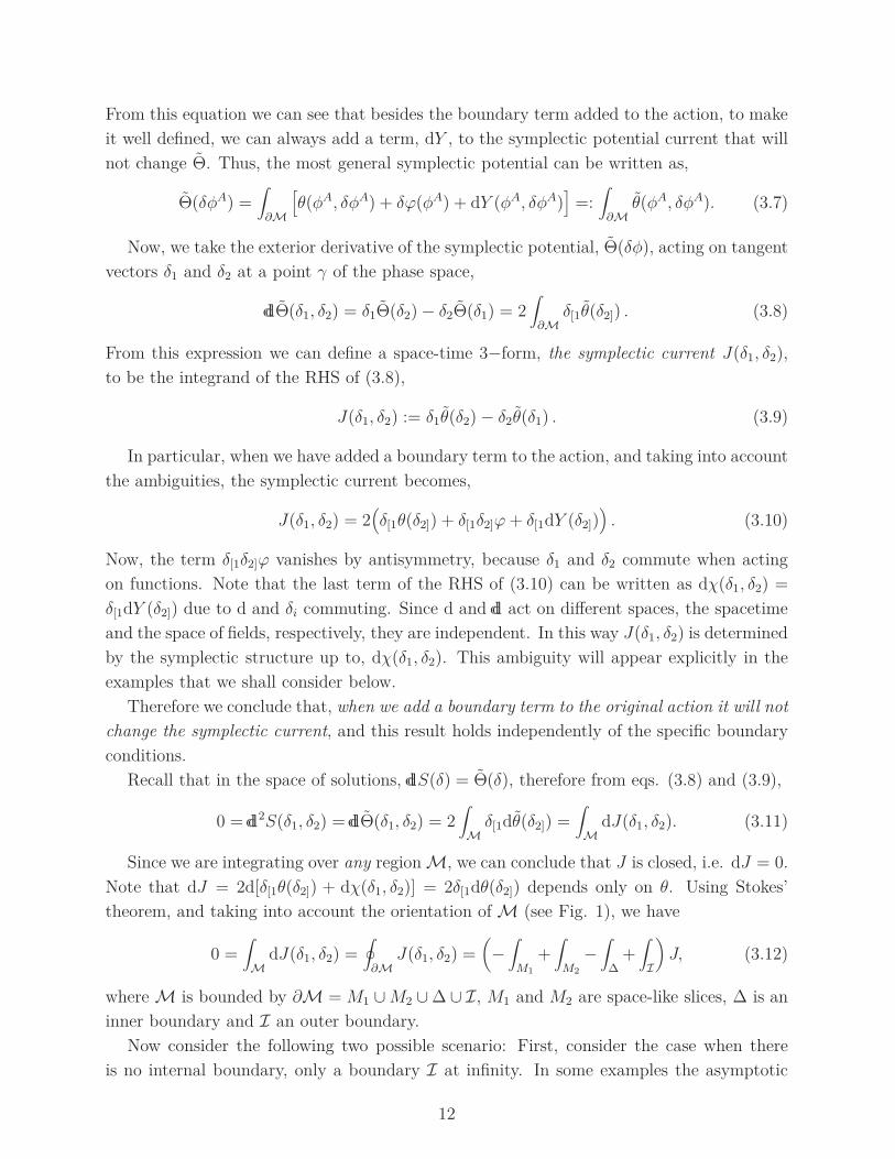
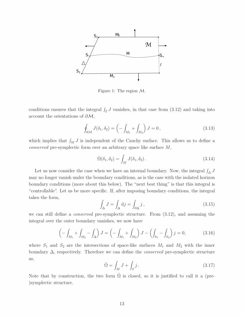
theorem, and taking into account the orientation of M (see Fig. 1), we have

0 =∫

MdJ(δ1, δ2) =

∮

∂MJ(δ1, δ2) =

(

−∫

M1

+∫

M2

−∫

∆+∫

I

)

J, (3.12)

where M is bounded by ∂M = M1 ∪M2 ∪ ∆ ∪ I, M1 and M2 are space-like slices, ∆ is an

inner boundary and I an outer boundary.

Now consider the following two possible scenario: First, consider the case when there

is no internal boundary, only a boundary I at infinity. In some examples the asymptotic

12

S1

S2M2

M1

I

S M

M

S

Figure 1: The region M.

conditions ensures that the integral∫

I J vanishes, in that case from (3.12) and taking into

account the orientations of ∂M,

∮

∂MJ(δ1, δ2) =

(

−∫

M1

+∫

M2

)

J = 0 , (3.13)

which implies that∫

M J is independent of the Cauchy surface. This allows us to define a

conserved pre-symplectic form over an arbitrary space like surface M ,

Ω(δ1, δ2) =∫

MJ(δ1, δ2) . (3.14)

Let us now consider the case when we have an internal boundary. Now, the integral∫

∆ J

may no longer vanish under the boundary conditions, as is the case with the isolated horizon

boundary conditions (more about this below). The “next best thing” is that this integral is

“controllable”. Let us be more specific. If, after imposing boundary conditions, the integral

takes the form,∫

∆J =

∫

∆dj =

∫

∂∆j , (3.15)

we can still define a conserved pre-symplectic structure. From (3.12), and assuming the

integral over the outer boundary vanishes, we now have

(

−∫

M1

+∫

M2

−∫

∆

)

J =(

−∫

M1

+∫

M2

)

J −(∫

S1

−∫

S2

)

j = 0, (3.16)

where S1 and S2 are the intersections of space-like surfaces M1 and M2 with the inner

boundary ∆, respectively. Therefore we can define the conserved pre-symplectic structure

as,

Ω =∫

MJ +

∫

Sj . (3.17)

Note that by construction, the two form Ω is closed, so it is justified to call it a (pre-

)symplectic structure.

13

B. Symmetries

Let us now explore how the covariant Hamiltonian formulation can deal with the existence

of symmetries, and their associated conserved quantities. Before that, let us recall the stan-

dard notion of a Hamiltonian vector field (HVF) in Hamiltonian dynamics. A Hamiltonian

vector field Z is defined as a symmetry of the symplectic structure, namely

£ZΩ = 0. (3.18)

From this condition and the fact that dd Ω = 0 we have,

£ZΩ = Z · dd Ω + dd (Z · Ω) = dd (Z · Ω) = 0. (3.19)

where Z · Ω ≡ iZΩ means the contraction of the 2-form Ω with the vector field Z. Note

that (Z · Ω)(δ) = Ω(Z, δ) is a one-form on Γ acting on an arbitrary vector δ. We can denote

it as X(δ) := Ω(Z, δ). From the previous equation we can see that X = Z · Ω is closed,

ddX = 0. It follows from (3.19) and from the Poincaré lemma that locally (on the CPS),

there exists a function H such that X = ddH . We call this function, H , the Hamiltonian,

that generates the infinitesimal canonical transformation defined by Z. Furthermore, and

by its own definition, H is a conserved quantity along the flow generated by Z.

Note that the directional derivative of the Hamiltonian H , along an arbitrary vector δ

can be written in several ways,

X(δ) = ddH(δ) = δH, (3.20)

some of which will be used in-distinctively in what follows.

So far this vector field Z is an arbitrary Hamiltonian vector field on Γ. Later on we

will relate it to certain space-time symmetries. For instance, for field theories that possess a

symmetry group, such as the Poincare group for field theories on Minkowski spacetime, there

will be corresponding Hamiltonian vector fields associated to the generators of the symmetry

group. In this article we are interested in exploring gravity theories that are diffeomorphism

invariant. That is, such that the diffeomorphism group acts as a (kinematical) symmetry of

the action. Of particular relevance is then to understand the role that these symmetries have

in the Hamiltonian formulation. In particular, one expects that diffeomorphisms play the

role of gauge symmetries of the theory. However, the precise form in which diffeomorphisms

can be regarded as gauge or not, depends on the details of the theory, and is dictated by

the properties of the corresponding Hamiltonian vector fields. Another important issue is

to separate those diffeomorphisms that are gauge from those that represent truly physical

canonical transformations that change the system. Those true motions could then be associ-

ated to symmetries of the theory. For instance, in the case of asymptotically flat spacetimes,

some diffeomorphism are regarded as gauge, while others represent nontrivial transforma-

tions at infinity and can be associated to the generators of the Poincaré group. In the case

14

when the vector field Z generates time evolution, one expects H to be related to the energy,

the ADM energy at infinity. Other conserved, Hamiltonian charges can thus be found, and

correspond to the generators of the asymptotic symmetries of the theory.

In what follows we shall explore the aspects of the theory that allow us to separate the

notion of gauge from standard symmetries of the theory.

1. Gauge and degeneracy of the symplectic structure

In the standard treatment of constrained systems, one starts out with the kinematical

phase space Γkin, and there exists a constrained surface Γ consisting of points that satisfy

the constraints present in the theory. One then notices that the pullback of Ω, the sym-

plectic structure to Γ is degenerate (for first class constraints). These degenerate directions

represent the gauge directions where two points are physically indistinguishable. In the

covariant Hamiltonian formulation we are considering here, the starting point is the space

Γ of solutions to all the equations of motion, where a (pre-)symplectic structure is naturally

defined, as we saw before. We call this a pre-symplectic structure since it might be degen-

erate. We say that Ω is degenerate if there exist vectors Zi such that Ω(Zi, X) = 0 for all

X. We call Zi a degenerate direction (or an element of the kernel of Ω). If Ω is degenerate

we have a gauge system, with a gauge submanifold generated by the degenerate directions

Zi (it is immediate to see that they satisfy the local integrability conditions to generate a

submanifold).

Note that since we are on the space of solutions to the field equations, tangent vectors X

to Γ must be solutions to the linearized equations of motion. Since the degenerate directions

Zi generate infinitesimal gauge transformations, configurations φ′ and φ on Γ, related by

such transformations, are physically indistinguishable. That is, φ′ ∼ φ and, therefore, the

quotient Γ = Γ/ ∼ constitutes the physical phase space of the system. It is only in the

reduced phase space Γ that one can define a non-degenerate symplectic structure Ω.

In the next subsection we explain how vector fields are the infinitesimal generators of

transformations on the space-time in general. Then we will point out when these transfor-

mations are diffeomorphisms and moreover, when these are also gauge symmetries of the

system.

2. Diffeomorphisms and Gauge

Let us start by recalling the standard notion of a diffeomorphism on the manifold M.

Later on, we shall see how, for diffeomorphism invariant theories, the induced action on

phase space of certain diffeomorphisms becomes gauge transformations.

There is a one-to-one relation between vector fields on a manifold and families of trans-

formations of the manifold onto itself. Let ϕ be a one-parameter group of transformations

15

on M, the map ϕτ : M → M, defined by ϕτ (x) = ϕ(x, τ), is a differentiable mapping.

If ξ is the infinitesimal generator of ϕ and f ∈ C∞(M), ϕ∗τf = f ϕτ also belongs to

C∞(M); then the Lie derivative of f along ξ, £ξf = ξ(f), represents the rate of change of

the function f under the family of transformations ϕτ . That is, the vector field ξ is the gen-

erator of infinitesimal diffeomorphisms. Now, given such a vector field, a natural question

is whether there exists a vector field Zξ on the CPS that represents the induced action of

the infinitesimal diffeos? As one can easily see, the answer is in the affirmative.

In order to see that, let us go back a bit to Section II. The action is defined on the space of

histories (the space of all possible configurations) and, after taking the variation, the vectors

δφα lie on the tangent space to the space of histories. It is only after we restrict ourselves to

the space of solutions Γ, that ddS(δ) = δS = Θ(δφA). Now these δφA represent any vector

on TφAΓ (tangent space to Γ at the point φA). As we already mentioned, these δφA can be

seen as “small changes” in the fields. What happens if we want the infinitesimal change of

fields to be generated by a particular group of transformations (e.g. spatial translations,

boosts, rotations, etc)? There is indeed a preferred tangent vector for the kind of theories

we are considering. Given ξ, consider

δξφA := £ξφ

A . (3.21)

From the geometric perspective, this is the natural candidate vector field to represent the

induced action of infinitesimal diffeomorphisms on Γ. The first question is whether such

objects are indeed tangent vectors to Γ. It is easy to see that, for kinematical diffeomorphism

invariant theories, Lie derivatives satisfy the linearized equations of motion.6 Of course, in

the presence of boundaries such vectors must preserve the boundary conditions of the theory

in order to be admissible (more about this below). For instance, in the case of asymptotically

flat boundary conditions, the allowed vector fields should preserve the asymptotic conditions.

Let us suppose that we have prescribed the phase space and pre-symplectic structure Ω,

and a vector field δξ := £ξφA. The question we would like to pose is: when is such vector a

degenerate direction of Ω? The equation that such vector δξ must satisfy is then:

Ω(δξ, δ) = 0 , ∀ δ . (3.22)

This equation will, as we shall see in detail below once we consider specific boundary con-

ditions, impose some conditions on the behaviour of ξ on the boundaries. An important

signature of diffeomorphism invariant theories is that Eq.(3.22) only has contributions from

the boundaries. Thus, the vanishing of such terms will depend on the behaviour of ξ there.

In particular, if ξ = 0 on the boundary, the corresponding vector field is guaranteed to be

a degenerate direction and therefore to generate gauge transformations. In some instances,

6 See, for instance [19]. When the theory is not diffeomorphism invariant, such Lie derivatives are admissible

vectors only when the defining vector field ξ is a symmetry of the background spacetime.

16

non vanishing vectors at the boundary also satisfy Eq. (3.22) and therefore define gauge

directions.

Let us now consider the case when ξ is non vanishing on ∂M and Eq. (3.22) is not zero.

In that case, we should have

Ω(δ, δξ) = ddHξ(δ) = δHξ , (3.23)

for some function Hξ. This function will be the generator of the symplectic transformation

generated by δξ. In other words, Hξ is the Hamiltonian conserved charge associated to the

symmetry generated by ξ.

Remark: One should make sure that Eq. (3.23) is indeed well defined, given the degeneracy

of Ω. In order to see that, note that one can add to δξ an arbitrary ‘gauge vector’ Z and

the result in the same: Ω(δξ + Z, δ) = Ω(δξ, δ). Therefore, if such function Hξ exists (and

we know that, locally, it does), it is insensitive to the existence of the gauge directions so

it must be constant along those directions and, therefore, projectable to Γ. Thus, one can

conclude that even when Hξ is defined through a degenerate pre-symplectic structure, it is

indeed a physical observable defined on the reduced phase space.

This concludes our review of the covariant phase space methods and the definition of

gauge and Hamiltonian conserved charges for diffeomorphism invariant theories. In the next

part we shall revisit another aspect of symmetries on covariant theories, namely the existence

of Noether conserved quantities, which are also associated to symmetries of field theories.

C. Diffeomorphism invariance: Noether charge

Let us briefly review some results about the Noether current 3-form JN and its relation to

the symplectic current J . For that, we shall rely on [20]. We know that to any Lagrangian

theory invariant under diffeomorphisms we can associate a corresponding Noether current

3-form. Consider infinitesimal diffeomorphism generated by a vector field ξ. These diffeo-

morphisms induce the infinitesimal change of fields, given by δξφA := £ξφ

A. From (3.2) it

follows that the corresponding change in the lagrangian four-form is given by

£ξL = EA ∧ £ξφA + dθ(φA,£ξφ

A) . (3.24)

On the other hand, using Cartan’s formula, we obtain

£ξL = ξ · dL + d(ξ · L) = d(ξ · L) , (3.25)

since dL = 0, in a four-dimensional spacetime. Now, we can define a Noether current 3-form

as

JN(δξ) = θ(δξ) − ξ · L , (3.26)

17

where we are using the simplified notation θ(δξ) := θ(φA,£ξφA). From the equations (3.24)

and (3.25) it follows that on the space of solutions, dJN(δξ) = 0, so at least locally one can

define a corresponding Noether charge density 2-form Qξ relative to ξ as

JN(δξ) = dQξ . (3.27)

Following [20], the integral of Qξ over some compact surface S is the Noether charge of S

relative to ξ. As we saw in the previous chapter there are ambiguities in the definition of

θ (3.7) , that produce ambiguities in Qξ. As we saw in the section III A, θ is defined up to

an exact form: θ → θ + dY (δ). Also, the change in Lagrangian L → L + dϕ produces the

change θ → θ + δϕ. These transformations affect the symplectic current in the following

way

J(δ1, δ2) → J(δ1, δ2) + d(

δ2Y (δ1) − δ1Y (δ2))

. (3.28)

The contribution of ϕ vanishes, as before, and as we have shown in section III A. The above

transformation leaves invariant the symplectic structure. It is easy to see that the two

changes, generated by Y and ϕ contribute to the following change of Noether current 3-form

JN(δξ) → JN (δξ) + dY (δξ) + δξϕ− ξ · dϕ , (3.29)

and the corresponding Noether charge 2-form changes as

Qξ → Qξ + Y (δξ) + ξ · ϕ+ dZ . (3.30)

The last term in the previous expression is due to the ambiguity present in (3.27). This

arbitrariness in Qξ was used in [20] to show that the Noether charge form of a general

theory of gravity arising from a diffeomorphism invariant Lagrangian, in the second order

formalism, can be decomposed in a particular way.

Since dJN (δξ) = 0 it follows, as in (3.12), that

0 =∫

MdJN (δξ) =

∮

∂MJN(δξ) =

(

−∫

M1

+∫

M2

−∫

∆+∫

I

)

JN(δξ), (3.31)

and we see that if∫

∆ JN(δξ) =∫

I JN (δξ) = 0 then the previous expression implies the

existence of the conserved quantity (independent on the choice of M),∫

MJN (δξ) =

∫

∂MQξ . (3.32)

Note that the above results are valid only on shell.

In the covariant phase space, and for ξ arbitrary and fixed, we have [20]

δJN(δξ) = δθ(δξ) − ξ · δL = δθ(δξ) − ξ · dθ(δ) . (3.33)

Since, ξ ·dθ = £ξθ−d(ξ ·θ) and δθ(δξ)−£ξθ(δ) = J(δ, δξ) by the definition of the symplectic

current J (3.9), it follows that the relation between the symplectic current J and the Noether

current 3-form JN is given by

J(δ, δξ) = δJN(δξ) − d(ξ · θ(δ)) . (3.34)

18

We shall use this relation in the following sections, for the various actions that describe first

order general relativity, to clarify the relation between the Hamiltonian and Noether charges.

We shall see that, in general, a Noether charge does not correspond to a Hamiltonian charge

generating symmetries of the phase space.

IV. THE ACTION FOR GRAVITY IN THE FIRST ORDER FORMALISM

As already mentioned in the introduction, we shall consider the most general action

for four-dimensional gravity in the first order formalism. The choice of basic variables

is the following: A pair of co-tetrads eIa and a Lorentz SO(3, 1) connection ωaIJ on the

spacetime M, possibly with a boundary. In order for the action to be physically relevant,

it should reproduce the equations of motion for general relativity and be: 1) differentiable,

2) finite on the configurations with a given asymptotic behaviour and 3) invariant under

diffeomorphisms and local internal Lorentz transformations. The most general action that

gives the desired equations of motion and is compatible with the symmetries of the theory

is given by the combination of Palatini action, SP, Holst term, SH, and three topological

terms, Pontryagin, SPo, Euler, SE, and Nieh-Yan, SNY, invariants. As we shall see, the

Palatini term contains the information of the ordinary Einstein-Hilbert 2nd order action, so

it represents the backbone of the formalism. Since we are considering a spacetime region Mwith boundaries, one should pay special attention to boundary conditions. For instance, it

turns out that the Palatini action, as well as Holst and Nieh-Yan terms are not differentiable

for asymptotically flat spacetimes, and appropriate boundary terms should be provided. This

section has four parts. In those subsections we are going to analyze, one by one, all of the

terms of the action. We shall take the corresponding variation of the terms and identify

both their contributions to the equations of motion and to the symplectic current. Since we

are not considering yet any particular boundary conditions, the results of this section are

generic.

A. Palatini action

Let us start by considering the Palatini action with boundary term is given by [11],

SPB = − 1

2κ

∫

MΣIJ ∧ FIJ +

1

2κ

∫

∂MΣIJ ∧ ωIJ . (4.1)

where κ = 8πG, ΣIJ = ⋆(eI ∧ eJ) := 12ǫIJ

JKeJ ∧ eK , FIJ = dωIJ +ωIK ∧ωK

J is a curvature

two-form of the connection ω and, as before, ∂M = M1 ∪M2 ∪ ∆ ∪ I. The boundary term

is not manifestly gauge invariant, but, as pointed out in [11], it is effectively gauge invariant

on the spacelike surfaces M1 and M2 and also in the asymptotic region I. This is due to the

fact that the only allowed gauge transformations that preserve the asymptotic conditions

are such that the boundary terms remain invariant. Let us consider first the behaviour of

19

this boundary term on M1 (or M2). First we ask that the compatibility condition between

the co-tetrad and connection should be satisfied on the boundary. Then, we partially fix

the gauge on M , by fixing the internal time-like tetrad nI , such that ∂anI = 0 and we

restrict field configurations such that na = eaIn

I is the unit normal to M1 and M2. Under

these conditions it has been shown in [11] that on M , ΣIJ ∧ ωIJ = 2Kd3V , where K is the

trace of the extrinsic curvature of M . Note that this is the Gibbons-Hawking surface term

that is needed in the Einstein-Hilbert action, with the constant boundary term equals to

zero. On the other hand, at spatial infinity, I, we fix the co-tetrads and only permit gauge

transformations that reduce to identity at infinity. Under these conditions the boundary

term is gauge invariant at M1, M2 and I. We shall show later that it is also invariant

under the residual local Lorentz transformations at a weakly isolated horizon, when such a

boundary exists.

It turns out that at spatial infinity this boundary term does not reduce to Gibbons-

Hawking surface term, the later one is divergent for asymptotically flat spacetimes, as shown

in [11]. Let us mention that there have been other proposals for boundary terms for Palatini

action, as for example in [21] and [22], that are equivalent to Gibbons-Hawking action and are

obtained without imposing the time gauge condition. They are manifestly gauge invariant

and well defined for finite boundaries, but they are not well defined for asymptotically flat

spacetimes. In time gauge they reduce to (4.1).

The variation of (4.1) is,

δSPB = − 1

2κ

∫

M

[

εIJKLδe

K ∧ eL ∧ FIJ −DΣIJ ∧ δωIJ − d(δΣIJ ∧ ωIJ)]

, (4.2)

where

DΣIJ = dΣIJ − ωIK ∧ ΣKJ + ωJ

K ∧ ΣKI . (4.3)

We shall show later that the contribution of boundary term δΣIJ ∧ ωIJ vanishes at I and

∆, so that from (4.2) we obtain the following equations of motion

εIJKLeJ ∧ FKL = 0 , (4.4)

εIJKLeK ∧DeL = 0 , (4.5)

where TL := DeL = deL +ωLK ∧eK is a torsion two-form. From (4.5) it follows that TL = 0,

and this is the condition of the compatibility of ωIJ and eI , that implies

ωaIJ = eb[I∂aebJ ] + Γc

abec[IebJ ] , (4.6)

where Γcab are the Christoffel symbols of the metric gab = ηIJe

Iae

Jb . Now, the equations (4.4)

are equivalent to Einstein’s equations Gab = 0.

From equations (3.6) and (4.2), the symplectic potential for SPB is given by

ΘPB(δ) =1

2κ

∫

∂MδΣIJ ∧ ωIJ . (4.7)

20

Therefore from (3.10) and (4.7) the corresponding symplectic current is,

JP(δ1, δ2) = − 1

2κ

(

δ1ΣIJ ∧ δ2ωIJ − δ2ΣIJ ∧ δ1ωIJ

)

. (4.8)

Note that the symplectic current is insensitive to the boundary term, as we discussed in

Sec. III.

As we shall discuss in the following sections, the Palatini action, in the asymptotically flat

case, is not well defined, but it can be made differentiable and finite after the addition of the

corresponding boundary term already discussed [11]. Furthermore, we shall also show that in

the case when the spacetime has as internal boundary an isolated horizon, the contribution

at the horizon to the variation of the Palatini action, either with a boundary term [23] or

without it [12], vanishes.

B. Holst term

The first additional term to the gravitational action that we shall consider is the so called

Holst term [9], first introduced with the aim of having a variational principle whose 3 + 1

decomposition yielded general relativity in the Ashtekar-Barbero (real) variables [24]. It

turns out that the Holst term, when added to the Palatini action, does not change the

equations of motion (although it is not a topological term), so that in the Hamiltonian

formalism its addition corresponds to a canonical transformation. This transformation leads

to the Ashtekar-Barbero variables that are the basic ingredients in the loop quantum gravity

approach. As we shall show in the next chapter, the Holst term is finite but not differentiable

for asymptotically flat spacetimes, so an appropriate boundary term should be added in order

to make it well defined. The result is [14],

SHB = − 1

2κγ

∫

MΣIJ ∧ ⋆FIJ +

1

2κγ

∫

∂MΣIJ ∧ ⋆ωIJ , (4.9)

where γ is the Barbero-Immirzi parameter. The variation of the Holst term, with its bound-

ary term, is given by

δSHB = − 1

2κγ

∫

M2FIJ ∧ eI ∧ δeJ +DΣIJ ∧ ⋆(δωIJ) − d(δΣIJ ∧ ⋆ωIJ) , (4.10)

and it leads to the following equations of motion in the bulk: DΣIJ = 0 and eI ∧ FIJ = 0.

The second one is just the Bianchi identity, and we see that the Holst term does not modify

the equations of motion of the Palatini action. The contribution of the boundary term (that

appears in the variation) should vanish at I and ∆, in order to have a well posed variational

principle. In the following section we shall see that this is indeed the case.

On the other hand we should also examine the gauge invariance of the boundary term in

(4.9). Under the same assumptions as in the case of the Palatini boundary term we obtain

that [14]∫

M1

ΣIJ ∧ ⋆ωIJ = 2∫

M1

ǫabceJb ∂ceaJd3x =

∫

M1

eI ∧ deI , (4.11)

21

and this term is not gauge invariant at M1 or M2. As we shall see in the following section, at

the asymptotic region it is gauge invariant, and also at ∆. In the analysis of differentiability

of the action and the construction of the symplectic structure and conserved quantities there

is no contribution from the spacial surfaces M1 and M2, and we can argue that the non-

invariance of the boundary term in (4.9) is not important, but it would be desirable to have

a boundary term that is compatible with all the symmetries of the theory. As we shall see

later, the combination of the Holst and Neih-Yan terms is differentiable and gauge invariant.

It is easy to see that the symplectic potential for SHB is given by [14]

ΘHB(δ) =1

2κγ

∫

∂MδΣIJ ∧ ⋆ωIJ =

1

κγ

∫

∂MδeI ∧ deI , (4.12)

where in the second line we used the equation of motion DeI = 0. The symplectic current

is given by

JHB(δ1, δ2) =1

κγd (δ1e

I ∧ δ2eI) . (4.13)

As we have seen in the subsection III A, this term does not contribute to the symplectic

structure, since it is an exterior derivative. Nevertheless, the Holst term modifies the Noether

charge associated to diffeomorphisms, as we shall see in Sec. VI.

C. Topological terms

In four dimensions there are three topological invariants constructed from eI , FIJ and

DeI , consistent with diffeomorphism and local Lorentz invariance. They are exact forms and

do not contribute to the equations of motion, but in order to be well defined they should be

finite, and their variation on the boundary of the spacetime region M should vanish. The

first two terms, the Pontryagin and Euler terms are constructed from the curvature FIJ and

its dual (in the internal space) ⋆FIJ , while the third one, the Neih-Yan invariant, is related

to torsion DeI .

These topological invariants can be thought of as 4-dimensional density lagrangians de-

fined on a manifold M, that additionally are exact forms, but they can also be seen as terms

living on ∂M. In that case it is obvious that they do not contribute to the equations of

motion in the bulk. But a natural question may arise. If we take the lagrangian density

in the bulk and take the variation, what are the corresponding equations of motion in the

bulk? One can check that, for Pontryagin and Euler, the resulting equations of motion are

trivial in the sense that one only gets the Bianchi identities, while for the Nieh-Yan term

they vanish identically. Let us now see how each of this terms contribute to the variation of

the action.

1. Pontryagin and Euler terms

The action corresponding to the Pontryagin term is given by,

22

SPo =∫

MF IJ ∧ FIJ = 2

∫

∂M

(

ωIJ ∧ dωIJ +2

3ωIJ ∧ ωIK ∧ ωK

J

)

. (4.14)

The boundary term is the Chern-Simons Lagrangian density, LCS . The variation of SPo,

calculated from the LHS expression in (4.14), is

δSPo = −2∫

MDF IJ ∧ δωIJ + 2

∫

∂MF IJ ∧ δωIJ , (4.15)

so it does not contribute to the equations of motion in the bulk, due to the Bianchi identity

DF IJ = 0, and additionally the surface integral in (4.15) should vanish for the variational

principle to be well defined. We will show later that this is indeed the case for boundary

conditions of interest to us, namely asymptotically flat spacetimes possibly with an isolated

horizon.

On the other hand, if we calculate the variation of the Pontryagin term directly from the

RHS of (4.14), we obtain

δSPo = 2∫

∂MδLCS . (4.16)

The two expressions for δSPo are, of course, identical since F IJ ∧ δωIJ = δLCS + d(ωIJ ∧δωIJ). The first one (4.15) is more convenient for the analysis of the differentiability of

the Pontryagin term, but the second one (4.16) is more suitable for the definition of the

symplectic current, which vanishes identically for any boundary contribution to the action,

as we have seen in (3.10).

Let us now consider the action for the Euler term, which is given by,

SE =∫

MF IJ ∧ ⋆FIJ = 2

∫

∂M

(

⋆ωIJ ∧ dωIJ +2

3⋆ ωIJ ∧ ωIK ∧ ωK

J

)

, (4.17)

with variation, calculated from the expression in the bulk, given by

δSE = −2∫

M⋆DF IJ ∧ δωIJ + 2

∫

∂M⋆F IJ ∧ δωIJ . (4.18)

Again, the action will only be well defined if the boundary contribution to the variation

(4.18) vanishes. In the following section we shall see that it indeed vanishes for our boundary

conditions. Let us denote by LCSE the boundary term on the RHS of (4.17), then we can

calculate the variation of SE from this term directly as

δSE = 2∫

∂MδLCSE . (4.19)

Finally, as before, the corresponding contribution to the symplectic current vanishes.

2. Nieh-Yan term

The Nieh-Yan topological invariant is of a different nature from the two previous terms.

It is related to torsion and its contribution to the action is [25, 26],

SNY =∫

M

(

DeI ∧DeI − ΣIJ ∧ ⋆FIJ

)

=∫

∂MDeI ∧ eI . (4.20)

23

Note that the Nieh-Yan term can be written as

SNY = 2κγSH +∫

MDeI ∧DeI , (4.21)

where SH is the Holst term (4.9) without boundary term. The variation of the term SNY is

given by

δSNY =∫

∂M2DeI ∧ δeI − eI ∧ eJ ∧ δωIJ . (4.22)

Contrary to what happens to the Euler and Pontryagin terms, the Nieh-Yan term has a

different asymptotic behavior. In the next chapter we will show that the Nieh-Yan term is

finite, but not differentiable, for asymptotically flat spacetimes. Thus, even when it is by

itself a boundary term, it has to be supplemented with an appropriate boundary term to

make the variational principle well defined. We shall see that this boundary term coincides

precisely with the boundary term in (4.9) (up to a multiplicative constant), and the resulting

well defined Neih-Yan action is given by

SNYB = SNY +∫

∂MΣIJ ∧ ⋆ωIJ . (4.23)

It is straightforward to see that the symplectic potential and symplectic current for this

action are the same as for (4.9) (up to a factor 2κγ).

This relation between SH and SNY points to another proposal for a boundary term for the

Holst action, different from that in (4.9), that has the advantage of being manifestly gauge

invariant. Namely, for asymptotically flat spacetimes, we can see that the surface term in

the variation of Neih-Yan term cancels the surface term in the variation of the Holst term,

and the action SHNY := SH − 12κγSNY, given by

SHNY = − 1

2κγ

∫

MΣIJ ∧ ⋆FIJ − 1

2κγ

∫

∂MDeI ∧ eI = − 1

2κγ

∫

MDeI ∧DeI , (4.24)

is well defined. This combination was proposed in [22], but since they were interested in finite

boundaries the boundary conditions that they considered are different from the ones we use,

namely they impose δhab ≡ δ(eIaebI) = 0 (hab is the metric induced on the boundary) and

leave δωIJ arbitrary, which is not compatible with our condition DeI = 0 on the boundary

(and is not compatible with isolated horizons boundary conditions either).

To end this part, let us also comment that in the presence of fermions one has to generalize

the Holst action to spacetimes with torsion, that naturaly leads to Neih-Yan topological

term, instead of the Holst term, as shown in [27]. But, as we saw the Neih-Yan term is not

well defined for our boundary conditions and should be modified as in (4.23).

D. The complete action

So far in this section we have introduced all the ingredients for the “most general” first

order diffeomorphism invariant action that classically describes general relativity.

24

As we have already mentioned and we shall prove in the following section, both Pontryagin

and Euler terms, SPo and SE respectively, are well defined in the case of asymptotically flat

spacetimes with a weakly isolated horizon. This means that we can add them to the Palatini

action with its boundary term, SPB, and the resulting action will be again well defined. As

we foresaw in the previous section, the addition of the Nieh-Yan term, SNY, could lead to

different possibilities for the construction of a well defined action. Therefore the complete

action can be written as,

S[e, ω] = SPB + SH + α1SPo + α2SE + α3SNY + α4SBH . (4.25)

Here α1, ..., α4 are coupling constants. The coupling constants α1 and α2, are not fixed by

our boundary conditions, while different choices for the Holst-Nieh-Yan sector of the theory,

discussed in the previous part, imply particular combinations of α3 and α4. To see that,

consider SBH that represents the boundary term that we need to add to Holst term in order

to make it well defined. As we have seen in the previous analysis, if α3 = − 12κγ

then the

combination of the Holst and Nieh-Yan terms is well defined and no additional boundary

term is needed, so α4 = 0 in that case. For every other value of α3 we need to add a boundary

term, and in that case α4 = 12κγ

+α3. Other than these cases, there is no important relation

between the different coupling constants.

This has to be contrasted with other asymptotic conditions studied in the literature (that

we shall, however, not consider here). It turns out that the Palatini action with the negative

cosmological constant term is not well defined for asymptotically anti-de Sitter (AAdS)

spacetimes, but it can be made differentiable after the addition of an appropriate boundary

term. In [13] it is shown that it can be the same boundary term as in the asymptotically flat

case, with an appropriately modified coupling constant. On the other hand, as shown in [28]

and [29], one can choose the Euler topological term as a boundary term and that choice fixes

the value of α2. In that case α2 ∼ 1Λ

, and the asymptotically flat case cannot be obtained

in the limit Λ → 0. The differentiability of Nieh-Yan term has been analyzed in [30]. The

result is that this term is well defined, for AAdS space-times, only after the addition of

the Pontryagin term, with an appropriate coupling constant. Let us also comment that the

details of the asymptotic behaviour in [13] are different than in the other mentioned papers.

V. BOUNDARY CONDITIONS

We have considered the most general action for general relativity in the first order for-

malism, including boundaries, in order to have a well defined action principle and covariant

Hamiltonian formalism. We have left, until now, the boundary conditions unspecified, other

that assuming that there is an outer and a possible inner boundary to the region M un-

der consideration. In this section we shall consider specific boundary conditions that are

physically motivated. For the outer boundary we will specify asymptotically flat boundary

25

conditions that capture the notion of isolated systems. For the inner boundary we will

consider isolated horizons boundary conditions. In this way, we allow for the possibility

of spacetimes that contain a black hole. This section has two parts. In the first one, we

consider the outer boundary conditions and in the second part, the inner horizon boundary

condition. In each case, we study the finiteness of the action, its variation and its differen-

tiability. Since this manuscript is to be self-contained, we include a detailed discussion of

the boundary conditions before analysing the different contributions to the action.

A. Asymptotically flat spacetimes

We are interested in spacetimes that at infinity look like a flat spacetime, in other words,

whose metric approaches a Minkowski metric at infinity (in some appropriately chosen co-

ordinates). Here we will follow the standard definition of asymptotically flat spacetimes in

the first order formalism (see e.g. [11], [14] and for a nice and pedagogical introduction in

the metric formulation [15] and [19]). Here we give a brief introduction into asymptotically

flat spacetimes, following closely [11].

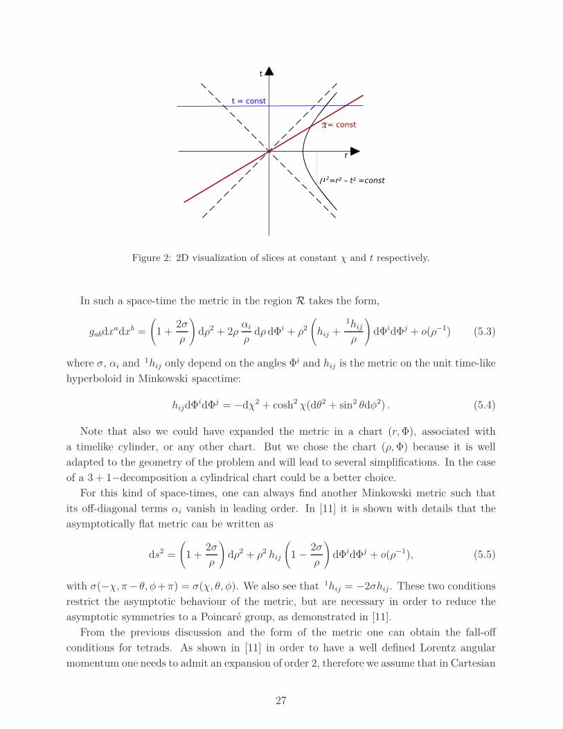
In order to describe the behaviour of the metric at spatial infinity, we will focus on

the region R, that is the region outside the light cone of some point p. We define a

4−dimensional radial coordinate ρ given by ρ2 = ηabxaxb, where xa are the Cartesian coor-

dinates of the Minkowski metric η on R4 with origin at p. We will foliate the asymptotic

region by timelike hyperboloids, H, given by ρ = const, that lie in R. Spatial infinity

I corresponds to a limiting hyperboloid when ρ → ∞. The standard angular coordi-

nates on a hyperboloid are denoted by Φi = (χ, θ, φ), and the relation between Cartesian

and hyperbolic coordinates is given by: x(ρ, χ, θ, φ) = ρ coshχ sin θ cosφ, y(ρ, χ, θ, φ) =

ρ coshχ sin θ sin φ, z(ρ, χ, θ, φ) = ρ coshχ cos θ, t(ρ, χ, θ, φ) = ρ sinhχ.

We shall consider functions f that admit an asymptotic expansion to order m of the

form,

f(ρ,Φ) =m∑

n=0

nf(Φ)

ρn+ o(ρ−m), (5.1)

where the remainder o(ρ−m) has the property that

limρ→∞

ρ o(ρ−m) = 0. (5.2)

A tensor field T a1...anb1...bm will be said to admit an asymptotic expansion to order m if

all its component in the Cartesian chart xa do so. Its derivatives ∂cTa1...an

b1...bm admit an

expansion of order m+ 1.

With these ingredients at hand we can now define an asymptotically flat spacetime in

terms of its metric: a smooth spacetime metric g on R is weakly asymptotically flat at spatial

infinity if there exist a Minkowski metric η such that outside a spatially compact world tube

(g − η) admits an asymptotic expansion to order 1 and limρ→∞(g − η) = 0.

26

X

2=r² – t² =const

t

r

= const

t = const

Figure 2: 2D visualization of slices at constant χ and t respectively.

In such a space-time the metric in the region R takes the form,

gabdxadxb =

(

1 +2σ

ρ

)

dρ2 + 2ραi

ρdρ dΦi + ρ2

(

hij +1hij

ρ

)

dΦidΦj + o(ρ−1) (5.3)

where σ, αi and 1hij only depend on the angles Φi and hij is the metric on the unit time-like

hyperboloid in Minkowski spacetime:

hijdΦidΦj = −dχ2 + cosh2 χ(dθ2 + sin2 θdφ2) . (5.4)

Note that also we could have expanded the metric in a chart (r,Φ), associated with

a timelike cylinder, or any other chart. But we chose the chart (ρ,Φ) because it is well

adapted to the geometry of the problem and will lead to several simplifications. In the case

of a 3 + 1−decomposition a cylindrical chart could be a better choice.

For this kind of space-times, one can always find another Minkowski metric such that

its off-diagonal terms αi vanish in leading order. In [11] it is shown with details that the

asymptotically flat metric can be written as

ds2 =

(

1 +2σ

ρ

)

dρ2 + ρ2 hij

(

1 − 2σ

ρ

)

dΦidΦj + o(ρ−1), (5.5)

with σ(−χ, π−θ, φ+π) = σ(χ, θ, φ). We also see that 1hij = −2σhij . These two conditions

restrict the asymptotic behaviour of the metric, but are necessary in order to reduce the

asymptotic symmetries to a Poincaré group, as demonstrated in [11].

From the previous discussion and the form of the metric one can obtain the fall-off

conditions for tetrads. As shown in [11] in order to have a well defined Lorentz angular

momentum one needs to admit an expansion of order 2, therefore we assume that in Cartesian

27

coordinates we have the following behaviour

eIa = oeI

a +1eI

a(Φ)

ρ+

2eIa(Φ)

ρ2+ o(ρ−2), (5.6)

where 0eI is a fixed co-frame such that g0ab = ηIJ

oeIa

oeIb is flat and ∂a

oeIb = 0.

The sub-leading term 1eIa can be obtained from (5.5) and is given by [11],

1eIa = σ(Φ)(2ρaρ

I − oeIa) (5.7)

where

ρa = ∂aρ and ρI = oeaIρa. (5.8)

The asymptotic expansion for connection can be obtained from the requirement that the

connection be compatible with tetrad on I, to appropriate leading order. This leads to the

asymptotic expansion of order 3 for the connection,

ωIJa = oωIJ

a +1ωIJ

a

ρ+

2ωIJa

ρ2+

3ωIJa

ρ3+ o(ρ−3) . (5.9)

We require that DeI vanishes, to an appropriate order, more precisely, we ask that the

term of order 0 in DeI vanishes

d oeI + oωIK ∧ oeK = 0 , (5.10)

and since d oeI = 0 it follows that oωIK = 0. The term of order 1 should also vanish leading

to 1ωIK = 0. We also ask that the term of order 2 in DeI vanishes, and we obtain

d(

1eI

ρ

)

= −2ωI

K

ρ2∧ oeK , (5.11)

and we shall demand compatibility between e and ω only based on this condition. As a

result, we obtain

2ωIJa (Φ) = 2ρ2 ∂[J (ρ−1 1eI]

a ) (5.12)

= 2ρ (2ρ[Iρa∂J ]σ − oe[I

a ∂J ]σ − ρ−1 oe[I

a ρJ ]σ) . (5.13)

Note that although ρ appears explicitly in the previous expression, it is independent of ρ.

Therefore, in the asymptotic region we have DeI = O(ρ−3). This condition has its

repercussions on the behaviour of the Holst and Neih-Yan terms, as we will show in what

follows.

1. Palatini action with boundary term

Now we have all necessary elements in order to prove the finiteness of the Palatini action

with boundary term, given by (4.1). This expression can be re-written as,

SPB(e, ω) =1

2κ

∫

M

(

dΣIJ ∧ ωIJ − ΣIJ ∧ ωIK ∧ ωKJ

)

(5.14)

28

or in components

SPB(e, ω) =1

2κ

∫

M

(

∂aΣIJbc ωdIJ − ΣIJ

abωcIKωdKJ

)

ǫabcd (5.15)

where ǫabcd is the metric compatible 4-form on M. This volume element is related by

ǫabcd =√g εabcd d4x, to the Levi-Civita tensor density of weight +1, εabcd. We will prove

that taking into account the boundary conditions (5.6) and (5.9), the integrand falls off

as ρ−4, while the volume element on any Cauchy slice in asymptotic region goes as ρ2,

so the action is manifestly finite always (even off-shell), if the two Cauchy surfaces are

asymptotically time-translated with respect to each other.

From (5.4) and (5.5), we see that the volume element in the asymptotic region takes

the form ρ3 cosh2 χ sin θ dρ dχ dθ dφ. In order to prove finiteness we will consider the region

bounded by Cauchy slices t = const instead of χ = const, since in the second case for ρ → ∞the volumen of the region does not need to converge (see Fig. 2). Since t(ρ, χ, θ, φ) = ρ sinhχ

at the surface with constant t we have ρ dχ = − tanhχdρ. Substituting this into the metric

we can see that the volume element is ρ2 coshχ sin θ dρ dθ dφ. As ρ → ∞, the angle χ → 0

so coshχ → 1. It follows that in the limit ρ → ∞ the volume of the region M behaves as

ρ2.

Now, we need to deduce the asymptotic behavior of dΣIJ ∧ ωIJ = ǫIJKLdeK ∧ eL ∧ ωIJ .

Since d( oeI) = 0 it follows that

deK =1

ρd[ 1eK(Φ)] +O(ρ−2) . (5.16)

The partial derivative, with respect to cartesian coordinates, of any function f(Φ) is pro-

portional to ρ−1,

∂af(Φ) =∂Φi

∂xa

∂f

∂Φi=

1

ρAi

a(Φ)∂f

∂Φi, (5.17)

where the explicit expression for Aia(Φ) can be obtained from the relation between Cartesian

and hyperbolic coordinates. As a consequence deK = O(ρ−2), and since ωIJ = O(ρ−2) it

follows that dΣIJ ∧ωIJ falls off as ρ−4, and the Palatini action with boundary term is finite.

Now let us prove the differentiability of the action (4.1). As we have commented after

(4.2), this action is differentiable if the boundary term that appears in the variation vanishes.

This boundary term is

1

2κ

∫

∂MδΣIJ ∧ ωIJ =

1

2κ

(

−∫

M1

+∫

M2

+∫

I−∫

∆

)

δΣIJ ∧ ωIJ , (5.18)

where we decomposed the boundary as ∂M = M1 ∪M2 ∪I ∪∆, as in Fig.1. On the Cauchy

slices, M1 and M2, we assume δeIa = 0 so the integrals vanish, and in the following section

we will prove that over ∆ this integral also vanishes. Here we will focus on the contribution

of the asymptotic region I.

29

On a time-like hyperboloid H, ρ = const, so that its volume element is

ρ3 cosh2 χ sin θ dχ dθ dφ = ρ3d3Φ and the boundary term can be written as,

1

2κ

∫

IδΣIJ ∧ ωIJ =

1

2κlim

ρ→∞

∫

HδΣIJ

ab ωcIJ εabcρ3d3Φ , (5.19)

Now we can use that,

δΣabIJ = ρ−1εIJKLoeK

a δσ(Φ)(

2ρbρL − oeL

b

)

+O(ρ−2) . (5.20)

Since ρ is constant on a hyperboloid, it follows that ρa is orthogonal to it and ρaεabc = 0.

Then, we obtain

δΣIJab ωcIJ ε

abc =2

ρ3δσ εIJKL

oeKa

oeLb

oeIc(ρ ∂Jσ + ρJσ)εabc +O(ρ−4) . (5.21)

In this expression the term with a derivative of σ is proportional to ∂ρσ = 0, so that the

variation (5.19) reduces to

1

2κ

∫

IδΣIJ ∧ ωIJ =

3

2κδ (∫

H1

σ2d3Φ) , (5.22)

where H1 is the unit hyperboloid. So we see that the Palatini action with the boundary term

is differentiable when we restrict to configurations that satisfy asymptotically flat boundary

conditions, such that Cσ :=∫

H1σ2d3Φ has the same (arbitrary) value for all of them. In

that case, the above expression (5.22) vanishes. This last condition is not an additional

restriction to the permissible configurations, because every one of them (compatible with

our boundary conditions) corresponds to some fixed value of Cσ.

Here we want to emphasize the importance of the boundary term added to the action

given that, without it, the action fails to be differentiable. The contribution from the

asymptotic region to the variation of the Palatini action is,

1

2κ

∫

IΣIJ ∧ δωIJ =

1

2κlim

ρ→∞

∫

HΣIJ

ab δωcIJ εabcρ3d3Φ . (5.23)

Our boundary conditions imply that ΣIJab δωcIJ = O(ρ−2), so that the integral behaves as

∫

I ρ d3Φ, and in the limit ρ → ∞ is explicitly divergent.

2. Holst term

As we have seen earlier, in the asymptotic region we have DeI = O(ρ−3). Furthermore,

as D(DeI) = F IK ∧ eK , we have that F IK ∧ eK = O(ρ−4). We can see that explicitly by

calculating the term of order 3 in this expression

F IK ∧ eK = d(

2ωIK

ρ2

)

∧ oeK +O(ρ−4) . (5.24)

30

The first term in the previous expression vanishes since d(

2ωIK

ρ2

)

∧ oeK = d(

2ωIK

ρ2 ∧ oeK)

= 0,

due to (5.11). So, we see that the Holst term

SH = − 1

2κγ

∫

MeI ∧ eJ ∧ FIJ , (5.25)

is finite under these asymptotic conditions, since eI ∧ eJ ∧FIJ goes as ρ−4, while the volume

element on every Cauchy surface goes as ρ2dρ d2Ω.

The variation of the Holst term is well defined if the boundary term, obtained as a result

of variation, vanishes. We will analyze the contribution of this term

1

2κγ

∫

∂MeI ∧ eJ ∧ δωIJ . (5.26)

Let us examine the term of order 2 of the integrand, it is

oeI ∧ oeJ ∧ δ( 2ωIJ)

ρ2= d

[

oeI ∧ δ( 1eI)

ρ

]

, (5.27)

due to (5.11) and d oeI = δ oeI = 0, and this term does not contribute to (5.26). So, the

leading term in eI ∧ eJ ∧ δωIJ is of order 3, and it does not vanish, since it depends also

on 3ωIJ(Φ), which is not fixed by our boundary conditions. Since the volume element on a

hyperboloid H goes as ρ3d3Φ, it follows that the boundary term (5.26) does not vanish at

I (though it is finite).

As our analysis shows we should provide a boundary term for the Holst term, in order to

make it differentiable. It turns out that this term should be [14]

SBH =1

2κγ

∫

∂MeI ∧ eJ ∧ ωIJ . (5.28)

Let us show first that this term is finite and for that we should prove that its term of order

2 vanishes. This term is

oeI ∧ oeJ ∧2ωIJ

ρ2= d

(

oeI ∧1eI

ρ

)

, (5.29)

due to the same arguments as in (5.27), and we see that it does not contribute to the

boundary term (5.28). So, the leading term of the integrand is of order 3, and since the

volume element at H goes as ρ3d3Φ, it follows that (5.28) is finite.

The Holst term with its boundary term (4.9) can be written as

SHB = − 1

2κγ

∫

MeI ∧ eJ ∧ FIJ +

1

2κγ

∫

∂MeI ∧ eJ ∧ ωIJ , (5.30)

and also as an integral over M

SHB = − 1

2κγ

∫

M2 deI ∧ eJ ∧ ωIJ − eI ∧ eJ ∧ ωIK ∧ ωK

J . (5.31)

31

As we have seen in (4.10), the variation of the Holst term with its boundary term is well

defined provided that the following boundary contribution

1

2κγ

∫

∂MδΣIJ ∧ ⋆ωIJ =

1

2κγ

(

−∫

M1

+∫

M2

+∫

I−∫

∆

)

δΣIJ ∧ ⋆ωIJ , (5.32)

vanishes. We first note that ωIJa and ⋆ωIJ

a have the expansion of the same order, the leading

term is O(ρ−2). Using (5.20), the fact that ρa is orthogonal to I and ηabεabc = 0, one

can see that the leading term in the integrand vanishes in the asymptotic region, so that

δΣIJ ∧ ⋆ωIJ = O(ρ−4) and the integral over I vanishes. In the next section we will prove

that the integral over ∆ vanishes, so that Holst action with boundary term is well defined.

3. Pontryagin and Euler terms

Since we are interested in a generalization of the first order action of general relativity,

that includes topological terms, we need to study their asymptotic behaviour. We begin

with Pontryagin and Euler terms, that turn out to be well defined.

It is straightforward to see that the Pontryagin term (4.14) is finite for asymptotically

flat boundary conditions. Since

SPo[e, ω] =∫

MF IJ

ab ∧ FcdIJǫabcd , (5.33)

the finiteness of this expression depends on the asymptotic behavior of FIJ . Taking into

account (5.9), we can see that the leading term of FabIJ falls off as ρ−3. Since the volume of

any Cauchy slice is ρ2 sin θdρdθdφ, in the limit when ρ → ∞ the integral goes to zero. As a

result, the Pontryagin term is finite even off-shell. The same result holds for the Euler term

(4.17), since the leading term in the asymptotic form of ⋆FIJ is of the same order as of FIJ .

Now we want to prove that both terms are differentiable. As we have showed in (4.15),

the variation of the Pontryagin term is,

δSPo = 2∫

∂MF IJ ∧ δωIJ = 2

(

−∫

M1

+∫

M2

+∫

I−∫

∆

)

F IJ ∧ δωIJ . (5.34)

In the following subsection we prove that on ∆ the integral vanishes. For I, we need to

prove that the integral∫

IF IJ ∧ δωIJ = 2 lim

ρ→∞

∫

HF IJ

ab δωcIJεabcρ3d3Φ , (5.35)

vanishes. Taking into account (5.9) we can see that the leading term of FabIJωcIJ goes as

ρ−5. Therefore the integral falls off as ρ−2 which in the limit ρ → ∞ goes to zero. The same

holds for the Euler term.

32

4. Nieh-Yan term

The Neih-Yan topological term is given by

SNY =∫

∂MDeI ∧ eI . (5.36)

and it is finite since the integrand is of order 3, and the volume element on H is ρ3d3Φ, so

the contribution at I is finite. The variation of SNY is

δSNY =∫

∂M2DeI ∧ δeI − eI ∧ eJ ∧ δωIJ , (5.37)

and we see that the first term vanishes, but the second one is exactly as in (5.26) and we

have seen that it does not vanish, so we need to add a boundary term to the Nieh-Yan action

in order to make it differentiable.

As we have seen in (IV C 2) the difference between the Nieh-Yan and Holst terms is given

by an expression quadratic in torsion ST,

ST =∫

MDeI ∧DeI , (5.38)

and we will analyze this term here. As we have seen before, our asymptotic boundary

conditions imply that DeI = O(ρ−3) and since the volume element on every Cauchy surface

goes as ρ2, it follows that ST is finite off-shell.

The variation of ST is given by

δST = 2∫

MδeI ∧ FIK ∧ eK + δωI

K ∧ eK ∧DeI + 2∫

∂MDeI ∧ δeI , (5.39)

and it is easy to see that it is well defined. Namely, the surface term vanishes since we demand

DeI = 0 on an isolated horizon ∆, while at the spatial infinity the integrand behaves as

O(ρ−5) and the volume element goes as ρ3d3Φ, and in the limit ρ → ∞ the contribution of

this term vanishes.

From (4.21) we see that the Neih-Yan term is not well defined due to the behaviour of

the Holst term, so one need to provide a corresponding boundary term in order to make it

well defined. The resulting action is given in (4.23), or equivalently

SNYB = 2κγSHB + ST . (5.40)

B. Internal boundary: Isolated horizons

We shall consider the contribution to the variation of the action at the internal boundary,

in this case a weakly isolated horizon. A weakly isolated horizon is a non-expanding null

3-dimensional hypersurface, with an additional condition that implies that surface gravity

is constant on a horizon. Let us specify with some details its definition and basic properties

[12].

33

Let ∆ be a 3-dimensional null surface of (M, gab), equipped with future directed null

normal l. Let qab = gab←−

be the (degenerate) induced metric on ∆ (we denote by = an equality

which holds only on ∆ and the arrow under a covariant index denotes the pullback of a

corresponding form to ∆). A tensor qab that satisfies qabqacqbd = qcd, is called an inverse of

qab. The expansion of a null normal l is defined by θ(l) = qab∇alb, where ∇a is a covariant

derivative compatible with the metric gab.

The null hypersurface ∆ is called a non-expanding horizon if it satisfies the following

conditions: (i) ∆ is topologically S2 × R, (ii) θ(l) = 0 for any null normal l and (iii) all

equations of motion hold at ∆ and −Tablb is future directed and causal for any l, where

Tab is matter stress-energy tensor at ∆. The second condition implies that the area of the

horizon is constant ’in time’, so that the horizon is isolated.

We need one additional condition in order to satisfy the zeroth law of black hole dynamics.

In order to introduce it let us first specify some details of the geometry of the isolated horizon.

It is convenient to use null-tetrads (l, n,m, m), where a real, future directed null vector field

n is transverse to ∆ and a complex vector field m is tangential to ∆, such that l · n = −1,

m · m = 1 and all the other scalar products vanish.

Since l is a null normal to ∆ it is geodesic and its twist vanishes. We define surface

gravity κ(l) as the acceleration of la

la∇alb = κ(l)l

b . (5.41)

We note that κ(l) is associated to a specific null normal l, if we replace l by l′ = fl the

acceleration changes κ(l′) = fκ(l) + £lf .

The Raychaudhuri and Einstein’s equations together with the condition on the stress-

energy tensor imply that every l is also shear free and since its expansion and twist vanish

there exists a one-form ωa such that [31]

∇ a←−lb =ωal

b . (5.42)

Under the rescaling of the null normal l → l′ = fl, ω transforms like a connection

ω → ω′ = ω+ d (lnf) (we see that ω is invariant under constant rescaling). It is also easy to

see that the horizon is ‘time’ invariant, in the sense that £lqab = 0. Furthermore, the area

two-form on the cross-sections of ∆, 2ǫ := im ∧ m is also preserved in ‘time’, £l2ǫ = 0.

Since l can be rescaled by an arbitrary positive function, in general κ(l) is not constant

on ∆. If we want to establish the zeroth law of black hole dynamics dκ(l) = 0 we need one

additional condition, the ‘time’ invariance of ω,

£lω = 0 . (5.43)

Now, if we restrict to constant rescaling of l, l → l′ = cl that leaves ω invariant, then the

zeroth law of black hole dynamics follows, for every null normal l related to each other by

constant rescaling.

34

All null normals related to each other by a constant rescaling form an equivalence class

[l]. Now, we can define a weakly isolated horizon (WIH) (∆, [l]) as a non-expanding horizon

equipped with an equivalence class [l], such that £lω = 0, for all l ∈ [l].

In order to analyze the contribution to the variation of the action over the internal

boundary, which is a WIH ∆, we equip ∆ with a fixed class of null normals [l] and fix an

internal null tetrads (lI , nI , mI , mI) on ∆, such that their derivative with respect to flat

derivative operator ∂a vanishes.The permissible histories at ∆ should satisfy two conditions:

(i) the vector field la := eaI l

I should belong to the fixed equivalence class [l] (this is a condition

on tetrads) and (ii) the tedrads and connection should be such that (∆, [l]) constitute a WIH.

The expression for tetrads on ∆ is given by [23]

eIa = − lIna + mIma +mIma , (5.44)

so that

ΣIJ = 2l[InJ ] 2ǫ+ 2i n ∧ (ml[ImJ ] − m l[ImJ ]) . (5.45)

The expression for the connection on ∆ is given by [23]

ωIJ = − 2ω l[InJ ] + 2U l[ImJ ] + 2U l[ImJ ] + 2V m[ImJ ] , (5.46)

where we have introduced two new one-forms, a complex one U and purely imaginary one

V . In [23] the expression for these one forms is given in terms of Newman-Penrose (NP)

spin coefficients and null tetrads. First we have

ωa = −(ε+ ε)na + (α+ β)ma + (α + β)ma , (5.47)

where α, β and ε are NP spin coefficients. In what follows we do not need their explicit

form, we will just write down the expression for ε since this coefficient will be of special

importance, ε = 12(malb∇bma − nalb∇bla). Since κ(l) = laωa it follows that κ(l) = ε+ ε.

Also, it can be shown that [12]

dω = G 2ǫ , (5.48)

where G = 2 Im [Ψ2] =, with Ψ2 = Cabcdlambmcnd, and Cabcd are the components of the Weyl

tensor. Now, it is easy to see that the condition £lω = 0 leads to d(Re ε) = 0.

On the other hand we have

Ua = − πna + µma + λma , (5.49)

and

Va = − (ε− ε)na + (β − α)ma + (α − β)ma , (5.50)

where π, µ and λ are additional NP spin coefficients. It has been also shown that

dV = F 2ǫ , (5.51)

35

where F is a function of the Riemann curvature and Weyl tensor. Then, we can calculate

£lV ,

£lV = l · dV + d(l · V ) = 2d(Im ε) . (5.52)

We shall also need the expression for the pull-back of the curvature two-form on the weakly

isolated non-rotating horizon (the details are given in [33])

F IJ = − 2iR 2ǫm[I mJ ] + 2FKLnL l[I(mJ ]mK + mJ ]mK) , (5.53)

where R is the scalar curvature of the cross-section of ∆.

Now we have all necessary elements in order to calculate the contribution of the variation

of the Palatini action, the Holst term and topological terms at isolated horizon. Before

that, let us first examine the gauge invariance of the boundary terms of Palatini action and

Holst term, given in (4.1) and (4.9), on a weakly isolated horizon ∆. The residual Lorentz

transformations, compatible with the definition of ∆ can be divided in two groups: ones

that preserve the direction of a vector l and rotate m

l → cl , n → 1

cn , m → eiθm, (5.54)

and ones that leave l invariant, but change n and m

l → l , n → n − um− um+ uul , m → m− ul . (5.55)

Note that c = const, since l ∈ [l]. We shall also partially fixed θ by the condition la∇aθ =

−2 (Imε). We will see below that this condition implies that Imε = 0 and then from (5.52)

it follows that £lV = 0. There are no restrictions on u.

The Palatini boundary term on the horizon reduces to

1

2κ

∫

∆ΣIJ ∧ ωIJ =

1

κ

∫

∆

2ǫ ∧ ω . (5.56)

It was shown in [32] that ω is invariant under both classes of transformations. Two-form2ǫ = im∧m is invariant under (5.54), and also under (5.55) since this transformation implies

ma → ma, due to la = 0.

Similarly, the Holst boundary term on the horizon is

1

2κγ

∫

∆ΣIJ ∧ ⋆ωIJ =

i

κ

∫

∆

2ǫ ∧ V . (5.57)

It turns out that V is invariant under (5.55), and under (5.54) it transforms as V → V −idθ.

Due to the restriction on θ, we have that ∇aθ =wma + wma, where w is arbitrary, so that2ǫ ∧ dθ = 0. As a consequence 2ǫ ∧ V is also invariant under gauge transformations on ∆.

36

1. Palatini action and isolated horizons

In this part we will analyze the variation of the Palatini action with boundary term (4.1),

on an isolated horizon ∆

δSPB|∆ =1

2κ

∫

∆ǫIJKLω

IJ ∧ eK ∧ δeL =1

2κ

∫

∆ω ∧ δ 2ǫ . (5.58)

Since ∆ is a non-expanding horizon, £l2ǫ = 0. Any other permissible configuration of tetrads,

(eaI)′, should also satisfy £l′

2ǫ′ = 0, where l′a ∈ [l] and 2ǫ′ = 2ǫ + δ 2ǫ. For the null normals in

the equivalence class [l], £l′2ǫ′ = c£l

2ǫ′ = 0, and it follows that £l δ2ǫ = 0. In the variational

principle all fields are fixed on initial and final Cauchy surfaces, M1 and M2, in particular

δ 2ǫ = 0 on two-spheres at the intersection of the initial and final Cauchy surface with the

WIH, S1,2 := M1,2 ∩ ∆ (see Fig. 1). Furthermore, δ2ǫ does not change along any null normal

l, so that δ 2ǫ = 0 on the entire horizon (comprised between the two Cauchy surfaces) and the

integral (5.58) vanishes. We should remark that, in the following parts, we will use the same

argument whenever we have some field configuration whose Lie derivative along l vanishes

on the horizon, to prove that its variation is zero on the horizon.

We note that the variation of the Palatini action, without boundary term, at ∆ is

δSP|∆ = − 1

2κ

∫

∆ǫIJKLδω

IJ ∧ eK ∧ eL = − 1

2κ

∫

∆δω ∧ 2ǫ . (5.59)

In this case, one can argue that the term on the RHS vanishes, because from £lω = 0 it

follows that δω = 0 (a similar, but slightly different, argument was used in [12]). We see that

the variational principle for the Palatini action is well defined even without boundary terms

on the horizon. Nevertheless, for the reasons already mentioned in the previous chapter we

shall keep the boundary terms in (4.1) on the whole boundary, including the internal one.

2. Holst term and isolated horizon

Let us now consider the contributions coming from the Holst term in the presence of an

isolated horizon. The variation of the Holst term, with its boundary term, on an isolated

horizon is given by

δSHB|∆ =1

2κγ

∫

∆ωIJ ∧ eI ∧ δeJ =

i

2κγ

∫

∆V ∧ δ 2ǫ , (5.60)

and for the same reasons that we used before, after the equation (5.58), since £l2ǫ = 0, it

follows that δ 2ǫ = 0 and the variation (5.60) vanishes.

On the other hand, the variation of the Holst term, without a boundary term, is also well

defined on a horizon, since

δSH|∆ = − 1

2κγ

∫

∆δωIJ ∧ eI ∧ eJ = − i

2κγ

∫

∆δV ∧ 2ǫ . (5.61)

37

Now we can not use the same argument as in the case of Palatini action since the Lie

derivative of V does not vanish on ∆, as shown in (5.52), £lV = 2 d (Imε). As we commented

earlier, we have a freedom to perform local Lorentz transformations in order to make ε a

real function. Namely, the rotation in the (m, m) plane, given by m → eiθm, where θ is an

arbitrary function, generates the following transformation of the NP spin coefficient ε [31]:

ε → ε + i2la∇aθ. So, ε can be made real after the appropriate rotation that satisfies the

condition la∇aθ = −2 (Imε). Due to this gauge freedom we can always choose a real ε, and

as a result £lV = 0. When we change the configuration of fields this condition could be

violated, but then again one can perform a gauge transformation to obtain £l′V′ = 0. Then,

using the same arguments as before we can conclude that δV = 0, in the variational principle

and (5.61) also vanishes. Note that this argument is simpler and departs significantly from

that in [23].

3. Topological terms and isolated horizon

Let us now consider the possible contributions coming from the topological terms. That

is, we shall see whether the above conditions are sufficient to make the variation of the

topological terms well defined at ∆. The variation of the Pontryagin term on the horizon is

δSPo|∆ = 2∫

∆F IJ ∧ δωIJ = 4i

∫

∆R 2ǫ ∧ δV , (5.62)

where we have used the expresions for the curvature at the horizon (5.53) and for the

connection (5.46). The argument just presented in the previous part implies that δV = 0, so

that the variation δSPo vanishes at the horizon.

The variation of the Euler term on the horizon is

δSE|∆ = 2∫

∆⋆ F IJ ∧ δωIJ = 4

∫

∆R 2ǫ ∧ δω , (5.63)

and it vanishes since δω = 0.

Note that the variational principle for the Neih-Yan term is also well defined, since it

reduces to the variation of the Holst term plus an additional term, given in (5.39), that

vanishes at ∆ since part of the boundary conditions defining an isolated horizon require

that the equation of motion DeI = 0, should also hold on ∆.

We can then conclude that the inclusion of the topological terms to the action is compat-

ible with a well defined action principle, without the need of adding new boundary terms at

the horizon.

VI. CONSERVED QUANTITIES: HAMILTONIAN AND NOETHER CHARGES

So far we have analyzed the action principle for gravity in the first order formulation

with two possible boundary conditions. We have seen that the action principle is well

38

defined for a suitable choice of boundary terms even in the case when topological terms are

incorporated. In this section we shall consider some of the information that comes from the

covariant Hamiltonian formulation. In particular, we shall see how one can define conserved

quantities. As we have discussed in Secs. III B and III C there are two classes of quantities,

namely those that are generators of Hamiltonian symmetries and the so called Noether

charges. We shall then analyze the relation between Hamiltonian and Noether charges for

the most general first order gravitational action, focusing on the role that the boundary

terms play. As one might anticipate, the fact that the boundary terms do not modify the

symplectic structure implies that the Hamiltonian charges are insensitive to the existence

of extra boundary terms. However, as we shall see in detail, the Noetherian quantities do

depend on the boundary terms. Specifically, we are interested in the relation of the Noether

charge with the energy at the asymptotic region and the energy of the horizon.

A. Symplectic structure and energy

Let us start with the Hamiltonian charge related to diffeomorphisms, in the first order

formalism, for asymptotically flat configurations. The first step is the construction of the

pre-symplectic structure Ω for the full theory, given by (4.25). As we have seen in (3.10)

the boundary terms in the action (topological terms) do not contribute to the symplectic

current J , so that the only contributions in our case come from Palatini action and the Holst

term7. For this reason we shall only consider the Palatini and Holst terms in this part. From

the equation (3.12) one can obtain a conserved pre-symplectic structure, as an integral of

J over a spatial surface, if the integral of the symplectic current over the asymptotic region

vanishes and if the integral over an isolated horizon behaves appropriately. As we saw in

(4.13), the symplectic current for the Holst term is an exterior derivative so it does not

appear in the (3.12), nor in the symplectic structure, so the only contribution comes from

the Palatini action. As shown in [11], for asymptotically flat spacetimes,∫

I JP = 0, where

JP is given by (4.8). On the other hand, in the presence of a weakly isolated horizon it is

shown in [12] that∫

∆JP (δ1, δ2) =

1

κ

∫

∂∆δ1ψ δ2(2ǫ) − δ2ψ δ1(2ǫ) , (6.1)

where ψ is a potential defined as

£lψ = κ(l) , ψ = 0 on S1∆ , (6.2)

with S1∆ = M1 ∩ ∆, 2-sphere at the intersection of a Cauchy surface with a horizon. Note

that the integral (6.1) reduces to a surface integral over ∂∆ = S1∆ ∪ S2∆.

7 Note that there have been some statement in the literature claiming that topological terms contribute to

the symplectic structure when there are boundaries present [34, 35].

39

Finally, as explained in the subsection III A, the pre-symplectic structure is of the form

given in (3.17), the sum of two integrals, one of them over a Cauchy surface and the other one

over a 2-sphere at the boundary of an isolated horizon. Taking into account the expression

for the symplectic current (4.8), and the result given above in (6.1), the pre-symplectic

structure for the Palatini action, for asymptotically flat spacetimes with weakly isolated

horizon, takes the form [12]

ΩP (δ1, δ2) = − 1

2κ

∫

Mδ1ΣIJ ∧ δ2ωIJ − δ2ΣIJ ∧ δ1ωIJ − 1

κ

∫

S∆

δ1ψ δ2(2ǫ) − δ2ψ δ1(2ǫ) . (6.3)

We see that the existence of an isolated horizon modifies the symplectic structure of the

theory. Let us now construct the conserved charges for this theory.

We shall consider the Hamiltonian Hξ that is a conserved quantity corresponding to

asymptotic symmetries and symmetries on the horizon of a spacetime. Our asymptotic

conditions are chosen in such a way that the asymptotic symmetry group be the Poincaré

group. The corresponding conserved quantities, energy-momentum and relativistic angular

momentum, are constructed in [11]. The contribution to the energy from a weakly isolated

horizon has been analyzed in [12], where the first law of mechanics of non-rotating black holes

was deduced. Rotating isolated horizons have been the topic of [36], where the contribution

from the angular momentum of a horizon has been included. In this paper we restrict our

attention to energy and give a review of the principal results presented in [12].

Let us consider a case when ξ is the infinitesimal generator of asymptotic time translations

of the spacetime. It induces time evolution on the covariant phase space, generated by a

vector field δξ := (£ξe,£ξω). At infinity ξ should approach a time-translation Killing vector

field of the asymptotically flat spacetime. On the other hand, if we have a non-rotating

horizon ∆, then ξ, at the horizon, should belong to the equivalence class [l]. In order that

δξ represents a phase space symmetry the condition £δξΩ = 0 should be satisfied. As we

have seen in Sec. III B, δξ is a Hamiltonian vector field iff the one-form

Xξ(δ) = Ω(δ, δξ) , (6.4)

is closed, and the Hamiltonian Hξ is defined as

Xξ(δ) = δHξ . (6.5)

In the presence of the isolated horizon, the symplectic structure (6.3) has two contributions,

one from the Cauchy surface M and the other one from the two-sphere S∆, at the intersection

of M with ∆. This second term does not appear in Ω(δ, δξ), since it is equal to

− 1

κ

∫

S∆

δl2ǫ δψ − δ2ǫ δlψ , (6.6)

and we will show that this integral vanishes. When acting on fields δl = £l, so that δl2ǫ =

£l2ǫ = 0. On the other hand, as pointed out in [36], ψ is a potential, a given function of the

40

basic variables. If we define δlψ = £lψ, as in the case of our basic fields, then the boundary

condition in (6.2) cannot be fulfilled. So we need to define δlψ more carefully. Let ψ′ denote

a potential that corresponds to a null vector l′ = cl in the sense that £l′ψ′ = κ(l′). Since

κ(l′) = cκ(l), it follows that £lψ′ = κ(l). We define δlψ = ψ′ − ψ, then

£l(δlψ) = 0 . (6.7)

We ask ψ to be fixed at S1∆, as a result δlψ = 0. Then, it is easy to see that the integral

(6.6) vanishes and the only contribution to Ω(δ, δξ) comes from the integral over the Cauchy

surface M in (6.3).

As shown in [12] it turns out that the integrand in Ω(δ, δξ) is a total derivative, so that

δHξ := Ω(δ, δξ) = − 1

2κ

∫

∂M(ξ · ωIJ)δΣIJ − (ξ · ΣIJ) ∧ δωIJ , (6.8)

where the integration is over the boundaries of the Cauchy surface M , the two-spheres S∞

and S∆. The integral at infinity vanishes for every permissible variation δ, if and only

if ξ vanishes asymptotically, so that only diffeomorphisms which preserve the boundary

conditions and which are identity at infinity are gauge transformations, i.e. they are in

the kernel of Ω. The asymptotic symmetry group is the quotient of the group of space-

time diffeomorphisms which preserve the boundary conditions by its subgroup consisting

of asymptotically identity diffeomorphisms. In our case this is the Poincaré group and its

action generates canonical transformations on the covariant phase space whose generating

function is H∞ξ . The situation is similar at the horizon ∆ and infinitesimal diffeomorphisms

need not be in the kernel of the symplectic structure unless they vanish on ∆ and the

horizon symmetry group is the quotient of the Lie group of all infinitesimal space-time

diffeomorphisms which preserve the horizon structure by its subgroup consisting of elements

which are identity on the horizon [36].

The surface term at infinity in the expression (6.8) defines the gravitational energy at the

asymptotic region, whose variation is given by

δEξ∞ := − 1

2κ

∫

S∞

(ξ · ωIJ)δΣIJ − (ξ · ΣIJ) ∧ δωIJ =1

2κ

∫

S∞

(ξ · ΣIJ) ∧ δωIJ , (6.9)

since due to the asymptotic behaviour of the tetrad and connection, the first term in the

above expression vanishes. As shown in [11], after inserting the asymptotic form of the

tetrad (5.6) and connection (5.9), this integral represents the variation of the ADM energy,

δEξADM, associated with the asymptotic time-translation defined by ξ

Eξ∞ = Eξ

ADM =2

κ

∫

S∞

σ d2So , (6.10)

where d2So is the area element of the unit 2-sphere.

On the other hand, the surface term at the horizon in the expression (6.8) represents the

horizon energy defined by the time translation ξ, whose variation is given by

δEξ∆ :=

1

2κ

∫

S∆

(ξ · ωIJ)δΣIJ − (ξ · ΣIJ ) ∧ δωIJ =1

2κ

∫

S∆

(ξ · ωIJ)δΣIJ , (6.11)

41

since the second term in the above expression vanishes at the horizon. The remaining term

is of the form

δEξ∆ =

1

κκ(ξ)δa∆ , (6.12)

where a∆ is the area of the horizon.

Now we see that the expression (6.8) encodes the first law of mechanics for non-rotating

black holes, since it follows that

δHξ = δEξADM − 1

κκ(ξ)δa∆ . (6.13)

We see that the necessary condition for the existence of Hξ is that surface gravity, κ(ξ), be

a function only of a horizon area a∆. In that case

Hξ = EξADM − Eξ

∆ . (6.14)

In the following section we want to calculate the Noether charge that corresponds to time

translation for every term of the action (4.25). We have just seen that δHξ is an integral over

a Cauchy surface of the symplectic current J(δ, δξ). In section III C we displayed the relation

between the symplectic and Noether currents, given in (3.34), and using the definition of

Noether charge Qξ (3.27), we obtain the following relation

δHξ =∫

MJ(δ, δξ) =

∫

∂MδQξ − ξ · θ(δ) . (6.15)

There are two contributions to the above expression, one at S∞ and the other one at S∆.

As before, δE∞, is the integral at the RHS of (6.15) calculated over S∞, and δE∆ the same

integral calculated over S∆. Note that the necessary and sufficient condition for the existence

of Hξ is the existence of the form B such that∫

∂Mξ · θ(δ) = δ

∫

∂Mξ · B . (6.16)

Let us now consider how the different terms appearing in the action contribute to the Noether

charges.

B. Noether charges

In this section we shall study the Noether charges for the most general first order action

we have been considering. It has two parts. In the first one, we focus our attention on the

Palatini action, while in the second part we look at the Holst and topological terms.

1. Palatini action

Let us see what happens in the case of Palatini action with boundary term. We have

seen in the section IV A that the symplectic potential current in this case is given by

θPB(δ) =1

2κδΣIJ ∧ ωIJ . (6.17)

42

In order to calculate the Noether current 3-form (3.26), JN(δξ) = θ(δξ) − ξ · L, we need the

following two expressions

θPB(δξ) =1

2κ£ξΣ

IJ ∧ ωIJ =1

2κ[d(ξ · ΣIJ) + ξ · dΣIJ ] ∧ ωIJ , (6.18)

and

ξ · LPB = − 1

2κ[ξ · (ΣIJ ∧ FIJ) − ξ · d(ΣIJ ∧ ωIJ)] . (6.19)

From these expressions we obtain the following result for the Noether current 3-form

JNPB(δξ) =1

2κ(ξ · ΣIJ) ∧ FIJ + (ξ · ωIJ)DΣIJ + d[(ξ · ΣIJ) ∧ ωIJ ] . (6.20)

We see that on-shell (eI ∧ FIJ = 0 and DΣIJ = 0), we have JN(δξ) = dQξ, where the

corresponding Noether charge is given by

QξPB =1

2κ(ξ · ΣIJ) ∧ ωIJ . (6.21)

We shall show that the contribution of the second term in (6.15) over S∞ vanishes. Namely,

∫

S∞

ξ · θPB(δ) =1

2κ

∫

S∞

ξ · (δΣIJ ∧ ωIJ) = 0 , (6.22)

since δΣ = O(ρ−1), ω = O(ρ−2) and the volume element goes as ρ2. It follows that B = 0

on S∞ and the Hamiltonian at infinity exists. The remaining term at infinity in (6.15) is

δ∫

S∞

QξPB =1

2κδ∫

S∞

(ξ · ΣIJ) ∧ ωIJ , (6.23)

and since∫

S∞δ(ξ · ΣIJ) ∧ ωIJ = 0, due to asymptotic behaviour of the fields, the above

expression is equal to δEξ∞ given in (6.9), so in this case

EξADM =

∫

S∞

QξPB , (6.24)

up to an additive constant that we choose to be zero. Note that a similar result is obtained

in the second order formalism for the Einstein Hilbert action with the Gibbons-Hawking

term, as shown in [37].

On the other hand, at the horizon the situation is different. In fact,

∫

S∆

QξPB =1

2κ

∫

S∆

(ξ · ΣIJ) ∧ ωIJ = 0 , (6.25)

because ξa = cla on the horizon, and due to the expressions for the tetrad (5.45) and

connection (5.46) at the horizon. Then, δE∆ is determined by the remaining term

∫

S∆

ξ · θPB(δ) =1

2κ

∫

S∆

[(ξ · δΣIJ ) ∧ ωIJ + δΣIJ(ξ · ωIJ)] . (6.26)

43

The first term vanishes since on ∆ we have (ξ ·δΣIJ)∧ωIJ = 2c(l ·2ǫ)∧ω = 0, because l ·2ǫ = 0.

We are then left with the expression given in (6.11), and the necessary condition for the

existence of E∆ is that the surface gravity κ(ξ) depends only on the area of the horizon [12].

It follows also that there exists a form B such that (6.16) is satisfied.

We see that in this case

δE∞ = δ∫

S∞

QξPB , δE∆ =∫

S∆

ξ · θPB(δ) . (6.27)

In globally stationary spacetimes, £ξe = £ξω = 0, so that δHξ = Ω(δ,£ξ) = 0, and from the

first law (6.13) it follows δE∞ = δE∆. For Palatini action with boundary term this implies

that

δ∫

S∞

QξPB =∫

S∆

ξ · θPB(δ) . (6.28)

This result depends on the particular form of the action, and it is sensitive to the presence

of boundary terms.

Let us briefly comment the case of Palatini action without boundary term. We know that

this action is not well defined, its symplectic potential ΘP(δ) diverges, but we can formally

calculate its Noether charge and compare it to the previous example. As we showed in the

sections III A and III C, the addition of the total derivative to the action changes its Noether

charge (3.30), but leaves the symplectic structure (3.10) unaltered. In the previous example

the ADM energy was determined completely by the integral of the Noether charge over the

two-sphere at infinity. Now, the situation is different and both terms in (6.15) contribute to

δE∞. We first note that

θP(δ) = − 1

2κΣIJ ∧ δωIJ , QξP = − 1

2κΣIJ(ξ · ωIJ) , (6.29)

where θP and QξP denote the corresponding quantities for Palatini action (without boundary

term). It turns out that

∫

S∞

ξ · θP(δ) = − 1

2κδ∫

S∞

ξ · (ΣIJ ∧ ωIJ) , (6.30)

since∫

S∞ξ · (δΣIJ ∧ ωIJ) = 0 due to our asymptotic conditions. On the other hand,

∫

S∞

δQξP = − 1

2κδ∫

S∞

(ξ · ωIJ)ΣIJ = − 1

2κ

∫

S∞

δ(ξ · ωIJ)ΣIJ , (6.31)

and the combination of the above expressions, as in (6.15) gives the previous expression for

δEξ∞ (6.9).

At the horizon both terms contribute, again. The results are

∫

S∆

ξ · θP(δ) = −1

κδκ(ξ)a∆ , (6.32)

44

where we used the fact that l · 2ǫ = 0 and ξ · δω = δ(ξ · ω) = δκ(ξ). We see again, that in

order to satisfy the condition (6.16), κ(ξ) should be a function of a∆ only. We also obtain

δ∫

S∆

QξP =1

κδ(κ(ξ)a∆) , (6.33)

and the combination of the above expressions, as in (6.15) gives the previous result for δEξ∆

(6.11).

Finally, let us compare these results for the Noether charge with the results of [20], and

to that end we shall recall one of the principal results in [20], referring to the variations of

a stationary black hole solution, that states that in diffeomorphism invariant theories, in

the second order formalism, the Noether charge relative to a bifurcate Killing horizon Σ0 is

proportional to the entropy of a black hole S. The result is the following

δ∫

Σ0

Qξ0=κ(ξ0)

2πδS , (6.34)

where ξ0 is the Killing field that vanishes on Σ0 and at infinity tends to a stationary Killing

vector field with unit norm and κ(ξ0) is the corresponding surface gravity of a stationary

black hole. In the proof of this result it is assumed that δκ(ξ0) = 0. Furthermore, it has been

shown that in the case of stationary variations the integral is independent of the choice of

horizon cross-section. Our analysis, based on [11] and [12], is different in various aspects: (1)

we consider the first order formalism, (2) in our case the existence of the internal boundary

is consistently treated, as, for example, in the expression for δH that involves integration

over the whole boundary, not only over the asymptotic region, as in [20], (3) our results

are valid also for nonstationary configurations and (4) in our approach the integration is

performed over an arbitrary 2-sphere cross section of a weakly isolated horizon, and not

restricted to a preferred bifurcation surface. Taking this into account we wanted to see if

in our approach the Noether charge can be related to the black hole energy. We already

know that in general this is not the case, since nor the Holst term nor the topological terms

contribute to the energy of black hole, though they modify the Noether charge.

We can formally compare the expression (6.34) with our result (6.33), taking in account

all differences between the two approaches. We see that, if we impose that δκ(ξ) = 0, then

the result in (6.33) would look like (6.34). But this restriction is not consistent with the

result of [12], as we saw in the previous subsection, that the surface gravity is a function of

the area of the horizon and that this is a necessary condition in order to have a well defined

Hamiltonian. As we have seen in this subsection in neither of the cases, Palatini action

with or without surface term, the variation of a corresponding Noether charge relative to an

isolated horizon is proportional to κ(ξ)δa∆.

45

2. Holst and topological terms

To end this section, let us calculate the Noether charges for the Holst term and the

topological terms. We will see that in most of these cases the integrals of the corresponding

Noether charge 2-form over S∞ and S∆ vanish. The only exception is the Euler term that

has a non-trivial contribution to the Noether charge.

Let us first consider the Holst term with its boundary term SHB, given by (4.9). We know

that this term does not contribute to the Hamiltonian notion of energy, since it does not

modify the symplectic structure of the Palatini action. As we have seen in section IV B, the

symplectic potential current of SHB is given by

θHB(δ) =1

2κγδΣIJ ∧ ⋆ωIJ =

1

κγδeI ∧ deI , (6.35)

where in the second line we used the equation of motion DeI = 0. The corresponding Noether

charge 2-form can be obtained by calculating “on shell” the expression dQ = θ(δξ) − ξ · Land the result is given by

QξHB =1

κγ(ξ · ΣIJ) ∧ ⋆ωIJ =

1

8πGγ(ξ · eI) deI . (6.36)

Now we can show that∫

S∞

QξHB = 0 . (6.37)

Namely∫

S∞

(ξ · eI) deI =∫

S∞

(ξ · oeI) d(

1eI

ρ

)

=∫

S∞

d[

(ξ · oeI)1eI

ρ

]

= 0 , (6.38)

since ξ is constant on S∞ and d oeI = 0. On the other hand, it is also easy to show that∫

S∆

QξHB = 0 . (6.39)

since∫

S∆

(ξ · eI) eJ ∧ ωIJ =∫

S∆

clI(eJ ∧ ωIJ) = 0 , (6.40)

due to the expressions for the tetrad (5.45) and connection (5.46) on the horizon.

For the Pontryagin term (4.14) we obtain

θPo(δ) = 2F IJ ∧ δωIJ , QξPo = 2(ξ · ωIJ)F IJ . (6.41)

We shall show that the integrals of the Noether charge 2-form QξPo over S∞ and S∆ vanish.

For the first one we have∫

S∞

QξPo = 2∫

S∞

(ξ · ωIJ)F IJ = 0 . (6.42)

since ωIJ = O(ρ−2), F IJ = O(ρ−3) and the volume element goes as ρ2.

46

Since, from (5.53), the pull-back of the connection on S∆ is given by

F IJ |S∆= −2iR 2ǫm[ImJ ] , (6.43)

we obtain that the integral of the Noether 2-form over S∆ is∫

S∆

QξPo = 4ic∫

S∆

(l · V )R 2ǫ = 0 , (6.44)

where we have used the form of the connection on the horizon given by (5.46). Now, since

l · V = 2 Imε, and given that we can always choose a real NP coefficient ε (as we have seen

in the Sec. V B), the results follows.

Similarly, for the Euler term we obtain

θE(δ) = 2 ⋆F IJ ∧ δωIJ , QξE = 2(ξ · ωIJ) ⋆F IJ . (6.45)

Then, just as in the case of the Pontryagin term it is easy to see that∫

S∞

QξE = 2∫

S∞

(ξ · ωIJ) ⋆F IJ = 0 , (6.46)

due to the asymptotic behaviour of the fields.

At the horizon the situation is different since the dual of the pull-back (6.43) is given by

⋆F IJ |S∆= −2 R 2ǫ l[InJ ] , (6.47)

the corresponding Noether charge is non vanishing∫

S∆

QξE = 4c∫

S∆

(l · ω) R 2ǫ = 16πc κ(l) (6.48)

since l · ω = κ(l) is constant on the horizon and the remaining integral is a topological

invariant. This result is consistent with the expression for the entropy of the Euler term in

[38], obtained in the second order formalism for stationary black holes. Though the Noether

charge of the Euler term over a WIH is non-vanishing, the corresponding contribution to

the energy is nonetheless, zero. As we have previously seen in Section VI A, the variation of

the energy at the horizon is

δHξ∆ =

∫

S∆

δQξ − ξ · θ(δ) , (6.49)

with ξ = cl. For the Euler term we obtain∫

S∆

cl · θE(δ) = 4c∫

S∆

l · (2ǫ ∧ δω) R = 16πc δκ(l) , (6.50)

since l · 2ǫ = 0 and l · δω = δκ(l). We see that this term cancels the variation of (6.48) in the

expression for the energy at the horizon.

Finally, we have seen in Section IV C that the variation of the Neih-Yan term on shell is

proportional to the variation of the Holst term, so all the results for the Noether charge of

47

the Holst term apply directly here. Namely, for the Neih-Yan term, with its boundary term,

given in (4.23), we obtain that its Noether charge 2-form is

QξNYB = 2κγQξHB , (6.51)

so that its integrals over S∞ and S∆ vanish as well.

Let us end this section with a remark. As we have shown, the Noether charges at infinity

of all the topological terms vanish for asymptotically flat boundary conditions, but this

is not the case for locally asymptotically anti-de Sitter (AAdS) space-times. In [28], AAdS

asymptotic conditions are considered and the Noether charge at infinity of the Palatini action

with negative cosmological constant term turns out to be divergent. In that case the Euler

term is added in order to make the action well defined and finite. With this modification,

the non vanishing (infinite) Noether charge becomes finite for the well defined action.

VII. DISCUSSION AND REMARKS

Let us start by summarizing the main results that we have here presented.

1. We have analyzed whether the most general first order action for general relativity in

four dimensions has a well posed variational principle in spacetimes with boundaries.

We showed that it is necessary to introduce additional boundary terms in order to

have a differentiable action, which is finite for the field configurations that satisfy our

boundary conditions: asymptotically flat spacetimes with an isolated horizon as an

internal boundary.

2. We discussed the impact of the topological terms and boundary terms added in or-

der to have a well defined variational principle, to the symplectic structure and the

conserved Hamiltonian and Noether charges of the theory. We showed that neither

the topological terms nor the Holst term modify the symplectic structure. Thus, the

Hamiltonian structure of the theory remains unaffected by the introduction of bound-

ary and topological terms. It is important to note that this result proves incorrect

several assertions that have repeatedly appeared in the literature.

3. We have shown that even when the Hamiltonian conserved charges remain insensitive

to the addition of boundary and topological terms, the corresponding Noetherian

charges do depend on such choices. This has as a consequence that the identification

of Noether charges with, say, energy depends on the details of the boundary terms one

has added. For instance, if one only had an internal boundary (and no asymptotic

region), several possibilities for the action are consistent, and the relation between

energy and Noether charge depends on such choices. We have also seen that one

particular topological terms, namely the Euler term, contributes non-trivially to the

Noether charge at the horizon.

48

Our analysis was done using the covariant Hamiltonian formalism, that has proved to

be economical and powerful to unravel the Hamiltonian structure of classical gauge field

theories. It should be interesting to perform a similar analysis using a 3+1 decomposition

of spacetime and taking special care on the effects of boundaries, extending the analysis

of [39, 40], where the boundaries were ignored. A natural question is whether the two

Hamiltonian approaches to treat this system are equivalent and, if not, understand the

underlying reasons for that discrepancy. This work is in progress and will be reported

elsewhere.

Acknowledgements

We would like to thank N. Bodendorfer, S. Deser, T. Jacobson and R. Olea for comments.

This work was in part supported by CONACyT 0177840, DGAPA-UNAM IN100212, and

NSF PHY 1205388 grants, the Eberly Research Funds of Penn State and by CIC, UMSNH.

[1] J. D. Romano, “Geometrodynamics versus connection dynamics (in the context of (2+1) and

(3+1) gravity,” Gen. Rel. Grav. 25, 759 (1993) [gr-qc/9303032].

[2] P. Peldan, “Actions for gravity, with generalizations: A Review,” Class. Quant. Grav. 11,

1087 (1994) [gr-qc/9305011].

[3] A. Palatini, “Deduzione invariativa delle equazioni gravitazionali dal principio di Hamilton,"

Rend. Circ. Mat. Palermo 43, 203 (1919).

[4] R. L. Arnowitt, S. Deser and C. W. Misner, “The Dynamics of general relativity,” Gen. Rel.

Grav. 40, 1997 (2008) [gr-qc/0405109].

[5] R. Utiyama, “Invariant theoretical interpretation of interaction,” Phys. Rev. 101, 1597 (1956).

[6] T. W. B. Kibble, “Lorentz invariance and the gravitational field,” J. Math. Phys. 2, 212

(1961).

[7] D. W. Sciama, “The Physical structure of general relativity,” Rev. Mod. Phys. 36, 463 (1964)

[Erratum-ibid. 36, 1103 (1964)].

[8] S. Deser and C. J. Isham, “Canonical Vierbein Form of General Relativity,” Phys. Rev. D 14,

2505 (1976).

[9] S. Holst, “Barbero’s Hamiltonian derived from a generalized Hilbert-Palatini action,” Phys.

Rev. D 53, 5966 (1996) [gr-qc/9511026].

[10] N. Barros e Sa, “Hamiltonian analysis of general relativity with the Immirzi parameter,” Int.

J. Mod. Phys. D 10, 261 (2001) [gr-qc/0006013].

[11] A. Ashtekar, J. Engle and D. Sloan, “Asymptotics and Hamiltonians in a First order formal-

ism”, Class. Quant. Grav. 25, 095020 (2008). [arXiv:0802.2527 [gr-qc]]

49

[12] A. Ashtekar, S. Fairhurst and B. Krishnan, “Isolated horizons: Hamiltonian evolution and the

first law”, Phys. Rev. D62, 104025 (2000). [arXiv:0005083 [gr-qc]]

[13] A. Ashtekar, T. Pawlowski and C. Van Den Broeck, “Mechanics of higher-dimensional black

holes in asymptotically anti-de Sitter space-times”, Class. Quant. Grav. 24, 625 (2007). [arXiv:

0611049 [gr-qc]]

[14] A. Corichi and E. Wilson-Ewing, “Surface terms, Asymptotics and Thermodynamics of the

Holst Action,” Class. Quant. Grav. 27, 205015 (2010) [arXiv:1005.3298 [gr-qc]].

[15] A. Ashtekar, L. Bombeli and O. Reula, “The covariant phase space of asymptotically flat grav-

itational fields”, Analysis, Geometry and Mechanics: 200 Years after Lagrange, eds. M. Fran-

caviglia and D. Holm, North-Holland, Amsterdam (1991).

[16] C. Crnkovic and E. Witten, “Covariant Description Of Canonical Formalism In Geometrical

Theories,” Three hundred years of gravitation, eds. Hawking, S.W. and Israel, W., Cambridge

U. Press (1987).

[17] J. Lee and R. M. Wald, “Local symmetries and constraints,” J. Math. Phys. 31, 725 (1990).

[18] A. N. Kolmogorov and S. V. Fomin, “Elements of the theory of functions and functional

analysis”, Volumes 1 and 2, Dover, New York (1999).

[19] R. M. Wald, “General Relativity”, The University of Chicago Press, Chicago (1994).

[20] V. Iyer and R. M. Wald, “Some properties of Noether charge and a proposal for dynamical

black hole entropy”, Phys. Rev. D50, 846 (1994).[arXiv:9403028 [gr-qc]]; R. M. Wald and

A. Zoupas, “A General definition of ’conserved quantities’ in general relativity and other

theories of gravity,” Phys. Rev. D 61, 084027 (2000) [gr-qc/9911095].

[21] Y. N. Obukhov, “The Palatini principle for manifold with boundary”, Class. Quantum Grav.

4, 1085 (1987).

[22] N. Bodendorfer and Y. Neiman, “Imaginary action, spinfoam asymptotics and the ’trans-

planckian’ regime of loop quantum gravity”. Class. Quantum Grav. 30, 195018 (2013).

[arXiv:1303.4752 [gr-qc]]

[23] A. Chatterjee and A. Ghosh, “Laws of black hole mechanics from Holst action”, Phys. Rev.

D80, 064036 (2009). [arXiv:0812.2121 [gr-qc]]

[24] J. F. Barbero G., “Real Ashtekar variables for Lorentzian signature space times,” Phys. Rev.

D 51, 5507 (1995) [gr-qc/9410014].

[25] H. T. Nieh and M. L. Yan, “An identity in Riemann–Cartan geometry”, J. Math. Phys. 23,

373 (1982).

[26] H. T. Nieh, “A Torsional Topological Invariant”, Int. J. Mod. Phys. A22, 5237 (2007).

[arXiv:1309.0915 [gr-qc]]

[27] S. Mercuri, “A possible topological interpretation of the Barbero-Immirzi parameter”,

[arXiv:0903.2270 [gr-qc]].

[28] R. Aros, M. Contreras, R. Olea, R. Troncoso and J. Zanelli, “Conserved charges for gravity

with locally AdS asymptotics”, Phys. Rev. Lett. 84, 1647 (2000). [arXiv:9909015 [gr-qc]]

50

[29] R. Aros, "Boundary conditions in first order gravity: Hamiltonian and Ensemble", Phys. Rev.

D73, 024004 (2006). [arXiv:0507091 [gr-qc]]

[30] S. Sengupta, “Gravity Asymptotics with Topological Parameters”, Phys. Rev. D88, 024031

(2013). [arXiv:1304.7597 [gr-qc]]

[31] S. Chandrasekhar, “The mathematical theory of black holes”, Clanderon Press, Oxford (1992).

[32] R. Basu, A. Chatterjee and A. Ghosh, “Local symmetries of non-expanding horizons”.

[arXiv:1004.3200 [gr-qc]]

[33] T. Liko and I. Booth, “Isolated horizons in higher-dimensional Einstein-Gauss-Bonnet grav-

ity”, Class. Quant. Grav. 24, 3769 (2007). [arXiv:0705.1371 [gr-qc]]

[34] T. Liko, “Topological deformation of isolated horizons”, Phys. Rev. D77, 064004 (2008).

[arXiv:0705.1518 [gr-qc]]

[35] D. J. Rezende and A. Perez, “The Theta parameter in loop quantum gravity: Effects on

quantum geometry and black hole entropy,” Phys. Rev. D 78, 084025 (2008) [arXiv:0711.3107

[gr-qc]].

[36] A. Ashtekar, C. Beetle and J. Lewandowski, “Mechanics of rotating isolated horizons” Phys.

Rev. D64, 044016 (2001). [arXiv:0103026 [gr-qc]]

[37] J. M. Pons, “Boundary conditions from boundary terms, Noether charges and the trace K

lagrangian in general relativity”, Gen. Rel. Grav. 35, 147 (2003). [arXiv:0105032 [gr-qc]]

[38] T. Jacobson and R. C. Myers, “Black hole entropy and higher curvature interactions”, Phys.

Rev. Lett. 70, 3684 (1993).

[39] R. K. Kaul and S. Sengupta, “Topological parameters in gravity”, Phys. Rev. D85, 024026

(2012). [arXiv:1106.3027 [gr-qc]]

[40] D. Jimenez Rezende, A. Perez, “4d Lorentzian Holst action with topological terms”, Phys.

Rev. D79, 064026 (2009). [arXiv:0902.3416 [gr-qc]]

51