
First Order Draft Chapter 3 IPCC AR6 WGI
163
First Order Draft Chapter 3 IPCC AR6 WGI Do Not Cite, Quote or Distribute 3-1 Total pages: 163 3 Chapter 3: Human influence on the climate system 1 2 3 Coordinating Lead Authors: 4 Veronika Eyring (Germany) and Nathan P. Gillett (Canada) 5 6 Lead Authors: 7 Krishna Achuta Rao (India), Rondrotiana Barimalala (South Africa/Madagascar), Marcelo Barreiro Parrillo 8 (Uruguay), Nicolas Bellouin (UK/France), Christophe Cassou (France), Paul J. Durack (USA/Australia), Yu 9 Kosaka (Japan), Shayne McGregor (Australia), Seung-Ki Min (Republic of Korea), Olaf Morgenstern (New 10 Zealand/Germany), Ying Sun (China) 11 12 Contributing Authors: 13 Lisa Bock (Germany), John Dunne (USA), John Fyfe (Canada), Lee de Mora (UK), Peter J. Gleckler (USA), 14 Peter Greve (Austria), Lukas Gudmundsson (Switzerland), Edward Hawkins (UK), Benjamin J. Henley 15 (Australia), Marika M. Holland (USA), Chris Huntingford (UK), Masa Kageyama (France), Charles Koven 16 (USA), Gerhard Krinner (France), Dan Lunt (UK), Adam Phillips (USA), Malcolm J. Roberts (UK), Jon 17 Robson (UK), Jean-Baptiste Sallee (France), Jessica Tierney (USA), Blair Trewin (Australia), Xuebin Zhang 18 (Canada) 19 20 Review Editors: 21 Tomas Halenka (Czech Republic), Jose A. Marengo Orsini (Brazil), Daniel Mitchell (UK) 22 23 Chapter Scientist: 24 Lisa Bock (Germany) 25 26 Date of Draft: 29 April 2019 27 28 Notes: TSU compiled version 29 30 31 During the compilation of this Chapter, some text was accidently replaced by the error message Erreur ! Source du renvoi introuvable. In order to give you access to the original text, a correspondence tables has been created and is available for download from the AR6 WGI FOD Review system (file AR6 WGI FOD - Chapter 3 Corrections.pdf).
-
Upload
khangminh22 -
Category
Documents
-
view
1 -
download
0
Transcript of First Order Draft Chapter 3 IPCC AR6 WGI
First Order Draft Chapter 3 IPCC AR6 WGI
Do Not Cite, Quote or Distribute 3-1 Total pages: 163
3 Chapter 3: Human influence on the climate system 1
2
3
Coordinating Lead Authors: 4
Veronika Eyring (Germany) and Nathan P. Gillett (Canada) 5
6
Lead Authors: 7
Krishna Achuta Rao (India), Rondrotiana Barimalala (South Africa/Madagascar), Marcelo Barreiro Parrillo 8
(Uruguay), Nicolas Bellouin (UK/France), Christophe Cassou (France), Paul J. Durack (USA/Australia), Yu 9
Kosaka (Japan), Shayne McGregor (Australia), Seung-Ki Min (Republic of Korea), Olaf Morgenstern (New 10
Zealand/Germany), Ying Sun (China) 11
12
Contributing Authors: 13
Lisa Bock (Germany), John Dunne (USA), John Fyfe (Canada), Lee de Mora (UK), Peter J. Gleckler (USA), 14
Peter Greve (Austria), Lukas Gudmundsson (Switzerland), Edward Hawkins (UK), Benjamin J. Henley 15
(Australia), Marika M. Holland (USA), Chris Huntingford (UK), Masa Kageyama (France), Charles Koven 16
(USA), Gerhard Krinner (France), Dan Lunt (UK), Adam Phillips (USA), Malcolm J. Roberts (UK), Jon 17
Robson (UK), Jean-Baptiste Sallee (France), Jessica Tierney (USA), Blair Trewin (Australia), Xuebin Zhang 18
(Canada) 19
20
Review Editors: 21
Tomas Halenka (Czech Republic), Jose A. Marengo Orsini (Brazil), Daniel Mitchell (UK) 22
23
Chapter Scientist: 24
Lisa Bock (Germany) 25
26
Date of Draft: 29 April 2019 27
28
Notes: TSU compiled version 29
30
31 During the compilation of this Chapter, some text was accidently replaced by the error message Erreur ! Source du renvoi introuvable.In order to give you access to the original text, a correspondence tables has been created and is available for download from the AR6 WGI FOD Review system (file AR6 WGI FOD - Chapter 3 Corrections.pdf).

First Order Draft Chapter 3 IPCC AR6 WGI
Do Not Cite, Quote or Distribute 3-2 Total pages: 163
Table of Contents 1
2
Executive Summary .................................................................................................................................................... 4 3
3.1 Scope and Overview....................................................................................................................................... 8 4
3.2 Methods ........................................................................................................................................................ 9 5
3.2.1 Methods Based on Optimal Fingerprinting ....................................................................................................... 9 6
3.2.2 Other Probabilistic Approaches ....................................................................................................................... 10 7
3.3 Human Influence on the Atmosphere and Surface ....................................................................................... 10 8
3.3.1 Temperature .................................................................................................................................................... 10 9
3.3.1.1 Surface Temperature .............................................................................................................................. 10 10
3.3.1.2 Upper-Air Temperature .......................................................................................................................... 16 11
3.3.2 Precipitation, Humidity .................................................................................................................................... 19 12
3.3.2.1 Precipitation ........................................................................................................................................... 19 13
3.3.2.2 Atmospheric Water Vapour .................................................................................................................... 22 14
3.3.2.3 Stream Flow ............................................................................................................................................ 23 15
3.3.3 Atmospheric Circulation .................................................................................................................................. 23 16
3.3.3.1 Tropospheric Overturning Circulation in the Tropics ............................................................................. 24 17
3.3.3.2 Global Monsoons .................................................................................................................................... 25 18
3.3.3.3 Extratropical Jets, Storm tracks and Blocking ......................................................................................... 26 19
3.3.3.4 The Quasi-Biennial Oscillation, Stratospheric Sudden Warming Activity, and the Brewer-Dobson 20
Circulation 28 21
3.4 Human Influence on the Cryosphere ............................................................................................................ 30 22
3.4.1 Sea Ice ............................................................................................................................................................. 30 23
3.4.1.1 Arctic Sea Ice .......................................................................................................................................... 30 24
3.4.1.2 Antarctic Sea Ice ..................................................................................................................................... 31 25
3.4.2 Snow cover ...................................................................................................................................................... 33 26
3.4.3 Glaciers and Ice Sheets .................................................................................................................................... 34 27
3.4.3.1 Glaciers ................................................................................................................................................... 34 28
3.4.3.2 Ice Sheets ................................................................................................................................................ 35 29
3.5 Human Influence on the Ocean .................................................................................................................... 36 30
3.5.1 Temperature .................................................................................................................................................... 37 31
3.5.1.1 Simulation of Tropical Mean State ......................................................................................................... 37 32
3.5.1.2 Changes in Temperature and Ocean Heat Content ................................................................................ 38 33
3.5.2 Salinity ............................................................................................................................................................. 40 34
3.5.2.1 Simulation of Surface and Depth-profile Salinity ................................................................................... 40 35
3.5.2.2 Changes to Ocean Salinity ...................................................................................................................... 41 36
3.5.3 Sea Level .......................................................................................................................................................... 42 37
3.5.3.1 Simulation of Components of the sea Level Budget............................................................................... 43 38
3.5.3.2 Sea Level Change .................................................................................................................................... 43 39
3.5.4 Circulation ....................................................................................................................................................... 44 40
3.5.4.1 Atlantic Meridional Overturning Circulation (AMOC) ............................................................................ 44 41
First Order Draft Chapter 3 IPCC AR6 WGI
Do Not Cite, Quote or Distribute 3-3 Total pages: 163
3.5.4.2 Southern Ocean Circulation.................................................................................................................... 45 1
3.6 Human Influence on the Biosphere .............................................................................................................. 47 2
3.6.1 Terrestrial Carbon Cycle .................................................................................................................................. 47 3
3.6.2 Ocean Biogeochemical Variables .................................................................................................................... 49 4
3.7 Human Influence on modes of climate variability and their teleconnections ............................................... 50 5
3.7.1 North Atlantic Oscillation and Northern Annular Mode .................................................................................. 50 6
3.7.2 Southern Annular Mode .................................................................................................................................. 52 7
3.7.3 El Niño-Southern Oscillation ............................................................................................................................ 54 8
3.7.4 Indian Ocean Basin and Dipole Modes ............................................................................................................ 56 9
3.7.5 Atlantic Meridional and Zonal Modes ............................................................................................................. 58 10
3.7.6 Pacific Decadal Variability ............................................................................................................................... 59 11
3.7.7 Atlantic Multidecadal Variability ..................................................................................................................... 60 12
3.8 Synthesis across Earth system components ................................................................................................. 62 13
3.8.1 Multivariate Attribution of Climate Change .................................................................................................... 62 14
Further, AR5 concluded that human influence on the climate system is clear (IPCC, 2013) ...................................... 63 15
3.8.2 Multivariate Model Evaluation........................................................................................................................ 63 16
3.8.2.1 Integrative Measures of Model Performance ........................................................................................ 63 17
3.8.2.2 Process Representation in Different Classes of Models ......................................................................... 65 18
3.8.2.3 Implications of Model Evaluation for Model Projections of Future Climate .......................................... 67 19
3.9 Knowledge Gaps .......................................................................................................................................... 68 20
Slower Surface Global Warming over the Early 21st Century ............................................ 69 21
Human Influence on Large-scale Changes in Temperature and Precipitation Extremes .... 72 22
Frequently Asked Questions ..................................................................................................................................... 75 23
FAQ 3.1: How much of Climate Change is Actually Natural Variability? ............................................................... 75 24
FAQ 3.2: Are Climate Models Improving? ............................................................................................................. 77 25
FAQ 3.3: How Do we Know Humans are Responsible for Climate Change? .......................................................... 79 26
References ................................................................................................................................................................ 80 27
Figures .................................................................................................................................................................... 116 28
29
30
First Order Draft Chapter 3 IPCC AR6 WGI
Do Not Cite, Quote or Distribute 3-4 Total pages: 163
Executive Summary 1
2
AR5 concluded that human influence on the climate system is clear, evident from increasing greenhouse 3
gas concentrations in the atmosphere, positive radiative forcing, observed warming, and physical 4
understanding of the climate system. This evidence has strengthened. {3.3-3.8} 5
6
The best estimate of human-induced warming since pre-industrial is approximately equal to observed 7
warming and it is virtually certain (P ≥ 99%) that human activities caused more than half of the 8
observed increase in global mean surface temperature over the 1951-2010 period. This assessment is 9
supported by studies using new attribution approaches that better account for internal climate variability, 10
observational uncertainty, model uncertainty and methodological uncertainties, and by the strong warming 11
observed since the publication of the AR5. It is very likely that greenhouse gas increases from human 12
activities caused more than half of the observed increase in global mean surface temperature. It is extremely 13
likely that human influence, dominated by greenhouse gases, contributed to the warming of the troposphere 14
since 1979, and that human influence, dominated by stratospheric ozone depletion, contributed to the cooling 15
of the lower stratosphere since 1979. {3.3.1} 16
17
Since AR5, further assessments have been made on model reproducibility of surface and atmospheric 18
temperature trends. The CMIP5 and CMIP6 (based on currently available data) multi-model ensemble 19
averages reproduce the observed surface temperature trend and temperature variability well on global and 20
continental scales. However, we assess with medium confidence that most CMIP5 models overestimate 21
observed warming in the tropical troposphere during the satellite era. Based on the latest updates to satellite 22
observations of stratospheric temperature, simulated and observed changes of global mean temperature 23
through the depth of the stratosphere are more consistent than based on previous datasets, but some 24
differences remain (medium confidence). {3.3.1} 25
26
There is very high confidence that the observed slower global mean surface temperature increase in 27
the 1998-2012 period was a temporary event induced by internal and naturally-forced variability that 28
partly offset the anthropogenic warming tendency over this period. Global upper to mid (0 to 2000 m) 29
ocean heat content, which represents more than 90% of the Earth’s energy imbalance continued to 30
increase throughout this period (very high confidence). Using updated observational data sets and like-31
for-like comparison of simulated and observed merged near-surface air temperature and sea surface 32
temperatures, most observed estimates of the 1998-2012 trend in global mean surface temperature lie within 33
the 2.5-97.5% range of CMIP5 trends and the 2.5-97.5% range of CMIP6 trends (based on currently 34
available data). Therefore, the observed 1998-2012 trend is not inconsistent with either the CMIP5 or CMIP6 35
multi-model ensemble of trends over the same period (medium confidence). Since 2012, global mean surface 36
temperature has warmed strongly, with the past five years (2014-2018) being the hottest five-year period in 37
the instrumental record (high confidence). {Cross-Chapter Box 3.1, 3.3.1; 3.5.1} 38
39
It is likely that human influence has contributed to large-scale precipitation changes since 1950. New 40
attribution studies find a detectable response of Northern Hemisphere high-latitude and tropical precipitation 41
to anthropogenic forcings. However, models still have several deficiencies in simulating the main 42
characteristics of the rainfall patterns, in particular in the tropical oceans, and also in simulated runoff. 43
{3.3.2} 44
45
There is high confidence that greenhouse gas increase and stratospheric ozone depletion has caused 46
acceleration of the Brewer-Dobson circulation in the lower stratosphere. By contrast, observed zonal 47
mean Hadley cell expansion since the 1970s and changes in the Pacific Walker circulation strength are 48
within the range of internal variability. Models capture the general characteristics of the tropospheric 49
circulation, including monsoons. Systematic errors are, however, still present, for example in frequency of 50
blocking events in the North Atlantic, and rainfall associated with monsoons. {3.3.3} 51
52
Since AR5 there is improved consistency between recent observed estimates and model simulations of 53
First Order Draft Chapter 3 IPCC AR6 WGI
Do Not Cite, Quote or Distribute 3-5 Total pages: 163
changes in upper ocean heat content (OHC), particularly when accounting for forcing discrepancies. It 1
is very likely that the anthropogenic forcing has made a substantial contribution to the OHC increase 2
that extends to the deeper ocean. Improved observed estimates in the upper ocean provide more confidence 3
in the ability of models to accurately simulate the historical change in OHC. New observational insights 4
suggest that ocean warming appears to be extending down to the abyssal layers. Observed global mean 5
estimates of warming along with model simulations agree that heat uptake is occurring in the deepest ocean 6
layer, with models suggesting the contribution is about one third of the global heat uptake. {3.5.1} 7
8
It is extremely likely that there is discernible human influence on observed surface and subsurface 9
oceanic salinity changes since the mid-20th century, with the broad-scale changes assessed in AR5 10
consistently reproduced in all subsequent studies. Recent observation- and model-based studies have 11
continued to suggest changes to the coincident atmospheric water cycle and ocean-atmosphere fluxes 12
(evaporation and precipitation) as the primary drivers of the observed salinity changes. The patterns of 13
observed broad-scale salinity changes over the historical period has been attributed to anthropogenic forcing, 14
with CMIP5 models only able to reproduce the basin-scale patterns in simulations including greenhouse 15
gases. These basin-scale integrated changes are consistent across models, however spatial patterns in the 16
North Atlantic in particular have a strong natural variability influence, and so model agreement is less good 17
at grid point scales. {3.5.2} 18
19
It is virtually certain that anthropogenic forcing is the dominant term in observed changes to global 20
mean sea level, with simulations that exclude greenhouse gases unable to capture the increasing trend 21
in thermosteric sea level rise over the historical period. Since the AR5, further studies have highlighted 22
that model simulations that include all forcings (anthropogenic and natural) most closely match observed 23
estimates of global mean sea level rise. {3.5.3} 24
25
The mean zonal and overturning circulations of the Southern Ocean and the mean overturning 26
circulation of the North Atlantic are broadly reproduced by CMIP5 models. However, biases are 27
apparent in the circulation strengths, which are thought to underpin biases in the model representation of 28
mean ocean temperature and salinity. While observations highlight recent changes in the circulation of both 29
the Southern Ocean and the Atlantic Ocean, the observational record is not long enough to determine if these 30
changes are due to natural climate variability or a response due to anthropogenic forcing. {3.5.4} 31
32
It is very likely that anthropogenic forcing, in paticular greenhouse gas increases, have contributed to 33
Arctic sea ice loss since 1979. There is new evidence that increases in anthropogenic aerosols have offset 34
part of the Arctic sea ice loss since the 1950s. In the Arctic, despite large differences in the mean sea ice 35
state, loss of sea ice extent and thickness during recent decades is captured by all CMIP5 and available 36
CMIP6 models. By contrast, the multidecadal increase of Antarctic sea ice for 1979-2015 is not generally 37
captured by global climate models, and there is low confidence in the scientific understanding of its causes. 38
{3.4.1} 39
40
It is likely that anthropogenic influence contributed to the observed reductions in Northern 41
Hemisphere springtime snow cover since 1950. The seasonal cycle in Northern Hemisphere snow cover is 42
mostly well reproduced by CMIP5 models, but the models underestimate the magnitude of the observed 43
reductions in snow extent. Anthropogenic forcings very likely contributed to the observed retreat of glaciers. 44
{3.4.3} 45
46
The observed increased amplitude of the seasonal cycle of atmospheric CO2, and photosynthetic 47
activity in general, is likely attributable to fertilisation of plant growth by increased CO2. There is 48
medium confidence that Earth system models simulate the magnitude and large interannual variability of the 49
land carbon sink well if they account for nutrient limitation on plant growth, but a possible underestimate by 50
models of the role of warming of surface temperature in affecting plant growth prevents a more confident 51
assessment. Earth system models simulate a realistic time evolution of the global ocean carbon sink. {3.6.1, 52
3.6.2} 53
54
It is virtually certain that the uptake of anthropogenic CO2 has substantially contributed to the 55
First Order Draft Chapter 3 IPCC AR6 WGI
Do Not Cite, Quote or Distribute 3-6 Total pages: 163
acidification of the global ocean. The observed increase in acidity over the North Atlantic subtropical 1
and equatorial regions since mid-2000 is likely in part associated with an increase in ocean 2
temperature, a response that corresponds to the expected weakening of the ocean carbon sink with 3
warming. We assess, consistently with AR5, that deoxygenation in the surface ocean is due in part to 4
anthropogenic forcing with medium confidence. {3.6.2} 5
6
There is high confidence that anthropogenic forcings have modulated the Southern Annular Mode 7
(SAM), and medium confidence that they have contributed to an observed weakening trend of the 8
Quasi-Biennial Oscillation (QBO) amplitude over the last five decades. Since AR5, further model 9
evidence supports the assessment that ozone depletion and greenhouse gas increases contributed to the 10
upward trend of the SAM, which is particularly pronounced in austral summer and autumn in the last several 11
decades. {3.3.3, 3.7.2} 12
13
There is no robust evidence that anthropogenic forcing has affected the principal modes of interannual 14
climate variability and associated regional teleconnections, with the exceptions of the QBO and the SAM. 15
Further assessment since the AR5 confirms that climate and Earth system models are able to reproduce most 16
of the statistical aspects of the interannual modes of variability, which are intrinsic to the atmosphere (NAO, 17
NAM, SAM) and coupled to the ocean (ENSO, IOB and IOD modes), although some underlying processes 18
are still misrepresented. Biases are found in details in spatial structure, magnitudes, and seasonality, whereas 19
in the Tropical Atlantic basin, major errors in mean state and variability remain. The influence of 20
anthropogenic forcing on these modes is assessed to be small compared to the influence of internal 21
variability. {3.7.1 to 3.7.5} 22
23
At decadal timescales, more evidence for anthropogenic influence on Atlantic Multidecadal Variability 24
has been found since AR5 [to be confirmed from CMIP6 results] but there is low confidence in its 25
amplitude. Large uncertainties remain in the evaluation of the human influence on decadal-to-multidecadal 26
modes of variability due to the brevity of the observational records, difficulty in separating externally and 27
internally driven decadal phenomena in observations, uncertainty in proxy reconstructions, moderate model 28
performance in reproducing these modes, and limited process understanding. Although considerable progress 29
has been made on the understanding of decadal-to-multidecadal variability and its role in modulating human-30
induced trends at regional scale through teleconnections, the key mechanisms that generate these modes are 31
still not fully understood. In addition to the models’ moderate skills in reproducing the decadal-to-32
multidecadal modes of variability and underlying mechanisms, there is also evidence for an underestimation 33
of the magnitudes of both Pacific Decadal and Atlantic Multidecadal Variability and for a crude 34
representation of their intrinsic tropical-extratropical teleconnectivity. {3.7.6, 3.7.7} 35
36
It is virtually certain that anthropogenic increases in greenhouse gases have caused increases in the 37
frequency and severity of hot extremes and decreases in those of cold extremes at global and most 38
continental scales. There is high confidence human influence has intensified heavy precipitation at the 39
global scale. {Cross-Chapter Box 3.2} 40
41
It is virtually certain that human influence has warmed the global climate system. Combining the 42
evidence from across the climate system increases the level of confidence in the attribution of observed 43
climate change to human influence and reduces the uncertainties associated with assessments based on single 44
variables. Large-scale indicators in the atmosphere, ocean and cryosphere show clear responses to 45
anthropogenic forcing consistent with those expected based on model simulations and physical 46
understanding. {3.8.1} 47
48
Climate models have continued to be developed and improved, with more high resolution climate 49
models that better capture small-scale processes and extremes, and more Earth system models that 50
include additional biogeochemical cycles. The models are based on physical principles and have been 51
further developed using new physical insights and newly available observations. The models capture 52
important aspects of climate, assessed with integrative measures of performance and with newly available 53
evaluation tools that ensure traceability and a more comprehensive evaluation with observations. While 54
biases remain, altogether this contributes to our confidence in the suitability of the multi-model ensemble for 55

First Order Draft Chapter 3 IPCC AR6 WGI
Do Not Cite, Quote or Distribute 3-7 Total pages: 163
future projections. New observational constraints have been deduced for clouds, the carbon cycle, and other 1
important Earth system processes and feedbacks that can serve as constraints on uncertainties in climate 2
sensitivity and future projections. {3.8.2} 3
4
[Will be updated with additional CMIP6 results in SOD.] 5
6
First Order Draft Chapter 3 IPCC AR6 WGI
Do Not Cite, Quote or Distribute 3-8 Total pages: 163
3.1 Scope and Overview 1
2
This chapter assesses the extent to which human influence on the climate system has affected its evolution 3
and to what extent climate models are able to simulate observed changes and variability. This assessment 4
informs our confidence in climate projections and is the basis for understanding what impacts of 5
anthropogenic climate change are already occurring. Moreover, an understanding of the amount of human-6
induced global warming to date is key to assessing how close we are to exceeding targets to limit the global 7
mean temperature increase to below 1.5°C or to well below 2°C above pre-industrial levels, as defined in the 8
Paris Agreement of the United Nations Framework Convention on Climate Change (UNFCCC) 21st session 9
of the Conference of the Parties (COP21, UNFCCC (2015)). 10
11
The evidence for human influence on the climate system has strengthened progressively over the course of 12
the previous five IPCC assessments, from the Second Assessment Report that concluded ‘the balance of 13
evidence suggests a discernible human influence on climate’ through to the Fifth Assessment Report (AR5) 14
which concluded that ‘it is extremely likely that human influence caused more than half of the observed 15
increase in GMST from 1951 to 2010’ (see also Section 3.3.1.1). In addition, significant uncertainties 16
remained in the separation of the contribution of greenhouse gases and other anthropogenic forcings to 17
observed temperature trends. These were related to uncertainties in forcings, particularly aerosol forcing, and 18
the simulated response to those forcings. There was also low confidence in the assessed contribution of 19
forcing to the reduced global mean temperature trend over the 1998-2012 period (Bindoff et al., 2013). AR5 20
concluded that climate models have continued to be developed and improved since the AR4 and were able to 21
reproduce many features of observed climate. Nonetheless, several systematic biases were detected and the 22
link between model performance and projections was not well established (Flato et al., 2013). 23
24
This chapter assesses the evidence for human influence on observed large-scale indicators of climate change 25
that are described in the Cross-Chapter Box 2.1 and assessed in Chapter 2. It takes advantage of the longer 26
period of record now available in most observational datasets. The evaluation of human influence on the 27
climate system requires an estimate of the expected responses to forcings and the contribution from internal 28
climate variability, which are obtained primarily from climate and Earth system models. Since the AR5, a 29
new set of coordinated model results from the World Climate Research Programme (WCRP) Coupled Model 30
Intercomparison Project Phase 6 (CMIP6; Eyring et al. (2016a)) has become available. Together with 31
updated observations of large-scale indicators of climate change (Chapter 2), CMIP simulations are a key 32
resource for assessing human influences on the climate system. Pre-industrial control and historical 33
simulations are of most relevance for model evaluation and an assessment of internal variability. CMIP6 also 34
includes an extensive set of idealized and single forcing experiments for attribution (Eyring et al., 2016a; 35
Gillett et al., 2016; Jones et al., 2016b). In addition to the assessment of model performance and human 36
influence on the climate system during the instrumental era until present-day, this chapter also includes 37
evidence from paleo-observations and simulations over past millennia (Kageyama et al., 2018). This First 38
Order Draft is based on combined evidence from CMIP5 and available CMIP6 model simualtions, and will 39
be updated for the Second Order Draft with additional CMIP6 results. 40
41
Whereas in previous IPCC Assessment Reports the comparison of simulated and observed climate change 42
was done separately in a model evaluation chapter and a chapter on detection and attribution, in AR6 these 43
comparisons are integrated together. This has the advantage of allowing a single discussion of the full set of 44
explanations for any inconsistency in simulated and observed climate change, including missing forcings, 45
errors in the simulated response to forcings, and observational errors, as well as an assessment of the 46
application of detection and attribution techniques to model evaluation. Where simulated and observed 47
changes are consistent, this can be interpreted both as supporting attribution statements, and as giving 48
confidence in simulated future change in the variable concerned. However, if a model’s simulation of 49
historical climate change has been tuned to agree with observations, or if the models used in an attribution 50
study have been selected or weighted on the basis of the realism of their simulated climate response, this 51
information would need to be considered in the assessment and any attribution results correspondingly 52
tempered: an integrated discussion of evaluation and attribution supports such a robust and transparent 53
assessment. 54
55
First Order Draft Chapter 3 IPCC AR6 WGI
Do Not Cite, Quote or Distribute 3-9 Total pages: 163
This chapter starts with a brief description of methods for model evaluation and for detection and attribution 1
of observed changes in Section 3.2. The following sections address the climate system component-by-2
component, in each case assessing human influence and evaluating climate models’ simulations of the 3
relevant aspects of climate and climate change. This chapter assesses the evaluation and attribution of 4
continental and ocean basin-scale large-scale indicators of climate change in the atmosphere and at the 5
surface (Section 3.3), cryosphere (Section 3.4), ocean (Section 3.5), and biosphere (Section 3.6), and the 6
evaluation and attribution of modes of variability (Cross-Chapter Box 3.1:) and large-scale analyses of 7
changes in extremes (Cross-Chapter Box 3.2:). Model evaluation or attribution on sub-continental scales and 8
extreme event attribution are not covered, since these are assessed in Chapters 10 and 11, respectively. 9
Section 3.8 assesses multivariate attribution and integrative measures of model performance based on 10
multiple variables, as well as the suitability of models for projections. The chapter concludes with a 11
discussion of remaining knowledge gaps in Section 3.9. 12
13
14
3.2 Methods 15
16
New methods for model evaluation that are used in this chapter are described in Section 1.4. These include 17
newly developed CMIP evaluation tools that allow a more rapid and comprehensive evaluation of the models 18
with observations (Eyring et al., 2016b, 2016c; Gleckler et al., 2016a; Phillips et al., 2014), new approaches 19
to link between model performance and projections including emergent constraints (Eyring et al., 2019; Hall 20
et al., 2019), as well as innovative machine learning and casual discovery techniques for application to Earth 21
system data (Reichstein et al., 2019; Runge et al., 2015). 22
23
In this chapter, we use the Earth System Model Evaluation Tool (ESMValTool, Eyring et al. (2016b)) and 24
the NCAR Climate Variability Diagnostic Package (CVDP, Phillips et al., 2014) that is included in the 25
ESMValTool to produce the figures in order to ensure traceability of the results and to provide an additional 26
level of quality control. Other evaluation tools such as the Coordinated set of Model Evaluation Capabilities 27
(CMEC, Gleckler et al. (2016a)) will also be explored. The code to produce the figures will be released as 28
open source software at the time of the publication of AR6. 29
30
An introduction to recent developments in detection and attribution methods is provided in Section 1.5.5, and 31
guidance on attribution approaches in the AR6 is provided in Cross-Chapter Box 1.4. Here we discuss new 32
methods and improvements applicable to the attribution of changes in large-scale indicators of climate 33
change which are used in this chapter. 34
35
36
3.2.1 Methods Based on Optimal Fingerprinting 37
38
Fingerprint methods are based on linear regressions and often consider more detailed space-time patterns of 39
the expected response to the different external forcings, as well as estimation of internal variability using 40
climate model simulations (Allen and Tett, 1999). A variant of linear regression was used to address 41
uncertainty in fingerprints due to internal variability (Allen and Stott, 2003) and structural model uncertainty 42
(Huntingford et al., 2006). In order to improve the signal-to-noise ratio, optimization is consistently applied 43
by normalizing observations and model-simulated responses by internal variability. This procedure requires 44
an estimate of the inverse covariance matrix of the internal variability and some approaches were proposed 45
for more reliable estimation (Ribes et al., 2009). The reliability of model-simulated variability typically 46
checked through comparison with the observed residual variations using a standard residual consistency test 47
(Allen and Tett, 1999), or an improved one (Ribes and Terray, 2013). In this respect, Imbers et al. (2014) 48
tested sensitivity of the detection and attribution results to the different theoretical representation of internal 49
variability associated with short-memory and long-memory processes. Their results supported the robustness 50
of the previous detection and attribution statement for the global mean temperature change but also 51
implicated the necessity of a wider variety of robustness tests. 52
53
Some recent studies focused on the improved estimation of the scaling factor (regression coefficient) and its 54
confidence interval. In order to address the same covariance structure assumption made between model error 55
First Order Draft Chapter 3 IPCC AR6 WGI
Do Not Cite, Quote or Distribute 3-10 Total pages: 163
and internal variability, Hannart et al. (2014) proposes an inference procedure of scaling factor estimation 1
using a maximum likelihood method. Hannart (2016) further suggested an integrated approach to optimal 2
fingerprinting where all uncertainty sources (i.e., observed error, model error, and internal variability) are 3
treated in one statistical model, which does not require a preliminary dimension reduction associated with 4
model performances at simulating internal variability. Katzfuss et al. (2017) introduced a similar integrated 5
approach based on a Bayesian model averaging. On the other hand, DelSole et al. (2018) suggested a 6
bootstrap method to better estimate confidence interval of scaling factors even in a weak-signal regime. It is 7
notable that some studies do not optimize fingerprints as uncertainty in the covariance introduces a further 8
layer of complexity, resulting in limited improvement in detection (Polson and Hegerl, 2017; Schurer et al., 9
2018). 10
11
12
3.2.2 Other Probabilistic Approaches 13
14
There are new studies suggesting probabilistic approaches to the detection and attribution question. 15
Considering the difficulty in accounting for climate modelling uncertainties in the regression-based 16
approaches, Ribes et al. (2017) introduced a new statistical inference framework for detection and attribution 17
that is based on an additivity assumption and likelihood maximization. Hannart and Naveau (2018) extended 18
the application of standard causal theory (Pearl, 2009) to the context of detection and attribution by 19
converting a time series into an event, calculating the probability of causation, and maximizing the causal 20
evidence associated with the forcing. Application results from both approaches support the dominant 21
anthropogenic contribution to the observed global warming. 22
23
Climate change signals can vary with time and discriminant analysis has been used to obtain more accurate 24
estimates of time-varying signals, and has been applied to different variables such as seasonal temperatures 25
(Jia and DelSole, 2012) and the South Asian monsoon (Srivastava and DelSole, 2014). The same approach 26
was applied to separate aerosol forcing responses from other forcings (Yan et al., 2016b) and results 27
indicated that using joint temperature-precipitation spatial structure may be more accurate. Paeth et al. 28
(2017) introduced a detection and attribution method applicable for multiple variables based on a 29
discriminant analysis and a Bayesian classification method. Finally, a systematic approach has been 30
proposed to translating quantitative analysis into a description of ‘confidence’ in the detection and attribution 31
of a climate response to anthropogenic drivers (Stone and Hansen, 2016). 32
33
34
3.3 Human Influence on the Atmosphere and Surface 35
36
This section assesses the causes of observed changes in climate variables in the atmosphere and at the 37
surface over land and ocean and evaluates climate model simulations of these variables. 38
39
3.3.1 Temperature 40
41
3.3.1.1 Surface Temperature 42
43
Surface temperature change is the aspect of climate in which the climate research community has had most 44
confidence over past IPCC Assessment Reports, largely because of relatively good long-term observations, a 45
response to anthropogenic forcing which is large compared to variability in the global mean, and a strong 46
theoretical understanding of the key thermodynamics driving its changes (Collins et al., 2010; Shepherd, 47
2014). AR5 assessed that it was extremely likely that human activities had caused more than half of the 48
observed increase in global mean surface temperature from 1951 to 2010, and virtually certain that internal 49
variability alone could not account for the observed global warming since 1951 (Bindoff et al., 2013). The 50
AR5 also assessed with very high confidence that climate models reproduce the general features of the 51
global-scale annual mean surface temperature increase over 1850-2011 and with high confidence that models 52
reproduce global and NH temperature variability on a wide range of time scales (Flato et al., 2013). This 53
section assesses the performance of the current generation of CMIP6 models in simulating the most 54
important aspects of surface temperature and its change, and assesses the evidence from detection and 55
First Order Draft Chapter 3 IPCC AR6 WGI
Do Not Cite, Quote or Distribute 3-11 Total pages: 163
attribution studies of human influence on surface temperature. 1
2
Paleoclimate context 3
Paleoclimate studies provide context in which to attribute past climate transitions to external forcings, 4
lengthen the period over which natural variability is quantified, and provide quantitative metrics for model 5
evaluation. AR5 assessed with high confidence that the 20th-century annual mean surface warming reversed 6
a 5000-year old cooling trend in mid-to-high latitudes of the Northern Hemisphere caused by orbital forcing, 7
attributing the reversal to anthropogenic forcing with high confidence. Since AR5, attribution studies on 8
paleo temperature reconstructions have shown that external forcings explain the reconstructed temperature 9
transitions well. Over the past 1500 years, a long-term period of cooling, attributed from year 801 onwards 10
by McGregor et al. (2015) to volcanism rather than orbital forcing, reversed around 1800 for ocean 11
temperatures (McGregor et al., 2015) and 1850 for ocean and land temperatures (Abram et al., 2016). Those 12
temperature variations have been attributed by Schurer et al. (2014) in the North Hemisphere to volcanic and 13
greenhouse gas forcing. Accurately estimating variability in surface temperature over multidecadal to 14
centennial scales is challenging over the short instrumental record, but paleoclimate reconstructions can 15
provide a longer-term context (Schurer et al., 2013). Finally, paleoclimate studies confirm important aspects 16
of modelled temperature change patterns. Looking at reconstructed temperatures from past periods of high 17
and low CO2, Masson-Delmotte et al. (2013) found high confidence for polar amplification of warming (see 18
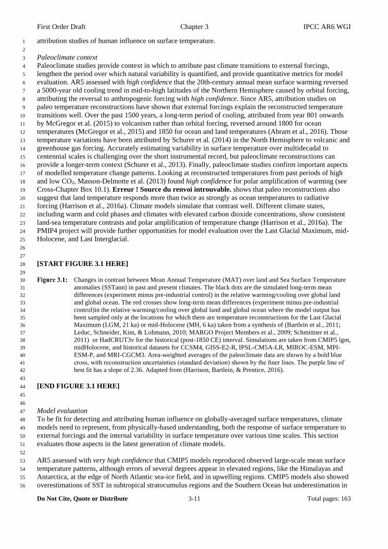
Cross-Chapter Box 10.1). Erreur ! Source du renvoi introuvable. shows that paleo reconstructions also 19
suggest that land temperature responds more than twice as strongly as ocean temperatures to radiative 20
forcing (Harrison et al., 2016a). Climate models simulate that contrast well. Different climate states, 21
including warm and cold phases and climates with elevated carbon dioxide concentrations, show consistent 22
land-sea temperature contrasts and polar amplification of temperature change (Harrison et al., 2016a). The 23
PMIP4 project will provide further opportunities for model evaluation over the Last Glacial Maximum, mid-24
Holocene, and Last Interglacial. 25
26
27
[START FIGURE 3.1 HERE] 28
29
Changes in contrast between Mean Annual Temperature (MAT) over land and Sea Surface Temperature 30
anomalies (SSTann) in past and present climates. The black dots are the simulated long-term mean 31
differences (experiment minus pre-industrial control) in the relative warming/cooling over global land 32
and global ocean. The red crosses show long-term mean differences (experiment minus pre-industrial 33
control)in the relative warming/cooling over global land and global ocean where the model output has 34
been sampled only at the locations for which there are temperature reconstructions for the Last Glacial 35
Maximum (LGM, 21 ka) or mid-Holocene (MH, 6 ka) taken from a synthesis of (Bartlein et al., 2011; 36
Leduc, Schneider, Kim, & Lohmann, 2010; MARGO Project Members et al., 2009; Schmittner et al., 37
2011) or HadCRUT3v for the historical (post-1850 CE) interval. Simulations are taken from CMIP5 lgm, 38
midHolocene, and historical datasets for CCSM4, GISS-E2-R, IPSL-CM5A-LR, MIROC-ESM, MPI-39
ESM-P, and MRI-CGCM3. Area-weighted averages of the paleoclimate data are shown by a bold blue 40
cross, with reconstruction uncertainties (standard deviation) shown by the finer lines. The purple line of 41
best fit has a slope of 2.36. Adapted from (Harrison, Bartlein, & Prentice, 2016). 42
43
[END FIGURE 3.1 HERE] 44
45
46
Model evaluation 47
To be fit for detecting and attributing human influence on globally-averaged surface temperatures, climate 48
models need to represent, from physically-based understanding, both the response of surface temperature to 49
external forcings and the internal variability in surface temperature over various time scales. This section 50
evaluates those aspects in the latest generation of climate models. 51
52
AR5 assessed with very high confidence that CMIP5 models reproduced observed large-scale mean surface 53
temperature patterns, although errors of several degrees appear in elevated regions, like the Himalayas and 54
Antarctica, at the edge of North Atlantic sea-ice field, and in upwelling regions. CMIP5 models also showed 55
overestimations of SST in subtropical stratocumulus regions and the Southern Ocean but underestimation in 56
First Order Draft Chapter 3 IPCC AR6 WGI
Do Not Cite, Quote or Distribute 3-12 Total pages: 163
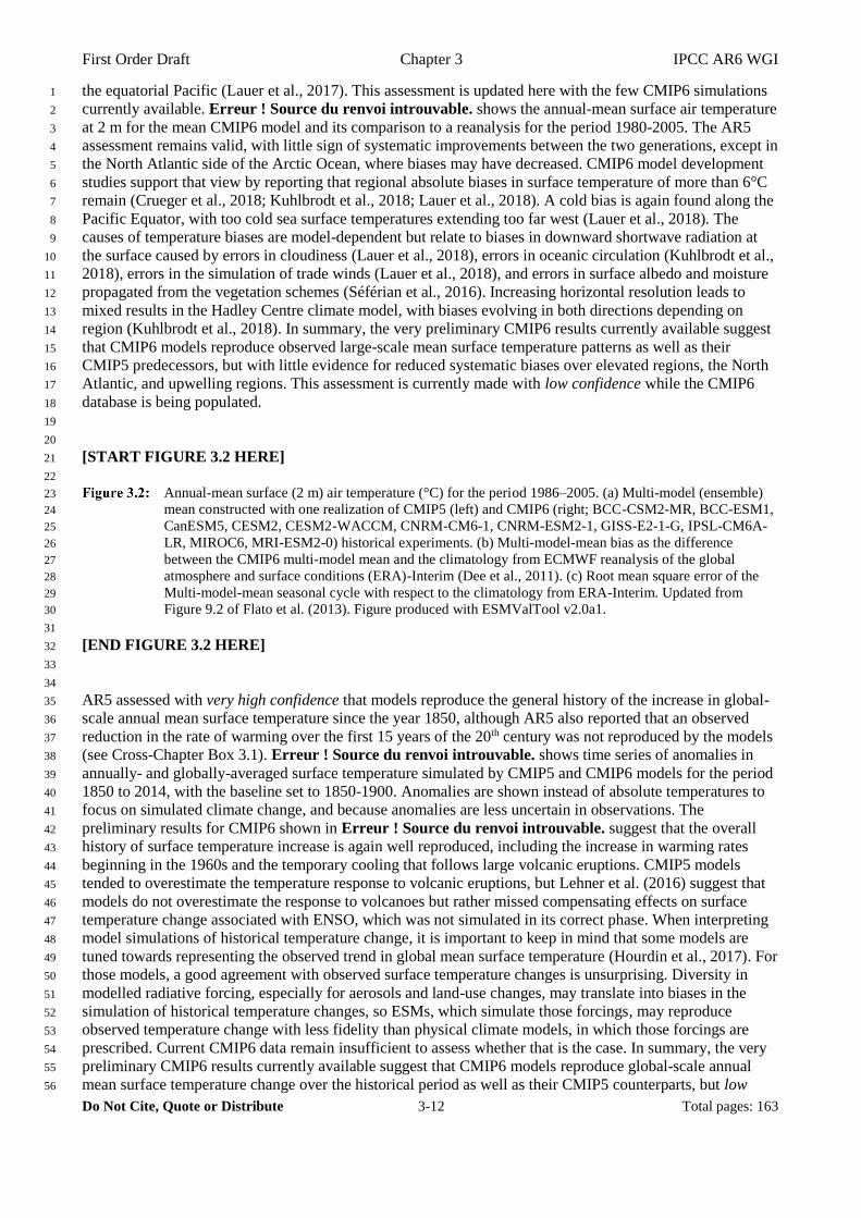
the equatorial Pacific (Lauer et al., 2017). This assessment is updated here with the few CMIP6 simulations 1
currently available. Erreur ! Source du renvoi introuvable. shows the annual-mean surface air temperature 2
at 2 m for the mean CMIP6 model and its comparison to a reanalysis for the period 1980-2005. The AR5 3
assessment remains valid, with little sign of systematic improvements between the two generations, except in 4
the North Atlantic side of the Arctic Ocean, where biases may have decreased. CMIP6 model development 5
studies support that view by reporting that regional absolute biases in surface temperature of more than 6°C 6
remain (Crueger et al., 2018; Kuhlbrodt et al., 2018; Lauer et al., 2018). A cold bias is again found along the 7
Pacific Equator, with too cold sea surface temperatures extending too far west (Lauer et al., 2018). The 8
causes of temperature biases are model-dependent but relate to biases in downward shortwave radiation at 9
the surface caused by errors in cloudiness (Lauer et al., 2018), errors in oceanic circulation (Kuhlbrodt et al., 10
2018), errors in the simulation of trade winds (Lauer et al., 2018), and errors in surface albedo and moisture 11
propagated from the vegetation schemes (Séférian et al., 2016). Increasing horizontal resolution leads to 12
mixed results in the Hadley Centre climate model, with biases evolving in both directions depending on 13
region (Kuhlbrodt et al., 2018). In summary, the very preliminary CMIP6 results currently available suggest 14
that CMIP6 models reproduce observed large-scale mean surface temperature patterns as well as their 15
CMIP5 predecessors, but with little evidence for reduced systematic biases over elevated regions, the North 16
Atlantic, and upwelling regions. This assessment is currently made with low confidence while the CMIP6 17
database is being populated. 18
19
20
[START FIGURE 3.2 HERE] 21
22
Annual-mean surface (2 m) air temperature (°C) for the period 1986–2005. (a) Multi-model (ensemble) 23
mean constructed with one realization of CMIP5 (left) and CMIP6 (right; BCC-CSM2-MR, BCC-ESM1, 24
CanESM5, CESM2, CESM2-WACCM, CNRM-CM6-1, CNRM-ESM2-1, GISS-E2-1-G, IPSL-CM6A-25
LR, MIROC6, MRI-ESM2-0) historical experiments. (b) Multi-model-mean bias as the difference 26
between the CMIP6 multi-model mean and the climatology from ECMWF reanalysis of the global 27
atmosphere and surface conditions (ERA)-Interim (Dee et al., 2011). (c) Root mean square error of the 28
Multi-model-mean seasonal cycle with respect to the climatology from ERA-Interim. Updated from 29
Figure 9.2 of Flato et al. (2013). Figure produced with ESMValTool v2.0a1. 30
31
[END FIGURE 3.2 HERE] 32
33
34
AR5 assessed with very high confidence that models reproduce the general history of the increase in global-35
scale annual mean surface temperature since the year 1850, although AR5 also reported that an observed 36
reduction in the rate of warming over the first 15 years of the 20th century was not reproduced by the models 37
(see Cross-Chapter Box 3.1). Erreur ! Source du renvoi introuvable. shows time series of anomalies in 38
annually- and globally-averaged surface temperature simulated by CMIP5 and CMIP6 models for the period 39
1850 to 2014, with the baseline set to 1850-1900. Anomalies are shown instead of absolute temperatures to 40
focus on simulated climate change, and because anomalies are less uncertain in observations. The 41
preliminary results for CMIP6 shown in Erreur ! Source du renvoi introuvable. suggest that the overall 42
history of surface temperature increase is again well reproduced, including the increase in warming rates 43
beginning in the 1960s and the temporary cooling that follows large volcanic eruptions. CMIP5 models 44
tended to overestimate the temperature response to volcanic eruptions, but Lehner et al. (2016) suggest that 45
models do not overestimate the response to volcanoes but rather missed compensating effects on surface 46
temperature change associated with ENSO, which was not simulated in its correct phase. When interpreting 47
model simulations of historical temperature change, it is important to keep in mind that some models are 48
tuned towards representing the observed trend in global mean surface temperature (Hourdin et al., 2017). For 49
those models, a good agreement with observed surface temperature changes is unsurprising. Diversity in 50
modelled radiative forcing, especially for aerosols and land-use changes, may translate into biases in the 51
simulation of historical temperature changes, so ESMs, which simulate those forcings, may reproduce 52
observed temperature change with less fidelity than physical climate models, in which those forcings are 53
prescribed. Current CMIP6 data remain insufficient to assess whether that is the case. In summary, the very 54
preliminary CMIP6 results currently available suggest that CMIP6 models reproduce global-scale annual 55
mean surface temperature change over the historical period as well as their CMIP5 counterparts, but low 56

First Order Draft Chapter 3 IPCC AR6 WGI
Do Not Cite, Quote or Distribute 3-13 Total pages: 163
confidence is placed on that assessment until CMIP6 historical simulations have been submitted in large 1
numbers. 2
3
[START FIGURE 3.3 HERE] 4
5
Observed and simulated time series of the anomalies in annual and global mean surface temperature. All 6
anomalies are differences from the 1850–1900 time-mean of each individual time series. The reference 7
period 1850–1900 is indicated by yellow shading. Single simulations for (a) CMIP5 and (b) CMIP6 8
models (thin lines); multi-model mean (thick red line). Observational data (thick black lines) are Hadley 9
Centre/Climatic Research Unit gridded surface temperature data set 4 (HadCRUT4; Morice et al., 2012), 10
and are merged surface temperature (2 m height over land and surface temperature over the ocean). All 11
models have been subsampled using the HadCRUT4 observational data mask (see Jones et al., 2013). 12
Inset: the global mean surface temperature for the reference period 1961–1990 of the subsampled fields. 13
Updated from Figure 9.8 of Flato et al. (2013). Figure produced with ESMValTool v2.0a1. 14
15
[END FIGURE 3.3 HERE] 16
17
18
The application of climate models to detection and attribution studies requires that those models simulate 19
realistic internal variability on multi-decadal timescales. An underestimate of variability in models would 20
make conclusions from detection and attribution overconfident. AR5 found that CMIP5 models simulate 21
realistic variability in global-mean surface temperature on decadal time scales, with variability on multi-22
decadal time scales being more difficult to evaluate because of the short observational record (Flato et al., 23
2013). Since AR5, new work has characterized the contributions of variability in different ocean areas to 24
SST variability, with tropical modes of variability like ENSO dominant on time scales of 5 to 10 years, while 25
longer time scales see the variance move poleward to the North Atlantic, North Pacific, and Southern oceans 26
(Monselesan et al., 2015). There may however be sizeable interdependencies between ENSO and sea surface 27
temperature variability in different basins (Kumar et al., 2014), and ENSO’s influence on global surface 28
temperature variability may not be confined only to decadal timescales (Triacca et al., 2014). Studies based 29
on large ensembles of 20th and 21st century climate change confirm that internal variability has a substantial 30
influence on global warming trends over a few decades (Dai and Bloecker, 2018; Kay et al., 2015) (FAQ 31
3.1). Although the equatorial Pacific seems to be the main source of internal variability on decadal 32
timescales, Brown et al. (2016) link diversity in modelled oceanic convection, sea ice, and energy budget in 33
high-latitude regions to overall diversity in modelled internal variability. 34
35
This renewed interest in internal variability stems in part from its importance in understanding the slowdown 36
in global warming rate in the early 21st century (see Cross-Chapter Box 3.1). Some evidence is emerging that 37
decadal to multidecadal modes of variability, such as Pacific decadal variability (Section 3.7.6) (England et 38
al., 2014a; Schurer et al., 2015; Thompson et al., 2014) and Atlantic Multidecadal variability (Section 3.7.7) 39
partly drive global scale temperature variations over the historical period, and that variability in these modes 40
may be underestimated by CMIP5 models. But evidence, coming mostly from paleo studies, is more mixed 41
on whether CMIP5 models also underestimate decadal and multi-decadal variability in global mean 42
temperature in general. Schurer et al. (2013) find good agreement between internal variability derived from 43
paleo reconstructions, estimated as the fraction of variance that is not explained by forced responses, and 44
modelled variability, although the subset of CMIP5 models they used may have been associated with larger 45
variability than the full CMIP5 ensemble. In the SH, Hegerl et al. (2018) report internal variability in the 46
early 20th century larger than that modelled. In addition, new literature suggests that anthropogenic forcing 47
itself may affect variability in surface temperatures, at least on an interannual basis, challenging a common 48
assumption in detection and attribution techniques that forcing does not change the variability. Screen (2014) 49
report an observed decrease in variance in the Northern Hemisphere mid-latitude land temperature, largest in 50
Autumn, associated with Arctic amplification, and qualitatively consistent with simulated future changes in 51
variance (Cross-Chapter Box 10.1). Qian and Zhang (2015) and Santer et al. (2018b) found an anthropogenic 52
influence on the seasonal cycle of surface and tropospheric temperatures, respectively. Erreur ! Source du 53
renvoi introuvable. shows the standard deviation of surface temperature in CMIP6 pre-industrial control 54
simulations. Although the CMIP6 database is currently too incomplete to update the AR5 statement on the 55
quality of the simulation of internal variability in surface temperature in climate models, the very preliminary 56
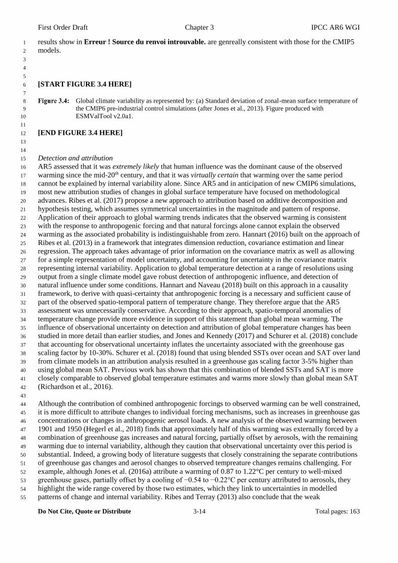
First Order Draft Chapter 3 IPCC AR6 WGI
Do Not Cite, Quote or Distribute 3-14 Total pages: 163
results show in Erreur ! Source du renvoi introuvable. are genreally consistent with those for the CMIP5 1
models. 2
3
4
5
[START FIGURE 3.4 HERE] 6
7
Global climate variability as represented by: (a) Standard deviation of zonal-mean surface temperature of 8
the CMIP6 pre-industrial control simulations (after Jones et al., 2013). Figure produced with 9
ESMValTool v2.0a1. 10
11
[END FIGURE 3.4 HERE] 12
13
14
Detection and attribution 15
AR5 assessed that it was extremely likely that human influence was the dominant cause of the observed 16
warming since the mid-20th century, and that it was virtually certain that warming over the same period 17
cannot be explained by internal variability alone. Since AR5 and in anticipation of new CMIP6 simulations, 18
most new attribution studies of changes in global surface temperature have focused on methodological 19
advances. Ribes et al. (2017) propose a new approach to attribution based on additive decomposition and 20
hypothesis testing, which assumes symmetrical uncertainties in the magnitude and pattern of response. 21
Application of their approach to global warming trends indicates that the observed warming is consistent 22
with the response to anthropogenic forcing and that natural forcings alone cannot explain the observed 23
warming as the associated probability is indistinguishable from zero. Hannart (2016) built on the approach of 24
Ribes et al. (2013) in a framework that integrates dimension reduction, covariance estimation and linear 25
regression. The approach takes advantage of prior information on the covariance matrix as well as allowing 26
for a simple representation of model uncertainty, and accounting for uncertainty in the covariance matrix 27
representing internal variability. Application to global temperature detection at a range of resolutions using 28
output from a single climate model gave robust detection of anthropogenic influence, and detection of 29
natural influence under some conditions. Hannart and Naveau (2018) built on this approach in a causality 30
framework, to derive with quasi-certainty that anthropogenic forcing is a necessary and sufficient cause of 31
part of the observed spatio-temporal pattern of temperature change. They therefore argue that the AR5 32
assessment was unnecessarily conservative. According to their approach, spatio-temporal anomalies of 33
temperature change provide more evidence in support of this statement than global mean warming. The 34
influence of observational uncertainty on detection and attribution of global temperature changes has been 35
studied in more detail than earlier studies, and Jones and Kennedy (2017) and Schurer et al. (2018) conclude 36
that accounting for observational uncertainty inflates the uncertainty associated with the greenhouse gas 37
scaling factor by 10-30%. Schurer et al. (2018) found that using blended SSTs over ocean and SAT over land 38
from climate models in an attribution analysis resulted in a greenhouse gas scaling factor 3-5% higher than 39
using global mean SAT. Previous work has shown that this combination of blended SSTs and SAT is more 40
closely comparable to observed global temperature estimates and warms more slowly than global mean SAT 41
(Richardson et al., 2016). 42
43
Although the contribution of combined anthropogenic forcings to observed warming can be well constrained, 44
it is more difficult to attribute changes to individual forcing mechanisms, such as increases in greenhouse gas 45
concentrations or changes in anthropogenic aerosol loads. A new analysis of the observed warming between 46
1901 and 1950 (Hegerl et al., 2018) finds that approximately half of this warming was externally forced by a 47
combination of greenhouse gas increases and natural forcing, partially offset by aerosols, with the remaining 48
warming due to internal variability, although they caution that observational uncertainty over this period is 49
substantial. Indeed, a growing body of literature suggests that closely constraining the separate contributions 50
of greenhouse gas changes and aerosol changes to observed tempreature changes remains challenging. For 51
example, although Jones et al. (2016a) attribute a warming of 0.87 to 1.22°C per century to well‐mixed 52
greenhouse gases, partially offset by a cooling of −0.54 to −0.22°C per century attributed to aerosols, they 53
highlight the wide range covered by those two estimates, which they link to uncertainties in modelled 54
patterns of change and internal variability. Ribes and Terray (2013) also conclude that the weak 55
First Order Draft Chapter 3 IPCC AR6 WGI
Do Not Cite, Quote or Distribute 3-15 Total pages: 163
observational constraints on the contributions of greenhouse gas and aerosol forcing call for new attribution 1
techniques. Linear addition of single-forcing responses implied by fingerprinting attribution techniques were 2
found to hold for large-scale surface temperature changes in Bindoff et al. (2013) based on two studies. A 3
more recent third study also finds additivity using the GISS climate model (Marvel et al., 2015). 4
5
IPCC SR1.5 notes that anthropogenic warming has essentially been equal to total warming since the early 6
2000s, based on the (Bindoff et al., 2013) assessment that the warming by solar and volcanic forcings is 7
small. By applying the method of Haustein et al. (2017), which accounts for forcing uncertainty and internal 8
variability, and moderating their uncertainty estimates to account for additional forcing and model 9
uncertainty, the IPCC SR1.5 assessed that warming attributable to anthropogenic forcing has reached 1.0°C 10
in 2017 with respect to the period 1850-1900, with a likely range of ±0.2°C. Otto et al. (2015) propose an 11
anthropogenic warming index, simply based on an impulse-response model fitted to observed temperatures, 12
which has the advantage of being only weakly dependent on uncertainties in climate sensitivity and forcing. 13
Using their index, they find an attributable warming of 0.91°C in 2014, relative to an 1860-1879 base period, 14
up from 0.5°C in 1992. Ribes et al. (2017), using the methods described above, estimate the 90% uncertainty 15
range for 1951-2010 anthropogenic attributable forcing at 0.55-0.80°C. Preliminary attribution results 16
derived from the first available CMIP6 simulations (Figure 3.5) are not yet sufficiently robust to influence 17
our assessment of attributable warming. 18
19
20
[START FIGURE 3.5 HERE] 21
22
Best estimates and estimated 5-95% confidence intervals for all-forcing attributable warming in °C in 23
global-mean near-surface air temperature for the period 2010-2014 [will be updated to 2010-2019 once 24
sufficient ScenarioMIP data is available] relative to an 1850-1900 base period. Preliminary results shown 25
were derived using three models’ historical simulations individually, and were derived by applying a 26
Regularized Optimal Fingerprint (Ribes and Terray, 2013) regression to decadal mean global mean 27
temperature from HadCRUT4 and CMIP6 historical simulations blended and masked following Cowtan 28
et al. (2015). Attributable warming was estimated by multiplying globally-complete ensemble mean 29
simulated 2010-2014 near-surface air temperature anomalies relative to 1850-1900 from each model by 30
the corresponding regression coefficient and confidence interval. Internal variability was estimated from 31
34 samples of intra-ensemble variability from available models. [Will be updated to use more internal 32
variability samples, and show anthropogenic, natural, GHG and other anthropogenic contributions in 33
SOD, once more CMIP6 DAMIP simulations are available]. 34
35
[END FIGURE 3.5 HERE] 36
37
38
The AR5 found high confidence for a major role for anthropogenic forcing in driving warming over each of 39
the inhabited continents, except for Africa where they found only medium confidence (Bindoff et al., 2013). 40
Friedman et al. (2019) detect an anthropogenically forced response of inter-hemispheric contrast in surface 41
temperature change, with the Northern Hemisphere cooling more than the southern hemisphere until 1980 42
but then warming more from 1980 to 2012. CMIP5 models simulate the correct response qualitatively when 43
forced with all forcings but underestimate its magnitude. There has been limited new literature on 44
continental-scale attribution since the AR5. Stone and Hansen (2016) proposed and developed an automated 45
empirical approach for developing confidence levels associated with detection and attribution statements, 46
based on the amount of modelling and observational evidence, and the results of a detection and attribution 47
analysis. Erreur ! Source du renvoi introuvable. shows global surface temperature change in CMIP5 and 48
CMIP6 all-forcing and natural-only simulations globally and separately over land and ocean surfaces. At this 49
stage, the CMIP6 database is too incomplete to assess whether those new simulations support the AR5 50
assessment. 51
52
53
[START FIGURE 3.6 HERE] 54
55
Global, land, ocean and continental annual mean temperatures anomalies for CMIP5 (brown) and CMIP6 56

First Order Draft Chapter 3 IPCC AR6 WGI
Do Not Cite, Quote or Distribute 3-16 Total pages: 163
(BCC-CSM2-MR, BCC-ESM1, CanESM5, CESM2, CESM2-WACCM, CNRM-CM6-1, CNRM-ESM2-1
1, GISS-E2-1-G, IPSL-CM6A-LR, MIROC6, MRI-ESM2-0) historical (grey) and CMIP5 historicalNat 2
(blue) simulations (multi-model means shown as thick lines, and 10 to 90% ranges shown as shaded area) 3
and for Hadley Centre/Climatic Research Unit gridded surface temperature data set 4 (HadCRUT4, 4
black). All models have been subsampled using the HadCRUT4 observational data mask (see Jones et al., 5
2013). Temperatures are shown with respect to 1850–1900. Figure produced with ESMValTool v2.0a1. 6
7
[END FIGURE 3.6 HERE] 8
9
10
[START FIGURE 3.7 HERE] 11
12
Same as Figure 3.6, but for single forcing simulations from CMIP6-DAMIP simulations. [Placeholder 13
for SOD.] 14
15
[END FIGURE 3.7 HERE] 16
17
18
Erreur ! Source du renvoi introuvable. will show the influence of single forcings on the global, land, o19
cean and continental annual mean temperatures anomylies from DAMIP simulations [Placeholder text]. 20
21
In summary, since the publication of the AR5, new literature has emerged which better accounts for 22
methodological and climate model uncertainties in attribution studies (Hannart and Naveau, 2018; Ribes et 23
al., 2017), reporting results consistent with probabilities above 99% for human activities causing more than 24
half the observed warming over the 1951-2010 period. Moreover calculated anthropogenic warming and 25
associated uncertainties calculated for 2017 relative to 1850-1900 (Haustein et al., 2017), and as assessed in 26
the IPCC SR1.5 also simply P > 99% that human activities caused more than half the observed warming 27
trend under the assumption of normally distributed uncertainties. And finally, the strong observed warming 28
that has occurred in the period since the publication of the AR5 (Chapter 2), and the improved understanding 29
of the causes of the apparent slowdown in warming over the beginning of the 21st century and the difference 30
in simulated and observed warming trends over this period (Cross-Chapter Box 3.1), further improve our 31
confidence in the assessment of the anthropogenic contribution to observed warming. Although there is 32
mixed evidence that models underestimate internal variability, there is no evidence for the severe 33
underestimate that would be needed to challenge the conclusions of the attribution studies assessed in this 34
section. Taking this evidence together, we assess that it is virtually certain (P ≥ 99%) that human activities 35
caused more than half of the observed warming over the 1951-2010 period. In addition, there is no basis at 36
this stage for revising the IPCC SR1.5 best estimate and likely range of anthropogenic attributable warming 37
of 1.0±0.2°C in 2017 with respect to the period 1850-1900. 38
39
40
3.3.1.2 Upper-Air Temperature 41
42
The AR5 (Bindoff et al., 2013) assessed that anthropogenic forcings, dominated by GHGs, likely contributed 43
to the warming of the troposphere since 1961 and that anthropogenic forcings, dominated by the depletion of 44
the ozone layer due to ozone-depleting substances, very likely contributed to the cooling of the lower 45
stratosphere since 1979. Since then, observational uncertainties in the radiosonde and satellite data have been 46
further understood with more available data and longer coverage. Differences between models and 47
observations in the tropical atmosphere have been further investigated. 48
49
Tropospheric temperature 50
The AR5 (Flato et al., 2013) assessed with low confidence that most, though not all, CMIP3 and CMIP5 51
models overestimated the observed warming trend in the tropical troposphere during the satellite period 52
1979-2012, and that a third to a half of this difference was due to an overestimate of the SST trend during 53
this period. Mitchell et al.( 2013) demonstrated an inconsistency between CMIP5 simulated and observed 54
temperature trends through the depth of the tropical troposphere over the 1979-2008 period (Erreur ! 55
Source du renvoi introuvable.), with models warming more than observations. However, the discrepancy is 56
First Order Draft Chapter 3 IPCC AR6 WGI
Do Not Cite, Quote or Distribute 3-17 Total pages: 163
smaller when examined in models forced with observed SSTs, and models and observations are consistent 1
below 150 hPa when viewed in terms of the ratio of temperature trends aloft to those at the surface. Kamae 2
et al. (2015) suggest that the recent slowdown of tropical upper tropospheric warming was associated with 3
Pacific climate variability. Moreover, Santer et al. (2017b) compared the global-mean mid-tropospheric 4
temperatures from multiple Microwave Sounding Unit (MSU) datasets and climate model data during the 5
satellite era and found that during the late twentieth century, the discrepancies between simulated and 6
satellite-derived tropospheric temperature trends are consistent with internal variability, while during most of 7
the early twenty-first century, simulated tropospheric warming is significantly larger than observed, which 8
they relate to systematic deficiencies in some of the external forcings used after year of 2000 in the models. 9
Focused on the temperature of the mid-to-upper troposphere (TMT), Santer et al. (2017c) used updated and 10
improved satellite retrievals to investigate model performance in simulating the TMT trends and vertical 11
profiles of warming, and removed the influence of stratospheric cooling by regression. These factors were 12
found to reduce the size of the discrepancy in TMT trends between models and observations over the 13
satellite era, but a discrepancy remained. 14
15
Overall, new studies continue to find that CMIP5 models warmed more than observed in the tropical mid- 16
and upper-troposphere over the 1979-2012 period (Mitchell et al., 2013; Santer et al., 2017a, 2017c; Suárez-17
Gutiérrez et al., 2017), and that overestimated surface warming is partially responsible (Mitchell et al., 18
2013). Internal variability and residual observational errors may also contribute to the discrepancy (Mitchell 19
et al., 2013; Suárez-Gutiérrez et al., 2017), but recent work also points to forcing errors in the CMIP5 20
simulations in the early 21st century as a possible contributor (Mitchell et al., 2013; Santer et al., 2017a; 21
Sherwood and Nishant, 2015). Hence, we now assess with medium confidence that most CMIP5 models 22
overestimate observed warming in the tropical troposphere during the satellite era. We assess that much of 23
this overestimate is due to an overestimate of the SST trend over this period, and that forcing errors in the 24
models may have contributed (low confidence). Outside the tropics, and over the period of the radiosonde 25
record beginning from 1961, the discrepancy between simulated and observed trends is smaller. 26
27
28
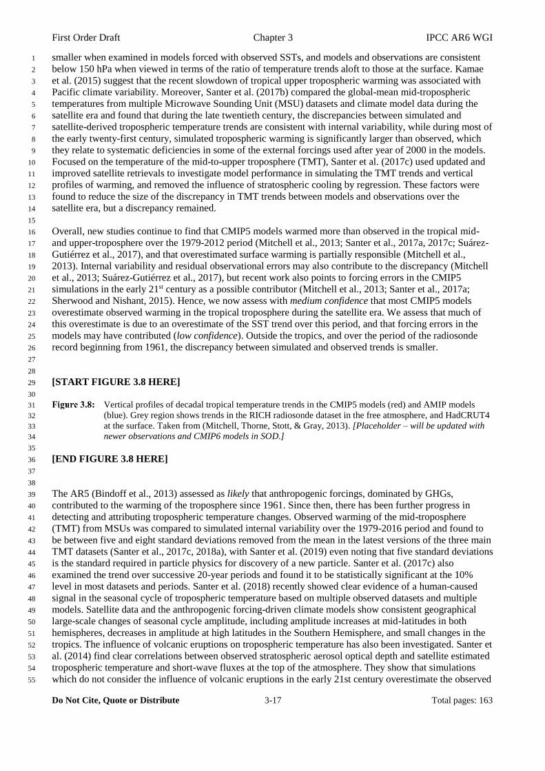
[START FIGURE 3.8 HERE] 29
30
Vertical profiles of decadal tropical temperature trends in the CMIP5 models (red) and AMIP models 31
(blue). Grey region shows trends in the RICH radiosonde dataset in the free atmosphere, and HadCRUT4 32
at the surface. Taken from (Mitchell, Thorne, Stott, & Gray, 2013). [Placeholder – will be updated with 33
newer observations and CMIP6 models in SOD.] 34
35
[END FIGURE 3.8 HERE] 36
37
38
The AR5 (Bindoff et al., 2013) assessed as likely that anthropogenic forcings, dominated by GHGs, 39
contributed to the warming of the troposphere since 1961. Since then, there has been further progress in 40
detecting and attributing tropospheric temperature changes. Observed warming of the mid-troposphere 41
(TMT) from MSUs was compared to simulated internal variability over the 1979-2016 period and found to 42
be between five and eight standard deviations removed from the mean in the latest versions of the three main 43
TMT datasets (Santer et al., 2017c, 2018a), with Santer et al. (2019) even noting that five standard deviations 44
is the standard required in particle physics for discovery of a new particle. Santer et al. (2017c) also 45
examined the trend over successive 20-year periods and found it to be statistically significant at the 10% 46
level in most datasets and periods. Santer et al. (2018) recently showed clear evidence of a human-caused 47
signal in the seasonal cycle of tropospheric temperature based on multiple observed datasets and multiple 48
models. Satellite data and the anthropogenic forcing-driven climate models show consistent geographical 49
large-scale changes of seasonal cycle amplitude, including amplitude increases at mid-latitudes in both 50
hemispheres, decreases in amplitude at high latitudes in the Southern Hemisphere, and small changes in the 51
tropics. The influence of volcanic eruptions on tropospheric temperature has also been investigated. Santer et 52
al. (2014) find clear correlations between observed stratospheric aerosol optical depth and satellite estimated 53
tropospheric temperature and short-wave fluxes at the top of the atmosphere. They show that simulations 54
which do not consider the influence of volcanic eruptions in the early 21st century overestimate the observed 55
First Order Draft Chapter 3 IPCC AR6 WGI
Do Not Cite, Quote or Distribute 3-18 Total pages: 163
tropospheric warming since 1998. 1
2
Based on these additional analyses, we assess that it is extremely likely that anthropogenic forcing, 3
dominated by GHGs, contributed to the warming of the troposphere since 1979. 4
5
Stratospheric temperature 6
The AR5 concluded that the CMIP5 models simulated the evolution of lower stratospheric temperatures 7
generally realistically (Bindoff et al., 2013; Flato et al., 2013) and better than the CMIP3 models, in part 8
because they generally include time-varying ozone concentrations, unlike many of the CMIP3 models. 9
Nonetheless, it was noted that there was a tendency for the simulations to underestimate stratospheric 10
cooling compared to observations. Based on attribution studies using CMIP5 and CCMVal simulations, 11
Bindoff et al. (2013) concluded that it is very likely that anthropogenic forcing, dominated by stratospheric 12
ozone depletion due to ozone-depleting substances, contributed to the cooling of the lower stratosphere since 13
1979. Since the AR5, Santer et al. (2017b) compared observed lower stratospheric temperature trends with 14
those simulated by the CMIP5 models, and found a tendency for the models to underestimate the cooling, 15
which they attributed to an underestimation of stratospheric ozone depletion in many CMIP5 models (Eyring 16
et al., 2013; Young et al., 2013), differences in stratospheric water vapour evolution, and internal variability. 17
Maycock et al. (2018a) compared lower stratospheric temperature trends over the 1979-2005 period in the 18
CCMI coupled chemistry climate simulations with satellite observations, and found that observed trends 19
were within the range of simulated trends, and the models reproduced the levelling off of lower stratospheric 20
temperatures in the 1998-2016 period due to the cessation of ozone depletion and onset of recovery. Young 21
et al. (2013) compared temperature trends based on various satellite and radiosonde observations and climate 22
(GCM) and chemistry-climate model (CCM) outputs, with a focus on the influence of ozone depletion in the 23
Antarctic lower stratosphere since mid-1950s. They found that CCMs and CMIP5 models’ simulation of 24
Antarctic stratospheric cooling is consistent with recent radiosonde datasets to within modelling and 25
observational uncertainties. In a modelling study, Aquila et al. (2016) find that in the lower stratosphere, the 26
cooling trend due to increasing GHGs is roughly constant over the satellite era. Changes in ODS 27
concentrations cause a significant stratospheric cooling only up to the mid-1990s. After that, a decrease in 28
ODS caused a flattening of temperature, with more rapid fluctuations caused by the eruption of Mount 29
Pinatubo and the solar cycle. 30
31
Upper stratospheric temperature changes were not assessed in the context of attribution or model evaluation 32
in AR5, but this is an area where there has been considerable progress over recent years, with new versions 33
of both Stratospheric Sounding Unit (SSU) datasets released, which are in better agreement than previous 34
versions (Maycock et al., 2018b, 2018a) (see also Section 2.3.1.1.4). Simulated temperature changes in the 35
CCMI coupled chemistry models show good consistency with the reprocessed dataset from NOAA STAR 36
SSU but are less consistent with the revised UK Met Office record. The latter still shows stronger cooling 37
than simulated in the chemistry-climate models (Maycock et al., 2018a). Mitchell (2016) used regularized 38
optimal fingerprinting techniques to make an attribution analysis of annual mid-upper stratospheric 39
temperature in response to external forcings. They find that anthropogenic forcing has caused an 40
approximate cooling of 2-3 °C in the upper stratosphere during the period of 1979-2015, with GHGs 41
contributing two thirds of this change and ozone depletion contributing one third. They find a temperature 42
change in response to volcanic forcing is larger than previous studies (0.4-0.6 °C for Mount Pinatubo) in the 43
upper stratosphere, although is still smaller than the lower-stratospheric signal. Aquila et al. (2016) used 44
chemistry climate models with added forcing factors and prescribed observed sea surface temperature to 45
investigate the influence of different forcings on global stratospheric temperature changes. They find that the 46
cooling of the stratosphere after 1979 is mainly due to changes in GHG concentrations in the middle and 47
upper stratosphere. The step-like changes of global temperature anomalies are mainly due to the changes in 48
solar irradiance and volcanically-induced ozone depletion and water vapour increases in the post-Pinatubo 49
years. Therefore, in the upper stratosphere, both a standard detection and attribution approach (Mitchell, 50
2016) and chemistry-climate model studies (Aquila et al., 2016; Maycock et al., 2018a) indicate that about 51
two-thirds of the global long-term cooling is attributed to GHGs and one third to ozone depletion. 52
Chemistry-climate model results further show that the relatively rapid decreases in global upper stratospheric 53
temperatures in the early 1980s and early 1990s are likely to be due to the combined influence of 54
temperature decreases after the warming from major tropical volcanic eruptions and the declining phase of 55
First Order Draft Chapter 3 IPCC AR6 WGI
Do Not Cite, Quote or Distribute 3-19 Total pages: 163
the 11-year solar cycle. 1
2
Based on the latest updates to satellite observations of stratospheric temperature, we assess that simulated 3
and observed changes of global mean temperature through the depth of the stratosphere are more consistent 4
than based on previous datasets, but some differences remain. Studies published since the AR5 increase our 5
confidence in the simulated stratospheric temperature response to greenhouse gas and ozone changes, and 6
support an assessment that it is extremely likely that anthropogenic forcing, dominated by stratospheric ozone 7
depletion due to ozone-depleting substances, has cooled the lower stratosphere since 1979. 8
9
10
3.3.2 Precipitation, Humidity 11
12
Paleoclimate context 13
14
Since they are rooted in biological or geochemical systems, paleoclimate proxies are typically sensitive to 15
moisture balance (P-E) and aridity rather than precipitation. Examples of indicators of past changes in the 16
water cycle include the levels of closed lake basins, plant pollen, stable isotopes of oxygen or hydrogen 17
(recorded in carbonate minerals or biomarkers), and drought-sensitive trees. These recorders of past changes 18
in the water cycle provide valuable context for observed trends in the 20th and 21st century and assist with the 19
attribution of these trends to human influence. For example, many areas of the subtropics – such as the 20
Mediterranean and the western United States – have experienced systematic drying in recent decades. This is 21
an expected response to elevated greenhouse gases (Seager et al., 2014b, 2014a), but can be difficult to attribute 22
due to the large internal variability of the water cycle. Tree ring records provide evidence that recent prolonged 23
dry spells in the Levant and Mongolia are unprecedented in the last millennium (Cook et al., 2016a; Pederson 24
et al., 2014) and thus may be attributable to anthropogenic forcing in agreement with historical observations 25
(Gudmundsson and Seneviratne, 2016; Kelley et al., 2015). Likewise, tree rings indicate that the 2012-2014 26
drought in California was very likely unusual in the context of natural variability in the last millennium, and 27
may have been exacerbated by the contribution of anthropogenic temperature rise (Griffin and Anchukaitis, 28
2014; Williams et al., 2015). East Africa has been drying in recent decades (Hoell et al., 2017), a trend that is 29
unusual in the context of the sedimentary paleorecord spanning the last millennium (Tierney et al., 2015). This 30
may be a signature of anthropogenic forcing (low confidence) but cannot as of yet be distinguished from natural 31
variability (Hoell et al., 2017; Philip et al., 2018). Tree rings also indicate the presence of prolonged 32
megadroughts (droughts lasting two decades or more) throughout the last millennium that were more severe 33
than 20th and 21st century events (high confidence) (Cook et al., 2004, 2010, 2015). These were likely associated 34
with internal climate variability (medium confidence) (Coats et al., 2016; Cook et al., 2016b) and demonstrate 35
that large-magnitude changes in the water cycle can occur irrespective of anthropogenic influence. 36
37
Paleoclimate records also provide context for the human influence on large-scale atmospheric circulation, such 38
as the inter-tropical convergence zone (ITCZ), the Walker circulation, and monsoon systems. In AR5, it was 39
determined with high confidence that orbital forcing produces strong interhemispheric rainfall variability 40
evident in multiple types of proxies. These large-magnitude intensifications and weakenings in the monsoon 41
systems involved in some cases orders-of-magnitude changes in precipitation (Harrison et al., 2014b; Tierney 42
et al., 2017), and thus are virtually certain to have been larger than changes observed in the 20th and 21st 43
centuries. Paleoclimate modeling and limited data from past climate states with high CO2 suggest that monsoon 44
systems intensify under elevated greenhouse gases (medium confidence), providing context for present and 45
future trends (Haywood et al., 2013; Passey et al., 2009; Zhang et al., 2013b). Paleoclimate data from the 46
Pliocene epoch suggest that the moderately higher CO2 of that time (400 ppm) weakened the Walker 47
circulation (Tierney et al., in review), in agreement with theory (Vecchi et al., 2006; Vecchi and Soden, 2007), 48
but in contradiction to recently-observed trends in the Pacific (England et al., 2014b; L’Heureux et al., 2013) 49
and the ambiguous trends across the last 100 years as a whole (DiNezio et al., 2013a; Karnauskas et al., 2009; 50
Vecchi et al., 2006). 51
52
53
3.3.2.1 Precipitation 54
55
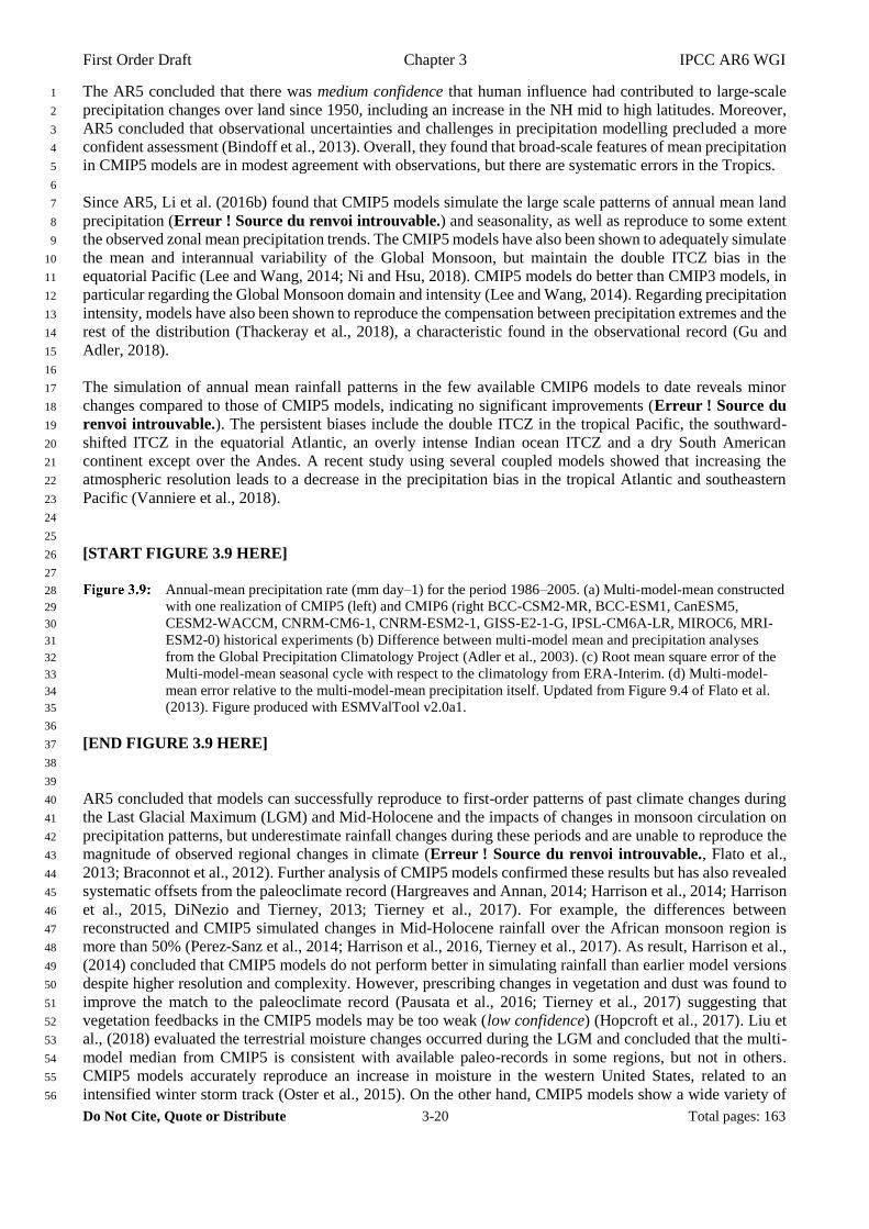
First Order Draft Chapter 3 IPCC AR6 WGI
Do Not Cite, Quote or Distribute 3-20 Total pages: 163
The AR5 concluded that there was medium confidence that human influence had contributed to large-scale 1
precipitation changes over land since 1950, including an increase in the NH mid to high latitudes. Moreover, 2
AR5 concluded that observational uncertainties and challenges in precipitation modelling precluded a more 3
confident assessment (Bindoff et al., 2013). Overall, they found that broad-scale features of mean precipitation 4
in CMIP5 models are in modest agreement with observations, but there are systematic errors in the Tropics. 5
6
Since AR5, Li et al. (2016b) found that CMIP5 models simulate the large scale patterns of annual mean land 7
precipitation (Erreur ! Source du renvoi introuvable.) and seasonality, as well as reproduce to some extent 8
the observed zonal mean precipitation trends. The CMIP5 models have also been shown to adequately simulate 9
the mean and interannual variability of the Global Monsoon, but maintain the double ITCZ bias in the 10
equatorial Pacific (Lee and Wang, 2014; Ni and Hsu, 2018). CMIP5 models do better than CMIP3 models, in 11
particular regarding the Global Monsoon domain and intensity (Lee and Wang, 2014). Regarding precipitation 12
intensity, models have also been shown to reproduce the compensation between precipitation extremes and the 13
rest of the distribution (Thackeray et al., 2018), a characteristic found in the observational record (Gu and 14
Adler, 2018). 15
16
The simulation of annual mean rainfall patterns in the few available CMIP6 models to date reveals minor 17
changes compared to those of CMIP5 models, indicating no significant improvements (Erreur ! Source du 18
renvoi introuvable.). The persistent biases include the double ITCZ in the tropical Pacific, the southward-19
shifted ITCZ in the equatorial Atlantic, an overly intense Indian ocean ITCZ and a dry South American 20
continent except over the Andes. A recent study using several coupled models showed that increasing the 21
atmospheric resolution leads to a decrease in the precipitation bias in the tropical Atlantic and southeastern 22
Pacific (Vanniere et al., 2018). 23
24
25
[START FIGURE 3.9 HERE] 26
27
Annual-mean precipitation rate (mm day–1) for the period 1986–2005. (a) Multi-model-mean constructed 28
with one realization of CMIP5 (left) and CMIP6 (right BCC-CSM2-MR, BCC-ESM1, CanESM5, 29
CESM2-WACCM, CNRM-CM6-1, CNRM-ESM2-1, GISS-E2-1-G, IPSL-CM6A-LR, MIROC6, MRI-30
ESM2-0) historical experiments (b) Difference between multi-model mean and precipitation analyses 31
from the Global Precipitation Climatology Project (Adler et al., 2003). (c) Root mean square error of the 32
Multi-model-mean seasonal cycle with respect to the climatology from ERA-Interim. (d) Multi-model-33
mean error relative to the multi-model-mean precipitation itself. Updated from Figure 9.4 of Flato et al. 34
(2013). Figure produced with ESMValTool v2.0a1. 35
36
[END FIGURE 3.9 HERE] 37
38
39
AR5 concluded that models can successfully reproduce to first-order patterns of past climate changes during 40
the Last Glacial Maximum (LGM) and Mid-Holocene and the impacts of changes in monsoon circulation on 41
precipitation patterns, but underestimate rainfall changes during these periods and are unable to reproduce the 42
magnitude of observed regional changes in climate (Erreur ! Source du renvoi introuvable., Flato et al., 43
2013; Braconnot et al., 2012). Further analysis of CMIP5 models confirmed these results but has also revealed 44
systematic offsets from the paleoclimate record (Hargreaves and Annan, 2014; Harrison et al., 2014; Harrison 45
et al., 2015, DiNezio and Tierney, 2013; Tierney et al., 2017). For example, the differences between 46
reconstructed and CMIP5 simulated changes in Mid-Holocene rainfall over the African monsoon region is 47
more than 50% (Perez-Sanz et al., 2014; Harrison et al., 2016, Tierney et al., 2017). As result, Harrison et al., 48
(2014) concluded that CMIP5 models do not perform better in simulating rainfall than earlier model versions 49
despite higher resolution and complexity. However, prescribing changes in vegetation and dust was found to 50
improve the match to the paleoclimate record (Pausata et al., 2016; Tierney et al., 2017) suggesting that 51
vegetation feedbacks in the CMIP5 models may be too weak (low confidence) (Hopcroft et al., 2017). Liu et 52
al., (2018) evaluated the terrestrial moisture changes occurred during the LGM and concluded that the multi-53
model median from CMIP5 is consistent with available paleo-records in some regions, but not in others. 54
CMIP5 models accurately reproduce an increase in moisture in the western United States, related to an 55
intensified winter storm track (Oster et al., 2015). On the other hand, CMIP5 models show a wide variety of 56

First Order Draft Chapter 3 IPCC AR6 WGI
Do Not Cite, Quote or Distribute 3-21 Total pages: 163
responses in the tropical Indo-Pacific region, with only a few matching the pattern of change inferred from the 1
paleoclimate record (DiNezio et al., 2018; DiNezio and Tierney, 2013). The variable response across models 2
is related to the effect of the exposure of the tropical shelves during glacial times, which variously intensifies 3
or weakens convection in the rising limb of the Walker cell, depending on model parameterization (DiNezio 4
et al., 2011). [Will be updated with figure multi-model and multivariate evaluation of PMIP4 simulations] 5
6
7
8
9
[START FIGURE 3.10 HERE] 10
11
Comparison of median and interquartile range (IQR) of reconstructed and simulated mean annual 12
precipitation for LGM (left) and MH (right). The comparisons are made using only the model land (or 13
ocean) grid cells where there are observations. The median value of the observations is shown as a black 14
vertical line, the IQR by dark grey shading and the 5-95 percentile limits by light grey shading. The 15
models are colour-coded to show whether they are PMIP2 or CMIP5 simulations, and whether they are 16
ocean-atmosphere (OA), ocean-atmosphere-vegetation (OAV) or OA carbon-cycle (OAC) models. The 17
simulated median for each model is shown by a vertical line, the box represents the IQR and the whiskers 18
the 5-95 percentile limits. From Harrison et al., 2014. [Will be replaced with results from CMIP6-PMIP4 19
showing multi-model and multivariate assessment for LGM and MH in SOD]. 20
21
[END FIGURE 3.10 HERE] 22
23
24
The observed precipitation increase in the NH high latitudes over the period 1966-2005 was attributed to 25
anthropogenic forcing by a study using CMIP5 models (Wan et al., 2015) supporting the AR5 assessment. 26
Osborne et al. (2015) identified a data problem in observed land precipitation around 1930, and proposed a 27
correction which made the precipitation record more consistent with the runoff record, and consistent with the 28
expected negative response to mid-20th century aerosol forcing. New results from CMIP6 support the role of 29
anthropogenic forcing in the precipitation increase observed in NH high latitudes. A smaller positive tendency 30
still within the bounds of natural variability is seen in NH mid-latitudes. In the tropics and SH mid-latitudes 31
the zonal mean precipitation shows large interdecadal variability that can not be attributed to anthropogenic 32
forcing (see Erreur ! Source du renvoi introuvable.). 33
34
35
[START FIGURE 3.11 HERE] 36
37
Global and zonal average changes in annual mean precipitation (mm day-1) over areas of land where 38
there are observations, expressed relative to the base-line period of 1961–1990, simulated by CMIP5 39
models forced with both anthropogenic and natural forcings and natural forcings only and CMIP6 (BCC-40
CSM2-MR, BCC-ESM1, CanESM5, CESM2-WACCM, CNRM-CM6-1, CNRM-ESM2-1, GISS-E2-1-41
G, IPSL-CM6A-LR, MIROC6, MRI-ESM2-0) models forced with both anthropogenic and natural 42
forcings for the global mean and for three latitude bands. Multi-model means are shown in thick solid 43
lines and shading shows 10-90% ranges of the individual model simulations (for CMIP6 models 44
minimum and maximum). Observations (gridded values derived from Global Historical Climatology 45
Network station data, updated from Zhang et al. (2007) are shown as a black solid line. An 11-year 46
smoothing is applied to both simulations and observations. Figure produced with ESMValTool v2.0a1. 47
48
[END FIGURE 3.11 HERE] 49
50
51
For the SH extratropics, Solman and Orlanski (2016) found that the observed rainfall increase over the high 52
latitudes and reduced rainfall over midlatitudes during austral summer are quasi-zonally symmetric and related 53
with the changes in eddy activity, which are in turn associated with the poleward shift of the westerlies due 54
mostly to ozone depletion. During austral winter wetting and drying conditions at high and middle latitudes, 55
respectively, are not zonally homogeneous, and both changes in eddy activity and increased lower troposphere 56
humidity contributed. They associate these changes to increase in GHG concentration levels. Recently, 57

First Order Draft Chapter 3 IPCC AR6 WGI
Do Not Cite, Quote or Distribute 3-22 Total pages: 163
Blazquez and Solman (2017) have shown that CMIP5 models represent very well the dynamical forcing and 1
the frequency of frontal precipitation in the SH winter extratropics, but the amount of precipitation due to 2
fronts is overestimated. 3
4
In the tropics Polson and Hegerl (2017) found that the effect of external forcing on precipitation following the 5
wet gets wetter, dry gets drier paradigm is robust if one takes into account the seasonal and interannual 6
movement of the regions (Allan, 2014). They found that the forced signal is already detectable over wet 7
regions, but not over dry ones in the period 1988-2014. Other studies also suggest that this paradigm does not 8
necessarily hold over dry regions where moisture is limited (Greve et al., 2014; Kumar et al., 2015). Based on 9
long-term island precipitation records, Polson et al. (2016) identified significant increases in precipitation in 10
the tropics and decreases in the subtropics, which are consistent with those simulated by the CMIP5 models. 11
Barkhordarian et al. (2018) attributed the observed reduced springtime precipitation in tropical South America 12
during 1983-2012 to elevated GHGs and land use. Undorf et al. (2018) found a detectable impact of aerosol 13
changes on West African and South Asian monsoon precipitation. Over the oceans, the observed pattern of 14
salinity change at high latitudes and in the subtropics is broadly consistent with the expected changes in 15
precipitation-evaporation due to the wet gets wetter, dry gets drier paradigm, although with observational 16
uncertainty (see Section 3.5.2.2, Hegerl and et al., 2015; Skliris et al., 2014). Over the Atlantic and Pacific 17
Oceans the salinity changes since the mid-twentieth century have been found to be outside the range of internal 18
climate variability in model simulations and have been attributed to anthropogenic influences (Pierce et al., 19
2012; Hegerl and et al., 2015). 20
21
One study found enhanced seasonality in land precipitation (Chiang et al., 2013), consistent with the simulated 22
response to anthropogenic forcing (Dwyer et al., 2014). However, observed trends in seasonality depend on 23
data set used (Li et al., 2016b; Marvel et al., 2017), and Marvel et al. (2017) found inconsistent trends in the 24
amplitude of the seasonal cycle of precipitation in global satellite precipitation observations and CMIP5 25
models. On the other hand, Marvel et al. (2017) found that observed changes to the annual cycle phase are 26
consistent with model estimates of forced changes. These phase changes are mainly characterized by earlier 27
onset of the wet season on the equatorward flanks of the extratropical storm tracks, particularly in the SH. 28
29
Overall, several new studies detect an anthropogenic influence on precipitation over the continents and oceans 30
in the high latitudes and tropics, and we therefore now assess that it is likely that human influence has 31
contributed to large-scale precipitation changes since 1950. Owing to observational uncertainties and 32
inconsistent results between studies, we conclude that there is low confidence in the attribution of changes in 33
the seasonality of precipitation. 34
35
36
3.3.2.2 Atmospheric Water Vapour 37
38
The AR5 concluded that an anthropogenic contribution to specific humidity is found with medium confidence 39
at and near the surface. A poorly understood levelling off of atmospheric water vapour over land in the last 40
two decades, and remaining observational uncertainties precluded a more confident assessment (Bindoff et al., 41
2013). 42
43
Water vapor is the most important natural greenhouse gas and its amount is expected to increase in a global 44
warming context leading to further warming. Particularly important are changes in the upper troposphere 45
because there water vapor regulates the strength of water-vapor feedback, an important process for amplifying 46
the response of the climate system to external radiative forcings. CMIP5 models have been shown to have a 47
wet bias in the tropical upper troposphere and a drier-than-observed lower troposphere, with the former bias 48
and model spread being larger than the latter (Jiang et al., 2012; Tian et al., 2013). Water vapor errors are 49
dominated by errors in relative humidity througout the troposphere, with temperature errors dominating near 50
the tropopause (Takahashi et al., 2016). 51
52
[Placeholder for evaluation of CMIP6 models] 53
54
Using satellite data as well as CMIP5 model output, Chung et al. (2014) demonstrated that the moistening 55

First Order Draft Chapter 3 IPCC AR6 WGI
Do Not Cite, Quote or Distribute 3-23 Total pages: 163
observed in the upper troposphere over the period 1979–2005 cannot be explained by natural causes and results 1
principally from an anthropogenic warming of the climate. This increase in water vapour is accompanied by a 2
reduction in mid-tropospheric relative humidity and clouds in the subtropics and mid-latitude in both models 3
and observations related to changes in the Hadley cell (Lau and Kim, 2015). 4
5
Dunn et al., (2017) showed that global mean surface relative humidity increased during 1973-2000, followed 6
by a steep decline, and specific humidity correspondingly increased and then remained approximately constant, 7
with none of the CMIP5 models capturing this behaviour. They also noted biases in the mean state of the 8
CMIP5 models’ surface relative humidity, and conclude that these biases preclude any detection and attribution 9
assessment. 10
11
Based on new evidence we assess that it is likely that human influence has contributed to tropical moistening 12
in the upper troposphere since 1979 with medium confidence. Owing to the limited number of studies and 13
model biases we conclude that there is low confidence in the attribution of changes in the surface humidity. 14
15
16
3.3.2.3 Stream Flow 17
18
Stream flow is to-date the only variable of the terrestrial water cycle with enough in-situ observations to 19
allow for detection and attribution analysis at continental to global scales. Based on evidence from a few 20
formal detection and attribution studies and the qualitative evaluation of studies reporting on observed and 21
simulated trends, AR5 concluded that there is medium confidence that anthropogenic climate change is 22
influencing streamflow in some middle and high latitude regions. AR5 also noted that observational 23
uncertainties are large and that often only a limited number of models were considered. 24
25
Section 2.3.1.2.6 assesses that there have not been significant trends in global average streamflow over the 26
last century, though regional trends have been observed, driven in part by internal variability. Only a limited 27
number of studies has systematically compared observed streamflow trends at continental to global scales 28
with changes simulated by global circulation models (GCM) in a detection and attribution setting. In a pan-29
European assessment, Gudmundsson et al. (2017) attribute the spatio-temporal pattern of decreasing 30
streamflow in southern Europe and increasing streamflow in northern Europe to anthropogenic climate 31
change, but also concluded that additional effects of human water withdrawals could not be excluded. 32
Focussing on continental runoff during 1958-2004, Alkama et al. (2013) could obtain a significant change 33
only when using reconstructed data over all rivers, indicating a large uncertainty in the global discharge 34
trend due to differnet statistical methods used and opposite changes over different continents. Gedney et al. 35
(2014) detect the influence of aerosols on streamflow in North America and Europe, with aerosols having 36
driven an increase in streamflow due to reduced evaporation. 37
38
While streamflow is assessed in numerous regional and watershed-based studies, model evaluations with a 39
continental/global focus are very limited. By using a Bayesian weighting approach based on historical 40
decadal simulations and observed runoff, model agreement is largely improved (Yang et al., 2017). Based on 41
this assessment the authors further found that simulated, multi-model mean runoff is generally overestimated 42
in non-weighted climate model assessments and that climate models barely replicate observed interannual 43
runoff. However, focusing on climate regions in North America, it was suggested that runoff is generally 44
underestimated, while spatial variations in runoff are reproduced by climate models (Sheffield et al., 2013). 45
46
In summary, there is medium confidence that anthropogenic climate change has altered local and regional 47
streamflow in various parts of the world and that the associated global-scale trend pattern is inconsistent with 48
pre-industrial control simulations. Nonetheless, it must be noted that streamflow is also subject to human 49
interventions and water withdrawals that may interfere with an unambiguous attribution of streamflow 50
changes. 51
52
53
3.3.3 Atmospheric Circulation 54
55

First Order Draft Chapter 3 IPCC AR6 WGI
Do Not Cite, Quote or Distribute 3-24 Total pages: 163
3.3.3.1 Tropospheric Overturning Circulation in the Tropics 1
2
The tropical tropospheric circulation features meridional and zonal overturning circulations, called Hadley 3
and Walker circulations. In the zonal mean, the downwelling branch of the Hadley circulation cell is located 4
in the subtropics and is often used as an indicator of the meridional extent of the tropics. In the zonal-vertical 5
section, the major rising branch of the Walker cell is located over the Maritime continent with secondary 6
upwelling regions over northern South America and Africa. The surface trade winds over most of the 7
equatorial Pacific and Atlantic are associated with the Walker circulation. 8
9
AR5 found medium confidence that the stratospheric ozone depletion had contributed to Hadley cell 10
widening in the Southern Hemisphere in austral summer. It also mentioned that in contrast to a simulated 11
weakening in response to GHG forcing, the Walker circulation had actually strengthened since the early 12
1990s, precluding any detection of human influence. 13
14
Since AR5, a growing body of literature has found an important role of internal variability, especially of 15
Pacific Decadal Variability (PDV) (Section 3.7.6), on the recent Hadley cell expansion (Adam et al., 2014; 16
Allen et al., 2014; Allen and Kovilakam, 2017; Amaya et al., 2018; Grise et al., 2018, 2019; Lucas and 17
Nguyen, 2015; Mantsis et al., 2017). Indeed, the simulated Hadley cell expansion in the ensemble mean of 18
CMIP5 historical simulations is weaker than observed, but the ensemble spread includes the observed trend 19
overall (Davis and Birner, 2017; Garfinkel et al., 2015; Grise et al., 2018; Figure 3.12:). The PDV influence 20
is stronger in the Northern Hemisphere (Grise et al., 2018, 2019), while simulated human influence, mostly 21
from GHG increase and ozone depletion, is stronger on the southern Hadley Cell boundary (Grise et al., 22
2019). These influences together led to a comparable Hadley cell expansion in both hemispheres. The 23
simulated Hadley cell expansion in CMIP5 historical simulations since the late 1970s is strongest in the 24
Southern Hemisphere in austral summer when the influence of ozone depletion peaks (Tao et al. 2016; 25
Figure 3.12:). When represented in terms of the latitude of the subtropical sea level pressure (SLP) 26
maximum, the observed shift of the South Atlantic Hadley Cell edge exceeds the 95th percentile of internal 27
variability in CMIP5 piControl simulations (Kim et al., 2017b). But in the zonal average, the shift has not yet 28
clearly emerged out of internal variability as simulated by CMIP5 models (Grise et al., 2019; Staten et al., 29
2018; Figure 3.12:). It is also noteworthy that many CMIP5 models underrepresent the magnitude of the 30
PDV (Section 3.7.6), implying potential overconfidence on the detection of human influence. 31
32
Studies since AR5 have found that a decadal-scale strengthening of the Walker circulation since the 1980s 33
(Section 2.4.1) is associated with a shift of the PDV in the late 1990s from positive to negative phase 34
(England et al., 2014a; Ma and Zhou, 2016; Watanabe et al., 2014) and an increasing inter-basin contrast of 35
SST (McGregor et al., 2014; Takahashi and Watanabe, 2016; Zhang and Karnauskas, 2017) between the 36
Atlantic and the Indo-Pacific oceans. Anthropogenic aerosol influence is found in some models to have 37
driven changes in the PDV (Hua et al., 2018) and the inter-basin contrast (Takahashi and Watanabe, 2016), 38
but large uncertainties remain (Hua et al., 2018; Oudar et al., 2018). On multidecadal to centennial time 39
scales, studies on the observed trend of the Walker circulation strength have mixed results. Bellomo and 40
Clement (2015a), DiNezio et al. (2013), and Tokinaga et al. (2011, 2012) found a consistent weakening, as 41
measured by zonal SLP gradient and cloud cover, which is successfully simulated by AGCM simulations 42
(Bellomo and Clement, 2015; Sandeep et al., 2014; Tokinaga et al., 2012), whereas L’Heureux et al., (2013) 43
instead found strengthening in zonal SLP gradient for 1950-2011. In coupled models, DiNezio et al. (2013) 44
find that simulated changes of the Walker circulation strength in the ensemble mean of CMIP5 historical 45
experiments can be interpreted as a result of compensating effects of GHGs and aerosols and are much 46
smaller than observed. These results suggest that any human-induced change may be minor compared to 47
large internal climate variability. Furthermore, the observed 1980-2012 and 1994-2013 strengthening trends 48
are both extremely strong compared to trends derived from CMIP5 ensemble (Bordbar et al., 2017; Kociuba 49
and Power, 2015), due to underestimated variability of the PDV (Section 3.7.6) and overall multidecadal 50
variability in inter-basin SST contrast (Kajtar et al., 2018; Zhang and Karnauskas, 2017). 51
52
In summary, the observed zonal mean Hadley cell expansion since the 1970s and changes in the Pacific 53
Walker circulation strength are within the range of internal variability. This assessment is justified by studies 54
since AR5, which on one hand confirm the contribution of human influence on the Hadley cell expansion, 55
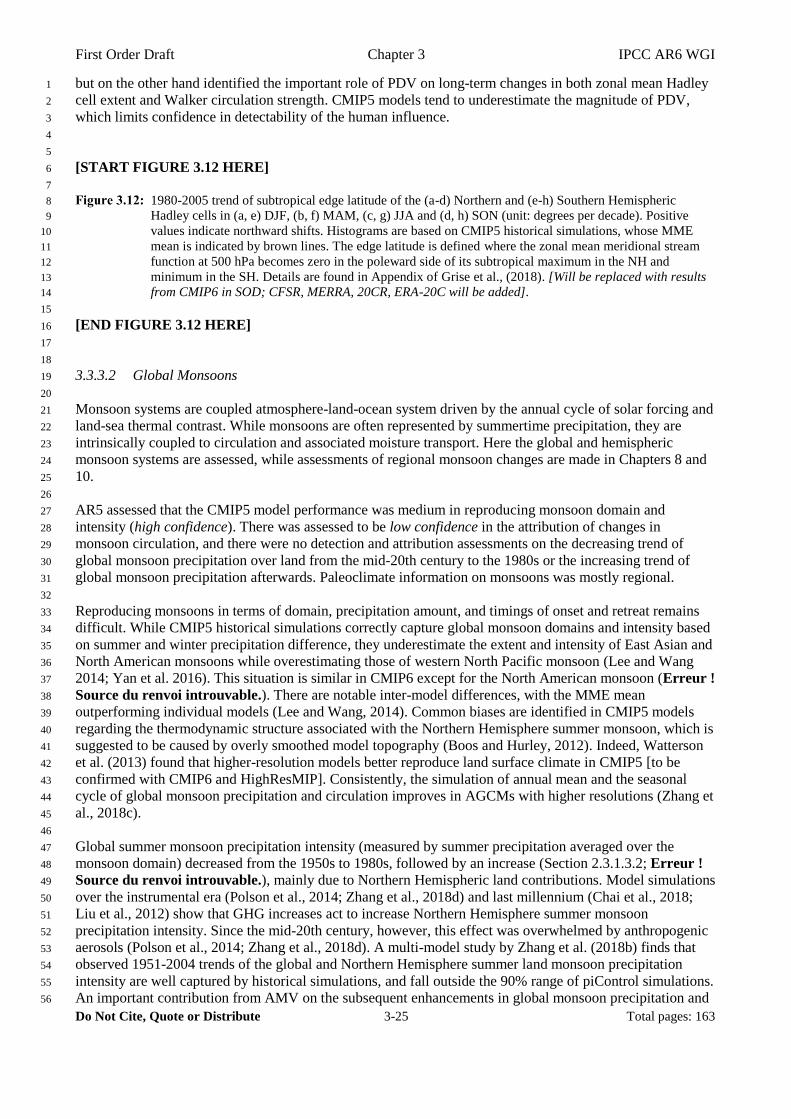
First Order Draft Chapter 3 IPCC AR6 WGI
Do Not Cite, Quote or Distribute 3-25 Total pages: 163
but on the other hand identified the important role of PDV on long-term changes in both zonal mean Hadley 1
cell extent and Walker circulation strength. CMIP5 models tend to underestimate the magnitude of PDV, 2
which limits confidence in detectability of the human influence. 3
4
5
[START FIGURE 3.12 HERE] 6
7
1980-2005 trend of subtropical edge latitude of the (a-d) Northern and (e-h) Southern Hemispheric 8
Hadley cells in (a, e) DJF, (b, f) MAM, (c, g) JJA and (d, h) SON (unit: degrees per decade). Positive 9
values indicate northward shifts. Histograms are based on CMIP5 historical simulations, whose MME 10
mean is indicated by brown lines. The edge latitude is defined where the zonal mean meridional stream 11
function at 500 hPa becomes zero in the poleward side of its subtropical maximum in the NH and 12
minimum in the SH. Details are found in Appendix of Grise et al., (2018). [Will be replaced with results 13
from CMIP6 in SOD; CFSR, MERRA, 20CR, ERA-20C will be added]. 14
15
[END FIGURE 3.12 HERE] 16
17
18
3.3.3.2 Global Monsoons 19
20
Monsoon systems are coupled atmosphere-land-ocean system driven by the annual cycle of solar forcing and 21
land-sea thermal contrast. While monsoons are often represented by summertime precipitation, they are 22
intrinsically coupled to circulation and associated moisture transport. Here the global and hemispheric 23
monsoon systems are assessed, while assessments of regional monsoon changes are made in Chapters 8 and 24
10. 25
26
AR5 assessed that the CMIP5 model performance was medium in reproducing monsoon domain and 27
intensity (high confidence). There was assessed to be low confidence in the attribution of changes in 28
monsoon circulation, and there were no detection and attribution assessments on the decreasing trend of 29
global monsoon precipitation over land from the mid-20th century to the 1980s or the increasing trend of 30
global monsoon precipitation afterwards. Paleoclimate information on monsoons was mostly regional. 31
32
Reproducing monsoons in terms of domain, precipitation amount, and timings of onset and retreat remains 33
difficult. While CMIP5 historical simulations correctly capture global monsoon domains and intensity based 34
on summer and winter precipitation difference, they underestimate the extent and intensity of East Asian and 35
North American monsoons while overestimating those of western North Pacific monsoon (Lee and Wang 36
2014; Yan et al. 2016). This situation is similar in CMIP6 except for the North American monsoon (Erreur ! 37
Source du renvoi introuvable.). There are notable inter-model differences, with the MME mean 38
outperforming individual models (Lee and Wang, 2014). Common biases are identified in CMIP5 models 39
regarding the thermodynamic structure associated with the Northern Hemisphere summer monsoon, which is 40
suggested to be caused by overly smoothed model topography (Boos and Hurley, 2012). Indeed, Watterson 41
et al. (2013) found that higher-resolution models better reproduce land surface climate in CMIP5 [to be 42
confirmed with CMIP6 and HighResMIP]. Consistently, the simulation of annual mean and the seasonal 43
cycle of global monsoon precipitation and circulation improves in AGCMs with higher resolutions (Zhang et 44
al., 2018c). 45
46
Global summer monsoon precipitation intensity (measured by summer precipitation averaged over the 47
monsoon domain) decreased from the 1950s to 1980s, followed by an increase (Section 2.3.1.3.2; Erreur ! 48
Source du renvoi introuvable.), mainly due to Northern Hemispheric land contributions. Model simulations 49
over the instrumental era (Polson et al., 2014; Zhang et al., 2018d) and last millennium (Chai et al., 2018; 50
Liu et al., 2012) show that GHG increases act to increase Northern Hemisphere summer monsoon 51
precipitation intensity. Since the mid-20th century, however, this effect was overwhelmed by anthropogenic 52
aerosols (Polson et al., 2014; Zhang et al., 2018d). A multi-model study by Zhang et al. (2018b) finds that 53
observed 1951-2004 trends of the global and Northern Hemisphere summer land monsoon precipitation 54
intensity are well captured by historical simulations, and fall outside the 90% range of piControl simulations. 55
An important contribution from AMV on the subsequent enhancements in global monsoon precipitation and 56
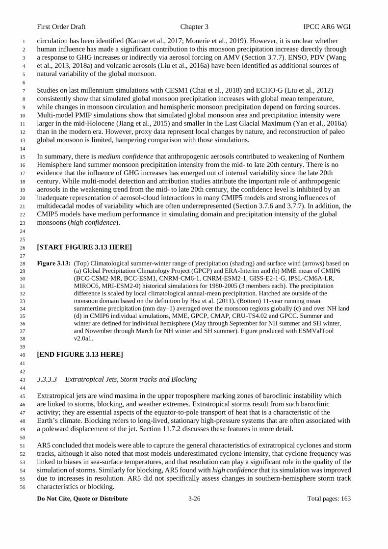
First Order Draft Chapter 3 IPCC AR6 WGI
Do Not Cite, Quote or Distribute 3-26 Total pages: 163
circulation has been identified (Kamae et al., 2017; Monerie et al., 2019). However, it is unclear whether 1
human influence has made a significant contribution to this monsoon precipitation increase directly through 2
a response to GHG increases or indirectly via aerosol forcing on AMV (Section 3.7.7). ENSO, PDV (Wang 3
et al., 2013, 2018a) and volcanic aerosols (Liu et al., 2016a) have been identified as additional sources of 4
natural variability of the global monsoon. 5
6
Studies on last millennium simulations with CESM1 (Chai et al., 2018) and ECHO-G (Liu et al., 2012) 7
consistently show that simulated global monsoon precipitation increases with global mean temperature, 8
while changes in monsoon circulation and hemispheric monsoon precipitation depend on forcing sources. 9
Multi-model PMIP simulations show that simulated global monsoon area and precipitation intensity were 10
larger in the mid-Holocene (Jiang et al., 2015) and smaller in the Last Glacial Maximum (Yan et al., 2016a) 11
than in the modern era. However, proxy data represent local changes by nature, and reconstruction of paleo 12
global monsoon is limited, hampering comparison with those simulations. 13
14
In summary, there is medium confidence that anthropogenic aerosols contributed to weakening of Northern 15
Hemisphere land summer monsoon precipitation intensity from the mid- to late 20th century. There is no 16
evidence that the influence of GHG increases has emerged out of internal variability since the late 20th 17
century. While multi-model detection and attribution studies attribute the important role of anthropogenic 18
aerosols in the weakening trend from the mid- to late 20th century, the confidence level is inhibited by an 19
inadequate representation of aerosol-cloud interactions in many CMIP5 models and strong influences of 20
multidecadal modes of variability which are often underrepresented (Section 3.7.6 and 3.7.7). In addition, the 21
CMIP5 models have medium performance in simulating domain and precipitation intensity of the global 22
monsoons (high confidence). 23
24
25
[START FIGURE 3.13 HERE] 26
27
(Top) Climatological summer-winter range of precipitation (shading) and surface wind (arrows) based on 28
(a) Global Precipitation Climatology Project (GPCP) and ERA-Interim and (b) MME mean of CMIP6 29
(BCC-CSM2-MR, BCC-ESM1, CNRM-CM6-1, CNRM-ESM2-1, GISS-E2-1-G, IPSL-CM6A-LR, 30
MIROC6, MRI-ESM2-0) historical simulations for 1980-2005 (3 members each). The precipitation 31
difference is scaled by local climatological annual-mean precipitation. Hatched are outside of the 32
monsoon domain based on the definition by Hsu et al. (2011). (Bottom) 11-year running mean 33
summertime precipitation (mm day–1) averaged over the monsoon regions globally (c) and over NH land 34
(d) in CMIP6 individual simulations, MME, GPCP, CMAP, CRU-TS4.02 and GPCC. Summer and 35
winter are defined for individual hemisphere (May through September for NH summer and SH winter, 36
and November through March for NH winter and SH summer). Figure produced with ESMValTool 37
v2.0a1. 38
39
[END FIGURE 3.13 HERE] 40
41
42
3.3.3.3 Extratropical Jets, Storm tracks and Blocking 43
44
Extratropical jets are wind maxima in the upper troposphere marking zones of baroclinic instability which 45
are linked to storms, blocking, and weather extremes. Extratropical storms result from such baroclinic 46
activity; they are essential aspects of the equator-to-pole transport of heat that is a characteristic of the 47
Earth’s climate. Blocking refers to long-lived, stationary high-pressure systems that are often associated with 48
a poleward displacement of the jet. Section 11.7.2 discusses these features in more detail. 49
50
AR5 concluded that models were able to capture the general characteristics of extratropical cyclones and storm 51
tracks, although it also noted that most models underestimated cyclone intensity, that cyclone frequency was 52
linked to biases in sea-surface temperatures, and that resolution can play a significant role in the quality of the 53
simulation of storms. Similarly for blocking, AR5 found with high confidence that its simulation was improved 54
due to increases in resolution. AR5 did not specifically assess changes in southern-hemisphere storm track 55
characteristics or blocking. 56
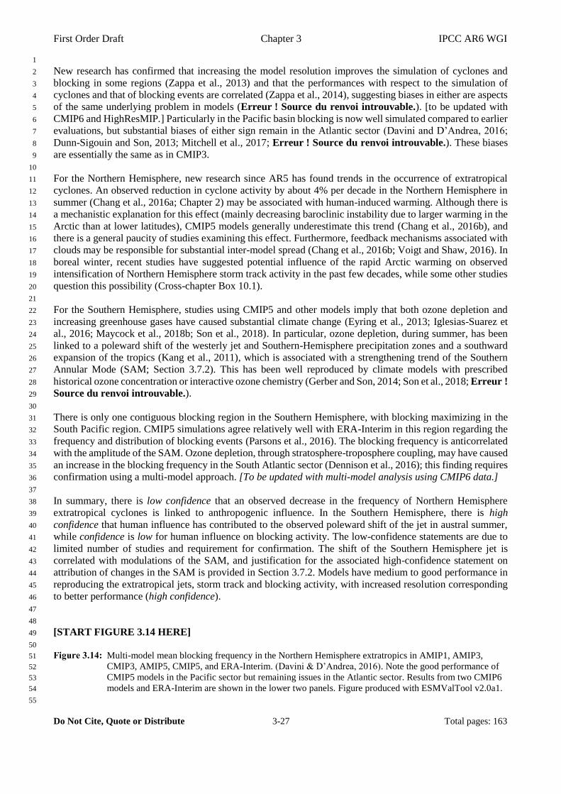
First Order Draft Chapter 3 IPCC AR6 WGI
Do Not Cite, Quote or Distribute 3-27 Total pages: 163
1
New research has confirmed that increasing the model resolution improves the simulation of cyclones and 2
blocking in some regions (Zappa et al., 2013) and that the performances with respect to the simulation of 3
cyclones and that of blocking events are correlated (Zappa et al., 2014), suggesting biases in either are aspects 4
of the same underlying problem in models (Erreur ! Source du renvoi introuvable.). [to be updated with 5
CMIP6 and HighResMIP.] Particularly in the Pacific basin blocking is now well simulated compared to earlier 6
evaluations, but substantial biases of either sign remain in the Atlantic sector (Davini and D’Andrea, 2016; 7
Dunn-Sigouin and Son, 2013; Mitchell et al., 2017; Erreur ! Source du renvoi introuvable.). These biases 8
are essentially the same as in CMIP3. 9
10
For the Northern Hemisphere, new research since AR5 has found trends in the occurrence of extratropical 11
cyclones. An observed reduction in cyclone activity by about 4% per decade in the Northern Hemisphere in 12
summer (Chang et al., 2016a; Chapter 2) may be associated with human-induced warming. Although there is 13
a mechanistic explanation for this effect (mainly decreasing baroclinic instability due to larger warming in the 14
Arctic than at lower latitudes), CMIP5 models generally underestimate this trend (Chang et al., 2016b), and 15
there is a general paucity of studies examining this effect. Furthermore, feedback mechanisms associated with 16
clouds may be responsible for substantial inter-model spread (Chang et al., 2016b; Voigt and Shaw, 2016). In 17
boreal winter, recent studies have suggested potential influence of the rapid Arctic warming on observed 18
intensification of Northern Hemisphere storm track activity in the past few decades, while some other studies 19
question this possibility (Cross-chapter Box 10.1). 20
21
For the Southern Hemisphere, studies using CMIP5 and other models imply that both ozone depletion and 22
increasing greenhouse gases have caused substantial climate change (Eyring et al., 2013; Iglesias-Suarez et 23
al., 2016; Maycock et al., 2018b; Son et al., 2018). In particular, ozone depletion, during summer, has been 24
linked to a poleward shift of the westerly jet and Southern-Hemisphere precipitation zones and a southward 25
expansion of the tropics (Kang et al., 2011), which is associated with a strengthening trend of the Southern 26
Annular Mode (SAM; Section 3.7.2). This has been well reproduced by climate models with prescribed 27
historical ozone concentration or interactive ozone chemistry (Gerber and Son, 2014; Son et al., 2018; Erreur ! 28
Source du renvoi introuvable.). 29
30
There is only one contiguous blocking region in the Southern Hemisphere, with blocking maximizing in the 31
South Pacific region. CMIP5 simulations agree relatively well with ERA-Interim in this region regarding the 32
frequency and distribution of blocking events (Parsons et al., 2016). The blocking frequency is anticorrelated 33
with the amplitude of the SAM. Ozone depletion, through stratosphere-troposphere coupling, may have caused 34
an increase in the blocking frequency in the South Atlantic sector (Dennison et al., 2016); this finding requires 35
confirmation using a multi-model approach. [To be updated with multi-model analysis using CMIP6 data.] 36
37
In summary, there is low confidence that an observed decrease in the frequency of Northern Hemisphere 38
extratropical cyclones is linked to anthropogenic influence. In the Southern Hemisphere, there is high 39
confidence that human influence has contributed to the observed poleward shift of the jet in austral summer, 40
while confidence is low for human influence on blocking activity. The low-confidence statements are due to 41
limited number of studies and requirement for confirmation. The shift of the Southern Hemisphere jet is 42
correlated with modulations of the SAM, and justification for the associated high-confidence statement on 43
attribution of changes in the SAM is provided in Section 3.7.2. Models have medium to good performance in 44
reproducing the extratropical jets, storm track and blocking activity, with increased resolution corresponding 45
to better performance (high confidence). 46
47
48
[START FIGURE 3.14 HERE] 49
50
Multi-model mean blocking frequency in the Northern Hemisphere extratropics in AMIP1, AMIP3, 51
CMIP3, AMIP5, CMIP5, and ERA-Interim. (Davini & D’Andrea, 2016). Note the good performance of 52
CMIP5 models in the Pacific sector but remaining issues in the Atlantic sector. Results from two CMIP6 53
models and ERA-Interim are shown in the lower two panels. Figure produced with ESMValTool v2.0a1. 54
55

First Order Draft Chapter 3 IPCC AR6 WGI
Do Not Cite, Quote or Distribute 3-28 Total pages: 163
[END FIGURE 3.14 HERE] 1
2
3
[START FIGURE 3.15 HERE] 4
5
Long-term mean (thin black contour) and linear trend (colour) of zonal mean DJF zonal winds for (a) 6
ERA-Interim and (b) CMIP5 over 1979–2005; (c) ERA-Interim and (d) CMIP6 (BCC-CSM2-MR, BCC-7
ESM1, CanESM5, CESM2, CESM2-WACCM , CNRM-CM6-1, CNRM-ESM2-1, GISS-E2-1-G, IPSL-8
CM6A-LR, MIROC6, MRI-ESM2-0) over 1979–2014. Only one ensemble member per model is 9
included. Figure produced with ESMValTool v1.0. 10
11
[END FIGURE 3.15 HERE] 12
13
14
3.3.3.4 The Quasi-Biennial Oscillation, Stratospheric Sudden Warming Activity, and the Brewer-Dobson 15
Circulation 16
17
The Quasi-Biennial Oscillation 18
19
The Quasi-Biennial Oscillation (QBO) is the nearly-periodic variation of tropical stratospheric zonal winds 20
alternating between a westerly and an easterly phase with a periodicity of about 28 months. It is the leading 21
mode of variability of the tropical stratosphere. Observational aspects of the QBO are discussed in Section 22
2.3.1.4.3. 23
24
AR5 commented that the QBO was well simulated in a subset of the CMIP5 models, including its latitudinal 25
extent, asymmetry between the two phases, and long-range correlations with extratropical climate and ozone. 26
Raising the model top to above the stratopause, increasing the vertical resolution, and improvements to 27
model physics were critical to this achievement. AR5 did not comment on any human influence on the QBO. 28
29
Of the 47 CMIP5 models assessed by Butchart et al. (2018) only five simulate a spontaneously occurring 30
QBO with any degree of realism. Most of the remaining models simulate perpetual easterly winds in the 31
tropical equatorial stratosphere. To simulate a realistic QBO, the model essentially needs to satisfy two 32
criteria, namely an adequate formulation of gravity wave drag and sufficient resolution in the stratosphere to 33
resolve the wave driving (Geller et al., 2016). Comparing four CMIP5 models with a realistic QBO against 34
radiosonde observations, Kawatani and Hamilton (2013) find that a long-term declining trend in the 35
observed amplitude of the QBO, which decreased by about one third over the period 1953-2012 at the 70 36
hPa level (Chapter 2), is consistently simulated by these models. While not strictly an attribution study, they 37
explain this as mechanistically linked to increasing tropical upwelling, an aspect of the speed-up of the 38
Brewer-Dobson Circulation (see below) which is consistently simulated across the CMIP5 ensemble and 39
linked to anthropogenic influences. 40
41
Until 2015, the QBO was considered one of the most predictable aspects of the climate system. However, in 42
2016 an unprecedented (in the observational record) event occurred, namely the development of easterlies 43
during what would have been a westerly phase of the QBO (Dunkerton, 2016; Newman et al., 2016b; Osprey 44
et al., 2016; see Chapter 2). While record wave forcing has been found to have caused this unusual behaviour 45
(Coy et al., 2017), this forcing may have been associated with an unusually strong ENSO event (Barton and 46
McCormack, 2017) and very low Arctic sea ice extent (Hirota et al., 2018). This provides a mechanism 47
whereby climate change may have been implicated in the event. However, such unusual behaviour is not 48
simulated in free-running GCMs driven with historical forcings, meaning an attribution of this event to 49
human influence, using this class of models, is not presently possible. The 2016 event raises the bar for 50
climate models, in that models are now expected not only to reproduce the usual, nearly periodic QBO 51
cycles, but also, under specific circumstances, the unusual behaviour seen in 2016. 52
53
In summary, anthropogenic forcing has contributed to an observed weakening trend of the amplitude of the 54
QBO since the mid-20th century (medium confidence). This assessment is supported by the good 55
First Order Draft Chapter 3 IPCC AR6 WGI
Do Not Cite, Quote or Distribute 3-29 Total pages: 163
correspondence between observations and the small subset of CMIP5 models that simulate the QBO well, 1
the existence of a mechanistic explanation which links this effect to the well-established and consistently 2
modelled strengthening tropical stratospheric upwelling (Kawatani and Hamilton, 2013; see below), and a 3
multi-model assessment of atmospheric stratosphere-resolving models which show similar responses to 4
idealised double CO2 conditions (Richter et al., 2019). Confidence is limited in part by the single 5
observational study reporting a decreasing trend in QBO amplitude, and the uncertain contribution of 6
internal variability. 7
8
Stratospheric Sudden Warming Activity 9
10
Sudden stratospheric warmings (SSWs) are planetary wave-breaking events in the stratosphere, causing the 11
Arctic polar vortex (and in one known case, the Antarctic vortex) to break up and weaken. Such events are 12
associated with anomalously high temperatures in the stratosphere at high latitudes. Section 2.3.1.4.1 13
discusses observational aspects of SSWs. 14
15
Seviour et al. (2016), analyzing stratosphere-resolving CMIP5 models, find that models, on average, 16
reproduce the observed frequency of vortex splits but with a wide range of model-specific biases. There is a 17
correlation between the quality of the mean state and the bias in SSW frequency. SSWs are generally 18
associated with SLP anomalies, although the resultant mean anomaly in the models differs substantially from 19
what is found in reanalyses (Seviour et al., 2016). Unlike high-top models, low-top models, which make up 20
more than half of the CMIP5 ensemble, underestimate the frequency of SSWs (Kim et al., 2017a; Osprey et 21
al., 2013). 22
23
Some studies find an increase in the frequency of SSWs under increasing GHGs (e.g. Kim et al., 2017a; 24
Schimanke et al., 2013; Young et al., 2013). However, this behaviour is not robust across ensembles of 25
chemistry-climate models (Ayarzagüena et al., 2018; Mitchell et al., 2012). There is an absence of studies 26
specifically focusing on simulated trends in SSWs during recent decades, possibly because large interannual 27
variability would mask any trend. 28
29
The Brewer-Dobson Circulation 30
31
The Brewer-Dobson circulation is the slow overturning circulation of the stratosphere whereby air rises in 32
the tropics and descends over the winter pole. It is usually characterized in terms of stratospheric age-of-air 33
(AoA), the time span since an air parcel last resided in the troposphere. This is discussed in Section 2.3.1.4.2. 34
35
Models consistently simulate an acceleration of the stratospheric overturning circulation for the past several 36
decades (Butchart, 2014). In the Tropics, this means a strengthening of the upwelling in the stratosphere is 37
simulated in chemistry-climate models, in general agreement with observations of temperature and 38
composition (Hardiman et al., 2014). This strengthening of tropical upwelling may cause a weakening of the 39
Quasi-Biennial Oscillation (Kawatani and Hamilton, 2013). Oberländer-Hayn et al. (2015) show that the 40
acceleration of the BDC can be viewed as an aspect of the tropopause rising under climate change, which 41
causes the mass of the stratosphere to reduce. Limited observational evidence for this acceleration 42
(summarized by Karpechko et al., 2018) leads to an estimated speed-up of tropical lower-stratospheric 43
upwelling of to 2-5% per decade, in agreement with climate model results (Butchart, 2014). However, 44
agreement between models and observations in the middle and upper stratosphere remains poor (Karpechko 45
et al., 2018), with observations suggesting an increase in AoA at these levels at northern mid-latitudes. The 46
observational record needs to be about 30 years in lengths for a 2% per decade trend in stratospheric age to 47
be robustly identified (Hardiman et al., 2017). Several observational records are shorter than this, but the 48
discrepancy remains with the longest available records. Several recent publications, using chemistry-climate 49
model simulations, find that increasing greenhouse gases and ozone depletion have both contributed in 50
comparable measures to the speed-up of recent decades (Morgenstern et al., 2018; Polvani et al., 2018; 51
Polvani and Bellomo, 2019). Muthers et al. (2016), studying a single model, find that the modelled speed-up 52
is unprecedented in simulations of the past four centuries. 53
54
In summary, a multidecadal acceleration of stratospheric overturning in the lower stratosphere, consistently 55
First Order Draft Chapter 3 IPCC AR6 WGI
Do Not Cite, Quote or Distribute 3-30 Total pages: 163
simulated by climate models and broadly in agreement with observations, is driven by human activities (high 1
confidence). There is medium confidence in the simulation of the BDC in climate models, with some 2
agreement between models and reanalyses on the structure of the BDC in the lower stratosphere but some 3
significant disagreements in the middle and upper stratosphere. Both increasing greenhouse gases and ozone 4
depletion caused by ozone-depleting substances have contributed in comparable measure to the acceleration 5
(medium confidence). It is unlikely that a disagreement on the sign of the trend in AoA in the middle-to-6
upper stratosphere between models and multidecadal observations is explained by natural variability and the 7
brevity of the observational record. 8
9
The assessment of human influence is based on a multi-model consensus in the literature that in climate 10
model simulations driven with historical forcings stratospheric overturning is accelerating (Butchart, 2014; 11
Karpechko et al., 2018). However, a significant spread remains regarding in the characteristics of the BDC in 12
climate models (Butchart, 2014), with an analysis of the morphology of the BDC in CMIP5 simulations 13
showing biases e.g. regarding the width of the region of tropical upwelling in the middle/upper stratosphere 14
(Hardiman et al., 2014), as well as remaining discrepancies between modelled and observed BDC trends in 15
the middle and upper stratosphere (see summary by Karpechko et al., 2018). The statement on the role of 16
ozone depletion versus increasing GHGs is assessed with only medium confidence because the number of 17
models this attribution statement is based on is small, and models do not universally exhibit this behaviour 18
(Morgenstern et al., 2018). Hardiman et al. (2017)’s quantification of the time of emergence of a 2% per 19
decade trend in AoA informs the final assessment statement. 20
21
22
3.4 Human Influence on the Cryosphere 23
24
3.4.1 Sea Ice 25
26
3.4.1.1 Arctic Sea Ice 27
28
AR5 concluded that “anthropogenic forcings are very likely to have contributed to Arctic sea ice loss since 29
1979” (Bindoff et al., 2013), based on studies showing that models can reproduce the observed decline only 30
when including anthropogenic forcings and formal attribution studies. Since the beginning of the modern 31
satellite era in 1979, Northern Hemisphere sea ice extent has exhibited significant declines in all months with 32
the largest reduction in September (see Erreur ! Source du renvoi introuvable. and Section 2.3.2.1.1 for 33
more details on observed changes). CMIP5 models also simulate Northern Hemisphere sea ice loss over the 34
satellite era but with large differences among models (e.g., Massonnet et al., 2012; Stroeve et al., 2012). The 35
simulated loss brackets the observed change, although observations fall at the low end of the CMIP5 36
distribution, which holds in the available CMIP6 models (Erreur ! Source du renvoi introuvable.). 37
Ivanova et al. (2016) evaluated the regional distribution of sea ice in the CMIP5 models, proposing and 38
evaluating metrics based on the longitudinal distribution of sea ice, to reduce the effects of the compensating 39
errors which may be occuring when evaluating models on the basis of the hemispheric mean sea ice extent 40
(see also Section 9.3.1.2 for details on the physical processes associated with regional changes in Arctic sea 41
ice). 42
43
Since AR5, there have been several new detection and attribution studies on Arctic sea ice. Kirchmeier-44
Young et al. (2017) compared the observed time series of the September sea ice extent (SIE) over the period 45
1979-2012 with those from different large ensembles (CanEAM2, CESM1, IPSL, and CMIP5) using an 46
optimal fingerprinting technique. They detected anthropogenic signals which were separable from natural 47
forcing due to solar irradiance variations and volcanic aerosol, supporting previous findings (Erreur ! 48
Source du renvoi introuvable.) (Kay et al., 2012; Min et al., 2008; Notz and Marotzke, 2012; Notz and 49
Stroeve, 2016). Using selected CMIP5 models and three independently derived sets of observations, Mueller 50
et al. (2018) detected fingerprints from greenhouse gases, natural, and other anthropogenic forcings 51
simultaneously in the September Arctic SIE over the period 1953-2012. They further showed that about a 52
quarter of the greenhouse gas-induced decrease in SIE has been offset by an increase due to other 53
anthropogenic forcing (mainly aerosols). Similarly, Gagné et al. (2017a) suggested that the observed increase 54
in Arctic sea ice concentration during 1950-1975 was primarily due to the cooling contribution of 55

First Order Draft Chapter 3 IPCC AR6 WGI
Do Not Cite, Quote or Distribute 3-31 Total pages: 163
anthropogenic aerosols forcing based on single model simulations. (Gagné et al., 2017b) identified a 1
detectable increase in Arctic SIE in response to volcanic eruptions using CMIP5 and four observational 2
datasets. 3
4
Differences in sea ice loss among the models have been attributed to a number of factors including the late 5
20th century simulated sea ice state (Massonnet et al., 2012), the magnitude of changing ocean heat transport 6
(Mahlstein and Knutti, 2011), and the rate of global warming (e.g., Gregory et al., 2002; Mahlstein and 7
Knutti, 2012; Rosenblum and Eisenman, 2017). Sea ice thermodynamic considerations indicate that the 8
magnitude of sea ice variability and loss depends on ice thickness (Bitz, 2008; Massonnet et al., 2018) and 9
hence the climatology simulated by different models may influence their projections of change. This allows 10
for the possibility of using observational constraints to sub-select models and thereby narrow projection 11
uncertainty (e.g., Knutti et al., 2017; Massonnet et al., 2012) although other studies find it difficult due to the 12
short observational record (Stroeve and Notz, 2015). 13
14
An important consideration in comparing models and observations is the role of internal variability. Using 15
ensemble simulations from a single model, Kay et al. (2012) suggested that internal variability could account 16
for about half of the observed September ice loss. More recently, large ensemble simulations have been 17
performed with many more ensemble members (Kay et al., 2015). These enable a more robust 18
characterization of internal variability in the presence of forced anthropogenic change. Using such large 19
ensembles, some studies discussed the influence of internal variability on Arctic sea-ice trends (Swart et al., 20
2015). Based on the large ensembles of CESM and CanESM, September Arctic sea ice extent variance first 21
increases and then decreases as SIE declines from its preindustrial value (Kirchmeier-Young et al., 2017; 22
Mueller et al., 2018), but neither study found a strong sensitivity of detection and attribution results to the 23
change in variability. Further work has indicated that internally-driven summer atmospheric circulation 24
trends are an important driver of the observed Arctic sea ice loss (Ding et al., 2017). 25
26
Some recent studies evaluated the human contribution to recent record minimum SIE events in the Arctic. 27
Analysing CMIP5 simulations, Zhang and Knutson (2013) found that the observed 2012 record low in 28
September Arctic SIE is inconsistent with internal climate variability alone. Based on several large 29
ensembles, Kirchmeier-Young et al. (2017) concluded that the observed 2012 SIE minimum is extremely 30
unlikely in a scenario excluding human influence. Fučkar et al. (2016) showed that the underlying climate 31
change has contributed to the record low March Arctic SIE in 2015 (Erreur ! Source du renvoi 32
introuvable.). 33
34
Based on the new attribution studies since AR5, we conclude that it is very likely that anthropogenic forcings 35
mainly due to greenhouse gas increases have contributed substantially to Arctic sea ice loss since 1979. 36
There is new evidence that increases in anthropogenic aerosols have offset part of the greenhouse-gas-37
induced Arctic sea ice loss since the 1950s. Despite large differences in the mean sea ice state in the Arctic, 38
Arctic sea ice loss is captured by all CMIP5 models and available CMIP6 models. Nonetheless, large inter-39
model differences in the Arctic sea ice decline remain, limiting our ability to quantify forced changes and 40
internal variability contributions. 41
42
43
[START FIGURE 3.16 HERE] 44
45
Climatology (x-axis) and trend (y-axis) in Arctic sea ice extent in September (left) and Antarctic sea ice 46
extent in February (right) for 1979-2014 from CMIP5 (upper) and CMIP6 (lower) models. All individual 47
model (ensemble means) and the multi-model mean values are compared with the observations 48
(HadISST). Solid line indicates a linear regression slope which is statistically significant at 5% level. 49
[Will be updated with results from CMIP6 in SOD]. 50
51
[END FIGURE 3.16 HERE] 52
53
54
3.4.1.2 Antarctic Sea Ice 55
First Order Draft Chapter 3 IPCC AR6 WGI
Do Not Cite, Quote or Distribute 3-32 Total pages: 163
1
AR5 concluded that “there is low confidence in the attribution of the observed increase in Antarctic SIE 2
since 1979” (Bindoff et al., 2013) due to the limited understanding of external forcing contribution as well as 3
the role of internal variability. Antarctic sea ice extent has linearly increased in all months over the 1979-4
2017 period (Erreur ! Source du renvoi introuvable.). However, these trends are often not statistically 5
significant and starting in November of 2016 the ice extent decreased strongly (Meehl et al., 2019; Wang et 6
al., 2019) and has since remained anomalously low (Erreur ! Source du renvoi introuvable.). This 7
decrease has been attributed to anomalous atmospheric conditions (Chenoli et al., 2017; Schlosser et al., 8
2018; Stuecker et al., 2017). The annual mean hemispheric sea ice trends result from much larger, but 9
partially compensating, regional changes with increases in the western Ross Sea and Weddell Sea and 10
declines in the Bellingshausen and Amundsen Seas (Hobbs et al., 2016). Observed regional trends have been 11
particularly large in austral fall (see Section 2.3.2.1.2, and also Section 9.3.2.2 for more details of regional 12
changes and related physical processess). 13
14
CMIP5 climate models generally simulate ice loss over the satellite era since 1979 (Mahlstein et al., 2013; 15
Turner et al., 2013) in contrast to the observed change (Erreur ! Source du renvoi introuvable.). A number 16
of studies have suggested that this discrepancy may be in part due to the role of internal variability in the 17
observed change (Mahlstein et al., 2013; Meehl et al., 2016; Polvani and Smith, 2013; Turner et al., 2016; 18
Zunz et al., 2013). However, when the spatial pattern is considered, trends in the summer and autumn (from 19
1979-2005) appear outside the range of internal variability (Hobbs et al., 2015). This suggests that the 20
models may have an unrealistic simulation of the Antarctic sea ice forced response or internal variability of 21
the system. Discrepancies among the models in simulated sea ice variability (Zunz et al., 2013), the sea ice 22
climatological state (Roach et al., 2018), upper ocean temperature trends (Schneider and Deser, 2018), 23
Southern hemisphere westerly wind jet trends (Purich et al., 2016), or the sea ice response to Southern 24
Annular Mode variations (Ferreira et al., 2014; Holland et al., 2017; Kostov et al., 2017; Landrum et al., 25
2017) may all play some role in explaining these differences with the observed trends. Increased fresh water 26
fluxes caused by mass loss of the Antarctic ice sheet (either by melting at the front of ice shelves or via ice 27
berg calving) have been suggested as a possible mechanism driving the multidecadal Antarctic sea ice 28
expansion (Bintanja et al., 2015; Pauling et al., 2016). A recent study based on decadal predictability 29
suggests that initializing the state of the Antarctic bottom water (AABW) cell can reproduce the observed 30
Antarctic sea ice increase (Zhang et al., 2017), consistent with the suggestion that multidecadal variability 31
associated with variations in deep convection has contributed to the observed increase in Antarctic sea ice 32
since 1979 (Latif et al., 2013; Zhang et al., 2017, 2018a) (see also Section Erreur ! Source du renvoi 33
introuvable.). A comprehensive assessment of these mechanisms using a multi-model ensemble of 34
simulations is still outstanding, and confidence in our understanding of this process remains low. 35
36
There have been several studies which aimed to identify causes of the observed Antarctic SIE changes. 37
Gagné et al. (2015) assessed the consistency of observed and simulated changes in Antarctic SIE for an 38
extended period using recovered satellite-based estimates, and found that the observed trends since the mid-39
1960s are not inconsistent with model simulated trends. Studies based on the satellite period also indicate 40
that the observed trends are largely within the range of simulated internal variability (Hobbs et al., 2016 and 41
references therein). A few distinct factors that led to the weak signal-to-noise ratio in Antarctic SIE trends 42
have been further identified, which include large multi-decadal variability (Monselesan et al., 2015), the 43
short observational record (e.g., Abram et al., 2013), and the limited model performances at representing the 44
complex Antarctic climate system as discussed above (Bintanja et al., 2013; Uotila et al., 2014). 45
46
In conclusion, the multidecadal increase of Antarctic sea ice extent for 1979-2015 is not generally captured 47
by global climate models, and there is low confidence in the attribution of this Antarctic sea-ice extent 48
increase. 49
50
51
[START FIGURE 3.17 HERE] 52
53
Seasonal evolution of observed and simulated Arctic (left) and Antarctic (right) sea ice extent (SIE) over 54
1953–2017. ASIE anomalies relative to the 1979–2000 means from HadISST observations (top) and 55
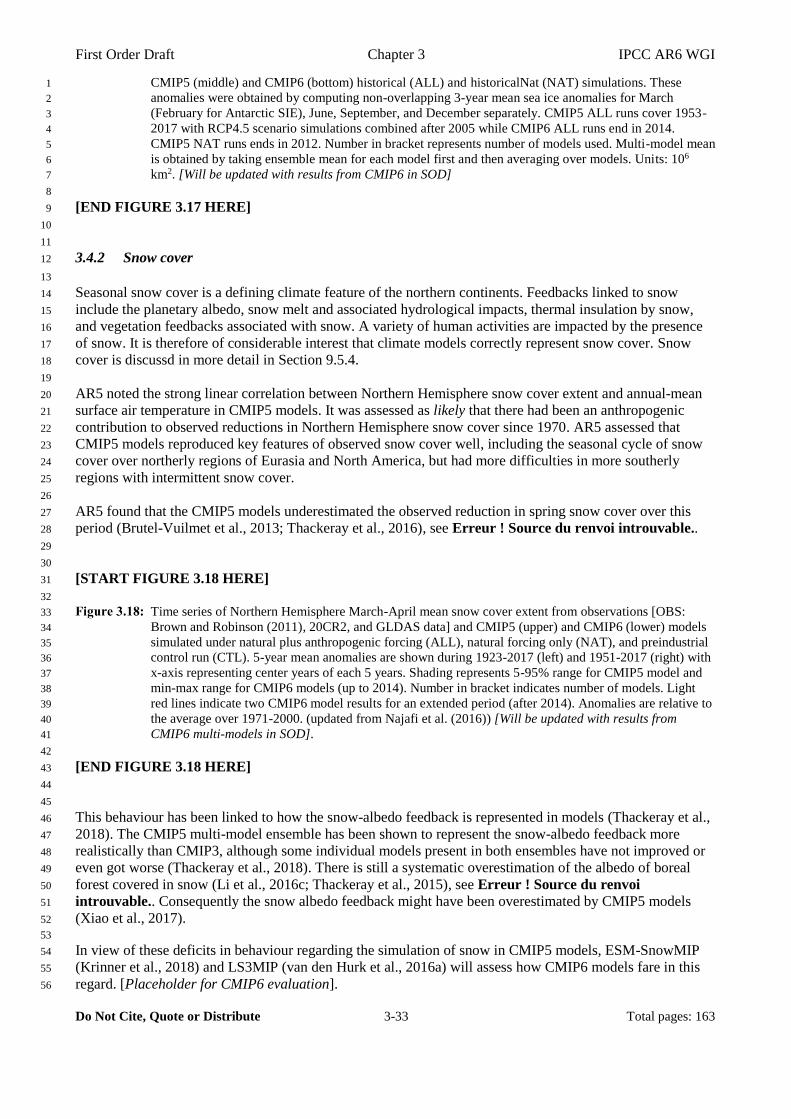
First Order Draft Chapter 3 IPCC AR6 WGI
Do Not Cite, Quote or Distribute 3-33 Total pages: 163
CMIP5 (middle) and CMIP6 (bottom) historical (ALL) and historicalNat (NAT) simulations. These 1
anomalies were obtained by computing non-overlapping 3-year mean sea ice anomalies for March 2
(February for Antarctic SIE), June, September, and December separately. CMIP5 ALL runs cover 1953-3
2017 with RCP4.5 scenario simulations combined after 2005 while CMIP6 ALL runs end in 2014. 4
CMIP5 NAT runs ends in 2012. Number in bracket represents number of models used. Multi-model mean 5
is obtained by taking ensemble mean for each model first and then averaging over models. Units: 106 6
km2. [Will be updated with results from CMIP6 in SOD] 7
8
[END FIGURE 3.17 HERE] 9
10
11
3.4.2 Snow cover 12
13
Seasonal snow cover is a defining climate feature of the northern continents. Feedbacks linked to snow 14
include the planetary albedo, snow melt and associated hydrological impacts, thermal insulation by snow, 15
and vegetation feedbacks associated with snow. A variety of human activities are impacted by the presence 16
of snow. It is therefore of considerable interest that climate models correctly represent snow cover. Snow 17
cover is discussd in more detail in Section 9.5.4. 18
19
AR5 noted the strong linear correlation between Northern Hemisphere snow cover extent and annual-mean 20
surface air temperature in CMIP5 models. It was assessed as likely that there had been an anthropogenic 21
contribution to observed reductions in Northern Hemisphere snow cover since 1970. AR5 assessed that 22
CMIP5 models reproduced key features of observed snow cover well, including the seasonal cycle of snow 23
cover over northerly regions of Eurasia and North America, but had more difficulties in more southerly 24
regions with intermittent snow cover. 25
26
AR5 found that the CMIP5 models underestimated the observed reduction in spring snow cover over this 27
period (Brutel-Vuilmet et al., 2013; Thackeray et al., 2016), see Erreur ! Source du renvoi introuvable.. 28
29
30
[START FIGURE 3.18 HERE] 31
32
Time series of Northern Hemisphere March-April mean snow cover extent from observations [OBS: 33
Brown and Robinson (2011), 20CR2, and GLDAS data] and CMIP5 (upper) and CMIP6 (lower) models 34
simulated under natural plus anthropogenic forcing (ALL), natural forcing only (NAT), and preindustrial 35
control run (CTL). 5-year mean anomalies are shown during 1923-2017 (left) and 1951-2017 (right) with 36
x-axis representing center years of each 5 years. Shading represents 5-95% range for CMIP5 model and 37
min-max range for CMIP6 models (up to 2014). Number in bracket indicates number of models. Light 38
red lines indicate two CMIP6 model results for an extended period (after 2014). Anomalies are relative to 39
the average over 1971-2000. (updated from Najafi et al. (2016)) [Will be updated with results from 40
CMIP6 multi-models in SOD]. 41
42
[END FIGURE 3.18 HERE] 43
44
45
This behaviour has been linked to how the snow-albedo feedback is represented in models (Thackeray et al., 46
2018). The CMIP5 multi-model ensemble has been shown to represent the snow-albedo feedback more 47
realistically than CMIP3, although some individual models present in both ensembles have not improved or 48
even got worse (Thackeray et al., 2018). There is still a systematic overestimation of the albedo of boreal 49
forest covered in snow (Li et al., 2016c; Thackeray et al., 2015), see Erreur ! Source du renvoi 50
introuvable.. Consequently the snow albedo feedback might have been overestimated by CMIP5 models 51
(Xiao et al., 2017). 52
53
In view of these deficits in behaviour regarding the simulation of snow in CMIP5 models, ESM-SnowMIP 54
(Krinner et al., 2018) and LS3MIP (van den Hurk et al., 2016a) will assess how CMIP6 models fare in this 55
regard. [Placeholder for CMIP6 evaluation]. 56
First Order Draft Chapter 3 IPCC AR6 WGI
Do Not Cite, Quote or Distribute 3-34 Total pages: 163
1
Observed Northern Hemisphere spring snow cover extent (SCE) changes (e.g., Hori et al., 2017) have been 2
consistently attributed to anthropogenic influences (Najafi et al., 2016; Rupp et al., 2013), the observed 3
changes being inconsistent with natural variability alone. Similarly, spring snow mass (SWE: Snow Water 4
Equivalent) changes on the scale of the Northern Hemisphere have been attributed to greenhouse gas forcing 5
(Jeong et al., 2017). In the Arctic (Brown et al., 2017), SWE changes are not expected to emerge from noise 6
before the mid-21st century. 7
8
In summary, an observed reduction of Northern Hemisphere snow cover in spring is likely associated with 9
anthropogenic warming of near-surface air. There is low confidence in the simulation of snow cover over the 10
Northern Continents, with significant deficits remaining regarding seasonality, geographical distribution, and 11
trends of snow cover. Although the above-mentioned shortcomings of the simulation of snow prompt the 12
low-confidence statement on the quality of these simulations, the models consistently link snow extent to 13
surface-air temperature. With surface air warming linked to anthropogenic influences, this implies that 14
reductions in snow cover are also caused by human activities. 15
16
17
3.4.3 Glaciers and Ice Sheets 18
19
Land surface ice in the form of glaciers has been included in simulations as components of the land models 20
in CMIP AOGCMs and ESMs for many years, however their representation is far simpler than observed and 21
omitted altogether in some less complex modelling systems. The Antarctic and Greenland ice sheets were 22
absent in AOGCMs and ESMs simulations that pre-date CMIP6 (Eyring et al., 2016a), however some 23
preliminary investigations that used results from CMIP5 were included in AR5 (Church et al., 2013b). In 24
CMIP3 (Meehl et al., 2007) and CMIP5 (Taylor et al., 2012) land ice area fraction was defined as a time-25
independent quantity, and in most model configurations was preset at initialization as a permanent land 26
feature. In CMIP6 (Eyring et al., 2016a), considerable progress has been made in improving and evaluating 27
the representation of land ice in models, in particular with the addition of the Ice Sheet Model 28
Intercomparison Project (ISMIP6) (Nowicki et al., 2016), which for the first time will lead to a coordinated 29
effort in temporally evolving ice sheet simulation and also ensure that a subset of observed glaciers and their 30
temporal change are also represented. Aspects of the cryospheric global water storage and contribution to 31
SLR, by glaciers and ice sheets have improved since AR5 with increasingly accurate estimates by models 32
and observations (Bamber et al., 2018a; Cazenave et al., 2018; Farinotti et al., 2019; Huss and Hock, 2015; 33
Shepherd et al., 2018) (see Section 3.5.3 and Sections 9.4.2 (Greenland) (high confidence in increased mass 34
loss since 1992), 9.4.3 (Antarctica) (likely accelerated mass loss of WAIS and Antarctic Peninsula, medium 35
confidence for EAIS contributing to mass loss), and 9.5.2 (Glaciers) (high confidence in glacier contribution 36
after 1992 and recent acceleration)), and are currently contributing 21% (glaciers) and 23% (ice sheets) 37
respectively to the global sea level rise budget for 1993 to 2016 (WCRP Global Sea Level Budget Group, 38
2018). These results are broadly consistent with the results found for 1993 to 2010 in AR5 (29%/0.86 mm yr-39
1 from glaciers and 20%/0.6 mm yr-1 from ice sheets), with a contribution from glaciers for the longer 1971 40
to 2010 period of 0.68 mm yr-1, and 0.69 mm yr-1 for 1901 to 1990. The mass balance and sea level 41
contributions of the Antarctic ice sheet have been extended back 40 years (Rignot et al., 2019) and 42
Greenland ice sheet the whole 20th century and a few decades before 1900 (Box and Colgan, 2013; Khan et 43
al., 2015; Kjeldsen et al., 2015). 44
45
46
3.4.3.1 Glaciers 47
48
Glaciers are defined as perennial surface land ice masses outside of the Antarctic and Greenland ice sheets. 49
Glaciers occur most often in high altitude, cold regions where climate and topographic characteristics allow 50
snow to accumulate over many years, and this snow is then transformed into firn (snow that persists for more 51
than a year) and finally to ice, which flows and possibly slides downhill under pull of gravity (Section 9.5.2). 52
The representation of glaciers in climate models is captured by the land sub-component or Land Surface 53
Models (LSMs), and for CMIP6 a small number of land sub-models are being used across the 100 54
contributing model configurations. In addition to ongoing glacier and land ice developments in full AOGCM 55
First Order Draft Chapter 3 IPCC AR6 WGI
Do Not Cite, Quote or Distribute 3-35 Total pages: 163
and ESM systems, independent collaborative research efforts such as GlacierMIP (Hock et al., 2019b) that 1
exist outside of the CMIP project are also underway. This project aims to systematically compare several 2
preceding modelling efforts. Compared to the relative abundance of ice sheet models, only very few models 3
capable of modelling glaciers on a global scale have been reported in the literature (for a review see Radić 4
and Hock 2014), with a key limitation being the observed record of global glacier changes prior to the 5
Randolf Glacier Inventory. which led to highly simplified approaches and extrapolation of results to regions 6
of no data coverage (Hock et al., 2019b). In Section 9.5.2.3 medium confidence is assigned to projections of 7
global glacier mass loss by the global glacier models due to differences among the models that are attributed 8
to differences in model physics, calibration and downscaling procedures (Hock et al., 2019a) 9
10
While direct attribution of glacier changes from the CMIP5 archive is not currently possible, offline 11
simulations forced by a subset of CMIP5 historical simulations were used to drive a model that represents all 12
global glaciers outside of Antarctica over the period 1851 to 2010, leading to the finding that 25 ± 35% of 13
the global glacier mass loss could be attributable to human causes, with this number increasing to 69 ± 24% 14
over the 1991 to 2010 period (Marzeion et al., 2014). A similar more regional study that considered 85 15
Northern Hemisphere glacier systems, also concluded a discernible human influence on glacier mass 16
balance, with CMIP5 historical and greenhouse gas -only simulations showing a negative trend, whereas 17
natural-only forced simulations showed a positive trend (Hirabayashi et al., 2016). In addition, statistical 18
assessment of the role of climate change in glacier retreat (Roe et al., 2016) concludes that observed length 19
changes would not have occurred without anthropogenic climate change. With these results it is concluded in 20
Section 9.5.2.4 that it is very likely (high confidence) that global glacier retreat during the 20th and beginning 21
of 21st century is a result of anthropogenic climate change. 22
23
24
3.4.3.2 Ice Sheets 25
26
Ice sheets are defined as a mass of glacial ice that extends over a region covering more than 50,000 km2. The 27
persistent ice sheets of Antarctica are the largest cryospheric mass store, followed by the ice sheets of 28
Greenland, which combined are two orders of magnitude larger than glaciers, the next largest global 29
reservoir. These structures contain more than 99% of the freshwater ice on Earth. Ice sheets play an active 30
role in sea level rise, with the Antarctic and Greenland ice sheets containing 58.3 m and 7.36 m of SLE 31
respectively (Vaughan et al., 2013). Ice sheet models have been developed in parallel to the CMIP project, 32
with intercomparisons activities extending across multiple decades, including the EISMINT (Huybrechts et 33
al., 1996; Payne et al., 2000; Saito et al., 2006), ISMIP-HOM (Pattyn et al., 2008) and MISMIP (Pattyn et 34
al., 2012) projects and SeaRise (Bindschadler et al., 2013; Nowicki et al., 2013). With CMIP6, ice sheet 35
modelling has formally become a contribution with ISMIP6 (Nowicki et al., 2016), marking the first time 36
that coupled ice-sheet-climate models have been part of the project. It is likely that at least 3 ice-sheet-37
climate models will be contributing to CMIP6, with PISM coupled to the HTESSEL LSM (Balsamo et al., 38
2015; Bueler and Brown, 2009; Winkelmann et al., 2011) land model in EC-Earth3-GrIS, CISM (Lipscomb 39
et al., 2013) in the CESM2 and various NorESM2 variants through the CLM LSM, and GRISLI (Boone et 40
al., 2017; Napoly et al., 2017) in CNRM-CM6-1 in the Surfex LSM. 41
42
Detection and attribution studies targeting the Greenland and Antarctic ice sheets remain challenging 43
(Kjeldsen et al., 2015). This is in part due to the short continental wide observational record (1992-present) 44
(Bamber et al., 2018b; Cazenave et al., 2018; Shepherd et al., 2012, 2018), and the limitations faced by 45
modelling efforts (Chapter 9.4.2.3 (Greenland) and 9.4.3.3 (Antarctica). The latter require not only dynamic 46
ice sheet models, but also appropriate atmospheric and oceanic forcing for ice sheet models (Nowicki and 47
Seroussi, 2018). Since the AR4 and AR5, a new generation of ice sheet models has been developed; with 48
recent improvements and current challenges reviewed for Antarctica (Pattyn et al., 2017) and Greenland 49
(Goelzer et al., 2017). Ice sheet models are being coupled as dynamic components of climate models, such 50
that scenario projections are becoming possible in a coupled framework (Vizcaino et al., 2015) as well as 51
being used for improving our understanding of interactions and feedbacks between ice sheets and the Earth 52
system (Fyke et al., 2018). In parallel to these developments, community efforts targeting AR5 with 53
standalone ice sheet models, such as the Sea level Response to Ice Sheet Evolution (SeaRISE) (Bindschadler 54
et al., 2013; Nowicki et al., 2013), laid the momentum for an effort that was more closely aligned with 55

First Order Draft Chapter 3 IPCC AR6 WGI
Do Not Cite, Quote or Distribute 3-36 Total pages: 163
CMIP, resulting in ISMIP6 (Nowicki et al., 2016). 1
2
The ISMIP6 framework targets both ice sheet models that are fully coupled to climate models and 3
simulations with standalone ice sheet models. Evaluation of standalone ice sheet models (Goelzer et al., 4
2018; Nowicki et al., 2013) is primarily focused on comparing the models’ initial state to present day ice 5
sheet geometry (extent, volume, thickness) and metrics such as observed surface velocities (Aschwanden et 6
al., 2016). Evaluations of coupled ice sheet-climate models (Vizcaino et al., 2015) also include an evaluation 7
of the polar climate with particular focus on surface processes, as these provide the surface mass balance and 8
temperature needed for the ice sheet models. This includes an evaluation of surface mass balance against 9
regional climate models (e.g Lipscomb et al. 2013; Vizcaíno et al. 2013; Lenaerts et al. 2016), with regional 10
climate models evaluated against measurements taken by automatic weather stations, ice core, snow radars 11
and satellite derived melt extent (e.g. Lenaerts et al. 2012; Fettweis et al. 2017). As the complexity of surface 12
mass balance schemes within climate models increases, other components such as surface albedo are also 13
being evaluated (Helsen et al., 2017). With increased availability of historical and contemporary surface 14
mass balance and temperature products (e.g. Vizcaíno et al. 2013; Fettweis et al. 2017) and the increasing 15
duration of observations of ice sheet wide mass change, it is now becoming possible to evaluate simulated 16
ice sheet temporal evolution against observations (Aschwanden et al., 2013; Schlegel et al., 2016). 17
18
19
3.5 Human Influence on the Ocean 20
21
The global ocean plays an important role in the climate system, as it is responsible for transporting and 22
storing large amounts of heat (Section 3.5.1.2), freshwater (Section 3.5.2) and carbon (Section 3.6.2) that are 23
exchanged with the atmosphere. The importance of the ocean in the climate system indicates that the 24
accurate simulation of the ocean in climate models is essential for the accurate representation of the climatic 25
response to anthropogenic warming, including the rate of warming, sea level rise and the representation of 26
coupled modes of climate variability. Since AR5 (Flato et al., 2013; Rhein et al., 2013) ocean model 27
development has considerably advanced, and a move toward more systematic evaluation, facilitated by the 28
Coordinated Ocean-Ice Reference Experiments (COREs) (Griffies et al., 2009) have expanded ocean multi-29
model assessment. With the application on the CORE-II interannual forcing protocol (1948-2007), studies 30
have focused on model intercomparison for sea level (Griffies et al., 2014), the North Atlantic mean state 31
and variability (Danabasoglu et al., 2014, 2016), the Southern Ocean watermass structure, Antarctic 32
Circumpolar Current (ACC) and meridional overturning (Downes et al., 2015; Farneti et al., 2015), North 33
and equatorial Pacific Ocean circulation (Tseng et al., 2016) and the Arctic Ocean, sea ice and freshwater 34
(Ilicak et al., 2016; Wang et al., 2014b, 2016). 35
36
With CMIP6, the coming of age of ocean modelling is highlighted by the inclusion of the Ocean Model 37
Intercomparison Project (OMIP) (Griffies et al., 2016), with ocean model intercomparison a formal endorsed 38
part of the project. Ongoing model development since AR5 has focused on improving the realism of the 39
simulated ocean, with horizontal nominal resolutions increasing to 25 to 100 km (from about 200 km in 40
CMIP5), and improved vertical resolutions of up to 1 m near-surface levels (from around 10 m in CMIP5) 41
aimed at improving representation of the diurnal cycle coupling to the atmosphere (e.g. Bernie et al. 2005, 42
2007, 2008). A recent comparison using a hierarchy of GFDL ocean models with horizontal resolutions 43
representing the CMIP5 contribution (nominal 1°) down to an eddy-permitting (0.1°), showed that with 44
increasing resolution, the high resolution model was able to recover the spatial distribution and variability 45
magnitude in sea surface height when compared to the satellite based AVISO measurements (Griffies et al., 46
2015). 47
48
In this section we assess the broad- or basin-scale properties of the simulated ocean, with a focus on 49
evaluation of the modelled realism in ocean properties, and the detection and attribution of a human-induced 50
signal in changes to observed and simulated ocean properties over the period of observational coverage. A 51
more process-based understanding of the changes reported here, alongside the assessment of variability and 52
changes of ocean properties with spatial scales smaller than ocean basin scale, are presented in Chapter 9. 53
54
55
First Order Draft Chapter 3 IPCC AR6 WGI
Do Not Cite, Quote or Distribute 3-37 Total pages: 163
3.5.1 Temperature 1
2
Potential temperature is one of the key physical ocean variables considered for climate model evaluation. 3
From CMIP3 (Meehl et al., 2007) to CMIP5 (Taylor et al., 2012), the zonally averaged ocean temperature 4
from the multi-model mean shows persistent warm biases between 200 m and 2000 m over most latitudes; 5
whereas cold biases are seen in the deep ocean and near the surface (see Erreur ! Source du renvoi 6
introuvable.) (Flato et al., 2013). 7
8
9
[START FIGURE 3.19 HERE] 10
11
Potential temperature (degrees C) and (b) salinity biases of CMIP5 r1i1p1 ensemble member and CMIP6 12
(only HadGEM2-CC, HadGEM2-ES, MPI-ESM-LR, CMCC-CESM) minus observed World Ocean Atlas 13
2013 (WOA09) fields (updated from Antonov et al., 2010; Locarnini et al., 2010). Shown in colour are 14
the time-mean differences between the multi model mean and observations, zonally averaged for the 15
global ocean (excluding marginal and regional seas). The observed climatological values are sourced 16
from the WOA13 and are shown as labelled black contours. White contours follow the colour scale at 17
regular intervals. The simulated annual mean climatologies are obtained for 1975-2000 from available 18
historical simulations. Figure produced with ESMValTool v2.0a1. 19
20
[END FIGURE 3.19 HERE] 21
22
23
CMIP5 models showed an improvement in the representation of the global upper layer (0 – 700m) ocean 24
heat content (OHC) compared to CMIP3 models, which is partly due to the inclusion of improved volcanic 25
forcings in most of the models. Overall, CMIP5 and observational estimates show an increase in OHC over 26
time (see Erreur ! Source du renvoi introuvable.) (Flato et al., 2013). Recent progress in the observational 27
estimates, however, shows that the changes in OHC estimates of the upper ocean layer since 1970 have been 28
underestimated due to poor sampling in the Southern Hemisphere and a limitation in the methods for 29
infilling sparse-data (Cheng et al., 2016; Durack et al., 2014a). Estimations of long-term OHC change 30
presented in AR5 could therefore be biased low, which is supported by an increasing consistency between 31
model simulated changes and new observed estimates (Section 3.5.1.2). 32
33
34
[START FIGURE 3.20 HERE] 35
36
Time series of simulated and observed global ocean heat content anomalies (with respect to 1971). 37
CMIP5 historical simulations and observations for both the upper 700 m of the ocean (a) as well as for 38
the total ocean heat content (b). The 0 to 700 m and total heat content observational estimates (thick lines) 39
are respectively described in AR5 Figure 3.2 and AR5 Box 3.1, Figure 1. Simulation drift has been 40
removed from all CMIP5 runs with a contemporaneous portion of the quadratic fit to each corresponding 41
pre-industrial control run (Gleckler et al., 2012). Units are 1022 Joules. [Will be replaced with results 42
from CMIP6 in SOD] 43
44
45
[END FIGURE 3.20 HERE] 46
47
48
3.5.1.1 Simulation of Tropical Mean State 49
50
Tropical Pacific 51
In CMIP5, mean state biases in the tropical Pacific Ocean including the excessive equatorial cold tongue, 52
erroneous mean thermocline depth and slope along the equator are improved relative to CMIP3, but still 53
remain. Misrepresentation of the interaction between the atmosphere and ocean via a Bjerknes feedback, 54
vertical mixing parameterization, and a bias in winds are among the suggested reasons for these biases (Li et 55
al., 2014; Zhu and Zhang, 2018). 56
First Order Draft Chapter 3 IPCC AR6 WGI
Do Not Cite, Quote or Distribute 3-38 Total pages: 163
In CMIP6, [Placeholder for CMIP6] 1
2
Tropical Atlantic 3
Fundamental features such as the mean zonal SST gradient in the tropical Atlantic are not reproduced in 4
CMIP5 (see Erreur ! Source du renvoi introuvable.). Studies have proposed that weaker than observed 5
alongshore winds, underestimation of stratocumulus clouds, coarse model resolution, and insufficient 6
oceanic cooling due to a deeper thermocline depth and too weak vertical velocities at the base of the mixed 7
layers in the eastern basin, could lead to the tropical Atlantic biases (Hourdin et al., 2015; Richter, 2015). 8
In CMIP6, [Placeholder for CMIP6] 9
10
Tropical Indian Ocean 11
The tropical Indian Ocean mean state appears to be reasonably well simulated both in CMIP3 and CMIP5 12
(see Erreur ! Source du renvoi introuvable.). However the models show a large spread in the thermocline 13
depth, particularly in the equatorial part of the basin (Fathrio et al., 2017a; Saji et al., 2006), which could be 14
partly due to the parameterizations of the vertical mixing and the wind structure (Schott et al., 2009). 15
In CMIP6, [Placeholder for CMIP6] 16
17
18
[START FIGURE 3.21 HERE] 19
20
(a) Zonally averaged sea surface temperature (SST) error in CMIP5 models. (b) Equatorial SST error in 21
CMIP5 models. (c) Zonally averaged multi-model mean SST error for CMIP5 (red curve) and CMIP3 22
(blue curve), together with inter-model standard deviation (shading). (d) Equatorial multi-model mean 23
SST in CMIP5 (red curve), and CMIP3 (blue curve) together with inter-model standard deviation 24
(shading) and observations (black). Model climatologies are derived from 1979-1999 mean of the 25
historical simulations. The Hadley Centre Sea Ice and Sea Surface Temperature (HadISST) (Rayner et al., 26
2003) observational climatology for 1979-1999 is used as the reference for the error calculation (a), (b) 27
and (c); and for observations (d). [Will be replaced with results from CMIP6 in SOD] 28
29
30
[END FIGURE 3.21 HERE] 31
32
33
3.5.1.2 Changes in Temperature and Ocean Heat Content 34
35
The ocean plays an important role as the Earth’s primary energy store. It contains more than 90% of the heat 36
associated with greenhouse-gas-attributed warming over the observational record (Abraham et al., 2013; 37
Allan et al., 2014; Balmaseda et al., 2013; Otto et al., 2013; Palmer and McNeall, 2014a; Rhein et al., 2013; 38
Trenberth et al., 2014a; von Schuckmann et al., 2016). In recent decades, observational studies show a 39
continued increase in OHC, not only in the ocean upper layers but also in the intermediate and deeper layers 40
(Cheng et al., 2016, 2017; Gleckler et al., 2016b; Palmer et al., 2017; von Schuckmann et al., 2016). Despite 41
the uncertainties in ocean analysis products (Good, 2017), the observed increase in near surface temperature 42
and OHC is robust (Jones and Kennedy, 2017; Wang et al., 2018b), however regional inconsistencies in the 43
rate of OHC change are seen in the Pacific and Southern Ocean, along with differences in the vertical 44
distribution of warming when contrasting three global reconstructions since 1970 (Wang et al., 2018b). 45
Observed OHC changed are discussed in Section 2.3.3.1, where it is reported that it is virtually certain that 46
that the global ocean warmed substantially between 1971 to present. Further to this, a high confidence is 47
reported that layer contributions are approximately 60% (0-700m), 30% (700-2000m) and 10% (2000-48
6000m) (Section 2.3.3.1). The spatial distribution of these changes for different ocean depths are assessed in 49
Section 9.2.3. 50
51
The AR5 concluded that anthropogenic forcing has very likely made a substantial contribution to upper 52
ocean warming. Below 700 m, limited measurements restricted the assessment of OHC changes and restrain 53
a robust comparison between observational estimates and model outputs. The recent increase in ocean 54
sampling by Argo up to 2000 m (Riser et al., 2016; Roemmich et al., 2015; von Schuckmann et al., 2016) 55
with the improvements in the recent estimates of ocean heat content (Balmaseda et al., 2013; Cheng et al., 56
First Order Draft Chapter 3 IPCC AR6 WGI
Do Not Cite, Quote or Distribute 3-39 Total pages: 163
2017; Durack et al., 2014a) allow the quantitative assessment of the global OHC changes to extend into the 1
intermediate ocean (700 to 2000 m) over the more recent period (from 2005 to the present) (Durack et al., 2
2018). SROCC (Chapter 5), therefore, assessed that it is virtually certain that both the upper and 3
intermediate ocean warmed from 2004 to 2016. In fact, the upper OHC has continued to increase through the 4
so called “hiatus” period (Cross-Chapter Box 3.1). SROCC also stated with high confidence that the abyssal 5
ocean (below 4000m), particularly the Southern Hemisphere, continues to warm. 6
7
Since AR5, the attribution of OHC increase to anthropogenic forcings has been supported by more evidence 8
from detection and attribution studies. Gleckler et al. (2016b) examined the OHC changes in the context of 9
Earth’s global energy budget for the industrial era (1865-2015). Output from CMIP5 historical simulations 10
forced with time varying natural and anthropogenic forcing were compared with OHC from a suite of 11
updated observational analyses over the period 1960 to 2015 (Domingues et al., 2008; Ishii and Kimoto, 12
2009; Purkey and Johnson, 2010; Roemmich et al., 2012, 2015). They found that the upper to intermediate (0 13
to 2000 m) OHC changes from the multi-model mean are consistent with the observed estimates. Deep 14
observed estimates (2000 m to bottom), while only available for the period of 1992 to 2005, also share 15
remarkable similarity to the rate of coincident simulated change. The CMIP5 historical simulations also 16
suggest that the full depth ocean warming since the pre-industrial period, half of which occurred since 1997, 17
is mainly due to greenhouse gas forcing. The deeper ocean layer (below 2000 m) is found to contribute 18
around one third of the heat uptake and its heat content was rapidly increasing through the analysis period 19
(Erreur ! Source du renvoi introuvable.). While observational coverage cannot replicate this model-based 20
1865-2015 assessment, there is good agreement since 1960 for upper ocean (0 to 700 m) OHC change, and 21
though short, good agreement with the deeper ocean (2000 m to bottom) from 1992 to the present (Gleckler 22
et al., 2016b). 23
24
More recently, (Tokarska et al., 2019) analyzed the contribution of different forcings, including all-forcing 25
(natural and anthropogenic), natural only, greehouse gas and other anthropogenic to ocean warming at 0-26
2000m depth. Using the regularized optimal fingerprint method, an anthropogenic signal in ocean warming 27
was detected and found to be attributable to contributions from aggregate anthropogenic forcing and 28
greenhouse gas. The warming signal in the greenhouse gas forcing experiments penetrates deeper in the 29
North Atlantic than other basins. Natural forcing is found to have made only a small contribution. 30
31
At a basin scale, the Indo-Pacific Warm Pool warming and expansion is found to be dominantly caused by 32
greenhouse gas forcing with a small effect of the natural fluctuations (Weller et al., 2016). Whereas, 33
warming in the Southern Ocean is attributed to greenhouse gas emissions and ozone depletion (Swart et al., 34
2018). By using an isothermal approach for a multi-model ensemble detection and attribution analysis, 35
Weller et al. (2016b) found a robust influence of both anthropogenic and natural forcings on the upper ocean 36
warming. 37
38
The recent growing evidence and understanding on the increase in global OHC confirm that it is very likely 39
that the anthropogenic forcing has made a substantial contribution to the OHC increase that extends to the 40
deeper ocean. 41
42
43
[START FIGURE 3.22 HERE] 44
45
(a) Ocean heat uptake (percentage of total 1865-2017 change) for the CMIP5 multi-model mean layers. 46
The three shaded wedges are combined similarly to the AR5 change in global inventory (Rhein et al. 47
(2013); Box 3.1, Figure 1). The thick vertical grey bar represents a +/- one standard deviation spread from 48
the CMIP5 simulations about the year (1999) at which the multi-model heat uptake reaches 50% of the 49
net (1865-2017) industrial-era increase, and the thick horizontal grey bar indicates the CMIP5 +/- one 50
standard deviation spread om the year at which 50% of the total accumulated heat is reached. Black 51
(forcing included) and grey (forcing not included) triangles represent major twentieth- and twenty-first-52
century volcanic eruptions with magnitude (volcanic explosivity index [VEI] represented by symbol size. 53
(b) The inset box displays the upper and intermediate layer warming for the years 1998 to 2017, with an 54
adjustment for the 0 to 2000 m total warming by -0.19 W m-2, the estimated discrepancy between CMIP5 55
modelled and the observed volcanic forcing (Ridley et al., 2014). When observed 0 to 2000 m ocean 56

First Order Draft Chapter 3 IPCC AR6 WGI
Do Not Cite, Quote or Distribute 3-40 Total pages: 163
warming is compared across five independent available estimates these rates of change are approximately 1
equal. Reproduced from Durack et al., 2018. [Will be replaced with results from CMIP6 in SOD] 2
3
4
[END FIGURE 3.22 HERE] 5
6
7
3.5.2 Salinity 8
9
While the primary focus of ocean assessments has considered temperature, with the advent of improving 10
observational salinity products since the early 2000s, recent assessments of long-term ocean salinity change 11
and variability have received increasing attention from AR4 (Bindoff et al., 2007) to AR5 across both 12
models and observations (Flato et al., 2013; Rhein et al., 2013). AR5 assessed that it was very likely that 13
anthropogenic forcings have made a discernible contribution to surface and subsurface oceanic salinity 14
changes since the 1960s. Since AR5 the assessment of observed broad- and basin-scale salinity changes has 15
considerably expanded, with many new studies reproducing the key patterns of long-term salinity change 16
reported in AR5 (Rhein et al., 2013), and linking these through modelling studies to coincident changes to 17
evaporation-precipitation patterns at the ocean surface (see Section 2.3.4). The advancement in knowledge 18
since AR5 has led to a strengthening of evidence, supporting an assessment that it is extremely likely that 19
there is discernible human influence on observed surface and subsurface oceanic salinity changes since the 20
mid-20th century (Section 2.3.3.2), driven by coincident water cycle change at the ocean-atmosphere 21
interface (see Section 8.1.2). 22
23
Unlike sea surface temperature (SST), simulated sea surface salinity (SSS) does not provide a direct 24
feedback to the atmosphere. The absence of a feedback is the key reason why salinity simulation is difficult 25
in both coupled and ocean-only modelling systems, and why deviations from the observed near-surface 26
salinity mean state between models and observations are apparent (Durack et al., 2012; Shi et al., 2017). Due 27
to the recent availability of a number of surface salinity satellite products (SMOS, Aquarius and SMAP) 28
(Berger et al., 2002; Lagerloef et al., 2008; Tang et al., 2017), recent modelling studies have been 29
investigating the role of surface salinity in the diurnal cycle and atmosphere-ocean coupling (Bellenger et al., 30
2017; Fine et al., 2015; Large and Caron, 2015; Song et al., 2015). Following dedicated observational 31
campaigns (see Chapter 1), modelling studies have also started investigating the processes that maintain the 32
high mean salinity regime in the North Atlantic in a global ocean model (Bryan and Bachman, 2015; Qu et 33
al., 2011, 2013). 34
35
While absolute rates of multi-decadal salinity change cannot be ascertained definitively from the sparse 36
historical observing system, all observational studies have documented a clear pattern of salinity 37
amplification in the near-surface and subsurface ocean, with fresh regions becoming fresher and salty 38
regions saltier. Even when considering unforced natural variability of NAO and AMO modes from the best-39
sampled Atlantic Ocean over the complete 20th and early 21st century, this salinity pattern amplification is 40
clear. Salinity amplification patterns are replicated across numerous climate model studies and have been 41
shown to have a strong dependence on coincident changes to the evaporation-precipitation field which 42
defines the global water cycle. Further discussion of water cycle changes can be found in Section 8.1.2 and a 43
comprehensive discussion of regional ocean changes is found in Section 9.2. 44
45
46
3.5.2.1 Simulation of Surface and Depth-profile Salinity 47
48
For the first time in AR5, alongside global zonal mean temperature, global zonal mean salinity through depth 49
was also assessed for the CMIP5 models. This showed a strong upper ocean (< 300 m) negative fresh bias of 50
order 0.3 PSS-78 (see Section 2.3.4.2, with a tendency toward a positive salty bias (< 0.25 PSS-78) in the 51
Northern Hemisphere intermediate layers (200 to 2000 m) (Erreur ! Source du renvoi introuvable.) (Flato 52
et al., 2013). While these biases are evident in the CMIP5 multi-model mean (which averages across many 53
simulations with differing subsurface geographies), it must be noted that assessing each simulation field 54
independently yields a subsurface salinity structure and salinity minima subduction pathways that 55

First Order Draft Chapter 3 IPCC AR6 WGI
Do Not Cite, Quote or Distribute 3-41 Total pages: 163
approximate observations, albeit with large regional differences expressed across models that contributed to 1
CMIP5 (e.g., Sallée et al., 2013b). 2
3
When evaluating simulated ocean salinity fields, it is useful to consider available observational products, and 4
their representativeness when compared to a 1-degree horizontal, 5 m vertical resolution and monthly mean 5
CMIP salinity simulation. Many ocean surface properties such as SST and SSS are based on remotely sensed 6
satellite retrievals reflecting swath measurements of the surface ocean skin properties (top cm) and complete 7
their global coverage over a 7-day or similar time period. These measurements are composited to provide 8
weekly or monthly maps, with the resulting observational products representing the surface layer, much 9
shallower than a typical simulated ocean model top layer, but with comparable horizontal scales of 10
approximately 100 km. In the case of in situ measurements, gridded products developed from Argo floats 11
aim to reproduce monthly mean maps of the upper 2000 m ocean state, with Argo floats providing a point 12
source in space and time measurement, which may be influenced by ocean eddies, fronts and other features 13
not explicitly resolved in CMIP-class models. This temporal and spatial scale mismatch adds a level of 14
complexity when attempting to relate high frequency, point measurement salinity measurements from in-situ 15
and remote observations, to those of CMIP-class models which represent grid-box averaged fields. 16
17
When compared to the assessment of simulated SST, simulated SSS has not been systematically investigated 18
at global- to basin-scales. For CMIP3, there was reasonable agreement between the basin-scale patterns of 19
salinity, with a comparatively fresher Pacific when contrasted to the salty Atlantic, and basin salinity 20
maxima features aligning well with the corresponding evaporation-precipitation field (Durack et al., 2012). 21
Similar features are also reproduced in CMIP5 along with realistic variability in the upper layers, but less 22
than observations at 300 m and deeper, especially in the poorly sampled Antarctic region (Pierce et al., 23
2012). In a regional study, only considering the Indian Ocean, CMIP5 SSS was assessed and it was shown 24
that model biases were primarily linked to biases in the precipitation field, with ocean circulation biases 25
playing a secondary role (Fathrio et al., 2017b). For the Southern Ocean, Sallee et al. (2013b) found that 26
considerable fresh biases exist through the water column, and are most pronounced in the ventilated layers 27
representing the subtropical, mode and intermediate water masses. 28
29
30
3.5.2.2 Changes to Ocean Salinity 31
32
AR5 (Bindoff et al., 2013; Rhein et al., 2013) concluded that it was very likely that anthropogenic forcings 33
had made a discernible contribution to surface and subsurface ocean salinity changes since the 1950s and 34
1960s. They highlighted that the spatial patterns of salinity trends, along with the mean fields of salinity and 35
evaporation-precipitation (E-P) are all similar, with an enhancement to Atlantic Ocean salinity, and a 36
freshening in the Pacific and Southern Oceans. Since AR5 all subsequent work focused on assessing 37
observed and modelled salinity changes has confirmed these results. 38
39
Considerable changes to observed broad- or basin-scale ocean near-surface salinity fields have been reported 40
(see Chapter 2), and these have been linked to changes in the evaporation-precipitation patterns at the ocean 41
surface through model simulations (Erreur ! Source du renvoi introuvable.). The depth-integrated effect 42
of mean salinity changes as captured in halosteric sea level for the top 0 to 2000 m has also been assessed, 43
and these results mirror near-surface patterns (Durack et al., 2014b) (Erreur ! Source du renvoi 44
introuvable.). Further investigations using observations and models together have tied the long-term 45
patterns of surface and subsurface salinity changes to coincident changes to the evaporation-precipitation 46
field over the ocean (Durack, 2015; Durack et al., 2012, 2013; Grist et al., 2016; Levang and Schmitt, 2015; 47
Zika et al., 2015), however the rate of these changes through time continues to be an active area of research 48
(Skliris et al., 2014, 2016, Zika et al., 2015, 2018). 49
50
Climate change detection and attribution assessments have considered salinity, with the first of these 51
assessed in AR5 (Bindoff et al., 2013). Since this time the positive detection conclusions of (Pierce et al., 52
2012; Stott et al., 2008; Terray et al., 2012) are supported by a number of more recent and independent 53
assessments which have replicated the reported basin-scale patterns of change in observations and models 54
(Erreur ! Source du renvoi introuvable.) (Durack, 2015). Basin depth-integrated contrasting responses, 55

First Order Draft Chapter 3 IPCC AR6 WGI
Do Not Cite, Quote or Distribute 3-42 Total pages: 163
with emphasis on the Pacific and Atlantic basin contrasts (freshening Pacific and enhanced salinity Atlantic) 1
were also shown to be replicated in all (natural and anthropogenic) simulations, and no contrast apparent in 2
CMIP5 natural only simulations that excluded the greenhouse gas forcing (Durack et al., 2014b) (Erreur ! 3
Source du renvoi introuvable.). 4
5
Considering the bulk of evidence, it is extremely likely that near-surface and subsurface salinity changes 6
driven by human activities have occurred across the globe since the mid-20th century. All available multi-7
decadal assessments have confirmed that there are coherent large-scale patterns of fresh ocean regions 8
becoming fresher and salty ocean regions saltier across the globe. This result is supported by all available 9
observational assessments, along with a growing number of CMIP5 and idealised climate modelling studies 10
targeted at assessing ocean and water cycle changes. While observational sparsity considerably limits 11
quantifying all regional changes, a recent study by (Friedman et al., 2017) assessed salinity changes in the 12
Atlantic Ocean from 1896 to 2013 and confirmed the pattern of mid-to-low latitude enhanced salinity, and 13
high latitude north Atlantic freshening over the period exists, even after removing the effects of variability 14
modes NAO and AMO. 15
16
17
[START FIGURE 3.23 HERE] 18
19
Maps of 50-year salinity trends for the near-surface ocean. (a) the 1950-2000 observational change and 20
(b) the corresponding 1950-2000 climatological mean (Durack & Wijffels, 2010) ( analysis period 1950-21
2008). (c) Modelled changes for the 1950-2000 period from the CMIP5 historical experiment multi-22
model mean, and (d) 2050-2099 future projected changes for the most strongly forced CMIP5 RCP85 23
experiment multi-model mean. Black contours bound the climatological mean salinity associated with 24
each map, and white contours bound the salinity trend in increments of 0.25 (PSS-78). [Will be replaced 25
with results from CMIP6 in SOD] 26
27
[END FIGURE 3.23 HERE] 28
29
30
[START FIGURE 3.24 HERE] 31
32
Long-term trends in 0 to 2000 dbar total halosteric (salinity-driven) sea level anomaly, and the contrast of 33
basin-integrated results for the Pacific and Atlantic Oceans compared to CMIP5 models. Units are mm 34
year-1. Maps of 0 to 2000 dbar halosteric anomalies (left column, a3, b3 and c3) from (Ishii and Kimoto, 35
2009, a3), (Durack and Wijffels, 2010a, b3) and the CMIP5 historical multi-model mean (c3). Blue 36
colours show a halosteric contraction (enhanced salinity) and orange a halosteric expansion (reduced 37
salinity). Stippling is used to mark regions where the two observational estimates do not agree in their 38
sign (a3, b3) and where less than 50% of the contributing models do not agree in sign with the multi-39
model mean map from the ensemble. Basin-integrated halosteric anomalies for the Pacific (right column, 40
top panel A), where Pacific anomalies are presented on the x-axis and Atlantic on the y-axis. 41
Observational estimates are presented in the red (Ishii & Kimoto, 2009) and black (Durack & Wijffels, 42
2010) diamonds, CMIP5 historical models are shown in grey diamonds, with the multi-model mean in 43
dark grey, and CMIP5 historicalNat models are shown in green diamonds with the multi-model mean in 44
dark green. [Will be replaced with results from CMIP6 in SOD] 45
46
[END FIGURE 3.24 HERE] 47
48
49
3.5.3 Sea Level 50
51
In the AR5, the observed sea level budget was closed by considering all contributing factors including ocean 52
warming, mass contributions from terrestrial storage, glaciers and ice caps, and the Antarctic and Greenland 53
ice sheets (Church et al., 2013a). A complication with modelling sea level change is that many of the 54
necessary components, such as glaciers, ice sheets and land water storage required to close the observed 55
budget were partially resolved or missing from CMIP5 modelling systems (see Section 3.4.3). Consequently, 56
most CMIP-based analyses have focused on the thermosteric sea level changes, driven by ocean warming, 57

First Order Draft Chapter 3 IPCC AR6 WGI
Do Not Cite, Quote or Distribute 3-43 Total pages: 163
which are simulated in CMIP5-generation models. Slangen et al. (2017) and Meyssignac et al. (2017) 1
analyzed the CMIP5 models' simulations of global and regional sea level changes respectively and suggest 2
that including corrections to several contributions to sea level changes including to the Greenland surface 3
mass balance and glacier contributions, based on differences between CMIP5-driven results and reanalysis-4
driven results, helps close the gap between models and observations but that the model simulated regional 5
scale interannual and multi-decadal variability compare reasonably well against tide gauge observations. 6
7
While CMIP5 models did not include all necessary components, some meta-studies using offline mass inputs 8
to account for glacier and terrestrial contributions, alongside CMIP5 simulations, recreated sea level change 9
within 20% of observed estimates, and if an estimate for ice sheet contributions since 1993 are also added, 10
this reduces to about 10% (Church et al., 2013b). These models have some utility in capturing the ocean 11
responses to climate change. The CCSM3 (Hu and Deser, 2013) CMIP3 and CESM1 (Hu and Bates, 2018) 12
CMIP5 models have also been used to investigate the role of internal climate variability on the regional 13
patterns of dynamic sea level rise. In the CCSM3 assessment they found that sea level changes in the North 14
Atlantic and Pacific have a higher forcing sensitivity to other parts of the global ocean, and that mid-century 15
sea level change can vary by a factor of 2 in some locations. For CESM1, forcing-driven intensified internal 16
variability and resulting ocean dynamical changes, led to a large spread in the Western Pacific Warm Pool 17
and off Western Australia for their large model ensemble results. 18
19
[For CMIP6 – also refer to Chapter 9 Ocean, cryosphere and sea level change] 20
21
3.5.3.1 Simulation of Components of the sea Level Budget 22
23
As noted above, sea level change is a product of many varied processes and coupled model subcomponents, 24
with many of the processes absent in CMIP5. In CMIP6, ice sheets (see Section 3.4.3.2) will be included for 25
the first time in the dedicated Ice Sheet Model Intercomparison Project (ISMIP6) (Nowicki et al., 2016). 26
There is also scope for new insights of terrestrial water contributions from land surface (and sub-surface) 27
modelling in the Land Surface, Snow and Soil moisture Model Intercomparison Project (LS3MIP) (van den 28
Hurk et al., 2016b), providing a more comprehensive assessment of land surface snow and soil moisture 29
feedbacks, as well as diagnosing systematic biases in land models. This effort is a formal CMIP6 expansion 30
of the GLACE-CMIP (Seneviratne et al., 2013) and the Global Soil Wetness Project Phase 3 (GSWP3) (e.g. 31
Dirmeyer et al. 2006). In parallel, the GlacierMIP project (Hock et al.) (see Section 3.4.3.1) is also 32
underway, and will provide more quantitative guidance and a comprehensive assessment of the uncertainties 33
and best estimates of the sea level budget. 34
35
[For CMIP6 – also refer to Chapter 9 Ocean, cryosphere and sea level change] 36
37
38
3.5.3.2 Sea Level Change 39
40
The AR5 concluded that it is very likely that there is a substantial contribution from anthropogenic forcings 41
to the global mean sea level rise since the 1970s. Since the AR5, several studies have successfully identified 42
a human contribution to observed sea level change, manifest in thermosteric sea level (thermal expansion 43
due to warming) which can be separated into global mean and spatial pattern assessments. For the global 44
mean assessments, Slangen et al. (2014) show the importance of anthropogenic (combined greenhouse gas 45
and aerosol forcings) to explain the magnitude of the observed changes between 1957-2005 and natural 46
forcings in order to capture the variability. Dangendorf et al. (2015) identified that for 1900 to 2011 it is 47
virtually certain (P = 0.99) that at least 45% is human-induced and extremely likely (P = 0.95) that at least 48
61% is human-induced. Over the shorter 1950-2005 time period, Marcos and Amores (2014) assigned 49
human influence to be a larger percentage (87%). Slangen et al. (2016) considered all quantifiable 50
components of the sea level budget and showed that anthropogenic forced changes account for 69 ± 31% 51
during 1970 to 2005, whereas natural forcings combined with internal climate variability have a much 52
smaller impact only contributing 9 ± 18% of the change over the same period (see also Erreur ! Source du 53
renvoi introuvable.). Both thermosteric and regional dynamic patterns of sea level change in individual 54
forcing experiments from CMIP5 were considered by Slangen et al. (2015) who showed that responses to 55
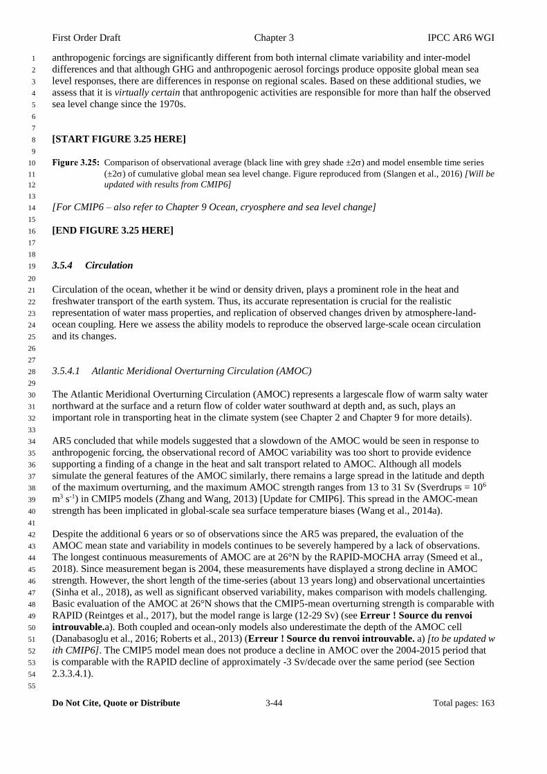
First Order Draft Chapter 3 IPCC AR6 WGI
Do Not Cite, Quote or Distribute 3-44 Total pages: 163
anthropogenic forcings are significantly different from both internal climate variability and inter-model 1
differences and that although GHG and anthropogenic aerosol forcings produce opposite global mean sea 2
level responses, there are differences in response on regional scales. Based on these additional studies, we 3
assess that it is virtually certain that anthropogenic activities are responsible for more than half the observed 4
sea level change since the 1970s. 5
6
7
[START FIGURE 3.25 HERE] 8
9
Comparison of observational average (black line with grey shade ±2) and model ensemble time series 10
(±2) of cumulative global mean sea level change. Figure reproduced from (Slangen et al., 2016) [Will be 11
updated with results from CMIP6] 12
13
[For CMIP6 – also refer to Chapter 9 Ocean, cryosphere and sea level change] 14
15
[END FIGURE 3.25 HERE] 16
17
18
3.5.4 Circulation 19
20
Circulation of the ocean, whether it be wind or density driven, plays a prominent role in the heat and 21
freshwater transport of the earth system. Thus, its accurate representation is crucial for the realistic 22
representation of water mass properties, and replication of observed changes driven by atmosphere-land-23
ocean coupling. Here we assess the ability models to reproduce the observed large-scale ocean circulation 24
and its changes. 25
26
27
3.5.4.1 Atlantic Meridional Overturning Circulation (AMOC) 28
29
The Atlantic Meridional Overturning Circulation (AMOC) represents a largescale flow of warm salty water 30
northward at the surface and a return flow of colder water southward at depth and, as such, plays an 31
important role in transporting heat in the climate system (see Chapter 2 and Chapter 9 for more details). 32
33
AR5 concluded that while models suggested that a slowdown of the AMOC would be seen in response to 34
anthropogenic forcing, the observational record of AMOC variability was too short to provide evidence 35
supporting a finding of a change in the heat and salt transport related to AMOC. Although all models 36
simulate the general features of the AMOC similarly, there remains a large spread in the latitude and depth 37
of the maximum overturning, and the maximum AMOC strength ranges from 13 to 31 Sv (Sverdrups = 106 38
m3 s-1) in CMIP5 models (Zhang and Wang, 2013) [Update for CMIP6]. This spread in the AMOC-mean 39
strength has been implicated in global-scale sea surface temperature biases (Wang et al., 2014a). 40
41
Despite the additional 6 years or so of observations since the AR5 was prepared, the evaluation of the 42
AMOC mean state and variability in models continues to be severely hampered by a lack of observations. 43
The longest continuous measurements of AMOC are at 26°N by the RAPID-MOCHA array (Smeed et al., 44
2018). Since measurement began is 2004, these measurements have displayed a strong decline in AMOC 45
strength. However, the short length of the time-series (about 13 years long) and observational uncertainties 46
(Sinha et al., 2018), as well as significant observed variability, makes comparison with models challenging. 47
Basic evaluation of the AMOC at 26°N shows that the CMIP5-mean overturning strength is comparable with 48
RAPID (Reintges et al., 2017), but the model range is large (12-29 Sv) (see Erreur ! Source du renvoi 49
introuvable.a). Both coupled and ocean-only models also underestimate the depth of the AMOC cell 50
(Danabasoglu et al., 2016; Roberts et al., 2013) (Erreur ! Source du renvoi introuvable. a) [to be updated w51
ith CMIP6]. The CMIP5 model mean does not produce a decline in AMOC over the 2004-2015 period that 52
is comparable with the RAPID decline of approximately -3 Sv/decade over the same period (see Section 53
2.3.3.4.1). 54
55

First Order Draft Chapter 3 IPCC AR6 WGI
Do Not Cite, Quote or Distribute 3-45 Total pages: 163
The discrepancy between modelled ensemble means and observations has led studies to suggest that the 1
observed weakening over 2004-2015 is largely due to internal variability (Yan et al., 2018). However, 2
comparison of observed RAPID AMOC variability with modelled variability reveals that CMIP5 models 3
also appear to underestimate the interannual and decadal timescale variability (Roberts et al., 2014; Yan et 4
al., 2018) (Erreur ! Source du renvoi introuvable.b,c). It is currently unknown why models underestimate 5
this variability, but it is thought to at least partly stem from underestimated wind variability and the NAO 6
(see Section 3.3.3.3). This underestimation of AMOC variability likely also has implications for detection 7
and attribution, the relationship between AMOC and AMV (see Section 3.7.7Erreur ! Source du renvoi 8
introuvable.), and near-term predictions. 9
10
The AMOC in models is sensitive to natural (Menary and Scaife, 2014; Swingedouw et al., 2017) and 11
anthropogenic external forcing (Caesar et al., 2018; Menary et al., 2013; Undorf et al., 2018b). However, the 12
response between models can be different and, hence, the relative importance of these external forcings and 13
AMOC’s evolution in models is uncertain. Although changes in solar, volcanic and anthropogenic aerosol 14
emissions can lead to temporary increases in AMOC on decadal-to-multidecadal timescales (Menary and 15
Scaife, 2014; Swingedouw et al., 2017), there is general agreement that anthropogenic forcing dominated by 16
the influence of GHG will lead to a weakening of the modelled AMOC by 2100 (Collins et al., 2013). 17
Indirect proxies of observed AMOC, such as relative temperature indices, that are calibrated with CMIP5 18
historical and RCP simulations also suggest that AMOC has weakened over the period 1870 – 2015 by 19
approximately 15% (Caesar et al., 2018). 20
21
There is also emerging evidence, based on analysis of freshwater transports, that the AMOC in CMIP5-era 22
models is too stable, largely due to systematic biases in ocean salinity (Liu et al., 2017; Mecking et al., 23
2017). Such a systematic bias may potentially be linked with the underestimation of simulated AMOC 24
internal variability and externally forced change. 25
26
A large decrease in AMOC strength has been observed at 26°N since direct measurement began, but AMOC 27
variability is so large that this change is not considered statistically significant (Section 2.3.3.4.1). Models do 28
not currently help us to understand the role of anthropogenic forcing in these recent changes, as the observed 29
trends are outside of the range of forced AMOC trends and outside of the range of modelled internal 30
variability. Thus, we have low confidence that anthropogenic forcing has had an impact on observed changes 31
in AMOC strength in the post-2000 period. 32
33
Chapter 2 identified agreement from proxy evidence for a century-or longer-term decline in the AMOC, 34
however, low confidence was placed on these findings (Section 2.3.3.4.1). We also note that the proxy 35
evidence for the longer-term decline of the AMOC is consistent with longer term projections of CMIP5 36
simulations. However, given the uncertainty around the proxy evidence, we have low confidence that 37
anthropogenic forcing has had an impact on observed changes in AMOC strength over the last century. 38
39
40
[START FIGURE 3.26 HERE] 41
42
(a; left column) AMOC streamfunction profiles at 26.5N from pre-industrial control simulations 43
compared with the mean overturning from the RAPID array (stars). Overturning maxima are indicated by 44
diamonds and values are given in the legend. (b; right top) distribution of 8-year AMOC trends in CMIP5 45
piControls and the observed trend (grey line). (c; right bottom) distribution of interannual AMOC 46
variability in CMIP5 piControls. The grey line is the observed value for 2009/2010 minus 2008/2009. All 47
annual means are for April-March. Boxes indicate 25th to 75th percentile, whiskers indicate 1st and 99th 48
percentiles, and dots indicate outliers. Figure produced with ESMValTool v2.0a1. [Will be replaced with 49
results from CMIP6 in SOD]. 50
51
[END FIGURE 3.26 HERE] 52
53
54
3.5.4.2 Southern Ocean Circulation 55
56
First Order Draft Chapter 3 IPCC AR6 WGI
Do Not Cite, Quote or Distribute 3-46 Total pages: 163
The Southern Ocean circulation provides the principal connections between the world’s major ocean basins 1
through the circulation of the Antarctic Circumpolar Current (ACC), while also largely controlling the 2
connection between the deep and upper layers of the global ocean circulation, through its upper and lower 3
overturning cells. 4
5
Interannual time scale analysis conducted in several studies suggest that the observed changes in wind stress 6
over the Southern Ocean (Section 2.4.5.2) may drive an increase in the transports of the Southern Ocean 7
circulation, however, AR5 reported that there was no direct observational evidence to support these 8
circulation changes (AR5 Section 3.6.4, and 3.6.5.2). However, it was reported in AR5 with medium 9
confidence that observations of temperature, salinity and SSH indicate that the ACC has shifted polewards 10
(AR5 Section 3.6.5.2). 11
12
Consistent with AR5, these findings since then also suggest that ACC transport has been stable since the 13
1990s (Section 9.4.2.2). In contrast to AR5, however, observational evidence suggests that it is unlikely that 14
the ACC meridional position has shifted in recent decades despite observed changes in Southern Hemisphere 15
westerly winds observed in the recent decades. In addition, the magnitude of ACC transport in the 16
observation has been re-evaluated to higher than what reported in AR5, due to observational advances. 17
Overall, CMIP5 models tend to slightly underestimate the strength of the ACC, but the ensemble of CMIP5 18
simulations encapsulate the observation-based values (Meijers et al., 2012). While the two-cell structure of 19
the overturning circulation appears to be well captured by CMIP5 models (Russell et al., 2018; Sallée et al., 20
2013a), they tend to underestimate the intensity of the lower cell overturning, and overestimate the intensity 21
of the upper cell overturning (Sallée et al., 2013b). As the lower overturning cell is closely related to bottom 22
water formation and deep convection, both fields also display substantial errors in CMIP5 models (Heuzé et 23
al., 2013, 2015). 24
25
Since the 1950s, the Southern Ocean has been rapidly warming to the north of the ACC, and slowly 26
warming, or even slightly cooling since the 1980s, in the surface layer south of the ACC (Armour et al., 27
2016; Fan et al., 2014; Swart et al., 2018a; Frölicher et al., 2015a; Marshall et al., 2015). Results of one 28
study suggest that the rapid warming to the north of the ACC can be attributed to human-induced greenhouse 29
gas increases, with a secondary role for stratospheric ozone depletion (Swart et al., 2018a). In the south of 30
the ACC, most coupled models fail to reproduce observed cooling of the Southern Ocean since the 1970s 31
(Armour et al., 2016; Kostov et al., 2018), and more generally, CMIP5 climate models have a warm bias in 32
the Southern Ocean that has been primarily linked to cloud-related short-wave errors (Hyder et al., 2018). 33
Upper ocean freshening and strengthening of surface westerlies have been proposed as drivers of Southern 34
Ocean cooling. Possible multidecadal-to-centennial variability that is linked to the variability in Southern 35
Ocean deep convection has been proposed as one alternative explanation of observed Southern Ocean SST 36
trends of the past decades (Eyring et al., 2016c; Polvani and Smith, 2013). However, the scarceness of 37
observations and the lack of long time-series in the Southern Ocean make the detection of any low frequency 38
variability very difficult in this basin. Both ocean-only and climate models have been shown to simulate 39
interannual to centennial mode of SST variability, with similar patterns to the 1980-2010 observed trend 40
(Latif et al., 2013, 2017; Le Bars et al., 2016; Zhang et al., 2019). Those models suggest that SST changes 41
could be related to the modulation of deep convection in the Weddell Sea, and associated with opposite 42
multi-decadal temperature oscillations in the surface and abyssal Southern Ocean (Latif et al., 2013, 2017; 43
Le Bars et al., 2016; Martin et al., 2013b; Zhang et al., 2019). There is as yet no observational evidence 44
validating or discrediting such model-based hypothesis because of the relatively short observational record. 45
46
More generally, some of the climate model biases in characterizing Southern Ocean circulation come from 47
inherent limitations in representing important processes at play in the horizontal and vertical overturning 48
circulation of the Southern Ocean (Chapter 9). For instance, ocean mesoscale eddies are poorly represented 49
because of the relatively coarse-resolution of the current generation of climate models and despite their small 50
spatial scales they are a key element for establishing the ACC and upper overturning cell, as well as for their 51
future evolution under changing atmospheric forcing (Downes et al., 2018; Downes and Hogg, 2013; Gent, 52
2016; Kuhlbrodt et al., 2012; Poulsen et al., 2018). 53
54
At higher latitudes, ocean interactions with ice-shelves and sea-ice are thought to have important 55

First Order Draft Chapter 3 IPCC AR6 WGI
Do Not Cite, Quote or Distribute 3-47 Total pages: 163
consequences for the equilibrium and future evolution of the Southern Ocean overturning cells (Pellichero et 1
al., 2018; Silvano et al., 2018). However, Southern Hemisphere sea-ice is still poorly represented in CMIP5 2
models (Turner et al., 2013, 2015); [Placeholder: to be updated with CMIP6 if possible], and Antarctic ice-3
shelves are not represented in the current generation of climate models. 4
5
No significant changes in SO circulation have been observed during the relatively short observational period 6
(Section 2.3.3.4). The modelling limitations described above place important limits in the correct 7
representation of the ACC and Southern Ocean overturning cells, and their future evolution, as well as in 8
their representation of associated water-masses. Despite this, the representation of the ACC strength in 9
climate models has been improved from CMIP3 to CMIP5 (Meijers et al., 2012). [Placeholder: add note 10
about CMIP6]. 11
12
13
3.6 Human Influence on the Biosphere 14
15
3.6.1 Terrestrial Carbon Cycle 16
17
The AR5 did not make attribution statements on changes in global carbon sinks. The IPCC SRCCL reported 18
medium evidence but high agreement that global vegetation photosynthetic activity has increased since the 19
1980s. That increase is attributed to CO2 fertilisation, nitrogen deposition, and climate change. The AR5 20
assessed with high confidence that CMIP5 ESMs simulate the global mean land and ocean carbon sinks 21
within the range of observation-based estimates (Flato et al., 2013). The IPCC SRCCL however notes the 22
remaining shortcomings of carbon cycle scheme in ESMs, which for example do not properly incorporate 23
thermal responses of respiration and photosynthesis (Jia and et al., 2019). 24
25
This section considers three main indicators relevant to the terrestrial carbon cycle: atmospheric CO2 26
concentration, atmosphere-land CO2 fluxes, and leaf area index. Because CMIP5/CMIP6 ESMs provide 27
century-timescale projections and diagnose CO2 emissions consistent with concentration scenarios and 28
warming thresholds, it is important that the models simulate realistic changes in the carbon cycle over the 29
historical period (1860-present). 30
31
Since the AR5, atmospheric inversion studies have helped test or constrain models and new datasets have 32
been used to constrain specific parts of the terrestrial carbon cycle (Huntingford et al., 2017). Erreur ! 33
Source du renvoi introuvable. shows CMIP5 simulations with prescribed CO2 emissions to compare the 34
simulated global mean atmospheric CO2 concentration, ocean and land carbon sinks to observational 35
estimates provided by the Global Carbon Project (Le Quéré et al., 2016). The ESMs simulate a range of 36
current CO2 values centred around the observed value of 380 ppmv in 2010, with a range of approximately 37
360 to 400 ppmv. Most models simulate a realistic temporal evolution of the global ocean carbon sink 38
(Erreur ! Source du renvoi introuvable.b, see also Section 3.6.2). Models without nutrient limitations on 39
plant growth generally overestimate the contemporary land carbon sink (Erreur ! Source du renvoi 40
introuvable.c), predominantly because they do not include a modelled terrestrial nitrogen cycle (Peng and 41
Dan, 2015). All models and the observational estimates agree that interannual variability in CO2 uptake is 42
much larger over land than ocean. Differences in the simulated interannual variability of the land carbon sink 43
reveal differences in the simulated sensitivity of land carbon storage to climate fluctuations, and comparison 44
of this variability with observations can be used to derive an emergent constraint on this sensitivity to long-45
term climate change (Section 5.4.6). In the absence of new simulations or new global studies evaluating the 46
carbon cycle in ESMs, there is currently no basis for revising the AR5 statement that ESMs simulate the 47
global mean land and ocean carbon sinks within the range of observation-based estimates with high 48
confidence. 49
50
51
[START FIGURE 3.27 HERE] 52
53
Evaluation of historical emissions-driven ESM simulations (CMIP5) for 1860-2010, against observational 54
estimates of global mean (a) atmospheric CO2 (ppmv) (observational constraints are not yet included; red 55
First Order Draft Chapter 3 IPCC AR6 WGI
Do Not Cite, Quote or Distribute 3-48 Total pages: 163
dot: 2005 Global CO2 value), (b) ocean carbon uptake (PgC yr-1) (c) land carbon uptake (PgC yr-1). 1
Figure produced with ESMValTool v2.0a1. [Will be replaced with results from CMIP6 in SOD]. 2
3
[END FIGURE 3.27 HERE] 4
5
6
The seasonal cycle in atmospheric CO2 in remote locations across the Northern Hemisphere (NH), which is 7
driven by the drawdown of carbon by photosynthesis on the land during the summer and release by 8
respiration during the winter, has increased its amplitude since the start of systematic monitoring (Erreur ! 9
Source du renvoi introuvable.). This trend, which is larger at higher latitudes, was first reported by Keeling 10
et al. (1996) and has continued. Proposed causes of this trend, and its amplification at higher latitudes, 11
include increases in the summer productivity and/or increases in the magnitude of winter respiration of 12
northern ecosystems (Barichivich et al., 2013; Forkel et al., 2016; Graven et al., 2013), increases in 13
productivity throughout the NH by CO2 fertilization, and increases in the productivity of agricultural crops in 14
northern mid-latitudes (Gray et al., 2014; Zeng et al., 2014). More recently the increasing trend has been 15
noted as slowing down, linked to a slowdown of both vegetation greening and growing-season length 16
increases (Li et al., 2018). Terrestrial carbon cycle models partially capture the increasing amplitude 17
observed at Mauna Loa Observatory, Hawaii, and suggest that the dominant driver is CO2 fertilization, with 18
substantial uncertainty in the contributions from climate change and land use change (Zhao et al., 2016). 19
However, many of these global models do not include nitrogen fertilization or changes to crop cultivars 20
which may influence the response. Attribution of the drivers at Barrow, Alaska suggests a more even 21
contribution of CO2 fertilization and warming in the high northern latitudes (Piao et al., 2017). Deficiencies 22
in phenological representation of greenness levels in land models, and particularly for Autumn, are suggested 23
as an explanation for remaining seasonal discrepancies between expected and measured CO2 levels at 24
Barrow (Li et al., 2018). Based on these studies and noting the uncertainty in the processes ultimately driving 25
changes in atmospheric CO2 seasonal cycles (Section 5.2.2.4.3), we assess as likely, with medium 26
confidence, that anthropogenic increases in CO2 have resulted in an increase in the amplitude of its 27
atmospheric seasonal cycle. 28
29
Detection and attribution methods have been applied to Leaf Area Index (LAI), which represents 30
“greenness” and general photosynthetic productivity. Using three satellite products and ten land models, Zhu 31
et al. (2016) find increases in LAI (greening) over 25-50% of global vegetated areas, which they attribute 32
mostly to increasing atmospheric CO2 concentrations, confirming similar findings of Mao et al. (2016). 33
Nitrogen deposition and land cover change trends remain small compared to variability, so attributing 34
changes in LAI to those processes is difficult. These conclusions remain in Zhu et al. (2017), where land 35
models were additionally first weighted by performance. LAI changes attributed to CO2 fertilisation may be 36
due to a direct raised physiological response, but also for drylands, by stomatal closure conserving soil 37
moisture to aid photosynthesis (Lu et al., 2016). For models with nitrogen deposition, there is attributable 38
evidence that this simulated effect is observable as influencing LAI trends. However, because only a very 39
small number of CMIP5 model include both nutrient limitation and crop intensification, it is not yet possible 40
to make an attribution statement about their relative roles in LAI changes. 41
42
In summary, based on new studies that attribute changes in atmospheric CO2 seasonal cycle mostly on CO2 43
fertilisation, combined with the high confidence that ESMs simulate the global mean land and ocean carbon 44
sinks within the range of observation-based estimates and the medium confidence that models represent the 45
processes driving changes in the seasonal cycle, we assess that anthropogenic increases in CO2 have likely 46
resulted in an increase in the amplitude of its atmospheric seasonal cycle. Based on new studies that attribute 47
increases in LAI to CO2 fertilisation, but noting the low number of models that represent the whole suite of 48
processes involved, especially nutrient limitation and crop intensification, we assess with low confidence that 49
CO2 fertilisation due to the increase in atmospheric CO2 has contributed to observed increases in LAI. 50
51
52
[START FIGURE 3.28 HERE] 53
54
Changes to the amplitude of the seasonal cycle of atmospheric CO2 at Mauna Loa. (a) observations and 55
First Order Draft Chapter 3 IPCC AR6 WGI
Do Not Cite, Quote or Distribute 3-49 Total pages: 163
estimates from global land models. (b) Attribution of causes of increasing amplitude from global land 1
models (Zhao et al., 2016). [Will be replaced with results from CMIP6 in SOD]. 2
3
[END FIGURE 3.28 HERE] 4
5
6
3.6.2 Ocean Biogeochemical Variables 7
8
Since AR5 a great deal of research has focused on the detection and attribution of regional patterns in ocean 9
biogeochemical change relating to interior deoxygenation, air sea CO2 flux, and ocean carbon uptake and 10
associated acidification. Characterization of flux variability requires understanding of the suite of physical 11
and biological processes including transport, heat fluxes, interior ventilation, biological production and gas 12
exchange which can have very different controls on seasonal versus interannual timescales in both the North 13
Pacific (Ayers and Lozier, 2012) and North Atlantic (Breeden and McKinley, 2016). In the Southern Ocean, 14
models have difficulty reproducing the observed seasonal cycle and interannual variability, making 15
attribution particularly challenging (Lovenduski et al., 2016). 16
17
The AR5 concluded that oxygen concentrations have decreased in the open ocean since 1960 and such 18
decreases can be attributed in part to human influences with medium confidence. Observed oxygen declines 19
over the last several decades (Schmidtko et al., 2017; Stendardo and Gruber, 2012; Stramma et al., 2012) 20
match model estimates in the surface ocean (Oschlies et al., 2017) but are much larger than model derived 21
estimates in the interior (Bopp et al., 2013; Cocco et al., 2013). Some of this difference has been interpreted 22
as a lack of representation of coastal eutrophication in these models (Breitburg et al., 2018), but much of it 23
remains unexplained. This disparity is particularly true in the Eastern Pacific oxygen minimum zone, where 24
some CMIP5 models showed increasing trends whereas observations show a strong decrease (Cabré et al., 25
2015). However, proxy reconstructions suggest that the last century may have in fact undergone increases in 26
oxygen in the most oxygen poor regions (Deutsch et al., 2014). The global upper ocean O2 inventory (0–27
1000 m) changed at the rate of −243 ± 124 T mol O2 per decade and is negatively correlated with ocean heat 28
content (r = −0.86; 0–1000 m) with a regression coefficient of −8.2 ± 0.66 nmol O2 J−1, on the same order of 29
magnitude as the simulated O2-heat relationship typically found in ocean climate models (Ito et al., 2017). 30
Variability and trends in the observed upper ocean O2 concentration are dominated by the apparent oxygen 31
utilization component with relatively small contributions from O2 solubility. While not providing a direct 32
biogeochemical process, this consistency between the correlations suggests that changing ocean circulation, 33
mixing, and/or biochemical processes, rather than the direct thermally induced solubility effects may be the 34
explanation. 35
36
As one of the most commonly observed surface parameters, pCO2 (the partial pressure of CO2) has been the 37
topic of considerable detection and attribution work. In North Atlantic subtropical and equatorial biomes, 38
warming has been shown to be a significant and persistent contributor to the observed increase in pCO2 since 39
the mid‐2000s with long‐term warming leading to a reduction in ocean carbon uptake (Fay and McKinley, 40
2013), and with both pCO2 and associated carbon uptake demonstrating strong predictability as a function of 41
interannual to decadal climate state (Li et al., 2016a; Li and Ilyina, 2018). In the Southern Ocean however, 42
detection and attribution of surface pCO2 trends has proven more elusive and dependent on methodology, 43
with some suggestion that Southern Ocean carbon uptake slowed from about 1990 to 2006 and subsequently 44
strengthened from 2007 to 2010 (Fay et al., 2014; Lovenduski et al., 2008; Ritter et al., 2017). Other 45
methods have suggested that representation of the seasonal cycle may confound models’ ability to represent 46
these signals (Mongwe et al., 2018; Nevison et al., 2016). 47
48
Based on pCO2, the global net flux of CO2 into the ocean is estimated to have weakened during the 1990s to 49
-0.8 ± 0.5 PgC yr-1 in 2000, and thereafter to have strengthened considerably to rates of -2.0 ± 0.5 PgC yr-1, 50
associated with changes in SST, the surface concentration of dissolved inorganic carbon and alkalinity, and 51
decadal variations in atmospheric forcing (Landschützer et al., 2016). 52
53
As the primary biogeochemically relevant parameter globally observable from space, satellite-derived ocean 54
colour has been the focus of considerable research. While early work centred on the difficulty of observing 55

First Order Draft Chapter 3 IPCC AR6 WGI
Do Not Cite, Quote or Distribute 3-50 Total pages: 163
an anthropogenic trend in the context of interannual variability (Henson et al., 2010), later work has applied 1
longer records and more sophisticated tools to detect a small global decrease of 0.023 ± 0.12% yr-1 over 2
1997-2013 (Hammond et al., 2017) with regional trends becoming attributable to anthropogenic climate 3
change from an observing period varying from 20 to over 80 years (Henson et al., 2018). 4
5
Ocean acidification is also one of the most detectible and attributable metrics of environmental change and 6
was well covered in the AR5. The AR5 assessed with high confidence that the uptake of anthropogenic CO2 7
has resulted in ocean acidification. Since then, observations and synthesis of multidecadal trends in surface 8
carbon chemistry have increased in robustness, suggesting a detectable surface pH decrease of 0.018 ± 0.004 9
decade−1 for the period of 1991-2011 (Lauvset et al., 2015) with an observed range of 0.013 - 0.026 decade-1 10
(Bates et al., 2014). Rates have been observed to be nearly as high (between −0.015 and −0.020 decade-1) in 11
mode and intermediate waters of the North Atlantic through the combination of increased anthropogenic and 12
remineralized carbon (Ríos et al., 2015) and down to 3000 m in the deep water formation regions (Perez et 13
al., 2018). There has also been considerable improvement in detection and attribution of anthropogenic CO2 14
versus eutrophication based acidification in coastal waters (Wallace et al., 2014). 15
16
Increased evidence in recent studies supports an assessment that it is virtually certain that the uptake of 17
anthropogenic CO2 has substantially contributed to the acidification of the global ocean. The observed 18
increase in acidity over the North Atlantic subtropical and equatorial regions since mid-2000 is likely in part 19
associated with an increase in ocean temperature, a response which corresponds to the expected weakening 20
of the ocean carbon sink with warming. Due to strong internal climate variability, systematic changes in 21
carbon uptake in response to climate warming have not been observed in most other ocean basins at present. 22
We assess, consistent with AR5, that deoxygenation in the surface ocean is due in part to anthropogenic 23
forcing, with medium confidence. 24
25
3.7 Human Influence on modes of climate variability and their teleconnections 26
27
3.7.1 North Atlantic Oscillation and Northern Annular Mode 28
29
The Northern Annular Mode (NAM; also known as Arctic Oscillation) is an oscillation of atmospheric mass 30
between the Arctic and northern mid-latitudes, analogous to the Southern Annular Mode (Section 3.7.2). It is 31
the leading mode of variability of sea-level pressure in the northern extra-tropics but also has a clear 32
fingerprint through the troposphere up to the lower stratosphere, with maximum expression in boreal winter 33
(Kidston et al., 2015). The North Atlantic Oscillation (NAO) is a regional expression of the NAM and 34
captures most of the related variance in the troposphere (Section 2.4.5.1). Indices measuring the state of the 35
NAO correlate highly with those of the NAM, and teleconnection patterns for both modes are rather similar 36
(Feldstein and Franzke, 2006). 37
38
AR5 found that while models simulated some general aspects of the NAM, substantial inter-model 39
differences remained regarding the details of the associated teleconnection patterns. Also, models did not 40
reproduce short-term variability of the NAM index and generally produced too few persistent episodes. Most 41
models did not reproduce the observed positive trend of the NAM during the late 20th century; it was unclear 42
to which extent this failure reflected model shortcomings and/or could be related to internal climate 43
variability. AR5 accordingly did not comment on any anthropogenic influence on the NAM/NAO. 44
45
CMIP5 and newer models reproduce the structure and magnitude of the NAO/NAM reasonably well (Davini 46
and Cagnazzo, 2014; Deser et al., 2017b; Gong et al., 2017; Lee and Black, 2013; Ning and Bradley, 2016; 47
Ying et al., 2014; Zuo et al., 2013). But any progress from CMIP3 to CMIP5 models remains unclear 48
(Davini and Cagnazzo, 2014). North Pacific SLP anomalies remain generally too strong (Gong et al., 2017; 49
Zuo et al., 2013) while the subtropical North Atlantic lobe of SLP anomalies is too weak (Ning and Bradley, 50
2016) in many models. This is confirmed for available CMIP6 models (Erreur ! Source du renvoi i51
ntrouvable.). Despite some outliers, the majority of CMIP5 models successfully simulate associations of the 52
NAO with jet, storm track and blocking variations over a broad North-Atlantic/Europe domain (Davini and 53
Cagnazzo, 2014). [to be updated with CMIP6] 54
55

First Order Draft Chapter 3 IPCC AR6 WGI
Do Not Cite, Quote or Distribute 3-51 Total pages: 163
Low-top CMIP5 models seriously underestimate the variability of the wintertime NAM in the stratosphere, 1
in contrast to high-top models (Lee and Black, 2015). However, even in the latter models, the stratospheric 2
NAM events are insufficiently persistent (Lee and Black, 2015), and so are their downward influences on the 3
troposphere (Charlton-Perez et al., 2013). Increased vertical resolution does not show any significant added 4
value in reproducing the structure and magnitude of the tropospheric NAM (Lee and Black, 2013). 5
6
The observed trend of the NAM and NAO over 1951-2011 is positive (Section 2.4.5.1), but its amplitude and 7
seasonality depend on the definition of the related indices and are clearly affected by sampling issues. 8
Therefore, trends are not statistically significant (Gillett et al., 2013) and large ensembles suggest that they 9
are not detectable due to the presence of very large internal variability at multidecadal timescale (Deser et 10
al., 2017b). This is confirmed in available CMIP6 models (Erreur ! Source du renvoi introuvable.).This 11
has strong implications in the interpretation of climate seasonal trends over the Northern Hemisphere 12
continents affected by NAM/NAO through teleconnections (Iles and Hegerl, 2017). Since the mid-1990s, 13
trends are mostly negative, albeit weak. Evidence is provided from observations (Gastineau and Frankignoul, 14
2015) and dedicated modeling experiments (Davini et al., 2015; Peings and Magnusdottir, 2016) that the sign 15
reversal could be partly related to the latest shift of the Atlantic Multidecadal Variability in a warm phase 16
(AMV, Sections 2.4.3 and 3.7.7). Some recent modelling studies also find that the Arctic sea ice decline 17
might be partly responsible for more recurrent negative NAM/NAO (Kim et al., 2014a; Nakamura et al., 18
2015; Peings and Magnusdottir, 2013), while other studies do not robustly identify such responses in models 19
(Boland et al., 2017; Screen et al., 2013; Sun et al., 2016). Related mechanisms to polar influence on 20
midlatitude dynamics are still uncertain and debated (Barnes, 2013; Cattiaux and Cassou, 2013; Francis and 21
Vavrus, 2012). Apparently contradictory results may arise from nonlinearity in the NAO/NAM response to 22
sea ice perturbations (Chen et al., 2016b; Semenov and Latif, 2015) and sensitivity to background state 23
(Smith et al., 2017) in the atmospheric response to sea ice changes, lack of atmosphere-ice-ocean coupling in 24
many model experiments (Deser et al., 2016), and strong internal variability in the extratropics (Boland et 25
al., 2017; Screen et al., 2014) (see also Cross-chapter Box 10.1). 26
27
Regarding the direct effects of external forcings, Gillett and Fyfe (2013) find a significant strengthening of 28
the NAM in the CMIP5 historical ensemble, strongest in boreal autumn and winter. A single-model study 29
suggests that aerosol changes may also have driven significant climate change in the Arctic in recent decades 30
(Navarro et al., 2016) which would have been reflected in the NAO/NAM, but a multi-model assessment of 31
eight CMIP5 models finds no robust influence of aerosol changes onto the NAM (Gillett et al., 2013). In 32
contrast to the SAM, ozone depletion does not have a robust detectable influence on long-term trends of the 33
NAO/NAM (Maycock et al., 2018b), but there are indications that extreme Arctic ozone depletion events 34
and their surface expression are linked to an anomalously strong NAM (Calvo et al., 2015; Ivy et al., 2017). 35
However, the direction of causality here is not clear. [Statement to be updated here based on results from 36
DAMIP and based on the new figure about NAO/NAM devoted to D&A, Erreur ! Source du renvoi 37
introuvable.] 38
39
Despite some model suggestions that anthropogenic forcings influence the NAM/NAO, the balance of 40
evidence indicates that there is little evidence for a significant role for anthropogenic forcings in driving the 41
observed multidecadal variations of the NAM/NAO over the instrumental period. There is however very 42
high confidence that the associated teleconnections have contributed to a signification fraction of observed 43
multidecadal variability over the Northern Hemisphere continents and have modulated human-induced 44
changes. The difficulty in detecting and attributing NAM/NAO changes is mostly related to the larger role of 45
natural variability relative to any human imprint over the historical period. Nonetheless, CMIP5 models have 46
medium to high performance in simulating statistical features of the NAO/NAM and teleconnectivity (high 47
confidence). In addition, large ensembles and related new statistical techniques such as dynamical 48
adjustment (Deser et al., 2016; Saffioti et al., 2016) allow us to better quantify the contributions of human-49
forced and internal components in observed changes in temperature and precipitation over land. 50
51
52
[START FIGURE 3.29 HERE] 53
54
Regression of Mean Sea Level Pressure (MSLP) anomalies (in hPa) onto the normalized principal 55
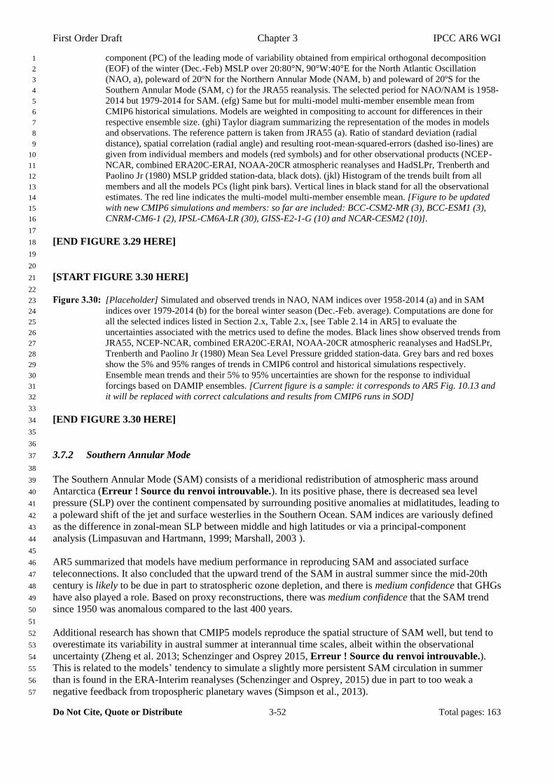
First Order Draft Chapter 3 IPCC AR6 WGI
Do Not Cite, Quote or Distribute 3-52 Total pages: 163
component (PC) of the leading mode of variability obtained from empirical orthogonal decomposition 1
(EOF) of the winter (Dec.-Feb) MSLP over 20:80°N, 90°W:40°E for the North Atlantic Oscillation 2
(NAO, a), poleward of 20ºN for the Northern Annular Mode (NAM, b) and poleward of 20ºS for the 3
Southern Annular Mode (SAM, c) for the JRA55 reanalysis. The selected period for NAO/NAM is 1958-4
2014 but 1979-2014 for SAM. (efg) Same but for multi-model multi-member ensemble mean from 5
CMIP6 historical simulations. Models are weighted in compositing to account for differences in their 6
respective ensemble size. (ghi) Taylor diagram summarizing the representation of the modes in models 7
and observations. The reference pattern is taken from JRA55 (a). Ratio of standard deviation (radial 8
distance), spatial correlation (radial angle) and resulting root-mean-squared-errors (dashed iso-lines) are 9
given from individual members and models (red symbols) and for other observational products (NCEP-10
NCAR, combined ERA20C-ERAI, NOAA-20CR atmospheric reanalyses and HadSLPr, Trenberth and 11
Paolino Jr (1980) MSLP gridded station-data, black dots). (jkl) Histogram of the trends built from all 12
members and all the models PCs (light pink bars). Vertical lines in black stand for all the observational 13
estimates. The red line indicates the multi-model multi-member ensemble mean. [Figure to be updated 14
with new CMIP6 simulations and members: so far are included: BCC-CSM2-MR (3), BCC-ESM1 (3), 15
CNRM-CM6-1 (2), IPSL-CM6A-LR (30), GISS-E2-1-G (10) and NCAR-CESM2 (10)]. 16
17
[END FIGURE 3.29 HERE] 18
19
20
[START FIGURE 3.30 HERE] 21
22
[Placeholder] Simulated and observed trends in NAO, NAM indices over 1958-2014 (a) and in SAM 23
indices over 1979-2014 (b) for the boreal winter season (Dec.-Feb. average). Computations are done for 24
all the selected indices listed in Section 2.x, Table 2.x, [see Table 2.14 in AR5] to evaluate the 25
uncertainties associated with the metrics used to define the modes. Black lines show observed trends from 26
JRA55, NCEP-NCAR, combined ERA20C-ERAI, NOAA-20CR atmospheric reanalyses and HadSLPr, 27
Trenberth and Paolino Jr (1980) Mean Sea Level Pressure gridded station-data. Grey bars and red boxes 28
show the 5% and 95% ranges of trends in CMIP6 control and historical simulations respectively. 29
Ensemble mean trends and their 5% to 95% uncertainties are shown for the response to individual 30
forcings based on DAMIP ensembles. [Current figure is a sample: it corresponds to AR5 Fig. 10.13 and 31
it will be replaced with correct calculations and results from CMIP6 runs in SOD] 32
33
[END FIGURE 3.30 HERE] 34
35
36
3.7.2 Southern Annular Mode 37
38
The Southern Annular Mode (SAM) consists of a meridional redistribution of atmospheric mass around 39
Antarctica (Erreur ! Source du renvoi introuvable.). In its positive phase, there is decreased sea level 40
pressure (SLP) over the continent compensated by surrounding positive anomalies at midlatitudes, leading to 41
a poleward shift of the jet and surface westerlies in the Southern Ocean. SAM indices are variously defined 42
as the difference in zonal-mean SLP between middle and high latitudes or via a principal-component 43
analysis (Limpasuvan and Hartmann, 1999; Marshall, 2003 ). 44
45
AR5 summarized that models have medium performance in reproducing SAM and associated surface 46
teleconnections. It also concluded that the upward trend of the SAM in austral summer since the mid-20th 47
century is likely to be due in part to stratospheric ozone depletion, and there is medium confidence that GHGs 48
have also played a role. Based on proxy reconstructions, there was medium confidence that the SAM trend 49
since 1950 was anomalous compared to the last 400 years. 50
51
Additional research has shown that CMIP5 models reproduce the spatial structure of SAM well, but tend to 52
overestimate its variability in austral summer at interannual time scales, albeit within the observational 53
uncertainty (Zheng et al. 2013; Schenzinger and Osprey 2015, Erreur ! Source du renvoi introuvable.). 54
This is related to the models’ tendency to simulate a slightly more persistent SAM circulation in summer 55
than is found in the ERA-Interim reanalyses (Schenzinger and Osprey, 2015) due in part to too weak a 56
negative feedback from tropospheric planetary waves (Simpson et al., 2013). 57

First Order Draft Chapter 3 IPCC AR6 WGI
Do Not Cite, Quote or Distribute 3-53 Total pages: 163
1
Since AR5, new research continues to indicate that both ozone depletion and increasing greenhouse gases 2
have contributed to the positive trend of SAM observed during recent decades, with ozone depletion 3
dominating in austral summer and GHGs in the other seasons, in general agreement with AR5 (Gerber and 4
Son, 2014; Son et al., 2018). Results are confirmed based on available CMIP6 simulations (Erreur ! Source d5
u renvoi introuvable.) [to be confirmed]. It is also found that high-top models tend to simulate stronger 6
summertime trends in the late 20th century than their low-top counterparts despite large inter-model 7
diversity. It is however unclear to what extent the higher model tops are causing this behaviour, versus other 8
differences between high-top and low-top models, such as additional physical processes operating in the 9
stratosphere or interactive ozone chemistry (Gillett et al., 2003; Rea et al., 2018; Sigmond et al., 2008). 10
Morgenstern et al. (2014) found that GHGs influence the SAM both by direct radiative effects and by 11
indirect effects on ozone, but these two actions tend to cancel each other. While some studies find 12
anthropogenic aerosol influence on the SAM (Gillett et al., 2013; Rotstayn, 2013), recent studies with a 13
larger multi-model ensemble find that this effect may not be robust (Choi et al., 2019; Steptoe et al., 2016). 14
In the CMIP5 simulations, volcanic stratospheric aerosol has a significant weakening effect on the SAM in 15
autumn and winter (Gillett and Fyfe, 2013). Beyond external forcing, Fogt et al. (2017) shows a significant 16
contribution from the tropical Pacific variability to the SAM trend since the mid-20th century but this is 17
based on a single AGCM experiment. 18
19
Generally consistent ozone and GHG influences have been derived from sensitivity experiments. Although 20
paleo-reconstructions of the SAM index are uncertain and vary in terms of their long-term trends (Hessl et 21
al., 2017), new reconstructions show that the summertime SAM trend since the mid-20th century is outside 22
the 5-95% range of pre-industrial variability (Dätwyler et al., 2018). While Thomas et al. (2015) emphasized 23
that there is more than a 5% chance for the observed summertime SAM trend since 1980 to occur only due to 24
internal variability in many of CMIP5 models, the chance is still less than 10% in most models.[This will be 25
confirmed based on CMIP6 and Erreur ! Source du renvoi introuvable.]. Last Millennium experiments by 26
CMIP5 models capture the long-term trends seen in the reconstructions (Abram et al. 2014, Erreur ! Source 27
du renvoi introuvable.), which additionally suggest that multidecadal positive SAM trends may have 28
occurred prior to the beginning of anthropogenic forcing (Hessl et al., 2017) and may be related to a 29
teleconnection with the tropical Pacific region (Abram et al., 2014). 30
31
In summary, there is high confidence that stratospheric ozone depletion and GHG increases have contributed 32
to the positive SAM trend during the late 20th century, with ozone depletion dominating in austral summer 33
and GHG increases in other seasons. There is medium confidence that, notwithstanding short-term 34
variability, these human influences have forced the multidecadal-mean summertime SAM into a positive 35
state of an amplitude unprecedented over the past millennium. The human influence on the SAM trend is 36
supported by further model evidence on the influence of ozone depletion and GHG increases on the SAM 37
and improved understanding of associated processes since AR5. However, models continue to exhibit 38
medium performance in reproducing aspects of the SAM (high confidence), with biases in the magnitude and 39
persistence and a large spread in the intensity of the SAM response to ozone and GHG changes [To be 40
updated with more CMIP6 models]. Confidence in the assessment of human influence on the positive state of 41
the SAM is supported by the successful simulation of long-term SAM changes found in paleoclimate 42
reconstructions. 43
44
45
[START FIGURE 3.31 HERE] 46
47
SAM indices in the last millennium. (a), (b) SAM reconstructions by (a) Abram et al. (2014) and (b) 48
Villalba et al., (2012; for DJF). 7 yr moving averages (thin lines) and 70 yr Loess filtered (thick lines). (c) 49
CMIP5 Last Millenium simulations extended by historical simulations. 70 yr moving averages for 50
individual simulations (grey lines) and their ensemble mean (red). (a-c) are relative to AD 1961-1990 51
means. (d) Radiative forcing in one model relative to AD1001-1200 mean. From Abram et al. (2014). 52
[Simplify and replace with results from CMIP6 in SOD]. 53
54
[END FIGURE 3.31 HERE] 55
56
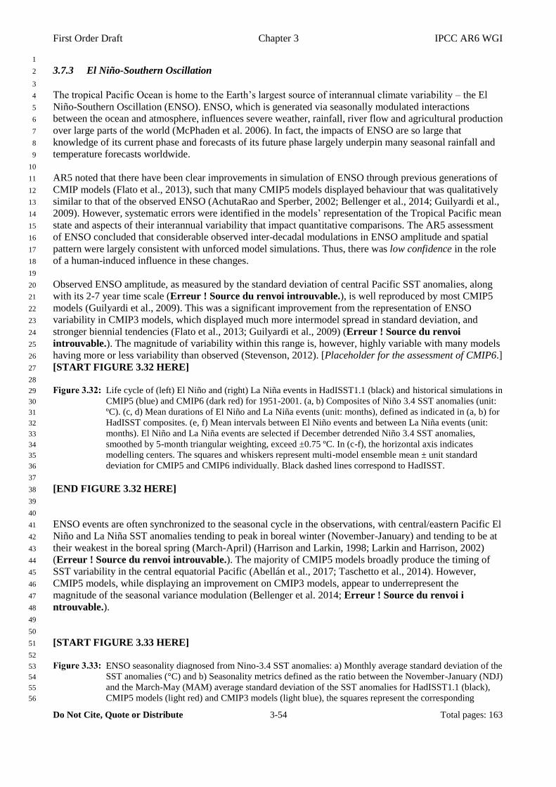
First Order Draft Chapter 3 IPCC AR6 WGI
Do Not Cite, Quote or Distribute 3-54 Total pages: 163
1
3.7.3 El Niño-Southern Oscillation 2
3
The tropical Pacific Ocean is home to the Earth’s largest source of interannual climate variability – the El 4
Niño-Southern Oscillation (ENSO). ENSO, which is generated via seasonally modulated interactions 5
between the ocean and atmosphere, influences severe weather, rainfall, river flow and agricultural production 6
over large parts of the world (McPhaden et al. 2006). In fact, the impacts of ENSO are so large that 7
knowledge of its current phase and forecasts of its future phase largely underpin many seasonal rainfall and 8
temperature forecasts worldwide. 9
10
AR5 noted that there have been clear improvements in simulation of ENSO through previous generations of 11
CMIP models (Flato et al., 2013), such that many CMIP5 models displayed behaviour that was qualitatively 12
similar to that of the observed ENSO (AchutaRao and Sperber, 2002; Bellenger et al., 2014; Guilyardi et al., 13
2009). However, systematic errors were identified in the models’ representation of the Tropical Pacific mean 14
state and aspects of their interannual variability that impact quantitative comparisons. The AR5 assessment 15
of ENSO concluded that considerable observed inter-decadal modulations in ENSO amplitude and spatial 16
pattern were largely consistent with unforced model simulations. Thus, there was low confidence in the role 17
of a human-induced influence in these changes. 18
19
Observed ENSO amplitude, as measured by the standard deviation of central Pacific SST anomalies, along 20
with its 2-7 year time scale (Erreur ! Source du renvoi introuvable.), is well reproduced by most CMIP5 21
models (Guilyardi et al., 2009). This was a significant improvement from the representation of ENSO 22
variability in CMIP3 models, which displayed much more intermodel spread in standard deviation, and 23
stronger biennial tendencies (Flato et al., 2013; Guilyardi et al., 2009) (Erreur ! Source du renvoi 24
introuvable.). The magnitude of variability within this range is, however, highly variable with many models 25
having more or less variability than observed (Stevenson, 2012). [Placeholder for the assessment of CMIP6.] 26
[START FIGURE 3.32 HERE] 27
28
Life cycle of (left) El Niño and (right) La Niña events in HadISST1.1 (black) and historical simulations in 29
CMIP5 (blue) and CMIP6 (dark red) for 1951-2001. (a, b) Composites of Niño 3.4 SST anomalies (unit: 30
ºC). (c, d) Mean durations of El Niño and La Niña events (unit: months), defined as indicated in (a, b) for 31
HadISST composites. (e, f) Mean intervals between El Niño events and between La Niña events (unit: 32
months). El Niño and La Niña events are selected if December detrended Niño 3.4 SST anomalies, 33
smoothed by 5-month triangular weighting, exceed ±0.75 ºC. In (c-f), the horizontal axis indicates 34
modelling centers. The squares and whiskers represent multi-model ensemble mean ± unit standard 35
deviation for CMIP5 and CMIP6 individually. Black dashed lines correspond to HadISST. 36
37
[END FIGURE 3.32 HERE] 38
39
40
ENSO events are often synchronized to the seasonal cycle in the observations, with central/eastern Pacific El 41
Niño and La Niña SST anomalies tending to peak in boreal winter (November-January) and tending to be at 42
their weakest in the boreal spring (March-April) (Harrison and Larkin, 1998; Larkin and Harrison, 2002) 43
(Erreur ! Source du renvoi introuvable.). The majority of CMIP5 models broadly produce the timing of 44
SST variability in the central equatorial Pacific (Abellán et al., 2017; Taschetto et al., 2014). However, 45
CMIP5 models, while displaying an improvement on CMIP3 models, appear to underrepresent the 46
magnitude of the seasonal variance modulation (Bellenger et al. 2014; Erreur ! Source du renvoi i47
ntrouvable.). 48
49
50
[START FIGURE 3.33 HERE] 51
52
ENSO seasonality diagnosed from Nino-3.4 SST anomalies: a) Monthly average standard deviation of the 53
SST anomalies (°C) and b) Seasonality metrics defined as the ratio between the November-January (NDJ) 54
and the March-May (MAM) average standard deviation of the SST anomalies for HadISST1.1 (black), 55
CMIP5 models (light red) and CMIP3 models (light blue), the squares represent the corresponding 56

First Order Draft Chapter 3 IPCC AR6 WGI
Do Not Cite, Quote or Distribute 3-55 Total pages: 163
average with whiskers representing the inter-model standard deviation. [Will be replaced with results 1
from CMIP6 in SOD] 2
3
[END FIGURE 3.33 HERE] 4
5
6
Observations show strong multi-decadal modulation of ENSO variability throughout the 20th century, with 7
the most recent period displaying larger variability while the mid-century displays a relative low of ENSO 8
variability. As reported in Section 2.4.1.1, analysis of many paleo reconstructions of ENSO over the past 9
500-1000 years suggests that recent ENSO variability appears to be higher than during the 1400-1850 period 10
(Figure 2.40; Hope et al., 2017; Li et al., 2013; McGregor et al., 2013). Contrary to this evidence, however, 11
coral records from within the tropical Pacific suggest that ENSO had higher variability than present during 12
the mid 17th century. The former suggests that external forcing plays a role in the ENSO variance changes 13
(Hope et al., 2017), while the later suggests a prominent role for internal climate variability (Cobb et al., 14
2013). Large ensembles of single model or multiple model simulations do not find strong trends in ENSO 15
variability, which suggests that external forcing does not modulate ENSO variability with any appreciable 16
magnitude (Hope et al., 2017; Stevenson et al., 2017). However, there is a possibility that the models may 17
underrepresent the impact of external forcing on ENSO. 18
19
Most CMIP5 models are found to realistically represent the intensity and location of maximum SST 20
anomalies during ENSO events (Kim and Yu, 2012; Taschetto et al., 2014). However, systematic biases exist 21
in ENSO related SST anomalies as the majority of models display anomalies that: i) extend too far to the 22
west (Capotondi et al., 2014; Taschetto et al., 2014); and ii) have meridional widths that are too narrow 23
(Zhang and Jin, 2012) compared to the observations. Further to this, the ENSO phase asymmetry, where 24
observed strong El Niño events are larger than strong La Niña events, is underrepresented in CMIP5 models 25
(Zhang and Sun, 2014). [Placeholder on the representation of these features in CMIP6 models]. 26
27
The continuum of El Niño events are typically stratified into two types (or flavours), Central Pacific (CP) 28
and East Pacific (EP), where the name denotes the location of the events’ largest SST anomalies. As 29
discussed in Section 2.4.1.2, the different types of events tend to produce different teleconnections and 30
climatic impacts. For most of the CMIP5 models, the characteristics of El Niño events of these two flavours 31
are comparable to the observations (Taschetto et al., 2014) [To be updated with CMIP6.]. Observations and 32
paleo proxies also suggest an increase in the number of the CP type events in recent decades (Section 33
2.4.1.3; Ashok et al., 2007; McPhaden et al., 2011). However, the short observational record and 34
observational uncertainties (L’Heureux et al., 2013) preclude firm conclusions being made about the long-35
term changes in the occurrence of different El Niño event types. Initial analysis with a select number of 36
CMIP3 models suggested that there may be a forced component to this recent prominence of CP type events 37
(Yeh et al., 2009), but analysis since then suggests that this behavior is i) consistent with that expected from 38
internal climate variability (Newman et al., 2011); and ii) not apparent across the full CMIP5 ensemble of 39
historical simulations (Taschetto et al., 2014) [Add a sentence for updates with CMIP6]. An analysis of a 40
large ensemble of simulations from one model suggests that changes to ENSO event type in response to 41
combined anthropogenic forcing are not significant (Stevenson et al., 2017). 42
43
The impacts of ENSO outside of the tropical Pacific largely arise through atmospheric teleconnections that 44
are driven by changes in deep convection and atmospheric heating (Yeh et al., 2018). The teleconnections to 45
higher latitudes are forced by waves that propagate into the extratropics (Hoskins and Karoly, 1981) and 46
respectively excite a Pacific-North American (PNA) pattern (Horel and Wallace, 1981) and Pacific-South 47
American (PSA) pattern (Karoly, 1989) in the Northern and Southern Hemispheres. Given the impact of 48
these teleconnections on climate and extremes around the globe, is important to understand how well they 49
are reproduced in CMIP5 models. What has also become clear is that spatial correlations of ENSO’s 50
teleconnections over relatively short periods may not be the most effective way to assess these relationships 51
(Langenbrunner and Neelin, 2013; Perry et al., 2017). This is because the spatial patterns are significantly 52
impacted by internal atmospheric variability on relatively short time scales (Batehup et al., 2015; Perry et al., 53
2017). However, looking at simplified metrics like the agreement in the sign of the teleconnections 54
(Langenbrunner and Neelin, 2013), regional average teleconnection strength over land (Perry et al. 2018), or 55

First Order Draft Chapter 3 IPCC AR6 WGI
Do Not Cite, Quote or Distribute 3-56 Total pages: 163
a combination of both (Power and Delage, 2018) provides a more robust depiction of the teleconnection 1
representation. Examining sign agreement for the teleconnection patterns, ensembles of CMIP5 AMIP 2
simulations display broad spatial regions with high sign agreement with the observations, suggesting that the 3
model ensemble is producing useful information regarding the teleconnected precipitation signal 4
(Langenbrunner and Neelin, 2013) (Erreur ! Source du renvoi introuvable.). Looking at regional averages, 5
Power and Delage (2018) show that the average teleconnection pattern of the CMIP5 coupled models can 6
reproduce the sign of the observed teleconnections in the majority of the 25 SREX defined regions. [Update 7
for CMIP6] 8
9
10
[START FIGURE 3.34 HERE] 11
12
Observed ENSO teleconnections for (a) temperature and (b) precipitation during DJF. Teleconnections 13
are identified by linear region with the Nino34 index, with temperature calculated during the period 1958-14
2010, while precipitation teleconnections are calculated during 1979-2010. Stippling indicates significant 15
teleconnections at p < 0.05 and grey boxes in both panels indicate region boundaries used in regional 16
average teleconnection strength shown in (c, d). (c) and (d) display box and whisker plots (indicated with 17
black colouring here) which show the ensemble range of modelled teleconnections for all members of all 18
CMIP6 models for each identified region [to be redefined for SOD]. The observed teleconnections for 19
each region will also be displayed by a box and whisker plot (indicated by magenta colouring here) that is 20
identified following the methodology identified by Deser et al. (2017) [This is a sample figure: will be 21
redesigned and replaced with results from CMIP6 in SOD] 22
23
[END FIGURE 3.34 HERE] 24
25
26
It is clear that many CMIP5 models exhibit ENSO behavior that, to first order, is qualitatively similar to that 27
of the observed ENSO. Many studies are now delving deeper into the models to understand if they are 28
accurately producing the dynamics driving ENSO and its initiation (Bellenger et al., 2014; Jin et al., 2006; 29
Vijayeta and Dommenget, 2017). For both CMIP3 and CMIP5, diagnostics of ENSO event growth appear to 30
show that the models, while producing ENSO variability that is qualitatively similar to that observed, do not 31
represent the balance of the underlying dynamics well. The atmospheric Bjerknes feedback is too weak in 32
the majority of models, while fluxes of heat at the surface are also too weak in the majority of models. The 33
former restricts event growth, while the latter restricts event damping, which when combined allow most 34
models to produce variability in a range that is consistent with the observations (Bellenger et al., 2014; Kim 35
et al., 2014b; Vijayeta and Dommenget, 2017). [To be updated with CMIP6 models] 36
37
The instrumental record, paleo proxy evidence through the Holocene and coupled models all suggest that 38
ENSO can display considerable modulations in amplitude, pattern and period (see also Section 2.4.1). 39
Further to this, paleo-proxy evidence indicates (medium confidence) that ENSO activity in the late 20th and 40
early 21st century was greater than at any time between 1400 and 1850 (Section 2.4.1). Coupled models 41
display large changes of ENSO behaviour in the absence of external forcing changes, and little-to-no 42
variance sensitivity to anthropogenic forcing. Thus, we have low confidence that anthropogenic forcing has 43
led to changes of ENSO activity. 44
45
Chapter 2 reported low confidence that the apparent change from eastern Pacific to central Pacific type El 46
Niño events that occurred in the last 20-30 years was representative of a long term change. While some 47
coupled models do suggest external forcing may impact El Niño event type, model simulations also suggest 48
that what has been observed is well within the range of natural variability. Thus, there is no evidence that 49
anthropogenic forcing has had an impact on observed changes in El Niño event type. Low confidence is 50
given for the role of anthropogenic forcing in the observed change in ENSO activity as the behaviour is not 51
reproduced in ensembles of coupled model simulations. 52
53
54
3.7.4 Indian Ocean Basin and Dipole Modes 55
56

First Order Draft Chapter 3 IPCC AR6 WGI
Do Not Cite, Quote or Distribute 3-57 Total pages: 163
The Indian Ocean Basin (IOB) and Dipole (IOD) modes are the two leading modes of interannual SST 1
variability over the tropical Indian Ocean, featuring basin-wide warming/cooling and an east-west dipole of 2
SST anomalies, respectively (Section 2.4.2). The IOD mode is anchored to boreal summer to autumn by the 3
air-sea feedback, and develops often in concert with ENSO. Driven by matured ENSO, the IOB mode peaks 4
in boreal spring and often persists into the subsequent summer. Similar patterns of Indian Ocean SST 5
variability also dominate its decadal and longer time scale variability (Han et al., 2014b). 6
7
AR5 concluded that models show high and medium performance in reproducing IOB and IOD, respectively 8
(medium confidence), whereas there was low confidence that changes in the IOD were detectable or 9
attributable to human influence. GHG-induced warming projects onto the IOB, and its 20th century trend is 10
captured by CMIP3 20th century simulations. 11
12
Since the AR5, CMIP5 models have been analysed, finding that most of the models qualitatively reproduce 13
the spatial and seasonal features of the IOB and IOD modes (Chu et al., 2014; Liu et al., 2014; Tao et al., 14
2016b). Improvements in simulating the IOB mode since CMIP3 have been identified in reduced multi-15
model mean bias and inter-model spread (Tao et al., 2016b). CMIP5 models overall capture the transition 16
from the IOD to IOB modes during an ENSO event (Tao et al., 2016b). The IOB mode is forced through the 17
cross-equatorial wind-evaporation-SST feedback triggered by ENSO-forced anomalous ocean Rossby waves 18
that propagate to the shallow climatological thermocline dome in the tropical southwestern Indian Ocean (Du 19
et al., 2009). Consistently, models with a deeper climatological thermocline dome produce a weaker and less 20
persistent IOB mode (Li et al., 2015b; Zheng et al., 2016). The deep thermocline bias remains in the 21
ensemble mean of CMIP5 models due to a common surface easterly wind bias over the equatorial Indian 22
Ocean (Lee et al., 2013) associated with a weaker South Asian summer monsoon (Li et al., 2015c). 23
However, the influence of this systematic bias is compensated by other biases, resulting in a realistic IOB 24
magnitude (Tao et al., 2016b). By contrast, the IOD magnitude is overestimated by CMIP5 models on 25
average, with noticeable improvements from CMIP3 models (Liu et al., 2014). Both a shallower 26
climatological thermocline off Sumatra and Java and biases in ENSO contribute to this IOD magnitude bias 27
(Liu et al., 2014). [to be updated with CMIP6] 28
29
Since the late 19th century, the relationship between ENSO and the IOB mode in the following boreal 30
summer, has varied on multidecadal time scales (Chowdary et al., 2012). In selected CMIP5 models that 31
show similar modulations, a strengthening tendency of the ENSO-IOB mode correlation and resultant 32
intensification of the IOB mode are found in historical or future simulations (Hu et al., 2014; Tao et al., 33
2015). However, such a change has not been detected from observational records. Likewise, while changes 34
in frequency of extreme events (Cai et al., 2014) and skewness (Cowan et al., 2015) in the IOD mode are 35
simulated in CMIP5 models, such changes have not been detected in observations. While paleoclimate 36
reconstructions show modulations in the magnitude and seasonality of the IOD mode (Section 2.4.2), but few 37
comparison studies with model simulations have been made. One such study by Brown et al. (2009) finds 38
weaker IOD variability in a mid-Holocene simulation than in the preindustrial simulation, contradicting 39
proxy-based findings. 40
41
The observed Indian Ocean basin-average sea surface temperature (SST) increase on multidecadal and 42
centennial time scales is well represented by CMIP5 historical simulations, and attributed to compensating 43
effects by GHGs and anthropogenic aerosols mainly through aerosol-cloud interactions (Dong et al., 2014b; 44
Dong and Zhou, 2014). The observed SST trend is larger in the western than eastern tropical Indian Ocean, 45
which leads to an apparent upward trend of the IOD index, but this trend is statistically insignificant (Section 46
2.4.2). CMIP5 models capture this warming pattern, which may be associated with Walker circulation 47
weakening over the Indian Ocean due to GHG forcing (Dong and Zhou, 2014). However, strong internal 48
decadal IOD-like variability and observational uncertainty preclude validation of the simulated modulations 49
and attribution (Cai et al., 2013; Han et al., 2014b). 50
51
After linear detrending, Pacific decadal variability (PDV) has been identified as the major driver of the 52
decadal-to-multidecadal IOB mode (Dong et al., 2016). However, correlation between the PDV and a 53
decadal IOB index, defined from linearly detrended SST, changed from positive to negative during the 1980s 54
(Han et al., 2014a). The accelerating anthropogenic Indian Ocean warming and recovery from the eruptions 55

First Order Draft Chapter 3 IPCC AR6 WGI
Do Not Cite, Quote or Distribute 3-58 Total pages: 163
of El Chichón in 1982 and Pinatubo in 1991, may have overwhelmed the PDV influence, and explain this 1
change (Dong and McPhaden, 2017; Zhang et al., 2018b). However, the low number of statistical degrees of 2
freedom hampers clear detection of human influence in this correlation change. 3
4
To summarize, there is no evidence that anthropogenic forcing has changed the interannual IOB and IOD. 5
On decadal-to-multidecadal time scales, there is low confidence that human influence has caused a reversal 6
of the correlation between PDV and the decadal IOB mode. The low level of confidence in the latter 7
assessment is due to the short observational record, limited number of models used for the attribution, lack of 8
model evaluation on reproducibility of the decadal IOB mode, and uncertainty in the contribution from 9
volcanic aerosols. Nevertheless, models have medium overall performance in reproducing both the 10
interannual IOB and IOD modes (high confidence). 11
12
13
3.7.5 Atlantic Meridional and Zonal Modes 14
15
The Atlantic Equatorial Mode, often referred to as the Atlantic Niño, and Atlantic Meridional Mode (AMM) 16
are the two leading basin wide patterns of interannual-to-decadal variability in the tropical Atlantic (Section 17
2.4.6). Akin to ENSO in the Pacific, the term Atlantic Niño is broadly used to refer to years when the SSTs 18
in the tropical eastern Atlantic basin along the cold tongue significantly depart from the climatological 19
average. The AMM is characterized by anomalous cross-equatorial gradients in SST. Both modes are 20
associated with altered strength of the ITCZ and/or latitudinal shifts in the ITCZ, which locally affect 21
African and American monsoon systems and remotely affect Tropical Pacific and Indian Ocean variability 22
through inter-basins teleconnections. 23
24
AR5 mentioned considerable difficulty simulating both Atlantic Niño and AMM despite some improvements 25
in CMIP5 for some models. Severe biases in mean state and variance for both SST and atmospheric 26
dynamics including rainfall (e.g. double ITCZ) as well as teleconnections were reported. AR5 highlighted 27
the complexity of the Tropical Atlantic biases, which were explained by multiples sources both in the ocean 28
and atmosphere. 29
30
Since AR5, further understanding of the major persistent biases in models has been reported (Dippe et al., 31
2018; Jouanno et al., 2017; Lübbecke et al., 2018; Xu et al., 2014; Yang et al., 2017b). Critical errors in 32
equatorial and basin wide trade winds, cloud cover and ocean vertical mixing and dynamics both locally and 33
in remote subtropical upwelling regions (essentially Angola-Benguela system), key thermodynamic ocean-34
atmosphere feedbacks, tropical land-atmosphere interaction, have been shown to be detrimental to the 35
representation of both Atlantic Niño and AMM leading to poor teleconnectivity over land (Rodríguez-36
Fonseca et al., 2015) and between tropical basins (Ott et al., 2015). 37
38
Despite some improvements (Nnamchi et al., 2015; Richter et al., 2014) mean biases are so large that the 39
mean east-west tridimensional temperature gradient at the equator remain opposite to observed in two thirds 40
of the CMIP5 models (Section 3.5.1.1) and clearly affect the simulation of the Atlantic Niño and associated 41
dynamics (Deppenmeier et al., 2016; Ding et al., 2015; Muñoz et al., 2012) . The interhemispheric SST 42
gradient is also systematically underestimated in models with erroneously too cold (warm) north (south) 43
Atlantic mean state. The seasonality is poorly reproduced and the wind-SST coupling is weaker than 44
observed so that all together, and despite AMM-like variability in 20th century climate simulations, AMM is 45
not the dominant Atlantic mode in all CMIP5 models (Amaya et al., 2017; Liu et al., 2013). These biases 46
translate into biases in modelling the ITCZ (Flato et al., 2013). Similar biases were found in other 47
experiments with CMIP5 simulations, such as Last Glacial Maximum, Mid-Holocene and future scenario 48
simulations (Brierley and Wainer, 2017) . [Initial results from CMIP6 show improvements (or no change) in 49
both the modelled climatology and the representation of the Atlantic Nino/AMM. To be updated.] 50
51
There are some recent indications that increasing model resolution both vertically and horizontally, in the 52
ocean and atmospheric component (Harlaß et al., 2018; Richter, 2015; Small et al., 2015), could partly 53
alleviate tropical Atlantic biases in mean state, seasonality, interannual-to-decadal variability and associated 54
teleconnectivity over land (Sahel monsoon, Steinig et al., 2018), though this result appears to be model 55
First Order Draft Chapter 3 IPCC AR6 WGI
Do Not Cite, Quote or Distribute 3-59 Total pages: 163
dependent (Goubanova et al., 2019). [This statement should be updated based on HighResMIP when 1
available]. 2
3
Based on CMIP5 and CMIP6 [to be confirmed] results, there is no robust evidence that observed changes in 4
either Atlantic Niño or AMM modes and associated teleconnections are detectable and attributable to 5
anthropogenic forcing. Considering the physical processes responsible for model biases in these modes, it is 6
probable that increasing resolution in both ocean and atmosphere components may be an opportunity for 7
progress [to be confirmed by HighResMIP]. The lack of confidence on possible human influence on the 8
Atlantic Modes and associated teleconnections is dictated by the poor fidelity of CMIP5- and CMIP6-class 9
models in reproducing the mean tropical Atlantic climate, its seasonality and variability. For instance, there 10
has been an observed decrease in the variability of the Atlantic Niño since the 1960s (Tokinaga and Xie, 11
2011). The fact that most models poorly represent the climatology and variability of the tropical Atlantic 12
combined with the short observational record makes it difficult to place the recent observed changes in the 13
context of natural internal variability versus anthropogenic forcing. 14
15
16
3.7.6 Pacific Decadal Variability 17
18
Pacific decadal variability (PDV) refers to a mode of variability in the Pacific Ocean that varies on decadal 19
to interdecadal timescales. PDV encompasses the Pacific Decadal Oscillation (PDO; Mantua et al. 1997; 20
Mantua and Hare 2002; Zhang et al. 1997), an SST pattern in the North Pacific, as well as a broader SST 21
pattern associated with Pacific-wide SSTs termed the Interdecadal Pacific Oscillation (IPO; Power et al. 22
1999; Folland et al. 2002; Henley et al. 2015), although neither of these are true “oscillations” (Section 23
2.4.4). It is now recognized that a superposition of several phenomena, each governed by different physical 24
mechanisms, underlies PDV (Newman et al., 2016a). 25
26
AR5 mentioned an overall limited level of evidence for both CMIP3 and CMIP5 evaluation leading to low 27
confidence statements about the models’ performance in reproducing PDV and similarly low confidence in 28
the attribution of the observed PDV changes to human influence. 29
30
The implication of PDV in the observed slowdown of the global mean surface temperature (GMST) 31
warming rate in early 2000s (Cross-Chapter Box 3.1:) has triggered considerable research on decadal climate 32
variability since the AR5 (Cassou et al., 2018; Dai et al., 2015; England et al., 2014b; Kosaka and Xie, 33
2016). Many studies find that the broad spatial characteristics of PDV are reasonably well represented in 34
unforced climate models (Henley 2017; Newman et al. 2016) and in historical simulations in CMIP5 and 35
CMIP6 (Erreur ! Source du renvoi introuvable.), although sensitivity to methodology used to remove the 36
externally-forced component of the SST exists (Bonfils and Santer, 2011; Xu and Hu, 2018). Compared with 37
CMIP3, CMIP5 models exhibit overall slightly better performance in reproducing PDV and associated 38
teleconnections (Joshi and Kucharski, 2017; Polade et al., 2013), and also smaller inter-model spread (Lyu et 39
al., 2016). 40
41
However, serious biases in the PDV temporal properties and amplitude remain (Cheung et al., 2017; Henley, 42
2017). It is noted that while model evaluation is severely hampered by short instrumental observations, the 43
duration of PDV phases appears to be shorter in coupled models than in observations, and correspondingly 44
the ratio of decadal to interannual variance is underestimated (Henley et al. 2017; Erreur ! Source du 45
renvoi introuvable.). This apparent bias may be associated with overly biennial behaviour of Pacific trade 46
wind variability and related ENSO activity (Kociuba and Power, 2015), although basin-scale ENSO 47
influence in the extratropics at decadal timescales is very diverse among both CMIP3 and CMIP5 models, 48
being controlled by multiple factors (Nidheesh et al., 2017). In terms of amplitude, some observed variations 49
of PDV over the historical period are outside of the modelled range, likely due to an incomplete 50
representation of decadal-scale mechanisms in climate models (Erreur ! Source du renvoi introuvable.). 51
The results of McGregor et al. (2018) suggest that the underrepresentation of PDV magnitude stems from 52
Atlantic mean SST bias through inter-basin coupling. 53
54
While PDV is primarily understood as an internal mode of variability (Si and Hu, 2017), there are some 55
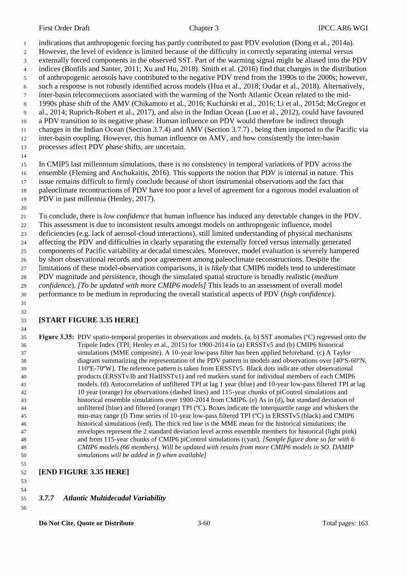
First Order Draft Chapter 3 IPCC AR6 WGI
Do Not Cite, Quote or Distribute 3-60 Total pages: 163
indications that anthropogenic forcing has partly contributed to past PDV evolution (Dong et al., 2014a). 1
However, the level of evidence is limited because of the difficulty in correctly separating internal versus 2
externally forced components in the observed SST. Part of the warming signal might be aliased into the PDV 3
indices (Bonfils and Santer, 2011; Xu and Hu, 2018). Smith et al. (2016) find that changes in the distribution 4
of anthropogenic aerosols have contributed to the negative PDV trend from the 1990s to the 2000s; however, 5
such a response is not robustly identified across models (Hua et al., 2018; Oudar et al., 2018). Alternatively, 6
inter-basin teleconnections associated with the warming of the North Atlantic Ocean related to the mid-7
1990s phase shift of the AMV (Chikamoto et al., 2016; Kucharski et al., 2016; Li et al., 2015d; McGregor et 8
al., 2014; Ruprich-Robert et al., 2017), and also in the Indian Ocean (Luo et al., 2012), could have favoured 9
a PDV transition to its negative phase. Human influence on PDV would therefore be indirect through 10
changes in the Indian Ocean (Section 3.7.4) and AMV (Section 3.7.7) , being then imported to the Pacific via 11
inter-basin coupling. However, this human influence on AMV, and how consistently the inter-basin 12
processes affect PDV phase shifts, are uncertain. 13
14
In CMIP5 last millennium simulations, there is no consistency in temporal variations of PDV across the 15
ensemble (Fleming and Anchukaitis, 2016). This supports the notion that PDV is internal in nature. This 16
issue remains difficult to firmly conclude because of short instrumental observations and the fact that 17
paleoclimate recontructions of PDV have too poor a level of agreement for a rigorous model evaluation of 18
PDV in past millennia (Henley, 2017). 19
20
To conclude, there is low confidence that human influence has induced any detectable changes in the PDV. 21
This assessment is due to inconsistent results amongst models on anthropogenic influence, model 22
deficiencies (e.g. lack of aerosol-cloud interactions), still limited understanding of physical mechanisms 23
affecting the PDV and difficulties in clearly separating the externally forced versus internally generated 24
components of Pacific variability at decadal timescales. Moreover, model evaluation is severely hampered 25
by short observational records and poor agreement among paleoclimate reconstructions. Despite the 26
limitations of these model-observation comparisons, it is likely that CMIP6 models tend to underestimate 27
PDV magnitude and persistence, though the simulated spatial structure is broadly realistic (medium 28
confidence). [To be updated with more CMIP6 models] This leads to an assessment of overall model 29
performance to be medium in reproducing the overall statistical aspects of PDV (high confidence). 30
31
32
[START FIGURE 3.35 HERE] 33
34
PDV spatio-temporal properties in observations and models. (a, b) SST anomalies (ºC) regressed onto the 35
Tripole Index (TPI; Henley et al., 2015) for 1900-2014 in (a) ERSSTv5 and (b) CMIP6 historical 36
simulations (MME composite). A 10-year low-pass filter has been applied beforehand. (c) A Taylor 37
diagram summarizing the representation of the PDV pattern in models and observations over [40ºS-60ºN, 38
110ºE-70ºW]. The reference pattern is taken from ERSSTv5. Black dots indicate other observational 39
products (ERSSTv3b and HadISSTv1) and red markers stand for individual members of each CMIP6 40
models. (d) Autocorrelation of unfiltered TPI at lag 1 year (blue) and 10-year low-pass filtered TPI at lag 41
10 year (orange) for observations (dashed lines) and 115-year chunks of piControl simulations and 42
historical ensemble simulations over 1900-2014 from CMIP6. (e) As in (d), but standard deviation of 43
unfiltered (blue) and filtered (orange) TPI (ºC). Boxes indicate the interquartile range and whiskers the 44
min-max range (f) Time series of 10-year low-pass filtered TPI (ºC) in ERSSTv5 (black) and CMIP6 45
historical simulations (red). The thick red line is the MME mean for the historical simulations; the 46
envelopes represent the 2 standard deviation level across ensemble members for historical (light pink) 47
and from 115-year chunks of CMIP6 piControl simulations (cyan). [Sample figure done so far with 6 48
CMIP6 models (66 members). Will be updated with results from more CMIP6 models in SO. DAMIP 49
simulations will be added in f) when available] 50
51
[END FIGURE 3.35 HERE] 52
53
54
3.7.7 Atlantic Multidecadal Variability 55
56
First Order Draft Chapter 3 IPCC AR6 WGI
Do Not Cite, Quote or Distribute 3-61 Total pages: 163
Atlantic Multidecadal Variability (AMV) refers to a climate mode representing basin-wide multidecadal 1
fluctuations in surface temperatures in the North Atlantic, with teleconnections to the adjacent continents and 2
the Arctic (Section 2.4.3). A fingerprint of AMV exists in the subsurface ocean in AMOC fluctuations, gyre 3
adjustments and salt and heat transport. 4
5
In AR5, climate models suggested that the AMV was primarily internally-driven alongside some 6
contribution from external forcings (mainly anthropogenic aerosols) over the late 20th century. But AR5 also 7
concluded that models show medium performance in reproducing the observed AMV (low confidence), with 8
difficulties in simulating the timescale and spatial structure. 9
10
Climate models analyzed since AR5 continue to simulate AMV-like variability as part of their internal 11
variability (Brown et al., 2016b; Chen et al., 2016a; Menary et al., 2015; Ruprich-Robert and Cassou, 2015; 12
Schmith et al., 2014; Wouters et al., 2012) and continue to support links to a wide array of climate impacts 13
through teleconnections (Martin et al., 2013a; Monerie et al., 2019; Ruprich-Robert et al., 2017). Even if 14
debate remains (Cane et al., 2017; Clement et al., 2015), there is now stronger evidence for a crucial role of 15
internal oceanic dynamics that is primarily linked to AMOC and NAO variability (Delworth et al., 2017). 16
However, considerable diversity in the spatio-temporal properties of the simulated AMV is found in both 17
piControl and historical CMIP5 experiments (Wills et al., 2019; Zhang and Wang, 2013). Such model 18
diversity is presumably associated with the wide range of coupled processes and regional atmospheric 19
feedbacks whose representations are specific to each model (Brown et al., 2016, Martin et al, 2014). 20
21
Additional studies since the AR5 corroborate that CMIP5-era models tend to overall underestimate many 22
aspects of observed AMV including its magnitude, timescale, and spatial extent and more particularly, the 23
link between the tropical North Atlantic and the subpolar gyre/Nordic seas (Martin et al., 2013a; Qasmi et 24
al., 2017), while the mechanisms producing tropical-extratropical connections at decadal timescales remain 25
poorly understood. Such mismatches between observed and simulated AMV can be due to intrinsic model 26
biases in both mean state (Drews and Greatbatch, 2016; Menary et al., 2015) and variability. In addition, 27
CMIP-class models appear to underestimate decadal timescale variability in the AMOC and NAO relative to 28
interannual timescale variability (Kim et al., 2018; Yan et al., 2018), which has strong implications for 29
AMV-forced teleconnections (Ault et al., 2012; Menary et al., 2015) and the predictability of AMV. All 30
these conclusions are consistent with results from available CMIP6 simulations (Erreur ! Source du renvoi 31
introuvable.) [to be updated with results from CMIP6]. 32
33
Since AR5, there has been increased evidence of an important role for external forcings in driving AMV. 34
The competition between GHG warming and anthropogenic sulphate aerosol cooling has been proposed to 35
be particularly important over the latter half of the 20th century (Booth et al., 2012; Murphy et al., 2017; 36
Steinman et al., 2015; Undorf et al., 2018a), but volcanic forcings may have also played a role, to a lesser 37
extent (Bellucci et al., 2017; Swingedouw et al., 2017; Terray, 2012). Over the last millennium, natural 38
forcings including major volcanic eruptions and fluctuations in solar activity may have driven multidecadal 39
variations in the AMV, with some interplay with internal processes (Otterå et al., 2010). Consistently, the 40
timing of phase changes, and the magnitude and timescale of AMV, tend to be better reproduced in historical 41
simulations compared to piControl simulations (Bellomo et al., 2018). However, there remain significant 42
discrepancies in simulated AMV when compared to multivariate observations, which may in part be related 43
to deficiencies in atmospehre-ocean coupling in some models (Kim et al., 2018). Model evaluation remains 44
difficult due to a lack of stationarity in the spatio-temporal properties of simulated AMV as assessed from 45
long control experiments (Qasmi et al., 2017), and because of the difficulties in estimating the forced signals 46
in both historical simulations and observations (Tandon and Kushner, 2015). [Add results from CMIP6 47
DAMIP simulations]. 48
49
To summarize, results from CMIP5- and CMIP6-era models [to be confirmed] together with new statistical 50
techniques to evaluate the forced component in modelled and observed AMV, provide robust evidence that 51
natural climate processes and feedbacks (including internal mechanisms and response to natural, mostly 52
volcanic, forcings) are important in generating AMV (high confidence). There is also increased evidence that 53
anthropogenic aerosols have played a role in the timing and intensity of the negative (cold) phase of AMV 54
recorded from the mid-1960s to mid-1990s and subsequent warming, but there is low confidence in the 55
First Order Draft Chapter 3 IPCC AR6 WGI
Do Not Cite, Quote or Distribute 3-62 Total pages: 163
estimated magnitude of the human influence. The limited level of confidence is primarily explained by the 1
difficulties in accurately evaluating model performance in simulating realistic AMV phenomena. The 2
evaluation is severely hampered by short instrumental records but also, equally importantly, by the lack of 3
detailed and coherent long-term process-based observations (for example of the AMOC, aerosol optical 4
depth, surface fluxes and cloud changes), which limit our process understanding. The underestimation of 5
AMV magnitude found in most of the models could denote a poorly represented forced response (e.g. due to 6
aerosol-cloud interactions, Booth et al. 2012), an underestimation of internal variability (Yan et al., 2018), or 7
both. In addition, studies often rely solely on simplistic SST indices that may be hard to interpret (Zhang et 8
al., 2016) and may mask critical physical inconsistency in simulations of AMV compared to observational 9
estimates and processes (Zhang et al., 2013a). Therefore, the relative importance of anthropogenic forcing on 10
AMV and associated teleconnections in the historical period compared to natural (forced or internal) 11
variability remains poorly understood and difficult to assess. 12
13
14
[START FIGURE 3.36 HERE] 15
16
AMV spatio-temporal properties in observations and models. As in Figure 3.35: but based on the AMV 17
index defined as the10-year low-pass filtered North Atlantic (0º-60°N, 80°W-0°E) area-weighted SST* 18
anomalies over 1900-2014. Asterisk denotes that the global mean SST anomaly has been removed at each 19
time step of the computation. The Taylor diagram (c) is made for the same region. [Sample figure done so 20
far with 6 CMIP6 models (66 members). Will be updated with results from more CMIP6 models in SO. 21
DAMIP simulations will be added in f) when available] 22
23
[END FIGURE 3.36 HERE] 24
25
26
27
3.8 Synthesis across Earth system components 28
29
3.8.1 Multivariate Attribution of Climate Change 30
31
Evidence has grown since AR5 that observed changes since the 1950s in many parts of the climate system 32
are attributable to anthropogenic influences. So far, this chapter has mostly focused on examining individual 33
aspects of the climate system in separate sections. The results presented in Sections 3.3 to 3.7 strengthen the 34
conclusion that human influence on climate has played the dominant role in observed warming since the 35
1950s. In this section we look across the whole climate system to assess whether and to what extent a 36
physically consistent picture of human induced change emerges across the climate system (Erreur ! Source 37
du renvoi introuvable.). 38
39
The assessed likelihood of a detectable and quantifiable, human contribution ranges from likely to extremely 40
likely for temperatures from the depths of the ocean on up through the surface of the Earth to the troposphere 41
and stratosphere. The observed warming trends in the atmosphere, ocean and at the surface over the past 65 42
years are best explained when contributions from both anthropogenic and natural forcings are included. As 43
might be expected from a warming atmosphere, moisture in the troposphere has increased and precipitation 44
patterns have changed. Anthropogenic factors have likely contributed to the observed changes in humidity 45
and precipitation. Sea ice in the Arctic continues to decline; this is very likely due to increases in greenhouse 46
gases. There is medium confidence that reductions in snow cover over the Northern Hemisphere are 47
associated with warming of near surface air, and that anthropogenic climate change has changed streamflow 48
in many parts of the world. There continues to be low confidence in the scientific understanding of the 49
changes in Antarctic sea ice. 50
51
Combining the evidence from across the climate system increases the level of confidence in the attribution of 52
observed climate change to human influence and reduces the uncertainties associated with assessments based 53
on a single variable. From this combined evidence, it is virtually certain that human influence has warmed 54
the global climate system. 55

First Order Draft Chapter 3 IPCC AR6 WGI
Do Not Cite, Quote or Distribute 3-63 Total pages: 163
1
Further, AR5 concluded that human influence on the climate system is clear (IPCC, 2013). This assessment 2
was based on observed increasing greenhouse gas concentrations in the atmosphere, positive radiative 3
forcing, observed warming, and physical understanding of the climate system. Further observed increases in 4
greenhouse gas concentrations and global temperatures (Chapter 2), as well as stronger and better-5
constrained estimates of anthropogenic radiative forcing (Chapter 5), and improved physical understanding 6
of these changes as reflected in stronger attribution assessments (Sections 3.3 to 3.7) demonstrate that this 7
evidence has strengthened. 8
9
10
[START FIGURE 3.37 HERE] 11
12
Synthesis D&A across variables and for different regions (CMIP5). Figure produced with ESMValTool 13
v2.0a1. [Additional variables (e.g. sea ice extent and ocean heat uptake), more models and an underlying 14
map will be added in SOD]. 15
16
[END FIGURE 3.37 HERE] 17
18
19
3.8.2 Multivariate Model Evaluation 20
21
Similar to the assessment of multivariate attribution of climate change in the previous section, in this section 22
we assess the performance of the models across different variables (Sections 3.8.2.1) and different classes of 23
models (Section 3.8.2.2). Here the focus is on a system-wide assessment using integrative measures of model 24
performance that characterize model performance using multiple diagnostic fields derived from multi-model 25
ensembles. This leads to an overall conclusion regarding climate models’ fitness for purpose of simulating 26
historical climate and their suitability for future projections (Section 3.8.2.3). This section expands the 27
assessment of the performance of CMIP5 models in AR5. [This will be updated with results from CMIP6 28
models in the SOD.] 29
30
31
3.8.2.1 Integrative Measures of Model Performance 32
33
For every diagnostic field considered, model performance is compared to one or multiple observational 34
references, and the quality of the simulation is expressed as a single number, e.g. a correlation coefficient or 35
a root mean square difference versus the observational reference. By simultaneously assessing different 36
performance indices, model improvements can be quantified (see FAQ 3.2:), similarities in behaviour 37
between different models become apparent, and dependencies between various indices become evident 38
(Gleckler et al., 2008; Waugh and Eyring, 2008). 39
40
AR5 found significant variations in skill across the CMIP5 ensemble when measured against meteorological 41
reanalyses and observations (Flato et al., 2013). AR5 determined that for the diagnostics analysed, the models 42
usually compared similarly against two different reference datasets, suggesting that model errors were 43
generally larger than observational uncertainties or other differences between the observational references. In 44
agreement with previous assessments, the CMIP5 multi-model mean generally performed better than 45
individual models (Rougier, 2016). AR5 considered 13 atmospheric fields in its assessment for the 46
instrumental period but did not assess multi-variate model performance in other climate domains (e.g., ocean, 47
land, and sea ice). AR5 found only modest improvement regarding the simulation of climate for two periods 48
of the Earth’ history (the Last Glacial Maximum and the Mid-Holocene) between CMIP5 and the previous 49
paleoclimate simulations. Similarly, for the modern period only incremental progress was found between 50
CMIP3 and CMIP5 regarding the simulation of precipitation and radiation. The representation of clouds 51
remained a leading problem in climate modelling. 52
53
The multi-variate analysis of CMIP5 models presented in AR5 is expanded to more variables and more climate 54
domains, also covering land and ocean as well as sea ice. The multi-variate evaluation of the CMIP5 models 55
First Order Draft Chapter 3 IPCC AR6 WGI
Do Not Cite, Quote or Distribute 3-64 Total pages: 163
is performed relative to the datasets listed in the Technical Annex on observations. For many of the 1
observational datasets, a rigorous characterization of the observational uncertainty is not available, see 2
discussion in Chapter 2. Here, as much as possible, multiple independent observational datasets are used. 3
Disagreements amongst them would cause differences in model scoring, indicating that observational 4
uncertainties may be substantial compared to model errors. Conversely, similar scores against different 5
observational datasets would suggest model issues may be more important than the observational uncertainty. 6
7
In agreement with AR5, the analysis of atmosphere variables (Erreur ! Source du renvoi introuvable.a) 8
indicates that several models perform better compared to observational references than the median, across a 9
majority of the climate variables assessed, and conversely some other models compare more poorly against 10
these reference datasets. Family relationships between the models are apparent, for example, the 11
HadGEM2/ACCESS, GISS, MPI-ESM, GFDL, and CESM1 families score similarly across all atmosphere 12
variables. In accordance with AR5, the multi-model mean, with one notable exception, is better than any 13
individual model (Rougier, 2016). In most cases, the models score similarly against the two observational 14
references. To the extent that differences between these references reflect observational uncertainties, this 15
suggests that model errors are often bigger than these observational uncertainties. 16
17
Regarding performance with regards to the ocean and the cryosphere (Erreur ! Source du renvoi 18
introuvable.b), it is apparent that for many models there are substantial differences between the scores for 19
Arctic and Antarctic sea ice concentration. This might suggest that it is not sea ice physics directly that is 20
driving such differences in performance but rather other influences, such as differences in geography or large-21
scale ocean dynamics. 22
23
The simulation of land variables, like the atmosphere variables, reveals model family relationships between 24
various family members, e.g. the IPSL family (Erreur ! Source du renvoi introuvable.c). Coherence across 25
different variables is less pronounced than in the case of the atmosphere variables. This means that a model 26
that scores poorly for one variable (as indicated by a dark red colour) in several cases scores better than the 27
median for other land variables. This might reflect that the simulation of land and particularly terrestrial 28
vegetation is less mature than the simulations of many meteorological fields. Again, the multi-model mean 29
often scores better than individual models. 30
31
Using centred pattern correlations for selected fields, the AR5 had documented improvements between 32
CMIP3 and CMIP5 in surface air temperature (tas), outgoing longwave radiation (rlut), and precipitation 33
(pr). Little progress was found for fields that were well simulated (such as tas and rlut). For precipitation, the 34
spread reduced because the worst-performing models improved. The short-wave cloud radiative effect 35
remained relatively poorly simulated with significant inter-model spread. This comparison is designed to 36
help determine the quality of simulation of different diagnostics relative to each other, and also to 37
demonstrate progress between generations of models. Based on early results, the CMIP6 models appear to 38
perform at least as well as the CMIP5 models in tas, precipitation, rlut, and shortwave cloud radiative effect 39
(swcre) (FAQ 3.2:, Figure 1). 40
41
42
[START FIGURE 3.38 HERE] 43
44
Relative space-time root-mean-square deviation (RMSD) calculated from the climatological seasonal 45
cycle of the CMIP5 simulations. The years averaged depend on the years with observational data 46
available and are summarized in Table X of the Technical Annex on Observations. A relative 47
performance is displayed, with blue shading indicating better and red shading indicating worse 48
performance than the median of all model results. A diagonal split of a grid square shows the relative 49
error with respect to the reference data set (lower right triangle) and the alternative data set (upper left 50
triangle). White boxes are used when data are not available for a given model and variable. The 51
performance metrics are shown separately for atmosphere (upper row left), ocean and sea-ice (upper row 52
right), and land (lower row left). Updated and expanded from Figure 9.7 of Flato et al. (2013). Figure 53
produced with ESMValTool v1.0. [Will be replaced with results from CMIP6 in SOD and expanded to 54
cover the agreed large-scale indicators of climate change assessed in Chapter 3]. 55
56

First Order Draft Chapter 3 IPCC AR6 WGI
Do Not Cite, Quote or Distribute 3-65 Total pages: 163
[END FIGURE 3.38 HERE] 1
2
3
Simulations of selected periods of the Earth’s past can help benchmark climate models by exposing them to 4
climate forcings that are more radically different from the present and recent past (Kageyama et al., 2018). 5
These time periods provide an out-of-sample test of models because they are not in general used in the 6
process of model development. The Last Glacial Maximum (LGM, about 21,000 years ago; 21ka) was a 7
period with lower CO2 concentrations than preindustrial levels (Section 5.1.3.2), and was several degrees 8
colder than present (Section 2.3.1.1.1), with large ice sheets covering much of the northern continents 9
(Peltier et al., 2015), lower sea levels (Section 9.4.2.1, 9.6.2.1), generally lower precipitation (Section 10
8.2.1.1), and significant differences in the distribution of vegetation compared with the present-day 11
(Hoogakker et al., 2016). The Mid-Holocene (MH, about 6 ka; Section 2.3.1.1.2) was a period in the middle 12
of the present interglacial, but before the onset of major human industrial activities, with CO2 concentrations 13
similiar to preindustrial (Section 5.1.3.3), but with an orbital configuration that led to warming compared 14
with preindustrial in the Northern Hemisphere (Section 2.3.1.1.2), and substantial pertubations to the 15
hydrological cycle (Chapter 8). The Last Interglacial (130 to 115ka b.p.) was similiar to the mid-Holocene 16
but had a more extreme orbital forcing and an associated reduction in the Greenland and West Antarctic ice 17
sheets (Section 9.4.2.1; 9.4.3.1). The Pliocene Warm Period (3.3-3 Ma b.p.) is characterized by broadly 18
similar topography to the modern-day, CO2 concentrations about 120 ppmv greater than preindustrial 19
(Martinez-Botí et al., 2015; ~400 ppmv, similiar to the concentration in the year 2016), and a signal of polar 20
amplification in sea surface temperatures (Section 7.6.3), with a much warmer Arctic than today, but tropical 21
temperatures slightly warmer or similar to today (forthcoming PlioVAR/PlioMIP2 papers). 22
23
The AR5 assessment found that there was only a slight improvement in CMIP5/PMIP3 models compared 24
with earlier model versions (PMIP2), when evaluating the mid Holocene and LGM simulations to a range of 25
variables, including annual mean temperatures, mean temperature of the coldest and warmest month, 26
growing degree days above a threshold of 5°C, mean annual precipitation, and ratio of actual to equilibrium 27
evapotranspiration. For several regional signals, the magnitude of change seen in the proxies (for example 28
the north-south temperature gradient in Europe, and regional precipitation changes) was underestimated by 29
the models. For the Last Interglacial, it was noted that the magnitude of observed annual mean warming in 30
the Northern Hemisphere was only reached in summer in the models. For the Pliocene, it was noted that both 31
proxies and models showed polar amplification of temperature compared with preindustrial, but a formal 32
model evaluation was not carried out. 33
34
Several features can be discerned from Erreur ! Source du renvoi introuvable.. As found above (Erreur ! 35
Source du renvoi introuvable.), the multi-model mean, for the mean distance (bias), performs better than 36
most individual models (Rougier, 2016). The ESM class of models (PMIP2 ESM and CMIP5/PMIP3 ESM) 37
behaves appreciably differently from the ocean-atmosphere (OA) class of models. For the pattern 38
correlations, in the cases of some diagnostics the ESMs, in the mean, score better than the OA models. 39
However, this masks some substantial deviations from the reference for individual models regarding this 40
metric. [to be revised with CMIP6-PMIP results; Pliocene and the Last Interglacial to be added compared 41
with AR5]. 42
43
44
START FIGURE 3.39 HERE] 45
46
Multi-model, multivariate assessment of PMIP models (AR5, figure 9.12). The upper triangles show a 47
measure of the distance between models and data. The lower triangles show a measure of the spatial 48
correlation pattern. [Will be replaced with results from CMIP6 in SOD]. 49
50
[END FIGURE 3.39 HERE] 51
52
53
3.8.2.2 Process Representation in Different Classes of Models 54
55
First Order Draft Chapter 3 IPCC AR6 WGI
Do Not Cite, Quote or Distribute 3-66 Total pages: 163
AR5 noted progress in the simulation of clouds in the CMIP5 models compared to their CMIP3 counterparts. 1
However, there were lingering issues such as large errors in subtropical clouds (that adversely impact 2
simulated SST patterns), as well as poor simulation of subpolar clouds in the Arctic and the Southern Ocean. 3
[Update with CMIP6 discussion]. AR5 had concluded that there was medium confidence that CMIP5 models 4
were better than the previous generation of models at reproducing internal variability but that several biases 5
that affect detection and attribution studies remained. These biases included a warm bias in the lower-6
stratospheric temperature trends linked to uncertainties in stratospheric ozone forcing. [Update with CMIP6 7
discussion]. 8
9
AR5 had concluded that detection and attribution studies focused on extreme events were constrained by 10
model resolution. Recent studies have shown that enhancing the horizontal resolution of models is seen to 11
significantly affect aspects of large-scale circulation as well as improve the simulation of small-scale 12
processes and extremes when compared to CMIP3 and CMIP5 models (Haarsma et al., 2016). Erreur ! 13
Source du renvoi introuvable. shows a schematic of the processes and phenomena and the resolutions 14
required to resolve them with fidelity – much finer than a typical AOGCM or ESM. [The set of high 15
resolution simulations under HighResMIP in CMIP6 were assessed and …]. The schematic on climate 16
process-resolution attempts to summarize a variety of important climate processes together with indications 17
of the necessary (if not sufficient) model resolution (grid-point spacing) required to adequately represent the 18
required physical/dynamical processes explicitly in climate models. The resolutions are indicative, in that 19
there is published evidence for them, though some of it currently relies on single model realisations. The 20
processes chosen are those for which there is known evidence, in addition to being of particular relevance to 21
simulated climate mean-state or extremes. There are of course many other key processes not specified here. 22
The figure also assumes that the model physics schemes are adequate, in addition to the resolution. [The aim 23
is to use CMIP6 simulations (including HighResMIP) to increase the robustness of the evidence.] 24
25
A key advance in CMIP6 compared to CMIP5 is the presence of several high-resolution models that have 26
participated in the High-Resolution Model Intercomparison Project (HighResMIP, Haarsma et al., 2016). 27
Resolution alone can significantly affect a model’s performance, with some effects propagating to the global 28
scale. For example, the equilibrium climate sensitivity (ECS) and the total climate response (TCR), both 29
measures of the climate’s response to anthropogenic forcings, can display a significant dependence on model 30
resolution in experiments where resolution is the only difference between two model versions, although such 31
findings are model dependent (e.g., Kiehl et al., 2006; Senior et al., 2016). 32
33
[The following are placeholder assessment statements, to be updated/confirmed/changed for the SOD as 34
more CMIP6 data become available. Also statements on variability would included] 35
Annual-mean surface temperature and [more fields] are well simulated in the CMIP6 historical simulations, 36
as they were in CMIP5, with little apparent improvement versus CMIP5. Short- and longwave cloud 37
radiative forcing fields are improved in the CMIP6 historical ensemble, versus CMIP5. However, major 38
discrepancies remain, indicating that radiation feedbacks associated with clouds remain a major factor of 39
uncertainty in climate models. Precipitation remains problematic in low-resolution climate models, with no 40
substantial improvements simulated in CMIP6 low-resolution models, versus the CMIP5 historical 41
ensemble. The high resolution (<25 km) class of models participating in HighResMIP compares better 42
against observations than low resolution models, mostly because of an improved representation of 43
orographic (mountain-induced) precipitation which constitutes a major fraction of precipitation on land 44
(Vanniere et al., 2018). [Update with CMIP6 discussion and additional literature] 45
46
47
START FIGURE 3.40 HERE] 48
49
Placeholder for mind map of high resolution and process requirements in CMIP6 models. 50
51
Finally, Erreur ! Source du renvoi introuvable. provides a synthesis of key results from model evaluation o52
f the CMIP models. [This will be an update of Figure 9.44 in AR5 that provided a qualitative picture making 53
use of calibrated language. The figure will be updated for improvements from CMIP5 to CMIP6 and will 54
include quantitative information gained from systematically applying the ESMValTool.] 55

First Order Draft Chapter 3 IPCC AR6 WGI
Do Not Cite, Quote or Distribute 3-67 Total pages: 163
1
[END FIGURE 3.40 HERE] 2
3
4
START FIGURE 3.41 HERE] 5
6
Placeholder for an update of Figure 9.44 of Flato et al. (2013). [Will be replaced with results from CMIP6 7
in SOD]. 8
9
[END FIGURE 3.41 HERE] 10
11
12
3.8.2.3 Implications of Model Evaluation for Model Projections of Future Climate 13
14
AR5 concluded that while models used to calculate temperature projections agreed on the direction of future 15
global change, the projected size of those changes could not be precisely predicted (Cubasch et al., 2013). 16
Despite improvements in model performance at the time of the AR5, uncertainties in climate projections 17
remained and the link between model errors and future projections were not fully established (Flato et al., 18
2013; Stouffer et al., 2017). These uncertainties arise from (a) the inherently chaotic nature of the climate 19
system, (b) estimations needed to infer emissions, and (c) the parameterizations and approximations of the 20
complex Earth system that must be made when constructing a model (Hawkins and Sutton, 2011), which 21
affect the response of the climate system to external forcings. The use of multiple future scenarios allows to 22
some extent to quantify the uncertainty due to estimated future emissions. Multi-model ensemble 23
experiments such as CMIP (Section 1.4.4) help to quantify the other sources of uncertainty, although due to 24
differences in model performance versus observations and interdependencies among models, there is now 25
evidence that giving equal weight to each available model projection is suboptimal and that uncertainties in 26
individual feedbacks can be constrained with observations (Eyring et al., 2019) using the method of 27
‘emergent constraints’ (introduced in Section 1.4). A key requirement for such approaches is that the multi-28
model ensemble spans the behaviour of the observed climate system. Based on the evience presented in 29
sections 3.3 to 3.5, there is high confidence that the available multi-model ensembles (CMIP5 and CMIP6) 30
span the true behaviour of the climate system for long-term changes in continental-scale averages of 31
temperature and precipitation, Arctic sea ice extent, and global ocean heat content. 32
33
Since the AR5 many attempts have been made to constrain uncertainty in some key feedbacks that affect 34
future climate change using the method of emergent constraints. The dominant contribution to the 35
uncertainty range of simulated estimates for equilibrium climate sensitivity comes from shortwave low cloud 36
feedbacks. Observational constraints have been derived for cloud feedbacks and equilibrium climate 37
sensitivity (Brient and Bony, 2013; Brient and Schneider, 2016; Cox et al., 2018; Dessler and Forster, 2018; 38
Klein and Hall, 2015; Lipat et al., 2017; Sherwood et al., 2014; Tian, 2015; Tsushima et al., 2016) yet their 39
results are not fully consistent and observational uncertainties limit the constraints. Some emergent 40
constratings have lacked a clear physically-explained relationship (Caldwell et al., 2018a). Among the 41
notable exceptions is DeAngelis et al. (2015) who not only constrain hydrological cycle changes using 42
observed covariations of water vapour and shortwave absorption, but also isolate models with inadequate 43
radiation schemes. More recently, Cox et al. (2018) have proposed an emergent constraint on the equilibrium 44
climate sensitivity using a metric of global temperature variability. Emergent constraints have also been 45
deduced for the carbon cycle from ESMs where understanding the feedbacks from terrestrial ecosystems to 46
changes in atmospheric CO2 concentrations and climate are critical to reducing uncertainty (Huntzinger et 47
al., 2017; Schimel et al., 2015). Interannual variations (especially ENSO-related) of atmospheric CO2 growth 48
rates have been exploited to constrain the sensitivity of tropical land carbon to climate exchange (Davin, 49
2017; Friedlingstein, 2015; Wang et al., 2014c; Wenzel et al., 2014), and the impact of increased CO2 on 50
photosynthesis was constrained with observed changes in the seasonal cycle of atmospheric CO2 (Wenzel et 51
al., 2016). In addition, emergent constraints studies have been published for the ocean net primary 52
production (Kwiatkowski et al., 2017), permafrost loss (Chadburn et al., 2017), changes in natural sources 53
and sinks of CO2 (Hoffman et al., 2013) and mid-latitude daily heat extremes (Donat et al., 2018). 54
55

First Order Draft Chapter 3 IPCC AR6 WGI
Do Not Cite, Quote or Distribute 3-68 Total pages: 163
As emergent constraints relate an observable, simulated aspect of past climate to an unobserved aspect of 1
future climate, their full examination will be addressed in the subsequent chapters (Chapters 5, 6, 7). Here, 2
we assess what selected aspects of CMIP6 model behaviour derived from historical simulations imply for 3
future projections, using published emergent constraints derived from the CMIP5 ensemble for the following 4
two key aspects of climate change: the equilibrium climate sensitivity and the CO2 fertilization feedback 5
effect (Erreur ! Source du renvoi introuvable.). For the equilibrium climate sensitivity, the criterion after 6
Brient and Schneider (2016), which uses a dependence of low-level cloud reflectivity over the tropical 7
oceans on surface temperature, fares well in the analysis by Caldwell et al. (2018b). The Brient and 8
Schneider (2016) emergent constaint of CMIP5 models suggests that the equilibrium climate sensitivity is 9
very likely larger than the CMIP5 multi-model mean of 2.3 K, and propose a best estimate of 4 K. The 10
second example assessed here is the response of terrestrial gross primary productivity (GPP) to increasing 11
CO2. The size of this effect is dependent on the ecosystem in question and on factors such as nutrient 12
availability; hence estimates of its global magnitude vary between 20 and 60% for a doubling of CO2 13
(Wenzel et al., 2016a, and references therein). The seasonal cycle in CO2, which arises because Northern-14
Hemisphere terrestrial vegetation seasonally takes up and releases CO2, has been used to constrain how the 15
GPP has increased under increasing CO2. (Wenzel et al., 2016) estimate 37±9 and 32±9% increases of GPP 16
under a doubling of CO2 for high-latitude and extratropical ecosystems, respectively. [Update with 17
additional examples and with CMIP6 models in SOD]. 18
19
Altogether, the assessment in Section 3.8.2 demonstrates that climate models have continued to be developed 20
and improve since the AR5. Physical model components have been further developed, and there are now 21
more Earth System Models that additionally represent new or improved representations of biogeochemical 22
cycles. While simulating such biogeochemical feedbacks can also increase biases − usually abundances of 23
greenhouse gases and other constituents, prescribed in less complex physical climate models, are better 24
known than their source and sink processes represented in Earth System models − such models produce more 25
self-consistent, unconstrained simulations of climate and climate change. Hence both types of models are 26
represented in CMIP6. The CMIP6 ensemble also comprises more high-resolution models that capture small-27
scale processes and extremes. Observational relationships have been deduced for cloud feedbacks and carbon 28
and hydrological cycle feedbacks that serve as constraints for climate sensitivity and therefore for future 29
projections. Hence the set of models assesed in this chapter is suitable for producing policy-relevant climate 30
projections and calculations such as the CO2 emissions compatible with a specified climate stabilization 31
target. 32
33
34
START FIGURE 3.42 HERE] 35
36
Two-panel emergent constraint figure. From Eyring et al. (2019): “Left: Emergent constraint on 37
equilibrium climate sensitivity showing a correlation between ECS and a lower-tropospheric mixing 38
index (LTMI) from 43 CMIP5 models. LTMI is calculated as the sum of an index for the small-scale 39
component of mixing that is proportional to the differences of temperature and relative humidity between 40
700 hPa and 850 hPa and an index for the large-scale lower-tropospheric mixing. The linear correlation 41
coefficient r and error bars of the two reanalyses ERA-I and MERRA are given in addition. Right: 42
Emergent constraint on the relative increase of large-scale GPP for a doubling of CO2 showing a 43
correlation between the increase in the amplitude of the CO2 seasonal cycle with increases in annual 44
mean CO2 atmospheric concentrations at Point Barrow (BRW: 71.3°N, 156.6°W) and the high-latitude 45
(60°N–90°N) CO2 fertilization on GPP at 2 × CO2.” [Will be replaced with results from CMIP6 and 46
additional emergent constraint examples in SOD]. 47
48
[END FIGURE 3.42 HERE] 49
50
51
3.9 Knowledge Gaps 52
53
• Although new observational constraints on important Earth system feedbacks have been published since 54
the AR5, more accurate constraints on the indirect aerosol effect and on climate sensitivity are required. 55
First Order Draft Chapter 3 IPCC AR6 WGI
Do Not Cite, Quote or Distribute 3-69 Total pages: 163
• Historical simulations of CMIP6 models, like previous generations of coupled model simulations, are 1
driven by a common set of forcings, including greenhouse gas concentrations and aerosol precursor 2
emissions, solar irradiance variations and volcanic aerosols. However, there are uncertainties in these 3
forcings, which are not typically accounted for in model evaluation or attribution exercises. Planned 4
simulations with alternate realizations of aerosols and natural forcings under the Detection and 5
Attrtibution Model Intercomparison Project, will partly address this. 6
• Antarctic sea ice extent has been expanding from the beginning of the satellite era (when modern 7
observations began) to 2016 but has seen record low summer extents in the austral summers of 2017 and 8
2018. Literature provides evidence for a link between the observed positive trend and the multidecadal 9
modes of climate variability. The overall increase of the Antarctic sea ice over the recent decades is 10
compatible with the outcome of CMIP5 historical experiments but falls in the lowest tail of the simulated 11
distribution of the trends and would hence only be consistent with the models if the observed upward 12
trend in Antarctic sea ice extent has been driven by an unusual realization of internal variability. The 13
evaluation of the models and the associated assessment for the observed trend is severely hampered by 14
the brevety of the instrumental records at high latitudes in the Southern Hemisphere and by the lack of 15
process-understanding leading to potential deficiencies in CMIP5 models in the representation of 16
Antarctica sea ice physics and/or in the coupling between sea ice and atmosphere-ocean dynamics and 17
decadal modes of variability. 18
• Short instrumental observations, uncertainty in paleoclimate reconstructions, and gaps in process 19
understanding constrain the evaluation of PDV and AMV. In particular, the magnitude of PDV and 20
AMV, some aspects of their intrinsic tropical-extratropical teleconnections and their remote impacts over 21
land appear on average to be underrepresented in models. Uncertainty in the magnitude of the forced-22
response related to anthropogenic aerosols and its interplay with internal climate phenomena (such as the 23
AMOC in the Atlantic) is also a critical gap to correctly assess the human influence on decadal climate 24
variability. 25
• The impact of anthropogenic land use and land cover change on large-scale climate indicators remains 26
very difficult to assess based on the current set of available historical simulations since a large number of 27
models do not or only partially include the surface changes. Progress is expected with dedicated studies 28
under the Land-Use and Land Surface, Snow and Soil Moisture Model Intercomparison Projects initiated 29
in CMIP6. 30
31
32
[START CROSS-CHAPTER BOX 3.1 HERE] 33
34
35
Slower Surface Global Warming over the Early 21st Century 36
37
Contributors: Christophe Cassou (France), John Fyfe (Canada), Nathan Gillett (Canada), Edward Hawkins 38
(UK), Yu Kosaka (Japan), Blair Trewin (Australia) 39
40
The observed rate of global mean surface temperature (GMST) increase was lower from the late 1990s to early 41
2010s compared to the preceding decades and to the ensemble mean of historical simulations produced by 42
both CMIP5 (extended by RCP scenarios beyond 2005) and CMIP6. This apparent slowdown of surface global 43
warming, often called the “hiatus”, was assessed with medium confidence to have been caused in roughly equal 44
measure by a cooling contribution from internal variability and a reduced trend in external forcing (particularly 45
associated with solar and volcanic forcing) in the AR5 (Flato et al., 2013). In the AR5 it was assessed that 46
almost all CMIP5 simulations did not reproduce the hiatus, and that there was medium confidence that the 47
difference in trends was to a substantial degree caused by internal variability with possible contributions from 48
forcing error and model response uncertainty. This Cross-Chapter Box assesses new findings on trends over 49
the 1998-2012 period considered in AR5 for which the observed GMST trend was at or near its lowest when 50
computed for running 15-year periods starting in 1981. 51
52
First Order Draft Chapter 3 IPCC AR6 WGI
Do Not Cite, Quote or Distribute 3-70 Total pages: 163
Updated GMST observations and comparison with model simulations 1
Since the AR5, there have been version updates and new releases of most observational GMST data sets (see 2
Chapter 2). All the updated products now available consistently find stronger positive trends for 1998-2012 3
than those assessed in AR5 (Cowtan and Way, 2014; Hausfather et al., 2017; Karl et al., 2015; Medhaug et al., 4
2017; Risbey et al., 2018; Simmons et al., 2017), a result which is also supported by satellite data (Hausfather 5
et al., 2017). Simmons et al. (2017) report that the 1998-2012 trends in the updated data sets including 6
reanalyses range from 0.06 °C to 0.14 °C per decade, compared with the 0.05 °C per decade on average as 7
reported in AR5. The upward revision is mainly due to improved sea surface temperature (SST) data sets that 8
account for an increased amount of buoy data (which has a cool bias relative to ship observations), improved 9
information on ship observations over time (bucket measurements versus engine room intake measurements 10
or hull-mounted sensors, which all require different calibration; Karl et al., 2015), and interpolation of surface 11
temperature to non-observed locations, mainly in the Arctic, where warming since the 1990s has been faster 12
than the global average (Cowtan and Way, 2014; Huang et al., 2017b). Another artificial source of apparent 13
model-observation discrepancy has been identified among the different methods of global temperature 14
calculation used to evaluate models. Global mean near-surface air temperature (GSAT), a field widely used 15
for model outputs including by Flato et al. (2013) is expected to show stronger warming trends than GMST, a 16
blend of surface air temperature over land and sea ice and SST over open ocean, which currently available 17
observational data sets operationally use (Cowtan et al., 2015; Chapter 2). 18
19
Using updated observations and blending and masking of simulated near-surface air temperature and SSTs 20
(Cowtan et al., 2015), observed trends lie within the 0.5th and 11th percentile of the simulated trend 21
distribution in CMIP5, and preliminary results based on the limited available data at present indicate that the 22
observed trends lie within the 6th and 16th percentile of the simulated trends in CMIP6 (Cross-Chapter Box 23
3.1, Figure 1a) [to be updated with more CMIP6 simulations]. Most observed trend estimates lie within the 24
2.5-97.5 percentile range of both the CMIP5 trends and CMIP6 trends. Therefore the observed 1998-2012 25
trend is not inconsistent with either the CMIP5 or CMIP6 multi-model ensemble of trends over the same period 26
(medium confidence). 27
28
Internal variability 29
The deviation of the observed GMST trend from the ensemble mean of historical model simulations suggests 30
a possible cooling contribution from internal variability during this period. This is supported by initialized 31
decadal hindcasts, which account for the phase of the multidecadal modes of variability (Section 3.7), and 32
which better reproduce observed GMST trends than uninitialized historical simulations (Guemas et al., 2013; 33
Meehl et al., 2014). 34
35
On interannual timescales, the El Niño-Southern Oscillation (ENSO) is the leading internal driver of GMST 36
(Pan and Oort, 1983; Trenberth et al., 2002). Pacific Decadal Variability (PDV), which encompasses decadal 37
modulations of ENSO, transitioned from positive (El Niño-like) to negative (La Niña-like) phases during the 38
slow warming period (Cross-Chapter Box 3.1, Figure 1c). Statistical models based on the observed ENSO-39
GMST relationship, which is expected to hold between PDV and GMST, yield a slower GMST increase over 40
the slowdown period and a better match with observations (Hu and Fedorov, 2017; Schmidt et al., 2014). 41
Moreover, analyses of observations and model simulations result in PDV as the leading mode of variability 42
associated with unforced decadal GMST fluctuations in general (Brown et al., 2015; Maher et al., 2014; Meehl 43
et al., 2011, 2013, 2014; Middlemas and Clement, 2016; Risbey et al., 2014), with secondary influence from 44
AMV (Dai et al., 2015; Steinman et al., 2015). Selecting ensemble members and time segments from model 45
simulations where PDV by chance evolves in phase with observations over the slowdown period yields 46
considerably better agreement with the observed GMST increase (Huber and Knutti, 2014; Risbey et al., 2014; 47
Cross-Chapter Box 3.1, Figure 1d). Coupled model experiments in which PDV evolution is constrained to 48
follow the observations, simulate a slower GMST increases than the ensemble mean of the historical 49
simulations, and match the observations better (Delworth et al., 2015; England et al., 2014a; Kosaka and Xie, 50
2013; Watanabe et al., 2014), despite uncertainties related to model and protocol sensitivity (Douville et al., 51
2015; Xu and Hu, 2018). 52
53
New observational and modelling studies have improved understanding of how PDV affects GMST. Stronger 54
Pacific trade winds associated with the negative phase of PDV bring ocean subsurface cold water to the tropical 55
First Order Draft Chapter 3 IPCC AR6 WGI
Do Not Cite, Quote or Distribute 3-71 Total pages: 163
eastern Pacific sea surface and subsiding warm water to the subsurface Indo-western Pacific Oceans (about 1
100-300 m; England et al., 2014; Lee et al., 2015; Maher et al., 2018; Nieves et al., 2015). The tropical eastern 2
Pacific SST anomalies affect global air temperature through teleconnections (Trenberth et al., 2014b; Wang et 3
al., 2017). However, it is noteworthy that there is large model-to-model difference in remote influence of PDV 4
(Wang et al., 2017), introducing uncertainty in quantifying the PDV contribution to observed GMST trends. 5
6
The reduced GMST trend over 1998-2012 is most pronounced in boreal winter, which accounts for the largest 7
fraction of GMST variance at interannual timescale. This seasonality results from additional contributions 8
from wintertime Northern Hemisphere atmospheric internal variability to GMST changes, particularly 9
associated with a trend towards the negative phase of the Northern Annular Mode/North Atlantic Oscillation 10
(Section 3.7.1) leading to regional continental cooling over a large part of Eurasia and North America (Deser 11
et al., 2017; Guan et al., 2015; Huang et al., 2017a; Iles and Hegerl, 2017; Li et al., 2015; Molteni et al., 2017; 12
Cross-Chapter Box 3.1, Figure 1c). 13
14
Internally-driven decadal variations in GMST trend are commonly found in climate model simulations under 15
transient forcing (Section 1.5.1.2). Periods can be found where the observed trend is larger than the ensemble 16
mean of historical simulations (e.g. 1974-1988). Also of note is that the contribution of internal variability to 17
surface temperature changes over the 1998-2012 period is regionally-varying (See Chapter 10 and 11), and 18
has amplified warming in some regions (Cross-Chapter Box 3.1, Figure 1c). 19
20
Updated forcing 21
CMIP5 historical simulations driven by observed forcing variations ended in 2005 and have been extended 22
with RCP scenario simulations for model-observation comparisons beyond that date. Post AR5 studies based 23
on updated external forcing show that while no net effect of updated anthropogenic aerosols is found (Murphy, 24
2013; Oudar et al., 2018), natural forcing by moderate volcanic eruptions in the 21st century (Ridley et al., 25
2014; Santer et al., 2014) and a prolonged solar irradiance minimum around 2009 compared to the normal 11-26
year cycle (Lean, 2018) yields a negative contribution to radiative forcing, which was missing in CMIP5. This 27
explains part of the difference between observed trend deviations and CMIP5 trends, as shown based on EMIC 28
simulations (Huber and Knutti, 2014; Ridley et al., 2014), statistical and mathematical models (Lean, 2018; 29
Schmidt et al., 2014), and dynamical GCMs (Santer et al., 2014). However, in a single model study, updating 30
all forcings (GHG concentrations, solar irradiance, and volcanic and anthropogenic aerosols) does not make a 31
significant difference in 1998-2012 GMST trend from that obtained with original CMIP5 forcing (Thorne et 32
al., 2015). Uncertainty thus remains in the contribution to the difference in observed and ensemble mean 33
GMST trends over the hiatus period from net forcing. New datasets suggest an overestimation of decrease in 34
lower stratospheric water vapour (Hegglin et al., 2014; Section 2.2.5.1), which was considered as a contributor 35
to the warming slowdown (Solomon et al., 2010). Thus, while there is medium confidence that natural forcing 36
that was missing in CMIP5 contributed to the difference of observed and simulated GMST trends, confidence 37
remains low on the net forcing contribution. [To be updated when enough CMIP6 simulations become 38
available] 39
40
Energy budget and heat redistribution 41
The early 21st century warming slowdown was observed in atmospheric temperatures, but the heat capacity 42
of the atmosphere is very small compared to that of the ocean. Although there is noticeable uncertainty among 43
observational products (Su et al., 2017a) and observation quality changes through time, global ocean heat 44
content and sea level rise continued to increase during the slower surface warming period at a pace similar to 45
before and similar to that in CMIP5 historical simulations (Section 2.3.3.1 and 3.5.1.2). Internal decadal 46
variability is mainly associated with redistribution of heat within the climate system (Drijfhout, 2018; Yan et 47
al., 2016c) while associated top of the atmosphere radiation anomalies are weak (Palmer and McNeall, 2014b). 48
In the top 350 m of the ocean, heat redistribution in the Indian and Pacific Oceans has been the main contributor 49
to reduced warming during the slow warming period (Lee et al., 2015; Liu et al., 2016b; Nieves et al., 2015), 50
consistent with the simulated signature of PDV (England et al., 2014a; Maher et al., 2018). Below 700 m, 51
enhanced heat uptake over the slowdown period is observed mainly in the North Atlantic and Southern Ocean 52
(Chen and Tung, 2014), though whether this is a response to forcing or a unique signature of the slow GMST 53
warming is questioned (Liu et al., 2016b). 54
55
First Order Draft Chapter 3 IPCC AR6 WGI
Do Not Cite, Quote or Distribute 3-72 Total pages: 163
Summary and implications for post-slow warming period 1
With updated GMST observations and forcing, improved analysis methods, new modelling evidence and 2
deeper understanding of mechanisms, there is very high confidence that the observed slower GMST increase 3
in the 1998-2012 period was a temporary event induced by internal and naturally-forced variability that partly 4
offset the anthropogenic warming tendency over this period. Global ocean heat content continued to increase 5
throughout this period (very high confidence), and the slowdown was only evident in the atmosphere and 6
surface. Considering all the sources of uncertainties, it is impossible to robustly identify a single cause of the 7
early 2000s slowdown (Hedemann et al., 2017); rather, it should be interpreted as a combination of several 8
factors (Medhaug et al., 2017). 9
10
A major El Niño event in 2014-2016 led to three consecutive years of record annual GMST with unusually 11
strong heat release from the Northwestern Pacific Ocean (Yin et al., 2018), which marked the end of the slower 12
warming period (Cha et al., 2018; Hu and Fedorov, 2017; Su et al., 2017b). This was accompanied by a PDV 13
shift toward its positive phase. Consistent with the important role of internal variability, ensemble members 14
with a slower GMST increase for 1998-2012 in the CMIP5 historical ensemble simulate faster warming for 15
2012-2024 (Cross-Chapter Box 3.1, Figure 1b), but with no clear signal of PDV (Cross-Chapter Box 3.1, 16
Figure 1e). This is consistent with the predictions in AR5 Box 9.2 (Flato et al., 2013) and with a statistical 17
prediction system (Sévellec and Drijfhout, 2018). [This part can be updated when more CMIP6 simulations 18
become available.] The latest initialized decadal predictions show higher GMST trends in the early 2020s 19
compared to uninitialized simulations (Meehl et al., 2016b; Thoma et al., 2015). Whatever the scenario, it is 20
very likely that events of reduced and increased GMST trend at decadal timescales will continue to occur in 21
the 21st century (Meehl et al., 2013; Roberts et al., 2015). 22
23
24
[START CROSS-CHAPTER BOX 3.1, FIGURE 1 HERE] 25
26
Cross-Chapter Box 3.1, Figure 1: (a, b) GMST trends for 1998-2012 (a) and 2012-2026 (b). Shadings represent 27
probability density functions (PDFs; scaled so that the area under the curve sums 28
to one) based on historical simulations of CMIP5 (extended by RCP4.5, 95 29
members) and CMIP6 (40 members), with white lines indicating individual 30
ensemble means. Hatching shows a PDF of HadCRUT4.6.0.0. Vertical lines 31
represent GISTEMP, NOAAGlobalTemp and BerkeleyEarth estimates. Selected 32
members whose trends are lower than the maximum observational estimates (dark 33
blue shading in a) are indicated by blue lines in the PDF of the 2012-2026 trends 34
(b). Model GMST is based on a blend of SST and SAT masked to match 35
HadCRUT data coverage, following Cowtan et al. (2015). The masking is not 36
applied to GISTEMP, NOAAGlobalTemp and BerkeleyEarth data. (c-e) Trend 37
maps of annual near-surface temperature. (c, d) 1998-2012 trends based on 38
GISTEMP (c) and composited trends of subsampled CMIP simulations included 39
in dark blue shading area in (a). (e) Corresponding composited trends but for 2012-40
2026 indicated by blue lines in (b). [d and e will be made only by CMIP6 models 41
when enough size of ensemble becomes available] 42
43
[END CROSS-CHAPTER BOX 3.1, FIGURE 1 HERE] 44
45
46
47
[END CROSS-CHAPTER BOX 3.1 HERE] 48
49
50
[START CROSS-CHAPTER BOX 3.2 HERE] 51
52
53
Human Influence on Large-scale Changes in Temperature and 54
Precipitation Extremes 55
56
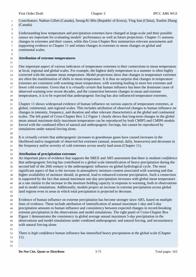
First Order Draft Chapter 3 IPCC AR6 WGI
Do Not Cite, Quote or Distribute 3-73 Total pages: 163
Contributors: Nathan Gillett (Canada), Seung-Ki Min (Republic of Korea), Ying Sun (China), Xuebin Zhang 1
(Canada) 2
3
Understanding how temperature and precipitation extremes have changed at large-scale and their possible 4
causes are important for evaluating models’ performance as well as future projections. Chapter 11 assesses 5
changes in extremes and their causes, while this Cross-Chapter Box summarizes relevant assessments and 6
supporting evidence in Chapter 11 and relates changes in extremes to mean changes on global and 7
continental scales. 8
9
Attribution of extreme temperatures 10
11
One important aspect of various indicators of temperature extremes is their connections to mean temperature 12
at local, regional and global scales. For example, the highest daily temperature in a summer is often highly 13
corrected with the summer mean temperature. Model projections show that changes in temperature extremes 14
are often the manifestation of shifts in mean temperature. It is thus no surprise that changes in temperature 15
extremes are consistent with warming mean temperature, with warming leading to more hot extremes and 16
fewer cold extremes. Given that it is virtually certain that human influence has been the dominant cause of 17
observed warming over recent decades, and the connection between changes in mean and extreme 18
temperatures, it is to be expected that anthropogenic forcing has also influenced temperature extremes. 19
20
Chapter 11 shows widespread evidence of human influence on various aspects of temperature extremes, at 21
global, continental, and regional scales. This includes attribution of observed changes to human influnece on 22
changes in intensity, frequency, and duration and other relevant characteristics at the global and continental 23
scales. The left panel of Cross-Chapter Box 3.2 Figure 1 clearly shows that long-term changes in the global 24
mean annual maximum daily maximum temperature can be reproduced by both CMIP5 and CMIP6 models 25
forced with the combined effect of natural and anthropogenic forcings, but cannot be reproduced by 26
simulations under natural forcing alone. 27
28
It is virtually certain that anthropogenic increases in greenhouse gases have caused increases in the 29
likelihood and/or magnitude of observed hot extremes (annual, seasonal, daily, heatwaves) and decreases in 30
the frequency and/or severity of cold extremes across nearly land areas (Chapter 11). 31
32
Attribution of precipitation extremes 33
An important piece of evidence that supports the SREX and AR5 assessment that there is medium confidence 34
that anthropogenic forcing has contributed to a global scale intensification of heavy precipitation during the 35
second half of the 20th century is the anthropogenic influence on global hydrological cycle. The most 36
significant aspect of that is the increase in atmospheric moisture content associated with warming and that 37
higher availability of moisture should, in general, lead to enhanced extreme precipitation. Such a connection 38
is supported by the fact that annual maximum one-day precipitation increases with global mean temperature 39
at a rate similar to the increase in the mositure holding capacity in response to warming, both in observations 40
and in model simulations. Additionally, models project an increase in extreme precipitation across global 41
land regions even in areas in which total precipitation is projected to decrease. 42
43
Evidence of human influence on extreme precipitation has become stronger since AR5, based on multiple 44
lines of evidence. These include attribution of intensification of annual maximum 1-day and 5-day 45
precipitation amounts to human influence and consisitency between expected changes in record-breaking 46
extreme precipitation in the observations and model simulations. The right panel of Cross-Chapter Box 47
Figure 1 demonstrates the consistency in global average annual maximum 5-day precipitation in the 48
observations and model simulations under combined anthropogenic and natural forcing, and inconsistency 49
with natural forcing alone. 50
51
There is high confidence human influence has intensified heavy precipitation at the global scale (Chapter 52
11). 53
54
55

First Order Draft Chapter 3 IPCC AR6 WGI
Do Not Cite, Quote or Distribute 3-74 Total pages: 163
[START CROSS-CHAPTER BOX 3.2, FIGURE 1 HERE] 1
2
Cross-Chapter Box 3.2, Figure 1: Time series of global averaged 5-year mean anomalies of TXx (°C) and Rx1day (mm) 3
during 1953-2017 from the GHCNDEX observations and the CMIP5 and CMIP6 4
multi-models with natural and human forcing (upper) and natural forcing only 5
(lower). For CMIP5, historical simulations for 1953-2005 are combined with 6
corresponding RCP4.5 scenario runs for 2006-2017. For observations, grids with 7
more than 90% data availability during 1951-2017 are used and global means are 8
calculated only for years when more than 80% of grids compared to the 1961-1990 9
coverage have data. The time-fixed observational mask (based on grids with more 10
than 90% data availability during 1951-2017) has been applied to model data 11
throughout the whole period. For CMIP5, shading represents the range of individual 12
model (ensemble means) and thick line indicates multi-model means (with equal 13
weighting given for each model). For CMIP6, only each model results (ensemble 14
means) are displayed as thin lines. Anomalies are relative to 1961-1990 means. 15
16
[END CROSS-CHAPTER BOX 3.2, FIGURE 1 HERE] 17
18
[END CROSS-CHAPTER BOX 3.2 HERE] 19
20
First Order Draft Chapter 3 IPCC AR6 WGI
Do Not Cite, Quote or Distribute 3-75 Total pages: 163
Frequently Asked Questions 1
2
FAQ 3.1: How much of Climate Change is Actually Natural Variability? 3
4
Natural variability refers to variations in climate which are caused by processes other than human influence. 5
It includes variability that is internally generated within the climate system, as well as variations in climate 6
driven by changes in solar brightness and by aerosol from large volcanic eruptions. Natural variability 7
influences all aspects of the climate system, but compared to human-induced climate change, it plays a 8
smaller role in long-term variations in globally-averaged temperatures in the oceans and atmosphere, and a 9
relatively larger role in shorter-term, and smaller-scale fluctuations in climate, particularly in other 10
variables such as precipitation and winds. Compared to human-induced changes, natural variability has a 11
large impact on global mean temperature variations on inter-annual time scales. However, if you consider 12
changes avareged over longer and longer time periods, the relative importance of natural variability in 13
global mean temperatures decreases. Changes due to natural variability are small compared to human-14
induced change on centennial time scales. On decadal to inter-decadal time scales, there is a middle ground 15
in which natural variability can have similar magnitudes to human-induced change. On this temporal range, 16
natural variability can substantially enhance or diminish global warming; creating periods of faster 17
warming or periods with little to no global warming at all. 18
19
Observational, paleoclimatic records (indirect measurements that span back thousands of years) and 20
computer models all show that global temperatures have, and are always changing – and that these changes 21
can occur for many reasons. One of these reasons is natural variability, which refers to the changes generated 22
within the climate system that are not connected to human-induced changes in atmospheric forcing. 23
24
The El Nino-Southern Oscillation is a phenomena that is a large source of natural climate variability, causing 25
winds and sea surface temperatures over the tropical eastern Pacific Ocean to change. ENSO, as it sometimes 26
referred to, lasts several years and can change ocean temperatures and rainfall patterns for that region as well 27
as alter global mean temperatures. The Northern Annular Mode is another example of natural variability, 28
which can effect weather in the high northern latitudes. 29
30
To understand which aspects of observed climate change have been caused by natural variability, scientists 31
seperate the forcings of climate model simulations due to there anthropogenic or natural origins. When the 32
latter are used as forcing the resulting simulations are generally called natural forced similations, and these 33
can be used to assess the range of variations expects due to natural climate variability alone. Use of these 34
simulations will allow us to assess which aspects of observed climate change are consistent with the 35
expected response to human influences, which are consistent with natural variability. 36
37
It is clear that natural variability on inter-annual time scales can have a much larger impact on global mean 38
temperatures than has been observed over the entire 100yr period (FAQ 3.1, Figure 1). As the temporal 39
window increases, it is also clear that the influence of natural variability on global mean temperatures 40
decreases, such that at decadal to inter-decadal time scales natural variability can have similar magnitudes to 41
the observed trend over the last 100-years (FAQ 3.1, Figure 1, black line). This suggests that natural 42
variability can lead to decadal periods of enhanced global warming and periods with little to no global 43
warming. As we move to temporal windows between 50-100 years in length, the impact of natural forcing is 44
so small that it is dwarfed by the mean warming rate observed over the last 100 years (FAQ 3.1, Figure 1). 45
46
Although humans are causing recent increases in global temperatures, natural variability plays a role in how 47
fast or slow temperatures rise. Much like riding a bike over hilly terrain, the bike is always going forward but 48
the presence of the hills will either reduce or increase the speed. 49
50
51
[START FAQ 3.1, FIGURE 1 HERE] 52
53
FAQ 3.1, Figure 1: Box and whisker plots displaying the magnitude of global mean surface temperature trends 54
calculated in various temporal windows (x-axis) from observations and pre-industrial control 55

First Order Draft Chapter 3 IPCC AR6 WGI
Do Not Cite, Quote or Distribute 3-76 Total pages: 163
simulations. The horizontal line within the box indicates the median, boundaries of the box 1
indicate the 25th- and 75th -percentile, and the whiskers indicate the highest and lowest values of 2
the results (note whiskers not displayed in this schematic illustration). The horizontal black line 3
indicates the observed global mean surface temperature trend value calculated over the 1910-2010 4
period. [Schematic illustration – will be updated with CMIP6 data for SOD] 5
6
[END FAQ 3.1, FIGURE 1 HERE] 7
8

First Order Draft Chapter 3 IPCC AR6 WGI
Do Not Cite, Quote or Distribute 3-77 Total pages: 163
FAQ 3.2: Are Climate Models Improving? 1
2
Yes, climate models have improved and continue to do so. Models are now more suitable for capturing the 3
complexities and small-scale processes of the climate system and they compare better with observations for 4
key climate variables. For decades, models have shown that changes to the climate comes from man-made 5
greenhouse gas emissions, but now, our understanding of the impacts of these changes, and of the changes 6
yet to come, are better than ever before. 7
8
Since the 1950s, scientists have used computer models to understand the Earth’s climate. Fundamentally, 9
models have improved due to advances in technology that allows for greater sophistication and more 10
complex computer simulations, resulting in models that compare more closely with real-world observations 11
of climate change. 12
13
[Paragraph introducing a climate model: its key parts – how they model the world, which processes/aspects 14
are always included, which additional ones are only included in more sophisticated models etc.] 15
16
The internal make-up of climate models is evolving to make them more suitable for simulating a variety of 17
climate processes, driven both by improved understanding of the climate system and scientists’ ability to 18
represent their understanding of processes by computer code and calculations, as well as the availability of 19
ever-bigger high-performance computing resources needed to run such code. The most recent generation of 20
models often has improved resolution in the atmosphere, ocean, and land domains. Higher resolution means 21
for example that the ocean components of some climate models now explicitly simulate the 100 km-scale 22
eddies that are responsible for much of oceanic heat transport. Unlike the previous generation of models, the 23
latest generation of models, in many cases now simulate higher atmospheric altitudes (often extending to 24
above 50 km in altitude), meaning that coupling processes between the upper atmosphere and the lower 25
atmosphere are now more realistic. Models are also increasingly able to simulate changes in the 26
concentrations of greenhouse gases and aerosols in response to changes in emissions, rather than having 27
these changes prescribed. For carbon dioxide, this means that such models include interactive representations 28
of the absorption of carbon dioxide by plants on land and by the ocean and its response to climate and 29
environmental change. 30
31
Progress in climate modelling is gradual, and more remains to be achieved. For example, it is still impossible 32
to explicitly simulate atmospheric convection globally for multidecadal timescales. 33
34
Key aspects of climate are now better simulated than in previous model evaluations. We know this through 35
comparisons against observational estimates, often using many multiple climate variables. For example, [key 36
physical fields, TBD] compare better against their observational references for recent decades (that are best 37
covered by observations; FAQ 3.1, Figure 1), although in most cases the improvement is only gradual. A 38
prime example is surface temperature, which was already well simulated in previous intercomparisons, so 39
did not substantially improve in the current generation of models. Reflection of sunlight by clouds and 40
precipitation, two key aspects of climate which in previous evaluations were problematic, are improved 41
compared to the previous generation of models. However, these improvements are gradual, partly because 42
climate models still do not operate at the resolution of about 1 km needed to realistically represent clouds. In 43
several diagnostics, it appears that the top-performing models of the previous generation have not 44
substantially improved but more poorly performing models have, meaning the CMIP6 ensemble as a whole 45
is more suitable for simulating climate than the CMIP5 ensemble. 46
47
48
[START FAQ 3.2, FIGURE 1 HERE] 49
50
FAQ 3.2, Figure 1: Centred pattern correlations between models and observations for the annual mean climatology 51
over the period 1980–1999 for four different variables: tas (surface air temperature), pr 52
(precipitation), rlut (outgoing longwave radiation), and swcre (shortwave cloud radiative effect). 53
Note the different scales. Results are shown for individual CMIP5 (black) and CMIP6 (blue) 54
models as thin lines, along with the corresponding ensemble average (thick line) and median (open 55

First Order Draft Chapter 3 IPCC AR6 WGI
Do Not Cite, Quote or Distribute 3-78 Total pages: 163
circle). The correlations are shown between the models and the reference observational data set. In 1
addition, the correlation between the reference and alternate observational data sets are shown 2
(solid green circles). To ensure a fair comparison across a range of model resolutions, the pattern 3
correlations are computed at a resolution of 4º in longitude and 5º in latitude. Only one realization 4
is used from each model from the CMIP5 and CMIP6 historical simulations. Figure produced with 5
ESMValTool v2.0a1. [Update with CMIP3 and additional CMIP6 models in the SOD] 6
7
[END FAQ 3.2, FIGURE 1 HERE] 8
9
10
First Order Draft Chapter 3 IPCC AR6 WGI
Do Not Cite, Quote or Distribute 3-79 Total pages: 163
FAQ 3.3: How Do we Know Humans are Responsible for Climate Change? 1
2
Synthesizing information from observations of climate change, from paleoclimate records that can show 3
changes over the past hundreds of thousands of years, and from computer models that can simulate past 4
climate change, allows us to clearly identify the role of humans in driving recent climate change. 5
6
Firstly, the current rates of increase of the concentration of the major greenhouse gases (carbon dioxide, 7
methane and nitrous oxide) are unprecedented over at least the last 22,000 years. Multiple lines of evidence 8
show that these increases are the results of human activities. The basic physics underlying the warming 9
effect of greenhouse gases on the climate has been understood for more than a century, and our latest 10
understanding is encapsulated in the latest generation climate models. Results consistently show that such 11
climate models can only reproduce the observed arming when including the effects of human activities, 12
including the increasing concentrations of these greenhouse gases. These simulations show a dominant 13
warming effect of greenhouse gas increases, which has been partly offset by the cooling effect of increases in 14
atmospheric aerosols. By contrast, simulations that include only natural processes, including internal climate 15
variability related to El Nino and other similar variations, as well as variations in solar brightness and 16
emissions from large volcanoes, are not able to reproduce the observed warming - they simulate much 17
smaller temperature trends, indicating that these natural factors cannot explain the strong warming rate 18
observed. 19
20
An additional line of evidence for the role of humans in driving climate change comes from comparing the 21
rate of warming observed over recent decades with that which occurred prior to human influence on climate. 22
Evidence from tree rings and other paleoclimate records shows that the rate of increase of global mean 23
surface temperature observed over the past fifty years far exceeded that which occurred in any previous 50 24
year period over the past 2000 years. Taken together this evidence shows that that humans are the dominant 25
cause of observed global warming over recent decades. 26
27
28
[START FAQ 3.3, FIGURE 1 HERE] 29
30
FAQ 3.3, Figure 1: Global average changes in continental land surface air temperatures (yellow panels), and upper 31
ocean heat content (blue panel). Anomalies are given relative to 1880–1919 for surface 32
temperatures and 1960–1980 for ocean heat content. All time-series are decadal averages, plotted 33
at the centre of the decade. For temperature panels, observations are dashed lines if the spatial 34
coverage of areas being examined is below 50%. For ocean heat content the solid line is where the 35
coverage of data is good and higher in quality, and the dashed line is where the data coverage is 36
only adequate, and thus, uncertainty is larger. Model results shown are Coupled Model 37
Intercomparison Project Phase 5 (CMIP5) multi-model ensemble ranges, with shaded bands 38
indicating the 5 to 95% confidence intervals. For further technical details see the Technical 39
Summary Supplementary Material. {Figure 10.21; Figure TS.12} 40
41
[END FAQ 3.3, FIGURE 1 HERE] 42
43
44
First Order Draft Chapter 3 IPCC AR6 WGI
Do Not Cite, Quote or Distribute 3-80 Total pages: 163
References 1
2
Abellán, E., McGregor, S., and England, M. H. (2017). Analysis of the southward wind shift of ENSO in CMIP5 3
models. J. Clim. 30, 2415–2435. doi:10.1175/JCLI-D-16-0326.1. 4
Abraham, J. P., Baringer, M., Bindoff, N. L., Boyer, T., Cheng, L. J., Church, J. A., et al. (2013). A review of global 5
ocean temperature observations: Implications for ocean heat content estimates and climate change. Rev. Geophys. 6
51, 450–483. doi:10.1002/rog.20022. 7
Abram, N. J., McGregor, H. V., Tierney, J. E., Evans, M. N., McKay, N. P., Kaufman, D. S., et al. (2016). Early onset 8
of industrial-era warming across the oceans and continents. Nature 536, 411–418. doi:10.1038/nature19082. 9
Abram, N. J., Mulvaney, R., Vimeux, F., Phipps, S. J., Turner, J., and England, M. H. (2014). Evolution of the Southern 10
Annular Mode during the past millennium. Nat. Clim. Chang. 4, 564–569. doi:10.1038/nclimate2235. 11
Abram, N. J., Wolff, E. W., and Curran, M. A. J. (2013). A review of sea ice proxy information from polar ice cores. 12
Quat. Sci. Rev. 79, 168–183. doi:https://doi.org/10.1016/j.quascirev.2013.01.011. 13
AchutaRao, K., and Sperber, K. (2002). Simulation of the El Niño Southern Oscillation: Results from the Coupled 14
Model Intercomparison Project. Clim. Dyn. 19, 191–209. doi:10.1007/s00382-001-0221-9. 15
Adam, O., Schneider, T., and Harnik, N. (2014). Role of Changes in Mean Temperatures versus Temperature Gradients 16
in the Recent Widening of the Hadley Circulation. J. Clim. 27, 7450–7461. doi:10.1175/JCLI-D-14-00140.1. 17
Adler, R. F., Huffman, G. J., Chang, A., Ferraro, R., Xie, P. P., Janowiak, J., et al. (2003). The version-2 global 18
precipitation climatology project (GPCP) monthly precipitation analysis (1979-present). J. Hydrometeorol. 4, 19
1147–1167. doi:10.1175/1525-7541(2003)004<1147:TVGPCP>2.0.CO;2. 20
Alkama, R., Marchand, L., Ribes, A., and Decharme, B. (2013). Detection of global runoff changes: results from 21
observations and CMIP5 experiments. Hydrol. Earth Syst. Sci. 17, 2967–2979. doi:10.5194/hess-17-2967-2013. 22
Allan, R. P. (2014). Dichotomy of drought and deluge. Nat. Geosci. 7, 700–701. doi:10.1038/ngeo2243. 23
Allan, R. P., Liu, C., Loeb, N. G., Palmer, M. D., Roberts, M., Smith, D., et al. (2014). Changes in global net radiative 24
imbalance 1985-2012. Geophys. Res. Lett. 41, 5588–5597. doi:10.1002/2014GL060962. 25
Allen, M. R., and Stott, P. A. (2003). Estimating signal amplitudes in optimal fingerprinting, part I: theory. Clim. Dyn. 26
21, 477–491. doi:10.1007/s00382-003-0313-9. 27
Allen, M. R., and Tett, S. F. B. (1999). Checking for model consistency in optimal fingerprinting. Clim. Dyn. 15, 419–28
434. doi:10.1007/s003820050291. 29
Allen, R. J., and Kovilakam, M. (2017). The role of natural climate variability in recent tropical expansion. J. Clim. 30, 30
6329–6350. doi:10.1175/JCLI-D-16-0735.1. 31
Allen, R. J., Norris, J. R., and Kovilakam, M. (2014). Influence of anthropogenic aerosols and the Pacific Decadal 32
Oscillation on tropical belt width. Nat. Geosci. 7, 270–274. doi:10.1038/ngeo2091. 33
Amaya, D. J., DeFlorio, M. J., Miller, A. J., and Xie, S.-P. (2017). WES feedback and the Atlantic Meridional Mode: 34
observations and CMIP5 comparisons. Clim. Dyn. 49, 1665–1679. doi:10.1007/s00382-016-3411-1. 35
Amaya, D. J., Siler, N., Xie, S.-P., and Miller, A. J. (2018). The interplay of internal and forced modes of Hadley Cell 36
expansion: lessons from the global warming hiatus. Clim. Dyn. 51, 305–319. doi:10.1007/s00382-017-3921-5. 37
Antonov, J. I., Seidov, D., Boyer, T. P., Locarnini, R. A., Mishonov, A. V., Garcia, H. E., et al. (2010). World Ocean 38
Atlas 2009, Volume 2: Salinity. Washington, D.C. Available at: 39
ftp://ftp.nodc.noaa.gov/pub/WOA09/DOC/woa09_vol2_text.pdf. 40
Aquila, V., Swartz, W. H., Waugh, D. W., Colarco, P. R., Pawson, S., Polvani, L. M., et al. (2016). Isolating the roles 41
of different forcing agents in global stratospheric temperature changes using model integrations with 42
incrementally added single forcings. J. Geophys. Res. 121, 8067–8082. doi:10.1002/2015JD023841. 43
Armour, K. C., Marshall, J., Scott, J. R., Donohoe, A., and Newsom, E. R. (2016). Southern Ocean warming delayed by 44
circumpolar upwelling and equatorward transport. Nat. Geosci. 9, 549. doi:10.1038/ngeo2731. 45
Aschwanden, A., Aøalgeirsdóttir, G., and Khroulev, C. (2013). Hindcasting to measure ice sheet model sensitivity to 46
initial states. Cryosphere 7, 1083–1093. doi:10.5194/tc-7-1083-2013. 47
Aschwanden, A., Fahnestock, M. A., and Truffer, M. (2016). Complex Greenland outlet glacier flow captured. Nat. 48
Commun. 7, 10524. doi:10.1038/ncomms10524. 49
Ashok, K., Behera, S. K., Rao, S. A., Weng, H., and Yamagata, T. (2007). El Niño Modoki and its possible 50
teleconnection. J. Geophys. Res. Ocean. 112, 1–27. doi:10.1029/2006JC003798. 51
Ault, T. R., Cole, J. E., and St. George, S. (2012). The amplitude of decadal to multidecadal variability in precipitation 52
simulated by state-of-the-art climate models. Geophys. Res. Lett. 39, n/a-n/a. doi:10.1029/2012GL053424. 53
Ayarzagüena, B., Polvani, L. M., Langematz, U., Akiyoshi, H., Bekki, S., Butchart, N., et al. (2018). No Robust 54
Evidence of Future Changes in Major Stratospheric Sudden Warmings: A Multi-model Assessment from CCMI. 55
Atmos. Chem. Phys. Discuss. 2018, 1–17. doi:10.5194/acp-2018-296. 56
First Order Draft Chapter 3 IPCC AR6 WGI
Do Not Cite, Quote or Distribute 3-81 Total pages: 163
Ayers, J. M., and Lozier, M. S. (2012). Unraveling dynamical controls on the North Pacific carbon sink. J. Geophys. 1
Res. Ocean. 117. doi:10.1029/2011JC007368. 2
Balmaseda, M. A., Trenberth, K. E., and Källén, E. (2013). Distinctive climate signals in reanalysis of global ocean heat 3
content. Geophys. Res. Lett. 40, 1754–1759. doi:10.1002/grl.50382. 4
Balsamo, G., Albergel, C., Beljaars, A., Boussetta, S., Brun, E., Cloke, H., et al. (2015). ERA-Interim/Land: A global 5
land surface reanalysis data set. Hydrol. Earth Syst. Sci. 19, 389–407. doi:10.5194/hess-19-389-2015. 6
Bamber, J. L., Westaway, R. M., Marzeion, B., and Wouters, B. (2018a). A new synthesis of annual land ice mass 7
trends 1992 to 2016. doi:10.1594/PANGAEA.890030. 8
Bamber, J., Westaway, R. M., Marzeion, B., and Wouters, B. (2018b). The land ice contribution to sea level during the 9
satellite era. Environ. Res. Lett. doi:10.1088/1748-9326/aac2f0. 10
Barichivich, J., Briffa, K. R., Myneni, R. B., Osborn, T. J., Melvin, T. M., Ciais, P., et al. (2013). Large-scale variations 11
in the vegetation growing season and annual cycle of atmospheric CO2 at high northern latitudes from 1950 to 12
2011. Glob. Chang. Biol. 19, 3167–3183. doi:doi:10.1111/gcb.12283. 13
Barkhordarian, A., von Storch, H., Behrangi, A., Loikith, P., Mechoso, C. R., and Detzer, J. (2018). Simultaneous 14
regional detection of land-use changes and elevated GHG levels: the case of spring precipitation in tropical South 15
America. Geophys. Res. Lett. 45. 16
Barnes, E. A. (2013). Revisiting the evidence linking Arctic amplification to extreme weather in midlatitudes. Geophys. 17
Res. Lett. 40, 4734–4739. 18
Bartlein, P. J., Harrison, S. P., Brewer, S., Connor, S., Davis, B. A. S., Gajewski, K., et al. (2011). Pollen-based 19
continental climate reconstructions at 6 and 21 ka: A global synthesis. Clim. Dyn. 37, 775–802. 20
doi:10.1007/s00382-010-0904-1. 21
Barton, C. A., and McCormack, J. P. (2017). Origin of the 2016 QBO Disruption and Its Relationship to Extreme El 22
Niño Events: Origin of the 2016 QBO Disruption. Geophys. Res. Lett. 44. 23
Batehup, R., McGregor, S., and Gallant, A. J. E. (2015). The influence of non-stationary teleconnections on 24
palaeoclimate reconstructions of ENSO variance using a pseudoproxy framework. Clim. Past 11, 1733–1749. 25
doi:10.5194/cp-11-1733-2015. 26
Bates, N., Astor, Y., Church, M., Currie, K., Dore, J., Gonaález-Dávila, M., et al. (2014). A Time-Series View of 27
Changing Ocean Chemistry Due to Ocean Uptake of Anthropogenic CO2 and Ocean Acidification. 28
Oceanography 27, 126–141. doi:10.5670/oceanog.2014.16. 29
Bellenger, H., Drushka, K., Asher, W., Reverdin, G., Katsumata, M., and Watanabe, M. (2017). Extension of the 30
prognostic model of sea surface temperature to rain-induced cool and fresh lenses. J. Geophys. Res. Ocean. 122, 31
484–507. doi:10.1002/2016JC012429. 32
Bellenger, H., Guilyardi, E., Leloup, J., Lengaigne, M., and Vialard, J. (2014). ENSO representation in climate models: 33
From CMIP3 to CMIP5. Clim. Dyn. 42, 1999–2018. doi:10.1007/s00382-013-1783-z. 34
Bellomo, K., and Clement, A. C. (2015). Evidence for weakening of the Walker circulation from cloud observations. 35
Geophys. Res. Lett. 42, 7758–7766. doi:10.1002/2015GL065463. 36
Bellomo, K., Murphy, L. N., Cane, M. A., Clement, A. C., and Polvani, L. M. (2018). Historical forcings as main 37
drivers of the Atlantic multidecadal variability in the CESM large ensemble. Clim. Dyn. 50, 3687–3698. 38
doi:10.1007/s00382-017-3834-3. 39
Bellucci, A., Mariotti, A., and Gualdi, S. (2017). The Role of Forcings in the Twentieth-Century North Atlantic 40
Multidecadal Variability: The 1940–75 North Atlantic Cooling Case Study. J. Clim. 30, 7317–7337. 41
doi:10.1175/JCLI-D-16-0301.1. 42
Berger, M., Camps, A., Font, J., Kerr, Y., Miller, J., Johannessen, J. A., et al. (2002). Measuring Ocean Salinity with 43
ESA’s SMOS Mission – Advancing the Science. in (ESA Publications Division), 113–121. Available at: 44
http://bora.uib.no/handle/1956/867 [Accessed September 16, 2018]. 45
Bernie, D. J., Guilyardi, E., Madec, G., Slingo, J. M., and Woolnough, S. J. (2007). Impact of resolving the diurnal 46
cycle in an ocean-atmosphere GCM. Part 1: A diurnally forced OGCM. Clim. Dyn. 29, 575–590. 47
doi:10.1007/s00382-007-0249-6. 48
Bernie, D. J., Guilyardi, E., Madec, G., Slingo, J. M., Woolnough, S. J., and Cole, J. (2008). Impact of resolving the 49
diurnal cycle in an ocean-atmosphere GCM. Part 2: A diurnally coupled CGCM. Clim. Dyn. 31, 909–925. 50
doi:10.1007/s00382-008-0429-z. 51
Bernie, D. J., Woolnough, S. J., Slingo, J. M., and Guilyardi, E. (2005). Modeling diurnal and intraseasonal variability 52
of the ocean mixed layer. J. Clim. 18, 1190–1202. doi:10.1175/JCLI3319.1. 53
Bindoff, N. L., Stott, P. A., AchutaRao, K. M., Allen, M. R., Gillett, N. P., Gutzler, D., et al. (2013). “Detection and 54
attribution of climate change: From global to regional,” in Climate Change 2013 the Physical Science Basis: 55
Working Group I Contribution to the Fifth Assessment Report of the Intergovernmental Panel on Climate 56
First Order Draft Chapter 3 IPCC AR6 WGI
Do Not Cite, Quote or Distribute 3-82 Total pages: 163
Change, ed. Intergovernmental Panel on Climate Change (Cambridge: Cambridge University Press), 867–952. 1
doi:10.1017/CBO9781107415324.022. 2
Bindoff, N. L., Willebrand, J., Artale, V., Cazenave, A., Gregory, J. M., Gulev, S., et al. (2007). “Observations: oceanic 3
climate change and sea level,” in Intergovernmental Panel on Climate Change Fourth Assessment Report Climate 4
Change 2007: The Physical Science Basis, ed. Intergovernmental Panel on Climate Change (Cambridge: 5
Cambridge University Press), 385–432. Available at: http://nora.nerc.ac.uk/id/eprint/15400. 6
Bindschadler, R. A., Nowicki, S., Abe-OUCHI, A., Aschwanden, A., Choi, H., Fastook, J., et al. (2013). Ice-sheet 7
model sensitivities to environmental forcing and their use in projecting future sea level (the SeaRISE project). J. 8
Glaciol. 59, 195–224. doi:10.3189/2013JoG12J125. 9
Bintanja, R., van Oldenborgh, G. J., Drijfhout, S. S., Wouters, B., and Katsman, C. A. (2013). Important role for ocean 10
warming and increased ice-shelf melt in Antarctic sea-ice expansion. Nat. Geosci. 6, 376. Available at: 11
http://dx.doi.org/10.1038/ngeo1767. 12
Bintanja, R., van Oldenborgh, G. J., and Katsman, C. A. (2015). The effect of increased fresh water from Antarctic ice 13
shelves on future trends in Antarctic sea ice. Ann. Glaciol. 56, 120–126. doi:DOI: 10.3189/2015AoG69A001. 14
Bitz, C. M. (2008). Some aspects of uncertainty in predicting sea ice thinning. 15
Blazquez, J., and Solman, S. (2017). Fronts and precipitation in CMIP5 models for the austral winter of the Southern 16
Hemisphere. Clim. Dyn. 50, 2705–2717. doi:10.1007/s00382-017-3765-z. 17
Boland, E. J. D., Bracegirdle, T. J., and Shuckburgh, E. F. (2017). Assessment of sea ice-atmosphere links in CMIP5 18
models. Clim. Dyn. 49, 683–702. doi:10.1007/s00382-016-3367-1. 19
Bonfils, C., and Santer, B. D. (2011). Investigating the possibility of a human component in various pacific decadal 20
oscillation indices. Clim. Dyn. 37, 1457–1468. doi:10.1007/s00382-010-0920-1. 21
Boone, A., Samuelsson, P., Gollvik, S., Napoly, A., Jarlan, L., Brun, E., et al. (2017). The interactions between soil-22
biosphere-atmosphere land surface model with a multi-energy balance (ISBA-MEB) option in SURFEXv8-Part 1: 23
Model description. Geosci. Model Dev. 10, 843–872. doi:10.5194/gmd-10-843-2017. 24
Boos, W. R., and Hurley, J. V (2012). Thermodynamic Bias in the Multimodel Mean Boreal Summer Monsoon. J. 25
Clim. 26, 2279–2287. doi:10.1175/JCLI-D-12-00493.1. 26
Booth, B. B. B., Dunstone, N. J., Halloran, P. R., Andrews, T., and Bellouin, N. (2012). Aerosols implicated as a prime 27
driver of twentieth-century North Atlantic climate variability. Nature 484, 228–232. doi:10.1038/nature10946. 28
Bopp, L., Resplandy, L., Orr, J. C., Doney, S. C., Dunne, J. P., Gehlen, M., et al. (2013). Multiple stressors of ocean 29
ecosystems in the 21st century: projections with CMIP5 models. Biogeosciences 10, 6225–6245. doi:10.5194/bg-30
10-6225-2013. 31
Bordbar, M. H., Martin, T., Latif, M., and Park, W. (2017). Role of internal variability in recent decadal to multidecadal 32
tropical Pacific climate changes. Geophys. Res. Lett. 44, 4246–4255. doi:10.1002/2016GL072355. 33
Box, J. E., and Colgan, W. (2013). Greenland ice sheet mass balance reconstruction. Part III: Marine ice loss and total 34
mass balance (1840-2010). J. Clim. doi:10.1175/JCLI-D-12-00546.1. 35
Braconnot, P., Harrison, S. P., Kageyama, M., and et al. (2012). Evaluation of climate models using palaeoclimatic 36
data. Nat. Clim. Chang. 2, 417–424. doi:10.1038/nclimate1456. 37
Breeden, M. L., and McKinley, G. A. (2016). Climate impacts on multidecadal pCO2 variability in the North Atlantic: 38
1948–2009. Biogeosciences 13, 3387–3396. doi:10.5194/bg-13-3387-2016. 39
Breitburg, D., Levin, L. A., Oschlies, A., Grégoire, M., Chavez, F. P., Conley, D. J., et al. (2018). Declining oxygen in 40
the global ocean and coastal waters. Science 359, eaam7240. doi:10.1126/science.aam7240. 41
Brient, F., and Bony, S. (2013). Interpretation of the positive low-cloud feedback predicted by a climate model under 42
global warming. Clim. Dyn. 40, 2415–2431. 43
Brient, F., and Schneider, T. (2016). Constraints on Climate Sensitivity from Space-Based Measurements of Low-44
Cloud Reflection. J. Clim. 29, 5821–5835. doi:10.1175/JCLI-D-15-0897.1. 45
Brierley, C., and Wainer, I. (2017). Interannual Variability in the Tropical Atlantic from the Last Glacial Maximum into 46
Future Climate Projections simulated by CMIP5/PMIP3. Clim. Past Discuss. doi:10.5194/cp-2017-145. 47
Brown, R., Vikhamar-Schuler, D., Bulygina, O., Derksen, C., Loujus, K., Mudryk, L., … Yang, D. (2017). “Arctic 48
terrestrial snow cover,” in (Oslo: Arctic Monitoring and Assessment Programme (AMAP).), 25–64. 49
Brown, J., Lynch, A. H., and Marshall, A. G. (2009). Variability of the Indian Ocean Dipole in coupled model 50
paleoclimate simulations. J. Geophys. Res. 114, D11105. doi:10.1029/2008JD010346. 51
Brown, P. T., Li, W., Jiang, J. H., and Su, H. (2016a). Spread in the magnitude of climate model interdecadal global 52
temperature variability traced to disagreements over high-latitude oceans. Geophys. Res. Lett. 43, 12,543-12,549. 53
doi:10.1002/2016GL071442. 54
Brown, P. T., Li, W., and Xie, S.-P. (2015). Regions of significant influence on unforced global mean surface air 55
temperature variability in climate models. J. Geophys. Res. Atmos. 120, 480–494. doi:10.1002/2014JD022576. 56

First Order Draft Chapter 3 IPCC AR6 WGI
Do Not Cite, Quote or Distribute 3-83 Total pages: 163
Brown, P. T., Lozier, M. S., Zhang, R., and Li, W. (2016b). The necessity of cloud feedback for a basin-scale Atlantic 1
Multidecadal Oscillation. Geophys. Res. Lett. 43, 3955–3963. doi:10.1002/2016GL068303. 2
Brown, R. D., and Robinson, D. A. (2011). Northern Hemisphere spring snow cover variability and change over 1922-3
2010 including an assessment of uncertainty. Cryosphere 5, 219–229. doi:10.5194/tc-5-219-2011. 4
Brutel-Vuilmet, C., Menegoz, M., and Krinner, G. (2013). An analysis of present and future seasonal Northern 5
Hemisphere land snow cover simulated by CMIP5 coupled climate models. CRYOSPHERE 7, 67–80. 6
doi:10.5194/tc-7-67-2013. 7
Bryan, F., and Bachman, S. (2015). Isohaline Salinity Budget of the North Atlantic Salinity Maximum. J. Phys. 8
Oceanogr. 45, 724–736. doi:10.1175/JPO-D-14-0172.1. 9
Bueler, E., and Brown, J. (2009). Shallow shelf approximation as a “sliding law” in a thermomechanically coupled ice 10
sheet model. J. Geophys. Res. Solid Earth 114, F03008. doi:10.1029/2008JF001179. 11
Butchart, N. (2014). The Brewer-Dobson circulation. Rev. Geophys. 52, 157–184. doi:10.1002/2013RG000448. 12
Butchart, N., Anstey, J. A., Hamilton, K., Osprey, S., McLandress, C., Bushell, A. C., et al. (2018). Overview of 13
experiment design and comparison of models participating in phase 1 of the SPARC Quasi-Biennial Oscillation 14
initiative (QBOi). Geosci. Model Dev. 11, 1009–1032. doi:10.5194/gmd-11-1009-2018. 15
Cabré, A., Marinov, I., Bernardello, R., and Bianchi, D. (2015). Oxygen minimum zones in the tropical Pacific across 16
CMIP5 models: mean state differences and climate change trends. Biogeosciences 12, 5429–5454. 17
doi:10.5194/bg-12-5429-2015. 18
Caesar, L., Rahmstorf, S., Robinson, A., Feulner, G., and Saba, V. (2018). Observed fingerprint of a weakening 19
Atlantic Ocean overturning circulation. Nature 556, 191–196. doi:10.1038/s41586-018-0006-5. 20
Cai, W., Santoso, A., Wang, G., Weller, E., Wu, L., Ashok, K., et al. (2014). Increased frequency of extreme Indian 21
Ocean Dipole events due to greenhouse warming. Nature 510, 254. Available at: 22
http://dx.doi.org/10.1038/nature13327. 23
Cai, W., Zheng, X.-T., Weller, E., Collins, M., Cowan, T., Lengaigne, M., et al. (2013). Projected response of the 24
Indian Ocean Dipole to greenhouse warming. Nat. Geosci. 6, 999. Available at: 25
http://dx.doi.org/10.1038/ngeo2009. 26
Caldwell, P., Zelinka, M., and Klein, S. (2018a). Evaluating Emergent Constraints on Equilibrium Climate Sensitivity. 27
J. Clim. 31, 3921–3942. doi:doi: 10.1175/JCLI-D-17-0631.1. 28
Caldwell, P., Zelinka, M., and Klein, S. (2018b). Evaluating Emergent Constraints on Equilibrium Climate Sensitivity. 29
J. Clim. 31, 3921–3942. doi:doi: 10.1175/JCLI-D-17-0631.1. 30
Calvo, N., Polvani, L. M., and Solomon, S. (2015). On the surface impact of Arctic stratospheric ozone extremes. 31
Environ. Res. Lett. 10. doi:10.1088/1748-9326/10/9/094003. 32
Cane, M. A., Clement, A. C., Murphy, L. N., and Bellomo, K. (2017). Low-Pass Filtering, Heat Flux, and Atlantic 33
Multidecadal Variability. J. Clim. 30, 7529–7553. doi:10.1175/JCLI-D-16-0810.1. 34
Capotondi, A., Wittenberg, A. T., Newman, M., Di Lorenzo, E., Yu, J.-Y., Braconnot, P., et al. (2014). Understanding 35
ENSO Diversity. Bull. Am. Meteorol. Soc. 96, 921–938. doi:10.1175/BAMS-D-13-00117.1. 36
Cassou, C., Kushnir, Y., Hawkins, E., Pirani, A., Kucharski, F., Kang, I.-S., et al. (2018). Decadal Climate Variability 37
and Predictability: Challenges and Opportunities. Bull. Am. Meteorol. Soc. 99, 479–490. doi:10.1175/BAMS-D-38
16-0286.1. 39
Cattiaux, J., and Cassou, C. (2013). Opposite CMIP3/CMIP5 trends in the wintertime Northern Annular Mode 40
explained by combined local sea ice and remote tropical influences. Geophys. Res. Lett. 40, 3682–3687. 41
doi:10.1002/grl.50643. 42
Cazenave, A., Meyssignac, B., Ablain, M., Balmaseda, M., Bamber, J., Barletta, V., et al. (2018). Global sea-level 43
budget 1993-present. Earth Syst. Sci. Data. doi:10.5194/essd-10-1551-2018. 44
Cha, S.-C., Moon, J.-H., and Song, Y. T. (2018). A Recent Shift Toward an El Niño-Like Ocean State in the Tropical 45
Pacific and the Resumption of Ocean Warming. Geophys. Res. Lett. 45, 11,885-11,894. 46
doi:10.1029/2018GL080651. 47
Chadburn, S. E., Burke, E. J., Cox, P. M., Friedlingstein, P., Hugelius, G., and Westermann, S. (2017). An observation-48
based constraint on permafrost loss as a function of global warming. Nat. Clim. Chang. 7, 340–344. 49
doi:10.1038/nclimate3262. 50
Chai, J., Liu, F., Liu, J., and Shen, X. (2018). Enhanced Global Monsoon in Present Warm Period Due to Natural and 51
Anthropogenic Forcings. Atmosphere (Basel). 9, 136. doi:10.3390/atmos9040136. 52
Chang, E. K. M., Ma, C.-G., Zheng, C., and Yau, A. M. W. (2016a). Observed and projected decrease in Northern 53
Hemisphere extratropical cyclone activity in summer and its impacts on maximum temperature. Geophys. Res. 54
Lett. 43, 2200–2208. doi:10.1002/2016GL068172. 55
First Order Draft Chapter 3 IPCC AR6 WGI
Do Not Cite, Quote or Distribute 3-84 Total pages: 163
Chang, E. K. M., Ma, C.-G., Zheng, C., and Yau, A. M. W. (2016b). Observed and projected decrease in Northern 1
Hemisphere extratropical cyclone activity in summer and its impacts on maximum temperature. Geophys. Res. 2
Lett. 43, 2200–2208. doi:10.1002/2016GL068172. 3
Charlton-Perez, A. J., Baldwin, M. P., Birner, T., Black, R. X., Butler, A. H., Calvo, N., et al. (2013). On the lack of 4
stratospheric dynamical variability in low-top versions of the CMIP5 models. J. Geophys. Res. Atmos. 118, 2494–5
2505. doi:10.1002/jgrd.50125. 6
Chen, H., Schneider, E. K., and Wu, Z. (2016a). Mechanisms of internally generated decadal-to-multidecadal variability 7
of SST in the Atlantic Ocean in a coupled GCM. Clim. Dyn. 46, 1517–1546. doi:10.1007/s00382-015-2660-8. 8
Chen, H. W., Zhang, F., and Alley, R. B. (2016b). The Robustness of Midlatitude Weather Pattern Changes due to 9
Arctic Sea Ice Loss. J. Clim. 29, 7831–7849. doi:10.1175/JCLI-D-16-0167.1. 10
Chen, X., and Tung, K.-K. (2014). Varying planetary heat sink led to global-warming slowdown and acceleration. 11
Science (80-. ). 345, 897–903. doi:10.1126/science.1254937. 12
Cheng, L., Trenberth, K. E., Fasullo, J., Boyer, T., Abraham, J., and Zhu, J. (2017). Improved estimates of ocean heat 13
content from 1960 to 2015. Sci. Adv. 3, e1601545. doi:10.1126/sciadv.1601545. 14
Cheng, L., Trenberth, K. E., Palmer, M. D., Zhu, J., and Abraham, J. P. (2016). Observed and simulated full-depth 15
ocean heat-content changes for 1970-2005. Ocean Sci. 12, 925–935. doi:10.5194/os-12-925-2016. 16
Chenoli, S. N., Mazuki, M. Y. A., Turner, J., and Abu Samah, A. (2017). Historical and projected changes in the 17
Southern Hemisphere Sub-tropical Jet during winter from the CMIP5 models. Clim. Dyn. 48, 661–681. 18
doi:10.1007/s00382-016-3102-y. 19
Cheung, A. H., Mann, M. E., Steinman, B. A., Frankcombe, L. M., England, M. H., and Miller, S. K. (2017). 20
Comparison of low-frequency internal climate variability in CMIP5 models and observations. J. Clim. 30, 4763–21
4776. doi:10.1175/JCLI-D-16-0712.1. 22
Chiang, J., Lan, C.-W., Chung, C.-H., Liao, Y.-C., and Lee, C.-J. (2013). Increase in the range between wet and dry 23
season precipitation. Nat. Geosci. 6, 263–267. 24
Chikamoto, Y., Mochizuki, T., Timmermann, A., Kimoto, M., and Watanabe, M. (2016). Potential tropical Atlantic 25
impacts on Pacific decadal climate trends. Geophys. Res. Lett. 43, 7143–7151. doi:10.1002/2016GL069544. 26
Choi, J., Son, S.-W., and Park, R. J. (2019). Aerosol versus greenhouse gas impacts on Southern Hemisphere general 27
circulation changes. Clim. Dyn. 52, 4127–4142. doi:10.1007/s00382-018-4370-5. 28
Chowdary, J. S., Xie, S.-P., Tokinaga, H., Okumura, Y. M., Kubota, H., Johnson, N., et al. (2012). Interdecadal 29
Variations in ENSO Teleconnection to the Indo–Western Pacific for 1870–2007. J. Clim. 25, 1722–1744. 30
doi:10.1175/JCLI-D-11-00070.1. 31
Chu, J.-E., Ha, K.-J., Lee, J.-Y., Wang, B., Kim, B.-H., and Chung, C. E. (2014). Future change of the Indian Ocean 32
basin-wide and dipole modes in the CMIP5. Clim. Dyn. 43, 535–551. doi:10.1007/s00382-013-2002-7. 33
Chung, E.-S., Soden, B. J., Sohn, B. J., and Shi, L. (2014). Upper-tropospheric moistening in response to anthropogenic 34
warming. Proc. Natl. Acad. Sci. U. S. A. doi:10.1073/pnas.1409659111. 35
Church, J. A., Clark, P. U., Cazenave, A., Gregory, J. M., Jevrejeva, S., Levermann, A., et al. (2013a). “Sea Level 36
Change,” in Climate Change 2013 - The Physical Science Basis, ed. Intergovernmental Panel on Climate Change 37
(Cambridge: Cambridge University Press), 1137–1216. doi:10.1017/CBO9781107415324.026. 38
Church, J. A., Monselesan, D., Gregory, J. M., and Marzeion, B. (2013b). Evaluating the ability of process based 39
models to project sea-level change. Environ. Res. Lett. 8, 014051. doi:10.1088/1748-9326/8/1/014051. 40
Clement, A., Bellomo, K., Murphy, L. N., Cane, M. A., Mauritsen, T., Rädel, G., et al. (2015). The Atlantic 41
Multidecadal Oscillation without a role for ocean circulation. Science (80-. ). 350, 320–324. 42
doi:10.1126/science.aab3980. 43
Coats, S., Smerdon, J. E., Cook, B. I., Seager, R., Cook, E. R., and Anchukaitis, K. J. (2016). Internal ocean-atmosphere 44
variability drives megadroughts in Western North America. Geophys. Res. Lett. 43, 9886–9894. 45
doi:10.1002/2016GL070105. 46
Cobb, K. M., Westphal, N., Sayani, H. R., Watson, J. T., Di Lorenzo, E., Cheng, H., et al. (2013). Highly variable El 47
Niño-Southern Oscillation throughout the Holocene. Science (80-. ). 339, 67–70. doi:10.1126/science.1228246. 48
Cocco, V., Joos, F., Steinacher, M., Frölicher, T. L., Bopp, L., Dunne, J., et al. (2013). Oxygen and indicators of stress 49
for marine life in multi-model global warming projections. Biogeosciences 10, 1849–1868. doi:10.5194/bg-10-50
1849-2013. 51
Collins, M., An, S.-I., Cai, W., Ganachaud, A., Guilyardi, E., Jin, F.-F., et al. (2010). The impact of global warming on 52
the tropical Pacific Ocean and El Niño. Nat. Geosci. 3, 391. Available at: https://doi.org/10.1038/ngeo868. 53
Collins, M., Knutti, R., Arblaster, J., Dufresne, J.-L., Fichefet, T., Friedlingstein, P., et al. (2013). “Long-term Climate 54
Change: Projections, Commitments and Irreversibility,” in Climate Change 2013: The Physical Science Basis. 55

First Order Draft Chapter 3 IPCC AR6 WGI
Do Not Cite, Quote or Distribute 3-85 Total pages: 163
Contribution of Working Group I to the Fifth Assessment Report of the Intergovernmental Panel on Climate 1
Change doi:10.1017/CBO9781107415324.024. 2
Cook, B. I., Anchukaitis, K. J., Touchan, R., Meko, D. M., and Cook, E. R. (2016a). Spatiotemporal drought variability 3
in the mediterranean over the last 900 years. J. Geophys. Res. doi:10.1002/2015JD023929. 4
Cook, B. I., Cook, E. R., Smerdon, J. E., Seager, R., Williams, A. P., Coats, S., et al. (2016b). North American 5
megadroughts in the Common Era: reconstructions and simulations. Wiley Interdiscip. Rev. Clim. Chang. 7, 411–6
432. doi:10.1002/wcc.394. 7
Cook, E. R., Anchukaitis, K. J., Buckley, B. M., D’Arrigo, R. D., Jacoby, G. C., and Wright, W. E. (2010). Asian 8
monsoon failure and megadrought during the last millennium. Science (80-. ). doi:10.1126/science.1185188. 9
Cook, E. R., Seager, R., Kushnir, Y., Briffa, K. R., Büntgen, U., Frank, D., et al. (2015). Old World megadroughts and 10
pluvials during the Common Era. Sci. Adv. doi:10.1126/sciadv.1500561. 11
Cook, E. R., Woodhouse, C. A., Eakin, C. M., Meko, D. H., and Stahle, D. W. (2004). Long-term aridity changes in the 12
western United States. Science (80-. ). doi:10.1126/science.1102586. 13
Cowan, T., Cai, W., Ng, B., and England, M. (2015). The Response of the Indian Ocean Dipole Asymmetry to 14
Anthropogenic Aerosols and Greenhouse Gases. J. Clim. 28, 2564–2583. doi:10.1175/JCLI-D-14-00661.1. 15
Cowtan, K., Hausfather, Z., Hawkins, E., Jacobs, P., Mann, M. E., Miller, S. K., et al. (2015). Robust comparison of 16
climate models with observations using blended land air and ocean sea surface temperatures. 42, 6526–6535. 17
doi:10.1002/2015GL064888.Abstract. 18
Cowtan, K., and Way, R. G. (2014). Coverage bias in the HadCRUT4 temperature series and its impact on recent 19
temperature trends. Q. J. R. Meteorol. Soc. 140, 1935–1944. doi:10.1002/qj.2297. 20
Cox, P. M., Huntingford, C., and Williamson, M. S. (2018). Emergent constraint on equilibrium climate sensitivity 21
from global temperature variability. Nature 553, 319. Available at: http://dx.doi.org/10.1038/nature25450. 22
Coy, L., Newman, P. A., Pawson, S., and Lait, L. R. (2017). Dynamics of the Disrupted 2015/16 Quasi-Biennial 23
Oscillation. J. Clim. 30, 5661–5674. doi:10.1175/JCLI-D-16-0663.1. 24
Crueger, T., Giorgetta, M. A., Brokopf, R., Esch, M., Fiedler, S., Hohenegger, C., et al. (2018). ICON-A, The 25
Atmosphere Component of the ICON Earth System Model: II. Model Evaluation. J. Adv. Model. Earth Syst. 26
doi:10.1029/2017MS001233. 27
Cubasch, U., Wuebbles, D., Chen, D., Facchini, M. C., Frame, D., Mahowald, N., et al. (2013). “Introduction,” in mate 28
Change 2013: The Physical Science Basis. Contribution of Working Group I to the Fifth Assessment Report of the 29
Intergovernmental Panel on Climate Change (IPCC). 30
Dai, A., and Bloecker, C. E. (2018). Impacts of internal variability on temperature and precipitation trends in large 31
ensemble simulations by two climate models. Clim. Dyn., 1–18. doi:10.1007/s00382-018-4132-4. 32
Dai, A., Fyfe, J. C., Xie, S. P., and Dai, X. (2015). Decadal modulation of global surface temperature by internal 33
climate variability. Nat. Clim. Chang. 5. doi:10.1038/nclimate2605. 34
Danabasoglu, G., Yeager, S., Bailey, D., Behrens, E., Bentsen, M., Bi, D., et al. (2014). North Atlantic Simulations in 35
Coordinated Ocean-ice Reference Experiments phase 2 (CORE-II). Part 1: Mean States. Ocean Model. 73, 76–36
107. doi:10.1016/j.ocemod.2013.10.005. 37
Danabasoglu, G., Yeager, S. G., Kim, W. M., Behrens, E., Bentsen, M., Bi, D., et al. (2016). North Atlantic simulations 38
in Coordinated Ocean-ice Reference Experiments phase II (CORE-II). Part II: Inter-annual to decadal variability. 39
Ocean Model. 97, 65–90. doi:10.1016/j.ocemod.2015.11.007. 40
Dangendorf, S., Marcos, M., Müller, A., Zorita, E., Riva, R., Berk, K., et al. (2015). Detecting anthropogenic footprints 41
in sea level rise. Nat. Commun. 6, 7849. doi:10.1038/ncomms8849. 42
Dätwyler, C., Neukom, R., Abram, N. J., Gallant, A. J. E., Grosjean, M., Jacques-Coper, M., et al. (2018). 43
Teleconnection stationarity, variability and trends of the Southern Annular Mode (SAM) during the last 44
millennium. Clim. Dyn. 51, 2321–2339. doi:10.1007/s00382-017-4015-0. 45
Davin, S. M. and S. I. S. and N. G. and E. L. (2017). Hydrological and biogeochemical constraints on terrestrial carbon 46
cycle feedbacks. Environ. Res. Lett. 12, 14009. Available at: http://stacks.iop.org/1748-9326/12/i=1/a=014009. 47
Davini, P., and Cagnazzo, C. (2014). On the misinterpretation of the North Atlantic Oscillation in CMIP5 models. Clim. 48
Dyn. 43, 1497–1511. doi:10.1007/s00382-013-1970-y. 49
Davini, P., and D’Andrea, F. (2016). Northern Hemisphere Atmospheric Blocking Representation in Global Climate 50
Models: Twenty Years of Improvements? J. Clim. 29, 8823–8840. doi:10.1175/JCLI-D-16-0242.1. 51
Davini, P., von Hardenberg, J., and Corti, S. (2015). Environmental Research Letters Related content Tropical origin 52
for the impacts of the Atlantic Multidecadal Variability on the Euro-Atlantic climate. Environ. Res. Lett. 10, 53
94010. Available at: http://iopscience.iop.org/article/10.1088/1748-9326/8/3/034037/pdf. 54
Davis, N., and Birner, T. (2017). On the Discrepancies in Tropical Belt Expansion between Reanalyses and Climate 55
Models and among Tropical Belt Width Metrics. J. Clim. 30, 1211–1231. doi:10.1175/JCLI-D-16-0371.1. 56
First Order Draft Chapter 3 IPCC AR6 WGI
Do Not Cite, Quote or Distribute 3-86 Total pages: 163
DeAngelis, A. M., Qu, X., Zelinka, M. D., and Hall, A. (2015). An observational radiative constraint on hydrologic 1
cycle intensification. Nature 528, 249. Available at: http://dx.doi.org/10.1038/nature15770. 2
Dee, D. P., Uppala, S. M., Simmons, A. J., Berrisford, P., Poli, P., Kobayashi, S., et al. (2011). The ERA-Interim 3
reanalysis: configuration and performance of the data assimilation system. Q. J. R. Meteorol. Soc. 137, 553–597. 4
doi:10.1002/qj.828. 5
DelSole, T., Trenary, L., Yan, X., and Tippett, M. K. (2018). Confidence intervals in optimal fingerprinting. Clim. Dyn. 6
doi:10.1007/s00382-018-4356-3. 7
Delworth, T. L., Zeng, F., Rosati, A., Vecchi, G. A., and Wittenberg, A. T. (2015). A Link between the Hiatus in Global 8
Warming and North American Drought. J. Clim. 28, 3834–3845. doi:10.1175/JCLI-D-14-00616.1. 9
Delworth, T. L., Zeng, F., Zhang, L., Zhang, R., Vecchi, G. A., and Yang, X. (2017). The Central Role of Ocean 10
Dynamics in Connecting the North Atlantic Oscillation to the Extratropical Component of the Atlantic 11
Multidecadal Oscillation. J. Clim. 30, 3789–3805. doi:10.1175/JCLI-D-16-0358.1. 12
Dennison, F. W., McDonald, A., and Morgenstern, O. (2016). The influence of ozone forcing on blocking in the 13
Southern Hemisphere. J. Geophys. Res. Atmos. 121, 14,358-14,371. doi:10.1002/2016JD025033. 14
Deppenmeier, A.-L., Haarsma, R. J., and Hazeleger, W. (2016). The Bjerknes feedback in the tropical Atlantic in 15
CMIP5 models. Clim. Dyn. 47, 2691–2707. doi:10.1007/s00382-016-2992-z. 16
Deser, C., Guo, R., and Lehner, F. (2017a). The relative contributions of tropical Pacific sea surface temperatures and 17
atmospheric internal variability to the recent global warming hiatus. Geophys. Res. Lett. 44, 7945–7954. 18
doi:10.1002/2017GL074273. 19
Deser, C., Hurrell, J. W., and Phillips, A. S. (2017b). The role of the North Atlantic Oscillation in European climate 20
projections. Clim. Dyn. 49, 3141–3157. doi:10.1007/s00382-016-3502-z. 21
Deser, C., Simpson, I. R., McKinnon, K. A., and Phillips, A. S. (2017c). The Northern Hemisphere Extratropical 22
Atmospheric Circulation Response to ENSO: How Well Do We Know It and How Do We Evaluate Models 23
Accordingly? J. Clim. 30, 5059–5082. doi:10.1175/JCLI-D-16-0844.1. 24
Deser, C., Sun, L., Tomas, R. A., and Screen, J. (2016). Does ocean coupling matter for the northern extratropical 25
response to projected Arctic sea ice loss? Geophys. Res. Lett. 43, 2149–2157. doi:10.1002/2016GL067792. 26
Dessler, A. E., and Forster, P. M. (2018). An estimate of equilibrium climate sensitivity from interannual variability. J. 27
Geophys. Res. Atmos. 123, 8634–8645. doi:10.1029/2018JD028481. 28
Deutsch, C., Berelson, W., Thunell, R., Weber, T., Tems, C., McManus, J., et al. (2014). Oceanography. Centennial 29
changes in North Pacific anoxia linked to tropical trade winds. Science 345, 665–8. doi:10.1126/science.1252332. 30
DiNezio, P. N., Clement, A., Vecchi, G. A., Soden, B., Broccoli, A. J., Otto-Bliesner, B. L., et al. (2011). The response 31
of the Walker circulation to Last Glacial Maximum forcing: Implications for detection in proxies. 32
Paleoceanography 26. doi:10.1029/2010PA002083. 33
DiNezio, P. N., and Tierney, J. E. (2013). The effect of sea level on glacial Indo-Pacific climate. Nat. Geosci. 6, 485–34
491. doi:10.1038/ngeo1823. 35
DiNezio, P. N., Tierney, J. E., Otto-Bliesner, B. L., Timmermann, A., Bhattacharya, T., Rosenbloom, N., et al. (2018). 36
Glacial changes in tropical climate amplified by the Indian Ocean. Sci. Adv. 4, eaat9658. 37
DiNezio, P. N., Vecchi, G. A., and Clement, A. C. (2013a). Detectability of changes in the walker circulation in 38
response to global warming. J. Clim. 26, 4038–4048. doi:10.1175/JCLI-D-12-00531.1. 39
DiNezio, P. N., Vecchi, G. A., and Clement, A. C. (2013b). Detectability of Changes in the Walker Circulation in 40
Response to Global Warming. J. Clim. 26, 4038–4048. doi:10.1175/JCLI-D-12-00531.1. 41
Ding, H., Greatbatch, R. J., Latif, M., and Park, W. (2015). The impact of sea surface temperature bias on equatorial 42
Atlantic interannual variability in partially coupled model experiments. Geophys. Res. Lett. 42, 5540–5546. 43
doi:10.1002/2015GL064799. 44
Ding, Q., Schweiger, A., L’Heureux, M., Battisti, D. S., Po-Chedley, S., Johnson, N. C., et al. (2017). Influence of high-45
latitude atmospheric circulation changes on summertime Arctic sea ice. Nat. Clim. Chang. 7, 289. Available at: 46
http://dx.doi.org/10.1038/nclimate3241. 47
Dippe, T., Greatbatch, R. J., and Ding, H. (2018). On the relationship between Atlantic Niño variability and ocean 48
dynamics. Clim. Dyn. 51, 597–612. doi:10.1007/s00382-017-3943-z. 49
Dirmeyer, P. A., Gao, X., Zhao, M., Guo, Z., Oki, T., and Hanasaki, N. (2006). GSWP-2: Multimodel analysis and 50
implications for our perception of the land surface. Bull. Am. Meteorol. Soc. 87, 1381–1397. doi:10.1175/BAMS-51
87-10-1381. 52
Domingues, C. M., Church, J. A., White, N. J., Gleckler, P. J., Wijffels, S. E., Barker, P. M., et al. (2008). Improved 53
estimates of upper-ocean warming and multi-decadal sea-level rise. Nature 453, 1090–1093. 54
doi:10.1038/nature07080. 55
First Order Draft Chapter 3 IPCC AR6 WGI
Do Not Cite, Quote or Distribute 3-87 Total pages: 163
Donat, M. G., Pitman, A. J., and Angélil, O. (2018). Understanding and reducing future uncertainty in mid-latitude 1
daily heat extremes via land surface feedback constraints. Geophys. Res. Lett. doi:10.1029/2018GL079128. 2
Dong, L., and McPhaden, M. J. (2017). Why has the relationship between Indian and Pacific Ocean decadal variability 3
changed in recent decades? J. Clim. 30, 1971–1983. doi:10.1175/JCLI-D-16-0313.1. 4
Dong, L., and Zhou, T. (2014). The Indian Ocean Sea Surface Temperature Warming Simulated by CMIP5 Models 5
during the Twentieth Century: Competing Forcing Roles of GHGs and Anthropogenic Aerosols. J. Clim. 27, 6
3348–3362. doi:10.1175/JCLI-D-13-00396.1. 7
Dong, L., Zhou, T., and Chen, X. (2014a). Changes of Pacific decadal variability in the twentieth century driven by 8
internal variability, greenhouse gases, and aerosols. Geophys. Res. Lett. 41, 8570–8577. 9
doi:10.1002/2014GL062269. 10
Dong, L., Zhou, T., Dai, A., Song, F., Wu, B., and Chen, X. (2016). The Footprint of the Inter-decadal Pacific 11
Oscillation in Indian Ocean Sea Surface Temperatures. Sci. Rep. 6, 21251. Available at: 12
http://dx.doi.org/10.1038/srep21251. 13
Dong, L., Zhou, T., and Wu, B. (2014b). Indian Ocean warming during 1958-2004 simulated by a climate system 14
model and its mechanism. Clim. Dyn. 42, 203–217. doi:10.1007/s00382-013-1722-z. 15
Douville, H., Voldoire, A., and Geoffroy, O. (2015). The recent global warming hiatus: What is the role of Pacific 16
variability? Geophys. Res. Lett. 42, 880–888. doi:10.1002/2014GL062775. 17
Downes, S. M., Farneti, R., Uotila, P., Griffies, S. M., Marsland, S. J., Bailey, D., et al. (2015). An assessment of 18
Southern Ocean water masses and sea ice during 1988-2007 in a suite of interannual CORE-II simulations. Ocean 19
Model. 94, 67–94. doi:10.1016/j.ocemod.2015.07.022. 20
Downes, S. M., and Hogg, A. M. (2013). Southern Ocean Circulation and Eddy Compensation in CMIP5 Models. J. 21
Clim. 26, 7198–7220. doi:10.1175/JCLI-D-12-00504.1. 22
Downes, S. M., Spence, P., and Hogg, A. M. (2018). Understanding variability of the Southern Ocean overturning 23
circulation in CORE-II models. Ocean Model. 123, 98–109. doi:https://doi.org/10.1016/j.ocemod.2018.01.005. 24
Drews, A., and Greatbatch, R. J. (2016). Atlantic Multidecadal Variability in a model with an improved North Atlantic 25
Current. Geophys. Res. Lett. 43, 8199–8206. doi:10.1002/2016GL069815. 26
Drijfhout, S. (2018). The relation between natural variations in ocean heat uptake and global mean surface temperature 27
anomalies in CMIP5. Sci. Rep. 8, 7402. doi:10.1038/s41598-018-25342-7. 28
Du, Y., Xie, S.-P., Huang, G., and Hu, K. (2009). Role of Air–Sea Interaction in the Long Persistence of El Niño–29
Induced North Indian Ocean Warming. J. Clim. 22, 2023–2038. doi:10.1175/2008JCLI2590.1. 30
Dunkerton, T. J. (2016). The quasi-biennial oscillation of 2015–2016: Hiccup or death spiral? Geophys. Res. Lett. 43, 31
10,510-547,552. doi:10.1002/2016GL070921. 32
Dunn-Sigouin, E., and Son, S.-W. (2013). Northern Hemisphere blocking frequency and duration in the CMIP5 models. 33
J. Geophys. Res. 118, 1179–1188. doi:10.1002/jgrd.50143. 34
Dunn, R. J. H., Willett, K. M., Ciavarella, A., and Stott, P. A. (2017). Comparison of land surface humidity between 35
observations and CMIP5 models. Earth Syst. Dyn. 8, 719–747. doi:10.5194/esd-8-719-2017. 36
Durack, P., Gleckler, P., Purkey, S., Johnson, G., Lyman, J., and Boywe, T. (2018). Ocean Warming: From the Surface 37
to the Deep in Observations and Models. Oceanography 31, 41–51. doi:10.5670/oceanog.2018.227. 38
Durack, P. J. (2015). Ocean Salinity and the Global Water Cycle. Oceanography 28, 20–31. 39
doi:10.5670/oceanog.2015.03. 40
Durack, P. J., Gleckler, P. J., Landerer, F. W., and Taylor, K. E. (2014a). Quantifying underestimates of long-term 41
upper-ocean warming. Nat. Clim. Chang. 4, 999–1005. doi:10.1038/nclimate2389. 42
Durack, P. J., and Wijffels, S. E. (2010). Fifty-Year trends in global ocean salinities and their relationship to broad-scale 43
warming. J. Clim. 23, 4342–4362. doi:10.1175/2010JCLI3377.1. 44
Durack, P. J., Wijffels, S. E., and Boyer, T. P. (2013). Long-term salinity changes and implications for the global water 45
cycle. Int. Geophys. 103, 727–757. doi:10.1016/B978-0-12-391851-2.00028-3. 46
Durack, P. J., Wijffels, S. E., and Gleckler, P. J. (2014b). Long-term sea-level change revisited: The role of salinity. 47
Environ. Res. Lett. 9. doi:10.1088/1748-9326/9/11/114017. 48
Durack, P. J., Wijffels, S. E., and Matear, R. J. (2012). Ocean salinities reveal strong global water cycle intensification 49
during 1950 to 2000. Science (80-. ). 336, 455–458. doi:10.1126/science.1212222. 50
Dwyer, J. G., Biasutti, M., and Sobel, A. H. (2014). The effect of greenhouse gas-induced changes in SST on the annual 51
cycle of zonal mea tropical precipitation. J. Clim. 27, 4544–4565. 52
England, M. H., Mcgregor, S., Spence, P., Meehl, G. A., Timmermann, A., Cai, W., et al. (2014a). Recent 53
intensification of wind-driven circulation in the Pacific and the ongoing warming hiatus. Nat. Clim. Chang. 4, 54
222–227. doi:10.1038/nclimate2106. 55
First Order Draft Chapter 3 IPCC AR6 WGI
Do Not Cite, Quote or Distribute 3-88 Total pages: 163
England, M. H., Mcgregor, S., Spence, P., Meehl, G. A., Timmermann, A., Cai, W., et al. (2014b). Recent 1
intensification of wind-driven circulation in the Pacific and the ongoing warming hiatus. Nat. Clim. Chang. 4. 2
doi:10.1038/nclimate2106. 3
Eyring, V., Arblaster, J. M., Cionni, I., Sedláček, J., Perlwitz, J., Young, P. J., et al. (2013). Long-term ozone changes 4
and associated climate impacts in CMIP5 simulations. J. Geophys. Res. Atmos. 118, 5029–5060. 5
doi:10.1002/jgrd.50316. 6
Eyring, V., Bony, S., Meehl, G. A., Senior, C. A., Stevens, B., Stouffer, R. J., et al. (2016a). Overview of the Coupled 7
Model Intercomparison Project Phase 6 (CMIP6) experimental design and organization. Geosci. Model Dev. 9, 8
1937–1958. doi:10.5194/gmd-9-1937-2016. 9
Eyring, V., Cox, P. M., Flato, G. M., Gleckler, P. J., Abramowitz, G., Caldwell, P., et al. (2019). Taking climate model 10
evaluation to the next level. Nat. Clim. Chang. 9, 102–110. doi:10.1038/s41558-018-0355-y. 11
Eyring, V., Gleckler, P. J., Heinze, C., Stouffer, R. J., Taylor, K. E., Balaji, V., et al. (2016b). Towards improved and 12
more routine Earth system model evaluation in CMIP. Earth Syst. Dyn. 7, 813–830. doi:10.5194/esd-7-813-2016. 13
Eyring, V., Righi, M., Lauer, A., Evaldsson, M., Wenzel, S., Jones, C., et al. (2016c). ESMValTool (v1.0) – a 14
community diagnostic and performance metrics tool for routine evaluation of Earth system models in CMIP. 15
Geosci. Model Dev. 9, 1747–1802. doi:10.5194/gmd-9-1747-2016. 16
Fan, T., Deser, C., and Schneider, D. P. (2014). Recent Antarctic sea ice trends in the context of Southern Ocean 17
surface climate variations since 1950. Geophys. Res. Lett. doi:10.1002/2014GL059239. 18
Farinotti, D., Huss, M., Fürst, J. J., Landmann, J., Machguth, H., Maussion, F., et al. (2019). A consensus estimate for 19
the ice thickness distribution of all glaciers on Earth. Nat. Geosci. 2019, 1. doi:10.1038/s41561-019-0300-3. 20
Farneti, R., Downes, S. M., Griffies, S. M., Marsland, S. J., Behrens, E., Bentsen, M., et al. (2015). An assessment of 21
Antarctic Circumpolar Current and Southern Ocean meridional overturning circulation during 1958-2007 in a 22
suite of interannual CORE-II simulations. Ocean Model. 93, 84–120. doi:10.1016/j.ocemod.2015.07.009. 23
Fathrio, I., Iizuka, S., Manda, A., Kodama, Y.-M., Ishida, S., Moteki, Q., et al. (2017a). Assessment of western Indian 24
Ocean SST bias of CMIP5 models. J. Geophys. Res. Ocean. 122, 3123–3140. doi:10.1002/2016JC012443. 25
Fathrio, I., Manda, A., Iizuka, S., Kodama, Y.-M., and Ishida, S. (2017b). Evaluation of CMIP5 models on sea surface 26
salinity in the Indian Ocean. IOP Conf. Ser. Earth Environ. Sci. 54, 012039. doi:10.1088/1755-1315/54/1/012039. 27
Fay, A. R., and McKinley, G. A. (2013). Global trends in surface ocean p CO 2 from in situ data. Global Biogeochem. 28
Cycles 27, 541–557. doi:10.1002/gbc.20051. 29
Fay, A. R., McKinley, G. A., and Lovenduski, N. S. (2014). Southern Ocean carbon trends: Sensitivity to methods. 30
Geophys. Res. Lett. 41, 6833–6840. doi:10.1002/2014GL061324. 31
Feldstein, S. B., and Franzke, C. (2006). Are the North Atlantic Oscillation and the Northern Annular Mode 32
Distinguishable? J. Atmos. Sci. 63, 2915–2930. doi:10.1175/JAS3798.1. 33
Ferreira, D., Marshall, J., Bitz, C. M., Solomon, S., and Plumb, A. (2014). Antarctic Ocean and Sea Ice Response to 34
Ozone Depletion: A Two-Time-Scale Problem. J. Clim. 28, 1206–1226. doi:10.1175/JCLI-D-14-00313.1. 35
Fettweis, X., Box, J. E., Agosta, C., Amory, C., Kittel, C., Lang, C., et al. (2017). Reconstructions of the 1900–2015 36
Greenland ice sheet surface mass balance using the regional climate MAR model. Cryosph. 11, 1015–1033. 37
doi:10.5194/tc-11-1015-2017. 38
Fine, E. C., Bryan, F. O., Large, W. G., and Bailey, D. A. (2015). An initial estimate of the global distribution of 39
diurnal variation in sea surface salinity. J. Geophys. Res. Ocean. 120, 3211–3228. doi:10.1002/2014JC010483. 40
Flato, G., Marotzke, J., Abiodun, B., Braconnot, P., Chou, S. C., Collins, W., et al. (2013). “Evaluation of climate 41
models,” in Climate Change 2013 the Physical Science Basis: Working Group I Contribution to the Fifth 42
Assessment Report of the Intergovernmental Panel on Climate Change, ed. Intergovernmental Panel on Climate 43
Change (Cambridge: Cambridge University Press), 741–866. doi:10.1017/CBO9781107415324.020. 44
Fleming, L. E., and Anchukaitis, K. J. (2016). North Pacific decadal variability in the CMIP5 last millennium 45
simulations. Clim. Dyn. 47, 3783–3801. doi:10.1007/s00382-016-3041-7. 46
Fogt, R. L., Goergens, C. A., Jones, J. M., Schneider, D. P., Nicolas, J. P., Bromwich, D. H., et al. (2017). A twentieth 47
century perspective on summer Antarctic pressure change and variability and contributions from tropical SSTs 48
and ozone depletion. Geophys. Res. Lett. 44, 9918–9927. doi:10.1002/2017GL075079. 49
Folland, C. K., Renwick, J. A., Salinger, M. J., and Mullan, A. B. (2002). Relative influences of the Interdecadal Pacific 50
Oscillation and ENSO on the South Pacific Convergence Zone. Geophys. Res. Lett. 29, 2–5. 51
doi:10.1029/2001GL014201. 52
Forkel, M., Carvalhais, N., Rödenbeck, C., Keeling, R., Heimann, M., Thonicke, K., et al. (2016). Enhanced seasonal 53
CO2 exchange caused by amplified plant productivity in northern ecosystems. Science (80-. ). 351, 696–699. 54
doi:10.1126/science.aac4971. 55

First Order Draft Chapter 3 IPCC AR6 WGI
Do Not Cite, Quote or Distribute 3-89 Total pages: 163
Francis, J. A., and Vavrus, S. J. (2012). Evidence linking Arctic Amplification to Extreme Weather.pdf. Geophys. Res. 1
Lett. 39, 1–6. doi:10.1029/2012GL051000. 2
Friedlingstein, P. (2015). Carbon cycle feedbacks and future climate change. Philos. Trans. R. Soc. A Math. Phys. Eng. 3
Sci. 373. Available at: http://rsta.royalsocietypublishing.org/content/373/2054/20140421.abstract. 4
Friedman, A. R., Hegerl, G. C., Schurer, A., Lee, S.-Y., Kong, W., and Chiang, J. C. H. (2019). Forced and unforced 5
behavior of the interhemispheric SST contrast during the instrumental period. submitted. 6
Friedman, A. R., Reverdin, G., Khodri, M., and Gastineau, G. (2017). A new record of Atlantic sea surface salinity 7
from 1896 to 2013 reveals the signatures of climate variability and long-term trends. Geophys. Res. Lett. 44, 8
1866–1876. doi:10.1002/2017GL072582. 9
Fučkar, N. S., Massonnet, F., Guemas, V., García-Serrano, J., Bellprat, O., Acosta, M., et al. (2016). Record Low 10
Northern Hemisphere Sea Ice Extent in March 2015. Bull. Am. Meteorol. Soc. 97, S136–S140. 11
doi:10.1175/BAMS-D-16-0153.1. 12
Fyke, J., Sergienko, O., Löfverström, M., Price, S., and Lenaerts, J. T. M. (2018). An Overview of Interactions and 13
Feedbacks Between Ice Sheets and the Earth System. Rev. Geophys. 56, 361–408. doi:10.1029/2018RG000600. 14
Gagné, M.-È., Fyfe, J. C., Gillett, N. P., Polyakov, I. V, and Flato, G. M. (2017a). Aerosol-driven increase in Arctic sea 15
ice over the middle of the twentieth century. Geophys. Res. Lett. 44, 7338–7346. doi:10.1002/2016GL071941. 16
Gagné, M.-È., Gillett, N. P., and Fyfe, J. C. (2015). Observed and simulated changes in Antarctic sea ice extent over the 17
past 50 years. Geophys. Res. Lett. 42, 90–95. doi:10.1002/2014GL062231. 18
Gagné, M.-È., Kirchmeier-Young, M. C., Gillett, N. P., and Fyfe, J. C. (2017b). Arctic sea ice response to the eruptions 19
of Agung, El Chichón, and Pinatubo. J. Geophys. Res. Atmos. 122, 8071–8078. doi:10.1002/2017JD027038. 20
Garfinkel, C. I., Waugh, D. W., and Polvani, L. M. (2015). Recent Hadley cell expansion: The role of internal 21
atmospheric variability in reconciling modeled and observed trends. Geophys. Res. Lett. 42, 10,824-10,831. 22
doi:10.1002/2015GL066942. 23
Gastineau, G., and Frankignoul, C. (2015). Influence of the North Atlantic SST variability on the atmospheric 24
circulation during the twentieth century. J. Clim. 28, 1396–1416. doi:10.1175/JCLI-D-14-00424.1. 25
Gedney, N., Huntingford, C., Weedon, G. P., Bellouin, N., Boucher, O., and Cox, P. M. (2014). Detection of solar 26
dimming and brightening effects on Northern Hemisphere river flow. Nat. Geosci. 7, 796. 27
Geller, M. A., Zhou, T., Shindell, D., Ruedy, R., Aleinov, I., Nazarenko, L., et al. (2016). Modeling the QBO—28
Improvements resulting from higher-model vertical resolution. J. Adv. Model. Earth Syst. 8, 1092–1105. 29
doi:10.1002/2016MS000699. 30
Gent, P. R. (2016). Effects of Southern Hemisphere Wind Changes on the Meridional Overturning Circulation in Ocean 31
Models. Ann. Rev. Mar. Sci. 8, 79–94. doi:10.1146/annurev-marine-122414-033929. 32
Gerber, E. P., and Son, S.-W. (2014). Quantifying the Summertime Response of the Austral Jet Stream and Hadley Cell 33
to Stratospheric Ozone and Greenhouse Gases. J. Clim. 27, 5538–5559. doi:10.1175/JCLI-D-13-00539.1. 34
Gillett, N. P., Allen, M. R., and Williams, K. D. (2003). Modelling the atmospheric response to doubled CO2 and 35
depleted stratospheric ozone using a stratosphere-resolving coupled GCM. Q. J. R. Meteorol. Soc. 129, 947–966. 36
doi:10.1256/qj.02.102. 37
Gillett, N. P., and Fyfe, J. C. (2013). Annular mode changes in the CMIP5 simulations. Geophys. Res. Lett. 40, 1189–38
1193. doi:10.1002/grl.50249. 39
Gillett, N. P., Fyfe, J. C., and Parker, D. E. (2013). Attribution of observed sea level pressure trends to greenhouse gas, 40
aerosol, and ozone changes. Geophys. Res. Lett. 40, 2302–2306. doi:10.1002/grl.50500. 41
Gillett, N. P., Shiogama, H., Funke, B., Hegerl, G., Knutti, R., Matthes, K., et al. (2016). The Detection and Attribution 42
Model Intercomparison Project (DAMIP v1.0) contribution to CMIP6. Geosci. Model Dev. 9, 3685–3697. 43
doi:10.5194/gmd-9-3685-2016. 44
Gleckler, P., Doutriaux, C., Durack, P., Taylor, K., Zhang, Y., Williams, D., et al. (2016a). A More Powerful Reality 45
Test for Climate Models. Eos (Washington. DC). 97. doi:10.1029/2016EO051663. 46
Gleckler, P. J., Durack, P. J., Stouffer, R. J., Johnson, G. C., and Forest, C. E. (2016b). Industrial-era global ocean heat 47
uptake doubles in recent decades. Nat. Clim. Chang. 6, 394–398. doi:10.1038/nclimate2915. 48
Gleckler, P. J., Santer, B. D., Domingues, C. M., Pierce, D. W., Barnett, T. P., Church, J. A., et al. (2012). Human-49
induced global ocean warming on multidecadal timescales. Nat. Clim. Chang. 2, 524–529. 50
doi:10.1038/nclimate1553. 51
Gleckler, P. J., Taylor, K. E., and Doutriaux, C. (2008). Performance metrics for climate models. J. Geophys. Res. 113, 52
D06104. doi:10.1029/2007JD008972. 53
Goelzer, H., Nowicki, S., Edwards, T., Beckley, M., Abe-Ouchi, A., Aschwanden, A., et al. (2018). Design and results 54
of the ice sheet model initialisation initMIP-Greenland: An ISMIP6 intercomparison. Cryosphere 12, 1433–1460. 55
doi:10.5194/tc-12-1433-2018. 56
First Order Draft Chapter 3 IPCC AR6 WGI
Do Not Cite, Quote or Distribute 3-90 Total pages: 163
Goelzer, H., Robinson, A., Seroussi, H., and van de Wal, R. S. W. (2017). Recent Progress in Greenland Ice Sheet 1
Modelling. Curr. Clim. Chang. Reports 3, 291–302. doi:10.1007/s40641-017-0073-y. 2
Gong, H., Wang, L., Chen, W., Chen, X., and Nath, D. (2017). Biases of the wintertime Arctic Oscillation in CMIP5 3
models. Environ. Res. Lett. 12, 14001. Available at: http://stacks.iop.org/1748-9326/12/i=1/a=014001. 4
Good, S. A. (2017). The impact of observational sampling on time series of global 0–700 m ocean average temperature: 5
a case study. Int. J. Climatol. 37, 2260–2268. doi:10.1002/joc.4654. 6
Goubanova, K., Sanchez-Gomez, E., Frauen, C., and Voldoire, A. (2019). Respective roles of remote and local wind 7
stress forcings in the development of warm SST errors in the South-Eastern Tropical Atlantic in a coupled high-8
resolution model. Clim. Dyn. 52, 1359–1382. doi:10.1007/s00382-018-4197-0. 9
Graven, H. D., Keeling, R. F., Piper, S. C., Patra, P. K., Stephens, B. B., Wofsy, S. C., et al. (2013). Enhanced Seasonal 10
Exchange of CO2 by Northern Ecosystems Since 1960. Science (80-. ). doi:10.1126/science.1239207. 11
Gray, J. M., Frolking, S., Kort, E. A., Ray, D. K., Kucharik, C. J., Ramankutty, N., et al. (2014). Direct human 12
influence on atmospheric CO2 seasonality from increased cropland productivity. Nature 515, 398. 13
Gregory, J. M., Stott, P. A., Cresswell, D. J., Rayner, N. A., Gordon, C., and Sexton, D. M. H. (2002). Recent and 14
future changes in Arctic sea ice simulated by the HadCM3 AOGCM. Geophys. Res. Lett. 29, 24–28. 15
doi:10.1029/2001GL014575. 16
Greve, P., Orlowsky, B., Mueller, B., Sheffield, J., Reichstein, M., and Seneviratne, S. I. (2014). Global assessment of 17
trends in wetting and drying over land. Nat. Geosci. 7, 716–721. doi:10.1038/ngeo2247. 18
Griffies, S. M., Biastoch, A., Böning, C., Bryan, F., Danabasoglu, G., Chassignet, E. P., et al. (2009). Coordinated 19
Ocean-ice Reference Experiments (COREs). Ocean Model. 26, 1–46. doi:10.1016/j.ocemod.2008.08.007. 20
Griffies, S. M., Danabasoglu, G., Durack, P. J., Adcroft, A. J., Balaji, V., Böning, C. W., et al. (2016). OMIP 21
contribution to CMIP6: Experimental and diagnostic protocol for the physical component of the Ocean Model 22
Intercomparison Project. Geosci. Model Dev. 9, 3231–3296. doi:10.5194/gmd-9-3231-2016. 23
Griffies, S. M., Winton, M., Anderson, W. G., Benson, R., Delworth, T. L., Dufour, C. O., et al. (2015). Impacts on 24
ocean heat from transient mesoscale eddies in a hierarchy of climate models. J. Clim. 28, 952–977. 25
doi:10.1175/JCLI-D-14-00353.1. 26
Griffies, S. M., Yin, J., Durack, P. J., Goddard, P., Bates, S. C., Behrens, E., et al. (2014). An assessment of global and 27
regional sea level for years 1993-2007 in a suite of interannual core-II simulations. Ocean Model. 78, 35–89. 28
doi:10.1016/j.ocemod.2014.03.004. 29
Griffin, D., and Anchukaitis, K. J. (2014). How unusual is the 2012-2014 California drought? Geophys. Res. Lett. 30
doi:10.1002/2014GL062433. 31
Grise, K. M., Davis, S. M., Simpson, I. R., Waugh, D. W., Fu, Q., Allen, R. J., et al. (2019). Recent Tropical 32
Expansion: Natural Variability or Forced Response? J. Clim. 32, 1551–1571. doi:10.1175/JCLI-D-18-0444.1. 33
Grise, K. M., Davis, S. M., Staten, P. W., and Adam, O. (2018). Regional and Seasonal Characteristics of the Recent 34
Expansion of the Tropics. J. Clim. 31, 6839–6856. doi:10.1175/JCLI-D-18-0060.1. 35
Grist, J. P., Josey, S. A., Zika, J. D., Evans, D. G., and Skliris, N. (2016). Assessing recent air-sea freshwater flux 36
changes using a surface temperature-salinity space framework. J. Geophys. Res. Ocean. 121, 8787–8806. 37
doi:10.1002/2016JC012091. 38
Gu, G., and Adler, R. F. (2018). Precipitation Intensity Changes in the Tropics from Observations and Models. J. Clim. 39
31, 4775–4790. doi:10.1175/JCLI-D-17-0550.1. 40
Guan, X., Huang, J., Guo, R., and Lin, P. (2015). The role of dynamically induced variability in the recent warming 41
trend slowdown over the Northern Hemisphere. Sci. Rep. 5, 12669. doi:10.1038/srep12669. 42
Gudmundsson, L., and Seneviratne, S. I. (2016). Anthropogenic climate change affects meteorological drought risk in 43
Europe. Environ. Res. Lett. doi:10.1088/1748-9326/11/4/044005. 44
Gudmundsson, L., Seneviratne, S. I., and Zhang, X. (2017). Anthropogenic climate change detected in European 45
renewable freshwater resources. Nat. Clim. Chang. 7, 813. Available at: http://dx.doi.org/10.1038/nclimate3416. 46
Guemas, V., Doblas-Reyes, F. J., Andreu-Burillo, I., and Asif, M. (2013). Retrospective prediction of the global 47
warming slowdown in the past decade. Nat. Clim. Chang. 3, 649. Available at: 48
http://dx.doi.org/10.1038/nclimate1863. 49
Guilyardi, E., Wittenberg, A., Fedorov, A., Collins, M., Wang, C., Capotondi, A., et al. (2009). Understanding El Niño 50
in ocean-atmosphere general circulation models: Progress and challenges. Bull. Am. Meteorol. Soc. 90, 325–340. 51
doi:10.1175/2008BAMS2387.1. 52
Haarsma, R. J., Roberts, M. J., Vidale, P. L., Senior, C. A., Bellucci, A., Bao, Q., et al. (2016). High Resolution Model 53
Intercomparison Project (HighResMIP~v1.0) for CMIP6. Geosci. Model Dev. 9, 4185–4208. doi:10.5194/gmd-9-54
4185-2016. 55
First Order Draft Chapter 3 IPCC AR6 WGI
Do Not Cite, Quote or Distribute 3-91 Total pages: 163
Hall, A., Cox, P., Huntingford, C., and Klein, S. (2019). Progressing emergent constraints on future climate change. 1
Nat. Clim. Chang. 2
Hammond, M. L., Beaulieu, C., Sahu, S. K., and Henson, S. A. (2017). Assessing trends and uncertainties in satellite-3
era ocean chlorophyll using space-time modeling. Global Biogeochem. Cycles 31, 1103–1117. 4
doi:10.1002/2016GB005600. 5
Han, W., Meehl, G. A., Hu, A., Alexander, M. A., Yamagata, T., Yuan, D., et al. (2014a). Intensification of decadal and 6
multi-decadal sea level variability in the western tropical Pacific during recent decades. Clim. Dyn. 43, 1357–7
1379. doi:10.1007/s00382-013-1951-1. 8
Han, W., Vialard, J., McPhaden, M. J., Lee, T., Masumoto, Y., Feng, M., et al. (2014b). Indian ocean decadal 9
variability: A review. Bull. Am. Meteorol. Soc. 95, 1679–1703. doi:10.1175/BAMS-D-13-00028.1. 10
Hannart, A. (2016). Integrated optimal fingerprinting: Method description and illustration. J. Clim. 29, 1977–1998. 11
doi:10.1175/JCLI-D-14-00124.1. 12
Hannart, A., and Naveau, P. (2018). Probabilities of causation of climate changes. J. Clim. 31, 5507–5524. 13
doi:10.1175/JCLI-D-17-0304.1. 14
Hannart, A., Ribes, A., and Naveau, P. (2014). Optimal fingerprinting under multiple sources of uncertainty. Geophys. 15
Res. Lett. 41, 1261–1268. doi:10.1002/2013GL058653. 16
Hardiman, S. C., Butchart, N., and Calvo, N. (2014). The morphology of the Brewer-Dobson circulation and its 17
response to climate change in CMIP5 simulations. Q. J. R. Meteorol. Soc. 140, 1958–1965. doi:10.1002/qj.2258. 18
Hardiman, S. C., Lin, P., Scaife, A. A., Dunstone, N. J., and Ren, H.-L. (2017). The influence of dynamical variability 19
on the observed Brewer-Dobson circulation trend. Geophys. Res. Lett. 44, 2885–2892. 20
Hargreaves, J. C., and Annan, J. (2014). Can we trust climate models? WIREs Clim. Chang. 5, 435–440. 21
doi:10.1002/wcc.288. 22
Harlaß, J., Latif, M., and Park, W. (2018). Alleviating tropical Atlantic sector biases in the Kiel climate model by 23
enhancing horizontal and vertical atmosphere model resolution: climatology and interannual variability. Clim. 24
Dyn. 50, 2605–2635. doi:10.1007/s00382-017-3760-4. 25
Harrison, D. E., and Larkin, N. K. (1998). El Nino-Southern Oscillation sea surface temperature and wind anomalies, 26
1946-1993. Rev. Geophys. 36, 353–399. doi:10.1029/98RG00715. 27
Harrison, S. P., Bartlein, P. J., Brewer, S., and et al. (2014a). Climate model benchmarking with glacial and mid-28
Holocene climates. Clim. Dyn. 43, 671–688. doi:10.1007/s00382-013-1922-6. 29
Harrison, S. P., Bartlein, P. J., Brewer, S., Prentice, I. C., Boyd, M., Hessler, I., et al. (2014b). Climate model 30
benchmarking with glacial and mid-Holocene climates. Clim. Dyn. 43, 671–688. doi:10.1007/s00382-013-1922-6. 31
Harrison, S. P., Bartlein, P. J., Izumi, K., Li, G., Annan, J., Hargreaves, J., et al. (2015). Evaluation of CMIP5 palaeo-32
simulations to improve climate projections. Nat. Clim. Chang. 5, 735. Available at: 33
http://dx.doi.org/10.1038/nclimate2649. 34
Harrison, S. P., Bartlein, P. J., and Prentice, I. C. (2016a). What have we learnt from palaeoclimate simulations? J. 35
Quat. Sci. 31, 363–385. doi:10.1002/jqs.2842. 36
Harrison, S. P., Bartlein, P. J., and Prentice, I. C. (2016b). What have we learnt from paleoclimate simulations? Quat. 37
Sci. Rev. 31, 363–385. doi:10.1002/jqs.2842. 38
Hausfather, Z., Cowtan, K., Clarke, D. C., Jacobs, P., Richardson, M., and Rohde, R. (2017). Assessing recent warming 39
using instrumentally homogeneous sea surface temperature records. Sci. Adv. 3. doi:10.1126/sciadv.1601207. 40
Haustein, K., Allen, M. R., Forster, P. M., Otto, F. E. L., Mitchell, D. M., Matthews, H. D., et al. (2017). A real-time 41
Global Warming Index. Sci. Rep. 7. doi:10.1038/s41598-017-14828-5. 42
Hawkins, E., and Sutton, R. (2011). The potential to narrow uncertainty in projections of regional precipitation change. 43
Clim. Dyn. 37, 407–418. doi:10.1007/s00382-010-0810-6. 44
Haywood, A. M., Hill, D. J., Dolan, A. M., Otto-Bliesner, B. L., Bragg, F., Chan, W. L., et al. (2013). Large-scale 45
features of Pliocene climate: Results from the Pliocene Model Intercomparison Project. Clim. Past. 46
doi:10.5194/cp-9-191-2013. 47
Hedemann, C., Mauritsen, T., Jungclaus, J., and Marotzke, J. (2017). The subtle origins of surface-warming hiatuses. 48
Nat. Clim. Chang. 7, 336. Available at: http://dx.doi.org/10.1038/nclimate3274. 49
Hegerl, G. C., Brönnimann, S., Schurer, A., and Cowan, T. (2018). The early 20th century warming: Anomalies, 50
causes, and consequences. Wiley Interdiscip. Rev. Clim. Chang. 9, e522. doi:10.1002/wcc.522. 51
Hegerl, G. C., and et al. (2015). Challenges in quantifying changes in the global water cycle. Bull. Am. Meteor. Soc. 96, 52
1097–1115. doi:10.1175/BAMS-D-13-00212.1. 53
Hegglin, M. I., Plummer, D. A., Shepherd, T. G., Scinocca, J. F., Anderson, J., Froidevaux, L., et al. (2014). Vertical 54
structure of stratospheric water vapour trends derived from merged satellite data. Nat. Geosci. 7, 768–776. 55
doi:10.1038/NGEO2236. 56
First Order Draft Chapter 3 IPCC AR6 WGI
Do Not Cite, Quote or Distribute 3-92 Total pages: 163
Helsen, M. M., Van De Wal, R. S. W., Reerink, T. J., Bintanja, R., Madsen, M. S., Yang, S., et al. (2017). On the 1
importance of the albedo parameterization for the mass balance of the Greenland ice sheet in EC-Earth. 2
Cryosphere 11, 1949–1965. doi:10.5194/tc-11-1949-2017. 3
Henley, B. J. (2017). Pacific decadal climate variability: Indices, patterns and tropical-extratropical interactions. Glob. 4
Planet. Change 155, 42–55. doi:https://doi.org/10.1016/j.gloplacha.2017.06.004. 5
Henley, B. J., Gergis, J., Karoly, D. J., Power, S., Kennedy, J., and Folland, C. K. (2015). A Tripole Index for the 6
Interdecadal Pacific Oscillation. Clim. Dyn. 45, 3077–3090. doi:10.1007/s00382-015-2525-1. 7
Henley, B. J., Meehl, G., Power, S. B., Folland, C. K., King, A. D., Brown, J. N., et al. (2017). Spatial and temporal 8
agreement in climate model simulations of the Interdecadal Pacific Oscillation. Environ. Res. Lett. 12, 44011. 9
Available at: http://stacks.iop.org/1748-9326/12/i=4/a=044011. 10
Henson, S. A., Cole, H. S., Hopkins, J., Martin, A. P., and Yool, A. (2018). Detection of climate change-driven trends 11
in phytoplankton phenology. Glob. Chang. Biol. 24, e101–e111. doi:10.1111/gcb.13886. 12
Henson, S. A., Sarmiento, J. L., Dunne, J. P., Bopp, L., Lima, I., Doney, S. C., et al. (2010). Detection of anthropogenic 13
climate change in satellite records of ocean chlorophyll and productivity. Biogeosciences 7, 621–640. 14
doi:10.5194/bg-7-621-2010. 15
Hessl, A., Allen, K. J., Vance, T., Abram, N. J., and Saunders, K. M. (2017). Reconstructions of the southern annular 16
mode (SAM) during the last millennium. Prog. Phys. Geogr. 41, 834–849. doi:10.1177/0309133317743165. 17
Heuzé, C., Heywood, K. J., Stevens, D. P., and Ridley, J. K. (2013). Southern Ocean bottom water characteristics in 18
CMIP5 models. Geophys. Res. Lett. 40, 1409–1414. doi:10.1002/grl.50287. 19
Heuzé, C., Heywood, K. J., Stevens, D. P., and Ridley, J. K. (2015). Changes in Global Ocean Bottom Properties and 20
Volume Transports in CMIP5 Models under Climate Change Scenarios. J. Clim. 28, 2917–2944. 21
doi:10.1175/JCLI-D-14-00381.1. 22
Hirabayashi, Y., Nakano, K., Zhang, Y., Watanabe, S., Tanoue, M., and Kanae, S. (2016). Contributions of natural and 23
anthropogenic radiative forcing to mass loss of Northern Hemisphere mountain glaciers and quantifying their 24
uncertainties. Sci. Rep. 6, 29723. doi:10.1038/srep29723. 25
Hirota, N., Shiogama, H., Akiyoshi, H., Ogura, T., Takahashi, M., Kawatani, Y., et al. (2018). The influences of El 26
Nino and Arctic sea-ice on the QBO disruption in February 2016. npj Clim. Atmos. Sci. 1, 10. 27
doi:10.1038/s41612-018-0020-1. 28
Hobbs, W. R., Bindoff, N. L., and Raphael, M. N. (2015). New Perspectives on Observed and Simulated Antarctic Sea 29
Ice Extent Trends Using Optimal Fingerprinting Techniques. J. Clim. 28, 1543–1560. doi:10.1175/JCLI-D-14-30
00367.1. 31
Hobbs, W. R., Massom, R., Stammerjohn, S., Reid, P., Williams, G., and Meier, W. (2016). A review of recent changes 32
in Southern Ocean sea ice, their drivers and forcings. Glob. Planet. Change 143, 228–250. 33
doi:https://doi.org/10.1016/j.gloplacha.2016.06.008. 34
Hock, R., Marzeion, B., Bliss, A., Giesen, R., Hirabayashi, Y., Huss, M., et al. GlacierMIP - A Model Intercomparison 35
of Global-scale Glacier Mass-balance Models and Projections What is GlacierMIP ? How do recent global-scale 36
glacier projections compare ? J. Glaciol. (submitted. 37
Hock, R., Marzeion, B., Bliss, A., Giesen, R., Hirabayashi, Y., Huss, M., et al. (2019a). GlacierMIP - A model 38
intercomparison of global-scale glacier mass-balance models and projections. J. Glaciol., submitted. 39
Hock, R., Marzeion, B., Bliss, A., Giesen, R., Hirabayashi, Y., Huss, M., et al. (2019b). GlacierMIP - A Model 40
Intercomparison of Global-scale Glacier Mass-balance Models and Projections What is GlacierMIP ? How do 41
recent global-scale glacier projections compare ? J. Glaciol., submitted. 42
Hoell, A., Hoerling, M., Eischeid, J., Quan, X.-W., and Liebmann, B. (2017). Reconciling Theories for Human and 43
Natural Attribution of Recent East Africa Drying. J. Clim. 30, 1939–1957. doi:10.1175/JCLI-D-16-0558.1. 44
Hoffman, F. M., Lindsay, K., and Wu, T. (2013). The Causes and Implications of Persistent Atmospheric Carbon 45
Dioxide Biases in Earth System Models. J. Geophys. Res. Biogeosciences 119, 1–58. 46
doi:10.1002/2013JG002381.Abstract. 47
Holland, M. M., Landrum, L., Kostov, Y., and Marshall, J. (2017). Sensitivity of Antarctic sea ice to the Southern 48
Annular Mode in coupled climate models. Clim. Dyn. 49, 1813–1831. doi:10.1007/s00382-016-3424-9. 49
Hoogakker, B. A. A., Smith, R. S., Singarayer, J. S., Marchant, R., Prentice, I. C., Allen, J. R. M., et al. (2016). 50
Terrestrial biosphere changes over the last 120 kyr. Clim. Past 12, 51–73. doi:10.5194/cp-12-51-2016. 51
Hopcroft, P. O., Valdes, P. J., Harper, A. B., and Beerling, D. J. (2017). Multi vegetation model evaluation of the Green 52
Sahara climate regime. Geophys. Res. Lett. doi:10.1002/2017GL073740. 53
Hope, P., Henley, B. J., Gergis, J., Brown, J., and Ye, H. (2017). Time-varying spectral characteristics of ENSO over 54
the Last Millennium. Clim. Dyn. 49, 1705–1727. doi:10.1007/s00382-016-3393-z. 55

First Order Draft Chapter 3 IPCC AR6 WGI
Do Not Cite, Quote or Distribute 3-93 Total pages: 163
Horel, J. D., and Wallace, J. M. (1981). Planetary-Scale Atmospheric Phenomena Associated with the Southern 1
Oscillation. Mon. Weather Rev. 109, 813–829. doi:10.1175/1520-0493(1981)109<0813:PSAPAW>2.0.CO;2. 2
Hori, M., Sugiura, K., Kobayashi, K., Aoki, T., Tanikawa, T., Kuchiki, K., et al. (2017). A 38-year (1978-2015) 3
Northern Hemisphere daily snow cover extent product derived using consistent objective criteria from satellite-4
borne optical sensors. Remote Sens. Environ. 191, 402–418. doi:10.1016/j.rse.2017.01.023. 5
Hoskins, B. J., and Karoly, D. J. (1981). The Steady Linear Response of a Spherical Atmosphere to Thermal and 6
Orographic Forcing. J. Atmos. Sci. 38, 1179–1196. doi:10.1175/1520-0469(1981)038<1179:TSLROA>2.0.CO;2. 7
Hourdin, F., Găinusă-Bogdan, A., Braconnot, P., Dufresne, J.-L., Traore, A.-K., and Rio, C. (2015). Air moisture 8
control on ocean surface temperature, hidden key to the warm bias enigma. Geophys. Res. Lett. 42, 10,885-9
10,893. doi:10.1002/2015GL066764. 10
Hourdin, F., Mauritsen, T., Gettelman, A., Golaz, J.-C., Balaji, V., Duan, Q., et al. (2017). The art and science of 11
climate model tuning. Bull. Am. Meteorol. Soc. 98, 589–602. doi:10.1175/BAMS-D-15-00135.1. 12
Hsu, P., Li, T., and Wang, B. (2011). Trends in global monsoon area and precipitation over the past 30 years. Geophys. 13
Res. Lett. 38, n/a-n/a. doi:10.1029/2011GL046893. 14
Hu, A., and Bates, S. C. (2018). Internal climate variability and projected future regional steric and dynamic sea level 15
rise. Nat. Commun. 9, 1068. doi:10.1038/s41467-018-03474-8. 16
Hu, A., and Deser, C. (2013). Uncertainty in future regional sea level rise due to internal climate variability. Geophys. 17
Res. Lett. 40, 2768–2772. doi:10.1002/grl.50531. 18
Hu, K., Huang, G., Zheng, X.-T., Xie, S.-P., Qu, X., Du, Y., et al. (2014). Interdecadal Variations in ENSO Influences 19
on Northwest Pacific–East Asian Early Summertime Climate Simulated in CMIP5 Models. J. Clim. 27, 5982–20
5998. doi:10.1175/JCLI-D-13-00268.1. 21
Hu, S., and Fedorov, A. V. (2017). The extreme El Niño of 2015-2016 and the end of global warming hiatus. Geophys. 22
Res. Lett. 44, 3816–3824. doi:10.1002/2017GL072908. 23
Hua, W., Dai, A., and Qin, M. (2018). Contributions of Internal Variability and External Forcing to the Recent Pacific 24
Decadal Variations. Geophys. Res. Lett. 45, 7084–7092. doi:10.1029/2018GL079033. 25
Huang, J., Xie, Y., Guan, X., Li, D., and Ji, F. (2017a). The dynamics of the warming hiatus over the Northern 26
Hemisphere. Clim. Dyn. 48, 429–446. doi:10.1007/s00382-016-3085-8. 27
Huang, J., Zhang, X., Zhang, Q., Lin, Y., Hao, M., Luo, Y., et al. (2017b). Recently amplified arctic warming has 28
contributed to a continual global warming trend. Nat. Clim. Chang. 7, 875–879. doi:10.1038/s41558-017-0009-5. 29
Huber, M., and Knutti, R. (2014). Natural variability, radiative forcing and climate response in the recent hiatus 30
reconciled. Nat. Geosci. 7, 651. Available at: http://dx.doi.org/10.1038/ngeo2228. 31
Huntingford, C., Atkin, O. K., Martinez-de la Torre, A., Mercado, L. M., Heskel, M. A., Harper, A. B., et al. (2017). 32
Implications of improved representations of plant respiration in a changing climate. Nat. Commun. 8, 1602. 33
doi:10.1038/s41467-017-01774-z. 34
Huntingford, C., Stott, P. A., Allen, M. R., and Lambert, F. H. (2006). Incorporating model uncertainty into attribution 35
of observed temperature change. Geophys. Res. Lett. 33. doi:10.1029/2005GL024831. 36
Huntzinger, D. N., Michalak, A. M., Schwalm, C., Ciais, P., King, A. W., Fang, Y., et al. (2017). Uncertainty in the 37
response of terrestrial carbon sink to environmental drivers undermines carbon-climate feedback predictions. Sci. 38
Rep. 7, 4765. doi:10.1038/s41598-017-03818-2. 39
Huss, M., and Hock, R. (2015). A new model for global glacier change and sea-level rise. Front. Earth Sci. 3. 40
doi:10.3389/feart.2015.00054. 41
Huybrechts, P., Payne, T., Abe-Ouchi, A., Calov, R., Fabre, A., Fastook, J. L., et al. (1996). The EISMINT benchmarks 42
for testing ice-sheet models. Ann. Glaciol. 23, 1-X1. doi:10.1017/S0260305500013197. 43
Hyder, P., Edwards, J. M., Allan, R. P., Hewitt, H. T., Bracegirdle, T. J., Gregory, J. M., et al. (2018). Critical Southern 44
Ocean climate model biases traced to atmospheric model cloud errors. Nat. Commun. 9, 3625. 45
doi:10.1038/s41467-018-05634-2. 46
Iglesias-Suarez, F., Young, P. J., and Wild, O. (2016). Stratospheric ozone change and related climate impacts over 47
1850-2100 as modelled by the ACCMIP ensemble. Atmos. Chem. Phys. 16, 343–363. doi:10.5194/acp-16-343-48
2016. 49
Iles, C., and Hegerl, G. (2017). Role of the North Atlantic Oscillation in decadal temperature trends. Environ. Res. Lett. 50
12, 114010. doi:10.1088/1748-9326/aa9152. 51
Ilicak, M., Drange, H., Wang, Q., Gerdes, R., Aksenov, Y., Bailey, D., et al. (2016). An assessment of the Arctic Ocean 52
in a suite of interannual CORE-II simulations. Part III: Hydrography and fluxes. Ocean Model. 100, 141–161. 53
doi:10.1016/j.ocemod.2016.02.004. 54
Imbers, J., Lopez, A., Huntingford, C., and Allen, M. (2014). Sensitivity of Climate Change Detection and Attribution 55
to the Characterization of Internal Climate Variability. J. Clim. 27, 3477–3491. doi:10.1175/JCLI-D-12-00622.1. 56

First Order Draft Chapter 3 IPCC AR6 WGI
Do Not Cite, Quote or Distribute 3-94 Total pages: 163
IPCC (2013). “Summary for Policymakers,” in Climate Change 2013: The Physical Science Basis. Contribution of 1
Working Group I to the Fifth Assessment Report of the Intergovernmental Panel on Climate Change, eds. T. F. 2
Stocker, D. Qin, G. K. Plattner, M. Tignor, S. K. Allen, J. Boschung, et al. (Cambridge, United Kingdom and 3
New York, NY, USA: Cambridge University Press), 3–29. 4
Ishii, M., and Kimoto, M. (2009). Reevaluation of historical ocean heat content variations with time-varying XBT and 5
MBT depth bias corrections. J. Oceanogr. 65, 287–299. doi:10.1007/s10872-009-0027-7. 6
Ito, T., Minobe, S., Long, M. C., and Deutsch, C. (2017). Upper ocean O 2 trends: 1958-2015. Geophys. Res. Lett. 44, 7
4214–4223. doi:10.1002/2017GL073613. 8
Ivanova, D. P., Gleckler, P. J., Taylor, K. E., Durack, P. J., and Marvel, K. D. (2016). Moving beyond the total sea ice 9
extent in gauging model biases. J. Clim. 29, 8965–8987. doi:10.1175/JCLI-D-16-0026.1. 10
Ivy, D. J., Solomon, S., Calvo, N., and Thompson, D. W. J. (2017). Observed connections of Arctic stratospheric ozone 11
extremes to Northern Hemisphere surface climate. Environ. Res. Lett. 12. doi:10.1088/1748-9326/aa57a4. 12
Jeong, D. Il, Sushama, L., and Naveed Khaliq, M. (2017). Attribution of spring snow water equivalent (SWE) changes 13
over the northern hemisphere to anthropogenic effects. Clim. Dyn. 48, 3645–3658. doi:10.1007/s00382-016-3291-14
4. 15
Jia, G., and et al. (2019). SRCCL report Chapter 2: Land-Climate Interactions. SRCCL Rep., submitted. 16
Jia, L., and DelSole, T. (2012). Optimal Determination of Time-Varying Climate Change Signals. J. Clim. 25, 7122–17
7137. doi:10.1175/JCLI-D-11-00434.1. 18
Jiang, D., Tian, Z., and Lang, X. (2015). Mid-Holocene global monsoon area and precipitation from PMIP simulations. 19
Clim. Dyn. 44, 2493–2512. doi:10.1007/s00382-014-2175-8. 20
Jiang, J. H., Su, H., and Zhai, C. (2012). Evaluation of cloud and water vapor simulations in CMIP5 climate models 21
using NASA “A-Train” satellite observations. J. Geophys. Res. 118. doi:10.10 29/2011JD017237. 22
Jin, F. F., Kim, S. T., and Bejarano, L. (2006). A coupled-stability index for ENSO. Geophys. Res. Let. 33, L23708. 23
Jones, G. S., and Kennedy, J. J. (2017). Sensitivity of attribution of anthropogenic near-surface warming to 24
observational uncertainty. J. Clim. 30, 4677–4691. doi:10.1175/JCLI-D-16-0628.1. 25
Jones, G. S., Stott, P. A., and Christidis, N. (2013). Attribution of observed historical near-surface temperature 26
variations to anthropogenic and natural causes using CMIP5 simulations. J. Geophys. Res. Atmos. 118, 4001–27
4024. doi:10.1002/jgrd.50239. 28
Jones, G. S., Stott, P. A., and Mitchell, J. F. B. (2016a). Uncertainties in the attribution of greenhouse gas warming and 29
implications for climate prediction. J. Geophys. Res. 121, 6969–6992. doi:10.1002/2015JD024337. 30
Jones, J. M., Gille, S. T., Goosse, H., Abram, N. J., Canziani, P. O., Charman, D. J., et al. (2016b). Assessing recent 31
trends in high-latitude Southern Hemisphere surface climate. Nat. Clim. Chang. 6, 917. 32
Joshi, M. K., and Kucharski, F. (2017). Impact of Interdecadal Pacific Oscillation on Indian summer monsoon rainfall: 33
an assessment from CMIP5 climate models. Clim. Dyn. 48, 2375–2391. doi:10.1007/s00382-016-3210-8. 34
Jouanno, J., Hernandez, O., and Sanchez-Gomez, E. (2017). Equatorial Atlantic interannual variability and its relation 35
to dynamic and thermodynamic processes. Earth Syst. Dyn. 8, 1061–1069. doi:10.5194/esd-8-1061-2017. 36
Kageyama, M., Braconnot, P., Harrison, S. P., Haywood, A. M., Jungclaus, J. H., Otto-Bliesner, B. L., et al. (2018). 37
The PMIP4 contribution to CMIP6 – Part 1: Overview and over-archinganalysis plan. Geosci. Model Dev. 11, 38
1033–1057. doi:10.5194/gmd-11-1033-2018. 39
Kajtar, J. B., Santoso, A., McGregor, S., England, M. H., and Baillie, Z. (2018). Model under-representation of decadal 40
Pacific trade wind trends and its link to tropical Atlantic bias. Clim. Dyn. 50, 1471–1484. doi:10.1007/s00382-41
017-3699-5. 42
Kamae, Y., Li, X., Xie, S.-P., and Ueda, H. (2017). Atlantic effects on recent decadal trends in global monsoon. Clim. 43
Dyn. 49, 3443–3455. doi:10.1007/s00382-017-3522-3. 44
Kamae, Y., Shiogama, H., Watanabe, M., Ishii, M., Ueda, H., and Kimoto, M. (2015). Recent slowdown of tropical 45
upper tropospheric warming associated with Pacific climate variability. Geophys. Res. Lett. 42, 2995–3003. 46
doi:10.1002/2015GL063608. 47
Kang, S. M., Polvani, L. M., Fyfe, J. C., and Sigmond, M. (2011). Impact of Polar Ozone Depletion on Subtropical 48
Precipitation. Science (80-. ). 332, 951–954. doi:10.1126/science.1202131. 49
Karl, T. R., Arguez, A., Huang, B., Lawrimore, J. H., McMahon, J. R., Menne, M. J., et al. (2015). Possible artifacts of 50
data biases in the recent global surface warming hiatus. Science (80-. ). 348, 1469–1472. 51
doi:10.1126/science.aaa5632. 52
Karnauskas, K. B., Seager, R., Kaplan, A., Kushnir, Y., and Cane, M. A. (2009). Observed Strengthening of the Zonal 53
Sea Surface Temperature Gradient across the Equatorial Pacific Ocean. J. Clim. 22, 4316–4321. 54
doi:10.1175/2009JCLI2936.1. 55
First Order Draft Chapter 3 IPCC AR6 WGI
Do Not Cite, Quote or Distribute 3-95 Total pages: 163
Karoly, D. J. (1989). Southern Hemisphere Circulation Features Associated with El Niño–Southern Oscillation Events. 1
J. Clim. 2, 1239–1252. 2
Karpechko, A. Y., Charlton-Perez, A., Balmaseda, M., Tyrrell, N., and Vitart, F. (2018). Predicting Sudden 3
Stratospheric Warming 2018 and Its Climate Impacts With a Multimodel Ensemble. Geophys. Res. Lett. 45, 13–4
538. 5
Katzfuss, M., Hammerling, D., and Smith, R. L. (2017). A Bayesian hierarchical model for climate change detection 6
and attribution. Geophys. Res. Lett. 44, 5720–5728. doi:10.1002/2017GL073688. 7
Kawatani, Y., and Hamilton, K. (2013). Weakened stratospheric quasibiennial oscillation driven by increased tropical 8
mean upwelling. Nature 497, 478. Available at: http://dx.doi.org/10.1038/nature12140. 9
Kay, J. E., Deser, C., Phillips, A., Mai, A., Hannay, C., Strand, G., et al. (2015). The community earth system model 10
(CESM) large ensemble project : A community resource for studying climate change in the presence of internal 11
climate variability. Bull. Am. Meteorol. Soc. 96, 1333–1349. doi:10.1175/BAMS-D-13-00255.1. 12
Kay, J. E., Holland, M. M., and Jahn, A. (2012). Inter-annual to multi-decadal Arctic sea ice extent trends in a warming 13
world. Geophys. Res. Lett. 38. doi:10.1029/2011GL048008. 14
Keeling, C. D., Chin, J. F. S., and Whorf, T. P. (1996). Increased activity of northern vegetation inferred from 15
atmospheric CO2 measurements. Nature 382, 146. 16
Kelley, C. P., Mohtadi, S., Cane, M. A., Seager, R., and Kushnir, Y. (2015). Climate change in the Fertile Crescent and 17
implications of the recent Syrian drought. Proc. Natl. Acad. Sci. 112, 3241–3246. 18
Khan, S. A., Aschwanden, A., Bjørk, A. A., Wahr, J., Kjeldsen, K. K., and Kjær, K. H. (2015). Greenland ice sheet 19
mass balance: a review. Reports Prog. Phys. 78, 46801. doi:10.1088/0034-4885/78/4/046801. 20
Kidston, J., Scaife, A. A., Hardiman, S. C., Mitchell, D. M., Butchart, N., Baldwin, M. P., et al. (2015). Stratospheric 21
influence on tropospheric jet streams, storm tracks and surface weather. Nat. Geosci. 8, 433–440. 22
doi:10.1038/ngeo2424. 23
Kiehl, J. T., Shields, C. A., Hack, J. J., and Collins, W. D. (2006). The Climate Sensitivity of the Community Climate 24
System Model Version 3 (CCSM3). J. Clim. 19, 2584–2596. doi:10.1175/JCLI3747.1. 25
Kim, B. M., Son, S. W., Min, S. K., Jeong, J. H., Kim, S. J., Zhang, X., et al. (2014a). Weakening of the stratospheric 26
polar vortex by Arctic sea-ice loss. Nat. Commun. 5, 1–8. doi:10.1038/ncomms5646. 27
Kim, J., Son, S.-W., Gerber, E. P., and Park, H.-S. (2017a). Defining Sudden Stratospheric Warming in Climate 28
Models: Accounting for Biases in Model Climatologies. J. Clim. 30, 5529–5546. doi:10.1175/JCLI-D-16-0465.1. 29
Kim, S. T., Cai, W., Jin, F. F., and Yu, J. Y. (2014b). ENSO stability in coupled climate models and its association with 30
mean state. Clim. Dyn. 42, 3313–3321. doi:10.1007/s00382-013-1833-6. 31
Kim, S. T., and Yu, J. Y. (2012). The two types of ENSO in CMIP5 models. Geophys. Res. Lett. 39, 1–6. 32
doi:10.1029/2012GL052006. 33
Kim, W. M., Yeager, S., Chang, P., and Danabasoglu, G. (2018). Low-Frequency North Atlantic Climate Variability in 34
the Community Earth System Model Large Ensemble. J. Clim. 31, 787–813. doi:10.1175/JCLI-D-17-0193.1. 35
Kim, Y. H., Min, S. K., Son, S. W., and Choi, J. (2017b). Attribution of the local Hadley cell widening in the Southern 36
Hemisphere. Geophys. Res. Lett. 44, 1015–1024. doi:10.1002/2016GL072353. 37
Kirchmeier-Young, M. C., Zwiers, F. W., and Gillett, N. P. (2017). Attribution of Extreme Events in Arctic Sea Ice 38
Extent. J. Clim. 30, 553–571. doi:10.1175/JCLI-D-16-0412.1. 39
Kjeldsen, K. K., Korsgaard, N. J., Bjørk, A. A., Khan, S. A., Box, J. E., Funder, S., et al. (2015). Spatial and temporal 40
distribution of mass loss from the Greenland Ice Sheet since AD 1900. Nature 528, 396. 41
Klein, S. A., and Hall, A. (2015). Emergent Constraints for Cloud Feedbacks. Curr. Clim. Chang. Reports 1, 276–287. 42
doi:10.1007/s40641-015-0027-1. 43
Knutti, R., Sedláček, J., Sanderson, B. M., Lorenz, R., Fischer, E. M., and Eyring, V. (2017). A climate model 44
projection weighting scheme accounting for performance and interdependence. Geophys. Res. Lett. 44, 1909–45
1918. doi:10.1002/2016GL072012. 46
Kociuba, G., and Power, S. B. (2015). Inability of CMIP5 models to simulate recent strengthening of the walker 47
circulation: Implications for projections. J. Clim. 28, 20–35. doi:10.1175/JCLI-D-13-00752.1. 48
Kosaka, Y., and Xie, S.-P. (2013). Recent global-warming hiatus tied to equatorial Pacific surface cooling. Nature 501, 49
403–407. doi:10.1038/nature12534. 50
Kosaka, Y., and Xie, S.-P. (2016). The tropical Pacific as a key pacemaker of the variable rates of global warming. Nat. 51
Geosci. 9. doi:10.1038/ngeo2770. 52
Kostov, Y., Ferreira, D., Armour, K. C., and Marshall, J. (2018). Contributions of Greenhouse Gas Forcing and the 53
Southern Annular Mode to Historical Southern Ocean Surface Temperature Trends. Geophys. Res. Lett. 45, 54
1086–1097. doi:10.1002/2017GL074964. 55
First Order Draft Chapter 3 IPCC AR6 WGI
Do Not Cite, Quote or Distribute 3-96 Total pages: 163
Kostov, Y., Marshall, J., Hausmann, U., Armour, K. C., Ferreira, D., and Holland, M. M. (2017). Fast and slow 1
responses of Southern Ocean sea surface temperature to SAM in coupled climate models. Clim. Dyn. 48, 1595–2
1609. doi:10.1007/s00382-016-3162-z. 3
Krinner, G., Derksen, C., Essery, R., Flanner, M., Hagemann, S., Clark, M., et al. (2018). ESM-SnowMIP: Assessing 4
models and quantifying snow-related climate feedbacks. Geosci. Model Dev. Discuss. 2018, 1–32. 5
doi:10.5194/gmd-2018-153. 6
Kucharski, F., Ikram, F., Molteni, F., Farneti, R., Kang, I.-S., No, H.-H., et al. (2016). Atlantic forcing of Pacific 7
decadal variability. Clim. Dyn. 46, 2337–2351. doi:10.1007/s00382-015-2705-z. 8
Kuhlbrodt, T., Jones, C. G., Sellar, A., Storkey, D., Blockley, E., Stringer, M., et al. (2018). The Low-Resolution 9
Version of HadGEM3 GC3.1: Development and Evaluation for Global Climate. J. Adv. Model. Earth Syst. 10, 10
2865–2888. doi:10.1029/2018MS001370. 11
Kuhlbrodt, T., Smith, R. S., Wang, Z., and Gregory, J. M. (2012). The influence of eddy parameterizations on the 12
transport of the Antarctic Circumpolar Current in coupled climate models. Ocean Model. 52–53, 1–8. 13
doi:https://doi.org/10.1016/j.ocemod.2012.04.006. 14
Kumar, A., Jha, B., and Wang, H. (2014). Attribution of SST variability in global oceans and the role of ENSO. Clim. 15
Dyn. 43, 209–220. doi:10.1007/s00382-013-1865-y. 16
Kumar, S., Allan, R. P., Zwiers, F. W., Lawrence, D. M., and Dirmeyer, P. A. (2015). Revisiting trends in wetness and 17
dryness in the presence of internal climate variability and water limitations over land. Geophys. Res. Lett. 42, 18
10867–10875. doi:10.1002/2015GL066858. 19
Kwiatkowski, L., Bopp, L., Aumont, O., Ciais, P., Cox, P. M., Laufkötter, C., et al. (2017). Emergent constraints on 20
projections of declining primary production in the tropical oceans. Nat. Clim. Chang. 7, 355–358. 21
doi:10.1038/nclimate3265. 22
L’Heureux, M. L., Lee, S., and Lyon, B. (2013). Recent multidecadal strengthening of the Walker circulation across the 23
tropical Pacific. Nat. Clim. Chang. 3, 571–576. doi:10.1038/nclimate1840. 24
Lagerloef, G., Colomb, F. R., Le Vine, D., Wentz, F., Yueh, S., Ruf, C., et al. (2008). The Aquarius/SAC-D Mission: 25
Designed to Meet the Salinity Remote-Sensing Challenge. Oceanography 21, 68–81. 26
doi:10.5670/oceanog.2008.68. 27
Landrum, L. L., Holland, M. M., Raphael, M. N., and Polvani, L. M. (2017). Stratospheric Ozone Depletion: An 28
Unlikely Driver of the Regional Trends in Antarctic Sea Ice in Austral Fall in the Late Twentieth Century. 29
Geophys. Res. Lett. 44, 11,11-62,70. doi:10.1002/2017GL075618. 30
Landschützer, P., Gruber, N., and Bakker, D. C. E. (2016). Decadal variations and trends of the global ocean carbon 31
sink. Global Biogeochem. Cycles 30, 1396–1417. doi:10.1002/2015GB005359. 32
Langenbrunner, B., and Neelin, J. D. (2013). Analyzing enso teleconnections in cmip models as a measure of model 33
fidelity in simulating precipitation. J. Clim. 26, 4431–4446. doi:10.1175/JCLI-D-12-00542.1. 34
Large, W. G., and Caron, J. M. (2015). Diurnal cycling of sea surface temperature, salinity, and current in the CESM 35
coupled climate model. J. Geophys. Res. Ocean. 120, 3711–3729. doi:10.1002/2014JC010691. 36
Larkin, N. K., and Harrison, D. E. (2002). ENSO warm (El Niño) and cold (La Niña) event life cycles: Ocean surface 37
anomaly patterns, their symmetries, asymmetries, and implications. J. Clim. 15, 1118–1140. doi:10.1175/1520-38
0442(2002)015<1118:EWENOA>2.0.CO;2. 39
Latif, M., Martin, T., and Park, W. (2013). Southern ocean sector centennial climate variability and recent decadal 40
trends. J. Clim. 26, 7767–7782. doi:10.1175/JCLI-D-12-00281.1. 41
Latif, M., Martin, T., Reintges, A., and Park, W. (2017). Southern Ocean Decadal Variability and Predictability. Curr. 42
Clim. Chang. Reports 3, 163–173. doi:10.1007/s40641-017-0068-8. 43
Lau, W. K. M., and Kim, K.-M. (2015). Robust Hadley Circulation changes and increasing global dryness due to 44
CO2warming from CMIP5 model projections. Proc. Natl. Acad. Sci. U. S. A. 112, 3630–3635. 45
doi:10.1073/pnas.1418682112. 46
Lauer, A., Eyring, V., Righi, M., Buchwitz, M., Defourny, P., Evaldsson, M., et al. (2017). Benchmarking CMIP5 47
models with a subset of ESA CCI Phase 2 data using the ESMValTool. Remote Sens. Environ. 203, 9–39. 48
doi:10.1016/j.rse.2017.01.007. 49
Lauer, A., Jones, C., Eyring, V., Evaldsson, M., Hagemann, S., Mäkelä, J., et al. (2018). Process-level improvements in 50
CMIP5 models and their impact on tropical variability, the Southern Ocean, and monsoons. Earth Syst. Dyn. 9, 51
33–67. doi:10.5194/esd-9-33-2018. 52
Lauvset, S. K., Gruber, N., Landschützer, P., Olsen, A., and Tjiputra, J. (2015). Trends and drivers in global surface 53
ocean pH over the past 3 decades. Biogeosciences 12, 1285–1298. doi:10.5194/bg-12-1285-2015. 54
Le Bars, D., Viebahn, J. P., and Dijkstra, H. A. (2016). A Southern Ocean mode of multidecadal variability. Geophys. 55
Res. Lett. 43, 2102–2110. doi:10.1002/2016GL068177. 56
First Order Draft Chapter 3 IPCC AR6 WGI
Do Not Cite, Quote or Distribute 3-97 Total pages: 163
Le Quéré, C., Andrew, R. M., Canadell, J. G., Sitch, S., Ivar Korsbakken, J., Peters, G. P., et al. (2016). Global Carbon 1
Budget 2016. Earth Syst. Sci. Data. doi:10.5194/essd-8-605-2016. 2
Lean, J. L. (2018). Observation-based detection and attribution of 21st century climate change. Wiley Interdiscip. Rev. 3
Clim. Chang. 9. doi:10.1002/wcc.511. 4
Leduc, G., Schneider, R., Kim, J.-H., and Lohmann, G. (2010). Holocene and Eemian sea surface temperature trends as 5
revealed by alkenone and Mg/Ca paleothermometry. Quat. Sci. Rev. 29, 989–1004. 6
doi:10.1016/j.quascirev.2010.01.004. 7
Lee, J.-Y., and Wang, B. (2014). Future change of global monsoon in the CMIP5. Clim. Dyn. 42, 101–119. 8
doi:10.1007/s00382-012-1564-0. 9
Lee, J.-Y., and Wang, B. (2014). Future change of global monsoon in the CMIP5. Clim. Dyn. 42, 101–119. 10
doi:10.1007/s00382-012-1564-0. 11
Lee, S. K., Park, W., Baringer, M. O., Gordon, A. L., Huber, B., and Liu, Y. (2015). Pacific origin of the abrupt 12
increase in Indian Ocean heat content during the warming hiatus. Nat. Geosci. 8, 445–449. 13
doi:10.1038/NGEO2438. 14
Lee, T., Waliser, D. E., Li, J.-L. F., Landerer, F. W., and Gierach, M. M. (2013). Evaluation of CMIP3 and CMIP5 15
Wind Stress Climatology Using Satellite Measurements and Atmospheric Reanalysis Products. J. Clim. 26, 5810–16
5826. doi:10.1175/JCLI-D-12-00591.1. 17
Lee, Y.-Y., and Black, R. X. (2013). Boreal winter low-frequency variability in CMIP5 models. J. Geophys. Res. 18
Atmos. 118, 6891–6904. doi:10.1002/jgrd.50493. 19
Lee, Y.-Y., and Black, R. X. (2015). The Structure and Dynamics of the Stratospheric Northern Annular Mode in 20
CMIP5 Simulations. J. Clim. 28, 86–107. doi:10.1175/JCLI-D-13-00570.1. 21
Lehner, F., Schurer, A. P., Hegerl, G. C., Deser, C., and Frölicher, T. L. (2016). The importance of ENSO phase during 22
volcanic eruptions for detection and attribution. Geophys. Res. Lett. 43, 2851–2858. doi:10.1002/2016GL067935. 23
Lenaerts, J. T. M., Van Den Broeke, M. R., Van De Berg, W. J., Van Meijgaard, E., and Kuipers Munneke, P. (2012). 24
A new, high-resolution surface mass balance map of Antarctica (1979-2010) based on regional atmospheric 25
climate modeling. Geophys. Res. Lett. 39, n/a-n/a. doi:10.1029/2011GL050713. 26
Lenaerts, J. T. M., Vizcaino, M., Fyke, J., van Kampenhout, L., and van den Broeke, M. R. (2016). Present-day and 27
future Antarctic ice sheet climate and surface mass balance in the Community Earth System Model. Clim. Dyn. 28
47, 1367–1381. doi:10.1007/s00382-015-2907-4. 29
Levang, S. J., and Schmitt, R. W. (2015). Centennial changes of the global water cycle in CMIP5 models. J. Clim. 28, 30
6489–6502. doi:10.1175/JCLI-D-15-0143.1. 31
Li, C., Stevens, B., and Marotzke, J. (2015a). Eurasian winter cooling in the warming hiatus of 1998-2012. Geophys. 32
Res. Lett. 42, 8131–8139. doi:10.1002/2015GL065327. 33
Li, G., Xie, S.-P., and Du, Y. (2015b). Climate Model Errors over the South Indian Ocean Thermocline Dome and 34
Their Effect on the Basin Mode of Interannual Variability. J. Clim. 28, 3093–3098. doi:10.1175/JCLI-D-14-35
00810.1. 36
Li, G., Xie, S.-P., and Du, Y. (2015c). Monsoon-Induced Biases of Climate Models over the Tropical Indian Ocean. J. 37
Clim. 28, 3058–3072. doi:10.1175/JCLI-D-14-00740.1. 38
Li, G., Xie, S.-P., Li, G., and Xie, S.-P. (2014). Tropical Biases in CMIP5 Multimodel Ensemble: The Excessive 39
Equatorial Pacific Cold Tongue and Double ITCZ Problems*. J. Clim. 27, 1765–1780. doi:10.1175/JCLI-D-13-40
00337.1. 41
Li, H., and Ilyina, T. (2018). Current and Future Decadal Trends in the Oceanic Carbon Uptake Are Dominated by 42
Internal Variability. Geophys. Res. Lett. 45, 916–925. doi:10.1002/2017GL075370. 43
Li, J., Xie, S. P., Cook, E. R., Morales, M. S., Christie, D. A., Johnson, N. C., et al. (2013). El Niño modulations over 44
the past seven centuries. Nat. Clim. Chang. 3, 822–826. doi:10.1038/nclimate1936. 45
Li, L., Schmitt, R. W., Ummenhofer, C. C., and Karnauskas, K. B. (2016a). Implications of North Atlantic sea surface 46
salinity for summer precipitation over the U.S. Midwest: Mechanisms and predictive value. J. Clim. 29, 3143–47
3159. doi:10.1175/JCLI-D-15-0520.1. 48
Li, X., Hu, Z.-Z., Xingwen, J., Yueqing, L., Zongting, D., Song, Y., et al. (2016b). Trend and seasonality of land 49
precipitation in observations and CMIP5 model simulations. Int. J. Climatol. 36, 3781–3793. 50
Li, X., Xie, S.-P., Gille, S. T., and Yoo, C. (2015d). Atlantic-induced pan-tropical climate change over the past three 51
decades. Nat. Clim. Chang. 6. doi:10.1038/nclimate2840. 52
Li, Y., Wang, T., Zeng, Z., Peng, S., Lian, X., and Piao, S. (2016c). Evaluating biases in simulated land surface albedo 53
from CMIP5 global climate models. J. Geophys. Res. 121, 6178–6190. doi:10.1002/2016JD024774. 54
First Order Draft Chapter 3 IPCC AR6 WGI
Do Not Cite, Quote or Distribute 3-98 Total pages: 163
Li, Z., Xia, J., Ahlström, A., Rinke, A., Koven, C., Hayes, D. J., et al. (2018). Non-uniform seasonal warming regulates 1
vegetation greening and atmospheric CO2 amplification over northern lands. Environ. Res. Lett. 13, 124008. 2
doi:10.1088/1748-9326/aae9ad. 3
Limpasuvan, V., and Hartmann, D. L. (1999). Eddies and the annular modes of climate variability. Geophys. Res. Lett. 4
26, 3133–3136. doi:10.1029/1999GL010478. 5
Lipat, B. R., Tselioudis, G., Grise, K. M., and Polvani, L. M. (2017). CMIP5 models’ shortwave cloud radiative 6
response and climate sensitivity linked to the climatological Hadley cell extent. Geophys. Res. Lett. 44, 5739–7
5748. doi:10.1002/2017GL073151. 8
Lipscomb, W. H., Fyke, J. G., Vizcaíno, M., Sacks, W. J., Wolfe, J., Vertenstein, M., et al. (2013). Implementation and 9
Initial Evaluation of the Glimmer Community Ice Sheet Model in the Community Earth System Model. J. Clim. 10
26, 7352–7371. doi:10.1175/JCLI-D-12-00557.1. 11
Liu, F., Chai, J., Wang, B., Liu, J., Zhang, X., and Wang, Z. (2016a). Global monsoon precipitation responses to large 12
volcanic eruptions. Sci. Rep. 6, 24331. doi:10.1038/srep24331. 13
Liu, H., Wang, C., Lee, S.-K., and Enfield, D. (2013). Atlantic Warm Pool Variability in the CMIP5 Simulations. J. 14
Clim. 26, 5315–5336. doi:10.1175/JCLI-D-12-00556.1. 15
Liu, J., Wang, B., Yim, S.-Y., Lee, J.-Y., Jhun, J.-G., and Ha, K.-J. (2012). What drives the global summer monsoon 16
over the past millennium? Clim. Dyn. 39, 1063–1072. doi:10.1007/s00382-012-1360-x. 17
Liu, L., Xie, S.-P., Zheng, X.-T., Li, T., Du, Y., Huang, G., et al. (2014). Indian Ocean variability in the CMIP5 multi-18
model ensemble: the zonal dipole mode. Clim. Dyn. 43, 1715–1730. doi:10.1007/s00382-013-2000-9. 19
Liu, S., Jiang, D., and Lang, X. (2018). A multi-model analysis of moisture changes during the last glacial maximum. 20
Quat. Sci. Rev. 191, 363–377. 21
Liu, W., Xie, S.-P., Liu, Z., and Zhu, J. (2017). Overlooked possibility of a collapsed Atlantic Meridional Overturning 22
Circulation in warming climate. Sci. Adv. 3. Available at: 23
http://advances.sciencemag.org/content/3/1/e1601666.abstract. 24
Liu, W., Xie, S. P., and Lu, J. (2016b). Tracking ocean heat uptake during the surface warming hiatus. Nat. Commun. 7, 25
1–9. doi:10.1038/ncomms10926. 26
Locarnini, R. A., Mishonov, A. V., Antonov, J. I., Boyer, T. P., Garcia, H. E., Baranova, O. K., et al. (2010). World 27
Ocean Atlas 2009, Volume 1: Temperature. Washington, D.C. Available at: 28
ftp://ftp.nodc.noaa.gov/pub/WOA09/DOC/woa09_vol1_text.pdf. 29
Lovenduski, N. S., Gruber, N., and Doney, S. C. (2008). Toward a mechanistic understanding of the decadal trends in 30
the Southern Ocean carbon sink. Global Biogeochem. Cycles 22, n/a-n/a. doi:10.1029/2007GB003139. 31
Lovenduski, N. S., McKinley, G. A., Fay, A. R., Lindsay, K., and Long, M. C. (2016). Partitioning uncertainty in ocean 32
carbon uptake projections: Internal variability, emission scenario, and model structure. Global Biogeochem. 33
Cycles 30, 1276–1287. doi:10.1002/2016GB005426. 34
Lu, X., Wang, L., and McCabe, M. F. (2016). Elevated CO2 as a driver of global dryland greening. Sci. Rep. 6, 20716. 35
Available at: http://dx.doi.org/10.1038/srep20716. 36
Lübbecke, J. F., Rodríguez-Fonseca, B., Richter, I., Martín-Rey, M., Losada, T., Polo, I., et al. (2018). Equatorial 37
Atlantic variability—Modes, mechanisms, and global teleconnections. Wiley Interdiscip. Rev. Clim. Chang. 9, 38
e527. doi:10.1002/wcc.527. 39
Lucas, C., and Nguyen, H. (2015). Regional characteristics of tropical expansion and the role of climate variability. J. 40
Geophys. Res. Atmos. 120, 6809–6824. doi:10.1002/2015JD023130. 41
Luo, J.-J., Sasaki, W., and Masumoto, Y. (2012). Indian Ocean warming modulates Pacific climate change. Proc. Natl. 42
Acad. Sci. 109, 18701–18706. doi:10.1073/pnas.1210239109. 43
Lyu, K., Zhang, X., Church, J. A., and Hu, J. (2016). Evaluation of the interdecadal variability of sea surface 44
temperature and sea level in the Pacific in CMIP3 and CMIP5 models. Int. J. Climatol. 36, 3723–3740. 45
doi:10.1002/joc.4587. 46
Ma, S., and Zhou, T. (2016). Robust Strengthening and Westward Shift of the Tropical Pacific Walker Circulation 47
during 1979–2012: A Comparison of 7 Sets of Reanalysis Data and 26 CMIP5 Models. J. Clim. 29, 3097–3118. 48
doi:10.1175/JCLI-D-15-0398.1. 49
Maher, N., England, M. H., Gupta, A. Sen, and Spence, P. (2018). Role of Pacific trade winds in driving ocean 50
temperatures during the recent slowdown and projections under a wind trend reversal. Clim. Dyn. 51, 321–336. 51
doi:10.1007/s00382-017-3923-3. 52
Maher, N., Gupta, A. Sen, and England, M. H. (2014). Drivers of decadal hiatus periods in the 20th and 21st centuries. 53
Geophys. Res. Lett. 41, 5978–5986. doi:10.1002/2014GL060527. 54
Mahlstein, I., Gent, P. R., and Solomon, S. (2013). Historical Antarctic mean sea ice area, sea ice trends, and winds in 55
CMIP5 simulations. J. Geophys. Res. Atmos. 118, 5105–5110. doi:10.1002/jgrd.50443. 56

First Order Draft Chapter 3 IPCC AR6 WGI
Do Not Cite, Quote or Distribute 3-99 Total pages: 163
Mahlstein, I., and Knutti, R. (2011). Ocean Heat Transport as a Cause for Model Uncertainty in Projected Arctic 1
Warming. J. Clim. 24, 1451–1460. doi:10.1175/2010JCLI3713.1. 2
Mahlstein, I., and Knutti, R. (2012). September Arctic sea ice predicted to disappear near 2°C global warming above 3
present. J. Geophys. Res. Atmos. 117. doi:10.1029/2011JD016709. 4
Mantsis, D. F., Sherwood, S., Allen, R., and Shi, L. (2017). Natural variations of tropical width and recent trends. 5
Geophys. Res. Lett. 44, 3825–3832. doi:10.1002/2016GL072097. 6
Mantua, N. J., and Hare, S. R. (2002). The Pacific Decadal Oscillation. J. Oceanogr. 58, 35–44. 7
doi:10.1023/A:1015820616384. 8
Mantua, N. J., Hare, S. R., Zhang, Y., Wallace, J. M., and Francis, R. C. (1997). A Pacific Interdecadal Climate 9
Oscillation with Impacts on Salmon Production*. Bull. Am. Meteorol. Soc. 78, 1069–1080. doi:10.1175/1520-10
0477(1997)078<1069:APICOW>2.0.CO;2. 11
Mao, J., Ribes, A., Yan, B., Shi, X., Thornton, P. E., Séférian, R., et al. (2016). Human-induced greening of the 12
northern extratropical land surface. Nat. Clim. Chang. 6, 959. Available at: https://doi.org/10.1038/nclimate3056. 13
Marcos, M., and Amores, A. (2014). Quantifying anthropogenic and natural contributions to thermosteric sea level rise. 14
Geophys. Res. Lett. 41, 2502–2507. doi:10.1002/2014GL059766. 15
MARGO Project Members, Waelbroeck, C., Paul, A., Kucera, M., Rosell-Melé, A., Weinelt, M., et al. (2009). 16
Constraints on the magnitude and patterns of ocean cooling at the Last Glacial Maximum. Nat. Geosci. 2, 127. 17
Available at: https://doi.org/10.1038/ngeo411. 18
Marshall, G. J. (2003). Trends in the Southern Annular Mode from Observations and Reanalyses. J. Clim. 19
Martin, E. R., Thorncroft, C., and Booth, B. B. B. (2013a). The Multidecadal Atlantic SST—Sahel Rainfall 20
Teleconnection in CMIP5 Simulations. J. Clim. 27, 784–806. doi:10.1175/JCLI-D-13-00242.1. 21
Martin, T., Park, W., and Latif, M. (2013b). Multi-centennial variability controlled by Southern Ocean convection in 22
the Kiel Climate Model. Clim. Dyn. 40, 2005–2022. doi:10.1007/s00382-012-1586-7. 23
Martinez-Botí, M. A., Foster, G. L., Chalk, T. B., Rohling, E. J., Sexton, P. F., Lunt, D. J., et al. (2015). Plio-24
Pleistocene climate sensitivity evaluated using high-resolution CO2 records. Nature 518, 49–54. 25
Marvel, K., Biasutti, M., Bonfils, C., Taylor, K., Kushnir, Y., and Cook, B. (2017). Observed and projected changes to 26
the precipitation annual cycle. J Clim. 30, 4983–4995. 27
Marvel, K., Schmidt, G. A., Shindell, D., Bonfils, C., Legrande, A. N., Nazarenko, L., et al. (2015). Do responses to 28
different anthropogenic forcings add linearly in climate models? Environ. Res. Lett. 10. doi:10.1088/1748-29
9326/10/10/104010. 30
Marzeion, B., Cogley, J. G., Richter, K., and Parkes, D. (2014). Glaciers. Attribution of global glacier mass loss to 31
anthropogenic and natural causes. Science 345, 919–921. doi:10.1126/science.1254702. 32
Masson-Delmotte, V., Schulz, M., Abe-Ouchi, A., Beer, J., Ganopolski, A., González Rouco, J. F., et al. (2013). 33
Information from paleoclimate archives. Clim. Chang. 383464, 2013. 34
Massonnet, F., Fichefet, T., Goosse, H., Bitz, C. M., Philippon-Berthier, G., Holland, M. M., et al. (2012). Constraining 35
projections of summer Arctic sea ice. Cryosph. 6, 1383–1394. doi:10.5194/tc-6-1383-2012. 36
Massonnet, F., Vancoppenolle, M., Goosse, H., Docquier, D., Fichefet, T., and Blanchard-Wrigglesworth, E. (2018). 37
Arctic sea-ice change tied to its mean state through thermodynamic processes. Nat. Clim. Chang. 8, 599–603. 38
doi:10.1038/s41558-018-0204-z. 39
Maycock, A. C., Randel, W. J., Steiner, A. K., Karpechko, A. Y., Cristy, J., Saunders, R., et al. (2018a). Revisiting the 40
mystery of recent stratospheric temperature trends. Geophys. Res. Lett. doi:10.1029/2018GL078035. 41
Maycock, A., Karpechko, A. Y., and et al. (2018b). Chapter 5 of Scientific Assessment of Ozone Depletion: 2014. 42
Geneva. 43
McGregor, H. V., Evans, M. N., Goosse, H., Leduc, G., Martrat, B., Addison, J. A., et al. (2015). Robust global ocean 44
cooling trend for the pre-industrial Common Era. Nat. Geosci. 8, 671–677. doi:10.1038/ngeo2510. 45
McGregor, S., Stuecker, M. F., Kajtar, J. B., England, M. H., and Collins, M. (2018). Model tropical Atlantic biases 46
underpin diminished Pacific decadal variability. Nat. Clim. Chang. 8, 493–498. doi:10.1038/s41558-018-0163-4. 47
McGregor, S., Timmermann, A., England, M. H., Elison Timm, O., and Wittenberg, A. T. (2013). Inferred changes in 48
El Niño–Southern Oscillation variance over the past six centuries. Clim. Past 9, 2269–2284. doi:10.5194/cp-9-49
2269-2013. 50
McGregor, S., Timmermann, A., Stuecker, M. F., England, M. H., Merrifield, M., Jin, F. F., et al. (2014). Recent 51
walker circulation strengthening and pacific cooling amplified by atlantic warming. Nat. Clim. Chang. 4. 52
doi:10.1038/nclimate2330. 53
McPhaden, M. J., Lee, T., and McClurg, D. (2011). El Niño and its relationship to changing background conditions in 54
the tropical Pacific Ocean. Geophys. Res. Lett. 38, 2–5. doi:10.1029/2011GL048275. 55
First Order Draft Chapter 3 IPCC AR6 WGI
Do Not Cite, Quote or Distribute 3-100 Total pages: 163
McPhaden, M. J., Zebiak, S. E., and Glantz, M. H. (2006). ENSO as an integrating concept in earth science. Science 1
(80-. ). 314, 1740–1745. doi:10.1126/science.1132588. 2
Mecking, J. V, Drijfhout, S. S., Jackson, L. C., and Andrews, M. B. (2017). The effect of model bias on Atlantic 3
freshwater transport and implications for AMOC bi-stability. Tellus A Dyn. Meteorol. Oceanogr. 69, 1299910. 4
doi:10.1080/16000870.2017.1299910. 5
Medhaug, I., Stolpe, M. B., Fischer, E. M., and Knutti, R. (2017). Reconciling controversies about the ‘global warming 6
hiatus.’ Nature 545, 41. Available at: http://dx.doi.org/10.1038/nature22315. 7
Meehl, G. A., Arblaster, J. M., Bitz, C. M., Chung, C. T. Y., and Teng, H. (2016a). Antarctic sea-ice expansion between 8
2000 and 2014 driven by tropical Pacific decadal climate variability. Nat. Geosci. 9, 590. Available at: 9
http://dx.doi.org/10.1038/ngeo2751. 10
Meehl, G. A., Arblaster, J. M., Chung, C. T. Y., Holland, M. M., DuVivier, A., Thompson, L., et al. (2019). Sustained 11
ocean changes contributed to sudden Antarctic sea ice retreat in late 2016. Nat. Commun. 10, 14. 12
doi:10.1038/s41467-018-07865-9. 13
Meehl, G. A., Arblaster, J. M., Fasullo, J. T., Hu, A., and Trenberth, K. E. (2011). Model-based evidence of deep-ocean 14
heat uptake during surface-temperature hiatus periods. Nat. Clim. Chang. 1, 360–364. doi:10.1038/nclimate1229. 15
Meehl, G. A., Covey, C., Delworth, T., Latif, M., McAvaney, B., Mitchell, J. F. B., et al. (2007). The WCRP CMIP3 16
multimodel dataset: A new era in climatic change research. Bull. Am. Meteorol. Soc. 88, 1383–1394. 17
doi:10.1175/BAMS-88-9-1383. 18
Meehl, G. A., Hu, A., Arblaster, J. M., Fasullo, J., and Trenberth, K. E. (2013). Externally Forced and Internally 19
Generated Decadal Climate Variability Associated with the Interdecadal Pacific Oscillation. J. Clim. 26, 7298–20
7310. doi:10.1175/JCLI-D-12-00548.1. 21
Meehl, G. A., Hu, A., and Teng, H. (2016b). Initialized decadal prediction for transition to positive phase of the 22
Interdecadal Pacific Oscillation. Nat. Commun. 7, 1–7. doi:10.1038/ncomms11718. 23
Meehl, G. A., Teng, H., and Arblaster, J. M. (2014). Climate model simulations of the observed early-2000s hiatus of 24
global warming. Nat. Clim. Chang. 4, 898–902. doi:10.1038/nclimate2357. 25
Meijers, A. J. S., Shuckburgh, E., Bruneau, N., Sallee, J. B., Bracegirdle, T. J., and Wang, Z. (2012). Representation of 26
the Antarctic Circumpolar Current in the CMIP5 climate models and future changes under warming scenarios. J. 27
Geophys. Res. Ocean. 117, n/a-n/a. doi:10.1029/2012JC008412. 28
Menary, M. B., Hodson, D. L. R., Robson, J. I., Sutton, R. T., Wood, R. A., and Hunt, J. A. (2015). Exploring the 29
impact of CMIP5 model biases on the simulation of North Atlantic decadal variability. Geophys. Res. Lett. 42, 30
5926–5934. doi:10.1002/2015GL064360. 31
Menary, M. B., Roberts, C. D., Palmer, M. D., Halloran, P. R., Jackson, L., Wood, R. A., et al. (2013). Mechanisms of 32
aerosol-forced AMOC variability in a state of the art climate model. J. Geophys. Res. Ocean. 118, 2087–2096. 33
doi:10.1002/jgrc.20178. 34
Menary, M. B., and Scaife, A. A. (2014). Naturally forced multidecadal variability of the Atlantic meridional 35
overturning circulation. Clim. Dyn. 42, 1347–1362. doi:10.1007/s00382-013-2028-x. 36
Meyssignac, B., Slangen, A. B. A., Melet, A., Church, J. A., Fettweis, X., Marzeion, B., et al. (2017). Evaluating model 37
simulations of twentieth-century sea-level rise. Part II: Regional sea-level changes. J. Clim. 30, 8565–8593. 38
doi:10.1175/JCLI-D-17-0112.1. 39
Middlemas, E. A., and Clement, A. C. (2016). Spatial Patterns and Frequency of Unforced Decadal-Scale Changes in 40
Global Mean Surface Temperature in Climate Models. J. Clim. 29, 6245–6257. doi:10.1175/JCLI-D-15-0609.1. 41
Min, S.-K., Zhang, X., Zwiers, F. W., and Agnew, T. (2008). Human influence on Arctic sea ice detectable from early 42
1990s onwards. Geophys. Res. Lett. 35. doi:10.1029/2008GL035725. 43
Mitchell, D., Davini, P., Harvey, B., Massey, N., Haustein, K., Woollings, T., et al. (2017). Assessing mid-latitude 44
dynamics in extreme event attribution systems. Clim. Dyn. 48, 3889–3901. doi:10.1007/s00382-016-3308-z. 45
Mitchell, D. M. (2016). Attributing the forced components of observed stratospheric temperature variability to external 46
drivers. Q. J. R. Meteorol. Soc. 142, 1041–1047. doi:10.1002/qj.2707. 47
Mitchell, D. M., Osprey, S. M., Gray, L. J., Butchart, N., Hardiman, S. C., Charlton-Perez, A. J., et al. (2012). The 48
effect of climate change on the variability of the Northern Hemisphere stratospheric polar vortex. J. Atmos. Sci. 49
69, 2608–2618. 50
Mitchell, D. M., Thorne, P. W., Stott, P. A., and Gray, L. J. (2013). Revisiting the controversial issue of tropical 51
tropospheric temperature trends. Geophys. Res. Lett. 40, 2801–2806. doi:10.1002/grl.50465. 52
Molteni, F., Farneti, R., Kucharski, F., and Stockdale, T. N. (2017). Modulation of air-sea fluxes by extratropical 53
planetary waves and its impact during the recent surface warming slowdown. Geophys. Res. Lett. 44, 1494–1502. 54
doi:10.1002/2016GL072298. 55
First Order Draft Chapter 3 IPCC AR6 WGI
Do Not Cite, Quote or Distribute 3-101 Total pages: 163
Monerie, P.-A., Robson, J., Dong, B., Hodson, D. L. R., and Klingaman, N. P. (2019). Effect of the Atlantic 1
Multidecadal Variability on the Global Monsoon. Geophys. Res. Lett. 46, 1765–1775. 2
doi:10.1029/2018GL080903. 3
Mongwe, N. P., Vichi, M., and Monteiro, P. M. S. (2018). The seasonal cycle of pCO2 and CO2 fluxes in the Southern 4
Ocean: diagnosing anomalies in CMIP5 Earth system models. Biogeosciences 15, 2851–2872. doi:10.5194/bg-15-5
2851-2018. 6
Monselesan, D. P., O’Kane, T. J., Risbey, J. S., and Church, J. (2015). Internal climate memory in observations and 7
models. Geophys. Res. Lett. 42, 1232–1242. doi:10.1002/2014GL062765. 8
Morgenstern, O., Stone, K. A., Schofield, R., Akiyoshi, H., Yamashita, Y., Kinnison, D. E., et al. (2018). Ozone 9
sensitivity to varying greenhouse gases and ozone-depleting substances in CCMI-1 simulations. Atmos. Chem. 10
Phys. 18, 1091–1114. doi:10.5194/acp-18-1091-2018. 11
Morgenstern, O., Zeng, G., Dean, S. M., Joshi, M., Abraham, N. L., and Osprey, A. (2014). Direct and ozone-mediated 12
forcing of the Southern Annular Mode by greenhouse gases. Geophys. Res. Lett. 41, 9050–9057. 13
doi:10.1002/2014GL062140. 14
Morice, C. P., Kennedy, J. J., Rayner, N. A., and Jones, P. D. (2012). Quantifying uncertainties in global and regional 15
temperature change using an ensemble of observational estimates: The HadCRUT4 data set. J. Geophys. Res. 16
Atmos. 117. 17
Mueller, B. L., Gillett, N. P., Monahan, A. H., and Zwiers, F. W. (2018). Attribution of Arctic Sea Ice Decline from 18
1953 to 2012 to Influences from Natural, Greenhouse Gas, and Anthropogenic Aerosol Forcing. J. Clim. 31, 19
7771–7787. doi:10.1175/JCLI-D-17-0552.1. 20
Muñoz, E., Weijer, W., Grodsky, S. A., Bates, S. C., and Wainer, I. (2012). Mean and Variability of the Tropical 21
Atlantic Ocean in the CCSM4*. J. Clim. 25, 4860–4882. doi:10.1175/JCLI-D-11-00294.1. 22
Murphy, D. M. (2013). Little net clear-sky radiative forcing from recent regional redistribution of aerosols. Nat. Geosci. 23
6, 258. 24
Murphy, L. N., Bellomo, K., Cane, M., and Clement, A. (2017). The role of historical forcings in simulating the 25
observed Atlantic multidecadal oscillation. Geophys. Res. Lett. 44, 2472–2480. doi:10.1002/2016GL071337. 26
Muthers, S., Raible, C. C., Rozanov, E., and Stocker, T. F. (2016). Response of the AMOC to reduced solar radiation 27
– The modulating role of atmospheric chemistry. Earth Syst. Dyn. 7, 877–892. doi:10.5194/esd-7-877-28
2016. 29
Najafi, M. R., Zwiers, F. W., and Gillett, N. P. (2016). Attribution of the spring snow cover extent decline in the 30
Northern Hemisphere, Eurasia and North America to anthropogenic influence. Clim. Change 136, 571–586. 31
doi:10.1007/s10584-016-1632-2. 32
Nakamura, T., Yamazaki, K., Iwamoto, K., Honda, M., Miyoshi, Y., Ogawa, Y., et al. (2015). A negative phase shift of 33
the winter AO/NAO due to the recent Arctic sea-ice reduction in late autumn. J. Geophys. Res. Atmos. 120, 3209–34
3227. doi:10.1002/2014JD022848. 35
Napoly, A., Boone, A., Samuelsson, P., Gollvik, S., Martin, E., Seferian, R., et al. (2017). The interactions between 36
soil–biosphere–atmosphere (ISBA) land surface model multi-energy balance (MEB) option in SURFEXv8 – Part 37
2: Introduction of a litter formulation and model evaluation for local-scale forest sites. Geosci. Model Dev. 10, 38
1621–1644. doi:10.5194/gmd-10-1621-2017. 39
Navarro, J. C. A., Varma, V., Riipinen, I., Seland, O., Kirkevag, A., Struthers, H., et al. (2016). Amplification of Arctic 40
warming by past air pollution reductions in Europe (vol 9, pg 277, 2016). Nat. Geosci. 9, 470. 41
Nevison, C. D., Manizza, M., Keeling, R. F., Stephens, B. B., Bent, J. D., Dunne, J., et al. (2016). Evaluating CMIP5 42
ocean biogeochemistry and Southern Ocean carbon uptake using atmospheric potential oxygen: Present-day 43
performance and future projection. Geophys. Res. Lett. 43, 2077–2085. doi:10.1002/2015GL067584. 44
Newman, M., Alexander, M. A., Ault, T. R., Cobb, K. M., Deser, C., Di Lorenzo, E., et al. (2016a). The Pacific decadal 45
oscillation, revisited. J. Clim. 29, 4399–4427. doi:10.1175/JCLI-D-15-0508.1. 46
Newman, M., Shin, S.-I., and Alexander, M. A. (2011). Natural variation in ENSO flavors. Geophys. Res. Lett. 38. 47
doi:10.1029/2011GL047658. 48
Newman, P. A., Coy, L., Pawson, S., and Lait, L. R. (2016b). The anomalous change in the QBO in 2015–2016. 49
Geophys. Res. Lett. 43, 8791–8797. doi:10.1002/2016GL070373. 50
Ni, Y., and Hsu, P.-C. (2018). Inter‐annual variability of global monsoon precipitation in present‐day and future 51
warming scenarios based on 33 Coupled Model Intercomparison Project Phase 5 models. Int. J. Clim. 52
doi:10.1002/joc.5704. 53
Nidheesh, A. G., Lengaigne, M., Vialard, J., Izumo, T., Unnikrishnan, A. S., and Cassou, C. (2017). Influence of ENSO 54
on the Pacific decadal oscillation in CMIP models. Clim. Dyn. 49, 3309–3326. doi:10.1007/s00382-016-3514-8. 55

First Order Draft Chapter 3 IPCC AR6 WGI
Do Not Cite, Quote or Distribute 3-102 Total pages: 163
Nieves, V., Willis, J. K., and Patzert, W. C. (2015). Recent hiatus caused by decadal shift in Indo-Pacific heating. 1
Science (80-. ). 349, 532–535. doi:10.1126/science.aaa4521. 2
Ning, L., and Bradley, R. S. (2016). NAO and PNA influences on winter temperature and precipitation over the eastern 3
United States in CMIP5 GCMs. Clim. Dyn. 46, 1257–1276. doi:10.1007/s00382-015-2643-9. 4
Nnamchi, H. C., Li, J., Kucharski, F., Kang, I.-S., Keenlyside, N. S., Chang, P., et al. (2015). Thermodynamic controls 5
of the Atlantic Niño. Nat. Commun. 6, 8895. doi:10.1038/ncomms9895. 6
Notz, D., and Marotzke, J. (2012). Observations reveal external driver for Arctic sea-ice retreat. Geophys. Res. Lett. 39. 7
doi:10.1029/2012GL051094. 8
Notz, D., and Stroeve, J. (2016). Observed Arctic sea-ice loss directly follows anthropogenic CO2 emission. Science 9
(80-. ). 354, 747–750. doi:10.1126/science.aag2345. 10
Nowicki, S., Bindschadler, R. A., Abe-Ouchi, A., Aschwanden, A., Bueler, E., Choi, H., et al. (2013). Insights into 11
spatial sensitivities of ice mass response to environmental change from the SeaRISE ice sheet modeling project II: 12
Greenland. J. Geophys. Res. Earth Surf. 118, 1025–1044. doi:10.1002/jgrf.20076. 13
Nowicki, S. M. J., Payne, A., Larour, E., Seroussi, H., Goelzer, H., Lipscomb, W., et al. (2016). Ice Sheet Model 14
Intercomparison Project (ISMIP6) contribution to CMIP6. Geosci. Model Dev. 9, 4521–4545. doi:10.5194/gmd-15
9-4521-2016. 16
Nowicki, S., and Seroussi, H. (2018). Projections of Future Sea Level Contributions from the Greenland and Antarctic 17
Ice Sheets: Challenges Beyond Dynamical Ice Sheet Modeling. Oceanography 31. 18
doi:10.5670/oceanog.2018.216. 19
Oberländer-Hayn, S., Meul, S., Langematz, U., Abalichin, J., and Haenel, F. (2015). A chemistry-climate model study 20
of past changes in the Brewer-Dobson circulation. J. Geophys. Res. 120, 6742–6757. doi:10.1002/2014JD022843. 21
Osborne, J., Lambert, F. H., Groenendijk, M., Harper, A., Koven, C., Poulter, B., et al. (2015). Reconciling 22
precipitation with runoff: observed hydrological change in the midlatitudes. J. Hydrometeorol. 16, 2403–2420. 23
Oschlies, A., Duteil, O., Getzlaff, J., Koeve, W., Landolfi, A., and Schmidtko, S. (2017). Patterns of deoxygenation: 24
sensitivity to natural and anthropogenic drivers. Philos. Trans. R. Soc. A Math. Eng. Sci. 375, 20160325. 25
doi:10.1098/rsta.2016.0325. 26
Osprey, S. M., Butchart, N., Knight, J. R., Scaife, A. A., Hamilton, K., Anstey, J. A., et al. (2016). An unexpected 27
disruption of the atmospheric quasi-biennial oscillation. Science (80-. ). doi:10.1126/science.aah4156. 28
Osprey, S. M., Gray, L. J., Hardiman, S. C., Butchart, N., and Hinton, T. J. (2013). Stratospheric Variability in 29
Twentieth-Century CMIP5 Simulations of the Met Office Climate Model: High Top versus Low Top. J. Clim. 26, 30
1595–1606. doi:10.1175/JCLI-D-12-00147.1. 31
Oster, J. L., Ibarra, D. E., Winnick, M. J., and Maher, K. (2015). Steering of westerly storms over western North 32
America at the Last Glacial Maximum. Nat. Geosci. doi:10.1038/ngeo2365. 33
Ott, I., Romberg, K., and Jacobeit, J. (2015). Teleconnections of the tropical Atlantic and Pacific Oceans in a CMIP5 34
model ensemble. Clim. Dyn. 44, 3043–3055. doi:10.1007/s00382-014-2394-z. 35
Otterå, O. H., Bentsen, M., Drange, H., and Suo, L. (2010). External forcing as a metronome for Atlantic multidecadal 36
variability. Nat. Geosci. 3, 688–694. doi:10.1038/ngeo955. 37
Otto, A., Otto, F. E. L., Boucher, O., Church, J., Hegerl, G., Forster, P. M., et al. (2013). Energy budget constraints on 38
climate response. Nat. Geosci. 6, 415–416. doi:10.1038/ngeo1836. 39
Otto, F. E. L., Frame, D. J., Otto, A., and Allen, M. R. (2015). Embracing uncertainty in climate change policy. Nat. 40
Clim. Chang. 5, 917–921. doi:10.1038/nclimate2716. 41
Oudar, T., Kushner, P. J., Fyfe, J. C., and Sigmond, M. (2018). No impact of anthropogenic aerosols on early 21st 42
century global temperature trends in a large initial-condition ensemble. Geophys. Res. Lett. 45. 43
doi:10.1029/2018GL078841. 44
Paeth, H., Pollinger, F., and Ring, C. (2017). Detection and Attribution of Multivariate Climate Change Signals Using 45
Discriminant Analysis and Bayesian Theorem. J. Clim. 30, 7757–7776. doi:10.1175/JCLI-D-16-0850.1. 46
Palmer, M. D., and McNeall, D. J. (2014a). Internal variability of Earth’s energy budget simulated by CMIP5 climate 47
models. Environ. Res. Lett. 9, 34016. Available at: http://stacks.iop.org/1748-9326/9/i=3/a=034016. 48
Palmer, M. D., and McNeall, D. J. (2014b). Internal variability of Earth’s energy budget simulated by CMIP5 climate 49
models. Environ. Res. Lett. 9, 34016. doi:10.1088/1748-9326/9/3/034016. 50
Palmer, M. D., Roberts, C. D., Balmaseda, M., Chang, Y.-S., Chepurin, G., Ferry, N., et al. (2017). Ocean heat content 51
variability and change in an ensemble of ocean reanalyses. Clim. Dyn. 49, 909–930. doi:10.1007/s00382-015-52
2801-0. 53
Pan, Y. H., and Oort, A. H. (1983). Global Climate Variations Connected with Sea Surface Temperature Anomalies in 54
the Eastern Equatorial Pacific Ocean for the 1958–73 Period. Mon. Weather Rev. 111, 1244–1258. 55
doi:10.1175/1520-0493(1983)111<1244:GCVCWS>2.0.CO;2. 56
First Order Draft Chapter 3 IPCC AR6 WGI
Do Not Cite, Quote or Distribute 3-103 Total pages: 163
Parsons, S., Renwick, J. A., and McDonald, A. J. (2016). An Assessment of Future Southern Hemisphere Blocking 1
Using CMIP5 Projections from Four GCMs. J. Clim. 29, 7599–7611. doi:10.1175/JCLI-D-15-0754.1. 2
Passey, B. H., Ayliffe, L. K., Kaakinen, A., Zhang, Z., Eronen, J. T., Zhu, Y., et al. (2009). Strengthened East Asian 3
summer monsoons during a period of high-latitude warmth? Isotopic evidence from Mio-Pliocene fossil 4
mammals and soil carbonates from northern China. Earth Planet. Sci. Lett. doi:10.1016/j.epsl.2008.11.008. 5
Pattyn, F., Favier, L., Sun, S., and Durand, G. (2017). Progress in Numerical Modeling of Antarctic Ice-Sheet 6
Dynamics. Curr. Clim. Chang. Reports 3, 174–184. doi:10.1007/s40641-017-0069-7. 7
Pattyn, F., Perichon, L., Aschwanden, A., Breuer, B., De Smedt, B., Gagliardini, O., et al. (2008). Benchmark 8
experiments for higher-order and full-Stokes ice sheet models (ISMIP-HOM). Cryosphere 2, 95–108. 9
doi:10.5194/tc-2-95-2008. 10
Pattyn, F., Schoof, C., Perichon, L., Hindmarsh, R. C. A., Bueler, E., de Fleurian, B., et al. (2012). Results of the 11
Marine Ice Sheet Model Intercomparison Project, MISMIP. Cryosph. 6, 573–588. doi:10.5194/tc-6-573-2012. 12
Pauling, A. G., Bitz, C. M., Smith, I. J., and Langhorne, P. J. (2016). The Response of the Southern Ocean and 13
Antarctic Sea Ice to Freshwater from Ice Shelves in an Earth System Model. J. Clim. 29, 1655–1672. 14
doi:10.1175/JCLI-D-15-0501.1. 15
Pausata, F. S. R., Messori, G., and Zhang, Q. (2016). Impacts of dust reduction on the northware expansion of the 16
African monsoon during the Green Sahara period. Earth Planet. Sci. Lett. 434, 298–307. 17
Payne, A. J., Huybrechts, P., Abe-Ouchi, A., Calov, R., Fastook, J. L., Greve, R., et al. (2000). Results from the 18
EISMINT model intercomparison: The effects of thermomechanical coupling. J. Glaciol. 46, 227–238. 19
doi:10.3189/172756500781832891. 20
Pearl, J. (2009). Causality. Cambridge university press. 21
Pederson, N., Hessl, A. E., Baatarbileg, N., Anchukaitis, K. J., and Di Cosmo, N. (2014). Pluvials, droughts, the 22
Mongol Empire, and modern Mongolia. Proc. Natl. Acad. Sci. doi:10.1073/pnas.1318677111. 23
Peings, Y., and Magnusdottir, G. (2013). Response of the Wintertime Northern Hemisphere Atmospheric Circulation to 24
Current and Projected Arctic Sea Ice Decline: A Numerical Study with CAM5. J. Clim. 27, 244–264. 25
doi:10.1175/JCLI-D-13-00272.1. 26
Peings, Y., and Magnusdottir, G. (2016). Wintertime atmospheric response to Atlantic multidecadal variability: effect 27
of stratospheric representation and ocean–atmosphere coupling. Clim. Dyn. 47, 1029–1047. doi:10.1007/s00382-28
015-2887-4. 29
Pellichero, V., Sallée, J.-B., Chapman, C. C., and Downes, S. M. (2018). The southern ocean meridional overturning in 30
the sea-ice sector is driven by freshwater fluxes. Nat. Commun. 9. doi:10.1038/s41467-018-04101-2. 31
Peltier, W. R., Argus, D. F., and Drummond, R. (2015). Space geodesy constrains ice age terminal deglaciation: The 32
global ICE-6G_C (VM5a) model. J. Geophys. Res. Solid Earth 120, 450–487. doi:10.1002/2014JB011176. 33
Peng, J., and Dan, L. (2015). Impacts of CO2 concentration and climate change on the terrestrial carbon flux using six 34
global climate--carbon coupled models. Ecol. Modell. 304, 69–83. 35
Perez-Sanz, A., Li, G., Gonzalez-Samperiz, P., and et al. (2014). Evaluation of modern and mid-Holocene seasonal 36
precipitation of the Mediterranean and northern Africa in the CMIP5 simulations. Clim Past 10, 551–568. 37
doi:10.5194/cp-10-551-2014. 38
Perez, F. F., Fontela, M., García-Ibáñez, M. I., Mercier, H., Velo, A., Lherminier, P., et al. (2018). Meridional 39
overturning circulation conveys fast acidification to the deep Atlantic Ocean. Nature 554, 515–518. 40
doi:10.1038/nature25493. 41
Perry, S. J., McGregor, S., Gupta, A. Sen, and England, M. H. (2017). Future Changes to El Niño–Southern Oscillation 42
Temperature and Precipitation Teleconnections. Geophys. Res. Lett. 44, 10,608-10,616. 43
doi:10.1002/2017GL074509. 44
Philip, S., Kew, S. F., van Oldenborgh, G. J., Otto, F., O’Keefe, S., Haustein, K., et al. (2018). Attribution analysis of 45
the Ethiopian drought of 2015. J. Clim. doi:10.1175/JCLI-D-17-0274.1. 46
Phillips, A. S., Deser, C., and Fasullo, J. (2014). Evaluating Modes of Variability in Climate Models. Eos, Trans. Am. 47
Geophys. Union 95, 453–455. doi:10.1002/2014EO490002. 48
Piao, S., Liu, Z., Wang, Y., Ciais, P., Yao, Y., Peng, S., et al. (2017). On the causes of trends in the seasonal amplitude 49
of atmospheric CO2. Glob. Chang. Biol. 24, 608–616. doi:doi:10.1111/gcb.13909. 50
Pierce, D. W., Gleckler, P. J., Barnett, T. P., Santer, B. D., and Durack, P. J. (2012). The fingerprint of human-induced 51
changes in the ocean’s salinity and temperature fields. Geophys. Res. Lett. 39, n/a-n/a. 52
doi:10.1029/2012GL053389. 53
Polade, S. D., Gershunov, A., Cayan, D. R., Dettinger, M. D., and Pierce, D. W. (2013). Natural climate variability and 54
teleconnections to precipitation over the Pacific-North American region in CMIP3 and CMIP5 models. Geophys. 55
Res. Lett. 40, 2296–2301. doi:10.1002/grl.50491. 56

First Order Draft Chapter 3 IPCC AR6 WGI
Do Not Cite, Quote or Distribute 3-104 Total pages: 163
Polson, D., Bollasina, M., Hegerl, G. C., and Wilcox, L. J. (2014). Decreased monsoon precipitation in the Northern 1
Hemisphere due to anthropogenic aerosols. Geophys. Res. Lett. 41, 6023–6029. doi:10.1002/2014GL060811. 2
Polson, D., and Hegerl, G. C. (2017). Strengthening contrast between precipitation in tropical wet and dry regions. 3
Geophys. Res. Lett. 44, 365–373. 4
Polson, D., Hegerl, G. C., and Solomon, S. (2016). Precipitation sensitivity to warming estimated from long island 5
records. Environ. Res. Lett. 11, 074024. doi:10.1088/1748-9326/11/7/074024. 6
Polvani, L. M., and Bellomo, K. (2019). The Key Role of Ozone-Depleting Substances in Weakening the Walker 7
Circulation in the Second Half of the Twentieth Century. J. Clim. 32. 8
Polvani, L. M., and Smith, K. L. (2013). Can natural variability explain observed Antarctic sea ice trends? New 9
modeling evidence from CMIP5. Geophys. Res. Lett. 40, 3195–3199. doi:10.1002/grl.50578. 10
Polvani, L. M., Wang, L., Abalos, M., and et al. (2018). Large impacts, past and future, of ozone depleting substances 11
on Brewer-Dobson circulation trends: A multi-model assessment. J. Geophys. Res. Atmos. in review. 12
Poulsen, M. B., Jochum, M., and Nuterman, R. (2018). Parameterized and resolved Southern Ocean eddy 13
compensation. Ocean Model. 124, 1–15. doi:https://doi.org/10.1016/j.ocemod.2018.01.008. 14
Power, S. B., and Delage, F. P. D. (2018). El Niño-Southern oscillation and associated climatic conditions around the 15
world during the latter half of the twenty-first century. J. Clim. 31, 6189–6207. doi:10.1175/JCLI-D-18-0138.1. 16
Power, S., Casey, T., Folland, C., Colman, A., and Mehta, V. (1999). Inter-decadal modulation of the impact of ENSO 17
on Australia. Clim. Dyn. 15, 319–324. doi:10.1007/s003820050284. 18
Purich, A., Cai, W., England, M. H., and Cowan, T. (2016). Evidence for link between modelled trends in Antarctic sea 19
ice and underestimated westerly wind changes. Nat. Commun. 7, 10409. Available at: 20
http://dx.doi.org/10.1038/ncomms10409. 21
Purkey, S. G., and Johnson, G. C. (2010). Warming of global abyssal and deep Southern Ocean waters between the 22
1990s and 2000s: Contributions to global heat and sea level rise budgets. J. Clim. 23, 6336–6351. 23
doi:10.1175/2010JCLI3682.1. 24
Qasmi, S., Cassou, C., and Boé, J. (2017). Teleconnection Between Atlantic Multidecadal Variability and European 25
Temperature: Diversity and Evaluation of the Coupled Model Intercomparison Project Phase 5 Models. Geophys. 26
Res. Lett. doi:10.1002/2017GL074886. 27
Qian, C., and Zhang, X. (2015). Human Influences on Changes in the Temperature Seasonality in Mid- to High-28
Latitude Land Areas. J. Clim. 28, 5908–5921. doi:10.1175/JCLI-D-14-00821.1. 29
Qu, T., Gao, S., and Fukumori, I. (2011). What governs the North Atlantic salinity maximum in a global GCM? 30
Geophys. Res. Lett. 38, n/a-n/a. doi:10.1029/2011GL046757. 31
Qu, T., Gao, S., and Fukumori, I. (2013). Formation of salinity maximum water and its contribution to the overturning 32
circulation in the North Atlantic as revealed by a global general circulation model. J. Geophys. Res. Ocean. 118, 33
1982–1994. doi:10.1002/jgrc.20152. 34
Radić, V., and Hock, R. (2014). Glaciers in the Earth’s Hydrological Cycle: Assessments of Glacier Mass and Runoff 35
Changes on Global and Regional Scales. Surv. Geophys. 35, 813–837. doi:10.1007/s10712-013-9262-y. 36
Rayner, N. A., Parker, D. E., Horton, E. B., Folland, C. K., Alexander, L. V, Rowell, D. P., et al. (2003). Global 37
analyses of sea surface temperature, sea ice, and night marine air temperature since the late nineteenth century. J. 38
Geophys. Res. Atmos. 108. doi:10.1029/2002JD002670. 39
Rea, G., Riccio, A., Fierli, F., Cairo, F., and Cagnazzo, C. (2018). Stratosphere-resolving CMIP5 models simulate 40
different changes in the Southern Hemisphere. Clim. Dyn. 50, 2239–2255. doi:10.1007/s00382-017-3746-2. 41
Reichstein, M., Camps-Valls, G., Stevens, B., Jung, M., Denzler, J., Carvalhais, N., et al. (2019). Deep learning and 42
process understanding for data-driven Earth system science. Nature 566, 195. doi:10.1038/s41586-019-0912-1. 43
Reintges, A., Martin, T., Latif, M., and Keenlyside, N. S. (2017). Uncertainty in twenty-first century projections of the 44
Atlantic Meridional Overturning Circulation in CMIP3 and CMIP5 models. Clim. Dyn. 49, 1495–1511. 45
doi:10.1007/s00382-016-3180-x. 46
Rhein, M., Rintoul, S. R., Aoki, S., Campos, E., Chambers, D., Feely, R. A., et al. (2013). “Observations: Ocean,” in 47
Climate Change 2013 the Physical Science Basis: Working Group I Contribution to the Fifth Assessment Report 48
of the Intergovernmental Panel on Climate Change, ed. Intergovernmental Panel on Climate Change (Cambridge: 49
Cambridge University Press), 255–316. doi:10.1017/CBO9781107415324.010. 50
Ribes, A., Azaïs, J.-M., and Planton, S. (2009). Adaptation of the optimal fingerprint method for climate change 51
detection using a well-conditioned covariance matrix estimate. Clim. Dyn. 33, 707–722. doi:10.1007/s00382-009-52
0561-4. 53
Ribes, A., Planton, S., and Terray, L. (2013). Application of regularised optimal fingerprinting to attribution. Part I: 54
method, properties and idealised analysis. Clim. Dyn. 41, 2817–2836. doi:10.1007/s00382-013-1735-7. 55
First Order Draft Chapter 3 IPCC AR6 WGI
Do Not Cite, Quote or Distribute 3-105 Total pages: 163
Ribes, A., and Terray, L. (2013). Application of regularised optimal fingerprinting to attribution. Part II: Application to 1
global near-surface temperature. Clim. Dyn. 41, 2837–2853. doi:10.1007/s00382-013-1736-6. 2
Ribes, A., Zwiers, F. W., Azaïs, J.-M., and Naveau, P. (2017). A new statistical approach to climate change detection 3
and attribution. Clim. Dyn. 48, 367–386. doi:10.1007/s00382-016-3079-6. 4
Richardson, M., Cowtan, K., Hawkins, E., and Stolpe, M. B. (2016). Reconciled climate response estimates from 5
climate models and the energy budget of Earth. Nat. Clim. Chang. 6, 931–935. doi:10.1038/nclimate3066. 6
Richter, I. (2015). Climate model biases in the eastern tropical oceans: causes, impacts and ways forward. Wiley 7
Interdiscip. Rev. Clim. Chang. 6, 345–358. doi:10.1002/wcc.338. 8
Richter, I., Xie, S. P., Behera, S. K., Doi, T., and Masumoto, Y. (2014). Equatorial Atlantic variability and its relation to 9
mean state biases in CMIP5. Clim. Dyn. 42, 171–188. doi:10.1007/s00382-012-1624-5. 10
Richter, J. H., Butchart, N., Kawatani, Y., Bushell, A. C., Holt, L., Serva, F., et al. (2019). Response of the quasi-11
biennial oscillation to a warming climate in global climate models. (preprint). 12
Ridley, D. A., Solomon, S., Barnes, J. E., Burlakov, V. D., Deshler, T., Dolgii, S. I., et al. (2014). Total volcanic 13
stratospheric aerosol optical depths and implications for global climate change. Geophys. Res. Lett. 41, 7763–14
7769. doi:10.1002/2014GL061541. 15
Rignot, E., Mouginot, J., Scheuchl, B., van den Broeke, M. R., van Wessem, M. J., and Morlighem, M. (2019). Four 16
decades of Antarctic Ice Sheet mass balance from 1979-2017. Proc. Natl. Acad. Sci. 116, 1–9. 17
doi:10.1073/pnas.1812883116. 18
Ríos, A. F., Resplandy, L., García-Ibáñez, M. I., Fajar, N. M., Velo, A., Padin, X. A., et al. (2015). Decadal 19
acidification in the water masses of the Atlantic Ocean. Proc. Natl. Acad. Sci. U. S. A. 112, 9950–5. 20
doi:10.1073/pnas.1504613112. 21
Risbey, J. S., Lewandowsky, S., Cowtan, K., Oreskes, N., Rahmstorf, S., Jokimäki, A., et al. (2018). A fluctuation in 22
surface temperature in historical context: reassessment and retrospective on the evidence. Environ. Res. Lett. 13, 23
123008. doi:10.1088/1748-9326/aaf342. 24
Risbey, J. S., Lewandowsky, S., Langlais, C., Monselesan, D. P., O’Kane, T. J., and Oreskes, N. (2014). Well-estimated 25
global surface warming in climate projections selected for ENSO phase. Nat. Clim. Chang. 4, 835. Available at: 26
http://dx.doi.org/10.1038/nclimate2310. 27
Riser, S. C., Freeland, H. J., Roemmich, D., Wijffels, S., Troisi, A., Belbéoch, M., et al. (2016). Fifteen years of ocean 28
observations with the global Argo array. Nat. Clim. Chang. 6, 145–153. doi:10.1038/nclimate2872. 29
Ritter, R., Landschützer, P., Gruber, N., Fay, A. R., Iida, Y., Jones, S., et al. (2017). Observation-Based Trends of the 30
Southern Ocean Carbon Sink. Geophys. Res. Lett. 44, 12,339-12,348. doi:10.1002/2017GL074837. 31
Roach, L. A., Dean, S. M., and Renwick, J. A. (2018). Consistent biases in Antarctic sea ice concentration simulated by 32
climate models. Cryosph. 12, 365–383. doi:10.5194/tc-12-365-2018. 33
Roberts, C. D., Garry, F. K., and Jackson, L. C. (2013). A Multimodel Study of Sea Surface Temperature and 34
Subsurface Density Fingerprints of the Atlantic Meridional Overturning Circulation. J. Clim. 26, 9155–9174. 35
doi:10.1175/JCLI-D-12-00762.1. 36
Roberts, C. D., Jackson, L., and McNeall, D. (2014). Is the 2004–2012 reduction of the Atlantic meridional overturning 37
circulation significant? Geophys. Res. Lett. 41, 3204–3210. doi:10.1002/2014GL059473. 38
Roberts, C. D., Palmer, M. D., McNeall, D., and Collins, M. (2015). Quantifying the likelihood of a continued hiatus in 39
global warming. Nat. Clim. Chang. 5, 337–342. doi:10.1038/nclimate2531. 40
Rodríguez-Fonseca, B., Mohino, E., Mechoso, C. R., Caminade, C., Biasutti, M., Gaetani, M., et al. (2015). Variability 41
and Predictability of West African Droughts: A Review on the Role of Sea Surface Temperature Anomalies. J. 42
Clim. 28, 4034–4060. doi:10.1175/JCLI-D-14-00130.1. 43
Roe, G. H., Baker, M. B., and Herla, F. (2016). Centennial glacier retreat as categorical evidence of regional climate 44
change. Nat. Geosci. 10, 95. 45
Roemmich, D., Church, J., Gilson, J., Monselesan, D., Sutton, P., and Wijffels, S. (2015). Unabated planetary warming 46
and its ocean structure since 2006. Nat. Clim. Chang. 5, 240–245. doi:10.1038/nclimate2513. 47
Roemmich, D., John Gould, W., and Gilson, J. (2012). 135 years of global ocean warming between the Challenger 48
expedition and the Argo Programme. Nat. Clim. Chang. 2, 425–428. doi:10.1038/nclimate1461. 49
Rosenblum, E., and Eisenman, I. (2017). Sea Ice Trends in Climate Models Only Accurate in Runs with Biased Global 50
Warming. J. Clim. 30, 6265–6278. doi:10.1175/JCLI-D-16-0455.1. 51
Rotstayn, L. D. (2013). Projected effects of declining anthropogenic aerosols on the southern annular mode. Environ. 52
Res. Lett. 8, 044028. doi:10.1088/1748-9326/8/4/044028. 53
Rougier, J. (2016). Ensemble Averaging and Mean Squared Error. J. Clim. 29, 8865–8870. doi:10.1175/JCLI-D-16-54
0012.1. 55
First Order Draft Chapter 3 IPCC AR6 WGI
Do Not Cite, Quote or Distribute 3-106 Total pages: 163
Runge, J., Petoukhov, V., Donges, J. F., Hlinka, J., Jajcay, N., Vejmelka, M., et al. (2015). Identifying causal gateways 1
and mediators in complex spatio-temporal systems. Nat. Commun. 6, 8502. doi:10.1038/ncomms9502. 2
Rupp, D. E., Mote, P. W., Bindoff, N. L., Stott, P. A., and Robinson, D. A. (2013). Detection and attribution of 3
observed changes in northern hemisphere spring snow cover. J. Clim. doi:10.1175/JCLI-D-12-00563.1. 4
Ruprich-Robert, Y., and Cassou, C. (2015). Combined influences of seasonal East Atlantic Pattern and North Atlantic 5
Oscillation to excite Atlantic multidecadal variability in a climate model. Clim. Dyn. 44, 229–253. 6
doi:10.1007/s00382-014-2176-7. 7
Ruprich-Robert, Y., Msadek, R., Castruccio, F., Yeager, S., Delworth, T., and Danabasoglu, G. (2017). Assessing the 8
climate impacts of the observed atlantic multidecadal variability using the GFDL CM2.1 and NCAR CESM1 9
global coupled models. J. Clim. 30, 2785–2810. doi:10.1175/JCLI-D-16-0127.1. 10
Russell, J. L., Kamenkovich, I., Bitz, C., Ferrari, R., Gille, S. T., Goodman, P. J., et al. (2018). Metrics for the 11
Evaluation of the Southern Ocean in Coupled Climate Models and Earth System Models. J. Geophys. Res. Ocean. 12
123, 3120–3143. doi:10.1002/2017JC013461. 13
Saffioti, C., Fischer, E. M., Scherrer, S. C., and Knutti, R. (2016). Reconciling observed and modeled temperature and 14
precipitation trends over Europe by adjusting for circulation variability. Geophys. Res. Lett. 43, 8189–8198. 15
doi:10.1002/2016GL069802. 16
Saito, F., Abe-Ouchi, A., and Blatter, H. (2006). European Ice Sheet Modelling Initiative (EISMINT) model 17
intercomparison experiments with first-order mechanics. J. Geophys. Res. Earth Surf. 111, F02012. 18
doi:10.1029/2004JF000273. 19
Saji, N. H., Xie, S.-P., Yamagata, T., Saji, N. H., Xie, S.-P., and Yamagata, T. (2006). Tropical Indian Ocean 20
Variability in the IPCC Twentieth-Century Climate Simulations*. J. Clim. 19, 4397–4417. 21
doi:10.1175/JCLI3847.1. 22
Sallée, J.-B., Shuckburgh, E., Bruneau, N., Meijers, A. J. S., Bracegirdle, T. J., Wang, Z., et al. (2013a). Assessment of 23
Southern Ocean water mass circulation and characteristics in CMIP5 models: Historical bias and forcing 24
response. J. Geophys. Res. Ocean. 118, 1830–1844. doi:10.1002/jgrc.20135. 25
Sallée, J. B., Shuckburgh, E., Bruneau, N., Meijers, A. J. S., Bracegirdle, T. J., Wang, Z., et al. (2013b). Assessment of 26
Southern Ocean water mass circulation and characteristics in CMIP5 models: Historical bias and forcing 27
response. J. Geophys. Res. Ocean. 118, 1830–1844. doi:10.1002/jgrc.20135. 28
Sandeep, S., Stordal, F., Sardeshmukh, P. D., and Compo, G. P. (2014). Pacific Walker Circulation variability in 29
coupled and uncoupled climate models. Clim. Dyn. 43, 103–117. doi:10.1007/s00382-014-2135-3. 30
Santer, B. D., Bonfils, C., Fu, Q., Fyfe, J. C., Hegerl, G. C., Mears, C., et al. (2018a). Celebrating the anniversary of 31
three key events in climate change science. Nat. Clim. Chang., submitted. 32
Santer, B. D., Bonfils, C. J. W., Fu, Q., Fyfe, J. C., Hegerl, G. C., Mears, C., et al. (2019). Celebrating the anniversary 33
of three key events in climate change science. Nat. Clim. Chang. 9, 180. 34
Santer, B. D., Bonfils, C., Painter, J. F., Zelinka, M. D., Mears, C., Solomon, S., et al. (2014). Volcanic contribution to 35
decadal changes in tropospheric temperature. Nat. Geosci. 7, 185–189. doi:10.1038/ngeo2098. 36
Santer, B. D., Fyfe, J. C., Pallotta, G., Flato, G. M., Meehl, G. A., England, M. H., et al. (2017a). Causes of differences 37
in model and satellite tropospheric warming rates. Nat. Geosci. 10, 478–485. doi:10.1038/ngeo2973. 38
Santer, B. D., Po-Chedley, S., Zelinka, M. D., Cvijanovic, I., Bonfils, C., Durack, P. J., et al. (2018b). Human influence 39
on the seasonal cycle of tropospheric temperature. Science (80-. ). 361. doi:10.1126/science.aas8806. 40
Santer, B. D., Solomon, S., Pallotta, G., Mears, C., Po-Chedley, S., Fu, Q., et al. (2017b). Comparing tropospheric 41
warming in climate models and satellite data. J. Clim. 30, 373–392. doi:10.1175/JCLI-D-16-0333.1. 42
Santer, B. D., Solomon, S., Wentz, F. J., Fu, Q., Po-Chedley, S., Mears, C., et al. (2017c). Tropospheric Warming over 43
the Past Two Decades. Sci. Rep. 7. doi:10.1038/s41598-017-02520-7. 44
Schenzinger, V., and Osprey, S. M. (2015). Interpreting the nature of Northern and Southern Annular Mode variability 45
in CMIP5 Models. J. Geophys. Res. Atmos. 120, 11203–11214. doi:10.1002/2014JD022989. 46
Schimanke, S., Spangehl, T., Huebener, H., and Cubasch, U. (2013). Variability and trends of major stratospheric 47
warmings in simulations under constant and increasing GHG concentrations. Clim. Dyn. 40, 1733–1747. 48
Schimel, D., Stephens, B. B., and Fisher, J. B. (2015). Effect of increasing CO<sub>2</sub> on the 49
terrestrial carbon cycle. Proc. Natl. Acad. Sci. 112, 436 LP-441. Available at: 50
http://www.pnas.org/content/112/2/436.abstract. 51
Schlegel, N. J., Wiese, D. N., Larour, E. Y., Watkins, M. M., Box, J. E., Fettweis, X., et al. (2016). Application of 52
GRACE to the assessment of model-based estimates of monthly Greenland Ice Sheet mass balance (2003-2012). 53
Cryosphere 10, 1965–1989. doi:10.5194/tc-10-1965-2016. 54
Schlosser, E., Haumann, F. A., and Raphael, M. N. (2018). Atmospheric influences on the anomalous 2016 Antarctic 55
sea ice decay. Cryosph. 12, 1103–1119. doi:10.5194/tc-12-1103-2018. 56
First Order Draft Chapter 3 IPCC AR6 WGI
Do Not Cite, Quote or Distribute 3-107 Total pages: 163
Schmidt, G. A., Shindell, D. T., and Tsigaridis, K. (2014). Reconciling warming trends. Nat. Geosci. 7, 158. 1
Schmidtko, S., Stramma, L., and Visbeck, M. (2017). Decline in global oceanic oxygen content during the past five 2
decades. Nature 542, 335–339. doi:10.1038/nature21399. 3
Schmith, T., Yang, S., Gleeson, E., and Semmler, T. (2014). How Much Have Variations in the Meridional Overturning 4
Circulation Contributed to Sea Surface Temperature Trends since 1850? A Study with the EC-Earth Global 5
Climate Model. J. Clim. 27, 6343–6357. doi:10.1175/JCLI-D-13-00651.1. 6
Schmittner, A., Urban, N. M., Shakun, J. D., Mahowald, N. M., Clark, P. U., Bartlein, P. J., et al. (2011). Climate 7
Sensitivity Estimated from Temperature Reconstructions of the Last Glacial Maximum. Science (80-. ). 334, 1385 8
LP-1388. doi:10.1126/science.1203513. 9
Schneider, D. P., and Deser, C. (2018). Tropically driven and externally forced patterns of Antarctic sea ice change: 10
reconciling observed and modeled trends. Clim. Dyn. 50, 4599–4618. doi:10.1007/s00382-017-3893-5. 11
Schott, F. A., Xie, S.-P., and McCreary Julian P., J. (2009). Indian Ocean circulation and climate variability. Rev. 12
Geophys. 47, RG1002. Available at: http://dx.doi.org/10.1029/2007RG000245. 13
Schurer, A., Hegerl, G., Ribes, A., Polson, D., Morice, C., and Tett, S. (2018). Estimating the Transient Climate 14
Response from Observed Warming. J. Clim. 31, 8645–8663. doi:10.1175/JCLI-D-17-0717.1. 15
Schurer, A. P., Hegerl, G. C., Mann, M. E., Tett, S. F. B., and Phipps, S. J. (2013). Separating Forced from Chaotic 16
Climate Variability over the Past Millennium. J. Clim. 26, 6954–6973. doi:10.1175/JCLI-D-12-00826.1. 17
Schurer, A. P., Hegerl, G. C., and Obrochta, S. P. (2015). Determining the likelihood of pauses and surges in global 18
warming. Geophys. Res. Lett. 42, 5974–5982. doi:10.1002/2015GL064458. 19
Schurer, A. P., Tett, S. F. B., and Hegerl, G. C. (2014). Small influence of solar variability on climate over the past 20
millennium. Nat. Geosci. 7, 104–108. doi:10.1038/ngeo2040. 21
Screen, J. A. (2014). Arctic amplification decreases temperature variance in northern mid- to high-latitudes. Nat. Clim. 22
Chang. 4, 577–582. doi:10.1038/nclimate2268. 23
Screen, J. A., Deser, C., Simmonds, I., and Tomas, R. (2014). Atmospheric impacts of Arctic sea-ice loss, 1979--2009: 24
separating forced change from atmospheric internal variability. Clim. Dyn. 43, 333–344. doi:10.1007/s00382-013-25
1830-9. 26
Screen, J. A., Simmonds, I., Deser, C., and Tomas, R. (2013). The Atmospheric Response to Three Decades of 27
Observed Arctic Sea Ice Loss. J. Clim. 26, 1230–1248. doi:10.1175/JCLI-D-12-00063.1. 28
Seager, R., Liu, H., Henderson, N., Simpson, I., Kelley, C., Shaw, T., et al. (2014a). Causes of increasing aridification 29
of the mediterranean region in response to rising greenhouse gases. J. Clim. doi:10.1175/JCLI-D-13-00446.1. 30
Seager, R., Neelin, D., Simpson, I., Liu, H., Henderson, N., Shaw, T., et al. (2014b). Dynamical and Thermodynamical 31
Causes of Large-Scale Changes in the Hydrological Cycle over North America in Response to Global Warming*. 32
J. Clim. 27, 7921–7948. doi:10.1175/JCLI-D-14-00153.1. 33
Séférian, R., Delire, C., Decharme, B., Voldoire, A., David Salas, Y. M., Chevallier, M., et al. (2016). Development and 34
evaluation of CNRM Earth system model-CNRM-ESM1. Geosci. Model Dev. 9, 1423–1453. doi:10.5194/gmd-9-35
1423-2016. 36
Semenov, V. A., and Latif, M. (2015). Nonlinear winter atmospheric circulation response to Arctic sea ice 37
concentration anomalies fordifferent periods during 1966–2012. Environ. Res. Lett. 10, 054020. Available at: 38
http://stacks.iop.org/1748-9326/10/i=5/a=054020. 39
Seneviratne, S. I., Wilhelm, M., Stanelle, T., Van Den Hurk, B., Hagemann, S., Berg, A., et al. (2013). Impact of soil 40
moisture-climate feedbacks on CMIP5 projections: First results from the GLACE-CMIP5 experiment. Geophys. 41
Res. Lett. 40, 5212–5217. doi:10.1002/grl.50956. 42
Senior, C. A., Andrews, T., Burton, C., Chadwick, R., Copsey, D., Graham, T., et al. (2016). Idealized climate change 43
simulations with a high-resolution physical model: HadGEM3-GC2. J. Adv. Model. Earth Syst. 8, 813–830. 44
doi:10.1002/2015MS000614. 45
Sévellec, F., and Drijfhout, S. S. (2018). A novel probabilistic forecast system predicting anomalously warm 2018-2022 46
reinforcing the long-term global warming trend. Nat. Commun. 9, 3024. doi:10.1038/s41467-018-05442-8. 47
Seviour, W. J. M., Gray, L. J., and Mitchell, D. M. (2016). Stratospheric polar vortex splits and displacements in the 48
high-top CMIP5 climate models. J. Geophys. Res. Atmos. 121, 1400–1413. doi:10.1002/2015JD024178. 49
Sheffield, J., Barrett, A. P., Colle, B., Nelun Fernando, D., Fu, R., Geil, K. L., et al. (2013). North American Climate in 50
CMIP5 Experiments. Part I: Evaluation of Historical Simulations of Continental and Regional Climatology. J. 51
Clim. 26, 9209–9245. doi:10.1175/JCLI-D-12-00592.1. 52
Shepherd, A., Ivins, E. R., Geruo, A., Barletta, V. R., Bentley, M. J., Bettadpur, S., et al. (2012). A reconciled estimate 53
of ice-sheet mass balance. Science (80-. ). 338, 1183–1189. doi:10.1126/science.1228102. 54
Shepherd, A., Ivins, E., Rignot, E., Smith, B., Van Den Broeke, M., Velicogna, I., et al. (2018). Mass balance of the 55
Antarctic Ice Sheet from 1992 to 2017. Nature 558, 219–222. doi:10.1038/s41586-018-0179-y. 56
First Order Draft Chapter 3 IPCC AR6 WGI
Do Not Cite, Quote or Distribute 3-108 Total pages: 163
Shepherd, T. G. (2014). Atmospheric circulation as a source of uncertainty in climate change projections. Nat. Geosci. 1
7, 703–708. doi:10.1038/NGEO2253. 2
Sherwood, S. C., Bony, S., and Dufresne, J. L. (2014). Spread in model climate sensitivity traced to atmospheric 3
convective mixing. Nature 505, 37–42. doi:10.1038/nature12829. 4
Sherwood, S. C., and Nishant, N. (2015). Atmospheric changes through 2012 as shown by iteratively homogenized 5
radiosonde temperature and wind data (IUKv2). Environ. Res. Lett. 10. doi:10.1088/1748-9326/10/5/054007. 6
Shi, L., Alves, O., Wedd, R., Balmaseda, M. A., Chang, Y., Chepurin, G., et al. (2017). An assessment of upper ocean 7
salinity content from the Ocean Reanalyses Inter-comparison Project (ORA-IP). Clim. Dyn. 49, 1009–1029. 8
doi:10.1007/s00382-015-2868-7. 9
Si, D., and Hu, A. (2017). Internally Generated and Externally Forced Multidecadal Oceanic Modes and Their Influence 10
on the Summer Rainfall over East Asia. J. Clim. 30, 8299–8316. doi:10.1175/JCLI-D-17-0065.1. 11
Sigmond, M., Scinocca, J. F., and Kushner, P. J. (2008). Impact of the stratosphere on tropospheric climate change. 12
Geophys. Res. Lett. 35. doi:10.1029/2008GL033573. 13
Silvano, A., Rintoul, S. R., Peña-Molino, B., Hobbs, W. R., van Wijk, E., Aoki, S., et al. (2018). Freshening by glacial 14
meltwater enhances melting of ice shelves and reduces formation of Antarctic Bottom Water. Sci. Adv. 4. 15
doi:10.1126/sciadv.aap9467. 16
Simmons, A. J., Berrisford, P., Dee, D. P., Hersbach, H., Hirahara, S., and Thépaut, J.-N. (2017). A reassessment of 17
temperature variations and trends from global reanalyses and monthly surface climatological datasets. Q. J. R. 18
Meteorol. Soc. 143, 101–119. doi:10.1002/qj.2949. 19
Simpson, I. R., Shepherd, T. G., Hitchcock, P., and Scinocca, J. F. (2013). Southern Annular Mode Dynamics in 20
Observations and Models. Part II: Eddy Feedbacks. J. Clim. 26, 5220–5241. doi:10.1175/JCLI-D-12-00495.1. 21
Sinha, B., Smeed, D. A., McCarthy, G., Moat, B. I., Josey, S. A., Hirschi, J. J.-M., et al. (2018). The accuracy of 22
estimates of the overturning circulation from basin-wide mooring arrays. Prog. Oceanogr. 160, 101–123. 23
doi:https://doi.org/10.1016/j.pocean.2017.12.001. 24
Skliris, N., Marsh, R., Josey, S. A., Good, S. A., Liu, C., and Allan, R. P. (2014). Salinity changes in the World Ocean 25
since 1950 in relation to changing surface freshwater fluxes. Clim. Dyn. 43, 709–736. doi:10.1007/s00382-014-26
2131-7. 27
Skliris, N., Zika, J. D., Nurser, G., Josey, S. A., and Marsh, R. (2016). Global water cycle amplifying at less than the 28
Clausius-Clapeyron rate. Sci. Rep. 6, 38752. doi:10.1038/srep38752. 29
Slangen, A. B. A., Church, J. A., Agosta, C., Fettweis, X., Marzeion, B., and Richter, K. (2016). Anthropogenic forcing 30
dominates global mean sea-level rise since 1970. Nat. Clim. Chang. 6, 701–705. doi:10.1038/nclimate2991. 31
Slangen, A. B. A., Church, J. A., Zhang, X., and Monselesan, D. (2014). Detection and attribution of global mean 32
thermosteric sea level change. Geophys. Res. Lett. 41, 5951–5959. doi:10.1002/2014GL061356. 33
Slangen, A. B. A., Church, J. A., Zhang, X., and Monselesan, D. P. (2015). The sea level response to external forcings 34
in historical simulations of CMIP5 climate models. J. Clim. 28, 8521–8539. doi:10.1175/JCLI-D-15-0376.1. 35
Slangen, A. B. A., Meyssignac, B., Agosta, C., Champollion, N., Church, J. A., Fettweis, X., et al. (2017). Evaluating 36
Model Simulations of Twentieth-Century Sea Level Rise. Part I: Global Mean Sea Level Change. J. Clim. 30, 37
8539–8563. doi:10.1175/JCLI-D-17-0110.1. 38
Small, R. J., Curchitser, E., Hedstrom, K., Kauffman, B., and Large, W. G. (2015). The Benguela Upwelling System: 39
Quantifying the Sensitivity to Resolution and Coastal Wind Representation in a Global Climate Model*. J. Clim. 40
28, 9409–9432. doi:10.1175/JCLI-D-15-0192.1. 41
Smeed, D. A., Josey, S. A., Beaulieu, C., Johns, W. E., Moat, B. I., Frajka-Williams, E., et al. (2018). The North 42
Atlantic Ocean Is in a State of Reduced Overturning. Geophys. Res. Lett. 45, 1527–1533. 43
doi:10.1002/2017GL076350. 44
Smith, D. M., Booth, B. B. B., Dunstone, N. J., Eade, R., Hermanson, L., Jones, G. S., et al. (2016). Role of volcanic 45
and anthropogenic aerosols in the recent global surface warming slowdown. Nat. Clim. Chang. 6, 936–940. 46
doi:10.1038/nclimate3058. 47
Smith, D. M., Dunstone, N. J., Scaife, A. A., Fiedler, E. K., Copsey, D., and Hardiman, S. C. (2017). Atmospheric 48
Response to Arctic and Antarctic Sea Ice: The Importance of Ocean–Atmosphere Coupling and the Background 49
State. J. Clim. 30, 4547–4565. doi:10.1175/JCLI-D-16-0564.1. 50
Solman, S., and Orlanski, I. (2016). Climate change over the extratropical southern hemisphere: the tale from an 51
ensemble of reanalysis datasets. J. Clim. doi:10.1175/JCLI-D-15-0588.1. 52
Solomon, S., Rosenlof, K. H., Portmann, R. W., Daniel, J. S., Davis, S. M., Sanford, T. J., et al. (2010). Contributions 53
of Stratospheric Water Vapor to Decadal Changes in the Rate of Global Warming. Science (80-. ). 327, 1219–54
1223. doi:10.1126/science.1182488. 55

First Order Draft Chapter 3 IPCC AR6 WGI
Do Not Cite, Quote or Distribute 3-109 Total pages: 163
Son, S.-W., Han, B.-R., Garfinkel, C. I., Kim, S.-Y., Park, R., Abraham, N. L., et al. (2018). Tropospheric jet response 1
to Antarctic ozone depletion: An update with Chemistry-Climate Model Initiative (CCMI) models. Environ. Res. 2
Lett. 13. doi:10.1088/1748-9326/aabf21. 3
Song, Y. T., Lee, T., Moon, J. H., Qu, T., and Yueh, S. (2015). Modeling skin-layer salinity with an extended surface-4
salinity layer. J. Geophys. Res. Ocean. 120, 1079–1095. doi:10.1002/2014JC010346. 5
Srivastava, A. K., and DelSole, T. (2014). Robust Forced Response in South Asian Summer Monsoon in a Future 6
Climate. J. Clim. 27, 7849–7860. doi:10.1175/JCLI-D-13-00599.1. 7
Staten, P. W., Lu, J., Grise, K. M., Davis, S. M., and Birner, T. (2018). Re-examining tropical expansion. Nat. Clim. 8
Chang. 8, 768–775. doi:10.1038/s41558-018-0246-2. 9
Steinig, S., Harlaß, J., Park, W., and Latif, M. (2018). Sahel rainfall strength and onset improvements due to more 10
realistic Atlantic cold tongue development in a climate model. Sci. Rep. 8, 2569. doi:10.1038/s41598-018-20904-11
1. 12
Steinman, B. A., Mann, M. E., and Miller, S. K. (2015). Atlantic and Pacific multidecadal oscillations and Northern 13
Hemisphere temperatures. Science (80-. ). 347, 988–991. doi:10.1126/science.1257856. 14
Stendardo, I., and Gruber, N. (2012). Oxygen trends over five decades in the North Atlantic. J. Geophys. Res. Ocean. 15
117, n/a-n/a. doi:10.1029/2012JC007909. 16
Steptoe, H., Wilcox, L. J., and Highwood, E. J. (2016). Is there a robust effect of anthropogenic aerosols on the 17
Southern Annular Mode? J. Geophys. Res. Atmos. 121, 10,029-10,042. doi:10.1002/2015JD024218. 18
Stevenson, S., Capotondi, A., Fasullo, J., and Otto-Bliesner, B. (2017). Forced changes to twentieth century ENSO 19
diversity in a last Millennium context. Clim. Dyn. doi:10.1007/s00382-017-3573-5. 20
Stevenson, S. L. (2012). Significant changes to ENSO strength and impacts in the twenty-first century: Results from 21
CMIP5. Geophys. Res. Lett. 39, 1–5. doi:10.1029/2012GL052759. 22
Stone, D. A., and Hansen, G. (2016). Rapid systematic assessment of the detection and attribution of regional 23
anthropogenic climate change. Clim. Dyn. 47, 1399–1415. doi:10.1007/s00382-015-2909-2. 24
Stott, P. A., Sutton, R. T., and Smith, D. M. (2008). Detection and attribution of Atlantic salinity changes. Geophys. 25
Res. Lett. 35, L21702. doi:10.1029/2008GL035874. 26
Stouffer, R. J., Eyring, V., Meehl, G. A., Bony, S., Senior, C., Stevens, B., et al. (2017). CMIP5 scientific gaps and 27
recommendations for CMIP6. Bull. Am. Meteorol. Soc. 98, 95–105. 28
Stramma, L., Oschlies, A., and Schmidtko, S. (2012). Mismatch between observed and modeled trends in dissolved 29
upper-ocean oxygen over the last 50 yr. Biogeosciences 9, 4045–4057. doi:10.5194/bg-9-4045-2012. 30
Stroeve, J. C., Kattsov, V., Barrett, A., Serreze, M., Pavlova, T., Holland, M., et al. (2012). Trends in Arctic sea ice 31
extent from CMIP5, CMIP3 and observations. Geophys. Res. Lett. 39. doi:10.1029/2012GL052676. 32
Stroeve, J., and Notz, D. (2015). Insights on past and future sea-ice evolution from combining observations and models. 33
Glob. Planet. Change 135, 119–132. 34
Stuecker, M. F., Bitz, C. M., and Armour, K. C. (2017). Conditions leading to the unprecedented low Antarctic sea ice 35
extent during the 2016 austral spring season. Geophys. Res. Lett. 44, 9008–9019. doi:10.1002/2017GL074691. 36
Su, H., Wu, X., Lu, W., Zhang, W., and Yan, X.-H. (2017a). Inconsistent Subsurface and Deeper Ocean Warming 37
Signals During Recent Global Warming and Hiatus. J. Geophys. Res. Ocean. 122, 8182–8195. 38
doi:10.1002/2016JC012481. 39
Su, J., Zhang, R., and Wang, H. (2017b). Consecutive record-breaking high temperatures marked the handover from 40
hiatus to accelerated warming. Sci. Rep. 7, 43735. Available at: http://dx.doi.org/10.1038/srep43735. 41
Suárez-Gutiérrez, L., Li, C., Thorne, P. W., and Marotzke, J. (2017). Internal variability in simulated and observed 42
tropical tropospheric temperature trends. Geophys. Res. Lett. 44, 5709–5719. doi:10.1002/2017GL073798. 43
Sun, L., Perlwitz, J., and Hoerling, M. (2016). What caused the recent “Warm Arctic, Cold Continents” trend pattern in 44
winter temperatures? Geophys. Res. Lett. 43, 5345–5352. doi:10.1002/2016GL069024. 45
Swart, N. C., Fyfe, J. C., Hawkins, E., Kay, J. E., and Jahn, A. (2015). Influence of internal variability on Arctic sea-ice 46
trends. Nat. Clim. Chang. 5, 86. 47
Swart, N. C., Gille, S. T., Fyfe, J. C., and Gillett, N. P. (2018). Recent Southern Ocean warming and freshening driven 48
by greenhouse gas emissions and ozone depletion. Nat. Geosci., 1. doi:10.1038/s41561-018-0226-1. 49
Swingedouw, D., Mignot, J., Ortega, P., Khodri, M., Menegoz, M., Cassou, C., et al. (2017). Impact of explosive 50
volcanic eruptions on the main climate variability modes. Glob. Planet. Change 150, 24–45. 51
doi:https://doi.org/10.1016/j.gloplacha.2017.01.006. 52
Takahashi, C., and Watanabe, M. (2016). Pacific trade winds accelerated by aerosol forcing over the past two decades. 53
Nat. Clim. Chang. 6, 768–772. doi:10.1038/nclimate2996. 54
Takahashi, H., Su, H., and Jiang, J. H. (2016). Error analysis of upper tropospheric water vapor in CMIP5 models using 55
“A-Train” satellite observations and reanalysis data. Clim. Dyn. 46, 2787–2803. 56
First Order Draft Chapter 3 IPCC AR6 WGI
Do Not Cite, Quote or Distribute 3-110 Total pages: 163
Tandon, N. F., and Kushner, P. J. (2015). Does External Forcing Interfere with the AMOC’s Influence on North 1
Atlantic Sea Surface Temperature? J. Clim. 28, 6309–6323. doi:10.1175/JCLI-D-14-00664.1. 2
Tang, W., Fore, A., Yueh, S., Lee, T., Hayashi, A., Sanchez-Franks, A., et al. (2017). Validating SMAP SSS with in 3
situ measurements. in International Geoscience and Remote Sensing Symposium (IGARSS) (Elsevier), 2561–4
2564. doi:10.1109/IGARSS.2017.8127518. 5
Tao, L., Hu, Y., and Liu, J. (2016a). Anthropogenic forcing on the Hadley circulation in CMIP5 simulations. Clim. 6
Dyn. 46, 3337–3350. doi:10.1007/s00382-015-2772-1. 7
Tao, W., Huang, G., Hu, K., Gong, H., Wen, G., and Liu, L. (2016b). A study of biases in simulation of the Indian 8
Ocean basin mode and its capacitor effect in CMIP3/CMIP5 models. Clim. Dyn. 46, 205–226. 9
doi:10.1007/s00382-015-2579-0. 10
Tao, W., Huang, G., Hu, K., Qu, X., Wen, G., and Gong, H. (2015). Interdecadal modulation of ENSO teleconnections 11
to the Indian Ocean Basin Mode and their relationship under global warming in CMIP5 models. Int. J. Climatol. 12
35, 391–407. doi:10.1002/joc.3987. 13
Taschetto, A. S., Gupta, A. Sen, Jourdain, N. C., Santoso, A., Ummenhofer, C. C., and England, M. H. (2014). Cold 14
tongue and warm pool ENSO Events in CMIP5: Mean state and future projections. J. Clim. 27, 2861–2885. 15
doi:10.1175/JCLI-D-13-00437.1. 16
Taylor, K. E., Stouffer, R. J., and Meehl, G. A. (2012). An overview of CMIP5 and the experiment design. Bull. Am. 17
Meteorol. Soc. 93, 485–498. doi:10.1175/BAMS-D-11-00094.1. 18
Terray, L. (2012). Evidence for multiple drivers of North Atlantic multi-decadal climate variability. Geophys. Res. Lett. 19
39, n/a-n/a. doi:10.1029/2012GL053046. 20
Terray, L., Corre, L., Cravatte, S., Delcroix, T., Reverdin, G., and Ribes, A. (2012). Near-surface salinity as nature’s 21
rain gauge to detect human influence on the Tropical water cycle. J. Clim. 25, 958–977. doi:10.1175/JCLI-D-10-22
05025.1. 23
Thackeray, C. W., Fletcher, C. G., and Derksen, C. (2015). Quantifying the skill of CMIP5 models in simulating 24
seasonal albedo and snow cover evolution. J. Geophys. Res. 120, 5831–5849. doi:10.1002/2015JD023325. 25
Thackeray, C. W., Fletcher, C. G., Mudryk, L. R., and Derksen, C. (2016). Quantifying the Uncertainty in Historical 26
and Future Simulations of Northern Hemisphere Spring Snow Cover. J. Clim. 29, 8647–8663. doi:10.1175/JCLI-27
D-16-0341.1. 28
Thackeray, C. W., Hall, A., DeAngelis, A. M., and Swain, D. (2018). On the connection between global hydrologic 29
sensitivity and regional wet extremes. Geophys. Res. Lett. doi:10.1029/2018GL079698. 30
Thoma, M., Greatbatch, R. J., Kadow, C., and Gerdes, R. (2015). Decadal hindcasts initialized using observed surface 31
wind stress: Evaluation and prediction out to 2024. Geophys. Res. Lett. 42, 6454–6461. 32
doi:10.1002/2015GL064833. 33
Thomas, J. L., Waugh, D. W., and Gnanadesikan, A. (2015). Southern Hemisphere extratropical circulation: Recent 34
trends and natural variability. Geophys. Res. Lett. 42, 5508–5515. doi:10.1002/2015GL064521. 35
Thompson, D. M., Cole, J. E., Shen, G. T., Tudhope, A. W., and Meehl, G. A. (2014). Early twentieth-century warming 36
linked to tropical Pacific wind strength. Nat. Geosci. 8, 117. 37
Thorne, P., Outten, S., Bethke, I., and Seland, Ø. (2015). Investigating the recent apparent hiatus in surface temperature 38
increases: 2. Comparison of model ensembles to observational estimates. J. Geophys. Res. Atmos. 120, 8597–39
8620. doi:10.1002/2014JD022805. 40
Tian, B. (2015). Spread of model climate sensitivity linked to double-Intertropical Convergence Zone bias; Spread of 41
model climate sensitivity linked to double-Intertropical Convergence Zone bias. Geophys. Res. Lett. 42, 4133–42
4141. doi:10.1002/2015GL064119. 43
Tian, B., Fetzer, E. J., Kahn, B. H., Teixeira, J., Manning, E., and Hearty, T. (2013). Evaluating CMIP5 models using 44
AIRS tropospheric air temperature and specific humidity climatology. J. Geophys. Res. Atmos. 118, 114–134. 45
doi:10.1029/2012JD018607. 46
Tierney, J. E., Pausata, F. S. R., and deMenocal, P. B. (2017). Rainfall regimes of the Green Sahara. Sci. Adv. 3. 47
doi:10.1126/sciadv.1601503. 48
Tierney, J. E., Ummenhofer, C. C., and DeMenocal, P. B. (2015). Past and future rainfall in the Horn of Africa. Sci. 49
Adv. 1, e1500682--e1500682. doi:10.1126/sciadv.1500682. 50
Tokarska, K. B., Hegerl, G. C., Schurer, A. P., Ribes, A., and Fasullo, J. T. (2019). Quantifying human contributions to 51
past and future ocean warming and thermosteric sea level rise. submitted. 52
Tokinaga, H., and Xie, S.-P. (2011). Weakening of the equatorial Atlantic cold tongue over the past six decades. Nat. 53
Geosci. 4, 222. Available at: http://dx.doi.org/10.1038/ngeo1078. 54

First Order Draft Chapter 3 IPCC AR6 WGI
Do Not Cite, Quote or Distribute 3-111 Total pages: 163
Tokinaga, H., Xie, S.-P., Timmermann, A., McGregor, S., Ogata, T., Kubota, H., et al. (2011). Regional Patterns of 1
Tropical Indo-Pacific Climate Change: Evidence of the Walker Circulation Weakening. J. Clim. 25, 1689–1710. 2
doi:10.1175/JCLI-D-11-00263.1. 3
Tokinaga, H., Xie, S. P., Deser, C., Kosaka, Y., and Okumura, Y. M. (2012). Slowdown of the Walker circulation 4
driven by tropical Indo-Pacific warming. Nature 491, 439–443. doi:10.1038/nature11576. 5
Trenberth, K., Dai, A., van der Shrier, G., Jones, P. D., Barichivich, J., Briffa, K. R., et al. (2014a). Global warming and 6
changes in drought. Nat. Clim. Chang. 4, 17–22. 7
Trenberth, K. E., Caron, J. M., Stepaniak, D. P., and Worley, S. (2002). Evolution of El Niño–Southern Oscillation and 8
global atmospheric surface temperatures. J. Geophys. Res. 107, 4065. doi:10.1029/2000JD000298. 9
Trenberth, K. E., Fasullo, J. T., Branstator, G., and Phillips, A. S. (2014b). Seasonal aspects of the recent pause in 10
surface warming. Nat. Clim. Chang. 4, 911–916. doi:10.1038/nclimate2341. 11
Trenberth, K. E., and Paolino Jr, D. A. (1980). The Northern Hemisphere sea-level pressure data set: Trends, errors and 12
discontinuities. Mon. Weather Rev. 108, 855–872. 13
Triacca, U., Pasini, A., Attanasio, A., Giovannelli, A., and Lippi, M. (2014). Clarifying the roles of greenhouse gases 14
and ENSO in recent global warming through their prediction performance. J. Clim. 27, 7903–7910. 15
doi:10.1175/JCLI-D-13-00784.1. 16
Tseng, Y. heng, Lin, H., Chen, H. ching, Thompson, K., Bentsen, M., Böning, C. W., et al. (2016). North and equatorial 17
Pacific Ocean circulation in the CORE-II hindcast simulations. Ocean Model. 104, 143–170. 18
doi:10.1016/j.ocemod.2016.06.003. 19
Tsushima, Y., Ringer, M. A., Koshiro, T., Kawai, H., Roehrig, R., Cole, J., et al. (2016). Robustness, uncertainties, and 20
emergent constraints in the radiative responses of stratocumulus cloud regimes to future warming. Clim. Dyn. 46, 21
3025–3039. doi:10.1007/s00382-015-2750-7. 22
Turner, J., Bracegirdle, T. J., Phillips, T., Marshall, G. J., and Scott Hosking, J. (2013). An initial assessment of 23
antarctic sea ice extent in the CMIP5 models. J. Clim. 26, 1473–1484. doi:10.1175/JCLI-D-12-00068.1. 24
Turner, J., Hosking, J. S., Bracegirdle, T. J., Marshall, G. J., and Phillips, T. (2015). Recent changes in Antarctic Sea 25
Ice. Philos. Trans. R. Soc. A Math. Phys. Eng. Sci. 373, 20140163. doi:10.1098/rsta.2014.0163. 26
Turner, J., Hosking, J. S., Marshall, G. J., Phillips, T., and Bracegirdle, T. J. (2016). Antarctic sea ice increase 27
consistent with intrinsic variability of the Amundsen Sea Low. Clim. Dyn. 46, 2391–2402. doi:10.1007/s00382-28
015-2708-9. 29
Undorf, S., Bollasina, M. A., Booth, B. B. B., and Hegerl, G. C. (2018a). Contrasting the Effects of the 1850–1975 30
Increase in Sulphate Aerosols from North America and Europe on the Atlantic in the CESM. Geophys. Res. Lett. 31
45, 11,911-930,940. doi:10.1029/2018GL079970. 32
Undorf, S., Polson, D., Bollasina, M. A., Ming, Y., Schurer, A., and Hegerl, G. C. (2018b). Detectable Impact of Local 33
and Remote Anthropogenic Aerosols on the 20th Century Changes of West African and South Asian Monsoon 34
Precipitation. J. Geophys. Res. Atmos. 123, 4871–4889. doi:10.1029/2017JD027711. 35
UNFCCC, S. (2015). Report of the Conference of the Parties on its twenty-first session, held in Paris from 30 36
November to 13 December 2015. Addendum. Part two: Action taken by the Conference of the Parties at its 37
twenty-first session. in. 38
Uotila, P., Holland, P. R., Vihma, T., Marsland, S. J., and Kimura, N. (2014). Is realistic Antarctic sea-ice extent in 39
climate models the result of excessive ice drift? Ocean Model. 79, 33–42. 40
doi:https://doi.org/10.1016/j.ocemod.2014.04.004. 41
van den Hurk, B., Kim, H., Krinner, G., Seneviratne, S. I., Derksen, C., Oki, T., et al. (2016a). LS3MIP (v1.0) 42
contribution to CMIP6: the Land Surface, Snow and Soil moisture Model Intercomparison Project - aims, setup 43
and expected outcome. Geosci. Model Dev. 9, 2809–2832. doi:10.5194/gmd-9-2809-2016. 44
van den Hurk, B., Kim, H., Krinner, G., Seneviratne, S. I., Derksen, C., Oki, T., et al. (2016b). LS3MIP (v1.0) 45
contribution to CMIP6: the Land Surface, Snow and Soil moisture Model Intercomparison Project – aims, setup 46
and expected outcome. Geosci. Model Dev. 9, 2809–2832. doi:10.5194/gmd-9-2809-2016. 47
Vanniere, B., Demory, M.-E., Vidale, P. L., Schiemann, R., Roberts, M. J., Roberts, C. D., et al. (2018). Multi-model 48
evaluation of the sensitivity of the global energy budget and hydrological cycle to resolution. Clim. Dyn. 49
doi:10.1007/s00382-018-4547-y. 50
Vaughan, D. G., Comiso, J. C., Allison, I., Carrasco, J., Kaser, G., Kwok, R., et al. (2013). “Observations: Cryosphere,” 51
in Climate Change 2013 - The Physical Science Basis, ed. Intergovernmental Panel on Climate Change 52
(Cambridge: Cambridge University Press), 317–382. doi:10.1017/CBO9781107415324.012. 53
Vecchi, G. A., and Soden, B. J. (2007). Global Warming and the Weakening of the Tropical Circulation. J. Clim. 20, 54
4316–4340. doi:10.1175/JCLI4258.1. 55
First Order Draft Chapter 3 IPCC AR6 WGI
Do Not Cite, Quote or Distribute 3-112 Total pages: 163
Vecchi, G. A., Soden, B. J., Wittenberg, A. T., Held, I. M., Leetmaa, A., and Harrison, M. J. (2006). Weakening of 1
tropical Pacific atmospheric circulation due to anthropogenic forcing. Nature 441, 73. Available at: 2
http://dx.doi.org/10.1038/nature04744. 3
Vijayeta, A., and Dommenget, D. (2017). An evaluation of ENSO dynamics in CMIP simulations in the framework of 4
the recharge oscillator model. Clim. Dyn., 1–19. doi:10.1007/s00382-017-3981-6. 5
Villalba, R., Lara, A., Masiokas, M. H., Urrutia, R., Luckman, B. H., Marshall, G. J., et al. (2012). Unusual Southern 6
Hemisphere tree growth patterns induced by changes in the Southern Annular Mode. Nat. Geosci. 5, 793–798. 7
doi:10.1038/ngeo1613. 8
Vizcaíno, M., Lipscomb, W. H., Sacks, W. J., Van Angelen, J. H., Wouters, B., and Van Den Broeke, M. R. (2013). 9
Greenland surface mass balance as simulated by the community earth system model. Part I: Model evaluation and 10
1850-2005 results. J. Clim. 26, 7793–7812. doi:10.1175/JCLI-D-12-00615.1. 11
Vizcaino, M., Mikolajewicz, U., Ziemen, F., Rodehacke, C. B., Greve, R., and Van Den Broeke, M. R. (2015). Coupled 12
simulations of Greenland Ice Sheet and climate change up to A.D. 2300. Geophys. Res. Lett. 42, 3927–3935. 13
doi:10.1002/2014GL061142. 14
Voigt, A., and Shaw, T. A. (2016). Impact of Regional Atmospheric Cloud Radiative Changes on Shifts of the 15
Extratropical Jet Stream in Response to Global Warming. J. Clim. 29, 8399–8421. doi:10.1175/JCLI-D-16-16
0140.1. 17
von Schuckmann, K., Palmer, M. D., Trenberth, K. E., Cazenave, A., Chambers, D., Champollion, N., et al. (2016). An 18
imperative to monitor Earth’s energy imbalance. Nat. Clim. Chang. 6, 138–144. doi:10.1038/nclimate2876. 19
Wallace, R. B., Baumann, H., Grear, J. S., Aller, R. C., and Gobler, C. J. (2014). Coastal ocean acidification: The other 20
eutrophication problem. Estuar. Coast. Shelf Sci. 148, 1–13. doi:10.1016/J.ECSS.2014.05.027. 21
Wan, H., Zhang, X., Zwiers, F., and Min, S.-K. (2015). Attributing northern high-latitude precipitation change over the 22
period 1966--2005 to human influence. Clim. Dyn. 45, 1713–1726. doi:10.1007/s00382-014-2423-y. 23
Wang, B., Li, J., Cane, M. A., Liu, J., Webster, P. J., Xiang, B., et al. (2018a). Toward Predicting Changes in the Land 24
Monsoon Rainfall a Decade in Advance. J. Clim. 31, 2699–2714. doi:10.1175/JCLI-D-17-0521.1. 25
Wang, B., Liu, J., Kim, H.-J., Webster, P. J., Yim, S.-Y., and Xiang, B. (2013). Northern Hemisphere summer monsoon 26
intensified by mega-El Nino/southern oscillation and Atlantic multidecadal oscillation. Proc. Natl. Acad. Sci. 110, 27
5347–5352. doi:10.1073/pnas.1219405110. 28
Wang, C.-Y., Xie, S.-P., Kosaka, Y., Liu, Q., and Zheng, X.-T. (2017). Global influence of tropical Pacific variability 29
with implications for global warming slowdown. J. Clim. 30. doi:10.1175/JCLI-D-15-0496.1. 30
Wang, C., Zhang, L., Lee, S.-K., Wu, L., and Mechoso, C. R. (2014a). A global perspective on CMIP5 climate model 31
biases. Nat. Clim. Chang. 4, 201. Available at: http://dx.doi.org/10.1038/nclimate2118. 32
Wang, G., Cheng, L., Abraham, J., and Li, C. (2018b). Consensuses and discrepancies of basin-scale ocean heat content 33
changes in different ocean analyses. Clim. Dyn. 50, 2471–2487. doi:10.1007/s00382-017-3751-5. 34
Wang, G., Hendon, H. H., Arblaster, J. M., Lim, E.-P., Abhik, S., and van Rensch, P. (2019). Compounding tropical 35
and stratospheric forcing of the record low Antarctic sea-ice in 2016. Nat. Commun. 10, 13. doi:10.1038/s41467-36
018-07689-7. 37
Wang, Q., Ilicak, M., Gerdes, R., Drange, H., Aksenov, Y., Bailey, D. A., et al. (2016). An assessment of the Arctic 38
Ocean in a suite of interannual CORE-II simulations. Part II: Liquid freshwater. Ocean Model. 99, 86–109. 39
doi:10.1016/J.OCEMOD.2015.12.009. 40
Wang, Q., Ilicak, M., Samuels, B. L., Spence, P., Tsujino, H., Valcke, S., et al. (2014b). An assessment of the Arctic 41
Ocean in a suite of interannual CORE-II simulations : Sea ice and freshwater. Ocean Model. 99, 2014. 42
doi:10.1016/j.ocemod.2015.12.009. 43
Wang, X., Piao, S., Ciais, P., Friedlingstein, P., Myneni, R. B., Cox, P., et al. (2014c). A two-fold increase of carbon 44
cycle sensitivity to tropical temperature variations. Nature 506, 212. Available at: 45
http://dx.doi.org/10.1038/nature12915. 46
Watanabe, M., Shiogama, H., Tatebe, H., Hayashi, M., Ishii, M., and Kimoto, M. (2014). Contribution of natural 47
decadal variability to global warming acceleration and hiatus. Nat. Clim. Chang. 4. doi:10.1038/nclimate2355. 48
Watterson, I. G., Bathols, J., and Heady, C. (2013). What Influences the Skill of Climate Models over the Continents? 49
Bull. Am. Meteorol. Soc. 95, 689–700. doi:10.1175/BAMS-D-12-00136.1. 50
Waugh, D. W., and Eyring, V. (2008). Quantitative performance metrics for stratospheric-resolving chemistry-climate 51
models. Atmos. Chem. Phys. 8, 5699–5713. doi:10.5194/acp-8-5699-2008. 52
WCRP Global Sea Level Budget Group (2018). Global sea-level budget 1993–present. Earth Syst. Sci. Data 10, 1551–53
1590. doi:10.5194/essd-10-1551-2018. 54
Weller, E., Min, S. K., Cai, W., Zwiers, F. W., Kim, Y. H., and Lee, D. (2016). Human-caused Indo-Pacific warm pool 55
expansion. Sci. Adv. 2, e1501719–e1501719. doi:10.1126/sciadv.1501719. 56
First Order Draft Chapter 3 IPCC AR6 WGI
Do Not Cite, Quote or Distribute 3-113 Total pages: 163
Wenzel, S., Cox, P. M., Eyring, V., and Friedlingstein, P. (2014). Emergent constraints on climate-carbon cycle 1
feedbacks in the CMIP5 Earth system models. J. Geophys. Res. Biogeosciences 119, 794–807. 2
doi:10.1002/2013JG002591. 3
Wenzel, S., Cox, P. M., Eyring, V., and Friedlingstein, P. (2016). Projected land photosynthesis constrained by changes 4
in the seasonal cycle of atmospheric CO2. Nature 538, 499–501. doi:10.1038/nature19772. 5
Williams, A. P., Seager, R., Abatzoglou, J. T., Cook, B. I., Smerdon, J. E., and Cook, E. R. (2015). Contribution of 6
anthropogenic warming to California drought during 2012-2014. Geophys. Res. Lett. 7
doi:10.1002/2015GL064924. 8
Wills, R. C. J., Armour, K. C., Battisti, D. S., and Hartmann, D. L. (2019). Ocean–Atmosphere Dynamical Coupling 9
Fundamental to the Atlantic Multidecadal Oscillation. J. Clim. 32, 251–272. doi:10.1175/JCLI-D-18-0269.1. 10
Winkelmann, R., Martin, M. A., Haseloff, M., Albrecht, T., Bueler, E., Khroulev, C., et al. (2011). The Potsdam 11
Parallel Ice Sheet Model (PISM-PIK) - Part 1: Model description. Cryosphere 5, 715–726. doi:10.5194/tc-5-715-12
2011. 13
Wouters, B., Drijfhout, S., and Hazeleger, W. (2012). Interdecadal North-Atlantic meridional overturning circulation 14
variability in EC-EARTH. Clim. Dyn. 39, 2695–2712. doi:10.1007/s00382-012-1366-4. 15
Xiao, L., Che, T., Chen, L., Xie, H., and Dai, L. (2017). Quantifying Snow Albedo Radiative Forcing and Its Feedback 16
during 2003–2016. Remote Sens. 9. 17
Xu, Y., and Hu, A. (2018). How Would the Twenty-First-Century Warming Influence Pacific Decadal Variability and 18
Its Connection to North American Rainfall: Assessment Based on a Revised Procedure for the IPO/PDO. J. Clim. 19
31, 1547–1563. doi:10.1175/JCLI-D-17-0319.1. 20
Xu, Z., Chang, P., Richter, I., Kim, W., and Tang, G. (2014). Diagnosing southeast tropical Atlantic SST and ocean 21
circulation biases in the CMIP5 ensemble. Clim. Dyn. 43, 3123–3145. doi:10.1007/s00382-014-2247-9. 22
Yan, M., Wang, B., and Liu, J. (2016a). Global monsoon change during the Last Glacial Maximum: a multi-model 23
study. Clim. Dyn. 47, 359–374. doi:10.1007/s00382-015-2841-5. 24
Yan, X., DelSole, T., and Tippett, M. K. (2016b). What Surface Observations Are Important for Separating the 25
Influences of Anthropogenic Aerosols from Other Forcings? J. Clim. 29, 4165–4184. doi:10.1175/JCLI-D-15-26
0667.1. 27
Yan, X. H., Boyer, T., Trenberth, K., Karl, T. R., Xie, S. P., Nieves, V., et al. (2016c). The global warming hiatus: 28
Slowdown or redistribution? Earth’s Futur. 4, 472–482. doi:10.1002/2016EF000417. 29
Yan, X., Zhang, R., and Knutson, T. R. (2018). Underestimated AMOC Variability and Implications for AMV and 30
Predictability in CMIP Models. Geophys. Res. Lett. 45, 4319–4328. doi:10.1029/2018GL077378. 31
Yang, H., Zhou, F., Piao, S., Huang, M., Chen, A., Ciais, P., et al. (2017a). Regional patterns of future runoff changes 32
from Earth system models constrained by observation. Geophys. Res. Lett. 44, 5540–5549. 33
doi:10.1002/2017GL073454. 34
Yang, Y., Xie, S.-P., Wu, L., Kosaka, Y., and Li, J. (2017b). Causes of Enhanced SST Variability over the Equatorial 35
Atlantic and Its Relationship to the Atlantic Zonal Mode in CMIP5. J. Clim. 30, 6171–6182. doi:10.1175/JCLI-D-36
16-0866.1. 37
Yeh, S.-W., Cai, W., Min, S.-K., McPhaden, M. J., Dommenget, D., Dewitte, B., et al. (2018). ENSO Atmospheric 38
Teleconnections and Their Response to Greenhouse Gas Forcing. Rev. Geophys., 77–117. 39
doi:110.1002/2017RG000568. 40
Yeh, S.-W., Kug, J.-S., Dewitte, B., Kwon, M.-H., Kirtman, B. P., and Jin, F.-F. (2009). El Niño in a changing climate. 41
Nature 461, 511. Available at: https://doi.org/10.1038/nature08316. 42
Yin, J., Overpeck, J., Peyser, C., and Stouffer, R. (2018). Big Jump of Record Warm Global Mean Surface Temperature 43
in 2014-2016 Related to Unusually Large Oceanic Heat Releases. Geophys. Res. Lett. 45, 1069–1078. 44
doi:10.1002/2017GL076500. 45
Ying, K.-R., Zhao, T.-B., and Zheng, X.-G. (2014). Slow and Intraseasonal Modes of the Boreal Winter Atmospheric 46
Circulation Simulated by CMIP5 Models. Atmos. Ocean. Sci. Lett. 7, 34–41. doi:10.3878/j.issn.1674-47
2834.13.0058. 48
Young, P. J., Butler, A. H., Calvo, N., Haimberger, L., Kushner, P. J., Marsh, D. R., et al. (2013). Agreement in late 49
twentieth century southern hemisphere stratospheric temperature trends in observations and ccmval-2, CMIP3, 50
and CMIP5 models. J. Geophys. Res. Atmos. 118, 605–613. doi:10.1002/jgrd.50126. 51
Zappa, G., Masato, G., Shaffrey, L., Woollings, T., and Hodges, K. (2014). Linking Northern Hemisphere blocking and 52
storm track biases in the CMIP5 climate models. Geophys. Res. Lett. 41, 135–139. doi:10.1002/2013GL058480. 53
Zappa, G., Shaffrey, L. C., and Hodges, K. I. (2013). The ability of CMIP5 models to simulate North Atlantic 54
extratropical cyclones. J. Clim. 26, 5379–5396. doi:10.1175/JCLI-D-12-00501.1. 55
First Order Draft Chapter 3 IPCC AR6 WGI
Do Not Cite, Quote or Distribute 3-114 Total pages: 163
Zeng, N., Zhao, F., Collatz, G. J., Kalnay, E., Salawitch, R. J., West, T. O., et al. (2014). Agricultural Green Revolution 1
as a driver of increasing atmospheric CO 2 seasonal amplitude. Nature 515, 394–397. doi:10.1038/nature13893. 2
Zhang, L., Delworth, T., Cooke, W., and Yang, X. (2018a). Natural variability of Southern Ocean convection as a 3
driver of observed climate trends. Nat. Clim. Chang., submitted. 4
Zhang, L., Delworth, T. L., Cooke, W., and Yang, X. (2019). Natural variability of Southern Ocean convection as a 5
driver of observed climate trends. Nat. Clim. Chang. 9, 59–65. doi:10.1038/s41558-018-0350-3. 6
Zhang, L., Delworth, T. L., Yang, X., Gudgel, R. G., Jia, L., Vecchi, G. A., et al. (2017). Estimating Decadal 7
Predictability for the Southern Ocean Using the GFDL CM2.1 Model. J. Clim. 30, 5187–5203. doi:10.1175/JCLI-8
D-16-0840.1. 9
Zhang, L., Han, W., and Sienz, F. (2018b). Unraveling Causes for the Changing Behavior of the Tropical Indian Ocean 10
in the Past Few Decades. J. Clim. 31, 2377–2388. doi:10.1175/JCLI-D-17-0445.1. 11
Zhang, L., and Karnauskas, K. B. (2017). The Role of Tropical Interbasin SST Gradients in Forcing Walker Circulation 12
Trends. J. Clim. 30, 499–508. doi:10.1175/JCLI-D-16-0349.1. 13
Zhang, L., and Wang, C. (2013). Multidecadal North Atlantic sea surface temperature and Atlantic meridional 14
overturning circulation variability in CMIP5 historical simulations. J. Geophys. Res. Ocean. 118, 5772–5791. 15
doi:10.1002/jgrc.20390. 16
Zhang, L., Zhou, T., Klingaman, N. P., Wu, P., and Roberts, M. (2018c). Effect of Horizontal Resolution on the 17
Representation of the Global Monsoon Annual Cycle in AGCMs. Adv. Atmos. Sci. 35, 1003–1020. 18
doi:10.1007/s00376-018-7273-9. 19
Zhang, R., Delworth, T. L., Sutton, R., Hodson, D. L. R., Dixon, K. W., Held, I. M., et al. (2013a). Have Aerosols 20
Caused the Observed Atlantic Multidecadal Variability? J. Atmos. Sci. 70, 1135–1144. doi:10.1175/JAS-D-12-21
0331.1. 22
Zhang, R., and Knutson, T. R. (2013). The role of global climate change in the extreme low summer Arctic sea ice 23
extent in 2012. Bull. Am. Meteorol. Soc. 94, S23. 24
Zhang, R., Sutton, R., Danabasoglu, G., Delworth, T. L., Kim, W. M., Robson, J., et al. (2016). Comment on “The 25
Atlantic Multidecadal Oscillation without a role for ocean circulation.” Science (80-. ). 352, 1527–1527. 26
doi:10.1126/science.aaf1660. 27
Zhang, R., Yan, Q., Zhang, Z. S., Jiang, D., Otto-Bliesner, B. L., Haywood, A. M., et al. (2013b). Mid-Pliocene East 28
Asian monsoon climate simulated in the PlioMIP. Clim. Past. doi:10.5194/cp-9-2085-2013. 29
Zhang, T., and Sun, D. Z. (2014). ENSO asymmetry in CMIP5 models. J. Clim. 27, 4070–4093. doi:10.1175/JCLI-D-30
13-00454.1. 31
Zhang, W., and Jin, F. F. (2012). Improvements in the CMIP5 simulations of ENSO-SSTA meridional width. Geophys. 32
Res. Lett. 39, 1–5. doi:10.1029/2012GL053588. 33
Zhang, X., Zwiers, F. W., Hegerl, G. C., Lambert, F. H., Gillett, N. P., Solomon, S., et al. (2007). Detection of human 34
influence on twentieth-century precipitation trends. Nature 448, 461. 35
Zhang, Y., Guo, Y., Dong, W., and Li, C. (2018d). What drives the decadal variation of global land monsoon 36
precipitation over the past 50 years? Int. J. Climatol. 38, 4818–4829. doi:10.1002/joc.5699. 37
Zhang, Y., Wallace, J. M., and Battisti, D. S. (1997). ENSO-like Interdecadal Variability: 1900–93. J. Clim. 10, 1004–38
1020. doi:10.1175/1520-0442(1997)010<1004:ELIV>2.0.CO;2. 39
Zhao, F., Zeng, N., Asrar, G., Friedlingstein, P., Ito, A., Jain, A., et al. (2016). Role of CO$_{2}$, climate and land use 40
in regulating the seasonal amplitude increase of carbon fluxes in terrestrial ecosystems: a multimodel analysis. 41
Biogeosciences 13, 5121–5137. doi:10.5194/bg-13-5121-2016. 42
Zheng, F., Li, J., Clark, R. T., and Nnamchi, H. C. (2013). Simulation and Projection of the Southern Hemisphere 43
Annular Mode in CMIP5 Models. J. Clim. 26, 9860–9879. doi:10.1175/JCLI-D-13-00204.1. 44
Zheng, X.-T., Gao, L., Li, G., and Du, Y. (2016). The Southwest Indian Ocean thermocline dome in CMIP5 models: 45
Historical simulation and future projection. Adv. Atmos. Sci. 33, 489–503. doi:10.1007/s00376-015-5076-9. 46
Zhu, Y., and Zhang, R. H. (2018). An Argo-Derived Background Diffusivity Parameterization for Improved Ocean 47
Simulations in the Tropical Pacific. Geophys. Res. Lett. 45, 1509–1517. doi:10.1002/2017GL076269. 48
Zhu, Z., Piao, S., Lian, X., Myneni, R. B., Peng, S., and Yang, H. (2017). Attribution of seasonal leaf area index trends 49
in the northern latitudes with “optimally” integrated ecosystem models. Glob. Chang. Biol. 23, 4798–4813. 50
doi:10.1111/gcb.13723. 51
Zhu, Z., Piao, S., Myneni, R. B., Huang, M., Zeng, Z., Canadell, J. G., et al. (2016). Greening of the Earth and its 52
drivers. Nat. Clim. Chang. 6, 791–795. doi:10.1038/nclimate3004. 53
Zika, J. D., Skliris, N., Blaker, A., Marsh, R., Nurser, A. J. G., and Josey, S. (2018). Improved estimates of water cycle 54
change from ocean salinity: the key role of ocean warming. Environ. Res. Lett. 13, 074036. doi:10.1088/1748-55
9326/aace42. 56

First Order Draft Chapter 3 IPCC AR6 WGI
Do Not Cite, Quote or Distribute 3-115 Total pages: 163
Zika, J. D., Skliris, N., Nurser, A. J. G., Josey, S. A., Mudryk, L., Laliberté, F., et al. (2015). Maintenance and 1
broadening of the ocean’s salinity distribution by the water cycle. J. Clim. 28, 9550–9560. doi:10.1175/JCLI-D-2
15-0273.1. 3
Zunz, V., Goosse, H., and Massonnet, F. (2013). How does internal variability influence the ability of CMIP5 models to 4
reproduce the recent trend in Southern Ocean sea ice extent? Cryosph. 7, 451–468. doi:10.5194/tc-7-451-2013. 5
Zuo, J.-Q., Li, W.-J., and Ren, H.-L. (2013). Representation of the Arctic Oscillation in the CMIP5 Models. Adv. Clim. 6
Chang. Res. 4, 242–249. doi:10.3724/SP.J.1248.2013.242. 7
8
9

First Order Draft Chapter 3 IPCC AR6 WGI
Do Not Cite, Quote or Distribute 3-116 Total pages: 163
Figures 1
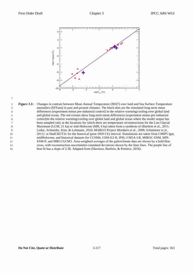
First Order Draft Chapter 3 IPCC AR6 WGI
Do Not Cite, Quote or Distribute 3-117 Total pages: 163
1
Changes in contrast between Mean Annual Temperature (MAT) over land and Sea Surface Temperature 2
anomalies (SSTann) in past and present climates. The black dots are the simulated long-term mean 3
differences (experiment minus pre-industrial control) in the relative warming/cooling over global land 4
and global ocean. The red crosses show long-term mean differences (experiment minus pre-industrial 5
control)in the relative warming/cooling over global land and global ocean where the model output has 6
been sampled only at the locations for which there are temperature reconstructions for the Last Glacial 7
Maximum (LGM, 21 ka) or mid-Holocene (MH, 6 ka) taken from a synthesis of (Bartlein et al., 2011; 8
Leduc, Schneider, Kim, & Lohmann, 2010; MARGO Project Members et al., 2009; Schmittner et al., 9
2011) or HadCRUT3v for the historical (post-1850 CE) interval. Simulations are taken from CMIP5 lgm, 10
midHolocene, and historical datasets for CCSM4, GISS-E2-R, IPSL-CM5A-LR, MIROC-ESM, MPI-11
ESM-P, and MRI-CGCM3. Area-weighted averages of the paleoclimate data are shown by a bold blue 12
cross, with reconstruction uncertainties (standard deviation) shown by the finer lines. The purple line of 13
best fit has a slope of 2.36. Adapted from (Harrison, Bartlein, & Prentice, 2016). 14
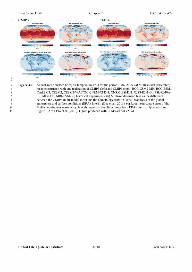
First Order Draft Chapter 3 IPCC AR6 WGI
Do Not Cite, Quote or Distribute 3-118 Total pages: 163
CMIP5: CMIP6: 1
2
3
Annual-mean surface (2 m) air temperature (°C) for the period 1986–2005. (a) Multi-model (ensemble) 4
mean constructed with one realization of CMIP5 (left) and CMIP6 (right; BCC-CSM2-MR, BCC-ESM1, 5
CanESM5, CESM2, CESM2-WACCM, CNRM-CM6-1, CNRM-ESM2-1, GISS-E2-1-G, IPSL-CM6A-6
LR, MIROC6, MRI-ESM2-0) historical experiments. (b) Multi-model-mean bias as the difference 7
between the CMIP6 multi-model mean and the climatology from ECMWF reanalysis of the global 8
atmosphere and surface conditions (ERA)-Interim (Dee et al., 2011). (c) Root mean square error of the 9
Multi-model-mean seasonal cycle with respect to the climatology from ERA-Interim. Updated from 10
Figure 9.2 of Flato et al. (2013). Figure produced with ESMValTool v2.0a1. 11
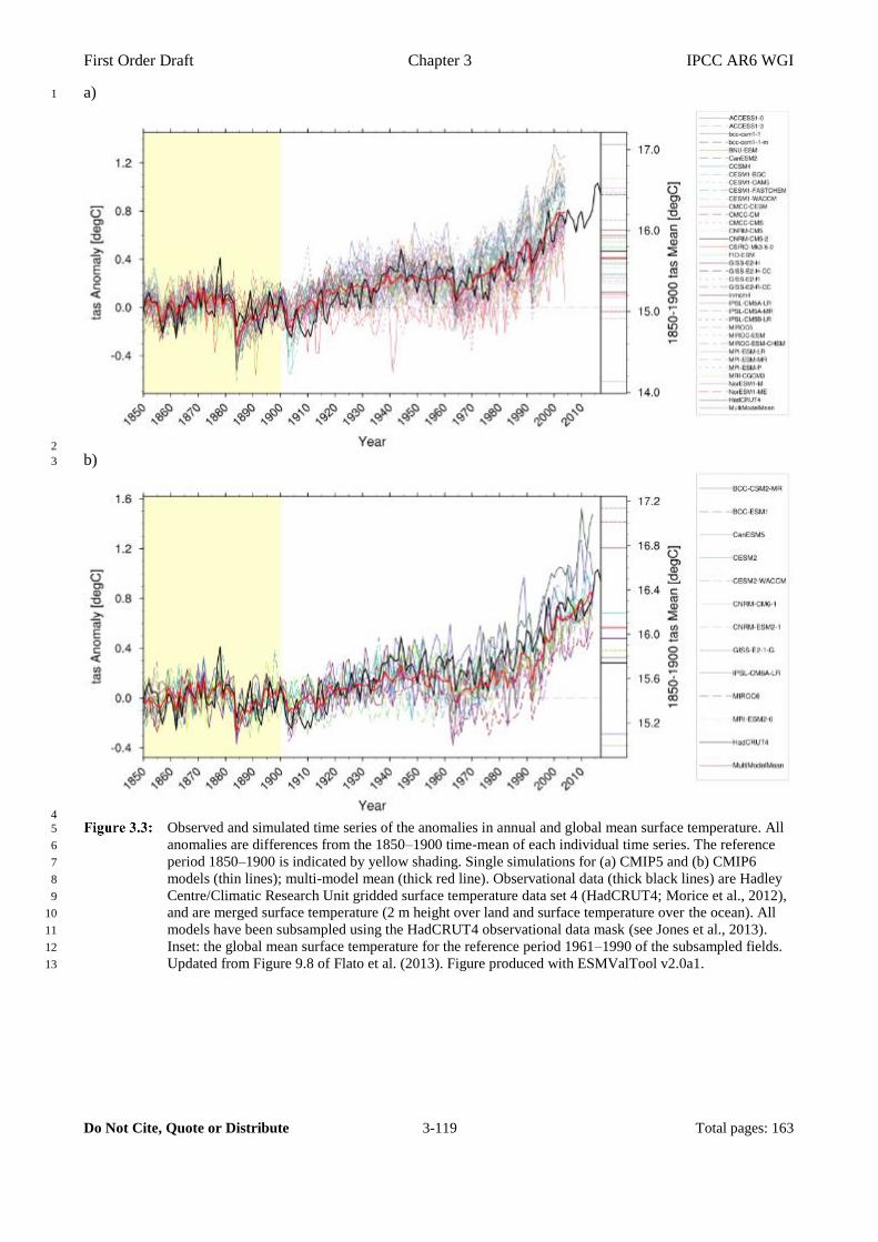
First Order Draft Chapter 3 IPCC AR6 WGI
Do Not Cite, Quote or Distribute 3-119 Total pages: 163
a) 1
2
b) 3
4
Observed and simulated time series of the anomalies in annual and global mean surface temperature. All 5
anomalies are differences from the 1850–1900 time-mean of each individual time series. The reference 6
period 1850–1900 is indicated by yellow shading. Single simulations for (a) CMIP5 and (b) CMIP6 7
models (thin lines); multi-model mean (thick red line). Observational data (thick black lines) are Hadley 8
Centre/Climatic Research Unit gridded surface temperature data set 4 (HadCRUT4; Morice et al., 2012), 9
and are merged surface temperature (2 m height over land and surface temperature over the ocean). All 10
models have been subsampled using the HadCRUT4 observational data mask (see Jones et al., 2013). 11
Inset: the global mean surface temperature for the reference period 1961–1990 of the subsampled fields. 12
Updated from Figure 9.8 of Flato et al. (2013). Figure produced with ESMValTool v2.0a1. 13
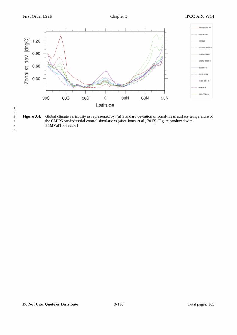
First Order Draft Chapter 3 IPCC AR6 WGI
Do Not Cite, Quote or Distribute 3-120 Total pages: 163
1
2
Global climate variability as represented by: (a) Standard deviation of zonal-mean surface temperature of 3
the CMIP6 pre-industrial control simulations (after Jones et al., 2013). Figure produced with 4
ESMValTool v2.0a1. 5
6
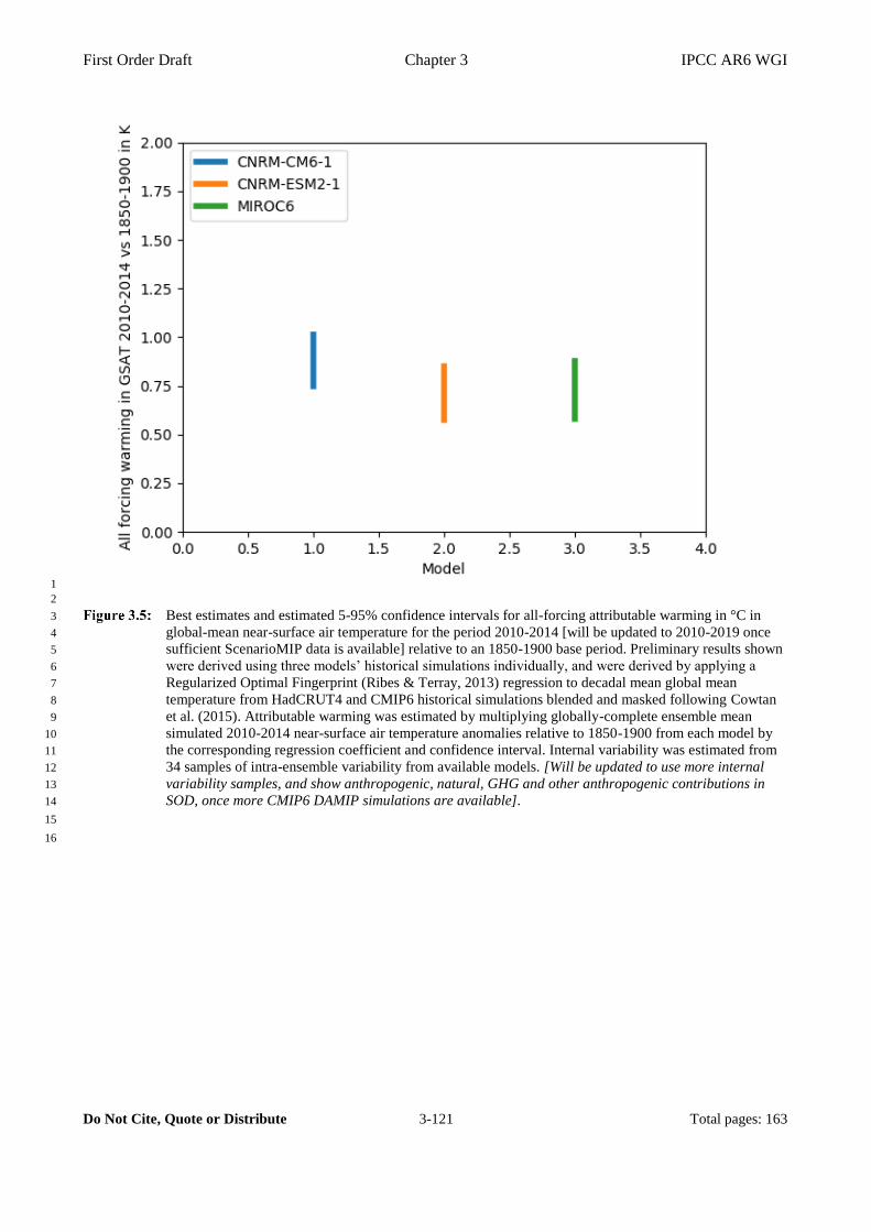
First Order Draft Chapter 3 IPCC AR6 WGI
Do Not Cite, Quote or Distribute 3-121 Total pages: 163
1
2
Best estimates and estimated 5-95% confidence intervals for all-forcing attributable warming in °C in 3
global-mean near-surface air temperature for the period 2010-2014 [will be updated to 2010-2019 once 4
sufficient ScenarioMIP data is available] relative to an 1850-1900 base period. Preliminary results shown 5
were derived using three models’ historical simulations individually, and were derived by applying a 6
Regularized Optimal Fingerprint (Ribes & Terray, 2013) regression to decadal mean global mean 7
temperature from HadCRUT4 and CMIP6 historical simulations blended and masked following Cowtan 8
et al. (2015). Attributable warming was estimated by multiplying globally-complete ensemble mean 9
simulated 2010-2014 near-surface air temperature anomalies relative to 1850-1900 from each model by 10
the corresponding regression coefficient and confidence interval. Internal variability was estimated from 11
34 samples of intra-ensemble variability from available models. [Will be updated to use more internal 12
variability samples, and show anthropogenic, natural, GHG and other anthropogenic contributions in 13
SOD, once more CMIP6 DAMIP simulations are available]. 14
15
16
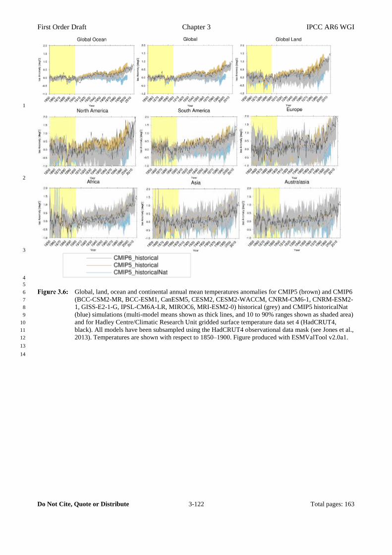
First Order Draft Chapter 3 IPCC AR6 WGI
Do Not Cite, Quote or Distribute 3-122 Total pages: 163
1
2
3
4
5
Global, land, ocean and continental annual mean temperatures anomalies for CMIP5 (brown) and CMIP6 6
(BCC-CSM2-MR, BCC-ESM1, CanESM5, CESM2, CESM2-WACCM, CNRM-CM6-1, CNRM-ESM2-7
1, GISS-E2-1-G, IPSL-CM6A-LR, MIROC6, MRI-ESM2-0) historical (grey) and CMIP5 historicalNat 8
(blue) simulations (multi-model means shown as thick lines, and 10 to 90% ranges shown as shaded area) 9
and for Hadley Centre/Climatic Research Unit gridded surface temperature data set 4 (HadCRUT4, 10
black). All models have been subsampled using the HadCRUT4 observational data mask (see Jones et al., 11
2013). Temperatures are shown with respect to 1850–1900. Figure produced with ESMValTool v2.0a1. 12
13
14

First Order Draft Chapter 3 IPCC AR6 WGI
Do Not Cite, Quote or Distribute 3-123 Total pages: 163
PLACEHOLDER 1
2
Same as Figure 3.7, but for single forcing simulations from CMIP6-DAMIP simulations. [Placeholder 3
for SOD.] 4
5
6
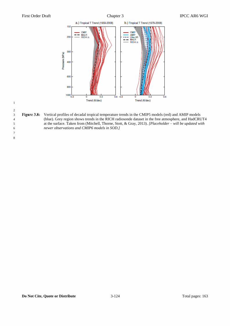
First Order Draft Chapter 3 IPCC AR6 WGI
Do Not Cite, Quote or Distribute 3-124 Total pages: 163
1
2
Vertical profiles of decadal tropical temperature trends in the CMIP5 models (red) and AMIP models 3
(blue). Grey region shows trends in the RICH radiosonde dataset in the free atmosphere, and HadCRUT4 4
at the surface. Taken from (Mitchell, Thorne, Stott, & Gray, 2013). [Placeholder – will be updated with 5
newer observations and CMIP6 models in SOD.] 6
7
8
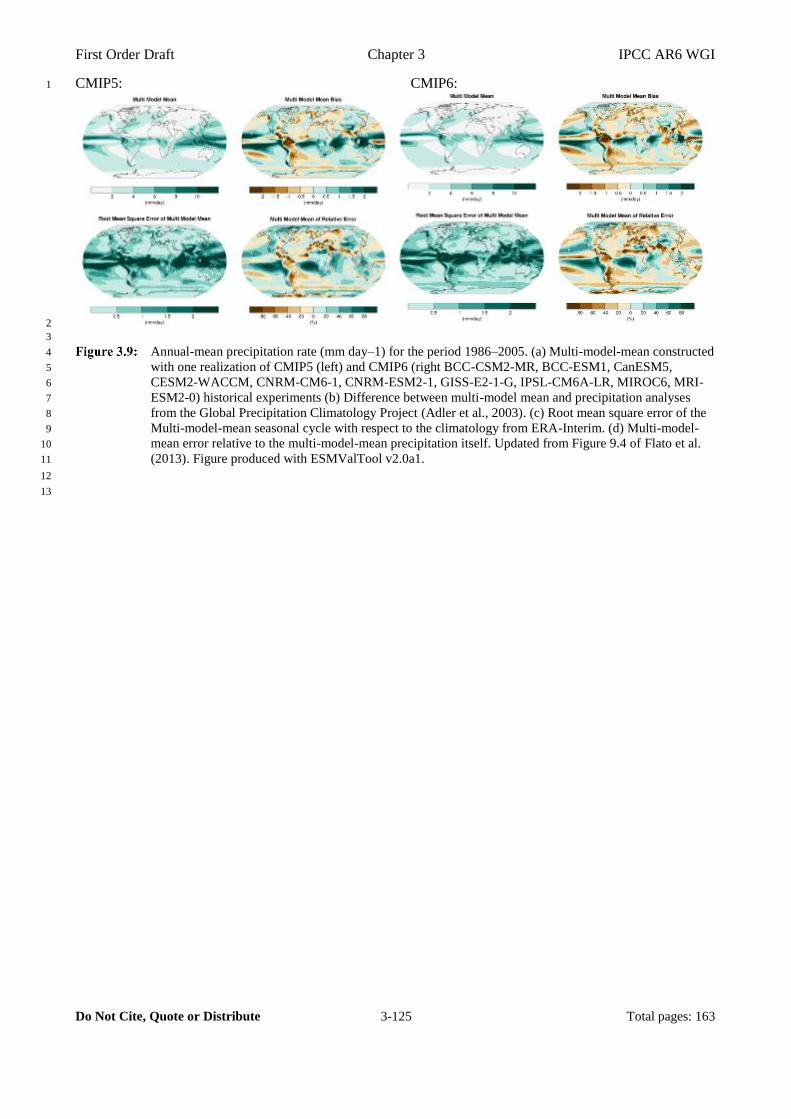
First Order Draft Chapter 3 IPCC AR6 WGI
Do Not Cite, Quote or Distribute 3-125 Total pages: 163
CMIP5: CMIP6: 1
2
3
Annual-mean precipitation rate (mm day–1) for the period 1986–2005. (a) Multi-model-mean constructed 4
with one realization of CMIP5 (left) and CMIP6 (right BCC-CSM2-MR, BCC-ESM1, CanESM5, 5
CESM2-WACCM, CNRM-CM6-1, CNRM-ESM2-1, GISS-E2-1-G, IPSL-CM6A-LR, MIROC6, MRI-6
ESM2-0) historical experiments (b) Difference between multi-model mean and precipitation analyses 7
from the Global Precipitation Climatology Project (Adler et al., 2003). (c) Root mean square error of the 8
Multi-model-mean seasonal cycle with respect to the climatology from ERA-Interim. (d) Multi-model-9
mean error relative to the multi-model-mean precipitation itself. Updated from Figure 9.4 of Flato et al. 10
(2013). Figure produced with ESMValTool v2.0a1. 11
12
13
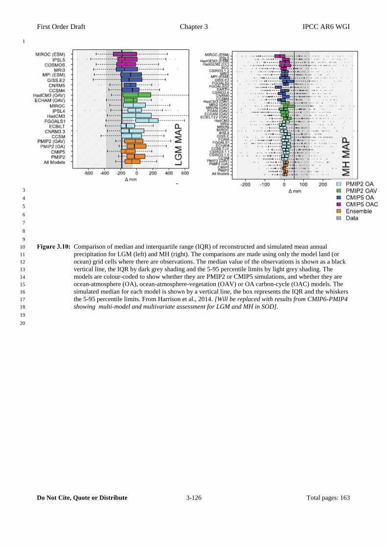
First Order Draft Chapter 3 IPCC AR6 WGI
Do Not Cite, Quote or Distribute 3-126 Total pages: 163
1
2
3
4
5
6
7
8
9
Comparison of median and interquartile range (IQR) of reconstructed and simulated mean annual 10
precipitation for LGM (left) and MH (right). The comparisons are made using only the model land (or 11
ocean) grid cells where there are observations. The median value of the observations is shown as a black 12
vertical line, the IQR by dark grey shading and the 5-95 percentile limits by light grey shading. The 13
models are colour-coded to show whether they are PMIP2 or CMIP5 simulations, and whether they are 14
ocean-atmosphere (OA), ocean-atmosphere-vegetation (OAV) or OA carbon-cycle (OAC) models. The 15
simulated median for each model is shown by a vertical line, the box represents the IQR and the whiskers 16
the 5-95 percentile limits. From Harrison et al., 2014. [Will be replaced with results from CMIP6-PMIP4 17
showing multi-model and multivariate assessment for LGM and MH in SOD]. 18
19
20

First Order Draft Chapter 3 IPCC AR6 WGI
Do Not Cite, Quote or Distribute 3-127 Total pages: 163
1
2
3
4
Global and zonal average changes in annual mean precipitation (mm day-1) over areas of land where 5
there are observations, expressed relative to the base-line period of 1961–1990, simulated by CMIP5 6
models forced with both anthropogenic and natural forcings and natural forcings only and CMIP6 (BCC-7
CSM2-MR, BCC-ESM1, CanESM5, CESM2-WACCM, CNRM-CM6-1, CNRM-ESM2-1, GISS-E2-1-8
G, IPSL-CM6A-LR, MIROC6, MRI-ESM2-0) models forced with both anthropogenic and natural 9
forcings for the global mean and for three latitude bands. Multi-model means are shown in thick solid 10
lines and shading shows 10-90% ranges of the individual model simulations (for CMIP6 models 11
minimum and maximum). Observations (gridded values derived from Global Historical Climatology 12
Network station data, updated from Zhang et al. (2007) are shown as a black solid line. An 11-year 13
smoothing is applied to both simulations and observations. Figure produced with ESMValTool v2.0a1. 14
15
16
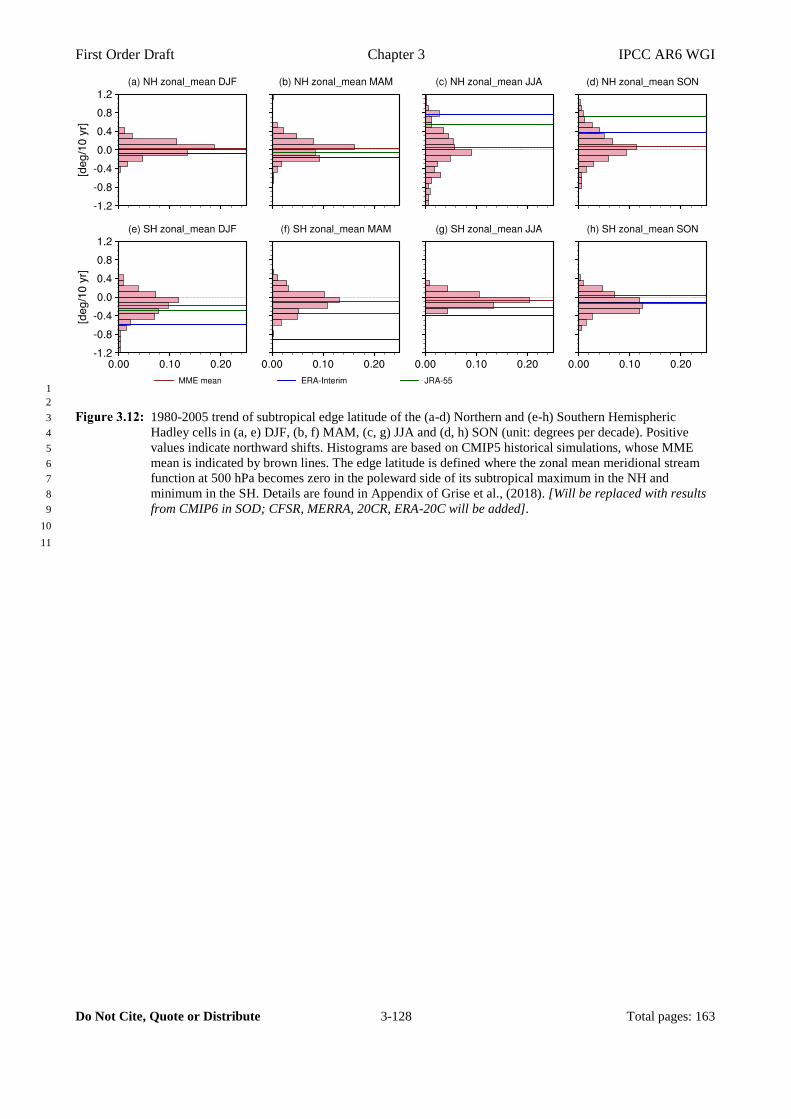
First Order Draft Chapter 3 IPCC AR6 WGI
Do Not Cite, Quote or Distribute 3-128 Total pages: 163
1
2
1980-2005 trend of subtropical edge latitude of the (a-d) Northern and (e-h) Southern Hemispheric 3
Hadley cells in (a, e) DJF, (b, f) MAM, (c, g) JJA and (d, h) SON (unit: degrees per decade). Positive 4
values indicate northward shifts. Histograms are based on CMIP5 historical simulations, whose MME 5
mean is indicated by brown lines. The edge latitude is defined where the zonal mean meridional stream 6
function at 500 hPa becomes zero in the poleward side of its subtropical maximum in the NH and 7
minimum in the SH. Details are found in Appendix of Grise et al., (2018). [Will be replaced with results 8
from CMIP6 in SOD; CFSR, MERRA, 20CR, ERA-20C will be added]. 9
10
11
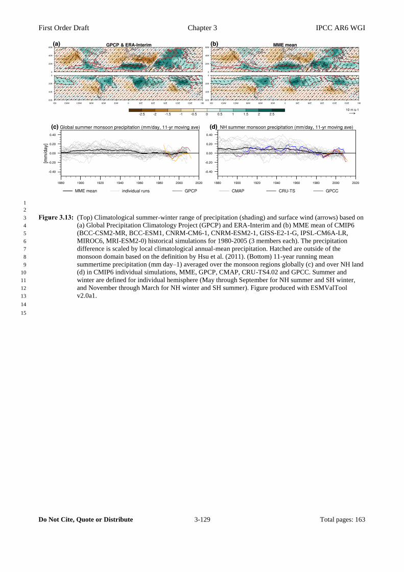
First Order Draft Chapter 3 IPCC AR6 WGI
Do Not Cite, Quote or Distribute 3-129 Total pages: 163
1
2
(Top) Climatological summer-winter range of precipitation (shading) and surface wind (arrows) based on 3
(a) Global Precipitation Climatology Project (GPCP) and ERA-Interim and (b) MME mean of CMIP6 4
(BCC-CSM2-MR, BCC-ESM1, CNRM-CM6-1, CNRM-ESM2-1, GISS-E2-1-G, IPSL-CM6A-LR, 5
MIROC6, MRI-ESM2-0) historical simulations for 1980-2005 (3 members each). The precipitation 6
difference is scaled by local climatological annual-mean precipitation. Hatched are outside of the 7
monsoon domain based on the definition by Hsu et al. (2011). (Bottom) 11-year running mean 8
summertime precipitation (mm day–1) averaged over the monsoon regions globally (c) and over NH land 9
(d) in CMIP6 individual simulations, MME, GPCP, CMAP, CRU-TS4.02 and GPCC. Summer and 10
winter are defined for individual hemisphere (May through September for NH summer and SH winter, 11
and November through March for NH winter and SH summer). Figure produced with ESMValTool 12
v2.0a1. 13
14
15
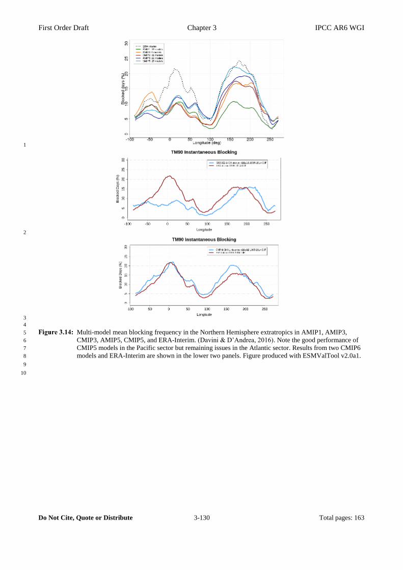
First Order Draft Chapter 3 IPCC AR6 WGI
Do Not Cite, Quote or Distribute 3-130 Total pages: 163
1
2
3
4
Multi-model mean blocking frequency in the Northern Hemisphere extratropics in AMIP1, AMIP3, 5
CMIP3, AMIP5, CMIP5, and ERA-Interim. (Davini & D’Andrea, 2016). Note the good performance of 6
CMIP5 models in the Pacific sector but remaining issues in the Atlantic sector. Results from two CMIP6 7
models and ERA-Interim are shown in the lower two panels. Figure produced with ESMValTool v2.0a1. 8
9
10
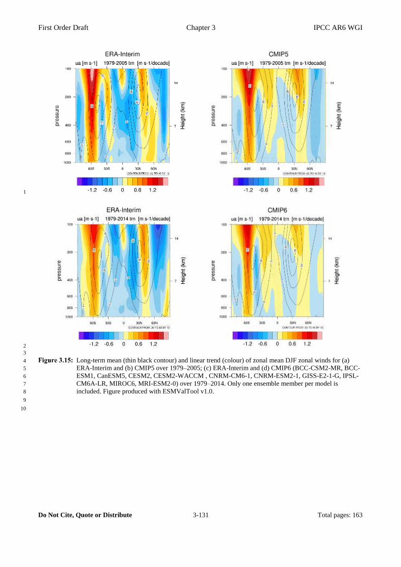
First Order Draft Chapter 3 IPCC AR6 WGI
Do Not Cite, Quote or Distribute 3-131 Total pages: 163
1
2
3
Long-term mean (thin black contour) and linear trend (colour) of zonal mean DJF zonal winds for (a) 4
ERA-Interim and (b) CMIP5 over 1979–2005; (c) ERA-Interim and (d) CMIP6 (BCC-CSM2-MR, BCC-5
ESM1, CanESM5, CESM2, CESM2-WACCM , CNRM-CM6-1, CNRM-ESM2-1, GISS-E2-1-G, IPSL-6
CM6A-LR, MIROC6, MRI-ESM2-0) over 1979–2014. Only one ensemble member per model is 7
included. Figure produced with ESMValTool v1.0. 8
9
10

First Order Draft Chapter 3 IPCC AR6 WGI
Do Not Cite, Quote or Distribute 3-132 Total pages: 163
1
2
Climatology (x-axis) and trend (y-axis) in Arctic sea ice extent in September (left) and Antarctic sea ice 3
extent in February (right) for 1979-2014 from CMIP5 (upper) and CMIP6 (lower) models. All individual 4
model (ensemble means) and the multi-model mean values are compared with the observations 5
(HadISST). Solid line indicates a linear regression slope which is statistically significant at 5% level. 6
[Will be updated with results from CMIP6 in SOD]. 7
8
9

First Order Draft Chapter 3 IPCC AR6 WGI
Do Not Cite, Quote or Distribute 3-133 Total pages: 163
1
2
Seasonal evolution of observed and simulated Arctic (left) and Antarctic (right) sea ice extent (SIE) over 3
1953–2017. ASIE anomalies relative to the 1979–2000 means from HadISST observations (top) and 4
CMIP5 (middle) and CMIP6 (bottom) historical (ALL) and historicalNat (NAT) simulations. These 5
anomalies were obtained by computing non-overlapping 3-year mean sea ice anomalies for March 6
(February for Antarctic SIE), June, September, and December separately. CMIP5 ALL runs cover 1953-7
2017 with RCP4.5 scenario simulations combined after 2005 while CMIP6 ALL runs end in 2014. 8
CMIP5 NAT runs ends in 2012. Number in bracket represents number of models used. Multi-model mean 9
is obtained by taking ensemble mean for each model first and then averaging over models. Units: 106 10
km2. [Will be updated with results from CMIP6 in SOD] 11
12
13
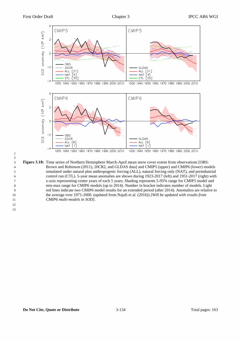
First Order Draft Chapter 3 IPCC AR6 WGI
Do Not Cite, Quote or Distribute 3-134 Total pages: 163
1
2
Time series of Northern Hemisphere March-April mean snow cover extent from observations [OBS: 3
Brown and Robinson (2011), 20CR2, and GLDAS data] and CMIP5 (upper) and CMIP6 (lower) models 4
simulated under natural plus anthropogenic forcing (ALL), natural forcing only (NAT), and preindustrial 5
control run (CTL). 5-year mean anomalies are shown during 1923-2017 (left) and 1951-2017 (right) with 6
x-axis representing center years of each 5 years. Shading represents 5-95% range for CMIP5 model and 7
min-max range for CMIP6 models (up to 2014). Number in bracket indicates number of models. Light 8
red lines indicate two CMIP6 model results for an extended period (after 2014). Anomalies are relative to 9
the average over 1971-2000. (updated from Najafi et al. (2016)) [Will be updated with results from 10
CMIP6 multi-models in SOD]. 11
12
13
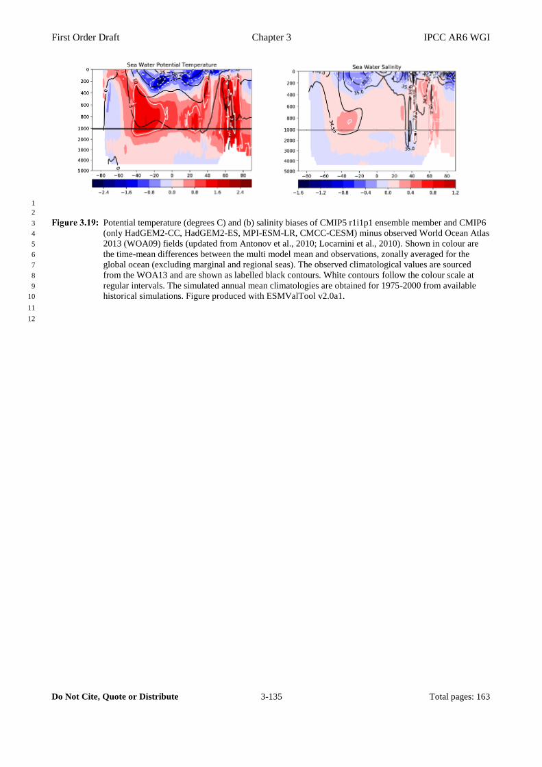
First Order Draft Chapter 3 IPCC AR6 WGI
Do Not Cite, Quote or Distribute 3-135 Total pages: 163
1
2
Potential temperature (degrees C) and (b) salinity biases of CMIP5 r1i1p1 ensemble member and CMIP6 3
(only HadGEM2-CC, HadGEM2-ES, MPI-ESM-LR, CMCC-CESM) minus observed World Ocean Atlas 4
2013 (WOA09) fields (updated from Antonov et al., 2010; Locarnini et al., 2010). Shown in colour are 5
the time-mean differences between the multi model mean and observations, zonally averaged for the 6
global ocean (excluding marginal and regional seas). The observed climatological values are sourced 7
from the WOA13 and are shown as labelled black contours. White contours follow the colour scale at 8
regular intervals. The simulated annual mean climatologies are obtained for 1975-2000 from available 9
historical simulations. Figure produced with ESMValTool v2.0a1. 10
11
12
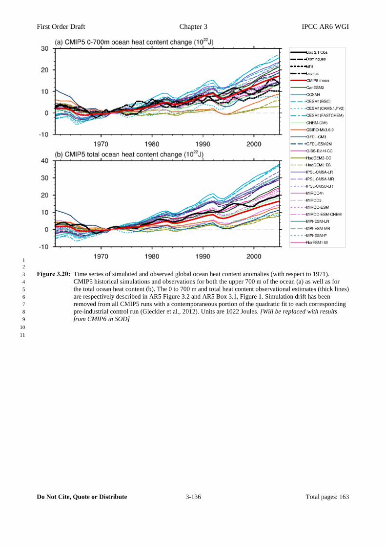
First Order Draft Chapter 3 IPCC AR6 WGI
Do Not Cite, Quote or Distribute 3-136 Total pages: 163
1
2
Time series of simulated and observed global ocean heat content anomalies (with respect to 1971). 3
CMIP5 historical simulations and observations for both the upper 700 m of the ocean (a) as well as for 4
the total ocean heat content (b). The 0 to 700 m and total heat content observational estimates (thick lines) 5
are respectively described in AR5 Figure 3.2 and AR5 Box 3.1, Figure 1. Simulation drift has been 6
removed from all CMIP5 runs with a contemporaneous portion of the quadratic fit to each corresponding 7
pre-industrial control run (Gleckler et al., 2012). Units are 1022 Joules. [Will be replaced with results 8
from CMIP6 in SOD] 9
10
11
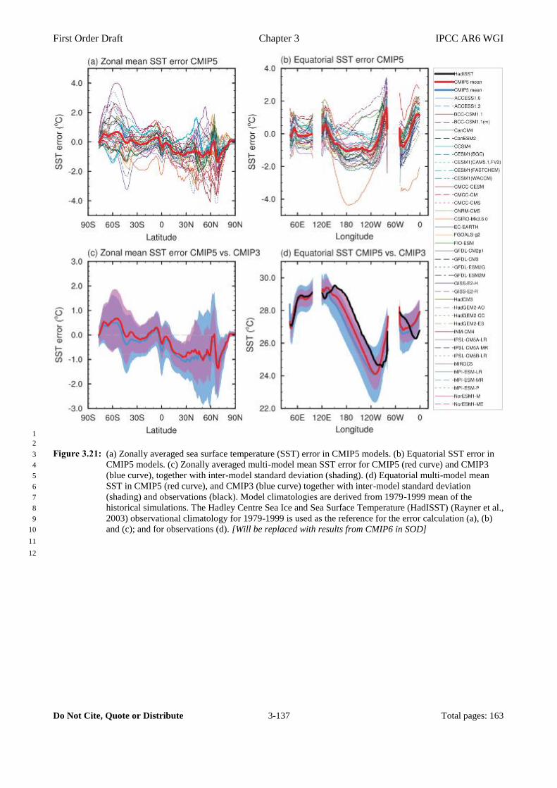
First Order Draft Chapter 3 IPCC AR6 WGI
Do Not Cite, Quote or Distribute 3-137 Total pages: 163
1
2
(a) Zonally averaged sea surface temperature (SST) error in CMIP5 models. (b) Equatorial SST error in 3
CMIP5 models. (c) Zonally averaged multi-model mean SST error for CMIP5 (red curve) and CMIP3 4
(blue curve), together with inter-model standard deviation (shading). (d) Equatorial multi-model mean 5
SST in CMIP5 (red curve), and CMIP3 (blue curve) together with inter-model standard deviation 6
(shading) and observations (black). Model climatologies are derived from 1979-1999 mean of the 7
historical simulations. The Hadley Centre Sea Ice and Sea Surface Temperature (HadISST) (Rayner et al., 8
2003) observational climatology for 1979-1999 is used as the reference for the error calculation (a), (b) 9
and (c); and for observations (d). [Will be replaced with results from CMIP6 in SOD] 10
11
12

First Order Draft Chapter 3 IPCC AR6 WGI
Do Not Cite, Quote or Distribute 3-138 Total pages: 163
1
2
(a) Ocean heat uptake (percentage of total 1865-2017 change) for the CMIP5 multi-model mean layers. 3
The three shaded wedges are combined similarly to the AR5 change in global inventory (Rhein et al. 4
(2013); Box 3.1, Figure 1). The thick vertical grey bar represents a +/- one standard deviation spread from 5
the CMIP5 simulations about the year (1999) at which the multi-model heat uptake reaches 50% of the 6
net (1865-2017) industrial-era increase, and the thick horizontal grey bar indicates the CMIP5 +/- one 7
standard deviation spread om the year at which 50% of the total accumulated heat is reached. Black 8
(forcing included) and grey (forcing not included) triangles represent major twentieth- and twenty-first-9
century volcanic eruptions with magnitude (volcanic explosivity index [VEI] represented by symbol size. 10
(b) The inset box displays the upper and intermediate layer warming for the years 1998 to 2017, with an 11
adjustment for the 0 to 2000 m total warming by -0.19 W m-2, the estimated discrepancy between CMIP5 12
modelled and the observed volcanic forcing (Ridley et al., 2014). When observed 0 to 2000 m ocean 13
warming is compared across five independent available estimates these rates of change are approximately 14
equal. Reproduced from Durack et al., 2018. [Will be replaced with results from CMIP6 in SOD] 15
16
17
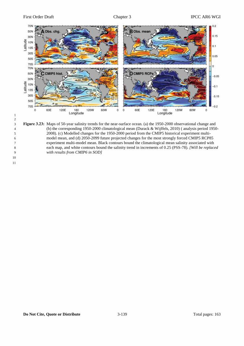
First Order Draft Chapter 3 IPCC AR6 WGI
Do Not Cite, Quote or Distribute 3-139 Total pages: 163
1
2
Maps of 50-year salinity trends for the near-surface ocean. (a) the 1950-2000 observational change and 3
(b) the corresponding 1950-2000 climatological mean (Durack & Wijffels, 2010) ( analysis period 1950-4
2008). (c) Modelled changes for the 1950-2000 period from the CMIP5 historical experiment multi-5
model mean, and (d) 2050-2099 future projected changes for the most strongly forced CMIP5 RCP85 6
experiment multi-model mean. Black contours bound the climatological mean salinity associated with 7
each map, and white contours bound the salinity trend in increments of 0.25 (PSS-78). [Will be replaced 8
with results from CMIP6 in SOD] 9
10
11
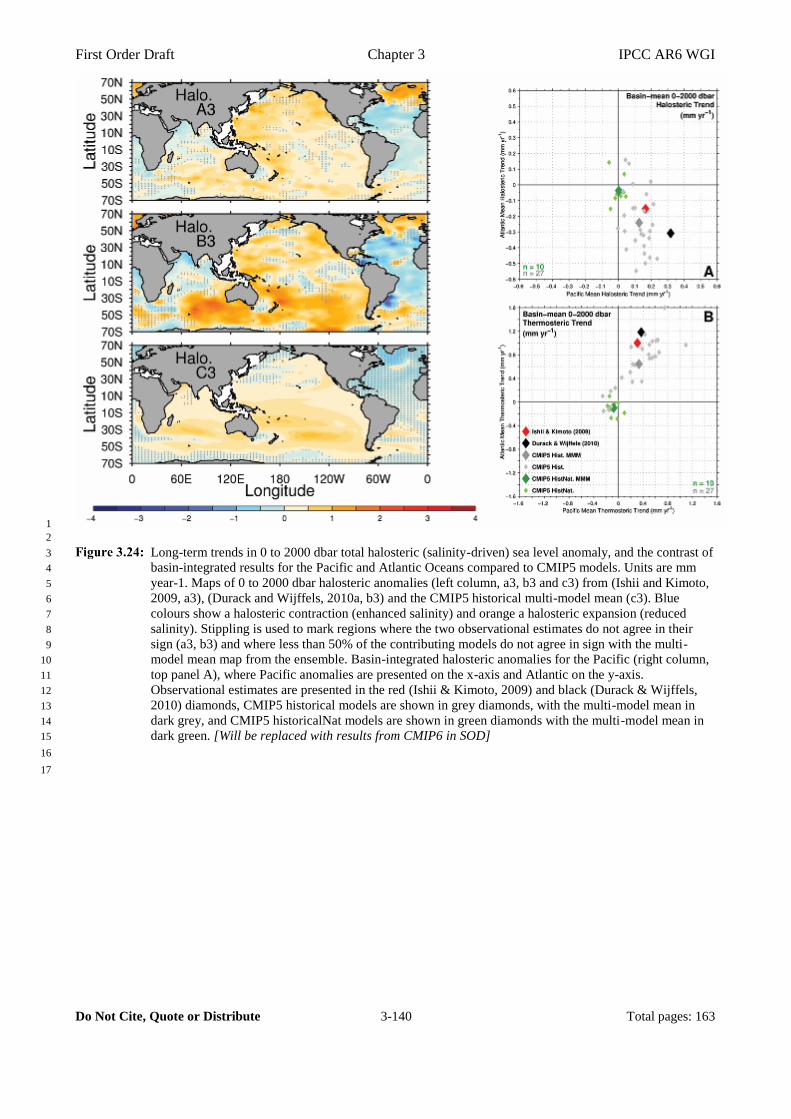
First Order Draft Chapter 3 IPCC AR6 WGI
Do Not Cite, Quote or Distribute 3-140 Total pages: 163
1
2
Long-term trends in 0 to 2000 dbar total halosteric (salinity-driven) sea level anomaly, and the contrast of 3
basin-integrated results for the Pacific and Atlantic Oceans compared to CMIP5 models. Units are mm 4
year-1. Maps of 0 to 2000 dbar halosteric anomalies (left column, a3, b3 and c3) from (Ishii and Kimoto, 5
2009, a3), (Durack and Wijffels, 2010a, b3) and the CMIP5 historical multi-model mean (c3). Blue 6
colours show a halosteric contraction (enhanced salinity) and orange a halosteric expansion (reduced 7
salinity). Stippling is used to mark regions where the two observational estimates do not agree in their 8
sign (a3, b3) and where less than 50% of the contributing models do not agree in sign with the multi-9
model mean map from the ensemble. Basin-integrated halosteric anomalies for the Pacific (right column, 10
top panel A), where Pacific anomalies are presented on the x-axis and Atlantic on the y-axis. 11
Observational estimates are presented in the red (Ishii & Kimoto, 2009) and black (Durack & Wijffels, 12
2010) diamonds, CMIP5 historical models are shown in grey diamonds, with the multi-model mean in 13
dark grey, and CMIP5 historicalNat models are shown in green diamonds with the multi-model mean in 14
dark green. [Will be replaced with results from CMIP6 in SOD] 15
16
17

First Order Draft Chapter 3 IPCC AR6 WGI
Do Not Cite, Quote or Distribute 3-141 Total pages: 163
1
2
Comparison of observational average (black line with grey shade ±2) and model ensemble time series 3
(±2) of cumulative global mean sea level change. Figure reproduced from (Slangen et al., 2016) [Will be 4
updated with results from CMIP6] 5
6
7

First Order Draft Chapter 3 IPCC AR6 WGI
Do Not Cite, Quote or Distribute 3-142 Total pages: 163
1
(a; left column) AMOC streamfunction profiles at 26.5N from pre-industrial control simulations 2
compared with the mean overturning from the RAPID array (stars). Overturning maxima are indicated by 3
diamonds and values are given in the legend. (b; right top) distribution of 8-year AMOC trends in CMIP5 4
piControls and the observed trend (grey line). (c; right bottom) distribution of interannual AMOC 5
variability in CMIP5 piControls. The grey line is the observed value for 2009/2010 minus 2008/2009. All 6
annual means are for April-March. Boxes indicate 25th to 75th percentile, whiskers indicate 1st and 99th 7
percentiles, and dots indicate outliers. Figure produced with ESMValTool v2.0a1. [Will be replaced with 8
results from CMIP6 in SOD]. 9
10
11
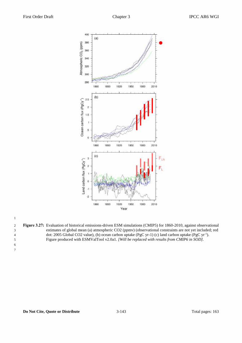
First Order Draft Chapter 3 IPCC AR6 WGI
Do Not Cite, Quote or Distribute 3-143 Total pages: 163
1
Evaluation of historical emissions-driven ESM simulations (CMIP5) for 1860-2010, against observational 2
estimates of global mean (a) atmospheric CO2 (ppmv) (observational constraints are not yet included; red 3
dot: 2005 Global CO2 value), (b) ocean carbon uptake (PgC yr-1) (c) land carbon uptake (PgC yr-1). 4
Figure produced with ESMValTool v2.0a1. [Will be replaced with results from CMIP6 in SOD]. 5
6
7
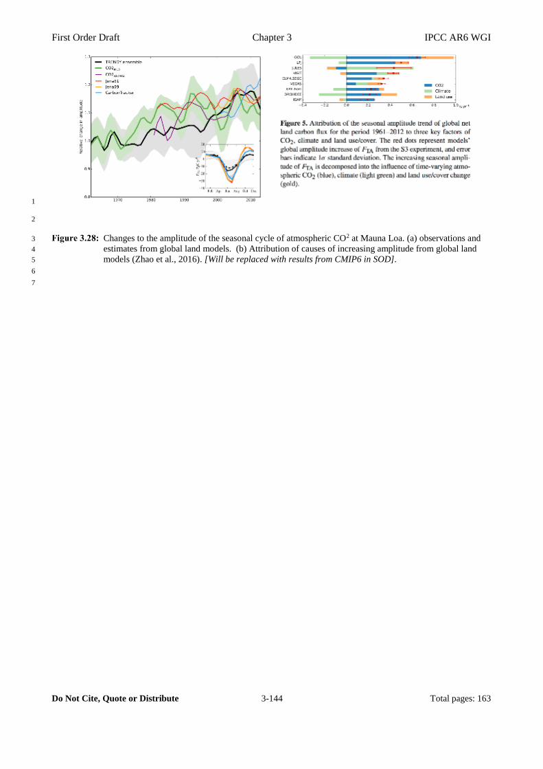
First Order Draft Chapter 3 IPCC AR6 WGI
Do Not Cite, Quote or Distribute 3-144 Total pages: 163
1
2
Changes to the amplitude of the seasonal cycle of atmospheric CO2 at Mauna Loa. (a) observations and 3
estimates from global land models. (b) Attribution of causes of increasing amplitude from global land 4
models (Zhao et al., 2016). [Will be replaced with results from CMIP6 in SOD]. 5
6
7
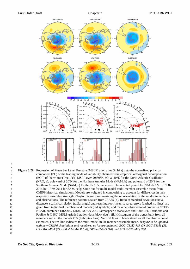
First Order Draft Chapter 3 IPCC AR6 WGI
Do Not Cite, Quote or Distribute 3-145 Total pages: 163
1
2
Regression of Mean Sea Level Pressure (MSLP) anomalies (in hPa) onto the normalized principal 3
component (PC) of the leading mode of variability obtained from empirical orthogonal decomposition 4
(EOF) of the winter (Dec.-Feb) MSLP over 20:80°N, 90°W:40°E for the North Atlantic Oscillation 5
(NAO, a), poleward of 20ºN for the Northern Annular Mode (NAM, b) and poleward of 20ºS for the 6
Southern Annular Mode (SAM, c) for the JRA55 reanalysis. The selected period for NAO/NAM is 1958-7
2014 but 1979-2014 for SAM. (efg) Same but for multi-model multi-member ensemble mean from 8
CMIP6 historical simulations. Models are weighted in compositing to account for differences in their 9
respective ensemble size. (ghi) Taylor diagram summarizing the representation of the modes in models 10
and observations. The reference pattern is taken from JRA55 (a). Ratio of standard deviation (radial 11
distance), spatial correlation (radial angle) and resulting root-mean-squared-errors (dashed iso-lines) are 12
given from individual members and models (red symbols) and for other observational products (NCEP-13
NCAR, combined ERA20C-ERAI, NOAA-20CR atmospheric reanalyses and HadSLPr, Trenberth and 14
Paolino Jr (1980) MSLP gridded station-data, black dots). (jkl) Histogram of the trends built from all 15
members and all the models PCs (light pink bars). Vertical lines in black stand for all the observational 16
estimates. The red line indicates the multi-model multi-member ensemble mean. [Figure to be updated 17
with new CMIP6 simulations and members: so far are included: BCC-CSM2-MR (3), BCC-ESM1 (3), 18
CNRM-CM6-1 (2), IPSL-CM6A-LR (30), GISS-E2-1-G (10) and NCAR-CESM2 (10)]. 19
20

First Order Draft Chapter 3 IPCC AR6 WGI
Do Not Cite, Quote or Distribute 3-146 Total pages: 163
1
2
3
4
[Placeholder] Simulated and observed trends in NAO, NAM indices over 1958-2014 (a) and in SAM 5
indices over 1979-2014 (b) for the boreal winter season (Dec.-Feb. average). Computations are done for 6
all the selected indices listed in Section 2.x, Table 2.x, [see Table 2.14 in AR5] to evaluate the 7
uncertainties associated with the metrics used to define the modes. Black lines show observed trends from 8
JRA55, NCEP-NCAR, combined ERA20C-ERAI, NOAA-20CR atmospheric reanalyses and HadSLPr, 9
Trenberth and Paolino Jr (1980) Mean Sea Level Pressure gridded station-data. Grey bars and red boxes 10
show the 5% and 95% ranges of trends in CMIP6 control and historical simulations respectively. 11
Ensemble mean trends and their 5% to 95% uncertainties are shown for the response to individual 12
forcings based on DAMIP ensembles. [Current figure is a sample: it corresponds to AR5 Fig. 10.13 and 13
it will be replaced with correct calculations and results from CMIP6 runs in SOD] 14
15
16
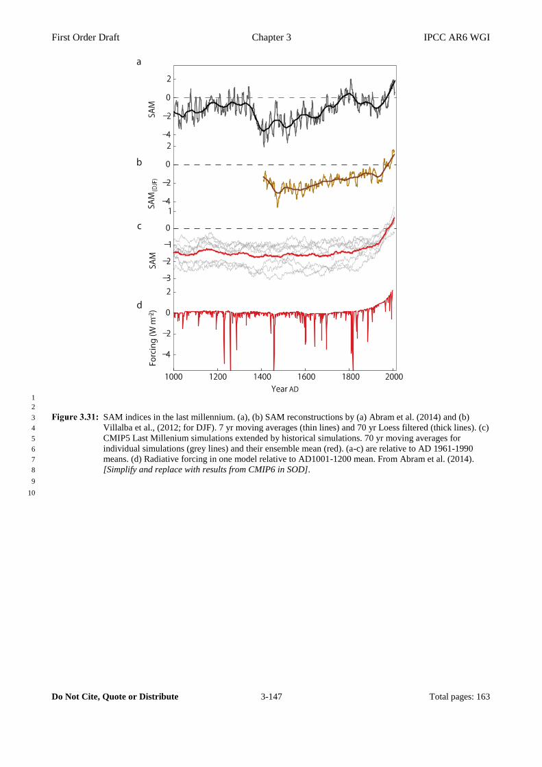
First Order Draft Chapter 3 IPCC AR6 WGI
Do Not Cite, Quote or Distribute 3-147 Total pages: 163
1
2
SAM indices in the last millennium. (a), (b) SAM reconstructions by (a) Abram et al. (2014) and (b) 3
Villalba et al., (2012; for DJF). 7 yr moving averages (thin lines) and 70 yr Loess filtered (thick lines). (c) 4
CMIP5 Last Millenium simulations extended by historical simulations. 70 yr moving averages for 5
individual simulations (grey lines) and their ensemble mean (red). (a-c) are relative to AD 1961-1990 6
means. (d) Radiative forcing in one model relative to AD1001-1200 mean. From Abram et al. (2014). 7
[Simplify and replace with results from CMIP6 in SOD]. 8
9
10
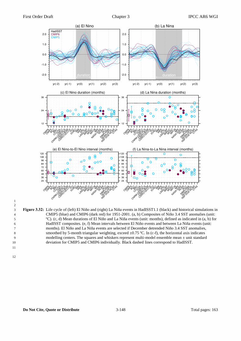
First Order Draft Chapter 3 IPCC AR6 WGI
Do Not Cite, Quote or Distribute 3-148 Total pages: 163
1
2
Life cycle of (left) El Niño and (right) La Niña events in HadISST1.1 (black) and historical simulations in 3
CMIP5 (blue) and CMIP6 (dark red) for 1951-2001. (a, b) Composites of Niño 3.4 SST anomalies (unit: 4
ºC). (c, d) Mean durations of El Niño and La Niña events (unit: months), defined as indicated in (a, b) for 5
HadISST composites. (e, f) Mean intervals between El Niño events and between La Niña events (unit: 6
months). El Niño and La Niña events are selected if December detrended Niño 3.4 SST anomalies, 7
smoothed by 5-month triangular weighting, exceed ±0.75 ºC. In (c-f), the horizontal axis indicates 8
modelling centers. The squares and whiskers represent multi-model ensemble mean ± unit standard 9
deviation for CMIP5 and CMIP6 individually. Black dashed lines correspond to HadISST. 10
11
12

First Order Draft Chapter 3 IPCC AR6 WGI
Do Not Cite, Quote or Distribute 3-149 Total pages: 163
1
2
ENSO seasonality diagnosed from Nino-3.4 SST anomalies: a) Monthly average standard deviation of the 3
SST anomalies (°C) and b) Seasonality metrics defined as the ratio between the November-January (NDJ) 4
and the March-May (MAM) average standard deviation of the SST anomalies for HadISST1.1 (black), 5
CMIP5 models (light red) and CMIP3 models (light blue), the squares represent the corresponding 6
average with whiskers representing the inter-model standard deviation. [Will be replaced with results 7
from CMIP6 in SOD] 8
9
10
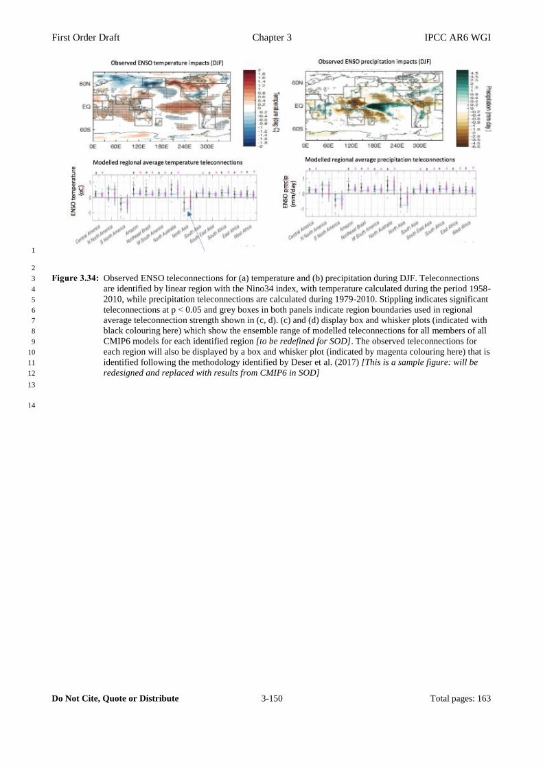
First Order Draft Chapter 3 IPCC AR6 WGI
Do Not Cite, Quote or Distribute 3-150 Total pages: 163
1
2
Observed ENSO teleconnections for (a) temperature and (b) precipitation during DJF. Teleconnections 3
are identified by linear region with the Nino34 index, with temperature calculated during the period 1958-4
2010, while precipitation teleconnections are calculated during 1979-2010. Stippling indicates significant 5
teleconnections at p < 0.05 and grey boxes in both panels indicate region boundaries used in regional 6
average teleconnection strength shown in (c, d). (c) and (d) display box and whisker plots (indicated with 7
black colouring here) which show the ensemble range of modelled teleconnections for all members of all 8
CMIP6 models for each identified region [to be redefined for SOD]. The observed teleconnections for 9
each region will also be displayed by a box and whisker plot (indicated by magenta colouring here) that is 10
identified following the methodology identified by Deser et al. (2017) [This is a sample figure: will be 11
redesigned and replaced with results from CMIP6 in SOD] 12
13
14

First Order Draft Chapter 3 IPCC AR6 WGI
Do Not Cite, Quote or Distribute 3-151 Total pages: 163
1
2
PDV spatio-temporal properties in observations and models. (a, b) SST anomalies (ºC) regressed onto the 3
Tripole Index (TPI; Henley et al., 2015) for 1900-2014 in (a) ERSSTv5 and (b) CMIP6 historical 4
simulations (MME composite). A 10-year low-pass filter has been applied beforehand. (c) A Taylor 5
diagram summarizing the representation of the PDV pattern in models and observations over [40ºS-60ºN, 6
110ºE-70ºW]. The reference pattern is taken from ERSSTv5. Black dots indicate other observational 7
products (ERSSTv3b and HadISSTv1) and red markers stand for individual members of each CMIP6 8
models. (d) Autocorrelation of unfiltered TPI at lag 1 year (blue) and 10-year low-pass filtered TPI at lag 9
10 year (orange) for observations (dashed lines) and 115-year chunks of piControl simulations and 10
historical ensemble simulations over 1900-2014 from CMIP6. (e) As in (d), but standard deviation of 11
unfiltered (blue) and filtered (orange) TPI (ºC). Boxes indicate the interquartile range and whiskers the 12
min-max range (f) Time series of 10-year low-pass filtered TPI (ºC) in ERSSTv5 (black) and CMIP6 13
historical simulations (red). The thick red line is the MME mean for the historical simulations; the 14
envelopes represent the 2 standard deviation level across ensemble members for historical (light pink) 15
and from 115-year chunks of CMIP6 piControl simulations (cyan). [Sample figure done so far with 6 16
CMIP6 models (66 members). Will be updated with results from more CMIP6 models in SO. DAMIP 17
simulations will be added in f) when available] 18
19
20
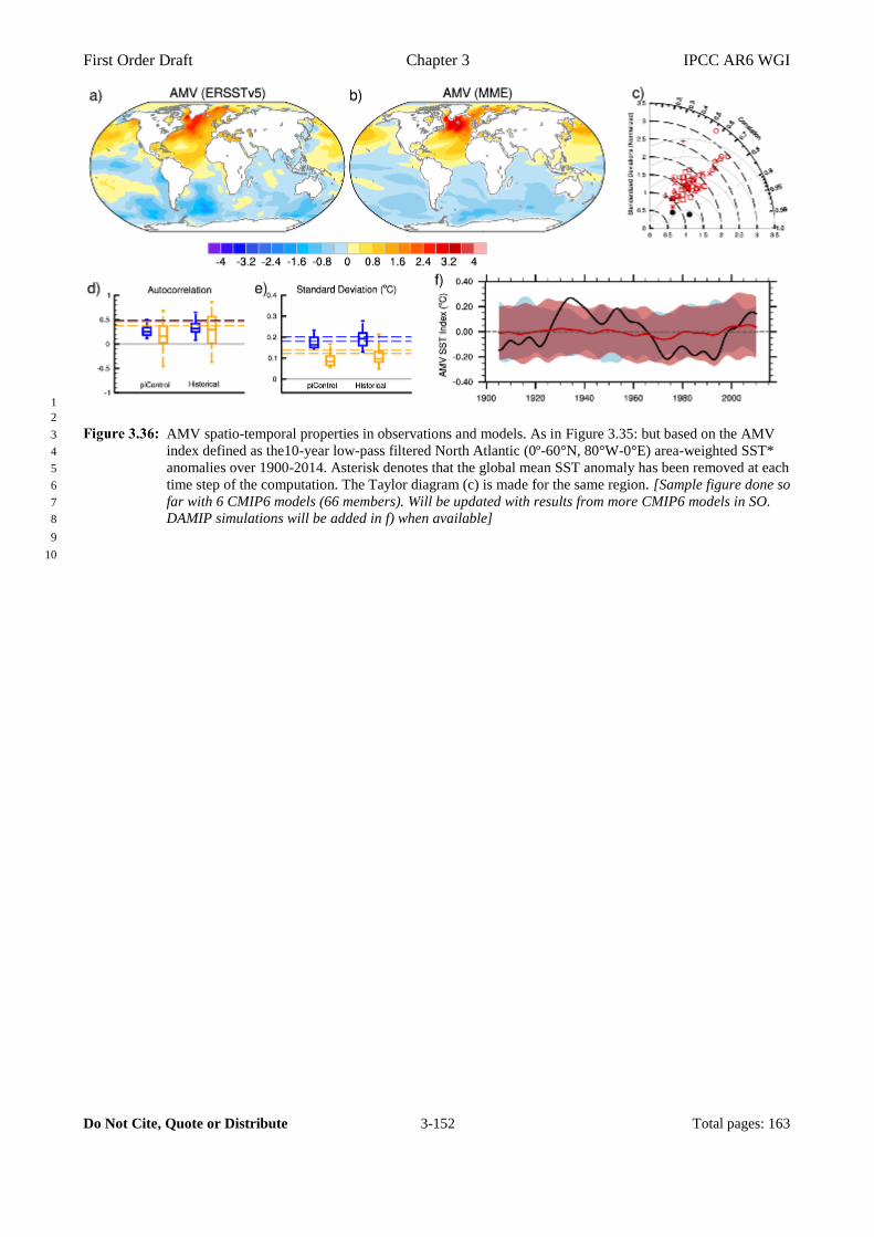
First Order Draft Chapter 3 IPCC AR6 WGI
Do Not Cite, Quote or Distribute 3-152 Total pages: 163
1
2
AMV spatio-temporal properties in observations and models. As in Figure 3.35: but based on the AMV 3
index defined as the10-year low-pass filtered North Atlantic (0º-60°N, 80°W-0°E) area-weighted SST* 4
anomalies over 1900-2014. Asterisk denotes that the global mean SST anomaly has been removed at each 5
time step of the computation. The Taylor diagram (c) is made for the same region. [Sample figure done so 6
far with 6 CMIP6 models (66 members). Will be updated with results from more CMIP6 models in SO. 7
DAMIP simulations will be added in f) when available] 8
9
10
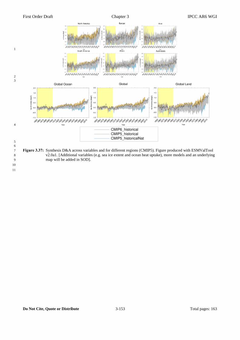
First Order Draft Chapter 3 IPCC AR6 WGI
Do Not Cite, Quote or Distribute 3-153 Total pages: 163
1
2
3
4
5
6
Synthesis D&A across variables and for different regions (CMIP5). Figure produced with ESMValTool 7
v2.0a1. [Additional variables (e.g. sea ice extent and ocean heat uptake), more models and an underlying 8
map will be added in SOD]. 9
10
11

First Order Draft Chapter 3 IPCC AR6 WGI
Do Not Cite, Quote or Distribute 3-154 Total pages: 163
1
2
3
Relative space-time root-mean-square deviation (RMSD) calculated from the climatological seasonal 4
cycle of the CMIP5 simulations. The years averaged depend on the years with observational data 5
available and are summarized in Table X of the Technical Annex on Observations. A relative 6
performance is displayed, with blue shading indicating better and red shading indicating worse 7
performance than the median of all model results. A diagonal split of a grid square shows the relative 8
error with respect to the reference data set (lower right triangle) and the alternative data set (upper left 9
triangle). White boxes are used when data are not available for a given model and variable. The 10
performance metrics are shown separately for atmosphere (upper row left), ocean and sea-ice (upper row 11
right), and land (lower row left). Updated and expanded from Figure 9.7 of Flato et al. (2013). Figure 12
produced with ESMValTool v1.0. [Will be replaced with results from CMIP6 in SOD and expanded to 13
cover the agreed large-scale indicators of climate change assessed in Chapter 3]. 14
15
16
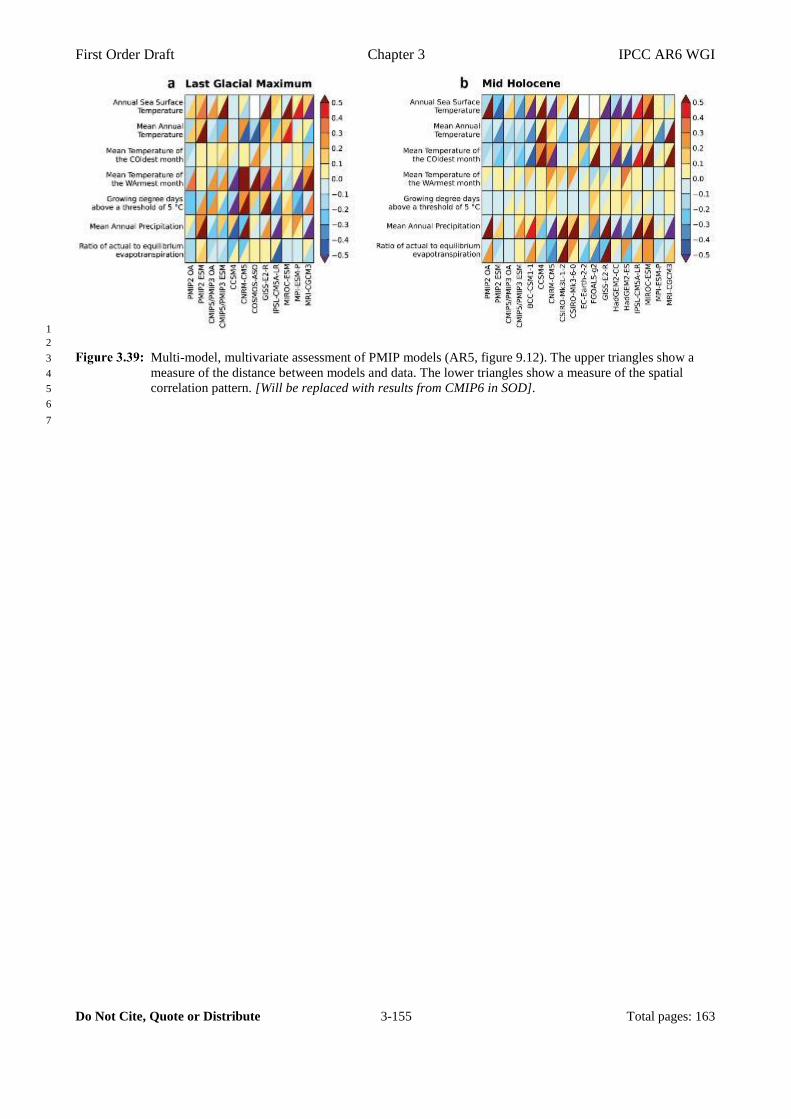
First Order Draft Chapter 3 IPCC AR6 WGI
Do Not Cite, Quote or Distribute 3-155 Total pages: 163
1
2
Multi-model, multivariate assessment of PMIP models (AR5, figure 9.12). The upper triangles show a 3
measure of the distance between models and data. The lower triangles show a measure of the spatial 4
correlation pattern. [Will be replaced with results from CMIP6 in SOD]. 5
6
7
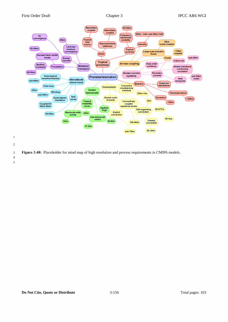
First Order Draft Chapter 3 IPCC AR6 WGI
Do Not Cite, Quote or Distribute 3-156 Total pages: 163
1
2
Placeholder for mind map of high resolution and process requirements in CMIP6 models. 3
4
5
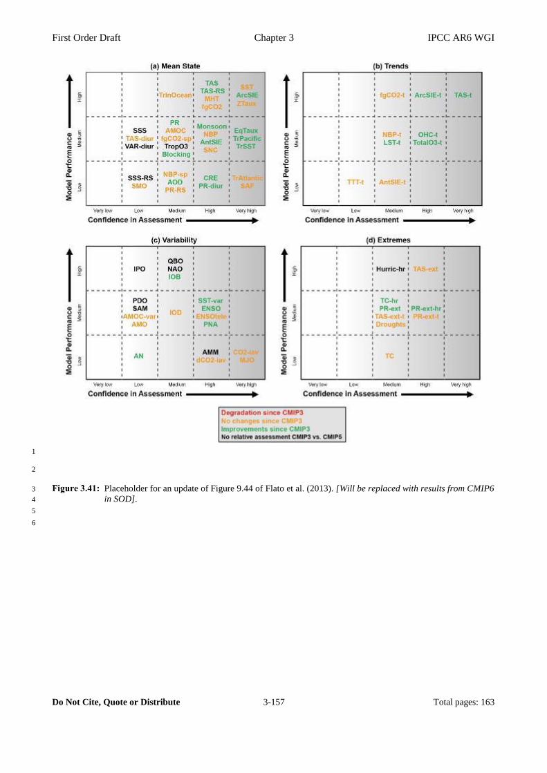
First Order Draft Chapter 3 IPCC AR6 WGI
Do Not Cite, Quote or Distribute 3-157 Total pages: 163
1
2
Placeholder for an update of Figure 9.44 of Flato et al. (2013). [Will be replaced with results from CMIP6 3
in SOD]. 4
5
6
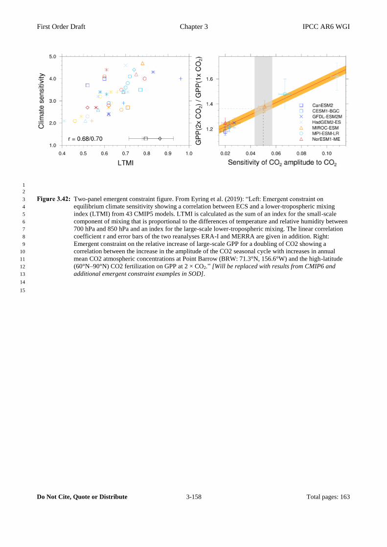
First Order Draft Chapter 3 IPCC AR6 WGI
Do Not Cite, Quote or Distribute 3-158 Total pages: 163
1
2
Two-panel emergent constraint figure. From Eyring et al. (2019): “Left: Emergent constraint on 3
equilibrium climate sensitivity showing a correlation between ECS and a lower-tropospheric mixing 4
index (LTMI) from 43 CMIP5 models. LTMI is calculated as the sum of an index for the small-scale 5
component of mixing that is proportional to the differences of temperature and relative humidity between 6
700 hPa and 850 hPa and an index for the large-scale lower-tropospheric mixing. The linear correlation 7
coefficient r and error bars of the two reanalyses ERA-I and MERRA are given in addition. Right: 8
Emergent constraint on the relative increase of large-scale GPP for a doubling of CO2 showing a 9
correlation between the increase in the amplitude of the CO2 seasonal cycle with increases in annual 10
mean CO2 atmospheric concentrations at Point Barrow (BRW: 71.3°N, 156.6°W) and the high-latitude 11
(60°N–90°N) CO2 fertilization on GPP at 2 × CO2.” [Will be replaced with results from CMIP6 and 12
additional emergent constraint examples in SOD]. 13
14
15

First Order Draft Chapter 3 IPCC AR6 WGI
Do Not Cite, Quote or Distribute 3-159 Total pages: 163
1
2
Cross-Chapter Box 3.1, Figure 1: (a, b) GMST trends for 1998-2012 (a) and 2012-2026 (b). Shadings represent 3
probability density functions (PDFs; scaled so that the area under the curve sums 4
to one) based on historical simulations of CMIP5 (extended by RCP4.5, 95 5
members) and CMIP6 (40 members), with white lines indicating individual 6
ensemble means. Hatching shows a PDF of HadCRUT4.6.0.0. Vertical lines 7
represent GISTEMP, NOAAGlobalTemp and BerkeleyEarth estimates. Selected 8
members whose trends are lower than the maximum observational estimates (dark 9
blue shading in a) are indicated by blue lines in the PDF of the 2012-2026 trends 10
(b). Model GMST is based on a blend of SST and SAT masked to match 11
HadCRUT data coverage, following Cowtan et al. (2015). The masking is not 12
applied to GISTEMP, NOAAGlobalTemp and BerkeleyEarth data. (c-e) Trend 13
maps of annual near-surface temperature. (c, d) 1998-2012 trends based on 14
GISTEMP (c) and composited trends of subsampled CMIP simulations included in 15
dark blue shading area in (a). (e) Corresponding composited trends but for 2012-16
2026 indicated by blue lines in (b). [d and e will be made only by CMIP6 models 17
when enough size of ensemble becomes available] 18
19
20

First Order Draft Chapter 3 IPCC AR6 WGI
Do Not Cite, Quote or Distribute 3-160 Total pages: 163
1
2
Cross-Chapter Box 3.2, Figure 1: Time series of global averaged 5-year mean anomalies of TXx (°C) and Rx1day (mm) 3
during 1953-2017 from the GHCNDEX observations and the CMIP5 and CMIP6 4
multi-models with natural and human forcing (upper) and natural forcing only 5
(lower). For CMIP5, historical simulations for 1953-2005 are combined with 6
corresponding RCP4.5 scenario runs for 2006-2017. For observations, grids with 7
more than 90% data availability during 1951-2017 are used and global means are 8
calculated only for years when more than 80% of grids compared to the 1961-1990 9
coverage have data. The time-fixed observational mask (based on grids with more 10
than 90% data availability during 1951-2017) has been applied to model data 11
throughout the whole period. For CMIP5, shading represents the range of individual 12
model (ensemble means) and thick line indicates multi-model means (with equal 13
weighting given for each model). For CMIP6, only each model results (ensemble 14
means) are displayed as thin lines. Anomalies are relative to 1961-1990 means. 15
16
17
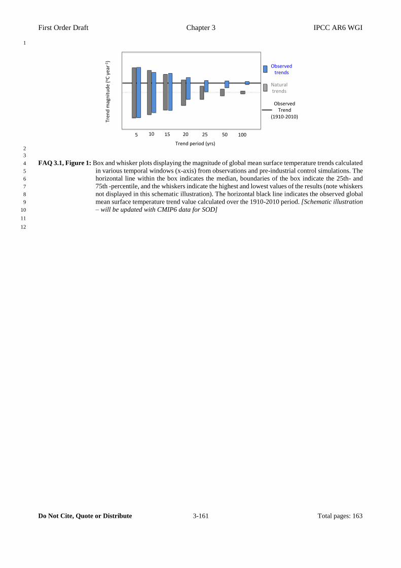
First Order Draft Chapter 3 IPCC AR6 WGI
Do Not Cite, Quote or Distribute 3-161 Total pages: 163
1
2
3
FAQ 3.1, Figure 1: Box and whisker plots displaying the magnitude of global mean surface temperature trends calculated 4
in various temporal windows (x-axis) from observations and pre-industrial control simulations. The 5
horizontal line within the box indicates the median, boundaries of the box indicate the 25th- and 6
75th -percentile, and the whiskers indicate the highest and lowest values of the results (note whiskers 7
not displayed in this schematic illustration). The horizontal black line indicates the observed global 8
mean surface temperature trend value calculated over the 1910-2010 period. [Schematic illustration 9
– will be updated with CMIP6 data for SOD] 10
11
12
Trendperiod(yrs)
Tren
dm
agnitude(oCyear-1)
5 10 15 20 1005025
Observedtrends
Naturaltrends
ObservedTrend
(1910-2010)
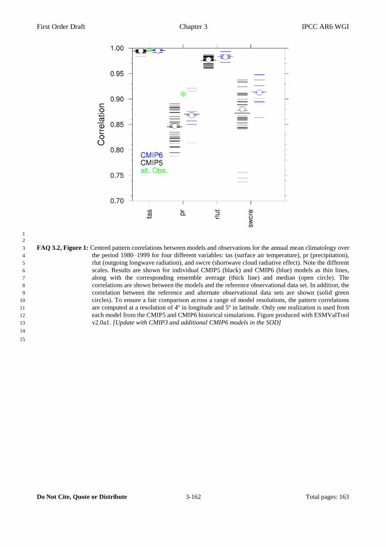
First Order Draft Chapter 3 IPCC AR6 WGI
Do Not Cite, Quote or Distribute 3-162 Total pages: 163
1
2
FAQ 3.2, Figure 1: Centred pattern correlations between models and observations for the annual mean climatology over 3
the period 1980–1999 for four different variables: tas (surface air temperature), pr (precipitation), 4
rlut (outgoing longwave radiation), and swcre (shortwave cloud radiative effect). Note the different 5
scales. Results are shown for individual CMIP5 (black) and CMIP6 (blue) models as thin lines, 6
along with the corresponding ensemble average (thick line) and median (open circle). The 7
correlations are shown between the models and the reference observational data set. In addition, the 8
correlation between the reference and alternate observational data sets are shown (solid green 9
circles). To ensure a fair comparison across a range of model resolutions, the pattern correlations 10
are computed at a resolution of 4º in longitude and 5º in latitude. Only one realization is used from 11
each model from the CMIP5 and CMIP6 historical simulations. Figure produced with ESMValTool 12
v2.0a1. [Update with CMIP3 and additional CMIP6 models in the SOD] 13
14
15
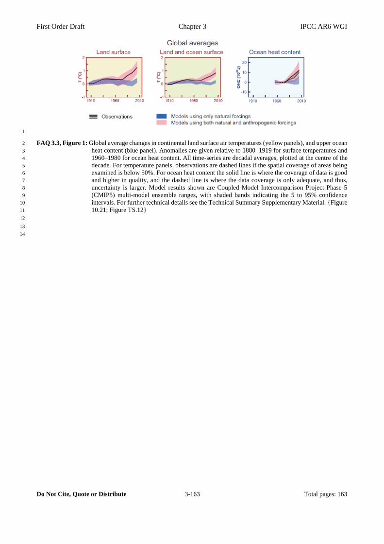
First Order Draft Chapter 3 IPCC AR6 WGI
Do Not Cite, Quote or Distribute 3-163 Total pages: 163
1
FAQ 3.3, Figure 1: Global average changes in continental land surface air temperatures (yellow panels), and upper ocean 2
heat content (blue panel). Anomalies are given relative to 1880–1919 for surface temperatures and 3
1960–1980 for ocean heat content. All time-series are decadal averages, plotted at the centre of the 4
decade. For temperature panels, observations are dashed lines if the spatial coverage of areas being 5
examined is below 50%. For ocean heat content the solid line is where the coverage of data is good 6
and higher in quality, and the dashed line is where the data coverage is only adequate, and thus, 7
uncertainty is larger. Model results shown are Coupled Model Intercomparison Project Phase 5 8
(CMIP5) multi-model ensemble ranges, with shaded bands indicating the 5 to 95% confidence 9
intervals. For further technical details see the Technical Summary Supplementary Material. {Figure 10
10.21; Figure TS.12} 11
12
13
14