6 Chapter 6: Short-lived climate forcers - IPCC
135
First Order Draft Chapter 6 IPCC AR6 WGI Do Not Cite, Quote or Distribute 6-1 Total pages: 135 6 Chapter 6: Short-lived climate forcers 1 2 3 4 Coordinating Lead Authors: 5 William D. Collins (USA), Hong Liao (China) 6 7 Lead Authors: 8 Bhupesh Adhikary (Nepal), Paulo Artaxo (Brazil), Terje Berntsen (Norway), Sandro Fuzzi (Italy), Laura 9 Gallardo (Chile), Astrid Kiendler-Scharr (Germany/Austria), Zbigniew Klimont (Austria/Poland), Vaishali 10 Naik (USA), Sophie Szopa (France), Nadine Unger (UK), Prodromos Zanis (Greece) 11 12 Contributing Authors: 13 Wenche Aas (Norway), Owen Cooper (USA), Sarah Doherty (USA), Matthew Gidden (Austria/USA), 14 Fabien Paulot (USA), Johannes Quaas (Germany) 15 16 Review Editors: 17 Yugo Kanaya (Japan), Michael Prather (USA), Nourredine Yassaa (Algeria) 18 19 Chapter Scientist: 20 Chaincy Kuo (USA) 21 22 Date of Draft: 23 29/04/2019 24 25 Notes: 26 TSU compiled version 27 28 During the compilation of this Chapter, some text was accidently replaced by the error message Erreur ! Source du renvoi introuvable. In order to give you access to the original text, a correspondence tables has been created and is available for download from the AR6 WGI FOD Review system (file AR6 WGI FOD - Chapter 6 Corrections.pdf).
-
Upload
khangminh22 -
Category
Documents
-
view
0 -
download
0
Transcript of 6 Chapter 6: Short-lived climate forcers - IPCC
First Order Draft Chapter 6 IPCC AR6 WGI
Do Not Cite, Quote or Distribute 6-1 Total pages: 135
6 Chapter 6: Short-lived climate forcers 1
2
3
4
Coordinating Lead Authors: 5
William D. Collins (USA), Hong Liao (China) 6
7
Lead Authors: 8
Bhupesh Adhikary (Nepal), Paulo Artaxo (Brazil), Terje Berntsen (Norway), Sandro Fuzzi (Italy), Laura 9
Gallardo (Chile), Astrid Kiendler-Scharr (Germany/Austria), Zbigniew Klimont (Austria/Poland), Vaishali 10
Naik (USA), Sophie Szopa (France), Nadine Unger (UK), Prodromos Zanis (Greece) 11
12
Contributing Authors: 13
Wenche Aas (Norway), Owen Cooper (USA), Sarah Doherty (USA), Matthew Gidden (Austria/USA), 14
Fabien Paulot (USA), Johannes Quaas (Germany) 15
16
Review Editors: 17
Yugo Kanaya (Japan), Michael Prather (USA), Nourredine Yassaa (Algeria) 18
19
Chapter Scientist: 20
Chaincy Kuo (USA) 21
22
Date of Draft: 23
29/04/2019 24
25
Notes: 26
TSU compiled version 27
28 During the compilation of this Chapter, some text was accidently replaced by the error message Erreur ! Source du renvoi introuvable.In order to give you access to the original text, a correspondence tables has been created and is available for download from the AR6 WGI FOD Review system (file AR6 WGI FOD - Chapter 6 Corrections.pdf).
First Order Draft Chapter 6 IPCC AR6 WGI
Do Not Cite, Quote or Distribute 6-2 Total pages: 135
Table of Contents 1
2
Executive Summary ........................................................................................................................................... 5 3
6.1 Importance of SLCFs on climate and AQ ....................................................................................... 10 4
6.1.1 Treatment of SLCF in previous assessments ........................................................................... 10 5
6.1.2 Sources & Processes ................................................................................................................ 11 6
6.1.2.1 Key sources of SLCFs ......................................................................................................... 12 7
6.1.2.2 Key processes ...................................................................................................................... 13 8
6.1.3 Influences on Climate and Air Quality .................................................................................... 14 9
6.1.3.1 Influence of SLCFs on climate ............................................................................................ 14 10
6.1.3.2 Influence of SLCFs on Air Quality ..................................................................................... 14 11
6.1.4 Policy relevance ....................................................................................................................... 16 12
BOX 6.1: Chain connecting emission to concentration to impact ............................................................... 17 13
6.2 SLCF emissions and atmospheric abundance.................................................................................. 17 14
6.2.1 Global and regional temporal evolution of SLCF emissions ................................................... 17 15
6.2.1.1 Anthropogenic sources ........................................................................................................ 18 16
6.2.1.2 Natural sources .................................................................................................................... 20 17
BOX 6.2: The three pillars to improve the SLCF understanding: Laboratory/Theoretical studies, 18
Observations, Atmospheric chemistry models ............................................................................ 21 19
6.2.2 Atmospheric processes and SLCF abundances ....................................................................... 23 20
6.2.2.1 Nitrogen Oxide (NOx) ......................................................................................................... 24 21
6.2.2.2 Carbon Monoxide (CO) ....................................................................................................... 25 22
6.2.2.3 Volatile Organic Compounds (VOCs)................................................................................. 27 23
6.2.2.4 Methane (CH4) ..................................................................................................................... 28 24
6.2.2.5 Ozone (O3) ........................................................................................................................... 29 25
6.2.2.5.1 Tropospheric ozone ....................................................................................................... 29 26
6.2.2.5.2 Stratospheric ozone ........................................................................................................ 31 27
6.2.2.6 Sulphur Dioxide (SO2) and Sulphate Aerosols (SO42-) ........................................................ 32 28
6.2.2.7 Ammonia (NH3) and Nitrate Aerosols (NO3-) .................................................................... 33 29
6.2.2.8 Carbonaceous Aerosols (BC, OC, SOA) ............................................................................. 34 30
6.2.2.9 Short-lived Halogenated Species ......................................................................................... 36 31
6.2.2.9.1 HCFCs ........................................................................................................................... 36 32
6.2.2.9.2 HFCs .............................................................................................................................. 36 33
6.2.2.9.3 Halons and methyl bromide ........................................................................................... 37 34
6.2.2.9.4 Very Short-Lived Halogenated Substances (VSLSs) .................................................... 37 35
6.2.3 Implications for Atmospheric Oxidizing Capacity .................................................................. 38 36
6.3 SLCF radiative forcing and impact ................................................................................................. 40 37
6.3.1 Mechanisms for Short-lived Climate Forcing ......................................................................... 40 38
6.3.1.1 Indirect vs direct forcers ...................................................................................................... 40 39
6.3.1.2 Aerosol-cloud interactions on hydrological cycle ............................................................... 41 40
First Order Draft Chapter 6 IPCC AR6 WGI
Do Not Cite, Quote or Distribute 6-3 Total pages: 135
6.3.1.3 Influence on terrestrial ecosystems and the carbon cycle .................................................... 43 1
6.3.1.4 Changes in ERFs ................................................................................................................. 44 2
6.3.1.5 Effects on cryosphere .......................................................................................................... 45 3
6.3.2 Observations of regional short-lived climate forcing .............................................................. 46 4
6.3.2.1 Observations of observables (recent advances in BC on snow dimming, human experiments 5
in India and China, and volcanoes, dust, methane, ACI) ...................................................... 48 6
6.3.2.2 Emergent constraints from recent observational studies ..................................................... 49 7
6.3.3 History of Regional Short-lived Climate Forcing ................................................................... 50 8
6.3.3.1 Characterise ARI and its increases ...................................................................................... 51 9
6.3.3.2 Characterise the forcing from coupled interactions, e.g., ACI, and its increases ................ 52 10
6.3.3.3 Characterisation of the time evolving uncertainty ............................................................... 53 11
6.3.4 Impacts of Short-lived Climate forcers.................................................................................... 54 12
6.3.4.1 Effects of transport .............................................................................................................. 54 13
6.3.4.2 Effects through atmospheric dynamics ................................................................................ 54 14
6.3.4.3 Effects on temperature and precipitation ............................................................................. 55 15
6.4 SLCF mitigation and climate/AQ interactions ................................................................................ 57 16
6.4.1 Implications of SLCF lifetime on response time horizon ........................................................ 57 17
6.4.2 Sectoral Attribution of SLCF impacts on AQ and climate ...................................................... 58 18
6.4.2.1 Household biofuel burning .................................................................................................. 58 19
6.4.2.2 Biomass burning .................................................................................................................. 59 20
6.4.2.3 Land-use .............................................................................................................................. 59 21
6.4.2.4 Impacts of SLCF emissions from megacities on climate .................................................... 60 22
6.4.3 Case studies of mitigation ........................................................................................................ 61 23
6.5 Implications of changing climate on AQ ......................................................................................... 63 24
6.5.1 How climate change influences air quality .............................................................................. 63 25
6.5.2 Impact of climate change on surface O3 ................................................................................. 64 26
6.5.3 Impact of climate change on particulate matter ....................................................................... 65 27
6.5.4 Impact of climate change on extreme pollution ...................................................................... 66 28
6.6 Future scenarios and impacts (Emissions, Concentration, forcing and AQ) ................................... 67 29
6.6.1 Scenarios for emissions and implications for concentrations of SLCFs.................................. 67 30
6.6.1.1 Differences in concentrations among scenarios .................................................................. 68 31
6.6.1.2 Model structural implications for uncertainty in future concentrations .............................. 69 32
6.6.2 Impacts of urbanization on SLCFs budgets ............................................................................. 70 33
6.6.3 Time-dependent implications of scenarios for RF and impacts .............................................. 70 34
6.6.3.1 Regional trends in RF .......................................................................................................... 71 35
6.6.4 Compensating effects (cooling vs. warming for SSPs) ........................................................... 71 36
6.6.5 Impacts on AQ (forced by SSP emissions) .............................................................................. 72 37
6.7 Knowledge gaps .............................................................................................................................. 73 38
6.7.1 Abundances and radiative forcing of SLCFs ........................................................................... 73 39
6.7.2 Climate effect of SLCFs .......................................................................................................... 73 40
First Order Draft Chapter 6 IPCC AR6 WGI
Do Not Cite, Quote or Distribute 6-4 Total pages: 135
6.7.3 Effects of SLCFs on health, agriculture, and ecosystems........................................................ 74 1
Frequently Asked Questions ............................................................................................................................ 75 2
FAQ 6.1: Why do we care about Short-Lived Climate Forcers? ............................................................. 75 3
FAQ 6.2: What is the link between air quality and climate change? ....................................................... 77 4
References ....................................................................................................................................................... 79 5
Figures ........................................................................................................................................................... 123 6
7
First Order Draft Chapter 6 IPCC AR6 WGI
Do Not Cite, Quote or Distribute 6-5 Total pages: 135
Executive Summary 1
2
SLCFs continue to contribute the largest uncertainty to estimates and interpretations of the Earth’s changing 3
energy budget. This chapter focuses on changes in sources and abundances of SLCFs to assess how SLCFs 4
contribute and respond to climate change. The following conclusions are drawn. 5
6
Emissions 7
8
Currently more than 50% of anthropogenic emissions of all species (including NH3) originate from Asia 9
(high confidence), as a result of the strong economic growth in Asia and declining emissions in North 10
America and Europe due to air quality legislation and declining capacity of energy intensive industry {6.2}. 11
12
In spite of the success of environmental legislation introduced in several countries affecting the trends in 13
specific regions: North America and recently in parts of Asia, especially China, emissions of most of the 14
species show no signs of stabilisation or decline, except decline of SO2 and CO (high confidence), and since 15
2011 stabilization or even decline of NOx (medium confidence). {6.2.1.2}. 16
17
For SO2, the strong growth of Asian emissions has been offset by reduction in North America and Europe 18
and since about 2006 also Chinese emissions appear to decline strongly (high confidence). {6.2.1.2} 19
20
NH3 emissions continue growing (high confidence) and the trends estimated in CMIP5 and CMIP6 are the 21
same, while in absolute terms CMIP6 has somewhat higher emissions as it includes emissions from 22
wastewater and human waste that were largely missing in CMIP5. {6.2.1.2} 23
24
Emissions of carbonaceous aerosols (BC, OC) have been steadily increasing and since 1950 about doubled 25
(medium confidence). Before 1950, North America and Europe contributed about half of the global total but 26
successful introduction of diesel particulate filters on road vehicles and declining reliance on solid fuels for 27
heating brought in large reductions (high confidence) {6.2.1.2} 28
29
Since AR5, there is medium evidence and high agreement based on global modelling studies that 30
anthropogenic LULCC, and the historical cropland expansion in particular, are the dominant drivers of 31
isoprene emission change since the preindustrial era. Results are converging on a 10-25% loss of isoprene 32
emission globally due to the historical cropland expansion between 1850 and the present day (high 33
confidence). Isoprene emission change over the past century was driven by human LULCC and is therefore a 34
human-induced climate forcing mechanism in addition to a climate feedback mechanism (high confidence) 35
{6.2.1.2} 36
37
Bottom up global emission estimates of CH4 for the last two decades are higher than top down assessments, 38
primarily due to larger estimates for natural sources, but the overall trends are similar – steady growth (high 39
confidence). {6.2.1.2} 40
41
It is likely that historical, present and future LULCC will have substantial impacts on global air quality and 42
the SLCFs. {6.4.2.2} 43
44
45
Atmospheric processes and SLCF abundances 46
47
It is very likely that global tropospheric NOx has increased from the pre-industrial period to the present day. 48
Satellite observations of tropospheric NOx indicate strong regional variations in trends over the 2005-2015 49
time period. It is very likely that NO2 has declined over the USA and western Europe since the mid 1990s 50
and increased over China until 2011. It is likely that NO2 trends have reversed (declined) over China 51
beginning in 2012 and likely that NO2 has increased over South Asia by 50% since 2005. {6.2.2.1}. 52
53
There is high confidence that the global tropospheric SO2 burden increased from 1850 to around 2005, but 54
there are large regional differences. The sulphate aerosol concentrations in North America and Europe have 55
First Order Draft Chapter 6 IPCC AR6 WGI
Do Not Cite, Quote or Distribute 6-6 Total pages: 135
declined over the 1980 to 2015 period, with slightly stronger reductions in North America (47%) than over 1
Europe (40%) in the 2000-2015 time period, though Europe had larger reductions in the prior decade (1990-2
2000). In Asia, the trends are more scattered, though there is medium confidence that there was a strong 3
increase up to around 2005, followed by a steep decline in China in the concentrations of SO2 and sulphate, 4
while over India, SO2 levels have doubled over the 2005 to 2015 period. {6.2.2.6} 5
6
There is high confidence in our estimates of modern period global total CO distribution since AR5. There is 7
medium confidence that in the modern period, global CO burden is declining. {6.2.2.2} 8
9
The overall distribution of ammonia column is well understood. However, there is medium confidence in the 10
attribution of recent trends in ammonia to emissions versus changes in the gas/aerosol partitioning of 11
ammonia. {6.2.2.7}. The sensitivity of nitrate aerosols to ammonia and nitric acid is well-understood from 12
thermodynamics. However, there is low confidence in the evolution of nitrate aerosols with time stemming 13
partly from limited understanding of how aerosol pH has evolved over time. {6.2.2.7} 14
15
There is medium evidence and high agreement that the abundances of light NMHCs such as ethane and 16
proprane in the NH reached a maximum around 1970-1985, then declined until between 2005-2010, and are 17
now increasing again due to oil and gas production. {6.2.2.3} 18
19
Global carbonaceous aerosol budget and trends remain poorly characterized due to limited observation 20
yielding low confidence in our current understanding. There is increased understanding that surface warming 21
due to BC maybe weaker than previously reported and that BC causes significant model spread in predicted 22
precipitation compared to other climate drivers. {6.2.2.8} 23
24
Overall, observational and modeling evidence suggests that it is about as likely as not that global mean OH 25
has remained constant over the past 35 years. Over longer time scales, global mean OH has remained nearly 26
constant in response to competing influences from changes in SLCFs and climate (low confidence) {6.2.3}. 27
Contradictory modeling results together with limited and uncertain observational constraints on OH impede 28
our ability to accurately elucidate the interannual variability in OH over the 1980 to present time period. 29
{6.2.3}. Further, it is argued that since the isotopic adjustment occurs slowly in response to OH changes, the 30
observed rapid shift in δ13CCH4 is less likely to be driven by OH variations and more likely due to changes in 31
methane sources. Given that it is about as likely as not that global mean OH has remained constant over the 32
past 35 years (section 6.2.3), the role of OH in driving the renewed increase in atmospheric methane remains 33
uncertain. {6.2.2.4} 34
35
It is virtually certain that atmospheric methane abundance has been increasing since 2007 after a period 36
(1999-2006) of stable concentrations. {6.2.2.4}. There is low confidence (low agreement and moderate 37
evidence) in the causes of methane increase because of uncertainties in source and sink estimates as well as 38
limitations in observational constraints, such as δ13CCH4 and ethane. {6.2.2.4}. 39
40
There is robust evidence with a medium to high level of agreement and overall a medium confidence about 41
changes in ozone at northern mid- and high latitudes from the early-20th century to the modern period 42
{6.2.2.5}. There is also overall medium confidence for profiles above North America and Europe to draw 43
conclusions about zonal mean ozone changes at the tropics and southern mid-latitudes due to sparseness of 44
historical observations {6.2.2.5}. 45
46
There is high confidence (high agreement and robust evidence) for the estimated present-day global average 47
tropospheric ozone burden based on an ensemble of models. However, there is medium confidence (low to 48
medium agreement and medium evidence) among the individual models for their estimates of tropospheric 49
ozone burden, and the related ozone budget terms. {6.2.2.5} 50
51
The near-global average (60°S-60°N) of total ozone columns in present-day remain lower than the 52
respective quantity during the unperturbed from ODS period with the estimated preindustrial to present-day 53
stratospheric ozone radiative forcing (RF) being similar to AR5 (high confidence). {6.2.2.5} 54
55
First Order Draft Chapter 6 IPCC AR6 WGI
Do Not Cite, Quote or Distribute 6-7 Total pages: 135
There is high agreement and robust evidence that the abundance of total chlorine from HCFCs has continued 1
to increase in the atmosphere with decreased growth rates. There is also high agreement and robust 2
evidence that total tropospheric bromine from halons and methyl bromide have continued to decrease while 3
abundances of most currently measured HFCs are increasing in the global atmosphere at accelerating rates, 4
consistent with expectations based on the ongoing transition away from the use of ozone-depleting 5
substances. {6.2.2.9} 6
7
SLCF radiative forcing and impact 8
9
Emissions of CO and NMVOCs are virtually certain to have induced a positive radiative forcing on climate 10
(Myhre et al., 2013) because they lead to increases in the concentrations of CO2, CH4, and O3 through 11
chemical reactions {6.1.2.1} 12
13
The models agree that the increasing emissions have resulted in the RF of 0.4±0.22 Wm-2 by tropospheric 14
ozone since 1850 with the confidence remaining low to medium as in AR5. Despite the fact that the 15
confidence in the 20th century ozone observations has increased since AR5 there is still a knowledge gap 16
from observations for preindustrial ozone levels and thus their estimates are based on model simulations. 17
{6.2.2.5} 18
19
There is high confidence that anthropogenic aerosols lead to an increase in cloud droplet concentrations. In 20
terms of the adjustments, it is most plausible that on average, no systematic changes in LWP occur. It is 21
more likely than not that liquid-cloud fraction increases than that it decreases. There is no observational 22
evidence at present for a significant response of ice clouds to aerosol perturbations. {6.3.2} 23
24
There is a consensus from recent modelling studies highlighting that the representation of both aerosol 25
chemistry as well as the parameterizations for direct and indirect aerosol radiative effects in current climate 26
models are subject to large uncertainties. These uncertainties imply that single-model studies investigating 27
the effects of changes in SLCFs on local and remote changes in temperature and precipitation generally have 28
low confidence (low to medium agreement) and limited evidence relative to a multi-model ensemble. 29
{6.3.4} 30
31
There is medium agreement and medium evidence across multi-model ensembles on the response to a given 32
local forcing with qualitatively similar temperature change patterns extending across much of the Northern 33
Hemisphere. However, the patterns of regional climate change will depend on the balance between SLCFs 34
and GHG forcing. {6.3.4} 35
36
There is medium evidence and agreement that SO2 emissions reductions may lead to the strongest response, 37
with an increase in surface air temperature in the northern hemisphere high latitudes, and a corresponding 38
increase in global mean precipitation while the BC and OC emissions reductions give a much weaker forcing 39
signal {6.3.4} 40
41
It is virtually certain that the cooling by aerosols in the Northern Hemisphere changes the interhemisphere 42
temperature gradient, thereby producing an anomalous Hadley cell circulation, a northward shift of ITCZ, 43
and an alteration to tropical precipitation patterns {6.3.4}. 44
45
Since AR5, there remains low confidence in even the net sign of the influence of carbonaceous aerosols from 46
solid fuel cookstoves on global radiative effect (warming or cooling). {6.4.2.1} 47
48
There is robust evidence and high agreement that SLCFs from fires have global and regional radiative 49
effects, and it is likely that the net global aerosol and aerosol-cloud radiative influence is cooling, despite the 50
substantial absorption from BC {6.4.2.1} 51
52
Preindustrial to present day anthropogenic LULCC have resulted in a global warming that is equivalent to up 53
to 45% of the net anthropogenic global warming including changes in the SLCFs from dust, fire, BVOCs, 54
soil, CH4 and NH3 emissions (low confidence). {6.4.2.2} 55
First Order Draft Chapter 6 IPCC AR6 WGI
Do Not Cite, Quote or Distribute 6-8 Total pages: 135
1
There is low confidence in the quantitative influence of past LULCC on radiative forcing by the SLCFs due 2
to limited historical data on concentrations and abundances of SLCFs and challenges in attributing changes 3
in SLCFs to LULCC. {6.4.2.2} 4
5
The attribution of emissions to megacities is of low confidence since different methodologies are considered 6
to define the megacity areas and since large differences remain between global emissions inventories and 7
city-specific inventories {6.4.2.3}. 8
9
The quantification of the climate impact potential of cookstove mitigation is subject to low confidence. 10
{6.4.3} 11
12
There is high confidence in the effects of reduced emissions of SLCFs on air quality, but medium confidence 13
in the sign and magnitude of the climatic impacts of these emission reductions, except CH4 of which 14
reductions are very likely to contribute to climate mitigation. {6.5} 15
16
Impact of climate change on air quality 17
18
The response of surface ozone to future climate change induced from LLCFs remains uncertain with largest 19
part of the uncertainty related to contribution of stratosphere-troposphere exchange. Hence there is medium 20
confidence (medium agreement and medium evidence) that in unpolluted regions, higher water vapour 21
abundances and temperatures in a warmer climate enhance ozone chemical destruction, leading to lower 22
baseline surface ozone levels. {6.5.2} 23
24
There is now high confidence (high agreement, but medium evidence) on a small effect on PM global burden 25
due to climate change. The regional effects, however, are predicted to be much higher {6.5.3} 26
27
Impacts of SLCFs on human health, agricultural production and ecosystems 28
29
There is medium confidence that PM impacts agriculture and ecosystems and may cause material and 30
property damage. 31
32
There is high confidence that elevated levels of ambient ozone impacts human health. However, there is 33
medium confidence on human health impacts from ambient concentrations of other trace gases such as NOx, 34
CO, and SO2. 35
36
The outdoor and indoor human health consequences of household solid fuel combustion are substantial (high 37
confidence). {6.4.2.1} 38
39
There is limited evidence but high agreement that the effects of ozone on vegetation influence the climate 40
system by changing the land carbon storage. There is medium evidence and high agreement that ozone 41
vegetation interactions further influence the climate system by affecting stomatal control over plant 42
transpiration of water vapour between the leaf surface and atmosphere. {6.3.1.3} 43
44
It is certain that ozone is phytotoxic and damages photosynthesis, reduces plant growth, and limits crop 45
yields in sensitive plants (very high confidence). {6.3.1.3} 46
47
There is new evidence that the SLCF effects on vegetation influences atmospheric surface ozone 48
concentrations by altering emissions of BVOCs, surface climate, and the dry deposition rate of trace gases 49
and particles including ozone itself. (low confidence). {6.3.1.3} 50
51
There is growing evidence that fire emissions influence regional air quality and human health (medium 52
confidence). There is limited evidence that fire air pollution vegetation damage reduces the global and 53
regional terrestrial productivity {6.4.1.2} 54
55
First Order Draft Chapter 6 IPCC AR6 WGI
Do Not Cite, Quote or Distribute 6-9 Total pages: 135
Global modelling studies agree that ozone-induced GPP losses are largest today in eastern USA, Europe and 1
eastern China ranging from 5-20% on the regional scale (medium confidence). {6.3.1.3}. The combined 2
effects of ozone and aerosol haze pollution in the present day in China have lowered regional net primary 3
production (NPP) by 9-16%. By 2030, this current level of NPP loss will increase by 20-30% following 4
IIASA ECLIPSE Current Legislation scenario, but will be reduced by 70% following the Maximum 5
Technically Feasible Reduction scenario (low confidence). {6.3.1.3} 6
7
Ozone pollution is estimated to decrease global crop yields from about 2.2-5.5% for maize to 3.9-15% and 8
8.5–14% for wheat and soybean crops, respectively, where the uncertainty range depends on genotype and 9
environmental conditions (medium confidence). {6.3.1.3} 10
11
Policy relavance 12
13
The IPCC Special Report on 1.5C found that reductions in SLCFs play a critical role in achieving 1.5C and 14
2C, and limiting warming to 1.5°C implies deep reductions in emissions of SCLFs, particularly CH4, as 15
well as reaching net zero CO2 emissions globally around 2050 (high confidence) {6.1} 16
17
There is a general consensus that measures to reduce SLCFs emissions should not reduce the pressure for an 18
immediate action on CO2 and other LLGHGs reduction (high agreement, robust evidence) {6.1.4} 19
20
Co-benefits of climate mitigation for air quality and human health to meet Nationally Determined 21
Contributions (NDCs) and/or specific global temperature targets can dominate the costs of the climate 22
measures (high agreement, medium evidence) {6.1.4} 23
24
There is high agreement and robust evidence that SLCFs mitigation measures act complementary to early 25
and stringent CO2 mitigation with important temperature effects for the near term but there is medium 26
agreement and medium evidence for their contribution in the long-term. {6.6.4} 27
28
The different socioeconomic developments in the SSP storylines and the different levels of climate policies 29
for each SSP have strong influence SLCF emissions and thus on air quality (high confidence). {6.6.5} 30
31
32
First Order Draft Chapter 6 IPCC AR6 WGI
Do Not Cite, Quote or Distribute 6-10 Total pages: 135
6.1 Importance of SLCFs on climate and AQ 1
2
Both natural and anthropogenic emissions of chemical species can either lead to the formation of climate 3
forcers in the atmosphere or directly act as climate forcers altering the radiative balance of the Earth. Based 4
on their atmospheric lifetimes (Erreur ! Source du renvoi introuvable.) these climate forcers are classified 5
into two categories for long-lived greenhouse gases (LLGHGs) and short-lived climate forcers (SLCFs). 6
LLGHGs are greenhouse gases with atmospheric lifetimes of decades to centuries much greater than the time 7
scales of tropospheric mixing on the order of a year. As a result, LLGHGs are well-mixed and exhibit 8
relatively homogeneous distributions in the troposphere. SLCFs, also known as short-lived climate pollutants 9
(SLCPs), consist of radiatively active atmospheric chemicals and their precursors with atmospheric lifetimes 10
shorter than those of LLGHGs. In contrast to the global extent and longer time scales of climatic impact 11
from LLGHGs, the climatic impacts of SLCFs are largest at local and regional scales and in the near- term 12
following their emissions due to their relatively short lifetimes. In AR5, this property was used to describe 13
SLCFs as near-term climate forcers (NTCFs). In addition to altering the Earth’s radiative balance, many 14
SLCFs are also air pollutants with adverse effects on human health and the ecosystems. 15
16
Radiatively active SLCFs include methane (CH4), tropospheric ozone (O3), halogenated species such as 17
hydrofluorocarbons (HFCs), and aerosols, including sulfate (SO42−), nitrate (NO3
−), ammonium (NH4+), 18
carbonaceous aerosols (e.g.,black carbon (BC), primary and secondary organic carbon (POA and SOA)), 19
mineral dust, and sea salt. SLCFs that are not all radiatively active but their emissions affect the abundance 20
of other radiatively active species include nitrogen oxides (NOx), carbon monoxide (CO), non-methane 21
volatile organic compounds (NMVOCs), sulphur dioxide (SO2), and ammonia (NH3). Erreur ! Source du 22
renvoi introuvable. provides an overview of the temporal and spatial scales relevant for SLCF classes. A 23
more detailed assessment of the lifetime of individual SLCFs is provided in section 6.2.2. 24
25
26
[START FIGURE 6.1 HERE] 27
28 Figure 6.1: Chemical lifetime versus spatial scale for SLCFs and their precursors. The precursors of SLCFs (NH3, 29
NOx and SO2) are denoted with asterisks. The error bars denote the range of the species chemical 30 lifetime and consequently of their spatial scale range. For example, the lifetime of tropospheric O3 ranges 31 from a few hours to several weeks. Apart from the certain species there are also considered families of 32 species such as NMVOCs, HCFCs, HFCs and Halons. Specifically, for the families of species 33 (NMVOCs, HCFCs, HFCs and Halons) the error bar in chemical lifetime reflects the range from the 34 species of this family with the minimum lifetime to the species of the family with the maximum lifetime. 35 The species and their chemical lifetimes for the families HCFCs, HFCs and Halons have been calculated 36 according to Appendix A (Table A-1) of the WMO Scientific Assessment of Ozone Depletion (WMO, 37 2018). 38
39
[END FIGURE 6.1 HERE] 40
41
42
Since there is clear evidence that SLCFs are contributing significantly to climate change while also harming 43
human health, agricultural production, and ecosystems, SLCFs are subject to regulations, in particular those 44
targeting air quality improvement (Fiore et al., 2015; Vandyck et al., 2018; Von Schneidemesser et al., 45
2015). 46
47
48
6.1.1 Treatment of SLCF in previous assessments 49
50
Although tropospheric O3 and aerosols have been considered in previous ARs, a real consideration of SLCFs 51
as a specific category of climate relevant compounds only appeared in AR5 with the definition of near-term 52
climate forcers (Myhre et al., 2013). In AR5, also the concept of air quality-climate interaction is introduced 53
(Kirtman et al., 2013; Myhre et al., 2013). 54
55
A full list of RF for short-lived gases, aerosol, aerosol precursors and aerosol cloud interaction (ERFaci) 56
First Order Draft Chapter 6 IPCC AR6 WGI
Do Not Cite, Quote or Distribute 6-11 Total pages: 135
were provided within AR5, also with an evaluation of the confidence level of the forcing mechanisms from 1
SAR to AR5. The evidence is also reported in AR5 that near-term climate forcers such as BC or SO2, due to 2
their highly inhomogeneous distribution, can - at the regional scale and over short time horizons - have a 3
climatic effect comparable to that of CO2 (Myhre et al., 2013). 4
5
AR5 also provided some evaluation of the air quality-climate interaction through the projected trends of O3 6
and PM2.5. Kirtman et al. (2013) concluded with high confidence that the response of air quality to climate-7
driven changes is more uncertain than the response to emission-driven changes, and also that locally higher 8
surface temperatures in polluted regions will trigger regional feedbacks in chemistry and local emissions that 9
will increase peak levels of O3 and PM2.5 (medium confidence). 10
11
A much more detailed analysis on SLCFs is reported within the Special Report on Global Warming of 1.5 °C 12
(SR15), published in fall 2018 (Allen et al., 2018a), where much more recent literature is analysed. 13
14
The SR15 provides evidence that an overall reduction of SLCFs can have effects of either sign on the Earth’s 15
temperature, depending on the balance between warming and cooling agents. In particular, it is evidenced 16
that, over the next two-three decades, removal of SO2 due to more stringent air quality legislation would 17
result in additional warming, but that reductions in CH4 emissions would partially compensate (high 18
confidence) this warming effect. It is also evidenced that some SLCFs are co-emitted alongside CO2, 19
especially in the energy and transport sectors, and can therefore largely be addressed through CO2 mitigation 20
measures (Rogelj et al., 2018). 21
22
On the other hand, specific reductions of the warming SLCFs (CH4 and BC) would in the short term 23
contribute significantly to the efforts of limiting warming to 1.5°. Reductions of BC and CH4 would have 24
substantial co-benefits improving air quality and therefore limit detrimental effects to human health and 25
agricultural yields. This would, in turn, enhance the institutional and socio-cultural feasibility of such actions 26
in line with the United Nations’ Sustainable Development Goals (H. de Coninck, A. Revi, M. Babiker, P. 27
Bertoldi, M. Buckeridge, A. Cartwright, W. Dong, J. Ford, S. Fuss, JC. Hourcade, D. Ley, R. Mechler, P. 28
Newman, A. Revokatova, S. Schultz, L. Steg, 2018). 29
30
31
6.1.2 Sources & Processes 32
33
[START FIGURE 6.2 HERE] 34
35 Figure 6.2: Schematic of the sources and processes leading to tropospheric SLCF burden. Both direct emissions of 36
SLCFs and the emission of precursors which can be transformed to SLCF through atmospheric chemsitry 37 processes or impact the lifetime of SLCF (indicated by CH4) are depicted. The natural emission source 38 types include volcanoes, lightning, ocean, soil, biosphere, and wild fires. Anthropogenic emission classes 39 illustrated are wild fires, agricultural sources, industry and transport. For a comprehensive list of SLCF 40 emission sources see (Table 6. 1. Radiative forcing by SLCF can be net positive through interactions of 41 SLCF with IR radiation, net negative through interactions with solar radiation, and net positive through 42 increases of the surface albedo e.g. by black carbon deposition on snow. All natural emission source types 43 but volcanoes can be influenced by climate change. A major air pollution influence on natural emissions 44 is known to exist for biogenic emissions. Climate influences on anthropogenic emission types exist for 45 wild fires and agricultural emissions. Both climate and air quality also impact atmospheric chemsitry 46 processes such as specific reaction rates, thus impacting SLCF concentration. For completeness the 47 influence of both climate and air quality on human health is also indicated. 48
49
[END FIGURE 6.2 HERE] 50
51
52
As depicted in anthropogenic activities lead to either direct emission of SLCF or emission of species which 53
through atmospheric chemsitry processes influence the lifetime and concentration of LLGHGs and SLCFs 54
(see section 6.2 for details). Atmospheric chemistry in this context is both, a source and sink of SLCFs. For 55
instance O3 and secondary aerosols are exclusively formed through atmospheric oxidation processes. The 56
First Order Draft Chapter 6 IPCC AR6 WGI
Do Not Cite, Quote or Distribute 6-12 Total pages: 135
OH radical, as key tropospheric oxidant, also reacts with SLCF, presenting a reactive sink for e.g. methane 1
and thereby impacting its lifetime. Through SLCF radiative forcing (see section 6.3) key climate parameters 2
such as temperature, hydrological cycle and weather patterns are changed, which influences the source 3
strength of mainly natural sources of SLCF. 4
5
The lifetime of ozone in the troposphere varies considerably with season and location, ranging from a few 6
hours in polluted urban regions up to several weeks in the upper troposphere (Monks et al., 2015b). Young et 7
al. (2013) calculated a global mean lifetime for tropospheric ozone of 23.4 ± 2.2 days, in agreement with 8
previous calculations by Stevenson et al. (2006). This means that tropospheric ozone has a sufficiently long 9
lifetime to be affected by climate variability and associated changes in large-scale atmospheric circulation 10
patterns on interannual to decadal time scales. The chemical lifetime of ozone in the stratosphere ranges also 11
from less than a day in the upper stratosphere to several months in the lower stratosphere (Bekki and 12
Lefevre, 2009). 13
14
The tropospheric lifetime of carbonaceous aerosol is estimated to be in the order of several days based on 15
global model estimates. Black carbon lifetimes range from 3.2-17.1 days based on the models of the 16
AEROCOM, ACCMIP multimodel projects and other published literature while OC lifetimes range from 17
3.2-6.9 days (He et al., 2016; Huang et al., 2013; Lee et al., 2013; Samset et al., 2014; Wang et al., 2014a). 18
Tsigaridis et al., (2014) reported median lifetime of POA to be 4.8 days with individual models varying from 19
2.7 to 7.6 days while OA lifetime varies from 3.8-9.6 days based on the AeroCom II model evaluation. The 20
same study reported higher lifetimes for secondary organic aerosols (SOA) with a range of 2.4-14.8 days. 21
22
For aerosols, the higher the solubility of the aerosol particles, the more efficiently precipitation can scavenge 23
and remove the particles from the atmosphere. Sulphate and nitrate aerosol particles are both highly soluble 24
and hence readily scavenged, while uncoated black carbon and soil dust are quite insoluble and hence less 25
efficiently removed by precipitation. In general aerosol particles tend to have higher concentrations close to 26
their sources, such as large urban areas, power plants or deserts, for instance. Aerosol deposition depends on 27
particle size, where a 5-10 um particles have a high sedimentation velocity, and particles less than 100 nm 28
can have significant larger lifetime. For average aerosol composition and particle size, the lifetime is 29
expected to be ZZ1 [ number To Be Determined] days. 30
31
32
6.1.2.1 Key sources of SLCFs 33
34
The combustion of fossil fuels and solid biomass are significant sources of anthropogenic SLCF emissions 35
with the exceptions of NH3, and NMVOCs. The majority of emissions originate from agricultural sources 36
including fertiliser application and livestock operations, while those of NMVOCs originate largely from 37
solvent use and evaporative losses from the production, distribution, and use of fossil fuels. Even though 38
combustion sources emit many SLCFs in conjunction with CO2 ( (Table 6. 1), the fractional amounts of total 39
emissions for a given SLCF vary dramatically between sources. For SO2 and NOx, most emissions arise from 40
combustion of fossil fuels in stationary large-scale sources with significant regional contributions from 41
transportation (NOx) and industrial processes, e.g., non-ferrous metals smelters (SO2). Emissions from the 42
use of solid biomass for cooking and heating are key sources of OC, BC, and CO, and mobile sources of BC 43
and CO are often equally important. Refrigeration and both stationary and mobile air conditioning are key 44
sources of hydrochlorofluorocarbons (HCFCs) and hydrofluorocarbons (HFCs) (Montzka et al., 2015; 45
Purohit and Höglund-Isaksson, 2017). 46
47
Open biomass burning by fires set in forests, savannahs, and agricultural fields is an important source of 48
some SLCFs(Bond et al., 2013; Giglio et al., 2013; van Marle et al., 2017), Burning contributes 50%, 35%, 49
and 20% of the global emissions of OC, CO, and BC subject to significant interannual variability. In the 50
southern hemisphere, biomass burning is the major source of BC, OC and O3 precursors. For other species 51
including SO2, NMVOC, and NOx, the contribution of biomass burning has been estimated at 2-10%. Large 52
scale deforestation has been shown to have significant impacts ecosystems and human health as well as 53
1 Need to insert value
First Order Draft Chapter 6 IPCC AR6 WGI
Do Not Cite, Quote or Distribute 6-13 Total pages: 135
climate (Scott et al., 2018). The biomass burning and biogenic emissions are subject to significant natural 1
variability and are expected to increase in a warmer climate (Bowman et al., 2009; Lasslop and Kloster, 2
2017; Pechony and Shindell, 2010; Squire et al., 2014). 3
4
As depicted in natural sources also contribute to the atmospheric SLCF burden. Land ecosystems return to 5
the atmosphere an estimated 1-2% of gross primary production in the form of biogenic volatile organic 6
compounds (BVOCs) (Guenther et al., 2012). Upon atmospheric oxidation BVOC serve as precursors for O3 7
and SOA and are involved in new particle formation. High uncertainty remains on the dependence of SOA 8
mass formation on chemical conditions and mixtures of BVOC and NOx. Lightning produces NOx and 9
since lightning NOx is released in the upper troposphere, it has a disproportionately large impact on ozone 10
(O3) and thereby on hydroxyl radical (OH) and on the lifetime of methane (Gressent et al., 2015; Murray, 11
2016; Tost, 2017). Soil processes result in the production of dust and NOx and could be sink or source of 12
CO (Liu et al., 2018c). Oceans are also a significant source of sea-salt, NMVOCs (Brüggemann et al., 2018), 13
carbon monoxide (Conte et al., 2019) and halogenated species (Simpson et al., 2015). Sulphur is also emitted 14
to the atmosphere from natural processes, primarily by volcanic eruptions and by microbiological activities 15
in the oceans. 16
17
The halogenated species that act as SLCFs are emitted in the atmosphere in the form of 18
hydrochlorofluorocarbons (HCFCs), hydrofluorocarbons (HFCs), halons and others with a varying lifetime 19
ranging from days to several years (1 to 2 decades) and act either as effective greenhouse gasses or as ozone-20
depleting substances (ODSs) in the stratosphere for the latter. The very short-lived halogenated substances 21
(VSLSs) include the halogenated trace gases whose local lifetimes are around 0.5 years or less. VSLSs have 22
non-uniform distribution in the troposphere and they contribute to stratospheric ozone depletion (WMO, 23
2018). 24
25
26
6.1.2.2 Key processes 27
28
The atmospheric oxidising capacity is key in the coupling between atmospheric chemical composition and 29
climate change (see ) and is characterised by the abundance of reactive oxidants, including hydroxyl radical 30
(OH), ozone, hydrogen peroxide (H2O2), nitrate radical (NO3-), and halogen radicals. OH is the primary 31
cleansing agent in the troposphere controlling the atmospheric abundance and lifetimes of SLCFs (section 32
6.2.3). Better constraints on OH trends and variability are needed to balance the methane budget, as OH is 33
the main sink of atmospheric methane. [Cross connection with Chapter 5] 34
35
Tropospheric ozone is produced photochemically by the oxidation of carbon monoxide (CO), methane 36
(CH4), and non-methane hydrocarbons (NMHC) in the presence of nitrogen oxides (NOx) and sunlight. The 37
stratosphere is another important source for tropospheric ozone with its magnitude determined by the 38
quantity of ozone in the lowermost stratosphere and by the frequency and location of stratospheric intrusion 39
events. The tropospheric ozone budget is governed by these production terms and sinks including deposition 40
at the Earth’s surface, and chemical loss processes such as the photolysis of O3 to O(1D) followed by reaction 41
with water vapour as well as reactions with HO2 and OH (Lelieveld and Dentener, 2000). 42
43
Both inorganic and organic aerosol species can be generated by secondary formation, with ammonium 44
sulphate, ammonium nitrate and secondary organic aerosol (SOA) being the most abundant secondary 45
aerosol components. 46
47
Reaction of ammonia with sulphuric acid and nitric acid produce ammonium sulphate and ammonium 48
nitrate, a process which is favored by low aerosol acidity, low temperature, and high humidity (Weber et al., 49
2016). Ammonia also promotes aerosol nucleation by stabilising sulphuric acid clusters (Kirkby et al., 2011) 50
and affects ecosystem functioning and biodiversity through deposition (Sheppard et al., 2011). SOA is 51
produced through atmospheric oxidation reactions in which VOC are transformed to oxidised organic 52
compounds (OVOC), generally also lowering the compound’s vapor pressure. 53
54
55
First Order Draft Chapter 6 IPCC AR6 WGI
Do Not Cite, Quote or Distribute 6-14 Total pages: 135
6.1.3 Influences on Climate and Air Quality 1
2
6.1.3.1 Influence of SLCFs on climate 3
4
The sign and magnitude of the effective radiative forcing induced by SLCFs on the climate system depend 5
on their chemical and physical characteristics. The main SLCFs that cause positive radiative forcing are 6
CH4, tropospheric O3, BC, and HFCs (Myhre et al., 2013). Emissions of CO and NMVOCs are virtually 7
certain to have induced a positive radiative forcing on climate (Myhre et al., 2013) because they lead to 8
increases in the concentrations of CO2, CH4, and O3 through chemical reactions (See Section 6.2 for more 9
detail). NOx is estimated to have a net negative radiative forcing through its effects on the concentrations of 10
nitrate aerosol, CH4, and tropospheric O3 (Section 6.3.3). Among the major anthropogenic aerosol species in 11
the atmosphere, SO42−, NO3
−, NH4+, and OC induce a negative radiative forcing through aerosol–radiation and 12
aerosol–cloud interactions (section 6.3.3), whereas BC causes a positive radiative forcing via the absorption 13
of sunlight (section 6.3.3). 14
15
Based on the climate influences being due to SLCF interaction with radiation, the tropospheric distribution 16
of SLCF determines their net radiative forcing. The limited atmospheric lifetime of SLCF implies that the 17
total radiative forcing of an individual SLCF is related to its rate of emission and not its accumulation over 18
decades as for LLGHG. As a result of their short lifetimes, SLCFs are heterogeneously distributed and hence 19
the impacts of SLCF on climate vary on small spatial scales. Quantifying their concentrations, radiative 20
forcings, and impacts on climate from sparse observational records of relatively short duration is challenging 21
and have been key sources of uncertainties for understanding of climate change. 22
23
24
6.1.3.2 Influence of SLCFs on Air Quality 25
26
Air pollutant(s) may adversely affect human and animal health, degrade visibility, and damage agricultural 27
systems, ecosystems, and property. These adverse impacts are incurred when pollutants in the atmospheric 28
boundary layer interact with the object that is potentially affected.The physical and chemical measure of 29
such pollutant(s) is defined as air quality. Air quality is strongly influenced by emissions of particular 30
pollutant(s) in the region and prevailing meteorology that modulates pollutant accumulation, transport, 31
transformation and removal. Air quality standards are often determined time delimited, for example daily 32
averages of near-surface concentrations of specific pollutants 33
34
Since AR5 there has been significant research devoted to quantifying the health impacts of PM. The WHO 35
has attributed 5.5-7 mio premature deaths due to air pollution of which about half from ambient pollution 36
(World Health Organization, 2018). The majority of health impact studies are based on correlation and 37
therefore do not firmly establish causal relationships. In addition, these health studies are still primarily 38
based on mass concentration of particulate pollutants and provide very little information on size, 39
composition or number concentration that are also important to assess health damage (Adams et al., 2015; 40
Ferreira et al., 2016; Yang et al., 2014). 41
42
In summary, there is high confidence that elevated PM concentration impacts human health. 43
44
There is very limited new knowledge about PM damage to agriculture, ecosystems, and material and 45
property damage since AR5. Some studies have documented damage to agricultural yield via solar dimming 46
(Gu et al., 2017a; Shuai et al., 2013; Yang et al., 2013) but are limited to specific geographic regions. Few 47
studies have examined aerosol-related damage to historical monuments mostly in Europe with little 48
information from elsewhere (Di Turo et al., 2016; Fermo et al., 2015; Kontozova-Deutsch et al., 2011). 49
50
In summary, there is medium confidence on the impacts of ambient PM on agricultural yield, ecosystem and 51
material damage. 52
53
Trace gases such as ozone, CO, NOx, and SO2 are important for air quality due to their impact on human 54
health, damage to agriculture, ecosystems and materials (Hazucha et al., 2018; Shah et al., 2013). While 55
First Order Draft Chapter 6 IPCC AR6 WGI
Do Not Cite, Quote or Distribute 6-15 Total pages: 135
much of the recent research has focused on impact of ozone on human health (Berman et al., 2012; Fleming 1
et al., 2018; Nuvolone et al., 2018), several studies have improved our knowledge on exposure to ambient 2
NO2, SO2 and carbon monoxide and their associated health endpoints (Atkinson et al., 2016; Cai et al., 2014; 3
Chen et al., 2012; Chossière et al., 2017; Franck et al., 2015; Lepeule et al., 2014; Liu et al., 2018a; Sifaki-4
Pistolla et al., 2017; World Health Organization, 2013; Yang et al., 2018). However, our knowledge on 5
health impact of ambient trace gases other than ozone is less certain. 6
7
In summary, there is high confidence that elevated levels of ambient ozone impacts human health. However, 8
there is medium confidence on human health impacts from ambient concentrations of other trace gases such 9
as NOx, CO, and SO2. 10
11
The impact of ozone on agriculture and ecosystem damage has been studied more compared to limited 12
studies of other trace gases such as sulphur dioxide and nitrogen oxides (Fuhrer et al., 2016; Lapina et al., 13
2016; Li et al., 2018a; Mills et al., 2018a; Wei et al., 2014). Ozone exposure impact on wheat (Bao et al., 14
2015; Kou et al., 2018; Mills et al., 2018b), rice (Danh et al., 2016; Sarkar et al., 2015; Yamaguchi et al., 15
2018) and soybean (McGrath et al., 2015; Osborne et al., 2016; Sun et al., 2014; Zhang et al., 2017b) yield 16
are topics that are prominently reported since AR5. 17
18
In summary, there is high confidence that elevated levels of ambient ozone concentration damages 19
agricultural yield and ecosystems. However, there is low confidence on the impacts of other trace gases such 20
as NOx, CO, and SO2 on agricultural yield and ecosystems. 21
22
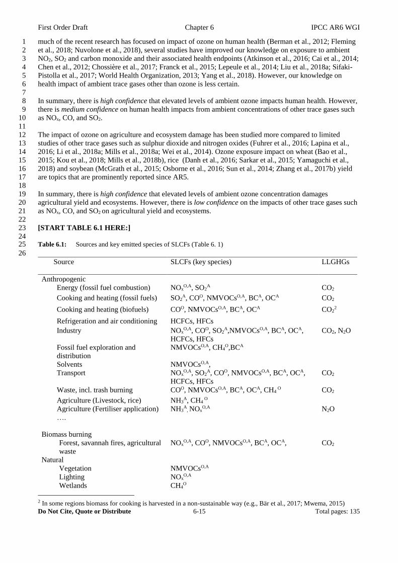
[START TABLE 6.1 HERE:] 23
24 Table 6.1: Sources and key emitted species of SLCFs (Table 6. 1) 25
26
Source SLCFs (key species)
LLGHGs
Anthropogenic
Energy (fossil fuel combustion) NOxO,A, SO2
A CO2
Cooking and heating (fossil fuels) SO2A, COO, NMVOCsO,A, BCA, OCA
CO2
Cooking and heating (biofuels) COO, NMVOCsO,A, BCA, OCA CO22
Refrigeration and air conditioning HCFCs, HFCs
Industry NOxO,A, COO, SO2
A,NMVOCsO,A, BCA, OCA,
HCFCs, HFCs
CO2, N2O
Fossil fuel exploration and
distribution
NMVOCsO,A, CH4O,BCA
Solvents NMVOCsO,A,
Transport NOxO,A, SO2
A, COO, NMVOCsO,A, BCA, OCA,
HCFCs, HFCs
CO2
Waste, incl. trash burning COO, NMVOCsO,A, BCA, OCA, CH4 O CO2
Agriculture (Livestock, rice) NH3A, CH4
O
Agriculture (Fertiliser application) NH3A
, NOxO,A N2O
….
Biomass burning
Forest, savannah fires, agricultural
waste
NOxO,A, COO, NMVOCsO,A, BCA, OCA, CO2
Natural
Vegetation NMVOCsO,A
Lighting NOxO,A
Wetlands CH4O
2 In some regions biomass for cooking is harvested in a non-sustainable way (e.g., Bär et al., 2017; Mwema, 2015)
First Order Draft Chapter 6 IPCC AR6 WGI
Do Not Cite, Quote or Distribute 6-16 Total pages: 135
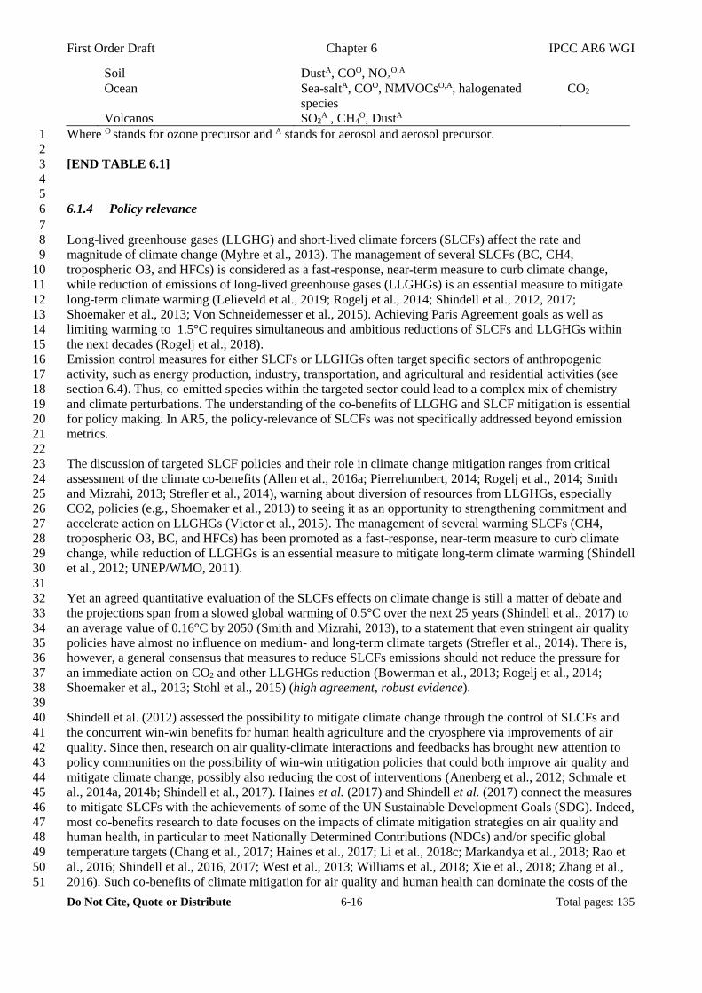
Soil DustA, COO, NOxO,A
Ocean Sea-saltA, COO, NMVOCsO,A, halogenated
species
CO2
Volcanos SO2A , CH4
O, DustA
Where O stands for ozone precursor and A stands for aerosol and aerosol precursor. 1
2
[END TABLE 6.1] 3
4
5
6.1.4 Policy relevance 6
7
Long-lived greenhouse gases (LLGHG) and short-lived climate forcers (SLCFs) affect the rate and 8
magnitude of climate change (Myhre et al., 2013). The management of several SLCFs (BC, CH4, 9
tropospheric O3, and HFCs) is considered as a fast-response, near-term measure to curb climate change, 10
while reduction of emissions of long-lived greenhouse gases (LLGHGs) is an essential measure to mitigate 11
long-term climate warming (Lelieveld et al., 2019; Rogelj et al., 2014; Shindell et al., 2012, 2017; 12
Shoemaker et al., 2013; Von Schneidemesser et al., 2015). Achieving Paris Agreement goals as well as 13
limiting warming to 1.5°C requires simultaneous and ambitious reductions of SLCFs and LLGHGs within 14
the next decades (Rogelj et al., 2018). 15
Emission control measures for either SLCFs or LLGHGs often target specific sectors of anthropogenic 16
activity, such as energy production, industry, transportation, and agricultural and residential activities (see 17
section 6.4). Thus, co-emitted species within the targeted sector could lead to a complex mix of chemistry 18
and climate perturbations. The understanding of the co-benefits of LLGHG and SLCF mitigation is essential 19
for policy making. In AR5, the policy-relevance of SLCFs was not specifically addressed beyond emission 20
metrics. 21
22
The discussion of targeted SLCF policies and their role in climate change mitigation ranges from critical 23
assessment of the climate co-benefits (Allen et al., 2016a; Pierrehumbert, 2014; Rogelj et al., 2014; Smith 24
and Mizrahi, 2013; Strefler et al., 2014), warning about diversion of resources from LLGHGs, especially 25
CO2, policies (e.g., Shoemaker et al., 2013) to seeing it as an opportunity to strengthening commitment and 26
accelerate action on LLGHGs (Victor et al., 2015). The management of several warming SLCFs (CH4, 27
tropospheric O3, BC, and HFCs) has been promoted as a fast-response, near-term measure to curb climate 28
change, while reduction of LLGHGs is an essential measure to mitigate long-term climate warming (Shindell 29
et al., 2012; UNEP/WMO, 2011). 30
31
Yet an agreed quantitative evaluation of the SLCFs effects on climate change is still a matter of debate and 32
the projections span from a slowed global warming of 0.5°C over the next 25 years (Shindell et al., 2017) to 33
an average value of 0.16°C by 2050 (Smith and Mizrahi, 2013), to a statement that even stringent air quality 34
policies have almost no influence on medium- and long-term climate targets (Strefler et al., 2014). There is, 35
however, a general consensus that measures to reduce SLCFs emissions should not reduce the pressure for 36
an immediate action on CO2 and other LLGHGs reduction (Bowerman et al., 2013; Rogelj et al., 2014; 37
Shoemaker et al., 2013; Stohl et al., 2015) (high agreement, robust evidence). 38
39
Shindell et al. (2012) assessed the possibility to mitigate climate change through the control of SLCFs and 40
the concurrent win-win benefits for human health agriculture and the cryosphere via improvements of air 41
quality. Since then, research on air quality-climate interactions and feedbacks has brought new attention to 42
policy communities on the possibility of win-win mitigation policies that could both improve air quality and 43
mitigate climate change, possibly also reducing the cost of interventions (Anenberg et al., 2012; Schmale et 44
al., 2014a, 2014b; Shindell et al., 2017). Haines et al. (2017) and Shindell et al. (2017) connect the measures 45
to mitigate SLCFs with the achievements of some of the UN Sustainable Development Goals (SDG). Indeed, 46
most co-benefits research to date focuses on the impacts of climate mitigation strategies on air quality and 47
human health, in particular to meet Nationally Determined Contributions (NDCs) and/or specific global 48
temperature targets (Chang et al., 2017; Haines et al., 2017; Li et al., 2018c; Markandya et al., 2018; Rao et 49
al., 2016; Shindell et al., 2016, 2017; West et al., 2013; Williams et al., 2018; Xie et al., 2018; Zhang et al., 50
2016). Such co-benefits of climate mitigation for air quality and human health can dominate the costs of the 51
First Order Draft Chapter 6 IPCC AR6 WGI
Do Not Cite, Quote or Distribute 6-17 Total pages: 135
climate measures (Li et al., 2018c; Saari et al., 2015) (high agreement, medium evidence). A growing 1
number of studies analyses the co-benefits of current and planned air quality policies on LLGHGs and global 2
and regional climate change impacts (Akimoto et al., 2015; Lee et al., 2016; Lund et al., 2014; Maione et al., 3
2016; Peng et al., 2017). 4
5
It must be recognized that neither ambitious climate change policy nor air quality abatement policy will 6
automatically yield co-benefits without integrated policies aimed at co-beneficial solutions (Melamed et al., 7
2016; Schmale et al., 2014b; Zusman et al., 2013), especially in the energy generation and transport sectors 8
(Rao et al., 2013; Thompson et al., 2016). 9
10
[START BOX 6.1 HERE] 11
12
BOX 6.1: Chain connecting emission to concentration to impact 13
14
Short-lived climate forcers include methane, ozone and aerosols, and their precursors, as well as some 15
halogenated species. They stem from multiple emission processes either natural or anthropogenic (Hoesly et 16
al., 2018). They interact with other species in the atmosphere which may lead to chemical and physical 17
changes. Eventually, over a time span that ranges from a few hours to a few years depending on their 18
characteristics, they are either chemically (e.g., reaction with oxidizing agents, such as hydroxyl radical 19
(OH), nitrate radical, ozone, reactive halogens) or physically (e.g., dry or wet deposition) removed from the 20
atmosphere. In addition to absorb/reflect radiation and interacting with clouds, thereby affecting climate 21
(Boucher et al., 2013), some of these compounds also have detrimental effects on human health, ecosystems 22
and weather (Landrigan et al., 2017; Li et al., 2016a; Rogelj et al., 2014; Sarangi et al., 2018; Stohl et al., 23
2015; Undorf et al., 2018; Von Schneidemesser et al., 2015). They can also be deposited on ecosystems and 24
the cryosphere affecting vegetation and agriculture (Shindell, 2016; Tai et al., 2014), or accelerating the 25
melting of snow and ice (Qian et al., 2015). 26
27
28
[START BOX 6.1, FIGURE 1 HERE] 29
30
Box 6.1, Figure 1: Schematic of the sources and processes leading to tropospheric SLCF impacts 31
32
[END BOX 6.1, Figure 1 HERE] 33
34
35
[END BOX 6.1 HERE] 36
37
38
6.2 SLCF emissions and atmospheric abundance 39
40
There are significant differences in emission structure across global regions. Until 1950, majority of SLCF 41
emissions associated with fossil fuel use (SO2, NOx, NMVOCs, CO) and about half of BC and OC originated 42
from North America and Europe (Hoesly et al., 2018; Lamarque et al., 2010). The last two decades brought a 43
dramatic change with strong economic growth in Asia and declining emissions in North America and Europe 44
due to air quality legislation and declining capacity of energy intensive industry, resulting in more than 50% 45
of anthropogenic emissions of all species (including NH3) originating from Asia (Amann et al., 2013; Bond 46
et al., 2013; Crippa et al., 2016, 2018; Fiore et al., 2015; Hoesly et al., 2018; Klimont et al., 2017a; 47
Lamarque et al., 2010) (high confidence). Growing remote sensing capacity has been providing independent 48
evaluation of estimated pollution trends in the last decade (Duncan et al., 2013; Fioletov et al., 2016; Geddes 49
et al., 2016; Irie et al., 2016; Krotkov et al., 2016; Lamsal et al., 2015; Luo et al., 2015; Richter et al., 2005; 50
Wen et al., 2018). 51
52
53
6.2.1 Global and regional temporal evolution of SLCF emissions 54
55
First Order Draft Chapter 6 IPCC AR6 WGI
Do Not Cite, Quote or Distribute 6-18 Total pages: 135
Recent work has led to revised global estimates of anthropogenic SLCF emissions (Crippa et al., 2016; 1
Klimont et al., 2017a; Montzka et al., 2015; Prinn et al., 2018; Sharma et al., 2015; Turnock et al., 2016; 2
Wang et al., 2014b, 2014c; Zheng et al., 2018b) and to the re-estimation of historical emissions of SLCFs 3
(Lamarque et al., 2010) that were used to develop the Representative Concentration Pathways. The historical 4
anthropogenic emissions for use in the CMIP6 are discussed in Hoesly et al. (2018) and for several species 5
the revised estimates show for all species, except SO2 and CO, a different trend than CMIP5, i.e., continued 6
strong growth of emissions driven primarily by developments in Asia (see 6.2.1.2). Additionally, Hoesly et 7
al. (2018) have extended estimates of anthropogenic emissions back to 1750 and developed an updated and 8
new set of spatial proxies allowing for more differentiated (source sector-wise) gridding of emissions (Feng 9
et al., 2019). Emissions from open biomass burning have been reviewed and updated for CMIP6 (van Marle 10
et al., 2017) and at the global level show fairly constant emissions until about 1980, followed by a significant 11
increase until about 2000. The CMIP5, based on GFED2, GICC, and RETRO (Lamarque et al., 2010), 12
estimated gradual decline of emission from 1920 to about 1950 and then steady, and stronger than CMIP6, 13
increase towards 2000. The differences in estimates of emissions vary across species due to the updated 14
emission factors and contribution of forest versus savannah fires with globally higher NOx and lower OC in 15
CMIP6. There are more substantial differences at the regional level, especially for the United States, South 16
America (south of Amazonas), and southern hemisphere Africa (for details see van Marle et al. (2017)). 17
18
19
6.2.1.1 Anthropogenic sources 20
21
For most of the SLCF species, the global and regional anthropogenic emission trends developed for CMIP6 22
for the period 1850 to 2000 are not dramatically different from those used in CMIP5. However, there are 23
some differences in magnitudes of emissions, i.e., the revised estimates are lower, than previously assumed, 24
in the period 1850-1950 (NOx, BC, OC, and CH4) and higher in the last few decades for NOx, BC, OC, and 25
NH3. At the global level, the differences between CMIP5 and CMIP6 historical estimates are typically below 26
10% for the pre-2000 period, except for CH4 and CO where for pre-1950 period CMIP6 shows 10-50% 27
higher values for CO and 10-50% lower for CH4 (Hoesly et al., 2018). For the last decades, CMIP6 dataset 28
shows for all species, except SO2, a different trend than CMIP5, i.e., continued strong growth of emissions 29
driven primarily by developments in Asia (see more detailed discussion in sections 6.2.2 and 6.2.1.2). 30
31
The RCP projections were harmonised for the year 2000 (van Vuuren et al., 2011), shortly before rapid 32
economic development of large Asian countries (China and India) started. The CMIP6 projections are 33
harmonised to 2015 and while this is only 15 years’ difference, the world, and especially Asia, lived through 34
very significant changes of LLGHGs and SLCF emissions. The unprecedented growth of East and South 35
Asian emissions since 2000 led to devastating air pollution episodes across the region and changed the global 36
landscape of emissions making Asia the dominant SLCF source region. In spite of the success of 37
environmental legislation introduced in several countries affecting the trends in specific regions: North 38
America and Europe (Amann et al., 2013; Crippa et al., 2016; Holland et al., 2012; Jiang et al., 2018; 39
Turnock et al., 2016), and recently in parts of Asia, especially China (Zhang et al., 2012; Zheng et al., 2018b, 40
2018a), emissions of most of the species show no signs of stabilisation or decline, except decline of SO2 and 41
CO (high confidence), and since 2011 stabilization of NOx (Hoesly et al., 2018) and Erreur ! Source du 42
renvoi introuvable. (medium confidence). This contrasts with assumptions in RCP projections for the last 43
decade, especially for NOx, NMVOCs, CH4, BC and OC (Figure 2 in Hoesly et al. (2018), Erreur ! Source 44
du renvoi introuvable., Erreur ! Source du renvoi introuvable.). 45
46
For SO2, the strong growth of Asian emissions have been offset by reduction in North America and Europe 47
and since about 2006 also Chinese emissions appear to decline strongly (Zheng et al., 2018b) (Erreur ! 48
Source du renvoi introuvable.) (high confidence). The estimated reduction in China counteracts continuing 49
strong growth of SO2 emissions in South Asia. 50
51
Global Emissions of NOx have been growing very fast in spite of the successful reduction of emissions in 52
North America, Europe, OECD Asia (Crippa et al., 2016; Jiang et al., 2018; Turnock et al., 2016) (Erreur ! 53
Source du renvoi introuvable.) and continuous efforts to strengthen the emission standards for road 54
vehicles in most countries. In many regions, vehicle increase and growing demand for energy, and 55
First Order Draft Chapter 6 IPCC AR6 WGI
Do Not Cite, Quote or Distribute 6-19 Total pages: 135
consequently large number of new fossil fuel power plants, have been more than offsetting these reductions. 1
Since about 2011, the global emissions appear to decline (medium confidence) and the rate of that decline 2
might be underestimated in CMIP6 data since one of the major drivers of change are reduction in China 3
which are rather small in CMIP6 (Erreur ! Source du renvoi introuvable. and (Hoesly et al., 2018)). 4
Recent bottom up emission estimates (Zheng et al., 2018b) largely confirm what has been shown in satellite 5
data; a strong decline of NO2 column over Eastern China (see section 6.2.2) although bottom up estimates 6
indicate slower decline than remote sensing. 7
8
Discovery of oil and a car marks the beginning of steep growth of NMVOC emissions; oil production-9
distribution and vehicles have dominated NMVOC emissions for most of the last century (Hoesly et al., 10
2018). Efforts to control transport emissions were largely offset by fast growth of emissions from chemical 11
industries and solvent use as well as emissions from fossil fuel production and distribution. At a global 12
level, anthropogenic emissions of NMVOC continue to grow (Erreur ! Source du renvoi introuvable.) 13
14
Emissions of carbonaceous aerosols (BC, OC) have been steadily increasing and since 1950 about doubled 15
(Hoesly et al., 2018) (medium confidence). Before 1950, North America and Europe contributed about half 16
of the global total but successful introduction of diesel particulate filters on road vehicles (Fiebig et al., 2014; 17
Klimont et al., 2017a; Robinson et al., 2015) and declining reliance on solid fuels for heating brought in 18
large reductions (Erreur ! Source du renvoi introuvable.) (high confidence). Currently, these emissions 19
originate primarily from Asia and Africa (Bond et al., 2004, 2007, 2013) . The recent estimates of BC and 20
OC highlighted some ‘new’ sources, e.g., kerosene lamps and gas flaring, revised estimates for open burning 21
of waste, regional coal consumption (e.g., China), and estimates for Russia (Conrad and Johnson, 2017; 22
Evans et al., 2017; Huang et al., 2015; Huang and Fu, 2016; Kholod et al., 2016; Klimont et al., 2017a; Stohl 23
et al., 2013). Consideration of these new and revised sources in emission levels led to increase of the global 24
anthropogenic BC estimate for 2010 by over a million tons; over 15 percent higher than in the CMIP5 25
estimates for the first decade of 21st century. (Erreur ! Source du renvoi introuvable.). The estimates of 26
emissions of carbonaceous aerosols remains, however, very uncertain. 27
28
Bottom up global emission estimates of CH4 (Hoesly et al., 2018; Höglund-Isaksson, 2012; Janssens-29
Maenhout et al., 2019; Lamarque et al., 2010) for the last two decades are higher than top down assessments 30
(Saunois et al., 2016), primarily due to larger estimates for natural sources, but the overall trends are similar 31
– steady growth (high confidence). Larger discrepancies exist at the sectoral and regional level, for example 32
for coal mining (Miller et al., 2019; Peng et al., 2016b) or oil and gas sector where higher losses were 33
estimated (Dalsøren et al., 2018; Höglund-Isaksson et al., 2017), especially from unconventional production 34
(Alvarez et al., 2018), i.e., up to 60% higher than previous US EPA estimates. Detailed discussion of 35
methane sources, sinks, trends, and their evaluation is provided in Chapter 5; section 5.2.3). 36
37
Invention of Haber-Bosch process over hundred years ago coincides with a strong increase in NH3 emissions 38
(Erisman et al., 2008), which has been further accelerated with increasing livestock production. NH3 39
emissions continue growing (high confidence) and the trends estimated in CMIP5 and CMIP6 are the same, 40
while in absolute terms CMIP6 has somewhat higher emissions as it includes emissions from wastewater and 41
human waste that were largely missing in CMIP5 (Hoesly et al., 2018). The continuing increase in NH3 42
emissions in the US and Europe has not been confirmed by recently available satellite retrievals of NH3 43
concentrations, however, this has been attributed to simultaneous decline in emissions of SO2 and NOx; see 44
section 6.2.2.7. 45
46
47
[START FIGURE 6.3 HERE] 48
49 Figure 6.3: Global evolution of anthropogenic and biomass burning SLCF emissions. Past emissions based on 50
(Hoesly et al., 2018; van Marle et al., 2017) for CMIP6 and (Lamarque et al., 2010) for CMIP5. 51 Projections originate from the SSP database [https://tntcat.iiasa.ac.at/SspDb/dsd] (Gidden et al., 2018; 52 Riahi et al., 2017; Rogelj et al., 2018) and RCP database [https://tntcat.iiasa.ac.at/RcpDb/dsd] (van 53 Vuuren et al., 2011). [further discussion needed if we add few points from other studies for the future 54 paths]. 55
56
First Order Draft Chapter 6 IPCC AR6 WGI
Do Not Cite, Quote or Distribute 6-20 Total pages: 135
[END FIGURE 6.3 HERE] 1
2
3
[START FIGURE 6.4 HERE] 4
5 Figure 6.4: Regional evolution of anthropogenic and biomass burning SLCF emissions. Past emissions based on 6
(Hoesly et al., 2018; van Marle et al., 2017) for CMIP6 and (Lamarque et al., 2010) for CMIP5 [not 7 included yet; also CH4 and NMVOC missing]. Projections originate from the SSP database 8 [https://tntcat.iiasa.ac.at/SspDb/dsd] (Gidden et al., 2018; Riahi et al., 2017; Rogelj et al., 2018). [RCP 9 ranges might be added later and we need to revisit the issue of showing here potentially only 10 anthropogenic emissions, i.e., no BB] 11
12
[END FIGURE 6.4 HERE] 13
14
15
6.2.1.2 Natural sources 16
17
Over the last decades, satellite-borne and ground sensors have improved the characterisation of the global 18
spatial and temporal distribution of lightning flashes (Cecil et al., 2014; Virts et al., 2011). Constraining the 19
amount of NOx produced per flash, and its vertical allocation has been more elusive (Medici et al., 2017; 20
Miyazaki et al., 2014; Nault et al., 2017). Atmospheric Chemistry and Climate Model Intercomparison 21
Project (ACCMIP) models in AR5 used a range of lightning NOx (LNOx) between 1.2 to 9.7 TgN yr-1 22
(Lamarque et al., 2013). Most of these models apply a parameterisation that relates cloud-top-height to 23
lightning intensity (Price and Rind, 1992). These models project an increase in lightning in a warmer world 24
(+0.44 ± 0.05 TgN per C) (Finney et al., 2016b); whereas models using parameterisations based on 25
convection (Grewe et al., 2001), updraft mass flux (Allen and Pickering, 2002), or ice flux (Finney et al., 26
2016a) show either much less sensitivity or a negative response (Finney et al., 2016b, 2018). In sum, changes 27
in LNOx with climate, and its impacts on ozone and methane remain highly uncertain. 28
29
[Place holder for analyses of LNOx under CMIP/AerChemMIP] 30
31
A wide range of organic compounds are emitted including isoprene, monoterpenes, sesquiterpenes, alkenes, 32
alcohols, aldehdyes, and ketones (Guenther et al., 2012). The ecological and physiological roles of BVOCs 33
are broad and range from abiotic and biotic stress functions to integrated components of carbon metabolism 34
(Loreto et al., 2014). The photo-oxidation of BVOC emissions plays a fundamental role in atmospheric 35
composition by controlling the regional and global budgets of ozone and organic aerosol and the lifetime of 36
methane (Arneth et al., 2010; Heald and Spracklen, 2015). Isoprene is the most abundant BVOC emission 37
and has an estimated annual source rate of 300–700 TgC yr-1 (Guenther et al., 2012). Isoprene is emitted 38
from terrestrial vegetation, primarily from woody plants, and its production is biochemically linked to 39
photosynthetic carbon assimilation in plant chloroplasts (Kesselmeier and Staudt, 1999; Loreto et al., 2014). 40
The biological function of isoprene production is not fully understood, but may be related to protection of the 41
plant against environmental stresses, such as heat or oxidative stresses (Sharkey and Monson, 2017). 42
Different species of vegetation exhibit different capacities to emit isoprene under standard light and 43
temperature conditions (Guenther et al., 2006). Among all biomes, broadleaf tropical forests are the world’s 44
largest emitters of isoprene; grassland and crops are either low or non-emitting for isoprene (Guenther et al., 45
2006). 46
47
The isoprene and monoterpene emission rates respond to a number of environmental factors, including light, 48
temperature, and ambient CO2 levels, and are therefore highly sensitive to global change (Guenther et al., 49
2012; Loreto et al., 2014). Since AR5, there is medium evidence and high agreement based on global 50
modelling studies that anthropogenic LULCC, and the historical cropland expansion in particular, are the 51
dominant drivers of isoprene emission change since the preindustrial with results converging on a 10-25% 52
loss of isoprene emission globally due to the historical cropland expansion between 1850 and present day 53
(Heald and Geddes, 2016; Lathière et al., 2010; Scott et al., 2017; Unger, 2013, 2014) (high confidence). 54
There are 2 implications of this new finding since AR5. Firstly, isoprene emission was higher in the 55
preindustrial than present day(Heald and Geddes, 2016; Lathière et al., 2010; Scott et al., 2017; Unger, 2013, 56
First Order Draft Chapter 6 IPCC AR6 WGI
Do Not Cite, Quote or Distribute 6-21 Total pages: 135
2014). Secondly, isoprene emission change over the past century was driven by human LULCC and is 1
therefore a human-induced climate forcing mechanism in addition to a climate feedback mechanism (Unger, 2
2013) (high confidence). The impacts of human land-use driven changes in BVOC emissions on the SLCFs 3
is discussed in Section 6.4.2. The historical evolution of monoterpene and sesquiterpene emissions is less 4
well studied and there is no robust consensus on even the sign of the change. A study in the Amazon found 5
that the chemical composition of monoterpene emissions changes under elevated temperature conditions 6
(Jardine et al., 2016). 7
8
Global fires burn 475 ± 44 M ha yr-1 during 1997-2016 (Giglio et al., 2013), contributing to an annual carbon 9
emission of 2.2 ± 0.3 PgC and the associated air pollutants such as organic carbon (16.4 ± 3.2 Tg yr-1), black 10
carbon (1.9 ± 0.3 Tg yr-1), nitrogen oxides (14.6 ± 1.8 Tg yr-1), non-methane hydrocarbon (17.8 ± 2.4 Tg yr-11 1), and PM2.5 (36.4 ± 6.0 Tg yr-1) (van der Werf et al., 2017). Regionally, fire emissions worsen air quality 12
over U.S., China, and Europe (Cheng et al., 2014; Yue et al., 2013), causing threats to the public health(Liu 13
et al., 2017a)and ecosystem productivity (Yue and Unger, 2018). Analyses based on historical charcoal data 14
(Harrison et al., 2018) or present-day fire frequency(Westerling, 2006) reveal high correlations between fire 15
activity and global average temperature, suggesting a likely enhancement of area burned and the consequent 16
fire pollution in a warming future. 17
18
[PLACEHOLDER: Add discussion of natural dust and sea salt] 19
20
[START BOX 6.2 HERE] 21
22
BOX 6.2: The three pillars to improve the SLCF understanding: Laboratory/Theoretical studies, 23
Observations, Atmospheric chemistry models 24
25
Together, laboratory studies, field observations, and modelling studies form the three pillars of atmospheric 26
chemistry that inform our understanding of the processes that influence atmospheric chemical composition, 27
including SLCFs (Abbatt et al., 2014). Laboratory studies provide detailed chemical reactions species go 28
through, which can then be used to develop simplified chemical mechanisms. These chemical mechanisms 29
are implemented in computer models along with numerical representations of emissions, deposition and 30
transport processes to predict atmospheric composition across a range of temporal and spatial scales. 31
Comparisons with field observations are used to build confidence in model predictions or to identify 32
shortcomings in chemical mechanisms. This box provides an overview of the development of chemical 33
mechanisms from laboratory/theoretical studies, types of observations available for evaluation, and models 34
applied for assessing SLCF distribution and evolution. 35
36
Process-level understanding of tropospheric chemistry developed through laboratory and simulation chamber 37
experiments as well as quantum chemical theory is used to generate chemical mechanisms. Atmospheric 38
simulation chambers are designed to identify the chemical pathways and quantify reaction kinetics. In such 39
system, atmospheric chemistry is isolated from atmospheric transport, deposition and emission processes. 40
Ideally the chemical regimes studied, simulate atmospheric complexity and concentration. Atmospheric 41
simulation chambers facilitate studies of both gas- and aqueous-phase chemistry as well as determination of 42
aerosol optical properties. Many experiments in atmospheric simulation chambers focus e.g. on the oxidation 43
mechanism of a single VOC. Recently quantum chemical (QC) theory has advanced to a level that it can 44
provide kinetic and product information in a parameter range not accessible to experiments (Vereecken et 45
al., 2015). Iterative and interlinked use of simulation chamber and QC-theory has led to the advancement of 46
chemical mechanisms, such as the photochemistry of isoprene under low NOx conditions (Fuchs et al., 47
2013a; Nguyen et al., 2010; Peeters et al., 2009, 2014). The sheer multitude of different chemical compounds 48
present in the troposphere precludes the experimental and theoretical investigation of the entire tropospheric 49
trace substances. On the basis of the available experimental and/or theoretical data, however, it is possible to 50
extrapolate the reactivity of compounds in a given class of reactions, and summarize them as a 51
structure−activity relationship (SAR) (Vereecken et al., 2015, 2018). Using such SARs, extensive chemical 52
schemes have been developed which describe the chemistry of hundreds of thousands of species through 53
millions of reactions. For application in chemistry climate models (CCM), the chemical mechanisms need to 54
be computationally efficient, requiring simplifications. Such simplifications include reduced hydrocarbon 55
First Order Draft Chapter 6 IPCC AR6 WGI
Do Not Cite, Quote or Distribute 6-22 Total pages: 135
representations, the application of lumping techniques (one species representing a family of compounds) 1
and/or the implementation of artificial operators representing artificially key steps of the chemistry, for 2
example for the NOx conversion essential for the ozone production (Carter, 2010; Emmerson and Evans, 3
2009; Stockwell et al., 2012; Xia et al., 2009). 4
5
Observations of atmospheric concentrations and fluxes are used to evaluate atmospheric chemistry models 6
and test the knowledge acquired from controlled laboratory experiments. A wide range of in situ (instrument 7
near the subject of interest) and remotely sensed (instrument some distance away from the subject of interest) 8
measurements conducted from a variety of platforms (ground-based stations, balloons, ships, aircrafts and 9
satellites) are used to characterize atmospheric composition (Brasseur and Jacob, 2017). Several methods, 10
including spectroscopy, mass spectrometry, wet chemistry and filters, are used to measure concentrations. 11
Measurements made routinely as part of long-term monitoring programs involve surface networks (e.g., 12
NOAA Global Greenhouse Gas Reference Network- GGGRN), sondes (e.g., Southern Hemisphere 13
Additional Ozonesondes - SHADOZ), commercial aircraft (e.g., In-service Aircraft for a Global Observing 14
System- IAGOS) or satellites (e.g., MOPITT, SCIAMACHY). Long-term monitoring initially started for a 15
few species but has proceeded to include more species as instrumentation techniques have advanced. They 16
are particularly useful for assessing long-term trends and variability and spatial distributions (as in section 17
6.2.2). Retrieval of atmospheric concentrations from satellites, in particular, has been tremendously useful 18
for providing global continuous coverage, although the retrievals themselves depend on prior information of 19
atmospheric composition usually derived from models. Intense field campaigns typically provide a more 20
comprehensive view of atmospheric composition at a specific location of interest for a limited time period. 21
Field campaign measurements are generally geared towards gaining an improved understanding of specific 22
processes. Over the last decade or so, observations of atmospheric concentrations have been combined with 23
information from models to produce global assimilation and forecasting systems. These systems estimate 24
the state of the atmosphere and its chemical composition either for near real time forecasts such as the 25
CAMS (Copernicus Atmosphere Monitoring Service) near-real-time system (Akritidis et al., 2018; Inness et 26
al., 2015b) or reanalysis products such as MERRA (Modern-Era Retrospective analysis for Research and 27
Applications) and MERRA-2 (Gelaro et al., 2017; Molod et al., 2015), MACC (Monitoring Atmospheric 28
Composition and Climate) (Eskes et al., 2015; Gaudel et al., 2015; Katragkou et al., 2015) and CAMS 29
(Flemming et al., 2017; Inness et al., 2019). 30
31
An atmospheric chemistry model is a mathematical representation of the many complex physical and 32
chemical processes that determine the atmospheric composition as informed by process-based laboratory 33
studies (Brasseur and Jacob, 2017). These models are applied extensively to simulate the distribution and 34
evolution of chemical species on a variety of spatial and temporal scales to improve current knowledge, and 35
to make future projections for various scenarios. Models are also used to interpret variability in observations 36
to gain scientific understanding of the processes that drive observed variability. The wide range of 37
atmospheric chemistry applications dictates an equally diverse collection of model types depending upon 38
model domain and resolution, the level of details in chemical mechanisms, and representation of 39
meteorology (e.g., Young et al. 2018). For example, local scale box models, at one extreme, can be applied 40
to evaluate chemical mechanisms through an extremely detailed representation of gas-phase or 41
heterogeneous chemistry and no treatment of transport (e.g., MCM, ISORROPIA). At the other extreme, 42
global three-dimensional chemistry-climate models (CCMs) (Figure 1) with atmospheric chemistry 43
processes (in simple parameterized forms) embedded within a climate model representing the full coupling 44
of chemistry with meteorology (e.g., Morgenstern et al. 2017) can be applied to study global scale chemistry-45
climate interactions. Results from global chemistry-climate models are used in this chapter to assess how 46
SLCFs have evolved in the past and predict their future evolution. 47
48
Quantifying model errors is critical to evaluate the value of the model for the application of interest. The 49
skill of CCMs is typically demonstrated by their ability to reproduce observations relevant to the problem of 50
interest. However, uncertainty remains large not only because of errors and uncertainties in observations 51
(e.g., Tarasick et al., 2019; Gaudel et al. (2018) but also because of the representativeness of the available 52
measurements (e.g., Young et al. 2018). Issues related to representativeness include incomplete sampling of 53
sparse observations, mismatch between spatial and/or temporal scales of the measurements and those of the 54
model output, and inconsistency between observed meteorological variability and that generated by free-55
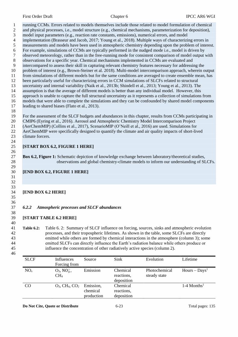
First Order Draft Chapter 6 IPCC AR6 WGI
Do Not Cite, Quote or Distribute 6-23 Total pages: 135
running CCMs. Errors related to models themselves include those related to model formulation of chemical 1
and physical processes, i.e., model structure (e.g., chemical mechanisms, parameterization for deposition), 2
model input parameters (e.g., reaction rate constants, emissions), numerical errors, and model 3
implementation (Brasseur and Jacob, 2017; Young et al., 2018). Multiple ways of characterizing errors in 4
measurements and models have been used in atmospheric chemistry depending upon the problem of interest. 5
For example, simulations of CCMs are typically performed in the nudged mode i.e., model is driven by 6
observed meteorology, rather than in the free-running mode for consistent comparison of model output with 7
observations for a specific year. Chemical mechanisms implemented in CCMs are evaluated and 8
intercompared to assess their skill in capturing relevant chemistry features necessary for addressing the 9
problem of interest (e.g., Brown-Steiner et al. 2018). Multi-model intercomparison approach, wherein output 10
from simulations of different models but for the same conditions are averaged to create ensemble mean, has 11
been particularly useful for characterizing errors in CCM simulations of SLCFs related to structural 12
uncertainty and internal variability (Naik et al., 2013b; Shindell et al., 2013; Young et al., 2013). The 13
assumption is that the average of different models is better than any individual model. However, this 14
approach is unable to capture the full structural uncertainty as it represents a collection of simulations from 15
models that were able to complete the simulations and they can be confounded by shared model components 16
leading to shared biases (Flato et al., 2013). 17
18
For the assessment of the SLCF budgets and abundances in this chapter, results from CCMs participating in 19
CMIP6 (Eyring et al., 2016). Aerosol and Atmospheric Chemistry Model Intercomparison Project 20
(AerChemMIP) (Collins et al., 2017), ScenarioMIP (O’Neill et al., 2016) are used. Simulations for 21
AerChemMIP were specifically designed to quantify the climate and air quality impacts of short-lived 22
climate forcers. 23
24
[START BOX 6.2, FIGURE 1 HERE] 25
26
Box 6.2, Figure 1: Schematic depiction of knowledge exchange between laboratory/theoretical studies, 27
observations and global chemistry-climate models to inform our understanding of SLCFs. 28
29
[END BOX 6.2, FIGURE 1 HERE] 30
31
32
33
[END BOX 6.2 HERE] 34
35
36
6.2.2 Atmospheric processes and SLCF abundances 37
38
[START TABLE 6.2 HERE] 39
40
Table 6.2: Table 6. 2: Summary of SLCF influence on forcing, sources, sinks and atmospheric evolution 41
processes, and their tropospheric lifetimes. As shown in the table, some SLCFs are directly 42
emitted while others are formed by chemical interactions in the atmosphere (column 3); some 43
emitted SLCFs can directly influence the Earth’s radiation balance while others produce or 44
influence the concentration of other radiatively active species (column 2). 45
46
SLCF Influences
Forcing from
Source Sink Evolution Lifetime
NOx O3, NO3−,
CH4
Emission Chemical
reactions,
deposition
Photochemical
steady state
Hours – Days1
CO O3, CH4, CO2 Emission,
chemical
production
Chemical
reactions,
deposition
1-4 Months1
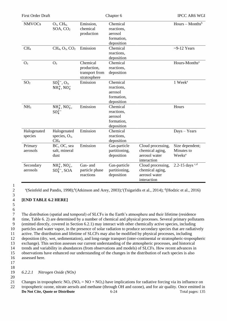
First Order Draft Chapter 6 IPCC AR6 WGI
Do Not Cite, Quote or Distribute 6-24 Total pages: 135
NMVOCs O3, CH4,
SOA, CO2
Emission,
chemical
production
Chemical
reactions,
aerosol
formation,
deposition
Hours – Monthsb
CH4 CH4, O3, CO2 Emission Chemical
reactions,
deposition
~9-12 Years
O3 O3 Chemical
production,
transport from
stratosphere
Chemical
reactions,
deposition
Hours-Monthsa
SO2 SO42−, O3,
NH4+, NO3
−
Emission Chemical
reactions,
aerosol
formation,
deposition
1 Weeka
NH3 NH4+, NO3
−,
SO42−
Emission Chemical
reactions,
aerosol
formation,
deposition
Hours
Halogenated
species
Halogenated
species, O3,
CH4
Emission Chemical
reactions,
deposition
Days – Years
Primary
aerosols
BC, OC, sea
salt, mineral
dust
Emission Gas-particle
partitioning,
deposition
Cloud processing,
chemical aging,
aerosol water
interaction
Size dependent;
Minutes to
Weeksa
Secondary
aerosols NH4
+, NO3−,
SO42−, SOA
Gas- and
particle phase
reactions
Gas-particle
partitioning,
deposition
Cloud processing,
chemical aging,
aerosol water
interaction
2.2-15 days c,d
1 a(Seinfeld and Pandis, 1998);b(Atkinson and Arey, 2003);c(Tsigaridis et al., 2014); d(Hodzic et al., 2016) 2
3
[END TABLE 6.2 HERE] 4
5
6
The distribution (spatial and temporal) of SLCFs in the Earth’s atmosphere and their lifetime (residence 7
time, Table 6. 2) are determined by a number of chemical and physical processes. Several primary pollutants 8
(emitted directly, covered in Section 6.2.1) may interact with other chemically active species, including 9
particles and water vapor, in the presence of solar radiation to produce secondary species that are radiatively 10
active. The distribution and lifetime of SLCFs may also be modified by physical processes, including 11
deposition (dry, wet, sedimentation), and long-range transport (inter-continental or stratospheric-tropospheric 12
exchange). This section assesses our current understanding of the atmospheric processes, and historical 13
trends and variability in abundances (from observations and models) of SLCFs. How recent advances in 14
observations have enhanced our understanding of the changes in the distribution of each species is also 15
assessed here. 16
17
18
6.2.2.1 Nitrogen Oxide (NOx) 19
20
Changes in tropospheric NOx (NOx = NO + NO2) have implications for radiative forcing via its influence on 21
tropospheric ozone, nitrate aersols and methane (through OH and ozone), and for air quality. Once emitted in 22
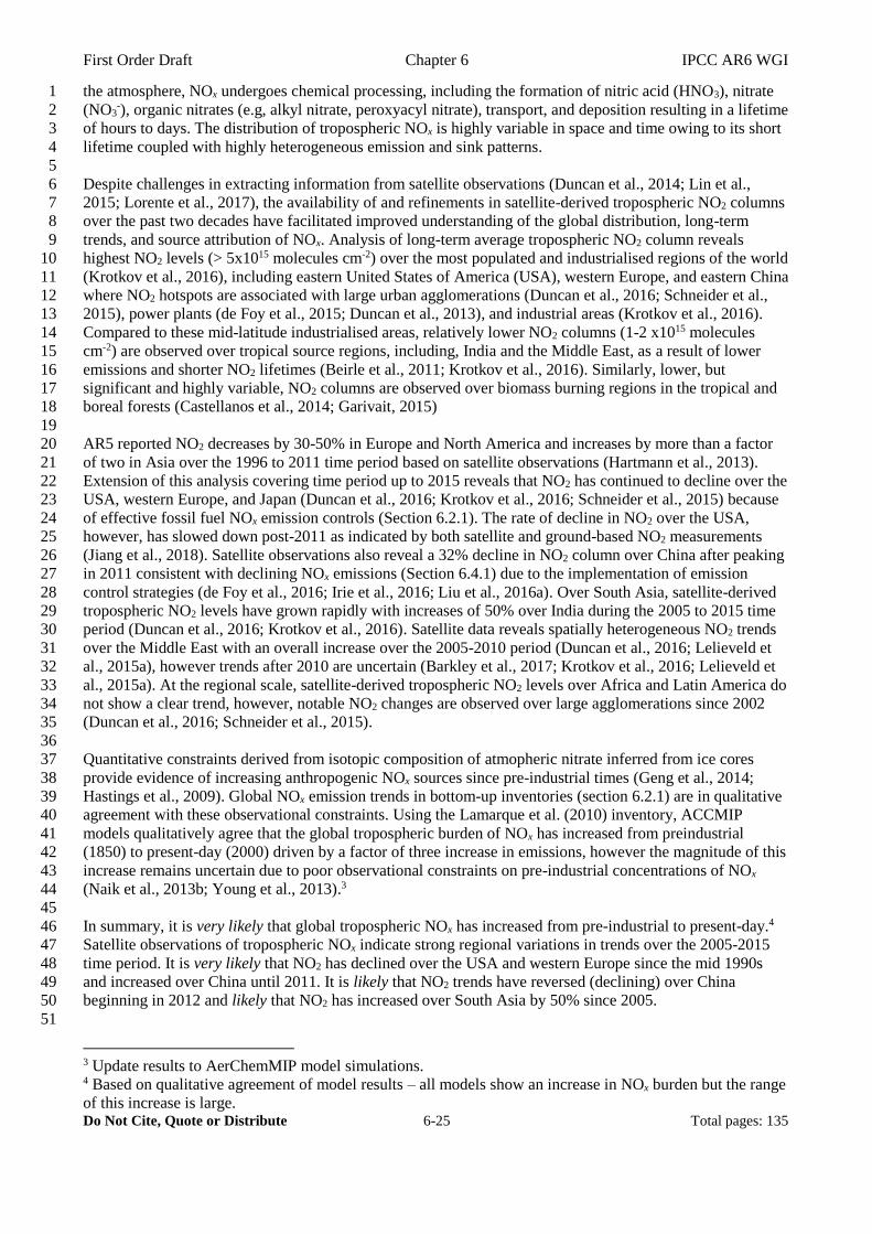
First Order Draft Chapter 6 IPCC AR6 WGI
Do Not Cite, Quote or Distribute 6-25 Total pages: 135
the atmosphere, NOx undergoes chemical processing, including the formation of nitric acid (HNO3), nitrate 1
(NO3-), organic nitrates (e.g, alkyl nitrate, peroxyacyl nitrate), transport, and deposition resulting in a lifetime 2
of hours to days. The distribution of tropospheric NOx is highly variable in space and time owing to its short 3
lifetime coupled with highly heterogeneous emission and sink patterns. 4
5
Despite challenges in extracting information from satellite observations (Duncan et al., 2014; Lin et al., 6
2015; Lorente et al., 2017), the availability of and refinements in satellite-derived tropospheric NO2 columns 7
over the past two decades have facilitated improved understanding of the global distribution, long-term 8
trends, and source attribution of NOx. Analysis of long-term average tropospheric NO2 column reveals 9
highest NO2 levels (> 5x10¹⁵ molecules cm-2) over the most populated and industrialised regions of the world 10
(Krotkov et al., 2016), including eastern United States of America (USA), western Europe, and eastern China 11
where NO2 hotspots are associated with large urban agglomerations (Duncan et al., 2016; Schneider et al., 12
2015), power plants (de Foy et al., 2015; Duncan et al., 2013), and industrial areas (Krotkov et al., 2016). 13
Compared to these mid-latitude industrialised areas, relatively lower NO2 columns (1-2 x10¹⁵ molecules 14
cm-2) are observed over tropical source regions, including, India and the Middle East, as a result of lower 15
emissions and shorter NO2 lifetimes (Beirle et al., 2011; Krotkov et al., 2016). Similarly, lower, but 16
significant and highly variable, NO2 columns are observed over biomass burning regions in the tropical and 17
boreal forests (Castellanos et al., 2014; Garivait, 2015) 18
19
AR5 reported NO2 decreases by 30-50% in Europe and North America and increases by more than a factor 20
of two in Asia over the 1996 to 2011 time period based on satellite observations (Hartmann et al., 2013). 21
Extension of this analysis covering time period up to 2015 reveals that NO2 has continued to decline over the 22
USA, western Europe, and Japan (Duncan et al., 2016; Krotkov et al., 2016; Schneider et al., 2015) because 23
of effective fossil fuel NOx emission controls (Section 6.2.1). The rate of decline in NO2 over the USA, 24
however, has slowed down post-2011 as indicated by both satellite and ground-based NO2 measurements 25
(Jiang et al., 2018). Satellite observations also reveal a 32% decline in NO2 column over China after peaking 26
in 2011 consistent with declining NOx emissions (Section 6.4.1) due to the implementation of emission 27
control strategies (de Foy et al., 2016; Irie et al., 2016; Liu et al., 2016a). Over South Asia, satellite-derived 28
tropospheric NO2 levels have grown rapidly with increases of 50% over India during the 2005 to 2015 time 29
period (Duncan et al., 2016; Krotkov et al., 2016). Satellite data reveals spatially heterogeneous NO2 trends 30
over the Middle East with an overall increase over the 2005-2010 period (Duncan et al., 2016; Lelieveld et 31
al., 2015a), however trends after 2010 are uncertain (Barkley et al., 2017; Krotkov et al., 2016; Lelieveld et 32
al., 2015a). At the regional scale, satellite-derived tropospheric NO2 levels over Africa and Latin America do 33
not show a clear trend, however, notable NO2 changes are observed over large agglomerations since 2002 34
(Duncan et al., 2016; Schneider et al., 2015). 35
36
Quantitative constraints derived from isotopic composition of atmopheric nitrate inferred from ice cores 37
provide evidence of increasing anthropogenic NOx sources since pre-industrial times (Geng et al., 2014; 38
Hastings et al., 2009). Global NOx emission trends in bottom-up inventories (section 6.2.1) are in qualitative 39
agreement with these observational constraints. Using the Lamarque et al. (2010) inventory, ACCMIP 40
models qualitatively agree that the global tropospheric burden of NOx has increased from preindustrial 41
(1850) to present-day (2000) driven by a factor of three increase in emissions, however the magnitude of this 42
increase remains uncertain due to poor observational constraints on pre-industrial concentrations of NOx 43
(Naik et al., 2013b; Young et al., 2013).3 44
45
In summary, it is very likely that global tropospheric NOx has increased from pre-industrial to present-day.4 46
Satellite observations of tropospheric NOx indicate strong regional variations in trends over the 2005-2015 47
time period. It is very likely that NO2 has declined over the USA and western Europe since the mid 1990s 48
and increased over China until 2011. It is likely that NO2 trends have reversed (declining) over China 49
beginning in 2012 and likely that NO2 has increased over South Asia by 50% since 2005. 50
51
3 Update results to AerChemMIP model simulations. 4 Based on qualitative agreement of model results – all models show an increase in NOx burden but the range
of this increase is large.
First Order Draft Chapter 6 IPCC AR6 WGI
Do Not Cite, Quote or Distribute 6-26 Total pages: 135
1
6.2.2.2 Carbon Monoxide (CO) 2
3
Changes in CO have implications for climate because of its influence on tropospheric ozone, methane (via 4
ozone and OH), and CO2. Carbon monoxide also plays an important role in air qaulity as a precursor to 5
ozone and by affecting the lifetime of a number of reduced chemical species via OH. Besides primary 6
emission sources, it is also produced by in situ oxidation of methane and NMVOCs. Reaction with OH is the 7
primary sink with smaller contributions from dry deposition. The atmospheric lifetime of CO ranges from 8
weeks to ~2 months that is long enough for it to be transported on intercontinental scales but short enough 9
for increases to be distinct from atmospheric background. 10
11
Present-day atmospheric CO distribution is well characterized using satellite based measurements (Warner et 12
al., 2013; Worden et al., 2013; Zhang, 2011) limited ground based columnar (Angelbratt et al., 2011; Té et 13
al., 2016; Zeng et al., 2012) airborne campaigns (Petetin et al., 2018) and surface measurement networks 14
(Andrews et al., 2014; Prinn et al., 2018; Schultz et al., 2015). Limited isotopic analysis of CO have been 15
carried out to re-construct CO concentration using ice-core samples to gain insight into recent past, pre-16
dating the modern satellite era (Petrenko et al., 2013; Wang et al., 2012b). The results from the ice-core 17
dataset show that CO mole fractions in the 1950s were higher than present day levels with concentration of 18
around 140–150 nmol/mol. The concentration rose by 10-15 nmol/mol in the 1970s-early to 1980s and then 19
declined by approximately 30 nmol/mol to today’s levels (Petrenko et al., 2013). 20
21
Modern period estimates of global CO burden ranges from approximately 246 to 475 Tg(CO) based on 22
different model analysis indicating the range of uncertainty (Duncan et al., 2007; Flemming et al., 2017; Fry 23
et al., 2013; Gaubert et al., 2017; Myriokefalitakis et al., 2016; Naik et al., 2013a; Stein et al., 2014; Zeng et 24
al., 2015). Multi-model estimates of modern period global CO burden increase by 89% relative to pre-25
industrial times (Naik et al., 2013b) consistent with available emissions estimate (Hoesly et al., 2018). 26
Currently, models underestimate observed CO concentration globally (Luo et al., 2015; Monks et al., 2015b; 27
Shindell et al., 2006) and regionally: North America and Arctic (Monks et al., 2015b), Europe- (Kumar et al., 28
2013a; Myriokefalitakis et al., 2016; Té et al., 2016), Australia- southern hemisphere (Fisher et al., 2017; 29
Zeng et al., 2015) except in certain regions like India and Eastern Asia (Kumar et al., 2013b; Strode et al., 30
2015a; Yarragunta et al., 2017) where models overestimate. Quantitatively, models underestimate surface 31
CO concentration by around 60 ppbv at different parts of the globe with biases reduced in the southern 32
hemisphere and the tropics (Naik et al., 2013b; Shindell et al., 2006). Consistent with surface observation, 33
the model underestimation persists throughout the troposphere with biases greater than 60 ppbv even up to 34
500 hPa level. 35
36
However, within the modern period estimates, global modelling (Flemming et al., 2017), ground based 37
observations (Angelbratt et al., 2011; Gratz et al., 2015; Khan et al., 2017; Kumar et al., 2013a; Zhou et al., 38
2017) and satellite based (Gaubert et al., 2017; Worden et al., 2013; Zheng et al., 2018a) studies have 39
reported declining CO trends and attribute the reduction to better emission controls. Model simulation 40
reported a decrease in global CO burden of 0.86% yr-1 over the years of 2003-2015 (Flemming et al., 2017). 41
Regionally, satellite observation of CO column burden showed trends of −0.92 and −0.74%yr−1 in the 42
Northern Hemisphere, −0.88 and −0.54%yr−1 in the Southern Hemisphere, −0.88 and −1.0% yr−1 in Eastern 43
China, −1.4 and −1.0%yr−1 in the eastern United States, and −1.4 and −1.0%yr−1 in Europe for the 44
MOPITT 11-yr (2000-2011) and AIRS 8-yr (2003-2011) records, respectively (Worden et al., 2013). 45
However, the reduction is not so clearly evident from recently available emissions inventory which shows 46
emissions as leveling off not necessarily declining in the modern period (Hoesly et al., 2018). 47
48
Models provide a link between emissions to concentrations despite their limitations to reproduce 49
observations. Multimodel mean chemical production of CO is in the range of 1210-1900 Tg(CO) yr-1 with 50
578-1086 Tg(CO) yr-1 from methane oxidation and 320-1198 Tg(CO) yr-1 from oxidation of NMVOC 51
indicating the current uncertainty range (Shindell et al., 2006; Zeng et al., 2015). Model studies estimate that 52
about 40% hydroxyl radical loss is via reactions with CO throughout the troposphere with 10% in the 53
boundary layer and rest in the free troposphere (Lelieveld et al., 2016). Dry deposition, although a minor 54
sink for CO, is another area of uncertainty with models reporting strength of 98-188 Tg(CO) yr-1 globally in 55
First Order Draft Chapter 6 IPCC AR6 WGI
Do Not Cite, Quote or Distribute 6-27 Total pages: 135
recent literature (Fisher et al., 2015; Myriokefalitakis et al., 2016; Stein et al., 2014; Zeng et al., 2015). 1
2
[CMIP 6 models burden range not yet reported in published literature for future burden and trends] 3
4
Understanding of global CO distribution has improved since AR5 with improvements in retrieval algorithm 5
and assimilated model products (Deeter et al., 2017; Flemming et al., 2017; Warner et al., 2014). It is now 6
possible to monitor CO from geo-stationary satellites which provides higher vertical resolution and accuracy 7
(Barré et al., 2015; Fu et al., 2016; Landgraf et al., 2016). However, information on total columnar CO 8
burden from these geostationary satelite based measurements are not yet readily available. 9
10
In summary, there is high confidence in our estimates of modern period global total CO distribution since 11
AR5. There is medium confidence that in the modern period, global CO burden is declining. 12
13
14
6.2.2.3 Volatile Organic Compounds (VOCs) 15
16
Atmospheric non-methane volatile organic compounds (NMVOCs) have both anthropogenic and biogenic 17
emission sources. NMVOCs are short-lived and highly variable with respect to space, time and chemical 18
composition. Thousands of different compounds with varying lifetimes and chemical behaviour have been 19
observed in the atmosphere, so most models of tropospheric chemistry include some chemical speciation of 20
the NMVOC. NMVOCs do not have direct impacts on climate, but the photo-oxidation of NMVOCs in the 21
atmosphere affects OH, ozone, and secondary organic aerosol. . The most abundant NMVOC, isoprene 22
(C5H8), has an estimated annual emission rate of 300-700 TgC yr-1 from vegetation that is around half of the 23
total BVOC global source from vegetation estimated at around 1 PgC yr-1 (Guenther et al., 2012) (see section 24
6.2.1.2). In comparison, recent estimates of contemporary global and annual anthropogenic NMVOC 25
emissions are about 150-160 Tg(NMVOC) yr-1 in the period 1990 to 2010 (Hoesly et al., 2018). 26
27
Since AR5, there has been some progress in the derivation of historical trends from ground-based networks 28
and satellites for some species (Helmig et al., 2014, 2016; Rossabi and Helmig, 2018; Zhu et al., 2017c). 29
Information on the historical evolution of some species is available in ice core proxies (Newland et al., 2017; 30
Nicewonger et al., 2016). Light alkane (C2-C5) NMVOC emissions are predominantly located in the NH due 31
to fossil fuel production and use, leading to strong hemispheric aysymmetry in abundances. Ethane is the 32
longest-lived and most abundant NMHC, found typically at about 0.4-2.5 ppb in the NH background 33
atmosphere. The light NMHCs exhibit strong seasonal cycles driven by summertime photochemical loss. 34
Analyses of firn air samples from Greenland cores and ambient air sampling at Arctic locations indicate that 35
light alkane NMHCs (C2 –C5 ) increased steadily in the early part of the twenthieth century before reaching a 36
maximum peak in abundance that was about 50% above 1950 levels during 1970–1985 (Helmig et al., 37
2014). Global atmospheric ethane peaked a decade earlier than other NMHCs around 1970. The light NMHC 38
concentrations then declined steadily due to air quality emission controls that were first implemented 50 39
years ago with the goal to reduce human exposure to NMHCs and surface ozone. New analyses using data 40
from a global surface network and atmospheric column observations suggest that this decline in light 41
NMHCs such as ethane and propane reversed between 2005-2010 and their abundances are now increasing 42
again primarily due to increases in emissions from oil and gas production (Helmig et al., 2016; Höglund-43
Isaksson, 2017). Formaldehyde (HCHO) column data from satellites have been widely used as a proxy for 44
emissions of NMVOCs at large-scale (Fu et al., 2007). In particular, HCHO is a high-yield product of 45
isoprene oxidation and has a short lifetime of a few hours against photolysis and oxidation by hydroxyl 46
radical (OH) (Palmer et al., 2006). Uncertainties in the application of satellite HCHO data are large due to 47
retrieval methods and the limited availability of ground measurements for validation (Zhu et al., 2016). A 48
recent study using aircraft measurements of NMVOCs suggests an emergent shift in USA urban sources 49
from transportation to chemical products (McDonald et al., 2018). 50
51
In summary, available measurements of NMVOCs are still sparse and/or uncertain enough to limit 52
comprehensive understanding of how their abundances and budgets are changing. There is medium evidence 53
and high agreement that the abundances of light NMHCs such as ethane and proprane in the NH reached a 54
maximum around 1970-1985, then declined until between 2005-2010, and are now increasing again due to 55
First Order Draft Chapter 6 IPCC AR6 WGI
Do Not Cite, Quote or Distribute 6-28 Total pages: 135
oil and gas production. 1
2
3
6.2.2.4 Methane (CH4) 4
5
Methane influences climate directly by absorbing infrared terrestrial as well as ultraviolet solar radiation 6
(Etminan et al., 2016) but also indirectly via the impact of its emissions on carbon dioxide, stratospheric 7
water vapour, ozone, sulphate aerosols, and the lifetimes of HCFCs and HFCs (Myhre et al., 2013). Methane 8
has both natural and anthropogenic emission sources, which can be categorized into biogenic (microbial), 9
thermogenic (fossil fuel), and pyrogenic (incomplete combustion) depending on the process of methane 10
formation. Emissions from wetlands, freshwaters and geological coastal sources are the dominant natural 11
sources, while emissions from agriculture and waste (including livestock, landfills, and rice cultivation) and 12
fossil fuels are the largest anthropogenic sources (Saunois et al., 2016) (see section 5.2.3 for details on how 13
these have evolved over time). The largest sink of methane is its reaction with OH in the troposphere (>90%) 14
with smaller contributions from photochemical loss in the stratosphere including reactions with excited 15
oxygen atom (O1D) and atomic chlorine (Cl), oxidation in soils, and reaction with Cl over marine boundary 16
layer (Saunois et al., 2016). 17
18
The global mean surface concentration of methane has increased by more than a factor of 2.5 since 19
preindustrial times from about 610-820 ppb to 1850 ± 0.7 ppb in 2017 (see section 2.2.2.1.2). Over the 20
contemporary period, in situ observations provide unequivocal evidence of methane increasing from 1645 ± 21
0.7 pbb in 1984 to 1772 ± 0.6 pbb in 1999 followed by a stable period until 2006 when methane was 1775 ± 22
0.5 ppb and renewed increase thereafter. Since AR5, atmospheric methane has continued to be on a rapid 23
increasing trajectory over the 2013-2017 time period with an average annual growth rate of 8.3 ± 0.6 ppb 24
(Dlugokencky et al., 2018). 25
26
Contemporary changes in global atmospheric methane are more likely driven by imbalances in sources and 27
sinks (Nisbet et al., 2019; Turner et al., 2019), and less likely due to variations in atmospheric transport 28
(Pandey et al., 2019). Application of several observational constraints, including measurements of methane, 29
carbon isotope ratio (δ13CCH4), ethane (C2H6), CO, and methyl chloroform (CH3CCl3) together with different 30
types of modelling framework, such as top-down atmospheric inversions and bottom-up three-dimensional 31
atmospheric models, has produced divergent reasons for the changes in methane since 2007. These 32
modelling frameworks are not mutually exclusive as bottom-up emission estimates are used to describe 33
“prior” spatial distributions of methane budget in atmospheric inversions. 34
35
Observed shift in methane 13C/12C isotope ratio (δ13CCH4) to more negative values since 2007 suggests 36
increases in biogenic emissions (isotopically lighter source) either from wetlands or agriculture or waste may 37
be driving the renewed growth in methane since 2007 (Nisbet et al., 2016; Patra et al., 2016; Schaefer et al., 38
2016). Contrarily, constraints from observations of ethane, a tracer for fossil methane emissions, suggest that 39
a sharp rise in methane emissions from the use of natural gas and oil may be contributing to the recent 40
methane increases (Hausmann et al., 2016). However, compatibility with δ13CCH4 observations requires 41
increases in more isotopically lighter fossil fuel emissions or a parallel decline in emissions from a 42
isotopically heavy methane source, such as from biomass burning (Worden et al., 2017), or increases in both 43
microbial and fossil fuel emissions but with increases in microbial emissions stronger than those from fossil 44
fuel sources (Nisbet et al., 2019). One inversion study, using observations of methane, ethane, and δ13CCH4, 45
inferred greater increases in microbial than fossil fuel emissions along with a small decline in biomass 46
burning emissions since 2007 (Thompson et al., 2018). Results derived from the mean of a multi-member 47
ensemble of atmospheric inversions agree, but individual inversions do not, with this partitioning in methane 48
emission changes resulting in the balance of sources consistent with δ13CCH4 observations (Saunois et al., 49
2017). Uncertainties in isotopic characteristics (Sherwood et al., 2017) and ethane/methane emission ratios 50
(Helmig et al., 2016) including their temporal variation induce uncertainty in these interpretations derived 51
from observations of methane, δ13CCH4 and ethane. 52
53
Variations in OH sink influence interannual variability of atmospheric methane abundance. Decline in OH 54
radical inferred from measurements of CH3CCl3, methane and δ13CCH4 (Rigby et al., 2017; Turner et al., 55
First Order Draft Chapter 6 IPCC AR6 WGI
Do Not Cite, Quote or Distribute 6-29 Total pages: 135
2017) has been suggested to cause the renewed increase in atmospheric methane since 2007 (see section 1
6.2.3). The inversion of Thompson et al., (2018) using measurements of methane, ethane, and δ13CCH4 but 2
not of CH3CCl3 does not find any significant role of changes in OH sink in the recent growth of atmospheric 3
methane. Further, it is argued that since the isotopic adjustment occurs slowly in response to OH changes, 4
the observed rapid shift in δ13CCH4 is less likely to be driven by OH variations and more likely due to changes 5
in methane sources (Nisbet et al., 2019). Given that it is about as likely as not that global mean OH has 6
remained constant over the past 35 years (section 6.2.3), the role of OH in driving the renewed increase in 7
atmospheric methane remains uncertain. 8
9
In summary, it is virtually certain that atmospheric methane abundance has been increasing since 2007 after 10
a period (1999-2006) of stable concentrations. This renewed growth in methane has been attributed to 11
changes in emissions from biogenic, thermogenic and pyrogenic sources and a decline in atmospheric sink of 12
methane or both. There is low confidence (low agreement and moderate evidence) in the causes of methane 13
increase because of uncertainties in source and sink estimates as well as limitations in observational 14
constraints, such as δ13CCH4 and ethane. 15
16
[Placeholder to discuss changes in lifetime of methane, adjustment times (Holmes et al., 2018); from CMIP6 17
models. ] 18
19
20
6.2.2.5 Ozone (O3) 21
22
Ozone is an important greenhouse gas, a major source of the OH radical which controls the oxidising 23
capacity of the troposphere, a gas that limits the transmission of dangerous short-wavelength ultraviolet 24
(UV) radiation to the Earth’s surface, and a surface pollutant detrimental to human health, crops and 25
ecosystems (Fleming et al., 2018; Lefohn et al., 2018; Mills et al., 2018a; Monks et al., 2015a). Ninety 26
percent of total-column ozone resides in the stratosphere, with the remainder in the troposphere where 27
observed ozone abundances range from less than 10 ppb over the tropical Pacific Ocean to as much as 100 28
ppb in the upper troposphere and more than 100 ppb downwind of major ozone precursor emissions regions 29
(Myhre et al., 2013). 30
31
32
6.2.2.5.1 Tropospheric ozone 33
The tropospheric ozone budget is controlled by chemical production and loss, by stratosphere troposphere 34
exchange (STE), and by deposition at the Earth’s surface (Lelieveld and Dentener, 2000). These processes 35
that influence the global tropospheric ozone budget were assessed by AR5 based on an ensemble of model 36
simulations yielding an annually averaged tropospheric ozone burden of 337 ± 23 TgO3 (Young et al., 2013). 37
Recently, the Tropospheric Ozone Assessement Report (TOAR) reviewed the ozone budget terms using 38
results from the models that took part in ACCENT, ACCMIP (Atmospheric Chemistry and Climate Model 39
Intercomparison Project) and recent single model studies (Young et al., 2018). TOAR reported a globally 40
averaged tropospheric ozone burden similar to the findings of AR5, with individual model estimates ranging 41
from 250-410 TgO3. While the tropospheric ozone burden and distribution during pre-industrial times is 42
unknown from observations (Tarasick, 2019), the present-day ozone monitoring network can be used to 43
evaluate global atmospheric chemistry models. In particular, multiple satellite products indicate a present-44
day tropospheric ozone burden of 300 TgO3 ± 4%, between 60˚N–60˚S, corroborated by the global 45
ozonesonde network (Gaudel et al., 2018). The respective ACCMIP model ensemble mean estimate of 299 ± 46
21 TgO3 between 60˚N–60˚S is very similar, affording high confidence in the ability of models to estimate 47
the present-day average tropospheric ozone burden. Despite the close agreement of model ensemble mean, 48
the values of individual budget terms can vary widely across models, with the burden ranging by a factor of 49
~1.5, the chemical terms by a factor of ~2, and the STE and deposition terms by a factor of ~3 (Young et al., 50
2018). In summary, there is high confidence (high agreement and robust evidence) for the estimated present-51
day global average tropospheric ozone burden based on an ensemble of models, but there is medium 52
confidence (low to medium evidence) among the individual models for their estimates of tropospheric ozone 53
burden, and the related ozone budget terms. 54
55
First Order Draft Chapter 6 IPCC AR6 WGI
Do Not Cite, Quote or Distribute 6-30 Total pages: 135
Chapter 2 of this assessment provides an update on observed global tropospheric ozone trends, relying on 1
recent findings from the peer-reviewed literature. These results are summarized here in the context of global 2
atmospheric chemistry model evaluation. Calculation of tropospheric ozone’s radiative forcing depends on 3
changes of ozone since the pre-industrial, which requires accurate knowledge of ozone’s global distribution 4
during the present-day and during pre-industrial times. Reliable quantitative ozone observations are not 5
available for the pre-industrial benchmark year of 1850. A new review of historical surface ozone 6
observations concludes that data prior to 1896 are either quantitatively unreliable or not representative of 7
ozone on regional or hemispheric scales (Tarasick, 2019). The quantitative ozone record from Montsouris on 8
the southern edge of Paris (1876-1910) has long been used to provide an indication of northern mid-latitude 9
ozone values during the late 19th century. However, a re-assessment has concluded that the reported ozone 10
values were probably lowered by emissions of other anthropogenic trace gases and are unlikely to be 11
representative of late 19th-century ozone levels (Tarasick, 2019). 12
13
Ozone observations made by the reliable, modern, ultra-violet detection method became available in the mid-14
1970s, and this method was quickly adopted world-wide. Prior to 1975, ozone observations at rural locations 15
were made using a variety of methods with potentially large uncertainties. Tarasick (2019) identified 60 16
surface ozone time series at rural locations worldwide during an historical period (1896-1975), made with 17
the early detection methods. A quality-screened data selection, compared to present day (1990-2014) rural 18
observations, indicated a surface ozone increase of 30-70% across the northern extra-tropics. Overall 19
confidence in these changes is medium, based on limited historical data with a medium to high level of 20
agreement. A very limited number of historical ozone profiles above North America and Europe indicate 21
tropospheric column ozone (TCO) increased by 48 ± 30% from 1934-1944 to 1990-2012, similar to the 22
surface increase (Tarasick, 2019). 23
24
Beyond the Northern extratropics the scarcity of historical data prevents a robust assessment of zonal mean 25
ozone changes. However, three remote locations are available for long-term model evaluation (Cooper et al., 26
2019). Ozone has roughly doubled since the late 1950s in the lower free troposphere of the northern tropics, 27
as measured at Mauna Loa Observatory, and ozone has increased significantly by 7% since 1975 at 28
American Samoa in the southern tropics. However, ozone at South Pole Observatory is largely unchanged 29
since the early 1960s. Since the advent of modern UV-detection methods in the 1970s, surface ozone trends 30
across the northern hemisphere show no clear pattern, with a wide range of ozone increases, and in recent 31
decades, ozone decreases. However, trends in the free troposphere are more consistent, where the burden of 32
evidence indicates ozone has increased by 2-10% decade-1 since the mid-1970s, in the limited regions of the 33
northern mid-latitudes and tropics where data are available. In the sparsely monitored Southern Hemisphere, 34
ozone has generally increased at the surface and in the free troposphere since the mid-1970s (1-11% decade-35 1) (see Chapter 2). 36
37
With observations mentioned above, there is robust evidence with a medium to high level of agreement and 38
overall a medium confidence about changes in ozone at northern mid- and high latitudes from the early-20th 39
century to the modern period. There is also overall medium confidence for profiles above North America and 40
Europe to draw conclusions about zonal mean ozone changes at the tropics and southern mid-latitudes due to 41
sparseness of historical observations. 42
43
From the models perspective it is essential to represent the long-term ozone trends to be able to assess ozone 44
radiative forcing from preindustrial to present day. Examining long-term changes in ozone and their link to 45
ozone precursor emissions, even on the decadal timescale, require understanding of the root causes of the 46
natural variability of ozone and more sophisticated models with a good resolution of stratospheric processes 47
(Hess et al., 2015). Interannual variability of STE is an important driver of tropospheric ozone variability 48
associated with changes of the strength of Brewer-Dobson circulation (BDC) (Boothe and Homeyer, 2017). 49
A number of recent studies indicate the the important role of stratosphere to troposphere transport (STT) to 50
lower tropospheric or nearsurface ozone interannual variability and trends at the global scale (Hess and 51
Zbinden, 2013; Neu et al., 2014) and the regional scale (Akritidis et al., 2016; Lefohn et al., 2014; Lin et al., 52
2012; Škerlak et al., 2014; Zanis et al., 2014; Zeng et al., 2017; Zhang et al., 2011). 53
54
Furthermore tropospheric ozone variability has been linked to circulation patterns (Lin et al., 2017; Okamoto 55
First Order Draft Chapter 6 IPCC AR6 WGI
Do Not Cite, Quote or Distribute 6-31 Total pages: 135
et al.,2018), biomass burning (Inness et al., 2015; Voulgarakis et al., 2015; Monks et al., 2015b) and various 1
modes of climate variability such as Asian monsoon, El Niño/Southern Oscillation (ENSO), quasi-biennial 2
oscillation (QBO) and the North Atlantic Oscillation (Lin et al., 2015b; Pausata et al., 2012; Olsen et al., 3
2016; Oman et al., 2013; Sekiya and Sudo, 2014; Wespes et al., 2016; Neu et al., 2014, Yang et al., 2014). 4
An ensemble of simulations with a CCM captured the observed springtime ozone variability at Mauna Loa 5
attributing this variability as a response to shifts in the position of the subtropical jet stream, consistent with 6
ENSO on interannual time scales and the Pacific Decadal Oscillation on decadal time scales (Lin et al., 7
2014b). Recent studies have shown that the observed and simulated surface O3 increase over East Asia of 1–8
2 ppb yr-1 since 1990, in association with Asian pollution outflow and intercontinental transport, is the major 9
driver of rising baseline O3 over the Western US during spring and summer, which has significant 10
implications for regional air quality and the global tropospheric ozone burden (Lin et al., 2017). However 11
another recent study reported a suppressed ozone trend in the 2010s in the lower troposphere over Japan 12
driven by large-scale decadal shifts in wind patterns and reduced continental Asian outflow (Okamoto et al., 13
2018). The impact of boreal forest fires on the interannual variability of tropospheric ozone is less 14
documented and quantified compared to the tropics where biomass burning has been recognised as a major 15
source of tropospheric ozone in a number of recent global modelling studies (Inness et al., 2015a; 16
Voulgarakis et al., 2015). 17
18
Sources of discrepancies between modelled and observed ozone trends (apart from uncertainties in early 19
measurements) include the issue of the representativeness of trends derived from sparse measurements 20
(Young et al., 2018), model limitations in resolving stratosphere-troposphere coupling and STE (Hess et al., 21
2015; Morgenstern et al., 2018), the impact of low-frequency climate variability on ozone trends, which free-22
running CCMs are not expected to reproduce exactly (Barnes et al., 2016; Garcia-Menendez et al., 2017; Lin 23
et al., 2014b, 2015b), errors in the underlying emission inventories used in the model (Hassler et al., 2016), 24
limitations of coarse-resolution models in resolving observed baseline conditions (Lin et al., 2017), and 25
weaknesses in the model representation of the controlling processes at a given location. Three free-running 26
CCMs showed that they can capture only about half of the long-term changes in ozone that occurred at 27
northern mid-latitudes over the past five to six decades (Parrish et al., 2014), while other free-running CCMs 28
showed that 20-year trends driven by internal climate variability can be as large as emission-driven trends 29
(Lin et al., 2014b, 2015b). However, model hindcasts forced (or nudged) with observed meteorology capture 30
observed decreases in summertime surface ozone in the populated regions of North America and Europe 31
during 1990–2010, but have difficulties simulating the ozone increases measured at remote baseline sites 32
(Brown-Steiner et al., 2015; Lin et al., 2017; Strode et al., 2015b; Tilmes et al., 2016). 33
34
[Place holder for CMIP6 results] In order to link tropospheric ozone changes from preindustrial to present 35
day with radiative forcing, the models agree that the increasing emissions have resulted in the RF of 36
0.4±0.22 Wm-2 since 1850 with the confidence remaining low to medium as in AR5. Despite the fact that the 37
confidence in the 20th century ozone observations has increased since AR5 there is still a knowledge gap 38
from observations for preindustrial ozone levels and thus their estimates are based on model simulations. 39
Furthermore, part of the RF uncertainty (which is ± 50%) is due to how the models handle changes in STE 40
on decadal or multi-decadal time-scales, thus highlighting another knowledge gap. 41
42
43
6.2.2.5.2 Stratospheric ozone 44
Chapter 2 of this assessment provides an update on global stratospheric ozone trends. Ground- and space-45
based observations indicate that there has not yet been a statistically significant increase in near-global 46
(60°S–60°N) total column ozone over the 1997–2016 period, while present-day (2014–2017) total ozone 47
columns remain lower than 1964–1980 column ozone by about 2.2% for the near-global average 48
(60°S-60°N) (WMO, 2018). 49
50
Additional and improved data sets and focused studies evaluating trend uncertainties have strengthened the 51
ability to assess ozone profile changes (Harris et al., 2015; Sofieva et al., 2017; Steinbrecht et al., 2017). 52
Following a large decline of 5 to 7% per decade through the 1980s and middle 1990s, upper stratospheric 53
ozone increased by 1 to 3% per decade from 2000 to 2016. Model simulations attribute about half of the 54
observed upper stratospheric ozone increase after 2000 to the decline of ODS since the late 1990s while the 55
First Order Draft Chapter 6 IPCC AR6 WGI
Do Not Cite, Quote or Distribute 6-32 Total pages: 135
other half of the ozone increase is attributed to the slowing of gas-phase ozone destruction cycles, which 1
result from cooling of the upper stratosphere caused by increasing GHGs (Aschmann et al., 2014; 2
Oberländer-Hayn et al., 2015; Polvani et al., 2017). 3
4
There is some evidence for a decrease in lower stratospheric ozone from 2000 – 2016 which is most 5
consistent across datasets in the tropics, but is not statistically significant in most analyses (Ball et al., 2018; 6
WMO, 2018). However, chemical transport model simulations point to dynamically driven large interannual 7
variability as a possible explanation for the decrease, rather than an ongoing downward trend (Chipperfield 8
et al., 2018), while Stone, Solomon, & Kinnison (2018) reported that in a 9-member ensemble of a free-9
running CCM, 1998-2016 trends in the lower stratosphere varied from -6% per decade to +6% per decade 10
among the ensemble members. 11
Within uncertainty estimates, the ACCMIP multi-model mean total column ozone compares favourably with 12
recent observational trends (1980–2000), although individual models often show significant deviations, 13
particularly those models that include interactive chemistry (Iglesias-Suarez et al., 2016). 14
15
[Place holder for CMIP6 results]The near-global average (60°S-60°N) of total ozone columns in present-day 16
remain lower than the respective quantity during the unpreturbed from ODS period with the estimated 17
preindustrial to present-day stratospheric ozone radiative forcing (RF) being similar to AR5. 18
19
20
6.2.2.6 Sulphur Dioxide (SO2) and Sulphate Aerosols (SO42-) 21
22
Once emitted, sulphur dioxide (SO2) undergoes gas and aqueous phase oxidation to form sulphate aerosols 23
that influence climate forcing directly by scattering solar radiation and indirectly by the formation of clouds 24
and precipitation (Myhre et al., 2017). Sulphur species also have large impact on air quality and ecosystems 25
26
Sulphur is removed from the atmosphere by dry deposition and wet scavenging, and these processes depend 27
on the characteristics of the Earth’s surface, and the intensity, frequency and amount of precipitation 28
(Boucher et al., 2013). Since AR5, atmospheric measurements in conjunction with model results have 29
provided insights in the spatial and temporal distribution of sulphur deposition (Aas et al., 2019; Vet et al., 30
2014). However model representation of wet scavenging and related cloud processes, and atmospheric 31
transport remains a key source of uncertainty in the simulated aerosol distribution and lifetime with further 32
consequences for aerosol forcing estimates (Kristiansen et al., 2016). Process understanding of sulphate 33
production pathways from SO2 emissions has also seen some progress, especially the role of pH under 34
changing SO2, NOx and NH3 emissions has been elucidated (Freedman et al., 2018). 35
36
AR5 did not report trends in SO2 concentrations. Based on long-term surface-based in situ observations, 37
AR5 reported strong decline in sulphate aerosols in Europe and the USA over the 1990 to 2009 period, with 38
the largest decreases occurring before 2000 in Europe and post 2000 in the USA. Since AR5, a more 39
comprehensive global overview of the trends and spatial distribution has emerged by comparison of global 40
or hemispheric chemistry transport models with in situ observations (Aas et al., 2019; Xing et al., 2015). In 41
both Europe and North America, the concentrations of primary emitted SO2 show greater decreases than 42
secondary sulphate aerosols due to a combination of higher oxidation rate and increased dry deposition rate 43
of SO2 (Banzhaf et al., 2015; Fowler et al., 2009). Over the period 1980 to 1990, in situ observations reveal a 44
decline in SO2 and sulphate in Europe of 5.0% yr-1 and 2.6% yr-1, respectively, while observations of 45
sulphate in precipitation indicate a reduction of 1.8% yr-1 in North America (Aas et al., 2019). Trend 46
calculations over the period 1990 to 2000 show a decline in the observed sulphate concentration with around 47
5.2 % yr-1 and 2.1 % yr-1 in Europe and North America, respectively. Corresponding reductions in observed 48
SO2 were 7.6 % yr-1 and 3.3% yr-1. For the 2000 to 2015 period, the observed reductions in North America 49
was 4.7% yr-1 and 3.2% yr-1 for SO2 and sulphate respectively, while the corresponding reductions were 3.9% 50
yr-1 and 2.7% yr-1 in Europe (Aas et al., 2019). A number of regional trend studies in Europe (Banzhaf et al., 51
2015; Theobald et al., 2019; Tørseth et al., 2012) and North America (Civerolo et al., 2010; Hand et al., 52
2012; Paulot et al., 2016a; Sickles II and Shadwick, 2015) confirm similar trend estimates given above for 53
these regions. Observed trends are qualitatively reproduced by global and regional models over North 54
America and Europe over the time period 1990-2015 for which emission changes are well quantified (Aas et 55
First Order Draft Chapter 6 IPCC AR6 WGI
Do Not Cite, Quote or Distribute 6-33 Total pages: 135
al., 2019), building confidence in the relationship between emissions, concentration, deposition and radiative 1
forcing derived from these models. 2
3
In situ observations over other parts of the world are scattered and too uncertain to quantify trends (Hammer 4
et al., 2018). The limited in-situ observations in East Asia indicate an increase in atmospheric sulphur up to 5
around 2005 and then a decline (Aas et al., 2019), with satellite observations revealing a rapid decline in 6
SO2 since 2012 to 2013 (Krotkov et al., 2016; Zheng et al., 2018b). In India, on the other hand, the SO2 7
levels have doubled over the 2005 to 2015 period (Krotkov et al., 2016). Long-term measurements of 8
sulphate in precipitation in India also provide evidence of an increasing trend from 1980 to 2010 (Aas et al., 9
2019; Bhaskar and Rao, 2017). Further improvements in global trend assessments are expected with new 10
reanalysed integrated products from the Global Earth Systems (Inness et al., 2019; Randles et al., 2017). 11
12
Indirect evidence of decadal trends in the atmospheric loading of sulphur are provided by Alpine ice cores, 13
mainly influenced by European sources (Engardt et al., 2017), and ice cores from Svalbard (Samyn et al., 14
2012) and Greenland (Iizuka et al., 2017; Patris et al., 2002) influenced by sources in Europe and North 15
America. These show similar patterns with a weak increase from the end of the nineteenth century up to 16
around 1950 followed by a steep increase up to around 1980, and then a significant decrease over the next 17
two decades. This general trend is consistent with the global emissions of SO2 for this period (Hoesly et al., 18
2018). 19
20
[Update to results from CMIP6 (AerChemMIP) model simulations: ] 21
22
In summary, there is high confidence that the global tropospheric sulphate burden increased from 1850 to 23
around 2005, but there are large regional differences. The sulphate aerosol concentrations in North America 24
and Europe have declined over the 1980 to 2015 period, with slightly stronger reductions in North America 25
(47%) than over Europe (40%) in the 2000-2015 time period, though Europe had larger reductions in the 26
prior decade (1990-2000). In Asia, the trends are more scattered, though there is medium confidence that 27
there was a strong increase up to around 2005, followed by a steep decline in China in the concentrations of 28
SO2 and sulphate, while over India, SO2 levels have doubled over the 2005 to 2015 period. 29
30
31
6.2.2.7 Ammonia (NH3) and Nitrate Aerosols (NO3-) 32
33
Ammonia is the most abundant alkaline gas in the atmosphere. Its reactions with nitric acid and sulfuric acid 34
produce ammonium sulfate and ammonium nitrate, which contribute to the aerosol burden. Ammonia also 35
promotes aerosol nucleation by stabilizing sulphuric acid clusters (Kirkby et al., 2011) and contributes to N 36
depositon, with impacts on ecosystem functioning and biodiversity (Sheppard et al., 2011). 37
38
Trends in ammonia were not reported in AR5. The considerable expansion of satellite (Clarisse et al., 2009; 39
Shephard and Cady-Pereira, 2015; Warner et al., 2016) and ground-based observations (Miller et al., 2014; 40
Pan et al., 2018) has advanced the understanding of the spatial distribution and seasonal to interannual 41
variability of ammonia. Regionally, maximum ammonia concentrations are observed over large agricultural 42
(e.g., Northern India, US Midwest and Central Valley) and biomass burning regions, in good qualitative 43
agreement with emission inventories (Van Damme et al., 2015). However large agricultural and industrial 44
hotspots remain poorly represented in bottom-up inventories (Van Damme et al., 2018). Ammonia exhibits a 45
strong vertical gradient, with maximum in the boundary layer (Schiferl et al., 2016). Observations (Froyd et 46
al., 2009; Höpfner et al., 2016) and theoretical considerations (Ge et al., 2018) also indicate that ammonia 47
can be transported into the upper free troposphere and lower stratosphere, which could promote the 48
formation of ammonium nitrate (Paulot et al., 2016b) and ammonium sulfate (Ge et al., 2018)5 with 49
implications for the Earth’s radiative energy budget. Since circa 2000, observed changes in ammonia 50
concentrations in the US (Butler et al., 2016; Warner et al., 2016; Yu et al., 2018), Western Europe (Tang et 51
al., 2018b; van Zanten et al., 2017; Warner et al., 2017), and China (Liu et al., 2018d; Warner et al., 2017) 52
5 Ge (2018) mention cirrus clouds
First Order Draft Chapter 6 IPCC AR6 WGI
Do Not Cite, Quote or Distribute 6-34 Total pages: 135
do not follow the rate of change in ammonia emissions from bottom-up inventories6. This has been attributed 1
to a reduction in the ammonium to ammonia ratio following reduction in the emissions of SO2 and NOx (Liu 2
et al., 2018d; Wichink Kruit et al., 2017; Yu et al., 2018). 3
4
Model simulations indicate that NHx (=NH3+NH4) burden has increased by more than a factor of 2 from 5
1850 to 2000 driven by anthropogenic emissions (Hauglustaine et al., 2014). This is broadly consistent with 6
the observed increase of ammonium concentration in ice cores (Iizuka et al., 2017; Kang et al., 2002; 7
Kekonen et al., 2005). 8
9
[CMIP6 place holder] 10
11
The overall distribution of ammonia column is well understood. However, there is medium confidence in the 12
attribution of recent trends in ammonia to emissions versus changes in the gas/aerosol partitioning of 13
ammonia. 14
15
Nitrate aerosols result from the partitioning of nitric acid, a photochemical product of NOx oxidation, from 16
the gas to the aerosol phase, a process which is favored by low aerosol acidity, low temperature, and high 17
humidity (Weber et al., 2016). Surface observations reveal that ammonium nitrate accounts on average for 18
~5% of fine particle mass in densely polluted areas (Murdymootoo et al., 2016). Much larger contributions 19
(>30%) have been documented in northern Italy (Masiol et al., 2015; Ricciardelli et al., 2017), Salt Lake City 20
(Franchin et al., 2018; Kuprov et al., 2014), the North China Plains (Chen et al., 2016; Guo et al., 2014b), 21
and New Delhi (Pant et al., 2015). Global models indicate that ammonium nitrate is maximum close to large 22
sources of ammonia and NOx, such as the North China Plains and Northern India, which is broadly 23
consistent with observations (Bian et al., 2017; Hauglustaine et al., 2014; Paulot et al., 2016b). 24
25
Since AR5, there has been increased understanding of the sensitivity of nitrate aerosols to changes in 26
precursor emissions (NOx, SO2, NH3). The increase of nitrate in Northern China from 2000 to 2015 (Wen et 27
al., 2018) and its decrease in the US Central valley (Pusede et al., 2016) have been shown to mirror regional 28
changes in NOx emissions, in good agreement with thermodynamic calculations (Guo et al., 2018). The 29
impact of changes in SO2 and NH3 emissions on nitrate aerosol is more complex and depends on aerosol 30
aciditiy and environmental conditions (Guo et al., 2018b; Weber et al., 2016). In particular, the limited 31
increase of nitrate aerosols in the Eastern US in spite of decreasing sulfate aerosols has been attributed to the 32
persistence of highly acidic particles. 33
34
Model simulations indicate that the ammonium nitrate burden has increased by a factor of 5 from 1850 to 35
2000 (Hauglustaine et al., 2014), an increase that has accelerated between 2001 and 2015 (Paulot et al., 36
2018a). However biases in aerosol pH or environmental conditions can significantly skew the simulated 37
trends in nitrate aerosols (Guo et al., 2018b). 38
39
The sensitivity of nitrate aerosols to ammonia and nitric acid is well-understood from thermodynamics. 40
However, there is low confidence in the evolution of nitrate aerosols with time stemming partly from limited 41
understanding of how aerosol pH has evolved over time. 42
43
44
6.2.2.8 Carbonaceous Aerosols (BC, OC, SOA) 45
46
Carbonaceous aerosol refers to all carbon containing aerosol, i.e. black carbon (BC, (Petzold et al., 2013)) 47
and organic carbon (OC), where OC can be of both primary (POA) and secondary (SOA) origin. Especially 48
black carbon, continues to receive greater attention due to its strong recognition as a short lived climate 49
forcer (Haines et al., 2017; Harmsen et al., 2015; Myhre et al., 2016; Rogelj et al., 2014; Shindell, 2016). 50
Extensive review on BC was carried out circa AR5 for the state of knowledge on BC and its impact on 51
climate (Bond et al., 2013). Recently, a multimodel climate sensitivity study examined the role of various 52
climate drivers, including BC, on warming and precipitation (Myhre et al., 2016). BC stood out as the unique 53
6 Warner (2017) applies to all regions, could be chosen as a single reference if needed
First Order Draft Chapter 6 IPCC AR6 WGI
Do Not Cite, Quote or Distribute 6-35 Total pages: 135
driver that caused significant model variability in predicted precipitation change (Samset et al., 2016) and a 1
weaker warming due to rapid adjustments (Stjern et al., 2017). 2
3
There is considerable variation in global model estimates of BC budget during the modern period with values 4
ranging from 60-325 Gg (Huang et al., 2013). Despite using same BC emissions, climate model estimates 5
varied by a factor of three for both historical and modern period (Lee et al., 2013). Multi model estimates of 6
BC burden from historical to modern day have doubled consistent with emissions inventory (Hoesly et al., 7
2018; Naik et al., 2013a). AR5 reported on decreasing BC trends from Europe, North America and Arctic 8
based on limited observation. Few more observational studies have concluded decreasing trends from Arctic 9
and Europe (Dutkiewicz et al., 2014; Singh et al., 2018). Despite growing observations worldwide of in-situ 10
BC concentration, global/regional BC trends based on harmonized data among various sites and network 11
does not currently exist. Recently, global estimates of black carbon have been constructed with satellite 12
based measurments of trace gases and aerosol optical depth with good correlation over northern pacific 13
which illustrated significant over estimation of BC over the region by climate models (Li et al., 2017). 14
Vertical measurements of BC are limited to few airborne field campaigns (Schwarz et al., 2013; Wofsy, 15
2011) despite growing knowledge on importance of BC vertical distribution in the troposphere on radiative 16
forcing (Samset et al., 2013). Global climate models, in general, currently underestimate BC observations 17
over the Arctic and Europe with slight over prediction over North America (Lee et al., 2013). However, 18
satellite derived BC suggests overprediction over northern India and eastern China and significant over 19
prediction over oceanic and remote contrinental regions by the AEROCOM models (Li et al., 2017). 20
21
Knowledge on carbonaceous aerosols ageing processes have continued to improve since AR5 with both 22
laboratory (Guo et al., 2016; Isaacman-Vanwertz et al., 2018; Li et al., 2018b) and model based studies (He 23
et al., 2016; Huang et al., 2013; Rojas et al., 2015). Microphysics and chemical oxidation based 24
carbonaceous aerosol ageing although show similar global lifetime (several days) as constant ageing scheme 25
in numerical models, they however show spatial and regional differences, especially in the upper and middle 26
troposphere and in remote versus pollutant source regions (He et al., 2016; Huang et al., 2013; Lee et al., 27
2013) illustrating the current state of knowledge and uncertainty. Limited experimental observations have 28
provided new insights into carbonaceous aerosol deposition over selected areas such as for cryosphere (Gul 29
et al., 2018; MacDonald et al., 2017; Sinha et al., 2018), ocean (Bao et al., 2017) and coastal sediments (Xu 30
et al., 2017) since AR5. Recent deposition observations over urban and high atmospheric concentration 31
regions are not available. Airborne observations have provided new insights into size dependence for wet 32
removal of BC (Moteki et al., 2012; Taylor et al., 2014). On a global scale numerical models provide 33
estimate on deposition strength. ACCMIP models provided modern preiod (year 2000) BC dry deposition 34
rate of 0.3 to 3.4 Tg(BC) yr-1 with a multi model mean value of 1.5 Tg(BC) yr-1; BC wet deposition was 35
approximately four times higher with values ranging from 3.8 to 7.0 Tg(BC) yr-1 with a multi model mean 36
value of 6.1 Tg(BC) yr-1 (Lee et al., 2013). Other modelling studies also reported that wet deposition 37
accounted for approximately 80% of global BC deposition (He et al., 2016; Wang et al., 2014a). 38
39
Thirty one global models of the AeroCom II project reported on the global burden of organic aerosols (OA) 40
as opposed to OC reasoning that OA mass is what is relevant for aerosol properties and its impact (eg. 41
absorption/scattering and its ability to act as cloud condensation nuclei) (Tsigaridis et al., 2014). 42
Interconversion between OA to OC is necessary due to differing measurement techniques that report 43
different species globally, which are then used to constrain modelled values. Ratio of OA to OC between 44
AeroCom II models ranged from 1.4 to 2.6 depending upon emission source while several models calculated 45
the ratio prognostically, illustrating the need for future studies to reduce the uncertainty. 46
47
Observations of OA are even more limited than BC. Modern period observations show total carbonaceous 48
aerosol (EC + OC) decreasing in North America and Europe (Hand et al., 2013; Querol et al., 2013). Current 49
climate models underestimate observations over urban areas and remote locations (Tsigaridis et al., 2014). A 50
dataset of published organic carbon deposition via precipitation has been synthesized and results show 51
differences in deposition flux over continent, coastal region and marine environment along with data gap 52
regions (Iavorivska et al., 2016). Recently, field observation of atmospheric dry deposition fluxes of 53
polycyclic aromatic hydrocarbons to global oceans have been measured and provide global estimates 54
400±200 Tg C yr-1 (González-Gaya et al., 2014, 2016) compared to the AeroCom II experiment range (28-55
First Order Draft Chapter 6 IPCC AR6 WGI
Do Not Cite, Quote or Distribute 6-36 Total pages: 135
209 Tg yr-1 ) of OC wet deposition. 1
2
Global OC burden for the modern period increased by 40% from the pre-industrial period Naik et al., (2013). 3
Median primary organic aerosol (POA) burden from the AeroCom II individual models varied from 0.1 – 2 4
Tg while total OA median annual burden varied between 0.6-1.8 Tg (Tsigaridis et al., 2014) with a median 5
SOA burden of 0.7 Tg (Tsigaridis et al., 2014). This is somewhat higher than the SOA burden of 0.88 Tg 6
derived by Hodzic et al., (2016). The annual source of global SOA remains highly uncertain with recent 7
model based estimates ranging from the AeroCom II mean of 35 Tg yr-1 (Tsigaridis et al., 2014) to 132.2 8
Tg yr-1 (Hodzic et al., 2016). 9
10
Some of the uncertainties in SOA sources originate from the model representations of SOA yields based on 11
simulation chamber studies, which may be severely under predicted due to wall losses of condensable 12
vapors. Previously OVOC were primarily considered to contribute to aerosol mass. The recent discovery of 13
fast autooxidation processes leading to the formation of highly oxidised molecules (HOM,(Ehn et al., 2014)) 14
identified a class of OVOC which can also contribute to new particle formation (Troestl et al., 2016). SOA 15
aging proceeds via condensation/evaporation of SOA compounds as well as heterogeneous oxidation 16
reactions and particle phase chemistry, altering SOA mass, size and phase state. In a sensitivity study with 17
GEOS-Chem Hodzic et al., (2016) conclude that losses of SOA through chemical and photolytic pathways 18
account for 50.3 Tg yr-1. Comparing results from more than 20 global aerosol models, the annual production 19
rate of SOA varies between 13 and 119 Tg yr-1 (Tsigaridis et al., 2014) with SOA lifetime spanning a range 20
from 5 to 15 days. Accounting for chemical losses of SOA Hodzic et al (2016) conclude that the lifetime of 21
SOA is shorter (2.2 – 3.3 days) implying also stronger vertical gradients in the troposphere. SOA deposition 22
is consistently dominated by wet deposition with Hodzic et al., (2016) reporting the balance of a global 23
source of 132.2 Tg yr-1 by losses through dry and wet deposition (8.9 Tg yr-1 and 73 Tg yr-1, respectively) 24
and losses through chemical and photolytical pathways (50.3 Tg yr-1). 25
26
[CMIP 6 models, AEROCOM, and ACCMIP burden range not yet reported in published literature for future 27
burden and trends] 28
29
In summary, global carbonaceous aerosol budget and trends remain poorly characterized due to limited 30
observation yielding low confidence in our current understanding. There is increased understanding that 31
surface warming due to BC maybe weaker than previously reported and that BC causes significant model 32
spread in predicted precipitation compared to other climate drivers. 33
34
35
6.2.2.9 Short-lived Halogenated Species 36
37
6.2.2.9.1 HCFCs 38
The abundance of total chlorine from HCFCs has continued to increase in the atmosphere but with decreased 39
annual average growth rate while combined emissions of the major HCFCs have declined in response to the 40
2007 Adjustment to the Montreal Protocol (UN, 1989) that limited HCFC emissions (WMO, 2018). The 41
global mean surface concentration of the most abundant HCFC, HCFC-22 (CHClF2), has continued to 42
increase reaching around 237 ppt in 2016 (higher than the respective concentration reported in AR5) but with 43
a declined growth rate relative to previous years and with annual emissions remaining relatively unchanged 44
since 2012 (WMO, 2018). Upper tropospheric trends based on global satellite observations of HCFC-22 45
agree with surface trends for the period from 2005 to 2012 (Chirkov et al., 2016). 46
The global mean surface concentration of the less abundant HCFCs—HCFC-141b (CH3CCl2F) and HCFC-47
142b (CH3CClF2) were about 24.5 ppt and 22 ppt in 2016, respectively (slightly higher than the respective 48
concentration reported in AR5) but their growth rates have declined substantially since 2012 and their 49
emissions declined by around 10% and 18%, respectively, between 2012 and 2016 (Montzka et al., 2015; 50
WMO Scientific Assesement of Ozone Depletion, 2018). Other HCFC compounds have concentrations of 51
less than 1 ppt. 52
53
6.2.2.9.2 HFCs 54
Hydrofluorocarbons (HFCs) are synthetically produced compounds primarily used for cooling purposes with 55
First Order Draft Chapter 6 IPCC AR6 WGI
Do Not Cite, Quote or Distribute 6-37 Total pages: 135
their emissions originating from both developed and developing countries. Atmospheric mole fractions of 1
most currently measured HFCs are increasing in the global atmosphere at accelerating rates, consistent with 2
expectations based on the ongoing transition away from use of ozone-depleting substances (WMO, 2018). 3
The radiative forcing from measured HFCs also continues to increase, accounting totally 0.030 W m−2 in 4
2016 which is about 1% of the radiative forcing of all well-mixed greenhouse gases including CO2, CH4, 5
N2O, and halocarbons. Specifically, the global mean surface concentration of the most abundant HFC, HFC-6
134a (CH2FCF3), has continued to increase reaching around 90 ppt in 2016 (higher than the respective 7
concentration of about 63 ppt reported in AR5). accounting for 47% of the HFCs radiative forcing in 2016 8
(WMO, 2018). The next four most abundant HFCs in 2016 were HFC-23 (CHF3), HFC-125 (C2HF5), HFC-9
143a (C2H3F3), and HFC-32 (CH2F2) with their global mean surface mole fractions in 2016 being 10
respectively 28.9 ppt, 20.4 ppt, 19.2 ppt, and 11.9 ppt (WMO, 2018), all higher than the relevant values 11
reported in IPCC AR5. HFC-23, HFC-125 and HFC-143a account 17%, 15% and 10%, respectively, of the 12
HFCs radiative forcing in 2016. The growing demand for cooling services, particularly in developing 13
countries, threatens to increase HFC emissions manifold over the next decades (Velders et al., 2015). With 14
the adoption of the Kigali Amendment (2016) to the Montreal Protocol by the Twenty-Eighth Meeting of the 15
Parties to the Montreal Protocol, parties agreed to the phasedown of HFCs, substances that are not ozone 16
depleting but are climate forcing agents (Papanastasiou et al., 2018). A case study showed that phasing down 17
HFCs could avoid between 4.0 GtCO2e and 5.3 GtCO2e per year by 2050, compared to a reference scenario 18
(Velders et al., 2015). Another recent study, which uses more up-to-date assumptions about emission 19
reduction policies and a revised reference scenario, found that full compliance with the Kigali Amendment to 20
the Montreal Protocol could reduce global HFCs emissions by 0.7 Gt CO2e per year by 2030, and up to 2.7 21
Gt CO2e per year by 2050 achieving 61% decrease in HFCs emissions in the period between 2018 and 2050 22
(Purohit and Höglund-Isaksson, 2017). The Kigali Amendment is projected to reduce future global average 23
warming in 2100 due to HFCs from a baseline of 0.3–0.5oC to less than 0.1oC (WMO, 2018). The 24
unsaturated HFCs, also known as hydrofluoroolefins (HFOs) is a new generation of substitute chemicals for 25
some HFCs with very low global warming potential that have now been detected in concentrations in 26
ambient air (Vollmer et al., 2015). These species have short atmospheric lifetimes (timescale of days) and 27
hence they are not included as controlled substances in the Kigali Amendment to the Montreal Protocol. 28
29
30
6.2.2.9.3 Halons and methyl bromide 31
The total tropospheric bromine from halons and methyl bromide (CH3Br), continued to decrease and by 32
2016 were 14.6 ppt, 2.3 ppt below the peak levels observed in 1998, with halons being the main driver of the 33
decrease over the recent period 2012-2016 (WMO, 2018).Specifically, Halon-1211 (CBrClF2), halon-2402 34
(CBrF2CBrF2), and halon-1202 (CBr2F2) abundances continued to decline between 2012 and 2016 from 35
their peak values, observed in the early and mid-2000s. Global surface mean mole fractions of approximately 36
3.5 ppt and 0.42 ppt were observed for halon-1211 and -2402, respectively, in 2016, and Southern 37
Hemispheric mole fractions of approximately 0.014 ppt were recorded for halon-1202 (Vollmer et al., 2015). 38
Methyl bromide mole fractions continued to decline between 2012 and 2015 but showed a small increase (2–39
3%) between 2015 and 2016 with an overall reduction being qualitatively consistent with the controls under 40
the Montreal Protocol (WMO, 2018). 41
42
43
6.2.2.9.4 Very Short-Lived Halogenated Substances (VSLSs) 44
These species are not explicitly discussed in IPCC AR5 but described extensively in the recent WMO 45
Scientific Assesement of Ozone Depletion (2018). Of the VSLSs identified in the atmosphere, brominated 46
and iodinated species are predominantly of oceanic origin, while chlorinated species have significant 47
additional anthropogenic sources. While longer-lived ODSs account for most of the present day stratospheric 48
halogen loading, there is strong evidence that VSLSs contribute to stratospheric bromine and chlorine 49
(Carpenter et al., 2014; Hossaini et al., 2015) thus also contributing to stratospheric ozone depletion. Their 50
radiative forcing is small due to their relatively short atmospheric lifetime but their role as ODSs cannot be 51
neglected, especially if consider that these species are not regulated under the Montreal Protocol (Oram et 52
al., 2017). The effectiveness of transport of short-lived halocarbons to the upper troposphere and lower 53
stratosphere remains an important unknown in quantifying the supply of ozone-depleting substances to the 54
stratosphere but recent estimates support the contribution of short-lived bromocarbons to the stratospheric 55
First Order Draft Chapter 6 IPCC AR6 WGI
Do Not Cite, Quote or Distribute 6-38 Total pages: 135
bromine budget (Filus et al., 2018). Global mean chlorine from the VSLSs has increased in the troposphere 1
from about 91 ppt in 2012 to about 110 ppt in 2016 with dichloromethane (CH2Cl2), a species that has 2
predominantly anthropogenic sources, accounting for most of this change (WMO, 2018). The upward 3
dichloromethane trend during the last decade is corroborated by upper tropospheric aircraft data (Leedham 4
Elvidge et al., 2015; Oram et al., 2017). Dichloromethane exhibits 3-times higher concentrations at northern 5
hemisphere than is southern hemisphere reflecting its industrial sources (Hossaini et al., 2017). The bromine 6
containing VSLSs are predominately of natural marine origin, with ocean phytoplankton and macroalgae 7
being the dominant sources. (Leedham Elvidge et al., 2015). There evidence that these species contribute 8
about 5 ppt to stratospheric bromine, which was about 25% of total stratospheric bromine in 2016 with no 9
long-term change being observed (WMO, 2018). The consideration of bromine, chlorine and iodine 10
chemistry in global tropospheric models has been more and more investigated since AR5. This chemistry 11
significantly reduce the tropospheric ozone burden and lifetime (Saiz-Lopez and Fernandez, 2016; Sherwen 12
et al., 2016), 13
14
15
There is high agreement and robust evidence that the abundance of total chlorine from HCFCs has continued 16
to increase in the atmosphere with decreased growth rates, total tropospheric bromine from halons and methyl 17
bromide continued to decrease while abundances of most currently measured HFCs are increasing in the global 18
atmosphere at accelerating rates, consistent with expectations based on the ongoing transition away from the 19
use of ODSs. 20
21
22
6.2.3 Implications for Atmospheric Oxidizing Capacity 23
24
The atmospheric oxidizing capacity is primarily determined by the abundance of hydroxyl (OH) radicals in 25
the troposphere. OH is the primary sink for many SLCFs, including methane, halogenated compounds 26
(HCFCs and HFCs), CO and NMVOCs, controlling their lifetimes and consequently their abundance and 27
climate influence. OH also contributes to the formation of particulate matter via gas to particle conversion 28
thereby affecting air quality. An understanding of how atmospheric oxidizing capacity of the Earth is 29
changing over time in response to human activities and natural processes is, therefore, of significance for 30
climate and air quality concerns. 31
32
The primary source of tropospheric OH is the reaction of water vapor with an electronically excited oxygen 33
atom, produced from the photolysis of ozone by ultraviolet sunlight with wavelength less than 340 nm. OH 34
radicals react rapidly with reduced and partly oxidized species, including methane, CO, and NMVOCs 35
producing peroxy radicals in the intermediate. Secondarly OH formation takes place as the reaction chain 36
propagates after the formation of the peroxy radical. In polluted air, NOx emissions control the secondary 37
OH production via radical recyling mechanism, while in pristine air, it occurs via other mechanisms 38
(Lelieveld et al., 2016). The local OH budget is controlled by local in situ chemistry and not by transport 39
processes. OH concentrations simulated by global models agree with measurments to within uncertainties for 40
many environments, however, measurements in environments rich in biogenic VOCs, particularly isoprene, 41
with low NOx levels show higher (up to a factor of 10) than modelled OH (Rohrer et al., 2014; Stone et al., 42
2012) Multiple explanations have been propounded to reconcile observed and modelled OH concentrations 43
in BVOC-rich environments (Liu et al., 2018e; Mao et al., 2012; Rohrer et al., 2014; Yang et al., 2016). 44
Comprehensive chemistry models that include complex BVOC degradation mechanisms have to some extent 45
been able to reproduce observations (Müller et al., 2018; Novelli et al., 2018), but these mechanisms have 46
yet to be tested in global chemistry-climate models. Uncertainties in atmospheric BVOC-NOx-OH 47
chemistry have implications for global model simulations of global OH trends (as well as SOA formation). 48
49
The dependence of OH on the complex photochemistry involving SLCFs implies that changes in the 50
abundance of ozone, NOx, methane, CO, and NMVOCs along with changes in solar ultraviolet radiation, 51
temperature, and humidity affect the evolution of global mean OH. While direct local measurements provide 52
a means to test the level of understanding of the underlying photochemistry, they cannot be integrated over 53
space and time to infer global annual mean OH concentrations because of the significant heterogeneity. 54
Observational constraints on global mean OH trends and variability are derived from long-term atmospheric 55
First Order Draft Chapter 6 IPCC AR6 WGI
Do Not Cite, Quote or Distribute 6-39 Total pages: 135
measurements of methyl chloroform (CH3CCl3, MCF), an industrial solvent with relatively accurate 1
emission estimates and whose primary atmospheric sink is OH oxidation (Prinn et al., 2018 and references 2
therein). Global OH inferred from MCF observations indicated much larger interannual variations (5 to 10%) 3
in the 1980s and 1990s (Bousquet et al., 2005; Prinn et al., 2005) but much smaller variability (within 5%) 4
during 1998 to 2007, a period with reduced uncertainty in MCF emissions and atmospheric concentrations, 5
suggesting that it is shielded from changes in SLCFs (Montzka et al., 2011), consistent with understanding 6
derived from global modelling studies (Lelieveld et al. 2016). 7
8
Since AR5, increasing attention has been placed on understanding OH variations in an effort to explain the 9
renewed growth in atmospheric methane since 2007 (Chapter 5). The evidence for changes in global mean 10
OH over the past three decades is variable. Two studies applying box model inversions using atmospheric 11
measurements of multiple species, including MCF, methane, and the C13/C12 ratio in atmospheric methane 12
(δ13C-CH4) infer small year-to-year variations in global OH over the early 1980s to early 1990s, increasing 13
by ~7% - 10% in the mid1990s and early 2000s and then declining by ~7%-11% up to 2014 (Rigby et al., 14
2017; Turner et al., 2017). Contrarily, studies using observations of multiple species applying box models 15
(Thompson et al., 2018) or 3-dimensional chemistry models (McNorton et al., 2016; 2018) find smaller 16
variations in OH. Similarly, an empirical model study combining information from atmospheric observations 17
and global model results found increases in OH resulting from the influence of NOx emissions, water vapor, 18
ozone column, and climate change driven tropical expansion countered by decreases in OH from rising 19
methane levels resulting in no OH trend but small interannual variability (within 4%) over the 1980-2015 20
time period (Nicely et al., 2018). In marked contrast to these observationally derived estimates, 21
comprehensive global models simulate an increasing OH trend over the same time period with small 22
interannual variability (Dalsøren et al., 2016; Elshorbany et al., 2016).7 23
24
Each of these methods for constraining OH change carry large uncertainties. For example, constraints on OH 25
derived from atmospheric observations using a box model are weak producing a wide range of temporal OH 26
variations (Naus et al., 2018). Complex global models, on the other hand, represent the multiple influences 27
on OH based on atmospheric chemistry principles but have difficulty in matching different observational 28
constraints (Lopez-Comi et al., 2016; Nicely et al., 2017; Strode et al., 2015a). Finally, uncertainties in 29
observational constraints, particularly the declining ambient MCF concentrations (Engel et al., 2019), limit 30
our ability to infer OH changes confidently (Turner et al., 2019). Progress is expected as alternate proxies 31
(Liang et al., 2017), techniques leveraging satellite measurements (Zhang et al., 2018b), and multi-32
constituent data assmilation techniques for better agreement of global models with observations (Miyazaki et 33
al., 2015) are developed. 34
35
Overall, observational and modeling evidence suggests that it is about as likely as not that global mean OH 36
has remained constant over the past 35 years. Contradictory modeling results together with limited and 37
uncertain obervational constraints on OH impede our ability to accurately elucidate the interannual 38
variability in OH over the 1980 to present time period . 39
40
Global OH evolution over longer time scales is derived from paleo-records of past atmospheres or global 41
models. Although highly uncertain, proxy-based observational constraints from paleo-records of past 42
atmosphere suggest much larger changes in OH over the glacial-interglacial (> + 50%) and preindustrial to 43
present-day (~-20%) timescales (Alexander and Mickley, 2015) in contrast to global model results (e.g., 44
Murray et al., 2014; Naik et al., 2013c; Quiquet et al., 2015). CCMs and CTMs disagree on both the sign and 45
magnitude of past changes in global OH abundance in response to changes in SLCFs demonstrating 46
uncertainties in the understanding of OH sensitivity to SLCF changes over long time scales (Achakulwisut et 47
al., 2015; Murray et al., 2014; Naik et al., 2013b). These uncertainties primarily stem from the lack of strong 48
process-level constraints on natural SLCF emissions (e.g, lightning, biogenic VOCs) and tropospheric OH 49
oxidation mechanism specifically involving secondary formation of OH (Achakulwisut et al., 2015; Nicely 50
et al., 2017), and uncertainties in the simulation of water vapor (Prather et al., 2018). Over longer time 51
scales, global mean OH has remained nearly constant in response to competing influences from changes in 52
SLCFs and climate (low confidence). 53
7 Results from CMIP6/AerChemMIP models can be inserted here for trends over the 1980-2015 period.
First Order Draft Chapter 6 IPCC AR6 WGI
Do Not Cite, Quote or Distribute 6-40 Total pages: 135
1
Additionally to anthropogenic SLCF emissions, OH also responds to climate change and variability via its 2
sensitivity to temperature and water vapor as well as the influence of climate on natural emissions (e.g., 3
lightning NOx, BVOCs) with consequent feedbacks on SLCF abundances and lifetimes. Global models 4
predict increase in global mean OH and a consequent reduction in methane lifetime in response to warmer 5
temperatures and higher humidity both for climate change from preindustrial to present-day (Naik et al., 6
2013b) as well as in the future (Voulgarakis et al., 2013). OH is particularly sensitive to lightning NOx 7
emissions (Murray et al., 2013) and projected increases in lightning NOx emissions driven by climate change 8
lead to increases in OH (Banerjee et al., 2014; Murray et al., 2014), though there is uncertainty in the impact 9
of climate change on lightning NOx (Clark et al., 2017)8. In the absence of any external forcing, ENSO 10
contributes to OH variability via changes in lightning NOx and deep convection (Turner et al., 2018). 11
12
13
[ PLACEHOLDER Figure: Include results from CMIP6 (AerChemMIP) models. A timeseries plot showing 14
trends over the past ~166 years overlaid with OH derived from methyl chloroform (Rigby et al and Turner et 15
al) and other observational based estimates (Nicely et al., 2018) over the 1980 to 2015 period. ] 16
17
18
6.3 SLCF radiative forcing and impact 19
20
The radiative forcing on the climate system introduced by SLCFs is distinguished from that of WMGHGs 21
(chapter 7) by the diversity of mechanisms for short-lived climate forcing, the challenges to observing these 22
mechanisms and inferring global forcings from available data, the much larger uncertainties in the history of 23
the short-lived climate forcing, and the historically larger but far more localized responses in the climate 24
system. The forcing mechanisms and the advances in our understanding of these mechanisms since AR5 are 25
discussed in section 6.3.1. The observable manifestations of these forcing mechanisms, progress since AR5 26
in their measurement and empirical characterization, and the rapid advances in utilizing emergent constraints 27
to infer or bound the short-lived climate forcings are presented in section 6.3.2. The history of ERF by 28
anthropogenic SLCFs is detailed by individual species in section 6.3.3 with foci on aerosol-radiative 29
interactions (ARI), aerosol-cloud interactions (ACI), and the time evolving uncertainties in the forcing 30
estimates. The connections between the short-lived climate forcings and impacts on atmospheric circulation 31
and transport, dynamics, precipitation, and surface air temperature are discussed in section 6.3.4. 32
33
34
6.3.1 Mechanisms for Short-lived Climate Forcing 35
36
SLCFs can be both directly emitted and also created indirectly via chemical processes in the Earth’s 37
atmosphere operating on natural and anthropogenic emissions of other compounds, and the state of 38
knowledge of these direct and indirect forcing mechanisms are assessed in section 6.3.1.1. Aerosols can 39
both interact with radiation directly and, since aerosols are required for the formation of cloud condensate, 40
can affect the microphysical and macrophysical properties of clouds. Advances in understanding these 41
aerosol-cloud interactions since AR5 are discussed in section 6.3.1.2. Knowledge of effects of the SLCFs, in 42
particular ozone, on the productivity of vegetation affects storage of carbon in terrestrial ecosystems are 43
evaluated in section 6.3.1.3. Recent refinement in estimates of ERFs by SLCFs are detailed in section 44
6.3.1.4. Light-absorbing particles (LAPs) e.g., dust, black carbon and brown carbon, can alter the cryosphere 45
through multiple mechanisms including darkening of snow and melting of snow pack, thereby reducing the 46
Earth’s albedo and enhancing the absorption of solar radiation. Advances in quantifying the forcing by 47
LAPs since AR5 are assessed in section 6.3.1.5. 48
49
50
6.3.1.1 Indirect vs direct forcers 51
52
The role of primary versus secondary, precursor versus forcers is quite intricate for the SLCF due to the 53
8 Ensure consistency with section on natural emissions
First Order Draft Chapter 6 IPCC AR6 WGI
Do Not Cite, Quote or Distribute 6-41 Total pages: 135
complex interactions between the species with the atmospheric chemistry, physical climate and radiative 1
forcing (Seinfeld and Pandis, 2006). 2
3
Aerosols in particular are a complex and dynamical ingredient of the climate system. They are both primary 4
and secondary in terms of particle formation mechanisms. These two components are not independent, since 5
they interact in the atmosphere, making internal mixture themselves, some of them evaporating and 6
condensing again, in a dynamic system (Seinfeld and Kroll, 2008). In particular, organic aerosols (OA) 7
originate from a wide range of both natural and anthropogenic sources including combustion of fossil fuels, 8
direct injection of unburnt fuel and lubricants, industrial emissions, plant matter debris, biomass burning, and 9
biogenic emissions (Jacobson et al., 2000). OA are divided in two categories, primary (POA) and secondary 10
(SOA). In general, organic aerosols exhibit large diurnal variations because during daytime, radiation 11
enhances their production and at night, a shallow boundary layers enhances their concentrations at ground 12
level. IPCC AR5 estimated that POA has a RF of -0.09 W m-², while SOA accounts for -0.03 W m-². 13
14
Biomass burning (BB) is one of the largest contributors of aerosols to the atmosphere and is a particularly 15
complex mixture or organic and inorganic particles (Hodgson et al., 2018). It ages as it gets transported into 16
the atmosphere and the particles evolve and participate in photochemical oxidation processes (Jimenez et al., 17
2009; Ng et al., 2010; Palm et al., 2018). The emitted primary particles get coated with organic vapours, and 18
the gas component itself makes new particles that grow rapidly. Biomass burning aerosols interacts with 19
natural and urban pollution components, which accelerates their aging (Isaacman-VanWertz et al., 2016; 20
Martin et al., 2016).9 21
22
Ozone is a gas that is not produced directly from primary emissions but is formed by photochemical 23
processes in the atmosphere (Lefohn et al., 2018; Schultz et al., 2017). Ozone is also a greenhouse gas and an 24
important air pollutant (Schultz et al., 2017). Emissions of the two major ozone precursors, nitrogen oxides 25
(NOx) and volatile organic compounds (VOCs), can have varying impacts on ozone depending on the local 26
conditions. In NOx limited conditions, increases in NOx emissions lead to ozone increases while increases in 27
VOC emissions may have limited impacts (Sillman, 1999). These conditions often occur in locations with 28
lower NOx emission levels (i.e. locations that are rural or downwind of urban plumes and major point 29
sources) and at times of high photochemical activity (i.e., hot sunny summer days) (Duncan et al., 2010; 30
Simon et al., 2015). In VOC or radical-limited conditions, increases in NOx emissions may lead to localised 31
ozone decreases, while increases in VOC emissions result in ozone increases (Sillman, 1999). Because of 32
this chemically complex mechanism, ozone concentrations and ozone radiative forcing exhibit strong 33
geographically and seasonal variability (Schultz et al., 2017). IPCC AR5 estimated tropospheric ozone 34
forcing at 0.40 W m-² (Myhre et al., 2013). Tropospheric ozone can also affect the natural uptake of CO2 by 35
decreasing plant productivity, and it is found that this indirect effect could have contributed to the total CO2 36
RF, roughly doubling the overall RF attributed to ozone precursors because of the influence on the 37
biogeochemical cycle of CO2. 38
39
40
6.3.1.2 Aerosol-cloud interactions on hydrological cycle 41
42
Clouds, aerosols, radiative forcing, atmospheric thermodynamic properties and the hydrological cycle are all 43
very closely linked together. But these connections are very complex and nonlinear, and collectively 44
constitute the largest source of uncertainty in climate models (Boucher et al., 2013; Seinfeld et al., 2016). 45
These relationships depend on cloud type, availability of energy, particles and many other factors. Cloud-46
drop formation requires aerosols that can serve as cloud-condensation nuclei (CCN) (Koren et al., 2014). The 47
cloud development and production of precipitation is another major uncertainty in regional and climate 48
models because the detailed precipitation production mechanisms must be approximated for inclusion in 49
models (Seinfeld et al., 2016; Stevens and Feingold, 2009). The representations of microphysical and 50
macrophysical processes relating aerosol particles, clouds, precipitation, dynamics, and thermodynamics in 51
current general circulation models ally depend on parameterisations that are highly uncertain due to the 52
simplifications required (Fan et al., 2016). Barriers to calculating robustly these interactions include the wide 53
9 Insert global forcing estimates.
First Order Draft Chapter 6 IPCC AR6 WGI
Do Not Cite, Quote or Distribute 6-42 Total pages: 135
range of length scales ranging from a single particle or droplet to synoptic scale systems, the complexity of 1
cloud systems and associated feedbacks, the strong coupling between aerosol particles and atmospheric 2
dynamics and in particular with convection, and the very inhomogeneous spatial distribution and short 3
lifetime of aerosols (Sorooshian et al., 2018). 4
5
The atmosphere contains a complex mixture of individual particles of differing sizes and composition 6
determined by their sources and by subsequent atmospheric processing. Those particles that can act as CCN 7
are determined primarily by their size and chemical composition (Farmer et al., 2015; McFiggans et al., 8
2006). The chemical composition can be assessed by a measures of hygroscopicity (Pohlker et al., 2016) that 9
express the aggregate effects of aerosol composition on CCN activity. The hygroscopicities of organic 10
aerosols are especially uncertain due to their complex chemical composition and tendency to mix with 11
sulphate, nitrate and other inorganic compounds (Schmale et al., 2018). Studies demonstrate clear impacts of 12
particle mixing state on CCN behaviour (Collins et al., 2013). The effects of black carbon on aerosols and 13
cloud droplets are particularly complex due to its strong absorption of sunlight. The aerosol absorption 14
effects on clouds include effects on cloud heating by absorbing inclusions in droplets and of absorbing 15
aerosol particles interstitially between droplets (Jacobson, 2012; Koren et al., 2008). 16
17
For deep convective clouds, ice nucleation (IN) is a key process in the formation of cold clouds. Ice particles 18
can form in the atmosphere by a multitude of processes (Pruppacher and Klett, 1997). In the simplest case 19
known as homogeneous freezing, ice particles nucleate directly out of the liquid phase without involvement 20
of solid ice nuclei. This can occur at temperatures of about −36 to −38 °C. Solid, insoluble particles with 21
suitable surface structure can initiate freezing at temperatures well above those typical for homogeneous 22
freezing, and are called ice nuclei. Mineral dust has been shown to be effective IN. Primary biogenic 23
particles, e.g., bacteria, pollen and spores, can also induce ice formation at temperatures well above the range 24
of homogeneous freezing (Poschl et al., 2010; Prenni et al., 2009). The role of soot carbon as IN is 25
controversial (DeMott et al., 1999). Studies have suggested that IN represent a very small subset of the total 26
aerosol population. Such IN particles are typically present at concentrations of 0.01 cm−3 or less, which is 27
orders of magnitude below typical aerosol number concentrations (DeMott et al., 2003; Poschl et al., 2010). 28
29
While we have made important progress in understanding some mechanisms behind cloud droplet formation, 30
the impacts of aerosol on precipitation remain a daunting task (Tao et al., 2012). Convective invigoration has 31
been suggested in several studies whereby the height of deep convective clouds increases with aerosol 32
loading, thereby leading to stronger storms in polluted environments (e.g., Fan et al., 2013). At the same 33
time, the inhibition of light precipitation by aerosols has also been reported in different regions of the world 34
(Guo et al., 2014a; Wang et al., 2015). The invigoration theory was recently generalised by Fan et al., (2018) 35
who show that it can also occur for shallower warm clouds under sufficiently clean conditions such that 36
ultra-fine mode aerosol particles may be nucleated to release latent heat to promote cloud development. 37
38
Salzmann (2016)shows that global climate models simulate an increase of global mean precipitation of about 39
1.5 to 2% per Kelvin surface warming in response to GHG forcing. However, this relationship is also 40
affected by aerosols. Several studies (Andrews et al., 2010; O’Gorman et al., 2012; Previdi, 2010; Wu et al., 41
2013) have shown that the effects of aerosol must be included in order to explain observed precipitation 42
trends and that these effects may also be important in determining the overall hydrological sensitivity to 43
higher temperatures. At the scale of individual clouds, aerosols alter precipitation formation mechanisms. 44
The precipitation formation in the liquid phase is delayed (Albrecht, 1989). In mixed-phase, especially 45
convective clouds, this may lead to a shift towards the ice phase (Lohmann, 2002) and thus possibly 46
intensified precipitation (Khain et al., 2005; Koren et al., 2005). At a large scale, the impact of aerosols 47
should be assessed from an energy- and mass balance perspective. It has been postulated that aerosols reduce 48
downward surface solar radiation by increasing the magnitude ERFaci thereby causing a reduction in 49
evaporation and hence in precipitation (Liepert et al., 2004). This demonstrates that to the extent aerosol-50
cloud interactions are strong, their influence on the surface energy budget may lead to substantial circulation 51
changes and thus to shifts in precipitation patterns (Booth et al., 2012; Rotstayn and Lohmann, 2002). It is 52
noteworthy that aerosol-cloud interactions impact the precipitation rate averaged over large spatio-temporal 53
domains only to the extent that the surface energy budget – and subsequently, surface evaporation rate - is 54
changed, since the water mass budget is closed within the atmosphere. These processes can affect the spatio-55
First Order Draft Chapter 6 IPCC AR6 WGI
Do Not Cite, Quote or Distribute 6-43 Total pages: 135
temporal distributions of precipitation including its frequency of occurrence, intensity spectrum, and 1
geographical location. 2
3
The net effects of aerosols on precipitation are strongly influenced and confounded by atmospheric dynamic 4
and thermodynamic conditions, such as updraft strength, wind shear, atmospheric instability and other 5
effects (Guo et al., 2018c). The relationships between aerosols and precipitation vary significantly on 6
seasonal and spatial scales. It has been a great challenge to single out the aerosol effects, largely due to 7
various processes influencing precipitation, radiation, and even the state of the atmosphere that is induced by 8
the aerosol particles (Rosenfeld et al., 2008, 2014) 9
10
11
6.3.1.3 Influence on terrestrial ecosystems and the carbon cycle 12
13
It is certain that ozone is phytotoxic and damages photosynthesis, reduces plant growth, and limits crop 14
yields in sensitive plants (Ainsworth et al., 2012; Emberson et al., 2018; Feng et al., 2015a, 2015b) (very 15
high confidence). Atmospheric aerosols may influence plant photosynthesis through scattering and absorbing 16
solar radiation that alters the direct and diffuse visible light at the surface, sometimes with beneficial impacts 17
known as diffuse radiation fertilization (Mercado et al., 2009). Atmospheric aerosols also influence the land 18
carbon cycle though concomitant changes to meteorology and physical climate (Cox et al., 2008; Jones, 19
2003; Mahowald, 2011; Unger et al., 2017). The effects of the SLCFs on plant physiology are a source of 20
anthropogenic carbon not accounted for in regional or global carbon cycle assessments. There is limited 21
evidence but high agreement that the effects of ozone on vegetation influence the climate system by 22
changing the land carbon storage (Oliver et al., 2018; Sitch et al., 2007). There is medium evidence and high 23
agreement that ozone vegetation interactions further influence the climate system by affecting stomatal 24
control over plant transpiration of water vapour between the leaf surface and atmosphere (Arnold et al., 25
2018; Hoshika et al., 2015; Lombardozzi et al., 2013; Sun et al., 2012; VanLoocke et al., 2012; Wittig et al.). 26
Since AR5, the magnitude of the SLCFs on the land carbon sink and indirect CO2 radiative forcing remains 27
uncertain. In turn, there is new evidence that the SLCF effects on vegetation influences atmospheric surface 28
ozone concentrations by altering the dry deposition rate of trace gases and particles including ozone itself, 29
emissions of BVOCs, and surface climate (Zhou et al., 2018) (low confidence). Reducing uncertainties 30
requires improved information on the sensitivity of different plant species to ozone, and measurements of 31
ozone dose-response relationships for tropical plants, which are currently lacking10. 32
33
Since AR5, there has been an increase in published research in the influence of the SLCFs on terrestrial 34
ecosystems but studies have focussed on impacts on terrestrial plant productivity (GPP and NPP) rather than 35
the land carbon storage. Global modelling studies agree that ozone-induced GPP losses are largest today in 36
eastern USA, Europe and eastern China ranging from 5-20% on the regional scale (Lombardozzi et al., 2015; 37
Oliver et al., 2018; Yue et al., 2017; Yue and Unger, 2014) (medium confidence). The combined effects of 38
ozone and aerosol haze pollution in the present day in China decrease regional NPP by 9-16%; by 2030, this 39
current level of NPP loss will increase by 2030 following IIASA ECLIPSE Current Legislation scenario, but 40
be reduced by 70% following the Maximum Technically Feasible Reduction scenario (Yue et al., 2017) (low 41
confidence). 42
43
Ozone pollution reduces agricultural yields and the nutritional quality of major crops (Ainsworth et al., 2012; 44
Avnery et al., 2011) with consequences for global food security (Tai et al., 2014). The most accurate metrics 45
for the calculation of ozone vegetation and crop damage use accumulated ozone fluxes that are the time-46
dependent product of ozone concentration and stomatal conductance (Büker et al., 2015; Mills et al., 2011a, 47
2011b). It is certain that wheat, water melon, pulses, cotton, turnip, tomato, onion, soybean and lettuce are 48
sensitive to ozone; and that sugar beet, potato, oilseed rape, tobacco, rive, maize, grape and broccoli are 49
moderately sensitive to ozone (Mills et al., 2007) . Ozone pollution is estimated to decrease global crop 50
yields from about 2.2-5.5% for maize to 3.9-15% and 8.5–14% for wheat and soybean, respectively, where 51
the uncertainty range depends on genotype and environmental conditions (Mills et al., 2018b; Wilkinson et 52
al., 2012) (medium confidence). Relative yield loss of wheat in 2000 was estimated to be 6.4–14.9% for 53
10 Copy into section 6.7 on knowledge gaps.
First Order Draft Chapter 6 IPCC AR6 WGI
Do Not Cite, Quote or Distribute 6-44 Total pages: 135
China and 8.2–22.3% for India, and estimated to increase from 2000 to 2020 in the range 8.1–9.4% and 5.4–1
7.7% for China and India, respectively (Tang et al., 2013). Large losses to wheat yields are estimated for 2
India due to the combined effects of air pollution and climate change, up to 36% reductions in 2010, with 3
some densely populated states experiencing 50% losses in relative yield loss (Burney and Ramanathan, 4
2014). Air pollution impacts on agriculture are not included in the Agriculture Model Intercomparison and 5
Improvement Project (Emberson et al., 2018).11. 6
7
There is growing evidence that NH3 emissions from agriculture generate secondary inorganic aerosol that 8
affects human health, as well as influencing ecosystem functioning via excess nitrogen deposition (Fowler et 9
al., 2015; Lelieveld et al., 2015b). 10
11
12
6.3.1.4 Changes in ERFs 13
14
Anthropogenic aerosol impacts clouds, and in consequence the Earth energy budget and the hydrological 15
cycle. All previous IPCC reports have discussed this topic, using the term « aerosol indirect effects » in AR1 16
– AR4, and introducing the more general notion of « aerosol-cloud interactions » (ACI) in AR5. The AR5 17
concept is now established and also used here. It distinguishes between the basic and quasi-immediate 18
perturbation of the cloud particle number concentration in response to an aerosol perturbation, that implies 19
the radiative forcing due to aerosol-cloud interactions (RFaci) on the one hand, and subsequent adjustment 20
processes on the other hand. The latter, together with RFaci, define the effective radiative forcing due to 21
aerosol-cloud interactions, ERFaci. 22
23
Since AR5, substantial progress in understanding and quantification of ERFaci has been achieved. This in 24
particular concerns the identification of observables for ACI especially from satellite data (see Section 25
6.3.2.1), and, subsequently the application in modelling studies as emergent constraints (Section 6.3.2.2). 26
This section introduces and assesses the importance of ACI for the Earth radiation budget; the importance for 27
the hydrological cycle is assessed in Section 6.3.1.2. 28
29
There are four bulk cloud properties that govern their impact on the Earth radiation budget. These are the 30
cloud horizontal extent (cloud fraction), cloud water path (vertical integral of cloud liquid- or ice specific 31
mass), cloud particle number concentration (droplet or ice crystals), and – relevant for the terrestrial 32
spectrum only – cloud top temperature. 33
34
The immediate impact of aerosols is on the cloud particle number concentration (resulting in RFaci). Cloud 35
droplets from on aerosols serving as cloud condensation nuclei (CCN) so that an increase in the aerosol 36
concentration implies more droplets, thus a larger scattering cross section and a larger albedo (larger fraction 37
of sunlight that is reflected back to space; (Twomey, 1974)). Since the supersaturation necessary for cloud 38
droplet formation is determined solely by the cooling rate (usually via updrafts), and since all CCN compete, 39
only some of the extra CCN are activated to droplets; the resulting drop concentration is approximately 40
logarithmic in CCN. The impact on the terrestrial radiation at the top of the atmosphere usually is small. 41
42
Ice crystals form at low temperatures via homogeneous freezing of supercooled liquid droplets and haze 43
particles. In such cases, and when the dynamical forcing of the cloud is strong, an increase in CCN leads to 44
an increase in ice crystal concentration, too (Kärcher and Voigt, 2017; Kay and Wood, 2008). This implies 45
an increase in albedo as for liquid clouds, and also an increase of emissivity and thus of the cloud greenhouse 46
effect. At temperatures between about -38°C and 0°C, mixed-phase clouds may exist. Ice crystals form via 47
heterogeneous freezing where ice nucleating particles (INP) are present (Hoose and Möhler, 2012). 48
Anthropogenic aerosol may possibly serve as INP (e.g. anthropogenic dust, possibly black carbon, and other 49
particles). Depending on whether or not natural INP are present, this may lead to more or to less ice crystals 50
(Kärcher and Lohmann, 2003). Secondary anthropogenic aerosol may coat natural INP, diminishing their 51
ability to serve as INP. 52
53
11 Copy this knowledge gap to section 6.7 on knowledge gaps.
First Order Draft Chapter 6 IPCC AR6 WGI
Do Not Cite, Quote or Distribute 6-45 Total pages: 135
There is ample observational evidence that droplet number concentration is enhanced at larger aerosol 1
concentrations (Malavelle et al., 2017; Quaas et al., 2009a; Toll et al., 2017). However, due to the large 2
natural variability of cloud optical properties, the related increase in cloud albedo is only observed when 3
accounting for variability in cloud liquid water path (Werner et al., 2014). 4
5
A multitude of hypotheses have been formulated on how clouds may adjust to the initial perturbation of the 6
cloud particle number concentrations. A reduction in peak supersaturation (Twomey, 1959) and reduction in 7
the droplet size spectrum width (Liu and Daum, 2002) both mitigate the impact of additional CCN on cloud 8
droplet concentration. Since cloud particles tend to be smaller (Bréon et al., 2002) at larger CCN 9
concentrations, they evaporate faster (Seifert et al., 2015; Xue and Feingold, 2006). This may entail stronger 10
entrainment rates and subsequently a reduction in cloud water path (Ackerman et al., 2004; Small et al., 11
2009). In turn, the formation of precipitation via coagulation may be delayed, implying larger cloud fraction 12
and water path (Albrecht, 1989; Pincus and Baker, 1994). In mixed-phase clouds, if anthropogenic aerosols 13
serve as INP, clouds may glaciate and thus precipitate out faster (Lohmann, 2002), and the phase change 14
implies a reduction in albedo (Storelvmo et al., 2008). Deep convective clouds may grow taller (Koren et al., 15
2005) and anvils of deep convective clouds may become thicker if water is transported to high altitudes, 16
rather than rained out (Fan et al., 2013). 17
The notion of aerosol-cloud interactions also includes the impact of clouds on aerosols. The fundamental 18
impact is the scavenging of aerosol by clouds and precipitation: aerosols serving as CCN or INP, or 19
coagulating with cloud- or precipitation particles are deposited at the Earth’s surface by precipitation. 20
Besides, clouds also enhance the formation rate of secondary aerosol. 21
22
Besides the response of cloud microphysical and dynamical processes to aerosol perturbations, there are also 23
adjustments to the perturbation in temperature and humidity similar to what is expected in response to 24
greenhouse gas concentration changes. However, in global models, these thermodynamic adjustments are 25
generally small (Heyn et al., 2017). 26
27
28
6.3.1.5 Effects on cryosphere 29
30
The influence of light-absorbing particles (LAP), e.g., dust, black carbon and brown carbon, on the 31
cryosphere occurs through multiple mechanisms (Qian et al., 2015 and references therein). As a component 32
of atmospheric aerosols, they affect surface radiative fluxes through aerosol-radiation interactions (ERFari; 33
Section 6.3.1.4), leading to atmospheric heating and reducing the amount sunlight reaching the surface 34
(dimming). They also affect aerosol-cloud interactions (ERFaci; Section 6.3.1.4), either reducing or 35
increasing insolation, and, by changing cloud properties, may affect precipitation. Combined, depending on 36
the net of ERFari and ERFaci on surface fluxes, and possibly their effects on snowfall, LAP can either increase 37
or reduce surface snow and ice. [Space holder for best estimate of the net effect]. When LAP are deposited to 38
or with surface snow and ice the surface albedo is darkened, which definitively accelerates snow aging and 39
snow melt and constitutes a positive surface and TOA radiative forcing. In addition, effective forcing by 40
LAP in snow is about a factor of three12 higher than its radiative forcing due to the feedbacks that follow: an 41
increase in snow grain size with snowpack warming; accelerated snow melt leading to the accumulation of 42
LAP at the snow surface, where its effect on albedo is greatest (“melt amplification”); likely enhance snow 43
loss through sublimation; and, once the surface below the snow is exposed, the snow-albedo feedback effect. 44
45
There is an increasing number of studies intended to quantify the effects of LAP on the cryosphere. The 46
majority of these studies focus on the Artic, the Himalayas and Tibetan Plateau, Greenland and mid-latitude 47
mountain regions in the Northern Hemisphere (Doherty et al., 2016; Dumont et al., 2014; Gertler et al., 48
2016; Ruppel et al., 2017; Schmale et al., 2017; Wang et al., 2018b; Yasunari et al., 2015; Zhang et al., 49
2015). Pollution impacts on the Andean cryosphere are deemed to be plausible but observations are scarce 50
(Molina et al., 2015; Rowe et al., 2019; Vuille et al., 2018). Ice-core records of BC in Antarctica reveal long-51
12 This factor of ‘three’ may be revised depending on further literature review. Using as a space holder for
FOD.
First Order Draft Chapter 6 IPCC AR6 WGI
Do Not Cite, Quote or Distribute 6-46 Total pages: 135
range transport from biomass burning in South America as the main source of BC in modern times (Arienzo 1
et al., 2017), though there the concentrations there are so small as to be climatically insignificant. Some of 2
these studies focus on the effect of deposited LAP only (i.e. the snow darkening effect) and some on the 3
effects of both atmospheric LAP and LAP in snow/ice. In addition, some focus on quantifying radiative 4
forcing but do not include estimates of the effect on snow and ice cover and melt rates. Most focus on BC or 5
the combination of BC and BrC as the forcing agent, not on all LAP in combination. 6
7
[Placeholder for results from CMIP6 regarding global BC or BC+BrC/carbonaceous aerosol radiative 8
forcing] While LAP might lead to increases in snowfall, it is likely that the combined effects of ERFair, 9
ERFaci and forcing by LAP in surface snow and ice have a net effect of decreasing snow and ice cover 10
(Flanner et al., 2009). No best estimate of this net effect is possible at this time due to a lack of studies 11
comprehensively accounting for all LAP effects in the atmosphere and in snow. 12
13
Despite a growing number of observational and modeling studies of the impact of light-absorbing aerosols 14
on the cryosphere, large uncertainties remain. Uncertainties in observational studies stem, inter alia, from the 15
lack of representativeness of sparse measurements made over short periods of time with different techniques 16
that are difficult to compare as they assess different physical properties (e.g., Doherty et al., 2016). 17
Modelling forcing by LAP in snow requires accurate representation of atmospheric LAP concentrations, wet 18
and dry-deposition rates, precipitation rates, and post-depositional processes in snow. Assessing the impacts 19
of LAP on snow and ice in mountainous regions is particularly difficult. Global and regional models lack the 20
resolution to capture small scale terrain and snow-cover variations and local patterns of airflow/transport 21
(Jiao et al., 2014; Qian et al., 2015), and do not account for locally-generated glacial debris. In mountainous 22
(and other) regions with significant deposition of dust and/or glacial debris from both long-range and local 23
transport (e.g. the Tibetan plateau and parts of the Himalaya; the southwestern U.S.), the effects of 24
carbonaceous aerosol on snow albedo and snow cover must be considered in the context of a snowpack 25
already darkened by dust and debris, which will lessen the effect of deposited BC/BrC. 26
27
[Placeholder for results from CMIP6 regarding LAP impacts on the cryosphere] 28
29
30
6.3.2 Observations of regional short-lived climate forcing 31
32
Time series of ERF for all climate forcers, global and hemispheric, are needed in order to assess how 33
emissions (primary and precursors) have influenced the observed climate change. These time series are also 34
key input to observationally based methods for estimating climate sensitivity (Chapter 7). For estimating 35
climate sensitivity, it is not only the current ERF that is important, but the whole time series. For ozone and 36
aerosols there are large spatial variations and the historical concentrations are not well constrained by 37
observations, and thus estimates of ERF have to rely to a large extent on historical emissions inventories and 38
models (Lund et al., 2018). However, there have been improvements in observational information for the 39
current radiative effect of many species which helps constrain the models for present day situation. 40
41
There has been important progress since AR5 in quantifying the absorption of short wave radiation by 42
methane which has not been taken into account previously. This is effectively increasing the RF of methane 43
by 25% (Collins et al., 2018; Etminan et al., 2016) These data increases the 1750-2011 RF from 0.48 to 44
0.61 W m-2. Part of the observed concentration increase is caused by feedbacks (e.g. thawing permafrost), 45
and should thus not be counted as a forcing. Saunois et al. (2016) raise the question, but do not answer it.13 46
47
Since AR5 there has been progress in the understanding of the physical state and processes in snow that 48
governs the albedo reduction by black carbon (BC). (He et al., 2018a) found that taking into account non-49
spherical shape of snow grains and internal mixing of BC in snow both had significant effects on the BC-50
albedo reduction, but with different signs. 51
52
The RF of atmospheric BC depends on its residence time in the atmosphere and how effectively it absorbs 53
13 Raise which question specifically?
First Order Draft Chapter 6 IPCC AR6 WGI
Do Not Cite, Quote or Distribute 6-47 Total pages: 135
SW radiation. Based new observational data on BC (surface and atmospheric profiles) the estimated 1
residence times have been reduced (Hodnebrog et al., 2014; Kipling et al., 2016; Samset et al., 2018b) 2
3
(Samset et al., 2018b) review current understanding and recent progress in understanding the properties of 4
absorbing aerosols in the atmosphere. There is an improved understanding of how remote sensing data 5
(Figure 6.5) such as AAOD from AERONET can be used to constrain RF by BC, however there are still 6
large uncertainties and lack of observational data. 7
8
9
[START FIGURE 6.5 HERE] 10
11 Figure 6.5: “Plate 1. (a–d) Global maps for January, April, July, and October, respectively, showing the spatial 12
distribution of the five aerosol mixing groups defined as major headings in Table 2 of Kahn et al. (2001), 13 based on the aggregate of aerosol transport models listed in Table 1 of Kahn et al. (2001). “ From (Kahn 14 et al., 2001). 15
16
[END FIGURE 6.5 HERE] 17
18
19
Wang et al. (2014a) used observed BC profiles from the HIPPO campaigns over the Pacific to constrain the 20
BC concentrations in the GEOS Chem model. They infer a global RF of 0.19 W m-2 from BC, which is lower 21
than previous estimates due to reduced BC concentrations in the free troposphere over oceans. 22
23
There has been progress in using remote sensing data in estimating the long wave radiative effect (LWRE, 24
the TOA radiative imbalance caused by all (natural and anthropogenic) ozone in the troposphere) of current 25
tropospheric ozone (Gaudel et al., 2018; Rap et al., 2015) . There is also a RE caused by ozone absorbing 26
SW radiation, (Rap et al., 2015) show that the LWRE constitutes about 80% of the full RE. The RF of ozone 27
is the change over time in the RE of ozone. The LWRE estimate from observations provides a valuable 28
constraint that can be used to evaluate models, however quantifying the RF remains a challenge due to lack 29
of knowledge of pre industrial ozone concentrations. 30
31
Both methane and ozone absorb infrared emissions from the Earth and atmosphere in specific combinations 32
of wavelengths that are unique to those gases. These spectral features can be readily detected in either space-33
based or ground-based instrumentation and used to construct empriical estimates of radiative forcing 34
(Feldman et al., 2018; Rap et al., 2015). 35
36
Absorptive aerosols alter the upward and downward shortwave fluxes in the atmosphere and hence alter the 37
shortwave heating rate of the atmosphere (Li et al., 2016b). Both conservatively scattering and absorptive 38
aerosols reduce the incident solar radiation at the Earth’s surface, and both downward and upward trends in 39
the surface insolation known as `global dimming’ and `global brightening’ have been observed (Wild, 2016). 40
41
Light-absorbing particles on snow and ice (LAPSI) are comprised of black carbon (BC), elemental carbon 42
(EC), organic carbon (OC), and mineral dust (Qian et al., 2015). The concentrations of LAPSI are inferred 43
using indirect methods, including measurements of volatility, light-absorbing properties, and solubility, to 44
estimate mass mixing ratios of BC, EC, OC, and mineral dust (Qian et al., 2015). Errors in the resulting mass 45
mixing ratios are highly contingent on technique, ranging from collection efficiencies of less than 30% for 46
thermo-optical analysis to overestimates by factors of 1.5 to 2 for spectral absorption methods (Qian et al., 47
2015). 48
49
Cloud observables include the cloud vertical configuration, cloud liquid water, and cloud ice water (Peng et 50
al., 2016a). The uncertainties in cloud altitude is 500 m (Marchand et al., 2008), cloud liquid water path is up 51
to 50% among satellite retrievals from CloudSat and MODIS (Christensen et al., 2013), and cloud ice water 52
path is -40% to +25% (Austin et al., 2009), Aerosol observables include passive retrievals of aerosol optical 53
depth and the Angstrom coefficient (Peng et al., 2016a). The uncertainties in aerosol optical depth is 0.03 +54
0.2𝜏, where 𝜏 is the aerosol optical depth at 550 nanometers wavelength, and in the Angstrom coefficient is 55
First Order Draft Chapter 6 IPCC AR6 WGI
Do Not Cite, Quote or Distribute 6-48 Total pages: 135
0.4514. These observables can be combined in emprical measures of the aerosol effect on clouds, including 1
XXX [number To Be Determined] and YYY15[number To Be Determined]. The satellite retrievals of cloud 2
and aerosol properties is sufficient to quantify changes in these empirical measures to within ZZ% [number 3
To Be Determined], sufficient to establish ACI with a QQ [number To Be Determined] level of confidence16. 4
The radiative effects can be quantified using the aerosol-mediated cloud radiative forcing, the difference 5
between the cloud forcing in the presence of aerosols minus the cloud forcing for identical types of clouds 6
under aerosol-free conditions (Peng et al., 2016a). 7
8
In terms of ACI, two main aerosol sources external to the physical climate system have been exploited. (i) 9
The fact that ships emit aerosols and aerosol precursor gases into an otherwise pristine marine air, sometimes 10
visible as ship tracks (Conover, 1966), has been used as a means to assess cloud adjustments to the aerosol 11
emissions. (Goren and Rosenfeld, 2014) suggested that both, cloud liquid water path and cloud cover 12
increase in response to the ship emissions, contributing three quarter to the total ERFaci for a case of mid-13
latitude stratocumulus. Christensen and Stephens (2011) found that such a strong adjustment occurs for 14
open-cell regimes, while the adjustments are small compared to the Twomey effect in closed-cell regimes. 15
Also exploiting satellite observations of ship emissions, Christensen et al. (2014) demonstrated that ice- and 16
mixed-phase cloud adjustments are such that the overall ERFaci for these clouds is only small. Toll et al. 17
(2017) found an overall little response of LWP and cloud fraction, with some discernible change only for 18
raining clouds, especially in moist regimes. (ii) Volcanic emissions were identified as another source of 19
information. Yuan et al. (2011) document from satellite observations substantially larger cloud fraction, 20
higher cloud tops, reduced precipitation likelihood, and increased albedo in the volcanic plume of the 21
Kilauea volcano in cumulus cloud fields; Ebmeier et al. (2014) confirmed the increased LWP and albedo 22
for other volcanoes, too. In turn, for the very large eruption of in the Holuhraun (Iceland), Malavelle et al. 23
(2017) did find a strong decrease in cloud droplet effective radius in satellite observations, but no large-scale 24
change in LWP. However, when carefully accounting for meteorological conditions, McCoy et al. (2018) 25
concluded that at least for cyclonic conditions, the extra Holuhraun aerosol did enhance LWP. Toll et al. 26
(2017) examined a large sample of volcanoes and also found a distinct Twomey effect, but found on average 27
only little LWP change. In summary, there is high confidence that anthropogenic aerosols lead to an increase 28
in cloud droplet concentrations. In terms of the adjustments, it is most plausible that on average, no 29
systematic changes in LWP occur. It is more likely that liquid-cloud fraction increases than that it decreases. 30
There is no observational evidence at present for a significant response of ice clouds to aerosol perturbations. 31
32
33
6.3.2.1 Observations of observables (recent advances in BC on snow dimming, human experiments in 34
India and China, and volcanoes, dust, methane, ACI) 35
36
The radiative effects of methane have been observed at the Earth’s surface using upward-facing 37
spectrometers that measure the infrared energy emitted from the atmosphere to the surface and have 38
sufficiently stable calibration to enable estimates of trends in that infrared emission on decadal timescales. 39
Spectrometer data from Oklahoma shows that the trend in methane forcing was -0.003 ± 0.006 W m-2 yr-1 40
between 2002 to 2007, a period during which global atmospheric methane concentrations were nearly 41
constant at 3.3 ± 4.9 (95% CI) ppbv yr-1. The trend subsequently increased to +0.026 ± 0.006 W m-2 yr-1 42
between 2007 to 2012, a period during which atmospheric methane concentrations increased by 43
7.5 ± 4.4 (95% CI) ppbv yr-1 while atmospheric humidity declined over the site by − 1.5 ± 1.0 g kg-1 (99.7% 44
CI) (Feldman et al., 2018). 45
46
The observed increase in surface shortwave radiation by 5% between 1960 to 2009 is known as global 47
brightening. A model with aerosol radiative effects simulates an increase over the same period of 3% and 48
hence is more realistic than the same model without these effects which simulates an increase of just 0.2% 49
(Turnock et al., 2015). The observed trends are 2.5 ± 1 W m-2 between 1983 and 2001 (Wild, 2009). 50
14 https://darktarget.gsfc.nasa.gov/products/ocean 15 Insert recent measures of the ACI, e.g., dCWP / d AOD, and include citations to these measures. 16 Insert uncertainties here as well as significance levels for changes
First Order Draft Chapter 6 IPCC AR6 WGI
Do Not Cite, Quote or Distribute 6-49 Total pages: 135
1
The reductions of snow albedo ranging between 1% to 5% (Hansen and Nazarenko, 2004) by either dust 2
and/or black carbon have been extensively measured and characterised in the Arctic, the Tibetan Plateau, and 3
mid-latitude regions subject to seasonal snowfall including North America and Northern and Eastern Asia 4
(Qian et al., 2015). 5
6
In the tropics, statistically significant changes in CRE are observed for mixed phase cloud but not water 7
clouds (Peng et al., 2016a). The changes are consistent with the Twomey and aerosol-induced convective 8
invigoration effects. The changes in the shortwave and longwave aerosol-mediated cloud radiative forcing 9
(AMCRF; Section 6.3.2) from very clean to polluted conditions are observed to -104 W m-2 and +27 W m-2, 10
respectively, over land and -14 W m-2 and +5 W m-2 over ocean. During the Bárðarbunga-Veiðivötn eruption 11
near Iceland, cloud droplet effective radii retrieved by MODIS decreased by 4μm relative to their 12
climatological values (Malavelle et al., 2017; McCoy and Hartmann, 2015). Oceanic biogenic aerosols are 13
observed to increase the magnitude of the shortwave cloud radiative effect by more than 10 W m-2 over parts 14
of the southern ocean (McCoy et al., 2015). 15
16
High concentrations of Arctic Haze, which is comprised primarily of anthropogenic aerosols and their 17
precursors transported into the Arctic Basin, can measurably alter the CREs of clouds embedded in it. 18
In February, the haze changes the net CRE +12.2 W m-2 thereby enhancing the net warming effect of the 19
affected clouds, while in August, the haze changes the net CRE by -11.8 W m-2 thereby enhancing the net 20
cooling effect of the affected clouds. In liquid clouds, between 50% to 70% of these perturbations to CRE 21
are caused by changes in cloud particle effective radius, with the remainder being caused increased cloud 22
water path due to unknown feedbacks (Zhao and Garrett, 2015). 23
24
25
6.3.2.2 Emergent constraints from recent observational studies 26
27
A number of emergent constraints have been developed in recent years that make use of known 28
characteristics of the anthropogenic aerosol perturbation, or of natural variability in aerosol to assess ACI in 29
observations and compare these to model simulations. 30
31
(i) long-term trends – surface radiation (e.g., (Wild et al., 2005) and surface temperature (e.g., (Ekman, 32
2014)) respond to the spatio-temporal variability in anthropogenic aerosol emissions. Cherian et al. (2014) 33
made use of the observed increase in surface solar radiation between 1990 and 2005 over Europe as an 34
emergent constraint for the total-aerosol ERF, to infer a plausible value of -1.3±0.4 Wm-2. Rotstayn et al. 35
(2015) made use of the observed temperature change as emergent constraint and propose a most plausible 36
aerosol ERF of -0.9 Wm-2. In stark contrast, Storelvmo et al. (2018) suggest that all CMIP5 models 37
underestimated the observed change in surface solar radiation between 1960 and 1990 by almost an order of 38
magnitude, despite a plausible temperature change in the same period. 39
40
ii) statistical relationships – satellite retrievals of clouds and aerosols have been analysed in statistics to infer 41
information about ACI. (Quaas et al., 2009b)made use of the regression coefficient between cloud droplet 42
number concentration and AOD (« ACI metric », Feingold (2003) as an emergent constraint to infer a 43
plausible cloud-sky aerosol ERF of -0.7±0.4 Wm-2 (total-aerosol ERF of -1.2±0.4 Wm-2). Wang et al. 44
(2012a) proposed to relate the frequency of occurrence of precipitation to aerosol concentration as a metric 45
to constrain the cloud-lifetime effect in GCMs. Their results suggested that a weakly positive response of 46
LWP to CCN perturbations is most plausible. Michibata et al. (2016) show that the satellite-derived LWP – 47
Nd relationship mostly is negative, inconsistent with the result from a GCM they investigated. 48
49
(iii) volcanic eruptions – As reported in Section 6.3.2, there is a growing interest in the exploitation of 50
volcanic eruptions to study ACI. Malavelle et al. (2017) demonstrate that three different GCMs simulate the 51
reduction in cloud-top droplet effective radius in response to the extra sulphate aerosol from the Holuhraun 52
eruption in 2014 realistically; however, they also concluded that the adjustment of cloud liquid water path in 53
the models was unrealistically positive. This finding was corroborated by Toll et al. (2017) for one of the 54
models when they investigated a large set of volcanic eruptions across the globe. 55
First Order Draft Chapter 6 IPCC AR6 WGI
Do Not Cite, Quote or Distribute 6-50 Total pages: 135
1
(iv) weekly cycle – anthropogenic aerosol emissions in many regions exhibit a weekly periodicity that can be 2
exploited for analysis of the climate effect (Sanchez-Lorenzo et al., 2012). The atmospheric lifetime of the 3
aerosol is approximately one week, so that the signal is smeared out. The two climate models investigated by 4
Quaas et al. (2009a) exhibited a slightly stronger weekly amplitude in AOD over continental Europe 5
compared to 5-6 % inferred from satellite retrievals, and also somewhat stronger than the 3-5 % in cloud 6
droplet number concentration shown by the data. For all other quantities, especially those relevant for cloud 7
adjustments to ACI, no conclusive results were found. General circulation models still have a too coarse 8
resolution to properly simulate the effects of cities (e.g. (Rosenfeld, 2000)) or ship tracks (cf. Section 6.3.2) 9
to an extent that the differences between polluted and unpolluted regions could be resolved adequately. It is 10
expected that for future model generations, such emergent constraints may prove useful, too. 11
12
From these studies, it clearly emerges that current GCMs mostly show a too strongly positive LWP 13
adjustment to ACI. The total-aerosol ERF inferred from various emergent-constraint studies varies between -14
1.3 and -0.9 Wm-2 with the uncertainty ranges mostly overlapping. 15
16
17
6.3.3 History of Regional Short-lived Climate Forcing 18
19
The effective radiative forcings (ERFs) by SLCFs due to human-induced changes in their concentrations will 20
be quantified through the Aerosol Chemistry Model Intercomparison Project (AerChemMIP) by differencing 21
simulations with time-evolving emissions of SLCFs and SLCF precursors from simulations with those 22
emissions set to 1850 CE (pre-industrial) conditions (Collins et al., 2017) 23
24
[START FIGURE 6.6 HERE] 25
26 Figure 6.6: Meridionally- averaged annual evolution of difference in TOA outgoing SW flux, between models with 27
man-made aerosol forcing and models with natural aerosols from stratospheric volcanoes (CMIP5 28 experiments historicalMisc and historicalNat, respectively, from GFDL-CM3, ensemble r1i1p1). Near-29 infrared absorption of CO, NOx, and CH4 are not included 30
31
[END FIGURE 6.6 HERE] 32
33
34
Prior estimates suggest that the combined aerosol and ozone ERF between 1850 and 2000 for 9 CMIP5 35
models is -0.72 ± 0.5217 W m-2 (Shindell et al., 2015). This estimate brackets that of (Naik et al., 2013a), who 36
simulate the PI to PD changes in short-lived pollutant emissions and CH4 concentrations and find that the net 37
global annual average all-sky TOA RFP from these SLCFs is -1.05 W m-2. The RFP due to cloud radiative 38
effects of -0.65 W m-2 has a larger magnitude than the RFP of -0.40 W m-2 under clear-sky conditions. (Naik 39
et al., 2013a) suggest that aerosol indirect effects and direct cloud modifications are therefore the dominant 40
contributor to total RFP. 41
42
Relative to prior assessments, the total RF of methane is 15% higher (pre stratospheric adjustment) due to 43
shortwave absorption by CH4 (Collins et al., 2018; Etminan et al., 2016) and 25% higher after accounting for 44
stratospheric adjustment (Etminan et al., 2016). 45
46
For some SLCFs, the total radiative effect (RE) can be estimated directly from satellite data. (Rap et al., 47
2015) estimate that the annual global mean tropospheric ozone RE is 1.17 ± 0.03 W m-2 and is comprised of 48
a dominant longwave (LW) RE of 0.95 ± 0.02 W m-2 and a smaller but nonnegligible shortwave (SW) RE of 49
0.21 ± 0.01 W m-2. This RE is comprised of the RE from naturally-sourced ozone and an anthropogenic 50
forcing term. (Myhre et al., 2017) find a stronger increase in RF by ozone than AR5 since 1990 due mainly 51
due to increased estimates of precursor emissions in (Hoesly et al., 2018). For the period from 1990 to 2015, 52
the mean forcing from the ECLIPSE (Stohl et al., 2015) multi-model ensemble is +0.06 W m-2 with a 53
17 Calculated from Figure 1, LH most column of (Shindell et al., 2017)
First Order Draft Chapter 6 IPCC AR6 WGI
Do Not Cite, Quote or Distribute 6-51 Total pages: 135
multiple uncertainty range of order 50 (Myhre et al., 2017). The magnitude of ozone forcing has been 1
reduced by losses due to short-lived forces by −0.02 W m-2 since pre-industrial times (Hossaini et al., 2015). 2
In fact when normalized by halogen content, natural short-lived bromine substances exert a 3.6 times larger 3
ozone radiative effect than long-lived halocarbons (Hossaini et al., 2015) 4
5
The magnitude of forcing by anthropogenic BC has decreased relative to prior estimates. Central estimates 6
range from 0.19 W m-2 (Wang et al., 2014a) to +0.21 W m-2(Wang et al., 2014d) with a range of 0.17–7
0.31 W m-2 based on uncertainties in the BC atmospheric distribution. Estimates for Brown Carbon (BrC) 8
differ in sign, ranging from -0.21 W m-2 in SW and +0.0021 in the LW (Hammer et al., 2016) to 9
+0.11 W m-2 of warming from BrC (Wang et al., 2014d) with even higher estimates of +0.22 to +0.57 W m-2 10
from (Lin et al., 2014a). The uncertainty in DRF from BrC are due in large part to the high variable light 11
absorption properties of BrC, with reported absorptivities spanning two orders of magnitude (Saleh et al., 12
2014). For light-absorbing particles in snow and ice (LAPSI), which include BC and BrC, advances since the 13
summary of literature up to the AR5 (Qian et al., 2015) include measurements from the Hindu-Kush 14
Himalayan (HKH) Mountains of the reduction in snow albedo due to effects of BC deposition of-5.2±3.2% 15
(Gertler et al., 2016). Many studies focus on regional aspects, in particular on the Himalays, the Tibetian 16
plateau and northern China and the Arctic, also quantifying local and seasonal RF. The radiative forcing by 17
organic aerosols deposited on snow and sea ice ranges is between +0.0011 to +0.0031 W m-2 (Lin et al., 18
2014a). 19
20
Recent models of secondary organic aerosol (SOA) find that that its direct radiative forcing is negative, 21
although the uncertainty bounds are large, ranging from -0.12 to -0.31 W m-2 (Lin et al., 2014a) 22
through -0.26 to -0.5 W m-2 (Shrivastava et al., 2015) to −0.08 W m-2 and −0.78 W m-2 in the present day 23
(Scott et al., 2014). (Scott et al., 2014) attribute the large range to uncertainties in the amount of SOA 24
produced by oxidation of BVOCs, and (Shrivastava et al., 2015) emphasise the importance of improving 25
process-level treatments of SOA in global models. Estimates of first indirect forcing are similarly divergent 26
in both magnitude and sign, ranging from +0.01 W m-2 and −0.12 W m-2 (Scott et al., 2014) through -0.22 27
to -0.29 W m-2 (Lin et al., 2014a) to −0.22 W m-2 and −0.77 W m-2.” (Scott et al., 2014), with the ranges due 28
to variation in assumed SOA optical properties and presence or absence of new particle formation from 29
biogenic oxidation products. . 30
31
Recent estimates of total direct radiative forcing by nitrate are −0.056 W m-2 (Hauglustaine et al., 2014). This 32
value is consistent with those obtained by Myhre et al. (2013) from the eight global models in AeroCom 33
phase II of −0.03 to −0.17 W m-2 and a mean of −0.10±0.04 W m-2 and by Shindell et al. (2013) from the 34
Atmospheric Chemistry and Climate Model Inter- comparison Project (ACCMIP) historical simulations of 35
−0.03 W m-2 to −0.41 W m-2 with a mean of −0.19±0.18 W m-2. 36
37
Ammonium sulphate and ammonium nitrate contribute ~-0.4 W m-2 (Hauglustaine et al., 2014; Heald et al., 38
2014; Paulot et al., 2018b) of direct aerosol radiative forcing. 39
40
The estimated net top of atmosphere direct dust radiative forcing is generally found to be negative, with 41
estimates ranging from -0.14 W m-2 (Stanelle et al., 2014) to -0.23 ± 0.14 W m-2 for present day (Albani et 42
al., 2014), although the uncertainties represented by the literature remain large (Choobari et al., 2014) for 43
many reasons, including details regarding the microphysical and optical properties of dust (Colarco et al., 44
2014). Estimates of the longwave DRF by dust are positive and range between 6 and 26 % (with opposite 45
sign) of the SW component (Sicard et al., 2014). 46
47
48
6.3.3.1 Characterise ARI and its increases 49
50
[Note: This is one of the main objectives of two of the MIPs (AerChemMip and RFMIP). These simulations 51
are underway with multiple models. Significant updates to this section can be expected. This includes all 52
aerosols and ozone. So far the style of the section is more a literature review than an assessment. ] 53
54
Globally, the 5-95% confidence interval on forcing ranges from 0.23 to 0.57 W m-2 for BC, -0.11 to -0.025 55
First Order Draft Chapter 6 IPCC AR6 WGI
Do Not Cite, Quote or Distribute 6-52 Total pages: 135
W m-2 for OC, and -0.6 to -0.3 W m-2 for direct effects of SO2 (Smith and Bond, 2014). Samset et al. (in 1
prep) review recent understanding including uncertainties of the factors (emissions, lifetime, mass absorption 2
coefficient and radiative forcing efficiency) that determine the ERFari of BC. For BC they find a significant 3
negative rapid adjustment, estimated to -0.1 W m-2, consistent with the estimate used in AR5. The RF of BC 4
is estimated to 0.21 W m-2, giving an ERFari of +0.11 (0.04-0.21) W m-2. 5
6
Estimates of ERFari obtained from the CMIP5 ensemble are the sum of −0.62 ± 0.30 W m-2 due to aerosol 7
scattering and +0.26 ± 0.12 W m-2 due to aerosol absorption. The total ERFari due to nonsulphate aerosols is 8
+0.13 ± 0.09 W m-2 and is the sum of −0.15 ± 0.11 W m-2 due to scattering and +0.29 ± 0.15 W m-2 due to 9
absorption. ERFari for clear-sky conditions overestimates ERFari for all-sky conditions since the presence of 10
clouds reduces the magnitude and intermodel spread of ERFari by 40-50% (Zelinka et al., 2014). (Regayre et 11
al., 2018) perform a detailed uncertainty analysis of the ERF of aerosols using the HadGEM model (and 12
emulators). They estimate an ERFari over the period 1850-2008 of -0.03 W m-2 with a 95% credible interval 13
of (-0.19, 0.13), using emission estimates as in CMIP5 (and AR5) (Lamarque et al., 2010). (Lund et al., 14
2018) have used the OsloCTM3 model with updated emissions from CEDS (for use in CMIP6) to calculate 15
ERFari for all aerosols (1750-2014). They estimate an ERFari for anthropogenic aerosols of -0.16 W m-2 16
(1750-2014). Both estimates are smaller in magntiude than the AR5 estimate of -0.45 (-0.95, 0.05) W m-2. 17
Lund et al. (2018) explain the lower estimate compared to AR5 as a combination of many factors including 18
stronger absorption by organic aerosol, updated parameterisation of BC absorption, and reduced sulphate 19
cooling. 20
21
22
[START FIGURE 6.7 HERE] 23
24 Figure 6.7: Effective radiative SW forcing at the top of the atmosphere of aerosols, derived from the difference 25
between TOA shortwave outgoing radiative flux for CMIP5 experiments sstClimAerosol and sstClim, for 26 model GFDL-CM3, ensemble r1i1p1, over a 30-year climatology. 27
28
[END FIGURE 6.7 HERE] 29
30
31
The aerosol radiative interactions vary regionally due to regional variations in aerosol concentration, 32
composition, altitude profile, and solar insolation (Erreur ! Source du renvoi introuvable.). For southeast 33
Asia, the annual mean radiative forcing of black carbon increases the solar energy absorbed at the top of the 34
atmosphere (TOA) by +1.7 W m-2 and +1.2 W m-2 under all-sky and clear-sky conditions, respectively, while 35
simultaneously reducing the surface insolation by -2.9 W m-2 and -3.5 W m-2, respectively. The annual mean 36
all-sky radiative forcing by SO4 reduced the solar energy absorbed at TOA by -2.8 W m-2 and -1.9 W m-2 37
under all-sky and clear-sky conditions, respectively, while reducing the surface insolation by -3.2 W m-2 38
and -2.4 W m-2, respectively (Gao et al., 2014). 39
40
41
6.3.3.2 Characterise the forcing from coupled interactions, e.g., ACI, and its increases 42
43
Combining satellite retrievals of cloud properties from the Moderate Resolution Imaging Spectroradiometer 44
(MODIS) with model simulations of the increase in cloud droplet number yields estimates of the Twomey 45
effect of -0.97 ± 0.23 W m−2 relative to the preindustrial era (McCoy et al., 2017). Globally, the composite 5 46
to 95% confidence interval on cloud indirect effects ranges from -1.2 to -0.3 W m-2 (Smith and Bond, 2014). 47
The mean SW ERFaci estimated from the CMIP5 multi-model ensemble has not converged. Estimates range 48
from -1.04 ± 0.67 W m−2 (Zelinka et al., 2014) to -1.01 Wm−2 with a credible interval of -1.235 W m−2 49
to -0.782 W m−2 (Regayre et al., 2014) to between -0.29 and -1.01 Wm−2 (Gryspeerdt et al., 2017). Estimates 50
based entirely on satellite observations are considerably smaller in magnitude, with the aerosol-cloud forcing 51
estimated to be -0.46 and -0.67 W m−2 for non-precipitating and precipitating clouds observed with CloudSat 52
(Chen et al., 2014). 53
54
Examination of volcanic perturbations to clouds has proven to be a useful test of aerosol-cloud interactions. 55
First Order Draft Chapter 6 IPCC AR6 WGI
Do Not Cite, Quote or Distribute 6-53 Total pages: 135
The Bárðarbunga-Veiðivötn fissure eruption in Iceland caused the cloud effective droplet radius to drop by 1
over two micrometers in the two months during the eruption, causing a 2 W m−2 increase in cloud 2
reflectivitiy around Iceland (McCoy and Hartmann, 2015) and a global-mean radiative forcing of around 3
−0.2 2 W m−2 during this same time period (Malavelle et al., 2017). Changes in cloud amount or cloud liquid 4
water path, however, were undetectable, as other studies have found, suggesting that models with large 5
Albrecht (cloud lifetime) effects may be inconsistent with multiple satellite data sets. 6
7
Biogenic aerosols have also been used to test for aerosol cloud interactions. Organic compounds produced by 8
the southern ocean form cloud condensation nuclei that increase the total droplet number in overlying clouds, 9
thereby contributing between -4 and -6 W m−2 at 40°S with decreasing contributions poleward to shortwave 10
cloud radiative effects (McCoy et al., 2015). 11
12
13
6.3.3.3 Characterisation of the time evolving uncertainty 14
15
Uncertainties in the time evolution of the forcing agents are important in many aspects of the role of SLCF 16
on climate (Collins et al., 2017). Some components, such as black and brown carbon are particularly 17
complicated since they are a very dynamical component, depending on aerosol ageing and mixture (Liu et 18
al., 2014; Mishra et al., 2014; Samset et al., 2014; Samset and Myhre, 2015; Wang et al., 2014a). One of the 19
4 main questions for the AerChemMIP exercise is how do uncertainties in historical SLCF emissions affect 20
radiative forcing estimates (Collins et al., 2017). 21
22
All proposed simulations rely on the usage of a central estimate; it is essential to take into account that there 23
is a range of emission estimates. Granier et al. (2011) analysed this issue for biomass burning emissions at 24
global and regional scales. (Bond et al., 2013) analysed this issue from the point of view of black carbon 25
emissions. Time-slice effective radiative forcing (ERFs) (pre-industrial to present-day) for each SLCF or 26
precursor species emitted have to consider the uncertainty of the whole estimate. These ERFs can be scaled 27
with the uncertainty in emission to provide information on this contribution to the SLCF forcing uncertainty. 28
While this uncertainty will clearly be region, sector and species dependent, it is important to calculate the 29
full spectrum of variations. An important component of the uncertainty are the climate feedbacks to natural 30
SLCF emissions, such as VOCs and aerosols in biogeochemical feedbacks. In a recent assessment of 28 31
modelled factors that could be a source of uncertainty in simulated cloud brightness, Carslaw et al. (2013) 32
identified that, in their model, approximately 45 % of the variance came from natural aerosols, especially 33
from dimethysulfide (DMS) and volcanic SO2 emissions. Among these important feedbacks are (1) dust 34
emissions, (2) sea-salt emissions, (3) DMS emissions, (4) fire emissions, (5) NOx emissions from lightning, 35
and (6) biogenic VOC emissions. These are important in the climate–emission feedbacks. 36
37
Another important aspect is the uncertainty in the magnitude of aerosol-cloud-radiative forcing. Zelinka et 38
al. (2014), and Regayre et al. (2014) have analysed 31 aerosol parameters and how it affects the uncertainty. 39
The greatest source of uncertainty in global cloud albedo effect (CAE) forcing between the preindustrial and 40
the present-day is the state of the preindustrial atmosphere (Carslaw et al., 2013). This arises because cloud 41
albedo responds logarithmically to increasing aerosol concentrations, so a large proportion of the uncertainty 42
in cloud radiative change over the industrial period is associated with low aerosol concentrations in the 43
preindustrial. Carslaw et al. (2013) found that 45% of CAE forcing variance, calculated between 1750 and 44
2000, was attributable to uncertain and potentially unconstrainable natural aerosol emissions. 45
46
Black carbon emissions and forcing is another important source of uncertainty, with estimates in the DRF of 47
BC ranging from 0.25 to 0.9 W m-2 (Allen and Landuyt, 2014), with a large source of uncertainty related to 48
the vertical distribution of BC in CMIP5, particularly relative to cloud layers. Additionally, because of the 49
co-emission factor where strong negative forcing from organic carbon coupled to strong positive forcing 50
from BC can cancel out providing net zero forcing (Bond et al., 2013). Any significant uncertainty in each of 51
the two sides can have large effects overall. Stevens (2015) using a simple model of aerosol forcing 52
revisited the lower bound of aerosol forcing. Based on this analysis it shows that an aerosol forcing less than 53
-1.0 W m-2 is very unlikely. Allen and Landuyt (Allen and Landuyt, 2014), using data from the m HIAPER 54
Pole-to-Pole Observations Flight 1 (HIPPO1), shows that the vertical distribution of BC in CMIP5 could 55
First Order Draft Chapter 6 IPCC AR6 WGI
Do Not Cite, Quote or Distribute 6-54 Total pages: 135
make large differences in the ERF and found that convective mass flux has opposing effects on the amount 1
of black carbon in the atmosphere. Convective transport is an important source of uncertainty, especially in 2
the tropics. 3
4
5
6.3.4 Impacts of Short-lived Climate forcers 6
7
6.3.4.1 Effects of transport 8
9
SLCFs can be transported from the emissions sources and perturb radiative balance in the downwind areas. 10
Methane has a relatively long lifetime of about 11 years (Ciais et al., 2013; Myhre et al., 2013), which is an 11
order of magnitude larger than the timescale for interhemispheric transport and results in a well-mixed global 12
distribution. Tropospheric O3 has a lifetime of weeks in the free troposphere (Monks et al., 2015a; Young et 13
al., 2013), which makes the intercontinental transport of O3 an important issue for understanding the role of 14
O3 in climate in remote regions. Long-range transport of O3 and its precursors have been reported to 15
influence O3 burden in the US (Jaffe et al., 2018; Parrish et al., 2017), Europe (Derwent et al., 2015; Sicard 16
et al., 2016), and Asia (Liao and Shang, 2015; Yang et al., 2015; Zhu et al., 2017a). For other SLCFs with 17
lifetimes of several days, the transport of these species mainly influences the nearby downwind 18
countries/oceans of emission sources. 19
20
SLCFs can be lifted by deep convection and then transported by the prevailing winds in the upper 21
troposphere, influencing the vertical distribution and deposition of SLCFs. This is especially important for 22
absorbing species such as black carbon aerosol (Das et al., 2017; Zhang et al., 2017c; Zhu et al., 2017b), 23
since the climate sensitivity to absorbing aerosols rapidly increases with altitude. In addition, ample 24
evidences have shown that the deposition of black carbon aerosol in the Arctic, Antarctic, and Tibetan 25
glaciers have led to the strong warming in these regions (see Section 6.3.1.5). 26
27
The intercontinental transport of SLCFs exhibits large seasonal, interannual, and decadal variations, which 28
are determined by changes in both emissions and meteorological fields. For example, model results show 29
that the Asian outflows of O3 and aerosols have interannual variations of ±10% relative to the averages over 30
decades (Yang et al., 2015; Zhu et al., 2017a). The large interannual variations in outflow fluxes are mainly 31
caused by variations in the meteorological conditions since the intercontinental transport is higly correlated 32
with zonal winds. The decadal changes in the ourflows are dominated by changes in anthropogenic 33
emissions. 34
35
36
6.3.4.2 Effects through atmospheric dynamics 37
38
SLCFs have heterogeneous spatial distributions closely following the patterns of emission sources. At 39
hemispheric scale, emissions from human activities predominantly located in the Northern Hemisphere. 40
While the local influence is reported to be strong (Bartlett et al., 2018; Sarangi et al., 2018; Thornhill et al., 41
2018; Zhang et al., 2018a) , the impact can extend beyond the emission regions via fast atmospheric 42
circulation adjustments (Boucher et al., 2013). Radiative forcings by SLCFs lead to both local and remote 43
changes in temperature, circulation, and precipitation by dynamical processes. The influence of remote 44
forcings on certain regions can often outweigh and even have an opposite sign to the influence of local 45
forcings. 46
47
Remote temperature responses to a local forcing have been examined by several studies. Reduction in 48
sulphur emission in China was found to lead to increases in temperature in much of the US, northern Eurasia, 49
and the Arctic(Kasoar et al., 2016a). Simulated surface temperature changes due to the removal of U.S. 50
anthropogenic SO2 emissions showed robust patterns of temperature responses over land, with increases in 51
temperature for most of the Northern Hemisphere land regions and the strongest response toward the Arctic 52
(Conley et al., 2018; Shindell et al., 2015). There is some agreement on the response to a given local forcing, 53
and model results show qualitatively similar temperature change patterns that extend across much of the 54
Northern Hemisphere (Conley et al., 2018; Kasoar et al., 2016a). The physical mechanisms of such remote 55
First Order Draft Chapter 6 IPCC AR6 WGI
Do Not Cite, Quote or Distribute 6-55 Total pages: 135
response include teleconnections and other long-range mechanisms (Kasoar et al., 2016a). 1
2
Changes in land-sea temperature contrast caused by aerosols were reported to modulate monsoon 3
precipitation in West Africa and the Sahel (Gu et al., 2017b; Undorf et al., 2018) and Asia (Guo et al., 2015; 4
Liao et al., 2015; Undorf et al., 2018; Zhang et al., 2018a). With respect to remote precipitation responses, it 5
is virtually certain that the cooling by aerosols in the Northern Hemisphere changes the interhemisphere 6
temperature gradient, producing an anomalous Hadley cell circulation and an northward shift of ITCZ, and 7
altering tropical precipitation patterns (Rotstayn et al., 2015a; Undorf et al., 2018; Westervelt et al., 2018). 8
Higher-latitude regional emissions reductions (e.g., US, Europe) lead to greater change in the hemispheric 9
tempearture and thus correspondingly larger changes in Sahel rainfall than lower-latitude aerosol emissions 10
perturbations (e.g., China, India, Africa, South America). Air pollution controls in Europe and the US may 11
help reduce the likelihood and severity of future doughts in the Sahel (Westervelt et al., 2018). Removal of 12
aerosols in the US, Europe, China, India, Africa, and South America was also reported to change 13
precipitation in Mediterranean (Tang et al., 2018a; Westervelt et al., 2018). 14
15
16
6.3.4.3 Effects on temperature and precipitation 17
18
The SLCFs are strongly coupled to the Earth's climate and can thereby affect temperature and precipitation. 19
The spatial distributions of key SLCFs including ozone and aerosols are highly inhomogeneous, and as has 20
been pointed in AR5 they show a greater geographical variation in radiative forcings than CO2 leading to 21
important uncertainties in the temperature and precipitation responses (Myhre et al., 2013)(Erreur ! Source 22
du renvoi introuvable.). While their local influence is reported to be strong (Bartlett et al., 2018; 23
Ramanathan and Feng, 2009; Sarangi et al., 2018; Thornhill et al., 2018; Zhang et al., 2018a) , their impact 24
can extend beyond their emission regions via fast atmospheric circulation adjustments by dynamic processes 25
(Boucher et al., 2013). Therefore radiative forcings by SLCFs lead to both local and remote changes in 26
temperature and precipitation with aerosol–cloud interactions complicating further these responses (Baker et 27
al., 2015; Boucher et al., 2013; Rosenfeld et al., 2014). The investigation of temperature and precipitation 28
responses to single-species forcings in different latitude bands showed that the influence of remote forcings 29
on certain regions can often outweigh and even have an opposite sign to the influence of local forcings 30
(Shindell et al., 2012). 31
32
33
[START FIGURE 6.8 HERE] 34
35 Figure 6.8: Surface impacts of aerosols in the atmosphere. 30-year climatology of precipitation at the surface, 36
including both liquid and solid phases, and surface air temperature differences between CMIP5 37 experiments sstClimAerosol and sstClim, for model GFDL-CM3, ensemble r1i1p1. 38
39
[END FIGURE 6.8 HERE] 40
41
In many regions, inclusion of inhomogeneous forcing from SLCFs greatly increases the spread in historical 42
temperature changes simulated by a number of CMIP5 models, suggesting that better forcing 43
characterisation could play an important role in improving modelling of decadal scale regional climate 44
change. The spatial pattern of the enhanced response to inhomogeneous forcing is plausibly linked to the 45
aerosol and ozone forcing pattern at regional scales (Shindell et al., 2015). Precipitation responses to aerosol 46
forcing on regional scales have been found to be stronger than those for carbon dioxide in some locations 47
(Hodnebrog et al., 2016; Shindell et al., 2012), but the magnitude and even the sign depend on the forcing 48
location and type (Kasoar et al., 2018; Shindell et al., 2012). 49
50
The quantification of the regional responses on temperature and precipitation due to SLCFs forcing has been 51
addressed in various recent modelling studies (with coupling between climate and chemistry/aerosol) either 52
using global climate models (Conley et al., 2018; Kasoar et al., 2016b; Samset et al., 2016, 2018a; 53
Westervelt et al., 2018) (Erreur ! Source du renvoi introuvable.) or regional climate models for different 54
regions across the globe (Ji et al., 2018; Li et al., 2016a, 2018d; Nabat et al., 2015; Solmon et al., 2012; 55
First Order Draft Chapter 6 IPCC AR6 WGI
Do Not Cite, Quote or Distribute 6-56 Total pages: 135
Tesfaye et al., 2015; Wang et al., 2010; Zanis et al., 2012). A summary of key results from recent studies 1
based on global climate models is shown in [PLACEHOLDER Table 6.yy18]. 2
3
As has been already pointed in earlier studies (Bond et al., 2013) and AR5 (Myhre et al., 2013), in general, 4
black carbon tends to warm the climate and stabilize the atmosphere while sulphate tends to cool the climate. 5
Recent model sensitivity experiments (with perturbations in anthropogenic emissions of SO2 and fossil fuel 6
black carbon and organic carbon.) with four global models, showed that the removal of present-day 7
anthropogenic aerosol emissions induces a global mean surface heating of 0.5–1.1°C and precipitation 8
increase of 2.0–4.6% implying that under near-term warming, the regional climate change will depend 9
strongly on the balance between aerosol and GHG forcing (Samset et al., 2018a). It was also shown that 10
sulphate is the dominant aerosol surface air temperature driver for present-day emissions even though there 11
is large intermodel spread which is likely driven by differences in modelled response to SO2 emission 12
changes (Samset et al., 2018a). In agreement with this study, simulations with four fully coupled 13
atmosphere-ocean global climate models showed that SO2 emissions reductions lead to the strongest 14
response, with an increase in surface air temperature in the northern hemisphere high latitudes, and a 15
corresponding increase in global mean precipitation while the BC and OC emissions reductions give a much 16
weaker forcing signal, with high degree of disagreement among the models in the sign of the climate 17
responses to these perturbations (Baker et al., 2015). This is also supported by recent multi-model studies 18
which show week temperature and precipitation response to high BC forcing due to rapid adjustments 19
(Samset et al., 2016; Stjern et al., 2017).Specifically, results from the Precipitation Driver and Response 20
Model Intercomparison Project (PDRMIP), where eight global climate models have perturbed black carbon 21
and sulphate, showed significant regional intermodel variability in precipitation response, (especially over 22
land) with black carbon being the component that may cause significant model diversity (Samset et al., 23
2016).They also identified land regions where the model ensemble consistently predicts that fast 24
precipitation responses to climate perturbations dominate over the slow, temperature-driven responses 25
(Samset et al., 2016). Nevertheless there are specific regions on which precipitation changes are more 26
sensitive to black carbon changes than SO2. For examble, a set of nine global climate models showed that 27
both greenhouse gases and aerosols can cause drying in the Mediterranean and that precipitation is more 28
sensitive to black carbon (BC) forcing than to well-mixed greenhouse gases or sulphate aerosol (Tang et al., 29
2018a). Also, local black carbon and organic carbon aerosol emissions from biomass burning activities found 30
to be a main cause of the observed decline in southern African dry season precipitation over the last century 31
(Hodnebrog et al., 2016). 32
33
Furthermore a number of recent modelling studies investigated the effect of regional/local emission 34
reductions on temperature and precipitation changes and the remote responses to a local forcing. 35
Investigation of surface temperature responses to removing anthropogenic sulphur dioxide emissions from 36
China in three global climate models revealed large range of results with the two models simulating a near-37
ubiquitous hemispheric warming in much of the US, northern Eurasia, and the Arctic with similarities in the 38
local and remote pattern of response, but with a substantially different magnitude and the third model 39
simulating almost no significant temperature response (Kasoar et al., 2016b). Another recent global 40
modelling study showed that removing sulphur dioxide emissions from any of the emission regions in the 41
northern-hemisphere results in significant warming across the hemisphere with a preferred spatial pattern 42
although the temperature response to these regionally localised forcings varies considerably in magnitude 43
(Kasoar et al., 2018). Multicentury perturbation runs in three earth system models with and without U.S. 44
anthropogenic SO2 emissions, showed robust patterns of temperature responses over land, with increases in 45
temperature for most of the Northern Hemisphere land regions and the strongest response toward the Arctic 46
(Conley et al., 2018). There is some agreement on the response to a given local forcing as model results 47
show qualitatively similar temperature change patterns that extend across much of the Northern Hemisphere 48
(Conley et al., 2018; Kasoar et al., 2016a). 49
50
Under the framework of PDRMIP, multiple models were used to simulate the influence of regional (Asian 51
and European) sulphate and BC forcing on global and regional precipitation. The results showed that Asian 52
sulphate aerosols appear to be a stronger driver of global temperature and precipitation change compared to 53
18 Ned to fill in table number.
First Order Draft Chapter 6 IPCC AR6 WGI
Do Not Cite, Quote or Distribute 6-57 Total pages: 135
European aerosols, but when the responses are normalised by unit radiative forcing or by aerosol burden 1
change, the picture reverses, with European aerosols being more efficient in driving global change (Liu et al., 2
2018b; Chen et al., 2018). In an another recent study, investigation of the precipitation response to regional 3
changes in aerosol emissions using three coupled chemistry–climate models showed that global and regional 4
precipitation mostly increases when regional aerosol emissions are reduced, with the strongest responses 5
occurring for sulphur dioxide emissions reductions from Europe and the United States and the region with 6
the highest impact being the tropics (Westervelt et al., 2018). 7
8
A factor of uncertainty is that most model studies do not represent nitrate chemistry which implies that the 9
climate responses to removal of SO2 emissions may be overestimated since reducing SO4 would increase the 10
potential amount of ammonium nitrate aerosol formation, counteracting some of the effects of the reduced 11
SO4 aerosol (Baker et al., 2015). 12
13
Summary 14
There is a consensus from a number of recent modelling studies highlighting that as large uncertainty 15
remains in the representation of both aerosol chemistry as well as direct and indirect aerosol radiative effects 16
in current climate models, caution must be paid when interpreting in single-model studies the effects of 17
changes in SLCFs on local and remote changes in temperature and precipitation. These uncertainties imply 18
that single-model studies investigating the effects of changes in SLCFs on local and remote changes in 19
temperature and precipitation generally have low confidence (low to medium agreement and limited 20
evidence) relative to a multi-model ensemble. 21
22
23
However there is medium agreement and medium evidence across multi-model ensembles on the response to 24
a given local forcing as model results show qualitatively similar temperature change patterns that extend 25
across much of the Northern Hemisphere implying that under near-term warming, the regional climate 26
change will depend on the balance between SLCFs and GHG forcing. 27
28
There is medium evidence and agreement that SO2 emissions reductions may lead to the strongest response, 29
with an increase in surface air temperature in the northern hemisphere high latitudes, and a corresponding 30
increase in global mean precipitation while the BC and OC emissions reductions give a much weaker forcing 31
signal. 32
33
34
6.4 SLCF mitigation and climate/AQ interactions 35
36
6.4.1 Implications of SLCF lifetime on response time horizon 37
38
The impact on global mean temperature following a climate mitigation measure affecting emissions of 39
LLGHGs as well as SLCFs depends on the composition of LLGHGs and SLCFs in the emissions,over what 40
time the emission reductions takes place and the inertia of the climate system itself. Mitigation of SLCFs are 41
often implemented through new legislation or technology standards for the different emission sectors and 42
components, implying that reductions are sustained over time. 43
44
It is often percieved that the full climatic response following mitigation of SLCFs will occur almost 45
immediately. How the lifetime and the inertia of the climate system determines the short-term and long-term 46
response of a sustained stepwise emission change, can be quantified using linear impulse response functions 47
(IRF), (Olivié and Peters, 2013; Smith et al., 2018). The IRF for climate response has been re-evaluted from 48
the CMIP5 multi-model ensemble (Geoffroy et al., 2013; Smith et al., 2018) A common statement is that a 49
sustained reduction in emissions of SLCFs gives rapid change in climate, while reductions in LLGHGs will 50
give a delayed response. Erreur ! Source du renvoi introuvable. shows this by using the two constant IRF 51
from (Boucher and Reddy, 2008) and calculating the reduction in global warming following an idealised 52
sustained step reduction in emissions of SLCFs with different lifetimes, from 4 days to 50 years. For SLCFs 53
with lifetimes less than a few years, the concentrations quickly reach a new steady state and the response 54
time is completely goverend by the thermal inertia of the climate system. For a species like methane with 55
First Order Draft Chapter 6 IPCC AR6 WGI
Do Not Cite, Quote or Distribute 6-58 Total pages: 135
lifetime of the order 10 years, there is about 10 years delay in the response during the first decades, however 1
on longer time scales the response is determined solely by the time scales of the climate system itself. This 2
means that for SLCFs including methane it is the rate of emissions important for long term stabilisation as 3
opposed to CO2 where cumulative emissions are important (Allen et al., 2018b). 4
5
For SLCFs with lifetimes shorter than the mixing time between the two hemispheres (1-2 years), mitigation 6
have lead to more spatially heterogeneous radiative forcing with impacts on regional patterns of response (cf 7
section 6.3). The same is true for some of the future emissions scenarios (cf section 6.6.3 and Erreur ! 8
Source du renvoi introuvable.). 9
10
[START FIGURE 6.9 HERE] 11
12 Figure 6.9: Response in global mean temperature as a function of lifetime for a forcing agent for a sustained step 13
reduction in emissions. The reduction in warming is relative to a baseline of constant emissions. The 14 sustained reduction in emissions give a 1 W m-2 reduction in global ERF for each component when 15 concentrations have reached a new steady state . The calculation have used the IRF by (Boucher and 16 Reddy, 2008) with and ECS of 1.06°C. 17
18
[END FIGURE 6.9 HERE] 19
20
21
SLCFs with lifetimes shorter than the time scales for atmospheric mixing can cause a more spatially 22
heterogeneous forcing than LLGHGs and thus potentially a different climate response. There is evidence 23
(Kasoar et al., 2018; Menon et al., 2002) that SLCF emissions mainly affect the temperature in the 24
hemisphere where the emisions are loacted, and that this also cause a shift in the location of the ITCZ and 25
thus the hydrological cycle. 26
27
28
6.4.2 Sectoral Attribution of SLCF impacts on AQ and climate 29
30
Emission control measures for either SLCFs or LLGHGs often target specific sectors of anthropogenic 31
activity, such as energy production, industry, transportation, and agricultural and residential activities. Co-32
emitted species within the targeted sector could lead to a complex mix of chemical and radiative 33
perturbations. AR5 introduced a multi-pollutant approach to radiative forcing impact assessment based on 34
economic sectors, a valuable method for identifying policy options that tackle a range of different pollutants 35
and activities. AR5 presented the net global temperature response to one-year pulse emissions (year 2008) at 36
20-years and 100-years after the perturbation, including all radiatively active species. Results indicated that 37
SLCFs do contribute substantially to the net global radiative forcing of source sectors on the 20-year time 38
horizon, but CO2 dominates for all sectors on longer time horizons. Shipping is the only sector with a net 39
global cooling impact on the 20-year time horizon. The energy and industry sectors have the largest global 40
warming influence of the source sectors on both 20 and 100 year time horizons, including both CO2 and 41
SLCFs. SLCFs are important for the net global radiative influence of the household biofuel burning and 42
transportation (typically BC-rich), and energy and agriculture (CH4-rich) sectors. Since AR5, studies have 43
examined the SLCF global radiative effects and air quality impacts of individual emission sources, in 44
particular household biofuel burning, biomass burning, transportation and agriculture. 45
46
47
6.4.2.1 Household biofuel burning 48
49
Worldwide about 3 billion people rely on solid fuels for the majority of their energy needs (Legros et al., 50
2009) and that number stayed fairly constant in the last decades (Bonjour et al., 2013). Household biofuel 51
combustion includes burning wood fuel, agricultural residues and dung for cooking, heating and lighting. 52
Globally, BC from household solid fuel emissions accounts for approximately 25% of the total 53
anthropogenic BC emissions (Bond et al., 2004, 2013; Klimont et al., 2017a). In India, residential biofuel 54
combustion represents the dominant energy sector and accounts for over 50% of the total source of BC and 55
First Order Draft Chapter 6 IPCC AR6 WGI
Do Not Cite, Quote or Distribute 6-59 Total pages: 135
OC emissions (Bond et al., 2004; Hoesly et al., 2018; Klimont et al., 2017a). Household biofuel burning 1
plays an important role in affecting regional air quality (Archer-Nicholls et al., 2016; Liu et al., 2016b; 2
Spracklen et al., 2018) and influencing global anthropogenic radiative effects (Butt et al., 2016; Huang et al., 3
2018; Kodros et al., 2015). 4
5
Since AR5, there remains low confidence in even the net sign of the influence of carbonaceous aerosols from 6
solid fuel cookstoves on global radiative effect (warming or cooling). (Kodros et al., 2015) estimated that net 7
global DRE of solid fuel aerosol emissions ranges from -20 to +60 mW m-2, AIE from -20 to +10 mW m-2, 8
with uncertainties due to assumptions of the aerosol emission masses, size distribution, aerosol optical 9
properties and mixing states. (Butt et al., 2016) reported that the net global DRE and AIE of aerosols from 10
the residential emission sector (including coal) ranged from -66 to +21 mW m-2, and from -52 to -16 mW m-11
2, respectively. Allowing BC to behave as IN, results in a larger range of estimates of -260 to +135 mW m-2 12
for the global net radiative effect (Huang et al., 2018). 13
14
The outdoor and indoor human health consequences of household solid fuel combustion are substantial 15
(Archer-Nicholls et al., 2016; Ezzati and Kammen, 2002; Lelieveld et al., 2015b; Spracklen et al., 2018) 16
(high confidence). Half of the world’s population is exposed to indoor air pollution mainly attributable to 17
solid fuel usage for household cooking and heating (Bonjour et al., 2013; Smith et al., 2014). There is 18
evidence that emissions from residential energy use such as heating and cooking, prevalent in India and 19
China, have the largest impact on outdoor air pollution premature mortality globally (Lelieveld et al., 20
2015b). In India, emissions from household biofuel burning dominate (52%) population-weighted annual 21
mean PM2.5 concentrations, and are attributed to 511,000 (340,000, 697,000) premature mortalities annually 22
(Spracklen et al., 2018). 23
24
25
6.4.2.2 Biomass burning 26
27
There is robust evidence and high agreement that SLCFs from fires have global and regional radiative 28
effects, and it is likely that the net global aerosol and aerosol-cloud radiative influence is cooling, despite the 29
substantial absorption from BC (Grandey et al., 2016; Hamilton et al., 2018; Jiang et al., 2016; Thornhill et 30
al., 2018; Tosca et al., 2013; Ward et al., 2012). 31
32
There is growing evidence that fire emissions influence regional air quality and human health (Knorr et al., 33
2017; Liu et al., 2017a; Reddington et al., 2015; Val Martin et al., 2015) (high agreement, medium evidence). 34
There is limited evidence that fire air pollution vegetation damage reduces the global and regional terrestrial 35
productivity (Yue and Unger, 2018) (low confidence). 36
37
[Placeholder for Transportation and Agriculture Sub-Sections] 38
39
40
6.4.2.3 Land-use 41
42
Human-driven land-use change includes agricultural development, urbanisation, forestry, and agricultural 43
waste burning or clearing. These changes have greatly altered the Earth’s surface such that cropland and 44
pasture now cover 34% of the Earth’s ice-free land surface area (Hurtt et al., 2011; Klein Goldewijk et al., 45
2017). Anthropogenic and natural land-use change can significantly influence the SLCFs through several 46
mechanisms and processes (Heald and Spracklen, 2015). Anthropogenic and natural land-use changes 47
modulate natural emissions of dust, primary biological particles, fire aerosols and reactive gases, and 48
BVOCs. LULCC also alters chemical and physical processes including dry and wet deposition rates of 49
SLCFs, as well as altering the underlying surface albedo that influences aerosol radiative forcing. Large-50
scale changes in forest cover affect BVOC emissions that influence both warming and cooling SLCFs. 51
Recent global modelling studies estimated that the historical cropland expansion has led to a decrease in 52
BVOC emissions in the range 10-25% between 1850 and 2000 (Section 6.2.1.2). Recent global atmospheric 53
chemistry modelling studies indicate that the BVOC emission losses from the Earth system between 1850 54
and 2000 drive reductions in radiative forcing by ozone, methane, and biogenic secondary organic aerosol 55
First Order Draft Chapter 6 IPCC AR6 WGI
Do Not Cite, Quote or Distribute 6-60 Total pages: 135
(Heald and Geddes, 2016; Scott et al., 2017; Unger, 2014). The influences of LULCC on the SLCFs depend 1
on the chemical and meteorological atmospheric background state. There is no consensus on the net sign of 2
historical BVOC emission changes influence on global radiative forcing. Cultivation, overgrasing, water 3
diversion, and deforestation lead to the development or intensification of dust sources. This type of 4
anthropogenic land degradation has been termed “desertification” by the United Nations Environment 5
Programme. An estimated 20-25 % of mineral dust is anthropogenic in nature owing to land-use change 6
(Boucher et al., 2013; Ginoux et al.). Global NH3 emissions are dominated by agricultural activities. NH3 7
contributes to the formation of inorganic particulate matter, ammonium nitrate and ammonium sulphate 8
aerosol. Accounting for changes in the SLCFs, Ward et al. (2014) estimated a net global warming from 9
LULCC that represents up to 45% of the net anthropogenic global radiative forcing. However, the SLCFs are 10
not currently included in climate impact assessments of LULCC, including the Land Use Model 11
Intercomparison Project (LUMIP) (Lawrence et al., 2016). Such global climate impact assessments of 12
LULCC usually only consider changes to the land carbon storage and surface albedo. 13
14
In summary, it is likely that historical, present and future LULCC has substantial impacts on air quality and 15
both warming and cooling SLCFs, including dust, organic and inorganic aerosol particles, ozone and 16
methane, and fire aerosols and trace gases, through multiple mechanisms and processes. There is low 17
confidence in the quantitative influence of past LULCC on radiative forcing by the SLCFs due to limited 18
historical data on concentrations and abundances of SLCFs and challenges in attributing changes in SLCFs 19
to LULCC. Assessment of the influences of changes in BVOC emissions on SLCFs and their radiative 20
forcing is limited by uncertainties in the knowledge of large-scale BVOC emission rates by plant species, 21
photo-oxidation mechanisms of BVOCs, ozone production efficiencies and BSOA formation yields, and 22
BSOA aerosol-cloud interactions. Observational evidence that BVOCs influence the methane growth rate in 23
the atmosphere does not currently exist. 24
25
26
6.4.2.4 Impacts of SLCF emissions from megacities on climate 27
28
Increasing urbanisation of the population is expected to take place worldwide with the highest rates in Asia 29
and Africa and to a lesser extent in Latin America, (United Nations, 2015). The consequences of this 30
projection for increasing urbanisation are discussed in section 6.6.2. Megacities are defined as urban 31
agglomerations with 10 million inhabitants or more and their number is expected to increase in the future 32
from 33 agglomerations in 2018 to 43 anticipated by 2030, most of them in developing regions (United 33
Nations, 2018). The proportion of global population residing in megacities is expected to increase from 6.8% 34
in 2016 to 8.7% in 2030 (United Nations, 2016). while the global population is projected to increase by 13% 35
during the same period (United Nations, 2017). 36
37
Major population centres in general, and megacities in particular, are large concentrated sources of SLCFs, 38
SLFC precursors, and LLGHGs. For example in 2000, the emissions of O3 precursors for several megacities 39
including Dhaka, Seoul, Tokyo, Mexico city, Manila, London, Bangkok, and Buenos Aires represented more 40
than 20% of the total emitted from their host countries (Butler et al., 2008). In modern megacities, the 41
emissions per capita are generally lower than for the rest of the respective countries (Baklanov et al., 2016). 42
However, the pollutant concentrations remain high in and around the megacities due to the density of 43
population. 44
45
The emissions per capita are highly variable from one megacity to another. For example, BC emissions per 46
person vary by a factor of 3 between European and Asian megacities due to differing emission sectors 47
associated with residential heating and cooking in Asia and Africa and with transport in Europe and America 48
megacities (Baklanov et al., 2016). For the year 2000, carbon monoxide emission per capita are estimated to 49
vary with a factor of 8 between the highest CO emitters including Beijing, Shanghai, and Los Angeles and 50
the lowest per capita emitters including Bombay, Calcutta, Dhaka, and Cairo (Gurjar et al., 2008). However, 51
the uncertainties related to the geographical distribution of emissions are large as they are poorly inventoried 52
for most of the megacities. Coarse hypotheses are thus applied such as correlation between emissions and 53
population density in most of the inventories. 54
55
First Order Draft Chapter 6 IPCC AR6 WGI
Do Not Cite, Quote or Distribute 6-61 Total pages: 135
The level of pollution is thus highly variable from one megacity to another. For example, the concentrations 1
of BC measured in urban backgrounds range from 2 μg m-3 to 15 μg m-3 for fast developing megacities 2
(Beekmann et al., 2015). 3
4
The emissions taking place in and around megacities represent between 2 and 14% of the total anthropogenic 5
SLCF and LL-GHG emissions (Folberth, et al. 2012,Dang & Unger, 2015). However, the attribution of 6
emissions to megacities is of low confidence since different methodologies are considered to define the 7
megacity areas and since large differences remain between global emissions inventories and city-specific 8
inventories (Amann et al., 2017; Butler et al., 2008). 9
10
The impact of megacities on climate has been assessed so far through “Annihilation” approaches (complete 11
removal of megacities emissions) in modelling experiments (Baklanov et al., 2016). 12
The total radiative forcing due to the SLCF and LLGHG emitted by a large number of megacities is 13
estimated to +150.9±0.24 mW m-2 and +228.1 mW m-2 yr over a 20-year horizon (Folberth et al. 2012, Dang 14
& Unger (2015)). Considered the individual impact of megacities, the largest global net radiative forcing 15
ranges from +0.03 to +0.05 W m-2 yr on 20-year timescales and +0.07 to +0.10 W m-2 yr on 100-year 16
timescales (Dang & Unger 2015). 17
18
The simultaneous removal of the SLCF emissions from megacities has no significant global effect on the 19
oxidising capacity of the atmosphere (Butler & Lawrence, 2009, Dang & Unger (2015) Folberth et al. 20
(2012)). 21
22
In aggregate, aerosols and tropospheric ozone precursors induce a slightly negative direct radiative forcing of 23
-0.8±0.24 mW m-2 resulting from a positive forcing of tropospheric ozone, a negative forcing due to aerosols 24
and a negative forcing due to the indirect impact of NOx and NMVOC on CH4 [Folberth et al. (2012) ] 25
26
The distribution of the radiative forcings due to aerosols and tropospheric ozone are strongly heterogeneous 27
and deserve to be considered regionally where they can be 2 orders of magnitude larger than globally. The 28
regional radiative forcing is dominated by the warming effect of black carbon and cooling effect of 29
sulphates, nitrates and to a lesser extent organic carbon. The net regional radiative forcing due to SLCF is 30
negative for all but one megacities (Dang and Unger, 2015)Folberth et al. (2012). 31
Due to uncertainties in emissions and the limited number of study (each done with a single global chemistry-32
transport model), these results are of low confidence. 33
34
The “annihilation” studies presented in this section have several limitations when applied in low resolution 35
global models (resolution from tens to hundreds of kilometres) due to nonlinearities related to chemical 36
processes which lead to an underestimation of the megacities contribution for ozone (Stock et al., 2013; 37
Stock, et al., 2014) and due to excluded emissions related to the megacities but occurring outside their 38
boundaries. A better quantification of the impacts of megacities request high resolution global models, multi-39
model studies, proper protocol to define the megacities mask and global emission datasets consistent with the 40
city-level ones. 41
42
43
6.4.3 Case studies of mitigation 44
45
The AQ and regional radiative forcing response to mitigation of SLCF precursors vary with location due to 46
differences in solar radiations, mix of pollutants, or topography, which can cause horizontal ventilation and 47
vertical mixing of air masses containing SLCFs and SLCF precursors. Hence at the megacities level, the 48
emission of a specific SLCF precursor can lead to regional radiative forcing of opposite signs depending on 49
the megacity for nitrate or ozone due to different chemical regimes. At the continental scale, the sensitivity 50
of secondary pollutant concentrations to emission reductions is also highly variable from one continent to 51
another. 52
53
In the past, emission mitigation efforts have been first driven by local then regional scales issues involving 54
air quality causing health impacts or acidity effect on ecosystems. Such efforts targeted various chemical 55
First Order Draft Chapter 6 IPCC AR6 WGI
Do Not Cite, Quote or Distribute 6-62 Total pages: 135
species and varied with location and time. They have made it possible to reduce or limit pollution exposure 1
in many megacities or highly populated regions e.g. in Los Angeles, Mexico city, Houston in North America 2
(Parrish et al., 2011), western Europe (Crippa et al., 2016) or Santiago in Chili (Lambert et al., 2018). 3
4
The impact of such air pollution mitigation on climate has been estimated for Europe. The implementation of 5
abatement measures and the exhaust cleaning technologies since the 1970’s has avoided in this region 6
increases in emissions of 129% for SO2, 71% for and 69.5% for PM2.5 (Crippa et al., 2016). It corresponds 7
to avoided increases of European annual mean concentrations of 44% for sulphate, 56% for BC 35 % for 8
PM2.5 and 23% for particulate organic matter (Turnock et al., 2016). In the absence of mitigation, aerosols 9
would have induced lower European surface temperature and lower precipitation accompanied by worse air 10
quality (Turnock et al., 2016). The changes compared with non-mitigated aerosols are of -0.45±0.11°C and 11
+13±0.8mm yr-1 for surface temperatures and precipitation respectively (Turnock et al., 2016). Based on a 12
single model and emission dataset, these numbers are of low confidence. 13
14
Future emission control strategies need of holistic approach to quantify the climate and air quality impact of 15
mitigation strategy (Fiore et al., 2015). Indeed, efforts to reduce air pollution can lead to an acceleration of 16
near term warming due to the unmasking of GHG-induced warming, for example when mitigating the 17
aerosol precursor emissions, (Samset et al., 2018a)(see Section 6.6.4). 18
19
[PLACEHOLDER Figure such as Sector-specific breakdown of regional emission totals (Tg) for 2010 for 20
NOx and BC (from Janssens-Maenhout et al., 2015)] 21
22
Among the control measures targeting to reduce air pollution and thus improve human health and food 23
security, the ones targeting black carbon and ozone via CH4 reductions are the most appropriate to mitigate 24
near term climate change and can offset the near-term climate disbenefit of reducing SO2 emissions (Fiore et 25
al., 2015; Shindell et al., 2012). Among these measures for methane, those identified as offering the largest 26
potential to mitigate climate change and improve air quality are efforts to reduce fossil fuel extraction and 27
distribution and, to a lesser extent, the utilization of waste/landfills treatments. For black carbon, the effort 28
should be focused mostly on residential and commercial combustion and transport (Figure S2 from Shindell 29
et al., 2012). (Stohl et al., 2015) reported that following a mitigation scenario of SLCFs can reduce warming 30
by 0.22 K for the decade 2041–2050 with non-CH4 SLCFs contributing 22% to this response and CH4 78 %. 31
The climate response from BC reductions in this study is smaller than reported in previous studies, possibly 32
due to the use of fully coupled climate models in which unforced variability and sea ice responses cause 33
relatively strong temperature fluctuations that may counteract the impacts of small emission reductions. 34
35
The use of solid fuel for heating and cooking is a major concern for public health in many parts of the 36
developing world since it leads to strong levels of indoor (and partly ambient) pollutants. The 37
implementation of cleaner cookstoves has thus been subject of many international initiatives and has led to 38
many studies to quantify their benefits. The benefits of this mitigation on premature deaths and social 39
benefits is well established (e.g. Anenberg et al., 2013, 2017; Archer-Nicholls et al., 2016; Butt et al., 2016; 40
Conibear et al., 2018; Lacey et al., 2017; Piedrahita et al., 2017). The impact of removal of cookstove 41
emissions through changes in CO2, CH4, OC, BC, SOA and SO2, is a cooling of -77mK in 2050 (20mK to -42
278mK) and -118mK (-11mK to -335mK) in 2100 (Lacey et al. 2017). It is noteworthy that the sign of the 43
net global impact of aerosols (which are mainly carbonaceous aerosols) vary from one country to another 44
depending on the co-emission of OC. Huang et al. (2018) estimate a globally averaged radiative forcing due 45
to aerosols emitted by solid fuel cookstoves of -59±215mW m-2. Their work shows that the sign of this RF 46
remains ambiguous if we consider the effect of BC on ice nuclei and the corresponding range of plausible 47
freezing efficiency. The quantification of the climate impact potential of cookstove mitigation is thus of low 48
confidence due to large spatial variability of signal combined with cancellation between large local forcings 49
of opposite sign. 50
51
The impacts of SLCF mitigation on climate and air quality are strongly interweaved: reducing atmospheric 52
CH4 is likely to benefit climate and improve O3 air quality, while sulphate reductions reflect a trade-off 53
between climate and air quality goals (Fiore et al., 2015). Energy-related BC aerosols have an overall 54
warming effect whereas sulphate aerosols and some biomass-related BC emissions together with their co-55
First Order Draft Chapter 6 IPCC AR6 WGI
Do Not Cite, Quote or Distribute 6-63 Total pages: 135
emitted species have a cooling effect (Bond et al., 2013). The uncertainties in net climate forcing from black‐1
carbon‐rich sources are substantial, largely due to lack of knowledge about cloud interactions with both 2
black carbon and co‐emitted organic carbon (Bond et al., 2013). Furthermore, CO2 and BC related emissions 3
often have common combustion and emission sources (Bond et al., 2013). Hence CO2 mitigation will also 4
influence the abundance of SLCFs and their influence on radiative forcing while mitigation measures 5
reducing the emissions of SLCFs can be complementary to CO2 mitigation. 6
7
Neglecting the CO2–SLCF linkages and co-benefits may lead to overestimating their climate benefits (Rogelj 8
et al., 2014). Therefore, their study revealed that not accounting for CO2–SLCF linkages can lead to 9
overestimating the temperature effect of the combined SLCF mitigation measures by almost 100% (Rogelj et 10
al., 2014). Earlier studies are in agreement and consistent with the above mentioned results but only in the 11
near term (2030). In the long term (2050 and beyond) under stringent CO2 mitigation scenarios, only modest 12
effects of SLCF reductions are reported (Shindell et al., 2012). Bowerman et al., (2013) pointed that 13
although immediate mitigation actions on SLCFs might potentially 'buy time' for adaptation by reducing 14
near-term warming, reductions in a future decade do not buy time to delay reductions in CO2. Enhanced 15
near-term reduction of short-lived climate forcers does not reduce the importance of the CO2 abatement since 16
the overall climate target is stricter (Berntsen et al., 2010), however, a reduction of SLCF emissions able to 17
slow projected global warming by 0.5°C over the next 25 years could yield to many potential benefits toward 18
achieving Sustainable Development Goals (SDGs) (Shindell et al., 2017). 19
20
Low-carbon policies are the only way to reduce climate change on a multi-decadal horizon (Pierrehumbert, 21
2014; Rogelj et al., 2014) and induce decreases of SLCF precursor emissions (Guo et al., 2018a) facilitating 22
the air pollution mitigation by reducing their costs (McCollum et al., 2018 ; Rafaj et al., 2018 ; However 23
some trade-offs in climate mitigation scenarios can locally induce adverse effects on pollutant control for 24
example if clean energy for cooking is neglected in developing countries or diesel and biofuel used are 25
encouraged to level off CO2 emissions (Heyes et al., 2018; Rao et al., 2016). 26
27
Regional air quality models are necessary to assess the relevance of air pollution reduction policies and still 28
need to be implemented in many developing countries. To properly apply such models, the quality of 29
spatialized emission inventories is essential, but the production of accurate emission inventories remain a 30
challenge for lots of rapidly growing urban areas. The combined use of bottom-up and top-down 31
methodologies combining ambient monitoring networks and satellite data are necessary to decrease the 32
uncertainties in emission inventories (e.g. Jiang et al., 2018). It is also necessary to consider the future global 33
changes to properly assess the local mitigation strategies which requires the use of multiscale modelling 34
chains (e.g. Colette et al., 2013). Multi-model approaches are also necessary to decrease the uncertainties. 35
36
37
6.5 Implications of changing climate on AQ 38
39
Since publication of the IPCC AR5, a long series of papers have addressed the effect of air quality on 40
climate, namely introducing in the climate arena the SLCFs. In particular, there is high confidence in the 41
effects of reduced emissions of SLCFs on air quality, but medium confidence in the sign and magnitude of 42
the climatic impacts of these emission reductions. 43
44
Much less is however available in the literature on the effects of future climate change on regional and global 45
air quality. 46
47
48
6.5.1 How climate change influences air quality 49
50
The climate drivers of changes in air pollutants can be split into physical changes (temperature, humidity, 51
precipitation, soil moisture, solar radiation, wind speed, sea ice extent, etc.), chemical changes (availabilityof 52
oxidants) and biological changes (vegetation cover and properties, plankton abundance and speciation, etc), 53
as summarized in AR5 and in recent studies that address the interlinkages between air quality and climate 54
change (Fiore et al., 2015; Maione et al., 2016; Melamed et al., 2016; Von Schneidemesser et al., 2015). 55
First Order Draft Chapter 6 IPCC AR6 WGI
Do Not Cite, Quote or Distribute 6-64 Total pages: 135
Ozone and PM are the species usually considered in literature as indicators for air quality and air quality 1
changes (e.g. Gonzalez-Abraham et al., 2015). 2
3
Changes in meteorology that would affect air quality directly concern transport patterns, the frequency of 4
stagnation episodes and stratosphere-troposphere exchange (mainly connected to changing ozone 5
concentration) (Von Schneidemesser et al., 2015). Changing precipitation patterns in a future climate would 6
also influence the wet removal efficiency of atmospheric aerosol (Hou et al., 2018). 7
8
Changes in primary emissions due to climate change that could influence air quality may include the 9
vegetation NMVOCs emissions that would influence both ozone and SOA concentration (Jardine et al., 10
2016), the agriculture/livestock emissions of ammonia that would affect PM concentrations (Skjøth and 11
Geels, 2013), a possible increase of forest fires that would increase polluting gas and aerosol concentrations 12
(Liu et al., 2017b), and droughts that would increase soil dust content in the atmosphere (Achakulwisut et al., 13
2018). 14
15
A warmer climate may also change the rate of reactions that generate in the atmosphere secondary species 16
from primary emissions. Changes in the oxidising capacity of the atmosphere have in fact been hypothesised 17
in a warmer climate (Lelieveld et al., 2016). A changing concentration of OH, the primary cleansing agent in 18
the troposphere, would have an effect on the atmospheric abundance and lifetimes of the main atmospheric 19
pollutants. 20
21
There is also a further class of ways in which climate change would influence air quality that pertain to the 22
“behavioural” factors such as an increased energy demand for air conditioning in a warmer climate. These 23
factors go beyond the scope of this chapter and will not be addressed here. 24
25
26
6.5.2 Impact of climate change on surface O3 27
28
The future tropospheric ozone changes in global scale depend on changes of the processes that control 29
tropospheric ozone budget, namely, chemical ozone production and loss, stratosphere-troposphere exchange 30
(STE) and deposition (Lelieveld and Dentener, 2000; von Kuhlmann et al., 2003; Young et al., 2013). 31
During the 21st century, changes in the emissions of ozone precursor species, WMGHGs and Ozone 32
Depleting Substances (ODSs) are expected to be the major factors governing ozone amounts and its 33
distribution in the stratosphere, the free troposphere and at the surface (Fiore et al., 2015; Revell et al., 2015). 34
The changes of the net stratospheric influx in STE are linked to changes of the stratospheric Brewer-Dobson 35
Circulation (BDC) and the amount of ozone in the lowermost stratosphere which are strongly influenced by 36
the emissions of ODSs and WMGHGs (Butchart, 2014; Morgenstern et al., 2018). 37
Changes in ozone precursor emissions have the largest effect on future tropospheric ozone concentrations 38
with reductions in most precursor emissions being common across the RCPs that drive ozone decreases 39
(except RCP8.5). A strong sensitivity to GHG scenarios is supported by previous and recent model results 40
revealing a net decrease in the global burden of tropospheric ozone in 2100 compared to that in 2000 for all 41
RCPs scenarios, except RCP8.5 scenario which shows an increase due to much larger methane 42
concentrations than the other RCPs (Naik et al., 2013c; Sekiya and Sudo, 2014; Stevenson et al., 2006; A. 43
Banerjee et al., 2016; Meul, Langematz, Kröger, Oberländer-Hayn, & Jöckel, 2018; Revell et al., 2015; 44
Young et al., 2013). Methane increases are found to exert the strongest influence on surface ozone compared 45
to the effect of and LLGHGs and ODSs suggesting that limiting methane growth in the future would be of 46
considerable benefit beyond avoiding the direct climate change associated with this growth (Morgenstern et 47
al., 2013, 2014). 48
49
Many recent modelling studies provide more evidence that both enhanced stratospheric ozone influx into the 50
troposphere and stratospheric ozone recovery will tend to increase the future global tropospheric ozone 51
burden despite the extended range of model results thus opposing decreases in net chemical production 52
associated with reductions in ozone precursor emissions (Banerjee et al., 2016; Kawase, Nagashima, Sudo, 53
& Nozawa, 2011; Meul et al., 2018; Young et al., 2013; Sekiya & Sudo, 2014). Neu et al. (2014) using the 54
covariability between STE and tropospheric ozone from observations and the projected GHG-driven future 55
First Order Draft Chapter 6 IPCC AR6 WGI
Do Not Cite, Quote or Distribute 6-65 Total pages: 135
strengthening of the BDC alone (without accounting for ozone recovery) could lead to an increase in zonal-1
mean tropospheric ozone of 2% by the end of the 21st century. Hess, Kinnison, & Tang, (2015) extrapolating 2
their model results from present time to future, concluded that a 30% increase in the ozone flux by 2100 due 3
to BDC strengthening would result in 3% increase in surface ozone and a 6% increase in mid-tropospheric 4
ozone. 5
6
As has been outlined in the 5th IPCC Assessment Report (Kirtman et al., 2013) there is high confidence that 7
in unpolluted regions, higher water vapour abundances and temperatures in a warmer climate enhance ozone 8
chemical destruction, leading to lower baseline surface ozone levels while there is medium confidence that in 9
polluted regions it is expected to increase surface ozone. This has been supported by a number of model 10
simulations with CCMs and CTMs participating in the Atmospheric Chemistry and Climate Model 11
Intercomparison Project (ACCMIP) (Young et al., 2013) and other studies (Doherty et al., 2013; Revell et 12
al., 2015). Recent developments in CCMs with merged tropospheric and stratospheric chemistry schemes, 13
resulted in improvements in the contribution of STE on modelled tropospheric ozone concentrations through 14
the inclusion of stratospheric ozone changes by ODS and GHGs induced changes of the BDC strength 15
(Morgenstern et al., 2018). Recent findings derived from for the first phase of the Chemistry-Climate Model 16
Initiative (CCMI-1) imply that the simulated ozone fields are subject to considerable uncertainties regarding 17
the impacts of the anthropogenic forcings from WMGHGs and ODSs (Morgenstern et al., 2018). 18
Specifically it is concluded that the total ozone column response to the anthropogenic forcings from 19
WMGHGs and ODSs is relatively consistently simulated, but the response of surface ozone remains highly 20
uncertain, with five CCMI-1 models suitable for this analysis disagreeing on major aspects of the impact 21
(Morgenstern et al., 2018) and exhibiting larger differences than a previous similar study using a different 22
ensemble of CCMs (Young et al., 2013). Morgenstern et al., (2018) suggested that this may reflect 23
uncertainties related to stratosphere–troposphere coupling. Conclusively, the response of surface ozone to 24
global warming remains uncertain (medium confidence) with the largest part of the uncertainty related to 25
contribution of stratosphere-troposphere exchange. 26
27
Other temperature-related factors, such as biogenic emissions from vegetation and soils, volatilization of 28
NMVOC, thermal decomposition of organic nitrates to NOx and wildfire frequency may increase with a 29
warming climate and are expected to increase surface O3 (e.g., (Doherty et al., 2013; Skjøth and Geels, 30
2013)). Overall, the integrated effect of these processes on O3 remains poorly understood, and they have 31
been implemented with varying levels of complexity in the models assessed here. 32
33
Moving down from global scale to regional scale, for the regional near surface ozone changes there should 34
be additionally considered changes in atmospheric circulation (e.g. anticyclonic stagnation conditions, 35
transport pathways from pollution sources, convection). Many recent studies have examined the impacts of 36
anthropogenic climate change on future tropospheric ozone and ozone precursor transport pathways (Barnes 37
et al., 2016; Doherty et al., 2017; Fiore et al., 2015; Shen et al., 2016). Over the mid-latitudes, there is a 38
general consensus that the storm tracks will shift poleward in response to future increases in greenhouse 39
gases, at least in the zonal mean (Barnes and Polvani, 2013; Shaw et al., 2016). In terms of ozone pollution 40
transport, this shift in the midlatitude storm track position has been related to increased summertime surface 41
ozone pollution episodes over the eastern USA and Europe (Forkel and Knoche, 2006; Leibensperger et al., 42
2008; Wu et al., 2008).The general ozone response in a warmer climate is an ozone reduction within air 43
masses transported over long distances, due to an increase in water vapour and a decrease in ozone lifetime, 44
but an ozone increase near the surface in regions where heat waves and air mass stagnation allow ozone 45
precursors to accumulate. 46
47
The response of surface ozone to future climate change induced from LLCFs remains uncertain with largest 48
part of the uncertainty related to contribution of stratosphere-troposphere exchange. Hence there is medium 49
confidence, medium agreement and medium evidence that in unpolluted regions, higher water vapour 50
abundances and temperatures in a warmer climate enhance ozone chemical destruction, leading to lower 51
baseline surface ozone levels. 52
53
54
First Order Draft Chapter 6 IPCC AR6 WGI
Do Not Cite, Quote or Distribute 6-66 Total pages: 135
6.5.3 Impact of climate change on particulate matter 1
2
Changes in concentration and chemistry of particulate matter (PM) in a changing climate are difficult to 3
assess since they depend in a complex manner on how the multiple interactions of changes in emissions, 4
chemical processes, deposition and other factors respond to changes in climate (e.g., temperature, 5
precipitation, circulation patterns). Possible changes induced by climate change may concern both 6
atmospheric concentration levels and chemical composition, that is mainly comprised of, in varying 7
proportions depending on the specific location, ammonium nitrate and sulphate, sea salt, organic 8
components, black carbon and soil dust (Fuzzi et al., 2015). 9
10
Changes in meteorology driven by climate change have diverse effects on PM concentration levels. Warmer 11
temperatures increase the reaction rate of gaseous sulphur dioxide to particulate sulphate conversion but, at 12
the same time, favour evaporation of particulate ammonium nitrate (Megaritis et al., 2013). Also, higher 13
temperatures are expected to increase biogenic volatile organic compounds emissions (e.g. Pacifico et al., 14
2012) that would increase the organic particulate concentration, although this latter result has been 15
questioned by more recent evidences (Wang et al., 2018a; Zhao et al., 2019). Wet deposition constitutes the 16
main sink for atmospheric PM. A decrease in the wet removal flux of 1 to 2% is expected during the 21st 17
century and this will likely cause an increase of the PM burden (Allen et al., 2016b; Xu and Lamarque, 18
2018). In particular, precipitation frequency has a higher effect on PM wet deposition than precipitation 19
intensity (Hou et al., 2018). PM is also sensitive to wind speed and atmospheric stability conditions 20
emphasising the importance of stagnation episodes and ventilation for increasing PM atmospheric 21
concentrations (Porter et al., 2015). 22
23
To disentangle all the above competing factors, Westervelt et al. (2016) conducted simulations where 24
emissions of PM and their precursors were kept constant at the 2005 level whereas all climate forcing agents 25
evolved in time for the four Representative Concentration Pathways (RCPs). A positive correlation between 26
temperature and PM concentration was found for all RCP scenarios. PM concentration is also anti-correlated 27
with precipitation and wind speed. The effect of relative humidity (RH) is small and only limited to a few 28
regions. As the overall result of this analysis, Westervelt et al. (2016) found a small increase in global mean 29
PM concentration levels of ca. 0.21 g m-3 for the RCP8.5 scenario, mainly controlled by sulphate and organic 30
aerosols. RCP2.6 was the only scenario that produced a small decrease (-0.06 g m-3) by the end of the 21st 31
century. 32
33
Due to the typical atmospheric lifetime of PM in the atmosphere, of the order of a few days, most studies 34
dealing with the future PM concentration levels have a regional character (Fiore et al., 2015; Gonzalez-35
Abraham et al., 2015; He et al., 2018b; Jiang et al., 2013; Lacressonniere et al., 2016; Lacressonniere et al., 36
2017; Megaritis et al., 2013; Penrod et al., 2014; Shen et al., 2017). All these studies generally agree that the 37
uncertainties in changes in emissions of PM and their precursors are generally higher than those connected to 38
climate change itself. Therefore, confidence in future PM concentration projections is mainly limited by the 39
reliability of natural (soil dust, sea spray) and anthropogenic emissions (including wildfires, largely caused 40
by human activity) of primary PM as well as that of the precursors. 41
42
More robust knowledge has been produced since the conclusions reported in AR5 (Boucher et al., 2013) and 43
there is now high confidence (high agreemen but medium evidence) on a small effect on PM global burden 44
due to climate change. The regional effects, however, are predicted to be much higher (e.g. Westervelt et al., 45
2016). With respect to possible changes in the chemical composition of PM as a result of future climate 46
change only a few sparse data are available in literature and the results are, as yet, inconclusive (Gonzalez-47
Abraham et al., 2015; He et al., 2018b; Jiang et al., 2013; Megaritis et al., 2013). 48
49
50
6.5.4 Impact of climate change on extreme pollution 51
52
Most studies on the impact of climate change on air quality have focused on the future changes of average 53
meteorological conditions, while the body of literature on the connection between climate change and 54
extreme pollution episodes is still rather limited and the conclusions of the different papers are often 55
First Order Draft Chapter 6 IPCC AR6 WGI
Do Not Cite, Quote or Distribute 6-67 Total pages: 135
contradictory. Extreme air pollution is identified as the concentration of an air polutant is above a threshhold 1
value. The threshhold can be a specified high concentration or a high percentile (for example, ∼95th 2
percentile) of the local concentrations during the period of analysis on the basis of statistics. 3
4
Ozone and PM2.5 concentrations are the parameters that are generally used to characterise air quality in the 5
available literature on climate change-extreme pollution relationship, since they are the two major pollutants 6
detrimental for human health. On the other hand, heat waves, atmospheric stability and atmospheric 7
stagnation episodes are the meteorological factors affected by climate change that are thought to be 8
conducive to air quality extreme conditions in different areas of the world. 9
10
Some authors have concluded, on the basis of multi-decadal modelling and statistical analyses, that high 11
temperature, and especially long-lasting heat waves, whose frequency is increasing due to a warming 12
climate, are the main meteorological parameters connected to extreme pollution events (Hou and Wu, 2016; 13
Lelieveld et al., 2014; Porter et al., 2015; Schnell and Prather, 2017; Zhang et al., 2017a). On the other hand, 14
in a study on the extent to which meteorological events and their persistence impact on ozone extreme 15
concentrations, Sun et al. (2017) did not find evidence that persistently high temperatures would result in an 16
amplification of ozone extremes. 17
18
Also, it is widely accepted that air stagnation is a major factor causing extreme pollution episodes, and 19
Horton et al. (2014) projected, by the end of the twenty-first century, increases of stagnation occurrence of 20
up to 40 days per year throughout the majority of the tropical and sub-tropical regions, as well as in some 21
isolated mid-latitude areas. Observed frequency of winter severe PM pollution episodes has increased 22
substantially in North China over the past decades. Cai et al. (2017) reported, by using model results from 15 23
CMIP5 climate models, that the frequency and persistence of s PM pollution episodes increase under climate 24
change driven by RCP8.5 emissions scenario. However, Kerr and Waugh (2018) and Schnell et al. (2018) 25
found only a weak correlation between the occurrence of stagnation episodes and high concentrations of both 26
ozone and PM2.5. 27
28
In conclusion, while it is clear that air pollution variability is strongly dependent on meteorology and that 29
any change in meteorology as a result of climate change would therefore affect air quality, the relationship 30
between climate-driven changes in the meteorological regimes and air quality extreme events is still poorly 31
investigated and not clearly defined. 32
33
34
6.6 Future scenarios and impacts (Emissions, Concentration, forcing and AQ) 35
36
This section discusses 21st century projections of SLCF emissions, concentrations (species covered in 37
Section 6.2), radiative forcing and responses in terms of climate and air quality following SSP (Shared 38
Socio-economic Pathways) scenarios (Gidden et al., 2018; Riahi et al., 2017), based predominantly on 39
ScenarioMIP (O’Neill et al., 2016) and AerChemMIP (W.J. Collins et al., 2017) model simulations. 40
41
42
6.6.1 Scenarios for emissions and implications for concentrations of SLCFs 43
44
The Shared Socio-economic Pathways scenarios consider only direct changes in anthropogenic emissions 45
(including biomass burning), similar to the RCP scenarios. Natural emissions respond to changes in climate 46
and land-use resulting in biospheric feedbacks, which are covered in Chapter 7 (cross-check). 47
48
Recently developed future SLCFs emission trajectories suggest a wider range of outcomes than considered in 49
the RCP scenarios used to inform AR5 (Rao et al., 2017). The RCP trajectories for SLCFs relied on the 50
assumption that economic growth will bring rapid strengthening of air pollution legislation effectively 51
reducing emissions of SLCFs. Consequently, all RCPs look alike for SLCF species, especially after 2030 52
(Erreur ! Source du renvoi introuvable. and Erreur ! Source du renvoi introuvable.). While in the long-53
term such trends are expected, the near-term developments might be much more diverse across the regions 54
and species as has been observed in the last decades, especially in several fast-growing economies, leading to 55
First Order Draft Chapter 6 IPCC AR6 WGI
Do Not Cite, Quote or Distribute 6-68 Total pages: 135
the difference in estimates since 2000 summarized in Hoesly et al. (2018) and RCPs (Erreur ! Source du 1
renvoi introuvable.). Since several SLCFs are air pollutants, the narrow range of their emissions in the 2
future allows for only limited analysis of near-future air quality using RCP trajectories (Amann et al., 2013; 3
Von Schneidemesser et al., 2015). The SSP SLCF emission trajectories (Rao et al., 2017) also assume a 4
long-term coupling of economic growth and specific emission indicators, i.e., sectoral emission densities. 5
However, the pace of change varies across regions and SSPs resulting in a wider range of air pollutant 6
futures (Erreur ! Source du renvoi introuvable.; Erreur ! Source du renvoi introuvable.) reflecting the 7
potential for large regional differences in ambition of air pollution legislation and discrepancies in 8
effectiveness of its implementation. 9
10
It is expected that at the global level emissions of all species, except NH3, would decline by the end of the 11
century. Similar to RCPs, for NH3 continuous increase has been estimated for most SSPs, except SSP1 and 12
SSP2, which is due to the fact that very few countries have effective policies targeting agricultural emissions 13
which could offset the expected growth in food demand. Additionally, mitigation potential for NH3 is 14
generally smaller than for other species (Klimont and Winiwarter, 2015; Mohankumar Sajeev et al., 2018; 15
Pinder et al., 2006; Sajeev et al., 2018). Most significant changes in the near- and long-term are expected for 16
SO2 owing to ever more stringent (and enforced) legislation in China’s power sector, extended recently to 17
industrial sources (Zheng et al., 2018b), declining coal use in most SSPs, recently announced power sector 18
policy in India, and reduction of sulphur content of oil fuel used in international shipping from 2020 (IMO, 19
2016). For the lower forcing targets, the SO2 trajectories are similar to the RCPs resulting in over 50% to 20
90% decline by 2050 and 2100, while for the scenarios with no climate policies, the SSPs show large spread 21
even at the end of the century. 22
23
[PLACEHOLDER Similar discussion for CH4, NOx, BC, (HFCs?), and 2-3 lines about CO and NMVOC. 24
Highlight key drivers behind the change, key regions (Erreur ! Source du renvoi introuvable.), and also 25
reasons for some SSPs having different trajectory leading to sometime large spread even at the end of the 26
century. Also, more explicit quantification of the difference to RCP for the aerosols and other SLCFs will be 27
included. Need to add reference to discussion of scenario in SR 1.5 and since the Erreur ! Source du renvoi 28
introuvable. and Erreur ! Source du renvoi introuvable. include the SSP1-1.9 scenario then it shall be 29
referred to as well…see also the last para on MTFR etc.] 30
31
The SSP SLCF trajectories reflect impact of recent legislation, however, they do not necessarily reflect the 32
full mitigation potential for several SLCFs that could be achieved with air quality or SDG targeted policies 33
(e.g., Amann et al., 2013; Klimont et al., 2017b; Rafaj et al., 2018; Rogelj et al., 2014). Such policies could 34
bring rapid mitigation of SLCFs, independent of the climate strategy; an estimated potential for the period up 35
to 2050 is shown in Erreur ! Source du renvoi introuvable. as e.g., MTFR (maximum technically feasible 36
reduction) or other strong policy cases. 37
38
39
6.6.1.1 Differences in concentrations among scenarios 40
41
This section discusses 21st century projections of SLCF concentrations (chemicals covered in section 6.2.2) 42
following SSP (Shared Socio-economic Pathways) scenarios, based predominantly on ScenarioMIP (O’Neill 43
et al., 2016) and AerChemMIP (W.J. Collins et al., 2017) model simulations. 44
45
At the time of preparing the FOD there are yet no results available from the AerChemMIP simulations. Thus, 46
the following is mainly based on results from the previous ACCMIP project (Lamarque et al., 2013) that 47
formed the basis for the assessment of future impacts of SLCFs in the IPCC AR5 report (Myhre et al., 2013) 48
and included here as a placeholder for the new AerChemMIP results. 49
50
A study using a simplified parameterisation approach predicts regional surface ozone concentration changes 51
due to precursor emission changes only by 2050, neglecting impact of future climate change for three SSP 52
scenarios (Turnock et al., 2018). Surface ozone increases of 1 to 5 ppb by 2050 relative to 2010 are predicted 53
for all regions for the SSP3 baseline scenario in which emissions of all ozone precursors increase, with 54
smaller increases over North America, Europe and East Asia compared to South Asia and the Middle East. 55
First Order Draft Chapter 6 IPCC AR6 WGI
Do Not Cite, Quote or Distribute 6-69 Total pages: 135
For SSP2-6.0, a medium pollution control scenario, small reductions in surface ozone concentration are 1
predicted for all regions by 2050, while for SSP1-2.6, a strong pollution mitigation scenario, large surface 2
ozone reductions are predicted across all world regions (Turnock et al., 2018). 3
4
The ACCMIP multimodel project (Lamarque et al., 2013) performed simulations of future responses to 5
SLCF emissions for the RCP scenarios in terms of concentration changes and radiative forcings. For 6
tropospheric ozone (Young et al., 2013) there is a reduction in the tropospheric burden for all RCPs except 7
the highest (RCP8.5). In ACCMIP, the responses are the net effect of changes in tropospheric and 8
stratospheric chemistry. Compared to 2000, the relative changes in the ensemble mean tropospheric ozone 9
burden in 2030 (2100) for the different RCPs are: −4% (−16 %) for RCP2.6, 2% (−7 %) for RCP4.5, 1% (−9 10
%) for RCP6.0, and 7% (18 %) for RCP8.5. 11
12
Westervelt et al. (2015) used the RCP scenarios to calculate the changes in AOD and radiative forcing 13
following the different RCP scenarios. For sulphate all scenarios gave the same reduction in AOD (-0.033 14
+/- 5%), while for the AOD of BC and OC there was more spraed between the scenarios (-0.0018 to -0.0011 15
for BC, and -0.0081 to -0.0005 for OC). 16
17
Many factors affect the future OH-concentrations and the oxidizing capacity of the atmosphere (cf section 18
6.2.3). The multimodel simulations within ACCMIP (Voulgarakis et al., 2013) estimated a decrease in 19
global methane lifetime by 2100 (relative to 2000) of 4.5±9.1% for RCP 2.6), while for RCP8.5 an increase 20
of 8.5±10.4% was simulated. For RCP8.5 the main driver for the decrease in OH was the large increase in 21
methane emissions, while there was a complex set of drivers for the smaller change in RCP2.6. 22
23
Velders et al. (2015) have developed a new baseline scenario (until 2050) for emissions of HFCs, based on 24
the storylines of the SSPs. The baseline emissions of HFCs could reach 4.0-5.3 GtCO2-eq yr-1 in 2050, with 25
corresponding radiative forcings of 0.2 – 0.25 Wm-2 in 2050. 26
27
28
6.6.1.2 Model structural implications for uncertainty in future concentrations 29
30
Model estimates of future concentrations of various SLCFs range considerably even when using the same 31
future emission scenarios which is related to sources of model structural uncertainty in the several physical, 32
chemical and natural emission model parameterisations. The general uncertainties in understanding and 33
representing chemical and physical processes governing the life cycle of SLCFs (cf Box 6.2) necessarily also 34
applies to simulations of future concentrations and RF. In addition, how the models are able to simulate 35
climate changes (i.e. circulation and precipitation) that affects the dispercion and removal of SLCFs 36
constitue a structural uncertainty in the models. Also how well climate feedbacks that affect natural 37
emissions (e.g. NOx from lightning or BVOCs from vegetation) adds to the uncertainty. 38
39
The biosphere releases a large quantity and variety of NMVOCs to the atmosphere that far exceeds 40
anthropogenic sources, with isoprene and monoterpenes being the most abundant compounds emitted 41
(Guenther et al., 2012). Global and regional models use empirical emission algorithms for estimating the 42
biogenic emissions which are sensitive to the meteorological, soil, and vegetation conditions (Guenther et al., 43
2012; Henrot et al., 2017) thus inducing another source of uncertainty among model with different 44
algorithms. 45
46
Another source of model structural uncertainty especially for future ozone concentrations is the way that the 47
global model parameterise lightning emissions as the biases among models to estimate the magnitude of 48
lightning emissions will remain dependent on the ability of the meteorological model to reproduce the 49
strength, timing and distribution of major convective events (Banerjee et al., 2014; Price, 2013). Recent 50
model studies show that the response of lightning to climate change is uncertain because of model 51
simplifications in parameterisations of lightning that neglect cloud ice fluxes, a component generally 52
considered to be fundamental to thunderstorm charging (Finney et al., 2016a, 2018). The soil emissions are 53
also subject to large uncertainties with global above-canopy estimates ranging by a factor 3 (Hudman et al., 54
2012; Vinken et al., 2014). Better physical parameterisations of these processes are needed for models to 55
First Order Draft Chapter 6 IPCC AR6 WGI
Do Not Cite, Quote or Distribute 6-70 Total pages: 135
represent the spatiotemporal variability of soil emissions (Hudman et al., 2012). 1
2
Finally as global models start incorporating more realistic representation of atmospheric methane with 3
emissions prescribed from inventories and/or calculated interactively for natural sources (instead of 4
prescribed methane concentrations), effort is needed to quantify the impact of this development on the 5
induced model uncertainty for the spatio-temporal distribution of methane and tropospheric ozone (Dalsøren 6
et al., 2016; Szopa et al., 2013). 7
8
9
6.6.2 Impacts of urbanization on SLCFs budgets 10
11
Urbanization levels vary across geographic regions : 82% of population reside in urban areas in Northern 12
America and 81% in Latin America and Caribbean, which makes these regions the most urbanized, 50% of 13
Asian population is urban, and Africa remains mostly rural with 43% of its population living in urban areas 14
in 2018 (DESA United Nations, 2018). The specific impact of megacities (generally defined as urban 15
agglomerations with a population exceeding 10 million) is discussed in Section 6.4.2.4. 16
17
While well planned, densely populated urban centres can help to maximize the benefits of agglomeration, 18
reduce the need for land conversion, provide proximity to infrastructure and services, and opportunity for 19
energy saving; however, many urban areas experience uncontrolled urban sprawl. Often in the developing 20
world new urban growth is populated by low income immigrants having poor accessibility to clean water, 21
clean indoor air, and transportation services. This is one of the main challenges of rapid urbanization. 22
23
In order to isolate the effect of population densification in megacities, modelling studies of “even-24
distribution” approach are conducted with population and emissions homogeneously spread in a country or 25
over the globe. Such approach applied with a global model shows that the spatial gradients of emissions in 26
megacities reduce surface ozone levels through NOx-saturated regimes, which inhibits the ozone formation 27
inside megacities (Stock et al., 2013). If this reduction of surface ozone can reach up to 30% as monthly 28
average, it does not exceed 0.12% of the global annual ozone burden (Stock et al., 2013). 29
30
31
6.6.3 Time-dependent implications of scenarios for RF and impacts 32
33
[START FIGURE 6.10 HERE] 34
35 Figure 6.10: Simulated contribution of SLCFs to GMST change relative to 1750 for a set of SSP scenarios using the 36
FaiR model. The lower panels show the contribution from the individual SLCFs for each scenario 37 38
[END FIGURE 6.10 HERE] 39
40
41
The SSP scenarios have very different temporal evolution of SLCF emissions, including differences in 42
global emissions of individual SLCFs (Erreur ! Source du renvoi introuvable.), but also differences in 43
regional trends (Erreur ! Source du renvoi introuvable.). In this section we assess how this affects 44
evolution of radiative forcing and GMST response. To quantify the contribution from emissions of 45
individual forcers and to span the range of scenarios, the analysis is based on a combination of simple 46
linearized emulators of the global temperature response and simulation with coupled AOGCMs. For the 47
Special report on 1.5°C (Rogelj et al., 2018) two of these simple models (MAGICC and FAiR) were used to 48
assess the forcing and GMST response of the scenarios, with the focus on those meeting a 1.5°C or 2°C 49
constraint on global warming. Using the FAiR model as described in (Smith et al., 2018) the impact of the 50
full range of SSP scenarios have been simulated following the same setup as for the simulation in the Special 51
report on 1.5°C. Although in principle fully coupled ESMs can be used to quantify the impact of individual 52
SLCFs for the range of scenarios, the amount of computer time required makes it prohibitive. Thus only a 53
very limited set of scenarios have been simulated within CMIP6 (Collins et al., 2017). Using a simple linear 54
model like FAIR, the global mean ERF by component (historic and future) for each forcing component (net 55
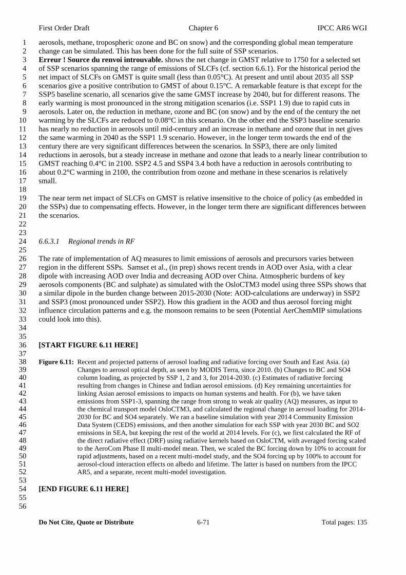
First Order Draft Chapter 6 IPCC AR6 WGI
Do Not Cite, Quote or Distribute 6-71 Total pages: 135
aerosols, methane, tropospheric ozone and BC on snow) and the corresponding global mean temperature 1
change can be simulated. This has been done for the full suite of SSP scenarios. 2
Erreur ! Source du renvoi introuvable. shows the net change in GMST relative to 1750 for a selected set 3
of SSP scenarios spanning the range of emissions of SLCFs (cf. section 6.6.1). For the historical period the 4
net impact of SLCFs on GMST is quite small (less than 0.05°C). At present and until about 2035 all SSP 5
scenarios give a positive contribution to GMST of about 0.15°C. A remarkable feature is that except for the 6
SSP5 baseline scenario, all scenarios give the same GMST increase by 2040, but for different reasons. The 7
early warming is most pronounced in the strong mitigation scenarios (i.e. SSP1 1.9) due to rapid cuts in 8
aerosols. Later on, the reduction in methane, ozone and BC (on snow) and by the end of the century the net 9
warming by the SLCFs are reduced to 0.08°C in this scenario. On the other end the SSP3 baseline scenario 10
has nearly no reduction in aerosols until mid-century and an increase in methane and ozone that in net gives 11
the same warming in 2040 as the SSP1 1.9 scenario. However, in the longer term towards the end of the 12
century there are very significant differences between the scenarios. In SSP3, there are only limited 13
reductions in aerosols, but a steady increase in methane and ozone that leads to a nearly linear contribution to 14
GMST reaching 0.4°C in 2100. SSP2 4.5 and SSP4 3.4 both have a reduction in aerosols contributing to 15
about 0.2°C warming in 2100, the contribution from ozone and methane in these scenarios is relatively 16
small. 17
18
The near term net impact of SLCFs on GMST is relative insensitive to the choice of policy (as embedded in 19
the SSPs) due to compensating effects. However, in the longer term there are significant differences between 20
the scenarios. 21
22
23
6.6.3.1 Regional trends in RF 24
25
The rate of implementation of AQ measures to limit emissions of aerosols and precursors varies between 26
region in the different SSPs. Samset et al., (in prep) shows recent trends in AOD over Asia, with a clear 27
dipole with increasing AOD over India and decreasing AOD over China. Atmospheric burdens of key 28
aerosols components (BC and sulphate) as simulated with the OsloCTM3 model using three SSPs shows that 29
a similar dipole in the burden change between 2015-2030 (Note: AOD-calculations are underway) in SSP2 30
and SSP3 (most pronounced under SSP2). How this gradient in the AOD and thus aerosol forcing might 31
influence circulation patterns and e.g. the monsoon remains to be seen (Potential AerChemMIP simulations 32
could look into this). 33
34
35
[START FIGURE 6.11 HERE] 36
37 Figure 6.11: Recent and projected patterns of aerosol loading and radiative forcing over South and East Asia. (a) 38
Changes to aerosol optical depth, as seen by MODIS Terra, since 2010. (b) Changes to BC and SO4 39 column loading, as projected by SSP 1, 2 and 3, for 2014-2030. (c) Estimates of radiative forcing 40 resulting from changes in Chinese and Indian aerosol emissions. (d) Key remaining uncertainties for 41 linking Asian aerosol emissions to impacts on human systems and health. For (b), we have taken 42 emissions from SSP1-3, spanning the range from strong to weak air quality (AQ) measures, as input to 43 the chemical transport model OsloCTM3, and calculated the regional change in aerosol loading for 2014-44 2030 for BC and SO4 separately. We ran a baseline simulation with year 2014 Community Emission 45 Data System (CEDS) emissions, and then another simulation for each SSP with year 2030 BC and SO2 46 emissions in SEA, but keeping the rest of the world at 2014 levels. For (c), we first calculated the RF of 47 the direct radiative effect (DRF) using radiative kernels based on OsloCTM, with averaged forcing scaled 48 to the AeroCom Phase II multi-model mean. Then, we scaled the BC forcing down by 10% to account for 49 rapid adjustments, based on a recent multi-model study, and the SO4 forcing up by 100% to account for 50 aerosol-cloud interaction effects on albedo and lifetime. The latter is based on numbers from the IPCC 51 AR5, and a separate, recent multi-model investigation. 52
53
[END FIGURE 6.11 HERE] 54
55
56
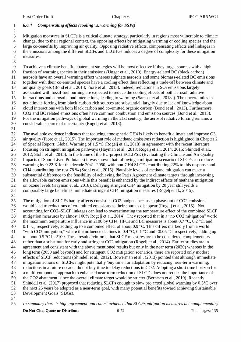
First Order Draft Chapter 6 IPCC AR6 WGI
Do Not Cite, Quote or Distribute 6-72 Total pages: 135
6.6.4 Compensating effects (cooling vs. warming for SSPs) 1
2
Mitigation measures in SLCFs is a critical climate strategy, particularly in regions most vulnerable to climate 3
change, due to their regional context, the opposing effects by mitigating warming or cooling species and the 4
large co-benefits by improving air quality. Opposing radiative effects, compensating effects and linkages in 5
the emissions among the different SLCFs and LLGHGs induces a degree of complexity for these mitigation 6
measures. 7
8
To achieve a climate benefit, abatement strategies will be most effective if they target sources with a high 9
fraction of warming species in their emissions (Unger et al., 2010). Energy-related BC (black carbon) 10
aerosols have an overall warming effect whereas sulphate aerosols and some biomass-related BC emissions 11
together with their co-emitted species have a cooling effect thus reflecting a trade-off between climate and 12
air quality goals (Bond et al., 2013; Fiore et al., 2015). Indeed, reductions in SO2 emissions largely 13
associated with fossil-fuel burning are expected to reduce the cooling effects of both aerosol radiative 14
interactions and aerosol cloud interactions, leading to warming (Samset et al., 2018a). The uncertainties in 15
net climate forcing from black‐carbon‐rich sources are substantial, largely due to lack of knowledge about 16
cloud interactions with both black carbon and co‐emitted organic carbon (Bond et al., 2013). Furthermore, 17
CO2 and BC related emissions often have common combustion and emission sources (Bond et al., 2013). 18
For the mitigation pathways of global warming in the 21st century, the aerosol radiative forcing remains a 19
considerable source of uncertainty (Rogelj et al., 2018). 20
21
The available evidence indicates that reducing atmospheric CH4 is likely to benefit climate and improve O3 22
air quality (Fiore et al., 2015). The important role of methane emissions reduction is highlighted in Chapter 2 23
of Special Report: Global Warming of 1.5 ºC (Rogelj et al., 2018) in agreement with the recent literature 24
focusing on stringent mitigation pathways (Hayman et al., 2018; Rogelj et al., 2014, 2015; Shindell et al., 25
2012; Stohl et al., 2015). In the frame of the EU-project ECLIPSE (Evaluating the Climate and Air Quality 26
Impacts of Short-Lived Pollutants) it was shown that following a mitigation scenario of SLCFs can reduce 27
warming by 0.22 K for the decade 2041–2050, with non-CH4 SLCFs contributing 22% to this response and 28
CH4 contributing the rest 78 % (Stohl et al., 2015). Plausible levels of methane mitigation can make a 29
substantial difference to the feasibility of achieving the Paris Agreement climate targets through increasing 30
the allowable carbon emissions while this benefit is enhanced by the indirect effects of methane mitigation 31
on ozone levels (Hayman et al., 2018). Delaying stringent CH4 mitigation by 20 year still yields a 32
comparably large benefit as immediate stringent CH4 mitigation measures (Rogelj et al., 2015). 33
34
The mitigation of SLCFs barely affects consistent CO2 budgets because a phase-out of CO2 emissions 35
would lead to reductions of co-emitted emissions as their sources disappear (Rogelj et al., 2015). Not 36
accounting for CO2–SLCF linkages can lead to overestimating the temperature effect of the combined SLCF 37
mitigation measures by almost 100% Rogelj et al., 2014). They reported that in a “no CO2 mitigation” world 38
the maximum temperature influence in 2100 by CH4, HFCs and BC measures is about 0.7 °C, 0.2 °C, and 39
0.1 °C, respectively, adding up to a combined effect of about 0.9 °C. This differs markedly from a world 40
“with CO2 mitigation,” where the influence declines to 0.4 °C, 0.1 °C and <0.05 °C, respectively, adding up 41
to about 0.5 °C in 2100. These results reinforce that SLCF measures are to be considered complementary 42
rather than a substitute for early and stringent CO2 mitigation (Rogelj et al., 2014). Earlier studies are in 43
agreement and consistent with the above mentioned results but only in the near term (2030) whereas in the 44
long term (2050 and beyond) and for stringent CO2 mitigation scenarios, there are reported only modest 45
effects of SLCF reductions (Shindell et al., 2012). Bowerman et al., (2013) pointed that although immediate 46
mitigation actions on SLCFs might potentially 'buy time' for adaptation by reducing near-term warming, 47
reductions in a future decade, do not buy time to delay reductions in CO2. Adopting a short time horizon for 48
a multi-component approach to enhanced near-term reduction of SLCFs does not reduce the importance of 49
the CO2 abatement, since the overall climate target would be stricter (Berntsen et al., 2010). Recently, 50
Shindell et al. (2017) proposed that reducing SLCFs enough to slow projected global warming by 0.5°C over 51
the next 25 years be adopted as a near-term goal, with many potential benefits toward achieving Sustainable 52
Development Goals (SDGs). 53
54
In summary there is high agreement and robust evidence that SLCFs mitigation measures act complementary 55
First Order Draft Chapter 6 IPCC AR6 WGI
Do Not Cite, Quote or Distribute 6-73 Total pages: 135
to early and stringent CO2 mitigation with important temperature effects for the near term but there is medium 1
agreement and medium evidence for their contribution in the long-term. 2
3
4
6.6.5 Impacts on AQ (forced by SSP emissions) 5
6
The different socioeconomic developments in the SSP storylines and the different levels of climate policies 7
for each SSP have strong influence SLCF emissions and thus on air quality (high confidence, good 8
agreement). Rao et al., (2017) developed the SSP scenarios to include narratives on future air pollution 9
control that are consistent with current trends in air quality policies explores some initial projections on air 10
quality. Reis et al. (2018) estimate regional impacts on AQ across the range of SSP scenarios using the 11
emission numbers developed by Rao et al. (2017) and the chemistry emulator TM5_FASST (Van Dingenen 12
et al., 2018). 13
14
Using a global averaged exposure based Air Quality Index . Reis et al. (2018) find that climate policies are 15
very relevant in reducing air pollution exposure by mid-century. Climate policies have a stronger effect on 16
the pollution reduction timing, while socioeconomic developments will have a greater impact on the absolute 17
pollution level. A 1.5°C policy target may prevent all regions from exceeding the annual average limit for all 18
pollutants considered, except PM2.5. 19
20
21
6.7 Knowledge gaps 22
23
This section summarizes the knowledge gaps articulated in earlier sections of the chapter. 24
25
26
6.7.1 Abundances and radiative forcing of SLCFs 27
28
There is gap of knowledge with respect to the budget, distribution, and radiative forcing of tropospheric 29
ozone [6.2.2.5]. Due to the sparseness of historical observations, there is limited evidence (low confidence) 30
to draw conclusions about zonal mean ozone changes at the tropics and southern mid-latitudes. From the 31
model perspective, model simulations show low agreement for ozone budget terms, including chemical 32
production and loss, stratosphere-troposphere exchange, and deposition of ozone. Radiative forcing estimates 33
depend on changes in tropospheric ozone from the preindustrial time to present day, but there is still a 34
knowledge gap from observations for preindustrial ozone levels. Furthermore, part of the RF uncertainty 35
(which is ± 50%) is due to how the models simulate changes in STE on decadal or multi-decadal time-scales, 36
thus highlighting another knowledge gap. 37
38
Global carbonaceous aerosol budget and trend remain poorly characterized due to limited observation, 39
yielding low confidence in our current understanding. Observations of OA are even more limited than BC. 40
The uncertainties arise from the understanding of the aging and deposition processes of carbonaceous 41
aerosols, the vertical distribution of BC, and the representations of SOA yields in models [6.2.2.8]. 42
Improved constraints on BC interactions with mixed-phase and ice clouds and better representations of 43
global solid fuel cookstove emissions in models are also needed [6.4.2.1]. 44
45
Concentrations of air pollutants are influenced by climate change. Most studies on the impact of climate 46
change on air quality have focused on the future changes of average meteorological conditions. The 47
relationship between climate-driven changes in the meteorological regimes and air quality extreme events is 48
still poorly investigated and not clearly defined. 49
50
51
6.7.2 Climate effect of SLCFs 52
53
There is considerable uncertainty in the interactions between LULCC, SLCFs, and climate [6.4.2.2]. 54
Preindustrial to present day anthropogenic LULCC have resulted in a global warming that is equivalent to up 55
First Order Draft Chapter 6 IPCC AR6 WGI
Do Not Cite, Quote or Distribute 6-74 Total pages: 135
to 45% of the net anthropogenic global warming when changes in the SLCFs from dust, fire, BVOCs, soil, 1
CH4 and NH3 emissions are properly accounted for (low confidence). Areas of research to improve 2
understanding of the effects LULCC on SLCFs include BVOC emissions at large-scale by plant species, 3
photo-oxidation mechanisms of BVOCs, ozone production efficiency of BVOCs, BSOA formation yields, in 4
addition to the BSOA aerosol-cloud interactions. Field measurements of BVOCs’ influence on the methane 5
growth rate in the atmosphere are also lacking. There is no consensus on the net sign of global radiative 6
forcing from the historical changes in BVOC emissions. 7
8
There is knowledge gap for quantifying the impacts of megacities on climate. The attribution of emissions to 9
megacities is of low confidence since different methodologies are considered to define the megacity areas 10
and since large differences remain between global emissions inventories and city-specific inventories 11
[6.4.2.3]. In addition, because of the use of a single global chemistry-transport model in the published 12
literature, the results regarding impacts of SLCF emissions from megacities on climate are of low confidence 13
[6.4.2.3]. The “annihilation” studies (complete removal of megacities emissions in modelling experiments) 14
have several limitations when applied in low resolution global models (resolution from tens to hundreds of 15
kilometers) due to nonlinearities related to chemical processes which lead to an underestimation of the 16
megacities contribution for ozone and due to excluded emissions related to the megacities but occurring 17
outside their boundaries [6.4.2.3]. A better quantification of the impacts of megacities on climate requests 18
high resolution global models, multi-model studies, proper protocol to define the megacities mask and global 19
emission datasets consistent with the city-level ones. 20
21
There are also large uncertainties in sign/magnitude of climate effects of mitigating SLCF emissions [6.4.3]. 22
The impact of air pollution mitigation on climate has been estimated, but usually based on a single model 23
and emission dataset, therefore conclusions from such studies are of low confidence. Specifically, the 24
quantification of the climate impact potential of cookstove mitigation is of low confidence due to large 25
spatial variability of signal combined with cancellation between large local forcings of opposite sign. To 26
assess the relevance of air pollution reduction policies, regional air quality models are necessary and still 27
need to be implemented in many developing countries. To properly apply such models, the quality of 28
spatialized emission inventories is essential, but the production of accurate emission inventories remain a 29
challenge for lots of rapidly growing urban areas. The combined use of bottom-up and top-down 30
methodologies combining ambient monitoring networks and satellite data are necessary to decrease the 31
uncertainties in emission inventories. It is also necessary to consider the future global changes to properly 32
assess the local mitigation strategies which requires the use of multiscale modelling chains. Multi-model 33
approaches are also necessary to decrease the uncertainties. 34
35
36
6.7.3 Effects of SLCFs on health, agriculture, and ecosystems 37
38
Our knowledge on health impact of ambient trace gases other than ozone is still very limited and uncertain 39
(6.1.2.2). With respect to the health impact of PM, the majority of studies are based on correlation and 40
therefore do not firmly establish causal relationships. These health studies are still primarily based on mass 41
concentration of particulate pollutants and provide very little information on size, composition or number 42
concentration that are also important to assess health damage. In addition, half of the world’s population is 43
exposed to indoor air pollution mainly attributable to solid fuel usage for household cooking and heating, 44
which requires understanding of epidemiological concentration-response functions in Asia and differential 45
particle toxicity [6.4.2.1]. 46
47
There are substantial knowledge gaps with respect to the impacts of SLCFs on agriculture and ecosystems. 48
Reducing uncertainties requires improved information on the sensitivity of different plant species to ozone, 49
and measurements of ozone dose-response relationships for tropical plants, which are currently lacking 50
[6.3.1.3]. There is low confidence on the likely impacts on agriculture and ecosystem damage from elevated 51
ambient concentration of trace gases such as NOx, CO, SO2. There is very limited new knowledge about PM 52
damage to agriculture, ecosystems, material and property damage since AR5. Air pollution impacts on 53
agriculture should be included in the Agriculture Model Intercomparison and Improvement Project [6.3.1.3]. 54
55
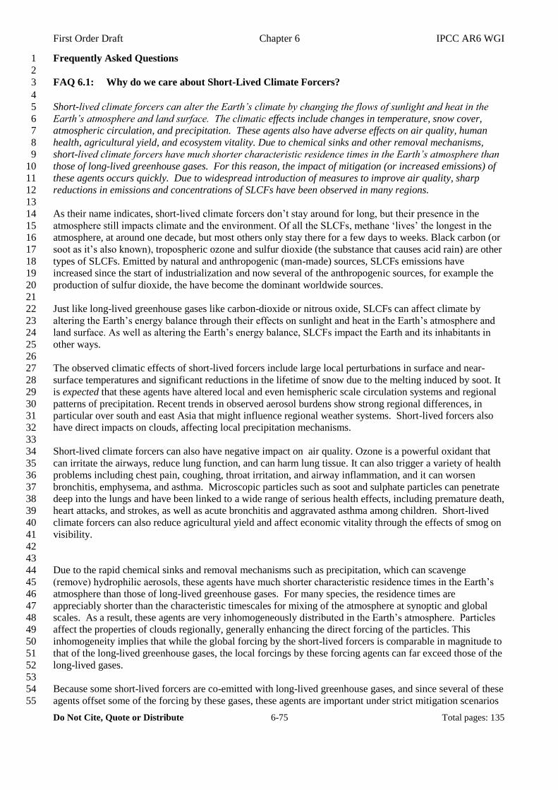
First Order Draft Chapter 6 IPCC AR6 WGI
Do Not Cite, Quote or Distribute 6-75 Total pages: 135
Frequently Asked Questions 1
2
FAQ 6.1: Why do we care about Short-Lived Climate Forcers? 3
4
Short-lived climate forcers can alter the Earth’s climate by changing the flows of sunlight and heat in the 5
Earth’s atmosphere and land surface. The climatic effects include changes in temperature, snow cover, 6
atmospheric circulation, and precipitation. These agents also have adverse effects on air quality, human 7
health, agricultural yield, and ecosystem vitality. Due to chemical sinks and other removal mechanisms, 8
short-lived climate forcers have much shorter characteristic residence times in the Earth’s atmosphere than 9
those of long-lived greenhouse gases. For this reason, the impact of mitigation (or increased emissions) of 10
these agents occurs quickly. Due to widespread introduction of measures to improve air quality, sharp 11
reductions in emissions and concentrations of SLCFs have been observed in many regions. 12
13
As their name indicates, short-lived climate forcers don’t stay around for long, but their presence in the 14
atmosphere still impacts climate and the environment. Of all the SLCFs, methane ‘lives’ the longest in the 15
atmosphere, at around one decade, but most others only stay there for a few days to weeks. Black carbon (or 16
soot as it’s also known), tropospheric ozone and sulfur dioxide (the substance that causes acid rain) are other 17
types of SLCFs. Emitted by natural and anthropogenic (man-made) sources, SLCFs emissions have 18
increased since the start of industrialization and now several of the anthropogenic sources, for example the 19
production of sulfur dioxide, the have become the dominant worldwide sources. 20
21
Just like long-lived greenhouse gases like carbon-dioxide or nitrous oxide, SLCFs can affect climate by 22
altering the Earth’s energy balance through their effects on sunlight and heat in the Earth’s atmosphere and 23
land surface. As well as altering the Earth’s energy balance, SLCFs impact the Earth and its inhabitants in 24
other ways. 25
26
The observed climatic effects of short-lived forcers include large local perturbations in surface and near-27
surface temperatures and significant reductions in the lifetime of snow due to the melting induced by soot. It 28
is expected that these agents have altered local and even hemispheric scale circulation systems and regional 29
patterns of precipitation. Recent trends in observed aerosol burdens show strong regional differences, in 30
particular over south and east Asia that might influence regional weather systems. Short-lived forcers also 31
have direct impacts on clouds, affecting local precipitation mechanisms. 32
33
Short-lived climate forcers can also have negative impact on air quality. Ozone is a powerful oxidant that 34
can irritate the airways, reduce lung function, and can harm lung tissue. It can also trigger a variety of health 35
problems including chest pain, coughing, throat irritation, and airway inflammation, and it can worsen 36
bronchitis, emphysema, and asthma. Microscopic particles such as soot and sulphate particles can penetrate 37
deep into the lungs and have been linked to a wide range of serious health effects, including premature death, 38
heart attacks, and strokes, as well as acute bronchitis and aggravated asthma among children. Short-lived 39
climate forcers can also reduce agricultural yield and affect economic vitality through the effects of smog on 40
visibility. 41
42
43
Due to the rapid chemical sinks and removal mechanisms such as precipitation, which can scavenge 44
(remove) hydrophilic aerosols, these agents have much shorter characteristic residence times in the Earth’s 45
atmosphere than those of long-lived greenhouse gases. For many species, the residence times are 46
appreciably shorter than the characteristic timescales for mixing of the atmosphere at synoptic and global 47
scales. As a result, these agents are very inhomogeneously distributed in the Earth’s atmosphere. Particles 48
affect the properties of clouds regionally, generally enhancing the direct forcing of the particles. This 49
inhomogeneity implies that while the global forcing by the short-lived forcers is comparable in magnitude to 50
that of the long-lived greenhouse gases, the local forcings by these forcing agents can far exceed those of the 51
long-lived gases. 52
53
Because some short-lived forcers are co-emitted with long-lived greenhouse gases, and since several of these 54
agents offset some of the forcing by these gases, these agents are important under strict mitigation scenarios 55
First Order Draft Chapter 6 IPCC AR6 WGI
Do Not Cite, Quote or Distribute 6-76 Total pages: 135
(e.g. a temperature limit of 1.5°C). But, the adverse effects of SLCFs on air quality make mitigation of 1
SLCFs a favourable policy option as a win-win strategy. In fact, the strong reduction in emissions of SLCFs 2
that is and has been observed in many regions, and predicted in future scenarios, are mainly a result of 3
policies to improve air quality. 4
5
[PLACEHOLDER Figure suggestion: Short-lived climate forcers – where do they come from and where do 6
they go? Schematic showing the main sources of CH4, SO2, O3, BC, HFCS (?) and their impacts: health, 7
crop yields, precipitation / clouds, and main removals: rain, atmospheric chemical reactions.] 8
9
First Order Draft Chapter 6 IPCC AR6 WGI
Do Not Cite, Quote or Distribute 6-77 Total pages: 135
FAQ 6.2: What is the link between air quality and climate change? 1
2
Air quality and climate change are intimately linked, since many air pollutant sources are also sources of 3
long-lived greenhouse gases and the pollutants themselves influence climate and are also altered by climate 4
change. Anthropogenic activities are responsible for the emission of gaseous and particulate chemical 5
species that modify atmospheric composition. Such changes are, in turn, responsible for the degradation of 6
air quality at the regional/local scale as well as for climate change. Indeed, many mitigation options offer 7
the possibility to both improve air quality and mitigate climate change but, in some cases, mitigation options 8
that may provide benefits to one aspect, may worsen the situation in the other. 9
10
Critical environmental issues, climate change and air pollution are already impacting humanity. The World 11
Health Organisation attributes 4.2 million deaths worldwide every year to ambient (outdoor) air pollution, 12
and climate change impacts water resources, food production, human health, extreme events, coastal erosion, 13
wildfires, and many other phenomena essential for our life. 14
15
All anthropogenic activities (e.g., energy production, agriculture, transportation, industrial processes, waste 16
management, residential heating, etc.) are responsible for the emission of gaseous and particulate pollutants 17
that modify atmospheric composition, leading to degradation of air quality as well as climate change. 18
19
All anthropogenic emission sources emit air pollutants and climate-forcing species at the same time, making 20
air pollution and climate change two intimately connected issues. Yet in the scientific and the policy arena, 21
air pollutants and climate-forcing species are often defined, investigated, and regulated independently of one 22
another and their impacts on climate, human health, and ecosystems are also often considered independently, 23
in spite of the scientific evidence, now well established, linking emissions of air pollutants and climate-24
forcing species and their associated impacts. 25
26
The chemical composition of the emission from any given source determines the actual effect on air quality 27
and climate change. When we drive our car or light a fire in the fireplace, it is not just CO2 or air pollutants 28
that are emitted, but always both. It is therefore not possible to unambiguously separate anthropogenic 29
emissions in two distinct groups: atmospheric pollutants and climate-forcing species, and many of the same 30
sources emit both climate-forcing species and air pollutants. What is more, many emitted species are at the 31
same time air pollutants and climate-forcing species. 32
33
Therefore, policy options aiming at addressing e.g. climate change, may have unintended benefits or trade-34
offs for air quality and vice-versa. 35
36
Win-win policies that benefit at the same time air quality while mitigating climate change are e.g. energy 37
efficiency measures, zero-emission vehicles, capturing and recovering methane from solid waste 38
management and oil and gas industry, reducing emissions of soot (particulates) from diesel vehicles, etc. 39
40
There are, however, also win-lose policy options. For example, wood burning is defined as carbon neutral, 41
because trees accumulate the same amount of CO2 throughout their lifetime as that released when wood is 42
burned. However, burning wood can also result in significant emissions of air pollutants (carbon monoxide, 43
nitrogen oxides, volatile organic compounds, particulate matter) that have local/regional impacts on climate, 44
human health and ecosystems, offsetting the CO2 benefit. On the opposite side, mitigation options to 45
improve air quality, such as such as exhaust gas desulphurization in power and industrial plants, unmasks 46
some warming since sulphate aerosols contribute to cooling the atmosphere. 47
48
Two sides of the same coin, addressing air quality and climate change together could lead to significant 49
synergies and economic benefits, avoiding policy actions intended to mitigate one of the two issues that 50
could worsen the situation in the other. 51
52
[START FAQ 6.2, FIGURE 1 HERE] 53
54
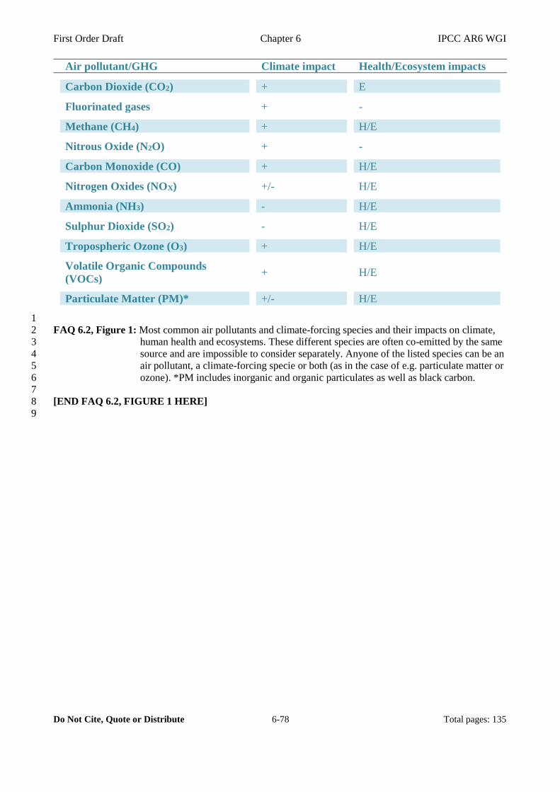
First Order Draft Chapter 6 IPCC AR6 WGI
Do Not Cite, Quote or Distribute 6-78 Total pages: 135
Air pollutant/GHG Climate impact Health/Ecosystem impacts
Carbon Dioxide (CO2) + E
Fluorinated gases + -
Methane (CH4) + H/E
Nitrous Oxide (N2O) + -
Carbon Monoxide (CO) + H/E
Nitrogen Oxides (NOX) +/- H/E
Ammonia (NH3) - H/E
Sulphur Dioxide (SO2) - H/E
Tropospheric Ozone (O3) + H/E
Volatile Organic Compounds
(VOCs) + H/E
Particulate Matter (PM)* +/- H/E
1
FAQ 6.2, Figure 1: Most common air pollutants and climate-forcing species and their impacts on climate, 2
human health and ecosystems. These different species are often co-emitted by the same 3
source and are impossible to consider separately. Anyone of the listed species can be an 4
air pollutant, a climate-forcing specie or both (as in the case of e.g. particulate matter or 5
ozone). *PM includes inorganic and organic particulates as well as black carbon. 6
7
[END FAQ 6.2, FIGURE 1 HERE] 8
9
First Order Draft Chapter 6 IPCC AR6 WGI
Do Not Cite, Quote or Distribute 6-79 Total pages: 135
References 1
2
Aas, W., Mortier, A., Bowersox, V., Cherian, R., Faluvegi, G., Fagerli, H., et al. (2019). Global and regional 3
trends of atmospheric sulfur. Sci. Rep. 9, 953. doi:10.1038/s41598-018-37304-0. 4
Abbatt, J., George, C., Melamed, M., Monks, P., Pandis, S., and Rudich, Y. (2014). New Directions: 5
Fundamentals of atmospheric chemistry: Keeping a three-legged stool balanced. Atmos. Environ. 84, 6
390–391. doi:https://doi.org/10.1016/j.atmosenv.2013.10.025. 7
Achakulwisut, P., Mickley, L. J., and Anenberg, S. C. (2018). Drought-sensitivity of fine dust in the US 8
Southwest: Implications for air quality and public health under future climate change. Environ. Res. 9
Lett. 13. doi:10.1088/1748-9326/aabf20. 10
Achakulwisut, P., Mickley, L. J., Murray, L. T., Tai, A. P. K., Kaplan, J. O., and Alexander, B. (2015). 11
Uncertainties in isoprene photochemistry and emissions: implications for the oxidative capacity of past 12
and present atmospheres and for climate forcing agents. Atmos. Chem. Phys. 15, 7977–7998. 13
doi:10.5194/acp-15-7977-2015. 14
Ackerman, A. S., Kirkpatrick, M. P., Stevens, D. E., and Toon, O. B. (2004). The impact of humidity above 15
stratiform clouds on indirect aerosol climate forcing. Nature 432, 1014–1017. 16
doi:10.1038/nature03174. 17
Adams, K., Greenbaum, D. S., Shaikh, R., van Erp, A. M., and Russell, A. G. (2015). Particulate matter 18
components, sources, and health: Systematic approaches to testing effects. J. Air Waste Manag. Assoc. 19
65, 544–558. doi:10.1080/10962247.2014.1001884. 20
Agyei, F., Wiedinmyer, C., Xie, M., Alirigia, R., Piedrahita, R., Dickinson, K. L., et al. (2016). Exposures to 21
and origins of carbonaceous PM 2.5 in a cookstove intervention in Northern Ghana. Sci. Total Environ. 22
576, 178–192. doi:10.1016/j.scitotenv.2016.10.069. 23
Ainsworth, E. A., Yendrek, C. R., Sitch, S., Collins, W. J., and Emberson, L. D. (2012). The Effects of 24
Tropospheric Ozone on Net Primary Productivity and Implications for Climate Change. Annu. Rev. 25
Plant Biol. 63, 637–661. doi:10.1146/annurev-arplant-042110-103829. 26
Akimoto, H., Kurokawa, J., Sudo, K., Nagashima, T., Takemura, T., Klimont, Z., et al. (2015). SLCP co-27
control approach in East Asia: Tropospheric ozone reduction strategy by simultaneous reduction of 28
NOx/NMVOC and methane. Atmos. Environ. 122, 588–595. doi:10.1016/j.atmosenv.2015.10.003. 29
Akritidis, D., Katragkou, E., Zanis, P., Pytharoulis, I., Melas, D., Flemming, J., et al. (2018). A deep 30
stratosphere-to-troposphere ozone transport event over Europe simulated in CAMS global and regional 31
forecast systems: analysis and evaluation. Atmos. Chem. Phys. 18, 15515–15534. doi:10.5194/acp-18-32
15515-2018. 33
Akritidis, D., Pozzer, A., Zanis, P., Tyrlis, E., Škerlak, B., Sprenger, M., et al. (2016). On the role of 34
tropopause folds in summertime tropospheric ozone over the eastern Mediterranean and the Middle 35
East. Atmos. Chem. Phys. 16, 14025–14039. doi:10.5194/acp-16-14025-2016. 36
Albani, S., Mahowald, N. M., Perry, A. T., Scanza, R. A., Zender, C. S., Heavens, N. G., et al. (2014). 37
Improved dust representation in the Community Atmosphere Model. J. Adv. Model. EARTH Syst. 6, 38
541–570. doi:10.1002/2013MS000279. 39
Albrecht, B. A. (1989). Aerosols, Cloud Microphysics, and Fractional Cloudiness. Science (80-. ). 245, 40
1227–1230. doi:10.1126/science.245.4923.1227. 41
Aleluia Reis, L., Drouet, L., Van Dingenen, R., and Emmerling, J. (2018). Future Global Air Quality Indices 42
under Different Socioeconomic and Climate Assumptions. Sustainability 10, 3645. 43
doi:10.3390/su10103645. 44
Alexander, B., and Mickley, L. J. (2015). Paleo-Perspectives on Potential Future Changes in the Oxidative 45
Capacity of the Atmosphere Due to Climate Change and Anthropogenic Emissions. Curr. Pollut. 46
Reports 1, 57–69. doi:10.1007/s40726-015-0006-0. 47
Allen, D. J., and Pickering, K. E. (2002). Evaluation of lighning flash rate parametrisations for use in a 48
global chemical transport model. J. Geophys. Res. 107(D23), doi:101029/2002JD002066. 49
doi:doi:10.1029/2002JD002066. 50
Allen, M. R., Dube, O. P., Solecki, W., Aragón–Durand, F., Cramer, W., Humphreys, S., et al. (2018a). 51
“Framing and Context,” in Global warming of 1.5°C. An IPCC Special Report on the impacts of global 52
warming of 1.5°C above pre-industrial levels and related global greenhouse gas emission pathways, in 53
the context of strengthening the global response to the threat of climate change, eds. V. Masson-54
Delmotte, P. Zhai, H. O. Pörtner, D. Roberts, J. Skea, P. R. Shukla, et al. (Geneva, Switzerland: World 55
First Order Draft Chapter 6 IPCC AR6 WGI
Do Not Cite, Quote or Distribute 6-80 Total pages: 135
Meteorological Organization). 1
Allen, M. R., Fuglestvedt, J. S., Shine, K. P., Reisinger, A., Pierrehumbert, R. T., and Forster, P. M. (2016a). 2
New use of global warming potentials to compare cumulative and short-lived climate pollutants. Nat. 3
Clim. Chang. 6, 773–776. doi:10.1038/nclimate2998. 4
Allen, M. R., Shine, K. P., Fuglestvedt, J. S., Millar, R. J., Cain, M., Frame, D. J., et al. (2018b). A solution 5
to the misrepresentations of CO2-equivalent emissions of short-lived climate pollutants under 6
ambitious mitigation. npj Clim. Atmos. Sci. 1, 16. doi:10.1038/s41612-018-0026-8. 7
Allen, R. J., and Landuyt, W. (2014). The vertical distribution of black carbon in CMIP5models: 8
Comparison to observations and the importance of convective transport. J. Geophys. Res. 119, 4808–9
4835. doi:10.1002/2014JD021595. 10
Allen, R. J., Landuyt, W., and Rumbold, S. T. (2016b). An increase in aerosol burden and radiative effects in 11
a warmer world. Nat. Clim. Chang. 6, 269–274. doi:10.1038/nclimate2827. 12
Alvarez, R. A., Zavala-Araiza, D., Lyon, D. R., Allen, D. T., Barkley, Z. R., Brandt, A. R., et al. (2018). 13
Assessment of methane emissions from the U.S. oil and gas supply chain. Science (80-. ). 361, 186 LP-14
188. doi:10.1126/science.aar7204. 15
Amann, M., Klimont, Z., and Wagner, F. (2013). Regional and global emissions of air pollutants: Recent 16
trends and future scenarios. doi:10.1146/annurev-environ-052912-173303. 17
Amann, M., Purohit, P., Bhanarkar, A. D., Bertok, I., Borken-Kleefeld, J., Cofala, J., et al. (2017). Managing 18
future air quality in megacities: A case study for Delhi. Atmos. Environ. 161, 99–111. 19
doi:https://doi.org/10.1016/j.atmosenv.2017.04.041. 20
Andrews, A. E., Kofler, J. D., Trudeau, M. E., Williams, J. C., Neff, D. H., Masarie, K. A., et al. (2014). 21
CO2, CO, and CH4 measurements from tall towers in the NOAA earth system research laboratory’s 22
global greenhouse gas reference network: Instrumentation, uncertainty analysis, and recommendations 23
for future high-accuracy greenhouse gas monitoring efforts. Atmos. Meas. Tech. doi:10.5194/amt-7-24
647-2014. 25
Andrews, T., Forster, P. M., Boucher, O., Bellouin, N., and Jones, A. (2010). Precipitation, radiative forcing 26
and global temperature change. Geophys. Res. Lett. 37. doi:10.1029/2010GL043991. 27
Anenberg, S. C., Balakrishnan, K., Jetter, J., Masera, O., Mehta, S., Moss, J., et al. (2013). Cleaner cooking 28
solutions to achieve health, climate, and economic cobenefits. Environ. Sci. Technol. 47, 3944–3952. 29
doi:10.1021/es304942e. 30
Anenberg, S. C., Henze, D. K., Lacey, F., Irfan, A., Kinney, P., Kleiman, G., et al. (2017). Air pollution-31
related health and climate benefits of clean cookstove programs in Mozambique. Environ. Res. Lett. 12. 32
doi:10.1088/1748-9326/aa5557. 33
Anenberg, S. C., Schwartz, J., Shindell, D., Amann, M., Faluvegi, G., Klimont, Z., et al. (2012). Global air 34
quality and health co-benefits of mitigating near-term climate change through methane and black 35
carbon emission controls. Environ. Health Perspect. 120, 831–839. doi:10.1289/ehp.1104301. 36
Angelbratt, J., Mellqvist, J., Simpson, D., Jonson, J. E., Blumenstock, T., Borsdorff, T., et al. (2011). Carbon 37
monoxide (CO) and ethane (C2H6) trends from ground-based solar FTIR measurements at six 38
European stations, comparison and sensitivity analysis with the EMEP model. Atmos. Chem. Phys. 11, 39
9253–9269. doi:10.5194/acp-11-9253-2011. 40
Archer-Nicholls, S., Carter, E., Kumar, R., Xiao, Q., Liu, Y., Frostad, J., et al. (2016). The regional impacts 41
of cooking and heating emissions on ambient air quality and disease burden in China. Environ. Sci. 42
Technol. 50, 9416–9423. doi:10.1021/acs.est.6b02533. 43
Arienzo, M. M., McConnell, J. R., Murphy, L. N., Chellman, N., Das, S., Kipfstuhl, S., et al. (2017). 44
Holocene black carbon in Antarctica paralleled Southern Hemisphere climate. J. Geophys. Res. 122, 45
6713–6728. doi:10.1002/2017JD026599. 46
Arneth, A., Sitch, S., Bondeau, A., Butterbach-Bahl, K., Foster, P., Gedney, N., et al. (2010). From biota to 47
chemistry and climate: towards a comprehensive description of trace gas exchange between the 48
biosphere and atmosphere. Biogeosciences 7, 121–149. doi:10.5194/bg-7-121-2010. 49
Arnold, S. R., Lombardozzi, D., Lamarque, J.-F., Richardson, T., Emmons, L. K., Tilmes, S., et al. (2018). 50
Simulated Global Climate Response to Tropospheric Ozone-Induced Changes in Plant Transpiration. 51
Geophys. Res. Lett. 45, 13,13-70,79. doi:10.1029/2018GL079938. 52
Aschmann, J., Burrows, J. P., Gebhardt, C., Rozanov, A., Hommel, R., Weber, M., et al. (2014). On the 53
hiatus in the acceleration of tropical upwelling since the beginning of the 21st century. Atmos. Chem. 54
Phys. 14, 12803–12814. doi:10.5194/acp-14-12803-2014. 55
First Order Draft Chapter 6 IPCC AR6 WGI
Do Not Cite, Quote or Distribute 6-81 Total pages: 135
Atkinson, R., and Arey, J. (2003). Gas-phase tropospheric chemistry of biogenic volatile organic 1
compounds: a review. Atmos. Environ. 37, 197–219. doi:10.1016/S1352-2310(03)00391-1. 2
Atkinson, R. W., Analitis, A., Samoli, E., Fuller, G. W., Green, D. C., Mudway, I. S., et al. (2016). Short-3
term exposure to traffic-related air pollution and daily mortality in London, UK. J. Expo. Sci. Environ. 4
Epidemiol. 26, 125–132. doi:10.1038/jes.2015.65. 5
Austin, R. T., Heymsfield, A. J., and Stephens, G. L. (2009). Retrieval of ice cloud microphysical parameters 6
using the CloudSat millimeter-wave radar and temperature. J. Geophys. Res. Atmos. 114. 7
doi:10.1029/2008JD010049. 8
Avnery, S., Mauzerall, D. L., Liu, J., and Horowitz, L. W. (2011). Global crop yield reductions due to 9
surface ozone exposure: 1. Year 2000 crop production losses and economic damage. Atmos. Environ. 10
45, 2284–2296. doi:10.1016/j.atmosenv.2010.11.045. 11
Baker, L. H., Collins, W. J., Olivié, D. J. L., Cherian, R., Hodnebrog, Myhre, G., et al. (2015). Climate 12
responses to anthropogenic emissions of short-lived climate pollutants. Atmos. Chem. Phys. 15, 8201–13
8216. doi:10.5194/acp-15-8201-2015. 14
Baklanov, A., Molina, L. T., and Gauss, M. (2016). Megacities, air quality and climate. Atmos. Environ. 126, 15
235–249. doi:10.1016/j.atmosenv.2015.11.059. 16
Ball, W. T., Alsing, J., Mortlock, D. J., Staehelin, J., Haigh, J. D., Peter, T., et al. (2018). Evidence for a 17
continuous decline in lower stratospheric ozone offsetting ozone layer recovery. Atmos. Chem. Phys. 18
18, 1379–1394. doi:10.5194/acp-18-1379-2018. 19
Banerjee, A., Archibald, A. T., Maycock, A. C., Telford, P., Abraham, N. L., Yang, X., et al. (2014). 20
Lightning NOx, a key chemistry-climate interaction: Impacts of future climate change and 21
consequences for tropospheric oxidising capacity. Atmos. Chem. Phys. 14, 9871–9881. 22
doi:10.5194/acp-14-9871-2014. 23
Banerjee, A., Maycock, A. C., Archibald, A. T., Abraham, N. L., Telford, P., Braesicke, P., et al. (2016). 24
Drivers of changes in stratospheric and tropospheric ozone between year 2000 and 2100. Atmos. Chem. 25
Phys. 16, 2727–2746. doi:10.5194/acp-16-2727-2016. 26
Banzhaf, S., Schaap, M., Kranenburg, R., Manders, A. M. M., Segers, A. J., Visschedijk, A. J. H., et al. 27
(2015). Dynamic model evaluation for secondary inorganic aerosol and its precursors over {Europe} 28
between 1990 and 2009. Geosci. Model Dev. 8, 1047–1070. doi:10.5194/gmd-8-1047-2015. 29
Bao, H., Niggemann, J., Luo, L., Dittmar, T., and Kao, S. J. (2017). Aerosols as a source of dissolved black 30
carbon to the ocean. Nat. Commun. 8, 510. doi:10.1038/s41467-017-00437-3. 31
Bao, X., Yu, J., Liang, W., Lu, C., Zhu, J., and Li, Q. (2015). The interactive effects of elevated ozone and 32
wheat cultivars on soil microbial community composition and metabolic diversity. Appl. Soil Ecol. 87, 33
11–18. doi:10.1016/j.apsoil.2014.11.003. 34
Barkley, M. P., González Abad, G., Kurosu, T. P., Spurr, R., Torbatian, S., and Lerot, C. (2017). OMI air-35
quality monitoring over the Middle East. Atmos. Chem. Phys. 17, 4687–4709. doi:10.5194/acp-17-36
4687-2017. 37
Barnes, E. A., Fiore, A. M., and Horowitz, L. W. (2016). Detection of trends in surface ozone in the presence 38
of climate variability. J. Geophys. Res. Atmos. 121, 6112–6129. doi:10.1002/2015JD024397. 39
Barnes, E. A., and Polvani, L. (2013). Response of the midlatitude jets, and of their variability, to increased 40
greenhouse gases in the CMIP5 models. J. Clim. 26, 7117–7135. doi:10.1175/JCLI-D-12-00536.1. 41
Barré, J., Edwards, D., Worden, H., Da Silva, A., and Lahoz, W. (2015). On the feasibility of monitoring 42
carbon monoxide in the lower troposphere from a constellation of Northern Hemisphere geostationary 43
satellites. (Part 1). Atmos. Environ. 113, 63–77. doi:10.1016/J.ATMOSENV.2015.04.069. 44
Bartlett, R. E., Bollasina, M. A., Booth, B. B. B., Dunstone, N. J., Marenco, F., Messori, G., et al. (2018). Do 45
differences in future sulfate emission pathways matter for near-term climate? A case study for the 46
Asian monsoon. Clim. Dyn. 50, 1863–1880. doi:10.1007/s00382-017-3726-6. 47
Beekmann, M., Prévôt, A. S. H., Drewnick, F., Sciare, J., Pandis, S. N., Denier Van Der Gon, H. A. C., et al. 48
(2015). In situ, satellite measurement and model evidence on the dominant regional contribution to fine 49
particulate matter levels in the Paris megacity. Atmos. Chem. Phys. doi:10.5194/acp-15-9577-2015. 50
Beirle, S., Boersma, K. F., Platt, U., Lawrence, M. G., and Wagner, T. (2011). Megacity Emissions and 51
Lifetimes of Nitrogen Oxides Probed from Space. Science (80-. ). 333, 1737–1739. 52
doi:10.1126/science.1207824. 53
Bekki, S., and Lefevre, F. (2009). Stratospheric ozone: History and concepts and interactions with climate. 54
EPJ Web Conf. 1, 113–136. Available at: https://doi.org/10.1140/epjconf/e2009-00914-y. 55
First Order Draft Chapter 6 IPCC AR6 WGI
Do Not Cite, Quote or Distribute 6-82 Total pages: 135
Berman, J. D., Fann, N., Hollingsworth, J. W., Pinkerton, K. E., Rom, W. N., Szema, A. M., et al. (2012). 1
Health benefits from large-scale ozone reduction in the United States. Environ. Health Perspect. 120, 2
1404–1410. doi:10.1289/ehp.1104851. 3
Berntsen, T., Tanaka, K., and Fuglestvedt, J. S. (2010). Does black carbon abatement hamper 4
CO2abatement? Clim. Change 103, 627–633. doi:10.1007/s10584-010-9941-3. 5
Bhaskar, V. V., and Rao, P. S. P. (2017). Annual and decadal variation in chemical composition of rain 6
water at all the ten GAW stations in India. J. Atmos. Chem. 74, 23–53. doi:10.1007/s10874-016-9339-7
3. 8
Bian, H., Chin, M., Hauglustaine, D. A., Schulz, M., Myhre, G., Bauer, S. E., et al. (2017). Investigation of 9
global particulate nitrate from the AeroCom phase III experiment. Atmos. Chem. Phys. 17, 12911–10
12940. doi:10.5194/acp-17-12911-2017. 11
Bond, T. C., Bhardwaj, E., Dong, R., Jogani, R., Jung, S., Roden, C., et al. (2007). Historical emissions of 12
black and organic carbon aerosol from energy-related combustion, 1850–2000. Glob. Biogeochem. 13
Cycles 21, 1–16. doi:10.1029/2006GB002840. 14
Bond, T. C., Doherty, S. J., Fahey, D. W., Forster, P. M., Berntsen, T., Deangelo, B. J., et al. (2013). 15
Bounding the role of black carbon in the climate system: A scientific assessment. J. Geophys. Res. 16
Atmos. 118, 5380–5552. doi:10.1002/jgrd.50171. 17
Bond, T. C., Streets, D. G., Yarber, K. F., Nelson, S. M., Woo, J.-H., and Klimont, Z. (2004). A technology-18
based global inventory of black and organic carbon emissions from combustion. J. Geophys. Res. 19
Atmos. 109. doi:10.1029/2003JD003697. 20
Bonjour, S., Wolf, J., and Lahiff, M. (2013). Solid Fuel Use for Household Cooking : Country and Regional 21
Estimates for 1980 – 2010 Solid Fuel Use for Household Cooking : Country and Regional Estimates. 22
784, 784–790. doi:10.1289/ehp.1205987. 23
Booth, B. B. B., Dunstone, N. J., Halloran, P. R., Andrews, T., and Bellouin, N. (2012). Aerosols implicated 24
as a prime driver of twentieth-century North Atlantic climate variability. Nature 484, 228 EP-. 25
Available at: https://doi.org/10.1038/nature10946. 26
Boothe, A. C., and Homeyer, C. R. (2017). Global large-scale stratosphere–troposphere exchange in modern 27
reanalyses. Atmos. Chem. Phys. 17, 5537–5559. doi:10.5194/acp-17-5537-2017. 28
Boucher, O., Randall, D., Artaxo, P., Bretherton, C., Feingold, G., Forster, P., et al. (2013). “Clouds and 29
aerosols,” in Climate Change 2013 the Physical Science Basis: Working Group I Contribution to the 30
Fifth Assessment Report of the Intergovernmental Panel on Climate Change, eds. T. F. Stocker, D. Qin, 31
G.-K. Plattner, M. Tignor, S. K. Allen, J. Boschung, et al. (Cambridge, United Kingdom and New 32
York, NY, USA: Cambridge University Press), 571–658. doi:10.1017/CBO9781107415324.016. 33
Boucher, O., and Reddy, M. S. (2008). Climate trade-off between black carbon and carbon dioxide 34
emissions. Energy Policy 36, 193–200. doi:https://doi.org/10.1016/j.enpol.2007.08.039. 35
Bousquet, P., Hauglustaine, D. A., Peylin, P., Carouge, C., and Ciais, P. (2005). Two decades of OH 36
variability as inferred by an inversion of atmospheric transport and chemistry of methyl chloroform. 37
Atmos. Chem. Phys. 5, 2635–2656. doi:10.5194/acp-5-2635-2005. 38
Bowerman, N. H. A., Frame, D. J., Huntingford, C., Lowe, J. A., Smith, S. M., and Allen, M. R. (2013). The 39
role of short-lived climate pollutants in meeting temperature goals. Nat. Clim. Chang. 3, 1021–1024. 40
doi:10.1038/nclimate2034. 41
Bowman, D. M. J. S., Balch, J. K., Artaxo, P., Bond, W. J., Carlson, J. M., Cochrane, M. A., et al. (2009). 42
Fire in the Earth System. Science (80-. ). 324, 481 LP-484. doi:10.1126/science.1163886. 43
Brasseur, G. P., and Jacob, D. J. (2017). Modeling of Atmospheric Chemistry. Cambridge: Cambridge 44
University Press. 45
Bréon, F.-M., Tanré, D., and Generoso, S. (2002). Aerosol Effect on Cloud Droplet Size Monitored from 46
Satellite. Science (80-. ). 295, 834–838. doi:10.1126/science.1066434. 47
Brown-Steiner, B., Hess, P. G., and Lin, M. Y. (2015). On the capabilities and limitations of GCCM 48
simulations of summertime regional air quality: A diagnostic analysis of ozone and temperature 49
simulations in the US using CESM CAM-Chem. Atmos. Environ. 101, 134–148. 50
doi:10.1016/j.atmosenv.2014.11.001. 51
Brown-Steiner, B., Selin, N. E., Prinn, R., Tilmes, S., Emmons, L., Lamarque, J.-F., et al. (2018). Evaluating 52
simplified chemical mechanisms within present-day simulations of the Community Earth System 53
Model version 1.2 with CAM4 (CESM1.2 CAM-chem): MOZART-4 vs. Reduced Hydrocarbon vs. 54
Super-Fast chemistry. Geosci. Model Dev. 11, 4155–4174. doi:10.5194/gmd-11-4155-2018. 55
First Order Draft Chapter 6 IPCC AR6 WGI
Do Not Cite, Quote or Distribute 6-83 Total pages: 135
Brüggemann, M., Hayeck, N., and George, C. (2018). Interfacial photochemistry at the ocean surface is a 1
global source of organic vapors and aerosols. Nat. Commun. 9, 2101. doi:10.1038/s41467-018-04528-2
7. 3
Büker, P., Feng, Z., Uddling, J., Briolat, A., Alonso, R., Braun, S., et al. (2015). New flux based dose–4
response relationships for ozone for European forest tree species. Environ. Pollut. 206, 163–174. 5
doi:10.1016/j.envpol.2015.06.033. 6
Burney, J., and Ramanathan, V. (2014). Recent climate and air pollution impacts on Indian agriculture. Proc. 7
Natl. Acad. Sci. 111, 16319–16324. doi:10.1073/pnas.1317275111. 8
Butchart, N. (2014). The Brewer-Dobson circulation. Rev. Geophys. 52, 157–184. 9
doi:10.1002/2013RG000448. 10
Butler, T. M., and Lawrence, M. G. (2009). The influence of megacities on global atmospheric chemistry: A 11
modelling study. Environ. Chem. 6, 219–225. doi:10.1071/EN08110. 12
Butler, T. M., Lawrence, M. G., Gurjar, B. R., van Aardenne, J., Schultz, M., and Lelieveld, J. (2008). The 13
representation of emissions from megacities in global emission inventories. Atmos. Environ. 42, 703–14
719. doi:https://doi.org/10.1016/j.atmosenv.2007.09.060. 15
Butler, T., Vermeylen, F., Lehmann, C. M., Likens, G. E., and Puchalski, M. (2016). Increasing ammonia 16
concentration trends in large regions of the USA derived from the NADP/AMoN network. Atmos. 17
Environ. 146, 132–140. doi:https://doi.org/10.1016/j.atmosenv.2016.06.033. 18
Butt, E. W., Rap, A., Schmidt, A., Scott, C. E., Pringle, K. J., Reddington, C. L., et al. (2016). The impact of 19
residential combustion emissions on atmospheric aerosol, human health, and climate. Atmos. Chem. 20
Phys. 16. doi:10.5194/acp-16-873-2016. 21
Cai, J., Zhao, A., Zhao, J., Chen, R., Wang, W., Ha, S., et al. (2014). Acute effects of air pollution on asthma 22
hospitalization in Shanghai, China. Environ. Pollut. 191, 139–144. doi:10.1016/j.envpol.2014.04.028. 23
Cai, W., Li, K., Liao, H., Wang, H., and Wu, L. (2017). Weather conditions conducive to Beijing severe 24
haze more frequent under climate change. Nat. Clim. Chang. 7, 257–262. doi:10.1038/nclimate3249. 25
Carpenter, L. J., Reimann, S., Burkholder, J. B., Clerbaux, C., Hall, B., Hossaini, R., et al. (2014). “Chapter 26
1: Update on Ozone-Depleting Substances (ODSs) and Other Gases of Interest to the Montreal 27
Protocol,” in Global Ozone Research and Monitoring Project Report. (World Meteorological 28
Organization (WMO)), 21–125 BT–Scientific Assessment of Ozone Depleti. 29
Carslaw, K. S., Lee, L. A., Reddington, C. L., Pringle, K. J., Rap, A., Forster, P. M., et al. (2013). Large 30
contribution of natural aerosols to uncertainty in indirect forcing. Nature 503, 67 EP-. Available at: 31
https://doi.org/10.1038/nature12674. 32
Carter, W. P. L. (2010). Development of the SAPRC-07 chemical mechanism. Atmos. Environ. 33
doi:10.1016/j.atmosenv.2010.01.026. 34
Castellanos, P., Boersma, K. F., and van der Werf, G. R. (2014). Satellite observations indicate substantial 35
spatiotemporal variability in biomass burning NOx emission factors for South America. Atmos. Chem. 36
Phys. 14, 3929–3943. doi:10.5194/acp-14-3929-2014. 37
Cecil, D. J., Buechler, D. E., and Blakeslee, R. J. (2014). Gridded lightning climatology from TRMM-LIS 38
and OTD: Dataset description. Atmos. Res. 135–136, 404–414. doi:10.1016/j.atmosres.2012.06.028. 39
Chang, K. M., Hess, J. J., Balbus, J. M., Buonocore, J. J., Cleveland, D. A., Grabow, M. L., et al. (2017). 40
Ancillary health effects of climate mitigation scenarios as drivers of policy uptake: A review of air 41
quality, transportation and diet co-benefits modeling studies. Environ. Res. Lett. 12. doi:10.1088/1748-42
9326/aa8f7b. 43
Chen, D., Liu, Z., Fast, J., and Ban, J. (2016). Simulations of sulfate-nitrate-ammonium (SNA) aerosols 44
during the extreme haze events over northern China in October 2014. Atmos. Chem. Phys. 16, 10707–45
10724. doi:10.5194/acp-16-10707-2016. 46
Chen, R., Huang, W., Wong, C. M., Wang, Z., Quoc Thach, T., Chen, B., et al. (2012). Short-term exposure 47
to sulfur dioxide and daily mortality in 17 Chinese cities: The China air pollution and health effects 48
study (CAPES). Environ. Res. 118, 101–106. doi:10.1016/j.envres.2012.07.003. 49
Chen, Y.-C., Christensen, M. W., Stephens, G. L., and Seinfeld, J. H. (2014). Satellite-based estimate of 50
global aerosol-cloud radiative forcing by marine warm clouds. Nat. Geosci. 7, 643–646. 51
doi:10.1038/NGEO2214. 52
Chen, Y., Wang, H., Singh, B., Ma, P.-L., Rasch, P. J., and Bond, T. C. (2018). Investigating the Linear 53
Dependence of Direct and Indirect Radiative Forcing on Emission of Carbonaceous Aerosols in a 54
Global Climate Model. J. Geophys. Res. Atmos. 123, 1657–1672. doi:10.1002/2017JD027244. 55
First Order Draft Chapter 6 IPCC AR6 WGI
Do Not Cite, Quote or Distribute 6-84 Total pages: 135
Cheng, Z., Wang, S., Fu, X., Watson, J. G., Jiang, J., Fu, Q., et al. (2014). Impact of biomass burning on 1
haze pollution in the Yangtze River delta, China: a case study in summer 2011. Atmos. Chem. Phys. 14, 2
4573–4585. doi:10.5194/acp-14-4573-2014. 3
Cherian, R., Quaas, J., Salzmann, M., and Wild, M. (2014). Pollution trends over Europe constrain global 4
aerosol forcing as simulated by climate models. Geophys. Res. Lett. 41, 2176–2181. 5
doi:10.1002/2013GL058715. 6
Chipperfield, M. P., Dhomse, S., Hossaini, R., Feng, W., Santee, M. L., Weber, M., et al. (2018). On the 7
Cause of Recent Variations in Lower Stratospheric Ozone. Geophys. Res. Lett. 45, 5718–5726. 8
doi:10.1029/2018GL078071. 9
Chirkov, M., Stiller, G. P., Laeng, A., Kellmann, S., Von Clarmann, T., Boone, C. D., et al. (2016). Global 10
HCFC-22 measurements with MIPAS: Retrieval, validation, global distribution and its evolution over 11
2005-2012. Atmos. Chem. Phys. 16, 3345–3368. doi:10.5194/acp-16-3345-2016. 12
Choobari, O. A., Zawar-Reza, P., and Sturman, A. (2014). The global distribution of mineral dust and its 13
impacts on the climate system: A review. Atmos. Res. 138, 152–165. 14
doi:10.1016/j.atmosres.2013.11.007. 15
Chossière, G. P., Malina, R., Ashok, A., Dedoussi, I. C., Eastham, S. D., Speth, R. L., et al. (2017). Public 16
health impacts of excess NOx emissions from Volkswagen diesel passenger vehicles in Germany. 17
Environ. Res. Lett. 12, 034014. doi:10.1088/1748-9326/aa5987. 18
Christensen, M. W., and Stephens, G. L. (2011). Microphysical and macrophysical responses of marine 19
stratocumulus polluted by underlying ships: Evidence of cloud deepening. J. Geophys. Res. Atmos. 116. 20
doi:10.1029/2010JD014638. 21
Christensen, M. W., Stephens, G. L., and Lebsock, M. D. (2013). Exposing biases in retrieved low cloud 22
properties from CloudSat: A guide for evaluating observations and climate data. J. Geophys. Res. 23
Atmos. 118, 12,112-120,131. doi:10.1002/2013JD020224. 24
Christensen, M. W., Suzuki, K., Zambri, B., and Stephens, G. L. (2014). Ship track observations of a 25
reduced shortwave aerosol indirect effect in mixed-phase clouds. Geophys. Res. Lett. 41, 6970–6977. 26
doi:10.1002/2014GL061320. 27
Ciais, P., Sabine, C., Bala, G., Bopp, L., Brovkin, V., Canadell, J., et al. (2013). “Carbon and other 28
biogeochemical cycles,” in Climate Change 2013 the Physical Science Basis: Working Group I 29
Contribution to the Fifth Assessment Report of the Intergovernmental Panel on Climate Change, eds. 30
T. F. Stocker, D. Qin, G.-K. Plattner, M. Tignor, S. K. Allen, J. Boschung, et al. (Cambridge, United 31
Kingdom and New York, NY, USA: Cambridge University Press), 465–570. 32
doi:10.1017/CBO9781107415324.015. 33
Civerolo, K., Hogrefe, C., Zalewsky, E., Hao, W., Sistla, G., Lynn, B., et al. (2010). Evaluation of an 18-year 34
CMAQ simulation: Seasonal variations and long-term temporal changes in sulfate and nitrate. Atmos. 35
Environ. 44, 3745–3752. doi:10.1016/j.atmosenv.2010.06.056. 36
Clarisse, L., Clerbaux, C., Dentener, F., Hurtmans, D., and Coheur, P.-F. (2009). Global ammonia 37
distribution derived from infrared satellite observations. Nat. Geosci 2, 479–483. 38
Clark, S. K., Ward, D. S., and Mahowald, N. M. (2017). Parameterization-based uncertainty in future 39
lightning flash density. Geophys. Res. Lett. 44, 2893–2901. doi:10.1002/2017GL073017. 40
Colarco, P. R., Nowottnick, E. P., Randles, C. A., Yi, B., Yang, P., Kim, K.-M., et al. (2014). Impact of 41
radiatively interactive dust aerosols in the NASA GEOS-5 climate model: Sensitivity to dust particle 42
shape and refractive index. J. Geophys. Res. 119, 753–786. doi:10.1002/2013JD020046. 43
Colette, A., Vautard, R., Clain, G., Klimont, Z., Menut, L., Curci, G., et al. (2013). European atmosphere in 44
2050, a regional air quality and climate perspective under CMIP5 scenarios. Atmos. Chem. Phys. 13, 45
7451–7471. doi:10.5194/acp-13-7451-2013. 46
Collins, D. B., Ault, A. P., Moffet, R. C., Ruppel, M. J., Cuadra-Rodriguez, L. A., Guasco, T. L., et al. 47
(2013). Impact of marine biogeochemistry on the chemical mixing state and cloud forming ability of 48
nascent sea spray aerosol. J. Geophys. Res. Atmos. 118, 8553–8565. doi:10.1002/jgrd.50598. 49
Collins, W. D., Feldman, D. R., Kuo, C., and Nguyen, N. H. (2018). Large regional shortwave forcing by 50
anthropogenic methane informed by Jovian observations. Sci. Adv. 4. doi:10.1126/sciadv.aas9593. 51
Collins, W. J., Lamarque, J. F., Schulz, M., Boucher, O., Eyring, V., Hegglin, I. M., et al. (2017). 52
AerChemMIP: Quantifying the effects of chemistry and aerosols in CMIP6. Geosci. Model Dev. 10, 53
585–607. doi:10.5194/gmd-10-585-2017. 54
Conley, A. J., Westervelt, D. M., Lamarque, J.-F., Fiore, A. M., Shindell, D., Correa, G., et al. (2018). 55
First Order Draft Chapter 6 IPCC AR6 WGI
Do Not Cite, Quote or Distribute 6-85 Total pages: 135
Multimodel Surface Temperature Responses to Removal of U.S. Sulfur Dioxide Emissions. J. 1
Geophys. Res. Atmos. 123, 2773–2796. doi:10.1002/2017JD027411. 2
Conover, J. H. (1966). Anomalous Cloud Lines. J. Atmos. Sci. 23, 778–785. doi:10.1175/1520-3
0469(1966)023<0778:ACL>2.0.CO;2. 4
Conrad, B. M., and Johnson, M. R. (2017). Field Measurements of Black Carbon Yields from Gas Flaring. 5
Environ. Sci. Technol. 51, 1893–1900. doi:10.1021/acs.est.6b03690. 6
Conte, L., Szopa, S., Séférian, R., and Bopp, L. (2019). The oceanic cycle of carbon monoxide and its 7
emissions to the atmosphere. Biogeosciences 16, 881–902. doi:10.5194/bg-16-881-2019. 8
Cooper, O. R. Multi-decadal surface ozone trends at globally distributed remote locations. (in prep). 9
Cox, P. M., Harris, P. P., Huntingford, C., Betts, R. A., Collins, M., Jones, C. D., et al. (2008). Increasing 10
risk of Amazonian drought due to decreasing aerosol pollution. Nature 453, 212–215. 11
doi:10.1038/nature06960. 12
Crippa, M., Guizzardi, D., Muntean, M., Schaaf, E., Dentener, F., van Aardenne, J. A., et al. (2018). Gridded 13
emissions of air pollutants for the period 1970--2012 within EDGAR v4.3.2. Earth Syst. Sci. Data 10, 14
1987–2013. doi:10.5194/essd-10-1987-2018. 15
Crippa, M., Janssens-Maenhout, G., Dentener, F., Guizzardi, D., Sindelarova, K., Muntean, M., et al. (2016). 16
Forty years of improvements in European air quality: regional policy-industry interactions with global 17
impacts. Atmos. Chem. Phys. 16, 3825–3841. doi:10.5194/acp-16-3825-2016. 18
Dalsøren, S. B., Myhre, C. L., Myhre, G., Gomez-Pelaez, A. J., Søvde, O. A., Isaksen, I. S. A., et al. (2016). 19
Atmospheric methane evolution the last 40 years. Atmos. Chem. Phys. 16, 3099–3126. 20
doi:10.5194/acp-16-3099-2016. 21
Dalsøren, S. B., Myhre, G., Hodnebrog, Ø., Myhre, C. L., Stohl, A., Pisso, I., et al. (2018). Discrepancy 22
between simulated and observed ethane and propane levels explained by underestimated fossil 23
emissions. Nat. Geosci. 11, 178–184. doi:10.1038/s41561-018-0073-0. 24
Dang, H., and Unger, N. (2015). Contrasting regional versus global radiative forcing by megacity pollution 25
emissions. Atmos. Environ. 119, 322–329. doi:10.1016/j.atmosenv.2015.08.055. 26
Danh, N. T., Huy, L. N., and Oanh, N. T. K. (2016). Assessment of rice yield loss due to exposure to ozone 27
pollution in Southern Vietnam. Sci. Total Environ. 566–567, 1069–1079. 28
doi:10.1016/j.scitotenv.2016.05.131. 29
Das, S., Harshvardhan, H., Bian, H., Chin, M., Curci, G., Protonotariou, A. P., et al. (2017). Biomass burning 30
aerosol transport and vertical distribution over the South African-Atlantic region. J. Geophys. Res. 31
Atmos. 122, 6391–6415. doi:10.1002/2016JD026421. 32
de Foy, B., Lu, Z., and Streets, D. G. (2016). Satellite NO2 retrievals suggest China has exceeded its NOx 33
reduction goals from the twelfth Five-Year Plan. Sci. Rep. 6. doi:10.1038/srep35912. 34
de Foy, B., Lu, Z., Streets, D. G., Lamsal, L. N., and Duncan, B. N. (2015). Estimates of power plant NOx 35
emissions and lifetimes from OMI NO2 satellite retrievals. Atmos. Environ. 116, 1–11. 36
doi:https://doi.org/10.1016/j.atmosenv.2015.05.056. 37
Deeter, M. N., Edwards, D. P., Francis, G. L., Gille, J. C., Martínez-Alonso, S., Worden, H. M., et al. (2017). 38
A climate-scale satellite record for carbon monoxide: The MOPITT Version 7 product. Atmos. Meas. 39
Tech. doi:10.5194/amt-10-2533-2017. 40
DeMott, P. J., Chen, Y., Kreidenweis, S. M., Rogers, D. C., and Sherman, D. E. (1999). Ice formation by 41
black carbon particles. Geophys. Res. Lett. 26, 2429–2432. doi:10.1029/1999gl900580. 42
DeMott, P. J., Cziczo, D. J., Prenni, A. J., Murphy, D. M., Kreidenweis, S. M., Thomson, D. S., et al. (2003). 43
Measurements of the concentration and composition of nuclei for cirrus formation. Proc. Natl. Acad. 44
Sci. 100, 14655–14660. doi:10.1073/pnas.2532677100. 45
Derwent, R. G., Utembe, S. R., Jenkin, M. E., and Shallcross, D. E. (2015). Tropospheric ozone production 46
regions and the intercontinental origins of surface ozone over Europe. Atmos. Environ. 112, 216–224. 47
doi:10.1016/j.atmosenv.2015.04.049. 48
DESA United Nations (2018). Revision of World Urbanization Prospects. UN Department of Economic and 49
Social Affairs Available at: https://www.un.org/development/desa/publications/graphic/world-50
urbanization-prospects-2018-urbanization-around-the-world. 51
Di Turo, F., Proietti, C., Screpanti, A., Fornasier, M. F., Cionni, I., Favero, G., et al. (2016). Impacts of air 52
pollution on cultural heritage corrosion at European level: What has been achieved and what are the 53
future scenarios. Environ. Pollut. 218, 586–594. doi:10.1016/j.envpol.2016.07.042. 54
Dlugokencky, E. J., Lang, P. M., Crotwell, A. M., Mund, J. W., Crotwell, M. J., and Thoning, K. W. (2018). 55
First Order Draft Chapter 6 IPCC AR6 WGI
Do Not Cite, Quote or Distribute 6-86 Total pages: 135
Methane Dry Air Mole Fractions from the NOAA ESRL Carbon Cycle Cooperative Global Air 1
Sampling Network. Version: 2018-08-01. Available at: 2
ftp://aftp.cmdl.noaa.gov/data/trace_gases/ch4/flask/surface/, 2018.%0A%0A. 3
Doherty, R. M., Orbe, C., Zeng, G., Plummer, D. A., Prather, M. J., Wild, O., et al. (2017). Multi-model 4
impacts of climate change on pollution transport from global emission source regions. Atmos. Chem. 5
Phys. 17, 14219–14237. doi:10.5194/acp-17-14219-2017. 6
Doherty, R. M., Wild, O., Shindell, D. T., Zeng, G., MacKenzie, I. A., Collins, W. J., et al. (2013). Impacts 7
of climate change on surface ozone and intercontinental ozone pollution: A multi-model study. J. 8
Geophys. Res. Atmos. 118, 3744–3763. doi:10.1002/jgrd.50266. 9
Doherty, S. J., Hegg, D. A., Johnson, J. E., Quinn, P. K., Schwarz, J. P., Dang, C., et al. (2016). Causes of 10
variability in light absorption by particles in snow at sites in Idaho and Utah. J. Geophys. Res. Atmos. 11
121, 4751–4768. doi:10.1002/2015JD024375. 12
Dumont, M., Brun, E., Picard, G., Michou, M., Libois, Q., Petit, J. R., et al. (2014). Contribution of light-13
absorbing impurities in snow to Greenland’s darkening since 2009. Nat. Geosci. 7, 509–512. 14
doi:10.1038/ngeo2180. 15
Duncan, B. N., Lamsal, L. N., Thompson, A. M., Yoshida, Y., Lu, Z., Streets, D. G., et al. (2016). A space-16
based, high-resolution view of notable changes in urban NOxpollution around the world (2005–2014). 17
J. Geophys. Res. 121, 976–996. doi:10.1002/2015JD024121. 18
Duncan, B. N., Logan, J. A., Bey, I., Megretskaia, I. A., Yantosca, R. M., Novelli, P. C., et al. (2007). Global 19
budget of CO, 1988 - 1997: Source estimates and validation with a global model. J. Geophys. Res. 20
Atmos. 112. doi:10.1029/2007JD008459. 21
Duncan, B. N., Prados, A. I., Lamsal, L. N., Liu, Y., Streets, D. G., Gupta, P., et al. (2014). Satellite data of 22
atmospheric pollution for U.S. air quality applications: Examples of applications, summary of data end-23
user resources, answers to FAQs, and common mistakes to avoid. Atmos. Environ. 94, 647–662. 24
doi:https://doi.org/10.1016/j.atmosenv.2014.05.061. 25
Duncan, B. N., Yoshida, Y., de Foy, B., Lamsal, L. N., Streets, D. G., Lu, Z., et al. (2013). The observed 26
response of Ozone Monitoring Instrument (OMI) NO2 columns to NOx emission controls on power 27
plants in the United States: 2005–2011. Atmos. Environ. 81, 102–111. 28
doi:http://dx.doi.org/10.1016/j.atmosenv.2013.08.068. 29
Duncan, B. N., Yoshida, Y., Olson, J. R., Sillman, S., Martin, R. V, Lamsal, L., et al. (2010). Application of 30
OMI observations to a space-based indicator of NOx and VOC controls on surface ozone formation. 31
Atmos. Environ. 44, 2213–2223. doi:10.1016/j.atmosenv.2010.03.010. 32
DuplicateShindell, N., Shindell, D., Kuylenstierna, J. C. I., Vignati, E., Van Dingenen, R., Amann, M., et al. 33
(2012). Simultaneously mitigating near-term climate change and improving human health and food 34
security. Science (80-. ). 335, 183–189. doi:10.1126/science.1210026. 35
Dutkiewicz, V. A., DeJulio, A. M., Ahmed, T., Laing, J., Hopke, P. K., Skeie, R. B., et al. (2014). Forty-36
seven years of weekly atmospheric black carbon measurements in the Finnish Arctic: Decrease in black 37
carbon with declining emissions. J. Geophys. Res. doi:10.1002/2014JD021790. 38
Ebmeier, S. K., Sayer, A. M., Grainger, R. G., Mather, T. A., and Carboni, E. (2014). Systematic satellite 39
observations of the impact of aerosols from passive volcanic degassing on local cloud properties. 40
Atmos. Chem. Phys. 14, 10601–10618. doi:10.5194/acp-14-10601-2014. 41
Ehn, M., Thornton, J. A., Kleist, E., Sipilä, M., Junninen, H., Pullinen, I., et al. (2014). A large source of 42
low-volatility secondary organic aerosol. Nature 506, 476–479. doi:10.1038/nature13032. 43
Ekman, A. M. L. (2014). Do sophisticated parameterizations of aerosol-cloud interactions in CMIP5 models 44
improve the representation of recent observed temperature trends? J. Geophys. Res. Atmos. 119, 817–45
832. doi:10.1002/2013JD020511. 46
Elshorbany, Y. F., Duncan, B. N., Strode, S. A., Wang, J. S., and Kouatchou, J. (2016). The description and 47
validation of the computationally Efficient CH4-CO-OH (ECCOHv1.01) chemistry module for 3-D 48
model applications. Geosci. Model Dev. 9, 799–822. doi:10.5194/gmd-9-799-2016. 49
Emberson, L. D., Pleijel, H., Ainsworth, E. A., van den Berg, M., Ren, W., Osborne, S., et al. (2018). Ozone 50
effects on crops and consideration in crop models. Eur. J. Agron. 51
doi:https://doi.org/10.1016/j.eja.2018.06.002. 52
Emmerson, K. M., and Evans, M. J. (2009). Comparison of tropospheric gas-phase chemistry schemes for 53
use within global models. Atmos. Chem. Phys. doi:10.5194/acp-9-1831-2009. 54
Engardt, M., Simpson, D., Schwikowski, M., and Granat, L. (2017). Deposition of sulphur and nitrogen in 55
First Order Draft Chapter 6 IPCC AR6 WGI
Do Not Cite, Quote or Distribute 6-87 Total pages: 135
Europe 1900–2050. Model calculations and comparison to historical observations AU - Engardt, 1
Magnuz. Tellus B Chem. Phys. Meteorol. 69, 1328945. doi:10.1080/16000889.2017.1328945. 2
Engel, A., Rigby, M., Burkholder, J., Fernandez, R. P., Froidevaux, L., Hall, B., et al. (2019). Scientific 3
Assessment of Ozone Depletion: 2018. Update on Ozone-Depleting Substances (ODSs) and Other 4
Gases of Interest to the Montreal Protocol. Available at: 5
https://library.wmo.int/doc_num.php?explnum_id=5705. 6
Erisman, J. W., Sutton, M. A., Galloway, J., Klimont, Z., and Winiwarter, W. (2008). How a century of 7
ammonia synthesis changed the world. Nat. Geosci. 1. doi:10.1038/ngeo325. 8
Eskes, H., Huijnen, V., Arola, A., Benedictow, A., Blechschmidt, A.-M., Botek, E., et al. (2015). Validation 9
of reactive gases and aerosols in the MACC global analysis and forecast system. Geosci. Model Dev. 8, 10
3523–3543. doi:10.5194/gmd-8-3523-2015. 11
Etminan, M., Myhre, G., Highwood, E. J., and Shine, K. P. (2016). Radiative forcing of carbon dioxide, 12
methane, and nitrous oxide: A significant revision of the methane radiative forcing. Geophys. Res. Lett. 13
43, 12614–12623. doi:10.1002/2016GL071930. 14
Evans, M., Kholod, N., Kuklinski, T., Denysenko, A., Smith, S. J., Staniszewski, A., et al. (2017). Black 15
carbon emissions in Russia: A critical review. Atmos. Environ. 163, 9–21. 16
doi:10.1016/j.atmosenv.2017.05.026. 17
Eyring, V., Bony, S., Meehl, G. A., Senior, C. A., Stevens, B., Stouffer, R. J., et al. (2016). Overview of the 18
Coupled Model Intercomparison Project Phase 6 (CMIP6) experimental design and organization. 19
Geosci. Model Dev. 9, 1937–1958. doi:10.5194/gmd-9-1937-2016. 20
Ezzati, M., and Kammen, D. M. (2002). The health impacts of exposure to indoor air pollution from solid 21
fuels in developing countries: Knowledge, gaps, and data needs. Environ. Health Perspect. 110, 1057–22
1068. doi:10.1289/ehp.021101057. 23
Fan, J., Leung, L. R., Rosenfeld, D., Chen, Q., Li, Z., Zhang, J., et al. (2013). Microphysical effects 24
determine macrophysical response for aerosol impacts on deep convective clouds. Proc. Natl. Acad. 25
Sci. 110, E4581–E4590. doi:10.1073/pnas.1316830110. 26
Fan, J., Rosenfeld, D., Zhang, Y., Giangrande, S. E., Li, Z., Machado, L. A. T., et al. (2018). Substantial 27
convection and precipitation enhancements by ultrafine aerosol particles. Science (80-. ). 359, 411–418. 28
doi:10.1126/science.aan8461. 29
Fan, J., Wang, Y., Rosenfeld, D., and Liu, X. (2016). Review of Aerosol-Cloud Interactions: Mechanisms, 30
Significance, and Challenges. J. Atmos. Sci. 73, 4221–4252. doi:10.1175/JAS-D-16-0037.1. 31
Farmer, D. K., Cappa, C. D., and Kreidenweis, S. M. (2015). Atmospheric Processes and Their Controlling 32
Influence on Cloud Condensation Nuclei Activity. Chem. Rev. 115, 4199–4217. 33
doi:10.1021/cr5006292. 34
Fay, M., Poblete-Cazenave, M., Kriegler, E., Després, J., Pachauri, S., Riahi, K., et al. (2018). Energy 35
investment needs for fulfilling the Paris Agreement and achieving the Sustainable Development Goals. 36
Nat. Energy 3, 589–599. doi:10.1038/s41560-018-0179-z. 37
Feingold, G. (2003). Modeling of the first indirect effect: Analysis of measurement requirements. Geophys. 38
Res. Lett. 30. doi:10.1029/2003GL017967. 39
Feldman, D. R., Collins, W. D., Biraud, S. C., Risser, M. D., Turner, D. D., Gero, P. J., et al. (2018). 40
Observationally derived rise in methane surface forcing mediated by water vapour trends. Nat. Geosci. 41
11, 238–243. doi:10.1038/s41561-018-0085-9. 42
Feng, L., Smith, S. J., Braun, C., Crippa, M., Gidden, M., Hoesly, R. M., et al. (2019). Gridded emissions for 43
CMIP6. Geosci. Model Dev. Discuss. (in prep). 44
Feng, Z., Hu, E., Wang, X., Jiang, L., and Liu, X. (2015a). Ground-level O3 pollution and its impacts on 45
food crops in China: A review. Environ. Pollut. 199, 42–48. doi:10.1016/j.envpol.2015.01.016. 46
Feng, Z., Paoletti, E., Bytnerowicz, A., and Harmens, H. (2015b). Ozone and plants. Environ. Pollut. 202, 47
215–216. doi:10.1016/j.envpol.2015.02.004. 48
Fermo, P., Turrion, R. G., Rosa, M., and Omegna, A. (2015). A new approach to assess the chemical 49
composition of powder deposits damaging the stone surfaces of historical monuments. Environ. Sci. 50
Pollut. Res. 22, 6262–6270. doi:10.1007/s11356-014-3855-y. 51
Ferreira, T. M., Forti, M. C., de Freitas, C. U., Nascimento, F. P., Junger, W. L., and Gouveia, N. (2016). 52
Effects of particulate matter and its chemical constituents on elderly hospital admissions due to 53
circulatory and respiratory diseases. Int. J. Environ. Res. Public Health 13. 54
doi:10.3390/ijerph13100947. 55
First Order Draft Chapter 6 IPCC AR6 WGI
Do Not Cite, Quote or Distribute 6-88 Total pages: 135
Fiebig, M., Wiartalla, A., Holderbaum, B., and Kiesow, S. (2014). Particulate emissions from diesel engines: 1
correlation between engine technology and emissions. J. Occup. Med. Toxicol. 9, 6. doi:10.1186/1745-2
6673-9-6. 3
Filus, M. T., Atlas, E. L., Navarro, M. A., Meneguz, E., Thomson, D., Ashfold, M. J., et al. (2018). 4
Transport of short-lived halocarbons to the stratosphere over the Pacific Ocean. Atmos. Chem. Phys. 5
Discuss., 1–30. doi:10.5194/acp-2018-640. 6
Finney, D. L., Doherty, R. M., Wild, O., and Abraham, N. L. (2016a). The impact of lightning on 7
tropospheric ozone chemistry using a new global lightning parametrisation. Atmos. Chem. Phys. 8
doi:10.5194/acp-16-7507-2016. 9
Finney, D. L., Doherty, R. M., Wild, O., Stevenson, D. S., MacKenzie, I. A., and Blyth, A. M. (2018). A 10
projected decrease in lightning under climate change. Nat. Clim. Chang. 8, 210–213. 11
doi:10.1038/s41558-018-0072-6. 12
Finney, D. L., Doherty, R. M., Wild, O., Young, P. J., and Butler, A. (2016b). Response of lightning NO x 13
emissions and ozone production to climate change: Insights from the Atmospheric Chemistry and 14
Climate Model Intercomparison Project. Geophys. Res. Lett. 43, 5492–5500. 15
doi:10.1002/2016GL068825. 16
Fioletov, V. E., McLinden, C. A., Krotkov, N., Li, C., Joiner, J., Theys, N., et al. (2016). A global catalogue 17
of large SO2 sources and emissions derived from the Ozone Monitoring Instrument. Atmos. Chem. 18
Phys. 16, 11497–11519. doi:10.5194/acp-16-11497-2016. 19
Fiore, A. M., Naik, V., and Leibensperger, E. M. (2015). Air Quality and Climate Connections. J. Air Waste 20
Manage. Assoc. 65, 645–685. doi:10.1080/10962247.2015.1040526. 21
Fisher, J. A., Murray, L. T., Jones, D. B. A., and Deutscher, N. M. (2017). Improved method for linear 22
carbon monoxide simulation and source attribution in atmospheric chemistry models illustrated using 23
GEOS-Chem v9. Geosci. Model Dev. doi:10.5194/gmd-10-4129-2017. 24
Fisher, J. A., Wilson, S. R., Zeng, G., Williams, J. E., Emmons, L. K., Langenfelds, R. L., et al. (2015). 25
Seasonal changes in the tropospheric carbon monoxide profile over the remote Southern Hemisphere 26
evaluated using multi-model simulations and aircraft observations. Atmos. Chem. Phys. 27
doi:10.5194/acp-15-3217-2015. 28
Flanner, M. G., Zender, C. S., Hess, P. G., Mahowald, N. M., Painter, T. H., Ramanathan, V., et al. (2009). 29
Springtime warming and reduced snow cover from carbonaceous particles. Atmos. Chem. Phys. 9, 30
2481–2497. doi:10.5194/acp-9-2481-2009. 31
Flato, G., Marotzke, J., Abiodun, B., Braconnot, P., Chou, S. C., Collins, W., et al. (2013). “Evaluation of 32
climate models,” in Climate Change 2013 the Physical Science Basis: Working Group I Contribution 33
to the Fifth Assessment Report of the Intergovernmental Panel on Climate Change, eds. T. F. Stocker, 34
D. Qin, G.-K. Plattner, M. Tignor, S. K. Allen, J. Boschung, et al. (Cambridge, United Kingdom and 35
New York, NY, USA: Cambridge University Press), 741–866. doi:10.1017/CBO9781107415324.020. 36
Fleming, Z. L., Doherty, R. M., Von Schneidemesser, E., Malley, C. S., Cooper, O. R., Pinto, J. P., et al. 37
(2018). Tropospheric Ozone Assessment Report: Present-day ozone distribution and trends relevant to 38
human health. Elem Sci Anth 6, 12. doi:10.1525/elementa.273. 39
Flemming, J., Benedetti, A., Inness, A., Engelen J, R., Jones, L., Huijnen, V., et al. (2017). The CAMS 40
interim Reanalysis of Carbon Monoxide, Ozone and Aerosol for 2003-2015. Atmos. Chem. Phys. 17, 41
1945–1983. doi:10.5194/acp-17-1945-2017. 42
Folberth, G. A., Rumbold, S. T., Collins, W. J., and Butler, T. M. (2012). Urban Climate Global radiative 43
forcing and megacities. Urban Clim. 1, 4–19. doi:10.1016/j.uclim.2012.08.001. 44
Forkel, R., and Knoche, R. (2006). Regional climate change and its impact on photooxidant concentrations 45
in southern Germany: Simulations with a coupled regional climate-chemistry model. J. Geophys. Res. 46
Atmos. 111. doi:10.1029/2005JD006748. 47
Fowler, D., Pilegaard, K., Sutton, M. A., Ambus, P., Raivonen, M., Duyzer, J., et al. (2009). Atmospheric 48
composition change: Ecosystems-Atmosphere interactions. Atmos. Environ. 43, 5193–5267. 49
doi:10.1016/j.atmosenv.2009.07.068. 50
Fowler, D., Steadman, C. E., Stevenson, D., Coyle, M., Rees, R. M., Skiba, U. M., et al. (2015). Effects of 51
global change during the 21st century on the nitrogen cycle. Atmos. Chem. Phys. 15, 13849–13893. 52
doi:10.5194/acp-15-13849-2015. 53
Franchin, A., Fibiger, D. L., Goldberger, L., McDuffie, E. E., Moravek, A., Womack, C. C., et al. (2018). 54
Airborne and ground-based observations of ammonium nitrate dominated aerosols in a shallow 55
First Order Draft Chapter 6 IPCC AR6 WGI
Do Not Cite, Quote or Distribute 6-89 Total pages: 135
boundary layer during intense winter pollution episodes in northern Utah. Atmos. Chem. Phys. Discuss., 1
1–32. doi:10.5194/acp-2018-629. 2
Franck, U., Leitte, A. M., and Suppan, P. (2015). Multifactorial airborne exposures and respiratory hospital 3
admissions - The example of Santiago de Chile. Sci. Total Environ. 502, 114–121. 4
doi:10.1016/j.scitotenv.2014.08.093. 5
Freedman, M. A., Ott, E.-J. E., and Marak, K. E. (2018). Role of pH in Aerosol Processes and Measurement 6
Challenges. J. Phys. Chem. A. doi:10.1021/acs.jpca.8b10676. 7
Froyd, K. D., Murphy, D. M., Sanford, T. J., Thomson, D. S., Wilson, J. C., Pfister, L., et al. (2009). Aerosol 8
composition of the tropical upper troposphere. Atmos. Chem. Phys. 9, 4363–4385. doi:10.5194/acp-9-9
4363-2009. 10
Fry, M. M., Schwarzkopf, M. D., Adelman, Z., Naik, V., Collins, W. J., and West, J. J. (2013). Net radiative 11
forcing and air quality responses to regional CO emission reductions. Atmos. Chem. Phys. 12
doi:10.5194/acp-13-5381-2013. 13
Fu, D., Bowman, K. W., Worden, H. M., Natraj, V., Worden, J. R., Yu, S., et al. (2016). High-resolution 14
tropospheric carbon monoxide profiles retrieved from CrIS and TROPOMI. Atmos. Meas. Tech. 9, 15
2567–2579. doi:10.5194/amt-9-2567-2016. 16
Fu, T.-M., Jacob, D. J., Palmer, P. I., Chance, K., Wang, Y. X., Barletta, B., et al. (2007). Space-based 17
formaldehyde measurements as constraints on volatile organic compound emissions in east and south 18
Asia and implications for ozone. J. Geophys. Res. 112, D06312. doi:10.1029/2006JD007853. 19
Fuchs, H., Hofzumahaus, A., Rohrer, F., Bohn, B., Brauers, T., Dorn, H.-P., et al. (2013). Experimental 20
evidence for efficient hydroxyl radical regeneration in isoprene oxidation. Nat. Geosci. 6, 1023. 21
Available at: http://dx.doi.org/10.1038/ngeo1964. 22
Fuhrer, J., Val Martin, M., Mills, G., Heald, C. L., Harmens, H., Hayes, F., et al. (2016). Current and future 23
ozone risks to global terrestrial biodiversity and ecosystem processes. Ecol. Evol. 6, 8785–8799. 24
doi:10.1002/ece3.2568. 25
Fuzzi, S., Baltensperger, U., Carslaw, K., Decesari, S., Denier Van Der Gon, H., Facchini, M. C., et al. 26
(2015). Particulate matter, air quality and climate: Lessons learned and future needs. Atmos. Chem. 27
Phys. 15, 8217–8299. doi:10.5194/acp-15-8217-2015. 28
Gao, Y., Zhao, C., Liu, X., Zhang, M., and Leung, L. R. (2014). WRF-Chem simulations of aerosols and 29
anthropogenic aerosol radiative forcing in East Asia. Atmos. Environ. 92, 250–266. 30
doi:10.1016/j.atmosenv.2014.04.038. 31
Garcia-Menendez, F., Monier, E., and Selin, N. E. (2017). The role of natural variability in projections of 32
climate change impacts on U.S. ozone pollution. Geophys. Res. Lett. 44, 2911–2921. 33
doi:10.1002/2016GL071565. 34
Garivait, H. T. and K. I. and K. F. B. and R. J. van der A. and S. (2015). Interannual variability of nitrogen 35
oxides emissions from boreal fires in Siberia and Alaska during 1996–2011 as observed from space. 36
Environ. Res. Lett. 10, 65004. Available at: http://stacks.iop.org/1748-9326/10/i=6/a=065004. 37
Gaubert, B., Worden, H. M., Arellano, A. F. J., Emmons, L. K., Tilmes, S., Barré, J., et al. (2017). Chemical 38
Feedback From Decreasing Carbon Monoxide Emissions. Geophys. Res. Lett. 44, 9985–9995. 39
doi:10.1002/2017GL074987. 40
Gaudel, A., Clark, H., Thouret, V., Jones, L., Inness, A., Flemming, J., et al. (2015). On the use of 41
MOZAIC-IAGOS data to assess the ability of the MACC reanalysis to reproduce the distribution of 42
ozone and CO in the UTLS over Europe. Tellus B Chem. Phys. Meteorol. 67, 27955. 43
doi:10.3402/tellusb.v67.27955. 44
Gaudel, A., Cooper, O. R., Ancellet, G., Barret, B., Boynard, A., Burrows, J. P., et al. (2018). Tropospheric 45
Ozone Assessment Report: Present-day distribution and trends of tropospheric ozone relevant to 46
climate and global atmospheric chemistry model evaluation. Elem Sci Anth 6, 39. 47
doi:10.1525/elementa.291. 48
Ge, C., Zhu, C., Francisco, J. S., Zeng, X. C., and Wang, J. (2018). A molecular perspective for global 49
modeling of upper atmospheric NH3 from freezing clouds. Proc. Natl. Acad. Sci. 115, 6147–6152. 50
doi:10.1073/pnas.1719949115. 51
Geddes, J. A., Martin, R. V, Boys, B. L., and van Donkelaar, A. (2016). Long-Term Trends Worldwide in 52
Ambient NO(2) Concentrations Inferred from Satellite Observations. Environ. Health Perspect. 124, 53
281–289. doi:10.1289/ehp.1409567. 54
Gelaro, R., McCarty, W., Suárez, M. J., Todling, R., Molod, A., Takacs, L., et al. (2017). The Modern-Era 55
First Order Draft Chapter 6 IPCC AR6 WGI
Do Not Cite, Quote or Distribute 6-90 Total pages: 135
Retrospective Analysis for Research and Applications, Version 2 (MERRA-2). J. Clim. 30, 5419–5454. 1
doi:10.1175/JCLI-D-16-0758.1. 2
Geng, L., Alexander, B., Cole-Dai, J., Steig, E. J., Savarino, J., Sofen, E. D., et al. (2014). Nitrogen isotopes 3
in ice core nitrate linked to anthropogenic atmospheric acidity change. Proc. Natl. Acad. Sci. 111, 5808 4
LP-5812. doi:10.1073/pnas.1319441111. 5
Geng, L., Murray, L. T., Mickley, L. J., Lin, P., Fu, Q., Schauer, A. J., et al. (2017). Isotopic evidence of 6
multiple controls on atmospheric oxidants over climate transitions. Nature 546, 133–+. 7
doi:10.1038/nature22340. 8
Geoffroy, O., Saint-Martin, D., Olivié, D. J. L., Voldoire, A., Bellon, G., and Tytéca, S. (2013). Transient 9
Climate Response in a Two-Layer Energy-Balance Model. Part I: Analytical Solution and Parameter 10
Calibration Using CMIP5 AOGCM Experiments. J. Clim. 26, 1841–1857. doi:10.1175/JCLI-D-12-11
00195.1. 12
Gertler, C. G., Puppala, S. P., Panday, A., Stumm, D., and Shea, J. (2016). Black carbon and the Himalayan 13
cryosphere: A review. Atmos. Environ. 125, 404–417. doi:10.1016/j.atmosenv.2015.08.078. 14
Gidden, M. J., Riahi, K., Smith, S. J., Fujimori, S., Luderer, G., Kriegler, E., et al. (2018). Global emissions 15
pathways under different socioeconomic scenarios for use in CMIP6: a dataset of harmonized 16
emissions trajectories through the end of the century. Geosci. Model Dev. Discuss. 2018, 1–42. 17
doi:10.5194/gmd-2018-266. 18
Giglio, L., Randerson, J. T., and Werf, G. R. (2013). Analysis of daily, monthly, and annual burned area 19
using the fourth-generation global fire emissions database (GFED4). J. Geophys. Res. Biogeosciences 20
118, 317–328. doi:10.1002/jgrg.20042. 21
Ginoux, P., Prospero, J. M., Gill, T. E., Hsu, N. C., and Zhao, M. Global-scale attribution of anthropogenic 22
and natural dust sources and their emission rates based on MODIS Deep Blue aerosol products. Rev. 23
Geophys. 50. doi:10.1029/2012RG000388. 24
Gonzalez-Abraham, R., Chung, S. H., Avise, J., Lamb, B., Salathé, E. P., Nolte, C. G., et al. (2015). The 25
effects of global change upon United States air quality. Atmos. Chem. Phys. 15, 12645–12665. 26
doi:10.5194/acp-15-12645-2015. 27
González-Gaya, B., Fernández-Pinos, M. C., Morales, L., Méjanelle, L., Abad, E., Piña, B., et al. (2016). 28
High atmosphere-ocean exchange of semivolatile aromatic hydrocarbons. Nat. Geosci. 9, 438–442. 29
doi:10.1038/ngeo2714. 30
González-Gaya, B., Zúñiga-Rival, J., Ojeda, M. J., Jiménez, B., and Dachs, J. (2014). Field measurements of 31
the atmospheric dry deposition fluxes and velocities of polycyclic aromatic hydrocarbons to the global 32
oceans. Environ. Sci. Technol. 48, 5583–5592. doi:10.1021/es500846p. 33
Goren, T., and Rosenfeld, D. (2014). Decomposing aerosol cloud radiative effects into cloud cover, liquid 34
water path and Twomey components in marine stratocumulus. Atmos. Res. 138, 378–393. 35
doi:10.1016/j.atmosres.2013.12.008. 36
Grandey, B. S., Lee, H.-H., and Wang, C. (2016). Radiative effects of interannually varying vs. interannually 37
invariant aerosol emissions from fires. Atmos. Chem. Phys. 16, 14495–14513. doi:10.5194/acp-16-38
14495-2016. 39
Granier, C., Bessagnet, B., Bond, T., D’Angiola, A., van der Gon, H. D., Frost, G. J., et al. (2011). Evolution 40
of anthropogenic and biomass burning emissions of air pollutants at global and regional scales during 41
the 1980-2010 period. Clim. Change 109. doi:10.1007/s10584-011-0154-1. 42
Gratz, L. E., Jaffe, D. A., and Hee, J. R. (2015). Causes of increasing ozone and decreasing carbon monoxide 43
in springtime at the Mt. Bachelor Observatory from 2004 to 2013. Atmos. Environ. 109, 323–330. 44
doi:10.1016/j.atmosenv.2014.05.076. 45
Gressent, A., Sauvage, B., Cariolle, D., Evans, M., Leriche, M., Mari, C., et al. (2015). Modeling lightning-46
NO<sub><i>x</i></sub> chemistry at sub-grid scale in a global chemical 47
transport model. Atmos. Chem. Phys. Discuss. 15, 34091–34147. doi:10.5194/acpd-15-34091-2015. 48
Grewe, V., Brunner, D., Dameris, M., Grenfell, J. L., Hein, R., Shindell, D., et al. (2001). Origin and 49
variability of upper tropospheric nitrogen oxides and ozone at northern mid-latitudes. Atmos. Environ. 50
35, 3421–3433. doi:10.1016/S1352-2310(01)00134-0. 51
Gryspeerdt, E., Quaas, J., Ferrachat, S., Gettelman, A., Ghan, S., Lohmann, U., et al. (2017). Constraining 52
the instantaneous aerosol influence on cloud albedo. Proc. Natl. Acad. Sci. 114, 4899–4904. 53
doi:10.1073/pnas.1617765114. 54
Gu, Y., Li, G., Sun, Y., Luo, W., Liu, X., Zhang, W., et al. (2017a). The effects of global dimming on the 55
First Order Draft Chapter 6 IPCC AR6 WGI
Do Not Cite, Quote or Distribute 6-91 Total pages: 135
wheat crop grown in the Yangtze Basin of China simulated by SUCROS_LL, a process-based model. 1
Ecol. Modell. 350, 42–54. doi:10.1016/j.ecolmodel.2017.02.009. 2
Gu, Y., Liou, K. N., Jiang, J. H., Fu, R., Lu, S., and Xue, Y. (2017b). A GCM investigation of impact of 3
aerosols on the precipitation in Amazon during the dry to wet transition. Clim. Dyn. 48, 2393–2404. 4
doi:10.1007/s00382-016-3211-7. 5
Guenther, A. B., Jiang, X., Heald, C. L., Sakulyanontvittaya, T., Duhl, T., Emmons, L. K., et al. (2012). The 6
Model of Emissions of Gases and Aerosols from Nature version 2.1 (MEGAN2.1): an extended and 7
updated framework for modeling biogenic emissions. Geosci. Model Dev. 5, 1471–1492. 8
doi:10.5194/gmd-5-1471-2012. 9
Guenther, A., Karl, T., Harley, P., Wiedinmyer, C., Palmer, P. I., and Geron, C. (2006). Estimates of global 10
terrestrial isoprene emissions using MEGAN (Model of Emissions of Gases and Aerosols from 11
Nature). Atmos. Chem. Phys. 6, 3181–3210. doi:10.5194/acp-6-3181-2006. 12
Gul, C., Praveen Puppala, S., Kang, S., Adhikary, B., Zhang, Y., Ali, S., et al. (2018). Concentrations and 13
source regions of light-absorbing particles in snow/ice in northern Pakistan and their impact on snow 14
albedo. Atmos. Chem. Phys. 18. doi:10.5194/acp-18-4981-2018. 15
Guo, F., Frank, S., Krey, V., Rogelj, J., Rao, N. D., Fricko, O., et al. (2018a). A low energy demand scenario 16
for meeting the 1.5 °C target and sustainable development goals without negative emission 17
technologies. Nat. Energy 3, 515–527. doi:10.1038/s41560-018-0172-6. 18
Guo, H., Otjes, R., Schlag, P., Kiendler-Scharr, A., Nenes, A., and Weber, R. J. (2018b). Effectiveness of 19
ammonia reduction on control of fine particle nitrate. Atmos. Chem. Phys. 18, 12241–12256. 20
doi:10.5194/acp-18-12241-2018. 21
Guo, J., Deng, M., Fan, J., Li, Z., Chen, Q., Zhai, P., et al. (2014a). Precipitation and air pollution at 22
mountain and plain stations in northern China: Insights gained from observations and modeling. J. 23
Geophys. Res. 119, 4793–4807. doi:10.1002/2013JD021161. 24
Guo, J., Jiang, J. H., Liu, H., Jiang, M., He, J., Min, M., et al. (2018c). Aerosol-induced changes in the 25
vertical structure of precipitation: a perspective of TRMM precipitation radar. Atmos. Chem. Phys. 18, 26
13329–13343. doi:10.5194/acp-18-13329-2018. 27
Guo, L., Turner, A. G., and Highwood, E. J. (2015). Impacts of 20th century aerosol emissions on the South 28
Asian monsoon in the CMIP5 models. Atmos. Chem. Phys. 15, 6367–6378. doi:10.5194/acp-15-6367-29
2015. 30
Guo, S., Hu, M., Lin, Y., Gomez-Hernandez, M., Zamora, M. L., Peng, J., et al. (2016). OH-Initiated 31
Oxidation of m-Xylene on Black Carbon Aging. Environ. Sci. Technol. 50, 8605–8612. 32
doi:10.1021/acs.est.6b01272. 33
Guo, S., Hu, M., Zamora, M. L., Peng, J., Shang, D., Zheng, J., et al. (2014b). Elucidating severe urban haze 34
formation in China. Proc. Natl. Acad. Sci. 111, 17373–17378. doi:10.1073/pnas.1419604111. 35
Gurjar, B. R., Butler, T. M., Lawrence, M. G., and Lelieveld, J. (2008). Evaluation of emissions and air 36
quality in megacities. Atmos. Environ. 42, 1593–1606. doi:10.1016/j.atmosenv.2007.10.048. 37
Gurjar, B. R., Lawrence, M. G., Lelieveld, J., Butler, T. M., van Aardenne, J., and Schultz, M. (2007). The 38
representation of emissions from megacities in global emission inventories. Atmos. Environ. 42, 703–39
719. doi:10.1016/j.atmosenv.2007.09.060. 40
H. de Coninck, A. Revi, M. Babiker, P. Bertoldi, M. Buckeridge, A. Cartwright, W. Dong, J. Ford, S. Fuss, 41
JC. Hourcade, D. Ley, R. Mechler, P. Newman, A. Revokatova, S. Schultz, L. Steg, T. S. (2018). 42
Strengthening and Implementing the Global Response. in Global warming of 1.5°C. An IPCC Special 43
Report on the impacts of global warming of 1.5°C above pre-industrial levels and related global 44
greenhouse gas emission pathways, in the context of strengthening the global response to the threat of 45
climate change, eds. V. Masson-Delmotte, P. Zhai, H. O. Portner, D. Roberts, J. Skea, P. R. Shukla, et 46
al., 132. Available at: 47
https://www.ipcc.ch/site/assets/uploads/sites/2/2018/11/SR15_Chapter4_Low_Res.pdf. 48
Haines, A., Amann, M., Borgford-Parnell, N., Leonard, S., Kuylenstierna, J., and Shindell, D. (2017). Short-49
lived climate pollutant mitigation and the Sustainable Development Goals. Nat. Clim. Chang. 7, 863–50
869. doi:10.1038/s41558-017-0012-x. 51
Hamilton, D. S., Hantson, S., Scott, C. E., Kaplan, J. O., Pringle, K. J., Nieradzik, L. P., et al. (2018). 52
Reassessment of pre-industrial fire emissions strongly affects anthropogenic aerosol forcing. Nat. 53
Commun. 9, 3182. doi:10.1038/s41467-018-05592-9. 54
Hammer, M. S., Martin, R. V, Li, C., Torres, O., Manning, M., and Boys, B. L. (2018). Insight into global 55
First Order Draft Chapter 6 IPCC AR6 WGI
Do Not Cite, Quote or Distribute 6-92 Total pages: 135
trends in aerosol composition from 2005 to 2015 inferred from the OMI Ultraviolet Aerosol Index. 1
Atmos. Chem. Phys. 18, 8097–8112. doi:10.5194/acp-18-8097-2018. 2
Hammer, M. S., Martin, R. V, van Donkelaar, A., Buchard, V., Torres, O., Ridley, D. A., et al. (2016). 3
Interpreting the ultraviolet aerosol index observed with the OMI satellite instrument to understand 4
absorption by organic aerosols: implications for atmospheric oxidation and direct radiative effects. 5
Atmos. Chem. Phys. 16, 2507–2523. doi:10.5194/acp-16-2507-2016. 6
Hand, J. L., Schichtel, B. A., Malm, W. C., and Frank, N. H. (2013). Spatial and temporal trends in PM2.5 7
organic and elemental carbon across the United States. Adv. Meteorol. doi:10.1155/2013/367674. 8
Hand, J. L., Schichtel, B. A., Malm, W. C., and Pitchford, M. L. (2012). Particulate sulfate ion concentration 9
and SO2emission trends in the United States from the early 1990s through 2010. Atmos. Chem. Phys. 10
12, 10353–10365. doi:10.5194/acp-12-10353-2012. 11
Hansen, J., and Nazarenko, L. (2004). Soot climate forcing via snow and ice albedos. Proc. Natl. Acad. Sci. 12
101, 423–428. doi:10.1073/pnas.2237157100. 13
Harmsen, M. J. H. M., van Vuuren, D. P., van den Berg, M., Hof, A. F., Hope, C., Krey, V., et al. (2015). 14
How well do integrated assessment models represent non-CO2 radiative forcing? Clim. Change 133, 15
565–582. doi:10.1007/s10584-015-1485-0. 16
Harris, N. R. P., Hassler, B., Tummon, F., Bodeker, G. E., Hubert, D., Petropavlovskikh, I., et al. (2015). 17
Past changes in the vertical distribution of ozone – Part 3: Analysis and interpretation of trends. Atmos. 18
Chem. Phys. 15, 9965–9982. doi:10.5194/acp-15-9965-2015. 19
Harrison, S. P., Bartlein, P. J., Brovkin, V., Houweling, S., Kloster, S., and Prentice, I. C. (2018). The 20
biomass burning contribution to climate–carbon-cycle feedback. Earth Syst. Dyn. 9, 663–677. 21
doi:10.5194/esd-9-663-2018. 22
Hartmann, D. L., Klein Tank, A. M. G., Rusticucci, M., Alexander, L. V., Brönnimann, S., Charabi, Y. A. 23
R., et al. (2013). “Observations: Atmosphere and surface,” in Climate Change 2013 the Physical 24
Science Basis: Working Group I Contribution to the Fifth Assessment Report of the Intergovernmental 25
Panel on Climate Change, eds. T. F. Stocker, D. Qin, G.-K. Plattner, M. Tignor, S. K. Allen, J. 26
Boschung, et al. (Cambridge, United Kingdom and New York, NY, USA: Cambridge University 27
Press), 159–254. doi:10.1017/CBO9781107415324.008. 28
Hassler, B., McDonald, B. C., Frost, G. J., Borbon, A., Carslaw, D. C., Civerolo, K., et al. (2016). Analysis 29
of long-term observations of NO x and CO in megacities and application to constraining emissions 30
inventories. Geophys. Res. Lett. 43, 9920–9930. doi:10.1002/2016GL069894. 31
Hastings, M. G., Jarvis, J. C., and Steig, E. J. (2009). Anthropogenic Impacts on Nitrogen Isotopes of Ice-32
Core Nitrate. Science (80-. ). 324, 1288. doi:10.1126/science.1170510. 33
Hauglustaine, D. A., Balkanski, Y., and Schulz, M. (2014). A global model simulation of present and future 34
nitrate aerosols and their direct radiative forcing of climate. Atmos. Chem. Phys. 14, 11031–11063. 35
doi:10.5194/acp-14-11031-2014. 36
Hausmann, P., Sussmann, R., and Smale, D. (2016). Contribution of oil and natural gas production to 37
renewed increase in atmospheric methane (2007–2014): top–down estimate from ethane and methane 38
column observations. Atmos. Chem. Phys. 16, 3227–3244. doi:10.5194/acp-16-3227-2016. 39
Hayman, G., Huntingford, C., Collins, W. J. (Bill), Powell, T., Webber, C., Lowe, J. A., et al. (2018). 40
Increased importance of methane reduction for a 1.5 degree target. Environ. Res. Lett. 13, 54003. 41
doi:10.1088/1748-9326/aab89c. 42
Hazucha, M., Sicard, P., Simon, H., Kobayashi, K., Mills, G., Paoletti, E., et al. (2018). Tropospheric ozone 43
assessment report: Global ozone metrics for climate change, human health, and crop/ecosystem 44
research. Elem Sci Anth 6, 28. doi:10.1525/elementa.279. 45
He, C., Flanner, M. G., Chen, F., Barlage, M., Liou, K. N., Kang, S., et al. (2018a). Black carbon-induced 46
snow albedo reduction over the Tibetan Plateau: Uncertainties from snow grain shape and aerosol-snow 47
mixing state based on an updated SNICAR model. Atmos. Chem. Phys. doi:10.5194/acp-18-11507-48
2018. 49
He, C., Li, Q., Liou, K. N., Qi, L., Tao, S., and Schwarz, J. P. (2016). Microphysics-based black carbon 50
aging in a global CTM: Constraints from HIPPO observations and implications for global black carbon 51
budget. Atmos. Chem. Phys. 16, 3077–3098. doi:10.5194/acp-16-3077-2016. 52
He, H., Liang, X. Z., and Wuebbles, D. J. (2018b). Effects of emissions change, climate change and long-53
range transport on regional modeling of future U.S. particulate matter pollution and speciation. Atmos. 54
Environ. 179, 166–176. doi:10.1016/j.atmosenv.2018.02.020. 55
First Order Draft Chapter 6 IPCC AR6 WGI
Do Not Cite, Quote or Distribute 6-93 Total pages: 135
Heald, C. L., and Geddes, J. A. (2016). The impact of historical land use change from 1850 to 2000 on 1
secondary particulate matter and ozone. Atmos. Chem. Phys. 16, 14997–15010. doi:10.5194/acp-16-2
14997-2016. 3
Heald, C. L., Ridley, D. A., Kroll, J. H., Barrett, S. R. H., Cady-Pereira, K. E., Alvarado, M. J., et al. (2014). 4
Contrasting the direct radiative effect and direct radiative forcing of aerosols. Atmos. Chem. Phys. 14, 5
5513–5527. doi:10.5194/acp-14-5513-2014. 6
Heald, C. L., and Spracklen, D. V (2015). Land Use Change Impacts on Air Quality and Climate. Chem. 7
Rev. 115, 4476–4496. doi:10.1021/cr500446g. 8
Helmig, D., Petrenko, V., Martinerie, P., Witrant, E., Röckmann, T., Zuiderweg, A., et al. (2014). 9
Reconstruction of Northern Hemisphere 1950–2010 atmospheric non-methane hydrocarbons. 10
Atmos. Chem. Phys. 14, 1463–1483. doi:10.5194/acp-14-1463-2014. 11
Helmig, D., Rossabi, S., Hueber, J., Tans, P., Montzka, S. A., Masarie, K., et al. (2016). Reversal of global 12
atmospheric ethane and propane trends largely due to US oil and natural gas production. Nat. Geosci. 9, 13
490. Available at: http://dx.doi.org/10.1038/ngeo2721. 14
Henrot, A.-J., Stanelle, T., Schröder, S., Siegenthaler, C., Taraborrelli, D., and Schultz, M. G. (2017). 15
Implementation of the MEGAN (v2.1) biogenic emission model in the ECHAM6-HAMMOZ 16
chemistry climate model. Geosci. Model Dev. 10, 903–926. doi:10.5194/gmd-10-903-2017. 17
Hess, P. G., and Zbinden, R. (2013). Stratospheric impact on tropospheric ozone variability and trends: 18
1990–2009. Atmos. Chem. Phys. 13, 649–674. doi:10.5194/acp-13-649-2013. 19
Hess, P., Kinnison, D., and Tang, Q. (2015). Ensemble simulations of the role of the stratosphere in the 20
attribution of northern extratropical tropospheric ozone variability. Atmos. Chem. Phys. 15, 2341–2365. 21
doi:10.5194/acp-15-2341-2015. 22
Heyes, C., Purohit, P., Borken-Kleefeld, J., Gül, T., Schöpp, W., Klimont, Z., et al. (2018). Outlook for clean 23
air in the context of sustainable development goals. Glob. Environ. Chang. 53, 1–11. 24
doi:10.1016/j.gloenvcha.2018.08.008. 25
Heyn, I., Block, K., Mülmenstädt, J., Gryspeerdt, E., Kühne, P., Salzmann, M., et al. (2017). Assessment of 26
simulated aerosol effective radiative forcings in the terrestrial spectrum. Geophys. Res. Lett. 44, 1001–27
1007. doi:10.1002/2016GL071975. 28
Hodgson, A. K., Morgan, W. T., O’Shea, S., Bauguitte, S., Allan, J. D., Darbyshire, E., et al. (2018). Near-29
field emission profiling of tropical forest and Cerrado fires in Brazil during SAMBBA 2012. Atmos. 30
Chem. Phys. 18, 5619. 31
Hodnebrog, Ø., Myhre, G., Forster, P. M., Sillmann, J., and Samset, B. H. (2016). Local biomass burning is 32
a dominant cause of the observed precipitation reduction in southern Africa. Nat. Commun. 7, 11236. 33
Available at: http://10.0.4.14/ncomms11236. 34
Hodnebrog, Ø., Myhre, G., and Samset, B. H. (2014). How shorter black carbon lifetime alters its climate 35
effect. Nat. Commun. 5, 5065. Available at: http://dx.doi.org/10.1038/ncomms6065. 36
Hodzic, A., Kasibhatla, P. S., Jo, D. S., Cappa, C. D., Jimenez, J. L., Madronich, S., et al. (2016). Rethinking 37
the global secondary organic aerosol (SOA) budget: stronger production, faster removal, shorter 38
lifetime. Atmos. Chem. Phys. 16, 7917–7941. doi:10.5194/acp-16-7917-2016. 39
Hoesly, R. M., Smith, S. J., Feng, L., Klimont, Z., Janssens-Maenhout, G., Pitkanen, T., et al. (2018). 40
Historical (1750-2014) anthropogenic emissions of reactive gases and aerosols from the Community 41
Emissions Data System (CEDS). Geosci. Model Dev. 11, 369–408. doi:10.5194/gmd-11-369-2018. 42
Höglund-Isaksson, L. (2012). Global anthropogenic methane emissions 2005–2030: technical 43
mitigation potentials and costs. Atmos. Chem. Phys. 12, 9079–9096. doi:10.5194/acp-12-9079-2012. 44
Höglund-Isaksson, L. (2017). Bottom-up simulations of methane and ethane emissions from global oil and 45
gas systems 1980 to 2012. Environ. Res. Lett. 12, 24007. doi:10.1088/1748-9326/aa583e. 46
Höglund-Isaksson, L., Purohit, P., Amann, M., Bertok, I., Rafaj, P., Schöpp, W., et al. (2017). Cost estimates 47
of the Kigali Amendment to phase-down hydrofluorocarbons. Environ. Sci. Policy 75, 138–147. 48
doi:10.1016/j.envsci.2017.05.006. 49
Holland, M., ApSimon, H., Sutton, M. A., Amann, M., Hettelingh, J.-P., Posch, M., et al. (2012). From Acid 50
Rain to Climate Change. Science (80-. ). 338, 1153–1154. doi:10.1126/science.1226514. 51
Hoose, C., and Möhler, O. (2012). Heterogeneous ice nucleation on atmospheric aerosols: a review of results 52
from laboratory experiments. Atmos. Chem. Phys. 12, 9817–9854. doi:10.5194/acp-12-9817-2012. 53
Höpfner, M., Volkamer, R., Grabowski, U., Grutter, M., Orphal, J., Stiller, G., et al. (2016). First detection 54
of ammonia (NH3) in the Asian summer monsoon upper troposphere. Atmos. Chem. Phys. 16, 14357–55
First Order Draft Chapter 6 IPCC AR6 WGI
Do Not Cite, Quote or Distribute 6-94 Total pages: 135
14369. doi:10.5194/acp-16-14357-2016. 1
Horton, D. E., Skinner, C. B., Singh, D., and Diffenbaugh, N. S. (2014). Occurrence and persistence of 2
future atmospheric stagnation events. Nat. Clim. Chang. 4, 698–703. doi:10.1038/nclimate2272. 3
Hoshika, Y., Katata, G., Deushi, M., Watanabe, M., Koike, T., and Paoletti, E. (2015). Ozone-induced 4
stomatal sluggishness changes carbon and water balance of temperate deciduous forests. Sci. Rep. 5, 5
9871. doi:10.1038/srep09871. 6
Hossaini, R., Chipperfield, M. P., Montzka, S. A., Leeson, A. A., Dhomse, S. S., and Pyle, J. A. (2017). The 7
increasing threat to stratospheric ozone from dichloromethane. Nat. Commun. 8, 15962. Available at: 8
http://dx.doi.org/10.1038/ncomms15962. 9
Hossaini, R., Chipperfield, M. P., Montzka, S. A., Rap, A., Dhomse, S., and Feng, W. (2015). Efficiency of 10
short-lived halogens at influencing climate through depletion of stratospheric ozone. Nat. Geosci. 8, 11
186–190. doi:10.1038/NGEO2363. 12
Hou, P., and Wu, S. (2016). Long-term Changes in Extreme Air Pollution Meteorology and the Implications 13
for Air Quality. Sci. Rep. 6. doi:10.1038/srep23792. 14
Hou, P., Wu, S., McCarty, J. L., and Gao, Y. (2018). Sensitivity of atmospheric aerosol scavenging to 15
precipitation intensity and frequency in the context of global climate change. Atmos. Chem. Phys. 18, 16
8173–8182. doi:10.5194/acp-18-8173-2018. 17
Huang, K., and Fu, J. S. (2016). A global gas flaring black carbon emission rate dataset from 1994 to 2012. 18
Sci. Data 3, 160104. Available at: http://dx.doi.org/10.1038/sdata.2016.104. 19
Huang, K., Fu, J. S., Prikhodko, V. Y., Storey, J. M., Romanov, A., Hodson, E. L., et al. (2015). Russian 20
anthropogenic black carbon: Emission reconstruction and Arctic black carbon simulation. J. Geophys. 21
Res. Atmos. 120, 11,306-311,333. doi:10.1002/2015JD023358. 22
Huang, Y., Unger, N., Storelvmo, T., Harper, K., Zheng, Y., and Heyes, C. (2018). Global radiative effects 23
of solid fuel cookstove aerosol emissions. Atmos. Chem. Phys. 18, 5219–5233. doi:10.5194/acp-18-24
5219-2018. 25
Huang, Y., Wu, S., Dubey, M. K., and French, N. H. F. (2013). Impact of aging mechanism on model 26
simulated carbonaceous aerosols. Atmos. Chem. Phys. doi:10.5194/acp-13-6329-2013. 27
Hudman, R. C., Moore, N. E., Mebust, A. K., Martin, R. V., Russell, A. R., Valin, L. C., et al. (2012). Steps 28
towards a mechanistic model of global soil nitric oxide emissions: implementation and space based-29
constraints. Atmos. Chem. Phys. 12, 7779–7795. doi:10.5194/acp-12-7779-2012. 30
Hurtt, G. C., Chini, L. P., Frolking, S., Betts, R. A., Feddema, J., Fischer, G., et al. (2011). Harmonization of 31
land-use scenarios for the period 1500--2100: 600 years of global gridded annual land-use transitions, 32
wood harvest, and resulting secondary lands. Clim. Change 109, 117. doi:10.1007/s10584-011-0153-2. 33
Iavorivska, L., Boyer, E. W., and DeWalle, D. R. (2016). Atmospheric deposition of organic carbon via 34
precipitation. Atmos. Environ. 146, 153–163. doi:10.1016/j.atmosenv.2016.06.006. 35
Iglesias-Suarez, F., Young, P. J., and Wild, O. (2016). Stratospheric ozone change and related climate 36
impacts over 1850&amp;ndash;2100 as modelled by the ACCMIP ensemble. Atmos. Chem. Phys. 37
16, 343–363. doi:10.5194/acp-16-343-2016. 38
Iizuka, Y., Uemura, R., Fujita, K., Hattori, S., Seki, O., Miyamoto, C., et al. (2017). A 60 Year Record of 39
Atmospheric Aerosol Depositions Preserved in a High-Accumulation Dome Ice Core, Southeast 40
Greenland. J. Geophys. Res. Atmos. 123, 574–589. doi:10.1002/2017JD026733. 41
IMO (2016). Effective date of implementation of the fuel oil standard in regulation 14.1.3 of MARPOL 42
Annex VI. Resolution MEPC 280(70) - Adopted on 28 October 2016. Available at: www.imo.org. 43
Inness, A., Ades, M., Agustí-Panareda, A., Barré, J., Benedictow, A., Blechschmidt, A.-M., et al. (2019). 44
The CAMS reanalysis of atmospheric composition. Atmos. Chem. Phys. 19, 3515–3556. 45
doi:10.5194/acp-19-3515-2019. 46
Inness, A., Benedetti, A., Flemming, J., Huijnen, V., Kaiser, J. W., Parrington, M., et al. (2015a). The ENSO 47
signal in atmospheric composition fields: emission-driven versus dynamically induced changes. Atmos. 48
Chem. Phys. 15, 9083–9097. doi:10.5194/acp-15-9083-2015. 49
Inness, A., Blechschmidt, A.-M., Bouarar, I., Chabrillat, S., Crepulja, M., Engelen, R. J., et al. (2015b). Data 50
assimilation of satellite-retrieved ozone, carbon monoxide and nitrogen dioxide with ECMWF’s 51
Composition-IFS. Atmos. Chem. Phys. 15, 5275–5303. doi:10.5194/acp-15-5275-2015. 52
Irie, H., Muto, T., Itahashi, S., Kurokawa, J., and Uno, I. (2016). Turnaround of Tropospheric Nitrogen 53
Dioxide Pollution Trends in China, Japan, and South Korea. SOLA 12, 170–174. 54
doi:10.2151/sola.2016-035. 55
First Order Draft Chapter 6 IPCC AR6 WGI
Do Not Cite, Quote or Distribute 6-95 Total pages: 135
Isaacman-Vanwertz, G., Massoli, P., O’Brien, R., Lim, C., Franklin, J. P., Moss, J. A., et al. (2018). 1
Chemical evolution of atmospheric organic carbon over multiple generations of oxidation. Nat. Chem. 2
10, 462–468. doi:10.1038/s41557-018-0002-2. 3
Isaacman-VanWertz, G., Yee, L. D., Kreisberg, N. M., Wernis, R., Moss, J. A., Hering, S. V., et al. (2016). 4
Ambient Gas-Particle Partitioning of Tracers for Biogenic Oxidation. Environ. Sci. Technol. 50, 9952–5
9962. doi:10.1021/acs.est.6b01674. 6
Jacobson, M. C., Hansson, H. C., Noone, K. J., and Charlson, R. J. (2000). Organic atmospheric aerosols: 7
Review and state of the science. Rev. Geophys. 38, 267–294. doi:10.1029/1998RG000045. 8
Jacobson, M. Z. (2012). Investigating cloud absorption effects: Global absorption properties of black carbon, 9
tar balls, and soil dust in clouds and aerosols. J. Geophys. Res. Atmos. 117. 10
doi:10.1029/2011JD017218. 11
Jaffe, D. A., Cooper, O. R., Fiore, A. M., Henderson, B. H., Tonneson, G. S., Russell, A. G., et al. (2018). 12
Scientific assessment of background ozone over the U.S.: Implications for air quality management. 13
Elem Sci Anth 6, 56. doi:10.1525/elementa.309. 14
Janssens-Maenhout, G., Crippa, M., Guizzardi, D., Dentener, F., Muntean, M., Pouliot, G., et al. (2015). 15
HTAP_v2.2: a mosaic of regional and global emission grid maps for 2008 and 2010 to study 16
hemispheric transport of air pollution. Atmos. Chem. Phys. 15, 11411–11432. doi:10.5194/acp-15-17
11411-2015. 18
Janssens-Maenhout, G., Crippa, M., Guizzardi, D., Muntean, M., Schaaf, E., Dentener, F., et al. (2019). 19
EDGAR v4.3.2 Global Atlas of the three major Greenhouse Gas Emissions for the period 1970--2012. 20
Earth Syst. Sci. Data Discuss. 2019, 1–52. doi:10.5194/essd-2018-164. 21
Jardine, K. J., Jardine, A. B., Holm, J. A., Lombardozzi, D. L., Negron-Juarez, R. I., Martin, S. T., et al. 22
(2016). Monoterpene ‘thermometer’ of tropical forest-atmosphere response to climate warming. Plant. 23
Cell Environ. 40, 441–452. doi:10.1111/pce.12879. 24
Ji, Z., Wang, G., Yu, M., and Pal, J. S. (2018). Potential climate effect of mineral aerosols over West Africa: 25
Part II—contribution of dust and land cover to future climate change. Clim. Dyn. 50, 2335–2353. 26
doi:10.1007/s00382-015-2792-x. 27
Jiang, H., Liao, H., Pye, H. O. T., Wu, S., Mickley, L. J., Seinfeld, J. H., et al. (2013). Projected effect of 28
2000–2050 changes in climate and emissions on aerosol levels in China and associated transboundary 29
transport. Atmos. Chem. Phys. 13, 7937–7960. doi:10.5194/acp-13-7937-2013. 30
Jiang, Y., Lu, Z., Liu, X., Qian, Y., Zhang, K., Wang, Y., et al. (2016). Impacts of global open-fire aerosols 31
on direct radiative, cloud and surface-albedo effects simulated with CAM5. Atmos. Chem. Phys. 16, 32
14805–14824. doi:10.5194/acp-16-14805-2016. 33
Jiang, Z., McDonald, B. C., Worden, H., Worden, J. R., Miyazaki, K., Qu, Z., et al. (2018). Unexpected 34
slowdown of US pollutant emission reduction in the past decade. Proc. Natl. Acad. Sci. U. S. A. 115, 35
5099–5104. doi:10.1073/pnas.1801191115. 36
Jiao, C., Flanner, M. G., Balkanski, Y., Bauer, S. E., Bellouin, N., Berntsen, T. K., et al. (2014). An aerocom 37
assessment of black carbon in Arctic snow and sea ice. Atmos. Chem. Phys. 14, 2399–2417. 38
doi:10.5194/acp-14-2399-2014. 39
Jimenez, J. L., Canagaratna, M. R., Donahue, N. M., Prevot, A. S. H., Zhang, Q., Kroll, J. H., et al. (2009). 40
Evolution of Organic Aerosols in the Atmosphere. Science (80-. ). 326, 1525–1529. 41
doi:10.1126/science.1180353. 42
Jones, C. D. (2003). Strong carbon cycle feedbacks in a climate model with interactive CO 2 and sulphate 43
aerosols. Geophys. Res. Lett. 30, 1479. doi:10.1029/2003GL016867. 44
Kahn, R., Banerjee, P., and McDonald, D. (2001). Sensitivity of multiangle imaging to natural mixtures of 45
aerosols over ocean. J. Geophys. Res. Atmos. 106, 18219–18238. doi:10.1029/2000JD900497. 46
Kang, S., Mayewski, P. A., Qin, D., Yan, Y., Zhang, D., Hou, S., et al. (2002). Twentieth century increase of 47
atmospheric ammonia recorded in Mount Everest ice core. J. Geophys. Res. Atmos. 107, ACL 13-1-48
ACL 13-9. doi:10.1029/2001JD001413. 49
Kärcher, B., and Lohmann, U. (2003). A parameterization of cirrus cloud formation: Heterogeneous 50
freezing. J. Geophys. Res. Atmos. 108. doi:10.1029/2002JD003220. 51
Kärcher, B., and Voigt, C. (2017). Susceptibility of contrail ice crystal numbers to aircraft soot particle 52
emissions. Geophys. Res. Lett. 44, 8037–8046. doi:10.1002/2017GL074949. 53
Kasoar, M., Shawki, D., and Voulgarakis, A. (2018). Similar spatial patterns of global climate response to 54
aerosols from different regions. npj Clim. Atmos. Sci. doi:10.1038/s41612-018-0022-z. 55
First Order Draft Chapter 6 IPCC AR6 WGI
Do Not Cite, Quote or Distribute 6-96 Total pages: 135
Kasoar, M., Voulgarakis, A., Lamarque, J.-F., Shindell, D. T., Bellouin, N., Collins, W. J., et al. (2016a). 1
Regional and global temperature response to anthropogenic 2
SO&lt;sub&gt;2&lt;/sub&gt; emissions from China in three climate models. 3
Atmos. Chem. Phys. 16, 9785–9804. doi:10.5194/acp-16-9785-2016. 4
Kasoar, M., Voulgarakis, A., Lamarque, J. F., Shindell, D. T., Bellouin, N., Faluvegi, G., et al. (2016b). 5
Regional and global temperature response to anthropogenic SO2 emissions from China in three climate 6
models. Atmos. Chem. Phys. 16, 9785–9804. doi:10.5194/acp-16-9785-2016. 7
Katragkou, E., Zanis, P., Tsikerdekis, A., Kapsomenakis, J., Melas, D., Eskes, H., et al. (2015). Evaluation of 8
near-surface ozone over Europe from the MACC reanalysis. Geosci. Model Dev. 8, 2299–2314. 9
doi:10.5194/gmd-8-2299-2015. 10
Kawase, H., Nagashima, T., Sudo, K., and Nozawa, T. (2011). Future changes in tropospheric ozone under 11
Representative Concentration Pathways (RCPs). Geophys. Res. Lett. 38, n/a-n/a. 12
doi:10.1029/2010GL046402. 13
Kay, J. E., and Wood, R. (2008). Timescale analysis of aerosol sensitivity during homogeneous freezing and 14
implications for upper tropospheric water vapor budgets. Geophys. Res. Lett. 35. 15
doi:10.1029/2007GL032628. 16
Kekonen, T., Moore, J., Perämäki, P., Mulvaney, R., Isaksson, E., Pohjola, V., et al. (2005). The 800 year 17
long ion record from the Lomonosovfonna (Svalbard) ice core. J. Geophys. Res. Atmos. 110. 18
doi:10.1029/2004JD005223. 19
Kerr, G. H., and Waugh, D. W. (2018). Connections between summer air pollution and stagnation. Environ. 20
Res. Lett. 13, 084001. doi:10.1088/1748-9326/aad2e2. 21
Kesselmeier, J., and Staudt, M. (1999). Biogenic Volatile Organic Compounds (VOC): An Overview on 22
Emission, Physiology and Ecology. J. Atmos. Chem. 33, 23–88. doi:10.1023/A:1006127516791. 23
Khain, A., Rosenfeld, D., and Pokrovsky, A. (2005). Aerosol impact on the dynamics and microphysics of 24
deep convective clouds. Q. J. R. Meteorol. Soc. 131, 2639–2663. doi:10.1256/qj.04.62. 25
Khan, A., Szulejko, J. E., Bae, M. S., Shon, Z. H., Sohn, J. R., Seo, J. W., et al. (2017). Long-term trend 26
analysis of CO in the Yongsan district of Seoul, Korea, between the years 1987 and 2013. Atmos. 27
Pollut. Res. 8, 988–996. doi:10.1016/j.apr.2017.03.006. 28
Kholod, N., Evans, M., and Kuklinski, T. (2016). Russia’s black carbon emissions: Focus on diesel sources. 29
Atmos. Chem. Phys. 16, 11267–11281. doi:10.5194/acp-16-11267-2016. 30
Kipling, Z., Stier, P., Johnson, C. E., Mann, G. W., Bellouin, N., Bauer, S. E., et al. (2016). What controls 31
the vertical distribution of aerosol? Relationships between process sensitivity in HadGEM3-UKCA and 32
inter-model variation from AeroCom Phase II. Atmos. Chem. Phys. 16, 2221–2241. doi:10.5194/acp-33
16-2221-2016. 34
Kirkby, J., Curtius, J., Almeida, J., Dunne, E., Duplissy, J., Ehrhart, S., et al. (2011). Role of sulphuric acid, 35
ammonia and galactic cosmic rays in atmospheric aerosol nucleation. Nature 476, 429–433. 36
doi:http://www.nature.com/nature/journal/v476/n7361/abs/nature10343.html#supplementary-37
information. 38
Kirtman, B., Power, S. B., Adedoyin, J. A., Boer, G. J., Bojariu, R., Camilloni, I., et al. (2013). Chapter 11: 39
Near-term Climate Change: Projections and Predictability. Clim. Chang. 2013 Phys. Sci. Basis. 40
Contrib. Work. Gr. I to Fifth Assess. Rep. Intergov. Panel Clim. Chang., 953–1028. 41
doi:10.1017/CBO9781107415324.023. 42
Klein Goldewijk, K., Beusen, A., Doelman, J., and Stehfest, E. (2017). Anthropogenic land use estimates for 43
the Holocene -- HYDE 3.2. Earth Syst. Sci. Data 9, 927–953. doi:10.5194/essd-9-927-2017. 44
Klimont, Z., Kupiainen, K., Heyes, C., Purohit, P., Cofala, J., Rafaj, P., et al. (2017a). Global anthropogenic 45
emissions of particulate matter including black carbon. Atmos. Chem. Phys. 17. doi:10.5194/acp-17-46
8681-2017. 47
Klimont, Z., Shindell, D., Borgford-Parnell, N., Höglund Isaksson, L., Kallbekken, S., Kuylenstierna, J. C. I., 48
et al. (2017b). Bridging the gap – The role of short-lived climate pollutants. In: The Emissions Gap 49
Report 2017-A UN Environment Synthesis Report. Nairobi, Kenya: United Nations Environment 50
Programme (UNEP) Available at: https://www.unenvironment.org/resources/emissions-gap-report. 51
Klimont, Z., and Winiwarter, W. (2015). “Estimating Costs and Potential for Reduction of Ammonia 52
Emissions from Agriculture in the GAINS Model,” in Costs of Ammonia Abatement and the Climate 53
Co-Benefits, eds. S. Reis, C. Howard, and M. A. Sutton (Springer Netherlands), 284. Available at: 54
http://www.springer.com/gp/book/9789401797214. 55

First Order Draft Chapter 6 IPCC AR6 WGI
Do Not Cite, Quote or Distribute 6-97 Total pages: 135
Knorr, W., Dentener, F., Lamarque, J. F., Jiang, L., and Arneth, A. (2017). Wildfire air pollution hazard 1
during the 21st century. Atmos. Chem. Phys. 17, 9223–9236. doi:10.5194/acp-17-9223-2017. 2
Kodros, J. K., Scott, C. E., Farina, S. C., Lee, Y. H., L’Orange, C., Volckens, J., et al. (2015). Uncertainties 3
in global aerosols and climate effects due to biofuel emissions. Atmos. Chem. Phys. 15, 8577–8596. 4
doi:10.5194/acp-15-8577-2015. 5
Kontozova-Deutsch, V., Cardell, C., Urosevic, M., Ruiz-Agudo, E., Deutsch, F., and Van Grieken, R. 6
(2011). Characterization of indoor and outdoor atmospheric pollutants impacting architectural 7
monuments: The case of San Jerónimo Monastery (Granada, Spain). Environ. Earth Sci. 63, 1433–8
1445. doi:10.1007/s12665-010-0657-5. 9
Koren, I., Dagan, G., and Altaratz, O. (2014). From aerosol-limited to invigoration of warm convective 10
clouds. Science (80-. ). 344, 1143–1146. doi:10.1126/science.1252595. 11
Koren, I., Kaufman, Y. J., Rosenfeld, D., Remer, L. A., and Rudich, Y. (2005). Aerosol invigoration and 12
restructuring of Atlantic convective clouds. Geophys. Res. Lett. 32. doi:10.1029/2005GL023187. 13
Koren, I., Vanderlei Martins, J., Remer, L. A., and Afargan, H. (2008). Smoke invigoration versus inhibition 14
of clouds over the amazon. Science (80-. ). 321, 946–949. doi:10.1126/science.1159185. 15
Kou, T. J., Yu, W. W., Lam, S. K., Chen, D. L., Hou, Y. P., and Li, Z. Y. (2018). Differential root responses 16
in two cultivars of winter wheat (Triticum aestivum L.) to elevated ozone concentration under fully 17
open-air field conditions. J. Agron. Crop Sci. 204, 325–332. doi:10.1111/jac.12257. 18
Kristiansen, N. I., Stohl, A., Olivié, D. J. L., Croft, B., Søvde, O. A., Klein, H., et al. (2016). Evaluation of 19
observed and modelled aerosol lifetimes using radioactive tracers of opportunity and an ensemble of 19 20
global models. Atmos. Chem. Phys 16, 3525–3561. 21
Krotkov, N. A., McLinden, C. A., Li, C., Lamsal, L. N., Celarier, E. A., Marchenko, S. V, et al. (2016). Aura 22
OMI observations of regional SO2 and NO2 pollution changes from 2005 to 2015. Atmos. Chem. Phys. 23
16, 4605–4629. doi:10.5194/acp-16-4605-2016. 24
Kumar, A., Wu, S., Weise, M. F., Honrath, R., Owen, R. C., Helmig, D., et al. (2013a). Free-troposphere 25
ozone and carbon monoxide over the North Atlantic for 2001-2011. Atmos. Chem. Phys. 26
doi:10.5194/acp-13-12537-2013. 27
Kumar, R., Naja, M., Pfister, G. G., Barth, M. C., and Brasseur, G. P. (2013b). Source attribution of carbon 28
monoxide in India and surrounding regions during wintertime. J. Geophys. Res. Atmos. 29
doi:10.1002/jgrd.50134. 30
Kuprov, R., Eatough, D. J., Cruickshank, T., Olson, N., Cropper, P. M., and Hansen, J. C. (2014). 31
Composition and secondary formation of fine particulate matter in the Salt Lake Valley: Winter 2009. 32
J. Air Waste Manage. Assoc. 64, 957–969. doi:10.1080/10962247.2014.903878. 33
Lacressonnière, G., Foret, G., Beekmann, M., Siour, G., Engardt, M., Gauss, M., et al. (2016). Impacts of 34
regional climate change on air quality projections and associated uncertainties. Clim. Change 136, 309–35
324. doi:10.1007/s10584-016-1619-z. 36
Lacressonni�re, G., Watson, L., Gauss, M., Engardt, M., Andersson, C., Beekmann, M., et al. (2017). 37
Particulate matter air pollution in Europe in a +2 �C warming world. Atmos. Environ. 154, 129–140. 38
doi:10.1016/j.atmosenv.2017.01.037. 39
Lamarque, J.-F., Bond, T. C., Eyring, V., Granier, C., Heil, A., Klimont, Z., et al. (2010). Historical (1850-40
2000) gridded anthropogenic and biomass burning emissions of reactive gases and aerosols: 41
Methodology and application. Atmos. Chem. Phys. 10, 7017–7039. doi:10.5194/acp-10-7017-2010. 42
Lamarque, J. F., Shindell, D. T., Josse, B., Young, P. J., Cionni, I., Eyring, V., et al. (2013). The atmospheric 43
chemistry and climate model intercomparison Project (ACCMIP): Overview and description of models, 44
simulations and climate diagnostics. Geosci. Model Dev. 6, 179–206. doi:10.5194/gmd-6-179-2013. 45
Lambert, F., O’Ryan, R., Munizaga, M., Huneeus, N., Galleguillos, M., Osses, M., et al. (2018). Evolution of 46
air quality in Santiago: The role of mobility and lessons from the science-policy 47
interface. Elem Sci Anth 6, 38. doi:10.1525/elementa.293. 48
Lamsal, L. N., Duncan, B. N., Yoshida, Y., Krotkov, N. A., Pickering, K. E., Streets, D. G., et al. (2015). 49
U.S. NO2 trends (2005–2013): EPA Air Quality System (AQS) data versus improved observations 50
from the Ozone Monitoring Instrument (OMI). Atmos. Environ. 110, 130–143. 51
doi:https://doi.org/10.1016/j.atmosenv.2015.03.055. 52
Landgraf, J., Aan De Brugh, J., Scheepmaker, R., Borsdorff, T., Hu, H., Houweling, S., et al. (2016). Carbon 53
monoxide total column retrievals from TROPOMI shortwave infrared measurements. Atmos. Meas. 54
Tech. 9, 4955–4975. doi:10.5194/amt-9-4955-2016. 55
First Order Draft Chapter 6 IPCC AR6 WGI
Do Not Cite, Quote or Distribute 6-98 Total pages: 135
Landrigan, P. J., Fuller, R., Acosta, N. J. R., Adeyi, O., Arnold, R., Basu, N., et al. (2017). The Lancet 1
Commission on pollution and health. Lancet 391, 462–512. doi:10.1016/S0140-6736(17)32345-0. 2
Lapina, K., Henze, D. K., Milford, J. B., and Travis, K. (2016). Impacts of Foreign, Domestic, and State-3
Level Emissions on Ozone-Induced Vegetation Loss in the United States. Environ. Sci. Technol. 50, 4
806–813. doi:10.1021/acs.est.5b04887. 5
Lasslop, G., and Kloster, S. (2017). Human impact on wildfires varies between regions and with vegetation 6
productivity. Environ. Res. Lett. 12, 115011. doi:10.1088/1748-9326/aa8c82. 7
Lathière, J., Hewitt, C. N., and Beerling, D. J. (2010). Sensitivity of isoprene emissions from the terrestrial 8
biosphere to 20th century changes in atmospheric CO2 concentration, climate, and land use. Global 9
Biogeochem. Cycles 24. doi:10.1029/2009GB003548. 10
Lawrence, D. M., Hurtt, G. C., Arneth, A., Brovkin, V., Calvin, K. V, Jones, A. D., et al. (2016). The Land 11
Use Model Intercomparison Project (LUMIP) contribution to CMIP6: rationale and experimental 12
design. Geosci. Model Dev. 9, 2973–2998. doi:10.5194/gmd-9-2973-2016. 13
Lee, Y. H., Lamarque, J. F., Flanner, M. G., Jiao, C., Shindell, D. T., Berntsen, T., et al. (2013). Evaluation 14
of preindustrial to present-day black carbon and its albedo forcing from Atmospheric Chemistry and 15
Climate Model Intercomparison Project (ACCMIP). Atmos. Chem. Phys. 13, 2607–2634. 16
doi:10.5194/acp-13-2607-2013. 17
Lee, Y., Shindell, D. T., Faluvegi, G., and Pinder, R. W. (2016). Potential impact of a US climate policy and 18
air quality regulations on future air quality and climate change. Atmos. Chem. Phys. 16, 5323–5342. 19
doi:10.5194/acp-16-5323-2016. 20
Leedham Elvidge, E. C., Oram, D. E., Laube, J. C., Baker, A. K., Montzka, S. A., Humphrey, S., et al. 21
(2015). Increasing concentrations of dichloromethane, 22
CH&lt;sub&gt;2&lt;/sub&gt;Cl&lt;sub&gt;2&lt;/sub&gt;, 23
inferred from CARIBIC air samples collected 1998–2012. Atmos. Chem. Phys. 15, 1939–1958. 24
doi:10.5194/acp-15-1939-2015. 25
Lefohn, A. S., Emery, C., Shadwick, D., Wernli, H., Jung, J., and Oltmans, S. J. (2014). Estimates of 26
background surface ozone concentrations in the United States based on model-derived source 27
apportionment. Atmos. Environ. 84, 275–288. doi:10.1016/j.atmosenv.2013.11.033. 28
Lefohn, A. S., Malley, C. S., Smith, L., Wells, B., Hazucha, M., Simon, H., et al. (2018). Tropospheric ozone 29
assessment report: Global ozone metrics for climate change, human health, and crop/ecosystem 30
research. Elem Sci Anth 6, 28. doi:10.1525/elementa.279. 31
Legros, G., Havet, I., Bruce, N., and Bonjour, S. (2009). The Energy Access Situation in Developing 32
Countries. WHO UNDP, 142. 33
Leibensperger, E. M., Mickley, L. J., and Jacob, D. J. (2008). Sensitivity of US air quality to mid-latitude 34
cyclone frequency and implications of 1980–2006 climate change. Atmos. Chem. Phys. 8, 7075–7086. 35
doi:10.5194/acp-8-7075-2008. 36
Lelieveld, J., Beirle, S., Hörmann, C., Stenchikov, G., and Wagner, T. (2015a). Abrupt recent trend changes 37
in atmospheric nitrogen dioxide over the Middle East. Sci. Adv. 1. Available at: 38
http://advances.sciencemag.org/content/1/7/e1500498.abstract. 39
Lelieveld, J., and Dentener, F. J. (2000). What controls tropospheric ozone? J. Geophys. Res. Atmos. 105, 40
3531–3551. doi:10.1029/1999JD901011. 41
Lelieveld, J., Evans, J. S., Fnais, M., Giannadaki, D., and Pozzer, A. (2015b). The contribution of outdoor air 42
pollution sources to premature mortality on a global scale. Nature 525, 367–371. 43
doi:10.1038/nature15371. 44
Lelieveld, J., Gromov, S., Pozzer, A., and Taraborrelli, D. (2016). Global tropospheric hydroxyl distribution, 45
budget and reactivity. Atmos. Chem. Phys. 16, 12477–12493. doi:10.5194/acp-16-12477-2016. 46
Lelieveld, J., Hadjinicolaou, P., Kostopoulou, E., Giannakopoulos, C., Pozzer, A., Tanarhte, M., et al. 47
(2014). Model projected heat extremes and air pollution in the eastern Mediterranean and Middle East 48
in the twenty-first century. Reg. Environ. Chang. 14, 1937–1949. doi:10.1007/s10113-013-0444-4. 49
Lelieveld, J., Klingmüller, K., Pozzer, A., Burnett, R. T., Haines, A., and Ramanathan, V. (2019). Effects of 50
fossil fuel and total anthropogenic emission removal on public health and climate. Proc. Natl. Acad. 51
Sci., 201819989. doi:10.1073/pnas.1819989116. 52
Lelieveld, J., Peters, W., Dentener, F. J., and Krol, M. C. (2002). Stability of tropospheric hydroxyl 53
chemistry. J. Geophys. Res. Atmos. 107. doi:10.1029/2002JD002272. 54
Lepeule, J., Bind, M.-A. C., Baccarelli, A. A., Koutrakis, P., Tarantini, L., Litonjua, A., et al. (2014). 55
First Order Draft Chapter 6 IPCC AR6 WGI
Do Not Cite, Quote or Distribute 6-99 Total pages: 135
Epigenetic Influences on Associations between Air Pollutants and Lung Function in Elderly Men: The 1
Normative Aging Study. Environ. Health Perspect. 122, 566–572. doi:10.1289/ehp.1206458. 2
Li, C., Song, Y., Guo, L., Gu, X., Muminov, M. A., and Wang, T. (2018a). Nitric oxide alleviates wheat 3
yield reduction by protecting photosynthetic system from oxidation of ozone pollution. Environ. Pollut. 4
236, 296–303. doi:10.1016/j.envpol.2018.01.093. 5
Li, M., Bao, F., Zhang, Y., Song, W., Chen, C., and Zhao, J. (2018b). Role of elemental carbon in the 6
photochemical aging of soot. Proc. Natl. Acad. Sci. 115, 201804481. doi:10.1073/pnas.1804481115. 7
Li, M., Zhang, D., Li, C.-T., Mulvaney, K. M., Selin, N. E., and Karplus, V. J. (2018c). Air quality co-8
benefits of carbon pricing in China. Nat. Clim. Chang. 8, 398–403. doi:10.1038/s41558-018-0139-4. 9
Li, S., Wang, T., Solmon, F., Zhuang, B., Wu, H., Xie, M., et al. (2016a). Impact of aerosols on regional 10
climate in southern and northern China during strong/weak east asian summer monsoon years. J. 11
Geophys. Res. 121, 4069–4081. doi:10.1002/2015JD023892. 12
Li, S., Wang, T., Zanis, P., Melas, D., and Zhuang, B. (2018d). Impact of Tropospheric Ozone on Summer 13
Climate in China. J. Meteorol. Res. 32, 279–287. doi:10.1007/s13351-018-7094-x. 14
Li, Z., Lau, W. K.-M., Ramanathan, V., Wu, G., Ding, Y., Manoj, M. G., et al. (2016b). Aerosol and 15
monsoon climate interactions over Asia. Rev. Geophys. 54, 866–929. doi:10.1002/2015RG000500. 16
Li, Z., Liu, J., Mauzerall, D. L., Li, X., Fan, S., Horowitz, L. W., et al. (2017). A potential large and 17
persistent black carbon forcing over Northern Pacific inferred from satellite observations. Sci. Rep. 7, 18
43429. doi:10.1038/srep43429. 19
Liang, Q., Chipperfield, M. P., Fleming, E. L., Abraham, N. L., Braesicke, P., Burkholder, J. B., et al. 20
(2017). Deriving Global OH Abundance and Atmospheric Lifetimes for Long-Lived Gases: A Search 21
for CH3CCl3 Alternatives. J. Geophys. Res. 122, 11914–11933. doi:10.1002/2017jd026926. 22
Liao, H., Chang, W., and Yang, Y. (2015). Climatic effects of air pollutants over china: A review. Adv. 23
Atmos. Sci. 32, 115–139. doi:10.1007/s00376-014-0013-x. 24
Liao, H., and Shang, J. (2015). Regional warming by black carbon and tropospheric ozone: A review of 25
progresses and research challenges in China. J. Meteorol. Res. 29, 525–545. doi:10.1007/s13351-015-26
4120-0. 27
Liepert, B. G., Feichter, J., Lohmann, U., and Roeckner, E. (2004). Can aerosols spin down the water cycle 28
in a warmer and moister world? Geophys. Res. Lett. 31. doi:10.1029/2003GL019060. 29
Lin, G., Penner, J. E., Flanner, M. G., Sillman, S., Xu, L., and Zhou, C. (2014a). Radiative forcing of organic 30
aerosol in the atmosphere and on snow: Effects of SOA and brown carbon. J. Geophys. Res. 119, 31
7453–7476. doi:10.1002/2013JD021186. 32
Lin, J.-T., Liu, M.-Y., Xin, J.-Y., Boersma, K. F., Spurr, R., Martin, R., et al. (2015a). Influence of aerosols 33
and surface reflectance on satellite NO2 retrieval: seasonal and spatial characteristics and implications 34
for NOx emission constraints. Atmos. Chem. Phys. 15, 11217–11241. doi:10.5194/acp-15-11217-2015. 35
Lin, M., Fiore, A. M., Horowitz, L. W., Cooper, O. R., Naik, V., Holloway, J., et al. (2012). Transport of 36
Asian ozone pollution into surface air over the western United States in spring. J. Geophys. Res. Atmos. 37
117, n/a-n/a. doi:10.1029/2011JD016961. 38
Lin, M., Fiore, A. M., Horowitz, L. W., Langford, A. O., Oltmans, S. J., Tarasick, D., et al. (2015b). Climate 39
variability modulates western US ozone air quality in spring via deep stratospheric intrusions. Nat. 40
Commun. 6, 7105. Available at: http://dx.doi.org/10.1038/ncomms8105. 41
Lin, M., Horowitz, L. W., Oltmans, S. J., Fiore, A. M., and Fan, S. (2014b). Tropospheric ozone trends at 42
Mauna Loa Observatory tied to decadal climate variability. Nat. Geosci. 7, 136–143. 43
doi:10.1038/ngeo2066. 44
Lin, M., Horowitz, L. W., Payton, R., Fiore, A. M., and Tonnesen, G. (2017). US surface ozone trends and 45
extremes from 1980 to 2014: quantifying the roles of rising Asian emissions, domestic controls, 46
wildfires, and climate. Atmos. Chem. Phys. 17, 2943–2970. doi:10.5194/acp-17-2943-2017. 47
Liu, C., Yin, P., Chen, R., Meng, X., Wang, L., Niu, Y., et al. (2018a). Ambient carbon monoxide and 48
cardiovascular mortality: a nationwide time-series analysis in 272 cities in China. Lancet Planet. Heal. 49
2, e2–e3. doi:10.1016/S2542-5196(17)30181-X. 50
Liu, F., Zhang, Q., Ronald, J. van der A., Zheng, B., Tong, D., Yan, L., et al. (2016a). Recent reduction in 51
NOx emissions over China: synthesis of satellite observations and emission inventories. Environ. Res. 52
Lett. 11. doi:10.1088/1748-9326/11/11/114002. 53
Liu, J. C., Wilson, A., Mickley, L. J., Dominici, F., Ebisu, K., Wang, Y., et al. (2017a). Wildfire-specific 54
Fine Particulate Matter and Risk of Hospital Admissions in Urban and Rural Counties. Epidemiology 55
First Order Draft Chapter 6 IPCC AR6 WGI
Do Not Cite, Quote or Distribute 6-100 Total pages: 135
28. Available at: 1
https://journals.lww.com/epidem/Fulltext/2017/01000/Wildfire_specific_Fine_Particulate_Matter_and_2
Risk.13.aspx. 3
Liu, J., Mauzerall, D. L., Chen, Q., Zhang, Q., Song, Y., Peng, W., et al. (2016b). Air pollutant emissions 4
from Chinese households: A major and underappreciated ambient pollution source. Proc. Natl. Acad. 5
Sci. 113, 7756–7761. doi:10.1073/pnas.1604537113. 6
Liu, J., Scheuer, E., Dibb, J., Ziemba, L. D., Thornhill, K. L., Anderson, B. E., et al. (2014). Brown carbon in 7
the continental troposphere. Geophys. Res. Lett. 41, 2191–2195. doi:10.1002/2013GL058976. 8
Liu, L., Shawki, D., Voulgarakis, A., Kasoar, M., Samset, B. H., Myhre, G., et al. (2018b). A PDRMIP 9
Multimodel Study on the Impacts of Regional Aerosol Forcings on Global and Regional Precipitation. 10
J. Clim. 31, 4429–4447. doi:10.1175/JCLI-D-17-0439.1. 11
Liu, L., Zhuang, Q., Zhu, Q., Liu, S., van Asperen, H., and Pihlatie, M. (2018c). Global soil consumption of 12
atmospheric carbon monoxide: an analysis using a process-based biogeochemistry model. Atmos. 13
Chem. Phys. 18, 7913–7931. doi:10.5194/acp-18-7913-2018. 14
Liu, M., Huang, X., Song, Y., Xu, T., Wang, S., Wu, Z., et al. (2018d). Rapid SO2 emission reductions 15
significantly increase tropospheric ammonia concentrations over the North China Plain. Atmos. Chem. 16
Phys. Discuss. 2018, 1–19. doi:10.5194/acp-2018-880. 17
Liu, X., Huey, L. G., Yokelson, R. J., Selimovic, V., Simpson, I. J., Müller, M., et al. (2017b). Airborne 18
measurements of western U.S. wildfire emissions: Comparison with prescribed burning and air quality 19
implications. J. Geophys. Res. 122, 6108–6129. doi:10.1002/2016JD026315. 20
Liu, Y., and Daum, P. H. (2002). Indirect warming effect from dispersion forcing. Nature 419, 580–581. 21
doi:10.1038/419580a. 22
Liu, Y., Seco, R., Kim, S., Guenther, A. B., Goldstein, A. H., Keutsch, F. N., et al. (2018e). Isoprene photo-23
oxidation products quantify the effect of pollution on hydroxyl radicals over Amazonia. Sci. Adv. 4. 24
doi:10.1126/sciadv.aar2547. 25
Lohmann, U. (2002). Possible Aerosol Effects on Ice Clouds via Contact Nucleation. J. Atmos. Sci. 59, 647–26
656. doi:10.1175/1520-0469(2001)059<0647:PAEOIC>2.0.CO;2. 27
Lombardozzi, D., Levis, S., Bonan, G., Hess, P. G., and Sparks, J. P. (2015). The Influence of Chronic 28
Ozone Exposure on Global Carbon and Water Cycles. J. Clim. 28, 292–305. doi:10.1175/JCLI-D-14-29
00223.1. 30
Lombardozzi, D., Sparks, J. P., and Bonan, G. (2013). Integrating O$_{3}$ influences on terrestrial 31
processes: photosynthetic and stomatal response data available for regional and global modeling. 32
Biogeosciences 10, 6815–6831. doi:10.5194/bg-10-6815-2013. 33
Lopez-Comi, L., Morgenstern, O., Zeng, G., Masters, S. L., Querel, R. R., and Nedoluha, G. E. (2016). 34
Assessing the sensitivity of the hydroxyl radical to model biases in composition and temperature using 35
a single-column photochemical model for Lauder, New Zealand. Atmos. Chem. Phys. 16, 14599–36
14619. doi:10.5194/acp-16-14599-2016. 37
Lorente, A., Folkert Boersma, K., Yu, H., Dörner, S., Hilboll, A., Richter, A., et al. (2017). Structural 38
uncertainty in air mass factor calculation for NO2 and HCHO satellite retrievals. Atmos. Meas. Tech. 39
10, 759–782. doi:10.5194/amt-10-759-2017. 40
Loreto, F., Dicke, M., Schnitzler, J.-P., and Turlings, T. C. J. (2014). Plant volatiles and the environment. 41
Plant. Cell Environ. 37, 1905–1908. doi:10.1111/pce.12369. 42
Lund, M. T., Berntsen, T. K., Heyes, C., Klimont, Z., and Samset, B. H. (2014). Global and regional climate 43
impacts of black carbon and co-emitted species from the on-road diesel sector. Atmos. Environ. 98, 50–44
58. doi:10.1016/j.atmosenv.2014.08.033. 45
Lund, M. T., Myhre, G., Haslerud, A. S., Skeie, R. B., Griesfeller, J., Platt, S. M., et al. (2018). 46
Concentrations and radiative forcing of anthropogenic aerosols from 1750--2014 simulated with the 47
OsloCTM3 and CEDS emission inventory. Geosci. Model Dev. Discuss. 2018, 1–42. doi:10.5194/gmd-48
2018-133. 49
Luo, M., Shephard, M. W., Cady-Pereira, K. E., Henze, D. K., Zhu, L., Bash, J. O., et al. (2015). Satellite 50
observations of tropospheric ammonia and carbon monoxide: Global distributions, regional correlations 51
and comparisons to model simulations. Atmos. Environ. doi:10.1016/j.atmosenv.2015.02.007. 52
MacDonald, K. M., Sharma, S., Toom, D., Chivulescu, A., Hanna, S., Bertram, A. K., et al. (2017). 53
Observations of atmospheric chemical deposition to high Arctic snow. Atmos. Chem. Phys. 17, 5775–54
5788. doi:10.5194/acp-17-5775-2017. 55
First Order Draft Chapter 6 IPCC AR6 WGI
Do Not Cite, Quote or Distribute 6-101 Total pages: 135
Mahowald, N. (2011). Aerosol Indirect Effect on Biogeochemical Cycles and Climate. Science (80-. ). 334, 1
794–796. doi:10.1126/science.1207374. 2
Maione, M., Fowler, D., Monks, P. S., Reis, S., Rudich, Y., Williams, M. L., et al. (2016). Air quality and 3
climate change: Designing new win-win policies for Europe. Environ. Sci. Policy 65, 48–57. 4
doi:10.1016/j.envsci.2016.03.011. 5
Malavelle, F. F., Haywood, J. M., Jones, A., Gettelman, A., Clarisse, L., Bauduin, S., et al. (2017). Strong 6
constraints on aerosol–cloud interactions from volcanic eruptions. Nature 546, 485. Available at: 7
http://dx.doi.org/10.1038/nature22974. 8
Mao, J., Ren, X., Zhang, L., Van Duin, D. M., Cohen, R. C., Park, J.-H., et al. (2012). Insights into hydroxyl 9
measurements and atmospheric oxidation in a California forest. Atmos. Chem. Phys. 12, 8009–8020. 10
doi:10.5194/acp-12-8009-2012. 11
Marchand, R., Mace, G. G., Ackerman, T., and Stephens, G. (2008). Hydrometeor Detection Using 12
Cloudsat—An Earth-Orbiting 94-GHz Cloud Radar. J. Atmos. Ocean. Technol. 25, 519–533. 13
doi:10.1175/2007JTECHA1006.1. 14
Markandya, A., Sampedro, J., Smith, S. J., Van Dingenen, R., Pizarro-Irizar, C., Arto, I., et al. (2018). Health 15
co-benefits from air pollution and mitigation costs of the Paris Agreement: a modelling study. Lancet 16
Planet. Heal. 2, e126–e133. doi:10.1016/S2542-5196(18)30029-9. 17
Martin, S. T., Artaxo, P., Machado, L. A. T., Manzi, A. O., Souza, R. A. F., Schumacher, C., et al. (2016). 18
Introduction: Observations and Modeling of the Green Ocean Amazon (GoAmazon2014/5). Atmos. 19
Chem. Phys. 16, 4785–4797. doi:10.5194/acp-16-4785-2016. 20
Masiol, M., Benetello, F., Harrison, R. M., Formenton, G., Gaspari, F. De, and Pavoni, B. (2015). Spatial, 21
seasonal trends and transboundary transport of PM2.5 inorganic ions in the Veneto region 22
(Northeastern Italy). Atmos. Environ. 117, 19–31. doi:10.1016/j.atmosenv.2015.06.044. 23
Mccoy, D. T., Bender, F. A.-M., Mohrmann, J. K. C., Hartmann, D. L., Wood, R., and Grosvenor, D. P. 24
(2017). The global aerosol-cloud first indirect effect estimated using MODIS, MERRA, and AeroCom. 25
J. Geophys. Res. 122, 1779–1796. doi:10.1002/2016JD026141. 26
McCoy, D. T., Burrows, S. M., Wood, R., Grosvenor, D. P., Elliott, S. M., Ma, P.-L., et al. (2015). Natural 27
aerosols explain seasonal and spatial patterns of Southern Ocean cloud albedo. Sci. Adv. 1. 28
doi:10.1126/sciadv.1500157. 29
McCoy, D. T., Field, P. R., Schmidt, A., Grosvenor, D. P., Bender, F. A.-M., Shipway, B. J., et al. (2018). 30
Aerosol midlatitude cyclone indirect effects in observations and high-resolution simulations. Atmos. 31
Chem. Phys. 18, 5821–5846. doi:10.5194/acp-18-5821-2018. 32
McCoy, D. T., and Hartmann, D. L. (2015). Observations of a substantial cloud-aerosol indirect effect during 33
the 2014–2015 Bárðarbunga-Veiðivötn fissure eruption in Iceland. Geophys. Res. Lett. 42, 10,409-34
10,414. doi:10.1002/2015GL067070. 35
McDonald, B. C., de Gouw, J. A., Gilman, J. B., Jathar, S. H., Akherati, A., Cappa, C. D., et al. (2018). 36
Volatile chemical products emerging as largest petrochemical source of urban organic emissions. 37
Science (80-. ). 359, 760–764. doi:10.1126/science.aaq0524. 38
McFiggans, G., Artaxo, P., Baltensperger, U., Coe, H., Facchini, M. C., Feingold, G., et al. (2006). The 39
effect of physical and chemical aerosol properties on warm cloud droplet activation. Atmos. Chem. 40
Phys. 6, 2593–2649. doi:10.5194/acp-6-2593-2006. 41
McGrath, J. M., Betzelberger, A. M., Wang, S., Shook, E., Zhu, X.-G., Long, S. P., et al. (2015). An analysis 42
of ozone damage to historical maize and soybean yields in the United States. Proc. Natl. Acad. Sci. 43
112, 14390–14395. doi:10.1073/pnas.1509777112. 44
Medici, G., Cummins, K. L., Cecil, D. J., Koshak, W. J., and Rudlosky, S. D. (2017). The Intracloud 45
Lightning Fraction in the Contiguous United States. Mon. Weather Rev. 145, 4481–4499. 46
doi:10.1175/MWR-D-16-0426.1. 47
Megaritis, A. G., Fountoukis, C., Charalampidis, P. E., Pilinis, C., and Pandis, S. N. (2013). Response of fine 48
particulate matter concentrations to changes of emissions and temperature in Europe. Atmos. Chem. 49
Phys. 13, 3423–3443. doi:10.5194/acp-13-3423-2013. 50
Melamed, M. L., Schmale, J., and von Schneidemesser, E. (2016). Sustainable policy—key considerations 51
for air quality and climate change. Curr. Opin. Environ. Sustain. 23, 85–91. 52
doi:10.1016/j.cosust.2016.12.003. 53
Menon, S., Hansen, J., Nazarenko, L., and Luo, Y. (2002). Climate Effects of Black Carbon Aerosols in 54
China and India. Science (80-. ). 297, 2250–2253. doi:10.1126/science.1075159. 55
First Order Draft Chapter 6 IPCC AR6 WGI
Do Not Cite, Quote or Distribute 6-102 Total pages: 135
Mercado, L. M., Bellouin, N., Sitch, S., Boucher, O., Huntingford, C., Wild, M., et al. (2009). Impact of 1
changes in diffuse radiation on the global land carbon sink. Nature 458, 1014–1017. 2
doi:10.1038/nature07949. 3
Meul, S., Langematz, U., Kröger, P., Oberländer-Hayn, S., and Jöckel, P. (2018). Future changes in the 4
stratosphere-to-troposphere ozone mass flux and the contribution from climate change and ozone 5
recovery. Atmos. Chem. Phys. 18, 7721–7738. doi:10.5194/acp-18-7721-2018. 6
Michibata, T., Suzuki, K., Sato, Y., and Takemura, T. (2016). The source of discrepancies in aerosol--cloud-7
-precipitation interactions between GCM and A-Train retrievals. Atmos. Chem. Phys. 16, 15413–15424. 8
doi:10.5194/acp-16-15413-2016. 9
Miller, D. J., Sun, K., Tao, L., Khan, M. A., and Zondlo, M. A. (2014). Open-path, quantum cascade-laser-10
based sensor for high-resolution atmospheric ammonia measurements. Atmos. Meas. Tech. 7, 81–93. 11
doi:10.5194/amt-7-81-2014. 12
Miller, S. M., Michalak, A. M., Detmers, R. G., Hasekamp, O. P., Bruhwiler, L. M. P., and Schwietzke, S. 13
(2019). China’s coal mine methane regulations have not curbed growing emissions. Nat. Commun. 10, 14
303. doi:10.1038/s41467-018-07891-7. 15
Mills, G., Buse, A., Gimeno, B., Bermejo, V., Holland, M., Emberson, L., et al. (2007). A synthesis of 16
AOT40-based response functions and critical levels of ozone for agricultural and horticultural crops. 17
Atmos. Environ. 41, 2630–2643. doi:10.1016/j.atmosenv.2006.11.016. 18
Mills, G., Hayes, F., Simpson, D., Emberson, L., Norris, D., Harmens, H., et al. (2011a). Evidence of 19
widespread effects of ozone on crops and (semi-)natural vegetation in Europe (1990-2006) in relation 20
to AOT40- and flux-based risk maps. Glob. Chang. Biol. 17, 592–613. doi:10.1111/j.1365-21
2486.2010.02217.x. 22
Mills, G., Pleijel, H., Braun, S., Büker, P., Bermejo, V., Calvo, E., et al. (2011b). New stomatal flux-based 23
critical levels for ozone effects on vegetation. Atmos. Environ. 45, 5064–5068. 24
doi:https://doi.org/10.1016/j.atmosenv.2011.06.009. 25
Mills, G., Pleijel, H., Malley, C. S., Sinha, B., Cooper, O. R., Schultz, M. G., et al. (2018a). Tropospheric 26
Ozone Assessment Report: Present-day tropospheric ozone distribution and trends relevant to 27
vegetation. Elem Sci Anth 6, 47. doi:10.1525/elementa.302. 28
Mills, G., Sharps, K., Simpson, D., Pleijel, H., Broberg, M., Uddling, J., et al. (2018b). Ozone pollution will 29
compromise efforts to increase global wheat production. Glob. Chang. Biol. 24, 3560–3574. 30
doi:10.1111/gcb.14157. 31
Mishra, A. K., Klingmueller, K., Fredj, E., Lelieveld, J., Rudich, Y., and Koren, I. (2014). Radiative 32
signature of absorbing aerosol over the eastern Mediterranean basin. Atmos. Chem. Phys. 14, 7213–33
7231. doi:10.5194/acp-14-7213-2014. 34
Miyazaki, K., Eskes, H. J., and Sudo, K. (2015). A tropospheric chemistry reanalysis for the years 2005-35
2012 based on an assimilation of OMI, MLS, TES, and MOPITT satellite data. Atmos. Chem. Phys. 15, 36
8315–8348. doi:10.5194/acp-15-8315-2015. 37
Miyazaki, K., Eskes, H. J., Sudo, K., and Zhang, C. (2014). Global lightning NOx production estimated by 38
an assimilation of multiple satellite data sets. Atmos. Chem. Phys. 14, 3277–3305. doi:10.5194/acp-14-39
3277-2014. 40
Mohankumar Sajeev, E. P., Winiwarter, W., and Amon, B. (2018). Greenhouse Gas and Ammonia 41
Emissions from Different Stages of Liquid Manure Management Chains: Abatement Options and 42
Emission Interactions. J. Environ. Qual. 47, 30–41. doi:10.2134/jeq2017.05.0199. 43
Molina, L. T., Gallardo, L., Andrade, M., Baumgardner, D., Borbor-Cõrdova, M., Bõrquez, R., et al. 44
(2015). Pollution and its Impacts on the South American Cryosphere. Earth’s Futur. 3, 345–369. 45
doi:10.1002/2015EF000311. 46
Molod, A., Takacs, L., Suarez, M., and Bacmeister, J. (2015). Development of the GEOS-5 atmospheric 47
general circulation model: evolution from MERRA to MERRA2. Geosci. Model Dev. 8, 1339–1356. 48
doi:10.5194/gmd-8-1339-2015. 49
Monks, P. S., Archibald, A. T., Colette, A., Cooper, O., Coyle, M., Derwent, R., et al. (2015a). Tropospheric 50
ozone and its precursors from the urban to the global scale from air quality to short-lived climate 51
forcer. Atmos. Chem. Phys. 15, 8889–8973. doi:10.5194/acp-15-8889-2015. 52
Monks, S. A., Arnold, S. R., Emmons, L. K., Law, K. S., Turquety, S., Duncan, B. N., et al. (2015b). Multi-53
model study of chemical and physical controls on transport of anthropogenic and biomass burning 54
pollution to the Arctic. Atmos. Chem. Phys. doi:10.5194/acp-15-3575-2015. 55
First Order Draft Chapter 6 IPCC AR6 WGI
Do Not Cite, Quote or Distribute 6-103 Total pages: 135
Montzka, S. A., Krol, M., Dlugokencky, E., Hall, B., Jöckel, P., and Lelieveld, J. (2011). Small Interannual 1
Variability of Global Atmospheric Hydroxyl. Science (80-. ). 331, 67–69. 2
doi:10.1126/science.1197640. 3
Montzka, S. A., McFarland, M., Andersen, S. O., Miller, B. R., Fahey, D. W., Hall, B. D., et al. (2015). 4
Recent Trends in Global Emissions of Hydrochlorofluorocarbons and Hydrofluorocarbons: Reflecting 5
on the 2007 Adjustments to the Montreal Protocol. J. Phys. Chem. A 119, 4439–4449. 6
doi:10.1021/jp5097376. 7
Morgenstern, O., Hegglin, M. I., Rozanov, E., O’Connor, F. M., Abraham, N. L., Akiyoshi, H., et al. (2017). 8
Review of the global models used within phase 1 of the Chemistry–Climate Model Initiative (CCMI). 9
Geosci. Model Dev. 10, 639–671. doi:10.5194/gmd-10-639-2017. 10
Morgenstern, O., Stone, K. A., Schofield, R., Akiyoshi, H., Yamashita, Y., Kinnison, D. E., et al. (2018). 11
Ozone sensitivity to varying greenhouse gases and ozone-depleting substances in CCMI-1 simulations. 12
Atmos. Chem. Phys. 18, 1091–1114. doi:10.5194/acp-18-1091-2018. 13
Morgenstern, O., Zeng, G., Abraham, N. L., Telford, P. J., Braesicke, P., Pyle, J. A., et al. (2013). Impacts of 14
climate change, ozone recovery, and increasing methane on surface ozone and the tropospheric 15
oxidizing capacity. J. Geophys. Res. Atmos. 118, 1028–1041. doi:10.1029/2012JD018382. 16
Morgenstern, O., Zeng, G., Abraham, N. L., Telford, P. J., Braesicke, P., Pyle, J. A., et al. (2014). Correction 17
to “Impacts of climate change, ozone recovery, and increasing methane on surface ozone and the 18
tropospheric oxidizing capacity.” J. Geophys. Res. Atmos. 119, 5028–5036. 19
doi:10.1002/2014JD021515. 20
Moteki, N., Kondo, Y., Oshima, N., Takegawa, N., Koike, M., Kita, K., et al. (2012). Size dependence of 21
wet removal of black carbon aerosols during transport from the boundary layer to the free troposphere. 22
Geophys. Res. Lett. doi:10.1029/2012GL052034. 23
Müller, J.-F., Stavrakou, T., and Peeters, J. (2018). Chemistry and deposition in the Model of Atmospheric 24
composition at Global and Regional scales using Inversion Techniques for Trace gas Emissions 25
(MAGRITTEv1.0). Part A. Chemical mechanism. Geosci. Model Dev. Discuss. (submitted, 1–59. 26
doi:10.5194/gmd-2018-316. 27
Murdymootoo, K. K., Liu, Y., Martin, R. V., Stone, E., Ritchie, Y., Quel, E. J., et al. (2016). Variation in 28
global chemical composition of PM2.5: emerging results from SPARTAN. Atmos. Chem. Phys. 16, 29
9629–9653. doi:10.5194/acp-16-9629-2016. 30
Murray, L. T. (2016). Lightning NO x and Impacts on Air Quality. Curr. Pollut. Reports 2, 115–133. 31
doi:10.1007/s40726-016-0031-7. 32
Murray, L. T., Logan, J. A., and Jacob, D. J. (2013). Interannual variability in tropical tropospheric ozone 33
and OH: The role of lightning. J. Geophys. Res. Atmos. 118, 11,411-468,480. doi:10.1002/jgrd.50857. 34
Murray, L. T., Mickley, L. J., Kaplan, J. O., Sofen, E. D., Pfeiffer, M., and Alexander, B. (2014). Factors 35
controlling variability in the oxidative capacity of the troposphere since the Last Glacial Maximum. 36
Atmos. Chem. Phys. 14, 3589–3622. doi:Doi 10.5194/Acp-14-3589-2014. 37
Myhre, G., Aas, W., Cherian, R., Collins, W., Faluvegi, G., Flanner, M., et al. (2017). Multi-model 38
simulations of aerosol and ozone radiative forcing due to anthropogenic emission changes during the 39
period 1990&amp;ndash;2015. Atmos. Chem. Phys. 17, 2709–2720. doi:10.5194/acp-17-2709-40
2017. 41
Myhre, G., Forster, P. M., Samset, B. H., Kirkevåg, A., Richardson, T. B., Andrews, T., et al. (2016). 42
PDRMIP: A Precipitation Driver and Response Model Intercomparison Project—Protocol and 43
Preliminary Results. Bull. Am. Meteorol. Soc. 98, 1185–1198. doi:10.1175/bams-d-16-0019.1. 44
Myhre, G., Shindell, D., Breon, F.-M., Collins, W., Fuglestvedt, J., Huang, J., et al. (2013). “Anthropogenic 45
and natural radiative forcing,” in Climate Change 2013 the Physical Science Basis: Working Group I 46
Contribution to the Fifth Assessment Report of the Intergovernmental Panel on Climate Change, eds. 47
T. F. Stocker, D. Qin, G.-K. Plattner, M. Tignor, S. K. Allen, J. Boschung, et al. (Cambridge, United 48
Kingdom and New York, NY, USA: Cambridge University Press), 659–740. 49
doi:10.1017/CBO9781107415324.018. 50
Myriokefalitakis, S., Daskalakis, N., Fanourgakis, G. S., Voulgarakis, A., Krol, M. C., Aan de Brugh, J. M. 51
J., et al. (2016). Ozone and carbon monoxide budgets over the Eastern Mediterranean. Sci. Total 52
Environ. 563–564, 40–52. doi:10.1016/j.scitotenv.2016.04.061. 53
Nabat, P., Somot, S., Mallet, M., Sevault, F., Chiacchio, M., and Wild, M. (2015). Direct and semi-direct 54
aerosol radiative effect on the Mediterranean climate variability using a coupled regional climate 55
First Order Draft Chapter 6 IPCC AR6 WGI
Do Not Cite, Quote or Distribute 6-104 Total pages: 135
system model. Clim. Dyn. 44, 1127–1155. doi:10.1007/s00382-014-2205-6. 1
Naik, V., Horowitz, L. W., Fiore, A. M., Ginoux, P., Mao, J., Aghedo, A. M., et al. (2013a). Impact of 2
preindustrial to present-day changes in short-lived pollutant emissions on atmospheric composition and 3
climate forcing. J. Geophys. Res. Atmos. 118, 8086–8110. doi:10.1002/jgrd.50608. 4
Naik, V., Voulgarakis, A., Fiore, A. M., Horowitz, L. W., Lamarque, J. F., Lin, M., et al. (2013b). 5
Preindustrial to present-day changes in tropospheric hydroxyl radical and methane lifetime from the 6
Atmospheric Chemistry and Climate Model Intercomparison Project (ACCMIP). Atmos. Chem. Phys. 7
13, 5277–5298. doi:10.5194/acp-13-5277-2013. 8
Nault, B. A., Laughner, J. L., Wooldridge, P. J., Crounse, J. D., Dibb, J., Diskin, G., et al. (2017). Lightning 9
NOxEmissions: Reconciling Measured and Modeled Estimates With Updated NOxChemistry. 10
Geophys. Res. Lett. 44, 9479–9488. doi:10.1002/2017GL074436. 11
Naus, S., Montzka, S. A., Pandey, S., Basu, S., Dlugokencky, E. J., and Krol, M. (2018). Constraints and 12
biases in a tropospheric two-box model of OH. Atmos. Chem. Phys. Discuss. 2018, 1–29. 13
doi:10.5194/acp-2018-798. 14
Neu, J. L., Flury, T., Manney, G. L., Santee, M. L., Livesey, N. J., and Worden, J. (2014). Tropospheric 15
ozone variations governed by changes in stratospheric circulation. Nat. Geosci. 7, 340–344. 16
doi:10.1038/ngeo2138. 17
Newland, M. J., Martinerie, P., Witrant, E., Helmig, D., Worton, D. R., Hogan, C., et al. (2017). Changes to 18
the chemical state of the Northern Hemisphere atmosphere during the second half of the twentieth 19
century. Atmos. Chem. Phys. 17, 8269–8283. doi:10.5194/acp-17-8269-2017. 20
Ng, N. L., Chhabra, P. S., Dinar, E., Seinfeld, J. H., Worsnop, D. R., Bahreini, R., et al. (2010). Organic 21
aerosol components observed in Northern Hemispheric datasets from Aerosol Mass Spectrometry. 22
Atmos. Chem. Phys. 10, 4625–4641. doi:10.5194/acp-10-4625-2010. 23
Nguyen, T. L., Vereecken, L., and Peeters, J. (2010). HOx Regeneration in the Oxidation of Isoprene III: 24
Theoretical Study of the key Isomerisation of the Z-δ-hydroxy-peroxy Isoprene Radicals. 25
ChemPhysChem 11, 3996–4001. doi:10.1002/cphc.201000480. 26
Nicely, J. M., Canty, T. P., Manyin, M., Oman, L. D., Salawitch, R. J., Steenrod, S. D., et al. (2018). 27
Changes in Global Tropospheric OH Expected as a Result of Climate Change Over the Last Several 28
Decades. J. Geophys. Res. Atmos. 123, 10,710-774,795. doi:10.1029/2018JD028388. 29
Nicely, J. M., Salawitch, R. J., Canty, T., Anderson, D. C., Arnold, S. R., Chipperfield, M. P., et al. (2017). 30
Quantifying the causes of differences in tropospheric OH within global models. J. Geophys. Res. 122, 31
1983–2007. doi:10.1002/2016jd026239. 32
Nicewonger, M. R., Verhulst, K. R., Aydin, M., and Saltzman, E. S. (2016). Preindustrial atmospheric ethane 33
levels inferred from polar ice cores: A constraint on the geologic sources of atmospheric ethane and 34
methane. Geophys. Res. Lett. 43, 214–221. doi:10.1002/2015GL066854. 35
Nisbet, E. G., Dlugokencky, E. J., Manning, M. R., Lowry, D., Fisher, R. E., France, J. L., et al. (2016). 36
Rising atmospheric methane: 2007–2014 growth and isotopic shift. Global Biogeochem. Cycles 30, 37
2016GB005406. doi:10.1002/2016GB005406. 38
Nisbet, E. G., Manning, M. R., Dlugokencky, E. J., Fisher, R. E., Lowry, D., Michel, S. E., et al. (2019). 39
Very Strong Atmospheric Methane Growth in the 4 Years 2014–2017: Implications for the Paris 40
Agreement. Global Biogeochem. Cycles 0. doi:doi:10.1029/2018GB006009. 41
Novelli, A., Kaminski, M., Rolletter, M., Acir, I.-H., Bohn, B., Dorn, H.-P., et al. (2018). Evaluation of OH 42
and \chem{HO_{2}} concentrations and their budgets during photooxidation of 2-methyl-3-butene-2-43
ol (MBO) in the atmospheric simulation chamber SAPHIR. Atmos. Chem. Phys. 18, 11409–11422. 44
doi:10.5194/acp-18-11409-2018. 45
Nuvolone, D., Petri, D., and Voller, F. (2018). The effects of ozone on human health. Environ. Sci. Pollut. 46
Res. 25, 8074–8088. doi:10.1007/s11356-017-9239-3. 47
O’Gorman, P. A., Allan, R. P., Byrne, M. P., and Previdi, M. (2012). Energetic Constraints on Precipitation 48
Under Climate Change. Surv. Geophys. 33, 585–608. doi:10.1007/s10712-011-9159-6. 49
O’Neill, B. C., Tebaldi, C., van Vuuren, D. P., Eyring, V., Friedlingstein, P., Hurtt, G., et al. (2016). The 50
Scenario Model Intercomparison Project (ScenarioMIP) for CMIP6. Geosci. Model Dev. 9, 3461–3482. 51
doi:10.5194/gmd-9-3461-2016. 52
Oberländer-Hayn, S., Meul, S., Langematz, U., Abalichin, J., and Haenel, F. (2015). A chemistry-climate 53
model study of past changes in the Brewer-Dobson circulation. J. Geophys. Res. 120, 6742–6757. 54
doi:10.1002/2014JD022843. 55
First Order Draft Chapter 6 IPCC AR6 WGI
Do Not Cite, Quote or Distribute 6-105 Total pages: 135
Okamoto, S., Tanimoto, H., Hirota, N., Ikeda, K., and Akimoto, H. (2018). Decadal Shifts in Wind Patterns 1
Reduced Continental Outflow and Suppressed Ozone Trend in the 2010s in the Lower Troposphere 2
Over Japan. J. Geophys. Res. Atmos. 123, 12,980-12,993. doi:10.1029/2018JD029266. 3
Oliver, R. J., Mercado, L. M., Sitch, S., Simpson, D., Medlyn, B. E., Lin, Y.-S., et al. (2018). Large but 4
decreasing effect of ozone on the European carbon sink. Biogeosciences 15, 4245–4269. 5
doi:10.5194/bg-15-4245-2018. 6
Olivié, D. J. L., and Peters, G. P. (2013). Variation in emission metrics due to variation in CO$_{2}$ and 7
temperature impulse response functions. Earth Syst. Dyn. 4, 267–286. doi:10.5194/esd-4-267-2013. 8
Oram, D. E., Ashfold, M. J., Laube, J. C., Gooch, L. J., Humphrey, S., Sturges, W. T., et al. (2017). A 9
growing threat to the ozone layer from short-lived anthropogenic chlorocarbons. Atmos. Chem. Phys. 10
17, 11929–11941. doi:10.5194/acp-17-11929-2017. 11
Osborne, S. A., Mills, G., Hayes, F., Ainsworth, E. A., Büker, P., and Emberson, L. (2016). Has the 12
sensitivity of soybean cultivars to ozone pollution increased with time? An analysis of published dose-13
response data. Glob. Chang. Biol. 22, 3097–3111. doi:10.1111/gcb.13318. 14
Pacifico, F., Folberth, G. A., Jones, C. D., Harrison, S. P., and Collins, W. J. (2012). Sensitivity of biogenic 15
isoprene emissions to past, present, and future environmental conditions and implications for 16
atmospheric chemistry. J. Geophys. Res. 117. doi:10.1029/2012JD018276. 17
Palm, B. B., Martin, S. T., de Sá, S. S., Goldstein, A. H., Artaxo, P., Newburn, M. K., et al. (2018). 18
Secondary organic aerosol formation from ambient air in an oxidation flow reactor in central 19
Amazonia. Atmos. Chem. Phys. 18, 467–493. doi:10.5194/acp-18-467-2018. 20
Palmer, P. I., Abbot, D. S., Fu, T.-M., Jacob, D. J., Chance, K., Kurosu, T. P., et al. (2006). Quantifying the 21
seasonal and interannual variability of North American isoprene emissions using satellite observations 22
of the formaldehyde column. J. Geophys. Res. 111. doi:10.1029/2005JD006689. 23
Pan, Y., Tian, S., Zhao, Y., Zhang, L., Zhu, X., Gao, J., et al. (2018). Identifying Ammonia Hotspots in 24
China Using a National Observation Network. Environ. Sci. Technol. 52, 3926–3934. 25
doi:10.1021/acs.est.7b05235. 26
Pandey, S., Houweling, S., Krol, M., Aben, I., Nechita-Banda, N., Thoning, K., et al. (2019). Influence of 27
Atmospheric Transport on Estimates of Variability in the Global Methane Burden. Geophys. Res. Lett. 28
46, 2302–2311. doi:doi:10.1029/2018GL081092. 29
Pant, P., Shukla, A., Kohl, S. D., Chow, J. C., Watson, J. G., and Harrison, R. M. (2015). Characterization of 30
ambient PM2.5 at a pollution hotspot in New Delhi, India and inference of sources. Atmos. Environ. 31
109, 178–189. doi:10.1016/j.atmosenv.2015.02.074. 32
Papanastasiou, D. K., Beltrone, A., Marshall, P., and Burkholder, J. B. (2018). Global warming potential 33
estimates for the C&lt;sub&gt;1&lt;/sub&gt;–34
C&lt;sub&gt;3&lt;/sub&gt; hydrochlorofluorocarbons (HCFCs) included in the 35
Kigali Amendment to the Montreal Protocol. Atmos. Chem. Phys. 18, 6317–6330. doi:10.5194/acp-18-36
6317-2018. 37
Parrish, D. D., Lamarque, J.-F., Naik, V., Horowitz, L., Shindell, D. T., Staehelin, J., et al. (2014). Long-38
term changes in lower tropospheric baseline ozone concentrations: Comparing chemistry-climate 39
models and observations at northern midlatitudes. J. Geophys. Res. 119, 5719–5736. 40
doi:10.1002/2013JD021435. 41
Parrish, D. D., Petropavlovskikh, I., and Oltmans, S. J. (2017). Reversal of Long-Term Trend in Baseline 42
Ozone Concentrations at the North American West Coast. Geophys. Res. Lett. 44, 10,675-10,681. 43
doi:10.1002/2017GL074960. 44
Parrish, D. D., Singh, H. B., Molina, L., and Madronich, S. (2011). Air quality progress in North American 45
megacities: A review. Atmos. Environ. 45, 7015–7025. doi:10.1016/j.atmosenv.2011.09.039. 46
Patra, P. K., Saeki, T., Dlugokencky, E. J., Ishijima, K., Umezawa, T., Ito, A., et al. (2016). Regional 47
Methane Emission Estimation Based on Observed Atmospheric Concentrations (2002-2012). J. 48
Meteorol. Soc. Japan. Ser. II 94, 91–113. doi:10.2151/jmsj.2016-006. 49
Patris, N., Delmas, R., Legrand, M., De Angelis, M., Ferron, F. A., Stiévenard, M., et al. (2002). First sulfur 50
isotope measurements in central Greenland ice cores along the preindustrial and industrial periods. J. 51
Geophys. Res. Atmos. 107, ACH 6-1-ACH 6-11. doi:10.1029/2001JD000672. 52
Paulot, F., Fan, S., and Horowitz, L. W. (2016a). Contrasting seasonal responses of sulfate aerosols to 53
declining SO2 emissions in the Eastern U.S.: Implications for the efficacy of SO2 emission controls. 54
Geophys. Res. Lett. 44, 455–464. doi:10.1002/2016GL070695. 55
First Order Draft Chapter 6 IPCC AR6 WGI
Do Not Cite, Quote or Distribute 6-106 Total pages: 135
Paulot, F., Ginoux, P., Cooke, W. F., Donner, L. J., Fan, S., Lin, M.-Y., et al. (2016b). Sensitivity of nitrate 1
aerosols to ammonia emissions and to nitrate chemistry: implications for present and future nitrate 2
optical depth. Atmos. Chem. Phys. 16, 1459–1477. doi:10.5194/acp-16-1459-2016. 3
Paulot, F., Malyshev, S., Nguyen, T., Crounse, J. D., Shevliakova, E., and Horowitz, L. W. (2018a). 4
Representing sub-grid scale variations in nitrogen deposition associated with land use in a global Earth 5
system model: implications for present and future nitrogen deposition fluxes over North America. 6
Atmos. Chem. Phys. 18, 17963–17978. doi:10.5194/acp-18-17963-2018. 7
Paulot, F., Paynter, D., Ginoux, P., Naik, V., and Horowitz, L. (2018b). Changes in the aerosol direct 8
radiative forcing from 2001 to 2015: observational constraints and regional mechanisms. Atmos. Chem. 9
Phys. Discuss. 18, 13265–13281. doi:10.5194/acp-2018-148. 10
Pausata, F. S. R., Pozzoli, L., Vignati, E., and Dentener, F. J. (2012). North Atlantic Oscillation and 11
tropospheric ozone variability in Europe: model analysis and measurements intercomparison. Atmos. 12
Chem. Phys. 12, 6357–6376. doi:10.5194/acp-12-6357-2012. 13
Pechony, O., and Shindell, D. T. (2010). Driving forces of global wildfires over the past millennium and the 14
forthcoming century. Proc. Natl. Acad. Sci. 107, 19167 LP-19170. doi:10.1073/pnas.1003669107. 15
Peeters, J., Nguyen, T. L., and Vereecken, L. (2009). HOx radical regeneration in the oxidation of isoprene. 16
Phys. Chem. Chem. Phys. 11, 5935–5939. doi:10.1039/B908511D. 17
Peng, J., Li, Z., Zhang, H., Liu, J., and Cribb, M. (2016a). Systematic Changes in Cloud Radiative Forcing 18
with Aerosol Loading for Deep Clouds in the Tropics. J. Atmos. Sci. 73, 231–249. doi:10.1175/JAS-D-19
15-0080.1. 20
Peng, S., Piao, S., Bousquet, P., Ciais, P., Li, B., Lin, X., et al. (2016b). Inventory of anthropogenic methane 21
emissions in mainland China from 1980 to 2010. Atmos. Chem. Phys. 16, 14545–14562. 22
doi:10.5194/acp-16-14545-2016. 23
Peng, W., Yang, J., Wagner, F., and Mauzerall, D. L. (2017). Substantial air quality and climate co-benefits 24
achievable now with sectoral mitigation strategies in China. Sci. Total Environ. 598, 1076–1084. 25
doi:10.1016/j.scitotenv.2017.03.287. 26
Penrod, A., Zhang, Y., Wang, K., Wu, S. Y., and Leung, L. R. (2014). Impacts of future climate and 27
emission changes on U.S. air quality. Atmos. Environ. 89, 533–547. 28
doi:10.1016/j.atmosenv.2014.01.001. 29
Petetin, H., Jeoffrion, M., Sauvage, B., Athier, G., Blot, R., Boulanger, D., et al. (2018). Representativeness 30
of the IAGOS airborne measurements in the lower troposphere. Elem Sci Anth. 31
doi:10.1525/elementa.280. 32
Petrenko, V. V., Martinerie, P., Novelli, P., Etheridge, D. M., Levin, I., Wang, Z., et al. (2013). A 60 yr 33
record of atmospheric carbon monoxide reconstructed from Greenland firn air. Atmos. Chem. Phys. 34
doi:10.5194/acp-13-7567-2013. 35
Petzold, A., Ogren, J. A., Fiebig, M., Laj, P., Li, S.-M., Baltensperger, U., et al. (2013). Recommendations 36
for reporting &quot;black carbon&quot; measurements. Atmos. Chem. Phys. 13, 8365–8379. 37
doi:10.5194/acp-13-8365-2013. 38
Pierrehumbert, R. T. (2014). Short-Lived Climate Pollution. Annu. Rev. Earth Planet. Sci. 42, 341–379. 39
doi:10.1146/annurev-earth-060313-054843. 40
Pincus, R., and Baker, M. B. (1994). Effect of precipitation on the albedo susceptibility of clouds in the 41
marine boundary layer. Nature 372, 250–252. doi:10.1038/372250a0. 42
Pinder, R. W., Adams, P. J., and Pandis, S. N. (2006). Ammonia Emission Controls as a Cost-Effective 43
Strategy for Reducing Atmospheric Particulate Matter in the Eastern United States. Environ. Sci. 44
Technol. 41, 380–386. doi:10.1021/es060379a. 45
Pohlker, M. L., Pohlker, C., Ditas, F., Klimach, T., Hrabe de Angelis, I., Ara\’ujo, A., et al. (2016). Long-46
term observations of cloud condensation nuclei in the Amazon rain forest – Part 1: Aerosol size 47
distribution, hygroscopicity, and new model parametrizations for CCN prediction. Atmos. Chem. Phys. 48
16, 15709–15740. doi:10.5194/acp-16-15709-2016. 49
Polvani, L. M., Wang, L., Aquila, V., and Waugh, D. W. (2017). The Impact of Ozone-Depleting Substances 50
on Tropical Upwelling, as Revealed by the Absence of Lower-Stratospheric Cooling since the Late 51
1990s. J. Clim. 30, 2523–2534. doi:10.1175/JCLI-D-16-0532.1. 52
Porter, W. C., Heald, C. L., Cooley, D., and Russell, B. (2015). Investigating the observed sensitivities of 53
air-quality extremes to meteorological drivers via quantile regression. Atmos. Chem. Phys. 15, 10349–54
10366. doi:10.5194/acp-15-10349-2015. 55
First Order Draft Chapter 6 IPCC AR6 WGI
Do Not Cite, Quote or Distribute 6-107 Total pages: 135
Poschl, U., Martin, S. T., Sinha, B., Chen, Q., Gunthe, S. S., Huffman, J. A., et al. (2010). Rainforest 1
Aerosols as Biogenic Nuclei of Clouds and Precipitation in the Amazon. Science (80-. ). 329, 1513–2
1516. doi:10.1126/science.1191056. 3
Prather, M. J., Flynn, C. M., Zhu, X., Steenrod, S. D., Strode, S. A., Fiore, A. M., et al. (2018). How well can 4
global chemistry models calculate the reactivity of short-lived greenhouse gases in the remote 5
troposphere, knowing the chemical composition. Atmos. Meas. Tech. 11, 2653–2668. doi:10.5194/amt-6
11-2653-2018. 7
Prenni, A. J., Petters, M. D., Kreidenweis, S. M., Heald, C. L., Martin, S. T., Artaxo, P., et al. (2009). 8
Relative roles of biogenic emissions and saharan dust as ice nuclei in the amazon basin. Nat. Geosci. 2, 9
402–405. doi:10.1038/ngeo517. 10
Previdi, M. (2010). Radiative feedbacks on global precipitation. Environ. Res. Lett. 5, 25211. 11
doi:10.1088/1748-9326/5/2/025211. 12
Price, C. G. (2013). Lightning Applications in Weather and Climate Research. Surv. Geophys. 34, 755–767. 13
doi:10.1007/s10712-012-9218-7. 14
Price, C., and Rind, D. (1992). A simple lightning parameterization for calculating global lightning 15
distributions. J. Geophys. Res. 97, 9919–9933. doi:10.1029/92JD00719. 16
Prinn, R. G., Huang, J., Weiss, R. F., Cunnold, D. M., Fraser, P. J., Simmonds, P. G., et al. (2005). Evidence 17
for variability of atmospheric hydroxyl radicals over the past quarter century. Geophys. Res. Lett. 32. 18
doi:10.1029/2004GL022228. 19
Prinn, R. G., Weiss, R. F., Arduini, J., Arnold, T., DeWitt, H. L., Fraser, P. J., et al. (2018). History of 20
chemically and radiatively important atmospheric gases from the Advanced Global Atmospheric Gases 21
Experiment (AGAGE). Earth Syst. Sci. Data 10, 985–1018. doi:10.5194/essd-10-985-2018. 22
Pruppacher, H. R., and Klett, J. D. (1997). Microphysics of Clouds and Precipitation. 2nd ed. Springer 23
Netherlands doi:10.1007/978-0-306-48100-0. 24
Purohit, P., and Höglund-Isaksson, L. (2017). Global emissions of fluorinated greenhouse gases 2005–2050 25
with abatement potentials and costs. Atmos. Chem. Phys. 17, 2795–2816. doi:10.5194/acp-17-2795-26
2017. 27
Pusede, S. E., Duffey, K. C., Shusterman, A. A., Saleh, A., Laughner, J. L., Wooldridge, P. J., et al. (2016). 28
On the effectiveness of nitrogen oxide reductions as a control over ammonium nitrate aerosol. Atmos. 29
Chem. Phys. 16, 2575–2596. doi:10.5194/acp-16-2575-2016. 30
Qian, Y., Yasunari, T. J., Doherty, S. J., Flanner, M. G., Lau, W. K. M., Ming, J., et al. (2015). Light-31
absorbing particles in snow and ice: Measurement and modeling of climatic and hydrological impact. 32
Adv. Atmos. Sci. 32, 64–91. doi:10.1007/s00376-014-0010-0. 33
Quaas, J., Boucher, O., Jones, A., Weedon, G. P., Kieser, J., and Joos, H. (2009a). Exploiting the weekly 34
cycle as observed over Europe to analyse aerosol indirect effects in two climate models. Atmos. Chem. 35
Phys. 9, 8493–8501. doi:10.5194/acp-9-8493-2009. 36
Quaas, J., Ming, Y., Menon, S., Takemura, T., Wang, M., Penner, J. E., et al. (2009b). Aerosol indirect 37
effects – general circulation model intercomparison and evaluation with satellite data. Atmos. Chem. 38
Phys. 9, 8697–8717. doi:10.5194/acp-9-8697-2009. 39
Querol, X., Alastuey, A., Viana, M., Moreno, T., Reche, C., Minguillón, M. C., et al. (2013). Variability of 40
carbonaceous aerosols in remote, rural, urban and industrial environments in Spain: Implications for air 41
quality policy. Atmos. Chem. Phys. doi:10.5194/acp-13-6185-2013. 42
Quiquet, A., Archibald, A. T., Friend, A. D., Chappellaz, J., Levine, J. G., Stone, E. J., et al. (2015). The 43
relative importance of methane sources and sinks over the Last Interglacial period and into the last 44
glaciation. Quat. Sci. Rev. 112, 1–16. doi:10.1016/j.quascirev.2015.01.004. 45
Rafaj, P., Kiesewetter, G., Gül, T., Schöpp, W., Cofala, J., Klimont, Z., et al. (2018). Outlook for clean air in 46
the context of sustainable development goals. Glob. Environ. Chang. 53, 1–11. 47
doi:10.1016/j.gloenvcha.2018.08.008. 48
Ramanathan, V., and Feng, Y. (2009). Air pollution, greenhouse gases and climate change: Global and 49
regional perspectives. Atmos. Environ. 43, 37–50. doi:10.1016/j.atmosenv.2008.09.063. 50
Randles, C. A., da Silva, A. M., Buchard, V., Colarco, P. R., Darmenov, A., Govindaraju, R., et al. (2017). 51
The MERRA-2 Aerosol Reanalysis, 1980 Onward. Part I: System Description and Data Assimilation 52
Evaluation. J. Clim. 30, 6823–6850. doi:10.1175/JCLI-D-16-0609.1. 53
Rao, S., Klimont, Z., Leitao, J., Riahi, K., van Dingenen, R., Reis, L. A., et al. (2016). A multi-model 54
assessment of the co-bene fi ts of climate mitigation for global air quality. Environ. Res. Lett. 11, 55
First Order Draft Chapter 6 IPCC AR6 WGI
Do Not Cite, Quote or Distribute 6-108 Total pages: 135
124013. 1
Rao, S., Klimont, Z., Smith, S. J., Van Dingenen, R., Dentener, F., Bouwman, L., et al. (2017). Future air 2
pollution in the Shared Socio-economic Pathways. Glob. Environ. Chang. 42, 346–358. 3
doi:10.1016/j.gloenvcha.2016.05.012. 4
Rao, S., Pachauri, S., Dentener, F., Kinney, P., Klimont, Z., Riahi, K., et al. (2013). Better air for better 5
health: Forging synergies in policies for energy access, climate change and air pollution. Glob. 6
Environ. Chang. 23, 1122–1130. doi:https://doi.org/10.1016/j.gloenvcha.2013.05.003. 7
Rap, A., Richards, N. A. D., Forster, P. M., Monks, S. A., Arnold, S. R., and Chipperfield, M. P. (2015). 8
Satellite constraint on the tropospheric ozone radiative effect. Geophys. Res. Lett. 42, 5074–5081. 9
doi:10.1002/2015GL064037. 10
Reddington, C. L., Butt, E. W., Ridley, D. A., Artaxo, P., Morgan, W. T., Coe, H., et al. (2015). Air quality 11
and human health improvements from reductions in deforestation-related fire in Brazil. Nat. Geosci. 8, 12
768. Available at: https://doi.org/10.1038/ngeo2535. 13
Regayre, L. A., Johnson, J. S., Yoshioka, M., Pringle, K. J., Sexton, D. M. H., Booth, B. B. B., et al. (2018). 14
Aerosol and physical atmosphere model parameters are both important sources of uncertainty in aerosol 15
ERF. Atmos. Chem. Phys. 18, 9975–10006. doi:10.5194/acp-18-9975-2018. 16
Regayre, L. A., Pringle, K. J., Booth, B. B. B., Lee, L. A., Mann, G. W., Browse, J., et al. (2014). 17
Uncertainty in the magnitude of aerosol-cloud radiative forcing over recent decades. Geophys. Res. 18
Lett. 41, 9040–9049. doi:10.1002/2014GL062029. 19
Revell, L. E., Tummon, F., Stenke, A., Sukhodolov, T., Coulon, A., Rozanov, E., et al. (2015). Drivers of the 20
tropospheric ozone budget throughout the 21st century under the medium-high climate scenario RCP 21
6.0. Atmos. Chem. Phys. 15, 5887–5902. doi:10.5194/acp-15-5887-2015. 22
Riahi, K., van Vuuren, D. P., Kriegler, E., Edmonds, J., O’Neill, B. C., Fujimori, S., et al. (2017). The 23
Shared Socioeconomic Pathways and their energy, land use, and greenhouse gas emissions 24
implications: An overview. Glob. Environ. Chang. 42, 153–168. doi:10.1016/j.gloenvcha.2016.05.009. 25
Ricciardelli, I., Bacco, D., Rinaldi, M., Bonafè, G., Scotto, F., Trentini, A., et al. (2017). A three-year 26
investigation of daily PM2.5 main chemical components in four sites: the routine measurement 27
program of the Supersito Project (Po Valley, Italy). Atmos. Environ. 152, 418–430. 28
doi:10.1016/j.atmosenv.2016.12.052. 29
Richter, A., Burrows, J. P., Nüß, H., Granier, C., and Niemeier, U. (2005). Increase in tropospheric nitrogen 30
dioxide over China observed from space. Nature 437, 129. Available at: 31
https://doi.org/10.1038/nature04092. 32
Rigby, M., Montzka, S. A., Prinn, R. G., White, J. W. C., Young, D., O’Doherty, S., et al. (2017). Role of 33
atmospheric oxidation in recent methane growth. Proc. Natl. Acad. Sci. Available at: 34
http://www.pnas.org/content/early/2017/04/11/1616426114.abstract. 35
Robinson, M. A., Olson, M. R., Liu, Z. G., and Schauer, J. J. (2015). The effects of emission control 36
strategies on light-absorbing carbon emissions from a modern heavy-duty diesel engine. J. Air Waste 37
Manage. Assoc. 65, 759–766. doi:10.1080/10962247.2015.1005850. 38
Rogelj, J., Meinshausen, M., Schaeffer, M., Knutti, R., and Riahi, K. (2015). Impact of short-lived non-39
CO2mitigation on carbon budgets for stabilizing global warming. Environ. Res. Lett. 10, 75001. 40
doi:10.1088/1748-9326/10/7/075001. 41
Rogelj, J., Popp, A., Calvin, K. V, Luderer, G., Emmerling, J., Gernaat, D., et al. (2018). Scenarios towards 42
limiting global mean temperature increase below 1.5 °C. Nat. Clim. Chang. 8, 325–332. 43
doi:10.1038/s41558-018-0091-3. 44
Rogelj, J., Schaeffer, M., Meinshausen, M., Shindell, D. T., Hare, W., Klimont, Z., et al. (2014). 45
Disentangling the effects of CO 2 and short-lived climate forcer mitigation. Proc. Natl. Acad. Sci. 111, 46
16325–16330. doi:10.1073/pnas.1415631111. 47
Rohrer, F., Lu, K., Hofzumahaus, A., Bohn, B., Brauers, T., Chang, C.-C., et al. (2014). Maximum 48
efficiency in the hydroxyl-radical-based self-cleansing of the troposphere. Nat. Geosci. 7, 559–563. 49
doi:10.1038/ngeo2199. 50
Rojas, L., Peraza, A., and Ruette, F. (2015). Aging Oxidation Reactions on Atmospheric Black Carbon by 51
OH Radicals. A Theoretical Modeling Study. J. Phys. Chem. A 119, 13038–13047. 52
doi:10.1021/acs.jpca.5b07073. 53
Rosenfeld, D. (2000). Suppression of Rain and Snow by Urban and Industrial Air Pollution. Science (80-. ). 54
287, 1793–1796. doi:10.1126/science.287.5459.1793. 55
First Order Draft Chapter 6 IPCC AR6 WGI
Do Not Cite, Quote or Distribute 6-109 Total pages: 135
Rosenfeld, D., Lohmann, U., Raga, G. B., O’Dowd, C. D., Kulmala, M., Fuzzi, S., et al. (2008). Flood or 1
Drought: How Do Aerosols Affect Precipitation? Science (80-. ). 321, 1309–1313. 2
doi:10.1126/science.1160606. 3
Rosenfeld, D., Sherwood, S., Wood, R., and Donner, L. (2014). Climate Effects of Aerosol-Cloud 4
Interactions. Science (80-. ). 343, 379 LP-380. Available at: 5
http://science.sciencemag.org/content/343/6169/379.abstract. 6
Rossabi, S., and Helmig, D. (2018). Changes in Atmospheric Butanes and Pentanes and Their Isomeric 7
Ratios in the Continental United States. J. Geophys. Res. Atmos. 123, 3772–3790. 8
doi:10.1002/2017JD027709. 9
Rotstayn, L. D., Collier, M. A., and Luo, J.-J. (2015a). Effects of declining aerosols on projections of zonally 10
averaged tropical precipitation. Environ. Res. Lett. 10, 044018. doi:10.1088/1748-9326/10/4/044018. 11
Rotstayn, L. D., Collier, M. A., Shindell, D. T., and Boucher, O. (2015b). Why Does Aerosol Forcing 12
Control Historical Global-Mean Surface Temperature Change in CMIP5 Models? J. Clim. 28, 6608–13
6625. doi:10.1175/JCLI-D-14-00712.1. 14
Rotstayn, L. D., and Lohmann, U. (2002). Tropical Rainfall Trends and the Indirect Aerosol Effect. J. Clim. 15
15, 2103–2116. doi:10.1175/1520-0442(2002)015<2103:TRTATI>2.0.CO;2. 16
Rowe, P. M., Cordero, R. R., Warren, S. G., Stewart, E., Doherty, S. J., Pankow, A., et al. (2019). Black 17
carbon and other light-absorbing impurities in snow in the Chilean Andes. Sci. Rep. 9, 4008. 18
doi:10.1038/s41598-019-39312-0. 19
Ruppel, M. M., Soares, J., Gallet, J. C., Isaksson, E., Martma, T., Svensson, J., et al. (2017). Do 20
contemporary (1980-2015) emissions determine the elemental carbon deposition trend at 21
Holtedahlfonna glacier, Svalbard? Atmos. Chem. Phys. 17, 12779–12795. doi:10.5194/acp-17-12779-22
2017. 23
Saari, R. K., Selin, N. E., Rausch, S., and Thompson, T. M. (2015). A self-consistent method to assess air 24
quality co-benefits from U.S. climate policies. J. Air Waste Manage. Assoc. 65, 74–89. 25
doi:10.1080/10962247.2014.959139. 26
Saiz-Lopez, A., and Fernandez, R. P. (2016). On the formation of tropical rings of atomic halogens: Causes 27
and implications. Geophys. Res. Lett. 43, 2928–2935. doi:10.1002/2015GL067608. 28
Sajeev, E. P. M., Amon, B., Ammon, C., Zollitsch, W., and Winiwarter, W. (2018). Evaluating the potential 29
of dietary crude protein manipulation in reducing ammonia emissions from cattle and pig manure: A 30
meta-analysis. Nutr. Cycl. Agroecosystems 110, 161–175. doi:10.1007/s10705-017-9893-3. 31
Saleh, R., Robinson, E. S., Tkacik, D. S., Ahern, A. T., Liu, S., Aiken, A. C., et al. (2014). Brownness of 32
organics in aerosols from biomass burning linked to their black carbon content. Nat. Geosci. 7, 647–33
650. doi:10.1038/NGEO2220. 34
Salzmann, M. (2016). Global warming without global mean precipitation increase’. Sci. Adv. 2. 35
doi:10.1126/sciadv.1501572. 36
Samset, B. H., Lund, M. T., Bollasina, M., and Wilcox, L. Rapidly emerging patterns of Asian aerosol 37
forcing. In prep. 38
Samset, B. H., and Myhre, G. (2015). Climate response to externally mixed black carbon as a function of 39
altitude. J. Geophys. Res. 120, 2913–2927. doi:10.1002/2014JD022849. 40
Samset, B. H., Myhre, G., Forster, P. M., Hodnebrog, Andrews, T., Faluvegi, G., et al. (2016). Fast and slow 41
precipitation responses to individual climate forcers: A PDRMIP multimodel study. Geophys. Res. Lett. 42
43, 2782–2791. doi:10.1002/2016GL068064. 43
Samset, B. H., Myhre, G., Herber, A., Kondo, Y., Li, S.-M., Moteki, N., et al. (2014). Modelled black carbon 44
radiative forcing and atmospheric lifetime in AeroCom Phase II constrained by aircraft observations. 45
Atmos. Chem. Phys. 14, 12465–12477. doi:10.5194/acp-14-12465-2014. 46
Samset, B. H., Myhre, G., Schulz, M., Balkanski, Y., Bauer, S., Berntsen, T. K., et al. (2013). Black carbon 47
vertical profiles strongly affect its radiative forcing uncertainty. Atmos. Chem. Phys. 13, 2423–2434. 48
doi:10.5194/acp-13-2423-2013. 49
Samset, B. H., Sand, M., Smith, C. J., Bauer, S. E., Forster, P. M., Fuglestvedt, J. S., et al. (2018a). Climate 50
Impacts From a Removal of Anthropogenic Aerosol Emissions. Geophys. Res. Lett. 45, 1020–1029. 51
doi:10.1002/2017GL076079. 52
Samset, B. H., Stjern, C. W., Andrews, E., Kahn, R. A., Myhre, G., Schulz, M., et al. (2018b). Aerosol 53
Absorption: Progress Towards Global and Regional Constraints. Curr. Clim. Chang. Reports 4, 65–83. 54
doi:10.1007/s40641-018-0091-4. 55
First Order Draft Chapter 6 IPCC AR6 WGI
Do Not Cite, Quote or Distribute 6-110 Total pages: 135
Samyn, D., Vega, C. P., Motoyama, H., and Pohjola, V. A. (2012). Nitrate and Sulfate Anthropogenic 1
Trends in the 20th Century from Five Svalbard Ice Cores. Arctic, Antarct. Alp. Res. 44, 490–499. 2
doi:10.1657/1938-4246-44.4.490. 3
Sanchez-Lorenzo, A., Laux, P., Hendricks Franssen, H.-J., Calbó, J., Vogl, S., Georgoulias, A. K., et al. 4
(2012). Assessing large-scale weekly cycles in meteorological variables: a review. Atmos. Chem. Phys. 5
12, 5755–5771. doi:10.5194/acp-12-5755-2012. 6
Sarangi, C., Kanawade, V. P., Tripathi, S. N., Thomas, A., and Ganguly, D. (2018). Aerosol-induced 7
intensification of cooling effect of clouds during Indian summer monsoon. Nat. Commun. 9, 3754. 8
doi:10.1038/s41467-018-06015-5. 9
Sarkar, A., Singh, A. A., Agrawal, S. B., Ahmad, A., and Rai, S. P. (2015). Cultivar specific variations in 10
antioxidative defense system, genome and proteome of two tropical rice cultivars against ambient and 11
elevated ozone. Ecotoxicol. Environ. Saf. 115, 101–111. doi:10.1016/j.ecoenv.2015.02.010. 12
Saunois, M., Bousquet, P., Poulter, B., Peregon, A., Ciais, P., Canadell, J. G., et al. (2016). The global 13
methane budget 2000-2012. Earth Syst. Sci. Data 8, 697–751. doi:10.5194/essd-8-697-2016. 14
Saunois, M., Bousquet, P., Poulter, B., Peregon, A., Ciais, P., Canadell, J. G., et al. (2017). Variability and 15
quasi-decadal changes in the methane budget over the period 2000–2012. Atmos. Chem. Phys. 17, 16
11135–11161. doi:10.5194/acp-17-11135-2017. 17
Schaefer, H., Fletcher, S. E. M., Veidt, C., Lassey, K. R., Brailsford, G. W., Bromley, T. M., et al. (2016). A 18
21st-century shift from fossil-fuel to biogenic methane emissions indicated by 19
<sup>13</sup>CH<sub>4</sub>. Science (80-. ). 352, 80. 20
Schiferl, L. D., Heald, C. L., Damme, M. Van, Clarisse, L., Clerbaux, C., Coheur, P.-F., et al. (2016). 21
Interannual variability of ammonia concentrations over the United States: sources and implications. 22
Atmos. Chem. Phys. 16, 12305–12328. doi:10.5194/acp-16-12305-2016. 23
Schmale, J., Flanner, M., Kang, S., Sprenger, M., Zhang, Q., Guo, J., et al. (2017). Modulation of snow 24
reflectance and snowmelt from Central Asian glaciers by anthropogenic black carbon. Sci. Rep. 7, 1–25
10. doi:10.1038/srep40501. 26
Schmale, J., Henning, S., Decesari, S., Henzing, B., Keskinen, H., Sellegri, K., et al. (2018). Long-term 27
cloud condensation nuclei number concentration, particle number size distribution and chemical 28
composition measurements at regionally representative observatories. Atmos. Chem. Phys. 18, 2853–29
2881. doi:10.5194/acp-18-2853-2018. 30
Schmale, J., Shindell, D., Von Schneidemesser, E., Chabay, I., and Lawrence, M. (2014a). Air pollution: 31
Clean up our skies. Nature 515, 335–337. doi:10.1038/515335a. 32
Schmale, J., van Aardenne, J., and Von Schneidemesser, E. (2014b). New Directions: Support for integrated 33
decision-making in air and climate policies - Development of a metrics-based information portal. 34
Atmos. Environ. 90, 146–148. doi:10.1016/j.atmosenv.2014.03.016. 35
Schneider, P., Lahoz, W. A., and van der A, R. (2015). Recent satellite-based trends of tropospheric nitrogen 36
dioxide over large urban agglomerations worldwide. Atmos. Chem. Phys. 15, 1205–1220. 37
doi:10.5194/acp-15-1205-2015. 38
Schnell, J. L., Naik, V., Horowitz, L. W., Paulot, F., Mao, J., Ginoux, P., et al. (2018). Exploring the 39
relationship between surface PM&lt;sub&gt;2.5&lt;/sub&gt; and meteorology in 40
Northern India. Atmos. Chem. Phys. 18, 10157–10175. doi:10.5194/acp-18-10157-2018. 41
Schnell, J. L., and Prather, M. J. (2017). Co-occurrence of extremes in surface ozone, particulate matter, and 42
temperature over eastern North America. Proc. Natl. Acad. Sci. 114, 2854–2859. 43
doi:10.1073/pnas.1614453114. 44
Schultz, M. G., Akimoto, H., Bottenheim, J., Buchmann, B., Galbally, I. E., Gilge, S., et al. (2015). The 45
Global Atmosphere Watch reactive gases measurement network. Elem Sci Anth 3. 46
doi:10.12952/journal.elementa.000067. 47
Schultz, M. G., Schröder, S., Lyapina, O., Cooper, O., Galbally, I., Petropavlovskikh, I., et al. (2017). 48
Tropospheric Ozone Assessment Report: Database and Metrics Data of Global Surface Ozone 49
Observations. Elem Sci Anth 5, 58. doi:10.1525/elementa.244. 50
Schwarz, J. P., Samset, B. H., Perring, A. E., Spackman, J. R., Gao, R. S., Stier, P., et al. (2013). Global-51
scale seasonally resolved black carbon vertical profiles over the Pacific. Geophys. Res. Lett. 40, 5542–52
5547. doi:10.1002/2013GL057775. 53
Scott, C. E., Monks, S. A., Spracklen, D. V., Arnold, S. R., Forster, P. M., Rap, A., et al. (2017). Impact on 54
short-lived climate forcers (SLCFs) from a realistic land-use change scenario: Via changes in biogenic 55
First Order Draft Chapter 6 IPCC AR6 WGI
Do Not Cite, Quote or Distribute 6-111 Total pages: 135
emissions. Faraday Discuss. 200, 101–120. doi:10.1039/c7fd00028f. 1
Scott, C. E., Monks, S. A., Spracklen, D. V., Arnold, S. R., Forster, P. M., Rap, A., et al. (2018). Impact on 2
short-lived climate forcers increases projected warming due to deforestation. Nat. Commun. 9, 157. 3
doi:10.1038/s41467-017-02412-4. 4
Scott, C. E., Rap, A., Spracklen, D. V, Forster, P. M., Carslaw, K. S., Mann, G. W., et al. (2014). The direct 5
and indirect radiative effects of biogenic secondary organic aerosol. Atmos. Chem. Phys. 14, 447–470. 6
doi:10.5194/acp-14-447-2014. 7
Seifert, A., Heus, T., Pincus, R., and Stevens, B. (2015). Large-eddy simulation of the transient and near-8
equilibrium behavior of precipitating shallow convection. J. Adv. Model. Earth Syst. 7, 1918–1937. 9
doi:10.1002/2015MS000489. 10
Seinfeld, J. H., Bretherton, C., Carslaw, K. S., Coe, H., DeMott, P. J., Dunlea, E. J., et al. (2016). Improving 11
our fundamental understanding of the role of aerosol−cloud interactions in the climate system. Proc. 12
Natl. Acad. Sci. 113, 5781–5790. doi:10.1073/pnas.1514043113. 13
Seinfeld, J. H., and Kroll, J. H. (2008). Chemistry of secondary organic aerosol: Formation and evolution of 14
low-volatility organics in the atmosphere. Atmos. Environ. 42, 3593–3624. 15
doi:10.1016/j.atmosenv.2008.01.003. 16
Seinfeld, J. H., and Pandis, S. N. (1998). Atmsopheric Chemistry and Physics: From Air Pollution to Climate 17
Change. John Wiley & Sons Inc, New York. 18
Seinfeld, J. H., and Pandis, S. N. (2006). Atmospheric Chemistry and Physics, A Wiley-Inter Science 19
Publication. John Wiley & Sons Inc, New York. 20
Sekiya, T., and Sudo, K. (2014). Roles of transport and chemistry processes in global ozone change on 21
interannual and multidecadal time scales. J. Geophys. Res. 119, 4903–4921. 22
doi:10.1002/2013JD020838. 23
Serrano-Cinca, C., Fuertes-Callén, Y., and Mar-Molinero, C. (2005). Measuring DEA efficiency in Internet 24
companies. Decis. Support Syst. 38, 557–573. doi:10.1016/j.dss.2003.08.004. 25
Shah, A. S. V, Langrish, J. P., Nair, H., McAllister, D. A., Hunter, A. L., Donaldson, K., et al. (2013). Global 26
association of air pollution and heart failure: A systematic review and meta-analysis. Lancet 382, 27
1039–1048. doi:10.1016/S0140-6736(13)60898-3. 28
Sharkey, T. D., and Monson, R. K. (2017). Isoprene research – 60 years later, the biology is still enigmatic. 29
Plant. Cell Environ. 40, 1671–1678. doi:10.1111/pce.12930. 30
Sharma, S., Goel, A., Gupta, D., Kumar, A., Mishra, A., Kundu, S., et al. (2015). Emission inventory of non-31
methane volatile organic compounds from anthropogenic sources in India. Atmos. Environ. 102. 32
doi:10.1016/j.atmosenv.2014.11.070. 33
Shaw, T. A., Baldwin, M., Barnes, E. A., Caballero, R., Garfinkel, C. I., Hwang, Y.-T., et al. (2016). Storm 34
track processes and the opposing influences of climate change. Nat. Geosci. 9, 656. Available at: 35
http://dx.doi.org/10.1038/ngeo2783. 36
Shen, L., Mickley, L. J., and Gilleland, E. (2016). Impact of increasing heat waves on U.S. ozone episodes in 37
the 2050s: Results from a multimodel analysis using extreme value theory. Geophys. Res. Lett. 43, 38
4017–4025. doi:10.1002/2016GL068432. 39
Shen, L., Mickley, L. J., and Murray, L. T. (2017). Influence of 2000-2050 climate change on particulate 40
matter in the United States: Results from a new statistical model. Atmos. Chem. Phys. 17, 4355–4367. 41
doi:10.5194/acp-17-4355-2017. 42
Shephard, M. W., and Cady-Pereira, K. E. (2015). Cross-track Infrared Sounder (CrIS) satellite observations 43
of tropospheric ammonia. Atmos. Meas. Tech. 8, 1323–1336. doi:10.5194/amt-8-1323-2015. 44
Shephard, M. W., Cady-Pereira, K. E., Luo, M., Henze, D. K., Pinder, R. W., Walker, J. T., et al. (2011). 45
TES ammonia retrieval strategy and global observations of the spatial and seasonal variability of 46
ammonia. Atmos. Chem. Phys. 11, 10743–10763. 47
Sheppard, L. J., Leith, I. D., Mizunuma, T., Neil Cape, J., Crossley, A., Leeson, S., et al. (2011). Dry 48
deposition of ammonia gas drives species change faster than wet deposition of ammonium ions: 49
evidence from a long-term field manipulation. Glob. Chang. Biol. 17, 3589–3607. doi:10.1111/j.1365-50
2486.2011.02478.x. 51
Sherwen, T., Schmidt, J. A., Evans, M. J., Carpenter, L. J., Großmann, K., Eastham, S. D., et al. (2016). 52
Global impacts of tropospheric halogens (Cl, Br, I) on oxidants and composition in GEOS-Chem. 53
Atmos. Chem. Phys. 16, 12239–12271. doi:10.5194/acp-16-12239-2016. 54
Sherwood, O. A., Schwietzke, S., Arling, V. A., and Etiope, G. (2017). Global Inventory of Gas 55
First Order Draft Chapter 6 IPCC AR6 WGI
Do Not Cite, Quote or Distribute 6-112 Total pages: 135
Geochemistry Data from Fossil Fuel, Microbial and Burning Sources, version 2017. Earth Syst. Sci. 1
Data 9, 639–656. doi:10.5194/essd-9-639-2017. 2
Shindell, D., Borgford-Parnell, N., Brauer, M., Haines, A., Kuylenstierna, J. C. I., Leonard, S. A., et al. 3
(2017). A climate policy pathway for near- and long-term benefits. Science (80-. ). 356, 493–494. 4
doi:10.1126/science.aak9521. 5
Shindell, D., Kuylenstierna, J. C. I., Vignati, E., Van Dingenen, R., Amann, M., Klimont, Z., et al. (2012). 6
Simultaneously mitigating near-term climate change and improving human health and food security. 7
Science (80-. ). 335, 183–189. doi:10.1126/science.1210026. 8
Shindell, D. T. (2016). Crop yield changes induced by emissions of individual climate-altering pollutants. 9
Earth’s Futur. 4, 373–380. doi:10.1002/2016EF000377. 10
Shindell, D. T., Faluvegi, G., Rotstayn, L., and Milly, G. (2015). Spatial patterns of radiative forcing and 11
surface temperature response. J. Geophys. Res. Atmos. 120, 5385–5403. doi:10.1002/2014JD022752. 12
Shindell, D. T., Faluvegi, G., Stevenson, D. S., Krol, M. C., Emmons, L. K., Lamarque, J. F., et al. (2006). 13
Multimodel simulations of carbon monoxide: Comparison with observations and projected near-future 14
changes. J. Geophys. Res. Atmos. doi:10.1029/2006JD007100. 15
Shindell, D. T., Lamarque, J.-F., Schulz, M., Flanner, M., Jiao, C., Chin, M., et al. (2013). Radiative forcing 16
in the ACCMIP historical and future climate simulations. Atmos. Chem. Phys. 13, 2939–2974. 17
doi:10.5194/acp-13-2939-2013. 18
Shindell, D. T., Lee, Y., and Faluvegi, G. (2016). Climate and health impacts of {US} emissions reductions 19
consistent with 2{\hspace{0.167em}}{\textdegree}C. Nat. Clim. Chang. 6, 503–507. 20
doi:10.1038/nclimate2935. 21
Shoemaker, J. K., Schrag, D. P., Molina, M. J., and Ramanathan, V. (2013). What role for short-lived 22
climate pollutants in mitigation policy? Science (80-. ). 342, 1323–1324. doi:10.1126/science.1240162. 23
Shrivastava, M., Easter, R. C., Liu, X., Zelenyuk, A., Singh, B., Zhang, K., et al. (2015). Global 24
transformation and fate of SOA: Implications of low-volatility SOA and gas-phase fragmentation 25
reactions. J. Geophys. Res. 120, 4169–4195. doi:10.1002/2014JD022563. 26
Shuai, J., Zhang, Z., Liu, X., Chen, Y., Wang, P., and Shi, P. (2013). Increasing concentrations of aerosols 27
offset the benefits of climate warming on rice yields during 1980-2008 in Jiangsu Province, China. 28
Reg. Environ. Chang. 13, 287–297. doi:10.1007/s10113-012-0332-3. 29
Sicard, M., Bertolin, S., Mallet, M., Dubuisson, P., and Comeron, A. (2014). Estimation of mineral dust 30
long-wave radiative forcing: sensitivity study to particle properties and application to real cases in the 31
region of Barcelona. Atmos. Chem. Phys. 14, 9213–9231. doi:10.5194/acp-14-9213-2014. 32
Sicard, P., Serra, R., and Rossello, P. (2016). Spatiotemporal trends in ground-level ozone concentrations 33
and metrics in France over the time period 1999–2012. Environ. Res. 149, 122–144. 34
doi:10.1016/j.envres.2016.05.014. 35
Sickles II, J. E., and Shadwick, D. S. (2015). Air quality and atmospheric deposition in the eastern US: 20 36
years of change. Atmos. Chem. Phys. 15, 173–197. doi:10.5194/acp-15-173-2015. 37
Sifaki-Pistolla, D., Lionis, C., Koinis, F., Georgoulias, V., and Tzanakis, N. (2017). Lung cancer and annual 38
mean exposure to outdoor air pollution in Crete, Greece. Eur. J. Cancer Prev. 26, S208–S214. 39
doi:10.1097/CEJ.0000000000000407. 40
Sillman, S. (1999). The relation between ozone, NOx and hydrocarbons in urban and polluted rural 41
environments. Atmos. Environ. 33, 1821–1845. doi:https://doi.org/10.1016/S1352-2310(98)00345-8. 42
Simon, H., Reff, A., Wells, B., Xing, J., and Frank, N. (2015). Ozone trends across the United States over a 43
period of decreasing NOx and VOC emissions. Environ. Sci. Technol. 49, 186–195. 44
doi:10.1021/es504514z. 45
Simpson, W. R., Brown, S. S., Saiz-Lopez, A., Thornton, J. A., and Glasow, R. von (2015). Tropospheric 46
halogen chemistry: sources, cycling, and impacts. Chem. Rev. 115, 4035–4062. doi:10.1021/cr5006638. 47
Singh, V., Ravindra, K., Sahu, L., and Sokhi, R. (2018). Trends of atmospheric black carbon concentration 48
over United Kingdom. Atmos. Environ. doi:10.1016/j.atmosenv.2018.01.030. 49
Sinha, P. R., Kondo, Y., Goto-Azuma, K., Tsukagawa, Y., Fukuda, K., Koike, M., et al. (2018). Seasonal 50
Progression of the Deposition of Black Carbon by Snowfall at Ny-Ålesund, Spitsbergen. J. Geophys. 51
Res. Atmos. 123, 997–1016. doi:10.1002/2017JD028027. 52
Sitch, S., Cox, P. M., Collins, W. J., and Huntingford, C. (2007). Indirect radiative forcing of climate change 53
through ozone effects on the land-carbon sink. Nature 448, 791–794. doi:10.1038/nature06059. 54
Škerlak, B., Sprenger, M., and Wernli, H. (2014). A global climatology of stratosphere–troposphere 55
First Order Draft Chapter 6 IPCC AR6 WGI
Do Not Cite, Quote or Distribute 6-113 Total pages: 135
exchange using the ERA-Interim data set from 1979 to 2011. Atmos. Chem. Phys. 14, 913–937. 1
doi:10.5194/acp-14-913-2014. 2
Skjøth, C. A., and Geels, C. (2013). The effect of climate and climate change on ammonia emissions in 3
Europe. Atmos. Chem. Phys. 13, 117–128. doi:10.5194/acp-13-117-2013. 4
Small, J. D., Chuang, P. Y., Feingold, G., and Jiang, H. (2009). Can aerosol decrease cloud lifetime? 5
Geophys. Res. Lett. 36. doi:10.1029/2009GL038888. 6
Smith, C. J., Forster, P. M., Allen, M., Leach, N., Millar, R. J., Passerello, G. A., et al. (2018). FAIR v1.3: a 7
simple emissions-based impulse response and carbon cycle model. Geosci. Model Dev. 11, 2273–2297. 8
doi:10.5194/gmd-11-2273-2018. 9
Smith, K. R., Bruce, N., Balakrishnan, K., Adair-Rohani, H., Balmes, J., Chafe, Z., et al. (2014). Millions 10
Dead: How Do We Know and What Does It Mean? Methods Used in the Comparative Risk 11
Assessment of Household Air Pollution. Annu. Rev. Public Health 35, 185–206. doi:10.1146/annurev-12
publhealth-032013-182356. 13
Smith, S. J., and Bond, T. C. (2014). Two hundred fifty years of aerosols and climate: the end of the age of 14
aerosols. Atmos. Chem. Phys. 14, 537–549. doi:10.5194/acp-14-537-2014. 15
Smith, S. J., and Mizrahi, A. (2013). Near-term climate mitigation by short-lived forcers. Proc. Natl. Acad. 16
Sci. 110, 14202–14206. doi:10.1073/pnas.1308470110. 17
Sofieva, V. F., Kyrölä, E., Laine, M., Tamminen, J., Degenstein, D., Bourassa, A., et al. (2017). Merged 18
SAGE II, Ozone_cci and OMPS ozone profile dataset and evaluation of ozone trends in the 19
stratosphere. Atmos. Chem. Phys. 17, 12533–12552. doi:10.5194/acp-17-12533-2017. 20
Solmon, F., Elguindi, N., and Mallet, M. (2012). Radiative and climatic effects of dust over West Africa, as 21
simulated by a regional climate model. Clim. Res. 52, 97–113. doi:10.3354/cr01039. 22
Sorooshian, A., MacDonald, A. B., Dadashazar, H., Bates, K. H., Coggon, M. M., Craven, J. S., et al. (2018). 23
A multi-year data set on aerosol-cloud-precipitation-meteorology interactions for marine stratocumulus 24
clouds. Sci. Data 5, 180026. doi:10.1038/sdata.2018.26. 25
Spracklen, D. V., Arnold, S. R., Conibear, L., Butt, E. W., and Knote, C. (2018). Residential energy use 26
emissions dominate health impacts from exposure to ambient particulate matter in India. Nat. Commun. 27
9. doi:10.1038/s41467-018-02986-7. 28
Squire, O. J., Archibald, A. T., Abraham, N. L., Beerling, D. J., Hewitt, C. N., Lathière, J., et al. (2014). 29
Influence of future climate and cropland expansion on isoprene emissions and tropospheric ozone. 30
Atmos. Chem. Phys. 14, 1011–1024. doi:10.5194/acp-14-1011-2014. 31
Stanelle, T., Bey, I., Raddatz, T., Reick, C., and Tegen, I. (2014). Anthropogenically induced changes in 32
twentieth century mineral dust burden and the associated impact on radiative forcing. J. Geophys. Res. 33
119, 13526–13546. doi:10.1002/2014JD022062. 34
Stein, O., Schultz, M. G., Bouarar, I., Clark, H., Huijnen, V., Gaudel, A., et al. (2014). On the wintertime 35
low bias of Northern Hemisphere carbon monoxide found in global model simulations. Atmos. Chem. 36
Phys. doi:10.5194/acp-14-9295-2014. 37
Steinbrecht, W., Froidevaux, L., Fuller, R., Wang, R., Anderson, J., Roth, C., et al. (2017). An update on 38
ozone profile trends for the period 2000 to 2016. Atmos. Chem. Phys. 17, 10675–10690. 39
doi:10.5194/acp-17-10675-2017. 40
Stevens, B. (2015). Rethinking the Lower Bound on Aerosol Radiative Forcing. J. Clim. 28, 4794–4819. 41
doi:10.1175/JCLI-D-14-00656.1. 42
Stevens, B., and Feingold, G. (2009). Untangling aerosol effects on clouds and precipitation in a buffered 43
system. Nature 461, 607–613. doi:10.1038/nature08281. 44
Stevenson, D. S., Dentener, F. J., Schultz, M. G., Ellingsen, K., van Noije, T. P. C., Wild, O., et al. (2006). 45
Multimodel ensemble simulations of present-day and near-future tropospheric ozone. J. Geophys. Res. 46
Atmos. 111. doi:10.1029/2005JD006338. 47
Stjern, C. W., Samset, B. H., Myhre, G., Forster, P. M., Hodnebrog, Ø., Andrews, T., et al. (2017). Rapid 48
Adjustments Cause Weak Surface Temperature Response to Increased Black Carbon Concentrations. J. 49
Geophys. Res. Atmos. 122, 11,462-11,481. doi:10.1002/2017JD027326. 50
Stock, Z. S., Russo, M. R., Butler, T. M., Archibald, A. T., Lawrence, M. G., Telford, P. J., et al. (2013). 51
Modelling the impact of megacities on local, regional and global tropospheric ozone and the deposition 52
of nitrogen species. Atmos. Chem. Phys. 13, 12215–12231. doi:10.5194/acp-13-12215-2013. 53
Stock, Z. S., Russo, M. R., and Pyle, J. A. (2014). Representing ozone extremes in European megacities: The 54
importance of resolution in a global chemistry climate model. Atmos. Chem. Phys. 14, 3899–3912. 55
First Order Draft Chapter 6 IPCC AR6 WGI
Do Not Cite, Quote or Distribute 6-114 Total pages: 135
doi:10.5194/acp-14-3899-2014. 1
Stockwell, W. R., Lawson, C. V., Saunders, E., and Goliff, W. S. (2012). A Review of Tropospheric 2
Atmospheric Chemistry and Gas-Phase Chemical Mechanisms for Air Quality Modeling. Atmosphere 3
(Basel). 3, 1–32. 4
Stohl, A., Aamaas, B., Amann, M., Baker, L. H., Bellouin, N., Berntsen, T. K., et al. (2015). Evaluating the 5
climate and air quality impacts of short-lived pollutants. Atmos. Chem. Phys. 15, 10529–10566. 6
doi:10.5194/acp-15-10529-2015. 7
Stohl, A., Klimont, Z., Eckhardt, S., Kupiainen, K., Shevchenko, V. P., Kopeikin, V. M., et al. (2013). Black 8
carbon in the Arctic: The underestimated role of gas flaring and residential combustion emissions. 9
Atmos. Chem. Phys. 13. doi:10.5194/acp-13-8833-2013. 10
Stone, D., Whalley, L. K., and Heard, D. E. (2012). Tropospheric OH and HO2 radicals: field measurements 11
and model comparisons. Chem. Soc. Rev. 41, 6348–6404. doi:10.1039/c2cs35140d. 12
Stone, K. A., Solomon, S., and Kinnison, D. E. (2018). On the Identification of Ozone Recovery. Geophys. 13
Res. Lett. 45, 5158–5165. doi:10.1029/2018GL077955. 14
Storelvmo, T., Heede, U. K., Leirvik, T., Phillips, P. C. B., Arndt, P., and Wild, M. (2018). Lethargic 15
Response to Aerosol Emissions in Current Climate Models. Geophys. Res. Lett. 45, 9814–9823. 16
doi:10.1029/2018GL078298. 17
Storelvmo, T., Kristjánsson, J. E., and Lohmann, U. (2008). Aerosol Influence on Mixed-Phase Clouds in 18
CAM-Oslo. J. Atmos. Sci. 65, 3214–3230. doi:10.1175/2008JAS2430.1. 19
Strefler, J., Luderer, G., Kriegler, E., and Meinshausen, M. (2014). Can air pollutant controls change global 20
warming? Environ. Sci. Policy 41, 33–43. doi:10.1016/j.envsci.2014.04.009. 21
Strode, S. A., Duncan, B. N., Yegorova, E. A., Kouatchou, J., Ziemke, J. R., and Douglass, A. R. (2015a). 22
Implications of carbon monoxide bias for methane lifetime and atmospheric composition in chemistry 23
climate models. Atmos. Chem. Phys. doi:10.5194/acp-15-11789-2015. 24
Strode, S. A., Rodriguez, J. M., Logan, J. A., Cooper, O. R., Witte, J. C., Lamsal, L. N., et al. (2015b). 25
Trends and variability in surface ozone over the United States. J. Geophys. Res. Atmos. 120, 9020–26
9042. doi:10.1002/2014JD022784. 27
Sun, G. E., McLaughlin, S. B., Porter, J. H., Uddling, J., Mulholland, P. J., Adams, M. B., et al. (2012). 28
Interactive influences of ozone and climate on streamflow of forested watersheds. Glob. Chang. Biol. 29
18, 3395–3409. doi:10.1111/j.1365-2486.2012.02787.x. 30
Sun, J., Feng, Z., and Ort, D. R. (2014). Impacts of rising tropospheric ozone on photosynthesis and 31
metabolite levels on field grown soybean. Plant Sci. 226, 147–161. doi:10.1016/j.plantsci.2014.06.012. 32
Sun, W., Hess, P., and Liu, C. (2017). The impact of meteorological persistence on the distribution and 33
extremes of ozone. Geophys. Res. Lett. 44, 1545–1553. doi:10.1002/2016GL071731. 34
Szopa, S., Balkanski, Y., Schulz, M., Bekki, S., Cugnet, D., Fortems-Cheiney, A., et al. (2013). Aerosol and 35
ozone changes as forcing for climate evolution between 1850 and 2100. Clim. Dyn. 40, 2223–2250. 36
doi:10.1007/s00382-012-1408-y. 37
Tai, A. P. K., Martin, M. V., and Heald, C. L. (2014). Threat to future global food security from climate 38
change and ozone air pollution. Nat. Clim. Chang. 4, 817–821. doi:10.1038/nclimate2317. 39
Tang, H., Takigawa, M., Liu, G., Zhu, J., and Kobayashi, K. (2013). A projection of ozone-induced wheat 40
production loss in China and India for the years 2000 and 2020 with exposure-based and flux-based 41
approaches. Glob. Chang. Biol. 19, 2739–2752. doi:10.1111/gcb.12252. 42
Tang, T., Shindell, D., Samset, B. H., Boucher, O., Forster, P. M., Hodnebrog, Ø., et al. (2018a). Dynamical 43
response of Mediterranean precipitation to greenhouse gases and aerosols. Atmos. Chem. Phys. 18, 44
8439–8452. doi:10.5194/acp-18-8439-2018. 45
Tang, Y. S., Braban, C. F., Dragosits, U., Dore, A. J., Simmons, I., van Dijk, N., et al. (2018b). Drivers for 46
spatial, temporal and long-term trends in atmospheric ammonia and ammonium in the UK. Atmos. 47
Chem. Phys. 18, 705–733. doi:10.5194/acp-18-705-2018. 48
Tao, W. K., Chen, J. P., Li, Z., Wang, C., and Zhang, C. (2012). Impact of aerosols on convective clouds and 49
precipitation. Rev. Geophys. 50. doi:10.1029/2011RG000369. 50
Tarasick, D. et al. (2019). Tropospheric Ozone Assessment Report: Tropospheric ozone observations – How 51
well do we know tropospheric ozone changes? Elem. Sci. Anthr. 52
Taylor, J. W., Allan, J. D., Allen, G., Coe, H., Williams, P. I., Flynn, M. J., et al. (2014). Size-dependent wet 53
removal of black carbon in Canadian biomass burning plumes. Atmos. Chem. Phys. doi:10.5194/acp-54
14-13755-2014. 55
First Order Draft Chapter 6 IPCC AR6 WGI
Do Not Cite, Quote or Distribute 6-115 Total pages: 135
Té, Y., Jeseck, P., Franco, B., Mahieu, E., Jones, N., Paton-Walsh, C., et al. (2016). Seasonal variability of 1
surface and column carbon monoxide over the megacity Paris, high-altitude Jungfraujoch and Southern 2
Hemispheric Wollongong stations. Atmos. Chem. Phys. 16, 10911–10925. doi:10.5194/acp-16-10911-3
2016. 4
Tesfaye, M., Tsidu, G. M., Botai, J., Sivakumar, V., and deW. Rautenbach, C. J. (2015). Mineral dust 5
aerosol distributions, its direct and semi-direct effects over South Africa based on regional climate 6
model simulation. J. Arid Environ. 114, 22–40. doi:https://doi.org/10.1016/j.jaridenv.2014.11.002. 7
Theobald, M. R., Vivanco, M. G., Aas, W., Andersson, C., Ciarelli, G., Couvidat, F., et al. (2019). An 8
evaluation of European nitrogen and sulfur wet deposition and their trends estimated by six chemistry 9
transport models for the period 1990–2010. Atmos. Chem. Phys. 19, 379–405. doi:10.5194/acp-19-379-10
2019. 11
Thompson, R. L., Nisbet, E. G., Pisso, I., Stohl, A., Blake, D., Dlugokencky, E. J., et al. (2018). Variability 12
in Atmospheric Methane From Fossil Fuel and Microbial Sources Over the Last Three Decades. 13
Geophys. Res. Lett. 45, 11,411-499,508. doi:doi:10.1029/2018GL078127. 14
Thompson, T. M., Rausch, S., Saari, R. K., and Selin, N. E. (2016). Air quality co-benefits of subnational 15
carbon policies. J. Air Waste Manage. Assoc. 66, 988–1002. doi:10.1080/10962247.2016.1192071. 16
Thornhill, G. D., Ryder, C. L., Highwood, E. J., Shaffrey, L. C., and Johnson, B. T. (2018). The effect of 17
South American biomass burning aerosol emissions on the regional climate. Atmos. Chem. Phys. 18, 18
5321–5342. doi:10.5194/acp-18-5321-2018. 19
Tilmes, S., Lamarque, J.-F., Emmons, L. K., Kinnison, D. E., Marsh, D., Garcia, R. R., et al. (2016). 20
Representation of the Community Earth System Model (CESM1) CAM4-chem within the Chemistry-21
Climate Model Initiative (CCMI). Geosci. Model Dev. 9, 1853–1890. doi:10.5194/gmd-9-1853-2016. 22
Toll, V., Christensen, M., Gassó, S., and Bellouin, N. (2017). Volcano and ship tracks indicate excessive 23
aerosol-induced cloud water increases in a climate model. Geophys. Res. Lett. 44, 12492—12500. 24
doi:10.1002/2017GL075280. 25
Tørseth, K., Aas, W., Breivik, K., Fjæraa, A. M., Fiebig, M., Hjellbrekke, A. G., et al. (2012). Introduction to 26
the European Monitoring and Evaluation Programme (EMEP) and observed atmospheric composition 27
change during 1972--2009. Atmos. Chem. Phys. 12, 5447–5481. 28
Tosca, M. G., Randerson, J. T., and Zender, C. S. (2013). Global impact of smoke aerosols from landscape 29
fires on climate and the Hadley circulation. Atmos. Chem. Phys. 13, 5227–5241. doi:10.5194/acp-13-30
5227-2013. 31
Tost, H. (2017). Chemistry–climate interactions of aerosol nitrate from lightning. Atmos. Chem. Phys. 32
17, 1125–1142. doi:10.5194/acp-17-1125-2017. 33
Troestl, J., Chuang, W. K., Gordon, H., Heinritzi, M., Yan, C., Molteni, U., et al. (2016). The role of low-34
volatility organic compounds in initial particle growth in the atmosphere. Nature 533, 527+. 35
doi:10.1038/nature18271. 36
Tsigaridis, K., Daskalakis, N., Kanakidou, M., Adams, P. J., Artaxo, P., Bahadur, R., et al. (2014). The 37
AeroCom evaluation and intercomparison of organic aerosol in global models. Atmos. Chem. Phys. 14, 38
10845–10895. doi:10.5194/acp-14-10845-2014. 39
Turner, A. J., Frankenberg, C., and Kort, E. A. (2019). Interpreting contemporary trends in atmospheric 40
methane. Proc. Natl. Acad. Sci. 116, 2805–2813. doi:10.1073/pnas.1814297116. 41
Turner, A. J., Frankenberg, C., Wennberg, P. O., and Jacob, D. J. (2017). Ambiguity in the causes for 42
decadal trends in atmospheric methane and hydroxyl. Proc. Natl. Acad. Sci. Available at: 43
http://www.pnas.org/content/early/2017/04/18/1616020114.abstract. 44
Turner, A. J., Fung, I., Naik, V., Horowitz, L. W., and Cohen, R. C. (2018). Modulation of hydroxyl 45
variability by ENSO in the absence of external forcing. Proc. Natl. Acad. Sci. Available at: 46
http://www.pnas.org/content/early/2018/08/16/1807532115.abstract. 47
Turnock, S. T., Butt, E. W., Richardson, T. B., Mann, G. W., Reddington, C. L., Forster, P. M., et al. (2016). 48
The impact of European legislative and technology measures to reduce air pollutants on air quality, 49
human health and climate. Environ. Res. Lett. 11. doi:10.1088/1748-9326/11/2/024010. 50
Turnock, S. T., Spracklen, D. V, Carslaw, K. S., Mann, G. W., Woodhouse, M. T., Forster, P. M., et al. 51
(2015). Modelled and observed changes in aerosols and surface solar radiation over Europe between 52
1960 and 2009. Atmos. Chem. Phys. 15, 9477–9500. doi:10.5194/acp-15-9477-2015. 53
Turnock, S. T., Wild, O., Dentener, F. J., Davila, Y., Emmons, L. K., Flemming, J., et al. (2018). The impact 54
of future emission policies on tropospheric ozone using a parameterised approach. Atmos. Chem. Phys. 55
First Order Draft Chapter 6 IPCC AR6 WGI
Do Not Cite, Quote or Distribute 6-116 Total pages: 135
18, 8953–8978. doi:10.5194/acp-18-8953-2018. 1
Twomey, S. (1959). The nuclei of natural cloud formation part II: The supersaturation in natural clouds and 2
the variation of cloud droplet concentration. Geofis. pura e Appl. 43, 243–249. 3
doi:10.1007/BF01993560. 4
Twomey, S. (1974). Pollution and the planetary albedo. Atmos. Environ. 8, 1251–1256. 5
doi:https://doi.org/10.1016/0004-6981(74)90004-3. 6
UN (1989). “The Montreal Protocol on Substances that Deplete the Ozone Layer,” in United Nations – 7
Treaty Series No. 26369 (United Nations (UN)), 29–111. 8
Undorf, S., Polson, D., Bollasina, M. A., Ming, Y., Schurer, A., and Hegerl, G. C. (2018). Detectable Impact 9
of Local and Remote Anthropogenic Aerosols on the 20th Century Changes of West African and South 10
Asian Monsoon Precipitation. J. Geophys. Res. Atmos. 123, 4871–4889. doi:10.1029/2017JD027711. 11
UNEP/WMO (2011). Integrated Assessment of Black Carbon and Tropospheric Ozone. Nairobi, Kenya 12
Available at: http://wedocs.unep.org/handle/20.500.11822/8028. 13
Unger, N. (2013). Isoprene emission variability through the twentieth century. J. Geophys. Res. Atmos. 118, 14
13606–13613. 15
Unger, N. (2014). Human land-use-driven reduction of forest volatiles cools global climate. Nat. Clim. 16
Chang. 4, 907–910. 17
Unger, N., Bond, T. C., Wang, J. S., Koch, D. M., Menon, S., Shindell, D. T., et al. (2010). Attribution of 18
climate forcing to economic sectors. Proc. Natl. Acad. Sci. U. S. A. 107, 3382–3387. 19
doi:10.1073/pnas.0906548107. 20
Unger, N., Yue, X., and Harper, K. L. (2017). Aerosol climate change effects on land ecosystem services. 21
Faraday Discuss. 200. doi:10.1039/c7fd00033b. 22
United Nations (2015). World Urbanization Prospects, the 2014 revision, Department of Economic and 23
Social Affairs. 24
United Nations (2016). The World’s Cities in 2016. doi:ISBN 978-92-1-151549-7. 25
UnitedNations World Population Prospects: The 2017 Revision. Available at: 26
https://population.un.org/wpp/Publications/Files/WPP2017_KeyFindings.pdf. 27
UnitedNations (2018). World Urbanization Prospects: The 2018 Revision. 28
Val Martin, M., Heald, C. L., Lamarque, J.-F., Tilmes, S., Emmons, L. K., and Schichtel, B. A. (2015). How 29
emissions, climate, and land use change will impact mid-century air quality over the United States: a 30
focus on effects at national parks. Atmos. Chem. Phys. 15, 2805–2823. doi:10.5194/acp-15-2805-2015. 31
Van Damme, M., Clarisse, L., Whitburn, S., Hadji-Lazaro, J., Hurtmans, D., Clerbaux, C., et al. (2018). 32
Industrial and agricultural ammonia point sources exposed. Nature 564, 99–103. doi:10.1038/s41586-33
018-0747-1. 34
Van Damme, M., Erisman, J. W., Clarisse, L., Dammers, E., Whitburn, S., Clerbaux, C., et al. (2015). 35
Worldwide spatiotemporal atmospheric ammonia (NH3) columns variability revealed by satellite. 36
Geophys. Res. Lett. 42, 8660–8668. doi:10.1002/2015GL065496. 37
van der Werf, G. R., Randerson, J. T., Giglio, L., van Leeuwen, T. T., Chen, Y., Rogers, B. M., et al. (2017). 38
Global fire emissions estimates during 1997–2016. Earth Syst. Sci. Data 9, 697–720. doi:10.5194/essd-39
9-697-2017. 40
Van Dingenen, R., Dentener, F., Crippa, M., Leitao, J., Marmer, E., Rao, S., et al. (2018). TM5-FASST: a 41
global atmospheric source--receptor model for rapid impact analysis of emission changes on air quality 42
and short-lived climate pollutants. Atmos. Chem. Phys. 18, 16173–16211. doi:10.5194/acp-18-16173-43
2018. 44
van Donkelaar, A., Henze, D. K., Lee, C. J., Martin, R. V., and Lacey, F. G. (2017). Transient climate and 45
ambient health impacts due to national solid fuel cookstove emissions. Proc. Natl. Acad. Sci. 114, 46
1269–1274. doi:10.1073/pnas.1612430114. 47
van Marle, M. J. E., Kloster, S., Magi, B. I., Marlon, J. R., Daniau, A.-L., Field, R. D., et al. (2017). Historic 48
global biomass burning emissions for CMIP6 (BB4CMIP) based on merging satellite observations with 49
proxies and fire models (1750--2015). Geosci. Model Dev. 10, 3329–3357. doi:10.5194/gmd-10-3329-50
2017. 51
van Vuuren, D. P., Edmonds, J., Kainuma, M., Riahi, K., Thomson, A., Hibbard, K., et al. (2011). The 52
representative concentration pathways: an overview. Clim. Change 109, 5. doi:10.1007/s10584-011-53
0148-z. 54
van Zanten, M. C., Kruit, R. J. W., Hoogerbrugge, R., der Swaluw, E. Van, and van Pul, W. A. J. (2017). 55
First Order Draft Chapter 6 IPCC AR6 WGI
Do Not Cite, Quote or Distribute 6-117 Total pages: 135
Trends in ammonia measurements in the Netherlands over the period 1993-2014. Atmos. Environ. 148, 1
352–360. doi:10.1016/j.atmosenv.2016.11.007. 2
Vandyck, T., Keramidas, K., Kitous, A., Spadaro, J. V, Van Dingenen, R., Holland, M., et al. (2018). Air 3
quality co-benefits for human health and agriculture counterbalance costs to meet Paris Agreement 4
pledges. Nat. Commun. 9, 4939. doi:10.1038/s41467-018-06885-9. 5
VanLoocke, A., Betzelberger, A. M., Ainsworth, E. A., and Bernacchi, C. J. (2012). Rising ozone 6
concentrations decrease soybean evapotranspiration and water use efficiency whilst increasing canopy 7
temperature. New Phytol. 195, 164–171. doi:10.1111/j.1469-8137.2012.04152.x. 8
Velders, G. J. M., Fahey, D. W., Daniel, J. S., Andersen, S. O., and McFarland, M. (2015). Future 9
atmospheric abundances and climate forcings from scenarios of global and regional hydrofluorocarbon 10
(HFC) emissions. Atmos. Environ. 123, 200–209. doi:10.1016/j.atmosenv.2015.10.071. 11
Vereecken, L., Aumont, B., Barnes, I., Bozzelli, J. W., Goldman, M. J., Green, W. H., et al. (2018). 12
Perspective on Mechanism Development and Structure-Activity Relationships for Gas-Phase 13
Atmospheric Chemistry. Int. J. Chem. Kinet. 50, 435–469. doi:doi:10.1002/kin.21172. 14
Vereecken, L., Glowacki, D. R., and Pilling, M. J. (2015). Theoretical Chemical Kinetics in Tropospheric 15
Chemistry: Methodologies and Applications. Chem. Rev. 115, 4063–4114. doi:10.1021/cr500488p. 16
Vet, R., Artz, R. S., Carou, S., Shaw, M., Ro, C.-U., Aas, W., et al. (2014). A global assessment of 17
precipitation chemistry and deposition of sulfur, nitrogen, sea salt, base cations, organic acids, acidity 18
and pH, and phosphorus. Atmos. Environ. 93, 3–100. 19
doi:https://doi.org/10.1016/j.atmosenv.2013.10.060. 20
Victor, D. G., Zaelke, D., and Ramanathan, V. (2015). Soot and short-lived pollutants provide political 21
opportunity. Nat. Clim. Chang. 5, 796–798. doi:10.1038/nclimate2703. 22
Vinken, G. C. M., Boersma, K. F., Maasakkers, J. D., Adon, M., and Martin, R. V. (2014). Worldwide 23
biogenic soil NO&lt;sub&gt;x&lt;/sub&gt; emissions inferred from OMI 24
NO&lt;sub&gt;2&lt;/sub&gt; observations. Atmos. Chem. Phys. 14, 10363–10381. 25
doi:10.5194/acp-14-10363-2014. 26
Virts, K., Wallace, J. M., Holzworth, R., Hutchins, M., Location, W. L., and Wwlln, N. (2011). A New 27
Ground-Based , Hourly Global Lightning Climatology ( A53J-0286 ). Bull. Am. Meteorol. Soc. 94, 28
2004. 29
Vollmer, M. K., Reimann, S., Hill, M., and Brunner, D. (2015). First Observations of the Fourth Generation 30
Synthetic Halocarbons HFC-1234yf, HFC-1234ze(E), and HCFC-1233zd(E) in the Atmosphere. 31
Environ. Sci. Technol. 49, 2703–2708. doi:10.1021/es505123x. 32
von Kuhlmann, R., Lawrence, M. G., Crutzen, P. J., and Rasch, P. J. (2003). A model for studies of 33
tropospheric ozone and nonmethane hydrocarbons: Model description and ozone results. J. Geophys. 34
Res. Atmos. 108, n/a-n/a. doi:10.1029/2002jd002893. 35
Von Schneidemesser, E., Monks, P. S., Allan, J. D., Bruhwiler, L., Forster, P., Fowler, D., et al. (2015). 36
Chemistry and the Linkages between Air Quality and Climate Change. Chem. Rev. 115, 3856–3897. 37
doi:10.1021/acs.chemrev.5b00089. 38
Voulgarakis, A., Marlier, M. E., Faluvegi, G., Shindell, D. T., Tsigaridis, K., and Mangeon, S. (2015). 39
Interannual variability of tropospheric trace gases and aerosols: The role of biomass burning emissions. 40
J. Geophys. Res. Atmos. 120, 7157–7173. doi:10.1002/2014JD022926. 41
Voulgarakis, A., Naik, V., Lamarque, J. F., Shindell, D. T., Young, P. J., Prather, M. J., et al. (2013). 42
Analysis of present day and future OH and methane lifetime in the ACCMIP simulations. Atmos. 43
Chem. Phys. 13, 2563–2587. doi:10.5194/acp-13-2563-2013. 44
Vuille, M., Carey, M., Huggel, C., Buytaert, W., and Rabatel, A. (2018). Rapid decline of snow and ice in 45
the tropical Andes-Impacts , uncertainties and challenges ahead Earth-Science Reviews Rapid decline 46
of snow and ice in the tropical Andes – Impacts , uncertainties and challenges ahead. Earth-Science 47
Rev. 176, 195–213. doi:10.1016/j.earscirev.2017.09.019. 48
Wang, B., Shuman, J., Shugart, H. H., and Lerdau, M. T. (2018a). Biodiversity matters in feedbacks between 49
climate change and air quality: a study using an individual-based model. Ecol. Appl. 28, 1223–1231. 50
doi:10.1002/eap.1721. 51
Wang, M., Ghan, S., Liu, X., L’Ecuyer, T. S., Zhang, K., Morrison, H., et al. (2012a). Constraining cloud 52
lifetime effects of aerosols using A-Train satellite observations. Geophys. Res. Lett. 39. 53
doi:10.1029/2012GL052204. 54
Wang, Q., Jacob, D. J., Spackman, J. R., Perring, A. E., Schwarz, J. P., Moteki, N., et al. (2014a). Global 55
First Order Draft Chapter 6 IPCC AR6 WGI
Do Not Cite, Quote or Distribute 6-118 Total pages: 135
budget and radiative forcing of black carbon aerosol: Constraints from pole-to-pole (HIPPO) 1
observations across the Pacific. J. Geophys. Res. 119, 195–206. doi:10.1002/2013JD020824. 2
Wang, R., Tao, S., Shen, H., and et.al. (2014b). Trend in global black carbon emissions from 1960 to 2007. 3
Environ. Sci. Technol. 48, 6780–6787. 4
Wang, S. X., Zhao, B., Cai, S. Y., Klimont, Z., Nielsen, C. P., Morikawa, T., et al. (2014c). Emission trends 5
and mitigation options for air pollutants in East Asia. Atmos. Chem. Phys. 14. doi:10.5194/acp-14-6
6571-2014. 7
Wang, T., Li, S., Shen, Y., Deng, J., and Xie, M. (2010). Investigations on direct and indirect effect of nitrate 8
on temperature and precipitation in China using a regional climate chemistry modeling system. J. 9
Geophys. Res. Atmos. 115. doi:10.1029/2009JD013264. 10
Wang, X., Heald, C. L., Ridley, D. A., Schwarz, J. P., Spackman, J. R., Perring, A. E., et al. (2014d). 11
Exploiting simultaneous observational constraints on mass and absorption to estimate the global direct 12
radiative forcing of black carbon and brown carbon. Atmos. Chem. Phys. 14, 10989–11010. 13
doi:10.5194/acp-14-10989-2014. 14
Wang, Y., Jiang, J. H., and Su, H. (2015). Atmospheric responses to the redistribution of anthropogenic 15
aerosols. J. Geophys. Res. 120, 9625–9641. doi:10.1002/2015JD023665. 16
Wang, Y., Jiang, J. H., Su, H., Choi, Y.-S., Huang, L., Guo, J., et al. (2018b). Elucidating the Role of 17
Anthropogenic Aerosols in Arctic Sea Ice Variations. J. Clim. 31, 99–114. doi:10.1175/JCLI-D-17-18
0287.1. 19
Wang, Z., Chappellaz, J., Martinerie, P., Park, K., Petrenko, V., Witrant, E., et al. (2012b). The isotopic 20
record of Northern Hemisphere atmospheric carbon monoxide since 1950: Implications for the CO 21
budget. Atmos. Chem. Phys. doi:10.5194/acp-12-4365-2012. 22
Ward, D. S., Kloster, S., Mahowald, N. M., Rogers, B. M., Randerson, J. T., and Hess, P. G. (2012). The 23
changing radiative forcing of fires: global model estimates for past, present and future. Atmos. Chem. 24
Phys. 12, 10857–10886. doi:10.5194/acp-12-10857-2012. 25
Ward, D. S., Mahowald, N. M., and Kloster, S. (2014). Potential climate forcing of land use and land cover 26
change. Atmos. Chem. Phys. 14, 12701–12724. doi:10.5194/acp-14-12701-2014. 27
Warner, J., Carminati, F., Wei, Z., Lahoz, W., and Attié, J. L. (2013). Tropospheric carbon monoxide 28
variability from AIRS under clear and cloudy conditions. Atmos. Chem. Phys. 13, 12469–12479. 29
doi:10.5194/acp-13-12469-2013. 30
Warner, J. X., Dickerson, R. R., Wei, Z., Strow, L. L., Wang, Y., and Liang, Q. (2017). Increased 31
atmospheric ammonia over the world’s major agricultural areas detected from space. Geophys. Res. 32
Lett., 2016GL072305. doi:10.1002/2016GL072305. 33
Warner, J. X., Wei, Z., Strow, L. L., Dickerson, R. R., and Nowak, J. B. (2016). The global tropospheric 34
ammonia distribution as seen in the 13-year {AIRS} measurement record. Atmos. Chem. Phys. 16, 35
5467–5479. doi:10.5194/acp-16-5467-2016. 36
Warner, J. X., Yang, R., Wei, Z., Carminati, F., Tangborn, A., Sun, Z., et al. (2014). Global carbon 37
monoxide products from combined AIRS, TES and MLS measurements on A-train satellites. Atmos. 38
Chem. Phys. doi:10.5194/acp-14-103-2014. 39
Weber, R. J., Guo, H., Russell, A. G., and Nenes, A. (2016). High aerosol acidity despite declining 40
atmospheric sulfate concentrations over the past 15 years. Nat. Geosci. 9, 282–285. 41
doi:10.1038/ngeo2665. 42
Wei, J., Guo, X., Marinova, D., and Fan, J. (2014). Industrial SO2pollution and agricultural losses in China: 43
Evidence from heavy air polluters. J. Clean. Prod. 64, 404–413. doi:10.1016/j.jclepro.2013.10.027. 44
Wen, L., Xue, L., Wang, X., Xu, C., Chen, T., Yang, L., et al. (2018). Summertime fine particulate nitrate 45
pollution in the North China Plain: increasing trends, formation mechanisms and implications for 46
control policy. Atmos. Chem. Phys. 18, 11261–11275. doi:10.5194/acp-18-11261-2018. 47
Werner, F., Ditas, F., Siebert, H., Simmel, M., Wehner, B., Pilewskie, P., et al. (2014). Twomey effect 48
observed from collocated microphysical and remote sensing measurements over shallow cumulus. J. 49
Geophys. Res. Atmos. 119, 1534–1545. doi:10.1002/2013JD020131. 50
West, J. J., Smith, S. J., Silva, R. A., Naik, V., Zhang, Y., Adelman, Z., et al. (2013). Co-benefits of 51
mitigating global greenhouse gas emissions for future air quality and human health. Nat. Clim. Chang. 52
3, 885. Available at: http://dx.doi.org/10.1038/nclimate2009. 53
Westerling, A. L. (2006). Warming and Earlier Spring Increase Western U.S. Forest Wildfire Activity. 54
Science (80-. ). 313, 940–943. doi:10.1126/science.1128834. 55
First Order Draft Chapter 6 IPCC AR6 WGI
Do Not Cite, Quote or Distribute 6-119 Total pages: 135
Westervelt, D. M., Conley, A. J., Fiore, A. M., Lamarque, J.-F., Shindell, D. T., Previdi, M., et al. (2018). 1
Connecting regional aerosol emissions reductions to local and remote precipitation responses. Atmos. 2
Chem. Phys. 18, 12461–12475. doi:10.5194/acp-18-12461-2018. 3
Westervelt, D. M., Horowitz, L. W., Naik, V., Golaz, J.-C., and Mauzerall, D. L. (2015). Radiative forcing 4
and climate response to projected 21st century aerosol decreases. Atmos. Chem. Phys. 15, 12681–5
12703. doi:10.5194/acp-15-12681-2015. 6
Westervelt, D. M., Horowitz, L. W., Naik, V., Tai, A. P. K., Fiore, A. M., and Mauzerall, D. L. (2016). 7
Quantifying PM2.5-meteorology sensitivities in a global climate model. Atmos. Environ. 142, 43–56. 8
doi:10.1016/j.atmosenv.2016.07.040. 9
Wichink Kruit, R. J., Aben, J., de Vries, W., Sauter, F., van der Swaluw, E., van Zanten, M. C., et al. (2017). 10
Modelling trends in ammonia in the Netherlands over the period 1990–2014. Atmos. Environ. 154, 20–11
30. doi:https://doi.org/10.1016/j.atmosenv.2017.01.031. 12
Wild, M. (2009). Global dimming and brightening: A review. J. Geophys. Res. Atmos. 114. 13
doi:10.1029/2008JD011470. 14
Wild, M. (2016). Decadal changes in radiative fluxes at land and ocean surfaces and their relevance for 15
global warming. WILEY Interdiscip. Rev. Chang. 7, 91–107. doi:10.1002/wcc.372. 16
Wild, M., Gilgen, H., Roesch, A., Ohmura, A., Long, C. N., Dutton, E. G., et al. (2005). From Dimming to 17
Brightening: Decadal Changes in Solar Radiation at Earth’s Surface. Science (80-. ). 308, 847–850. 18
doi:10.1126/science.1103215. 19
Wilkinson, S., Mills, G., Illidge, R., and Davies, W. J. (2012). How is ozone pollution reducing our food 20
supply? J. Exp. Bot. 63, 527–536. doi:10.1093/jxb/err317. 21
Williams, M. L., Lott, M. C., Kitwiroon, N., Dajnak, D., Walton, H., Holland, M., et al. (2018). The Lancet 22
Countdown on health benefits from the UK Climate Change Act: a modelling study for Great Britain. 23
Lancet Planet. Heal. 2, e202–e213. doi:https://doi.org/10.1016/S2542-5196(18)30067-6. 24
Wittig, V. E., Ainsworth, E. A., and Long, S. P. To what extent do current and projected increases in surface 25
ozone affect photosynthesis and stomatal conductance of trees? A meta-analytic review of the last 3 26
decades of experiments. Plant. Cell Environ. 30, 1150–1162. doi:10.1111/j.1365-3040.2007.01717.x. 27
WMO (2018). WMO (World Meteorological Organization), Scientific Assessment of Ozone Depletion: 28
2018. Available at: https://library.wmo.int/index.php?lvl=notice_display&id=20763#.XFxZHBlKhBw. 29
Wofsy, S. C. (2011). HIAPER Pole-to-Pole Observations (HIPPO): fine-grained, global-scale measurements 30
of climatically important atmospheric gases and aerosols. Philos. Trans. R. Soc. A Math. Phys. Eng. 31
Sci. 369, 2073–2086. doi:10.1098/rsta.2010.0313. 32
Worden, H. M., Deeter, M. N., Frankenberg, C., George, M., Nichitiu, F., Worden, J., et al. (2013). Decadal 33
record of satellite carbon monoxide observations. Atmos. Chem. Phys. doi:10.5194/acp-13-837-2013. 34
Worden, J. R., Bloom, A. A., Pandey, S., Jiang, Z., Worden, H. M., Walker, T. W., et al. (2017). Reduced 35
biomass burning emissions reconcile conflicting estimates of the post-2006 atmospheric methane 36
budget. Nat. Commun. 8, 2227. doi:10.1038/s41467-017-02246-0. 37
World Health Organization (2013). Health risks of air pollution in Europe—HRAPIE project 38
recommendations for concentration–response functions for cost–benefit analysis of particulate matter, 39
ozone and nitrogen dioxide. 40
World Health Organization (2016). Ambient Air Pollution: A global assessment of exposure and burden of 41
disease. World Heal. Organ., 1–131. doi:9789241511353. 42
Wu, L., Su, H., and Jiang, J. H. (2013). Regional simulation of aerosol impacts on precipitation during the 43
East Asian summer monsoon. J. Geophys. Res. Atmos. 118, 6454–6467. doi:10.1002/jgrd.50527. 44
Wu, S., Mickley, L. J., Leibensperger, E. M., Jacob, D. J., Rind, D., and Streets, D. G. (2008). Effects of 45
2000–2050 global change on ozone air quality in the United States. J. Geophys. Res. Atmos. 113. 46
doi:10.1029/2007JD008917. 47
Xia, A. G., Michelangeli, D. V, and Makar, P. A. (2009). Mechanism reduction for the formation of 48
secondary organic aerosol for integration into a 3-dimensional regional air quality model: α-pinene 49
oxidation system. 9, 4341–4362. doi:10.5194/acp-9-4341-2009. 50
Xie, Y., Dai, H., Xu, X., Fujimori, S., Hasegawa, T., Yi, K., et al. (2018). Co-benefits of climate mitigation 51
on air quality and human health in Asian countries. Environ. Int. 119, 309–318. 52
doi:https://doi.org/10.1016/j.envint.2018.07.008. 53
Xing, J., Mathur, R., Pleim, J., Hogrefe, C., Gan, C. M., Wong, D. C., et al. (2015). Observations and 54
modeling of air quality trends over 1990–2010 across the Northern Hemisphere: China, the United 55
First Order Draft Chapter 6 IPCC AR6 WGI
Do Not Cite, Quote or Distribute 6-120 Total pages: 135
States and Europe. Atmos. Chem. Phys. 15, 2723–2747. doi:10.5194/acp-15-2723-2015. 1
Xu, W., Wang, F., Li, J., Tian, L., Jiang, X., Yang, J., et al. (2017). Historical variation in black carbon 2
deposition and sources to Northern China sediments. Chemosphere 172, 242–248. 3
doi:10.1016/j.chemosphere.2016.12.155. 4
Xu, Y., and Lamarque, J. F. (2018). Isolating the Meteorological Impact of 21st Century GHG Warming on 5
the Removal and Atmospheric Loading of Anthropogenic Fine Particulate Matter Pollution at Global 6
Scale. Earth’s Futur. 6, 428–440. doi:10.1002/2017EF000684. 7
Xue, H., and Feingold, G. (2006). Large-Eddy Simulations of Trade Wind Cumuli: Investigation of Aerosol 8
Indirect Effects. J. Atmos. Sci. 63, 1605–1622. doi:10.1175/JAS3706.1. 9
Yamaguchi, M., Nishi, Y., Kawada, S., and Nakashima, K. (2018). Tropospheric ozone reduces resistance of 10
Japonica rice (Oryza sativa L., cv. Koshihikari) to lodging. J. Agric. Meteorol. 74, 97–101. 11
doi:10.2480/agrmet.D-17-00036. 12
Yang, B. Y., Qian, Z., Howard, S. W., Vaughn, M. G., Fan, S. J., Liu, K. K., et al. (2018). Global association 13
between ambient air pollution and blood pressure: A systematic review and meta-analysis. Environ. 14
Pollut. 235, 576–588. doi:10.1016/j.envpol.2018.01.001. 15
Yang, L., Gao, X., Wang, X., Nie, W., Wang, J., Gao, R., et al. (2014). Impacts of firecracker burning on 16
aerosol chemical characteristics and human health risk levels during the chinese new year celebration in 17
jinan, china. Sci. Total Environ. 476–477, 57–64. doi:10.1016/j.scitotenv.2013.12.110. 18
Yang, X., Asseng, S., Wong, M. T. F., Yu, Q., Li, J., and Liu, E. (2013). Quantifying the interactive impacts 19
of global dimming and warming on wheat yield and water use in China. Agric. For. Meteorol. 182–20
183, 342–351. doi:10.1016/j.agrformet.2013.07.006. 21
Yang, Y., Liao, H., and Lou, S. (2015). Decadal trend and interannual variation of outflow of aerosols from 22
East Asia: Roles of variations in meteorological parameters and emissions. Atmos. Environ. 100, 141–23
153. doi:10.1016/j.atmosenv.2014.11.004. 24
Yang, Y., Shao, M., Wang, X., Noelscher, A. C., Kessel, S., Guenther, A., et al. (2016). Towards a 25
quantitative understanding of total OH reactivity: A review. Atmos. Environ. 134, 147–161. 26
doi:10.1016/j.atmosenv.2016.03.010. 27
Yarragunta, Y., Srivastava, S., and Mitra, D. (2017). Validation of lower tropospheric carbon monoxide 28
inferred from MOZART model simulation over India. Atmos. Res. doi:10.1016/j.atmosres.2016.09.010. 29
Yasunari, T. J., Koster, R. D., Lau, W. K. M., and Kim, K. M. (2015). Impact of snow darkening via dust, 30
black carbon, and organic carbon on boreal spring climate in the earth system. J. Geophys. Res. 120, 31
5485–5503. doi:10.1002/2014JD022977. 32
Young, P. J., Archibald, A. T., Bowman, K. W., Lamarque, J.-F., Naik, V., Stevenson, D. S., et al. (2013). 33
Pre-industrial to end 21st century projections of tropospheric ozone from the Atmospheric Chemistry 34
and Climate Model Intercomparison Project (ACCMIP). Atmos. Chem. Phys. 13, 2063–2090. 35
doi:10.5194/acp-13-2063-2013. 36
Young, P. J., Naik, V., Fiore, A. M., Gaudel, A., Guo, J., Lin, M. Y., et al. (2018). Tropospheric Ozone 37
Assessment Report: Assessment of global-scale model performance for global and regional ozone 38
distributions, variability, and trends. Elem Sci Anth 6, 10. doi:10.1525/elementa.265. 39
Yu, F., Nair, A. A., and Luo, G. (2018). Long-Term Trend of Gaseous Ammonia Over the United States: 40
Modeling and Comparison With Observations. J. Geophys. Res. Atmos. doi:10.1029/2018jd028412. 41
Yuan, T., Remer, L. A., and Yu, H. (2011). Microphysical, macrophysical and radiative signatures of 42
volcanic aerosols in trade wind cumulus observed by the A-Train. Atmos. Chem. Phys. 11, 7119–7132. 43
doi:10.5194/acp-11-7119-2011. 44
Yue, X., Mickley, L. J., Logan, J. A., and Kaplan, J. O. (2013). Ensemble projections of wildfire activity and 45
carbonaceous aerosol concentrations over the western United States in the mid-21st century. Atmos. 46
Environ. 77, 767–780. doi:10.1016/j.atmosenv.2013.06.003. 47
Yue, X., and Unger, N. (2014). Ozone vegetation damage effects on gross primary productivity in the United 48
States. Atmos. Chem. Phys. 14, 9137–9153. doi:10.5194/acp-14-9137-2014. 49
Yue, X., and Unger, N. (2018). Fire air pollution reduces global terrestrial productivity. Nat. Commun. 9, 50
5413. doi:10.1038/s41467-018-07921-4. 51
Yue, X., Unger, N., Harper, K., Xia, X., Liao, H., Zhu, T., et al. (2017). Ozone and haze pollution weakens 52
net primary\hack{\break} productivity in China. Atmos. Chem. Phys. 17, 6073–6089. doi:10.5194/acp-53
17-6073-2017. 54
Zanis, P., Hadjinicolaou, P., Pozzer, A., Tyrlis, E., Dafka, S., Mihalopoulos, N., et al. (2014). Summertime 55
First Order Draft Chapter 6 IPCC AR6 WGI
Do Not Cite, Quote or Distribute 6-121 Total pages: 135
free-tropospheric ozone pool over the eastern Mediterranean/middle east. Atmos. Chem. Phys. 14, 115–1
132. doi:10.5194/acp-14-115-2014. 2
Zanis, P., Ntogras, C., Zakey, A., Pytharoulis, I., and Karacostas, T. (2012). Regional climate feedback of 3
anthropogenic aerosols over Europe using RegCM3. Clim. Res. 52, 267–278. doi:10.3354/cr01070. 4
Zelinka, M. D., Andrews, T., Forster, P. M., and Taylor, K. E. (2014). Quantifying components of aerosol-5
cloud-radiation interactions in climate models. J. Geophys. Res. 119, 7599–7615. 6
doi:10.1002/2014JD021710. 7
Zeng, G., Morgenstern, O., Shiona, H., Thomas, A. J., Querel, R. R., and Nichol, S. E. (2017). Attribution of 8
recent ozone changes in the Southern Hemisphere mid-latitudes using statistical analysis and 9
chemistry–climate model simulations. Atmos. Chem. Phys. 17, 10495–10513. doi:10.5194/acp-17-10
10495-2017. 11
Zeng, G., Williams, J. E., Fisher, J. A., Emmons, L. K., Jones, N. B., Morgenstern, O., et al. (2015). Multi-12
model simulation of CO and HCHO in the Southern Hemisphere: comparison with observations and 13
impact of biogenic emissions. Atmos. Chem. Phys. 15, 7217–7245. doi:10.5194/acp-15-7217-2015. 14
Zeng, G., Wood, S. W., Morgenstern, O., Jones, N. B., Robinson, J., and Smale, D. (2012). Trends and 15
variations in CO, C2H6, and HCN in the Southern Hemisphere point to the declining anthropogenic 16
emissions of CO and C2H6. Atmos. Chem. Phys. doi:10.5194/acp-12-7543-2012. 17
Zhang, H., Wang, Y., Park, T.-W., and Deng, Y. (2017a). Quantifying the relationship between extreme air 18
pollution events and extreme weather events. Atmos. Res. 188, 64–79. 19
doi:10.1016/j.atmosres.2016.11.010. 20
Zhang, H., Xie, B., and Wang, Z. (2018a). Effective Radiative Forcing and Climate Response to Short-Lived 21
Climate Pollutants Under Different Scenarios. Earth’s Futur. 6, 857–866. doi:10.1029/2018EF000832. 22
Zhang, L., Jacob, D. J., Downey, N. V., Wood, D. A., Blewitt, D., Carouge, C. C., et al. (2011). Improved 23
estimate of the policy-relevant background ozone in the United States using the GEOS-Chem global 24
model with 1/2° × 2/3° horizontal resolution over North America. Atmos. Environ. 45, 6769–6776. 25
doi:10.1016/j.atmosenv.2011.07.054. 26
Zhang, Q., He, K., and Huo, H. (2012). Policy: Cleaning China’s air. Nature 484, 161–162. Available at: 27
http://www.nature.com/nature/journal/v484/n7393/full/484161a.html. 28
Zhang, R., Wang, H., Qian, Y., Rasch, P. J., Easter, R. C., Ma, P. L., et al. (2015). Quantifying sources, 29
transport, deposition, and radiative forcing of black carbon over the Himalayas and Tibetan Plateau. 30
Atmos. Chem. Phys. 15, 6205–6223. doi:10.5194/acp-15-6205-2015. 31
Zhang, W., Feng, Z., Wang, X., Liu, X., and Hu, E. (2017b). Quantification of ozone exposure- and stomatal 32
uptake-yield response relationships for soybean in Northeast China. Sci. Total Environ. 599–600, 710–33
720. doi:10.1016/j.scitotenv.2017.04.231. 34
Zhang, Y. (2011). Mean global and regional distributions of MOPITT carbon monoxide during 2000-2009 35
and during ENSO. Atmos. Environ. doi:10.1016/j.atmosenv.2010.11.044. 36
Zhang, Y., Bowden, J. H., Adelman, Z., Naik, V., Horowitz, L. W., Smith, S. J., et al. (2016). Co-benefits of 37
global and regional greenhouse gas mitigation for US air quality in 2050. Atmos. Chem. Phys. 16, 38
9533–9548. doi:10.5194/acp-16-9533-2016. 39
Zhang, Y., Forrister, H., Liu, J., Dibb, J., Anderson, B., Schwarz, J. P., et al. (2017c). Top-of-atmosphere 40
radiative forcing affected by brown carbon in the upper troposphere. Nat. Geosci. 10, 486–489. 41
doi:10.1038/ngeo2960. 42
Zhang, Y., Jacob, D. J., Maasakkers, J. D., Sulprizio, M. P., Sheng, J.-X., Gautam, R., et al. (2018b). 43
Monitoring global tropospheric OH concentrations using satellite observations of atmospheric methane. 44
Atmos. Chem. Phys. 18, 15959–15973. doi:10.5194/acp-18-15959-2018. 45
Zhao, C., and Garrett, T. J. (2015). Effects of Arctic haze on surface cloud radiative forcing. Geophys. Res. 46
Lett. 42, 557–564. doi:10.1002/2014GL062015. 47
Zhao, Z., Wang, Y., Qin, M., Hu, Y., Xie, Y., and Russell, A. G. (2019). Drought Impacts on Secondary 48
Organic Aerosol: A Case Study in the Southeast United States. Environ. Sci. Technol. 53, 242–250. 49
doi:10.1021/acs.est.8b04842. 50
Zheng, B., Chevallier, F., Ciais, P., Yin, Y., Deeter, M. N., Worden, H. M., et al. (2018a). Rapid decline in 51
carbon monoxide emissions and export from East Asia between years 2005 and 2016. Environ. Res. 52
Lett. 13, 44007. doi:10.1088/1748-9326/aab2b3. 53
Zheng, B., Tong, D., Li, M., Liu, F., Hong, C., Geng, G., et al. (2018b). Trends in China’s anthropogenic 54
emissions since 2010 as the consequence of clean air actions. Atmos. Chem. Phys. Discuss. 2018, 1–27. 55
First Order Draft Chapter 6 IPCC AR6 WGI
Do Not Cite, Quote or Distribute 6-122 Total pages: 135
doi:10.5194/acp-2018-374. 1
Zhou, S. S., Tai, A. P. K., Sun, S., Sadiq, M., Heald, C. L., and Geddes, J. A. (2018). Coupling between 2
surface ozone and leaf area index in a chemical transport model: Strength of feedback and implications 3
for ozone air quality and vegetation health. Atmos. Chem. Phys. Discuss. 2018, 1–23. doi:10.5194/acp-4
2018-351. 5
Zhou, Y., Mao, H., Demerjian, K., Hogrefe, C., and Liu, J. (2017). Regional and hemispheric influences on 6
temporal variability in baseline carbon monoxide and ozone over the Northeast US. Atmos. Environ. 7
doi:10.1016/j.atmosenv.2017.06.017. 8
Zhu, J., Liao, H., Mao, Y., Yang, Y., and Jiang, H. (2017a). Interannual variation, decadal trend, and future 9
change in ozone outflow from East Asia. Atmos. Chem. Phys. 17, 3729–3747. doi:10.5194/acp-17-10
3729-2017. 11
Zhu, J., Xia, X., Wang, J., Zhang, J., Wiedinmyer, C., Fisher, J. A., et al. (2017b). Impact of Southeast Asian 12
smoke on aerosol properties in Southwest China: First comparison of model simulations with satellite 13
and ground observations. J. Geophys. Res. Atmos. 122, 3904–3919. doi:10.1002/2016JD025793. 14
Zhu, L., Jacob, D. J., Kim, P. S., Fisher, J. A., Yu, K., Travis, K. R., et al. (2016). Observing atmospheric 15
formaldehyde (HCHO) from space: validation and intercomparison of six retrievals from 16
four\hack{\newline} satellites (OMI, GOME2A, GOME2B, OMPS) with SEAC$^{4}$RS aircraft 17
observations over the southeast US. Atmos. Chem. Phys. 16, 13477–13490. doi:10.5194/acp-16-13477-18
2016. 19
Zhu, L., Mickley, L. J., Jacob, D. J., Marais, E. A., Sheng, J., Hu, L., et al. (2017c). Long-term (2005–2014) 20
trends in formaldehyde (HCHO) columns across North America as seen by the OMI satellite 21
instrument: Evidence of changing emissions of volatile organic compounds. Geophys. Res. Lett. 44, 22
7079–7086. doi:10.1002/2017GL073859. 23
Zusman, E., Miyatsuka, A., Evarts, D., Oanh, N. K., Klimont, Z., Amann, M., et al. (2013). Co-benefits: 24
Taking a multidisciplinary approach. Carbon Manag. 4, 135–137. doi:10.4155/cmt.13.12. 25
26
27
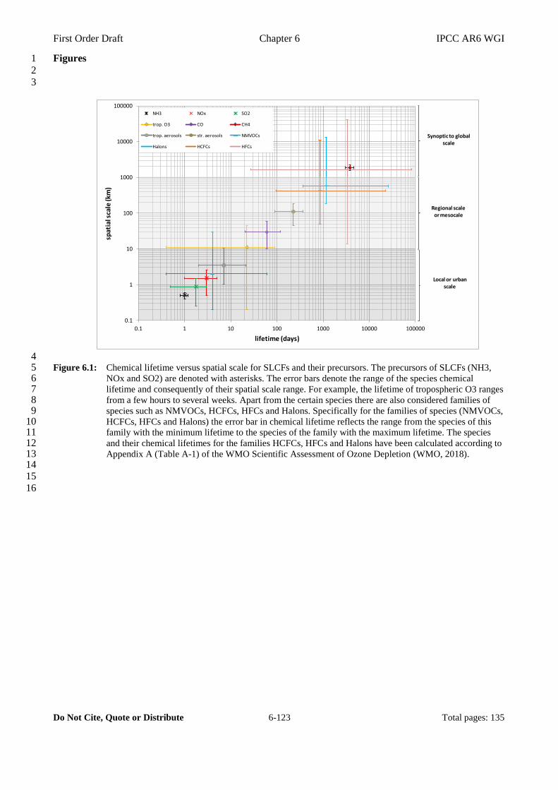
First Order Draft Chapter 6 IPCC AR6 WGI
Do Not Cite, Quote or Distribute 6-123 Total pages: 135
Figures 1
2
3
4 Figure 6.1: Chemical lifetime versus spatial scale for SLCFs and their precursors. The precursors of SLCFs (NH3, 5
NOx and SO2) are denoted with asterisks. The error bars denote the range of the species chemical 6 lifetime and consequently of their spatial scale range. For example, the lifetime of tropospheric O3 ranges 7 from a few hours to several weeks. Apart from the certain species there are also considered families of 8 species such as NMVOCs, HCFCs, HFCs and Halons. Specifically for the families of species (NMVOCs, 9 HCFCs, HFCs and Halons) the error bar in chemical lifetime reflects the range from the species of this 10 family with the minimum lifetime to the species of the family with the maximum lifetime. The species 11 and their chemical lifetimes for the families HCFCs, HFCs and Halons have been calculated according to 12 Appendix A (Table A-1) of the WMO Scientific Assessment of Ozone Depletion (WMO, 2018). 13 14
15
16
0.1
1
10
100
1000
10000
100000
0.1 1 10 100 1000 10000 100000
spat
ial s
cale
(km
)
lifetime (days)
NH3 NOx SO2
trop. O3 CO CH4
trop. aerosols str. aerosols NMVOCs
Halons HCFCs HFCs
Synoptic to global scale
Regional scale or mesocale
Local or urban scale
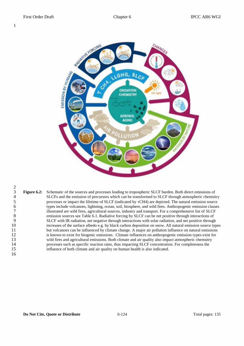
First Order Draft Chapter 6 IPCC AR6 WGI
Do Not Cite, Quote or Distribute 6-124 Total pages: 135
1
2 Figure 6.2: Schematic of the sources and processes leading to tropospheric SLCF burden. Both direct emissions of 3
SLCFs and the emission of precursors which can be transformed to SLCF through atmospheric chemsitry 4 processes or impact the lifetime of SLCF (indicated by CH4) are depicted. The natural emission source 5 types include volcanoes, lightning, ocean, soil, biosphere, and wild fires. Anthropogenic emission classes 6 illustrated are wild fires, agricultural sources, industry and transport. For a comprehensive list of SLCF 7 emission sources see Table 6.1. Radiative forcing by SLCF can be net positive through interactions of 8 SLCF with IR radiation, net negative through interactions with solar radiation, and net positive through 9 increases of the surface albedo e.g. by black carbon deposition on snow. All natural emission source types 10 but volcanoes can be influenced by climate change. A major air pollution influence on natural emissions 11 is known to exist for biogenic emissions. Climate influences on anthropogenic emission types exist for 12 wild fires and agricultural emissions. Both climate and air quality also impact atmospheric chemsitry 13 processes such as specific reaction rates, thus impacting SLCF concentration. For completeness the 14 influence of both climate and air quality on human health is also indicated. 15
16
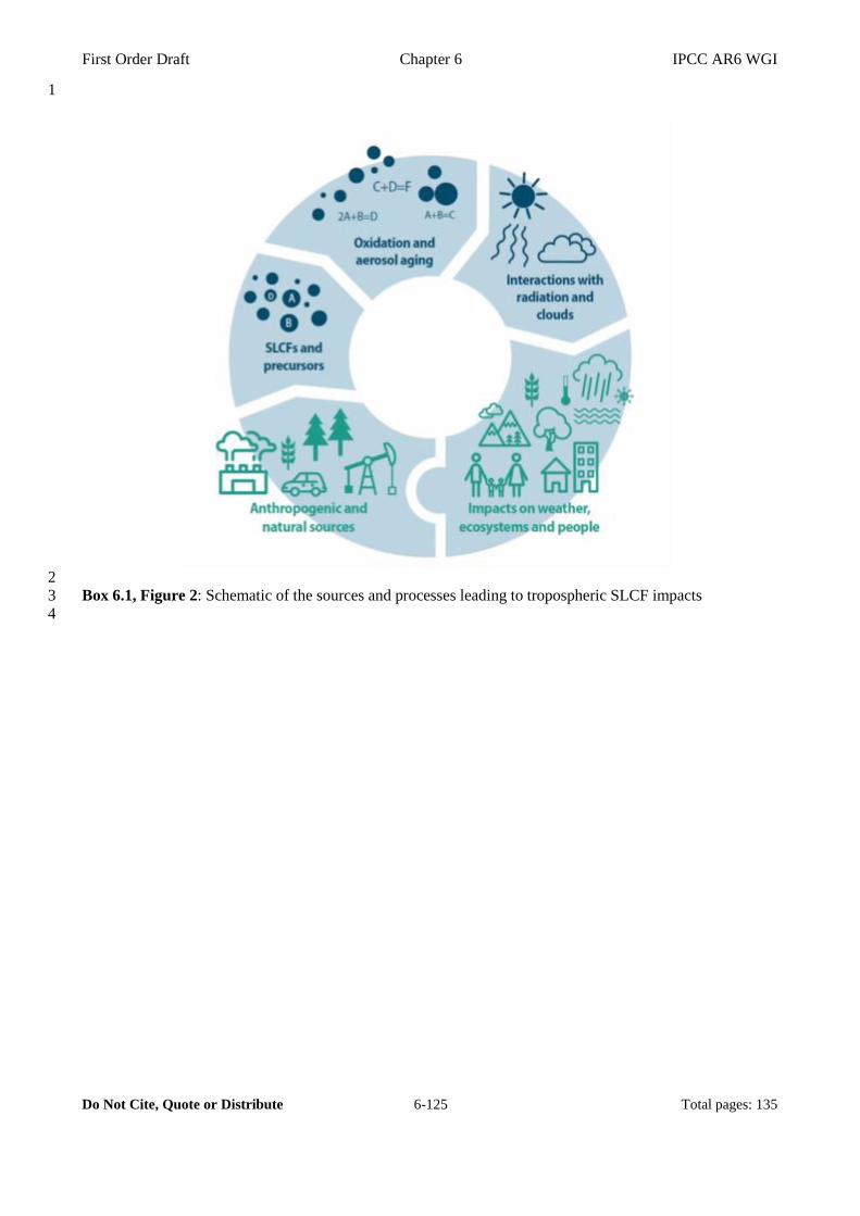
First Order Draft Chapter 6 IPCC AR6 WGI
Do Not Cite, Quote or Distribute 6-125 Total pages: 135
1
2
Box 6.1, Figure 2: Schematic of the sources and processes leading to tropospheric SLCF impacts 3
4
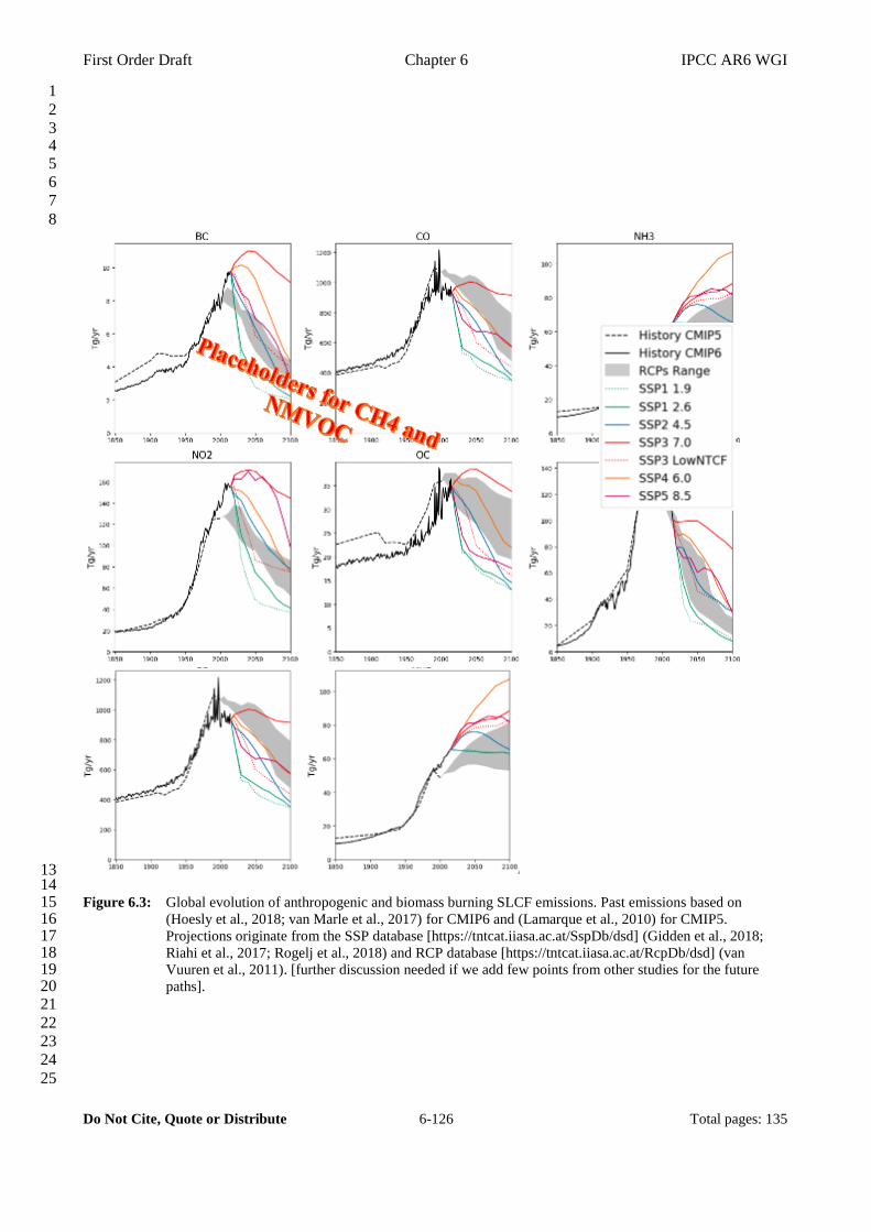
First Order Draft Chapter 6 IPCC AR6 WGI
Do Not Cite, Quote or Distribute 6-126 Total pages: 135
1
2
3 4 5
6
7
8
9
10
11
12
13 14 Figure 6.3: Global evolution of anthropogenic and biomass burning SLCF emissions. Past emissions based on 15
(Hoesly et al., 2018; van Marle et al., 2017) for CMIP6 and (Lamarque et al., 2010) for CMIP5. 16 Projections originate from the SSP database [https://tntcat.iiasa.ac.at/SspDb/dsd] (Gidden et al., 2018; 17 Riahi et al., 2017; Rogelj et al., 2018) and RCP database [https://tntcat.iiasa.ac.at/RcpDb/dsd] (van 18 Vuuren et al., 2011). [further discussion needed if we add few points from other studies for the future 19 paths]. 20
21
22
23
24
25
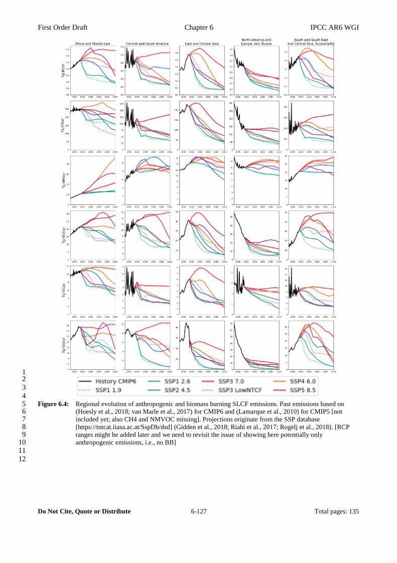
First Order Draft Chapter 6 IPCC AR6 WGI
Do Not Cite, Quote or Distribute 6-127 Total pages: 135
1 2
3
4 Figure 6.4: Regional evolution of anthropogenic and biomass burning SLCF emissions. Past emissions based on 5
(Hoesly et al., 2018; van Marle et al., 2017) for CMIP6 and (Lamarque et al., 2010) for CMIP5 [not 6 included yet; also CH4 and NMVOC missing]. Projections originate from the SSP database 7 [https://tntcat.iiasa.ac.at/SspDb/dsd] (Gidden et al., 2018; Riahi et al., 2017; Rogelj et al., 2018). [RCP 8 ranges might be added later and we need to revisit the issue of showing here potentially only 9 anthropogenic emissions, i.e., no BB] 10
11
12
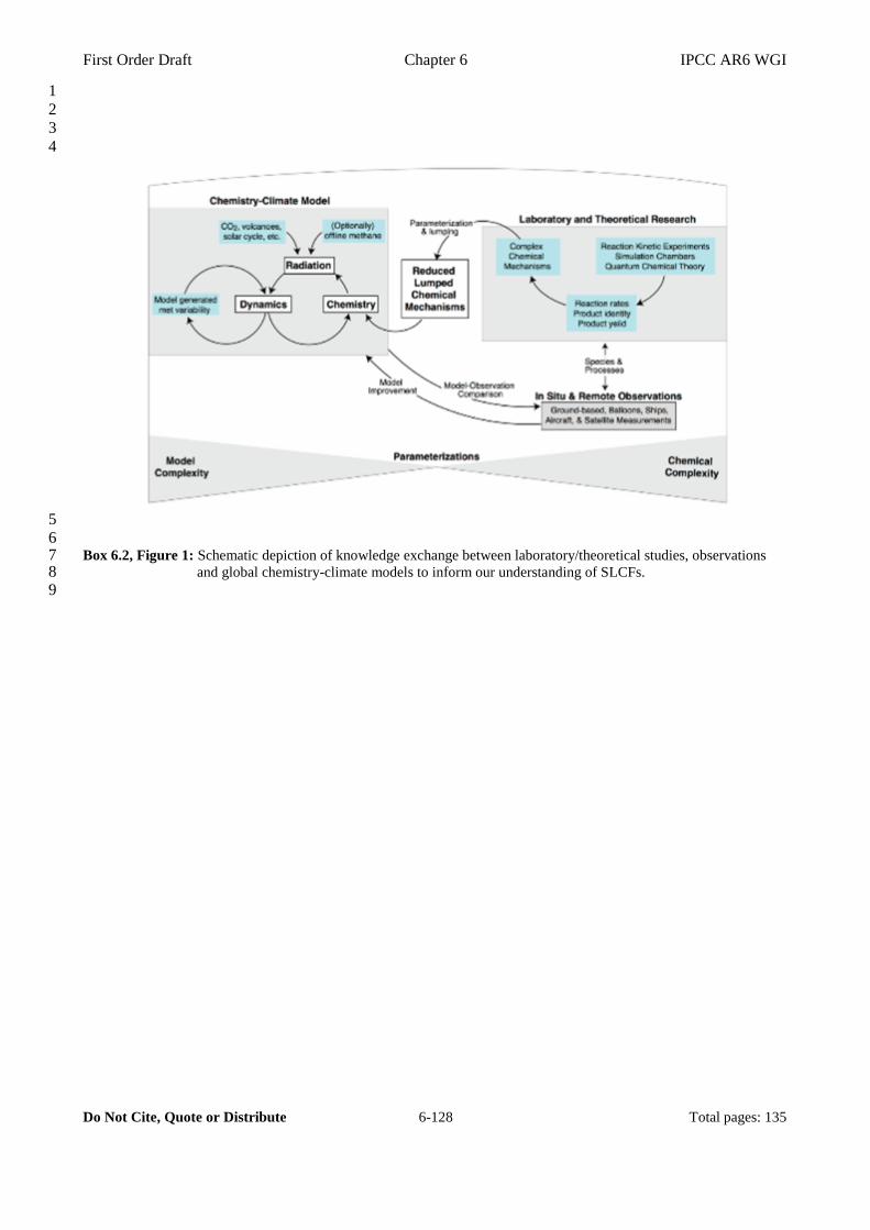
First Order Draft Chapter 6 IPCC AR6 WGI
Do Not Cite, Quote or Distribute 6-128 Total pages: 135
1
2
3
4
5
6 Box 6.2, Figure 1: Schematic depiction of knowledge exchange between laboratory/theoretical studies, observations 7
and global chemistry-climate models to inform our understanding of SLCFs. 8 9
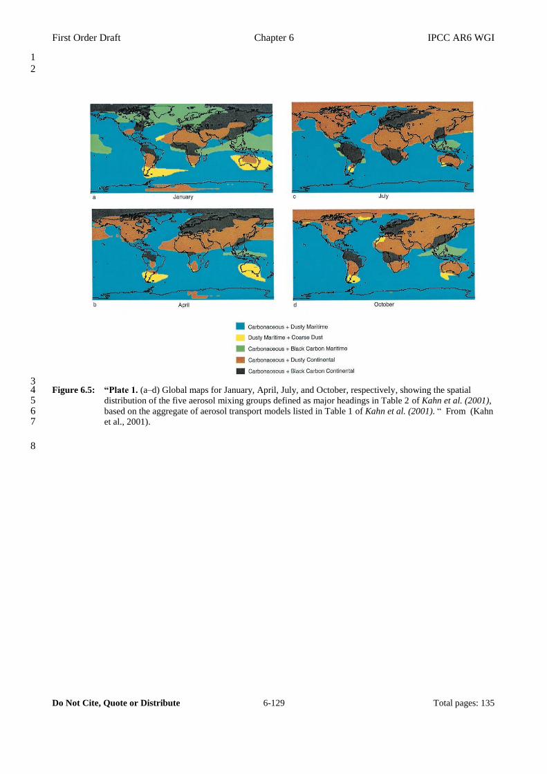
First Order Draft Chapter 6 IPCC AR6 WGI
Do Not Cite, Quote or Distribute 6-129 Total pages: 135
1
2
3 Figure 6.5: “Plate 1. (a–d) Global maps for January, April, July, and October, respectively, showing the spatial 4
distribution of the five aerosol mixing groups defined as major headings in Table 2 of Kahn et al. (2001), 5 based on the aggregate of aerosol transport models listed in Table 1 of Kahn et al. (2001). “ From (Kahn 6 et al., 2001). 7
8
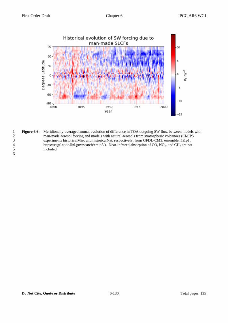
First Order Draft Chapter 6 IPCC AR6 WGI
Do Not Cite, Quote or Distribute 6-130 Total pages: 135
Figure 6.6: Meridionally-averaged annual evolution of difference in TOA outgoing SW flux, between models with 1 man-made aerosol forcing and models with natural aerosols from stratospheric volcanoes (CMIP5 2 experiments historicalMisc and historicalNat, respectively, from GFDL-CM3, ensemble r1i1p1, 3 https://esgf-node.llnl.gov/search/cmip5/). Near-infrared absorption of CO, NOx, and CH4 are not 4 included 5
6
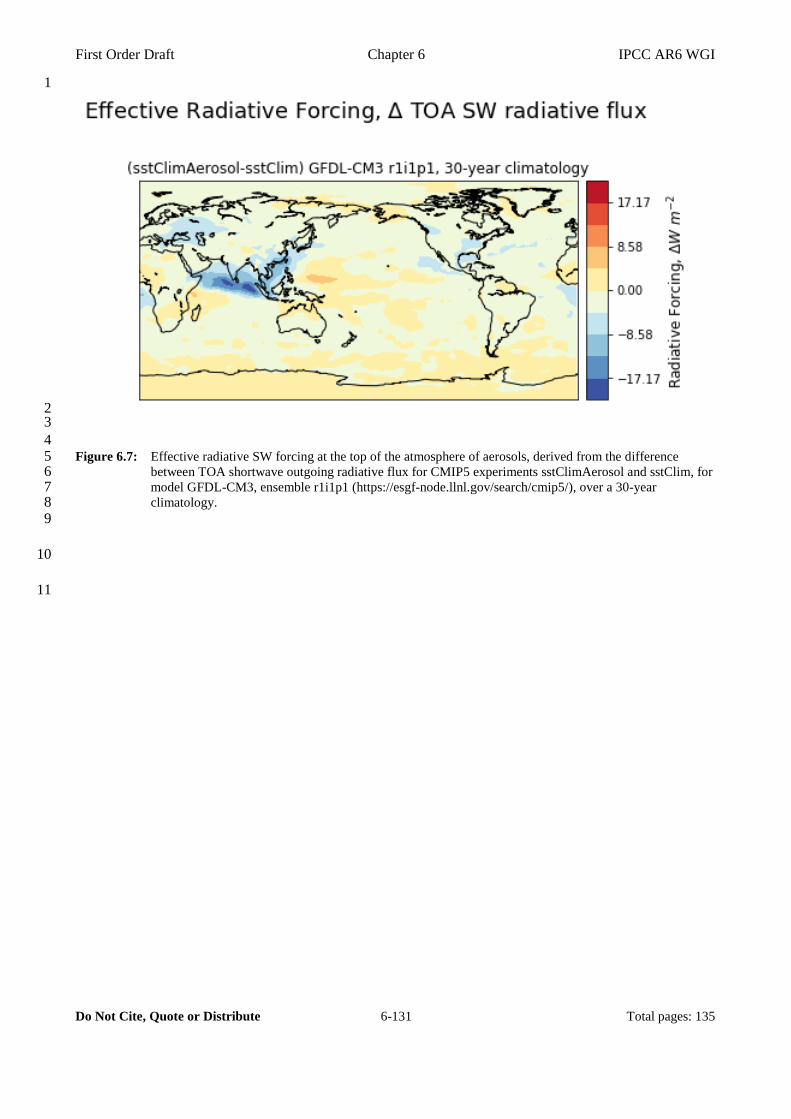
First Order Draft Chapter 6 IPCC AR6 WGI
Do Not Cite, Quote or Distribute 6-131 Total pages: 135
1
2 3
4 Figure 6.7: Effective radiative SW forcing at the top of the atmosphere of aerosols, derived from the difference 5
between TOA shortwave outgoing radiative flux for CMIP5 experiments sstClimAerosol and sstClim, for 6 model GFDL-CM3, ensemble r1i1p1 (https://esgf-node.llnl.gov/search/cmip5/), over a 30-year 7 climatology. 8
9
10
11
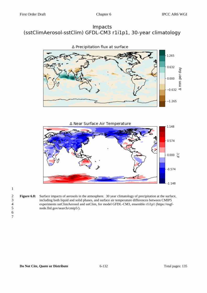
First Order Draft Chapter 6 IPCC AR6 WGI
Do Not Cite, Quote or Distribute 6-132 Total pages: 135
1
Figure 6.8: Surface impacts of aerosols in the atmosphere. 30 year climatology of precipitation at the surface, 2 including both liquid and solid phases, and surface air temperature differences between CMIP5 3 experiments sstClimAerosol and sstClim, for model GFDL-CM3, ensemble r1i1p1 (https://esgf-4 node.llnl.gov/search/cmip5/). 5
6
7
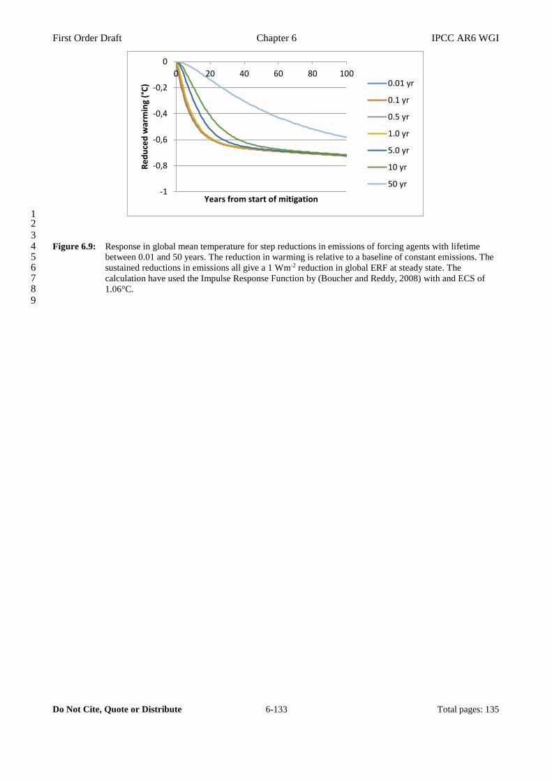
First Order Draft Chapter 6 IPCC AR6 WGI
Do Not Cite, Quote or Distribute 6-133 Total pages: 135
1 2
3 Figure 6.9: Response in global mean temperature for step reductions in emissions of forcing agents with lifetime 4
between 0.01 and 50 years. The reduction in warming is relative to a baseline of constant emissions. The 5 sustained reductions in emissions all give a 1 Wm-2 reduction in global ERF at steady state. The 6 calculation have used the Impulse Response Function by (Boucher and Reddy, 2008) with and ECS of 7 1.06°C. 8
9
-1
-0,8
-0,6
-0,4
-0,2
0
0 20 40 60 80 100
Re
du
ced
war
min
g (°
C)
Years from start of mitigation
0.01 yr
0.1 yr
0.5 yr
1.0 yr
5.0 yr
10 yr
50 yr
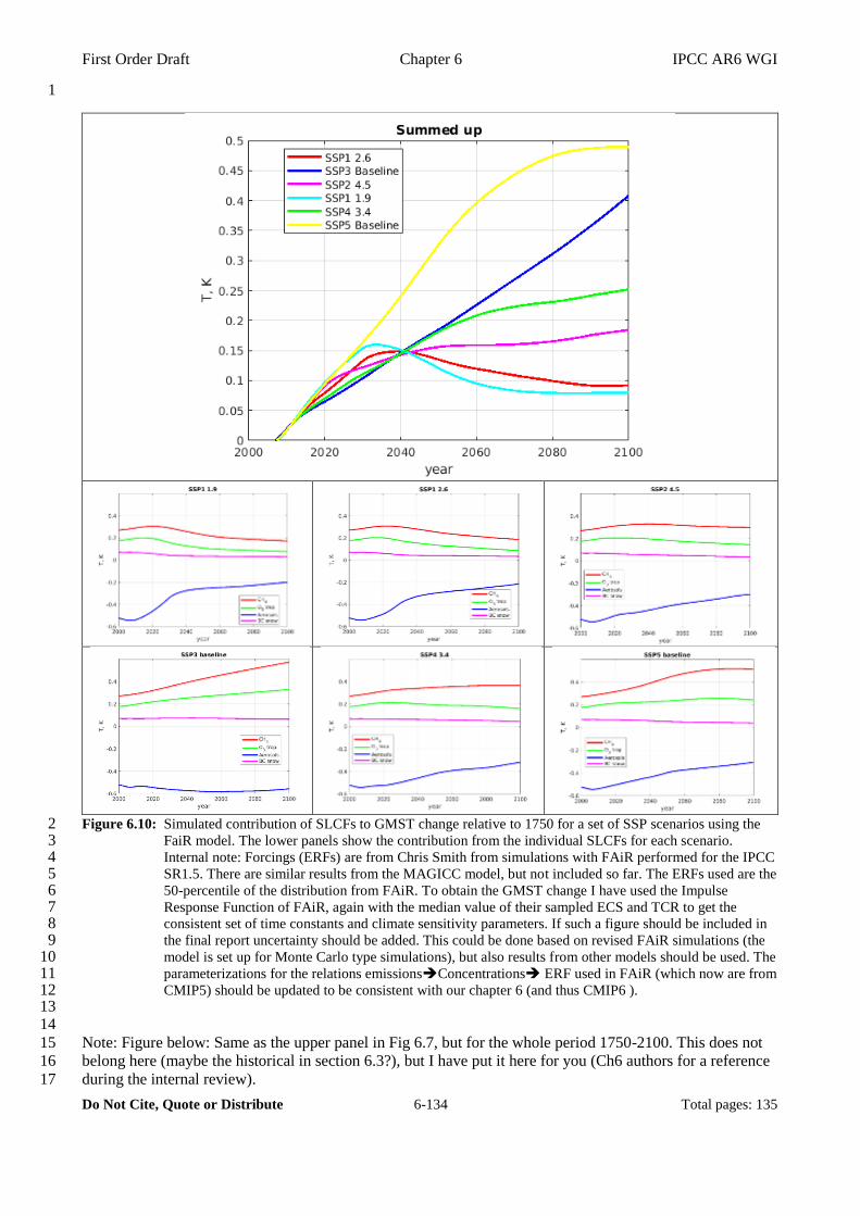
First Order Draft Chapter 6 IPCC AR6 WGI
Do Not Cite, Quote or Distribute 6-134 Total pages: 135
1
Figure 6.10: Simulated contribution of SLCFs to GMST change relative to 1750 for a set of SSP scenarios using the 2
FaiR model. The lower panels show the contribution from the individual SLCFs for each scenario. 3 Internal note: Forcings (ERFs) are from Chris Smith from simulations with FAiR performed for the IPCC 4 SR1.5. There are similar results from the MAGICC model, but not included so far. The ERFs used are the 5 50-percentile of the distribution from FAiR. To obtain the GMST change I have used the Impulse 6 Response Function of FAiR, again with the median value of their sampled ECS and TCR to get the 7 consistent set of time constants and climate sensitivity parameters. If such a figure should be included in 8 the final report uncertainty should be added. This could be done based on revised FAiR simulations (the 9 model is set up for Monte Carlo type simulations), but also results from other models should be used. The 10 parameterizations for the relations emissions➔Concentrations➔ ERF used in FAiR (which now are from 11 CMIP5) should be updated to be consistent with our chapter 6 (and thus CMIP6 ). 12
13 14
Note: Figure below: Same as the upper panel in Fig 6.7, but for the whole period 1750-2100. This does not 15
belong here (maybe the historical in section 6.3?), but I have put it here for you (Ch6 authors for a reference 16
during the internal review). 17
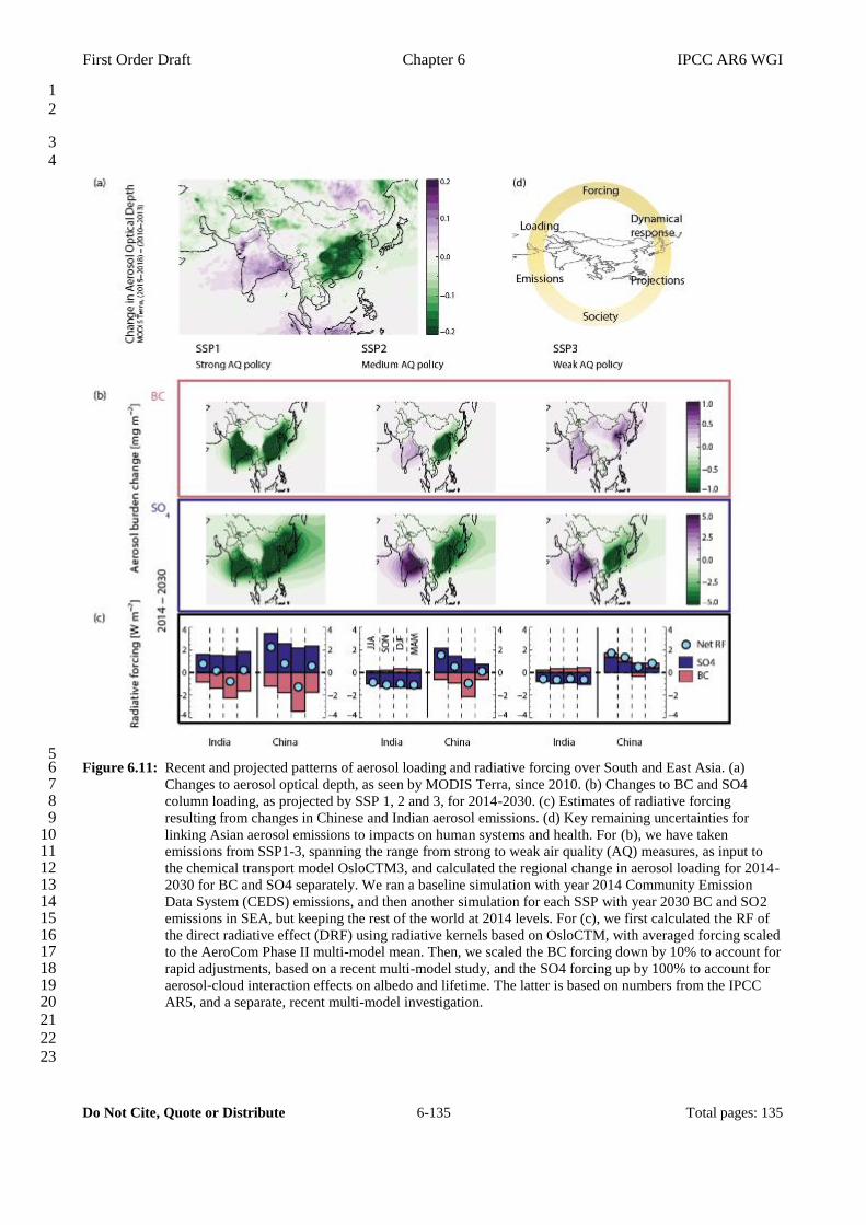
First Order Draft Chapter 6 IPCC AR6 WGI
Do Not Cite, Quote or Distribute 6-135 Total pages: 135
1
2
3
4
5 Figure 6.11: Recent and projected patterns of aerosol loading and radiative forcing over South and East Asia. (a) 6
Changes to aerosol optical depth, as seen by MODIS Terra, since 2010. (b) Changes to BC and SO4 7 column loading, as projected by SSP 1, 2 and 3, for 2014-2030. (c) Estimates of radiative forcing 8 resulting from changes in Chinese and Indian aerosol emissions. (d) Key remaining uncertainties for 9 linking Asian aerosol emissions to impacts on human systems and health. For (b), we have taken 10 emissions from SSP1-3, spanning the range from strong to weak air quality (AQ) measures, as input to 11 the chemical transport model OsloCTM3, and calculated the regional change in aerosol loading for 2014-12 2030 for BC and SO4 separately. We ran a baseline simulation with year 2014 Community Emission 13 Data System (CEDS) emissions, and then another simulation for each SSP with year 2030 BC and SO2 14 emissions in SEA, but keeping the rest of the world at 2014 levels. For (c), we first calculated the RF of 15 the direct radiative effect (DRF) using radiative kernels based on OsloCTM, with averaged forcing scaled 16 to the AeroCom Phase II multi-model mean. Then, we scaled the BC forcing down by 10% to account for 17 rapid adjustments, based on a recent multi-model study, and the SO4 forcing up by 100% to account for 18 aerosol-cloud interaction effects on albedo and lifetime. The latter is based on numbers from the IPCC 19 AR5, and a separate, recent multi-model investigation. 20
21
22
23