1. Chapter 1: Framing, context, methods - IPCC
184
First Order Draft Chapter 1 IPCC AR6 WGI Do Not Cite, Quote or Distribute 1-1 Total pages: 184 1. Chapter 1: Framing, context, methods 1 2 3 4 Coordinating Lead Authors: 5 Deliang Chen (Sweden), Maisa Rojas (Chile) 6 7 Lead Authors: 8 Kim Cobb (USA), Aida Diongue-Niang (Senegal), Paul Edwards (USA), Seita Emori (Japan), Sergio 9 Henrique Faria (Spain/Brazil), Ed Hawkins (UK), Pandora Hope (Australia), Philippe Huybrechts 10 (Belgium), Malte Meinshausen (Australia/Germany), Sawsan Mustafa (Sudan), Gian-Kasper Plattner 11 (Switzerland), Bjørn Samset (Norway), Anne Marie Treguier (France) 12 13 Contributing Authors: 14 Maarten van Aalst (Netherlands), Rondrotiana Barimalala (South Africa/Madagascar), Rosario Carmona 15 (Chile), Peter Cox (UK), Wolfgang Cramer (France/Germany), Francisco Doblas-Reyes (Spain), Alessandro 16 Dosio (Italy), Veronika Eyring (Germany), David Frame (New Zealand), Joelle Gergis (Australia), 17 Nathan Gillet (UK), Michael Grose (Australia), Eric Guilyardi (France), Celine Guivarch (France), Susan 18 Hassol (USA), Zeke Hausfather (USA), Bart van den Hurk (Netherlands), Richard Jones (UK), Anthony 19 Leiserowitz (USA), Rob Lempert (USA), Hong Liao (China), Nikki Lovenduski (USA), Jochem Marotzke 20 (Germany), Zebedee Nicholls (Australia), Brian O’Neill (USA), Friederike Otto (UK/Germany), Wendy 21 Parker (UK), Warren Pearce (UK), James Renwick (New Zealand), Joeri Rogelj (Belgium), Jana Sillmann 22 (Norway/Germany), Rodolfo Sapiains (Chile), Sonia Seneviratne (Switzerland) Lucas Silva 23 (Portugal/Switzerland), Anna Sorensson (Argentina), Thomas F. Stocker (Switzerland), Abigail Swann 24 (USA), Izuru Takayabu (Japan), Claudia Tebaldi (USA), Blair Trewin (Australia) 25 26 Review Editors: 27 Nares Chuersuwan (Thailand), Gabriele Hegerl (UK/Germany), Tetsuzo Yasunari (Japan) 28 29 Chapter Scientist: 30 Hui-Wen Lai (Sweden) 31 32 Date of Draft: 33 29 April 2019 34 35 Notes: 36 TSU Compiled version 37 38 39 40 41 42 43 44 45 46 47
-
Upload
khangminh22 -
Category
Documents
-
view
2 -
download
0
Transcript of 1. Chapter 1: Framing, context, methods - IPCC

First Order Draft Chapter 1 IPCC AR6 WGI
Do Not Cite, Quote or Distribute 1-1 Total pages: 184
1. Chapter 1: Framing, context, methods 1
2
3
4
Coordinating Lead Authors: 5
Deliang Chen (Sweden), Maisa Rojas (Chile) 6
7
Lead Authors: 8
Kim Cobb (USA), Aida Diongue-Niang (Senegal), Paul Edwards (USA), Seita Emori (Japan), Sergio 9
Henrique Faria (Spain/Brazil), Ed Hawkins (UK), Pandora Hope (Australia), Philippe Huybrechts 10
(Belgium), Malte Meinshausen (Australia/Germany), Sawsan Mustafa (Sudan), Gian-Kasper Plattner 11
(Switzerland), Bjørn Samset (Norway), Anne Marie Treguier (France) 12
13
Contributing Authors: 14
Maarten van Aalst (Netherlands), Rondrotiana Barimalala (South Africa/Madagascar), Rosario Carmona 15
(Chile), Peter Cox (UK), Wolfgang Cramer (France/Germany), Francisco Doblas-Reyes (Spain), Alessandro 16
Dosio (Italy), Veronika Eyring (Germany), David Frame (New Zealand), Joelle Gergis (Australia), 17
Nathan Gillet (UK), Michael Grose (Australia), Eric Guilyardi (France), Celine Guivarch (France), Susan 18
Hassol (USA), Zeke Hausfather (USA), Bart van den Hurk (Netherlands), Richard Jones (UK), Anthony 19
Leiserowitz (USA), Rob Lempert (USA), Hong Liao (China), Nikki Lovenduski (USA), Jochem Marotzke 20
(Germany), Zebedee Nicholls (Australia), Brian O’Neill (USA), Friederike Otto (UK/Germany), Wendy 21
Parker (UK), Warren Pearce (UK), James Renwick (New Zealand), Joeri Rogelj (Belgium), Jana Sillmann 22
(Norway/Germany), Rodolfo Sapiains (Chile), Sonia Seneviratne (Switzerland) Lucas Silva 23
(Portugal/Switzerland), Anna Sorensson (Argentina), Thomas F. Stocker (Switzerland), Abigail Swann 24
(USA), Izuru Takayabu (Japan), Claudia Tebaldi (USA), Blair Trewin (Australia) 25
26
Review Editors: 27
Nares Chuersuwan (Thailand), Gabriele Hegerl (UK/Germany), Tetsuzo Yasunari (Japan) 28
29
Chapter Scientist: 30
Hui-Wen Lai (Sweden) 31
32
Date of Draft: 33
29 April 2019 34
35
Notes: 36
TSU Compiled version 37
38
39
40
41
42
43
44
45
46
47

First Order Draft Chapter 1 IPCC AR6 WGI
Do Not Cite, Quote or Distribute 1-2 Total pages: 184
1
Executive Summary ........................................................................................................................................... 4 2
1.1 Chapter preview ..................................................................................................................................... 6 3
1.2 The global context of the present assessment ........................................................................................ 6 4
1.2.1 The changing state of the physical climate system ........................................................................ 7 5
1.2.1.1 Change across multiple indicators ............................................................................................. 7 6
1.2.1.2 Change across multiple timescales ............................................................................................ 8 7
1.2.2 International governance to address challenges posed by climate change .................................... 9 8
Cross-Chapter Box 1.1: The WGI AR6 Contribution and its Relevance for the Global Stocktake ............. 11 9
1.2.3 Climate, science, and societies: perceptions, values, and ethics .................................................. 20 10
1.2.4 New approaches in the WGI AR6 report ..................................................................................... 21 11
1.2.4.1 Risk framing ............................................................................................................................ 22 12
Cross-Chapter Box 1.2: Risk Framing in IPCC AR6 ................................................................................... 24 13
1.2.4.2 Abrupt climate change, tipping points, and surprises .............................................................. 26 14
1.2.4.3 Narratives and Storylines ......................................................................................................... 27 15
1.3 History of climate understanding ........................................................................................................ 28 16
1.3.1 Climate science before 1950 ........................................................................................................ 28 17
1.3.2 Climate understanding matures: 1950-1990 ................................................................................ 30 18
1.3.3 Climate science and global change, 1990-present: the IPCC era ................................................ 34 19
Box 1.1: Treatment of uncertainty and calibrated uncertainty language used in IPCC reports ................. 37 20
1.3.4 Key findings of previous IPCC assessments ............................................................................... 39 21
1.3.4.1 Key findings of AR5................................................................................................................ 39 22
1.3.4.2 Key findings of post-AR5 Special Reports ............................................................................. 41 23
1.3.5 How do previous climate projections compare with subsequent observations? .......................... 42 24
1.4 Developments in observing systems, reanalyses, climate modelling and other techniques ................ 44 25
1.4.1 Observational data and observing systems .................................................................................. 44 26
1.4.2 Reanalyses ................................................................................................................................... 47 27
1.4.3 Climate Models............................................................................................................................ 49 28
1.4.3.1 Earth System Models ............................................................................................................... 49 29
1.4.3.2 Models of lower complexity .................................................................................................... 53 30
1.4.3.3 Model tuning and adjustment .................................................................................................. 54 31
1.4.4 Modelling techniques, comparisons and performance assessments ............................................ 55 32
1.4.4.1 The sixth phase of the Coupled Model Intercomparison Project (CMIP6) ............................. 57 33
1.4.4.2 CMIP Evaluation Tools ........................................................................................................... 60 34
1.4.4.3 Evaluation against observations .............................................................................................. 61 35
1.4.4.4 Climate informatics ................................................................................................................. 61 36
1.4.5 Techniques for constraining uncertainties and informing projections ......................................... 62 37
1.4.5.1 Scaling based on detection and attribution .............................................................................. 62 38
1.4.5.2 Emergent constraints on climate feedbacks, sensitivities and projections .............................. 63 39
1.4.5.3 Weighting techniques for model comparisons ........................................................................ 64 40

First Order Draft Chapter 1 IPCC AR6 WGI
Do Not Cite, Quote or Distribute 1-3 Total pages: 184
1.5 Cross-cutting topics for this assessment: variability, regional definitions, uncertainty, reference 1
periods and attribution ..................................................................................................................................... 64 2
1.5.1 Natural variability and the emergence of the climate change signal ........................................... 65 3
1.5.1.1 How does variability influence trends over short periods? ...................................................... 65 4
1.5.1.2 The emergence of the climate change signal ........................................................................... 65 5
1.5.2 Regional climate change .............................................................................................................. 66 6
1.5.2.1 Foundations of the definition of climate regions ..................................................................... 66 7
1.5.2.2 Types of regions used in AR6 ................................................................................................. 67 8
1.5.3 Anomalies, baselines and warming since pre-industrial .............................................................. 68 9
1.5.3.1 Why are anomalies used? ........................................................................................................ 68 10
1.5.3.2 What is meant by a ‘pre-industrial’ baseline? ......................................................................... 69 11
Cross-Chapter Box 1.3: Baselines used in AR6 ........................................................................................... 70 12
1.5.4 Sources of uncertainty in climate projections .............................................................................. 72 13
1.5.5 Attribution of climatic changes ................................................................................................... 73 14
Cross-Chapter Box 1.4: Attribution in the IPCC Sixth Assessment Report ................................................. 73 15
1.6 Dimensions of Integration: Scenarios, temperature levels and cumulative carbon emissions ............ 76 16
1.6.1 Dimensions of knowledge integration within and across Working Groups ................................ 77 17
1.6.2 Scenarios reflecting choices within an uncertain future .............................................................. 79 18
1.6.2.1 Scenarios with their shared socio-economic pathways, their reference and mitigation 19
scenarios .................................................................................................................................. 82 20
1.6.2.2 Scenarios in the context of the Paris Agreement ..................................................................... 84 21
1.6.3 Temperature levels as additional tool for cross-Working Group integration .............................. 85 22
Cross-Chapter Box 1.5: Physical emulators of global mean temperatures for scenario classification and 23
knowledge integration. ............................................................................................. 86 24
1.6.4 Cumulative CO2 Emissions as a new dimension of integration .................................................. 90 25
1.6.5 How do AR6 scenarios compare with those used in previous IPCC reports? ............................. 91 26
Cross-Chapter Box 1.6: Scenarios, Projections, Pathways and temperature-levels ..................................... 94 27
1.7 Gaps and opportunities for integration of climate knowledge ............................................................. 98 28
1.8 Structure / key elements of AR6 .......................................................................................................... 99 29
Frequently Asked Questions .......................................................................................................................... 101 30
FAQ 1.1: Do we understand climate change better now, compared to when the IPCC started? ........... 101 31
FAQ 1.2: At what point do we know it’s climate change? .................................................................... 103 32
FAQ 1.3: What can past climate teach us about the future? .................................................................. 104 33
FAQ 1.4: How do we calculate global temperature change?................................................................. 106 34
References ..................................................................................................................................................... 107 35
Appendix 1.A ................................................................................................................................................ 139 36
Figures: .......................................................................................................................................................... 149 37
38
39
First Order Draft Chapter 1 IPCC AR6 WGI
Do Not Cite, Quote or Distribute 1-4 Total pages: 184
Executive Summary 1
2
The IPCC 6th Assessment Report assessing information that is relevant for the knowledge needs of a 3
world that is rapidly changing, in terms of the physical climate system and the international processes 4
set in place to address the changes and resulting challenges. The Paris Agreement set a long-term goal to 5
hold the increase in the global average temperature to “well below 2°C above pre-industrial levels and to 6
pursue efforts to limit the temperature increase to 1.5°C above pre-industrial levels, recognizing that this 7
would significantly reduce the risks and impacts of climate change”. Together with a range of related 8
international processes and initiatives, such as the Sustainable Development Goals, the Sendai Framework 9
for Disaster Risk Reduction, the Global Framework of the Climate Services, and the Intergovernmental 10
Science-Policy Platform on Biodiversity and Ecosystem Services, the Paris Agreement forms a key framing 11
for the present report. A consistent risk framework is adopted across the 6th Assessment Report. {1.2, 1.2.2, 12
1.2.4} 13
14
The IPCC 5th Assessment Report (AR5) concluded that warming of the climate system is unequivocal. 15
Since the AR5, multiple concurrent changes have continued throughout the physical climate system, 16
including increasing global mean surface temperature, loss of glacial mass, sea level rise, increasing 17
ocean heat content, changes to global precipitation patterns, and rising greenhouse gas concentrations. 18
Many of these changes occur at rates and magnitudes beyond what can be attributed to natural variability. 19
The rapid changes to the physical climate system represent a key framing for the present report. The changes 20
presently observed are significant even when considering a long time frame such as the last two millennia. 21
Multiple independent lines of evidence, reaching from the recent observational era back to the mid Pliocene 22
(3.6 million years BP), indicate the unique nature of the present, global scale rate of change, even when seen 23
in the context of a million year period. {1.2.1} 24
25
Understanding of essential features of the climate system is robust and well established. The major 26
natural forcings governing the climate system have been known since the early 20th century. The possibility 27
of anthropogenic climate change was proposed in the 19th century, and major anthropogenic forcings 28
(primarily heat-trapping gases and aerosols) were established by the mid-1970s. Since systematic scientific 29
assessments began in the late 1970s, anthropogenic climate change has evolved from a hypothesis to a fact. 30
Climate change projections made since the 1980s are generally in good agreement with the amplitude and 31
pattern of subsequent observed temperature change. {1.3} 32
33
Capabilities to observe across the breadth of the physical climate system continue to improve and 34
expand, but recent and/or pending losses in key observational systems underscore the vulnerability of 35
some classes of climate observations. Progress in climate science relies on the quality and quantity of 36
observations from a range of platforms: surface-based instrumental measurements, aircraft observations, 37
satellite-based retrievals, in-situ measurements and palaeoclimatic records. Overall, observational coverage of 38
the climate system is as good for the AR6 as it was for the AR5, with notable improvements in some areas, 39
but also some emerging risks of loss of coverage or continuity. In addition to the reduced coverage of certain 40
satellite products, surface station networks, and radiosonde launches, paleoclimate archives such as corals, 41
tropical ice cores, and trees are rapidly disappearing owing to a host of anthropogenic pressures, including 42
high temperatures caused by anthropogenic climate change (high confidence) {1.4.1} 43
44
New reanalyses have been developed with various combinations of increased resolution, extended 45
records, more consistent data assimilation, and/or a full representation of the coupled atmosphere-46
ocean system. Reanalysis datasets provide gridded output, physical consistency across variables (within the 47
limitations of the forecast model used), information about variables that are not directly observed, and 48
information at locations that are unobserved. {1.4.2} 49
50
Climate models have been further improved since the AR5, with more Earth system models that 51
represent biogeochemical cycles and more high resolution models that capture small-scale processes 52
and extremes. Improved constraints on cloud and carbon cycle feedbacks have been deduced from 53
observations since AR5 and these in turn constrain climate sensitivity and future projections. {1.4.3} 54
55
First Order Draft Chapter 1 IPCC AR6 WGI
Do Not Cite, Quote or Distribute 1-5 Total pages: 184
New tools and advanced techniques are available to more rapidly and comprehensively evaluate 1
climate and Earth system models, attribute observed changes, and constrain the ranges of key Earth 2
system variables. There is now a host of methods to attribute change in events, impacts, and even adaptive 3
measures. Newly developed evaluation tools ensure traceability and reproducibility of the results from model 4
evaluation and analysis. Moreover, the emerging use of machine learning in climate science complements 5
classical model evaluation approaches and provides new insights on the dynamics of the climate system. 6
Large ensembles of climate model simulations have supported improved understanding of the relative roles 7
of internal variability and forced change in the climate system. {1.4.4; 1.4.5; 1.5.5} 8
9
Regional climate change is emphasized in AR6 and throughout this Working Group I report. A 10
unified set of land and ocean regions is introduced. These regions are semi-continental domains defined in 11
terms of characteristic climate and environmental features, as recognized from the assessed literature. 12
Particular aspects of climate change are also addressed in this report by higher-resolution, specialized 13
domains called typological regions such as monsoon regions, mountains, megacities, etc. {1.5.2; 1.8} 14
15
The early industrial period (1850-1900) is used as an approximation for pre-industrial global 16
temperatures. In terms of radiative forcing, “pre-industrial” refers to the period around 1750 when large-17
scale natural forcings (solar irradiance, astronomical factors, and volcanic activity) were similar to the 18
modern period. It is likely (medium confidence) that some anthropogenic warming occurred before 1850; the 19
magnitude of this warming is between 0.0-0.1°C. {1.5.3} 20
21
In addition to internal variability, uncertainties in projections of the physical climate system stem 22
from a number of sources. These include (a) the actual future trajectory of radiative forcing, which depends 23
on sociotechnical change (including climate policy) and natural events such as volcanic eruptions, and (b) 24
how the climate will respond to that specific trajectory. A third source of uncertainty regards “unknown 25
unknowns”, or possible aspects of climatic behavior not yet identified or accounted for. {1.5.4} 26
27
In AR6 scenarios, future temperature levels and cumulative carbon emissions are used as dimensions 28
of integration within and across the three IPCC Working Groups. A new set of emission and 29
concentration scenarios, the Shared Socioeconomic Pathways (SSPs), is used to synthesize knowledge across 30
the physical sciences, impact and adaptation and mitigation research. Two additional ‘dimensions of 31
integration’ are global mean temperature levels as well as a categorization of emission scenarios or 32
geophysical impacts in relation to their cumulative carbon emissions. The SSP scenarios cover lower levels 33
of warming compared to previous Assessment Reports, including scenarios consistent with a 1.5°C warming 34
in line with the lower climate target envisaged in the Paris Agreement {1.6} 35
36
Reducing key knowledge gaps via the integration of knowledge across disciplines will accelerate 37
climate understanding. A better understanding of climate processes and phenomena leads to better 38
informed risk assessment, and it is therefore important to identify areas primed for rapid advances. {1.7} 39
40
First Order Draft Chapter 1 IPCC AR6 WGI
Do Not Cite, Quote or Distribute 1-6 Total pages: 184
1
1.1 Chapter preview 2
3
The Sixth Assessment Report (AR6) of the Intergovernmental Panel on Climate Change (IPCC) now marks 4
more than 30 years of global international collaboration to describe and understand one of the defining 5
challenges of the 21st century and beyond: human-induced climate change. Since the inception of the IPCC 6
in 1990, our understanding of the physical science basis of climate change has much advanced, and the 7
amount and quality of direct observations and information from palaeoclimate archives has substantially 8
increased. Climate model capabilities have evolved in line with the increased computational capacities of the 9
world's supercomputers, understanding of individual processes has improved, and there is more realistic 10
treatment of interactions among the components of the climate system. At the same time, some key 11
assessment conclusions from previous IPCC reports remained practically unchanged, indicating the 12
robustness of our understanding around the primary causes and consequences of anthropogenic climate 13
change. 14
15
The role of the IPCC is to assess on a comprehensive, objective, open and transparent basis the scientific, 16
technical and socio-economic information relevant to understanding the risks of human-induced climate 17
change, its potential impacts and options for adaptation and mitigation. Starting from the work on the First 18
Assessment Report (FAR) published in 1990, the IPCC Assessments have been structured into three 19
Working Groups. Working Group I (WGI) assesses the physical science basis of climate change, Working 20
Group II (WGII) assesses associated impacts, vulnerability and adaptation to climate change, and Working 21
Group III (WGIII) assesses mitigation response options. The volume of knowledge and also the cross-22
linkages between the three Working Groups has evolved over time. 23
24
As part of the AR6 cycle from 2017 to 2022, the IPCC is preparing the set of the three Working Group 25
reports plus three targeted Special Reports and, finally, the Synthesis Report. The three AR6 Special Reports 26
cover the topics of “Global Warming of 1.5°C”, “Climate Change and Land” and the “The Ocean and 27
Cryosphere in a Changing Climate” and are, for the first time in the IPCC, coordinated across all three 28
Working Groups. 29
30
This chapter provides the introduction to the WGI contribution to the AR6. The main purposes of the 31
Chapter are: 1) to frame AR6 in the current global context with a focus on international climate governance 32
frameworks, 2) to set the scene for the assessment and to place it in the context of ongoing global changes, 33
the history of climate science and the evolution from previous IPCC assessments, including the Special 34
Reports prepared as part of this Assessment Cycle, 3) to describe key concepts, approaches, and methods 35
used in this assessment. 36
37
The Chapter comprises eight sections. The present state of Earth’s climate, in the context of observed long-38
term changes and variations caused by natural and anthropogenic drivers, as well as the international climate 39
change governance structure, which serves as context to the present assessment, are described in section 1.2. 40
The evolution of knowledge about climate change and the development of earlier IPCC assessments is 41
presented in Section 1.3. New developments in observations, reanalyses, modelling capabilities and 42
techniques since AR5 are discussed in Section 1.4. Approaches, methods, and key concepts of this 43
assessment are introduced in Section 1.5. The three main ‘dimensions of integration’ across Working Groups 44
in the AR6, i.e. scenarios, temperature levels and cumulative carbon emissions, are described in Section 1.6. 45
The Chapter closes with a discussion of opportunities and gaps in knowledge integration in Section 1.7, 46
before presenting the structure and chapter organization of the overall WGI AR6 report in Section 1.8. 47
48
49
1.2 The global context of the present assessment 50
51
The context of the IPCC 6th Assessment cycle is different from those of its predecessors. Numerous, 52

First Order Draft Chapter 1 IPCC AR6 WGI
Do Not Cite, Quote or Distribute 1-7 Total pages: 184
substantial changes have been observed across the physical climate system, many of which can be attributed 1
to anthropogenic influences, with impacts on natural and human systems. Governments and societies are 2
responding to these changes and deciding on specific courses of action to mitigate and adapt to 3
anthropogenic climate change. 4
5
This section summarizes key elements of this context. Starting by illustrating the changing state of the 6
climate system, as presently observed and in a longer term context (1.2.1). Then, summarizing ongoing 7
processes in international governance that form part of the wider context of the AR6 process (1.2.2), and 8
changes to the wider perceptions of climate change and climate science (1.2.3). Finally, approaches and 9
rationale that are different in the present assessment cycle, relative to past IPCC assessment cycles, are 10
introduced (1.2.4): The risk framing, the possibility of abrupt climate change, and the usage of narratives and 11
storylines. 12
13
14
1.2.1 The changing state of the physical climate system 15
16
The starting point for the present report is the context of rapid, ongoing changes in the physical climate 17
system, increased monitoring capability, and improved knowledge. In 2013, the WGI contribution to the 18
IPCC AR5 (AR5WGI) concluded that “warming of the climate system is unequivocal,” and since the 1950s, 19
many of the observed changes are unprecedented over decades to millennia (IPCC, 2013b) 20
21
Since AR5, changes to the state of the physical climate system have continued, and, in places, accelerated. 22
Details of these changes are assessed in full in the coming chapters. Ongoing changes are illustrated through 23
key large-scale observables and shown in relation to the longer-term evolution of the climate. 24
25
26
1.2.1.1 Change across multiple indicators 27
28
The physical climate system comprises all components and processes that combine to form weather and 29
climate. Broadly speaking the physical climate system is divided into five realms: The atmosphere, the land 30
surface, the cryosphere, the oceans and the biosphere. Figure 1.1 shows these components of the climate 31
system, highlights a set of related indicators of rapidly evolving changes, and links to their full assessment in 32
subsequent chapters. The climate change ‘rosette’ shows year-to-year variability, as deviations from their 33
mean (see caption), illustrating that many components of the climate system have now been altered outside 34
of their natural range of interannual variability. Here, natural variability is estimated from the observed 35
record, but in Section 1.2.1.2, variability in longer records is also discussed. 36
37
[Note: The following discussion uses earlier datasets as placeholders and will be updated for the Second 38
Order Draft based] 39
40
Atmospheric concentrations of a range of greenhouse gases are increasing, notably carbon dioxide 41
(CO2), methane (CH4), and nitrous oxide (N2O). These observed changes are consistent with known 42
anthropogenic emissions, when accounting for observed and inferred uptake by the oceans and biosphere 43
respectively. Presently, the global mean CO2 concentration is increasing by [XX] ppm per year. Figure 1.1 44
(wedges a and b), shows the evolution of global mean surface temperature (GMST) since 1850, and the 45
concentration of CO2 at Mauna Loa since 1959. 46
47
Both the atmosphere and the land surface are undergoing rapid changes. Most notably, the global mean 48
surface temperature has increased by [XX] °C since [YYYY] and is presently increasing at a rate of 0.17 °C 49
per decade [SR15]. 50
51
Precipitation patterns are also changing, but with a different regional pattern than surface temperature. Figure 52
1.1 (wedge c) shows the evolution of annual mean precipitation over land in five latitude bands (shown is the 53
[XXX] series of observations, available for the period [19XX-201X]). [Considering changing this to a time 54
series of ocean surface pH.] 55

First Order Draft Chapter 1 IPCC AR6 WGI
Do Not Cite, Quote or Distribute 1-8 Total pages: 184
1
The cryosphere, which comprises all frozen parts of the globe, including terrestrial snow, permafrost, sea ice, 2
glaciers, and the massive ice sheets covering Greenland and Antarctica, is also undergoing rapid changes. 3
Globally, glaciers have been continuously losing mass for the last century; presently their mass balance is at 4
[-XXX] Gt/year. See Figure 1.1 (wedge d). 5
6
In the oceans as well, changes have progressed beyond year-to-year variability. Notably, the averaged heat 7
content of the oceans down to [700, 2000] meters is steadily increasing, presently at a rate of [XX] GJ/year 8
(Figure 1.1, wedge e). The global mean sea level is rising at the rate of [XX] mm/year over [19XX-20XX] 9
(Figure 1.1, wedge f), and this rate has itself increased, from [XX] mm/yr over [19XX-19XX]. 10
11
Figure 1.1 presents examples of datasets illustrating recent changes. Overall, the current conditions are such 12
that s one of marked, ongoing and concurrent changes to many components of the physical climate system. 13
These changes, and many others, will be further presented in the coming chapters, together with a rigorous 14
assessment of the recent supporting literature. 15
16
17
[START FIGURE 1.1 HERE] 18 19 Figure 1.1: The changing state of the physical climate system. Left: Schematic of the components of the climate 20
system, and examples of how key physical observables are changing. Right: Each wedge of the rosette 21 shows annual means of one variable, from 1850 (center) out to 2017 (outer circle). Grey indicates missing 22 data. [To be updated for SOD. All data plotted so far temporary, taken predominantly from AR5.] 23
24
[END FIGURE 1.1 HERE] 25
26
27
1.2.1.2 Change across multiple timescales 28
29
Information from paleoclimate archives provides an essential long-term context for the anthropogenic 30
climate change of the past 150 years and the projected changes in the 21st century and beyond (Masson-31
Delmotte et al., 2013). Figure 1.2 shows reconstructions of three key indicators of change over the past 32
800,000 years, comprising eight complete glacial-interglacial cycles (EPICA Community Members, 2004). 33
The dominant 100,000-year cycles are characterized by natural CO2 variations between 174 ppm and 299 34
ppm (±1.3 ppm), as measured directly in air trapped in ice at Dome Concordia, Antarctica (Bereiter et al., 35
2015; Lüthi et al., 2008), reconstructed global average surface temperature variations relative to 1850-1900 36
between -7°C to +2°C (Snyder, 2016), and sea level changes from about-126 m to +1.85 m (Bintanja and 37
van de Wal, 2008) [range to be reviewed in the SOD to ensure consistency with Chapter 9]. The ranges 38
represent roughly the amplitudes of natural variations for the last 800,000 years, prior to greenhouse gas 39
emissions caused by human activity, although more precise estimates are available for shorter time periods 40
(ref. Chapter 9 and SROCC). 41
42
43
[START FIGURE 1.2 HERE] 44
45 Figure 1.2: Long-term context of anthropogenic climate change based on selected paleoclimatic reconstructions over 46
the past 800,000 years for three key indicators: atmospheric CO2 concentrations, global mean surface 47 temperature, and sea level. a) Measurements of CO2 in air enclosed in Antarctic ice cores (Lüthi et al., 48 2008; MacFarling Meure et al., 2006) and direct air measurements (Dlugokenky and Tans, 2019) 49 (Keeling et al., 1976). Inferred CO2 concentrations for the RCPs are indicated by the bars on the right side 50 of the figure and taken from Zickfeld et al. (2013). Reconstruction of global average surface air 51 temperature based on a combination of several marine paleoclimate proxies and PMIP model simulations 52 (Snyder, 2016). Observed temperature changes since 1850 are from the HadCRUT4 dataset, re-referenced 53 to 1850-1900; bars indicate the projected ranges of warming derived from CMIP5 simulations (IPCC, 54 2013b) Sea level changes reconstructed from oxygen isotope measurements on several ocean sediment 55 cores (Bintanja and van de Wal, 2008, re-referenced to 1850-1900). The observed sea level record is from 56

First Order Draft Chapter 1 IPCC AR6 WGI
Do Not Cite, Quote or Distribute 1-9 Total pages: 184
Jevrejeva et al. (2014); projections are based on a combination of CMIP5 ensembles and process-based 1 models (IPCC, 2013b). [PLACEHOLDER: projections are based on CMIP5. They will be replaced by 2 CMIP6 in the SOD; uncertainties will be added to the paleoclimate reconstructions in the SOD. Also, 3 SLR projections will likely use Spratt and Lisiecki (2016) (re-referenced to 1850-1900) for the SOD 4 instead of Bintanja and van de Wal (2008). 5
6
[END FIGURE 1.2 HERE] 7
8 9 Paleoclimate reconstructions also shed light on the causes of these variations, revealing processes that need 10
to be considered when projecting climate change. The records presented in Figure 1.2 show that sustained 11
changes in global mean temperature of a few degrees Celsius cause increases in sea level by several tens of 12
meters, rising rapidly over several millennia at the end of ice ages (Bintanja and van de Wal, 2008). Seen 13
against this background, ongoing present-day warming represents a commitment to long-term sea level rise 14
and many other impacts (Clark et al., 2016; Fischer et al., 2018; Pfister and Stocker, 2016). 15
16
The records also show centennial- to millennial-scale variations, particularly during the ice ages, which 17
indicate rapid or abrupt changes of the Atlantic Meridional Overturning Circulation and the occurance of a 18
bipolar seesaw (Members WAIS Divide Project et al., 2015; Pedro et al., 2018; Stocker and Johnsen, 2003). 19
This process suggests that instabilities and irreversible changes could be triggered in the future if critical 20
thresholds are passed (ref. Section 1.2.4.2). High-resolution paleoclimate data also confirm the synchronicity 21
between changes in greenhouse gas concentrations and global mean temperature (Members WAIS Divide 22
Project et al., 2015; Parrenin et al., 2013). This underlines the important role of greenhouse gases as one 23
driver of climate change in the past. 24
25
The values derived from direct instrumental observations and ice core CO2 data since 1850 CE, combined 26
with the paleoclimate record, are in Figure 1.2. By the first decade of the 20th century, CO2 concentrations 27
had already outside the reconstructed range of natural variation over the past 800,000 years, while global 28
average temperature and sea level were higher than today during several interglacials across that period. 29
Projections of these three indicators for the end of the 21st century, however, show that for all but the 30
mitigation scenario RCP2.6 (IPCC, 2013b) (ref. Section 1.6) , these global-scale indicators will rapidly move 31
out of their long-term natural range within the next few decades. Detection and attribution studies of climate 32
change (ref. Section 1.5.3), in particular of global mean temperature and sea level, have long demonstrated 33
that the anthropogenic increase of greenhouse gas concentrations is the dominant cause for this development 34
(Bindoff et al., 2013; Slangen et al., 2014; Stott et al., 2000) (ref. Section 1.5). 35
36
The rate, scale, and magnitude of anthropogenic changes in the climate system since the mid-20th century 37
support the concept of an Anthropocene epoch, in other words, an era in which human activity is altering 38
Earth systems on a magtude and scale similar to geophysical forces, leaving measureable traces which will 39
remain in the permanent geological record (SR1.5). Such changes include not only climate change itself, but 40
also a sixth mass extinction of species, rapid ocean acidification due to uptake of anthropogenic carbon 41
dioxide, and massive destruction of tropical forests (Crutzen and Stoermer, 2000; Scholes et al., 2018; 42
Steffen et al., 2007, 2018; Zalasiewicz et al., 2017, Steffen et al., 2017). 43
44
45
1.2.2 International governance to address challenges posed by climate change 46
47
Since a wide range of human impacts on our environment have emerged, various previously independent 48
international agendas have become more closely integrated. These developments recognize how strongly 49
climate change, disaster risk, global development, and human well-being are interconnected. This section 50
summarizes key ongoing international governance processes that form the context of this report, and which 51
have shaped its assessment approach. 52
53
The Paris Agreement was agreed to at the 21st Conferences of Parties to the UN Framework Convention on 54
Climate Change in December 2015 (UNFCCC, 2015) aims at strengthening the global response to climate 55
First Order Draft Chapter 1 IPCC AR6 WGI
Do Not Cite, Quote or Distribute 1-10 Total pages: 184
change in the context of sustainable development and efforts to eradicate poverty. The Paris agreement sets a 1
long-term goal to limit global average temperature to “well below 2°C above pre-industrial levels, and to 2
pursue efforts to limit the temperature increase to 1.5°C above pre-industrial levels, recognizing that this 3
would significantly reduce the risks and impacts of climate change.” The Paris agreement will be 4
implemented from 2020 onwards. It addresses both mitigating and adapting to climate change, as well as loss 5
and damage, finance, technology transfer, capacity-building and education (UNFCCC, 2015). 6
7
In the near term (2031–2050), the Paris agreement calls for emission reduction pledges through Nationally 8
Determined Contributions (NDCs) (e.g. Geng et al., 2018; Rogelj et al., 2016; Winkler et al., 2017). Pledges 9
of many lower-income countries, whose emissions may increase as their populations and affluence grow, are 10
conditional on international financial and technical assistance (Rose et al., 2017). Also the majority of 11
countries, particularly developing countries, include an adaptation component in their NDCs (Kato and Ellis, 12
2016). Article 4 of the Paris Agreement specifies that NDCs are to be updated every five years and 13
successive NDCs are to be informed by the global stocktake specified in Article 14 of the Paris Agreement 14
(see Cross-Chapter Box 1.1). 15
16
The IPCC will inform the global stocktake through the series of reports prepared for its Sixth Assessment 17
cycle. The AR6 cycle will end with the publication of the Synthesis Report in 2022, with its outcomes 18
expected to contribute the global stocktaking process planned for 2023 and then every five years (e.g. 19
Schleussner et al. 2016, Cross-Chapter Box 1.1). 20
21
The 2030 Agenda for Sustainable Development ‘Transforming our World’ (UNGA, 2015) was agreed to 22
in September 2015 at the UN General Assembly and the Addis Ababa Action Agenda in July 2015 to 23
support their implementation. The Sustainable Development Goals (SDGs) adopted in support of the new 24
2030 Agenda urge nations to “take the bold and transformative steps which are urgently needed to shift the 25
world onto a sustainable and resilient path.” The seventeen goals are integrated, indivisible and balanced 26
between the economic, social, and environmental dimensions of sustainable development: to support people, 27
prosperity, peace, partnership, and the planet (UNGA, 2015). Goal 13, “Action for Climate Change,” deals 28
explicitly with climate change, establishing several targets to implement “urgent action to address climate 29
change and its impacts”. Most other SDGs are also tightly linked to climate and climate change. 30
31
AR6 comes in the context of post UN 2030 Agenda and new literature linking sustainable development to 32
climate (e.g. Nunan, 2017). The IPCC Special Report on Global Warming of 1.5°C was prepared in the 33
context of strengthening the global response to the threat of climate change, sustainable development and 34
efforts to eradicate poverty (SR1.5 2018). 35
36
The Special Report on Ocean and Cryosphere in a Changing Climate (SROCC), in exploring the impacts of 37
changes of physical and biogeochemical properties and processes on marine environment in conjunction 38
with non-climate drivers, will provide valuable information for the achievement of for example the SDG 14 39
(Life below water). The Special Report on Climate Change and Land (SRLCC) assess synergies and trade-40
offs of response options that affect sustainable development, linked to SDG 15 (Life on land). Finally, SDG 41
11 (sustainable cities and communities) and SDG 7 (affordable and clean energy) are addressed in Chapter 6 42
of this report and are also connected to the New Urban Agenda (see below). 43
44
The New Urban Agenda was established in 2016 in Quito as an outcome of the UN Conference on Housing 45
and Sustainable Development to contribute to the 2030 Agenda for “sustainable cities and communities” 46
(United Nations, 2017). It envisages cities that “adopt and implement disaster risk reduction and 47
management, reduce vulnerability, build resilience and responsiveness to natural and human-made hazards 48
and foster mitigation of and adaptation to climate change.” The assembly committed to undertake various 49
climate actions, consistent with the goals of the Paris Agreement, to reduce emissions of greenhouse gases 50
from all sectors, and, in particular, to manage and minimize short-lived climate forcers (SLCFs). AR6 51
evaluates the consequences of increasing urbanisation — particularly in developing countries — and the 52
contribution of megacities to SLCF emissions and the impacts of these emissions on climate (see Chapter 6). 53
54
The Sendai Framework for Disaster Risk Reduction (SFDRR) 2015-2030 (UNISDR, 2015), successor to 55
First Order Draft Chapter 1 IPCC AR6 WGI
Do Not Cite, Quote or Distribute 1-11 Total pages: 184
the Hyogo Framework for Action (HFA), is a voluntary pathway to reduce risks associated with disasters of 1
all scales, frequencies, and onset rates caused by natural or manmade hazards. Disaster risk reduction (DRR), 2
climate change, and sustainable development are tightly linked (Forino et al., 2015; Kelman, 2015, 2017; 3
McBean, 2012). As a result, a more holistic picture of climate change adaptation with DRR integration 4
(Forino et al., 2015) and of climate change mitigation with pollution prevention is needed in the broader 5
context of sustainable development (Kelman, 2017). Therefore, AR6 adopts a risk and solution-oriented 6
framing (see section 1.2.4.1, Risk Framing) that calls for a multidisciplinary approach and Cross-Working 7
Group coordination in order to ensure integrative discussions of major scientific issues associated with 8
integrative risk management and sustainable solutions (IPCC, 2017). 9
10
The Global Framework for Climate Services (GFCS) was established by the World Meteorological 11
Organisation (WMO) and partners in 2009 to provide science-based information for risk management and 12
adaptation to climate change (Hewitt et al., 2017a; Trenberth et al., 2016). The GFCS intends to “guide the 13
development and application of science-based climate information and services in support of decision 14
making in climate sensitive sectors”, in particular for five priority areas: Agriculture and Food Security, 15
Disaster Risk Reduction, Energy, Health, and Water (WMO, 2014b, Lúcio and Grasso, 2016). Multiple 16
initiatives have been proposed to deliver climate services (Brasseur and Gallardo, 2016). Climate services 17
support the National Adaptation Plan (NAP) process, established by the UNFCCC as a way to facilitate 18
adaptation in Least Developed Countries (LDCs; WMO, 2016) and can play a major role in achieving the 19
SDGs (WMO, 2017). In AR5, climate services were somewhat addressed in WGII (Jones, 2014). With links 20
between WGI and WGII becoming stronger, and a greater focus in WGI on regional information to feed into 21
WGII, the WGI IPCC AR6 assessment provides an assessment of regional information methods (Chapter 22
10), projections at regional level (Atlas) that can form the basis for critical hazard indicators (Chapter 12) 23
and for some basic climate services. The current landscape of climate services (including GFCS) is assessed 24
in detail in Chapter 12 (Section 12.6). 25
26
The Intergovernmental Science-Policy Platform on Biodiversity and Ecosystem Services (IPBES), 27
established in 2012, builds on the IPCC model “to strengthen knowledge foundations for better policy 28
through science, for the conservation and sustainable use of biodiversity, long-term human well-being and 29
sustainable development.” Due to the strong linkages between biodiversity and climate (e.g. Pecl et al., 30
2017), UNFCCC and the Convention on Biological Diversity (CBD) have invited Climate Change and 31
Biodiversity communities to further collaborate, in particular through IPCC and IPBES assessments cycles, 32
and have committed for strengthened and more coherent implementation under the Convention on Biological 33
Diversity and UNFCCC (CBD, 2018). In that context, the IPBES future work programme plans to address 34
the nexus between climate change and food systems. In turn, the IPCC Special Report on Climate Change 35
and Land (2019) will assess in particular feedbacks on the climate system created by changes in biodiversity. 36
37
This evolving governance context challenges the IPCC to produce an assessment report that can provide the 38
necessary information for future actions in a more integrative manner. This requires more common 39
frameworks to be adopted across the three WGs. For the WGI contribution, this means providing relevant 40
information for both adaptation and mitigation of climate change. This challenge has translated into a change 41
in the WGI structure compared to previous assessments, which will be further explained in Section 1.2.4. 42
43
44
[START CROSS-CHAPTER BOX 1.1 HERE] 45
46
Cross-Chapter Box 1.1: The WGI AR6 Contribution and its Relevance for the Global Stocktake 47
48
The IPCC AR6 will prominently inform the global stocktake through relevant assessment information from 49
the series of AR6 Special Reports (SR1.5, SROCC and SRCCL), the individual Working Group 50
contributions to the AR6 and ultimately the AR6 SYR. This box aims to serve as the entry point to the WGI 51
contributions to the global stocktake. Cross-Chapter Box 1.1, Table 1 lists topics and related key assessment 52
findings from the WGI assessment and provides a brief explanation of their potential relevance for the global 53
stocktake. Pointers to the relevant chapter and sections are also provided. 54
55
First Order Draft Chapter 1 IPCC AR6 WGI
Do Not Cite, Quote or Distribute 1-12 Total pages: 184
Article 14 of the Paris Agreement provides for a periodic global stocktake "of the implementation of this 1
Agreement to assess the collective progress towards achieving the purpose of this Agreement and its 2
long-term goals." This stocktake should be done in a "comprehensive and facilitative manner, considering 3
mitigation, adaptation and the means of implementation and support, and in the light of equity and the best 4
available science”. The first global stocktake is due in 2023, and then every five years thereafter, unless 5
otherwise decided by the Conference of the Parties, the decision-making body of the UN Framework 6
Convention on Climate Change (UNFCCC), serving as the meeting of the Parties to the Paris Agreement 7
(CMA). The CMA oversees the implementation of the Paris Agreement and takes decisions to promote its 8
effective implementation (https://unfccc.int/topics/science/workstreams/global-stocktake-referred-to-in-9
article-14-of-the-paris-agreement). 10
11
To take stock of the implementation of the Paris Agreement and to assess the collective progress, the 12
global stocktake will consider the thematic areas of “mitigation, adaptation and means of implementation 13
and support, noting, in this context, that the global stocktake may take into account, as appropriate, efforts 14
related to its work that: (i) address the social and economic consequences and impacts of response measures 15
and; (ii) avert, minimize and address loss and damage associated with the adverse effects of climate change; 16
(paragraph 6 of decision -/CMA.1 in FCCC/CP/2018/L.161). 17
18
The purpose and long-term goals towards which the “collective progress” shall be assessed as part of the 19
global stocktake are different across those thematic areas and have not yet been specified by Parties. For 20
mitigation, the long-term goals will include Art. 2.1 (a) of the Paris Agreement, referring to the “well below 21
2°C” and “1.5°C” temperature increases above pre-industrial levels - as well as in Art. 4.1, in which the Paris 22
Agreement states “Parties aim to reach global peaking of greenhouse gas emissions as soon as possible, 23
recognizing that peaking will take longer for developing country Parties, and to undertake rapid reductions 24
thereafter in accordance with best available science, so as to achieve a balance between anthropogenic 25
emissions by sources and removals by sinks of greenhouse gases in the second half of this century, on the 26
basis of equity, and in the context of sustainable development and efforts to eradicate poverty”. For 27
adaptation, Art. 2 1(b) of the Paris Agreement sets the aim of “Increasing the ability to adapt to the adverse 28
impacts of climate change and foster climate resilience and low greenhouse gas emissions development, in a 29
manner that does not threaten food production”; and Art. 7 of the Agreement further establishes “the global 30
goal on adaptation of enhancing adaptive capacity, strengthening resilience and reducing vulnerability to 31
climate change, with a view to contributing to sustainable development and ensuring an adequate adaptation 32
response in the context of the temperature goal referred to in Article 2”. On the “means of implementation 33
and support” thematic area, the long-terms goals will likely include Art 2.1(c), which sets the aim of 34
“making finance flows consistent with a pathway towards low greenhouse gas emissions and climate 35
resilient development”, and relevant goals under the Paris Agreement related to finance, technology and 36
capacity-building. Other goals might also be identified in relation to response measures and loss and damage. 37
38
The sources of input that the global stocktake envisages to consider explicitly include the “latest reports of 39
the Intergovernmental Panel on Climate Change” as a central source of information, as confirmed recently 40
(paragraph 36 in -/CMA.1 in FCCC/CP/2018/L.16, pursuant decision 1/CP.21, paragraph 99 of the adoption 41
of the Paris Agreement in FCCC/CP/2015/10/Add.12). In fact, the Subsidiary Body on Scientific and 42
Technical Advice explicitly “encouraged the IPCC to pay particular attention to the first global stocktake 43
when scoping the Sixth Assessment Report, taking into account that the global stocktake will assess 44
collective progress towards achieving the purpose of the Paris Agreement and its long-term goals in a 45
comprehensive and facilitative manner, considering mitigation, adaptation and the means of implementation 46
and support, in the light of equity and the best available science”. (paragraph 52 of FCCC/SBSTA/2016/43). 47
48
The type of information that the global stocktake in its assessments of the progress towards the purpose and 49
goals of the Paris Agreement is explicitly seeking - at a collective level - has been described by UNFCCC 50
1 available at: https://unfccc.int/sites/default/files/resource/FCCC_CP_2018_L.16.pdf
2 available at: https://unfccc.int/resource/docs/2015/cop21/eng/10a01.pdf 3 available at: https://unfccc.int/sites/default/files/resource/docs/2016/sbsta/eng/04.pdf

First Order Draft Chapter 1 IPCC AR6 WGI
Do Not Cite, Quote or Distribute 1-13 Total pages: 184
parties in paragraph 36 of -/CMA.1 in FCCC/CP/2018/L.16. Cognizant of the complementary contributions 1
of other Special Reports and IPCC Working Group contributions, the areas where the WGI assessment is 2
particularly relavant are: 3
(a) The state of greenhouse gas emissions by sources and removals by sinks, including information that 4
would allow to discuss long-term low greenhouse gas emission development strategies (Art. 4, 5
paragraph 15 of the Paris Agreement) (paragraph 36 (b) of -/CMA.1 in FCCC/CP/2018/L.16). 6
(b) Information that allows to put the overall effect of nationally determined contributions and overall 7
progress made by Parties towards the implementation of their nationally determined contributions 8
and long-term plans into the context of the Paris Agreement’s purpose and goals (paragraph 36 (b)). 9
(c) Information that enhances understanding of loss and damage associated with the adverse effects of 10
climate change (paragraph 36 (e)). 11
12
13
[START CROSS-CHAPTER BOX 1.1, TABLE 1 HERE] 14
15 Cross-Chapter Box 1.1, Table 1: Working Group I (WGI) assessment findings and their relevance for the global 16
stocktake. The table combines information assessed in this report that could 17 potentially be relevant for the global stocktake process. Section 1 “State of the 18 Climate” is focused on the state of the climate, understanding of historical and 19 current emission balances, any biogeophysical Earth System changes that can pose 20 challenges for adaptation, and methodologies, like attribution of extreme events. 21 Section 2 “Future Projections” is focused on future projections in the context of the 22 Paris Agreement’s long term 1.5°C, 2.0°C goals and the progress towards net-zero 23 greenhouse gas emission. Note: We include here only information covered in the 24 WGI contribution to the AR6. Working Groups II and III will cover further relevant 25 information in their contributions to the AR6. The overarching synthesis will be part 26 of the AR6 Synthesis Report. 27
28
29
Section 1: State of the Climate
Topic Question Chapter/
Section
Potential Relevance
Changing
state of the
climate
system
(Chapter 2)
How much
warming did we
observe in global-
mean surface air
temperatures since
pre-industrial or
early-industrial
times?
2.3.1.1 The knowledge about the current warming relative
to pre-industrial levels allows us an understanding
of the distance towards the Paris Agreement goal
of keeping global-mean temperatures well below
2°C or pursue best efforts to limit warming to
1.5°C.
By how much are
the oceans
warming?
2.3.3.1 Warming oceans can affect marine life (e.g. coral
bleaching) and also are among the main
contributors to long-term sea level rise
(thermosteric expansion). Also, knowing the heat
uptake of the oceans helps to better project future
warming.
How did the sea ice
extent change in
recent decades in
both the Arctic and
Antarctic?
2.3.2.1.1,
2.3.2.1.2
9
Sea ice extent can affect polar life, influences heat
exchange between the atmosphere and oceans.
Sea ice extent is also related to complex
dynamical changes in atmospheric flows.
Are mountain
glaciers across the
globe shrinking?
By how much?
2.3.2.3
9
9.5.2.2/4
Mountain glaciers often feed downstream river
systems during the melting period, can be an
important source for freshwater. Changing river
discharge can pose adaptation challenges. Melting
First Order Draft Chapter 1 IPCC AR6 WGI
Do Not Cite, Quote or Distribute 1-14 Total pages: 184
mountain glaciers are among the main
contributors to observed global-mean sea level
rise.
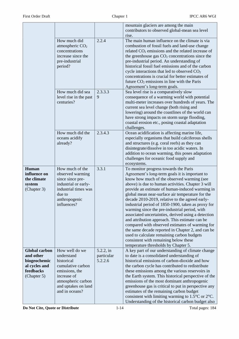
How much did
atmospheric CO2
concentrations
increase since the
pre-industrial
period?
2.2.4 The main human influence on the climate is via
combustion of fossil fuels and land-use change
related CO2 emissions and the related increase of
the greenhouse gas CO2 concentrations since the
pre-industrial period. An understanding of
historical fossil fuel emissions and of the carbon
cycle interactions that led to observed CO2
concentrations is crucial for better estimates of
future CO2 emissions in line with the Paris
Agreement’s long-term goals.
How much did sea
level rise in the past
centuries?
2.3.3.3
9
Sea level rise is a comparatively slow
consequence of a warming world with potential
multi-meter increases over hundreds of years. The
current sea level change (both rising and
lowering) around the coastlines of the world can
have strong impacts on storm surge flooding,
coastal erosion etc., posing coastal adaptation
challenges.
How much did the
oceans acidify
already?
2.3.4.3 Ocean acidification is affecting marine life,
especially organisms that build calciferous shells
and structures (e.g. coral reefs) as they can
disintegrate/dissolve in too acidic waters. In
addition to ocean warming, this poses adaptation
challenges for oceanic food supply and
ecosystems.
Human
influence on
the climate
system
(Chapter 3)
How much of the
observed warming
since since pre-
industrial or early-
industrial times was
due to
anthropogenic
influences?
3.3.1 To monitor progress towards the Paris
Agreement’s long-term goals it is important to
know how much of the observed warming (see
above) is due to human activities. Chapter 3 will
provide an estimate of human-induced warming in
global mean near-surface air temperature for the
decade 2010-2019, relative to the agreed early-
industrial period of 1850-1900, taken as proxy for
warming since the pre-industrial period, with
associated uncertainties, derived using a detection
and attribution approach. This estimate can be
compared with observed estimates of warming for
the same decade reported in Chapter 2, and can be
used to calculate remaining carbon budgets
consistent with remaining below these
temperature thresholds by Chapter 5.
Global carbon
and other
biogeochemic
al cycles and
feedbacks
(Chapter 5)
How well do we
understand
historical
cumulative carbon
emissions, the
increase of
atmospheric carbon
and uptakes on land
and in oceans?
5.2.2, in
particular
5.2.2.6
A key part of our understanding of climate change
to date is a consolidated understanding of
historical emissions of carbon-dioxide and how
the carbon cycle has contributed to redistribute
these emissions among the various reservoirs in
the Earth system. This historical perspective of the
emissions of the most dominant anthropogenic
greenhouse gas is critical to put in perspective any
estimates of the remaining carbon budget
consistent with limiting warming to 1.5°C or 2°C.
Understanding of the historical carbon budget also
First Order Draft Chapter 1 IPCC AR6 WGI
Do Not Cite, Quote or Distribute 1-15 Total pages: 184
allows us to realize that anthropogenic carbon-
dioxide emissions do not disappear from the
active carbon cycle over timescales of centuries,
but are merely redistributed.
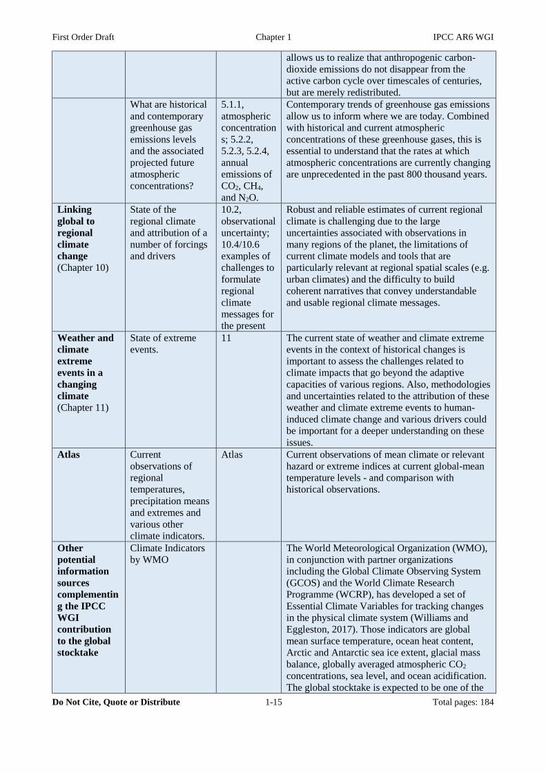
What are historical
and contemporary
greenhouse gas
emissions levels
and the associated
projected future
atmospheric
concentrations?
5.1.1,
atmospheric
concentration
s; 5.2.2,
5.2.3, 5.2.4,
annual
emissions of
CO2, CH4,
and N2O.
Contemporary trends of greenhouse gas emissions
allow us to inform where we are today. Combined
with historical and current atmospheric
concentrations of these greenhouse gases, this is
essential to understand that the rates at which
atmospheric concentrations are currently changing
are unprecedented in the past 800 thousand years.
Linking
global to
regional
climate
change
(Chapter 10)
State of the
regional climate
and attribution of a
number of forcings
and drivers
10.2,
observational
uncertainty;
10.4/10.6
examples of
challenges to
formulate
regional
climate
messages for
the present
Robust and reliable estimates of current regional
climate is challenging due to the large
uncertainties associated with observations in
many regions of the planet, the limitations of
current climate models and tools that are
particularly relevant at regional spatial scales (e.g.
urban climates) and the difficulty to build
coherent narratives that convey understandable
and usable regional climate messages.
Weather and
climate
extreme
events in a
changing
climate
(Chapter 11)
State of extreme
events.
11 The current state of weather and climate extreme
events in the context of historical changes is
important to assess the challenges related to
climate impacts that go beyond the adaptive
capacities of various regions. Also, methodologies
and uncertainties related to the attribution of these
weather and climate extreme events to human-
induced climate change and various drivers could
be important for a deeper understanding on these
issues.
Atlas Current
observations of
regional
temperatures,
precipitation means
and extremes and
various other
climate indicators.
Atlas Current observations of mean climate or relevant
hazard or extreme indices at current global-mean
temperature levels - and comparison with
historical observations.
Other
potential
information
sources
complementin
g the IPCC
WGI
contribution
to the global
stocktake
Climate Indicators
by WMO
The World Meteorological Organization (WMO),
in conjunction with partner organizations
including the Global Climate Observing System
(GCOS) and the World Climate Research
Programme (WCRP), has developed a set of
Essential Climate Variables for tracking changes
in the physical climate system (Williams and
Eggleston, 2017). Those indicators are global
mean surface temperature, ocean heat content,
Arctic and Antarctic sea ice extent, glacial mass
balance, globally averaged atmospheric CO2
concentrations, sea level, and ocean acidification.
The global stocktake is expected to be one of the

First Order Draft Chapter 1 IPCC AR6 WGI
Do Not Cite, Quote or Distribute 1-16 Total pages: 184
major applications for this set of indicators,
alongside more frequent monitoring, such as
through WMO's annual State of the Climate
reports. The WMO's chosen set of indicators is
intended to capture the widest possible picture of
climate change whilst still keeping the number of
indicators to a manageable level.
The criteria that WMO has used for shortlisting
indicators are relevance, representativeness,
traceability, timeliness and data adequacy. Whilst
some indicators, such as global mean surface
temperature and sea ice extent, are available in
close to real time, others, such as glacial mass
balance and globally averaged atmospheric CO2
concentrations, can be 12 months or more in
arrears.
Section 2: Future Projections
Topic Question Chapter/
Section
Potential Relevance
Future global
climate:
scenario-
based
projections
and near-term
information
(Chapter 4)
What are
projected key
climate indices
under low,
medium and high
emission
scenarios in the
near-term, i.e. the
next 20 years?
4.3, 4.4,
FAQ 4.1
Much of the near-term information allows us to
sketch the climate adaptation challenges for the next
decades as well as the opportunities to reduce climate
change by pursuing lower emission scenarios.
If lower emission
scenarios are
pursued, what are
the differences in
climate over the
21st century
compared to
emission
scenarios where
no additional
climate policies
are implemented?
4.6 The new generation of scenarios spans the response
space from very low emission scenarios (SSP1-1.9)
under the assumption of climate policy
implementation to very high emission scenarios that
are projected in the absence of climate policies
(SSP3-7.0 or SSP5-8.5). The climate differences
between those future high emission scenarios and
those compatible with the Paris Agreement’s long-
term targets can help inform about differences in
corresponding adaptation challenges.
How much
confidence can
we have in the
ensembles of
climate model
projections and
what are the
techniques to
derive a range of
future global and
Box 4.1 The scientific literature provides new insights
regarding ensemble evaluation and weighting that
can lead to more appropriate projection ranges, which
take into account the skill of climate models and
interdependencies among them. These techniques
have a strong relevance to quantifying future
uncertainties, for example regarding the likelihood
with which the various scenarios would exceed the
Paris Agreement’s long-term goals of 1.5°C or 2°C.

First Order Draft Chapter 1 IPCC AR6 WGI
Do Not Cite, Quote or Distribute 1-17 Total pages: 184
regional climate
changes?
When greenhouse
gas emissions are
reduced, what
changes will we
see and when?
FAQ 4.2 The understanding the response to a change of
anthropogenic emissions is important to estimate an
appropriate scale and timing of mitigation compatible
with the Paris Agreement’s long-term targets.
Global carbon
and other
biogeochemic
al cycles and
feedbacks
(Chapter 5)
What is the
remaining carbon
budget that is
consistent with
the Paris
Agreement’s
long-term
objectives?
5.5; 5.5.1,
TCRE;
5.5.2,
remaining
carbon
budget.
The remaining carbon budget provides an estimate of
how much CO2 can still be emitted into the
atmosphere by human activities while keeping global
warming to a specific temperature limit. It thus
provides key geophysical information about
emissions limits consistent with limiting global
warming to well below 2 °C above pre-industrial
levels and to pursue efforts to limit the temperature
increase to 1.5 °C. Remaining carbon budgets should
be seen in context of historical CO2 emissions to
date. The concept of the transient climate response to
cumulative emissions of carbon-dioxide (TCRE)
indicates that one tonne of carbon-dioxide has the
same incremental effect on global warming
irrespective of whether it is emitted in the past, today
or in the future.
Short-lived
climate
forcers
(Chapter 6)
How important
are reductions in
short-lived
climate forcers
compared to the
reduction of CO2
and other long-
lived greenhouse
gases?
6.1.4 Short-lived climate forcers play an important role in
the anthropogenic effect on climate change. Many
aerosol species tend to cool the climate and their
reduction leads to an unmasking of greenhouse gas
induced warming. On the other hand, many shorter
lived species themselves exert a warming effect,
including black carbon and also methane, the second
most important anthropogenic greenhouse gas (in
terms of current radiative forcing). Thus, strategies to
limit future climate change need to undertake a mix
of mitigation strategies and the question is how
important are reduction in short-lived climate
pollutants, often driven by additional clean air policy
objectives, compared to the reduction of CO2 and
other long-lived greenhouse gases.
What are the co-
benefits of and
co-challenges of
climate
mitigation?
6.1.4 The reduction of fossil-fuel related emissions often
goes hand in hand with a reduction of air pollutants,
like aerosols. Those reductions in air pollutants can
accrue co-benefits in terms of increased air quality
and improved human health and could be factored
into a response strategy to climate change.
The Earth’s
energy
budget,
climate
feedbacks,
and climate
sensitivity
(Chapter 7)
What is the
Transient Climate
Response and
what does it tell
us about expected
warming over the
21st century under
various scenarios?
7.5.7 The transient climate response is a is a measure of the
strength of climate feedbacks and the timescale of
ocean heat uptake.
Equilibrium
Climate
Sensitivity
7.5.7 The Equilibrium Climate Sensitivity (ECS) has
summarized our understanding for decades of how
sensitive the Earth’s climate system is to elevated
First Order Draft Chapter 1 IPCC AR6 WGI
Do Not Cite, Quote or Distribute 1-18 Total pages: 184
CO2 concentrations. The higher the ECS, the lower
are the greenhouse gas emissions that are consistent
with the Paris Agreement’s long-term targets.
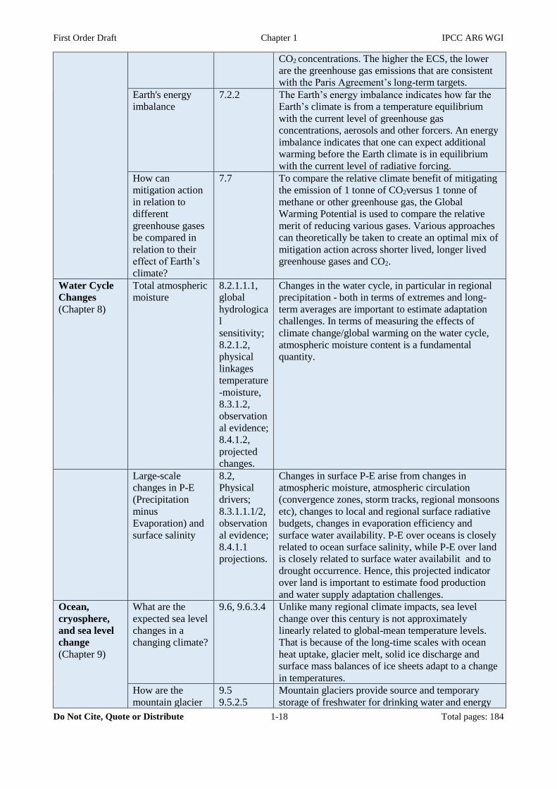
Earth's energy
imbalance
7.2.2 The Earth’s energy imbalance indicates how far the
Earth’s climate is from a temperature equilibrium
with the current level of greenhouse gas
concentrations, aerosols and other forcers. An energy
imbalance indicates that one can expect additional
warming before the Earth climate is in equilibrium
with the current level of radiative forcing.
How can
mitigation action
in relation to
different
greenhouse gases
be compared in
relation to their
effect of Earth’s
climate?
7.7
To compare the relative climate benefit of mitigating
the emission of 1 tonne of CO2versus 1 tonne of
methane or other greenhouse gas, the Global
Warming Potential is used to compare the relative
merit of reducing various gases. Various approaches
can theoretically be taken to create an optimal mix of
mitigation action across shorter lived, longer lived
greenhouse gases and CO2.
Water Cycle
Changes
(Chapter 8)
Total atmospheric
moisture
8.2.1.1.1,
global
hydrologica
l
sensitivity;
8.2.1.2,
physical
linkages
temperature
-moisture,
8.3.1.2,
observation
al evidence;
8.4.1.2,
projected
changes.
Changes in the water cycle, in particular in regional
precipitation - both in terms of extremes and long-
term averages are important to estimate adaptation
challenges. In terms of measuring the effects of
climate change/global warming on the water cycle,
atmospheric moisture content is a fundamental
quantity.
Large-scale
changes in P-E
(Precipitation
minus
Evaporation) and
surface salinity
8.2,
Physical
drivers;
8.3.1.1.1/2,
observation
al evidence;
8.4.1.1
projections.
Changes in surface P-E arise from changes in
atmospheric moisture, atmospheric circulation
(convergence zones, storm tracks, regional monsoons
etc), changes to local and regional surface radiative
budgets, changes in evaporation efficiency and
surface water availability. P-E over oceans is closely
related to ocean surface salinity, while P-E over land
is closely related to surface water availabilit and to
drought occurrence. Hence, this projected indicator
over land is important to estimate food production
and water supply adaptation challenges.
Ocean,
cryosphere,
and sea level
change
(Chapter 9)
What are the
expected sea level
changes in a
changing climate?
9.6, 9.6.3.4 Unlike many regional climate impacts, sea level
change over this century is not approximately
linearly related to global-mean temperature levels.
That is because of the long-time scales with ocean
heat uptake, glacier melt, solid ice discharge and
surface mass balances of ice sheets adapt to a change
in temperatures.
How are the
mountain glacier
9.5
9.5.2.5
Mountain glaciers provide source and temporary
storage of freshwater for drinking water and energy
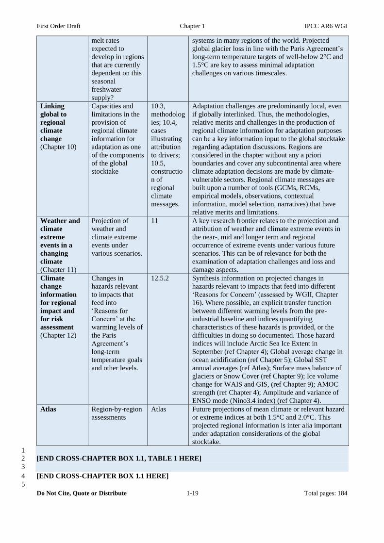
First Order Draft Chapter 1 IPCC AR6 WGI
Do Not Cite, Quote or Distribute 1-19 Total pages: 184
melt rates
expected to
develop in regions
that are currently
dependent on this
seasonal
freshwater
supply?
systems in many regions of the world. Projected
global glacier loss in line with the Paris Agreement’s
long-term temperature targets of well-below 2°C and
1.5°C are key to assess minimal adaptation
challenges on various timescales.
Linking
global to
regional
climate
change
(Chapter 10)
Capacities and
limitations in the
provision of
regional climate
information for
adaptation as one
of the components
of the global
stocktake
10.3,
methodolog
ies; 10.4,
cases
illustrating
attribution
to drivers;
10.5,
constructio
n of
regional
climate
messages.
Adaptation challenges are predominantly local, even
if globally interlinked. Thus, the methodologies,
relative merits and challenges in the production of
regional climate information for adaptation purposes
can be a key information input to the global stocktake
regarding adaptation discussions. Regions are
considered in the chapter without any a priori
boundaries and cover any subcontinental area where
climate adaptation decisions are made by climate-
vulnerable sectors. Regional climate messages are
built upon a number of tools (GCMs, RCMs,
empirical models, observations, contextual
information, model selection, narratives) that have
relative merits and limitations.
Weather and
climate
extreme
events in a
changing
climate
(Chapter 11)
Projection of
weather and
climate extreme
events under
various scenarios.
11 A key research frontier relates to the projection and
attribution of weather and climate extreme events in
the near-, mid and longer term and regional
occurrence of extreme events under various future
scenarios. This can be of relevance for both the
examination of adaptation challenges and loss and
damage aspects.
Climate
change
information
for regional
impact and
for risk
assessment
(Chapter 12)
Changes in
hazards relevant
to impacts that
feed into
‘Reasons for
Concern’ at the
warming levels of
the Paris
Agreement’s
long-term
temperature goals
and other levels.
12.5.2 Synthesis information on projected changes in
hazards relevant to impacts that feed into different
‘Reasons for Concern’ (assessed by WGII, Chapter
16). Where possible, an explicit transfer function
between different warming levels from the pre-
industrial baseline and indices quantifying
characteristics of these hazards is provided, or the
difficulties in doing so documented. Those hazard
indices will include Arctic Sea Ice Extent in
September (ref Chapter 4); Global average change in
ocean acidification (ref Chapter 5); Global SST
annual averages (ref Atlas); Surface mass balance of
glaciers or Snow Cover (ref Chapter 9); Ice volume
change for WAIS and GIS, (ref Chapter 9); AMOC
strength (ref Chapter 4); Amplitude and variance of
ENSO mode (Nino3.4 index) (ref Chapter 4).
Atlas Region-by-region
assessments
Atlas Future projections of mean climate or relevant hazard
or extreme indices at both 1.5°C and 2.0°C. This
projected regional information is inter alia important
under adaptation considerations of the global
stocktake.
1
[END CROSS-CHAPTER BOX 1.1, TABLE 1 HERE] 2
3
[END CROSS-CHAPTER BOX 1.1 HERE] 4
5
First Order Draft Chapter 1 IPCC AR6 WGI
Do Not Cite, Quote or Distribute 1-20 Total pages: 184
1
1.2.3 Climate, science, and societies: perceptions, values, and ethics 2
3
Values and ethics play critical roles in climate understanding. Science can answer questions about what, 4
how, and why: how and why Earth’s climate is changing (IPCC WGI), how climate change may affect 5
human societies and natural systems (WGII), how societies might adapt (WGII), and how it might be 6
mitigated (WGIII). By contrast, science can offer no response to questions of value or importance, such as 7
which courses of action are best or of highest priority. Answers to those questions depend on what people 8
judge to be good and bad, right and wrong, important and unimportant. Some values are widely shared, but 9
others vary considerably across cultures, groups, and individuals; one key example is the differing human 10
value of “subsistence” carbon emissions — those needed for simple survival — versus the “luxury” 11
emissions of wealthy people and nations (Agarwal and Narain, 2012; Jasanoff, 2010). Values are reflected in 12
ethics, or moral principles and rules of conduct, as well as in social norms, political rhetoric, and decision-13
making. They also have powerful effects on perceptions of climate change and on literacy about climate 14
science. Although few high-quality trans-national surveys exist, they show that in many countries education 15
is the strongest predictor of climate change perceptions (Lee et al., 2015). However, values are also strong 16
influences, in some cases (e.g. the USA and UK) dominating education and knowledge as predictors of 17
attitudes (McCright and Dunlap, 2011; Whitmarsh, 2011). 18
19
The international governance efforts and strengthening the response to climate change necessitates that 20
leaders, policymakers, and the broader public have literacy in the causes, effects, and possible future course 21
of climate change. Achieving this is complicated by the fact that scientific knowledge adds to, and interacts 22
with, other understandings of weather and climate built up in diverse world cultures over centuries (Hulme, 23
2009, 2018; Nakashima et al., 2012). These localized understandings contrast with the vast geographical and 24
temporal scales of climate science (Green et al., 2010; Jasanoff, 2010; Orlove et al., 2010). Political cultures 25
also give rise to geographical variations in how climate science knowledge is interpreted, used, and 26
challenged (Jasanoff, 2011; Mahony, 2014, 2015). Furthermore, climate change itself is not uniform: some 27
regions face steady, readily observable change, while others experience high variability that masks 28
underlying trends. Short-term temperature trends, such as cold spells or warm days, have been shown to 29
influence public concern (Bohr, 2017; Hamilton and Stampone, 2013; Zaval et al., 2014). 30
31
Against this background, ethical practice requires that scientists take special care when communicating 32
findings and uncertainties that inform high-stakes decisions. In some cases evidence is sufficient to assign a 33
precise probability to a conclusion, but often uncertainty is deeper and will be more accurately characterized 34
in alternative ways (Kandlikar et al., 2005). To achieve this, the IPCC uses standardised calibrated language 35
of likelihood and confidence to communicate the outcomes of the assessment (see Box 1.1). Yet even with 36
calibrated language, the choice of category (e.g. likely vs. very likely) may itself be uncertain. Further, this 37
calibrated language does not prevent confusion or misunderstandings. Studies show that even when shown 38
IPCC uncertainty guidance, lay readers systematically underestimate the intended level of certainty; 39
indicating numerical ranges alongside likelihood terminology, and allowing for narrower (more precise) 40
ranges when appropriate, could help to reduce confusion in public communication (Budescu et al., 2014). 41
42
Media coverage of climate change plays a major role in climate perception and literacy (Brulle et al., 2012; 43
Jaspal and Nerlich, 2014). While research into media reporting on climate change has expanded, research 44
remains largely focused on Western countries (Schäfer and Schlichting, 2014). In the USA, analyses of 45
television network news show that climate change receives minimal attention, is most often framed in a 46
political context, and largely fails to draw appropriate linkages between climate change and some types of 47
extreme weather events (Hassol et al., 2016). In five EU countries, television coverage of AR5 used 'disaster' 48
and 'opportunity' as its principal themes; it virtually ignored the “explicit risk” frame, introduced by WGII 49
(Painter, 2015) and now extended by the cross-WG AR6 risk framework (see Section 1.2.4.1). This is 50
important considering that framing studies have confirmed that the way climate change is presented to 51
people has a significant and differential impact on the quality of their responses (Dewulf, 2013)d. For 52
example, when framed as a catastrophe (e.g., Hine et al., 2015), associated with local identities (Sapiains et 53
al., 2016), or as a social justice issue (Howell, 2013), people have different types of reactions. Similarly, 54
audience segmentation studies have shown how responses to climate change vary between groups of people 55

First Order Draft Chapter 1 IPCC AR6 WGI
Do Not Cite, Quote or Distribute 1-21 Total pages: 184
with different, although not necessarily opposed, views on this phenomenon (e.g., Detenber et al., 2016; 1
Sherley et al., 2014). In Brazil two studies have shown the influence of mass media on the high level of 2
public climate change concern in this country (Dayrell, 2019; Rodas and Giulio., 2017). 3
4
5
Social media platforms have dramatically altered the mass-media landscape, bringing about a shift from 6
unidirectional transfer of information and ideas to more fluid, multi-directional flows (Pearce et al., 2019). 7
Climate science remains well-represented and prominent on social media. For example, in studies of Twitter 8
reactions to the AR5, “settled science” was the most dominant theme and professional media organizations 9
were the most linked-to sources (Newman, 2017; O’Neill et al., 2015). Social media suffer from well known 10
problems, such as incivility that inhibits consensus-building and “filter bubbles” that restrict interactions to 11
those with broadly similar views (Anderson and Huntington, 2017). However, at certain moments (such as at 12
the release of the AR5 WGI report), Twitter studies have found that more mixed, highly-connected groups 13
existed, within which members were less polarized (Pearce et al., 2014; Williams et al., 2015). Thus, social 14
media platforms may in some circumstances support dialogic approaches to climate communication. 15
16
Science itself strives for an ethic of honesty, objectivity, and openness, though it does not always succeed 17
(Medicine et al., 2009). In its theories and results, science values such features as predictive accuracy, 18
explanatory power, falsifiability, and replicability (Kuhn, 1977; Popper, 1959). Practices embodying these 19
scientific values include peer review, publication, model intercomparison projects (MIPs), and multiple 20
groups analysing the same problems and data; in recent decades, open data and open code have facilitated 21
greater independent scrutiny of published results. 22
23
Whether and how societal, political, and personal values should influence science continues to be debated. 24
While such contextual values (Longino, 1990) can bias research, they can also play positive roles, especially 25
in decision-relevant science when stakeholder values are taken into account in a transparent way (Douglas, 26
2009; Elliott, 2017). Some climate science questions are deemed a higher priority for investigation, or 27
expressed in particular ways, because of their societal relevance; one example is the question of how the 28
effects of a 1.5 °C warming would differ from 2 °C (Hoegh-Guldberg et al., 2018). Likewise, particular 29
model outputs — such as projected precipitation in a specific region or sea level rise — are sometimes 30
prioritized in model improvement efforts because of their practical relevance for specific groups of people 31
(Intemann, 2015; Winsberg, 2018). Groups whose interests do not influence research and modelling 32
priorities may thus receive less attention in support their climate-related decisions (Parker and Winsberg, 33
2018). 34
35
36
1.2.4 New approaches in the WGI AR6 report 37
38
The assessment approach, scope, and structure of the WGI AR6 have been shaped by the twin contexts of the 39
changing climate system and the evolving political and societal responses. As a result of the scoping process, 40
the WGI contribution to the AR6 is focused on results and understanding relevant to the global stocktake, as 41
well as to adaptation, mitigation, and impacts at both global and regional scales. The report builds on the 42
conclusions of previous IPCC assessments, and on the possibilities for integration along topics resulting 43
from the maturation of climate science since AR5 and across multiple lines of evidence. 44
45
Based on this rationale, some changes in the structure of WGI AR6 have ben introduced. The new structure 46
is designed to strengthen the assessment of climate information for regions and thus provide greater 47
relevance for policymakers and to enhance links with WGII and WGIII (see also Section 1.8). Earlier reports 48
divided topics along boundaries between modern observations, paleoclimatic data, and understanding from 49
models. In contrast, the AR6 outline is structured around topics such as large-scale climate changes 50
(Chapters 2-4), climate processes (Chapters 5-9), and regional climate information (Chapters 10-12 and 51
Atlas). This approach aims at a greater visibility for key knowledge developments relevant for policymakers, 52
particularly for the global stocktake and for regional adaptation planning based on a risk management 53
framework. 54

First Order Draft Chapter 1 IPCC AR6 WGI
Do Not Cite, Quote or Distribute 1-22 Total pages: 184
1
Some Chapters integrate research elements such as observations, paleoclimate information, and modelling 2
approaches. Two subjects presented separately in AR5, paleoclimate and model evaluation, are distributed 3
among multiple Chapters. Observations, detection and attribution, and future projections are also distributed 4
over multiple Chapters. This approach provides closer integration of different research elements in each 5
Chapter. 6
7
Regional information provision is enhanced in this report, with an emphasis on the role of variability. The 8
single regional chapter in the AR5 has been expanded to three chapters in AR6. The assessment on extreme 9
events, distributed across multiple Chapters in the AR5, while there is a dedicated Chapter 11 in this report. 10
The Atlas of global and regional climate projection was included as an Annex in the AR5; instead, the Atlas 11
in this report involves the assessment of regional climate change and will include an interactive web-based 12
product. This enhancement of regional assessment, together with a common framework of risk, enables a 13
strong and consistent link between the WGI, WGII as well as WGIII AR6 reports. A more detailed 14
description of the structure of this report may be found in Section 1.8. 15
16
17
1.2.4.1 Risk framing 18
19
Although climate change can potentially have both positive or adverse consequences for human or ecological 20
systems, a major focus has been on understanding and assessing the adverse consequences. This focus stems 21
directly from the UNFCCC, which states in its preamble: “Acknowledging that change in the Earth’s climate 22
and its adverse effects are a common concern of humankind”. Furthermore, Article 2 declares that the 23
ultimate goal of the convention is to “…. prevent dangerous anthropogenic interference with the climate 24
system". This emphasis has led to the development of a common risk framework in order to assess such 25
adverse consequences. 26
27
Risks to human and natural systems result from the interactions of climate-related hazards (including 28
extreme weather and climate events) with exposure to and vulnerability to those hazards. Impacts generally 29
refer to effects on lives; livelihoods; health and wellbeing; ecosystems and species; economic, social and 30
cultural assets; services (including ecosystem services); and infrastructure. Impacts may be referred to as 31
consequences or outcomes and can be adverse or beneficial. Risk can however also result from responses to 32
climate change (adaptation and mitigation). 33
34
Evolution of the risk framework in IPCC assessments. The IPCC Special Report on Managing the Risks 35
of Extreme Events and Disasters to Advance Climate Change Adaptation SREX (IPCC, 2012) integrated 36
climate science, climate impacts, adaptation and disaster risk management in the context of changing climate 37
in response to the Hyogo Framework for Action (predecessor of SFDRR) and subsequent United Nations 38
statements. AR5 WGII further explored the emergent risks and key vulnerabilities to climate change by 39
analysing the “interaction of the changing physical characteristics of the climate system with evolving 40
characteristics of socioeconomic and biological systems (exposure and vulnerability) to produce risk.” 41
SREX and subsequently AR5 WGII moved from a notion of climate change adaptation based upon 42
vulnerability to one based on risk (Connelly et al., 2018). This concept of risk combines the language of 43
probability and consequences with a focus on spatial relationships between hazard, exposure and 44
vulnerability. 45
46
WGII AR5 assessed that in order to reduce risk, effective adaptation should include actions with co-benefits 47
for other objectives or effective risk reduction and adaptation strategies that consider the dynamics of 48
vulnerability and exposure and their linkages with socioeconomic processes, sustainable development, and 49
climate change. Strategies should therefore include actions with co-benefits for other objectives. 50
Organizations bridging science and decision making, including climate services, can play an important role 51
in the communication, transfer, and development of climate-related knowledge, including translation, 52
engagement, and knowledge exchange (Field et al., 2014). The risk framework has then also been used in 53
the IPCC special reports following AR5. IPCC SR1.5 builds upon SREX Chapter 3, AR5 WGI and new 54
relevant literature to assess hazards associated with global and regional climate changes when the globally 55
First Order Draft Chapter 1 IPCC AR6 WGI
Do Not Cite, Quote or Distribute 1-23 Total pages: 184
averaged surface temperature is 1.5°C above the pre-industrial baseline versus 2°C or higher levels of 1
warming. IPCC SR1.5 added to the framework the concept of “climate resilient pathways”, illustrated as an 2
iterative process of effectively reducing risk through pathways that combine adaptation and mitigation in a 3
synergistic manner (IPCC, 2019). 4
5
[Placeholder: include SROCC and SRCCL discussion]. 6
7
Risk concept in AR6. The conceptual risk framework is an integral element of the AR6. The risk 8
framework is wider than the concept of “hazard-exposure-vulnerability” defined in SREX and AR5. The 9
framework also encompasses risks related to climate policies (adaptation, mitigation, investment). A cross-10
Working Group process has been underway as part of the AR6 to develop a common risk definition and is 11
presented in Cross-Chapter Box 1.2. 12
13
In WGI, the risk concept is related to climate change impacts and builds upon the concept first developed in 14
the IPCC SREX (IPCC, 2012), which focused particularly on the negative consequences of hazards and 15
disaster risk. The risk framework was then also adopted by IPCC AR5 WGII Ch19 (Oppenheimer et al., 16
2014), which refers more generally to the characteristics of climate change and its effects on geophysical 17
systems. This conceptual risk framing can be applied across timescales and across spatial scales in the 18
context of different regional and sectoral aspects. In the IPCC risk framework, the dynamic interaction 19
between hazards, exposure and vulnerability determines risk. These elements are driven by both climate and 20
socioeconomic processes. Climate influences mainly hazards, (although not exclusively) through a 21
combination of natural climate variability and anthropogenic climate change. 22
23
Integrating adaptation in line with the Paris Agreement and SDGs into planning and decision making 24
(including incremental and transformational adjustments) can promote synergies with development and 25
disaster risk reduction and environmental quality (IPCC 2018). The AR6 risk framework builds on WGII 26
AR5, which assessed the potential for reducing risks through both adaptation and mitigation (Oppenheimer 27
et al, 2014). The Shared Socioeconomic Pathways (SSPs, see section 1.6) describe characteristics of a set of 28
global reference futures. They are designed to promote more integrated assessments of climate change and 29
its impacts by linking them to adaption, mitigation, and sustainable development. They will be used in AR6 30
and interpreted in the light of the large body of literature that has become available since the publication of 31
AR5 (O’Neill et al., 2017c; Riahi et al., 2017a; Rogelj et al., 2018). 32
33
Some post-AR5 literature has critically discussed the IPCC risk framework. Arven and Renn (2015) point out 34
the need for moving beyond the probability-based perspectives on risk and have proposed alternative 35
definitions of risk, focusing mainly on consequences and uncertainties. The IPCC risk framework and 36
associated terminology has since been revised and the updated definitions are provided in Cross-Chapter Box 37
1.2. Sutton (2018) proposes to include unlikely but high impact risks (Figure 1.3). 38
39
The reasons for concern framework. The Reasons for Concern (RFC) framework, used by WGII since 40
IPCC TAR and also in post AR5 Special reports (SR1.5, SROCC and SRCCL) is a classification framework 41
that compiles key risks across regions and sectors. Key risks have potentially severe impacts related to 42
implications of warming and adaptation limits for the society, the economy and the environment, relevant to 43
Article 2 of the UNFCCC. The RFC framework aggregates risks in five categories as a function of global 44
mean temperature: (1) risks to unique and threatened systems, (2) risks associated with extreme weather 45
events, (3) risks associated with the distribution of impacts, (4) risks associated with global aggregate 46
impacts and (5) risks associated with large-scale singular events. AR5 assessed literature related to each of 47
the RFCs, taking into account the socio-economic development pathway (Oppenheimer et al. 2014) to risk 48
associated with each RFC. The SR1.5 builds upon AR5 but with a focus on the consequences of 1.5ºC of 49
warming compared to 2°C and consequently develops RFC diagrams only up to 2.5ºC. It also accounts for 50
the rate and timing of impacts when assessing RFC 1 and 5. In addition, the RFC framework was broadened 51
in SR1.5 to include new and more specific evaluation of certain natural, managed and human systems. By 52
adopting a common risk framework across working groups, the contribution of WGI is explicitly integrated 53
into the assessments of the RFCs. 54
55

First Order Draft Chapter 1 IPCC AR6 WGI
Do Not Cite, Quote or Distribute 1-24 Total pages: 184
Multiple lines of evidence show that there has been a substantial increase since AR5 in the levels of risk 1
associated with four of the five Reasons for Concern (RFCs) for global warming levels of up to 2°C (IPCC, 2
2018). The key risks identified in AR5-WGII-SPM that follow, all of which are identified with high 3
confidence, span sectors and regions. Each of these key risks contributes to one or more RFCs (IPCC, 2014). 4
5
Post-AR5 literature (e.g. O’Neill et al., 2017) calls for the extension of the RFC framework in AR6 to 6
consider complementary climate change metrics, individual risk assessments and better inclusion of socio 7
ecological vulnerabilities in addition to the impacts on physical and ecological systems. 8
9
The WGI contribution to the risk framework focuses primarily on the assessment of hazards (see Cross-10
Chapter Box 1.2) and how these are changing under anthropogenic climate change. Chapter 12 forms the 11
direct handshake to WGII by assessing climate-related hazards for different regions and sectors and relating 12
those to essential climate variables and climate extreme indices as assessed in other chapters. The rate of 13
change and the intensity of climate-related hazards is related to the emission pathways and corresponding 14
mitigation policies as assessed by WGIII. 15
16
[START CROSS-CHAPTER BOX 1.2 HERE] 17
18
Cross-Chapter Box 1.2: Risk Framing in IPCC AR6 19
20
Since its inception, the UNFCCC has seen climate change as a risk to human and ecological systems, as 21
stated in its preamble: “Acknowledging that change in the Earth’s climate and its adverse effects are a 22
common concern of humankind”. 23
24
In order to assess those adverse effects, the IPCC has long addressed the understanding of the physical 25
climate change, its impacts and mitigation options as a risk. However, up to now, there was no common 26
framework to assess risk, that could then be applied with the specificities of each Working Group. 27
28
A cross-Working Group process has been underway as part of the AR6 to develop a common risk definition. 29
The resulting definition is as follows: 30
31
Risk: The potential for adverse consequences for human or ecological systems, recognizing the diversity of 32
values and objectives associated with such systems. In the context of climate change, risks can arise from 33
potential impacts of climate change as well as human responses to climate change. Relevant adverse 34
consequences include those on lives, livelihoods, health and wellbeing, economic, social and cultural assets 35
and investments, infrastructure, services (including ecosystem services), ecosystems and species. 36
37
In the context of climate change impacts, risks result from dynamic interactions between climate-related 38
hazards with the exposure and vulnerability of the affected human or ecological system to the hazards. 39
Hazards, exposure and vulnerability may each be subject to uncertainty in terms of magnitude and likelihood 40
of occurrence, and each may change over time and space due to socio-economic changes and human 41
decision-making (see also risk management, adaptation, mitigation). 42
43
In the context of climate change responses, risks result from the potential for such responses not achieving 44
the intended objective(s), or from potential trade-offs with, or negative side-effects on, other societal 45
objectives, such as the Sustainable Development Goals (see also risk trade-off). Risks can arise for example 46
from uncertainty in implementation, effectiveness or outcomes of climate policy, climate-related 47
investments, technology development or adoption, and system transitions. 48
49
Risk management: Plans, actions, strategies or policies to reduce the likelihood and/or magnitude of 50
adverse potential consequences, based on assessed or perceived risks (see also risk assessment, risk 51
perception, risk transfer). 52
53
The following definitions of key concepts are included within the definition of risk: 54
55
First Order Draft Chapter 1 IPCC AR6 WGI
Do Not Cite, Quote or Distribute 1-25 Total pages: 184
Exposure: The presence of people, livelihoods, species or ecosystems, environmental functions, services, 1
and resources, infrastructure, or economic, social, or cultural assets in places and settings that could be 2
adversely affected. 3
4
Vulnerability: The propensity or predisposition to be adversely affected. Vulnerability encompasses a 5
variety of concepts and elements including sensitivity or susceptibility to harm and lack of capacity to cope 6
and adapt. It also includes structural, economic, social, or cultural assets in places and settings that could be 7
adversely affected. A broad set of factors such as wealth, social status, and gender determine vulnerability 8
and exposure to climate-related risk. 9
10
Hazard: The potential occurrence of a natural or human-induced physical event or trend or physical impact 11
that may cause loss of life, injury, or other health impacts, as well as damage and loss to property, 12
infrastructure, livelihoods, service provision, ecosystems, and environmental resources. In this report, the 13
term hazard usually refers to climate-related physical events or trends or their physical impacts. Relevant to 14
WGI (and further discussed in Chapter 12), the definition of ‘hazards’ includes both trends and extreme 15
events,' impact’ for AR6 in general, is a specific intersection of hazard, vulnerability, and exposure within a 16
sector. 17
18
Impacts: Effects on natural and human systems. In this report, the term impacts is used primarily to refer to 19
the effects on society and ecosystems of extreme weather and climate events and of climate change. Impacts 20
generally refer to effects on lives, livelihoods, health, ecosystems, economies, societies, cultures, services, 21
and infrastructure due to the interaction of climate changes or hazardous climate events occurring within a 22
specific time period and the vulnerability of an exposed society or ecosystem. Impacts are also referred to as 23
consequences and outcomes. The impacts of climate change on geophysical systems, including floods, 24
droughts, and sea level rise, are a subset of impacts called physical impacts. 25
26
In the context of climate change impacts, risks result from dynamic interactions between climate-related 27
hazards with the exposure and vulnerability of the affected human or ecological system to the hazards. 28
Hazards, exposure and vulnerability may each be subject to uncertainty in terms of likelihood of occurrence 29
and magnitude. Each of these may change over time and space as a result of socio-economic changes and 30
human decision-making (risk management). Examples of risks include those arising from potential impacts 31
on lives, livelihoods, health and wellbeing, ecosystems and species, economic, social and cultural assets, 32
services (including ecosystem services), and infrastructure (e.g. risk of heat-related deaths). But adverse 33
consequences can also arise as human responses to climate change (e.g. risk of wind turbines harming birds. 34
35
It is recognized that much of the literature assessed within WGI talks about risk when evaluating impacts on 36
physical system, such as floods for example. In the context of the IPCC, such studies assess the «frequency 37
and or magnitude of flood events », and risk only applies if an explicit assessment to humans is included 38
(exposure or vulnerability). 39
40
Risk is intrinsically related to uncertainty, and since its beginning, the IPCC has developed a consistent 41
treatment and communication of scientific uncertainty (see Box 1.1). 42
43
Some post-AR5 literature has critically discussed the earlier IPCC risk framework. Arven and Renn (2015) 44
point out the need for moving beyond the probability-based perspectives on risk and have proposed 45
alternative definitions of risk, focusing mainly on consequences and uncertainties (Box 1.1 and Section 46
1.2.4.2). 47
48
[START CROSS-CHAPTER BOX 1.2, FIGURE 1. HERE] 49
50
Cross-Chapter Box 1.2, Figure 1: Schematic of the Risk Framework used in AR6. Risk results from the interaction 51 between hazards, exposure and vulnerability. Vulnerability and exposure are mainly 52 driven by socioeconomic processes. Climate mainly influences hazards through 53 natural climate variability as well as anthropogenic climate change. Risk can be 54 reduced via adaptation and mitigation, thereby constructing resilience. 55
First Order Draft Chapter 1 IPCC AR6 WGI
Do Not Cite, Quote or Distribute 1-26 Total pages: 184
1 [END CROSS-CHAPTER BOX 1.2, FIGURE 1. HERE] 2
3
[END CROSS-CHAPTER BOX 1.2 HERE] 4
5
6
1.2.4.2 Abrupt climate change, tipping points, and surprises 7
8
A key aspect of risk is the potential for abrupt climate change, defined in this report as one that occurs much 9
faster than the rate of change of the external climate forcing. In some cases, abrupt change occurs because 10
the current state becomes unstable, such that the subsequent rate of change is actually independent of the 11
forcing. We refer to this class of abrupt climate change a “tipping point” (Lenton et al., 2008). 12
13
There is evidence of abrupt changes and tipping points in Earth System Models (ESM) projections (Drijfhout 14
et al., 2015). Tipping points occur in narrow regions of parameter space (e.g. CO2 concentration or 15
temperature increase), and for specific climate background states. This makes them difficult to predict using 16
mechanistic ESMs. Tipping points may show up in one model but not in others, or even in one specific run 17
with a given model, but not in other runs. In such cases, a probability of tipping could be estimated in 18
principle, but this would require many more ESM simulations than are typically available. In some cases, it 19
is possible to detect forthcoming tipping points through time-series analysis that identifies reduced resilience 20
to perturbations as the tipping point is approached (e.g. ‘critical slowing-down’, Scheffer et al., 2012) 21
22
Many proposed climate tipping points are actually bifurcation points, where transitions from one 23
(equilibrium) state to another occur. These tipping points will display hysteresis (sometimes called path-24
dependence or irreversibility) if there are regions of parameter space where multiple stable states exist. A 25
well-known example is multi-states and hysteresis in the ocean’s thermohaline circulation in response to 26
changes in freshwater input from rainfall and ice-sheet melt (Rahmstorf et al., 2005). Transitions from one 27
state to another can also be prompted by stochastic perturbations (such as climate extremes) which force the 28
system outside of its current basin of attraction – this is called noise-induced tipping (Ashwin et al., 2012). 29
For example, the tropical forest dieback seen in some ESM projections is accelerated by longer and more 30
frequent droughts over tropical land (Good et al., 2013). 31
32
The tipping point concept is most commonly framed for systems in which the forcing changes relatively 33
slowly. However, this is not the case for most scenarios of anthropogenic forcing projected for the 21st 34
century. Systems with inertia struggle to keep up with rapidly-increasing forcing, which can lead to the 35
failure of early warning signals, and also the possibility of rate-induced tipping – when a fast positive 36
feedback overwhelms a slow negative feedback (e.g. the “compost bomb”; Wieczorek et al., 2011) — or 37
even temporarily overshooting a bifurcation point without provoking tipping (Ritchie et al., 2019). 38
39
Many of the tipping points discussed in this report (see, e.g., Sections 4.7.2, 5.4.5, 8.6) would have severe 40
local impacts relevant to the concept of dangerous climate change. There is also evidence of abrupt change 41
and tipping points in the palaeoclimate record (Dakos et al., 2008). Some of these are associated with 42
significant changes in the global climate, most notably deglaciations in the Quaternary and rapid warming at 43
the end of the Palaeocene (Bowen et al., 2015). Such events changed the planetary climate for tens to 44
hundreds of thousands of years, but at a rate that is actually much slower than projected anthropogenic 45
climate change over the coming century. 46
47
“Surprises” are a class of risks involving very unlikely but well-understood events, on the one hand, and 48
“unknown unknowns,” or events that cannot be predicted with current understanding, on the other. Examples 49
of the former include a series of major volcanic eruptions or a large-scale nuclear war, either of which would 50
cause substantial planetary cooling (Mills et al., 2014; Robock et al., 2007). An example of the latter is 51
unexpected biological epidemics, such as the massive infestation of pine bark beetles that is currently 52
devastating North American conifer forests, which may cause large-scale, irreversible changes in ecological 53
regimes with feedback effects on climate (Bentz et al., 2010). In this context Sutton (2018) proposes to include 54
unlikely but high impact risks as an integral part of the WGI assessment. 55
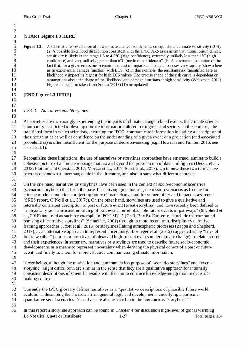
First Order Draft Chapter 1 IPCC AR6 WGI
Do Not Cite, Quote or Distribute 1-27 Total pages: 184
1
2
[START Figure 1.3 HERE] 3
4 Figure 1.3: A schematic representation of how climate change risk depends on equilibrium climate sensitivity (ECS). 5
(a) A possible likelihood distribution consistent with the IPCC AR5 assessment that “Equilibrium climate 6 sensitivity is likely in the range 1.5 to 4.5°C (high confidence), extremely unlikely less than 1°C (high 7 confidence) and very unlikely greater than 6°C (medium confidence)”. (b) A schematic illustration of the 8 fact that, for a given emissions scenario, the cost of impacts and adaptation rises very rapidly (shown here 9 as an exponential damage function) with ECS. (c) In this example, the resultant risk (quantified here as 10 likelihood × impact) is highest for high ECS values. The precise shape of the risk curve is dependent on 11 assumptions about the shape of the likelihood and damage functions at high sensitivity (Weitzman, 2011). 12 Figure and caption taken from Sutton (2018) [To be updated] 13
14
[END Figure 1.3 HERE] 15
16
17
1.2.4.3 Narratives and Storylines 18
19
As societies are increasingly experiencing the impacts of climate change related events, the climate science 20
community is solicited to develop climate information tailored for regions and sectors. In this context, the 21
traditional form in which scientists, including the IPCC, communicate information including a description of 22
the uncertainties as well as confidence on the understanding of a given event or a projection (and associated 23
probabilities) is often insufficient for the purpose of decision-making (e.g., Howarth and Painter, 2016, see 24
also 1.2.4.1). 25
26
Recognizing these limitations, the use of narratives or storylines approaches have emerged, aiming to build a 27
cohesive picture of a climate message that moves beyond the presentation of data and figures (Dessai et al., 28
2018; Fløttum and Gjerstad, 2017; Moezzi et al., 2017; Scott et al., 2018). Up to now these two terms have 29
been used somewhat interchangeable in the literature, and also in somewhat different contexts. 30
31
On the one hand, narratives or storylines have been used in the context of socio-economic scenarios 32
(scenario-storylines) that form the basis for deriving greenhouse gas emission scenarios as forcing for 33
climate model simulations projecting future climate change and for vulnerability and impact assessment 34
(SRES report, O’Neill et al., 2017c). On the other hand, storylines are used to give a qualitative and 35
internally consistent description of past or future event (event-storyline), and have recently been defined as 36
"a physically self-consistent unfolding of past events, or of plausible future events or pathways" (Shepherd et 37
al., 2018) and used as such for example in IPCC SR1.5 (Ch 3, Box 8). Earlier uses include the compound 38
phrasing of “narrative storylines” (Schneider, 2001) through to more recent transdisciplinary narrative 39
framing approaches (Scott et al., 2018) or storylines linking atmospheric processes (Zappa and Shepherd, 40
2017), as an alternative approach to represent uncertainty. Hazeleger et al. (2015) suggested using “tales of 41
future weather” (stories or narratives of observed high-impact events under climate change) to relate to users 42
and their experiences. In summary, narratives or storylines are used to describe future socio-economic 43
developments, as a means to represent uncertainty when deriving the physical conext of a past or future 44
event, and finally as a tool for more effective communicating climate information. 45
46
Nevertheless, although the motivation and communication purpose of “scenario-storylines” and “event-47
storyline” might differ, both are similar in the sense that they are a qualitative approach for internally 48
consistent descriptions of scientific results with the aim to enhance knowledge-integration in decision-49
making contexts. 50
51
Currently the IPCC glossary defines narratives as a “qualitative descriptions of plausible future world 52
evolutions, describing the characteristics, general logic and developments underlying a particular 53
quantitative set of scenarios. Narratives are also referred to in the literature as “storylines”.” 54
55
In this report a storyline approach can be found in Chapter 4 for discussion high-level of global warming 56
First Order Draft Chapter 1 IPCC AR6 WGI
Do Not Cite, Quote or Distribute 1-28 Total pages: 184
projections. Chapter 10, Chapter 12 and the Atlas focus on the role of narratives and storylines for 1
communication purposes, and also propose a distinction between the two terms. Chapter 11 uses a storyline 2
approach for discussing low-probability high-impact extreme events (section 11.10). Scenario-storylines are 3
further discussed in section 1.6.1 of this chapter. 4
5
1.3 History of climate understanding 6
7
Chapter 1 of the Working Group I (WGI) contribution to the AR4 (2007) provided a comprehensive 8
overview of the history of climate knowledge. This section summarizes some of the important milestones 9
and adds new discussions of the more recent history, including the IPCC era. It introduces the treatment of 10
uncertainty and calibrated uncertainty language used in IPCC reports. Finally, it presents key findings from 11
AR5 and the post-AR5 IPCC Special Reports, and compares projections from previous reports with recent 12
observations. The Appendix to this chapter summarizes the principal findings of all six IPCC assessment 13
reports, including the present one. 14
15
16
1.3.1 Climate science before 1950 17
18
Modern climate science combines aspects of meteorology, oceanography, geography, geology, ecology, 19
chemistry, hydrology, glaciology, and geophysics, as well as other disciplines. It coalesced as a separate field 20
of study in the mid-20th century. Scientists first developed theories of anthropogenic climate change in the 21
19th century, but these were not systematically explored until after World War II. This section reviews major 22
lines of work contributing to its emergence. 23
24
Observations. Observing patterns of weather and climate is an ancient practice, as evidenced by descriptions 25
and typologies of climatic regions in many cultures and literatures. Instrumental weather observation dates to 26
the invention of thermometers and barometers in the 16th and 17th centuries. Several synoptic observing 27
networks were established in 17th century Eurasia, but none endured more than two decades (Cassidy, 1985; 28
Khrgian and Hardin, 1970; Nebeker, 1995). Isolines and other graphical techniques for representing synoptic 29
measurements were invented in the early 19th century (Humboldt, 1817). By the mid-19th century, semi-30
standardized naval logs provided records of winds, ocean currents, precipitation, and air and sea surface 31
temperatures, and low-resolution seasonal climatologies (long-term means) had already been prepared for 32
much of the globe (Dove and Sabine, 1853; Maury, 1855, 1860; Maury and United States Naval 33
Observatory, 1849). The five-zone Köppen climate classification, developed in 1884, remains in use today 34
(Belda et al., 2014). It was even used as a diagnostic tool for climate models (Lohmann et al., 1993) and to 35
describe climate changes (Chen and Chen, 2013). Peruvian fishermen first identified the El Niño 36
phenomenon; related global teleconnections were noted in the late 19th century, and the atmospheric 37
Southern Oscillation was first described in the 1920s (Cushman, 2004). Japanese meteorologist, Wasaburo 38
Ooishi, discovered the jet stream in the 1920s using pilot balloons (Lewis, 2003). 39
40
Synoptic meteorology began in the 1840s with the spread of the electric telegraph. Telegraph operators 41
transmitted weather data at no cost, establishing a crucial tradition of free exchange of data. 19th-century 42
national weather services developed networks of surface stations and issued weather forecasts starting in 43
1861; recognizing the value of shared data and standards, they created the International Meteorological 44
Organization (IMO) in 1873. A patchy data-sharing network reached all continents except Antarctica by 45
1900. Regular collection of climatological data for the world began in 1905 with the Réseau Mondial (Great 46
Britain Meteorological Office and Shaw, 1920), and the similar collections World Weather Records 47
(Clayton, 1927) and Monthly Climatic Data for the World (est. 1948) have been published continuously 48
since their founding. 49
50
Palaeoclimate perspectives. With the gradual acceptance of “deep time” in the 19th century came 51
investigation of fossils, geological strata, and other evidence pointing to large periodic shifts in Earth’s 52
climate, from ice ages to much warmer periods, across hundreds of millions of years. Orbital theories of 53
long-term climatic change, first suggested by Herschel around 1830, entered the literature starting with Croll 54

First Order Draft Chapter 1 IPCC AR6 WGI
Do Not Cite, Quote or Distribute 1-29 Total pages: 184
(1864, 1885). The interacting periodicities of orbital eccentricity, axial tilt, and axial precession were 1
theorized in the early 20th century (Milankovich, 1920), but were not definitively linked to ice age cycles 2
until decades later (Broecker et al., 1968; Emiliani, 1978). The reconstruction of more recent climate 3
variability and change began in the 1800s, with the recovery of tree rings, ice cores, and lake sediments for 4
early paleoclimate investigation. By the early 20th century, laboratory research had begun using tree rings to 5
measure precipitation and the possible influence of sunspots on climatic change (Douglass, 1914, 1919, 6
1922). The advent of radiocarbon dating in the 1940s (Arnold and Libby, 1949) would usher in an era of 7
rapid progress in paleoclimatology. 8
9
Understanding the climate system. The fact that climate is a globally interconnected system has been 10
known since ancient times. The English word “climate” derives from the Greek root klima (“inclination”), a 11
reference to the angle of incidence of the sun’s rays at different latitudes, a key cause of climatic differences. 12
Ocean currents and prevailing winds were well known to ancient mariners of many cultures, such as the 13
Polynesian islanders who navigated vast distances of open ocean (Genz et al., 2009). Scientific theories of 14
climate begin with Halley (1686), who articulated a theory of vertical circulation in the tropics to explain the 15
trade winds. Hadley (1735) improved on Halley’s explanation by including the Earth’s rotation as well as 16
solar heating; these large-scale tropical circulatory patterns are known today as Hadley cells. Ferrel (1856) 17
added the Coriolis force to existing theory, describing and explaining the major structures of the global 18
circulation. 19th-century scientists also established the main physical principles governing Earth’s 19
temperature. By 1822, the principle of radiative equilibrium (the balance between incoming solar radiation 20
and the energy Earth re-radiates into space) had been articulated, and the atmosphere’s role in retaining heat 21
had been likened to a serre, or greenhouse (Fleming, 1998; Fourier, 1822). 22
23
Before computers, models of climate were conceptual, analog, or mathematical. Conceptual models, such as 24
those of Hadley and Ferrel, explained major climatic features and processes in qualitative terms. Analogue 25
“dishpan” models simulated atmospheric circulatory patterns by means of rotating cylinders or globes filled 26
with viscous fluids and exposed to a heat source. Mathematical models applied basic physical principles, 27
such as radiative equilibrium or the Coriolis force, expressed in equations. Arrhenius (1896), seeking the 28
cause of ice ages, developed a 2-dimensional mathematical model of radiative transfer. In the early 1900s 29
Bjerknes extended the Navier-Stokes equations of fluid dynamics to the atmosphere, creating the 30
mathematical basis for a three-dimensional model of the global circulation (Bjerknes, 1906; Bjerknes et al., 31
1910). During World War I, Richardson developed a system for numerical weather prediction based on these 32
equations (Richardson, 1922). When his attempt to apply his own method failed dramatically, meteorologists 33
turned away from numerical modeling until after World War II (Nebeker, 1995). 34
35
Human and natural drivers. The first to measure the heat-absorbing capacity of carbon dioxide was Eunice 36
Foote (1856), though her contribution was ignored until very recently. By the late 1850s, spectrophotometers 37
permitted direct measurements of the radiative activity of gases. Water vapor, ozone, carbon dioxide, and 38
certain hydrocarbons were found to absorb longwave radiation emitted from the ground, the principal 39
mechanism of the greenhouse effect (Tyndall, 1861). Investigators established the major elements of the 40
geochemical carbon cycle on geological time scales: volcanic outgassing, coal formation, rock weathering, 41
deep-sea sedimentation, and oceanic absorption (Chamberlin, 1897, 1898; Ekholm, 1901). Some speculated 42
that variations in solar activity, such as the 17th-century “Maunder minimum” when few sunspots or aurorae 43
were observed, might affect short-term weather or climate (Weart, Discovery of Global Warming, 2018 web 44
version). Scientists speculatively linked volcanic aerosols to ice ages in the 1890s (Dörries, 2006; 45
Humphreys, 1913). 46
47
In the 1890s Högbom estimated that worldwide coal combustion of about 500 megatonnes per annum had 48
already completely offset the natural absorption of CO2 by silicate rock weathering (Berner, 1995; Crawford, 49
1997). Arrhenius (1896) found that a doubling of carbon dioxide would produce a 5-6°C warming, but in 50
1900 new measurements seemed to rule out CO2 as a greenhouse gas due to overlap with the absorption 51
bands of water vapor (Angström, 1900; Anonymous, 1901). Nonetheless, as coal combustion reached 900 52
megatonnes per annum, Arrhenius wrote that anthropogenic carbon dioxide might eventually warm the 53
planet (Arrhenius and Borns, 1908). However, Hann’s Handbook of Climatology — the field’s standard 54
textbook for 50 years — dismissed the carbon dioxide theory based on Angström’s result (Hann, 1883; Hann 55
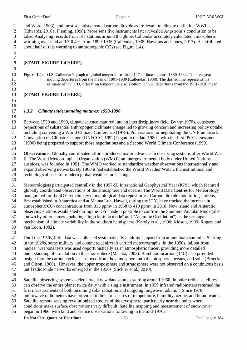
First Order Draft Chapter 1 IPCC AR6 WGI
Do Not Cite, Quote or Distribute 1-30 Total pages: 184
and Ward, 1903), and most scientists treated carbon dioxide as irrelevant to climate until after WWII 1
(Edwards, 2010a; Fleming, 1998). More sensitive instruments later revealed Angström’s conclusion to be 2
false. Analysing records from 147 stations around the globe, Callendar accurately calculated atmospheric 3
warming over land at 0.3-0.4°C from 1890-1935 (Callendar, 1938; Hawkins and Jones, 2013). He attributed 4
about half of this warming to anthropogenic CO2 (see Figure 1.4). 5
6
7
[START FIGURE 1.4 HERE] 8
9
Figure 1.4: G.S. Callendar’s graph of global temperatures from 147 surface stations, 1880-1934. Top: ten-year 10 moving departures from the mean of 1901-1930 (Callendar, 1938). The dashed line represents his 11 estimate of the “CO2 effect” on temperature rise. Bottom: annual departures from the 1901-1930 mean. 12
13
[START FIGURE 1.4 HERE] 14
15
16
1.3.2 Climate understanding matures: 1950-1990 17
18
Between 1950 and 1990, climate science matured into an interdisciplinary field. By the 1970s, consistent 19
projections of substantial anthropogenic climate change led to growing concern and increasing policy uptake, 20
including convening a World Climate Conference (1979). Preparations for negotiating the UN Framework 21
Convention on Climate Change (UNFCCC, 1992) began in the late 1980s, with the first IPCC assessment 22
(1990) being prepared to support those negotiations and a Second World Climate Conference (1990). 23
24
Observations. Globally coordinated efforts produced major advances in observing systems after World War 25
II. The World Meteorological Organization (WMO), an intergovernmental body under United Nations 26
auspices, was founded in 1951. The WMO worked to standardize weather observations internationally and 27
expand observing networks. By 1968 it had established the World Weather Watch, the institutional and 28
technological base for modern global weather forecasting. 29
30
Meteorologists participated centrally in the 1957-58 International Geophysical Year (IGY), which featured 31
globally coordinated observations of the atmosphere and oceans. The World Data Centres for Meteorology 32
inaugurated for the IGY remain key climatological data repositories. Carbon dioxide monitoring stations, 33
first established in Antarctica and at Mauna Loa, Hawaii, during the IGY, have tracked the increase in 34
atmospheric CO2 concentrations from 315 ppmv in 1958 to 410 ppmv in 2018. New island and Antarctic 35
observing stations established during the IGY made it possible to confirm the Southern Annular Mode (also 36
known by other names, including “high latitude mode” and “Antarctic Oscillation") as the principal 37
mechanism of climate variability in the southern hemisphere (Karoly et al., 1996; Kidson, 1999; Rogers and 38
van Loon, 1982). 39
40
Until the 1950s, little data was collected systematically at altitude, apart from at mountain summits. Starting 41
in the 1920s, some military and commercial aircraft carried meteorographs. In the 1950s, fallout from 42
nuclear weapons tests was used opportunistically as an atmospheric tracer, providing more detailed 43
understanding of circulation in the stratosphere (Machta, 2002). Bomb radiocarbon (14C) also provided 44
insight into the carbon cycle as it moved from the atmosphere into the biosphere, oceans, and soils (Broecker 45
and Olson, 1960). However, the upper troposphere and stratosphere were not observed on a continuous basis 46
until radiosonde networks emerged in the 1950s (Stickler et al., 2010). 47
48
Satellite observing systems added crucial new data sources starting around 1960. In polar orbits, satellites 49
can observe the entire planet twice daily with a single instrument. In 1959 infrared radiometers returned the 50
first measurements of both incoming solar radiation and outgoing longwave radiation. Since 1978, 51
microwave radiometers have provided indirect measures of temperature, humidity, ozone, and liquid water. 52
Satellite remote sensing revolutionized studies of the cryosphere, particularly near the poles where 53
conditions make surface observations very difficult. Satellite mapping and measurement of snow cover 54
began in 1966, with land and sea ice observations following in the mid-1970s. 55
First Order Draft Chapter 1 IPCC AR6 WGI
Do Not Cite, Quote or Distribute 1-31 Total pages: 184
1
Earth’s oceans store the vast majority of heat retained by the planet and play a major role in the climate 2
system. In addition to temperature, pressure, and other meteorological variables, military and merchant ships 3
measured sea surface temperature (SST), a major variable in climate studies. Both natural radiocarbon and 4
radionuclides from nuclear weapons tests provided tracers that helped establish circulatory patterns, 5
especially in the deep ocean (Broecker et al., 1960, 1980). Marine observations for the globe were first 6
assembled in the mid-1980s in the International Comprehensive Ocean-Atmosphere Data Set (ICOADS; 7
Woodruff et al., 1987, 2005). Sea level was historically measured by onshore tide gauges, but due to 8
numerous sources of error and limited spatial distribution, these are valuable mainly for measuring long-term 9
change. Satellite radar altimetry can measure sea level and ocean circulation from space at much higher 10
spatial and temporal resolutions, but after the brief SeaSat mission in 1978, was not deployed operationally 11
until the TOPEX/Poseidon missions of the 1990s (Katsaros and Brown, 1991). Ocean surface and subsurface 12
data collection efforts expanded in the 1980s with the Tropical Ocean Global Experiment (TOGA), which 13
eventually deployed 70 moored buoys (Gould, 2003). 14
15
Palaeoclimate perspectives. Palaeoclimatology covers a wide range of temporal scales, ranging from the 16
historical past to geological deep time (millions of years). Historical climatology aids near-term 17
palaeoclimate reconstructions using media such as diaries, almanacs, and merchant accounts that describe 18
climate-related events as frosts, flowers, harvests, droughts, famines, and grain prices. Meticulous records by 19
Chinese scholars and government workers, for example, have permitted detailed reconstructions of China’s 20
climate back to 1000 AD, and even beyond (Ge et al., 2008; Louie and Liu, 2003). Climatic phenomena such 21
as the Little Ice Age and the Medieval Climate Anomaly were originally proposed using data from historical 22
records from across Europe (Lamb, 1965, 1995; Le Roy Ladurie, 1967). 23
24
Most palaeoclimate research relies on climate proxy data generated from geological archives. Among the 25
few direct sources of observations about ancient climates are tiny air bubbles trapped in ice cores; these can 26
be sampled, providing direct evidence of past atmospheric composition (including CO2 levels). Climate 27
research using ice cores began in the 1950s, with oxygen-18 isotope in precipitation serving as a proxy 28
marker for temperature (Dansgaard, 1954). Cores were taken in Greenland, Antarctica, and various Arctic 29
locations during the 1957-58 International Geophysical Year, but palaeoclimate reconstructions were first 30
published a decade later on an almost 100,000-year core taken at Camp Century, Greenland (Dansgaard et 31
al., 1969; Langway Jr, 2008). Subsequent ice cores from Dome C in East Antarctica have extended this 32
climatic record to 800,000 years (Jouzel, 2013). 33
34
In the 1950s, glacial-interglacial cycles were observed in deep-sea sediment cores using oxygen isotope 35
ratios (Emiliani, 1955). The same technique was later combined with magnetic stratigraphy to establish 22 36
glacial-interglacial cycles over the past 870,000 years (Shackleton and Opdyke, 1973), confirming the 37
Milankovitch theory of orbital cycles as a key driver of natural climate change (Hays et al., 1976). Beginning 38
in the 1970s and continuing through the 1980s, global reconstructions of sea-surface temperature were 39
developed from hundreds of deep-sea sediment cores (McIntyre et al., 1976), providing the first quantitative 40
constraints for model simulations of ice age climates (e.g. Rind and Peteet, 1985). 41
42
Major volcanic eruptions, which can cause pronounced global cooling lasting 1-3 years, are recorded in ash 43
layers within ice cores and sediment layers. Starting in the 1960s, long-term changes in solar irradiance were 44
reconstructed from combinations of sunspot and aural observations, radiocarbon captured in tree wood, 10Be 45
in ice cores, and other indicators (Eddy, 1976; Stuiver, 1965). By the 1980s, other palaeoclimate archives, 46
including loess deposits, corals, pollen, tree rings, ice cores, lake sediments, and marine sediments, were also 47
contributing to past climate reconstructions, with temporal resolutions as high as monthly, in the case of 48
corals (Bradley, 2015; Jones et al., 2009). 49
50
Human and natural drivers. The major anthropogenic driver of climate change is greenhouse gases, with 51
aerosols and land use change playing significant secondary roles. Carbon dioxide’s key role in climate was 52
re-established following World War II. Studies established that the oceanic carbon sink absorbed some, but 53
not all anthropogenic CO2, thus accounting for its buildup in the atmosphere as well as for ocean 54
acidification. Revelle and Suess (1957) famously described fossil fuel emissions as a “large scale 55
First Order Draft Chapter 1 IPCC AR6 WGI
Do Not Cite, Quote or Distribute 1-32 Total pages: 184
geophysical experiment,” in which “within a few centuries we are returning to the atmosphere and oceans 1
the concentrated organic carbon stored in sedimentary rocks over hundreds of millions of years”. The 1960s 2
saw increasing attention to other radiatively active gases, especially ozone (Manabe and Möller, 1961; Plass, 3
1961). Methane, nitrous oxide, and chlorofluorocarbons were not considered systematically until the 1970s, 4
when anthropogenic increases in those gases were first noted (Rasmussen and Khalil, 1981) 5
. The US Climatic Impact Assessment Program (CIAP) of the early 1970s found that proposed fleets of 6
supersonic aircraft, flying in the stratosphere, would cause substantial depletion of the ozone layer (10-20 7
percent or more) and possible aerosol cooling, stimulating efforts to understand and to model stratospheric 8
circulation, atmospheric chemistry, and aerosol radiative effects (Mormino et al., 1975). 9
10
Natural drivers on decadal to centennial time scales include volcanoes, changes in solar irradiance, and 11
natural carbon sources and sinks. In the 1960-1990 period, volcanic activity of the recent past was traced via 12
historical records and quantified through observations of major eruptions by aircraft, satellites, and other 13
instruments (Dörries, 2006). Detailed global measurements of surface-level solar irradiance were first 14
conducted during the IGY (Landsberg, 1961), while top-of-atmosphere irradiance has been measured by 15
satellites since 1959 (House et al., 1986). Investigation of the carbon cycle was extended to the biosphere 16
and soils as well as the atmosphere, oceans, and marine sediments, with the ultimate goal of quantifying all 17
natural and anthropogenic carbon sources and sinks (Broecker and Olson, 1960). 18
19
Understanding and attributing climate change. With the arrival of digital computers in the 1950s, 20
mathematical models could be built to simulate climatic processes and climate change. A crude proof-of-21
concept climate simulation was created in 1956 (Phillips, 1956), and several laboratories devoted to climate 22
modelling emerged in the 1960s. By 1975, numerous laboratories had created general circulation models 23
(GCMs) for climate research. Rapid increases in computer power enabled higher resolutions and longer 24
model runs, and the inclusion of more physical processes. Of the latter, heat exchange between the oceans 25
and the atmosphere was the most essential. The first coupled ocean-atmosphere model (OAGCM) with 26
realistic topography appeared in 1975 (Bryan et al., 1975; Manabe et al., 1975). Over time, modelers 27
introduced more physical processes, including aerosols, atmospheric chemistry, sea ice, and snow, into 28
climate models (see Table 1.2). At the same time, research continued on zero- , one- , and two-dimensional 29
models, which provided constraints on the more complex GCMs. 30
31
Laboratory measurements, simpler models, and GCMs all supported the possibility of significant surface 32
warming as carbon emissions increased. From 1931-1980, most estimates of equilibrium climate sensitivity 33
fell into the 2-4°C range (see Edwards, 2010, p. 182). The detection of an anthropogenic warming “signal” 34
against the backdrop of natural variability was achieved in the 1990s. Nonetheless, the relatively consistent 35
results from measurements and models supported a series of policy reports flagging “inadvertent climate 36
modification” as a potential future policy concern (Conservation Foundation, 1963; Panel on Weather and 37
Climate Modification, 1966; Tukey et al., 1965). By 1970, the potential impacts of climate change on human 38
societies were being studied as inputs to the 1972 UN Conference on the Human Environment (Study of 39
Critical Environmental Problems, 1970; Study of Man’s Impact on Climate, 1971). 40
41
Projections of future climate change. General circulation modelling matured in the 1970s. By 1979, 42
responding to mounting concern, the US National Research Council (NRC) reported on the “best present 43
understanding of the carbon dioxide/climate issue for the benefit of policymakers.” The NRC evaluated 44
results from GCMs, radiative-convective models, and energy-balance models. The report estimated climate 45
sensitivity at 3°±1.5°C, stating the most likely range as 2-3.5°C, based on “consistent and mutually 46
supporting” model results (National Research Council; Ad Hoc Study Group on Carbon Dioxide and 47
Climate, 1979). 48
49
Throughout the 1980s, increasing attention to the climate change issue drove multidisciplinary research, 50
seeking more detailed understanding of regional effects, human and environmental impacts, and mitigation 51
strategies. Ecology, glaciology, hydrology, and atmospheric chemistry joined the list of contributing natural 52
sciences. Analysts developed integrated assessment models (IAMs) to study how human activity influences 53
climate change, how societies might be affected, and how they might respond (Rotmans, 1990). Numerous 54
organizations at both national and international levels began to assess the physical science of climate change, 55
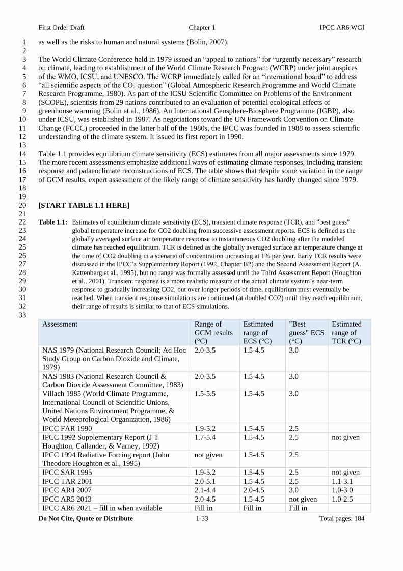
First Order Draft Chapter 1 IPCC AR6 WGI
Do Not Cite, Quote or Distribute 1-33 Total pages: 184
as well as the risks to human and natural systems (Bolin, 2007). 1
2
The World Climate Conference held in 1979 issued an “appeal to nations” for “urgently necessary” research 3
on climate, leading to establishment of the World Climate Research Program (WCRP) under joint auspices 4
of the WMO, ICSU, and UNESCO. The WCRP immediately called for an “international board” to address 5
“all scientific aspects of the CO2 question” (Global Atmospheric Research Programme and World Climate 6
Research Programme, 1980). As part of the ICSU Scientific Committee on Problems of the Environment 7
(SCOPE), scientists from 29 nations contributed to an evaluation of potential ecological effects of 8
greenhouse warming (Bolin et al., 1986). An International Geosphere-Biosphere Programme (IGBP), also 9
under ICSU, was established in 1987. As negotiations toward the UN Framework Convention on Climate 10
Change (FCCC) proceeded in the latter half of the 1980s, the IPCC was founded in 1988 to assess scientific 11
understanding of the climate system. It issued its first report in 1990. 12
13
Table 1.1 provides equilibrium climate sensitivity (ECS) estimates from all major assessments since 1979. 14
The more recent assessments emphasize additional ways of estimating climate responses, including transient 15
response and palaeoclimate reconstructions of ECS. The table shows that despite some variation in the range 16
of GCM results, expert assessment of the likely range of climate sensitivity has hardly changed since 1979. 17
18
19
[START TABLE 1.1 HERE] 20
21 Table 1.1: Estimates of equilibrium climate sensitivity (ECS), transient climate response (TCR), and "best guess" 22
global temperature increase for CO2 doubling from successive assessment reports. ECS is defined as the 23 globally averaged surface air temperature response to instantaneous CO2 doubling after the modeled 24 climate has reached equilibrium. TCR is defined as the globally averaged surface air temperature change at 25 the time of CO2 doubling in a scenario of concentration increasing at 1% per year. Early TCR results were 26 discussed in the IPCC’s Supplementary Report (1992, Chapter B2) and the Second Assessment Report (A. 27 Kattenberg et al., 1995), but no range was formally assessed until the Third Assessment Report (Houghton 28 et al., 2001). Transient response is a more realistic measure of the actual climate system’s near-term 29 response to gradually increasing CO2, but over longer periods of time, equilibrium must eventually be 30 reached. When transient response simulations are continued (at doubled CO2) until they reach equilibrium, 31 their range of results is similar to that of ECS simulations. 32
33
Assessment Range of
GCM results
(°C)
Estimated
range of
ECS (°C)
"Best
guess" ECS
(°C)
Estimated
range of
TCR (°C)
NAS 1979 (National Research Council; Ad Hoc
Study Group on Carbon Dioxide and Climate,
1979)
2.0-3.5 1.5-4.5 3.0
NAS 1983 (National Research Council &
Carbon Dioxide Assessment Committee, 1983)
2.0-3.5 1.5-4.5 3.0
Villach 1985 (World Climate Programme,
International Council of Scientific Unions,
United Nations Environment Programme, &
World Meteorological Organization, 1986)
1.5-5.5 1.5-4.5 3.0
IPCC FAR 1990 1.9-5.2 1.5-4.5 2.5
IPCC 1992 Supplementary Report (J T
Houghton, Callander, & Varney, 1992)
1.7-5.4 1.5-4.5 2.5 not given
IPCC 1994 Radiative Forcing report (John
Theodore Houghton et al., 1995)
not given 1.5-4.5 2.5
IPCC SAR 1995 1.9-5.2 1.5-4.5 2.5 not given
IPCC TAR 2001 2.0-5.1 1.5-4.5 2.5 1.1-3.1
IPCC AR4 2007 2.1-4.4 2.0-4.5 3.0 1.0-3.0
IPCC AR5 2013 2.0-4.5 1.5-4.5 not given 1.0-2.5
IPCC AR6 2021 – fill in when available Fill in Fill in Fill in

First Order Draft Chapter 1 IPCC AR6 WGI
Do Not Cite, Quote or Distribute 1-34 Total pages: 184
1
[END TABLE 1.1 HERE] 2
3
4
1.3.3 Climate science and global change, 1990-present: the IPCC era 5
6
Since 1990, numerous national science agencies, academic researchers, and international and 7
intergovernmental scientific organizations — many of them newly established — have contributed to 8
increased understanding of the climate system and to projections of future climate change. IPCC assessments 9
consider data and understanding as published in the peer-reviewed scientific literature. IPCC reports undergo 10
one of the most exhaustive, open, and rigorous review and revision processes ever designed for science 11
assessments; the assessment and review process itself has undergone intensive scrutiny and multiple 12
revisions in response to critique (Mach et al., 2016; Shapiro et al., 2010). 13
14
Observations. Increasing confidence in an unprecedented warming trend in both atmosphere and oceans is 15
based on a large and growing body of observational evidence. New organizations and networks were 16
established to coordinate and standardize climate-related observing systems on a global scale. These include 17
the Global Ocean Observing System (GOOS, est. 1991), the Global Climate Observing System (GCOS, est. 18
1992), the Global Historical Climatology Network (GHCN, est. 1992), the Global Earth Observing System 19
of Systems (GEOSS, est. 2005), and the Global Cryosphere Watch (est. 2011). As a result, most but not all 20
observing systems have experienced improvement in consistency and coverage since 1990 (see Section 1.4). 21
22
Data on surface temperature have been repeatedly extended, refined, and evaluated. Global land-ocean 23
surface datasets, first developed in the 1980s by three independent groups (NOAA, NASA GISS, and 24
HadCRU), introduced numerous new methods for quality control, adjustment, and error analysis (Hansen et 25
al., 2010; Morice et al., 2012; Vose et al., 2012). A new, independently developed land surface dataset for 26
1753-2011 used novel adjustment techniques and data from over 36,000 thermometer sites (Muller et al., 27
2013; Rohde et al., 2013), and agrees closely with the three established datasets. 28
29
Data sources for the vertical dimension — principally radiosondes and satellites — have evolved 30
considerably since 1990. New methods for spatial and temporal homogenization of radiosonde records, using 31
comparisons with reanalyses and with neighboring stations, were introduced in the early 2010s (Haimberger 32
et al., 2012). As for satellite data, vertical profiles must be derived algorithmically and calibrated against in 33
situ radiosonde measurements. Over time, numerous adjustments to these algorithms have been made to 34
account for such factors as orbital precession and decay. As a result, new versions of these datasets have 35
been released every few years since 1978 (Edwards, 2010). However, despite repeated adjustments, 36
differences remain in the temperature trends from surface, radiosonde, and satellite observations. These are 37
the subject of ongoing research (Santer et al., 2017; Thorne et al., 2011). 38
39
Ocean data sources have expanded dramatically since 1990. ICOADS extended its coverage to 1662-2014 40
using newly recovered marine records and metadata (Freeman et al., 2017; Woodruff et al., 1998). In the 41
2000s, a major improvement in SST data came from adjustment for biases resulting from differing methods 42
of measuring sea surface temperature (from buckets to engine intake thermometers), especially in the period 43
around World War II (Kent et al., 2007). The World Ocean Circulation Experiment (1990-1997) collected 44
data on subsurface currents at 1000 m, as well as temperature and salinity, using autonomous submersible 45
floats (Gould, 2003). Since 2000, Argo floats have measured temperature, salinity, and current velocity from 46
the surface to 2000m, covering most of the globe with almost 4000 floats by 2018 (Cheng et al., 2017). 47
These new sources provide much more information on ocean heat content at depth. The first IPCC 48
discussion of global ocean heat content appeared in the Third Assessement Report (TAR), which reported a 49
1948-1998 time series for the upper 300m. By the time of AR5, more accurate global data were available for 50
1971-2010 to 700 m and for 1957-2009 from 700 to 2000 m. 51
52
Beginning in 1992, sparse data from coastal tide gauges were augmented by global sea level measurements 53
from TOPEX/POSEIDON satellite altimetry (Fu et al., 1994). These data were first incorporated in the TAR. 54
Since the early 2000s, those satellites have been replaced by data from subsequent missions. 55
First Order Draft Chapter 1 IPCC AR6 WGI
Do Not Cite, Quote or Distribute 1-35 Total pages: 184
1
Knowledge of the state and evolution of the cryosphere increased spectacularly after 1990. Prior to the TAR, 2
the sign of the mass budget of the Greenland and Antarctic ice sheets could not be determined. Through a 3
combination of satellite and airborne altimetry and gravity measurements, and a better knowledge of surface 4
mass balance and perimeter fluxes, a consistent signal of ice loss for both ice sheets was established by the 5
time of AR5 (Shepherd et al., 2012). After 2000, satellite radar interferometry revealed rapid changes in 6
surface velocity at ice-sheet margins, often linked to reduction or loss of ice shelves (Rignot and 7
Kanagaratnam, 2006; Scambos et al., 2004). The Greenland Climate Network (GC-Net) was established in 8
1994 to monitor climatological and glaciological parameters with Automatic Weather Stations (Steffen and 9
Box, 2001). Data sources for assessing the evolution of mountain glaciers and ice caps improved 10
considerably, with internationally coordinated activities compiling worldwide glacier length and mass 11
balance observations (World Glacier Monitoring Service, Zemp et al., 2015), global glacier outlines 12
(Randolph Glacier Inventory, Pfeffer et al., 2014), and ice thickness of about 1100 glaciers (GlaThiDa, 13
Gärtner-Roer et al., 2014). Whereas sea ice extent and concentration had been continuously monitored since 14
1979 from multichannel passive microwave imagery, datasets for ice thickness emerged later from upward 15
sonar profiling by submarines (Rothrock et al., 1999) and radar altimetry of sea-ice freeboards (Laxon et al., 16
2003). 17
18
The increased amount and quality of global data permitted AR5 to provide estimates of changes in the global 19
energy inventory, i.e., the amount of incoming solar energy retained by the atmosphere, oceans, land surface, 20
and cryosphere (see Box 3.1 of AR5). 21
22
Palaeoclimate perspectives. Since 1990, paleoclimate records have increased in both temporal span and 23
spatio-temporal resolution, including seasonally–annually resolved reconstructions of temperature, 24
hydroclimate, and large-scale circulation modes (Masson-Delmotte et al., 2013). Marine sediment and ice 25
core records provide quantitative estimates of past temperature, ice volume, sea level, and atmospheric 26
chemistry associated with glacial–interglacial cycles over the past 800,000 years (Section 1.2.1.2, Figure 1.2) 27
(EPICA Community Members, 2004; Jouzel, 2013; Lisiecki and Raymo, 2005; Past Interglacials Working 28
Group of PAGES, 2016; Siddall et al., 2003). As dating techniques continue to improve, there has been 29
major progress in the development of seasonally–annually resolved palaeoclimate records covering the last 30
2,000 years (Abram et al., 2016; Emile-Geay et al., 2017; PAGES 2k Consortium, 2013; PAGES Hydro2k 31
Consortium, 2017; Tierney et al., 2015). 32
33
Of particular relevance to AR6 are recent efforts to reconstruct seasonal extremes in continental-scale 34
temperature (Luterbacher, 2004) and ocean temperatures (Abram et al., 2007; Cobb et al., 2003; Cole and 35
Fairbanks, 1990) over the last centuries to millennia. This interval contains well documented periods of 36
human history that can be used to verify climate variability reconstructed using palaeoclimate sources (White 37
et al., 2018). In particular, notable advances from regions of the Southern Hemisphere have improved our 38
description of global and hemispheric climate variability and change (Dätwyler et al., 2018; Nash et al., 39
2016; Neukom et al., 2014; Neukom and Gergis, 2012; Palmer et al., 2015). 40
41
Paleoclimate modeling advanced significantly during this period, with Paleoclimate Modeling 42
Intercomparison Projects (PMIP) assessed by the TAR (PMIP), AR4 (PMIP2), and AR5 (PMIP3). Recent 43
improvements in paleoclimate modeling include data assimilation approaches that combine high-resolution 44
paleoclimate data with AOGCMs to generate gridded reconstruction of climate over the last millennium (e.g. 45
Hakim et al., 2016). Global climate models that incorporate water isotope tracers now provide a rich 46
resource for advanced paleoclimate data-model intercomparisons (Jouzel et al., 1998; Stevenson et al., 2018; 47
Xi, 2014). 48
49
Indigenous perspectives. During this period, indigenous and traditional knowledge (ITK) has played an 50
increasing role in historical climatology on decadal and centennial timescales, especially in areas such as the 51
Arctic where instrumental observations are sparse. Inuit communities have contributed to climatic history 52
and community based monitoring (Gearheard et al., 2010; Riedlinger and Berkes, 2001). Indigenous 53
Australian knowledge of climatic patterns has been offered as a complement to sparse observational records 54
(Green et al., 2010; Head et al., 2014), while researchers have documented sophisticated awareness of 55

First Order Draft Chapter 1 IPCC AR6 WGI
Do Not Cite, Quote or Distribute 1-36 Total pages: 184
interannual variability in the timing and seasonality of rainfall in Uganda (Orlove et al., 2010). In order to 1
harmonize scientific and local knowledge, ongoing research seeks to conduct further dialogue, systematize 2
indigenous knowledge, and analyze its utility for multiple purposes, especially adaptation (Alexander et al., 3
2011; Laidler, 2006). 4
5
Human and natural drivers of climate change. Changes in solar irradiance, a natural climate forcing, have 6
been small and slightly negative since about 1980 (Matthes et al., 2017a). The negative radiative forcing 7
(RF) of major volcanic eruptions was considered in the FAR; in subsequent assessments, the negative RF of 8
smaller eruptions has also been included. The FAR (1990) focused attention on human emissions of carbon 9
dioxide, methane, halocarbons, and nitrous oxide; of these, only the sources of CO2 and halocarbons were 10
well measured, with methane sources known only “semi-quantitatively” (IPCC, 1990, p. 29). Since then, 11
new natural sources of methane have been identified (O’Connor et al., 2010; Ruppel and Kessler, 2017), as 12
well as anthropogenic ones (Conley et al., 2016; Duren and Miller, 2012; Howarth, 2014). 13
[PLACEHOLDER: add role of ocean circulation as a driver when SROCC is ready]. 14
15
Unlike previous assessments, AR5 (2013) characterized anthropogenic radiative forcing relative to 16
greenhouse gas emissions rather than to concentrations, thus accounting directly for how emissions of some 17
substances cause changes in others. For example, emissions of halocarbons cause stratospheric ozone 18
depletion; emission-based RF of halocarbons includes both the positive radiative forcing (RF) of halocarbons 19
and the negative RF of reduced ozone concentrations. Overall, concentration-based and emissions-based 20
forcings are identical, but the latter does a better job of accounting for anthropogenic effects. The RFs of 21
short-lived greenhouse gases such as carbon monoxide and nitrogen oxides other than N2O were quantified 22
and included in overall calculations. Among the greatest advances has been increased understanding of the 23
nature and complex role of aerosols, with both positive and negative RF. In addition to its positive RF in 24
aerosols (Gustafsson and Ramanathan, 2016), black carbon (soot) from fuel combustion was identified as a 25
significant contributor to accelerating ice melt (AMAP, 2015; Gertler et al., 2016). The extent and role of 26
land use change has been better quantified, and a more complex understanding of its effects on the carbon 27
cycle has emerged (Houghton and Nassikas, 2017). 28
29
Understanding and attributing climate change. The FAR (1990) concluded that while both theory and 30
models suggested that anthropogenic warming was underway, its signal could not yet be detected in 31
observational data against the “noise” of natural variability (also see Barnett and Schlesinger, 1987). Since 32
then, increased warming and progressively stronger attribution studies using multiple lines of evidence have 33
identified human activities as the “dominant cause of the observed warming since the mid-20th century” 34
(AR5 SPM). Starting in the early 1990s, “fingerprint” studies examined specific model-predicted changes in 35
certain variables (such as nights warming faster than days, a rising tropopause, a cooling stratosphere, and 36
multi-year record-breaking temperatures) that could not be caused by natural climate drivers such as changes 37
in solar irradiance or volcanic forcing (Davy et al., 2017; Karoly et al., 1994; Mann et al., 2017; Santer, 38
2003; Santer et al., 2013; Schneider, 1994; Stott et al., 2010). 39
40
Although climate models remain imperfect, their spatial resolution has increased dramatically while 41
including ever more physical processes. In the 1990s, coupled AOGCMs were state of the art; by the 2010s, 42
Earth system models (ESMs) and coupled carbon-cycle climate models incorporated land surface, sea ice, 43
snow, vegetation, and other elements of the climate system. By 2000, some major modeling centers had 44
deployed “unified” models for both weather prediction and climate modeling, with the goal of a “seamless” 45
modeling approach that uses the same dynamics, physics, and parameterizations at multiple scales of time 46
and space (WMO, 2015). Cloud processes and feedbacks, including indirect aerosol feedbacks, are better 47
understood empirically, but they remain the single largest source of spread in GCM calculations of climate 48
sensitivity, with numerous parameterization schemes in use (Gettelman and Sherwood, 2016; Stephens, 49
2005). ENSO forecasting, an exceptionally difficult test for prediction models, has improved slightly since 50
the 1980s (Barnston et al., 2017). 51
52
Since climate models and model runs vary along many dimensions, comparing their results requires special 53
techniques. Since the late 1980s, the climate modeling community has developed increasingly sophisticated 54
model intercomparison projects (MIPs) (Covey et al., 2003; Gates et al., 1999). MIPs prescribe standardized 55

First Order Draft Chapter 1 IPCC AR6 WGI
Do Not Cite, Quote or Distribute 1-37 Total pages: 184
experimental design, time periods, output variables, and observational reference data, thus permitting direct 1
comparison of model results and helping to diagnose the reasons for biases and other differences among 2
models and further process understanding. In both CMIP3 and CMIP5 experiments, climate model 3
ensembles successfully reproduced 20th century global trends when they incorporated realistic 4
anthropogenic forcings (Meehl et al., 2007a; Taylor et al., 2012). Yet when only natural forcings were 5
included (creating the equivalent of a “control Earth” without human influences), the same experiment could 6
not reproduce the observed post-1970 warming (Jones et al., 2013). This result held true at both global and 7
continental scales. 8
9
Projections of future changes in climate. Because greenhouse gas and aerosol emissions, land use, and 10
other human activities may change in numerous ways, future climate change cannot be precisely predicted. 11
Therefore, each IPCC report has considered a range of possible scenarios, typically a “business as usual” 12
scenario in which societies continue on their present course as well as several others reflecting 13
socioeconomic and policy responses that may limit emissions and/or increase the rate of carbon dioxide 14
removal from the atmosphere. IPCC Working Group III assesses scenarios and their implications for 15
emissions, land use, and other key variables. (For further details on scenarios, see Section 1.6 of this 16
chapter.) 17
18
Climate models are then run to simulate the outcomes of each scenario for the climate system. Since 1990, 19
the quality and precision of model projections has improved due to better process understanding as well as 20
higher model resolution. MIPs have increased confidence in the quality of these projections, as have 21
comparisons of projections with observations (see Figure 4.X in chapter 4). Due to the high computational 22
cost of GCM runs, starting with the SAR “Earth system models of intermediate complexity” (EMICs) were 23
also employed, especially for such purposes as long-term projections and estimates of climate change 24
commitment, irreversibility, and thresholds for ice-sheet decay (see Section 1.4.3.2). 25
26
[START BOX 1.1 HERE] 27
28
Box 1.1: Treatment of uncertainty and calibrated uncertainty language used in IPCC reports 29
Throughout the IPCC’s history, the consistent treatment and communication of scientific uncertainty across 30
all three Working Groups (WGs) has been important (Cubasch et al., 2013; Le Treut et al., 2007). Already in 31
its 1990 first report, the IPCC specified terms and methods for communicating authors’ expert judgments 32
(Mastrandrea and Mach, 2011). Over time, the IPCC has developed and revised a framework to treat 33
uncertainties consistently between assessment cycles, reports and across WGs through the use of calibrated 34
language (IPCC, 2005; Moss and Schneider, 2000). The framework was updated in preparation of the AR5 35
(Mastrandrea et al., 2010, 2011). 36
37
Considerable critical attention has focused on whether applying the IPCC framework effectively achieves 38
consistent treatment of uncertainties and clear communication of findings to users (Adler and Hirsch Hadorn, 39
2014; Shapiro et al., 2010). Specific concerns include, e.g., the transparency and traceability of expert 40
judgements underlying the assessment conclusions (Oppenheimer et al., 2016) or the context-dependent 41
representations and interpretations of probability terms (Budescu et al., 2014). 42
43
Mach et al. (2017) investigated the advances and challenges in approaches to expert judgment in the IPCC 44
AR5. Their analysis showed that the shared framework increased the overall comparability of assessment 45
conclusions across all WGs and topics related to climate change, from the physical science basis to resulting 46
impacts, risks, and options for response. While the WGs in the AR5 still favored different expert-judgment 47
scales, the differences more directly reflected the different evidence bases across the WGs. Nevertheless, 48
many challenges in developing and communicating assessment conclusions persist (Mach et al., 2017), 49
especially for findings drawn from multiple disciplines and Working Groups, for findings with substantial 50
(or “deep”; SROCC Chapter 1) uncertainties, and for subjective aspects of judgments. 51
52
Approach for the AR6 53
AR6 follows the approach developed for AR5 (Box 1.1, Figure 1), as described in the “Guidance Notes for 54
First Order Draft Chapter 1 IPCC AR6 WGI
Do Not Cite, Quote or Distribute 1-38 Total pages: 184
Lead Authors of the IPCC Fifth Assessment Report on Consistent Treatment of Uncertainties” (Mastrandrea 1
et al., 2010). The three WGs use two metrics to communicate the degree of certainty in key findings, which 2
is based on author teams’ evaluations of underlying scientific understanding: 3
4
(1) Confidence is a qualitative measure of the validity of a finding, based on the type, amount, quality 5
and consistency of evidence (e.g., data, mechanistic understanding, theory, models, expert judgment) 6
and the degree of agreement; and 7
(2) Likelihood provides a quantified measure of uncertainty in a finding expressed probabilistically (e.g., 8
based on statistical analysis of observations or model results, or both, and expert judgement). 9
10
Where appropriate, findings can also be formulated as statements of fact without uncertainty qualifiers. 11
Throughout IPCC reports, the calibrated language is clearly identified by being typeset in italics. 12
13
The uncertainty guidance note clarifies the relationship between the qualitative description of confidence and 14
the quantitative representation of uncertainty expressed by the likelihood scale. Responding in part to 15
criticisms (Shapiro et al., 2010), it emphasizes traceability of the assessment throughout the process. Key 16
chapter findings elevated to the Executive Summary are supported in the chapter text by detailed 17
descriptions of the underlying evaluations of evidence and agreement, confidence, and likelihood. The 18
guidance note also leaves flexibility to convey the most information when multiple options or combinations 19
of confidence and likelihood are possible to characterize key findings. 20
21
Direct comparisons of uncertainties assessed in this Report with those from earlier WGI reports are, 22
however, sometimes difficult due to a number of factors. These include the application of the revised 23
guidance note on uncertainties (in the case of, e.g., WGI AR4, SREX and earlier reports), as well as the 24
availability of new information, improved scientific understanding, continued analyses of data and models, 25
and specific methodological differences in studies assessed by previous reports. For some climate variables, 26
different aspects have been assessed from report to report and therefore a direct comparison between 27
assessments would be difficult and limited. 28
29
30
[START BOX 1.1, FIGURE 1 HERE] 31
32 Box 1.1, Figure 1: The IPCC AR6 approach for characterizing understanding and uncertainty in assessment findings. 33
This diagram illustrates the step-by-step process authors use to evaluate and communicate the state 34 of knowledge in their assessment (Mastrandrea et al., 2010). Authors present evidence/agreement, 35 confidence, or likelihood terms with assessment conclusions, communicating their expert judgments 36 accordingly. Example conclusions are drawn from the IPCC WGI AR5. [adapted from Mach et al. 37 (2017)] 38
39
[END BOX 1.1, FIGURE 1 HERE] 40
41
42
Box.1.1, Figure 1 illustrates the idealized step-by-step process of the IPCC assessment of scientific 43
understanding and uncertainties (adapted from Mach et al. (2017)). The process starts with evaluation of the 44
available evidence and agreement (Box.1.1, Figure 1, Steps 1–3). The following summary terms are used to 45
describe the available evidence: limited, medium, or robust; and the degree of agreement: low, medium, or 46
high. Generally, evidence is most robust when there are multiple, consistent, independent lines of high-47
quality evidence. 48
49
Next, the level of confidence is evaluated, combining the assessments of evidence and agreement into a 50
single metric (Box.1.1, Figure 1, Steps 3–5). The assessed level of confidence is expressed using five 51
qualifiers: very low, low, medium, high, and very high. It is typeset in italics to highlight that this is based on 52
a formal confidence assessment, e.g., medium confidence. Box.1.1, Figure 1, Step 4, depicts summary 53
statements for evidence and agreement and their relationship to confidence. There is flexibility in this 54
relationship; for a given evidence and agreement statement, different confidence levels can be assigned, but 55
increasing levels of evidence and degrees of agreement correlate with increasing confidence. 56
First Order Draft Chapter 1 IPCC AR6 WGI
Do Not Cite, Quote or Distribute 1-39 Total pages: 184
1
Where uncertainties can be quantified probabilistically, assessment conclusions can be expressed with 2
likelihood statements (Box.1.1, Figure 1, Steps 5–6). However, unless indicated otherwise, likelihood 3
statements are limited to findings for which the authors’ assessment of confidence is “high” or “very high”. 4
Terms used to indicate the assessed likelihood of an outcome or a result include: virtually certain: 99–100% 5
probability, very likely: 90–100%, likely: 66–100%, about as likely as not: 33–66%, unlikely: 0–33%, very 6
unlikely: 0–10%, exceptionally unlikely: 0–1%. Additional terms (extremely likely: 95–100%, more likely 7
than not >50–100%, and extremely unlikely 0–5%) may also be used when appropriate. Likelihood can 8
indicate probabilities for single events or broader outcomes. The associated probabilistic judgments may 9
build from statistical or modeling analyses, elicitation of expert views, or other quantitative analyses. The 10
framework encourages authors, where appropriate, to present probability more precisely than can be done 11
with the likelihood scale, for example with complete probability distributions or percentile ranges, including 12
quantification of tails of distributions important for risk management (Mach et al., 2017; see also sections 13
1.2.4.1 and 1.2.4.2). 14
15
Throughout this WGI report and unless stated otherwise, uncertainty is quantified using 90% uncertainty 16
intervals. The 90% uncertainty interval, reported in square brackets, is expected to have a 90% likelihood of 17
covering the value that is being estimated. (i.e., the range encompasses the median value and there is an 18
estimated 5% likelihood of the value being below the lower end of the range or above its upper end). 19
Uncertainty intervals are not necessarily symmetric about the corresponding best estimate. A best estimate of 20
that value is also given where available. 21
22
[END BOX 1.1 HERE] 23
24
25
1.3.4 Key findings of previous IPCC assessments 26
27
Working Group I (WGI) of the IPCC considers new evidence of climate change based on independent 28
scientific analyses from observations of the climate system, palaeoclimate archives, theoretical studies of 29
climate processes, and simulations using climate models. Each consecutive report builds on previous 30
assessments of the physical science of climate change by incorporating new research and updating previous 31
findings (see previous sections, in particular 1.3.3). The robustness of the IPCC assessment stems from the 32
systematic consideration and combination of multiple lines of independent evidence. 33
34
35
1.3.4.1 Key findings of AR5 36
37
The WGI contribution to AR5 is the most comprehensive assessment since the IPCC’s first report in 1990. It 38
is also the most extensively reviewed, with over 54,000 comments received and responded to by the authors. 39
AR5 highlighted many important advances in climate science understanding. Compared to WGI AR4 40
(IPCC, 2007), more palaeoclimate reconstructions, more detailed and longer observations and improved 41
climate models were available, resulting in better understanding of the physical basis of climate change. 42
43
The WGI contribution to AR5 comprehensively assessed observations of climate change (“what has 44
changed”), understanding of these changes and their causes (“why has it changed”), and future projections of 45
climate change (“how will it change in the future”). 46 47 1) Warming of the climate system is unequivocal 48 49 The WGI AR5 assessed that warming of the climate system is unequivocal and that many of the observed 50
changes since 1950 are unprecedented over decades to millennia. Changes are evident in all components of 51
the climate system: the atmosphere and ocean have warmed, the amounts of snow and ice have diminished, 52
sea level has risen, and the atmospheric concentrations of greenhouse gases have increased. The WGI AR5 53
also, for the first time in IPCC, highlighted at the level of the SPM the “other side of the CO2 problem” 54
(Doney et al., 2009), i.e., ocean acidification caused by the absorption of about 30% of anthropogenic carbon 55
First Order Draft Chapter 1 IPCC AR6 WGI
Do Not Cite, Quote or Distribute 1-40 Total pages: 184
dioxide from the atmosphere. 1
2
Many key WGI AR5 findings on recent changes could be placed in a longer-term context, linking the present 3
state of the climate with observational evidence from the historical period and with evidence from 4
paleoclimate archives. For surface air temperature, for example, the WGI AR5 assessed that each of the last 5
three decades has been successively warmer at the Earth’s surface than any preceding decade since 1850. In 6
the Northern Hemisphere, 1983–2012 was likely the warmest 30-year period of the last 1400 years (medium 7
confidence). For sea level, the WGI AR5 assessed with high confidence that the rate of sea level rise since 8
the mid-19th century has been larger than the mean rate during the previous two millennia. 9
10
The WGI AR5 also assessed the ocean’s role in trapping extra energy and highlighted its importance: ocean 11
warming massively dominates the increase in energy stored in the climate system, accounting for more than 12
90% of the energy accumulated between 1971 and 2010 (high confidence). In comparison, warming of the 13
atmosphere only corresponds to roughly 1% of the energy accumulated over the same period. 14
15
2) Human influence on the climate system is clear. 16
17
The WGI AR5 assessed the vast evidence supporting the human influence on the climate system. The 18
multiple lines of independent evidence include, among others, increasing greenhouse gas concentrations, 19
positive radiative forcing estimates, unequivocal observed warming across climate system components, and 20
the theoretical understanding of the climate system. 21
22
As for drivers of climate change, the WGI AR5 assessment confirmed the dominant role of carbon dioxide 23
(CO2) and the net cooling effect from aerosols. The 40% increase in atmospheric CO2 since pre-industrial 24
times, primarily from fossil fuel emissions and secondarily from net land use change emissions, contributed 25
most to changes in total radiative forcing since 1750. Concentrations of CO2, methane (CH4), and nitrous 26
oxide (N2O), have all increased to levels unprecedented in at least the last 800,000 years. Aerosols and their 27
interactions with clouds, on the other hand, have offset a substantial portion of the positive global mean 28
radiative forcing resulting from the increase in well-mixed greenhouse gases (high confidence). 29
30
The evidence for human influence has grown since the time of the WGI AR4 (IPCC, 2007) and attribution of 31
a human contribution to detected changes was possible in WGI AR5 in more climate system components 32
than in previous reports. In the WGI AR5, human influence has been detected in warming of the atmosphere 33
and the ocean; changes in the global water cycle; reductions in snow and ice; global mean sea level rise; and 34
changes in some climate extremes. One of the key assessment findings of the WGI AR5 is that it is extremely 35
likely that human influence has been the dominant cause of the observed warming since the mid-20th 36
century. 37
38
3) Limiting climate change will require substantial and sustained reductions of greenhouse gas 39
emissions. 40 41 A critical policy-relevant finding of WGI AR5 is the close, approximately linear relationship of cumulative 42
total emissions of CO2 and global mean surface temperature response. This finding has important 43
implications for understanding current changes and projecting possible futures and thus provided crucial 44
information for negotiation of the Paris agreement (UNFCCC, 2015). For example, it implies that continued 45
emissions of greenhouse gases will cause further warming and changes in all components of the climate 46
system, independent of any specific scenario or pathway. Further emissions and increase in atmospheric CO2 47
will also lead to further uptake of carbon by the ocean and increase ocean acidification. From the close link 48
between cumulative emissions and warming it follows that any given level of warming (such as the 1.5°C 49
and 2°C warming targets in the Paris agreement) is associated with a total budget of CO2 emissions. To stay 50
within the budget, higher emissions in earlier decades imply lower emissions later on. In the absence of a 51
large net removal of CO2 from the atmosphere, stabilizing warming thus requires that CO2 emissions 52
descend to zero. 53
54
Climate projections based on the Representative Concentration Pathways (RCPs) assessed in WGI AR5 55
First Order Draft Chapter 1 IPCC AR6 WGI
Do Not Cite, Quote or Distribute 1-41 Total pages: 184
result in continued warming over the 21st century in all scenarios, and beyond 2100 under all RCP scenarios 1
except the strong mitigation scenario RCP2.6. Similarly, global mean sea level will continue to rise during 2
the 21st century. Under all RCP scenarios, the rate of sea level rise will very likely exceed that observed 3
during 1971-2010 due to increased ocean warming and increased loss of mass from glaciers and ice sheets. 4
By the mid-21st century the magnitudes of the projected changes are substantially affected by the choice of 5
emissions scenario. The WGI AR5 assessed that a 1.5°C target relative to 1850 to 1900 will likely be missed 6
under all RCP scenarios except the strong mitigation scenario RCP2.6. 7
8
Considering the long term, multi-century perspective, the WGI AR5 assessed that cumulative emissions of 9
CO2 will largely determine global mean surface warming by the late 21st century and beyond. Past, present 10
and future emissions of CO2 thus commit the world to substantial multi-century climate change, and most 11
aspects of climate change will thus persist for many centuries even if emissions of CO2 were stopped 12
immediately. According to the WGI AR5 assessment, a large fraction of this change is essentially 13
irreversible on a multi-century to millennial time scale, except in the case of a large net removal of CO2 from 14
the atmosphere over a sustained period through as yet unavailable technological means. 15
16
17
1.3.4.2 Key findings of post-AR5 Special Reports 18
19
Following the AR5 reports in 2013 and 2014, IPCC assessed new literature relevant to specific topics in 20
three Special Reports. The Special Report on Global Warming of 1.5°C (SR1.5) was produced in response to 21
an invitation of the United Nations Framework Convention on Climate Change (UNFCCC). The subjects of 22
the two others, the Special Report on the Ocean and Cryosphere in a Changing Climate (SROCC) and the 23
Special Report on Climate Change and Land (SRCCL), were the result of consultation with governments. 24
All Special Reports assess material relevant to all three IPCC Working Groups. Here we focus on key 25
findings related to the physical science basis. 26
27
The Special Report on Global Warming of 1.5°C (Masson-Delmotte et al., 2018) assessed current knowledge 28
on the impacts of global warming of 1.5°C above pre-industrial levels and related global greenhouse gas 29
emission pathways, in the context of strengthening global efforts to respond to climate change, pursue 30
sustainable development, and eradicate poverty. The key findings of SR1.5 most relevant to WGI revolve 31
around three overarching themes. These themes respectively address progress in understanding climate 32
change (“where we are”), potential impacts and associated risks for a global warming of 1.5°C compared to 33
2°C (“what can be avoided”), and emission pathways and system transitions consistent with 1.5°C global 34
warming (“how do we get there”). 35
36
1) Global warming continues unabated 37
38
The SR1.5 estimates with very high confidence that human activities have caused a global warming of 39
approximately 1°C above pre-industrial levels in 2017 and that observed global mean surface temperature for 40
2006-2015 was 0.87°C higher than the average over the 1850-1900 period. It concluded that the estimated 41
anthropogenic global warming likely matches the level of observed warming to within ±20%. Warming 42
greater than the global annual average is being experienced in many regions and seasons, and changes in 43
weather extremes are already detectable today. 44
45
The report also concludes that “global warming is likely to reach 1.5°C between 2030 and 2052 if it 46
continues to increase at the current rate (high confidence)”. However, even though warming from 47
anthropogenic emissions will persist for centuries to millennia and will continue to cause further long-term 48
changes such as sea-level rise and associated impacts, past emissions alone are unlikely to raise GMST to 49
1.5°C above pre-industrial levels. 50
51
Furthermore, climate models project robust differences in regional climate characteristics between the 52
present day (average of 30-year period centred around 2017) and a global warming of 1.5°C, and between 53
1.5°C and 2°C, including mean temperature in most land and ocean regions and hot extremes in most 54
inhabited regions (high confidence). There is medium confidence in robust differences in heavy precipitation 55

First Order Draft Chapter 1 IPCC AR6 WGI
Do Not Cite, Quote or Distribute 1-42 Total pages: 184
events in several regions and the probability of droughts in some regions. 1
2
2) Limiting warming to 1.5°C reduces impacts and risks compared to 2°C 3
4
The report concludes that “climate-related risks for natural and human systems for global warming of 1.5°C 5
are lower than at 2°C, depending on the magnitude and rate of warming, geographic location, levels of 6
development and vulnerability, and on the choices of adaptation and mitigation options (high confidence)”. 7
Also, risks are higher if global warming exceeds 1.5°C before returning to that level by the end of the 8
century (“overshoot”) than if global warming stabilizes at 1.5°C, especially if the peak temperature is high 9
(high confidence). 10
11
Comparing 2°C versus 1.5°C warming, the report outlines numerous avoided impacts to land and marine 12
biodiversity and ecosystems. As a prominent example, warm-water coral reefs are projected to decline by a 13
further 70-90% at 1.5°C and even by more than 99% at 2°C (very high confidence). 14
15
Importantly, by 2100, sea level rise would be around 0.1 m lower with 1.5°C global warming compared to 16
2°C (medium confidence). Even though sea level will continue to rise well beyond 2100, it will do so at a 17
slower rate and a lower magnitude for a lower warming, enabling greater opportunities for adaptation in 18
vulnerable environments such as small islands, low-lying coastal areas, and deltas. Instabilities and/or 19
irreversible loss of the Greenland and Antarctic ice sheets are less likely to be triggered for 1.5°C than for 20
2°C. 21
22
3) Rapid emission cuts are required to limit global warming to 1.5°C 23
24
Building upon the understanding from AR5 of the quasi-linear relationship between cumulative net 25
anthropogenic CO2 emissions since the pre-industrial period and maximum global mean atmospheric 26
temperature, the report assesses the remaining carbon budgets compatible with the 1.5°C or 2°C warming 27
limits. The remaining carbon budget for a one-in-two chance of limiting global warming to 1.5°C is about 28
770 GtCO2, and about 570 GtCO2 for a two-in-three chance (medium confidence). At constant 2017 29
emissions, these budgets would be depleted by about the years 2035 and 2030, respectively. These remaining 30
budgets are larger than those estimated in AR5 because SR1.5 used GMST as a measure of surface 31
temperature instead of global mean surface air temperature as in AR5 (see section 1.5.3). 32
33
It is concluded that all emission pathways with no or limited overshoot of 1.5°C imply global net 34
anthropogenic CO2 emissions to decline by about 45% from 2010 levels by 2030, reaching net zero around 35
2050, together with deep reductions in other anthropogenic emissions such as methane and black carbon. For 36
limiting global warming to below 2°C, CO2 emissions are projected to decline by about 25% by 2030 and 37
reach net zero around 2070. 38
39
The report also highlights the use of carbon dioxide removal (CDR) techniques to compensate for residual 40
emissions and achieve net negative emissions to return global warming to 1.5°C following a peak. 41
42
The SR1.5 concludes that there is no single answer to the question of whether it is feasible to limit warming 43
to 1.5°C and adapt to the consequences because feasibility has multiple dimensions that need to be 44
considered simultaneously and systematically. 45
46
[PLACEHOLDER for SROCC SPM statements] 47
48
[PLACEHOLDER for SRCCL SPM statements] 49
50
51
1.3.5 How do previous climate projections compare with subsequent observations? 52
53
Many different sets of climate projections have been produced over the past several decades and it is 54
valuable to assess how well those projections have compared against subsequent observations. Successful 55
First Order Draft Chapter 1 IPCC AR6 WGI
Do Not Cite, Quote or Distribute 1-43 Total pages: 184
outcomes add confidence in the process of making projections for the future. For example, Stouffer and 1
Manabe (2017) compared projections made in the early 1990s with subsequent observations with a focus on 2
the spatial pattern of warming. They found that the projected surface pattern of warming, and the vertical 3
structure of temperature change in both the atmosphere and ocean, were realistic. 4
5
AR5 examined earlier IPCC Assessment Reports to evaluate their projections of how GMST and global sea 6
level would change (Cubasch et al., 2013). Although there was good agreement between the past projections 7
and subsequent observations, this type of analysis is complicated because the emissions scenarios used in 8
earlier projections did not precisely match what actually occurred. Any mismatch between the projections 9
and subsequent observations could be due to incorrect specified radiative forcings (e.g. aerosol emissions, 10
greenhouse gas concentrations or volcanic eruptions that were not included) or an incorrect modelled 11
response to those forcings, or both. Alternatively, an agreement between projections and observations may 12
be fortuitous due to a compensating balance of errors, e.g. too low climate sensitivity but too strong radiative 13
forcings. 14
15
A set of prior climate model projections were compared to observations and assessed in Hausfather et al. 16
(2019, in prep.), both based on the change in temperature over time and based on the change in temperature 17
with respect to the change in radiative forcing (expressed as the implied TCR, following Otto et al. (2013)). 18
This latter approach partly corrects for any mismatches between the forcings used in the projections and the 19
forcings that actually occurred, though it does have some limitations when the modelled forcings differ 20
greatly from observations. 21
22
Model projections of global mean surface temperature and estimated radiative forcings were taken from 23
seven historical studies: (Broecker, 1975; Hansen et al., 1981, 1988; Manabe, 1970; Manabe and Stouffer, 24
1993; Nordhaus, 1977; Rasool and Schneider, 1971), along with the baseline no-policy scenarios from the 25
first three IPCC assessment reports. They are shown compared to observations over the model forecast 26
period in Figure 1.5 for both change in temperature over time (as a linear trend, top row) and change in 27
temperature with respect to change in radiative forcing (as an implied TCR, bottom row). 28
29
30
[START FIGURE 1.5 HERE] 31
32 Figure 1.5: Top row: Trend in temperature change over time (°C per decade) for observations (blue) and climate 33
models projections (red) for a selection of prominent past climate model forecasts. Bottom: Implied 34 Transient Climate Response (°C per doubled CO2) for observations and models based on the ratio of 35 change in temperature to change in anthropogenic radiative forcing. Radiative forcing values are taken 36 from each separate model; observed radiative forcing estimates use a 1000-member ensemble extended 37 from Dessler and Forster (2018). Observed temperatures are based data from five groups: NASA 38 GISTEMP, Hadley/UEA HadCRUT4, NOAA GlobalTemp, Berkeley Earth, and Cowtan and Way. Both 39 modeled and observed trends are shown over the forecast period of each model between date of 40 publication and the end of 2017 (or the last available model forecast year). 41
42
[END FIGURE 1.5 HERE] 43
44
45
In general, past climate projections were quite successful in simulating future warming, particularly when 46
mismatches in forecast and observed radiative forcings were addressed. For example, the Scenario B 47
presented in Hansen et al. (1988) projected around 50 percent more warming than has been observed during 48
the 1988-2017 period, largely due to a misspecification of future radiative forcings. However, the observed 49
change in temperature compared to the observed change in forcings is consistent with the model simulation 50
(Hausfather et al 2019, in prep). 51
52
Similarly, while the IPCC FAR projected a higher rate of global mean surface temperature warming than has 53
been observed, this is largely due to an overestimate of future greenhouse gas concentrations – with an 54
increase in anthropogenic forcing between 1990 and 2017 of 1.6Wm-2 in the FAR compared to a best 55
observational estimate of 1.1Wm-2 (Dessler and Forster, 2018). When this is taken into account, the change 56

First Order Draft Chapter 1 IPCC AR6 WGI
Do Not Cite, Quote or Distribute 1-44 Total pages: 184
in temperature with respect to the change in forcings in the FAR aligns with observations. Note that past 1
climate model projections have tended to overestimate the growth in atmospheric CO2 concentrations and 2
other components of radiative forcing compared to observations, with a number of models published in the 3
1970s and 1980s forecasting atmospheric CO2 concentrations of up to 450 ppm by 2017 (Hausfather et al 4
2019, in prep). 5
6
In addition to global mean surface temperature, the regional projections of past climate models can be 7
evaluated. For example, the First Assessment Report of the IPCC (1990) presented a series of temperature 8
projections for 1990 to 2030 for several regional boxes around the world. Projections were given primarily 9
for a best estimate of global warming of 1.8°C since preindustrial by 2030, but it was noted that the change 10
should be reduced by 30% for the low global warming estimate and 50% higher for the higher estimate. 11
There was low confidence in the regional estimates. 12
13
These regional projections are compared to the observed temperature change in the period since 1990 14
(Figure 1.6, following Grose et al. (2017)). Subsequent observed regional temperature change has tracked 15
within the projected range for the best estimate of regional warming in the Sahel, South Asia and Southern 16
Europe boxes, but temperature change has tracked at or below this range for Central North America and 17
Australia boxes (but within the range scaled 30% lower for a lower global warming estimate). 18
19
20
[START FIGURE 1.6 HERE] 21
22 Figure 1.6: Range of projected temperature change for 1990-2030 for regions defined in IPCC FAR (1990). Darker 23
red bands show the range of projected change given for the best estimate of 1.8°C global warming since 24 pre-industrial, faint bands show the range scaled for lower and higher estimates of global warming. Blue 25 lines show the observations from several global temperature gridded datasets, red lines show the linear 26 trends in those datasets for 1990-2018 extrapolated to 2030. Observed datasets are: HadCRUT4.6, 27 Cowtan and Way, GISTEMP, Berkeley Earth and University of Delaware. 28
29
[END FIGURE 1.6 HERE] 30
31
32
1.4 Developments in observing systems, reanalyses, climate modelling and other techniques 33
34
1.4.1 Observational data and observing systems 35
36
The quality and quantity of observations of Earth’s climate system largely determine the pace of advances in 37
our understanding of changes in Earth’s climate. While early efforts used large-scale temperature 38
reconstructions over the 19th to 20th century to identify a causal link between rising greenhouse gases and 39
global-scale temperature (see Section 1.3), recent efforts leverage a growing set of observations gathered 40
from diverse platforms to probe the regional to global-scale changes in the climate system and its causes 41
across a wide variety of climate indicators. In addition to a large set of physical variables related to 42
temperature and hydrological trends and variability, sea level rise, and the circulation of the atmosphere and 43
ocean, key variables include the chemical composition of the atmosphere, as well as a rapidly expanding set 44
of ecological indicators (GCOS, 2015). 45
46
Progress in climate science relies on the quality and quantity of observations from a range of platforms: 47
surface-based instrumental measurements, aircraft observations, satellite-based retrievals, in-situ 48
measurements and palaeoclimatic records. Overall, the observational coverage of the climate system is as 49
good for the AR6 as it was for the AR5, with notable improvements in some areas, but also with some 50
emerging risks of loss of coverage or continuity. 51
52
Figure 1.7 summarizes some key avenues for weather and climate related information, and how they have 53
become available over time. While some, like satellite imaging and retrievals, have been ever improving and 54
increasing in detail over the last decades, others are in decline. This includes surface temperature 55

First Order Draft Chapter 1 IPCC AR6 WGI
Do Not Cite, Quote or Distribute 1-45 Total pages: 184
observations, where spatial coverage is decreasing in recent years, and some palaeoclimate records such as 1
corals, and ice cores, where climate change itself is a factor in their reduced availability. 2
3
In the following, we briefly review the progress and changes in observational capacity since the AR5. 4
5
6
[START FIGURE 1.7 here] 7
8 Figure 1.7: Schematic of climate data coverage through time, indicating time span covered by different sources, as 9
well as density of coverage from a given source (i.e. satellite coverage increasing through time, whereas 10 ground-based instrumental coverage is decreasing in recent years, and corals and tropical ice cores are a 11 “vanishing” archive). 12
13
[END FIGURE 1.7 here] 14
15
16
Land and atmosphere 17
For land surface and atmospheric observations, coverage has improved for a number of long-established in 18
situ networks, including the main meteorological networks. The quality of measurements has also shown 19
improvement (GCOS, 2015). Further, there is a general increase in the availability of time series of 20
consistent measurements of sufficient length to provide trend analysis, from both surface networks and 21
orbital platforms. An example is the monitoring of short-lived climate forcers, from networks such as the 22
Aerosols, Clouds, and Trace Gases Research infrastructure (ACTRIS), or the Ozone Monitoring Instrument 23
(OMI) aboard NASAs Auri satellite. (REFS UPCOMING). 24
25
Instrumental observations of the atmosphere have also recently expanded to include satellite retrievals of 26
atmospheric CO2 via the NASA Orbiting Carbon Observatory satellites, which allow for improved 27
quantification of CO2 fluxes between the atmosphere and the Earth’s surface. With the addition of sensors to 28
measure wind speed and direction on the ESA Aeolus satellite, scientists can better constrain the fluxes of 29
heat and momentum associated with atmospheric circulation patterns. 30
31
Recently, several programs aimed at reconstructing and digitizing older sources of data, such as hand written 32
weather journals and ships logs, have become active. Examples, many of which have a strong element of 33
citizen science, include Atmospheric Reconstructions over the Earth (ACRE) (http://met-acre.net), 34
oldWeather.org, and weatherrescue.org. Such observations are becoming a valuable source of weather and 35
climate information above and beyond the presently active observational platforms noted above. Ongoing, 36
coordinated efforts to rescue historical climate data archives build on previous efforts, and include IDARE 37
(WMO) - https://www.idare-portal.org as well as the US Climate Data Modernization Program - 38
https://www.ncdc.noaa.gov/climate-information/research-programs/climate-database-modernization-39
program. 40
41
New satellite missions such as ESA’s SMOS and NASA’s SMAP provide estimates of soil moisture. 42
43
Biosphere 44
Satellite retrievals of land properties have recently expanded to include fluorescence data of land plants as a 45
measure of photosynthetic activity via satellites GOME (Yang et al., 2015) and OCO-2 (Sun et al., 2017). 46
47
In the ocean, efforts are underway to coordinate observations of marine biological variables around the globe 48
(Muller-Karger et al., 2018). A large number of coordinated field campaigns during the 2015/2016 El Niño 49
event enabled the collection of short-lived biological phenomonen such as coral bleaching and mortality 50
caused by a months-long ocean heat extreme (Hughes et al., 2018). 51
52
International progress towards the identification of Essential Biodiversity Variables is underway, under the 53
umbrella of the GEO-BON group (Navarro et al., 2017). 54
55
First Order Draft Chapter 1 IPCC AR6 WGI
Do Not Cite, Quote or Distribute 1-46 Total pages: 184
Cryosphere 1
For the cryosphere, there has recently been much progress in synthesizing global datasets covering larger 2
areas and longer time periods from multi-platform observations. For glaciers, this concerns an expanded 3
Global Terrestrial Network for Glaciers (GTN-G), which combines inventory data on glacier fluctuations, 4
mass balance and elevation change with glacier outlines and ice thickness, providing input for assessing the 5
global glacier evolution. New data sources include archived and declassified aerial photographs and satellite 6
missions and high-resolution digital elevation models like Arctic DEM and Tandem-X (Braun et al., 2019; 7
Porter et al., 2018). Improvements have also been made in the monitoring of permafrost parameters. The 8
Global Terrestrial Network for Permafrost (GTN-P) provides long-term records of permafrost temperature 9
and active layer thickness at key sites to assess their changes over time. 10
11
New data were obtained from ESA’s Cryosat-2 radar altimetry satellite mission, providing changes in the 12
thickness of sea ice and the elevation of the Greenland and Antarctic ice sheets. Other missions include 13
NASA’s Operation IceBridge, collecting airborne remote sensing measurements to bridge the gap between 14
ICESat (Ice, Cloud and land Elevation Satellite) and the upcoming ICESat-2 laser altimetry missions. Longer 15
time series from multiple missions have led to considerable advances in understanding the origin of 16
inconsistencies and reducing uncertainties to quantify changes of the Greenland and Antarctic ice sheets 17
(Bamber et al., 2018). 18
19
Other systematic efforts towards synthesizing remotely sensed cryospheric data include ESA’s Climate 20
Change Initiative (CCI) for snow, sea-ice, glaciers, ice sheets, and permafrost. These delivered global 21
datasets on selected Essential Climate Variables (ECVs) to support climate monitoring and modelling, using 22
data from ESA Earth Observation missions, including the recent Copernicus Sentinel series of satellites 23
(http://cci.esa.int/). 24
25
Oceans 26
Regarding ocean observations, a large number of Oceanobs19 community white papers provide an up to date 27
perspective on all aspects of ocean observation relevant to climate [at the time of FOD only 26 community 28
white papers are published; an analysis will be done after the Oceanobs19 conference]. These papers 29
emphasize the need to develop synergies between in situ and satellite observations and to enhance 30
interoperability in order to achieve fully integrated observing systems that address users needs. Observing 31
systems are proposed for new variables such as Nitrous Oxyde (Bange et al, white paper in progress) or for 32
complete ecosystems (Lombard et al, white paper in progress). 33
34
Recently developed “Deep Argo” floats capable of sampling down to 6,000m, and "Biogeochemical Argo" 35
instruments designed to quantify carbon fluxes, will enable improved estimates of ocean-atmosphere heat 36
and carbon fluxes relevant to climate change. 37
38
Basin-scale arrays of moored ocean buoys have expanded since AR5, providing continuous records of ocean 39
and atmosphere properties on regional to basin scales that are especially important in the detection of climate 40
change signals in decades-long records of ocean properties. Key basin-scale arrays include the 41
TAO/TRITON in the Pacific Ocean, the RAMA array in the Indian Ocean, and the PIRATA and OSNAP 42
arrays in the Atlantic Ocean. 43
44
Ships logs and other records that extend into the mid-18th century, and in rare cases, into the early part of the 45
second millennium provide rare data about ocean temperatures and currents. Likewise, early records from 46
ports and other coastal observing stations provide datasets that complement instrumental and paleoclimate 47
data from prior to 1900CE. 48
49
Palaeoclimate 50
Palaeoenvironmental archives provide climate data ranging in resolution from sub-monthly (in the case of 51
corals) to thousands of years (in the case of the slowest-accumulating deep-sea sediments); see Figure 1.7 52
Typically, the higher the resolution, the more limited the temporal coverage of the archive in question. 53
Quantitative reconstructions of past climate and carbon cycle states require calibration of modern-day 54
versions of these archives against instrumental records of climate. In many cases, such reconstructions 55
First Order Draft Chapter 1 IPCC AR6 WGI
Do Not Cite, Quote or Distribute 1-47 Total pages: 184
leverage climate model output to provide a richer and more dynamic interpretation of the archive’s 1
sensitivity to different climate variables. In turn, climate models increasingly incorporate palaeo-climate and 2
palaeo-carbon constraints to improve the accuracy of decadal-centennial to glacial-interglacial variability, 3
developing new data assimilation frameworks along the way. 4
5
Major efforts completed since AR5 include an ever-expanding set of large-scale, multi-proxy temperature 6
syntheses spanning the last 2000 years under the auspices of the PAGES2K initiative. As of 2018, a number 7
of regional temperature reconstructions exist, including one for every continent and major ocean basins 8
(Tierney et al., 2015). The Last Millennium Reanalysis Project (https://www.atmos.uw.edu/~hakim/LMR/) 9
took advantage of the PAGES2K data collection and homogenization efforts to deliver a gridded 10
reconstruction of global climate over the last millennium by combining the PAGES2K data with the 11
Community Earth System Model in a novel offline data assimilation scheme (Hakim et al., 2016). 12
13
Ongoing efforts to expand the number of large-scale, tree-ring-based drought reconstructions have resulted 14
in the Old World Drought Atlas (OWDA; Cook et al. (2015)). The PAGES Iso2K group uses stable water 15
isotopic records from across the world to constrain global hydroclimate variability over the last 2,000 years 16
(http://pastglobalchanges.org/ini/wg/2k-network/projects/iso2k). 17
18
New reconstructions of past climate extremes are particularly important to the detection and attribution of 19
anthropogenic impacts on present and future climate extremes. Aside from the advances in drought 20
reconstruction, recent advances include expanded datasets of past El Nino-Southern Oscillation extremes 21
(e.g. Barrett et al., 2018, Grothe et al., submitted) and hurricane activity (e.g. Donnelly et al., 2015). 22
23
Recent advances in sea level reconstructions over the last thousands of years (Cook et al., 2015); others) and 24
the last interglacial period (DeConto and Pollard, 2016a; Dutton and Lambeck, 2012; Rovere et al., 2016) 25
provide key constraints on the relationship between global to regional temperature variability and sea level 26
rise from different sources on centennial to millennial timescales. 27
28
A large number of paleo-climate archives are under threat from human activities, including long-lived trees 29
disappearing owing to deforestation (especially critical in tropical areas), long-lived corals succumbing to 30
heat-related mortality, tropical ice cores melting under accelerated warming, and loss and/or destruction of 31
historical data archives. While internationally coordinated salvage efforts are focused on recovering these 32
latter sources of pre-instrumental records of past climate, no such coordinated efforts exist for other 33
vulnerable paleoclimate archives. 34
35
Improved constraints on the rates and magnitude of regional to global-scale impacts of ongoing climate 36
change require continued, strategic investments in the collection of sustained observations of the climate 37
system, the carbon cycle, and metrics of ecosystem health. While many new data streams, such as high-38
resolution satellites (e.g. Himawari), are coming online in support of this mission, many existing 39
observational platforms and archives are at grave risk. These include long-term ocean observing sites dating 40
to the mid- to late 20th century, such as the TAO/TRITON ocean buoy array, whose international funding 41
structure remains precarious. With the advent of satellite-based retrievals of many climate parameters of 42
interest, a decrease in the number of surface-based meteorological stations statistics on this may seem less of 43
a concern than without the satellite data. However, we still require robust ground-based observations to 44
calibrate satellite retrievals. 45
46
47
1.4.2 Reanalyses 48
49
Reanalyses complement observed datasets in describing the changes through the historical record. 50
Reanalysis datasets are useful because they provide gridded output, physical consistency across variables 51
(within the limitations of the model used), and information about variables (such as potential vorticity) and 52
locations that are not observed. The methods used in the development of reanalyses have progressed since 53
the AR5, and in some cases this has important implications for the information they provide on how the 54
climate is changing. In this section, these new developments will be addressed. For a list of reanalysis 55
First Order Draft Chapter 1 IPCC AR6 WGI
Do Not Cite, Quote or Distribute 1-48 Total pages: 184
datasets used in the present report, see Annex AI.1. 1
2
Recent major developments in reanalyses include the assimilation of a wider range of fields, higher spatial 3
resolution, and greater efforts to minimise the influence of a temporally varying observational network. 4
Coupled reanalyses are also being developed, allowing for a consistent picture of the ocean, atmosphere and 5
cryosphere. 6
7
The term reanalysis has traditionally implied gridded datasets statistically interpolated from station-based 8
data (see Annex of Ch10). However, more commonly now, reanalyses are created by assimilating historical 9
data using a single modern forecast model. Forecast periods are typically short, often 6 hours, to limit the 10
development of model biases (Dee et al., 2011). Details of many of the early reanalyses are outlined in Table 11
2.3 of AR5 WGI, including their limitations. These limitations include model biases, changes in the 12
observational systems (e.g., spatial coverage, introduction of satellite data), and time-dependent errors in the 13
underlying observations or in the boundary conditions, which may lead to stepwise changes in time. 14
15
Atmospheric reanalyses 16
Atmospheric reanalyses that were assessed in AR5 are still being used in the literature, and results from 17
ERA-Interim (Dee et al., 2011) and JRA-55 (Ebita et al., 2011; Harada et al., 2016) reanalyses will be used 18
in AR6. In the post-satellite era (post 1979), (Simmons and Poli, 2015) found that the ERA-Interim and JRA-19
55 reanalyses continued to be consistent, over the last 20 years, with those surface data sets which fully 20
represented the polar regions. This provides confidence to the approach of combining reanalyses results with 21
observed datasets in the AR6 assessment. 22
23
The Modern-Era Retrospective Analysis for Research and Applications, version 2 (MERRA-2) (Gelaro et al. 24
2017) includes many updates to both the range of variables that are assimilated, and the model used 25
compared to MERRA that was assessed in AR5. Of note is the inclusion is the assimilation of aerosol 26
observations, several improvements to the representation of the stratosphere including ozone, and improved 27
representations of cryospheric processes. However, the MERRA-2 reanalysis cooled sharply over the last 28
few years relative to ERA-Interim and JRA-55 (see Chapter 2). 29
30
Since the AR5, the growing demand for high resolution data has led to the development of higher-resolution 31
reanalyses, such as ERA5 (Hersbach and Dee, 2016). ERA5 provides atmospheric fields at about 30 km 32
resolution on 137 vertical levels and is available for the years 1979 to the present but will be extended back 33
to 1950. The desire for higher resolution data has also led to the development of a number of regional 34
datasets e.g. BARRA, Australia. 35
36
Many studies will compare results from a number of reanalyses for their particular metric of interest (e.g. 37
Pepler et al., 2018 for surface high pressure systems). More formal intercomparisons are also underway, for 38
instance the S-RIP intercomparison for the upper troposphere and stratosphere (Fujiwara et al., 2017). 39
40
Ocean reanalyses 41
Ocean reanalyses are now more diverse and many have higher resolution than at the time of AR5 (see Annex 42
I). The first Ocean Reanalyses Intercomparison project has been carried out (Balmaseda et al., 2015), and 43
areas of uncertainties have been identified, such as the deep ocean, the Southern Ocean and western 44
boundary currents. Intercomparisons have also been dedicated to specific variables such as ocean heat 45
content (Palmer et al., 2017), eddy kinetic energy (Masina et al., 2017) or the polar regions (Uotila et al., 46
2019). Due to limited observations and imperfect assimilation methods, ocean reanalyses do not provide a 47
consistent time series of the Atlantic Meridional Overturning Circulation (Karspeck et al., 2017). 48
49
Coupled reanalyses 50
Reanalyses of the atmosphere or ocean alone may not account for important atmosphere-ocean coupling, and 51
thus coupled reanalyses are also being developed, including CERA-SAT (Schepers et al., 2018). CERA-SAT 52
combines an eddy-permitting quarter-degree ocean model with an atmosphere modelled at approximately 65 53
km horizontal resolution. 54
https://www.ecmwf.int/en/newsletter/150/meteorology/cera-20c-earth-system-approach-climate-reanalysis 55

First Order Draft Chapter 1 IPCC AR6 WGI
Do Not Cite, Quote or Distribute 1-49 Total pages: 184
How these reanalyses compare with individual atmosphere or ocean reanalyses is an area of current research. 1
2
Limited assimilation 20th century reanalyses 3
In order to examine longer-term low frequency changes and overcome some of the step-changes due to 4
varying observational networks, some reanalyses limit the ingested observations to a select number of 'white-5
listed' reliable long observed records. These have resulted in a number of reanalyses of the atmosphere: 6
20CR (Compo et al., 2011) and ERA-20C (Poli et al., 2016) (1900-2010), and ocean: ORA-20C, (1900-7
2010). In addition, CERA-20C is a centennial-scale reanalysis that assimilates both atmospheric and oceanic 8
observations back to 1900 (Laloyaux et al., 2018). Another advantage of 20CR is that it includes an 9
ensemble of results, allowing for an estimate of the uncertainty arising from the method choice. The interest 10
in longer timescales has motivated additional centennial reanalyses back to 1900 (ERA-20C) and 1834 11
(20CRv3, Compo et al., in prep). 12
13
Longer reanalyses 14
[Discuss Last Millennium reanalyses] (Tardif et al., 2018) 15
16
Recent applications of reanalyses 17
18
As their spatial resolution increases, new analysis becomes possible, such as the exploration of fine-scale 19
extremes (e.g. precipitation, wind). The longer reanalyses allow greater confidence in detecting the change in 20
the climate over the last 100 years. The growing interest in longer-term climate forecasts (from seasonal to 21
multi-year and decadal) means that reanalyses are now more routinely being used to develop the initial state 22
for these forecasts. These have been applied under the Decadal Climate Prediction Project (DCPP; (Boer et 23
al., 2016). 24
[How reanalyses are used to initialize some CMIP6 models used in this assessment will be discussed here.] 25
26
27
1.4.3 Climate Models 28
29
Numerical models are widely used in climate science across time and spatial scales. They are used to 30
understand the climate of the past and present, and to project future climate. In fact, numerical models are 31
the only tool available to look ahead into possible climate futures under a range of socio-economic scenarios 32
(see Section 1.6). Models are also used to perform idealized experiments, such as instantaneous changes to 33
climate parameters (e.g. a doubling of CO2 concentrations or an increase in the solar constant) (Eyring et al., 34
2016a; Myhre et al., 2017), or simulations of the climate conditions of aquaplanets (Webb et al., 2017), in 35
order to understand key processes and feedback mechanisms. 36
37
Global Earth System Models (ESMs) are the most complex, most advanced models which form the basis for 38
assessments of future climate assessed by the IPCC. At the core of each ESM is a model of the physical 39
climate system called a Globlal Circulation Model (GCM), to which are added models of the terrestrial and 40
oceanic carbon cycles. The evolution of models up to AR5 was outlined in Section 1.3. We discuss in this 41
section the main evolutions of ESMs since the AR5. Key characteristics of models participating in CMIP5 42
and CMIP6 are listed in Annex III, and a synthesis is provided in Table 1.2. Other types of models used in 43
this report are then presented briefly. 44
45
46
1.4.3.1 Earth System Models 47
48
Earth system models are mathematical formulations of the laws that govern the evolution of climate-relevant 49
systems: atmosphere, ocean, cryosphere, geosphere, biosphere. The laws may be fundamental laws of 50
physics (e.g., Navier stokes equations and thermodynamics for the atmosphere) or empirical relations 51
established based on observations, and when possible, constrained by the fundamental conservation laws 52
(e.g. mass, energy). The evolution of climate-relevant variables is computed numerically using high 53
performance computers, on discrete grids: the spatial resolution of these grids is an important measure of the 54
relevance and accuracy of the model solutions. 55
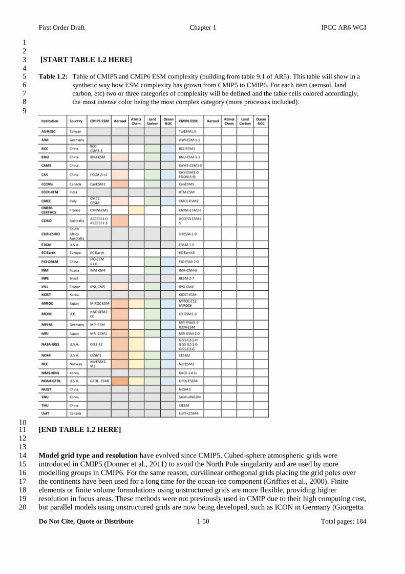
First Order Draft Chapter 1 IPCC AR6 WGI
Do Not Cite, Quote or Distribute 1-50 Total pages: 184
1
2
[START TABLE 1.2 HERE] 3
4 Table 1.2: Table of CMIP5 and CMIP6 ESM complexity (building from table 9.1 of AR5). This table will show in a 5
synthetic way how ESM complexity has grown from CMIP5 to CMIP6. For each item (aerosol, land 6 carbon, etc) two or three categories of complexity will be defined and the table cells colored accordingly, 7 the most intense color being the most complex category (more processes included). 8
9
10 [END TABLE 1.2 HERE] 11
12
13
Model grid type and resolution have evolved since CMIP5. Cubed-sphere atmospheric grids were 14
introduced in CMIP5 (Donner et al., 2011) to avoid the North Pole singularity and are used by more 15
modelling groups in CMIP6. For the same reason, curvilinear orthogonal grids placing the grid poles over 16
the continents have been used for a long time for the ocean-ice component (Griffies et al., 2000). Finite 17
elements or finite volume formulations using unstructured grids are more flexible, providing higher 18
resolution in focus areas. These methods were not previously used in CMIP due to their high computing cost, 19
but parallel models using unstructured grids are now being developed, such as ICON in Germany (Giorgetta 20

First Order Draft Chapter 1 IPCC AR6 WGI
Do Not Cite, Quote or Distribute 1-51 Total pages: 184
et al., 2018). Two new ocean-ice models with unstructured grids participate in CMIP6: FESOM (Wang et al., 1
2014) and MPAS (Petersen et al, 2018, submitted to JAMES). 2
3
The spatial resolution of ESMs is modestly higher in CMIP6 than it was in CMIP5. Oceanic horizontal 4
resolution has increased both for models used for future projection scenario experiments and for assessing 5
biogeochemical feedbacks, while the change in atmospheric resolution is not systematic (Figure 1.8). Global 6
models with finer horizontal grids represent much better the large-scale circulation of the atmosphere and 7
ocean, bringing key improvements in the simulation of the global hydrological cycle (Roberts et al., 2018). 8
CMIP6 includes a dedicated effort (HighResMip) to explore the impact of higher resolution, such as ~50km, 9
~25km and even ~10km (see 1.4.4.1). Important improvements, such as reduced SST biases in the Southern 10
Ocean, are documented in the highest-resolution coupled models used for HighResMip (Hewitt et al., 11
2017b). 12
13
14
[START FIGURE 1.8 HERE] 15
16 Figure 1.8: The population distributions of global climate models in terms of nominal horizontal atmospheric and 17
oceanic resolutions. (a) (b) Models used for future projection scenario experiments in CMIP6 and CMIP5 18 model intercomparison projects respectively. (c) (d) Models used for assessing biogeochemical feedbacks 19 in CMIP6 and CMIP5.The CMIP6 models are those registered as of December, 2018 20 (https://rawgit.com/WCRP-CMIP/CMIP6_CVs/master/src/CMIP6_source_id.html), while the CMIP5 21 models are those available at the IPCC Data Distribution Centre AR5 Reference Snapshot 22 (http://www.ipcc-data.org/sim/gcm_monthly/AR5/Reference-Archive.html). [To be updated]. 23
24
[END FIGURE 1.8 HERE] 25
26
27
The number of atmospheric vertical levels has increased in order to raise the top level of models and better 28
represent stratospheric processes (Charlton-Perez et al., 2013; Kawatani et al., 2019). Half the modelling 29
groups use "high top" models with a top level above the stratopause (a pressure of about 1 hPa); four groups 30
have switched to "high top" models since CMIP5. The number of vertical levels in the ocean models has also 31
increased, in order to achieve finer meshes over the water column and especially in the upper mixed layer. 32
Six modelling groups used ocean models with less than 40 layers in CMIP5, but only one group (NASA-33
GISS) does so in CMIP6 (See Annex III). 34
35
Atmospheric models include parameterizations of physical processes such as radiation, clouds, turbulence, 36
convection, and gravity waves that are not represented by grid-scale dynamics. The CMIP6 models have 37
undergone updates in some of their parameterizations in terms of schemes and parameters over their CMIP5 38
counterparts. Most notably, CLUBB (Cloud Layers Unified by Binormals), an advanced scheme to treat 39
cloud and turbulence in an integrated theory, has been developed and tested (Bogenschutz et al., 2013; Golaz 40
et al., 2002; Guo et al., 2015), and it is now adopted in some CMIP6 models. Although the CLUBB scheme 41
has theoretical and scientific advantages over traditional separated approaches, it is computationally more 42
expensive; some modeling groups did not adopt it for CMIP6 for this reason (Zhao et al., 2018). 43
44
The representation of atmospheric aerosols is advancing, both in Earth System Models and in the more 45
detailed Chemistry-Climate Models (CCMs). Most models now include explicit treatment of tropospheric 46
aerosol and aerosol precursor emission and transport, although the norm is a bulk treatment where only the 47
total mass of each aerosol type is predicted. In CCMs, recent advances include improved treatment of 48
stratospheric aerosols and chemistry, updates to the treatment of volcanic aerosols, explicit tropospheric 49
ozone chemistry, and increased complexity in cloud representation and aerosol-cloud interactions 50
(Morgenstern et al., 2017). Broadly, aerosol-cloud microphysics has been a key topic for the aerosol and 51
chemistry modelling communities since AR5, leading to improved understanding of the climate influence of 52
aerosols and short-lived climate forcers, but also still representing a major source of scientific uncertainty 53
and inter-model diversity. 54
55
Models of ocean and cryosphere dynamics have evolved significantly since CMIP5. The SROCC 56
First Order Draft Chapter 1 IPCC AR6 WGI
Do Not Cite, Quote or Distribute 1-52 Total pages: 184
documents the key role of ocean mesoscale eddies in CO2 uptake, in oceanic heat uptake, and in generating 1
freshwater anomalies, as well as the equator-to-pole transports of these properties. Eddy parameterizations 2
are used in coarse resolution ESMs, but they fail to mimic some aspects of the coupled high resolution 3
ocean-ice-atmosphere system, especially in the Southern Ocean (Poulsen et al., 2018). Ocean-atmosphere 4
feedbacks at the eddy scale arise from SST anomalies as well as surface current anomalies which modify the 5
wind stress. Eddy feedbacks are shown to have effects on the larger scales, for example on the dynamics of 6
ocean western boundary currents in the Pacific (Ma et al., 2016) and in the Atlantic (Renault et al., 2016). 7
The explicit representation of ocean eddies, due to increased grid resolution (typically, from 1° to ¼°), is 8
thus a major advance in a number of CMIP6 models (Hewitt et al., 2017b). 9
10
Progress has been made since AR5 regarding the simulation of ocean-cryosphere interactions. More models 11
consider the drift of icebergs, as it ensures that the freshwater input due to iceberg melting is not artificially 12
concentrated at the coast, although such refinements are still not incorporated into CMIP6 (Griffies et al., 13
2016; Nowicki et al., 2016). The ocean interaction with ice shelves is better accounted for by new 14
parameterizations that more realistically represent heat and freshwater fluxes occurring at depth, rather than 15
at the ocean surface. All CMIP6 ESMs include a sea ice component (Annex III, Table AIII.3, and Table 16
9.A.1 of AR5; Notz et al., 2016). ). While the core modelling is technically similar to CMIP5 versions, 17
advances have been made through focusing on the diagnosis and correction of some shortcomings of the 18
simulations adopted in AR5, in particular the persistent underestimation of the rapid decline in summer 19
Arctic sea-ice extent and the inability to reproduce the slightly increasing trend in Antarctic sea-ice extent 20
observed in the past decades. Investigations have confirmed that these discrepancies can be partly attributed 21
to the large internal variability of the Arctic and Antarctic climate systems (Ding et al., 2017; Jones et al., 22
2016a; Swart et al., 2015; Turner et al., 2015), although systematic biases still play a significant role in the 23
(Notz and Stroeve, 2018; Rosenblum and Eisenman, 2016, 2017; Turner and Comiso, 2017). As a 24
consequence, simulations of sea ice in ESMs have been used to estimate the ranges of possible internal 25
variability (Serreze and Stroeve, 2015) and the sea-ice sensitivity to external forcings (Notz and Stroeve, 26
2016; Rosenblum and Eisenman, 2016). On the other hand, recent improvements in stand-alone sea-ice 27
models have significantly contributed to the understanding of the physical processes underlying the 28
systematic biases of sea-ice simulations in ESMs. Such improvements include more realistic mechanisms of 29
ice–ocean–atmosphere interaction (Dupont et al., 2015; Spreen et al., 2017), ice–ice interactions (Sammonds 30
et al., 2017), and more complex thermodynamics (Li et al., 2017; Massonnet et al., 2018), e.g. through the 31
use of multiple ice categories or better parametrization of albedo changes, caused e.g. by surface melt ponds. 32
33
Glacier and ice-sheet models have greatly improved since the AR5. In particular, the resolution of ice-sheet 34
models has continuously increased, not only because of increasing computing power and parallelization, but 35
also due to spatial grid refinements, including nested grids, subgrid interpolation schemes, and adaptive 36
mesh approaches (Cornford et al., 2013; Cuzzone et al., 2018). Thanks in part to the recent boost in satellite 37
data availability, data-assimilation methods have been increasingly used to infer non-measurable variables 38
needed as inputs to the modelling of glaciers and ice sheets in transient state (Goldberg et al., 2015; Pattyn, 39
2018). Improved understanding of key physical processes — including grounding line dynamics, 40
stratigraphy and microstructure evolution, sub-shelf melting, and glacier and ice-shelf calving, among others 41
(DeConto and Pollard, 2016b; Depoorter et al., 2013; Faria et al., 2014, 2018; Haseloff and Sergienko, 2018) 42
— has served to motivate and guide the development of glacier and ice-sheet models. Even though most of 43
these processes are still not fully implemented in models, the knowledge is still used to improve validation 44
procedures and reducing model uncertainties. Despite the sophistication of current glacier and ice-sheet 45
models, their coupling to global climate models is still complicated and is a matter of current research. 46
47
ESMs include the terrestrial and oceanic carbon cycle so that natural sources and sinks of CO2 or other 48
greenhouse gases can be simulated in the same numerical framework as the anthropogenic forcings. 49
Land models have developed through the implementation of relatively sophisticated land use and land cover 50
change representations to explore the impacts of land management on surface fluxes of carbon, water and 51
energy (Lawrence et al., 2016). In terms of biogeochemical cycles, the importance of nitrogen availability to 52
limit the terrestrial carbon sequestration has been recognized (Zaehle et al., 2014) and, thus, an increasing 53
number of models now include a prognostic representation of the terrestrial nitrogen cycle and its coupling to 54
the land carbon cycle (Jones et al., 2016a). Although the responses of permafrost to climate change is 55
First Order Draft Chapter 1 IPCC AR6 WGI
Do Not Cite, Quote or Distribute 1-53 Total pages: 184
another area of focus (Gasser et al., 2018), CO2 and CH4 releases from permafrost are not implemented in an 1
interactive manner in CMIP6 generation models. 2
3
Ocean biogeochemical models range in complexity from geochemical only (no representation of biological 4
compartments), to NPZD class (nutrients, plankton, zooplankton and detritus), to increasingly complex 5
versions with several plankton functional types (Annex III, Table AIII.3). Since AR5, models have evolved 6
to enhance the consistency of the exchanges between ocean, atmosphere and land, through riverine input and 7
dust deposition (Aumont et al., 2015; Stock et al., 2014). Other developments include flexible plankton 8
stoichiometric ratios (Galbraith and Martiny, 2015), improvements in the representation of nitrogen fixation 9
(Paulsen et al., 2017), and the limitation of plankton growth by iron (Aumont et al., 2015). Several modelling 10
centers carried out large ensembles of simulations of the historical and/or future periods using their CMIP5 11
ESMs with interactive ocean biogeochemistry, including CESM1-BEC (Brady et al., 2019; Freeman et al., 12
2018; Krumhardt et al., 2017; Long et al., 2016; Lovenduski et al., 2016; McKinley et al., 2016, 2017), MPI-13
ESM-LR (Li and Ilyina, 2018), and GFDL-ESM2M (Frölicher et al., 2016; Rodgers et al., 2015). These 14
simulations allow an unprecedented look at internal variability versus forced change in ocean 15
biogeochemical fields of interest, such as air-sea CO2 flux, nutrient and oxygen concentrations, sea surface 16
temperature, and phytoplankton productivity. 17
18
Increasing resolution and increasing complexity place huge demands on model development teams and on 19
computing resources. As a result, the number of climate centres that carry out IPCC-relevant global 20
simulations has grown slowly from one intercomparison project to the next: from 10 in CMIP1 to 17 in 21
CMIP5 and 26 in CMIP6 (Figure 1.9). At the same time, the need for accurate climate information at the 22
regional scale is increasing, and many modelling centers use the global scenarios to develop regional climate 23
models. High-resolution global climate models, such as those taking part in HighResMip, provide more 24
detailed information at the regional scale (Roberts et al., 2018). However, due to the high cost of these 25
models, only a limited number of scenarios are available. Regional information can be derived from standard 26
CMIP6 models using regional climate models and downscaling techniques, presented in Chapter 10 and in 27
the Atlas. Regional climate models are more diverse than the global ESMs and engage a wider international 28
community (Figure 1.9). 29
30
31
[START FIGURE 1.9 HERE] 32
33 Figure 1.9: A world map showing the increased diversity of modelling centres contributing to CMIP (idea, use 34
different symbols or colors or sizes for climate centres that participated in CMIP3, CMIP5, CMIP6), and 35 also modelling contributions to CORDEX. [TO BE UPDATED, CORDEX information is incomplete] 36
37
[END FIGURE 1.9 HERE] 38
39
40
1.4.3.2 Models of lower complexity 41
42
Earth System Models of Intermediate Complexity (EMICs) complement the model hierarchy and fill the 43
gap between conceptual, simple climate models and full-blown atmosphere–ocean general circulation 44
models (AOGCMs) and Earth system models (ESMs) (Claussen et al., 2002). EMICs are simplified; they 45
include processes in a more parameterized form and have generally lower resolution compared to the 46
complex ESMs. As a result, EMICs require much less in terms of computer resources and can be integrated 47
for many thousands of years without supercomputers (Hajima et al., 2014). The EMICs used in climate 48
change research, however, are highly heterogeneous, ranging from zonally averaged or mixed-layer ocean 49
models coupled to statistical–dynamical models of the atmosphere to low-resolution 3-dimensional ocean 50
general circulation models coupled to simplified dynamical models of the atmosphere. An increasing number 51
of EMICs include interactive representations of the global carbon cycle, with varying levels of complexity 52
and numbers of processes considered (Zickfeld et al., 2013). Given the heterogeneity of the EMICs 53
community, modelers tend to focus on specific research questions and develop individual models 54
accordingly. 55
First Order Draft Chapter 1 IPCC AR6 WGI
Do Not Cite, Quote or Distribute 1-54 Total pages: 184
1
EMICs have been used extensively in past IPCC reports, providing long-term integrations on paleo-climate 2
and future timescales, including stabilization pathways and a range of commitment scenarios, with perturbed 3
physics ensembles and sensitivity studies, or with simulations targeting the uncertainty in global climate-4
carbon cycle systems (e.g., Collins et al., 2013; Meehl et al., 2007b). In this report, EMICs are again used in 5
a number of chapters. Chapters 4 and 5, for example, draw on EMIC results for the assessment of long-term 6
climate change beyond 2100 (Sections 4.7.1, 5.4.9), zero-emission commitments, overshoot and recovery 7
(Section 4.7.2), impacts of carbon dioxide removal (CDR) on the climate system and the carbon cycle 8
(Section 4.7.2, 5.6.2) and long-term carbon cycle – climate feedbacks (Section 5.4.9). While some EMICs 9
contribute to parts of the CMIP6 suite of MIPs, a coordinated EMICs modeling effort similar to the ones for 10
AR4 (Plattner et al., 2008) and AR5 (Eby et al., 2013; Zickfeld et al., 2013) is not in place for IPCC AR6. 11
More recently, a number of studies have pointed to the possibility of systematically different climate 12
responses to external forcings in EMICs and complex ESMs (Frölicher and Paynter, 2015; Pfister and 13
Stocker, 2017, 2018) that need to be considered when applying EMICs for long-term projections and 14
sensitivity studies complementing complex ESMs in the context of this report. 15
16
Physical emulators make up a class of heavily parametrized simplified climate models designed to 17
reproduce the responses of the more complex models, and provide rapid translations of emissions, via 18
concentrations and radiative forcing, into probabilistic estimates of climate impacts. For example, in the 19
AR5, the Model for the Assessment of Greenhouse-gas Induced Climate Change (MAGICC) energy balance 20
model was used to estimate the greenhouse gas concentration time series resulting from the Representative 21
Concentration Pathways (RCPs). They are also heavily used in the Integrated Assessment Model 22
community, as translators of the complex information from Earth System Modelling into global temperature 23
responses. 24
25
Since the AR5, development has progressed for several such simplified climate models, and their use is 26
increasing. Two models in particular (MAGICC and Smith et al. (2018)) were heavily used in the SR1.5 to 27
categorize mitigation pathways into classes of scenarios that peak near 1.5°C, overshoot 1.5°C, or stay below 28
2°C and similar. The report concluded that there was high agreement in the relative temperature response of 29
pathways, but medium agreement on the precise absolute magnitude of warming, introducing a level of 30
imprecision in the attribution of a single pathway into a given category. Other recently updated models 31
include OSCAR and BernSCM. Recent progress generally includes added complexity of atmospheric 32
chemistry and treatment of the carbon cycle, inclusion of recent estimates of the radiative forcing of 33
greenhouse gases, and tuning of parameterizations to represent more recent Earth System Model results 34
(generally CMIP5 and recently CMIP6). 35
36
For a more thorough overview of the use of simple models in the present report, see Cross-Chapter Box 1.5 37
“Temperature-based scenario classification using physical emulators”. 38
39
40
1.4.3.3 Model tuning and adjustment 41
42
When developing climate models, choices have to be made in a number of areas. For Earth System Models, 43
these include (i) model formulation: although equations for fluids such as the atmosphere and ocean are well 44
known and have been applied in models for a long time, different mathematical formulations exist. There are 45
no unique equations for complex processes such as vegetation in ocean ecosystems; (ii) model resolution, 46
grid type, coupling and numerical methods. These choices are often related to the available computer power 47
(higher resolution is more computationally costly) and computer architecture (some numerical methods are 48
better suited for highly parallel computing); (iii) parameterization of processes unresolved by the model 49
equations or by the model spatio-temporal resolution. For example, the evolution of an individual cloud is 50
not resolved by a standard atmospheric GCM grid (100km resolution). Instead, clouds are parameterized 51
using integrated variables (e.g., cloud fraction) and empirical formulae. 52
53
Choices must also be made within each formulation, numerical method and parameterization, as, for each of 54
these, several parameters can be set. The acceptable range for these parameters is set by mathematical 55
First Order Draft Chapter 1 IPCC AR6 WGI
Do Not Cite, Quote or Distribute 1-55 Total pages: 184
consistency (e.g., convergence of a numerical scheme), physical considerations (e.g., energy conservations), 1
observations or a combination thereof. The art of modelling is to choose a set of parameters that both falls 2
within this range and mimics observations or their statistics. 3
4
An initial set of such choices is usually made by (often extensive) groups of modellers working on one single 5
component of the earth system (ocean, atmosphere, sea ice…). As components are assembled to build an 6
ESM, the choices are refined to best represent a number of pre-defined “tuning targets”. When these are met 7
the model is deemed “fit for purpose” and a release is made for using in intercomparisons such as CMIP or 8
other science projects. Tuning targets come in three levels: mean climate, regional phenomena and features, 9
and historical trend (Hourdin et al., 2017). One example of such a goal is that “the climate system should 10
reach a mean equilibrium temperature close to observations when energy received from the sun is close to its 11
real value (340 w.m-2)”. Whether tuning should be performed to approach realistic climate-related features, 12
such as accurately simulating the global mean temperature evolution over the historical era, or rather be 13
performed for each individual process independently such that all collective behaviour is emergent, is a 14
matter of debate in the climate community (Burrows et al., 2018) 15
16
Each modelling group has its own strategy and, after the AR5, a survey was conducted to understand the 17
tuning approach used in 23 CMIP5 modelling centers. The results are discussed in (Hourdin et al., 2017) 18
which stress that the behaviour of ESMs depends on the tuning strategy, which should therefore be 19
documented. In CMIP6 each modelling group now describes the three levels of tuning both for the complete 20
ESM and for components ([gradually] available at https://explore.es-doc.org/). Global tuning targets for 21
CMIP6 model include: top-of-the-atmosphere (TOA) heat flux and its radiative components, the 22
decomposition of each of these fluxes in terms of clear sky and radiative effect of clouds, global-mean ocean 23
temperature, sea-ice extent, sea-ice volume, glacial mass balance, global root mean square error (RMSE) of 24
precipitation [to be completed when model documentation is complete]. The TOA heat flux balance is 25
achieved using a diversity of approaches, usually unique to each modelling group: for example, adjustments 26
of the aerosol indirect effects, adjustments to ocean albedo, marine DMS parameterization, cloud properties 27
by reducing the autoconversion threshold for liquid precipitation over the ocean. [to be completed when 28
CMIP6 model documentation is complete]. 29
30
Regional tuning targets include: ocean meridional overturning circulation (AMOC, AABW cell), regional 31
sea surface temperatures, temperature profiles in the ocean, seasonal sea-ice extent (e.g. Labrador Sea, 32
Greenland Sea), regional land properties, latitudinal distribution of radiation, spatial contrasts in top-of-33
atmosphere radiative fluxes or surface fluxes, stationary waves in the Northern Hemisphere [to be completed 34
when CMIP6 model documentation is complete]. 35
36
Trend tuning is not systematic and can include: adjustments of aerosol indirect effect (guided by available 37
observations) to obtain near-observed 20th century surface temperature evolution [to be completed when 38
CMIP6 model documentation is complete]. 39
40
41
1.4.4 Modelling techniques, comparisons and performance assessments 42
43
A key approach in climate science is the comparison of results from multiple model simulations with each 44
other and against observations. These simulations have typically been performed by separate models set up 45
with consistent boundary conditions and forcings, as in the series of Phases of the Coupled Model 46
Intercomparison Project (CMIP,Eyring et al., 2016; Meehl et al., 2000, 2007a; Taylor et al., 2012) run under 47
the auspices of the World Climate Research Program WCRP (see section 1.4.4.1). Such multi-model 48
ensembles (MMEs) have proven highly useful, as they help quantify, and reduce the influence of, the 49
particular sets of parametrizations and physical components simulated by individual models. The primary 50
usage of MMEs is to provide a well quantified model range, but when used carefully they can also increase 51
confidence in projections (Knutti et al., 2010). 52
53
First Order Draft Chapter 1 IPCC AR6 WGI
Do Not Cite, Quote or Distribute 1-56 Total pages: 184
Since the AR5, increases in computing power have made it increasingly possible to investigate simulated 1
internal variability using large initial conditions ensembles (ICEs). Such ensembles employ a single climate 2
model in a fixed configuration, but starting from a variety of different initial states. In some experiments 3
these initial states only differ slightly. As the climate system is chaotic, such tiny changes in temperatures, 4
winds, and humidity may lead to different evolutions for the system as a whole, as is well known in weather 5
forecasting. Other experiments start from a set of well-separated ocean initial conditions to sample the 6
uncertainty in the circulation state of the ocean and its role in longer-timescale variations. 7
8
Although mostly applied in numerical weather prediction, ICEs can also be used to evaluate climate model 9
parameterizations, if models are initialized appropriately (Phillips et al., 2004; Williams et al., 2013), mostly 10
within the framework of seamless weather and climate predictions (e.g. Brown et al., 2012; Hurrell et al., 11
2009; Palmer et al., 2008). Initializing an atmospheric model in hindcast mode and observing the biases as 12
they develop permits testing of the parameterized processes, by starting from a known state rather than one 13
dominated by quasi-random short term variability (Ma et al., 2014; Vannière et al., 2014; Williams et al., 14
2013). 15
16
Due to the large computational requirements of any ensemble large enough to fully span the range of 17
modelled variability, only a limited number of large ICEs is yet available. Examples in the literature 18
supporting the present report include the CESM Large Ensemble (Kay et al., 2015), the MPI Grand 19
Ensemble (Maher 2019; submitted), and the CanESM2 large ensembles (Kirchmeier-Young et al., 2017). 20
21
Recently, the ICE technique has been extended to observation-based large ensembles (McKinnon and Deser, 22
2018)and to regional modelling (Mote et al., 2015; Schaller et al., 2018), the latter often produced using 23
crowdsourcing and volunteer computing power. 24
25
A third common technique is the perturbed physics ensemble (PPE). These are used to assess uncertainty 26
based on a single model, with individual parameters perturbed to reflect the full range of their uncertainty 27
(Hawkins and Sutton, 2009a; Knutti et al., 2010; Tebaldi and Knutti, 2007). Statistical methods can then be 28
used to detect which parameters are the main drivers of uncertainty across the ensemble. PPEs have been 29
used frequently in simpler models, such as EMICs, and are now being applied to more complex models. The 30
disadvantage of PPEs is that they do not explore structural uncertainty, i.e. differences or shortcomings in the 31
parametrizations themselves, and thus the estimated uncertainty will depend on the underlying model and 32
may be an underestimation of the “true” uncertainty. 33
34
[PLACEHOLDER: PPEs TO BE ADDED.] 35
36
Together, the three ensemble methods (MMEs, ICEs, PPEs) allow investigation of climate models’ 37
uncertainty arising from internal variability, boundary conditions, model formulations and parameterizations. 38
Figure 1.10 illustrates the ensemble types. 39
40
41
[START FIGURE 1.10 HERE] 42
43
Figure 1.10: Illustration of common types of model ensemble, simulating the time evolution of a quantity V (such as 44 surface temperature or precipitation). (a) Multi-model ensemble, where each model has its own 45 realization of the processes affecting V, and its own internal variability around the baseline value (dashed 46 line). (b) Initial condition ensemble, where several realizations from a single model are compared. These 47 differ only by minute perturbations to the initial conditions of the simulation, such that over time, internal 48 variability will progress differently in each ensemble member. (c) Perturbed physics ensemble, which 49 also compares realizations from a single model, but where one or more quantities that may affect V are 50

First Order Draft Chapter 1 IPCC AR6 WGI
Do Not Cite, Quote or Distribute 1-57 Total pages: 184
systematically changed to allow for a quantification of the impact of those quantities on the model results. 1 2
[END FIGURE 1.10 HERE] 3
4
5
1.4.4.1 The sixth phase of the Coupled Model Intercomparison Project (CMIP6) 6
7
The present report assesses a range of results from CMIP5 that were not published until after the AR5. In 8
addition, the first results of the 6th phase of CMIP (CMIP6) will be assessed. The CMIP6 experiment design 9
is somewhat different to previous phases. It now consists of a limited set of DECK (Diagnostic, Evaluation 10
and Characterization of Klima) simulations and the historical simulation that must be performed by all 11
participating models, and a wide range of CMIP6-Endorsed Model Intercomparison Projects (MIPs) 12
covering specialized topics (Eyring et al., 2016a). Participation in CMIP6-Endorsed MIPs is voluntary and at 13
the discretion of each modelling centre. 14
15
The CMIP DECK simulations form the basis for a range of assessments and projections in the following 16
chapters. As in CMIP5, they consist of a preindustrial control simulation (piControl, where “pre-industrial” 17
is taken as 1850 conditions), an idealized abrupt quadrupling of CO2 concentrations relative to piControl, a 18
1% per year increase in CO2 concentrations relative to piControl, and a transient simulation with prescribed 19
sea-surface temperatures for the period 1979-2014 (AMIP). In addition, all participating models perform a 20
historical simulation for the period 1850-2014. For the latter, common CMIP6 forcings are prescribed. These 21
include emissions (concentrations) of short-lived species (Hoesly et al., 2018) and long-lived greenhouse 22
gases (Meinshausen et al., 2017), biomass burning emissions (van Marle et al., 2017), global gridded land-23
use forcing data (Lawrence et al., 2016), solar forcing (Matthes et al., 2017a), and stratospheric aerosol data 24
from volcanoes (Zanchettin et al., 2016). For AMIP simulations, common sea surface temperatures (SSTs) 25
and sea ice concentrations (SICs) are prescribed. For simulations with prescribed aerosol abundances (i.e. 26
not calculated from emissions), optical properties and fractional changes in cloud droplet effective radius are 27
prescribed in order to provide a more consistent representation of aerosol forcing relative to earlier phases. 28
For models without ozone chemistry, time-varying gridded ozone concentrations and nitrogen deposition are 29
also provided. 30
31
Beyond the DECK and the historical simulations, the CMIP6-Endorsed MIPs aim to investigate the 32
responses of models to forcings, their potential systematic biases, their variability and usability for 33
projections and predictions, and their responses to detailed future scenarios such as the Shared 34
Socioeconomic Pathways (SSPs) (Section 1.6). Table 1.3 lists the 23 CMIP6-Endorsed MIPs, the main 35
science questions they pose, the number of models participating in each. Results from a range of these MIPs 36
will be assessed in the following chapters (also shown in Table 1.3). 37
38
39
[START FIGURE 1.11 HERE] 40
41 Figure 1.11: Structure of the CMIP6 multi-model intercomparison project (Eyring et al., 2016a). The centre shows the 42
common DECK and historical experiments that all participating models must perform, the outer circle 43 shows the topics covered by the endorsed MIPs. 44
45
[END FIGURE 1.11 HERE] 46
47
48
[START TABLE 1.3 HERE] 49
50 Table 1.3: CMIP6-Endorsed MIPS and participating models used in this assessment. [To be completed for the SOD] 51
52
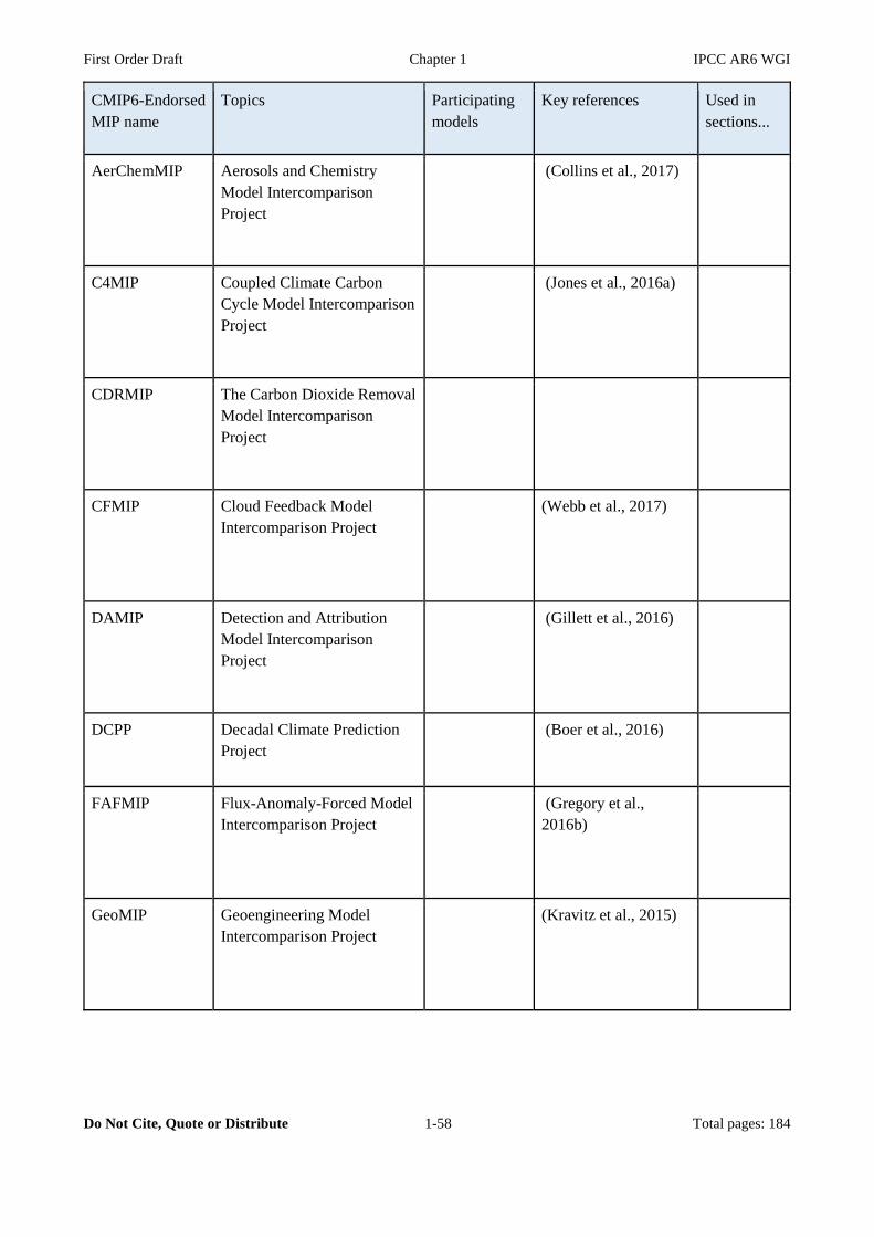
First Order Draft Chapter 1 IPCC AR6 WGI
Do Not Cite, Quote or Distribute 1-58 Total pages: 184
CMIP6-Endorsed
MIP name
Topics Participating
models
Key references Used in
sections...
AerChemMIP Aerosols and Chemistry
Model Intercomparison
Project
(Collins et al., 2017)
C4MIP Coupled Climate Carbon
Cycle Model Intercomparison
Project
(Jones et al., 2016a)
CDRMIP The Carbon Dioxide Removal
Model Intercomparison
Project
CFMIP Cloud Feedback Model
Intercomparison Project
(Webb et al., 2017)
DAMIP Detection and Attribution
Model Intercomparison
Project
(Gillett et al., 2016)
DCPP Decadal Climate Prediction
Project
(Boer et al., 2016)
FAFMIP Flux-Anomaly-Forced Model
Intercomparison Project
(Gregory et al.,
2016b)
GeoMIP Geoengineering Model
Intercomparison Project
(Kravitz et al., 2015)

First Order Draft Chapter 1 IPCC AR6 WGI
Do Not Cite, Quote or Distribute 1-59 Total pages: 184
GMMIP Global Monsoons Model
Intercomparison Project
(Zhou et al., 2016)
HighResMIP High Resolution Model
Intercomparison Project
(Haarsma et al., 2016)
ISMIP6 Ice Sheet Model
Intercomparison Project for
CMIP6
(Nowicki et al., 2016)
LS3MIP Land Surface, Snow and Soil
Moisture
(van den Hurk et al.,
2016)
LUMIP Land-Use Model
Intercomparison Project
(Lawrence et al.,
2016)
OMIP Ocean Model
Intercomparison Project
(Orr et al., 2017)
PAMIP Polar Amplification Model
Intercomparison Project
(Smith et al., 2019)
PMIP Palaeoclimate Modelling
Intercomparison Project
(Kageyama et al.,
2018)
RFMIP Radiative Forcing Model
Intercomparison Project
(Pincus et al., 2016)
ScenarioMIP Scenario Model
Intercomparison Project
(O'Neill et
al., 2016)
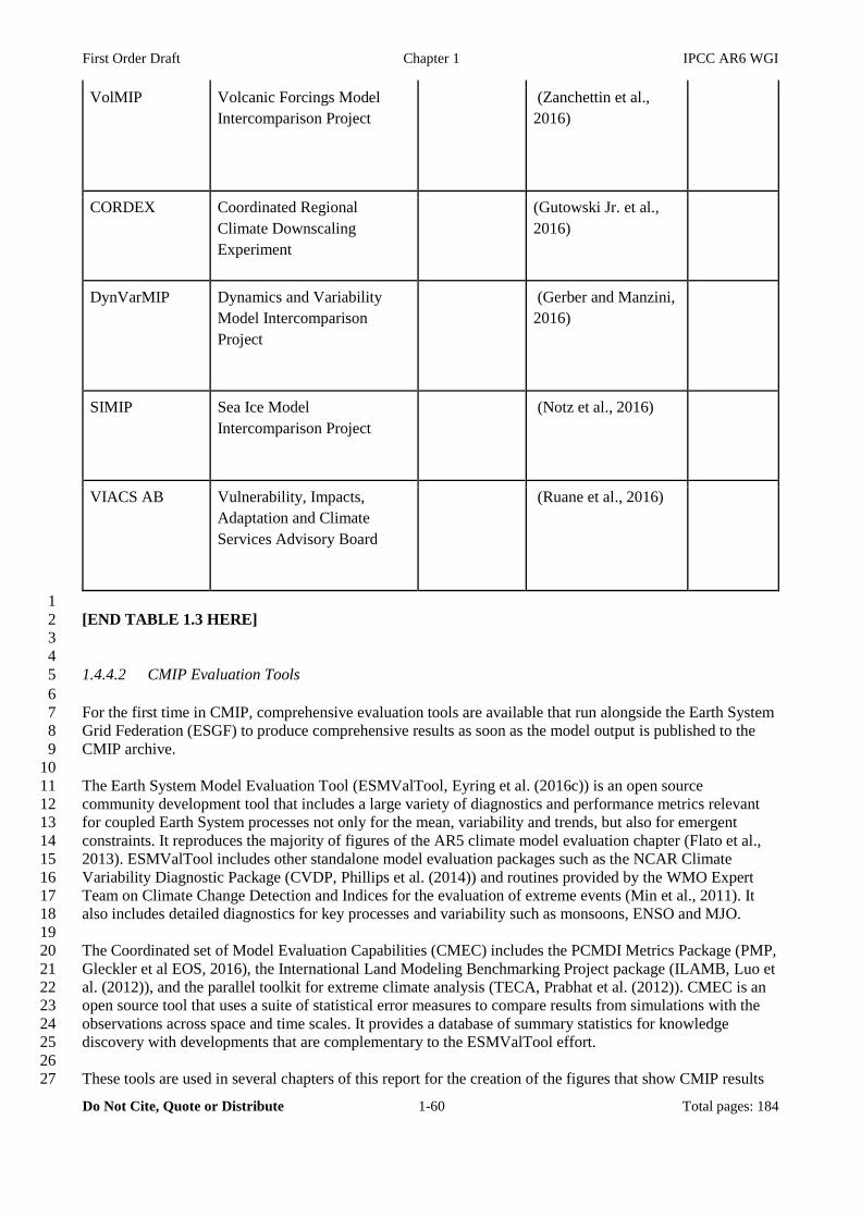
First Order Draft Chapter 1 IPCC AR6 WGI
Do Not Cite, Quote or Distribute 1-60 Total pages: 184
VolMIP Volcanic Forcings Model
Intercomparison Project
(Zanchettin et al.,
2016)
CORDEX Coordinated Regional
Climate Downscaling
Experiment
(Gutowski Jr. et al.,
2016)
DynVarMIP Dynamics and Variability
Model Intercomparison
Project
(Gerber and Manzini,
2016)
SIMIP Sea Ice Model
Intercomparison Project
(Notz et al., 2016)
VIACS AB Vulnerability, Impacts,
Adaptation and Climate
Services Advisory Board
(Ruane et al., 2016)
1
[END TABLE 1.3 HERE] 2
3
4
1.4.4.2 CMIP Evaluation Tools 5
6
For the first time in CMIP, comprehensive evaluation tools are available that run alongside the Earth System 7
Grid Federation (ESGF) to produce comprehensive results as soon as the model output is published to the 8
CMIP archive. 9
10
The Earth System Model Evaluation Tool (ESMValTool, Eyring et al. (2016c)) is an open source 11
community development tool that includes a large variety of diagnostics and performance metrics relevant 12
for coupled Earth System processes not only for the mean, variability and trends, but also for emergent 13
constraints. It reproduces the majority of figures of the AR5 climate model evaluation chapter (Flato et al., 14
2013). ESMValTool includes other standalone model evaluation packages such as the NCAR Climate 15
Variability Diagnostic Package (CVDP, Phillips et al. (2014)) and routines provided by the WMO Expert 16
Team on Climate Change Detection and Indices for the evaluation of extreme events (Min et al., 2011). It 17
also includes detailed diagnostics for key processes and variability such as monsoons, ENSO and MJO. 18
19
The Coordinated set of Model Evaluation Capabilities (CMEC) includes the PCMDI Metrics Package (PMP, 20
Gleckler et al EOS, 2016), the International Land Modeling Benchmarking Project package (ILAMB, Luo et 21
al. (2012)), and the parallel toolkit for extreme climate analysis (TECA, Prabhat et al. (2012)). CMEC is an 22
open source tool that uses a suite of statistical error measures to compare results from simulations with the 23
observations across space and time scales. It provides a database of summary statistics for knowledge 24
discovery with developments that are complementary to the ESMValTool effort. 25
26
These tools are used in several chapters of this report for the creation of the figures that show CMIP results 27
First Order Draft Chapter 1 IPCC AR6 WGI
Do Not Cite, Quote or Distribute 1-61 Total pages: 184
(e.g., Chapters 3, 4, and 5). This allows us not only to ensure traceability of the results, but also provides an 1
additional level of quality control whether published figures can be reproduced. It also allows updating 2
published figures with, as much as possible, the same set of models in all figures, and to assess model 3
improvements across different phases of CMIP (Section 3.8.2). 4
5
These new developments are facilitated by the definition of common formats for CMIP model output (Balaji 6
et al., 2018) and the availability of observations (obs4MIPs, Ferraro et al., 2015) and reanalyses in the same 7
format as CMIP output. The evaluation tools for the first time ensure traceability and reproducibility of the 8
results at all stages, using a well-established analysis. The tools are also used to support routine evaluation at 9
individual model centres and enable a fast track to assess improvements of individual models or generations 10
of model ensembles (Eyring et al., 2016b). 11
12
13
1.4.4.3 Evaluation against observations 14
15
Techniques used for evaluating climate models against observations were assessed in AR5 (Flato et al., 2013), 16
and have progressed rapidly since (Eyring et al., 2019) The most direct approach that is continued to be widely 17
used is to compare climatologies or time series of simulated model output with observations while considering 18
observational uncertainty. In addition to a comparison of climatological means, trends and variability, AR5 19
already made use of a large set of performance metrics for a quantitative evaluation of the models. 20
21
Since the AR5, objective summaries of model agreement with observations have become more prominent, and 22
now extend well beyond the large scale mean climate (e.g. Bellenger et al., 2014; Covey et al., 2016; Goelzer 23
et al., 2018; Meehl et al., 2007a; Pendergrass and Deser, 2017). They provide an overall summary of model 24
performance across multiple variables and components of the Earth system (e.g. Anav et al., 2013; Gleckler et 25
al., 2008; Guan and Waliser, 2017) and are used in this report additionally to assess model improvements 26
across different CMIP ensembles and differences in model performance between different classes of models, 27
such as high- versus low-resolution models (see e.g. Section 3.3). 28
29
30
In addition, process- or regime-oriented evaluation of models has been expanded since the AR5. By focusing 31
on processes, causes of systematic errors in the models can be identified and insights can be gained whether a 32
mean state or trend is correctly simulated for the right reasons. This approach is commonly used for the 33
evaluation of clouds (e.g. Bony et al., 2015; Dal Gesso et al., 2015; Jin et al., 2017; Konsta et al., 2012; 34
Williams and Webb, 2009), dust emissions (e.g. Parajuli et al., 2016; Wu et al., 2016) as well as aerosol-cloud 35
(e.g. Gryspeerdt and Stier, 2012) and chemistry-climate (SPARC-CCMVal, 2010) interactions. Recently, 36
process-oriented diagnostics have also been used to evaluate specific phenomena such as the El Niño Southern 37
Oscillation (ENSO, Guilyardi et al. (2016)), the Madden–Julian Oscillation (MJO) (Ahn et al., 2017; Jiang et 38
al., 2018), monsoons (Boo et al., 2011), and tropical cyclones (Kim et al., 2018). 39
40
Instrument simulators that improve the direct comparison of modelled variables such as clouds, precipitation 41
and upper tropospheric humidity with observations from satellites have also been further developed (e.g. 42
Cesana and Waliser, 2016; Chepfer et al., 2018; Jin et al., 2017; Kay et al., 2011; Klein et al., 2013; Konsta et 43
al., 2016; Swales et al., 2018; Zhang et al., 2018). These approaches consist of converting model variables to 44
what a satellite would be providing by using methods such as radiative transfer calculations or by sampling 45
the model output in the same way than the observations. Within the framework of the Cloud Feedback Model 46
Intercomparison Project (CFMIP) contribution to CMIP6 (Webb et al., 2017), a new version of the Cloud 47
Feedback Model Intercomparison Project Observational Simulator (COSP, Swales et al., 2018) has been 48
released which makes use of a collection of observation proxies or satellite simulators. 49
50
51
1.4.4.4 Climate informatics 52
53
The growing data volume from Earth system observations and models urge the need for new theories and 54
tools that complement classical approaches to extract relevant information. A significant development since 55
First Order Draft Chapter 1 IPCC AR6 WGI
Do Not Cite, Quote or Distribute 1-62 Total pages: 184
the AR5 is an emerging field of climate informatics, a promising and growing path of research (Reichstein et 1
al., 2019). Data science methods such as data mining (Friedman et al., 2001), causal graphical model 2
discovery (Runge et al., 2015), and other machine learning techniques (Reichstein et al., 2019) that have 3
successfully been applied in other scientific disciplines (e.g., bioinformatics) provide new ways of analysing 4
Earth system data. 5
6
The most common approach, climate networks, uses complex network analysis to investigate 7
interdependency within a climate dataset (Tsonis and Roebber, 2004). In a climate network, each node 8
typically represents the value of a climate variable in a particular grid cell, or a climate index (Bracco et al., 9
2018; Donges et al., 2009; Fountalis et al., 2014; Kirtman et al., 2013; Tsonis et al., 2007; Wang et al., 10
2009). Links between nodes represent a strong statistical relationship, commonly defined based on methods 11
such as pairwise correlation, mutual information, or phase synchronization (Barreiro et al., 2011; Boers et 12
al., 2013; Tsonis and Roebber, 2004; Yamasaki et al., 2009). Climate networks were first used to study the 13
behaviour of global geopotential height (Tsonis and Roebber, 2004). Since then, the method has been further 14
developed for multivariate networks (Steinhaeuser et al., 2012) and lagged interaction (Tirabassi and 15
Masoller, 2016; Wang et al., 2013). Such climate networks may produce novel insights not revealed by 16
classical methods regarding the topology, dynamics and teleconnection of the climate system. Numerous 17
studies have applied climate networks in model evaluation and intercomparison at both local and global 18
scales (Bracco et al., 2018; Feldhoff et al., 2015; Fountalis et al., 2014, 2015; Lange et al., 2015; 19
Steinhaeuser and Tsonis, 2014; Tantet and Dijkstra, 2014). The method has also been used to investigate 20
large-scale circulations, modes of variability, and their teleconnections (Arizmendi and Barreiro, 2017; 21
Berezin et al., 2012; Bracco et al., 2018; Deza et al., 2015; Donges et al., 2009, 2011; Ebert-Uphoff and 22
Deng, 2012; Fountalis et al., 2015; Gozolchiani et al., 2011; Guez et al., 2012; Ludescher et al., 2014; 23
Martín-Gómez and Barreiro, 2016, 2017; Tsonis and Swanson, 2008; Wang et al., 2013; Yamasaki et al., 24
2008). Further studies have applied networks to the dynamics of the Indian monsoon, statistical prediction of 25
climate indices, and identification of sudden changes and extreme events (Boers et al., 2015; Malik et al., 26
2012; Marwan and Kurths, 2015; Rehfeld et al., 2013; Steinhaeuser et al., 2011; Stolbova et al., 2014, 2016). 27
28
Climate network analyses in which linkages are based solely on correlation cannot, however, be used to 29
directly assess cause-effect relationships between modes of variability or ocean-atmosphere interaction 30
processes. To do so, a different type of climate network based on causal discovery was introduced where 31
techniques such as transfer entropy, recurrence-based methods, and Granger causality define the linkages 32
(Deza et al., 2015; Ebert-Uphoff and Deng, 2012, 2014, 2017, Hlinka et al., 2013, 2017). These approaches 33
illustrate pathways of information flow, both direct and indirect, from one node to another, thereby providing 34
information that helps to identify the cause-effect relationships between climate interactions at different 35
locations (Ebert-Uphoff and Deng, 2012, 2014, 2017, Hlinka et al., 2013, 2017). This was extended to allow 36
the identification of major gateways for spreading and mediating perturbations in the atmosphere, such as 37
regions of strong ascent in the tropics (Runge et al., 2014, 2015). Advancing the understanding of climate 38
variability requires that results from climate network studies be interpreted in physical terms, and thus these 39
approaches can complement studies of atmospheric dynamics and process-based climate model analysis. To 40
improve the detection of multivariate extreme events (Zscheischler et al., 2018), machine learning anomaly 41
detection techniques are being explored (Barz et al., 2019). 42
43
44
1.4.5 Techniques for constraining uncertainties and informing projections 45
46
Since the AR5, new or further developed techniques allow constraining the uncertainty in multi-model 47
climate projections with observations, narrowing the uncertainty in climate responses and feedbacks. 48
49
1.4.5.1 Scaling based on detection and attribution 50
51
Results from detection and attribution have been considered as a possible way to constrain estimates of 52
changes in the climate system and some key properties in the future (Bindoff et al., 2013; Kirtman et al., 53
2013). In particular, scaling factors derived from detection and attribution analyses, applied to observed 54
global temperature changes, can adjust model responses to different external forcings to best match the 55

First Order Draft Chapter 1 IPCC AR6 WGI
Do Not Cite, Quote or Distribute 1-63 Total pages: 184
observations. If the scaling relationship over the historical time period is found to be robust, it may provide a 1
useful way to adjust future projections, assuming the empirical relationship will continue to hold (Gillett et 2
al., 2012; Kirtman et al., 2013; Stott et al., 2013; Stott and Jones, 2012). Future projections and associated 3
uncertainties can then be estimated by applying the scaling factors to projected changes in response to 4
individual forcing agents and summing. Biases in the resulting projections could arise from errors in 5
historical forcings, errors in the simulated patterns response to those forcings, or departures from linearity or 6
linear additivity in the response to forcings (Kirtman et al., 2013), and derived uncertainties may be large if 7
scaling factors are weakly constrained because of degeneracies in the responses to different (Collins et al., 8
2012), or if the responses to some forcings included are weak. While linear additivity has been found to hold 9
for temperature responses at global and continental scales in general, it may not hold for precipitation in 10
certain cases of future projections (Marvel et al., 2015; Shiogama et al., 2013). The robustness of the scaling 11
factors is a key to the usability of this approach, but scaling factors are not always robust (Bindoff et al., 12
2013; Gillett et al., 2013a; Jones et al., 2013; Ribes et al., 2013). Since the signal to noise ratio shrinks at 13
smaller spatial scales and shorter periods of time, scaling factors derived from regional analyses and for short 14
periods tend to be less robust (Jones et al., 2016b). 15
16
1.4.5.2 Emergent constraints on climate feedbacks, sensitivities and projections 17
18
An emergent constraint is a relationship between an uncertain aspect of future climate change and an 19
observable feature of the Earth System, evident across an ensemble of models (Allen and Ingram, 2002). 20
Complex Earth system models (ESMs) simulate variations on timescales from hours to centuries, so in 21
principle ESMs tell us how aspects of the current climate relate to its sensitivity to anthropogenic forcing. 22
Where an ensemble of different ESMs agrees on a relationship between a short-term observable variation 23
and a longer-term sensitivity, an observation of the short-term variation in the real world can be converted, 24
via the model-based relationship, into an ‘emergent constraint’ on the sensitivity. This is shown 25
schematically in Figure 1.12. 26
27
Emergent constraints are attractive because they use the spread in model projections to estimate the 28
sensitivities of the real climate system to anthropogenic forcing, providing one way to make an ensemble of 29
ESMs more than the sum of the parts. As emergent constraints depend on identifying those observable 30
aspects of the climate system which are most related to climate projections, they also help to focus model 31
evaluation on the most relevant observations (Hall et al., in press). However, there are risks that 32
indiscriminate data-mining of the multidimensional outputs from ESMs could lead to spurious correlations 33
(Caldwell et al., 2014) and less than robust emergent constraints on future changes (Bracegirdle and 34
Stephenson, 2013). To mitigate against this risk, emergent constraints need to be tested “out of sample” 35
(Caldwell et al., 2018), and should ideally be based on sound physical understanding and mathematical 36
theory (Hall et al., in press). In this report, we evaluate emergent constraints developed using the previous 37
CMIP5 ensemble against the newer CMIP6 models. 38
39
For general applications and discussions of recent usage of emergent constraints, see Section 3.8.2.3. 40
Assessment of individual emergent constraints appear throughout later chapters. 41
42
43
[START FIGURE 1.12 HERE] 44
45 Figure 1.12: The principle of Emergent Constraints. An ensemble of models (blue dots) define a relationship between 46
an observable trend or variation in the climate (x-axis) and an uncertain climate sensitivity or feedback 47 (y-axis). An observation of the x-axis variable can then be combined with the model-derived relationship 48 to provide a tighter estimate of the climate sensitivity or feedback on the y-axis (adapted from Eyring et 49 al. (2019)). 50
51
[END FIGURE 1.12 HERE] 52
53
54
First Order Draft Chapter 1 IPCC AR6 WGI
Do Not Cite, Quote or Distribute 1-64 Total pages: 184
1.4.5.3 Weighting techniques for model comparisons 1
2
Many results in the present report, and in the assessed literature, are based on ensembles of climate model 3
simulations or projections. Such ensemble-based results have commonly assumed that each individual model 4
is of equal value (“model democracy”). In other words, when combining simulations to estimate the mean 5
and variance of quantities of interest, they are typically unweighted (Haughton et al., 2015). However, 6
exceptions to this approach exist, and more studies on this topic have appeared since the AR5 (Eyring et al., 7
2019). Ensembles are typically pared down by removing either poorly performing model simulations or 8
model simulations that are perceived to add little additional information - typically where multiple 9
simulations have come from the same model. They may also be weighted based on model performance 10
differences relative to some set of observations - typically time series of global mean properties such as 11
surface temperature). 12
13
Several recent studies have attempted to quantify the impact of various strategies for selection or weighting 14
of ensemble members based on some set of criteria (Haughton et al., 2015; Sanderson et al., 2017). Boé 15
(2018) investigated the dependence of ensemble members sharing climate components. Regarding the 16
detection of anthropogenic forced signals versus internal climate variability, Frankcombe et al. (2015) found 17
that the ensemble mean of runs from a single climate model provides a good estimate of a forced signal even 18
when only a few ensemble members are available. In cases where only a single member is available for each 19
model, however, the scaled ensemble mean from all available climate model simulations of the same forcing 20
generally performs better. However, such a scaled mean leads to increasing errors the further the simulation 21
is taken from the time period used in the weighting. 22
23
Model weighting strategies have been further employed since the AR5 to reduce the spread in climate 24
projections for a given scenario by using weights based on one or more model performance metrics (Knutti 25
et al., 2017; Lorenz et al., 2018; Sanderson et al., 2017; Wenzel et al., 2016). However, models may share 26
representations of processes, parameterization schemes, or even parts of code, leading to common biases. 27
The models may therefore not be fully independent, calling into question inferences derived from multi-28
model ensembles (MMEs) (Abramowitz et al., 2018). Selecting models based on performance criteria alone 29
was shown by Herger et al. (2018a) to result in a poorer ensemble mean than a random selection of ensemble 30
members. 31
32
Concern has been raised about the large extent of code-sharing within the CMIP5 multi-model ensemble 33
(Sanderson et al., 2015b). Boé (2018) showed that a clear relationship exists between the number of 34
components shared by climate models and how similar the simulations are. The resulting similarities in 35
behaviour need to be accounted for in the generation of best-estimate multi-model climate projections. This 36
has led to calls to move beyond equally-weighted multi-model means towards weighted means that take into 37
account both model performance and model dependence (Knutti et al., 2017; Sanderson et al., 2015b, 2017). 38
Model independence has been defined in terms of performance differences within an ensemble (Knutti et al., 39
2013, 2017; Lorenz et al., 2018; Masson and Knutti, 2011; Sanderson et al., 2015b, 2015a, 2017). However, 40
this is very sensitive to the choice of variable, observational data set, metric, time period, and region (Herger 41
et al., 2018a). The adequacy of the constraint provided by the data and experimental methods can be tested 42
using a calibration-validation style partitioning of observations into two sets (Bishop and Abramowitz, 43
2013), or a "perfect model approach" where one of the ensemble members is treated as the reference dataset 44
and all model weights are calibrated against it (Bishop and Abramowitz, 2013), or a "perfect model 45
approach" where one of the ensemble members is treated as the reference dataset and all model weights are 46
calibrated against it (Bishop and Abramowitz, 2013; Herger et al., 2018a, 2018b; Knutti et al., 2017; 47
Sanderson et al., 2017; Wenzel et al., 2016). Sunyer et al. (2014) use a Bayesian framework to account for 48
model dependencies and changes in model biases. 49
50
51
1.5 Cross-cutting topics for this assessment: variability, regional definitions, uncertainty, reference 52
periods and attribution 53
54
First Order Draft Chapter 1 IPCC AR6 WGI
Do Not Cite, Quote or Distribute 1-65 Total pages: 184
This section highlights some of the cross-cutting methods applied in the climate change literature and topics 1
discussed repeatedly throughout this report. First, climate change trends are discussed, with a particular 2
focus on regional climate variability (Section 1.5.1). This section also presents the regional definitions used 3
in this report (Section 1.5.2). A consistent set of reference periods to describe past, historical, current and 4
future climate change assists the knowledge integration across IPCC Working Groups (WGs) and the policy-5
relevance of the findings, if those periods coincide with those used in the policy discussions (Section 1.5.3). 6
Future projections assessed in the various chapters are subject to a number of uncertainties, with their 7
general typology being introduced here (Section 1.5.4). The attribution of observed trends and weather 8
events, including those considered ‘extreme events’, to human-induced climate change is now applied on 9
ever more local scales (Section 1.5.5). 10
11
12
1.5.1 Natural variability and the emergence of the climate change signal 13
14
1.5.1.1 How does variability influence trends over short periods? 15
16
Natural variations in both weather and longer timescale phenomena can temporarily mask or enhance any 17
long-term (multi-decadal) anthropogenic trends. These effects are larger on small spatial and temporal 18
scales, but can occur on the global scale as well. For example, Cross-Chapter Box 3.1 discusses how 19
observed and simulated changes in global surface air temperature compare over the recent past. More 20
broadly, Figure 1.13 shows a set of examples using a large ensemble of model simulations with a single 21
GCM (Maher et al. 2019, in review). The long-term trends in various climate metrics are clearly visible 22
when considering the ensemble as a whole (grey shading). However, when considering single realisations 23
(colours), the trends over short periods can vary considerably (thin coloured lines). All the simulations have 24
very similar trends for ocean heat content (OHC) which is an integrated measure of climate change, but can 25
have significantly different trends for global surface air temperature (GSAT), UK summer temperatures and 26
Arctic sea-ice variations for the same period. For 11-year periods, both positive and negative trends can be 27
found in all these metrics, even though the long-term trend is for increasing temperatures and decreasing sea-28
ice. Climate change trends are traditionally defined over 20-or 30-year periods to isolate the long-term 29
trends, but - depending on the observed variable, its variability and applied detection method - an appropriate 30
period can be shorter or longer (WMO, 2017). 31
32
It should not be a surprise if observations, which are akin to a single realisation, show short-term trends 33
which are apparently different from the long-term trend or the expectation from climate models – in fact, it 34
should be expected (high confidence). 35
36
37
[START FIGURE 1.13 HERE] 38 39 Figure 1.13: Simulated changes in various climate metrics using historical and RCP4.5 scenarios using the MPI Grand 40
Ensemble (Maher et al. 2019, in review). The top row shows temperature-related metrics (Ocean Heat 41 Content to 2000m, annual global surface air temperature and UK summer temperatures) and the bottom 42 row shows Arctic sea-ice related metrics (annual ice volume and September sea-ice area). The grey 43 shading shows the 5-95% range from the 100-member ensemble, and the coloured lines represent three 44 individual ensemble members. All three members shown have very similar OHC trends (top left) but vary 45 considerably for other climate metrics (only two are shown for each). Trends are shown with thin solid 46 lines for the 2011-2021 period. 47
48
[END FIGURE 1.13 HERE] 49
50
51
1.5.1.2 The emergence of the climate change signal 52
53
The signal of climate change is most obvious at the global scale, but is increasingly emerging from the 54
background ‘noise’ of internal variability on smaller spatial scales and in a range of climate variables. An 55
example for air temperature is shown in Figure 1.14, which contrasts the changes in observed temperature in 56

First Order Draft Chapter 1 IPCC AR6 WGI
Do Not Cite, Quote or Distribute 1-66 Total pages: 184
two countries: the UK and Ghana. Both countries are at the same longitude and cover the same spatial area 1
(around 240,000 km2, or 0.05% of the planet), but Ghana is located in the tropics, in the West African 2
Monsoon region, where variability in temperature from year-to-year is smaller than in the extra-tropics 3
where the UK sits at the end of one of the major global storm track regions. Both countries show a similar 4
temporal fingerprint of the global temperature change signal but, for Ghana, the signal of temperature change 5
has already emerged more clearly from the background variations than for the UK. 6
7
Numerous studies have focussed on this topic of climate change ‘emergence’ (also see FAQ1.2). It has been 8
studied in observations of historical temperature change (e.g. Mahlstein et al., 2011), and of temperature 9
changes in the future (e.g. Hawkins and Sutton, 2012). The concept has also been extensively studied for 10
other climate variables such as precipitation (e.g. Giorgi and Bi, 2009), regional sea level change (Lyu et al., 11
2014) and extremes (e.g. King et al., 2015), and applied to issues such as the effects on crop growing regions 12
(Rojas et al., 2019). 13
14
Although there is considerable attention given to the magnitude of any change, regions which have a larger 15
signal of change relative to the background variations will potentially face greater risks as they will see 16
unusual or unprecedented climates more quickly (e.g. Frame et al., 2017). As in Figure 1.14, the signal of 17
temperature change is often smaller in tropical countries, but their lower amplitude of variability means they 18
may see the effects of climate change earlier than the mid-latitudes. In addition, the tropical countries with 19
lowest variability in temperature are often amongst the most vulnerable nations (e.g. Harrington et al., 2016), 20
increasing the risk. Providing more information about changes and variations on regional scales, and the 21
associated attribution to particular causes, is therefore important for adaptation planning. 22
23
24
[START FIGURE 1.14 HERE] 25
26 Figure 1.14: Observed temperatures in the UK and Ghana from 1900-2018 in the Berkeley Earth temperature dataset, 27
and GMST from HadCRUT4. The shaded band indicates the amplitude of internal variability [over X 28 year periods] for each region. After Sutton et al. (2015). 29
30 [END FIGURE 1.14 HERE] 31
32
33
1.5.2 Regional climate change 34
35
1.5.2.1 Foundations of the definition of climate regions 36
37
Climate change is a multiscale phenomenon with diverse cross-scale feedbacks. The evolution of trends in 38
the global climate system emerges from the aggregate of regional climate changes, but it drives also a great 39
variety of regional impacts. One useful element in climate change research has been the use of characteristic 40
climate zones, clusters or regions, across which the emergent climate change signal can be analysed and 41
projected. Several traditional methods exists to define these climate regions (Geiger, 1954; Köppen, 1936; 42
Sanderson, 1999; Thornthwaite, 1948; Trewartha, 1954), but also new approaches: as the climate signal 43
emerges from small spatial scales and evolves out of short-term variations, characteristic patterns are formed, 44
which manifest themselves as multiscale structures in space and time that can be detected with new data-45
driven ‘complex network’ approaches (Steinhaeuser et al., 2011). Such structures, clusters or patterns, may 46
be studied separately for each climate variable, like sea surface temperatures or pressures, for instance 47
through spectral studies of climate-proxy time series (Boers, 2018), or aggregated in multiple variables to 48
reveal spatio-temporal patterns that express the full complexity of the coupled climate system (Grigholm et 49
al., 2009; Rubel et al., 2017; Vidal et al., 2010). 50
51
Many of these spatio-temporal patterns are related to geophysical features, like orography, buoyancy or 52
Earth’s motion. This led scientists to define typical space and time scales for various meteorological and 53
climatic phenomena (Figure 1.15), including the classical statistical definition of climate by the World 54
Meteorological Organization (WMO) as the average weather over a period of 30 years (WMO, 2017). 55

First Order Draft Chapter 1 IPCC AR6 WGI
Do Not Cite, Quote or Distribute 1-67 Total pages: 184
1
[START FIGURE 1.15 HERE] 2
3 Figure 1.15: Spatial and temporal scales of atmospheric processes and their relations to the region sets used in this 4
report, namely reference land and ocean regions (Reference), WGII-type regions (WGII-Type), and 5 typological land and ocean regions (Typological). The domain “Local” stands for local domains not 6 formally defined but occasionally mentioned in specific situations (see Figure 10.1 in Chapter 10 for a 7 comparison with various modelled processes at regional and global scales. [To be updated] 8
9
[END FIGURE 1.15 HERE] 10
11
12
Understanding and predicting climate change at the regional scale remains, however, one of the greatest 13
challenges of climate science. The complexity of this problem from a modelling point of view is discussed in 14
Chapter 10. From the viewpoint of observations; one way of approaching this issue is by averaging the 15
signals of the aggregated variables over several decades, in such a way that more stable and definite climate 16
regions emerge. This process is called climate classification and gives rise to climate regions loosely defined 17
as spatial domains where the aggregated variables form similar patterns. 18
19
There are several approaches to the climate classification of climate regions. When climate observation data 20
was sparse and limited, the aggregation of climate variables was implicitly achieved through the 21
consideration of biomes, giving rise to the traditional vegetation-based classification (Köppen, 1936). In the 22
last decades, the substantial increases in climate observations, climate modelling, and data processing 23
capabilities have allowed new approaches to climate classification, e.g. through interpolation of aggregated 24
global data from thousands of stations (Beck et al., 2018; Belda et al., 2014; Peel et al., 2007). Experience 25
shows that each method has strengths and weaknesses through trade-offs between detail and convenience. 26
For instance, a very detailed classification, with numerous complex-shaped regions derived from a large set 27
of variables, may be most useful for the validation of climate models (Beck et al., 2018; Rubel and Kottek, 28
2010), whereas geometrically simple, convex regions are often best suited domains for regional climate 29
modelling and downscaling (e.g. the Coordinated Reginal Climate Downscaling Experiment, CORDEX 30
domains, see Giorgi and Gutowski (2015)). 31
32
33
1.5.2.2 Types of regions used in AR6 34
35
IPCC’s recognition of the importance of regional climates can be traced back to its First Assessment Report 36
(IPCC, 1990), where climate projections for 2030 were presented for five subcontinental regions. In 37
subsequent reports, there has been a growing emphasis on the analysis of regional climate, including two 38
special reports: one on regional impacts (IPCC, 1997) and another on extreme events, SREX (IPCC, 2012). 39
A general feature of previous IPCC reports is that the number and coverage of climate regions vary 40
according to the subject and across IPCC Working Groups (WGs). Such varied definitions have the 41
advantage of optimizing the results for a particular application (e.g. national boundaries are crucial for 42
decision making, but they rarely delimit distinctive climate regions), whereas variable region definitions may 43
have the disadvantage of hindering multidisciplinary assessments and comparisons between studies or WGs. 44
45
In this report, regional climate change is addressed through the introduction of four classes of regions. The 46
first two are the unified reference sets of (1) land and (2) ocean regions, respectively, which are used 47
throughout the report. These are supplemented by additional sets of (3) typological regions and (4) 48
continental-scale “Working Group II (WGII) -type” regions, which are invoked in some chapters to describe 49
specific issues (Figure 1.16). Reference land and ocean regions are sub-continental domains defined in terms 50
of characteristic climate and environmental features, as recognized from the literature assessed in this report. 51
Merging the diverse functions and purposes of the regions assessed in the literature into a common reference 52
set implies that the resulting regions are detailed enough for a basic climate classification and regional 53
impact assessment, but simple enough to be used as domains for regional simulations and downscaling 54
(Giorgi and Gutowski, 2015). The Atlas shows averages over those regions from CMIP6 model results. 55
First Order Draft Chapter 1 IPCC AR6 WGI
Do Not Cite, Quote or Distribute 1-68 Total pages: 184
1
In conformity with the approach previously adopted by the AR5, the starting point for defining the AR6 2
reference sets of land regions was the collection of 26 regions introduced in SREX (IPCC, 2012). The SREX 3
collection was then revised, reshaped, complemented and optimized to reflect the recent scientific literature 4
and lately observed climate-change trends, giving rise to the novel AR6 reference set of 37 land regions. 5
Additionally, AR6 introduces, for the first time, a whole new reference set of 12 ocean regions which 6
complete the coverage of the whole Earth. Particular aspects of climate change are also through higher-7
resolution, specialized domains called typological regions, like monsoon regions, mountains, megacities, etc. 8
Finally, consistency with WGII regions is also pursued in Chapter 12 with the use of a Continental Set of 9
WGII-Type Regions (Figure 1.16). All four type of regions will be presented systematically in the Atlas. 10
11
12
[START FIGURE 1.16 HERE] 13
14 Figure 1.16: Main types of regions used in this report. (a): AR6 WGI reference set of land and ocean regions, used 15
throughout this report. There are 37 land regions and 12 ocean regions in total. Notice that SPO, NPO and 16 EPO continue on the left side of the map, indicated with an asterisk. For the meaning of the acronyms and 17 details of each region, see the Atlas. [The reference set of ocean regions are still tentative and will be 18 confirmed in the SOD]. (b): Example of typological land regions. Land monsoon domains adopted in 19 Chapter 8 [to be updated accordingly with chapter 8], as defined in AR5 WGI. The acronyms stand for 20 North America Monsoon System (NAMS), North Africa (NAF), Southern Asia (SAS), East Asian 21 Summer (EAS), South America Monsoon System (SAMS), South Africa (SAF), and Australian-Maritime 22 Continent (AUSMC). All the regions are within 40°S to 40°N. For further details, see Chap. 8. (c): 23 Example of typological ocean regions. Ocean biome zones used in Chapters 5 and 9, which reflect the 24 historical mean of the dynamics. The following regions are displayed: (0) Northern Hemisphere High 25 Latitudes, (1) Northern Hemisphere Subtropics, (2) Equatorial, (3) Southern Hemisphere Subtropics, (4) 26 Southern Hemisphere High Latitudes, (5) Arabian Sea, (6) Eastern Boundaries, (7) Amazon River, (8) 27 Gulf of Mexico and (9) Indonesian Flowthrough. For more information, see Chapter 5. (d): WGII-type 28 regions used in Chapter 12, as defined in AR5 WGII Part B. 29
30 31
[END FIGURE 1.16 HERE] 32 33 34
1.5.3 Anomalies, baselines and warming since pre-industrial 35
36
1.5.3.1 Why are anomalies used? 37
38
Variations in observed and simulated climate variables are often presented as ‘anomalies’, i.e. the changes 39
relative to a ‘baseline’ or ‘reference period’, rather than using the absolute values. This is done for several 40
reasons. First, when combining data from multiple locations, anomalies are often used because the absolute 41
values can vary over short spatial scales which are not densely observed or simulated, whereas the 42
correlation scale for anomalies can be much larger (e.g. for temperature, Hansen and Lebedeff, 1987). As a 43
specific example, Callendar, (1938) was able to accurately demonstrate that Earth’s land regions were 44
warming using observations of temperature anomalies from just 147 well-spaced locations (Hawkins and 45
Jones, 2013). Second, different datasets can produce different absolute values for the same climate variable, 46
meaning that effective comparisons require removing the absolute differences to compare the variations. 47
This is particularly true when comparing climate simulations with each other, or when comparing 48
simulations with observations, but can also occur when comparing observation-based datasets (Figure 1.17). 49
Understanding the reasons for any absolute differences is important, but often the most relevant aspect for 50
climate change research and decision makers is the change in a specific observed or simulated variable. 51
These reasons motivate the need to define a suitable baseline period to allow effective comparisons. For 52
some variables, such as precipitation, the anomalies are often expressed as percentages because they have 53
higher spatial correlation than the anomalies themselves. 54
55
The choice of reference period has important consequences for evaluating both observations and simulations 56
of the climate, for comparing observations with simulations, and for presenting climate projections. There is 57

First Order Draft Chapter 1 IPCC AR6 WGI
Do Not Cite, Quote or Distribute 1-69 Total pages: 184
usually no perfect choice of baseline as many factors have to be considered and compromises may need to be 1
made. It is important therefore to evaluate the sensitivity of an analysis or assessment to the choice of 2
baseline (Figure 1.17, Hawkins and Sutton, 2016). 3
4
5
[START FIGURE 1.17 HERE] 6 7
Figure 1.17: Global mean surface air temperature from the range of CMIP5 historical simulations (1861-2005) using 8 absolute values (top) and anomalies relative to two different baselines (bottom). In order to compare the 9 models with each other and with reanalyses and observations (colours), a baseline or reference period has 10 to be chosen, and that choice can affect the comparison. (Taken from Hawkins and Sutton, 2016, and to 11 be updated with CMIP6 data.) 12
13
[END FIGURE 1.17 HERE] 14
15
16
1.5.3.2 What is meant by a ‘pre-industrial’ baseline? 17
18
The definition of ‘pre-industrial’ is required as this report assesses literature on carbon budgets and 19
emissions scenarios which are compatible with the Paris Agreement aspirations to limit global temperatures 20
to specific thresholds ‘above pre-industrial levels’. Different choices can result in different conclusions. For 21
example, Millar et al. (2017) and Schurer et al. (2017) demonstrated that the remaining carbon budget and 22
the chance of crossing global temperature thresholds is sensitive to the choice of pre-industrial baseline. 23
Pfleiderer et al., (2018) also highlighted that projections of risks from hot extremes and sea level rise at 24
target warming levels are dependent on the assumptions made about a pre-industrial baseline. 25
26
Historically, the widespread use of fossil-fuel driven machinery started the Industrial Revolution in Britain in 27
the late 18th century (Ashton, 1997), but the global effects were relatively small for several decades. The text 28
of the Paris Agreement does not precisely define what is meant by ‘pre-industrial’. In line with the 18th 29
century onset of the industrial revolution, previous IPCC assessment reports considered pre-industrial to be 30
1750 (e.g. for its radiative forcing definition) (Knutti et al., 2016); Stocker et al., IPCC AR5, 2013), while 31
making the pragmatic choice in AR5 to approximate pre-industrial global temperatures as the average of the 32
1850-1900 period. As anthropogenic radiative forcing had already increased slightly by 1850, some warming 33
may not have been included, but there was no instrumental global temperature dataset available for the 34
period before 1850 to estimate or attribute any temperature change. Although Lüning and Vahrenholt (2017) 35
suggest a much longer context for defining pre-industrial, estimates of natural radiative forcings and global 36
temperature are too uncertain to allow a reliable estimate for longer periods. 37
38
Several studies since AR5 have attempted to estimate and attribute the change in global temperatures before 39
1850. Hawkins et al. (2017) used observations and simulations to determine a range for the warming from 40
the 1720-1800 period up to 1986-2005 of 0.55-0.80°C, which is slightly larger than the equivalent values 41
starting from 1850-1900. The 1720-1800 period was chosen as it has approximately the same levels of 42
natural radiative forcings as present-day. From proxy evidence, PAGES2K (2019, in review) found that the 43
global average temperature for the period around 1750 was indistinguishable from 1850-1900, though the 44
uncertainties are around 0.2°C. Schurer et al. (2017) used climate model simulations of the last millennium 45
to estimate that there was an additional 0.0-0.2°C anthropogenic warming that occurred before 1850. 46
Haustein et al. (2017a) also implies an additional attributable warming from 1750 to 1850-1900 of around 47
0.05K. 48
49
In this report, the term ‘pre-industrial’ is retained for the period around 1750, normalizing anthropogenic 50
forcing to zero at that time. It is likely (medium confidence) that some additional anthropogenic warming 51
occurred before 1850 which needs to be accounted for when considering remaining carbon budgets 52
consistent with avoiding particular policy-relevant temperature limits. The magnitude of this warming is 53
plausibly between 0.0-0.1°C. The term ‘early-industrial’ is introduced for the 1850-1900 period to more 54
clearly distinguish it from the pre-industrial period and resolve differences in terminology used in different 55

First Order Draft Chapter 1 IPCC AR6 WGI
Do Not Cite, Quote or Distribute 1-70 Total pages: 184
circumstances. As any anthropogenic warming which occurred before 1850 is at least partially offset by the 1
volcanic activity during 1850-1900, the average global temperature during the early-industrial period is 2
considered as an approximate proxy for “true” pre-industrial global temperatures. This is consistent with 3
IPCC SR1.5 which also considered average global temperature during 1850-1900 to be equivalent to pre-4
industrial. The validity of the early-industrial period as a proxy for other aspects of pre-industrial climate, 5
such as regional temperatures or sea level, is not assessed. 6
7
An additional factor, which has become better understood since the AR5, is the role of the type of 8
observation used to construct the global mean surface temperature (GMST). In all existing observation based 9
global temperature reconstructions, sea surface temperatures are used for ocean regions, air temperatures are 10
used over land regions, and these are ‘blended’ together to form the global dataset (also see FAQ 1.4). 11
Cowtan et al. (2015) highlighted that, in model simulations, this choice underestimates the warming that 12
occurs during the historical period compared to sampling air temperatures everywhere. Chapter 2 discusses 13
this issue in more detail and assesses that the observed warming since the early-industrial period should be 14
increased by 6% to account for this effect (see Section 2.3.1.1). Further research on pre-1850 temperatures, 15
and the change in observed air temperatures over the ocean would be beneficial to increasing confidence in 16
these assessments. 17
18
19
[START CROSS-CHAPTER BOX 1.3 HERE] 20
21
Cross-Chapter Box 1.3: Baselines used in AR6 22
23
Pre-industrial and early-industrial baselines 24
Radiative forcings in previous IPCC assessment reports have always been referenced to 1750, during which 25
the natural radiative forcings (e.g. orbital, solar, volcanic) are similar to today, but before the effects of fossil 26
fuel combustion associated with the industrial revolution arose. In AR6 we retain the definition of ‘pre-27
industrial’ as the period around 1750 to examine changes in radiative forcing and to consider remaining 28
carbon budgets. The term ‘early-industrial’ is introduced for the 1850-1900 period to distinguish it from the 29
pre-industrial period (see 1.5.3.2). 30
31
Modern baseline 32
IPCC AR5 used 1986-2005 as a modern baseline when estimating past observed warming and to present the 33
relative changes in future climate using model projections. The reasons for this choice were that 2005 was 34
the final year of the historical simulations, and 20 years was deemed long enough to average over natural 35
variations in a multi-model ensemble of simulations and be representative of the current state. The equivalent 36
‘modern’ period for AR6 is defined to be 1995-2014, to end in the final year of the CMIP6 historical 37
simulations. Projections with alternative modern baselines (such as 1986-2005 or the WMO current standard 38
climate normal period of 1981-2010) will be presented in the Atlas. 39
40
Future periods 41
In AR5 there were three future periods – near-term, mid-term and long-term. These are three important 42
timescales to provide assessments for, so this structure is retained in AR6 with the near-term referring to 43
2021-2040, mid-term referring to 2041-2060 and the long-term referring to 2081-2100. Note that the Atlas 44
will produce projections for a wider range of future periods and warming levels. 45
46
Paleo-climate periods 47
In AR6, various terms are used to refer to periods further in the past, defined in the Table below. 48
49
[START CROSS-CHAPTER BOX 1.3, TABLE 1 HERE] 50
51 Cross-Chapter Box 1.3, Table 1: 52 53 54
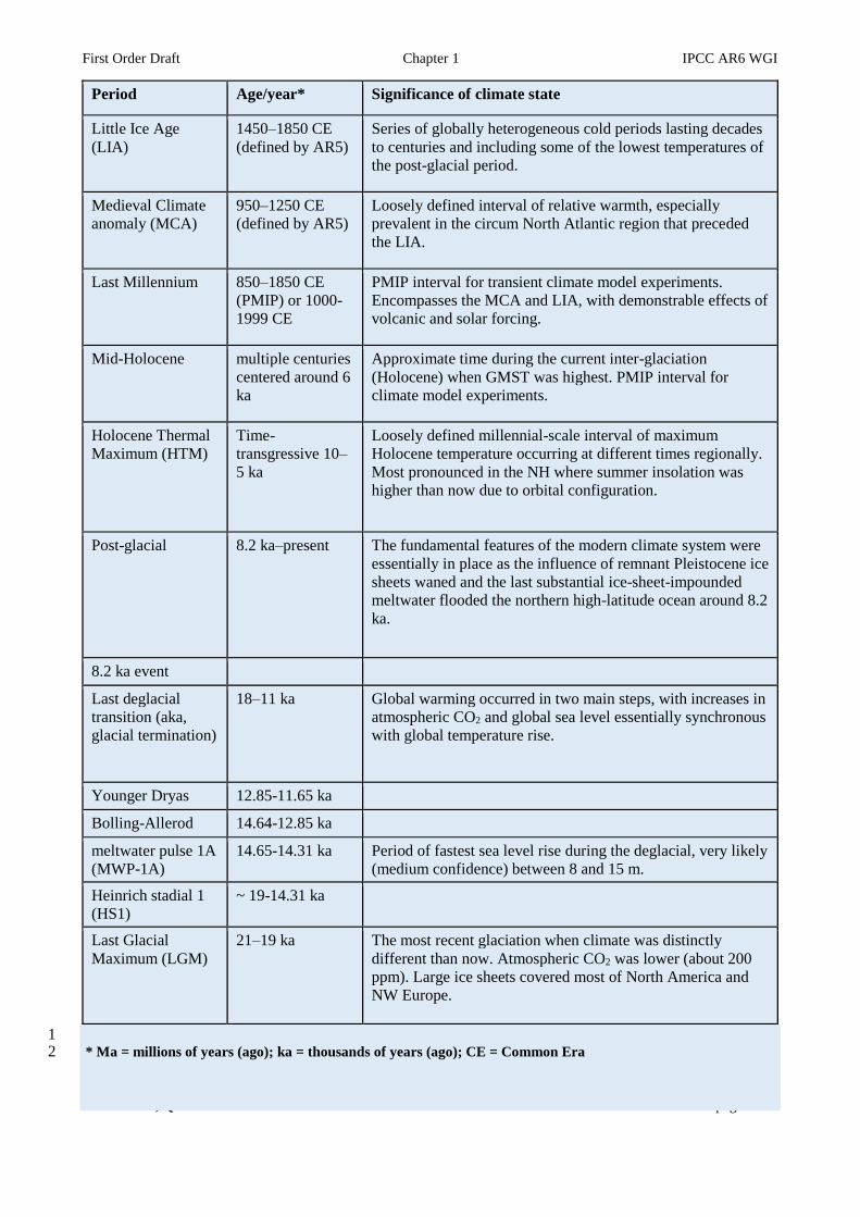
First Order Draft Chapter 1 IPCC AR6 WGI
Do Not Cite, Quote or Distribute 1-71 Total pages: 184
Period Age/year* Significance of climate state
Little Ice Age
(LIA)
1450–1850 CE
(defined by AR5)
Series of globally heterogeneous cold periods lasting decades
to centuries and including some of the lowest temperatures of
the post-glacial period.
Medieval Climate
anomaly (MCA)
950–1250 CE
(defined by AR5)
Loosely defined interval of relative warmth, especially
prevalent in the circum North Atlantic region that preceded
the LIA.
Last Millennium 850–1850 CE
(PMIP) or 1000-
1999 CE
PMIP interval for transient climate model experiments.
Encompasses the MCA and LIA, with demonstrable effects of
volcanic and solar forcing.
Mid-Holocene multiple centuries
centered around 6
ka
Approximate time during the current inter-glaciation
(Holocene) when GMST was highest. PMIP interval for
climate model experiments.
Holocene Thermal
Maximum (HTM)
Time-
transgressive 10–
5 ka
Loosely defined millennial-scale interval of maximum
Holocene temperature occurring at different times regionally.
Most pronounced in the NH where summer insolation was
higher than now due to orbital configuration.
Post-glacial 8.2 ka–present The fundamental features of the modern climate system were
essentially in place as the influence of remnant Pleistocene ice
sheets waned and the last substantial ice-sheet-impounded
meltwater flooded the northern high-latitude ocean around 8.2
ka.
8.2 ka event
Last deglacial
transition (aka,
glacial termination)
18–11 ka Global warming occurred in two main steps, with increases in
atmospheric CO2 and global sea level essentially synchronous
with global temperature rise.
Younger Dryas 12.85-11.65 ka
Bolling-Allerod 14.64-12.85 ka
meltwater pulse 1A
(MWP-1A)
14.65-14.31 ka Period of fastest sea level rise during the deglacial, very likely
(medium confidence) between 8 and 15 m.
Heinrich stadial 1
(HS1)
~ 19-14.31 ka
Last Glacial
Maximum (LGM)
21–19 ka The most recent glaciation when climate was distinctly
different than now. Atmospheric CO2 was lower (about 200
ppm). Large ice sheets covered most of North America and
NW Europe.
1 * Ma = millions of years (ago); ka = thousands of years (ago); CE = Common Era 2
First Order Draft Chapter 1 IPCC AR6 WGI
Do Not Cite, Quote or Distribute 1-72 Total pages: 184
[END CROSS-CHAPTER BOX 1.3, TABLE 1 HERE] 1
2
[END CROSS-CHAPTER BOX 1.3 HERE] 3
4
5
1.5.4 Sources of uncertainty in climate projections 6
7
When considering the range of future projections of the physical climate system there are several different 8
contributing sources of uncertainty, often separated into scenario uncertainty, model response uncertainty 9
and uncertainty due to internal variability. 10
11
Scenario uncertainty 12
Divergent future projections often result from different scenarios being assumed for anthropogenic drivers of 13
climate change (see Section 1.6 for a detailed description of scenarios). The RCP and SSP scenarios, which 14
form the basis for climate projections assessed in this report, are designed to span a plausible range of future 15
pathways but the real world will differ from these example storylines. Although termed an ‘uncertainty’, this 16
component is distinct from other uncertainties, given that - at least from the viewpoint of decision makers - 17
future anthropogenic emissions can be considered as the outcome of a set of collective choices (see Section 18
1.6.2). Scenario uncertainty is often the largest source of uncertainty when looking to the long-term, but is 19
relatively small in the next few decades, especially globally (Hawkins and Sutton, 2009b). 20
21
Model response uncertainty 22
Assuming a particular scenario, there is uncertainty in how the climate will respond to the specified 23
emissions or radiative forcing combinations. A range of climate models are used to sample uncertainty in our 24
understanding of the key physical processes and to define the ‘model response’ uncertainty. There are 25
several subcategories of this ‘model response’ uncertainty related to, for example, carbon cycle feedbacks, 26
radiative forcing efficiencies, cloud parameterisations and other climate feedbacks, but these are hard to 27
quantify individually. 28
29
Internal variability 30
In the absence of any changes in radiative forcing there would still be intrinsic uncertainty in the projections 31
due to internal climate variability - the random fluctuations of the climate like those associated with modes 32
of variability (e.g. ENSO, IPO, AMV). 33
34
Uncertainty quantification and missing uncertainties 35
From long-term model projections it is possible to approximately quantify the relative amplitude of these 36
uncertainty sources. A sample of different scenarios defines the scenario uncertainty, and ensemble means 37
from different models can estimate the model response uncertainty. The unforced component of internal 38
variability can be approximated from individual ensemble members of the same climate model (see Figure 39
1.18). In principle, the intrinsic uncertainty due to internal variability can be estimated probabilistically – it is 40
‘aleatoric’ – whereas the other two sources of uncertainty are ‘epistemic’ and should not be considered as 41
reliable probabilities due to their ad-hoc sampling approaches. The real world will also experience future 42
changes in natural forcing, i.e. variations in volcanic and solar activity, which are not included in the 43
projections but could be significant for short periods (e.g. Bethke et al., 2017). Interactions between these 44
different sources of uncertainty are also plausible as, for example, changes in radiative forcings could alter 45
the phasing or amplitude of internal variability. 46
47
48
[START FIGURE 1.18 HERE] 49
50 Figure 1.18: The ‘cascade of uncertainties’ in climate projections of global mean surface temperature change for 2080-51
2099 from CMIP5. The multi-model mean for each scenario is indicated at the top of the cascade. This 52 branches downwards to show the multi-realisation mean for each model (middle row), and further 53 branches into the individual realisations (bottom row), though often only a single realisation is available. 54 For this time period, the scenario uncertainty and model response uncertainty are larger than the internal 55

First Order Draft Chapter 1 IPCC AR6 WGI
Do Not Cite, Quote or Distribute 1-73 Total pages: 184
variability. (To be updated to CMIP6 and include a near-term regional example to highlight the role of 1 internal variability on smaller spatial and temporal scales.) 2
3 [END FIGURE 1.18 HERE] 4 5 6 1.5.5 Attribution of climatic changes 7
8
Attribution of climate change intends to connect an observed change to one or several drivers, and to 9
quantify their respective contribution. This field of research started out with detecting statistically significant 10
trends in global temperature patterns and attributing them to human influences (Hasselmann, 1997; Hegerl et 11
al., 1997). Moving to individual events, studies that investigated the European heatwave in 2003 were some 12
of the first that attributed a part of the likelihood of such an extreme occurring to the human influence (Stott 13
et al., 2004). Now, a wide array of the changes in the climate system can be attributed to human influence, 14
including changes in regional temperature, precipitation, and also features that integrate many drivers of 15
change such as regional sea-level. The attribution of impacts is now also an emerging field. The wide range 16
of attribution methods and applications are outlined in Box 1.4. 17
18
19
[START CROSS-CHAPTER BOX 1.4 HERE] 20
21
Cross-Chapter Box 1.4: Attribution in the IPCC Sixth Assessment Report 22
23
Attribution exercises provide valuable information to a wide range of stakeholders to allow them to 24
understand the drivers of the change or extreme event they are experiencing (James et al., 2019; Parker et al., 25
2017; Sippel et al., 2015; Stott and Walton, 2013) 26
27
Definitions and practice of detection and attribution have evolved over the years, starting with a guidance 28
paper (Hegerl et al., 2010). Other relevant reviews and IPCC assessments providing orientation include: 29
(National Academies of Sciences Engineering and Medicine, 2016); AR5 WGI Chapter 10 and AR5 WGII 30
Chapter 18. There have also been many developments in the attribution of events (Jézéquel et al., 2018). 31
Here we briefly describe new developments in the different approaches of attribution, providing examples 32
from the literature relevant to Working Grous I and II (WGII and WGII). 33
34
Factors to consider in attribution studies 35
36
Climate changes or events of relevance in the context of this report are those where human-induced climate 37
change might have played a role. For most variables in the physical climate system, for example global mean 38
temperature, baseline conditions on human time-scales will consist of some variability on both sides of 39
quasi-static conditions (See 1.5.3). For impacted systems, baseline conditions may or may not be static. 40
Agricultural productivity, for example, has been increasing over recent decades as a consequence of 41
technological progress in crop management (e.g. Hochman et al., 2017). For such systems, deviation from 42
this increase could be a consequence of climate change. 43
44
Attribution studies firstly require a reliable description of the observed change or of extreme event in 45
question. This requires observations that are deemed of high enough temporal and spatial coverage, quality 46
and homogeneity to capture the change or event. In some cases, such observations are not available, for 47
instance, there are too few sea-level records prior to the satellite era to accurately capture change across the 48
Pacific Ocean (Palanisamy et al., 2015). 49
50
Common to all attribution studies is that they draw on a modelling approach (physical, conceptual or 51
empirical) to establish the counterfactual system behaviour. One example of such a counterfactual system is 52
a dynamical climate model simulation of the historical period with greenhouse gas forcing omitted from the 53
suite of forcing agents (e.g. Ribes and Terray, 2013). If not all important drivers are taken into account in an 54
attribution study, it is important to highlight which potentially confounding factors are not considered 55
First Order Draft Chapter 1 IPCC AR6 WGI
Do Not Cite, Quote or Distribute 1-74 Total pages: 184
(Hegerl et al., 2010), e.g. for climate attribution land-surface feedbacks or land-use changes or absorbing 1
aerosols (Hauser et al., 2016; Lejeune et al., 2018; Mueller et al., 2018; Whan et al., 2015). 2
3
All studies make the assumption that models used are fit for purpose. The veracity of the model assessment 4
will be included in the examination of each study and the robustness of the result crucially depends on this 5
assessment. The range of variables analysed can lead to highly uncertain outcomes in some cases (Uhe et al., 6
2017) and very robust estimates of the influence of anthropogenic climate change in other cases (Haustein et 7
al., 2017; Otto et al., 2018). 8
9
Detection and attribution of observed large-scale changes in climate variables – e.g. global near-surface air 10
temperature 11
12
Detection and attribution of large-scale trends in climate variables such as near-surface air temperature will 13
provide the basis for the assessment of the causes of those trends, and are found in WGI Chapter 3. The 14
methods used will generally follow the approaches detailed in Hegerl et al. (2010) and Stone et al. (2009). 15
Detection of observed changes will include efforts to characterize the internal variability contribution as 16
compared to the externally forced climate response using a range of statistical detection and attribution time 17
series and fingerprint techniques (e.g. Frankcombe et al., 2015; Hannart, 2016). Time series methods aim to 18
determine if the change is outside the range of internal variability while fingerprint techniques rely on 19
regressing observations onto model-simulated climate response patterns (i.e. fingerprints), assuming that the 20
climate system generates unique responses to various external forcings. There can also be the attribution of 21
detected changes to a number of individual forcings, including the proportion attributable to greenhouse gas 22
influence, aerosol influence, or other forcing (e.g. Gillett et al., 2013b; Slangen et al., 2016). The ‘fit’ 23
between observations and these fingerprints is termed a ‘scaling factor’ (See Figure 10.4 of AR5 WGI 24
Chapter 10). The scaling factors obtained in attribution studies may be used to constrain projections, under 25
the assumption that the scaling factors which provide a best fit between simulated and observed historical 26
changes and associated uncertainties may be applied to future climate change (Allen et al., 2000; Stott and 27
Kettleborough, 2002). There can however be various feedbacks and localized factors that also influence 28
temperature trends, particularly in the diurnal range. These include variations in soil moisture, water vapour 29
(Dai et al., 1999; Zhou et al., 2009), and the depth of the boundary layer which relates to the effective heat 30
capacity of the atmosphere (Davy and Esau, 2016). Multi-variable (e.g. temperature and precipitation) 31
analyses have thus been found to provide increased confidence in the recognition of the signal (Paeth et al., 32
2017; Yan et al., 2016). 33
34
Attribution of changes at regional scales 35
36
The WGI report has a renewed focus of attribution of changes on regional scales, due to their relevance to 37
WGII, policymakers and other stakeholders. Changes in regional climate at the scale of a continent, country 38
or region are more complex to attribute to external drivers (See 1.5.1.2), mainly due to increased internal 39
variability on smaller spatial scales which decreases the signal-to-noise ratio (See 1.5.1.1). In addition, some 40
non-greenhouse gas human forcings, such as land use change and aerosol forcings, tend to have strong 41
regional footprints (Lejeune et al., 2018; Nabat et al., 2014; Persad et al., 2017) further complicating efforts 42
at attribution. Fingerprinting methodologies (Dileepkumar et al., 2018; Ribes et al., 2009) can still be used 43
for regional attribution studies. 44
45
The attribution of change in components of the climate system such as monsoons or regional sea-level can be 46
more complex than single variables, as they integrate the response to temperature changes, amongst other 47
factors. 48
49
Change in features such as the South Asian summer monsoon can be due to many factors including rapid and 50
substantial changes in land use, land management and industrial activities over the subcontinent, variability 51
in the Indian Ocean, along with the response to rising global greenhouse gas emissions (Singh et al., 2019). 52
Attributing changes in such systems can be done qualitatively, but new efforts to model the monsoon system 53
allow more quantitative statements on the influences from climate change. This forms a case study in AR6 54
WGI Chapter 10. 55
First Order Draft Chapter 1 IPCC AR6 WGI
Do Not Cite, Quote or Distribute 1-75 Total pages: 184
1
In AR6 WGI, Chapter 9, the attribution of changes in regional sea-level is presented for the first time. While 2
there is some confidence in the change in components of sea-level change, such as that due to thermal 3
expansion (Marcos and Amores, 2014), for attribution of change at a regional scale (e.g. the Pacific Ocean), 4
there are confounding factors such as the Pacific Decadal Oscillation. Accounting for these variations allows 5
the signal of change due to human-induced forcing to be revealed (Hamlington et al., 2014; Palanisamy et 6
al., 2015). An alternative approach is to consider regional sea-level as the sum of attributed global mean sea-7
level change, unattributed global mean sea-level change, and unattributed local relative sea-level change 8
(Strauss et al. 2016) and use the combined information to estimate which part would not have happened in 9
the absence of attributed global mean sea-level change. 10
11
While decadal variability was seen as a confounding factor to the signal of sea-level changes in the Pacific in 12
the examples above, in some cases, it is seen as a component of the causal factors. This is important when 13
explaining short-term trends to policy makers, e.g. the rainfall trends from the 1980s to 2010s in south-west 14
US (Lehner et al., 2018) or recent Eurasian cooling (Mori et al., 2019). In the literature this is referred to as 15
process-based attribution as it seeks to highlight the physical processes and uncertainties involved in the 16
driver’s influence, including those drivers that are internal variability. This style of attribution study is very 17
useful in communicating the influence of climate change on recent changes and links closely with the study 18
of event attribution. 19
20
Event Attribution 21
22
Event attribution is the attribution of the drivers of a particular event (e.g. Hope et al., 2016) or class of 23
events e.g. (Christidis et al., 2015; Lewis et al., 2014). The events assessed are usually recent records that 24
have been broken or major events with widespread impacts. An example of an extreme event might be a 25
record hot week or month over the scale of a country. The basic principle of event attribution is that the 26
characteristics (often occurrence probability and intensity) of a type of weather or climate event (or an 27
individual event) are analysed under present day climate conditions and counterfactual conditions in a 28
“world that might have been” without anthropogenic climate change. The attribution of changes in extremes 29
were assessed in AR5 WGI Section 10.6 for the first time based upon a very small body of literature. In AR6 30
WGI these changes in extremes are assessed in Chapter 11. 31
32
A wide range of approaches and events are described in special issues published in the Bulletin of the 33
American Meteorological Society (BAMS) each year (Herring et al., 2014, 2015, 2016, 2019, Peterson et al., 34
2012, 2013). The studies in these special issues cover a wide range of events from around the globe 35
(Jézéquel et al., 2018). Jézéquel et al. (2018) reviewed the methods in these studies and describes two main 36
approaches. One is a probabilistic approach that focuses on quantifying the role of anthropogenic climate 37
change on the probability of a particular class of events occurring or crossing a threshold. This is sometimes 38
also called the risk-based approach and the ‘fraction of attributable risk’ or statements on the likelihood of a 39
particular event occurring with or without climate change can be made. The other is a storyline approach that 40
aims at unveiling the qualitative ways in which anthropogenic climate change affects the processes leading 41
to the event (see section1.2.4.3). These approaches can be complementary, however, the clear definition of 42
the event and the framing of the attribution question and method is imperative in the comparison of studies 43
(Otto et al., 2016). 44
45
The largest differences in framing result from the level of conditioning of the specific event on a range of 46
factors. Conditional attribution links anthropogenic climate change combined with a precursor to either an 47
extreme observable, or its impacts. This precursor is an internal element of the climate system which played 48
a role in the occurrence of the event. This approach is not specific to event attribution, as seen in the 49
examples of regional attribution above that were conditioned on decadal variability. Conditioning factors can 50
also include the exact circulation state (Meredith et al., 2015), the observed sea surface temperatures (Otto et 51
al., 2015a), forecasts of the event (Hope et al., 2016, 2018), or the large scale warming only (Lewis and 52
Karoly, 2013). There are also studies that combine different levels of conditioning (e.g. Cheng et al., 2018; 53
Philip et al., 2018a). As the results crucially depend on the event definition and framing, in some cases 54
alternative framing means that direct comparison of results from different studies is not possible. In order to 55
First Order Draft Chapter 1 IPCC AR6 WGI
Do Not Cite, Quote or Distribute 1-76 Total pages: 184
be able to assess the confidence in assessments of changes in particular types of weather events it is 1
important to either assess multi-method and multi-model approaches that combine different framings in a 2
single study (e.g. Grose et al., 2018; Martins et al., 2017; Philip et al., 2018; Uhe et al., 2017; Van 3
Oldenborgh et al., 2018) or assess multiple studies on the same event or type of event. 4
5
Attribution of impacts 6
7
In the context of IPCC (refer to the Glossary), impacts refer to effects of climate extremes or climate change 8
on natural and human systems. Whereas attribution of physical impacts of climate change on variables such 9
as sea level rise or droughts are assessed in WGI (Funk et al., 2013; Uhe et al., 2017; (Philip et al., 2018a)), 10
attribution of climate change on other natural and human systems will be assessed by WGII (e.g., Hansen et 11
al., 2016; Hansen and Cramer, 2015; Stone et al., 2013). 12
13
Climate impacts on an ecological or social system are the result of interactions of a climate hazard with 14
vulnerability and exposure of the system. Therefore, detecting and attributing an anthropogenic climate 15
signal in observed impacts starts from identifying the climate variables that create the hazard, how they have 16
changed and why (Otto, 2017; Sippel and Otto, 2014). Trends in vulnerability and exposure should also be 17
considered ((Otto et al., 2015b); Sheridan and Allen, 2018). However, final detection and attribution of the 18
impacts can still be complicated by the convergence of multiple factors, variables and feedbacks, sometimes 19
non-linear ones. 20
21
There are now a number of studies where attribution assessments of changes in climatic variables (e.g. local 22
temperatures or precipitation) are combined with what that change means for systems of interest, for 23
example fire or river flow and inundation (Hope et al., 2019; Kirchmeier-Young et al., 2019; Schaller et al., 24
2016). 25
26
Attribution of (observed/past) changes, such as changes in probabilities of extreme weather, to human 27
influence on the climate is useful as it lends confidence to predictions/projections of future change, and may 28
also be policy-relevant in relation to climate-related loss and damage. However, it is important to recognise 29
caveats regarding the challenges of untangling trends in hazards, sensitivity, vulnerability and exposure in 30
determining actual impacts. 31
32
Attribution of adaptation actions has been attempted, for example in the context of water management in 33
cities (Grant et al., 2013; Low et al., 2015) but in general it can be confounded by the presence of 34
contemporaneous drivers unrelated to climate change, including population changes. 35
36
Attribution in the WGI and WGII assessments 37
38
In WGI, attribution of changes in large-scale indicators of change in the atmosphere, ocean and cryosphere 39
will be assessed in Chapter 3, attribution of changes in extremes and extreme events will be assessed in 40
Chapter 11, while attribution of regional changes in water cycle in Chapter 8, the ocean and cryosphere will 41
be assessed in Chapter 9, and other aspects of regional climate change in Chapter 10. Attribution of changes 42
in human and natural systems will be assessed by WGII. 43
44
[END CROSS-CHAPTER BOX 1.4 HERE] 45
46
47
1.6 Dimensions of Integration: Scenarios, temperature levels and cumulative carbon emissions 48
49
This section describes and discusses the emission and concentration scenarios that are considered in this 50
Report, building a common reference point with the Working Groups II and III (WGII and WGIII) to 51
synthesize knowledge across the physical sciences, impact and adaptation and mitigation research. Two 52
additional ‘dimensions of integration’ to synthesize the literature are presented: global-mean temperature 53
levels as well as a categorization of emission scenarios or geophysical impacts in relation to their cumulative 54
carbon emissions (see Figure 1.19). 55
First Order Draft Chapter 1 IPCC AR6 WGI
Do Not Cite, Quote or Distribute 1-77 Total pages: 184
1
[START FIGURE 1.19 HERE] 2 3 Figure 1.19: The Dimensions of Integration (DI) across Chapters and Working Groups in the IPCC AR6 assessment 4
report. Building on the Synthesis Reports of the Fifth IPCC Assessment report (background image detail) 5 this report adopts three explicit dimensions of integration to integrate knowledge across chapters and 6 Working Groups. The first dimension (DI 1) are scenarios, the second dimension (DI 2) are global-mean 7 temperature levels relative to pre-industrial levels and the third dimension (DI 3) are cumulative CO2 8 emissions. 9
10
[END FIGURE 1.19 HERE] 11
12
13
1.6.1 Dimensions of knowledge integration within and across Working Groups 14
15
While scenarios are a key tool for integration across working groups, scenarios allow the integration of 16
knowledge within each scientific community. For example, agricultural yield, infrastructure and human 17
health impacts of increased drought occurrences, extreme rainfall events and hurricanes are often examined 18
in isolation. New insights can however be gained on climate impacts in WGII, if compound effects of 19
multiple cross-sectoral impacts are considered across multiple research communities under consistent 20
scenario frameworks (Leonard et al., 2014; Warszawski et al., 2014). Similarly, a synthesis of WGI 21
knowledge on sea level rise contributions is enabled by a consistent application of future scenarios across all 22
specialised research communities, such as ice-sheet surface mass balances, mountain glacier loss projections 23
and thermosteric expansion from ocean heat uptake (e.g. Kopp et al., 2014) (Chapter 9). 24
25
Scenarios used for a synthesis of findings across Working Groups. Building on earlier results in AR4, 26
AR5 and the Special Reports, this Report continues to provide consistent analysis of specific scenarios, but 27
also on the knowledge integration across the two policy-relevant dimensions: emissions and global-mean 28
temperatures. Simplified, those two policy-relevant dimensions frame the cause-effect chain investigated by 29
WGI: emissions and the resulting projected temperatures. The handover with WGIII are the emissions, as 30
WGIII considers drivers of emissions and mitigation options. The handover with WGII are the geophysical 31
climate projections from the Earth System Models (Figure 1.20). This offers a strong synthesis across the 32
Working Groups, as mitigation, impact or adaptation results can be tied towards these three dimensions: 33
scenarios, cumulative emissions and temperatures. 34
35
Not only does a consistent application of scenarios serve the integration of knowledge across the three 36
Working Groups. Also, the scenario generation process itself is a cross-Working Group activity. The 37
scenario generation starts in the scientific community related to WGIII, new storylines (O’Neill et al., 38
(2014); see also Section 1.2.4.3) are quantified in terms of their the drivers GDP, population, technology, 39
energy and land use demand and their resulting emissions (Riahi et al., 2017a). Then, numerous 40
complementation and harmonisation activities within the WGIII and WGI communities are performed, 41
gridding anthropogenic short-lived forcers, providing open biomass burning emission estimates, land use 42
patterns, observed and projected greenhouse gas concentration time series, stratospheric aerosol fields, 43
stratospheric and tropospheric ozone, nitrogen deposition datasets, solar irradiance and aerosol optical 44
property estimates. These activities are compiled under the WCRP CMIP6 input4mips umbrella (Durack et 45
al., 2018) (see Section 1.6.2.1). With those completed datasets, the Earth System Models are then run, 46
providing the sets of experiments under multiple model intercomparison protocols that are now part of 47
CMIP6 (Eyring et al., 2016a) (see Section 1.4.3). Using emulators calibrated with the Earth System Models’ 48
temperature responses under those given scenarios, the WGI community is then feeding back tools to WGIII 49
that allow to compute several high-level climate indicators (concentrations, temperatures, sea level rise) for a 50
much wider set of hundreds of scenarios that are assessed by WGIII. The main use of the climate projections 51
is however the further assessments of its implied future geophysical climate impacts - feeding into 52
specialised impact models to assess the ecological, food security, infrastructure and human impacts under the 53
main set of scenarios (Figure 1.20). 54
55
56
First Order Draft Chapter 1 IPCC AR6 WGI
Do Not Cite, Quote or Distribute 1-78 Total pages: 184
[START FIGURE 1.20 HERE] 1
2 Figure 1.20: The scenario generation process that weaves through the three Working Groups and its scientific 3
communities. The top level indicates the main set of models used in that scenario generation process, 4 with the lower level indicating the datasets. Also, the three dimensions of integration (scenarios, 5 cumulative carbon emissions and global-mean temperature levels) are indicated as open circles, with 6 cumulative emissions sitting at the handover between WGIII (orange) and WGI (blue), and global-mean 7 temperatures sitting - simplified speaking - at the connection point between WGI and WGII (green). 8
9
[END FIGURE 1.20 HERE] 10
11
12
[START FIGURE 1.21 HERE] 13
14 Figure 1.21: Analysis of the marker SSP scenarios, RCP and the wider AR6 scenario database regarding cumulative 15
carbon emissions over time (panel a). The implied CO2-induced warming given those cumulative 16 emissions and the TCRE is shown for SSP scenarios and SR1.5 emission scenario database (panel b). The 17 variation of non-CO2 emission rates at the time of peak cumulative emissions is here exemplified with 18 total methane emissions that can substantially influence the remaining carbon budget (cf. Collins et al. 19 (2018)) (panel c). Overall, the GWP-weighted sum of all greenhouse gas emissions is a close indicator of 20 cumulative carbon emissions until 2050 in the literature scenarios, lending some support to policy 21 architectures that address GWP-weighted emission baskets as one of many options (see discussion in 22 Chapter 7) (panel d). The timing of net positive and net negative emissions across the 9 SSP marker 23 scenarios over time (panels e on the right side). [Note: this graph is only a sketch to highlight a few 24 aspects of the AR6 emission database. To be updated] 25
26
[END FIGURE 1.21 HERE] 27
28
29
The temperature and cumulative-emission based scenario classification. 30
The Integrated Assessment Model (IAMs) community provides a wealth of hundreds of scenarios, in 31
addition to the ESMs scenario runs carried out under CMIP6 for a set of “marker scenarios”. These IAMs 32
scenarios follow various shared policy assumptions (SPAs) - resulting in a mix of low and high emission 33
scenarios with various timings, multi-gas shares and regional differences. This wealth of scenarios can then 34
be classified according to a scenario’s peak temperature (or the likelihood to exceed a certain temperature 35
level relative to pre-industrial), relating directly to a key policy variable of interest. Examining the emission 36
pathway characteristics of all scenarios in one temperature class allows for a better insight of cost-optimal 37
and second-best emission milestones and characteristics while at the same time providing insights regarding 38
the flexibility to divert from the middle-of-the-road pathways in a specific scenario class. The disadvantage 39
is clearly that uncertainties are folded into the scenario classification that are external to the scenarios 40
themselves. However, with a proper characterisation and synthesis of uncertainties across the AR6 report, 41
ranging from the CO2-induced warming, non-CO2 greenhouse gas and aerosol effect, as well as carbon cycle 42
and Earth system feedbacks. This integration of uncertainties is assessed in this WGI Report. Furthermore, a 43
temperature-defined scenario classification enables a closer integration of results across the various research 44
communities – linking to temperature-tagged impact results from WGII, but also paleoclimatic studies 45
assessed elsewhere in this report (see Section 1.6.3). In addition to temperature-based scenario 46
classifications, this report will perform a cumulative carbon emission classification of scenarios, as described 47
in Section 1.6.4. 48
49
Cumulative carbon emissions and global-mean temperatures are representative for a broad spectrum 50
of climate effects. 51
Global mean temperature levels are nearly-linearly related to a number of a number of regional climate 52
impacts, temperatures (Mitchell, 2003; Mitchell et al., 2000; Tebaldi and Arblaster, 2014), aggregated 53
impacts against temperature levels have been widely used and embedded in the iconic ‘Reasons for concern’ 54
(RFC) figure (Smith et al., 2009; IPCC, 2014). The RFC framework has been further expanded in the SR15, 55
the SROCC and SRCCL by explicitly looking at the differential impacts between half-degree warming levels 56
(cf. King et al. (2017), and more specific impacts. Global-mean temperatures are hence the ‘pars-pro-toto’ 57
First Order Draft Chapter 1 IPCC AR6 WGI
Do Not Cite, Quote or Distribute 1-79 Total pages: 184
representation and approximation of a much wider range of regional climate impacts, cognizant of some of 1
the limitations as for example regional precipitation responses also strongly depend on the forcings 2
themselves, the vertical structure of the troposphere (Andrews et al., 2010) and aerosols in particular (Frieler 3
et al., 2012). Similarly, cumulative carbon emissions are a good proxy and a pars-pro-toto, offering the 4
opportunity to synthesise insights by WGI along the dimension of cumulative carbon emissions. With the 5
overwhelming majority of future greenhouse gas induced warming resulting from elevated carbon dioxide 6
concentrations across the scenarios, it is also key to keep the second-order variations in mind. For example, 7
methane emission rates shortly before and at the time of peak warming levels can have a strong effect on the 8
remaining carbon budget (Collins et al., 2018) (see Figure 1.21, panel c). In summary, in addition to 9
scenarios, knowledge integration across the cumulative emission and temperature axes opens additional 10
opportunities to synthesize knowledge across Chapters and Working Groups. 11
12
13
[START FIGURE 1.22 HERE] 14
15 Figure 1.22: The marker SSP scenarios used throughout the AR6 report, their cumulative CO2 emissions and 2050 16
GHG emission levels in the context of the risks from climate change. Shown is the Synthesis Report 17 Figure SPM.10 from AR5, updated by the 21st century characteristics of the new SSP scenarios in panel 18 b and c. [Note, this is only a hand-drawn sketch]. 19
20
[END FIGURE 1.22 HERE] 21
22
23
Nuances and limitations of the ‘dimensions of integration’. 24
Ever since the ‘dimensions of integration’ have emerged in the scientific literature, a body of literature has 25
also investigated the limitations, non-linearities and shortcomings of those. Regarding the dimension of 26
cumulative emissions, the potential disadvantage is – to the extent that CO2 trajectories and non-CO2 27
emissions materially differ (see e.g. Figure 1.21, panel c) – that the categorisation of scenarios according to 28
their cumulative carbon emissions does not imply similarly distinct climate outcomes of the adjacent 29
emission-defined scenario classes. As further explored as part of the WGIII assessment, one potential 30
limitation when presenting emission pathway characteristics in cumulative emission budget categories, the 31
knowledge around path-dependencies and lock-in effects should also be fully considered. For example, 32
continuously high emission early-on might imply strongly net negative emissions later on to reach the same 33
cumulative emission and temperature target envelope by the end of the century. This report will explore 34
options to address some of those potential issues from a WGI perspective. Regarding the dimension of 35
global-mean temperatures, for example, distilling geophysical climate effects for low warming before the 36
emergence of 1.5°C specific scenarios is often performed by using early-century time slices of higher 37
emission scenarios. Similarly, for 2°C, higher scenarios or idealized scenarios had been used before RCP2.6 38
climate results were available. Distilling robust results from time slices of transient but ultimately higher 39
warming scenarios is for example hampered by relatively higher aerosol emissions compared to scenarios in 40
which 1.5°C or well-below 2°C temperature levels above pre-industrial levels are achieved and maintained. 41
Low aerosol emission levels are projected under low mitigation scenarios for the middle and end of this 42
century, rendering the geographical and precipitation responses different from a transient 1.5°C snapshot of a 43
higher warming scenario. Another aspect is how long-term sea level rise correlates with the global-mean 44
temperatures. For sea level rise, time is important as several sea level rise contributions are approximately 45
proportional to the integral over global-mean temperature. Thus, sea level rise after a 1°C warming for 50 46
years will be quite a bit lower than the sea level rise that arises from keeping that 1°C warming for 150 years. 47
48
49
1.6.2 Scenarios reflecting choices within an uncertain future 50
51
As a tool to methodologically examine the future, scenarios have risen to prominence since the ‘Limits to 52
Growth’ report in 1972 by Meadows et al. (1972) (see Cross Chapter Box 2 on “Scenarios and other methods 53
to characterise the future” in SRCCL). Rather than predicting the future, scenarios examine future 54
developments in a “what-if” explorative sense (cf. Moss et al., 2010). While there are some probabilistic 55

First Order Draft Chapter 1 IPCC AR6 WGI
Do Not Cite, Quote or Distribute 1-80 Total pages: 184
socio-economic and emission scenarios in the literature (e.g. Webster et al., 2003), the scenario literature 1
does not assign probabilities to individual scenarios, as the future is intrinsically unpredictable. The 2
plausibility assigned to various scenarios can change over time. For example, the likelihood of a scenario of 3
‘regional rivalry’ would have been discussed very differently during the adoption of the Paris Agreement in 4
2015 compared to just two years later. The public acceptability and assessments of potentials of large-scale 5
biomass plantations with carbon capture and storage (CCS) also changes over time and across countries and 6
leads to differing assessments as towards their likelihood or desirability of scenarios that employ high shares 7
of that particular negative emission technology (e.g. Fuss et al., 2014). In summary, the foundational 8
principle of scenarios is that they are “what-if” projections, discussed in regard to their (changing) 9
plausibility, facilitating factors, side effects and their respective desirability, rather than scenarios being 10
deterministic or probabilistic predictions. 11
12
Scenarios are a core element to WGI, even though largely exogenous. Scenarios have been used in IPCC 13
reports since the First Assessment Report (Legget, 1992) with so-called IS92, SRES, and RCPs informing 14
more than three decades of climate change research. For this WGI Report, the emissions of the main set of 15
scenarios are the Shared Socioeconomic Pathways (SSPs, Riahi et al 2017), reflecting future emissions that 16
result from socio-economic scenarios that are assessed in detail in WGIII. However, the scenario generation 17
process with the harmonisation of emissions, completion with natural forcings, biomass burning emissions, 18
land use patterns, greenhouse gas concentrations and ultimately the climate projection is a process that 19
weaves through all three Working Groups of the IPCC and their respective scientific communities (Figure 20
1.20). In addition to those transient long-term scenarios, multiple idealized pathways and time-slice 21
experiments independent of scenarios are investigated by climate models. Ever after the first transient 22
climate modelling runs in 1988 with a General Circulation Model (Hansen et al., 1988), the transient 23
modelling experiments with scenarios are a core element of physical climate science. Except for seasonal 24
and most decadal predictions, future climate projections are conditional on the respective scenario. 25
26
The use of different scenarios for climate change projections introduces a so-called ‘scenario-uncertainty’ in 27
the projections (Collins et al., 2013) (see Section 1.5.4). However, ‘scenario uncertainty’ might be a slight 28
misnomer, as scenarios are technically not an uncertainty, but an outcome of many collective choices (Knutti 29
et al., 2008). Future emissions are, to a large extent, the outcome of a collective choice in relation to 30
population growth, economic activity, or choices regarding an activities’ emission intensity. For example, 31
the future share with which electricity demand is met by coal power plants, or renewables or whether energy 32
efficiency is lowering energy demand, are explicit or implicit collective choices. Scenarios are hence 33
fundamentally different from geo-physical uncertainties. On the other hand, from an adaptation planning 34
perspective, an investment into long-term water infrastructure, for example, faces the uncertainty as to what 35
the collective aggregate choice of humanity that ultimately determine human-induced emission levels. 36
37
Long-term scenario uncertainties can be made accessible by means of ‘scenario storylines’. ‘Storylines’ in 38
this context (see Section 1.2.4.3 for a broader discussion on ‘storylines’ that also discusses ‘event storylines’) 39
are descriptions of that state of a future world and the large-scale development towards there (e.g. ‘regional 40
rivalry’ vs. ‘global cooperation’) that are deemed plausible with the current state of knowledge and historical 41
experiences. They do not ‘seek truth’, but attempt to ‘stimulate, provoke, and communicate visions of what 42
the future could hold for us’ (Rounsevell and Metzger, 2010) in settings, where either limited knowledge or 43
inherent unpredictability in social systems prevents a forecast or numerical prediction. Storylines are nothing 44
new in climate research, as they are the explicit or implicit starting point of any scenario exercise, whether 45
for SRES scenarios or SSPs (e.g. O’Neill et al., 2017a). 46
47
However, a new paradigm has emerged over the decades of considering socio-economic storylines and 48
emission futures as orthogonal. Until the mid 2000s, socio-economic storylines have often been represented 49
by a single marker or illustrative scenario. That led to the misperception that a certain socio-economic 50
development path dictated greenhouse gas and short-lived climate forcer levels. Within reference scenarios, 51
this paradigm started to be differentiated when the high-economic A1 scenario family in the set of SRES 52
scenarios was represented by three scenarios, A1FI, A1B and A1T, that imply high, medium and 53
comparatively lower future emission levels (SRES, Nakicenovic and Swart, 2000). The set of scenarios that 54
followed, the Representative Concentration Pathways (RCPs, Moss et al., 2010), were intentionally devoid 55

First Order Draft Chapter 1 IPCC AR6 WGI
Do Not Cite, Quote or Distribute 1-81 Total pages: 184
of the socio-economic underlying storylines, and was the starting point for a more systematic exploration of 1
the two-dimensional space of socio-economic storylines (O’Neill et al., 2014) and emission levels. This new 2
matrix approach made explicit that any socio-economic development storyline can be consistent with almost 3
any emission future assuming the appropriate level of mitigation action. This approach was further 4
developed with the current set of scenarios used, the SSPs. Employing various levels of mitigation action, 5
the new SSP-RCP scenarios span five broad future socio-economic developments and emission futures that 6
are consistent with global warming of 1.5°C, or well-below 2°C above pre-industrial levels on the one hand, 7
and, on the other hand, high emission levels that would reach global mean temperature levels beyond 4°C 8
this century. When assuming a more sustainability-oriented future, in contrast to one in which regional 9
rivalry is a dominating element, the emission levels consistent with the lower temperature levels are 10
achievable with comparatively low mitigation efforts. However, in all scenarios, substantial co-benefits of 11
mitigation action materialize, such as reduced air pollution and increasingly cost-savings for electricity 12
consumers due to falling technology costs of renewable energies. 13
14
The five shared socio-economic pathways represent the broad developments of ‘sustainability’ (SSP1), a 15
‘middle of the road’ development (SSP2), ‘regional rivalry’ (SSP3), ‘inequality’ (SSP4) and ‘fossil fuel 16
intensive’ development (SSP5) (Figure 1.23) While the lowest emission levels are generally not achieved in 17
a world that is otherwise set on a course of fossil-fuel development, likewise, a sustainability-oriented socio-18
economic world development is not envisaged to go hand in hand with very high emission levels, even 19
without additional mitigation action. A total of nine scenarios populating a range of forcing levels across all 20
five socio-economic developments have been prepared to drive the Earth System Models for the CMIP6 (see 21
Figure 1.23). Of those, this report mainly focuses on those four scenarios in “Tier 1” (SSP1-2.6, SSP2-34, 22
SSP3-70 and SSP5-85) that all climate modelling groups were asked to run as a priority, in addition to the 23
low emission scenarios SSP1-1.9, which examines the lower temperature targets envisaged in the Paris 24
Agreement (see Section 1.4.4 on CMIP6). 25
26
Multi-scenario analysis can enhance robustness of policy-relevant results. Depending on the research or 27
policy question, an integration of uncertainties across a multitude of scenarios enables policy-relevant 28
results. For example, the remaining amount of cumulative carbon emissions to stay well below 2°C or below 29
1.5°C, the so-called remaining carbon budget, is crucially dependent on the non-CO2 forcing contribution at 30
the time of peak temperatures. While for example the RCP2.6 scenario had comparatively low non-CO2 31
emission levels, an analysis across a large set of low emission scenarios is enhancing the robustness and 32
enables the uncertainty analysis of derived carbon budgets within WGI (see Chapter 5). 33
34
Idealized scenarios go beyond the key set of socio-economically anchored scenarios. This report explores a 35
range of idealized scenarios, temperature levels and examinations of the more complete set of scenarios 36
collected by the integrated assessment community in recent years, asssembled in the AR6 scenario database 37
that is set up by WGIII. Idealized scenarios refer to experiments where CO2 concentrations are, for example, 38
increased by 1% per year, or instantly quadrupled and have extensively been used in previous and current 39
intercomparison projects. The idealized experiments are used to diagnose climate sensitivity and the pattern 40
of feedbacks across the suite of models. 41
42
43
[START FIGURE 1.23 HERE] 44
45 Figure 1.23: The five future shared socio-economic scenarios SSP1 to SSP5, their model-specific reference scenarios 46
and mitigation scenario within each future world. Here, the nine marker SSP scenarios from ScenarioMIP 47 are shown with the higher priority scenarios SSP1-1.9, SSP1-2.6, SSP2-4.5, SSP3-7.0 and SSP5-8.5 48 being shown in higher opaqueness. The illustrative temperature evolution is derived from the default 49 MAGICC 7.0 setting used to produce the greenhouse gas concentrations for those SSP scenarios 50 (greenhousegases.science.unimelb.edu.au). Note that those temperature evolutions are illustrative only 51 and subject to large uncertainties. The black stripes on the respective scenario panels indicate SSP 52 scenarios that were not selected to be marker scenarios, but span the scenario range more fully [Note, this 53 graph is a sketch only. To be updated]. 54
55
[END FIGURE 1.23 HERE] 56

First Order Draft Chapter 1 IPCC AR6 WGI
Do Not Cite, Quote or Distribute 1-82 Total pages: 184
1
2
1.6.2.1 Scenarios with their shared socio-economic pathways, their reference and mitigation scenarios 3
4
This section provides some background and synthesis regarding the considered Shared Socio-economic 5
Pathways (SSPs). The long-term and multi-faceted nature of climate change requires scenarios to describe 6
how socio-economic evolutions in the 21st century could influence future energy and land use, resulting 7
emissions and possibilities to mitigate them, as well as the evolution of human vulnerability and exposure to 8
climate change impacts. These evolutions are driven by demographic trends, economic processes, 9
technological innovation, governance and lifestyles. Although many scenarios of future socio-economic 10
developments could be plausible, a small set of scenarios are needed to harmonize assumptions and facilitate 11
research coordination and synthesis. 12
13
The five Shared Socioeconomic Pathways (SSPs) were developed by the research community to serve this 14
goal (Nakicenovic et al., 2014). Each SSP is an internally consistent, plausible and integrated description of a 15
possible future. Between SSPs, they are contrasted in terms of socio-economic challenges to mitigation and 16
to adaptation. The SSPs form a set of qualitative storylines describing societal futures (O’Neill et al., 2017b) 17
associated with quantitative projections of socio-economic determinants such as population, GDP and 18
urbanization (Dellink et al., 2017; Jiang and O’Neill, 2017; KC and Lutz, 2017), as well as quantifications of 19
the energy system, land use and GHG emissions developments (Riahi et al., 2017a). Socio-economic driving 20
forces consistent with any of the SSPs can be combined with a set of climate policy assumptions (Kriegler et 21
al., 2014) that together would lead to emissions and concentration outcomes consistent with the RCPs, 22
therefore creating the SSP-RCPs scenarios matrix (van Vuuren et al., 2014). 23
24
25
[START TABLE 1.4 HERE] 26
27 Table 1.4: The marker SSP scenarios and their specific challenges to mitigation and adaptation. Figure taken from 28
IPCC SR1.5 (O’Neill et al. 2017b). 29
30
31 32
[END TABLE 1.4 HERE] 33
34
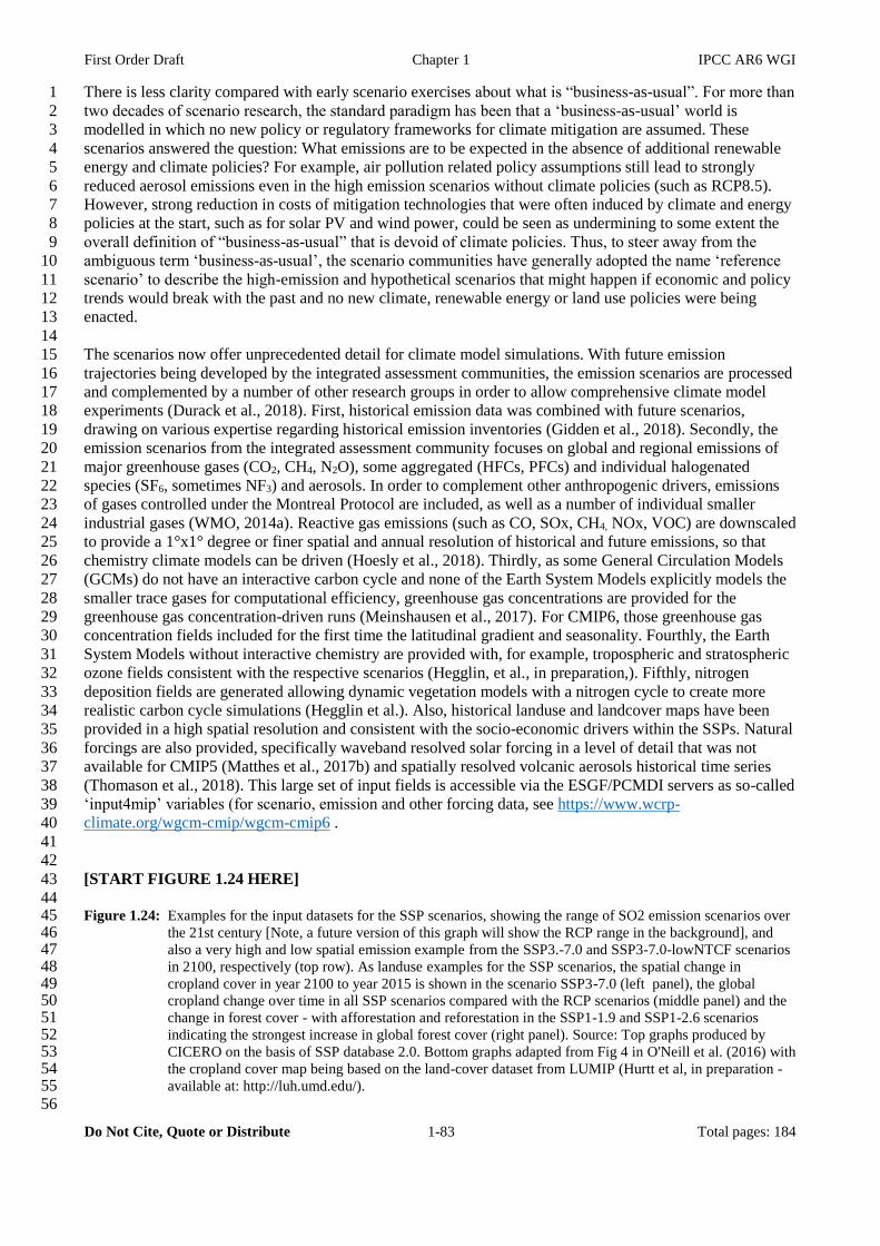
First Order Draft Chapter 1 IPCC AR6 WGI
Do Not Cite, Quote or Distribute 1-83 Total pages: 184
There is less clarity compared with early scenario exercises about what is “business-as-usual”. For more than 1
two decades of scenario research, the standard paradigm has been that a ‘business-as-usual’ world is 2
modelled in which no new policy or regulatory frameworks for climate mitigation are assumed. These 3
scenarios answered the question: What emissions are to be expected in the absence of additional renewable 4
energy and climate policies? For example, air pollution related policy assumptions still lead to strongly 5
reduced aerosol emissions even in the high emission scenarios without climate policies (such as RCP8.5). 6
However, strong reduction in costs of mitigation technologies that were often induced by climate and energy 7
policies at the start, such as for solar PV and wind power, could be seen as undermining to some extent the 8
overall definition of “business-as-usual” that is devoid of climate policies. Thus, to steer away from the 9
ambiguous term ‘business-as-usual’, the scenario communities have generally adopted the name ‘reference 10
scenario’ to describe the high-emission and hypothetical scenarios that might happen if economic and policy 11
trends would break with the past and no new climate, renewable energy or land use policies were being 12
enacted. 13
14
The scenarios now offer unprecedented detail for climate model simulations. With future emission 15
trajectories being developed by the integrated assessment communities, the emission scenarios are processed 16
and complemented by a number of other research groups in order to allow comprehensive climate model 17
experiments (Durack et al., 2018). First, historical emission data was combined with future scenarios, 18
drawing on various expertise regarding historical emission inventories (Gidden et al., 2018). Secondly, the 19
emission scenarios from the integrated assessment community focuses on global and regional emissions of 20
major greenhouse gases (CO2, CH4, N2O), some aggregated (HFCs, PFCs) and individual halogenated 21
species (SF6, sometimes NF3) and aerosols. In order to complement other anthropogenic drivers, emissions 22
of gases controlled under the Montreal Protocol are included, as well as a number of individual smaller 23
industrial gases (WMO, 2014a). Reactive gas emissions (such as CO, SOx, CH4, NOx, VOC) are downscaled 24
to provide a 1°x1° degree or finer spatial and annual resolution of historical and future emissions, so that 25
chemistry climate models can be driven (Hoesly et al., 2018). Thirdly, as some General Circulation Models 26
(GCMs) do not have an interactive carbon cycle and none of the Earth System Models explicitly models the 27
smaller trace gases for computational efficiency, greenhouse gas concentrations are provided for the 28
greenhouse gas concentration-driven runs (Meinshausen et al., 2017). For CMIP6, those greenhouse gas 29
concentration fields included for the first time the latitudinal gradient and seasonality. Fourthly, the Earth 30
System Models without interactive chemistry are provided with, for example, tropospheric and stratospheric 31
ozone fields consistent with the respective scenarios (Hegglin, et al., in preparation,). Fifthly, nitrogen 32
deposition fields are generated allowing dynamic vegetation models with a nitrogen cycle to create more 33
realistic carbon cycle simulations (Hegglin et al.). Also, historical landuse and landcover maps have been 34
provided in a high spatial resolution and consistent with the socio-economic drivers within the SSPs. Natural 35
forcings are also provided, specifically waveband resolved solar forcing in a level of detail that was not 36
available for CMIP5 (Matthes et al., 2017b) and spatially resolved volcanic aerosols historical time series 37
(Thomason et al., 2018). This large set of input fields is accessible via the ESGF/PCMDI servers as so-called 38
‘input4mip’ variables (for scenario, emission and other forcing data, see https://www.wcrp-39
climate.org/wgcm-cmip/wgcm-cmip6 . 40
41
42
[START FIGURE 1.24 HERE] 43
44 Figure 1.24: Examples for the input datasets for the SSP scenarios, showing the range of SO2 emission scenarios over 45
the 21st century [Note, a future version of this graph will show the RCP range in the background], and 46 also a very high and low spatial emission example from the SSP3.-7.0 and SSP3-7.0-lowNTCF scenarios 47 in 2100, respectively (top row). As landuse examples for the SSP scenarios, the spatial change in 48 cropland cover in year 2100 to year 2015 is shown in the scenario SSP3-7.0 (left panel), the global 49 cropland change over time in all SSP scenarios compared with the RCP scenarios (middle panel) and the 50 change in forest cover - with afforestation and reforestation in the SSP1-1.9 and SSP1-2.6 scenarios 51 indicating the strongest increase in global forest cover (right panel). Source: Top graphs produced by 52 CICERO on the basis of SSP database 2.0. Bottom graphs adapted from Fig 4 in O'Neill et al. (2016) with 53 the cropland cover map being based on the land-cover dataset from LUMIP (Hurtt et al, in preparation - 54 available at: http://luh.umd.edu/). 55
56

First Order Draft Chapter 1 IPCC AR6 WGI
Do Not Cite, Quote or Distribute 1-84 Total pages: 184
[END FIGURE 1.24 HERE] 1
2
3
The SSP scenarios are emission and concentration scenarios, not forcing scenarios. It is worth noting that 4
although this detailed scenario information is often described as forcing scenarios or elements thereof, the 5
input information on anthropogenic forcers to Earth System Models only comes in the form of emissions and 6
concentrations (i.e. dry mol fractions for greenhouse gases or mass and size distributions for aerosols), and 7
landuse/landcover maps, not to actual forcing data. The radiative forcing labels of the RCP and SSP 8
scenarios, such as “2.6” in RCP2.6, are approximate nameplate labels. The actual global mean effective 9
forcing will be different from Earth System Model to Earth System Model due to different radiative forcing 10
schemes, uncertainties in aerosol-cloud interactions and different fast feedback mechanisms, among other 11
reasons. The advantage of using approximate radiative forcing labels however is that a clear ranking between 12
the scenarios can be established and that multiple climate driving forcers that are at play in those scenarios 13
can be summarized into one number. The classification in this report according to cumulative carbon 14
emissions (see Section 1.6.4) and temperature levels (Section 1.6.3 and Cross-Chapter Box 1.5 on emulators) 15
complements those forcing labels. 16
17
18
[START FIGURE 1.25 HERE] 19
20 Figure 1.25: An illustrative comparison of the relative importance of greenhouse gas concentrations for projected 21
climate change. The blue shaded area indicates the approximate forcing exerted by CO2 in three of the 22 SSP scenarios, SSP1-1.9, SSP1-2.6 and SSP3-7.0. The CO2 concentrations under the SSP1-1.9 scenarios 23 approximately reach 350 ppm after 2150, those of SSP1-2.6 around 400 ppm and the SSP3-7.0 as one of 24 the higher scenarios will reach levels of nearly 1500 ppm CO2 in the longer term until 2300. Also shown 25 are the effects of reducing short-lived climate forcers in the SSP3-7.0 scenario at the example of methane 26 (panel c, black arrows in the top right), when comparing the SSP3-7.0 scenarios with the AerChemMIP 27 variant SSP3-7.0-lowNTCF [To be updated] 28
29
[END FIGURE 1.25 HERE] 30 31 32
1.6.2.2 Scenarios in the context of the Paris Agreement 33
34
The long-term goal of the Paris Agreement is “to is to keep the increase in global average temperature to 35
well below 2 °C above pre-industrial levels; and to limit the increase to 1.5 °C”. Furthermore, the 1.5°C 36
target emerged as part of the Paris Agreement, for example due to the expected climate impacts and implied 37
sea level rise of 2°C warming (e.g. Levermann et al., 2013). Therefore a range of SSP marker scenarios as 38
well as the larger AR6 scenario database are examined according to the degree the individual scenarios are in 39
line with the Paris Agreement targets. Specifically, following from the IPCC SR1.5 classification of 40
emission scenarios in various categories by both the likelihood to stay below certain temperature levels, as 41
well as – in the case of 1.5°C – their respective implications for no overshoot or a low or higher initial 42
overshoot. 43
44
The current emissions targets under the Paris Agreement reach until 2030. This report is using the existing 45
literature of the aggregate emission levels under the nationally determined contributions (NDCs) of the Paris 46
Agreement to put the scenarios investigated in this WGI into context. A much closer look at aggregate NDCs 47
is performed in WGIII, so that here only the aggregate global emission ranges (UNFCCC, 2016) are 48
compared against the scenarios’ 2025 and 2030 emission levels (see also Cross-Chapter Box 1.1 on the 49
global stocktake process) 50
51
[Placeholder for a table with explanatory text to be inserted that provides results of the contextualisation of 52
the AR6 emission scenario database in the light of the Paris agreement] 53
54
55
First Order Draft Chapter 1 IPCC AR6 WGI
Do Not Cite, Quote or Distribute 1-85 Total pages: 184
[START FIGURE 1.26 HERE] 1
2 Figure 1.26: Historical concentrations for the past 2000 years of CO2, CH4 and N2O (Meinshausen et al., 2017), and 3
[draft sketch of] temperature reconstructions joined with scenario information up to year 2300. The 4 temperature proxies over the last 2000 years were compiled by the Pages 2K project (Emile-Geay et al., 5 2017) and also shown are northern hemispheric temperature reconstructions by Mann et al. (1999) (dark 6 blue ranges). Future temperature projections are from the CMIP6 ScenarioMIP experiment, examined in 7 Chapter 4 of this report. The grey vertical band indicates the 21st century. [ Note: this is a draft sketch 8 figure only]. 9
10
[END FIGURE 1.26 HERE] 11
12
13
[START FIGURE 1.27 HERE] 14
15 Figure 1.27: Illustrative synthesis figure on the “decision power/policy-relevance” of scenarios in the context of the 16
Paris Agreement. The ‘decision power’ for this analysis is here defined as the range between reference 17 and various mitigation scenarios that include shared policy assumptions (SPAs), separated by gases and 18 scenario characteristics in relation to their effect (attributable warming) on peak 21st century temperatures 19 [and end of century sea level rise] (y-axis). The individual elements on the x-axis can be: Next decade 20 cumulative CO2 emissions, CH4 emissions, non-methane SLCF, second half of century net negative CO2 21 emissions, and GHG emission levels in 2030 (possibly shown by various metrics, (GWP|GTP, and GWP* 22 in some form)). For example, methane emissions, cumulative CO2 emissions, cumulative GHG emissions 23 (GWP|GTP\GWP* weighted), SLCF emissions and other GHG emissions. [dependent on AR6 scenario 24 database analysis]. 25
26
[END FIGURE 1.27 HERE] 27
28
29
1.6.3 Temperature levels as additional tool for cross-Working Group integration 30
31
This section provides the methodological underpinning for an additional ‘dimension of integration’ along 32
global-mean temperature bands. 33
34
As the IPCC SR1.5 concluded, every half a degree or even smaller fractions of a degree of warming matter 35
in terms of climate impacts (see IPCC SR1.5; Schleussner et al., 2016 - see also Chapter 11). Following 36
these SR1.5 results, this report adopts the half-degree temperature bands, starting from a pre-industrial 37
reference point (see Section 1.5.3), across which climate projections, impacts, adaptation challenges and 38
mitigation challenges can be integrated within and across the three WGs. Specifically, the categorisation is 39
performed in half-degree steps with 1.5°C, 2.0°C, 3.0°C, 4.0°C as the central points the higher importance 40
‘Tier 1’ levels, with additional half-degree categories around 2.5°C, 3.5°C up to a level around 6.0°C (see 41
Table 1.5) [This will depend on CMIP6 results]. 42
43
The average global temperature during the early-industrial period (1850-1900) is approximately equivalent 44
to pre-industrial temperature, and so can be used as a baseline to assess issues associated with warming 45
levels. However, it is also likely (medium confidence) that there was some anthropogenic warming which 46
occurred between pre-industrial and early-industrial periods, which was at least partially offset by volcanic 47
activity during the early-industrial period. The magnitude of this warming is plausibly 0.0-0.1C which is 48
pertinent for assessments involving remaining carbon budgets consistent with the Paris Agreement and 49
earlier policy targets that refer to pre-industrial temperature levels (see 1.5.3.2). 50
51
52
[START TABLE 1.5 HERE] 53
54 Table 1.5: Description of the Tier 1 and Tier 2 global mean-surface air temperature relative to pre-industrial levels. 55
56
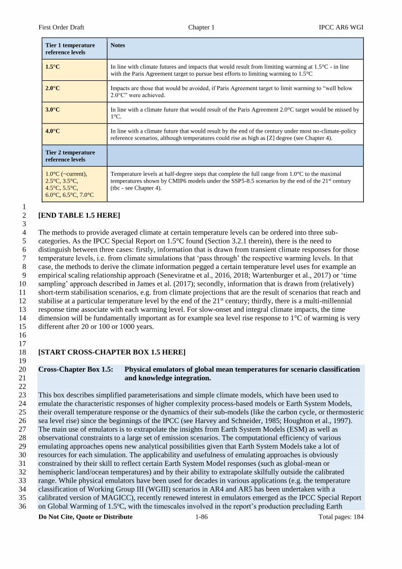
First Order Draft Chapter 1 IPCC AR6 WGI
Do Not Cite, Quote or Distribute 1-86 Total pages: 184
Tier 1 temperature
reference levels
Notes
1.5°C In line with climate futures and impacts that would result from limiting warming at 1.5°C - in line
with the Paris Agreement target to pursue best efforts to limiting warming to 1.5°C
2.0°C Impacts are those that would be avoided, if Paris Agreement target to limit warming to “well below
2.0°C” were achieved.
3.0°C In line with a climate future that would result of the Paris Agreement 2.0°C target would be missed by
1°C.
4.0°C In line with a climate future that would result by the end of the century under most no-climate-policy
reference scenarios, although temperatures could rise as high as [Z] degree (see Chapter 4).
Tier 2 temperature
reference levels
1.0°C (~current),
2.5°C, 3.5°C,
4.5°C, 5.5°C,
6.0°C, 6.5°C, 7.0°C
Temperature levels at half-degree steps that complete the full range from 1.0°C to the maximal
temperatures shown by CMIP6 models under the SSP5-8.5 scenarios by the end of the 21st century
(tbc - see Chapter 4).
1
[END TABLE 1.5 HERE] 2
3
The methods to provide averaged climate at certain temperature levels can be ordered into three sub-4
categories. As the IPCC Special Report on 1.5°C found (Section 3.2.1 therein), there is the need to 5
distinguish between three cases: firstly, information that is drawn from transient climate responses for those 6
temperature levels, i.e. from climate simulations that ‘pass through’ the respective warming levels. In that 7
case, the methods to derive the climate information pegged a certain temperature level uses for example an 8
empirical scaling relationship approach (Seneviratne et al., 2016, 2018; Wartenburger et al., 2017) or ‘time 9
sampling’ approach described in James et al. (2017); secondly, information that is drawn from (relatively) 10
short-term stabilisation scenarios, e.g. from climate projections that are the result of scenarios that reach and 11
stabilise at a particular temperature level by the end of the 21st century; thirdly, there is a multi-millennial 12
response time associate with each warming level. For slow-onset and integral climate impacts, the time 13
dimension will be fundamentally important as for example sea level rise response to 1°C of warming is very 14
different after 20 or 100 or 1000 years. 15
16
17
[START CROSS-CHAPTER BOX 1.5 HERE] 18
19
Cross-Chapter Box 1.5: Physical emulators of global mean temperatures for scenario classification 20
and knowledge integration. 21
22
This box describes simplified parameterisations and simple climate models, which have been used to 23
emulate the characteristic responses of higher complexity process-based models or Earth System Models, 24
their overall temperature response or the dynamics of their sub-models (like the carbon cycle, or thermosteric 25
sea level rise) since the beginnings of the IPCC (see Harvey and Schneider, 1985; Houghton et al., 1997). 26
The main use of emulators is to extrapolate the insights from Earth System Models (ESM) as well as 27
observational constraints to a large set of emission scenarios. The computational efficiency of various 28
emulating approaches opens new analytical possibilities given that Earth System Models take a lot of 29
resources for each simulation. The applicability and usefulness of emulating approaches is obviously 30
constrained by their skill to reflect certain Earth System Model responses (such as global-mean or 31
hemispheric land/ocean temperatures) and by their ability to extrapolate skilfully outside the calibrated 32
range. While physical emulators have been used for decades in various applications (e.g. the temperature 33
classification of Working Group III (WGIII) scenarios in AR4 and AR5 has been undertaken with a 34
calibrated version of MAGICC), recently renewed interest in emulators emerged as the IPCC Special Report 35
on Global Warming of 1.5oC, with the timescales involved in the report’s production precluding Earth 36
First Order Draft Chapter 1 IPCC AR6 WGI
Do Not Cite, Quote or Distribute 1-87 Total pages: 184
system models running multiple future scenarios in time to for assessment therein. 1
2
The term emulators is different from the term simple climate models. Simple climate models can be used as 3
emulators of ESM models, but such emulation can also be performed with very simple parameterisations 4
(‘one-or-few-line-climate-models’), statistical methods like neural networks, genetic algorithms or other 5
Artificial Intelligence approaches. The term simple climate models (SCMs) generally refers to a broad class 6
of lower dimensional models of the energy balance, radiative transfer, carbon cycle, or a combination of 7
such physical components. SCMs are however also suitable for performing emulations of climate-mean 8
variables of ESMs given that their structural flexibility can capture both the parametric and structural 9
uncertainties across Earth System Model responses. The advantage of SCMs compared to simpler or 10
statistical approaches is that their rudimentary physical process parameterisations provide additional reason 11
to trust moderate extrapolations from the response space that is covered by Earth System Models. Simple 12
climate models do not have to be run in ‘emulation’ mode, though, as they can also be used to test 13
consistency across multiple lines of evidence with regard to climate sensitivity ranges, transient climate 14
responses (TCR), transient climate response to cumulative emissions (TCRE) and carbon cycle feedbacks 15
(see Chapters 5, 7). 16
17
Current emulators can be classified into many different categories, depending on their comprehensiveness 18
(i.e. whether they emulate glacier responses or the whole Earth System with permafrost, sea level rise and a 19
large set of gas cycles), or their ocean heat uptake parameterisations, which strongly affect the long-term 20
climate responses (i.e. a simple diffusive ocean or an upwelling, diffusive entrainment parameterisation), 21
and/or their overall model complexity (single line impulse response functions or compact Earth System 22
models), but also according to their parameterisation and model structure. We here provide an approximate 23
categorisation of the literature according to model complexity. Impulse response function characterisations 24
of the Earth’s temperature response and climate models with a small set of equations (e.g. DICE, AR5-IR) 25
are in the first category. The more comprehensive simple climate models that do not have a purely diffusive 26
ocean (e.g. MAGICC, BernSCM, Hector) or impulse response representations that come with a sophisticated 27
representation of one or more Earth System elements (e.g. OSCAR) are in the second category. The third 28
category comprises statistical approaches, ranging from neural networks to more recent AI approaches, 29
which are particularly well suited to emulate variability - a capacity that is outside the standard design 30
ambitions for simple climate models. However, the literature overview below is particularly focussed on 31
those models that attempt to emulate global mean temperatures (among other things), acknowledging that the 32
literature on emulators for specific climate system domains is much wider. 33

First Order Draft Chapter 1 IPCC AR6 WGI
Do Not Cite, Quote or Distribute 1-88 Total pages: 184
[START CROSS-CHAPTER BOX 1.5, TABLE 1 HERE] 1
2 Cross-Chapter Box 1.5, Table 1: categorisation of different approaches that can be used to emulated global-mean 3
temperatures of Earth System Models. 4 5 6
Emulator Type4 Examples in the literature Notes on general use in literature / in AR6
The impulse response
and diffusive ocean
SCMs
● AR5-IR (Supplementary
Material 8.SM.11 of Myhre et
al. (2013))
● “Two-layer EBM” (Geoffroy et
al., 2013)
● Bern-SAR (IPCC SAR); Bern-
TAR (IPCC TAR)
● “5-equation IR” (Jenkins et al.,
2019)
● FaIR (Smith et al., 2018)
● DICE (Knutti et al., 2003);
Often used for emission metric calculations with
simplified impulse response (IR) equations for
concentrations and temperatures. See for example
Supplementary Material 8.SM.11 in the Fifth
Assessment Report. The more encompassing of the
impulse response models are also used for multi-gas
assessments and ESM emulations.
[AR6 usage tbc]
Comprehensive SCMs
“upwelling, diffusion,
entrainment” or
“compact Earth System
Models”
● UDE-EBM (Schlesinger et al.,
1990)
● ACC2 (Tanaka et al., 2007)
● BernSCM (Strassmann and
Joos, 2018)
● Hector (Hartin et al., 2015),
● HILDA (SIEGENTHALER and
JOOS, 1992)
● MAGICC. Version 5.3 (Raper
et al., 2001; Wigley et al.,
2009), Version 6.0
(Meinshausen et al., 2011c;
Wigley et al., 2009) and
● OSCAR 2.2 (Gasser et al.,
2017)
Several simple climate models have been used in the
past under a wide range of applications ranging from
metric calculations, scenario classification in WGIII,
probabilistic assessments with historical constraints,
uncertainty integration across various domains and sea
level rise projections. Also used to project GHG
concentrations from emission scenarios.
[AR6 usage tbc]
Statistical approaches Neural networks (Knutti et al., 2003)
[to be completed.]
Various applications to analyse, emulate and
probabilistically investigate the behaviour of more
complex models.
[AR6 usage tbc]
7
[END CROSS-CHAPTER 1.5, TABLE 1 HERE] 8
9
An intercomparison of emulators investigates limitations and skills of emulators, which often depend on 10
their complexity. Simple climate models can provide good approximations of the hemispheric-scale and 11
land/ocean scale of surface air temperatures, sea level rise contributions, and global carbon cycle responses, 12
but come with a number of potential limitations. As one example, at the time of the IPCC AR5, very simple 13
climate models were used in historical constraining studies that suggested rather low climate sensitivities 14
(such as a median of 1.9K) to be in line with the observational records (e.g. Otto et al., 2013). Subsequent 15
publications discussed to what degree simplified model structures could be responsible for those particular 16
results, given that resolving the global-mean responses of heterogeneous radiative forcers such as aerosols 17
might be difficult in global-mean models (Shindell, 2014), and effectively time-variable or state-dependent 18
climate sensitivities as shown from Earth System models (Houghton et al., 1997; Meinshausen et al., 2011a) 19
were not included in some of the studies that suggested lower climate sensitivities on the basis of 20
observational constraints. Some studies suggest, for example, that including the effect of time-changing 21
temperature patterns on effective or inferred climate sensitivity increases the observationally constrained 22
values from a best estimate of 1.9K to 3.2K (Andrews et al., 2018) (see Chapter 7). Also, the divergence of 23
4 categorisation following Schwarber et al. 2019 [10.5194/esd-2018-63])
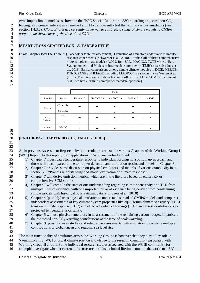
First Order Draft Chapter 1 IPCC AR6 WGI
Do Not Cite, Quote or Distribute 1-89 Total pages: 184
two simple climate models as shown in the IPCC Special Report on 1.5°C regarding projected non-CO2 1
forcing, also created interest in a renewed effort to transparently test the skill of various emulators (see 2
section 1.4.3.2). [Note: Efforts are currently underway to calibrate a range of simple models to CMIP6 3
output to be shown here by the time of the SOD]. 4 5 6 [START CROSS-CHAPTER BOX 1.5, TABLE 2 HERE] 7
8 Cross-Chapter Box 1.5, Table 2: [Placeholder table for assessment]. Evaluation of emulators under various impulse 9
response experiments (Schwarber et al., 2018). For the skill of three comprehensive 10 4-box simple climate models (ACC2, BernSAR, MAGICC, TOTEM) with Earth 11 System models and Models of intermediate complexity (EMICs), see also Joos et 12 al., 2013). Earlier comparisons among simple climate modules in DICE, MERGE, 13 FUND, PAGE and IMAGE, including MAGICC4 are shown in van Vuuren et al. 14 (2011) [The intention is to show test and skill results of OpenSCM by the time of 15 SOD, see https://github.com/openclimatedata/openscm]. 16
17
18 19
[END CROSS-CHAPTER BOX 1.5, TABLE 2 HERE] 20
21
22
As in previous Assessment Reports, physical emulators are used in various Chapters of the Working Group I 23
(WGI) Report. In this report, their applications in WGI are centred around: 24
1) Chapter 7 investigates temperature response to individual forgings in a bottom up approach and 25
those will be compared to the top-down detection and attribution results and models in Chapter 3. 26
2) Chapter 7 provides some discussion on physical emulators and models of various complexity in its 27
section 7.6 “Process understanding and model evaluation of climate response”. 28
3) Chapter 7 will derive emission metrics, which are in the literature based on either IRF or 29
comprehensive SCM studies. 30
4) Chapter 7 will compile the state of our understanding regarding climate sensitivity and TCR from 31
multiple lines of evidence, with one important pillar of evidence being derived from constraining 32
simple models with historical observational data (e.g. Skeie et al., 2018) 33
5) Chapter 4 [possibly] uses physical emulators to understand spread of CMIP6 models and compare to 34
independent assessments of key climate system properties like equilibrium climate sensitivity (ECS), 35
transient climate response (TCR) and effective radiative forcings (ERF) and assess contributions to 36
projected temperature uncertainty. 37
6) Chapter 5 will use physical emulators in its assessment of the remaining carbon budget, in particular 38
the estimated non-CO2 warming contributions at the time of peak warming. 39
7) Chapter 9 [possibly] uses studies and integrative assessments with emulators to combine multiple 40
contributions to global-mean and regional sea level rise. 41
42
The main functionality of emulators across the Working Groups is however that they play a key role in 43
‘communicating’ WGI physical climate science knowledge to the research community associated with 44
Working Group II and III. Some individual research studies associated with the WGIII community for 45
example investigate whether current infrastructure until its technical lifetime commits the world to 1.5°C 46
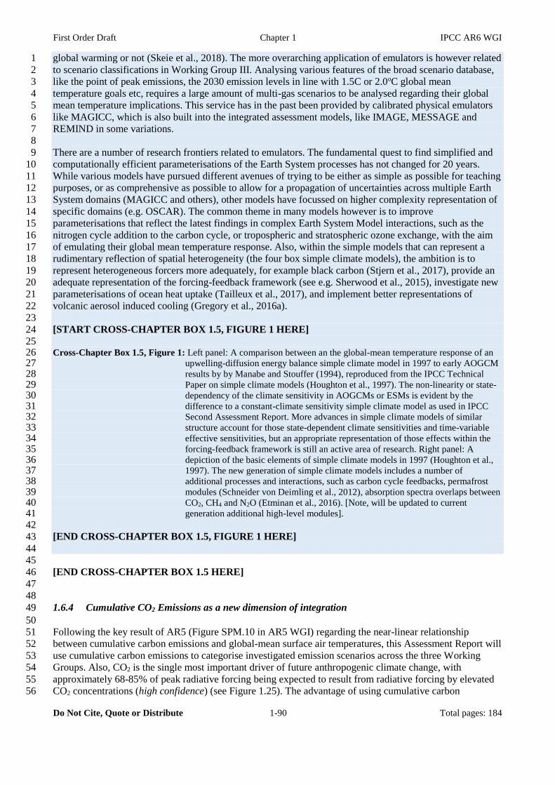
First Order Draft Chapter 1 IPCC AR6 WGI
Do Not Cite, Quote or Distribute 1-90 Total pages: 184
global warming or not (Skeie et al., 2018). The more overarching application of emulators is however related 1
to scenario classifications in Working Group III. Analysing various features of the broad scenario database, 2
like the point of peak emissions, the 2030 emission levels in line with 1.5C or 2.0oC global mean 3
temperature goals etc, requires a large amount of multi-gas scenarios to be analysed regarding their global 4
mean temperature implications. This service has in the past been provided by calibrated physical emulators 5
like MAGICC, which is also built into the integrated assessment models, like IMAGE, MESSAGE and 6
REMIND in some variations. 7
8
There are a number of research frontiers related to emulators. The fundamental quest to find simplified and 9
computationally efficient parameterisations of the Earth System processes has not changed for 20 years. 10
While various models have pursued different avenues of trying to be either as simple as possible for teaching 11
purposes, or as comprehensive as possible to allow for a propagation of uncertainties across multiple Earth 12
System domains (MAGICC and others), other models have focussed on higher complexity representation of 13
specific domains (e.g. OSCAR). The common theme in many models however is to improve 14
parameterisations that reflect the latest findings in complex Earth System Model interactions, such as the 15
nitrogen cycle addition to the carbon cycle, or tropospheric and stratospheric ozone exchange, with the aim 16
of emulating their global mean temperature response. Also, within the simple models that can represent a 17
rudimentary reflection of spatial heterogeneity (the four box simple climate models), the ambition is to 18
represent heterogeneous forcers more adequately, for example black carbon (Stjern et al., 2017), provide an 19
adequate representation of the forcing-feedback framework (see e.g. Sherwood et al., 2015), investigate new 20
parameterisations of ocean heat uptake (Tailleux et al., 2017), and implement better representations of 21
volcanic aerosol induced cooling (Gregory et al., 2016a). 22
23
[START CROSS-CHAPTER BOX 1.5, FIGURE 1 HERE] 24
25 Cross-Chapter Box 1.5, Figure 1: Left panel: A comparison between an the global-mean temperature response of an 26
upwelling-diffusion energy balance simple climate model in 1997 to early AOGCM 27 results by by Manabe and Stouffer (1994), reproduced from the IPCC Technical 28 Paper on simple climate models (Houghton et al., 1997). The non-linearity or state-29 dependency of the climate sensitivity in AOGCMs or ESMs is evident by the 30 difference to a constant-climate sensitivity simple climate model as used in IPCC 31 Second Assessment Report. More advances in simple climate models of similar 32 structure account for those state-dependent climate sensitivities and time-variable 33 effective sensitivities, but an appropriate representation of those effects within the 34 forcing-feedback framework is still an active area of research. Right panel: A 35 depiction of the basic elements of simple climate models in 1997 (Houghton et al., 36 1997). The new generation of simple climate models includes a number of 37 additional processes and interactions, such as carbon cycle feedbacks, permafrost 38 modules (Schneider von Deimling et al., 2012), absorption spectra overlaps between 39 CO2, CH4 and N2O (Etminan et al., 2016). [Note, will be updated to current 40 generation additional high-level modules]. 41
42
[END CROSS-CHAPTER BOX 1.5, FIGURE 1 HERE] 43
44
45
[END CROSS-CHAPTER BOX 1.5 HERE] 46
47
48
1.6.4 Cumulative CO2 Emissions as a new dimension of integration 49
50
Following the key result of AR5 (Figure SPM.10 in AR5 WGI) regarding the near-linear relationship 51
between cumulative carbon emissions and global-mean surface air temperatures, this Assessment Report will 52
use cumulative carbon emissions to categorise investigated emission scenarios across the three Working 53
Groups. Also, CO2 is the single most important driver of future anthropogenic climate change, with 54
approximately 68-85% of peak radiative forcing being expected to result from radiative forcing by elevated 55
CO2 concentrations (high confidence) (see Figure 1.25). The advantage of using cumulative carbon 56
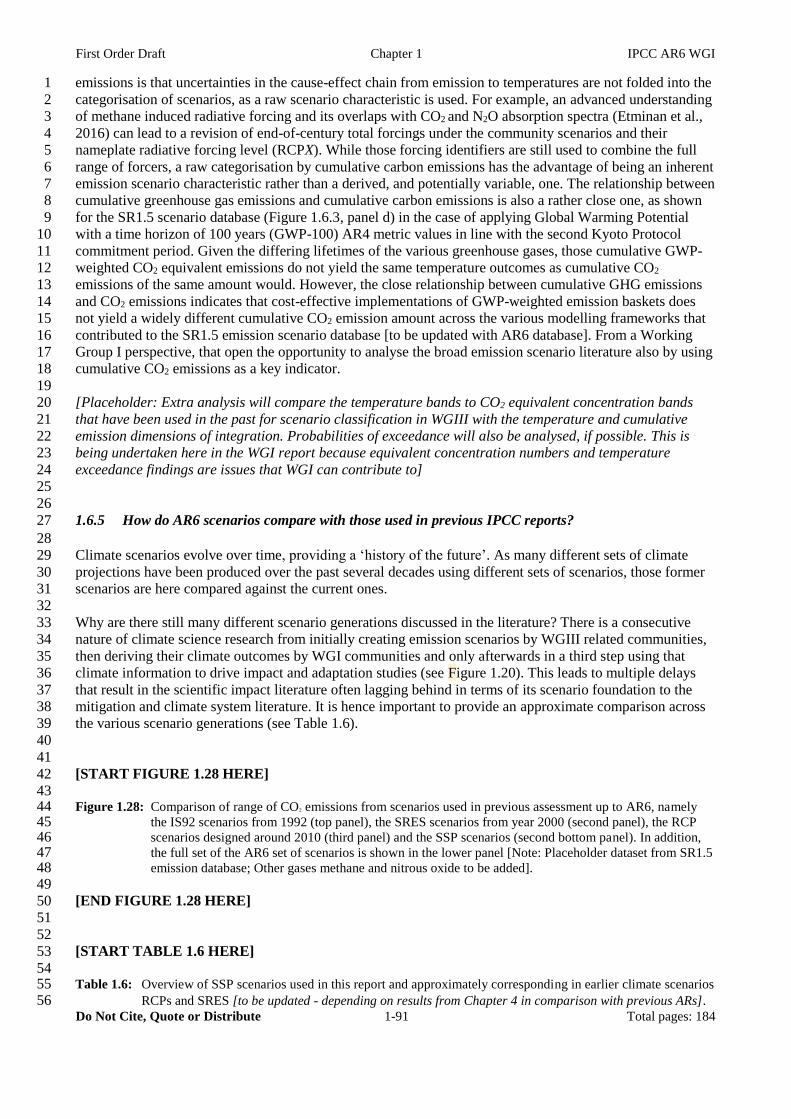
First Order Draft Chapter 1 IPCC AR6 WGI
Do Not Cite, Quote or Distribute 1-91 Total pages: 184
emissions is that uncertainties in the cause-effect chain from emission to temperatures are not folded into the 1
categorisation of scenarios, as a raw scenario characteristic is used. For example, an advanced understanding 2
of methane induced radiative forcing and its overlaps with CO2 and N2O absorption spectra (Etminan et al., 3
2016) can lead to a revision of end-of-century total forcings under the community scenarios and their 4
nameplate radiative forcing level (RCPX). While those forcing identifiers are still used to combine the full 5
range of forcers, a raw categorisation by cumulative carbon emissions has the advantage of being an inherent 6
emission scenario characteristic rather than a derived, and potentially variable, one. The relationship between 7
cumulative greenhouse gas emissions and cumulative carbon emissions is also a rather close one, as shown 8
for the SR1.5 scenario database (Figure 1.6.3, panel d) in the case of applying Global Warming Potential 9
with a time horizon of 100 years (GWP-100) AR4 metric values in line with the second Kyoto Protocol 10
commitment period. Given the differing lifetimes of the various greenhouse gases, those cumulative GWP-11
weighted CO2 equivalent emissions do not yield the same temperature outcomes as cumulative CO2 12
emissions of the same amount would. However, the close relationship between cumulative GHG emissions 13
and CO2 emissions indicates that cost-effective implementations of GWP-weighted emission baskets does 14
not yield a widely different cumulative CO2 emission amount across the various modelling frameworks that 15
contributed to the SR1.5 emission scenario database [to be updated with AR6 database]. From a Working 16
Group I perspective, that open the opportunity to analyse the broad emission scenario literature also by using 17
cumulative CO2 emissions as a key indicator. 18
19
[Placeholder: Extra analysis will compare the temperature bands to CO2 equivalent concentration bands 20
that have been used in the past for scenario classification in WGIII with the temperature and cumulative 21
emission dimensions of integration. Probabilities of exceedance will also be analysed, if possible. This is 22
being undertaken here in the WGI report because equivalent concentration numbers and temperature 23
exceedance findings are issues that WGI can contribute to] 24
25
26
1.6.5 How do AR6 scenarios compare with those used in previous IPCC reports? 27
28
Climate scenarios evolve over time, providing a ‘history of the future’. As many different sets of climate 29
projections have been produced over the past several decades using different sets of scenarios, those former 30
scenarios are here compared against the current ones. 31
32
Why are there still many different scenario generations discussed in the literature? There is a consecutive 33
nature of climate science research from initially creating emission scenarios by WGIII related communities, 34
then deriving their climate outcomes by WGI communities and only afterwards in a third step using that 35
climate information to drive impact and adaptation studies (see Figure 1.20). This leads to multiple delays 36
that result in the scientific impact literature often lagging behind in terms of its scenario foundation to the 37
mitigation and climate system literature. It is hence important to provide an approximate comparison across 38
the various scenario generations (see Table 1.6). 39
40
41
[START FIGURE 1.28 HERE] 42
43 Figure 1.28: Comparison of range of CO2 emissions from scenarios used in previous assessment up to AR6, namely 44
the IS92 scenarios from 1992 (top panel), the SRES scenarios from year 2000 (second panel), the RCP 45 scenarios designed around 2010 (third panel) and the SSP scenarios (second bottom panel). In addition, 46 the full set of the AR6 set of scenarios is shown in the lower panel [Note: Placeholder dataset from SR1.5 47 emission database; Other gases methane and nitrous oxide to be added]. 48
49
[END FIGURE 1.28 HERE] 50
51
52
[START TABLE 1.6 HERE] 53
54 Table 1.6: Overview of SSP scenarios used in this report and approximately corresponding in earlier climate scenarios 55
RCPs and SRES [to be updated - depending on results from Chapter 4 in comparison with previous ARs]. 56
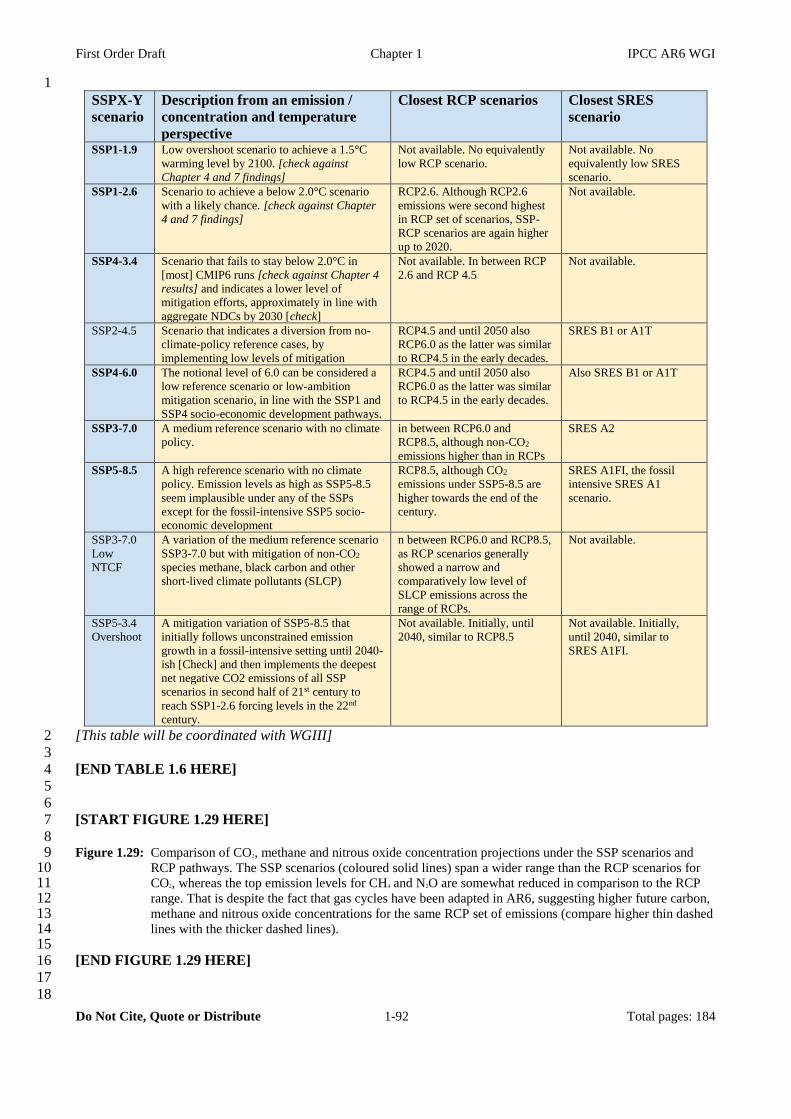
First Order Draft Chapter 1 IPCC AR6 WGI
Do Not Cite, Quote or Distribute 1-92 Total pages: 184
1
SSPX-Y
scenario
Description from an emission /
concentration and temperature
perspective
Closest RCP scenarios Closest SRES
scenario
SSP1-1.9 Low overshoot scenario to achieve a 1.5°C
warming level by 2100. [check against
Chapter 4 and 7 findings]
Not available. No equivalently
low RCP scenario.
Not available. No
equivalently low SRES
scenario.
SSP1-2.6 Scenario to achieve a below 2.0°C scenario
with a likely chance. [check against Chapter
4 and 7 findings]
RCP2.6. Although RCP2.6
emissions were second highest
in RCP set of scenarios, SSP-
RCP scenarios are again higher
up to 2020.
Not available.
SSP4-3.4 Scenario that fails to stay below 2.0°C in
[most] CMIP6 runs [check against Chapter 4
results] and indicates a lower level of
mitigation efforts, approximately in line with
aggregate NDCs by 2030 [check]
Not available. In between RCP
2.6 and RCP 4.5
Not available.
SSP2-4.5 Scenario that indicates a diversion from no-
climate-policy reference cases, by
implementing low levels of mitigation
RCP4.5 and until 2050 also
RCP6.0 as the latter was similar
to RCP4.5 in the early decades.
SRES B1 or A1T
SSP4-6.0 The notional level of 6.0 can be considered a
low reference scenario or low-ambition
mitigation scenario, in line with the SSP1 and
SSP4 socio-economic development pathways.
RCP4.5 and until 2050 also
RCP6.0 as the latter was similar
to RCP4.5 in the early decades.
Also SRES B1 or A1T
SSP3-7.0 A medium reference scenario with no climate
policy.
in between RCP6.0 and
RCP8.5, although non-CO2
emissions higher than in RCPs
SRES A2
SSP5-8.5 A high reference scenario with no climate
policy. Emission levels as high as SSP5-8.5
seem implausible under any of the SSPs
except for the fossil-intensive SSP5 socio-
economic development
RCP8.5, although CO2
emissions under SSP5-8.5 are
higher towards the end of the
century.
SRES A1FI, the fossil
intensive SRES A1
scenario.
SSP3-7.0
Low
NTCF
A variation of the medium reference scenario
SSP3-7.0 but with mitigation of non-CO2
species methane, black carbon and other
short-lived climate pollutants (SLCP)
n between RCP6.0 and RCP8.5,
as RCP scenarios generally
showed a narrow and
comparatively low level of
SLCP emissions across the
range of RCPs.
Not available.
SSP5-3.4
Overshoot
A mitigation variation of SSP5-8.5 that
initially follows unconstrained emission
growth in a fossil-intensive setting until 2040-
ish [Check] and then implements the deepest
net negative CO2 emissions of all SSP
scenarios in second half of 21st century to
reach SSP1-2.6 forcing levels in the 22nd
century.
Not available. Initially, until
2040, similar to RCP8.5
Not available. Initially,
until 2040, similar to
SRES A1FI.
[This table will be coordinated with WGIII] 2
3
[END TABLE 1.6 HERE] 4
5
6
[START FIGURE 1.29 HERE] 7
8 Figure 1.29: Comparison of CO2, methane and nitrous oxide concentration projections under the SSP scenarios and 9
RCP pathways. The SSP scenarios (coloured solid lines) span a wider range than the RCP scenarios for 10 CO2, whereas the top emission levels for CH4 and N2O are somewhat reduced in comparison to the RCP 11 range. That is despite the fact that gas cycles have been adapted in AR6, suggesting higher future carbon, 12 methane and nitrous oxide concentrations for the same RCP set of emissions (compare higher thin dashed 13 lines with the thicker dashed lines). 14
15 [END FIGURE 1.29 HERE] 16
17
18

First Order Draft Chapter 1 IPCC AR6 WGI
Do Not Cite, Quote or Distribute 1-93 Total pages: 184
The first prominent set of IPCC emission scenarios were the so-called IS92 scenarios in 1992. Apart from 1
reference scenarios, those IS92 scenarios also included a set of stabilisation scenarios, the so-called S 2
scenarios. Those ‘S’ pathways were designed to lead to CO2 stabilisation levels of 350ppm, 450ppm etc. By 3
1996, those latter stabilisation levels were complemented in the scientific literature by alternative trajectories 4
that assumed a delayed onset of mitigation action (Figure 1. In IPCC 1995 and see also Wigley et al., 1996). 5
By 2000, the IPCC Special Report produced the so-called SRES scenarios (Nakicenovic and Swart, 2000), 6
albeit without mitigation scenarios. The four broad SRES scenario families A1, A2, B1 and B2 were the first 7
scenarios that emphasized socio-economic scenario storylines (see Section 1.2.4.3 on a discussion on the 8
different uses of the term “storyline”). Represented by three scenarios for the high-growth A1 scenario 9
family, those 6 illustrative marker SRES scenarios (A1FI, A1B, A1T, A2, B1, and B2) can still be 10
sometimes found in today’s impact literature. The void of missing mitigation scenarios was filled by a range 11
of community exercises, including the so-called post-SRES scenarios (Swart et al., 2002). The RCP 12
scenarios then broke new ground after the main SRES scenarios did not include any mitigation scenarios by 13
also providing low pathways that implied strong mitigation action, including negative CO2 emissions on a 14
large scale, namely the RCP2.6. As shown in Figure 1.28, the upper side of the scenario range has not 15
substantially shifted. For the SSP scenarios, the higher end of CO2 emissions further increased a bit, although 16
the most significant change is again the addition of a very low mitigation scenario in. Also, the SSP scenario 17
family includes an overshoot scenario SSP5-3.4-OS that initially follows the highest emission scenario 18
before featuring a collapsing decline of emissions and strongly net negative CO2 emissions in the second half 19
of 21st century. An additional aspect of the scenario classes over time is the later peak of global emission for 20
the lower scenarios. To some extent, this is simply a consequence of new scenario families adjusting to the 21
real-world evolution of recent emissions. Those tracked approximately at the two-third quantile or upper half 22
in the case of fossil and industrial CO2 emissions (see Figure 1.28) in the recent decade, making scenarios 23
that assume an early peak of global emissions before 2010 redundant. For another set of emissions, namely 24
aerosol emissions, the SSP scenarios have an advantage over the RCP scenarios, as the latter had a rather 25
uniformly strong reduction across all RCP levels in short-lived pollution species. 26
27
Is a scenario’s consistency with recent emission developments a good indicator in terms of the 28
scenarios’ long-term validity? Over the last decades, a persistent feature how scenarios have been 29
discussed was related to the question whether recent emission trends make certain future scenarios more or 30
less likely. At the onset of SRES scenarios, the public debate was often whether the emission scenarios over-31
dramatize actual world emission developments (e.g. Castles and Henderson, 2003). With the strong emission 32
boom throughout the 2000s, that debate then shifted towards the question of whether the lower future 33
mitigation scenarios are now rendered unfeasible (Pielke et al., 2008; van Vuuren and Riahi, 2008). That 34
debate continued into the 2010s. The RCP set of scenarios happened to not show the same ranking of 35
scenarios according to their 2020 and longer-term emission levels. Specifically, in the period until 2020, the 36
lowest mitigation scenario RCP2.6 was in fact the second highest emission scenario before embarking on a 37
strong global emission decline after 2020. Implicitly, this feature was cautioning against the assumption that 38
a short-term trend predicates a long-term trajectory. With the onset of the consideration of cumulative carbon 39
emissions as a key indicator for future climate change, a nuance has been brought to the debate. That is that 40
delay in the onset of mitigation does not exclude low concentration levels, but it comes at the cost of having 41
to bring about even lower emissions in the future to keep overall cumulative emissions the same. 42
43
Recent emission trends are within the scenario envelope, but seldomly in its middle. Fossil & industrial CO2 44
emissions have historically tracked the lower edge of the IS92 scenarios until the year 2000. In relation to 45
SRES and RCP scenarios, that changed. Historical emissions now approximately tracked the upper half of 46
SRES and RCP projections (Figure 1.28), with only the most recent emission developments indicating slow-47
down of global emission growth [to be updated – cf Chapter 2, 5 and others]. 48
49
There are known limitations of the SSP scenarios and historical datasets. There are some limitations 50
associated with the current set of scenarios. For example, recent decreases in SO2 aerosol emissions since 51
2013 in the East-Asia region (Zheng et al., 2018) are not fully captured in the last years of the historical 52
aerosol emissions that reach until end of 2014. Future SSP scenarios from 2015 onwards however capture 53
that lower evolution of aerosol emissions in that region. Another limitation is that substances controlled 54
under the Montreal Protocol are uniformly reduced following the Kigali Agreement, rather than representing 55
First Order Draft Chapter 1 IPCC AR6 WGI
Do Not Cite, Quote or Distribute 1-94 Total pages: 184
a full range of possible high and lower emission futures, possibly even lower than the Kigali phase-out 1
pathways (UNEP, 2016). While this might have advantages to dissect the potential effect of the Paris 2
Agreement and climate-focussed mitigation action, it might suggest a too narrow band of future temperatures 3
if the research question is to examine the full range of possible geophysical futures in the absence of 4
international agreements. 5
6
[START CROSS-CHAPTER BOX 1.6 HERE] 7 8 Cross-Chapter Box 1.6: Scenarios, Projections, Pathways and temperature-levels 9
10
This Box provides an overview of definitions of key terms regarding the investigation of the broad set of 11
possible future evolutions of human-induced emissions, climate change, and its impacts. It builds on the 12
Synthesis Report of IPCC AR5 and the set of three AR6 Special Reports. A feature in this Assessment 13
Report is the added emphasis on temperature-levels to support consistency and comparability across the 14
three Working Groups and across Assessment Reports. See the respective glossaries in WGI, WGII and 15
WGIII for additional terms and definitions. [Placeholder: to be updated for SOD] 16
17
Climate prediction. A climate prediction or climate forecast is the result of an attempt to produce (starting 18
from a particular state of the climate system) an estimate of the actual evolution of the climate in the future, 19
for example, at seasonal, interannual or decadal time scales. Because the future evolution of the climate 20
system may be highly sensitive to initial conditions, have chaotic elements and are subject to natural 21
variability, such predictions are usually probabilistic in nature. [adapted from WGI AR5] 22
23
Climate projection. A climate projection is the simulated response of the climate system to a scenario of 24
future emission or concentration of greenhouse gases and aerosols, generally derived using climate models. 25
Climate projections are distinguished from climate predictions by their dependence on the 26
emission/concentration/radiative forcing scenario used, which is in turn based on assumptions concerning, 27
for example, future socioeconomic and technological developments that may or may not be realized. 28
[adapted from SR1.5, WGI AR5, SYR AR5] 29
30
Regional Climate Scenarios. A narrative used to describe how the future might unfold for a region (IPCC-31
TGICA et al., 2007). These are often used to guide impact understanding and adaptation efforts. They can 32
include quantitative information based on scaled historical data or derived from GCM-based internally 33
consistent future climates. 34
35
Scenario. A plausible description of how the future may develop based on a coherent and internally 36
consistent set of assumptions about key driving forces (e.g., rate of technological change, prices) and 37
relationships. Note that scenarios are neither predictions nor forecasts, but are used to provide a view of the 38
implications of developments and actions in a ‘what-if’ kind of investigation. In a broader sense, the term 39
‘scenarios’ is often used to encompass ‘pathways’. In the Sixth Assessment Report a minimum set of five 40
scenarios is chosen to assist cross-working group comparisons: the so-called SSP1-1.9, SSP1-2.6, SSP2-4.5, 41
SSP3-7.0 and SSP5-8.5 scenarios that span a wide range of plausible futures from potentially below 1.5°C 42
best-estimate warming to very high warming in excess of 4°C over the course of this century. [adapted from 43
SR1.5, WGI AR5] 44
45
Emissions scenario. A plausible representation of the future development of emissions of substances that 46
are potentially radiatively active (e.g., greenhouse gases, aerosols), plus human-induced land cover changes 47
that can be radiatively active via albedo changes, based on a coherent and internally consistent set of 48
assumptions about driving forces (such as demographic and socioeconomic development, technological 49
change) and their key relationships. [adapted from AR5 WG1 Glossary] 50
51
Concentrations scenario. A plausible representation of the future development of atmospheric 52
concentrations of substances that are potentially radiatively active (e.g., greenhouse gases, aerosols, 53
tropospheric ozone), plus human-induced land cover changes that can be radiatively active via albedo 54
changes, and used as input to a climate model to compute climate projections. [NEW] 55
First Order Draft Chapter 1 IPCC AR6 WGI
Do Not Cite, Quote or Distribute 1-95 Total pages: 184
1
Socioeconomic scenario. A scenario that describes a plausible future in terms of population, gross domestic 2
product, and other socioeconomic factors relevant to understanding the implications of climate change. 3
[WGIII AR5] 4
5
Scenario storyline. A narrative description of a longer-term scenario (or family of scenarios), highlighting 6
the main (socio-economic) scenario characteristics, relationships between key driving forces and the 7
dynamics of their evolution. 8
9
Pathway. A plausible or idealized trajectory of emissions and or concentrations. The difference to scenarios 10
is that pathways are disconnected or independent from a coherent set of assumptions about key driving 11
forces, which might or might not have been used to generate those pathways. The idealized pathways with 12
1% annual increases in CO2 concentrations or, strictly speaking, the ‘representative concentration pathways 13
(RCPs)’ are two prominent examples in this category. While the RCPs have been derived from a consistent 14
set of socio-economic and technological drivers, they are - unlike the new SSP-RCP scenarios - purposefully 15
separated from those socio-economic drivers. In the IPCC Special report, the term ‘pathway’ has also been 16
used to describe ‘target-oriented scenarios’, such as pathways compatible with 1.5°C global warming. [NEW, 17
different from SR1.5] 18
19
Trajectories. The general term to emphasise the time-evolution of emissions, concentrations, climate 20
impacts or other quantities as opposed to an emphasis on the outcome. Specifically, while many scenarios 21
and pathways can lead to the same, e.g., 2100 radiative forcing, temperature level or cumulative emissions 22
(or any other target quantities), their trajectories might differ. [NEW] 23
24
Temperature-levels. A categorisation for future global and regional climate change, associated impacts, 25
emission and concentration scenarios by global-mean surface air temperature relative to pre-industrial levels 26
around approximately 1750 in half-degree steps. The categorisation is performed around half-degree levels, 27
with the higher-priority ‘Tier 1’ levels being 1.5°C, 2.0°C, 3.0°C and 4.0°C. The ‘Tier 2’ temperature levels 28
complement those at all half-degree steps between 1.0°C and 6.0°C - or at the highest temperature level that 29
can be assessed from CMIP6 SSP5-8.5 projections (see Table 1.6 in Chapter 1). Given that some impact 30
analysis is based on previous scenarios, i.e. RCPs or SRES, and mitigation analysis is based on new emission 31
scenarios in addition to the main SSP scenarios, these temperature-levels assist in the comparison of climate 32
states across scenarios and in the synthesis across the broader literature. There are several advantages and 33
limitations of cross-chapter and cross-working group comparisons by temperature levels as opposed to 34
scenarios. For specific applications, temperature-levels will need to be complemented by information in 35
regard to their associated CO2 concentrations (e.g. fertilization or ocean acidification), or socio-economic 36
conditions (e.g. to estimate societal impacts). For the classification of emission scenarios by their best-37
estimate temperature outcome, also the information of whether ‘peaking’ or, for example, 2100 temperature 38
levels are used for the classification, is important. There are various methods to determine the climate states 39
or climate impacts at certain temperature levels. Each method comes with its challenges and limitations. The 40
transferability of results is sometimes challenging, as e.g. time changing forcing or response patterns create 41
differences in regional climates for the same global-mean temperature level, depending on whether near-term 42
transient climate, end of century or equilibrium climate is considered. (see Section 1.6.3 and Table 1.5) 43
44
Representative Concentration Pathways (RCPs). Scenarios that include time series of emissions and 45
concentrations of the full suite of greenhouse gases and aerosols and chemically active gases, as well as land 46
use/land cover (Moss et al., 2010). The word representative signifies that each RCP provides only one of 47
many possible scenarios that would lead to the specific radiative forcing characteristics. The term pathway 48
emphasizes that not only the long-term concentration levels are of interest, but also the trajectory taken over 49
time to reach that outcome. (Moss et al., 2010). RCPs usually refer to the portion of the concentration 50
pathway extending up to 2100, for which Integrated Assessment Models produced corresponding emission 51
scenarios. Extended Concentration Pathways (ECPs) describe extensions of the RCPs from 2100 to 2300 that 52
were calculated using simple rules generated by stakeholder consultations, and do not represent fully 53
consistent scenarios. Four RCPs produced from Integrated Assessment Models were selected from the 54
published literature and are used in the Fifth IPCC Assessment and also used in this Assessment for 55
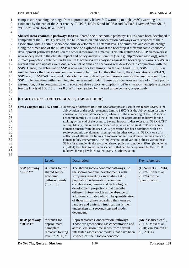
First Order Draft Chapter 1 IPCC AR6 WGI
Do Not Cite, Quote or Distribute 1-96 Total pages: 184
comparison, spanning the range from approximately below 2°C warming to high (>4°C) warming best-1
estimates by the end of the 21st century: RCP2.6, RCP4.5 and RCP6.0 and RCP8.5. [adapted from SR1.5, 2
WGI AR5, SYR AR5, WGIII AR5] 3
4
Shared socio-economic pathways (SSPs). Shared socio-economic pathways (SSPs) have been developed to 5
complement the RCPs. By design, the RCP emission and concentration pathways were stripped of their 6
association with a certain socio-economic development. Different levels of emissions and climate change 7
along the dimension of the RCPs can hence be explored against the backdrop if different socio-economic 8
development pathways (SSPs) on the other dimension in a matrix. This integrative SSP-RCP framework is 9
now widely used in the climate impact and policy analysis literature (see e.g. http://iconics-ssp.org), where 10
climate projections obtained under the RCP scenarios are analysed against the backdrop of various SSPs. As 11
several emission updates were due, a new set of emission scenarios was developed in conjunction with the 12
SSPs. Hence, the abbreviation SSP is now used for two things: On the one hand SSP1, SSP2, …, SSP5 is 13
used to denote the five socio-economic scenario families. On the other hand, the abbreviations SSP1-1.9, 14
SSP1-2.6, … SSP5-8.5 are used to denote the newly developed emission scenarios that are the result of an 15
SSP implementation within an integrated assessment model. Those SSP scenarios are bare of climate policy 16
assumption, but in combination with so-called share policy assumptions (SPAs), various nameplate radiative 17
forcing levels of 1.9, 2.6, …, or 8.5 W/m2 are reached by the end of the century, respectively. 18 19 20 [START CROSS-CHAPTER BOX 1.6, TABLE 1 HERE] 21
22 Cross-Chapter Box 1.6, Table 1: Overview of different RCP and SSP acronyms as used in this report. SSPX is the 23
abbreviation of the socio-economic family. SSPX-Y is the abbreviation for a new 24 emission or concentration scenario, where X is the numbering of the SSP socio-25 economic family (1 to 5) and the Y indicates the approximate radiative forcing 26 ranking by the end of the century. Several impact studies refer to an SSPX-RCPY 27 setting. Mostly, this refers to a model setup, when an original RCP emission or 28 climate scenario from the IPCC AR5 generation has been combined with a SSP 29 socio-economic development assumption. In other words, an SSPX is one of a 30 collection of alternative futures of socio-economic development in the absence of 31 climate policy intervention. The implementation of various policies within those 32 SSPs (for example via the so-called shared policy assumptions SPAs, (Kriegler et 33 al., 2014) then lead to emission scenarios that can be categorised by their 2100 34 radiative forcing levels Y, called SSPX-Y. Abbreviation 35
36
Levels Description Key references
SSP pathway
“SSP X”
X stands for the
shared socio-
economic
pathway family
(1, 2, ...5)
The shared socio-economic pathways, i.e.
the socio-economic developments with
storylines regarding - inter alia- GDP,
population, urbanisation, economic
collaboration, human and technological
development projections that describe
different future worlds in the absence of
additional climate policy. The quantification
of those storylines regarding their energy,
landuse and emission implications is then
undertaken in a second step and model
dependent.
(O’Neill et al., 2014,
2017b; Riahi et al.,
2017b) for the
quantification.
RCP pathway
“RCP Y”
Y stands for
approximate
nameplate
radiative forcing
level in 2100, at
Representative Concentration Pathways.
Those are greenhouse gas concentration and
aerosol emission time series from several
integrated assessment models that have been
stripped off their socio-economic
(Meinshausen et al.,
2011b; Moss et al.,
2010; van Vuuren et
al., 2011a)

First Order Draft Chapter 1 IPCC AR6 WGI
Do Not Cite, Quote or Distribute 1-97 Total pages: 184
levels 2.6, 4.5,
6.0 or 8.5.
backgrounds. The CMIP5 intercomparison
has developed the climate futures in line
with the RCPs.
The SSP
pathway and
RCP pathway
combination
“SSPX-
RCPY”
X and Y as
above.
Combination of the SSPs socio-economic
background family X with climate futures
stemming from AOGCM or Earth system
model runs that used the RCP Y.
See special issue on
(van Vuuren et al.,
2014). See also wide
range of literature
gathered in the
ICONICS database (
http://iconics-
ssp.org).
The SSP
scenario “SSP
X-Y”
X and Y as
above.
The integrated update of the SSPs and RCPs,
in which the whole matrix of five SSP
families (X=1,2,...,5) and seven RCP levels
(Y=1.9,2.6,3.4,4.5,6.0,7.0 and 8.5) is
explored. The main scenarios, called
‘Marker SSP scenarios' in this report are
SSP1-1.9, SSP1-2.6, SSP2-4.5, SSP4-7.0
and SSP5-8.5. Those are the four ‘Tier 1’
scenarios of ScenarioMIP in addition to
SSP1-1.9 which is the scenario that most
closely reflects the lower Paris Agreement
1.5°C goal. In addition, there are four ‘Tier
2’ scenarios, two within the ‘middle of the
road’ socio-economic family, i.e. SSP3-3.4
and SSP3-6.0, one variant of the SSP4-7.0
scenario which considers low short-lived
climate forcer emissions, SSP4-7.0-
lowNTCF, and one strong peak & decline
scenario that first follows SSP5-8.5 and then
descends to strong net negative emissions:
SSP5-3.4-OS.
1
[END CROSS-CHAPTER BOX 1.6, TABLE 1 HERE] 2
3
Baseline / Reference scenarios, business-as-usual, pathways or levels. The state against which change is 4
measured. In the context of transformation pathways, the term ‘baseline scenarios’ refers to scenarios that 5
are based on the assumption that no mitigation policies or measures will be implemented beyond those that 6
are already in force and / or are legislated or planned to be adopted. Baseline scenarios are not intended to be 7
predictions of the future, but rather counterfactual constructions that can serve to highlight the level of 8
emissions that would occur without further policy effort. Typically, baseline scenarios are then compared to 9
mitigation scenarios that are constructed to meet different goals for greenhouse gas (GHG) emissions, 10
atmospheric concentrations, or temperature change. The term ‘baseline scenario’ is used interchangeably 11
with ‘reference scenario’ and ‘no policy scenario’. In much of the literature the term is also synonymous 12
with the term ‘business-as-usual (BAU) scenario,’ although the term ‘BAU’ has fallen out of favour because 13
the idea of ‘business-as-usual’ in century-long socioeconomic projections is hard to fathom. [adapted from 14
SR1.5, taken from WGIII AR5] 15
16
[END CROSS-CHAPTER BOX 1.6 HERE] 17

First Order Draft Chapter 1 IPCC AR6 WGI
Do Not Cite, Quote or Distribute 1-98 Total pages: 184
1
2
3
1.7 Gaps and opportunities for integration of climate knowledge 4
5
Throughout the present report, the authors of each chapter identify knowledge gaps that represents 6
significant opportunities for improving our understanding of the climate system, including its natural 7
variability and its response to anthropogenic forcing. In the text below, we take a holistic view of the WGI 8
contribution to the AR6 cycle, and highlight three cross-cutting opportunities that reflect the diversity of the 9
challenges in climate science as they relate to the quantification of climate change risks and vulnerabilities. 10
11
Opportunity area #1: Creating an integrated framework for the assessment of the social-ecological 12
impacts of climate change, and opportunities for adaptation and mitigation 13
Humans have become the primary driver of global environmental change (SR1.5). IPCC Special Reports and 14
Assessment Reports outline a variety of strategies to minimize the ongoing risks of present climate change 15
(adaptation) while reducing the magnitude of future climate change (mitigation). As the role for the IPCC 16
shifts from a focus on the detection of climate change signals in the Earth System to a focus on the relative 17
benefits of a variety of climate solutions, the separations between WGI, WGII, and WGIII represent barriers 18
to the integration of knowledge. As the gap between our current emissions trajectories and those required to 19
remain under established international targets (1.5 – 2°C) climate solutions grows wider, the scale of any 20
climate risk mitigation efforts requires urgent, global-scale action. Indeed, any meaningful action to reduce 21
the impacts of climate change - whether by adaptation or mitigation exercises - involves large-scale shifts in 22
the global economy (i.e. decarbonization of electricity), land use (i.e. afforestation), and/or planetary energy 23
balance (i.e. solar radiation management), that a fully integrated assessment of the social-ecological system 24
is required in order to provide adequate policy guidance. End-to-end assessments of policy pathways that 25
include key feedbacks between social and physical systems are not possible under the current structure of the 26
IPCC assessment reporting processes. 27
28
Opportunity area #2: Improving knowledge of past, present, and future sea level rise 29
Sea level rise sits at the nexus of acute societal risk and large uncertainties, with a wide range of projections 30
having been made for the coming decades. While analysis of present-day data is focused on quantifying the 31
rates of ice sheet melting as a transient response to anthropogenic climate change (Hay et al., 2015) studies 32
that focus on quantifying the equilibrium response of global sea level to a variety of climatic forcings hold 33
unique promise as key constraints on the rates of and magnitude of ice sheet melting during the geologic past 34
(DeConto and Pollard, 2016b). Recent studies consider sea level rise estimates over the last millennium 35
(Kopp et al., 2016), the most recent interglacials (Dutton et al., 2015), and the Eocene - the most recent time 36
period during which atmospheric CO2 concentrations were similar to those of the 21st century (Burke et al., 37
2018). Such studies provide an opportunity to quantify not only the magnitude of equilibrium sea level rise 38
to a given level of global temperature variability, but can, through the combination of higher-resolution sea 39
level reconstructions with climate models that contain representative ice sheet physics, constrain the rates of 40
transient sea level rise to changes in global temperature. Such an effort will result in critical gains in our 41
ability to provide policy-relevant estimates of near- and long-term sea level rise, in particular data-driven 42
estimates of potential worst-case scenarios that may drive decisions around sea level rise adaptation in 43
vulnerable locations. 44
45
Opportunity area #3: Accelerating improvements in the observational record of climate variability 46
and change with integration of paleoclimate datasets 47
With each passing year, the climate record lengthens while becoming more diverse through the addition of 48
newly observed climate variables and observational platforms. Even so, in the near-term, the biggest gains in 49
our observational capacity of the Earth’s climate system will likely come from a more complete integration 50
of paleoclimate observations and newly available early instrumental data into extended reanalyses datasets 51
that can inform the accuracy of numerical climate models. Such integration leverages ongoing development 52
of climate models that can simulate paleoclimate records in their units of analysis (i.e. oxygen isotopes, tree 53
ring width, etc), in many cases using physical climate variables as input for so-called “proxy system models” 54
(Dee et al., 2015; Evans et al., 2013). Early efforts towards proxy-model integration aim to generate gridded 55

First Order Draft Chapter 1 IPCC AR6 WGI
Do Not Cite, Quote or Distribute 1-99 Total pages: 184
climate data spanning the last centuries using data assimilation techniques (Hakim et al., 2016). As these 1
efforts mature, they will open new avenues for improvements in the state of climate knowledge, with 2
particularly high potential in the following key areas: 3
4
i. detection and attribution of changes in the frequency and severity of climate extremes 5
ii. links between climate variability and change, ecosystem structure and function, and 6
biogeochemical cycles 7
iii. improvements in the initialization of climate models with applications to near-term (decadal-8
scale) prediction of climate variability and change 9
10
11
1.8 Structure / key elements of AR6 12
13
[This is a preliminary version, which will be updated for the SOD with the outlines of all chapters] 14
15
The WGI contribution to the IPCC 6th Assessment Report has twelve chapters plus the Atlas and can be 16
grouped into three main categories: 17
18
Global Information (Chapters 2, 3 and 4). These chapters assess climate information from global to 19
hemispheric scales. The three chapters start with an assessment of the changing state of the climate system 20
(Chapter 2), including the atmosphere, biosphere, ocean and cryosphere. It then assesses the human influence 21
on the changing climate (Chapter 3), covering the attribution of observed changes, and the evaluation of 22
climate models used to conduct the attribution studies. Chapter 4 assesses climate change projections, from 23
the near to the long term, including climate change beyond 2100, as well as the assessment for potential 24
abrupt changes and low-probability-high-impact changes. 25
26
Process Understanding (Chapters 5, 6, 7, 8 and 9). These five chapters provide end-to-end assessments of 27
fundamental Earth system processes: the carbon budget and biogeochemical cycles (Chapter 5), short-lived 28
climate forcers (Chapter 6), the Earth’s energy budget (Chapter 7), the water cycle (Chapter 8) and the 29
ocean, cryosphere and sea-level changes (Chapter 9). All these chapters provide assessments of observed 30
changes, including relevant paleoclimatic information, understanding of processes and mechanisms, as well 31
as projections, including model evaluation. 32
33
Regional Information (Chapters 10, 11, 12 and Atlas). Since AR5, a large volume of climate information, 34
understanding, observed impacts and projections at regional scales has been published. This new knowledge 35
is reflected in this report with three chapters covering regional information. Chapter 10 provides the basis for 36
regional climate information, including methods, physical processes and an assessment of observed changes 37
at regional scales. Chapter 11 builds on the regional framework and addresses extreme weather and climate 38
events, including their definition. It assesses observations for extremes, and the understanding of 39
mechanisms, drivers and feedbacks leading to extremes. The chapter also covers new methods to perform 40
event attribution, and an assessment of projected changes of extremes. The main objective of Chapter 12 is 41
to provide a comprehensive, region-specific assessment of observed impacts of anthropogenic climate 42
change and regional projections under key future scenarios. The chapter therefore contributes to the overall 43
risk framework of the AR6 by assessing the hazard component of the risk (cf. Figure 1 of Cross-Chapter Box 44
1.2). Lastly this report builds upon the Atlas presented in AR5, with the development of a novel, interactive 45
Atlas, which synthesizes information by expanding and integrating results from the rest of the report. The 46
interactive Atlas tool extends the regional assessment with flexible spatial and temporal analyses. 47
48
Integration across the WGI report and with Working Groups II and III occurs in various forms. As already 49
mentioned in Section 1.6, one important venue of integration within WGI and among working groups is the 50
presentation of results at various temperature levels. Chapters 8 to 12 and the Atlas contribute to common 51
topics with WGII in two specific areas: regional climate information and a common risk framework. This 52
should produce a more integrated assessment of impacts of climate change across working groups. In 53
particular, Chapter 12 provides a “handshake” instead of just a “handover” of information useful for the 54
evaluation of climate change impacts. The science assessed in Chapters 4 to 7, such as the carbon budget or 55
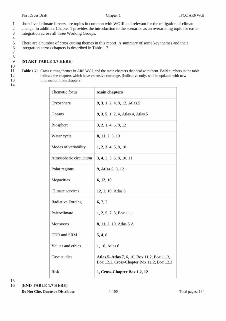
First Order Draft Chapter 1 IPCC AR6 WGI
Do Not Cite, Quote or Distribute 1-100 Total pages: 184
short-lived climate forcers, are topics in common with WGIII and relevant for the mitigation of climate 1
change. In addition, Chapter 1 provides the introduction to the scenarios as an overarching topic for easier 2
integration across all three Working Groups. 3
4
There are a number of cross cutting themes in this report. A summary of some key themes and their 5
integration across chapters is described in Table 1.7. 6 7 8
[START TABLE 1.7 HERE] 9
10 Table 1.7: Cross cutting themes in AR6 WGI, and the main chapters that deal with them. Bold numbers in the table 11
indicate the chapters which have extensive coverage. [Indicative only, will be updated with new 12 information from chapters]. 13
14
Thematic focus Main chapters
Cryosphere 9, 3, 1, 2, 4, 8, 12, Atlas.5
Oceans 9, 3, 5, 1, 2, 4, Atlas.4, Atlas.5
Biosphere 3, 2, 1, 4, 5, 8, 12
Water cycle 8, 11, 2, 3, 10
Modes of variability 1, 2, 3, 4, 5, 8, 10
Atmospheric circulation 3, 4, 2, 3, 5, 8, 10, 11
Polar regions 9, Atlas.5, 8, 12
Megacities 6, 12, 10
Climate services 12, 1, 10, Atlas.6
Radiative Forcing 6, 7, 2
Paleoclimate 1, 2, 5, 7, 8, Box 11.1
Monsoons 8, 11, 2, 10, Atlas.5 A
CDR and SRM 5, 4, 8
Values and ethics 1, 10, Atlas.6
Case studies Atlas.5–Atlas.7, 6, 10, Box 11.2, Box 11.3,
Box 12.1, Cross-Chapter Box 11.2, Box 12.2
Risk 1, Cross-Chapter Box 1.2, 12
15
[END TABLE 1.7 HERE] 16
First Order Draft Chapter 1 IPCC AR6 WGI
Do Not Cite, Quote or Distribute 1-101 Total pages: 184
Frequently Asked Questions 1
2
FAQ 1.1: Do we understand climate change better now, compared to when the IPCC started? 3
4
Yes — much better. The first IPCC report, in 1990, predicted that human-caused climate change would soon 5
occur, but could not yet confirm that it was already happening. Today, evidence is abundant that the climate 6
has already changed since the mid-20th century, and we know that human emissions of carbon dioxide, 7
methane, and other gases are the principal cause of that change. With much more and much better data, we 8
understand more about how the oceans and atmosphere interact, as well as about the ice and snow that 9
cover large parts of the Earth. Compared with the computer climate simulations of 1990, today’s Earth 10
system models include many more physical processes, and they can make more specific projections of future 11
changes in different places. Many early climate model predictions have been confirmed. 12
13
Since 1990, large numbers of new instruments have been deployed to collect data in the air, on land, at sea, 14
and in outer space. These instruments measure temperature, clouds, winds, ice, snow, ocean currents, sea 15
level, soot and dust in the air, and many other aspects of the climate system. New satellite instruments, as 16
well as decades of additional data from older observing systems, have provided a wealth of new, increasingly 17
accurate data. Ice cores, sediments, fossils, and other evidence from the distant past have taught us much 18
about how Earth’s climate has changed throughout its history. We also now know that most of the heat in the 19
overall climate system is being retained in the oceans, and that even the deep ocean is warming up. In 1990, 20
relatively little was known about exactly how the gigantic glaciers of Greenland and Antarctica would 21
respond to warming. With much more data and better models of their behavior, evidence has emerged of 22
unexpectedly high melt rates that may lead to major changes within this century, including substantial sea 23
level rise. 24
25
The major natural factors contributing to climate change on timescales of decades to centuries are volcanic 26
eruptions and the sun’s heat. Today, data show us that the sun’s heat has not changed much in the last 27
century, and that major volcanic eruptions have occasionally cooled the planet for short periods of time 28
(typically 1-3 years). The main human causes of climate change are heat-trapping gases emitted by burning 29
fossil fuels, which warm the planet, and tiny particles in the air such as soot from burning coal, which have 30
both warming and cooling effects depending on their size, color, and location. Since 1990 measurements of 31
all these factors have become more accurate and precise, while older data have been recovered and 32
integrated into the long-term record. 33
34
While most climate models in 1990 focused on the atmosphere, using only highly simplified oceans, today’s 35
Earth system models include detailed models of oceans, ice, snow, vegetation, and often many other 36
variables as well. An important test of models is their ability to simulate past climates. Several rounds of 37
such testing have taken place since 1990, and the testing itself has become more rigorous and extensive. As a 38
group, in these tests models have predicted the actual changes reasonably well. Since there is no way to do a 39
controlled laboratory experiment on the actual Earth, climate simulations can also provide a kind of “control 40
Earth” to see what would have happened without human influences. These experiments show that without 41
our influence, the observed post-1960s warming would not have occurred. 42
43
Finally, climate models make specific predictions of exactly how the climate should change if human 44
influences and not natural causes are the reason, and many of those predictions have been confirmed by 45
observations. For example, nights are warming faster than days; satellite measurements show that less heat is 46
escaping to space; and the lower atmosphere (troposphere) is warming but the upper atmosphere 47
(stratosphere) is cooling. 48
49
[Figure proposal: 2-panel schematic of climate models then in 1990 (FAR) vs. climate models now in AR6. 50
The figure below (from AR4) is an initial idea. FAR would have only solar radiation, GHGs, rain, clouds, 51
land surface, prescribed ice, and swamp ocean. CMIP6 would add volcanoes, sulphates, aerosols, carbon 52
cycle, rivers, overturning ocean circulation, interactive vegetation, air chemistry, ocean biogeochemistry, 53
ocean eddies, “high-top” atmosphere (top level above stratopause), terrestrial nitrogen cycle, and dynamic 54
sea ice at a minimum.] 55

First Order Draft Chapter 1 IPCC AR6 WGI
Do Not Cite, Quote or Distribute 1-102 Total pages: 184
1
[START FAQ 1.1, FIGURE 1 HERE] 2
3 FAQ 1.1, Figure 1: [PLACEHOLDER] 4
[END FAQ 1.1, FIGURE 1 HERE] 5
6 7

First Order Draft Chapter 1 IPCC AR6 WGI
Do Not Cite, Quote or Distribute 1-103 Total pages: 184
FAQ 1.2: At what point do we know it’s climate change? 1
2
[PLACE HOLDER: This FAQ will be reshaped later to better coordinate with related FAQs in Chapters 2 3
and 3 (on detection and attribution)] 4
5
The signs of climate change are most obvious at the global scale, but they are increasingly clear on smaller 6
spatial scales and in a range of climate variables. Regions which have a larger signal of change relative to 7
the size of background climate variations will potentially face greater risks as they will see unusual or 8
unprecedented climates earlier. 9
10
Observed and projected temperature change is often smaller in the tropics than at higher latitudes, but 11
smaller variations means that tropical countries have potentially seen the effects of climate change earlier 12
(see FAQ Figure 1.2). Often it is not necessarily the size of the change which is most important for climate-13
related risks, instead, it is the size of the change relative to the background fluctuations of the climate to 14
which ecosystems or society is already adapted to. 15
16
[Paragraph on projections and the implication of mitigation choices. A future where a strong mitigation 17
strategy is in place will have different climate signal emerging compared to a projection where less 18
mitigation occurs. Figure to be updated to include : 19
• Example of differences between climate signals 20
• Air temperature changes vs precip or sea level changes in the future 21
• How emergence depends on the GHG mitigation pathway / scenario chosen] 22
23
24
[START FAQ 1.2, FIGURE 1 HERE] 25 26 FAQ 1.2, Figure 1: Observed variations in regional temperatures since 1920 from CRUTEM4. Europe has warmed by 27
a larger amount than tropical Africa, but the background variations are also larger (shading 28 represents 1 and 3 standard deviations of background interannual variations). The signal of 29 observed temperature change emerged earlier in tropical Africa than in Europe. 30
31
[END FAQ 1.2, FIGURE 1 HERE] 32
33
34
First Order Draft Chapter 1 IPCC AR6 WGI
Do Not Cite, Quote or Distribute 1-104 Total pages: 184
FAQ 1.3: What can past climate teach us about the future? 1
2
Rising greenhouse gas concentrations are driving a suite of profound changes to the earth system, including 3
warming, sea level rise, increases in climate and weather extremes, ocean acidification, and ecological 4
shifts. Past climate variability over the last centuries to millennia serves as the most relevant baseline 5
against which to measure anthropogenic changes in climate. Farther back in time, larger reorganizations of 6
the earth system provide critical information about the rates and magnitudes of physical, chemical, and 7
ecological changes under a suite of different greenhouse gas concentrations. Careful observation of these 8
past changes challenges our understanding of how our planet operates, and also allows us to test our latest 9
models that are used for predicting future climate change. Of particular relevance, the “hothouse Earth” of 10
~50 million years ago represents the most recent time that atmospheric carbon dioxide concentrations were 11
as high as those projected for the late 21st century if emission rates continue at present rates. 12
13
Although we have been taking measurements of the Earth’s climate for centuries, the vast majority of 14
instrumental observations began during the late 20th century, during a period already experiencing rapid 15
human-made (anthropogenic) warming. Unlocking information spanning millions of years of the Earth’s 16
history, so-called ‘paleoclimate records’ are indirect climate measurements (from tree rings, ice cores, corals, 17
and ocean and lake sediments, for example) that climate scientists use to understand current and future 18
climate change. 19
20
The earth climate is a complex system in which the different components (atmosphere, ocean, cryosphere, 21
etc) respond with very different paces to forcing. As a consequence of this, it will take several millennia for 22
the earth system to come into equilibrium with present-day atmospheric greenhouse gas concentrations, past 23
climate states help scientists understand the true sensitivity of the earth system to both small and large 24
changes in climate forcing. 25
26
At their most basic level, records of past climate change serve as a critical backdrop for current 27
anthropogenic climate trends, in many cases allowing for the separation of natural causes of climate change 28
(natural variability) and greenhouse-induced trends in earth’s climate. In recent millennia, atmospheric CO2 29
concentrations were relatively stable, such that changes in solar irradiance and volcanic eruptions 30
represented the primary external drivers of global climate variability. During this time, global temperature 31
variations amounted to less than 0.5C and sea level varied by no more than 10cm. Exceptionally high-32
resolution records spanning the last several centuries allow for the quantification of past climate extremes 33
such as drought, El Niño/La Niña events, wildfires, and even tropical storms. Indeed, the last millennia 34
provides a wealth of data that climate scientists use to probe the relationship between global climate state 35
and the character of climate extremes. As such, it offers a “baseline” to which human-induced changes can 36
be compared, and also a rich testbed for climate models that are used to project 21st century climate changes, 37
which must account for natural as well as solar-, volcanic-, and greenhouse-forced climate variability. 38
39
Rising greenhouse gas concentrations reflect large-scale changes in the Earth’s carbon cycle, such that 40
studies of past changes in carbon fluxes and associated climate changes are highly relevant to projections of 41
future anthropogenic climate change. Over the last million years, Earth has transitioned from glacial climate 42
states characterized by markedly lower atmospheric CO2 concentrations (200 parts per million) to 43
interglacial climate states (with CO2 concentrations of 280-300 parts per million) every ~100,000 years. 44
Profound shifts in polar ice sheet mass, sea ice extent, sea level, ocean circulation, global temperature, 45
precipitation patterns, vegetation and climate extremes accompanied these glacial-interglacial shifts. 46
Intriguingly, glacial states are marked by examples of abrupt climate changes that illustrate the potential for 47
rapid climate responses to much slower changes in climate forcing – a high-risk but highly uncertain 48
scenario for 21st century climate changes. 49
50
Much further back in geologic time, deep-sea sediments record a climate state when changes in volcanic 51
activity/crustal formation rates and weathering caused atmospheric CO2 concentrations to climb to ~800ppm 52
or higher – similar to levels expected in coming decades if emissions continue at present rates. During the 53
Eocene period, roughly 50 million years ago, global temperatures were as much as 8C warmer, sea level 54
was 20-40m higher, and ocean pH varied appreciably. While the rates of present-day atmospheric CO2 55

First Order Draft Chapter 1 IPCC AR6 WGI
Do Not Cite, Quote or Distribute 1-105 Total pages: 184
change, temperature change, ocean pH change, and sea level rise are many times higher than they were 1
during past geologic intervals, these “hothouse” worlds hold key lessons for our climate future. In particular, 2
they provide a window into how our planet may eventually end up like, if emissions of greenhouse gases 3
continue unabated, and allow us to test how well our climate models perform under these extreme 4
conditions. This is especially true as models that were constructed and tested against instrumental climate 5
data are charged with projecting climate changes that occur under vastly different boundary conditions than 6
today. As such, past climate data allows us to test the general applicability of our models, and therefore the 7
reliability of our future climate predictions 8
9
[Figure concept: 10
4 vertical panels, illustrating (from left to right): 11
i) the PETM, 12
ii) the last millennium/pre-industrial, 13
iii) present-day, and 14
iv) 2100 projections (RCP8.5 or similar) 15
with an infographic denoting changes in the following variables: 16
● atmospheric CO2 concentrations 17
● global temperature 18
● global sea level 19
● (other variables?)] 20
21
[START FAQ 1.3, FIGURE 1 HERE] 22
23 FAQ 1.3, Figure 1: [PLACEHOLDER] 24
[END FAQ 1.3, FIGURE 1 HERE] 25
26
27
First Order Draft Chapter 1 IPCC AR6 WGI
Do Not Cite, Quote or Distribute 1-106 Total pages: 184
FAQ 1.4: How do we calculate global temperature change? 1
2
We calculate global surface temperature change by analyzing the readings of thermometers all over the 3
globe using statistical techniques to take into account areas like the poles where there are fewer 4
measurements. Multiple independent groups of scientists work with an ever increasing number of readings 5
and all have very similar results. 6
The surface temperature of the world has, on average, increased by around 1 °C since the pre-industrial 7
period – hence the term ‘global warming’. Making such a statement implies that we are confident in the 8
ability of science to determine how surface temperatures change over time. 9
Multiple scientific organizations monitor global surface temperature and all datasets rely on long-term series 10
of temperature measurements made of the air near the surface over land and of the ocean surface, collected 11
by ships, buoys and satellites. Much like having multiple watches that may be set differently but still 12
consistently count seconds and minutes, the numerous temperature measurements may all be calibrated 13
slightly differently but can still give comparable changes. For that reason it is easier to measure temperature 14
change, and not the absolute average temperature of the Earth’s surface. 15
Three main issues arise when estimating changes in global temperature from a large set of measurements 16
spread unevenly across the globe. The first is how to deal with areas where measurements are sparse or 17
mostly unavailable, such as close to the poles. While the different groups producing temperature records all 18
perform rigorous analyses in order to handle the fact that the measurements are not spread evenly, they differ 19
somewhat in how they treat areas with no information. 20
The second issue, which has recently seen a lot of discussion, is what type of measurement to use over the 21
ocean regions. Traditionally, ship or buoy measurements of the temperature of surface water, have been 22
combined with air temperature measurements (typically at 2 metres) over land. However, analyses with 23
global climate models have tended to use simulated air temperatures everywhere. As air temperatures over 24
the ocean can be expected to warm slightly faster than surface water, it is important to use the same 25
methodology when comparing measurements to models. 26
The third issue is which time period to report the changes over. As global temperatures have a natural year-27
to-year variability, scientists normally average at least 20 years to obtain a representative value - but which 28
years? For current temperatures, they naturally use the latest two decades. The period before significant 29
human influence is more difficult to define, partly because measurements were much more sparse in the 18th 30
and 19th centuries. Currently scientists use an ‘early industrial’ period from 1850 to 1900 as the starting 31
point, though sometimes the ‘pre-industrial’ period around 1750 is also used. 32
While global temperatures have risen by about one degree over the last hundred years or so, the formal 33
assessment, based on several independently produced data series, is that surface air temperatures changed by 34
+0.87 °C between the average of 1850-1900 and 2006-2015. 35
36
[START FAQ 1.4, FIGURE 1 HERE] 37
FAQ 1.4, Figure 1: Suggestion: Global map of measurement site/point densities. With a side list of all the different 38 techniques (eg, buoys, satellites, ships etc – could have icons for each?) Present placeholder is 39 from Rennie et al. (2014). 40
[END FAQ 1.4, FIGURE 1 HERE] 41
42

First Order Draft Chapter 1 IPCC AR6 WGI
Do Not Cite, Quote or Distribute 1-107 Total pages: 184
References 1 2 A. KATTENBERG, R. G., GRASSL, H., MEEHL, G. A., MITCHELL, J. F. B., STOUFFER, R. J., TOKIOKA, T., et 3
al. (1995). “Climate Models - Projections of Future Climate,” in Climate Change 1995: The Science of Climate 4 Change. Contribution of Working Group I to the Second Assessment Report of the Intergovernmental Panel on 5 Climate Change, 285–357. 6
Abram, N. J., Gagan, M. K., Liu, Z., Hantoro, W. S., McCulloch, M. T., and Suwargadi, B. W. (2007). Seasonal 7 characteristics of the Indian Ocean Dipole during the Holocene epoch. Nature 445, 299–302. 8 doi:10.1038/nature05477. 9
Abram, N. J., McGregor, H. V., Tierney, J. E., Evans, M. N., McKay, N. P., and Kaufman, D. S. (2016). Early onset of 10 industrial-era warming across the oceans and continents. Nature 536, 411–418. doi:10.1038/nature19082. 11
Abramowitz, G., Herger, N., Gutmann, E., Hammerling, D., Knutti, R., Leduc, M., et al. (2018). Model dependence in 12 multi-model climate ensembles: weighting, sub-selection and out-of-sample testing. Earth Syst. Dyn. Discuss., 1–13 20. doi:10.5194/esd-2018-51. 14
Adler, C. E., and Hirsch Hadorn, G. (2014). The IPCC and treatment of uncertainties: topics and sources of dissensus. 15 Wiley Interdiscip. Rev. Clim. Chang. 5, 663–676. doi:10.1002/wcc.297. 16
Agarwal, A., and Narain, S. (2012). “Global warming in an unequal world: A case of environmental colonialism 17 (selected excerpts),” in Handbook of Climate Change and India, ed. N. Dubash (Routledge). 18 doi:10.4324/9780203153284. 19
Ahn, M.-S., Kim, D., Sperber, K. R., Kang, I.-S., Maloney, E., Waliser, D., et al. (2017). MJO simulation in CMIP5 20 climate models: MJO skill metrics and process-oriented diagnosis. Clim. Dyn. 49, 4023–4045. 21 doi:10.1007/s00382-017-3558-4. 22
Alexander, C., Bynum, N., Johnson, E., King, U., Mustonen, T., Neofotis, P., et al. (2011). Linking Indigenous and 23 Scientific Knowledge of Climate Change. Bioscience 61, 477–484. doi:10.1525/bio.2011.61.6.10. 24
Allen, M. R., and Ingram, W. J. (2002). Constraints on future changes in climate and the hydrologic cycle. Nature 419, 25 228–232. doi:10.1038/nature01092. 26
Allen, M. R., Stott, P. A., Mitchell, J. F. B., Schnur, R., and Delworth, T. L. (2000). Quantifying the uncertainty in 27 forecasts of anthropogenic climate change. Nature 407, 617–620. doi:10.1038/35036559. 28
AMAP (2015). AMAP assessment 2015 : black carbon and ozone as Arctic climate forcers. Oslo : Arctic Monitoring 29 and Assessment Programme (AMAP). 30
Anav, A., Friedlingstein, P., Kidston, M., Bopp, L., Ciais, P., Cox, P., et al. (2013). Evaluating the Land and Ocean 31 Components of the Global Carbon Cycle in the CMIP5 Earth System Models. J. Clim. 26, 6801–6843. 32 doi:10.1175/JCLI-D-12-00417.1. 33
Anderson, A. A., and Huntington, H. E. (2017). Social Media, Science, and Attack Discourse: How Twitter Discussions 34 of Climate Change Use Sarcasm and Incivility. Sci. Commun. 39, 598–620. doi:10.1177/1075547017735113. 35
Andrews, T., Forster, P. M., Boucher, O., Bellouin, N., and Jones, A. (2010). Precipitation, radiative forcing and global 36 temperature change. Geophys. Res. Lett. 37, n/a-n/a. doi:10.1029/2010GL043991. 37
Andrews, T., Gregory, J. M., Paynter, D., Silvers, L. G., Zhou, C., Mauritsen, T., et al. (2018). Accounting for 38 Changing Temperature Patterns Increases Historical Estimates of Climate Sensitivity. Geophys. Res. Lett. 45, 39 8490–8499. doi:10.1029/2018GL078887. 40
Angström, K. (1900). Über die Bedeutung des Wasserdampfes und der Kohlensäure bei der Absorption der 41 Erdatmosphäre. Ann. Phys. 3, 720–732. 42
Anonymous (1901). Knut Angstrom on Atmospheric Absorption. Mon. Weather Rev. 29, 268. 43 Arizmendi, F., and Barreiro, M. (2017). ENSO teleconnections in the southern hemisphere: A climate network view. 44
Chaos An Interdiscip. J. Nonlinear Sci. 27, 093109. doi:10.1063/1.5004535. 45 Arnold, J. R., and Libby, W. F. (1949). Age determinations by radiocarbon content: Checks with samples of known age. 46
Science (80-. ). 110, 678–680. doi:10.1126/science.110.2869.678. 47 Arrhenius, S. (1896). XXXI. On the influence of carbonic acid in the air upon the temperature of the ground. London, 48
Edinburgh, Dublin Philos. Mag. J. Sci. 41, 237–276. doi:10.1080/14786449608620846. 49 Arrhenius, S., and Borns, H. (1908). Worlds in the Making: The Evolution of the Universe. New York: Harper and 50
Brothers. 51 Ashton, T. . (1997). The industrial revolution, 1760-1830. Oxford: Oxford University Press Available at: 52
https://trove.nla.gov.au/work/8794617?q&sort=holdings+desc&_=1553489019694&versionId=210078368 53 [Accessed March 25, 2019]. 54
Ashwin, P., Wieczorek, S., Vitolo, R., and Cox, P. (2012). Tipping points in open systems: bifurcation, noise-induced 55 and rate-dependent examples in the climate system. Philos. Trans. R. Soc. A Math. Phys. Eng. Sci. 370, 1166–56 1184. doi:10.1098/rsta.2011.0306. 57
Aumont, O., Ethé, C., Tagliabue, A., Bopp, L., and Gehlen, M. (2015). PISCES-v2: an ocean biogeochemical model for 58 carbon and ecosystem studies. Geosci. Model Dev. 8, 2465–2513. doi:10.5194/gmd-8-2465-2015. 59
Balaji, V., Taylor, K. E., Juckes, M., Lautenschlager, M., Blanton, C., Cinquini, L., et al. (2018). Requirements for a 60

First Order Draft Chapter 1 IPCC AR6 WGI
Do Not Cite, Quote or Distribute 1-108 Total pages: 184
global data infrastructure in support of CMIP6. Geosci. Model Dev. Discuss., 1–28. doi:10.5194/gmd-2018-52. 1 Balmaseda, M. A., Hernandez, F., Storto, A., Palmer, M. D., Alves, O., Shi, L., et al. (2015). The Ocean Reanalyses 2
Intercomparison Project (ORA-IP). J. Oper. Oceanogr. 8, s80–s97. doi:10.1080/1755876X.2015.1022329. 3 Bamber, J. L., Westaway, R. M., Marzeion, B., and Wouters, B. (2018). The land ice contribution to sea level during 4
the satellite era. Environ. Res. Lett. 13, 063008. doi:10.1088/1748-9326/aac2f0. 5 Barnett, T. P., and Schlesinger, M. E. (1987). Detecting changes in global climate induced by greenhouse gases. J. 6
Geophys. Res. 92, 14772. doi:10.1029/JD092iD12p14772. 7 Barnston, A. G., Tippett, M. K., Ranganathan, M., and L’Heureux, M. L. (2017). Deterministic skill of ENSO 8
predictions from the North American Multimodel Ensemble. Clim. Dyn. 0, 1–20. doi:10.1007/s00382-017-3603-9 3. 10
Barreiro, M., Marti, A. C., and Masoller, C. (2011). Inferring long memory processes in the climate network via ordinal 11 pattern analysis. Chaos An Interdiscip. J. Nonlinear Sci. 21, 013101. doi:10.1063/1.3545273. 12
Barrett, H. G., Jones, J. M., and Bigg, G. R. (2018). Reconstructing El Niño Southern Oscillation using data from ships’ 13 logbooks, 1815–1854. Part II: Comparisons with existing ENSO reconstructions and implications for 14 reconstructing ENSO diversity. Clim. Dyn. 50, 3131–3152. doi:10.1007/s00382-017-3797-4. 15
Barz, B., Rodner, E., Garcia, Y. G., and Denzler, J. (2019). Detecting Regions of Maximal Divergence for Spatio-16 Temporal Anomaly Detection. IEEE Trans. Pattern Anal. Mach. Intell. 41, 1088–1101. 17 doi:10.1109/TPAMI.2018.2823766. 18
Beck, H. E., Zimmermann, N. E., McVicar, T. R., Vergopolan, N., Berg, A., and Wood, E. F. (2018). Present and future 19 Köppen-Geiger climate classification maps at 1-km resolution. Sci. Data 5, 180214. Available at: 20 https://doi.org/10.1038/sdata.2018.214. 21
Belda, M., Holtanová, E., Halenka, T., and Kalvová, J. (2014). Climate classification revisited: from Köppen to 22 Trewartha. Clim. Res. 59, 1–13. doi:10.3354/cr01204. 23
Bellenger, H., Guilyardi, E., Leloup, J., Lengaigne, M., and Vialard, J. (2014). ENSO representation in climate models: 24 from CMIP3 to CMIP5. Clim. Dyn. 42, 1999–2018. doi:10.1007/s00382-013-1783-z. 25
Bentz, B. J., Régnière, J., Fettig, C. J., Hansen, E. M., Hayes, J. L., Hicke, J. A., et al. (2010). Climate Change and Bark 26 Beetles of the Western United States and Canada: Direct and Indirect Effects. Bioscience 60, 602–613. 27 doi:10.1525/bio.2010.60.8.6. 28
Bereiter, B., Eggleston, S., Schmitt, J., Nehrbass-Ahles, C., Stocker, T. F., Fischer, H., et al. (2015). Revision of the 29 EPICA Dome C CO 2 record from 800 to 600 kyr before present. Geophys. Res. Lett. 42, 542–549. 30 doi:10.1002/2014GL061957. 31
Berezin, Y., Gozolchiani, A., Guez, O., and Havlin, S. (2012). Stability of Climate Networks with Time. Sci. Rep. 2, 32 666. doi:10.1038/srep00666. 33
Berner, R. A. (1995). A. G. Högbom and the development of the concept of the geochemical carbon cycle. Am. J. Sci. 34 295, 491–495. 35
Bethke, I., Outten, S., Otterå, O. H., Hawkins, E., Wagner, S., Sigl, M., et al. (2017). Potential volcanic impacts on 36 future climate variability. Nat. Clim. Chang. 7, 799–805. doi:10.1038/nclimate3394. 37
Bindoff, N. L., Stott, P. A., AchutaRao, K. M., Allen, M. R., Gillett, N., Gutzler, D., et al. (2013). “Detection and 38 Attribution of Climate Change: from Global to Regional,” in Climate Change 2013: The Physical Science Basis. 39 Contribution of Working Group I to the Fifth Assessment Report of the Intergovernmental Panel on Climate 40 Change, eds. T. F. Stocker, D. Qin, G.-K. Plattner, M. Tignor, S. K. Allen, J. Boschung, et al. (Cambridge, United 41 Kingdom and New York, NY, USA: Cambridge University Press), 867–952. 42 doi:10.1017/CBO9781107415324.022. 43
Bintanja, R., and van de Wal, R. S. W. (2008). North American ice-sheet dynamics and the onset of 100,000-year 44 glacial cycles. Nature 454, 869–872. doi:10.1038/nature07158. 45
Bishop, C. H., and Abramowitz, G. (2013). Climate model dependence and the replicate Earth paradigm. Clim. Dyn. 41, 46 885–900. doi:10.1007/s00382-012-1610-y. 47
Bjerknes, V. (1906). Fields of Force: Supplementary Lectures, Applications to Meteorology. New York: Columbia 48 University Press. 49
Bjerknes, V., Sandström, J. W., Hesselberg, T., and Devik, O. M. (1910). Dynamic Meteorology and Hydrography. 50 Washington: Carnegie Institution of Washington. 51
Boé, J. (2018). Interdependency in Multimodel Climate Projections: Component Replication and Result Similarity. 52 Geophys. Res. Lett. 45, 2771–2779. doi:10.1002/2017GL076829. 53
Boer, G. J., Smith, D. M., Cassou, C., Doblas-Reyes, F., Danabasoglu, G., Kirtman, B., et al. (2016). The Decadal 54 Climate Prediction Project (DCPP) contribution to CMIP6. Geosci. Model Dev. 9, 3751–3777. doi:10.5194/gmd-55 9-3751-2016. 56
Boers, N. (2018). Early-warning signals for Dansgaard-Oeschger events in a high-resolution ice core record. Nat. 57 Commun. 9, 2556. doi:10.1038/s41467-018-04881-7. 58
Boers, N., Bookhagen, B., Marengo, J., Marwan, N., von Storch, J.-S., and Kurths, J. (2015). Extreme Rainfall of the 59 South American Monsoon System: A Dataset Comparison Using Complex Networks. J. Clim. 28, 1031–1056. 60 doi:10.1175/JCLI-D-14-00340.1. 61
First Order Draft Chapter 1 IPCC AR6 WGI
Do Not Cite, Quote or Distribute 1-109 Total pages: 184
Boers, N., Bookhagen, B., Marwan, N., Kurths, J., and Marengo, J. (2013). Complex networks identify spatial patterns 1 of extreme rainfall events of the South American Monsoon System. Geophys. Res. Lett. 40, 4386–4392. 2 doi:10.1002/grl.50681. 3
Bogenschutz, P. A., Gettelman, A., Morrison, H., Larson, V. E., Craig, C., and Schanen, D. P. (2013). Higher-Order 4 Turbulence Closure and Its Impact on Climate Simulations in the Community Atmosphere Model. J. Clim. 26, 5 9655–9676. doi:10.1175/JCLI-D-13-00075.1. 6
Bohr, J. (2017). Is it hot in here or is it just me? Temperature anomalies and political polarization over global warming 7 in the American public. Clim. Change 142, 271–285. doi:10.1007/s10584-017-1934-z. 8
Bolin, B. (2007). A History of the Science and Politics of Climate Change: The Role of the Intergovernmental Panel on 9 Climate Change. Cambridge University Press. 10
Bolin, B., Döös, B. R., Jäger, J., and Warrick, R. A. (1986). The Greenhouse Effect, Climatic Change, and Ecosystems. 11 Wiley. 12
Bony, S., Stevens, B., Frierson, D. M. W., Jakob, C., Kageyama, M., Pincus, R., et al. (2015). Clouds, circulation and 13 climate sensitivity. Nat. Geosci. 8, 261–268. doi:10.1038/ngeo2398. 14
Boo, K.-O., Martin, G., Sellar, A., Senior, C., and Byun, Y.-H. (2011). Evaluating the East Asian monsoon simulation 15 in climate models. J. Geophys. Res. 116, D01109. doi:10.1029/2010JD014737. 16
Bowen, G. J., Maibauer, B. J., Kraus, M. J., Röhl, U., Westerhold, T., Steimke, A., et al. (2015). Two massive, rapid 17 releases of carbon during the onset of the Palaeocene–Eocene thermal maximum. Nat. Geosci. 8, 44–47. 18 doi:10.1038/ngeo2316. 19
Bracco, A., Falasca, F., Nenes, A., Fountalis, I., and Dovrolis, C. (2018). Advancing climate science with knowledge-20 discovery through data mining. npj Clim. Atmos. Sci. 1, 20174. doi:10.1038/s41612-017-0006-4. 21
Bracegirdle, T. J., and Stephenson, D. B. (2013). On the Robustness of Emergent Constraints Used in Multimodel 22 Climate Change Projections of Arctic Warming. J. Clim. 26, 669–678. doi:10.1175/JCLI-D-12-00537.1. 23
Bradley, R. S. (2015). Paleoclimatology. Elsevier doi:10.1016/C2009-0-18310-1. 24 Brady, R. X., Lovenduski, N. S., Alexander, M. A., Jacox, M., and Gruber, N. (2019). On the role of climate modes in 25
modulating the air--sea \chem{CO_2} fluxes in eastern boundary upwelling systems. Biogeosciences 16, 329–26 346. doi:10.5194/bg-16-329-2019. 27
Brasseur, G. P., and Gallardo, L. (2016). Climate services: Lessons learned and future prospects. Earth’s Futur. 4, 79–28 89. doi:10.1002/2015EF000338. 29
Braun, M. H., Malz, P., Sommer, C., Farías-Barahona, D., Sauter, T., Casassa, G., et al. (2019). Constraining glacier 30 elevation and mass changes in South America. Nat. Clim. Chang. 9, 130–136. doi:10.1038/s41558-018-0375-7. 31
Broecker, W. S. (1975). Climatic Change: Are We on the Brink of a Pronounced Global Warming? Science (80-. ). 189, 32 460–463. doi:10.1126/science.189.4201.460. 33
Broecker, W. S., Gerard, R., Ewing, M., and Heezen, B. C. (1960). Natural radiocarbon in the Atlantic Ocean. J. 34 Geophys. Res. 65, 2903–2931. doi:10.1029/JZ065i009p02903. 35
Broecker, W. S., and Olson, E. A. (1960). Radiocarbon from Nuclear Tests, II. Science (80-. ). 132, 712–721. 36 doi:10.1126/science.132.3429.712. 37
Broecker, W. S., Peng, T. H., and Takahashi, T. (1980). A strategy for the use of bomb-produced radiocarbon as a 38 tracer for the transport of fossil fuel CO2 into the deep-sea source regions. Earth Planet. Sci. Lett. 49, 463–468. 39 doi:10.1016/0012-821X(80)90087-4. 40
Broecker, W. S., Thurber, D. L., Goddard, J., Ku, T. -l., Matthews, R. K., and Mesolella, K. J. (1968). Milankovitch 41 Hypothesis Supported by Precise Dating of Coral Reefs and Deep-Sea Sediments. Science (80-. ). 159, 297–300. 42 doi:10.1126/science.159.3812.297. 43
Brown, A., Milton, S., Cullen, M., Golding, B., Mitchell, J., and Shelly, A. (2012). Unified Modeling and Prediction of 44 Weather and Climate: A 25-Year Journey. Bull. Am. Meteorol. Soc. 93, 1865–1877. doi:10.1175/BAMS-D-12-45 00018.1. 46
Brulle, R. J., Carmichael, J., and Jenkins, J. C. (2012). Shifting public opinion on climate change: an empirical 47 assessment of factors influencing concern over climate change in the U.S., 2002–2010. Clim. Change 114, 169–48 188. doi:10.1007/s10584-012-0403-y. 49
Brunet, G., Jones, S., and Ruti, P. M. (2015). Seamless prediction of the Earth System: from minutes to months. , eds. G. 50 Brunet, S. Jones, and P. M. Ruti World Meteorological Organization. 51
Bryan, K., Manabe, S., and Pacanowski, R. C. (1975). A Global Ocean-Atmosphere Climate Model. Part II. The 52 Oceanic Circulation. J. Phys. Oceanogr. 5, 30–46. doi:10.1175/1520-53 0485(1975)005<0030:AGOACM>2.0.CO;2. 54
Budescu, D. V., Por, H.-H., Broomell, S. B., and Smithson, M. (2014). The interpretation of IPCC probabilistic 55 statements around the world. Nat. Clim. Chang. 4, 508–512. doi:10.1038/nclimate2194. 56
Burke, K. D., Williams, J. W., Chandler, M. A., Haywood, A. M., Lunt, D. J., and Otto-Bliesner, B. L. (2018). Pliocene 57 and Eocene provide best analogs for near-future climates. Proc. Natl. Acad. Sci. 115, 13288–13293. 58 doi:10.1073/pnas.1809600115. 59
Burrows, S. M., Dasgupta, A., Reehl, S., Bramer, L., Ma, P.-L., Rasch, P. J., et al. (2018). Characterizing the Relative 60 Importance Assigned to Physical Variables by Climate Scientists when Assessing Atmospheric Climate Model 61
First Order Draft Chapter 1 IPCC AR6 WGI
Do Not Cite, Quote or Distribute 1-110 Total pages: 184
Fidelity. Adv. Atmos. Sci. 35, 1101–1113. doi:10.1007/s00376-018-7300-x. 1 Caldwell, P. M., Bretherton, C. S., Zelinka, M. D., Klein, S. A., Santer, B. D., and Sanderson, B. M. (2014). Statistical 2
significance of climate sensitivity predictors obtained by data mining. Geophys. Res. Lett. 41, 1803–1808. 3 doi:10.1002/2014GL059205. 4
Caldwell, P. M., Zelinka, M. D., and Klein, S. A. (2018). Evaluating Emergent Constraints on Equilibrium Climate 5 Sensitivity. J. Clim. 31, 3921–3942. doi:10.1175/JCLI-D-17-0631.1. 6
Callendar, G. S. (1938). The artificial production of carbon dioxide and its influence on temperature. Q. J. R. Meteorol. 7 Soc. 64, 223–240. doi:10.1002/qj.49706427503. 8
Cassidy, D. C. (1985). Meteorology in Mannheim: The Palatine Meteorological Society, 1780-1795. Sudhoffs Arch. 69, 9 8–25. Available at: •Cassidy- Palatine Meteo Soc. 10
Castles, I., and Henderson, D. (2003). Economics, Emissions Scenarios and the Work of the IPCC. Energy Environ. 14, 11 415–435. doi:10.1260/095830503322364430. 12
CBD (2018). KEY MESSAGES FROM THE WORKSHOP ON “BIODIVERSITY AND CLIMATE CHANGE: 13 INTEGRATED SCIENCE FOR COHERENT POLICY.” Sharm El-Sheikh, Egypt Available at: 14 https://www.cbd.int/doc/c/c429/2df7/dc8cc589bbf1f5b58f8a1d63/cop-14-inf-22-en.pdf. 15
Cesana, G., and Waliser, D. E. (2016). Characterizing and understanding systematic biases in the vertical structure of 16 clouds in CMIP5/CFMIP2 models. Geophys. Res. Lett. 43, 10,538-10,546. doi:10.1002/2016GL070515. 17
Chamberlin, T. C. (1897). A Group of Hypotheses Bearing on Climatic Changes. J. Geol. 5, 653–683. 18 doi:10.1086/607921. 19
Chamberlin, T. C. (1898). The Influence of Great Epochs of Limestone Formation upon the Constitution of the 20 Atmosphere. J. Geol. 6, 609–621. doi:10.1086/608185. 21
Charlton-Perez, A. J., Baldwin, M. P., Birner, T., Black, R. X., Butler, A. H., Calvo, N., et al. (2013). On the lack of 22 stratospheric dynamical variability in low-top versions of the CMIP5 models. J. Geophys. Res. Atmos. 118, 2494–23 2505. doi:10.1002/jgrd.50125. 24
Chen, D., and Chen, H. W. (2013). Using the Köppen classification to quantify climate variation and change: An 25 example for 1901–2010. Environ. Dev. 6, 69–79. doi:10.1016/j.envdev.2013.03.007. 26
Cheng, L., Hoerling, M., Smith, L., and Eischeid, J. (2018). Diagnosing Human-Induced Dynamic and Thermodynamic 27 Drivers of Extreme Rainfall. J. Clim. 31, 1029–1051. doi:10.1175/JCLI-D-16-0919.1. 28
Cheng, L., Trenberth, K. E., Fasullo, J., Boyer, T., Abraham, J., and Zhu, J. (2017). Improved estimates of ocean heat 29 content from 1960 to 2015. Sci. Adv. 3, e1601545. doi:10.1126/sciadv.1601545. 30
Chepfer, H., Noel, V., Chiriaco, M., Wielicki, B., Winker, D., Loeb, N., et al. (2018). The Potential of a Multidecade 31 Spaceborne Lidar Record to Constrain Cloud Feedback. J. Geophys. Res. Atmos. 123, 5433–5454. 32 doi:10.1002/2017JD027742. 33
Christidis, N., Jones, G. S., and Stott, P. A. (2015). Dramatically increasing chance of extremely hot summers since the 34 2003 European heatwave. Nat. Clim. Chang. 5, 46–50. doi:10.1038/nclimate2468. 35
Clark, P. U., Shakun, J. D., Marcott, S. A., Mix, A. C., Eby, M., Kulp, S., et al. (2016). Consequences of twenty-first-36 century policy for multi-millennial climate and sea-level change. Nat. Clim. Chang. 6, 360–369. 37 doi:10.1038/nclimate2923. 38
Claussen, M., Mysak, L., Weaver, A., Crucifix, M., Fichefet, T., Loutre, M., et al. (2002). Earth system models of 39 intermediate complexity: closing the gap in the spectrum of climate system models. Clim. Dyn. 18, 579–586. 40 doi:10.1007/s00382-001-0200-1. 41
Clayton, H. H. (1927). World Weather Records. Washington: Smithsonian Institution. 42 Cobb, K. M., Charles, C. D., Cheng, H., and Edwards, R. L. (2003). El Niño/Southern Oscillation and tropical Pacific 43
climate during the last millennium. Nature 424, 271–276. doi:10.1038/nature01779. 44 Cole, J. E., and Fairbanks, R. G. (1990). The Southern Oscillation recorded in the δ 18 O of corals from Tarawa Atoll. 45
Paleoceanography 5, 669–683. doi:10.1029/PA005i005p00669. 46 Collins, M., Chandler, R. E., Cox, P. M., Huthnance, J. M., Rougier, J., and Stephenson, D. B. (2012). Quantifying 47
future climate change. Nat. Clim. Chang. 2, 403–409. doi:10.1038/nclimate1414. 48 Collins, M., Knutti, R., Arblaster, J., Dufresne, J.-L., Fichefet, T., Friedlingstein, P., et al. (2013). “Long-term Climate 49
Change: Projections, Commitments and Irreversibility,” in Climate Change 2013: The Physical Science Basis. 50 Contribution of Working Group I to the Fifth Assessment Report of the Intergovernmental Panel on Climate 51 Change, eds. T. F. Stocker, D. Qin, G.-K. Plattner, M. Tignor, S. K. Allen, J. Boschung, et al. (Cambridge, United 52 Kingdom and New York, NY, USA: Cambridge University Press), 1029–1136. 53 doi:10.1017/CBO9781107415324.024. 54
Collins, W. J., Lamarque, J.-F., Schulz, M., Boucher, O., Eyring, V., Hegglin, M. I., et al. (2017). AerChemMIP: 55 quantifying the effects of chemistry and aerosols in CMIP6. Geosci. Model Dev. 10, 585–607. doi:10.5194/gmd-56 10-585-2017. 57
Collins, W. J., Webber, C. P., Cox, P. M., Huntingford, C., Lowe, J., Sitch, S., et al. (2018). Increased importance of 58 methane reduction for a 1.5 degree target. Environ. Res. Lett. 13, 054003. doi:10.1088/1748-9326/aab89c. 59
Compo, G. P., Whitaker, J. S., Sardeshmukh, P. D., Matsui, N., Allan, R. J., Yin, X., et al. (2011). The Twentieth 60 Century Reanalysis Project. Q. J. R. Meteorol. Soc. 137, 1–28. doi:10.1002/qj.776. 61
First Order Draft Chapter 1 IPCC AR6 WGI
Do Not Cite, Quote or Distribute 1-111 Total pages: 184
Conley, S., Franco, G., Faloona, I., Blake, D. R., Peischl, J., and Ryerson, T. B. (2016). Methane emissions from the 1 2015 Aliso Canyon blowout in Los Angeles, CA. Science (80-. ). 351, 1317–1320. doi:10.1126/science.aaf2348. 2
Connelly, A., Carter, J., Handley, J., and Hincks, S. (2018). Enhancing the practical utility of risk assessments in 3 climate change adaptation. Sustain. 10, 1–12. doi:10.3390/su10051399. 4
Conservation Foundation (1963). Implications of Rising Carbon Dioxide Content of the Atmosphere. New York: The 5 Conservation Foundation Available at: •Conser. Found. 1963 Implic. at. 6
Cook, E. R., Seager, R., Kushnir, Y., Briffa, K. R., Büntgen, U., Frank, D., et al. (2015). Old World megadroughts and 7 pluvials during the Common Era. Sci. Adv. 1. Available at: 8 http://advances.sciencemag.org/content/1/10/e1500561.abstract. 9
Cornford, S. L., Martin, D. F., Graves, D. T., Ranken, D. F., Le Brocq, A. M., Gladstone, R. M., et al. (2013). Adaptive 10 mesh, finite volume modeling of marine ice sheets. J. Comput. Phys. 232, 529–549. 11 doi:10.1016/j.jcp.2012.08.037. 12
Covey, C., AchutaRao, K. M., Cubasch, U., Jones, P., Lambert, S. J., Mann, M. E., et al. (2003). An overview of results 13 from the Coupled Model Intercomparison Project. Glob. Planet. Change 37, 103–133. doi:10.1016/S0921-14 8181(02)00193-5. 15
Covey, C., Gleckler, P. J., Doutriaux, C., Williams, D. N., Dai, A., Fasullo, J., et al. (2016). Metrics for the Diurnal 16 Cycle of Precipitation: Toward Routine Benchmarks for Climate Models. J. Clim. 29, 4461–4471. 17 doi:10.1175/JCLI-D-15-0664.1. 18
Cowtan, K., Hausfather, Z., Hawkins, E., Jacobs, P., Mann, M. E., Miller, S. K., et al. (2015). Robust comparison of 19 climate models with observations using blended land air and ocean sea surface temperatures. Geophys. Res. Lett. 20 42, 6526–6534. doi:10.1002/2015GL064888. 21
Crawford, E. (1997). Arrhenius’ 1896 Model of the Greenhouse Effect in Context. Ambio 26, 6–11. 22 Croll, J. (1864). XIII. On the physical cause of the change of climate during geological epochs. London, Edinburgh, 23
Dublin Philos. Mag. J. Sci. 28, 121–137. doi:10.1080/14786446408643733. 24 Croll, J. (1885). Climate and time in their geological relations. Edinburgh: Adam and Charles Black. 25 Crutzen, P. J., and Stoermer, E. F. (2000). The “Anthropocene.” IGBP Newsl., 17–18. Available at: 26
http://www.igbp.net/download/18.316f18321323470177580001401/1376383088452/NL41.pdf. 27 Cubasch, U., Wuebbles, D., Chen, D., Facchini, M. C., Frame, D., Mahowald, N., et al. (2013). “Introduction,” in 28
Climate Change 2013: The Physical Science Basis. Contribution of Working Group I to the Fifth Assessment 29 Report of the Intergovernmental Panel on Climate Change, eds. T. F. Stocker, D. Qin, G.-K. Plattner, M. Tignor, 30 S. K. Allen, J. Boschung, et al. (Cambridge, United Kingdom and New York, NY, USA: Cambridge University 31 Press), 119–158. doi:10.1017/CBO9781107415324.007. 32
Cushman, G. T. (2004). Enclave Vision: Foreign Networks in Peru and the Internationalization of El Niño Research 33 during the 1920s. in Proceedings of the International Commission on History of Meteorology (International 34 Commission on the History of Meteorology), 65–74. 35
Cuzzone, J. K., Morlighem, M., Larour, E., Schlegel, N., and Seroussi, H. (2018). Implementation of higher-order 36 vertical finite elements in ISSM v4.13 for improved ice sheet flow modeling over paleoclimate timescales. 37 Geosci. Model Dev. 11, 1683–1694. doi:10.5194/gmd-11-1683-2018. 38
Dai, A., Trenberth, K. E., and Karl, T. R. (1999). Effects of clouds, soil moisture, precipitation, and water vapor on 39 diurnal temperature range. J. Clim. 12, 2451–2473. doi:10.1175/1520-0442(1999)012<2451:EOCSMP>2.0.CO;2. 40
Dakos, V., Scheffer, M., van Nes, E. H., Brovkin, V., Petoukhov, V., and Held, H. (2008). Slowing down as an early 41 warning signal for abrupt climate change. Proc. Natl. Acad. Sci. 105, 14308–14312. 42 doi:10.1073/pnas.0802430105. 43
Dal Gesso, S., Siebesma, A. P., and de Roode, S. R. (2015). Evaluation of low-cloud climate feedback through single-44 column model equilibrium states. Q. J. R. Meteorol. Soc. 141, 819–832. doi:10.1002/qj.2398. 45
Dansgaard, W. (1954). The O18-abundance in fresh water. Geochim. Cosmochim. Acta 6, 241–260. 46 Dansgaard, W., Johnsen, S. J., Möller, J., and Langway, C. C. (1969). One thousand centuries of climatic record from 47
Camp Century on the Greenland ice sheet. Science (80-. ). 166, 377–380. doi:10.1126/science.166.3903.377. 48 Dätwyler, C., Neukom, R., Abram, N. J., Gallant, A. J. E., Grosjean, M., Jacques-Coper, M., et al. (2018). 49
Teleconnection stationarity, variability and trends of the Southern Annular Mode (SAM) during the last 50 millennium. Clim. Dyn. 51, 2321–2339. doi:10.1007/s00382-017-4015-0. 51
Davy, R., and Esau, I. (2016). Differences in the efficacy of climate forcings explained by variations in atmospheric 52 boundary layer depth. Nat. Commun. 7. doi:10.1038/ncomms11690. 53
Davy, R., Esau, I., Chernokulsky, A., Outten, S., and Zilitinkevich, S. (2017). Diurnal asymmetry to the observed 54 global warming. Int. J. Climatol. 37, 79–93. doi:10.1002/joc.4688. 55
Dayrell, C. (2019). Discourses around climate change in Brazilian newspapers: 2003–2013. Discourse Commun. 13, 56 149–171. doi:10.1177/1750481318817620. 57
DeConto, R. M., and Pollard, D. (2016a). Contribution of Antarctica to past and future sea-level rise. Nature 531, 591–58 597. doi:10.1038/nature17145. 59
DeConto, R. M., and Pollard, D. (2016b). Contribution of Antarctica to past and future sea-level rise. Nature 531, 591. 60 Available at: http://dx.doi.org/10.1038/nature17145. 61

First Order Draft Chapter 1 IPCC AR6 WGI
Do Not Cite, Quote or Distribute 1-112 Total pages: 184
Dee, D. P., Uppala, S. M., Simmons, A. J., Berrisford, P., Poli, P., Kobayashi, S., et al. (2011). The ERA-Interim 1 reanalysis: Configuration and performance of the data assimilation system. Q. J. R. Meteorol. Soc. 137, 553–597. 2 doi:10.1002/qj.828. 3
Dee, S., Emile-Geay, J., Evans, M. N., Allam, A., Steig, E. J., and Thompson, D. M. (2015). PRYSM: An open-source 4 framework for PRoxY System Modeling, with applications to oxygen-isotope systems. J. Adv. Model. Earth Syst. 5 7, 1220–1247. doi:10.1002/2015MS000447. 6
Dellink, R., Chateau, J., Lanzi, E., and Magné, B. (2017). Long-term economic growth projections in the Shared 7 Socioeconomic Pathways. Glob. Environ. Chang. 42, 200–214. doi:10.1016/j.gloenvcha.2015.06.004. 8
Depoorter, M. A., Bamber, J. L., Griggs, J. A., Lenaerts, J. T. M., Ligtenberg, S. R. M., van den Broeke, M. R., et al. 9 (2013). Calving fluxes and basal melt rates of Antarctic ice shelves. Nature 502, 89. Available at: 10 http://dx.doi.org/10.1038/nature12567. 11
Dessai, S., Bhave, A., Birch, C., Conway, D., Garcia-Carreras, L., Gosling, J. P., et al. (2018). Building narratives to 12 characterise uncertainty in regional climate change through expert elicitation. Environ. Res. Lett. 13, 074005. 13 doi:10.1088/1748-9326/aabcdd. 14
Dessler, A. E., and Forster, P. M. (2018). An Estimate of Equilibrium Climate Sensitivity From Interannual Variability. 15 J. Geophys. Res. Atmos. 123, 8634–8645. doi:10.1029/2018JD028481. 16
Detenber, B., Rosenthal, S., Liao, Y., and Ho, S. (2016). Audience Segmentation for Campaign Design: Addressing 17 Climate Change in Singapore. Int. J. Commun. 10, 4736–4758. 18
Dewulf, A. (2013). Contrasting frames in policy debates on climate change adaptation. Wiley Interdiscip. Rev. Clim. 19 Chang. 4, 321–330. doi:10.1002/wcc.227. 20
Deza, J. I., Barreiro, M., and Masoller, C. (2015). Assessing the direction of climate interactions by means of complex 21 networks and information theoretic tools. Chaos An Interdiscip. J. Nonlinear Sci. 25, 033105. 22 doi:10.1063/1.4914101. 23
Dileepkumar, R., Achutarao, K., and Arulalan, T. (2018). Human influence on sub-regional surface air temperature 24 change over India. Sci. Rep. 8. doi:10.1038/s41598-018-27185-8. 25
Ding, Q., Schweiger, A., L’Heureux, M., Battisti, D. S., Po-Chedley, S., Johnson, N. C., et al. (2017). Influence of high-26 latitude atmospheric circulation changes on summertime Arctic sea ice. Nat. Clim. Chang. 7, 289–295. 27 doi:10.1038/nclimate3241. 28
Dlugokenky, E., and Tans, P. (2019). Trends in atmospheric carbon dioxide. National Oceanic & Atmospheric 29 Administration, www.esrl.noaa.gov/gmd/ccgg/trends/global.html. 30
Doney, S. C., Fabry, V. J., Feely, R. A., and Kleypas, J. A. (2009). Ocean Acidification: The Other CO 2 Problem. Ann. 31 Rev. Mar. Sci. 1, 169–192. doi:10.1146/annurev.marine.010908.163834. 32
Donges, J. F., Schultz, H. C. H., Marwan, N., Zou, Y., and Kurths, J. (2011). Investigating the topology of interacting 33 networks. Eur. Phys. J. B 84, 635–651. doi:10.1140/epjb/e2011-10795-8. 34
Donges, J. F., Zou, Y., Marwan, N., and Kurths, J. (2009). The backbone of the climate network. EPL (Europhysics 35 Lett. 87, 48007. doi:10.1209/0295-5075/87/48007. 36
Donnelly, J. P., Hawkes, A. D., Lane, P., MacDonald, D., Shuman, B. N., Toomey, M. R., et al. (2015). Climate forcing 37 of unprecedented intense-hurricane activity in the last 2000 years. Earth’s Futur. 3, 49–65. 38 doi:10.1002/2014EF000274. 39
Donner, L. J., Wyman, B. L., Hemler, R. S., Horowitz, L. W., Ming, Y., Zhao, M., et al. (2011). The Dynamical Core, 40 Physical Parameterizations, and Basic Simulation Characteristics of the Atmospheric Component AM3 of the 41 GFDL Global Coupled Model CM3. J. Clim. 24, 3484–3519. doi:10.1175/2011JCLI3955.1. 42
Dörries, M. (2006). In the public eye: Volcanology and climate change studies in the 20th century. Hist. Stud. Phys. 43 Biol. Sci. 37, 87–125. doi:10.1525/hsps.2006.37.1.87. 44
Douglas, H. (2009). Science, Policy, and the Value-Free Ideal. University of Pittsburgh Press Available at: 45 https://www.amazon.com/Science-Policy-Value-Free-Heather-Douglas/dp/0822960265. 46
Douglass, A. E. (1914). A method of estimating rainfall by the growth of trees. Bull. Am. Geogr. Soc. 46, 321–335. 47 Available at: https://pdfs.semanticscholar.org/59c4/24adad2c19856490e312ecef202e4bb4ccaa.pdf. 48
Douglass, A. E. (1919). Climatic cycles and tree-growth: a study of the annual rings of trees in relation to climate and 49 solar activity. Washington, D.C.: Carnegie Institution of Washington Available at: 50 https://books.google.com/books?hl=en&lr=&id=sfjNAAAAMAAJ&oi=fnd&pg=PA9&dq=Climatic+Cycles+and51 +Tree+Growth:+A+Study+of+the+Annual+Rings+of+Trees+in+Relation+to+Climate+and+Solar+Activity&ots=52 s6yhMdS1U5&sig=2KmUV-gPwFPGwsjgKPibDojEj1k. 53
Douglass, A. E. (1922). Some aspects of the use of the annual rings of trees in climatic study. Sci. Mon. 15, 5–21. 54 Dove, H. W., and Sabine, M. E. (1853). The Distribution of Heat over the Surface of the Globe: Illustrated by 55
Isothermal, Thermic Isabnormal, and Other Curves of Temperature. London: Taylor and Francis. 56 Drijfhout, S., Bathiany, S., Beaulieu, C., Brovkin, V., Claussen, M., Huntingford, C., et al. (2015). Catalogue of abrupt 57
shifts in Intergovernmental Panel on Climate Change climate models. Proc. Natl. Acad. Sci. 112, E5777–E5786. 58 doi:10.1073/pnas.1511451112. 59
Dupont, F., Higginson, S., Bourdallé-Badie, R., Lu, Y., Roy, F., Smith, G. C., et al. (2015). A high-resolution ocean and 60 sea-ice modelling system for the Arctic and North Atlantic oceans. Geosci. Model Dev. 8, 1577–1594. 61

First Order Draft Chapter 1 IPCC AR6 WGI
Do Not Cite, Quote or Distribute 1-113 Total pages: 184
doi:10.5194/gmd-8-1577-2015. 1 Durack, P., Taylor, K., Eyring, V., Ames, S., Hoang, T., Nadeau, D., et al. (2018). Toward Standardized Data Sets for 2
Climate Model Experimentation. Eos (Washington. DC). 99. doi:10.1029/2018EO101751. 3 Duren, R. M., and Miller, C. E. (2012). Measuring the carbon emissions of megacities. Nat. Clim. Chang. 2, 560–562. 4
doi:10.1038/nclimate1629. 5 Dutton, A., Carlson, A. E., Long, A. J., Milne, G. A., Clark, P. U., DeConto, R., et al. (2015). Sea-level rise due to polar 6
ice-sheet mass loss during past warm periods. Science (80-. ). 349, aaa4019-aaa4019. 7 doi:10.1126/science.aaa4019. 8
Dutton, A., and Lambeck, K. (2012). Ice Volume and Sea Level During the Last Interglacial. Science (80-. ). 337, 216–9 219. doi:10.1126/science.1205749. 10
Ebert-Uphoff, I., and Deng, Y. (2012). Causal Discovery for Climate Research Using Graphical Models. J. Clim. 25, 11 5648–5665. doi:10.1175/JCLI-D-11-00387.1. 12
Ebert-Uphoff, I., and Deng, Y. (2014). Causal Discovery from Spatio-Temporal Data with Applications to Climate 13 Science. in 2014 13th International Conference on Machine Learning and Applications (IEEE), 606–613. 14 doi:10.1109/ICMLA.2014.96. 15
Ebert-Uphoff, I., and Deng, Y. (2017). Causal discovery in the geosciences—Using synthetic data to learn how to 16 interpret results. Comput. Geosci. 99, 50–60. doi:10.1016/j.cageo.2016.10.008. 17
Eby, M., Weaver, A. J., Alexander, K., Zickfeld, K., Abe-Ouchi, A., Cimatoribus, A. A., et al. (2013). Historical and 18 idealized climate model experiments: an intercomparison of Earth system models of intermediate complexity. 19 Clim. Past 9, 1111–1140. doi:10.5194/cp-9-1111-2013. 20
Eddy, J. A. (1976). The Maunder Minimum. Science (80-. ). 192, 1189–1202. doi:10.1126/science.192.4245.1189. 21 Edwards, P. N. (2010). A Vast Machine: Computer Models, Climate Data, and the Politics of Global Warming. 22
Cambridge: MIT Press. 23 Ekholm, N. (1901). On the variations of the climate of the geological and historical past and their causes. Q. J. R. 24
Meteorol. Soc. 27, 1–62. Available at: http://onlinelibrary.wiley.com/doi/10.1002/qj.49702711702/abstract. 25 Elliott, K. C. (2017). A Tapestry of Values: An Introduction to Values in Science. Oxford University Press Available at: 26
https://www.amazon.com/Tapestry-Values-Introduction-Science/dp/0190260807. 27 Emile-Geay, J., McKay, N. P., Kaufman, D. S., von Gunten, L., Wang, J., Anchukaitis, K. J., et al. (2017). A global 28
multiproxy database for temperature reconstructions of the Common Era. Sci. Data 4, 170088. 29 doi:10.1038/sdata.2017.88. 30
Emiliani, C. (1955). Pleistocene Temperatures. J. Geol. 63, 538–578. doi:10.1086/626295. 31 Emiliani, C. (1978). The cause of the ice ages. Earth Planet. Sci. Lett. 37, 349–354. doi:10.1016/0012-821X(78)90050-32
X. 33 EPICA Community Members (2004). Eight glacial cycles from an Antarctic ice core. Nature 429, 623–628. 34
doi:10.1038/nature02599. 35 Etminan, M., Myhre, G., Highwood, E. J., and Shine, K. P. Radiative forcing of carbon dioxide, methane, and nitrous 36
oxide: A significant revision of the methane radiative forcing. doi:10.1002/2016GL071930. 37 Evans, M. N., Tolwinski-Ward, S. E., Thompson, D. M., and Anchukaitis, K. J. (2013). Applications of proxy system 38
modeling in high resolution paleoclimatology. Quat. Sci. Rev. 76, 16–28. doi:10.1016/j.quascirev.2013.05.024. 39 Eyring, V., Bony, S., Meehl, G. A., Senior, C. A., Stevens, B., Stouffer, R. J., et al. (2016a). Overview of the Coupled 40
Model Intercomparison Project Phase 6 (CMIP6) experimental design and organization. Geosci. Model Dev. 9, 41 1937–1958. doi:10.5194/gmd-9-1937-2016. 42
Eyring, V., Cox, P. M., Flato, G. M., Gleckler, P. J., Abramowitz, G., Caldwell, P., et al. (2019). Taking climate model 43 evaluation to the next level. Nat. Clim. Chang. 9, 102–110. doi:10.1038/s41558-018-0355-y. 44
Eyring, V., Gleckler, P. J., Heinze, C., Stouffer, R. J., Taylor, K. E., Balaji, V., et al. (2016b). Towards improved and 45 more routine Earth system model evaluation in CMIP. Earth Syst. Dyn. 7, 813–830. doi:10.5194/esd-7-813-2016. 46
Eyring, V., Righi, M., Lauer, A., Evaldsson, M., Wenzel, S., Jones, C., et al. (2016c). ESMValTool (v1.0) – a 47 community diagnostic and performance metrics tool for routine evaluation of Earth system models in CMIP. 48 Geosci. Model Dev. 9, 1747–1802. doi:10.5194/gmd-9-1747-2016. 49
Faria, S. H., Kipfstuhl, S., and Lambrecht, A. (2018). The EPICA-DML Deep Ice Core: A Visual Record. Berlin: 50 Springer doi:10.1007/978-3-662-55308-4_3. 51
Faria, S. H., Weikusat, I., and Azuma, N. (2014). The microstructure of polar ice. Part II: State of the art. J. Struct. 52 Geol. 61, 21–49. doi:10.1016/j.jsg.2013.11.003. 53
Feldhoff, J. H., Lange, S., Volkholz, J., Donges, J. F., Kurths, J., and Gerstengarbe, F.-W. (2015). Complex networks 54 for climate model evaluation with application to statistical versus dynamical modeling of South American 55 climate. Clim. Dyn. 44, 1567–1581. doi:10.1007/s00382-014-2182-9. 56
Ferraro, R., Waliser, D. E., Gleckler, P., Taylor, K. E., and Eyring, V. (2015). Evolving Obs4MIPs to Support Phase 6 57 of the Coupled Model Intercomparison Project (CMIP6). Bull. Am. Meteorol. Soc. 96, ES131-ES133. 58 doi:10.1175/BAMS-D-14-00216.1. 59
Ferrel, W. (1856). An Essay on the Winds and Currents of the Ocean. Nashv. J. Med. Surg. 11, 287-301,375-389. 60 Available at: •Ferrel 1856 WindsCurrents pt 1%0A•Ferrel 1856 WindsCurrents pt 2. 61

First Order Draft Chapter 1 IPCC AR6 WGI
Do Not Cite, Quote or Distribute 1-114 Total pages: 184
Field, C. B., Barros, V. R., Dokken, D. J., Mach, K. J., Mastrandrea, M. D., Bilir, T. E., et al. (2014). IPCC, 2014: 1 Summary for policymakers. In: Climate Change 2014: Impacts, Adaptation, and Vulnerability. Part A: Global and 2 Sectoral Aspects. Contribution of Working Group II to the Fifth Assessment Report of the Intergovernmental 3 Panel on Climate Change. 4
Fischer, H., Meissner, K. J., Mix, A. C., Abram, N. J., Austermann, J., Brovkin, V., et al. (2018). Palaeoclimate 5 constraints on the impact of 2 °C anthropogenic warming and beyond. Nat. Geosci. 11, 474–485. 6 doi:10.1038/s41561-018-0146-0. 7
Flato, G., Marotzke, J., Abiodun, B., Braconnot, P., Chou, S. C., Collins, W., et al. (2013). “Evaluation of Climate 8 Models,” in Climate Change 2013: The Physical Science Basis. Contribution of Working Group I to the Fifth 9 Assessment Report of the Intergovernmental Panel on Climate Change, eds. T. F. Stocker, D. Qin, G.-K. Plattner, 10 M. Tignor, S. K. Allen, J. Boschung, et al. (Cambridge, United Kingdom and New York, NY, USA: Cambridge 11 University Press), 741–866. doi:10.1017/CBO9781107415324.020. 12
Fleming, J. R. (1998). Historical Perspectives on Climate Change. New York: Oxford University Press. 13 Fløttum, K., and Gjerstad, Ø. (2017). Narratives in climate change discourse. Wiley Interdiscip. Rev. Clim. Chang. 8, 14
e429. doi:10.1002/wcc.429. 15 Foote, E. (1856). Circumstances affecting the Heat of the Sun’s Rays. Am. J. Sci. Arts 22, 382–383. 16 Forino, G., von Meding, J., and Brewer, G. J. (2015). A conceptual governance framework for climate change 17
adaptation and disaster risk reduction integration. Int. J. Disaster Risk Sci. doi:10.1007/s13753-015-0076-z. 18 Fountalis, I., Bracco, A., and Dovrolis, C. (2014). Spatio-temporal network analysis for studying climate patterns. Clim. 19
Dyn. 42, 879–899. doi:10.1007/s00382-013-1729-5. 20 Fountalis, I., Bracco, A., and Dovrolis, C. (2015). ENSO in CMIP5 simulations: network connectivity from the recent 21
past to the twenty-third century. Clim. Dyn. 45, 511–538. doi:10.1007/s00382-014-2412-1. 22 Fourier, J. B. J. (1822). Théorie analytique de la chaleur. Paris: F. Didot. 23 Frame, D., Joshi, M., Hawkins, E., Harrington, L. J., and de Roiste, M. (2017). Population-based emergence of 24
unfamiliar climates. Nat. Clim. Chang. 7, 407. Available at: http://dx.doi.org/10.1038/nclimate3297. 25 Frankcombe, L. M., England, M. H., Mann, M. E., and Steinman, B. A. (2015). Separating internal variability from the 26
externally forced climate response. J. Clim. 28, 8184–8202. doi:10.1175/JCLI-D-15-0069.1. 27 Freeman, E., Woodruff, S. D., Worley, S. J., Lubker, S. J., Kent, E. C., Angel, W. E., et al. (2017). ICOADS Release 28
3.0: a major update to the historical marine climate record. Int. J. Climatol. 37, 2211–2232. doi:10.1002/joc.4775. 29 Freeman, N. M., Lovenduski, N. S., Munro, D. R., Krumhardt, K. M., Lindsay, K., Long, M. C., et al. (2018). The 30
Variable and Changing Southern Ocean Silicate Front: Insights From the CESM Large Ensemble. Global 31 Biogeochem. Cycles 32, 752–768. doi:10.1029/2017GB005816. 32
Frieler, K., Meinshausen, M., Mengel, M., Braun, N., Hare, W., Frieler, K., et al. (2012). A Scaling Approach to 33 Probabilistic Assessment of Regional Climate Change. J. Clim. 25, 3117–3144. doi:10.1175/JCLI-D-11-00199.1. 34
Frölicher, T. L., and Paynter, D. J. (2015). Extending the relationship between global warming and cumulative carbon 35 emissions to multi-millennial timescales. Environ. Res. Lett. 10, 075002. doi:10.1088/1748-9326/10/7/075002. 36
Frölicher, T. L., Rodgers, K. B., Stock, C. A., and Cheung, W. W. L. (2016). Sources of uncertainties in 21st century 37 projections of potential ocean ecosystem stressors. Global Biogeochem. Cycles 30, 1224–1243. 38 doi:10.1002/2015GB005338. 39
Fu, L.-L., Christensen, E. J., Yamarone, C. A., Lefebvre, M., Ménard, Y., Dorrer, M., et al. (1994). 40 TOPEX/POSEIDON mission overview. J. Geophys. Res. 99, 24369. doi:10.1029/94JC01761. 41
Fujiwara, M., Wright, J. S., Manney, G. L., Gray, L. J., Anstey, J., Birner, T., et al. (2017). Introduction to the SPARC 42 Reanalysis Intercomparison Project (S-RIP) and overview of the reanalysis systems. Atmos. Chem. Phys. 17, 43 1417–1452. doi:10.5194/acp-17-1417-2017. 44
Funk, C., Husak, G., Michaelsen, J., Shukla, S., Hoell, A., Fieldbrad, L., et al. (2013). 15 . ATTRIBUTION OF 2012 45 AND 2003 – 12 RAINFALL DEFICITS IN EASTERN KENYA AND SOUTHERN SOMALIA. Bull. Amer. 46 Meteor. Soc. 94, S45–S48. 47
Fuss, S., Canadell, J. G., Peters, G. P., Tavoni, M., Andrew, R. M., Ciais, P., et al. (2014). Betting on negative 48 emissions. Nat. Clim. Chang. 4, 850–853. doi:10.1038/nclimate2392. 49
Galbraith, E. D., and Martiny, A. C. (2015). A simple nutrient-dependence mechanism for predicting the stoichiometry 50 of marine ecosystems. Proc. Natl. Acad. Sci. 112, 8199–8204. doi:10.1073/pnas.1423917112. 51
Gärtner-Roer, I., Naegeli, K., Huss, M., Knecht, T., Machguth, H., and Zemp, M. (2014). A database of worldwide 52 glacier thickness observations. Glob. Planet. Change 122, 330–344. doi:10.1016/j.gloplacha.2014.09.003. 53
Gasser, T., Ciais, P., Boucher, O., Quilcaille, Y., Tortora, M., Bopp, L., et al. (2017). The compact Earth system model 54 OSCAR v2.2: description and first results. Geosci. Model Dev 10, 271–319. doi:10.5194/gmd-10-271-2017. 55
Gasser, T., Kechiar, M., Ciais, P., Burke, E. J., Kleinen, T., Zhu, D., et al. (2018). Path-dependent reductions in CO2 56 emission budgets caused by permafrost carbon release. Nat. Geosci. 11, 830–835. doi:10.1038/s41561-018-0227-57 0. 58
Gates, W. L., Boyle, J. S., Covey, C., Dease, C. G., Doutriaux, C. M., Drach, R. S., et al. (1999). An Overview of the 59 Results of the Atmospheric Model Intercomparison Project (AMIP I). Bull. Am. Meteorol. Soc. 80, 29–55. 60 doi:10.1175/1520-0477(1999)080<0029:AOOTRO>2.0.CO;2. 61
First Order Draft Chapter 1 IPCC AR6 WGI
Do Not Cite, Quote or Distribute 1-115 Total pages: 184
GCOS (2015). Status of the global observing system for climate (GEOS No. 195). Geneva, Switzerland. 1 Ge, Q., Zheng, J., Tian, Y., Wu, W., Fang, X., and Wang, W.-C. (2008). Coherence of climatic reconstruction from 2
historical documents in China by different studies. Int. J. Climatol. 28, 1007–1024. doi:10.1002/joc.1552. 3 Gearheard, S., Pocernich, M., Stewart, R., Sanguya, J., and Huntington, H. P. (2010). Linking Inuit knowledge and 4
meteorological station observations to understand changing wind patterns at Clyde River, Nunavut. Clim. Change 5 100, 267–294. doi:10.1007/s10584-009-9587-1. 6
Geiger, R. (1954). “Klassifikationen der Klimate nach W. Köppen,” in Landolt-Börnstein: Zahlenwerte und Funktionen 7 aus Physik, Chemie, Astronomie, Geophysik und Technik, (alte Serie), Vol. 3. (Berlin: Springer), 603−607. 8
Geng, Y., Fujita, T., Chiu, A., Dai, H., and Hao, H. (2018). Responding to the Paris Climate Agreement: global climate 9 change mitigation efforts. Front. Energy 12, 333–337. doi:10.1007/s11708-018-0587-6. 10
Genz, J., Aucan, J., Merrifield, M., Finney, B., Joel, K., and Kelen, A. (2009). Wave Navigation in the Marshall 11 Islands: Comparing Indigenous and Western Scientific Knowledge of the Ocean. Oceanography 22, 234–245. 12 doi:10.5670/oceanog.2009.52. 13
Geoffroy, O., Saint-Martin, D., Olivié, D. J. L., Voldoire, A., Bellon, G., Tytéca, S., et al. (2013). Transient Climate 14 Response in a Two-Layer Energy-Balance Model. Part I: Analytical Solution and Parameter Calibration Using 15 CMIP5 AOGCM Experiments. J. Clim. 26, 1841–1857. doi:10.1175/JCLI-D-12-00195.1. 16
Gerber, E. P., and Manzini, E. (2016). The Dynamics and Variability Model Intercomparison Project (DynVarMIP) for 17 CMIP6: assessing the stratosphere–troposphere system. Geosci. Model Dev. 9, 3413–3425. doi:10.5194/gmd-9-18 3413-2016. 19
Gertler, C. G., Puppala, S. P., Panday, A., Stumm, D., and Shea, J. (2016). Black carbon and the Himalayan cryosphere: 20 A review. Atmos. Environ. 125, 404–417. doi:10.1016/j.atmosenv.2015.08.078. 21
Gettelman, A., and Sherwood, S. C. (2016). Processes Responsible for Cloud Feedback. Curr. Clim. Chang. Reports 2, 22 179–189. doi:10.1007/s40641-016-0052-8. 23
Gidden, M. J., Riahi, K., Smith, S. J., Fujimori, S., Luderer, G., Kriegler, E., et al. (2018). Global emissions pathways 24 under different socioeconomic scenarios for use in CMIP6: a dataset of harmonized emissions trajectories through 25 the end of the century. Geosci. Model Dev. Discuss., 1–42. doi:10.5194/gmd-2018-266. 26
Gillett, N. P., Arora, V. K., Flato, G. M., Scinocca, J. F., and von Salzen, K. (2012). Improved constraints on 21st-27 century warming derived using 160 years of temperature observations. Geophys. Res. Lett. 39, n/a-n/a. 28 doi:10.1029/2011GL050226. 29
Gillett, N. P., Arora, V. K., Matthews, D., and Allen, M. R. (2013a). Constraining the Ratio of Global Warming to 30 Cumulative CO 2 Emissions Using CMIP5 Simulations*. J. Clim. 26, 6844–6858. doi:10.1175/JCLI-D-12-31 00476.1. 32
Gillett, N. P., Fyfe, J. C., and Parker, D. E. (2013b). Attribution of observed sea level pressure trends to greenhouse gas, 33 aerosol, and ozone changes. Geophys. Res. Lett. 40, 2302–2306. doi:10.1002/grl.50500. 34
Gillett, N. P., Shiogama, H., Funke, B., Hegerl, G., Knutti, R., Matthes, K., et al. (2016). The Detection and Attribution 35 Model Intercomparison Project (DAMIP v1.0) contribution to CMIP6. Geosci. Model Dev. 9, 3685–3697. 36 doi:10.5194/gmd-9-3685-2016. 37
Giorgetta, M. A., Brokopf, R., Crueger, T., Esch, M., Fiedler, S., Helmert, J., et al. (2018). ICON-A, the Atmosphere 38 Component of the ICON Earth System Model: I. Model Description. J. Adv. Model. Earth Syst. 10, 1613–1637. 39 doi:10.1029/2017MS001242. 40
Giorgi, F., and Bi, X. (2009). Time of emergence (TOE) of GHG-forced precipitation change hot-spots. Geophys. Res. 41 Lett. 36, 653–656. Available at: http://doi.wiley.com/10.1029/2009GL037593. 42
Giorgi, F., and Gutowski, W. J. (2015). Regional Dynamical Downscaling and the CORDEX Initiative. Annu. Rev. 43 Environ. Resour. 40, 467–490. doi:10.1146/annurev-environ-102014-021217. 44
Gleckler, P. J., Taylor, K. E., and Doutriaux, C. (2008). Performance metrics for climate models. J. Geophys. Res. 113, 45 D06104. doi:10.1029/2007JD008972. 46
Global Atmospheric Research Programme, and World Climate Research Programme (1980). Report of the first session 47 of the Joint Scientific Committee for the World Climate Research Programme and the Global Atmospheric 48 Research Program. Geneva: World Meteorological Organization. 49
Goelzer, H., Nowicki, S., Edwards, T., Beckley, M., Abe-Ouchi, A., Aschwanden, A., et al. (2018). Design and results 50 of the ice sheet model initialisation experiments initMIP-Greenland: an ISMIP6 intercomparison. Cryosph. 12, 51 1433–1460. doi:10.5194/tc-12-1433-2018. 52
Golaz, J.-C., Larson, V. E., and Cotton, W. R. (2002). A PDF-Based Model for Boundary Layer Clouds. Part I: Method 53 and Model Description. J. Atmos. Sci. 59, 3540–3551. doi:10.1175/1520-54 0469(2002)059<3540:APBMFB>2.0.CO;2. 55
Goldberg, D. N., Heimbach, P., Joughin, I., and Smith, B. (2015). Committed retreat of Smith, Pope, and Kohler 56 Glaciers over the next 30 years inferred by transient model calibration. Cryosph. 9, 2429–2446. doi:10.5194/tc-9-57 2429-2015. 58
Good, P., Jones, C., Lowe, J., Betts, R., and Gedney, N. (2013). Comparing Tropical Forest Projections from Two 59 Generations of Hadley Centre Earth System Models, HadGEM2-ES and HadCM3LC. J. Clim. 26, 495–511. 60 doi:10.1175/JCLI-D-11-00366.1. 61
First Order Draft Chapter 1 IPCC AR6 WGI
Do Not Cite, Quote or Distribute 1-116 Total pages: 184
Gould, J. (2003). WOCE and TOGA—The Foundations of the Global Ocean Observing System. Oceanography 16, 24–1 30. doi:10.5670/oceanog.2003.05. 2
Gozolchiani, A., Havlin, S., and Yamasaki, K. (2011). Emergence of El Niño as an Autonomous Component in the 3 Climate Network. Phys. Rev. Lett. 107, 148501. doi:10.1103/PhysRevLett.107.148501. 4
Grant, S. B., Fletcher, T. D., Feldman, D., Saphores, J. D., Cook, P. L. M., Stewardson, M., et al. (2013). Adapting 5 urban water systems to a changing climate: Lessons from the millennium drought in southeast Australia. Environ. 6 Sci. Technol. 47, 10727–10734. doi:10.1021/es400618z. 7
Great Britain Meteorological Office, and Shaw, N. (1920). Réseau Mondial, 1910: Monthly and annual summaries of 8 pressure, temperature, and precipitation at land stations. London: H. M. Stationery Office. 9
Green, D., Billy, J., and Tapim, A. (2010). Indigenous Australians’ knowledge of weather and climate. Clim. Change 10 100, 337–354. doi:10.1007/s10584-010-9803-z. 11
Gregory, J. M., Andrews, T., Good, P., Mauritsen, T., and Forster, P. M. (2016a). Small global-mean cooling due to 12 volcanic radiative forcing. Clim. Dyn. 47, 3979–3991. doi:10.1007/s00382-016-3055-1. 13
Gregory, J. M., Bouttes, N., Griffies, S. M., Haak, H., Hurlin, W. J., Jungclaus, J., et al. (2016b). The Flux-Anomaly-14 Forced Model Intercomparison Project (FAFMIP) contribution to CMIP6: investigation of sea-level and ocean 15 climate change in response to CO&lt;sub&gt;2&lt;/sub&gt; forcing. Geosci. Model Dev. 9, 16 3993–4017. doi:10.5194/gmd-9-3993-2016. 17
Griffies, S. M., Böning, C., Bryan, F. O., Chassignet, E. P., Gerdes, R., Hasumi, H., et al. (2000). Developments in 18 ocean climate modelling. Ocean Model. 2, 123–192. doi:10.1016/S1463-5003(00)00014-7. 19
Griffies, S. M., Danabasoglu, G., Durack, P. J., Adcroft, A. J., Balaji, V., Böning, C. W., et al. (2016). OMIP 20 contribution to CMIP6: experimental and diagnostic protocol for the physical component of the Ocean Model 21 Intercomparison Project. Geosci. Model Dev. 9, 3231–3296. doi:10.5194/gmd-9-3231-2016. 22
Grigholm, B., Mayewski, P. A., Kang, S., Zhang, Y., Kaspari, S., Sneed, S. B., et al. (2009). Atmospheric soluble dust 23 records from a Tibetan ice core: Possible climate proxies and teleconnection with the Pacific Decadal Oscillation. 24 J. Geophys. Res. Atmos. 114. doi:10.1029/2008JD011242. 25
Grose, M. R., Black, M., Risbey, J. S., Uhe, P., Hope, P. K., Haustein, K., et al. (2018). Severe Frosts in Western 26 Australia in September 2016. Bull. Am. Meteorol. Soc. 99, S150–S154. doi:10.1175/BAMS-D-17-0088.1. 27
Grose, M. R., Risbey, J. S., and Whetton, P. H. (2017). Tracking regional temperature projections from the early 1990s 28 in light of variations in regional warming, including ‘warming holes.’ Clim. Change 140, 307–322. 29 doi:10.1007/s10584-016-1840-9. 30
Gryspeerdt, E., and Stier, P. (2012). Regime-based analysis of aerosol-cloud interactions. Geophys. Res. Lett. 39, n/a-31 n/a. doi:10.1029/2012GL053221. 32
Guan, B., and Waliser, D. E. (2017). Atmospheric rivers in 20 year weather and climate simulations: A multimodel, 33 global evaluation. J. Geophys. Res. Atmos. 122, 5556–5581. doi:10.1002/2016JD026174. 34
Guez, O., Gozolchiani, A., Berezin, Y., Brenner, S., and Havlin, S. (2012). Climate network structure evolves with 35 North Atlantic Oscillation phases. EPL (Europhysics Lett. 98, 38006. doi:10.1209/0295-5075/98/38006. 36
Guilyardi, E., Wittenberg, A., Balmaseda, M., Cai, W., Collins, M., McPhaden, M. J., et al. (2016). Fourth CLIVAR 37 Workshop on the Evaluation of ENSO Processes in Climate Models: ENSO in a Changing Climate. Bull. Am. 38 Meteorol. Soc. 97, 817–820. doi:10.1175/BAMS-D-15-00287.1. 39
Guo, H., Golaz, J.-C., Donner, L. J., Wyman, B., Zhao, M., and Ginoux, P. (2015). CLUBB as a unified cloud 40 parameterization: Opportunities and challenges. Geophys. Res. Lett. 42, 4540–4547. doi:10.1002/2015GL063672. 41
Gustafsson, Ö., and Ramanathan, V. (2016). Convergence on climate warming by black carbon aerosols. Proc. Natl. 42 Acad. Sci. 113, 4243–4245. doi:10.1073/pnas.1603570113. 43
Gutowski Jr., W. J., Giorgi, F., Timbal, B., Frigon, A., Jacob, D., Kang, H.-S., et al. (2016). WCRP COordinated 44 Regional Downscaling EXperiment (CORDEX): a diagnostic MIP for CMIP6. Geosci. Model Dev. 9, 4087–4095. 45 doi:10.5194/gmd-9-4087-2016. 46
Haarsma, R. J., Roberts, M. J., Vidale, P. L., Senior, C. A., Bellucci, A., Bao, Q., et al. (2016). High Resolution Model 47 Intercomparison Project (HighResMIP v1.0) for CMIP6. Geosci. Model Dev. 9, 4185–4208. doi:10.5194/gmd-9-48 4185-2016. 49
Hadley, G. (1735). Concerning the Cause of the General Trade-Winds. Philos. Trans. R. Soc. London 39, 58–62. 50 doi:10.1098/rstl.1735.0014. 51
Haimberger, L., Tavolato, C., and Sperka, S. (2012). Homogenization of the global radiosonde temperature dataset 52 through combined comparison with reanalysis background series and neighboring stations. J. Clim. 25, 8108–53 8131. doi:10.1175/JCLI-D-11-00668.1. 54
Hajima, T., Kawamiya, M., Watanabe, M., Kato, E., Tachiiri, K., Sugiyama, M., et al. (2014). Modeling in Earth 55 system science up to and beyond IPCC AR5. Prog. Earth Planet. Sci. 1, 29. doi:10.1186/s40645-014-0029-y. 56
Hakim, G. J., Emile-Geay, J., Steig, E. J., Noone, D., Anderson, D. M., Tardif, R., et al. (2016). The last millennium 57 climate reanalysis project: Framework and first results. J. Geophys. Res. Atmos. 121, 6745–6764. 58 doi:10.1002/2016JD024751. 59
Halley, E. (1686). An Historical Account of the Trade Winds, and Monsoons, Observable in the Seas between and Near 60 the Tropicks, with an Attempt to Assign the Phisical Cause of the Said Winds. Philos. Trans. R. Soc. London 1, 61

First Order Draft Chapter 1 IPCC AR6 WGI
Do Not Cite, Quote or Distribute 1-117 Total pages: 184
153–168. doi:10.1098/rstl.1686.0026. 1 Hamilton, L. C., and Stampone, M. D. (2013). Blowin’ in the Wind: Short-Term Weather and Belief in Anthropogenic 2
Climate Change. Weather. Clim. Soc. 5, 112–119. doi:10.1175/WCAS-D-12-00048.1. 3 Hamlington, B. D., Strassburg, M. W., Leben, R. R., Han, W., Nerem, R. S., and Kim, K. Y. (2014). Uncovering an 4
anthropogenic sea-level rise signal in the Pacific Ocean. Nat. Clim. Chang. 4, 782–785. 5 doi:10.1038/nclimate2307. 6
Hann, J. von (1883). Handbuch der Klimatologie. Stuttgart: J. Engelhorn. 7 Hann, J. von, and Ward, R. D. (1903). Handbook of Climatology. New York: Macmillan. 8 Hannart, A. (2016). Integrated optimal fingerprinting: Method description and illustration. J. Clim. 29, 1977–1998. 9
doi:10.1175/JCLI-D-14-00124.1. 10 Hansen, G., and Cramer, W. (2015). Global distribution of observed climate change impacts. Nat. Clim. Chang. 5, 182–11
185. Available at: https://doi.org/10.1038/nclimate2529. 12 Hansen, G., Stone, D., Auffhammer, M., Huggel, C., and Cramer, W. (2016). Linking local impacts to changes in 13
climate: a guide to attribution. Reg Env. Chang. 16, 527–541. doi:10.1007/s10113-015-0760-y. 14 Hansen, J., Fung, I., Lacis, A., Rind, D., Lebedeff, S., Ruedy, R., et al. (1988). Global climate changes as forecast by 15
Goddard Institute for Space Studies three-dimensional model. J. Geophys. Res. 93, 9341. 16 doi:10.1029/JD093iD08p09341. 17
Hansen, J., Johnson, D., Lacis, A., Lebedeff, S., Lee, P., Rind, D., et al. (1981). Climate Impact of Increasing 18 Atmospheric Carbon Dioxide. Science (80-. ). 213, 957–966. doi:10.1126/science.213.4511.957. 19
Hansen, J., and Lebedeff, S. (1987). Global Trends of Measured Surface Air Temperature. J. Geophys. Res. 20 doi:10.1029/JD092iD11p13345. 21
Hansen, J., Ruedy, R., Sato, M., and Lo, K. (2010). GLOBAL SURFACE TEMPERATURE CHANGE. Rev. Geophys. 22 48, RG4004. doi:10.1029/2010RG000345. 23
HARADA, Y., KAMAHORI, H., KOBAYASHI, C., ENDO, H., KOBAYASHI, S., OTA, Y., et al. (2016). The JRA-24 55 Reanalysis: Representation of Atmospheric Circulation and Climate Variability. J. Meteorol. Soc. Japan. Ser. 25 II 94, 269–302. doi:10.2151/jmsj.2016-015. 26
Harrington, L. J., Frame, D. J., Fischer, E. M., Hawkins, E., Joshi, M., and Jones, C. D. (2016). Poorest countries 27 experience earlier anthropogenic emergence of daily temperature extremes. Environ. Res. Lett. 11, 055007. 28 doi:10.1088/1748-9326/11/5/055007. 29
Hartin, C. A., Patel, P., Schwarber, A., Link, R. P., and Bond-Lamberty, B. P. (2015). A simple object-oriented and 30 open-source model for scientific and policy analyses of the global climate system – Hector v1.0. Geosci. Model 31 Dev. 8, 939–955. doi:10.5194/gmd-8-939-2015. 32
Harvey, L. D. D., and Schneider, S. H. (1985). Transient climate response to external forcing on 10 0 –10 4 year time 33 scales part 1: Experiments with globally averaged, coupled, atmosphere and ocean energy balance models. J. 34 Geophys. Res. 90, 2191. doi:10.1029/JD090iD01p02191. 35
Haseloff, M., and Sergienko, O. V. (2018). The effect of buttressing on grounding line dynamics. J. Glaciol. 64, 417–36 431. doi:10.1017/jog.2018.30. 37
Hasselmann, K. (1997). Multi-pattern fingerprint method for detection and attribution of climate change. Clim. Dyn. 13, 38 601–611. doi:10.1007/s003820050185. 39
Hassol, S. J., Torok, S., and Lewis Patrick, S. L. (2016). (Un)Natural Disasters: Communicating Linkages Between 40 Extreme Events and Climate Change. WMO Bull. 65. Available at: 41 https://public.wmo.int/en/resources/bulletin/unnatural-disasters-communicating-linkages-between-extreme-42 events-and-climate. 43
Haughton, N., Abramowitz, G., Pitman, A., and Phipps, S. J. (2015). Weighting climate model ensembles for mean and 44 variance estimates. Clim. Dyn. 45, 3169–3181. doi:10.1007/s00382-015-2531-3. 45
Hauser, M., Orth, R., and Seneviratne, S. I. (2016). Role of soil moisture versus recent climate change for the 2010 heat 46 wave in western Russia. Geophys. Res. Lett. 43, 2819–2826. doi:10.1002/2016GL068036. 47
Haustein, K., Allen, M. R., Forster, P. M., Otto, F. E. L., Mitchell, D. M., Matthews, H. D., et al. (2017a). A real-time 48 Global Warming Index. Sci. Rep. doi:10.1038/s41598-017-14828-5. 49
Haustein, K., Allen, M. R., Forster, P. M., Otto, F. E. L., Mitchell, D. M., Matthews, H. D., et al. (2017b). A real-time 50 Global Warming Index. Sci. Rep. 7, 15417. doi:10.1038/s41598-017-14828-5. 51
Hawkins, E., and Jones, P. D. (2013). On increasing global temperatures: 75 years after Callendar. Q. J. R. Meteorol. 52 Soc. 139. doi:10.1002/qj.2178. 53
Hawkins, E., and Sutton, R. (2009a). The Potential to Narrow Uncertainty in Regional Climate Predictions. Bull. Am. 54 Meteorol. Soc. 90, 1095–1108. doi:10.1175/2009BAMS2607.1. 55
Hawkins, E., and Sutton, R. (2009b). The Potential to Narrow Uncertainty in Regional Climate Predictions. Bull. Am. 56 Meteorol. Soc. 90, 1095–1108. doi:10.1175/2009BAMS2607.1. 57
Hawkins, E., and Sutton, R. (2012). Time of emergence of climate signals. Geophys. Res. Lett. 39. 58 doi:10.1029/2011GL050087. 59
Hawkins, E., and Sutton, R. (2016). Connecting climate model projections of global temperature change with the real 60 world. Bull. Am. Meteorol. Soc. 97. doi:10.1175/BAMS-D-14-00154.1. 61
First Order Draft Chapter 1 IPCC AR6 WGI
Do Not Cite, Quote or Distribute 1-118 Total pages: 184
Hay, C. C., Morrow, E., Kopp, R. E., and Mitrovica, J. X. (2015). Probabilistic reanalysis of twentieth-century sea-level 1 rise. Nature 517, 481–484. doi:10.1038/nature14093. 2
Hays, J. D., Imbrie, J., and Shackleton, N. J. (1976). Variations in the Earth’s Orbit: Pacemaker of the Ice Ages. Science 3 (80-. ). 194, 1121–1132. doi:10.1126/science.194.4270.1121. 4
Hazeleger, W., van den Hurk, B. J. J. M., Min, E., van Oldenborgh, G. J., Petersen, A. C., Stainforth, D. A., et al. 5 (2015). Tales of future weather. Nat. Clim. Chang. 5, 107–113. doi:10.1038/nclimate2450. 6
Head, L., Adams, M., Mcgregor, H. V, and Toole, S. (2014). Climate change and Australia. WIREs Clim Chang. 5, 7 175–197. doi:10.1002/wcc.255. 8
Hegerl, G. C., Hasselmann, K., Cubasch, U., Mitchell, J. F. B., Roeckner, E., Voss, R., et al. (1997). Multi-fingerprint 9 detection and attribution analysis of greenhouse gas, greenhouse gas-plus-aerosol and solar forced climate 10 change. Clim. Dyn. 13, 613–634. doi:10.1007/s003820050186. 11
Hegerl, G. C., Hoegh-Guldberg, O., Casassa, G., Hoerling, M. P., Kovats, R. S., Parmesan, C., et al. (2010). “Good 12 practice guidance paper on detection and attribution related to anthropogenic climate change,” in Meeting Report 13 of the Intergovernmental Panel on Climate Change Expert Meeting on Detection and Attribution of 14 Anthropogenic Climate Change. 15
Hegglin, M. I., Kinnison, D., Lamarque, J.-F. J.-F., and Al., E. CCMI nitrogen deposition database (1850-2100) in 16 support of CMIP6. Geosci. Model Dev. 17
Herger, N., Abramowitz, G., Knutti, R., Angélil, O., Lehmann, K., and Sanderson, B. M. (2018a). Selecting a climate 18 model subset to optimise key ensemble properties. Earth Syst. Dyn. 9, 135–151. doi:10.5194/esd-9-135-2018. 19
Herger, N., Angélil, O., Abramowitz, G., Donat, M., Stone, D., and Lehmann, K. (2018b). Calibrating Climate Model 20 Ensembles for Assessing Extremes in a Changing Climate. J. Geophys. Res. Atmos. 123, 5988–6004. 21 doi:10.1029/2018JD028549. 22
Herring, S. C., Christidis, N., Hoell, A., Hoerling, M. P., and Stott, P. A. (2019). Explaining Extreme Events of 2017 23 from a Climate Perspective. Bull. Amer. Meteor. Soc. 100, S1–S117. doi:10.1175/BAMS-24 ExplainingExtremeEvents2017.1. 25
Herring, S. C., Hoell, A., Hoerling, M. P., Kossin, J. P., Schreck, C. J., and Stott, P. A. (2016). Introduction to 26 explaining extreme events of 2015 from a climate perspective. Bull. Am. Meteorol. Soc. 97, S1–S3. 27 doi:10.1175/BAMS-D-16-0313.1. 28
Herring, S. C., Hoerling, M. P., Kossin, J. P., Peterson, T. C., and Stott, P. A. (2015). Explaining Extreme Events of 29 2014 from a Climate Perspective. Bull. Am. Meteorol. Soc. 96, S1–S172. doi:10.1175/BAMS-30 ExplainingExtremeEvents2014.1. 31
Herring, S. C., Hoerling, M. P., Peterson, T. C., and Stott, P. A. (2014). Explaining extreme events of 2013 from a 32 climate perspective. Bull. Am. Meteorol. Soc. 95, S1–S96. doi:10.1175/1520-0477-95.9.S1.1. 33
Hersbach, H., and Dee, D. (2016). ERA5 reanalysis is in production. ECMWF Newsl. 147. Available at: 34 https://www.ecmwf.int/en/newsletter/147/news/era5-. 35
Hewitt, C. D., Stone, R. C., and Tait, A. B. (2017a). Improving the use of climate information in decision-making. Nat. 36 Clim. Chang. 7. doi:10.1038/nclimate3378. 37
Hewitt, H. T., Bell, M. J., Chassignet, E. P., Czaja, A., Ferreira, D., Griffies, S. M., et al. (2017b). Will high-resolution 38 global ocean models benefit coupled predictions on short-range to climate timescales? Ocean Model. 120, 120–39 136. doi:10.1016/j.ocemod.2017.11.002. 40
Hine, D. W., Phillips, W. J., Cooksey, R., Reser, J. P., Nunn, P., Marks, A. D., et al. (2015). Preaching to different 41 choirs: How to motivate dismissive, uncommitted, and alarmed audiences to adapt to climate change? Glob. 42 Environ. Chang. 36, 1–11. 43
Hlinka, J., Hartman, D., Vejmelka, M., Runge, J., Marwan, N., Kurths, J., et al. (2013). Reliability of Inference of 44 Directed Climate Networks Using Conditional Mutual Information. Entropy 15, 2023–2045. 45 doi:10.3390/e15062023. 46
Hlinka, J., Jajcay, N., Hartman, D., and Paluš, M. (2017). Smooth information flow in temperature climate network 47 reflects mass transport. Chaos An Interdiscip. J. Nonlinear Sci. 27, 035811. doi:10.1063/1.4978028. 48
Hochman, Z., Gobbett, D. L., and Horan, H. (2017). Climate trends account for stalled wheat yields in Australia since 49 1990. Glob. Chang. Biol. 23, 2071–2081. doi:10.1111/gcb.13604. 50
Hoegh-Guldberg, O., Jacob, D., Taylor, M., Bindi, M., Brown, S., Camilloni, I., et al. (2018). “Impacts of 1.5oC Global 51 Warming on Natural and Human Systems,” in Global Warming of 1.5°C. An IPCC Special Report on the impacts 52 of global warming of 1.5°C above pre-industrial levels and related global greenhouse gas emission pathways, in 53 the context of strengthening the global response to the threat of climate change, eds. V. Asson-Delmotte, P. Zhai, 54 H.-O. Pörtner, D. Roberts, J. Skea, P. R. Shukla, et al. 55
Hoesly, R. M., Smith, S. J., Feng, L., Klimont, Z., Janssens-Maenhout, G., Pitkanen, T., et al. (2018). Historical (1750–56 2014) anthropogenic emissions of reactive gases and aerosols from the Community Emissions Data System 57 (CEDS). Geosci. Model Dev. 11, 369–408. doi:10.5194/gmd-11-369-2018. 58
Hope, P., Black, M. T., Lim, E.-P., Dowdy, A., Wang, G., Fawcett, R. J. B., et al. (2019). On Determining the Impact of 59 Increasing Atmospheric CO 2 on the Record Fire Weather in Eastern Australia in February 2017. Bull. Am. 60 Meteorol. Soc. 100, S111–S117. doi:10.1175/BAMS-D-18-0135.1. 61

First Order Draft Chapter 1 IPCC AR6 WGI
Do Not Cite, Quote or Distribute 1-119 Total pages: 184
Hope, P., Lim, E.-P., Hendon, H., and Wang, G. (2018). The Effect of Increasing CO 2 on the Extreme September 1 2016 Rainfall Across Southeastern Australia . Bull. Am. Meteorol. Soc. 99, S133–S138. doi:10.1175/bams-d-17-2 0094.1. 3
Hope, P., Wang, G., Lim, E.-P., Hendon, H. H., and Arblaster, J. M. (2016). What caused the record-breaking heat 4 across Australia in October 2015? Bull. Am. Meteorol. Soc. 97, S122–S126. doi:10.1175/BAMS-D-16-0141.1. 5
Houghton, J. T., Ding, Y., Griggs, D. J., Noguer, M., Linden, P. J. van der, Dai, X., et al. (2001). Climate change 2001: 6 the scientific basis : contribution of Working Group I to the third assessment report of the Intergovernmental 7 Panel on Climate Change. 8
Houghton, J. T., Gylvan, L., Filho, M., Griggs, D. J., and Maskell, K. (1997). An Introduction to Simple Climate 9 Models used in the IPCC Second Assessment Report. Available at: 10 http://large.stanford.edu/courses/2015/ph240/girard1/docs/houghton.pdf [Accessed March 18, 2019]. 11
Houghton, R. A., and Nassikas, A. A. (2017). Global and regional fluxes of carbon from land use and land cover change 12 1850-2015. Global Biogeochem. Cycles 31, 456–472. doi:10.1002/2016GB005546. 13
Hourdin, F., Mauritsen, T., Gettelman, A., Golaz, J.-C., Balaji, V., Duan, Q., et al. (2017). The Art and Science of 14 Climate Model Tuning. Bull. Am. Meteorol. Soc. 98, 589–602. doi:10.1175/BAMS-D-15-00135.1. 15
House, F. B., Gruber, A., Hunt, G. E., and Mecherikunnel, A. T. (1986). History of satellite missions and measurements 16 of the Earth Radiation Budget (1957–1984). Rev. Geophys. 24, 357–377. doi:10.1029/RG024i002p00357. 17
Howarth, C., and Painter, J. (2016). Exploring the science–policy interface on climate change: The role of the IPCC in 18 informing local decision-making in the UK. Palgrave Commun. 2, 16058. doi:10.1057/palcomms.2016.58. 19
Howarth, R. W. (2014). A bridge to nowhere: methane emissions and the greenhouse gas footprint of natural gas. 20 Energy Sci. Eng. 2, 47–60. doi:10.1002/ese3.35. 21
Howell, R. A. (2013). It’s not (just) ‘the environment, stupid!’ Values, motivations, and routes to engagement of people 22 adopting lower-carbon lifestyles. Glob. Environ. Chang. 23, 281–290. 23
Hughes, T. P., Anderson, K. D., Connolly, S. R., Heron, S. F., Kerry, J. T., Lough, J. M., et al. (2018). Spatial and 24 temporal patterns of mass bleaching of corals in the Anthropocene. Science (80-. ). 359, 80–83. 25 doi:10.1126/science.aan8048. 26
Hulme, M. (2009). Why we disagree about climate change: understanding controversy, inaction and opportunity. 27 Cambridge, UK: Cambridge University Press. 28
Hulme, M. (2018). “Gaps” in Climate Change Knowledge. Environ. Humanit. 10, 330–337. doi:10.1215/22011919-29 4385599. 30
Humboldt, A. von (1817). Sur les lignes isothermes. Ann. Chim. Phys. 5, 102–112. 31 Humphreys, W. J. (1913). Volcanic dust and other factors in the production of climatic changes, and their possible 32
relation to ice ages. J. Franklin Inst. 176, 131–160. doi:10.1016/S0016-0032(13)91294-1. 33 Hurrell, J., Meehl, G. A., Bader, D., Delworth, T. L., Kirtman, B., and Wielicki, B. (2009). A Unified Modeling 34
Approach to Climate System Prediction. Bull. Am. Meteorol. Soc. 90, 1819–1832. 35 doi:10.1175/2009BAMS2752.1. 36
Intemann, K. (2015). Distinguishing Between Legitimate and Illegitimate Values in Climate Modeling. Eur. J. Philos. 37 Sci. 5. doi:10.1007/s13194-014-0105-6. 38
IPCC-TGICA, Group, T., Support, S., Assessment, C., Panel, I., and Change, C. (2007). General Guidelines on the Use 39 of Scenario Data for climate impact and adaptation assessment. Finnish Environ. Inst. 312, 66. 40 doi:10.1144/SP312.4. 41
IPCC (1990). Climate Change: The IPCC Scientific Assessment. , eds. J. T. Houghton, G. J. Jenkins, and J. J. Ephraums 42 Cambridge, United Kingdom and New York, NY, USA: Cambridge University Press. 43
IPCC (1997). The Regional Impacts of Climate Change: An Assessment of Vulnerability. 44 IPCC (2005). Guidance notes for lead authors of the IPCC Fourth Assessment Report on addressing uncertainties. 4. 45 IPCC (2007). Climate Change 2007: The Physical Science Basis. Contribution of Working Group I to the Fourth 46
Assessment Report of the Intergovernmental Panel on Climate Change (IPCC). , eds. S. Solomon, D. Qin, M. 47 Manning, Z. Chen, M. Marquis, K. B. Averyt, et al. Cambridge, United Kingdom and New York, NY, USA: 48 Cambridge University Press. 49
IPCC (2012). Special Report on Managing the Risks of Extreme Events and Disasters to Advance Climate Change 50 Adaptation. 51
IPCC (2013a). “Annex V: Contributors to the IPCC WGI Fifth Assessment Report,” in Climate Change 2013: The 52 Physical Science Basis. Contribution of Working Group I to the Fifth Assessment Report of the Intergovernmental 53 Panel on Climate Change, eds. T. F. Stocker, D. Qin, G.-K. Plattner, M. Tignor, S. K. Allen, J. Boschung, et al. 54 (Cambridge, United Kingdom and New York, NY, USA: Cambridge University Press), 1477–1496. 55 doi:10.1017/CBO9781107415324. 56
IPCC (2013b). “Summary for Policymakers,” in Climate Change 2013: The Physical Science Basis. Contribution of 57 Working Group I to the Fifth Assessment Report of the Intergovernmental Panel on Climate Change, eds. T. F. 58 Stocker, D. Qin, G.-K. Plattner, M. Tignor, S. K. Allen, J. Boschung, et al. (Cambridge, United Kingdom and 59 New York, NY, USA: Cambridge University Press), 1–30. doi:10.1017/CBO9781107415324.004. 60
IPCC (2019). The Ocean and Cryosphere in a Changing Climate. A Special Report of Working Groups I and II of the 61
First Order Draft Chapter 1 IPCC AR6 WGI
Do Not Cite, Quote or Distribute 1-120 Total pages: 184
Intergovernmental Panel on Climate Change. 1 James, R. A., Jones, R. G., Boyd, E., Young, H. R., Otto, F. E. L., Huggel, C., et al. (2019). “Attribution: How Is It 2
Relevant for Loss and Damage Policy and Practice? BT - Loss and Damage from Climate Change: Concepts, 3 Methods and Policy Options,” in, eds. R. Mechler, L. M. Bouwer, T. Schinko, S. Surminski, and J. Linnerooth-4 Bayer (Cham: Springer International Publishing), 113–154. doi:10.1007/978-3-319-72026-5_5. 5
James, R., Washington, R., Schleussner, C.-F., Rogelj, J., and Conway, D. (2017). Characterizing half-a-degree 6 difference: a review of methods for identifying regional climate responses to global warming targets. Wiley 7 Interdiscip. Rev. Clim. Chang. 8, e457. doi:10.1002/wcc.457. 8
Jasanoff, S. (2010). A New Climate for Society. Theory, Cult. Soc. 27, 233–253. doi:10.1177/0263276409361497. 9 Jasanoff, S. (2011). “Cosmopolitan Knowledge: Climate Science and Global Civic Epistemology,” in The Oxford 10
Handbook of Climate Change and Society, eds. J. S. Dryzek, R. B. Norgaard, and D. Schlosberg (Oxford 11 University Press). doi:10.1093/oxfordhb/9780199566600.003.0009. 12
Jaspal, R., and Nerlich, B. (2014). When climate science became climate politics: British media representations of 13 climate change in 1988. Public Underst. Sci. 23, 122–141. doi:10.1177/0963662512440219. 14
Jenkins, S., Leach, N., Wu, B., Nicholls, Z., and Allen, M. (2019). A minimal state-dependent impulse-response model 15 of the atmospheric composition and surface temperature response to multi-gas emissions scenarios. Available at: 16 https://meetingorganizer.copernicus.org/EGU2019/EGU2019-8206.pdf [Accessed March 21, 2019]. 17
Jevrejeva, S., Moore, J. C., Grinsted, A., Matthews, A. P., and Spada, G. (2014). Trends and acceleration in global and 18 regional sea levels since 1807. Glob. Planet. Change 113, 11–22. doi:10.1016/j.gloplacha.2013.12.004. 19
Jézéquel, A., Dépoues, V., Guillemot, H., Trolliet, M., Vanderlinden, J. P., and Yiou, P. (2018). Behind the veil of 20 extreme event attribution. Clim. Change 149, 367–383. doi:10.1007/s10584-018-2252-9. 21
Jiang, L., and O’Neill, B. C. (2017). Global urbanization projections for the Shared Socioeconomic Pathways. Glob. 22 Environ. Chang. 42, 193–199. doi:10.1016/j.gloenvcha.2015.03.008. 23
Jiang, X., Adames, Á. F., Zhao, M., Waliser, D., and Maloney, E. (2018). A Unified Moisture Mode Framework for 24 Seasonality of the Madden–Julian Oscillation. J. Clim. 31, 4215–4224. doi:10.1175/JCLI-D-17-0671.1. 25
Jin, D., Oreopoulos, L., and Lee, D. (2017). Regime-based evaluation of cloudiness in CMIP5 models. Clim. Dyn. 48, 26 89–112. doi:10.1007/s00382-016-3064-0. 27
Jones, C. D., Arora, V., Friedlingstein, P., Bopp, L., Brovkin, V., Dunne, J., et al. (2016a). C4MIP &amp;ndash; 28 The Coupled Climate–Carbon Cycle Model Intercomparison Project: experimental protocol for CMIP6. Geosci. 29 Model Dev. 9, 2853–2880. doi:10.5194/gmd-9-2853-2016. 30
Jones, G. S., Stott, P. A., and Christidis, N. (2013). Attribution of observed historical near-surface temperature 31 variations to anthropogenic and natural causes using CMIP5 simulations. J. Geophys. Res. Atmos. 118, 4001–32 4024. doi:10.1002/jgrd.50239. 33
Jones, G. S., Stott, P. A., and Mitchell, J. F. B. (2016b). Uncertainties in the attribution of greenhouse gas warming and 34 implications for climate prediction. J. Geophys. Res. Atmos. 121, 6969–6992. doi:10.1002/2015JD024337. 35
Jones, P. D., Briffa, K. R., Osborn, T. J., Lough, J. M., van Ommen, T. D., Vinther, B. M., et al. (2009). High-36 resolution palaeoclimatology of the last millennium: a review of current status and future prospects. The 37 Holocene 19, 3–49. doi:10.1177/0959683608098952. 38
Jones, R. N. (2014). 2. Foundations for Decision Making. Contrib. Work. Gr. II to Fifth Assess. Rep. Intergov. Panel 39 Clim. Chang., 195–228. doi:10.1017/CBO9781107415379.007. 40
Joos, F., Roth, R., Fuglestvedt, J. S., Peters, G. P., Enting, I. G., Von Bloh, W., et al. (2013). Carbon dioxide and 41 climate impulse response functions for the computation of greenhouse gas metrics: a multi-model analysis. 42 Atmos. Chem. Phys 13, 2793–2825. doi:10.5194/acp-13-2793-2013. 43
Jouzel, J. (2013). A brief history of ice core science over the last 50 yr. Clim. Past 9, 2525–2547. doi:10.5194/cp-9-44 2525-2013. 45
Jouzel, J., Hoffman, G., Koster, R. D., and Armegaud, A. (1998). “Model evaluations of the water isotope-climate 46 relationships used in reconstructuring palaeotemperatures,” in Isotope techniques in the study of environmental 47 change: Proceedings of an International Symposium on Isotope Techniques in the Study of Past and ... and the 48 Atmosphere, ed. International Atomic Energy Agency (Vienna: IAEA), 485–502. 49
Kageyama, M., Braconnot, P., Harrison, S. P., Haywood, A. M., Jungclaus, J. H., Otto-Bliesner, B. L., et al. (2018). 50 The PMIP4 contribution to CMIP6 – Part 1: Overview and over-arching analysis plan. Geosci. Model Dev. 11, 51 1033–1057. doi:10.5194/gmd-11-1033-2018. 52
Kandlikar, M., Risbey, J., and Dessai, S. (2005). Representing and communicating deep uncertainty in climate-change 53 assessments. Comptes Rendus Geosci. 337, 443–455. doi:10.1016/j.crte.2004.10.010. 54
Karoly, D., Cohen, J., Meehl, G., Mitchell, J., Oort, A., Stouffer, R., et al. (1994). An example of fingerprint detection 55 of greenhouse climate change. Clim. Dyn. 10, 97–105. doi:10.1007/BF00210339. 56
Karoly, D. J., Hope, P., and Jones, P. D. (1996). Decadal variations of the southern hemisphere circulation. Int. J. 57 Climatol. 16. doi:10.1002/(SICI)1097-0088(199607)16:7<723::AID-JOC54>3.0.CO;2-6. 58
Karspeck, A. R., Stammer, D., Köhl, A., Danabasoglu, G., Balmaseda, M., Smith, D. M., et al. (2017). Comparison of 59 the Atlantic meridional overturning circulation between 1960 and 2007 in six ocean reanalysis products. Clim. 60 Dyn. 49, 957–982. doi:10.1007/s00382-015-2787-7. 61
First Order Draft Chapter 1 IPCC AR6 WGI
Do Not Cite, Quote or Distribute 1-121 Total pages: 184
Kato, T., and Ellis, J. (2016). Communicating Progress in National and Global Adaptation to Climate Change. Clim. 1 Chang. Expert Gr. Paper No., 47. doi:10.1787/5jlww009v1hj-en. 2
Katsaros, K. B., and Brown, R. A. (1991). Legacy of the Seasat Mission for Studies of the Atmosphere and Air-Sea-Ice 3 Interactions. Bull. Am. Meteorol. Soc. 72, 967–981. doi:10.1175/1520-0477(1991)072<0967:LOTSMF>2.0.CO;2. 4
Kawatani, Y., Hamilton, K., Gray, L. J., Osprey, S. M., Watanabe, S., and Yamashita, Y. (2019). The effects of a well-5 resolved stratosphere on the simulated boreal winter circulation in a climate model. J. Atmos. Sci. 0, JAS-D-18-6 0206.1. doi:10.1175/JAS-D-18-0206.1. 7
Kay, J. E., Deser, C., Phillips, A., Mai, A., Hannay, C., Strand, G., et al. (2015). The Community Earth System Model 8 (CESM) Large Ensemble Project: A Community Resource for Studying Climate Change in the Presence of 9 Internal Climate Variability. Bull. Am. Meteorol. Soc. 96, 1333–1349. doi:10.1175/BAMS-D-13-00255.1. 10
Kay, J. E., Holland, M. M., and Jahn, A. (2011). Inter-annual to multi-decadal Arctic sea ice extent trends in a warming 11 world. Geophys. Res. Lett. 38. doi:10.1029/2011GL048008. 12
KC, S., and Lutz, W. (2017). The human core of the shared socioeconomic pathways: Population scenarios by age, sex 13 and level of education for all countries to 2100. Glob. Environ. Chang. 42, 181–192. 14 doi:10.1016/J.GLOENVCHA.2014.06.004. 15
Keeling, C. D., Bacastow, R. B., Bainbridge, A. E., Ekdahl, C. A., Guenther, P. R., Waterman, L. S., et al. (1976). 16 Atmospheric carbon dioxide variations at Mauna Loa Observatory, Hawaii. Tellus 28, 538–551. 17 doi:10.1111/j.2153-3490.1976.tb00701.x. 18
Kelman, I. (2015). Climate Change and the Sendai Framework for Disaster Risk Reduction. Int. J. Disaster Risk Sci. 6, 19 117–127. doi:10.1007/s13753-015-0046-5. 20
Kelman, I. (2017). Linking disaster risk reduction, climate change, and the sustainable development goals. Disaster 21 Prev. Manag. 26, 254–258. doi:10.1108/DPM-02-2017-0043. 22
Kent, E. C., Woodruff, S. D., and Berry, D. I. (2007). Metadata from WMO Publication No. 47 and an Assessment of 23 Voluntary Observing Ship Observation Heights in ICOADS. J. Atmos. Ocean. Technol. 24, 214–234. 24 doi:10.1175/JTECH1949.1. 25
Khrgian, A. K., and Hardin, R. (1970). Meteorology: A Historical Survey. Jerusalem: Israel Program for Scientific 26 Translations. 27
Kidson, J. W. (1999). Principal Modes of Southern Hemisphere Low-Frequency Variability Obtained from NCEP–28 NCAR Reanalyses. J. Clim. 12, 2808–2830. doi:10.1175/1520-0442(1999)012<2808:PMOSHL>2.0.CO;2. 29
Kim, W. M., Yeager, S., Chang, P., and Danabasoglu, G. (2018). Low-Frequency North Atlantic Climate Variability in 30 the Community Earth System Model Large Ensemble. J. Clim. 31, 787–813. doi:10.1175/JCLI-D-17-0193.1. 31
King, A. D., Donat, M. G., Fischer, E. M., Hawkins, E., Alexander, L. V., Karoly, D. J., et al. (2015). The timing of 32 anthropogenic emergence in simulated climate extremes. Environ. Res. Lett. 10, 094015. doi:10.1088/1748-33 9326/10/9/094015. 34
King, A. D., Karoly, D. J., and Henley, B. J. (2017). Australian climate extremes at 1.5 °C and 2 °C of global warming. 35 Nat. Clim. Chang. 7, 412–416. doi:10.1038/nclimate3296. 36
Kirchmeier-Young, M. C., Gillett, N. P., Zwiers, F. W., Cannon, A. J., and Anslow, F. S. (2019). Attribution of the 37 Influence of Human-Induced Climate Change on an Extreme Fire Season. Earth’s Futur. 7, 2–10. 38 doi:10.1029/2018EF001050. 39
Kirchmeier-Young, M. C., Zwiers, F. W., and Gillett, N. P. (2017). Attribution of Extreme Events in Arctic Sea Ice 40 Extent. J. Clim. 30, 553–571. doi:10.1175/JCLI-D-16-0412.1. 41
Kirtman, B., Power, S. B., Adedoyin, J. A., Boer, G. J., Bojariu, R., Camilloni, I., et al. (2013). “Chapter 11: Near-term 42 Climate Change: Projections and Predictability,” in Climate Change 2013: The Physical Science Basis. 43 Contribution of Working Group I to the Fifth Assessment Report of the Intergovernmental Panel on Climate 44 Change doi:10.1017/CBO9781107415324.023. 45
Klein, S. A., Zhang, Y., Zelinka, M. D., Pincus, R., Boyle, J., and Gleckler, P. J. (2013). Are climate model simulations 46 of clouds improving? An evaluation using the ISCCP simulator. J. Geophys. Res. Atmos. 118, 1329–1342. 47 doi:10.1002/jgrd.50141. 48
Knutti, R., Allen, M. R., Friedlingstein, P., Gregory, J. M., Hegerl, G. C., Meehl, G. A., et al. (2008). A Review of 49 Uncertainties in Global Temperature Projections over the Twenty-First Century. J. Clim. 21, 2651–2663. 50 doi:10.1175/2007JCLI2119.1. 51
Knutti, R., Furrer, R., Tebaldi, C., Cermak, J., and Meehl, G. A. (2010). Challenges in Combining Projections from 52 Multiple Climate Models. J. Clim. 23, 2739–2758. doi:10.1175/2009JCLI3361.1. 53
Knutti, R., Masson, D., and Gettelman, A. (2013). Climate model genealogy: Generation CMIP5 and how we got there. 54 Geophys. Res. Lett. 40, 1194–1199. doi:10.1002/grl.50256. 55
Knutti, R., Rogelj, J., Sedlácek, J., and Fischer, E. M. (2016). A scientific critique of the two-degree climate change 56 target. Nat. Geosci. 9, 13–18. doi:10.1038/ngeo2595. 57
Knutti, R., Sedláček, J., Sanderson, B. M., Lorenz, R., Fischer, E. M., and Eyring, V. (2017). A climate model 58 projection weighting scheme accounting for performance and interdependence. Geophys. Res. Lett. 59 doi:10.1002/2016GL072012. 60
Knutti, R., Stocker, T. F., Joos, F., and Plattner, G.-K. (2003). Probabilistic climate change projections using neural 61
First Order Draft Chapter 1 IPCC AR6 WGI
Do Not Cite, Quote or Distribute 1-122 Total pages: 184
networks. Clim. Dyn. 21, 257–272. doi:10.1007/s00382-003-0345-1. 1 Konsta, D., Chepfer, H., and Dufresne, J.-L. (2012). A process oriented characterization of tropical oceanic clouds for 2
climate model evaluation, based on a statistical analysis of daytime A-train observations. Clim. Dyn. 39, 2091–3 2108. doi:10.1007/s00382-012-1533-7. 4
Konsta, D., Dufresne, J.-L., Chepfer, H., Idelkadi, A., and Cesana, G. (2016). Use of A-train satellite observations 5 (CALIPSO–PARASOL) to evaluate tropical cloud properties in the LMDZ5 GCM. Clim. Dyn. 47, 1263–1284. 6 doi:10.1007/s00382-015-2900-y. 7
Kopp, R. E., Horton, R. M., Little, C. M., Mitrovica, J. X., Oppenheimer, M., Rasmussen, D. J., et al. (2014). 8 Probabilistic 21st and 22nd century sea-level projections at a global network of tide-gauge sites. Earth’s Futur. 2, 9 383–406. doi:10.1002/2014EF000239. 10
Kopp, R. E., Kemp, A. C., Bittermann, K., Horton, B. P., Donnelly, J. P., Gehrels, W. R., et al. (2016). Temperature-11 driven global sea-level variability in the Common Era. Proc. Natl. Acad. Sci. 113, E1434–E1441. 12 doi:10.1073/pnas.1517056113. 13
Köppen, W. (1936). “Das geographische System der Klimate,” in Handbuch der Klimatologie (Berlin: Gebrueder 14 Borntraeger). 15
Kravitz, B., Robock, A., Tilmes, S., Boucher, O., English, J. M., Irvine, P. J., et al. (2015). The Geoengineering Model 16 Intercomparison Project Phase 6 (GeoMIP6): simulation design and preliminary results. Geosci. Model Dev. 8, 17 3379–3392. doi:10.5194/gmd-8-3379-2015. 18
Kriegler, E., Edmonds, J., Hallegatte, S., Ebi, K. L., Kram, T., Riahi, K., et al. (2014). A new scenario framework for 19 climate change research: the concept of shared climate policy assumptions. Clim. Change 122, 401–414. 20 doi:10.1007/s10584-013-0971-5. 21
Krumhardt, K. M., Lovenduski, N. S., Long, M. C., and Lindsay, K. (2017). Avoidable impacts of ocean warming on 22 marine primary production: Insights from the CESM ensembles. Global Biogeochem. Cycles 31, 114–133. 23 doi:10.1002/2016GB005528. 24
Kuhn, T. S. (1977). The Essential Tension: Selected Studies in Scientific Tradition and Change. Chicago: University of 25 Chicago Press Available at: https://www.amazon.com/Essential-Tension-Selected-Scientific-26 Tradition/dp/0226458067. 27
Laidler, G. J. (2006). Inuit and Scientific Perspectives on the Relationship Between Sea Ice and Climate Change: The 28 Ideal Complement? Clim. Change 78, 407–444. doi:10.1007/s10584-006-9064-z. 29
Laloyaux, P., de Boisseson, E., Balmaseda, M., Bidlot, J. R., Broennimann, S., Buizza, R., et al. (2018). CERA-20C: A 30 Coupled Reanalysis of the Twentieth Century. J. Adv. Model. Earth Syst. 10, 1172–1195. 31 doi:10.1029/2018MS001273. 32
Lamb, H. H. (1965). The early medieval warm epoch and its sequel. Palaeogeogr. Palaeoclimatol. Palaeoecol. 1, 13–33 37. doi:10.1016/0031-0182(65)90004-0. 34
Lamb, H. H. (1995). Climate, History, and the Modern World. London: Routledge. 35 Landsberg, H. E. (1961). Solar radiation at the earth’s surface. Sol. Energy 5, 95–98. doi:10.1016/0038-36
092X(61)90051-2. 37 Lange, S., Donges, J. F., Volkholz, J., and Kurths, J. (2015). Local Difference Measures between Complex Networks 38
for Dynamical System Model Evaluation. PLoS One 10, e0118088. doi:10.1371/journal.pone.0118088. 39 Langway Jr, C. C. (2008). The history of early polar ice cores. Hanover, NH: U.S. Army Engineer Research and 40
Development Center, Cold Regions Research and Engineering Laboratory. 41 Lawrence, D. M., Hurtt, G. C., Arneth, A., Brovkin, V., Calvin, K. V, Jones, A. D., et al. (2016). The Land Use Model 42
Intercomparison Project (LUMIP) contribution to CMIP6: rationale and experimental design. Geosci. Model Dev. 43 9, 2973–2998. doi:10.5194/gmd-9-2973-2016. 44
Laxon, S., Peacock, N., and Smith, D. (2003). High interannual variability of sea ice thickness in the Arctic region. 45 Nature 425, 947–950. doi:10.1038/nature02050. 46
Le Roy Ladurie, E. (1967). Histoire du climat depuis l’an mil. Paris: Flammarion. 47 Le Treut, H., Sommervile, R., Cubasch, U., Ding, Y., Mauritzen, C., Mokssit, A., et al. (2007). “Historical Overview of 48
Climate Change.,” in Climate Change 2007: The Physical Science Basis. Contribution of Working Group I to the 49 Fourth Assessment Report of the Intergovernmental Panel on Climate Changelimate Change 2007: The Physical 50 Science Basis. Contribution of Working Group I to the Fourth, eds. S. Solomon, D. Qin, M. Manning, Z. Chen, 51 M. Marquis, K. B. Averyt, et al. (Cambridge, United Kingdom and New York, NY, USA: Cambridge University 52 Press), 93–127. 53
Lee, T. M., Markowitz, E. M., Howe, P. D., Ko, C.-Y., and Leiserowitz, A. A. (2015). Predictors of public climate 54 change awareness and risk perception around the world. Nat. Clim. Chang. 5, 1014–1020. 55 doi:10.1038/nclimate2728. 56
Legget, J. et al (1992). Emissions scenarios for the IPCC: an update. In: Climate change 1992: The Supplementary 57 Report to the IPCC Scientific Assessment [Houghton, J.T., B.A. Callander, and S.K. Varney (eds.)]. Cambridge 58 University Press, Cambridge, United Kingdom and New York,. 59
Lehner, F., Deser, C., Simpson, I. R., and Terray, L. (2018). Attributing the U.S. Southwest’s Recent Shift Into Drier 60 Conditions. Geophys. Res. Lett. 45, 6251–6261. doi:10.1029/2018GL078312. 61
First Order Draft Chapter 1 IPCC AR6 WGI
Do Not Cite, Quote or Distribute 1-123 Total pages: 184
Lejeune, Q., Davin, E. L., Gudmundsson, L., Winckler, J., and Seneviratne, S. I. (2018). Historical deforestation locally 1 increased the intensity of hot days in northern mid-latitudes. Nat. Clim. Chang. 8, 386–390. doi:10.1038/s41558-2 018-0131-z. 3
Lenton, T. M., Held, H., Kriegler, E., Hall, J. W., Lucht, W., Rahmstorf, S., et al. (2008). Tipping elements in the 4 Earth’s climate system. Proc. Natl. Acad. Sci. 105, 1786–1793. doi:10.1073/pnas.0705414105. 5
Leonard, M., Westra, S., Phatak, A., Lambert, M., van den Hurk, B., McInnes, K., et al. (2014). A compound event 6 framework for understanding extreme impacts. Wiley Interdiscip. Rev. Clim. Chang. 5, 113–128. 7 doi:10.1002/wcc.252. 8
Levermann, A., Clark, P. U., Marzeion, B., Milne, G. A., Pollard, D., Radic, V., et al. (2013). The multimillennial sea-9 level commitment of global warming. Proc. Natl. Acad. Sci. 110, 13745–13750. doi:10.1073/pnas.1219414110. 10
Lewis, J. M. (2003). OOISHI’S OBSERVATION. Bull. Am. Meteorol. Soc. 84, 357–370. doi:10.1175/BAMS-84-3-11 357. 12
Lewis, S. C., and Karoly, D. J. (2013). Anthropogenic contributions to Australia’s record summer temperatures of 2013. 13 Geophys. Res. Lett. 40, 3705–3709. doi:10.1002/grl.50673. 14
Lewis, S., Karoly, D., and Yu, M. (2014). Quantitative estimates of anthropogenic contributions to extreme national and 15 State monthly, seasonal and annual average temperatures for Australia. Aust. Meteorol. Oceanogr. J. 64, 215–16 230. Available at: http://www.bom.gov.au/amm/docs/2014/lewis2_hres.pdf [Accessed August 18, 2016]. 17
Li, H., and Ilyina, T. (2018). Current and Future Decadal Trends in the Oceanic Carbon Uptake Are Dominated by 18 Internal Variability. Geophys. Res. Lett. 45, 916–925. doi:10.1002/2017GL075370. 19
Li, J.-L. F., Richardson, M., Hong, Y., Lee, W.-L., Wang, Y.-H., Yu, J.-Y., et al. (2017). Improved simulation of 20 Antarctic sea ice due to the radiative effects of falling snow. Environ. Res. Lett. 12, 084010. doi:10.1088/1748-21 9326/aa7a17. 22
Lisiecki, L. E., and Raymo, M. E. (2005). A Pliocene-Pleistocene stack of 57 globally distributed benthic δ 18 O 23 records. Paleoceanography 20, n/a-n/a. doi:10.1029/2004PA001071. 24
Lohmann, U., Sausen, R., Bengtsson, L., Cubasch, U., Perlwitz, J., and Roeckner, E. (1993). The Köppen climate 25 classification as a diagnostic tool for general circulation models. Clim. Res. 3, 177–193. doi:10.3354/cr003177. 26
Long, M. C., Deutsch, C., and Ito, T. (2016). Finding forced trends in oceanic oxygen. Global Biogeochem. Cycles 30, 27 381–397. doi:10.1002/2015GB005310. 28
Longino, H. E. (1990). Science as Social Knowledge: Values and Objectivity in Scientific Inquiry. Princeton University 29 Press Available at: https://www.amazon.com/Science-Social-Knowledge-Objectivity-Scientific/dp/0691020515. 30
Lorenz, R., Herger, N., Sedláček, J., Eyring, V., Fischer, E. M., and Knutti, R. (2018). Prospects and Caveats of 31 Weighting Climate Models for Summer Maximum Temperature Projections Over North America. J. Geophys. 32 Res. Atmos. 123, 4509–4526. doi:10.1029/2017JD027992. 33
Louie, K., and Liu, K. (2003). Earliest historical records of typhoons in China. J. Hist. Geogr. 29, 299–316. 34 doi:10.1006/jhge.2001.0453. 35
Lovenduski, N. S., McKinley, G. A., Fay, A. R., Lindsay, K., and Long, M. C. (2016). Partitioning uncertainty in ocean 36 carbon uptake projections: Internal variability, emission scenario, and model structure. Global Biogeochem. 37 Cycles 30, 1276–1287. doi:10.1002/2016GB005426. 38
Low, K. G., Grant, S. B., Hamilton, A. J., Gan, K., Saphores, J.-D., Arora, M., et al. (2015). Fighting drought with 39 innovation: Melbourne’s response to the Millennium Drought in Southeast Australia. Wiley Interdiscip. Rev. 40 Water 2, 315–328. doi:10.1002/wat2.1087. 41
Lúcio, F. D. F., and Grasso, V. (2016). The Global Framework for Climate Services (GFCS). Clim. Serv. 42 doi:10.1016/j.cliser.2016.09.001. 43
Ludescher, J., Gozolchiani, A., Bogachev, M. I., Bunde, A., Havlin, S., and Schellnhuber, H. J. (2014). Very early 44 warning of next El Niño. Proc. Natl. Acad. Sci., 201323058. doi:10.1073/pnas.1323058111. 45
Lüning, S., and Vahrenholt, F. (2017). Paleoclimatological Context and Reference Level of the 2°C and 1.5°C Paris 46 Agreement Long-Term Temperature Limits. Front. Earth Sci. doi:10.3389/feart.2017.00104. 47
Luo, Y. Q., Randerson, J. T., Abramowitz, G., Bacour, C., Blyth, E., Carvalhais, N., et al. (2012). A framework for 48 benchmarking land models. Biogeosciences 9, 3857–3874. doi:10.5194/bg-9-3857-2012. 49
Luterbacher, J. (2004). European Seasonal and Annual Temperature Variability, Trends, and Extremes Since 1500. 50 Science (80-. ). 303, 1499–1503. doi:10.1126/science.1093877. 51
Lüthi, D., Le Floch, M., Bereiter, B., Blunier, T., Barnola, J.-M., Siegenthaler, U., et al. (2008). High-resolution carbon 52 dioxide concentration record 650,000–800,000 years before present. Nature 453, 379–382. 53 doi:10.1038/nature06949. 54
Lyu, K., Zhang, X., Church, J. A., Slangen, A. B. A., and Hu, J. (2014). Time of emergence for regional sea-level 55 change. Nat. Clim. Chang. 4, 1006–1010. doi:10.1038/NCLIMATE2397. 56
Ma, H.-Y., Xie, S., Klein, S. A., Williams, K. D., Boyle, J. S., Bony, S., et al. (2014). On the Correspondence between 57 Mean Forecast Errors and Climate Errors in CMIP5 Models. J. Clim. 27, 1781–1798. doi:10.1175/JCLI-D-13-58 00474.1. 59
Ma, X., Jing, Z., Chang, P., Liu, X., Montuoro, R., Small, R. J., et al. (2016). Western boundary currents regulated by 60 interaction between ocean eddies and the atmosphere. Nature 535, 533. Available at: 61
First Order Draft Chapter 1 IPCC AR6 WGI
Do Not Cite, Quote or Distribute 1-124 Total pages: 184
https://doi.org/10.1038/nature18640. 1 MacFarling Meure, C., Etheridge, D., Trudinger, C., Steele, P., Langenfelds, R., van Ommen, T., et al. (2006). Law 2
Dome CO 2 , CH 4 and N 2 O ice core records extended to 2000 years BP. Geophys. Res. Lett. 33, L14810. 3 doi:10.1029/2006GL026152. 4
Mach, K. J., Freeman, P. T., Mastrandrea, M. D., and Field, C. B. (2016). A multistage crucible of revision and 5 approval shapes IPCC policymaker summaries. Sci. Adv. 2, e1600421. doi:10.1126/sciadv.1600421. 6
Mach, K. J., Mastrandrea, M. D., Freeman, P. T., and Field, C. B. (2017). Unleashing expert judgment in assessment. 7 Glob. Environ. Chang. 44, 1–14. doi:10.1016/j.gloenvcha.2017.02.005. 8
Machta, L. (2002). METEOROLOGICAL BENEFITS FROM ATMOSPHERIC NUCLEAR TESTS. Health Phys. 82, 9 635–643. doi:10.1097/00004032-200205000-00010. 10
Mahlstein, I., Knutti, R., Solomon, S., and Portmann, R. W. (2011). Early onset of significant local warming in low 11 latitude countries. Environ. Res. Lett. 6. doi:10.1088/1748-9326/6/3/034009. 12
Mahony, M. (2014). The predictive state: Science, territory and the future of the Indian climate. Soc. Stud. Sci. 44, 109–13 133. doi:10.1177/0306312713501407. 14
Mahony, M. (2015). Climate change and the geographies of objectivity: the case of the IPCC’s burning embers 15 diagram. Trans. Inst. Br. Geogr. 40, 153–167. doi:10.1111/tran.12064. 16
Malik, N., Bookhagen, B., Marwan, N., and Kurths, J. (2012). Analysis of spatial and temporal extreme monsoonal 17 rainfall over South Asia using complex networks. Clim. Dyn. 39, 971–987. doi:10.1007/s00382-011-1156-4. 18
Manabe, S. (1970). “The Dependence of Atmospheric Temperature on the Concentration of Carbon Dioxide,” in Global 19 Effects of Environmental Pollution, ed. S. F. Singer (Dordrecht: Springer Netherlands), 25–29. doi:10.1007/978-20 94-010-3290-2_4. 21
Manabe, S., Bryan, K., and Spelman, M. J. (1975). A Global Ocean-Atmosphere Climate Model. Part I. The 22 Atmospheric Circulation. J. Phys. Oceanogr. 5, 3–29. doi:10.1175/1520-23 0485(1975)005<0003:AGOACM>2.0.CO;2. 24
Manabe, S., and Möller, F. (1961). On the Radiative Equilibrium and Heat Balance of the AtmosphereE. Mon. Weather 25 Rev. 89, 503–532. doi:10.1175/1520-0493(1961)089<0503:OTREAH>2.0.CO;2. 26
Manabe, S., and Stouffer, R. J. (1993). Century-scale effects of increased atmospheric C02 on the ocean–atmosphere 27 system. Nature 364, 215–218. doi:10.1038/364215a0. 28
Manabe, S., and Stouffer, R. J. (1994). Multiple-Century Response of a Coupled Ocean–Atmosphere Model to an 29 Increase of Atmospheric Carbon Dioxide. J. Clim. 7, 5–23. doi:10.2307/26197823. 30
Mann, M. E., Bradley, R. S., and Hughes, M. K. (1999). Northern hemisphere temperatures during the past millennium: 31 Inferences, uncertainties, and limitations. Geophys. Res. Lett. 26, 759–762. 32 doi:10.1029/[email protected]/(ISSN)1944-8007.GRL40. 33
Mann, M. E., Miller, S. K., Rahmstorf, S., Steinman, B. A., and Tingley, M. (2017). Record temperature streak bears 34 anthropogenic fingerprint. Geophys. Res. Lett. 44, 7936–7944. doi:10.1002/2017GL074056. 35
Marcos, M., and Amores, A. (2014). Quantifying anthropogenic and natural contributions to thermosteric sea level rise. 36 Geophys. Res. Lett. 41, 2502–2507. doi:10.1002/2014GL059766. 37
Martín-Gómez, V., and Barreiro, M. (2016). Analysis of oceans’ influence on spring time rainfall variability over 38 Southeastern South America during the 20th century. Int. J. Climatol. 36, 1344–1358. doi:10.1002/joc.4428. 39
Martín-Gómez, V., and Barreiro, M. (2017). Effect of future climate change on the coupling between the tropical 40 oceans and precipitation over Southeastern South America. Clim. Change 141, 315–329. doi:10.1007/s10584-41 016-1888-6. 42
Martins, E.S.P.R., Coelho, C.A.S., Haarsma, R., Otto, F.E.L., King, A.D., van Oldenborgh, G.J., Kew, S., Philip, S., 43 Vasconcelos Junior, F.C. and Cullen, H. (2017). A multimethod attribution analysis of the prolonged Northeast 44 Brazil hydrometeorological drought (2012-16). Bull. Am. Meteorol. Soc. 98, 65–68. 45
Marvel, K., Schmidt, G. A., Shindell, D., Bonfils, C., LeGrande, A. N., Nazarenko, L., et al. (2015). Do responses to 46 different anthropogenic forcings add linearly in climate models? Environ. Res. Lett. 10, 104010. 47 doi:10.1088/1748-9326/10/10/104010. 48
Marwan, N., and Kurths, J. (2015). Complex network based techniques to identify extreme events and (sudden) 49 transitions in spatio-temporal systems. Chaos An Interdiscip. J. Nonlinear Sci. 25, 097609. 50 doi:10.1063/1.4916924. 51
Masina, S., Storto, A., Ferry, N., Valdivieso, M., Haines, K., Balmaseda, M., et al. (2017). An ensemble of eddy-52 permitting global ocean reanalyses from the MyOcean project. Clim. Dyn. 49, 813–841. doi:10.1007/s00382-015-53 2728-5. 54
Masson-Delmotte, V., Schulz, M., Abe-Ouchi, A., Beer, J., Ganopolski, A., González Rouco, J. F., et al. (2013). 55 “Information from Paleoclimate Archives,” in Climate Change 2013: The Physical Science Basis. Contribution of 56 Working Group I to the Fifth Assessment Report of the Intergovernmental Panel on Climate Change, eds. T. F. 57 Stocker, D. Qin, G.-K. Plattner, M. Tignor, S. K. Allen, J. Boschung, et al. (Cambridge, United Kingdom and 58 New York, NY, USA: Cambridge University Press), 383–464. doi:10.1017/CBO9781107415324.013. 59
Masson, D., and Knutti, R. (2011). Climate model genealogy. Geophys. Res. Lett. 38, n/a-n/a. 60 doi:10.1029/2011GL046864. 61
First Order Draft Chapter 1 IPCC AR6 WGI
Do Not Cite, Quote or Distribute 1-125 Total pages: 184
Massonnet, F., Vancoppenolle, M., Goosse, H., Docquier, D., Fichefet, T., and Blanchard-Wrigglesworth, E. (2018). 1 Arctic sea-ice change tied to its mean state through thermodynamic processes. Nat. Clim. Chang. 8, 599–603. 2 doi:10.1038/s41558-018-0204-z. 3
Mastrandrea, M. D., Field, C. B., Stocker, T. F., Edenhofer, O., Ebi, K. L., Frame, D. J., et al. (2010). Guidance Note 4 for Lead Authors of the IPCC Fifth Assessment Report on Consistent Treatment of Uncertainties. 5 Intergovernmental Panel on Climate Change (IPCC). IPCC guidance note. 7 pp. 6
Mastrandrea, M. D., and Mach, K. J. (2011). Treatment of uncertainties in IPCC Assessment Reports: past approaches 7 and considerations for the Fifth Assessment Report. Clim. Change 108, 659–673. doi:10.1007/s10584-011-0177-8 7. 9
Mastrandrea, M. D., Mach, K. J., Plattner, G.-K., Edenhofer, O., Stocker, T. F., Field, C. B., et al. (2011). The IPCC 10 AR5 guidance note on consistent treatment of uncertainties: a common approach across the working groups. 11 Clim. Change 108, 675–691. doi:10.1007/s10584-011-0178-6. 12
Matthes, K., Funke, B., Andersson, M. E., Barnard, L., Beer, J., Charbonneau, P., et al. (2017a). Solar forcing for 13 CMIP6 (v3.2). Geosci. Model Dev. 10, 2247–2302. doi:10.5194/gmd-10-2247-2017. 14
Matthes, K., Funke, B., Andersson, M. E., Barnard, L., Beer, J., Charbonneau, P., et al. (2017b). Solar forcing for 15 CMIP6 (v3.2). Geosci. Model Dev. 10, 2247–2302. doi:10.5194/gmd-10-2247-2017. 16
Maury, M. F. (1855). The Physical Geography of the Sea. New York: Harper & Brothers. 17 Maury, M. F. (1860). The Physical Geography of the Sea, and its Meteorology. New York: Harper & Brothers. 18 Maury, M. F., and United States Naval Observatory (1849). Wind and Current Charts of the North and South Atlantic. 19
Washington: National Observatory. 20 McBean, G. A. (2012). Integrating disaster risk reduction towards sustainable development. Curr. Opin. Environ. 21
Sustain. 4, 122–127. doi:10.1016/j.cosust.2012.01.002. 22 McCright, A. M., and Dunlap, R. E. (2011). Cool dudes: The denial of climate change among conservative white males 23
in the United States. Glob. Environ. Chang. 21, 1163–1172. doi:10.1016/j.gloenvcha.2011.06.003. 24 McIntyre, A., Moore, T. C., Andersen, B., Balsam, W., Bé, A., Brunner, C., et al. (1976). The Surface of the Ice-Age 25
Earth. Science (80-. ). 191, 1131–1137. doi:10.1126/science.191.4232.1131. 26 McKinley, G. A., Fay, A. R., Lovenduski, N. S., and Pilcher, D. J. (2017). Natural Variability and Anthropogenic 27
Trends in the Ocean Carbon Sink. Ann. Rev. Mar. Sci. 9, 125–150. doi:10.1146/annurev-marine-010816-060529. 28 McKinley, G. A., Pilcher, D. J., Fay, A. R., Lindsay, K., Long, M. C., and Lovenduski, N. S. (2016). Timescales for 29
detection of trends in the ocean carbon sink. Nature 530, 469. Available at: https://doi.org/10.1038/nature16958. 30 McKinnon, K. A., and Deser, C. (2018). Internal Variability and Regional Climate Trends in an Observational Large 31
Ensemble. J. Clim. 31, 6783–6802. doi:10.1175/JCLI-D-17-0901.1. 32 Meadows, D. H., Meadows, D. L., Randers, J., and Behrens III, W. W. (1972). The Limits to Growth: A Report for the 33
Club of Rome’s Project on the Predicament of Mankind. New York: Universe Books. 34 Medicine, I. of, Engineering, N. A. of, Sciences, N. A. of, and Science and Public Policy Committee on, E. (2009). On 35
Being a Scientist: A Guide to Responsible Conduct in Research. National Academies Press Available at: 36 https://www.amazon.com/Being-Scientist-Responsible-Research-Foundations/dp/0309119707. 37
Meehl, G. A., Boer, G. J., Covey, C., Latif, M., and Stouffer, R. J. (2000). The Coupled Model Intercomparison Project 38 (CMIP). Bull. Am. Meteorol. Soc. 81, 313–318. doi:10.1175/1520-0477(2000)081<0313:TCMIPC>2.3.CO;2. 39
Meehl, G. A., Covey, C., Delworth, T., Latif, M., McAvaney, B., Mitchell, J. F. B., et al. (2007a). THE WCRP CMIP3 40 Multimodel Dataset: A New Era in Climate Change Research. Bull. Am. Meteorol. Soc. 88, 1383–1394. 41 doi:10.1175/BAMS-88-9-1383. 42
Meehl, G. A., Stocker, T. F., Collins, W. D., Friedlingstein, P., Gaye, A. T., Gregory, J. M., et al. (2007b). Climate 43 Change 2007: The Physical Science Basis. Contribution of Working Group I to the Fourth Assessment Report of 44 the Intergovernmental Panel on Climate Change. 45
Meinshausen, M., Raper, S. C. B., and Wigley, T. M. L. (2011a). Emulating coupled atmosphere-ocean and carbon 46 cycle models with a simpler model, MAGICC6 – Part 1: Model description and calibration. Atmos. Chem. Phys. 47 11, 1417–1456. doi:10.5194/acp-11-1417-2011. 48
Meinshausen, M., Smith, S. J., Calvin, K., Daniel, J. S., Kainuma, M. L. T., Lamarque, J.-F., et al. (2011b). The RCP 49 greenhouse gas concentrations and their extensions from 1765 to 2300. Clim. Change 109, 213–241. 50 doi:10.1007/s10584-011-0156-z. 51
Meinshausen, M., Vogel, E., Nauels, A., Lorbacher, K., Meinshausen, N., Etheridge, D. M., et al. (2017). Historical 52 greenhouse gas concentrations for climate modelling (CMIP6). Geosci. Model Dev. 10, 2057–2116. 53 doi:10.5194/gmd-10-2057-2017. 54
Meinshausen, M., Wigley, T. M. L., and Raper, S. C. B. (2011c). Emulating atmosphere-ocean and carbon cycle models 55 with a simpler model, MAGICC6 – Part 2: Applications. Atmos. Chem. Phys. 11, 1457–1471. doi:10.5194/acp-56 11-1457-2011. 57
Members WAIS Divide Project, Buizert, C., Adrian, B., Ahn, J., Albert, M., Alley, R. B., et al. (2015). Precise 58 interpolar phasing of abrupt climate change during the last ice age. Nature 520, 661–665. 59 doi:10.1038/nature14401. 60
Meredith, E. P., Semenov, V. A., Maraun, D., Park, W., and Chernokulsky, A. V. (2015). Crucial role of Black Sea 61
First Order Draft Chapter 1 IPCC AR6 WGI
Do Not Cite, Quote or Distribute 1-126 Total pages: 184
warming in amplifying the 2012 Krymsk precipitation extreme. Nat. Geosci. 8, 615. 1 Milankovich, M. (1920). Théorie mathématique des phénomènes thermiques produits par la radiation solaire. Paris: 2
Gauthier-Villars et Cie. 3 Millar, R. J., Fuglestvedt, J. S., Friedlingstein, P., Rogelj, J., Grubb, M. J., Matthews, H. D., et al. (2017). Emission 4
budgets and pathways consistent with limiting warming to 1.5 °C. Nat. Geosci. 10, 741–747. 5 doi:10.1038/ngeo3031. 6
Mills, M. J., Toon, O. B., Lee-Taylor, J., and Robock, A. (2014). Multidecadal global cooling and unprecedented ozone 7 loss following a regional nuclear conflict. Earth’s Futur. 2, 161–176. doi:10.1002/2013EF000205. 8
Mitchell, J. F. B., Johns, T. C., Ingram, W. J., and Lowe, J. A. (2000). The effect of stabilising atmospheric carbon 9 dioxide concentrations on global and regional climate change. Geophys. Res. Lett. 27, 2977–2980. 10 doi:10.1029/1999GL011213. 11
Mitchell, T. D. (2003). Pattern Scaling: An Examination of the Accuracy of the Technique for Describing Future 12 Climates. Clim. Change 60, 217–242. doi:10.1023/A:1026035305597. 13
Moezzi, M., Janda, K. B., and Rotmann, S. (2017). Using stories, narratives, and storytelling in energy and climate 14 change research. Energy Res. Soc. Sci. 31, 1–10. doi:10.1016/j.erss.2017.06.034. 15
Morgenstern, O., Hegglin, M. I., Rozanov, E., O&apos;Connor, F. M., Abraham, N. L., Akiyoshi, H., et al. (2017). 16 Review of the global models used within phase 1 of the Chemistry–Climate Model Initiative (CCMI). Geosci. 17 Model Dev. 10, 639–671. doi:10.5194/gmd-10-639-2017. 18
Mori, M., Kosaka, Y., Watanabe, M., Nakamura, H., and Kimoto, M. (2019). A reconciled estimate of the influence of 19 Arctic sea-ice loss on recent Eurasian cooling. Nat. Clim. Chang. 9, 123–129. doi:10.1038/s41558-018-0379-3. 20
Morice, C. P., Kennedy, J. J., Rayner, N. A., and Jones, P. D. (2012). Quantifying uncertainties in global and regional 21 temperature change using an ensemble of observational estimates: The HadCRUT4 data set. J. Geophys. Res. 22 Atmos. doi:10.1029/2011JD017187. 23
Mormino, J., Sola, D., and Patten, C. (1975). Climatic Impact Assessment Program: Development and 24 Accomplishments, 1971-1975. U. S. Dept. of Transportation, Climatic Impact Assessment Program Office 25 Available at: hdl.handle.net/2027/mdp.39015039968873. 26
Moss, R. H., Edmonds, J. A., Hibbard, K. A., Manning, M. R., Rose, S. K., van Vuuren, D. P., et al. (2010). The next 27 generation of scenarios for climate change research and assessment. Nature 463, 747. Available at: 28 http://dx.doi.org/10.1038/nature08823. 29
Moss, R. H., and Schneider, S. H. (2000). Uncertainties in the IPCC TAR: Recommendations to lead authors for more 30 consistent assessment and reporting. In: Guidance Papers on the Cross Cutting Issues of the Third Assessment 31 Report of the IPCC. 33–51. 32
Mote, P. W., Allen, M. R., Jones, R. G., Li, S., Mera, R., Rupp, D. E., et al. (2015). Superensemble Regional Climate 33 Modeling for the Western United States. Bull. Am. Meteorol. Soc. 97, 203–215. doi:10.1175/BAMS-D-14-34 00090.1. 35
Mueller, B. L., Gillett, N. P., Monahan, A. H., and Zwiers, F. W. (2018). Attribution of Arctic Sea Ice Decline from 36 1953 to 2012 to Influences from Natural, Greenhouse Gas, and Anthropogenic Aerosol Forcing. J. Clim. 31, 37 7771–7787. doi:10.1175/JCLI-D-17-0552.1. 38
Muller-Karger, F. E., Miloslavich, P., Bax, N. J., Simmons, S., Costello, M. J., Sousa Pinto, I., et al. (2018). Advancing 39 Marine Biological Observations and Data Requirements of the Complementary Essential Ocean Variables 40 (EOVs) and Essential Biodiversity Variables (EBVs) Frameworks. Front. Mar. Sci. 5. 41 doi:10.3389/fmars.2018.00211. 42
Muller, R. A., Rohde, R., Jacobsen, R., Muller, E., and Wickham, C. (2013). A New Estimate of the Average Earth 43 Surface Land Temperature Spanning 1753 to 2011. Geoinformatics Geostatistics An Overv. 01. 44 doi:10.4172/2327-4581.1000101. 45
Myhre, G., Forster, P. M., Samset, B. H., Hodnebrog, Ø., Sillmann, J., Aalbergsjø, S. G., et al. (2017). PDRMIP: A 46 Precipitation Driver and Response Model Intercomparison Project—Protocol and Preliminary Results. Bull. Am. 47 Meteorol. Soc. 98, 1185–1198. doi:10.1175/BAMS-D-16-0019.1. 48
Myhre, G., Shindell, D. T., Breon, F.-M., Collins, W. J., Fuglestvedt, J. S., Huang, J., et al. (2013). “Anthropogenic and 49 Natural Radiative Forcing - Supplementary Material,” in Climate Change 2013 - The Physical Science Basis, 44. 50
Nabat, P., Somot, S., Mallet, M., Sanchez-Lorenzo, A., and Wild, M. (2014). Contribution of anthropogenic sulfate 51 aerosols to the changing Euro-Mediterranean climate since 1980. Geophys. Res. Lett. 41, 5605–5611. 52 doi:10.1002/2014GL060798. 53
Nakashima, D. J., United Nations University. Traditional Knowledge Initiative., K., Unesco., H., Ramos-Castillo, A., 54 and Rubis, J. (2012). Weathering uncertainity : traditional knowledge for climate change assessment and 55 adaptation. UNESCO Available at: https://collections.unu.edu/view/UNU:1511 [Accessed March 21, 2019]. 56
Nakicenovic, N., Lempert, R. J., and Janetos, A. C. (2014). A Framework for the Development of New Socio-economic 57 Scenarios for Climate Change Research: Introductory Essay. Clim. Change 122, 351–361. doi:10.1007/s10584-58 013-0982-2. 59
Nakicenovic, N., and Swart, R. (2000). IPCC Special Report on Emissions Scenarios: A special report of Working 60 Group III of the Intergovernmental Panel on Climate Change. Emiss. Scenar., 608. 61
First Order Draft Chapter 1 IPCC AR6 WGI
Do Not Cite, Quote or Distribute 1-127 Total pages: 184
Nash, D. J., De Cort, G., Chase, B. M., Verschuren, D., Nicholson, S. E., Shanahan, T. M., et al. (2016). African 1 hydroclimatic variability during the last 2000 years. Quat. Sci. Rev. 154, 1–22. 2 doi:10.1016/j.quascirev.2016.10.012. 3
National Academies of Sciences Engineering and Medicine (2016). Attribution of Extreme Weather Events in the 4 Context of Climate Change. doi:10.17226/21852. 5
National Research Council; Ad Hoc Study Group on Carbon Dioxide and Climate (1979). Carbon Dioxide and Climate. 6 Washington, D.C.: National Academies Press doi:10.17226/12181. 7
Navarro, L. M., Fernández, N., Guerra, C., Guralnick, R., Kissling, W. D., Londoño, M. C., et al. (2017). Monitoring 8 biodiversity change through effective global coordination. Curr. Opin. Environ. Sustain. 29, 158–169. 9 doi:10.1016/j.cosust.2018.02.005. 10
Nebeker, F. (1995). Calculating the Weather: Meteorology in the 20th Century. New York: Academic Press. 11 Neukom, R., and Gergis, J. (2012). Southern Hemisphere high-resolution palaeoclimate records of the last 2000 years. 12
The Holocene 22, 501–524. doi:10.1177/0959683611427335. 13 Neukom, R., Gergis, J., Karoly, D. J., Wanner, H., Curran, M., Elbert, J., et al. (2014). Inter-hemispheric temperature 14
variability over the past millennium. Nat. Clim. Chang. 4, 362–367. doi:10.1038/nclimate2174. 15 Newman, T. P. (2017). Tracking the release of IPCC AR5 on Twitter: Users, comments, and sources following the 16
release of the Working Group I Summary for Policymakers. Public Underst. Sci. 26, 815–825. 17 doi:10.1177/0963662516628477. 18
Nordhaus, W. D. (1977). Strategies for the control of carbon dioxide. Cowles Foundation Discussion Paper No. 443. 19 New Have: Yale University Available at: https://ideas.repec.org/p/cwl/cwldpp/443.html. 20
Notz, D., Jahn, A., Holland, M., Hunke, E., Massonnet, F., Stroeve, J., et al. (2016). The CMIP6 Sea-Ice Model 21 Intercomparison Project (SIMIP): understanding sea ice through climate-model simulations. Geosci. Model Dev. 22 9, 3427–3446. doi:10.5194/gmd-9-3427-2016. 23
Notz, D., and Stroeve, J. (2016). Observed Arctic sea-ice loss directly follows anthropogenic CO2 emission. Science 24 (80-. ). doi:10.1126/science.aag2345. 25
Notz, D., and Stroeve, J. (2018). The Trajectory Towards a Seasonally Ice-Free Arctic Ocean. Curr. Clim. Chang. 26 Reports 4, 407–416. doi:10.1007/s40641-018-0113-2. 27
Nowicki, S. M. J., Payne, A., Larour, E., Seroussi, H., Goelzer, H., Lipscomb, W., et al. (2016). Ice Sheet Model 28 Intercomparison Project (ISMIP6) contribution to CMIP6. Geosci. Model Dev. 9, 4521–4545. doi:10.5194/gmd-29 9-4521-2016. 30
Nunan, F. (2017). Making Climate Dompatible Development Happen. doi:10.4324/9781315621579. 31 O’Connor, F. M., Boucher, O., Gedney, N., Jones, C. D., Folberth, G. A., Coppell, R., et al. (2010). Possible role of 32
wetlands, permafrost, and methane hydrates in the methane cycle under future climate change: A review. Rev. 33 Geophys. 48, RG4005. doi:10.1029/2010RG000326. 34
O’Neill, B. C., Kriegler, E., Ebi, K. L., Kemp-Benedict, E., Riahi, K., Rothman, D. S., et al. (2017a). The roads ahead: 35 Narratives for shared socioeconomic pathways describing world futures in the 21st century. Glob. Environ. 36 Chang. 42, 169–180. doi:10.1016/j.gloenvcha.2015.01.004. 37
O’Neill, B. C., Kriegler, E., Ebi, K. L., Kemp-Benedict, E., Riahi, K., Rothman, D. S., et al. (2017b). The roads ahead: 38 Narratives for shared socioeconomic pathways describing world futures in the 21st century. Glob. Environ. 39 Chang. 42, 169–180. doi:10.1016/j.gloenvcha.2015.01.004. 40
O’Neill, B. C., Kriegler, E., Riahi, K., Ebi, K. L., Hallegatte, S., Carter, T. R., et al. (2014). A new scenario framework 41 for climate change research: The concept of shared socioeconomic pathways. Clim. Change 122, 387–400. 42 doi:10.1007/s10584-013-0905-2. 43
O’Neill, B. C., Oppenheimer, M., Warren, R., Hallegatte, S., Kopp, R. E., Pörtner, H. O., et al. (2017c). IPCC reasons 44 for concern regarding climate change risks. Nat. Clim. Chang. 7, 28–37. doi:10.1038/nclimate3179. 45
O’Neill, S., Williams, H. T. P., Kurz, T., Wiersma, B., and Boykoff, M. (2015). Dominant frames in legacy and social 46 media coverage of the IPCC Fifth Assessment Report. Nat. Clim. Chang. 5, 380–385. doi:10.1038/nclimate2535. 47
O&apos;Neill, B. C., Tebaldi, C., van Vuuren, D. P., Eyring, V., Friedlingstein, P., Hurtt, G., et al. (2016). The 48 Scenario Model Intercomparison Project (ScenarioMIP) for CMIP6. Geosci. Model Dev. 9, 3461–3482. 49 doi:10.5194/gmd-9-3461-2016. 50
Oppenheimer, M., Campos, M., Warren, R., Birkmann, J., Luber, G., O’Neill, B., et al. (2014). “Emergent risks and key 51 vulnerabilities,” in Climate Change 2014 Impacts, Adaptation and Vulnerability: Part A: Global and Sectoral 52 Aspects doi:10.1017/CBO9781107415379.024. 53
Oppenheimer, M., Little, C. M., and Cooke, R. M. (2016). Expert judgement and uncertainty quantification for climate 54 change. Nat. Clim. Chang. 6, 445–451. doi:10.1038/nclimate2959. 55
Orlove, B., Roncoli, C., Kabugo, M., and Majugu, A. (2010). Indigenous climate knowledge in southern Uganda: the 56 multiple components of a dynamic regional system. Clim. Change 100, 243–265. doi:10.1007/s10584-009-9586-57 2. 58
Orr, J. C., Najjar, R. G., Aumont, O., Bopp, L., Bullister, J. L., Danabasoglu, G., et al. (2017). Biogeochemical 59 protocols and diagnostics for the CMIP6 Ocean Model Intercomparison Project (OMIP). Geosci. Model Dev. 10, 60 2169–2199. doi:10.5194/gmd-10-2169-2017. 61

First Order Draft Chapter 1 IPCC AR6 WGI
Do Not Cite, Quote or Distribute 1-128 Total pages: 184
Otto, A., Otto, F. E. L., Boucher, O., Church, J., Hegerl, G., Forster, P. M., et al. (2013). Energy budget constraints on 1 climate response. Nat. Geosci. 6, 415–416. doi:10.1038/ngeo1836. 2
Otto, F. E. L. (2017). Attribution of Weather and Climate Events. Annu. Rev. Environ. Resour. 42, 627–646. 3 doi:10.1146/annurev-environ-102016-060847. 4
Otto, F. E. L., Boyd, E., Jones, R. G., Cornforth, R. J., James, R., Parker, H. R., et al. (2015a). Attribution of extreme 5 weather events in Africa: a preliminary exploration of the science and policy implications. Clim. Change 132, 6 531–543. doi:10.1007/s10584-015-1432-0. 7
Otto, F. E. L., Haustein, K., Uhe, P., Coelho, C. A. S., Aravequia, J. A., Almeida, W., et al. (2015b). Factors Other 8 Than Climate Change, Main Drivers of 2014/15 Water Shortage in Southeast Brazil. Bull. Am. Meteorol. Soc. 96, 9 S35–S40. doi:10.1175/BAMS-D-15-00120.1. 10
Otto, F. E. L., Van Der Wiel, K., Van Oldenborgh, G. J., Philip, S., Kew, S. F., Uhe, P., et al. (2018). Climate change 11 increases the probability of heavy rains in Northern England/Southern Scotland like those of storm Desmond - A 12 real-time event attribution revisited. Environ. Res. Lett. 13, 024006. doi:10.1088/1748-9326/aa9663. 13
Otto, F. E. L., van Oldenborgh, G. J., Eden, J., Stott, P. A., Karoly, D. J., and Allen, M. R. (2016). The attribution 14 question. Nat. Clim. Chang. 6, 813–816. doi:10.1038/nclimate3089. 15
Paeth, H., Pollinger, F., and Ring, C. (2017). Detection and attribution of multivariate climate change signals using 16 discriminant analysis and Bayesian theorem. J. Clim. 30, 7757–7776. doi:10.1175/JCLI-D-16-0850.1. 17
PAGES 2k Consortium (2013). Continental-scale temperature variability during the past two millennia. Nat. Geosci. 6, 18 339–346. doi:10.1038/ngeo1797. 19
PAGES Hydro2k Consortium (2017). Comparing proxy and model estimates of hydroclimate variability and change 20 over the Common Era. Clim. Past 13, 1851–1900. doi:10.5194/cp-13-1851-2017. 21
Painter, J. (2015). Disaster, uncertainty, opportunity or risk? Key messages from the television coverage of the IPCC’s 22 2013/2014 reports. Mètode Rev. difusió la Investig. doi:10.7203/metode.85.4179. 23
Palanisamy, H., Meyssignac, B., Cazenave, A., and Delcroix, T. (2015). Is anthropogenic sea level fingerprint already 24 detectable in the Pacific Ocean? Environ. Res. Lett. 10. doi:10.1088/1748-9326/10/8/084024. 25
Palmer, J. G., Cook, E. R., Turney, C. S. M., Allen, K., Fenwick, P., Cook, B. I., et al. (2015). Drought variability in the 26 eastern Australia and New Zealand summer drought atlas (ANZDA, CE 1500–2012) modulated by the 27 Interdecadal Pacific Oscillation. Environ. Res. Lett. 10, 124002. doi:10.1088/1748-9326/10/12/124002. 28
Palmer, M. D., Roberts, C. D., Balmaseda, M., Chang, Y.-S., Chepurin, G., Ferry, N., et al. (2017). Ocean heat content 29 variability and change in an ensemble of ocean reanalyses. Clim. Dyn. 49, 909–930. doi:10.1007/s00382-015-30 2801-0. 31
Palmer, T. N., Doblas-Reyes, F. J., Weisheimer, A., and Rodwell, M. J. (2008). Toward Seamless Prediction: 32 Calibration of Climate Change Projections Using Seasonal Forecasts. Bull. Am. Meteorol. Soc. 89, 459–470. 33 doi:10.1175/BAMS-89-4-459. 34
Panel on Weather and Climate Modification, N. A. of S. (1966). Weather and Climate Modification: Problems and 35 Prospects. Washington D.C.: National Academy of Sciences, National Research Council. 36
Parajuli, S. P., Yang, Z.-L., and Lawrence, D. M. (2016). Diagnostic evaluation of the Community Earth System Model 37 in simulating mineral dust emission with insight into large-scale dust storm mobilization in the Middle East and 38 North Africa (MENA). Aeolian Res. 21, 21–35. doi:10.1016/j.aeolia.2016.02.002. 39
Parker, H. R., Boyd, E., Cornforth, R. J., James, R., Otto, F. E. L., and Allen, M. R. (2017). Stakeholder perceptions of 40 event attribution in the loss and damage debate. Clim. Policy 17, 533–550. doi:10.1080/14693062.2015.1124750. 41
Parker, W. S., and Winsberg, E. (2018). Values and evidence: how models make a difference. Eur. J. Philos. Sci. 8, 42 125–142. doi:10.1007/s13194-017-0180-6. 43
Parrenin, F., Masson-Delmotte, V., Kohler, P., Raynaud, D., Paillard, D., Schwander, J., et al. (2013). Synchronous 44 Change of Atmospheric CO2 and Antarctic Temperature During the Last Deglacial Warming. Science (80-. ). 45 339, 1060–1063. doi:10.1126/science.1226368. 46
Past Interglacials Working Group of PAGES (2016). Interglacials of the last 800,000 years. Rev. Geophys. 54, 162–219. 47 doi:10.1002/2015RG000482. 48
Pattyn, F. (2018). The paradigm shift in Antarctic ice sheet modelling. Nat. Commun. 9, 2728. doi:10.1038/s41467-018-49 05003-z. 50
Paulsen, H., Ilyina, T., Six, K. D., and Stemmler, I. (2017). Incorporating a prognostic representation of marine nitrogen 51 fixers into the global ocean biogeochemical model HAMOCC. J. Adv. Model. Earth Syst. 9, 438–464. 52 doi:10.1002/2016MS000737. 53
Pearce, W., Holmberg, K., Hellsten, I., and Nerlich, B. (2014). Climate Change on Twitter: Topics, Communities and 54 Conversations about the 2013 IPCC Working Group 1 Report. PLoS One 9, e94785. 55 doi:10.1371/journal.pone.0094785. 56
Pearce, W., Niederer, S., Özkula, S. M., and Sánchez Querubín, N. (2019). The social media life of climate change: 57 Platforms, publics, and future imaginaries. Wiley Interdiscip. Rev. Clim. Chang. 10, e569. doi:10.1002/wcc.569. 58
Pecl, G. T., Araújo, M. B., Bell, J. D., Blanchard, J., Bonebrake, T. C., Chen, I.-C., et al. (2017). Biodiversity 59 redistribution under climate change: Impacts on ecosystems and human well-being. Science (80-. ). 355, 60 eaai9214. doi:10.1126/science.aai9214. 61

First Order Draft Chapter 1 IPCC AR6 WGI
Do Not Cite, Quote or Distribute 1-129 Total pages: 184
Pedro, J. B., Jochum, M., Buizert, C., He, F., Barker, S., and Rasmussen, S. O. (2018). Beyond the bipolar seesaw: 1 Toward a process understanding of interhemispheric coupling. Quat. Sci. Rev. 192, 27–46. 2 doi:10.1016/j.quascirev.2018.05.005. 3
Peel, M. C., Finlayson, B. L., and McMahon, T. A. (2007). Updated world map of the Köppen-Geiger climate 4 classification. Hydrol. Earth Syst. Sci. 11, 1633–1644. doi:10.5194/hess-11-1633-2007. 5
Pendergrass, A. G., and Deser, C. (2017). Climatological Characteristics of Typical Daily Precipitation. J. Clim. 30, 6 5985–6003. doi:10.1175/JCLI-D-16-0684.1. 7
Pepler, A., Dowdy, A., and Hope, P. (2018). A global climatology of surface anticyclones, their variability, associated 8 drivers and long-term trends. Clim. Dyn. doi:10.1007/s00382-018-4451-5. 9
Persad, G. G., Paynter, D. J., Ming, Y., and Ramaswamy, V. (2017). Competing atmospheric and surface-driven 10 impacts of absorbing aerosols on the East Asian summertime climate. J. Clim. 30, 8929–8949. doi:10.1175/JCLI-11 D-16-0860.1. 12
Peterson, T. C., Stott, P. A., and Herring, S. (2012). Explaining extreme events of 2011 from a climate perspective. 13 Bull. Am. Meteorol. Soc. 93, 1041–1067. doi:10.1175/BAMS-D-12-00021.1. 14
Peterson, T., Hoerling, M., Stott, P., and Herring, S. (2013). Explaining extreme events of 2012 from a climate 15 perspective. Bull. Am. Meteorol. Soc. 94, S1–S74. Available at: 16 http://journals.ametsoc.org/doi/pdf/10.1175/BAMS-D-13-00085.1. 17
Pfeffer, W. T., Arendt, A. A., Bliss, A., Bolch, T., Cogley, J. G., Gardner, A. S., et al. (2014). The Randolph Glacier 18 Inventory: a globally complete inventory of glaciers. J. Glaciol. 60, 537–552. doi:10.3189/2014JoG13J176. 19
Pfister, P. L., and Stocker, T. F. (2016). Earth system commitments due to delayed mitigation. Environ. Res. Lett. 11, 20 014010. doi:10.1088/1748-9326/11/1/014010. 21
Pfister, P. L., and Stocker, T. F. (2017). State-Dependence of the Climate Sensitivity in Earth System Models of 22 Intermediate Complexity. Geophys. Res. Lett. 44, 10,643-10,653. doi:10.1002/2017GL075457. 23
Pfister, P. L., and Stocker, T. F. (2018). The realized warming fraction: a multi-model sensitivity study. Environ. Res. 24 Lett. 13, 124024. doi:10.1088/1748-9326/aaebae. 25
Pfleiderer, P., Schleussner, C.-F., Mengel, M., and Rogelj, J. (2018). Global mean temperature indicators linked to 26 warming levels avoiding climate risks. Environ. Res. Lett. doi:10.1088/1748-9326/aac319. 27
Philip, S., Kew, S. F., Jan van Oldenborgh, G., Otto, F., O’Keefe, S., Haustein, K., et al. (2018a). Attribution Analysis 28 of the Ethiopian Drought of 2015. J. Clim. 31, 2465–2486. doi:10.1175/JCLI-D-17-0274.1. 29
Philip, S., Sparrow, S., Kew, S. F. F., van der Wiel, K., Wanders, N., Singh, R., et al. (2018b). Attributing the 2017 30 Bangladesh floods from meteorological and hydrological perspectives. Hydrol. Earth Syst. Sci. Discuss. 2018, 1–31 32. doi:10.5194/hess-2018-379. 32
Phillips, A. S., Deser, C., and Fasullo, J. (2014). Evaluating Modes of Variability in Climate Models. Eos, Trans. Am. 33 Geophys. Union 95, 453–455. doi:10.1002/2014EO490002. 34
Phillips, N. A. (1956). The general circulation of the atmosphere: A numerical experiment. Q. J. R. Meteorol. Soc. 82, 35 123–164. doi:10.1002/qj.49708235202. 36
Phillips, T. J., Potter, G. L., Williamson, D. L., Cederwall, R. T., Boyle, J. S., Fiorino, M., et al. (2004). Evaluating 37 Parameterizations in General Circulation Models: Climate Simulation Meets Weather Prediction. Bull. Am. 38 Meteorol. Soc. 85, 1903–1916. doi:10.1175/BAMS-85-12-1903. 39
Pielke, R., Wigley, T., and Green, C. (2008). Dangerous assumptions. Nature 452, 531–532. doi:10.1038/452531a. 40 Pincus, R., Forster, P. M., and Stevens, B. (2016). The Radiative Forcing Model Intercomparison Project (RFMIP): 41
experimental protocol for CMIP6. Geosci. Model Dev. 9, 3447–3460. doi:10.5194/gmd-9-3447-2016. 42 Plass, G. N. (1961). The Influence of Infrared Absorptive Molecules on the Climate. Ann. N. Y. Acad. Sci. 95, 61–71. 43
doi:10.1111/j.1749-6632.1961.tb50025.x. 44 Plattner, G.-K., Knutti, R., Joos, F., Stocker, T. F., von Bloh, W., Brovkin, V., et al. (2008). Long-Term Climate 45
Commitments Projected with Climate–Carbon Cycle Models. J. Clim. 21, 2721–2751. 46 doi:10.1175/2007JCLI1905.1. 47
Poli, P., Hersbach, H., Dee, D. P., Berrisford, P., Simmons, A. J., Vitart, F., et al. (2016). ERA-20C: An atmospheric 48 reanalysis of the twentieth century. J. Clim. 29, 4083–4097. doi:10.1175/JCLI-D-15-0556.1. 49
Popper, S. K. R. (1959). The Logic of Scientific Discovery. New York: Basic Books. 50 Porter, C., Morin, P., Howat, I., Noh, M.-J., Bates, B., Peterman, K., et al. (2018). ArcticDEM. V1 ed. Harvard 51
Dataverse doi:10.7910/DVN/OHHUKH. 52 Poulsen, M. B., Jochum, M., and Nuterman, R. (2018). Parameterized and resolved Southern Ocean eddy 53
compensation. Ocean Model. 124, 1–15. doi:https://doi.org/10.1016/j.ocemod.2018.01.008. 54 Prabhat, Rübel, O., Byna, S., Wu, K., Li, F., Wehner, M., et al. (2012). TECA: A Parallel Toolkit for Extreme Climate 55
Analysis. Procedia Comput. Sci. 9, 866–876. doi:10.1016/j.procs.2012.04.093. 56 Rahmstorf, S., Crucifix, M., Ganopolski, A., Goosse, H., Kamenkovich, I., Knutti, R., et al. (2005). Thermohaline 57
circulation hysteresis: A model intercomparison. Geophys. Res. Lett. 32, L23605. doi:10.1029/2005GL023655. 58 Raper, S. C. B., Gregory, J. M., and Osborn, T. J. (2001). Use of an upwelling-diffusion energy balance climate model 59
to simulate and diagnose A/OGCM results. Clim. Dyn. 17, 601–613. doi:10.1007/PL00007931. 60 Rasmussen, R. A., and Khalil, M. A. K. (1981). Atmospheric methane (CH 4 ): Trends and seasonal cycles. J. Geophys. 61
First Order Draft Chapter 1 IPCC AR6 WGI
Do Not Cite, Quote or Distribute 1-130 Total pages: 184
Res. 86, 9826. doi:10.1029/JC086iC10p09826. 1 Rasool, S. I., and Schneider, S. H. (1971). Atmospheric Carbon Dioxide and Aerosols: Effects of Large Increases on 2
Global Climate. Science (80-. ). 173, 138–141. doi:10.1126/science.173.3992.138. 3 Rehfeld, K., Marwan, N., Breitenbach, S. F. M., and Kurths, J. (2013). Late Holocene Asian summer monsoon 4
dynamics from small but complex networks of paleoclimate data. Clim. Dyn. 41, 3–19. doi:10.1007/s00382-012-5 1448-3. 6
Reichstein, M., Camps-Valls, G., Stevens, B., Jung, M., Denzler, J., Carvalhais, N., et al. (2019). Deep learning and 7 process understanding for data-driven Earth system science. Nature 566, 195–204. doi:10.1038/s41586-019-8 0912-1. 9
Renault, L., Molemaker, M. J., Gula, J., Masson, S., and McWilliams, J. C. (2016). Control and Stabilization of the 10 Gulf Stream by Oceanic Current Interaction with the Atmosphere. J. Phys. Oceanogr. 46, 3439–3453. 11 doi:10.1175/JPO-D-16-0115.1. 12
Rennie, J. J., Lawrimore, J. H., Gleason, B. E., Thorne, P. W., Morice, C. P., Menne, M. J., et al. (2014). The 13 international surface temperature initiative global land surface databank: monthly temperature data release 14 description and methods. Geosci. Data J. 1, 75–102. doi:10.1002/gdj3.8. 15
Revelle, R., and Suess, H. E. (1957). Carbon Dioxide Exchange Between the Atmosphere and Ocean and the Question 16 of an Increase of Atmospheric CO2 during the Past Decades. Tellus 9, 18–27. doi:10.1111/j.2153-17 3490.1957.tb01849.x. 18
Rhein, M., Rintoul, S. R., Aoki, S., Campos, E., Chambers, D., Feely, R. A., et al. (2013). “Observations: Ocean,” in 19 Climate Change 2013: The Physical Science Basis. Contribution of Working Group I to the Fifth Assessment 20 Report of the Intergovernmental Panel on Climate Change, eds. T. F. Stocker, D. Qin, G.-K. Plattner, M. Tignor, 21 S. K. Allen, J. Boschung, et al. (Cambridge, United Kingdom and New York, NY, USA: Cambridge University 22 Press), 255–316. doi:10.1017/CBO9781107415324.010. 23
Riahi, K., van Vuuren, D. P., Kriegler, E., Edmonds, J., O’Neill, B. C., Fujimori, S., et al. (2017a). The Shared 24 Socioeconomic Pathways and their energy, land use, and greenhouse gas emissions implications: An overview. 25 Glob. Environ. Chang. 42, 153–168. Available at: 26 https://www.sciencedirect.com/science/article/pii/S0959378016300681 [Accessed March 18, 2019]. 27
Riahi, K., van Vuuren, D. P., Kriegler, E., Edmonds, J., O’Neill, B. C., Fujimori, S., et al. (2017b). The Shared 28 Socioeconomic Pathways and their energy, land use, and greenhouse gas emissions implications: An overview. 29 Glob. Environ. Chang. 42, 153–168. doi:10.1016/j.gloenvcha.2016.05.009. 30
Ribes, A., Azaís, J.-M., and Planton, S. (2009). Adaptation of the optimal fingerprint method for climate change 31 detection using a well-conditioned covariance matrix estimate. Clim. Dyn. 33, 707–722. doi:10.1007/s00382-009-32 0561-4. 33
Ribes, A., Planton, S., and Terray, L. (2013). Application of regularised optimal fingerprinting to attribution. Part I: 34 method, properties and idealised analysis. Clim. Dyn. 41, 2817–2836. doi:10.1007/s00382-013-1735-7. 35
Ribes, A., and Terray, L. (2013). Application of regularised optimal fingerprinting to attribution. Part II: application to 36 global near-surface temperature. Clim. Dyn. 41, 2837–2853. doi:10.1007/s00382-013-1736-6. 37
Richardson, L. F. (1922). Weather Prediction by Numerical Process. Cambridge: Cambridge University Press. 38 Riedlinger, D., and Berkes, F. (2001). Contributions of traditional knowledge to understanding climate change in the 39
Canadian Arctic. Polar Rec. (Gr. Brit). 37, 315–328. 40 Rignot, E., and Kanagaratnam, P. (2006). Changes in the Velocity Structure of the Greenland Ice Sheet. Science (80-. ). 41
311, 986–990. doi:10.1126/science.1121381. 42 Rind, D., and Peteet, D. (1985). Terrestrial Conditions at the Last Glacial Maximum and CLIMAP Sea-Surface 43
Temperature Estimates: Are They Consistent? Quat. Res. 24, 1–22. doi:10.1016/0033-5894(85)90080-8. 44 Ritchie, P., Karabacak, Ö., and Sieber, J. (2019). Inverse-square law between time and amplitude for crossing tipping 45
thresholds. Proc. R. Soc. A Math. Phys. Eng. Sci. 475, 20180504. doi:10.1098/rspa.2018.0504. 46 Roberts, M. J., Vidale, P. L., Senior, C., Hewitt, H. T., Bates, C., Berthou, S., et al. (2018). The benefits of global high-47
resolution for climate simulation: process-understanding and the enabling of stakeholder decisions at the regional 48 scale. Bull. Am. Meteorol. Soc. 0, null. doi:10.1175/BAMS-D-15-00320.1. 49
Robock, A., Oman, L., and Stenchikov, G. L. (2007). Nuclear winter revisited with a modern climate model and current 50 nuclear arsenals: Still catastrophic consequences. J. Geophys. Res. Atmos. 112, n/a-n/a. 51 doi:10.1029/2006JD008235. 52
Rodas, C. D., and Giulio., G. M. Di (2017). Brazilian Media and Climate Change: Analysis of Media Coverage Trends, 53 Approaches and Criteria of Newsworthiness. Desenvolv. E Meio Ambient. 40, 101–124. 54
Rodgers, K. B., Lin, J., and Frölicher, T. L. (2015). Emergence of multiple ocean ecosystem drivers in a large ensemble 55 suite with an Earth system model. Biogeosciences 12, 3301–3320. doi:10.5194/bg-12-3301-2015. 56
Rogelj, J., Den Elzen, M., Höhne, N., Fransen, T., Fekete, H., Winkler, H., et al. (2016). Paris Agreement climate 57 proposals need a boost to keep warming well below 2 °c. Nature. doi:10.1038/nature18307. 58
Rogelj, J., Shindell, D., Jiang, K., Fifita, S., Forster, P., Ginzburg, V., et al. (2018). “Mitigation Pathways Compatible 59 with 1.5°C in the Context of Sustainable Development,” in Global Warming of 1.5°C. An IPCC Special Report on 60 the impacts of global warming of 1.5°C above pre-industrial levels and related global greenhouse gas emission 61
First Order Draft Chapter 1 IPCC AR6 WGI
Do Not Cite, Quote or Distribute 1-131 Total pages: 184
pathways, in the context of strengthening the global response to the threat of climate change, eds. V. Masson-1 Delmotte, P. Zhai, H.-O. Pörtner, D. Roberts, J. Skea, P. R. Shukla, et al. (In Press). 2
Rogers, J. C., and van Loon, H. (1982). Spatial Variability of Sea Level Pressure and 500 mb Height Anomalies over 3 the Southern Hemisphere. Mon. Weather Rev. 110, 1375–1392. doi:10.1175/1520-4 0493(1982)110<1375:SVOSLP>2.0.CO;2. 5
Rohde, R., Muller, R., Jacobsen, R., Perlmutter, S., and Mosher, S. (2013). Berkeley Earth Temperature Averaging 6 Process. Geoinformatics Geostatistics An Overv. 01. doi:10.4172/2327-4581.1000103. 7
Rojas, M., Lambert, F., Ramirez-Villegas, J., and Challinor, A. J. (2019). Emergence of robust precipitation changes 8 across crop production areas in the 21st century. Proc. Natl. Acad. Sci. 116, 6673–6678. 9 doi:10.1073/pnas.1811463116. 10
Rose, S. K., Richels, R., Blanford, G., and Rutherford, T. (2017). The Paris Agreement and next steps in limiting global 11 warming. Clim. Change 142, 255–270. doi:10.1007/s10584-017-1935-y. 12
Rosenblum, E., and Eisenman, I. (2016). Faster Arctic Sea Ice Retreat in CMIP5 than in CMIP3 due to Volcanoes. J. 13 Clim. 29, 9179–9188. doi:10.1175/JCLI-D-16-0391.1. 14
Rosenblum, E., and Eisenman, I. (2017). Sea Ice Trends in Climate Models Only Accurate in Runs with Biased Global 15 Warming. J. Clim. 30, 6265–6278. doi:10.1175/JCLI-D-16-0455.1. 16
Rothrock, D. A., Yu, Y., and Maykut, G. A. (1999). Thinning of the Arctic sea-ice cover. Geophys. Res. Lett. 26, 3469–17 3472. doi:10.1029/1999GL010863. 18
Rotmans, J. (1990). Image: An Integrated Model to Assess the Greenhouse Effect. Dordrecht: Springer Netherlands 19 doi:10.1007/978-94-009-0691-4. 20
Rounsevell, M. D. A., and Metzger, M. J. (2010). Developing qualitative scenario storylines for environmental change 21 assessment. Wiley Interdiscip. Rev. Clim. Chang. 1, 606–619. doi:10.1002/wcc.63. 22
Rovere, A., Raymo, M. E., Vacchi, M., Lorscheid, T., Stocchi, P., Gómez-Pujol, L., et al. (2016). The analysis of Last 23 Interglacial (MIS 5e) relative sea-level indicators: Reconstructing sea-level in a warmer world. Earth-Science 24 Rev. 159, 404–427. doi:10.1016/j.earscirev.2016.06.006. 25
Ruane, A. C., Teichmann, C., Arnell, N. W., Carter, T. R., Ebi, K. L., Frieler, K., et al. (2016). The Vulnerability, 26 Impacts, Adaptation and Climate Services Advisory Board (VIACS AB v1.0) contribution to CMIP6. Geosci. 27 Model Dev. 9, 3493–3515. doi:10.5194/gmd-9-3493-2016. 28
Rubel, F., Brugger, K., Haslinger, K., and Auer, I. (2017). The climate of the European Alps: Shift of very high 29 resolution Köppen-Geiger climate zones 1800?2100. Meteorol. Zeitschrift 26, 115–125. 30 doi:10.1127/metz/2016/0816. 31
Rubel, F., and Kottek, M. (2010). Observed and projected climate shifts 1901-2100 depicted by world maps of the 32 Köppen-Geiger climate classification. Meteorol. Zeitschrift 19, 135–141. doi:10.1127/0941-2948/2010/0430. 33
Runge, J., Petoukhov, V., Donges, J. F., Hlinka, J., Jajcay, N., Vejmelka, M., et al. (2015). Identifying causal gateways 34 and mediators in complex spatio-temporal systems. Nat. Commun. 6, 8502. doi:10.1038/ncomms9502. 35
Runge, J., Petoukhov, V., and Kurths, J. (2014). Quantifying the Strength and Delay of Climatic Interactions: The 36 Ambiguities of Cross Correlation and a Novel Measure Based on Graphical Models. J. Clim. 27, 720–739. 37 doi:10.1175/JCLI-D-13-00159.1. 38
Ruppel, C. D., and Kessler, J. D. (2017). The interaction of climate change and methane hydrates. Rev. Geophys. 55, 39 126–168. doi:10.1002/2016RG000534. 40
Sammonds, P. R., Hatton, D. C., and Feltham, D. L. (2017). Micromechanics of sea ice frictional slip from test basin 41 scale experiments. Philos. Trans. R. Soc. A Math. Phys. Eng. Sci. 375, 20150354. doi:10.1098/rsta.2015.0354. 42
Sanderson, B. M., Knutti, R., and Caldwell, P. (2015a). A Representative Democracy to Reduce Interdependency in a 43 Multimodel Ensemble. J. Clim. 28, 5171–5194. doi:10.1175/JCLI-D-14-00362.1. 44
Sanderson, B. M., Knutti, R., and Caldwell, P. (2015b). Addressing Interdependency in a Multimodel Ensemble by 45 Interpolation of Model Properties. J. Clim. 28, 5150–5170. doi:10.1175/JCLI-D-14-00361.1. 46
Sanderson, B. M., Wehner, M., and Knutti, R. (2017). Skill and independence weighting for multi-model assessments. 47 Geosci. Model Dev 10, 2379–2395. doi:10.5194/gmd-10-2379-2017. 48
Sanderson, M. (1999). The Classification of Climates from Pythagoras to Koeppen. Bull. Am. Meteorol. Soc. 80, 669–49 674. doi:10.1175/1520-0477(1999)080<0669:TCOCFP>2.0.CO;2. 50
Santer, B. D. (2003). Contributions of Anthropogenic and Natural Forcing to Recent Tropopause Height Changes. 51 Science (80-. ). 301, 479–483. doi:10.1126/science.1084123. 52
Santer, B. D., Fyfe, J. C., Pallotta, G., Flato, G. M., Meehl, G. A., England, M. H., et al. (2017). Causes of differences 53 in model and satellite tropospheric warming rates. Nat. Geosci. 10, 478–485. doi:10.1038/ngeo2973. 54
Santer, B. D., Painter, J. F., Bonfils, C., Mears, C. A., Solomon, S., Wigley, T. M. L., et al. (2013). Human and natural 55 influences on the changing thermal structure of the atmosphere. Proc. Natl. Acad. Sci. 110, 17235–17240. 56 doi:10.1073/pnas.1305332110. 57
Sapiains, R., Beeton, R. J. S., and Walker, I. A. (2016). Individual responses to climate change: Framing effects on pro-58 environmental behaviors. J. Appl. Soc. Psychol. 46, 483–493. doi:10.1111/jasp.12378. 59
Scambos, T. A., Bohlander, J. A., Shuman, C. A., and Skvarca, P. (2004). Glacier acceleration and thinning after ice 60 shelf collapse in the Larsen B embayment, Antarctica. Geophys. Res. Lett. 31, L18402. 61
First Order Draft Chapter 1 IPCC AR6 WGI
Do Not Cite, Quote or Distribute 1-132 Total pages: 184
doi:10.1029/2004GL020670. 1 Schäfer, M. S., and Schlichting, I. (2014). Media Representations of Climate Change: A Meta-Analysis of the Research 2
Field. Environ. Commun. 8, 142–160. doi:10.1080/17524032.2014.914050. 3 Schaller, N., Kay, A. L., Lamb, R., Massey, N. R., van Oldenborgh, G. J., Otto, F. E. L., et al. (2016). Human influence 4
on climate in the 2014 southern England winter floods and their impacts. Nat. Clim. Chang. 6, 627–634. 5 doi:10.1038/nclimate2927. 6
Schaller, N., Sillmann, J., Anstey, J., Fischer, E. M., Grams, C. M., and Russo, S. (2018). Influence of blocking on 7 Northern European and Western Russian heatwaves in large climate model ensembles. Environ. Res. Lett. 13, 8 054015. doi:10.1088/1748-9326/aaba55. 9
Scheffer, M., Carpenter, S. R., Lenton, T. M., Bascompte, J., Brock, W., Dakos, V., et al. (2012). Anticipating Critical 10 Transitions. Science (80-. ). 338, 344–348. doi:10.1126/science.1225244. 11
Schepers, D., de Boisseson, E., Eresmaa, R., Lupu, C., and Rosnay, P. (2018). CERA-SAT: A coupled satellite-era 12 reanalysis. 13
Schlesinger, M. E., Jiang, X., Schlesinger, M. E., and Jiang, X. (1990). Simple Model Representation of Atmosphere-14 Ocean GCMs and Estimation of the Time Scale of C0 2 -Induced Climate Change. J. Clim. 3, 1297–1315. 15 doi:10.1175/1520-0442(1990)003<1297:SMROAO>2.0.CO;2. 16
Schleussner, C.-F., Lissner, T. K., Fischer, E. M., Wohland, J., Perrette, M., Golly, A., et al. (2016). Differential climate 17 impacts for policy-relevant limits to global warming: the case of 1.5 &amp;deg;C and 2 &amp;deg;C. 18 Earth Syst. Dyn. 7, 327–351. doi:10.5194/esd-7-327-2016. 19
Schneider, S. H. (1994). Detecting Climatic Change Signals: Are There Any “Fingerprints”? Science (80-. ). 263, 341–20 347. doi:10.1126/science.263.5145.341. 21
Schneider, S. H. (2001). What is “dangerous” climate change? Nature 411, 17–19. 22 Schneider von Deimling, T., Meinshausen, M., Levermann, A., Huber, V., Frieler, K., Lawrence, D. M., et al. (2012). 23
Estimating the near-surface permafrost-carbon feedback on global warming. Biogeosciences 9, 649–665. 24 doi:10.5194/bg-9-649-2012. 25
Scholes, R. J., Montanarella, L., Brainich, E., Brainich, E., Barger, N., ten Brink, B., et al. eds. (2018). NoIPBES 26 (2018): Summary for policymakers of the assessment report on land degradation and restoration of the 27 Intergovernmental Science- Policy Platform on Biodiversity and Ecosystem Services Title. Intergovernmental 28 Science-Policy Platform on Biodiversity and Ecosystem Services. 29
Schurer, A. P., Mann, M. E., Hawkins, E., Tett, S. F. B., and Hegerl, G. C. (2017). Importance of the pre-industrial 30 baseline for likelihood of exceeding Paris goals. Nat. Clim. Chang. 7. doi:10.1038/NCLIMATE3345. 31
Schwarber, A. K., Smith, S. J., Hartin, C. A., Vega-Westhoff, B. A., and Sriver, R. (2018). Evaluating Climate 32 Emulation: Unit Testing of Simple Climate Models. Earth Syst. Dyn. Discuss., 1–13. doi:10.5194/esd-2018-63. 33
Scott, D., Iipinge, K., Mfune, J., Muchadenyika, D., Makuti, O., and Ziervogel, G. (2018). The Story of Water in 34 Windhoek: A Narrative Approach to Interpreting a Transdisciplinary Process. Water 10, 1366. 35 doi:10.3390/w10101366. 36
Seneviratne, S. I., Donat, M. G., Pitman, A. J., Knutti, R., and Wilby, R. L. (2016). Allowable CO2 emissions based on 37 regional and impact-related climate targets. Nature 529, 477–483. doi:10.1038/nature16542. 38
Seneviratne, S. I., Wartenburger, R., Guillod, B. P., Hirsch, A. L., Vogel, M. M., Brovkin, V., et al. (2018). Climate 39 extremes, land–climate feedbacks and land-use forcing at 1.5°C. Philos. Trans. R. Soc. A Math. Eng. Sci. 376, 40 20160450. doi:10.1098/rsta.2016.0450. 41
Serreze, M. C., and Stroeve, J. (2015). Arctic sea ice trends, variability and implications for seasonal ice forecasting. 42 Philos. Trans. R. Soc. A Math. Phys. Eng. Sci. 373, 20140159. doi:10.1098/rsta.2014.0159. 43
Shackleton, N. J., and Opdyke, N. D. (1973). Oxygen Isotope and Palaeomagnetic Stratigraphy of Equatorial Pacific 44 Core V28-238: Oxygen Isotope Temperatures and Ice Volumes on a 105 Year and 106 Year Scale. Quat. Res. 3, 45 39–55. doi:10.1016/0033-5894(73)90052-5. 46
Shapiro, H. T., Diab, R., de Brito Cruz, C. H., Cropper, M. L., Fang, J., Fresco, L. O., et al. (2010). Climate change 47 assessments: Review of the processes and procedures of the IPCC. Available at: 48 http://www.nationalacademies.org/PDFs/shapirostatement.pdf. 49
Shepherd, A., Ivins, E. R., Geruo A, Barletta, V. R., Bentley, M. J., Bettadpur, S., et al. (2012). A Reconciled Estimate 50 of Ice-Sheet Mass Balance. Science (80-. ). 338, 1183–1189. doi:10.1126/science.1228102. 51
Shepherd, T. G., Boyd, E., Calel, R. A., Chapman, S. C., Dessai, S., Dima-West, I. M., et al. (2018). Storylines: an 52 alternative approach to representing uncertainty in physical aspects of climate change. Clim. Change 151, 555–53 571. doi:10.1007/s10584-018-2317-9. 54
Sheridan, S. C., and Allen, M. J. (2018). Temporal trends in human vulnerability to excessive heat. Environ. Res. Lett. 55 13. doi:10.1088/1748-9326/aab214. 56
Sherley, C., Morrison, M., Roderick, D., and Paton, K. (2014). Using Segmentation and Prototyping in Engaging 57 Politically-Salient Climate-Change Household Segments. J. Nonprofit Public Sect. Mark. 26, 258–280. 58
Sherwood, S. C., Bony, S., Boucher, O., Bretherton, C., Forster, P. M., Gregory, J. M., et al. (2015). Adjustments in the 59 Forcing-Feedback Framework for Understanding Climate Change. Bull. Am. Meteorol. Soc. 96, 217–228. 60 doi:10.1175/BAMS-D-13-00167.1. 61
First Order Draft Chapter 1 IPCC AR6 WGI
Do Not Cite, Quote or Distribute 1-133 Total pages: 184
Shindell, D. T. (2014). Inhomogeneous forcing and transient climate sensitivity. Nat. Clim. Chang. 4, 274–277. 1 doi:10.1038/nclimate2136. 2
Shiogama, H., Stone, D. A., Nagashima, T., Nozawa, T., and Emori, S. (2013). On the linear additivity of climate 3 forcing-response relationships at global and continental scales. Int. J. Climatol. 33, 2542–2550. 4 doi:10.1002/joc.3607. 5
Siddall, M., Rohling, E. J., Almogi-Labin, A., Hemleben, C., Meischner, D., Schmelzer, I., et al. (2003). Sea-level 6 fluctuations during the last glacial cycle. Nature 423, 853–858. doi:10.1038/nature01690. 7
SIEGENTHALER, U., and JOOS, F. (1992). Use of a simple model for studying oceanic tracer distributions and the 8 global carbon cycle. Tellus B 44, 186–207. doi:10.1034/j.1600-0889.1992.t01-2-00003.x. 9
Simmons, A. J., and Poli, P. (2015). Arctic warming in ERA-Interim and other analyses. Q. J. R. Meteorol. Soc. 141, 10 1147–1162. doi:10.1002/qj.2422. 11
Singh, D., Ghosh, S., Roxy, M. K., and McDermid, S. (2019). Indian summer monsoon: Extreme events, historical 12 changes, and role of anthropogenic forcings. Wiley Interdiscip. Rev. Clim. Chang. 10, e571. doi:10.1002/wcc.571. 13
Sippel, S., and Otto, F. E. L. (2014). Beyond climatological extremes - assessing how the odds of hydrometeorological 14 extreme events in South-East Europe change in a warming climate. Clim. Change 125, 381–398. 15 doi:10.1007/s10584-014-1153-9. 16
Sippel, S., Walton, P., and Otto, F. E. L. (2015). Stakeholder Perspectives on the Attribution of Extreme Weather 17 Events: An Explorative Enquiry. Weather. Clim. Soc. 7, 224–237. doi:10.1175/WCAS-D-14-00045.1. 18
Skeie, R. B., Berntsen, T., Aldrin, M., Holden, M., and Myhre, G. (2018). Climate sensitivity estimates – sensitivity to 19 radiative forcing time series and observational data. Earth Syst. Dyn. 9, 879–894. doi:10.5194/esd-9-879-2018. 20
Slangen, A. B. A., Church, J. A., Agosta, C., Fettweis, X., Marzeion, B., and Richter, K. (2016). Anthropogenic forcing 21 dominates global mean sea-level rise since 1970. Nat. Clim. Chang. 6, 701–705. doi:10.1038/nclimate2991. 22
Slangen, A. B. A., Church, J. A., Zhang, X., and Monselesan, D. (2014). Detection and attribution of global mean 23 thermosteric sea level change. Geophys. Res. Lett. 41, 5951–5959. doi:10.1002/2014GL061356. 24
Smith, C. J., Forster, P. M., Allen, M., Leach, N., Millar, R. J., Passerello, G. A., et al. (2018). FAIR v1.3: a simple 25 emissions-based impulse response and carbon cycle model. Geosci. Model Dev. 11, 2273–2297. 26 doi:10.5194/gmd-11-2273-2018. 27
Smith, D. M., Screen, J. A., Deser, C., Cohen, J., Fyfe, J. C., García-Serrano, J., et al. (2019). The Polar Amplification 28 Model Intercomparison Project (PAMIP) contribution to CMIP6: investigating the causes and consequences of 29 polar amplification. Geosci. Model Dev. 12, 1139–1164. doi:10.5194/gmd-12-1139-2019. 30
Snyder, C. W. (2016). Evolution of global temperature over the past two million years. Nature 538, 226–228. 31 doi:10.1038/nature19798. 32
Spratt, R. M., and Lisiecki, L. E. (2016). A Late Pleistocene sea level stack. Clim. Past 12, 1079–1092. doi:10.5194/cp-33 12-1079-2016. 34
Spreen, G., Kwok, R., Menemenlis, D., and Nguyen, A. T. (2017). Sea-ice deformation in a coupled ocean–sea-ice 35 model and in satellite remote sensing data. Cryosph. 11, 1553–1573. doi:10.5194/tc-11-1553-2017. 36
Steffen, K., and Box, J. (2001). Surface climatology of the Greenland Ice Sheet: Greenland Climate Network 1995-37 1999. J. Geophys. Res. Atmos. 106, 33951–33964. doi:10.1029/2001JD900161. 38
Steffen, W., Crutzen, P. J., and McNeill, J. R. (2007). The Anthropocene: Are Humans Now Overwhelming the Great 39 Forces of Nature. AMBIO A J. Hum. Environ. 36, 614–621. doi:10.1579/0044-40 7447(2007)36[614:TAAHNO]2.0.CO;2. 41
Steffen, W., Rockström, J., Richardson, K., Lenton, T. M., Folke, C., Liverman, D., et al. (2018). Trajectories of the 42 Earth System in the Anthropocene. Proc. Natl. Acad. Sci. 43
Steinhaeuser, K., Chawla, N. V., and Ganguly, A. R. (2011). Complex networks as a unified framework for descriptive 44 analysis and predictive modeling in climate science. Stat. Anal. Data Min. 4, 497–511. doi:10.1002/sam.10100. 45
Steinhaeuser, K., Ganguly, A. R., and Chawla, N. V (2012). Multivariate and multiscale dependence in the global 46 climate system revealed through complex networks. Clim. Dyn. 39, 889–895. doi:10.1007/s00382-011-1135-9. 47
Steinhaeuser, K., and Tsonis, A. A. (2014). A climate model intercomparison at the dynamics level. Clim. Dyn. 42, 48 1665–1670. doi:10.1007/s00382-013-1761-5. 49
Stephens, G. L. (2005). Cloud Feedbacks in the Climate System: A Critical Review. J. Clim. 18, 237–273. 50 doi:10.1175/jcli-3243.1. 51
Stevenson, S., Powell, B., Cobb, K., Nusbaumer, J., Merrifield, M., and Noone, D. (2018). Twentieth Century Seawater 52 δ 1 8 O Dynamics and Implications for Coral-Based Climate Reconstruction. Paleoceanogr. Paleoclimatology 33, 53 606–625. doi:10.1029/2017PA003304. 54
Stickler, A., Grant, A. N., Ewen, T., Ross, T. F., Vose, R. S., Comeaux, J., et al. (2010). The Comprehensive Historical 55 Upper-Air Network. Bull. Am. Meteorol. Soc. 91, 741–752. doi:10.1175/2009BAMS2852.1. 56
Stjern, C. W., Samset, B. H., Myhre, G., Forster, P. M., Hodnebrog, Ø., Andrews, T., et al. (2017). Rapid Adjustments 57 Cause Weak Surface Temperature Response to Increased Black Carbon Concentrations. J. Geophys. Res. Atmos. 58 122, 11,462-11,481. doi:10.1002/2017JD027326. 59
Stock, C. A., Dunne, J. P., and John, J. G. (2014). Global-scale carbon and energy flows through the marine planktonic 60 food web: An analysis with a coupled physical–biological model. Prog. Oceanogr. 120, 1–28. 61

First Order Draft Chapter 1 IPCC AR6 WGI
Do Not Cite, Quote or Distribute 1-134 Total pages: 184
doi:10.1016/j.pocean.2013.07.001. 1 Stocker, T. F., and Johnsen, S. J. (2003). A minimum thermodynamic model for the bipolar seesaw. Paleoceanography 2
18, n/a-n/a. doi:10.1029/2003PA000920. 3 Stocker, T. F., Qin, D., Plattner, G.-K., Tignor, M. M. B., Allen, S. K., Boschung, J., et al. (2013). Climate change 4
2013: The physical science basis-conclusions. doi:10.5169/seals-391142. 5 Stolbova, V., Martin, P., Bookhagen, B., Marwan, N., and Kurths, J. (2014). Topology and seasonal evolution of the 6
network of extreme precipitation over the Indian subcontinent and Sri Lanka. Nonlinear Process. Geophys. 21, 7 901–917. doi:10.5194/npg-21-901-2014. 8
Stolbova, V., Surovyatkina, E., Bookhagen, B., and Kurths, J. (2016). Tipping elements of the Indian monsoon: 9 Prediction of onset and withdrawal. Geophys. Res. Lett. 43, 3982–3990. doi:10.1002/2016GL068392. 10
Stone, D. A., Allen, M. R., Stott, P. A., Pall, P., Min, S.-K., Nozawa, T., et al. (2009). The detection and attribution of 11 human influence on climate. Annu. Rev. Environ. Resour. 34, 1–16. doi:10.1146/annurev.environ.040308.101032. 12
Stone, D., Auffhammer, M., Carey, M., Hansen, G., Huggel, C., Cramer, W., et al. (2013). The challenge to detect and 13 attribute effects of climate change on human and natural systems. Clim. Change 121, 381–395. 14 doi:10.1007/s10584-013-0873-6. 15
Stott, P. A., Gillett, N. P., Hegerl, G. C., Karoly, D. J., Stone, D. A., Zhang, X., et al. (2010). Detection and attribution 16 of climate change: a regional perspective. Wiley Interdiscip. Rev. Clim. Chang. 1, 192–211. doi:10.1002/wcc.34. 17
Stott, P. A., and Jones, G. S. (2012). Observed 21st century temperatures further constrain likely rates of future 18 warming. Atmos. Sci. Lett. 13, 151–156. doi:10.1002/asl.383. 19
Stott, P. A., and Kettleborough, J. A. (2002). Origins and estimates of uncertainty in predictions of twenty-first century 20 temperature rise. Nature 416, 723–726. doi:10.1038/416723a. 21
Stott, P. A., Stone, D. A., and Allen, M. R. (2004). Human contribution to the European heatwave of 2003. Nature 432, 22 610–614. doi:10.1038/nature03089. 23
Stott, P. A., Tett, S. F. B., Jones, G. S., Allen, M. R., Mitchell, J. F. B., and Jenkins, G. J. (2000). External Control of 24 20th Century Temperature by Natural and Anthropogenic Forcings. Science (80-. ). 290, 2133–2137. 25 doi:10.1126/science.290.5499.2133. 26
Stott, P. A., and Walton, P. (2013). Attribution of climate-related events: Understanding stakeholder needs. Weather 68, 27 274–279. doi:10.1002/wea.2141. 28
Stott, P., Good, P., Jones, G., Gillett, N., and Hawkins, E. (2013). The upper end of climate model temperature 29 projections is inconsistent with past warming. Environ. Res. Lett. 8, 014024. doi:10.1088/1748-9326/8/1/014024. 30
Stouffer, R. J., and Manabe, S. (2017). Assessing temperature pattern projections made in 1989. Nat. Clim. Chang. 31 doi:10.1038/nclimate3224. 32
Strassmann, K. M., and Joos, F. (2018). The Bern Simple Climate Model (BernSCM) v1.0: an extensible and fully 33 documented open-source re-implementation of the Bern reduced-form model for global carbon cycle-climate 34 simulations. Geosci. Model Dev 11, 1887–1908. doi:10.5194/gmd-11-1887-2018. 35
Study of Critical Environmental Problems (1970). Man’s Impact on the Global Environment: Assessment and 36 Recommendations for Action. Cambridge: MIT Press. 37
Study of Man’s Impact on Climate (1971). Inadvertent Climate Modification: Report of the Study of Man’s Impact on 38 Climate. Cambridge: MIT Press. 39
Stuiver, M. (1965). Carbon-14 Content of 18th- and 19th-Century Wood: Variations Correlated with Sunspot Activity. 40 Science (80-. ). 149, 533–534. doi:10.1126/science.149.3683.533. 41
Sun, Y., Frankenberg, C., Wood, J. D., Schimel, D. S., Jung, M., Guanter, L., et al. (2017). OCO-2 advances 42 photosynthesis observation from space via solar-induced chlorophyll fluorescence. Science (80-. ). 358, 43 eaam5747. doi:10.1126/science.aam5747. 44
Sunyer, M. A., Madsen, H., Rosbjerg, D., and Arnbjerg-Nielsen, K. (2014). A Bayesian Approach for Uncertainty 45 Quantification of Extreme Precipitation Projections Including Climate Model Interdependency and Nonstationary 46 Bias. J. Clim. 27, 7113–7132. doi:10.1175/JCLI-D-13-00589.1. 47
Sutton, R., Suckling, E., and Hawkins, E. (2015). What does global mean temperature tell us about local climate? 48 Philos. Trans. R. Soc. A Math. Phys. Eng. Sci. doi:10.1098/rsta.2014.0426. 49
Swales, D. J., Pincus, R., and Bodas-Salcedo, A. (2018). The Cloud Feedback Model Intercomparison Project 50 Observational Simulator Package: Version 2. Geosci. Model Dev. 11, 77–81. doi:10.5194/gmd-11-77-2018. 51
Swart, N. C., Fyfe, J. C., Hawkins, E., Kay, J. E., and Jahn, A. (2015). Influence of internal variability on Arctic sea-ice 52 trends. Nat. Clim. Chang. 5, 86–89. doi:10.1038/nclimate2483. 53
Swart, R., Mitchell, J., Morita, T., and Raper, S. (2002). Stabilisation scenarios for climate impact assessment. Glob. 54 Environ. Chang. 12, 155–165. doi:10.1016/S0959-3780(02)00039-0. 55
Tailleux, R., Hochet, A., Ferreira, D., Kuhlbrodt, T., and Gregory, J. (2017). A new process-based vertical 56 advection/diffusion theoretical model of ocean heat uptake. Available at: https://arxiv.org/abs/1708.02085 57 [Accessed March 18, 2019]. 58
Tanaka, K., Kriegler, E., Bruckner, T., Hooss, G., Knorr, W., and Raddatz, T. (2007). Aggregated Carbon Cycle, 59 Atmospheric Chemistry and Climate Model (ACC2) - Description of the forward and inverse modes. Hamburg, 60 German Available at: www.mpimet.mpg.de [Accessed March 18, 2019]. 61

First Order Draft Chapter 1 IPCC AR6 WGI
Do Not Cite, Quote or Distribute 1-135 Total pages: 184
Tantet, A., and Dijkstra, H. A. (2014). An interaction network perspective on the relation between patterns of sea 1 surface temperature variability and global mean surface temperature. Earth Syst. Dyn. 5, 1–14. doi:10.5194/esd-5-2 1-2014. 3
Tardif, R., Hakim, G. J., Perkins, W. A., Horlick, K. A., Erb, M. P., Emile-Geay, J., et al. (2018). Last Millennium 4 Reanalysis with an expanded proxy database and seasonal proxy modeling. Clim. Past Discuss., 1–37. 5 doi:10.5194/cp-2018-120. 6
Taylor, K. E., Stouffer, R. J., and Meehl, G. A. (2012). An Overview of CMIP5 and the Experiment Design. Bull. Am. 7 Meteorol. Soc. 93, 485–498. doi:10.1175/BAMS-D-11-00094.1. 8
Tebaldi, C., and Arblaster, J. M. (2014). Pattern scaling: Its strengths and limitations, and an update on the latest model 9 simulations. Clim. Change 122, 459–471. doi:10.1007/s10584-013-1032-9. 10
Tebaldi, C., and Knutti, R. (2007). The use of the multi-model ensemble in probabilistic climate projections. Philos. 11 Trans. R. Soc. A Math. Phys. Eng. Sci. 365, 2053–2075. doi:10.1098/rsta.2007.2076. 12
Thomason, L. W., Ernest, N., Millán, L., Rieger, L., Bourassa, A., Vernier, J.-P., et al. (2018). A global space-based 13 stratospheric aerosol climatology: 1979–2016. Earth Syst. Sci. Data 10, 469–492. doi:10.5194/essd-10-469-2018. 14
Thorne, P. W., Lanzante, J. R., Peterson, T. C., Seidel, D. J., and Shine, K. P. (2011). Tropospheric temperature trends: 15 history of an ongoing controversy. Wiley Interdiscip. Rev. Clim. Chang. 2, 66–88. doi:10.1002/wcc.80. 16
Thornthwaite, C. W. (1948). An Approach Toward a Rational Classification of Climate. Geogr. Rev. 38, 55–94. 17 Tierney, J. E., Abram, N. J., Anchukaitis, K. J., Evans, M. N., Giry, C., Kilbourne, K. H., et al. (2015). Tropical sea 18
surface temperatures for the past four centuries reconstructed from coral archives. Paleoceanography 30, 226–19 252. doi:10.1002/2014PA002717. 20
Tirabassi, G., and Masoller, C. (2016). Unravelling the community structure of the climate system by using lags and 21 symbolic time-series analysis. Sci. Rep. 6, 29804. doi:10.1038/srep29804. 22
Trenberth, K. E., Marquis, M., and Zebiak, S. (2016). The vital need for a climate information system. Nat. Clim. 23 Chang. doi:10.1038/nclimate3170. 24
Trewartha, G. T. (1954). An Introduction to Climate. 3rd ed. New York: McGraw-Hill. 25 Tsonis, A. A., and Roebber, P. J. (2004). The architecture of the climate network. Phys. A Stat. Mech. its Appl. 333, 26
497–504. doi:10.1016/j.physa.2003.10.045. 27 Tsonis, A. A., Swanson, K., and Kravtsov, S. (2007). A new dynamical mechanism for major climate shifts. Geophys. 28
Res. Lett. 34, n/a-n/a. doi:10.1029/2007GL030288. 29 Tsonis, A. A., and Swanson, K. L. (2008). Topology and Predictability of El Niño and La Niña Networks. Phys. Rev. 30
Lett. 100, 228502. doi:10.1103/PhysRevLett.100.228502. 31 Tukey, J. W., Alexander, M., Bennett, H. S., Brady, N. C., Calhoun Jr, J. C., Geyer, J. C., et al. (1965). Restoring the 32
quality of our environment: Report of the Environmental Pollution Panel, President’s Science Advisory 33 Committee. Washington, DC: US Government Printing Office. 34
Turner, J., and Comiso, J. (2017). Solve Antarctica’s sea-ice puzzle. Nature 547, 275–277. 35 Turner, J., Hosking, J. S., Bracegirdle, T. J., Marshall, G. J., and Phillips, T. (2015). Recent changes in Antarctic Sea 36
Ice. Philos. Trans. R. Soc. A Math. Phys. Eng. Sci. 373, 20140163. doi:10.1098/rsta.2014.0163. 37 Tyndall, J. (1861). I. The Bakerian Lecture.−−On the absorption and radiation of heat by gases and vapours, and on the 38
physical connexion of radiation, absorption, and conduction. Philos. Trans. R. Soc. London 151, 1–36. 39 doi:10.1098/rstl.1861.0001. 40
Uhe, P., Sjoukje, P., Sarah, K., Kasturi, S., Joyce, K., Emmah, M., et al. (2017). Attributing drivers of the 2016 Kenyan 41 drought. Int. J. Climatol. 38, e554–e568. doi:10.1002/joc.5389. 42
UNEP (2016). The Montreal Protocol on Substances that Deplete the Ozone Layer - as adjusted and amended up to 43 15th October 2016 (Kigali Agreement). Kigali, Rwanda Available at: 44 https://ozone.unep.org/sites/default/files/Consolidated-Montreal-Protocol-November-2016.pdf [Accessed March 45 22, 2019]. 46
UNFCCC (1992). UNITED NATIONS FRAMEWORK CONVENTION ON CLIMATE CHANGE. 47 UNFCCC (2015). Report of the Conference of the Parties on its twenty-first session, held in Paris from 30 November to 48
13 December 2015. Addendum. Part two: Action taken by the Conference of the Parties at its twenty-first session. 49 Paris. 50
UNFCCC (2016). Aggregate effect of the intended nationally determined contributions: an update - Synthesis report by 51 the secretariat. 75. Available at: https://unfccc.int/sites/default/files/resource/docs/2016/cop22/eng/02.pdf 52 [Accessed April 5, 2019]. 53
UNGA (2015). Transforming our world: the 2030 Agenda for Sustainable Development. Resolution adopted by the 54 70th UN General Assembly. Available at: http://www.un.org/en/ga/search/view_doc.asp?symbol=A/RES/70/1. 55
UNISDR (2015). Sendai Framework for Disaster Risk Reduction 2015-2030. 56 United Nations (2017). New Urban Agenda. doi:ISBN: 978-92-1-132757-1. 57 Uotila, P., Goosse, H., Haines, K., Chevallier, M., Barthélemy, A., Bricaud, C., et al. (2019). An assessment of ten 58
ocean reanalyses in the polar regions. Clim. Dyn. 52, 1613–1650. doi:10.1007/s00382-018-4242-z. 59 van den Hurk, B., Kim, H., Krinner, G., Seneviratne, S. I., Derksen, C., Oki, T., et al. (2016). LS3MIP (v1.0) 60
contribution to CMIP6: the Land Surface, Snow and Soil moisture Model Intercomparison Project – aims, setup 61
First Order Draft Chapter 1 IPCC AR6 WGI
Do Not Cite, Quote or Distribute 1-136 Total pages: 184
and expected outcome. Geosci. Model Dev. 9, 2809–2832. doi:10.5194/gmd-9-2809-2016. 1 van Marle, M. J. E., Kloster, S., Magi, B. I., Marlon, J. R., Daniau, A.-L., Field, R. D., et al. (2017). Historic global 2
biomass burning emissions for CMIP6 (BB4CMIP) based on merging satellite observations with proxies and fire 3 models (1750–2015). Geosci. Model Dev. 10, 3329–3357. doi:10.5194/gmd-10-3329-2017. 4
Van Oldenborgh, G. J., Philip, S., Kew, S., Van Weele, M., Uhe, P., Otto, F., et al. (2018). Extreme heat in India and 5 anthropogenic climate change. Nat. Hazards Earth Syst. Sci. 18, 365–381. doi:10.5194/nhess-18-365-2018. 6
van Vuuren, D. P., Edmonds, J., Kainuma, M., Riahi, K., Thomson, A., Hibbard, K., et al. (2011a). The representative 7 concentration pathways: an overview. Clim. Change 109, 5–31. doi:10.1007/s10584-011-0148-z. 8
van Vuuren, D. P., Kriegler, E., O’Neill, B. C., Ebi, K. L., Riahi, K., Carter, T. R., et al. (2014). A new scenario 9 framework for Climate Change Research: scenario matrix architecture. Clim. Change 122, 373–386. 10 doi:10.1007/s10584-013-0906-1. 11
van Vuuren, D. P., Lowe, J., Stehfest, E., Gohar, L., Hof, A. F., Hope, C., et al. (2011b). How well do integrated 12 assessment models simulate climate change? Clim. Change 104, 255–285. doi:10.1007/s10584-009-9764-2. 13
van Vuuren, D. P., and Riahi, K. (2008). Do recent emission trends imply higher emissions forever? Clim. Change 91, 14 237–248. doi:10.1007/s10584-008-9485-y. 15
Vannière, B., Guilyardi, E., Toniazzo, T., Madec, G., and Woolnough, S. (2014). A systematic approach to identify the 16 sources of tropical SST errors in coupled models using the adjustment of initialised experiments. Clim. Dyn. 43, 17 2261–2282. doi:10.1007/s00382-014-2051-6. 18
Vidal, J.-P., Martin, E., Franchistéguy, L., Habets, F., Soubeyroux, J.-M., Blanchard, M., et al. (2010). Multilevel and 19 multiscale drought reanalysis over France with the Safran-Isba-Modcou hydrometeorological suite. Hydrol. Earth 20 Syst. Sci. 14, 459–478. doi:10.5194/hess-14-459-2010. 21
Vose, R. S., Arndt, D., Banzon, V. F., Easterling, D. R., Gleason, B., Huang, B., et al. (2012). NOAA’s Merged Land–22 Ocean Surface Temperature Analysis. Bull. Am. Meteorol. Soc. 93, 1677–1685. doi:10.1175/BAMS-D-11-23 00241.1. 24
Wang, G., Swanson, K. L., and Tsonis, A. A. (2009). The pacemaker of major climate shifts. Geophys. Res. Lett. 36, 25 n/a-n/a. doi:10.1029/2008GL036874. 26
Wang, Q., Danilov, S., Sidorenko, D., Timmermann, R., Wekerle, C., Wang, X., et al. (2014). The Finite Element Sea 27 Ice-Ocean Model (FESOM) v.1.4: formulation of an ocean general circulation model. Geosci. Model Dev. 7, 663–28 693. doi:10.5194/gmd-7-663-2014. 29
Wang, Y., Gozolchiani, A., Ashkenazy, Y., Berezin, Y., Guez, O., and Havlin, S. (2013). Dominant Imprint of Rossby 30 Waves in the Climate Network. Phys. Rev. Lett. 111, 138501. doi:10.1103/PhysRevLett.111.138501. 31
Warszawski, L., Frieler, K., Huber, V., Piontek, F., Serdeczny, O., and Schewe, J. (2014). The Inter-Sectoral Impact 32 Model Intercomparison Project (ISI-MIP): project framework. Proc. Natl. Acad. Sci. U. S. A. 111, 3228–32. 33 doi:10.1073/pnas.1312330110. 34
Wartenburger, R., Hirschi, M., Donat, M. G., Greve, P., Pitman, A. J., and Seneviratne, S. I. (2017). Changes in 35 regional climate extremes as a function of global mean temperature: an interactive plotting framework. Geosci. 36 Model Dev. 10, 3609–3634. doi:10.5194/gmd-10-3609-2017. 37
Webb, M. J., Andrews, T., Bodas-Salcedo, A., Bony, S., Bretherton, C. S., Chadwick, R., et al. (2017). The Cloud 38 Feedback Model Intercomparison Project (CFMIP) contribution to CMIP6. Geosci. Model Dev. 10, 359–384. 39 doi:10.5194/gmd-10-359-2017. 40
Webster, M., Forest, C., Reilly, J., Babiker, M., Kicklighter, D., Mayer, M., et al. (2003). Uncertainty Analysis of 41 Climate Change and Policy Response. Clim. Change 61, 295–320. doi:10.1023/B:CLIM.0000004564.09961.9f. 42
Wenzel, S., Eyring, V., Gerber, E. P., and Karpechko, A. Y. (2016). Constraining Future Summer Austral Jet Stream 43 Positions in the CMIP5 Ensemble by Process-Oriented Multiple Diagnostic Regression*. J. Clim. 29, 673–687. 44 doi:10.1175/JCLI-D-15-0412.1. 45
Whan, K., Zscheischler, J., Orth, R., Shongwe, M., Rahimi, M., Asare, E. O., et al. (2015). Impact of soil moisture on 46 extreme maximum temperatures in Europe. Weather Clim. Extrem. 9, 57–67. doi:10.1016/j.wace.2015.05.001. 47
White, S., Pfister, C., and Mauelshagen, F. eds. (2018). The Palgrave Handbook of Climate History. London: Palgrave 48 Macmillan UK doi:10.1057/978-1-137-43020-5. 49
Whitmarsh, L. (2011). Scepticism and uncertainty about climate change: Dimensions, determinants and change over 50 time. Glob. Environ. Chang. 21, 690–700. doi:10.1016/j.gloenvcha.2011.01.016. 51
Wieczorek, S., Ashwin, P., Luke, C. M., and Cox, P. M. (2011). Excitability in ramped systems: the compost-bomb 52 instability. Proc. R. Soc. A Math. Phys. Eng. Sci. 467, 1243–1269. doi:10.1098/rspa.2010.0485. 53
Wigley, T. M. L., Clarke, L. E., Edmonds, J. A., Jacoby, H. D., Paltsev, S., Pitcher, H., et al. (2009). Uncertainties in 54 climate stabilization. Clim. Change 97, 85–121. doi:10.1007/s10584-009-9585-3. 55
Wigley, T. M. L., Richels, R., and Edmonds, J. A. (1996). Economic and environmental choices in the stabilization of 56 atmospheric CO2concentrations. Nature 379, 240–243. doi:10.1038/379240a0. 57
Williams, H. T. P., McMurray, J. R., Kurz, T., and Hugo Lambert, F. (2015). Network analysis reveals open forums and 58 echo chambers in social media discussions of climate change. Glob. Environ. Chang. 32, 126–138. 59 doi:10.1016/j.gloenvcha.2015.03.006. 60
Williams, K. D., Bodas-Salcedo, A., Déqué, M., Fermepin, S., Medeiros, B., Watanabe, M., et al. (2013). The 61
First Order Draft Chapter 1 IPCC AR6 WGI
Do Not Cite, Quote or Distribute 1-137 Total pages: 184
Transpose-AMIP II Experiment and Its Application to the Understanding of Southern Ocean Cloud Biases in 1 Climate Models. J. Clim. 26, 3258–3274. doi:10.1175/JCLI-D-12-00429.1. 2
Williams, K. D., and Webb, M. J. (2009). A quantitative performance assessment of cloud regimes in climate models. 3 Clim. Dyn. 33, 141–157. doi:10.1007/s00382-008-0443-1. 4
Williams, M., and Eggleston, S. (2017). Using indicators to explain our changing climate to policymakers and the 5 public. WMO Bull. 6
Winkler, H., Mantlana, B., and Letete, T. (2017). Transparency of action and support in the Paris Agreement. Clim. 7 Policy 17, 853–872. doi:10.1080/14693062.2017.1302918. 8
Winsberg, E. (2018). Philosophy and Climate Science. Cambridge University Press Available at: 9 https://www.amazon.com/Philosophy-Climate-Science-Eric-Winsberg/dp/1316646920. 10
WMO (2014a). Assessment for Decision-Makers: Scientific Assessment of Ozone Depletion. Available at: 11 https://www.esrl.noaa.gov/csd/assessments/ozone/2014/assessment_for_decision-makers.pdf [Accessed April 5, 12 2019]. 13
WMO (2014b). Implementation plan of the global framework for climate services. Geneva. 14 WMO (2016). Climate Services for Supporting Climate Change Adaptation: Supplement to the Technical Guidelines 15
for The National Adaptation Plan Process. 16 WMO (2017). WMO Guidelines on the Calculation of Climate Normals (WMO 1203). Geneva, Switzerland. 17 Woodruff, S. D., Diaz, H. F., Elms, J. D., and Worley, S. J. (1998). COADS Release 2 data and metadata enhancements 18
for improvements of marine surface flux fields. Phys. Chem. Earth 23, 517–526. doi:10.1016/S0079-19 1946(98)00064-0. 20
Woodruff, S. D., Diaz, H. F., Worley, S. J., Reynolds, R. W., and Lubker, S. J. (2005). Early Ship Observational Data 21 and Icoads. Clim. Change 73, 169–194. doi:10.1007/s10584-005-3456-3. 22
Woodruff, S. D., Slutz, R. J., Jenne, R. L., and Steurer, P. M. (1987). A Comprehensive Ocean-Atmosphere Data Set. 23 Bull. Am. Meteorol. Soc. 68, 1239–1250. doi:10.1175/1520-0477(1987)068<1239:ACOADS>2.0.CO;2. 24
Wu, C., Lin, Z., He, J., Zhang, M., Liu, X., Zhang, R., et al. (2016). A process-oriented evaluation of dust emission 25 parameterizations in CESM: Simulation of a typical severe dust storm in East Asia. J. Adv. Model. Earth Syst. 8, 26 1432–1452. doi:10.1002/2016MS000723. 27
Xi, X. (2014). A Review of Water Isotopes in Atmospheric General Circulation Models: Recent Advances and Future 28 Prospects. Int. J. Atmos. Sci. 2014, 1–16. doi:10.1155/2014/250920. 29
Yamasaki, K., Gozolchiani, A., and Havlin, S. (2008). Climate Networks around the Globe are Significantly Affected 30 by El Niño. Phys. Rev. Lett. 100, 228501. doi:10.1103/PhysRevLett.100.228501. 31
Yamasaki, K., Gozolchiani, A., and Havlin, S. (2009). Climate Networks Based on Phase Synchronization Analysis 32 Track El-Niño. Prog. Theor. Phys. Suppl. 179, 178–188. doi:10.1143/PTPS.179.178. 33
Yan, X., DelSole, T., and Tippett, M. K. (2016). What surface observations are important for separating the influences 34 of anthropogenic aerosols from other forcings? J. Clim. 29, 4165–4184. doi:10.1175/JCLI-D-15-0667.1. 35
Yang, X., Tang, J., Mustard, J. F., Lee, J.-E., Rossini, M., Joiner, J., et al. (2015). Solar-induced chlorophyll 36 fluorescence that correlates with canopy photosynthesis on diurnal and seasonal scales in a temperate deciduous 37 forest. Geophys. Res. Lett. 42, 2977–2987. doi:10.1002/2015GL063201. 38
Zaehle, S., Jones, C. D., Houlton, B., Lamarque, J.-F., and Robertson, E. (2014). Nitrogen Availability Reduces CMIP5 39 Projections of Twenty-First-Century Land Carbon Uptake. J. Clim. 28, 2494–2511. doi:10.1175/JCLI-D-13-40 00776.1. 41
Zalasiewicz, J., Waters, C., and Head, M. J. (2017). Anthropocene: its stratigraphic basis. Nature 541, 289. Available 42 at: http://dx.doi.org/10.1038/541289b. 43
Zanchettin, D., Khodri, M., Timmreck, C., Toohey, M., Schmidt, A., Gerber, E. P., et al. (2016). The Model 44 Intercomparison Project on the climatic response to Volcanic forcing (VolMIP): experimental design and forcing 45 input data for CMIP6. Geosci. Model Dev. 9, 2701–2719. doi:10.5194/gmd-9-2701-2016. 46
Zaval, L., Keenan, E. A., Johnson, E. J., and Weber, E. U. (2014). How warm days increase belief in global warming. 47 Nat. Clim. Chang. 4, 143–147. doi:10.1038/nclimate2093. 48
Zemp, M., Frey, H., Gärtner-Roer, I., Nussbaumer, S. U., Hoelzle, M., Paul, F., et al. (2015). Historically 49 unprecedented global glacier decline in the early 21st century. J. Glaciol. 61, 745–762. 50 doi:10.3189/2015JoG15J017. 51
Zhang, Y., Xie, S., Klein, S. A., Marchand, R., Kollias, P., Clothiaux, E. E., et al. (2018). The ARM Cloud Radar 52 Simulator for Global Climate Models: Bridging Field Data and Climate Models. Bull. Am. Meteorol. Soc. 99, 21–53 26. doi:10.1175/BAMS-D-16-0258.1. 54
Zhao, M., Golaz, J.-C., Held, I. M., Guo, H., Balaji, V., Benson, R., et al. (2018). The GFDL Global Atmosphere and 55 Land Model AM4.0/LM4.0: 1. Simulation Characteristics With Prescribed SSTs. J. Adv. Model. Earth Syst. 10, 56 691–734. doi:10.1002/2017MS001208. 57
Zheng, B., Tong, D., Li, M., Liu, F., Hong, C., Geng, G., et al. (2018). Trends in China’s anthropogenic emissions since 58 2010 as the consequence of clean air actions. Atmos. Chem. Phys. 18, 14095–14111. doi:10.5194/acp-18-14095-59 2018. 60
Zhou, L., Dai, A., Dai, Y., Vose, R. S., Zou, C. Z., Tian, Y., et al. (2009). Spatial dependence of diurnal temperature 61

First Order Draft Chapter 1 IPCC AR6 WGI
Do Not Cite, Quote or Distribute 1-138 Total pages: 184
range trends on precipitation from 1950 to 2004. Clim. Dyn. 32, 429–440. doi:10.1007/s00382-008-0387-5. 1 Zhou, T., Turner, A. G., Kinter, J. L., Wang, B., Qian, Y., Chen, X., et al. (2016). GMMIP (v1.0) contribution to 2
CMIP6: Global Monsoons Model Inter-comparison Project. Geosci. Model Dev. 9, 3589–3604. doi:10.5194/gmd-3 9-3589-2016. 4
Zickfeld, K., Eby, M., Weaver, A. J., Alexander, K., Crespin, E., Edwards, N. R., et al. (2013). Long-Term Climate 5 Change Commitment and Reversibility: An EMIC Intercomparison. J. Clim. 26, 5782–5809. doi:10.1175/JCLI-6 D-12-00584.1. 7
Zscheischler, J., Westra, S., van den Hurk, B. J. J. M., Seneviratne, S. I., Ward, P. J., Pitman, A., et al. (2018). Future 8 climate risk from compound events. Nat. Clim. Chang. 8, 469–477. doi:10.1038/s41558-018-0156-3. 9
10

First Order Draft Chapter 1 IPCC AR6 WGI
Do Not Cite, Quote or Distribute 1-139 Total pages: 184
Appendix 1.A 1
2
[START TABLE 1.A.1 HERE] 3
Table 1.A.1: Historical overview of major conclusions of IPCC assessment reports. The table repeats Table 1.1 from the IPCC Fifth Assessment Report (AR5; IPCC, 2013) and 4 extends it with the AR5 and AR6 key findings. The table provides a non-comprehensive selection of key statements from previous assessment reports—IPCC First 5 Assessment Report (FAR; IPCC, 1990), IPCC Second Assessment Report (SAR; IPCC, 1996), IPCC Third Assessment Report (TAR; IPCC, 2001), IPCC Fourth 6 Assessment Report (AR4; IPCC, 2007), IPCC Fifth Assessment Report (AR5; IPCC, 2013), and the IPCC Sixth Assessment Report (AR6; 202X) —with a focus on 7 global mean surface air temperature and sea level change as two policy relevant quantities that have been covered in IPCC since the first assessment report. 8
9
Topic FAR SPM Statement SAR SPM
Statement
TAR SPM Statement AR4 SPM Statement AR5 SPM statement AR6
SPM
statement
Human and
Natural Drivers
of Climate
Change
There is a natural
greenhouse effect which
already keeps the Earth
warmer than it would
otherwise be. Emissions
resulting from human
activities are substantially
increasing the atmospheric
concentrations of the
greenhouse gases carbon
dioxide, methane,
chlorofluorocarbons and
nitrous oxide. These
increases will enhance the
greenhouse effect, resulting
on average in an additional
warming of the Earth’s
surface.
Greenhouse gas
concentrations have
continued to increase.
These trends can be
attributed largely to
human activities,
mostly fossil fuel use,
land use change and
agriculture.
Emissions of
greenhouse gases and
aerosols due to human
activities continue to
alter the atmosphere in
ways that are expected
to affect the climate.
The atmospheric
concentration of CO2
has increased by 31%
since 1750 and that of
methane by 151%.
Global atmospheric
concentrations of
carbon dioxide,
methane and nitrous
oxide have increased
markedly as a result of
human activities since
1750 and now far
exceed pre-industrial
values determined
from ice cores
spanning many
thousands of years.
The global increases in
carbon dioxide
concentration are due
primarily to fossil fuel
use and land use
change, while those of
methane and nitrous
oxide are primarily
due to agriculture.
Total radiative forcing
is positive, and has
led to an uptake of
energy by the climate
system. The largest
contribution to total
radiative forcing is
caused by the increase
in the atmospheric
concentration of CO2
since 1750.

First Order Draft Chapter 1 IPCC AR6 WGI
Do Not Cite, Quote or Distribute 1-140 Total pages: 184
Continued emissions of
these gases at present rates
would commit us to
increased concentrations
for centuries ahead.
Anthropogenic
aerosols are short-
lived and tend to
produce negative
radiative forcing.
Anthropogenic aerosols
are short-lived and
mostly produce
negative radiative
forcing by their direct
effect. There is more
evidence for their
indirect effect, which is
negative, although of
very uncertain
magnitude.
Very high confidence
that the global average
net effect of human
activities since 1750
has been one of
warming, with a
radiative forcing of
+1.6 [+0.6 to +2.4] W
m–2.
The total
anthropogenic RF for
2011 relative to 1750
is 2.29 [1.13 to 3.33]
W m−2), and it has
increased more
rapidly since 1970
than during prior
decades. The total
anthropogenic RF
best estimate for 2011
is 43% higher than
that reported in AR4
for the year 2005.
Natural factors have
made small
contributions to
radiative forcing over
the past century.
The total natural RF
from solar irradiance
changes and
stratospheric volcanic
aerosols made only a
small contribution to
the net radiative
forcing throughout the
last century, except
for brief periods after
large volcanic
eruptions.
Observations of
Recent Climate
Change -
Temperature
Global mean surface air
temperature has increased
by 0.3°C to 0.6°C over the
last 100 years, with the five
global-average warmest
years being in the 1980s.
Climate has changed
over the past century.
Global mean surface
temperature has
increased by between
about 0.3 and 0.6°C
since the late 19th
century. Recent years
have been among the
An increasing body of
observations gives a
collective picture of a
warming world and
other changes in the
climate system.
Warming of the
climate system is
unequivocal, as is now
evident from
observations of
increases in global
average air and ocean
temperatures,
widespread melting of
Warming of the
climate system is
unequivocal, and
since the 1950s, many
of the observed
changes are
unprecedented over
decades to millennia.
The atmosphere and
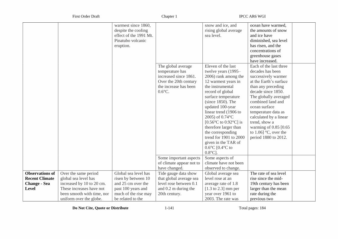
First Order Draft Chapter 1 IPCC AR6 WGI
Do Not Cite, Quote or Distribute 1-141 Total pages: 184
warmest since 1860,
despite the cooling
effect of the 1991 Mt.
Pinatubo volcanic
eruption.
snow and ice, and
rising global average
sea level.
ocean have warmed,
the amounts of snow
and ice have
diminished, sea level
has risen, and the
concentrations of
greenhouse gases
have increased.
The global average
temperature has
increased since 1861.
Over the 20th century
the increase has been
0.6°C.
Eleven of the last
twelve years (1995–
2006) rank among the
12 warmest years in
the instrumental
record of global
surface temperature
(since 1850). The
updated 100-year
linear trend (1906 to
2005) of 0.74°C
[0.56°C to 0.92°C] is
therefore larger than
the corresponding
trend for 1901 to 2000
given in the TAR of
0.6°C [0.4°C to
0.8°C].
Each of the last three
decades has been
successively warmer
at the Earth’s surface
than any preceding
decade since 1850.
The globally averaged
combined land and
ocean surface
temperature data as
calculated by a linear
trend, show a
warming of 0.85 [0.65
to 1.06] °C, over the
period 1880 to 2012.
Some important aspects
of climate appear not to
have changed.
Some aspects of
climate have not been
observed to change.
Observations of
Recent Climate
Change - Sea
Level
Over the same period
global sea level has
increased by 10 to 20 cm.
These increases have not
been smooth with time, nor
uniform over the globe.
Global sea level has
risen by between 10
and 25 cm over the
past 100 years and
much of the rise may
be related to the
Tide gauge data show
that global average sea
level rose between 0.1
and 0.2 m during the
20th century.
Global average sea
level rose at an
average rate of 1.8
[1.3 to 2.3] mm per
year over 1961 to
2003. The rate was
The rate of sea level
rise since the mid-
19th century has been
larger than the mean
rate during the
previous two
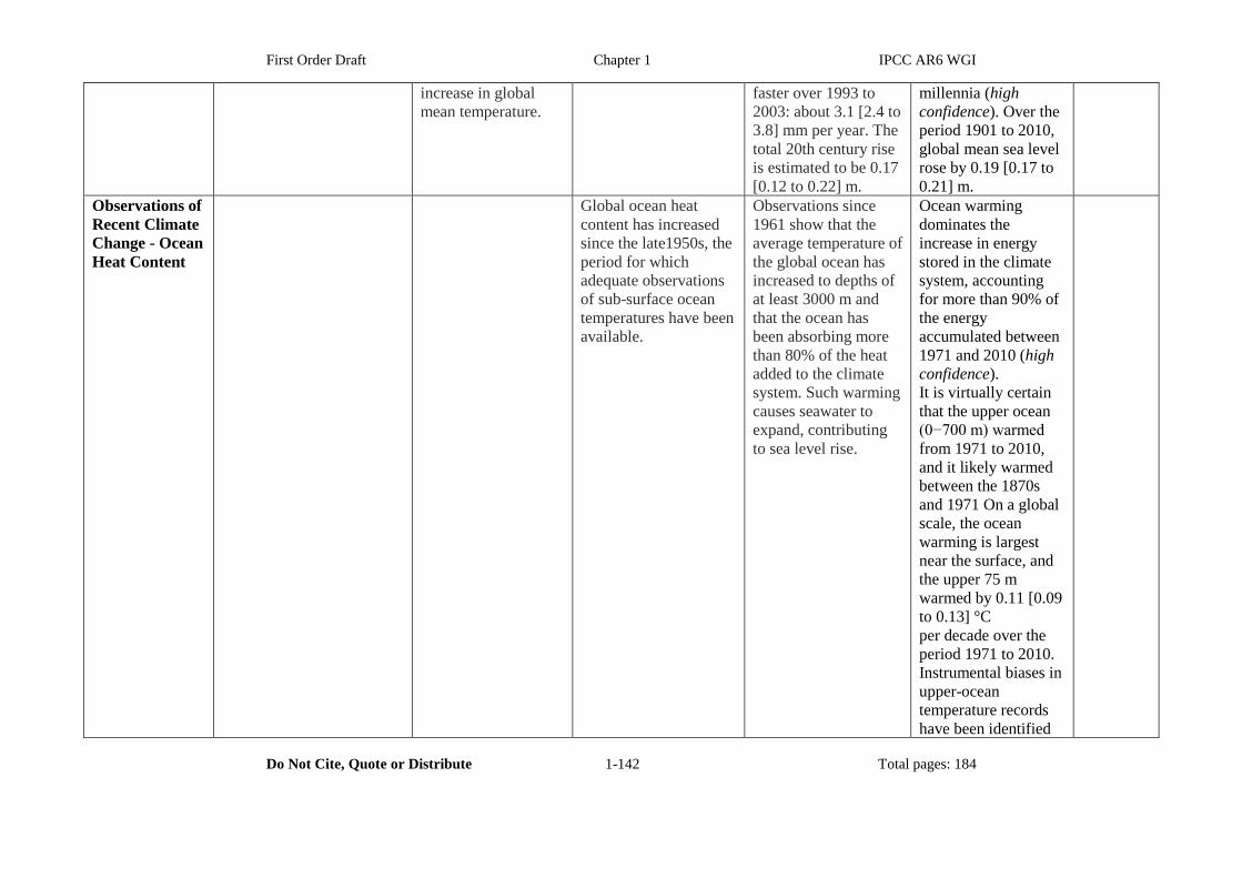
First Order Draft Chapter 1 IPCC AR6 WGI
Do Not Cite, Quote or Distribute 1-142 Total pages: 184
increase in global
mean temperature.
faster over 1993 to
2003: about 3.1 [2.4 to
3.8] mm per year. The
total 20th century rise
is estimated to be 0.17
[0.12 to 0.22] m.
millennia (high
confidence). Over the
period 1901 to 2010,
global mean sea level
rose by 0.19 [0.17 to
0.21] m.
Observations of
Recent Climate
Change - Ocean
Heat Content
Global ocean heat
content has increased
since the late1950s, the
period for which
adequate observations
of sub-surface ocean
temperatures have been
available.
Observations since
1961 show that the
average temperature of
the global ocean has
increased to depths of
at least 3000 m and
that the ocean has
been absorbing more
than 80% of the heat
added to the climate
system. Such warming
causes seawater to
expand, contributing
to sea level rise.
Ocean warming
dominates the
increase in energy
stored in the climate
system, accounting
for more than 90% of
the energy
accumulated between
1971 and 2010 (high
confidence).
It is virtually certain
that the upper ocean
(0−700 m) warmed
from 1971 to 2010,
and it likely warmed
between the 1870s
and 1971 On a global
scale, the ocean
warming is largest
near the surface, and
the upper 75 m
warmed by 0.11 [0.09
to 0.13] °C
per decade over the
period 1971 to 2010.
Instrumental biases in
upper-ocean
temperature records
have been identified
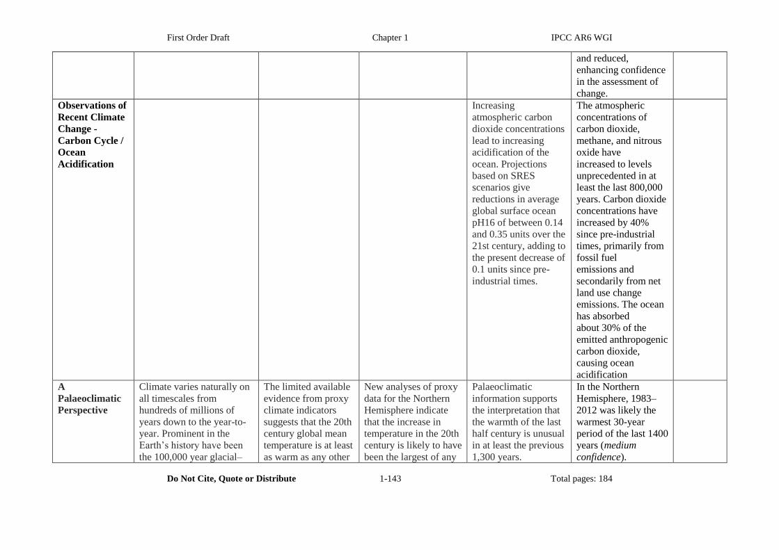
First Order Draft Chapter 1 IPCC AR6 WGI
Do Not Cite, Quote or Distribute 1-143 Total pages: 184
and reduced,
enhancing confidence
in the assessment of
change.
Observations of
Recent Climate
Change -
Carbon Cycle /
Ocean
Acidification
Increasing
atmospheric carbon
dioxide concentrations
lead to increasing
acidification of the
ocean. Projections
based on SRES
scenarios give
reductions in average
global surface ocean
pH16 of between 0.14
and 0.35 units over the
21st century, adding to
the present decrease of
0.1 units since pre-
industrial times.
The atmospheric
concentrations of
carbon dioxide,
methane, and nitrous
oxide have
increased to levels
unprecedented in at
least the last 800,000
years. Carbon dioxide
concentrations have
increased by 40%
since pre-industrial
times, primarily from
fossil fuel
emissions and
secondarily from net
land use change
emissions. The ocean
has absorbed
about 30% of the
emitted anthropogenic
carbon dioxide,
causing ocean
acidification
A
Palaeoclimatic
Perspective
Climate varies naturally on
all timescales from
hundreds of millions of
years down to the year-to-
year. Prominent in the
Earth’s history have been
the 100,000 year glacial–
The limited available
evidence from proxy
climate indicators
suggests that the 20th
century global mean
temperature is at least
as warm as any other
New analyses of proxy
data for the Northern
Hemisphere indicate
that the increase in
temperature in the 20th
century is likely to have
been the largest of any
Palaeoclimatic
information supports
the interpretation that
the warmth of the last
half century is unusual
in at least the previous
1,300 years.
In the Northern
Hemisphere, 1983–
2012 was likely the
warmest 30-year
period of the last 1400
years (medium
confidence).
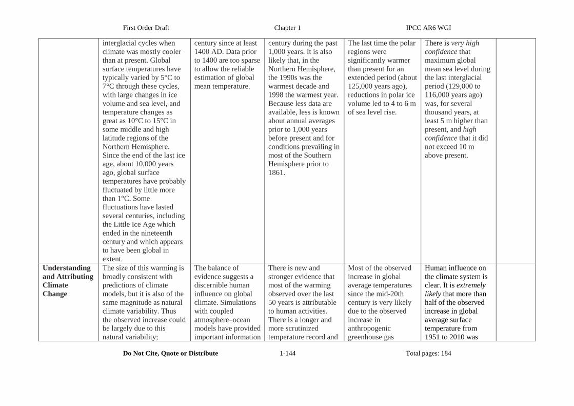
First Order Draft Chapter 1 IPCC AR6 WGI
Do Not Cite, Quote or Distribute 1-144 Total pages: 184
interglacial cycles when
climate was mostly cooler
than at present. Global
surface temperatures have
typically varied by 5°C to
7°C through these cycles,
with large changes in ice
volume and sea level, and
temperature changes as
great as 10°C to 15°C in
some middle and high
latitude regions of the
Northern Hemisphere.
Since the end of the last ice
age, about 10,000 years
ago, global surface
temperatures have probably
fluctuated by little more
than 1°C. Some
fluctuations have lasted
several centuries, including
the Little Ice Age which
ended in the nineteenth
century and which appears
to have been global in
extent.
century since at least
1400 AD. Data prior
to 1400 are too sparse
to allow the reliable
estimation of global
mean temperature.
century during the past
1,000 years. It is also
likely that, in the
Northern Hemisphere,
the 1990s was the
warmest decade and
1998 the warmest year.
Because less data are
available, less is known
about annual averages
prior to 1,000 years
before present and for
conditions prevailing in
most of the Southern
Hemisphere prior to
1861.
The last time the polar
regions were
significantly warmer
than present for an
extended period (about
125,000 years ago),
reductions in polar ice
volume led to 4 to 6 m
of sea level rise.
There is very high
confidence that
maximum global
mean sea level during
the last interglacial
period (129,000 to
116,000 years ago)
was, for several
thousand years, at
least 5 m higher than
present, and high
confidence that it did
not exceed 10 m
above present.
Understanding
and Attributing
Climate
Change
The size of this warming is
broadly consistent with
predictions of climate
models, but it is also of the
same magnitude as natural
climate variability. Thus
the observed increase could
be largely due to this
natural variability;
The balance of
evidence suggests a
discernible human
influence on global
climate. Simulations
with coupled
atmosphere–ocean
models have provided
important information
There is new and
stronger evidence that
most of the warming
observed over the last
50 years is attributable
to human activities.
There is a longer and
more scrutinized
temperature record and
Most of the observed
increase in global
average temperatures
since the mid-20th
century is very likely
due to the observed
increase in
anthropogenic
greenhouse gas
Human influence on
the climate system is
clear. It is extremely
likely that more than
half of the observed
increase in global
average surface
temperature from
1951 to 2010 was
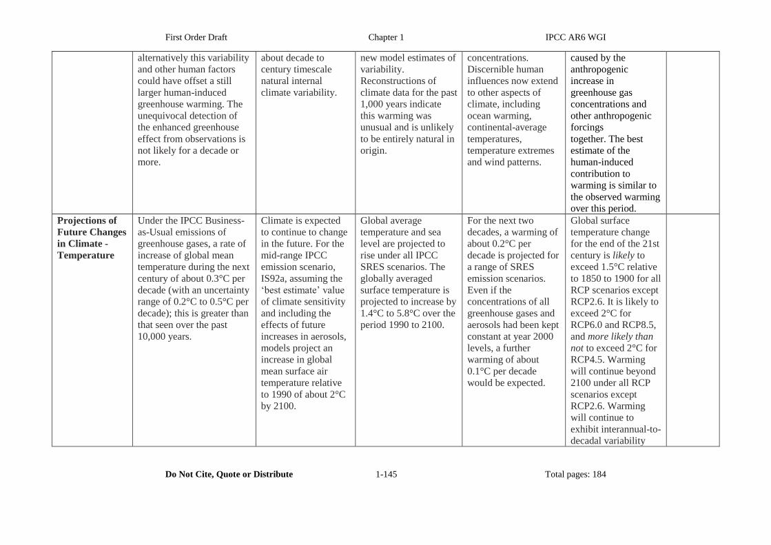
First Order Draft Chapter 1 IPCC AR6 WGI
Do Not Cite, Quote or Distribute 1-145 Total pages: 184
alternatively this variability
and other human factors
could have offset a still
larger human-induced
greenhouse warming. The
unequivocal detection of
the enhanced greenhouse
effect from observations is
not likely for a decade or
more.
about decade to
century timescale
natural internal
climate variability.
new model estimates of
variability.
Reconstructions of
climate data for the past
1,000 years indicate
this warming was
unusual and is unlikely
to be entirely natural in
origin.
concentrations.
Discernible human
influences now extend
to other aspects of
climate, including
ocean warming,
continental-average
temperatures,
temperature extremes
and wind patterns.
caused by the
anthropogenic
increase in
greenhouse gas
concentrations and
other anthropogenic
forcings
together. The best
estimate of the
human-induced
contribution to
warming is similar to
the observed warming
over this period.
Projections of
Future Changes
in Climate -
Temperature
Under the IPCC Business-
as-Usual emissions of
greenhouse gases, a rate of
increase of global mean
temperature during the next
century of about 0.3°C per
decade (with an uncertainty
range of 0.2°C to 0.5°C per
decade); this is greater than
that seen over the past
10,000 years.
Climate is expected
to continue to change
in the future. For the
mid-range IPCC
emission scenario,
IS92a, assuming the
‘best estimate’ value
of climate sensitivity
and including the
effects of future
increases in aerosols,
models project an
increase in global
mean surface air
temperature relative
to 1990 of about 2°C
by 2100.
Global average
temperature and sea
level are projected to
rise under all IPCC
SRES scenarios. The
globally averaged
surface temperature is
projected to increase by
1.4°C to 5.8°C over the
period 1990 to 2100.
For the next two
decades, a warming of
about 0.2°C per
decade is projected for
a range of SRES
emission scenarios.
Even if the
concentrations of all
greenhouse gases and
aerosols had been kept
constant at year 2000
levels, a further
warming of about
0.1°C per decade
would be expected.
Global surface
temperature change
for the end of the 21st
century is likely to
exceed 1.5°C relative
to 1850 to 1900 for all
RCP scenarios except
RCP2.6. It is likely to
exceed 2°C for
RCP6.0 and RCP8.5,
and more likely than
not to exceed 2°C for
RCP4.5. Warming
will continue beyond
2100 under all RCP
scenarios except
RCP2.6. Warming
will continue to
exhibit interannual-to-
decadal variability

First Order Draft Chapter 1 IPCC AR6 WGI
Do Not Cite, Quote or Distribute 1-146 Total pages: 184
and will not be
regionally uniform.
Confidence in the
ability of models to
project future climate
has increased.
There is now higher
confidence in
projected patterns of
warming and other
regional-scale
features, including
changes in wind
patterns, precipitation
and some aspects of
extremes and of ice.
Climate models have
improved since the
AR4. Models
reproduce observed
continental-scale
surface temperature
patterns and trends
over many decades,
including the more
rapid warming since
the mid-20th century
and the cooling
immediately
following large
volcanic eruptions.
Anthropogenic climate
change will persist for
many centuries.
Anthropogenic
warming and sea level
rise would continue
for centuries, even if
greenhouse gas
concentrations were to
be stabilised.
Cumulative emissions
of CO2 largely
determine global
mean surface
warming by the late
21st
century and beyond.
Most aspects of
climate change will
persist for many
centuries even if
emissions of CO2 are
stopped. This
represents a
substantial multi-
century climate
change commitment
created by past,

First Order Draft Chapter 1 IPCC AR6 WGI
Do Not Cite, Quote or Distribute 1-147 Total pages: 184
present and future
emissions of CO2.
Projections of
Future Changes
in Climate - Sea
Level
An average rate of global
mean sea level rise of about
6 cm per decade over the
next century (with an
uncertainty range of 3 to 10
cm per decade) is
projected.
Models project a sea
level rise of 50 cm
from the present to
2100.
Global mean sea level
is projected to rise by
0.09 to 0.88 m between
1990 and 2100.
Global sea level rise
for the range of
scenarios is projected
as 0.18 to 0.59 m by
the end of the 21st
century.
Global mean sea level
rise for 2081–2100
relative to 1986–2005
will likely be in the
ranges of 0.26 to 0.55
m for RCP2.6, 0.32 to
0.63 m for RCP4.5,
0.33 to 0.63 m for
RCP6.0, and 0.45 to
0.82 m for RCP8.5.
Projections of
Future Changes
in Climate -
AMOC
Most simulations
show a reduction in
the strength of the
north Atlantic
thermohaline
circulation. Future
unexpected, large and
rapid climate system
changes are difficult
to predict. These arise
from the non-linear
nature of the climate
system. Examples
include rapid
circulation changes in
the North Atlantic.
Most models show
weakening of the ocean
thermohaline
circulation which leads
to a reduction of the
heat transport into high
latitudes of the
Northern Hemisphere.
However, even in
models where the
thermohaline
circulation weakens,
there is still a warming
over Europe due to
increased greenhouse
gases. The current
projections using
climate models do not
exhibit a complete
shut-down of the
thermohaline
circulation by 2100.
Beyond 2100, the
Based on current
model simulations, it
is very likely that the
meridional overturning
circulation (MOC) of
the Atlantic Ocean
will slow down during
the 21st century. It is
very unlikely that the
MOC will undergo a
large abrupt transition
during the 21st
century. Longer-term
changes in the MOC
cannot be assessed
with confidence.
It is that the Atlantic
Meridional
Overturning
Circulation (AMOC)
will weaken over the
21st century. It is very
unlikely that the
AMOC will undergo
an abrupt transition or
collapse in the 21st
century for the
scenarios considered.
There is low
confidence in
assessing the
evolution of the
AMOC beyond the
21st century because
of the limited number
of analyses and
equivocal results.
However, a collapse
beyond the 21st
First Order Draft Chapter 1 IPCC AR6 WGI
Do Not Cite, Quote or Distribute 1-148 Total pages: 184
thermohaline
circulation could
completely, and
possibly irreversibly,
shut-down in either
hemisphere if the
change in radiative
forcing is large enough
and applied long
enough.
century for large
sustained warming
cannot be excluded.
1
[END TABLE 1.A.1 HERE] 2
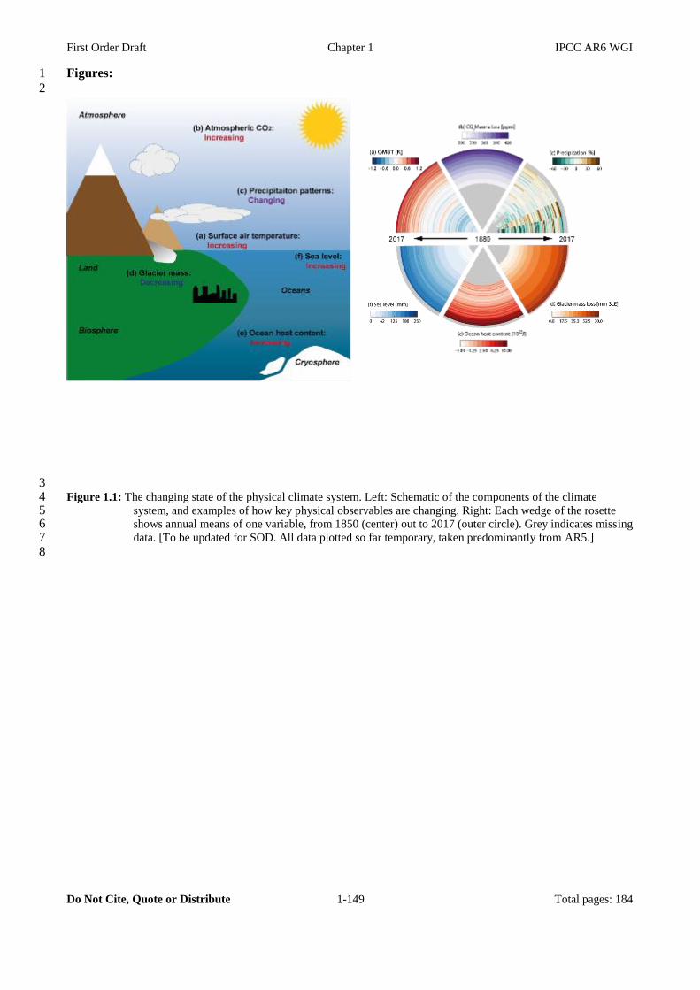
First Order Draft Chapter 1 IPCC AR6 WGI
Do Not Cite, Quote or Distribute 1-149 Total pages: 184
Figures: 1
2
3 Figure 1.1: The changing state of the physical climate system. Left: Schematic of the components of the climate 4
system, and examples of how key physical observables are changing. Right: Each wedge of the rosette 5 shows annual means of one variable, from 1850 (center) out to 2017 (outer circle). Grey indicates missing 6 data. [To be updated for SOD. All data plotted so far temporary, taken predominantly from AR5.] 7
8
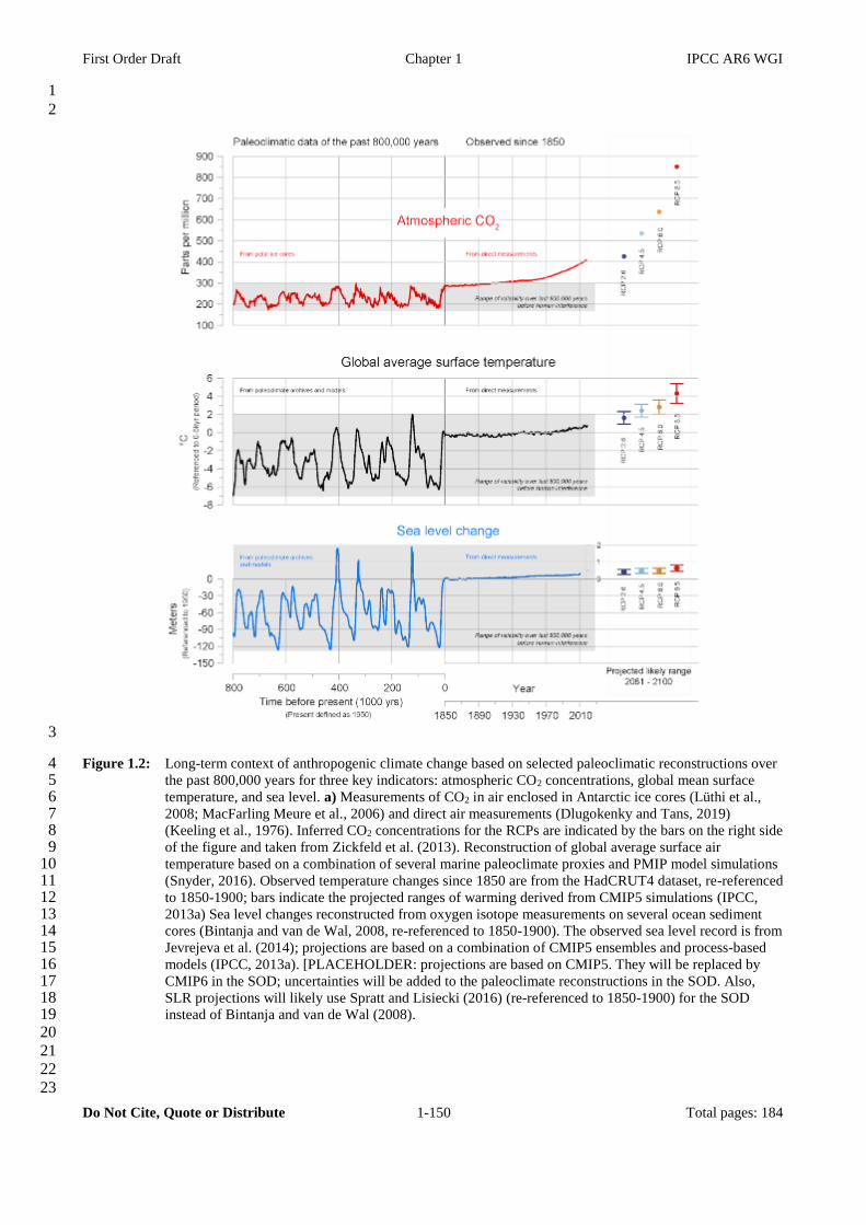
First Order Draft Chapter 1 IPCC AR6 WGI
Do Not Cite, Quote or Distribute 1-150 Total pages: 184
1
2
3
Figure 1.2: Long-term context of anthropogenic climate change based on selected paleoclimatic reconstructions over 4 the past 800,000 years for three key indicators: atmospheric CO2 concentrations, global mean surface 5 temperature, and sea level. a) Measurements of CO2 in air enclosed in Antarctic ice cores (Lüthi et al., 6 2008; MacFarling Meure et al., 2006) and direct air measurements (Dlugokenky and Tans, 2019) 7 (Keeling et al., 1976). Inferred CO2 concentrations for the RCPs are indicated by the bars on the right side 8 of the figure and taken from Zickfeld et al. (2013). Reconstruction of global average surface air 9 temperature based on a combination of several marine paleoclimate proxies and PMIP model simulations 10 (Snyder, 2016). Observed temperature changes since 1850 are from the HadCRUT4 dataset, re-referenced 11 to 1850-1900; bars indicate the projected ranges of warming derived from CMIP5 simulations (IPCC, 12 2013a) Sea level changes reconstructed from oxygen isotope measurements on several ocean sediment 13 cores (Bintanja and van de Wal, 2008, re-referenced to 1850-1900). The observed sea level record is from 14 Jevrejeva et al. (2014); projections are based on a combination of CMIP5 ensembles and process-based 15 models (IPCC, 2013a). [PLACEHOLDER: projections are based on CMIP5. They will be replaced by 16 CMIP6 in the SOD; uncertainties will be added to the paleoclimate reconstructions in the SOD. Also, 17 SLR projections will likely use Spratt and Lisiecki (2016) (re-referenced to 1850-1900) for the SOD 18 instead of Bintanja and van de Wal (2008). 19
20
21
22
23
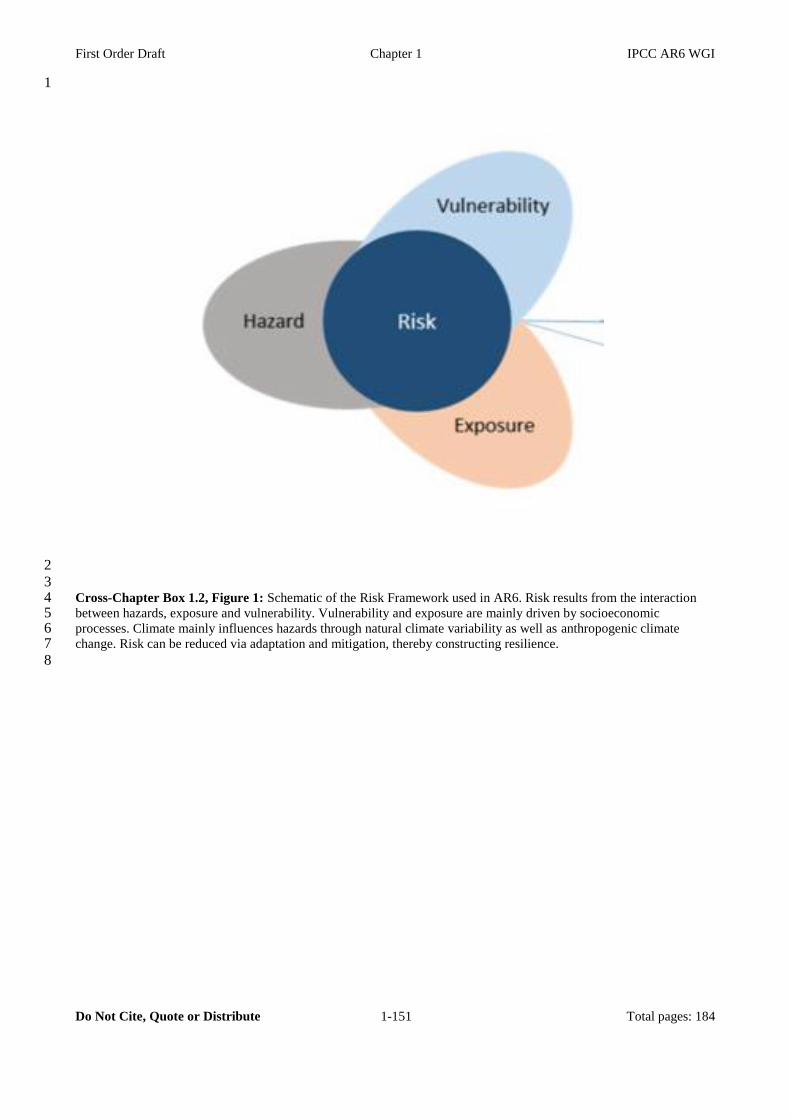
First Order Draft Chapter 1 IPCC AR6 WGI
Do Not Cite, Quote or Distribute 1-151 Total pages: 184
1
2
3 Cross-Chapter Box 1.2, Figure 1: Schematic of the Risk Framework used in AR6. Risk results from the interaction 4 between hazards, exposure and vulnerability. Vulnerability and exposure are mainly driven by socioeconomic 5 processes. Climate mainly influences hazards through natural climate variability as well as anthropogenic climate 6 change. Risk can be reduced via adaptation and mitigation, thereby constructing resilience. 7
8
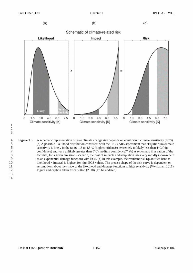
First Order Draft Chapter 1 IPCC AR6 WGI
Do Not Cite, Quote or Distribute 1-152 Total pages: 184
1 2 3
Figure 1.3: A schematic representation of how climate change risk depends on equilibrium climate sensitivity (ECS). 4 (a) A possible likelihood distribution consistent with the IPCC AR5 assessment that “Equilibrium climate 5 sensitivity is likely in the range 1.5 to 4.5°C (high confidence), extremely unlikely less than 1°C (high 6 confidence) and very unlikely greater than 6°C (medium confidence)”. (b) A schematic illustration of the 7 fact that, for a given emissions scenario, the cost of impacts and adaptation rises very rapidly (shown here 8 as an exponential damage function) with ECS. (c) In this example, the resultant risk (quantified here as 9 likelihood × impact) is highest for high ECS values. The precise shape of the risk curve is dependent on 10 assumptions about the shape of the likelihood and damage functions at high sensitivity (Weitzman, 2011). 11 Figure and caption taken from Sutton (2018) [To be updated] 12
13
14
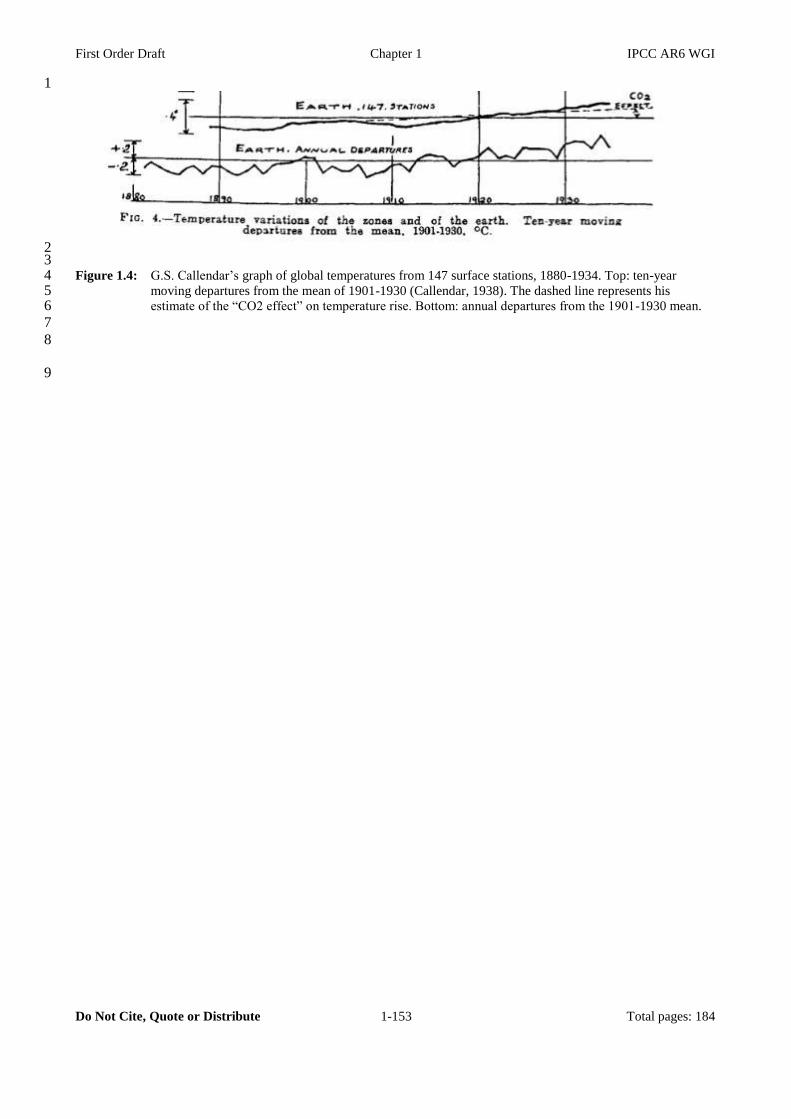
First Order Draft Chapter 1 IPCC AR6 WGI
Do Not Cite, Quote or Distribute 1-153 Total pages: 184
1
2 3
Figure 1.4: G.S. Callendar’s graph of global temperatures from 147 surface stations, 1880-1934. Top: ten-year 4 moving departures from the mean of 1901-1930 (Callendar, 1938). The dashed line represents his 5 estimate of the “CO2 effect” on temperature rise. Bottom: annual departures from the 1901-1930 mean. 6
7
8
9

First Order Draft Chapter 1 IPCC AR6 WGI
Do Not Cite, Quote or Distribute 1-154 Total pages: 184
1
2 Box 1.1, Figure 1.1: The IPCC AR6 approach for characterizing understanding and uncertainty in assessment findings. 3
This diagram illustrates the step-by-step process authors use to evaluate and communicate the state 4 of knowledge in their assessment (Mastrandrea et al., 2010). Authors present evidence/agreement, 5 confidence, or likelihood terms with assessment conclusions, communicating their expert 6 judgments accordingly. Example conclusions are drawn from the IPCC WGI AR5 [adapted, from 7 Mach et al. (2017)]. 8
9
10
11
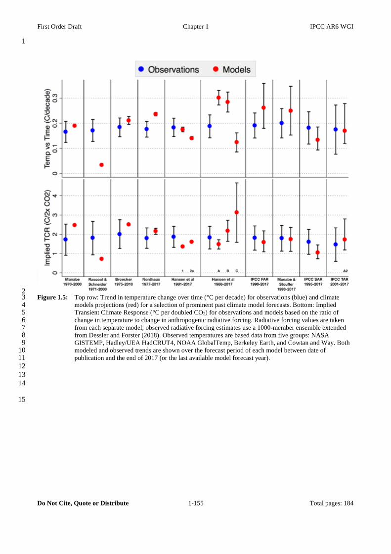
First Order Draft Chapter 1 IPCC AR6 WGI
Do Not Cite, Quote or Distribute 1-155 Total pages: 184
1
2 Figure 1.5: Top row: Trend in temperature change over time (°C per decade) for observations (blue) and climate 3
models projections (red) for a selection of prominent past climate model forecasts. Bottom: Implied 4 Transient Climate Response (°C per doubled CO2) for observations and models based on the ratio of 5 change in temperature to change in anthropogenic radiative forcing. Radiative forcing values are taken 6 from each separate model; observed radiative forcing estimates use a 1000-member ensemble extended 7 from Dessler and Forster (2018). Observed temperatures are based data from five groups: NASA 8 GISTEMP, Hadley/UEA HadCRUT4, NOAA GlobalTemp, Berkeley Earth, and Cowtan and Way. Both 9 modeled and observed trends are shown over the forecast period of each model between date of 10 publication and the end of 2017 (or the last available model forecast year). 11
12
13
14
15

First Order Draft Chapter 1 IPCC AR6 WGI
Do Not Cite, Quote or Distribute 1-156 Total pages: 184
1
2 Figure 1.6: Range of projected temperature change for 1990-2030 for regions defined in IPCC FAR (1990). Darker 3
red bands show the range of projected change given for the best estimate of 1.8°C global warming since 4 pre-industrial, faint bands show the range scaled for lower and higher estimates of global warming. Blue 5 lines show the observations from several global temperature gridded datasets, red lines show the linear 6 trends in those datasets for 1990-2018 extrapolated to 2030. Observed datasets are: HadCRUT4.6, 7 Cowtan and Way, GISTEMP, Berkeley Earth and University of Delaware. 8
9

First Order Draft Chapter 1 IPCC AR6 WGI
Do Not Cite, Quote or Distribute 1-157 Total pages: 184
Figure 1.30: 1 Figure 1.7: Schematic of climate data coverage through time, indicating time span covered by different sources, as 2
well as density of coverage from a given source (i.e. satellite coverage increasing through time, whereas 3 ground-based instrumental coverage is decreasing in recent years, and corals and tropical ice cores are a 4 “vanishing” archive). 5

First Order Draft Chapter 1 IPCC AR6 WGI
Do Not Cite, Quote or Distribute 1-158 Total pages: 184
Figure 1.31: 1
2 Figure 1.8: The population distributions of global climate models in terms of nominal horizontal atmospheric and 3
oceanic resolutions. (a) (b) Models used for future projection scenario experiments in CMIP6 and CMIP5 4 model intercomparison projects respectively. (c) (d) Models used for assessing biogeochemical feedbacks 5 in CMIP6 and CMIP5.The CMIP6 models are those registered as of December, 2018 6 (https://rawgit.com/WCRP-CMIP/CMIP6_CVs/master/src/CMIP6_source_id.html), while the CMIP5 7 models are those available at the IPCC Data Distribution Centre AR5 Reference Snapshot 8 (http://www.ipcc-data.org/sim/gcm_monthly/AR5/Reference-Archive.html). [To be updated]. 9

First Order Draft Chapter 1 IPCC AR6 WGI
Do Not Cite, Quote or Distribute 1-159 Total pages: 184
1
2 3 Figure 1.9: A world map showing the increased diversity of modelling centres contributing to CMIP (idea, use 4
different symbols or colors or sizes for climate centres that participated in CMIP3, CMIP5, CMIP6), and 5 also modelling contributions to CORDEX. [TO BE UPDATED, CORDEX information is incomplete] 6
7
Boulder
NCAR
Victoria
CCCMa
MelbourneCSIRO/BMRC
Tsukuba
MRI
Paulista
INPE
EC-Earth
Livermore
ES3M Princeton
NOAA-GFDL
Toronto
UofT
New York
NASA-GISS
Exeter
MOHC
Paris
IPSL
Tokyo
MIROC
Taipei
AS-RCEC
Nanjin
NUIST
Qingdao
FIO-QNLM
Seogwipo
NIMS-KMA
Seoul
SNU
ToulouseCNRM-CERFACS
Moscow
INM
Hamburg
MPI
Beijing
BCC
BNU
CAS
CAMS
THU
Bologna
CMCC
Bremerhaven
AWI
Pune
CCCR-IITM
BergenNCC
CORDEXCity Institution Participation to: New Cordex partner:CMIP 1 CMIP 2 CMIP 3 CMIP 5 CMIP 6

First Order Draft Chapter 1 IPCC AR6 WGI
Do Not Cite, Quote or Distribute 1-160 Total pages: 184
Figure 1.32: 1
2 Figure 1.10: Illustration of common types of model ensemble, simulating the time evolution of a quantity V (such as 3
surface temperature or precipitation). (a) Multi-model ensemble, where each model has its own 4 realization of the processes affecting V, and its own internal variability around the baseline value (dashed 5 line). (b) Initial condition ensemble, where several realizations from a single model are compared. These 6 differ only by minute perturbations to the initial conditions of the simulation, such that over time, internal 7 variability will progress differently in each ensemble member. (c) Perturbed physics ensemble, which 8 also compares realizations from a single model, but where one or more quantities that may affect V are 9 systematically changed to allow for a quantification of the impact of those quantities on the model results. 10
11
12
13
14
15

First Order Draft Chapter 1 IPCC AR6 WGI
Do Not Cite, Quote or Distribute 1-161 Total pages: 184
1 Figure 1.11: Structure of the CMIP6 multi-model intercomparison project (Eyring et al., 2016a). The centre shows the 2
common DECK and historical experiments that all participating models must perform, the outer circle 3 shows the topics covered by the endorsed MIPs. 4
5
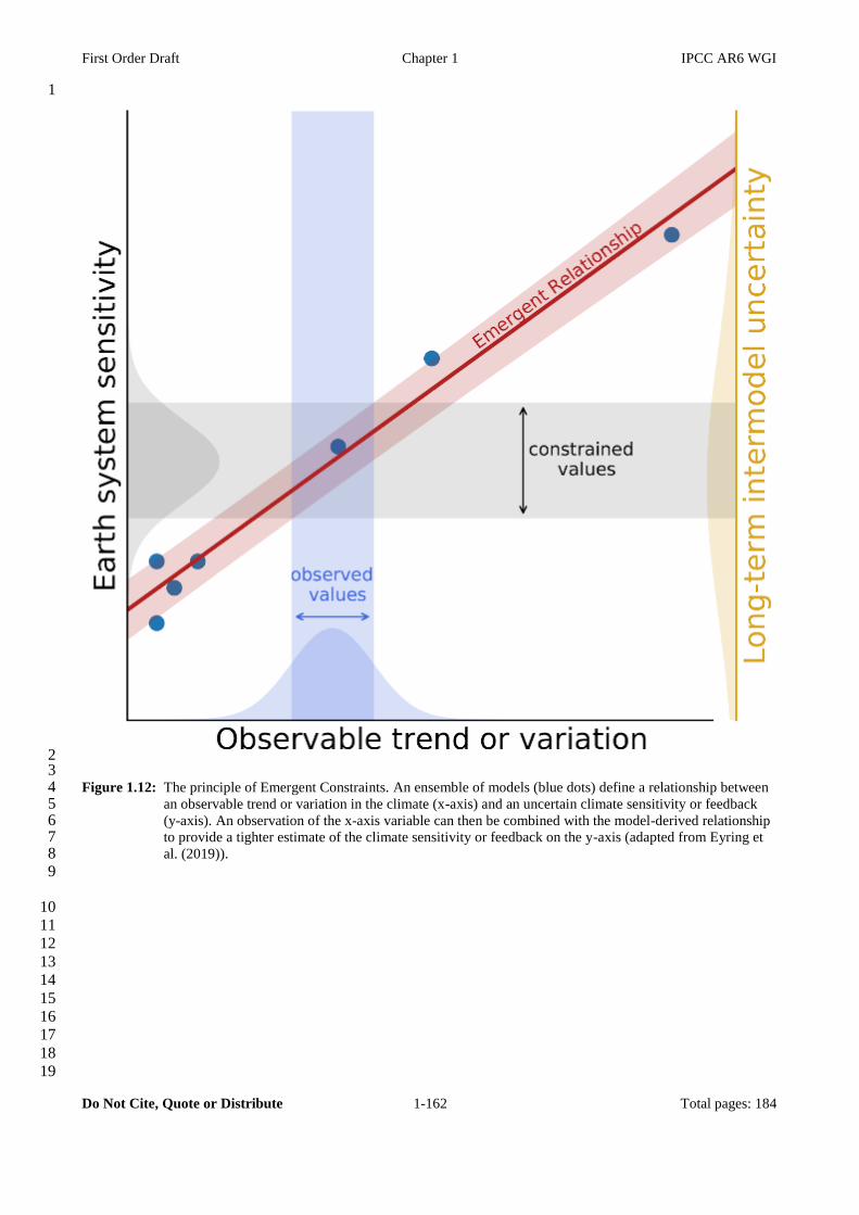
First Order Draft Chapter 1 IPCC AR6 WGI
Do Not Cite, Quote or Distribute 1-162 Total pages: 184
1
2 3 Figure 1.12: The principle of Emergent Constraints. An ensemble of models (blue dots) define a relationship between 4
an observable trend or variation in the climate (x-axis) and an uncertain climate sensitivity or feedback 5 (y-axis). An observation of the x-axis variable can then be combined with the model-derived relationship 6 to provide a tighter estimate of the climate sensitivity or feedback on the y-axis (adapted from Eyring et 7 al. (2019)). 8
9
10
11
12
13
14
15
16
17
18
19
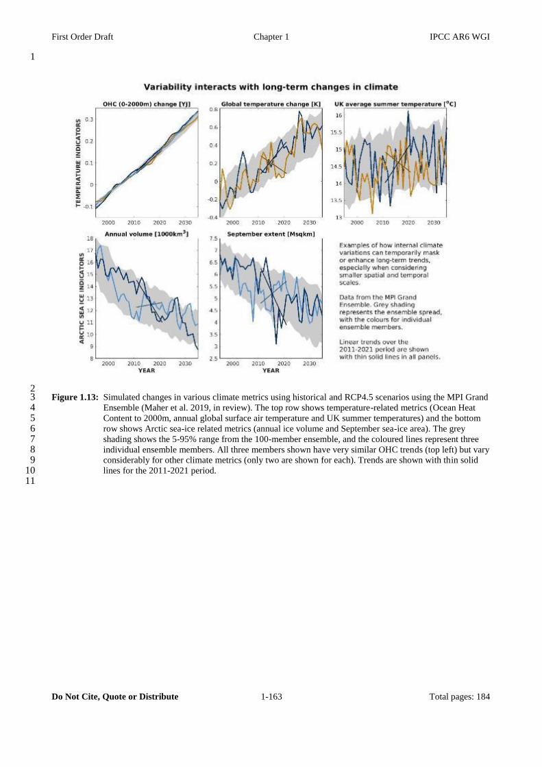
First Order Draft Chapter 1 IPCC AR6 WGI
Do Not Cite, Quote or Distribute 1-163 Total pages: 184
1
2 Figure 1.13: Simulated changes in various climate metrics using historical and RCP4.5 scenarios using the MPI Grand 3
Ensemble (Maher et al. 2019, in review). The top row shows temperature-related metrics (Ocean Heat 4 Content to 2000m, annual global surface air temperature and UK summer temperatures) and the bottom 5 row shows Arctic sea-ice related metrics (annual ice volume and September sea-ice area). The grey 6 shading shows the 5-95% range from the 100-member ensemble, and the coloured lines represent three 7 individual ensemble members. All three members shown have very similar OHC trends (top left) but vary 8 considerably for other climate metrics (only two are shown for each). Trends are shown with thin solid 9 lines for the 2011-2021 period. 10
11
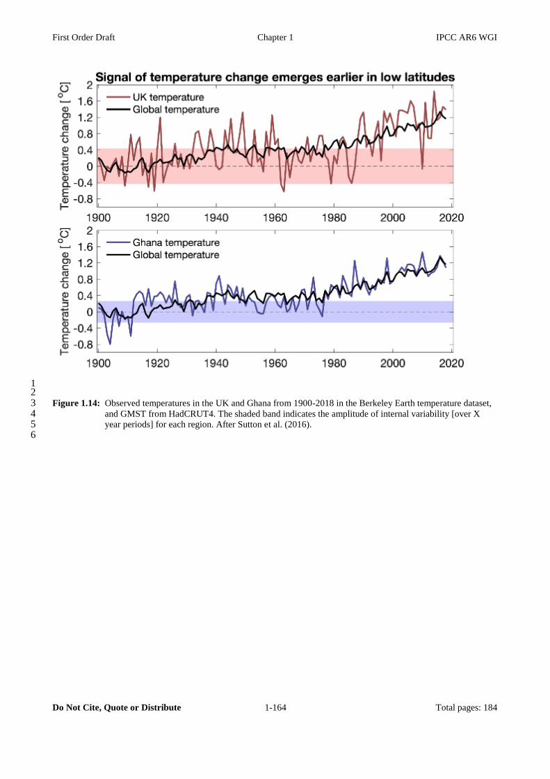
First Order Draft Chapter 1 IPCC AR6 WGI
Do Not Cite, Quote or Distribute 1-164 Total pages: 184
1 2 Figure 1.14: Observed temperatures in the UK and Ghana from 1900-2018 in the Berkeley Earth temperature dataset, 3
and GMST from HadCRUT4. The shaded band indicates the amplitude of internal variability [over X 4 year periods] for each region. After Sutton et al. (2016). 5
6
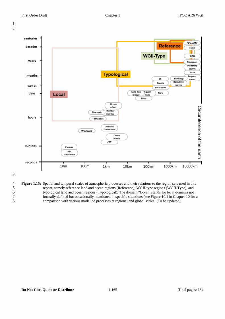
First Order Draft Chapter 1 IPCC AR6 WGI
Do Not Cite, Quote or Distribute 1-165 Total pages: 184
1
2
3
Figure 1.15: Spatial and temporal scales of atmospheric processes and their relations to the region sets used in this 4 report, namely reference land and ocean regions (Reference), WGII-type regions (WGII-Type), and 5 typological land and ocean regions (Typological). The domain “Local” stands for local domains not 6 formally defined but occasionally mentioned in specific situations (see Figure 10.1 in Chapter 10 for a 7 comparison with various modelled processes at regional and global scales. [To be updated] 8

First Order Draft Chapter 1 IPCC AR6 WGI
Do Not Cite, Quote or Distribute 1-166 Total pages: 184
1
Figure 1.16: Main types of regions used in this report. (a): AR6 WGI reference set of land and ocean regions, used 2 throughout this report. There are 37 land regions and 12 ocean regions in total. Notice that SPO, NPO and 3 EPO continue on the left side of the map, indicated with an asterisk. For the meaning of the acronyms and 4 details of each region, see the Atlas. [The reference set of ocean regions are still tentative and will be 5 confirmed in the SOD]. (b): Example of typological land regions. Land monsoon domains adopted in 6 Chapter 8 [to be updated accordingly with chapter 8], as defined in AR5 WGI. The acronyms stand for 7 North America Monsoon System (NAMS), North Africa (NAF), Southern Asia (SAS), East Asian 8 Summer (EAS), South America Monsoon System (SAMS), South Africa (SAF), and Australian-Maritime 9 Continent (AUSMC). All the regions are within 40°S to 40°N. For further details, see Chap. 8. (c): 10 Example of typological ocean regions. Ocean biome zones used in Chapters 5 and 9, which reflect the 11 historical mean of the dynamics. The following regions are displayed: (0) Northern Hemisphere High 12 Latitudes, (1) Northern Hemisphere Subtropics, (2) Equatorial, (3) Southern Hemisphere Subtropics, (4) 13 Southern Hemisphere High Latitudes, (5) Arabian Sea, (6) Eastern Boundaries, (7) Amazon River, (8) 14 Gulf of Mexico and (9) Indonesian Flowthrough. For more information, see Chapter 5. (d): WGII-type 15 regions used in Chapter 12, as defined in AR5 WGII Part B. 16
17

First Order Draft Chapter 1 IPCC AR6 WGI
Do Not Cite, Quote or Distribute 1-167 Total pages: 184
1
2 3 Figure 1.17: Global mean surface air temperature from the range of CMIP5 historical simulations (1861-2005) using 4
absolute values (top) and anomalies relative to two different baselines (bottom). In order to compare the 5 models with each other and with reanalyses and observations (colours), a baseline or reference period has 6 to be chosen, and that choice can affect the comparison. (Taken from Hawkins and Sutton, 2016, and to 7 be updated with CMIP6 data.) 8
9
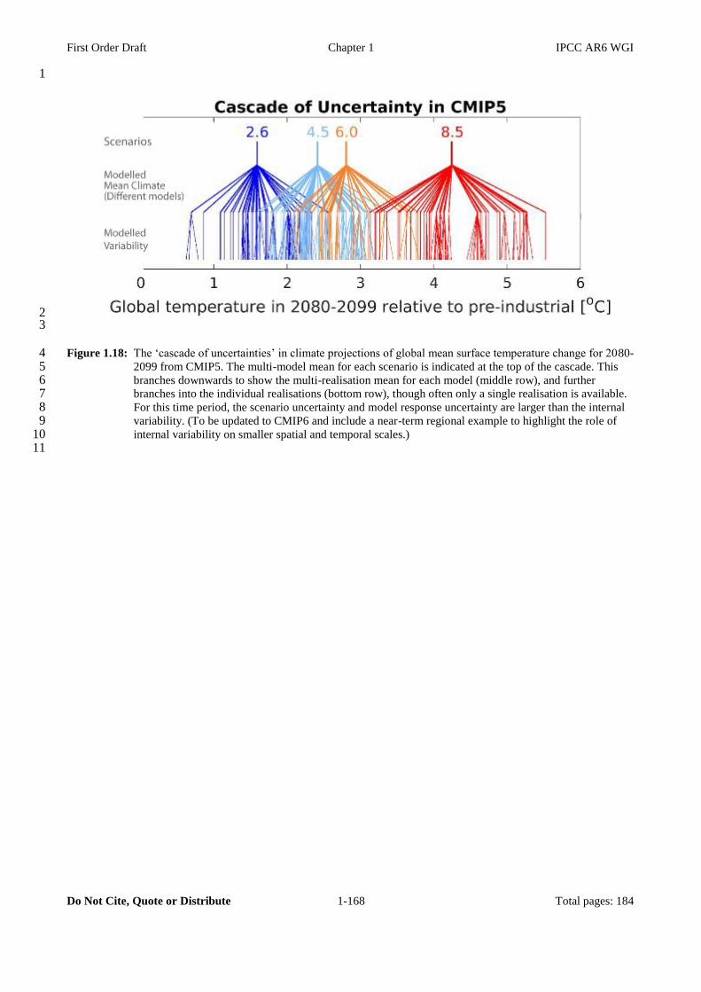
First Order Draft Chapter 1 IPCC AR6 WGI
Do Not Cite, Quote or Distribute 1-168 Total pages: 184
1
2 3
Figure 1.18: The ‘cascade of uncertainties’ in climate projections of global mean surface temperature change for 2080-4 2099 from CMIP5. The multi-model mean for each scenario is indicated at the top of the cascade. This 5 branches downwards to show the multi-realisation mean for each model (middle row), and further 6 branches into the individual realisations (bottom row), though often only a single realisation is available. 7 For this time period, the scenario uncertainty and model response uncertainty are larger than the internal 8 variability. (To be updated to CMIP6 and include a near-term regional example to highlight the role of 9 internal variability on smaller spatial and temporal scales.) 10
11

First Order Draft Chapter 1 IPCC AR6 WGI
Do Not Cite, Quote or Distribute 1-169 Total pages: 184
1
2
3
4 Figure 1.19: The Dimensions of Integration (DI) across Chapters and Working Groups in the IPCC AR6 assessment 5
report. Building on the Synthesis Reports of the Fifth IPCC Assessment report (background image detail) 6 this report adopts three explicit dimensions of integration to integrate knowledge across chapters and 7 Working Groups. The first dimension (DI 1) are scenarios, the second dimension (DI 2) are global-mean 8 temperature levels relative to pre-industrial levels and the third dimension (DI 3) are cumulative CO2 9 emissions. 10
11
12
13
14
15
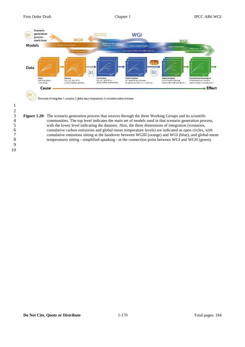
First Order Draft Chapter 1 IPCC AR6 WGI
Do Not Cite, Quote or Distribute 1-170 Total pages: 184
1
2 Figure 1.20: The scenario generation process that weaves through the three Working Groups and its scientific 3
communities. The top level indicates the main set of models used in that scenario generation process, 4 with the lower level indicating the datasets. Also, the three dimensions of integration (scenarios, 5 cumulative carbon emissions and global-mean temperature levels) are indicated as open circles, with 6 cumulative emissions sitting at the handover between WGIII (orange) and WGI (blue), and global-mean 7 temperatures sitting - simplified speaking - at the connection point between WGI and WGII (green). 8
9
10
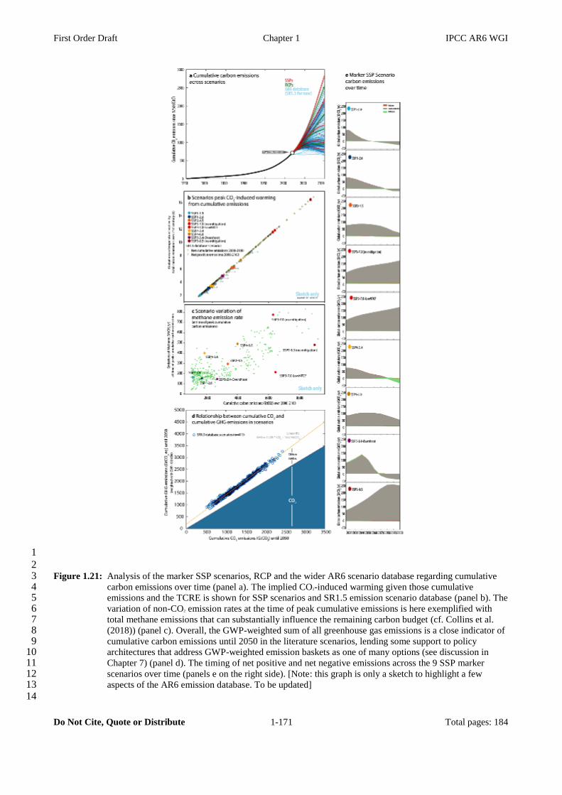
First Order Draft Chapter 1 IPCC AR6 WGI
Do Not Cite, Quote or Distribute 1-171 Total pages: 184
1
2 Figure 1.21: Analysis of the marker SSP scenarios, RCP and the wider AR6 scenario database regarding cumulative 3
carbon emissions over time (panel a). The implied CO2-induced warming given those cumulative 4 emissions and the TCRE is shown for SSP scenarios and SR1.5 emission scenario database (panel b). The 5 variation of non-CO2 emission rates at the time of peak cumulative emissions is here exemplified with 6 total methane emissions that can substantially influence the remaining carbon budget (cf. Collins et al. 7 (2018)) (panel c). Overall, the GWP-weighted sum of all greenhouse gas emissions is a close indicator of 8 cumulative carbon emissions until 2050 in the literature scenarios, lending some support to policy 9 architectures that address GWP-weighted emission baskets as one of many options (see discussion in 10 Chapter 7) (panel d). The timing of net positive and net negative emissions across the 9 SSP marker 11 scenarios over time (panels e on the right side). [Note: this graph is only a sketch to highlight a few 12 aspects of the AR6 emission database. To be updated] 13
14
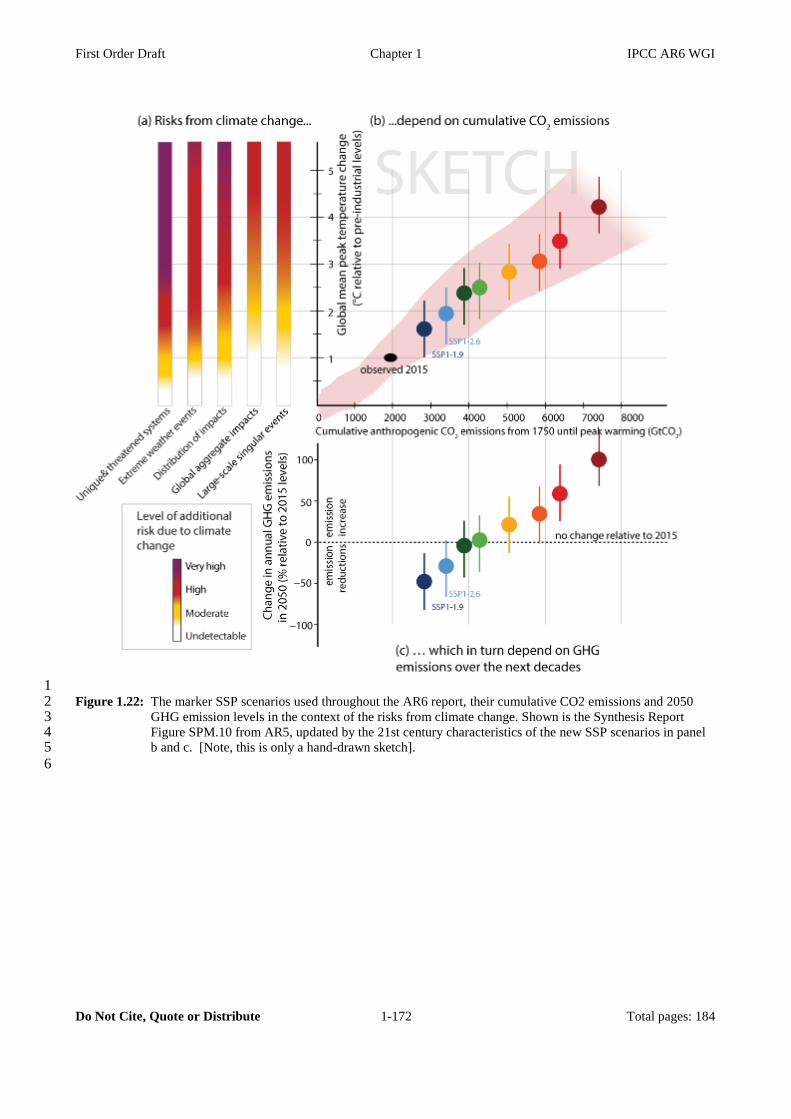
First Order Draft Chapter 1 IPCC AR6 WGI
Do Not Cite, Quote or Distribute 1-172 Total pages: 184
1 Figure 1.22: The marker SSP scenarios used throughout the AR6 report, their cumulative CO2 emissions and 2050 2
GHG emission levels in the context of the risks from climate change. Shown is the Synthesis Report 3 Figure SPM.10 from AR5, updated by the 21st century characteristics of the new SSP scenarios in panel 4 b and c. [Note, this is only a hand-drawn sketch]. 5
6
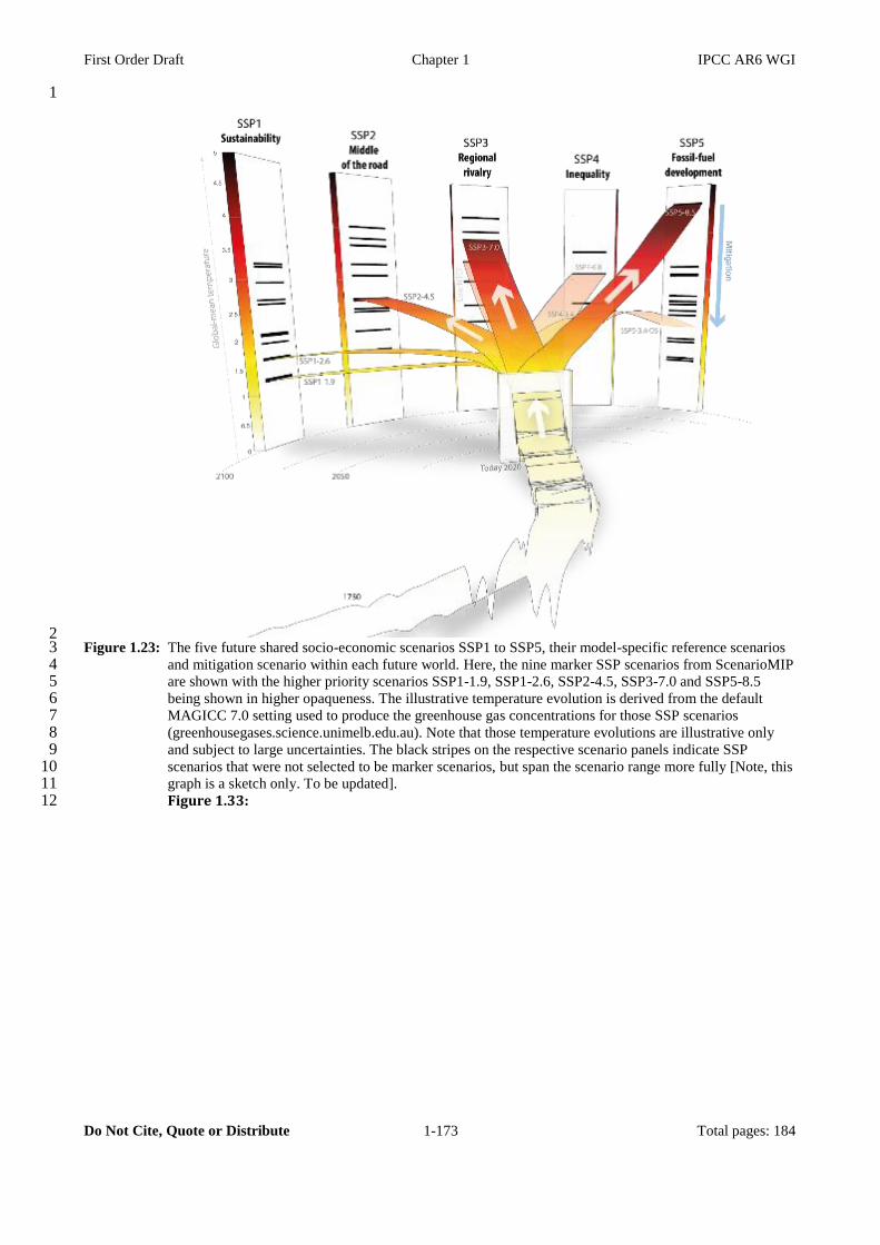
First Order Draft Chapter 1 IPCC AR6 WGI
Do Not Cite, Quote or Distribute 1-173 Total pages: 184
1
2 Figure 1.23: The five future shared socio-economic scenarios SSP1 to SSP5, their model-specific reference scenarios 3
and mitigation scenario within each future world. Here, the nine marker SSP scenarios from ScenarioMIP 4 are shown with the higher priority scenarios SSP1-1.9, SSP1-2.6, SSP2-4.5, SSP3-7.0 and SSP5-8.5 5 being shown in higher opaqueness. The illustrative temperature evolution is derived from the default 6 MAGICC 7.0 setting used to produce the greenhouse gas concentrations for those SSP scenarios 7 (greenhousegases.science.unimelb.edu.au). Note that those temperature evolutions are illustrative only 8 and subject to large uncertainties. The black stripes on the respective scenario panels indicate SSP 9 scenarios that were not selected to be marker scenarios, but span the scenario range more fully [Note, this 10 graph is a sketch only. To be updated]. 11 Figure 1.33: 12
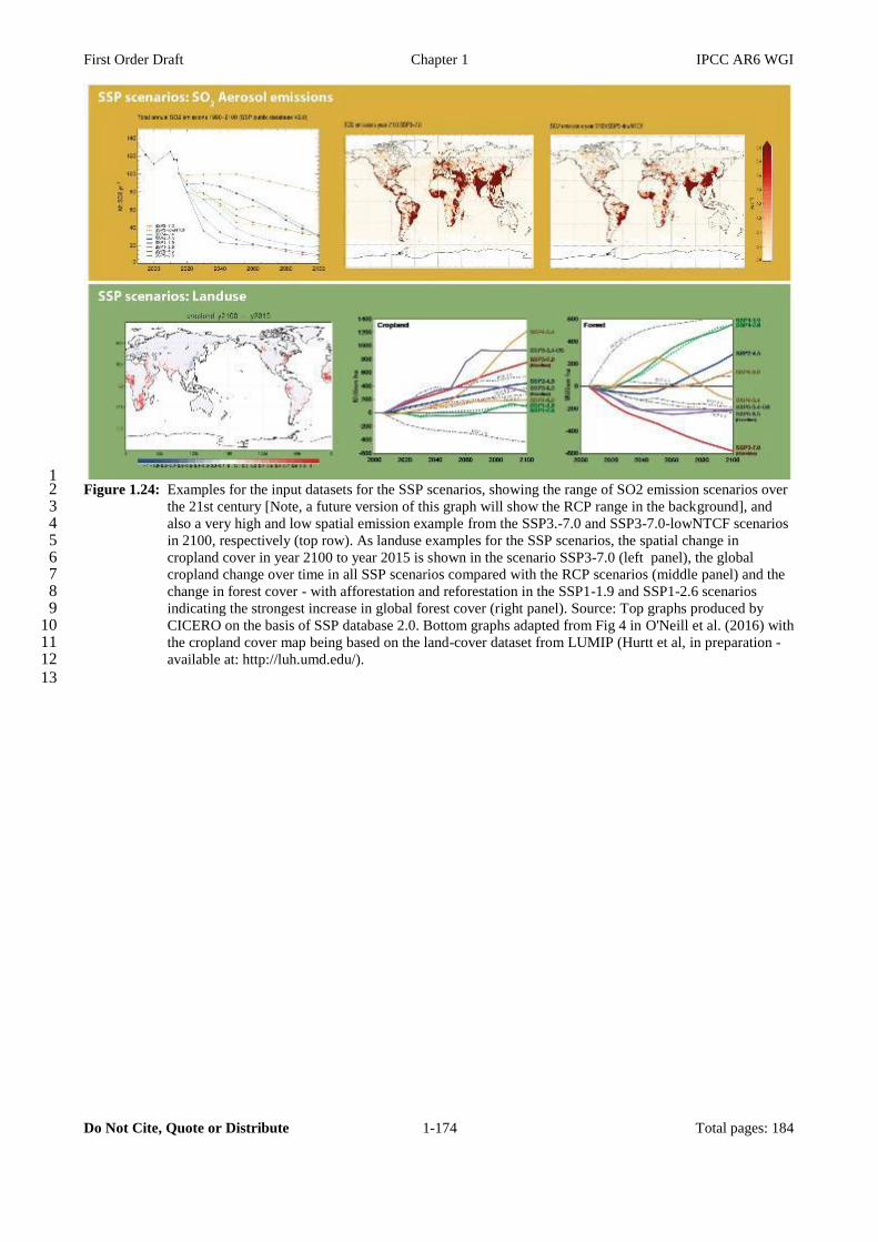
First Order Draft Chapter 1 IPCC AR6 WGI
Do Not Cite, Quote or Distribute 1-174 Total pages: 184
1 Figure 1.24: Examples for the input datasets for the SSP scenarios, showing the range of SO2 emission scenarios over 2
the 21st century [Note, a future version of this graph will show the RCP range in the background], and 3 also a very high and low spatial emission example from the SSP3.-7.0 and SSP3-7.0-lowNTCF scenarios 4 in 2100, respectively (top row). As landuse examples for the SSP scenarios, the spatial change in 5 cropland cover in year 2100 to year 2015 is shown in the scenario SSP3-7.0 (left panel), the global 6 cropland change over time in all SSP scenarios compared with the RCP scenarios (middle panel) and the 7 change in forest cover - with afforestation and reforestation in the SSP1-1.9 and SSP1-2.6 scenarios 8 indicating the strongest increase in global forest cover (right panel). Source: Top graphs produced by 9 CICERO on the basis of SSP database 2.0. Bottom graphs adapted from Fig 4 in O'Neill et al. (2016) with 10 the cropland cover map being based on the land-cover dataset from LUMIP (Hurtt et al, in preparation - 11 available at: http://luh.umd.edu/). 12
13

First Order Draft Chapter 1 IPCC AR6 WGI
Do Not Cite, Quote or Distribute 1-175 Total pages: 184
1 Figure 1.25: An illustrative comparison of the relative importance of greenhouse gas concentrations for projected 2
climate change. The blue shaded area indicates the approximate forcing exerted by CO2 in three of the 3 SSP scenarios, SSP1-1.9, SSP1-2.6 and SSP3-7.0. The CO2 concentrations under the SSP1-1.9 scenarios 4 approximately reach 350 ppm after 2150, those of SSP1-2.6 around 400 ppm and the SSP3-7.0 as one of 5 the higher scenarios will reach levels of nearly 1500 ppm CO2 in the longer term until 2300. Also shown 6 are the effects of reducing short-lived climate forcers in the SSP3-7.0 scenario at the example of methane 7 (panel c, black arrows in the top right), when comparing the SSP3-7.0 scenarios with the AerChemMIP 8 variant SSP3-7.0-lowNTCF [To be updated] 9
10

First Order Draft Chapter 1 IPCC AR6 WGI
Do Not Cite, Quote or Distribute 1-176 Total pages: 184
1 2 Figure 1.26: Historical concentrations for the past 2000 years of CO2, CH4 and N2O (Meinshausen et al., 2017), and 3
[draft sketch of] temperature reconstructions joined with scenario information up to year 2300. The 4 temperature proxies over the last 2000 years were compiled by the Pages 2K project (Emile-Geay et al., 5 2017) and also shown are northern hemispheric temperature reconstructions by Mann et al. (1999) (dark 6 blue ranges). Future temperature projections are from the CMIP6 ScenarioMIP experiment, examined in 7 Chapter 4 of this report. The grey vertical band indicates the 21st century. [ Note: this is a draft sketch 8 figure only]. 9
10
First Order Draft Chapter 1 IPCC AR6 WGI
Do Not Cite, Quote or Distribute 1-177 Total pages: 184
1
2
3
[PLACEHOLDER for figure] 4
5
6
7 Figure 1.27: Illustrative synthesis figure on the “decision power/policy-relevance” of scenarios in the context of the 8
Paris Agreement. The ‘decision power’ for this analysis is here defined as the range between reference 9 and various mitigation scenarios that include shared policy assumptions (SPAs), separated by gases and 10 scenario characteristics in relation to their effect (attributable warming) on peak 21st century temperatures 11 [and end of century sea level rise] (y-axis). The individual elements on the x-axis can be: Next decade 12 cumulative CO2 emissions, CH4 emissions, non-methane SLCF, second half of century net negative CO2 13 emissions, and GHG emission levels in 2030 (possibly shown by various metrics, (GWP|GTP, and GWP* 14 in some form)). For example, methane emissions, cumulative CO2 emissions, cumulative GHG emissions 15 (GWP|GTP\GWP* weighted), SLCF emissions and other GHG emissions. [dependent on AR6 scenario 16 database analysis]. 17
18
19
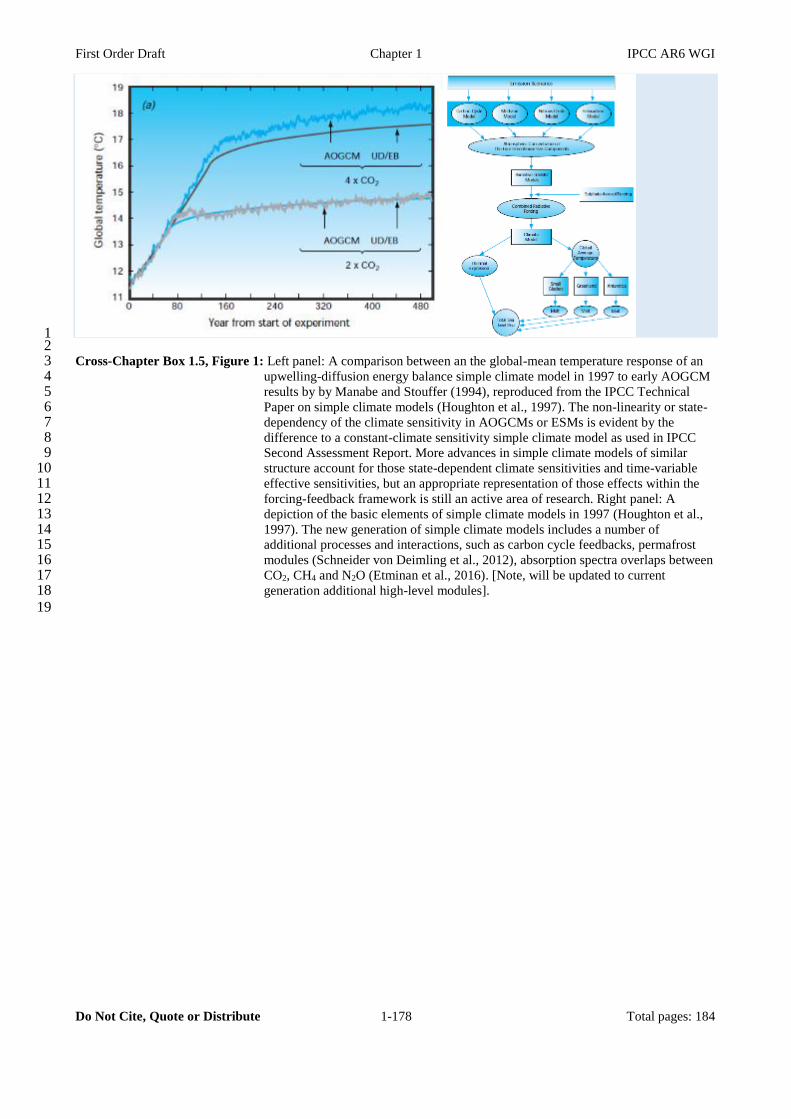
First Order Draft Chapter 1 IPCC AR6 WGI
Do Not Cite, Quote or Distribute 1-178 Total pages: 184
1 2 Cross-Chapter Box 1.5, Figure 1: Left panel: A comparison between an the global-mean temperature response of an 3
upwelling-diffusion energy balance simple climate model in 1997 to early AOGCM 4 results by by Manabe and Stouffer (1994), reproduced from the IPCC Technical 5 Paper on simple climate models (Houghton et al., 1997). The non-linearity or state-6 dependency of the climate sensitivity in AOGCMs or ESMs is evident by the 7 difference to a constant-climate sensitivity simple climate model as used in IPCC 8 Second Assessment Report. More advances in simple climate models of similar 9 structure account for those state-dependent climate sensitivities and time-variable 10 effective sensitivities, but an appropriate representation of those effects within the 11 forcing-feedback framework is still an active area of research. Right panel: A 12 depiction of the basic elements of simple climate models in 1997 (Houghton et al., 13 1997). The new generation of simple climate models includes a number of 14 additional processes and interactions, such as carbon cycle feedbacks, permafrost 15 modules (Schneider von Deimling et al., 2012), absorption spectra overlaps between 16 CO2, CH4 and N2O (Etminan et al., 2016). [Note, will be updated to current 17 generation additional high-level modules]. 18
19
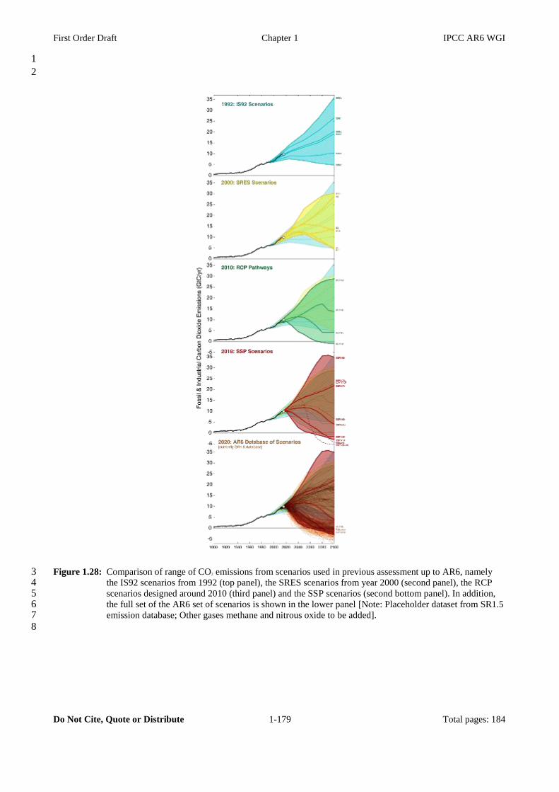
First Order Draft Chapter 1 IPCC AR6 WGI
Do Not Cite, Quote or Distribute 1-179 Total pages: 184
1
2
Figure 1.28: Comparison of range of CO2 emissions from scenarios used in previous assessment up to AR6, namely 3 the IS92 scenarios from 1992 (top panel), the SRES scenarios from year 2000 (second panel), the RCP 4 scenarios designed around 2010 (third panel) and the SSP scenarios (second bottom panel). In addition, 5 the full set of the AR6 set of scenarios is shown in the lower panel [Note: Placeholder dataset from SR1.5 6 emission database; Other gases methane and nitrous oxide to be added]. 7
8
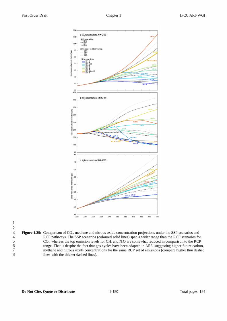
First Order Draft Chapter 1 IPCC AR6 WGI
Do Not Cite, Quote or Distribute 1-180 Total pages: 184
1
2 Figure 1.29: Comparison of CO2, methane and nitrous oxide concentration projections under the SSP scenarios and 3
RCP pathways. The SSP scenarios (coloured solid lines) span a wider range than the RCP scenarios for 4 CO2, whereas the top emission levels for CH4 and N2O are somewhat reduced in comparison to the RCP 5 range. That is despite the fact that gas cycles have been adapted in AR6, suggesting higher future carbon, 6 methane and nitrous oxide concentrations for the same RCP set of emissions (compare higher thin dashed 7 lines with the thicker dashed lines). 8

First Order Draft Chapter 1 IPCC AR6 WGI
Do Not Cite, Quote or Distribute 1-181 Total pages: 184
1 FAQ 1.1, Figure 1: [PLACEHOLDER] 2 3

First Order Draft Chapter 1 IPCC AR6 WGI
Do Not Cite, Quote or Distribute 1-182 Total pages: 184
1 FAQ 1.2, Figure 1: Observed variations in regional temperatures since 1920 from CRUTEM4. Europe has warmed by 2
a larger amount than tropical Africa, but the background variations are also larger (shading 3 represents 1 and 3 standard deviations of background interannual variations). The signal of observed 4 temperature change emerged earlier in tropical Africa than in Europe. 5
6

First Order Draft Chapter 1 IPCC AR6 WGI
Do Not Cite, Quote or Distribute 1-183 Total pages: 184
1
2 3
4
FAQ 1.3, Figure 1: [PLACEHOLDER] 5 6 7

First Order Draft Chapter 1 IPCC AR6 WGI
Do Not Cite, Quote or Distribute 1-184 Total pages: 184
1
2 FAQ 1.4, Figure 1: Suggestion: Global map of measurement site/point densities. With a side list of all the different 3
techniques (eg, buoys, satellites, ships etc – could have icons for each?) Present placeholder is 4 from Rennie et al. (2014). 5
6 7