Non-isothermal Flow through a Curved Rectangular Duct for Large Grashof Number

Journal of Physical Sciences, Vol. 12, 2008, 109-121

109

Non-isothermal Flow through a Curved Rectangular Duct for Large Grashof Number

Rabindra Nath Mondal *, Md. Sharif Uddin and Ariful Islam

Mathematics Discipline; Science, Engineering and Technology School, Khulna University, Khulna-9208, Bangladesh.

*Corresponding author: [email protected]

Received February 25, 2008; accepted May 18, 2008

ABSTRACT

Non-isothermal flow through a curved rectangular duct of differentially heated vertical sidewalls is investigated numerically by using the spectral method, and covering a wide range of the Dean number, Dn, 10000 ≤< Dn , and the Grashof number, Gr, 20001000 ≤≤ Gr . After a comprehensive survey over the parametric ranges, five branches of asymmetric steady solutions are obtained with two- and multi-vortex solutions by using the Newton-Raphson iteration method. Linear stability of the steady solutions is then investigated. When there is no stable steady solution, time evolution calculations are performed, and it is found that for any Gr in the range, the steady flow turns into chaos through various flow instabilities, if Dn is increased. Keywords: Curved duct, secondary flow, steady solutions, linear stability, time-evolution. 1. Introduction

The study of flows through a curved duct is of fundamental importance because of its numerous applications in fluids engineering, such as in heat exchangers, ventilators, gas turbines, aircraft intakes and centrifugal pumps. The flow through a curved duct shows physically interesting features under the action of the centrifugal force caused by the curvature of the duct. The earliest studies on curved pipes to predict the onset of secondary flows and its characteristics were began by Dean [2], who first formulated the problem in mathematical terms under the fully developed flow condition. Since then, there have been a lot of theoretical and experimental works concerning this flow.

One of the interesting phenomena of the flow through a curved duct is the bifurcation of the flow because generally there exist many steady solutions due to channel curvature. Studies of the flow through a curved duct have been made, experimentally or numerically, for various shapes of the cross section. However, an extensive treatment of the bifurcation structure of the flow through a curved duct of rectangular cross section was presented by Winters [9], Daskopoulos and Lenhoff [1] and Mondal [5].

Time dependent behavior of the fully developed curved duct flows was initiated by Yanase et al. [10] for a rectangular cross section in connection with the

Rabindra Nath Mondal, Md. Sharif Uddin and Ariful Islam

110

bifurcation diagram of steady solutions. In the study they investigated unsteady solutions for the case where dual solutions exist. Wang and Yang [8] performed numerical as well as experimental investigations of periodic oscillations for the fully developed flow in a curved square duct. They showed that a temporal oscillation takes place between symmetric/asymmetric 2-cell and 4-cell flows when there are no stable steady solutions. Very recently, Mondal et al. [7] performed numerical prediction of the unsteady solutions by time-evolution calculations and showed that the steady flow turns into chaos through periodic or multi-periodic flows if the Dean number is increased. They also showed that the periodic or the chaotic state is retarded with an increase of curvature.

A remarkable characteristic of the flow through a curved duct is to enhance heat transfer from the heated wall to the fluid. Recently, Yanase et al. [11] performed numerical prediction of isothermal and non-isothermal flows through a curved rectangular duct of aspect ratio 2, where they found multiple branches of steady solutions and discussed transitional behavior of the unsteady solutions. In the succeeding paper, Yanase et al. [12] extended their work for moderate Grashof numbers and studied the effects of secondary flows on convective heat transfer. Very recently, Mondal et al. [6] performed numerical investigation of non-isothermal flow through a curved square duct for the Grashof number Gr = 100, where they showed that secondary flow enhances heat transfer from the heated wall to the fluid. From the scientific as well as engineering point of view, it is quite interesting to study curved duct flows with differentially heated vertical sidewalls for the large Grashof number, because this type of flow is often encountered in engineering applications.

In the present paper, a numerical study is presented for the fully developed two-dimensional flow of viscous incompressible fluid through a curved rectangular duct with differentially heated vertical sidewalls. Flow characteristics are studied over a wide range of the Dean number and the Grashof number by finding the steady solutions, investigating their linear stability and analyzing nonlinear behavior of the unsteady solutions by time evolution calculations. 2. Governing Equations

Consider an incompressible viscous fluid streaming through a curved duct of constant curvature. The cross section of the duct is a rectangle with width 2d and height 2h. It is assumed that the outer wall of the duct is heated while the inner one is cooled. The temperature of the outer wall is TT ∆+0 and that of the inner wall is TT ∆−0 , where 0>∆T . The y,x and z axes are taken to be in the horizontal, vertical, and axial directions, respectively. It is assumed that the flow is uniform in the z-direction and that it is driven by a constant pressure gradient G along center-line of the duct, i.e., the main flow in the z-direction as shown in Fig. 1.

The variables are non-dimensionalized by using of the representative length d, the representative velocity d/vU =0 , where ν is the kinematic viscosity of the fluid. We introduce the non-dimensional variables defined as


111

.,,,,

,,,2,,

20

20

0

000

Ud

zPG

UPP

Ldt

dU

tT

TT

dzz

dyy

dxxw

Uw

Uvv

Uuu

ρρδ

δ

′∂′∂

−=′

==′=∆′

=

′=

′=

′=′=

′=

′=

where u , v and w are the non-dimensional velocity components in the x , y and z directions, respectively; t is the non-dimensional time, P the non-dimensional pressure, and δ is the non-dimensional curvature. Temperature is non-dimensionalized by T∆ . Henceforth all the variables are non-dimensionalized if not specified.

Fig. 1. Coordinate system of the curved rectangular duct

Since the flow field is uniform in the z-direction, the sectional stream function

ψ is introduced as follows:

xx

vyx

u∂∂

+−=

∂∂

+=

ψδ

ψδ 1

1,1

1 (1)

A new coordinate variable /y is introduced in the y-direction as /lyy = ,

where dhl = is the aspect ratio of the duct cross section. From now on, y

denotes /y for the sake of simplicity. Then the basic equations for ψ,w and T are derived from the Navier-Stokes equations and the energy equation with the Boussinesq approximation as,

( ) ( )( ) ( ) ( ) ,

11

1,,11 2

2

xww

yxlwx

xwD

yxw

ltwx n ∂

∂+

∂∂

+−∆+=

++−

∂∂

+∂∂

+ δψδδδ

δδψδ (2)


112

( )( )( ) ( )

( )

( ) yww

lxxxxx

xyxxxxxy

xlyxxltxx

∂∂

+∆∂∂

+−

∂∂

+−

∂∂

×

++

∂∂∂

∂∂

−

∂∂

+∂∂

+−∆

∂∂

×

++

∂∆∂

+−=

∂∂

∂∂

+−∆

11

2133

1132

1,,

11

1

2

2

2

2

2

2

2

2

2

22

2

ψδδψ

δδψδ

δδψψψψ

δδψψ

δδψψ

δψ

δδ

( ) ,122 x

TxGr∂∂

+−∆+ δψ (3)

( )( )( ) ,

1Pr1

,,

11

2

∂∂

++∆=

∂∂

++

∂∂

xT

xT

yxT

xltT

δδψ

δ (4)

where

( )( ) .

,,,1

2

2

22

2

2 xg

yf

yg

xf

yxgf

ylx ∂∂

∂∂

−∂∂

∂∂

≡∂∂

∂∂

+∂∂

≡∆ (5)

The Dean number, Dn, the Grashof number, Gr, and the Prandtl number Pr, which appear in Eqs. (2) - (4), are defined as

.vPr,vTdgGr,

Ld

vGdDn

κγ

µ=

∆== 2

33 2 (6)

where µ , γ , κ and g are the viscosity, the coefficient of thermal expansion, the coefficient of thermal diffusivity and the gravitational acceleration, respectively.

The rigid boundary conditions for w and ψ are

( ) ( ) ( ) ( ) ( ) ( ) ,,xy

y,x

,xy,,xwy,w 0111111 =±∂∂

=±∂∂

=±=±=±=±ψψψψ (7)

and the conducting boundary conditions for T are assumed as ( ) ( ) ( ) x,xT,y,T,y,T =±−=−= 11111 . (8)

In the present study, Dn and Gr are varied, whileδ , Pr and l are fixed as 1.0=δ , Pr = 7.0 (water) and 2=l .

3. Method of Numerical Calculation

The method adopted in the present numerical calculation is the spectral method. By this method the variables are expanded in the series of functions consisting of Chebyshev polynomials. Details of this method are discussed by Mondal [5]. By this method, the expansion functions ( )xnΦ and ( )xnΨ are expressed as

( ) ( ) ( ) ( ) ( ) ( ),1,1 222 xCxxxCxx nnnn −=Ψ−=Φ (9)

where ( ) ( )( )xcosncosxCn1−= is the n-th order Chebyshev polynomial.

( ) ( )t,y,x,z,y,xw ψ and ( )t,y,xT are expanded in terms of the functions ( )xnΦ and ( )xnΨ as


113

( ) ( ) ( ) ( )

( ) ( ) ( ) ( )

( ) ( ) ( )

+ΦΦ=

ΨΨ=

ΦΦ=

∑∑

∑∑

∑∑

= =

= =

= =

M

m

N

nnmmn

M

m

N

nnmmn

M

mnm

N

nmn

xyxtTtyxT

yxttyx

yxtwzyxw

0 0

0 0

0 0

,),,(

,,,

,,,

ψψ (10)

where M and N are the truncation numbers in the x- and y-directions, respectively. The collocation points are taken to be

+−=

+−=

21cos,

21cos

Njy

Mix ji ππ (11)

where 1,...,1 += Mi and 1,...,1 += Nj . In the present numerical calculations, 20=M and N = 40 have been used for sufficient accuracy of the solutions. To

obtain the steady solutions, we use Newton-Raphson iteration method and to calculate the unsteady solutions, we use the Crank-Nicolson and Adams-Bashforth methods together with the function expansion (10) and the collocation method. 4. Resistance Coefficient

In the present study, the resistance coefficientλ is used as the representative quantity of the flow state. It is also called the hydraulic resistance coefficient, and is generally used in fluid engineering, defined as

,21 2*

**

*2

*1 w

dhzPP

ρλ=

∆−

(12)

where quantities with an asterisk denote the dimensional ones, stands for the mean over the cross section of the rectangular duct, ρ the density, and

( ) ( )dddddh 84/424* ××= is the hydraulic diameter. The mean axial velocity *w is calculated by

( )∫∫−−

=1

1

1

1

* ,,24

dytyxwdxd

wδ

ν (13)

Since ( ) ,Gz/PP *** =∆− 21 λ is related to the mean non-dimensional axial velocity w as

( )

,1

282wl

Dnl+

=δλ (14)

where ./2 * νδ wdw = In this paper, λ is used to discriminate the steady

solution branches and to pursue the time evolution of the unsteady solutions.


114

5. Results and Discussion We obtain steady solutions, investigate their linear stability and perform

nonlinear behavior of the unsteady solutions by time-evolution calculations. Though the present study covers a wide range of Gr ( 20001000 ≤< Gr ), in the present paper, however, a single the case of the Grashof numbers, Gr = 2000, is discussed in detail, and a schematic diagram for the distribution of the steady and unsteady solutions, obtained by the time evolution calculations, is presented in the Dean number vs. Grashof number plane for 10000 ≤≤ Dn and 20001000 ≤≤ Gr . 5.1. Steady solutions

With the present numerical calculations, five branches of asymmetric steady solutions are obtained by the path continuation technique with various initial guesses as discussed by Mondal [5]. Figure 2(a) shows bifurcation diagram of the steady solutions for Gr = 2000 and 1000100 ≤≤ Dn . The steady solution branches are named the first steady solution branch (first branch, thick solid line), the second steady solution branch (second branch, thin solid line), the third steady solution branch (third branch, dash dotdot line), the fourth steady solution branch (fourth branch, dashed line) and the fifth steady solution branch (fifth branch, dash dotted line), respectively. In order to see the intricate branch structure and to distinguish the steady solution branches from each other, an enlargement of Fig. 2(a) is shown in Fig. 2(b) at larger Dn, where it is observed that the steady solution branches are independent and there exists no bifurcating relationship among the branches in the parameter range investigated in this paper. It is found that the first branch is composed of one- and two-vortex solutions. The second branch consists of two- and four- vortex solutions. The third branch is characterized by two- and four-vortex solutions, but different from the second branch in the form of vortices generated near the outer wall. The fourth branch contains two-, four- and six-vortex solutions and the fifth branch two-, four-, six- and eight-vortex solutions.

(a) (b)

Fig. 2. (a) Steady solution branches for Gr = 2000 and 1000100 ≤≤ Dn (thick solid line: first branch, thin solid line: second branch, dash dotdot line: third branch, dashed line: fourth branch, dash dotted line: fifth branch). (b) Enlargement of (a) at larger Dean numbers ( )1000695 ≤≤ Dn .


115

ψ T Dn = 0 100 200 400 500 1000

(a) (b) Fig. 3. (a) First steady solution branch ( 100010 ≤≤ Dn ) with the region of linear

stability (bold line), (b) contours of secondary flow (top) and temperature profile (bottom) for the first steady solution branch for Gr = 2000 and

10000 ≤< Dn . The first steady solution branch is exclusively depicted in Fig. 3(a)

for 100010 ≤≤ Dn . Among five branches of steady solutions, this is the only branch exists throughout the whole range of the Dean numbers investigated in this paper. To observe the change of the flow patterns and temperature distributions, contours of typical secondary flow and temperature profile at several Dn's are shown in Fig. 3(b), where the contours of ψ and T are drawn with the increments

6.0=∆ψ and 2.0=∆T , respectively. The same increments of ψ and T are used for all the figures in this paper, if not specified. As seen in Fig. 3(b), the first steady solution branch contains one- and two-vortex solutions which are asymmetric with respect to the horizontal centre plane y = 0. Heating the outer wall causes deformation of the secondary flow and yields asymmetry of the flow. 5.2 Linear stability of the steady solutions

In the present study, linear stability of the steady solutions is investigated against only two-dimensional perturbations. To do this, the eigenvalue problem is solved which is constructed by the application of the function expansion method together with the collocation method to the perturbation equations obtained from Eqs. (2), (3) and (4). It is assumed that the time dependence of the perturbation is σie , where ir σσσ += is the eigenvalue with rσ the real part, iσ the imaginary

part and 1−=i . If all the real parts of the eigenvalue σ are negative, the steady solution is linearly stable, but if there exists at least one positive real part of the eigenvalue, it is linearly unstable. In the unstable region, the perturbation grows monotonically for 0=iσ and oscillatory for 0≠iσ .


116

Table 1. Linear stability of the first steady solution branch for Gr = 2000.

Dn λ rσ iσ 0 0.000000 -9.6536× 110− 0

50 0.962074 -1.0095× 110− 0 100 0.535108 -1.0010× 110− 0 115 0.481988 -3.2498× 210− ± 1.087× 10 116 0.478959 1.5081× 110− ± 1.096× 10 300 0.269664 8.2333 ± 1.060× 10 500 0.210999 2.3734× 10 ± 3.844

1000 0.143630 5.8754×10 ± 4.508×10

On the basis of the above-mentioned criterion, linear stability of the steady solutions is studied. It is found that among five branches of steady solutions; only the first branch is linearly stable while the other branches are linearly unstable. Eigenvalues of the first steady solution branch are shown in Table 1, where the eigenvalues with the maximum real part of σ are presented. Those for the linearly stable solutions are printed in bold letters. As seen in Table 1, the stability region exists for 1150 ≤≤ Dn . Linearly stable steady solution region is shown with thick solid line in Fig. 3(a). It is found that the Hopf bifurcation occurs at 115≈Dn . 5.3 Time evolution

In order to study the nonlinear behavior of the unsteady solutions, time evolution calculations of the velocity and temperature fields are performed for Gr = 2000 at Dn = 100, 200, 400, 450, 500, 600 and 1000. It is found that the flow approaches a steady state solution for Dn = 100, no matter what the initial condition we use. A single contour of the secondary flow and temperature profile for Dn = 100 at time t = 8 is shown in Fig. 4, where it is observed that the flow is a single-vortex solution which closely agrees with the steady solution on the first branch at Dn = 100, which is linearly stable. ψ T Fig. 4. Contours of secondary flow (left) and temperature profile (right) for Gr =

2000 at time t = 8.

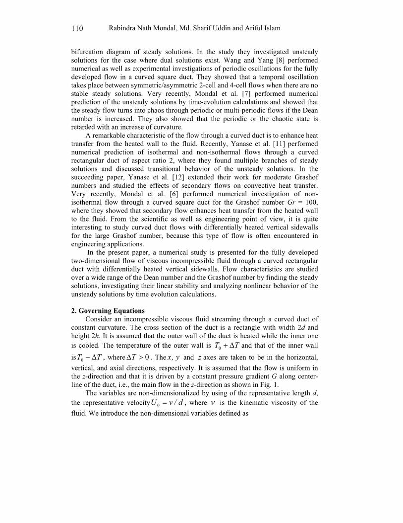
Time evolution of λ together with the value of λ for the first steady solution branch, indicated by straight line, is shown in Fig. 5(a) for Dn = 200. Figure 5(a) shows that the flow is periodic, which takes place above the first steady solution branch. To observe the periodic change of the flow pattern, contours of typical secondary flow and temperature profile are shown in Fig. 5(b) for Dn = 200 which


117

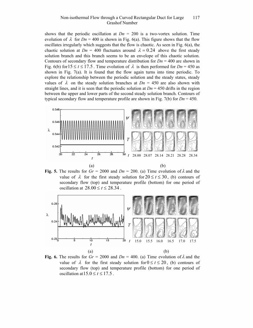
shows that the periodic oscillation at Dn = 200 is a two-vortex solution. Time evolution of λ for Dn = 400 is shown in Fig. 6(a). This figure shows that the flow oscillates irregularly which suggests that the flow is chaotic. As seen in Fig. 6(a), the chaotic solution at Dn = 400 fluctuates around 24.0=λ above the first steady solution branch and this branch seems to be an envelope of this chaotic solution. Contours of secondary flow and temperature distribution for Dn = 400 are shown in Fig. 6(b) for 5.1715 ≤≤ t . Time evolution of λ is then performed for Dn = 450 as shown in Fig. 7(a). It is found that the flow again turns into time periodic. To explore the relationship between the periodic solution and the steady states, steady values of λ on the steady solution branches at Dn = 450 are also shown with straight lines, and it is seen that the periodic solution at Dn = 450 drifts in the region between the upper and lower parts of the second steady solution branch. Contours of typical secondary flow and temperature profile are shown in Fig. 7(b) for Dn = 450. ψ T t 28.00 28.07 28.14 28.21 28.28 28.34 (a) (b) Fig. 5. The results for Gr = 2000 and Dn = 200. (a) Time evolution ofλ and the

value of λ for the first steady solution for 3020 ≤≤ t , (b) contours of secondary flow (top) and temperature profile (bottom) for one period of oscillation at 34.2800.28 ≤≤ t .

ψ T t 15.0 15.5 16.0 16.5 17.0 17.5 (a) (b) Fig. 6. The results for Gr = 2000 and Dn = 400. (a) Time evolution ofλ and the



118

ψ T t 28.50 28.53 28.56 28.60 28.63 28.66 (a) (b) Fig. 7. The results for Gr = 2000 and Dn = 450. (a) Time evolution ofλ and the


ψ

T T t 20.0 20.5 21.0 21.5 22.0 22.5 (a) (b) Fig. 8. The results for Gr = 2000 and Dn = 500. (a) Time evolution ofλ and the


Next, time evolution of λ for Dn = 500 is conducted as shown in Fig. 8(a).

Figure 8(a) shows that the flow again turns into chaotic. To comprehend the relationship between the chaotic solution and the steady states, steady values of λ on the steady solution branches at Dn = 500 are also shown which are indicated by straight lines using the same kind of lines as were used in the bifurcation diagram in Fig. 2. It is found that the chaotic solution at Dn = 500 oscillates in the region between the second and third steady solution branch. To observe the change of the flow characteristics, as time proceeds, contours of typical secondary flow and temperature profile for Dn = 500 are shown in Fig. 8(b). Time evolution ofλ is then performed for Dn = 1000 as shown in Fig. 9(a). In this figure, the steady values ofλ for the steady solution branches at Dn = 1000 are also shown. Figure 9(a) shows


119

that the unsteady flow at Dn = 1000 is also chaotic, which moves around 1655.0=λ above all the steady solution branches and the steady solution branch

having the maximum λ ( 1607.0=λ , upper part of the fifth steady solution branch) looks like an envelope of this chaotic solution. The chaotic solution for Dn = 500 is called a ‘weak chaos’ but that for Dn = 1000 a ‘strong chaos’ (Mondal et al. [7]), because the chaotic solution at Dn = 500 is still trapped by the steady solution branches but that for Dn = 1000 tends to get away from them. Thus it is suggested that occurrence of the chaotic state is related with destabilization of the steady solutions, which reminds us the case of Lorenz chaos [3]. In this regard, it is worth mentioning that irregular oscillation of isothermal flows through a curved rectangular duct has been observed experimentally by Ligrani and Niver [4] for the large aspect ratio. To observe the change of the flow patterns, contours of typical secondary flow and temperature profile are shown in Fig. 9(b) for Dn = 1000 at 0.80.6 ≤≤ t , where the increments 2.1=∆ψ and 4.0=∆T have been used for Dn= 1000. ψ T t 6.0 6.4 6.8 7.2 7.6 8.0 (a) (b) Fig. 9. The results for Gr = 2000 and Dn = 1000. (a) Time evolution ofλ and the


5.4 Phase diagram in the Dn-Gr plane

Finally, the distribution of the time-dependent solutions, obtained by the time evolution calculations of the flow, is shown in Fig. 10 in the Dean number vs. Grashof number plane ( GrDn − plane) for 10000 ≤≤ Dn and 20001000 ≤≤ Gr . In this picture, the circles indicate the steady-state solution, the crosses periodic solutions and the triangles chaotic solution. As seen in Fig. 10, the steady flow turns into chaos through various flow instabilities, if Dn is increased keeping Gr fixed. At some Gr ( )20001000 ≤≤ Gr , however, sometimes there exist three or two exclusive regions of Dn where the solution is time periodic, and at 2000=Gr the flow undergoes in the scenario steady→ periodic→ chaotic→ periodic→ chaotic, if Dn is increased. It is also found that, if Gr is increased further


120

( 2000>Gr ), the regions of periodic solutions shrink and consequently the regions of chaotic solutions expand.

Fig. 10. Distribution of the time-dependent solutions in the Dean number vs.

Grashof number (Dn-Gr) plane for 10000 ≤≤ Dn and 20001000 ≤≤ Gr (Ο : steady-stable solution, × : periodic solution, ∆ : chaotic solution).

6. Conclusions

In this paper, a detailed numerical study of the non-isothermal flow through a curved rectangular duct of aspect ratio 2 has been presented by using the spectral method over a wide range of the Dean number 10000 ≤< Dn and the Grashof number 20001000 ≤≤ Gr for the curvature 1.0=δ .

After a comprehensive survey over range of the parameters, five branches of asymmetric steady solutions are obtained. Linear stability analysis shows that among five branches of steady solutions, only the first branch is linearly stable, while the other branches are linearly unstable. It is found that the Hopf bifurcation occurs at the Dean numbers on the boundary where stability disappears. Time evolutions of the flow show that, the steady flow turns into chaos through various flow instabilities, if Dn is increased keeping Gr fixed. It is found that, there exist three or two exclusive regions of Dn where the solution is time periodic. If Gr is increased further (Gr > 2000), the region of chaotic solution expands and consequently the regions of periodic solutions merge into a single region of periodic solution.

REFERENCES 1. Daskopoulos, P. and Lenhoff, A. M., Flow in curved ducts: bifurcation structure

for stationary ducts, J. Fluid Mech., 203(1989), 125--148. 2. Dean, W. R., Note on the motion of fluid in a curved pipe, Philos. Mag.,

4(1927), 208--223.


121

3. Lorenz, E. N., Deterministic non-periodic flow, J. Atms. Sci., 20(1963), 130-141.

4. Ligrani, P. M. and Niver, R. D., Flow visualization of Dean vortices in a curved hannel with 40 to 1 aspect ratio, Phys. Fluids, 31(1988), 3605--3617.

5. Mondal, R. N., Isothermal and non-isothermal flows through curved ducts with square and rectangular cross sections, Ph.D. Thesis, Department of Mechanical Engineering, Okayama University, Japan, (2006).

6. Mondal, R. N., Kaga, Y., Hyakutake, T. and Yanase, S., Effects of curvature and convective heat transfer in curved square duct flows, Trans. ASME, Journal of Fluids engineering, 128(9)(2006), 3264--3275.

7. Mondal, R. N., Kaga, Y., Hyakutake, T. and Yanase, S., Bifurcation diagram for two-dimensional steady flow and unsteady solutions in a curved square duct, Fluid Dyn. Res., 39(2007), 413--446.

8. Wang, L. and Yang, T., Periodic oscillation in curved duct flows, Physica D, 200(2005), 296--302.

9. Winters, K. H., A bifurcation study of laminar flow in a curved tube of rectangular cross-section, J. Fluid Mech., 180(1987), 343--369.

10. Yanase, S. and Nishiyama, K., On the bifurcation of laminar flows through a curved rectangular tube, J. Phys. Soc. Japan, 57(1988), 3790--3795.

11. Yanase, S., Mondal, R. N., Kaga, Y. and Yamamoto, K., Transition from steady to chaotic states of isothermal and non-isothermal flows through a curved rectangular duct, J. Phys. Soc. Japan, 74(2005a), 345--358.

12. Yanase, S., Mondal, R. N. and Kaga, Y., Numerical study of non-isothermal flow with convective heat transfer in a curved rectangular duct, Int. J. Thermal Sci., 44(2005b), 1047--1060

Non-isothermal Flow through a Curved Rectangular Duct for Large Grashof Number

Documents

Transcript of Non-isothermal Flow through a Curved Rectangular Duct for Large Grashof Number