Multisite seasonal forecast of arid river flows using a dynamic

model combination approach

Shahadat Chowdhury1 and Ashish Sharma1

Received 7 October 2008; revised 3 April 2009; accepted 26 June 2009; published 21 October 2009.

[1] This paper dynamically combines three independent forecasts of multiple river flowvolumes a season in advance for arid catchments. The case study considers five inflowlocations in the upper Namoi Catchment of eastern Australia. The seasonal flows arepredicted on the basis of concurrent sea surface temperature anomalies (SSTAs), whichare predicted a season forward using a dynamic combination of three SSTA forecasts. Theriver flows are predicted using three statistical forecasting models: (1) a mixture ofgeneralized lognormal and multinomial logit models, (2) the local regression ofindependent components of five inflows, and (3) the weighted nearest neighbor method,where each of these models use the forecasted SSTA along with prior lags of the flowas the main driving variables. The study demonstrates that improved SSTA forecast (dueto dynamic combination) in turn improves all three flow forecasts, while the dynamiccombination of the three flow forecasts results in further, although smaller, improvements.

Citation: Chowdhury, S., and A. Sharma (2009), Multisite seasonal forecast of arid river flows using a dynamic model combination

approach, Water Resour. Res., 45, W10428, doi:10.1029/2008WR007510.

1. Introduction

[2] Seasonal forecast of river flow is vital for efficientwater resource management, aiding irrigation, hydropowergeneration, flood mitigation, drinking water supply andmanaging water-dependent ecosystems. The water availabil-ity in the coming irrigation season is a prime consideration todecide plantation areas of water sensitive annual crops at thestart of the season. The potential benefit of seasonal flowforecast is high for agricultural economies of arid regions[Podbury et al., 1998; Letcher et al., 2004]. Hydrologistshave a number of models at their disposal to forecast riverflow, with a varying degree of success. The structuraluncertainty of a single model can be reduced by combiningalternative modeling platforms. This paper investigates thescope of improving forecast skill by dynamically combiningalternative forecasting approaches. Various hydrologicalstudies have reported improvement of flow forecast aftercombination of multiple methods [Shamseldin et al., 1997;Georgakakos et al., 2004; Ajami et al., 2006; Regonda et al.,2006;Goswami and O’Connor, 2007;Devineni et al., 2008].This research uses a pairwise dynamic combination approachfirst introduced by Chowdhury and Sharma [2009] in thecontext of combining forecasts of the NINO3.4 sea surfacetemperature anomaly (SSTA) based index representative of thestrength of an El Nino–Southern Oscillation anomaly. Theimprovement of global SSTA forecast was recently reportedby Chowdhury and Sharma [2009] and Chowdhury [2009]after dynamically combining three SSTA forecast models.Can similar improvements be achieved for flow forecastmodels?When can we expect forecast combination to exhibit

improvement? What improvement of flow forecast is deliv-ered by better global SSTA forecast? This paper seeks toexplore these questions.[3] This study forecasts streamflow directly circumvent-

ing the uncertainty of needing to specify rainfall-runoffmodels. This approach has certain advantages especiallyfor regions with few rainfall events and sparse rain gaugenetworks. For example, flow is mostly a continuous variablewith considerable memory which assimilates informationspatially. Uncertainty of flow measurement is less demand-ing than the extrapolation of point rain gauge into catchmentscale. Consequently forecast of flow rather than rainfall isoften recommended [Chiew et al., 1998; Dutta et al., 2006],which is strengthen by the fact that streamflow is the ulti-mate variable of interest for water resource management.The main challenge in such a predictive framework is toidentify the climate variables that constitute predictors offlow.[4] Various indices and transformations of SSTA have

been found to be useful as predictors of hydrological var-iables such as rain and flow [Sharma, 2000b; Drosdowskyand Chambers, 2001a; Verdon et al., 2004]. The relation-ship of El Nino–Southern Oscillation (ENSO) and flow hasbeen well established in many parts of the world [Hamlet andLettenmaier, 1999; Chiew and McMahon, 2002;Muluye andCoulibaly, 2007]. Accordingly, the concurrent SSTA field atthe Pacific and Indian oceans is used as the predictor sourcein our case study.[5] The case study comprises forecasting seasonal flow at

five locations of an arid catchment. The details of the catch-ment and flow characteristics are documented in section 3.Since, forecast error of any model is generally a culminationof imprecise predictors and structural uncertainty [Butts etal., 2004; Huard and Mailhot, 2006]; we first attempt toreduce the flow forecast error by using a more precisepredictor approximation selected from a SSTA forecast field

1School of Civil and Environmental Engineering, University of NewSouth Wales, Sydney, New South Wales, Australia.

Copyright 2009 by the American Geophysical Union.0043-1397/09/2008WR007510

W10428

WATER RESOURCES RESEARCH, VOL. 45, W10428, doi:10.1029/2008WR007510, 2009

1 of 16

that arises through a dynamic model combination approach[Chowdhury, 2009]. Second the structural uncertainty isreduced by considering three flow forecast models andusing a dynamic combination approach to arrive at the finalforecast. Last, we analyze the performances of the variousforecast methods considered and scrutinize the advantagesof forecast combination in light of our case study.[6] This paper is organized as follows. First we describe

the methodology of dynamic combination algorithm precededby background literature on time series combination. Thenwe illustrate the benefit of dynamically combining threeSSTA forecasts as reported by Chowdhury [2009]. Section 3describes the study catchment along with the three flowforecast models considered. This is followed by an analysis ofresults and related discussions on the merits and demeritsassociated with the various approaches presented.

2. Model Combination

2.1. Background

[7] Combinations of multiple forecasts have been widelyadopted in practice in the time series forecasting discipline[Clemen, 1989; Hoeting et al., 1999; Armstrong, 2001].There has been various studies supporting and analyzing arange of forecast combination methods [de Menezes et al.,2000, Ajami et al., 2006, Kim et al., 2006, Devineni et al.,2008] that provide a good background to this area of research.In general the model combination involves linear combina-tion of multiple response time series where the combinationweights remains time invariant. While McLeod et al. [1987]were the first to propose a nonstationary model combina-tion weight, only few studies using such dynamic weightsin hydrology [See and Abrahart, 2001; Xiong et al., 2001;Marshall et al., 2007] have been reported since. Oneapproach is to combine the models in pairs using combi-nation weights that vary in time reflecting the persistenceof individual model skills. A summary of the pairwisedynamic weight combination method is presented next,with readers being referred to Chowdhury and Sharma[2009; Chowdhury, 2009] for additional details on thistopic.

2.2. Dynamic Weight Combination

[8] Consider the case of two component hydrologicforecasts, u1,l,t and u2,l,t, at a location l. For ease of notationlet us conceal the location subscript l within the straight fontnotation as u1,t � {u1,l,t; l = 1, 2, 3..}. These can becombined as

yt ¼ u1;twt þ u2;tð1� wtÞ ð1Þ

where yt: combined forecast at time t and wt: weightdynamically assigned to model 1.[9] The observed dynamic weight is defined as

wt ¼ e2;t=ðe2;t � e1;tÞ ð2Þ

Here e1,t and e2,t are residuals of the model 1 and 2. Ignoreany forecast bias and constraint the weights to positivefractions only, {wt 2 0 ! 1}. The combination procedureis as follows.[10] First, prepare a time series of weights {wt; t = 1, 2, 3,..}

using component model hind cast residuals as shown in

equation (2). Next predict the weight time series forward byformulating a model with appropriate predictors and autoregressive components as well as multi site characteristicof wt that is {wl,t; l = 1, 2, 3..}. Two such models werepresented by Chowdhury [2009], one being a mixedregression model and the other being a weighted nearestneighbor method. Once such a predictive model has beenformulated, we use the predicted future weight (say wt+1) tocombine two alternative forecasts u1,t+1 and u2,t+1 into yt+1.Note that the model combination operates on a pairwisebasis, with multiple pairs being formulated if more thantwo model forecasts are to be combined. Details on therationale behind the model combination and the logic forimparting spatial dependence in multivariate forecastfields are presented by Chowdhury [2009].[11] This paper demonstrates weighted combination of

mean forecast only. As a result, the information about theuncertainty in the process contained in the forecast ensem-ble is not retained in the dynamic combination forecasts.However, estimates of the standard error associated with theforecasts can be obtained by building a conditional variancemodel (similar to the dynamic combination that is analo-gous to a conditional mean), or alternately by using wellformulated conditional bootstrap alternatives to developnonparametric error estimates. A practical application ofimprovements due to dynamically combining three sepa-rate sea surface temperature forecast is described next.

2.3. Combining Sea Surface Temperature Forecasts

[12] Concurrent reconstructed sea surface temperatureanomalies (SSTA) at 5� by 5� grids of the global sea surfacebetween 60�N to 40�S are prime source of flow predictorsused in this research. Reconstructed, monthly sea surfacetemperature anomalies, known as the Kaplan optimalsmoother SSTA [Kaplan et al., 1997, 1998] are sourceof observed SSTA time series. This reconstructed data setextends from 1856 to 2003.[13] One, two and three months SSTA forecast are neces-

sary to predict flow volumes over the next three months. Twosets of SSTA forecasts have been used in the study reportedhere. The first of these originates fromMeteo-France [Madecet al., 1997], which is referred as MetF here, it is developedby the DEMETER project [European Centre for Medium-Range Weather Forecasts, 2004]. The second forecast set isdeveloped by dynamically combining the following threemodels. They are (1) MetF, (2) another DEMETER modelthat is referred to as ECM [Wolff et al., 1997], and (3) astatistical model fromClimate Prediction Centre (CPC) of theNational Oceanic and Atmospheric Administration, UnitedStates [van den Dool, 2000; van den Dool et al., 2003]. Thecommon hindcast period of these models used in our study is1958 to 2001.[14] The combined SSTA forecast is named the DW

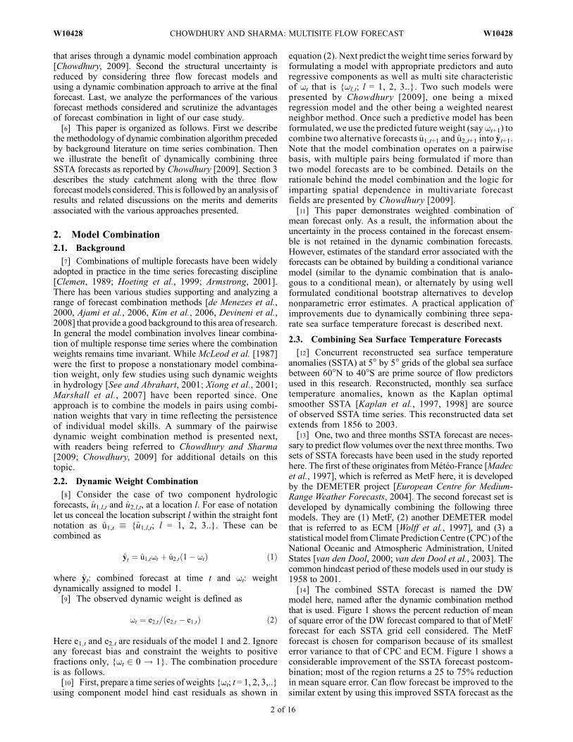
model here, named after the dynamic combination methodthat is used. Figure 1 shows the percent reduction of meanof square error of the DW forecast compared to that of MetFforecast for each SSTA grid cell considered. The MetFforecast is chosen for comparison because of its smallesterror variance to that of CPC and ECM. Figure 1 shows aconsiderable improvement of the SSTA forecast postcom-bination; most of the region returns a 25 to 75% reductionin mean square error. Can flow forecast be improved to thesimilar extent by using this improved SSTA forecast as the

2 of 16

W10428 CHOWDHURY AND SHARMA: MULTISITE FLOW FORECAST W10428

basis of concurrent prediction? Additionally, could furtherimprovements in flow forecasts be possible by consideringa dynamic combination of multiple flow forecast models?These are two of the questions we seek to address in theremainder of this paper.

3. Catchment Description and Flow ForecastingMethods

3.1. Catchment and River Description

[15] The Namoi River Catchment, with an area of42,000 km2, is a major contributor of flows within theMurray Darling Basin in eastern Australia. The centroid ofthe catchment is about 450 km northwest of Sydney. Thereare three major reservoirs with a total storage capacity of872 � 106 m3 and numerous other small dams, weirs andon farm ponds. The river supports 96,000 ha of irrigatedagriculture in addition to stock and domestic water use ofthe local population. Cotton is the major crop grown alongwith wheat and grazing pasture for the live stocks. Long-termmean surfacewater use is estimated to be 320� 106m3whichis close to half of the available runoff in the catchment[Commonwealth Scientific and Industrial Research Organi-sation (CSIRO), 2007]. Water extraction is regulated by thegovernment of the state of New South Wales (NSW). Avail-able water resources are allocated at the start of a sowingseason to the irrigators proportional to individual entitlementof annual extraction volume. The allocation is continuallyrevised throughout the irrigation season. Australian climaticvariability results in an unreliable pattern such as a lowallocation (less than 50%) era of 5 years followed by aresource abundant decade. Hence, it is typical of farming inan arid environment to vary sowing area of irrigated annualcrops from year to year. The land developed at the start ofthe sowing period is dependent on present allocation ofirrigation water and a forecast of likely increase in alloca-tion due to higher inflow in next few seasons. Overdevel-opment of the land than the available water increases capitalexpenditure, while underdevelopment amounts to a lostopportunity of the rare water abundant years. Henceimproved forecast of next seasons flow in the major riversin the Namoi Catchment has good economic potential.[16] The eastern half of the catchment is relatively wet

[Preece and Jones, 2002] and includes all the major streams

notably meeting irrigation demand. This study chose fivemajor river flow locations in the eastern half of the NamoiCatchment as shown in Figure 2. The overall natural flowhas been artificially altered to a varying degree by extrac-tions, weirs and river regulations since the European settle-ment in the catchment in the nineteenth century. The flow ofNamoi River at Keepit and the Peel River at Carroll Gap areregulated by the Split Rock Dam and the Chaffey Damconstructed in 1987 and 1979. We removed any humaninduced change in volumes (response time series) prior tosetting up the seasonal forecasting models. This is doneby modeling the river system by the integrated quantityquality model (IQQM). The hydrologic model IQQM wasprogressively developed in the 1990s by the NSW gov-ernment in Australia [Simons et al., 1996]. This is aconceptual deterministic model that mainly simulates(using a node link structure) daily rainfall-runoff, riverrouting, reservoir operation, irrigation demand and asso-ciated extractions subject to legal compliance [Hameedand Podger, 2001]. The calibrated Namoi IQQM has beenapplied in various water management studies [CSIRO,2007] including the development of a legal frameworkto share water resources of the catchment [Government ofNew South Wales, 2003]. All the dams, weirs, towns,irrigation and other extraction points are removed fromthe Namoi IQQM to simulate natural daily flow free ofhuman interference. The natural daily flows of 1898 to2007 are aggregated to estimate the seasonal flows used inthis study.

3.2. Flow Variability

[17] Strong flow variability is customary to arid riversin Australia and southern Africa. A number of studies inpast and present acknowledged the annual variability[McMahon, 1979;Ward, 1984;Chiew et al., 2003;McMahonet al., 2007] which tends to get more erratic at seasonal timescales. Mean volumes of Namoi inflows are two to ten timeshigher than the median flow volumes, see Table 1. Consid-erable spatial difference of flow height within Namoi Catch-ment were reported in past studies as well [Crapper et al.,1999].[18] Readers may refer to Kachroo [1992] for an overview

of the formulation process behind a flow forecast model.Forecasting flows of arid rivers pose additional challengesrelated to long hydrograph tails [Anderson and Meerschaert,1998] as seasonal pattern and persistence forms a minorportion of the total variance. A number of prior researchesidentified various SSTA derived indicators (includingNINO3.4) as prime predictors of flow and rainfall in easternAustralia. However, simulation of a variable that exhibits ahigh coefficient of skewness through a simple (linear) modelusing predictors that are not as highly skewed is difficult.[19] This section presents three methods that are primar-

ily aimed at our case study of forecasting flows at fivelocations using predictors from a concurrent SSTA field.Three flow forecasting models are developed with an aim ofdemonstrating the dynamic combination of three forecasts.One of the prime considerations in forming these threemodels is to maximize the structural independence amongthe three. Prior to presenting detail formula of the flowforecasting models in sections 3.3–3.6, let us introduce thenotation style for the ease of readership. This paper denotes

Figure 1. Percent reduction in square error of combinedSSTA forecast compared to that of the single best SSTAforecast (MetF model).

W10428 CHOWDHURY AND SHARMA: MULTISITE FLOW FORECAST

3 of 16

W10428

variables in italics for scalar values (e.g., yl,t), in roman forvectors (e.g., yt = {yl,t; l = 1, 2,..}) and in bold for higher-dimension matrices (e.g., V = {vi,t; i = 1, 2..I; t = 1, 2,..T}).Functions are defined by names followed by brackets, suchas logarithm being specified as log(.). The response vector(river flow) at a location l at time t is denoted by yl,t andrandom predictors are usually given a notation of X or Z,Greek characters denotes parameters.

3.3. Mixture of Linear and Multinomial Regression

[20] The generalized linear model (GLM) [McCullaghand Nelder, 1989; Chandler, 2005; Yang et al., 2005] is anextension of linear regression to include response variablesthat follow a family of exponential distributions. The expo-nential family relevant to hydrology includes lognormal,multinomial and Gamma distributions. We have used amixture of two GLMs in our forecast model. The firstGLM forecasts total flow (sum of flows across the fivesites) assuming a lognormal distribution. The second GLMforecast the proportion of the total flow at each site

assuming a multinomial distribution. This approach isbased on the rationale that overall water availability in acatchment is dictated by global climate indices while thespatial variation is more localized related to factors such asthe wind direction or vegetation profile (evapotranspira-tion). The two stages are outlined below.[21] The first stage involves a forecast of the sum of five

river flows using a generalized linear autoregressive(GLAR) model [Shephard, 1995; Yu et al., 2005]. TheGLAR is a special case of GLM that includes both auto-regressive terms and random covariates. The autoregres-sive variable exploits the persistence structure, a commonfeature in flow time series, and the random covariateallows inclusion of long-range climate indicators knownto influence the regional precipitation [Sveinsson et al.,2008]. While the choice of sum of flows, instead of singlesite, simplify the regression into univariate GLAR, thesummation also reduces the high variance of an arid riverflow system. Besides, a skewness stabilizing logarithmic

Table 1. Flow Locations, Catchment Area, and Associated Statisticsa

Location and Catchment Area Area (km2) Minimum Flow Median Flow Mean Flow Maximum Flow

Manila River at Split Rock 1650 70 5790 18780 429920Namoi River at Keepit Dam 5700 830 45410 94560 1050040Peel River at Carroll Gap 4670 1440 29300 65830 640570Mooki River at Breeza 3630 0 3150 29090 635860Cox’s Creek at Boggabri 4040 0 1770 16430 417860

aNote the spatial and temporal variability across the five rivers. Flow units are 1000 m3.

Figure 2. Namoi River Catchment flowing in a westerly direction. The five flow locations modeled arehighlighted. The main stream, called the Namoi River, flows in a westerly direction. The catchmentboundary lies within a grid box of 29.4�–32.2�S and 147.7�–151.7�E.

4 of 16

W10428 CHOWDHURY AND SHARMA: MULTISITE FLOW FORECAST W10428

transformation is used to allow proper specification of theforecasting model:

logðYtÞ ¼ ~Y s þ a logðYt�:Þ þ bXt ð3Þ

where Y t sum of multisite seasonal flow forecasted at time t;[22] Yt�. sum of multisite flow matrix at selected earlier

time steps;

[23] ~Ys seasonally varying intercept where s = 1, 2, 3and 4;[24] Xt multiple exogenous indicators derived using sea

surface temperature anomalies;[25] a, b GLAR parameters.[26] The first two elements of equation (3) model sea-

sonality and persistence in the flow time series. The thirdelement models climatic influences using variables derivedfrom concurrent SSTA fields. Our case study exploredvarious climatic indices and the first five principal compo-nents (PC) of the Indian and Pacific Ocean SSTA. Redun-dant predictors were screened out by backward stepwisemodel selection using the partial F test [Chambers, 1992;Hastie and Pregibon, 1992; Hastie et al., 2000]. Inaddition to the seasonal intercept, the autoregressors inthis example were identified as Yt�. = {Yt�1; Yt�3}. Thefollowing exogenous predictors were retained: Xt ={PC1+, PC1�, PC2}, where PC1+ denotes the positive

part in the first principal component with negative valuesbeing replaced by zeroes, PC1�, the negative part, andPC2 the second principal component. While separatingPC1 into the positive and negative parts may not adhereto distributional assumption (e.g., Gaussian) of linearmodel, it allows nonproportional influence of two oppos-ing climate state for example El Nino and La Nina. Theloadings of the first two principal components are shownin Figure 3. The positive or negative PCs are designed toseparate the strong positive or negative anomalies in thetransformed SSTA series. This association of SSTA PCs toflows has been reported in numerous past studies [Guetterand Georgakakos, 1996; Piechota et al., 1998; Hamletand Lettenmaier, 1999; Hsieh et al., 2003; Cardoso et al.,2005; Araghinejad et al., 2006; Cardoso and Dias, 2006].[27] Next, the total catchment flow Y t is apportioned to

various locations using a multinomial logit model [Agresti,1996, p. 206; Augustin et al., 2008]. The multinomial dis-tribution is an extension to the widely used binomial distri-bution (e.g., rainfall occurrence model). The multinomiallogit model predicts the log odds ratio of proportions of totalflow at a site as shown below:

logðrl;t=r5;tÞ ¼ ql þ llZt ð4Þ

Figure 3. Loadings of the first two principal components used as predictors of the forecast model GLM.

W10428 CHOWDHURY AND SHARMA: MULTISITE FLOW FORECAST

5 of 16

W10428

where rl,t proportion of total flow at a location l at time t, l =1, 2, 3 and 4;[28] r5,t proportion of total flow at fifth location at time t;[29] Zt multiple predictor set at time t;[30] ql, ll location specific intercept and the coefficient

vectors.[31] It should be noted that subscript l in equation (4) can

assume any 4 values, as r5,t = 1 � Srl,t. A common set ofthe multiple predictor vector Zt is used for all 4 locations.In simple terms this can be seen as four linear modelspredicting the four log odds ratio on the basis of a samepredictor set.[32] Candidate predictors of the multinomial model may

include inflow ratios in past time steps of all the riversalong with suitable climatic indices. The stepwise back-ward removal [Hastie et al., 2000] from the pool of can-didate predictors of this case study retained two predictorvectors Zt = {Yt�1, r2,t�1}. The first predictor is thesummation of the flows at the previous time step, Yt�1.The second predictor is the proportion of the Namoi Riverflow of the previous season (r2,t�1 = y2,t�1/Yt�1, wherey2,t�1 is flow from the second river). These predictorvariables are useful indicators of the state of the overallwetness of the system and the spatial spread of the totalcatchment inflow at the previous time step. The flow atindividual site is then estimated as yl,t

(G) = rl,t . Y t.[33] The above mixture of lognormal and multinomial

generalized regression models is necessary to replicate spa-tial dependence across the predicted flows over the fiverivers. However, there is an alternative way to maintainspatial dependence while utilizing the flexibility of univariateregression as shown next.

3.4. Independent Component and Local Polynomial(ICM)

[34] The need of a multivariate regression arises from theinterdependence of the flow variables constituting themultiple response vector. The need to have a multivariatemodel can be removed if the multivariate response matrixcan be transformed in a manner that removes the interde-pendence. Independent component analysis (ICA) yieldssuch transformation [Westra et al., 2007]. As per the centrallimit theorem, linearly mixing a number of independentsignals leads to response that approaches a Gaussian prob-ability distribution. ICA reverses the above logic by arguingthat there must exist a set of independent signals that can beidentified through transformations that result in these vari-ables being maximally non-Gaussian, or, characterized byprobability distributions that are as different as possiblefrom the Gaussian distribution. Independent components(ICs) are the result of unmixing the multivariate responsematrix using the above rationale. The ICA is performed onthe log-transformed flow series in which the Markov order 1persistence structure has been removed [Westra et al.,2008]:

logðyl;tÞ ¼ as logðYt�:Þ þ ql;t ð5Þ

where yl,t flow at location l and time t;[35] Yt�. sum of multisite flow at various earlier time

steps;

[36] as seasonal parameter, function of time t, where s �{1, 2, 3 or 4};[37] ql,t regression residual at location l and time t.[38] Because of the common predictors for all 5 flow sites

the dependence structure is maintained within the regressionresidual Q = {ql,t; l = 1, 2..L; t = 1, 2,..T}. The derivation ofICs of Q simplifies the multivariate regression into multipleunivariate regressions. The generic procedure is as follows[Hyvarinen and Oja, 2000].[39] First, the data is centered by subtracting the mean of

each column of the data matrix Q. The large data matrixmay then be condensed by projecting the data onto its prin-cipal component (PC) directions QE where E is eigenvectormatrix. The number of PCs to retain can be specified by theuser. Note that the intermediate step of estimating PC isnot a prerequisite of ICA. The ICA algorithm deducesthe unmixing matrix W subject to QE.W = V. Theunmixing matrix W is chosen to maximize the neg-entropyapproximation [Comon, 1994; Girolami, 1998] i.e., non-Gaussianity of the components under the constraints that Wis an orthonormal matrix. As a result, the columns of V areindependent of each other and can bemodeled as independentunivariate time series. Say V = {vi,t; i = 1, 2..I; t = 1, 2,..T}denotes I number of ICs of flow residualsQ = {ql,t; l = 1, 2..L;t = 1, 2,..T} where I � L. Next V is modeled using localregression as described below.[40] The use of local regression to forecast flow is not

new [Grantz et al., 2005; Lall et al., 2006]. Local regressionblends much of the simplicity of linear least squaresregression with the flexibility of nonlinear regression pro-viding a convenient tool to ascertain complex nonlinearrelationship between V and the SSTA predictor field.Prediction of V is done using a locally weighted polyno-mial regression, called Loess, originally proposed byCleveland [1979] and further developed later [Clevelandet al., 1988; Cleveland and Grosse, 1991]. At each pointin the data set a quadratic curve is fit to a local subset ofthe data. The polynomial is fit using weighted least squares,giving more weight to points near the point whose responseis being estimated and less weight to points further away.The use of the weights is based on the idea that points nearthe explanatory variable space are more likely to be relatedto each other in a simple way than points that are furtherapart. The following second degree local polynomial re-gressionGi,j(.) is used to predict the ICs of the flow residualmatrix:

vi;t ¼ Gi;jð8jXt þ yjX2t Þ þ ei;t ð6Þ

where Xt multiple predictor vector that includes persis-tence and climatic indices;[41] 8j; yj locally weighted regression parameters where

j is within the neighborhood of Xt.[42] ei,t regression error of ith IC at time t.[43] The inverse of ICA (and PC) weight matrices trans-

form back the predicted vi;tinv�!ql;t, the substitution of

estimated regression residual in equation (5) gives the flowforecast for the ICM method: yl,t

(I). Note that as each IC isindependent, their associated predictors must be indepen-dent too. Hence, separate predictor vectors Xt are identifiedin the forecasting model for each IC.

6 of 16

W10428 CHOWDHURY AND SHARMA: MULTISITE FLOW FORECAST W10428

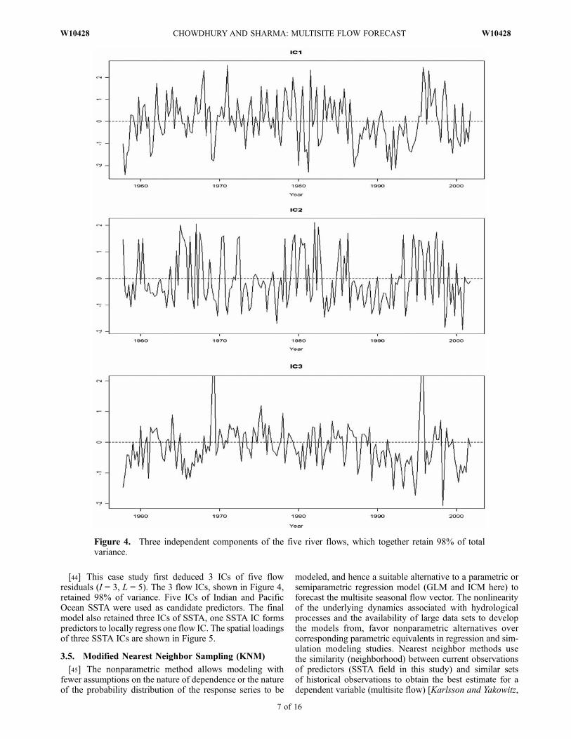
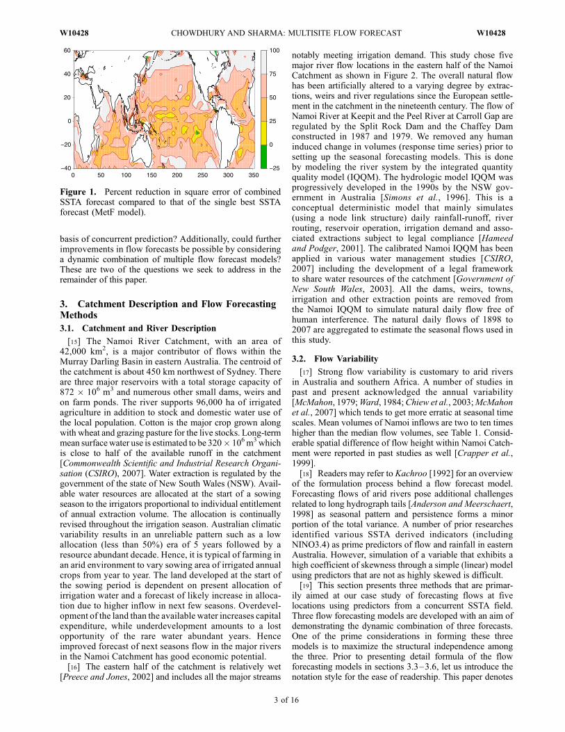
[44] This case study first deduced 3 ICs of five flowresiduals (I = 3, L = 5). The 3 flow ICs, shown in Figure 4,retained 98% of variance. Five ICs of Indian and PacificOcean SSTA were used as candidate predictors. The finalmodel also retained three ICs of SSTA, one SSTA IC formspredictors to locally regress one flow IC. The spatial loadingsof three SSTA ICs are shown in Figure 5.

3.5. Modified Nearest Neighbor Sampling (KNM)

[45] The nonparametric method allows modeling withfewer assumptions on the nature of dependence or the natureof the probability distribution of the response series to be

modeled, and hence a suitable alternative to a parametric orsemiparametric regression model (GLM and ICM here) toforecast the multisite seasonal flow vector. The nonlinearityof the underlying dynamics associated with hydrologicalprocesses and the availability of large data sets to developthe models from, favor nonparametric alternatives overcorresponding parametric equivalents in regression and sim-ulation modeling studies. Nearest neighbor methods usethe similarity (neighborhood) between current observationsof predictors (SSTA field in this study) and similar setsof historical observations to obtain the best estimate for adependent variable (multisite flow) [Karlsson and Yakowitz,

Figure 4. Three independent components of the five river flows, which together retain 98% of totalvariance.

W10428 CHOWDHURY AND SHARMA: MULTISITE FLOW FORECAST

7 of 16

W10428

1987; Lall and Sharma, 1996]. We have applied a weightednearest neighbor approach [Souza Filho and Lall, 2003;Mehrotra and Sharma, 2006] in formulating the forecastingmodel reported here. We refer this K nearest neighbormodeling approach as KNM in this paper. The KNMapproach aims to ascertain the conditional dependence ofmultisite seasonal flow yt = {yl,t, l = 1,2,. . .L} on a weightedset of predictors by identifying K nearest neighbors in thehistorical record. Identification of the nearest neighborsproceeds by ranking historical responses using a modifiedsquared Euclidean distance (x) metric:

xðtÞt ¼X

pbpðxp;t � xp;tÞ2 ð7Þ

where xp,t the scaled pth predictor at a past time t;[46] p 1, 2,. . . index of multiple predictor vectors;[47] t t � 1, t � 2,. . . index of past time;[48] bp the influence load to pth predictor vector. This

load can be approximated as the coefficients of the linearrelationship of (Yt � xt) where xt = {xp,t; p = 1, 2,..}and Yt = Slyl,t.[49] The response time series {yt; t = t � 1, t � 2, t �

3. . .} is ranked on the basis of the order of the current xt(t). If

kt is the sorted rank of yt then kt 2 {1, 2, 3,. . .K, 1},where K is the farthest neighbor considered for ascertainingthe prediction in the KNM approach. We recommend Kequals the nearest integer of

pT [Lall and Sharma, 1996].

A forecast is then expressed as an expected value of theconditional probability distribution formed on the basis ofthe nearest neighbors. The probability of resampling a pastobservation at time t is then specified as follows [Lall andSharma, 1996]:

Prðyt ¼ yt jXÞ ¼ k�1t =ð1þ 2�1 þ 3�1 . . .þ K�1Þ ð8Þ

where X is the multiple predictor vector {xp,t}. Note thatflows at all sites are sampled together from past observationyt = {yl,t.; l = 1, 2. . .L}. This concurrent multisite samplingreflects historical spatial dependence. The expected valueof the forecast by KNM method is yl,t

(K).[50] This case study selected KNM model predictors in

few steps. First the total flow time series (Yt) is scaled byremoving the mean and normalizing the variance to one.Alternatively, variance stabilizing transformation like takinglogarithm can also be used. The seasonal mean and the lagone scaled flow forms first two predictor vectors. Then we

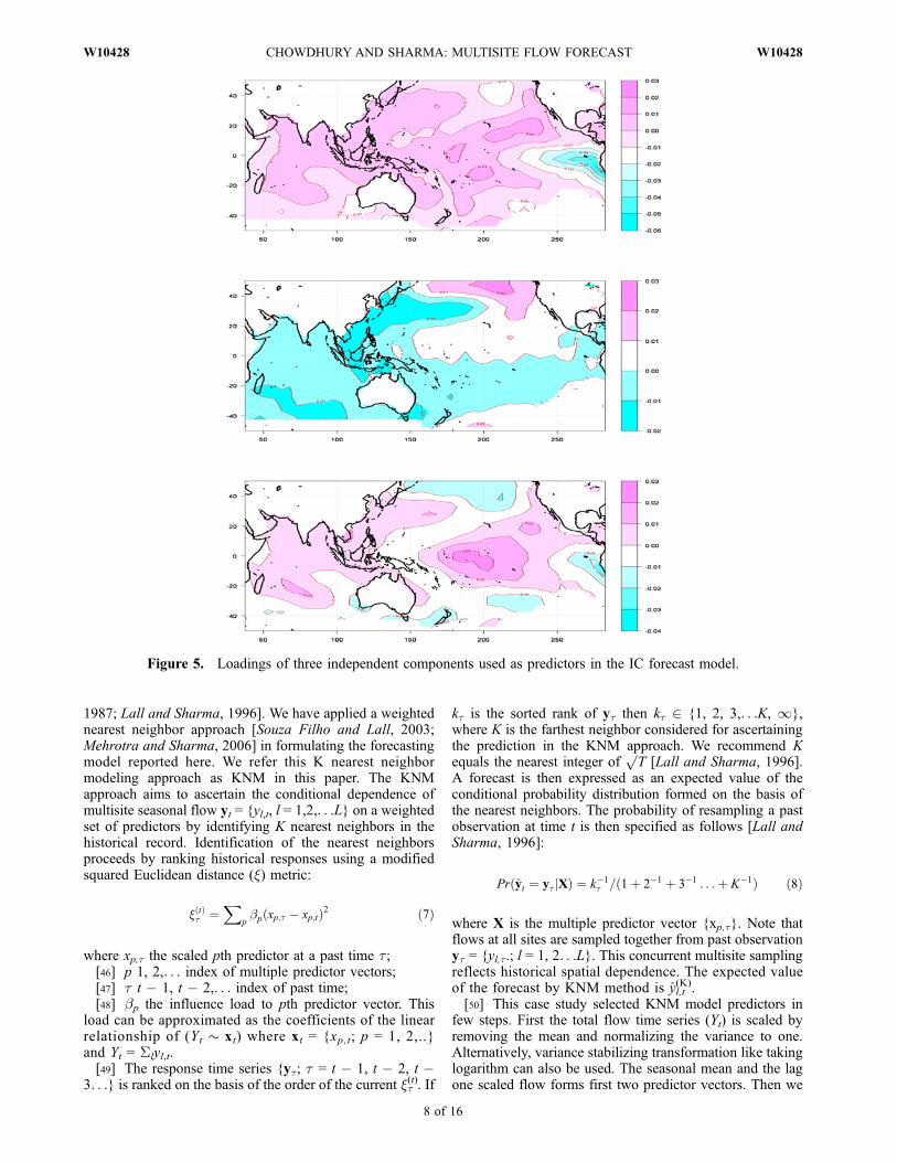
Figure 5. Loadings of three independent components used as predictors in the IC forecast model.

8 of 16

W10428 CHOWDHURY AND SHARMA: MULTISITE FLOW FORECAST W10428

globally explored the spread of correlation and mutualinformation scores [Sharma, 2000a] (see the notation sec-tion for mutual information formulation) of Yt to the SSTAfield. Seven SSTA zones with high dependence scores areselected as potential predictors. A partial F test of linearassociation of Yt to the seven zones retained four zones (seeFigure 6). Hence xt = {seasonal mean flow, Yt�1, averageSSTA zones at Pacific Ocean north, central, south and IndianOcean north}. The influence loads (bp) of the predictors are{0.55, 0.07, 0.08, 0.08, 0.11, 0.11}. This approach of usingzone averaged SSTA is not new in hydrological studies[Sharma et al., 2000; Verdon et al., 2004; Verdon and Franks,2005; Maity and Kumar, 2009].

3.6. Dynamic Combination of Forecasts

[51] The three component forecasts GLM, ICM andKNM are dynamically combined to reduce the structuraluncertainty of any single forecast. It should be noted that theapproach presented assumes that the component modelsbeing used are predefined and nonalterable. This is especiallyso when the component models are conceptual water balancemodels that have been developed by different groups andagencies, and hence are difficult to modify at each time stepof the simulation.[52] The pairwise dynamic weight requires presorting the

model pairs and the design of a hierarchical tree structure. Incase of a univariate response, Chowdhury and Sharma[2009] recommended models to be paired such that thecovariance of the paired responses was the minimum acrossall possible pairs. The guideline to optimal design of thehierarchical tree for multivariate response remains a poten-tial future research topic. In this case study, the residual covariances are all of similar magnitudes. Hence any variationof the tree architecture has a minor influence on the finalresult. After a few evaluations we decided on the treestructure as shown in Figure 7. For simplicity, the first levelof combination used static weight with dynamic combina-tion assigned to the highest level, an approach similar tomultivariate SSTA combination of Chowdhury [2009].Accordingly, KNM is combined to GLM using staticweights. The static weight assigned to KNM is the ratio ofprecision of KNM forecast to the sum of precision of KNMand GLM [Granger and Newbold, 1977; McLeod et al.,1987]. Then the KNM+GLM are dynamically combined to

ICM. Note that the tree structure keeps the number of weightsto two, same number as a static combination of three fore-casts.[53] The predictors of the time variant weights are {wt�1;

PC1� and PC1+}, where PC1 represents the first principalcomponent of the Indian and Pacific Ocean SSTA field, andPC1+ and PC1� their respective positive and negative com-ponents. The weights imply that the comparative forecaststrength of next season of any single model is reflected bythis season’s performance and the current state of climate.Figure 8 shows the observed weight time series and thefitted weight prediction. The forecast flow time series isdrawn against the observation in Figure 9. Note that onlythe time series of the wettest and the driest rivers are shownin this manuscript for sake of brevity.

4. Results and Discussion

4.1. Model Calibration and Validation

[54] All three models (GLM, ICM, KNM) forecast thetotal flow volume of the next season at the end of currentseason. For example the autumn flow volume is forecastedusing summer flow volume and the autumn SSTA forecast.

Figure 6. Predictors of the KNM model as the meanseasonal SSTA at four zones shown as hatched boxes in thisgraph. The mutual information score of total flow volumesto mean seasonal SSTA is shown in the background.

Figure 7. Pairwise forecast combination tree.

Figure 8. The time series of weights corresponding tothree models. The forecast time series are extracted from±6 month cross-validation results. Only the largest andsmallest rivers are chosen for brevity: (top) Namoi Riverand (bottom) Cox’s Creek.

W10428 CHOWDHURY AND SHARMA: MULTISITE FLOW FORECAST

9 of 16

W10428

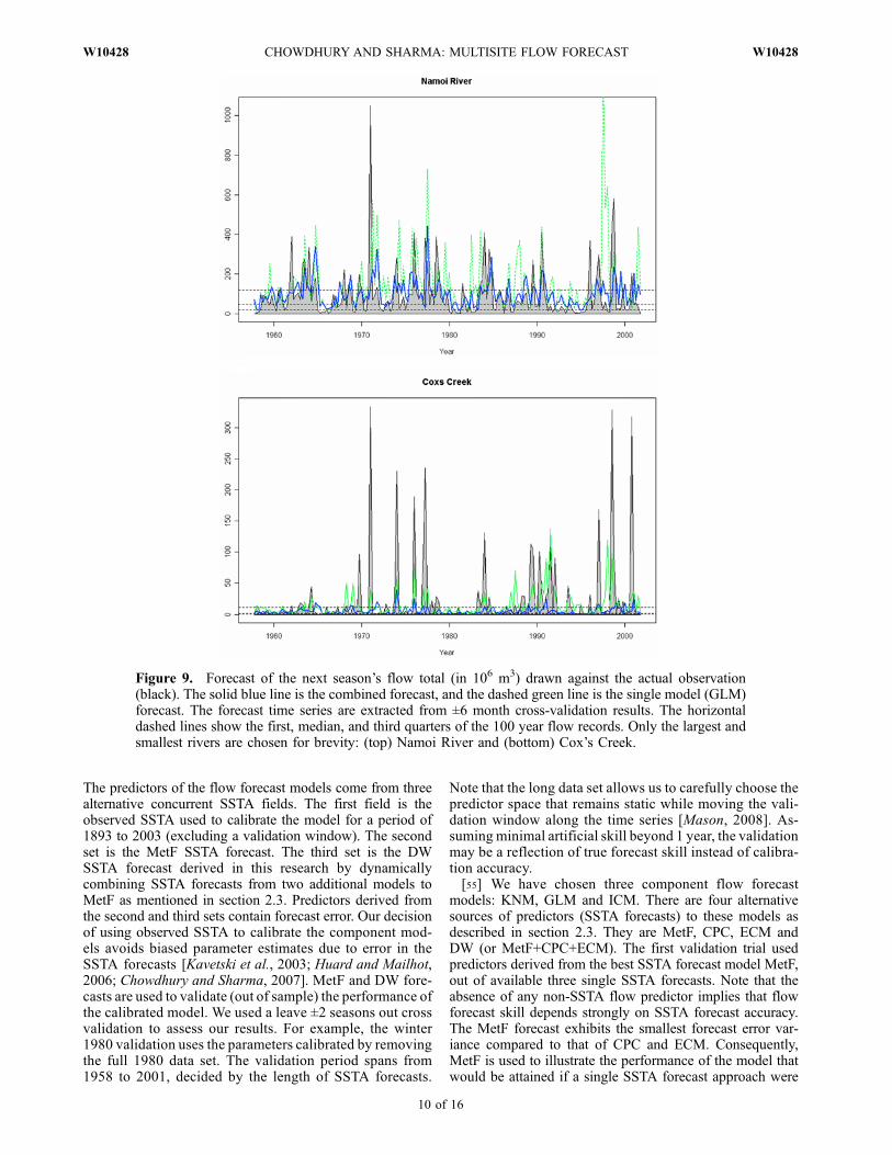
The predictors of the flow forecast models come from threealternative concurrent SSTA fields. The first field is theobserved SSTA used to calibrate the model for a period of1893 to 2003 (excluding a validation window). The secondset is the MetF SSTA forecast. The third set is the DWSSTA forecast derived in this research by dynamicallycombining SSTA forecasts from two additional models toMetF as mentioned in section 2.3. Predictors derived fromthe second and third sets contain forecast error. Our decisionof using observed SSTA to calibrate the component mod-els avoids biased parameter estimates due to error in theSSTA forecasts [Kavetski et al., 2003; Huard and Mailhot,2006; Chowdhury and Sharma, 2007]. MetF and DW fore-casts are used to validate (out of sample) the performance ofthe calibrated model. We used a leave ±2 seasons out crossvalidation to assess our results. For example, the winter1980 validation uses the parameters calibrated by removingthe full 1980 data set. The validation period spans from1958 to 2001, decided by the length of SSTA forecasts.

Note that the long data set allows us to carefully choose thepredictor space that remains static while moving the vali-dation window along the time series [Mason, 2008]. As-suming minimal artificial skill beyond 1 year, the validationmay be a reflection of true forecast skill instead of calibra-tion accuracy.[55] We have chosen three component flow forecast

models: KNM, GLM and ICM. There are four alternativesources of predictors (SSTA forecasts) to these models asdescribed in section 2.3. They are MetF, CPC, ECM andDW (or MetF+CPC+ECM). The first validation trial usedpredictors derived from the best SSTA forecast model MetF,out of available three single SSTA forecasts. Note that theabsence of any non-SSTA flow predictor implies that flowforecast skill depends strongly on SSTA forecast accuracy.The MetF forecast exhibits the smallest forecast error var-iance compared to that of CPC and ECM. Consequently,MetF is used to illustrate the performance of the model thatwould be attained if a single SSTA forecast approach were

Figure 9. Forecast of the next season’s flow total (in 106 m3) drawn against the actual observation(black). The solid blue line is the combined forecast, and the dashed green line is the single model (GLM)forecast. The forecast time series are extracted from ±6 month cross-validation results. The horizontaldashed lines show the first, median, and third quarters of the 100 year flow records. Only the largest andsmallest rivers are chosen for brevity: (top) Namoi River and (bottom) Cox’s Creek.

10 of 16

W10428 CHOWDHURY AND SHARMA: MULTISITE FLOW FORECAST W10428

used instead of the dynamic combination approach. Thesecond validation trial is based on predictors derived fromcombined SSTA forecast: DW. Finally we investigatedincremental skill postcombination of the three flow forecastmodels where the predictors came from DW SSTA forecast.[56] Model combination, because of extra parameters,

reduces degrees of freedom. The method relies on duediligence of the modelers in maintaining parsimony, usingminimal parameters and testing extensive validation. Wechose not to present the calibration results as this does notreflect the true predictive errors. Validation results aremainly unaffected by model complexity and hence betterrepresent predictive performance. Accordingly, it is empha-sized that sections 4.2 and 4.3 analyzed validation resultsonly.

4.2. Measures of Forecast Strength

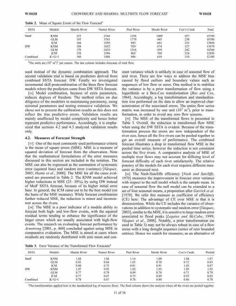
[57] One of the most commonly used performance criteriais the mean of square errors (MSE). MSE is a measure ofsquared deviation of forecast from the observation. Notethat the mathematical formulations of the error measuresdiscussed in this section are included in the notation. TheMSE can also be expressed as the summation of systematicerror (squared bias) and random error (variance) [Vazquez,2003; Hastie et al., 2000]. The MSE for all the cases eval-uated are presented in Table 2. The KNM model achievedhigher reductions in MSE (25–30%), by using DW insteadof MetF SSTA forecast, because of its higher initial errorbase. In general, the ICM came out to be the best model (onthe basis of the MSE measure). While forecast combinationfurther reduced MSE, the reduction is minor and inconsis-tent across the rivers.[58] The MSE is a poor indicator of a models ability to

forecast both high- and low-flow events, with the squaredresidual terms tending to enhance the significance of thelarger errors which are usually associated with high-flowevents. The research on evaluating forecast performance byArmstrong [2001, p. 460] concluded against using MSE incomparative evaluation. The MSE is aimed at cases whereresiduals are randomly distributed with zero mean and con-

stant variance which is unlikely in case of seasonal flow ofarid river. There are few ways to address the MSE biascaused by flood outliers and boundary values such assequences of low flow or zeros. One method is to stabilizethe variance is by a prior transformation of flow using alogarithmic or a Box-Cox transformation [Box and Cox,1964]. Accordingly, a log transformation and standardiza-tion was performed on the data to allow an improved char-acterization of the associated errors. The entire flow seriesmatrix was increased by one unit (103 m3), prior to trans-formation, in order to avoid any zero flow seasons.[59] The MSE of the transformed flows is presented in

Table 3. Overall, the reduction in transformed flow MSEwhen using the DW SSTA is evident. Because of the trans-formation process the errors are now independent of theriver size, hence all the five rivers can be pooled together toget an overall measure of performance. The combinedforecast illustrates a drop in transformed flow MSE in thepooled time series; however the reduction is not consistentacross the five rivers. A comparative analysis of MSE ofmultiple river flows may not account for differing level offorecast difficulty of each river satisfactorily. The relativepotency of the models for each river requires different mea-sures as discussed next.[60] The Nash-Sutcliffe efficiency [Nash and Sutcliffe,

1970] measures the improvement in forecast error variancewith respect to the null model which is the sample mean. Incase of seasonal flow the null model can be extended to aset of four seasonal means, a proposition after Garrick et al.[1978]. We refer this measure as coefficient of efficiency(CE) here. The advantage of CE over MSE is that it isdimensionless. While the CE includes the variance of obser-vations in addition to systematic and random error [Vazquez,2003], similar to theMSE, it is sensitive to large random errorassociated to flood peaks [Legates and McCabe, 1999;Vazquez et al., 2008]. Notably, a prior transformation (asused in Table 3) may not be always robust in case of a flowseries with a long drought sequence (series of zero boundedentries). Hence we search for measures, as an alternative of

Table 2. Mean of Square Errors of the Flow Forecasta

SSTA Models Manila River Namoi River Peel River Mooki River Cox’s Creek Total

MetF KNM 253 2344 1258 1009 457 19740GLM 193 3763 1779 445 238 18780ICM 168 1959 893 663 333 13850

DW KNM 188 1652 929 674 327 13670GLM 170 2435 1316 459 242 14760ICM 158 1594 805 768 324 12850

Combined K+G+I 160 1488 806 610 310 12180

aThe units are (106 m3)2 per season. The last column includes forecasts of total flow.

Table 3. Error Variance of the Transformed Flow Forecastsa

SSTA Models Manila River Namoi River Peel River Mooki River Cox’s Creek Pooled

MetF KNM 1.04 1.06 1.14 1.09 1.04 1.07GLM 0.83 0.84 1.03 0.70 0.72 0.83ICM 0.80 0.73 0.81 0.91 1.05 0.87

DW KNM 1.07 0.92 1.02 1.03 1.05 1.03GLM 0.77 0.79 0.99 0.70 0.71 0.79ICM 0.77 0.67 0.75 0.89 0.93 0.82

Combined K+G+I 0.78 0.67 0.78 0.80 0.86 0.78

aThe transformation applied here is the standardized log of nonzero flows. The final column shows the analysis where all the rivers are pooled together.

W10428 CHOWDHURY AND SHARMA: MULTISITE FLOW FORECAST

11 of 16

W10428

CE, which is suitable for arid river flow (time series withunstable variance).[61] The relative absolute error (RAE), which is the ratio

of absolute residual error to that of null model error, servesas a useful alternative to CE. The RAE returns 1 or a highervalue for no model skill to 0 for a perfect forecast. In orderto avoid outliers due to near zero null error and rivers withlong dry seasons, either a Winsorized or a median value ofRAE (MdRAE) is recommended. Winsorizing trims timeseries at an upper and lower boundary [Wu, 2006; Jose andWinkler, 2008]. Winsorizing relies on selection of appro-priate boundary limit, requiring external deliberation. Forsimplicity we chose the ultimate trimming by acceptingMdRAE as presented in Table 4. New insights to theforecast strength of the two driest rivers (Mooki and Cox’srivers) are evident, as they are most prone to outliers in theMSE-based measure. The MdRAE measures of Mooki andCox’s rivers are 0.5 and 0.3, which is lower (hence superiorskill) than the other three rivers. The combined flowforecast yields a narrower range of MdRAE across all thefive rivers (0.30 to 0.95) than either GLM (0.22 to 0.94) orICM (0.34 to 1.04). It is important to note that if thecombined model results are compared with any one of themodels on an individual basis, the combined model out-performs the other model on a majority of the riversanalyzed. Similar conclusion can be reached using otherstatistics (not shown here) such as the linear error inprobability space skill score [Potts et al., 1996].[62] In summary, the improvement in predictor field by

using DW rather than MetF SSTA forecast advances theflow forecast accuracy. The performance of single forecastmodel ICM and GLM are similar while KNM is a weakeralternative. There is an overall reduction of errors aftercombining the three forecast models. However, the incre-mental reduction in error due to the combination is smalland not consistent across all the five rivers. Note that theseremarks are based on univariate measures only. Thesemeasures do not consider spatial dependence of the rivers.

4.3. Representation of Spatial Dependence

[63] One of the key requirements for forecasting a mul-tivariate response is the representation of spatial dependenceacross the river system. A Pearson’s correlation can be usedas a simple measure of spatial dependence. The correlationof the raw flows of the arid river system would reflect lineardependence among larger rivers duringmajor flooding periodonly. Hence, the flow time series is transformed using a logtransformation (after adding a unit volume to avoid zeroes)and standardized to reduce the influence of outliers. The cor-relations of each transformed river flow against the four otherrivers are estimated next. Accordingly an observed vector of

10 correlation statistic is established. Figure 10 shows thecomparative graph of observed versus modeled correlationvalues. For clarity we only presented the set derived usingDW SSTA forecast. Figure 10 provides some interestinginsights into the differing capabilities of each model. Thesimple GLM structure is able to model the correlation insix out of the ten cases. The structure of GLM is weak inreproducing low correlation or interdependence between dryrivers. On the other hand linear regression tends to inflatedependency between the larger rivers. KNM and ICM struc-tures are primarily aimed at forecasting multivariate responsevariable. The KNM model maintained the intersite correla-tion better than GLM, however there is an apparent bias ofunderestimation. Conversely ICM returns a pattern of over-estimated correlation. The dynamically combined flow fore-casts illustrate superior replication of intersite correlationreducing the scatter present in the GLM estimates andmitigating the bias in KNM and ICM.

4.4. Discussion

[64] Combining flow forecast in this case study yieldsimprovement as compared to forecasts where no combina-tion was performed. However, the improvements in the com-bined flow forecasts are smaller compared to what wasachieved through a similar combination in order to arrive at

Table 4. Median Relative Absolute Error of the Flow Forecast

SSTA Models Manila River Namoi River Peel River Mooki River Cox’s Creek Pooleda

MetF KNM 0.92 1.14 1.13 1.09 1.09 1.07GLM 0.87 1.03 1.19 0.38 0.44 0.77ICM 0.90 1.08 0.98 0.40 0.51 0.81

DW KNM 0.90 1.04 1.01 1.00 0.92 0.98GLM 0.69 0.97 1.04 0.34 0.40 0.66ICM 0.81 0.93 0.94 0.56 0.22 0.78

Combined K+G+I 0.74 0.92 0.95 0.49 0.30 0.74

aAnalysis where all the rivers are pooled together.

Figure 10. Spatial dependence presented as pairedcorrelation of log flow of two rivers. Component modelsare as follows: k, KNM; g, GLM; i, ICM; and d, the com-bined model legend.

12 of 16

W10428 CHOWDHURY AND SHARMA: MULTISITE FLOW FORECAST W10428

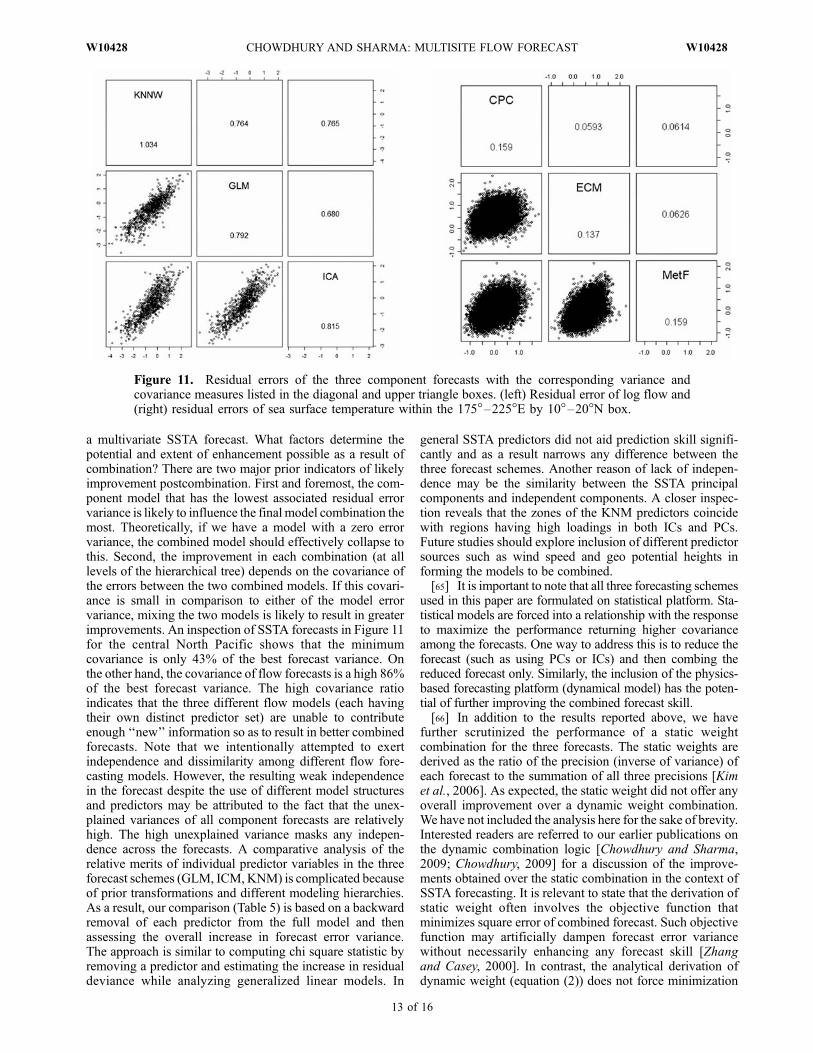
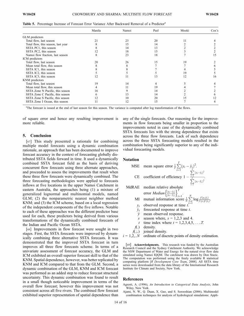
a multivariate SSTA forecast. What factors determine thepotential and extent of enhancement possible as a result ofcombination? There are two major prior indicators of likelyimprovement postcombination. First and foremost, the com-ponent model that has the lowest associated residual errorvariance is likely to influence the final model combination themost. Theoretically, if we have a model with a zero errorvariance, the combined model should effectively collapse tothis. Second, the improvement in each combination (at alllevels of the hierarchical tree) depends on the covariance ofthe errors between the two combined models. If this covari-ance is small in comparison to either of the model errorvariance, mixing the two models is likely to result in greaterimprovements. An inspection of SSTA forecasts in Figure 11for the central North Pacific shows that the minimumcovariance is only 43% of the best forecast variance. Onthe other hand, the covariance of flow forecasts is a high 86%of the best forecast variance. The high covariance ratioindicates that the three different flow models (each havingtheir own distinct predictor set) are unable to contributeenough ‘‘new’’ information so as to result in better combinedforecasts. Note that we intentionally attempted to exertindependence and dissimilarity among different flow fore-casting models. However, the resulting weak independencein the forecast despite the use of different model structuresand predictors may be attributed to the fact that the unex-plained variances of all component forecasts are relativelyhigh. The high unexplained variance masks any indepen-dence across the forecasts. A comparative analysis of therelative merits of individual predictor variables in the threeforecast schemes (GLM, ICM, KNM) is complicated becauseof prior transformations and different modeling hierarchies.As a result, our comparison (Table 5) is based on a backwardremoval of each predictor from the full model and thenassessing the overall increase in forecast error variance.The approach is similar to computing chi square statistic byremoving a predictor and estimating the increase in residualdeviance while analyzing generalized linear models. In

general SSTA predictors did not aid prediction skill signifi-cantly and as a result narrows any difference between thethree forecast schemes. Another reason of lack of indepen-dence may be the similarity between the SSTA principalcomponents and independent components. A closer inspec-tion reveals that the zones of the KNM predictors coincidewith regions having high loadings in both ICs and PCs.Future studies should explore inclusion of different predictorsources such as wind speed and geo potential heights informing the models to be combined.[65] It is important to note that all three forecasting schemes

used in this paper are formulated on statistical platform. Sta-tistical models are forced into a relationship with the responseto maximize the performance returning higher covarianceamong the forecasts. One way to address this is to reduce theforecast (such as using PCs or ICs) and then combing thereduced forecast only. Similarly, the inclusion of the physics-based forecasting platform (dynamical model) has the poten-tial of further improving the combined forecast skill.[66] In addition to the results reported above, we have

further scrutinized the performance of a static weightcombination for the three forecasts. The static weights arederived as the ratio of the precision (inverse of variance) ofeach forecast to the summation of all three precisions [Kimet al., 2006]. As expected, the static weight did not offer anyoverall improvement over a dynamic weight combination.We have not included the analysis here for the sake of brevity.Interested readers are referred to our earlier publications onthe dynamic combination logic [Chowdhury and Sharma,2009; Chowdhury, 2009] for a discussion of the improve-ments obtained over the static combination in the context ofSSTA forecasting. It is relevant to state that the derivation ofstatic weight often involves the objective function thatminimizes square error of combined forecast. Such objectivefunction may artificially dampen forecast error variancewithout necessarily enhancing any forecast skill [Zhangand Casey, 2000]. In contrast, the analytical derivation ofdynamic weight (equation (2)) does not force minimization

Figure 11. Residual errors of the three component forecasts with the corresponding variance andcovariance measures listed in the diagonal and upper triangle boxes. (left) Residual error of log flow and(right) residual errors of sea surface temperature within the 175�–225�E by 10�–20�N box.

W10428 CHOWDHURY AND SHARMA: MULTISITE FLOW FORECAST

13 of 16

W10428

of square error and hence any resulting improvement ismore reliable.

5. Conclusion

[67] This study presented a rationale for combiningmultiple model forecasts using a dynamic combinationrationale, an approach that has been documented to improveforecast accuracy in the context of forecasting globally dis-tributed SSTA fields forward in time. It used a dynamicallycombined SSTA forecast field as the basis of derivingconcurrent flow forecasts using three alternate approaches,and proceeded to assess the improvements that result whenthese three flow forecasts were dynamically combined. Thethree forecasting methodologies were applied to forecastsinflows at five locations in the upper Namoi Catchment ineastern Australia, the approaches being (1) a mixture ofgeneralized lognormal and multinomial models, namedGLM; (2) the nonparametric nearest neighbor methodKNM; and (3) the ICM scheme, based on a local regressionof the independent components of the five inflows. Notableto each of these approaches was the different predictor baseused for each, these predictors being derived from varioustransformations of the dynamically combined forecasts ofthe Indian and Pacific Ocean SSTA.[68] Improvements in flow forecast were sought in two

stages. First, the SSTA forecasts were improved by dynam-ically combining three alternative SSTA forecasts. It wasdemonstrated that the improved SSTA forecast in turnimproves all three flow forecasts scheme. In terms of aunivariate assessment of forecast accuracy, the GLM andICM exhibited an overall superior forecast skill to that of theKNM. Spatial dependence, however, was better replicated byKNM and ICM compared to that from the GLM. Second, adynamic combination of the GLM, KNM and ICM forecastwas performed as an added step to reduce forecast structuraluncertainty. This dynamic combination was found to resultin a small though noticeable improvement in terms of theoverall flow forecast; however this improvement was notconsistent across all five rivers. The combined flow forecastexhibited superior representation of spatial dependence than

any of the single forecasts. Our reasoning for the improve-ments in flow forecasts being smaller in proportion to theimprovements noted in case of the dynamically combinedSSTA forecasts lies with the strong dependence that existsacross the three flow forecasts. Lack of such dependenceacross the three SSTA forecasting models resulted in thecombination being significantly superior to any of the indi-vidual forecasting models.

Notation

MSE mean square error 1T

PTt¼1

yt � ytð Þ2.

CE coefficient of efficiency 1�

PTt¼1

yt�ytð Þ2

PTt¼1

yt�ysð Þ2.

MdRAE median relative absolute

error Medianjyt�yt jjyt�ysj

n oT

t¼1.

MI mutual information score 1N

PNi¼1

logf yi;yið Þf yið Þf yið Þ

.

yt observed response at time t.yt forecasted response at time t.y mean observed response.s season where, s = 1,2,3 and 4.t time index where t = 1,2,3,4,5, . . ..T.

f(.) density.f(.;.) joined density.

i = 1,2,..N ordinate of discrete points of density estimation.

[69] Acknowledgments. This research was funded by the AustralianResearch Council and the Sydney Catchment Authority. We acknowledgethe NSW Department of Water and Energy for the natural river flow datasimulated using Namoi IQQM. The catchment was drawn by Don Stazic.The computation was performed using the freely available R statisticalcomputing platform [R Development Core Team, 2008]. All SSTA timeseries were downloaded from the data library of the International ResearchInstitute for Climate and Society, New York.

ReferencesAgresti, A. (1996), An Introduction to Categorical Data Analysis, JohnWiley, New York.

Ajami, N. W., Q. Duan, X. Gao, and S. Sorooshian (2006), Multimodelcombination techniques for analysis of hydrological simulations: Appli-

Table 5. Percentage Increase of Forecast Error Variance After Backward Removal of a Predictora

Manila Namoi Peel Mooki Cox’s

GLM predictorsTotal flow, last season 21 23 20 11 4Total flow, this season, last year 8 15 14 2 2SSTA PC1, this season 8 14 13 2 2SSTA PC2, this season 12 18 15 3 2Namoi flow fraction, last season 8 23 18 7 15

ICM predictorsTotal flow, last season 20 26 15 19 2Mean total flow, this season 8 8 7 7 6SSTA IC1, this season 8 8 7 4 5SSTA IC2, this season 5 5 5 19 5SSTA IC3, this season 12 11 13 12 16

KNM predictorsTotal flow, last season 19 14 4 5 4Mean total flow, this season 4 11 19 4 7SSTA Zone N Pacific, this season 16 9 14 2 2SSTA Zone C Pacific, this season 6 13 14 2 6SSTA Zone S Pacific, this season 12 10 20 15 12SSTA Zone I Ocean, this season 11 12 15 7 4

aThe forecast is issued at the end of last season for this season. The variance is computed after log transformation of the flows.

14 of 16

W10428 CHOWDHURY AND SHARMA: MULTISITE FLOW FORECAST W10428

cation to distributed model intercomparison project results, J. Hydrome-teorol., 7, 755–768, doi:10.1175/JHM519.1.

Anderson, P. L., and M. M. Meerschaert (1998), Modeling river flows withheavy tails,Water Resour. Res., 34, 2271–2280, doi:10.1029/98WR01449.

Araghinejad, S., D. H. Burn, and M. Karamouz (2006), Long-lead prob-abilistic forecasting of streamflow using ocean atmospheric and hydrolo-gical predictors, Water Resour. Res., 42, W03431, doi:10.1029/2004WR003853.

Armstrong, J. S. (2001), Combining forecasts, in Principles of Forecasting:A Handbook for Researchers and Practitioners, edited by J. S. Armstrong,pp. 417–439, Kluwer Acad., Norwell, Mass.

Augustin, N. H., L. Beevers, and W. T. Sloan (2008), Predicting river flowsfor future climates using an autoregressive multinomial logit model,Water Resour. Res., 44, W07403, doi:10.1029/2006WR005127.

Box, G. E. P., and D. R. Cox (1964), An analysis of transformations, J. R.Stat. Soc., Ser. B, 26, 211–252.

Butts, M. B., J. T. Payne, M. Kristensen, and H. Madsen (2004), Anevaluation of the impact of model structure on hydrological modellinguncertainty for streamflow simulation, J. Hydrol., 298, 242 – 266,doi:10.1016/j.jhydrol.2004.03.042.

Cardoso, A. O., and P. L. S. Dias (2006), The relationship between ENSOand Paran’a River flow, Adv. Geosci., 6, 189–193.

Cardoso, A. O., R. T. Clarke, and P. L. S. Dias (2005), A case study of thesea surface temperatures (SSTs) to obtain predictors of river flow, in Re-gional Hydrological Impacts of Climatic Variability and Change– ImpactAssessment andDecisionMaking, edited by T.Wagener et al., IAHS Publ.,295, 231–238.

Chambers, J. M. (1992), Linear models, in Statistical Models in S, edited byJ. M. Chambers and T. Hastie, pp. 95–144, Wadsworth and Brooks,Pacific Grove, Calif.

Chandler, R. E. (2005), On the use of generalized linear models for interpretingclimate variability, Environmetrics, 16, 699–715, doi:10.1002/env.731.

Chiew, F. H. S., and T. A. McMahon (2002), Global ENSO-streamflowteleconnection, streamflow forecasting and interannual variability,Hydrol.Sci. J., 47, 505–522.

Chiew, F. H. A., T. C. Piechota, J. A. Dracup, and T. A. McMahon (1998),El Nino/Southern Oscillation and Australian rainfall, streamflow anddrought: Links and potential for forecasting, J. Hydrol., 204, 138–149,doi:10.1016/S0022-1694(97)00121-2.

Chiew, F. H. S., S. L. Zhou, and T. A. McMahon (2003), Use of seasonalstreamflow forecasts in water resources management, J. Hydrol., 270,135–144, doi:10.1016/S0022-1694(02)00292-5.

Chowdhury, S. (2009), Mitigating predictive uncertainty in hydroclimaticforecasts: Impact of uncertain inputs and model structural form, Ph.D.thesis, pp. 107–132, Univ. of New South Wales, Sydney, N.S.W.,Australia.

Chowdhury, S., and A. Sharma (2007), Mitigating parameter bias in hydro-logical modelling due to uncertainty in covariates, J. Hydrol., 340, 197–204, doi:10.1016/j.jhydrol.2007.04.010.

Chowdhury, S., and A. Sharma (2009), Long range NINO3.4 predictionsusing pair wise dynamic combinations of multiple models, J. Clim., 22,793–805, doi:10.1175/2008JCLI2210.1.

Clemen, R. T. (1989), Combining forecasts: A review and annotated biblio-graphy, Int. J. Forecast., 5, 559–583, doi:10.1016/0169-2070(89)90012-5.

Cleveland, W. S. (1979), Robust locally weighted regression and smoothingscatterplots, J. Am. Stat. Assoc., 74, 829–836, doi:10.2307/2286407.

Cleveland, W. S., and E. Grosse (1991), Computational methods for localregressions, Stat. Comput., 1, 47–62, doi:10.1007/BF01890836.

Cleveland, W. S., S. J. Devlin, and E. Grosse (1988), Regression by localfitting methods, properties, and computational algorithms, J. Econometrics,37, 87–114, doi:10.1016/0304-4076(88)90077-2.

Commonwealth Scientific and Industrial Research Organisation (CSIRO)(2007), Water availability in the Namoi. A report to the Australian govern-ment from the CSIRO Murray-Darling Basin Sustainable Yields Project,Canberra.

Comon, P. (1994), Independent component analysis, a new concept?, SignalProcess., 36, 287–314, doi:10.1016/0165-1684(94)90029-9.

Crapper, P. F., S. G. Beavis, and L. Zhang (1999), The relationship betweenclimate and streamflow in the Namoi Basin, Environ. Int., 25, 827–839,doi:10.1016/S0160-4120(99)00048-3.

de Menezes, L. M., D. W. Bunn, and J. W. Taylor (2000), Review ofguidelines for the use of combined forecasts, Eur. J. Oper. Res., 120,190–204, doi:10.1016/S0377-2217(98)00380-4.

Devineni, N., A. Sankarasubramanian, and S. Ghosh (2008), Multimodelensembles of streamflow forecasts: Role of predictor state in developingoptimal combinations, Water Resour. Res., 44, W09404, doi:10.1029/2006WR005855.

Drosdowsky, W., and L. E. Chambers (2001a), Near-global sea surfacetemperature anomalies as predictors of Australian seasonal rainfall,J.Clim., 14, 1677 – 1687, doi:10.1175/1520-0442(2001)014<1677:NACNGS>2.0.CO;2.

Dutta, S. C., J. W. Ritchie, D. M. Freebairn, and G. Y. Abawi (2006),Rainfall and streamflow response to El Nino Southern Oscillation: Acase study in a semiarid catchment, Australia, Hydrol. Sci. J., 51,1006–1020, doi:10.1623/hysj.51.6.1006.

European Centre for Medium-Range Weather Forecasts (2004), Develop-ment of a European multi-model ensemble system for seasonal to inter-annual prediction (DEMETER), 434 pp., Reading, U. K.

Garrick, M., C. Cunnane, and J. E. Nash (1978), A criterion of efficiencyfor rainfall runoff modelling, J. Hydrol., 36, 375–381, doi:10.1016/0022-1694(78)90155-5.

Georgakakos, K. P., D.-J. Seo, H. Gupta, J. Schaake, and M. B. Butts(2004), Towards the characterization of streamflow simulation uncer-tainty through multimodel ensembles, J. Hydrol., 298, 222 – 241,doi:10.1016/j.jhydrol.2004.03.037.

Girolami, M. (1998), An alternative perspective on adaptive independentcomponent analysis algorithms, Neural Comput., 10(8), 2103–2114,doi:10.1162/089976698300016981.

Goswami, M., and K. M. O’Connor (2007), Real-time flow forecasting inthe absence of quantitative precipitation forecasts: A multi-model ap-proach, J. Hydrol., 334, 125–140, doi:10.1016/j.jhydrol.2006.10.002.

Government of New South Wales (2003), Water sharing plan for the UpperNamoi and Lower Namoi regulated river water sources 2003,Gov. GazetteState N. S. W., 49, 2843–2908.

Granger, C. W. J., and P. Newbold (1977), Forecasting Economic TimeSeries, Academic, San Diego, Calif.

Grantz, K., B. Rajagopalan, M. Clark, and E. Zagona (2005), A techniquefor incorporating large-scale climate information in basin-scale ensemblestreamflow forecasts, Water Resour. Res., 41, W10410, doi:10.1029/2004WR003467.

Guetter, A., and K. Georgakakos (1996), Are the El Nino and La Ninapredictors of the Iowa River seasonal flow?, J. Appl. Meteorol., 35, 690–705, doi:10.1175/1520-0450(1996)035<0690:ATENAL>2.0.CO;2.

Hameed, T., and G. Podger (2001), Use of the IQQM simulation model forplanning andmanagement of a regulated system, IAHS Publ., 272, 83–89.

Hamlet, A. F., and D. P. Lettenmaier (1999), Columbia River stream-flow forecasting based on ENSO and PDO climate signals, J. WaterResour. Plann. Manage., 125, 333 –341, doi:10.1061/(ASCE)0733-9496(1999)125:6(333).

Hastie, T., and D. Pregibon (1992), Generalised linear models, in StatisticalModels in S, edited by J. M. Chambers and T. Hastie, pp. 195–248,Wadsworth and Brooks, Pacific Grove, Calif.

Hastie, T., R. Tibshirani, and J. Friedman (2000), The Elements of Sta-tistical Learning, Data Mining, Inference and Prediction, Springer,New York.

Hoeting, J. A., D. Madigan, A. E. Raftery, and C. T. Volinsky (1999),Bayesian model averaging: a tutorial (with comments by M. Clyde, DavidDraper and E. I. George, and a rejoinder by the authors), Stat. Sci., 14,382–417, doi:10.1214/ss/1009212519.

Hsieh, W. W., J. Li Yuval, A. Shabbar, and S. Smith (2003), Seasonalprediction with error estimation of Columbia River streamflow in BritishColumbia, J. Water Resour. Plann. Manage., 129, 146 – 149,doi:10.1061/(ASCE)0733-9496(2003)129:2(146).

Huard, D., and A. Mailhot (2006), A Bayesian perspective on input un-certainty in model calibration: Application to hydrological model ‘‘abc,’’Water Resour. Res., 42, W07416, doi:10.1029/2005WR004661.

Hyvarinen, A., and E. Oja (2000), Independent component analysis: Algo-rithms and applications, Neural Networks, 13, 411–430, doi:10.1016/S0893-6080(00)00026-5.

Jose, V. R. R., and R. L. Winkler (2008), Simple robust averages of forecasts:Some empirical results, Int. J. Forecast., 24, 163–169, doi:10.1016/j.ijforecast.2007.06.001.

Kachroo, R. K. (1992), River flow forecasting. Part 1. A discussion of theprinciples, J. Hydrol., 133, 1–15, doi:10.1016/0022-1694(92)90146-M.

Kaplan, A., Y. Kushnir, M. A. Cane, and M. B. Blumenthal (1997), Reducedspace optimal analysis for historical data sets: 136 years of Atlantic seasurface temperatures, J. Geophys. Res., 102, 27,835–27,860.

Kaplan, A., M. A. Cane, Y. Kushnir, A. C. Clement, M. B. Blumenthal, andB. Rajagopalan (1998), Analyses of global sea surface temperature1856–1991, J. Geophys. Res., 103, 18,567–18,589.

Karlsson, M., and S. Yakowitz (1987), Nearest-neighbor methods for non-parametric rainfall-runoff forecasting, Water Resour. Res., 23, 1300–1308, doi:10.1029/WR023i007p01300.

W10428 CHOWDHURY AND SHARMA: MULTISITE FLOW FORECAST

15 of 16

W10428

Kavetski, D., S. Franks, and G. Kuczera (2003), Confronting input uncer-tainty in environmental modelling, in Calibration of Watershed Models,Water Sci. Appl., vol. 6, edited by Q. Duan et al.., pp. 49–68, AGU,Washington, D. C.

Kim, Y. O., D. Jeong, and I. H. Ko (2006), Combining rainfall-runoffmodel outputs for improving ensemble streamflow prediction, J. Hydrol.Eng., 11, 578–588, doi:10.1061/(ASCE)1084-0699(2006)11:6(578).

Lall, U., and A. Sharma (1996), A nearest neighbor bootstrap for time seriesresampling, Water Resour. Res., 32, 679–693, doi:10.1029/95WR02966.

Lall, U., Y.-I. Moon, H.-H. Kwon, and K. Bosworth (2006), Locallyweighted polynomial regression: Parameter choice and application toforecasts of the Great Salt Lake, Water Resour. Res., 42, W05422,doi:10.1029/2004WR003782.

Legates, D. R., and G. J. McCabe (1999), Evaluating the use of ‘‘goodness-of-fit’’ measures in hydrologic and hydroclimatic model validation,Water Resour. Res., 35, 233–241, doi:10.1029/1998WR900018.

Letcher, R. A., F. H. S. Chiew, and A. J. Jakeman (2004), An assessment ofthe value of seasonal forecasts in Australian farming systems, in In-ternational Environmental Modelling and Software Society (iEMSs)Conference, edited by C. Pahl-Wostl, S. Schmidt, and A. J. Jakeman,pp. 1511–1516, Univ. of Osnabruck, Osnabruck, Germany.

Madec, G., P. Delecluse, M. Imbard, and C. Levy (1997), OPA release 8,Ocean General Circulation Model reference manual, Lab. d’Oceangr.Dyn. et de Climatol., Inst. Pierre Simon Laplace, Paris.

Maity, R., and D. N. Kumar (2009), Hydroclimatic influence of large-scalecirculation on the variability of reservoir inflow, Hydrol. Processes, 23,934–942, doi:10.1002/hyp.7227.

Marshall, L., D. Nott, and A. Sharma (2007), Towards dynamic catchmentmodelling: A Bayesian hierarchical modelling framework, Hydrol.Processes, 21, 847–861, doi:10.1002/hyp.6294.

Mason, S. J. (2008), Understanding forecast verification statistics,Meteorol.Appl., 15, 31–40, doi:10.1002/met.51.

McCullagh, P., and J. A. Nelder (1989),Generalized Linear Models, 2nd ed.,Chapman and Hall, London.

McLeod, A. I., D. J. Noakes, K. W. Hipel, and R. M. Thompstone (1987),Combining hydrologic forecast, J. Water Resour. Plann. Manage., 113,29–41, doi:10.1061/(ASCE)0733-9496(1987)113:1(29).

McMahon, T. A. (1979), Hydrological characteristics of arid zones, in TheHydrology of Areas of LowPrecipitation, IAHSAISHPubl., 128, 105–123.

McMahon, T. A., R. M. Vogel, M. C. Peel, and G. G. S. Pegram (2007),Global streamflows –Part 1: Characteristics of annual streamflows,J. Hydrol., 347, 243–259, doi:10.1016/j.jhydrol.2007.09.002.

Mehrotra, R., andA. Sharma (2006), Conditional resampling of hydrologic timeseries using multiple predictor variables: A K-nearest neighbour approach,Adv. Water Resour., 29, 987–999, doi:10.1016/j.advwatres.2005.08.007.

Muluye, G. Y., and P. Coulibaly (2007), Seasonal reservoir inflow forecast-ing with low-frequency climatic indices: A comparison of data-drivenmethods, Hydrol. Sci. J., 52, 508–522, doi:10.1623/hysj.52.3.508.

Nash, J. E., and J. V. Sutcliffe (1970), River flow forecasting throughconceptual models, Part I –A discussion of principles, J. Hydrol., 10,282–290, doi:10.1016/0022-1694(70)90255-6.

Piechota, T. C., F. H. S. Chiew, J. A. Dracup, and T. A. McMahon (1998),Seasonal streamflow forecasting in eastern Australia and the El Nino–Southern Oscillation, Water Resour. Res., 34, 3035–3044, doi:10.1029/98WR02406.

Podbury, T., T. C. Scheales, I. Hussain, and B. S. Fischer (1998), Use of ElNino climate forecast in Australia, Am. J. Agric. Econ., 80, 1096–1101,doi:10.2307/1244211.

Potts, J. M., C. K. Folland, I. T. Jolliffe, and D. Sexton (1996), Revised‘‘LEPS’’ score for assessing climate model simulations and long-rangeforecasts, J. Clim., 9, 34–53, doi:10.1175/1520-0442(1996)009(0034:RSFACM(2.0.CO;2.

Preece, R. M., and H. A. Jones (2002), The effect of Keepit Dam on thetemperature regime of the Namoi River, Australia, River Res. Appl., 18,397–414, doi:10.1002/rra.686.

R Development Core Team (2008), R: A language and environment forstatistical computing, R Found. for Stat. Comput., Vienna.

Regonda, S. K., B. Rajagopalan, M. Clark, and E. Zagona (2006), A multi-model ensemble forecast framework: Application to spring seasonalflows in the Gunnison River Basin, Water Resour. Res., 42, W09404,doi:10.1029/2005WR004653.

See, L., and R. J. Abrahart (2001), Multi-model data fusion for hydrologicalforecasting, Comput. Geosci., 27, 987 – 994, doi:10.1016/S0098-3004(00)00136-9.

Shamseldin, A. Y., K. M. O’Connor, and G. C. Liang (1997), Methods forcombining the outputs of different rainfall-runoff models, J. Hydrol.,197, 203–229, doi:10.1016/S0022-1694(96)03259-3.

Sharma, A. (2000a), Seasonal to interannual rainfall probabilistic forecastsfor improved water supply management: Part 1–A strategy for systempredictor identification, J. Hydrol., 239, 232–239, doi:10.1016/S0022-1694(00)00346-2.

Sharma, A. (2000b), Seasonal to interannual rainfall probabilistic forecastsfor improved water supply management: Part 3–A nonparametric prob-abilistic forecast model, J. Hydrol., 239, 249–258, doi:10.1016/S0022-1694(00)00348-6.

Sharma, A., K. C. Luk, I. Cordery, and U. Lall (2000), Seasonal to interannualrainfall probabilistic forecasts for improved water supply management: Part2–Predictor identification of quarterly rainfall using ocean-atmosphere in-formation, J. Hydrol., 239, 240–248, doi:10.1016/S0022-1694(00)00347-4.

Shephard, N. (1995), Generalized linear autoregressions, Econ. Pap. 8,Nuffield Coll., Oxford, U. K.

Simons, M., G. Podger, and R. Cooke (1996), IQQM–A hydrologic mod-elling tool for water resource and salinity management, Environ. Soft-ware, 11, 185–192, doi:10.1016/S0266-9838(96)00019-6.

Souza Filho, F. A., and U. Lall (2003), Seasonal to interannual ensemblestreamflow forecasts for Ceara, Brazil: Applications of a multivariate,semiparametric algorithm, Water Resour. Res., 39(11), 1307,doi:10.1029/2002WR001373.

Sveinsson, O. G. B., U. Lall, V. Fortin, L. Perrault, J. Gaudet, S. Zebiak,and Y. Kushnir (2008), Forecasting spring reservoir inflows in ChurchillBasin in Quebec, Canada, J. Hydrol. Eng., 13, 426–437, doi:10.1061/(ASCE)1084-0699(2008)13:6(426).

van den Dool, H. (2000), Constructed analogue prediction of the eastcentral tropical Pacific SST and the entire world ocean for 2001, Exp.Long Lead Forecast Bull., 9, 38–41.

van den Dool, H., J. Huang, and Y. Fan (2003), Performance and analysis ofthe constructed analoguemethod applied to U.S. soil moisture over 1981–2001, J. Geophys. Res., 108(D16), 8617, doi:10.1029/2002JD003114.

Vazquez, R. F. (2003), Assessment of the performance of physically baseddistributed codes simulating medium size hydrological systems, PhD.dissertation, Kath. Univ. Leuven, Leuven, Belgium.

Vazquez, R. F., P. Willems, and J. Feyen (2008), Improving the predictionsof a MIKE SHE catchment-scale application by using a multi-criteriaapproach, Hydrol. Processes, 22, 2159–2179, doi:10.1002/hyp.6815.

Verdon, D. C., and S. W. Franks (2005), Indian Ocean sea surface tempera-ture variability and winter rainfall: Eastern Australia, Water Resour. Res.,41, W09413, doi:10.1029/2004WR003845.

Verdon, D. C., A. M. Wyatt, A. S. Kiem, and S. W. Franks (2004), Multi-decadal variability of rainfall and streamflow: Eastern Australia, WaterResour. Res., 40, W10201, doi:10.1029/2004WR003234.

Ward, R. C. (1984), Some aspects of river flow in northern New SouthWales,Australia, J. Hydrol., 71, 31–51, doi:10.1016/0022-1694(84)90070-2.

Westra, S., C. Brown, U. Lall, and A. Sharma (2007), Modeling multi-variable hydrological series: Principal component analysis or independentcomponent analysis?, Water Resour. Res., 43, W06429, doi:10.1029/2006WR005617.

Westra, S., A. Sharma, C. Brown, and U. Lall (2008), Multivariate stream-flow forecasting using independent component analysis, Water Resour.Res., 44, W02437, doi:10.1029/2007WR006104.

Wolff, J. E., E. Maier-Reimer, and S. Legutke (1997), The Hamburg oceanprimitive equation model, Tech. Rep. 13, Dtsch. Klimarechenzent.,Hamburg, Germany.

Wu, M. (2006), Trimmed and winsorized estimators, PhD thesis, Mich.State Univ., East Lansing.

Xiong, L., A. Y. Shamseldin, and K. M. O’Connor (2001), A non-linearcombination of the forecasts of rainfall-runoff models by the first-orderTakagi-Sugeno fuzzy system, J. Hydrol., 245, 196–217, doi:10.1016/S0022-1694(01)00349-3.

Yang, C., R. E. Chandler, and V. S. Isham (2005), Spatial-temporal rainfallsimulation using generalized linear models, Water Resour. Res., 41,W11415, doi:10.1029/2004WR003739.

Yu, L., S. Wang, and K. K. Lai (2005), A novel nonlinear ensemble fore-casting model incorporating GLAR and ANN for foreign exchange rates,Comput. Oper. Res., 32, 2523–2541, doi:10.1016/j.cor.2004.06.024.

Zhang, H., and T. Casey (2000), Verification of categorical probabilityforecasts, Weather Forecast. , 15 , 80 – 89, doi:10.1175/1520-0434(2000)015<0080:VOCPF>2.0.CO;2.

����������������������������S. Chowdhury and A. Sharma, School of Civil and Environmental

Engineering, University of New SouthWales, Sydney, NSW2052, Australia.(a.sharma@unsw.edu.au)

16 of 16

W10428 CHOWDHURY AND SHARMA: MULTISITE FLOW FORECAST W10428