Annual Planning Outlook - Demand Forecast Methodology ...

Annual Planning Outlook Demand Forecast Methodology December 2020

Independent Electricity System Operator | 2020 Annual Planning Outlook: Demand Forecast Methodology 1

Table of Contents

1. Introduction 3

2. Role of the Demand Forecast within the Bulk System Planning Process and the Annual Planning Outlook 4

3. Demand Forecasting Process 5

3.1 Annual Gross Energy Demand Forecast 6

3.1.1 End-Use Forecasting Model 6

3.1.2 EUF Modules 7

3.1.2.1 EUF Market Segmentation Module 7

3.1.2.2 EUF Energy Usage Module 8

3.1.2.3 EUF Customer Growth Module 8

3.1.2.4 EUF Equipment Choice Module 8

3.1.2.5 Scenario Forecasting Module 9

3.1.3 Calibration, Consultation and Professional Judgement 9

3.2 Hourly Gross Energy Demand Forecast 10

3.3 Hourly Net Energy Demand Forecast 11

3.3.1 Conservation 11

3.3.1.1 Conservation Programs 11

3.3.1.2 Conservation Regulations 12

3.3.1.2.1 Ontario Building Codes 12

3.3.1.2.2 Equipment Standards 13

3.4 Delta Process 14

3.4.1 Base Year Calibration 14

3.4.1.1 Weather Correction 15

3.4.1.2 Embedded Generation 15

4. Drivers Used in the Demand Forecast 16

4.1 Market Segmentation 17

4.1.1 Residential Sector 17


4.1.2 Commercial Sector 18

4.1.3 Industrial Sector 20

4.2 Electric Vehicles 21

4.3 Rail Transit Electrification 22

4.4 Other Electricity Demand 22


1. Introduction

The IESO produces annual planning outlooks (APOs) for the province. The demand for electricity establishes the context for resource adequacy planning as it determines the amount of electricity that must be served.


2. Role of the Demand Forecast within the Bulk System Planning Process and the Annual Planning Outlook

The demand for electricity establishes the context for integrated planning as it determines the amount of electricity that must be served. The IESO updates the demand forecast to provide context for updated integrated plans, conservation program planning and supply procurement decisions. The demand for electricity establishes the context for integrated planning as it determines the amount of electricity that must be served. Electricity requirements are affected by many factors, including choice of energy form, technology, equipment purchasing decisions, behaviour, demographics, population, the economy, energy prices, transportation policy and conservation. The IESO monitors and interprets these and other factors on an ongoing basis to develop outlooks against which integrated planning can take place. The first step in the development of the APO is to determine a long-term demand forecast.

Figure 1: How the Demand Forecast Fits into Bulk System Planning Process


3. Demand Forecasting Process

Overview: the process used to develop the demand forecast is illustrated in Figure 2 below.

Figure 2: Demand Forecasting Process

1. Annual Gross Energy Demand Forecast: the production of the IESO’s planning forecast begins with the estimation of annual sectoral and zonal gross energy demands at the end-use level. Demographic and economic drivers are considered in the development of the annual gross energy demand forecast, including changes in household counts and types, commercial floor space, industrial output and energy price. Annual gross energy demand estimates are computed with the IESO’s End-Use Forecaster model (EUF). The EUF produces estimates of energy consumption at the consumer level. The IESO applies transmission and distribution line losses to convert these energy values to the generator level.

2. Hourly Gross Energy Demand Forecast: once completed, annual sectoral and zonal gross energy demands are transformed into gross hourly energy demand values through the application of end-use level hourly load shapes.

3. Hourly Net Energy Demand Forecast:

Energy-Efficiency Programs and Codes and Standards Regulations: the hourly gross energy demand forecast is then corrected for projected policy-induced conservation savings (i.e., savings from energy-efficiency incentive programs, appliance and products standards, and commercial building codes). The outcome of this derivation is the hourly net energy demand forecast.

Net Demand Forecast: once completed, the zonal hourly net demand forecast establishes the amount of electricity that is to be served and forms the starting point for reliability assessment and integrated planning analysis.


3.1 Annual Gross Energy Demand Forecast

3.1.1 End-Use Forecasting Model The IESO’s demand forecast is developed on an end-use level basis. An end-use forecasting approach was chosen for a number of reasons, including the need to:

1. Capture structural changes in the economy, including the growth and decline of specific industries and change in the relative strength of sectors;

2. Address the impact on demand of the penetration of new electricity using technologies;

3. Ensure linkages between conservation savings estimates and underlying assumptions of the demand forecast;

4. Specifically address the impact on peak demand of the growth of different end-uses;

5. Allow updates to the codes and standards.

The EUF is built at the geographic zonal level with all zones aggregating up to the Ontario total. The EUF is an end-use model that tracks equipment and building stocks over time and simulates technology acquisition in the economy. The residential, commercial/institutional and industrial sectors are each analyzed separately and independently.

A schematic of the EUF is shown in Figure 3.

Figure 3: EUF Modules and Structure

https://www.ieso.ca/localContent/zonal.map/index.html


3.1.2 EUF Modules

Several primary modules form the heart of the EUF analytical framework. Figure 3 also depicts the relationships between these modules.

1. Market Segmentation Module

2. Energy Usage Module

3. Equipment Choice Module

4. Customer Growth Module

5. Scenario Forecasting Module

3.1.2.1 EUF Market Segmentation Module The EUF Market Segmentation Module governs the development of customized market segmentation designs and the population of the model with the necessary data. A third-party consultant supplied the majority of the data characterizing the end-uses as they apply to Ontario and its zones. The data includes: building characteristics, equipment saturations, fuel shares, end-use equipment efficiency shares, replacement technology relative efficiencies and capital costs. The IESO has been in the process of updating the end-use information whenever updates becomes available. The market segmentation of the model, shown in Figure 4, contains sectors, zones, building types, end-uses, fuel types and efficiency levels.

Figure 4: EUF Market Segmentation Data Category


3.1.2.2 EUF Energy Usage Module

The EUF Energy Usage Module tracks equipment utilization given the stock of equipment, building characteristics, and customer behaviour at any moment in time over the forecast horizon. For example, single-family homes may have a discrete set of central air conditioner efficiency choices, with each efficiency level having an associated electric consumption for each year. That consumption can vary in the short run as customers modify behaviour that results in changes to equipment utilization without changing the equipment itself. Factors that can affect consumption in the short run include weather, non-weather seasonal factors, building and customer characteristics, energy prices, disposable income, and other user-specified attributes. These relationships are specified in the EUF Energy Usage Module by combining:

1. a forecast of consumption factors or drivers (independent or exogenous variables); with

2. a set of coefficients associated with each exogenous variable.

3.1.2.3 EUF Customer Growth Module The EUF Customer Growth Module tracks the number of customers (facilities) within each vintage, geographic zone, and dwelling type or sub-sector from the market characterization. Customer growth varies over time through a range of factors, including forecasts of population (typically applicable to the residential sector) and square footage of different building types (typically applicable to the commercial sector). As with the EUF Energy Usage Module, these relationships are specified in the EUF Customer Growth Module by combining:

1. a forecast of customer growth factors or drivers (i.e., independent or exogenous variables); with

2. a set of coefficients associated with each exogenous variable.

The main drivers used in EUF Customer Growth Module, including residential households, commercial floor space and industrial physical drivers/activities, are provided by either third-party consultants or IESO internal analyses.

3.1.2.4 EUF Equipment Choice Module

Equipment stock changes in the EUF occur in response to new driver growth, as well as to end-of-life retirement and replacement of equipment. Increasing saturation and utilization is also considered (e.g., increasing number of computers per household). Equipment acquisition choices are governed by choice equations that consider energy operating costs, as well as capital costs. Different technologies are represented by five efficiency choice levels for each end-use. Discount rates by sector vary from 25 to 50 per cent. Recognizing that price and cost savings are not the only factors that determine consumer action, the choice equation is, therefore, a weighting of financial and non-financial factors.

The EUF Equipment Choice Module analyzes customer choice decisions among competitors and product options. For example, customers choose their end-use equipment based on fuel types and efficiency levels. Purchase decisions are represented by a nested structure of provider (fuel choices) and product (efficiency choices) choices. This is illustrated in Figure 5.


Choice equations are calibrated against base year new stock acquisition decisions across technology levels. For end-uses with a fuel choice (e.g., domestic water heating), purchase decisions are represented by nested fuel and efficiency choices.

Short-term behavioural response to price that reflects changes in equipment utilization without changing the equipment itself is captured through the use of behavioural price elasticity. The range of the elasticity is from -0.25 to -0.1 and captures behaviours, such as lowering thermostats and turning off lights and computer monitors.

The hierarchy of equipment choice module is shown in Figure 5.

Figure 5: EUF Customer Choice Module Hierarchy

3.1.2.5 Scenario Forecasting Module The EUF Scenario Forecasting Module combines the outputs from the EUF Energy Usage Module, EUF Equipment Choice Module and EUF Customer Growth Module. The EUF Scenario Forecasting Module then performs additional calculations regarding the turnover of equipment at the end of its useful life to produce forecasts for energy demand.

3.1.3 Calibration, Consultation and Professional Judgement

For calibration, the IESO’s zonal residential energy forecasts are compared with the annual local distribution company (LDC) yearbook published by the Ontario Energy Board (OEB), which summarizes actual energy demand by rate class. The IESO’s industrial forecast is also compared with IESO transmission-connected customer trends and market intelligence based on research and consultation with IESO power system planners, industrial conservation program account managers and others.


Energy consumption trends from Natural Resource Canada’s (NRCan) Office of Energy Efficiency are also used as check points with respect to provincial end-use energy and sector and sub-sector consumption trends. Information from NRCan’s Survey of Household Energy Use and sales data from the Canada Appliance Manufacturers Association are used to check the IESO’s equipment forecasts.

Other sources are used to check the energy demand forecast results, including but not limited to: The American Society of Heating, Refrigerating and Air-Conditioning Engineers (ASHRAE); the Residential Energy Consumption Survey (RECS) and Commercial Building Energy Consumption Surveys (CBECS) conducted by the U.S. Energy Information Administration; and the Residential Energy Use Survey conducted by the IESO Energy Efficiency division.

The IESO undertook extensive testing and calibration during model development and implementation, work that continues today.1

3.2 Hourly Gross Energy Demand Forecast In the “Bottom Up” method, individual end-use load profiles are aggregated to create residential, commercial and industrial sector profiles. These sector profiles are then aggregated to form the total Ontario system load profile. The advantage of this approach is that it provides detailed results that assist with activities such as conservation planning and sensitivity analysis. The IESO has compared the result from the “Bottom Up” method to the IESO 2019 weather-corrected demand profile to ensure that it represents a reasonable depiction of the Ontario demand profile.

In the “Delta” method, the Ontario system profile for a given base year is taken and used as a basis for the future energy demand forecast. The change in electricity use associated with a particular end-use over time is mapped to the corresponding end-use load shape, which is then added to or subtracted from the overall Ontario system profile.

If more electricity is to be used by an end-use over time, this constitutes an increment to the system profile. If less electricity is to be used by an end-use over time, this constitutes a decrement to the system profile.

Using a measured system profile as a base and adding only increments and decrements produces better alignment between the modeled and actual system profiles.

1 Over time the data that supports the demand forecast needs to be updated. Some of this data is updated by internal systems as they become available, while other inputs are procured through third-party resources and primary research. As technology and consumer behaviour evolves, end-use and other profiles require a refresh.


3.3 Hourly Net Energy Demand Forecast In this process, conservation will be deducted from the hourly gross energy demand forecast and results in the hourly net demand forecast.

3.3.1 Conservation Conservation is the cleanest and most cost-effective resource for helping to meet Ontario’s electricity needs. Ontario benefits from approximately 19 TWh of annual energy savings from programs delivered from 2006 to 2019. These savings can be attributed to energy-efficiency programs and improved building codes and equipment standards regulations. Conservation has made a significant contribution to electricity service in Ontario and have been an integral part of reliable and sustainable electricity system in the province.

3.3.1.1 Conservation Programs On March 21, 2019 the 2015-2020 Conservation First Framework (CFF) and Industrial Accelerator Program (IAP) Frameworks were discontinued and replaced with the Interim Framework. Given the current market conditions and the nature of certain projects, some savings from these frameworks are forecast to materialize after 2020. Collectively, all energy-efficiency programs from the CFF and IAP wind-down and Interim Framework are expected to realize annual electricity savings of 2.5 TWh in 2023.

On September 30, 2020, the Minister of Energy, Northern Development and Mines directed the IESO to implement a 2021-2024 Conservation and Demand Management Framework, starting in January 2021. The new framework will be centrally delivered by the IESO under the Save on Energy brand and will include incentive programs targeted to those who need them most, including opportunities for commercial, industrial, institutional, on-reserve First Nations, and income-eligible electricity consumers. The forecasted annual savings are 3 TWh in 2026 with a total budget close to $700 million.

Federally and municipally funded programs, including the Green Municipal Fund and the Climate Action Incentive Fund, are expected to result in electricity savings in Ontario. The savings are estimated with high uncertainty as not all program details are currently available.

Beyond existing and near-term committed energy-efficiency programs, from 2025 to 2040, there are potential opportunities to achieve greater electricity savings. Continued delivery of energy-efficiency initiatives is assumed and forecasted savings are included in the demand forecast. For planning purposes, annual incremental annual energy savings is assumed to be 0.46 per cent of annual gross demand, which is informed by the planned savings level of the 2021-2024 Framework. This will be updated when a future policy decision is made.


3.3.1.2 Conservation Regulations

3.3.1.2.1 Ontario Building Codes Building code regulations (hereinafter referred to “codes”) set minimum energy-efficiency requirements for new and substantially renovated buildings.

New commercial buildings or buildings undergoing major renovations are subject to provincial and federal codes. The energy-efficiency requirements in codes are often defined as a reduction factor (e.g., 25% more efficient than a design conforming to Model National Energy Code for Buildings (MNECB)). Given the broad range of design and technology choices that can meet these requirements, the IESO codes analysis also uses reduction factors.

The codes analysis deals with Cooling, Lighting, and Ventilation end-uses. Collectively, they represent about 60 per cent of the gross energy consumed by the commercial sector in the EUF. Each end-use has an energy use intensity (EUI) measured in energy per unit floor space (kWh/ft2) in the base year, which is used as its baseline performance. Estimated reduction factors set the minimum codes-compliant EUI relative to this baseline.

Floor space turnover: Each end-use has a retirement rate, defined as 1/EUL (effective useful life). For example, commercial chillers have an estimated lifespan of 40 years, so the annual retirement rate is 2.5 per cent. The demand forecast for each end-use is re-modeled by breaking the annual floor space value into annual values for:

1. Existing floor space;

2. New floor space; and

3. Renovated floor space.

Existing floor space decreases at the retirement rate. Renovated floor space for a given year is equal to the total floor space that was retired in the previous year. New floor space is estimated as the annual increase in total floor space. For each year, renovated floor space is subject to EUI reduction associated with federal building standards and new floor space is assigned an EUI based on the Ontario Building Code.

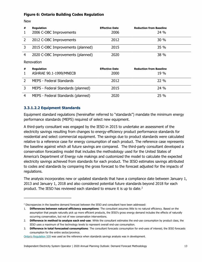
Reduction Factors: The reduction factors below were developed from estimates of the effect of existing codes on electricity-consuming end-uses. Planned future improvements to codes reflect a long-term trajectory of conservation policy with incremental improvements.


Figure 6: Ontario Building Codes Regulation

New # Regulation Effective Date Reduction from Baseline 1 2006 C-OBC Improvements 2006 24 %

2 2012 C-OBC Improvements 2012 30 %

3 2015 C-OBC Improvements (planned) 2015 35 %

4 2020 C-OBC Improvements (planned) 2020 38 %

Renovation # Regulation Effective Date Reduction from Baseline 1 ASHRAE 90.1-1999/MNECB 2000 19 %

2 MEPS - Federal Standards 2012 22 %

3 MEPS - Federal Standards (planned) 2015 24 %

4 MEPS - Federal Standards (planned) 2020 25 %

3.3.1.2.2 Equipment Standards Equipment standard regulations (hereinafter referred to “standards”) mandate the minimum energy performance standards (MEPS) required of select new equipment.

A third-party consultant was engaged by the IESO in 2015 to undertake an assessment of the electricity savings resulting from changes to energy-efficiency product performance standards for residential and select commercial equipment. The savings due to product standards were calculated relative to a reference case for energy consumption of each product. The reference case represents the baseline against which all future savings are compared. The third-party consultant developed a conservation forecasting model that includes the methodology used for the United States of America’s Department of Energy rule makings and customized the model to calculate the expected electricity savings achieved from standards for each product. The IESO estimates savings attributed to codes and standards by comparing the gross forecast to the forecast adjusted for the impacts of regulations.

The analysis incorporates new or updated standards that have a compliance date between January 1, 2013 and January 1, 2018 and also considered potential future standards beyond 2018 for each product. The IESO has reviewed each standard to ensure it is up to date.2

2 Discrepancies in the baseline demand forecast between the IESO and consultant have been addressed: 1. Differences between natural efficiency assumptions: The consultant assumes little to no natural efficiency. Based on the

assumption that people naturally pick up more efficient products, the IESO’s gross energy demand includes the effects of naturally occurring conservation, but not of new conservation interventions.

2. Difference in method to analyze each end-use: While the consultant estimates the end-use consumption by product class, the IESO uses a maximum of five technology levels to represent overall end-use consumption.

3. Difference in total forecasted consumptions: The consultant forecasts consumption for end-uses of interest; the IESO forecasts consumption for the entire sector/province.

Ontario Regulation 509 was used as the reference when standards savings analysis was in development.

https://www.ontario.ca/laws/regulation/180509


3.4 Delta Process Two different methods are used to produce the total system hourly gross energy demand forecast. The first, “Bottom Up” aggregation method, sums up sectoral demands. The second, “Delta” method, uses a historical system (for the 2020 APO, the year 2019 was used) hourly demand profile as a basis and then, each year, adds hourly increments or decrements in end-use demand.

Schematics of the Delta method is shown in Figure 7.

Figure 7: Converting Annual Energy to Hourly Peak

3.4.1 Base Year Calibration

For the 2020 APO demand forecast, the IESO used 2019 as the base year for the Delta method. The 2019 actual hourly energy demand profiles by zone and total Ontario system on a non-weather-corrected basis are available on the IESO’s power data - data directory - reports website. Under the Delta method, however, the base year profile, end-use energy forecasts and load shapes must be weather normalized to ensure that projected demand profiles include normal weather variability. The 2019 actual demand profile was weather corrected by the IESO using its weather-corrected daily peak and energy values (monthly normalization). The actual energy in each day was redistributed such that the daily peak meets the weather-corrected daily peak, while the daily energy will meet the weather-corrected daily energy. This was performed at the provincial level as zonal weather-corrected peak and energy values were not available.

https://ieso.ca/en/Power-Data/Data-Directory


The 2019 weather-corrected zonal hourly energy demand profile was obtained by allocating the hourly weather correction to each zone based on the zone’s share of Ontario system demand in each hour. The weather correction for each hour was then either added to or subtracted from the zone’s actual demand at that hour. The resulting demand profile by zone was checked to ensure the weather-corrected peak demand does not deviate from the usual time of day and occurs on the same day as or close to the day of the actual peak.

The base year forms the basis of the forecast as it is used as the starting point within the succeeding demand forecasting tools. The 2020 APO long-term demand forecast is at net (of conservation) level. The difference between net and grid demand is embedded generation and the Industrial Conservation Initiative (ICI). A number of steps are taken to generate hourly net energy demand profile from the hourly grid energy demand profile for the base year.

3.4.1.1 Weather Correction The demand on the IESO-controlled grid is the actual demand, which includes weather effects. Weather correction methodology is adopted to make sure normal weather variability is used. The IESO uses a rolling 31 years of weather data to generate “Normal” and “Extreme” weather scenarios. For each historical day, the daily weather can be converted into a "weather factor" based on wind, cloud, temperature and humidity conditions. As this weather factor represents that day’s weather in terms of a MW demand impact, each day in January from the 31 years history is converted into a number based on that day's weather. Then, within each month, the 31 days are ranked from highest to lowest based on weather impact. Next, the median value of the highest-ranked days becomes the highest-ranked day in the Normal month. The median value of the second-highest ranked days becomes the second highest ranked day in the Normal weather. This is repeated until 31 Normal days are generated for January. Detailed weather correction methodology can be found in the Reliability Outlook: Methodology to Perform the Reliability Assessment Outlook which can be found in the IESO’s Reliability Outlook webpage.

3.4.1.2 Embedded Generation

One important element from hourly grid energy demand forecasts to hourly net energy demand forecasts is embedded generation. Embedded generation is defined as an electricity-generating resource that does not participate in the IESO-administered wholesale market. Since such resources are not market participants, it is challenging to obtain accurate hourly data on actual generation and actual resources where such resources are non-IESO contracted. The most credible data is often available as monthly energy by fuel type through IESO’s settlements. Hourly embedded generation is calculated using hourly profiles. The fuel types of embedded generation generally includes: wind, solar, hydroelectric, natural gas and biomass. One generic hourly profile is developed for each fuel type by using available information from various sources, including: Hydro One hourly data, IESO contracts information (capacity), and IESO settlements data (monthly energy).

https://www.ieso.ca/en/Sector-Participants/Planning-and-Forecasting/Reliability-Outlook


4. Drivers Used in the Demand Forecast

Residential household count is the main driver used in the residential sector forecast. Household counts have a direct relationship with electricity consumption, as end-uses are measured using households as the unit. The household count forecast is based on information provided by a third-party consultant.

Commercial floor space is the main driver used in the commercial sector forecasts. Similar to household counts in the residential sector, commercial floor space has a direct relationship with electricity consumption. The commercial floor space forecast is provided by a third-party consultant.

The major driver for industrial sector electricity demand is industrial sector activity. The relationship between industrial sector GDP growth and industrial sector electricity demand use is often weak. A first effort at producing a set of physical drivers having a stronger connection with electricity use was made for each industry. Research, industry news, regional planning activities, and various analyses inform the development of physical drivers.

The agricultural sector’s electricity demand is heavily affected by greenhouse growth light utilization associated with vegetables and cannabis in southwestern Ontario. Data provided by LDCs and direct-connect customers was used to conduct energy and peak demand analyses. Additional electricity demand in this sector is also outlined in the reference scenario in the IESO West of London Bulk Study.

Electricity price and natural gas price also play an important role in the forecast. For example, higher electricity prices lead to greater energy efficiency measure uptake; lower natural gas prices lead to fuel switching (from electricity fueled to natural gas fueled measures), for example, space heating, water heating and cooking. The electricity and natural gas price forecast assumptions are discussed in the 2020 APO Supply, Adequacy and Energy Outlook Module.

http://www.ieso.ca/en/Get-Involved/Regional-Planning/Southwest-Ontario/Southwest-Ontario-Bulk-Planning-Initiatives

http://www.ieso.ca/en/Get-Involved/Regional-Planning/Southwest-Ontario/Southwest-Ontario-Bulk-Planning-Initiatives

https://ieso.ca/-/media/Files/IESO/Document-Library/planning-forecasts/apo/APO-Supply-Adequacy-Energy-Outlook-Module.pdf


4.1 Market Segmentation This section includes a listing of end-uses and building type for different sectors.

4.1.1 Residential Sector Figure 8: Residential Sector End-Uses

# Residential Sector End-Use

1 Air Conditioning - Central

2 Air Conditioning - Room

3 Baseboard Heating

4 Clothes Dryer

5 Clothes Washer

6 Computer

7 Cooking

8 Dehumidifier

9 Dishwasher

10 Domestic Hot Water

11 Elevator

12 Forced Air Central Heating

13 Freezer

14 Lighting

15 Lighting - Common Area

16 Miscellaneous

17 Other Consumer Electronics

18 Refrigerator

19 Set Top Box

20 Space Heating - Room

21 Swimming Pool Pump

22 Television

23 Ventilation and Circulation


Figure 9: Residential Sector Building Types # Residential Sector Building Type

1 Multi-Residential High Rise

2 Multi-Residential Low Rise

3 Other Residential Building

4 Row House

5 Single Family

4.1.2 Commercial Sector Figure 10: Commercial Sector End-Uses

# Commercial Sector End-Use

1 Commercial Electric Space Heating

2 Computer Equipment

3 Cooking

4 Cooling Chiller

5 Cooling - Direct Expansion

6 Domestic Hot Water

7 Elevator

8 Heating, Ventilation, Air Conditioning - Fans and Pumps

9 Lighting - Exterior

10 Lighting - General

11 Lighting - High Bay

12 Lighting - Interior Architectural

13 Miscellaneous Equipment

14 Other Plug Load

15 Refrigeration


Figure 11: Commercial Sector Business Types # Commercial Sector Business Type

1 Food Retail

2 Hospital

3 Large Hotel

4 Large Non-Food Retail

5 Large Office

6 Nursing Home

7 Other Commercial Building

8 Other Hotel, Motel

9 Other Non-Food Retail

10 Other Office

11 Restaurant

12 School

13 University and College

14 Warehouse Wholesale


4.1.3 Industrial Sector

Figure 12: Industrial Sector End-Uses # Industrial Sector End-Use

1 Compressed Air

2 Electro-Chemical

3 Heating, Ventilation, Air-Conditioning

4 Lighting

5 Motors - Fans and Blowers

6 Motors - Other

7 Motors - Pumps

8 Other

9 Process Cooling

10 Process Heating

11 Process Specific

Figure 13: Industrial Sector Sub-Sectors # Industrial Sector Sub-Sector

1 Chemical Manufacturing

2 Fabricated Metals

3 Food and Beverage

4 Mining

5 Miscellaneous Industrial

6 Non-Metallic Minerals

7 Paper Manufacturing

8 Petroleum Refineries

9 Plastic and Rubber Manufacturing

10 Primary Metals

11 Transportation and Machinery

12 Wood Products


4.2 Electric Vehicles The electric vehicle (EV) fleet in Ontario and its electricity charging needs are relatively small, but growing fast. Government policy has been and will continue to be the driver for EV adoption. Several measures are in place to support EV adoption, including purchase incentives; tax benefits for business vehicles; and support for EV charging infrastructure, automobile manufacturers, and automobile parts suppliers. Canada has set a target to sell 100 per cent zero-emission vehicles by 2040, with sales goals of 10 per cent by 2025 and 30 per cent by 2030.

EV charging demand is influenced by many factors, including adoption rates, utilization rates, policy, technology and consumer behaviour. The IESO’s EV charging projections are informed by a wide range of projections from various organizations, including consulting firms, academia and government and government agencies, and have a higher uncertainty than other sectors.

The EV forecast is based on historical trends and available information, such as EV sales, vehicle registration data, and forecast from other reputable organizations.

Using the 2019 APO EV charging forecast as the starting point, the 2020 plan makes two updates. The first is charging profiles, when and how EVs are charged, which are as important as the total charging electricity needs. Real-world charging data from the Charge the North project was used to develop the charging profile and EV hourly demand forecast. The second is pandemic impacts. Both EV sales and driving distance dropped in 2020, reflecting restriction measures and increases in the number of people working from home. Two scenarios are developed reflecting various levels of EV charging demand growth.

1. Scenario one: informed by the general trend of gross forecast scenario one, EV charging demand rebounds fast, reaching the level of the 2019 APO in 2030. The annual electricity charging demand is estimated at 4 TWh in 2040.

2. Scenario two: informed by the general trend of gross forecast scenario two, EV charging demand rebounds slower. The annual electricity charging demand in 2040 is estimated at 3 TWh, 75 per cent of the level in scenario one.


4.3 Rail Transit Electrification During the forecast horizon, more rail transit systems in Ontario will be electrified, including the GO rail system, various light rail transit projects, and subway lines in the Greater Toronto Area (GTA). These projects, when in operation, are expected to have an annual energy demand of about 1.8 TWh by 2029. Eight light rail transit projects are being built or planned across the province. The ION rapid transit project connecting Kitchener and Waterloo and the Confederation line in Ottawa have been in service since 2019. Early work on new subway projects, including the planned Ontario Line and two subway line extensions in GTA, is underway. Electrifying GO rail corridors is a multi-year project and the procurement process is underway.

Electricity demand arising from rail transit electrification is estimated and included in the plan based on most recent plans and schedules. A couple of these projects are at the early planning stage with little information on electricity requirements. Two demand scenarios have been developed, with the only variance being the timeline of the GO rail system electrification implementation. The IESO will update its rail transit electrification electricity demand projection, both in terms of magnitude and timing, when more information becomes available.

4.4 Other Electricity Demand The “Other Electricity Demand” category of demand includes:

1. connection of remote communities

2. street lighting;

3. electricity generator demand; and

4. water treatment facilities

Demand forecasting methodologies vary for each of the Other Electricity Demand sub-sectors and reflect study results from third-party consultants, the IESO’s regional resource planning, and consultations with LDCs.

Independent Electricity System Operator 1600-120 Adelaide Street West Toronto, Ontario M5H 1T1

Phone: 905.403.6900 Toll-free: 1.888.448.7777 E-mail: [email protected]

ieso.ca

@IESO_Tweets facebook.com/OntarioIESO linkedin.com/company/IESO

mailto:[email protected]

http://www.ieso.ca/

https://twitter.com/IESO_Tweets?ref_src=twsrc%5Egoogle%7Ctwcamp%5Eserp%7Ctwgr%5Eauthor

https://www.facebook.com/OntarioIESO

https://www.linkedin.com/company/ieso/

Annual Planning Outlook - Demand Forecast Methodology ...

Documents

Transcript of Annual Planning Outlook - Demand Forecast Methodology ...