Forecast Combination through Dimension Reduction

Techniques

Pilar Poncela, Julio Rodríguez, Rocío Sánchez-Mangas

Dept. Análisis Económico: Economía Cuantitativa

Universidad Autónoma de Madrid

Avenida Tomás y Valiente, 5. 28049 Madrid. SPAIN

Eva Senra

Dept. Estadística, Estructura Eca. y O.E.I.

Universidad de Alcalá

Plaza de la Victoria 2. 28802 Alcalá de Henares, Madrid. SPAIN.

July 7, 2008

1

Abstract:

The combination of individual forecasts is often a useful tool to improve forecast accuracy.

This paper considers several methods to produce a single forecast from several individual fore-

casts. We compare "standard" but hard to beat combination schemes (like the average at each

period of time or consensus forecast and OLS-based combinations schemes) to more sophisticated

alternatives that involve dimension reduction techniques. First, we will compare it to dimension

reduction techniques that do not take into account the previous values of the variable of interest

y (the one we want to forecast) as principal components and dynamic factor models, but only the

forecasts being made (the X�s). Secondly, we compare it to dimension reduction techniques that

take into account not only the forecasts made by the experts (the X�s), but also the previous

values of the variable being forecast y; as Partial Least Squares and Sliced Inverse Regression.

We will use the Survey of Professional Forecasters as the source of forecasts. Therefore, we do not

know how the forecasts were made. The survey provides forecasts for the main US macroeconomic

aggregates.

We have obtained that both PLS and PC regression are good alternatives to the average of

forecasts, while factor models are always outperformed by one of the previous two alternatives

considered.

Keywords:

Combining forecasts, dimension reduction, factor analysis, PLS, principal components, SIR,

Survey of Professional Forecasters

2

1 Introduction

There is nowadays a growing literature about combination of forecasts since from the early

work of Bates and Granger (1969) it has been proven to improve forecast accuracy. Surveys

on this topic are Clemen (1989), Diebold and Lopez (1996), de Menezes et al (2000), Newbold

and Harvey (2001) and more recently, Timmerman (2006), among others. The recent literature

(see, for instance, Clements and Hendry, 2004 and Timmerman , 2006) has stressed the lack

of optimality of the individual forecasts (for instance, due to mis-speci�cation, mis-estimation,

non-stationarities, breaks, partial information or di¤erent loss functions of the forecasters) so the

forecast combination can improve, in terms of forecasting accuracy, the performance of individual

forecasts. The most commonly used technique for forecast combination is the equal weights for

all the individual forecasts (mean), that it is hard to beat by most sophisticated alternatives, like

basing the weighting mechanism in the variance-covariance matrix of the forecast errors or ridge

regressions, among others, (see, for instance, Stock and Watson, 2004).

To be more precise, let yt+1jt;i be the 1 period ahead forecast, with information up to time t,

given by forecaster i; i = 1; 2; :::; N ; and let yt+1jt = (yt+1jt;1; :::; yt+1jt;N )0 be a N -dimensional

vector of 1-step ahead forecasts at time t of a certain variable. Our purpose is to produce at time

t; with information up to time t; a single combined forecast ft, from the N initial forecasts, that

is,

ft = w01yt+1jt

where w1 = (w11; :::; w1N )

0 is the weighting vector. A constant might be added to the previous

combining scheme in order to correct the possible bias of the combined forecast. The key question

is to reduce the dimension of the problem from N forecasts to just a single one ft:

3

Sometimes, the �nal combined forecast is built with more than one linear combination of the

forecasters. In that case, let fit = w0iyt+1jt and let ft = (f1t; :::; frt)

0 be the �rst estimated r

linear combinations or "prediction factors" coming from the expert opinions. The combining rule

to produce a unique one step ahead forecast by�t+1jt from all the sources of information is given by

by�t+1jt = b�0 + b�1f1t + � � �+ b�rfrt; (1)

where b� = (b�0; :::; b�r)0 is the ordinary least squares estimate from the regression

�t = �0 + �1f1t�1 + � � �+ �rfrt�1 + ut; (2)

with �t the observed variable at time t: Notice that by�t+1jt is a true ex-ante forecast since thecoe¢ cients �i are estimated only with information up to time t and do not include any information

of the forecasting sample. We are most interested in (i) �rst, how to build fit; i = 1; ::; r; that

is, how to determine the weighting vectors wi; (ii) second, the forecasting performance of the

di¤erent approaches; and (iii) third, how this performance depends on the number of linear

combinations or "prediction factors" r chosen.

We will consider several multivariate dimension reduction techniques to produce the r linear

combinations (f1t; :::; frt) that we classify into two groups: some that do not use the information

available in the variable (�t) we are forecasting to form the prediction factors (f1t; :::; frt), that

is, to compute the weighting vectors wi; like principal components analysis and dynamic factor

analysis related techniques; other ones that use the information available in the variable being

forecast (�t) to compute the weighting vectors wi as Partial Least Squares and Sliced Inverse

Regression.

In fact, we are interested in analyzing the performance of di¤erent combination schemes when

applied to surveys. We do not know the models (if any) used to produce the forecasts, so we are

4

concentrating on the formation of the linear combinations (f1t; :::; frt) given the forecasts of the

variable. We do not enter, neither know, the process of production of forecasts. Particularly, we

will consider the individual forecasts for several US macroeconomic aggregates from the Survey

of Professional Forecasters (SPF from now on). The Survey was started in 1968 by the American

Statistical Association and the National Bureau of Economic Research and in 1990 was relaunched

by the Federal Reserve Bank of Philadelphia. This Survey gives regular macroeconomic forecasts

from private sector economists (Wall Street �nancial �rms, banks, economic consulting and other

private �rms). The survey is conducted quarterly, and at each moment in time, it provides the

last observed value and forecasts for one to �ve quarters ahead of the variable of interest, that

allows us to have actual forecasts.

Several papers have attempt to make partial or related comparisons of some of the above

techniques with large data sets of observed variables. See, for instance, Stock andWatson (2002b),

Boivin and Ng (2006), Heij et al (2007), Lin and Tsay (2007), and Wang (2008) among the most

recent ones. All of them use the Stock and Watson�s (2002b) database. None of the previous

papers has analyzed the performance of the dimension reduction techniques where the variables

being reduced are themselves forecasts of the same variable. This might condition the number of

combined forecasts r used and, of course, their interpretation. While in the Stock and Watson�s

(2002b) database the variables being combined are heterogeneous (for instance, some of them

are real economic activity variables, while other ones are monetary of �nancial variables, or some

other might be classi�ed as prices or in�ation related), a key feature of these survey data is that

all the variables being combined are alike. All of them are forecasts of the same macroeconomic

indicator, giving a particular correlation structure, di¤erent from the one that might be found

when combining heterogenous measured variables.

5

Some recent papers related to the combination of forecasts with survey data are Poncela

and Senra (2006) that use factor related techniques to combine forecasts of in�ation, Nolte and

Pohlmeier (2007) that compare probability methods and regression methods and Issler and Lima

(2007) that use data panel models in order to correct the bias of the consensus forecast.

Finally, when using these type of techniques more emphasis is put in the common information.

To be more speci�c, when using factor models the variables of the factor model are represented

as linear combinations of the common factors plus speci�c or idiosyncratic errors

yt+1jt = Pf t + et; (3)

where P is a N � r factor loading matrix, and et = (e1t; :::; eNt)0 is the vector of speci�c

errors. Therefore, all the common correlated information comes through the common factors,

ft, and the vector et contains information speci�c to each individual. Recall that in our case the

yt+1jt are themselves forecasts. Usually, the only information used to combine is the correlated

information among forecasters. No attempt has been made to evaluate the loss from not using

the contribution of the speci�c or idiosyncratic information (that part of the forecast that is new

or uncorrelated to other forecasters).

We can summarize the contributions of this paper as follows: First, to provide a unifying

framework for forecast comparisons using reducing dimension techniques in order to produce the

�nal combined forecast and relate them under the "umbrella" of principal components. Second,

to point out the di¤erences in scope and results when using techniques that take into account

the information in the variable being forecast and the ones that do not. We will check, for

instance, how the results might be a¤ected by the number r of linear combinations of the forecasts.

Third, to interpret the resulting combinations since we apply it to the SPF data where all the

6

variables being combined are themselves forecasts. Fourth, to evaluate the loss from not using

the uncorrelated information among forecasters when forming the �nal combination.

The article is organized as follows: section 2 describes the di¤erent dimension reduction

techniques in a unifying framework; section 3 describes the data and applies the techniques

presented in 2 to the SPF; section 4 evaluates the loss from not using uncorrelated information

from the forecasters and �nally, section 5 concludes.

2 Multivariate reduction dimension techniques

We classify the multivariate techniques for the reduction of the dimension in two groups: the ones

that take into account the variable being forecast in the process of reduction of the dimension

and the ones that do not take it into account. On the latest group we will examine principal

components and factor models, on the �rst one we will consider partial least squares and sliced

inverse regression. All of them will be compared to benchmark models as the average of forecasts

and crude OLS combinations. We will brie�y review each of these techniques. In what follows we

are assuming stationarity. Therefore, if the variables being forecast and the forecasts themselves

are not stationary, we will transform them in order to achieve stationarity. We will end this

section with a comparison of the di¤erent techniques considered.

2.1 Principal components

Given a set of variables X1; :::; XN , we can de�ne N linear combinations of these variables,

orthogonal among each other, such that the �rst linear combination is in the direction of maximum

variability among the data. The second linear combination, being orthogonal to the �rst one, is in

7

the second direction of maximum variability, and so on. These linear combinations are obtained

solving the following eigenvalue problem. Let �X ; be the variance-covariance matrix of the Xs

and let c = (c1; :::; cN )0 a vector of dimension N �1. The direction of maximum variation among

the Xs is given by the solution of

maxcc0�Xc (4)

c0c = 1

where it is required that the modulus of c is equal 1, in order to obtain a �nite solution. It is

well known that they will be given by the eigenvector c in

�X c = �c

and the corresponding eigenvalue, �; will be the variance of the linear combination. The remaining

principal components are de�ned by the ordered eigenvalues (from the 2nd onwards) and their

corresponding eigenvectors. Notice that in our case the Xs are forecasts of a certain variable and

that in the process of extracting the principal components (linear combinations of the forecasts)

we have not taking into account the variable being forecast, besides the information contained

in the forecasts themselves. For forecast combination we will use principal component regression

which is a two step procedure based on principal components. First, we will extract the principal

components of our set of forecasts. Then, we will retain a small number of them r < N; that

will be used as our prediction factors ft = (f1t; :::; frt)0; as indicated indicated on equations

(1) and (2) in the introduction. Notice that in our case the Xs are the forecasts contained in

yt+1jt; t = 1; :::; T:

8

2.2 Factor analysis

A generalization of the idea of linear combinations with useful properties is the Dynamic Factor

model. In this model, the N -dimensional vector of observed time series is generated by a set of

r non-observed common factors and N speci�c components as follows:

yt+1jt = P f t + et;

N � 1 N � r r � 1 N � 1(5)

where f t is the r-dimensional vector of common factors, P is the factor loading matrix, and et is

the vector of speci�c components. Thus, all the common dynamic structure comes through the

common factors, f t, whereas the vector et explains the speci�c dynamics for each component. If

there is no speci�c dynamic structure, et is reduced to white noise. We assume univariate linear

time series models for each of the latent variables in f t and noises in et: In particular, using the

VARMA(p; q) representation, the common factors will be given by

�(B) f t = �(B) at;

r � r r � 1 r � r r � 1(6)

where B is the backshift operator, such that Bxt = xt�1, and (i) the r � r diagonal matrices

�(B) = I ��1B � � � � � �pBp and �(B) = I � �1B � � � � � �qBq have the roots of the

determinantal equations j�(B)j = 0 and j�(B)j = 0 outside the unit circle; and (ii) at � (0;�a)

is serially uncorrelated, E(ata0t�h) = 0, h 6= 0: To take into account the remaining correlation, if

any, we also assume that the noise et also follows a diagonal VARMA model

�e(B)et = �e(B)ut; (7)

where �e(B) and �e(B) are N �N diagonal matrices with �e(B) = I ��e1B � � � � ��emBm

and �e(B) = I ��e1B � � � � ��enBn: The roots of the determinantal equations j�e(B)j = 0

9

and j�e(B)j = 0 are also outside the unit circle. Therefore, each speci�c component follows a

univariate ARMA(mi; ni), i = 1; 2; � � � ; N , being m=max(mi) and n=max(ni), i = 1; 2; � � � ; N .

The sequence of vectors ut have zero mean and diagonal covariance matrix �u. We assume that

the noises from the common factors and speci�c components are also uncorrelated for all lags,

that is, 8h E(atu0t�h) = 0:When et is white noise, model (5) and (6) is the factor model studied

by Peña and Box (1987). In the nonstationary case, the model was studied by Peña and Poncela

(2004, 2006). The model as stated is not identi�ed since for any r� r full rank matrix H, the set

of factors Hf t can generate the same covariance structure on the variables yt+1jt:We can choose

either �a = I or P 0P = I; although the model is not yet identi�ed under rotations. Harvey

(1989) imposes the additional condition that pij = 0 for j > i, where P = [pij ].

2.3 Partial Least Squares

Partial Least Squares (PLS from now on) dates back to the 60�s and was originally proposed by

Wold (1966). It is a sequential procedure where the correlation of the variable being forecast (up

to time t, in order to get true ex-ante forecasts) and the forecasts themselves with information

up to time t serves as a guide to form the PLS components as follows: the �rst PLS component is

obtained projecting the covariance between the variable being forecast and the forecast themselves

in the direction of the forecasts, that is

f1t�NXi=1

cov(yi;tjt�1; �t)yi;tjt�1;

being the constant of proportionality depending on the normalization chosen. Next, regress �t

and each of the forecasts, yi;tjt�1; i = 1; :::; N over f1t and a constant and retain the residuals

which contain all the information orthogonal to the �rst PLS component, f1t: LetM1yi;tjt�1 and

M1�t be the residuals of the simple regressions of the forecasts yi;tjt�1 and the variable being

10

forecast �t over the �rst PLS component, respectively. To construct the second PLS component

we will use this information orthogonal to f1t and build a new linear combination

f2t�NXi=1

cov(M1yi;tjt�1;M1�t)M1yi;tjt�1:

The next PLS component will use the information orthogonal to the �rst two PLS components.

Regress �t and each of the forecasts, yi;tjt�1; i = 1; :::; N over a constant, f1t and f2t and retain the

residuals M2yi;tjt�1 and M2�t: Use these residuals as above to de�ne the third PLS component

as

f3t�NXi=1

cov(M2yi;tjt�1;M2�t)M2yi;tjt�1:

which contain all the information orthogonal to the �rst and second PLS components. Proceed

in a similar way to de�ne r PLS components. These components will be used as our prediction

factors in (1) and (2).

2.4 Sliced Inverse Regression

The Sliced Inverse Regression (SIR) also uses the information in �t (up to time t) to build the

prediction factors for the forecasts made at t for t + 1: Instead of the direct regression (2) con-

sider the inverse regressions of yi;tjt�1; i = 1; :::; N over �t: Partition the �t into several slices

and partition the whole data set of forecasts according to the slices of �t: Compute the sample

means of the forecasts according to these slices. This gives a crude estimate of the expectation

E(ytjt�1j�t): Finally, apply principal component analysis over the sample sliced means of ytjt�1:

Then, retain a small number of them r < N; that will be used as our prediction factors ft as

indicated indicated on equations (1) and (2) in the introduction. Notice that the information con-

tained in �t is used to de�ne the slices and, therefore, a¤ects the principal components extracted

11

from the sample sliced means of ytjt�1:

2.5 A comparison

In the recent literature there is a growing presence of large dynamic factor models, that is, factor

models for large N , sometimes even larger than T (the time span considered). In these later

models, the assumption of orthogonality across the noises is relaxed allowing for some degree of

cross correlation (see, for instance, Stock and Watson, 2002a, and Forni et al. 2000, 2005). In this

case, the common factors are consistently estimated by principal components as both N;T !1:

Moreover, in the papers by Forni et al the speci�c or idiosyncratic noises are related to dynamic

principal components associated to the smallest eigenvalues. These results are asymptotic and if

we do not want to impose the restriction of N ! 1; but derive results for �nite N; we have to

impose uncorrelation among the speci�c components for identi�cation.

To relate both techniques for any N �nite, �rst let us suppose that the idiosyncractic com-

ponents are white noise. Assume for simplicity zero mean variables and let �y(0) and �f (0) be

the variance-covariance matrix of the vectors of 1-step ahead forecasts ytjt�1 and the common

factors ft, respectively. Let �y(k) be the autocovariance (lagged k covariance) matrices between

ytjt�1 and yt�kjt�k�1 for k = 1; 2; ::: De�ne �f (k) in a similar way for the common factors. As

we are assuming that the speci�c noises are white noise, the factor model implies

�y(0) = P�f (0)P0 +�e (8)

�y(k) = P�f (k)P0; k = 1; 2; ::: (9)

which means that although the zero-lagged covariance matrix of ytjt�1 will be in general of full

rank, the lagged covariance matrices will at most of rank r: Furthermore, they will be symmetric

12

and will have real eigenvalues and associated eigenvectors. Assume now that we have imposed

the identi�cation condition P0P = Ir (for instance, this is the one imposed in large factor models

when estimating the common factors through principal components). Recall that �f (k) is a

diagonal matrix whose i-th element is the autocovariance between fit and fi;t�k, i = 1; :::; r and

denote it by �i(k): Let P? be the N � (N � r) matrix which de�nes the null space of P; such

that P0P? = 0; postmultiplying (9) by P?we have

�y(k)P? = 0; k = 1; 2; :::

This means that the columns of P? (the matrix that de�nes the orthogonal space to the one

de�ned by the columns ofP) are eigenvectors associated to the zero eigenvalues of �y(k): Consider

now the i�th column of the factor loading matrix, pi, i = 1; ::; r. By (9) all the �y(k) are

symmetric and have real eigenvectors and postmultiplying (9) by pi we have

�y(k)pi = �i(k)pi; k = 1; 2; :::

Therefore, the columns of P are the eigenvectors associated to the �rst r eigenvalues. These

eigenvectors are common for all k 6= 0; k = 1; 2; ::: and have associated eigenvalues the auto-

covariances or order k, k 6= 0; k = 1; 2; ::: of the common factors. So, factor analysis is like

performing principal components to all lagged covariance matrices of ytjt�1 at once except for

lag zero and retaining the �rst r principal components. The principal components de�ned in this

way are the same for all lags, but k = 0; and will be associated to nonzero eigenvalues if the

autocovariances of the common factors for lag k are di¤erent from zero.

Assume now that we have speci�c components that are not white noise. Assume that they

are associated to processes with shorter memory than the common factors; then, equation (9)

will be true for a certain lag K when the autocovariances of the noises have already died out.

13

Therefore, all of the previous conclusions will be true for k � K: Of course, if the memory of the

speci�c components does not die out before the one from the common factors, the above is not

true, but this seems not to be the case in our context.

Assume now that the factor model is static, that is, neither the common factors nor the

speci�c components have dynamic structure. Then (9) is trivially ful�lled and we do no obtain

any conclusion about the columns of P: Only if �y(0) � P�f (0)P0 (which means that the

variance of the speci�c components is very small compared to the variance associated to the

common component) we will obtain similar conclusions and when performing principal component

analysis over �y(0) we will obtain N � r very small eigenvalues and r big ones, with associated

eigenvectors that might not be very di¤erent from the columns of P? and P; respectively.

As regards SIR it is naturally related to principal components since it implies the application

of principal components not over ytjt�1 but the sliced averages of ytjt�1:

To compare PLS, denote by (�j ;vj) the corresponding eigenvalues and eigenvectors of the

variance-covariance matrix of ytjt�1;�y(0). Then, by the spectral decomposition theorem we can

write

�y(0) =

NXj=1

�jvjv0j :

Recall that the eigenvectors vj de�ne the principal components. PLS gives an approximation

of the eigen pairs (�j ;vj), known as Ritz pairs (�j ;qj) such that we obtain an approximation of

�y(0) of rank r < N ,

�y(0) 'rXj=1

�jqjq0j :

(see Kondylis and Whittaker, 2008, for further details). Principal components solve the problem

14

given in (4) with �X = �y(0) while PLS related algorithms solve

maxcc0�y� (10)

c0c = 1

where �y� is the covariance between the predictors and the variable being forecast. In fact, the

� estimator of equation (2) can be expressed as

b� = (Z 0Z)�1 Z 0�with Z = yR, being y the data matrix of T � N 1-step ahead forecasts, � the vector of T � 1

observed or measured values of the variable we are forecasting and R of rank r: In the case of

principal components R is given by r eigenvectors of �y(0), that is,

R = Rr = (v1; :::;vr) ;

and in the case of PLS R is given by

R = (q1; :::;qr)

where q1 = Y 0� and qi is de�ned recursively for i = 2; :::; r as qi = Y 0��Y 0Y Ri�1(R0i�1Y 0Y Ri�1)�1

R0i�1Y0�: See, for instance, Stone and Brooks (1990), Almoy (2004) and Elden (2004) to relate

principal component regression and PLS.

3 The SPF

This paper considers the individual forecasts for several US macroeconomic aggregates from

the Survey of Professional Forecasters, provided since 1990 by the Federal Reserve Bank of

Philadelphia. This Survey gives regular macroeconomic forecasts from private sector economists

15

(Wall Street �nancial �rms, banks, economic consulting and other private �rms). It is distributed

free of charge and its forecasts are widely watched as they are reported in major newspapers like

the Wall Street Journal and on �nancial newswires. The forecasts are anonymous and do not

re�ect the ideas of the institutions they belong to. The survey is conducted quarterly, and at

each moment in time, it provides the last observed value and forecasts for one to �ve quarters

ahead of the variable of interest, that allows us to have real one period ahead forecasts. Other

surveys like the Livingston Survey, the Blue Chip Economic Indicators, the National Association

of Business Economists (NABE) or the Consensus Forecast do not �ll our requirements because

of their periodicity or because they provide the forecasts for the mean of the year and in that

case the forecasts are updated for the same time period but with di¤erent information sets.

The Survey of Professional Forecasters has been thoroughly analyzed. At the web page

http://www.philadelphiafed.org/econ/spf/bibliography.cfm there is a list that contains academic

articles that either discuss or use the data generated by the SPF. Zarnowitz and Braun (1993)

found that the forecast combination of many of these individuals provided a consensus forecast

with lower average errors than most individual forecasts. More recently, Harvey and Newbold

(2003) have checked the non-normality of some of the forecast errors and Clements (2007) studies

the relation between disagreement and uncertainty in the SPF.

We consider one period ahead forecasts from the third quarter of 1991 until the last quarter

of 2003 of the main U.S. Business Indicators at quarterly periodicity used in this paper that are

shown in table 1. Information on the variables and their transformations in order to achieve

stationarity are also given in table 1, where � denotes de di¤erence operator, ln is the natural

logarithm, sa means seasonally adjusted, and ar means annual rate. The initial number of

panelists provided by the Survey has to be reduced to those individuals that systematically

16

collaborate, that is, they have been in the panel for a minimum of seven years and did not miss

more than 4 consecutive forecasts.

Table 1: Information on the variables and their transformations. � denotes de di¤erence

operator, sa means seasonally adjusted, and ar means annual rate. N is the number of panelists

(cross forecasts) at each time considered.

Variable Acronysm Transformation N

Gross Domestic Product (saar, $billions) NGDP � lnNGDP 14

Civilian Unemployment Rate (sa, percent) UNEMP � lnUNEMP 16

Housing Starts (saar, millions, monthly) HOUSING � lnHOUSING 14

Consumer Price Index, CPI-U (saar, percent) CPI CPI 14

Treasury Bill Rate (three month, secondary market

rate, discount basis percent)

TBILL � lnTBILL 14

AAA Corporate Bond Yield, Moody�s (percent) BOND �BOND 14

Regarding the treatment of missing data, we have estimated the unavailable one step ahead

forecast by the two steps ahead forecasts made by the same individual in the previous quarter.

With these considerations in mind, we ended up with 14 to 16 forecasters, depending on the

variable, for the sample from 1991-III to 2003-IV. We are going to use only the �rst part of the

sample, from 1991-III to 1999-IV to estimate the models, and leave the remaining data to produce

true ex-ante forecasts. We have checked that the results are quite robust to di¤erent samples.

The benchmark forecast for comparison will be the average forecast of all the panelists. Results

from plain OLS combination of the forecasts plus a constant are also given. The procedure to

analyze the di¤erent combinations of forecasts is as follows:

1. Estimate the di¤erent models described in section 2 for the time span 1991-III to 1999-IV.

17

2. Generate one-step-ahead forecasts for the years in our forecasting sample, 2000-I to 2003-

IV. In order to obtain one step-ahead forecasts, models will be reestimated adding one data point

at the time, using all previous data prior to each forecast period.

3. Compute forecast errors for each forecast period. The root mean squared errors (RMSEs)

by model will be computed to verify the forecasting performance of alternative combinations of

forecasts.

4. Compare the RMSE of a particular model with the benchmark model by calculating the

ratio between them.

RMSE(model)RMSE(average)

If this ratio is less than one, then the alternative model improves the average of forecasts. We

have extended the forecasting sample to 2000-I to 2003-IV and obtained very similar results, so

we only present the results for one of the samples.

Table 2 compares the forecasting results in terms of the ratio of the RMSE of the di¤erent

models over the RMSE of the average forecast (benchmark forecast). A ratio less than one

means that the model considered improves the benchmark forecast. The rows show the RMSE

ratios for the di¤erent models considered: OLS combinations of all forecasts; 1, 2 and 3 principal

component regression (named after PC1,PC2 and PC3); static factor analysis estimated by the

principal factor method with 1 to 3 common factors (named FA1, FA2 and FA3); dynamic

factor analysis as in Peña and Box (1987) where we extract the common factors as the linear

combinations given by the eigenvectors of the lagged 1 (L1FA1, L1FA2, L1FA3) and lagged 5

(L5FA1, L5FA2, L5FA3) autocovariance matrices; and dynamic factor models estimated in state

space form, via the Kalman �lter, with the EM algorithm to estimate the unknown parameters

(named as DFA1 and DFA2); PLS with 1 to 3 components (named as PLS1, PLS2 and PLS3) and

18

SIR. The last number of each name denotes the number of components or "prediction factors"

used for forecast combination. For instance, PC2 means retaining 2 principal components to

generate the �nal forecast combination.

� lnNGDP � lnUNEMP � lnHOUSING CPI � lnTBILL �BOND

OLS 1.018 1.434 0.898 1.111 1.049 1.107

PC1 0.952 0.885 0.815 1.047 0.690 0.947

PC2 0.957 0.939 0.807 1.012 0.681 0.947

PC3 0.989 0.936 0.814 1.045 0.682 0.961

FA1 0.930 0.956 0.798* 1.080 0.581* 0.933*

FA2 0.910 0.957 0.794 1.085 0.702 0.941

FA3 0.932 0.997 0.741 0.980 0.795 0.899

L1FA1 1.080 1.457 0.829 1.036 0.701 1.102

L1FA2 0.946 1.015 0.824 1.085 0.729 0.950

L1FA3 0.900 0.971 0.831 1.089 0.728 0.908

L5FA1 0.951 1.281 0.832 0.972* 0.782 0.952

L5FA2 0.876 0.965 0.811 1.032 0.740 0.882

L5FA3 0.811 0.900 0.807 1.001 0.786 0.841

DFA1 0.927* 0.975 0.810 1.159 0.581* 0.934

DFA2 0.895 1.014 0.819 0.994 0.708 0.914

PLS1 0.935 0.881* 0.809 1.018 0.683 0.940

PLS2 0.909 0.977 0.829 1.022 0.626 0.962

PLS3 0.950 1.045 0.859 1.074 0.826 1.015

Table 2: RMSE ratios of 1-step ahead forecasts for the di¤erent models considered over the

average of forecasts at each time t: Forecasting sample: 2000:I-2003:IV. Bold �gures indicate the

procedure that ranks �rst while italic �gures indicate the procedure that ranks second.

Some comments are in order:

1) It seems that all three procedures (PLS, factor analysis and principal components) are

good alternatives to the average of forecasts but plain OLS estimates of equation (2) that only

outperforms the average of forecasts for � lnHOUSING.

19

2) The best models, in terms of giving the smallest RMSEs, are the di¤erent versions of factor

analysis, although this conclusion cannot be fare, since we tried several versions of factor analysis.

It ranked �rst in 5 out of 6 times and second in 4 out of 6 times.

3) The performance of PLS and PC regression seems quite good and comparable to factor

analysis. PLS ranks �rst in 1 out 6 possible cases and ranks second in 1 out of 6. PC regression

ranks second in 1 out of 6 cases.

4) As regards the number of components, not always more components mean better results.

In fact, the best overall results with PLS are obtained with 1 and 2 components and never with 3,

while in 2 out 6 times one principal component gives better results than 2 principal components.

The same type of conclusions regarding the number of factors can be drawn from the factor

models performance.

5) All the methods but the crude average of forecasts include a constant on the regression

(2), which might indicate that the comparison is not fair in terms of bias. Nevertheless, the

good performance of the multivariate dimension reduction techniques cannot be assigned to bias

correction since plain OLS combinations of all the panelists also include a constant for bias

correction and overall it performs worst than the remaining alternatives, even worst that the

average of forecasts at each time t:

4 Uncorrelated information

In this section we want to evaluate the loss (if any) in forecasting accuracy measured in terms of

RMSE from not using the speci�c components for forecast combination in the context of factor

models. Since principal component regression and PLS, both give better results than factor

20

analysis, we wonder what might be the reason. A possible reason could be that the dynamic

structure in the forecasts is not useful to estimate a combined forecast and trying to estimate the

parameters associated to it might introduce too much uncertainty. We have already checked this

conjecture since we have performed both static and dynamic factor analysis over the data set of

forecasts and found very similar results for both of them. Therefore, we discard it. An alternative

conjecture that we want to explore is that factor models separate the information of the forecasters

into correlated among them and uncorrelated or speci�c to each of them, and we are only using

the correlated part in the combining regression (2) when estimating the ft as common factors. To

check this conjecture we have performed a small experiment and estimated factor models with 1 to

4 common factors for all the variables considered using the principal factor estimation technique

adding as regressors in (2) those speci�c components whose share of the variance is larger than

a certain value a; for values of a between 0 and 1, increasing in 0.05 steps. For brevity we show

the results for a = 1; 0:8; 0:6; 0:4; 0:2 and 0. We have computed the RMSE and for easiness of

comparison we have calculated its ratio over the average of forecasts. The results are given in

table 3, where we have shown by rows the results for factor models with 1 to 4 common factors

(named as AF1 to AF4) and by columns the results of adding speci�c components based on their

share of the variance. For instance, the last column of each subpanel represents those models

that add as additional regressors in equation (2) those speci�c components whose share of the

variance is greater than a = 0. In this case, this means all the speci�c components. Therefore,

for a = 0, we add all the information contained on the original predictors, although decomposed

as correlated (common factors) and uncorrelated (speci�c components) and, therefore, we obtain

the same results as plain OLS combination weights. On the contrary, the second column shows

the RMSE ratios for values of a greater than 1, that is, with no speci�c components (trivially,

21

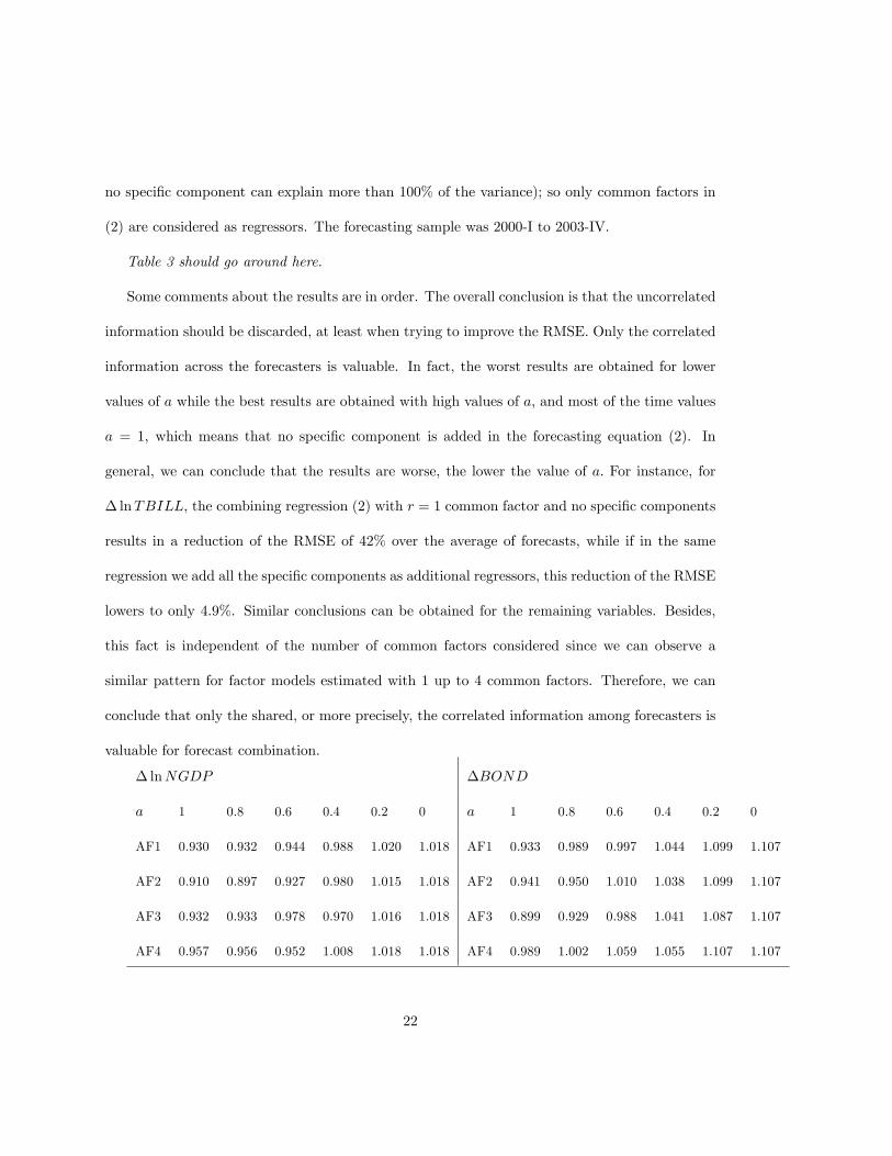
no speci�c component can explain more than 100% of the variance); so only common factors in

(2) are considered as regressors. The forecasting sample was 2000-I to 2003-IV.

Table 3 should go around here.

Some comments about the results are in order. The overall conclusion is that the uncorrelated

information should be discarded, at least when trying to improve the RMSE. Only the correlated

information across the forecasters is valuable. In fact, the worst results are obtained for lower

values of a while the best results are obtained with high values of a, and most of the time values

a = 1, which means that no speci�c component is added in the forecasting equation (2). In

general, we can conclude that the results are worse, the lower the value of a: For instance, for

� lnTBILL, the combining regression (2) with r = 1 common factor and no speci�c components

results in a reduction of the RMSE of 42% over the average of forecasts, while if in the same

regression we add all the speci�c components as additional regressors, this reduction of the RMSE

lowers to only 4.9%. Similar conclusions can be obtained for the remaining variables. Besides,

this fact is independent of the number of common factors considered since we can observe a

similar pattern for factor models estimated with 1 up to 4 common factors. Therefore, we can

conclude that only the shared, or more precisely, the correlated information among forecasters is

valuable for forecast combination.

� lnNGDP

a 1 0.8 0.6 0.4 0.2 0

AF1 0.930 0.932 0.944 0.988 1.020 1.018

AF2 0.910 0.897 0.927 0.980 1.015 1.018

AF3 0.932 0.933 0.978 0.970 1.016 1.018

AF4 0.957 0.956 0.952 1.008 1.018 1.018

�BOND

a 1 0.8 0.6 0.4 0.2 0

AF1 0.933 0.989 0.997 1.044 1.099 1.107

AF2 0.941 0.950 1.010 1.038 1.099 1.107

AF3 0.899 0.929 0.988 1.041 1.087 1.107

AF4 0.989 1.002 1.059 1.055 1.107 1.107

22

� lnUNEMP

a 1 0.8 0.6 0.4 0.2 0

AF1 0.956 1.112 1.090 1.338 1.434 1.439

AF2 0.957 1.038 1.060 1.193 1.227 1.439

AF3 0.997 1.040 1.089 1.225 1.479 1.439

AF4 1.001 1.015 1.096 1.121 1.477 1.439

� lnHOUSING

a 1 0.8 0.6 0.4 0.2 0

AF1 0.798 0.798 0.865 0.935 0.960 0.898

AF2 0.794 0.794 0.794 0.903 0.985 0.898

AF3 0.741 0.741 0.741 0.764 0.997 0.898

AF4 0.752 0.752 0.752 0.808 0.985 0.898

� lnTBILL

a 1 0.8 0.6 0.4 0.2 0

AF1 0.581 0.607 0.671 0.996 1.033 1.049

AF2 0.704 0.709 0.721 0.724 1.129 1.049

AF3 0.795 0.815 0.815 0.808 1.067 1.049

AF4 0.644 0.645 0.645 0.662 0.882 1.049

CPI

a 1 0.8 0.6 0.4 0.2 0

AF1 1.080 1.115 1.037 1.092 1.111 1.111

AF2 1.085 1.097 1.095 1.208 1.111 1.111

AF3 0.980 0.988 1.018 1.218 1.111 1.111

AF4 0.980 0.978 1.023 1.122 1.111 1.111

Table 3: RMSE ratios of 1 step ahead forecasts of factor models over the average of forecasts.

Factor models are estimated with 1 to 4 common factors. In the combined forecasts we have

added as additional regressors the speci�c components whose share of the variance is greater

than a: Bold �gures indicate the model that has the lower RMSE for each variable.

5 Conclusions

We have compared several methods for dimension reduction and relate them under the prism

of principal components. The methods can be divided in two groups: the ones that take into

account the past values of the variable being forecast in the process of dimension reduction as

PLS and SIR, and the ones that do not take them into account as factor models and principal

23

components. We have check their performance accuracy in forecasting using the SPF and found

that the methods that do take into account the values of the variable being forecast did not

outperform the ones that did not. A possible reason for this could be that the past values of the

observed variables are already incorporated in the forecasts themselves and do not add any more

valuable information in the construction of the �nal combined forecast. They may have a better

behavior with other data sets where the variables being combined are not themselves forecasts.

We have found that for the SPF forecasts all the methods outperformed the average of forecasts

and this might not be due simply to bias correction implied by equation (2) since plain OLS over

the forecasts and a constant for possible bias does not. In fact, plain OLS combinations of all

the forecasters give the overall worst results (worst than the average of forecasts).

As regards the uncorrelated information among forecasters, it is not useful for to improve

forecast accuracy, at least, in terms of reduction of the RMSE. Only the correlated information

among forecasters is valuable.

We have found that PLS, factor analysis and principal components work very well for fore-

cast combination. A possible reason for this might be that all three methods imply shrinkage

estimates and that can be the ultimate reason for forecast improvement. This is left for further

research.

24

6 References

Almoy, T. (2004) A simulation study on comparison of prediction methods when only a few

components are relevant. Computational Statistics and Data Analysis, 21, 87-107.

Bates, J.M. and C.W.J. Granger (1969) The combination of forecasts, Operations Research

Quarterly, 20, 451-468.

Boivin, J. and S. Ng (2006) Are more data always better for factor analysis? Journal of Econo-

metrics, 132, 169-194.

Clemen, R.T. (1989) Combining forecasts: A review and annotated bibliography, International

Journal of Forecasting, 5, 559-583.

Clements, M. (2007) Consensus and uncertainty: Using forecast probabilities of output declines.

International Journal of Forecasting, doi:10.1016/j.iforecast.2007.06.003.

Clements, M. and Hendry, D. (2004) Pooling of forecasts (2004). Econometrics Journal, 7, 1-31.

de Menezes, L. Bunn, D. and Taylor, J. (2000) Review of guidelines for the use of combined

forecasts. European Journal of Operational Research, 120, 190-204.

Diebold, F.X. and J.A. López (1996) Forecast Evaluation and Combination, Handbook of Sta-

tistics, vol. 14, 241-268 (North-Holland, Amsterdam).

Eldén, L. (2004) Partial least-squares vs. Lanczos bidiagonalization� I: analysis of a projection

method for multiple regression. Computational Statistics & Data Analysis, 46, 11-31.

Forni, M., M. Hallin, M. Lippi and L. Reichlin (2000) The generalized factor model: Identi�ca-

tion and estimation, Review of Economic and Statistics, 82, 540-554.

25

Forni, M., M. Hallin, M. Lippi and L. Reichlin (2005) The Generalized Dynamic Factor Model:

One-Sided Estimation and Forecasting. Journal of the American Statistical Association,

Vol. 100, No. 471, 830-840 .

Harvey, D. and Newbold, P. (2003) The non-normality of some macroeconomic forecast errors

International Journal of Forecasting, Volume 19, Issue 4, 635-653.

Heij, C. van Dick, D. and Groenen, P. (2007) Forecast comparison of principal component

regression and principal covariate regression, Computational Statistics and Data Analysis,

51, 3612-3625.

Issler, J.V. and L.R. Lima (2007) A panel data approach to economic forecasting: The bias-

corrected average forecast. Mimeo.

Kondylis, A. and Whittaker, J. (2008) Spectral preconditioning of Krylov spaces: Combining

PLS and PC regression. Computational Statistics and Data Analysis, 52, 2588-2603.

Lin, J.L. and R. Tsay (2007). Comparisons of forecasting models with many predictors. Mimeo.

Newbold, P. and D.I. Harvey (2001) Forecasting combination and encompassing in A companion

to economic forecasting (Eds.) M. Clements and D. Hendry, Blackwells, Oxford, pp. 268-

283.

Nolte, I. and W. Pohlmeier (2007) Using forecasts of forecasters to forecast. International

Journal of Forecasting, 23, 15-28.

Peña, D., Box, G. (1987). Identifying a simplifying structure in time series. J. Am. Statist.

Ass., 82, 836-43.

26

Peña, D. and Poncela, P. (2004). Forecasting with nonstationary dynamic factor models. Jour-

nal of Econometrics 119, 291-321.

Peña, D. and Poncela, P. (2006) Nonstationary dynamic factor analysis. Journal of Statistical

Planning and Inference, 136, 1237-1257.

Poncela, P. and Senra, E. (2006) A two factor model to forecast US in�ation. Applied Economics,

Volume 38, Issue 18, 2191-2197.

Stock, J.H. and M. Watson (2002a) Forecasting using principal components from a large number

of predictors, Journal of the American Statistical Association, 97, 1167-1179.

Stock, J.H., M. Watson (2002b) Macroeconomic Forecasting Using Di¤usion Indexes, Journal

of Business & Economic Statistics, 20, 147-163

Stock, J.H., M. Watson (2004) Combination forecasts of output growth in a seven-country data

set. Journal of Forecasting, 23, 405-430.

Stone, M. and R.J. Brooks (1990) Contiuuum regression: Cross-validated sequentially con-

structed prediction embrancing ordinary least squares, partial least squares and principal

components regression. Journal of the Royal Statistical Society B, 52, 237-269.

Timmerman, A. (2006) Forecast combinations, in Handbook of Economic Forecasting (Eds.)

G. Elliot, C.W.J. Granger and A. Timmerman, North-Holland, Amsterdam, chapter 4,

135-196.

Wang, C. (2008) Dimension reduction techniques for forecasting: An empirical comparison.

Mimeo.

27

Zarnowitz, V. and P. Braun (1993) Twenty-two years of the NBER-ASA quarterly economic

Outlook Survey: Aspects and Comparisons of Forecasting Performance, in Business Cycles,

Indicators and Forecasting (Eds.) J. Stock and M. Watson, The University of Chicago Press,

Chicago, pp. 11-93.

28