Density forecast combinations: the real-time dimension

Working Paper Series Density forecast combinations: the real-time dimension

Peter McAdam, Anders Warne

Disclaimer: This paper should not be reported as representing the views of the European Central Bank (ECB). The views expressed are those of the authors and do not necessarily reflect those of the ECB.

No 2378 / February 2020

Abstract: Density forecast combinations are examined in real-time using the log score to

compare five methods: fixed weights, static and dynamic prediction pools, as well as Bayesian

and dynamic model averaging. Since real-time data involves one vintage per time period and

are subject to revisions, the chosen actuals for such comparisons typically differ from the infor-

mation that can be used to compute model weights. The terms observation lag and information

lag are introduced to clarify the different time shifts involved for these computations and we dis-

cuss how they influence the combination methods. We also introduce upper and lower bounds

for the density forecasts, allowing us to benchmark the combination methods. The empirical

study employs three DSGE models and two BVARs, where the former are variants of the Smets

and Wouters model and the latter are benchmarks. The models are estimated on real-time euro

area data and the forecasts cover 2001–2014, focusing on inflation and output growth. We find

that some combinations are superior to the individual models for the joint and the output

forecasts, mainly due to over-confident forecasts of the BVARs during the Great Recession.

Combinations with limited weight variation over time and with positive weights on all models

provide better forecasts than those with greater weight variation. For the inflation forecasts,

the DSGE models are better overall than the BVARs and the combination methods.

Keywords: Bayesian inference, euro area, forecast comparisons, model averaging, prediction

pools, predictive likelihood.

JEL Classification Numbers: C11, C32, C52, C53, E37.

ECB Working Paper Series No 2378 / February 2020 1

Non-Technical Summary

The benefits of combining density forecasts from different models or forecasters have long been

recognized across many academic fields. Not only does model combination provide a way to guard

against model uncertainty, it is also a means to improve forecast accuracy. The improvement

in forecast accuracy can, for instance, arise from individual models being over-confident in the

sense of delivering predictive densities that are too narrow and thereby not well-calibrated.

There is though less empirical agreement on the performance and robustness of different com-

bination schemes. Different methods can generate quite different outcomes and reflect different

philosophies. For instance, the well-known method of Bayesian model averaging is predicated

on the assumption of a complete model space and, accordingly, there is a tendency for a single

model to attract all the weight. Optimal prediction pools, make no such assumption: all models

in the pool may be false, but nonetheless useful. Straddling these extremes is the enduring

puzzle that naïve schemes, such as equal model weights, often outperform more sophisticated

alternatives. Equal weighting schemes, though, preclude the possibility of adaption to partic-

ular episodes of model improvements. If the forecast horizon contains some dramatic event or

particular constellation of shocks, this may be costly. On the other hand, schemes that yield

volatile model weights may undermine the practical case for combination methods.

Against this background, our paper makes the following four principle contributions. First,

like forecasting itself, gains from model combinations matter most in real time. Yet, the inter-

action between model combination schemes and real time data has not been emphasized in the

literature. Apart from fixed-weight combinations, model weights are computed using informa-

tion about each model’s past predictive performance. Measures of predictive performance, such

as the log predictive score, are typically dependent on the recorded predictive likelihood values

of the individual models. In a real-time context, model weighting emerges when outcomes are

imperfectly known: measured values of the predicted variables for period t are, by construc-

tion, not observed until t + l, which implies that the predictive likelihoods for models should

be lagged at least l periods when computing the incremental weights. The upshot is that an

event such as the Great Recession—wherein large forecast errors emerge, model performance

may diverge, and data revisions may be substantial—mechanically takes time to influence the

model weights. Consequently, a “better” model may be under-utilized depending on these lags,

or existing sub-optimal model weights may persist.

To that end we define the following terms: observation lag is the time difference between the

date of the variable and the vintage its actual value is taken from, while information lag is the

time difference between the date of the variable and the vintage a measured value is taken from.

The former concept concerns the data used for the performance measure of density forecast

combinations, while the latter is related to the information used for computing combination

weights. It should be kept in mind that the information lag comes on top of the forecast horizon

so that the sum of the two make up the delay before historical density forecasts can be used for


model weighting. We demonstrate that the assumed length of the information lag matters for

the attainable gains from forecast combinations and the ranking of the methods over time.

A second contribution is that, unlike the bulk of the literature, we consider multi-step-ahead

forecasts in our density combination comparisons: backcasts, nowcasts and up to eight-quarter-

ahead forecasts. This matters because models’ predictive performance can be highly horizon

specific. Again, the Great Recession episode is telling: all models incur large forecast errors,

but some “recover” better than others over different horizons and for different reasons. This has

implications for the gains obtainable from model combinations in general as well as the specific

performance of different combination schemes. A standard one-step-ahead density forecast would

be silent on these issues. Third, we introduce upper and lower bounds for the density forecasts,

allowing us to benchmark the combination methods not only with respect to the available models

but against the best and the worst cases given the models involved. These bounds are easily

formed from the density forecasts of the models and to our knowledge they have not been

discussed in the literature. Fourth, we contribute to the literature on model combinations in a

euro area context. Relative to that of the US, evidence of real-time density forecasting on euro

area data remains scant, despite its similar economic weight, and corresponding evidence on

model combinations is scanter still.

The study employs three DSGE models and two Bayesian vector autoregressions (BVARs),

where the former are variants of the Smets and Wouters model and the latter are benchmarks.

The models are estimated on real-time euro area data and the forecasts cover 2001–2014, focusing

on inflation and output growth. We find that some combinations are superior to the individual

models for the joint and the output forecasts, mainly due to over-confident forecasts of the

BVARs during the Great Recession. Combinations with limited weight variation over time and

with positive weights on all models provide better forecasts than those with greater weight

variation. For the inflation forecasts, the DSGE models are better overall than the BVARs and

the combination methods.


1. Introduction

The benefits of combining density forecasts from different models or forecasters have long been

recognized across many academic fields, such as management science, meteorology and statis-

tics. Density forecast combinations have also received a growing interest among economists

and policy makers. Not only does model combination provide a way to guard against model

uncertainty, it is also a means to improve forecast accuracy; see, in particular, a recent survey

by Aastveit, Mitchell, Ravazzolo, and van Dijk (2019). The improvement in forecast accuracy

can, for instance, arise from individual models being over-confident in the sense of delivering

predictive densities that are too narrow and thereby not well-calibrated ; see, e.g., Dawid (1984)

and Diebold, Gunther, and Tay (1998). More intuitively, it strains belief that any single model

would strictly outperform all others in every time interval. Instead, model rankings are likely to

change over time as different information sets and different modelling aspects come into play.

Notwithstanding this positive consensus on forecast combinations, there is less empirical agree-

ment on the performance and robustness of different combination schemes. Different methods

can generate quite different outcomes and reflect different philosophies; see Amisano and Geweke

(2017). For instance, the well-known method of Bayesian model averaging is predicated on the

assumption of a complete model space and, accordingly, there is a tendency for a single model to

attract all the weight. Optimal prediction pools, suggested by Hall and Mitchell (2007), make no

such assumption: all models in the pool may be false, but nonetheless useful. Straddling these

extremes is the enduring puzzle that naïve schemes, such as equal model weights, often outper-

form more sophisticated alternatives. Equal weighting schemes, though, preclude the possibility

of adaption to particular episodes of model improvements. If the forecast horizon contains some

dramatic event or particular constellation of shocks, this may be costly. On the other hand,

schemes that yield volatile model weights may undermine the practical case for combination

methods, especially so perhaps in real time.

Against this background, our paper makes the following four principle contributions. First,

like forecasting itself, gains from model combinations matter most in real time. Yet, the inter-

action between model combination schemes and real time data has not been emphasized in the

literature. Apart from fixed-weight combinations, model weights are computed using informa-

tion about each model’s past predictive performance. Measures of predictive performance, such

as the log predictive score, are typically dependent on the recorded predictive likelihood values

of the individual models. In a real-time context, model weighting emerges when outcomes are

imperfectly known: measured values of the predicted variables for period t are, by construc-

tion, not observed until t + l, which implies that the predictive likelihoods for models should

be lagged at least l periods when computing the incremental weights. The upshot is that an

event such as the Great Recession—wherein large forecast errors emerge, model performance

may diverge, and data revisions may be substantial—mechanically takes time to influence the


model weights. Consequently, a “better” model may be under-utilized depending on these lags,

or existing sub-optimal model weights may persist.

To that end we define the following terms: observation lag is the time difference between the

date of the variable and the vintage its actual value is taken from, while information lag is the

time difference between the date of the variable and the vintage a measured value is taken from.

The former concept concerns the data used for the performance measure of density forecast

combinations, while the latter is related to the information used for computing combination

weights. It should be kept in mind that the information lag comes on top of the forecast horizon

so that the sum of the two make up the delay before historical density forecasts can be used for

model weighting. We demonstrate that the assumed length of the information lag matters for

the attainable gains from forecast combinations and the ranking of the methods over time.

A second contribution is that, unlike the bulk of the literature, we consider multi-step-ahead

forecasts in our density combination comparisons: backcasts, nowcasts and up to eight-quarter-

ahead forecasts.1 This matters because models’ predictive performance can be highly horizon

specific. Again, the Great Recession episode is telling: all models incur large forecast errors,

but some “recover” better than others over different horizons and for different reasons. This has

implications for the gains obtainable from model combinations in general as well as the specific

performance of different combination schemes. A standard one-step-ahead density forecast would

suppress these issues. Third, we introduce upper and lower bounds for the density forecasts,

allowing us to benchmark the combination methods not only with respect to the available models

but against the best and the worst cases given the models involved. These bounds are easily

formed from the density forecasts of the models and to our knowledge have not been discussed

in the literature. Fourth, we contribute to the literature on model combinations in a euro

area context. Relative to that of the US, evidence of real-time density forecasting on euro area

data remains scant, despite its similar economic weight, and corresponding evidence on model

combinations is scanter still.

The paper is organized as follows. Section 2 discusses probabilistic forecasting and the particu-

lar combination methods that we use, namely fixed weights, static and dynamic prediction pools,

as well as Bayesian and dynamic model averaging. In so doing, we clarify the equivalence of

some methods under different limiting assumptions, and highlight specific methodological mod-

ifications required for our exercises. Section 3 overviews the models used: three DSGE models

that are variants of the canonical Smets and Wouters model (McAdam and Warne, 2019), as well

as two Bayesian vector autoregressions (BVARs), embodying standard and recently developed

priors; see Giannone, Lenza, and Primiceri (2015, 2019).

Section 4 describes the recursive estimation of the BVAR models which, like the three DSGE

models, are estimated on vintages taken from the euro area real-time database (RTD); see

Giannone, Henry, Lalik, and Modugno (2012). In Section 5, the forecast performance of the

1 One exception is Jore, Mitchell, and Vahey (2010) who also suggest a simple recursive weighting scheme fordensity forecast combinations based on the log predictive score.


models is presented for the sample 2001–2014. This period constitutes an especially challenging

laboratory: not only given the real-time and differing information dimensions, but also because

it spans a period of relatively calm macroeconomic conditions, undone by the Great Recession.2

Section 6 contains the bulk of our key results in terms of forecast combinations. We consider

the predictive performance of the individual models as well as that of the different combination

schemes, study the combination weights and compare the combination methods to the upper

and the lower bounds for the selection of models. The sensitivity of results to the information

lag assumption is examined and we experiment with combination schemes that modify the

initialization of the weights. Finally, Section 7 summarizes the main findings, while additional

material is in the Appendices.

2. Density Forecast Combination Methods

Scoring rules are widely used in econometrics and statistics to compare the quality of probabilistic

forecasts by attaching a numerical value based on the predictive distribution and an event or

value that materializes; see Gneiting and Raftery (2007) for a survey on scoring rules and

Gneiting and Katzfuss (2014) for a review on probabilistic forecasting. A scoring rule is said to

be proper if a forecaster who maximizes the expected score provides his or her true subjective

distribution, and it is said to be local if the rule only depends on the predictive density and the

realized value of the predicted variables. A well-known scoring rule is the log predictive score

and, as shown by Bernardo (1979), it is the only proper local scoring rule.3

Suppose there are M models to compare in a density forecast exercise and let p(i)t+h|t =

p(x(a)t+h|I

(i)t , Ai) denote the predictive likelihood conditional on the assumptions of model i, de-

noted by Ai, and the information set of model i, given by I(i)t . The predictive likelihood is

given by the predictive density evaluated at the actual or observed value of the vector of random

variables x, realized at time t + h and denoted by x(a)t+h, with the integer h being the forecast

horizon. The log predictive score of model i for h-step-ahead density forecasts is given by

S(i)T :Th,h

=

Th∑

t=T

log(

p(i)t+h|t

)

, i = 1, . . . ,M. (1)

The larger the log predictive score is, the better a model can predict the vector of variables x

at the h-step-ahead forecast horizon.

A Kalman-filter-based approach to the estimation of the log predictive likelihood in linear

state-space models was suggested in a recent paper by Warne, Coenen, and Christoffel (2017).

This method was also utilized in our recent paper, McAdam and Warne (2019), where we

compare real-time density forecasts for the euro area based on three estimated DSGE models. In

the current section, we discuss four approaches to combining the density forecasts from individual

2 Papadopoulos (2017) examines model combination approaches to develop robust macro-financial models forcredit risk stress testing in the wake of the Great Recession.

3 Specifically, the log predictive score is unique up to a positive coefficient of proportionality and a constantwhich only depends on the historical data.


models: static optimal and dynamic prediction pools (SOP and DP), and Bayesian and dynamic

model averaging (BMA and DMA). It may also be noted that these combination schemes cover

the three broad combination methodologies discussed by Aastveit et al. (2019): frequentist based

optimized combination weights (SOP); Bayesian model averaging weights (BMA and DMA); and

flexible Bayesian forecast combination structures (DP). In addition to these four combination

schemes, the empirical part of the paper utilizes fixed-weight-based approaches, such as equal

weights on all or on a subset of the models.

Notice that the predictive likelihood, p(x(a)t+h|I

(i)t , Ai), does not include the parameters of the

model as these have already been integrated out by accounting for the posterior distribution.

Waggoner and Zha (2012) allow the combination weights to follow a hidden Markov process and

emphasize the joint estimation of the weights and the parameters of all models. In the empirical

exercise we recycle the predictive likelihoods estimates of three DSGE models from McAdam and

Warne (2019), while the predictive likelihoods of the VAR models are also estimated separately.

This decision is based not only on computational constraints but also on the arguments and

justification presented in Del Negro, Hasegawa, and Schorfheide (2016).

Several other density forecast combination methods have recently been introduced to the

literature, such as the dynamic Bayesian predictive synthesis in McAlinn and West (2019); the

so called generalized density forecast combinations of Kapetanios, Mitchell, Price, and Fawcett

(2015); and the state-space approach of Billio, Casarin, Ravazzolo, and van Dijk (2013); see also

Aastveit et al. (2019) for additional approaches. We have opted to omit these methods from the

current study.

2.1. Static Optimal Prediction Pools

Static optimal predictions pools were introduced by Hall and Mitchell (2007) as a means to

improve the density forecasts of individual forecasters or models by computing the optimal linear

combination of these forecasts. The basic idea is to maximize the log predictive score of a linear

combination of the predictive likelihoods of the models in the pool. This linear combination

is constrained such that the model weights are constant, non-negative and sum to unity. As a

result, the combination of the predictive likelihoods is also a predictive likelihood and the log

predictive score is formed by accumulating the log of the pooled predictive likelihoods.

This forecast combination is referred to as static since the weights are treated as constant over

time. A recursive approach to the estimation of these weights is more realistic when viewing the

problem of comparing models in real time. In that case, the weights of the models can change

due to re-optimization with more recent information. Hall and Mitchell (2007) motivate the use

of static optimal pools on the grounds that the weights are chosen to minimize the “distance”

between the forecasted and the unknown true predictive density in the sense of the Kullback-

Leibler information criterion; see Kullback and Leibler (1951). In contrast with combination

approaches such as BMA, discussed in Section 2.4, Geweke and Amisano (2011, 2012) point out

that static optimal prediction pools do not rely on the assumption that one of the models in


the pool is true, i.e., the approach allows for incomplete models with the effect that all of the

models in the pool may be false; see Geweke (2010).4

Let wi,h be the weight on model i for h-step-ahead forecasts, satisfying wi,h ≥ 0 and∑M

i=1wi,h =

1. The log predictive score of the static optimal pool is therefore given by

S(SOP)T :Th,h

=

Th∑

t=T

log

(M∑

i=1

wi,hp(i)t+h|t

)

, (2)

where the predictive likelihood of the pool is given by the term being logged on the right hand

side of this equation. Estimates of the weights are obtained by maximizing the log score in (2)

with respect to the weights and subject to their restrictions.

2.2. Observation and Information Lags

From a recursive perspective, the weights in (2) can only be estimated based on the predictive

likelihoods that have been observed at the time. The standard assumption for discrete time data

is that variables are observed in the same period that they measure, i.e., xt is both realized and

observed in period t. From a real-time perspective, however, a first release or first estimate of xt

is often not available in period t but is published at a later date. Moreover, most macroeconomic

variables are subject to revisions, due to more accurate information appearing with some delay

and/or due to changes in measurement methodology. When comparing or evaluating forecasts,

a decision must be made regarding which vintage to use for the actuals; see, e.g., Croushore

and Stark (2001) and Croushore (2011). In principle, any vintage can be used for the actual

value and common choices in the real-time literature are the first release, the annual revision

and the latest vintage. Although the latest vintage may reflect actuals that for many periods

have not been subject to large revisions, it suffers from possible methodological changes to the

measurements that were not known in real time.5 Similarly, first release data is typically subject

to larger revisions in comparison to, for instance, annual revisions data.

The choice of actuals is important since it represents the “true value” of the forecasted variables

and therefore affects the outcome of the comparison exercise. To distinguish the data used for

comparing forecasts from the data used for computing model weights for combination methods,

the time difference between the date of the variable and the date of the vintage the actual value

is taken from is henceforth called the observation lag and in the empirical exercise we use annual

revisions data. This means that x(a)t is taken from vintage t + 4 such that x

(a)t = x

(t+4)t , with

the consequence that the observation lag k = 4. At the same time, the vintages t + 1, t + 2

and t + 3 typically include measures of xt, denoted by x(m)t , and these values may be useful

when computing the optimal weights recursively. To account for this we also define the term

information lag, denoted by l, to be the time difference between the date of the variable and

4 See also Pauwels and Vasnev (2016) for further analysis of optimal prediction pool weights and the underlyingoptimization problem, and Opschoor, van Dijk, and van der Wel (2017) for extensions to alternative scoring rules.

5 This is certainly true for the euro area RTD, which also reflects a time-varying country composition, whereseven EU member countries have been admitted since 2007.


the vintage a measured value is taken from. The minimum information lag is determined by

the time delay before to the first publication of xt, while the maximum may be set equal to the

observation lag. These real-time lag concepts are illustrated in Figure 1 and it may be noted

that both these lags are zero if one assumes that the date of the variable is equal to the time

period when it is observed, as is standard for the single database (vintage) forecast exercises.

It should be emphasized that the information lag is a distinct concept from the ragged edge of

real-time data; see Wallis (1986). The latter is a property of the database and is a consequence

of individual time series in a real-time vintage being measured up to different time periods. For

instance, interest rates may be measured up to the vintage date, while real GDP growth lags

with one quarter, and some labor market variables such as wages with two quarters. The ragged

edge directly affects the data available for estimation of model parameters and the conditioning

information when forecasting with the models. The minimum information lag is influenced by

the ragged edge since it depends on the dates for which historical measured values of all the

forecasted variables are available. At the same time, the information lag concerns only the

forecasted variables and may be selected by the user of the combination method.

To clarify the relevance of these concepts and the decision problems implied by them, consider

the following example based on one-quarter-ahead density forecasts with a static optimal pool:

Suppose the minimum information lag is equal to one quarter for the vector x in vintage τ , while

the observation lag is equal to four quarters. This means that xτ−1 has a measured value x(m)τ−1

for vintage τ and that similarly xτ−2, xτ−3, . . . have measured values for this vintage. By having

a measured value it is understood that there are not any missing data for any element of x.

Furthermore, an observation lag of four means that actual values of xτ−4, xτ−5, . . . are available

at τ and are taken from vintages τ, τ − 1, . . .. Similarly, forecast densities of the current and

all previous one-quarter-ahead forecasts of x are available for the M models at time τ , where

each model makes use of data from the corresponding vintage. This means that the predictive

likelihood values based on the actual values p(x(a)t+1|I

(i)t , Ai) can be observed for t = T, . . . , τ −5.

In addition, the predictive likelihood values based on the measured values p(x(m)t+1|I

(i)t , Ai) can

be observed for t = T, . . . , τ − 2.

The user of a static optimal pool needs to make two decisions before determining the recursive

weights for the pool at time τ : (i) which information lag to use among l = 1, 2, 3, 4; and (ii)

whether to use the predictive likelihoods based on the actual values or on the measured values

for t = T, . . . , τ − 4. The decisions to these two issues determine the objective function for

selecting the optimal weights. Since the actual values represent the “true values” we assume in

the empirical exercise that the second decision always brings the predictive likelihood values for

the actuals to the weight estimation problem. If an information lag longer than the minimum

possible is selected, this means for our example that all x(m)τ−j for j < l along with the predictive

likelihood values based on these measured values are discarded when estimating the optimal

weights at τ . For the possible choices of l it holds that the optimal weights at τ are selected


such that the log predictive score function

S(SOP)T :τ−l−1,1 =

τ−5∑

t=T

log

(M∑

i=1

wi,1,τp(x(a)t+1

∣∣I(i)

t , Ai

)

)

+

τ−l−1∑

t=τ−4

log

(M∑

i=1

wi,1,τp(x(m)t+1

∣∣I(i)

t , Ai

)

)

,

is maximized with respect to wi,1,τ , i = 1, . . . ,M , and subject to having non-negative weights

adding to unity. Notice that the first term on the right hand side involves a sum up to the

vintage date (τ) minus the observation lag (k = 4) and the forecast horizon (h = 1), while the

sum for the second term begins at the vintage date minus the observation lag (plus the forecast

horizon minus 1) and ends at the vintage date minus the information lag (l) and the forecast

horizon. Notice also that when τ ≤ T + l the above log predictive score function for selecting

weights cannot be determined. Initial values for the weights are then needed for these vintages

and one candidate is wi,1,τ = 1/M for all i.

In the empirical exercise we initially make the mechanical assumption that the information

lag is equal to the observation lag, but also examine the more realistic case when the information

lag is shorter than the observation lag. For the variables we forecast in the empirical analysis,

the shortest possible information lag for quarterly data is one quarter for most vintages and two

quarters for the remaining ones. Finally, the two lag concepts are applied to density forecasts in

this paper, they are also relevant for point forecast combination methods with real-time data.

2.3. Dynamic Prediction Pools

Dynamic prediction pools, suggested by Del Negro et al. (2016), directly allow the weights to

vary as well as to be correlated over time. While their setup is based on two models, Amisano

and Geweke (2017) extends the dynamic prediction pool from two to three models. In fact, the

approach in Amisano and Geweke allows for any finite number of models and it is for such a

general case that we present dynamic prediction pools below. Accordingly, the number of models

is, as before, equal to M and the log predictive score for the dynamic prediction pool is:

S(DP)T :Th,h

=

Th∑

t=T

log

(M∑

i=1

wi,t+h|tp(i)t+h|t

)

, (3)

where wi,t+h|t is the weight on model i for h-step-ahead density forecasts at t, where all weights

are non-negative and sum to unity.

To model the time variation of the weights, we follow Amisano and Geweke (2017) and consider

a parsimoniously parameterized M -dimensional process for the state variable

ξt = ρξt−1 +√(1 − ρ2

)ηt, t = T, . . . , Th, (4)

where 0 ≤ ρ ≤ 1 is a scalar and ηt ∼ i.i.d.N(0, IM ).6 The ρ parameter is referred to as

a “forgetting factor” for dynamic pools by Del Negro et al. (2016) since with ρ < 1 there is

6 For the implementation of the dynamic prediction pool in Del Negro et al. (2016), they have a univariate processsimilar to (4), but also allow for a drift parameter µ and a standard deviation σ. The process for ξ in (4) can beenriched in various ways, but for the sake of parsimony we only allow for one free parameter.


discounting of past information. The parameterization of ξt in (4) ensures that its covariance is

the identity matrix when ρ < 1, while ξt is constant (static) otherwise.

The weights are determined from a logistic transformation of the individual elements of the

state vector, ξi,t which ensures that each element is non-negative and that the sum of the elements

is unity:

wi,t =exp(ξi,t)

∑Mj=1 exp

(ξj,t) , i = 1, . . . ,M. (5)

The vector wt is consequentlyM -dimensional with individual entries given by the model weights.

As pointed out by Amisano and Geweke (2017, Appendix E.4) the specification in (5) implies a

symmetric prior across weights.

To estimate the log predictive score in (3) conditional on ρ, Amisano and Geweke (2017)

follow the approach in Del Negro et al. (2016) and employ the Bayesian bootstrap particle filter ;

see, e.g., Gordon, Salmond, and Smith (1993) and Herbst and Schorfheide (2016) for details and

further references. This filter is initialized as follows: At t = T − 1, draw N particles from the

unconditional distribution of ξT−1 and map these into wi,T−1 using (5), while each particle is

assigned equal weight; i.e., for i = 1, . . . ,M and n = 1, . . . , N

ξ(n)T−1 ∼ N

(0, IM

),

w(n)i,T−1 =

exp(ξ(n)i,T−1

)

∑Mj=1 exp

(ξ(n)j,T−1

) ,

W(n)T−1 = 1.

During the recursions of the bootstrap particle filter for t = T, . . . , Th, each iteration involves

three steps: forecasting, updating, and selection. The forecasting step concerns propagating the

N particles forward by drawing innovations η(n)t ∼ N(0, IM ) such that

ξ(n)t = ρξ

(n)t−1 +

√(1 − ρ2

)η(n)t ,

w(n)i,t =

exp(ξ(n)i,t

)

∑Mj=1 exp

(ξ(n)j,t

) ,

for i = 1, . . . ,M and n = 1, . . . , N . Next, the incremental weights are calculated as

ω(n)t = p

(x(m)t

∣∣w

(n)t ,I(P)

t−h,P)=

M∑

i=1

w(n)i,t p

(x(m)t

∣∣I(i)

t−h, Ai

), n = 1, . . . , N,

where these weights depend on ρ via w(n)t , a vector with w

(n)i,t in element i, and with I(P)

t being

the joint information set of the pooled models. Notice that the incremental weights are formed

from the h-steps-ahead predictive likelihoods of the individual models based on measured values

of the predicted variables in period t, x(m)t .


The updating step consists in recomputing the weights according to

W(n)t =

ω(n)t W

(n)t−1

(1/N)∑N

j=1 ω(j)t W

(j)t−1

.

Notice that the sum of the updated weights W(n)t over all particles is equal toN . If all the weights

from recursion t − 1 are equal, then the updated weights are proportional to the incremental

weights and therefore the particle likelihood values.

For the selection step we first compute the effective sample size (ESS) according to

ESSt =N

(1/N)∑N

n=1

(W

(n)t

)2.

On the one hand, if ESSt < δ∗N for a suitable value of the hyperparameter δ∗, where 0 < δ∗ < 1,

the particles are resampled with multinomial resampling, characterized by support points and

weights ξ(n)t , w(n)t , W

(n)t Nn=1. Let ξ(n)t , w

(n)t ,W

(n)t Nn=1 denote a swarm of N i.i.d. draws where

the weights are given byW(n)t = 1. On the other hand, if ESSt ≥ δ∗N , the weights W

(n)t = W

(n)t

while the state variables ξ(n)t = ξ

(n)t and the corresponding model weights w

(n)t = w

(n)t .

The conditional predictive likelihood of the dynamic pool in recursion t is approximated with

p(P)t+h|t

(ρ)= p(x(a)t+h

∣∣I(P)

t ,P; ρ)=

M∑

i=1

wi,t+h|t(ρ)p(x(a)t+h

∣∣I(i)

t , Ai

), (6)

where the particle weights depend on the parameter ρ, and the weights w(n)i,t+h|t are computed

by iterating forward using the law of motion in (4). That is

wi,t+h|t(ρ) = E[wi,t+h

∣∣I(P)

t ,P; ρ]

≈ 1

N

N∑

n=1

w(n)i,t+h(ρ)W

(n)t ,

where for each particle n

ξ(n)i,t+s(ρ) = ρξ

(n)i,t+s−1 +

√(1 − ρ2

)η(n)t+s,

w(n)i,t+h(ρ) =

exp(ξ(n)i,t+h(ρ)

)

∑Mj=1 exp

(ξ(n)j,t+h(ρ)

) ,

for s = 1, . . . , h, and where η(n)t+s is a draw from an M -variate standard normal distribution.

In a real-time setting, the information lag needs to be taken into account. Consider the

convenient, albeit mechanical, assumption that the information lag is equal to the observation

lag. With annual revisions data, this means that the predictive likelihoods for the individual

models are lagged four periods when computing the incremental weights. Since measured values

of x may be available for periods t − 3, t − 2 and t − 1 in vintage t, a shorter information lag

is feasible. Unless the measured values are equal to the actual values for these time periods,

however, the bootstrap particle filter requires two loops, where for each vintage t the iterations


from T until t are (at least partly) revisited. The assumption that the information lag is equal

to the observation lags means that the second loop can be avoided. Alternatively, it may also

be skipped if one assumes that measured values are well approximated by the actual values, i.e.,

that the revisions are sufficiently small that they can be neglected.7

Amisano and Geweke (2017) apply the bootstrap particle filter over a fine grid of values for

ρ and compute ρτ by maximizing the log score

ρτ,h = argmaxρ

τ−h∑

t=T

log(

p(x(m)t+h

∣∣I(P)

t ,P; ρ))

, τ = T, . . . , Th (7)

where the predictive likelihood on the right hand side are computed as in (6), but with the

measured value instead of the actual value. This means that the first period τ when the h-step-

ahead predictive likelihood of the individual models can be observed occurs at τ = T+h. Taking

the real-time aspect fully into account means that the information lag, l ≤ k, is added to this

number. It follows that for all τ less than T + h+ l, a unique value of ρ cannot be determined

as there are no data on the predictive likelihoods available. This initialization problem may

be dealt with by replacing the unobserved predictive likelihood values with a positive constant,

such as 1/M , with the consequence that all values of ρ from T up to T + h + l − 1 obtain the

same log score when computing the weights. As the number of particles becomes very large,

this amounts to giving all models the same weight.

With the sequence ρtτt=T , the real-time log predictive score of the dynamic prediction pool

is then estimated by

S(DP)T :τ,h =

τ∑

t=T

log(

p(P)t+h|t

(ρt,h))

.

According to Amisano and Geweke (2017), this procedure may be interpreted as a Bayesian

analysis based on a flat (uniform) prior on ρ.

Resampling was originally employed by Gordon et al. (1993) to reduce the effects from sample

degeneracy—a highly uneven distribution of particle weights—as this part of the selection step

adds noise; see Chopin (2004). It also allows for the removal of low weight particles with

a high probability and this is very practical as it is preferable that the filter is focused on

regions with a high probability mass. However, this also means that resampling may produce

sample impoverishment as the diversity of the particle values is reduced. The hyperparameter

δ∗ provides a ‘crude’ tool for balancing the algorithm against the pitfalls of degeneracy or

impoverishment by ensuring that resampling takes place but does not occur ‘too often’.8

7 If only data on x from vintage t are used as measured values they are all subject to revision and the doubleloop has to be executed from period T for each vintage t. On the other hand, if actuals are used up to periodt − 4 and measured values from vintage t for periods t − 3, t − 2 and t − 1, then the double loop would start int − 4 since the earlier computations were run for vintage t − 1. Finally, if the measured values for t − 3, t − 2and t − 1 are approximated by the actual values, then the double loop can be dispensed with. For each of thesecases, an information lag of one is applied.

8 A more direct approach to combatting sample impoverishment is based on taking the particle values intoaccount when resampling; see, e.g., Doucet and Johansen (2011) for discussions on the resample-move algorithmof Gilks and Berzuini (2001) and the block sampling algorithm of Doucet, Briers, and Sénécal (2006).


Del Negro et al. (2016) use a multinomial distribution for the selection step with δ∗ = 2/3,

but as pointed out by, for example, Douc, Cappé, and Moulines (2005), this resampling algo-

rithm produces an unnecessarily large variance of the particles. Moreover, and as emphasized

by Hol, Schön, and Gustafsson (2006), ordering of the underlying uniform draws improves the

computational speed considerably. The commonly used alternative resampling algorithms are

faster and have a smaller variance of the particles. Systematic resampling, introduced by Kita-

gawa (1996) and also emphasized by Carpenter, Clifford, and Fearnhead (1999), is a commonly

used approach as it is very easy to implement, comparatively fast, and, according to Doucet and

Johansen (2011), as it often outperforms other sequential resampling schemes. It is a faster ver-

sion of stratified resampling (Kitagawa, 1996), where instead of drawing N uniforms only one is

required, while stratification and, simultaneously, sorting is dealt with via the same simple affine

function. A drawback with systematic resampling is that it generates cross-sectional dependen-

cies among the particles, which also makes it difficult to establish its theoretical properties; see

Chopin (2004). For an overview of sequential resampling schemes see, e.g., Hol et al. (2006),

who also discuss theoretical criteria for choosing between multinomial, stratified, systematic and

residual resampling (suggested by Liu and Chen, 1998); Douc et al. (2005), who also study large

sample behavior; and more recently Li, Bolić, and Djurić (2015), who also discusses distributed

or parallel algorithms.9

2.4. Bayesian Model Averaging

BMA provides a coherent framework for accounting for model uncertainty; see Hoeting, Madigan,

Raftery, and Volinsky (1999). The standard BMA weights rely on posterior model probabilities

and therefore require the calculation of marginal likelihoods over a set of models which predict

the same observables. The DSGE and VAR models we examine, however, do not satisfy this

condition: the VAR models predict all nine observable variables comprising the full information

set, while the DSGE models do not predict all variables.

However, an alternative BMA weighting scheme may be obtained by only using the predictive

likelihood values of the variables of interest (xt) and a prior for the weights; see Eklund and

Karlsson (2007) for discussions on the general idea. Specifically, BMA weights may be obtained

as in Del Negro et al. (2016, Section 3) such that

wi,t,h =wi,t−1,hp

(x(m)t

∣∣I(i)

t−h, Ai

)

∑Mj=1 wj,t−1,hp

(x(m)t

∣∣I(j)

t−h, Aj

) , (8)

for t = T + 1, . . . , Th, with wi,T,h denoting the prior predictive probability that wi = 1. In this

case, the model weights at t are built using only the predictive likelihood values up to period t.

As long as wi,T,h = 1 for some model i does not hold, these BMA weights will be positive for

9 Since the bootstrap particle filter will spend a considerable share of the computational time in the resamplingstage, especially when δ∗ is high, the precise implementation of the selected resampling scheme is also important;see also Warne (2019, Section 8.4) for some details on how to implement the standard sequential algorithms.


several models until the recursive log score of one model dominates the others sufficiently. In

the empirical sections below, we primarily let wi,T,h = 1/M .

It should be kept in mind that the predictive likelihood generated BMA weights are based on

the following assumption:

p(xt∣∣I(i)

t−h, Ai

)= p(xt∣∣I(P)

t−h, Ai

).

That is, the additional information available in I(P)t−h relative to I(i)

t−h does not change the density

forecast of xt for any model i = 1, . . . ,M . This holds trivially for the two VAR models, but

also for the three DSGE models since the “missing” variables in I(i)t−h are not predicted by these

models.

The BMA weights in (8) are based on the assumption that x(m)t is observed at t. As discussed

in Section 2.2, the real-time dimension means the BMA weights need to be adjusted by lagging

the predictive likelihoods on the right hand side by the information lag. In other words, we

replace equation (8) with

wi,t,h =wi,t−1,hp

(x(m)t−l

∣∣I(i)

t−h−l, Ai

)

∑Mj=1 wj,t−1,hp

(x(m)t−l

∣∣I(j)

t−h−l, Aj

) . (9)

Like in the cases of the prediction pools, the first period when an h-step-ahead predictive like-

lihood value is observed occurs at T + h+ l. For t = T + 1, . . . , T + h+ l − 1 we can therefore

replace the predictive likelihood values in (9) with a positive constant such that wi,t,h = wi,T,h,

the prior predictive probability of model i.

The predictive likelihood for the BMA combination is given by

p(x(a)t+h

∣∣I(P)

t ,P)=

M∑

i=1

wi,t,hp(x(a)t+h

∣∣I(i)

t , Ai

),

from which it is straightforward to compute the log predictive score, denoted by S(BMA)T :Th,h

, of this

density forecast combination method.

2.5. Dynamic Model Averaging

Raftery, Kárný, and Ettler (2010) proposed a model combination method, called dynamic model

averaging (DMA), where the weights of the log predictive score may be regarded as depending

on a hidden Markov process, st, as in Waggoner and Zha (2012), but where the estimates of the

Markov transition probabilities are approximated. Specifically, Raftery et al. (2010) suggest to

estimate the weights as follows

wi,t+h|t =wϕh

i,t,h∑M

j=1 wϕh

j,t,h

, (10)

where ϕ is a parameter such that 0 ≤ ϕ ≤ 1. Notice that the weights wi,t,h on the right hand side

of equation (10) correspond to the weights from the recursive BMA calculation. Accordingly,

if ϕ = 1 then DMA is identical to BMA, and if ϕ = 0 then DMA implies that the weights are

equal (1/M) for all time periods. The parameter ϕ is interpreted as a forgetting factor, where


lower values means that past forecast performance is given a lower weight; see also Koop and

Korobilis (2012). Provided that ϕ < 1, it follows that the DMA weights approach the equal

weights as h increases.

The predictive likelihood for the DMA forecast combination is given by

p(x(a)t+h

∣∣I(P)

t ,P)=

M∑

i=1

wi,t+h|tp(x(a)t+h

∣∣I(i)

t , Ai

),

from which the log predictive score, denoted by S(DMA)T :Th,h

, can be directly computed.

Amisano and Geweke (2017) estimate the forgetting factor by recursively maximizing the log

predictive score over a grid of ϕ values, similar to the case for ρ in Section 2.3. They suggest

that the procedure can be given a Bayesian interpretation where the researcher assigns a flat

(uniform) prior on ϕ. DMA is also considered by Del Negro et al. (2016), who consider three

values of ϕ below but close to unity.

3. The DSGE and the VAR Models

3.1. The DSGE Models

We use three DSGE models. The first is that of Smets and Wouters (2007), as adapted to the

euro area (labelled SW). This contains a continuum of utility-maximizing households and profit-

maximizing intermediate good firms who, respectively, supply labor and intermediate goods in

monopolistic competition and set wages and prices. Final good producers use these intermediate

goods and operate under perfect competition.

The model incorporates several real and nominal rigidities, such as habit formation, invest-

ment adjustment costs, variable capital utilization and Calvo staggering in prices and wages.

The monetary authority follows a Taylor-type rule when setting the nominal interest rate. There

are seven stochastic processes: a TFP shock; a price and a wage markup shock; a risk premium

(preference) shock; an exogenous spending shock; an investment-specific technology shock; and

a monetary policy shock. The observed variables are: real GDP, real private consumption, real

investment, employment, real wages, the GDP deflator (all transformed as 100 times the first

difference of the natural logarithm), and the short-term nominal interest rate in percent.

The second model (SWFF) adds the financial accelerator mechanism of Bernanke, Gertler,

and Gilchrist (1999) (BGG) to the SW model and augments the list of observables to include

a measure of the external finance premium; see McAdam and Warne (2019) for details.10 The

final model (SWU) instead allows for an extensive labor margin, following Galí, Smets, and

Wouters (2012), and adds the unemployment rate in percent to the set of observables. McAdam

and Warne (2018) describes the models’ structure and estimation properties in greater depth

and provides a comparative impulse response analysis.

10 A variant of the SWFF which includes long-term inflation expectations data for the US is used by, e.g.,Del Negro and Schorfheide (2013), Del Negro, Giannoni, and Schorfheide (2015) and more recently Cai, Del Negro,Herbst, Matlin, Sarfati, and Schorfheide (2019).


3.2. The VAR Models

The two BVAR models we consider in this paper make use of the priors discussed in Giannone

et al. (2015, 2019). Below we first present the prior and posterior distributions conditional on a

vector of hyperparameters and show the relation between the prior parameters and Td dummy

observations and when the observables are not subject to missing observations; see also Bańbura,

Giannone, and Lenza (2015). The marginal likelihood conditional on the hyperparameters can

then be computed analytically and acts as a likelihood function when the hyperparameters are

estimated. To achieve this, a hyperprior for the hyperparameters is presented and we discuss

how they can be estimated in this setting.

Before we continue, it should be stressed that the discussion below is based on complete

datasets, i.e., when there are no missing observations of the observable variables. The real-

time data vintages we use in the paper have a so-called ragged edge, with some variables being

missing for the vintage date as well as for the quarter prior to the vintage date. To incorporate

such datasets makes direct sampling of the VAR parameters impossible and further complicates

the posterior analysis as an analytical expression of the marginal likelihood conditional on the

hyperparameters is not available, with the effect that all these parameters need to be estimated

simultaneously. The computational costs of dealing with the ragged edge can therefore be very

high and for this reason a second best approach may be considered, where the dataset is trimmed

during the parameter estimation step. We return to this issue in Section 3.2.5.

3.2.1. The Normal-Inverted Wishart BVAR Model

To establish notation, let yt be an n-dimensional vector of observable variables with a VAR

representation given by

yt = Φ0 +

p∑

j=1

Φjyt−j + ǫt, t = 1, . . . , T, (11)

where ǫt ∼ Nn(0,Ω) and Φj are n × n matrices for j ≥ 1 and an n × 1 vector if j = 0.

Let Xt = [1 y′t · · · y′

t−p+1]′ be an (np + 1)-dimensional vector, while the n × (np + 1) matrix

Φ = [Φ0 Φ1 · · · Φp] such that the VAR can be expressed as:

yt = ΦXt−1 + ǫt. (12)

Stacking the VAR system as y = [y1 · · · yT ], X = [X0 · · · XT−1] and ǫ = [ǫ1 · · · ǫT ], we can

express this as

y = ΦX + ǫ. (13)

The normal-inverted Wishart prior for (Φ,Ω) is given by

∣

∣

vec(Φ)∣

Ω, α ∼ Nn(np+1)

(vec(µΦ),[ΩΦ ⊗ Ω

]), (14)

Ω∣

α ∼ IWn

(A, v

), (15)


where the prior parameters (µΦ,ΩΦ, A, v) are determined through a vector of hyperparameters,

denoted by α.11 Combining this prior with the likelihood function and making use of standard

“Zellner” algebra, it can be shown that the conjugate normal-inverted Wishart prior gives us a

normal posterior for Φ|Ω, α and an inverted Wishart posterior for Ω|α. Specifically,

vec(Φ)∣∣Ω, y,X0, α ∼ Nn(np+1)

(vec(Φ),[(XX ′ +Ω−1

Φ )−1 ⊗ Ω]), (16)

Ω∣∣y,X0, α ∼ IWn

(S, T + v

), (17)

where

Φ =(yX ′ + µΦΩ

−1Φ

) (XX ′ +Ω−1

Φ

)−1,

S = yy′ +A+ µΦΩ−1Φ µ′

Φ − Φ(XX ′ +Ω−1

Φ

)Φ′.

The log marginal likelihood has an analytical expression which is given by

log p(y∣∣X0, α

)= −nT

2log(π) + log Γn(T + v) − log Γn(v) − n

2log∣∣ΩΦ

∣∣

+v

2log∣∣A∣∣− n

2log∣∣XX ′ +Ω−1

Φ

∣∣− T + v

2log∣∣S∣∣,

(18)

where Γb(a) =∏b

i=1 Γ([a − i + 1]/2) for positive integers a and b with a ≥ b, while Γ(·) is the

gamma function; see Appendix A for further details.

3.2.2. Sum-Of-Coefficients Prior

In this paper we consider two ways of parameterizing the prior parameters (µΦ,ΩΦ, A, v). The

first approach is based on Giannone et al. (2015) with a Minnesota prior combined with the

standard sum-of-coefficients prior by Doan, Litterman, and Sims (1984), and the dummy-initial-

observation prior by Sims (1993). As pointed out by Sims and Zha (1998), the latter part of

the prior was designed to neutralize the bias against cointegration due to the sum-of-coefficients

prior, while still treating the issue of overfitting of the deterministic component; see also Sims

(2000). This parameterization is henceforth called the SoC prior.

Specifically, the SoC prior can be implemented through Td = n(p+2)+1 dummy observations

by prepending the y (n× T ) and X (np+ 1 × T ) matrices with the following:

y(d) =

[

λ−1o diag

(ψ ⊙ ω

)0n×n(p−1) diag(ω) δ−1y0 µ−1diag

(ψ ⊙ y0

)

]

,

X(d) =

01×np 01×n δ−1 01×n

λ−1o

(jp ⊗ diag(ω)

)0np×n δ−1

(ıp ⊗ y0

)µ−1

(ıp ⊗ diag(y0)

)

,

(19)

where ⊙ is the Hadamard product, i.e., element-by-element multiplication. The vector ıp is a

p-dimensional unit vector, while the p×p matrix jp = diag[1 · · · p]. Notice that the first n(p+1)

11 For notational simplicity, the model assumptions (Ai), including any calibrated hyperparameters, are notexplicitly specified as conditioning information.


columns of the matrices in (19) cover the Minnesota prior, the following column is the dummy-

initial-observation prior, while the remaining n columns determine the sum-of-coefficients prior.

The hyperparameter λo > 0 gives the overall tightness in the Minnesota prior, the cross-

equation tightness is set to unity, while the harmonic lag decay hyperparameter is equal to 2.

The hyperparameter δ captures shrinkage for the dummy-initial-observation prior, where δ → ∞gives the standard diffuse prior for Φ0. The hyperparameter µ similarly determines shrinkage for

the sum-of-coefficients prior, while the vector ω handles scaling issues. In this paper we focus

on forecasting and let the each element of ω be given by the estimated innovation standard

deviation from AR processes of order p for the corresponding observed variable. The vector

ψ is the prior mean of the diagonal of Φ1, and y0 is given by the pre-sample mean of yt, i.e.,

y0 = (1/p)∑p

j=1 yj−p. This is consistent with the treatment in Bańbura, Giannone, and Reichlin

(2010) and Giannone et al. (2019).12

The vector ψ is given by ın under the orthodox Minnesota prior (random walk prior mean),

but can also be given by, for instance, a 0-1 vector as in Bańbura et al. (2010), where ψi is set to

unity if yit is a levels variable and to zero if it is a first differenced variable. For the SoC prior,

we let ψi = 1 for all variables that appear in first differences in the measurement equations of

the DSGE models and as levels variables in the VAR models, while the remaining elements have

ψi = 0.9. It now follows that the three-dimensional vector of hyperparameters to be estimated

is given by α = [λo δ µ]′ under the SoC prior.

From, e.g., Bańbura et al. (2010) we find that the relationship between the dummy observa-

tions and the prior parameters (µΦ,ΩΦ, A, v) are:

µΦ = y(d)X′(d)

(

X(d)X′(d)

)−1, ΩΦ =

(

X(d)X′(d)

)−1,

A =(y(d) − µΦX(d)

) (y(d) − µΦX(d)

)′, v = Td − (np+ 1).

If we make use of the expression for the number of degrees of freedom above, it follows that

v = 2n and the prior mean of Ω exists as v > n+1 when n ≥ 2. However, the number of degrees

of freedom can instead be selected as desired rather than taken literally from the dimensions

of the dummy observation matrices. For example, the choice v = n + 2 is sufficient to ensure

that the expectation of Ω|α under the prior density exists and this is the choice we make in this

paper for the SoC prior as well as for the prior discussed in Section 3.2.3.

Given the dummy observations in equation (19), simple analytical expressions for the prior

location matrices µΦ and A can be shown to be

µΦ =[((ın − ψ) ⊙ y0

)diag

(ψ)0n×n(p−1)

]

,

A = diag(ω)2.

12 An alternative approach is considered by, e.g., Giannone et al. (2015) who treat ω as a hyperparameter to beestimated.


Furthermore, since ΩΦ only depends on the parameters affecting X(d), the prior covariance

matrix of Φ does not depend on the vector ψ.

Letting y⋆ = [y(d) y] and X⋆ = [X(d) X], it can be verified that the posterior parameters can

be conveniently expressed as

Φ = y⋆X′⋆

(X⋆X

′⋆

)−1,

XX ′ +Ω−1Φ = X⋆X

′⋆,

S =(y⋆ − ΦX⋆

)(y⋆ − ΦX⋆

)′.

3.2.3. Prior for the Long Run

The second parameterization of the normal-inverted Wishart prior is based on the prior for the

long run (PLR) suggested by Giannone et al. (2019). The PLR provides an alternative to the

SoC prior for formulating the disbelief in an excessive explanatory power of the deterministic

component of the model; see Sims (2000). Specifically, the PLR focuses on long-run relations,

stationary as well as non-stationary, where economic theory can play an important role for

eliciting the priors. The PLR does not impose the long-run relations but instead allows for

shrinkage of the VAR parameters towards them.

Let B be an n× n nonsingular matrix with two blocks of rows

B =

β′⊥

β′

, (20)

where β are r ≤ n potential cointegration relations (Johansen, 1996) and β⊥ reflects coefficients

on the n − r possible stochastic trends, with β′β⊥ = 0 whenever 1 ≤ r ≤ n − 1. For the PLR

with a diffuse prior for the constant term (Φ0) we replace the last n+1 columns of y(d) and X(d)

in equation (19) such that

y(d) =

[

λ−1o diag(ψ ⊙ ω) 0n×n(p−1) diag(ω) 0n×1 B−1diag(ψ ⊙By0 ⊖ φ)

]

,

X(d) =

01×np 01×n γ−1 01×n

λ−1o

(jp ⊗ diag(ω)

)0np×n 0np×1

(ıp ⊗B−1diag(By0 ⊖ φ)

)

,

(21)

where element-by-element division is denoted by ⊖. The hyperparameter γ reflects overall

tightness of Φ0 such that a diffuse and improper prior is obtained when γ−1 is (arbitrarily close

to) zero. The hyperparameter φ is an n × 1 vector which captures shrinkage of the prior on

the possibly non-stationary and stationary linear combinations of y in the rows of B. Since the

PLR addresses the issue of the overfitting of the deterministic component, while also allowing for

cointegration relations, there is no strong a priori reason for also including the dummy-initial-

observation prior in this setup, other than it being an elegant approach for including a proper

prior for the constant term of the VAR model.


Note that the original PLR is based on ψ = ın, but we have introduced it here as a convenient

way of allowing for non-unit means of the diagonal elements of Φ1 also for this prior. As a

consequence, it complements the treatment of possible cointegration relations, where the prior

mean may otherwise imply a unit root. For instance, if a possible cointegration relation is

a single variable, then having the corresponding ψ element set to some value less than one

in absolute terms ensures that the prior mean of the VAR parameters is consistent with this

variable being stationary. In this paper, we let ψi = 0.8 for such variables under the PLR; see

also the specification of β below. Furthermore, we let γ−1 = 0 such that the prior for Φ0 is

diffuse and improper. How this affects the posterior distributions of the VAR parameters and

the analytical expression of the marginal likelihood are discussed in Appendix A.13

The vector of unknown hyperparameters is given by α = [λo φ′]′, with n + 1 elements, while

the matrix B is suggested by economic theory, such as from the three DSGE models considered

in this paper. As pointed out by Giannone et al. (2019), the PLR simplifies to the sum-of-

coefficients prior when B = In and φi = µ for i = 1, . . . , n; see the last n rows of y(d) and X(d)

in (19) and (21).

With the nine variables of yt being ordered as real GDP, real private consumption, real

total investment, GDP deflator inflation, total employment, real wages, the nominal short-term

interest rate, the spread between the total lending rate and the policy rate, and unemployment,

the DSGEmodels may be used directly to suggest the following non-stationary long-run relations:

β′⊥ =

1 1 1 0 0 1 0 0 0

1 1 1 0 1 0 0 0 0

.

This means that the two potential stochastic trends are given by a technology trend shared by

GDP, consumption, investment and wages, and a labor supply (population) trend shared by

GDP, consumption, investment and employment. The possibly stationary long-run relations are

similarly given by

β′ =

−1 1 0 0 0 0 0 0 0

−1 0 1 0 0 0 0 0 0

−1 0 0 0 1 1 0 0 0

0 0 0 1 0 0 0 0 0

0 0 0 0 0 0 1 0 0

0 0 0 0 0 0 0 1 0

0 0 0 0 0 0 0 0 1

.

13 For details, see equations (A.13)–(A.15) and (A.16), respectively.


These seven linear combinations yield (the log of) the consumption-output ratio, the investment-

output ratio, the labor share, inflation, the short-term nominal interest rate, the spread, and

unemployment.14

3.2.4. Hyperpriors and Posterior Inference

The use of hyperpriors is by no means new and has recently been employed in the BVAR models

studied in the papers by Giannone et al. (2015, 2019) and Bańbura et al. (2015). Following

Giannone et al. (2015), as hyperpriors for λo, δ and µ we use a Gamma distribution with mode

0.2, 1 and 1 (also as in Sims and Zha, 1998) and standard deviations 0.4, 1 and 1, respectively.15

Furthermore, following Giannone et al. (2019), the hyperprior for each element of φ is Gamma

with mode and standard deviation equal to 1.

By combining the marginal likelihood in (18) with the SoC prior for the hyperparameters, or

the expression in (A.16) for the marginal likelihood with the PLR for the hyperparameters, the

hyperparameters in the vector α can be estimated from the corresponding log posterior kernel.

A numerical optimizer, such as csminwel by Chris Sims, may now be used to compute the

posterior mode of α as well as a suitable covariance matrix, such as the inverse Hessian at the

mode. To obtain posterior draws of α one may, for instance, apply the standard random-walk

Metropolis algorithm using the mode estimates, a normal proposal density and a suitable scaling

parameter for the covariance matrix such that the acceptance rate lies within a suitable interval.

Once these draws are available, posterior draws of Φ and Ω may be obtained from their posterior

distributions conditional on α.

3.2.5. Dealing with the Ragged Edge

To formally deal with the ragged edge property of real-time data vintages, the methodology

discussed above is not feasible and needs to be replaced with a computationally heavier approach.

Specifically, the expression of the likelihood function16 is no longer valid as it assumes that

all variables have observations for the full sample. The likelihood function can instead be

computed recursively with a Kalman filter that supports missing observations; see, e.g., Durbin

14 A possible contender to this setup is to follow Giannone et al. (2019) and instead consider also a third possiblestochastic trend, given by a vector with unit coefficients on inflation and the short-term nominal interest rateand zeros elsewhere, i.e., a nominal stochastic trend. This means that the two vectors in β′ above that pick thesetwo variables (rows four and five) should be replaced with one vector taken as row five minus row four, providinga possibly stationary real interest rate.

15 Recall that the gamma distribution has the following density

pG(z|a, b) = 1

Γ(a)baza−1 exp

(−z

b

)

,

with shape parameter a > 0 and scale parameter b > 0. The mean is here ab while the variance is ab2. Themode is unique when a > 1 and is then given by b(a − 1). With mode denoted by µ and standard deviation by

σ, it holds that b = (√

µ+ 4σ2 − µ)/2, while a = (σ/b)2. For the case with σ = 1 and µ = 1, it follows that

b = (√5 − 1)/2 ≈ 0.6180, a = 1/b2 ≈ 2.6180, and the mean is close to 1.6180. The other case with σ = 0.4 and

µ = 0.2 means that b = (√17 − 1)/10 ≈ 0.3123 and a = (2/5b)2 ≈ 1.6404, such that the mean is approximately

equal to 0.5123.

16 See, e.g., equation (A.4) in Appendix A.


and Koopman (2012, Chap. 4.10). This is technically uncomplicated, but the need to take

missing data into account in a stepwise manner when computing the likelihood function means

that an analytical expression for the marginal likelihood conditional on α is not available. The

joint prior density of the parameters (Φ,Ω, α) can, of course, be computed and the product

between it and the likelihood function yields the usual posterior kernel. Numerical optimization

of all the parameters can now be applied to this kernel, yielding the posterior mode estimate

of all parameters. Posterior sampling of the parameters can be conducted using, e.g., Markov

Chain Monte Carlo (MCMC) or Sequential Monte Carlo (SMC) methods which, often, take the

posterior mode estimate and the inverse Hessian at the mode as part of the tuning parameters

for the selected posterior sampler.

While this procedure is formally valid, the dimension of the parameter space is typically large,

making posterior mode estimation and posterior sampling cumbersome and time consuming.

Moreover, this is expected to be numerically very challenging since restrictions on Ω (positive

definite) and α (positive) must hold. Since the real-time data vintages used by, for instance,

our study only have missing data for the last two time periods, one option is to discard these

periods when estimating the parameters. Doing so would allow for the approach advocated by

Giannone et al. (2015, 2019), which reduces the posterior mode estimation and MCMC or SMC

posterior sampling dimension problems from having n2p+n+dim(α) parameters to simply having

dim(α) parameters, while the VAR parameters can be obtained from direct sampling once the

α parameters have been computed. The trade-off between using a formally valid approach with

a high computational burden and a procedure based on the disposal of some information during

the estimation stage for lower computational costs is expected to favor the latter case when n and

p are large enough compared with the number of data points being disposed of. For the current

study with n = 9 and p = 4, this amounts to having 333 fewer parameters in the latter case.

From McAdam and Warne (2019, Table 4) the number of available observations on the different

variables for the last time period is less than or equal to 2 of 9, while the corresponding number

for the second last time period is 7 of 9. Hence, the number of data points being discarded is at

most 9. It should be kept in mind, however, that the discarded data may be highly important

when forecasting and may also influence the parameter estimates, especially when the discarded

data is sufficiently different from the utilized data. The direct effect is avoided by including

all the available vintage data during the forecast stage, while the indirect effect through the

parameter estimates is the cost of discarding data during the estimation stage.

Once posterior draws of the VAR parameters are available, the predictive likelihood can be

estimated using the approach advocated by Warne et al. (2017) and McAdam and Warne (2019),

where the last two time periods of each data vintage are now included in the information set. In

this paper we do not evaluate the costs of using the two approaches with respect to computational

time and difference between the predictive likelihood estimates. To save valuable computational

time, we opt for the second approach and to further save time, we do not use posterior draws


of the hyperparameters when sampling the VAR parameters from their posteriors, but fix them

at the posterior mode estimates for each data vintage.

4. Estimation of the Models

In this section we discuss certain features concerning the recursive estimation of the BVAR

models. The real-time euro area dataset is extensively discussed in McAdam and Warne (2019),

including how these vintages can be extended back in time until 1970 using vintages from the

area-wide model database; we refer the reader to this article as well as to Smets, Warne, and

Wouters (2014) for details. Below, we use exactly the same sample of vintages from the euro

area real-time database, i.e., from 2001Q1 until 2014Q4. The three DSGE models in McAdam

and Warne (2019) are estimated using observations from 1985Q1, while 1980Q1–1984Q4 is used

as a training sample. We also estimate the BVAR models using observations from 1985Q1, while

the initialization vector X0 is built from observations prior to this date. Specifically, the two

BVAR models we study below have p = 4 lags such that X0 is formed by observations from

1984. Details on the data transformations and the variables included in the various models are

provided in the Appendix, Part C.

The predictive likelihoods of the DSGE models have already been estimated for this sample

of real-time vintages and the Bayesian estimation approach is discussed in McAdam and Warne

(2019). In their study, 750,000 posterior draws of the parameters of each DSGE model—using the

random-walk Metropolis sampler—have been computed on an annual basis for the Q1 vintages,

reflecting how often such models are typically re-estimated by policy institutions in practise.

The Q1 parameter draws are then also used for the Q2 until Q4 vintages within the same year.

Treating the first 250,000 draws as a burn-in period of the sampler, the predictive likelihoods

for backcasts, nowcasts and up to eight-quarter-ahead forecasts have thereafter been estimated

using 10,000 of the remaining 500,000 draws, where each used draw is separated by 50 draws; see

also Warne et al. (2017) for additional information about the approach as well as the numerical

precision of the predictive likelihood estimates using DSGE models.

The BVARmodels comprise all nine observed variables that appear in the three DSGE models.

While real GDP, private consumption, total investment, total employment and real wages appear

as (100 times) the first differences of the natural logarithms of the data for these variables in the

DSGE models, the BVAR models instead use (100 times) the natural logarithms of the data,

i.e., the log-levels rather than the first differences of the logs. The other four observed variables

(GDP deflator inflation, short-term nominal interest rate, the spread and the unemployment

rate) are measured identically for both groups of models.

As already discussed in Section 3.2.5, the parameters of the BVAR models are estimated by

trimming the data such that the last two time periods of the vintage are discarded. Furthermore,

the posterior draws of the VAR parameters are obtained from their normal-inverted Wishart

distributions by setting the α hyperparameters to its posterior mode value. In contrast to

the DSGE models, we let the BVAR models be re-estimated for each vintage and we take


100,000 posterior draws. The backcasts, nowcasts and forecasts are based on the full vintage

dataset, where the technical details are presented in Appendix B, as well as the estimation of

the predictive likelihoods. Since the posterior draws are independent, all draws are made use of

when estimating the predictive likelihoods for the BVAR models.

Before we turn to the empirical results on forecasting properties of the models, the recursive

posterior mode estimates of the α hyperparameters are depicted in Figure 2 for the BVAR with

the SoC prior (top) and the PLR (bottom). The former model has three hyperparameters and

from the plots we find that the estimates of the overall Minnesota tightness hyperparameter,

λo, vary between roughly 0.2 and 0.3 with an average of 0.26. The shrinkage hyperparameter

for the dummy-initial-observation part of the prior, δ, typically takes values around 1.5 (the

mean is 1.56) with most of the values below 1.5 up to 2005, and values above thereafter. The µ

hyperparameter related to the sum-of-coefficients part is estimated at about 2.30 on average.

Turning next to the hyperparameters of the PLR case, we find that the recursive estimates

of the λo parameter are similar to those for the SoC prior. Concerning the shrinkage hyper-

parameters on the long-run relations in the B matrix, we find that the φ1, φ2 and φ4 are all

very close to unity. Recall that these parameters reflect shrinkage for the two possibly non-

stationary relations reflecting a technology and a labor trend, as well as the potential stationary

investment-output ratio. The high stability of the posterior mode estimates around the prior

mode for these hyperparameters reflects a lack of information from the (marginal) likelihood

about these parameters.17 Concerning the hyperparameter for the consumption-output ratio,

φ3, the recursive estimates are upward sloping with an average value of 0.96. Next, for the

labor-share hyperparameter, φ5, the estimates are below unity with an average of 0.55, suggest-

ing more shrinkage than at the prior mode, with a fairly large drop in 2003 from 0.9 to around

0.4 and a jump up to roughly 0.7 in 2010.

The last four hyperparameters concern shrinkage for specific variables: inflation, the short-

term nominal interest rate, the spread and the unemployment rate, respectively. The average

posterior mode estimate of φ6 is 0.08, with a mild upward trend for the recursive estimates.

The remaining three hyperparameters all have larger average values of 2.35, 0.85 and 4.95,

respectively. Overall, there is some variation for these hyperparameters and in the cases of φ7,

for the short-term nominal interest rate, an upward trending path consistent with less shrinkage

over the sample. For the shrinkage hyperparameter related to the spread, φ8, there are instead

two jumps in the path around 2003 and 2005, respectively, until a new plateau of approximately

0.9 is reached.

17 Specifically, if one plots the log marginal likelihood function for this BVAR model, fixing all hyperparametersat their posterior mode values except one (for anyone of the vintages) and making use of a suitable grid aroundthe mode value for, say, φ1 gives a very flat profile, while the corresponding log posterior kernel has the sameshape as the underlying gamma prior.


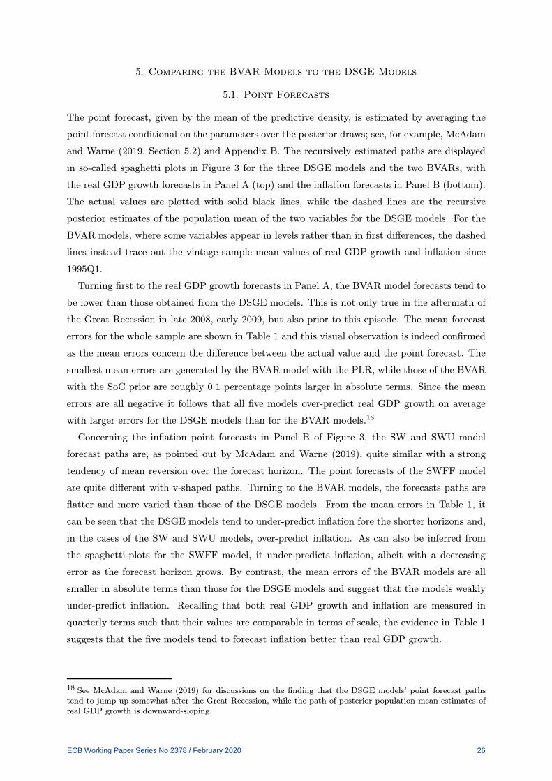
5. Comparing the BVAR Models to the DSGE Models

5.1. Point Forecasts

The point forecast, given by the mean of the predictive density, is estimated by averaging the

point forecast conditional on the parameters over the posterior draws; see, for example, McAdam

and Warne (2019, Section 5.2) and Appendix B. The recursively estimated paths are displayed

in so-called spaghetti plots in Figure 3 for the three DSGE models and the two BVARs, with

the real GDP growth forecasts in Panel A (top) and the inflation forecasts in Panel B (bottom).

The actual values are plotted with solid black lines, while the dashed lines are the recursive

posterior estimates of the population mean of the two variables for the DSGE models. For the

BVAR models, where some variables appear in levels rather than in first differences, the dashed

lines instead trace out the vintage sample mean values of real GDP growth and inflation since

1995Q1.

Turning first to the real GDP growth forecasts in Panel A, the BVAR model forecasts tend to

be lower than those obtained from the DSGE models. This is not only true in the aftermath of

the Great Recession in late 2008, early 2009, but also prior to this episode. The mean forecast

errors for the whole sample are shown in Table 1 and this visual observation is indeed confirmed

as the mean errors concern the difference between the actual value and the point forecast. The

smallest mean errors are generated by the BVAR model with the PLR, while those of the BVAR

with the SoC prior are roughly 0.1 percentage points larger in absolute terms. Since the mean

errors are all negative it follows that all five models over-predict real GDP growth on average

with larger errors for the DSGE models than for the BVAR models.18

Concerning the inflation point forecasts in Panel B of Figure 3, the SW and SWU model

forecast paths are, as pointed out by McAdam and Warne (2019), quite similar with a strong

tendency of mean reversion over the forecast horizon. The point forecasts of the SWFF model

are quite different with v-shaped paths. Turning to the BVAR models, the forecasts paths are

flatter and more varied than those of the DSGE models. From the mean errors in Table 1, it

can be seen that the DSGE models tend to under-predict inflation fore the shorter horizons and,

in the cases of the SW and SWU models, over-predict inflation. As can also be inferred from

the spaghetti-plots for the SWFF model, it under-predicts inflation, albeit with a decreasing

error as the forecast horizon grows. By contrast, the mean errors of the BVAR models are all

smaller in absolute terms than those for the DSGE models and suggest that the models weakly

under-predict inflation. Recalling that both real GDP growth and inflation are measured in

quarterly terms such that their values are comparable in terms of scale, the evidence in Table 1

suggests that the five models tend to forecast inflation better than real GDP growth.

18 See McAdam and Warne (2019) for discussions on the finding that the DSGE models’ point forecast pathstend to jump up somewhat after the Great Recession, while the path of posterior population mean estimates ofreal GDP growth is downward-sloping.


5.2. Density Forecasts

The predictive likelihood function of each DSGE model is estimated as discussed in McAdam

and Warne (2019, Section 5.1),19 while the Kalman filter framework for the BVAR models is

presented in Appendix B; see also Warne et al. (2017) for additional discussions on this topic.

The log predictive scores for the three DSGE and the two BVAR models based on the full sample

of vintages (2001Q1–2014Q4) are provided in Table 2. For each horizon (h) and variable set

(real GDP growth, inflation, and their joint forecast of real GDP growth and inflation) in a row,

the log score values shown in the top are in deviation from the largest value, while the row below

gives the largest value in the column of the corresponding model.

Starting with the joint real GDP growth and GDP deflator inflation density forecasts in

columns 2–6, the SW or SWU typically has the highest log score for the shorter horizons, while

the SoC or PLR model performs best for many of the longer forecast horizons. The SWFF

model generally performs markedly worse than the other models, except for the backcast and,

possibly, the eight-quarter-ahead forecast.

Turning next to the real GDP growth density forecasts in columns 7–11, it can be seen that for

most horizons (all except for h = 0, 1), the PLR model obtains the largest value. For the shorter

horizons, the SW model is ranked second among the five, while the SWU model comes in second

for h ≥ 4. The difference in values between the two BVARs and the SW and SWU models is

overall not big, and we return to a probabilistic assessment of this issue when discussing the

weighted likelihood ration tests of Amisano and Giacomini (2007).

Finally, the inflation forecasts in columns 12–16, the SWU model has the highest values for

many horizons (0 ≤ h ≤ 5), while the SoC model ranks as second best for these horizons and

ahead when h = 6, 7 and the SWFF performs best at the eight-quarter-ahead horizon. It is also

noteworthy that the SWFF model performs very poorly for the shorter horizons, as also pointed

out in McAdam and Warne (2019).

Overall, it appears to be a tight race between the DSGE and BVAR models, with the DSGE

models possibly doing better when forecasting inflation and the BVARs with real GDP growth.

Furthermore, the SW and SWU models tend to forecast both variables better than the BVARs

for the nowcast and one-quarter-ahead horizon, while the BVARs succeed at the six- and seven-

quarter-ahead horizons. Since the number of backcasts is very small for real GDP growth (3),

small for inflation (16), and very small for the joint density forecasts (3), this horizon is excluded

from the discussion below.

19 Notice that the equation for the h-step-ahead covariance matrix of the state variables on page 558 of McAdamand Warne (2019) contains an error. It should read:

P(i)

T+h|T = F hP(i)

T |T (F′)h +

h−1∑

j=0

F jBB′(F ′)j ,

where the second term on the right hand side is missing in McAdam and Warne (2019); see also equation (B.27)in Appendix B.


The equality of the log predictive scores of two models can be tested formally using the

weighted likelihood ratio tests advocated by Amisano and Giacomini (2007); see also Diks,

Panchenko, and van Dijk (2011). The empirical evidence over the full forecast sample for the

five models is presented in Figure 4; see also Appendix D, Tables D.1–D.4. The underlying

test statistic is based on equal weights and the percentile values are plotted in the charts for

ten model pairs over the nowcast and the one- to eight-quarter-ahead horizon, where the model

pair is shown in the title of the chart. The values for the real GDP growth density forecasts

are plotted as a solid red line, for GDP deflator inflation as a dashed blue line, and the joint

real GDP growth and inflation density forecasts as a dash-dotted green line. It should be kept

in mind that large percentile values favor the first model, while small values favor the second

model.

The top four charts display percentile values when testing the BVAR with an SoC prior versus

the three DSGE models and the PLR model. The following three charts give the values for the

PLR model versus the DSGE models, and the last three the values for pairs of the different

DSGE models. Concerning the two BVAR models when paired with the SW or SWU model,

the percentile values are often close the center (50 percent), with the exception of the inflation

forecasts with the PLR model. This is contrasted with the values obtains for both BVARs versus

the SWFF model, where the results generally favor the BVAR model, except for the long-term

inflation forecasts.

When testing the SoC model versus the PLR model, the formal evidence for the univariate

forecasts is fairly strong, with the PLR being favored for real GDP growth and the SoC for

inflation. Similarly, when pairing the DSGE models against one another the test values typically

gives strong formal evidence that both the SW and SWU models are better than the SWFF

for the full sample, again with the exception of the long-term inflation forecasts. Furthermore,

when the SW model is paired with the SWU model the latter comes weakly on top, with the

SW being stronger at the short-term real GDP growth forecasts, while the SWU outperforms

the SW for the shorter-term inflation forecasts.

It is interesting to note that the formal test evidence involving a pair from the BVAR or from

the DSGE model group is typically stronger, i.e. having low or high percentile values, than when

one model from the BVAR group is paired with a model from the DSGE group, albeit with the

SWFF model being an outlier as it typically performs worse than any of the other models. For

example, the difference in log score between the PLR and the SoC models for four-quarters-

ahead real GDP growth forecasts is 4.80 log-units while the difference between the PLR and the

SWU model is 4.50 and, all else equal, the difference in log score between the SoC and the SWU

of 0.30 is small. However, the percentile values for PLR versus SoC and versus SWU are 0.99

and 0.62, respectively. We therefore expect to find an event or several events within the forecast

sample that can account for this difference in behavior.


It should be pointed out that the Amisano-Giacomini weighted likelihood ratio test can gen-

erate seemingly counter-intuitive results. Suppose that equal weights are applied to the N

observations of the difference in log predictive likelihood for the model pair, with a lag trunca-

tion of zero for the Newey and West (1987) estimator of the asymptotic variance, as in Amisano

and Giacomini (2007), then the test statistic is given by the sample mean of the difference in

log predictive likelihood values divided by the square root of the sample mean of the squared

difference in log predictive likelihoods divided by N . One may expect a test statistic to be larger

when the average log score between two models is large rather than when it is tiny, but as the

following example shows this need not be the case.

Suppose that the difference in log predictive likelihood between model 1 and model 2 is c for

all time periods. For this case the value of the test statistic is equal to√N for all c and, hence,

it is invariant to such constants. Moreover, this particular test value is larger than the value

obtained when the difference in log predictive likelihood is c for half of the observations and

kc for the other half, with k > 1.20 In fact, the larger k is, the lower is the test value, while

simultaneously the value of the difference in log predictive score increases in k. More generally,

an increase of the variability in the differences between log predictive likelihoods of a pair of

forecasting methods dampens the absolute value of the weighted likelihood ratio test statistic

and can thereby lower the overall small sample power of the test, unless the increased variability

is at least matched by a larger difference in average log predictive score.

Recursive estimates of the average log scores for the joint density forecasts of real GDP growth

and inflation over the real-time vintages from 2001Q1 until 2014Q4 are shown in Figure 5. Each

chart displays the five models for a given horizon with the SW model being represented by a

solid red line, the SWFF model with a dark blue dash-dotted line, the SWU model with a green

dashed line, the SoC BVAR with a rose pink dash-dotted and the PLR with a light blue dashed

line. The horizontal axis in the panels represents the dating of the predicted variables, while the

average log predictive score for a model in that period is based on all the vintages dated up to h

periods prior to the date. Concerning the DSGE models it can be seen that the paths look quite

similar with the SWFF model path shifted down from the other two. The average log score for

each DSGE model is fairly constant with the downward shift in 2008Q4. The BVAR models, on

the other hand, display an upward trending behavior until 2008Q4, when a large drop occurs,

before the upward trending path begins again in the aftermath of the Great Recession.

The most striking feature of the charts in the figure is the size of the drop in average log score

of the BVARs compared with the DSGE models. The latter models lose roughly twice as much

in average log score as the latter models. For example, for the vintage 2008Q3 the one-quarter-

ahead log predictive likelihood value for the SW and SWU models is somewhat larger than −4

log units, while it is less than −11 for the BVAR models. The two-quarter-ahead log predictive

likelihood is around −7 for these two DSGE models and below −17 for the BVAR models. In

20 For this stylized case, the test statistic is equal to [(1+k)/√

2(1 + k2)]√N . If we consider k ≥ 0, this function

is increasing in k when 0 ≤ k < 1 with a maximum at 1 and is decreasing in k for k ≥ 1.


fact, the relative losses for the BVAR models are such that the model ranking changes from

the BVAR models obtaining a higher average log score than the DSGE models, to the SW and

SWU overtaking both BVARs. It is only towards the end of the vintage sample that the BVARs

regain higher log scores for some of the forecast horizons.

Moving to the recursive average log scores for the real GDP growth density forecasts in

Figure 6, the pattern in connection with the onset of the Great Recession is again present. The

loss in average log predictive score for the BVAR models is nearly one log unit, while it is a little

less than half a log unit for the DSGE models. As a consequence, the BVAR models at least

temporarily lose their top rankings to the SW and SWU models

Turning to the recursive average log scores for the inflation forecasts in Figure 7, the DSGE

models often perform better than the BVAR models, especially for the one-quarter to four-

quarter-ahead horizons. It is also notable that there is little or no effect on the short-term

density forecasts from the drop in inflation during the first half of 2009, while the medium- and

longer-term forecasts display a visible, albeit modest, drop in average log score for all models

except the SWFF model, which includes the BGG type of financial frictions. This result is

particularly interesting since the BVAR models have access to the same data on the external

finance premium, yet they are unable to utilize this information as fruitfully as the SWFF model

does when forecasting inflation over 2009Q1–Q2, even two-years-ahead.

To analyse what may underlie the large drop in log score of the BVAR models relative to

the DSGE models, Table 3 provides prediction errors (PEs), predictive variances (PVs) and

log predictive likelihoods (LPLs) over the various horizons when the objective is to predict real

GDP growth in 2008Q4 and in 2009Q1. Since the log predictive likelihood is expected to be well

approximated by a Gaussian likelihood function,21 the cause for the large drop in log score is

due to prediction errors, the predictive variance or, possibly, both.

In the case of 2008Q4, the sizes of the prediction errors for the BVAR models and the DSGE

models are similar in size, with all models greatly over-predicting actual quarterly real GDP

growth. Moreover, there are no major differences between the prediction errors based on the

vintage underlying the forecast, especially in the case of the BVARs. For example, the SoC

model forecasts in 2006Q4 (h = 8) are roughly of the same magnitude as those made in 2008Q3.

The only possible exception concerns the SWFF model, which has somewhat larger errors in

absolute terms than the other models. Turning to the predictive variances, the estimates from

the BVAR models are nearly three times smaller than those from the DSGE models. Hence, the

considerably smaller log predictive likelihoods of the BVAR models in 2008Q4 can be almost

fully accounted for by their narrow predictive densities.

21 Based on the evidence presented in McAdam and Warne (2019), the predictive likelihood of each one of thethree DSGE models is well approximated by a normal density based on the prediction error and the predictivevariance, albeit that the approximation error is larger when the value of the log predictive likelihood is smaller.Similar results were also obtained in Warne et al. (2017) when comparing a DSGE model to DSGE-VARs and,in particular, a BVAR model based on the methodology in Bańbura et al. (2010).


Concerning real GDP growth in 2009Q1, the same explanation is supported by the estimates

in Table 3. Overall, the prediction errors are larger than in 2008Q4 while the predictive variances

are broadly the same for all models, with the consequence that the log predictive likelihoods

are much smaller for this quarter. Nevertheless, the explanation for the much larger drop in

log predictive score for the BVARs than for the DSGE models is the predictive variance. The

small predictive variances of the BVARs are beneficial in terms of log score prior to the Great

Recession since the prediction errors are modest. However, the punishment is also severe for

when these over-confident models fail to predict large changes to the variables of interest. Still,

the lower predictive variances of the BVARs is also the reason why these models recover their

losses relative to the DSGE models once the Great Recession is over.

6. Forecast Combination Results

6.1. Comparing the Models to the Combination Methods

Forecast combinations offer an opportunity for combining individual model density forecasts such

that the combination provides a superior forecast. An indicator for such combinations to exist

is that the density forecasts of the individual models are not dominated by one model. The joint

real GDP growth and GDP deflator inflation forecasts display time varying top ranks among

the five models and similarly for real GDP growth. Concerning the inflation density forecasts,

however, some horizons at the shorter term have a dominant model throughout the forecast

sample; see, e.g., the three-quarter-ahead forecasts in Figure 7 with the SWU in a dominant

position. Even so, this model does not dominate the other models in terms of log predictive

likelihood for each time period, and it is therefore possible, albeit difficult, for a combination

scheme to outperform the SWU model.

The five combination methods discussed in Section 2 will be applied below for the DSGE and

BVAR models and, as the default value, we let the information lag follow the actuals release

lag, the observation lag, and be equal to four quarters (k = 4) for the SOP, the DP, the BMA

and the DMA combination methods. Since data releases of the predicted variables are available

prior to the annual revision data release, albeit with at least one lag, we shall also examine the

case when the information lag is exactly one quarter for real GDP growth and inflation; see

Section 6.4.1.

Concerning the dynamic prediction pool, the δ∗ parameter is given by 0.90 in the Bayesian

bootstrap filter. This means that an effective sample size below 90 percent of the number of

particles (N) results in resampling during the selection step of the filter. The size of the latter

parameter is 10,000 particles, while the grid for the ρ parameter, reflecting persistence of the

dynamic pool weights, is given by ρ ∈ 0.01, 0.02, . . . , 0.99.22 The initial values of the weights

are, by construction, equal to 1/5 for large N and these weights are used until the first time

22 Del Negro et al. (2016) use 5,000 particles in their study with δ∗ = 2/3 and 10,000 posterior draws of ρ, via therandom-walk Metropolis algorithm. We have checked the dynamic prediction pool results for alternative valuesof δ∗, namely, 0.8 and 2/3. This did not have a notable impact on the resulting log predictive scores.


period when historical predictive likelihood values are available. With an information lag of four

quarters, this occurs in period h+ 4 of the forecast sample.

The other combination methods that allow for time-varying weights are initialized by setting

them to 1/5 for each model; in Section 6.4.2 we shall analyse in some details the importance of

the initial values of the resulting log scores. Furthermore, and as mentioned in Section 2.5, we

follow the approach in Amisano and Geweke (2017) and estimate the DMA forgetting factor, ϕ,

and we have opted to set its grid to ϕ ∈ 0.01, 0.02, . . . , 0.99, keeping in mind that small values

approximate the equal weights density forecasts and large are close to BMA.

The full forecast sample log predictive scores of the five individual models, equal weights

(EW), SOP, BMA and DMA combination methods are displayed in Figure 8 in deviation from

the log score of the dynamic pool. The top left panel displays the results for the joint real GDP

growth and inflation density forecasts, where the five DSGE and BVAR models are plotted with

unchanged linestyles and colors relative to the earlier graphs. The four combination methods

are given by the grey dashed line for EW, black dotted line for SOP, grey solid line for DMA and

black dash-dotted line for DMA, while the zero line represents the dynamic pool. It can be seen

from the chart that nearly all combination methods and individual models obtain a lower log

score than DP for all horizons, with EW typically being in second place; the exceptions are EW

for the outer two horizons. The differences between EW and SOP are quite small, ranging from

around −3.13 log units at the one-quarter-ahead horizon to 0.07 at the seven-quarter-horizon.

Overall, the gaps in log score between the four combination approaches, the five models and DP

decrease with the forecast horizon.

Turning to real GDP growth in the top right panel, the picture is broadly similar, with the

DP and EW forecast combinations at the forefront while the individual models are ranked below

them. As in the joint density forecast case, the DMA approach obtains higher log scores than

the BMA approach. The SOP approach ranks above the DMA for the shorter horizons and

below both for the longer horizons.

Moving to the inflation density forecasts in the bottom left panel, an individual model is

ranked first for most horizons, with the exception of the seven-quarter-ahead forecasts and the

EW. For the shorter horizons, the SWU ranks first, while the SoC prior BVAR and the SWFF

are competitive at the longer horizons. For the shorter terms, the SOP ranks first among the

combination approaches and DP and EW obtain the lowest scores, while the picture is reversed

at the longer horizons. Overall, the combination approaches result in log predictive scores within

a range of 3 to -2 log units relative to the DP. Over the shorter horizons, the SOP fares best

among the five methods, while over the longer horizons it obtains the lowest score.

The equality of the log predictive scores of the DP and five individual models and the four

alternative combination methods are formally tested with the Amisano and Giacomini weighted

likelihood ratio test and the percentile values are shown in Figure 9. It is noteworthy that

the DP is strongly favored to the SW and SWFF models for the joint real GDP growth and


inflation forecasts and the marginal real GDP growth forecasts, while the formal test evidence

is somewhat weaker regarding the SWU model at the longer horizons. Concerning the inflation

forecasts, the evidence favoring the SWU model is strong, except for the longer horizons. When

comparing the DP to the BVAR models, the percentile values are generally closer to the middle

region, apart from the comparison with the PLR and the marginal inflation forecasts from the

two-quarter-ahead horizon and further out.

Turning to the comparisons with the other combination methods, the DP is favored to the

EW approach for the joint forecasts over the shorter term and generally the real GDP growth

forecasts, excluding the nowcasts, as well as the short term inflation forecasts. At the same

time, the formal evidence when comparing the DP to the SOP is somewhat weaker, especially

the real GDP growth forecasts. In view of the differences in log score shown in Figure 8, it is

perhaps somewhat surprising that the evidence in favor of the DP is weaker when examined to

the SOP than to the EW. The discussion in Section 5.2 may be recalled and the reason for these

seemingly counter-intuitive results is simply that the numerical standard error is substantially

larger for the SOP tests than for the EW tests.

Concerning the model averaging methods, the test evidence is quite similar for both combi-

nation schemes, with the DP being favored for the joint and the real GDP growth forecasts,

and especially the shorter term, although the percentile values tend to be somewhat larger when

comparing DP to BMA than to DMA. Regarding inflation and the shorter term, the percentile

values are close to zero, thereby favoring BMA and DMA, respectively, over the DP.

To examine the behavior of the combination methods in more detail, the recursively estimated

average log predictive scores of the joint density forecasts of the models and combination methods

are plotted in Figure 10. To highlight the differences, the results are again shown in deviation

from the recursive estimates of the average log predictive scores for the dynamic prediction

pool, i.e., the zero line represents to DP. Concerning the EW method, the deviations from zero

are small, especially for the longer horizons, while for the SOP combination the differences are

occasionally highly varying and cross the zero line. Similar behavior is also recorded for the

BVAR models, while the differences to the SW and SWU models are often positive until early

2005 and negative or very small thereafter. Recalling that the percentile values for the full

sample weighted likelihood ratio tests in Figure 9 are close to unity, these results can broadly be

understood from the discussion above and the impact of variability on the numerical standard

error.23

6.2. Model Weights

The empirical evidence presented so far gives fairly convincing support for the usefulness of

combination methods in a real-time density forecast comparison exercise. It is therefore of

interest to learn how the weights of the five models develop over time, also relative to the

23 The recursive estimates of the average log predictive scores for real GDP growth and inflation separately andrelative to the estimates from the DP are shown in Figures D.1–D.2 of Appendix D.


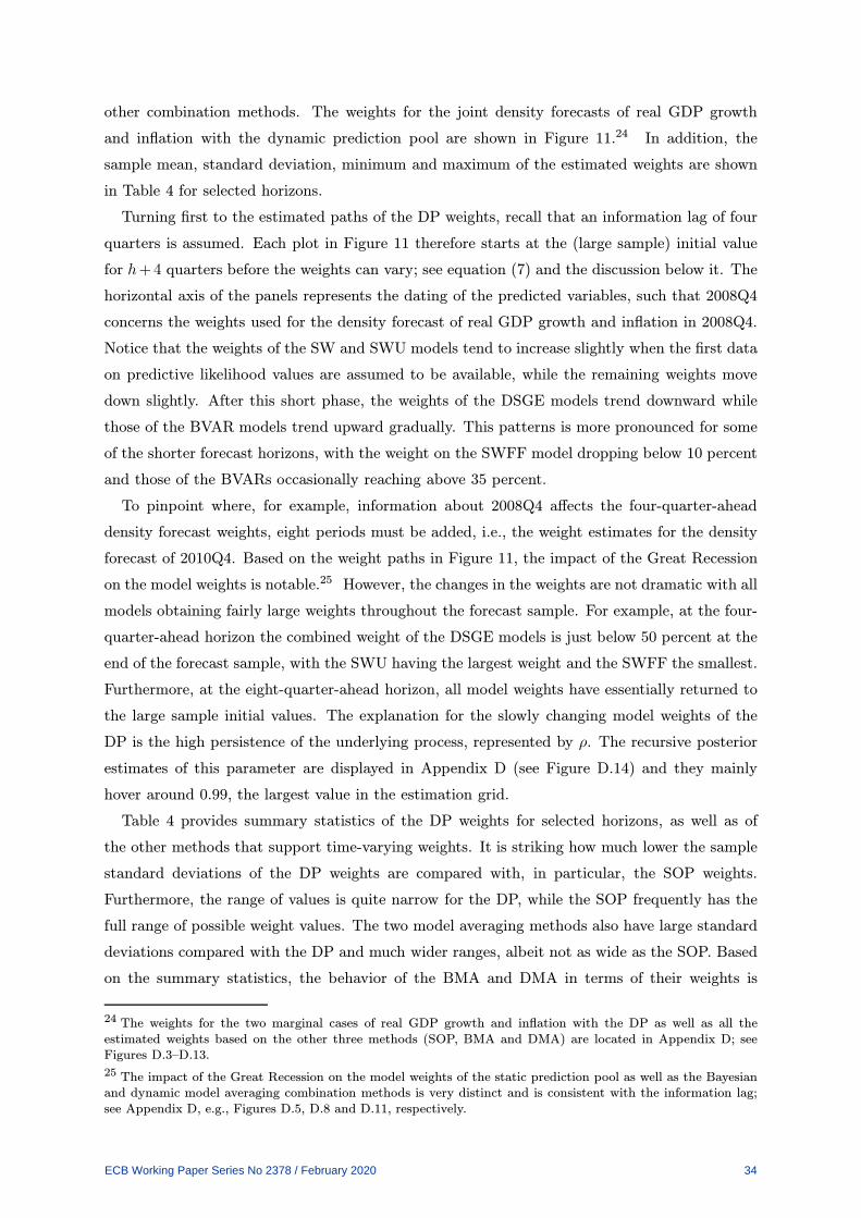
other combination methods. The weights for the joint density forecasts of real GDP growth

and inflation with the dynamic prediction pool are shown in Figure 11.24 In addition, the

sample mean, standard deviation, minimum and maximum of the estimated weights are shown

in Table 4 for selected horizons.

Turning first to the estimated paths of the DP weights, recall that an information lag of four

quarters is assumed. Each plot in Figure 11 therefore starts at the (large sample) initial value

for h+4 quarters before the weights can vary; see equation (7) and the discussion below it. The

horizontal axis of the panels represents the dating of the predicted variables, such that 2008Q4

concerns the weights used for the density forecast of real GDP growth and inflation in 2008Q4.

Notice that the weights of the SW and SWU models tend to increase slightly when the first data

on predictive likelihood values are assumed to be available, while the remaining weights move

down slightly. After this short phase, the weights of the DSGE models trend downward while

those of the BVAR models trend upward gradually. This patterns is more pronounced for some

of the shorter forecast horizons, with the weight on the SWFF model dropping below 10 percent

and those of the BVARs occasionally reaching above 35 percent.

To pinpoint where, for example, information about 2008Q4 affects the four-quarter-ahead

density forecast weights, eight periods must be added, i.e., the weight estimates for the density

forecast of 2010Q4. Based on the weight paths in Figure 11, the impact of the Great Recession

on the model weights is notable.25 However, the changes in the weights are not dramatic with all

models obtaining fairly large weights throughout the forecast sample. For example, at the four-

quarter-ahead horizon the combined weight of the DSGE models is just below 50 percent at the

end of the forecast sample, with the SWU having the largest weight and the SWFF the smallest.

Furthermore, at the eight-quarter-ahead horizon, all model weights have essentially returned to

the large sample initial values. The explanation for the slowly changing model weights of the

DP is the high persistence of the underlying process, represented by ρ. The recursive posterior

estimates of this parameter are displayed in Appendix D (see Figure D.14) and they mainly

hover around 0.99, the largest value in the estimation grid.

Table 4 provides summary statistics of the DP weights for selected horizons, as well as of

the other methods that support time-varying weights. It is striking how much lower the sample

standard deviations of the DP weights are compared with, in particular, the SOP weights.

Furthermore, the range of values is quite narrow for the DP, while the SOP frequently has the

full range of possible weight values. The two model averaging methods also have large standard

deviations compared with the DP and much wider ranges, albeit not as wide as the SOP. Based

on the summary statistics, the behavior of the BMA and DMA in terms of their weights is

24 The weights for the two marginal cases of real GDP growth and inflation with the DP as well as all theestimated weights based on the other three methods (SOP, BMA and DMA) are located in Appendix D; seeFigures D.3–D.13.

25 The impact of the Great Recession on the model weights of the static prediction pool as well as the Bayesianand dynamic model averaging combination methods is very distinct and is consistent with the information lag;see Appendix D, e.g., Figures D.5, D.8 and D.11, respectively.


more alike compared to results obtained for the dynamic and the SOP, especially at the longer

horizons. As might be expected, this is mainly due to the posterior estimates of the forgetting

factor, ϕ, being close to unity for these cases; see Appendix D, Figure D.17.

To summarize, the weights of the most successful density forecast combination method over the

full forecast sample, the DP, vary moderately over time, less as the forecast horizon increases, and

gives substantial weight to all models. By construction, the EW method shares these properties

which help to explain its relative success over the other combination methods, whose weights

are volatile and cover a wider range of values.26 Furthermore, we have found in Section 6.1 that

the longer the forecast horizon is, the more difficult it is for the combination methods to beat

the EW combination; see, e.g., Figure 8. In the case of the DP, this can be understood from

the increased discounting (ρh) that comes with longer horizons. Technically, this means that

the inherent equal-weights force is strengthened as h becomes larger and, hence, that the DP

resembles the EW combination more and more. At the same time, this property also reflects

well the idea that a predictive likelihood value used to predict far into the future has a lower

information value than a predictive likelihood value used for a shorter-term forecast.

6.3. Upper and Lower Bounds For Density Forecasts

The model weights for any density forecast combination method are formed using information

available at the time the density forcast is made. One question that comes to mind when

comparing density forecast is: given the models at hand, what is the best result that could have

been obtained by combining them? Likewise, we may ask: what is the worst result that could

have occurred? The answers to these questions give the user an upper and a lower bound for

density forecast combination based on the M models being considered.

It is straightforward to construct both bounds ex post when the log score is used as the

scoring rule. Specifically, the upper and lower bounds for each forecast horizon are obtained

by collecting the maximum and the minimum of the log predictive likelihoods of the M models

in each time period and adding these “optima” as the log scores of the upper and lower bound

combinations, respectively. That is, the upper and the lower bound of the log scores are given

by

S(U)T :Th,h

=

Th∑

t=T

maxi=1,...,M

log(

p(i)t+h|t

)

, (22)

S(L)T :Th,h

=

Th∑

t=T

mini=1,...,M

log(

p(i)t+h|t

)

. (23)

From the perspective of a forecaster combining models in real time, however, these bounds are,

as Th increases, close to probability zero events as they involve always picking the winner or

26 It is noteworthy that DMA approximates the equal (fixed) weights method when the forgetting factor is low.However, despite the fact that very low values of ϕ are allowed for when estimating this factor, the posteriormode estimates are always in the upper most part of the considered grid.


the loser. They nevertheless form natural benchmarks when comparing density forecasts. The

spread between the upper and lower bounds gives a measure of how much room exists for the

log score of any combination method using the same models and forecast sample. Moreover,

the difference between the upper bound and the log score of the best model is the interval

available to combination methods for improving on the model forecasts. Should this interval be

“too narrow”, it may be prudent to consider additional forecasting models before carrying out a

combination exercise.27

The the recursively estimated log scores for the five combination methods and the recursive

average lower bound for the joint real GDP growth and inflation density forecasts are plotted in

Figure 12 in deviation from the recursive average upper bound.28 This means that the upper

bound is equal to zero. Since the log scores concern recursive averages, the distances of their

paths from the upper bound are not always increasing, but can also approach this bound, as

in the case of the SOP in the wake of the Great Recession. Concerning the average differences

between the upper and lower bounds, note that it tends to decrease with the forecast horizon.

The average interval is close to unity for the eight-quarter-ahead forecasts towards the end of the

forecast sample, while for nowcasts and up to the three-quarter-ahead forecasts the difference is

around 1.5 log units. The main explanation for this appears to be the real GDP growth forecasts

which cover the negative growth rate in 2001Q4, where the BVAR models in particular have

very low scores which are submitted to the lower bound.29 In addition, from the graphs in

Figures 6 and 7 it appears that this behavior of the log scores is mainly due to the real GDP

growth forecasts. Furthermore, the recursive average log scores of the five combination methods

tend to lie closer to the upper bound than the lower bound with the best combinations being

around 2/3’s up from the lower bound at the end of the forecast sample. Hence, given the

pool of models available, there is room for improvement for combination methods and, from the

perspective of these bounds, the gains from using the best combination methods over the best

models are modest.

6.4. Sensitivity Analysis

The combination methods depend on specific assumptions that may affect the outcome of the

empirical exercises above. First, the information lag l = 4 is mechanical as it follows exactly

the observation lag and it neglects the fact that the information lag for real GDP growth and

inflation for the euro area RTD is often only one quarter. To simplify computational issues

27 What constitutes a “too narrow” interval is subjective, but it is nevertheless not hard to imagine cases wherenear consensus can be reached.

28 The results for the marginal real GDP growth and inflation forecasts are shown in Appendix D, Figures D.20and D.21, respectively. Similarly, upper and lower bounds graphs for the models instead of the combinations areshown in Figures D.22–D.24.

29 This may be inferred from Figure 5 where the paths of the average log scores prior to 2005 for the models aremore volatile with greater deviations between the best (DSGE) and the worst (BVAR) model for the shorter-termforecasts than for the longer-term forecasts. This is especially true for the negative real GDP growth in 2001Q4, aperiod which is covered by the density forecasts up to three-quarters-ahead but not by the longer-term forecasts.


and make comparisons less complex, we consider the case of l = 1 with the measured values

given by the actuals rather than taken from the corresponding vintage. Consequently, the

underlying log predictive likelihoods of the DSGE and BVAR models are not re-estimated for

the three additional time periods per vintage and horizon, but instead the timing of the available

information is shifted backwards.

Second, all methods are based on having equal initial values of the model weights in one form

or another. Given that the sample is relatively short, this may have an effect on the outcome. For

this reason, as well as to have an instrument for explicitly assessing the importance of including

a model with financial frictions in the pool of models, the case when the weight on the SWFF

model is initialized at zero and when the other models receive an initial weight of 1/4 will be

examined. For the fixed weight approach we likewise study the case when the weight is zero on

the SWFF model and 1/4 on the remaining four models.

6.4.1. The Information Lag

The information lag for real GDP growth and GDP deflator inflation data is often one quarter

for the euro area RTD. For the former variable it is two quarters in three out of 56 cases and for

the latter variable in 16 cases; see McAdam and Warne (2019, Table 4). With l = 1, we assume

that the measured data are well approximated by the annual revisions actuals, i.e., for vintage

t we let x(m)t−j = x

(a)t−j for j = 1, 2, 3, with the consequence that the predictive likelihood values of

the individual models do not need to be recomputed for these periods.30 Instead, we can simply

append three already estimated h-step-ahead predictive likelihood values to the information set

used to compute the weights at each point in time during the forecast sample. It follows that the

recursively obtained weights on the models for the SOP and the two model averaging methods

are not affected by the information lag other than by shifting the weights back in time three

time periods and by allowing for three new sets of weights at the end of the forecast sample. In

the case of the DP, the effect of the shorter information lag is also a simple time shift of the

weights, provided that the number of particles, N , is large enough.

Table 5 shows the full sample log predictive scores of the joint real GDP growth and inflation

density forecasts for the combination methods with time-varying weights. It is notable that

mainly the short-term horizons are affected by the shortened information lag for all methods

except the DP. In particular, substantially higher log scores are recorded for the nowcast of

the SOP and the two model averaging approaches, while the differences are smaller at the

four-quarter-ahead horizon and thereafter. Furthermore, the DP still obtains the largest log

30 It should be kept in mind that the relative impact on the predictive likelihood from the revisions is unlikely tobe substantial enough to affect the overall conclusions from the exercise in this section. For example, having someinformation about the real GDP growth in 2008Q4 when computing model weights in 2009Q1 is likely to havea great impact on the combined predictive likelihood of the shorter term forecasts for the combination methodsthat react strongly to new information, regardless of the precise value given to real GDP growth in 2008Q4. Forexample, the actual value of real GDP growth in 2008Q4 is −1.89 percent, while the measured value for thisquarter from the 2009Q1 vintage is −1.48 percent, both values representing strong negative growth.


predictive score among the four methods, with the exception of the nowcast where DMA has a

somewhat larger value.

The improvement in log predictive scores based on the shorter information lag is mainly due

to being able to react earlier to the large forecast errors in real GDP growth recorded for the

BVARs at the onset of the Great Recession. The full sample log scores for real GDP growth and

inflation separately are located in Appendix D, Table D.7, and the pattern recorded in Table 5

also applies to the log predictive scores for real GDP growth, while the log scores of inflation are

only marginally affected by the shorter information lag. The reason for the improvement in log

scores with the shorter information lag can also be inferred by plotting the difference between

the recursively estimated log predictive scores; see Figure 13. For the static prediction pool the

improvement for the nowcast is approximately 18 log units and it occurs in 2009Q1 by having

access to the log predictive likelihood for 2008Q4. Based on the model values for that quarter,

the SOP approach leads to lower weights on the BVARs, especially the PLR, and a larger weight

on the SW model at an earlier date. The BMA and DMA combination methods also gain in log

score from the more timely information regarding real GDP growth at the onset of the Great

Recession, although the impact on the log score is somewhat less pronounced than for the SOP.

Concerning the two-quarter-ahead to eight-quarter-ahead density forecasts, a shorter infor-

mation lag does not always improve the log score. The full sample log scores of BMA are, with

the exception of h = 6, lower for the shorter information lag, while it generally improves the log

score for DMA. For the recursive estimates, the picture is more complex with all combinations

displaying both gains and losses for some time periods and some horizons.

It is also striking how little the recursive log score of the DP is affected by the information

lag. From Table 4 we know that its weights are substantially less volatile than those of the other

combination methods and, hence, shifting the weights back in time only has a moderate effect

on the log score. This applies to all forecast horizons and explains why the DP is robust to the

choice of information lag for the euro area RTD vintages of 2001Q1 until 2014Q4.

6.4.2. The Initial Weights

Changing the initialization from equal weights to some other weighting scheme is straightforward

when applying the static prediction pool as well as BMA and DMA. For the DP, the weight

initialization depends on the parameters of the underlying process, ξt, as well as on the informa-

tion available through the model predictive likelihood values. The default parameterization of

ξt favors the propagation of equal weights through the initialization of ξT−1 and the innovation

ηt.

The predictive likelihood values of the models are initially set to a constant, such as unity

or 1/M , for the time periods t = T, . . . , T + h + l − 1 due to the information lag, l, and the

forecast horizon, h, delaying when actual realizations of the model predictive likelihoods can be

observed. When the number of particles is large enough, this initialization period means that


the model weights estimator

1

N

N∑

n=1

w(n)i,t+h|t

(ρ)W

(n)t ≈ 1

M, t = T, . . . , T + h+ l − 1.

One way to influence the weights during this initialization phase is to feed the bootstrap

particle filter with alternative predictive likelihood values. For instance, the case when the

SWFF model should be given zero initial weights while the other four models each have the

weight 1/4 can, partially, be implemented by setting the predictive likelihood values of the

models equal to these weights during the first h+ l periods. The reason why this only partially

changes the weights to the desired values is related to the initialization of ξT−1 and to the

assumption about ηt. Since both vectors are assumed to be standard normal, it follows that for

large N , the large sample average of wi,T−1 = 1/5 and similarly for the candidate model weights

wi,t at the beginning of the forecasting step in the Bootstrap filter. The expected value of the

incremental weights in period T , ωT , is therefore given by the weighted average of the predictive

likelihood values (1/5).

During the updating step, the particles are given a candidate re-weighting scheme, W(n)T , based

on the old particle weights (unity) and the incremental weights. This candidate scheme will not

favor equal weights since the predictive likelihood value of those particles based on a low weight

on the SWFF model will achieve a larger predictive likelihood than average. For the selection

step, two possibilities exist, but with similar outcomes. If the effective sample size remains

above the selected threshold size, δ∗N , the re-weighted candidate scheme of particle weights will

be applied to the candidate model weights when estimating the model weights that are used

to compute the predictive likelihood for the nowcast and the h-quarter-ahead forecasts. The

corresponding model weights will have values less than 1/5 for the SWFF model but greater

than zero since the candidate model weights have mean 1/5. The other models will obtains

approximately equal values somewhat larger than 1/5. On the other hand, if the effective

sample size is below the threshold size, resampling occurs based on the swarm of candidate

model and particle weights where model weights for particles with larger particle weights have a

greater chance of survival, i.e., those with a low weight on the SWFF model. Again, the result

is that average model weight has a value less than 1/5 for the SWFF model but greater than

zero, while the average model weights on the other four models are approximately equal and

somewhat larger than 1/5.

The inherent equal-weights force of ξt through its initialization and ηt can be guided towards

other steady-state weights by tuning its distribution. One option is to change the mean of the

normal distribution from zero to, say, −1.96 for the models where we wish to consider an initial

weight close to zero. Since the purpose is to aim at a particular vector of near fixed weights

during the first h + l time periods of the forecast sample, the mean of the normal distribution

need only be swapped during this period. Thereafter, the zero mean value is applied again,

bearing in mind that the ηt random draws again push the DP weights towards equal weights. In


this section, we consider the case when the mean of ξT−1 and ηt are equal to −1.96 for the SWFF

model and zero for the other models. This not only ensures that the weight on the SWFF model

is relatively close to 0 while the other weights are close to 1/4 up to time period T + h+ l − 1,

but it also allows the ξi,t process for the SWFF model to recover thereafter, provided that its

predictive likelihood values give sufficient support for the model. Furthermore, by limiting the

number of periods for the change of ηt to the initial h+ l periods of the forecast sample, it follows

that this also applies when iterating the ξt process forward when computing the h-step-ahead

weight.31

The full sample log predictive scores for the alternative initialization scheme with “zero weight”

on the SWFF model and equal weights on the other models are shown in Table 6 for the joint real

GDP growth and inflation case.32 The fixed weights cases in the table are denoted FW since this

covers both the EW combination and the combination with zero weight on the SWFF model.

It is striking that the log scores of all combination methods are positively affected by having

a zero initial weight on the SWFF model, with the exception of the SOP nowcasts. The fixed

weight combination scheme obtains the highest log score for all horizons when the SWFF model

is excluded and the improvement is particular notable for the shorter horizons. Although the

DP also records substantial gains, they are not sufficiently large for the combination approach to

retain its first rank. The smallest improvements are recorded for the SOP, where by construction

the selection of weights does not depend on lagged weights.

The differences for the recursively estimated log scores of the two initialization cases are

displayed in Figure 14.33 The SOP and BMA typically both obtain their total gain from the

initialization sample since the differences in log scores are nearly constant thereafter for all

horizons. Furthermore, the fixed weight and DP both display drops in their gains at the onset of

the Great Recession, suggesting that excluding the SWFF model (FW) or, at least, giving it a

lower weight (DP) has a negative impact on the log predictive likelihoods of these combination

methods during this period. This result is explained by having larger weights on the BVAR

models when the SWFF model receives a lower weight. Furthermore, it is interesting to note

that the DMA log scores improve relative to the benchmark case at the onset of the Great

Recession for the short-term forecasts. This is mainly explained by DMA having larger weights

on the SW and SWU models and lower on the SWFF model during this episode, while those on

the BVAR models are largely unaffected.

Formal test results for the hypothesis that the log predictive score of the SWFF zero and the

equal weights initialization are equal are displayed in Figure 15 for the five combination methods.

With the exception of the inflation density forecasts and the SOP, the empirical evidence from

31 This implementation is equivalent to introducing a time-varying drift-term into the equation for ξi,t, when iis the SWFF model, and having a zero mean for the distributions of ξT−1 and ηt.

32 The full sample results for real GDP growth and GDP deflator inflation separately are shown in Tables D.8and D.9, respectively. The information lag is given by the default value of four lags for annual revisions data.

33 The recursive estimates for real GDP growth and GDP deflator inflation separately are plotted in Figures D.27and D.28, respectively.


the Amisano and Giacomini tests strongly favors the SWFF zero initialization for all methods

and horizons. In the case of the SOP, the joint and the real GDP growth nowcasts test results

yield percentile values around 50 percent, suggesting that the two initialization alternatives

yield equal log scores. For the inflation density forecasts and with the exception of the SOP, the

percentile values are large for the short-term and small for the long-term, thereby supporting

setting the initial weight on the SWFF model to zero in the former case and being indifferent

or preferring equal initial weights in the latter case.

The posterior model weights for the joint real GDP growth and inflation density forecasts

using the DP and the SWFF zero initialization are displayed in Figure 16. The grey lines in

the panels are the posterior weights based on the equal weights initialization; see also Figure 11.

The SWFF zero initialization method we have proposed for the DP indeed provides the intended

properties, i.e., close to zero weights during the first h+ l periods of the forecast sample and a

chance to recover thereafter. The largest weights on the SWFF model during the initial periods

are obtained for the nowcasts, while in general the weights on this model gradually become

larger over the sample, especially for the longer term forecasts. The weights on the other models

shift proportionally relative to the equal weights initialization to offset the lower weight on the

SWFF model, and with the shift becoming smaller as the weight on the SWFF model depends

less on the selected initialization method.34

7. Summary And Conclusions

This paper examines density forecast combinations of three DSGE models (the Smets and

Wouters variants: SW, SWFF and SWU) and two BVARs (sum-of-coefficients, SoC, and prior

for the long run, PLR) to compare five methods: fixed weights, static optimal and dynamic

prediction pools, as well as Bayesian and dynamic model averaging. The models are estimated

on real-time euro area data and the forecasts cover the sample 2001–2014, focusing on inflation,

real GDP growth and their joint forecast. The main findings from the methodological presenta-

tion and the empirical exercises fall under two broad themes: (1) assessing model combinations

in real time, and (2) assessing model combinations over multi-step horizons.

Concerning the first theme, the literature on density forecast combinations has, to our knowl-

edge, omitted important characteristics of the real-time data dimension. Apart from fixed-weight

combinations, model weights are computed using information about each model’s past predictive

performance. In a real-time context, model weighting emerges when outcomes are imperfectly

known. This implies that the predictive likelihoods for models should be suitably lagged when

computing the model weights. To that end, we introduce the terms observation lag and informa-

tion lag to clarify the different time shifts involved for performance and weighting computations.

The former term denotes the time difference between the date of a variable and the vintage its

actual value is taken from, while the latter term gives the time difference between the date of a

34 The posterior model weights for the marginal real GDP growth and inflation density forecasts subject to theSWFF zero initialization are displayed in Figures D.29–D.30 for the DP.


variable and the vintage a measured value is taken from. While the information lag affects the

data available when computing model weights for predictions, the observation lag concerns the

predictive performance of a combination method in a forecast comparison exercise. Depending

on which actual values are selected, the measured data used for the model weight assessment

may differ from the actual values since earlier releases of the variables may be available prior

to the selected actual value. This stands in contrasts to the standard case of a single database,

where both lags are zero and this distinction is suppressed.

Regarding the weighting structure itself, for the real GDP growth and joint forecasts, the

DP and EW generally perform better than the other combination methods and the individual

models. For inflation, the picture is more fluid with DSGE models typically obtaining higher

log scores than the BVARs and the combination methods. Over short horizons, the SOP fares

well, but loses out thereafter to EW and the DP. Overall, the DP performs well. An analogue of

this can be gauged by the range of weights used by the different combination schemes. Whilst

the DP generates a relatively narrow range with all models being influential, the SOP exploits

the full support from zero to one, as do, to a lesser extent, BMA and DMA.

Another dimension in which the DP is robust (and, for instance, the SOP may not be) is

with respect to the information lag. Shortening the lag from four quarters to one quarter has

minimal effect on the log score of the DP, but dramatically lowers it for the other methods

and especially so for the SOP—although this improvement abates after two or more step-ahead-

forecasts. The gain is mainly due to being able to react earlier to the large real GDP growth

standardized forecast errors for the BVARs at the onset of the Great Recession. This illustrates

the case where better models (SW and SWU) are under-utilized since the historical performance

of the BVARs is maintained by the long information lag. The treatment of this lag in real-time

applications, therefore, reveals a trade-off in combination schemes as to the degree to which they

react quickly or slowly to the most recently available information.

The second theme concerns the assessment of model combinations over multi-step horizons.

Density forecast combinations are often conducted in a one-step-ahead environment yet, in our

exercises, we demonstrate that models’ predictive performance is horizon and variable specific.

For instance the BVARs generally forecast real GDP growth better than the DSGEs, whereas

for inflation it is the reverse. Taking this at face value, we may therefore be inclined to discard

some models (à la BMA), or at least discard some model types.

In a rich model combination framework, however, the pitfalls of such a strategy become readily

apparent. For instance some models, like SWFF, perform well for inflation but only at long

horizons, whereas others, like SWU, see their initially strong inflation predictive performance

recede as the forecast horizon increases. Likewise for real GDP growth, the SW performs well

over the shortest horizons, before the PLR overtakes its first rank among the individual models

thereafter, while the SWU becomes more attractive over the longer horizons. The bottom line

is that the more one engages in a multi-step, multivariate predictive setting, the more likely it


is that a set of different models contain information that can be usefully combined.35 A variant

on this theme, and indeed a validation of it, can also be seen in our exercises to initialize to zero

the weight on the SWFF model. This has a bearing on the weighting of the other models, but

also does not preclude the eventual return of SWFF to predictive and combinatory usefulness.

Finally, our exercises can be extended in a number of directions. First of all, when shortening

the information lag from four to one, we assume that the additional measured values of the

predicted variables that are required to compute the predictive likelihoods for the resulting time

periods are equal to the actual values. This is a convenient assumption when computing the

weights as it implies that the models’ predictive likelihood values based on the actuals can simply

be shifted back in time. Instead, one may consider using the measured values for each given

vintage, thereby requiring additional calculations for each real-time vintage. For most vintages,

all three such values are available while two values exist for the remaining vintages. In addition,

the minimum information lag need not be the same for all variables. The assumption that the

actual values approximation for the shortened information lag case does not distort the results

much is, for example, based on the observation that the revisions to the predicted variables are

quite small compared with the predictive variances, also for the Great Recession. Second, the

setup of the DP involves an inherent equal-weights force through the innovation process. In one

of our exercises, we introduce a parameterization which gives a low weight on the SWFF model

over the initialization phase, i.e., until predictive likelihood values from the forecast sample can

be observed. An alternative approach is to ignore the underlying VAR-process associated with

the SWFF model over the initialization sample, thereby effectively forcing its weight to zero.

Furthermore, the VAR process itself can receive a richer parameterization relative to the case

of one common autoregressive parameter and common unit innovation variance by allowing for

some model-dependent parameters. For instance, one may allow for different rates of mean

reversion or different means, thereby permitting model-weights to react individually to past

performance as well as for the long-run forecast model weights to deviate from equal weights. It

might also be an interesting robustness exercise to extend our analysis to a wider set of models,

for instance to reduded-form models such as the random walk implementation in Warne et al.

(2017), BVARs with stochastic volatility as in Clark (2011) and to dynamic factor models. We

leave these issues open for future research.

35 Another interesting conclusion is that DSGE models—whose performance around the Great Recession at-tracted particular criticism; see Kocherlakota (2010) for a discussion—appear quite competitive compared withless theory-constrained models, such as BVARs. In the wake of the Great Recession, all models incur large fore-cast errors, but “recover” their predictive abilities to varying degrees afterwards. This realization further bolstersthe case against a narrow model selection.


Table 1: Mean errors based on predictive mean as point forecast for the sample2001Q1–2014Q4.

Real GDP growth Inflation

DSGE BVAR DSGE BVAR

h SW SWFF SWU SoC PLR SW SWFF SWU SoC PLR

-1 0.045 −0.337 −0.218 −0.243 −0.139 0.154 0.227 0.136 0.116 0.089

0 −0.168 −0.388 −0.279 −0.200 −0.142 0.067 0.228 0.039 0.051 0.023

1 −0.382 −0.595 −0.439 −0.234 −0.162 0.028 0.278 0.004 0.054 0.017

2 −0.472 −0.655 −0.490 −0.256 −0.164 −0.018 0.284 −0.040 0.058 0.018

3 −0.502 −0.666 −0.486 −0.280 −0.173 −0.064 0.270 −0.084 0.067 0.022

4 −0.488 −0.650 −0.443 −0.287 −0.174 −0.113 0.241 −0.132 0.064 0.016

5 −0.467 −0.637 −0.400 −0.298 −0.183 −0.155 0.211 −0.172 0.062 0.015

6 −0.440 −0.622 −0.358 −0.306 −0.192 −0.186 0.185 −0.202 0.064 0.019

7 −0.411 −0.607 −0.318 −0.306 −0.195 −0.215 0.155 −0.231 0.058 0.016

8 −0.380 −0.587 −0.279 −0.296 −0.186 −0.238 0.129 −0.252 0.054 0.015


Table2:Log

predictive

scores

forbackcasts,now

castsan

don

e-to

eigh

t-quarter-ah

eadforecastsover

thevintages2001Q1–2014Q4,

withh=

−1beingthebackcasthorizon

andh=

0thenow

cast

horizon

.

RealGDP

growth

&inflation

RealGDP

growth

Inflation

DSGE

BVAR

DSGE

BVAR

DSGE

BVAR

hSW

SW

FF

SW

USoC

PLR

SW

SW

FF

SW

USoC

PLR

SW

SW

FF

SW

USoC

PLR

−1

−3.90

−5.07

−3.70

−0.20

0.00

−1.53

−1.73

−1.59

−0.26

0.00

−2.90

−7.51

−2.37

−0.11

0.00

−5.30

−0.79

−1.59

00.00

−25.57

−2.40

−5.88

−5.11

0.00

−5.46

−6.05

−5.03

−2.72

−3.87

−23.49

0.00

−1.37

−2.67

−36.77

−46.18

13.30

1−0.06

−39.12

0.00

−0.62

−0.24

0.00

−9.33

−3.48

−2.36

−0.07

−3.36

−27.57

0.00

−1.32

−2.82

−48.39

−56.53

11.21

2−0.99

−38.88

0.00

−2.10

−4.03

−0.98

−10.05

−2.62

−2.41

0.00

−2.67

−24.94

0.00

−2.58

−6.35

−53.75

−58.58

7.10

3−2.02

−34.05

0.00

−0.70

−1.98

−4.28

−12.31

−4.37

−3.53

0.00

−2.37

−20.48

0.00

−1.83

−6.02

−57.72

−56.40

2.93

4−2.18

−26.89

−0.19

−0.55

0.00

−5.52

−13.24

−4.50

−4.80

0.00

−1.48

−13.96

0.00

−0.82

−5.04

−59.47

−53.99

−0.90

5−2.39

−21.84

0.00

−1.70

−1.86

−5.11

−12.96

−2.86

−4.65

0.00

−0.78

−9.12

0.00

−1.02

−5.53

−60.01

−52.78

−3.71

6−2.65

−17.16

−0.08

0.00

−1.56

−4.10

−11.87

−1.32

−3.59

0.00

−1.30

−5.56

−0.89

0.00

−5.20

−61.11

−52.50

−5.63

7−1.87

−11.32

−0.03

0.00

−1.15

−4.23

−12.19

−1.48

−4.03

0.00

−1.21

−0.96

−1.54

0.00

−5.34

−62.71

−50.90

−7.80

8−1.54

−8.05

−0.63

0.00

−2.31

−2.74

−11.26

−0.70

−2.39

0.00

−3.16

0.00

−3.81

−1.87

−6.94

−63.57

−50.47

−8.15

Notes:Thelogscoresare

displayed

indev

iationfrom

thelargestva

lueforagiven

forecasted

vectorofva

riablesandhorizon.Thelargestlogscore

isshow

nin

therow

below

forthemodel

whichach

ieves

this

value.


Table 3: Predictions error, variance and log predictive likelihood of real GDPgrowth in 2008Q4 and 2009Q1.

2008Q4 2009Q1

DSGE BVAR DSGE BVAR

h Type SW SWFF SWU SoC PLR SW SWFF SWU SoC PLR

PE −1.85 −2.13 −2.03 −1.98 −1.93 −1.81 −1.82 −2.74 −2.37 −2.32

0 PV 0.45 0.46 0.42 0.15 0.14 0.48 0.50 0.43 0.19 0.18

LPL −4.30 −5.42 −5.32 −12.05 −12.10 −3.95 −3.96 −8.92 −13.41 −13.41

PE −1.92 −2.31 −1.99 −2.26 −2.27 −2.69 −3.00 −2.80 −2.71 −2.69

1 PV 0.54 0.55 0.59 0.20 0.18 0.54 0.55 0.59 0.20 0.19

LPL −3.98 −5.38 −4.00 −11.92 −12.67 −7.07 −8.46 −7.12 −16.06 −16.22

PE −2.11 −2.41 −2.08 −2.25 −2.26 −2.68 −3.06 −2.72 −2.80 −2.79

2 PV 0.56 0.56 0.64 0.22 0.20 0.56 0.56 0.64 0.21 0.20

LPL −4.54 −5.69 −4.04 −10.88 −11.67 −6.79 −8.61 −6.33 −16.06 −17.39

PE −2.25 −2.51 −2.28 −2.29 −2.24 −2.79 −3.09 −2.78 −2.82 −2.80

3 PV 0.57 0.57 0.66 0.23 0.21 0.57 0.57 0.66 0.22 0.20

LPL −4.97 −6.08 −4.64 −10.51 −10.99 −7.19 −8.72 −6.40 −15.10 −16.46

PE −2.23 −2.55 −2.17 −2.28 −2.17 −2.92 −3.18 −2.93 −2.89 −2.82

4 PV 0.59 0.60 0.68 0.24 0.21 0.58 0.57 0.67 0.24 0.21

LPL −4.85 −6.06 −4.16 −10.22 −10.19 −7.74 −9.15 −6.96 −14.93 −16.04

PE −2.30 −2.58 −2.14 −2.21 −2.15 −2.89 −3.20 −2.81 −2.90 −2.78

5 PV 0.59 0.60 0.69 0.25 0.22 0.59 0.60 0.69 0.24 0.22

LPL −5.07 −6.17 −4.02 −9.09 −9.99 −7.45 −8.97 −6.29 −14.68 −15.16

PE −2.37 −2.58 −2.24 −2.24 −2.11 −2.94 −3.23 −2.78 −2.83 −2.76

6 PV 0.60 0.60 0.70 0.25 0.22 0.60 0.60 0.70 0.25 0.22

LPL −5.31 −6.14 −4.30 −9.26 −9.44 −7.68 −9.08 −6.13 −13.02 −14.97

PE −2.36 −2.62 −2.23 −2.21 −2.08 −3.01 −3.22 −2.88 −2.84 −2.72

7 PV 0.60 0.60 0.71 0.25 0.22 0.60 0.60 0.71 0.26 0.22

LPL −5.22 −6.29 −4.23 −8.91 −9.21 −7.95 −9.05 −6.42 −13.35 −14.32

PE −2.29 −2.65 −2.24 −2.23 −2.10 −2.98 −3.25 −2.86 −2.83 −2.70

8 PV 0.63 0.63 0.71 0.26 0.23 0.60 0.60 0.72 0.26 0.22

LPL −4.82 −6.19 −4.29 −8.85 −9.15 −7.78 −9.18 −6.30 −12.78 −14.12

Notes: The three types of predictive distribution estimates are: prediction error (PE), predictive variance

(PV) and log predictive likelihood (LPL). The forecast horizon, h, determines which euro area RTD vintage

was used to predict real GDP growth in 2008Q4 and 2009Q1, respectively. For example, h = 4 when

predicting the outcome in 2008Q4 implies that the 2007Q4 vintage was employed. The actual values of

quarterly real GDP growth in 2008Q4 and 2009Q1 are given by −1.89 and −2.53 percent, respectively.


Table4:Summarystatistics

oftheweigh

tson

theDSGEan

dBVAR

modelsfordensity

forecast

combinationmethodsof

real

GDP

grow

than

dinflationover

thevintages2001Q1–2014Q4.

DP

SOP

BMA

DMA

hmodel

mean

std

min

max

mean

std

min

max

mean

std

min

max

mean

std

min

max

0SW

0.190

0.054

0.108

0.313

0.121

0.140

0.000

0.362

0.406

0.426

0.000

0.990

0.241

0.287

0.002

0.937

SW

FF

0.122

0.039

0.074

0.200

0.014

0.052

0.000

0.200

0.022

0.056

0.000

0.200

0.040

0.055

0.000

0.200

SW

U0.168

0.035

0.118

0.246

0.144

0.302

0.000

1.000

0.108

0.155

0.000

0.507

0.149

0.146

0.002

0.472

SoC

0.254

0.054

0.181

0.365

0.155

0.188

0.000

1.000

0.175

0.159

0.000

0.476

0.254

0.169

0.000

0.577

PLR

0.267

0.059

0.180

0.366

0.565

0.326

0.000

1.000

0.289

0.281

0.000

0.776

0.317

0.219

0.000

0.740

1SW

0.173

0.037

0.106

0.225

0.048

0.146

0.000

1.000

0.258

0.218

0.000

0.594

0.212

0.206

0.002

0.618

SW

FF

0.108

0.041

0.068

0.200

0.018

0.058

0.000

0.200

0.025

0.061

0.000

0.200

0.026

0.060

0.000

0.200

SW

U0.182

0.038

0.112

0.252

0.252

0.311

0.000

1.000

0.268

0.204

0.000

0.562

0.201

0.172

0.002

0.494

SoC

0.261

0.049

0.176

0.369

0.129

0.193

0.000

0.708

0.168

0.148

0.000

0.446

0.244

0.171

0.000

0.568

PLR

0.275

0.064

0.179

0.407

0.552

0.380

0.000

1.000

0.281

0.278

0.000

0.765

0.317

0.223

0.000

0.677

4SW

0.186

0.021

0.145

0.222

0.109

0.262

0.000

1.000

0.189

0.135

0.000

0.381

0.176

0.120

0.004

0.380

SW

FF

0.144

0.032

0.100

0.200

0.031

0.072

0.000

0.200

0.040

0.074

0.000

0.200

0.051

0.076

0.000

0.225

SW

U0.202

0.037

0.142

0.282

0.152

0.186

0.000

1.000

0.284

0.268

0.000

0.756

0.238

0.225

0.002

0.729

SoC

0.241

0.044

0.197

0.342

0.585

0.376

0.000

1.000

0.298

0.260

0.001

0.748

0.298

0.214

0.000

0.685

PLR

0.227

0.032

0.182

0.282

0.124

0.222

0.000

1.000

0.190

0.143

0.000

0.454

0.236

0.147

0.000

0.482

8SW

0.198

0.011

0.172

0.228

0.182

0.323

0.000

1.000

0.262

0.200

0.019

0.612

0.185

0.083

0.061

0.512

SW

FF

0.182

0.027

0.129

0.242

0.050

0.087

0.000

0.200

0.067

0.085

0.000

0.200

0.143

0.129

0.001

0.490

SW

U0.202

0.027

0.167

0.305

0.148

0.156

0.000

0.432

0.198

0.150

0.003

0.510

0.185

0.140

0.026

0.696

SoC

0.216

0.030

0.178

0.273

0.536

0.359

0.000

1.000

0.297

0.264

0.004

0.793

0.282

0.189

0.001

0.624

PLR

0.204

0.013

0.168

0.235

0.084

0.102

0.000

0.453

0.176

0.114

0.000

0.413

0.205

0.090

0.000

0.374

Notes:Theden

sity

combination

methodsare:dynamic

prediction

pool(D

P),

staticoptimalprediction

pool(SOP),

Bay

esian

model

averaging

(BMA),

anddynamic

model

averaging(D

MA).


Table 5: Log predictive scores of joint real GDP growth and GDP deflator in-flation for nowcasts and one-to eight-quarter-ahead forecasts of fourcombination methods based on different information lags over the vin-tages 2001Q1–2014Q4.

h l SOP DP BMA DMA

0 1 −29.59 −29.13 −38.29 −27.89

4 −47.13 −30.85 −49.83 −40.86

1 1 −51.97 −40.44 −57.71 −43.48

4 −55.23 −41.18 −58.09 −47.40

2 1 −48.87 −48.26 −62.18 −49.40

4 −50.20 −49.18 −61.21 −51.92

3 1 −63.11 −53.18 −66.38 −57.67

4 −65.54 −53.79 −65.95 −57.94

4 1 −62.28 −55.27 −66.06 −60.02

4 −64.25 −55.78 −65.30 −60.96

5 1 −64.61 −57.32 −65.09 −59.72

4 −64.77 −57.63 −64.97 −61.36

6 1 −65.25 −58.70 −65.43 −61.93

4 −64.84 −58.80 −65.00 −62.45

7 1 −65.62 −59.63 −64.95 −62.87

4 −66.05 −59.62 −65.58 −63.55

8 1 −66.34 −60.46 −65.42 −62.49

4 −66.83 −60.38 −65.27 −62.34


Table 6: Log predictive scores of joint real GDP growth and GDP deflator in-flation for nowcasts and one-to eight-quarter-ahead forecasts of fivecombination methods based on different initializations over the vin-tages 2001Q1–2014Q4.

h Initial weights FW SOP DP BMA DMA

0 SWFF zero −27.53 −47.14 −29.21 −49.37 −38.30

Equal −31.61 −47.13 −30.85 −49.83 −40.86

1 SWFF zero −38.28 −54.83 −38.75 −57.44 −45.46

Equal −44.31 −55.23 −41.18 −58.09 −47.40

2 SWFF zero −45.33 −49.71 −46.34 −60.49 −49.51

Equal −51.05 −50.20 −49.18 −61.21 −51.92

3 SWFF zero −49.98 −65.00 −51.21 −65.21 −56.71

Equal −55.02 −65.54 −53.79 −65.95 −57.94

4 SWFF zero −52.36 −63.65 −53.40 −64.49 −59.66

Equal −56.60 −64.25 −55.78 −65.30 −60.96

5 SWFF zero −54.50 −64.17 −55.50 −64.15 −59.64

Equal −58.04 −64.77 −57.63 −64.97 −61.36

6 SWFF zero −56.10 −64.24 −57.05 −64.26 −60.60

Equal −58.99 −64.84 −58.80 −65.00 −62.45

7 SWFF zero −57.52 −65.43 −58.32 −64.90 −61.60

Equal −59.56 −66.05 −59.62 −65.58 −63.55

8 SWFF zero −58.98 −66.20 −59.48 −64.75 −60.56

Equal −60.38 −66.83 −60.38 −65.27 −62.34

Notes: The initial weight scheme denoted “SWFF zero” has equal weights 1/4 on the SW, SWU, BVAR

SoC and BVAR PLR models and weight 0 on the SWFF model, except for the dynamic pool, where the

initialization scheme is random but where the weights approximate such fixed weights on average. The initial

weight scheme “Equal” gives weight 1/5 to each model during the initialization sample. For the fixed weight

(FW) combination method the weights are constant at the “initial weights”.


Figure 1: Illustration of the real-time information lag, l, and observation lag,k, for forecast combination methods, with l ≤ k.

timet t+ l t+ k

xt x(a)tx

(m)t

Information lag︸︷︷︸

Observation lag︸︷︷︸

Notes: The actual (or “true”) value of x in period t is denoted by x(a)t with t + k being the time period

when this value can be observed. The measured value of x in period t is x(m)t with t + l being the vintage

its value is taken from.


Figure 2: Recursive posterior mode estimates of the hyperparameters of theBVAR models for 2001Q1–2014Q4.

SoC Model

λo δ µ

200520052005 201020102010 201520152015

3

2.5

2

2

1.5

1.5

1.2

11

0.4

0.3

0.2

0.1

0

PLR Model

λo φ1 φ2

φ3 φ4 φ5

φ6 φ7 φ8

φ9

2005

200520052005

200520052005

200520052005

2010

201020102010

201020102010

201020102010

2015

201520152015

201520152015

201520152015

6

5.5

5

4.5

4

2.6

2.4

2.2

2

1.8

1.5

1.2

1.21.2

1.21.2

1.1

1.11.1

1

1

11

11

0.9

0.90.9

0.8

0.8

0.8

0.80.8

0.6

0.6

0.50.4

0.4

0.3

0.2

0.2

0.15

0.1

0.1

0.05

0

0


Figure 3: Recursive point backcasts, nowcasts and forecasts of real GDP growthand GDP deflator inflation using the RTD vintages 2001Q1–2014Q4.

A. Real GDP Growth

SW model SWFF model SWU model

BVAR SoC BVAR PLR

20002000

200020002000

20052005

200520052005

20102010

201020102010

20152015

201520152015

11

111

0.50.5

0.50.50.5

00

000

-0.5-0.5

-0.5-0.5-0.5

B. GDP Deflator Inflation

SW model SWFF model SWU model

BVAR SoC BVAR PLR

20002000

200020002000

20052005

200520052005

20102010

201020102010

20152015

201520152015

11

111

0.50.5

0.50.50.5

00

000

-0.5-0.5

-0.5-0.5-0.5

Notes: The actual values are plotted as solid black lines. Recursively estimated posterior mean values of mean

real GDP growth and mean inflation are plotted as dashed lines using the DSGE models. By contrast, the dashed

lines are vintage sample mean values since 1995Q1 of real GDP growth and inflation for the BVAR plots.


Figure 4: Percentile values of the Amisano-Giacomini weighted likelihood ratiotests for the equality of the average log predictive scores of ten BVARand DSGE model pairs for the sample 2001Q1–2014Q4.

SoC vs. SW SoC vs. SWFF

SoC vs. SWU SoC vs. PLR

PLR vs. SW PLR vs. SWFF

PLR vs. SWU SW vs. SWFF

SW vs. SWU SWFF vs. SWU

00

00

00

00

00

00

00

00

00

00

0.50.5

0.50.5

0.50.5

0.50.5

0.50.5

11

11

11

11

11

22

22

22

22

22

44

44

44

44

44

66

66

66

66

66

88

88

88

88

88

Real GDP growth and inflation

Real GDP growth

GDP deflator inflation

Notes: The test statistics have been computed with equal weights and using the Bartlett kernel for the HAC

estimator (Newey and West, 1987). Following Amisano and Giacomini (2007) we use a short truncation lag, but

rather than using their selection of zero lags we use one lag. The percentile value of the test statistic is taken

from a standard normal distribution, where large percentile values favor the first model of the test and small

percentile values the second model.


Figure 5: Recursive estimates of the average log predictive scores of joint realGDP growth and GDP deflator inflation for the vintages 2001Q1–2014Q4.

nowcast one-quarter-ahead

two-quarter-ahead three-quarter-ahead

four-quarter-ahead five-quarter-ahead

six-quarter-ahead seven-quarter-ahead

eight-quarter-ahead

2000

20002000

20002000

20002000

20002000

2005

20052005

20052005

20052005

20052005

2010

20102010

20102010

20102010

20102010

2015

20152015

20152015

20152015

20152015

0

00

00

00

00

-0.5

-0.5-0.5

-0.5-0.5

-0.5-0.5

-0.5-0.5

-1

-1-1

-1-1

-1-1

-1-1

-1.5

-1.5-1.5

-1.5-1.5

-1.5-1.5

-1.5-1.5

-2

-2-2

-2-2

-2-2

-2-2

SWSWFFSWUBVAR SoCBVAR PLR


Figure 6: Recursive estimates of the average log predictive scores of real GDPgrowth for the vintages 2001Q1–2014Q4.





eight-quarter-ahead

2000

20002000

20002000

20002000

20002000

2005

20052005

20052005

20052005

20052005

2010

20102010

20102010

20102010

20102010

2015

20152015

20152015

20152015

20152015

0

00

00

00

00

-0.5

-0.5-0.5

-0.5-0.5

-0.5-0.5

-0.5-0.5

-1

-1-1

-1-1

-1-1

-1-1

-1.5

-1.5-1.5

-1.5-1.5

-1.5-1.5

-1.5-1.5



Figure 7: Recursive estimates of the average log predictive scores of GDP de-flator inflation for the vintages 2001Q1–2014Q4.





eight-quarter-ahead

2000

20002000

20002000

20002000

20002000

2005

20052005

20052005

20052005

20052005

2010

20102010

20102010

20102010

20102010

2015

20152015

20152015

20152015

20152015

0.5

0.4

0.40.4

0.40.4

0.40.4

0.4

0.2

0.20.2

0.20.2

0.20.2

0.2

0

00

00

00

0

0

-0.2

-0.2-0.2

-0.2-0.2

-0.2-0.2

-0.2

-0.4

-0.4-0.4

-0.4-0.4

-0.4-0.4

-0.4

-0.5

-1

-1.5

-2



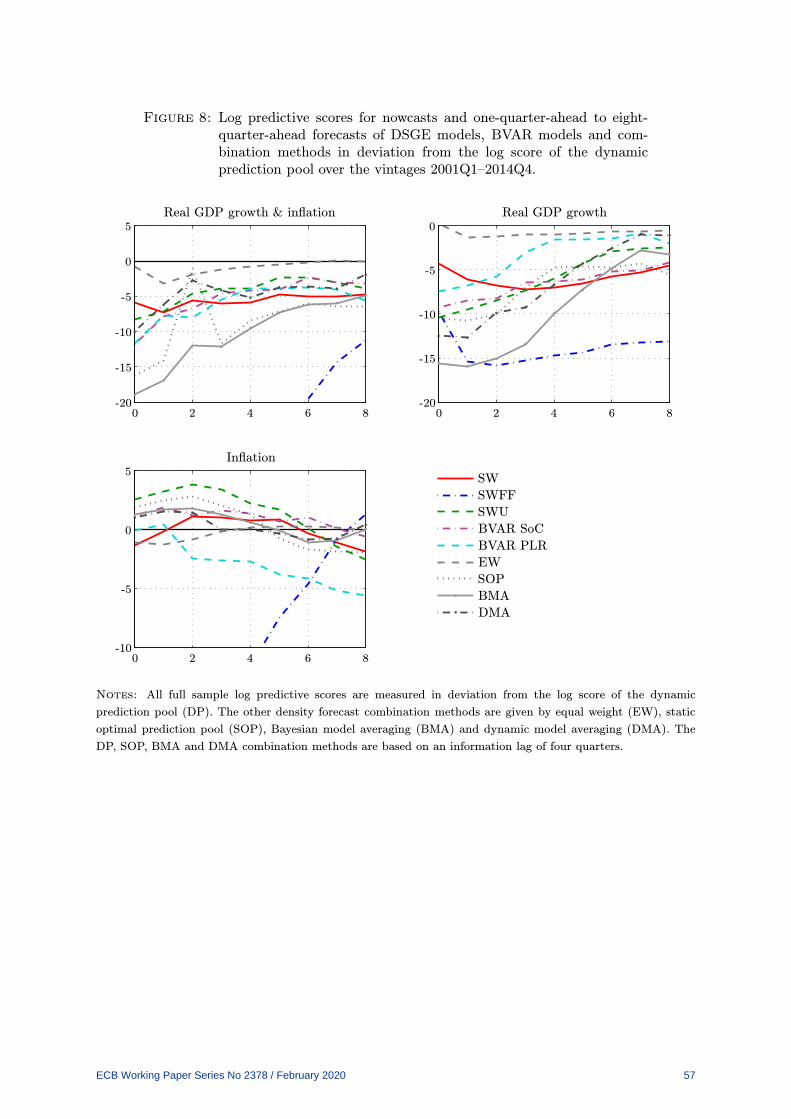
Figure 8: Log predictive scores for nowcasts and one-quarter-ahead to eight-quarter-ahead forecasts of DSGE models, BVAR models and com-bination methods in deviation from the log score of the dynamicprediction pool over the vintages 2001Q1–2014Q4.

Real GDP growth & inflation Real GDP growth

Inflation5

5

0

0

0

0

0

0

-5

-5

-5

-10

-10

-10

-15-15

-20-20

2

22

4

44

6

66

8

88

SW

SWFF

SWU

BVAR SoC

BVAR PLR

EW

SOP

BMA

DMA

Notes: All full sample log predictive scores are measured in deviation from the log score of the dynamic

prediction pool (DP). The other density forecast combination methods are given by equal weight (EW), static

optimal prediction pool (SOP), Bayesian model averaging (BMA) and dynamic model averaging (DMA). The

DP, SOP, BMA and DMA combination methods are based on an information lag of four quarters.


Figure 9: Percentile values of the Amisano-Giacomini weighted likelihood ra-tio tests for the equality of the average log predictive scores of thedynamic prediction pool versus nine alternative forecast schemes forthe sample 2001Q1–2014Q4.

DP vs. SW DP vs. SWFF

DP vs. SWU DP vs. SoC

DP vs. PLR DP vs. EW

DP vs. SOP DP vs. BMA

DP vs. DMA

00

00

00

00

00

00

00

00

00

0.5

0.50.5

0.50.5

0.50.5

0.50.5

1

11

11

11

11

2

22

22

22

22

4

44

44

44

44

6

66

66

66

66

8

88

88

88

88


Real GDP growth


Notes: See Figures 4 and 8 for details.


Figure 10: Recursive estimates of the average log predictive scores of joint realGDP growth and GDP deflator inflation and in deviation from therecursive estimates of the average log scores of the dynamic predic-tion pool covering the vintages 2001Q1–2014Q4.





eight-quarter-ahead

2000

20002000

20002000

20002000

20002000

2005

20052005

20052005

20052005

20052005

2010

20102010

20102010

20102010

20102010

2015

20152015

20152015

20152015

20152015

0.2

0.20.2

0.20.2

0.20.2

0.20.2

0.1

0.10.1

0.1

0

00

0

0

00

00

-0.1

-0.1-0.1

-0.1

-0.2

-0.2-0.2

-0.2

-0.2

-0.2-0.2

-0.2-0.2

-0.4

-0.4-0.4

-0.4-0.4

SWSWFFSWUBVAR SoCBVAR PLREWSOPBMADMA


Figure 11: Posterior estimates of the model weights for the dynamic predictionpool of joint real GDP growth and GDP deflator inflation coveringthe vintages 2001Q1–2014Q4.






eight-quarter-ahead

2000

20002000

20002000

20002000

20002000

2005

20052005

20052005

20052005

20052005

2010

20102010

20102010

20102010

20102010

2015

20152015

20152015

20152015

20152015

0.5

0.50.5

0.50.5

0.50.5

0.50.5

0.4

0.40.4

0.40.4

0.40.4

0.40.4

0.3

0.30.3

0.30.3

0.30.3

0.30.3

0.2

0.20.2

0.20.2

0.20.2

0.20.2

0.1

0.10.1

0.10.1

0.10.1

0.10.1

0

00

00

00

00


Figure 12: Recursive estimates of the average log predictive scores of joint realGDP growth and GDP deflator inflation for the combinations andin deviation from the recursive value of the upper bound coveringthe vintages 2001Q1–2014Q4.





eight-quarter-ahead

2000

20002000

20002000

20002000

20002000

2005

20052005

20052005

20052005

20052005

2010

20102010

20102010

20102010

20102010

2015

20152015

20152015

20152015

20152015

0

00

00

00

00

-0.5

-0.5-0.5

-0.5-0.5

-0.5-0.5

-0.5-0.5

-1

-1-1

-1-1

-1-1

-1-1

-1.5

-1.5-1.5

-1.5-1.5

-1.5-1.5

-1.5-1.5

-2

-2-2

-2-2

-2-2

-2-2

EWSOPDPBMADMAUpper/lower bound


Figure 13: Recursive estimates of the differences of log predictive scores of jointreal GDP growth and GDP deflator inflation for information lag 1and 4 covering the vintages 2001Q1–2014Q4.





eight-quarter-ahead

2000

20002000

20002000

20002000

20002000

2005

20052005

20052005

20052005

20052005

2010

20102010

20102010

20102010

20102010

2015

20152015

20152015

20152015

20152015

20

15

10

5

44

4

2

22

22

22

2

1

11

11

0

00

00

00

0

0

-1

-1-1

-1-1

-2

-2-2

-2-2

-2-2

-2

SOPDPBMADMA


Figure 14: Recursive estimates of the differences of log predictive scores of jointreal GDP growth and GDP deflator inflation for the SWFF zero ini-tialization and the equal weights initialization covering the vintages2001Q1–2014Q4.





eight-quarter-ahead

2000

20002000

20002000

20002000

20002000

2005

20052005

20052005

20052005

20052005

2010

20102010

20102010

20102010

20102010

2015

20152015

20152015

20152015

20152015

6

66

66

4

4

4

44

44

3

3

3

3

2

2

2

2

2

22

22

1

11

1

0

00

00

00

00

FWSOPDPBMADMA


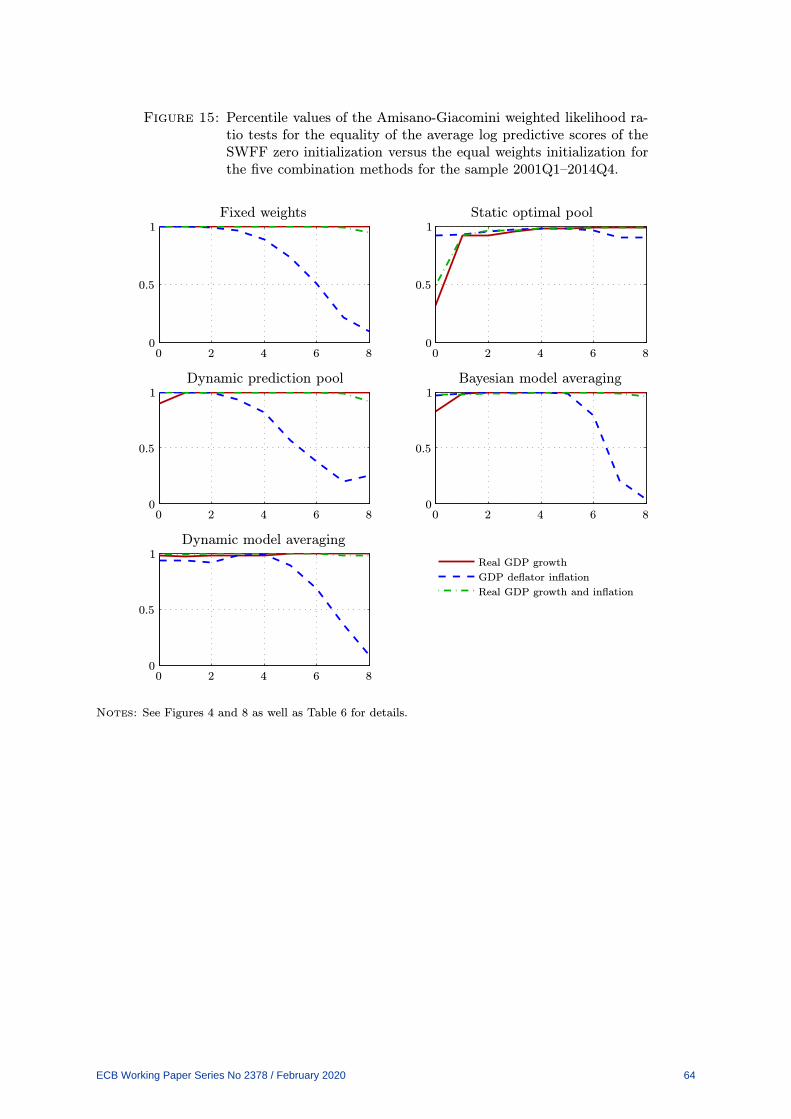
Figure 15: Percentile values of the Amisano-Giacomini weighted likelihood ra-tio tests for the equality of the average log predictive scores of theSWFF zero initialization versus the equal weights initialization forthe five combination methods for the sample 2001Q1–2014Q4.

Fixed weights Static optimal pool

Dynamic prediction pool Bayesian model averaging

Dynamic model averaging

00

00

00

00

00

0.5

0.50.5

0.50.5

1

11

11

2

22

22

4

44

44

6

66

66

8

88

88


Real GDP growth


Notes: See Figures 4 and 8 as well as Table 6 for details.


Figure 16: Posterior estimates of the model weights for the dynamic predictionpool of joint real GDP growth and GDP deflator inflation basedon the SWFF zero initialization and covering the vintages 2001Q1–2014Q4.






eight-quarter-ahead

2000

20002000

20002000

20002000

20002000

2005

20052005

20052005

20052005

20052005

2010

20102010

20102010

20102010

20102010

2015

20152015

20152015

20152015

20152015

0.5

0.50.5

0.50.5

0.50.5

0.50.5

0.4

0.40.4

0.40.4

0.40.4

0.40.4

0.3

0.30.3

0.30.3

0.30.3

0.30.3

0.2

0.20.2

0.20.2

0.20.2

0.20.2

0.1

0.10.1

0.10.1

0.10.1

0.10.1

0

00

00

00

00


Appendix A: Prior and Posterior Properties of the BVAR Models

The General Normal-Inverted Wishart BVAR Model

Let yt be an n-dimensional vector of observable variables such that its VAR representation is

given by

yt = Φ0 +

p∑

j=1

Φjyt−j + ǫt, t = 1, . . . , T, (A.1)

where ǫt ∼ Nn(0,Ω) and Φj are n × n matrices for j ≥ 1 and an n × 1 vector if j = 0.

Let Xt = [1 y′t · · · y′

t−p+1]′ be an (np + 1)-dimensional vector, while the n × (np + 1) matrix

Φ = [Φ0 Φ1 · · · Φp] such that the VAR can be expressed as:

yt = ΦXt−1 + ǫt. (A.2)

Stacking the VAR system as y = [y1 · · · yT ], X = [X0 · · · XT−1] and ǫ = [ǫ1 · · · ǫT ], we can

express this as

y = ΦX + ǫ, (A.3)

with log-likelihood

log p(y∣∣X0; Φ,Ω

)= −nT

2log(2π) − T

2log∣∣Ω∣∣− 1

2tr[Ω−1ǫǫ′

], (A.4)

where, for convenience, we use the same notation for the random variables as their realizations.

The normal-inverted Wishart prior for (Φ,Ω) is given by

vec(Φ)∣∣Ω, α ∼ Nn(np+1)

(vec(µΦ),[ΩΦ ⊗ Ω

]), (A.5)

Ω∣∣α ∼ IWn

(A, v

), (A.6)

where the prior parameters (µΦ,ΩΦ, A, v) are determined through a vector of hyperparameters,

denoted by α. This means that the sum of the log-likelihood and the log prior is given by

log p(y,Φ,Ω

∣∣X0, α

)= −n(T + np+ 1)

2log(2π) − nv

2log(2) − n(n− 1)

4log(π)

− log Γn(v) − n

2log∣∣ΩΦ

∣∣+

v

2log∣∣A∣∣

− T + n(p+ 1) + v + 2

2log∣∣Ω∣∣

− 1

2tr[

Ω−1(

ǫǫ′ +A+(Φ − µΦ

)Ω−1Φ

(Φ − µΦ

)′)]

.

(A.7)

Using standard “Zellner” algebra, it is straightforward to show that

ǫǫ′ +A+ (Φ − µΦ)Ω−1Φ (Φ − µΦ)

′)=(Φ − Φ

) (XX ′ +Ω−1

Φ

) (Φ − Φ

)′+ S, (A.8)

where

Φ =(yX ′ + µΦΩΦ

−1) (XX ′ +ΩΦ

−1)−1

,

S = yy′ +A+ µΦΩΦ−1µΦ

′ − Φ(XX ′ +ΩΦ

−1)Φ′.


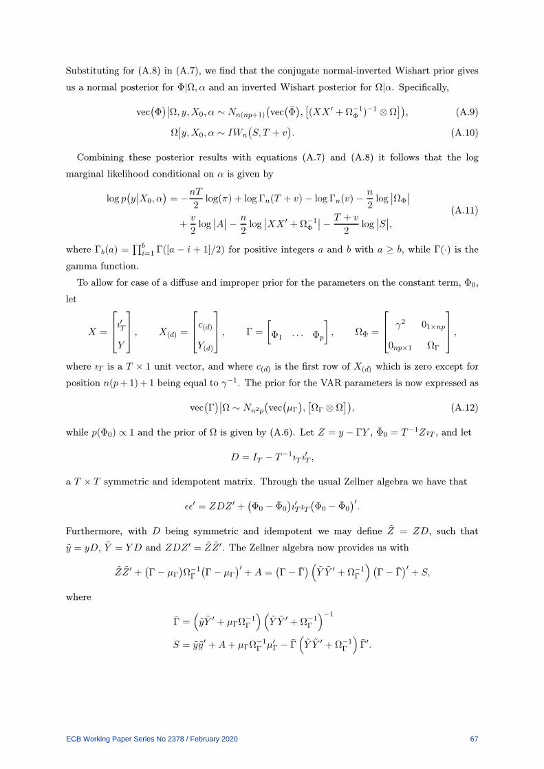
Substituting for (A.8) in (A.7), we find that the conjugate normal-inverted Wishart prior gives

us a normal posterior for Φ|Ω, α and an inverted Wishart posterior for Ω|α. Specifically,

vec(Φ)∣∣Ω, y,X0, α ∼ Nn(np+1)

(vec(Φ),[(XX ′ +Ω−1

Φ )−1 ⊗ Ω]), (A.9)


(S, T + v

). (A.10)

Combining these posterior results with equations (A.7) and (A.8) it follows that the log

marginal likelihood conditional on α is given by

log p(y∣∣X0, α

)= −nT

2log(π) + log Γn(T + v) − log Γn(v) − n

2log∣∣ΩΦ

∣∣

+v


2log∣∣XX ′ +Ω−1

Φ

∣∣− T + v

2log∣∣S∣∣,

(A.11)

where Γb(a) =∏b

i=1 Γ([a − i + 1]/2) for positive integers a and b with a ≥ b, while Γ(·) is the

gamma function.

To allow for case of a diffuse and improper prior for the parameters on the constant term, Φ0,

let

X =

ı′T

Y

, X(d) =

c(d)

Y(d)

, Γ =

[

Φ1 · · · Φp

]

, ΩΦ =

γ2 01×np

0np×1 ΩΓ

,

where ıT is a T × 1 unit vector, and where c(d) is the first row of X(d) which is zero except for

position n(p+1)+1 being equal to γ−1. The prior for the VAR parameters is now expressed as

vec(Γ)∣∣Ω ∼ Nn2p

(vec(µΓ),[ΩΓ ⊗ Ω

]), (A.12)

while p(Φ0) ∝ 1 and the prior of Ω is given by (A.6). Let Z = y − ΓY , Φ0 = T−1ZıT , and let

D = IT − T−1ıT ı′T ,

a T × T symmetric and idempotent matrix. Through the usual Zellner algebra we have that

ǫǫ′ = ZDZ ′ +(Φ0 − Φ0

)ı′T ıT

(Φ0 − Φ0

)′.

Furthermore, with D being symmetric and idempotent we may define Z = ZD, such that

y = yD, Y = Y D and ZDZ ′ = ZZ ′. The Zellner algebra now provides us with

ZZ ′ +(Γ − µΓ

)Ω−1Γ

(Γ − µΓ

)′+A =

(Γ − Γ

) (

Y Y ′ +Ω−1Γ

) (Γ − Γ

)′+ S,

where

Γ =(

yY ′ + µΓΩ−1Γ

)(

Y Y ′ +Ω−1Γ

)−1

S = yy′ +A+ µΓΩ−1Γ µ′

Γ − Γ(

Y Y ′ +Ω−1Γ

)

Γ′.


It can therefore be shown that the normal-inverted Wishart posterior for the VAR parameters

is given by

Φ0

∣∣Γ,Ω, y,X0, α ∼ Nn

(Φ0, T

−1Ω), (A.13)

vec(Γ)∣∣Ω, y,X0, α ∼ Nn2p

(vec(Γ),[(Y Y ′ +Ω−1

Γ )−1 ⊗ Ω])

(A.14)


(S, T + v − 1

). (A.15)

Hence, the improper prior on Φ0 results in a loss of degrees of freedom for the posterior of Ω.36

Furthermore, the log marginal likelihood is

log p(y∣∣X0, α

)= −n(T − 1)

2log(π) + log Γn(T + v − 1) − log Γn(v) − n

2log∣∣ΩΓ

∣∣

+v


2log(T ) − n

2log∣∣Y Y ′ +Ω−1

Γ

∣∣− T + v − 1

2log∣∣S∣∣,

(A.16)

where the term log(T ) stems from T = ı′T ıT and is obtained when integrating out Φ0 from the

joint posterior. The relationship between the dummy observations and the prior parameters is

µΓ = y(d)Y′(d)

(

Y(d)Y′(d)

)−1, ΩΓ =

(

Y(d)Y′(d)

)−1,

A =(y(d) − µΓY(d)

) (y(d) − µΓY(d)

)′, v = Td − (np+ 1).

Letting y⋆ = [y(d) y] and Y⋆ = [Y(d) Y ], it follows that the posterior parameters

Γ = y⋆Y′⋆

(Y⋆Y

′⋆

)−1,

Y Y ′ +Ω−1Γ = Y⋆Y

′⋆ ,

S =(y⋆ − ΓY⋆

)(y⋆ − ΓY⋆

)′.

36 This loss of one degree of freedom is due to (y(d), X(d)) having one observation less as γ → 0, i.e., as the prioron Φ0 becomes improper.


Appendix B: Real-Time Backcasts, Nowcasts and Forecasts from VAR Models

This Appendix first describes how the VAR model in equation (11) can be applied to backcast,

nowcast and forecast when we have real-time data. To be specific, we shall assume that data on

some variables are missing in periods T − 1 and T , corresponding to the situation for the RTD

of the euro area. The second part is concerned with the estimation of the marginal likelihood

of the VAR model when taking the ragged edge of the real-time data into account.

In addition to being interested in the yt variables, we are also interested in forecasting the

first differences of some of these variables. To this end, let S be an n×s matrix with full column

rank s ≤ n which selects unique elements of yt such that

zt = S′(yt − yt−1

).

In other words, zt is an s-dimensional vector whose elements are first differences of some of the

elements in yt. This means that

zt = Φ∗0 +

p∑

j=1

Φ∗jyt−j + S′ǫt,

where

Φ∗j =

S′(Φ1 − In

), if j = 1,

S′Φj , otherwise.

In order to derive a state-space system for the VAR model, including the first difference

variables zt, we stack these equations as follows:

zt

1

yt

yt−1

...

yt−p+2

yt−p+1

=

0 Φ∗0 Φ∗

1 Φ∗2 · · · Φ∗

p−2 Φ∗p−1 Φ∗

p

0 1 0 0 · · · 0 0 0

0 Φ0 Φ1 Φ2 · · · Φp−2 Φp−1 Φp

0 0 In 0 · · · 0 0 0

......

. . ....

...

0 0 0 0 In 0 0

0 0 0 0 · · · 0 In 0

zt−1

1

yt−1

yt−2

...

yt−p+1

yt−p

+

S′ǫt

0

ǫt

0

...

0

0

.

This gives us the state equation of the system. More compactly, we express it as

ξt = Fξt−1 + Cǫt. (B.1)

The measurement equation of the system is now given by

yt = H ′ξt, t = 1, . . . , T − 2. (B.2)


where

H ′ =[

0n×(s+1) In 0n×n(p−1)

]

.

For t = T − 1, T , when some of the variables in yt are unobserved, we introduce the matrices

St, where yt = S′tyt includes all the observed values of yt and none (NaN) of the unobserved.

Accordingly, we have that for Ht = HSt the measurement equations are given by

yt = H ′tξt, t = T − 1, T. (B.3)

We are now equipped with the state-space system and can proceed to setup a suitable Kalman

filter, updater and smoother; see, e.g., Durbin and Koopman (2012) for details.

To this end, note that for t = 1, . . . , T − 2 the vector ξt is observed and determined as

ξt = KXt,

where

K =

0 S′ −S′ 0

1 0 0 0

0 In 0 0

0 0 In 0

0 0 0 In(p−2)

,

is an (np+ s+1)× (np+1) matrix. Notice that the case p = 1 is treated as p = 2 with Φ2 = 0.

Letting ξt|t−1 denote the standard Kalman filter projection of ξt based on the data up to period

t− 1 and taking the parameters as fixed, it follows that

ξt|t−1 = Fξt−1, t = 1, . . . , T − 2.

Similarly, let Pt|t−1 denote the covariance matrix of ξt|t−1 with the consequence that

Pt|t−1 = CΩC ′, t = 1, . . . , T − 2.

Furthermore, it holds that ξt|t = ξt and Pt|t = 0 for the same time periods. It can also be seen

that the covariance matrix of yt given the data up to period t− 1 is given by

Σy,t|t−1 = H ′CΩC ′H = Ω, t = 1, . . . , T − 2.

Unless one is interested in computing the likelihood function, there is no need to run this Kalman

filter recursively. Rather, the above filter equations are merely used as input for the interesting

time periods t = T − 1, T, T +1, . . . , T +h, where we shall perform backcasting, nowcasting and

forecasting taking the ragged edge into account.


The smooth estimates for period T are used for the nowcasts, while the smooth estimates for

period T − 1 are similarly employed for the backcasts.

Define the (np+ s+ 1) × s matrix G such that

G′ =[

Is 0s,np+1

]

,

with the consequence that zt = G′ξt. The backcast (T − 1) and nowcast (T ) of zt are therefore

given by

zt|T = G′ξt|T , t = T − 1, T, (B.18)

while the covariance matrices are

Σz,t|T = G′Pt|TG. (B.19)

We can similarly compute the backcast and nowcast of yt as

yt|T = H ′ξt|T , (B.20)

and covariance matrices

Σy,t|T = H ′Pt|TH. (B.21)

Forecasting is also straightforward in this setup. Specifically, the forecasts of zT+h and yT+h

for h ≥ 1 are:

zT+h|T = G′ξT+h|T , (B.22)

yT+h|T = H ′ξT+h|T , (B.23)

with covariance matrices

Σz,T+h|T = G′PT+h|TG, (B.24)

Σy,T+h|T = H ′PT+h|TH. (B.25)

The required forecasts of the state variables and corresponding covariance matrices are deter-

mined from

ξT+h|T = F hξT |T = FξT+h−1|T , (B.26)

PT+h|T = F hPT |T

(F ′)h

+

h−1∑

j=0

F jCΩC ′(F ′)j

= FPT+h−1|TF′ + CΩC ′. (B.27)

To compute the projected value and the covariance matrix for a combination of variables in

zt and yt, we simply construct a matrix D from the corresponding columns of G and H and use

this matrix instead of G or H in the expressions above. We can thereafter proceed to compute

the predictive likelihood of the combination of variables as in Warne et al. (2017) and McAdam

and Warne (2019), using the actual values of the variables for the normal density with mean

and covariance given by the values of these objects for a fixed posterior value of (Φ,Ω, α), and

average these likelihoods conditional on the parameters over all the posterior draws.


Appendix C: Data and Transformations

Table C.1 lists the observable variables and expresses their different treatment across the DSGE

and BVAR models. The SW model uses seven observables: real GDP, private consumption, total

investment, real wages (real compensation per employee), total employment, the GDP deflator,

and the short-term nominal interest rate (given by the three-month EURIBOR). For the SWU

model there is the addition of the unemployment rate, and for SWFF there is the addition of

the financial lending Spread. The BVARs, by contrast, use all nine observables (albeit mostly

with a different transformation, see below).

For the DSGE models, the first five observables are transformed into quarterly growth rates

by the first difference of their logarithm multiplied by 100, whilst the BVARs instead use the log

level of the these variables multiplied by 100. The inflation time series is obtained as the first

difference of the log of the GDP deflator times 100 and the same transformation is used in all

models. The final three observables (r, u and s) are also defined in the same manner across the

DSGEs and BVARs with the interest rate and spread being expressed in annualised percentage

terms. As in Smets et al. (2014), we only consider data from 1979Q4, such that the growth

rates are available from 1980Q1. All variables are available at quarterly frequency, except for

the unemployment and the interest rate series which exist at a monthly frequency.

The euro area real-time database (RTD), on which these models are estimated and assessed,

is described in Giannone et al. (2012). To extend the data back in time, we follow Smets et al.

(2014) and McAdam and Warne (2019) and link the real-time data to various updates from the

area-wide model (AWM) database; see Fagan, Henry, and Mestre (2005). The exception is the

spread which is not included in the RTD vintages nor in the AWM updates.

The RTD covers vintages starting in January 2001 and has been available on a monthly

basis until early 2015 when the vintage frequency changed from three to two per quarter. We

consider the vintages from 2001Q1–2014Q4 for estimation and forecasting. For more detailed

information, see McAdam and Warne (2019).


Table C.1: Observables used in the DSGE and BVAR models.

Observed Variables

Variable Symbol DSGEs: SW SWU SWFF BVARS:

real GDP (log) y 100 × ∆yt√ √ √

100 × yt

real private consumption (log) c 100 × ∆ct√ √ √

100 × ct

real total investment (log) i 100 × ∆it√ √ √

100 × it

real wages (log) w 100 × ∆wt

√ √ √100 ×wt

total employment (log) e 100 × ∆et√ √ √

100 × et

GDP deflator inflation (log, quarterly) π 100 × πt√ √ √

100 × πt

short-term nominal interest rate (%) r rt√ √ √

rt

unemployment rate (%) u 100 × ut√

100 × ut

spread (%) s st√

st


Appendix D: Additional Tables and Figures

Table D.1: Amisano-Giacomini weighted likelihood ratio tests for the equalityof the average log predictive scores of the BVAR SoC model versusthe DSGE models and percentile values of the statistics for thesample 2001Q1–2014Q4.

SoC vs. SW SoC vs. SWFF SoC vs. SWU

h ∆y π ∆y & π ∆y π ∆y & π ∆y π ∆y & π

0 −0.31 0.90 −0.29 0.03 3.69 0.98 0.09 −0.50 −0.23

0.38 0.82 0.38 0.51 1.00 0.84 0.54 0.31 0.41

1 −0.15 0.70 −0.03 0.53 3.65 2.12 0.07 −0.45 −0.04

0.44 0.75 0.49 0.70 1.00 0.98 0.53 0.33 0.48

2 −0.10 0.03 −0.07 0.64 3.05 2.20 0.01 −0.81 −0.13

0.46 0.51 0.47 0.74 1.00 0.99 0.50 0.21 0.45

3 0.06 0.17 0.10 0.85 2.65 2.24 0.06 −0.56 −0.05

0.52 0.57 0.54 0.80 1.00 0.99 0.52 0.29 0.48

4 0.06 0.21 0.14 0.90 2.09 2.03 −0.02 −0.26 −0.03

0.52 0.58 0.55 0.82 0.98 0.98 0.49 0.40 0.49

5 0.04 −0.07 0.06 1.00 1.50 1.82 −0.15 −0.34 −0.14

0.52 0.47 0.52 0.84 0.93 0.96 0.44 0.37 0.44

6 0.06 0.41 0.31 1.21 1.11 1.89 −0.21 0.29 0.01

0.52 0.66 0.62 0.89 0.87 0.97 0.42 0.61 0.50

7 0.02 0.35 0.21 1.21 0.20 1.27 −0.24 0.44 0.00

0.51 0.64 0.58 0.89 0.58 0.90 0.40 0.67 0.50

8 0.04 0.40 0.18 1.43 −0.44 1.02 −0.17 0.55 0.06

0.52 0.65 0.57 0.92 0.33 0.85 0.43 0.71 0.52

Notes: Real GDP growth is denoted by ∆y and inflation by π. The test statistics have been

computed with equal weights and using the Bartlett kernel for the HAC estimator (Newey

and West, 1987). Following Amisano and Giacomini (2007) we use a short truncation lag,

but rather than using their selection of zero lags we use one lag. The percentile value of the

test statistic, taken from a standard normal distribution, is shown below the test statistics,

where large percentile values favor the first (SoC) model of the test and small percentile

values the second model.


Table D.2: Amisano-Giacomini weighted likelihood ratio tests for the equalityof the average log predictive scores of the BVAR PLR model versusthe DSGE models and percentile values of the statistics for thesample 2001Q1–2014Q4.

PLR vs. SW PLR vs. SWFF PLR vs. SWU

h ∆y π ∆y & π ∆y π ∆y & π ∆y π ∆y & π

0 −0.19 0.44 −0.29 0.15 3.26 0.96 0.25 −0.97 −0.22

0.42 0.67 0.39 0.56 1.00 0.83 0.60 0.17 0.41

1 −0.04 0.22 −0.03 0.60 3.42 1.96 0.17 −1.11 −0.03

0.48 0.59 0.49 0.72 1.00 0.98 0.57 0.13 0.49

2 0.06 −1.34 −0.14 0.73 2.76 1.90 0.16 −2.18 −0.19

0.52 0.09 0.44 0.77 1.00 0.97 0.56 0.01 0.42

3 0.30 −1.39 0.04 1.00 2.38 1.97 0.28 −2.13 −0.09

0.62 0.08 0.51 0.84 0.99 0.98 0.61 0.02 0.46

4 0.43 −1.34 0.15 1.22 1.74 1.86 0.32 −1.87 0.00

0.67 0.09 0.56 0.89 0.96 0.97 0.62 0.03 0.50

5 0.43 −1.93 0.08 1.31 0.86 1.65 0.20 −2.27 −0.11

0.67 0.03 0.53 0.90 0.81 0.95 0.58 0.01 0.46

6 0.42 −1.45 0.12 1.37 0.09 1.45 0.12 −1.62 −0.11

0.66 0.07 0.55 0.91 0.54 0.93 0.55 0.05 0.46

7 0.48 −1.41 0.09 1.55 −1.10 1.04 0.15 −1.25 −0.09

0.68 0.08 0.54 0.94 0.14 0.85 0.56 0.10 0.46

8 0.26 −1.38 −0.08 1.40 −1.85 0.63 0.05 −1.05 −0.16

0.60 0.08 0.47 0.92 0.03 0.74 0.21 0.15 0.44

Notes: See Table D.1.


Table D.3: Amisano-Giacomini weighted likelihood ratio tests for the equalityof the average log predictive scores of the BVAR SoC model versusthe PLR model and percentile values of the statistics for the sample2001Q1–2014Q4.

SoC vs. PLR

h ∆y π ∆y & π

0 −1.44 0.86 −0.05

0.07 0.80 0.48

1 −0.97 0.94 −0.02

0.17 0.83 0.49

2 −1.05 2.12 0.42

0.15 0.98 0.66

3 −1.49 2.06 0.27

0.07 0.98 0.61

4 −2.30 1.92 −0.14

0.01 0.97 0.44

5 −2.10 2.19 −0.10

0.02 0.98 0.46

6 −1.46 2.53 0.47

0.07 0.99 0.68

7 −2.14 2.76 0.50

0.02 1.00 0.69

8 −1.00 2.66 0.99

0.16 1.00 0.84


Table D.4: Amisano-Giacomini weighted likelihood ratio tests for the equal-ity of the average log predictive scores of two DSGE models andpercentile values of the statistics for the sample 2001Q1–2014Q4.

SW vs. SWFF SW vs. SWU SWFF vs. SWU

h ∆y π ∆y & π ∆y π ∆y & π ∆y π ∆y & π

0 2.74 4.02 4.36 1.07 −3.06 0.41 0.12 −4.05 −2.93

1.00 1.00 1.00 0.86 0.00 0.66 0.55 0.00 0.00

1 3.07 4.03 4.61 4.06 −3.49 −0.08 −2.10 −4.12 −4.50

1.00 1.00 1.00 1.00 0.00 0.47 0.02 0.00 0.00

2 2.83 3.71 4.47 1.56 −3.27 −0.92 −1.90 −3.84 −4.34

1.00 1.00 1.00 0.94 0.00 0.18 0.03 0.00 0.00

3 2.78 3.20 4.10 0.08 −3.05 −1.64 −2.06 −3.39 −4.02

1.00 1.00 1.00 0.53 0.00 0.05 0.02 0.00 0.00

4 2.75 2.52 3.63 −0.72 −1.96 −1.46 −2.13 −2.69 −3.53

1.00 0.99 1.00 0.24 0.02 0.07 0.02 0.00 0.00

5 2.84 1.89 3.20 −1.10 −1.07 −1.28 −2.15 −2.00 −3.06

1.00 0.97 1.00 0.14 0.14 0.10 0.02 0.02 0.00

6 3.00 1.03 2.64 −1.18 −0.59 −1.24 −2.20 −1.12 −2.64

1.00 0.85 1.00 0.12 0.28 0.11 0.01 0.13 0.00

7 3.03 −0.06 1.82 −1.18 0.45 −0.90 −2.25 0.13 −1.85

1.00 0.48 0.96 0.12 0.67 0.18 0.01 0.55 0.03

8 2.80 −0.74 1.25 −1.02 0.73 −0.49 −2.18 0.84 −1.21

1.00 0.23 0.89 0.15 0.77 0.31 0.01 0.80 0.11

Notes: See Table D.1.


TableD.5:Summarystatistics

oftheweigh

tson

theDSGE

andBVAR

modelsfordensity

forecast


real

GDP

grow

thover


DP

SOP

BMA

DMA

hmodel

mean

std

min

max

mean

std

min

max

mean

std

min

max

mean

std

min

max

0SW

0.189

0.044

0.112

0.299

0.198

0.227

0.000

1.000

0.426

0.429

0.000

0.988

0.232

0.245

0.000

0.805

SW

FF

0.156

0.032

0.106

0.211

0.014

0.052

0.000

0.200

0.043

0.067

0.000

0.209

0.108

0.096

0.000

0.316

SW

U0.158

0.027

0.114

0.212

0.014

0.052

0.000

0.200

0.049

0.079

0.000

0.249

0.092

0.087

0.000

0.304

SoC

0.232

0.036

0.168

0.304

0.014

0.052

0.000

0.200

0.132

0.116

0.000

0.371

0.194

0.127

0.000

0.509

PLR

0.265

0.060

0.170

0.380

0.759

0.275

0.000

1.000

0.350

0.322

0.000

0.801

0.375

0.262

0.000

0.767

1SW

0.176

0.039

0.111

0.248

0.213

0.274

0.000

1.000

0.384

0.382

0.000

0.931

0.285

0.307

0.000

0.798

SW

FF

0.135

0.033

0.098

0.200

0.018

0.058

0.000

0.200

0.034

0.066

0.000

0.200

0.045

0.065

0.000

0.200

SW

U0.166

0.035

0.110

0.235

0.018

0.058

0.000

0.200

0.100

0.091

0.000

0.318

0.129

0.107

0.000

0.340

SoC

0.237

0.038

0.174

0.307

0.018

0.058

0.000

0.200

0.132

0.103

0.000

0.258

0.168

0.113

0.000

0.312

PLR

0.285

0.066

0.187

0.394

0.733

0.322

0.000

1.000

0.351

0.326

0.000

0.789

0.373

0.297

0.000

0.760

4SW

0.173

0.020

0.143

0.201

0.031

0.072

0.000

0.200

0.134

0.110

0.000

0.314

0.160

0.131

0.003

0.409

SW

FF

0.152

0.026

0.126

0.200

0.031

0.072

0.000

0.200

0.043

0.075

0.000

0.200

0.054

0.071

0.001

0.200

SW

U0.194

0.036

0.138

0.290

0.098

0.103

0.000

0.257

0.271

0.294

0.000

0.787

0.245

0.249

0.002

0.780

SoC

0.218

0.022

0.186

0.271

0.031

0.072

0.000

0.200

0.128

0.082

0.001

0.214

0.176

0.117

0.000

0.392

PLR

0.265

0.046

0.200

0.340

0.810

0.276

0.200

1.000

0.424

0.336

0.001

0.850

0.365

0.276

0.000

0.747

8SW

0.188

0.011

0.169

0.206

0.050

0.087

0.000

0.200

0.137

0.101

0.001

0.278

0.162

0.098

0.029

0.361

SW

FF

0.170

0.022

0.132

0.200

0.050

0.087

0.000

0.200

0.065

0.086

0.000

0.200

0.080

0.078

0.005

0.200

SW

U0.199

0.034

0.160

0.312

0.110

0.107

0.000

0.276

0.234

0.253

0.000

0.763

0.248

0.243

0.017

0.817

SoC

0.211

0.018

0.173

0.251

0.050

0.087

0.000

0.200

0.130

0.061

0.005

0.200

0.194

0.117

0.000

0.423

PLR

0.233

0.027

0.189

0.277

0.740

0.326

0.200

1.000

0.434

0.331

0.006

0.883

0.317

0.231

0.000

0.685

Notes:See

Table

4.


TableD.6:Summarystatistics

oftheweigh

tson

theDSGE

andBVAR

modelsfordensity

forecast


GDP

deflator

inflationover


DP

SOP

BMA

DMA

hmodel

mean

std

min

max

mean

std

min

max

mean

std

min

max

mean

std

min

max

0SW

0.191

0.009

0.170

0.204

0.014

0.052

0.000

0.200

0.093

0.050

0.019

0.200

0.120

0.038

0.043

0.200

SW

FF

0.122

0.034

0.086

0.200

0.014

0.052

0.000

0.200

0.025

0.059

0.000

0.200

0.025

0.059

0.000

0.200

SW

U0.262

0.029

0.194

0.316

0.788

0.224

0.200

1.000

0.557

0.185

0.200

0.858

0.471

0.170

0.200

0.792

SoC

0.217

0.013

0.196

0.245

0.140

0.153

0.000

0.521

0.198

0.081

0.046

0.388

0.221

0.080

0.058

0.396

PLR

0.208

0.014

0.179

0.241

0.043

0.084

0.000

0.297

0.127

0.062

0.028

0.257

0.163

0.075

0.041

0.339

1SW

0.207

0.009

0.188

0.223

0.018

0.058

0.000

0.200

0.164

0.057

0.047

0.244

0.181

0.044

0.071

0.250

SW

FF

0.131

0.033

0.087

0.200

0.018

0.058

0.000

0.200

0.030

0.064

0.000

0.200

0.031

0.064

0.000

0.200

SW

U0.247

0.024

0.200

0.285

0.850

0.272

0.000

1.000

0.542

0.191

0.200

0.818

0.470

0.167

0.192

0.739

SoC

0.216

0.015

0.196

0.258

0.096

0.181

0.000

1.000

0.160

0.076

0.045

0.392

0.184

0.080

0.060

0.430

PLR

0.199

0.011

0.178

0.221

0.018

0.058

0.000

0.200

0.104

0.054

0.018

0.200

0.133

0.060

0.028

0.274

4SW

0.214

0.014

0.183

0.241

0.584

0.401

0.000

1.000

0.376

0.100

0.200

0.526

0.276

0.076

0.133

0.420

SW

FF

0.183

0.034

0.125

0.282

0.031

0.072

0.000

0.200

0.054

0.076

0.000

0.200

0.125

0.127

0.000

0.563

SW

U0.210

0.009

0.189

0.230

0.198

0.338

0.000

1.000

0.316

0.119

0.200

0.558

0.247

0.047

0.153

0.371

SoC

0.208

0.019

0.168

0.250

0.156

0.172

0.000

0.658

0.195

0.110

0.017

0.452

0.233

0.090

0.053

0.439

PLR

0.185

0.011

0.165

0.200

0.031

0.072

0.000

0.200

0.059

0.068

0.002

0.200

0.119

0.051

0.038

0.204

8SW

0.209

0.018

0.173

0.242

0.622

0.314

0.200

1.000

0.355

0.175

0.103

0.686

0.253

0.113

0.039

0.476

SW

FF

0.214

0.043

0.161

0.318

0.170

0.220

0.000

0.682

0.237

0.221

0.008

0.835

0.272

0.213

0.033

0.852

SW

U0.201

0.012

0.167

0.224

0.050

0.087

0.000

0.200

0.195

0.064

0.042

0.323

0.201

0.062

0.039

0.308

SoC

0.194

0.013

0.164

0.213

0.108

0.114

0.000

0.421

0.145

0.082

0.006

0.288

0.167

0.068

0.034

0.302

PLR

0.182

0.012

0.158

0.200

0.050

0.087

0.000

0.200

0.069

0.082

0.000

0.200

0.108

0.058

0.023

0.200

Notes:See

Table

4.


Table D.7: Log predictive scores for nowcasts and one-to eight-quarter-aheadforecasts of four combination methods based on different informa-tion lags over the vintages 2001Q1–2014Q4.

Real GDP growth Inflation

h l SOP DP BMA DMA SOP DP BMA DMA

0 1 −39.97 −40.36 −47.74 −39.84 12.30 10.76 11.99 11.78

4 −52.36 −41.88 −57.45 −54.37 12.61 10.74 12.01 11.78

1 1 −59.59 −49.88 −65.64 −61.16 10.14 8.06 9.50 9.20

4 −61.19 −50.46 −66.39 −63.14 10.49 7.97 9.69 9.52

2 1 −61.56 −52.29 −67.87 −61.51 6.47 3.40 5.41 4.77

4 −62.83 −52.75 −67.85 −62.64 6.11 3.28 5.10 4.71

3 1 −58.85 −53.01 −65.75 −61.24 1.62 0.49 1.09 0.04

4 −60.48 −53.44 −66.84 −62.68 1.52 −0.50 0.74 −0.49

4 1 −56.32 −52.24 −62.04 −58.36 −2.13 −3.10 −2.53 −3.13

4 −57.25 −52.52 −62.43 −59.18 −1.83 −3.13 −2.54 −3.07

5 1 −55.33 −51.20 −59.86 −55.71 −5.41 −5.32 −5.12 −5.47

4 −55.98 −51.33 −58.61 −55.60 −6.10 −5.39 −5.44 −5.71

6 1 −54.81 −50.88 −57.05 −54.12 −7.78 −6.59 −7.58 −7.49

4 −55.57 −50.86 −55.75 −53.44 −8.28 −6.63 −7.72 −7.47

7 1 −53.40 −49.86 −53.87 −51.40 −10.13 −8.09 −9.52 −9.14

4 −54.11 −49.82 −52.63 −50.80 −9.74 −7.92 −8.85 −8.69

8 1 −53.53 −48.63 −52.36 −49.56 −11.02 −9.62 −10.49 −10.28

4 −54.19 −48.68 −51.91 −49.73 −11.40 −9.45 −9.40 −9.04


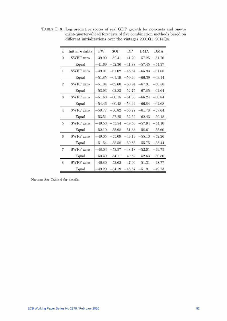
Table D.8: Log predictive scores of real GDP growth for nowcasts and one-toeight-quarter-ahead forecasts of five combination methods based ondifferent initializations over the vintages 2001Q1–2014Q4.


0 SWFF zero −39.99 −52.41 −41.20 −57.25 −51.76

Equal −41.69 −52.36 −41.88 −57.45 −54.37

1 SWFF zero −49.01 −61.02 −48.84 −65.93 −61.68

Equal −51.85 −61.19 −50.46 −66.39 −63.14

2 SWFF zero −51.04 −62.60 −50.94 −67.31 −60.58

Equal −53.93 −62.83 −52.75 −67.85 −62.64

3 SWFF zero −51.63 −60.15 −51.66 −66.24 −60.84

Equal −54.46 −60.48 −53.44 −66.84 −62.68

4 SWFF zero −50.77 −56.82 −50.77 −61.78 −57.64

Equal −53.51 −57.25 −52.52 −62.43 −59.18

5 SWFF zero −49.53 −55.54 −49.56 −57.94 −54.10

Equal −52.19 −55.98 −51.33 −58.61 −55.60

6 SWFF zero −49.05 −55.09 −49.19 −55.10 −52.26

Equal −51.54 −55.58 −50.86 −55.75 −53.44

7 SWFF zero −48.03 −53.57 −48.18 −52.01 −49.75

Equal −50.49 −54.11 −49.82 −52.63 −50.80

8 SWFF zero −46.80 −53.62 −47.06 −51.31 −48.77

Equal −49.20 −54.19 −48.67 −51.91 −49.73

Notes: See Table 6 for details.


Table D.9: Log predictive scores of GDP deflator inflation for nowcasts andone-to eight-quarter-ahead forecasts of five combination methodsbased on different initializations over the vintages 2001Q1–2014Q4.


0 SWFF zero 12.45 12.82 12.15 12.45 12.17

Equal 9.66 12.61 10.74 12.01 11.78

1 SWFF zero 10.12 10.75 9.68 10.15 10.01

Equal 6.74 10.49 7.97 9.69 9.52

2 SWFF zero 5.22 6.32 4.77 5.56 5.45

Equal 2.47 6.11 3.28 5.10 4.71

3 SWFF zero 1.39 1.75 0.44 1.19 0.92

Equal −0.68 1.52 −0.50 0.74 −0.49

4 SWFF zero −1.66 −1.61 −2.56 −2.10 −1.77

Equal −2.97 −1.83 −3.13 −2.54 −3.07

5 SWFF zero −4.55 −5.88 −5.27 −5.05 −4.88

Equal −5.16 −6.10 −5.39 −5.44 −5.71

6 SWFF zero −6.38 −8.13 −6.88 −7.52 −7.14

Equal −6.40 −8.28 −6.63 −7.72 −7.47

7 SWFF zero −8.62 −9.63 −8.72 −9.45 −9.06

Equal −7.76 −9.74 −7.92 −8.85 −8.69

8 SWFF zero −10.92 −11.32 −9.75 −11.93 −11.13

Equal −9.52 −11.40 −9.45 −9.40 −9.04

Notes: See Table 6 for details.


Figure D.1: Recursive estimates of the average log predictive scores of realGDP growth in deviation from the recursive estimates of the aver-age log scores of the dynamic prediction pool covering the vintages2001Q1–2014Q4.





eight-quarter-ahead

2000

20002000

20002000

20002000

20002000

2005

20052005

20052005

20052005

20052005

2010

20102010

20102010

20102010

20102010

2015

20152015

20152015

20152015

20152015

0.2

0.20.2

0.20.2

0.20.2

0.20.2

0

00

00

00

00

-0.2

-0.2-0.2

-0.2-0.2

-0.2-0.2

-0.2-0.2

-0.4

-0.4-0.4

-0.4-0.4

-0.4-0.4

-0.4-0.4



Figure D.2: Recursive estimates of the average log predictive scores of GDPdeflator inflation in deviation from the recursive estimates of theaverage log scores of the dynamic prediction pool covering thevintages 2001Q1–2014Q4.





eight-quarter-ahead

2000

20002000

20002000

20002000

20002000

2005

20052005

20052005

20052005

20052005

2010

20102010

20102010

20102010

20102010

2015

20152015

20152015

20152015

20152015

0.2

0.20.2

0.20.2

0.20.2

0.20.2

0.1

0.10.1

0.10.1

0.10.1

0.10.1

0

00

00

00

00

-0.1

-0.1-0.1

-0.1-0.1

-0.1-0.1

-0.1-0.1

-0.2

-0.2-0.2

-0.2-0.2

-0.2-0.2

-0.2-0.2



Figure D.3: Posterior estimates of the model weights for the dynamic pre-diction pool of real GDP growth covering the vintages 2001Q1–2014Q4.






eight-quarter-ahead

2000

20002000

20002000

20002000

20002000

2005

20052005

20052005

20052005

20052005

2010

20102010

20102010

20102010

20102010

2015

20152015

20152015

20152015

20152015

0.5

0.50.5

0.50.5

0.50.5

0.50.5

0.4

0.40.4

0.40.4

0.40.4

0.40.4

0.3

0.30.3

0.30.3

0.30.3

0.30.3

0.2

0.20.2

0.20.2

0.20.2

0.20.2

0.1

0.10.1

0.10.1

0.10.1

0.10.1

0

00

00

00

00


Figure D.4: Posterior estimates of the model weights for the dynamic predic-tion pool of GDP deflator inflation covering the vintages 2001Q1–2014Q4.






eight-quarter-ahead

2000

20002000

20002000

20002000

20002000

2005

20052005

20052005

20052005

20052005

2010

20102010

20102010

20102010

20102010

2015

20152015

20152015

20152015

20152015

0.5

0.50.5

0.50.5

0.50.5

0.50.5

0.4

0.40.4

0.40.4

0.40.4

0.40.4

0.3

0.30.3

0.30.3

0.30.3

0.30.3

0.2

0.20.2

0.20.2

0.20.2

0.20.2

0.1

0.10.1

0.10.1

0.10.1

0.10.1

0

00

00

00

00


Figure D.5: Recursive estimates of the model weights for the static predictionpool of joint real GDP growth and GDP deflator inflation coveringthe vintages 2001Q1–2014Q4.






eight-quarter-ahead

2000

20002000

20002000

20002000

20002000

2005

20052005

20052005

20052005

20052005

2010

20102010

20102010

20102010

20102010

2015

20152015

20152015

20152015

20152015

1

11

11

11

11

0.8

0.80.8

0.80.8

0.80.8

0.80.8

0.6

0.60.6

0.60.6

0.60.6

0.60.6

0.4

0.40.4

0.40.4

0.40.4

0.40.4

0.2

0.20.2

0.20.2

0.20.2

0.20.2

0

00

00

00

00


Figure D.6: Recursive estimates of the model weights for the static predictionpool of real GDP growth covering the vintages 2001Q1–2014Q4.






eight-quarter-ahead

2000

20002000

20002000

20002000

20002000

2005

20052005

20052005

20052005

20052005

2010

20102010

20102010

20102010

20102010

2015

20152015

20152015

20152015

20152015

1

11

11

11

11

0.8

0.80.8

0.80.8

0.80.8

0.80.8

0.6

0.60.6

0.60.6

0.60.6

0.60.6

0.4

0.40.4

0.40.4

0.40.4

0.40.4

0.2

0.20.2

0.20.2

0.20.2

0.20.2

0

00

00

00

00


Figure D.7: Recursive estimates of the model weights for the static predic-tion pool of GDP deflator inflation covering the vintages 2001Q1–2014Q4.






eight-quarter-ahead

2000

20002000

20002000

20002000

20002000

2005

20052005

20052005

20052005

20052005

2010

20102010

20102010

20102010

20102010

2015

20152015

20152015

20152015

20152015

1

11

11

11

11

0.8

0.80.8

0.80.8

0.80.8

0.80.8

0.6

0.60.6

0.60.6

0.60.6

0.60.6

0.4

0.40.4

0.40.4

0.40.4

0.40.4

0.2

0.20.2

0.20.2

0.20.2

0.20.2

0

00

00

00

00


Figure D.8: Estimates of the model weights for Bayesian model averaging ofjoint real GDP growth and GDP deflator inflation covering thevintages 2001Q1–2014Q4.






eight-quarter-ahead

2000

20002000

20002000

20002000

20002000

2005

20052005

20052005

20052005

20052005

2010

20102010

20102010

20102010

20102010

2015

20152015

20152015

20152015

20152015

1

11

11

11

11

0.8

0.80.8

0.80.8

0.80.8

0.80.8

0.6

0.60.6

0.60.6

0.60.6

0.60.6

0.4

0.40.4

0.40.4

0.40.4

0.40.4

0.2

0.20.2

0.20.2

0.20.2

0.20.2

0

00

00

00

00


Figure D.9: Estimates of the model weights for Bayesian model averaging ofreal GDP growth covering the vintages 2001Q1–2014Q4.






eight-quarter-ahead

2000

20002000

20002000

20002000

20002000

2005

20052005

20052005

20052005

20052005

2010

20102010

20102010

20102010

20102010

2015

20152015

20152015

20152015

20152015

1

11

11

11

11

0.8

0.80.8

0.80.8

0.80.8

0.80.8

0.6

0.60.6

0.60.6

0.60.6

0.60.6

0.4

0.40.4

0.40.4

0.40.4

0.40.4

0.2

0.20.2

0.20.2

0.20.2

0.20.2

0

00

00

00

00


Figure D.10: Estimates of the model weights for Bayesian model averaging ofGDP deflator inflation covering the vintages 2001Q1–2014Q4.






eight-quarter-ahead

2000

20002000

20002000

20002000

20002000

2005

20052005

20052005

20052005

20052005

2010

20102010

20102010

20102010

20102010

2015

20152015

20152015

20152015

20152015

1

11

11

11

11

0.8

0.80.8

0.80.8

0.80.8

0.80.8

0.6

0.60.6

0.60.6

0.60.6

0.60.6

0.4

0.40.4

0.40.4

0.40.4

0.40.4

0.2

0.20.2

0.20.2

0.20.2

0.20.2

0

00

00

00

00


Figure D.11: Posterior estimates of the model weights for dynamic model av-eraging of joint real GDP growth and GDP deflator inflationcovering the vintages 2001Q1–2014Q4.






eight-quarter-ahead

2000

20002000

20002000

20002000

20002000

2005

20052005

20052005

20052005

20052005

2010

20102010

20102010

20102010

20102010

2015

20152015

20152015

20152015

20152015

1

11

11

11

11

0.8

0.80.8

0.80.8

0.80.8

0.80.8

0.6

0.60.6

0.60.6

0.60.6

0.60.6

0.4

0.40.4

0.40.4

0.40.4

0.40.4

0.2

0.20.2

0.20.2

0.20.2

0.20.2

0

00

00

00

00


Figure D.12: Posterior estimates of the model weights for dynamic model aver-aging of real GDP growth covering the vintages 2001Q1–2014Q4.






eight-quarter-ahead

2000

20002000

20002000

20002000

20002000

2005

20052005

20052005

20052005

20052005

2010

20102010

20102010

20102010

20102010

2015

20152015

20152015

20152015

20152015

1

11

11

11

11

0.8

0.80.8

0.80.8

0.80.8

0.80.8

0.6

0.60.6

0.60.6

0.60.6

0.60.6

0.4

0.40.4

0.40.4

0.40.4

0.40.4

0.2

0.20.2

0.20.2

0.20.2

0.20.2

0

00

00

00

00


Figure D.13: Posterior estimates of the model weights for dynamic model av-eraging of GDP deflator inflation covering the vintages 2001Q1–2014Q4.






eight-quarter-ahead

2000

20002000

20002000

20002000

20002000

2005

20052005

20052005

20052005

20052005

2010

20102010

20102010

20102010

20102010

2015

20152015

20152015

20152015

20152015

1

11

11

11

11

0.8

0.80.8

0.80.8

0.80.8

0.80.8

0.6

0.60.6

0.60.6

0.60.6

0.60.6

0.4

0.40.4

0.40.4

0.40.4

0.40.4

0.2

0.20.2

0.20.2

0.20.2

0.20.2

0

00

00

00

00


Figure D.14: Recursive posterior estimates of ρ for the dynamic prediction poolof joint real GDP growth and GDP deflator inflation covering thevintages 2001Q1–2014Q4.





eight-quarter-ahead

2000

20002000

20002000

20002000

20002000

2005

20052005

20052005

20052005

20052005

2010

20102010

20102010

20102010

20102010

2015

20152015

20152015

20152015

20152015

1

11

11

11

11

0.9

0.90.9

0.90.9

0.90.9

0.9

0.8

0.80.8

0.80.8

0.80.8

0.8

0.8

0.7

0.70.7

0.70.7

0.70.7

0.7

0.6

0.4

0.2

0


Figure D.15: Recursive posterior estimates of ρ for the dynamic prediction poolof real GDP growth covering the vintages 2001Q1–2014Q4.





eight-quarter-ahead

2000

20002000

20002000

20002000

20002000

2005

20052005

20052005

20052005

20052005

2010

20102010

20102010

20102010

20102010

2015

20152015

20152015

20152015

20152015

1

11

11

11

11

0.9

0.90.9

0.90.9

0.90.9

0.9

0.8

0.80.8

0.80.8

0.80.8

0.8

0.8

0.7

0.70.7

0.70.7

0.70.7

0.7

0.6

0.4

0.2

0


Figure D.16: Recursive posterior estimates of ρ for the dynamic prediction poolof GDP deflator inflation covering the vintages 2001Q1–2014Q4.





eight-quarter-ahead

2000

20002000

20002000

20002000

20002000

2005

20052005

20052005

20052005

20052005

2010

20102010

20102010

20102010

20102010

2015

20152015

20152015

20152015

20152015

1

11

11

11

11

0.9

0.90.9

0.90.9

0.90.9

0.9

0.8

0.80.8

0.80.8

0.80.8

0.8

0.8

0.7

0.70.7

0.70.7

0.70.7

0.7

0.6

0.4

0.2

0


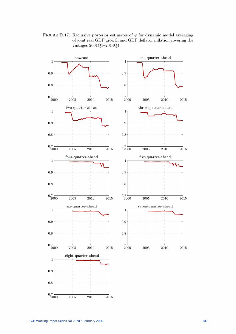
Figure D.17: Recursive posterior estimates of ϕ for dynamic model averagingof joint real GDP growth and GDP deflator inflation covering thevintages 2001Q1–2014Q4.





eight-quarter-ahead

2000

20002000

20002000

20002000

20002000

2005

20052005

20052005

20052005

20052005

2010

20102010

20102010

20102010

20102010

2015

20152015

20152015

20152015

20152015

1

11

11

11

11

0.9

0.90.9

0.90.9

0.90.9

0.90.9

0.8

0.80.8

0.80.8

0.80.8

0.80.8

0.7

0.70.7

0.70.7

0.70.7

0.70.7


Figure D.18: Recursive posterior estimates of ϕ for dynamic model averagingof real GDP growth covering the vintages 2001Q1–2014Q4.





eight-quarter-ahead

2000

20002000

20002000

20002000

20002000

2005

20052005

20052005

20052005

20052005

2010

20102010

20102010

20102010

20102010

2015

20152015

20152015

20152015

20152015

1

11

11

11

11

0.9

0.90.9

0.90.9

0.90.9

0.90.9

0.8

0.80.8

0.80.8

0.80.8

0.80.8

0.7

0.70.7

0.70.7

0.70.7

0.70.7


Figure D.19: Recursive posterior estimates of ϕ for dynamic model averagingof GDP deflator inflation covering the vintages 2001Q1–2014Q4.





eight-quarter-ahead

2000

20002000

20002000

20002000

20002000

2005

20052005

20052005

20052005

20052005

2010

20102010

20102010

20102010

20102010

2015

20152015

20152015

20152015

20152015

1

11

11

11

11

0.9

0.90.9

0.90.9

0.90.9

0.90.9

0.8

0.80.8

0.80.8

0.80.8

0.80.8

0.7

0.70.7

0.70.7

0.70.7

0.70.7


Figure D.20: Recursive estimates of the average log predictive scores of realGDP growth for the combinations and in deviation from the re-cursive value of the upper bound covering the vintages 2001Q1–2014Q4.





eight-quarter-ahead

2000

20002000

20002000

20002000

20002000

2005

20052005

20052005

20052005

20052005

2010

20102010

20102010

20102010

20102010

2015

20152015

20152015

20152015

20152015

0

00

00

00

00

-0.5

-0.5-0.5

-0.5-0.5

-0.5-0.5

-0.5-0.5

-1

-1-1

-1-1

-1-1

-1-1

-1.5

-1.5-1.5

-1.5-1.5

-1.5-1.5

-1.5-1.5



Figure D.21: Recursive estimates of the average log predictive scores of GDPdeflator inflation for the combinations and in deviation from therecursive value of the upper bound covering the vintages 2001Q1–2014Q4.





eight-quarter-ahead

2000

20002000

20002000

20002000

20002000

2005

20052005

20052005

20052005

20052005

2010

20102010

20102010

20102010

20102010

2015

20152015

20152015

20152015

20152015

0

00

00

00

00

-0.2

-0.2-0.2

-0.2-0.2

-0.2-0.2

-0.2-0.2

-0.4

-0.4-0.4

-0.4-0.4

-0.4-0.4

-0.4-0.4

-0.6

-0.6-0.6

-0.6-0.6

-0.6-0.6

-0.6-0.6

-0.8

-0.8-0.8

-0.8-0.8

-0.8-0.8

-0.8-0.8

-1

-1-1

-1-1

-1-1

-1-1



Figure D.22: Recursive estimates of the average log predictive scores of jointreal GDP growth and GDP deflator inflation for the models andin deviation from the recursive value of the upper bound coveringthe vintages 2001Q1–2014Q4.





eight-quarter-ahead

2000

20002000

20002000

20002000

20002000

2005

20052005

20052005

20052005

20052005

2010

20102010

20102010

20102010

20102010

2015

20152015

20152015

20152015

20152015

0

00

00

00

00

-0.5

-0.5-0.5

-0.5-0.5

-0.5-0.5

-0.5-0.5

-1

-1-1

-1-1

-1-1

-1-1

-1.5

-1.5-1.5

-1.5-1.5

-1.5-1.5

-1.5-1.5

-2

-2-2

-2-2

-2-2

-2-2

SWSWFFSWUBVAR SoCBVAR PLRUpper/lower bound


Figure D.23: Recursive estimates of the average log predictive scores of realGDP growth for the models and in deviation from the recursivevalue of the upper bound covering the vintages 2001Q1–2014Q4.





eight-quarter-ahead

2000

20002000

20002000

20002000

20002000

2005

20052005

20052005

20052005

20052005

2010

20102010

20102010

20102010

20102010

2015

20152015

20152015

20152015

20152015

0

00

00

00

00

-0.5

-0.5-0.5

-0.5-0.5

-0.5-0.5

-0.5-0.5

-1

-1-1

-1-1

-1-1

-1-1

-1.5

-1.5-1.5

-1.5-1.5

-1.5-1.5

-1.5-1.5



Figure D.24: Recursive estimates of the average log predictive scores of GDPdeflator inflation for the models and in deviation from the re-cursive value of the upper bound covering the vintages 2001Q1–2014Q4.





eight-quarter-ahead

2000

20002000

20002000

20002000

20002000

2005

20052005

20052005

20052005

20052005

2010

20102010

20102010

20102010

20102010

2015

20152015

20152015

20152015

20152015

0

00

00

00

00

-0.2

-0.2-0.2

-0.2-0.2

-0.2-0.2

-0.2-0.2

-0.4

-0.4-0.4

-0.4-0.4

-0.4-0.4

-0.4-0.4

-0.6

-0.6-0.6

-0.6-0.6

-0.6-0.6

-0.6-0.6

-0.8

-0.8-0.8

-0.8-0.8

-0.8-0.8

-0.8-0.8

-1

-1-1

-1-1

-1-1

-1-1



Figure D.25: Recursive estimates of the differences of log predictive scores ofreal GDP growth for information lag 1 and 4 covering the vintages2001Q1–2014Q4.





eight-quarter-ahead

2000

20002000

20002000

20002000

20002000

2005

20052005

20052005

20052005

20052005

2010

20102010

20102010

20102010

20102010

2015

20152015

20152015

20152015

20152015

20

15

10

5

2

22

22

22

2

1

11

11

11

1

0

00

00

00

0

0

-1

-1-1

-1-1

-1-1

-1

-2

-2-2

-2-2

-2-2

-2

SOPDPBMADMA


Figure D.26: Recursive estimates of the differences of log predictive scores ofGDP deflator inflation for information lag 1 and 4 covering thevintages 2001Q1–2014Q4.





eight-quarter-ahead

2000

20002000

20002000

20002000

20002000

2005

20052005

20052005

20052005

20052005

2010

20102010

20102010

20102010

20102010

2015

20152015

20152015

20152015

20152015

1.5

1.51.5

1.51.5

1.51.5

1.51.5

1

11

11

11

11

0.5

0.50.5

0.50.5

0.50.5

0.50.5

0

00

00

00

00

-0.5

-0.5-0.5

-0.5-0.5

-0.5-0.5

-0.5-0.5

-1

-1-1

-1-1

-1-1

-1-1

-1.5

-1.5-1.5

-1.5-1.5

-1.5-1.5

-1.5-1.5

SOPDPBMADMA


Figure D.27: Recursive estimates of the differences of log predictive scores ofreal GDP growth for the SWFF zero initialization and the equalweights initialization covering the vintages 2001Q1–2014Q4.





eight-quarter-ahead

2000

20002000

20002000

20002000

20002000

2005

20052005

20052005

20052005

20052005

2010

20102010

20102010

20102010

20102010

2015

20152015

20152015

20152015

20152015

3

33

33

33

33

2

22

22

22

22

1

11

11

11

11

0

00

00

00

00

FWSOPDPBMADMA


Figure D.28: Recursive estimates of the differences of log predictive scoresof GDP deflator inflation for the SWFF zero initialization andthe equal weights initialization covering the vintages 2001Q1–2014Q4.





eight-quarter-ahead

2000

20002000

20002000

20002000

20002000

2005

20052005

20052005

20052005

20052005

2010

20102010

20102010

20102010

20102010

2015

20152015

20152015

20152015

20152015

4

44

44

3

33

33

22

2

2

22

22

1

11

1

1

11

11

0

00

0

0

00

00

-1

-1-1

-1

-2

-2-2

-2

-3

FWSOPDPBMADMA


Figure D.29: Posterior estimates of the model weights for the dynamic predic-tion pool of real GDP growth based on the SWFF zero initial-ization and covering the vintages 2001Q1–2014Q4.






eight-quarter-ahead

2000

20002000

20002000

20002000

20002000

2005

20052005

20052005

20052005

20052005

2010

20102010

20102010

20102010

20102010

2015

20152015

20152015

20152015

20152015

0.5

0.50.5

0.50.5

0.50.5

0.50.5

0.4

0.40.4

0.40.4

0.40.4

0.40.4

0.3

0.30.3

0.30.3

0.30.3

0.30.3

0.2

0.20.2

0.20.2

0.20.2

0.20.2

0.1

0.10.1

0.10.1

0.10.1

0.10.1

0

00

00

00

00


Figure D.30: Posterior estimates of the model weights for the dynamic pre-diction pool of GDP deflator inflation based on the SWFF zeroinitialization and covering the vintages 2001Q1–2014Q4.






eight-quarter-ahead

2000

20002000

20002000

20002000

20002000

2005

20052005

20052005

20052005

20052005

2010

20102010

20102010

20102010

20102010

2015

20152015

20152015

20152015

20152015

0.5

0.50.5

0.50.5

0.50.5

0.50.5

0.4

0.40.4

0.40.4

0.40.4

0.40.4

0.3

0.30.3

0.30.3

0.30.3

0.30.3

0.2

0.20.2

0.20.2

0.20.2

0.20.2

0.1

0.10.1

0.10.1

0.10.1

0.10.1

0

00

00

00

00


References

Aastveit, K. A., Mitchell, J., Ravazzolo, F., and van Dijk, H. K. (2019), “The Evolution of

Forecast Density Combinations in Economics,” Oxford Research Encyclopedia, Economics and

Finance, April, DOI: 10.1093/acrefore/9780190625979.013.381.

Amisano, G. and Geweke, J. (2017), “Prediction Using Several Macroeconomic Models,” The

Review of Economics and Statistics, 99(5), 912–925.

Amisano, G. and Giacomini, R. (2007), “Comparing Density Forecasts via Weighted Likelihood

Ratio Tests,” Journal of Business & Economic Statistics, 25(2), 177–190.

Bańbura, M., Giannone, D., and Lenza, M. (2015), “Conditional Forecasts and Scenario Analysis

with Vector Autoregressions for Large Cross-Sections,” International Journal of Forecasting,

31(3), 739–756.

Bańbura, M., Giannone, D., and Reichlin, L. (2010), “Large Bayesian Vector Auto Regressions,”

Journal of Applied Econometrics, 25, 71–92.

Bernanke, B. S., Gertler, M., and Gilchrist, S. (1999), “The Financial Accelerator in a Quanti-

tative Business Cycle Framework,” in J. B. Taylor and M. Woodford (Editors), Handbook of

Macroeconomics, volume 1C, 1341–1393, North Holland, Amsterdam.

Bernardo, J. M. (1979), “Expected Information as Expected Utility,” The Annals of Statistics,

7(3), 686–690.

Billio, M., Casarin, R., Ravazzolo, F., and van Dijk, H. K. (2013), “Time-Varying Combinations

of Predictive Densities using Nonlinear Filtering,” Journal of Econometrics, 177(2), 213–232.

Cai, M., Del Negro, M., Herbst, E., Matlin, E., Sarfati, R., and Schorfheide, F. (2019), “Online

Estimation of DSGE Models,” Federal Reserve Bank of New York Staff Report No. 893.

Carpenter, J., Clifford, P., and Fearnhead, P. (1999), “An Improved Particle Filter for Non-linear

Prolems,” IEE Proceedings—Radar, Sonar and Navigation, 146(1), 2–7.

Chopin, N. (2004), “Central Limit Theorem for Sequential Monte Carlo Methods and its Appli-

cation to Bayesian Inference,” The Annals of Statistics, 32(6), 2385–2411.

Clark, T. E. (2011), “Real-Time Density Forecasts From Bayesian Vector Autoregressions With

Stochastic Volatility,” Journal of Business & Economic Statistics, 29(3), 327–341.

Croushore, D. (2011), “Frontiers of Real-Time Data Analysis,” Journal of Economic Literature,

49(1), 72–110.

Croushore, D. and Stark, T. (2001), “A Real-Time Data Set for Macroeconomists,” Journal of

Econometrics, 105(1), 111–130.

Dawid, A. P. (1984), “Statistical Theory: The Prequential Approach,” Journal of the Royal

Statistical Society, Series A, 147(2), 278–292.

Del Negro, M., Giannoni, M. P., and Schorfheide, F. (2015), “Inflation in the Great Recession

and New Keynesian Models,” American Economic Journal: Macroeconomics, 7(1), 168–196.

Del Negro, M., Hasegawa, R. B., and Schorfheide, F. (2016), “Dynamic Prediction Pools: An

Investigation of Financial Frictions and Forecasting Performance,” Journal of Econometrics,


192(2), 391–403.

Del Negro, M. and Schorfheide, F. (2013), “DSGE Model-Based Forecasting,” in G. Elliott

and A. Timmermann (Editors), Handbook of Economic Forecasting, volume 2, 57–140, North

Holland, Amsterdam.

Diebold, F., Gunther, T. A., and Tay, A. S. (1998), “Evaluating Density Forecasts with Appli-

cations to Financial Risk Management,” International Economic Review, 39(4), 863–883.

Diks, C., Panchenko, V., and van Dijk, D. (2011), “Likelihood-Based Scoring Rules for Compar-

ing Density Forecasts in Tails,” Journal of Econometrics, 163(2), 215–230.

Doan, T., Litterman, R., and Sims, C. A. (1984), “Forecasting and Conditional Projection Using

Realistic Prior Distributions,” Econometric Reviews, 3(1), 1–100.

Douc, R., Cappé, O., and Moulines, E. (2005), “Comparison of Resampling Schemes for Particle

Filtering,” in Proceedings of the 4th International Symposium on Image and Signal Processing

and Analysis, ISPA 2005, IEEE, conference Location: Zagreb, Crotia.

Doucet, A., Briers, M., and Sénécal, S. (2006), “Efficient Block Sampling Strategies for Sequential

Monte Carlo Methods,” Journal of Computational and Graphical Statistics, 15(3), 693–711.

Doucet, A. and Johansen, A. M. (2011), “A Tutorial on Particle Filtering and Smoothing: Fifteen

Years Later,” in D. Crisan and B. Rozovskiı (Editors), The Oxford Handbook of Nonlinear

Filtering, volume 12, 656–704, Oxford University Press, Oxford.

Durbin, J. and Koopman, S. J. (2012), Time Series Analysis by State Space Methods, Oxford

University Press, Oxford, 2nd edition.

Eklund, J. and Karlsson, S. (2007), “Forecast Combinations and Model Averaging using Predic-

tive Measures,” Econometric Reviews, 26(2–4), 329–363.

Fagan, G., Henry, J., and Mestre, R. (2005), “An Area-Wide Model for the Euro Area,” Economic

Modelling, 22(1), 39–59.

Galí, J., Smets, F., and Wouters, R. (2012), “Unemployment in an Estimated New Keynesian

Model,” in D. Acemoglu and M. Woodford (Editors), NBER Macroeconomics Annual 2011,

329–360, University of Chicago Press.

Geweke, J. (2010), Complete and Incomplete Econometrics Models, Princeton University Press,

Princeton.

Geweke, J. and Amisano, G. (2011), “Optimal Prediction Pools,” Journal of Econometrics,

164(1), 130–141.

Geweke, J. and Amisano, G. (2012), “Prediction and Misspecified Models,” American Economic

Review, 102(3), 482–486.

Giannone, D., Henry, J., Lalik, M., and Modugno, M. (2012), “An Area-Wide Real-Time Data-

base for the Euro Area,” The Review of Economics and Statistics, 94(4), 1000–1013.

Giannone, D., Lenza, M., and Primiceri, G. E. (2015), “Prior Selection for Vector Autoregres-

sions,” The Review of Economics and Statistics, 97(2), 436–451.


Giannone, D., Lenza, M., and Primiceri, G. E. (2019), “Priors for the Long Run,” Journal of

the American Statistical Association, 114(526), 565–580.

Gilks, W. R. and Berzuini, C. (2001), “Following a Moving Target—Monte Carlo Inference for

Dynamic Bayesian Models,” Journal of the Royal Statistical Society Series B, 63(1), 127–146.

Gneiting, T. and Katzfuss, M. (2014), “Probabilistic Forecasting,” The Annual Review of Sta-

tistics and Its Applications, 1, 125–151.

Gneiting, T. and Raftery, A. E. (2007), “Strictly Proper Scoring Rules, Prediction, and Estima-

tion,” Journal of the American Statistical Association, 102(477), 359–378.

Gordon, N. J., Salmond, D. J., and Smith, A. F. M. (1993), “Novel Approach to Nonlinear/non-

Gaussian Bayesian State Estimation,” Radar and Signal Processing, IEE Proceedings-F,

140(2), 107–113.

Hall, S. G. and Mitchell, J. (2007), “Combining Density Forecasts,” International Journal of

Forecasting, 23(1), 1–13.

Herbst, E. and Schorfheide, F. (2016), Bayesian Estimation of DSGE Models, Princeton Uni-

versity Press, Princeton.

Hoeting, J. A., Madigan, D., Raftery, A. E., and Volinsky, C. T. (1999), “Bayesian Model

Averaging: A Tutorial,” Statistical Science, 14(4), 382–417.

Hol, J. D., Schön, T. B., and Gustafsson, F. (2006), “On Resampling Algorithms for Particle Fil-

ters,” Proceedings of the IEEE Nonlinear Statistical Signal Processing Workshop, Cambridge,

U. K., Sept. 2006, 79–82.

Johansen, S. (1996), Likelihood-Based Inference in Cointegrated Vector Autoregressive Models,

Oxford University Press, Oxford, 2nd edition.

Jore, A. S., Mitchell, J., and Vahey, S. P. (2010), “Combining Forecast Densities from VARs

with Uncertain Instabilities,” Journal of Applied Econometrics, 25(4), 621–634.

Kapetanios, G., Mitchell, J., Price, S., and Fawcett, N. (2015), “Generalised Density Forecast

Combinations,” Journal of Econometrics, 188(1), 150–165.

Kitagawa, G. (1996), “Monte Carlo Filter and Smoother for Non-Gaussian Nonlinear State Space

Models,” Journal of Computational and Graphical Statistics, 5(1), 1–25.

Kocherlakota, N. (2010), “Modern Macroeconomic Models as Tools for Economic Policy,” The

Region, May(1), 5–21, Federal Reserve Bank of Minneapolis.

Koop, G. and Korobilis, D. (2012), “Forecasting Inflation using Dynamic Model Averaging,”

International Economic Review, 53(3), 867–886.

Kullback, S. and Leibler, R. A. (1951), “On Information and Sufficiency,” The Annals of Math-

ematical Statistics, 22(1), 79–86.

Li, T., Bolić, M., and Djurić, P. M. (2015), “Resampling Methods for Particle Filtering: Classi-

fication, Implementation, and Strategies,” IEEE Signal Processing Magazine, 32(3), 70–86.

Liu, J. S. and Chen, R. (1998), “Sequential Monte Carlo Methods for Dynamic Systems,” Journal

of the American Statistical Association, 93(443), 1032–1044.


McAdam, P. and Warne, A. (2018), “Euro Area Real-Time Density Forecasting with Financial

or Labor Market Frictions,” ECB Working Paper Series No. 2140.

McAdam, P. and Warne, A. (2019), “Euro Area Real-Time Density Forecasting with Financial

or Labor Market Frictions,” International Journal of Forecasting, 35(2), 580–600.

McAlinn, K. and West, M. (2019), “Dynamic Bayesian Predictive Synthesis in Time Series

Forecasting,” Journal of Econometrics, 210(1), 155–169.

Newey, W. K. and West, K. D. (1987), “A Simple, Positive Semi-Definite, Heteroskedasticity

and Autocorrelation Consistent Covariance Matrix,” Econometrica, 55, 703–708.

Opschoor, A., van Dijk, D., and van der Wel, M. (2017), “Combining Density Forecasts using

Focused Scoring Rules,” Journal of Applied Econometrics, 32(7), 1298–1313.

Papadopoulos, G. (2017), “A Model Combination Approach to Developing Robust Models for

Credit Risk Stress Testing: An Application to a Stressed Economy,” Journal of Risk Model

Validation, 11(1), 49–72.

Pauwels, L. L. and Vasnev, A. L. (2016), “A Note on the Estimation of Optimal Weights for

Density Forecast Combinations,” International Journal of Forecasting, 32(2), 391–397.

Raftery, A. E., Kárný, M., and Ettler, P. (2010), “Online Prediction Under Model Uncertainty

via Dynamic Model Averaging: Application to a Cold Rolling Mill,” Technometrics, 52(1),

52–66.

Sims, C. A. (1993), “A Nine-Variable Probabilistic Macroeconomic Forecasting Model,” in J. H.

Stock and M. W. Watson (Editors), Business Cycles, Indicators and Forecasting, 179–212,

University of Chicago Press, Chicago.

Sims, C. A. (2000), “Using a Likelihood Perspective to Sharpen Econometric Discourse: Three

Examples,” Journal of Econometrics, 95(2), 443–462.

Sims, C. A. and Zha, T. (1998), “Bayesian Methods for Dynamic Multivariate Models,” Inter-

national Economic Review, 39(4), 949–968.

Smets, F., Warne, A., and Wouters, R. (2014), “Professional Forecasters and Real-Time Fore-

casting with a DSGE Model,” International Journal of Forecasting, 30(4), 981–995.

Smets, F. and Wouters, R. (2007), “Shocks and Frictions in US Business Cycles: A Bayesian

DSGE Approach,” American Economic Review, 97(3), 586–606.

Waggoner, D. F. and Zha, T. (2012), “Confronting Model Misspecification in Macroeconomics,”

Journal of Econometrics, 171(2), 167–184.

Wallis, K. F. (1986), “Forecasting with an Econometric Model: The Ragged Edge Problem,”

Journal of Forecasting, 5(1), 1–13.

Warne, A. (2019), “YADA Manual — Computational Details,” Manuscript, European Central

Bank. Available with the YADA distribution.

Warne, A., Coenen, G., and Christoffel, K. (2017), “Marginalized Predictive Likelihood Com-

parisons of Linear Gaussian State-Space Models with Applications to DSGE, DSGE-VAR and

VAR Models,” Journal of Applied Econometrics, 32(1), 103–119.


Acknowledgements We have benefitted from discussions with and suggestions by Szabolcs Deak, Mátyás Farkas, Domenico Giannone, Gary Koop, Michele Lenza, Giorgio Primiceri and Bernd Schwaab, as well as from participants at seminars at the European Central Bank and at the University of Kent, Canterbury. The opinions expressed in this paper are those of the authors and do not necessarily reflect views of the European Central Bank or the Eurosystem. Peter McAdam European Central Bank, Frankfurt am Main, Germany; email: [email protected] Anders Warne European Central Bank, Frankfurt am Main, Germany; email: [email protected]

© European Central Bank, 2020

Postal address 60640 Frankfurt am Main, Germany Telephone +49 69 1344 0 Website www.ecb.europa.eu

All rights reserved. Any reproduction, publication and reprint in the form of a different publication, whether printed or produced electronically, in whole or in part, is permitted only with the explicit written authorisation of the ECB or the authors.

This paper can be downloaded without charge from www.ecb.europa.eu, from the Social Science Research Network electronic library or from RePEc: Research Papers in Economics. Information on all of the papers published in the ECB Working Paper Series can be found on the ECB’s website.

PDF ISBN 978-92-899-4021-4 ISSN 1725-2806 doi:10.2866/50837 QB-AR-20-030-EN-N

mailto:[email protected]

mailto:[email protected]

http://www.ecb.europa.eu/

http://www.ecb.europa.eu/

http://ssrn.com/

https://ideas.repec.org/s/ecb/ecbwps.html

http://www.ecb.europa.eu/pub/research/working-papers/html/index.en.html

Density forecast combinations: the real-time dimension

Documents

Transcript of Density forecast combinations: the real-time dimension