Multilevel multivariate modelling of childhood growth, numbers of growth measurements and adult...

© 2009 Royal Statistical Society 0964–1998/09/172599

J. R. Statist. Soc. A (2009)172, Part 3, pp. 599–613

Multilevel multivariate modelling of childhoodgrowth, numbers of growth measurements and adultcharacteristics

Harvey Goldstein and Daphne Kounali

University of Bristol, UK

[Received January 2008. Final revision August 2008]

Summary. A general latent normal model for multilevel data with mixtures of response typesis extended in the case of ordered responses to deal with variates having a large number ofcategories and including count data. An example is analysed by using repeated measures dataon child growth and adult measures of body mass index and glucose. Applications are describedthat are concerned with the flexible prediction of adult measurements from collections of growthmeasurements and for studying the relationship between the number of measurement occa-sions and growth trajectories.

Keywords: Latent normal model; Mixed response types; Multilevel; Multivariate multilevelmodel; Ordered categories; Ordered probit model; Poisson latent normal transformation;Prediction

1. Introduction

In studies of childrens’ growth a common objective is to develop procedures that can be used topredict adult conditions from repeated measurements taken during childhood. Early attemptsto do this for adult variables such as stature essentially consider linear prediction models for theresponse regressed on a set of growth measures taken at a predefined set of ages (usually at wholeyears of age—see, for example, Tanner et al. (2000)). Such a system, however, lacks flexibilitysince in practice individuals will be measured at a set of ages that do not typically correspond tothe predetermined set. A more flexible approach is to model the growth measures as functionsof age, jointly with the adult measurements, by using suitable longitudinal data. The resultingmodel parameters can then be used to provide a suitable prediction model that will apply, inprinciple, to any set of growth measurements taken on an individual. In the present paper weconsider such a model applied to the prediction of adult glucose levels and body mass indexBMI (measured in kilograms per square metre), using measures of weight taken in childrenunder the age of 10 years. These predictions, together with suitable prediction intervals, canthen be used as a screening device for the early detection of later problems.

The basic design, therefore, is based on a two-level repeated measures model as described,for example, in Goldstein (2003), chapter 5. Level 1 is defined by the growth measurementoccasions and these are clustered within each individual, which is the level 2 unit. The ideais that the growth measurement parameters describing average growth, velocity of growth

Address for correspondence: Harvey Goldstein, Graduate School of Education, University of Bristol, Bristol,BS1 8JA, UK.E-mail: [email protected]

600 H. Goldstein and D. Kounali

etc. vary at the individual level and covary among themselves and with the adult outcomes.If we assume multivariate normality, the parameters of the fitted model, notably the ele-ments of the individual level covariance matrix, then provide sufficient statistics for the linearprediction of any of the adult measurements from any combination of growth measurements.

One of the problems in repeated measures growth studies is that attrition may be non-random,leading to parameter estimation bias. A further aim of the present paper is to study whether thismight be so. A standard procedure for dealing with informative dropout is via mixture models(Hogan and Laird, 1997) where the response vector, i.e. the set of growth measures, and thedropout distribution are jointly modelled. In the present paper we study the issue of informativedropout by modelling the actual number of occasions on which each individual was measured,jointly with the growth parameters and with adult measurements, providing estimates of therelevant correlations.

In the next section we describe a general procedure for these joint models and show how itcan be specialized to handle our data.

2. Modelling mixed response types at two levels

Goldstein et al. (2009) present a general model (the GCKL model) for multivariate responsesthat can occur at several levels of a data hierarchy and where the responses can be continuous ordiscrete. The basic methodology is described in a freely downloadable document from the Cen-tre for Multilevel Modelling Web site (Goldstein et al., 2007): http://www.cmm.bristol.ac.uk.

This work includes, as special cases, existing literature on the joint modelling of discreteand continuous responses, and this literature is referenced there. The GCKL model extendsprevious work by allowing for a multilevel structure for the data and can also jointly modelordered, unordered and continuous data. The ability to model ordered responses within theGCKL framework provides a very general procedure for any kind of discrete data where wecan treat the categories as an ordering, including count data. In the present paper we explorethe case where we have a mixture of normal and count data at two levels of a data hierarchy.If we treat count data as an ordered classification Goldstein et al. (2009) provide a procedureto obtain parameter estimates, but this may be inefficient and even numerically unstable, whenthe number of categories is very large, since it then involves the estimation of a large number of‘threshold’ parameters. We therefore propose two extensions to the GCKL model: one involvesusing smoothing functions for the large number of threshold parameters that are involved in thealgorithms that were proposed by Goldstein et al. (2009) and the other is based on a latent nor-mal characterization for the Poisson distribution that can model count data that can be assumedto follow such a distribution. Since the growth measure in our data is restricted to weight, itmay in practice have limited utility as a sensitive prediction model, but the methodology thatwe propose will have general applicability.

We now briefly review the two-level GCKL model as it applies to normal and orderedresponses. Full details are given in Goldstein et al. (2009). We begin by describing the mul-tivariate normal model and its estimation and in the following section we show how orderedresponses can be dealt with by using a transformation to underlying normality.

2.1. The GCKL latent normal modelLet j =1, . . . , J index level 2 units and i=1, . . . , Ij index level 1 units, nested within the level 2units. The underlying multivariate normal model is

Modelling of Childhood Growth, Numbers of Measurements and Adult Characteristics 601

y.1/ij =X1ijβ

.1/ +Z1iju.1/j + e

.1/ij ,

y.2/j =X2jβ

.2/ +Z2ju.2/j ,

e.1/ij ∼MVN.0, Ω1/, uj = .u

.1/j , u

.2/j /T, uj ∼MVN.0, Ω2/:

⎫⎪⎬⎪⎭ .1/

The superscripts denote the level at which a variable is measured or defined. Here y.1/ij is a p1 row

vector containing the normal responses that are defined at level 1 for level 1 unit (observation)i nested in level 2 unit j. Without loss of generality, we assume the same set of predictors foreach of these level 1 responses. Let X1ij be an f1 row vector that contains observations on thesepredictor variables for observation i nested in higher level unit j and β.1/ is an f1 ×p1 matrixcontaining their fixed coefficients. The columns of β.1/ correspond to coefficients for each level1 response variable. Similarly Z1ij is a q1 row vector that contains for observation i nested inhigher level unit j values of q1 predictor variables related to the q1 random effects for the level 1responses. Quite often they may be a subset of the X1ij. The u

.1/j is a q1 ×p1 matrix containing

the random effects at level 2 for the level 1 responses, with each column relating to a particularresponse variable. The random effects may be correlated with each other both within and acrosslevel 1 responses. Each response has an associated level 1 residual and these are contained inthe p1 row vector e

.1/ij . Their covariance matrix is Ω1.

Correspondingly, in the second part of the expression y.2/j is a p2 row vector containing the

remaining responses that are defined at level 2 and X2j is an f2 row vector that contains predictorvariables for higher level unit j, again assumed to be the same for each level 2 response variable.The fixed coefficients of these variables are contained in the f2 ×p2 matrix β.2/. The Z2j is a q2row vector related to the level 2 random effects for the level 2 responses. The u

.2/j is a q2 × p2

matrix of correlated level 2 residuals which are also correlated with the level 2 residuals for thelevel 1 response. The full covariance matrix of all the level 2 residuals is Ω2.

In the examples of this paper we assume that q2 = 1. We shall also assume that the level 1responses only have simple intercept random effects.

Estimates for the parameters of this model are obtained by using Markov chain Monte Carlosampling and details are given in Goldstein et al. (2009). Assuming starting values and a burn-inperiod, given current values, the sampling steps are outlined as follows.

Step 1: sample a new set of fixed coefficients at level 1.Step 2: sample a new set of fixed coefficients at level 2.Step 3: calculate a new set of level 2 residuals for level 2 responses by subtracting the fixedpredictor X2jβ

.2/ from the associated normal responses.Step 4: sample a new set of level 2 residuals for level 1 responses.Step 5: calculate a new set of level 1 residuals by subtracting the prediction using the fixed ef-fects plus the level 2 random effects, x1ijβ

.1/ +Z1iju.1/j , from the associated normal responses.

Step 6: sample a new level 1 covariance matrix.Step 7: sample a new level 2 covariance matrix.

Missing responses are treated by imputing the corresponding random effect conditional oncurrent values for all the fixed predictors and correlated random effects (Goldstein et al., 2009).In the application that we consider there are no missing responses for the level 2 (individual)unit measurements. We also note that, in the framework of a repeated measures model, there isno requirement to have the same number of level 1 (measurement occasion) units for each level2 unit (Goldstein (2003), chapter 5).

There are particular issues about the choice of default diffuse prior distributions for thecovariance matrices. For example, Goldstein et al. (2009) describe the choice of independentuniform priors for the elements of this matrix, and Browne (2006) suggested that, where max-


imum likelihood estimates for parameters are readily available from a preliminary fit, it may bereasonable to use an inverse Wishart prior with covariance parameter equal to the correspond-ing maximum likelihood (or quasi-likelihood) estimate and with degrees of freedom equal tothe order of the covariance matrix. We could also use an ‘adaptive prior’ whereby a set of iter-ations during a secondary burn-in period is averaged and this is used as the prior for a furtherburn-in period and the final set of iterations. In the examples of the present paper, because weshall be dealing with constrained covariance matrices, we shall need to update the elements ofthese matrices one by one and this leads us to use a set of independent uniform priors for theseelements.

The GCKL model also allows for non-normal responses by formulating a latent normalmodel where an extra step is inserted to sample an underlying (latent) normal variable from theobserved response. Goldstein et al. (2009) show how this can be done for ordered and unorderedcategorical data. They additionally allow for non-normal continuous data by using a Box–Coxtransformation. When such a latent normal variable is sampled, in addition to conditioning onthe current values of the parameters and the observations it is also necessary to condition onthe correlated responses and this ensures that the latent variables and observed normal variableshave a joint multivariate normal distribution at both level 1 and level 2. In the next two sectionswe outline the procedure for general ordered data and then describe the extension to Poissondata. In all these cases, for ease of exposition, we consider the single-level case. The extensionto two levels follows the description that was given above.

3. Sampling a latent normal variable for an ordered response

3.1. A general procedureSuppose that we have an ordered p-category response indexed by numbers g = 1, . . . , p. Forsimplicity we shall use a single-level index i and denote by πgi the probability that observationi occurs in category g. The cumulative distribution is defined as

γhi =h∑

g=1πgi, h=1, 2, . . . , p−1, with γpi =1:

We consider the probit link model for these as

γhi =∫ αh−.Xβ/i

−∞ϕ.t/ dt, .2/

where ϕ.t/ is the density function of the standard normal distribution and .Xβ/i is the value fori of a linear predictor expressed in matrix terms. The αh are known as threshold parameters. Ingeneral the linear predictor .Xβ/i will contain higher level random effects and also the termsthat arise from conditioning on all correlated random effects from the remaining responses.Since the joint distribution is multivariate normal, as pointed out above, this conditioning islinear and is readily derived from the current value of the covariance matrix. Details are givenin Goldstein et al. (2009).

We also note that in equation (2) the linear predictor remains constant over the categories thatare defined by the thresholds. Interactions between the threshold parameters and the predictorvariables are possible and can be included in straightforward ways.

We can also motivate the latent normal model (2) as follows. If yi is the observed categorythen yi �h if and only if a latent variable yÅ

i �0 where yÅi = .Xβ/i −αh + ei, ei ∼N.0, 1/. Thus,

we have


pr.yi �h/=pr.yÅi �0/=pr{ei �αh − .Xβ/i}=

∫ αh−.Xβ/i

−∞ϕ.t/dt:

If an intercept term is incorporated in the fixed part predictor then there must be a linearconstraint on the αh and it is convenient to take α1 =0 for this.

We can convert the categorical response to the latent normal model by sampling as follows.

(a) For a category 1 response we sample randomly from the standard normal distributionrestricted to [−∞, −.Xβ/i].

(b) For a category p response we sample from the standard normal distribution restricted to[αp−1 − .Xβ/i, ∞].

(c) For every other category h we sample from the standard normal distribution restrictedto [αh−1 − .Xβ/i, αh − .Xβ/i].

Sampling for the threshold parameters αh is most efficiently carried out by using a Metropolisstep (Goldstein et al., 2009).

3.2. Smoothing the threshold parametersAs mentioned in Section 1, for many kinds of count data, if we treat every observed count valueas a separate category, we may have a very large number of threshold parameters to estimate,and furthermore some of the categories may be small and these can cause computational prob-lems. One solution would be to merge adjacent categories where there are small numbers. This,however, suffers from several drawbacks.

First, if there are categories with few observations the associated threshold parameters willnot be well estimated and the computational time will be increased. Secondly, although themerging of adjacent categories will not change the parameters being estimated in an additivelinear model, this is not so if there are interactions between the threshold parameters and thelinear model coefficients. If such interactions exist and are ignored then in general we shall havedifferent values for these coefficients depending on which categories are merged. Likewise, ifan interactive model is fitted, and categories involved in these interactions are merged, thendifferent values generally will be estimated. Thirdly, if adjacent categories are merged and this isfelt to be justified in terms of the underlying model, it will not allow us to make inferences aboutthe proportions that are associated with the original, unmerged, categories. This restriction doesnot apply to the smoothing approach that is now described.

In this approach we seek a functional form to describe the threshold values based on a fewparameters and the following describes one such approach.

In equation (2) write

αh =f.h/, h=1, . . . , p−1, .3/

where f can be any suitable function. We shall illustrate by using a simple polynomial as aregression function of the category sequence number h typically centred at the mean value.Other choices are possible, including fractional polynomials and regression splines, and wecould also use, for example, a set of starting values computed for the thresholds that are deriveddirectly from assigning normal equivalent deviates to the cumulative category probabilities, butwe have not investigated these possibilities. A further possibility that is currently being explored(Goldstein, 2008) is a function that consists of a sum of exponential terms that automaticallysatisfies the monotonicity requirement (see below). We have, omitting subscripts,

αh = δ0 + δ1h+ δ2h2 + e: .4/


We sample each δ in turn by using a Metropolis step with a normal proposal. Using equation(4), with the αh so determined, we then can compute the set {αh} and thus the likelihoods foracceptance or rejection as in the standard algorithm for ordered data (Goldstein et al., 2009).The function f must be strictly increasing over the range of h and this is easily verified at eachstep: if the order constraints for the set of thresholds are not obeyed we do not update the value.We then sample from the latent normal distribution as in the ordered case as detailed above.

To obtain starting values we first obtain starting values for each separate α as described inGoldstein et al. (2009), and then we fit the regression

αh =q∑

t=0δth

t + eh .5/

to determine the order of polynomial to be fitted and starting values for coefficients. The esti-mated standard errors for the coefficients can be used for the normal proposal distributions.

Finally, it is possible to have a partially smoothed model where the smoothing takes placeonly over a contiguous subset of the threshold parameters, e.g. those where numbers aresmall.

3.3. Count dataAn alternative to the previous section’s treatment of count data is to assume a particular para-metric distribution for the counts and we shall consider the common one, namely that the countsfollow a Poisson distribution. If a Poisson distribution can be supported by the data then it willbe efficient to model the data explicitly assuming such a distribution, since we shall only need toestimate a single parameter. As with general ordered data we can then incorporate this distri-bution within the GCKL framework that underpins the procedures which are developed in thispaper. To do this we need to find a Markov chain Monte Carlo step to sample a latent normalvariable and we now show how this can be done.

Consider the Poisson density function

f.h; θ/= exp.−θ/θh=h!, h=0, . . . , p−1, .6/

for the first p categories that are observed.As in equation (2) we write the cumulative distribution

F.h; θ/=h∑

g=0f.g; θ/:

We choose a reference value h=h0 such that

F.h0; θi/=∫ −.Xβ/i

−∞ϕ.t/ dt, .7/

where we use i to index the units.We note that for a given h0 this is a flexible model relating the Poisson parameter θi for an

individual unit to the covariate values. Thus, given .Xβ/i, θi is determined. It is convenient tochoose h0 =0 so that

F.0; θi/= exp.−θi/=∫ −.Xβ/i

−∞ϕ.t/ dt:

We sample from the underlying standard normal distribution interval as follows for an observedcount hÅ, where the interval is indicated by brackets { }.


For an observed count in the first category we sample a value from the lower tail of the normaldistribution

N{−∞, −.Xβ/i} .8/

and for the remaining categories we sample from

N{a, b}, a=Φ−1{F.hÅ; θi/}, b=Φ−1{F.hÅ −1; θi/}: .9/

The resulting sampled values, just as in the ordered probit model, are thus sampled from thespecified standard normal distribution. Since this a novel characterization of the Poisson distri-bution there is no standard term for our procedure, and we shall refer to it simply as a Poissonlatent normal transformation.

To impute any missing values on the original scale we use the inverse transformation (Gold-stein et al., 2009).

We note that our models for ordered categories consider the latent normal distribution tobe defined by the observed categories, whereas the Poisson model is defined on .0, ∞/ and soassumes that the distribution exists beyond the categories observed. This suggests that we wouldexpect to obtain different estimates. Since our data counts have a specified minimum count of 1and a specified maximum possible count, the Poisson assumption may not be reasonable, andthis is confirmed in our example. In the Poisson case, in some circumstances, we might considerfitting a truncated distribution that covers only the observed categories, or a particular sub-set of categories specified in advance. One example is the zero-truncated Poisson distributionwhere a zero category exists but cannot be observed, but this does not seem to be a reasonableassumption for our data.

4. A growth data example

Our application uses data that consist of 1000 subjects with serial weight measurements betweenbirth and age 10 years together with adult body mass index BMI and plasma glucose level (mil-limoles per litre) measured on individuals at around the age of 30 years. During infancy (0–2years) the maximum number of measurement occasions observed is 9 and during childhood (2–10 years) it is 14. There are 7459 repeated measurements over childhood and 1000 adult BMIand glucose measurements. The data set was made publicly available at the Third InternationalCongress on Developmental Origins of Health and Disease (Gillman et al., 2007).

As explained in Section 1, the joint modelling of the growth data and the adult measurementsprovides a flexible prediction system. This is the part of the model that is of principal interest.We also include the counts of the number of measurements as a further two, level 2, responsesin infancy and in childhood. The principal purpose of this is to see whether the number of mea-surement occasions is related to characteristics of growth. Thus, we might suppose that childrenwith atypical characteristics may also have atypical growth patterns and that this may be asso-ciated with the propensity to continue participation in the study. A strong relationship betweenthe count of the number of measurements and such growth parameters may thus be indicativeof non-random dropout. Strictly speaking, a smaller number of measurement occasions is notalways indicative of dropout, although it is associated with it in the present data set. A moresensitive measure would be to count the number of measurements within more narrowly definedage groups, but this has not been done for the present data.

The responses in our model for prediction are as follows. At level 1 we have repeated mea-sures of the log(weight) of children up to 10 years .y1ij/ with birth weight (x) in kilograms as a


covariate. Growth is modelled by using a basic cubic polynomial in age. At adulthood we havemeasures on the same individuals of log(glucose level) .y2j/ and log(BMI) .y3j/. We write themodel as

y1ij =β0j +β1jδij +β2jtijδij +β3t2ijδij +β4t3

ijδij +β5jtij.1− δij/+β6t2ij.1− δij/+β8xj + eij,

β0j =β0 +u0j, β1j =β1 +u1j, β2j =β2 +u2j, β5j =β5 +u5j,

eij ∼N.0, σ2e /,

y2j =γ1 +u6j,

y3j =γ2 +u7j,

.u0j, u1j, u2j, u5j, u6j, u7j/T ∼N.0, Ωu/:

⎫⎪⎪⎪⎪⎪⎪⎪⎪⎬⎪⎪⎪⎪⎪⎪⎪⎪⎭

.10/

Here, in terms of our general notation in equation (1), we have two level 2 response variablesy

.2/j = .y2j, y3j/ and a single level 1 response variable y

.1/1ij =y1ij. The term δij, in the child growth

model, is an indicator variable taking the value 1 if the weight measurement is taken in infancy (0–2 years) and 0 if taken in childhood (2–10 years) so that the first line of model (10) fits two disjointpolynomial models: one for infancy and one for childhood. The two are linked through the level2 random effects. This separation was specified by the original investigators who wished to con-sider the two age ranges separately. An alternative would have been to fit, for example, a regres-sion spline to allow a smooth relationship across the age range, but we have not pursued this here.Age (t) in infancy is centred at 1.0 years and in childhood at 5.5 years. Note that Ωu is of order 6since the quadratic and cubic terms in model (10) are assumed not to have random coefficients.

The count data are introduced as follows. We have two further responses at level 2, namelya count of the number of measurement occasions in infancy .y4j/ and in childhood .y5j/.The random (intercept) effects for these (on the latent normal scale) at level 2 are respectivelyu8j and u9j. The only covariates are the intercepts for these responses.

For the Poisson model we have

pr.y4j =hÅ/=∫ b

a

φ.t/ dt

where

pr.y4j =0/=∫ γ4+u8j

−∞φ.t/ dt

and

pr.y5j =hÅ/=∫ b

a

φ.t/ dt

where

pr.y5j =0/=∫ γ5+u9j

−∞φ.t/ dt

where a and b are as defined in expressions (8) and (9).For the ordered model with threshold parameters we have for infancy

pr.y4j =h/=αh−.γ4+u8j/∫

αh−1−.γ4+u8j/

φ.t/ dt, α0 =−∞, α1 =0, αp4 =∞, h=1, . . . , p4,

.11/


and for childhood

pr.y5j =h/=αh−.γ5+u9j/∫

αh−1−.γ5+u9j/

φ.t/ dt, α0 =−∞, α1 =0, αp5 =∞, h=1, . . . , p5,

.12/

where p4 and p5 are the numbers of categories respectively for the numbers of occasions ininfancy and childhood. For the smoothing model, equations (11) and (12) are modified accord-ingly. Thus the level 2 covariance matrix Ωu has elements σ2

u8 =σ2u9 = 1 corresponding to the

latent normal variables for the ordered responses. The Markov chain Monte Carlo step thatsamples the remaining elements of Ωu first samples the variance terms followed by the correla-tions, which are then transformed to covariances.

5. Results

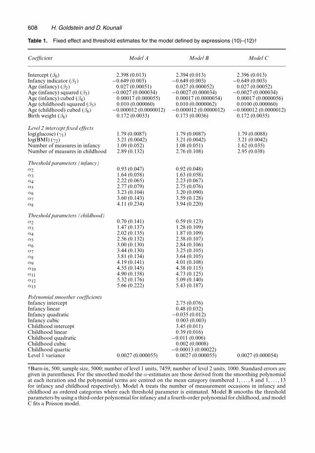
5.1. Latent normal modelsTable 1 shows the estimates for the fixed parameters for three models. Model A treats the numberof measurement occasions in infancy and childhood as ordered categories where each thresholdparameter is estimated. Model B smooths the threshold parameters during infancy by usinga third-order polynomial and the threshold parameters during childhood by using a fourth-order polynomial. Fitting a higher order polynomial in both cases does not change the otherparameter estimates and the higher order polynomial coefficient estimates are smaller than theirestimated standard errors. Model C fits a Poisson model. We comment further on these resultsbelow.

The chains for the threshold parameters were the least satisfactory in terms of howwell they mixed. The burn-in period was chosen after observing the behaviour of these chains,especially for the extreme thresholds, using trial runs with different subsets of parameters. Avalue of 500 was found to provide a reasonable period for the chains to become stationary.Likewise, we found that 5000 iterations provided reasonable mixing and summary statisticsin terms of means and standard deviations that were stable and did not change apprecia-bly with further iterations, using similar trial runs. Further support for the values that werechosen is provided by the fact that models A and B, using different parameterizations, doprovide similar estimates for the threshold parameters, albeit with different efficiencies (seebelow).

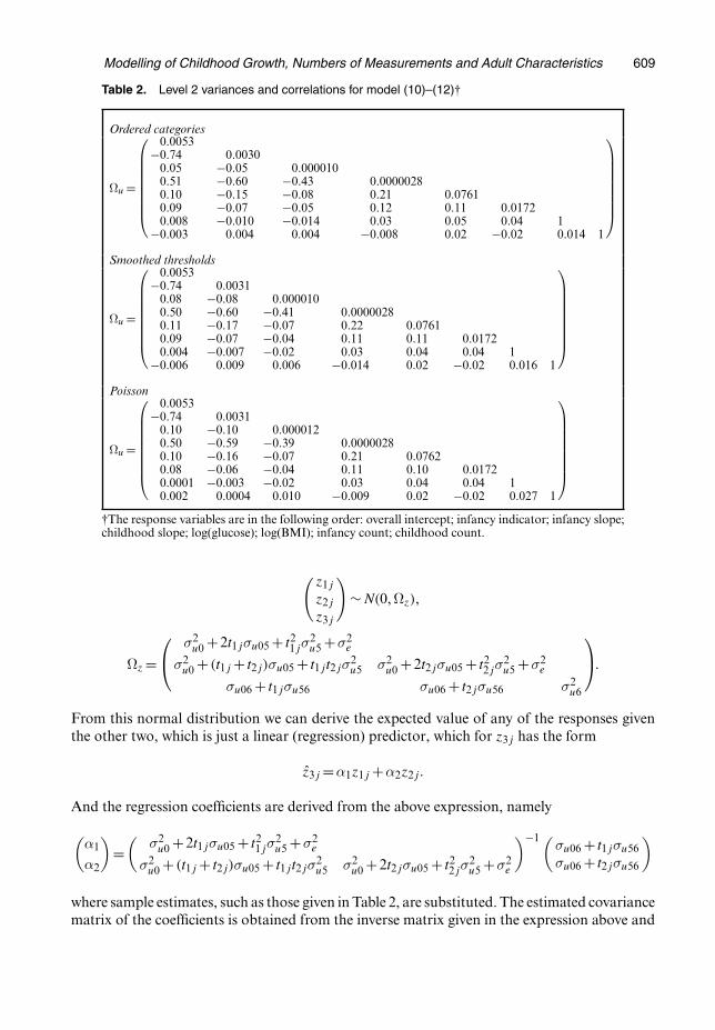
The level 2 covariance and correlation matrices are displayed in Table 2 where the variancesare on the diagonal, and correlations below the diagonal. It will be seen that, whereas there aremoderate correlations between the growth random effects, the correlations of growth randomeffects with adult measures are not large, so the usefulness of weight measures for predictionof the adult measures is limited. To illustrate the prediction procedure we consider predictinglog(BMI) by using two childhood weight measurements, together with birth weight.

We write the ‘raw’ residuals for the two weight measurements at times t1j and t2j and the adultlog(BMI) from model (10) as

z1j =y11j − .β0 +β5t1j +β6t21j +β8xj/,

z2j =y12j − .β0 +β5t2j +β6t22j +β8xj/,

z3j =y2j −γ1:

⎫⎪⎬⎪⎭ .13/

This defines a three-variate normal distribution that is given by


Table 1. Fixed effect and threshold estimates for the model defined by expressions (10)–(12)†

Coefficient Model A Model B Model C

Intercept (β0/ 2.398 (0.013) 2.394 (0.013) 2.396 (0.013)Infancy indicator (β1/ −0.649 (0.003) −0.649 (0.003) −0.649 (0.003)Age (infancy) (β2/ 0.027 (0.00051) 0.027 (0.000052) 0.027 (0.00052)Age (infancy) squared (β3/ −0.0027 (0.000034) −0.0027 (0.000034) −0.0027 (0.000034)Age (infancy) cubed (β4/ 0.00017 (0.000055) 0.00017 (0.0000054) 0.00017 (0.0000056)Age (childhood) squared (β5/ 0.010 (0.000060) 0.010 (0.0000062) 0.0100 (0.000060)Age (childhood) cubed (β6/ −0.000012 (0.0000012) −0.000012 (0.0000012) −0.000012 (0.0000012)Birth weight (β8/ 0.172 (0.0033) 0.173 (0.0036) 0.172 (0.0035)

Level 2 intercept fixed effectslog(glucose) (γ1/ 1.79 (0.0087) 1.79 (0.0087) 1.79 (0.0088)log(BMI) (γ2/ 3.21 (0.0042) 3.21 (0.0042) 3.21 (0.0042)Number of measures in infancy 1.09 (0.052) 1.08 (0.051) 1.62 (0.035)Number of measures in childhood 2.89 (0.132) 2.76 (0.108) 2.95 (0.038)

Threshold parameters (infancy)α2 0.93 (0.047) 0.92 (0.048)α3 1.64 (0.058) 1.63 (0.058)α4 2.22 (0.065) 2.23 (0.067)α5 2.77 (0.079) 2.75 (0.076)α6 3.23 (0.104) 3.20 (0.090)α7 3.60 (0.143) 3.59 (0.128)α8 4.11 (0.234) 3.94 (0.220)

Threshold parameters (childhood)α2 0.70 (0.141) 0.59 (0.123)α3 1.47 (0.137) 1.28 (0.109)α4 2.02 (0.135) 1.87 (0.109)α5 2.56 (0.132) 2.38 (0.107)α6 3.00 (0.130) 2.84 (0.106)α7 3.44 (0.130) 3.25 (0.105)α8 3.81 (0.134) 3.64 (0.105)α9 4.19 (0.141) 4.01 (0.108)α10 4.55 (0.145) 4.38 (0.115)α11 4.90 (0.158) 4.73 (0.125)α12 5.32 (0.176) 5.09 (0.140)α13 5.66 (0.222) 5.43 (0.187)

Polynomial smoother coefficientsInfancy intercept 2.75 (0.076)Infancy linear 0.48 (0.032)Infancy quadratic −0.035 (0.012)Infancy cubic 0.003 (0.003)Childhood intercept 3.45 (0.011)Childhood linear 0.39 (0.016)Childhood quadratic −0.011 (0.006)Childhood cubic 0.002 (0.0008)Childhood quartic −0.00013 (0.00022)Level 1 variance 0.0027 (0.000055) 0.0027 (0.000055) 0.0027 (0.000054)

†Burn-in, 500; sample size, 5000; number of level 1 units, 7459; number of level 2 units, 1000. Standard errors aregiven in parentheses. For the smoothed model the α-estimates are those derived from the smoothing polynomialat each iteration and the polynomial terms are centred on the mean category (numbered 1, . . . , 8 and 1, . . . , 13for infancy and childhood respectively). Model A treats the number of measurement occasions in infancy andchildhood as ordered categories where each threshold parameter is estimated. Model B smooths the thresholdparameters by using a third-order polynomial for infancy and a fourth-order polynomial for childhood, and modelC fits a Poisson model.


Table 2. Level 2 variances and correlations for model (10)–(12)†

Ordered categories

Ωu =

⎛⎜⎜⎜⎜⎜⎜⎜⎜⎝

0:0053−0:74 0:0030

0:05 −0:05 0:0000100:51 −0:60 −0:43 0:00000280:10 −0:15 −0:08 0:21 0:07610:09 −0:07 −0:05 0:12 0:11 0:01720:008 −0:010 −0:014 0:03 0:05 0:04 1

−0:003 0:004 0:004 −0:008 0:02 −0:02 0:014 1

⎞⎟⎟⎟⎟⎟⎟⎟⎟⎠

Smoothed thresholds

Ωu =

⎛⎜⎜⎜⎜⎜⎜⎜⎜⎝

0:0053−0:74 0:0031

0:08 −0:08 0:0000100:50 −0:60 −0:41 0:00000280:11 −0:17 −0:07 0:22 0:07610:09 −0:07 −0:04 0:11 0:11 0:01720:004 −0:007 −0:02 0:03 0:04 0:04 1

−0:006 0:009 0:006 −0:014 0:02 −0:02 0:016 1

⎞⎟⎟⎟⎟⎟⎟⎟⎟⎠

Poisson

Ωu =

⎛⎜⎜⎜⎜⎜⎜⎜⎜⎝

0:0053−0:74 0:0031

0:10 −0:10 0:0000120:50 −0:59 −0:39 0:00000280:10 −0:16 −0:07 0:21 0:07620:08 −0:06 −0:04 0:11 0:10 0:01720:0001 −0:003 −0:02 0:03 0:04 0:04 10:002 0:0004 0:010 −0:009 0:02 −0:02 0:027 1

⎞⎟⎟⎟⎟⎟⎟⎟⎟⎠

†The response variables are in the following order: overall intercept; infancy indicator; infancy slope;childhood slope; log(glucose); log(BMI); infancy count; childhood count.

(z1j

z2j

z3j

)∼N.0, Ωz/,

Ωz =⎛⎝ σ2

u0 +2t1jσu05 + t21jσ

2u5 +σ2

e

σ2u0 + .t1j + t2j/σu05 + t1jt2jσ

2u5 σ2


2u5 +σ2

e

σu06 + t1jσu56 σu06 + t2jσu56 σ2u6

⎞⎠:

From this normal distribution we can derive the expected value of any of the responses giventhe other two, which is just a linear (regression) predictor, which for z3j has the form

z3j =α1z1j +α2z2j:

And the regression coefficients are derived from the above expression, namely

(α1

α2

)=(

σ2u0 +2t1jσu05 + t2

1jσ2u5 +σ2

e

σ2u0 + .t1j + t2j/σu05 + t1jt2jσ

2u5 σ2


2u5 +σ2

e

)−1(σu06 + t1jσu56σu06 + t2jσu56

)

where sample estimates, such as those given in Table 2, are substituted. The estimated covariancematrix of the coefficients is obtained from the inverse matrix given in the expression above and


1 2 3 4 5 6 7 8 90

50

100

150

200

250

300

350

(a)

1 2 3 4 5 6 7 8 9 10 11 12 13 140

20

40

60

80

100

120

140

160

180

(b)

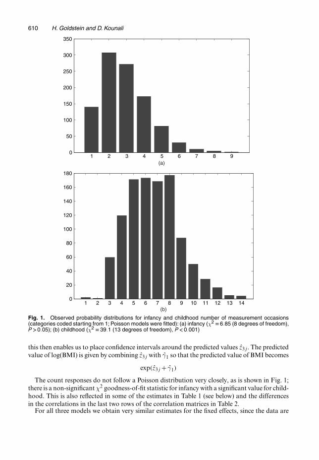
Fig. 1. Observed probability distributions for infancy and childhood number of measurement occasions(categories coded starting from 1; Poisson models were fitted): (a) infancy (χ2 D6:85 (8 degrees of freedom),P >0:05); (b) childhood (χ2 D39:1 (13 degrees of freedom), P <0:001)

this then enables us to place confidence intervals around the predicted values z3j. The predictedvalue of log(BMI) is given by combining z3j with γ1 so that the predicted value of BMI becomes

exp.z3j + γ1/

The count responses do not follow a Poisson distribution very closely, as is shown in Fig. 1;there is a non-significant χ2 goodness-of-fit statistic for infancy with a significant value for child-hood. This is also reflected in some of the estimates in Table 1 (see below) and the differencesin the correlations in the last two rows of the correlation matrices in Table 2.

For all three models we obtain very similar estimates for the fixed effects, since the data are


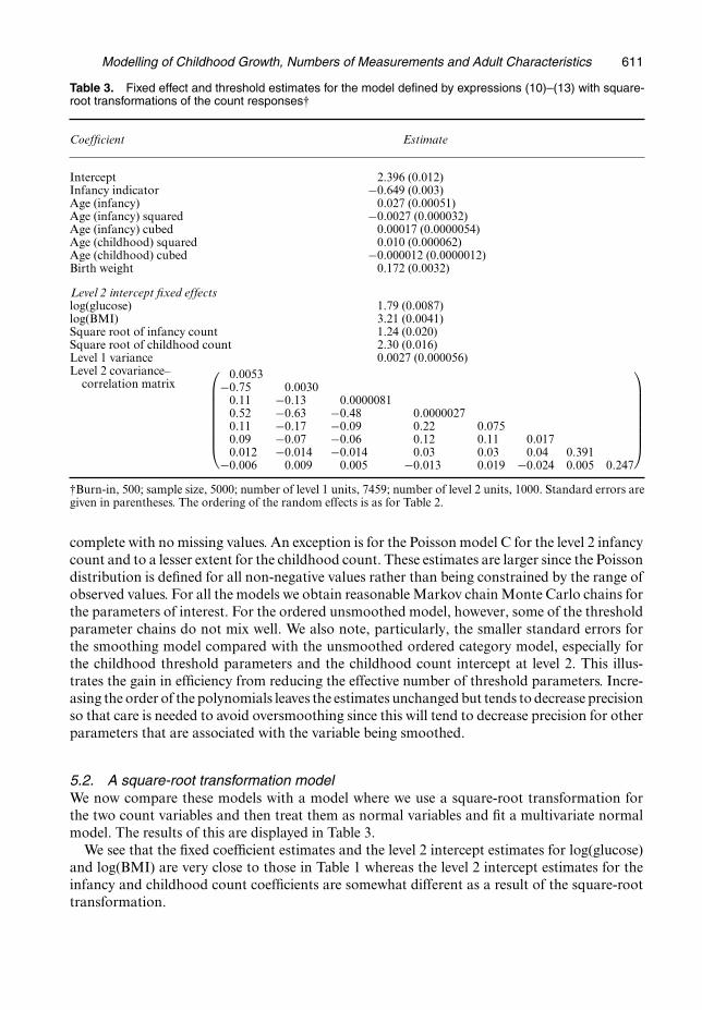
Table 3. Fixed effect and threshold estimates for the model defined by expressions (10)–(13) with square-root transformations of the count responses†

Coefficient Estimate

Intercept 2.396 (0.012)Infancy indicator −0.649 (0.003)Age (infancy) 0.027 (0.00051)Age (infancy) squared −0.0027 (0.000032)Age (infancy) cubed 0.00017 (0.0000054)Age (childhood) squared 0.010 (0.000062)Age (childhood) cubed −0.000012 (0.0000012)Birth weight 0.172 (0.0032)

Level 2 intercept fixed effectslog(glucose) 1.79 (0.0087)log(BMI) 3.21 (0.0041)Square root of infancy count 1.24 (0.020)Square root of childhood count 2.30 (0.016)Level 1 variance 0.0027 (0.000056)Level 2 covariance–

correlation matrix⎛⎜⎜⎜⎜⎜⎜⎜⎜⎝

0:0053−0:75 0:0030

0:11 −0:13 0:00000810:52 −0:63 −0:48 0:00000270:11 −0:17 −0:09 0:22 0:0750:09 −0:07 −0:06 0:12 0:11 0:0170:012 −0:014 −0:014 0:03 0:03 0:04 0:391

−0:006 0:009 0:005 −0:013 0:019 −0:024 0:005 0:247

⎞⎟⎟⎟⎟⎟⎟⎟⎟⎠

†Burn-in, 500; sample size, 5000; number of level 1 units, 7459; number of level 2 units, 1000. Standard errors aregiven in parentheses. The ordering of the random effects is as for Table 2.

complete with no missing values. An exception is for the Poisson model C for the level 2 infancycount and to a lesser extent for the childhood count. These estimates are larger since the Poissondistribution is defined for all non-negative values rather than being constrained by the range ofobserved values. For all the models we obtain reasonable Markov chain Monte Carlo chains forthe parameters of interest. For the ordered unsmoothed model, however, some of the thresholdparameter chains do not mix well. We also note, particularly, the smaller standard errors forthe smoothing model compared with the unsmoothed ordered category model, especially forthe childhood threshold parameters and the childhood count intercept at level 2. This illus-trates the gain in efficiency from reducing the effective number of threshold parameters. Incre-asing the order of the polynomials leaves the estimates unchanged but tends to decrease precisionso that care is needed to avoid oversmoothing since this will tend to decrease precision for otherparameters that are associated with the variable being smoothed.

5.2. A square-root transformation modelWe now compare these models with a model where we use a square-root transformation forthe two count variables and then treat them as normal variables and fit a multivariate normalmodel. The results of this are displayed in Table 3.

We see that the fixed coefficient estimates and the level 2 intercept estimates for log(glucose)and log(BMI) are very close to those in Table 1 whereas the level 2 intercept estimates for theinfancy and childhood count coefficients are somewhat different as a result of the square-roottransformation.


6. Discussion

We have described the use of three different latent normal model formulations for count data.The simplest model, assuming a Poisson distribution, is straightforward to implement and canbe combined with other normal or discrete responses in a multivariate model. The approach thatwe have adopted for a Poisson distribution is analogous to that used for a probit model for binarydata and can be further extended to other discrete distributions. Where data do not follow, atleast approximately, a Poisson distribution, we can treat the counts as an ordered classification,as we have done in the present application. In particular, we note that treating the counts asan ordered classification effectively conditions the latent normal distribution to be defined withrespect to the actual range of observed counts. Where there are many categories we have shownhow a smoothing formulation provides a good approximation with more efficient estimates.

The algorithm can be extended readily to further levels of nesting and cross-classifications. It isalso relatively straightforward to incorporate linear constraints on sets of parameters (Goldsteinet al., 2009).

The data set that we have used has no missing values for the level 2 responses so the optionthat is chosen to model the count data will not affect the fixed parameter estimates for theremaining responses, as illustrated in Tables 1–3. Where data are missing and where, for exam-ple, the count responses are used in any kind of imputation procedure, particular assumptions,e.g. that the counts follow a Poisson distribution, will lead in general to somewhat different fixedand random-part estimates. The same will be true with the use of a square-root transformationwhere this does not lead to (approximate) normality.

The joint modelling of growth data and data on adults allows for the development of anefficient prediction system of adult values given a collection of growth measurements, and inprinciple this can be extended to several growth measures and further adult measures. We havealso suggested that a model where the number of measurement occasions for different age rangesis jointly modelled with growth parameters may be useful for studying possible informative non-response patterns.

In the present example we only have birth weight as a covariate. In practice we may haveother useful covariates such as social class and gender that can improve the prediction and canin principle be incorporated either as predictors or responses. In particular we may wish to useheight as a ‘covariate’ since BMI is one of the adult measurements of interest, although it is notavailable in the present data set. In the case where height is not measured at the same times asweight, we may treat it as a further response that is modelled jointly with the other responses.When estimating the prediction we would then additionally condition on the observed heightmeasurements.

The experimental software for fitting these models is written in MATLAB (Mathworks, 2007).

Acknowledgements

This work was supported by an Economic and Social Research Council Fellowship to Dr Kou-nali, PTA-026-27-1600, and stems from work that was carried out under Economic and SocialResearch Council grants RES-000-23-0140 and RES-000-23-0784. We are very grateful to FionaSteele, Tony Robinson, two referees and the Joint Editor for helpful comments.

References

Browne, W. J. and Draper, D. (2006) A comparison of Bayesian and likelihood-based methods for fitting multilevelmodels. Bayes. Anal., 1, 473–514.


Gillman, M. W., Barker, D., Bier, D., Cagampang, F., Challis, J., Fall, C., Godfrey, K., Gluckman, P., Hanson,M., Kuh, D., Natanielsz, P., Nestel, P. and Thornburg, K. L. (2007) Meeting report on the 3rd InternationalCongress on Developmental Origins of Health and Disease (DOHaD). Ped. Res., 61, 625–629.

Goldstein, H. (2003) Multilevel Statistical Models, 3rd edn. London: Arnold.Goldstein, H. (2008) A general model for the analysis of discrete time multilevel survival data. To be published.Goldstein, H., Carpenter, J., Kenward, M. and Levin, K. (2009) Multilevel Models with multivariate mixed

response types. Statist. Modllng, to be published.Goldstein, H., Steele, F., Rasbash, J. and Charlton, C. (2007) REALCOM: methodology for realistically com-

plex multilevel modeling. Centre for Multilevel Modelling University of Bristol, Bristol. (Available fromhttp://www.cmm.bris.ac.uk/research/Realcom/index.shtml.)

Hogan, J. W. and Laird N. M. (1997) Model based approaches to analysing incomplete longitudinal and failuretime data. Statist. Med., 16, 259–272.

Mathworks (2007) Matlab. Natick: Mathworks. (Available from http://www.mathworks.co.uk.)Tanner, J. M., Healy, M. J. R., Goldstein, H. and Cameron, N. (2000) Assessment of Skeletal Maturity and

Prediction of Adult Height (TW3 Method). London: Saunders.

Multilevel multivariate modelling of childhood growth, numbers of growth measurements and adult...

Documents

Transcript of Multilevel multivariate modelling of childhood growth, numbers of growth measurements and adult...