A new approach for estimating anonlinear growth component inmultilevel modeling

Asko Tolvanen,1 Noona Kiuru,1 Esko Leskinen,1

Kai Hakkarainen,2 Mikko Inkinen,2 Kirsti Lonka,2 andKatariina Salmela-Aro2

AbstractThis study presents a new approach to estimation of a nonlinear growth curve component with fixed and random effects in multilevelmodeling. This approach can be used to estimate change in longitudinal data, such as day-of-the-week fluctuation. The motivation ofthe new approach is to avoid spurious estimates in a random coefficient regression model due to the synchronized periodical effect(e.g., day-of-the-week fluctuation) appearing both in independent and dependent variables. First, the new approach is introduced. Second,a Monte Carlo simulation study is carried out to examine the functioning of the proposed new approach in the case of small sample sizes.Third, the use of the approach is illustrated by using an empirical example.

Keywordsnonlinear growth model, multilevel modelling, Monte Carlo simulation, diary

Latent growth modeling using structural equation modeling (SEM)

provides a useful tool for modeling change in longitudinal data.

However, multilevel modeling can also be used to specify latent

growth models in data comprising repeated measurements of the

same constructs in the same individuals (see Raudenbush & Bryk,

2002). Although the SEM approach has many advantages compared

to the multilevel modeling approach, there are research questions

whose answers necessitate multilevel modeling techniques.

Research questions of this type include, for example, whether

individuals vary in how strongly they react emotionally to the

challenge of performing a given task in various daily situations.

In answering such questions, there is also often a need to control for

the effects of day-of-the-week fluctuation when the synchronized

periodical effect appears both in independent and dependent vari-

ables, and therefore changes the associations between these vari-

ables. Although fixed functions (e.g., fourth-order polynomial

functions) can be used indirectly to estimate the effects of nonlinear

growth when using multilevel modeling (see Hox, 2002;

Raudenbush & Bryk, 2002), previous multilevel studies have not

provided a way of using one latent factor for estimating the shape

of nonlinear growth with fixed and random effects. In the case of

using one independent and one dependent variable, for example,

a fourth-order polynomial function, the number of estimated para-

meters for the growth model is 36.

The aim of this study is to present a new approach for estimating

a nonlinear growth component in the multilevel context which

enables estimation not only of the average shape of nonlinear

growth but also of the individual variation around this mean trend.

In this approach, nonlinear growth is estimated with one factor,

which is a parsimonious way of modeling growth. The approach

also makes it possible to control for the effect of nonlinear growth

in repeatedly measured data while estimating a random coefficient

regression model. The new approach should benefit, in particular,

studies where the focus is on questions of dynamics in

developmental processes and where the purpose is to control and

estimate nonlinear periodical effects in repeated-measures data.

In this article, first, the new approach is introduced, after which,

in order to demonstrate its functionality, Monte Carlo simulations

are carried out to show how well the new approach works with

small sample sizes. Third, by utilizing an illustrative empirical

example the reader will be walked through the steps needed in

applying the new approach.

Modeling nonlinear growth by means ofstructural equation modeling andmultilevel modeling

In the structural equation modeling framework (SEM), it is pos-

sible to estimate a 1-factor model for nonlinear growth by esti-

mating factor loadings related to the growth component (for

estimating the growth model using SEM, see, for example, Bol-

len & Curran, 2006). The requirement of a minimum sample

size has been an important issue in SEM models for the proper

functioning of goodness-of-fit indices. Previous studies have

recommended that the ratio of the sample size to the number

of the estimated parameters should be at least 5:1, or at least

2:1 when the estimator is corrected in the proper way with

1 University of Jyvaskyla, Finland2 University of Helsinki, Finland,

Corresponding author:

Asko Tolvanen, Department of Psychology, University of Jyvaskyla, P.O.

Box 35, 40014 Jyvaskyla, Finland

Email: asko.j.tolvanen@jyu.fi

International Journal ofBehavioral Development

1–10ª The Author(s) 2011

Reprints and permissions:sagepub.co.uk/journalsPermissions.nav

DOI: 10.1177/0165025411406564ijbd.sagepub.com

information on the number of variables, degrees of freedom, and

sample size (Herzog & Boomsma, 2009; Westland, 2010).

Marsch, Hau, Balla, and Crayson (1998) also showed that an

increase in the number of indicators per factor decreases the sam-

ple size needed. These results are promising regarding the estima-

tion of the growth model in the case of a small sample size with

several repeated measurements.

Multilevel modeling is typically used to model hierarchical

datasets in which individuals are nested within higher level

units, such as work organizations, schools, and classrooms

(Heck & Thomas, 2009; Raudenbush & Bryk, 2002). However,

it can also be used to model, for example, linear growth in long-

itudinal data comprising repeated measurements of the same con-

structs in the same individuals. In this type of model, the variation

between individuals across repeated measurements is modeled as

the between-level variation, and the variation within individuals

across the repeated measurements as the within-level variation. It

has been suggested that the sample size needed to estimate

between-level parameters accurately should be at least N ¼ 50

(Maas & Hox, 2005).

If the specification of the latent growth model and the

estimator are the same, the results of latent growth modeling

using SEM or multilevel modeling will be equal (Stoel, van Den

Wittenboer, & Hox, 2003). When investigating change and

associated factors in longitudinal data, the SEM approach has,

however, many advantages compared to multilevel modeling

(Stoel et al., 2003). For example, with evenly spaced measure-

ments, the SEM approach for latent growth modeling provides

a possibility to test the goodness of fit of the model by using

several fit indices, an option which is not available when speci-

fying a latent growth model by means of multilevel modeling.

The SEM approach also enables estimation of both the average

shape of nonlinear growth (fixed effect) and individual variation

around it (random effect) from the data, while the previously

introduced multilevel approaches are able to estimate the shape

of nonlinear growth using only a fixed function (e.g., a polynomial,

spline or piecewise linear function; Hox, 2002; Raudenbush &

Bryk, 2002).

There are, however, research questions which require the

ability to investigate both individual differences in the strength

of associations at the daily level and to control for the con-

founding effects of nonlinear periodical effects in both indepen-

dent and dependent variables. Such research questions are

frequent, for example, in diary data (Bolger, Davis, & Rafaeli,

2003), where the aim is to investigate developmental processes

intensively at the daily level. However, it is not possible using

SEM to estimate a random regression model where nonlinear

periodical effects in both the independent and dependent vari-

ables are controlled for. Thus, multilevel modeling is needed.

The aim of this study is to introduce a new approach which

enables estimation of a nonlinear growth component in the mul-

tilevel context with fixed and random effects. This approach

enables estimation not only of the average shape of nonlinear

growth but also of the individual variation around this mean

trend. First, in this paper, the new approach is introduced. Sec-

ond, the utility of the approach is demonstrated by testing the

functioning of the new approach in the case of small sample

sizes by using Monte Carlo simulations. Finally, an empirical

example is presented on how to estimate a random regression

coefficient model when controlling for synchronized periodical

effects appearing in both independent and dependent variables.

In this illustrative example, the new approach is applied to esti-

mation of a nonlinear growth component representing day-of-

the-week fluctuation in diary data and controlling for the effects

of day-of-the-week fluctuation when estimating other para-

meters in the multilevel model.

Presentation of the new approach fornonlinear growth

Next, details of the new approach are presented. The notation used

is appropriate for modeling day-of-the-week fluctuation but can

be generalized for modeling for any other type of periodical

effects in longitudinal data. The estimation of nonlinear growth

in the case of day-of-the-week fluctuation needs additional

dummy variables for seven measurements (e.g., each day of the

week). Figure 1 shows a multilevel model applying the new

approach in the case of one variable (Model 1; for the graphical

notation see Heck & Thomas, 2009).

Model 1 is presented below in vector form:

Level 1 (within-level, within individuals across multiple

measurements)

y ¼ iþ dT sd þ e; e � Nð0;s2e Þ;

where i is a random intercept (randomly varying individual

level of the construct marked as a filled circle in Figure 1), sd is

a 7� 1 random day-slope vector (the shape of change that varies

in the strength randomly across individuals marked as a filled circle

Figure 1. Theoretical model for the day-of-the-week fluctuation component

as a multilevel model (Model 1).

Note: The filled circles presented in the within-level are latent random terms

i (randomly varied individual-level of the construct marked as filled circle in the

figure) and sd(the shape of change that varies in the strength randomly across

individuals is marked as filled circle in the figure) that have means (a0 and a1)

and variances (�2i and �2

s) of the corresponding latent components in the

between-level.

2 International Journal of Behavioral Development

in Figure 1), and e is a random residual term. The forms of the

7� 1 dummy day-vectors dT (superscript T means transpose) are

as follows:

dT1 ¼ ð1; 0; :::; 0Þ for Monday;

dT2 ¼ ð0; 1; :::; 0Þ for Tuesday;

..

.

dT7 ¼ ð0; 0; :::; 1Þ for Sunday:

Level 2 (between-level, between individuals)

i ¼ a0 þ z0; z0 � Nð0; s2i Þ;

sd ¼ λs;

s ¼ a1 þ z1; z1 � Nð0; s2s Þ;

where a0(fixed effect) is an expectation of the random intercept

i showing the average level over time and z0 is a random variable

representing individual variation in the level, so that varðiÞ ¼varðz0Þ ¼ s2

i (random effect).A latent random slope component, s, includes both the expec-

tation of day-of-the-week fluctuation (a1 is fixed effect) showing

the average day-of-the-week fluctuation with a given shape

(defined with the values of lambda) and the variation between indi-

viduals in the strength of day-of-the-week fluctuation (z1is random

effect). A loading vector, λ, (the shape of day-of-the-week fluctua-

tion) is assumed to be similar across all individuals with constraint

λT1 ¼ 0 (i.e.,

P7

d¼1

ld ¼ 0). This constraint allows us to find the

day-of-the-week fluctuation component, which is differentiated

from the individual intercept. In order to obtain an identifiable

model, the scale is defined by fixing the mean value a1 of

the random slope component s equal to some constant, for

example 1. This procedure means that no individual variation in the

day-of-the-week fluctuation component is mixed with individuals’

mean levels. The model is then comparable with a latent growth

model in the SEM context with two growth components (Bollen

& Curran, 2006), namely intercept and slope, in which the reference

time of the slope is in the middle of the measurements (cf. the cen-

tering of time in Biesanz, Deeb-Sossa, Papadakis, Bollen, &

Curran, 2004) and the shape of growth is freely estimated. The

equations (see also Figure 1) can be directly generalized to the

case of multiple observed variables. The graph in Figure 1 in

which the day-of-the-week fluctuation component is referred

to by the symbol s (i.e., the symbols λ and sd are omitted in the

between-level models) will be used in the later models in this arti-

cle. The parameters to be estimated in Model 1 are s2e (variance of

residual) in the within-level and a0(expectation of random inter-

cept), λ (vector that defines the shape of change over the week),

s2i (variance of random intercept of i), s2

s (variance of random

slope) and cov(i,s) (covariance between intercept and slope) in the

between-level.

Monte Carlo simulation study for testingthe functioning of the new approach withsmall sample sizes

Simulation plan

Next, the Monte Carlo simulation study was carried out to explore

the functioning of the proposed new approach in the case of small

sample sizes. The following sample sizes were used: N ¼ 50, N ¼75 and N ¼ 100. In the simulations the data were replicated 1,000

times. Four different values of the expectation of a1 (the average

shape) and three or four varying values of the variance s2s of the

slope were used to investigate the accuracy of the estimation in dif-

ferent combinations of true values. The number of repeated mea-

surements within individuals was 14 in all the simulations. When

generating the data, the form of the slope was defined as follows:

ðl1; :::; l7; l1; :::; l7Þ¼(-3,-2,-1,0,1,2,3, -3,-2,-1,0,1,2,3). Because

the order of lambda has no meaning when estimating the shape,

these linear successive series are representative of all possible non-

linear shapes. The expectation a0 and the variance s2i of the inter-

cept were fixed to 0 and the error variance s2r was fixed to 1. When

the models were estimated from the simulated datasets, the shape of

the growth was assumed to be unknown and thus had to be esti-

mated from the data. When doing this, the expectation a1 of the

slope was fixed, instead of 1, to the true value (.2, .3, .4 or .5),

thereby helping the comparison between the true and estimated val-

ues. Because the shape of growth was assumed to consist of two

successive series of seven measurements, seven parameters were

needed to estimate the form of the slope ld ; d ¼ 1; 2; :::; 7 with

the constraintP7

d¼1

ld ¼ 0.

Simulation results

Table 1 shows the results of the Monte Carlo simulations for two

(i.e., l5 ands2s ) of the eight parameters estimated. The parameter

(l5) was chosen for inclusion in the table to describe the model’s

ability to estimate the shape of day-of-the-week fluctuation,

because l5 had the smallest true positive value of ld ; d ¼1; 2; :::; 7 and because its estimation accuracy and power was one

of the weakest. The other parameter of interest is the variance of the

nonlinear slope,s2s . For these two parameters, Table 1 contains the

average estimates, average standard errors, standard deviations, and

power to detect statistically significant nonzero values at the level

of p < .05 across 1,000 replications. The power to detect statistically

significant nonzero values of ld ; d ¼ 1; 2; :::; 7 (mean-level non-

linear trend) and s2s (variance of nonlinear slope) is an important

indicator for the researcher to retain the nonlinear slope in the

model. The simulation study was performed using the Mplus pro-

gram Version 5 (Muthen & Muthen, 1998–2007).

The estimation results for the parameters l5 and s2s showed that

even with the smallest sample size of N ¼ 50 the power to detect

statistically significant nonzero value was over .80. When the val-

ues of both parameters (i.e., mean and variance of nonlinear

growth) are small, or when the variance of nonlinear growth (s2s )

is too large compared to the average nonlinear growth (a1), the

power to detect statistically significant nonzero values decreases.

The results showed further that the average value of l5 (i.e., indi-

cator of ability to estimate the shape of nonlinear growth) is clearly

Tolvanen et al. 3

unbiased so that the average value is slightly lower than the true

value (e.g., the bias is lower than 2%) in all the simulated para-

meter combinations. Instead, the average value of s2s (i.e.,

variance of nonlinear growth) is somewhat greater than the true

value in all the simulated parameter combinations. In parameter

combinations where the power to detect a statistically significant

nonzero value of s2s is high, that is, > .80 (34 combinations), the bias

is lower than 5% in 18 cases and lower than 10% in the other cases,

except for four cases where the bias of s2s is lower than 15%. The

bias of s2s seems to increase when the true value of s2

s increases.

Finally, the standard deviation of the parameter estimates across

1,000 replications decreases as a function of sample size, as

expected (when the sample size increases fourfold, the standard

deviation decreases to half) proving that the estimator behaves con-

sistently even in the case of small sample sizes. Similarly, when the

power is high, the average values of the standard errors of l5 (i.e.,

the mean values of standard errors across 1,000 replications) are

slightly greater compared to the standard deviations, in which case

the relative bias (i.e., difference between the standard error and

standard deviation divided by the standard deviation) is lower than

4%. Further, for parameter s2s the standard error is slightly lower

than the standard deviation, and the relative bias is lower than the

10% recommended by Hoogland and Boomsma (1998), with two

exceptions where the relative bias is lower than 13%.

Illustrative empirical example: Dailydynamics of competence, challenge,and affects

When modeling fixed (i.e., average nonlinear growth) and random

(variance of nonlinear growth) effects in diary data using a multi-

level modeling technique, the absence of parameters for the effect

of day-of-the-week fluctuation can distort other estimates and stan-

dard errors, resulting in misleading estimates of these effects. The

effects of the day-of-the-week fluctuation components are typically

nonlinear and can be attributed, for example, to weekday effects.

Next, an empirical example is presented which describes how to

estimate a nonlinear growth component for day-of-the-week fluc-

tuation and how to control for these day-of-the-week fluctuation

effects when estimating other parameters in the multilevel model.

In the empirical example, day-of-the-week fluctuation is modeled

simultaneously with examining the daily dynamics of higher educa-

tion students’ sense of competence and challenge and affects. The

research questions for the empirical application are the following:

1. Do higher education students show day-of-the week fluctuation

in sense of competence and challenge, and positive and

negative affects, and does the strength of this day-of-the-

week fluctuation vary between students? Does variation in the

day-of-the-week fluctuation components of competence and

challenge predict variation in the day-of-the-week fluctuation

components of positive and negative affects?

2. Do sense of competence and challenge, and their interaction,

predict higher education students’ positive and negative affects

on the daily level when the effect of day-of-the-week fluctua-

tion is controlled for?

Participants and procedure

The participants in the applied study comprised 72 (55 females, 17

males) first-year students at the University of Jyvaskyla (37 psy-

chology majors), the University of Helsinki (15 education majors),

Table 1. Average estimate, average standard error, standard deviation, and

power for estimation of parameters l5 and s2s, in Monte Carlo simulation

True

values

Average

estimate Average SE

Standard

deviation Power

a1 s2s l5 s2

s l5 s2s l5 s2

s l5 s2s

N ¼ 50

.2 .01 0.988 0.0108 0.4471 0.0067 0.4456 0.0069 .615 .188

.2 .025 0.9807 0.0265 0.4148 0.0127 0.4050 0.0137 .681 .772

.2 .05 0.9853 0.0556 0.3760 0.0283 0.3629 0.0303 .797 .774

.2 .1 0.9887 0.1241 0.3536 0.0845 0.3438 0.0939 .983 .410

.3 .025 0.9855 0.0254 0.2958 0.0103 0.2907 0.0109 .921 .911

.3 .1 0.9897 0.1080 0.2698 0.0467 0.2618 0.0490 1.0 .947

.3 .2 0.9917 0.2362 0.2789 0.1384 0.2740 0.1505 .997 .582

.4 .1 0.9908 0.1037 0.2189 0.0364 0.2127 0.0378 1.0 1.0

.4 .2 0.9924 0.2168 0.2250 0.0931 0.2204 0.0976 1.0 .942

.4 .3 0.9934 0.3413 0.2398 0.1765 0.2369 0.1893 1.0 .745

.5 .1 0.9919 0.1018 0.1834 0.0318 0.1787 0.0330 1.0 1.0

.5 .2 0.9930 0.2093 0.1896 0.0751 0.1855 0.0779 1.0 1.0

.5 .3 0.9938 0.3229 0.2007 0.1334 0.1977 0.1397 1.0 .965

.5 .4 0.9944 0.4436 0.2137 0.2081 0.2118 0.2212 1.0 .874

N ¼ 75

.2 .01 0.9836 0.0103 0.3661 0.0053 0.3620 0.0053 .772 .505

.2 .025 0.9837 0.0261 0.3382 0.0100 0.3366 0.0103 .847 .989

.2 .05 0.9858 0.0539 0.3060 0.0216 0.3043 0.0224 .936 .985

.2 .1 0.9874 0.1156 0.2877 0.0589 0.2871 0.0645 .983 .781

.3 .025 0.9844 0.0253 0.2416 0.0083 0.2394 0.0084 .990 .992

.3 .1 0.9896 0.1057 0.2201 0.0364 0.2184 0.0377 .999 1.0

.3 .2 0.9904 0.2242 0.2276 0.1009 0.2269 0.1106 1.0 .900

.3 .3 0.9907 0.3599 0.2470 0.2057 0.2469 0.2457 .993 .670

.4 .1 0.9914 0.1028 0.1788 0.0291 0.1769 0.0297 1.0 1.0

.4 .2 0.9918 0.2119 0.1837 0.0723 0.1826 0.0760 1.0 1.0

.4 .3 0.9921 0.3281 0.1959 0.1323 0.1953 0.1440 .974 .974

.4 .4 0.9924 0.4528 0.2104 0.2117 0.2102 0.2401 .866 .866

.5 .1 0.9927 0.1015 0.1499 0.0257 0.1481 0.0259 1.0 1.0

.5 .2 0.9929 0.2068 0.1549 0.0597 0.1537 0.0617 1.0 1.0

.5 .3 0.9932 0.3161 0.1640 0.1040 0.1632 0.1100 1.0 1.0

.5 .4 0.9934 0.4299 0.1747 0.1589 0.1742 0.1716 .990 .990

N ¼ 100

.2 .01 0.9865 0.0102 0.3173 0.0045 0.3130 0.0047 .877 .722

.2 .025 0.9879 0.0260 0.2928 0.0086 0.2857 0.0088 .933 1.0

.2 .05 0.9895 0.0532 0.2650 0.0182 0.2564 0.0189 .981 .999

.2 .1 0.9893 0.1121 0.2493 0.0477 0.2416 0.0526 .999 .938

.2 .2 0.9876 0.2554 0.2692 0.1675 0.2641 0.2187 .984 .555

.3 .025 0.9912 0.0254 0.2094 0.0072 0.2048 0.0073 .998 1.0

.3 .1 0.9916 0.1048 0.1907 0.0309 0.1847 0.0317 1.0 1.0

.3 .2 0.9911 0.2189 0.1973 0.0828 0.1925 0.0896 1.0 .986

.3 .3 0.9907 0.3446 0.2144 0.1608 0.2107 0.1846 .999 .882

.3 .4 0.9902 0.4857 0.2337 0.2743 0.2308 0.3367 .992 .704

.4 .1 0.9931 0.1025 0.1549 0.0250 0.1502 0.0252 1.0 1.0

.4 .2 0.9929 0.2098 0.1593 0.0612 0.1550 0.0633 1.0 1.0

.4 .3 0.9926 0.3223 0.1700 0.1100 0.1664 0.1174 1.0 .999

.4 .4 0.9924 0.4405 0.1827 0.1721 0.1797 0.1893 1.0 .971

.5 .1 0.9943 0.1014 0.1299 0.0222 0.1262 0.0221 1.0 1.0

.5 .2 0.9941 0.2059 0.1344 0.0511 0.1307 0.0518 1.0 1.0

.5 .3 0.9940 0.3133 0.1423 0.0882 0.1390 0.0912 1.0 1.0

.5 .4 0.9938 0.4239 0.1516 0.1332 0.1488 0.1406 1.0 1.0

Note: The true value of l5 is 1

4 International Journal of Behavioral Development

and Helsinki Metropolitan University of Applied Sciences (20

media engineering majors). The participants ranged in age from

19 to 37 (M ¼ 21.9; SD ¼ 3.0). The data were gathered during

2007 and 2008 using a 2-week mobile diary kept by participants

concerning their pursuits and affects.

The participants’ daily pursuits and affects were investigated by

the Contextual Activity Sampling System (CASS; Muukkonen,

Hakkarainen, Inkinen, Lonka, & Salmela-Aro, 2008), which allows

researchers to repeatedly sample participants’ contextual activities,

events, and personal experiences. The technical implementation of

CASS resembles that of the Ecological Momentary Assessment

(EMA) and Experience Sampling Method (ESM), which is based

on handheld computers (PDAs; Barrett & Barrett, 2001; Bolger

et al., 2003; Hektner, Schmidt, & Csikszentmihalyi, 2007), and is

one of the first full-scale EMA/ESM studies to utilize mobile

phones (see also Ronka, Malinen, Kinnunen, Tolvanen, & Lamsa,

2010). During the 2-week intensive data collection period queries

were prompted by mobile telephone for 14 days. In the present

report, the daytime measurements (three daytime measurements per

day for 14 days ¼ 42 measurements) are analyzed. On average the

students responded to 38 queries, with 10 students responding to all

42 queries and one student to only 19. Where the students

responded to a query, they were very conscientious, answering on

average 99.1% of the questions.

Measures

Based on the short version of the PANAS questionnaire (Positive

and Negative Affect Schedule; Watson, Clark, & Tellegen,

1988), three indicators of positive (interest, active mood, enthusi-

asm) and three indicators of negative (distress, irritability, nervous-

ness) affects were selected for the purposes of the present study. At

each measurement point during the 2-week period, the participants

were asked to rate how much they felt each affect (at that moment)

on a scale from 1 (not at all) to 7 (very much). On the basis of the

items measuring each construct, mean scores for positive and neg-

ative affects were calculated. The Cronbach’s alpha coefficient was

.85 for positive affects and .78 for negative affects.

Participants’ sense of competence and challenge was mea-

sured at each of the 42 measurement points by first asking them

an open-ended question about their present activities: ‘‘What are

you doing right now?’’ After that they were asked to appraise

their current activity on a 7-point Likert scale (1 ¼ not at all,

7 ¼ very much) with the questions (a) ‘‘How challenging is it

for you?’’ (sense of challenge) and (b) ‘‘How competent you

are?’’ (sense of competence).

Analysis strategy

To preliminarily investigate the extent to which higher education

students show individual differences and daily fluctuations in

positive affects, negative affects, and sense of competence and

challenge over a 2-week period, intraclass correlations were

calculated (Heck & Thomas, 2009). The first aim was to examine

whether higher education students show day-of-the-week fluctua-

tion in sense of competence, challenge, and positive and negative

affect, and whether the strength of this fluctuation varies between

students. These research questions were answered by using the pro-

posed new approach according to the following steps. First, the day-

of-the-week fluctuation components of sense of competence and,

challenge, and positive and negative affects, were estimated using

multilevel modeling. This made it possible not only to test whether

these day-of-the-week fluctuation components are statistically sig-

nificant at the mean level, but also to examine whether there is sta-

tistically significant variation between individuals in the strength of

this fluctuation. The approach made it possible to analyze the data

from all the measurements without any aggregation over the

measurement points (Model 1, Figure 1, see equations in the the

Presentation of the New Approach for Nonlinear Growth section).

Second, the question whether variation in the strength of the

fluctuation in competence and challenge predicts variation in the

strength of the fluctuation in positive and negative affects was

examined. Multilevel models were estimated for the effect of

day-of-the-week fluctuation on each variable, separately. Variation

in the day-of-the-week fluctuation in positive and negative affects,

separately, was then predicted by the variation in the day-of-the-

week fluctuation in sense of competence and challenge. This model

(Model 2) is presented in Figure 2.

The equations corresponding to Figure 2 are as follows (Model 2):

Level 1 (within-level, within individuals across multiple mea-

surements)

y ¼ iy þ dT sdyþ ey; ey � Nð0; s2

eyÞ;x1 ¼ ix1 þ dT sdx1 þ ex1; ex1 � Nð0; s2

ex1Þ;x2 ¼ ix2 þ dT sdx2 þ ex2; ex2 � Nð0; s2

ex2Þ;

where i’s are random intercepts (i.e., randomly varying individual

levels of variables), sd’s are 7� 1 random day-slope vectors (the

shape of change that varies randomly across individuals), and e0sare random residual terms. The forms of the 7� 1 dummy day-

vectors d are similar to those in Model 1; y refers to dependent vari-

able, whereas x1 and x2 refer to independent variables.

Within

dsdx2

ix2

Between

sx1

sx2

1

sy

α1x2

1

2sx1

1x1

x1

x2

2εx1

ix1

yiy

sdx1

sdy

ix1

1

2ix1

α0x1

α0x21

iy

1 α0y

β1

β2

1α1y

2sy

ix2

σ

2εx2σ

2εyσ

σ

σ

2sx2σ

2ix2σ

2iyσ

σ

Figure 2. Theoretical model for predicting the day-of-the-week fluctua-

tion of the endogenous variable with the day-of-the-week fluctuation of the

exogenous variables (Model 2).Note: The model includes the covariances between ix1; ix2; iy1; sx2 and sx2

although they are not shown in the figure. The model also includes factorstructures for sdy; sdx1

and sdx2, just as in Figure 1, although they are not shown in

the figure.

Tolvanen et al. 5

Level 2 (between-level, between individuals)

iy ¼ a0y þ z0y; z0y � Nð0; s2iyÞ;

ixj ¼ a0xj þ z0xj; z0xj � Nð0; s2ixjÞ ; j ¼ 1; 2;

sdy ¼ lysy; lTy 1 ¼ 0;

sdxj ¼ λxjsxj λTxj1 ¼ 0; j ¼ 1; 2;

sy ¼ a1y þ b1sx1 þ b2sx2 þ z1y; z1y � Nð0; s2syÞ;

sxj ¼ a1xj þ z1xj; z1xj � Nðo; s2sxjÞ;

where a0’s are expectations of the intercepts i and z0’s are random

variables. Latent slope random components sy, sx1 and sx2 include

the variation between individuals in the strength of the day-of-the-

week fluctuation components. At the between-level, the day-of-the-

week fluctuation in positive (or negative) affect sy is predicted by the

day-of-the-weak fluctuation in competence sx1 and challenge sx2.

The estimated parameters at the within-level are the three var-

iances of the e terms, and at the between-level they are the three

expectations of the intercepts, three loading vectors, two regression

parameters having only fixed effects, and the covariances between

the random intercepts and random slopes, except for two covar-

iances that are explained by regressions. When building this model,

the first step is to test whether the day-of-the-weak fluctuation com-

ponents are statistically significant at the mean level and whether

the strength of the day-of-the-weak fluctuation components varies

significantly between individuals. If the variation in the day-of-

the-week fluctuation components between individuals is significant,

the interesting question arises as to whether the day-of-the-week

fluctuation components of sense of competence and challenge predict

the day-of-the-week fluctuation components of positive and negative

affects. The results for the day-of-the-week fluctuation components in

the observed variables need to be taken into account in further

analyses.

Finally, the question whether sense of competence and

challenge, and their interaction, predict higher education students’

positive and negative affects at the daily level was examined. Two

different models were estimated separately for negative and

positive affects: (a) the random slope multilevel model (see Hox,

2002; Muthen & Muthen 1998–2007; Raudenbush & Bryk, 2002)

without the effect of the day of the week (Model 3), and (b) the ran-

dom slope multilevel model controlled for the effects of the day of

the week (Model 4). In these models, positive or negative affects

were regressed on the sense of competence and challenge, and their

interaction, using a random coefficient multilevel model implemen-

ted by Mplus. The interaction term was calculated by multiplying

the group mean-centered sense of competence and challenge.

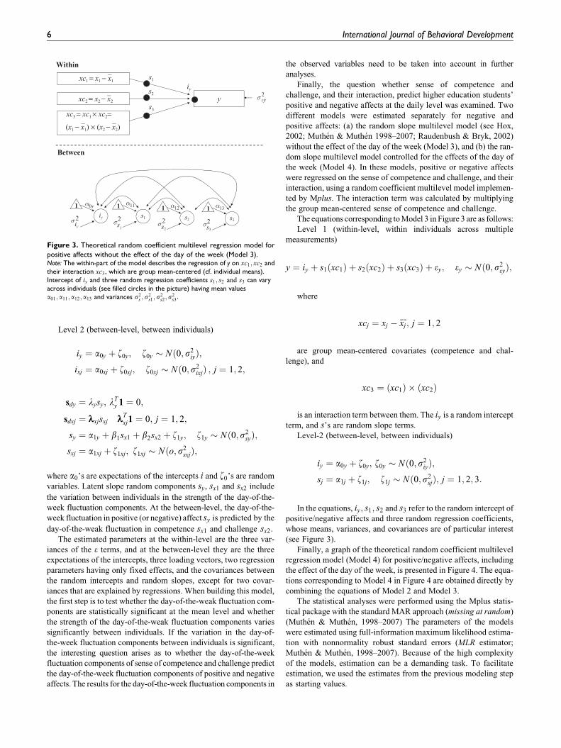
The equations corresponding to Model 3 in Figure 3 are as follows:

Level 1 (within-level, within individuals across multiple

measurements)

y ¼ iy þ s1ðxc1Þ þ s2ðxc2Þ þ s3ðxc3Þ þ ey; ey � Nð0; s2eyÞ;

where

xcj ¼ xj � xj; j ¼ 1; 2

are group mean-centered covariates (competence and chal-

lenge), and

xc3 ¼ ðxc1Þ � ðxc2Þ

is an interaction term between them. The iy is a random intercept

term, and s’s are random slope terms.

Level-2 (between-level, between individuals)

iy ¼ a0y þ z0y; z0y � Nð0; s2iyÞ;

sj ¼ a1j þ z1j; z1j � Nð0; s2sjÞ; j ¼ 1; 2; 3:

In the equations, iy; s1; s2 and s3 refer to the random intercept of

positive/negative affects and three random regression coefficients,

whose means, variances, and covariances are of particular interest

(see Figure 3).

Finally, a graph of the theoretical random coefficient multilevel

regression model (Model 4) for positive/negative affects, including

the effect of the day of the week, is presented in Figure 4. The equa-

tions corresponding to Model 4 in Figure 4 are obtained directly by

combining the equations of Model 2 and Model 3.

The statistical analyses were performed using the Mplus statis-

tical package with the standard MAR approach (missing at random)

(Muthen & Muthen, 1998–2007) The parameters of the models

were estimated using full-information maximum likelihood estima-

tion with nonnormality robust standard errors (MLR estimator;

Muthen & Muthen, 1998–2007). Because of the high complexity

of the models, estimation can be a demanding task. To facilitate

estimation, we used the estimates from the previous modeling step

as starting values.

Within

Between

–xc1 = x1 − x1

–xc2 = x2 − x2

– –xc3 = xc1 × xc2=

(x1 − x1) × (x2 − x2)

s1

s2

s3

iy

y2εy

s2s1

1 α11

2s

1

1 α12

2s2

iy

1 α0y

2iy

s3

1 α13

2s3

σ

σ σ σ σ

Figure 3. Theoretical random coefficient multilevel regression model for

positive affects without the effect of the day of the week (Model 3).Note: The within-part of the model describes the regression of y on xc1; xc2 andtheir interaction xc3 , which are group mean-centered (cf. individual means).Intercept of iy and three random regression coefficients s1; s2 and s3 can varyacross individuals (see filled circles in the picture) having mean valuesa01; a11; a12; a13 and variances s2

s ; s2s1; s

2s2; s

2s3 .

6 International Journal of Behavioral Development

Results

The effects of the day of the week and testingindividual variation in these effects

The intraclass correlations showed that 21.3% of the total variation

in sense of competence (p < .001), 11.9% of the total variation in

sense of challenge (p < .001), 35.6% of the total variation in posi-

tive affects (p < .001), and 41.3% of the total variation in negative

affects (p < .001) was due to variation between individuals (i.e.,

individual differences), suggesting moderate interindividual stabi-

lity. The rest of the total variation was due to daily fluctuation

within individuals (p < .001).

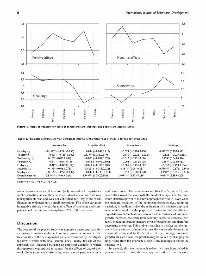
Figure 5 presents the means of weekdays for sense of compe-

tence and challenge, and positive and negative affects, illustrating

graphically the nonlinear day-of-the-week fluctuation effects (i.e.,

average shape of nonlinear change).

Next, multilevel analyses were conducted to estimate the

day-of-the-week fluctuation components (see analysis strategy

for details and the Appendix for building an input of Model 1).

The results of the Satorra-Bentler scaled w2-difference test

showed a significant mean-level day-of-the-week fluctuation

effect on positive affects ðw2diff ð6Þ ¼ 23:67; p < :001Þ, negative

affects ðw2diff ð6Þ ¼ 15:09; p ¼:020Þ and sense of challenge

ðw2diff ð6Þ ¼67:23; p < :0005Þ, whereas day of the week had no

effect on sense of competence (w2diff ð6Þ ¼ 9:57; p ¼ :144). The

statistically significant result of this ‘‘overall test’’ means that some

weekdays have special mean-level effects on daily experience. The

parameter estimates (captured with l parameters because a1is fixed

to 1), with 95% confidence intervals, of the overall mean and

daily deviations from this mean for sense of competence and

challenge, and positive and negative affects, are presented in

Table 2. A significant Saturday effect was detected in all the

variables: compared to the average level, individuals showed more

positive affects and less negative affects and less challenge on

Saturdays. Moreover, on Sundays and Mondays, in particular, indi-

viduals showed less positive affect and on Mondays more challenge

than usual. Finally, on Wednesdays individuals experienced a

higher level of both positive affects and challenge.

There was, however, no significant individual variation in

the strength of day-of-the-week fluctuation in either positive

(p ¼ 0.14) or negative affects (p ¼ 0.47). Consequently, in the

final models only mean-level day-of-the-week fluctuation com-

ponents were taken into account. For the same reason, no

further analyses to predict individual variation in day-of-the-

week fluctuation in positive and negative affects were carried

out (see the Appendix for building the input of Models 2–4,

including zero constraints for nonsignificant variance and

regression parameters).

Random slope multilevel models with andwithout day-of-the-week effects

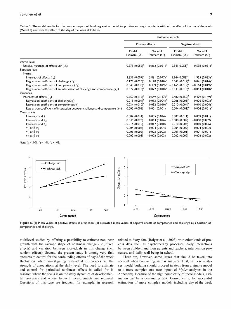
Table 3 shows the results of the random slope multilevel model for

positive affects when the day-of-the-week fluctuation components

were included (see the Appendix for building the input of Model 4)

and when they were excluded (see the Appendix for building the

input of Model 3). The results (see Table 3) showed, first, that all

the regression coefficients were statistically significant: sense of

challenge and competence, and their interaction, positively pre-

dicted the level of positive affects. The results for the interaction

of challenge and competence showed (see Figure 6a) that when

both competence and challenge were at a high level, the individual

reported a particularly high level of positive affects (cf. flow expe-

rience), whereas if competence was at a high level and challenge

low, the individual reported only slightly higher positive affects

than average. Conversely, if competence was at a low level, the

level of positive affects was also low, despite the level of challenge.

The results also showed (Table 3) statistically significant variation

between individuals in the strength of the regression coefficient of

challenge and competence. In other words, there were differences

between individuals in the strength of the positive affects they

reported in relation to their perception of the level of challenge

of the task and to their perceived competence. In turn, the variation

in the regression coefficient of the interaction term was not statis-

tically significant. The results of Model 3 (day-of-the-week fluc-

tuation not taken into account) and Model 4 (day-of-the-week

fluctuation taken into account) closely resembled each other. The

main effects of challenge and competence and the interaction

between challenge and competence explained 24%, whereas the

day-of-the-week fluctuation component explained 1% of the varia-

tion in positive affects. One explanation for small effect size of the

day-of-the-week component is the fact that in the present data, var-

iation between individuals in day-of-the-week fluctuation was non-

significant. Consequently, only mean-level day-of-the-week

fluctuation, which was statistically significant, was controlled for

in the models.

Table 3 also shows the results of the random slope multilevel

model for negative affects inclusive and exclusive of the effects of

the day of the week. The results for the interaction between sense

of challenge and competence showed (see Figure 6b) that when sense

of competence was at a low level and sense of challenge at a high

level (i.e., an overload of demand in relation to internal resources),

the individual reported a particularly high level of negative affects

(i.e., anxiety). Finally, individuals also varied in the strength of the

impacts of challenge, competence and their interaction. In other

words, individuals varied in how strongly they reacted with an

increased level of negative affects if their perceived competence was

low and the task highly challenging. The results were very similar

Within

Between

s1

s2

s3

iy

y

dsdx1

sdx2

sx1

sx2

2

1

syβ2

α1x2

1

2sx1

sx2

α1x1

β11α1y

2sy 2ss1

1 α11

2s1

1 α12iy

1 α0y

2iy

s3

1 α13

–xc1 = x1 − x1

–xc2 = x2 − x2

– –xc3 = xc1 × xc2=(x1 − x1) × (x2 − x2)

sdy

2εyσ

σ

σ σσ σ 2

s2σ 2

s3σ

Figure 4. Theoretical random coefficient multilevel regression model for

positive affects with the effect of the day of the week (Model 4).Note: Compared to Model 3 (Figure 3), this model also includes day-of-the-weekeffects (Model 2, Figure 2). All the covariances between the latent componentsare estimated, except two, which are replaced by regressions.

Tolvanen et al. 7

when day-of-the-week fluctuation (only mean-level day-of-the-

week fluctuation, as variation between individuals in this trend was

nonsignificant) was and was not controlled for. Day-of-the-week

fluctuation explained only a small proportion (1%) of the variation

in negative affects, whereas the main effects of challenge and com-

petence and their interaction explained 20% of this variation.

Discussion

The purpose of the present study was to present a new approach for

estimating a random multilevel nonlinear growth component. The

functionality of the new approach was also examined by investigat-

ing how it works with small sample sizes. Finally, the use of the

approach was illustrated by using an empirical example in which

this approach was applied to control for the effects of day-of-the-

week fluctuation when estimating other model parameters in a

multilevel model. The simulations results (N ¼ 50, N ¼ 75, and

N ¼ 100) showed that even with the smallest sample size, the min-

imum statistical power of the new approach was over .8. Even when

the standard deviation of the parameter estimates (i.e., sampling

variation) is medium in size, the estimation with this new approach

is accurate enough for the purpose of controlling for the effect of

day-of-the-week fluctuation. However, as the variance of nonlinear

growth increases, the estimation accuracy seems to decrease, cor-

rectly producing greater standard error of parameters and therefore

decreasing the power. This problem was due to the fact that the ran-

dom effect (variance of nonlinear growth) was clearly dominant in

magnitude compared to the fixed effect (i.e., average nonlinear

growth). In such a case, the problem may be solved by changing the

fixed value from the intercept to one of the loadings or fixing the

variance to 1.

In general, this new approach solved two problems raised in

previous research. First, the new approach adds to the previous

3,5

3,7

3,9

4,1

2,4

2,6

2,8

3

3,2

3,4

Mon

day

Tue

sday

Wed

nesd

ay

Thu

rsda

y

Frid

ay

Satu

rday

Sund

ay

Positive affects

Challenge

1,7

1,8

1,9

2

2,1

4,9

5

5,1

5,2

5,3

Mon

day

Tue

sday

Wed

nesd

ay

Thu

rsda

y

Frid

ay

Satu

rday

Sund

ay

Negative affects

Competence

Figure 5. Means of weekdays for sense of competence and challenge, and positive and negative affects.

Table 2. Parameter estimates and 95% confidence intervals of the mean value of Model 1 for the day of the week

Positive affect Negative affect Competence Challenge

Monday l1 �0.161** (�0.271,-0.050) 0.034 (�0.049,0.117) �0.079 (�0.209,0.050) 0.372*** (0.220,0.523)

Tuesday l2 �0.027 (�0.135, 0.080) 0.137** (0.055,0.219) �0.115 (�0.228,�0.002) 0.128 (�0.027,0.283)

Wednesday l3 0.139* (0.029,0.249) �0.003 (�0.097,0.091) �0.017 (�0.151,0.116) 0.194* (0.043,0.346)

Thursday l4 0.041 (�0.077,0.159) 0.015 (�0.071,0.101) �0.004 (�0.136,0.128) 0.197* (0.032,0.362)

Friday l5 0.017 (�0.077,0.111) �0.011 (�0.109,0.086) �0.005 (�0.126,0.117) �0.032 (�0.199,0.136)

Saturday l6 0.145* (0.016,0.275) �0.122* (�0.219,0.026) 0.161** (0.041,0.281) �0.510*** (�0.676,�0.345)

Sunday l7 �0.155* (�0.272,-0.037) �0.049 (�0.138, 0.040) 0.058 (�0.081,0.198) �0.350** (�0.556,�0.144)

Overall mean a0 3.834*** (3.644,4.024) 1.943*** (1.780,2.105) 5.071*** (4.903,5.239) 3.048*** (2.889,3.208)

Note: ***p < .001, **p < .01, *p < .05.

8 International Journal of Behavioral Development

multilevel studies by offering a possibility to estimate nonlinear

growth with the average shape of nonlinear change (i.e., fixed

effects) and variation between individuals in this change (i.e.,

random effects). Second, the present study is among very first

attempts to control for the confounding effects of day-of-the week

fluctuation when investigating individual differences in the

strength of associations at the daily level. The need to estimate

and control for periodical nonlinear effects is called for in

research where the focus is on the daily dynamics of developmen-

tal processes and where frequent measurements are required.

Questions of this type are frequent, for example, in research

related to diary data (Bolger et al., 2003) or to other kinds of pro-

cess data such as psychotherapy processes, daily interactions

between children and their parents and teachers, intervention pro-

cesses, and daily well-being in school.

There are, however, some issues that should be taken into

account when conducting similar analyses. First, in these analy-

ses, model building should proceed in steps from a simple model

to a more complex one (see inputs of Mplus analyses in the

Appendix). Because of the high complexity of these models, esti-

mation can be a demanding task. Consequently, for successful

estimation of more complex models including day-of-the-week

Table 3. The model results for the random slope multilevel regression model for positive and negative affects without the effect of the day of the week

(Model 3) and with the effect of the day of the week (Model 4)

Outcome variable

Positive affects Negative affects

Model 3

Estimate (SE)

Model 4

Estimate (SE)

Model 3

Estimate (SE)

Model 4

Estimate (SE)

Within level

Residual variance of affects var ( ey) 0.871 (0.052)a 0.862 (0.051)a 0.541(0.051)a 0.538 (0.051)a

Between level

Means

Intercept of affects ( iy) 3.837 (0.097)a 3.861 (0.097)a 1.944(0.083)a 1.955 (0.083)a

Regression coefficient of challenge (s1) 0.173 (0.020)a 0.178 (0.020)a 0.043 (0.014)b 0.041 (0.014)b

Regression coefficient of competence (s2) 0.343 (0.030)a 0.339 (0.029)a �0.165 (0.019)a �0.164 (0.019)a

Regression coefficient of an interaction of challenge and competence (s3) 0.072 (0.010)a 0.072 (0.010)a �0.043 (0.010)a �0.044 (0.010)a

Variances

Intercept of affects ( iy) 0.650 (0.116)a 0.649 (0.117)a 0.480 (0.150)b 0.479 (0.149)b

Regression coefficient of challenge(s1) 0.013 (0.004)b 0.013 (0.004)b 0.006 (0.003)c 0.006 (0.003)c

Regression coefficient of competence(s2) 0.034 (0.010)b 0.032 (0.010)b 0.010 (0.004)c 0.010 (0.004)c

Regression coefficient of interaction between challenge and competence (s3) 0.002 (0.001) 0.001 (0.001) 0.004 (0.001)b 0.004 (0.001)b

Covariances

Intercept and s1 0.004 (0.014) 0.005 (0.014) 0.009 (0.011) 0.009 (0.011)

Intercept and s2 0.045 (0.026) 0.043 (0.026) �0.008 (0.009) �0.008 (0.009)

Intercept and s3 �0.016 (0.010) �0.017 (0.010) 0.010 (0.006) 0.010 (0.006)

s1 and s2 0.004 (0.004) 0.004 (0.004) 0.004 (0.002) 0.004 (0.002)

s1 and s3 0.003 (0.002) 0.003 (0.002) �0.001 (0.001) �0.001 (0.001)

s2 and s3 �0.002 (0.003) �0.002 (0.003) 0.002 (0.002) 0.002 (0.002)

Note: ap < .001, bp < .01, cp < .05.

Figure 6. (a) Mean values of positive affects as a function; (b) estimated mean values of negative affects of competence and challenge as a function of

competence and challenge.

Tolvanen et al. 9

effects, good estimates of the initial/starting values of the

parameters of interest are essential. Initial values can be obtained

from the earlier steps in the modeling process. Second, it is also note-

worthy that although the mean-level day-of-the-week fluctuation

effects in the present empirical case were significant, the effect sizes

were small. The results, when minor day-of-the-week fluctuation

mean-level effects were included, closely resembled the results of the

models without the day-of-the-week fluctuation component. If day-

of-the-week fluctuation effects are very small, they could potentially

be ignored. However, ignoring them also means missed opportunities

to investigate some potentially crucial aspects of the studied phenom-

enon. In turn, ignoring large and significant periodical effects might

seriously distort other model estimates and standard errors, resulting

in misleading results. More research is needed to examine precisely

how small fixed or random nonlinear periodical effects need to be

in relation to sample size without significantly biasing estimation of

the other model parameters. These questions could be answered, for

example, by means of simulation studies. Also promising are recent

advances in the Bayesian approach to growth curves (Donnet, Foulley,

& Samson, 2010).

Conclusion

The present study presented a new approach for estimating a nonlinear

growth component in the multilevel context. This approach enables

estimation not only of the average shape of nonlinear growth but

also of the individual variation around this mean trend. The simu-

lation results revealed that this new approach worked accurately

and had reasonable power also in the case of low sample sizes.

The new approach has particular utility when multilevel modeling

is required to answer research questions and there is a need to con-

trol for nonlinear growth effects. In other words, the new approach

should be beneficial particularly in studies where the focus is on

questions of dynamics in developmental processes and the purpose

is to control and estimate periodical effects using a nonlinear

growth model in repeated-measures data. Research questions of

this type are frequent, for example, in diary data and in other kinds

of developmental data such as psychotherapy and intervention

processes.

Funding

This research received no specific grant from any funding agency in

the public, commercial, or not-for-profit sectors.

References

Barrett, F. L., & Barrett, D. J. (2001). An introduction to computerized

experience sampling in psychology. Social Science Computer

Review, 19, 175–185.

Biesanz, J. C., Deeb-Sossa, N., Papadakis, A. A., Bollen, K. A., &

Curran, P. J. (2004). The role of coding time in estimating and inter-

preting growth curve models. Psychological Methods, 9, 30–52.

Bolger, N., Davis, A., & Rafaeli, E. (2003). Diary methods: Capturing

life as it is lived. Annual Review of Psychology, 54, 579–616.

Bollen, K. A., & Curran, P. J. (2006). Latent curve models: A structural

equation approach. Hoboken, NJ: Wiley.

Donnet S., Foulley, J.-L., & Samson A. (2010). Bayesian analysis of

growth curves using mixed models defined by stochastic differential

equations. Biometrics, 66, 733–741.

Heck, R. H., & Thomas, S. L. (2009). An introduction to multilevel

modeling techniques. New York, NY: Routledge.

Hektner, J., Schmidt, J. A., & Csikszentmihalyi, M. (2007). Experience

sampling method: Measuring the quality of everyday life. Thousand

Oaks, CA: Sage.

Herzog, W., & Boomsma, A. (2009). Small-sample robust estimators of

noncentrality-based and incremental model fit. Structural Equation

Modeling, 16, 1–27.

Hoogland, J. J., & Boomsma, A. (1998). Robustness studies in

covariance structure modeling, Sociological Methods and Research,

26, 329–367.

Hox, J. (2002). Multilevel analysis: Techniques and applications.

Mahwah, NJ: Lawrence Erlbaum Associates.

Maas C. J. M., & Hox, J. J. (2005). Sufficient sample sizes for multile-

vel modeling. Methodology, 1, 86–92.

Marsh, H. W., Hau, K.-T., Balla, J. R., & Crayson, D. (1998). Is

more ever too much? The number of indicators per factor in con-

firmatory factor analysis. Multivariate Behavioral Research, 33,

191–220.

Muthen, L., & Muthen, B. O. (1998–2007). Mplus Version 5 & Mplus

users’ guide (5th ed.). Los Angeles, CA: Muthen & Muthen.

Muukkonen, H., Hakkarainen, K., Inkinen, M., Lonka, K., &

Salmela-Aro, K. (2008). CASS-methods and tools for investigating

higher education knowledge practices. In G. Kanselaar, V. Jonker,

P. Kirschner & F. Prins (Eds.), Proceedings of the 2008 International

Conference for the Learning Sciences (ICLS) (Vol. 2, pp. 107–115).

Utrecht, the Netherlands: International Society of the Learning

Sciences.

Raudenbush, S. W., & Bryk, A. S. (2002). Hierarchical linear models:

Applications and data analysis methods. Thousand Oaks, CA: Sage

Publications.

Ronka, A., Malinen, K., Kinnunen, U., Tolvanen, A., & Lamsa, T.

(2010). Capturing daily family dynamics via text messages:

Development of a mobile diary. Community, Work & Family,

13(1), 5–21.

Stoel, R. D., van Den Wittenboer, G., & Hox, J. (2003). Analyzing long-

itudinal data using multilevel regression and latent growth curve anal-

ysis. Metodologıa de las Ciencias del Comportamiento, 5, 21–42.

Watson, D., Clark, L. A., & Tellegen, A. (1988). Development and

validation of brief measures of positive and negative affect: The

PANAS scales. Journal of Personality and Social Psychology, 54,

1063–1070.

Westland, J. C. (2010). Lower bounds on sample size in structural

equation modeling. Electronic Commerce Research and Applica-

tions, 9, 476–487.

10 International Journal of Behavioral Development