Dynamics of polar boundary of the auroral oval derived from the IMAGE satellite data
Upload
khangminh22Category
view
1download
0
MULTIVARIATE DATA ANALYSIS OF SATELLITE-DERIVED MEASUREMENTS
TO DISTINGUISH NATURAL FROM MAN-MADE OIL SLICKS
ON THE SEA SURFACE OF CAMPECHE BAY (GULF OF MEXICO)
Gustavo de Araújo Carvalho
Tese de Doutorado apresentada ao Programa de
Pós-graduação em Engenharia Civil, COPPE, da
Universidade Federal do Rio de Janeiro, como
parte dos requisitos necessários à obtenção do
título de Doutor em Engenharia Civil.
Orientadores: Luiz Landau
Fernando Pellon de Miranda
Peter Minnett
Rio de Janeiro
Dezembro de 2015

iii
Carvalho, Gustavo de Araújo
Multivariate data analysis of satellite-derived
measurements to distinguish natural from man-made oil
slicks on the sea surface of Campeche Bay (Gulf of
Mexico)/Gustavo de Araújo Carvalho – Rio de Janeiro:
UFRJ/COPPE, 2015.
XV, 285 p.: il.; 29,7 cm.
Orientadores: Luiz Landau
Fernando Pellon de Miranda
Peter Minnett
Tese (doutorado) – UFRJ/COPPE/Programa de
Engenharia Civil, 2015.
Referências Bibliográficas: p. 205-254.
1. Algoritmo. 2. Análise Exploratória de Dados. 3.
Dados Multivariados 4. Análise Discriminante. 5.
Análise de Componentes Principal (PCA). 6. Petróleo.
7. Manchas de Óleo (Spill). 8. Exsudação Natural
(Seep). 9. Golfo do México. 10. Baía de Campeche. 11.
Cantarell. 12. Oceanografia. 13. Monitoramento
Ambiental. 14. Sensoriamento Remoto. 15. Satélite. 16.
Radar de Abertura Sintética (SAR). 17. RADARSAT. I.
Landau, Luiz et al. II. Universidade Federal do Rio de
Janeiro, COPPE, Programa de Engenharia Civil. III.
Título.

iv
In loving memory, always forever immortal...
For everything, despite everything!
eD i-mundo Muleke Pulguento Babão
(June 1998 – August 2014)
A friend to the end.
“Muito bem eD, você eD mais.”

v
“Sometimes the questions are complicated, but the answers are simple!”
Dr. Seuss
“Simple things should be simple, and complex things should be possible.”
Alan Kay
“Share your knowledge. It’s a way to achieve immortality.”
The Dalai Lama

vi
ACKNOWLEDGMENTS
It is with pleasure that I would like to register my paramount regards to:
• Dr. Minnett, who has taught me so much, scientifically- and personally-wise, not only
while pursuing this degree but also during the decade of his words of wisdom.
• Dr. Paes (E.T.), from LEMOPA-UFRA, for his clever guidance of excellence during
this fascinating multivariate expedition.
• Dr. Miranda for his thorough surgical text corrections, full of accurate insights.
• Dr. Landau for the opportunity, the support, and the infra structure.
• Dr. Moreira (LabSAR) for backing me up during the harsh image coding processes.
• Dra. Valério (DCC-IM-UFRJ) for making available clear enlightenments about PCA.
• Dr. Ebecken for being a very good listener and, above all, for his wise contributions.
• Dr. Valentin and Dra. Bentz for accepting the invitation to join the appraisal crew.
• UFRJ, COPPE, and PEC for the D.Sc. degree.
• PRH-ANP for the financial support.
• Pemex and MDA for the high-quality RADARSAT dataset.
• Øyvind Hammer (PAST), The University of Waikato (WEKA), Microsoft (MS Office),
ESRI (ArcGIS), and Geomatica (PCI) for the software packages.
• LAMCE and LabSAR colleagues: Adriano, Beisl, Gil, Hatsue, Humberto, Mônica,
Patrícia, Rosana, Sérgio, and Victor.
• Lucas and Patricia that already have room in my heart, but their assistance in text
editing and in listening to my loud thoughts, surely deserve the record.
• Lívia for the sincere companion at the start of this journey. And despite the "odds",
to AMA-DA AMAnDA for the lovely mid-way "evens".
• Always-good long-time comrades: Angrézinho, Dr. Cabelo, Carlinha, Catanzaro,
Davi, DuppreX, Elisa, Eugênio, Dra. Gebara, Dr. Halley, Malaquias, and Roma&zap.
• Contemporary wonders from the woods: Shei-Lá, Cesar, Léu, and Will.
• A long list of other beloved folks not listed in press, yet listened in the air.
• The pure shining beauty of Bia (trix) and her conceivers: Guilherme and Sheryl.
• The everlasting inspiration received from Adir, Sandra, Magali, Morel, Eva, Merice,
and Dr. Memél, as well as to the good memories from Vavá and Chico Adolfo.
• THE FOREVER OMNIPRESENT eD, THE MOST SPECIAL OF ALL PRESENTS ☺
• All Gods... For life, happiness, love, flowers, and the ocean!
vii
Resumo da Tese apresentada à COPPE/UFRJ como parte dos requisitos necessários
para a obtenção do grau de Doutor em Ciências (D.Sc.)
ANÁLISE DE DADOS MULTIVARIADOS DE MEDIÇÕES DE SATÉLITES PARA
DISTINGUIR EXSUDAÇÕES NATURAIS DE DERRAMES OPERACIONAIS DE ÓLEO
NA SUPERFÍCIE DO MAR NA BAÍA DE CAMPECHE (GOLFO DO MÉXICO)
Gustavo de Araújo Carvalho
Dezembro/2015
Orientadores: Luiz Landau
Fernando Pellon de Miranda
Peter Minnett
Programa: Engenharia Civil
A presente pesquisa de doutorado é uma análise exploratória com o objetivo
utilizar medidas de satélite para discriminar dois tipos de manchas de óleo:
exsudações naturais e derrames operacionais. O uso sensores remotos para realizar
esta tarefa ainda é pouco documentado. Um conjunto de vários anos (2000-2012) de
medições de radar de abertura sintética (SAR – RADARSAT) é utilizado para
investigar a distribuição espaço-temporal das manchas de óleo na superfície do mar
na Baía de Campeche (Golfo do México). Após o tratamento dos dados
(transformação logarítmica, padronização “ranging”, etc.), técnicas de análise
multivariada, tais como Correlação (modo-R), Análise de Componentes Principais
(ACP) e Função Discriminante, são utilizadas na elaboração de um algoritmo simples
de classificação para distinguir exsudações de derrames. Esta investigação propõe
uma nova interlocução entre a pesquisa geoquímica e o sensoriamento remoto para
expressar diferenças geofísicas entre exsudações naturais e derrames operacionais
de óleo. Nesta pesquisa, coeficientes de retroespalhamento SAR, i.e. sigma-zero (σo),
beta-zero (βo) e gamma-zero (γo), são combinados com vários atributos referentes à
geometria, forma e dimensão que descrevem as manchas de óleo (conjuntamente
referidas como tamanho). Os resultados indicam que a combinação dessas diversas
características com as técnicas propostas é capaz de distinguir o tipo de mancha de
óleo. Entretanto, o simples uso somente da informação correspondente ao tamanho
das manchas também é capaz de distinguir o óleo de exsudações daquele derramado
operacionalmente com precisão aceitável para uso sistemático: 70% de acuraria total.

viii
Abstract of Thesis presented to COPPE/UFRJ as a partial fulfillment of the
requirements for the degree of Doctor of Science (D.Sc.)
MULTIVARIATE DATA ANALYSIS OF SATELLITE-DERIVED MEASUREMENTS
TO DISTINGUISH NATURAL FROM MAN-MADE OIL SLICKS
ON THE SEA SURFACE OF CAMPECHE BAY (GULF OF MEXICO)
Gustavo de Araújo Carvalho
December/2015
Advisors: Luiz Landau
Fernando Pellon de Miranda
Peter Minnett
Department: Civil Engineering
The present D.Sc. research is an exploratory data analysis aiming to use
satellite-derived measurements to discriminate between two oil slick types: naturally-
occurring oil seeps and human-related oil spills. The use of satellite remote sensors for
this task is still poorly documented. A multi-year dataset (2000-2012) of synthetic
aperture radar (SAR – RADARSAT) is leveraged to investigate the spatio-temporal
distribution of the oil slicks on the surface of the ocean in Campeche Bay (Gulf of
Mexico). After a Data Treatment practice (Log Transformation, Ranging
Standardization, etc.), multivariate data analysis techniques, such as Correlation (R-
mode), Principal Components Analysis (PCA), and Discriminant Function, have been
explored to design a simple classification algorithm to distinguish natural from man-
made oil slicks. The proposed analysis promotes a novel idea bridging geochemistry
and remote sensing research to express geophysical differences between seeped and
spilled oil. SAR-derived backscatter coefficients, i.e. sigma-naught (σo), beta-naught
(βo), and gamma-naught (γo), are combined with various attributes referring to the
geometry, shape, and dimension that describe oil slicks (referred to as size
information). Results indicate that the synergy of combining these several
characteristics with the application of the multivariate data analysis techniques is
capable of distinguishing the oil slick type. Nevertheless, the sole, and simple use of
the oil slick size information is also capable of distinguishing oil seeps from oil spills
observed on the sea surface to a useful accuracy for systematic use: 70% of Overall
Accuracy.

ix
Table of Contents: Pages
ACKNOWLEDGMENTS................................................................................................VI
RESUMO......................................................................................................................VII
ABSTRACT.................................................................................................................VIII
GLOSSARY .................................................................................................................XII
INTRODUCTION ............................................................................................................ 1
CHAPTER 1RESEARCH RATIONALE .................................................................................................... 3
1.1. ENVIRONMENT, OIL SLICKS, AND SATELLITES ........................................................ 41.2. MOTIVATION ......................................................................................................... 61.3. OBJECTIVES ......................................................................................................... 81.4. RESEARCH STRATEGY .......................................................................................... 91.5. JUSTIFICATION ...................................................................................................... 91.6. CHALLENGES ...................................................................................................... 121.7. CONTRIBUTIONS ................................................................................................. 13
CHAPTER 2OPERATIONAL ENVIRONMENTAL MONITORING SYSTEM ................................................... 15
2.1. STUDY AREA: CAMPECHE BAY ............................................................................ 152.2. CAMPECHE BAY OIL SLICK SATELLITE PROJECT (CBOS-SATPRO)....................... 182.3. CAMPECHE BAY OIL SLICK SATELLITE DATABASE (CBOS-DATA) ......................... 22
2.3.1. CBOS-SATPRO PART 1: RADARSAT SCENE SELECTION............................ 252.3.2. CBOS-SATPRO PART 2: RADARSAT IMAGE PROCESSING ......................... 252.3.3. CBOS-SATPRO PART 3: DIGITAL IMAGE CLASSIFICATION (DIC) ................... 282.3.4. CBOS-SATPRO PART 4: DARK SPOT IDENTIFICATION .................................. 302.3.5. CBOS-SATPRO PART 5: FEATURE-EXTRACTION.......................................... 322.3.6. CBOS-SATPRO PART 6: PEMEX VALIDATION ............................................... 34
CHAPTER 3BLACK GOLD ................................................................................................................. 36
3.1. WEATHERING PROCESSES .................................................................................. 373.2. NATURAL HYDROCARBON SEEPAGES AT SEA ....................................................... 383.3. OIL AND GAS EXPLORATION AND PRODUCTION INDUSTRY (OGEPI) ..................... 40

x
CHAPTER 4SATELLITE REMOTE SENSING......................................................................................... 44
4.1. BEFORE THE SATELLITE ERA............................................................................... 444.2. BASIC CONCEPTS OF SYNTHETIC APERTURE RADAR (SAR) ................................. 454.3. RADARSAT RADIOMETRIC-CALIBRATED IMAGE PRODUCTS ................................ 504.4. DARK SPOT DETECTION IN SAR IMAGERY ........................................................... 54
4.4.1. DIGITAL IMAGE CLASSIFICATION (DIC) ......................................................... 544.4.2. FEATURE-EXTRACTION................................................................................ 554.4.3. DARK SPOT IDENTIFICATION ........................................................................ 56
4.5. SATELLITE SENSORS IN SUPPORT FOR OIL SLICK DETECTION .............................. 574.5.1. VISIBLE/NEAR INFRARED (VIS/NIR) ............................................................. 574.5.2. THERMAL INFRARED (TIR) ........................................................................... 604.5.3. MICROWAVE ALTIMETER.............................................................................. 614.5.4. MICROWAVE SCATTEROMETER .................................................................... 614.5.5. METEOROLOGICAL AND OCEANOGRAPHIC KIT (METOC-KIT) ......................... 62
4.6. SATELLITE OCEANOGRAPHY................................................................................ 62CHAPTER 5METHODS ...................................................................................................................... 68
5.1. PHASE 1: DATA FAMILIARIZATION ........................................................................ 715.2. PHASE 2: QUALITY CONTROL (QC)...................................................................... 725.3. PHASE 3: RADARSAT RE-PROCESSING ............................................................. 725.4. PHASE 4: NEW SLICK-FEATURE ATTRIBUTES ....................................................... 745.5. PHASE 5: DATA TREATMENT................................................................................ 805.6. PHASE 6: ATTRIBUTE SELECTION ........................................................................ 905.7. PHASE 7: PRINCIPAL COMPONENTS ANALYSIS (PCA)........................................... 965.8. PHASE 8: DISCRIMINANT FUNCTION ..................................................................... 995.9. PHASE 9: CORRELATION MATRIX ....................................................................... 1015.10. PHASE 10: OIL SLICK CLASSIFICATION ALGORITHM.......................................... 101
CHAPTER 6RESULTS ..................................................................................................................... 104
6.1. PHASE 1: DATA FAMILIARIZATION ...................................................................... 1046.2. PHASE 2: QUALITY CONTROL (QC).................................................................... 1226.3. PHASE 3: RADARSAT RE-PROCESSING ........................................................... 1256.4. PHASE 4: NEW SLICK-FEATURE ATTRIBUTES ..................................................... 1256.5. PHASE 5: DATA TREATMENT.............................................................................. 1366.6. PHASE 6: ATTRIBUTE SELECTION ...................................................................... 1426.7. PHASE 7: PRINCIPAL COMPONENTS ANALYSIS (PCA)......................................... 158
xi
6.8. PHASE 8: DISCRIMINANT FUNCTION ................................................................... 1726.9. PHASE 9: CORRELATION MATRIX ....................................................................... 1766.10. PHASE 10: OIL SLICK CLASSIFICATION ALGORITHM.......................................... 178
CHAPTER 7DISCUSSION................................................................................................................. 189CHAPTER 8CONCLUSIONS ............................................................................................................. 197CHAPTER 9RECOMMENDATIONS FOR FUTURE WORK ..................................................................... 201
REFERENCES ........................................................................................................... 205
APPENDIX 1
SCIENTIFIC PUBLICATIONS:...................................................................................... 255SBSR: BRAZILIAN REMOTE SENSING SYMPOSIUM .................................................... 256CJRS: CANADIAN JOURNAL OF REMOTE SENSING .................................................... 257RSE: REMOTE SENSING OF ENVIRONMENT .............................................................. 260
APPENDIX 2TYPICAL VALUES OF BASIC QUALITATIVE-QUANTITATIVE STATISTICS: 3RD ATTRIBUTE
TYPE (TABLE 5-4: GEOMETRY, SHAPE, AND DIMENSION – SIZE INFORMATION) .......... 263APPENDIX 3
TYPICAL VALUES OF BASIC QUALITATIVE-QUANTITATIVE STATISTICS: 4TH ATTRIBUTE
TYPE (TABLE 5-5: SAR BACKSCATTER SIGNATURE) ................................................. 267APPENDIX 4
ROOTED-TREE DENDROGRAMS BASED ON THE UPGMA (UNWEIGHTED PAIR GROUP
METHOD WITH ARITHMETIC MEAN) IMPLEMENTATION PER DATA SUB-DIVISION .......... 274APPENDIX 5
CONSTANT OFFSETS (COFF) OF THE DISCRIMINANT FUNCTIONS ................................. 281APPENDIX 6
CONFIGURATION OF THE TWO DESIGNED CLASSIFICATION ALGORITHMS PROPOSED ON
PHASE 10 (SECTIONS 5.10 AND 6.10) ...................................................................... 283

xii
GLOSSARY
AAD Average absolute deviation. Dispersion measure of all pixels inside oil slick polygons.
AVG Arithmetic mean. Central tendency measure of all pixels inside oil slick polygons.
AVHRR Advanced Very High Resolution Radiometer.
Beta-naught SAR backscatter coefficient (symbol: βo) corresponding to the radar cross section (RCS – σ) normalized by the unit area in the plane of the incident radar beam (i.e. slant range direction). It is sometimes referred to as radar brightness. Because it represents the reflectivity in the direction of the incident radar beam and it is independent of the terrain slope, system design engineers generally prefer to use measures of βo. See Section 4.3: C1 and C2.
Bmode Beam mode.
Brightspot Oil slick class defining oil spills from the same oilfield. See Section 2.3.2. C1 Radiometric-calibrated value (given in intensity or amplitude of the received
radar beam) corresponding to the radar cross section (RCS – σ) normalized by the unit area: SAR backscatter coefficient. This quantitative measurement represents the SAR backscatter signature in different surface planes: sigma-naught (σo), beta-naught (βo), or gamma-naught (γo): C1 = [{DN2}+B]/A where: DN: Digital Number. B: Constant offset (nominally set to zero for SGF products). A: Range-dependent gain that varies upon the LUT choice (i.e. metadata files – lutSigma.xml, lutBeta.xml, or lutGamma.xml) to obtain a corresponding A to calculate σo, βo, or γo.
C2 Radiometric-calibrated value (expressed in decibel units – dB) corresponding to the radar cross section (RCS – σ) normalized by the unit area: SAR backscatter coefficient. This quantitative measurement represents the SAR backscatter signature in different surface planes: sigma-naught (σo), beta-naught (βo), or gamma-naught (γo): C2 = (10*cc)*Log10(C1) where: cc: Equal to 2 for the amplitude of the received radar beam and 1 for pixel values given in intensity. C1: Radiometric-calibrated value of σo, βo, or γo given in intensity or amplitude, by: C1 = [{DN2}+B]/A DN: Digital Number. B: Constant offset (nominally set to zero for SGF products). A: Range-dependent gain that varies upon the LUT choice (i.e. metadata files – lutSigma.xml, lutBeta.xml, or lutGamma.xml) to obtain a corresponding A to calculate σo, βo, or γo.
CBOS-Data Campeche Bay Oil Slick Satellite Database. See Chapter 2.
CBOS-DScMod Campeche Bay Oil Slick Modified Database. Modified version of the Campeche Bay Oil Slick Satellite Database (i.e. CBOS-Data) used on this D.Sc. research Dissertation as the workable database. See Section 5.4.
CBOS-SatPro Campeche Bay Oil Slick Satellite Project. See Chapter 2.

xiii
CBRR Centro Brasileiro de Recursos RADARSAT. It is nowadays called LabSAR.
CCC Cophenetic Correlation Coefficient.
CENPES Centro de Pesquisas Leopoldo Américo Miguez de Mello.
CFS Correlation-Based Feature Selection. Centroid Represent the topological center of mass of the oil slick polygon.
Chl Chlorophyll-a concentration.
cLAT Latitude of the oil slick polygon centroid.
cLONG Longitude of the oil slick polygon centroid. Cluster Oil slick class defining oil seeps with repeated occurrences about the same
location observed on the surface of the ocean. See Section 2.3.2. COD Coefficient of dispersion. Dispersion measure of all pixels inside oil slick
polygons.
COPPE Instituto Alberto Luiz Coimbra de Pós-Graduação e Pesquisa de Engenharia.
COV Coefficient of variation: ration between mean and standard deviation. Dispersion measure of all pixels inside oil slick polygons. Distinct combined COV sets are explored on the present D.Sc. research. See Section 5.4 (Table 5-5).
CTT Cloud top temperature.
Damping ratio Compares the radar return decrease from inside to outside of oil slicks. dB Decibel unit.
DIC Digital image classification.
DN Digital Number represents the grey-level brightness count assigned to each gird position (i.e. pixel) of any given SAR image – for instance, between 0 and 255 for 8-bit images. DN is an uncalibrated measure, but it can be converted to obtain radiometric-calibrated SAR backscatter coefficients: sigma-naught (σo), beta-naught (βo), or gamma-naught (γo).
Dummy Variable Binary-coded variable: one (1) or zero (0), thus referring to its presence (Yes) or absence (No), respectively.
EDA Exploratory data analysis. EOS Earth Observing System.
ERS European Remote-Sensing Satellites: ERS-1 and ERS-2
FFROST Adaptive Frost Filter of the PCI Geomatics software. Gamma-naught SAR backscatter coefficient (symbol: γo) corresponding to the radar cross
section (RCS – σ) normalized by the unit area in the plane orthogonal to the incident radar beam (i.e. orthogonal to the slant range direction). It is the power returned to the antenna from the area orthogonal to the radar beam. This plane is uniformly distant from the satellite and has equal brightness from near to far range on the pixel level. In being so, measurements of γo are usually selected for antenna calibration purposes. See Section 4.3: C1 and C2.
HC Hydrocarbon compound (e.g. mineral oil or natural gas).
IOD Illegal oil dumping. Oil observed on the sea surface for which vessels are the identified source. Also referred to as Ship Spill or ship discharge.
IOP Inherent optical property of the water.
LabSAR Laboratório de Sensoriamento Remoto por Radar Aplicado à Indústria do Petróleo. Previously called CBRR.
LAMCE Laboratório de Métodos Computacionais em Engenharia.

xiv
Look alike feature
Harmless phenomena that can generate signatures in SAR imagery, which are similar to oil slicks, thus causing ambiguous interpretations and yielding false positives. These false targets range from regions of very weak wind or no wind, rain cells, atmospheric fronts, hydrodynamic effects, internal waves, long surface waves, shear zones, current boundaries, velocity bunching, eddies, upwelling zones, divergence and convergence regions, shallow water bathymetry, underwater vegetation beds, biogenic oil films, surfactants from phytoplankton blooms, grease ice, ice edge, ship’s stern wake turbulence, urban runoff, operational cleaning from ships, tankers, platforms, oil rigs or FPSO units, storm water discharge, freshwater intrusion from riverine origin, to shadow zones of waves behind offshore installations, islands or land, amongst others.
LUT Look-up-table.
MAD Median absolute deviation. Dispersion measure of all pixels inside oil slick polygons.
MARPOL International Convention for the Prevention of Pollution from Ships. MDA MacDonald Dettwiler and Associates Ltd.
MDA-GSI MDA Geospatial Services Inc.
MDM Mid-mean. Central tendency measure of all pixels inside oil slick polygons.
MED Median. Central tendency measure of all pixels inside oil slick polygons. MERIS MEdium Resolution Imaging Spectrometer.
MetOc-Kit Meteorological and Oceanographic Kit.
MOD Mode. Central tendency measure of all pixels inside oil slick polygons.
MODIS MODerate Resolution Imaging Spectroradiometer. NOAA National Oceanic and Atmospheric Administration.
OGEPI Oil and gas exploration and production industry.
Oil seep Oil floating on the sea surface that has naturally seeped on its liquid form out of the seafloor. This only considers the surface oil footprint, making no reference to the whole hydrocarbon seepage processes. This is also one of the two oil slick categories. See Section 2.3.2.
Oil slick Indiscriminately indicates, unless otherwise specified, the sea surface footprint of oil that has seeped naturally (oil seep) or spilled after human intervention (oil spill), both on its liquid form.
Oil slick descriptor
Characteristic belonging to oil slicks (e.g. latitude, longitude, area, perimeter, etc.). Also termed as slick-feature attribute.
Oil slick type Refers to the source of the oil observed on the sea surface: natural oil seep or man-made oil spill. Not related to the “source rock” that generates HC.
Oil spill Oil floating on the sea surface solely attributed to man-made activities, which may include platforms, ships, or pipelines. This is also one of the two oil slick categories. See Section 2.3.2.
Orphan Seep Oil seep not belonging to any specific Cluster class. Orphan Spill Oil spill not belonging to any specific Brightspot class.
PCA Principal Components Analysis.
PEC Programa de Engenharia Cívil.
Pemex The Mexican oil company, i.e. Petróleos Mexicanos. PEP Pemex Exploración y Producción.
Per Perimeter given in km.
Petrobras The Brazilian oil company, i.e. Petróleo Brasileiro S.A.

xv
QC-Standards Comprehensive set of criteria completed to guarantee that jumbled or inconsistent information are fixed and/or removed from the CBOS-Data.
RADAR RAdio Detection And Ranging.
RCS Radar cross section (σ). Characterizes a reflectivity property of the reflected radar signal strength (i.e. scattering intensity) of surface targets in the direction of the radar receiver. It has a unit of m2 and is a function of: time, position, viewing geometry, radar wavelength, and polarization (transmitted and received). The RCS normalized by the unit area (normalized-RCS) corresponds to a quantitative measure of SAR backscatter signature in different planes: sigma-naught (σo), beta-naught (βo), or gamma-naught (γo).
RMNE Región Marina Noreste.
RNG Range. Dispersion measure of all pixels inside oil slick polygons.
ROI Region of interest, more specifically, Campeche Bay.
SAR Synthetic Aperture Radar. SARdate Date of the SAR overpass above the Campeche Bay region.
SARname Name of the utilized SAR satellite.
SARtime Time of the SAR overpass above the Campeche Bay region.
Sea-truth Operator’s interpretation of SAR images. Refers to the occurrence, or not, of oil slicks, its category (oil seep or oil spill), and class (Cluster, Brightspot, etc.). It also refers to the value of the SAR backscatter coefficients: sigma-naught (σo), beta-naught (βo), or gamma-naught (γo).
SGF SAR Georeferenced Fine Resolution. RADARSAT product format. This Level-1 product is usually referred to as a “path-oriented image”.
Ship Spill Oil observed on the sea surface for which vessels are the identified source. Also referred to as illegal oil damping (IOD) or ship discharge.
Sigma-naught SAR backscatter coefficient (symbol: σo) corresponding to the radar cross section (RCS – σ) normalized by the unit area in the ground range plane (pixel projected onto the ground). Although its calculation depends upon the knowledge of terrain slope (not an issue on the sea surface) and the radar beam incidence angle, it is directly related to the target’s reflectance per unit area (i.e. pixel projected onto the ground). For this reason, scientists frequently used σo measurements. See Section 4.3: C1 and C2.
Slick-feature attribute
Characteristics belonging to oil slicks (e.g. latitude, longitude, area, perimeter, etc.). Also termed as oil slick descriptor.
slickID Unique identification number of each oil slick polygon. SOI Sphere of influence: Pemex’s OGEPI related activities at Campeche Bay.
SST Sea surface temperature.
STD Standard deviation. Dispersion measure of pixels inside oil slick polygons.
SWH Significant wave height. UFRJ Universidade Federal do Rio de Janeiro.
UPGMA Unweighted Pair Group Method with Arithmetic Mean.
USTC Unsupervised Semivariogram Textural Classifier algorithm.
VAR Variance. Dispersion measure of all pixels inside oil slick polygons. βo See beta-naught.
γo See gamma-naught.
σo See sigma-naught.

1
INTRODUCTION
The study accomplished during this D.Sc. research consists of investigating the sea
surface signature of oil slicks in remotely sensed images – these include both natural
oil seeps and man-made oil spills. Throughout the document, key concepts related to
this subject are emphasized providing enough detailed information enabling any
knowledgeable scientist to replicate the epistemology of the exercised methodology1.
The standard IMRaD (Introduction, Methods, Results, and Discussion; SOLLACI &
PEREIRA, 2004) writing organization structure is expanded and the text is divided in
two parts. The first part has a non-IMRaD format in which four Chapters are explored to
introduce the “status quo” of the context and background for the study: providing a
comprehensive literature review with the contribution of others to the present
investigation and introducing pertinent aspects for reaching the proposed objectives.
The second part evokes another five Chapters tailoring the IMRaD. Hence, the
proposed nine-Chapter structure of this D.Sc. research Dissertation is organized as
described below:
Chapter 1 gives the structure of the document, introduces the nature and scope of the
objectives under investigation, explaining why such effort is timely and necessary, as
well as its novelty perspective. It also presents the motivations driving this study. The
research rationale and structure are outlined. The justifications for the scientific effort
are addressed along with the main challenges faced on the course of the present
investigation and a legacy of contributions to the scientific community.
Chapter 2 provides three important matters: a description of the study area (i.e.
Campeche Bay – Figure 1-1), details about Pemex’s satellite-monitoring project that
produced the data collection utilized herein, and a complete description of the explored
multi-year dataset.
Chapter 3: gives a concise picture of the socioeconomic humankind dependence on
fossil fuels. It also provides particular negative impacts (i.e. social, ecological, and
economic) arising from natural and/or man-made oil releases in the environment.
1 “The word methodology comprises two nouns: method and ology, which means a branch of knowledge; hence, methodology is a branch of knowledge that deals with the general principles or axioms of the generation of new knowledge. It refers to the rationale and the philosophical assumptions that underlie any natural, social or human science study, whether articulated or not. Simply put, methodology refers to how each of logic, reality, values and what counts as knowledge inform research.” (MCGREGOR & MURNANE, 2010 – p. 2).

2
Chapter 4 starts with a brief introduction to classical oceanographic sampling methods
mostly used previous to the introduction of satellite sensors. It further provides a
concise assessment of the SAR technology focusing on the use of the two Canadian
RADARSAT satellites. Unless otherwise specified, every reference throughout this
manuscript to “RADARSAT imagery” refers to information from any, or both,
RADARSAT satellites. Two important matters are summarized: the calculation of
radiometric-calibrated SAR-derived backscatter coefficients (i.e. σo, βo, and γo), and the
three-step framework typically used to detect dark spots in SAR imagery: Digital Image
Classification (DIC), Feature-Extraction, and Feature-Classification. It also discusses
advantages and drawbacks of using satellite remote sensing to inspect environmental
phenomena observed on the sea surface (e.g. algal blooms, oil slicks, etc.).
Chapter 5 is devoted to the methods explored during this research. It has ten Sections
giving technical details about the ten Phases executed during the present investigation
(Figure 1-3): Workable-Database Preparation (Green Phases: 1 to 5) and Multivariate
Data Analysis Practice (Yellow Phases: 6 to 10). It starts by detailing the data
verification and systematic data scanning processes. It then presents aspects about
the satellite image re-processing and the calculation of new slick-feature attributes.
Data treatments and data sub-divisions are also discussed. The coherent step-by-step
of the data mining is addressed with explanations about the explored multivariate data
analysis techniques: correlation (R-mode), Principal Components Analysis (PCA),
Correlation Matrixes and Discriminant Function. The last Section explains the concepts
of the classification algorithm proposed to differentiate oil seeps from oil spills.
Chapter 6 presents the results mirroring the order of the methods’ Chapter. Although it
is not compulsory, the reader is encouraged to read them in pairs: methods-to-results.
Chapter 7 provides the relationships among the results, thus presenting a general
discussion of the observed results.
Chapter 8 outlines the concluding findings.
Chapter 9 suggests insights about recommended future work.
A vast and comprehensive list of References is provided.
While at the start of the manuscipt, the reader finds an all-inclusive Glossary that
provides a list of acronyms, abbreviations, and some of the most important terms and
definitions utilized on this D.Sc. research Dissertation, at the end of the manuscipt, six
Appendices are found presenting additional material.

3
CHAPTER 1
RESEARCH RATIONALE
Naturally occurring fossil fuels (e.g. mineral oil, natural gas, and coal) are generated
through geochemical and geological processes associated with the transformation of
buried organic matter – oil and gas involve further migration of the resulting products
(TISSOT & WELTE, 1984; NRCC, 2003). While oil and gas are predominantly
constituted of atoms of hydrogen and carbon (such molecules are collectively known as
hydrocarbon compounds – henceforth HCs), coal is mostly composed of carbon atoms
(BATISTA NETO et al., 2008).
Although HC is found in forms other than petrogenic-associated products (i.e. oil or
gas) – pyrogenic HC (associated with the combustion of wood, oil, coal) or phytogenic
HC (derived from plants) – throughout the current manuscript HC is only used to refer
to petroleum2 on its liquid form (i.e. mineral oil). Therefore, terms such as fossil fuels,
HCs, mineral oil, and petroleum are interchangeably used as synonyms to oil. Even
though a glossary is included as part of the document, the reader should bear in mind
the following terminology:
Oil seep Oil identified on the sea surface that has naturally seeped out of the
seafloor. It does not refer to the whole HC seepage process, as it
only considers the surface footprint of the oil – see Section 3.2.
Oil spill Oil observed floating on the surface of the ocean that is solely
attributed to man-made activities, which may include spillages from
platforms, ships, pipelines, amongst others.
Oil slick In a generic sense, it indicates, unless otherwise specified, the sea
surface footprint of oil that has seeped naturally (i.e. oil seep) or
spilled after human intervention (i.e. oil spill).
Oil slick type Source nature of the oil slicks observed on the sea surface: - Natural oil seep; or - Man-made oil spill. (It makes no reference to the “source rock” that generates HC).
2 Etymology from the Oxford English Dictionary: Classical Latin: petra rock (petro: either ancient Greek πέτρος stone or ancient Greek πέτρα rock) + oleum oil (a variant or early form of ancient Greek ἔλαιον).

4
1.1. ENVIRONMENT, OIL SLICKS, AND SATELLITES
Every year a multitude of oil slicks are observed throughout the world’s oceans. These
may come from a variety of sources that range from oil terminals, refineries, ships,
tankers, FPSO units (Floating Production, Storage, and Offloading), platforms,
industrial plants, to natural seeps (GARCIA et al., 2009; ITOPF, 2015a). Whether
naturally slowly leaking, occasionally discharged in operational activities, or
catastrophically released in accidents, the diffuse distribution in space and time of oil
and related products makes the process of tracking and monitoring oil slicks difficult
and complex to study (NRCC, 1985; HORNAFIUS et al., 1999).
Oil released to the environment can result in ecosystem contamination throughout the
Exclusive Economic Zones (EEZs). The proximity to shore worsens the problem and
the serious social, ecological, and economic impacts occur with major negative
consequences to many industry sectors such as tourism, fisheries, aquaculture,
shellfish beds, etc. (JERNELOV & LINDEN, 1981b; KVENVOLDEN & COOPER,
2003). Such hazards are capable of damaging a variety of natural habitats, and cause
detrimental effects that range from wild sea-life die-offs to problems to seawater
desalination systems (NRCC, 2003; EOE, 2010a; 2010b).
Given the multiplicity of ecological threats caused by natural products of HC seepage
and human-related oil, accurate mathematical modeling and effective surveillance
systems are a pressing need – e.g. CARTHE3. These are essential to streamline clean-
up operations at the sea surface across the EEZ and along shorelines (SAUER et al.,
1993; BOYD et al., 2001; JAYASRI et al., 2014). Likewise, there is a worldwide need
for active monitoring programs to support mitigation actions, sustainable management
practices, early warning systems, etc. (JOHANNESSEN et al., 1997; JHA et al., 2008).
The manifestations of various ocean surface processes (e.g. algal blooms, upwelling,
oil slicks, etc.) may be detected using instruments on aircraft or satellites (LUSCOMBE
et al., 1993; JOHANNESSEN et al., 2000; CARVALHO, 2002; BREKKE, 2007). In fact,
there are several sensors flying on platforms in space that combine synoptic
characteristics to provide valuable advantages for high-quality surveys of the Earth’s
surface, which, for instance, includes relevant information about the dynamics of
operational, accidental, and illegal oil spills, as well as oil seeps (GOWER et al., 1993;
THOMPSON & MCLEOD, 2004; IVANOV et al., 2002; 2004; 2005).
3 Consortium for Advanced Research on Transport of Hydrocarbon in the Environment (CARTHE): http://carthe.org
5
Numerous types of passive sensors (e.g. visible sensors, as well as those in the near
and thermal infrared) may be used to detect oil slicks floating on the surface of the
ocean (ASANUMA et al., 1986; BYFIELD, 1998; SANCHEZ et al., 2003). In addition,
airplanes and satellite also carry active sensors using a low-frequency pulse of
electromagnetic energy that is transmitted towards a scene, or object, in which a
portion of the transmitted energy reflects back (i.e. backscatters) to the source (CHAN
& KOO, 2008; KUMARI, 2014). These sensors observe the strength (detection) and
time delay (ranging) of the return signals – e.g. RAdio Detection And Ranging (RADAR;
GUARNIERI, 2013). Currently, the most useful radar systems are Synthetic Aperture
Radars (SAR)4, which are side-looking systems operating in the microwave region of
the electromagnetic spectrum (BIRK et al., 1995; ALPERS, 2002; THOMPSON, 2004).
However, as some environmental phenomena can generate signatures in SAR imagery
that are similar to oil slicks, this technology may yield false positives (ESPEDAL et al.,
1996; HOLT, 2004). The non-unique signature of oil caused by false targets can induce
to ambiguous interpretations (JOHANNESSEN et al., 1996). The so-called “look-alike
features” range from atmospheric phenomena (e.g. regions of weak wind or no wind,
rain cells, atmospheric fronts, etc.) and oceanographic features (e.g. hydrodynamic
effects, internal waves, surface waves, shear zones, current boundaries, velocity
bunching, eddies, upwelling zones, divergence and convergence regions, etc.), to other
events such as shallow water bathymetry, underwater vegetation beds, different sea
ice forms (e.g. grease ice or the ice edge), surfactants from phytoplankton blooms, and
biogenic oil films. It may also include several man-made activities (e.g. ship’s stern
wake turbulence, urban runoff, operational cleaning from ships, storm water discharge,
etc.) and natural phenomena too: freshwater intrusion from riverine origin, shadow
zones of waves behind offshore installations, islands or land, amongst others.
It is useful to draw attention to the large amount of information generated by
spaceborne systems, especially if compared to the limited aircraft surveillance range,
the scattered ship sampling coverage, and to other data collection devices such as
moored and drifting buoys (DUXBURY & DUXBURY, 1997). Hence, the use of satellite
measurements to identify oil slicks directly benefits the oil and gas exploration and
production industry (henceforth OGEPI), as well as a variety of societal stakeholders,
which may include the general public, non-governmental organizations, environmental
agencies, resource managers, governmental administrators, fishing industry, and the
scientific community (ANDERSON et al., 2010b; LONG, 2012).
4 SAR Marine User's Manual: http://www.sarusersmanual.com

6
1.2. MOTIVATION
The Mexican oil company (i.e. Petróleos Mexicanos – Pemex5) has an important and
well-established OGEPI operation in the Gulf of Mexico’s southernmost bight where it
has several platforms and oil rigs exploring and producing HCs (PEMEX, 2007). In fact,
Campeche Bay (or Bay of Campeche), located off the Mexican coast (Figure 1-1), has
what once was the most important petroleum province of the Western Hemisphere –
the Cantarell Oil Field (CARMALT & ST. JOHN, 1986; TALWANI, 2011).
Figure 1-1: Gulf of Mexico highlighting the Campeche Bay region. The rectangle illustrates the region from which most oil slicks (98%) analyzed herein have been observed (see Section 6.1). The dot corresponds to the location of the Cantarell Oil Seep. The Ixtoc-1 and Deepwater Horizon sites are represented with a star and a triangle, respectively. Isobaths of 200m, 1000m, and 3000m are also shown. Courtesy of Adriano Vasconcelos.
5 Pemex: http://www.pemex.com

7
The associated risk of operational petroleum leakage leads Pemex to be in a
continuous state of alert for reducing possible negative environmental impacts on
marine and coastal ecosystems (BROWN & FINGAS, 2001; SOLBERG, 2012;
STAPLES & RODRIGUES, 2013). However, not all the oil observed on the surface of
the ocean in this region comes from operational leaks, as oil naturally seeps in several
sites throughout Campeche Bay (MIRANDA et al., 2004).
The fragile and delicate coastal environment along the Mexican Gulf shoreline with its
embayments, fringed by beaches, inlets, bays, river mouths, and highly sensitive
mangroves, are in permanent jeopardy because of the constant occurrence of oil slicks
in the Campeche Bay region (JERNELOV & LINDEN, 1981a). As a result, Pemex uses
satellite measurements to monitor this region to map the oil slick occurrence, thus
giving support to its decision-making processes – see Chapter 2.
Environmental and economical issues associated to natural and man-made input of
HCs are a constant concern to the OGEPI (GADE et al., 1996; WISMANN et al., 1993).
But besides the effectiveness of using satellite imagery on coastal zone management
for oil contamination monitoring, a supplementary application for satellite sensors is on
the recognition of the oil slick type – i.e. seeps versus spills (SENGUPTA & SAHA,
2008).
Information about the oil slick type is an improvement requirement for several
purposes, for example, adequate decision support system (DSS), environmental
monitoring, emergency response, proper contingency measures, legal responsibility for
prosecuting the HC polluter, etc. (ENGELHARDT, 1999; MCHUGH, 2009; MERA et al.,
2012; 2014). Furthermore, reliable detection surveillance capable of distinguishing the
oil slick type can add accuracy to oil slick’s forecast systems (KULAWIAK et al., 2010;
OZGOKMEN et al., 2014). Additionally, the knowledge of the oil slick type can enhance
tridimensional mathematical models that backtrack (i.e. hindcast) oil seeps observed
on the sea surface to its geographical seafloor origin (MANO et al., 2011; 2014).
The oil slick type identification using satellite measurements can promote considerable
scientific advances and two distinct points of view come into play:
• From the standpoint of environmental monitoring programs, one of the positive
influences is the possibility of reducing ambiguities about the source of the
observed oil: seeped or spilled oil. This can develop the relationship between the
OGEPI and governmental agencies, thus reducing political uproar (PEMEX,
2013b).

8
• From an economic standpoint, the satellite synoptic view is an attractive option to
distinguish the oil slick type that can lead to offshore OGEPI discoveries, bringing
invaluable information for exploring active petroleum systems (BROOKS, 1990;
MIRANDA et al., 2001; RORIZ, 2006). Indeed, if the distinguishment of seeps
and spills becomes a reality, satellite information can directly assist in the search
to find new oil fields in offshore exploration frontiers, a constant goal of a crucial
sector for the world’s economic development (SENGUPTA & SAHA, 2008).
Inside this scope, the ability to map the surface of the ocean to distinguish seeps from
spills has a couple of scientific leading purposes linked to solve two OGEPI problems:
finding spills represents an environmental solution, whereas locating seeps turns out to
be an economic solution as it can indicate the presence of active petroleum systems.
1.3. OBJECTIVES
Naturally-occurring oil seeps and human-related oil spills are both products of mineral
oil floating on the sea surface, therefore, it is expected that their surface signatures in
satellite imagery are fairly similar. It is based on this assumption that the main objective
of this D.Sc. research is established:
• An exploratory data analysis (EDA) intends to distinguish natural from man-made
oil slicks observed on the sea surface of Campeche Bay to a useful level of
confidence for systematic use.
Specific goals are also recognized, and the present investigation aims to elucidate a
twofold goal concerning oil slicks observed on the surface of the ocean in the
Campeche Bay region (Figure 1-1):
• Describe their spatio-temporal distribution after disclosing important aspects
related to their occurrence.
• Evaluate, by means of multivariate data analysis techniques, the capacity of
distinguishing their oil slick type.
In the course of achieving the objective of this research, three scientific questions
about the footprint of the oil observed on the sea surface are sought:
• Does seeped oil floating on the ocean surface have SAR backscatter signature
distinctive enough to distinguish it from anthropogenically-spilled oil?
• Can the geometry, shape, and dimensions of oil slicks, as determined by digital
image classification of satellite imagery, be used to distinguish seeps from spills?

9
• Which combination of characteristics leads to the generation of a system capable
of distinguishing between seeped and spilled oil?
To address the aforementioned matters, a multi-year RADARSAT dataset (2000-2012)
is leveraged to perform a data mining of selected oil slicks’ characteristics, therefore,
this study devises an additional goal:
• Design an innovative qualitative-quantitative classification algorithm6 to
distinguish natural from man-made oil slicks.
1.4. RESEARCH STRATEGY
For convenience, two flow diagrams are presented to facilitate the comprehension of
the present D.Sc. research: Figure 1-2 shows a pictorial view of the research rationale,
whereas Figure 1-3 summarizes the research structure. The former is illustrated on
shades of grey and the latter is color-coded, both for clarity. Yet, specific details on the
reasons for the selected strategy and the description of how they have been
implemented are mustered in the length of the manuscript.
1.5. JUSTIFICATION
Along with the following two Sections (Challenges and Contributions), this Section
emphasizes relevant aspects about the rationale of the present investigation. Although
such information could be moved from one Section to another, the reader should bear
in mind that despite all possible reasons justifying the effort to distinguish natural from
man-made oil slicks, this D.Sc. research would not be possible without data.
Indeed, the exploratory nature of the investigation carried out herein is towards data
analysis, and as such, it requires a comprehensive scientific-environmental dataset to
reach the proposed objective. Data collections having extensive spatio-temporal
resolution are imperative to be representative of the phenomena under investigation
and to analyze ecological distresses (LEGENDRE & LEGENDRE, 2012). Preferably,
the dataset should have good spatial coverage with enough temporal resolution to
suitably reflect the environmental problem been studied.
6 “The word algorithm comes to us from the name of the ninth-century Persian mathematician Abu Ja‘far Mohammed ibn Mûsâ al-Khowârizmî, who wrote a treatise on mathematics entitled Kitab al jabr w’al-muqabala, whose title gave rise to the English word algebra. Informally, you can think of an algorithm as a strategy for solving a problem.” (ROBERTS, 2008 – p. 8).

10
ExploratoryData
Analysis
Spatio-Temporal
Distributionand
Occurence
MultivariateData
AnalysisTechniques
Are theirgeometry,shape, and
dimensions different?
Is their SARbackscattersignaturedifferent?
Campeche Bay(Gulf of Mexico)
SatelliteMeasurements(RADARSAT)
Whichcharacteristics
lead to theirdiferentiation?
EnvironmentalMonitoring
NewExploration
Frontiers
Oil SlickClassification
Algorithm
Campeche BayOil SlickSatellite
Database(CBOS-Data)
Oil and GasExploration
and ProductionIndustry(OGEPI)
SOLUTION:Environmental
OILSPILLS
SOLUTION:Economics
OILSEEPS
PROBLEM:Economics
PROBLEM:Environmental
OILSLICKS
Oil and GasExploration
and ProductionIndustry(OGEPI)
Figure 1-2: D.Sc. research rationale that uses multivariate data analysis applied to satellite-derived measurements to distinguish the type of the oil slicks (i.e. oil seeps versus oil spills) observed on the sea surface of Campeche Bay (Figure 1-1). Black circles correspond to the motivation driving this investigation (Section 1.2). Grey circles indicate the main objective and white circles represent the specific goals targeted herein (Section 1.3).

11
CBOS-SatProPart 3:
Digital ImageClassification (DIC)
CBOS-SatProPart 4:
Dark SpotIdentification
Phase 6:AttributeSelection
CBOS-SatProPart 6:Pemex
Validation
CBOS-SatProPart 5:Feature
Extraction
Phase 1:Data
Familiarization
CBOS-SatProPart 1:
RADARSATScene Selection
CBOS-SatProPart 2:
RADARSATImage Processing
Campeche BayOil Slick
Satellite Database(CBOS-Data)
Phase 3:RADARSAT
Re-Processing
Phase 2:Quality Control
(QC)
Campeche BayOil Slick
Modified Database(CBOS-DScMod)
Phase 5:Data
Treatment
Phase 8:Discriminant
Function
Phase 4:New
Slick-FeatureAttributes
Phase 9:Correlation
Matrix
Phase 10:Oil Slick
ClassificationAlgorithm
Phase 7:Principal
ComponentsAnalysis (PCA)
Data
Acq
uisi
tion
Sect
ion
Wor
kabl
e-Da
taba
se P
repa
ratio
n M
ultiv
aria
te D
ata
Anal
ysis
Pra
ctic
e
OIL SPILLS
OIL SEEPS
OIL SLICKS
Figure 1-3: D.Sc. research structure depicting the Phases followed during this Dissertation. Dotted line represents a benchmark between the six blue Parts of the Data Acquisition section that have been accomplished during the Campeche Bay Oil Slick Satellite Project (CBOS-SatPro: between 2000 and 2012), and the two sections executed during the present investigation: Workable-Database Preparation (Green Phases: 1 to 5) and Multivariate Data Analysis Practice (Yellow Phases: 6 to 10).

12
More specifically, since the intention of this research is to tell apart seeps from spills
using satellite imagery, a multi-year dataset imaging the surface of the ocean is a
prerequisite to provide evidences for enlightening the specific goals. Indeed, the
successful outcomes of the present study are only possible because of the availability
of a large historical archive of oil slick sites in the Campeche Bay region. A thorough
description of the Pemex monitoring project, as well as of its produced dataset used in
the course of this study are presented in Chapter 2.
1.6. CHALLENGES
A broad scientific basis exists regarding the identification of oil slicks in satellite
measurements (e.g. MONTALI et al., 2006; TOPOUZELIS, 2008; FISCELLA et al.,
2010). However, even after a thorough examination of an appropriate, and vast,
bibliography list (see References), the peer-reviewed, as well as the grey literature,
seem to be somewhat limited concerning the differentiation of natural from man-made
oil slicks. For this reason, it is good to bear in mind whilst reading this manuscript that
the present analysis has a strong exploratory nature.
The differentiation between seeped and spilled oil is, in fact, not well covered (e.g.
IVANOV et al., 2007; SENGUPTA & SAHA, 2008; MCCAFFERY et al., 2009). Instead,
the major focus of the studies regarding oil slicks is to distinguish oil slicks from
biogenic surface films (e.g. GADE et al., 1998a; 1998b; WISMANN et al., 1998) or oil
slicks from look-alike features (e.g. BREKKE & SOLBERG, 2005a; 2005b). Many
investigations describe manual image inspection processes or guidelines to establish
automated approaches (e.g. CALABRESI et al., 1999; TOPOUZELIS et al., 2009;
JONES, 2001). Undeniably, the exploratory data analysis performed on this
investigation is intricate by nature.
Whilst the conjecture of most studies detecting oil slicks with satellite measurements
tend to be short in terms of spaceborne image time series (ANDERSON et al., 2010a),
the present study makes use of a substantial number of oil slicks recognized in SAR
imegery on the surface of the ocean in the Campeche Bay region. On the other hand,
even though the dataset explored herein constitutes a noteworthy satellite resource for
Pemex’s environmental monitoring system, such a multi-year inventory has not been
specifically acquired or compiled to accomplish an investigation as the one attained
herein. As a result, challenges to reach the proposed objectives are implicit in the
nature of the explored dataset that is somewhat biased towards the incidence of oil
slicks related to Pemex’s sphere of influence (SOI): OGEPI-related activities.
13
Many reasons determine the accuracy of oil slick detection algorithms, e.g. dataset,
statistical approach, etc. (KUBAT et al., 1998; MONTALI et al., 2006). However, the
success of obtaining promising results occurs when a good set of characteristics are
incorporated into the automatic classifier (TOPOUZELIS, 2008). In fact, environmental
analyses are based on the use of descriptors (LEGENDRE & LEGENDRE, 2012).
Herein, these are also called as slick-features, attributes, or variables (i.e. items or
columns of a tabular framework). The information from the descriptors is used to
describe oil seeps and oil spills (i.e. transactions or tabulated lines).
Because the dataset originally explored on the present D.Sc. research (i.e. the one
provided by the Pemex’s environmental monitoring program) only has a handful of
basic oil slick descriptors, it turns out to be humped on its physical content. Important
measures describing the oil slicks’ characteristics are not included and must be
calculated, for instance, SAR-derived backscatter coefficients: sigma-naught (σo), beta-
naught (βo), and gamma-naught (γo). As such, the construction of a workable database
is required with the calculation of new slick-feature attributes useful to describe the oil
slick characteristics.
Additionally, the research completed herein differs from the other studies that have
utilized the same archive of oil slicks from Campeche Bay (e.g. BEISL et al., 2004;
MENDOZA et al., 2004a; 2004b; PEDROSO et al., 2007; DA SILVA, 2008). This
comes about the use of all observed oil slicks within Pemex monitoring effort use to
describe the oil slick occurrence and spatio-temporal distribution, the comprehensive
data filtering, the expansive data customization, as well as because of the multivariate
data analysis techniques explored herein performed to differentiate oil seeps from oil
spills.
1.7. CONTRIBUTIONS
Best and effective responses upon the strike of an environmental disaster come after a
comprehensive scientific understanding of the complex nature of the catastrophe, e.g.
oil release in the ocean (LAVROVA & KOSTIANOY, 2011; OZGOKMEN et al., 2014).
Based on this premise the investigation carried out herein promotes a novel idea
bridging geochemistry and remote sensing research to express geophysical differences
between seeped and spilled oil.
This D.Sc. research Dissertation presents experimental results of a successful attempt
to discriminate oil seeps from oil spills using satellite-derive measurements. The

14
present D.Sc. research is a breaking edge investigation in the field of SAR imagery
analysis as it positively establishes the possibilities of discriminating the oil slick type of
oil slicks observed on the surface of the ocean using SAR-derived measurements from
the RADARSAT satellites (CRSS, 1993; 2004; MDA, 2004; 2014). It is expected that
the results of the present D.Sc. research can provide an environmental solution, as well
as an economic boost while enhancing exploration programs directed at finding new oil
and gas fields in offshore frontiers.
Comprehensive, but simple-to-use algorithms aref designed. Although data-specific
(i.e. Pemex’s satellite monitoring), its replicable format can be explored with another
dataset from a different region. Along with the use of optical multispectral datasets to
detect oil slicks at sea, data-mining practices are emerging to assist in the exploration
for HCs (PLAZA et al., 2005; SHAHEEN et al., 2011; POLYCHRONIS & VASSILIA,
2013). Hence, the encouraging outcomes of the present D.Sc. research paves the way
for further exercises to differentiate different targets observed in SAR imagery, for
instance, oil slicks from look-alike features, also exploring classical multivariate data
analysis techniques7 as those emplyed here: Correlation (R-mode), Principal
Components Analysis (PCA), Correlation Matrixes and Discriminant Function (MOITA
NETO & MOITA, 1998; HAIR et al., 2005; PREARO et al., 2012).
In addition, as the present study uses data mining to differentiate the oil slick type, it
can serve as an archetype for developing new multispectral algorithms. The study
performed herein also shows that the differentiation of the oil slick type should indeed
be carried out with approaches conventionally used to detect dark spots in SAR
imagery, for instance, Artificial Neural Networks (ANN) – e.g. GERSHENSON (2003),
ANGIULI et al. (2006), SHARMA et al. (2012), etc. Additionally, polarimetric
investigations could indeed search ways to differentiate oil seeps from oil spills in SAR
imagery (e.g. GAMBARDELLA et al., 2007; NUNZIATA et al., 2013; NUNZIATA &
MIGLIACCIO, 2015).
7 “No single family of methods can answer all questions raised in numerical ecology.” (LEGENDRE & LEGENDRE, 2012 – p. 338).
15
CHAPTER 2
OPERATIONAL ENVIRONMENTAL MONITORING SYSTEM
Notwithstanding the concomitant oil input from both anthropogenically-spilled (i.e.
petroleum leakage from OGEPI facilities associated with marine traffic of busy shipping
lanes resulting in oil discharges) and naturally-occurring seepages sites varying in
water depth with sizable seepage rates, what makes Campeche Bay a compelling ROI
is the common presence and extensive monitoring of oil slicks observed at its sea
surface. As introduced in Chapter 1, Pemex maintained a particular oil slick satellite-
monitoring program from 2000 to 2012 that resulted in a comprehensive multi-year
dataset, which is being explored on the present D.Sc.research. This Chapter is divided
in three sections: Section 2.1 describes some peculiarities about the Campeche Bay
region and its OGEPI-related activities, Section 2.2 and Section 2.3 offer, respectively,
more details about the Pemex’s satellite monitoring program and its resulting dataset.
2.1. STUDY AREA: CAMPECHE BAY
The region of the Caribbean off the Mexican coast, more specifically the Campeche
Bay8 (or “Gulfo de Campeche” in Spanish) is the Region of Interest (ROI) investigated
herein (Figure 1-1). This region is bound by the western edge of Yucatán Peninsula
and bordered by four Mexican states, namely from east to west: Yucatán, Campeche,
Tabasco, and Veracruz. The local time for most of Gulf of Mexico, including the region
of Campeche Bay, is minus 6 hours from the Coordinated Universal Time (UTC).
The Gulf of Mexico is approximately 1000 km meridionally (from Alabama/USA to
Cancun/Mexico) and more than 1500 km zonally (from Florida/USA to Texas/USA)
(Figure 1-1). Its main circulation cell is represented by the Loop Current and its oceanic
rings, i.e. eddies, however, Campeche Bay is not directly influenced by such prevailing
oceanographic features (VUKOVICH, 2004; 2005; 2007; MULLER-KARGER et al.,
2015). Two other major features influencing this region are an upwelling that brings
nutrients to the surface oceanic layers of the northeastern edge of the Yucatán
Peninsula and a permanent cyclonic gyre on the inner side of the Bay that promotes
high phytoplankton productivity throughout the year (MERINO, 1997; GONZALEZ et
al., 2000).
8 Resource Database for Gulf of Mexico Research: http://www.gulfbase.org/facts.php

16
A noteworthy air-sea interaction observed in the Gulf is the coupled system between its
warm-water pool that acts as energy supply to tropical storms and/or hurricanes
(HONG et al., 2000; HU & MULLER-KARGER, 2007; NHC, 2015). In fact, Campeche
Bay annually experiences intense wind conditions during the Atlantic hurricane season:
boreal Summer-Fall running from June 1st through November 30th (MASTERS, 2010).
The predominant wind direction in Campeche Bay, year-round, is from the east.
Environmental issues have long been observed in the Gulf of Mexico. For instance,
anecdotal records, from as early as the 1650s, suggest that fish die-offs have been
caused by harmful algal blooms (MAGAÑA et al., 2003). However, even though such
blooms still cause problems (CARVALHO et al., 2010d; 2011), nowadays the major
environmental concern in the Gulf of Mexico is HC contamination (PATTON et al.,
1981; CROUT, 2011). Petroleum commonly leaks into the Gulf due to natural causes
or human-related activities, imposing a risk to the environment, shoreline inhabitants,
local communities, fisheries (artisan and commercial), and to the tourism industry
(MACDONALD et al., 1996; GARCIA et al., 2009; EOE, 2010c).
The attention of the OGEPI was brought to Campeche Bay, in the beginning of the
1960s, when a local fisherman – Rudesindo Cantarell Jiménez – reported seeing oil
afloat in the region (CH, 2014). Although this phenomenon has been visually confirmed
by Rudesindo, pre-Hispanic civilizations had long ago witnessed oil floating on the sea
surface in the same region: chapopotli9 in the Nahuatl native dialect – referred to it as
“chapopotera“ or “chapopote” in the language of the Spanish colonizers (QUINTERO-
MARMOL et al., 2005; PEMEX, 2013a). This is also referred to as asphalt, pitch, tar, or
bitumen (WENDT & CYPHERS, 2008; NAEHR et al., 2009). In fact, a prolific HC
seepage site is found at approximately 70 km north of Ciudad del Carmen in water
depths as shallow as 40 meters: the Cantarell Oil Seep (Figure 1-1 and Figure 2-1).
Over the past decades, many studies have used satellite resources to identify the oil
discharge on Campeche Bay – e.g. QUINTERO-MARMOL et al. (2003), MENDOZA et
al. (2004a), PEDROSO et al. (2007), DA SILVA (2008), etc. Such studies confirm that
the most prominent oil input in area coverage, dimension, flow magnitude, and
persistence is the Cantarell Oil Seep. The oil in this locality seeps intensely in visibly
noticeable pulses and, once on the sea surface, usually moves to the west driven by
the prevailing easterly wind (MIRANDA et al., 2004).
9 “Petróleo crudo que brota de la tierra y es arrastado por los ríos hast alas playas del mar. En el México prehispánico se usaba como combustible y como pagamento.” (JURADO & MONTEMAYOR, 2005 – p. 107).

17
Figure 2-1: Upper panel: RADARSAT-1 scene highlighting the sea surface expression of the Cantarell Oil Seep as detected by the USTC algorithm. Other oil spills are also shown (i.e. dark zones of reduced radar backscatter). Lower panel: All surface signatures of the Cantarell Oil Seep Cluster during 2001. Source: Miranda et al. (2004). See also Figure 1-1 for the geographic location of the Cantarell Oil Seep on the Gulf of Mexico and Section 2.3.4 for the definition of Cluster.

18
It is very common to come across offshore sedimentary basins where oil naturally
seeps to the sea surface (USGS, 2015). Indeed, about a decade after Rudesindo’s
revelation, Pemex started developing OGEPI activities in the Cantarell Oil Field10
(CARMALT & ST. JOHN, 1986; VILLALÓN, 1998; PEDROSO et al., 2006). The
Cantarell Complex became a promising oil and gas exploration frontier, highly
populated with platforms, oil rigs and pipelines; however, in recent years, its oil
productivity has sharply declined (PEMEX, 2007; 2012a; TALWANI, 2011).
Since 1938, only Pemex has been allowed to exploit Mexico’s oil and natural gas
resources – this government-owned enterprise has constitutional consent to control
OGEPI activity in Mexico. However, in 2015 its nationalized OGEPI was opened to
private companies (VN, 2015). Pemex is very important to Mexico’s economy and to
the Federal Government, and is one of the largest Latin American oil companies (RAE,
2010). Pemex has four subsidiary companies: Pemex Exploración y Producción (PEP),
Pemex Petroquímica, Pemex Gas y Petroquímica Básica and Pemex Refinación.
PEP has four petroleum administrative regions: Región Marina Noreste (RMNE),
Región Norte, Región Marina Suroeste (RMSO), and Región Sur (PEMEX, 2012b).
Even though the Cantarell Complex is situated at RMNE, oil spills, as well as oil seeps,
occurring in this area also cause environmental impacts in the adjoining regions.
2.2. CAMPECHE BAY OIL SLICK SATELLITE PROJECT (CBOS-SATPRO)
In the search for a dynamic, reliable, and cost-effective approach to survey oil slicks in
Campeche Bay, Pemex developed a plan to monitor its offshore OGEPI activities that
could overcome reliance on classic and conventional oceanographic surveillance, such
as direct contributions from airplane, helicopter, ship, moored, and drifting
observations. These point inspections are weather-biased, restricted to daylight hours
and visual inspections, thus having limited area coverage and high operational costs. In
fact, given the extremely high-costs of offshore OGEPI activities, monitoring of oil slicks
using satellite measurements is a well-accepted risk assessment approach in this
region (e.g. BANNERMAN et al., 2009; STANKIEWICZ, 2003).
10 The Cantarell Oil Field has light oil deposits formed on a salt tectonic province in which evaporites are reported to the top of the Upper Jurassic – main source rocks are of Tithonian age (152 to 145 million years ago) – and a large anticlinal structure is associated with salt diapirs contributing to the formation of migration pathways reaching the seafloor (VILLALÓN, 1998; MIRANDA et al., 2004; ALZAGA-RUIZ et al., 2009; PEDROSO, 2009; TEXEIRA et al., 2014).

19
Before the turn of the century in 2000, a technical group within PEP established an
international collaboration to use SAR measurements for monitoring Campeche Bay.
Having internal support from the Subdivision of Technology and Development (STDP)
and Corporate Geospatial Information System (SICORI), PEP’s environmental RMNE
operational team approached the Canadian company RADARSAT International Inc.
(RSI) and the Alberto Luiz Coimbra Institute for Graduate School and Research in
Engineering (referred to as COPPE11) at the Federal University of Rio de Janeiro
(UFRJ12) to elaborate a strategic oil slick environmental monitoring program. After
MacDonald Dettwiler and Associates Ltd. (MDA13) purchased RSI (the exclusive
distributor of the RADARSAT14 satellite data), RSI was designated as MDA Geospatial
Services Inc. (MDA-GSI). Both MDA-GSI and COPPE/UFRJ created the RADARSAT
Resource Centre in Brazil (CBRR) to conduct such a project, among other initiatives.
The CBRR is now called the Laboratory of Radar Remote Sensing Applied to the
Petroleum Industry (known as LabSAR15). LabSAR is an associate laboratory within
the Laboratory of Computational Methods in Engineering (LAMCE16) of the Civil
Engineering Program (PEC17) of COPPE/UFRJ, as well as it is part of a strategic
partnership with the Leopoldo Américo Miguez de Mello Research and Development
Centre (referred to as CENPES18) within the Brazilian oil company: (Petrobras19).
By means of available cutting-edge imaging processing technology, jointly developed
with CENPES, LabSAR researchers brought into play their multidisciplinary expertise
for oil slick detection (MIRANDA et al., 2004). In fact, two achievements are note:
1. The integration use of ancillary meteorological and oceanographic data from
Earth Observing Systems (EOS) sensors to support the selection of SAR
imagery, as well as to improve oil slick detection (MIRANDA et al., 2001; BEISL
et al., 2001; SILVA JUNIOR et al., 2003); and
2. Fully developed digital image classification (DIC) procedure exploring sea-surface
radar texture and radiometry to identify oil slicks on the sea surface: USTC
(Unsupervised Semivariogram Textural Classifier) (ALMEIDA-FILHO et al., 2005).
11 COPPE: http://www.coppe.ufrj.br 12 UFRJ: http://www.ufrj.br 13 MDA-GSI: http://gs.mdacorporation.com 14 Canadian Space Agency: http://www.asc-csa.gc.ca/eng/satellites 15 LabSAR: http://www.lamce.coppe.ufrj.br/secao-sensoriamento-remoto.html 16 LAMCE: http://www.lamce.coppe.ufrj.br 17 PEC: http://www.coc.ufrj.br 18 CENPES: http://www.petrobras.com.br/pt/nossas-atividades/tecnologia-e-inovacao 19 Petrobras: http://www.petrobras.br

20
These two encouraging outcomes that have the advantage of being low-cost compared
to the high investments characterizing OGEPI activities were used as proof of concept
to establish the basis for designing the environment monitoring strategy. Considering
the intentions to monitor potential HC contamination in Campeche Bay, a contract was
signed between PEP and MDA-GSI. This agreement aimed to use RADARSAT
measurements to elucidate the origin and magnitude of the oil slicks in Campeche Bay.
As a result, a subcontract was signed between MDA-GSI and COPPE Foundation
(COPPETEC20) for the execution the environmental monitoring project. Despite the fact
that this agreement involves institutions from Mexico, Canada, and Brazil, most efforts
to digitally process, interpret, and analyze the satellite imagery were conducted in the
LabSAR facility at LAMCE/PEC/COPPE/UFRJ.
In the middle of 2000, a Pilot Study provided a means to design a systematic
monitoring protocol for a Pre-Operational Application that took place a year later.
These two years of experiments refined the oil slick detection methods within the needs
and expectations of PEP’s interests, making it possible to demonstrate, test, and
establish a proven system capable of monitoring Pemex’s SOI. After these preliminary
two-years, a five-year contract (2002-2006) was employed in an operational fashion
and renewable for the same period (2007-2011). At the end of the renewed contract,
an additional contract assured the monitoring continuation during 2012. Supplementary
short-period exploration contracts have also been signed during 2011 and 2012.
The distinct titles of this satellite-based environmental monitoring effort are listed in
Table 2-1. For the sake of brevity, any reference made throughout this manuscript to
this environmental monitoring project ordered by PEP is identified as the Campeche
Bay Oil Slick Satellite Project – hereafter CBOS-SatPro.
This routine monitoring system has been incorporated into PEP’s efforts for the
assessment of potential environmental impacts and to evaluate the occurrence of oil
slicks in Campeche Bay. It is mostly based on the multi-temporal inspection of SAR
images of the RADARSAT satellites (MIRANDA et al., 2004). Many publications are
found describing this project, e.g. QUINTERO-MARMOL et al. (2003), MENDOZA et al.
(2004a; 2004b), PEDROSO et al. (2007), among others.
20 COPPETEC: http://www.coppetec.coppe.ufrj.br/site/

21
Table 2-1: Titles of the satellite-based environmental monitoring ordered by Pemex to detect oil slicks in Campeche Bay. Herein, such monitoring effort is referred to as the Campeche Bay Oil Slick Satellite Project (CBOS-SatPro).
Project (Start date) Title (English) Title (Spanish)
Pilot Study
(10 July 2000)
Local system design for detecting oil seeps and spills using images from
the RADARSAT-1 satellite in the Northeast Marine Region (RMNE)
Diseño de un sistema local de detección de emanaciones naturales y accidentales de hidrocarburos empleando
imágenes de radar del satélite RADARSAT-1, en la Región
Marina Noreste (RMNE)
Pre-Operational Application
(2001)
Regional program for detecting oil seeps
and spills using RADARSAT-1 images on the Gulf of Mexico
Programa regional para la detección de emanaciones
naturales y derrames de petróleo utilizando imágenes
del satélite RADARSAT-1 en el Golfo de México
Operational Contracts
(2002/2006) (2007/2011)
Oil seeps and spills monitoring using
RADARSAT images in the Gulf do México
Monitoreo de emanaciones naturales y derrames de
petróleo a través de imágenes del satélite RADARSAT en el Golfo de México
Additional Contract
(2012)
Monitoring of oil seeps and spills through the use of RADARSAT -1 and RADARSAT -2
satellite images in the Gulf of Mexico in 2012
Monitoreo de emanaciones naturales y derrames de
petróleo a través de imágenes del satélite
RADARSAT-1 y RADARSAT-2 en el Golfo de México en 2012
At the start, in 2000, only archived images of RADARSAT-1 (PARASHAR et al., 1993)
were explored, but programmed acquisitions were carried out in all subsequent years
of the project. After RADARSAT-2 (MORENA et al., 2004) was launched in 2008,
measurements from both satellites were used (BANNERMAN et al., 2009).
As concurrent oil seeps and oil spills occur in Campeche Bay, by ascertaining the
dynamics of the observed features, PEP can define advanced management practices
of decision-making strategies for environmental responses. Knowledge of the oil slick
spatio-temporal distribution (i.e. origin, magnitude, displacement, behavior and fate)
can be used to control and prevent deleterious impacts on the marine and coastal
environment.

22
Another asset of the CBOS-SatPro is that PEP’s initiative to characterize the oil slicks
in Campeche Bay also helps to optimize environmental countermeasures avoiding
financial penalties (PEMEX, 2013b). This can provide a better relationship between
PEP’s OGEPI operations and many societal stakeholders.
2.3. CAMPECHE BAY OIL SLICK SATELLITE DATABASE (CBOS-DATA)
The CBOS-SatPro was executed in a continuous manner for about 13 years (from
2000 to 2012) and a large amount of spaceborne SAR data was analyzed. With an
average of at least one SAR scene per week, more than 700 satellite scenes were
used to inspect Pemex’s SOI – this includes images from both RADARSAT satellites.
During this period, it was possible to observe over 14 thousand oil slicks in Campeche
Bay. All information produced in the course of the CBOS-SatPro forms a
comprehensive multi-year dataset of SAR measurements that is explored herein. For
the purpose of the present D.Sc. research, such dataset is referred to as the
Campeche Bay Oil Slick Satellite Database – hereafter CBOS-Data.
The CBOS-Data consists of the six Blue Parts of the CBOS-SatPro (Figure 1-3). As
such, an important point to note is that the content of this dataset has been collected
before the present investigation started. The first two parts have been performed to
select and process the satellite imagery: RADARSAT Scene Selection (CBOS-SatPro
Part 1: Section 2.3.1) and RADARSAT Image Processing (CBOS-SatPro Part 2:
Section 2.3.2) – their schematization is portrayed on Figure 2-2.
Once the images were selected and processed, the oil slicks were identified – this is a
complex process that relies on the differentiation of dark regions in SAR measurements
(MACDONALD et al., 1993). The final aim of the characterization of these dark regions
is to tell apart targets that are oil slicks from those originating from other processes –
i.e. look-alike features (HOVLAND et al., 1994; JOHANNESSEN et al., 1996). Specific
remote sensing aspects of satellite sensors capable of detecting oil slicks are
addressed in Chapter 4.
The basics of identifying dark regions in SAR imagery are often common to most oil
slick detection monitoring systems (BREKKE & SOLBERG, 2005a; 2005b; SINGHA et
al., 2013). This is typically divided into a three-step framework: Digital Image
Classification (DIC), Feature-Extraction, and Feature-Classification – Section 4.4
presents general details about these steps.
23
Level-1 product:GeoreferencedFine Resolution
(SGF)
PCIGeomaticasoftware
Only selectimages with
potential oil slickcandidates
Visual inspection oflow-resolution
quick looks (JPEG)of programmable
RADARSAT scenes
MDA-GSIprovides selected
RADARSATdata
CBOS-SatPro Part 1:RADARSAT Scene Selection
(Section 2.3.1)
CBOS-SatPro Part 2:RADARSAT Image Processing
(Section 2.3.2)
Geometriccorrection
(UTM / WGS-84)
geo.pix file
ConvertSGF product
to viwable image
.pix file
Antena PatternCompensation
(APC)
Visual appeal change
Enhanceimage
contrast
Visual appeal change
Nominalpixel size
re-sampling
Speckle noisesuppression
Adaptive Frost Filter(FFROST)
Radiometricre-sampling
From: 16 bit To: 8 bit
ProcessedRADARSAT
image
pro.pix file
Use uncalibratedDigital Number (DN)
No conversion to:σo, βo, or γo
geo.pix filex
.pix filex
pro.pix filex
Contextual analysis
Ancilarymeteo-oceanographic
information
Figure 2-2: First two parts of the Data Acquisition performed during the Campeche Bay Oil Slick Satellite Project (CBOS-SatPro). See also Figure 1-3.
A noteworthy aspect about the procedures performed during of the CBOS-SatPro is
that the operational processing structure completed to build the CBOS-Data has the
last two steps inverted: slick-feature attributes were only calculated after the
identification was completed. Essentially, this occurred because the oil slick
identification was carried under the visual inspection of domain specialists that
discounted look-alike features. Therefore, only targets classified as oil slicks (i.e. seeps
or spills) were accounted for on the CBOS-Data.
During the CBOS-SatPro this three-step framework has been completed on a semi-
automatic manner to recognize (CBOS-SatPro Part 3: Section 2.3.3), identify (CBOS-
SatPro Part 4: Section 2.3.4), and characterize (CBOS-SatPro Part 5: Section 2.3.5)
potential oil slicks. An additional validation (CBOS-SatPro Part 6: Section 2.3.6) took
place at the end of the oil slick detection processing chain. These, which correspond to
last blue Parts of the research structure flow diagram shown on Figure 1-3, are
schematized on Figure 2-3.

24
UnsupervisedISODATA
classification
Smoothen polygons’ edges
Raster to vectortransformation
STC software8 channels:1 DN despeckled1 DN median1 DN variance5 semivariogram lags
Re-import tothe pro.pix file:1 DN variance5 semivariogram lags
Look-up table (LUT)2-class image
RED (smooth sea)CYAN (rought sea)
Export processedRADARSAT image
(pro.pix file)to the
PCI raw format
CBOS-SatPro Part 3:Digital Image
Classification (DIC)(Section 2.3.3)
CBOS-SatPro Part 4:Dark Spot Identification
(Section 2.3.4)
CBOS-SatPro Part 5:Feature-Extraction
(Section 2.3.5)
CBOS-SatPro Part 6: Pemex Validation (Section 2.3.6)
Post-Processing
Individual reportsdelivered to Pemex
after SAR imageanalyses
Exclusive to eachoil slick polygon:
ID number (ID)Latitude (cLAT)
Longitude (cLONG)
Scene acquisition:SAR satellite (SARname)
Polarizaion (Pol)Beam mode (Bmode)
Orbit number (OrbNum)Date and Time
Geometry, shape,and dimension:
Area (Area)Perimeter (Per)
MetOc Kit:Wind, Chl,
CTT, SST, SWH
Contextual:Water depth (Wdepth)
Export oil slickvectors
ArcGIS software(.shp file)
Look-alike featuresare not considered
Only polygonsrecognized as oil slicks
are included
CBOS-Data
Contextual analysis
Ancilarymeteo-oceanographic
information:
Wind, Chlorophyll-a (Chl),Cloud Top Temperatere
(CTT), Sea SurfaceTemperature (SST),
and SignificantWave Hight (SWH).
CBOS-Data
UnsupervisedSemivariogram
Textural Classifier
USTC
Operator’sinterpretation
of SAR imagery
“Sea-truth”
Validation basedon Pemex
field reports
CATEGORY:- Oil Spill - Oil Seep(Category attribute)
CLASS:- Brightspot- Cluster - Ship Spill- Orphan (Seep or Spill)(Class attribute)
Slick-featureattributes
Table 2-2
Figure 2-3: Last four parts of the Data Acquisition performed during the Campeche Bay Oil Slick Satellite Project (CBOS-SatPro). See also Figure 1-3.
In summary, the six parts of the CBOS-SatPro (Figure 2-2 and Figure 2-3) gave rise to
the tabular content of the CBOS-Data. These have been executed before the start of
the present investigation and correspond to the Data Acquisition Section depicted on
Figure 1-3. Their description is presented below:
25
2.3.1. CBOS-SATPRO PART 1: RADARSAT SCENE SELECTION
Figure 2-2 schematizes the RADARSAT Scene Selection steps performed during the
CBOS-SatPro, in which a careful data selection was accomplished through visual
inspection of low-resolution “quick looks” (8-bit JPEG files) of scheduled RADARSAT
scenes21. The main scene selection criterion was the presence of potential and
recognizable oil slick candidates, as visually interpreted by the analyst.
This preliminary evaluation used to be performed prior to the purchase of the actual full
resolution RADARSAT image, thus provided by MDA-GSI. It occurred alongside the
analysis of concurrent meteo-oceanographic conditions (see Section 2.3.4) and if
ancillary information was not available, the SAR image might not to be selected (BEISL
et al., 2001; SILVA JUNIOR et al., 2003).
The ordered RADARSAT products were on the SAR Georeferenced Fine Resolution
(SGF) format. Such Level-1 product is frequently referred to as a “path-oriented image”
because the scene is orientated parallel to the satellite’s orbit path direction (i.e.
aligned with the swath geometry). Even though SGF products can be displayed as
viewable images, the utilization of specific supplementary image processing software is
a fundamental requirement, as described in the next Section.
2.3.2. CBOS-SATPRO PART 2: RADARSAT IMAGE PROCESSING
This Section describes the image processing chain applied to the RADARSAT images
explored in the course of the CBOS-SatPro. Such procedures were performed in the
order presented below – as depicted on Figure 2-2. However, they are project-specific,
as the approach of different projects can be different depending upon specific goals
(e.g. SOLER, 2000; SOUZA FILHO & PARADELLA, 2001; ALBUQUERQUE, 2004;
PADHYE & REGE, 2015). As shown on Section 5.3, the imaging processing performed
during the present D.Sc. research are not the same as those of the CBOS-SatPro.
The following ten paragraphs match the ten right-side boxes of Figure 2-2. This is
intended to help the reader’s comprehension of the image processing steps undergone
during the CBOS-SatPro, as well as of those executed during the present D.Sc.
research (see Section 5.3).
21 As of the time this Dissertation has been competed, the quick look purchase option was no longer available.

26
• The complete set of the CBOS-SatPro image processing utilized functions,
modules, filters, and algorithms of a specific image processing analysis tool: PCI
Geomatica Software Suite. A 30-day free trial version can be fully downloaded from
the PCI Geomatics webpage22 – nevertheless, only a limited amount of very basic
package functionalities are available.
• The SGF-provided products were imported to a viewable image in the PCI
Database file format with the .pix extension (PCIDSK). These images are given in
uncalibrated Digital Numbers (DN’s) that correspond to the grey-level count assigned
to each grid position (i.e. pixel) – for instance, between 0 and 255 for 8-bit images
(HENDERSON & LEWIS, 1998). DN represents the amplitude of the radar return
signal received by the antenna system (CHAN & KOO, 2008).
• DN values can be converted to obtain SAR-derived backscatter coefficients –
i.e. sigma-naught (σo), beta-naught (βo), or gamma-naught (γo) – in which a
straightforward procedure relates DN to σo, βo, or γo (see Section 4.3 and references
therein for further details). Nevertheless, it is important to highlight that during the
CBOS-SatPro this conversion was not performed and SAR images were processed
and analyzed using DN’s.
• A radiometric balancing (i.e. Antenna Pattern Compensation: APC) was applied
to compensate for the non-uniform SAR illumination in the range direction (PCI
manual). However, this procedure does not correct for the antenna beam pattern.
Instead, eventual antenna-related effects are reduced with the use of a polynomial
function of user-defined order: 2nd order was used in the CBOS-SatPro. In summary,
the APC function only changes the image visual appeal. A multiplicative
transformation is applied to each pixel: the output DN on a position X (Output(X)) is
set equal to the input DN on the position X, minus the minimum DN of the image
(DNmin), divided by the polynomial function (P(X)), minus DNmin, multiplied by the
mean DN of the image (DNmean):
Output(X) = [(Input(X)-DNmin)/(P(X)-DNmin)]*DNmean
22 PCI Geomatics: http://www.pcigeomatics.com

27
• High frequency noise (i.e. speckle23) can degrade the quality of SAR imagery. A
despeckle filter is frequently implemented on a pixel-by-pixel basis as a circular
symmetric user-defined exponential weighting function (PADHYE & REGE, 2015).
Out of the filters designed to improve signal-to-noise-ratio, the adaptive Frost filter
(FFROST algorithm) was selected with a 3x3 window surrounding individual pixel
(FROST et al., 1982; SOUZA, 2006). It has been demonstrated that this window is
adequate to smooth out speckled SAR data with low levels of textural information loss
and good balance in preserving image edges (ALMEIDA-FILHO et al., 2005).
• When applicable, the speckle-free SAR images underwent a radiometric re-
scaling correction, in which the image was re-sampled from 16 to 8 bit. This is a
prerequisite to use the USTC algorithm, as portrayed in Section 2.3.3.
• An additional re-scaling correction was performed using the Image Averaging
(IIIAVG) algorithm, in which the images were re-sampled for the nominal pixel size.
This varied per beam mode (e.g. ScanSAR Narrow: from 25m to 50m).
• The PCI OrthoEngine module was used to geometrically correct the .pix file
image: geo.pix file. Depending upon the operator’s choice, the images were
georeferenced using a nearest neighbor model with a 2nd-degree polynomial
rectification or a RADARSAT Satellite Modeling (Radar Specific Model). Regardless
of the method of choice, coordinates provided in the SGF header file were used:
ground control points (GCPs) at the Earth’s surface collected on the satellite GCP
receiver, i.e. satellite’s orbit and attitude ephemeris (RSI, 1997; 1998). Universal
Transverse Mercator (UTM) at 15o North with the geodetic datum World Geodetic
System 1984 (WGS-84) was used to register the images.
• Histograms of the 8-bit image (0-255) were linearly stretched to enhance the
contrast between low-return signal features and the return of neighboring sea clutter24
areas. This contrast adjustment is operator-dependent and equalizes DN frequencies
to a scale factor related to manually selected optimum levels of each image. As with
the APC, this only changes the image visual appeal to assist interpretation.
23 Speckle noise inherently occurs in SAR data as an intrinsic characteristic of the radiometric output. It is a multiplicative random granular noise associated with fluctuations in the pixel brightness intensity that may disrupt the visual interpretation of SAR images (HENDERSON & LEWIS, 1998; MASOOMI et al., 2012). 24 Sea clutter: textural and/or spectral signature defining (i.e. describing) the surface of the ocean from the satellite standpoint of view.

28
• After completing these image-processing steps (Figure 2-2), a processed image
was created: .pro.pix file. Hence, this file is ready to be fully utilized on the three-step
framework for detecting dark spots, as described in the following Sections.
2.3.3. CBOS-SATPRO PART 3: DIGITAL IMAGE CLASSIFICATION (DIC)
The DIC was performed on the .pro.pix files according to the schematization depicted
on Figure 2-3. The USTC algorithm enhances some aspects of two sea surface
domains: textural (shape and value of the circular semivariogram function) and
radiometric (despeckled DN values). A peculiar aspect is that the USTC works with 8-
bit data to lower computational costs. A broader discussion about the USTC algorithm
and a complete description of the semivariogram function are found in MIRANDA et al.
(2001; 2004) and ALMEIDA-FILHO et al. (2005). Yet, a synthesized USTC description
is presented here:
• USTC: Unsupervised Semivariogram Textural Classifier
Because every object on the Earth’s surface has its own set of textural and spectral
properties, different targets have distinct signatures when detected by remote sensors.
Based on this principle, the USTC algorithm identifies the fingerprint of specific targets
at the sea-surface, which can be potential oil slick candidates or look-alike features,
compared to the sea surface background (i.e. sea clutter). The USTC outcomes are
polygons delimiting the borders of such low-backscattering features.
This deterministic digital image classifier identifies dark regions of smooth texture (and
low backscatter) that present specular reflection of the incoming radar beam. The
adjoining sea clutter is characterized by rough texture (and diffuse backscatter), while
platforms and ships are related to a very strong return signal caused by double bounce
(in the sense of a corner-cube reflector) of the transmitted radar pulse (FREEMAN,
1992).
The USTC object detection is only semi-automatic, as it requires human intervention:
the shapes of interest are recognized by visual inspection of the operator, who builds a
better representation of the targets observed on the SAR imagery (see USTC stages
described below). Because of the USTC shaping complexity, the analyst eventually
needs to regroup the polygons, frequently consisting of several parts.

29
MIRANDA et al. (2004) presents an experiment that validated the oil slick mapping
capabilities of using RADARSAT imagery digitally classified with the USTC algorithm.
Pemex, under the supervision of the Mexican Navy (i.e. Secretaría de Marina Armada
de México – SEMAR), conducted a controlled oil spill exercise, releasing oil in the
marine environment. Two separate discharges (100 and 476 liters, about 0.63 and 3
barrels, respectively) were released approximately two km apart from each other and
two hours prior to the RADARSAT overpass. The accurate detection of such oil slicks
(with 0.02 km2 and 0.26 km2, respectively) corroborates the potential of combining
RADARSAT images with the USTC algorithm to monitor oil slicks observed on the sea
surface. Similar controlled experiments are found in the literature using other DIC
algorithms, e.g. BERN et al. (1993), OKAMOTO et al. (1994).
• USTC 1st stage: STC software
The processed RADARSAT images (.pro.pix files), delivered at the end of the
RADARSAT Image Processing (CBOS-SatPro Part 2: Section 2.3.2), were exported in
the PCI raw format (.raw file). This .raw file was utilized as input in the Semivariogram
Textural Classifier (STC) software (MACDONALD, 1991).
The STC software requires the user to specify the number of columns and lines of each
SAR image, as well as the number of semivariogram lag distances: 5 in the case of the
CBOS-SatPro (RORIZ, 2006). The STC outcome has a standard STC format (.stc file)
with 8 channels: 1 with the SAR despeckled DN values, 1 with the median DN, 1 with
the DN variance, and 5 semivariogram lag distances.
Using the PCI Imagerd function (Read Image File), 6 channels of the .stc file (i.e. the
variance channel and the 5 semivariogram lag distances) were imported and
incorporated into the one-channel .pro.pix file. As a result, the .pro.pix file ends up with
seven channels.
• USTC 2nd stage: Clustering
To accommodate the classification result of this clustering stage, an 8th channel is
created in the .pro.pix file. The PCI ISODATA clustering algorithm (TOU & GONZALEZ,
1974) is applied to perform an unsupervised classification, in which the numbers of
classes and iterations vary from case to case. A land mask was used and patches of
smooth texture (representing both, oceanic surface contaminated with oil and/or look-
alike features) were separated from intermediate to rough regions.

30
• USTC 3rd stage: Look-up-table (LUT)
An interactive class aggregation was performed using PCI. The previously ISODATA
created classes are merged together, consequently forming a two-class image. For
that, a LUT was created: Red class (Red: 255; Green: 0; Blue: 0) and Cyan class (Red:
0; Green: 255; Blue: 255). Such a color-scale (i.e. pseudo color table – PCT) is merely
arbitrary; but as seen below, the specification of these PCT indices are useful in the
description of the subsequent CBOS-SatPro Parts.
The PCT Red class is associated with regions with smooth textures (or low grey-scale
DN’s) that are indicative of oil slicks or look-alike features, whereas the PCT Cyan
class represents the rough textures. The latter corresponds to anything else in the
image: grey-scale DN’s ranging between intermediate (i.e. oil-free sea surface – sea
clutter) to high (i.e. double bounce of the transmitted radar pulse – ships, tankers,
platforms, oil rigs, etc.).
• USTC 4th stage: Vectorization
The PCI Mode Filter (FMO), with a 3-by-3-pixel window, was applied before the
vectorization process. This aimed to smooth the edges between the two PCT classes,
as well as to reduce whichever classification noise may have happened.
The last USTC procedure uses the PCI RTV (Raster to Vector) transformation function
to vectorize the raster polygons of the PCT Red class. The borders of the targets are
set in a semi-automatic manner, and all vectors must be closed polygons.
2.3.4. CBOS-SATPRO PART 4: DARK SPOT IDENTIFICATION
The Dark Spot Identificatio performed during the CBOS-SatPro (Figure 2-3) places
emphasis on three different aspects: visual inspection to select only oil slicks, and two
data separations: into categories and classes. While category is the broadest range
(i.e. oil seep or oil spill), classes are the next range in which each category has further
sub-groups.
• 1st Feature-Classification Aspect: Visual inspection
The systematic photo-interpretation started with a contextual analysis that explored
what is called herein as Meteorological and Oceanographic Kit (MetOc-Kit – see
Section 4.5.5). This consists of a combined broad-range of prevailing ancillary data
acquired from several EOS sensors at the SAR overpass time, or as close as possible

31
(BEISL et al., 2001; SILVA JUNIOR et al., 2003). It includes the examination of value-
added environmental products – i.e. meteo-oceanographic conditions such as wind
(speed and direction), chlorophyll-a concentration (Chl), cloud top temperature (CTT),
sea surface temperature (SST), and significant wave height (SWH).
This analysis assists the manual differentiation performed by the operator and plays a
crucial role because the PCT Red class is comprised of both, indicative oil slick
candidates and/or look-alike features. Therefore, the MetOc-Kit supported the
operator’s decision of whether the identified target was an actual oil slick or not.
As the CBOS-SatPro aimed to map oil slicks, SAR textural features that are identified
as ambiguities in the SAR imagery (i.e. look-alike features) were left out of the analysis.
These were not cataloged, and, in being so, from the polygons identified with the USTC
analysis (CBOS-SatPro Part 3: DIC – Section 2.3.3), only the ones truly recognized by
the operator as being oil slicks were included in the CBOS-Data.
• 2nd Feature-Classification Aspect: Categorization
The selected oil slicks were manually separated into their respective oil slick type: oil
seeps or oil spills. These are indexed under the Category attribute and are vital to the
design of the qualitative-quantitative classification algorithm proposed herein – see
Chapter 5.
OGEPI facilities are noticeable as brightspots on SAR imagery that are caused by the
double bounce of the transmitted radar pulse (ALPERS & ESPEDAL, 2004).
Depending upon the closeness of the floating oil to a specific OGEPI installation (or
vessel), it was possible to associate that structure (or ship) as the source of the leaked
oil – therefore classifying it as an oil spill. These are associated to passing vessels near
the leaked oil (ESPEDAL & JOHANNESSEN, 2000). OGEPI facilities and ships
locations were provided by PEP – see Section 2.3.6 (CBOS-SatPro Part 6: Pemex
Validation).
Oil seeps were identified when there were no OGEPI facilities, ships, or other recent
human activities on nearby locations associated to its location. Site repetitively is the
main indicator of any oil seepage site on the surface of the ocean. Once again it is
good to highlight that the term oil seep solely considers the surface oil footprint, not
referring to the whole HC seepage process – see Section 3.2.
32
• 3rd Feature-Classification Aspect: Classification
Each member of the two oil categories was manually classified into classes. These are
represented by a site-specific criterion based on the identity of their point source on the
sea surface: Class attribute. The following class terms are explored on the present
D.Sc. research to describe the CBOS-SatPro information:
Clusters25 A collection of oil seeps with repeated occurrences about the
same geographical location on several SAR images. At least
three different observations are necessary to identify a given
Cluster (e.g. Figure 2-1).
Brightspots A group of oil spills from different oil rigs within the same oilfield.
This nomenclature is in reference to the bright appearance of
platforms and ships, on SAR imagery.
Ship Spills Ship discharges are observed in random localities and have a
large variety of causes (i.e. vessels or tankers).
Orphan Seeps Oil seeps lacking site repeatability.
Orphan Spills Oil spills not belonging to any specific Brightspot.
Regarding the Cluster class nomenclature, the reader should not confuse it with
anything directly related to Clustering Analyses (e.g. TOU & GONZALEZ, 1974). The
number of Cluster and Brightspot classes is comparable to the number of observed
seepage sites and recognized oilfields, respectively. A ship discharge – i.e. moving oil
source or illegal oil dumping (IOD) – is referred herein as Ship Spills, and these form a
single class unit. As Orphan Seeps are not included to any Cluster they all comprise a
unit class – likewise, Orphan Spills also form a single class. The terminology “orphan”
follows the nomenclature utilized by BENTZ (2006).
2.3.5. CBOS-SATPRO PART 5: FEATURE-EXTRACTION
Once the look-alike features have been removed and the oil slick polygons separated
(i.e. categorized into seeps or spills and classified into its respective classes), some oil
slick descriptors were calculated. Figure 2-3 schematizes the Feature-Extraction steps.
The identified targets were spatially explored with the ArcGIS software, in which the
25 Such definition implies that the oil seeped from the ocean floor ascends vertically through the water column up to the sea surface, where it is detected by SAR systems.
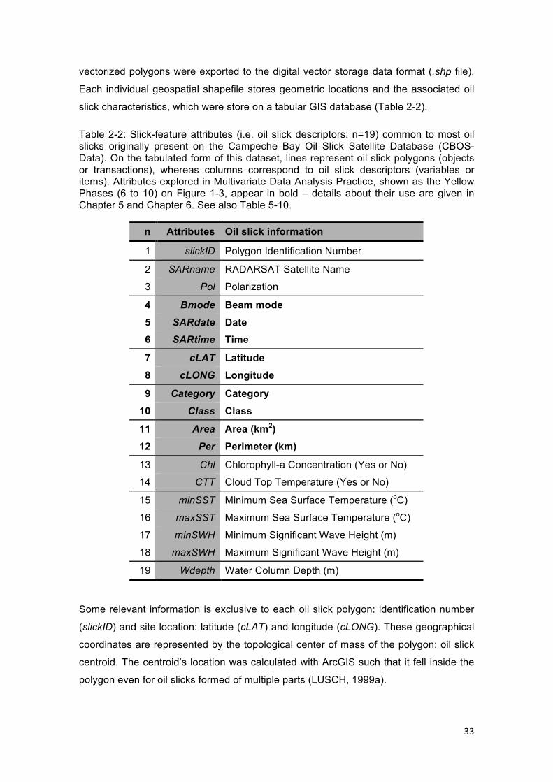
33
vectorized polygons were exported to the digital vector storage data format (.shp file).
Each individual geospatial shapefile stores geometric locations and the associated oil
slick characteristics, which were store on a tabular GIS database (Table 2-2).
Table 2-2: Slick-feature attributes (i.e. oil slick descriptors: n=19) common to most oil slicks originally present on the Campeche Bay Oil Slick Satellite Database (CBOS-Data). On the tabulated form of this dataset, lines represent oil slick polygons (objects or transactions), whereas columns correspond to oil slick descriptors (variables or items). Attributes explored in Multivariate Data Analysis Practice, shown as the Yellow Phases (6 to 10) on Figure 1-3, appear in bold – details about their use are given in Chapter 5 and Chapter 6. See also Table 5-10.
n Attributes Oil slick information
1 slickID Polygon Identification Number
2 SARname RADARSAT Satellite Name
3 Pol Polarization
4 Bmode Beam mode
5 SARdate Date
6 SARtime Time
7 cLAT Latitude
8 cLONG Longitude
9 Category Category
10 Class Class
11 Area Area (km2) 12 Per Perimeter (km)
13 Chl Chlorophyll-a Concentration (Yes or No)
14 CTT Cloud Top Temperature (Yes or No)
15 minSST Minimum Sea Surface Temperature (oC)
16 maxSST Maximum Sea Surface Temperature (oC)
17 minSWH Minimum Significant Wave Height (m)
18 maxSWH Maximum Significant Wave Height (m)
19 Wdepth Water Column Depth (m)
Some relevant information is exclusive to each oil slick polygon: identification number
(slickID) and site location: latitude (cLAT) and longitude (cLONG). These geographical
coordinates are represented by the topological center of mass of the polygon: oil slick
centroid. The centroid’s location was calculated with ArcGIS such that it fell inside the
polygon even for oil slicks formed of multiple parts (LUSCH, 1999a).

34
Particular information is retrieved from the satellite scene acquisition, such as the name
of the utilized SAR satellite (SARname) and the orientation of the transmitted and
received electric field (i.e. imaging polarization – Pol). The imaging configuration, as
defined by the swath width and ground resolution (i.e. beam mode – Bmode), and the
date (SARdate) and time (SARtime) of the SAR overpass are also given.
Only two basic variables of geometry, shape, and dimensions were accounted for: area
(Area) and perimeter (Per). These were calculated based on the identified target’s
vector shapefile (.shp file) that spatially represents each oil slick. Because most oil
slicks had multiple parts, these two attributes were estimated for the individual
elements and then added up. These were also computed with ArcGIS.
Considering the regional context (i.e. on the scale of the satellite image frame), some
information was obtained through the examination of the ancillary meteo-
oceanographic geophysical parameters (i.e. MetOc-Kit: Chl, CTT, SST, and SWH –
see Section 4.5.5). When the respective EOS scenes were available, the presence, or
not, of Chl and CTT were entered as discrete attributes: Chl and CTT. In addition, SST
and SWH were annotated in a qualitative manner: minimum and maximum values for
the SAR frame are logged (minSST, maxSST, minSWH, and maxSWH).
Another contextual attribute was provided: water column depth (Wdepth). This is
measured in meters for the location of the oil slicks’ centroid.
2.3.6. CBOS-SATPRO PART 6: PEMEX VALIDATION
On the CBOS-SatPro, the domain specialist’s interpretations were taken as the
reference for determining whether the oil slick was related to a seep or spill, as well as
to decide their class (i.e. Cluster, Brightspot, Ship Spill, Orphan Seeps, or Orphan
Spills). This type of operator-dependent analysis, as any manual inspection of satellite
images, can incur errors associated with uncertainties from the interpretation of various
operators (BREKKE & SOLBERG, 2005a; 2005b).
Even though a range of analysts entered information to the CBOS-Data for more than a
decade, a vital post-processing occurred after each SAR image was analyzed (Figure
1-3: CBOS-SatPro Part 6). Individual reports were delivered to PEP, and on this
protocol, a representative of MDA-GSI within Pemex’s office validates every decision of
the operators: approving, or not, whether the selected oil slicks were correctly
categorized and/or classified (Figure 2-3).

35
This validation was mostly based on internal field reports from the environmental
RMNE operational team, and, when necessary, additional direct field observations
were taken. Usually, the communication practice of this validation process occurred as
soon as possible after the SAR image analysis was completed.
If by any chance there was any incongruence between the SAR interpretation and the
Pemex Validation, a technical debate, involving the operator analysts and the MDA-
GSI representative, took place to resolve whichever difference might persist. If the
operator’s interpretation was found inconsistent with the field observation, the initial
analysis was adjusted to match the validated result.
At the end, the final outcomes of the CBOS-Data were kept as close as possible to the
actual oil slick characterization observed in the Campeche Bay region. Consequently,
the operator’s interpretation of the SAR images were taken as the baseline determining
the occurrence, or not, of oil slicks, as well as its category (i.e. seep or spill) and class
(i.e. Cluster, Brightspot, etc.).
This information is taken as a proxy of what is often termed “sea-truth”. Even though
such “absolute truthing” may incur errors (e.g. analyst interpretation), once the Pemex
Validation was configured and reported back, it validated the CBOS-Data that became
the foundation of the data mining performed on the present analysis.

36
CHAPTER 3
BLACK GOLD
Fossil fuels energy is enormously important in many facets of our contemporary global
society. Ever since the first oil wells were explored in the second half of the 19th
century, nearly all of the commerce, manufacturing and other types of businesses have
been dependent upon substances derived from refining and processing crude oil or
natural gas – such as gasoline (petrol), jet fuel, diesel, lubricating oil, kerosene,
naphtha, paraffin, wax, asphalt, tar, bitumen, polishes, solvents, sulfur and many
petrochemicals (NRCC, 2003). The byproducts list is vast and includes plastics
(ethylene and propylene), rubber, fertilizers, insecticides, detergents, roofing,
antifreeze, antiseptics, vitamin capsules, medicines (e.g. Aspirin), toothpaste,
deodorant, shampoo, fibers (e.g. nylon and polyesters), clothes, umbrellas, surf
boards, dog leashes, among many other goods of our everyday usage (NRCC, 1985;
and reference therein).
In some capacity, our food, medicines, comfort, entertainment, transportation, personal
devices, appliances, equipment, and machinery rely, at least partially, on fossil fuels as
prime substances for production, transport, or power. Moreover, fossil fuels are part of
the reasons for many political and military conflicts among nations in the world, thus
reflecting in the lack of peace in some regions (GATELY, 1986; GERGES, 1993;
CASCIELLO et al., 2011; ORNITZ & CHAMP, 2002).
In one-way or another, most of our everyday lives are related to the OGEPI (BOESCH
& RABALAIS, 1987). However, the worldwide society’s dependence of this dominant
non-renewable form of energy can pose an eminent risk of HC contamination
(SCHOLZ et al., 1999).
Releases of petroleum can be acute or chronic, occur in large amounts from
catastrophic accidents or slowly discharged on sporadic incidents, all of which can
considerably impact the environment and be lethal to animals, plants, and entire
ecosystems (NRCC, 1985). Damaging ecological impacts tend to worsen as the
industrialized nations, as well as developing countries, increase the demand for fossil
fuels.

37
3.1. WEATHERING PROCESSES
Immediately after being exposed to the environment, the composition and the
characteristics of oil rapidly and continuously change over time (ITOPF, 2015b).
Simultaneously occurring with changes in biological properties (such as those caused
by phyto-oxidation and bacterial degradation), other processes also affect the oil during
their lifetime in the environment, promoting evaporation, dissolution, emulsification,
oxidation, photo-oxidation, photolysis, flocculation, sedimentation, etc. (NRCC, 2003;
BATISTA NETO et al., 2008). These processes alter the oil physicochemical properties
and are collectively termed as weathering processes26 (BOYD et al., 2001).
Nonetheless, the most important weathering process acting over oil slicks once the oil
reach the surface of the ocean is linked to the air-sea interaction: meteorological (e.g.
wind, precipitation, etc.) and oceanographic (e.g. surface current circulation, waves,
etc.). These environmental conditions act as natural dispersants capable of influencing
superficial mixing, dispersion, spreading, advection, and drift of oil slicks.
Weathering processes also influence the oil slick detectability at sea surface with
satellite data. Knowledge of meteo-oceanographic conditions of each oil slick scenario
is a crucial requirement as it has a major control on the persistence and extension of
such features (ESPEDAL & WAHL, 1999). Indeed, the characterization of an individual
oil slick should include information on recent and past weather conditions (CALABRESI
et al., 1999; SINGHA et al., 2013).
There are two other important aspects to consider regarding the relationship between
oil and the marine environment:
1. The overall degree of negative effects is not always a function of the distance of
the oil-released source; and
2. The spilled amount of oil (i.e. its volume) is not always a measure of major
ecological concern.
Outsized events are not necessarily the most environmentally devastating ones. As a
further matter, the size of the impact caused is also dependent on the use of chemical
dispersants, oil skimming, and oil waste collection (ORNITZ & CHAMP, 2002). When
systematic burning of slicks containing large amounts of oil comes into play,
complicated environmental scenarios are created (EOE, 2010a, 2010c).
26 Weathering processes cartoon: http://www.nbcnews.com/id/37517080/ns/disaster_in_the_gulf

38
The nature of the liquid petroleum should not be ignored, as petroleum can vary in
density, viscosity, and solubility in seawater. The mass of a given volume of oil is
identified through its density, and in actual fact, the reason why oil floats on water is
because it is less dense. While light oil is lost to evaporation, as it degrades more
quickly, the remaining heavier fraction resists longer to weathering processes (NRCC,
1985). Light and heavy oil are classified based on American Petroleum Institute (API27)
gravity unit (VILLALÓN, 1998; LAMMOGLIA & SOUZA FILHO, 2012). A factor to notice
when dealing with oil at sea is the fluid's resistance to flow, i.e. viscosity. Fractions with
higher viscosity usually weather slowly and are carried for longer distances,
consequently building up thicker deposits that can persist for decades (ESSA et al.,
2005). Another applicable concept is solubilization – i.e. the quantity that measures the
molecular dissolution of oil in water. This is directly related to toxicity levels of different
oil slicks (HOSTETTLER et al., 1999; NRCC, 2003).
The fate and behavior of oil slicks are influenced by specific characteristics that depend
upon rate, duration, time of year, and site location. To this matter, the construction of
maps with Environmental Sensitivity Index (ESI28) is a common practice for evaluating
regions for their exposure and sensitivity to oil spillages (NOAA, 2002; ANDRADE &
SZLAFSZTEIN, 2012). This ranking aims to categorize locations of main ecological,
social, and economic concerns based on the spatio-temporal occurrence of animals
and plants, their habits, biological and human resources, archaeological, historical,
residential, recreational and cultural areas (JENSEN et al., 1998; IPIECA, 2012).
3.2. NATURAL HYDROCARBON SEEPAGES AT SEA
The whole HC seepage process is typically recognized to start whenever HC migrates
upwards from the source rock or from subsurface reservoirs through strata pores or
fissures (CLARKE & CLEVERLY, 1991). Subsequently, just like water in freshwater
springs, liquid or gaseous HC naturally ooze out of the underground (GER et al., 2002;
LEIFER & WILSON, 2004). If happening on the ocean, although oil and/or gas plumes
are formed on the water column, it is only when oil reaches the sea surface that an oil
seep can be observed with satellite measurements (MACDONALD et al., 1993; 1996).
As stated on preceding Chapters, the present D.Sc. research exclusively takes into
consideration the footprint signature of liquid HC (i.e. mineral oil) observed on the sea
surface – i.e. oil seeps (see Section 2.3.4).
27 API measures of how heavy or light liquid petroleum is compared to water. 28 ESI: http://oceanservice.noaa.gov/facts/esimap.html

39
As with rivers, the HC seepage processes do not occur everywhere in the world. Once
in the water column after escaping from the seafloor, individual proportions of HCs
behave differently. While the light fraction may dissolve and the heavier disperse, some
of the oil that arrives at the sea surface volatize, spread away or concentrate in clumps
forming an oil seep – the same are observed acting on oil that leaks from OGEPI
facilities, i.e. oil spills (see Section 2.3.4).
The U.S. National Research Council (NRCC, 2003) and the Woods Hole
Oceanographic Institution (WHOI, 2015) both revealed that almost half of the
petroleum annually entering the world’s oceans is attributed to natural seepages – see
Section 3.3. Because of this large amount, it is anticipated that the resulting
environmental impact should be extremely deleterious. On the other hand, most of this
oil slowly seeps out of the seafloor as sporadic releases at specific locations. Because
the HC seepage process usually persist over a very long period of time with low rates,
they can foster a local balance in which chemosynthetic organisms, ranging between
microbes to larger creatures, are able to reach an acclimation balance (NRCC, 1985).
For instance, the exposure to concentrations of HCs above background levels make
possible for successive generations of organisms to adapt, even feeding on HCs,
forming developed ecosystems around natural seepage sites (SPIES & DESMARIS,
1983; MONTAGNA et al., 1986; 1989). Therefore, the surrounding environment and/or
local communities where HC seeps out of the ground may be considered as a natural
laboratory for understanding how geologically-leaked gas or liquid petroleum behave
on the environment (MACDONALD et al., 2010). Because these ecosystems usually
host chemosynthetic communities, such locations can also assist with the
comprehension of marine life’s ecological response to the introduction of oil
contaminants (SPIES & DAVIS, 1979; DAVIS & SPIES, 1980). Yet, HC seepage sites
indicate the existence of present-day HC generation and migration; therefore, they are
important features to be considered in OGEPI exploration studies in offshore
sedimentary basis (CLARKE & CLEVERLY, 1991; ABRAMS, 1996).
Several strategic OGEPI fields are concentrated alongside oil seepage locations
(GARCIA et al., 2009; CSBPD; 2015). Around these areas, it is not rare for naturally
released oil to be mistakenly attributed to man-made oil spills from platforms, oil rigs,
ships, tankers or pipelines – the opposite also holds true (PEMEX, 2013b). OGEPI
members and societal stakeholders are continuous looking forward to reducing
ambiguous reports regarding oil spillage and/or oil seepage (SENGUPTA & SAHA,
2008). This has motivated the development of more accurate detection techniques for

40
responsive systems that can support in situ data collection (e.g. BENTZ et al., 2007a;
2007b; 2007c; 2012; SHCHERBAK et al., 2008; DASSENAKIS et al., 2012).
Usually, when oil is observed on the sea surface within the same area and is captured
by satellite imaging in different scenes during several years, there is a strong indication
of a persistent source on a nearby location (MACDONALD et al., 2002). However, this
repetitiveness may not always occur as vents comprising a seepage complex can get
blocked because of environmental or geologic factors (SENGUPTA & SAHA, 2008).
The petroleum reservoirs from where the oil may be seeping may not be directly
beneath the observed site on the sea surface (TRASHER et al., 1996). In fact, if an oil
seep occurring at deep waters is observed on the sea surface, its origin at the seafloor
may be situated tenths of kilometers away (MIRANDA et al., 1998).
Geologists and geophysicists are aware that wherever oil on the sea surface is
identified as coming from an oil seepage site, instead of an OGEPI installation, it is an
indication of the existence of active oil migration routes signifying possible HC active
source rocks in the vicinity (STANKIEWICZ, 2003; LEIFER et al., 2006; 2010; USGS,
2015). As pointed out in Chapter 2, OGEPI activity in Campeche Bay originated from
the discovery of the Cantarell Oil Seep. Perhaps, remarkable achievements in
discovering new HC accumulation areas may be possible if satellite measurements are
distinguish oil seeps from oil spills (ESSA et al., 2005).
It is reasonable to assume that if a system capable of recognizing the oil slick type
becomes available (i.e. seeps are distinguishable from spills), data assimilation in
mathematical models for forecasting or hindcasting oil trajectories based on numerical
simulations of ocean currents will potentially be more accurate (OLASCOAGA et al.,
2008; DIETRICH et al., 2012; OLITA et al., 2012). This is indeed one of the objectives
of the present D.Sc. research: design an innovative classification algorithm to
distinguish natural from man-made oil slicks using satellite-derived measurements.
3.3. OIL AND GAS EXPLORATION AND PRODUCTION INDUSTRY (OGEPI)
OGEPI activities are site-specific but their locations vary temporally and geographically.
At sea, most activities occur close enough to the shoreline to cause inevitable
damages to sensitive coastal habitats if oil is released during extraction, transportation,
refining, storage, distribution, or consumption (NRCC, 1985). Operational, accidental,
illicit, or intentional releases are diffuse, varying in frequency, location, and intensity.

41
HCs leakages are notorious for causing toxic effects ranging between the cellular level
to individual organisms (NOAA, 2013). Even a small amount of oil can cover a wide
area of several hundred meters (MIRANDA et al., 2004). Indeed, oil spills can
contaminate coastal marine environments and cause serious threats to entire
communities, populations, and ecosystems (NRCC, 2003).
Anthropogenic oil releases to the marine environment are frequently related to
accidents with oil rigs or ships, pipeline rupture, deliberate oil-contaminated ballast and
oily water discharge, disposal of what is termed as produced-water, oil-bearing cuttings
from drilling process, underwater blowouts, etc. (BENTZ & MIRANDA, 2001a; 2001b;
GARCIA et al., 2009; NEUPARTH et al., 2012). Because of continuing OGEPI activity,
HC releases into the environment are most likely to persist. Historically, major HC-
related disasters (e.g. Ixtoc-1, Exxon Valdez, Deepwater Horizon, etc.) draw attention
and raise the awareness of the public surfacing political, economic, ecological, and
scientific concerns (LEIFER et al., 2012). Over time, this perception tends to transform
local and international policies, hence reducing the frequency of accidents.
In 1979, the Campeche Bay experienced the blowout of an exploratory oil well, in
which oil from the Ixtoc-1 platform, operated by Pemex, leaked into the Gulf of Mexico
waters for more than 9 months (NOAA, 1980; 1981). The Ixtoc-1 disaster is ranked as
one of the world’s largest unintentional and peacetime oil spill event in history
(JERNELOV & LINDEN, 1981a; JERNELOV, 2010). It still calls the attention of the
media29 and of the scientific community as tar mats observed more than 30 years
later30 have been related to it.
An incident that attracted wide publicity because of severe ecological consequences
occurred in 1989, when the oil tanker Exxon Valdez grounded on the coast of Alaska
caused a major and destructive oil spill (MONSON et al. 2000; EOE, 2010d). Patches
of the Exxon Valdez oil were reported a decade later (HOSTETTLER et al., 1999).
Another example of oil persistence in the environment is shown by ESSA et al. (2005):
the collision of two super tankers 17 km offshore the United Arab Emirates in 1994.
Photos taken nine years later show the longevity of the spilled oil even after rigorous
beach clean-up procedures were applied.
29 Ixtoc disaster: http://www.harteresearchinstitute.org/ixtoc-i-and-oil-spill-resources 30 Ixtoc Expedition 30 years later: http://ixtoc1expedition.blogspot.com.br

42
A recent catastrophe that caused enormous environmental damage occurred in 2010.
The explosion and sinking of the Deepwater Horizon31 drilling oil rig, owned by
Transocean Ltd. (leased by BP, former British Petroleum), occurred less than 100 km
southeast of the Mississippi River in the northern Gulf of Mexico: Macondo Prospect
(EOE, 2010c; MACDONALD, 2010). This was accompanied by an oil well rupture at
the seafloor that leaked for about 4 months (INNMAN et al., 2010; DEL FRATE et al.,
2011).
The Office of Response and Restoration within the Emergency Response Division of
the National Oceanic and Atmospheric Administration's (NOAA) maintains a website32
that presents a myriad of oil spillages since the mid-1950s. It includes scientific articles,
news, photos, and site location of the most significant worldwide oil incidents. Other
similar sources are also found in the World Wide Web – e.g. a summary of the OGEPI
operations in the Gulf of Mexico Outer Continental Shelf region33.
Notwithstanding the numerous accidental oil spill episodes, it was after armored
divisions of the elite Iraqi Republican Guard of the dictator Saddam Hussein invaded
Kuwait, with subsequent USA-led coalition’s military offensive campaign to expel Iraqi
forces out of Kuwait, that the world saw an unprecedented amount of oil and
combustion products been intentionally released to air, land, and water (READMAN et
al., 1992). One of the major consequences of the “Gulf War” (1990-1991) was the
considerable quantity of crude oil that reached the coasts of Kuwait, Bahrain, Qatar,
United Arab Emirates, Oman, but mostly on Saudi Arabia (JONES et al., 1998). The
exact volume of strategic wartime petroleum purposefully dumped by Iraqi forces on
the Persian Gulf is difficult to determine but it is recognized as the largest oil spillage
disaster ever reported (MPB, 1993).
Many essential components ensuring compliance of safety standard protocols have
been agreed upon precautionary marine protection legislation (OGC, 2015). Several
actions have been taken to reduce environmental problems, ranging from coastal patrol
vessels, stringent environmental planning, enhanced contingency strategies, rigorous
regulations limiting operational spillage, new tanker design with partitioned
compartments or double hulls, etc. (IMO, 2010; IPIECA, 2015). Requirements for 31 NASA Earth Observatory: http://earthobservatory.nasa.gov/Features/OilSlick/ 32 NOAA Emergency Response Division: http://incidentnews.noaa.gov 33 Bureau of Ocean Energy Management, Regulation and Enforcement (BOEMRE): http://www.boemre.gov
43
ballast-water exchange when well out to sea, as well as strict law enforcement against
tank-washing discharges, lengthen the list of international regulations to reduce oil
impact in coastal regions. A procedure only allowing very small oil quantities (15 parts
per million) to be released at sea have been established: International Convention for
the Prevention of Pollution from Ships, 1973 as modified by the Protocol of 1978
(MARPOL 73/78). However, this is deceptively achieved by mixing oil with water (i.e.
bilge water), as the flow of oily water discharged at sea is not regulated (EPA, 2008).
Despite the OGEPI’s policies to reduce accidents, ineffective safety inspection
practices, malfunctioning equipment, aging installations and offloading operations can
cause environmental danger to nearby locations (NRCC, 1985; 2003). Another hazard
can emerge from increased supertanker traffic and broadening of major shipping routes
(ESSA et al., 2005). Together with extensive pipelines and conscious, but negligent
and/or illegal, sludge discarding from OGEPI installations and/or ships, these can all
bring risks to locations far from major OGEPI fields with reduced or no means to react
to oil contamination. Additional oil input to the sea comes from the human consumption
activities. These mostly occur on land and are carried to the marine environment via
urban runoff, wastewater, and rivers. Two-stroke boat engines, recreational and non-
tanker vessels are also significant sources.
Accordingly to NRCC (2003), the outcome of HCs released into the marine
environment can be separated into three different input types: production processes,
routine transportation, and consumption. Nonetheless, a non-anthropogenic input type
is the oil naturally coming from oil seeps. It is important to have an overall estimate of
the fossil fuel input. Yet, drawing an accurate assessment is somewhat complex.
For instance, in 1975, the U.S. National Research Council has estimated that an
annual average of 6,100,000 metric tons (~1,785 millions of gallons) of HCs were
released to the world’s oceans. However, a decade later, in 1985, the same agency
estimated a worldwide volume of about 3,200,000 metric tons (~935 millions of
gallons), and in their latest report, in 2003, the total load dropped to 1,300,000 metric
tons (~380 millions of gallons). Rather than an actual reduction, these long-term
changes are attributed to better measurement technologies and better estimation
techniques. Using their latest global estimates, 3% are recognized as coming from the
production processes, 12% from routine transportation, and 37% from human
consumption activity; the remaining 48% is related to natural HC seepage sources
(NRCC, 1985; 2003).

44
CHAPTER 4
SATELLITE REMOTE SENSING
The basis of remote sensing techniques lies in the acquisition of data (e.g. radiance)
about a target (e.g. ocean surface) without direct contact, thus having the collector (e.g.
satellite sensor) located at a certain distance of the observed target34. In Earth
Sciences, the remote sensing of the environment is usually performed with the
assistance of mechanical devices onboard aerial platforms such as helicopters,
airplanes, or satellites. The so-called remote sensors measure and record the
electromagnetic energy that is emitted, reflected or scattered from different targets
(LUSCH, 1999b; CLARK & RILEE, 2010). For instance, in the Oceanography field this
could easily be pictured as an oil slick detected with sensors onboard satellites
(SOUZA, 2009).
In fact, regarding the subjects particularly related to the lithosphere, biosphere,
cryosphere, hydrosphere, and atmosphere, satellite remote sensing measurements are
a valuable way of effectively documenting conditions over large areas, regions short of
in situ observations or inaccessible locations (NOVO, 1998). The use of satellite
sensors to monitor marine ecosystems is especially useful when dealing with recurring
phenomena that normally occur on the sea surface (GADE & ALPERS, 1999).
4.1. BEFORE THE SATELLITE ERA
For much of the last century, the bulk of the oceanographic investigations were
conducted with direct field sampling methods35. Although this way of data collection is
still largely used on environmental monitoring, traditional oceanographic surveys
involving direct field sampling are time-consuming and ship-time for deployment and
recovery operations have high operational costs (PRANDLE, 2000). Two different
reference viewpoints frames – Eulerian (i.e. moorings that are fixed in space) and
Lagrangian (i.e. drifting buoys that follow a tagged fluid parcel in time) – are extensively
used to study ocean processes (PICKARD & EMERY, 1996).
34 Remote Sensing Tutorial: http://www.crisp.nus.edu.sg/~research/tutorial/rsmain.htm 35 Portal NOAA CoastWatch: http://coastwatch.noaa.gov

45
Most monitoring programs that solely rely on field sampling have a spatial and temporal
bias. The weather is a major adversity for classical oceanographic surveillance
systems, in which favorable conditions are frequently required for data collection
(BROWN et al., 1997). In situ sampling efforts establish discrete and non-uniform
coverage with data stations that are not so often revisited. Visual observations from
boats, helicopters and airplanes are limited to daily observations and mostly dependent
on visual inspection capabilities. This sparse coverage creates considerable data gaps
that may prevent some conclusions to be drawn (SCHOFIELD & GLENN, 2004).
The inadequacy of acquiring in situ measurements on large areas constrains the use of
such methods in many cases and the ability to locate and track surface ocean features
incurs a considerable amount of work (DICKEY, 1991). This may inhibit the complete
observation of several phenomena (e.g. oil slicks, oceanic front, eddies, phytoplankton
blooms, offshore outflow of river plumes, etc.) and, as a result, many questions
regarding such processes have long remained unanswered (DIETRICH et al., 1980).
After the inception of spaceborne sensors, about forty years ago (LUSCH, 1999b), a
myriad of high-quality ocean-related studies has been accomplished (e.g. ROBINSON
& MITCHELSON, 1983; DENMAN & ABBOTT, 1994; SMYTH et al., 2003; YODER &
KENNELLY, 2006). However, even though satellites can provide a synoptic view of
numerous problems and many ocean features, they are not capable of replacing field
sampling, especially in circumstances requiring the study of depth-dependent
processes (STEWART, 2008). Nevertheless, if conventional ground sampling
techniques and satellite measurements are employed complementary, supplementary,
and supportively, several advances can be made in the management of surveillance
systems, early detection, environmental monitoring, law enforcement and
oceanographic science (GOWER, 2004; MCHUGH, 2009; TUFTE et al., 2004;
DASSENAKIS et al., 2012).
4.2. BASIC CONCEPTS OF SYNTHETIC APERTURE RADAR (SAR)
Many efforts of using SAR sensors are described showing a wide range of
oceanographic applications, for example, flood mapping, underwater bottom
topography, ship traffic monitoring, oil slicks reconnaissance, etc. (BIRK et al., 1995;
ROKOSH, 2000; VAN DER SANDEN, 2004). This Section offers to the reader a
summary of SAR theoretical concepts in language accessible to non-oceanographers,
as well as a didactic discussion on the advances in using SAR for environmental
monitoring focused on detecting oil slicks.

46
Radars are ranging instruments, i.e. account for the time elapsed between the
transmission of the signal and the reception of the returned signal (MCCANDLESS &
JACKSON, 2004; DPI, 2015). SAR is an active microwave-imaging sensor with its own
illumination source that measures the strength and time delay of the returning signal
(STEWART & LARSON, 2000). SAR measurements are independent of weather
conditions and can be operated during days and nights. Images created by SAR
systems are anisotropic, i.e. have different ground resolutions along (azimuth direction)
and across (range direction) the flight path (MARTIN, 2004; TRIVERO & BIAMINO,
2010). BUONO et al. (2015) present an extensive review of single-, co-, partially-, and
full-polarimetric SAR capabilities to detect oil slicks on the surface of the ocean.
The high dielectric constant36 of water causes microwave radar beams not to penetrate
in the sea surface (LUSCH, 1999c; HOLT, 2004). In association to that, it is well known
that oil films on the sea surface increase the top layer viscosity, which cause the
surface roughness of the water to decrease (NRCC, 2003). Smooth seas drastically
reduce the return signal, i.e. electromagnetic backscattering energy that characterizes
the Bragg scattering mechanism (HOVLAND et al., 1994; TRIVERO et al., 1998).
Active microwave radars (e.g. SAR) can detect changes in surface tension, and, as a
matter of fact, many investigations have focused on studying dark zones observed (i.e.
areas of reduced radar backscatter) in high-resolution SAR imagery (e.g. CALABRESI
et al., 1999; SOLBERG et al., 1999; LIU et al., 2011).
Unfortunately, and in principle, oil is not the only factor capable of smoothing the sea
surface, i.e. dampening out capillary waves and/or suppressing short gravity waves
that are only a few centimeters in length (MARTIN, 2004). SAR’s ability to detect
surfactants is strongly limited by several environmental conditions (e.g. low wind,
upwelling zones, etc.) that also modulate the surface roughness (STAPLES &
HODGINS, 1998). In addition, SAR detects the surface manifestation of some man-
made activities (e.g. ship wake, etc.) that cause the same type of response as oil
(MCHUGH, 2009). Just like oil slicks, look-alike features also appear darker than
surrounding water and this is caused by the lower microwave backscattering response
of such sea surface features (TRIVERO et al., 1998; DIGIACOMO & HOLT, 2001).
While the different dark features observed on SAR images are either oil slick
candidates or look-alike features, some of these ambiguities are not necessarily difficult
to distinguish from actual oil slicks, for instance, particular shape characteristics, 36 Dielectric constant is the ratio between any substance permittivity to the free space permittivity and influences the incident radar beam reflection, abosortion, and dissipation (ONSTOTT & SHUCHMAN, 2004).
47
distinct environmental configurations, or certain occurring weather-depend phenomena
(ESPEDAL, 1998; 1999). However, the differentiation between oil slicks and look-alike
features is not always straightforwardly achieved, as flawless models to identify oil
slicks are yet to be created (BREKKE & SOLBERG, 2005b). Recent studies have
investigated the polarimetric approaches to detect oil slicks in SAR images
(MIGLIACCIO et al., 2007; 2009a; 2009b; 2011a; 2011b; 2012).
Phenomenon that may cause other targets to be confused with the actual response of
oil slicks on SAR imagery are not addressed on the present D.Sc. research. Look-alike
features have not been taken into consideration during the CBOS-SatPro, as they were
filtered out of the CBOS-Data by experienced domain analysts (see Chapter 2).
An aspect to highlight while detecting oil slicks using SAR measurements is that the
knowledge of the wind speed is very important (CHRISTIANSEN et al., 2006). In low
wind conditions (< 2-3 m/s), oil slicks are not well distinguished from smoothened
ambient water, because little to no microwave energy is backscattered and dark
regions are formed all around in oil-free areas (BERN et al., 1993). In the lack of
backscattered energy reaching the SAR antenna that occur in the absence of wind, it is
often impossible to detect oil slicks. In other situations, under moderate wind speed
(approximately between 3 and 8 m/s) oil slicks appear darker in contrast with the
background radar signal of the surrounding water (STAPLES & HODGINS, 1998). At
high wind speed situations (> 8 m/s) oil slicks are spread away, dispersing or mixing
into the upper ocean and the resulting clutter makes its detection difficult (ALPERS &
HUHNERFUSS, 1989).
Despite the fairly narrow “ideal” wind speed range suggested in the literature to enable
oil detection on the sea surface, the nature of the oil and its thickness also play
important roles in the dampening of capillary waves on the ocean surface in SAR
imagery (ESPEDAL et al., 1998). Perhaps, in eventual cases, oil slicks may be
detected at wind speed up to 12 to 14 m/s (DIGIACOMO et al., 2004; LITOVCHENKO
et al., 1999). However, wind measurements are not considered on the research
presented herein.
Despite the advantages in imaging the world’s oceans surface for oil slick detection
(e.g. weather-independent, day-and-night coverage and a marine science toolset that
detect fine-scale texture of the sea surface), most SAR instruments present particular
limitations if compare to other meteo-oceanographic satellite sensors: cannot measure
true colors, restricted area coverage, long site-repeat intervals, and its relative high
operational costs that demand-specific collections. The concomitant use of SAR and

48
Earth Observing System (EOS) can, to some extent, increase the spatio-temporal
coverage of environmental monitoring surveys for detecting oil slicks (e.g. SIPELGAS
& UIBOUPIN, 2007; HU et al., 2009). To this end, it is desirable to explore other
sensors for detecting oil slicks, some of which are discussed in Section 4.6.
A number of satellite missions with SAR sensors are have been put in orbit over the
past decades providing commercial operational services, for example, COnstellation of
small Satellites for the Mediterranean basin Observation (COSMO-SkyMed37),
Environmental Satellite (Envisat38), European Remote Sensing Satellite (ERS39),
Japanese Earth Resources Satellite (JERS40), Phased Array type L-band Synthetic
Aperture Radar (PALSAR41), Radar Imaging Satellite (RISAT42), TerraSAR43, amongst
others44. The present D.Sc. research explores the Canadian RADSARSAT satellites:
RADARSAT-145 and RADARSAT-246 satellites (CRSS, 1993; 2004; MDA, 2004; 2014).
The RADARSAT SGF products explored during the CBOS-SatPro (see Chapter 2) are
generated with standard ground coordinate pixel dimensions of either 12.5m (for
operational beam modes of Standard, Wide, Extended Low and Extended High) or
6.25m (for Fine beam). The Standard beam mode swath width is 100 km wide, while
the one related to the Wide beam mode covers. Typical spatial resolutions are of the
order of 25 m – i.e. twice the pixel size (RSI, 1997; 1998). For the ScanSAR Narrow
and Wide beam modes, the nominal spatial resolution is, respectively, 50 m and 100 m
(Table 4-1 and Figure 4-1).
While all RADARSAT-1 beam modes only transmit and receive horizontally polarized
signals (HH), most RADARSAT-2 beam modes are able to generate a few single
polarimetric image products: linear parallel polarization (HH or VV) or linear cross-
polarization (HV or VH). Some RADARSAT-2 beam modes can generate dual parallel
and cross-polarizations (HH+HV or VV+VH) or even a full quad-polarized image can be
selected (HH, VV, HV, VH) (ALI et al., 2004a; 2004b; VAN DER SANDEN, 2004;
NRCAN, 2014).
37 COSMOS-SkyMed: http://www.cosmo-skymed.it/en/index.htm 38 Envisat: https://earth.esa.int/web/guest/missions/esa-operational-eo-missions/envisat 39 ERS: https://earth.esa.int/web/guest/missions/esa-operational-eo-missions/ers/satellite 40 JERS: http://global.jaxa.jp/projects/sat/jers1/index.html 41 PALSAR: http://www.alos-restec.jp/en/staticpages/index.php/aboutalos-palsar 42 RISAT: http://www.isro.gov.in/Spacecraft/risat-1 43 TerraSAR: http://www.geo-airbusds.com/terrasar-x/ 44 Earth Observation Portal: https://directory.eoportal.org/web/eoportal/satellite-missions 45 http://gs.mdacorporation.com/SatelliteData/Radarsat1/Radarsat1.aspx 46 http://gs.mdacorporation.com/SatelliteData/Radarsat2/Radarsat2.aspx

49
Table 4-1: RADARSAT-2 technical specifications. The radiometric depth of all RADARSAT beam modes is 16-bit. From: FOX et al. (2004).
Beam Modes Nominal Swath Width (km)
Spatial Ground Resolution (m) **
Approximate Incident Angles
Ultra-Fine 20x20 3x3 30ox40o Multi-Look Fine 50x50 8x8 30ox50o Fine 50x50 8x8 37ox49o Standard 100x100 25x26 20ox49o Wide 150x150 30x26 20ox45o ScanSAR Narrow * 300x300 50x50 20ox46o ScanSAR Wide * 500x500 100x100 20ox49o Extended Low 170x170 40x26 10ox23o Extended High 50x50 18x26 50ox60o Fine Quad-Pol 25x25 9x8 20ox41o Standard Quad-Pol 25x25 25x8 20ox41o * 8-bit in RADARSAT-1.
** Range x Azimuth.
Figure 4-1: RADARSAT-2 imaging modes. From: FOX et al. (2004).

50
4.3. RADARSAT RADIOMETRIC-CALIBRATED IMAGE PRODUCTS
The image format of the RADARSAT products varies between satellites. While
RADARSAT-1 images are stored in the standard CEOS format (Committee on Earth
Observation Satellites), RADARSAT-2 images have a specific data file structure based
on GeoTIFF imagery and encoded eXtensible Markup Language (.xml file) that
includes the SGF file (product.xml) and metadata files (i.e. lutSigma.xml, lutBeta.xml,
and lutGamma.xml).
Metadata of the data files from both RADARSAT satellites have an additional table
containing the incidence angle of the radar beam in the range direction. As shown on
Section 5.4, this table is used to derive an incidence angle image product to give the
satellite standpoint of view per pixel for individual oil slicks. Other supplementary
support files are also delivered together with the RADARSAT imagery, e.g. design
schema templates. The naming convention of the RADARSAT product files provided
by MDA-GSI is shown on Table 4-2 (GILL, 2010).
Table 4-2: Nomenclature of the RADARSAT products:
RS2_OK1111_PK2222_DK3333_Bmode_YYYYMMDD_HHMSS_PP_PTY.zip
RS2 Satellite Name Radarsat-2
OK1111 Order Key
PK2222 Product Key
DK3333 Delivery Key
Bmode Beam Mode e.g. SCNA, SCNB, WDE1, WDE2 or EXL1.
YYYYMMDD Acquisition Date Year (YYYY), Month (MM), and Day (DD)
HHMMSS Acquisition Start Time Hour (HH), Minute (MM), and Second (SS)
PP Polarization e.g. VV – transmits and receives vertically.
PTY Product Type SGF – SAR Georeferenced Fine
The SGF RADARSAT-2 products have three output scaling look-up-tables (LUTs)
supplied (i.e. metadata files) to calculate radiometric-calibrated SAR measurements,
whereby the uncalibrated grey-level count (i.e. Digital Number – DN) is directly related
to SAR-derived backscatter coefficients – i.e. sigma-naught (σo), beta-naught (βo), and
gamma-naught (γo) (MDA, 2011). The SGF RADARSAT-1 CEOS format only provides
a single LUT: βo (THOMPSON & MCLEOD, 2004).

51
SAR-derived backscatter coefficients represent the average radar reflectivity of the
target normalized by the unit area, i.e. normalized radar cross section47 (RCS: σ) (RSI,
1997; 1998). Quantitative measures of σo, βo, and γo correspond to the SAR
backscatter signature in different surface plane areas (AIRBUS, 2014b; EL-DARYMLI
et al., 2014; THAKUR, 2014; ASF, 2015), as explained (Table 4-3) and illustrated
(Figure 4-2) below.
Table 4-3: SAR backscatter coefficients that correspond to the SAR backscatter signature in different surface planes. These quantities are explored on this research.
Sigma- naught
(σo)
Normalized-RCS in the ground horizontal range plane. Sometimes referred to as scattering coefficient. Measure frequently adopted as the radar signal backscatter strength. Although its calculation depends upon the knowledge of terrain slope (not an issue on the sea surface) and the radar beam incidence angle, it is directly related to the target’s reflectance per unit area (i.e. pixel projected onto the ground). For this reason, scientists frequently use σo measurements.
Beta- naught
(βo)
Normalized-RCS in the radar’s line-of-sight (i.e. slant range). Sometimes referred to as radar brightness (or reflectivity) coefficient. Because it represents the reflectivity in the direction of the incident radar beam and is independent of the terrain slope, system design engineers generally prefer to use measures of βo.
Gamma- naught
(γo)
Normalized-RCS in the plane orthogonal to the slant range direction. It is the power returned to the antenna from the area orthogonal to the radar beam. This plane is uniformly distant from the satellite and has equal brightness from near to far range on the pixel level. In being so, measurements of γo are usually selected for antenna calibration purposes.
Even though DN values are enough for qualitative usage, such as the monitoring
implementation of the CBOS-SatPro that maps sea surface oil slicks, the use of DN is
not meaningful when comparing SAR images. For this reason, DN values are not
recommended to cross-compare time series of SAR images (FREEMAN, 1992; EL-
DARYMLI et al., 2014). Conversely, radiometric-calibrated SAR measurements (i.e. σo,
βo, or γo) are essential for quantitative analyses, as their use permits the comparison of
data acquired from the same sensor with different dates and beam modes, as well as
the evaluation of data acquired with various sensors (ESA, 2014).
47 RCS characterizes a reflectivity property of the reflected radar signal strength (i.e. scattering intensity) of any surface target (e.g. oil slick) in the direction of the radar receiver (i.e. antenna). It has a unit of m2 and is a function of sensor parameters (e.g. viewing geometry, radar wavelength, transmitted and received polarization, etc.), target’s properties (e.g. time, position dielectric constant, roughness, geometry, etc.), as well as of the terrain slope, etc. (HOLECZ et al., 1993).
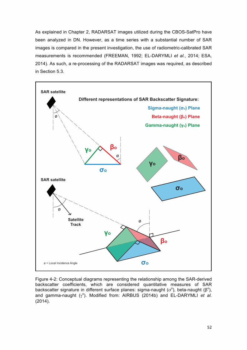
52
As explained in Chapter 2, RADARSAT images utilized during the CBOS-SatPro have
been analyzed in DN. However, as a time series with a substantial number of SAR
images is compared in the present investigation, the use of radiometric-calibrated SAR
measurements is recommended (FREEMAN, 1992; EL-DARYMLI et al., 2014; ESA,
2014). As such, a re-processing of the RADARSAT images was required, as described
in Section 5.3.
SAR satellite
SatelliteTrack
ø
ø
SAR satellite
ø
ø
γoβo
σo
Different representations of SAR Backscatter Signature:
Sigma-naught (σo) Plane
Beta-naught (βo) Plane
Gamma-naught (γo) Plane
σo
βoγo
ø = Local Incidence Angle σo
βo
γo
Figure 4-2: Conceptual diagrams representing the relationship among the SAR-derived backscatter coefficients, which are considered quantitative measures of SAR backscatter signature in different surface planes: sigma-naught (σo), beta-naught (βo), and gamma-naught (γo). Modified from: AIRBUS (2014b) and EL-DARYMLI et al. (2014).

53
The conversion of uncalibrated SGF DN values to radiometric-calibrated SAR-derived
backscatter coefficients (i.e. σo, βo, or γo) is achieved according to the following
expression:
C1 = [{DN2}+B]/A
While the constant offset (B) is nominally set to zero for SGF products, the gain value
(A) varies for each pixel in the range direction (MDA, 2011). Although the process to
calculate σo, βo, or γo is exactly the same, C1 depends upon the LUT choice (i.e.
metadata files: lutSigma.xml, lutBeta.xml, and lutGamma.xml) to obtain the
corresponding range-dependent gain values. These LUTs have only one gain listed for
each pixel in the range direction.
C1 is given in linear values of amplitude (Amp), or intensity (Int), of the radar return
signal received by the antenna system – their relationship is given by: Int=Amp2.
Therefore, if a log transformation is applied to C1, a dimensionless physical quantity
representing power is obtained (MDA, 2011). This is calculated as follows:
C2 = (10*cc)*Log10(C1)
where cc is equal to 1 for the intensity of the received radar beam and 2 for pixel
values given in amplitude. Regardless of the input being amplitude or intensity, C2 is
expressed in decibel units (dB).
In essence, the evaluation of σo, βo, and γo is similar among SAR sensors with different
specifications48, but their calculations vary somewhat from sensor to sensor; even
different RADARSAT products, i.e. Single Look Complex (SLC), have specific
calculations (LAUR et al., 1998; SHEPHERD, 2000; MDA, 2011; AIRBUS, 2014a;
2014b; IYYAPPAN et al., 2014; THAKUR, 2014). It is also important to distinguish
between the radiometric-calibrated SAR measurements explored herein (i.e. σo, βo, and
γo) and other SAR calibration methods49, for example, in-lab (e.g. chirp parameters), in-
orbit (e.g. lifetime instruments and parameters or gain changes), or external (e.g.
corner-cube reflector or geometric) (FREEMAN, 1992; FOX et al., 2003; JAYASRI,
2014; PADHYE & REGE, 2015).
48 TerraSAR-X Documentation: http://www.geo-airbusds.com/en/228-terrasar-x-technical-documents 49 SAR Calibration Workshop Proceedings: https://earth.esa.int/documents/10174/1597298/SAR26.pdf

54
4.4. DARK SPOT DETECTION IN SAR IMAGERY
Most oil slick detection monitoring systems follow a three-step framework: Digital
Image Classification (DIC), Feature-Extraction, and Feature-Classification (BREKKE &
SOLBERG, 2005b; GAMBARDELLA et al., 2010; SINGHA et al., 2013). While Figure
4-3 graphically represents such framework, this Section individually describes each
step. These steps are applied in tandem on SAR images, and can be fully either
automated, semi-automatic or manually operated. As pointed out in Chapter 2, the last
two steps have been inverted during the CBOS-SatPro and the slick-feature attributes
are only calculated once the oil slicks are identified.
Feature-Extraction(Section 4.4.2 and Section 2.3.5)
Dark Spot Identification(Section 4.4.3 and Section 2.3.4)
Digital ImageClassification (DIC)
(Section 4.4.1 and Section 2.3.3)
Look-alikeFeaturesOil Slicks
SAR Image
Figure 4-3: Typical three-step framework used to indentify dark spots in SAR imagery. During the Campeche Bay Oil Slick Satellite Project (CBOS-SatPro) the last two steps were inverted: slick-feature attributes were only calculated upon the identification of oil slicks (see Chapter 2). Adapted from BREKKE & SOLBERG (2005b).
4.4.1. DIGITAL IMAGE CLASSIFICATION (DIC)
The course of identifying oil slicks starts with the SAR imagery been digitally classified.
During the DIC, the image can be submitted to different procedures (e.g. deterministic
or statistic classification) that take into account some aspects of one, or two, sea
surface domains: radiometric and textural. This aims to discriminate regions with
smooth texture (i.e. low backscattering) from the rough sea surface background (i.e.
with diffuse backscattering). The former has a darker visual appeal than the latter.

55
Even though this defines two types of polygons (i.e. potential oil slick candidates and
look-alike features), at this stage there is not much certainty of which is which. Such
polygons are only identifying the presence, and its limits (i.e. borders), of dark spots in
the SAR image that are indicative of low backscatter response. Therefore, it is
essential to stress that every representative target, which may include oil slicks and
look-alike features, are flagged. As the polygons with smooth texture regions can be
yielded by several processes (HOVLAND et al., 1994; JOHANNESSEN et al., 1996;
HOLT, 2004; SENGUPTA & SAHA, 2008), the recognition of these targets is indeed
the purpose of the next two steps of the framework – explained in the next two
Sections.
Several studies have described a wide variety of image classification techniques: e.g.
user-defined or automatic adaptive threshold (MARONE et al., 1998; SOLBERG et al.,
1999; SHU et al., 2010; GANTA et al., 2002), hysteresis threshold (CANNY, 1986;
KANAA et al., 2003), Laplace or difference of Gaussian (CHANGE et al., 1996; HEN et
al., 1994), wavelets (WU & LIU, 2003), local variation of wave spectra (MERCIER et
al., 2003), mathematical morphology (GASULL et al., 2002), fuzzy clustering (BARNI et
al., 1995; FISCELLA et al., 2000), Artificial Neural Networks (ANN) (CALABRESI et al.,
1999; DEL FRATE et al., 2000; TOPOUZELIS et al., 2007; SINGHA et al., 2013),
among many others.
In the case of the CBOS-SatPro, the oil slicks observed in Campeche Bay and logged
on the CBOS-Data have been identified and classified after the use of the USTC
algorithm (ALMEIDA-FILHO et al., 2005). The USTC discriminates regions with
different backscattering based on the sea-surface radar textural (circular
semivariogram function shape and value) and radiometric (despeckled DN values
signatures). This classifier is described in Section 2.3.1 and further discussed in
MIRANDA et al. (2001; 2004). In addition, several studies are found demonstrating the
successful USTC applications in identifying oil slicks – e.g. BEISL et al. (2001), BENTZ
& MIRANDA (2001a; 2001b), RODRÍGUEZ et al. (2007).
4.4.2. FEATURE-EXTRACTION
Once the polygons are identified, several slick-feature attributes can be computed to
characterize each polygon, taking into account the information of the pixels within the
oil slick’s limits (MONTALI et al., 2006; TOPOUZELIS, 2008). Each oil slick is then
characterized either from the point of view of the satellite scene (e.g. incidence angle,
satellite beam mode, etc.), aspects related to the SAR-derived backscatter coefficient

56
(i.e. σo, βo, or γo), textural information (e.g. contrast), geometry, shape, and dimensions
variables (e.g. area, perimeter, etc.), and contextual descriptors (e.g. latitude,
longitude, bathymetry, etc.) features. Appropriate guidelines to acquire such
descriptors are a leading requirement for the success of any classification algorithm
(KUBAT et al., 1998; BREKKE & SOLBERG, 2005b).
Depending upon the line-of-attack of the investigation been executed, a range of
suitable slick-feature attributes arise to help the definition of criteria to discriminate oil
spills from look-alike features. However, as there is not a systematic Feature-Extraction
procedure, qualitative and quantitative statistical features are arbitrarily selected on
each of them – e.g. while COCOCCIONI et al. (2009) used 7 slick-features, PISANO
(2011) and TOPOUZELIS et al. (2007) used 10, CALABRESI et al. (1999), SOLBERG
et al. (1999) and DEL FRATE et al. (2000) used 11, FISCELLA et al. (2000; 2010) and
SINGHA et al. (2013) used, respectively, 12, 13 and 14, and BENTZ (2006) evaluated
40 different slick-features.
Some investigations describe the most common features, such as TOPOUZELIS et al.
(2009) and TOPOUZELIS & PSYLLOS (2012) that combine 25 of them: they used a
genetic classification algorithm and discovered that best results occurred with 10 slick-
features. While the handful of slick-feature attributes calculated during the CBOS-
SatPro are shown on Table 2-2, a comprehensive list of slick-feature attributes
explored on the present D.Sc. research is presented in Chapter 5.
4.4.3. DARK SPOT IDENTIFICATION
Oil slicks and look-alike features are classified based on descriptors – i.e. extracted
slick-feature attributes that characterize the polygons (i.e. identified targets). Hence, it
is in the Feature-Classification step that oil slicks are differentiated from other targets
capable of producing dark features in the SAR image which cause misidentification
issues on the analysis and interpretation for oil detection purposes (HOVLAND et al.,
1994; JOHANNESSEN et al., 1996; HOLT, 2004; SENGUPTA & SAHA, 2008).
Once the polygons are classified (i.e. identified as oil slicks), they are stored in a
geographical information system (GIS) to promote the spatial visualization of the oil
slicks (IVANOV & ZATYAGALOVA, 2008; LITOVCHENKO & IVANOV, 2008;
MOROVIC & IVANOV, 2011). This initiative can help with the identification of patterns
(or trends50) recognizable in the form of maps. On a tabular framework, each data entry
50 Physical Geography: http://www.physicalgeography.net
57
is sorted out in different events, in which the lines of this database represent
individualized oil slick polygons (i.e. objects or transactions) and the columns
correspond to the information used to characterize each oil slick polygon (i.e. variables
or items). Chapter 5 provides more information about ways to explore this type of
tabulated information.
A conversion from raster to vector polygons occurs after detecting such regions.
Alternatively, individual shapes that have contiguous pixels are grouped and then
individualized as polygons based on their SAR backscatter – this characterizes a
segmentation procedure.
Some environmental monitoring programs include on their database not only the oil
slick information, but also the look-alike feature attributes (e.g. BENTZ, 2006). This
intends to build a dataset capable of training classification algorithms to flag – i.e.
identify, and thus eliminate – features producing similar signatures in SAR imagery to
actual oil slicks (BREKKE & SOLBERG, 2005b).
Several ways to perform Feature-Classification are found in the peer-reviewed
literature (e.g. CALABRESI et al., 1999; SOLBERG et al., 1999; DEL FRATE et al.,
2000; FISCELLA et al., 2000; 2010; SINGHA et al., 2013). On the CBOS-SatPro, oil
slicks are manually identified by the careful interpretation of operators.
4.5. SATELLITE SENSORS IN SUPPORT FOR OIL SLICK DETECTION
This Section includes numerous aspects of a broad range of prevailing ancillary meteo-
oceanographic geophysical parameters used in support of oil detection. Despite the
individual limitations presented by each specific satellite system listed on this Section,
the complex approach of using combined spaceborne measurements from various
Earth Observing System (EOS) sensors with different resolutions makes it possible to
reduce the effects of their individual drawbacks (e.g. RORIZ, 2006).
4.5.1. VISIBLE/NEAR INFRARED (VIS/NIR)
Exactly because of the long site-revisiting interval of SAR satellites, the use of
additional satellite information with shorter revisit interval becomes an interesting and
advantageous strategy to monitor oil slicks on the sea surface (e.g. SIPELGAS &
UIBOUPIN, 2007). It is true that for environmental studies inspecting high temporal
variability processes (e.g. algal blooms, oil slicks, etc.), SAR images may be
inadequate depending on the scope of the monitoring program (e.g. BENTZ et al.,

58
2004). However, different from SAR imagery, the optimal use of visible/near infrared
sensors (VIS/NIR) for detecting and monitoring oil-contaminated areas are still under
evaluation (e.g. HU et al., 2009; CHEN & HU, 2014).
VIS/NIR that include ocean color sensors, have nearly daily coverage of most regions
on the globe. Nowadays, MODerate Resolution Imaging Spectroradiometer (MODIS;
SALOMONSON et al., 1989; ESAIAS et al., 1998), MEdium Resolution Imaging
Spectrometer (MERIS) and Visible Infrared Imager Radiometer Suite (VIIRS) are the
most utilized VIS/NIR sensors capable of providing a cost-effective supplementary tool
for environmental monitoring. Other sensors, such as the proof-of-concept Coastal
Zone Color Scanner (CZCS; HOVIS et al., 1980; EVANS & GORDON, 1994) that flew
from 1978 to 1986, and the more recently deceased (1997-2010) Sea-viewing Wide
Field-of-view Sensor (SeaWIFS; HOOKER et al., 1992; HOOKER & MCCLAIN, 2000;
MCCLAIN et al., 2004) are the heritage ocean color sensors of the National
Aeronautics and Space Administration (NASA).
One of the main characteristics of VIS/NIR sensors is the determination of a proxy of
chlorophyll-a on the sea surface. Chlorophyll-a maps can recognize regions with
phytoplankton activity and biological growth (GONZALEZ et al., 2000; GONZALEZ-
SILVERA et al., 2004). The knowledge of productive areas are relevant for the oil slick
detection processes as algal blooms on the sea surface can change the surface
roughness of the sea, thus misleading the search for oil in SAR images (BENTZ et al.,
2003; 2004; 2005).
MODIS acquires data in 36 spectral bands and images the Earth’s surface every 1 to 2
days (ANDERSON et al., 2003). Two distinct EOS mission satellites have the MODIS
instrument onboard: Aqua (EOS PM-1) and Terra (EOS AM-1). Of particular interest
whilst using the MODIS instrument is the relationship between the concomitant
acquisition of biological (e.g. Chlorophyll-a) and physical (e.g. Sea Surface
Temperature) variables that occurs with a large geophysical parameter library. This
sensor measures various inherent optical properties (IOPs) of the water (CARDER et
al., 1999) in nine different spectral wavelengths (λ = 412, 443, 488, 531, 551, 667, 678,
748 and 869 nm) ranging from particulate backscatter (bbp(λ)), total scatter (b(λ)),
phytoplankton absorption (aph(λ)), absorption of detritus and CDOM51 (adg(λ)), and total
absorption (a(λ)). MODIS also provides standard products such as water-leaving
radiance (Lw(λ)), normalized water-leaving radiance (nLw(λ)), remote sensing reflectance
51 CDOM: Colored Dissolved Organic Matter.
59
(Rrs(λ)), downwelling diffuse attenuation coefficient (K490) and fluorescence line height
(FLH).
It is important to highlight that oil slicks can be differed from actual seawater by some
characteristics (e.g. higher refractive index, higher absorption coefficient and higher
viscosity) that can influence the backscattered and reflected signals, hence providing
means for their recognition if using VIS/NIR (BULGARELLI & DJAVIDNIA, 2012). In
being so, the various MODIS-retrieved variables (i.e. Chl, IOPs and standard products)
have indeed the potential for detecting oil slicks (e.g. SIPELGAS & UIBOUPIN, 2007;
HU et al., 2009; CHEN & HU, 2014).
Even though VIS/NIR detect the reflected electromagnetic energy from sunlight, there
are situations in which the detection method applied to study oil slicks on the sea
surface using these sensors are similar to SAR principles (HU et al., 2003). These
occur because at certain viewing angles, more specifically at sunglint conditions, the
light reflected back to the sensor produces smoothed-like regions such as those
observed in SAR imagery (ADAMO et al., 2006; 2007).
In the absence of sunglint, the Lw can reflect the property of pure seawater areas, as
well as oily regions. The difference between the Lw of clear water and the Lw of oil-
contaminated regions can provide useful information that can be possibly used for oil
slick identification (BULGARELLI & DJAVIDNIA, 2012). The Rrs at 547 nm and 531 nm
are pointed out to be influenced by the particulate organic carbon and diffuse
attenuation coefficient of oil slicks (INNMAN et al., 2010).
Additionally, as different oil slicks present different colorations (BONN, 2009), the
spectral reflectance variation depends upon the oil chemical composition. ADAMO et
al. (2005; 2007) propose the use of MODIS band 2 (841-876 nm) and MERIS band 13
(855-875 nm) as the most sensitive bands (i.e. wavelengths) for extracting the spectral
properties of oil slicks.
Nevertheless, some limiting characteristics of using optical bands for environmental
monitoring should be pointed out. They are restricted by the need for solar illumination
and the requirement for cloud-free skies. As a result, VIS/NIR sensors only produce
meaningful measurements in the daytime. This is relevant because SAR images can
be acquired regardless of illumination, but SAR images acquired at night will not have
correspondent VIS/NIR data.
60
In addition, most VIS/NIR images have a coarse ground resolution of about 1 km at
nadir point. However, there are VIS/NIR imagers that acquire measurements with a
spatial resolution of approximately 250-300 meters (e.g. MODIS, MERIS), which is
practical for oil slick detection in the marine environment (GOWER et al., 2006).
4.5.2. THERMAL INFRARED (TIR)
Sensors working at the thermal infrared (TIR) portion of the electromagnetic spectrum
– also referred to as imaging radiometers – are suitable for retrieving Sea Surface
Temperature (SST) measurements. The oceanographic interpretation of SST maps
offers important information about ocean circulation pattern, for example, upwelling
zones, oceanic front, eddies, river plumes, urban runoff, wastewater, etc.
The most common sensor that retrieves SST information is the five channel Advanced
Very High Resolution Radiometer (AVHRR) installed onboard a series of NOAA
satellites. Another one is the Imager on the Geostationary Operational Environmental
Satellite (GOES).
A relevant issue to point out whilst using TIR measurements is the SST difference
between day and night observations, typically caused by diurnal heating and cooling
after nightfall. To avoid possible biases between day and night SST measurements,
CARVALHO et al. (2002; 2003a; 2003b) suggest splitting the SST dataset into daytime
and nighttime.
Furthermore, even a very thin cloud cover can interfere with the accuracy of SST
measurements. Because TIR cannot see the ocean surface in the presence of clouds,
another TIR application widely used is the location of clouds. The Cloud Top
Temperature (CTT) gives an idea of atmospheric fronts or heavy rain cells. These
atmospheric phenomena may be present at the time of SAR acquisition influencing on
the sea surface roughness, consequently causing misinterpretation on the oil slick
detection.
Depending upon the seawater composition, the absorption of sunlight can vary across
the sea surface, what can change the energy re-emission in thermal radiation
(MARTIN, 2004). Perhaps, the chemical composition of oil slicks can influence on SST
retrievals. Changes in emissivity are the possible cause for thick oil slicks appearing
hotter and oil slicks with intermediate oil thickness appearing cooler in TIR images
(FINGAS & BROWN, 2000). Indeed, ESSA et al. (2005) present satellite images
displaying oil slicks having lower SST than the surrounding clear water surface.
61
On the other hand, thin oil slicks can reach a thermal equilibrium with the surrounding
water preventing temperature differences to be noticed (YING et al., 2009). While
studying TIR imagery from the Deepwater Horizon incident, INNMAN et al. (2010) did
not find thick oil slicks capable of causing SST differences.
4.5.3. MICROWAVE ALTIMETER
Wave patterns and the sea state conditions are also important factors for oil slick
detection (PEDROSO et al., 2007). In calm seas, the radar backscatter signal can
better define an oil slick, if compared to rough sea conditions. Two satellite missions
acquire good-quality Significant Wave Height (SWH) measurements:
TOPEX/POSEIDON and Jason. Strong gradients found on SWH determinations can
result in sudden changes in local incidence angle values, affecting the SAR sea
surface response (RORIZ, 2006).
SWH are useful parameters in SAR interpretations, but not strictly applicable for the
present investigation. Satellite altimeters provide measurements only along the sub-
satellite track, which limits its usefulness while detecting oil slicks, as it requires oil
slicks to be directly beneath the satellite nadir to fulfill the prerequisite for matching
SAR measurements with the altimeter data. Chapter 5 presents more information about
the match-up analysis performed on the present D.Sc. research.
4.5.4. MICROWAVE SCATTEROMETER
The magnitude of the wind blowing over the ocean is a vital parameter for oil slick
detection (FALLAH & STARK, 1976). While the deceased QuikSCAT satellite used to
carry aboard the SeaWinds instrument, the EUMETSAT METOP satellites carry the
Advanced Scatterometer (ASCAT). Both sensors are all-weather microwave
measurements capable of providing near-surface data for the retrieval of wind
information.
Because of the spatial resolution of 25 km owned by this type of instrument, its
measurements may not be adequate for match-up analyses as the one performed on
the present investigation (see Chapter 5). However, wind vector retrievals from SAR
measurements may produce relevant information acquired at the moment of the oil
slick SAR image acquisition.

62
4.5.5. METEOROLOGICAL AND OCEANOGRAPHIC KIT (METOC-KIT)
As certain meteorological and oceanographic phenomena (e.g. low wind, upwelling
zones, etc.) express the same signature on SAR images as oil slicks (JOHANNESSEN
et al., 1996), satellite ancillary measurements can shed light on the differentiation of
targets that are actual oil spills from false targets (ESPEDAL et al., 1996; HOLT, 2004).
Within this perspective, the synergy of combining several sensors providing data in
accordance with such recognizable environmental features can assist with the
interpretation of dark spots present in SAR images.
As a result, improvements to OGEPI activities and to environmental monitoring can
both be achieved. SIPELGAS & UIBOUPIN (2007) discuss possible ways to distinguish
oil spills from false targets in SAR imagery off the coast of Estonia in the Gulf of
Finland. They use Chl and SST images from MODIS, as well as wind data from the
High Resolution Limited Area Model (HILRAM) to rule out the look-alike features. As for
the Cantarell Complex region, BEISL et al. (2001) and SILVA JUNIOR et al. (2003)
have both previously demonstrated the operational effectiveness of using meteo-
oceanographic satellite information in support to SAR imagery interpretation.
In fact, some retrieved products (e.g. wind, Chl, CTT, SST and SWH) acquired from
distinct EOS sensors (e.g. QuikSCAT, MODIS, AVHRR and TOPEX/POSEIDON) are
essential to aid in the selection and interpretation of SAR images (FINGAS & BROWN,
1997; BREKKE & SOLBERG, 2005a). To this extent, this collection of relevant meteo-
oceanographic ancillary information have been explored during the CBOS-SatPro in
support to the analyses of SAR images, as well as to provide environmental and
weather conditions at the closest time of the observed oil slicks scenarios. Herein, this
set of prevailing information is referred to as MetOc-Kit.
4.6. SATELLITE OCEANOGRAPHY
After introducing the spaceborne measurements acquired with EOS sensors, the
reader finds on this Section a general review of several remote sensing practical
applications that leverage such sensors.
Spaceborne sensors have long proved to be suitable for large-scale observation of
Earth’s ecosystems (NOVO, 1998). Remotely sensed data can, above all, be valuable
to detect, map, monitor and track oil before it reaches sensitive areas and becomes a
problem for animal and plant life. It has already been shown that remote sensors are a
valuable source of information to study ocean dynamics and monitoring trends in

63
ecological processes (JOHANNESSEN et al., 2000). Satellite oceanography lies on
global coverage. The vast amount of data produced by satellites provides the capability
of studying daily to periodic variability of large-scale phenomena with seasonal and
decadal temporal variability (GREGG & CONKRIGHT, 2001; 2002; MCCLAIN et al.,
2004; 2006). For instance, there are satellites (e.g. AVHRR/NOAA, GOES) capable of
assisting studies requiring a finer time-scale resolution, such as tracking ocean
currents or atmospheric circulation processes (BREAKER et al., 2000).
Indeed, the synoptic view provided by satellites offers the possibility to enhance
monitoring strategies and is capable of benefiting many societal stakeholders
(DIGIACOMO et al., 2004; INNMAN et al., 2010). Sensors varying in physical nature
(i.e. visible, infrared and microwave systems) have largely been explored and their use
covers wide applications (KOSTIANOY et al., 2006). As a matter of fact, near-real-time
surveillance provides successful services to trim down timelines to locate features at
the ocean surface such as oil slicks, shear current, upwelling, algal blooms, urban
runoff, wastewater, etc. (e.g. JOLLIFF et al., 2003; SMYTH et al., 2003; SOUZA, 2005;
Takahashi and Kawamura, 2005; CARVALHO et al., 2007; 2008; 2010a; 2010b;
2010c).
Nowadays, it is common to come across investigations using space technologies to
study oceanographic phenomena. For instance, CARVALHO et al. (2002; 2003a;
2003b) study the wind influence on Cabo Frio upwelling (23ºS/42ºW), in which the wind
has been acquired with QuikSCAT and the SST data with the AVHRR/NOAA. These
authors define a simple upwelling index that uses the area having SSTs ≤ 18°C and the
SST difference between the upwelling core temperature and the surrounding water (≥
18°C). SSTs of 18°C are about the warmer temperature of the South Atlantic Central
Water (SACW; CAMPOS et al., 1995; SILVEIRA et al., 2000), which is the water mass
upwelling in the Cabo Frio region. Significant Spearman correlation observed between
their simple upwelling index and wind data confirm that the upwelling intensity is
considerably influenced by the wind speed (>10m/s) and by the component parallel to
the shoreline 12h to 24h before each scenario.
Harmful algal blooms (HABs) are a major human health concern around the world’s
ocean (KUSEK et al., 1999). On the Gulf of Mexico, along the west Florida coast, most
investigations aiming to study the well know Florida Red Tide focus on in situ sampling
of laboratory experiments (e.g. MILLIE et al., 1997; MCLEROY-ETHERIDGE &
ROESLER, 1999; SCHOFIELD et al., 1999). However, CARVALHO et al. (2010d;
2011) survey this phenomenon performing a long-term pixel-by-pixel analysis (2002-
64
2006) using MODIS images. They introduce a satellite-based algorithm for the
identification of the main toxic alga, i.e. Karenia brevis, and compared it with two other
methods – i.e. CANNIZZARO et al. (2008) and STUMPF et al. (2003). Near-coincident
in situ samples provide the number of cells per liter (FWRI, 2002). After an optimization
procedure considering the optical characteristics of each method, the capabilities of
their algorithm and Cannizzaro’s technique are combined into a new hybrid algorithm
capable of enhancing the detection of such HABs.
Successful joint analyses are reported using several remote-sensing resources with
different resolution and coverage. This confirms the complexity of performing multi-
satellite assessment of biological and hydrodynamic surface oceanic features. For
example, SHCHERBAK et al. (2008) combine various EOS sensors with quasi-
concurrent measurements (i.e. MODIS from both Terra and Aqua satellites,
AVHRR/NOAA, Meteosat-8, QuikSCAT, TOPEX/Poseidon, Jason-1, Envisat
ASAR/MERIS and ERS-2) to study the oceanographic dynamics along the Russian
coast of the Sea of Azov and Black Sea. With an extensive campaign, exploring more
than 1100 images, eddies, coastal runoff outflow as well as anthropogenic and
biogenic oil are monitored, in which their summary map products consistently depict
the relationship between the coastal circulation and the pollutants’ evolution, transport
and drift.
Besides ecological phenomena, satellites play a vital importance in monitoring the
worlds’ oceans as they are extensively used to locate oil slicks on the sea surface
(FINGAS & BROWN, 1997; 2000; BREKKE & SOLBERG, 2005b). Previous studies
have shown that satellite measurements are effective in detecting oil slicks. While
STRINGER et al. (1989) visually interpret AVHRR/NOAA imagery of the Exxon Valdez
accident, ESPEDAL & JOHANNESSEN (2000) present a SAR image from the ERS-1
satellite illustrating the signatures of different surface features connected to offshore
OGEPI facilities on the British and Norwegian sectors of the North Sea that could be oil
related. Likewise, ADAMO et al. (2007) use SAR alongside MODIS and MERIS
imagery to explore the temporal resolution of the ocean color sensors in detecting oil
slicks.
Undeniably, the use of SAR imagery can, to some extent, present the position of oil
slicks by tracking its displacement (CLARK, 1993). Such ability is a valuable
mechanism for oil spill response efforts. Numerous implementations of operational
satellite-based surveillance for oil spill detection monitor different areas of world’s
oceans (e.g. North Sea, Norwegian Sea, and Baltic Sea), in which trained operators

65
process and interpret satellite images searching for oil signatures (e.g. TUFTE et al.,
2004; PEDERSEN et al. 1996; WAHL et al., 1996).
Yet, oil slicks do not have a particular or individual signature in satellite imagery. As a
result, specific ways to discriminate between oil slicks and ambiguous signatures are
the focus of many investigations. For example, ESPEDAL & JOHANNESSEN (2000)
discuss a Norwegian research effort of the Nansen Environmental and Remote
Sensing Center (NERSC) to discriminate man-made oil spills from look-alike features.
The main steps of the NERSC supervised discrimination algorithm, which have been
tested with 124 oil slicks, are briefly summarized below:
1. SAR processing consisting of normalization, 16 to 8 bit pixel re-scaling, re-
sampling to 100 m pixels and calibration;
2. Digital analysis that identifies the source and calculates some relevant
parameters such as texture, gradients, geometry, shape, and dimensions;
3. Contextual analysis that provides the location of platforms/oil rigs and the
repeated location of oil seepage sites, in which images are plotted and
incorporated on a database with local wind and its history, rain cells, SST, Chl,
grease ice, and bottom topography. Ancillary data that are used to rule out look-
alike features;
4. Modeling analysis accounting previous environmental conditions used to
characterize the behavior of doubtful dark spots; and
5. Concluding reports listing SAR backscatter signatures classified as operational oil
spills or look-alike features are issued.
The spatial and temporal distributions of oil slicks are widely inspected using SAR, but,
even though surveys exploring the synoptic view of a multi-satellite analysis are
infrequent, it is not rare to find them in the peer-reviewed literature (BREKKE &
SOLBERG, 2005b). Conversely, the use of the satellites for distinguishing natural oil
seeps from man-made oil spills is still poorly documented.
While SAR measurements provide a specific type of data (e.g. sea surface roughness)
and the visible imagery obtains other sort of information (e.g. Chl, Lw(λ), Rrs(λ), IOPs),
equivalent information can be extracted from both sensors (e.g. coast line). Even
though the combined use of SAR and visible measurements is a subject requiring
further investigation, IOANNIDIS & VASSILAKI (2008) summarize three ways to
integrate measurements from both sensors for high-quality mapping products:

66
1. In sequence: One sensor’s output serves as input for processing the other.
Monitoring systems that do not use other sort of data can benefit from SAR data
being used to improve the visible information, or vice-versa;
2. In parallel: Measurements of both sensors are processed separately, yet, having
their products’ effectiveness superimposed basically for presentation purposes;
and
3. Auxiliary: The output of one sensor is used as complementary information for the
other in cases when it is not possible to extract some information from one
sensor, or when there are gaps or incomplete acquisition (e.g. data fusion).
A multi-satellite oil slick detection example is shown by BULGARELLI & DJAVIDNIA
(2012) that analyze MODIS images from the Deepwater Horizon drilling oil rig accident
off the coast of Louisiana, Gulf of Mexico. Their analysis inspects the optical properties
of the water outside the sunglint zone. They demonstrate that it is possible to spectrally
discriminate between the water likely to be contaminated with oil and the surrounding
water with different Chl values. They suggest that oil slicks are not misinterpreted with
atmospheric processes if using their proposed uniform atmospheric correction other
than the SeaWiFS Data Analysis System (SeaDAS) default module.
ADAMO et al. (2005) suggest an interesting methodology using VIS/NIR satellite-
imaging sensors applied to several oil spill cases on the North Atlantic Ocean and on
the Mediterranean Sea. These authors support the usage of ocean color imagery for
tracking the oil spill evolution over time. They explore high-resolution (250 m) optical
measurements from MODIS (both onboard TERRA and AQUA) centered at 859 nm
(band 2), acquired a few hours from SAR measurements from the ERS-2 satellite. In
fact, their methodology just holds true if the inspected site is affected by sunglint. The
sunglint effect is affected by dampening of short wavelength waves that decrease the
sunlight reaching the sensor after reflection from the sea surface.
MODIS’s capability to detect natural oil seeps in the open ocean is also shown by HU
et al. (2009). For oil slick mapping, the roughness of the sea surface is used, as
revealed by the sun-glitter pattern, rather than exploring the optical properties of the
water (ADAMO et al., 2006; 2007). An approximately 30% overestimation of MODIS oil
slick coverage was observed in the NW Gulf of Mexico. Because of MODIS’s coarse
ground resolution if compared to SAR measurements (i.e. 250 m against 25 m), some
pixels at the oil slick edge may be a mixture of oil-contaminated and non-oily water.
These authors suggest a more systematic assessment for the global seepage rate

67
evaluation using MODIS imagery since its nearly daily coverage (cloud cover
permitting) could surely assist on the identification of new oil seeps.
MARGHANY et al. (2009) indicate the possibility of using a multi-fractal
characterization of different sea surface features observed in two RADARSAT-1
images: Wide (W1) and Standard (S2) beam modes. They propose a modified fractal
box count approach to construct maps of fractal dimension (FD) to discriminate oil
spills from other targets. Both images present good discrimination between different
textures and pixels corresponding to oil spills, which exhibit lower fractal values (1.48 >
FD > 2.0) than non-related oil patches: look-alike feature (2.4 > FD > 3.0), shear
current (3.7 > FD > 3.9), low wind (1.57 > FD > 2.5), and ship (2.4 > FD > 4.0). Lower
standard deviation errors are found for W1 mode possibly because of the preferable
steeper incidence angles for oil slick detection that maximizes the ocean surface signal
and provides a better backscattering contrast.
Similarly, SILVA et al. (2013) suggest using FD of transect lines to detect oil slicks on
another RADARSAT-1 beam mode image: ScanSAR Narrow 1 (SCNA). Their
proposed technique is based on the dynamic behavior of a spring-mass system-like, in
which the spring geometry is associated with the sea surface roughness and the spring
is configured from transect lines. Zonally and meridionally transects extract the SAR-
signal (grey level) from each feature. Three types of external forces acting on the
springs are considered: horizontal force, vertical force, and couple moment. They
conclude that the utilized dynamic fractal approach, originally introduced by
BEVILACQUA et al. (2008), is capable of discriminating among different targets: oil
slick, low wind, oil rig, and sea clutter.

68
CHAPTER 5
METHODS
The motivations of the present D.Sc. research provide developing solutions to two
problems of OGEPI-related activities: the first one copes with environmental monitoring
and the second one concerns in finding new oil exploration frontiers. The objectives
proposed herein are established based on three gaps of the peer-reviewed literature:
1) Describe the spatio-temporal distribution and occurrence of oil slicks; 2) Utilize
classical multivariate data analysis techniques for studying oil slicks; and 3)
Discriminate oil seeps from oil spills using satellite measurements.
The scientific questions under investigation are closely related to the existence of a
specific monitoring of oil slicks under Pemex’s SOI using RADARSAT imagery (i.e.
CBOS-SatPro). The design of the proposed qualitative-quantitative classification
algorithm benefits from the data choice: a large historical archive of oil slick information
in the Campeche Bay region (i.e. CBOS-Data).
While Figure 5-1 outlines the aforesaid, further considerations about the structure of
the present D.Sc. research are portrayed on Figure 1-2 (rationale) and Figure 1-3
(structure). This Chapter provides information about the methods employed through the
course of this investigation and it has a formal spirit of a wide-ranging tutorial to enable
knowledgeable scientists not only to understand, but to replicate straightforwardly,
every step performed herein on any equivalent dataset.
Oil and Gas Exploration
and ProductionIndustry(OGEPI):
Sampling Method:
Data Choice:
2nd Scientific Question:
ExplorationData
Analysis(EDA):
EnvironmentalMonitoringand New
ExplorationFrontiers
Seeps and Spills Have Distinct
SAR Backscattering
Signatures?
Geometry, Size, and Shape of
Seeps and Spillsare Different?
Satellite Measurements(RADARSAT)
Campeche BayOil SlickSatellite
Database(CBOS-Data)
1st Scientific Question:
MultivariateData AnalysisTechniques
Outcome:
Oil SlickClassification
Algorithm
Figure 5-1: Synoptic representation picturing the mainframe of the present D.Sc. research. Expanded details facilitating the comprehensiveness while reading this D.Sc. Dissertation are found on Figure 1-2 and Figure 1-3.
69
Data Acquisition: CBOS-SatPro Parts 1 to 6 (Blue Section: Figure 1-3)
The CBOS-Data has come out after the execution of the six blue Parts of the CBOS-
SatPro (Figure 1-3). However, the data acquisition has not been accomplished during
the present D.Sc. research, instead, it mostly occurred before 2012 at the LabSAR
facility (LAMCE/PEC/COPPE/UFRJ) – see Chapter 2 for extended details.
Notwithstanding that, these Parts are extremely relevant for the comprehensiveness of
the present study. Their summary is presented below:
CBOS SatPro Part 1
RADARSAT Scene Selection: Scene selection occurs with the analysis of concurrent meteo-oceanographic conditions. See Section 2.3.1.
CBOS SatPro Part 2
RADARSAT Image Processing: Processed images (.pro.pix) are given in uncalibrated Digital Numbers (DN’s). See Section 2.3.2.
CBOS SatPro Part 3
Digital Image Classification (DIC): The USTC algorithm is utilized to recognize smooth texture regions (i.e. low backscattering) in SAR imagery. Such dark regions delimit the borders of polygons representing potential oil slick candidates and/or look-alike features. See Section 2.3.3.
CBOS SatPro Part 4
Dark Spot Identification: Identified polygons are manually inspected to exclude look-alike features. Recognized oil slicks are grouped (i.e. oil seeps or oil spills) and divided in classes (based on its point source). See Section 2.3.4.
CBOS SatPro Part 5
Feature-Extraction: Compute, list, and tabulate slick-feature attributes that describe the oil slicks – whilst lines of this tabular framework represent oil slick polygons (or transactions), columns are their attributes (or items). Oil slick vectors are stored on a spatial GIS database. See Section 2.3.5.
CBOS SatPro Part 6
Pemex Validation: The operators’ interpretations is sent to Pemex representatives that validates the SAR image analysis as the baseline (i.e. a proxy of what is often termed as “sea-truth”) indicating the actual occurrence, or not, of oil slicks. See Section 2.3.6.
The scientific effort performed on the present D.Sc. research started upon the CBOS-
Data availability. The structure of the ten Phases of the present D.Sc. dissertation is
divided in two main color-coded sections. While the former represents the Workable-
Database Preparation (Green Phases: 1 to 5), the latter encompasses a Multivariate
Data Analysis Practice (Yellow Phases: 6 to 10), as portrayed on Figure 1-3.
The following sections present a thorough explanation about the methods performed
on such Phases; but first, however, their succinct descriptions are outlined. It is worth
pointing out that the results sections mirror the methods ones, thus, one may read
them in pairs – i.e. methods-to-results sections. However, this is not mandatory and
common continuous reading is also feasible.

70
Workable-Database Preparation: Phases 1 to 5 (Green Section: Figure 1-3)
Phase 1 Data Familiarization: Organize and carefully inspect the CBOS-Data
for inconsistent data entries. Describe the spatio-temporal distribution
related to the oil slicks’ occurrence. See Section 5.1.
Phase 2 Quality Control (QC): Define QC-Standards to guarantee that the
CBOS-Data meet some effective criteria and conditions to reach the
objectives of the present D.Sc. research. See Section 5.2.
Phase 3 RADARSAT Re-Processing: The RADARSAT-2 images are
processed to provide the SAR backscatter signature: sigma-naught
(σo), beta-naught (βo), and gamma-naught (γo). See Section 5.3.
Phase 4 New Slick-feature Attributes: Calculate new slick-feature attributes,
thus customizing the CBOS-Data into the actual workable dataset:
Campeche Bay Oil Slick Modified Database (CBOS-DScMod). See
Section 5.4.
Phase 5 Data Treatment: Set the CBOS-DScMod dimensionally
homogeneous: Negative Values Scaling, Log10 Transformation,
Ranging Standardization, and Dummy Variables. See Section 5.5.
Multivariate Data Analysis Practice: Phases 6 to 10 (Yellow Section: Figure 1-3)
Phase 6 Attribute Selection: The association among the CBOS-DScMod
attributes is explored to reduce the number of variables to those that
can better assist in distinguishing spills from seeps. See Section 5.6.
Phase 7 Principal Components Analysis (PCA): Select meaningful Principal
Components (PC’s). See Section 5.7.
Phase 8 Discriminant Function: Discriminate Analyses use the original
variables values and the selected PC’s. See Section 5.8.
Phase 9 Correlation Matrix: Verify the inter-variable correlation among all
variables and selected PC’s. See Section 5.9.
Phase 10 Oil Slick Classification Algorithm: Use Discriminant Functions to
design the qualitative-quantitative algorithm to differentiate oil spills
from oil seeps. See Section 5.10.

71
5.1. PHASE 1: DATA FAMILIARIZATION
This Section describes the first of two pre-processing data verification Phases (Figure
1-3), in which a careful inspection has been carried out to find eventual discrepancies
that may have happened whilst data entries were logged onto the CBOS-Data (i.e. oil
slick information: Table 2-2). The earlier any inconsistency is discovered, the smaller
the chance an error is propagated throughout the processing chain. Whenever
possible, eventual irregularities were fixed; otherwise, the uncovered mistake was
taken out from the analysis: remove respective polygon (line or transaction). This is a
“data cleaning” process as it removes noise and resolves incomplete data issues.
This organizes and prepares the information within the CBOS-Data. Recapitulating
Chapter 2 that fully described the CBOS-Data, this dataset has been compiled for over
a decade by a considerable number of analysts that have entered information of more
than 14 thousand oil slicks observed in Campeche Bay coming from 766 RADARSAT
scenes. To this extent, it was necessary to spend a great amount of time sorting out
the available information for the purposes of the environmental analysis attained
herein. Also, the format in which the information was stored added challenge to the
usage of the CBOS-Data, as different file formats were provided:
.xls Microsoft Excel
.doc Microsoft Word
.pdf Adobe Reader
.txt Text Editor
.shp ArcGIS vector
.jpg Image display
.tif Image display
.pix PCI Database file format
.xml SGF product
Imperatively, besides searching and organizing the CBOS-Data content, this
meticulous, labor-intensive Data Familiarization Phase provides a comprehensive
description of the information produced during the CBOS-SatPro. Because of its large
spatio-temporal range, with information acquired between 2000 and 2012, the
description of the CBOS-Data reveals important aspects related to the oil slicks’
occurrence in the Campeche Bay region. Indeed, the first of the two objectives
proposed on the present D.Sc. research is revealed by the outcomes of such practice.
The findings of the present Phase are shown on Section 6.1.

72
5.2. PHASE 2: QUALITY CONTROL (QC)
A systematic Quality Control (QC) is performed on this Section, the second pre-
processing data verification Phase (Figure 1-3). The QC bridges the rationale and
structure of this D.Sc. research (Section 1.4) with the organized basic oil slick
descriptors that came out of the preceding Phase. Once again, recalling that the
CBOS-Data has not been put together to reach the goals of the present D.Sc.
research. Instead, it was supposed to support Pemex’s decision-making processes by
identifying oil slicks on the surface of the ocean in the Campeche Bay region.
In spite of that, the CBOS-Data must meet certain effective criteria – these are referred
to as “QC-Standards” – to guarantee the quality of circumstances to cope with the
objective of the present D.Sc. research (Section 1.3). The extent of the QC actions is
dependent upon the familiarization processes, and in being so, the QC-Standards are
established after the accomplishment of the Data Familiarization practice. Accordingly,
such conditions are presented in Section 6.2.
5.3. PHASE 3: RADARSAT RE-PROCESSING
This Section presents details about the first of two image-processing Phases
performed during this research (Figure 1-3). It describes the satellite image processing
practices accomplished to reach the proposed objectives. Although it involves the
same RADARSAT images explored during the CBOS-SatPro, only scenes containing
oil slick polygons that have passed the QC-Standards (Section 6.2) are considered.
A threefold difference is evident from the image processing steps performed on the
CBOS-SatPro Part 2 (RADARSAT Image Processing: Section 2.3.2 – Figure 2-2):
1. The PCI .pix files (i.e. DN images) were converted to radiometric-calibrated
image products: σo, βo, and γo – see Table 4-3;
2. The two operations to make the image visually appealing were not performed:
APC (Antenna Pattern Compensation) and image contrast enhancement; and
3. No radiometric re-scaling was performed and images have been processed and
analyzed with their original radiometric depths (see Table 4-1).
While the former allows quantitative cross-comparison of images acquired in different
dates, the application of the 2nd would invalidate such assessment (FREEMAN, 1992;
THOMPSON & MCLEOD, 2004; EL-DARYMLI et al., 2014; ESA, 2014). The latter is a
requirement of the USTC algorithm (see Section 2.3.3), not employed herein.

73
Besides these differences, the image processing steps carried out herein correspond to
the ones performed during the CBOS-SatPro, following the same order depicted on
Figure 2-2. During the initial process that imports the provided-SGF Level-1 products to
the viewable image in the PCI .pix format, the radiometric-calibrated SAR-derived
backscatter coefficients (i.e. σo, βo, and γo) were already calculated following the
conversions presented in Section 4.3 (i.e. C1 and C2 given in amplitude and dB,
respectively). Subsequently, the adaptive Frost filter with 3x3 window was applied (see
Table 5-1) and followed by a nominal pixel re-sample. Then, the RADARSAT Satellite
Modeling (Radar Specific Model) was used to georeference the images.
Because of the exploratory nature of the present D.Sc. research, various radiometric-
calibrated image products are investigated: Table 5-1. These include several forms of
SAR backscatter signature (i.e. σo, βo, and γo) given with the amplitude of the received
radar beam (C1) and in dB units (C2), both with and without the application of the Frost
filter. An additional image product was crested to give the incidence angles – i.e.
satellite standpoint of view per pixel (see SAR scene attribute INC.ang in Section 5.4).
The image product with the incidence angle was derived from the provided-SGF table
containing the radar beam incidence angles in the range direction (Section 4.3). The
reader should remember the acronyms provided on Table 5-1 as they are extensively
used throughout the manuscript.
Table 5-1: Radiometric-calibrated image products (n=13) explored on the present D.Sc. research: incidence angle (INC.ang) and the various forms of SAR backscatter signature using sigma-naught (σo), beta-naught (βo), and gamma-naught (γo).
Image Products § FFROST * σo βo γo Without SIG.amp BET.amp GAM.amp C1 in Amplitude With SIG.amp.FF BET.amp.FF GAM.amp.FF Without SIG.dB BET.dB GAM.dB C2 in dB With SIG.dB.FF BET.dB.FF GAM.dB.FF
Incidence angle (INC.ang) § See Section 4.3 for further details: Table 4-3 and Figure 4-2. * Frost filter (FROST et al., 1982).
C1 = [{DN2}+B]/A C2 = (10*cc)*Log10(C1) where: DN: Digital Number. C1: Radiometric-calibrated values of σo, βo, or γo given in amplitude. C2: Radiometric-calibrated values of σo, βo, or γo expressed in dB. A: Range-dependent gain: lutSigma.xml, lutBeta.xml, or lutGamma.xml. B: Constant offset (nominally set to zero for SGF products).
cc: Equal to 2 for the amplitude of the received radar beam.

74
5.4. PHASE 4: NEW SLICK-FEATURE ATTRIBUTES
The second, and last image-processing Phase performed during the present D.Sc.
research (Figure 1-3) shows the calculation of new slick-feature attributes. These
attributes are calculated to describe the oil slicks that have passed the QC-Standards
established on Phase 2 (Quality Control: Section 6.2) using information retrieved from
the satellite scenes processed on Phase 3 (RADARSAT Re-Processing: Section 6.3).
Two main reasons explain why new slick-features are evoked:
1. Because the CBOS-Data is short of characteristics describing the observed oil
slicks (see Table 2-2); and
2. To guarantee the excellence of the proposed qualitative-quantitative classification
algorithm described in Section 5.10.
Although some of the new attributes explored herein are derived from the pre-existing
basic oil slick descriptors shown on Table 2-2, others are bridged from elemental
characteristics found in the peer-reviewed literature (Section 4.4.2). However, it is
essential to emphasize that all slick-feature attributes suggested by the literature have
been proposed to differentiate oil slicks from look-alike features (e.g. PISANO, 2011;
SINGHA et al., 2013), and not to distinguish oil seeps from oil spills as intended herein.
Additionally, because of the exploratory nature of the present D.Sc. research, a
particular set of basic statistical characteristics (LANE at al., 2015) is experimentally
used as new attributes to describe the characteristics of individual oil seeps and oil
spills.
The new slick-feature attributes are included as new columns (or items) in the tabular
framework of the CBOS-Data. Consequently, such practice builds-up a synergistic
multivariate data library describing the individual oil slick polygons in the hyperspace
(i.e. transactions or tabulated lines). This customized tabular dataset is used on this
D.Sc. research Dissertation as the workable database explored in the further Phases to
pave the way for the subsequent data mining. As such, from this point onwards, this
analysis makes use of the modified version of the CBOS-Data that is referred to as the
Campeche Bay Oil Slick Modified Database – hereafter CBOS-DScMod.
Four major types of attributes are considered, taking into account contextual
information, satellite scene descriptors, geometry, shape, and dimension characteristic
of individual oil slicks (i.e. size information), and SAR backscatter signature. A series of
acronyms is provided throughout this Section that the reader should pay close attention
as these are explored on the remaining of the manuscript.
75
The typical values and histograms of these attributes are provided in Section 6.4.
Three questions need to be answered before plotting a histogram: 1) What is the
number of bins? 2) What are the starting and ending points? 3) What is the bin width?
Although the answers for theses questions affect the histogram shape, there is no ideal
histogram binning selection method to provide correct answers. Herein, the number of
bins was selected after experimenting with different methods (WAND, 1997; HAMMER,
2015b). The “Rice Rule” has been used (LANE et al., 2015), in which the number of
bins is equal to two times the cubic root of the number of observations that is 4,916 oil
slicks, as for the QC-Standards outcome presented in Phase 2 (Section 6.2). This rule
answers the first question: 34 bins. The minimum and maximum values of each
attribute were initially applied as starting and ending points. The bin width was
calculated by subtracting the starting from the ending point, then dividing the result by
34. However, the starting and ending points were optimized based on visual analysis of
the resulted histogram shapes. This optimization was repeated several times to
accommodate the outliers flagged on this visual analysis. This manual adjustment let
the final number of intervals used in the histograms equals to 36 bins.
The calculation of the proposed new attributes is straightforward.
• 1st Attribute Type: Contextual Information
The Category attribute informs the oil slick type of each polygon as visually interpreted
by domain analysts: oil seep or oil spill. Likewise, the Class attributes classify its
respective class. Two other relevant contextual attributes provide the geographical
location of each polygon: latitude (cLAT) and longitude (cLONG) of the oil slick’s
centroid. A pair of satellite overpass attributes (i.e. SARtime and SARdate) also
contributes with valuable information about the observed oil slick: while the former
provides the time the oil slick has been imaged, the latter provides its observation date.
Table 5-2 presents the contextual descriptors (n=6) explored on the present D.Sc.
research; nonetheless, it is good to draw attention to the fact that these attributes are
expanded and replaced after undergoing a set of Data Treatments in the Section 5.5.
• 2nd Attribute Type: SAR Scene Descriptors
Of the existing CBOS-Data attributes (Table 2-2) related to the satellite scene, only the
one representing the imaging configurations defined by the swath width and ground
resolution of each oil slick polygon is kept – i.e. beam mode (Bmode). An additional
SAR scene attribute is retrieved from the incidence angle image product (Table 5-1:
INC.ang) to provide the acquisition geometry of the radar beam for each pixel within

76
the oil slick polygons. As shown below, when the SAR backscatter signature attributes
are introduced, different basic statistical characteristics are also calculated for the
INC.ang attribute. Table 5-3 presents the SAR scene descriptors (n=37) explored on
the present D.Sc. research; however, it is good to emphasize that the Bmode attribute
is expanded and replaced after a set of Data Treatments that occur in the Section 5.5.
Table 5-2: Oil slick characteristics explored on the present D.Sc. research: 1st Attribute Type (Contextual Information; n=6). These attributes are expanded and replaced after undergoing a set of Data Treatments proposed in Section 5.5 – see Table 5-10.
1st Attribute Type: Contextual Information § * 1 Category 2 Class
Oil Slick Type
3 cLAT Latitude (oN) 4 cLONG Longitude (oW) Spatial Location
5 SARtime Overpass Time 6 SARdate Overpass Date Temporal Location
§ Attributes originally present on the CBOS-Data – see Table 2-2.
* Attributes expanded and replaced in Section 5.5 – see Table 5-10.
Table 5-3: Oil slick characteristics explored on the present D.Sc. research: 2nd Attribute Type (SAR Scene Descriptors; n=37). These attributes undergo a set of Data Treatments proposed in Section 5.5 – see Table 5-10.
2nd Attribute Type: SAR Scene Descriptor 1 Bmode § * Beam mode 2-37 ** INC.ang Incidence angle of the radar beam
§ Attribute originally present on the CBOS-Data – see Table 2-2.
* Attribute expanded and replaced in Section 5.5 – see Table 5-10.
** Includes the 36 statistical measures calculated for the 4th Attribute Type.
• 3rd Attribute Type: Geometry, Shape, and Dimension – Size Information
The two basic attributes of geometry, shape, and dimensions present in the CBOS-
Data content (Table 2-2) are included in the CBOS-DScMod: area (Area) and perimeter
(Per). Based on these two simple attributes, seven intricate ratios are derived:
The first measure evoked herein is the area to perimeter ratio (km):
AtoP = Area/Per
FISCELLA et al. (2010) suggest using the perimeter to area ratio (km-1):
PtoA = Per/Area
77
Complementary, FISCELLA et al. (2010) and SINGHA et al. (2013) recommend using
a dimensionless normalized perimeter to area ratio:
PtoA.nor = Per/[(2*(Pi*Area))^(1/2)]
While small PtoA.nor values are usually related to simple geometry, larger values come
from oil slicks with more complex geometries (CALABRESI et al., 1999).
A dimensionless complexity measure is given by SOLBERG et al. (1999), such that:
COMPLEX.ind = (Per2)/Area
In addition, BENTZ (2006) uses another dimensionless descriptor to illustrate how
compact (i.e. close to a circle) is a sea-surface observed feature:
COMPACT.ind = (4*Pi*Area)/(Per2)
Two other indices have been utilized by PISANO (2011) to describe the oil slicks’
characteristics, two of which are given by:
SHAPE.ind = [0.25*Per]/[Area^(1/2)]
FRAC.ind = [2*ln(0.25*Per)]/[ln(Area)]
The former has a unit of km-1, whereas the latter is a dimensionless quantity. These
two indices yield values close to the unit for regular polygons (i.e. circular or square);
and larger numbers represent form irregularity (MCGARIGAL & MARKS, 1994).
An additional attribute is provided: the total number of pixels inside each oil slick
polygon (LEN). Table 5-4 summarizes the attributes of geometry, shape, and
dimension (n=10) explored herein.
• 4th Attribute Type: SAR Backscatter Signature
The match-up of remote sensing and near-coincident in situ measurements is
customarily completed to disclose the relationship between the satellite information and
what is observed on a specific time and location. The analysis performed herein uses
different measures to describe the backscatter radar signal strength of individual oil
slicks (i.e. σo, βo, and γo – see Table 4-3 and Figure 4-2) that are matched to the
outcomes of the oil slick mapping executed during the CBOS-SatPro. Accordingly, the
SAR backscatter signatures are compared with the sea-truthing introduced in Chapter
2 that represents the operator’s interpretation defining the oil slick’s categories and
classes.

78
Table 5-4: Oil slick characteristics explored on the present D.Sc. research: 3rd Attribute Type (n=10). These attributes describe the attributes of Geometry, Shape, and Dimension (i.e. Size Information) of the oil slick polygons.
3rd Attribute Type: Geometry, Shape, and Dimension
1 LEN Number of pixels inside the oil slick polygon.
2 Area § km2
3 Per § km Perimeter
4 AtoP km Area to Per ratio Area/Per
5 PtoA km-1 Per to Area ratio Per/Area
6 PtoA.nor * Normalized PtoA Per/[(2*(Pi*Area))^(1/2)]
7 COMPLEX.ind * Complexity Index (Per2)/Area
8 COMPACT.ind * Compact Index (4*Pi*Area)/(Per2)
9 SHAPE.ind km-1 Shape Index [0.25*Per]/[Area^(1/2)]
10 FRAC.ind * Fractal Index [2*ln(0.25.*Per)]/[ln(Area)]
§ Attributes originally present on the CBOS-Data – see Table 2-2.
* Dimensionless quantity.
The pairing of in situ measurements with collocated remote sensing data is usually
achieved by comparing field observation with the pixel matching the sampling location
(i.e. pixel-by-pixel evaluation) or with a multi-pixel box (i.e. 3x3, 5x5, etc.) centered at
this location (BAILEY & WERDELL, 2006; CARVALHO, 2008). However, as the
investigation performed herein analyses sea surface features (i.e. oil slicks), the
centroid value (or centered box) may not be representative of the textural and/or
radiometric information of the entire polygon (HU et al., 2000).
Based on this reasoning, the present D.Sc. research uses information from all pixels
within the individual polygons. As described below, different basic statistical measures
are experimentally used to characterize the SAR backscatter signature of each oil slick
observed during the CBOS-SatPro. These measures are separately calculated for the
13 radiometric-calibrated image products: SIG.amp, SIG.amp.FF, SIG.dB, SIG.dB.FF,
BET.amp, BET.amp.FF, BET.dB, BET.dB.FF, GAM.amp, GAM.amp.FF, GAM.dB,
GAM.dB.FF, and INC.ang (Table 5-1).
Firstly, as suggested by BENTZ (2006) and SINGHA et al. (2013), an arithmetic mean
(AVG) of all pixels inside individual polygons is computed for each radiometric-
calibrated image product. In the same way, three other numerical measures are given
to represent the central tendency of the oil slick’s SAR backscatter signature: the

79
median (MED), the mode (MOD), and the mid-mean (MDM52). These are used as
different indicative ways to express a location parameter for the distribution center.
To analyze the spread of the SAR backscatter signature of the pixel values within an oil
slick, six ways are explored as statistical measures of dispersion: standard deviation
(STD), coefficient of dispersion (COD53), variance (VAR), total range (RNG), average
absolute deviation (AAD54), and median absolute deviation (MAD55).
To evaluate the relative relationship between the dispersion of the pixel values around
the central tendency value of the pixels within an oil slick polygon, a dimensionless
quantity comes into play: the coefficient of variation (COV). Originally, this measure
involves the ratio between STD and AVG, and is useful to compare the degree of
variation of data with different units and different meanings. Because distinct forms of
dispersion and central tendency measures are explored, COV is adapted to match
other pair-values. As such, six COV sets are given combining different basic statistical
characteristics, for instance, STD/AVG, STD/MED, STD/MOD, and STD/MDM, and so
on.
SINGHA et al. (2013) and SOLBERG & VOLDEN (1997) refer to COV as power-to-
mean ratio. While SOLBERG et al. (1999) describe such relationship as a measure of
oil slick’s homogeneity, for BENTZ (2006) this depicts the oil slick’s heterogeneity.
Although different authors recommend exploring COV, it is imperative to emphasize
that oil slicks with different spatial structures (i.e. having a completely different pixel
configuration) can have identical average or median values and the same standard
deviation. Therefore, it might happen that the COV does not contribute much in target
differentiation (MIRANDA, 1990).
Besides the abovementioned statistical measures (i.e. central tendency, dispersion,
COV, etc.), minimum (MIN) and maximum (MAX) values of the pixels inside each
polygon are also used as supplementary quantities to describe the oil slicks’
radiometric-calibrated image products (Tables 5.1 and 5-5).
52 MDM trims 25% at both ends to calculate the mean of the values between the 2nd and 3rd interquartiles. 53 COD is calculated by subtracting the 1st interquartile from the 3rd interquartile, then dividing by the sum of these two interquartiles: (IQR3-IQR1)/(IQR3+IQR1) 54 AAD corresponds to the mean of the absolute difference of each value minus the mean. 55 MAD represents the median of the absolute difference of each value minus the median.
80
The information from the area surrounding the oil slicks also plays an essential role in
the oil slick identification process, i.e. classification between oil slick and look-alike
feature (e.g. SOLBERG et al., 1999; FISCELLA et al., 2000; 2010). Some authors
evoke the term “damping ratio”, making reference to the radar return decrease from the
inside to the outside of the oil slicks (HOLT, 2004). Nonetheless, no information from
the background oil-free surface around the oil slicks has been taken into consideration
in the experiments conducted herein and the objectives of the present study are solely
attained using information from the inside of polygons delimiting oil seeps and oil spills.
The decision of not using damping ratio variables has been made to evaluate a simpler
as possible range of variables that only accounts for information within the oil slicks
polygons’ limits.
Table 5-5 presents the pool of SAR backscatter signature descriptors (i.e. basic
statistical measures: n=432) explored to describe the characteristics of the pixels inside
the oil slicks as a function of radiometric-calibrated image products (Table 5-1). As
shown on Section 5.5, these attributes undergo a set of Data Treatments.
• Attribute Types: Summary
The collection of slick-feature attributes used on the present D.Sc. research to describe
the oil slicks observed during the CBOS-SatPro accounts for four major types of oil
slick characteristics: contextual (Table 5-2: n=6), satellite scene (Table 5-3: n=37),
geometry, shape, and dimension (Table 5-4: n=10), and SAR backscatter signature
(Table 5-5: n=432). Although 485 different descriptors have been introduced so far, the
number of attributes is expanded as some of them are replaced after undergoing a set
of Data Treatments on the next Section.
5.5. PHASE 5: DATA TREATMENT
This is the last Phase of the Workable-Database Preparation (Figure 1-3) and this
Section addresses three matters involving the oil slick characteristics of the CBOS-
DScMod proposed in the previous Phase:
1. Statistical methods of data comparison;
2. Slick-features with different units; and
3. Attributes with qualitative values.

81
Table 5-5: Oil slick characteristics explored on the present D.Sc. research: 4th Attribute Type (SAR Backscatter Signature; n=432 †). These attributes describe the basic statistical characteristics of all pixels inside the oil slick polygons.
4th Attribute Type: SAR Backscatter Signature n=36x12=432 § Basic statistical measures n=12x12=144 §
1 1-12 AVG Average 2 13-24 MED Median 3 25-36 MOD Mode 4 37-48 MDM Mid-Mean
Central Tendency
(n=4)
5 49-60 STD Standard Deviation 6 61-72 COD Coefficient of Dispersion 7 73-84 VAR Variance 8 85-96 RNG Total Range 9 97-108 AAD Average Absolute Deviation
10 109-120 MAD Median Absolute Deviation
Dispersion (n=6)
11 121-132 MIN † Minimum 12 133-144 MAX Maximum
COV = Coefficient of Variation n=24x12=288 § 13 145-156 COV.STD/AVG * 14 157-168 COV.STD/MED 15 169-180 COV.STDMOD 16 181-192 COV.STD/MDM
1st combined COV set STD divided by Central Tendency
(n=4)
17 192-204 COV.COD/AVG 18 205-216 COV.COD/MED 19 217-228 COV.COD/MOD 20 229-240 COV.COD/MDM
2nd combined COV set COD divided by Central Tendency
(n=4)
21 241-252 COV.VAR/AVG 22 253-264 COV.VAR/MED 23 265-276 COV.VAR/MOD 24 277-288 COV.VAR/MDM
3rd combined COV set VAR divided by Central Tendency
(n=4)
25 289-300 COV.RNG/AVG 26 301-312 COV.RNG/MED 27 313-324 COV.RNG/MOD 28 325-336 COV.RNG/MDM
4th combined COV set RNG divided by Central Tendency
(n=4)
29 337-348 COV.AAD/AVG 30 349-360 COV.AAD/MED 31 361-372 COV.AAD/MOD 32 373-384 COV.AAD/MDM
5th combined COV set AAD divided by Central Tendency
(n=4)
33 385-396 COV.MAD/AVG 34 397-408 COV.MAD/MED 35 409-420 COV.MAD/MOD 36 421-432 COV.MAD/MDM
6th combined COV set MAD divided by Central Tendency
(n=4)
§ Separately calculated for the 12 different forms of σo, βo, and γo (Table 5-1): SIG.amp, SIG.amp.FF, SIG.dB, SIG.dB.FF, BET.amp, BET.amp.FF, BET.dB, BET.dB.FF, GAM.amp, GAM.amp.FF, GAM.dB, GAM.dB.FF. † See Negative Values Scaling in Section 6.5 that eliminates 9 MIN variables. * Original COV ratio.
82
The 1st matter refers to subsequent data mining – e.g. Phase 8 (Discriminant Function:
Section 5.8) – that assumes normal distribution of the data. While the 2nd matter refers
to most slick-features within the CBOS-DScMod, the 3rd one concerns only to some
contextual variables (e.g. Category, Class, etc.) and a SAR scene descriptor (Bmode).
LEGENDRE & LEGENDRE (2012) define “coding” as the process in which a data
value is converted into another data value. Different coding ways are found in the
literature to overcome the three aforementioned matters (VALENTIN, 2012). In
preparation for the Multivariate Data Analysis Practices, shown as the Yellow Phases
(6 to 10) on Figure 1-3, specific Data Treatments (i.e. coding) are applied in sequence
to the oil slick characteristics within the CBOS-DScMod.
The CBOS-DScMod has both numeric values (i.e. quantitative or metric variables –
e.g. Area, FRAC.ind, SIG.amp.AVG, etc.) and non-numeric values (i.e. qualitative or
non-metric variables – e.g. Class, Bmode, etc.). A conspicuous aspect about the Data
Treatment performed on the present Phase is that, after its application, all oil slick
characteristics assume discrete (i.e. integer) or continuous (i.e. float) numerical metric
values, and no categorical variables are passed to further Phases.
• 1st Data Treatment: Log10 Transformation
Several non-linear transformations can be applied to quantitative attributes to bring
non-symmetric distributions (e.g. Figure 6-19, Figure 6-20, Figure 6-21, Figure 6-22,
and Figure 6-23) to, or at least close to, a normal distribution pattern (i.e. Gaussian
bell-shape). Various forms of transformation have been explored on this study: square,
cubic, and fourth root, as well as natural (napierian) and base 10 (Log10) logarithms
(LEGENDRE & LEGENDRE, 2012; VALENTIN, 2012; LANE et al., 2015).
Although such transformations can be independently applied to each attribute, for
consistency, during this investigation all-numeric variables have uniformly undergone
the same transformation (column-wise). The visual analysis of histograms showed that
Log10 had best results to stabilize the data, to decrease the effect of outliers, and to
reduce the skewness of most attributes. An exception is FRAC.ind with its negative to
positive range (Table 6-13) that was transformed with a cubic root.
• 2nd Data Treatment: Negative Values Scaling
Because logarithm functions can not be applied to negative values, the pixels inside
the oil slicks were inspected before the Log10 transformation. This mostly relates to the
SAR Backscatter Signature (Table 5-5: 4th Attribute Type), as the other Attribute Types
are all positive (except FRAC.ind). Oil slick measurements given in dB are negative
83
and also undergone this linear scaling action. Eventually, oil slicks that for some
reasons56 had negative amplitude pixel values also undertook the Negative Values
Scaling Data Treatment, which consists of subtracting the minimum negative pixel
value within the oil slick (negPIXmin) from each pixel inside this oil slick (PIX) and
adding one to it:
PIXpos = [PIX-(negPIXmin))+1]
where PIXpos is the new positive pixel value. This type of coding is usually called
“translation” (SNEATH & SOKAL, 1973). It simply adds two constants to each pixel
inside particular oil slicks: negPIXmin and 1. The pixel with the minimum negative value
becomes equal to 1: PIX=negPIXmin gives PIXpos=1. Although this additional Data
Treatment changes the values of the pixels inside some oil slicks, the relationship
among pixel values within individual oil slicks is preserved, therefore, this additional
Data Treatment does not cause any deleterious impact to the analysis performed
herein, which compares the relationship among pixel values (SNEATH & SOKAL,
1973; LANE et al., 2015).
• 3rd Data Treatment: Ranging Standardization
While some of the quantitative attributes within the CBOS-DScMod are dimensionless
(e.g. dB), others have incompatible units (e.g. km, km2, decimal degree, etc.). To
compare the oil slick characteristics in the subsequent data mining, the same common
scale is recommended (MOITA NETO & MOITA, 1998; LEGENDRE & LEGENDRE,
2012; VALENTIN, 2012). Of the various available methods, there is no dearth of
standardization. However, MILLIGAN & COOPER (1988), who investigated different
approaches to standardize variables, advocated that, depending upon the utilized
statistics (e.g. Clustering Analyses), Ranging is more effective than other methods (e.g.
z-score).
As such, after applying the two-abovementioned Data Treatments (i.e. Negative Values
Scaling and Log10 Transformation) the Ranging scaling procedure has been uniformly
applied (column-wise) to all-numeric variables within the CBOS-DScMod. The Ranging
Standardization, besides bounding the magnitude of the attributes to values between
zero (0) and one (1), also equalizes the variability of the attributes to a common scale
(SNEATH & SOKAL, 1973):
Xranged = [X-Xmin]/[Xmax-Xmin] 56 For instance: speckle noise, range-dependent gain calculation imprecision, open .shp files causing information not belonging to the oil slick to be accounted for, etc.

84
where Xranged is the new Ranged value, X is the actual attribute value for a particular
oil slick, Xmin is the minimum value of for this attribute among all oil slicks, and Xmax
is the maximum value of such attribute. For instance, if taking the SIG.amp.AVG value
of one oil slick: subtract the minimum AVG for this radiometric-calibrated image product
of all 4,916 oil slicks, and then the result is divided by the maximum AVG of all 4,916 oil
slicks minus the minimum AVG of all 4,916 oil slicks. The Xranged variables assume
non-negative values, and only one oil slick with Xranged=0 and another one with
Xranged=1, respectively when X=Xmin and when X=Xmax. Exceptions may occur if
there is more than one oil slick with the same Xmin or Xmax values.
• 4th Data Treatment: Dummy Variables
Certain slick-feature attributes within the CBOS-DScMod are converted to a specific
indicator type: “Dummy Variable” (LEGENDRE & LEGENDRE, 2012). These include
the qualitative attributes (i.e. string variables: Category, Class, and Bmode) and the
quantitative spatio-temporal variables (i.e. SARtime, SARdate, cLAT, and cLONG). For
convenience, the Dummy Variables explored herein have values of one (1) or zero (0),
thus referring to its presence (Yes) or absence (No), respectively. The usage of this
type of binary-coded variable has two explanations:
1. An attempt to decompose complex variabilities (i.e. hidden knowledge) into more
useful information; and
2. To allow the application of multivariate data analysis techniques that assume the
variables are quantitative descriptors.
Explanations of how the oil slick characteristics have been expanded and converted
into Dummy Variables are given below:
An easy way to understand Dummy Variables is, for instance, demonstrated with the
SARtime attribute. From this, one new Dummy Variable is created: DoN (day or night)
that corresponds to the oil slicks imaged during the daytime or at nighttime, thus
matching the RADARSAT orbit direction: descending and ascending overpasses above
the Campeche Bay region (Table 6-2: UTC). In this case, the oil slicks observed during
the day (descending passes) have the DoN variable equal to 1, and those imaged at
night (ascending passes) have the DoN variable equal to 0. Table 5-6 presents an
example to illustrate the conversion of the SARtime attribute into DoN.

85
Table 5-6: Example of a new numeric Dummy Variable (DoN: Day or Night) included in the Campeche Bay Oil Slick Modified Database (CBOS-DScMod) to replace one contextual attribute: SARtime. See also Table 5-2.
Numeric Dummy Values Example Contextual
Attribute
New Dummy
Variable (n=1) Oil slick image during the day Oil slick image at night
SARtime DoN 1 0
The SARdate attribute is broken down regarding eleven distinct date elements. The
first two are the actual day of year (DoY) and month (MON) when the oil slick has been
observed. Once these are retrieved, they undergo the Ranging Standardization.
Another date element considers the boreal seasons that is represented by four Dummy
Variables: WNT, SPG, SMM, and FLL, respectively for Winter (J/F/M), Spring (A/M/J),
Summer (J/A/S), and Fall (O/N/D). If an oil slick has been imaged during the boreal
Winter it has the WNT variable equal to 1, and the other dummy season variables
equal to 0; and so on for SPG, SMM, and FLL. Similarly, another date element set
corresponds to the five analyzed years: if an oil slick has been observed in the year
2008, a Dummy Variable equal to 1 was assigned for that observation and the other
dummy year variables were set to 0 for that oil slick; and so on for 2009, 2010, 2011,
and 2012. Table 5-7 presents a few dates to demonstrate the conversion of the
SARdate attribute into Dummy Variables.
From the qualitative Category attribute two new Dummy Variables are created: oSPILL
and oSEEP for the observations that are identified as oil spills and oil seeps,
respectively. Likewise, from the qualitative Class attribute, nine new Dummy Variables
come into play: six to classify oil spills (BGT, BGT-1, BGT-2, BGT-3, SHP, and orphSP)
and three to describe oil seeps (CANT, CLUS, and orphSE). Because three specific
Brightspots registered a large number of oil spills (Table 6-12), they have been
separated into: BGT-1, BGT-2, and BGT-3. Some examples of the new Dummy
Variables created from the Category and Class attributes are illustrated in Table 5-8.
The only qualitative SAR scene descriptor to undergo a Dummy Variable conversion is
the Bmode that is split in four: SCNA, SCNB, WDE1, and WDE2 (Table 5-9). These,
respectively, represent the RADARSAT-2 beam modes that imaged the oil slicks within
the CBOS-DScMod: ScanSAR Narrow 1, ScanSAR Narrow 2, Wide 1, and Wide 2.

86
Table 5-7: Example of eleven new numeric Dummy Variables (DoY, MON, WNT, SPG, SMM, FLL, 2008, 2009, 2010, 2011, and 2012) included in the Campeche Bay Oil Slick Modified Database (CBOS-DScMod) to replace one contextual attribute: SARdate. See also Table 5-2.
Numeric Dummy Values Examples Contextual Attribute
New Dummy Variables (n=11)
12 June 2009
10 January
2010
3 August 2008 **
31 December
2012 **
SARdate 1. DoY § * Day of Year 163 10 216 366 2. MON § * Months 6 1 8 12
3. WNT Winter 0 1 0 0 4. SPG Spring 1 0 0 0 5. SMM Summer 0 0 1 0 6. FLL Fall 0 0 0 1
7. 2008 ** 0 0 1 0 8. 2009 1 0 0 0 9. 2010 0 1 0 0 10. 2011 0 0 0 0 11. 2012 ** 0 0 0 1
§ Not Dummy Variable: require Log10 Transformation and Ranging Standardization. * DoY (from 1 to 366 **) and MON (from 1 to 12).
** Leap years.
Table 5-8: Example of eleven numeric Dummy Variables (oSPILL, oSEEP, BGT, BGT-1, BGT-2, BGT-3, SHP, orphP, CANT, CLUS, and orphSE) included in the Campeche Bay Oil Slick Modified Database (CBOS-DScMod) to replace two qualitative contextual attributes: Category and Class. See also Table 5-2.
Numeric Dummy Values Examples Contextual Attribute
New Dummy Variables (n=11) Cantarell
Oil Seep Orphan Seep
Orphan Spill
Ship Spill
1. oSPILL Oil spills 0 0 1 1 Category 2. oSEEP Oil seeps 1 1 0 0
3. BGT Brightspots 0 0 0 0 4. BGT-1 Bright-1 0 0 0 0 5. BGT-2 Bright-2 0 0 0 0 6. BGT-3 Bright-3 0 0 0 0 7. SHP Ship Spills 0 0 0 1 8. orphSP Orphan Spills 0 0 1 0
9. CANT Cantarell Oil Seep 1 0 0 0
10. CLUS Other Clusters 0 0 0 0
Class
11. orphSE Orphan Seeps 0 1 0 0

87
Table 5-9: Example of four new numeric Dummy Variables (SCNA, SCNB, WDE1, and WDE2) included in the Campeche Bay Oil Slick Modified Database (CBOS-DScMod) to replace one SAR scene attribute: Bmode. See also Table 5-3.
Numeric Dummy Values Examples SAR
Scene Attribute
New Dummy Variable
(n=4)
Oil slick imaged with ScanSAR Narrow 1
Oil slick imaged with ScanSAR Narrow 2
Oil slick imaged
with Wide 1
Oil slick Imaged
with Wide 2
1 SCNA 1 0 0 0 2 SCNB 0 1 0 0 3 WDE1 0 0 1 0
Bmode
4 WDE2 0 0 0 1
A more complicated Dummy Variable retrieval process comes from the two contextual
oil slick characteristics of spatio-location: latitude (cLAT) and longitude (cLONG). From
these, six new variables are created: three for latitude and three for longitude. This
occurs once the Log10 Transformation has been applied to both, which have been
converted to decimal degrees during Phase 1 (Data Familiarization: Section 6.1).
These six new variables are based on visual inspection of the latitude and longitude
Log-Transformed histograms (Figure 6-24) that have a bimodal distribution frequency.
In the latitude domain, two new Dummy Variables correspond to two regions of oil slick
occurrence (Figure 6-24 top panel: RG1.LAT and RG2.LAT); idem for the longitude
domain (Figure 6-24 bottom panel: RG1.LONG and RG2.LONG). The creation
processes are the same for both domains: the trough between the two peaks of each
histogram sets the limits between the two regions. While oil slicks on the left side of the
trough belong to Region-1 (RG1=1 and RG2=0), oil slicks on the right side (including
those from the trough) belong to Region-2 (RG1=0 and RG2=1).
Here it is where it gets intricate: the other two new variables that come into play
(PKD.LAT and PKD.LONG) are not binary-coded Dummy Variables; instead, they have
undergone an unusual Data Treatment, yet, identical for the two domains. The retrieval
of the so-called peak distance (PKD) is achieved by calculating the absolute difference
between the values of individual oil slicks to the peak (i.e. bivariate mode) of its
respective region. This is independently calculated per region: oil slicks within Region-1
(RG1=1) have the peak distance calculated in relation to the mode of this region,
whereas oil slicks from Region-2 (RG2=1) use the mode of its region. After the peak
distance calculation, the Ranging Standardization is separately applied to the two
regions per domains. This means that, differently from all variables that have
undergone the Ranging Standardization, PKD.LAT and PKD.LONG have each two
zeros (0) and two ones (1), one for each region.

88
• Data Treatment: Summary
The CBOS-DScMod, which was initially introduced in Phase 4 (New Slick-Feature
Attributes: Section 5.4) with 485 different oil slick descriptors, has been further refined
during the present Phase and now accounts for 511 variables: 485-7+33. The Data
Treatments performed herein are illustrated on Figure 5-2 and summarized below:
1. The values of all pixels inside the oil slicks are positive (e.g. dB) due to the
application of the Negative Values Scaling. This occurred before the Log10
Transformation and was followed by the Ranging Standardization;
2. The frequency of distribution of all variables has been brought to, or at least close
to, a Gaussian distribution: Log10 Transformation;
3. All qualitative variables are coded with values lying between 0 and 1 after the
Ranging Standardization; and
4. The 7 qualitative attributes (e.g. Category, Class, Bmode, etc.) have been
replaced by 33 new Dummy Variables (binary-coded to 1 or 0). These are
presented in Table 5-10.
Log10
Transformation
DummyVariables
RangingStandardization
CBOS-DScMod(n=485)
NegativeValues
Scaling*
CBOS-DScMod(n=511)*
CBOS-Data(n=19)
NewSlick-Feature
AttributesRADARSAT
Re-ProcessingQuality Control
(QC)
Figure 5-2: Sequence of Data Treatments applied to the attributes of the Campeche Bay Oil Slick Modified Database (CBOS-DScMod). *An important observation should be made about the Negative Values Scaling: 9 MIN variables were eliminated, leaving the CBOS-DScMod with 502 variables (as shown on Section 6.5), instead of 511.

89
Table 5-10: Summary of the thirty-three new numeric Dummy Variables (binary-coded to 1 or 0) used to describe oil slick characteristics. These are included in the tabular framework of the Campeche Bay Oil Slick Modified Database (CBOS-DScMod) to replace seven qualitative attributes.
Replaced: Old Attributes Included: New Dummy Variables 1 1 oSPILL Oil Spill 1 Category (Table 5-8) ¥ 2 2 oSEEP Oil Seep
3 1 BGT Brightspot 4 2 BGT-1 Bright-1 5 3 BGT-2 Bright-2 6 4 BGT-3 Bright-3 7 5 SHP Ship Spills 8 6 orphSP Orphan Spill 9 7 CANT Cantarell
10 8 CLUS Clusters
2 Class (Table 5-8) ¥
11 9 orphSE Orphan Seep
12 1 RG1.LAT Region-1 13 2 RG2.LAT Region-2 3 Latitude
(cLAT) ¥ 14 3 PKD.LAT * Peak Distance 15 1 RG1.LONG Region-1 16 2 RG2.LONG Region-2 4 Longitude
(cLONG) ¥ 17 3 PKD.LONG * Peak Distance
5 SARtime (Table 5-6) ¥ 18 1 DoN Day (1) or Night (0) 19 1 DoY * Day of Year 20 2 WNT Winter J/F/M 21 3 SPG Spring A/M/J 22 4 SMM Summer J/A/S 23 5 FLL Fall O/N/D 24 6 2008 25 7 2009 26 8 2011 27 9 2010 28 10 2012
Analyzed Years
6 SARdate (Table 5-7) ¥
29 11 MON * Month 30 1 SCNA ScanSAR Narrow 1 31 2 SCNB ScanSAR Narrow 2 32 3 WDE1 Wide 1
7 Beam Modes (Bmode) (Table5-9) ¥¥
33 4 WDE2 Wide 2
¥ Table 5-2: 1st Attribute Type (Contextual information). ¥¥ Table 5-3: 2nd Attribute Type (SAR scene descriptor).
* Not Dummy Variable: requires Log10 Transformation and Ranging Standardization (Figure 5-2).
90
5.6. PHASE 6: ATTRIBUTE SELECTION
This is the first Phase of the Multivariate Data Analysis Practice (Figure 1-3). This
Section discusses an imperative step in the numerical analysis of the CBOS-DScMod:
the choice of more relevant descriptors among the several attributes (n=511) proposed
in Phase 4 (New Slick-Feature Attributes: Sections 5.4 and 6.4) and further refined in
Phase 5 (Data Treatment: Sections 5.5 and 6.5). Attribute selection (also termed as
feature selection57) deals with the complex matter of reducing dimensionality.
In most instances of numerical ecology assessments, space reduction helps the
elucidation of the problem solution, as well as may improve the performance of
classification algorithms (HALL, 1999; LEGENDRE & LEGENDRE, 2012). An aspect of
notice is that the sample size is not affected: 4,916 oil slicks, as established in Phase 2
(Quality Control: Section 6.2).
Independent attributes (i.e. lower degree of dependence from one variable to another)
reduce the messiness of the subsequent data mining, as the use of correlated
variables does not fulfill a particular pre-requisite of the Discriminant Analysis
performed on Phase 8 (Section 5.8). That this assumption be satisfied (i.e. variables
not correlated with each other, or the least correlated as possible) is fundamental to
give robustness to the Discriminant Function results.
The analyses explored herein evaluate the relevance of the attributes to eliminate
redundant or irrelevant variables to the classification (prediction) processes (JAIN &
ZONGKER, 1997). The attributes within the CBOS-DScMod are clustered to select
more representative variables, in order to reduce the variable-hyperspace dimension. It
is expected that the attribute selection processes explored herein incurred without loss
of information. Accordingly, the multivariate data analysis techniques that are explored
to distinguish the oil slick type are not only performed with 502 attributes, as previously
proposed (Figure 5-2). Instead, they are also developed with what is called herein as
“original sets” and “optimal subsets” of selected variables.
As the choice of the attribute selection method strongly influences in the variable
subset, two distinct attribute selection approaches are explored mostly based on their
simplicity: UPGMA (Unweighted Pair Group Method with Arithmetic Mean) and CFS
(Correlation-Based Feature Selection).
57 GUYON & ELISSEEFF (2003 – p. 1157) list the feature selection objectives: “improving the prediction performance of the predictors, providing faster and more cost-effective predictors, and providing a better understanding of the underlying process that generated the data.”

91
• UPGMA: Unweighted Pair Group Method with Arithmetic Mean
Clustering analyses identify objects (or descriptors) that are similar enough to be
grouped together, and/or recognize differences among objects (or descriptors) to form
such groups (SNEATH & SOKAL, 1973). There are two viewpoints about clustering
data: Q-mode and R-mode (VALENTIN, 2012). While the former reveals the degree of
association among objects (i.e. transactions or lines of a tabular framework), the latter
measures resemblance between variables (i.e. items or table columns). These are
sometimes referred to as “single instances” as they uncover the relationship among the
objects (variables) based on the variables (objects). As the CBOS-DScMod objects are
oil slicks and its variables are the oil slick descriptors, the analysis proposed in this first
attribute selection method is in the R-mode.
Of the metrics available to quantify the dependence among variables (e.g. single
linkage, weighted clustering, etc.), the Unweighted Pair Group Method with Arithmetic
Mean (UPGMA) has been selected. This sequential, agglomerative, hierarchical, non-
overlapping (SNEATH & SOKAL, 1973) strategy is also referred to as Unweighted
Arithmetic Average Clustering (LEGENDRE & LEGENDRE, 2012).
The UPGMA choice was based on its clustering criteria: it uses an equally-weighted
pair wise group relationship among variables and, as the method’s name suggests,
groups are formed based on mean resemblance: a variable is attributed to a specific
group that has the larger mean resemblance with all other variables of that same group
(VALENTIN, 2012). The utilized resemblance measure (similarity) was the Pearson’s r
correlation coefficient, following LEGENDRE & LEGENDRE (2012): quantitative
physical, or environmental descriptors neither ordered nor monotonically related.
A free scientific data analysis software package (PAleontological STatistics: PAST58
version 2.17c) has been utilized to implement the UPGMA (HAMMER et al., 2001).
Rooted-tree dendrograms (i.e. diagrams of relationships) with a bootstrapping of 100
replicates help to find hierarchical relationships (i.e. affinity) among variables. PAST
lists in a separate table the order the variables appear in the dendrograms.
As there is a large subjectivity while interpretation dendrograms to decide the threshold
(i.e. cut-off level) to form groups (e.g. KELLEY et al., 1996), associated to the
exploratory nature of the present D.Sc. research, two values have been arbitrarily
selected to assess the robustness of the groups that were formed. These are simple to
58 PAST: http://folk.uio.no/ohammer/past/

92
incorporate but are user-defined values. Their choice aimed to guarantee replicability,
as different cut-offs gives different groups of variables.
The first threshold uses the Cophenetic Correlation Coefficient (CCC59), a metric
commonly used to quantify the deformation degree of the dendrogram, i.e. Pearson’s r
correlation between the distance matrixes: actual and predicted (FARRIS, 1969;
SARÇILI et al., 2013; SILVA & DIAS, 2013). Nevertheless, herein, the CCC value is
subjectively used as a cut-off to specify the clusters. Its value is automatically
calculated in PAST and varies depending upon dataset. The second threshold is simply
to use a fixed similarity value of 0.5 (i.e. Pearson’s r correlation coefficient).
These thresholds are used to draw horizontal lines (i.e. phenon lines) across the
dendrograms: when such lines cross a branch (“edge” or vertical line), a group is
formed (SOKAL & ROHLF, 1962; NCSS, 2015). One should note that the attribute
selection occurs twice for each UPGMA implementation, one for each phenon line:
CCC and 0.5 thresholds.
The order the variables are plotted is not relevant other than forming groups. In
addition, the number of groups and the number of members in each group (i.e. cluster
size; SNEATH & SOKAL, 1973) are not relevant while reducing the CBOS-DScMod
variables dimensionality. This is because the exploratory nature of this research
focuses on designing the simplest possible classification algorithm to distinguish
natural from man-made oil slicks, regardless of which and how many variables are
used. Therefore, from each group of similar variables, only one variable is selected.
Correlation imposes complicatedness on subsequent data mining, e.g. Phase 8
(Discriminant Function: Section 5.8).
Variable were selected giving preference to an arbitrary user-defined strategy based on
the simplicity of their meanings and on their calculation form: simple variables are
preferred over complicated ones: basic variables in lieu of ratios (e.g. Area versus
AtoP), C1 (amplitude) rather than C2 (dB), SAR backscatter signature without Frost filter
than with Frost, and central tendency is preferable to dispersion metrics. The variables
choice followed the order shown on Table 5-1 (σo, βo, or γo), as well as the order the
information is shown on Tables 5-2 to 5-5 (e.g. AVG, MED, MOD, and MDM, etc.).
59 CCC also determines the classification and clustering efficiency: clusters are considered useful with values of about 0.75 or 0.8 (VALENTIN, 2012; NCSS, 2015).

93
• CFS: Correlation-Based Feature Selection
The second method to evaluate the redundancy and irrelevancy of the CBOS-DScMod
variables (n=502) is the Correlation-Based Feature Selection – CFS (HALL & SMITH,
1997; 1999; BOUCKAERT et al., 2008). The scientific machine learning open source
package utilized to implement CFS subset evaluation was the Waikato Environment for
Knowledge Analysis: WEKA60 version 3.6.12.
Two reasons are given for using the CFS: application simplicity and its fully automated
processes, as compared to the semi-automatic UPGMA implementation manner, which
has two user-defined steps: variable selection strategy and thresholds to find clusters
(and therefore, variables). The CFS attribute selection characteristics also justify its
choice as it is based on a heuristic variable selection strategy. The worth of various
attributes subsets (i.e. groups of selected variables) is evaluated to choose attributes
with low inter-correlation but highly correlated to the categories been distinguished
(HALL, 1999). In essence, a “merit” is calculated as a measure of the usefulness of the
selected optimal subset of attributes. This is based on the redundancy among all
variables and the predictability of individual variables to distinguish spills and seeps. As
such, several possible combinations of attributes are searched to find the variables that
best classify (i.e. predict) the two pre-determined categories: oil seeps or oil spills.
The WEKA attribute selection tool has two separate parts the user needs to specify:
evaluation function and search algorithm. The former is the actual method by which the
subsets of attributes are evaluated: CFS (CfsSubsetEval). The purpose of the latter is
to improve the evaluation function and of the available suite of search algorithms, the
best-first searching strategy (BestFirst) has been selected to navigate through the
attribute subsets (WILT et al., 2010). This is one of the most commonly used search
algorithms: it searches the space of attributes that has a size of 2d (in which “d” is the
number of attributes) by greedy hill-climbing augmented (AHA & BANKERT, 1994).
WEKA default settings were used for all options of the attribute evaluator and search
method – except that the backward sequential selection (BSS) was used instead of the
default forward sequential selection (FSS), as it searched more subsets. Best first BSS
starts with a full set of attributes and backward search (remove) those that its removal
maximizes the search results, i.e. lower correlation among variables and higher
correlation to the distinguished category (TETKO et al., 2008).
60 WEKA: http://www.cs.waikato.ac.nz/ml/weka/

94
• Attribute Selection: Summary
The two methods utilized to select the attributes’ optimal subsets, i.e. UPGMA (CCC
and 0.5) and CFS (n=33), to be explored in the subsequent data mining were
performed in different original sets of data (n=11), as shown on Figure 5-3 – these are
collectively referred to as data sub-divisions (n=44). It is expected that the particularly
fruitful attribute-wise evaluations disclose hidden complexities into useful information
capable to distinguish oil spills from oil seeps. As such, the reader should bear in mind
that the information presented on Figure 5-3 is extremely relevant for the
comprehension of the rest of the manuscript, this includes, for instance, the order the
subsequent data mining is explored.
Firstly, a complete exploration of the full remote sensing library content of the CBOS-
DScMod was evaluated: all variables proposed in Section 5.4 and Section 5.5 (n=502).
Subsequently, an investigation was completed with all SAR backscatter signature
variables (Table 5-1 and Table 5-5: σo, βo, or γo) with (n=433)63‡ and without (n=423)61‡
the geometry, shape, and dimension attributes. To determine the associated
uncertainties of using different sets of attributes to differentiate the oil slick type,
several attribute selection investigations were completed in parallel to explore each of
the three SAR backscatter coefficients (σo, βo, and γo) with (n=151) and without (n=141)
the attributes of geometry, shape, and dimension. The geometry, shape, and
dimension attributes were also analyzed in a separate mode.
Although literature suggests not using images given in Digital Numbers (DN’s) to
compare SAR images (FREEMAN, 1992; THOMPSON & MCLEOD, 2004; EL-
DARYMLI et al., 2014), an assessment has explored DN’s. DN images were processed
in the same way as explained in Phase 3 (RADARSAT Re-Processing: Section 5.3),
except that there was no calculation of radiometric-calibrated SAR-derived backscatter
coefficients, and Frost filter and APC (Antenna Pattern Compensation) were applied
following the procedures depicted on Figure 2-2 – see also Section 2.3.2. DN
signatures have been expressed by the same set of basic statistical characteristics
calculated for the pixels inside the oil slicks experimentally used to describe SAR
backscatter signature (Table 5-5: 4th Attribute Type): AVG, MED, MOD, MDM, STD,
COD, VAR, RNG, AAD, MAD, six COV sets, and MAX (n=35)62. The Data Treatment
processes proposed in Phase 5 (Section 5.5) have also been performed (Figure 5-2).
61‡ 9 MIN variables were eliminated by the Negative Values Scaling (Section 6.5). 62The MIN variable was eliminated by the Negative Values Scaling (Section 6.5).

95
Only all SAR backscatter signature(Table 5-1 and Table 5-5)
(n=423)
Sigma-naught (σo)with Geometry, Shape, and Dimension
(n=151)Beta-naught (βo)
with Geometry, Shape, and Dimension(n=151)
Gamma-naught (γo)with Geometry, Shape, and Dimension
(n=151)
Only Geometry, Shape, and Dimension(Table 5-4)
(n=10)
OnlySigma-naught (σo)
(n=141)Only
Beta-naught (βo)(n=141)Only
Gamma-naught (γo)(n=141)
OnlyDigital Numbers
(n=35)*
UPGMA(CCC and 0.5)
All SAR backscatter signaturewith Geometry, Shape, and Dimension
(n=433)
Complete Explorationof the CBOS-DScMod
(n=502)
UPGMA(CCC and 0.5)
UPGMA(CCC and 0.5)
UPGMA(CCC and 0.5)
UPGMA(CCC and 0.5)
UPGMA(CCC and 0.5)
UPGMA(CCC and 0.5)
UPGMA(CCC and 0.5)
UPGMA(CCC and 0.5)
UPGMA(CCC and 0.5)
UPGMA(CCC and 0.5)
CFS
CFS
CFS
CFS
CFS
CFS
CFS
CFS
CFS
CFS
CFS
Figure 5-3: Forty-four data sub-divisions that have undergone two attribute selection methods: UPGMA (Unweighted Pair Group Method with Arithmetic Mean) and CFS (Correlation-Based Feature Selection). The UPGMA implementation performed herein employs two user-defined thresholds to form groups on the dendrogram analysis: CCC (Cophenetic Correlation Coefficient) and 0.5 (fixed similarity value). The CFS automatically provides the selected variables. These define the eleven original sets (shown on the middle column) and the thirty-three optimal subsets of selected variables within the Campeche Bay Oil Slick Modified Database (CBOS-MODD). *Digital Numbers (DN’s) were only explored in separate.

96
5.7. PHASE 7: PRINCIPAL COMPONENTS ANALYSIS (PCA)
The same software package (PAST) utilized to implement the UPGMA was used to run
the Principal Components Analysis (PCA) – however, with a more resent version: 3.06
(HAMMER et al., 2001). The PCA was applied to the forty-four data sub-divisions
proposed in the preceding Phase (Figure 5-3). For instance, complete exploration
(n=502), all SAR backscatter signature with (n=433) and without (n=423) the geometry,
shape, and dimension variables, only sigma-naught (n=141), only beta-naught (n=141),
only gamma-naught (n=141), etc.
The application of the PCA has a twofold justification:
• Reduce dimensionality in the attributes domain with the least possible loss of
information, similarly to the implementations of the Attribute Selection practice
(Phase 6: Section 5.6). Reduction of the variable-hyperspace dimension usually
helps on the interpretation of large multivariate datasets (HALL, 1999;
LEGENDRE & LEGENDRE, 2012), which is indeed the case of the CBOS-
DScMod (Tables 5-1 to 5.5). PCA identifies uncorrelated hypothetical variables,
called “Principal Components” (PC’s) axes, that concentrate, as much as
possible, the variance of the analyzed multi-dimensional dataset.
• Assure the absolute fulfillment of the pre-requisite of Discriminant Analyses
(Phase 8: Section 5.8) to avoid multi-collinearity among the explored variables. It
is true that the Attribute Selection practice (Phase 6: Section 5.6) has already
selected less correlated variables, but residual correlation might still be present.
The use of PC’s is supported because the PC’s axes are orthogonal to each
other – i.e. linearly independent related (SHLENS, 2005; VALENTIN, 2012).
PCA has long been utilized as an ordination-like technique63, e.g. RAO (1964). It is
frequently credited to be introduced by PEARSON (1901) and perhaps, nowadays, it is
probably the most used exploratory data analysis technique (ABDI & WILLIAMS, 2010;
DE LEEUW, 2011; 2013). While the “Ordination” term was proposed by GOODWALL
(1954), “Principal Component” was introduced by HOTELLING (1933).
63 Ordination Methods - An overview: http://ordination.okstate.edu/overview.htm

97
Fundamentally, PCA’s calculate the amount of variance (i.e. eigenvalues) per individual
PC axis (i.e. eigenvectors). Geometrically, successive rigid orthogonal rotations are
completed only of the axes system in the multi-dimensional space, in which each PC
accounts for as much of the variability as possible, and subsequent PC’s concentrate
less and less of the remaining variance. The success of PCA’s can, to some extent, be
determined by the percentages of variance per PC, and ideally, it is expected that most
of the variance is concentrated on fewer PC’s as possible (ALEXANDER, 2008;
LEGENDRE & LEGENDRE, 2012).
A multivariate dataset with ith variables involves a ith-dimensional hyperspace, in which
one PC is assigned per variable. If compared to the commonly used 2D space, a
hyperspace is very hard to picture, specially as the number of variables increases, e.g.
original set of the complete exploration of the CBOS-DScMod (Figure 5-3: n=502).
However, PCA is a powerful tool to deal with ith-dimension problems (SMITH, 2002).
As the quantitative attributes within the CBOS-DScMod have different meanings, and
different units, eigenvalues and eigenvectors have been computed with a correlation
matrix (i.e. normalized variance-covariance) with the Singular Value Decomposition
(SVD) algorithm (RICHARDSON, 2009). As such, all variables are automatically
standardized in PAST, i.e. divided by their standard deviations (HAMMER, 2015a).
The PCA assigns transformed values (“scores”) corresponding to each observation (i.e.
oil slicks: n=4,916) on the new coordinate system. Once eigenvalues, PC’s, scores,
and their loadings are computed, the PC’s concentrating the most part of the variance
can be selected. Different ad hoc rules64 are found in the literature to indicate the most
relevant PC’s (e.g. CATTELL, 1966; ALEXANDER, 2008). Informally, these rules aim
to answer the following question: “How many PC’s one should consider?”
Eigenvalues are conveniently expressed in percentages of variance, and as the sum of
all PC’s variances, i.e. amount of total variance of the data. The practice of selecting
the meaningful PC’s that concentrate the larger fraction of the total variance represents
pitfalls to the subsequent data mining: noise can be included (i.e. overestimation) or
some information can be lost (i.e. underestimation) (HAIR et al., 2005). It is very
helpful, while deciding the number of dimensions of the new reduced variable space, to
order the eigenvalues from the degree of variance they concentrate per PC: highest to
lowest. Even though some guidelines are available (e.g. PERES-NETO et al., 2003;
64 How many PC’s to keep? https://rip94550.wordpress.com/2008/02/11/pca-fa-example-2-jolliffe-discussion-3/

98
2005; LEDESMA & VALERO-MORA, 2007), there is no “rule of thumb” to determine
the best “stopping rule” method to proceed with PC-selection.
A widely used cut-off to decide the number of PC’s to account for is proposed by
JOLLIFFE (2002). In essence, the Jolliffe Cut selects the PC’s that have eigenvalues
greater than the average of all eigenvalues. Another frequently used cut-off visually
analyses what is called scree plot (i.e. eigenvalues on a decreasing order plotted
versus increasing PC’s axes), in which the PC-selection occurs on the “Elbow” (or
“Knee”) where the curve flattens (ABDI & WILLIAMS, 2010). These two cut-offs have
been initially investigated herein; however, the Jolliffe Cut showed to be too “loose” as
it considers too many PC’s, and a somewhat skeptical action was taken while
performing the Knee Test due to its subjective nature (MUTSVANGWA & DOUGLAS,
2007; ALEXANDER, 2008). As such, two other cut-offs have been explored and
implemented to select meaningful PC’s (HAIR et al., 2005).
The first one also analyzes the scree plot, but the PC-selection occurs based on the
random model curve of expected eigenvalues (i.e. “broken stick”). The broken stick is
also plotted on the scree plot and PC’s falling below this curve (i.e. to its right side) are
not considered (CATTELL, 1966; JACKSON, 1993). This cut-off strategy has a peculiar
particularity to select PC’s: if the broken stick curve crosses the bootstrapping65
eigenvalue error bars (i.e. is inside the 95% confidence interval), this PC is also not
considered (LEGENDRE & LEGENDRE, 2012; HAMMER, 2015a). Herein, this is
simply referred to as “Scree Plot”. The second selected PC cut-off was a simpler and
direct method based on the so-called Kaiser-Guttman criterion that discards any PC
after a specific lower bound: eigenvalue of 1 (KAISER, 1961; HAIR et al., 2005).
Herein, this is referred to as “Kaiser Criterion”.
Once the PC-selection process was completed, the loadings expressing the
relationship between variables (rows) and PC’s (columns) were considered. Loadings
plots were investigated to verify the importance (i.e. meaning) of the original variables
on each selected PC. This aimed to determine if there were variables with higher
weight (i.e. loadings) influencing each PC from a statistical point of view. Bootstrapping
error bars in the PAST coefficient mode were plotted per variable, and those having
bars not crossing the abscissa are deemed to influence the PC (HAMMER, 2015a).
65 PERES-NETO et al. (2003) suggest using one thousand row-wise bootstrapping replicates to give the confidence interval of 95% for the eigenvalues. However, only 500 replicates were applied herein as some PCA’s were taken more than 10 hours to run.
99
The PCA’s applied during this D.Sc. research aim to identify patterns within the
variables included in the CBOS-DScMod. Once the meaningful PC’s were selected, the
score values were subjected to the Discriminant Analysis (Phase 8: Section 5.8). As
with the Attribute Selection (Phase 6: Section 5.6), the PCA is an extremely important
practice in the design of the classification algorithm to distinguish oil spills from oil
seeps.
5.8. PHASE 8: DISCRIMINANT FUNCTION
A leading information shall be clear about Discriminant Analyses: it differ from
Clustering Analyses, as it is not meant to determine to which group each object
belongs to (VALENTIN, 2012). A preceding condition to perform Discriminant Analyses
is that every object is required to be sorted (i.e. labeled) into a known group – have a
membership of that specific group. Frequently, when there is no previous knowledge
about the relationship between groups and objects, a Clustering Analysis (for instance,
K-means) is accomplished to provide the grouping information. However, the present
D.Sc. research is fortunate, as the content of the CBOS-Data has been made available
– see Section 1.5 (Justification) and Chapter 2 (Operational Environmental Monitoring
System) – thus giving rise to the full remote sensing library content of the CBOS-
DScMod.
A Discriminant Analysis is a multivariate technique that is usually accomplished to
interpret a priori known groups of objects previously identified, thus having a twofold
intent: to discriminate “old” objects and to classify “new” objects (HAIR et al., 2005). At
first, the data is separated – i.e. discriminated. This is considered the exploratory part
of the Discriminant Analysis as it searches for characteristics (i.e. original attributes or
selected PC’s) capable of separating the objects (i.e. oil slicks: n=4,916) of a particular
population (i.e. CBOS-DScMod) into two or more groups (i.e. oil spills or oil seeps).
Afterwards, new objects can be allocated to one of these groups – i.e. classification.
The group information sorting the objects is used to assess the discriminant accuracy
(PUS, 2015). In another words, the exploratory part of Discriminant Analyses mainly
consist in finding a mathematical function that arranges the objects among the reported
groups. This is based on a linear combination of the selected characteristics seeking
the highest discriminating power, thus minimizing the probability of miss discrimination.
PAST (version 2.17c – the same one used on the UPGMA implementation; HAMMER
et al., 2001) was used to calculate this linear combination that is called “Discriminant
Function”, which is given by:

100
DF(X) = (w1X1 + w2X2 + w3X3 + ... + wnXn) - Coff
where:
DF(X) is the dependent variable (i.e. Discriminate Function).
Xn is the independent variable (i.e. attribute value).
wn is the weight of each independent variable.
Coff is the constant offset.
The discriminant process starts by drawing a proper straight line across the two
datasets (i.e. spills and seeps), as such it maximizes the differences between these
two groups and minimize the distances within the member of these groups
(LOHNINGER, 1999). It then, plots the projection of each oil slick along this line to
construct a histogram. The Hotelling’s t2 (counterpart of the Student’s t-test – i.e. the
square of the t-test) is used as a metric to test whether there is equality on their means,
thus examining how different they are; a p value of significance is provided (HAMMER,
2015a; 2015b). This represents the first intent of the Discriminant Analysis: discriminate
the objects. The second intent (to classify new objects) can be achieved by means of
DF(X) presented above.
In summary, the Discriminant Analysis executed herein uses information previously
measured (i.e. CBOS-DScMod variables) to tell apart the two possible oil slick types of
oil slick samples. While the dependent variable is the category information (i.e. seep or
spill), each analyzed sample is a member of only one of the two categories at a time:
simple binary discrimination. As such, the Discriminant Functions are utilized on the
design of the classification algorithm to distinguish natural from man-made oil slicks.
During the present D.Sc. research, a number of Discriminant Functions were tested
using as input various data sources following the structure of Figure 5-3 – forty-four
data sub-divisions, i.e. eleven original sets and their respective thrirty-three optimal
subsets: UPGMA (CCC and Fixed) and CFS. However, these were doubled, as two
sets were actually tested: the first set is represented by the original values of variables
(prior to the PCA: Table 6-31), and the second set is represented by the scores of the
PC’s that were selected on the PCA’s (Table 6-33).
The accuracy of the Discriminant Functions is assessed via Confusion Matrixes, which
are simple 2-by-2-tables where one can quantify misclassification chances by using a
cross validation estimate (SNEATH & SOKAL, 1973; MAIMON & ROKACH, 2010).
These are addressed in deeper details on Phase 10 (Oil Slick Classification Algorithm:
Section 5.10).
101
5.9. PHASE 9: CORRELATION MATRIX
Correlations matrixes aim to verify eventual residual inter-variable correlation that might
still be present even after the thorough Attribute Selection and PCA practices. These
matrixes are provided to determine the relationship among all original values of the
CBOS-MODD variables (no PCA applied: Table 6-31), as well as among the scores of
the selected PC’s (with PCA applied: Table 6-33). The parametric Pearson’s r
correlation coefficient are given along with the p(uncorrelated).
5.10. PHASE 10: OIL SLICK CLASSIFICATION ALGORITHM
The design of classification algorithms implies a deeper interpretation of the information
provided on Table 5-11, that illustrates adapted matrixes following the design proposed
by CARVALHO et al. (2010; 2011). Usually, only the Overall Accuracy is reported, but
CARVALHO (2008) has demonstrated that this yields a gap on the quality of the
provided information, which can mislead the user (ALBERG et al., 2004; THERIAULT
et al., 2006). As a result, various metrics come into play to report the effectiveness of
the Discriminant Functions.
The information on Table 5-11 assists in answering the question: "What is the cost of
incorrect discrimination?" One should not only look into the Overall Accuracy (i.e. the
diagonal of the Confusion Matrix), but a full line- and column-wise inspection of the
Matrix: Sensitivity-Specificity balance and a trade-off between the Positive and
Negative Predictive Values. The former is obtained by looking into the Matrix lines,
whereas the latter is achieved exploring the columns.
Steadiness is searched among line and column information of Table 5-11. This is
because the lines give the reference frame of the information of what it is previously
known (i.e. spills and seeps): how many of the known oil slick samples are correctly (or
incorrectly) identified? Conversely, the columns reference frame changes to: how many
oil slick samples identified by the algorithm are correctly (or incorrectly) identified?
While the first question (about lines) measures the success of identifying know
samples, the second question (about columns) provide a metric of the success of the
algorithm to identify oil slick samples.
One should be aware that the nomenclature of the various metrics utilized herein, as
presented on Table 5-11, can vary (e.g. LEE et al., 2009; NUSSMEIER et al., 2010).
For instance, Producer’s Accuracy (Sensitivity or Specificity), User’s Accuracy (Positive
or Negative Predictive Values), Commission Error instead of False Negative or False

102
Positive, and Omission Error rather than Inverse of the Positive Predictive Value or
Inverse of the Negative Predictive Value. However, any misunderstanding is clearly
explained with a careful inspection of Table 5-11, especially because of its wide-open
character.
To better obtain useful information of the capabilities shown herein to differentiate spills
from seeps, the reader should get acquainted with Table 5-11. It is crucial for the full
comprehension of the proposed algorithms that these metrics are understood. A
methodical step-by-step discussion is given in the form of a brief tutorial, thus intended
to assist those not very used to these metrics (CARVALHO, 2008).
Table 5-11: Confusion Matrixes utilized to assess the Discriminant Function accuracy. Adapted from CARVALHO et al. (2010; 2011). Given as percentages (¥) and as frequency of occurrence (§).
¥AlgorithmOutcome
Seeps
AlgorithmOutcome
Spills ¥
AlgorithmOutcome
Seeps
AlgorithmOutcome
Spills
ActualSeeps
PositivePredictive
Value
InvertNegPredictive
Value
ActualSeeps
A*100[A+C]
B*100[B+D]
ActualSpills
InvertPosPredictive
Value
NegativePredictive
Value
ActualSpills
C*100[A+C]
D*100[B+D]
100% 100% 100% 100%
¥AlgorithmOutcome
Seeps
AlgorithmOutcome
Spills ¥
AlgorithmOutcome
Seeps
AlgorithmOutcome
Spills
ActualSeeps
SensitivityFalse
Negative100%
ActualSeeps
A*100[A+B]
B*100[A+B]
100%
ActualSpills
FalsePositive
Specificity 100% ActualSpills
C*100[C+D]
D*100[C+D]
100%
§AlgorithmOutcome
Seeps
AlgorithmOutcome
Spills §
AlgorithmOutcome
Seeps
AlgorithmOutcome
Spills
ActualSeeps
GOODSeeps
BADSeeps
ALLActualSeeps
ActualSeeps
A B A+B
ActualSpills
BADSpills
GOODSpills
ALLActualSpills
ActualSpills
C D C+D
ALL
AlgorithmSeeps
ALLAlgorithm
Spills
ALLSlicks
A+C B+D A+B+C+D
OVERALLAccuracy
OVERALLAccuracy
103
As a starting point, one should answer the following set of four questions focusing on
the lines of Table 5-11: true condition These are frequently referred to as Producer’s
Accuracy (PA) and Commission Error (CE).
Q1-PA-CE: How many known oil seep samples are correctly identified? This is the
Sensitivity: A, also given by (A*100)/[A+B].
Q2-PA-CE: How many known oil spill samples are correctly identified? This is the
Specificity: D, also given by (D*100)/[C+D].
Q3-PA-CE: How many known oil seep samples are misidentified? These are the
False Negative cases (B, also given by (B*100)/[A+B]), which are coupled
with Sensitivity.
Q4-PA-CE: How many known oil spill samples are misidentified? These are the
cases of False Positive (C, also given by (C*100)/[C+D]), which are linked
to Specificity.
The second set of four questions are given to interpret the columns of Table 5-11:
predicted condition. These converge to what is usually called as User’s Accuracy (UA)
and Omission Error (OE).
Q1-UA-OE: How many oil seeps identified by the Function are indeed known oil
seeps? This is the Positive Predictive Value: A, also given by
(A*100)/[A+C].
Q2-UA-OE: How many oil spills identified by the Function are indeed known oil
spills? This is the Negative Predictive Value: D, also given by
(D*100)/[B+D].
Q3-UA-OE: Of samples identified by the Function as oil seeps, how many are oil
spills? This is the Inverse of the Positive Predictive Value: C, also given
by (C*100)/[A+C].
Q4-UA-OE: Of samples identified by the Function as oil spills, how many are oil
seeps? This is the Inverse of the Negative Predictive Value: B, also given
by (B*100)/[B+D].
104
CHAPTER 6
RESULTS
The results of the present D.Sc. research are shown mirroring the organization
structure of Chapter 5. In being so, a suggestion for the reader is to refer to the
following results’ sections right after reading its corresponding methods one, on a one-
to-one relation: methods-to-results sections. However, customary continuous reading is
also feasible.
6.1. PHASE 1: DATA FAMILIARIZATION
This Section presents the findings of the first pre-processing data verification Phase
(described in Section 5.1) that aims to search and organize the CBOS-Data content,
guaranteeing that jumbled information is fixed and/or removed (Table 2-2): polygon
identification (slickID), geographical coordinates (cLAT and cLONG), category
(Category), class (Class), date (SARdate), time (SARtime), satellite name (SARname),
beam mode (Bmode), polarization (Pol), area (Area), perimeter (Per), water column
depth (Wdepth), and the MetOc-kit, which include chlorophyll-a concentration (Chl),
cloud top temperature (CTT), sea surface temperature (minSST and maxSST), and
significant wave height (minSWH and maxSWH). This Section is also focused on
describing the oil slicks’ spatio-temporal distribution after revealing important aspects
related to their occurrence in the Campeche Bay region. It is based on this descriptive
analysis that the QC-Standards are defined – see Phase 2 (Section 6.2). A specific
color-code is instituted and followed in the course of the current Section.
• CBOS-Data Attributes: General Description
There are gaps on the unique oil slick polygon identification (slickID attribute). These
were mostly caused by the Pemex Validation (CBOS-SatPro Part 6: Section 2.3.6) that
occasionally re-grouped some polygons and disqualified others. Another point to note
about the slickIDs’ sequential numbering is that sometimes some oil slicks are not
logged in the order they have occurred. This is because the satellite imagery is not
always ordered, processed, or analyzed in chronological order. Despite the eventual
numbering gaps, 14,210 oil slicks have been observed and had their information
entered on the CBOS-Data.

105
The start of the CBOS-SatPro dates from 10 July 2000 (Pilot Study: Table 2-1), but its
first data entry (SARdate attribute) is from 15 April 1997 (Table 6-1). Archived images
(n=5) having oil slicks (n=33) identified between 1997 and 1999 are included from the
inspection of previous considerations (i.e. proof of concept) to design the CBOS-SatPro
(see Section 2.2). While RADARSAT-1 images were utilized during the entire CBOS-
SatPro, RADARSAT-2 imagery only started to be acquired upon its launch in 2008
(BANNERMAN et al., 2009). The last images used are from December/2012.
Table 6-1: Date range of the RADARSAT scenes explored during the Campeche Bay Oil Slick Satellite Project (CBOS-SatPro).
Date Range From To RADARSAT-1 15 April 1997 14 December 2012 RADARSAT-2 13 March 2008 15 December 2012
The satellite overpass time (SARtime attribute) reveals the lag differences between the
SAR scene and EOS sensors (MetOc-kit). Several mistakes appear logged on the
CBOS-Data but were corrected mostly by switching UTC and local time columns. The
RADARSAT overpasses above Campeche Bay are presented in Table 6-2.
Table 6-2: Overpass flight time of both RADARSAT satellites above Campeche Bay. Orbit direction is also shown.
Orbit Local Time UTC Descending 5am-7am Early morning (11am-1pm)
Ascending 5pm-7pm Late afternoon (11pm-1am)
The exact location of the oil slicks is of vital relevance. While verifying the geographical
coordinates (cLAT and cLONG attributes), several oil slicks were found with latitude
values > 90 degrees. Essentially, the latitude and longitude columns were switched
and have all been corrected. The latitude of the oil slicks’ centroids ranges from 18.2oN
to 26.5oN and the longitude varies between 85.6oW to 95.6oW. However, most oil slicks
(~98%) are observed below 23.0oN and from 91.0oW to 95.0oW (Figure 1-1).
• Category Attribute: Frequency and Area Coverage
The number of oil slicks per category is somewhat unevenly distributed (Figure 6-1). Of
the 14,210 oil slicks observed in the Campeche Bay region during the CBOS-SatPro,
there are more oil slicks identified as oil spills (n=8,008; 56.3%) than oil seeps
(n=6,202; 43.7%). If taking into consideration the overall surface area coverage of all
oil slicks this pattern is inverted (Figure 6-2), and oil seeps (31,447 km2; 67.4%) occupy
more than twice the area covered by oil spills (15,246 km2; 32.6%).

106
Figure 6-1: Frequency per Category attribute: oil slicks (black) observed during the Campeche Bay Oil Slick Satellite Project (CBOS-SatPro) imaged with both RADARSAT satellites – oil spills (blue) and oil seeps (brown). Refer to Figure 6-11 for equivalent information from each of the two RADARSAT satellites.
Figure 6-2: Overall surface area coverage per Category attribute: oil slicks (black) observed during the Campeche Bay Oil Slick Satellite Project (CBOS-SatPro) imaged with both RADARSAT satellites – oil spills (blue) and oil seeps (brown). Refer to Figure 6-12 or equivalent information from each of the two RADARSAT satellites.
• Class Attribute: Frequency and Area Coverage
Figure 6-3 shows the number of observation within each of the 71 recognized
Brightspots (i.e. groups of oil spills from individual OGEPI facilities belonging to the
same oilfield). While 12 Brightspots only have one oil spill observation, one has 528,
other 701, and another tops 1,674 oil slick observations.
Figure 6-4 shows that 89 Clusters (i.e. collection of oil seeps observed about the same
location, e.g. Figure 2-1) have been identified in the Campeche Bay region. Of these,
two have as low as 3 oil seeps (i.e. the minimum number of observations necessary to
identify a Cluster), one has 215 different occurrences, and the Cantarell Oil Seep
Cluster spots out with 653 oil seep observations.
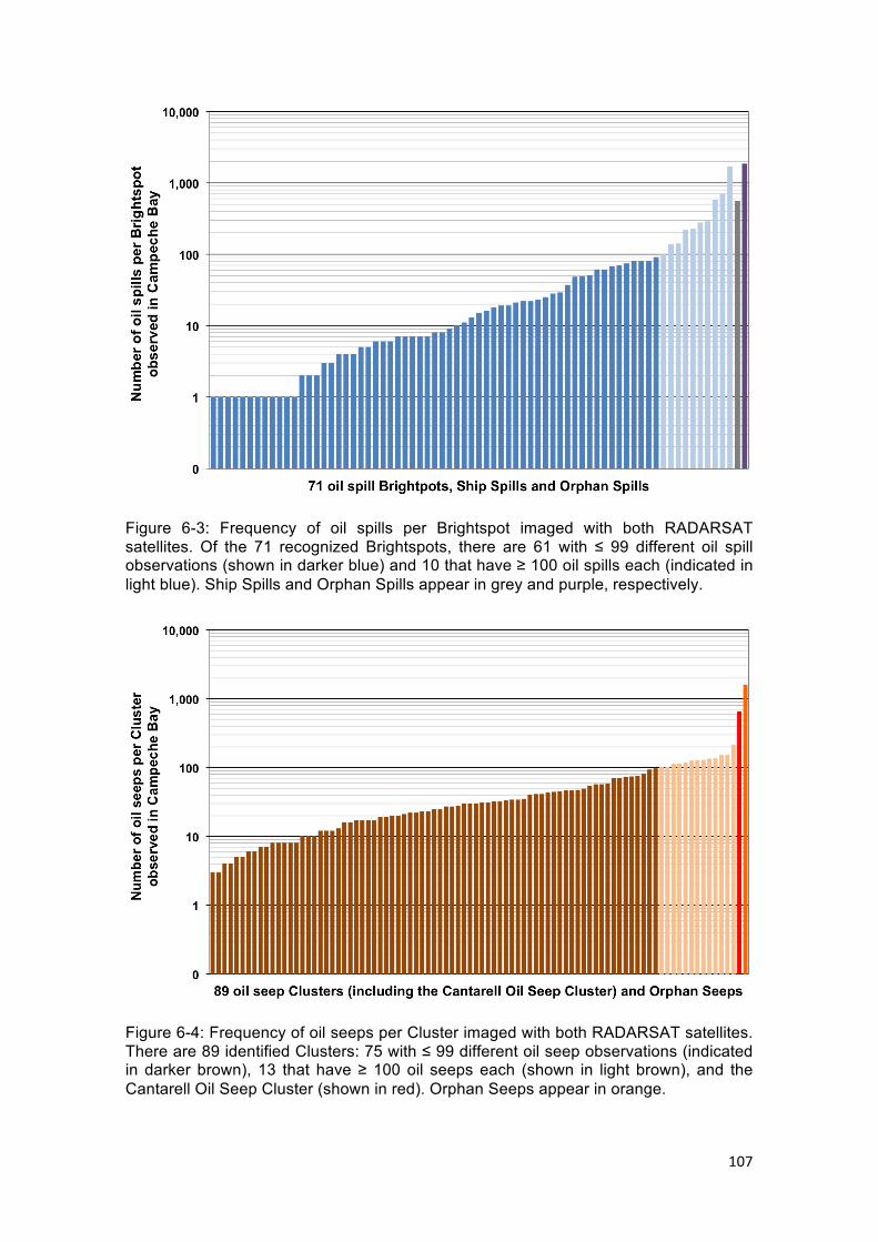
107
Figure 6-3: Frequency of oil spills per Brightspot imaged with both RADARSAT satellites. Of the 71 recognized Brightspots, there are 61 with ≤ 99 different oil spill observations (shown in darker blue) and 10 that have ≥ 100 oil spills each (indicated in light blue). Ship Spills and Orphan Spills appear in grey and purple, respectively.
Figure 6-4: Frequency of oil seeps per Cluster imaged with both RADARSAT satellites. There are 89 identified Clusters: 75 with ≤ 99 different oil seep observations (indicated in darker brown), 13 that have ≥ 100 oil seeps each (shown in light brown), and the Cantarell Oil Seep Cluster (shown in red). Orphan Seeps appear in orange.

108
An aspect of note whilst considering the oil classes is that Brightspots and Clusters,
respectively, color-coded presented on Figure 6-3 and Figure 6-4 are divided in groups
related to the number of different observations. The 71 recognized Brightspots are
divided in 61 with ≤ 99 oil spills each (n=1,263) and 10 with ≥ 100 oil spills each
(n=4,342) – Figure 6-3. The 89 identified Clusters have 75 with ≤ 99 oil seeps each
(n=2,242), 13 Clusters with ≥ 100 oil seeps each (n=1,715), and the Cantarell Oil Seep
Cluster (n=653) – Figure 6-4.
• Oil Slicks per Class: Total Frequency
Figure 6-5 (left side) depicts the frequency of oil spills per class. The majority of oil
spills are grouped to one of the 71 identified Brightspots (n=5,605; 70.0%). Orphan
Spills represent 23.1% (n=1,851) and Ship Spills are as low as 6.9% (n=552) of the oil
spills.
Figure 6-5 (right side) also depicts the frequency of oil seeps per class. Most oil seeps
belong to the 89 identified Clusters (n=3,957; 63.8%). The Cantarell Oil Seep Cluster is
a major exception (n=653; 10.5%), as its signature is present in most RADARSAT
scenes (n=766) analyzed during the CBOS-SatPro: 85%. The remaining 25.7%
(n=1,592) oil seeps are Orphan Seeps.
• Oil Slicks per Class: Total Area Coverage
Figure 6-6 (left side) shows the area (km2) of oil spills per class. The 61 Brightspots
with ≤ 99 different oil spill observations (5,690 km2; 37.3%) and the 10 Brightspots that
have ≥ 100 different oil spill observations (5,434 km2; 35.6%) cover about the same
surface area. While these 71 Brightspots sum 72.9% (11,124 km2), Orphan Spills
correspond to 21.2% (3,228 km2) of the total area of the observed oil spills. Ships Spills
covered about 894 km2 (5.9%), in which seldom ship discharges came from the same
moving oil source. However, some ships have 8-10 different observations, and two
vessels catch the attention with 22 and 65 oil slick features.
Figure 6-6 (right side) shows the area (km2) of oil seeps per class. While the 75
Clusters with ≤ 99 different oil seep observations cover 3,779 km2 (12.0%), the 13
Clusters with ≥ 100 different oil seep observations cover 5,168 km2 (16.4%). These 88
Clusters sum 8,947 km2 (28.4%), whereas Orphan Seeps are responsible for only
2,757 km2 (8.8%). The Cantarell Oil Seep (see Figure 2-1) itself has an exceptional
larger area coverage corresponding to 62.8% (19,743 km2) of the total area of the
observed oil seeps within the CBOS-Data.

109
Figure 6-5: Frequency per Class attribute: oil slicks (black) logged on the Campeche Bay Oil Slick Satellite Database (CBOS-Data) imaged with both RADARSAT satellites: oil spills (cold colors; left side) and oil seeps (warm colors; right side).
Figure 6-6: Total surface area coverage per Class attribute: oil slicks (black) logged on the Campeche Bay Oil Slick Satellite Database (CBOS-Data) imaged with both RADARSAT satellites: oil spills (cold colors; left side) and oil seeps (warm colors; right side).

110
• Occurrence of all oil slicks: Overall Frequency
Figure 6-7 portrays the percentage of frequency per class among the 14,210 oil slicks
observed during the CBOS-SatPro. Interesting to note is that whilst the 10 Brightspots
with ≥ 100 oil spill observations represent about one third of the entire dataset
(n=4,342; 30.5%), the 61 Brightspots with ≤ 99 oil spill observations correspond to a
much smaller fraction (n=1,263; 8.9%) of the identified oil slicks. A different pattern is
noticeable among the oil seep classes, in which the 13 Clusters with ≥ 100 oil seep
observations represent a little more than one tenth of the entire dataset (n=1,715;
12.1%) and the 75 Clusters with ≤ 99 oil seep observations correspond to a quite
similar portion (n=2,242; 15.8%).
Orphan Spills (n=1,851; 13.0%) and Orphan Seeps (n=1,592; 11.2%) also have
comparable proportions. The least frequent are the Cantarell Oil Seep that records
4.6% (n=653) of the oil slicks observed in Campeche Bay, followed by Ship Spills that
only occur in 3.9% (n=552) of times (Figure 6-7).
• Occurrence of all oil slicks: Overall Area Coverage
It is evident from Figure 6-8 that most of the 46,693 km2 covered by all oil slicks
observed in Campeche Bay comes from the Cantarell Oil Seep (19,743 km2; 42.3%),
what contrasts with its small frequency (see Figure 6-7). An interesting characteristic
about the oil slicks observed in the Campeche Bay region is that if the massive
contribution of the Cantarell Oil Seep is disregarded, from the remaining overall area
(26,950, km2) the oil spills’ influence (15,246 km2; 56.6%) is larger than of the oil seeps
(11,704 km2; 43.4%).
Figure 6-8 also illustrates that even though the 10 Brightspots with ≥ 100 oil spill
observations (5,434 km2; 11.6%) occur more frequently (see Figure 6-7) than the 61
Brightspots with ≤ 99 oil spill observations (5,690 km2; 12.2%), they both cover about
the same area. An equivalent areal representativeness is showed by the 13 Clusters
with ≥ 100 oil seep observations (5,168 km2; 11.1%).
Likewise, the 75 Clusters with ≤ 99 oil seep observations (3,779 km2; 8.1%), Orphan
Spills (3,228 km2; 6.9%), and Orphan Seeps (2,757 km2; 5.9%) also cover somewhat
similar areas. Ships spills only cover 1.9% (894 km2) of the area of all oil slicks
observed during the CBOS-SatPro (Figure 6-8).
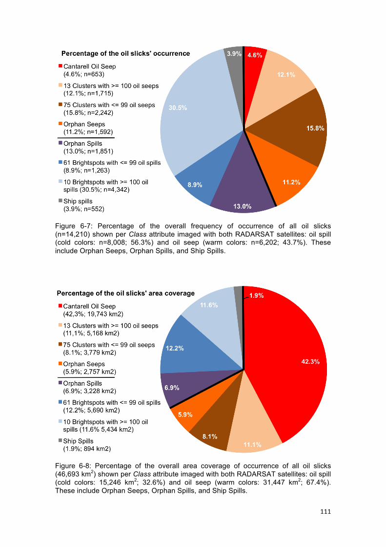
111
Figure 6-7: Percentage of the overall frequency of occurrence of all oil slicks (n=14,210) shown per Class attribute imaged with both RADARSAT satellites: oil spill (cold colors: n=8,008; 56.3%) and oil seep (warm colors: n=6,202; 43.7%). These include Orphan Seeps, Orphan Spills, and Ship Spills.
Figure 6-8: Percentage of the overall area coverage of occurrence of all oil slicks (46,693 km2) shown per Class attribute imaged with both RADARSAT satellites: oil spill (cold colors: 15,246 km2; 32.6%) and oil seep (warm colors: 31,447 km2; 67.4%). These include Orphan Seeps, Orphan Spills, and Ship Spills.

112
• RADARSAT Satellites: SARname
Because measurements from RADARSAT-1 have been explored for longer than those
of RADARSAT-2 (Table 6-1), there are more RADARSAT-1 scenes (n=482; 63%)
compared to RADARSAT-2 scenes (n=284; 37%) – see Table 6-3. Because of this
reason, more oil slicks are imaged with RADARSAT-1 (Figure 6-9: n=8,896; 62.6%)
than with RADARSAT-2 (Figure 6-10: n=5,314; 37.4%).
Table 6-3 illustrates the regular SAR image acquisition during the Operational
Contracts that usually provided on average at least one RADARSAT scene per week.
This table also shows the RADARSAT-1 acquisition (2009-2010) gap that occurred
because the onboard tape recorder was not functioning properly and only direct
downlink data were available (Figure 6-9). An unexplained slight increase in oil slick
frequency occurred from 2005 to 2008. The excessive number of oil slicks observed in
the last two years (2011-2012) reflects the larger amount of satellite scenes (Figure 6-9
and Figure 6-10) utilized due to supplementary short-period exploration contracts.
Table 6-3: RADARSAT scenes per year and annual number of oil slicks imaged during the Campeche Bay Oil Slick Satellite Project (CBOS-SatPro). RADARSAT-1 RADARSAT-2 Both RADARSAT Oil Slick
Year Scenes Scenes Scenes Frequency * 97/99 5 1.0% - - 5 0.7% 33 0.2%
2000 9 1.8% - - 9 1.2% 99 0.7% 2001 23 4.8% - - 23 3.0% 303 2.1%
** 2002 51 10.6% - - 51 6.7% 866 6.1% 2003 53 11.0% - - 53 6.9% 860 6.1% 2004 51 10.6% - - 51 6.7% 876 6.2% 2005 58 12.0% - - 58 7.6% 1,097 7.7% 2006 57 12.0% - - 57 7.4% 1,018 7.2% 2007 61 12.7% - - 61 8.0% 1,063 7.5%
*** 2008 10 2.0% 59 20.8% 69 9.0% 1,261 8.9% 2009 - - 39 13.7% 39 5.1% 887 6.2% 2010 - - 60 21.1% 60 7.8% 826 5.8% 2011 62 12.8% 62 21.8% 124 16.1% 2,619 18.4% 2012 42 8.7% 64 22.6% 106 13.8% 2,402 16.9%
Total 482 100.0% 284 100.0% 766 100.0% 14.210 100.0% * Inspection of previous considerations about the utilized methodology: proof of
concept with archived images (see Section 2.2). ** Start of Operational Contracts (Table 2-1).
*** Start of RADARSAT-2 acquisition (Table 6-1).

113
Figure 6-9: Annual distribution of oil slicks imaged with RADARSAT-1 imagery (n=8,896). Dashed line represents the start of the RADARSAT-2 acquisition.
Figure 6-10: Annual distribution of oil slicks imaged with RADARSAT-2 imagery (n=5,314). Dashed line represents the start of the RADARSAT-2 acquisition.

114
Considering the seasonal occurrence of oil slicks throughout the CBOS-SatPro, there
is an approximately even distribution among the Winter (J/F/M: 23.0%), Spring (A/M/J:
31.4%), Summer (J/A/S: 24.0%), and Fall (O/N/D: 21.6%). However, a predominant
incidence of oil slicks during the boreal Spring months is observed – this season have
the two first months preceding and the last one within the Atlantic hurricane season:
June 1st through November 30th (MASTERS, 2010). Figure 6-11 and Figure 6-12
portray, respectively, the frequency distribution and the total surface area coverage of
oil slicks per category imaged with each of the two RADARSAT satellites. As expected,
these are, respectively, similar to Figure 6-1 and Figure 6-2.
Figure 6-11: Frequency per Category attribute: oil slicks (black) as imaged with each of the two RADARSAT satellites during the Campeche Bay Oil Slick Satellite Project (CBOS-SatPro) – oil spills (blue) and oil seeps (brown). Refer to Figure 6-1 for equivalent information from both RADARSAT satellites together.
Figure 6-12: Total surface area coverage per Category attribute: oil slicks (black) as imaged with each of the two RADARSAT satellites during the Campeche Bay Oil Slick Satellite Project (CBOS-SatPro) – oil spills (blue) and oil seeps (brown). Refer to Figure 6-2 for equivalent information from both RADARSAT satellites together.

115
• Beam Mode: Bmode
About 91% (n=12,892) of the oil slicks observed during the CBOS-SatPro have been
imaged with the two ScanSAR Narrow modes: ScanSAR Narrow 1 (SCNA; n=8,777)
and ScanSAR Narrow 2 (SCNB; n=4,115), as portrayed in Table 6-4. In fact, their
imaging characteristics (e.g. incidence angle and ground resolution) are the most
appropriate RADARSAT beam modes to monitor the sea surface after detecting oil
slicks (NRCAN, 2014). The remaining 10% are divided such that the two Wide modes
sum 8% (WDE1: n=847; and WDE2: n=287) and Extended Low represents 1,3%
(EXL1; n=177). Only 7 oil slicks have been imaged with one ScanSAR Wide (SCW).
Table 6-4: Oil slick distribution per beam mode and per RADARSAT satellite. RADARSAT Beam Modes Oil Slicks RADARSAT-1 RADARSAT-2 SCNA ScanSAR Narrow 1 8,777 (61.7%) 5,888 (66.2%) 2,889 (54.3%) SCNB ScanSAR Narrow 2 4,115 (29.0%) 2,134 (24.0%) 1,981 (37.3%) WDE1 Wide 1 847 (6.0%) 462 (5.2%) 385 (7.3%) WDE2 Wide 2 287 (2.0%) 271 (3.0%) 16 (0.3%) EXL1 Extended Low 1 177 (1.1%) 134 (1.5%) 43 (0.8%) SCW ScanSAR Wide 7 (~0.1%) 7 (0.1%) 0 Total 14,210 (100%) 8,896 (100%) 5,314 (100%)
• Polarization: Pol
While all RADARSAT-1 products are HH-polarized, most RADARSAT-2 beams utilized
on the CBOS-SatPro are VV-polarized (n=276; 97%). VV is indeed the most suitable
polarization for oil slick detection on the sea surface (VAN DER SANDEN, 2004).
• Geometric Attributes: Area and Perimeter
A remarkable characteristic about the occurrence of oil spills and oil seeps in the
Campeche Bay region is their size distribution. Most oil slicks (Table 6-5: n=9,398;
66.1%) have, what is considered herein, “small” surface area coverage (i.e. < 1 km2).
This corresponds to more than 2/3 of the observed oil spills (Table 6-6: n=6,196;
77.4%) and to approximately half of the oil seeps (Table 6-7: n=3,202; 51.7%).
Of the 14,210 oil slicks of the CBOS-Data, only 5.2% (Table 6-5: n=734) have, what is
considered herein, “large” surface area coverage (i.e. ≥ 10 km2). Among these, there
are only 63 observations with major surface area coverage (i.e. ≥ 100 km2): 15 oil spills
(Table 6-6) and 48 oil seeps (Table 6-7). The frequency of oil slicks’ size per category
is illustrated on Figure 6-13 and Figure 6-14, respectively, per satellite.
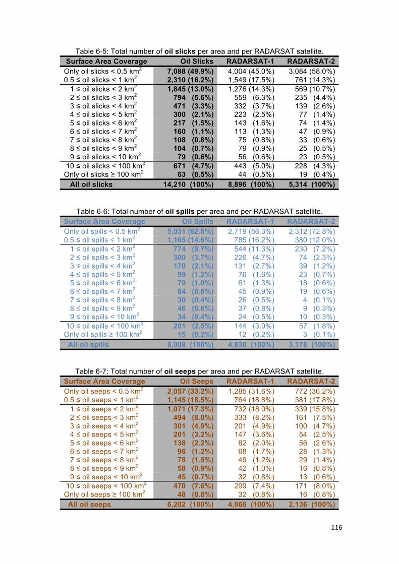
116
Table 6-5: Total number of oil slicks per area and per RADARSAT satellite. Surface Area Coverage Oil Slicks RADARSAT-1 RADARSAT-2 Only oil slicks < 0.5 km2 7,088 (49.9%) 4,004 (45.0%) 3,084 (58.0%) 0.5 ≤ oil slicks < 1 km2 2,310 (16.2%) 1,549 (17.5%) 761 (14.3%) 1 ≤ oil slicks < 2 km2 1,845 (13.0%) 1,276 (14.3%) 569 (10.7%) 2 ≤ oil slicks < 3 km2 794 (5.6%) 559 (6.3%) 235 (4.4%) 3 ≤ oil slicks < 4 km2 471 (3.3%) 332 (3.7%) 139 (2.6%) 4 ≤ oil slicks < 5 km2 300 (2.1%) 223 (2.5%) 77 (1.4%) 5 ≤ oil slicks < 6 km2 217 (1.5%) 143 (1.6%) 74 (1.4%) 6 ≤ oil slicks < 7 km2 160 (1.1%) 113 (1.3%) 47 (0.9%) 7 ≤ oil slicks < 8 km2 108 (0.8%) 75 (0.8%) 33 (0.6%) 8 ≤ oil slicks < 9 km2 104 (0.7%) 79 (0.9%) 25 (0.5%) 9 ≤ oil slicks < 10 km2 79 (0.6%) 56 (0.6%) 23 (0.5%) 10 ≤ oil slicks < 100 km2 671 (4.7%) 443 (5.0%) 228 (4.3%) Only oil slicks ≥ 100 km2 63 (0.5%) 44 (0.5%) 19 (0.4%) All oil slicks 14,210 (100%) 8,896 (100%) 5,314 (100%)
Table 6-6: Total number of oil spills per area and per RADARSAT satellite.
Surface Area Coverage Oil Spills RADARSAT-1 RADARSAT-2 Only oil spills < 0.5 km2 5,031 (62.8%) 2,719 (56.3%) 2,312 (72.8%) 0.5 ≤ oil spills < 1 km2 1,165 (14.6%) 785 (16.2%) 380 (12.0%) 1 ≤ oil spills < 2 km2 774 (9.7%) 544 (11.3%) 230 (7.2%) 2 ≤ oil spills < 3 km2 300 (3.7%) 226 (4.7%) 74 (2.3%) 3 ≤ oil spills < 4 km2 170 (2.1%) 131 (2.7%) 39 (1.2%) 4 ≤ oil spills < 5 km2 99 (1.2%) 76 (1.6%) 23 (0.7%) 5 ≤ oil spills < 6 km2 79 (1.0%) 61 (1.3%) 18 (0.6%) 6 ≤ oil spills < 7 km2 64 (0.8%) 45 (0.9%) 19 (0.6%) 7 ≤ oil spills < 8 km2 30 (0.4%) 26 (0.5%) 4 (0.1%) 8 ≤ oil spills < 9 km2 46 (0.6%) 37 (0.8%) 9 (0.3%) 9 ≤ oil spills < 10 km2 34 (0.4%) 24 (0.5%) 10 (0.3%) 10 ≤ oil spills < 100 km2 201 (2.5%) 144 (3.0%) 57 (1.8%) Only oil spills ≥ 100 km2 15 (0.2%) 12 (0.2%) 3 (0.1%) All oil spills 8,008 (100%) 4,830 (100%) 3,178 (100%)
Table 6-7: Total number of oil seeps per area and per RADARSAT satellite. Surface Area Coverage Oil Seeps RADARSAT-1 RADARSAT-2 Only oil seeps < 0.5 km2 2,057 (33.2%) 1,285 (31.6%) 772 (36.2%) 0.5 ≤ oil seeps < 1 km2 1,145 (18.5%) 764 (18.8%) 381 (17.8%) 1 ≤ oil seeps < 2 km2 1,071 (17.3%) 732 (18.0%) 339 (15.8%) 2 ≤ oil seeps < 3 km2 494 (8.0%) 333 (8.2%) 161 (7.5%) 3 ≤ oil seeps < 4 km2 301 (4.9%) 201 (4.9%) 100 (4.7%) 4 ≤ oil seeps < 5 km2 201 (3.2%) 147 (3.6%) 54 (2.5%) 5 ≤ oil seeps < 6 km2 138 (2.2%) 82 (2.0%) 56 (2.6%) 6 ≤ oil seeps < 7 km2 96 (1.2%) 68 (1.7%) 28 (1.3%) 7 ≤ oil seeps < 8 km2 78 (1.5%) 49 (1.2%) 29 (1.4%) 8 ≤ oil seeps < 9 km2 58 (0.9%) 42 (1.0%) 16 (0.8%) 9 ≤ oil seeps < 10 km2 45 (0.7%) 32 (0.8%) 13 (0.6%) 10 ≤ oil seeps < 100 km2 470 (7.6%) 299 (7.4%) 171 (8.0%) Only oil seeps ≥ 100 km2 48 (0.8%) 32 (0.8%) 16 (0.8%) All oil seeps 6,202 (100%) 4,066 (100%) 2,136 (100%)

117
It is important to note that the oil slick size distribution explored throughout this Section
is merely an arbitrary choice. The values selected to be shown on Table 6-5, Table 6-6,
and Table 6-7 are only used to illustrate the size disparity of the oil slicks observed in
the Campeche Bay region during the CBOS-SatPro.
Figure 6-13: Frequency of oil slicks’ area (km2) imaged with RADARSAT-1 (n=8,896): oil spills (blue) and oil seeps (brown). Dashed lines correspond to oil slicks with areas of 1 km2.
Figure 6-14: Frequency of oil slicks’ area (km2) imaged with RADARSAT-2 (n=5,314): oil spills (blue) and oil seeps (brown). Dashed lines correspond to oil slicks with areas of 1 km2.
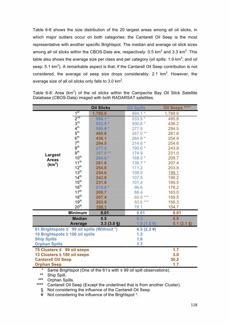
118
Table 6-8 shows the size distribution of the 20 largest areas among all oil slicks, in
which major outliers occur on both categories: the Cantarell Oil Seep is the most
representative with another specific Brightspot. The median and average oil slick sizes
among all oil slicks within the CBOS-Data are, respectively: 0.5 km2 and 3.3 km2. This
table also shows the average size per class and per category (oil spills: 1.9 km2; and oil
seep: 5.1 km2). A remarkable aspect is that, if the Cantarell Oil Seep contribution is not
considered, the average oil seep size drops considerably: 2.1 km2. However, the
average size of all oil slicks only falls to 3.0 km2.
Table 6-8: Area (km2) of the oil slicks within the Campeche Bay Oil Slick Satellite Database (CBOS-Data) imaged with both RADARSAT satellites.
Oil Slicks Oil Spills Oil Seeps **** 1st 1,789.0 994.1 * 1,789.0 2nd 994.1 * 533.5 * 495.8 3rd 533.5 * 500.8 * 436.2 4th 500.8 * 277.5 294.5 5th 495.8 267.0 ** 261.6 6th 436.1 264.8 * 254.9 7th 294.5 214.6 * 254.6 8th 277.5 190.6 * 243.8 9th 267.0 ** 174.9 231.0 10th 264.8 * 168.3 * 209.7 11th 261.6 139.7 * 207.4 12th 254.9 111.2 203.9 13th 254.6 108.0 198.1 14th 243.8 107.5 196.2 15th 231.0 101.4 189.5 16th 214.6 * 96.6 176.2 17th 209.7 88.4 163.0 18th 207.4 86.8 *** 159.5 19th 203.9 80.8 *** 156.3
Largest Areas (km2)
20th 198.1 78.1 154.7 Minimum 0.01 0.01 0.01
Median 0.5 0.3 0.9 Average 3.3 (3.0 §) 1.9 (1.5 ¥) 5.1 (2.1 §)
61 Brightspots ≤ 99 oil spills (Without *) 4.5 (2.2 ¥) 10 Brightspots ≥ 100 oil spills 1.3 Ship Spills 1.6 Orphan Spills 1.7 75 Clusters ≤ 99 oil seeps 1.7 13 Clusters ≥ 100 oil seeps 3.0 Cantarell Oil Seep 30.2 Orphan Seep 1.7
* Same Brightspot (One of the 61’s with ≤ 99 oil spill observations). ** Ship Spill.
*** Orphan Spills. **** Cantarell Oil Seep (Except the underlined that is from another Cluster).
§ Not considering the influence of the Cantarell Oil Seep. ¥ Not considering the influence of the Brightspot *.

119
Taking into account the perimeter attribute (Per), the minimum and maximum values
for all oil slicks are: 0.2 km and 5,093.2 km. Table 6-9 shows the 5 largest perimeters;
the second largest perimeters are also much smaller than the largest ones for both
categories. The average and median oil slick perimeters are, 35.3 km and 10.7 km,
respectively.
Table 6-9: Perimeter (km) information about the oil slicks separated for oil spills (blue) and oil seeps (brown) imaged with both RADARSAT satellites.
Oil Slicks Oil Spills * Oil Seeps *** 1st 5,093.2 5,093.2 3,536.7 2nd 3,536.7 2,086.9 2,826.8 3rd 2,826.8 2,084.8 ** 2,660.6 *** 4th 2,660.6 *** 1,895.4 2,605.3
Largest Perimeters
(m) 5th 2,086.9 1,521.2 2,484.8
Minimum 0.2 0.2 0.2 Median 35.3 18.8 56.6
Average 10.7 6.8 19.9 * Same Brightspot (From the 61’s with ≤ 99 oil spill observations).
** Largest Ship Spill. *** Largest Orphan Spills.
**** Cantarell Oil Seep.
The relationship between area and perimeter is displayed on Figure 6-15 per category.
Figure 6-15: Scatterplot (log scaled) with the relationship between area (km2) and perimeter (km) for all oil spills (blue solid circles) and oil seeps (brown open squares).
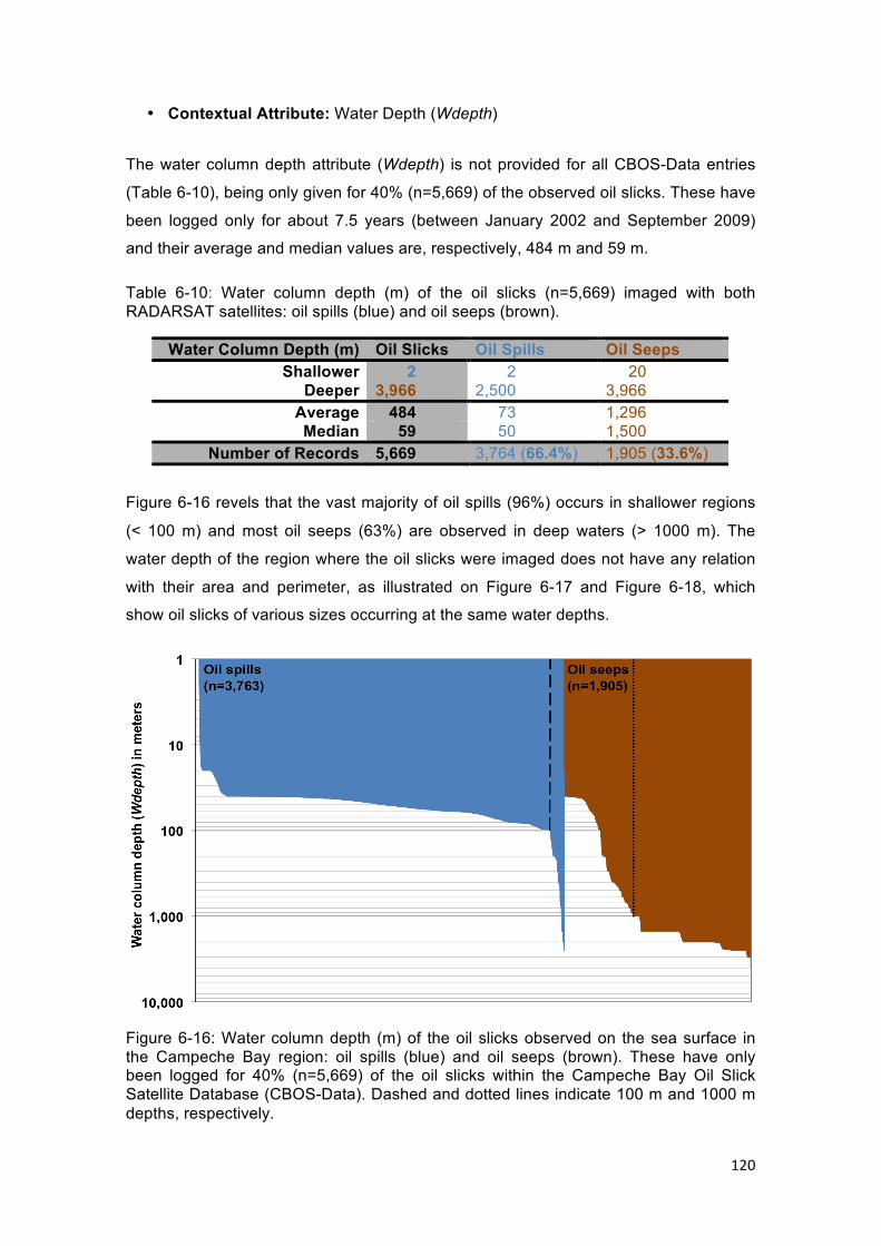
120
• Contextual Attribute: Water Depth (Wdepth)
The water column depth attribute (Wdepth) is not provided for all CBOS-Data entries
(Table 6-10), being only given for 40% (n=5,669) of the observed oil slicks. These have
been logged only for about 7.5 years (between January 2002 and September 2009)
and their average and median values are, respectively, 484 m and 59 m.
Table 6-10: Water column depth (m) of the oil slicks (n=5,669) imaged with both RADARSAT satellites: oil spills (blue) and oil seeps (brown).
Water Column Depth (m) Oil Slicks Oil Spills Oil Seeps Shallower 2 2 20
Deeper 3,966 2,500 3,966 Average 484 73 1,296 Median 59 50 1,500
Number of Records 5,669 3,764 (66.4%) 1,905 (33.6%)
Figure 6-16 revels that the vast majority of oil spills (96%) occurs in shallower regions
(< 100 m) and most oil seeps (63%) are observed in deep waters (> 1000 m). The
water depth of the region where the oil slicks were imaged does not have any relation
with their area and perimeter, as illustrated on Figure 6-17 and Figure 6-18, which
show oil slicks of various sizes occurring at the same water depths.
Figure 6-16: Water column depth (m) of the oil slicks observed on the sea surface in the Campeche Bay region: oil spills (blue) and oil seeps (brown). These have only been logged for 40% (n=5,669) of the oil slicks within the Campeche Bay Oil Slick Satellite Database (CBOS-Data). Dashed and dotted lines indicate 100 m and 1000 m depths, respectively.

121
Figure 6-17: Area (km2) versus water column depth (m): oil spills (blue solid circle) and oil seeps (brown open square).
Figure 6-18: Perimeter (km) versus water column depth (m): oil spills (blue solid circle) and oil seeps (brown open square).
122
• MetOc-Kit: Chl, CTT, minSST, maxSST, minSWH, and maxSWH
Unfortunately, there is not much to consider about the MetOc-Kit attributes logged on
the CBOS-Data. This is mostly because they were inappropriately logged for the
purposes of the analysis intended herein: they were not retrieved at the oil slicks’
location. Chl and CTT are discrete attributes that only indicate the presence (or
absence) of the chlorophyll-a concentration value and cold clouds (i.e. with
temperatures below 40oC). SST and SWH were logged as minimum and maximum
values within the satellite frame, i.e. not in the position of the oil slick.
In addition, they were not logged in a continuous manner, i.e. they have been
intermittently entered on the CBOS-Data. And even though these attributes started
being registered at the CBOS-SatPro start, SWH is only registered until November
2008, and SST, Chl, and CTT span to September 2009.
• Publication: Scientific Meeting and Journal Submission
While preliminary results of this Phase have been orally presented on the XVII Brazilian
Remote Sensing Symposium (SBSR66 – on April 2015 in João Pessoa-PB/Brazil:
CARVALHO et al., 2015a), the complete set of results have been submitted to a
special issue (Long-Term Satellite Data and Applications) of the Canadian Journal of
Remote Sensing (CJRS): CARVALHO et al. (2015b) – see Appendix 1. The results of
the Data Familiarization practice fully elucidate the first proposed specific goal of the
present D.Sc. research: the use of RADARSAT measurements to describe the
occurrence and spatio-temporal distribution of the oil slicks observed on the surface of
the ocean in the Campeche Bay region. Further discussion matters about the Data
Familiarization are found on Chapter 7.
6.2. PHASE 2: QUALITY CONTROL (QC)
The findings of the second pre-processing data verification Phase (described in Section
5.2) are presented on this Section. After analyzing the various aspects related to the
information within the CBOS-Data – as disclosed in the Data Familiarization (Phase 1:
Section 6.1) – it is possible to define certain QC-Standards. These, which are specified
to give consistency to the scene selection utilized in the present investigation, are
described below:
66 SBSR: http://www.dsr.inpe.br/sbsr2015/files/p0217.pdf

123
• 1st QC-Standard: SARname and Pol attributes
The two RADARSAT satellites have quite similar technical specifications – yet, they are
not exactly the same (CRSS, 1993; 2004; MDA, 2004; 2014). For instance, two main
differences are highlighted regarding the CBOS-SatPro imagery:
1. As showed in Table 6-4, most oil slicks observed during the CBOS-SatPro have
been imaged with SCNA and SCNB (n=12,892; 91%). These beam modes are
the RADARSAT modes suitable to image the sea surface, and therefore to detect
oil slicks (NRCAN, 2014). However, their radiometric depths are different (Table
4-1): RADARSAT-1 (8-bit) and RADARSAT-2 (16-bit); and
2. Whereas RADARSAT-1 is HH-polarized (n=482; 100%), most RADARSAT-2
explored in the CBOS-SatPro are VV-polarized (n=276; 97%). In fact, of these
two RADARSAT polarizations, VV is the most suitable to detect oil slicks due to
enhanced backscattering contrast compared to sea clutter (WISMANN et al.,
1998; GIRARD-ARDHUIN et al., 2003; VAN DER SANDEN, 2004).
As a result, it is based on these specifications aspects that the SARname and Pol
attributes are used to establish a primary QC-Standard. Accordingly, images from the
earlier RADARSAT (i.e. 8-bit HH-polarized) are not explored during the further Phases
of the present D.Sc. research because of its characteristics that differ from the ones
from the more sophisticated and useful RADARSAT-2 imagery: 16-bit, VV-polarized.
• 2nd QC-Standard: MetOc-Kit and Wdeth attributes
A secondary QC-Standard leaves out of the present analysis some of the original
attributes within the CBOS-Data (Table 2-2): the water column depth attribute (Wdepth)
and the MetOc-Kit information that include chlorophyll-a concentration (Chl), cloud top
temperature (CTT), sea surface temperature (minSST and maxSST), and significant
wave height (minSWH and maxSWH) are not considered herein. This decision is
based on the fact that such attributes are not provided for the bulk of the oil slicks
observed during the CBOS-SatPro (see Section 6.1).
• 3rd QC-Standard: Missing Data
Additionally, some RADARSAT images were not available, nor were some polygons
identifying certain oil slicks. This structures a further QC-Standard, in which the actual
existence of the satellite scene and its companion information (i.e. oil slick polygon)
defined the exclusion of some information out of the present analysis.

124
• QC-Standard: Summary
The establishment of the three QC-Standards constitutes the basis to filter the
information within the CBOS-Data. As a result, from this point onwards only
RADARSAT-2 scenes (16-bit, VV-polarized: n=277) and its imaged oil slicks (n=4,916)
are explored alongside the following CBOS-Data attributes (Table 2-2): geographical
coordinates (cLAT and cLONG), category (Category), class (Class), date (SARdate),
time (SARtime), beam mode (Bmode), area (Area), and perimeter (Per).
These conditions strengthen and give consistency to the calculation of the SAR
backscatter signature (i.e. σo, βo, and γo expressed in amplitude (C1) and in dB units
(C2) – Table 5-1), as described in the Phase 4 (New Slick-Feature Attributes: Section
5.4). As such, with the establishment of the QC-Standards, an appropriate plan is
devised for the data usage during the present D.Sc. research. A synoptic summary of
this plan is pictured on Figure 1-2 and Figure 1-3, and fully explained in Chapter 5.
• QC-Standard: Data Reduction
A consequence of applying the QC-Standards is a decrease in spatio-temporal
coverage of the observed oil slicks. Two data reductions are observed, one in the
number of satellite images and another in the frequency distribution of oil slicks. These
are related to the fact that RADARSAT-2 imagery started to be acquired in March of
2008, rather than in 1997 as for RADARSAT-1 (Table 6-1).
The data reduction rate caused by using only the 16-bit, VV-polarized RADARSAT-2
images is shown in Table 6-11. This information is presented in relation to the entire
content of the CBOS-Data (i.e. oil slicks imaged with both RADARSAT satellites) and
considering only the RADARSAT-2 images utilized during the CBOS-SatPro.
Table 6-11: Data reduction caused by the three QC-Standards.
QC-Standards After Before
Data Reduction RADARSAT-2
(16-bit, VV-polarized) Both
RADARSAT Only all
RADARSAT-2
SAR Scenes 277 766 (63.8%) 284 (2.5%)
Oil Spills 2,895 8,008 (63.8%) 3,178 (8.9%)
Oil Seeps 2,021 6,202 (67.4%) 2,136 (5.4%)
Oil Slicks 4,916 14,210 (65.4%) 5,314 (7.5%)
125
6.3. PHASE 3: RADARSAT RE-PROCESSING
The first image-processing Phase, described in Section 5.3, accounts for the re-
processing of the imagery that passed the QC-Standards: 277 RADARSAT-2 scenes
(Table 6-11: 16-bit, VV-polarized). Each scene processed includes the georeferenced
.tif files of 13 image products: SIG.amp, SIG.amp.FF, SIG.dB, SIG.dB.FF, BET.amp,
BET.amp.FF, BET.dB, BET.dB.FF, GAM.amp, GAM.amp.FF, GAM.dB, GAM.dB.FF,
and INC.ang (Table 5-1), as well as their corresponding PCI .pix files.
These have been processed using a personal computer (Sony Vaio with 700 GB of
disk space) running Windows 8.1 Pro. The operational system of such machine is 64
bit and its processor is an Intel Core i-7 2.9 GHz with 6 GB of RAM memory. Such
image processing procedures have been completed using PCI Geomatica version
2014, exclusively using in-house EASI command codes (i.e. batch scripting) of the
FOCUS Data Viewer.
The size of each processed scene is about 27 GB, and together, the 277 scenes
occupy almost 7.5 TB on disk. Due to storage limitation, external hard drives were used
(two LaCie 4 TB d2 Professional Thunderbolt Series HDD 7200 RPM with USB3
connection) and it took about 10 days to process the 277 scenes, as the average
processing time per scene was 55 min. When the computer hard disk was used
instead, the timescale to process each image was reduced to about half: 25 min.
6.4. PHASE 4: NEW SLICK-FEATURE ATTRIBUTES
This Section quantifies the products of the second image-processing Phase described
in Section 5.4, which considers the calculation of new slick-feature attributes. These
attributes pertain to four major types of oil slick characteristics: contextual information
(Table 5-2), satellite scene descriptors (Table 5-3), attributes describing the geometry,
shape, and dimension of the oil slicks (Table 5-4), as well as those characterizing the
SAR backscatter signature (Table 5-5). The typical value (represented by a set of basic
qualitative-quantitative statistics: minimum, maximum, average, and standard
deviation) of some of attribute within the CBOS-DScMod is presented herein.
The oil slick frequency, per category and per class, discussed on this Section follows
the explanation of Section 2.3.4 (CBOS-SatPro Part 4: Dark Spot Identification).
Herein, the same color-code instituted in Section 6.1 is followed; however, different
from Section 6.1 (Figure 6-3 and Figure 6-4), all documented Clusters and Brightspots
are respectively grouped to form two single classes; exceptions are discussed below.

126
The 2,021 oil seeps are classified in three distinct classes, i.e. Cantarell Oil Seep
Cluster (n=238), all other Clusters (n=1,200), and Orphan Seeps (n=583). Because of
its exceptionally large superficial area coverage, the signature from the Cantarell Oil
Seep is analyzed separately. The 2,895 oil spills have six classes: all recognized
Brightspots (n=1,050), Bright-1 (n=575), Bright-2 (n=276), Bright-3 (n=255), Ship Spills
(n=159), and Orphan Spills (n=580). As three particular Brightspots stand out in the
number of oil spills from the platforms belonging to these oilfields (n=1,106), their
signatures are also separated as stand alone classes: Bright 1 to 3 (see Table 5-8).
The frequency of oil slicks per Category and Class attributes is presented in Table 6-12
that also presents the range of the two contextual descriptors of spatial location:
latitude (cLAT) and longitude (cLONG). The two contextual descriptors of temporal
location explored in the CBOS-DScMod (i.e. SARdate and SARtime) spans about the
same distribution of all entries within the CBOS-Data (Table 6-1 and Table 6-2).
Table 6-12: Frequency, per category and per class, of the oil slicks within the Campeche Bay Oil Slick Modified Database (CBOS-DScMod) and their respective latitude (cLAT) and longitude (cLONG) range. See also Table 5-2 and Table 5-8.
Category and Class n % * Latitude (oN) ** Longitude (oW) ** 18.274 85.614 Oil Spills 2,895 58.9 26.366 94.814 18.460 91.123 Brightspots 1,050 36.3 21.4 26.366 94.814 19.227 92.004 Bright-1 575 19.9 11.7 19.500 92.385 19.451 92.030 Bright-2 276 9.5 5.6 19.641 92.265 19.120 92.031 Bright-3 255 8.8 5.2 19.435 92.436 18.502 90.819 Ship Spills 159 5.5 3.2 20.999 94.492 18.274 85.614 Orphan Spills 580 20.0 11.8 25.318 94.098 18.525 87.305 Oil Seeps 2,021 41.1 26.561 95.609 19.133 91.915 Cantarell 238 11.8 4.8 19.832 93.118 18.734 91.531 Clusters 1200 59.4 24.4 24.304 94.748 18.525 87.305 Orphan Seeps 583 28.8 11.9 26.561 95.609 18.274 85.614 Oil Slicks 4,916 100.0 26.561 95.609
* Percentages calculated per category, per class, and overall. ** Range: minimum and maximum values.

127
Table 6-13 presents the typical values, per oil slick category, describing the geometry,
shape, and dimension attributes of the oil slicks within the CBOS-DScMod (Table 5-4:
3rd Attribute Type). Such characteristics are presented per oil slick class in Appendix 2.
Table 6-13: Typical values (i.e. basic qualitative-quantitative statistics: minimum, maximum, average, and standard deviation) describing the geometry, shape, and dimension characteristics (Table 5-4: 3rd Attribute Type) of the oil slicks within the Campeche Bay Oil Slick Modified Database (CBOS-DScMod).
Oil Slicks (n=4,916)
Minimum Maximum Average Standard Deviation
Sum (km2)
LEN * 3.0 823,850.0 4,567.7 25,725.9 Area (km2) 0.0025 436.1525 2.7129 14.2145 13,336.6 Per (km) 0.2 2,484.8 33.9 116.1 AtoP (km) 0.0033 0.6582 0.0482 0.0355 PtoA (km-1) 1.5193 300.0000 27.9943 16.4569 PtoA.nor ** 0.8463 46.1191 5.5458 4.2786 COMPLEX.ind ** 9.0 26,728.3 616.5 1,611.7 COMPACT.ind ** 0.0005 1.3963 0.0848 0.0982 SHAPE.ind (km-1) 0.75 40.87 4.91 3.79 FRAC.ind ** -2,353.2 426,242.8 647.4 15,270.7
Oil Spills (n=2,895) Minimum Maximum Average Standard
Deviation Sum (km2)
LEN * 3.0 443,948.0 2,002.6 12,427.9 Area (km2) 0.0025 277.4900 1.2421 7.7306 3,595.8 Per (km) 0.2 772.3 15.5 39.6 AtoP (km) 0.0033 0.6582 0.0445 0.0366 PtoA (km-1) 1.5193 300.0000 30.2178 16.7603 PtoA.nor ** 1.1283 37.5652 4.3875 2.7407 COMPLEX.ind ** 16.0 17,732.9 336.3 712.8 COMPACT.ind ** 0.0007 0.7855 0.1074 0.1071 SHAPE.ind (km-1) 1.00 33.29 3.89 2.43 FRAC.ind ** -487.9 395,511.4 375.8 11,726.4
Oil Seeps (n=2,021)
Minimum Maximum Average Standard Deviation
Sum (km2)
LEN * 13.0 823,850.0 8,242.0 36,960.8 Area (km2) 0.0100 436.1525 4.8198 19.9617 9,740.9 Per (km) 0.3 2,484.8 60.2 171.4 AtoP (km) 0.0036 0.3978 0.0535 0.0333 PtoA (km-1) 2.5139 280.0000 24.8093 15.4690 PtoA.nor ** 0.8463 46.1191 7.2051 5.3947 COMPLEX.ind ** 9.0 26,728.3 1,017.9 2,306.3 COMPACT.ind ** 0.0005 1.3963 0.0525 0.0724 SHAPE.ind (km-1) 0.75 40.87 6.39 4.78 FRAC.ind ** -2,353.2 426,242.8 1,036.4 19,239.0
* Number of pixels inside the oil slicks. ** Dimensionless quantity.

128
The new slick-feature attributes referring to the geometry, shape, and dimension of the
oil slicks (Table 5-4: 3rd Attribute Type) have been retrieved with in-house Python
codes. Likewise, those involving basic statistical measures – i.e. INC.ang and SAR
backscatter signature (Table 5-5: 4th Attribute Type) – were also retrieved with Python,
but using batch ArcGIS scripting functions. The calculation of INC.ang and the
attributes of the 4th type were retrieved by matching the individual oil slick polygons
with the 13 radiometric-calibrated image products: SIG.amp, SIG.amp.FF, SIG.dB,
SIG.dB.FF, BET.amp, BET.amp.FF, BET.dB, BET.dB.FF, GAM.amp, GAM.amp.FF,
GAM.dB, GAM.dB.FF, and INC.ang (Table 5-1).
The AVG attribute (i.e. arithmetic mean of all pixels inside individual oil slick polygons)
is shown to describe the SAR backscatter signature of the CBOS-DScMod oil slicks:
Table 6-14 (sigma-naught: σo), Table 6-15 (beta-naught: βo), and Table 6-16 (gamma-
naught: γo).
Table 6-14: Typical values (i.e. basic qualitative-quantitative statistics: minimum, maximum, average, and standard deviation) of the average (AVG: arithmetic mean of all pixels inside individual oil slick polygons) SAR backscatter signature (Sigma-naught: σo) of the oil slicks within the CBOS-DScMod. These values correspond to incidence angles ranging from 19.5o to 46.6o. See also Table 5-1 and Table 5-5.
Sigma-naught (σo) SIG.amp.AVG SIG.amp.FF.AVG SIG.dB.AVG SIG.dB.FF.AVG
Amplitude Amplitude Decibels Decibels Oil Slicks (n=4,916) without Frost with Frost without Frost with Frost
Minimum 0.000907 0.000995 -62.195921 9.552999
Maximum 0.660908 0.635781 -8.801640 62.054795
Average 0.027028 0.029074 -40.873467 41.020277
Standard Deviation 0.045919 0.048927 10.705655 10.564339
Amplitude Amplitude Decibels Decibels Oil Spills (n=2,895) without Frost with Frost without Frost with Frost
Minimum 0.001060 0.001135 -61.211937 11.133664
Maximum 0.660908 0.635781 -9.089579 61.200692
Average 0.025685 0.027619 -41.490243 41.656948
Standard Deviation 0.048334 0.051418 10.556650 10.423009
Amplitude Amplitude Decibels Decibels Oil Seeps (n=2,021) without Frost with Frost without Frost with Frost
Minimum 0.000907 0.000995 -62.195921 9.552999
Maximum 0.447408 0.474392 -8.801640 62.054795
Average 0.028953 0.031158 -39.989960 40.108272
Standard Deviation 0.042155 0.045051 10.857283 10.700323
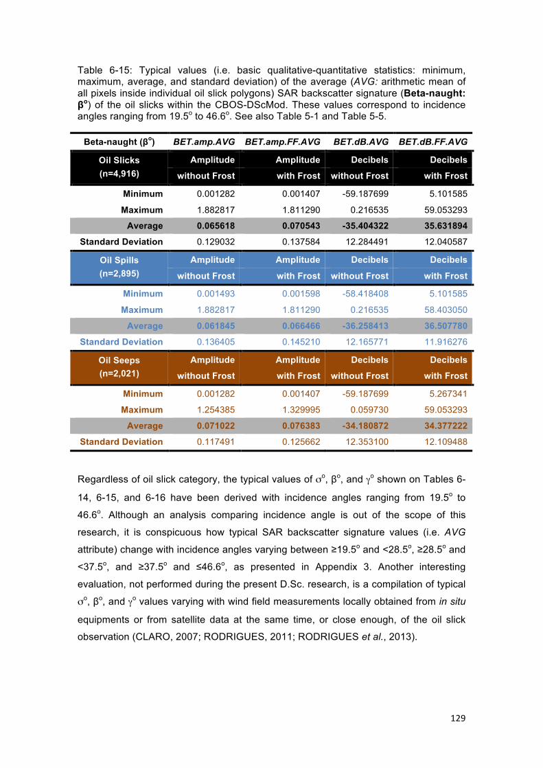
129
Table 6-15: Typical values (i.e. basic qualitative-quantitative statistics: minimum, maximum, average, and standard deviation) of the average (AVG: arithmetic mean of all pixels inside individual oil slick polygons) SAR backscatter signature (Beta-naught: βo) of the oil slicks within the CBOS-DScMod. These values correspond to incidence angles ranging from 19.5o to 46.6o. See also Table 5-1 and Table 5-5.
Beta-naught (βo) BET.amp.AVG BET.amp.FF.AVG BET.dB.AVG BET.dB.FF.AVG
Amplitude Amplitude Decibels Decibels Oil Slicks (n=4,916) without Frost with Frost without Frost with Frost
Minimum 0.001282 0.001407 -59.187699 5.101585
Maximum 1.882817 1.811290 0.216535 59.053293
Average 0.065618 0.070543 -35.404322 35.631894
Standard Deviation 0.129032 0.137584 12.284491 12.040587
Amplitude Amplitude Decibels Decibels Oil Spills (n=2,895) without Frost with Frost without Frost with Frost
Minimum 0.001493 0.001598 -58.418408 5.101585
Maximum 1.882817 1.811290 0.216535 58.403050
Average 0.061845 0.066466 -36.258413 36.507780
Standard Deviation 0.136405 0.145210 12.165771 11.916276
Amplitude Amplitude Decibels Decibels Oil Seeps (n=2,021) without Frost with Frost without Frost with Frost
Minimum 0.001282 0.001407 -59.187699 5.267341
Maximum 1.254385 1.329995 0.059730 59.053293
Average 0.071022 0.076383 -34.180872 34.377222
Standard Deviation 0.117491 0.125662 12.353100 12.109488
Regardless of oil slick category, the typical values of σo, βo, and γo shown on Tables 6-
14, 6-15, and 6-16 have been derived with incidence angles ranging from 19.5o to
46.6o. Although an analysis comparing incidence angle is out of the scope of this
research, it is conspicuous how typical SAR backscatter signature values (i.e. AVG
attribute) change with incidence angles varying between ≥19.5o and <28.5o, ≥28.5o and
<37.5o, and ≥37.5o and ≤46.6o, as presented in Appendix 3. Another interesting
evaluation, not performed during the present D.Sc. research, is a compilation of typical
σo, βo, and γo values varying with wind field measurements locally obtained from in situ
equipments or from satellite data at the same time, or close enough, of the oil slick
observation (CLARO, 2007; RODRIGUES, 2011; RODRIGUES et al., 2013).

130
Table 6-16: Typical values (i.e. basic qualitative-quantitative statistics: minimum, maximum, average, and standard deviation) of the average (AVG: arithmetic mean of all pixels inside individual oil slick polygons) SAR backscatter signature (Gamma-naught: γo) of the oil slicks within the CBOS-DScMod. These values correspond to incidence angles ranging from 19.5o to 46.6o. See also Table 5-1 and Table 5-5.
Gamma-naught (γo) GAM.amp.AVG GAM.amp.FF.AVG GAM.dB.AVG GAM.dB.FF.AVG
Amplitude Amplitude Decibels Decibels Oil Slicks (n=4,916) without Frost with Frost without Frost with Frost
Minimum 0.001282 0.001407 -59.183525 9.016371
Maximum 0.705821 0.682226 -8.194344 59.193962
Average 0.030161 0.032452 -39.234321 39.392071
Standard Deviation 0.049123 0.052329 10.106872 9.963671
Amplitude Amplitude Decibels Decibels Oil Spills (n=2,895) without Frost with Frost without Frost with Frost
Minimum 0.001467 0.001571 -59.162005 10.757918
Maximum 0.705821 0.682226 -8.547585 58.769908
Average 0.028796 0.030973 -39.738457 39.916931
Standard Deviation 0.051720 0.055008 9.904402 9.768760
Amplitude Amplitude Decibels Decibels Oil Seeps (n=2,021) without Frost with Frost without Frost with Frost
Minimum 0.001282 0.001407 -59.183525 9.016371
Maximum 0.479105 0.508002 -8.194344 59.193962
Average 0.032117 0.034571 -38.512166 38.640229
Standard Deviation 0.045084 0.048168 10.349790 10.191845
Typical values for the original COV attribute (Table 5-5: COV.STD/AVG) that describes
the relative dispersion of the pixel values around the central tendency inside the oil
slick are presented in Table 6-17 for the 13 radiometric-calibrated image products of
the oil slicks within the CBOS-DScMod. While low COV indicates low variability, high
COV values denote high variability within the pixels of individual oil slicks, for instance:
0.1 means that the STD is equal to 10% of the AVG.
Histograms with the frequency distribution of some of the attributes within the CBOS-
DScMod is shown on Figure 6-19, Figure 6-20, Figure 6-21, Figure 6-22, and Figure 6-
23. These histograms are helpful to examine the statistical distribution of such
attributes, as well as they assist on the characterization of the oil slicks observed in
Campeche Bay.

131
Table 6-17: Typical values (i.e. basic qualitative-quantitative statistics: minimum, maximum, average, and standard deviation) characterizing the Coefficient of Variation (COV: ratio between STD and AVG attributes) of the oil slicks within the Campeche Bay Oil Slick Modified Database (CBOS-DScMod). These values correspond to incidence angles ranging from 19.5o to 46.6o. See also Table 5-5.
Oil Slicks: COV.STD/AVG Minimum Maximum Average Standard Deviation
Incidence Angle INC.ang 0.000024 0.083812 0.002118 0.004341 SIG.amp 0.197564 16.407197 0.813826 0.748304 SIG.amp.FF 0.172066 15.281376 0.636604 0.742414 SIG.dB -1.111435 -0.056387 -0.176553 0.078373
Sigma-naugh (σo) *
SIG.dB.FF 0.030392 0.640210 0.124347 0.060784 BET.amp 0.197471 16.373387 0.813620 0.745226 BET.amp.FF 0.172094 15.058628 0.636383 0.738978 BET.dB -50.074967 101.814973 -0.215557 1.728912
Gamma-naugh (γo) *
BET.dB.FF 0.032990 1.137100 0.159431 0.106188 GAM.amp 0.197592 16.444979 0.813965 0.750020 GAM.amp.FF 0.172044 15.513617 0.636758 0.744536 GAM.dB -1.184094 -0.058703 -0.183557 0.080929
Beta-naugh (βo) *
GAM.dB.FF 0.032022 0.662951 0.129200 0.062331
Oil Spills: COV.STD/AVG Minimum Maximum Average Standard Deviation
Incidence Angle INC.ang 0.000024 0.031398 0.001186 0.001940 SIG.amp 0.197564 13.369330 0.823675 0.774880 SIG.amp.FF 0.172066 14.082050 0.647057 0.759865 SIG.dB -1.111435 -0.056387 -0.176553 0.078373
Sigma-naugh (σo) *
SIG.dB.FF 0.030392 0.640210 0.119729 0.059213 BET.amp 0.197471 13.363505 0.823582 0.774613 BET.amp.FF 0.172094 14.082496 0.646959 0.759597 BET.dB -50.074967 101.814973 -0.215557 1.728912
Gamma-naugh (γo) *
BET.dB.FF 0.032990 1.137100 0.151352 0.103104 GAM.amp 0.197592 13.375513 0.823716 0.775017 GAM.amp.FF 0.172044 14.081563 0.647102 0.760004 GAM.dB -1.184094 -0.058703 -0.179359 0.083345
Beta-naugh (βo) *
GAM.dB.FF 0.032022 0.662951 0.124737 0.060957
Oil Seeps: COV.STD/AVG Minimum Maximum Average Standard Deviation
Incidence Angle INC.ang 0.000053 0.083812 0.003453 0.006118 SIG.amp 0.472796 16.407197 0.799717 0.708450 SIG.amp.FF 0.263220 15.281376 0.621630 0.716595 SIG.dB -1.111435 -0.056387 -0.176553 0.078373
Sigma-naugh (σo) *
SIG.dB.FF 0.046627 0.448954 0.130963 0.062387 BET.amp 0.472687 16.373387 0.799349 0.700929 BET.amp.FF 0.263093 15.058628 0.621232 0.708309 BET.dB -50.074967 101.814973 -0.215557 1.728912
Gamma-naugh (γo) *
BET.dB.FF 0.049864 0.670910 0.171002 0.109448 GAM.amp 0.472803 16.444979 0.799997 0.712644 GAM.amp.FF 0.263246 15.513617 0.621940 0.721729 GAM.dB -0.722302 -0.086892 -0.189571 0.076958
Beta-naugh (βo) *
GAM.dB.FF 0.048900 0.467745 0.135594 0.063721 * Amplitude and decibels with and without the Frost filter (FROST et al., 1982).
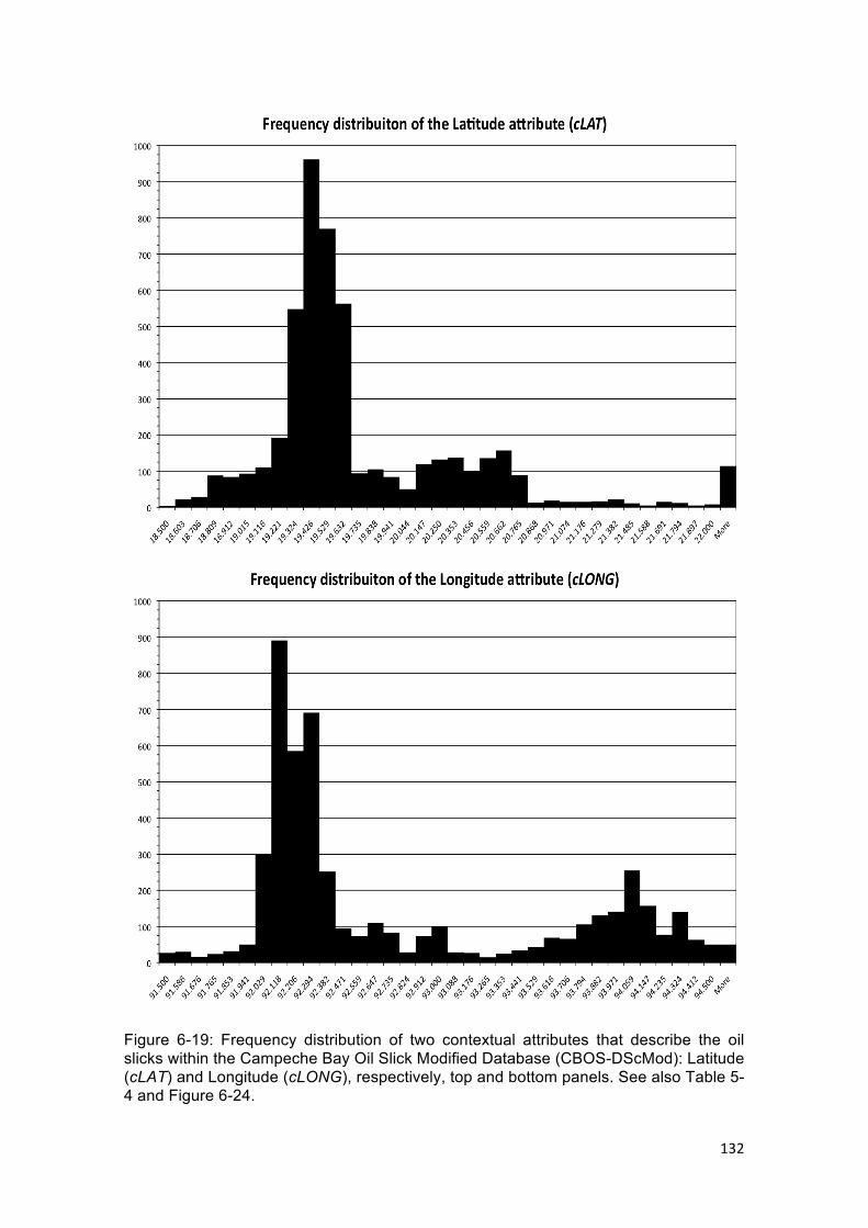
132
Figure 6-19: Frequency distribution of two contextual attributes that describe the oil slicks within the Campeche Bay Oil Slick Modified Database (CBOS-DScMod): Latitude (cLAT) and Longitude (cLONG), respectively, top and bottom panels. See also Table 5-4 and Figure 6-24.

133
Figure 6-20: Frequency distribution of two contextual attributes that describe the oil slicks within the Campeche Bay Oil Slick Modified Database (CBOS-DScMod): Area (Area) and Perimeter (Per), respectively, top and bottom panels. See also Table 5-4 and Figure 6-25.

134
Figure 6-21: Frequency distribution of three attributes of geometry, shape, and dimensions that describe the oil slicks within the Campeche Bay Oil Slick Modified Database (CBOS-DScMod): Area to Perimeter Ratio (AtoP), Perimeter to Area Ratio (PtoA), and Normalized Perimeter to Area Ratio (PtoA.nor), respectively shown on the upper, middle, and lower panels. See also Table 5-4 and Figure 6-26.

135
Figure 6-22: Frequency distribution of three attributes of geometry, shape, and dimensions that describe the oil slicks within the Campeche Bay Oil Slick Modified Database (CBOS-DScMod): Complex Index (COMPLEX.ind), Compact Index (COMPACT.ind), and Shape Index (SHAPE.ind), respectively shown on the upper, middle, and lower panels. See also Table 5-4 and Figure 6-27.

136
Figure 6-23: Frequency distribution of one attribute of geometry, shape, and dimensions that describes the oil slicks within the Campeche Bay Oil Slick Modified Database (CBOS-DScMod): Fractal Index (FRAC.ind). See also Table 5-4 and Figure 6-28.
6.5. PHASE 5: DATA TREATMENT
The information presented on this Section concludes the Workable-Database
Preparation (shown as the Green Phases: 1 to 5 on Figure 1-3). Histograms have also
been plotted after the application of the Negative Values Scaling and the Log10
Transformation. Such histograms illustrate the Log10 transformed frequency
distributions of some attributes within the CBOS-DScMod: Figure 6-24 (Latitude (cLAT)
and Longitude (cLONG)), Figure 6-25 (Area (Area) and Perimeter (Per)), Figure 6-26
(Area to Perimeter Ratio (AtoP), Perimeter to Area Ratio (PtoA), and Normalized
Perimeter to Area Ratio (PtoA.nor)), and Figure 6-27 (Complex Index (COMPLEX.ind),
Compact Index (COMPACT.ind), and Shape Index (SHAPE.ind)).
An exception is the Fractal Index (FRAC.ind), shown on Figure 6-28, which has a cubic
root transformation applied to it. It is possible to notice that the skewness of most data
transformed attributes is smaller in comparison to the frequency distributions shown on
Figure 6-19, Figure 6-20, Figure 6-21, Figure 6-22, and Figure 6-23.

137
Figure 6-24: Histogram of frequency distribution of two contextual attributes that describe the oil slicks within the Campeche Bay Oil Slick Modified Database (CBOS-DScMod): Latitude (cLAT) and Longitude (cLONG) with logarithm transformation (Log10), respectively, top and bottom panels. See also Table 5-4 and Figure 6-19.

138
Figure 6-25: Histogram of frequency distribution of two contextual attributes that describe the oil slicks within the Campeche Bay Oil Slick Modified Database (CBOS-DScMod): Area (Area) and Perimeter (Per) with logarithm transformation (Log10), respectively, top and bottom panels. See also Table 5-4 and Figure 6-20.

139
Figure 6-26: Histogram of frequency distribution of three attributes of geometry, shape, and dimensions that describe the oil slicks within the Campeche Bay Oil Slick Modified Database (CBOS-DScMod): Area to Perimeter Ratio (AtoP), Perimeter to Area Ratio (PtoA), and Normalized Perimeter to Area Ratio (PtoA.nor) with logarithm transformation (Log10), respectively shown on the upper, middle, and lower panels. See also Table 5-4 and Figure 6-21.
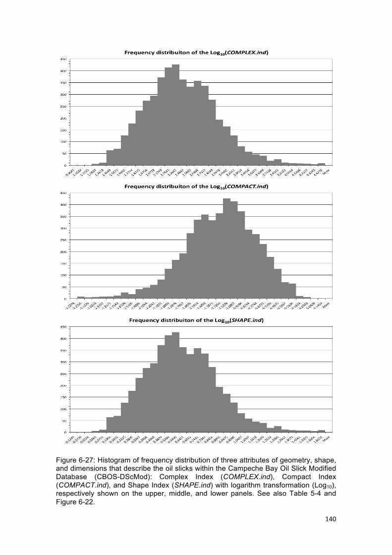
140
Figure 6-27: Histogram of frequency distribution of three attributes of geometry, shape, and dimensions that describe the oil slicks within the Campeche Bay Oil Slick Modified Database (CBOS-DScMod): Complex Index (COMPLEX.ind), Compact Index (COMPACT.ind), and Shape Index (SHAPE.ind) with logarithm transformation (Log10), respectively shown on the upper, middle, and lower panels. See also Table 5-4 and Figure 6-22.
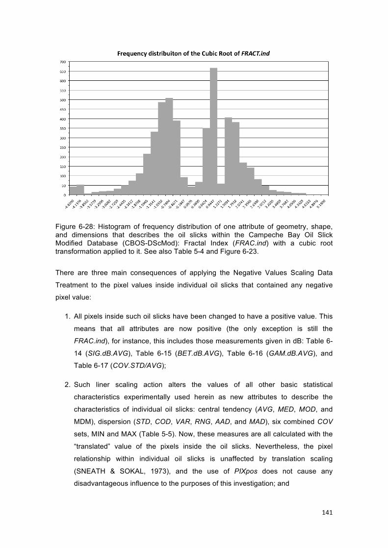
141
Figure 6-28: Histogram of frequency distribution of one attribute of geometry, shape, and dimensions that describes the oil slicks within the Campeche Bay Oil Slick Modified Database (CBOS-DScMod): Fractal Index (FRAC.ind) with a cubic root transformation applied to it. See also Table 5-4 and Figure 6-23.
There are three main consequences of applying the Negative Values Scaling Data
Treatment to the pixel values inside individual oil slicks that contained any negative
pixel value:
1. All pixels inside such oil slicks have been changed to have a positive value. This
means that all attributes are now positive (the only exception is still the
FRAC.ind), for instance, this includes those measurements given in dB: Table 6-
14 (SIG.dB.AVG), Table 6-15 (BET.dB.AVG), Table 6-16 (GAM.dB.AVG), and
Table 6-17 (COV.STD/AVG);
2. Such liner scaling action alters the values of all other basic statistical
characteristics experimentally used herein as new attributes to describe the
characteristics of individual oil slicks: central tendency (AVG, MED, MOD, and
MDM), dispersion (STD, COD, VAR, RNG, AAD, and MAD), six combined COV
sets, MIN and MAX (Table 5-5). Now, these measures are all calculated with the
“translated” value of the pixels inside the oil slicks. Nevertheless, the pixel
relationship within individual oil slicks is unaffected by translation scaling
(SNEATH & SOKAL, 1973), and the use of PIXpos does not cause any
disadvantageous influence to the purposes of this investigation; and

142
3. The MIN attribute of some radiometric-calibrated image products lost its
meaning: the PIXpos of several oil slicks became 1, as PIX=PIXmin gives
PIXpos=1. This happened for 9 products and their MIN attribute were removed.
Consequently, the CBOS-DScMod is left with 502 variables (instead of 511).
The information (frequency) from the Dummy Variables presented in Table 5-10 to
describe the oil slicks is summarized in Table 6-18. This table also presents their
respective percentage of occurrence in the CBOS-DScMod.
Table 6-18: Dummy Variables frequency included in the Campeche Bay Oil Slick Modified Database (CBOS-DScMod) to replace the qualitative attributes. These are binary-coded to 1 or 0. See also Table 5-2, Table 5-3, and Table 5-10.
Dummy Variables (Equal to 1) n % Region-1 RG1.LAT 3,917 79.7 Latitude Region-2 RG2.LAT 999 20.3 Region-1 RG1.LONG 3,573 72.7 Longitude Region-2 RG2.LONG 1,343 27.3
Day (1) or Night (0) DoN * 1,448 29.5 Winter J/F/M WNT 921 18.7 Spring A/M/J SPG 1,660 33.8
Summer J/A/S SMM 1,130 23.0 Fall O/N/D FLL 1,205 24.5
2008 678 13.8 2009 755 15.4 2010 821 16.7 2011 1,335 27.1
Analyzed Years
2012 1,327 27.0 ScanSAR Narrow 1 SCNA 2,661 54.1 ScanSAR Narrow 2 SCNB 1,899 38.6
Wide 1 WDE1 340 7.0 Wide 2 WDE2 16 0.3
* Oil slicks image at nighttime correspond to 70.5% (n=3,468): DoN=0 (Table 5-6).
6.6. PHASE 6: ATTRIBUTE SELECTION
Two methods were independently investigated to reduce the dimensionality within the
attributes domain and to establish hierarchical relationships among the CBOS-DScMod
variables within the thirty-three optimal subsets shown on Figure 5-3. The first method
to be implemented was the UPGMA (Unweighted Pair Group Method with Arithmetic
Mean), in which the attribute selection occurs with the analysis of rooted-tree
dendrograms. Figure 6-29 illustrates the use of the two thresholds (i.e. cut-off levels
shown as horizontal red lines across the dendrograms) on the complete exploration of
the entire dataset (n=502): CCC (in this case: 0.8175) and fixed similarity of 0.5. These
two lines are used to define the groups from which the attributes were selected.

143
When the CCC is utilized, 59 attributes of the CBOS-DScMod are selected to be
explored in the subsequent data mining, whereas 46 variables are selected with the
fixed similarity cut-off level. Table 6-19 presents the variables selected with both
thresholds on the complete exploration.
Figure 6-29: Rooted-tree dendrograms for the UPGMA implementation: complete exploration of the Campeche Bay Oil Slick Modified Database (CBOS-DScMod: n=502). In the lower panel, the two horizontal red lines correspond to the Cophenetic Correlation Coefficient (CCC=0.8175) and similarity of 0.5, respectively (top and bottom lines). Same information plotted in the upper and middle panels: respectively for 0.8175 and 0.5.

144
Table 6-19: Attributes selected (n=59) based on the UPGMA implementation: complete exploration of the Campeche Bay Oil Slick Modified Database (CBOS-DScMod: n=502). These are illustrated in the dendrograms shown on Figure 6-29. While these correspond to the Cophenetic Correlation Coefficient (0.8175), variables in bold (n=46) have been selected using the fixed similarity value of 0.5.
Attributes n UPGMA Selected Attributes
59 1 oSPILL Category
58 2 oSEEP
57 1 BGT 56 2 BGT-1 55 3 BGT-2 54 4 BGT-3 53 5 SHP 52 6 orphSP 51 7 CANT 50 8 CLUS
Class
49 9 orphSE
48 1 RG1.LAT 47 2 RG2.LAT 46 3 PKD.LAT 45 4 RG1.LONG 44 5 RG2.LONG
Latitude and
Longitude
43 6 PKD.LONG
Day or Night 42 1 DoN
41 1 DoY 40 2 WNT 39 3 SPG 38 4 SMM 37 5 FLL 36 6 2008 35 7 2009 34 8 2011 33 9 2010
Date
32 10 2012
31 1 SCNA 30 2 SCNB 29 3 WDE1
Beam Modes
28 4 WDE2
27 1 INC.ang.AVG Incidence Angles 26 2 INC.ang.STD
Continue in the next page.

145
Table 6-19: Continuation.
25 1 LEN 24 2 AtoP 23 3 PtoA 22 4 COMPACT.ind 21 5 COMPLEX.ind
Geometry, Shape,
and Dimension
¥ 20 6 FRAC.ind
19 1 SIG.amp.AVG 18 2 SIG.amp.STD 17 3 SIG.amp.COD 16 4 SIG.amp.FF.AVG 15 5 SIG.amp.FF.COD 14 6 SIG.amp.FF.COV.VAR/AVG 13 7 SIG.dB.AVG 12 8 SIG.dB.MOD 11 9 SIG.dB.STD 10 10 SIG.dB.COD 9 11 SIG.dB.MAD 8 12 SIG.dB.COV.STD/MOD 7 13 SIG.dB.COV.VAR/AVG 6 14 SIG.dB.COV.RNG/AVG 5 15 SIG.dB.COV.RNG/MOD 4 16 SIG.dB.FF.AVG 3 18 SIG.dB.FF.MIN 2 18 SIG.dB.FF.MAX
SAR Backscatter Signature
¥¥
1 19 SIG.dB.FF.COV.RNG/AVG
¥ Same variables shown on Table 6-20. ¥¥ Same variables shown on Table 6-21.
However, because the complete exploration is performed with the full remote sensing
library content of the CBOS-DScMod (n=502), the graphical representation shown on
Figure 6-29 is not very instructive. A more intuitive example of the attribute selection
using dendrograms is presented on Figure 6-30 (n=151) for the UPGMA
implementation that analyzes sigma-naught attributes (σo; n=141) together with
attributes of geometry, shape, and dimension (n=10). It is possible to observe that the
threshold corresponding to the CCC (0.8262) gives 26 groups from which only one
variable is selected per group. In the case of using the fixed similarity cut-off (0.5), 12
groups are formed; what leads to the selection of 12 variables.

146
Figure 6-30: Rooted-tree dendrograms for the UPGMA implementation: sigma-naught (σo; n=141) together with the geometry, shape, and dimension attributes (n=10). In the lower panel, the two horizontal red lines correspond to the Cophenetic Correlation Coefficient (CCC=0.8262) and similarity of 0.5, respectively (top and bottom lines). Same information plotted in the upper and middle panels: respectively for 0.8262 and 0.5.
Similarly, Figure 6-31 presents the dendrograms assessing the groups formed when
exploring only sigma-naught attributes (σo; n=141). The variables selected are the
same as those from the previous consideration depicted on Figure 6-30, however, not
including the ones of geometry, shape, and dimension.

147
Figure 6-31: Rooted-tree dendrograms for the UPGMA implementation: sigma-naught (σo) variables only (n=141). In the lower panel, the two horizontal red lines correspond to the Cophenetic Correlation Coefficient (CCC=0.8319) and similarity of 0.5, respectively (top and bottom lines). Same information plotted in the upper and middle panels: respectively for 0.8319 and 0.5.
Another comprehensible example of the attribute selection process using the UPGMA
is depicted on Figure 6-32 exploring only variables of geometry, shape, and dimension
(n=10). Of the initial 10 attributes, the CCC threshold (0.9143) forms six groups and the
fixed similarity of 0.5 gives five groups: 6 and 5 variables, respectively (Table 6-20).

148
Figure 6-32: Rooted-tree dendrograms for the UPGMA implementation: only attributes of geometry, shape, and dimension (n=10). In the right panel, the two horizontal red lines correspond to the Cophenetic Correlation Coefficient (CCC=0.9143) and similarity of 0.5, respectively (top and bottom lines). Same information plotted in the left and middle panels: respectively for 0.9143 and 0.5.
Table 6-20: Attributes selected (n=6) based on the UPGMA implementation: only attributes of geometry, shape, and dimension (n=10). These are illustrated in the dendrograms shown on Figure 6-30 (CCC=0.8262) and Figure 6-32 (CCC=0.9143). Variables in bold (n=5) were selected using the fixed similarity value of 0.5.
UPGMA Selected Attributes
1 LEN 2 AtoP 3 PtoA 4 COMPACT 5 COMPLEX 6 FRACTAL
The dendrograms resulting from the separate UPGMA implementation that analyzed
the beta-naught (βo) and gamma-naught (γo) variables, with (n=151) and without
(n=141) the geometry, shape, and dimension attributes, are presented in Appendix 4.
Even though the groups that have been formed are not exactly the same among the
different UPGMA implementations, nor are the CCC values (e.g. 0.8175, 0.8262,
0.8319, and 0.9143), the same SAR backscatter signature variables of σo, βo, and γo
have been selected with or without the geometry, shape, and dimension attributes
(Table 6-21). Likewise, the selection of the geometry, shape, and dimension attributes
was also the same when these are analyzed together or separately from the SAR
backscatter signature variables (Table 6-20).

149
The same behavior was observed between the complete exploration (n=502) and the
two analyses of all SAR backscatter signatures (σo, βo, and γo) with (n=433) and without
(n=423) the geometry, shape, and dimension attributes (see dendrograms in Appendix
4): the same groups (and variables) were selected as in the separate investigation of
the sigma-naught variables: left column of Table 6-21. This is explained because the
variable selection strategy defined in Section 5.6 gives preferable representativeness
to σo variables, and βo and γo variables have been grouped together with the σo ones.
Table 6-21: Variables selected based on the UPGMA implementation: separate analyses of sigma-naught (σo), beta-naught (βo), and gamma-naught (γo) with and without the geometry, shape, and dimension attributes. While these have been selected with the Cophenetic Correlation Coefficient (CCC), variables in bold were selected using the fixed similarity value of 0.5. These are illustrated on the dendrograms shown on Figure 6-30 and Figure 6-31, as well as those in Appendix 4.
UPGMA Selected Attributes CCC=0.8262 * CCC=0.8031 * CCC=0.8240 * CCC=0.8319 ** CCC=0.8130 ** CCC=0.8260 ** Sigma-naught (σo) Beta-naught (βo) Gamma-naught (γo) (n=20) ¥ (n=19) (n=20) SIG.amp.AVG BET.amp.AVG GAM.amp.AVG SIG.amp.STD BET.amp.STD GAM.amp.STD SIG.amp.COD BET.amp.COD GAM.amp.COD SIG.amp.FF.AVG BET.amp.FF.AVG GAM.amp.FF.AVG SIG.amp.FF.COD BET.amp.FF.COD GAM.amp.FF.COD SIG.amp.FF.VAR/AVG BET.amp.FF.VAR/AVG GAM.amp.FF.VAR/AVG BET.amp.FF.RNG/AVG SIG.dB.AVG BET.dB.AVG GAM.dB.AVG SIG.dB.MOD BET.dB.MOD GAM.dB.MOD SIG.dB.STD BET.dB.STD GAM.dB.STD SIG.dB.COD BET.dB.COD GAM.dB.COD SIG.dB.MAD BET.dB.MAD GAM.dB.MAD SIG.dB.STD/MOD BET.dB.STD/MOD GAM.dB.STD/MOD SIG.dB.VAR/AVG BET.dB.VAR/AVG GAM.dB.VAR/AVG SIG.dB.RNG/AVG BET.dB.RNG/AVG GAM.dB.RNG/AVG SIG.dB.RNG/MOD BET.dB.RNG/MOD GAM.dB.RNG/MOD SIG.dB.FF.AVG BET.dB.FF.AVG GAM.dB.FF.AVG SIG.dB.FF.COD § GAM.dB.FF.COD SIG.dB.FF.MIN GAM.dB.FF.MIN SIG.dB.FF.MAX BET.dB.FF.MAX GAM.dB.FF.MAX BET.dB.FF.VAR/AVG SIG.dB.FF.RNG/AVG GAM.dB.FF.RNG/AVG * With geometry, shape, and dimension variables.
** Without geometry, shape, and dimension variables. ¥ Also selected in the complete exploration (Table 6-19). § Only attribute not selected in the complete exploration (Table 6-19).

150
Figure 6-33 presents the dendrograms of the assessment investigating DN values
(n=35). The CCC (0.8020) and the fixed similarity (0.5) thresholds produced 5 and 3
groups (variables), respectively (Table 6-22).
Figure 6-33: Rooted-tree dendrograms based on the UPGMA implementation: only Digital Number (DN) variables (n=35). In the right panel, the two horizontal red lines correspond to the Cophenetic Correlation Coefficient (CCC=0.8020) and similarity of 0.5, respectively (top and bottom lines). Same information plotted in the left and middle panels: respectively for 0.8020 and 0.5.
Table 6-22: Attributes selected (n=5) based on the UPGMA implementation: only Digital Number (DN) variables (n=35). These are illustrated in the dendrograms shown on Figure 6-33 (CCC=0.8020). Variables in bold (n=3) were selected using the fixed similarity value of 0.5.
UPGMA Selected Attributes 1 DN.AVG 2 DN.COD 3 DN.STD/MOD 4 DN.COD/AVG 5 DN.RNG/AVG
The CFS (Correlation-Based Feature Selection) was the second method to investigate
the dimensionality reduction (attribute-wise) among the thirty-three optimal subsets
proposed to analyze the content of the CBOS-DScMod (Figure 5-3). The major
difference between the UPGMA and CFS outcomes interpretation is that the CFS does
not plots dendrograms. Instead, the CFS attribute selection directly provides a list with
the hierarchical relationships among variables. A series of tables are presented below
with the results of the several CFS implementations. An interesting aspect depicted on
the CFS-tables is that some variables are shown in bold. These correspond to the
same ones selected with the UPGMA implementation using the CCC threshold.

151
The first CFS-table (Table 6-23) presents the results of the complete exploration of all
CBOS-DScMod variables (n=502) that selected only 15 attributes, of which almost all
(13) are categorical contextual Dummy Variables. However, most of them (e.g.
Category and Class attributes) contain the sought answer of this research embedded
on them: information of which oil slick polygon is an oil spill or an oil seep. Even though
these variables are not directly used to design the proposed classification algorithm,
they are extremely useful to assess the effectiveness of the algorithm.
Table 6-23: Variables selected (n=15) based on the CFS implementation of the complete exploration of the Campeche Bay Oil Slick Modified Database (CBOS-DScMod: n=502). Categorical contextual Dummy Variables are shown in bold (n=13).
Subsets Evaluated: 126,256 Merit: 1.0 CFS Selected Attributes
1 oSPILL 2 BGT 3 BGT1 4 BGT2 5 BGT3 6 SHP 7 orphSP 8 oSEEP 9 CANT
10 orphSE 11 RG1.LAT 12 RG1.LONG 13 Month 14 PER 15 BET.dB.FF.MIN
Table 6-24 presents the results (n=3) of CFS implementation that separately analyzed
the geometry, shape, and dimension attributes. Table 6-25 and Table 6-26 present,
respectively, the attributes selected with the CFS implementation of all SAR
backscatter signature (σo, βo, or γo) variables analyzed with (n=20) and without (n=36)
the attributes of geometry, shape, and dimension. The results of the CFS attribute
selection that separately explored each of the three SAR backscatter coefficients with
(Table 6-27) and without (Table 6-28) the attributes of geometry, shape, and dimension
are also shown below. Table 6-29 presents the DN attributes (n=11) selected with the
CFS implementation.

152
Table 6-24: Geometry, shape, and dimension variables (n=3) selected based on the CFS implementation. These also have been selected in the analysis together with the each SAR backscatter coefficients (Table 6-25) and the one in bold was also selected with the UPGMA implementation (Table 6-20).
Subsets Evaluated: 80 Merit: 0.112 CFS Selected Attributes
1 LEN 2 PER 3 SHAPE
Table 6-25: Variables selected (n=20) based on the CFS implementation of all SAR backscatter signature variables (n=423: σo, βo, and γo) analyzed together with the attributes of geometry, shape, and dimension (n=10). Variables in bold (n=10) are the same as those selected with the UPGMA using the CCC thresholds: Table 6-20 and Table 6-21.
Subsets Evaluated: 93,846 Merit: 0.131
CFS Selected Attributes
1 LEN 2 AREA 3 PER 4 PtoA 5 COMPLEX 6 COMPACT 7 SHAPE 8 FRACTAL
9 SIG.amp.COD 10 SIG.amp.RNG/MDM 11 SIG.dB.COD 12 SIG.dB.MAD 13 SIG.dB.RNG/MED 14 SIG.dB.RNG/MOD
15 BET.amp.RNG 16 BET.amp.MAX 17 BET.dB.VAR/AVG 18 BET.dB.FF.MAD/AVG
19 GAM.dB.FF.RNG 20 GAM.dB.FF.MAD

153
Table 6-26: Variables selected (n=36) based on the CFS implementation of all SAR backscatter signature variables only (n=423: σo, βo, and γo). Variables in bold (n=8) are the same as those selected with the UPGMA using the CCC thresholds for the separate investigation of each SAR backscatter coefficient (Table 6-21).
Subsets Evaluated: 89,185 Merit: 0.103 CFS Selected Attributes
1 SIG.amp.MOD 2 SIG.amp.COD 3 SIG.amp.MAX 4 SIG.amp.RNG/AVG 5 SIG.amp.RNG/MDM 6 SIG.ampFF.RNG/AVG 7 SIG.ampFF.RNG/MOD 8 SIG.dB.COD 9 SIG.dB.MAD
10 SIG.dB.STD/AVG 11 SIG.dB.VAR/MOD 12 SIG.dB.RNG/MED 13 SIG.dB.RNG/MOD 14 SIG.dB.FF.RNG 15 BET.amp.RNG 16 BET.amp.MAX 17 BET.amp.FF.RNG 18 BET.dB.MED 19 BET.dB.STD/AVG 20 BET.dB.STD/MED 21 BET.dB.VAR/AVG 22 BET.dB.VAR/MOD 23 BET.dB.FF.MAD 24 BET.dB.FF.COD/AVG 25 BET.dB.FF.RNG/MOD 26 BET.dB.FF.MAD/AVG 27 GAM.amp.MOD 28 GAM.amp.FF.RNG/AVG 29 GAM.dB.STD 30 GAM.dB.COD 31 GAM.dB.MAD 32 GAM.dB.VAR/MED 33 GAM.dB.RNG/MOD 34 GAM.dB.FF.RNG 35 GAM.dB.FF.MAD 36 GAM.dB.FF.COD/AVG
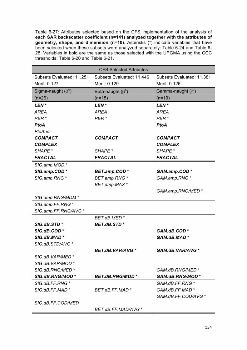
154
Table 6-27: Attributes selected based on the CFS implementation of the analysis of each SAR backscatter coefficient (n=141) analyzed together with the attributes of geometry, shape, and dimension (n=10). Asterisks (*) indicate variables that have been selected when these subsets were analyzed separately: Table 6-24 and Table 6-28. Variables in bold are the same as those selected with the UPGMA using the CCC thresholds: Table 6-20 and Table 6-21.
CFS Selected Attributes
Subsets Evaluated: 11,251 Subsets Evaluated: 11,446 Subsets Evaluated: 11,381 Merit: 0.127 Merit: 0.129 Merit: 0.126 Sigma-naught (σo) Beta-naught (βo) Gamma-naught (γo) (n=26) (n=15) (n=19)
LEN * LEN * LEN * AREA AREA AREA PER * PER * PER * PtoA PtoA PtoAnor COMPACT COMPACT COMPACT COMPLEX COMPLEX SHAPE * SHAPE * SHAPE * FRACTAL FRACTAL FRACTAL SIG.amp.MOD * SIG.amp.COD * BET.amp.COD * GAM.amp.COD * SIG.amp.RNG * BET.amp.RNG * GAM.amp.RNG * BET.amp.MAX * GAM.amp.RNG/MED * SIG.amp.RNG/MDM * SIG.amp.FF.RNG * SIG.amp.FF.RNG/AVG * BET.dB.MED * SIG.dB.STD * BET.dB.STD * SIG.dB.COD * GAM.dB.COD * SIG.dB.MAD * GAM.dB.MAD * SIG.dB.STD/AVG * BET.dB.VAR/AVG * GAM.dB.VAR/AVG * SIG.dB.VAR/MED * SIG.dB.VAR/MOD * SIG.dB.RNG/MED * GAM.dB.RNG/MED * SIG.dB.RNG/MOD * BET.dB.RNG/MOD * GAM.dB.RNG/MOD * SIG.dB.FF.RNG * GAM.dB.FF.RNG * SIG.dB.FF.MAD * BET.dB.FF.MAD * GAM.dB.FF.MAD * GAM.dB.FF.COD/AVG * SIG.dB.FF.COD/MED BET.dB.FF.MAD/AVG *

155
Table 6-28: Attributes selected based on the CFS implementation of the separately for each SAR backscatter coefficients (n=141). While the asterisks (*) indicate variables that also have been selected when the SAR attributes were analyzed together with the attributes of geometry, shape, and dimension (CFS: Table 6-27), the ones in bold are the same as those selected with the UPGMA using the CCC thresholds: Table 6-21.
CFS Selected Attributes Subsets Evaluated: 9,805 Subsets Evaluated: 9,881 Subsets Evaluated: 9,861 Merit: 0.099 Merit: 0.099 Merit: 0.097 Sigma-naught (σo) Beta-naught (βo) Gamma-naught (γo) (n=24) (n=21) (n=22) SIG.amp.MOD * GAM.amp.MOD SIG.amp.COD * BET.amp.COD * GAM.amp.COD * SIG.amp.RNG * BET.amp.RNG * GAM.amp.RNG * SIG.amp.MAX BET.amp.MAX * GAM.amp.STD/MOD SIG.amp.STD/MDM GAM.amp.RNG/MED * BET.amp.RNG/MOD SIG.amp.RNG/MDM * BET.amp.MAD/AVG SIG.amp.FF.RNG * BET.amp.FF.RNG SIG.amp.FF.RNG/AVG * BET.amp.FF.RNG/AVG GAM.amp.FF.RNG/AVG GAM.amp.FF.RNG/MDM SIG.amp.FF.RNG/MOD SIG.dB.MED BET.dB.MED * GAM.dB.MED SIG.dB.STD * BET.dB.STD * GAM.dB.STD SIG.dB.COD * BET.dB.COD GAM.dB.COD * SIG.dB.MAD * BET.dB.MAD GAM.dB.MAD * SIG.dB.STD/AVG * BET.dB.STD/AVG GAM.dB.STD/AVG SIG.dB.STD/MED BET.dB.STD/MED GAM.dB.STD/MED SIG.dB.VAR/AVG BET.dB.VAR/AVG * GAM.dB.VAR/AVG * SIG.dB.VAR/MED * BET.dB.VAR/MED GAM.dB.VAR/MED SIG.dB.VAR/MOD * BET.dB.VAR/MOD GAM.dB.VAR/MOD SIG.dB.RNG/MED * GAM.dB.RNG/MED * SIG.dB.RNG/MOD * BET.dB.RNG/MOD * GAM.dB.RNG/MOD * SIG.dB.FF.RNG * BET.dB.FF.RNG GAM.dB.FF.RNG * SIG.dB.FF.MAD * BET.dB.FF.MAD * GAM.dB.FF.MAD * GAM.dB.FF.COD/AVG * SIG.dB.FF.RNG/MOD BET.dB.FF.RNG/MOD GAM.dB.FF.RNG/MOD BET.dB.FF.MAD/AVG * SIG.dB.FF.MAD/MOD

156
Table 6-29: Variables selected (n=11) selected based on the CFS implementation of only Digital Numbers (DN’s) variables (n=35). Variables in bold are the same as those selected with the UPGMA implementation (Table 6-22).
Subsets Evaluated: 616 Merit: 0.059
CFS Selected Attributes
1 DN.AVG 2 DN.MDM 3 DN.STD 4 DN.COD 5 DN.RNG 6 DN.COD/MOD 7 DN.RNG/AVG 8 DN.RNG/MED 9 DN.RNG/MOD
10 DN.RNG/MDM 11 DN.MAD/MED
Two tables are provided to summarize the Attribute Selection practice introduced on
Section 5.8. While Table 6-30 presents the values of CCC (UPGMA) and Merit (CFS),
Table 6-31 reviews the number of variables per optimal subsets within the proposed
original sets shown on Figure 5-3.
Table 6-30: Summary of the CFS-Merit and of the CCC values resulted from the UPGMA implementation (Figure 5-3).
CCC and CFS-Merit per data sub-divisions UPGMA (CCC) CFS (Merit) Complete Exploration of the CBOS-DScMod 0.8175 1.000
All SAR Backscatter Signature ¥ with Size* 0.8227 0.131 Only all SAR Backscatter Signature ¥ 0.8253 0.103
Size* and Sigma-naught (σo) 0.8262 0.127 Size* and Beta-naught (βo) 0.8031 0.129 Size* and Gamma-naught (γo) 0.8240 0.126
Only Size* 0.9143 0.112
Only Sigma-naught (σo) 0.8319 0.099 Only Beta-naught (βo) 0.8130 0.099 Only Gamma-naught (γo) 0.8260 0.097
Only Digital Numbers (DN’s) 0.8020 0.059
* Attributes of geometry, shape, and dimension. ¥ See Table 5-1 and Table 5-5.
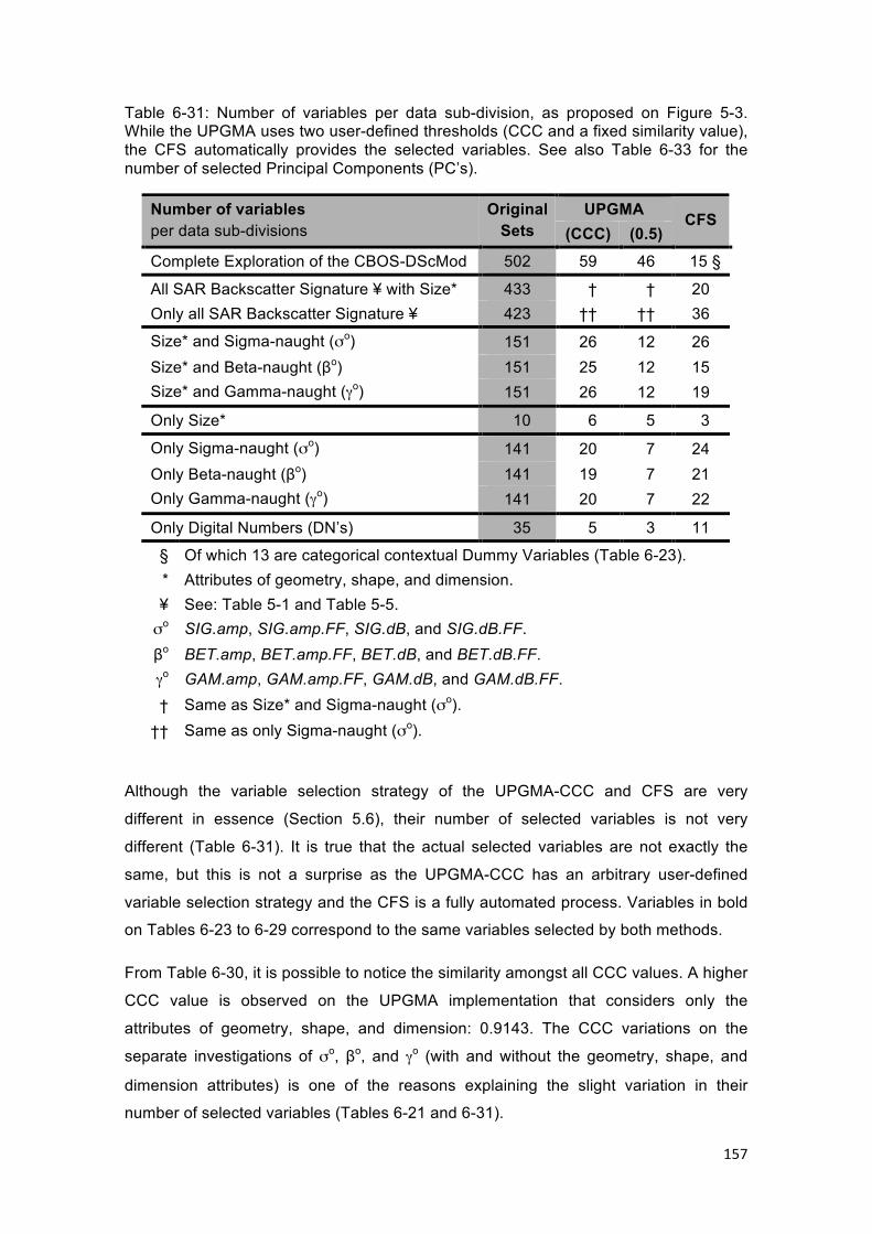
157
Table 6-31: Number of variables per data sub-division, as proposed on Figure 5-3. While the UPGMA uses two user-defined thresholds (CCC and a fixed similarity value), the CFS automatically provides the selected variables. See also Table 6-33 for the number of selected Principal Components (PC’s).
UPGMA Number of variables per data sub-divisions
Original Sets (CCC) (0.5)
CFS
Complete Exploration of the CBOS-DScMod 502 59 46 15 §
All SAR Backscatter Signature ¥ with Size* 433 † † 20 Only all SAR Backscatter Signature ¥ 423 †† †† 36
Size* and Sigma-naught (σo) 151 26 12 26 Size* and Beta-naught (βo) 151 25 12 15 Size* and Gamma-naught (γo) 151 26 12 19
Only Size* 10 6 5 3
Only Sigma-naught (σo) 141 20 7 24 Only Beta-naught (βo) 141 19 7 21 Only Gamma-naught (γo) 141 20 7 22
Only Digital Numbers (DN’s) 35 5 3 11
§ Of which 13 are categorical contextual Dummy Variables (Table 6-23). * Attributes of geometry, shape, and dimension. ¥ See: Table 5-1 and Table 5-5. σo SIG.amp, SIG.amp.FF, SIG.dB, and SIG.dB.FF. βo BET.amp, BET.amp.FF, BET.dB, and BET.dB.FF. γo GAM.amp, GAM.amp.FF, GAM.dB, and GAM.dB.FF.
† Same as Size* and Sigma-naught (σo).
†† Same as only Sigma-naught (σo).
Although the variable selection strategy of the UPGMA-CCC and CFS are very
different in essence (Section 5.6), their number of selected variables is not very
different (Table 6-31). It is true that the actual selected variables are not exactly the
same, but this is not a surprise as the UPGMA-CCC has an arbitrary user-defined
variable selection strategy and the CFS is a fully automated process. Variables in bold
on Tables 6-23 to 6-29 correspond to the same variables selected by both methods.
From Table 6-30, it is possible to notice the similarity amongst all CCC values. A higher
CCC value is observed on the UPGMA implementation that considers only the
attributes of geometry, shape, and dimension: 0.9143. The CCC variations on the
separate investigations of σo, βo, and γo (with and without the geometry, shape, and
dimension attributes) is one of the reasons explaining the slight variation in their
number of selected variables (Tables 6-21 and 6-31).
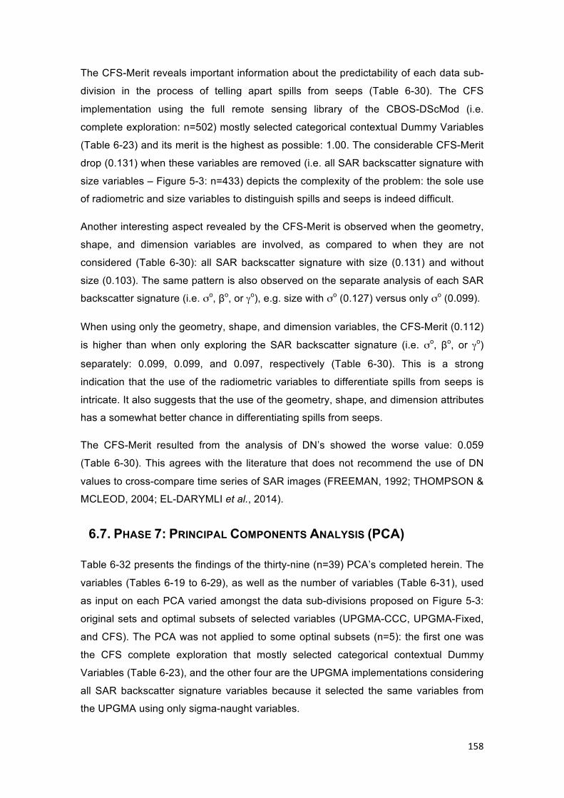
158
The CFS-Merit reveals important information about the predictability of each data sub-
division in the process of telling apart spills from seeps (Table 6-30). The CFS
implementation using the full remote sensing library of the CBOS-DScMod (i.e.
complete exploration: n=502) mostly selected categorical contextual Dummy Variables
(Table 6-23) and its merit is the highest as possible: 1.00. The considerable CFS-Merit
drop (0.131) when these variables are removed (i.e. all SAR backscatter signature with
size variables – Figure 5-3: n=433) depicts the complexity of the problem: the sole use
of radiometric and size variables to distinguish spills and seeps is indeed difficult.
Another interesting aspect revealed by the CFS-Merit is observed when the geometry,
shape, and dimension variables are involved, as compared to when they are not
considered (Table 6-30): all SAR backscatter signature with size (0.131) and without
size (0.103). The same pattern is also observed on the separate analysis of each SAR
backscatter signature (i.e. σo, βo, or γo), e.g. size with σo (0.127) versus only σo (0.099).
When using only the geometry, shape, and dimension variables, the CFS-Merit (0.112)
is higher than when only exploring the SAR backscatter signature (i.e. σo, βo, or γo)
separately: 0.099, 0.099, and 0.097, respectively (Table 6-30). This is a strong
indication that the use of the radiometric variables to differentiate spills from seeps is
intricate. It also suggests that the use of the geometry, shape, and dimension attributes
has a somewhat better chance in differentiating spills from seeps.
The CFS-Merit resulted from the analysis of DN’s showed the worse value: 0.059
(Table 6-30). This agrees with the literature that does not recommend the use of DN
values to cross-compare time series of SAR images (FREEMAN, 1992; THOMPSON &
MCLEOD, 2004; EL-DARYMLI et al., 2014).
6.7. PHASE 7: PRINCIPAL COMPONENTS ANALYSIS (PCA)
Table 6-32 presents the findings of the thirty-nine (n=39) PCA’s completed herein. The
variables (Tables 6-19 to 6-29), as well as the number of variables (Table 6-31), used
as input on each PCA varied amongst the data sub-divisions proposed on Figure 5-3:
original sets and optimal subsets of selected variables (UPGMA-CCC, UPGMA-Fixed,
and CFS). The PCA was not applied to some optinal subsets (n=5): the first one was
the CFS complete exploration that mostly selected categorical contextual Dummy
Variables (Table 6-23), and the other four are the UPGMA implementations considering
all SAR backscatter signature variables because it selected the same variables from
the UPGMA using only sigma-naught variables.
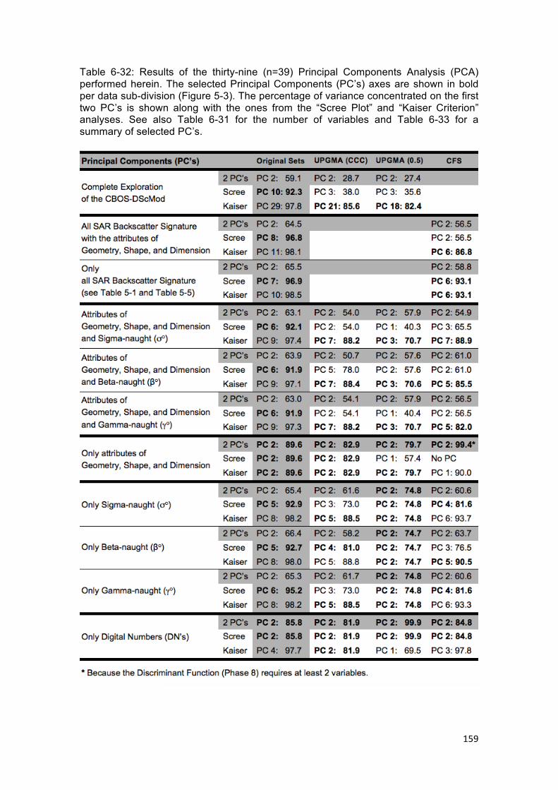
159
Table 6-32: Results of the thirty-nine (n=39) Principal Components Analysis (PCA) performed herein. The selected Principal Components (PC’s) axes are shown in bold per data sub-division (Figure 5-3). The percentage of variance concentrated on the first two PC’s is shown along with the ones from the “Scree Plot” and “Kaiser Criterion” analyses. See also Table 6-31 for the number of variables and Table 6-33 for a summary of selected PC’s.
160
Table 6-32 gives a global picture of the percentages of variance concentrated on
particular Principal Components (PC’s) axes among all data sub-divisions (Figure 5-3).
As each PC axis concentrates part of the variance within the dataset, and it is aimed to
have more variance on fewer PC’s, the variance concentrated on the first two PC’s are
shown as reference levels (LEGENDRE & LEGENDRE, 2012). The PC’s selected
using the “Scree Plot” (broken stick and row-wise bootstrapping eigenvalue error bars)
are also shown along with PC’s selected using the “Kaiser Criterion” (eigenvalue
greater than 1). The selection of the PC’s to be explored on the subsequent data
mining – e.g. Phase 8 (Discriminant Function: Section 5.8) – was based on the overall
analysis of all PC’s selected with the Scree Plot or Kaiser Criterion (Table 6-32). If the
Scree Plot PC concentrated less than 80.0% of the variance, the Kaiser Criterion PC
was selected; otherwise, the Scree Plot PC was the chosen one.
The line-wise inspection of Table 6-32 revels that the variance concentration per PC’s
of the original sets stands out. This is most likely to be caused because of the larger
number of input variables (Table 6-31) – see loading plots shown below. The column-
wise analysis of Table 6-32 discloses a particularly similar PC-selection within the
exploration of SAR backscatter signature (σo, βo, and γo separately or together, with
and without the geometry, shape, and dimension attributes), for instance, both Scree
Plot PC’s and Kaiser Criterion PC’s, concentrate equivalent variances.
The PCA of the data sub-divisions that considered only only the attributes of geometry,
shape, and dimension, and only the DN’s, showed the highest variance concentration
percentages on the first two PC’s: approximately 80.0% or more (Table 6-32). Another
aspect about these two data sub-divisions is that the first two PC’s have been selected
for their original sets and for all optimal subsets (line-wise).
An additional aspect about the information presented on Table 6-32, regards the CFS
PC-selection that analyzed only the attributes of geometry, shape, and dimension.
Because the Discriminant Function (Phase 8: Sections 5.8 and 6.8) requires at least
two variables, the first two PC’s were selected even though the Scree Plot did not
selected any PC and Kaiser Criterion only selected one PC – see Figure 6-36.
Because Table 6-32 contains a wide-range of information, a summary of selected PC’s
(shown in bold on Table 6-32) is presented on Table 6-33. The dimensionality
reduction promoted by the PCA is evident on a cross-comparison against Table 6-31.
These two tables (Tables 6-31 and 6-33) present the number of variables utilized as
input on the Discriminant Function (Phase 8: Sections 5.8 and 6.8).
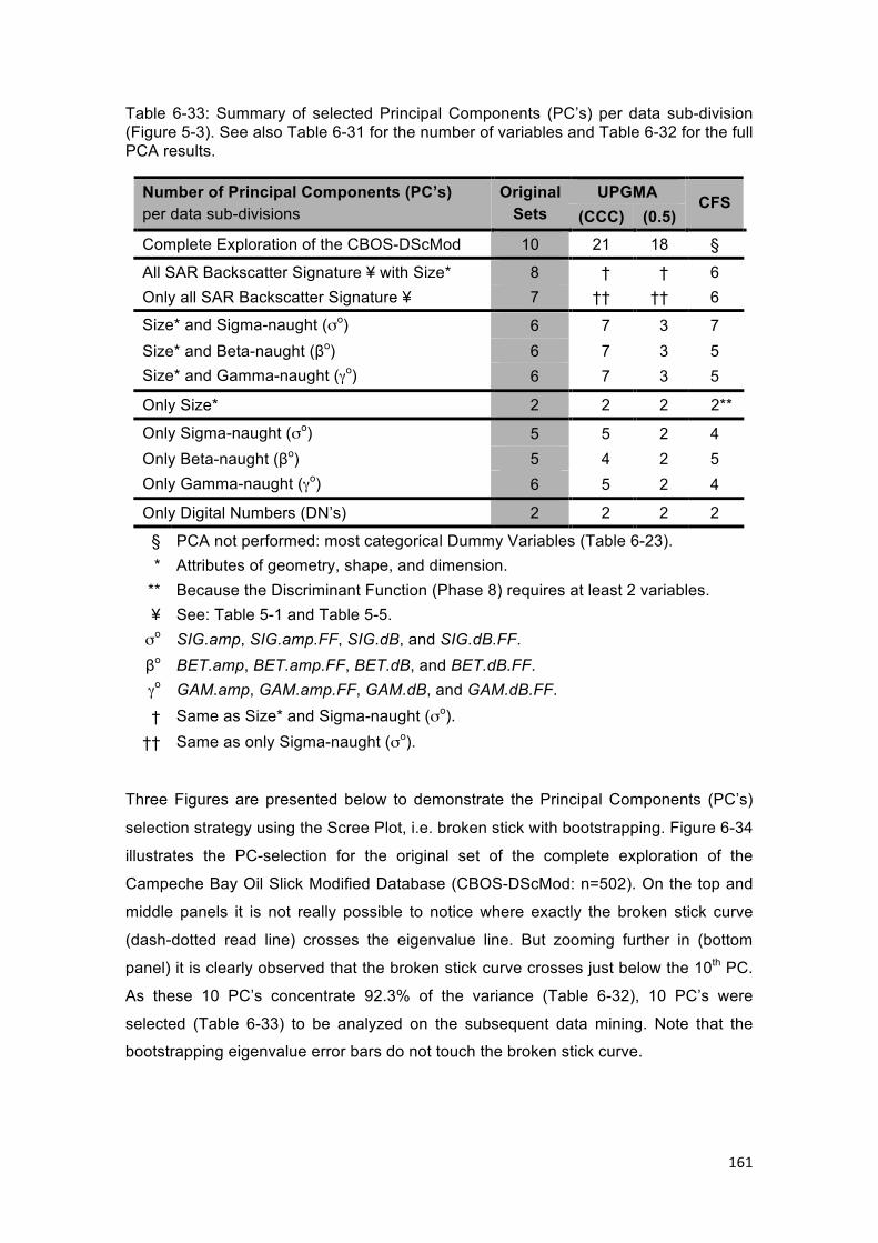
161
Table 6-33: Summary of selected Principal Components (PC’s) per data sub-division (Figure 5-3). See also Table 6-31 for the number of variables and Table 6-32 for the full PCA results.
UPGMA Number of Principal Components (PC’s) per data sub-divisions
Original Sets (CCC) (0.5)
CFS
Complete Exploration of the CBOS-DScMod 10 21 18 §
All SAR Backscatter Signature ¥ with Size* 8 † † 6 Only all SAR Backscatter Signature ¥ 7 †† †† 6
Size* and Sigma-naught (σo) 6 7 3 7 Size* and Beta-naught (βo) 6 7 3 5 Size* and Gamma-naught (γo) 6 7 3 5
Only Size* 2 2 2 2**
Only Sigma-naught (σo) 5 5 2 4 Only Beta-naught (βo) 5 4 2 5 Only Gamma-naught (γo) 6 5 2 4
Only Digital Numbers (DN’s) 2 2 2 2
§ PCA not performed: most categorical Dummy Variables (Table 6-23). * Attributes of geometry, shape, and dimension.
** Because the Discriminant Function (Phase 8) requires at least 2 variables. ¥ See: Table 5-1 and Table 5-5. σo SIG.amp, SIG.amp.FF, SIG.dB, and SIG.dB.FF. βo BET.amp, BET.amp.FF, BET.dB, and BET.dB.FF. γo GAM.amp, GAM.amp.FF, GAM.dB, and GAM.dB.FF.
† Same as Size* and Sigma-naught (σo).
†† Same as only Sigma-naught (σo).
Three Figures are presented below to demonstrate the Principal Components (PC’s)
selection strategy using the Scree Plot, i.e. broken stick with bootstrapping. Figure 6-34
illustrates the PC-selection for the original set of the complete exploration of the
Campeche Bay Oil Slick Modified Database (CBOS-DScMod: n=502). On the top and
middle panels it is not really possible to notice where exactly the broken stick curve
(dash-dotted read line) crosses the eigenvalue line. But zooming further in (bottom
panel) it is clearly observed that the broken stick curve crosses just below the 10th PC.
As these 10 PC’s concentrate 92.3% of the variance (Table 6-32), 10 PC’s were
selected (Table 6-33) to be analyzed on the subsequent data mining. Note that the
bootstrapping eigenvalue error bars do not touch the broken stick curve.
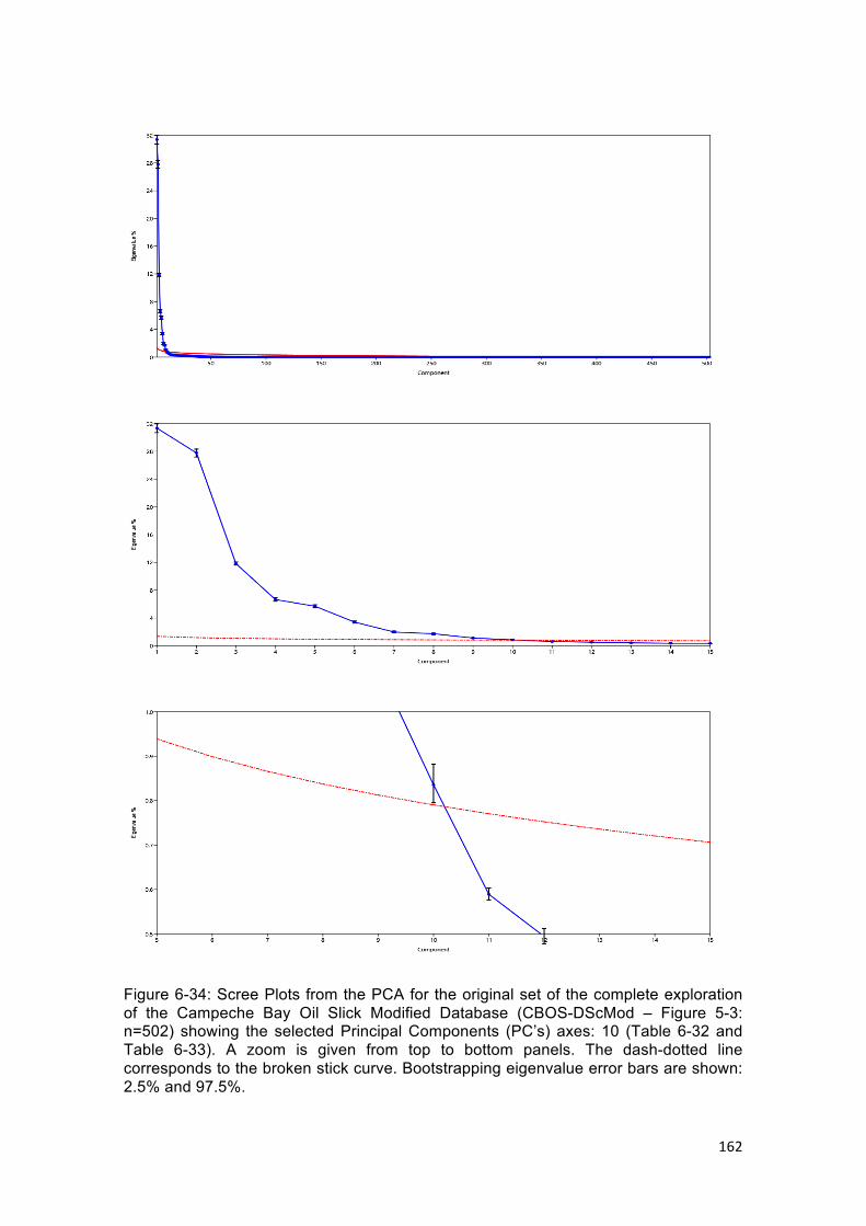
162
Figure 6-34: Scree Plots from the PCA for the original set of the complete exploration of the Campeche Bay Oil Slick Modified Database (CBOS-DScMod – Figure 5-3: n=502) showing the selected Principal Components (PC’s) axes: 10 (Table 6-32 and Table 6-33). A zoom is given from top to bottom panels. The dash-dotted line corresponds to the broken stick curve. Bootstrapping eigenvalue error bars are shown: 2.5% and 97.5%.

163
Correspondingly, Figure 6-35 depicts the Scree Plots from the different analyses
exploring only sigma-naught (σo) variables. The top panel shows the PCA of the
original set (Table 5-5: n=141) where it is possible to see that the broken stick (dash-
dotted red line) crosses the just below the 6th PC. However, the bootstrapping
eigenvalue error bars touch the broken stick curve. Therefore, only 5 PC’s were
selected (Tables 6-32 and 6-33). The 2nd panel from the top shows the UPGMA-CCC
(Table 6-21: n=20), where 3 PC’s were selected (Table 6-32). However, because these
only concentrate 73.0% of the variance, and the 5 PC’s selected with the Kaiser
Criterion concentrate 88.5%, 5 PC’s were selected (Tables 6-32 and 6-33). The last
two panels on Figure 6-35 show the PCA for the UPGMA-Fixed (Table 6-21: n=7) and
CFS (Table 6-28: n=24): selecting 2 and 4 PC’s, respectively.
Similarly, Figure 6-36 illustrates the PCA exploring only attributes of geometry, shape,
and dimension. Two PC’s were selected with the Scree Plot on the top two panels:
original set (Table 5-4: n=10) and UPGMA-CCC (Table 6-20: n=6). Coincidently, these
have also been selected with the Kaiser Criterion (Table 6-32). The PCA of the
UPGMA-Fixed (Table 6-20: n=5) is shown on the 3rd panel from the top, in which only
one PC was selected – concentrating only 57.4% of the variance (Table 6-32). Even
though the Kaiser Criterion selected 2 PC’s concentrating with less than 80.0% of the
variance, these were selected to be analyzed on the subsequent data mining (Table 6-
33). The bottom panel shows the PCA of the CFS (Table 6-24: n=3), and because the
bootstrapping eigenvalue error bars touch the broken stick curve, no PC has been
selected with the Scree Plot. Although the Kaiser Criterion selected one PC
concentrating 90.0% of the variance, the Discriminant Function (Phase 8: Sections 5.8
and 6.8) requires at least 2 variables (i.e. in this case, two PC’s); therefore, the first two
PC’s have been selected (Tables 6-32 and 6-33).
As a result, the subsequent data mining analyzing only the attributes of geometry,
shape, and dimension are carried with their respective first two PC’s (Tables 6-32 and
6-33). The PC’s selected for all other data sub-divisions (Figure 5-3) undergone the
same PC-selection process illustrated on Figure 6-34, Figure 6-35, and Figure 6-36,
and described above: Scree Plot and Kaiser Criterion.
Scatterplots illustrating the relationship between the selected PC’s resulted from the
PCA have also been investigated. Figure 6-37 and Figure 6-38 show, respectively, the
scatterplots of the first two PC’s for the PCA exploring only sigma-naught (σo) variables
and for the PCA exploring only attributes of geometry, shape, and dimension.
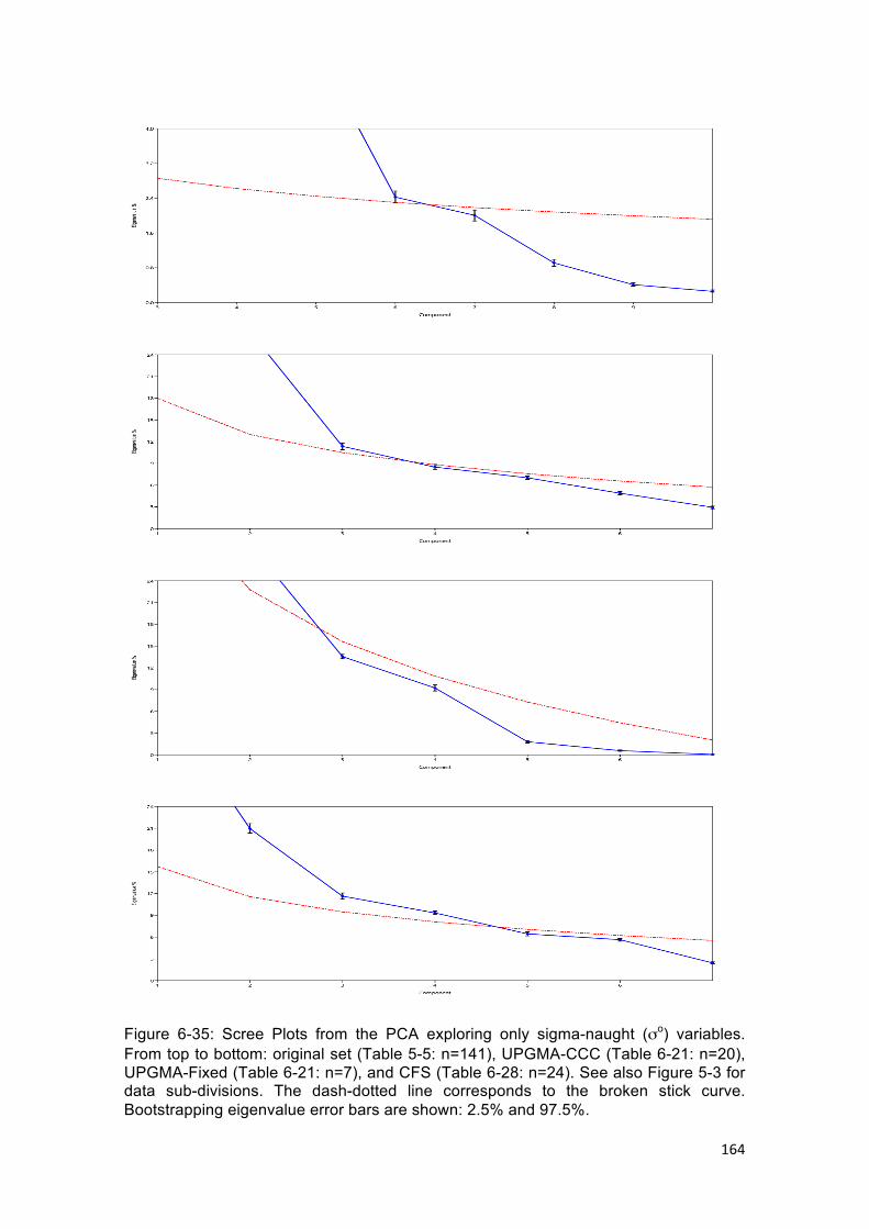
164
Figure 6-35: Scree Plots from the PCA exploring only sigma-naught (σo) variables. From top to bottom: original set (Table 5-5: n=141), UPGMA-CCC (Table 6-21: n=20), UPGMA-Fixed (Table 6-21: n=7), and CFS (Table 6-28: n=24). See also Figure 5-3 for data sub-divisions. The dash-dotted line corresponds to the broken stick curve. Bootstrapping eigenvalue error bars are shown: 2.5% and 97.5%.

165
Figure 6-36: Scree Plots from the PCA exploring only attributes of geometry, shape, and dimension. From top to bottom: original set (Table 5-4: n=10), UPGMA-CCC (Table 6-20: n=6), UPGMA-Fixed (Table 6-20: n=5), and CFS (Table 6-24: n=3). See also Figure 5-3 for data sub-divisions. The dash-dotted line corresponds to the broken stick curve. Bootstrapping eigenvalue error bars are shown: 2.5% and 97.5%.

166
Figure 6-37: Scatterplots of the first two Principal Components resulted from the PCA exploring only sigma-naught (σo) variables. From top to bottom: original set (Table 5-5: n=141), UPGMA-CCC (Table 6-21: n=20), UPGMA-Fixed (Table 6-21: n=7), and CFS (Table 6-28: n=24). See also Figure 5-3 for data sub-divisions. Open red triangles: oil spills. Open green circles: oil seeps.
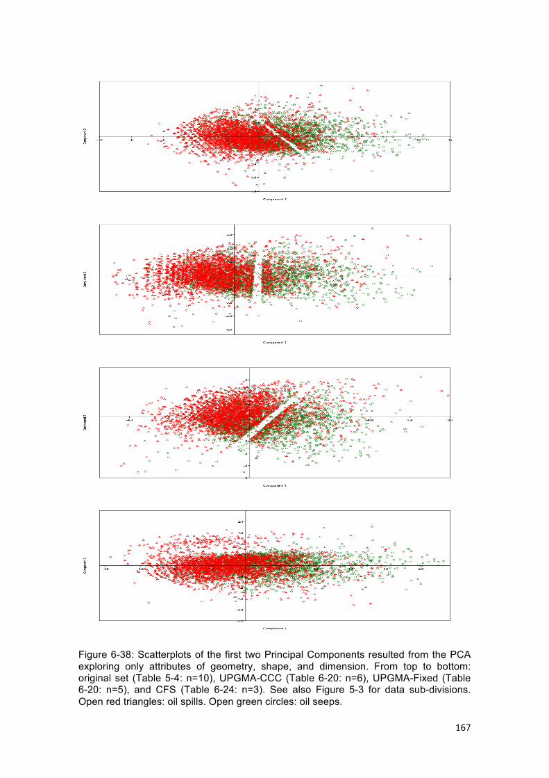
167
Figure 6-38: Scatterplots of the first two Principal Components resulted from the PCA exploring only attributes of geometry, shape, and dimension. From top to bottom: original set (Table 5-4: n=10), UPGMA-CCC (Table 6-20: n=6), UPGMA-Fixed (Table 6-20: n=5), and CFS (Table 6-24: n=3). See also Figure 5-3 for data sub-divisions. Open red triangles: oil spills. Open green circles: oil seeps.
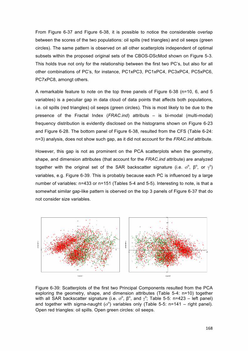
168
From Figure 6-37 and Figure 6-38, it is possible to notice the considerable overlap
between the scores of the two populations: oil spills (red triangles) and oil seeps (green
circles). The same pattern is observed on all other scatterplots independent of optimal
subsets within the proposed original sets of the CBOS-DScMod shown on Figure 5-3.
This holds true not only for the relationship between the first two PC’s, but also for all
other combinations of PC’s, for instance, PC1xPC3, PC1xPC4, PC3xPC4, PC5xPC6,
PC7xPC8, amongt others.
A remarkable feature to note on the top three panels of Figure 6-38 (n=10, 6, and 5
variables) is a peculiar gap in data cloud of data points that affects both populations,
i.e. oil spills (red triangles) oil seeps (green circles). This is most likely to be due to the
presence of the Fractal Index (FRAC.ind) attributs – is bi-modal (multi-modal)
frequency distribution is evidently disclosed on the histograms shown on Figure 6-23
and Figure 6-28. The bottom panel of Figure 6-38, resulted from the CFS (Table 6-24:
n=3) analysis, does not show such gap, as it did not account for the FRAC.ind attribute.
However, this gap is not as prominent on the PCA scatterplots when the geometry,
shape, and dimension attributes (that account for the FRAC.ind attribute) are analyzed
together with the original set of the SAR backscatter signature (i.e. σo, βo, or γo)
variables, e.g. Figure 6-39. This is probably because each PC is influenced by a large
number of variables: n=433 or n=151 (Tables 5-4 and 5-5). Interesting to note, is that a
somewhat similar gap-like pattern is oberved on the top 3 panels of Figure 6-37 that do
not consider size variables.
Figure 6-39: Scatterplots of the first two Principal Components resulted from the PCA exploring the geometry, shape, and dimension attributes (Table 5-4: n=10) together with all SAR backscatter signature (i.e. σo, βo, and γo; Table 5-5: n=423 – left panel) and together with sigma-naught (σo) variables only (Table 5-5: n=141 – right panel). Open red triangles: oil spills. Open green circles: oil seeps.

169
The influence (i.e. meaning) of each original variable to each PC has been quantified
by the inspection of Loadings plots. Figure 6-40 illustrates the first PC for the original
sets (n=141) of sigma-naught (σo), beta-naught (βo), and gamma-naught (γo). Likewise,
Figure 6-41 depicts the first PC of the separate UPGMA-CCC implementation of the
three SAR backscatter signature (σo, βo, and γo) with the attributes of geometry, shape,
and dimension. It is possible to observe that almost all variables are largely influencing
the respective PC.
Figure 6-40: Loadings expressing the relationship between the original variables (n=141) and the first Principal Component of sigma-naught (σo), beta-naught (βo), and gamma-naught (γo), respectively, top, middle, and bottom panels. See also Table 5-5 for the original attributes.

170
Figure 6-41: Loadings expressing the relationship between the optimal subset variables and the first Principal Component of sigma-naught (σo), beta-naught (βo), and gamma-naught (γo), respectively, top (n=26), middle (n=25), and bottom (n=26) panels. See also Tables 6-20 and 6-21 for the original attributes.
The loadings plot for the analyses of the attributes of geometry, shape, and dimension
and the first Principal Component show the same pattern of a fairly even influence of all
10 original variables on the first PC (Figure 6-42). The exception is on the CFS that has
the perimeter (Per) being the sole one to account for the variance on the first PC – the
second PC of this CFS PCA has the opposite occuring.

171
Figure 6-42: Loadings expressing the relationship between the attributes of geometry, shape, and dimension and the first Principal Component. From top to bottom: original set (Table 5-4: n=10), UPGMA-CCC (Table 6-20: n=6), UPGMA-Fixed (Table 6-20: n=5), and CFS (Table 6-24: n=3).
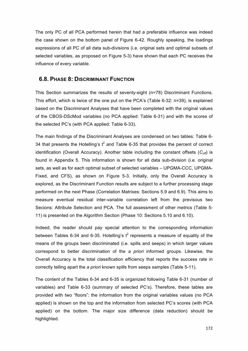
172
The only PC of all PCA performed herein that had a preferable influence was indeed
the case shown on the bottom panel of Figure 6-42. Roughly speaking, the loadings
expressions of all PC of all data sub-divisions (i.e. original sets and optimal subsets of
selected variables, as proposed on Figure 5-3) have shown that each PC receives the
influence of every variable.
6.8. PHASE 8: DISCRIMINANT FUNCTION
This Section summarizes the results of seventy-eight (n=78) Discriminant Functions.
This effort, which is twice of the one put on the PCA’s (Table 6-32: n=39), is explained
based on the Discriminant Analyses that have been completed with the original values
of the CBOS-DScMod variables (no PCA applied: Table 6-31) and with the scores of
the selected PC’s (with PCA applied: Table 6-33).
The main findings of the Discriminant Analyses are condensed on two tables: Table 6-
34 that presents the Hotelling’s t2 and Table 6-35 that provides the percent of correct
identification (Overall Accuracy). Another table including the constant offsets (Coff) is
found in Appendix 5. This information is shown for all data sub-division (i.e. original
sets, as well as for each optimal subset of selected variables – UPGMA-CCC, UPGMA-
Fixed, and CFS), as shown on Figure 5-3. Initially, only the Overall Accuracy is
explored, as the Discriminant Function results are subject to a further processing stage
performed on the next Phase (Correlation Matrixes: Sections 5.9 and 6.9). This aims to
measure eventual residual inter-variable correlation left from the previsous two
Secions: Attribute Selection and PCA. The full assessment of other metrics (Table 5-
11) is presented on the Algorithm Section (Phase 10: Sections 5.10 and 6.10).
Indeed, the reader should pay special attention to the corresponding information
between Tables 6-34 and 6-35. Hotelling’s t2 represents a measure of equality of the
means of the groups been discriminated (i.e. spills and seeps) in which larger values
correspond to better discrimination of the a priori informed groups. Likewise, the
Overall Accuracy is the total classification efficiency that reports the success rate in
correctly telling apart the a priori known spills from seeps samples (Table 5-11).
The content of the Tables 6-34 and 6-35 is organized following Table 6-31 (number of
variables) and Table 6-33 (summary of selected PC’s). Therefore, these tables are
provided with two “floors”: the information from the original variables values (no PCA
applied) is shown on the top and the information from selected PC’s scores (with PCA
applied) on the bottom. The major size difference (data reduction) should be
highlighted.
173
Table 6-34: Hotelling’s t2 values per data sub-divisions (Figure 5-3).
No PCA: See Table 6-31 for the number of variables.
Original Sets
UPGMA (CCC)
UPGMA (0.5) CFS
Complete Exploration of the CBOS-DScMod 11,509.0 10,598.0 10,529.0 §
All SAR Backscatter Signature ¥ with Size* 1,919.7 † † 1,485.3
Only all SAR Backscatter Signature ¥ 1,558.3 †† †† 1,115.8
Size* and Sigma-naught (σo) 1,583.5 1,508.3 1,383.0 1,462.4
Size* and Beta-naught (βo) 1,577.5 1,510.1 1,401.8 1,299.3
Size* and Gamma-naught (γo) 1,563.4 1,490.0 1,366.4 1,436.2
Only Size* 1,141.3 1,141.3 1,141.3 1,138.3
Only Sigma-naught (σo) 1,236.5 985.4 647.6 974.8
Only Beta-naught (βo) 1,231.4 1,019.8 632.8 919.1
Only Gamma-naught (γo) 1,213.4 968.68 635.7 950.7
Only Digital Numbers (DN’s) 663.7 218.8 138.4 550.35
With PCA: See Table 6-33 for the selected PC’s.
Original Sets
UPGMA (CCC)
UPGMA (0.5) CFS
Complete Exploration of the CBOS-DScMod 17,056.0 89,403.0 94,086.0 §
All SAR Backscatter Signature ¥ with Size* 1,065.5 † † 1,044.5
Only all SAR Backscatter Signature ¥ 598.9 †† †† 632.4
Size* and Sigma-naught (σo) 891.0 1,123.5 769.8 1,065.8
Size* and Beta-naught (βo) 908.7 1,099.5 722.3 1,106.2
Size* and Gamma-naught (γo) 863.1 1,115.4 753.4 1,028.4
Only Size* 1,034.2 1,064.7 1,086.4 1,085.9
Only Sigma-naught (σo) 594.1 589.5 447.7 640.9
Only Beta-naught (βo) 584.1 464.5 435.7 612.6
Only Gamma-naught (γo) 579.2 574.7 432.2 606.7
Only Digital Numbers (DN’s) 138.0 163.0 138.4 210.5
§ Discriminant Function not performed (see Table 6-23).
* Attributes of geometry, shape, and dimension.
¥ See: Table 5-1 and Table 5-5.
σo SIG.amp, SIG.amp.FF, SIG.dB, and SIG.dB.FF.
βo BET.amp, BET.amp.FF, BET.dB, and BET.dB.FF.
γo GAM.amp, GAM.amp.FF, GAM.dB, and GAM.dB.FF.
† Same as Size* and Sigma-naught (σo).
†† Same as only Sigma-naught (σo).

174
The first aspect to notice while considering the Hotteling’s t2 (Table 6-34) is that these
values are larger on the top floor (original values of variables prior to the PCA) than on
the bottom floor (scores of the PC’s selected on the PCA’s).
The second aspect is that the complete exploration of the CBOS-DScMod that
undergone a major data reduction (Table 6-31: 502, 59, and 46 variables, and Table 6-
33: 10, 21, and 18 PC’s), presents the higher Hotelling’s t2 values. This is anticipated
as many categorical contextual Dummy Variables (Table 5-10) are accounted for. An
enormous increase is evident on the PCA floor, from this original set to the two
UPGMA optimal subsets.
One can clearly see that the Hotelling’s t2 values for the analysis considering only DN’s
(e.g. UPGMA-CCC: 163.0) has the lower value by far. As with the CFS-Merit (Table 6-
30: DN=0.059), this agrees with literature that do not recommend DN values to cross-
compare time series of SAR images (FREEMAN, 1992; THOMPSON & MCLEOD,
2004; EL-DARYMLI et al., 2014). Important to highlight that the magnitude of the
Hotelling’s t2 values is not comparable to the one from the CFS-Merit; therefore, such
assessment should not be exercised.
Column-wise, the Hotelling’s t2 behavior is fairly similar to the one from the CFS-Merit
presented on the very end of Phase 6 (Attribute Selection: Section 5.6) – Table 6-30.
The pattern shown by the sole analyses of the attributes of geometry, shape, and
dimension present a higher Hotelling’s t2 values as compared to when these attributes
are not included.
Line-wise, the higher Hotelling’s t2 values are usually observed for the UPGMA-CCC
optimal subset. Again, the sole use of the attributes of geometry, shape, and dimension
has about the same effectiveness to discriminate spills from seeps, as when these
attributes are combined with the SAR backscatter signature: σo, βo, and γo. Thus
showing that the SAR backscatter signature is not adding much to the whole
differentiation process.
Continuing on the line-wise observation of Table 6-34, the UPGMA-Fixed optimal
subsets tend to present almost always the lower Hotelling’s t2 values. With the above
noticed about the UPGMA-CCC optimal subset, it is possible to confirm that the
number of variables has some influence on the discrimination process. This might be
related not only to the amount of variables, but also to their quality (i.e. redundant
correlated information or not).

175
Table 6-35: Overall Accuracy per data sub-divisions (Figure 5-3).
No PCA: See Table 6-31 for the number of variables.
Original Sets
UPGMA (CCC)
UPGMA (0.5) CFS
Complete Exploration of the CBOS-DScMod 90.70% 90.56% 90.40% §
All SAR Backscatter Signature ¥ with Size* 73.33% † † 72.36%
Only all SAR Backscatter Signature ¥ 70.87% †† †† 68.53%
Size* and Sigma-naught (σo) 72.88% 72.90% 71.95% 72.17%
Size* and Beta-naught (βo) 72.44% 72.62% 71.87% 70.50%
Size* and Gamma-naught (γo) 72.90% 72.64% 71.77% 71.89%
Only Size* 70.40% 70.40% 70.40% 70.28%
Only Sigma-naught (σo) 69.89% 67.51% 64.06% 67.41%
Only Beta-naught (βo) 70.00% 68.31% 64.16% 67.49%
Only Gamma-naught (γo) 69.87% 67.21% 63.63% 67.41%
Only Digital Numbers (DN’s) 66.68% 58.67% 56.75% 64.99%
With PCA: See Table 6-33 for the selected PC’s.
Original Sets
UPGMA (CCC)
UPGMA (0.5) CFS
Complete Exploration of the CBOS-DScMod 90.04% 99.98% 99.96% §
All SAR Backscatter Signature ¥ with Size* 68.61% † † 68.71%
Only all SAR Backscatter Signature ¥ 63.63% †† †† 63.93%
Size* and Sigma-naught (σo) 67.64% 69.51% 65.46% 69.18%
Size* and Beta-naught (βo) 68.02% 69.57% 65.58% 69.55%
Size* and Gamma-naught (γo) 67.47% 69.32% 65.79% 68.59%
Only Size* 69.59% 70.00% 70.02% 70.22%
Only Sigma-naught (σo) 63.28% 63.16% 63.26% 64.12%
Only Beta-naught (βo) 63.53% 63.20% 63.02% 64.46%
Only Gamma-naught (γo) 63.16% 63.02% 63.24% 64.18%
Only Digital Numbers (DN’s) 57.65% 57.89% 56.75% 59.48%
§ Discriminant Function not performed (see Table 6-23).
* Attributes of geometry, shape, and dimension.
¥ See: Table 5-1 and Table 5-5.
σo SIG.amp, SIG.amp.FF, SIG.dB, and SIG.dB.FF.
βo BET.amp, BET.amp.FF, BET.dB, and BET.dB.FF.
γo GAM.amp, GAM.amp.FF, GAM.dB, and GAM.dB.FF.
† Same as Size* and Sigma-naught (σo).
†† Same as only Sigma-naught (σo).

176
The UPGMA-CCC Hotelling’s t2 values are somewhat equivalent to those of the CFS.
Even though their variables are similar, they are not the same (Tables 6-19 to 6-29).
This also corroborates the importance of reducing the dimensionality on the attribute-
domain, for instance, Attribute Selection (Phase 6: Section 5.6) and PCA practices
(Phase 7: Section 5.7). These two processes should be applied with caution not to lose
information (i.e. underestimation) or to include noise (i.e. overestimation) (PERES-
NETO et al., 2003; 2005; HAIR et al., 2005).
Table 6-35 reports a summary of the Overall Accuracy distribution. The percentages
from the complete exploration stand out (>90.0%). To some extent, improved
accuracies are observed on the top floor that considers the original variables. Digital
Numbers (DN’s) are again the worse ones. There is a slight better discrimination while
using only the attributes of geometry, shape, and dimension. In general, the Overall
Accuracy somewhat matches the observations from Hotelling’s t2 values (Table 6-34).
6.9. PHASE 9: CORRELATION MATRIX
Once the Discriminant Functions were explored, Correlation Matrixes were computed
to verify the linear correlation among the variables and PC’s. PAST (version 2.17c) was
used for this task and it provides matrixes of linear correlation of Pearson’s r correlation
coefficient and p(uncorrelated).
Roughly all information from the original values of the CBOS-DScMod variables (no
PCA applied: Table 6-31) showed residual inter-variable correlation. This included all
data sub-division, i.e. original sets, as well as the optimal subsets of selected variables
(UPGMA-CCC, UPGMA-Fixed, and CFS) – Figure 5-3. On the other hand, as
expected, all information from the scores of the selected PC’s (with PCA applied –
Table 6-33) presented no inter-variable correlation. These, respectively, correspond to
the two “floors” explored on the Discriminant Function Tables 6-34 and 6-35.
While Table 6-36 (UPGMA-CCC: n=26) provides a clear example of the inter-variable
correlation, Table 6-37 (UPGMA-CCC: 7 PC’s) shows the anticipated lack of inter-PC
correlation. The linear correlation of Pearson r and p(uncorrelated) are shown on the
bottom and top of the table, respectively. Shown on grey are the uncorrelated relations.
This pattern was roughly the same for all other data sub-divisions (Figure 5-3). Most
original values of the CBOS-DScMod variables prior to the PCA are correlated,
whereas the scores of the selected PC’s are not. This brings to a close that only the
information of the Discriminant Function “floor” with the PCA is carried to design the
classification algorithm (Tables 6-34 and 6-35).
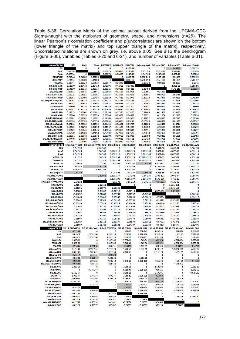
177
Table 6-36: Correlation Matrix of the optimal subset derived from the UPGMA-CCC Sigma-naught with the attributes of geometry, shape, and dimensions (n=26). The linear Pearson’s r correlation coefficient and p(uncorrelated) are shown on the bottom (lower triangle of the matrix) and top (upper triangle of the matrix), respectively. Uncorrelated relations are shown on grey, i.e. above 0.05. See also the dendrogram (Figure 6-30), variables (Tables 6-20 and 6-21), and number of variables (Table 6-31).
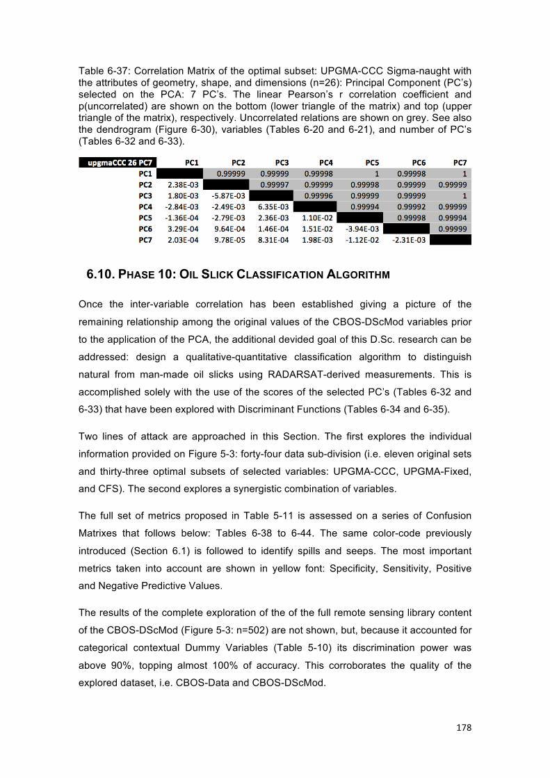
178
Table 6-37: Correlation Matrix of the optimal subset: UPGMA-CCC Sigma-naught with the attributes of geometry, shape, and dimensions (n=26): Principal Component (PC’s) selected on the PCA: 7 PC’s. The linear Pearson’s r correlation coefficient and p(uncorrelated) are shown on the bottom (lower triangle of the matrix) and top (upper triangle of the matrix), respectively. Uncorrelated relations are shown on grey. See also the dendrogram (Figure 6-30), variables (Tables 6-20 and 6-21), and number of PC’s (Tables 6-32 and 6-33).
6.10. PHASE 10: OIL SLICK CLASSIFICATION ALGORITHM
Once the inter-variable correlation has been established giving a picture of the
remaining relationship among the original values of the CBOS-DScMod variables prior
to the application of the PCA, the additional devided goal of this D.Sc. research can be
addressed: design a qualitative-quantitative classification algorithm to distinguish
natural from man-made oil slicks using RADARSAT-derived measurements. This is
accomplished solely with the use of the scores of the selected PC’s (Tables 6-32 and
6-33) that have been explored with Discriminant Functions (Tables 6-34 and 6-35).
Two lines of attack are approached in this Section. The first explores the individual
information provided on Figure 5-3: forty-four data sub-division (i.e. eleven original sets
and thirty-three optimal subsets of selected variables: UPGMA-CCC, UPGMA-Fixed,
and CFS). The second explores a synergistic combination of variables.
The full set of metrics proposed in Table 5-11 is assessed on a series of Confusion
Matrixes that follows below: Tables 6-38 to 6-44. The same color-code previously
introduced (Section 6.1) is followed to identify spills and seeps. The most important
metrics taken into account are shown in yellow font: Specificity, Sensitivity, Positive
and Negative Predictive Values.
The results of the complete exploration of the of the full remote sensing library content
of the CBOS-DScMod (Figure 5-3: n=502) are not shown, but, because it accounted for
categorical contextual Dummy Variables (Table 5-10) its discrimination power was
above 90%, topping almost 100% of accuracy. This corroborates the quality of the
explored dataset, i.e. CBOS-Data and CBOS-DScMod.

179
The finding from the use of the PC’s from the UPGMA-Fixed are also not presented
because the initial analysis of the Overall Accuracy (Table 6-35) showed a lower
discriminating power that of the UPGMA-CCC and CFS, which indeed is reflected on
the other methics. Consequently, the results shown on this Section focuses on PC’s
selected with the variables from the UPGMA-CCC and CFS: respectively, left and right
tables of Tables 6-38 to 6-43.
Table 6-38 presents the findings from the analysis that investigates all SAR backscatter
signature variables together (Table 5-5: n=423: σo, βo, and γo), with and without the
attributes of geometry, shape, and dimension (Table 5-4: n=10). The influence of the
size variables is clearly observed, as all metrics evaluated show an improvement when
size information is accounted for (from bottom to top tables).
With the initial analysis of Table 6-38, the reader should get acquainted to better obtain
useful information of the capabilities shown herein to differentiate spills from seeps. It is
crucial for the full comprehension of the proposed algorithms that the metrics introduce
on Table 5-11, and largely explored on this Section, are understood.
Using the upper left tables on Table 6-38, one should be able to answer the first set of
four questions focusing on the lines of the table:
Q1-PA-CE: How many known oil seep samples are correctly identified? As there
are 2,021 oil seeps on the CBOS-DScMod, and 1,395 have been identified
by this Discriminant Function as being oil seeps, the answer is 69.03%.
This is the Sensitivity of this Function.
Q2-PA-CE: How many known oil spill samples are correctly identified? As there
are 2,895 oil spills on the CBOS-DScMod, and 1,978 have been identified
by this Discriminant Function as being oil spills, the answer is 68.32%. This
is the Specificity of this Function.
Q3-PA-CE: How many known oil seep samples are misidentified? These are the
False Negative cases (n=626) that are coupled with Sensitivity. Therefore,
the answer is 30.97% oil seeps have been misidentified as being oil spills.
Q4-PA-CE: How many known oil spill samples are misidentified? These are the
cases of False Positive (n=917) that are linked to Specificity. So, 31.68%
of the oil spills have been misidentified as being oil seeps.
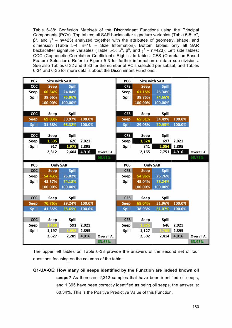
180
Table 6-38: Confusion Matrixes of the Discriminant Functions using the Principal Components (PC’s). Top tables: all SAR backscatter signature variables (Table 5-5: σo, βo, and γo – n=423) analyzed together with the attributes of geometry, shape, and dimension (Table 5-4: n=10 – Size Information). Bottom tables: only all SAR backscatter signature variables (Table 5-5: σo, βo, and γo – n=423). Left side tables: CCC (Cophenetic Correlation Coefficient). Right side tables: CFS (Correlation-Based Feature Selection). Refer to Figure 5-3 for further information on data sub-divisions. See also Tables 6-32 and 6-33 for the number of PC’s selected per subset, and Tables 6-34 and 6-35 for more details about the Discriminant Functions.
PC7 SizewithSAR PC6 SizewithSAR CCC Seep Spill CFS Seep Spill Seep 60.34% 24.04% Seep 61.15% 25.34% Spill 39.66% 75.96% Spill 38.85% 74.66%
100.00% 100.00% 100.00% 100.00%
CCC Seep Spill CFS Seep Spill Seep 69.03% 30.97% 100.0% Seep 65.51% 34.49% 100.0% Spill 31.68% 68.32% 100.0% Spill 29.05% 70.95% 100.0%
CCC Seep Spill CFS Seep Spill Seep 1,395 626 2,021 Seep 1,324 697 2,021 Spill 917 1,978 2,895 Spill 841 2,054 2,895
2,312 2,604 4,916 OverallA. 2,165 2,751 4,916 OverallA. 68.61% 68.71%
PC5 OnlySAR PC6 OnlySAR CCC Seep Spill CFS Seep Spill Seep 54.43% 25.82% Seep 54.96% 26.76% Spill 45.57% 74.18% Spill 45.04% 73.24%
100.00% 100.00% 100.00% 100.00%
CCC Seep Spill CFS Seep Spill Seep 70.76% 29.24% 100.0% Seep 68.04% 31.96% 100.0% Spill 41.35% 58.65% 100.0% Spill 38.93% 61.07% 100.0%
CCC Seep Spill CFS Seep Spill Seep 1,430 591 2,021 Seep 1,375 646 2,021 Spill 1,197 1,698 2,895 Spill 1,127 1,768 2,895
2,627 2,289 4,916 OverallA. 2,502 2,414 4,916 OverallA. 63.63% 63.93%
The upper left tables on Table 6-38 provide the answers of the second set of four
questions focusing on the columns of the table:
Q1-UA-OE: How many oil seeps identified by the Function are indeed known oil
seeps? As there are 2,312 samples that have been identified oil seeps,
and 1,395 have been correctly identified as being oil seeps, the answer is:
60.34%. This is the Positive Predictive Value of this Function.

181
Q2-UA-OE: How many oil spills identified by the Function are indeed known oil
spills? As 2,604 samples were identified as oil spills, and 1,978 have been
identified by this Discriminant Function as being oil spills, the answer is:
75.96%. This is the Negative Predictive Value of this Function.
Q3-UA-OE: Of samples identified by the Function as oil seeps, how many are oil
spills? This is the Inverse of the Positive Predictive Value (n=917). This is
the amount of samples that the Function misidentified when it classified the
oil seeps: 39.66%.
Q4-UA-OE: Of samples identified by the Function as oil spills, how many are oil
seeps? This is the Inverse of the Negative Predictive Value (n=626). This
informs how many samples that the Function misidentified when it
classified the oil spills: 24.04%.
This is a fairly balanced result when it is compared to the Overall Accuracy: 68.61%.
However, if looking into the lower left tables on Table 6-38, it is possible to notice that
the Overall Average (63.63%) informs an averaged effectiveness of the Function. Yet,
this information mislead the used about the real performance of the Function, as, for
instance, the Specificity (58.65%) and Positive Predictive Value (54.43%) present low
values. The take home message of the analyses of these metrics is that the user needs
to be aware of the real accuracy of the predictor (CARVALHO et al., 2010; 2011).
In fact, a comparison between the top left and the lower left tables on Table 6-38,
illustrates the influence of the attributes of geometry, shape, and dimension (Table 5-4:
n=10) on the discrimination of spills and seeps. A better result is observed on the top
left than compared to the lower left, respectively, when the size information is
accounted for than when it is not.
Two series of Confusion Matrixes follow below showing the results of the separate
anlayses of sigma-naught (σo), beta-naught (βo), and gamma-naught (γo) variables with
(Table 6-39) and without (Table 6-40) the attributes of geometry, shape, and
dimension. Again it is possible to observe the improvement when the size information
is considered, as well as of the use of the Overall Accuracy versus the other metrics.
The UPGMA-CCC utilizes the PC’s found from variables presented on Tables 6-20 and
6-21. The CFS variables that were used to find the PC’s are shown on Table 6-27.

182
Table 6-39: Confusion Matrixes of the Discriminant Functions (PC’s) of sigma (top), beta (middle), and gamma (bottom) analyzed together with geometry, shape, and dimension variables – Size Information. Left tables: UPGMA-CCC. Right tables: CFS.
PC7 SizewithSigma PC7 SizewithSigma CCC Seep Spill CFS Seep Spill Seep 61.98% 24.51% Seep 61.53% 24.65% Spill 38.02% 75.49% Spill 38.47% 75.35%
100.00% 100.00% 100.00% 100.00%
CCC Seep Spill CFS Seep Spill Seep 66.80% 33.20% 100.0% Seep 66.80% 33.20% 100.0% Spill 28.60% 71.40% 100.0% Spill 29.15% 70.85% 100.0%
CCC Seep Spill CFS Seep Spill Seep 1,350 671 2,021 Seep 1,350 671 2,021 Spill 828 2,067 2,895 Spill 844 2,051 2,895
2,178 2,738 4,916 OverallA. 2,194 2,722 4,916 OverallA. 69.51% 69.18%
PC7 SizewithBeta PC5 SizewithBeta CCC Seep Spill CFS Seep Spill Seep 62.15% 24.61% Seep 62.23% 24.80% Spill 37.85% 75.39% Spill 37.77% 75.20%
100.00% 100.00% 100.00% 100.00%
CCC Seep Spill CFS Seep Spill Seep 66.45% 33.55% 100.0% Seep 65.96% 34.04% 100.0% Spill 28.26% 71.74% 100.0% Spill 27.94% 72.06% 100.0%
CCC Seep Spill CFS Seep Spill Seep 1,343 678 2,021 Seep 1,333 688 2,021 Spill 818 2,077 2,895 Spill 809 2,086 2,895
2,161 2,755 4,916 OverallA. 2,142 2,774 4,916 OverallA. 69.57% 69.55%
PC7 SizewithGamma PC5 SizewithGamma CCC Seep Spill CFS Seep Spill Seep 61.79% 24.70% Seep 61.03% 25.46% Spill 38.21% 75.30% Spill 38.97% 74.54%
100.00% 100.00% 100.00% 100.00%
CCC Seep Spill CFS Seep Spill Seep 66.50% 33.50% 100.0% Seep 65.31% 34.69% 100.0% Spill 28.70% 71.30% 100.0% Spill 29.12% 70.88% 100.0%
CCC Seep Spill CFS Seep Spill Seep 1,344 677 2,021 Seep 1,320 701 2,021 Spill 831 2,064 2,895 Spill 843 2,052 2,895
2,175 2,741 4,916 OverallA. 2,163 2,753 4,916 OverallA. 69.32% 68.59%

183
Table 6-40: Confusion Matrixes of the Discriminant Functions (PC’s) of only sigma-naught (σo; top tables), beta-naught (βo; middle tables), and gamma-naught (γo; bottom tables) analyzed separately. Left tables: UPGMA-CCC. Right tables: CFS.
PC5 OnlySigma PC4 OnlySigma CCC Seep Spill CFS Seep Spill Seep 54.00% 26.31% Seep 55.07% 26.23% Spill 46.00% 73.69% Spill 44.93% 73.77%
100.00% 100.00% 100.00% 100.00%
CCC Seep Spill CFS Seep Spill Seep 70.21% 29.79% 100.0% Seep 69.12% 30.88% 100.0% Spill 41.76% 58.24% 100.0% Spill 39.38% 60.62% 100.0%
CCC Seep Spill CFS Seep Spill Seep 1,419 602 2,021 Seep 1,397 624 2,021 Spill 1,209 1,686 2,895 Spill 1,140 1,755 2,895
2,628 2,288 4,916 OverallA. 2,537 2,379 4,916 OverallA. 63.16% 64.12%
PC4 OnlyBeta PC5 OnlyBeta CCC Seep Spill CFS Seep Spill Seep 54.44% 28.52% Seep 55.62% 26.85% Spill 45.56% 71.48% Spill 44.38% 73.15%
100.00% 100.00% 100.00% 100.00%
CCC Seep Spill CFS Seep Spill Seep 64.32% 35.68% 100.0% Seep 67.05% 32.95% 100.0% Spill 37.58% 62.42% 100.0% Spill 37.34% 62.66% 100.0%
CCC Seep Spill CFS Seep Spill Seep 1,300 721 2,021 v 1,355 666 2,021 Spill 1,088 1,807 2,895 spill 1,081 1,814 2,895
2,388 2,528 4,916 OverallA. 2,436 2,480 4,916 OverallA. 63.20% 64.46%
PC5 OnlyGamma PC4 OnlyGamma CCC Seep Spill CFS Seep Spill Seep 53.83% 26.27% Seep 55.33% 27.10% Spill 46.17% 73.73% Spill 44.67% 72.90%
100.00% 100.00% 100.00% 100.00%
CCC Seep Spill CFS Seep Spill Seep 70.51% 29.49% 100.0% Seep 66.80% 33.20% 100.0% Spill 42.21% 57.79% 100.0% Spill 37.65% 62.35% 100.0%
CCC Seep Spill CFS Seep Spill Seep 1,425 596 2,021 Seep 1,350 671 2,021 Spill 1,222 1,673 2,895 Spill 1,090 1,805 2,895
2,647 2,269 4,916 OverallA. 2,440 2,476 4,916 OverallA. 63.02% 64.18%

184
Table 6-41 presents the results of two Discriminant Functions: for the attributes of
geometry, shape, and dimension (Table 5-4: n=10) and for the Digital Numbers (DN’s)
variables. While the Discriminant Function considering the size information presents
the best of all results, the one using only DN’s present the worse results. These are
extremely positive outcomes, both, showing the relevancy of the size information on
distinguishing natural from man-made oil slicks on the sea surface of the Campeche
Bay region and the corroboration with the literature that DN images are not meant to be
used to compare time-series of SAR imagery.
Table 6-41: Confusion Matrixes of the Discriminant Functions using the PC’s: Top tables: attributes of geometry, shape, and dimension (Size Information). Bottom tables: only Digital Numbers (DN’s). Left side: CCC (Cophenetic Correlation Coefficient). Right side: CFS (Correlation-Based Feature Selection). Refer to Figure 5-3 for information on data sub-divisions. See also Tables 6-32 and 6-33 for the number of PC’s selected per subset, Tables 6-34 and 6-35 for more details about the Discriminant Functions, and Table 6-20 (UPGMA-CCC) and Table 6-24 (CFS) for the original variables.
PC2 OnlySize PC2 OnlySize CCC Seep Spill CFS Seep Spill Seep 63.11% 24.95% Seep 63.16% 24.44% Spill 36.89% 75.05% Spill 36.84% 75.56%
100.00% 100.00% 100.00% 100.00%
CCC Seep Spill CFS Seep Spill Seep 65.02% 34.98% 100.0% Seep 66.16% 33.84% 100.0% Spill 26.53% 73.47% 100.0% Spill 26.94% 73.06% 100.0%
CCC Seep Spill CFS Seep Spill Seep 1,314 707 2,021 Seep 1,337 684 2,021 Spill 768 2,127 2,895 Spill 780 2,115 2,895
2,082 2,834 4,916 OverallA. 2,117 2,799 4,916 OverallA. 70.00% 70.22%
PC2 OnlyDN’s PC2 OnlyDN’s CCC Seep Spill CFS Seep Spill Seep 48.88% 34.83% Seep 50.68% 33.87% Spill 51.12% 65.17% Spill 49.32% 66.13%
100.00% 100.00% 100.00% 100.00%
CCC Seep Spill CFS Seep Spill Seep 53.14% 46.86% 100.0% Seep 53.09% 46.91% 100.0% Spill 38.79% 61.21% 100.0% Spill 36.06% 63.94% 100.0%
CCC Seep Spill CFS Seep Spill Seep 1,074 947 2,021 Seep 1,073 948 2,021 Spill 1,123 1,772 2,895 Spill 1,044 1,851 2,895
2,197 2,719 4,916 OverallA. 2,117 2,799 4,916 OverallA. 57.89% 59.48%
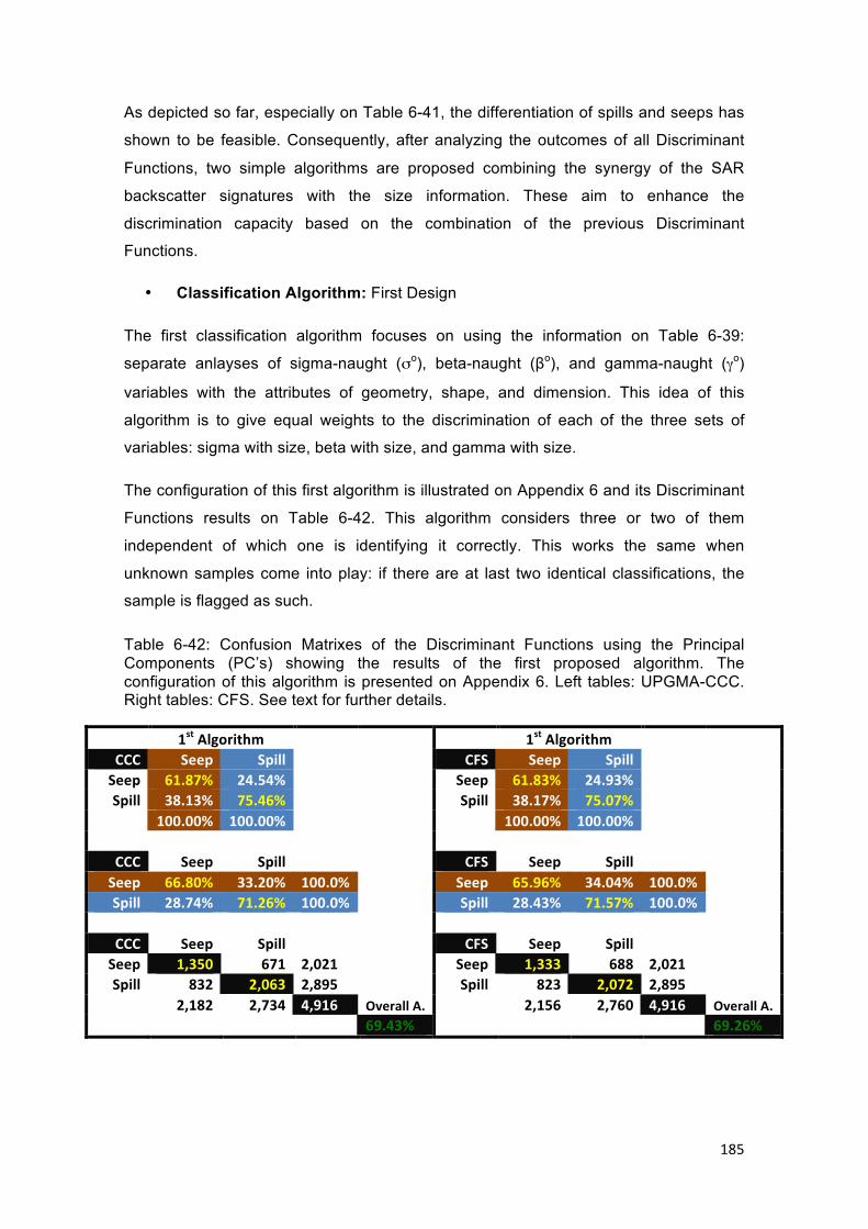
185
As depicted so far, especially on Table 6-41, the differentiation of spills and seeps has
shown to be feasible. Consequently, after analyzing the outcomes of all Discriminant
Functions, two simple algorithms are proposed combining the synergy of the SAR
backscatter signatures with the size information. These aim to enhance the
discrimination capacity based on the combination of the previous Discriminant
Functions.
• Classification Algorithm: First Design
The first classification algorithm focuses on using the information on Table 6-39:
separate anlayses of sigma-naught (σo), beta-naught (βo), and gamma-naught (γo)
variables with the attributes of geometry, shape, and dimension. This idea of this
algorithm is to give equal weights to the discrimination of each of the three sets of
variables: sigma with size, beta with size, and gamma with size.
The configuration of this first algorithm is illustrated on Appendix 6 and its Discriminant
Functions results on Table 6-42. This algorithm considers three or two of them
independent of which one is identifying it correctly. This works the same when
unknown samples come into play: if there are at last two identical classifications, the
sample is flagged as such.
Table 6-42: Confusion Matrixes of the Discriminant Functions using the Principal Components (PC’s) showing the results of the first proposed algorithm. The configuration of this algorithm is presented on Appendix 6. Left tables: UPGMA-CCC. Right tables: CFS. See text for further details.
1stAlgorithm 1stAlgorithm CCC Seep Spill CFS Seep Spill Seep 61.87% 24.54% Seep 61.83% 24.93% Spill 38.13% 75.46% Spill 38.17% 75.07%
100.00% 100.00% 100.00% 100.00%
CCC Seep Spill CFS Seep Spill Seep 66.80% 33.20% 100.0% Seep 65.96% 34.04% 100.0% Spill 28.74% 71.26% 100.0% Spill 28.43% 71.57% 100.0%
CCC Seep Spill CFS Seep Spill Seep 1,350 671 2,021 Seep 1,333 688 2,021 Spill 832 2,063 2,895 Spill 823 2,072 2,895
2,182 2,734 4,916 OverallA. 2,156 2,760 4,916 OverallA. 69.43% 69.26%
186
• Classification Algorithm: Second Design
The second classification algorithm uses the information on Table 6-40 (i.e. separate
anlayses of sigma-naught (σo), beta-naught (βo), and gamma-naught (γo)) and on the
top tables of Table 6-41 (i.e. attributes of geometry, shape, and dimension only).
Appendix 6 presents the conceptual classification design, whereas Table 6-43 presents
the accuracy assessment.
With a similar idea than on the first one, however, the second algorithm has four
independent options of classification: size, sigma, beta, and gamma. When there is an
even result for the same sample (i.e. two seep classifications and two spill
classifications), the user can decide what to do. For instance, a decision can be taken
to classify it as a seep if it is on a region where seeps usually occur (1st Mode) or he
can consider this sample as a spill (3rd Mode) based on site location or any other
decision making process.
But on the 2nd Mode, the user can leave it as an unknown oil slick, following the
nomenclature utilized during the present D.Sc. research, Orphan, but on this case, an
Orphan Slick. The middle tables on Table 6-43 do not consider these unknown
samples as the total number of oil slicks is less than the number of oil slicks within the
CBOS-DScMod: 4,916. On both cases (UPGMA-CCC and CFS), about 5.5% of the oil
slicks would fall into the Orphan Slick case: n=266 and n=201, respectively. This is
about one sixth to one tenth of the Orphan cases present on the CBOS-Data that were
analyzed during the Data Familiarization (Phase 1: Section 6.1), as show on Figure 6-
7: Orphan Spills (n=1,851; 13.0%) and Orphan Seeps (n=1,592; 11.2%).
• The Sole Use of Two Attributes: Area and Perimeter
Because it has been shown throughout the encompassed Multivariate Data Analysis
Practice (Yellow Phases: 6 to 10, as portrayed on Figure 1-3) that the attributes of
geometry, shape, and dimension (i.e. size information – 3rd Attribute Type: Table 5-4)
have stood out in distinguishing natural from man-made oil slicks on the sea surface of
Campeche Bay, these attributes are further explored. This means that the two basic
attributes of geometry, shape, and dimensions present in the CBOS-Data content
(Table 2-2) are explored in more details: area (Area) and perimeter (Per). The same
Data Treatment (Phase 5: Sections 5.5 and 6.5) have been applied preceding the PCA.
Two PC’s have been selected. The accuracy accessment is shown on Table 6-44.

187
Table 6-43: Confusion Matrixes (PC’s) showing the second proposed algorithm that separately explores sigma, beta, gamma, and size attributes. Left tables: UPGMA-CCC. Right tables: CFS. See text for further details.
1stMode 1stMode CCC Seep Spill CFS Seep Spill Seep 52.33% 28.55% Seep 53.89% 28.11% Spill 47.67% 71.45% Spill 46.11% 71.89%
100.00% 100.00% 100.00% 100.00%
CCC Seep Spill CFS Seep Spill Seep 67.24% 32.76% 100.0% Seep 66.11% 33.89% 100.0% Spill 42.76% 57.24% 100.0% Spill 39.48% 60.52% 100.0%
CCC Seep Spill CFS Seep Spill Seep 1,359 662 2,021 Seep 1,336 685 2,021 Spill 1,238 1,657 2,895 Spill 1,143 1,752 2,895
2,597 2,319 4,916 OverallA. 2,479 2,437 4,916 OverallA. 61.35% 62.82%
2ndMode 2ndMode CCC Seep Spill CFS Seep Spill Seep 56.16% 25.70% Seep 57.03% 26.68% Spill 43.84% 74.30% Spill 42.97% 73.32%
100.00% 100.00% 100.00% 100.00%
CCC Seep Spill CFS Seep Spill Seep 70.34% 29.66% 100.0% Seep 69.27% 30.73% 100.0% Spill 39.04% 60.96% 100.0% Spill 38.19% 61.81% 100.0%
CCC Seep Spill CFS Seep Spill Seep 1,359 573 1,932 Seep 1,359 603 1,962 Spill 1,061 1,657 2,718 Spill 1,024 1,657 2,681
2,420 2,230 4,650 OverallA. 2,383 2,260 4,643 OverallA. 64.86% 64.96%
3rdMode 3rdMode CCC Seep Spill CFS Seep Spill Seep 57.71% 23.81% Seep 58.07% 24.37% Spill 42.29% 76.19% Spill 41.93% 75.63%
100.00% 100.00% 100.00% 100.00%
CCC Seep Spill CFS Seep Spill Seep 71.65% 28.35% 100.0% Seep 70.16% 29.84% 100.0% Spill 36.65% 63.35% 100.0% Spill 35.37% 64.63% 100.0%
CCC Seep Spill CFS Seep Spill Seep 1,448 573 2,021 Seep 1,418 603 2,021 Spill 1,061 1,834 2,895 Spill 1,024 1,871 2,895
2,509 2,407 4,916 OverallA. 2,442 2,474 4,916 OverallA. 66.76% 66.90%

188
Table 6-44: Confusion Matrixes of the Discriminant Functions using the Principal Components (PC’s) exploring only the two basic attributes of geometry, shape, and dimension (Table 2-2): area (Area) and perimeter (Per).
PC2 Area&Perimeter Seep Spill
Seep 62.33% 25.18% Spill 37.67% 74.82%
100.00% 100.00% Seep Spill
Seep 65.02% 34.98% 100.0% Spill 27.43% 72.57% 100.0%
Seep Spill
Seep 1,314 707 2,021 Spill 794 2,102 2,895
2,108 2,808 4,916 OVERALL 69.47%
Interesting to note is that the results presented on Table 6-44 are not that different from
those shown on the top tables of Table 6-41 that accounts for the PC’s of different
combination of variables: UPGMA-CCC (Table 6-20) and CFS (Table 6-24). The
findings expressed on Table 6-44 demostrate that the sole use of area and perimeter of
the oil slicks is also capable of distinguishing the oil slick type to a useful accuracy.
• Publication: Scientific Journal Submission
The bulk of the data mining results achieved during this D.Sc. dissertation, i.e.
Workable-Database Preparation (Phases: 3 to 5) and Multivariate Data Analysis
Practice (Phases: 6 to 10), have been submitted to the Remote Sensing of
Environment (RSE) journal – see Appendix 1: CARVALHO et al. (2015c). This paper
summarizes most of the outcomes of the second proposed specific goal of the present
D.Sc. research: the use of RADARSAT measurements to evaluate the capacity of
distinguishing the oil slick type by means of multivariate data analysis techniques.

189
CHAPTER 7
DISCUSSION
• Phase 1: Data Familiarization
The first pre-processing data verification Phase (Section 5.1 and Section 6.1)
organized and analyzed the entire content of the Campeche Bay Oil Slick Satellite
Database (CBOS-Data). This dataset has been produced during the Campeche Bay
Oil Slick Satellite Project (CBOS-SatPro) that lasted for approximately 13 years (2000-
2012) with a regular SAR image acquisition of about one RADARSAT scene per week
(Table 6-3: n=766). Undeniably, the familiarization with this dataset provided means to
reveal a substantial amount of information related to the spatio-temporal distribution
and occurrence of 14,210 oil slicks, as reported in CARVALHO et al. (2015a) and
CARVALHO et al. (2015b) – see Appendix 1.
The slightly uneven distribution pattern of oil slicks per category (Figure 6-1: n=14,210)
is inverted when considering the area covered by all oil slicks (Figure 6-2: 46,693 km2).
Even though oil spills occur a little more frequently (n=8,008; 56.3%) than oil seeps
(n=6,202; 43.7%), the oil spills’ area coverage (15,246 km2; 32.6%) is about half of the
oil seeps (31,447 km2; 67.4%). However, when looking into the overall class
distribution, it is possible to notice that this strong pattern inversion occurs because of
the relative small frequency of the Cantarell Oil Seep (Figure 6-7: n=653; 4.6%) that
contrasts to its massive area coverage (Figure 6-8: 19,743 km2; 42.3%).
An exercise of removing the Cantarell Oil Seep influence is illustrated on Figure 7-1.
The total surface area coverage of oil spills (15,246 km2; 56.6%) becomes larger than
of the oil seeps without Cantarell (11,704 km2; 43.4%), revealing that the frequency
and the area covered by oil spills are larger if compared to all other oil seeps. Indeed,
the Cantarell Oil Seep signature has been present in most RADARSAT scenes
analyzed during the CBOS-SatPro: 85%. This exercise corroborates previous findings
about its massive HC contribution in this region as the most prominent in area
coverage, dimension, flow magnitude, and persistence (e.g. MENDOZA et al., 2004a).
An analysis presented by QUINTERO-MARMOL et al. (2003) uses data from the first
few years of CBOS-SatPro (2000-2002) to give a picture of Cantarell Oil Seep activity.
Out of the analyzed 83 SAR scenes, its signature was observed in 66 images: 79.5%.
The area covered by its seeped oil ranged from 0.04 to 207.4 km2, having an average
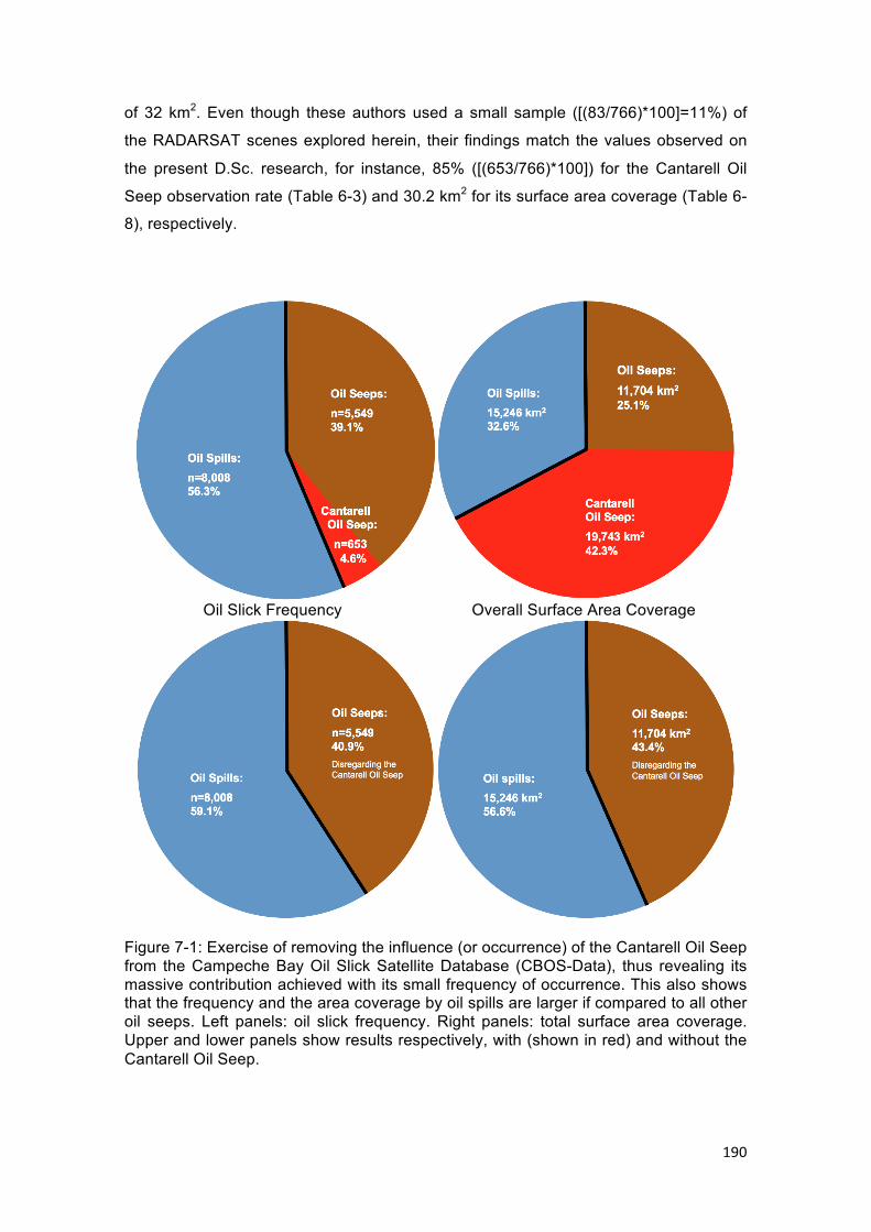
190
of 32 km2. Even though these authors used a small sample ([(83/766)*100]=11%) of
the RADARSAT scenes explored herein, their findings match the values observed on
the present D.Sc. research, for instance, 85% ([(653/766)*100]) for the Cantarell Oil
Seep observation rate (Table 6-3) and 30.2 km2 for its surface area coverage (Table 6-
8), respectively.
Oil Slick Frequency Overall Surface Area Coverage
Figure 7-1: Exercise of removing the influence (or occurrence) of the Cantarell Oil Seep from the Campeche Bay Oil Slick Satellite Database (CBOS-Data), thus revealing its massive contribution achieved with its small frequency of occurrence. This also shows that the frequency and the area coverage by oil spills are larger if compared to all other oil seeps. Left panels: oil slick frequency. Right panels: total surface area coverage. Upper and lower panels show results respectively, with (shown in red) and without the Cantarell Oil Seep.

191
The information depicted on Figure 6-5 and Figure 6-6 contains a few worthy of note
observations:
1. The 88 identified Clusters (n=3,957; 63.8% of oil seeps) have larger
representativeness frequency than Orphan Seeps (n=1,592; 25.7%), as well as
they occupy a larger surface area: 8,947 km2 (28.4%) versus 2,757 km2 (8.8%).
This is consistent with the hypothesis that seeped oil moves vertically through the
water column in most of the Campeche Bay region – see Section 2.3.4 for
Cluster definition and Section 3.2 for information about natural hydrocarbon
seepages at sea;
2. The 10 Brightspots ≥ 100 different oil spill observations correspond to more than
half (i.e. n=4,342; 54.2%) of the oil spill entries, but its superficial area coverage
(5,424 km2; 35.6%) is quite similar to the one of the 61 Brightspots with ≤ 99
different oil spill observations (5,690 km2; 37.3%) that have a much smaller
frequency (n=1,263; 15.8%). This reveals that despite the larger frequency, such
oil spills from those 10 Brightspots are of a much smaller size; and
3. The number of identified sources within the observed oil spills (i.e. Brightspots
and Ship Spills: n=6,157; 76.9%) is much larger than the number of Orphan Spills
(n=1,851; 23.1%). This revels the high rate of correct identification of the CBOS-
SatPro, and demonstrates the success of the Pemex Validation (CBOS-SatPro
Part 6: Section 2.3.6) that corroborates the operator interpretations.
Regarding the Brightspot class information, the 10 Brightspots that have been
registered having ≥ 100 different oil spill observations, which are color-coded in light
blue (Figure 6-3: n=4,342), correspond to more than half of the observed oil spills
(Figure 6-5: 54.2%) and to about one third of the oil slicks entries of the CBOS-Data
(Figure 6-7: 30.5%). Nevertheless, its surface area coverage contributions (Figure 6-6:
total coverage 35.6% and Figure 6-8: overall coverage 11.6%) is about the same as of
the other 61 Brightspots that have ≤ 99 different oil spill observations (Figure 6-6: total
coverage 37.3% and Figure 6-8: overall coverage 12.2%), even though these have 3.5
times less oil spills (Figure 6-5: n=1,263).
From the size distribution shown on Table 6-8, oil spills from the 10 Brightspots have a
much smaller average size (i.e. 1.3 km2 against 4.5 km2); however, the larger average
size of the 61 Brightspots is taking into account a major oil spill event occurred in
November 2007 in one of its Brightspots – this has been imaged at least 8 times as
shown on Table 6-8 with one asterisk.

192
An exercise can be executed by taking the oil spills from this atypical event (that sum
3,006.4 km2 – Table 6-8) out of the size distribution calculation. In doing so, the
average size of the oil slicks from the 61 Brightspots with ≤ 99 different oil spill
observations drastically lowers to from 4.5 to 2.2 km2 (Table 6-8). A slight drop is also
observed on the average sizes of all oil spills (from 1.9 to 1.5 km2) and all oil slicks
(from 3.3 to 3.0 km2). Hence, this exercise demonstrates that a single major oil spillage
can largely influence not only the environment, but also the oil slicks’ statistics
information of any dataset.
Another disclosure about the size distribution of the oil slicks (Table 6-5) is that most of
them (n=9,398; 66.1%) have “small” surface area coverage (i.e. < 1 km2). This pattern
is more preeminent among oil spills (Table 6-6: n=6,196; 77.4%) than oil seeps (Table
6-7: n=3,202; 51.7%), independent of the RADARSAT satellite. Oil slicks with “large”
surface area coverage (i.e. ≥ 10 km2) correspond to a minor part of the observations
(Table 6-5: n=734; 5.2%).
An additional aspect to highlight considering the size distribution is that the average oil
slick size is 3.3 km2 (Table 6-8). Also, oil seeps (5.1 km2) tend to be larger on average
than the oil spills (1.9 km2). However, this averaging calculation takes into account the
Cantarell Oil Seep influence, and its removal drops the oil slicks’ size to 3.0 km2 and
the oil seeps’s size to 2.1 km2.
A worth of notice comparison can be made between the Campeche Bay oil spills within
the CBOS-Data and the oil spills analyzed by BENTZ (2006) off the SE of Brazil
(Campos Basin). BENTZ analysis is based on 402 RADARSAT-1 images acquired
from July 2001 to June 2003 and the average size of the 358 oil spills (~6.5 km2) is
more about three times larger than the average size of the oil spills observed in
Campeche Bay during the CBOS-SatPro.
The water column depth (i.e. Wdepth attribute) in the location where the oil slicks have
been observed on the sea surface revealed an interesting aspect about the oil slicks’
occurrence. For instance, on Figure 6-16, oil spills (96%) usually tend to occur in water
depths shallower than 100 m (corresponding to the location of the Campeche Bay
OGEPI activity), whereas oil seeps (63%) commonly occur in waters deeper than 1000
m (related to the offshore salt tectonic province). The average water depths are: 484 m
(oil slicks), 73 m (oil spills), and 1,296 m (oil seeps) – Table 6-10.

193
• Phase 2: Quality Control (QC)
Despite this major data reduction that eliminated a fairly amount of information from the
CBOS-Data, i.e. from 14,210 oil slicks to 4,916 oil slicks (35%), the outcomes of the
QC-standards guaranteed that its handful basic attributes met certain requirements to
enable high-quality data to be used in the workable database preparation. This surely
supports the conciseness of the Campeche Bay Oil Slick Modified Database (CBOS-
DScMod) information to reach the goals of the present D.Sc. research.
The 277 RADARSAT-2 images (Table 6-11: 16-bit, VV-polarized) corresponds to
approximately 36% of 766 scenes utilized during the CBOS-SatPro (Table 6-3).
Likewise, the other reduction, i.e. on the oil slick of frequency (n=4,916), leaves to be
explored herein, only about 35% of the initial 14,210 oil slicks (Figure 6-1). Conversely,
if a comparison is made only regarding the RADARSAT-2 imagery (Figure 6-10), this
cut is less prominent, as 97% (n=277) out of the 284 scenes (Table 6-3) and 87%
(n=4,916) out of the 5,314 oil slicks are kept in the analysis.
As anticipated, this data reduction pattern also occurs on the frequency of oil slicks per
category. The QC-Standards reduce oil seeps to 2,021 (33% of 6,202) and oil spills to
2,895 (36% of 8,008) – see Figure 6-1. Considering only RADARSAT-2 imagery: 95%
(n=2,021) out of the 2,136 oil seeps and 91% (n=2,895) out of the 3,178 oil spills are
kept in the analysis – see Figure 6-11.
• Phase 3: RADARSAT Image Re-Processing
The re-processing of the RADARSAT-2 images has been accomplished following the
processing procedures executed during the CBOS-SatPro (Figure 2-2). However, three
steps were not performed herein: APC, image contrast enhancement, and radiometric
re-scalling. In addition, the DN values were converted to radiometric-calibrated image
products (Table 5-1: σo, βo, and γo).
These procedures assured the successful investigation of the three types of SAR
backscatter coefficients to distinguish oil spills from oil seeps. With these image-
processing procedures, the use of RADARSAT-2 measurements to design the
classification has been demostrated.

194
• Phase 4: New Slick-Feature Attributes
Even though the CBOS-DScMod (2008-2012: Section 5.4) represents a spatio-
temporal sample of the CBOS-Data (2000-2012: Section 2.3), it surely serves as a
benchmark describing the oil slicks’ observed in the Campeche Bay region. A collection
of slick-feature attributes used to describe the oil slicks observed in Campeche Bay are
represented by contextual information (Table 5-2: n=6), satellite scene descriptors
(Table 5-3: n=37), geometry, shape, and dimension attributes (Table 5-4: n=10 –, size
information), and SAR backscatter signature (Table 5-5: n=432). These account for
485 different descriptors that are further expanded once undergoing the Data
Treatments (Phase 5). Indeed, the reference levels shown on Section 6.4 (and in
Appendices 2 and 3) conclusively characterize the analyzed radiometric-calibrated
image products (Table 5-1: σo, βo, and γo) and their typical values (i.e. a set of basic
qualitative-quantitative statistics: minimum, maximum, average, and standard
deviation).
• Phase 5: Data Treatment
The amount of work put into the Data Treatment has shown to be successful on the
course of this D.Sc. research. It guaranteed quality of the statistical data comparison of
attributes with different units and those with qualitative values. The 485 different
attributes used to describe the CBOS-DScMod’s oil slicks have undergone four Data
Treatments, thus accounting for 511 variables (485-7+33): Negative Values Scaling
(altering the values of all pixels inside the oil slicks to positive values), Log10
Transformation (bringing the frequency of distribution of all variables to, or at least
close to, a Gaussian distribution), Ranging Standardization (coding all qualitative
variables to have values between 0 and 1), and Dummy Variables. The latter is
responsible for the replacement of 7 qualitative attributes (e.g. Category, Class,
Bmode, etc.) with 33 new Dummy Variables (binary-coded to 1 or 0) – Table 5-10.
The two contextual cLAT and cLONG attributes have been replaced by six new
variables: three for the latitude domain (RG1.LAT, RG2.LAT, and PKD.LAT) and three
analogous ones for the longitude domain (RG1.LONG, RG2.LONG, and PKD.LONG).
The former two are Dummy Variables and the latter is an unusual data treated
makeover. These variables reveal the existence of two populations that are domain-
specific and directly coupled with the two regions: POP1.LAT and POP2.LAT, and
POP1.LONG and POP2.LONG – such acronyms have not been further used on this
research.

195
• Phase 6: Attribute Selection
The two attribute selection methods, i.e. UPGMA (Unweighted Pair Group Method with
Arithmetic Mean) and CFS (Correlation-Based Feature Selection), have proposed
thirty-three optimal subsets of attributes to reduce the dimensionality of the eleven
original sets of data within the CBOS-DScMod (Figure 5-3). These optimal subsets
were explored in the Multivariate Data Analysis Practices shown as the Yellow Phases
(6 to 10) on Figure 1-3. As anticipated, the removal of variables with similar
characteristics yields good results in designing the proposed classification algorithm.
As expected, the optimal variable subsets (attribute-wise) helped to verify eventual
associated uncertainties in the process of distinguishing the oil slick type (HALL, 1999).
• Phase 7: Principal Components Analysis (PCA)
The application of the PCA’s has added value to the data reduction proposed by the
Attribute Selection (Phase 6). There was not a rigorous unchanging cut-off to select the
Principal Components (PC’s), instead, the new set of variables (i.e. PC’s) were
selected using a compound strategy based on the analysis of the Scree Plot (i.e.
broken stick with bootstrapping) and the Kaiser-Guttman criterion (i.e. eigenvalue
greater than 1). This seems a reasonable practice that followed strict guiding principles
from the literature to make sure a handful of meaningful PC’s were selected. In fact, the
the Discriminant Analysis (Phase 8) explored the score values of the selected PC’s.
• Phase 8: Discriminant Function
The several Discriminant Functions (n=78) are, in essence, one of the cores outcomes
of the present D.Sc. research. Various metrics have been used to assess the accuracy
of the Discriminant Analyses completed: Overall accuracy, Sensitivity, Specificity, False
Negative and Positives, Positive and Negative Predictive Values and their Inverse.
These help to decide the cost of misdiscrimination.
• Phase 9: Correlation Matrix
Even after a thorough data reduction (Attribute Selection: Phase 6), there optimal
subsets were still presenting inter-variable correlation. However, the use of meaningful
PC’s strictly selected made possible the use of half of the Discriminant Functions, i.e.
those exploring the PC’s, to accomplish the distinguishment of the oil slick type.

196
• Phase 10: Oil Slick Classification Algorithm
The assessment of the accuracy of the Discriminant Function exploring the PC’s has
demonstrated that the differentiation between oil spills and oil seeps is indeed not an
easy task to be achieved. This might explain why this subject is not that much
discussed on the published peer reviewed literature, or even on grey literature.
However, the way the present D.Sc. research has been guided towards the extensive
use of Data Treatments and multivariate data analysis techniques has shown that it is
possible to distinguish natural from man-made oil slicks using RADARSAT
measurements.

197
CHAPTER 8
CONCLUSIONS
As peer-reviewed and grey literature are somewhat short about the topic of
differentiating oil seeps from oil spills, the investigation carried out during the present
D.Sc. research has largely contributed to the scientific remote sensing research
community, as well as to the oil and gas exploration and production industry (OGEPI).
The field of environment monitoring also has gained knowledge with the fruitful
outcomes shown herein. The main objective of performing an exploratory data analysis
(EDA) to distinguish natural from man-made oil slicks observed on the sea surface of
Campeche Bay using RADARSAT measurements has been successfully accomplished
achieving up to 70% of Overall Accuracy on the distinguishment between natural and
man-made oil slicks on the sea surface observed on the Campeche Bay region (Gulf of
Mexico). This has been completed using classical multivariate data analysis of satellite-
derived measurements of the Canadian RADARSAT satellite.
The first proposed specific goal has also been accomplished with high-quality
outcomes. The spatio-temporal distribution of the oil slicks present on Campeche Bay
Oil Slick Satellite Database (CBOS-Data) has been thoroughly investigated. These oil
slicks were observed during the Campeche Bay Oil Slick Satellite Project (CBOS-
SatPro). The scientific investigation exploring this dataset has disclosed interesting
aspects about the occurrence of oil slicks observed on the sea surface. This is not only
relevant to a specific region, i.e. Campeche Bay, as the findings presented herein can
serve as a reference for comparison with other regions where oil slicks are observed
on the surface of the ocean. An entirely dedicated Section promoted an enormous
amount of information about oil slicks distribution. A complete extended abstract and a
scientific publication have come out of the Data Familiarization practice: CARVALHO et
al. (2015a; 2015b). The description of the spatio-temporal distribution of 14,210 oil
slicks using RADARSAT-derived measurements has also proven the capabilities of this
remote sensing tool to perform long-term operational environmental monitoring.
Even though the present D.Sc. research is not the first study to analyze the information
produced during the Campeche Bay Oil Slick Satellite Project (CBOS-SatPro) – e.g.
BEISL et al., 2004; MENDOZA et al., 2004a; PEDROSO et al., 2007 – it is the first one
to investigate all oil slicks within the Campeche Bay Oil Slick Satellite Database
(CBOS-Data: n=14,210). Another distinguishing aspects of the present investigation

198
are the strategy of inspecting a considerable fraction of this dataset – i.e. Campeche
Bay Oil Slick Modified Database (CBOS-DScMod: n=4,916) – with a comprehensive
data filtering, an expansive data customization, and a multivariate data analysis
approach. An additional original aspect about the present D.Sc. research is indeed the
exploration of the different subset divisions (attribute-wise: Figure 5-3).
The core of the large historical archive of oil slick sites in the Campeche Bay region,
i.e. Campeche Bay Oil Slick Satellite Database (CBOS-Data), is threefold: date/time of
the SAR overpasses, the location of the oil slicks, and their vectorized shape polygon
(.shp file). Indeed, the foremost outcome of the Campeche Bay Oil Slick Satellite
Project (CBOS-SatPro) is the validated categorization and classification of the
observed oil slick. While the former corresponds to oil spills and oil seeps, the latter
classifies the member of these two categories into classes: OGEPI facility or ship
information help to indicate whether the oil slick is a Brightspot or Ship Spill, and their
absence usually indicates an oil seep Cluster, e.g. Cantarell Oil Seep (Figure 1-1 and
Figure 2-1). Exceptions are Orphan Seeps and Orphan Spills.
Even though the CBOS-SatPro is mostly focused on finding oil slicks directly related to
Pemex’s sphere of influence, two aspects confirm that the content of the CBOS-Data is
capable of depicting the seasonality of the oil slick occurrence in Campeche Bay. The
first one is the regional context of the explored RADARSAT image frames that covers a
considerable area surrounding the Cantarell Oil Field. The second one is the
documented timescale of more than a decade of Pemex’s monitoring program,
acquiring enough data (i.e. 766 SAR images that imaged 14,210 oil slicks) to picture,
understand, and provide useful information about the dynamics of oil slicks observed in
the Campeche Bay region.
The use of an assorted pool of classical multivariate data analysis techniques have
been effectively applied to analyze the remote sensing library content of the Campeche
Bay Oil Slick Modified Database (CBOS-DScMod). It is true that the existence of the
CBOS-Data served as a justification for this research, but the Data Treatment and the
data mining practice surely assured the accomplishment of the main objective of this
D.Sc. research, i.e. distinguishing seeps from spills (CARVALHO et al., 2015c).
The three scientific questions are also answered based on the solid research findings
presented on this D.Sc. manuscript:
• Does seeped oil floating on the ocean surface have SAR backscatter signature
distinctive enough to distinguish it from anthropogenically-spilled oil?

199
Yes, oil seeps and oil spills can be differentiated, to some extent (63-68% of Overall
Accuracy), by looking into only the SAR backscatter signature, i.e. sigma-naught (σo),
beta-naught (βo), and gamma-naught (γo), as retrieved by satellite remote sensing.
• Can the geometry, shape, and dimensions of oil slicks, as determined by digital
image classification of satellite imagery, be used to distinguish seeps from spills?
Yes, oil seeps and oil spills can be differentiated to a better accuracy (~70% of Overall
Accuracy) by looking into size information (i.e. attributes of geometry, shape, and
dimension: e.g. area and perimeter) as determined by digital image classification.
• Which combination of characteristics leads to the generation of a system capable
of distinguishing between seeped and spilled oil?
The exploratory data analysis performed during the present D.Sc. research have
shown that different combinations of variables are able to promoted similar
differentiation between oil seeps and oil spills. The combination leading to the most
effective classification of the oil slick type uses several attributes of geometry, shape,
and dimensions – more specifically, area and perimeter of the oil slicks. On the other
way, the attributes with the worse capabilities are those expressed in Digital Numbers
(DN’s).
Different qualitative-quantitative classification algorithms have been proposed, all
simple-to-use. There is no complicatedness at all on their formulation or design. These
ranged from very simple ones based on the sole use of SAR backscatter signature or
size information, to orher also uncomplicated and simple algorithms combining the
synergy of different variables.
The algorithms herein investigated encourage a novel way to link geochemistry and
remote sensing research, thus suggesting that geophysical differences between
seeped and spilled oil can indeed be used to distinguish the oil slick type by means of
satellite measurements. In fact, the outcomes of the present D.Sc. research are
indications that the differentiation between oil seeps and oil spills should be deeper
investigated with convention approaches commonly used to identify dark spots in SAR
imagery, e.g. Artificial Neural Networks (ANN) (e.g. GARCIA-PINEDA et al., 2008;
2009; 2010). In the same direction, ways to differentiate oil slick type could indeed
investigate polarimetric SAR measurements (e.g. VELOTTO et al., 2010; 2011).

200
The successful findings of the present D.Sc. research open a new way, i.e. by means
of classical multivariate data analysis techniques, to investigate the differentiation of
the various targets observed in SAR imagery, e.g. oil slicks from look-alike features.
Conclusively, as the most effective differentiation achieved herein has been
accomplished using the oil slick size information, this is a significant result for the
scientific community. In fact, if the techniques applied herein are capable of
distinguishing oil from oil, what can they achieve if applied with the purpose of
discriminating oil from, for instance, a harmful algal bloom or even a low wind zone
signature on SAR imagery?

201
CHAPTER 9
RECOMMENDATIONS FOR FUTURE WORK
• Phase 1: Data Familiarization
Despite the careful labor-intensive data inspection performed to organize and become
familiarized with the CBOS-Data information (Phase 1: Sections 5.1 and 6.1), some
discrepant entries have not been corrected or removed during this initial pre-processing
data verification. For instance, the polygon representing the largest Cantarell Oil Seep
record (Area: 1,789.0 km2) has a very small measurement of its border (Perimeter:
18.3 km) – incompatible to its size (Figure 6-15). Although this has been observed in
December of 1999 with RADARSAT-1 and does not bring to much concern to the
designed oil slick classification algorithm, the spatio-temporal distribution is indeed
influenced by particular inaccuracies of this nature. In addition, this calls the attention to
the fact that any other inconsistency may have passed through the analysis performed
during Phase 1: Data Familiarization. Perhaps, an assessment based on the actual
values of each slick-feature attribute (Table 2-2) could avoid the insertion of any
inconsistent data entries of this nature and reduce the propagation of eventual errors in
the processing chain – i.e. an evaluation of the original CBOS-Data could be carried
out with more stringent criteria than those performed herein.
The water column depth attribute (Wdepth) disclosures valuable information about the
spatial distribution of the oil slicks observed in the Campeche Bay region (Figure 6-16)
However, such information was not logged for oil slicks within the CBOS-Data (Table 6-
10: n=5,669; 40%). As this is a relevant contextual aspect to be considered, a finer
picture of local bathymetry can be obtained to the position of the oil slick centroid from
public domain dataset of the Earth TOPOgraphy database at one-minute grid
resolution (ETOPO1, 2013).
• Phase 2: Quality Control (QC)
An investigation could be performed with less stringent QC-Standards, and, for
instance, ana anslysis could explore the entired content of the CBOS-Data that
includes measurements from the two RADARSAT satellites – both 16-bit and 8-bit, as
well as VV and HH polarized images. Such assessment could reveal differences, or
not, based on the sensors’ characteristics to distinguish the oil slick type.

202
Data separation in various regions and seasons of the year radically reduces the
number of valid samples to work with (CARVALHO et al., 2010d; 2011). Undeniably,
this justifies the use of the whole content of the CBOS-DScMod to start the analysis
performed herein. The exercise of analyzing a specific spatio-temporal distribution of oil
slicks separated by region and/or by season or by years (e.g. CARVALHO, 2008),
could be a singularity of a further investigation aiming to distinguish the oil slick type.
• Phase 3: RADARSAT Image Re-Processing
Because the present D.Sc. research only investigated the various forms of radiometric-
calibrated image products together (i.e. SIG.amp, SIG.amp.FF, SIG.dB, SIG.dB.FF,
BET.amp, BET.amp.FF, BET.dB, BET.dB.FF, GAM.amp, GAM.amp.FF, GAM.dB, and
GAM.dB.FF – C1 and C2 – 12x2=24), a study could be designed that the different SAR
backscatter signature could be explored in separate. This could disclose which of them
brings the best distinguishment capabilities.
• Phase 4: New Slick-Feature Attributes
As the investigation carried out herein only explored information from the inside of
polygons delimiting the oil slicks, the information from the area surrounding oil seeps
and oil spills (i.e. background oil-free surface – damping ratio) could come into play
(HOLT, 2004). BENTZ (2006) suggests using a buffer zone of 20 km from the border of
the oil slick; however, this practice does not guarantee that the selected surrounding
region does not have any oil influence.
The SAR backscatter signature can give a picture of the local area contrast
(TOPOUZELIS et al., 2007). FISCELLA et al. (2010) suggest the use of an intensity
ratio (ITR) to relate the averaged properties inside of the oil slicks with the ones of the
water outside the oil slicks. However, this has only been evaluated in the differentiation
between oil slicks and look-alike features: high contrast (i.e. large ITR) are related to
oil, whereas low contrast (i.e. small ITR) are due to look-alike features (SENGUPTA &
SAHA, 2008). Another ratio from FISCELLA et al. (2010) is the intensity standard
deviation ratio (ITRstd), which is the ITR divided by the standard deviation inside and
outside of the oil slick.
Fractal geometry can be used to characterize the roughness and self-similarity of
different features on satellite imagery (SARKAR & CHAUDHURI, 1994). The concept of
fractal dimension can be used to measure, analyze, and classify shapes and textures.
Several authors have proposed different approaches to estimate fractal dimension of
features in satellite images (e.g. GADE & REDONDO, 1999; MARGHANY et al., 2009).

203
The fractal dimension of the oil slicks’ polygons could be calculated with the box-
counting method (KLINKENBERG, 1994) or with the dynamic fractal approach
(BEVILACQUA et al., 2008).
A noteworthy assessment of the oil volume of the Cantarell Oil Seep has been
performed by QUINTERO-MARMOL et al. (2003). Using SAR measurements from
2000-2002 these authors obtain the typical color of the Cantarell Oil Seep oil, which
varies from Silvery to Rainbow. An equivalent oil volume equivalency input per square
kilometer is achieved based on a color-to-density scale (BONN, 2009). They used the
minimum and maximum area and estimated a median volume contribution of 3.24 tons
per day, giving 1,182 tons per year. In the same way, using the Oil Appearance Code
presented on the Bonn Agreement Aerial Operations Handbook (BONN, 2009), volume
estimations of each polygon could be accounted for the minimum and maximum typical
volume of the oil slicks observed in the Campeche Bay region.
The number of individual non-contiguous oil slick’s parts forming the polygons
(NUMparts) could also be explored (BENTZ, 2006). BENTZ (2006) also suggests other
contextual entries such as centroid distance from its point source (Dsource) that can be
a oil rig complex or an oil seep Cluster, and centroid distance from shoreline (Dshore).
• Phase 5: Data Treatment
Other approaches could be applied during the Data Treatment practice, for instance,
cubic root instead of Log10 Transformation, and z-score instead of Ranging
Standardization.
• Phase 6: Attribute Selection
Instead of forming groups using the two the threshold (i.e. cut-off level – UPGMA-CCC
and UPGMA-Fixed) in the implementation of the UPGMA (Unweighted Pair Group
Method with Arithmetic Mean), a visual analysis of the dendograms could be instituted
to choose the groups of variables. However, this would introduce a somewhat
subjectivity that could invalidate replicability, as of the individual interpretations. The
use of other methods is also recommended (e.g. Ward’s).
• Phase 7: Principal Components Analysis (PCA)
Different “stopping rule” methods, other then the Jolliffe Cut, Knee Test, Scree Plot, or
Kaiser Criterion, could be used in the process of selecting meaningful Principal
Components (PC’s) (PERES-NETO et al., 2003; 2005; LEDESMA & VALERO-MORA,
2007).
204
• Phase 8: Discriminant Function
Herein, only the first exploratory part of the Discriminant Analysis has been
accomplished to discriminate (i.e. discriminate) “old” objects (HAIR et al., 2005).
Perhaps, the second part of the Discriminant Analysis that classify “new” objects could
be exercised with samples from a separate dataset, or by dividing the CBOS-DScMod
into small portions to perform such classification.
• Phase 9: Correlation Matrix
This seems a required stage in the use of Discriminant Functions, thus guaranteeing
that no inter-variable correlation is present.
• Phase 10: Oil Slick Classification Algorithm
Among the many studies found in the published scientific literature, there is a gap
regarding the use of several satellites for detecting and monitoring oil slicks (BREKKE
& SOLBERG, 2005a; 2005b). the use of data mining techniques to find useful
Association Rules and to build classification algorithms is not the subject of many oil
slick detection analyses (QUISPE, 2003; DA SILVA, 2008). This could be used to
distinguish the oil slick type. In addition to that, such activity would also be explored by
using commonly approaches used to identify dark spots in SAR imagery, e.g. Artificial
Neural Networks (ANN) (e.g. GARCIA-PINEDA et al., 2008; 2009; 2010). Last but not
least, the multivariate data analysis approach explored herein could be used to
diferentiate oil slicks from look-alike features.
• Further Research: Clustering Analysis
Clustering Analyses (e.g. K-means) could reveal natual groupings among the oils slicks
observed in the Campeche Bay region, thus supporting the differentiation of the oil slick
type.

205
REFERENCES
ABDI, H., WILLIAMS, L. J., 2010, “Principal component analysis, Overview”, WIREs
Computational Statistics, v. 2, pp. 433-459, doi: 10.1002/wics.101. Available
online: < https://www.utdallas.edu/~herve/abdi-awPCA2010.pdf >. Accessed on:
15 November 2015.
ABRAMS, M. A., 1996, "Distinction of surface hydrocarbon seepage in near-surface
marine sediments". In: Schumacher, S., ABRAS, M. A. (eds), Hydrocarbon
migration and its near-surface expression, AAPG Memoir 66, Tulsa, Oklahoma,
American Association of Petroleum Geologists, pp. 1-14.
ADAMO, M., DE CAROLIS, G., DE PASQUALE, V., PASQUARIELLO, G., 2006, "Oil
spill surveillance and tracking with combined use of SAR and MODIS imagery: a
case study". In: Proceedings of the International Geoscience and Remote
Sensing Symposium (IGARSS '06), IEEE, pp. 1327-1330, Denver, Colorado,
31July-4 August.
ADAMO, M., DE CAROLIS, G., DE PASQUALE, V., PASQUARIELLO, G., 2005,
"Combined use of SAR and Modis imagery to detect marine oil spills". In:
Proceedings of the Symposium in Remote Sensing: SAR Image Analysis,
Modeling, and Techniques VII, SPIE, v. 5980, 12p., Bruges, doi:
10.1117/12.627505.
ADAMO, M., DE CAROLIS, G., DE PASQUALE, V., PASQUARIELLO, G., 2007,
"Exploring sunglint signatures from MERIS and MODIS imagery in combination to
SAR data to detect oil slicks". In: Proceedings of the Envisat Symposium, ESA,
6p., Montreux, Switzerland, 23-27 April.
AHA, D. W., BANKERT, R. L., 1994, "Feature selection for case-based classification of
cloud types: An empirical comparison", Case-Based Reasoning: Papers from the
1994 Workshop (Technical Report WS-94-01), Advancement of Artificial
Intelligence (AAAI), p.106-112, Menlo Park, CA. Available online: <
https://www.aaai.org/Papers/Workshops/1994/WS-94-01/WS94-01-019.pdf >.
Accessed on: 14 November 2015.
AIRBUS (Defense & Space), 2014a, Radiometric Calibration of TerraSAR-X Data: Beta
Naught and Sigma Naught Coefficient Calculation. In: Technical Report TSXX-
ITD-TN-0049, May, 15p. Available online: < http://www2.geo-
airbusds.com/files/pmedia/public/r465_9_tsx-x-itd-tn-0049-
radiometric_calculations_i3.00.pdf >. Accessed on: 14 November 2015.

206
AIRBUS (Defense & Space), 2014b, TerraSAR-X Value Added Product Specification.
In: Technical Report TSXX-ITD-SPE-0009, Issue/Revision: 1/3, 17 of June, 26p.
Available online: < http://www2.geo-
airbusds.com/files/pmedia/public/r20200_9_tsx-x-itd-spe-
0009_va_product_spec_i1.3ext.pdf >. Accessed on: 14 November 2015.
ALBERG, A. J., PARK, JI W., HAGER, B. W., BROCK, M. V., DIENER-WEST, M.,
2004, “The use of ‘Overall Accuracy’ to evaluate the validity of screening or
diagnostic tests”, Journal of General Internal Medicine, v. 19, n. 5, part 1, pp.
460-465, doi: 10.1111/j.1525-1497.2004.30091.x. Available online: <
http://www.ncbi.nlm.nih.gov/pmc/articles/PMC1492250/pdf/jgi_30091.pdf pdf >.
Accessed on: 18 November 2015.
ALBUQUERQUE, R. C. L., 2004, Aplicação do sensoriamento remoto e do sistema de
informações geográficas na detecção de manchas de óleo na região do Pólo de
Exploração de Guamaré, R.N. M.Sc. Thesis, Universidade Federal do Rio
Grande Do Norte (UFRN), Natal, Brazil, 74p., in Portuguese. Available online: <
http://repositorio.ufrn.br:8080/jspui/handle/123456789/18786 >. Accessed on: 14
November 2015.
ALEXANDER, I. ,2008, “Evaluating design options against requirements: How far can
statistics help?”. In: Proceedings of the 16th International Requirements
Engineering Conference, RE 2008, IEEE, pp. 259-264, Barcelona, Catalunya,
Spain, 8-12 September, doi: 10.1109/RE.2008.14. Available online: <
http://www.scenarioplus.org.uk/papers/statistics.pdf >. Accessed on: 15
November 2015.
ALI, Z., BARNARD, I., FOX, P., DUGGAN, P., GRAY, R., ALLAN, P., BRAND, A., STE-
MARI, R., 2004a, "Description of RADARSAT-2 synthetic aperture radar design",
Canadian Journal of Remote Sensing, v. 30, n. 3, pp. 336-344, doi: 10.5589/m03-
078.
ALI, Z., KROUPNIK, G., MATHARU, G., GRAHAM, J., BARNARD, I., FOX, P.,
RAIMONDO, G., 2004b, "RADARSAT-2 space segment design and its enhanced
capabilities with respect to RADARSAT-1", Canadian Journal of Remote Sensing,
v. 30, n. 3, pp. 235-245, doi: 10.5589/m03-077.
ALMEIDA-FILHO, R., MIRANDA, F. P., LORENZZETTI, J, A., PEDROSO, E. C.,
BEISL, C. H., LANDAU, L., BAPTISTA, M. C., CAMARGO, E. G., 2005,
"RADARSAT-1 images in support of petroleum exploration: the offshore Amazon
River mouth example", Canadian Journal of Remote Sensing, v. 31, n. 4, pp. 289-
303, doi: 10.5589/m05-013.

207
ALPERS, W., 2002, "Remote sensing of oil spills". In: Proceedings of the Symposium
of Maritime Disaster Management, pp. 57-68, Dhahran, Saudi Arabia, 19-23
January.
ALPERS, W., ESPEDAL, H. A., 2004, "Oils and surfactants". In: Jackson, C. R., Apel,
J. R. (eds), Synthetic Aperture Radar Marine User’s Manual, NOAA/NESDIS,
Office of Research and Applications, Chapter 11, pp. 263-275. Washington, DC,
USA. Available online: < http://www.sarusersmanual.com >. Accessed on: 14
November 2015.
ALPERS, W., HUHNERFUSS, H., 1989, "The damping of ocean waves by surface
films: A new look at an old problem", Journal of Geophysical Research: Oceans,
v. 94, n. C5, pp. 6251-6265, doi: 10.1029/JC094iC05p06251.
ALZAGA-RUIZ, H., LOPEZ, M., ROURE, F., SÉRANNE., M., 2009, "Interactions
between the Laramide Foreland and the passive margin of the Gulf of Mexico:
Tectonics and sedimentation in the Golden Lane area, Veracruz State, Mexico,
Marine and Petroleum Geology, v. 26, pp. 951-973, doi:
10.1016/j.marpetgeo.2008.03.009.
ANDERSON L. O., LATORRE, M. L., SHIMABUKURO, Y. E., ARAI., E., CARVALHO
JÚNIOR, O., A., 2003, Sensor MODIS: Uma abordagem geral. In: INPE-10131-
RPQ/752, INPE, São José dos Campos, 58p.
ANDERSON, S., RAUDSEPP, U., UIBOUPIN, R., 2010a, "Oil Spill statistics from SAR
images in the North Eastern Baltic Sea ship route in 2007–2009". In: Proceedings
of the International Geoscience and Remote Sensing Symposium (IGARSS '10),
IEEE, pp. 1883-1886, Honolulu, Hawaii, 25-30 July, doi:
10.1109/IGARSS.2010.5653222.
ANDERSON, S., UIBOUPIN, R., VERJOVKINA, S., RAUDSEPP, U., 2010b, "SAR
imagery and Seatrack Web as decision making tools for illegal oil spill combating
– a case study". In: Proceedings of the IEEE/OES US/EU Baltic International
Symposium (BALTIC), 5p., Riga, Latvia, 25-27 August.
ANDRADE, M., SZLAFSZTEIN, C., 2012, "Remote Sensing and Environmental
Sensitivity for Oil Spill in the Amazon, Brazil". In: Escalante-Ramirez, B. (ed),
Remote Sensing - Applications, Chapter 13, 528p., ISBN: 978-953-51-0651-7,
doi: 10.5772/48001. Available online: < http://cdn.intechopen.com/pdfs-
wm/37541.pdf >. Accessed on: 14 November 2015.
ANGIULI, E., DEL FRATE, F., SALVATORI, L., 2006, "Neural networks for oil spill
detection using ERS and ENVISAT imagery". In: Proceedings of the SEASAR '06
Workshop, ESA-ESRIN (ESA SP-613), 6p., Frascati, Italy, 23-26 January.
208
ASANUMA, I., MUNEYAMA, K., SASAKI, Y., IISAKA, J., YASUDA, Y., EMORI, Y.,
1986, "Satellite thermal observation of oil slicks on the Persian Gulf", Remote
Sensing of Environment, v. 19, n. 2, pp. 171-186.
ASF (Alaska Satellite Facility), 2015, MapReady User Manual Remote Sensing Tool
Kit, Engineering Group, 120p. Available online: <
https://media.asf.alaska.edu/uploads/pdf/mapready_manual_3.1.22.pdf >.
Accessed on: 14 November 2015.
BAILEY, S. W., WERDELL, P. J., 2006, "A multi-sensor approach for the on-orbit
validation of ocean color satellite data products", Remote Sensing of
Environment, v. 102, pp. 12-23. Available online: <
http://oceancolor.gsfc.nasa.gov/staff/jeremy/bailey_and_werdell_2006_rse.pdf >.
Accessed on: 14 November 2015.
BANNERMAN, K., RODRÍGUEZ, M. H., MIRANDA, F. P., PEDROSO, C. E.,
CÁCERES; R. G., CASTILLO, O. L., 2009, "Operational applications of
RADARSAT-2 for the environmental monitoring of oil slicks in the southern Gulf
of Mexico". In: Proceedings of the International Geoscience and Remote Sensing
Symposium (IGARSS '09), IEEE, v. 3, pp. iii-381-iii-383, Cape Town, South
Africa, 12-17 July, doi: 10.1109/IGARSS.2009.5417782.
BATISTA NETO, J. A., WALLNER-KERSANACH, M., PATCHINEELAM, S. M., 2008,
Poluição Marinha, Editora Interciência, 440p., ISBN: 978-85-7193-206-7.
BEISL, C. H., MIRANDA, F. P., SILVA JR., C. L., 2001, "Combined use of
RADARSAT-1 and AVHRR data for the identification of mesoscale oceanic
features in the Campos Basin, Brazil". In: Proceedings of the X Brazilian Remote
Sensing Symposium (SBSR), INPE, 8p., Foz do Iguaçu, Brazil, 21-26 April.
Available online: < http://www.dsr.inpe.br/sbsr2001/oral/076.pdf >. Accessed on:
14 November 2015.
BEISL, C. H., PEDROSO, E. C., SOLER, L. S., EVSUKOFF, A. G., MIRANDA, F. P.,
MENDOZA, A., VERA, A., MACEDO, J. M., 2004, "Use of genetic algorithm to
identify the source point of seepage slick clusters interpreted from RADARSAT-1
images in the Gulf of Mexico". In: Proceedings of the International Geoscience
and Remote Sensing Symposium (IGARSS '04), IEEE, pp. 4139-4142,
Anchorage, Alaska, 20-24 September.
BENTZ, C. M., 2006, Reconhecimento Automático de Eventos Ambientais Costeiros e
Oceânicos em Imagens de Radares Orbitais. D.Sc. Dissertation, Universidade
Federal do Rio de Janeiro, COPPE, 115p. Available online: <
http://www.coc.ufrj.br/index.php/teses-de-doutorado/150-2006/1048-cristina-
maria-bentz >. Accessed on: 14 November 2015.

209
BENTZ, C. M., LORENZZETTI, J. A., KAMPEL, M., 2004, "Multi-sensor synergetic
analysis of mesoscale oceanic features: Campos Basin, south-eastern Brazil",
International Journal of Remote Sensing, v. 25, n. 21, pp. 4835-4841.
BENTZ, C. M., LORENZZETTI, J. A., KAMPEL, M., POLITANO, A. T., GENOVEZ, P.,
LUCCA, E. V. D., 2007a, "Contribuição de dados ASTER, CBERS, R99/SIPAM e
OrbiSAR-1 para o monitoramento oceânico – Resultados do projeto FITOSAT".
In: Proceedings of the XIII Brazilian Remote Sensing Symposium (SBSR), INPE,
pp. 3755-3762, Florianópolis, Brasil, 21-26 April. Available online: <
http://marte.sid.inpe.br/col/dpi.inpe.br/sbsr@80/2006/11.14.19.25.29/doc/3755-
3762.pdf >. Accessed on: 14 November 2015.
BENTZ, C. M., LORENZZETTI, J., KAMPEL, M., MORAIS, M. C., BARROS, J. O.,
HARGREAVES, F. M., 2003, "Multi-sensor synergetic analysis of mesoscale
oceanic features in a SAR image: Campos Basin, southeastern Brazil". In:
Proceedings of the XI Brazilian Remote Sensing Symposium (SBSR), INPE, pp.
1493-1500, Belo Horizonte, Brasil, in Portuguese. Available online: <
http://marte.sid.inpe.br/col/ltid.inpe.br/sbsr/2002/11.17.19.30/doc/13_328.pdf >.
Accessed on: 14 November 2015.
BENTZ, C. M., MIRANDA, F. P., 2001a, "Application of remote sensing data for oil spill
monitoring in the Guanabara Bay, Rio de Janeiro, Brazil". In: Proceedings of the
X Brazilian Remote Sensing Symposium (SBSR), INPE, pp. 747-752, Foz do
Iguaçu, Brasil, 21-26 April. Available online: <
http://marte.sid.inpe.br/col/dpi.inpe.br/lise/2001/09.19.12.02/doc/0747.752.262.pd
f >. Accessed on: 14 November 2015.
BENTZ, C. M., MIRANDA, F. P., 2001b, "Application of remote sensing data for oil spill
monitoring in the Guanabara Bay, Rio de Janeiro, Brazil". In: Proceedings of the
International Geoscience and Remote Sensing Symposium (IGARSS '01), IEEE,
pp. 333-335, Sydney, Austrália, 9-13 July.
BENTZ, C. M., POLITANO, A. T., EBECKEN, N. F. F., 2007b, "Automatic recognition
of coastal and oceanic environmental events with orbital radars". In: Proceedings
of the International Geoscience and Remote Sensing Symposium (IGARSS '07),
IEEE, pp. 914-916, Barcelona, Spain, 23-28 July.
BENTZ, C. M., POLITANO, A. T., EBECKEN, N. F. F., 2012, "Classification of oil spills
and meteo oceanographic events detected in SAR images". In: Proceedings of
the 4th GEOBIA, pp. 618-621, Rio de Janeiro, 7-9 May.
BENTZ, C. M., POLITANO, A. T., GENOVEZ, P., 2005, "Monitoramento ambiental de
áreas costeiras e oceânicas com múltiplos sensores orbitais", Revista Brasileira
de Cartografia, v. 57, n. 1, pp. 43-47, ISSN 1808-0936.

210
BENTZ, C. M., POLITANO, A. T., GENOVEZ, P., LORENZZETTI, J. A., KAMPEL, M.,
2007c, "The contribution of ASTER, CBERS, R99/SIPAM e OrbiSAR-1 data to
improve the oceanic monitoring". In: Proceedings of the International Geoscience
and Remote Sensing Symposium (IGARSS '07), IEEE, pp. 994-996, Barcelona,
Spain, 23-28 July, doi: 10.1109/IGARSS.2007.4422967.
BERN, T.-I., WAHL, T., ANDERSSEN, T., OLSEN, R., 1993, "Oil Spill Detection Using
Satellite Based SAR: Experience from a Field Experiment", Photogrammetric
Engineering & Remote Sensing, v. 59, n. 3, pp. 423-428.
BEVILACQUA, L., BARROS, M., M., GALEÃO, A. C. R. N., 2008, "Geometry,
dynamics and fractals", Journal of the Brazilian Society of Mechanical Sciences
and Engineering, v. 30, n. 1, doi: 10.1590/S1678-58782008000100003. Available
online: < http://www.scielo.br/pdf/jbsmse/v30n1/a03v30n1.pdf >. Accessed on: 14
November 2015.
BIRK, R., CAMUS, W., VALENTI, E., MCCANDLES, W. J., 1995, "Synthetic aperture
radar imaging systems", IEEE Aerospace and Electronic Systems Magazine, v.
10, n. 11, p. 15-23, doi: p10.1109/62.473408.
BOESCH, D. F., RABALAIS, N. N., 1987, Long-term Effects of Offshore Oil and Gas
Development, New York, Elsevier Applied Science, 695 p.
BONN (Bonn Agreement Aerial Operations Handbook), 2009, Part 3: Guidelines for Oil
Pollution Detection, Investigation and Post Flight Analysis/Evaluation for Volume
Estimation. Available online: <
http://www.bonnagreement.org/site/assets/files/1081/ba-
aoh_revision_2_april_2012-1.pdf >. Accessed on: 14 November 2015.
BOUCKAERT, R. R., FRANK, E., HALL, M., KIRKBY, R., REUTEMANN, P.,
SEEWALD, A., SCUSE, D., 2008, WEKA Manual for Version 3-6-0, Hamilton,
New Zealand, The University of Waikato, 212p. Available online: <
http://citeseerx.ist.psu.edu/viewdoc/download?doi=10.1.1.153.9743&rep=rep1&ty
pe=pdf >. Accessed on: 14 November 2015.
BOYD, J. N., KUCKLICK, J. H., SCHOLZ, D. K., WALKER, A. H., POND, R. G.,
BOSTROM, A., 2001, Effects of oil and chemically dispersed oil in the
environment, Health and Environmental Sciences Department, Cape Charles,
Virginia, Scientific Environmental Associates Inc., 50p.
BREAKER, L. C., KRASNOPOLSKY, V. M., MATURI, E. M., 2000, GOES-8 Imagery
as a new source of data to conduct ocean feature tracking", Remote Sensing of
Environment, v. 73, pp. 198-206.
211
BREKKE, C., 2007, Automatic screening of Synthetic Aperture Radar imagery for
detection of oil pollution in the marine environment. Ph.D. Dissertation,
Universitetet i Oslo (UIO), 189p.
BREKKE, C., SOLBERG, A. H. S., 2005a, "Feature extraction for oil spill detection
based on SAR images, Lecture Notes in Computer Science (LNCS 3540), SCIA,
Springer-Verlag Berlin Heidelberg, p. 75-84. Available online: <
http://dx.doi.org/10.1007/b137285 >. Accessed on: 14 November 2015.
BREKKE, C., SOLBERG, A. H. S., 2005b, "Review: Oil spill detection by satellite
remote sensing", Remote Sensing of Environment, v. 95, n. 1, pp. 1-13, doi:
10.1016/j.rse.2004.11.015.
BROOKS, J., 1990, "Classic petroleum provinces", Geological Society, London,
Special Publications, v. 50, pp. 1-8, doi: 10.1144/GSL.SP.1990.050.01.01.
BROWN, C. E., FINGAS, M., 2001, "New space-borne sensors for oil spill response".
In: Proceedings of the International Oil Spill Conference, American Petroleum
Institute, pp. 911-916, Washington, DC.
BROWN, J., COLLING, A., PARK, D., PHILLIPS, J., ROTHERY, D., WRIGHT, J.,
1997, Waves, tides and shallow-water processes, The Open University Course
Team, UK, 5th edition (3rd reprint), Butterworth-Heinemann (BH), 187p., ISBN: 0-
7506-2827-8.
BULGARELLI B., DJAVIDNIA, S., 2012, "On MODIS retrieval of oil spill spectral
properties in the marine environment", IEEE Geoscience and Remote Sensing
Letters, v. 9, n. 3, pp. 398-402, doi: 10.1109/LGRS.2011.2169647.
BUONO, A., PAES, R. L., NUNZIATA, F., MIGLIACCIO, M., 2015, "Synthetic Aperture
Radar for oil spill monitoring: a brief review". In: Proceedings of the XVII Brazilian
Remote Sensing Symposium (SBSR), INPE, pp. 2806-2813, João Pessoa-PB,
Brasil, 25-29 April. Available online: <
http://www.dsr.inpe.br/sbsr2015/files/p0556.pdf >. Accessed on: 14 November
2014.
BYFIELD, V., 1998, Optical remote sensing of oil in the marine environment: An
investigation into the optical properties of surface and dispersed oil and the
means by which oil pollution may be detected using airborne optical instruments
at Visible and Near-Infrared wavelengths. Ph.D. Dissertation, University of
Southampton, 286p.
CALABRESI, G., DEL FRATE, F., LICHTENEGGER, I., PETROCCHI, A., TRIVERO,
P., 1999, "Neural networks for the oil spill detection using ERS–SAR data". In:
Proceedings of the International Geoscience and Remote Sensing Symposium

212
(IGARSS '99), IEEE, pp. 215-217, Hamburgo, Germany, 28 Jun-02 Jul, v. 1, doi:
10.1109/IGARSS.1999.773451.
CAMPOS, E. J. D., GONÇALVES, J. E., IKEDA, Y., 1995, "Water mass characteristics
and geostrophic circulation in the south Brazil Bight: summer of 91", Journal of
Geophysical Research, v. 100, n. C9, pp. 18573-18550.
CANNIZZARO, J. P., CARDER, K. L., CHEN, F. R., HEIL, C. A., VARGO, G. A., 2008,
"A novel technique for detection of the toxic dinoflagellate Karenia brevis in the
Gulf of Mexico from remotely sensed ocean color data", Continental Shelf
Research, v. 28, n. 1, pp. 137-158, doi: 10.1016/j.csr.2004.04.007.
CARDER, K. L., CHEN, F. R., LEE, Z. P., HAWES, S. K., KAMYKOWSKI, D., 1999,
"Semi-analytic Moderate-Resolution Imaging Spectrometer algorithms for
chlorophyll a and absorption with bio-optical domains based on nitrate-depletion
temperatures", Journal of Geophysical Research, v. 104, n. 3, pp. 5403-5421.
CARMALT, S. W., ST. JOHN, B., 1986, "Giant oil and gas fields". In: Halbouty, M. T.
(ed), Future petroleum provinces of the world, American Association of Petroleum
Geologists Memoir 40, pp. 11-53.
CARVALHO, G. A., 2002, Wind influence on the Sea Surface Temperature of the Cabo
Frio Upwelling (23ºS/42ºW - RJ/Brazil) during 2001, through the analysis of
satellite measurements (Seawinds-QuikScat/AVHRR-NOAA), B.Sc.
Undergraduate Thesis, UERJ, Rio de Janeiro, Brazil, 210p, in Portuguese.
CARVALHO, G. A., 2008, The use of satellite-based ocean color measurements for
detecting the Florida Red Tide (Karenia brevis). M.Sc. Thesis, University of Miami
(UM/RSMAS/MPO), Florida, USA, 156p. Available online: <
http://scholarlyrepository.miami.edu/oa_theses/116/ >. Accessed on: 14
November 2015.
CARVALHO, G. A., CABRAL, A. P., FERNANDEZ, M. A. S., 2002, "A preliminary study
about the wind influence on the superficial oceanic circulation of Cabo Frio
adjacent region (23ºS - 42ºW), through the analysis of orbital data
(AVHRR/QUIKSCAT)". In: Proceedings of the III Oceanic Detection Seminary
Using Space Sources, IEAPM, Arraial do Cabo, RJ, Brazil, in Portuguese.
CARVALHO, G. A., CABRAL, A. P., FERNANDEZ, M. A. S., 2003a, "Correlation
between average wind field and upwelling intensity index on Cabo Frio region
(23ºS - 42ºW), through the analysis of orbital data (AVHRR/QUIKSCAT)". In:
Proceedings of the XI Brazilian Remote Sensing Symposium (SBSR), INPE, pp.
1509-1514, Belo Horizonte, Brazil, in Portuguese. Available online: <
http://marte.dpi.inpe.br:80/col/ltid.inpe.br/sbsr/2002/11.18.01.27/doc/13_366.pdf
>. Accessed on: 14 November 2015.

213
CARVALHO, G. A., CABRAL, A. P., FERNANDEZ, M. A. S., 2003b, "The evaluation of
Cabo Frio (23ºS - 42ºW) upwelling intensity through the analysis of orbital data
(SST/Wind)". In: Proceedings of the X Latin-American Ocean Science Meeting
(COLACMAR), San Jose, Costa Rica.
CARVALHO, G. A., LANDAU, L., MIRANDA, F. P., MINNET, P., MOREIRA, F., BEISL,
C., 2015a, "The use of RADARSAT-derived information to investigate oil slick
occurrence in Campeche Bay, Gulf of Mexico". In: Proceedings of the XVII
Brazilian Remote Sensing Symposium (SBSR), INPE, pp. 1184-1191, João
Pessoa-PB, Brasil, 25-29 April. Available online: <
http://www.dsr.inpe.br/sbsr2015/files/p0217.pdf >. Accessed on: 14 November
2015.
CARVALHO, G. A., MINNETT, P. J., BARINGER, W., BANZON, V. F., 2007,
"Detection of Florida “red tides” from SeaWiFS and MODIS imagery". In:
Proceedings of the XIII Brazilian Remote Sensing Symposium (SBSR), INPE, pp.
4581-4588, Florianópolis, Brasil, 21-26 April. Available online: <
http://marte.dpi.inpe.br/col/dpi.inpe.br/sbsr%4080/2006/11.07.00.35/doc/4581-
4588.pdf >. Accessed on: 14 November 2015.
CARVALHO, G. A., MINNETT, P. J., BARINGER, W., BANZON, V. F., 2008, "Spatial
and temporal variability of three distinct satellite ocean color algorithms to identify
harmful algal blooms off the west Florida coast". In: Proceedings of the AGU
Ocean Sciences Meeting, Orlando, Florida, USA, 2-7 March, 1p.
CARVALHO, G. A., MINNETT, P. J., BARINGER, W., BANZON, V. F., 2010a, "Annual
(2002-2006) accuracy assessment of a new multi-algorithm method for detecting
harmful algal blooms of Karenia brevis along the central west Florida shelf during
the boreal Summer-Fall". In: Proceedings of the AGU Ocean Sciences Meeting,
Portland, Oregon, USA, 22-26 February.
CARVALHO, G. A., MINNETT, P. J., FLEMING, L. E., BANZON, V. F., BARINGER,
W., FRAMINAN, M., HEIL, C.A., 2010b, "Validation of three different algorithms
specifically designed for detecting the Florida Red Tide (Karenia brevis) using
ocean color satellite measurements (MODIS)". In: Proceedings of the AGU
Meeting of the Americas, Foz do Iguaçu, Paraná, Brazil.
CARVALHO, G. A., MINNETT, P. J., FLEMING, L. E., BANZON, V. F., BARINGER,
W., FRAMINAN, M., HEIL, C.A., 2010c, "Long-term (2002-2006) accuracy
assessment of a new multi-algorithm method for detecting harmful algal blooms
of Karenia brevis along the central west Florida shelf". In: Proceedings of the
Oceans from Space, Venice, Italy.

214
CARVALHO, G. A., MINNETT, P. J., FLEMING, L. E., BANZON, V. F., BARINGER,
W., 2010d, "Satellite remote sensing of harmful algal blooms: A new multi-
algorithm method for detecting the Florida Red Tide (Karenia brevis)", Harmful
Algae, v. 9, n. 5, pp. 440-448, doi: 10.1016/j.hal.2010.02.002. Available online: <
http://www.ncbi.nlm.nih.gov/pubmed/21037979 >. Accessed on: 25 December
2015.
CARVALHO, G. A., MINNETT, P. J., FLEMING, L. E., BANZON, V. F., BARINGER,
W., HEIL C. A., 2011, "Long-term evaluation of three satellite ocean color
algorithms for identifying harmful algal blooms (Karenia brevis) along the west
coast of Florida: A matchup assessment", Remote Sensing of Environment, v.
115, pp. 1-18, doi: 10.1016/j.rse.2010.07.007. Available online: <
http://www.ncbi.nlm.nih.gov/pubmed/22180667 >. Accessed on: 25 December
2015.
CARVALHO, G. A., MINNETT, P. J., MIRANDA, F. P., LANDAU, L., MOREIRA, F.,
2015b (Submitted), "The use of a RADARSAT-derived long-term dataset to
investigate the sea surface expressions of naturally-occurring oil seeps and
human-related oil spills in Campeche Bay, Gulf of Mexico", Canadian Journal of
Remote Sensing (Special Issue: Long-Term Satellite Data and Applications).
Available online: < goo.gl/DlfL94 >. Accessed on: 5 January 2016.
CARVALHO, G. A., MINNETT, P. J., MIRANDA, F. P., LANDAU, L., PAES, E. T.,
2015c (Submitted), "The use of Synthetic Aperture Radar (SAR) measurements
to distinguish naturally-occurring oil seeps from human-related oil spills on the
sea surface of Campeche Bay (Gulf of Mexico) using multivariate data analysis
techniques, Remote Sensing of Environment. Available online: < goo.gl/DlfL94 >.
Accessed on: 5 January 2016.
CASCIELLO, D., LACAVA, T., PERGOLA, N., TRAMUTOLI, V., 2011, "Robust satellite
techniques for oil spill detection and monitoring using AVHRR thermal infrared
bands", International Journal of Remote Sensing, v. 32, n. 14, pp. 4107-4129, doi:
10.1080/01431161.2010.484820.
CATTELL, R. B., 1966, “The Scree Test for the number of factors”, Multivariate
Behavioral Research, v. 1, n. 2, pp. 245-276, doi:
10.1207/s15327906mbr0102_10.
CH (Campeche Hoy), 2014, Rudesindo Cantarell de la gloria a la ignominia. Available
online: < http://www.campechehoy.mx/notas/index.php?ID=182736 >. Accessed
on: 15 November 2015.

215
CHAN, Y. K., KOO, V. C., 2008, "An introduction to synthetic aperture radar (SAR)",
Progress In Electromagnetics Research B, v. 2, pp. 27-60. Available online: <
http://www.jpier.org/PIERB/pierb02/03.07110101.pdf >. Accessed on: 14
November 2015.
CHEN, S., HU, C., 2014, "In search of oil seeps in the Cariaco basin using MODIS and
MERIS medium-resolution data", Remote Sensing Letters, v. 5, n. 5, pp. 442-450,
doi: 10.1080/2150704X.2014.917218.
CHRISTIANSEN, M. B., KOCH, W., HORSTMANN, J., HASAGER, C. B., NIELSEN,
M., 2006, "Wind resource assessment from C-band SAR", Remote Sensing of
Environment, v. 105, pp. 68-81.
CLARK, C. D., 1993, "Satellite remote sensing for marine pollution investigations,
Review Article", Marine Pollution Bulletin, v. 26, n. 7, pp. 357-368.
CLARK, P. E., RILEE, M., 2010, Remote sensing tools for exploration observing and
interpreting the electromagnetic spectrum, Berlin, Springer, 346p., ISBN: 978-1-
4419-6829-6.
CLARKE, R. H., CLEVERLY, R. W., 1991, "Petroleum seepage and post-accumulation
migration". In: England, W. A., Fleet, A. J. (eds), Petroleum Migration Geological
Society, Special Publication, n. 59, pp. 265-271.
CLARO, M. S., 2007, Extração do campo de vento na Bacia de Campos, RJ, a partir
de imagens ENVISAT/ASAR. M.Sc. Thesis, INPE, São José dos Campos, Brazil,
INPE-15218-TDI/1312, 112p. Available online: < http://mtc-
m17.sid.inpe.br/col/sid.inpe.br/mtc-
m17@80/2007/12.07.12.17/doc/publicacao.pdf >. Accessed on: 14 November
2015.
COCOCCIONI, M., CORUCCI, L., LAZZERINI, B., 2009, “Issues and preliminary
results in oil spill detection using optical remotely sensed images”, In:
Proceedings of the Oceans '05, IEEE, 4p.
CROUT, R. L., 2011, "Measurements in support of the Deepwater Horizon (MC-252) oil
spill response". In: Proceedings of the SPIE 8030, Ocean Sensing and Monitoring
III, 80300J; doi: 10.1117/12.888006.
CRSS (Canadian Remote Sensing Society), 1993, "RADARSAT Special Issue",
Canadian Journal of Remote Sensing, v. 19, n. 4, ISSN 0703-8992. Available
online: < http://www.tandfonline.com/toc/ujrs20/19/4#.Vd_FvOlPL60 >. Accessed
on: 14 November 2015.
CRSS (Canadian Remote Sensing Society), 2004, "Special issue: RADARSAT-2",
Canadian Journal of Remote Sensing, v. 30, n. 3, ISSN 0703-8992. Available
216
online: < http://www.tandfonline.com/toc/ujrs20/30/3#.Vd_GsOlPL60 >. Accessed
on: 14 November 2015.
CSBPD (County of Santa Barbara Planning and Development), 2015. Available online
< http://www.sbcountyplanning.org/energy/information.asp >. Accessed on: 14
November 2015.
DA SILVA, A. F. T., 2008, Identification of interesting association rules in a database
about oil seeps in the Gulf of Mexico. M.Sc. Thesis, LABSAR, PEC, COPPE,
UFRJ, Rio de Janeiro, 91p., in Portuguese. Available online: <
http://wwwp.coc.ufrj.br/teses/mestrado/Novas_2008/resumos/SILVA_AFT_08_R
A_M.pdf >. Accessed on: 14 November 2015.
DASSENAKIS, M., PARASKEVOPOULOU, V., CARTALIS, C., ADAKTILOU, N.,
KATSIABANI, K., 2012, "Remote sensing in coastal water monitoring:
Applications in the eastern Mediterranean Sea (IUPAC Technical Report)", Pure
Applied Chemistry, v. 84, n. 2, pp. 335-375, doi: 10.1351/PAC-REP-11-01-11.
DAVIS, P. H., SPIES, R. B.,1980, "Infaunal benthos of a natural petroleum seep: Study
of community structure", Marine Biology, n. 59, pp. 31-41.
DE LEEUW, J., 2011, “History of nonlinear principal component analysis”, In:
Proceedings of the International Conference on Correspondence Analysis and
Related Methods, CARME, Rennes, France, 8-11 February, 29p. Available
online: < http://gifi.stat.ucla.edu/janspubs/2014/chapters/deleeuw_C_14.pdf >.
Accessed on: 18 November 2015.
DE LEEUW, J., 2013, History of Nonlinear Principal Component Analysis, Department
of Statistics, UCLA, 14p. Available online: <
http://escholarship.org/uc/item/1vp9f9kz >. Accessed on: 18 November 2015.
DEL FRATE, F., GIACOMINI, A., LATINI, D., SOLIMINI, D., EMERY, W. J., 2011, "The
Gulf of Mexico oil rig accident: analysis by different SAR satellite images". In:
Proceedings of the SAR for Maritime Applications: SAR Image Analysis,
Modeling, and Techniques XI, SPIE, v. 8179, 81790F1-7, 26 October, doi:
10.1117/12.898599.
DEL FRATE, F., PETROCCHI, A., LICHTENEGGER, J., CALABRESI, G., 2000,
"Neural networks for oil spill detection using ERS-SAR data", IEEE Transactions
on Geoscience and Remote Sensing, v. 38, n. 5, pp. 2282-2287, doi:
10.1109/36.868885.
DENMAN, K. L., ABBOTT, M. R., 1994, "Timescales of pattern evolution from cross-
spectrum analysis of Advanced Very High Resolution Radiometer and Coastal
Zone Color Scanner imagery", Journal of Geophysical Research, v. 99, pp. 7433-
7442.

217
DICKEY, T. D., 1991, "The emergence of concurrent high-resolution physical and
biooptical measurements in the upper ocean and their applications", Reviews of
Geophysics, v. 29, n. 3, pp. 383-413, doi: 10.1029/91RG00578.
DIETRICH, G., KALLE, K., KRAUSS, W., SIEDLER, G., 1980, General Oceanography,
An introduction, Wiley-Interscience Publication, 2nd Edition, 626p.
DIETRICH, J. C., TRAHAN, C. J., HOWARD, M. T., FLEMING, J. G., WEAVER, R. J.,
TANAKA, S., YU, L., LUETTICH JR., R. A., DAWSON, C. N., WELLS, G.,
WESTERINK, J. J., LU, A., VEGA, K., KUBACH, A., DRESBACK, K. M., KOLAR,
R. L., KAISER, C., TWILLEY, R. R., 2012, "Surface trajectories of oil transport
along the northern coastline of the Gulf of Mexico", Continental Shelf Research,
v. 41, n. 1, pp. 17-47, doi: 10.1016/j.csr.2012.03.015.
DIGIACOMO, P. M., HOLT, B., 2001, "Satellite observations of small coastal ocean
eddies in the Southern California Bight", Journal of Geophysical Research, v.
106, n. C10, pp. 22521-22543.
DIGIACOMO, P. M., WASHBURN, L., HOLT, B., JONES, B. H., 2004, "Coastal
pollution hazards in southern California observed by SAR imagery: stormwater
plumes, wastewater plumes, and natural hydrocarbon", Marine Pollution Bulletin,
v. 49, pp. 1013-1024. doi: 10.1016/j.marpolbul.2004.07.016.
DPI (Divisão de Processamento de Imagens), 2015, Manuais: Tutorial de
Geoprocessamento, INPE, in Portuguese. Available online <
http://www.dpi.inpe.br/spring/portugues/tutorial/index.html >. Accessed on: 14
November 2015.
DUXBURY, A. C., DUXBURY, A. B., 1997, An introduction to the world's oceans, 5th
ed. Wm. C. Brown Publishers, 504p., ISBN: 0-697-28273-2.
EL-DARYMLI, K., MCGUIRE, P., GILL, E., POWER, D., MOLONEY, C., 2014,
"Understanding the significance of radiometric calibration for synthetic aperture
radar imagery". In: Proceedings of the 27th Canadian Conference on Electrical
and Computer Engineering (CCECE), IEEE, pp. 1-6, Toronto, ON, Canada, 4-7
May, doi: 10.1109/CCECE.2014.6901104.
ENGELHARDT, F. R., 1999, "Remote sensing for oil spill detection and response",
Pure Applied Chemistry: An issue of special reports reviewing oil spill
countermeasures, v. 71, n. 1, pp. 103-111.
EOE (The Encyclopedia of the Earth), 2010a, BP Deepwater Horizon oil budget.
Available online: < http://www.eoearth.org/view/article/159470/ >. Accessed on:
14 November 2015.

218
EOE (The Encyclopedia of the Earth), 2010b, Deepwater Horizon oil spill disaster: risk,
recovery, and insurance implications. Available online <
http://www.eoearth.org/view/article/161922/ >. Accessed on: 14 November 2015.
EOE (The Encyclopedia of the Earth), 2010c, Deepwater Horizon oil spill. Available
online: < http://www.eoearth.org/view/article/161185/ >. Accessed on: 15
November 2015.
EOE (The Encyclopedia of the Earth), 2010d, Exxon Valdez oil spill. Available online: <
http://www.eoearth.org/view/article/152720/ >. Accessed on: 14 November 2015.
EPA (Environmental Protection Agency), 2008, Cruise Ship Discharge Assessment
Report, Section 4: Oily Bilge Water, December 29, EPA 842-R-07-005, 22p.
Available online: <
http://water.epa.gov/polwaste/vwd/upload/2009_01_28_oceans_cruise_ships_se
ction4_bilgewater.pdf >. Accessed on: 14 November 2015.
ESA (European Space Agency), 2014, Available online: <
http://earth.eo.esa.int/polsarpro/ >. Accessed on: 14 November 2015.
ESAIAS, W., ABBOTT, M., BARTON, I., BROWN, O. B., CAMPBELL, J. W., CARDER,
K. L., CLARK, D. K., EVANS, R. H., HOGE, F. E., GORDON, H. R., BALCH, W.
M., LETELIER, R., MINNETT, P. J., 1998, “An overview of MODIS capabilities for
ocean science observations”, IEEE Transactions on Geoscience and Remote
Sensing, v. 36, n. 4, pp. 1250-1265.
ESPEDAL, H. A., 1998, Detection of oil spill and natural film in the marine environment
by spaceborne synthetic aperture radar. Ph.D. Dissertation, Department of
Physics, University of Bergen and Nansen Environmental and Remote Sensing
Center (NERSC), Norway, 200p.
ESPEDAL, H. A., JOHANNESSEN, O. M., 2000, "Detection of oil spills near offshore
installations using synthetic aperture radar (SAR)", Cover, International Journal of
Remote Sensing, v. 21, n. 11, pp. 2141-2144.
ESPEDAL, H. A., JOHANNESSEN, O. M., JOHANNESSEN, J. A., DAN, E, LYZENGA,
D. R., KNULST, J. C., 1998, "COASTWATCH'95: ERS 1/2 SAR detection of
natural film on the ocean surface", Journal of Geophysical Research, v. 103, n.
C11, pp. 24969-24982.
ESPEDAL, H. A., JOHANNESSEN, O. M., KNULST, J., 1996, "Satellite detection of
natural films on the ocean surface", Geophysical Research Letters, v. 23, n. 22,
pp. 3151-3154, doi: 10.1029/96GL03009.
ESPEDAL, H. A., WAHL, T., 1999, "Satellite SAR oil spill detection using wind history
information", International Journal of Remote Sensing, v. 20, n. 1, pp. 49-65, doi:
10.1080/014311699213596.

219
ESPEDAL, H., 1999, "Detection of oil spill and natural film in the marine environment
by spaceborne SAR" In: Proceedings of the International Geoscience and
Remote Sensing Symposium (IGARSS '09), IEEE, pp. 1478-1480, Cape Town,
South Africa, 12-17 July, v. 3, doi: 10.1109/IGARSS.1999.771993.
ESSA, S., HARAHSHEH, H., SHIOBARA, M., NISHIDAI, T., 2005, "Operational remote
sensing for the detection and monitoring of oil pollution in the Arabian Gulf: case
studies from the United Arab Emirates". In: Al-Azab, M., El-Shorbagy, W., Al-
Ghais, S. (eds), Oil Pollution and its Environmental Impact in the Arabian Gulf
Region, Developments in Earth and Environmental Sciences, v. 3, Chapter 3, pp.
31-48, Amsterdam, The Netherlands, Elsevier, doi: 10.1016/S1571-
9197(05)80027-8.
ETOPO1 (Earth TOPOgraphy database at one-minute grid resolution), 2013, Available
online: < http://www.ngdc.noaa.gov/mgg/gdas/gd_designagrid.html >. Accessed
on: 14 November 2015.
EVANS, R. H., GORDON, H. R., 1994, "Coastal Zone Color Scanner 'system
calibration': a retrospective examination", Journal of Geophysical Research, v.
99, pp. 7293-7307.
FALLAH, M. H., STARK, R. M., 1976, "Literature review: movement of spilled oil at
sea", Marine Technology Society Journal, v. 10, pp. 3-18.
FARRIS, J. S., 1969, "On the cophenetic correlation coefficient", Systematic Biology, v.
18, n. 3, p.279-285, doi: 10.2307/2412324. Available online: <
http://www.faculty.biol.ttu.edu/strauss/phylogenetics/Readings/Farris1969.pdf >.
Accessed on: 14 November 2015.
FINGAS, M. F., BROWN, C. E., 2000, "Oil-spill remote sensing – an update", Sea
Technology, v. 41, n. 10, pp. 21-26.
FINGAS, M. F., BROWN, C. E., 1997, "Review of oil spill remote sensing", Spill
Science and Technology Bulletin, v. 4, n. 4, pp. 199-208.
FISCELLA, B., GIANCASPRO, A., NIRCHIO, F., PAVESE, P., TRIVERO, P., 2000, "Oil
spill detection using marine SAR images", International Journal of Remote
Sensing, v. 21, n. 18, pp. 3561-3566, doi: 10.1080/014311600750037589.
FISCELLA, B., GIANCASPRO, A., NIRCHIO, F., PAVESE, P., TRIVERO, P., 2010, "Oil
spill monitoring in the Mediterranean Sea using ERS SAR data". In: Proceedings
of the Envisat Symposium, ESA, 9p., Göteborg, Sweeden, 16-20 October.
FOX, P. A., JAMES, K., LUSCOMBE, A., 2003, "The RADARSAT-2 synthetic aperture
radar diagnostics and calibration". In: Proceedings of the IEEE International
Symposium on Phased Array Systems and Technology, pp. 253-258, Chicago,
14-17 October.

220
FOX, P. A., LUSCOMBE, A. P. THOMPSON, A. A., 2004, "RADARSAT-2 SAR modes
development and utilization", Canadian Journal of Remote Sensing, v. 30, n. 3,
pp. 258-264, doi: 10.5589/m04-014.
FREEMAN, A., 1992, "Radiometric calibration of SAR image data". In: Proceedings of
the XVII Congress for Photogrammetry and Remote Sensing (ISPRS), pp. 212-
222. Available online: <
http://www.isprs.org/proceedings/XXIX/congress/part1/212_XXIX-part1.pdf >.
Accessed on: 14 November 2015.
FROST, V. S., STILES, J. A., SHANMUGAN, K. S., HOLTZMAN, J. C., 1982, "A model
for radar images and its application to adaptive digital filtering of multiplicative
noise", IEEE Transactions on Pattern Analysis and Machine Intelligence, v. 4, n.
2, pp. 157-166.
FWRI (Florida Wildlife Research Institute), 2002, Red tides in Florida, 1954-2002:
Harmful Algal Bloom Historical Database, CD-ROM, Version 2.0.
GADE, M., ALPERS, W., 1999, "Using ERS-2 SAR images for routine observation of
marine pollution in European coastal waters", The Science of the Total
Environment, v. 237/238, pp. 441-448.
GADE, M., ALPERS, W., BAO, M., HUHNERFUSS, H., 1996, "Measurements of the
radar backscattering over different oceanic surface films during the SIR-C/X-SAR
campaigns". In: Proceedings of the International Geoscience and Remote
Sensing Symposium (IGARSS '96), IEEE, v. 2, pp. 860-862, Lincoln, Nebraska,
USA, 27-31 May, doi: 10.1109/IGARSS.1996.516501.
GADE, M., ALPERS, W., HUEHNERFUSS, H., MASUKO, H., KOBAYASHI, T., 1998a,
"Imaging of biogenic and anthropogenic ocean surface films by the multi-
frequency/multi-polarization SIR-C/X-SAR", Journal of Geophysical Research, v.
103, pp. 18851-18866.
GADE, M., ALPERS, W., HUHNERFUSS, H., WISMANN, V. R., LANGE, P. A., 1998b,
"On the reduction of the radar backscatter by oceanic surface films:
Scatterometer measurements and their theoretical interpretation", Remote
Sensing of Environment, v. 66, n. 1, pp. 52-70.
GADE, M., REDONDO, J. M., 1999, "Marine pollution in European coastal waters
monitored by the ERS-2 SAR: a comprehensive statistical analysis". In:
Proceedings of the Oceans '99, IEEE, v. 3, pp. 1239-1243, doi:
10.1109/OCEANS.1999.800168.
GAMBARDELLA, A., GIACINTO, G., MIGLIACCIO, M., MONTALI, A., 2010, "One-
class classification for oil spill detection", Pattern Analysis and Applications, v. 13,
n. 3, pp. 349-366, doi: 10.1007/s10044-009-0164-z.
221
GAMBARDELLA, A., NUNZIATA, F., MIGLIACCIO, M., 2007, "Oil spill observation by
means of Co-polar Phase Difference". In: Proceedings of the 3rd International
Workshop on Science and Applications of SAR Polarimetry and Polarimetric
Interferometry (POLinSAR ’07), ESA, Frascati, Italy, 22-26 January. Available
online: < http://earth.esa.int/workshops/polinsar2007/papers/49_gambardella.pdf
>. Accessed on: 14 November 2015.
GARCIA-PINEDA, O., MACDONALD, I., ZIMMER, B., 2008, "Synthetic aperture radar
image processing using the Supervised Textural-Neural Network Classification
Algorithm". In: Proceedings of the International Geoscience and Remote Sensing
Symposium (IGARSS '08), IEEE, v. 4, pp. IV-1265-IV-1268, Boston,
Massachusetts, 8-11 July, doi: 10.1109/IGARSS.2008.4779960.
GARCIA-PINEDA, O., MACDONALD, I., ZIMMER, B., SHEDD, B., ROBERTS, H.,
2010. "Remote-sensing evaluation of geophysical anomaly sites in the outer
continental slope, northern Gulf of Mexico." Deep-Sea Research Part II - Topical
Studies in Oceanography, v. 57, pp. 1859-1869.
GARCIA-PINEDA, O., ZIMMER, B., HOWARD, M., PICHEL, W., LI, X., MACDONALD,
I. R., 2009, "Using SAR images to delineate ocean oil slicks with a texture
classifying neural network algorithm (TCNNA)", Canadian Journal of Remote
Sensing, v. 35, n. 5, 11p.
GARCIA, O., MACDONALD, I. R., ZIMMER, B., SHEDD, W., FRYE, M., 2009,
"Satellite SAR inventory of Gulf of Mexico oil seeps and shallow gas hydrates",
Geophysical Research Abstracts, EGU-11633, General Assembly, v. 11, 2p.
Available online: < http://www.sarsea.org/natural_seapage.html >. Accessed on:
14 November 2015.
GATELY, D., 1986, "Lessons from the 1986 Oil Price Collapse", Brookings Papers on
Economic Activity, n. 2, pp. 237-284. Available online: <
http://www.brookings.edu/~/media/Projects/BPEA/1986-
2/1986b_bpea_gately_adelman_griffin.PDF >. Accessed on: 14 November 2015.
GER, A., GONZALES, M., MAYBERRY, E., SHAMSZADEH, F., 2002, Marine
Hydrocarbon Seep Capture: Feasibility and potential impacts, Santa Barbara,
California, Master of environment science and management, Group project brief,
4p. Available online: <http://www2.bren.ucsb.edu/~seeps/Brief%204-
17%20FINAL%20VERSION.pdf >. Accessed on: 14 November 2015.
GERGES, M. A., 1993, "On the impacts of the 1991 Gulf War on the environment of
the region: General observations", Marine Pollution Bulletin, v. 27, pp. 305-314.
GERSHENSON, C., 2003, Artificial neural networks for beginners, Formal
Computational Skills Teaching Package, 8p.
222
GILL, J. P. S., 2010, RADARSAT-2: Data basics and processing, University of Calgary.
Available online: < http://www.ucalgary.ca/ccrg/system/files/radarsat-2-
presentation_black.pdf >. Accessed on: 14 November 2015.
GIRARD-ARDHUIN, F., MERCIER, G., COLLARD, F., GARELLO, R., 2003, "Oil slick
detection by SAR imagery: potential and limitation". In: Proceedings of the
Oceans '03, IEEE, v. 1, pp. 164-169, doi. 10.1109/OCEANS.2003.178539.
GONZALEZ-SILVERA, A., SANTAMARIA-DEL-ANGELA, E., GARCIA, V. M. T.,
GARCIA, C. A. E., MILLAN-NUNEZ, R., MULLER-KARGER, F., 2004,
"Biogeographical regions of the tropical and subtropical Atlantic Ocean off South
America: classification based on pigment (CZCS) and chlorophyll-a (SeaWiFS)
variability", Continental Shelf Research, n. 24, pp. 983-1000, doi:
10.1016/j.csr.2004.03.002.
GONZALEZ, N. M., MULLER-KARGER, F. E., ESTRADA, S. C., DE LOS REYES, R.
P., DEL RIO, I. V., PEDEREZ, P. C., ARENAL, I.M., 2000, "Near-surface
phytoplankton distribution in the western Intra-American Sea: The influence of El-
niño and weather events", Journal of Geophysical Research, v. 105, n. C6, pp.
14029-14043.
GOODWALL, D. W., 1954, “Objective methods for the classification of vegetation, III.
An essay in the use of factor analysis”, Australian Journal of Botany, v. 2, n. 3,
pp. 304-324, doi: 10.1071/BT9540304.
GOWER, J. F. R., 2004, "In situ measurements of chlorophyll fluorescence and water
optical properties as surface data for SeaWiFS, MODIS and MERIS",
International Journal of Remote Sensing, v. 25, n. 7/8, pp. 1489-1493, doi:
10.1080/01431160310001592490.
GOWER, J. F. R., VACHON P. W., EDEL, H., 1993, "Ocean Applications of
RADARSAT", Canadian Journal of Remote Sensing, v. 19, n. 4, pp. 372-383, doi:
10.1080/07038992.1993.10874572.
GOWER, J., HU, C., BORSTAD, G., KING, S., 2006, "Ocean color satellites show
extensive lines of floating sargassum in the Gulf of Mexico", IEEE Transactions
on Geoscience and Remote Sensing, v. 44, n. 12, pp. 3619-3625, doi:
10.1109/TGRS.2006.882258.
GREGG, W.W., CONKRIGHT, M.E., 2001, "Global seasonal climatologies of ocean
chlorophyll: Blending in situ and satellite data for the Coastal Zone Color Scanner
era", Journal of Geophysical Research, v. 106, n. C2, pp. 2499-2515.
GREGG, W.W., CONKRIGHT, M.E., 2002, "Decadal changes in global ocean
chlorophyll", Geophysical Research Letters, v. 29, n. 15, 4p., doi:
0.1029/2002GL014689. Available online: <
223
http://gmao.gsfc.nasa.gov/research/oceanbiology/reprints/greggconkright_GRL20
02.pdf >. Accessed on: 14 November 2015.
GUARNIERI, A. M., 2013, Introduction to RADAR, 1st ed., Politecnico di Milano, 136p.
Available online: < http://home.deib.polimi.it/monti/ftp/srl/SAR_I.pdf >. Accessed
on: 14 November 2015.
GUYON, I., ELISSEEFF, A., 2003, "An Introduction to Variable and Feature Selection",
Journal of Machine Learning Research, v. 3, pp. 1157-1182. Available online: <
http://jmlr.csail.mit.edu/papers/volume3/guyon03a/guyon03a.pdf >. Accessed on:
14 November 2015.
HAIR, J. F., ANSERSON, R. E., TATHAM, R. L., BLACK, W. C., 2005, Multivariate
data analysis, 5th ed, Pearson Education, Prentice Hall, Translated to Portuguese
by: Sant’Anna, A. S. and Chaves Neto, A., Análise multivariada de dados,
Bookman, Porto Alegre, RS, Brazil, ISBN: 0-13-014406-7. Available online: <
https://www.scribd.com/doc/242521055/187248100-Analise-Multivariada-de-
Dados-Joseph-Hair-pdf >. Accessed on: 16 November 2015.
HALL, M. A., 1999, Correlation-Based Feature Selection for machine learning. D.Sc.
Dissertation, The University of Waikato, Department of Computer Science,
Hamilton, New Zealand, 178p. Available online: <
http://www.cs.waikato.ac.nz/~mhall/thesis.pdf >. Accessed on: 14 November
2015.
HALL, M. A., SMITH, L. A., 1997, "Feature subset selection: a correlation based filter
approach". In: Proceedings of the 4th International Conference on Neural
Information and Intelligent Information Systems, pp. 855-858, Dunedin, New
Zealand. Available online: <
http://www.cs.waikato.ac.nz/ml/publications/1997/Hall-LSmith97.pdf >. Accessed
on: 14 November 2015.
HALL, M. A., SMITH, L. A., 1999, "Feature selection for machine learning: comparing a
correlation-based filter approach to the wrapper". In: Proceedings of the 12th
International FLAIRS Conference, Advancement of Artificial Intelligence (AAAI),
5p. Available online: < http://www.aaai.org/Papers/FLAIRS/1999/FLAIRS99-
042.pdf >. Accessed 14 November 2015.
HAMMER, Ø., 2015a, PAST: Multivariate statistics. Available online: <
http://folk.uio.no/ohammer/past/multivar.html >. Accessed on: 15 November 2015.
HAMMER, Ø., 2015b, PAST: PAleontological STatistics, Reference manual, Version
3.06, University of Oslo, 225p. Available online: <
http://folk.uio.no/ohammer/past/past3manual.pdf >. Accessed on: 29 April 2015.

224
HAMMER, Ø., HARPER, D. A. T., RYAN, P. D., 2001, "PAST: PAleontological
STatistics software package for education and data analysis", Palaeontologia
Electronica, v. 4, n. 1, 9p. Available online: < http://palaeo-
electronica.org/2001_1/past/issue1_01.htm >. Accessed on: 16 November 2015.
HENDERSON, F. M., LEWIS, A. J., 1998, Principles and applications of imaging radar,
Manual of Remote Sensing, 3rd ed, v. 2, Hoboken, New Jersey, USA, Wiley,
866p.
HOLECZ, F., MEIER, E., PIESBERGEN, J., NIIESCH, D., 1993, "Topographic effects
on radar cross section". In: Proceedings of the SAR Calibration Workshop, CEOS
Calibration/Validation Working Group, SAR Calibration Sub-Group, pp. 23-28,
Estec, Noordwijk, Netherlands, 20-24 September. Available online: <
https://earth.esa.int/documents/10174/1597298/SAR26.pdf >. Accessed on: 14
November 2015.
HOLT, B., 2004, “SAR imaging of the ocean surface”, In: Jackson, C. R., Apel, J. R.
(eds), Synthetic Aperture Radar Marine User’s Manual, NOAA/NESDIS, Office of
Research and Applications, Chapter 2, pp. 25-79. Washington, DC, USA.
Available online: < http://www.sarusersmanual.com >. Accessed on: 14
November 2015.
HONG, X., CHANG, S. W., RAMAN, S., SHAY, L. K., HODUR, R., 2000, "The
Interaction between Hurricane Opal (1995) and a Warm Core Ring in the Gulf of
Mexico", Monthly Weather Review, v. 128, pp. 1347-1365, doi: 10.1175/1520-
0493(2000)128<1347:TIBHOA>2.0.CO;2. Available online: <
http://homepage.ntu.edu.tw/~iilin/courses/ARSDAA/references/gulf.pdf >.
Accessed on: 14 November 2015.
HOOKER, S. B., ESAIAS, W. E., FELDMAN, G. C., GREGG, W. W., MCCLAIN, C. R.,
1992, "An overview of SeaWiFS and ocean color". In: Hooker, S. B., Firestone, E.
R. (eds), NASA Technical Memorandum 104566, v. 1, Greenbelt, Maryland,
NASA Goddard Space Flight Center, pp. 25 plus color plates.
HOOKER, S. B., MCCLAIN, C. R., 2000, "The calibration and validation of SeaWiFS
data", Progress in Oceanography, v. 45, pp. 427-465.
HORNAFIUS, J. S., QUIGLEY, D., LUYENDYK, B. P., 1999, "The world’s most
spectacular marine hydrocarbon seeps (Coal Oil Point, Santa Barbara Channel,
California): Quantification of emissions", Journal of Geophysical Research, v.
104, n. C9, pp. 20703-20711.
HOSTETTLER, F. D., KVENVOLDEN, K .A., ROSENBAUER, R. J., AND SHORT, J.
W., 1999, "Aspects of the Exxon Valdez oil spill – A forensic study and a toxics
controversy". In: U.S. Geological Survey Toxic Substances Hydrology Program –
225
Proceedings of the Technical Meeting, Charleston, South Carolina, v. 2, pp. 135-
144, 8-12 March.
HOTELLING, H., 1933, “Analysis of a complex of statistical variables into principal
components”, Journal of Educational Psychology, v. 24, n. 6, pp. 417-441, doi:
10.1037/h0071325. Available online: <
http://psycnet.apa.org/journals/edu/24/6/417/ >. Accessed on: 14 November
2015.
HOVIS, W. A., CLARK, D. K., ANDERSON, F., AUSTIN, R. W., WILSON, W. H.,
BAKER, E. T., BALL, D., GORDON, H. R., MUELLER, J. L., EL-SAYED, S. Z.,
STURM, B., WRIGLEY, R. C., YENTSCH, C. S., 1980, "Nimbus-7 Coastal Zone
Color Scanner: System Description and Initial Imagery", Science, New Series, v.
210, n. 4465, pp. 60-63.
HOVLAND, H. A., JOHANNESSEN, J. A., DIGRANES, G., 1994, "Slick detection in
SAR images". In: Proceedings of the International Geoscience and Remote
Sensing Symposium (IGARSS '94), IEEE, v. 4, pp. 2038-2040, Pasadena,
California, 8-12 August.
HU, C., CARDER, K. L., MULLER-KARGER, F. E., 2000, "How precise are SeaWiFS
ocean color estimates? Implications of digitization-noise errors", Remote Sensing
of Environment, v. 76, pp. 239- 249.
HU, C., LI, X., PICHEL, W. G., MULLER-KARGER, F. E., 2009, "Detection of natural
oil slicks in the NW Gulf of Mexico using MODIS imagery", Geophysical Research
Letters, v. 36, n. L01604, pp. 1-5, doi: 10.1029/2008GL036119.
HU, C., MULLER-KARGER, F. E., 2007, "Response of sea surface properties to
Hurricane Dennis in the eastern Gulf of Mexico", Geophysical Research Letters,
n. 34, v. L07606, doi: 10.1029/2006GL028935.
HU, C., MULLER- KARGER, F. E., TAYLOR, C. J., MYHRE, D., MURCH, B.,
ODRIOZOLA, A. L., GODOY, G., 2003, "MODIS detects oil spills in Lake
Maracaibo, Venezuela”, EOS Transactions American Geophysical Union, v. 84,
n. 33, pp. 313-319.
IMO (International Maritime Organization), 2010. Available online: <
http://www.imo.org/blast/mainframe.asp?topic_id=109 >. Accessed on: 14
November 2015.
INNMAN, A., EASSON, G., ASPER, V. L., DIERCKS, A. R., 2010, "The Effectiveness
of Using MODIS Products to Map Sea Surface Oil". In: Proceedings of the
Oceans '10, IEEE, v. 1, pp. 1-5.
IOANNIDIS, C., VASSILAKI, D., 2008, "Combined use of Spaceborne Optical and SAR
Data - Incompatible Data Sources or a Useful Procedure?, TS 1H -

226
Developments in Scanner and Sensor Technologies". In: Proceedings of the
Integrating Generations, FIG working week, 17p., Stockholm, Sweden, 14-19
June. Available online:
https://www.fig.net/pub/fig2008/papers/ts01h/ts01h_01_ioannidis_vassalaki_3022
.pdf. Accessed on: 14 November 2015.
IPIECA (International Petroleum Industry Environmental Conservation Association),
2015, Completed Products, Oil Spill Preparedness and Response: A Good
Practice Framework. Available online: <
http://oilspillresponseproject.org/completed-products >. Accessed on: 14
November 2015.
IPIECA (International Petroleum Industry Environmental Conservation Association),
2012, Sensitivity mapping for oil spill response, 33p. Available online: <
http://www.ogp.org.uk/pubs/477.pdf >. Accessed on: 14 November 2015.
ITOPF (International Tanker Owners Pollution Federation), 2015a, Recent Case
Studies. Available online: < http://www.itopf.com/in-action/recent-case-studies/ >.
Accessed on: 14 November 2015.
ITOPF (International Tanker Owners Pollution Federation), 2015b, Fate of marine oil
spills, 12p. Available online: <
http://www.itopf.com/fileadmin/data/Documents/TIPS%20TAPS/TIP2FateofMarin
eOilSpills.pdf >. Accessed on: 14 November 2015.
IVANOV, A. Y., ERMOSHKIN, I. S., FANG, M., HE, M. S., KROVOTYNTSEV, V. A.,
2005, "Use of the wide-swath synthetic aperture radar images for mapping sea oil
pollution", Earth Exploration from Space, n. 5, p. 78-95.
IVANOV, A. Y., GOLUBOV, B. N., ZATYAGALOVA, B. B., 2007, "On oil and gas seeps
and underground fluid discharge in the Southern Caspian Based on space radar
data", Oil And Gas Radar, Publication 27 - Radar data for oil and gas seeps
monitoring, 24p. Available online: <
http://www.scanex.ru/en/publications/pdf/publication27.pdf >. Accessed on: 15
November 2015.
IVANOV, A. Y., VOSTOKOV, S. V., ERMOSHKIN, I. S., 2004, "Mapping of oil slicks
polluting sea surface based on space radar data (the Caspian Sea)", Earth
Exploration from Space, n. 4, pp. 82-94.
IVANOV, A. Y., ZATYAGALOVA, V. V., 2008, "A GIS approach to mapping oil spills in
a marine environment", International Journal of Remote Sensing, v. 29, n. 21, pp.
6297-6313, doi: 10.1080/01431160802175587.
IVANOV, A., HE, M.-X., FANG, M.-Q., 2002, "Oil spill detection with the RADARSAT
SAR in the waters of the Yellow and East China Sea: A case study". In:

227
Proceedings of the 23rd Asian Conference on Remote Sensing (ACRS), 8p.,
Kathmandu, Nepal, 25-29 November.
IYYAPPAN, M., RAMAKRISHNAN, S. S., RAJU, K. S., 2014, Study of discrimination
between plantation and dense scrub based on backscattering behavior of C band
SAR data". In: Proceedings of the International Archives of the Photogrammetry,
Remote Sensing and Spatial Information Sciences, Volume XL-8, Technical
Commission VIII Symposium, International Society for Photogrametry and
Remote Sensing (ISPRS), pp. 755-760, Hyderabad, India, 9-12 December, doi:
10.5194/isprsarchives-XL-8-755-2014.
JACKSON, D. A., 1993, “Stopping rules in principal components analysis: a
comparison of heuristical and statistical approaches”, Ecology, v. 74, n. 8, pp.
2204-2214. Available online: < http://labs.eeb.utoronto.ca/jackson/pca.pdf >.
Accessed on: 15 November 2015.
JAIN, A., ZONGKER, D., 1997, "Feature Selection: Evaluation, Application, and Small
Sample Performance", IEEE Transactions on Pattern Analysis and Machine
Intelligence, v1. 9, n. 2, pp. 153-158. Available online: <
http://homes.cs.bilkent.edu.tr/~saksoy/courses/cs551-
Spring2009/papers/jain97_feature_selection.pdf >. Accessed on: 14 November
2015.
JAYASRI, P. V., 2014, "SAR data calibration". In: Proceedings of the Pre symposium
tutorials on polarimetric SAR data processing and applications, International
Society for Photogrametry and Remote Sensing (ISPRS), 41p., Hyderabad, India,
9-12 December. Available online: <
http://www.nrsc.gov.in/isprs/pdf/3.%20SAR_calibration_ISPRS_pre_symp_Dec20
14_Jayasri.pdf >. Accessed on 14 November 2015.
JAYASRI, P. V., USHA SUNDARI, H. S. V., SITA KUMARI, E. V. S., PRASAD, A. V.
V., 2014, "Study of Oil spill in Norwegian area using Decomposition Techniques
on RISAT-1 Hybrid Polarimetric Data". In: Proceedings of the International
Archives of the Photogrammetry, Remote Sensing and Spatial Information
Sciences, Volume XL-8, Technical Commission VIII Symposium, International
Society for Photogrametry and Remote Sensing (ISPRS), pp. 1043-1048,
Hyderabad, India, 9-12 December, doi: 10.5194/isprsarchives-XL-8-1043-2014.
Available online: < http://www.nrsc.gov.in/isprs/pdf/213.pdf >. Accessed on 14
November 2015.
JENSEN, J. R., HALLS, J. N., MICHEL, J., 1998, "A Systems Approach to
Environmental Sensitivity lndex (ESI) Mapping for Oil Spill Contingency Planning
and Response", Photogrammetric Engineering & Remote Sensing, v. 64, n. 10,

228
pp. 1003-1014, Available online: <
http://www.asprs.org/a/publications/pers/98journal/october/1998_oct_1003-
1014.pdf >. Accessed on: 14 November 2015.
JERNELOV, A., 2010, "The threats from oil spills: Now, then, and in the future",
AMBIO, n. 39, pp. 353-366, doi: 10.1007/s13280-010-0085-5.
JERNELOV, A., LINDEN, O., 1981a, "Ixtoc I: A case study of the world’s largest oil
spill", AMBIO, n. 10, n. 6, pp. 299-306.
JERNELOV, A., LINDEN, O., 1981b, "The effects of oil pollution on mangroves and
fisheries in Ecuador-Colombia", In: Teas, H.J. (ed), Tasks for vegetation science,
v. 8, Chapter 20, IVL Publ. B 610, ISBN: 978-90-481-8526-9.
JHA, M. N., LEVY, J., GAO, Y., 2008, "Review: Advances in remote sensing for oil spill
disaster management: state-of-the-art sensors technology for oil spill
surveillance", Sensors, v. 8, pp. 236-255.
JOHANNESSEN, O. M., ESPEDAL, H. A., JENKINS, A. J., KNULST, J., 1996, "SAR
surveillance of ocean surface slicks". In: Proceedings of the 2nd ERS Application
Workshop, pp. 187-192, London, UK, 6-8 December/1995.
JOHANNESSEN, O. M., KORSBAKKEN, E., SAMUEL, P., JENKINS, A. D., ESPEDAL,
H. A., 1997, "COAST WATCH: Using SAR imagery in an operational system for
monitoring coastal currents, wind, surfactants and oil spills". In: Stel, J.H.,
Behrens, H.W.A., Borst, J.C., Droppert, L.J., Meulen, J. v.d., Operational
Oceanography, The Challenge for European Co-operation, Elsevier Science, pp.
234-242.
JOHANNESSEN, O. M., SANDVEN, S., JENKINS, A. D., DURAND, D.,
PETTERSSON, L. H., ESPEDAL, H., EVENSEN, G., HAMRE, T., 2000, "Satellite
earth observation in operational oceanography", Coastal Engineering, v. 41, pp.
155-176.
JOLLIFF, J. K., WALSH, J. J., HE, R., WEISBERG, R., STOVALL-LEONARD, A.,
COBLE, P. G., CONMY, R., HEIL, C., NABABAN, B., ZHANG, H., HU, C.,
MULLER-KARGER, F. E., 2003, "Dispersal of the Suwannee River plume over
the West Florida shelf: Simulation and observation of the optical and biochemical
consequences of a flushing event", Geophysical Research Letters, v. 30, n. 13, p.
1709, doi: 10.1029/2003GL016964.
JOLLIFFE, I. T., 2002, Principal component analysis, 2nd ed, New York, USA, Springer-
Verlag, 487p., ISBN: 0-387-95442-2. Available online: <
http://cda.psych.uiuc.edu/statistical_learning_course/Jolliffe%20I.%20Principal%2
0Component%20Analysis%20(2ed.,%20Springer,%202002)(518s)_MVsa_.pdf >.
Accessed on: 15 November 2015.

229
JONES, B., 2001, "A comparison of visual observations of surface oil with Synthetic
Aperture Radar imagery of the Sea Empress oil spill", International Journal of
Remote Sensing, v. 22, n. 9, pp. 1619-1638, doi: 10.1080/01431160010008564.
JONES, D. A., PLAZA, J., WATT, I., AL SANEI, M., 1998, "Long-term (1991-1995)
monitoring of the intertidal biota of Saudi Arabia after the 1991 Gulf War oil spill",
Marine Pollution Bulletin, v. 36, n. 6, pp. 472-489.
JURADO, M., MONTEMAYOR, M., 2005, Pido la palabra, 5o nivel, 5th Edition,
Universidad Nacional Autónoma de Mexico (UNMA), ISBN: 978-968-36-1667-8,
255p.
KAISER, H. F., 1961, “A note on Guttman’s lower bound for the number of common
factors”, The British Journal of Statistical Psychology, v. 14, n. 1, pp. 1-2, doi:
10.1111/j.2044-8317.1961.tb00061.x.
KELLEY, L. A., GARDNER, S. P., SUTCLIFFE, M. J., 1996, "An automated approach
for clustering an ensemble of NMR-derived protein structures into
conformationally related subfamilies", Protein Engineering, v. 9, n. 11, pp. 1063-
1065. Available online: <
http://www.sbg.bio.ic.ac.uk/people/kelley/pdfs/nmrclust.pdf >. Accessed on: 14
November 2015.
KLINKENBERG, B., 1994, “A review of methods used to determine the fractal
dimension of linear features”, Mathematical Geology, v. 26, n. 1, 46p. Available
online: <
http://ibis.geog.ubc.ca/~brian/publications/review_of_methods_fractals.pdf >.
Accessed on: 14 November 2015.
KOSTIANOY, A. G., LITOVCHENKO, K. TS., LAVROVA, O., MITYAGINA, M. I.,
BOCHAROVA, T. Y., LEBEDEV, S. A., STANICHNY, S. V., SOLOVIEV, D. M.,
SIROTA, A. M., PICHUZHKINA, O. E., 2006, "Operational satellite monitoring of
oil spill pollution in the southeastern Baltic Sea: 18 months experience",
Environmental Research, Engineering and Management, v. 38, n. 4, pp. 70-77.
KUBAT, M., HOLTE, R. C., MATWIN, S., 1998, "Machine learning for the detection of
oil spills in satellite radar images", Machine Learning, v. 30, pp. 195-215.
KULAWIAK, M., PROSPATHOPOULOS, A., PERIVOLIOTIS, L., LUBA, M.,
KIOROGLOU, S., STEPNOWSKI, A., 2010, "Interactive visualization of marine
pollution monitoring and forecasting data via a Web-based GIS", Computers &
Geosciences, n. 36, pp. 1069-1080, doi: 10.1016/j.cageo.2010.02.008
KUMARI, E. V. S. S., 2014, "SAR Remote Sensing Technology and Applications". In:
Proceedings of the Pre symposium tutorials on polarimetric SAR data processing
and applications, International Society for Photogrametry and Remote Sensing

230
(ISPRS), 47p., Hyderabad, India, 9-12 December. Available online: <
http://www.nrsc.gov.in/isprs/pdf/1.%20ISPRS-SARRemoteSensing.pdf >.
Accessed on: 14 November 2015.
KUSEK, K.M., VARGO, G., STEIDINGER, K., 1999, "Gymnodinium breve in the field,
in the lab and in the newspaper – A scientific and journalistic analysis of Florida
red tides", Contributions in Marine Science, v. 34, pp. 1-229.
KVENVOLDEN, K. A., COOPER, C. K., 2003, "Natural seepage of crude oil into the
marine environment", Geo-Marine Letters, v. 23, pp. 140-146, doi:
10.1007/s00367-003-0135-0.
LAMMOGLIA, T., SOUZA FILHO, C. R., 2012, "Mapping and characterization of the
API gravity of offshore hydrocarbon seepages using multispectral ASTER data",
Remote Sensing of Environment, v. 123, pp. 381-389, ISSN 0034-4257, doi:
10.1016/j.rse.2012.03.026.
LANE, D. M., SCOTT, D., HEBL, M., GUERRA, R., OSHERSON, D., ZIEMER, H.,
2015, Introduction to Statistics, Online Edition, 695p. Available online: <
http://onlinestatbook.com/Online_Statistics_Education.pdf >. Accessed on: 14
November 2015.
LAUR, H., BALLY, P., MEADOWS, P., SANCHEZ, J., SCHAETTLER, B., LOPINTO,
E., ESTEBAN, D., 1998, Derivation of the Backscattering Coefficient Sigma-
Nought in ESA ERS SAR PRI Products, ERS SAR Calibration, Document No:
ES-TN-RS-PM-HL09, 7 September 1998, n. 2, Rev. 5b, 51p.
LAVROVA, O. Y., KOSTIANOY, A. G., 2011, "Catastrophic Oil Spill in the Gulf of
Mexico in April-May 2010". In: Proceedings of the Izvestiya, Atmospheric and
Oceanic Physics, v. 47, n. 9, pp. 1114-1118, Original Russian Text, published in
Issledovaniya Zemli iz Kosmosa, 2010, n. 6, pp. 67-72, doi:
10.1134/S0001433811090088.
LEDESMA, R. D., VALERO-MORA, P., 2007, “Determining the number of factors to
retain in EFA: an easy-to-use computer program for carrying out Parallel
Analysis”, Practical Assessment, Research & Evaluation, v. 12, n. 2, 11p.
Available online: < http://pareonline.net/pdf/v12n2.pdf >. Accessed on: 15
November 2015.
LEE, M.-J., YUN, M. J., PARK, M.-S., CHA, S. H., KIM, M.-J., LEE, J. D., KIM, K. W.,
2009, “Paraaortic lymph node metastasis in patients with intraabdominal
malignancies: CT vs PET”, World Journal of Gastroenterology, v. 15, n. 35, pp.
4434-4438, doi: 10.3748/wjg.15.4434. Available online: <
http://www.ncbi.nlm.nih.gov/pmc/articles/PMC2747065/pdf/WJG-15-4434.pdf >.
Accessed on: 18 November 2015.

231
LEGENDRE, P., LEGENDRE, L., 2012, Numerical ecology, 3rd English ed.,
Developments in Environmental Modelling, Amsterdam, Elsevier Science B.V.,
990p., ISBN: 978-0444538680.
LEIFER, I. KAMERLING, M. J., LUYENDYK, B. P., WILSON, D. S., 2010, "Geologic
control of natural marine hydrocarbon seep emissions, Coal Oil Point seep field,
California", Geo-Marine Letters, v. 30, pp. 331-338, doi: 10.1007/s00367-010-
0188-9.
LEIFER, I., LEHR, W. J., SIMECEK-BEATTY, D., BRADLEY, E., CLARK, R.,
DENNISON, P., HU, Y., MATHESON, S., JONES, C. E., HOLT, B., REIF, M.,
ROBERTS, D. A., SVEJKOVSKY, J., SWAYZE, G., WOZENCRAFT, J., 2012,
"Review – State of the art satellite and airborne marine oil spill remote sensing:
Application to the BP Deepwater Horizon oil spill", Remote Sensing of
Environment, v. 124, pp. 185-209, doi: 10.1016/j.rse.2012.03.024.
LEIFER, I., LUYENDYK, B., BRODERICK, K., 2006, "Tracking an oil slick from multiple
natural sources, Coal Oil Point, California", Marine and Petroleum Geology, v. 23,
n. 5, pp. 621-630, doi: 10.1016/j.marpetgeo.2006.05.001.
LEIFER, I., WILSON, K., 2004, "Quantified Oil Emissions with a video-monitored, oil
seep-tent", Marine Technology Society Journal, Underwater Pollution Threats to
Our Nation’s Marine Resources, v. 38, n. 3, pp. 44-53.
LITOVCHENKO, K., IVANOV, A., 2008, "Monitoring of Oil Spills in the North Caspian
Sea using SAR Imagery and Multi-Sensor Satellite Data". In: Proceedings of the
International Geoscience and Remote Sensing Symposium (IGARSS '08), IEEE,
v. 4, pp. IV-605-IV-608, Boston, Massachusetts, 8-11 July, doi:
10.1109/IGARSS.2008.4779794.
LITOVCHENKO, K., IVANOV, A., ERMAKOV, S., 1999, "Detection of oil slicks
parameters from ALMAZ and ERS-1 SAR imagery". In: Proceedings of the
International Geoscience and Remote Sensing Symposium (IGARSS '99), IEEE,
pp. 1484-1486, Hamburgo, Germany, 28 June-02 July, doi:
10.1109/IGARSS.1999.771995.
LIU, P., LI, X., QU, J. J., WANGD, W., ZHAO, C., PICHEL, W., 2011, "Oil spill detection
with fully polarimetric UAVSAR data", Marine Pollution Bulletin, v. 62, pp. 2611-
2618, doi: 10.1016/j.marpolbul.2011.09.036.
LOHNINGER, H., 1999, Teach/Me Data Analysis, Text-Only Light Edition, Springer-
Verlag, Berlin-New York-Tokyo. ISBN 3-540-14743-8. Available online: <
http://www.vias.org/tmdatanaleng/cc_classif_intro.html >. Accessed on: 18
November 2015.
232
LONG, M. D. 2012, Remote sensing for offshore marine oil spill emergency
management, security and pollution control, Bremerhaven, Germany,
Development for The Americas, Optimare Senso Systeme, AG., 9p. Available
online: < http://www.seadarq.com/lib/seadarq-bibliography/remote-sensing-for-
offshore-marine-oil-spill-emergency-management-security-and-pollution-control-
m.-d.-long >. Accessed on: 15 November 2015.
LUSCH, D. P., 1999a, Fundaments of GIS, Emphasizing GIS use for natural resource
managements Center for Remote Sensing and GIS, Basic Science and Remote
Sensing Initiative (BSRSI), Michigan State University, 84p.
LUSCH, D. P., 1999b, Introduction to environmental remote sensing, Center for
Remote Sensing and GIS, Basic Science and Remote Sensing Initiative (BSRSI),
Michigan State University, 247p.
LUSCH, D. P., 1999c, Introduction to microwave remote sensing, Center for Remote
Sensing and GIS, Basic Science and Remote Sensing Initiative (BSRSI),
Michigan State University, 84p.
LUSCOMBE, A. P., FERGUSON, I., SHEPHERD, N., ZIMCIK, D. G., NARAINE, P.,
1993, "The RADARSAT Synthetic Aperture Radar development", Canadian
Journal of Remote Sensing, v. 19, n. 4, pp. 298-310, doi:
10.1080/07038992.1993.10874565.
MACDONALD, I. R., 2010, "Deepwater disaster: how the oil spill estimates got it
wrong", Significance, v. 7, n. 4, pp. 149-154.
MACDONALD, I. R., GUINASSO, N. L., ACKLESON, S. G., AMOS, J. F.,
DUCKWORTH, R., BROOKS, J. M., 1993, "Natural oil slicks in the Gulf of Mexico
visible from space", Journal of Geophysical Research, v. 98, n. C9, pp. 16351-
16364.
MACDONALD, I. R., LEIFER, I., SASSEN, R., STINE, P., MITCHELL, R., GUINASSO,
N., 2002, "Transfer of hydrocarbons from natural seeps to the water column and
atmosphere", Geofluids, v. 2, n. 2, pp. 95-107, doi: 10.1046/j.1468-
8123.2002.00023.x.
MACDONALD, I. R., REILLY JR., J. F., BEST, S. E., VENKATARAMAIAH, R.,
SASSEN, R., AMOS, J., GUINASSO JR., N. L., 1996, "Remote sensing inventory
of active oil seeps and chemosynthetic communities in the northern Gulf of
Mexico". In: Schumacher, D., Abrams, M. A., Hydrocarbon migration and its near-
surface expression, AAPG Memoir 66, Tulsa, Oklahoma, American Association of
Petroleum Geologists, pp. 27-37.

233
MACDONALD, I. R., SMITH, M., HUFFER, F. W., 2010, "Community structure
comparisons of lower slope hydrocarbon seeps, northern Gulf of Mexico", Deep-
Sea Research II, n. 57, pp. 1904-1915.
MACDONALD, J. A., 1991, Automatic classification of satellite images in the textural
domains using semivariograms. M.Sc. Thesis, University of Nevada, Reno, NV,
82p.
MAGAÑA, H. A., CONTRERAS, C., VILLAREAL, T. A., 2003, "A historical assessment
of Karenia brevis in the western Gulf of Mexico", Harmful Algae, v. 2, pp. 163-
171.
MAIMON, O., ROKACH, L., 2010, Data Mining and Knowledge Discovery Handbook,
2nd Edition, New York, Springer Science, 1,285p., doi: 10.1007/978-0-387-09823-
4. Available online: <
http://www.cs.bme.hu/nagyadat/Data_Mining_and_Knowledge_Discovery.pdf >.
Accessed on: 18 November 2015.
MANO, M. F., BEISL, C. H., SIQUEIRA, C. Y. S., PEREIRA, J. S., 2014, "Evaluation of
remote technologies applied to natural seep mapping and their impact in oil
exploration". In: Proceedings of the Rio Oil & Gas Expo and Conference, 7p., 15-
18 September, Rio de Janeiro, Brazil.
MANO, M. F., BEISL, C., LANDAU, L., 2011, "Identifying Oil Seep Areas at Seafloor
Using Inverse Modeling. Extended Abstract." In: Proceedings of the American
Association of Petroleum Geologists International Conference & Exhibition,
AAPG, 3p., Milan.
MARGHANY, M., CRACKNELL, A. P., HASHIM, M., 2009, "Modification of fractal
algorithm for oil spill detection from RADARSAT-1 SAR data", International
Journal of Applied Earth Observation and Geoinformation, v. 11, pp. 96-102, doi:
10.1016/j.jag.2008.09.002.
MARTIN, S., 2004, An introduction to ocean remote sensing, 1st ed., Cambridge,
Cambridge University Press, 426p., ISBN: 0-521-80280-6.
MASOOMI, A., HAMZEHYAN, R., SHIRAZI, N. C., 2012, "Speckle reduction approach
for SAR image in satellite communication", International Journal of Machine
Learning and Computing, v. 2, n. 1, pp. 62-70.
MASTERS, J., 2010, Hurricane Karl: first major hurricane ever in the Bay of
Campeche, Weather Underground. Available online: <
http://www.wunderground.com/blog/JeffMasters/comment.html?entrynum=1622&
page=8 >. Accessed on: 14 November 2015.
MCCAFFERY, S. J., DAVIS, A., CRAIG, D., 2009, "Distinguishing between natural
crude oil seepage and anthropogenic petroleum hydrocarbons in soils at a crude

234
oil processing facility, coastal California", Environmental Forensics, v. 10, pp.
162-174, doi: 10.1080/15275920902873459.
MCCANDLESS JR., S. W., JACKSON, C. R., 2004, “Principles of Synthetic Aperture
Radar”, In: Jackson, C. R., Apel, J. R. (eds), Synthetic Aperture Radar Marine
User’s Manual, NOAA/NESDIS, Office of Research and Applications, Chapter 1:
pp. 1-23, Washington, DC, USA. Available online: <
http://www.sarusersmanual.com >. Accessed on: 14 November 2015.
MCCANDLESS, S. W., JACKSON, C. R., 2004, "Principles of Synthetic Aperture
Radar". In: Jackson, C. R., Apel, J. R. (eds), Synthetic Aperture Radar Marine
User’s Manual, NOAA/NESDIS, Office of Research and Applications, Chapter 1,
Washington, DC., USA, pp. 263-275. Available online: <
http://www.sarusersmanual.com >. Accessed on: 14 November 2015.
MCCLAIN, C. R., FELDMAN, G. C., HOOKER, S. B., 2004, "An overview of the
SeaWiFS project and strategies for producing a climate research quality global
ocean bio-optical time series", Deep-Sea Research II, v. 51, pp. 5-42.
MCCLAIN, C. R., HOOKER, S. FELDMAN, G., BONTEMPI, P., 2006, "Satellite Data
for Ocean Biology, Biogeochemistry, and Climate Research”, EOS Transactions,
American Geophysical Union, v. 87, n. 34, pp. 337-343.
MCGARIGAL , K., MARKS, B. J., 1994, FRAGSTATS: Spatial pattern analysis
program for quantifying landscape structure, USDA For. Serv. Gen. Tech. Rep.
PNW-351, 134p. Available online: <
http://www.umass.edu/landeco/pubs/mcgarigal.marks.1995.pdf >. Accessed on:
14 November 2015.
MCGREGOR, S. L. T., MURNANE, J. A., 2010, "Paradigm, methodology and method:
Intellectual integrity in consumer scholarship", International Journal of Consumer
Studies, v. 34, n. 4, pp. 419-427. Available online: <
http://www.consultmcgregor.com/documents/research/Methodological-paper-
2010-for-web.pdf >. Accessed on: 14 November 2015.
MCHUGH, S. L., 2009, Satellite synthetic aperture radar in the prosecution of illegal oil
discharges. M.Sc. Thesis, Memorial University of Newfoundland, 122p. Available
online: <
http://collections.mun.ca/cdm4/document.php?CISOROOT=/theses4&CISOPTR=
83576&REC=9 >. Accessed on: 14 November 2015.
MCLEROY-ETHERIDGE, S. L., ROESLER, C. S., 1999, "Are the inherent optical
properties of phytoplankton responsible for the distinct ocean colors observed
during harmful algal blooms?". In: Proceedings of the Ocean Optics XIV, SPIE,
7p., Kailua-Kona, Hawaii, 10-13 November.

235
MDA (MacDonald Dettwiler and Associates Ltd.), 2004, RADARSAT-1 Product
Description. In: Technical Report RSI-GS-026, Issue/Revision: 3/0, 19 of August,
125p. Available online: <
http://gs.mdacorporation.com/includes/documents/R1_PROD_SPEC.pdf >.
Accessed on: 14 November 2015.
MDA (MacDonald, Dettwiler and Associates Ltd.), 2011, RADARSAT-2 Product Format
definition. In: Technical Report RN-RP-51-2713, Issue/Revision: 1/10, 17 of
August, Richmond, B.C., Canada, 83p. Available online: <
http://gs.mdacorporation.com/includes/documents/RN-RP-51-2713%20RS-
2%20Product%20Format%20Definition_1_10.pdf >. Accessed on: 14 November
2015.
MDA (MacDonald, Dettwiler and Associates Ltd.), 2014, RADARSAT-2 Product
Description. In: Technical Report RN-SP-52-1238, Issue/Revision: 1/11, 5 of May,
Richmond, B.C., Canada, 84p. Available online: <
http://gs.mdacorporation.com/products/sensor/radarsat2/RS2_Product_Descriptio
n.pdf >. Accessed on: 14 November 2015.
MENDOZA, A., MIRANDA, F., BANNERMAN, K., PEDROSO, E., HERRERA, M.,
2004a, "Satellite Environmental Monitoring of Oil Spills in the South Gulf Of
Mexico". In: Proceedings of the Offshore Technology Conference, OCT 16410,
7p., Houston, Texas.
MENDOZA, A., MIRANDA, F., PEDROSO, E., BANNERMAN, K., LOPEZ, O., 2004b,
"Cantarell oil seep characterization using a satellite monitoring program in the
South Gulf of Mexico". In: Proceedings of the American Association of Petroleum
Geologists International Conference, AAPG, Cancun, Mexico, 24-27 October.
MERA, D., COTOS, J. M., VARELA-PET, J., GARCIA-PINEDA, O., 2012, "Adaptive
thresholding algorithm based on SAR images and wind data to segment oil spills
along the northwest coast of the Iberian Peninsula", Marine Pollution Bulletin, n.
64, pp. 2090-2096, doi: 10.1016/j.marpolbul.2012.07.018
MERA, D., COTOS, J. M., VARELA-PET, J., RODRÍGUEZ, P. G., CARO, A., 2014,
"Automatic decision support system based on SAR data for oil spill detection",
Computers & Geosciences, n. 72, pp. 184-191, doi:
10.1016/j.cageo.2014.07.015.
MERINO, M., 1997, "Upwelling on the Yucatan Shelf: hydrographic evidence", Journal
of Marine Systems, n. 13, pp. 101-121.
MIGLIACCIO, M., GAMBARDELLA, A., NUNZIATA, F., SHIMADA, M., ISOGUCHI, O.,
2009a, "The PALSAR polarimetric mode for sea oil slick observation, IEEE
236
Transactions on Geoscience and Remote Sensing, v. 47, n. 12, pp. 4032-4041,
doi: 10.1109/TGRS.2009.2028737.
MIGLIACCIO, M., GAMBARDELLA, A., TRANFAGLIA, M., 2007, "SAR polarimetry to
observe oil spills", IEEE Transactions on Geoscience and Remote Sensing, v. 45,
n. 2, pp. 506-511, doi: 10.1109/TGRS.2006.888097.
MIGLIACCIO, M., NUNZIATA, F., BROWN, C. E., HOLT, B., LI, X., PICHEL, W.,
SHIMADA, M., 2012, "Polarimetric synthetic aperture radar utilized to track oil
spills”, EOS Transactions, American Geophysical Union, v. 93, n. 16, pp. 161-
163. Available online: <
http://onlinelibrary.wiley.com/doi/10.1029/2012EO160001/epdf >. Accessed on:
14 November 2015.
MIGLIACCIO, M., NUNZIATA, F., GAMBARDELLA, A., 2009b, "On the co-polarized
phase difference for oil spill observation", International Journal of Remote
Sensing, v. 30, n. 6, pp. 1587-1602, doi: 10.1080/01431160802520741.
MIGLIACCIO, M., NUNZIATA, F., MONTUORI, A., BROWN, C. E., 2011a, "Marine
added-value products using RADARSAT-2 fine quad-polarization", Canadian
Journal of Remote Sensing, v. 37, n. 5, pp. 443-451, doi: 10.5589/m11-054.
MIGLIACCIO, M., NUNZIATA, F., MONTUORI, A., LI, X., PICHEL, W. G., 2011b, "A
multi-frequency polarimetric SAR processing chain to observe oil fields in the Gulf
of Mexico", IEEE Transactions on Geoscience and Remote Sensing, v. 47, pp.
4729-4737.
MILLIE, D. F., SCHOFIELD, O. M., KIRKPATRICK, G. J., JOHNSEN, G., TESTER, P.
A., VINYARD, B. T., 1997, "Detection of Harmful algal Bloom using
photopigments and absorption signatures: A case study of the Florida red tide
dinoflagellate, Gymnodinium Breve", Limnology and Oceanography, v. 42, n. 5,
part 2, pp. 1240-1251. Avaliable online: <
http://www.aslo.org/lo/toc/vol_42/issue_5_part_2/1240.pdf >. Accessed on: 14
November 2015.
MILLIGAN, G. W., COOPER, M. C., 1988, "A study of standardization of variables in
cluster analysis", Journal of Classification, v. 5, n. 2, pp. 181-204, doi:
10.1007/BF01897163.
MIRANDA, F. P., 1990, Reconnaissance geologic mapping of a heavily-forested shield
area (Guiana Shield, northwestern Brazil). Ph.D. Dissertation, University of
Nevada, Reno, 176p. MIRANDA, F. P., BEISL, C. H., BENTZ, C. M., 1998, "Application of the Unsupervised
Semivariogram Textural Classifier (USTC) for the detection of natural oil seeps

237
using RADARSAT-1 data obtained offshore the Amazon River mouth", American
Association of Petroleum Geology Bulletin, n. 82, p. 1944.
MIRANDA, F. P., LANDAU, L., BENTZ, C. M., BEISL, C. H., PEDROSO, E. C., 2001,
"Seepage slick detection in the Brazilian continental margin using RADARSAT-1
data". In: Proceedings of the 20th International Conference on Offshore
Mechanics and Arctic Engineering, OMAE '01, v. 5, pp. 275-281, Rio de Janeiro,
3-8 June, doi: OMAE2001/OSU-5161.
MIRANDA, F. P., QUINTERO-MARMOL, A. M., PEDROSO, E. C., BEISL, C. H.,
WELGAN, P., MORALES, L. M., 2004, "Analysis of RADARSAT-1 data for
offshore monitoring activities in the Cantarell Complex, Gulf of Mexico, using the
unsupervised semivariogram textural classifier (USTC)", Canadian Journal of
Remote Sensing, v. 30, n. 3, pp. 424-436, doi: 10.5589/m04-019.
MOITA NETO, J. M., MOITA, G. C., 1998, "Uma introdução à análise exploratória de
dados multivariados", Química Nova, v. 21, n. 4, pp. 467-469, in Portuguese, doi:
10.1590/S0100-40421998000400016. Available online: <
http://www.scielo.br/pdf/qn/v21n4/3193.pdf >. Accessed on: 14 November 2015.
MONSON, D. H., DOAK, D. F., BALLACHEY, B. E., JOHNSON, A., BODKIN, J. L.,
2000, "Long-term impacts of the Exxon Valdez oil spill on sea otters, assessed
through age-dependent mortality patterns". In: Proceedings of the National
Academy of Sciences of the United States of America, v. 97, n. 12, pp. 6562–
6567, doi: 10.1073/pnas.120163397
MONTAGNA, P. A., BAUER, J. E., PRIETO, M. C., HARDIN, D. H., SPIES, R. B.,
1986, "Benthic metabolism in a natural coastal petroleum seep", Marine Ecology
Progress Series, v. 34, p. 31-40.
MONTAGNA, P. A., BAUER, J. E., TOAL, J., HARDIN, D. H., SPIES, R. B., 1989,
"Vertical distribution of meiofauna in the sediment of a natural hydrocarbon seep",
Journal of Marine Research, v. 47 pp. 657-680.
MONTALI, A., GIANCITO, G., MIGLIACCIO, M., GAMBARDELLA, A., 2006,
"Supervised pattern classification techniques for oil spill classification in SAR
images: preliminary results". In: Proceedings of the SEASAR '06 Workshop, ESA-
ESRIN, 6p., Frascati, Italy, 23-26 January.
MORENA, L. C., JAMES, K. V., BECK, J., 2004, "An introduction to the RADARSAT-2
mission", Canadian Journal of Remote Sensing, v. 30, n. 3, pp. 221-234, doi:
10.5589/m04-004.
MOROVIC, M., IVANOV, A., 2011, "Oil spill monitoring in the Croatian Adriatic waters:
needs and possibilities", Acta Adriatrica, v. 52, n.1, pp. 45-56.

238
MPB (Marine Pollution Bulletin), 1993, The 1991 Gulf War: Coastal and Marine
Environmental Consequences, Special issue examining the consequences of the
1991 Gulf War, Price, A.R.G., Robinson, J.H. (eds), v. 27, Available online: <
http://www.sciencedirect.com/science/journal/0025326X/27/ >. Accessed on: 14
November 2015.
MULLER-KARGER, F. E., SMITH, J. P., WERNER, S., CHEN, R., ROFFER, M., LIU,
Y., MUHLING, B., LINDO-ATICHATI, D., LAMKIN, J., CERDEIRA-ESTRADA, S.,
ENFIELD, D. B., 2015, "Natural variability of surface oceanographic conditions in
the offshore Gulf of Mexico", Progress in Oceanography, n. 134, pp. 54-76, doi:
10.1016/j.pocean.2014.12.007.
MUTSVANGWA, T., DOUGLAS, T. S., 2007, “Morphometric analysis of facial landmark
data to characterize the facial phenotype associated with fetal alcohol syndrome”,
Journal of Anatomy, v. 210, n. 2, pp. 209-220, doi: 10.1111/j.1469-
7580.2006.00683.x. Available online: <
http://www.ncbi.nlm.nih.gov/pmc/articles/PMC2100273/ >. Accessed on: 15
November 2015.
NAEHR, T. H., BIRGEL, D., BOHRMANN, G., MACDONALD, I. R., KASTEN, S., 2009,
"Biogeochemical controls on authigenic carbonate formation at the Chapopote
'asphalt volcano', Bay of Campeche", Chemical Geology, v. 266, pp. 390-402,
doi: 10.1016/j.chemgeo.2009.07.002
NCSS (Number Cruncher Statistical System), 2015, Chapter 445: Hierarchical
Clustering and Dendrograms, NCSS Statistical Software, 15p., Available online: <
http://ncss.wpengine.netdna-cdn.com/wp-
content/themes/ncss/pdf/Procedures/NCSS/Hierarchical_Clustering-
Dendrograms.pdf >. Accessed on: 14 November 2015.
NEUPARTH, T., MOREIRA, S. M., SANTOS, M. M., REIS-HENRIQUES, M. A., 2012,
"Review of oil and HNS accidental spills in Europe: Identifying major
environmental monitoring gaps and drawing priorities", Marine Pollution Bulletin,
v. 64, n. 6, pp. 1085-1095, ISSN 0025-326X, doi:
10.1016/j.marpolbul.2012.03.016.
NHC (National Hurricane Center), 2015, Hurricanes in History, available online (last
accessed on November 2015): http://www.nhc.noaa.gov/outreach/history/
NOAA (National Oceanic and Atmospheric Administration), 1980, Proceedings of a
Symposium on Prerliminary results from the September 1979 research/pierce
Ixtoc-1 cruise, Key Biscayne, Florida, June 9-10, U.S. Department of Commerce.
Available online: < http://docs.lib.noaa.gov/noaa_documents/NOS/OMPA/IXTOC-
I_cruise_1980.pdf >. Accessed on: 14 November 2015.

239
NOAA (National Oceanic and Atmospheric Administration), 1981, The Ixtoc-1 oil spill:
The Federal Scientific Response, Hooper, C. H. (ed), Bolder, Colorado, USA,
Department of Commerce. Available online: <
http://docs.lib.noaa.gov/noaa_documents/NOS/OMPA/IXTOC_Special%20report.
pdf >. Accessed on: 14 November 2015.
NOAA (National Oceanic and Atmospheric Administration), 2002, Environmental
Sensitivity Index Guidelines, Version 3.0, NOAA Technical Memorandum NOS
OR&R 11, Hazardous Materials Response Division, Office of Response and
Restoration, NOAA Ocean Service, 89p. Available online: <
http://response.restoration.noaa.gov/sites/default/files/ESI_Guidelines.pdf >.
Accessed on: 14 November 2015.
NOAA (National Oceanic and Atmospheric Administration), 2013, Mearns Rock:
Watching Ecological Recovery from an Oil Spill, Emergency Response Division,
Office of Response and Restoration. Available online: <
http://response.restoration.noaa.gov/mearns-rock-watching-ecological-recovery-
oil-spill >. Accessed on: 15 November 2015.
NOVO, E. M. L. M., 1998, Sensoriamento remoto, princípios e aplicações, 2nd ed (3rd
reprint), Editora Edgard Blucher Ltda, 308p.
NRCAN (Natural Resources Canada), 2014, Fundamentals of Remote Sensing.
Available online: <
http://www.nrcan.gc.ca/sites/www.nrcan.gc.ca/files/earthsciences/pdf/resource/tut
or/fundam/pdf/fundamentals_e.pdf >. Accessed on: 14 November 2015.
NRCC (National Research Council Committee), 1985, Oil in the Sea: Inputs, fates, and
effects, Washington, DC, The National Academies Press. Available online: <
http://www.nap.edu/openbook.php?record_id=314 >. Accessed on: 14 November
2015.
NRCC (National Research Council Committee), 2003, Oil in the sea III: Inputs, fates,
and effects, Washington, DC, The National Academies Press, ISBN:
9780309084383. Available online: <
http://www.nap.edu/openbook.php?record_id=10388 >. Accessed on: 14
November 2015.
NUNZIATA, F., GAMBARDELLA, A., MIGLIACCIO, M., 2013, "On the degree of
polarization for SAR sea oil slick observation", Journal of Photogrammetry and
Remote Sensing, International Society for Photogrametry and Remote Sensing
(ISPRS), v. 78, pp. 41-49, doi: 10.1016/j.isprsjprs.2012.12.007.

240
NUNZIATA, F., MIGLIACCIO, M., 2015, "Oil spill monitoring and damage assessment
via PolSAR measurements, International Oil Spill Response Technical Seminar",
Aquatic Procedia, v. 3, pp. 95-102, doi: 10.1016/j.aqpro.2015.02.232.
NUSSMEIER, N. A., MIAO, Y., ROACH, G. W., WOLMAN, R. L., MORA-MANGANO,
C., FOX, M., SZEKELY, A., TOMMASINO, C., SCHWANN, N.M., MANGANO,
D.T., 2010, Predictive value of the National Institutes of Health Stroke Scale and
the Mini-Mental State Examination for neurologic outcome after coronary artery
bypass graft surgery, Journal of Thoracic and Cardiovascular Surgery, v. 139, n.
4, 12p., doi: 10.1016/j.jtcvs.2009.07.055.
OGC (Open Geospatial Consortium), 2015, Oil Spill Response Common Operating
Picture (COP). Available online: <
http://www.opengeospatial.org/projects/initiatives/ogpoilspill >. Accessed on: 15
November 2015.
OKAMOTO, K., KOBAYASHI, T., MUSUKO, H., SHIMADA, M., 1994, "Artificial
pollution detection experiments in the sea adjacent to Japan by the synthetic
aperture radar on the European Remote Sensing satellite-1", The Journal of
Space Technology and Science, Special Issue on the Earth as Seen from Space,
Japanese Rocket Society, v. 10, n. 1, pp. 19-27, doi: 10.11230/jsts.10.1_19.
OLASCOAGA, M. J., BERON-VERA, F. J., BRAND, L. E., KOÇAK, H., 2008, "Tracing
the early development of harmful algal blooms on the West Florida Shelf with the
aid of Lagrangian coherent structures", Journal of Geophysical Research, v. 113,
n. C12014, doi: 10.1029/2007JC004533.
OLITA, A., CUCCO, A., SIMEONE, S., RIBOTTI, A., FAZIOLI, L., SORGENTE, B.,
SORGENTE, R., 2012, "Oil spill hazard and risk assessment for the shorelines of
a Mediterranean coastal archipelago", Ocean & Coastal Management, n. 57, pp.
44-52, doi: 10.1016/j.ocecoaman.2011.11.006.
ONSTOTT, R. G., SHUCHMAN, R. A., 2004, "SAR measurements of sea ice". In:
Jackson, C. R., Apel, J. R. (eds), Synthetic Aperture Radar Marine User’s
Manual, NOAA/NESDIS, Office of Research and Applications, Chapter 3, pp.
263-275. Washington, DC, USA. Available online: <
http://www.sarusersmanual.com >. Accessed on: 14 November 2015.
ORNITZ, B. E., CHAMP, M. A., 2002, Oil Spills First Principles: Prevention and Best
Response, 1st ed., Kidlington, Oxford, Elsevier Science, 653p., ISBN
0080428142. Available online: < http://english.360elib.com/datu/T/EM298792.pdf
>. Accessed on: 14 November 2015.
OZGOKMEN, T. M., BERON-VERA, F. J., BOGUCKI, D., CHEN, S., DAWSON, C.,
DEWAR, W., GRIFFA, A., HAUS, B. K., HAZA, A. C., HUNTLEY, H.,

241
ISKANDARANI, M., JACOBS, G., JAGERS, B., KIRWAN JR., A. D., LAXAGUE,
N., LIPPHART JR., B., MACMAHAN, J., MARIANO, A. J., OLASCOAGA, J.,
NOVELLI, G., POJE, A. C., RENIERS, A. J. H. M., RESTREPO, J. M.,
ROSENHEIM, B., RYAN, E. H., SMITH, C., SOLOVIEV, A., VENKATARAMANI,
S., ZHA, G., ZHU, P., 2014, "Research overview of the Sonsortium for Advanced
Research on Transport of Hydrocarbon in the Environment (CARTHE)". In:
Proceedings of the International Oil Spill Conference, v. 2014, n. 1, pp. 544-560,
doi: 10.7901/2169-3358-2014.1.544. Available online: <
http://ioscproceedings.org/doi/full/10.7901/2169-3358-2014.1.544 >. Accessed on
14 November 2015.
PADHYE, S. A., REGE, P. P., 2015, "Feature extraction from microwave data using
backscatter coefficient". In: Proceedings of the International Conference on
Industrial Instrumentation and Control (ICIC), pp. 789-794, College of
Engineering Pune, India, 28-30 May.
PARASHAR, S., LANGHAM, E., MCNALLY, J., AHMED, S., 1993, "RADARSAT
Mission Requirements and Concept", Canadian Journal of Remote Sensing, v.
19, n. 4, pp. 280-288, doi: 10.1080/07038992.1993.10874563.
PATTON, J. S., RIGLER, M. W., BOEHM, P. D., FIEST, D. L., 1981, "Ixtoc I oil spill:
flaking of surface mousse in the Gulf of Mexico", Nature, v. 290 pp. 235-238.
PEARSON, K., 1901, “On lines and planes of closest fit to systems of points in space”,
Philosophical Magazine, Series 6, v. 2, n. 11, pp. 559-572. Available online: <
http://stat.smmu.edu.cn/history/pearson1901.pdf >. Accessed on: 14 November
2015.
PEDERSEN, J. P., SELJELEV, L. G., BAUNA, T., STROM, G. D., FOLLUM, O. A.,
ANDERSON, J. H., WAHL, T., SKOELV, A., 1996, "Towards an operational oil
spill detection service in the Mediterranean? The Norwegian Experience: a pre-
operational early warning detection service using ERS SAR Data", Spill Science
& Technology Bulletin, v. 3, n. 1/2, pp. 41-46.
PEDROSO, E. C., 2009, Ranking de exsudações de óleo como suporte à exploração
petrolífera em águas ultra-profundas: estudo de caso no Golfo do México. D.Sc.
Dissertation, LABSAR, PEC, COPPE, UFRJ, Rio de Janeiro, 238p., in
Portuguese. Available online: < http://www.coc.ufrj.br/index.php/teses-de-
doutorado/153-2009/1174-enrico-campos-pedroso >. Accessed on: 14 November
2015.
PEDROSO, E. C., MIRANDA, F. P., BANNERMAN, K., BEISL, C. H., RODRÍGUEZ, M.
H., CÁCERES, R. G., 2007, "A multi-sensor approach and ranking analysis
procedure for oil seeps detection in marine environments". In: Proceedings of the

242
International Geoscience and Remote Sensing Symposium (IGARSS '07), IEEE,
pp. 865-870, Barcelona, Spain, 23-28 July, doi: 10.1109/IGARSS.2007.4422934.
PEDROSO, E., HERRERA, M., MIRANDA, F. P., BANNERMAN, K., CACERES, R.,
BEISL, C., LANDAU, L., 2006, "Monitoring of the Cantarell oil seep in the
Campeche Bay, southern Gulf of Mexico, using ENVISAT ASAR data". In:
Proceedings of the SEASAR '06 Workshop, ESA-ESRIN, 1p., Frascati, Italy, 23-
26 January. Available online: <
https://earth.esa.int/workshops/seasar2006/proceedings/abstracts/272_pedroso.p
df >. Accessed on: 14 November 2015.
PEMEX (Petróleos Mexicanos), 2007, Anuario Estadístico. Available online: <
http://www.pemex.com/files/content/Anuario2007.pdf >. Accessed on: 14
November 2015).
PEMEX (Petróleos Mexicanos), 2012a, Anuario Estadístico. Available online: <
http://www.pemex.com/ri/Publicaciones/Anuario%20Estadistico%20Archivos/201
2_ae_00_vc_e.pdf >. Accessed on: 14 November 2015.
PEMEX (Petróleos Mexicanos), 2012b, Los reservas de Hidrocarburos de México, Los
principales campos de petróleo y gas de México, v2, Pemex Exploración
Producción, México. Available online: <
http://www.pemex.com/ri/Publicaciones/Reservas%20de%20hidrocarburos%20e
valuaciones/120101_rh_00_vc_e.pdf >. Accessed on: 14 November 2015.
PEMEX (Petróleos Mexicanos), 2013a, Historia de la exploracion petrolera en Mexico.
Available online: < http://www.ref.pemex.com/octanaje/23explo.htm >. Accessed
on: 14 November 2015.
PEMEX (Petróleos Mexicanos), 2013b, available online (last accessed on June 2013):
http://www.pemex.com/index.cfm?action=news§ionID=118&catID=11391&co
ntentID=20342
PERES-NETO, P. R., JACKSON, D. A., SOMERS, K. M., 2003. “Giving meaningful
interpretation to ordination axes: assessing loading significance in principal
component analysis”, Ecology, v. 84, pp. 2347-2363. Available online: <
http://labs.eeb.utoronto.ca/jackson/ecology84.pdf >. Accessed on: 15 November
2015.
PERES-NETO, P. R., JACKSON, D. A., SOMERS, K. M., 2005, “How many principal
components? Stopping rules for determining the number of non-trivial axes
revisited”, Computational Statistics & Data Analysis, v. 49, pp. 974-997, doi:
10.1016/j.csda.2004.06.015.

243
PICKARD, G. L., EMERY, W. J., 1996, Descriptive physical Oceanography: An
introduction, 5th ed. (2nd reprint), Oxford, Butterworth-Heinemann (BH), 320p.,
ISBN: 0-7506-2759-X.
PISANO, A., 2011, Development of oil spill detection techniques for satellite optical
sensors and their application to monitor oil spill discharge in the Mediterranean
Sea. Ph.D. Dissertation, Università di Bologna, 146p.
PLAZA, J., PÉREZ, R., PLAZA, A., MARTÍNEZ, P., VALENCIA, D., 2005, "Mapping oil
spills on sea water using spectral mixture analysis of hyperspectral image data".
In: Proceedings of the Chemical and Biological Standoff Detection III, SPIE, v.
5995, 8p., doi: 10.1117/12.631149. Available online: <
http://www.umbc.edu/rssipl/people/aplaza/Papers/Conferences/2005.SPIE.Oilspill
s.pdf >. Accessed on: 14 November 2015.
POLYCHRONIS, K., VASSILIA, K., 2013, "Detection of oil spills and underwater
natural oil outflow using multispectral satellite imagery", International Journal of
Remote Sensing Applications, v. 3, n. 3, pp. 145-154.
PRANDLE, D., 2000, "Introduction: Operational Oceanography in coastal waters",
Coastal Engineering, v. 41, pp. 3-12.
PREARO. L. C., GOUVÊA, M. A., ROMEIRO, M. C., 2012, "Avaliação da adequação
da aplicação de técnicas multivariadas de dependência em teses e dissertações
de algumas instituições de ensino superior", Ensaios FEE, v. 33, n. 1, pp. 267-
296, in Portuguese.
PUS (Penn State University), 2015, Applied multivariate statistical analysis, STAT 505.
Available online: < https://onlinecourses.science.psu.edu/stat505/node/89 >.
Accessed on: 18 November 2015.
QUINTERO-MARMOL, A. M., MIRANDA, F. P., GOODMAN, R., BANNERMAN, K.,
PEDROSO, E. C., RODRÍGUEZ, M. H., 2005, "Emanacíon natural de Cantarell:
laboratório natural para experimentos de derrames de petróleo". In: Proceedings
of the International Oil Spill Conference (IOSC), v. 2005, n. 1, pp. 1039-1044,
Miami, 15-17 May, doi: 10.7901/2169-3358-2005-1-1039.
QUINTERO-MARMOL, A. M., PEDROSO, E. C., BEISL, C. H., CACERES, R. G.,
MIRANDA, F. P., BANNERMAN, K., WELGAN, P., CASTILLO, O. L., 2003,
"Operational applications of RADARSAT-1 for the monitoring of natural oil seeps
in the South Gulf of Mexico". In: Proceedings of the International Geoscience and
Remote Sensing Symposium (IGARSS '03), IEEE, v. 4, pp. 2744-2746, Toulouse,
France, 21-25 July, doi: 10.1109/IGARSS.2003.1294571.

244
Quispe, N. R. P., 2003, Técnicas e ferramentas para a extração inteligente e
automática de conhecimento em banco de dados, M.Sc. Thesis, UNICAMP,
Campinas, SP, 95p., in Portuguese.
RAE (Rankings America Economia), 2010, Available online: <
http://rankings.americaeconomia.com/2010/500/ranking-500-america-latina.php
>. Accessed on: 14 November 2015.
RAO, C. R., 1964, “The use and interpretation of principal component analysis in
applied research”, Sankhyã, The Indian Journal of Statistics, Series A, v. 26, n. 4,
pp. 329-358.
READMAN, J. W., FOWLER, S. W., VILLENEUVE, J. P., CATTININ, C., OREGIONI,
B., MEE, L. D., 1992, "Oil and combustion-product contamination of the Gulf
marine environment following the war", Nature, v. 358, pp. 662-664.
RICHARDSON, M., 2009, Principal Component Analysis, 23p. Available online: <
http://people.maths.ox.ac.uk/richardsonm/SignalProcPCA.pdf >. Accessed on: 16
November 2015.
ROBERTS, E. S., 2008, The Art & Science of Java, An Introduction to Computer
Science, Pearson Education. Boston, Pearson Education, 587p., ISBN: 978-0-
321-48612-7.
ROBINSON, I. S., MITCHELSON, E. G., 1983, "Satellite observations of ocean colour
[and discussion]", Philosophical Transactions of the Royal Society of London,
Series A, Mathematical and Physical Sciences, v. 309, n. 1508, pp. 415-432.
Available online: <
http://rsta.royalsocietypublishing.org/content/309/1508/415.short >. Accessed on:
14 November 2015.
RODRIGUES, D. F., 2011, Obtenção de campos de vento na superfície do mar no
Golfo do México a partir de imagens de Radar de Abertura Sintética (SAR).
M.Sc. Thesis, LABSAR, PEC, COPPE, UFRJ, Rio de Janeiro, 78p., in
Portuguese. Available online: < http://www.coc.ufrj.br/index.php/dissertacoes-de-
mestrado/111-2011/1476-douglas-fraga-rodrigues >. Accessed on: 14 November
2015.
RODRIGUES, D. F., MIRANDA, F. P., TORRES JUNIOR, A. R., LANDAU, L., 2013,
"Obtenção de campos de vento na superfície do mar no Golfo do México a partir
de imagens de Radar de Abertura Sintética (SAR)". In: Proceedings of the XI
Brazilian Remote Sensing Symposium (SBSR), pp. 8382-8389, INPE, Foz do
Iguaçu, Brasil, 13-18 April, in Portuguese.
RODRÍGUEZ, M. H., BANNERMAN, K. CÁCERES, R. G., MIRANDA, F. P.,
PEDROSO, E. C., 2007, "Cantarell natural seep modelling using SAR derived

245
ocean surface wind and meteo- oceanographic buoy data". In: Proceedings of the
International Geoscience & Remote Sensing Symposium (IGARSS '07), IEEE,
pp. 3257-3260, Barcelona, Spain, 23-28 July, doi:
10.1109/IGARSS.2007.4423539.
ROKOSH, K., 2000, Introduction to RADARSAT, Reprinted courtesy of Canadian
Space Agency, Compiled By Kevin Rokosh - IEEE, RADARSAT Ebook. Available
online: < http://www.ieee.ca/millennium/radarsat/radarsat.pdf >. Accessed on: 14
November 2015.
RORIZ, C. E. D., 2006, Detecção de exsudações de óleo utilizando imagens do
satélite RADARSAT-1 na porção offshore do Delta do Niger. M.Sc. Thesis,
LABSAR, PEC, COPPE, UFRJ, Rio de Janeiro, 267p., in Portuguese. Available
online: < http://www.coc.ufrj.br/index.php/dissertacoes-de-mestrado/106-
2006/2036-carlos-eduardo-dias-roriz >. Accessed on: 14 November 2015.
RSI (RADARSAT International Inc.), 1997, RADARSAT Data Products Specifications.
In: Technical Report RSI-GS-026, Issue/Revision: 2/0, 7 of November, Richmond,
B.C., Canada. 148p. Available online: <
http://www.ga.gov.au/image_cache/GA10292.pdf >. Accessed on: 14 November
2015.
RSI (RADARSAT International Inc.), 1998, RADARSAT-1 Handbook: Guide to
products and services, 113p. Available online: <
http://gs.mdacorporation.com/products/sensor/radarsat/rsiug98_499.pdf >.
Accessed on: 14 November 2015.
SALOMONSON, V. V, BARNES, W. L., MAYMON, P. W., MONTGOMERY, H. E.,
OSTROW, H., 1989, “MODIS: Advanced Facility Instrument for Studies of the
Earth as a System”, IEEE Transactions on Geoscience and Remote Sensing, v.
27, n. 2, pp. 145-153.
SANCHEZ, G., ROPER, W. E., GOMEZ, R., 2003, "Detection and monitoring of oil
spills using hyperspectral imagery". In: Proceedings of the Geo-Spatial and
Temporal Image and Data Exploitation III, SPIE v. 5097, pp. 233-240, doi:
10.1117/12.502593.
SARACLI, S., DOGAN, N., DOGAN, I., 2013, "Comparison of hierarchical cluster
analysis methods by cophenetic correlation", Journal of Inequalities and
Applications, 8p. Available online: <
http://www.journalofinequalitiesandapplications.com/content/2013/1/203 >.
Accessed on: 14 November 2015.
SARKAR, N., CHAUDHURI, B. B., 1994, “An efficient differential box-counting
approach to compute fractal dimension of image”, IEEE Transactions on
246
Systems, Man, and Cybernetics, v. 24, n. 1, pp. 115-120, doi:
10.1109/21.259692.
SAUER, T. C., BROWN, J. S., BOEHM, P. D., AURAND, D. V., MICHEL, J., HAYES,
M. O., 1993, "Hydrocarbon source identification and weathering characterization
of intertidal and subtidal sediments along the Saudi Arabian coast after the Gulf
War oil spill", Marine Pollution Bulletin, v. 27, pp. 117-134.
SCHOFIELD, O., GLENN, S., 2004, "Introduction to special section: Coastal Ocean
Observatories", Journal of Geophysical Research, v. 109, n. C12S01, doi:
10.1029/2004JC002577.
SCHOFIELD, O., GRZYMSKI, J., BISSETT, W. P., KIRKPATRICK, G. J., MILLIE, D.
F., MOLINE, M., ROESLER, C. S., 1999, "Optical monitoring and forecasting
systems for harmful algal blooms: possibility or pipe dream?", Journal of
Psychology, v. 35, pp. 1477-1496.
SCHOLZ, D. K., KUCKLICK, J. H., POND, R., WALKER, A. H., BOSTROM, A.,
FISHBECK, P., 1999, Fate of Spilled Oil in Marine Waters: Where Does It Go?
What Does It Do? How Do Dispersants Affect It?: An information booklet for
decision makers, Scientific and Environmental Associates Inc., Sea Consulting
Group, 43p.
SENGUPTA, S., SAHA, K. K., 2008, "Use of satellite imageries to identify potential
hydrocarbon microseepage in off-shore areas". In: Proceedings of the 7th
International Conference & Exposition on Petroleum Geophysics, 7p.
SHAHEEN, M., SHAHBAZ, M., UR REHMAN, Z., GUERGACHI, A., 2011, "Data mining
applications in hydrocarbon exploration", Artificial Intelligence Review, v. 35, pp.
1-18, doi: 10.1007/s10462-010-9180-z.
SHARMA, V., RAI S., DEV, A., 2012, "A comprehensive study of Artificial Neural
Networks", International Journal of Advanced Research in Computer Science and
Software Engineering Research Paper, v. 2, n. 10, ISSN: 2277.128X.
SHCHERBAK, S. S., LAVROVA, O. Y., MITYAGINA, M. I., BOCHAROVA, T. Y.,
KROVOTYNTSEV, V. A., OSTROVSKII, A. G., 2008, "Multisensor satellite
monitoring of seawater state and oil pollution in the northeastern coastal zone of
the Black Sea", International Journal of Remote Sensing, v. 29, n. 21, pp. 6331-
6345, doi: 10.1080/01431160802175470.
SHEPHERD, N., 2000, Extraction of beta nought and sigma nought from RADARSAT
CDPF products. In: Techical Report, n. AS97-5001, Revision 4, Altrix Systems,
28 April, 16p.

247
SHLENS, J., 2005, A tutorial on Principal Component Analysis, 13p. Available online: <
http://www.brainmapping.org/NITP/PNA/Readings/pca.pdf >. Accessed on: 16
November 2015.
SILVA JUNIOR, C. L., MANO, M. F., HARGREAVES, F. M., CABRAL, A. P.,
MIRANDA, F. P., PEDROSO, E. C., BEISL, C. H., 2003, "Utilização de dados
orbitais multisensores na caracterização de exsudações naturais de óleo no
Golfo do México". In: Proceedings of the XIV Brazilian Remote Sensing
Symposium (SBSR), pp. 929-936, INPE, Belo Horizonte, Brasil, 05-10 April, in
Portuguese. Available online: <
http://marte.dpi.inpe.br/rep/ltid.inpe.br/sbsr/2002/11.20.10.39 >. Accessed on 14
November 2015.
SILVA, A. R., DIAS, C. T. S., 2013, "A cophenetic correlation coefficient for Tocher’s
method", Pesquisa Agropecuária Brasileira, v. 48, n. 6, pp. 589-596, doi:
10.1590/S0100-204X2013000600003. Available online: <
http://www.scielo.br/scielo.php?pid=S0100-
204X2013000600003&script=sci_arttext >. Accessed on: 14 November 2015.
SILVA, G. M. A., EBECKEN, N. F. F., BEVILACQUA, L., BARROS, M. M., MIRANDA,
F. P., 2013, "Target detection on offshore RADARSAT-1 images by dynamic
fractal". In: Proceedings of the Thirteenth PanAmerican Congress of Applied
Mechanics PACAMXIII, 9p., Houston, Texas, USA, May 22 a 24.
SILVEIRA, I. C. A., SCHMIDT, A. C. K., CAMPOS, E. J. D., GODOI, S. S., IKEDA Y.,
2000, "The Brazil Current off the Eastern Brazilian Coast", Revista Brasileira de
Oceanografia, v. 48, n. 2, pp. 171-183.
SINGHA, S., BELLERBY, T. J., TRIESCHMANN, O., 2013, "Satellite Oil Spill Detection
Using Artificial Neural Networks", IEEE Journal of Selected Topics in Applied
Earth Observations and Remote Sensing, n. 6, n. 6, pp. 2355-2363., doi:
10.1109/JSTARS.2013.2251864.
SIPELGAS, L., UIBOUPIN, R., 2007, "Elimination of oil spill like structures from radar
image using MODIS data". In: Proceedings of the International Geoscience and
Remote Sensing Symposium (IGARSS '07), IEEE, pp. 429-431, Barcelona,
Spain, 23-28 July, doi: 10.1109/IGARSS.2007.4422822.
SMITH, L. I., 2002, “A Tutorial on Principal Components Analysis”, 29p. Available
online: <
http://www.cs.otago.ac.nz/cosc453/student_tutorials/principal_components.pdf >.
Accessed on: 15 November 2015.

248
SMYTH, T. J., SHUTLER, J. D., LAND, P. E., REEVES, T. R., CHEN, T., GROOM, S.
B., 2003, "Near real time observations of ocean colour properties using NASA
MODIS", RSPSOC, 4p.
SNEATH, P. H. A., SOKAL, R. R., 1973, Numerical taxonomy – The principles and
practice of numerical classification, San Francisco, W. H. Freeman and
Company, 573p., ISBN: 0-7167-0697-0. Available online: <
http://www.brclasssoc.org.uk/books/Sneath/ >. Accessed on: 14 November 2015.
SOKAL, R. R., ROHLF, F. J., 1962, "The Comparison of dendrograms by objective
methods", Taxon, v. 11, n. 2, pp. 33-40, doi: 10.2307/1217208.
SOLBERG, A. H. S., 2012, "Remote sensing of ocean oil-spill pollution". In:
Proceedings of the IEEE, v. 100, n. 10, pp. 2931-2945, doi:
10.1109/JPROC.2012.2196250.
SOLBERG, A. H. S., STORVIK, G., SOLBERG, R., VOLDEN, E., 1999, "Automatic
Detection of Oil Spills in ERS SAR Images", IEEE Transactions on Geoscience
and Remote Sensing, v. 37, n. 4, pp. 1916-1944.
SOLBERG, A. H. S., VOLDEN, E., 1997, "Incorporation of prior knowledge in
automatic classification of oil spills in ERS SAR images". In: Proceedings of the
International Geoscience and Remote Sensing Symposium (IGARSS '97), IEEE,
v. 1, pp. 157-159, Singapore, 3-8 August, doi: 10.1109/IGARSS.1997.615826.
SOLER, L. S., 2000, Detecção de manchas de óleo na superfície do mar por meio de
técnicas de classificação textural de imagens de radar de imagens de abertura
sintética (RADARSAT-1). M.Sc. Thesis, INPE, São José dos Campos, Brazil,
INPE-8605-TDI/790, 167p.
SOLLACI, L. B., PEREIRA, M. G., 2004, "The introduction, methods, results, and
discussion (IMRAD) structure: a fifty-year survey", Journal of the Medical Library
Association, v. 92, n. 3, pp. 364-367. Available online: <
http://www.ncbi.nlm.nih.gov/pmc/articles/PMC442179/ >. Accessed on: 14
November 2015.
SOUZA FILHO, P. W. M., PARADELLA, W. R., 2001, "Synthetic aperture radar for
coastal erosion mapping and land-use assessment in the moist tropics: Bragança
coastal plain case study". In: Proceedings of the X Brazilian Remote Sensing
Symposium (SBSR), pp. 339-347, INPE, Foz do Iguaçu, Brasil, 21-26 April.
Available online: <
http://marte.sid.inpe.br/col/dpi.inpe.br/lise/2001/09.14.11.56/doc/0339.347.257.pd
f >. Accessed on: 14 November 2015.
SOUZA, D. L., 2006, Sistema inteligente para detecção de manchas de oleo na
superfície marinha através de imagens de SAR. M.Sc. Thesis, Universidade

249
Federal do Rio Grande Do Norte (UFRN), Natal, Brazil, PPgEE:M174, 105p., in
Portuguese. Available online: <
ftp://ftp.ufrn.br/pub/biblioteca/ext/bdtd/DaniloLS.pdf >. Accessed on: 14
November 2015.
SOUZA, R. B., 2005, "Satellite observations of eddies in the Southwestern Atlantic
Ocean during 1993 and 1994". In: Proceedings of the XIII Brazilian Remote
Sensing Symposium (SBSR), pp. 3687-3694, INPE, Goiânia, Brasil, 16-21 April.
Available online: <
http://marte.sid.inpe.br/col/ltid.inpe.br/sbsr/2004/10.05.09.42/doc/3687.pdf >.
Accessed on: 14 November 2015.
SOUZA, R. B., 2009, Oceanografia por satélites, 2 ed., São Paulo, Oficina de Textos,
382p., ISBN: 978-85-86238-74-1.
SPIES, R. B., DAVIS, P. H., 1979, "The infaunal benthos of a natural oil seep in the
Santa Barbara Channel", Marine Biology, v. 50, pp. 227-237.
SPIES, R. B., DESMARAIS, D. J., 1983, "Natural isotope study of trophic enrichment of
marine benthic communities by petroleum seepage", Marine Biology, v. 73, n. 1,
pp. 67-71.
STANKIEWICZ, B. A., 2003, "Integration of Geoscience and engineering in the oil
industry – just a dream?", Insight commentary, Nature, v. 426, pp. 360-363.
STAPLES, G. C., HODGINS, D. O., 1998, "RADARSAT-1 emergency response for oil
spill monitoring". In: Proceedings of the 5th International Conference on Remote
Sensing for Marine and Coastal Environments, pp. 163-170, San Diego,
California, Environmental Research Institute of Michigan (ERIM), 5-7 October.
STAPLES, G., RODRIGUES, D. R., 2013, "Maritime environmental surveillance with
RADARSAT-2". In: Proceedings of the XVI Brazilian Remote Sensing Symposium
(SBSR), pp. 8445-8452, INPE, Foz do Iguaçu, Brazil, 13-18 April. Available
online: < http://www.dsr.inpe.br/sbsr2013/files/p1061.pdf >. Accessed on: 14
November 2015.
STEWART, C., LARSON, V., 2000, "Synthetic Aperture Radar Algorithms". In:
Madisetti, V. K., Wollians, D. B. (eds), The digital signal processing handbook,
CRCnetBase, Chapter 33, 15p. Available online: < http://www.dsp-
book.narod.ru/DSPMW/33.PDF >. Accessed on: 14 November 2015.
STEWART, R. H., 2008, Introduction to Physical Oceanography, 2008 ed., Department
of Oceanography, Texas A & M University, 345p. Available online: <
http://oceanworld.tamu.edu/resources/ocng_textbook/PDF_files/book.pdf >.
Accessed on: 14 November 2015.

250
STRINGER, W. J., AHLNÄS, K., ROYER, T. C., DEAN, K. E., GROVES, J. E., 1989,
“Oil spill shows on satellite image”, EOS Transactions, American Geophysical
Union, v. 70, n. 18, pp. 564-564, doi: 10.1029/89EO00143.
STUMPF, R. P., CULVER, M. E., TESTER, P. A., TOMLINSON, M., KIRKPATRICK, G.
J., PEDERSON, B. A., TRUBY, E., RANSIBRAHMANAKUL, V., SORACCO, M.,
2003, "Monitoring Karenia brevis blooms in the Gulf of Mexico using satellite
ocean color imagery and other data", Harmful Algae, v. 2, pp. 147-160.
TAKAHASHI, W., KAWAMURA, H., 2005, “Detection method of the Kuroshio front
using the satellite-derived chlorophyll-a images”, Remote Sensing of
Environment, v. 97, pp. 83-91.
TALWANI, M., 2011, "The future of oil in Mexico", In: Oil and gas in Mexico: Geology,
production rates and reserves, 34p., Houston, Rice University, James A. Baker III
Institute for Public Policy. Available online: <
https://bakerinstitute.org/media/files/Research/1274a8e6/EF-pub-
TalwaniGeology-04292011.pdf >. Accessed on: 14 November 2015.
TETKO, I., BASKIN, I., VARNEK, A., 2008, Tutorial on Machine Learning, Part 2:
Descriptor Selection Bias, 12p. Available online: < http://infochim.u-
strasbg.fr/CS3/program/Tutorials/Tutorial2b.pdf >. Accessed on: 14 November
2015.
TEXEIRA, C. C., SIQUEIRA, C. Y. S., AQUINO NETO, F. R., MIRANDA, F. P.,
CERQUEIRA, J. R., VASCONCELOS, A. O., LANDAU, L., HERRERA, M.,
BANNERMAMAN, K., 2014, "Source identification of sea surface oil with
geochemical data in Cantarell, Mexico", Microchemical Journal, v. 117, pp. 202-
213, doi: 10.1016/j.microc.2014.06.025.
THAKUR, P. K., 2014, "SAR data processing to extract backscatter response from
various features". In: Proceedings of the In Proc. of the Pre symposium tutorials
on polarimetric SAR data processing and applications, International Society for
Photogrametry and Remote Sensing (ISPRS), 94p., Hyderabad, India, 9-12
December. Available online: <
http://www.nrsc.gov.in/isprs/pdf/4.%20SAR_Backscatter-Extraction_new.pdf >.
Accessed on: 14 November 2015.
THERIAULT, C., SCHEIBLING, R., HATCHER, B., JONES, W., 2006, “Mapping the
distribution of an invasive marine alga (Codium fragile spp. tomentosoides) in
optically shallow coastal waters using the compact airborne spectrographic
imager (CASI)”, Canadian Journal of Remote Sensing Canadian Journal of
Remote Sensing, v. 32, n. 5, pp. 315-329, doi: 10.5589/m06-027.
251
THOMPSON, A. A., MCLEOD, I. H., 2004, "The RADARSAT-2 SAR processor",
Canadian Journal of Remote Sensing, v. 30, n. 3, pp. 336–344, doi:
10.5589/m04-016.
THOMPSON, D. R., 2004, "Microwave scattering from the sea". In: Jackson, C. R.,
Apel, J. R. (eds), Synthetic Aperture Radar Marine User’s Manual,
NOAA/NESDIS, Office of Research and Applications, Chapter 4, pp. 117-138.
Washington, DC, USA. Available online: < http://www.sarusersmanual.com >.
Accessed on: 14 November 2015.
TISSOT, B. P., WELTE, D. H., 1984, “Coal and its relation to oil and gas”. In:
Petroleum formation and occurrence, Chapter 7, 2nd ed., Springer Berlin
Heidelberg, pp. 202-224, doi: 10.1007/978-3-642-96446-6_12.
TOPOUZELIS, K., 2008, "Oil spill detection by SAR Images: dark formation detection,
feature extraction and classification algorithms", SENSORS, v. 8, pp. 6642-6659,
ISSN 1424-8220, doi: 10.3390/s8106642.
TOPOUZELIS, K., KARATHANASSI, V., PAVLAKIS, P., ROKOS, D., 2007. "Detection
and discrimination between oil spills and look-alike phenomena through neural
networks", Journal of Photogrammetry and Remote Sensing, ISPRS, v. 62, pp.
264-270, doi: 10.1016/j.isprsjprs.2007.05.003.
TOPOUZELIS, K., PSYLLOS, A., 2012, "Oil spill feature selection and classification
using decision tree forest on SAR image data", Journal of Photogrammetry and
Remote Sensing, ISPRS, v. 68, pp. 135-143, doi:
10.1016/j.isprsjprs.2012.01.005.
TOPOUZELIS, K., STATHAKIS, D., KARATHANASSI, V., 2009, "Investigation of
genetic algorithms contribution to feature selection for oil spill detection",
International Journal of Remote Sensing, v. 30, n. 3, pp. 611-625, doi:
10.1080/01431160802339456.
TOU, J. T., GONZALEZ, R. C., 1974, Pattern recognition principals, MA, Addison
Wesley Reading, 377p.
TRASHER, J., FLEET, A. J., HAY, S. H., HOVLAND, M., DUPPENBACKER, S., 1996,
Understanding geodesy as the key to using seepage in exploration: spectrum of
seepage stiles. In: Schumacher, S., Abrams, M. A. (eds), Hydrocarbon migration
and its near-surface expression, AAPG Memoir 66, Tulsa, Oklahoma, American
Association of Petroleum Geologists, pp. 223-241.
TRIVERO, P., BIAMINO, W., 2010, "Observing marine pollution with Synthetic
Aperture Radar". In: Impertore, P., Riccio, D., Geoscience and remote sensing
new achievements, Chapter 21, In Tech, pp. 397-418.

252
TRIVERO, P., FISCELLA, B. GOMEZ, F., PAVESE, P., 1998, "SAR detection and
characterization of sea surface slicks", International Journal of Remote Sensing,
v. 19, n. 3, pp. 543-548, doi: 10.1080/014311698216161.
TUFTE, L., TRIESCHMANN, O., HUNSÄNGER, T., KRANZ, S., BARJENBRUCH, U.,
2004, "Using air- and spaceborne remote sensing data for the operational oil spill
monitoring of the German North Sea and Baltic Sea". In: Proceedings of the Xth
Photogrammetry and Remote Sensing Congress, ISPRS, 5p., Istanbul, Turkey,
12-23 July.
USGS (United States Geological Survey), 2015, Natural oil and gas seeps in California.
Available online: < http://walrus.wr.usgs.gov/seeps >. Accessed on: 14 November
2015.
VALENTIN, J. L., 2012, Ecologia numérica – Uma introdução à análise multivariada de
dados ecológicos, 2nd ed., Rio de Janeiro, Editora Interciência, 153p., ISBN: 978-
85-7193-230-2.
VAN DER SANDEN, J. J., 2004, "Anticipated applications potential of RADARSAT-2
data", Canadian Journal of Remote Sensing, v. 30, n. 3, pp. 369-379, doi:
10.5589/m04-001.
VELOTTO, D., MIGLIACCIO, M., NUNZIATA, F., LEHNER, S., 2010, "Oil-slick
observation using single look complex TerraSAR-X dual-polarized data". In:
Proceedings of the International Geoscience and Remote Sensing Symposium
(IGARSS '10), IEEE, 4p., Honolulu, Hawaii, 25-30 July, doi:
10.1109/IGARSS.2010.5648883.
VELOTTO, D., MIGLIACCIO, M., NUNZIATA, F., LEHNER, S., 2011, "Dual-polarized
TerraSAR-X data for oil-spill observation", IEEE Transactions on Geoscience and
Remote Sensing, v. 49, n. 12, doi: 10.1109/TGRS.2011.2162960.
VILLALÓN, R. M., 1998, Geoquímica de Reservatórios do Campo Taratunich da Área
Marinha de Campeche, México. M.Sc. Thesis, LABSAR, PEC, COPPE, UFRJ,
Rio de Janeiro, 126p., in Portuguese. Available online: <
http://www.coc.ufrj.br/index.php/dissertacoes-de-mestrado/98-1998/1622-rodrigo-
maldonado-villalon >. Accessed on: 14 November 2015.
VN (Vice News), 2015, Mexico finally opens auction for private oil exploration, but gets
few takers. Available online: < https://news.vice.com/article/mexico-finally-opens-
auction-for-private-oil-exploration-but-gets-few-takers >. Accessed on: 15
November 2015.
VUKOVICH, F. M., 2004, "Preliminary Results of a Study to Develop a Climatology of
Ocean Features in the Gulf of Mexico Using Satellite Remote Sensing Data". In:
Proceedings of the International Geoscience and Remote Sensing Symposium

253
(IGARSS '04), IEEE, n. 5, pp. 3050-3053, Anchorage, Alaska, 20-24 September,
doi: 10.1109/IGARSS.2004.1370463.
VUKOVICH, F. M., 2007, "Climatology of Ocean Features in the Gulf of Mexico Using
Satellite Remote Sensing Data", Journal of Physysical Oceanography, n. 37, pp.
689-707, doi: 10.1175/JPO2989.1.
VUKOVICH, F.M., 2005, Climatology of Ocean Features in the Gulf of Mexico: Final
Report. U.S. Department of the Interior, Minerals Management Service, Gulf of
Mexico OCS Region, New Orleans, LA, OCS Study MMS 2005-031. 58p.
WAHL, T., SKØELV, A., PEDERSEN , J. P., SELJELV, L. G., ANDERSEN, J. H.,
FOLLUM, O. A., ANDERSSEN, T., STRØM, G. D., BERN, T.-I., ESPEDAL, H. H.,
HAMNES, H., SOLBERG, R., 1996, "Radar satellites: A new tool for pollution
monitoring in coastal waters", Coastal Management, v. 24, n. 1, pp. 61-71, doi:
10.1080/08920759609362281.
WAND, M. P., 1997, "Data-Based Choice of Histogram Bin Width, Statistical computing
and graphics", The American Statistician, v. 51, n. 1, pp. 59-64, doi:
10.1080/00031305.1997.10473591.
WENDT, C. J., CYPHERS, A., 2008, "How the Olmed used bitumen in ancient
Mesoamerica", Journal of Anthropological Archaeology, v. 27, n. 2, pp. 175-191,
doi: 10.1016/j.jaa.2008.03.001.
WHOI (Woods Hole Oceanographic Institution), 2015, Natural Oil Seeps. Available
online: < http://www.whoi.edu/main/topic/natural-oil-seeps >. Accessed on: 25
December 2015.
WILT, C., THAYER J., RUML, W., 2010, "A Comparison of Greedy Search Algorithms".
In: Proceedings of the 3rd Annual Symposium on Combinatorial Search (SoCS-
10), Advancement of Artificial Intelligence (AAAI), pp. 129-136. Available online: <
http://aaai.org/ocs/index.php/SOCS/SOCS10/paper/viewFile/2101/2515 >.
Accessed on: 14 November 2015.
WISMANN, V., GADE, M., ALPERS, W., HUEHNERFUSS, H., 1993, "Radar
signatures of mineral oil spills measured by an airborne multi-frequency multi-
polarization microwave scatterometer". In: Proceedings of the Oceans '99, v. 2,
pp. 348-353, Victoria, British Columbia, Canada, doi:
10.1109/OCEANS.1993.326118.
WISMANN, V., GADE, M., ALPERS, W., HUEHNERFUSS, H., 1998, "Radar
signatures of marine mineral oil spills measured by an airborne multi-frequency
multi-polarization microwave scatterometer", International Journal of Remote
Sensing, v. 19, n. 18, pp. 3607-3623.

254
YING, L. I., GUO-XIN, L. A. N., JI-JUN, L. I., LONG, M. A., 2009, “Potential analysis of
maritime oil spill monitoring based on MODIS thermal infrared data”, In:
Proceedings of the International Geoscience and Remote Sensing Symposium
(IGARSS '09), IEEE, v. 3, pp. 373-376, Cape Town, South Africa, 12-17 July, doi:
10.1109/IGARSS.2009.5417780.
YODER, J., A., KENNELLY M. A., 2006, "What have we learned about ocean
variability from satellite ocean color images?", Oceanography, v. 19, n. 1, pp.
152-171.

255
APPENDIX 1
SCIENTIFIC PUBLICATIONS:
CARVALHO, G. A., LANDAU, L., MIRANDA, F. P., MINNET, P., MOREIRA, F., BEISL, C.,
2015a, "The use of RADARSAT-derived information to investigate oil slick occurrence in
Campeche Bay, Gulf of Mexico". In: Proceedings of the XVII Brazilian Remote Sensing
Symposium (SBSR), INPE, pp. 1184-1191, João Pessoa-PB, Brasil, 25-29 April.
Available online: < http://www.dsr.inpe.br/sbsr2015/files/p0217.pdf >. Accessed on: 5
January 2016.
CARVALHO, G. A., MINNETT, P. J., MIRANDA, F. P., LANDAU, L., MOREIRA, F., 2015b
(Submitted), "The use of a RADARSAT-derived long-term dataset to investigate the sea
surface expressions of human-related and naturally-occurring oil slicks in Campeche Bay,
Gulf of Mexico", Canadian Journal of Remote Sensing (Special Issue: Long-Term Satellite
Data and Applications). Available online: < goo.gl/DlfL94 >. Accessed on: 5 January
2016.
CARVALHO, G. A., MINNETT, P. J., MIRANDA, F. P., LANDAU, L., PAES, E. T., 2015c
(Submitted), "The use of Synthetic Aperture Radar measurements to distinguish natural
oil seeps from human-related oil spills on the sea surface of Campeche Bay (Gulf of
Mexico) using multivariate data analysis techniques, Remote Sensing of Environment.
Available online: < goo.gl/DlfL94 >. Accessed on: 5 January 2016.

256
SBSR: BRAZILIAN REMOTE SENSING SYMPOSIUM

257
CJRS: CANADIAN JOURNAL OF REMOTE SENSING

258

259

260
RSE: REMOTE SENSING OF ENVIRONMENT
261
262

263
APPENDIX 2
TYPICAL VALUES OF BASIC QUALITATIVE-QUANTITATIVE STATISTICS:
3RD ATTRIBUTE TYPE (TABLE 5-4: GEOMETRY, SHAPE, AND DIMENSION
– SIZE INFORMATION)
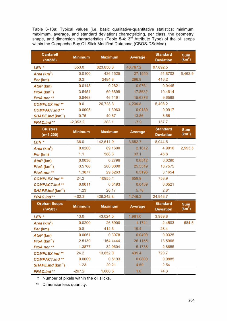
264
Table 6-13a: Typical values (i.e. basic qualitative-quantitative statistics: minimum, maximum, average, and standard deviation) characterizing, per class, the geometry, shape, and dimension characteristics (Table 5-4: 3rd Attribute Type) of the oil seeps within the Campeche Bay Oil Slick Modified Database (CBOS-DScMod).
Cantarell (n=238)
Minimum Maximum Average Standard Deviation
Sum (km2)
LEN * 353.0 823,850.0 46,767.2 97,892.5
Area (km2) 0.0100 436.1525 27.1550 51.8702 6,462.9 Per (km) 0.3 2484.8 296.9 416.2
AtoP (km) 0.0143 0.2821 0.0761 0.0445
PtoA (km-1) 3.5451 69.6899 17.8632 10.4614 PtoA.nor ** 0.8463 46.1191 15.6376 9.6568
COMPLEX.ind ** 9.0 26,728.3 4,239.8 5,408.2
COMPACT.ind ** 0.0005 1.3963 0.0180 0.0917 SHAPE.ind (km-1) 0.75 40.87 13.86 8.56
FRAC.ind ** -2,353.2 383.1 -7.9 157.7
Clusters (n=1,200)
Minimum Maximum Average Standard Deviation
Sum (km2)
LEN * 36.0 142,611.0 3,652.7 8,044.5
Area (km2) 0.0200 89.1600 2.1612 4.9010 2,593.5
Per (km) 1.1 588.3 33.1 46.8
AtoP (km) 0.0036 0.2796 0.0512 0.0290 PtoA (km-1) 3.5766 280.0000 25.5519 16.7575
PtoA.nor ** 1.3877 29.5263 6.5196 3.1654
COMPLEX.ind ** 24.2 10955.4 659.9 758.9
COMPACT.ind ** 0.0011 0.5193 0.0459 0.0521
SHAPE.ind (km-1) 1.23 26.17 5.78 2.81
FRAC.ind ** -402.3 426,242.8 1,746.2 24,946.7
Orphan Seeps (n=583)
Minimum Maximum Average Standard Deviation
Sum (km2)
LEN * 13.0 43,024.0 1,961.0 3,989.8
Area (km2) 0.0200 26.8900 1.1741 2.4503 684.5
Per (km) 0.8 414.5 19.4 28.4
AtoP (km) 0.0061 0.3978 0.0490 0.0325
PtoA (km-1) 2.5139 164.4444 26.1165 13.5966 PtoA.nor ** 1.3877 32.9604 5.1738 2.8655
COMPLEX.ind ** 24.2 13,652.0 439.4 720.7
COMPACT.ind ** 0.0009 0.5193 0.0800 0.0885 SHAPE.ind (km-1) 1.23 29.21 4.59 2.54
FRAC.ind ** -267.2 1,660.6 1.8 74.3
* Number of pixels within the oil slicks. ** Dimensionless quantity.

265
Table 6-13b: Typical values (i.e. basic qualitative-quantitative statistics: minimum, maximum, average, and standard deviation) characterizing, per class, the geometry, shape, and dimension characteristics (Table 5-4: 3rd Attribute Type) of the oil spills within the Campeche Bay Oil Slick Modified Database (CBOS-DScMod).
Brightspots (n=1,050)
Minimum Maximum Average Standard Deviation
Sum (km2)
LEN * 3.0 443,948.0 2,698.1 18,535.9
Area (km2) 0.0100 277.4900 1.6847 11.5151 1,769.0 Per (km) 0.6 772.3 18.0 48.6
AtoP (km) 0.0080 0.6311 0.0444 0.0412
PtoA (km-1) 1.5846 125.0000 30.5618 14.7221 PtoA.nor ** 1.1968 37.5652 4.5878 2.9400
COMPLEX.ind ** 18.0 17,732.9 373.0 895.4
COMPACT.ind ** 0.0007 0.6981 0.0982 0.1012 SHAPE.ind (km-1) 1.06 33.29 4.07 2.61
FRAC.ind ** -487.9 251.4 -2.2 32.0
Ship Spills (n=159)
Minimum Maximum Average Standard Deviation
Sum (km2)
LEN * 9.0 10,272.0 885.3 1,668.0
Area (km2) 0.0100 6.4200 0.5699 1.0558 90.6
Per (km) 0.6 106.5 11.3 17.0
AtoP (km) 0.0125 0.1558 0.0436 0.0234 PtoA (km-1) 6.4172 80.0000 28.8082 13.4818
PtoA.nor ** 1.2616 16.2815 4.0281 2.5582
COMPLEX.ind ** 20.0 3,331.2 285.6 468.1
COMPACT.ind ** 0.0038 0.6283 0.1343 0.1321
SHAPE.ind (km-1) 1.12 14.43 3.57 2.27
FRAC.ind ** -110.6 364,103.6 2,289.8 28,875.3
Orphan Spills (n=580)
Minimum Maximum Average Standard Deviation
Sum (km2)
LEN * 6.0 138,888.0 2,245.1 9,284.8
Area (km2) 0.0025 86.8100 1.2751 4.9817 739.6
Per (km) 0.2 504.3 15.6 36.7
AtoP (km) 0.0093 0.3880 0.0537 0.0403
PtoA (km-1) 2.5772 107.5000 25.0434 12.6311 PtoA.nor ** 1.1283 34.7857 4.0632 2.8377
COMPLEX.ind ** 16.0 15,205.9 308.5 773.1
COMPACT.ind ** 0.0008 0.7855 0.1310 0.1219 SHAPE.ind (km-1) 1.00 30.83 3.60 2.51
FRAC.ind ** -58.3 330,692.6 571.3 13,731.2
* Number of pixels within the oil slicks. ** Dimensionless quantity.

266
Table 6-13c: Typical values (i.e. basic qualitative-quantitative statistics: minimum, maximum, average, and standard deviation) characterizing, per class, the geometry, shape, and dimension characteristics (Table 5-4: 3rd Attribute Type) of the oil spills within the Campeche Bay Oil Slick Modified Database (CBOS-DScMod).
Bright-1 (n=575)
Minimum Maximum Average Standard Deviation
Sum (km2)
LEN * 3.0 66,268.0 1,352.0 4,830.4
Area (km2) 0.0100 78.1300 0.9150 4.2674 526.1 Per (km) 0.4 451.3 13.8 30.0
AtoP (km) 0.0036 0.6582 0.0396 0.0347
PtoA (km-1) 1.5193 280.0000 33.6563 20.3851 PtoA.nor ** 1.1284 19.7813 4.4930 2.5151
COMPLEX.ind ** 16.0 4,917.2 333.0 473.7
COMPACT.ind ** 0.0026 0.7854 0.0973 0.0971 SHAPE.ind (km-1) 1.00 17.53 3.98 2.23
FRAC.ind ** -85.5 278.6 -0.1 16.8
Bright-2 (n=276)
Minimum Maximum Average Standard Deviation
Sum (km2)
LEN * 4.0 20,516.0 613.8 1,411.2
Area (km2) 0.0100 12.8200 0.3867 0.8686 106.7
Per (km) 0.6 197.5 9.0 14.6
AtoP (km) 0.0033 0.2099 0.0381 0.0210 PtoA (km-1) 4.7642 300.0000 33.0007 21.5291
PtoA.nor ** 1.3029 15.5611 4.0231 2.0526
COMPLEX.ind ** 21.3 3,042.9 256.1 335.2
COMPACT.ind ** 0.0041 0.5890 0.1098 0.0979
SHAPE.ind (km-1) 1.15 13.79 3.57 1.82
FRAC.ind ** -322.3 251.8 -1.5 27.2
Bright-3 (n=255)
Minimum Maximum Average Standard Deviation
Sum (km2)
LEN * 4.0 106,696.0 2,254.4 9,037.1
Area (km2) 0.0076 66.6900 1.4264 5.6466 363.7
Per (km) 0.4 468.1 19.2 50.1
AtoP (km) 0.0060 0.2148 0.0427 0.0268
PtoA (km-1) 4.6564 168.0000 30.6835 17.0164 PtoA.nor ** 1.3029 19.4004 4.6806 2.8041
COMPLEX.ind ** 21.3 4,729.7 373.7 577.2
COMPACT.ind ** 0.0027 0.5891 0.0950 0.0974 SHAPE.ind (km-1) 1.15 17.19 4.15 2.49
FRAC.ind ** -41.0 395,511.4 1,550.3 24,767.9
* Number of pixels within the oil slicks. ** Dimensionless quantity.

267
APPENDIX 3
TYPICAL VALUES OF BASIC QUALITATIVE-QUANTITATIVE STATISTICS:
4TH ATTRIBUTE TYPE (TABLE 5-5: SAR BACKSCATTER SIGNATURE)
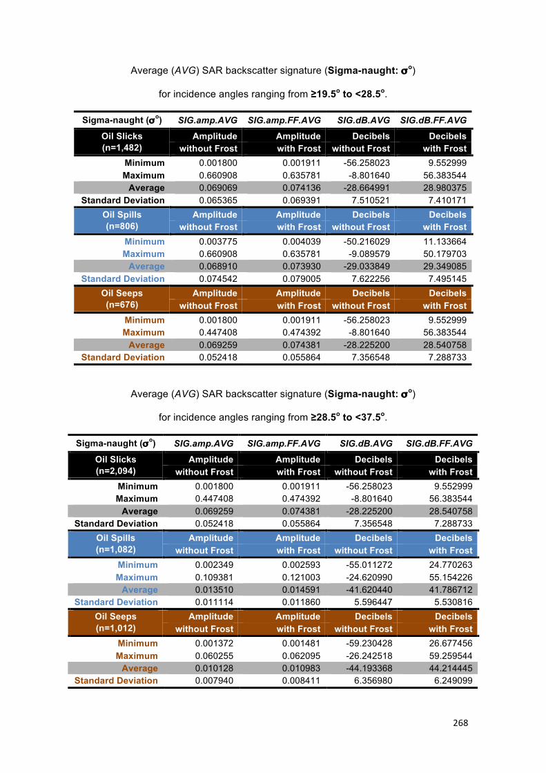
268
Average (AVG) SAR backscatter signature (Sigma-naught: σo)
for incidence angles ranging from ≥19.5o to <28.5o.
Sigma-naught (σo) SIG.amp.AVG SIG.amp.FF.AVG SIG.dB.AVG SIG.dB.FF.AVG
Amplitude Amplitude Decibels Decibels Oil Slicks (n=1,482) without Frost with Frost without Frost with Frost
Minimum 0.001800 0.001911 -56.258023 9.552999 Maximum 0.660908 0.635781 -8.801640 56.383544
Average 0.069069 0.074136 -28.664991 28.980375 Standard Deviation 0.065365 0.069391 7.510521 7.410171
Amplitude Amplitude Decibels Decibels Oil Spills (n=806) without Frost with Frost without Frost with Frost
Minimum 0.003775 0.004039 -50.216029 11.133664 Maximum 0.660908 0.635781 -9.089579 50.179703
Average 0.068910 0.073930 -29.033849 29.349085 Standard Deviation 0.074542 0.079005 7.622256 7.495145
Amplitude Amplitude Decibels Decibels Oil Seeps (n=676) without Frost with Frost without Frost with Frost
Minimum 0.001800 0.001911 -56.258023 9.552999 Maximum 0.447408 0.474392 -8.801640 56.383544
Average 0.069259 0.074381 -28.225200 28.540758 Standard Deviation 0.052418 0.055864 7.356548 7.288733
Average (AVG) SAR backscatter signature (Sigma-naught: σo)
for incidence angles ranging from ≥28.5o to <37.5o.
Sigma-naught (σo) SIG.amp.AVG SIG.amp.FF.AVG SIG.dB.AVG SIG.dB.FF.AVG
Amplitude Amplitude Decibels Decibels Oil Slicks (n=2,094) without Frost with Frost without Frost with Frost
Minimum 0.001800 0.001911 -56.258023 9.552999 Maximum 0.447408 0.474392 -8.801640 56.383544
Average 0.069259 0.074381 -28.225200 28.540758 Standard Deviation 0.052418 0.055864 7.356548 7.288733
Amplitude Amplitude Decibels Decibels Oil Spills (n=1,082) without Frost with Frost without Frost with Frost
Minimum 0.002349 0.002593 -55.011272 24.770263 Maximum 0.109381 0.121003 -24.620990 55.154226
Average 0.013510 0.014591 -41.620440 41.786712 Standard Deviation 0.011114 0.011860 5.596447 5.530816
Amplitude Amplitude Decibels Decibels Oil Seeps (n=1,012) without Frost with Frost without Frost with Frost
Minimum 0.001372 0.001481 -59.230428 26.677456 Maximum 0.060255 0.062095 -26.242518 59.259544
Average 0.010128 0.010983 -44.193368 44.214445 Standard Deviation 0.007940 0.008411 6.356980 6.249099

269
Average (AVG) SAR backscatter signature (Sigma-naught: σo)
for incidence angles ranging from ≥37.5o to ≤46.6o.
Sigma-naught (σo) SIG.amp.AVG SIG.amp.FF.AVG SIG.dB.AVG SIG.dB.FF.AVG
Amplitude Amplitude Decibels Decibels Oil Slicks (n=1,340) without Frost with Frost without Frost with Frost
Minimum 0.000907 0.000995 -62.195921 35.431792 Maximum 0.107952 0.114450 -35.080355 62.054795
Average 0.004213 0.004594 -51.265255 51.304869 Standard Deviation 0.005099 0.005513 4.549087 4.502321
Amplitude Amplitude Decibels Decibels Oil Spills (n=1,007) without Frost with Frost without Frost with Frost
Minimum 0.001060 0.001135 -61.211937 35.431792 Maximum 0.097043 0.107837 -35.080355 61.200692
Average 0.004171 0.004550 -51.320413 51.368698 Standard Deviation 0.004688 0.005118 4.402869 4.348059
Amplitude Amplitude Decibels Decibels Oil Seeps (n=333) without Frost with Frost without Frost with Frost
Minimum 0.000907 0.000995 -62.195921 37.106547 Maximum 0.107952 0.114450 -37.027594 62.054795
Average 0.004338 0.004726 -51.098454 51.111850 Standard Deviation 0.006182 0.006571 4.968460 4.941576
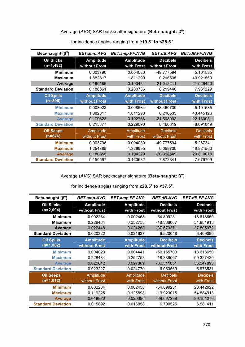
270
Average (AVG) SAR backscatter signature (Beta-naught: βo)
for incidence angles ranging from ≥19.5o to <28.5o.
Beta-naught (βo) BET.amp.AVG BET.amp.FF.AVG BET.dB.AVG BET.dB.FF.AVG Amplitude Amplitude Decibels Decibels Oil Slicks
(n=1,482) without Frost with Frost without Frost with Frost Minimum 0.003796 0.004030 -49.777594 5.101585 Maximum 1.882817 1.811290 0.216535 49.921560
Average 0.180189 0.193434 -21.012211 21.528420 Standard Deviation 0.188861 0.200736 8.219440 7.931229
Amplitude Amplitude Decibels Decibels Oil Spills (n=806) without Frost with Frost without Frost with Frost
Minimum 0.008022 0.008584 -43.460739 5.101585 Maximum 1.882817 1.811290 0.216535 43.445126
Average 0.179628 0.192768 -21.593993 22.130951 Standard Deviation 0.215877 0.229090 8.460319 8.091849
Amplitude Amplitude Decibels Decibels Oil Seeps (n=676) without Frost with Frost without Frost with Frost
Minimum 0.003796 0.004030 -49.777594 5.267341 Maximum 1.254385 1.329995 0.059730 49.921560
Average 0.180858 0.194229 -20.318549 20.810018 Standard Deviation 0.150597 0.160682 7.872841 7.679709
Average (AVG) SAR backscatter signature (Beta-naught: βo)
for incidence angles ranging from ≥28.5o to <37.5o.
Beta-naught (βo) BET.amp.AVG BET.amp.FF.AVG BET.dB.AVG BET.dB.FF.AVG Amplitude Amplitude Decibels Decibels Oil Slicks
(n=2,094) without Frost with Frost without Frost with Frost Minimum 0.002264 0.002458 -54.899231 18.618650 Maximum 0.228484 0.252758 -18.388067 54.884913
Average 0.022448 0.024268 -37.673371 37.805972 Standard Deviation 0.020322 0.021637 6.520048 6.409090
Amplitude Amplitude Decibels Decibels Oil Spills (n=1,082) without Frost with Frost without Frost with Frost
Minimum 0.004023 0.004441 -50.165700 18.618650 Maximum 0.228484 0.252758 -18.388067 50.327430
Average 0.025842 0.027889 -36.341631 36.547895 Standard Deviation 0.023227 0.024770 6.053569 5.978531
Amplitude Amplitude Decibels Decibels Oil Seeps (n=1,012) without Frost with Frost without Frost with Frost
Minimum 0.002264 0.002458 -54.899231 20.442622 Maximum 0.119225 0.125898 -19.923015 54.884913
Average 0.018820 0.020396 -39.097228 39.151070 Standard Deviation 0.015892 0.016858 6.700525 6.581411
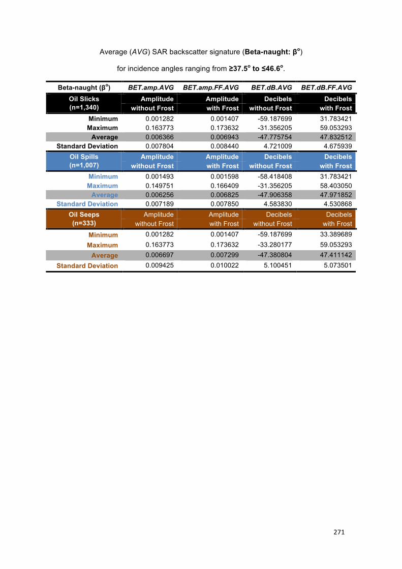
271
Average (AVG) SAR backscatter signature (Beta-naught: βo)
for incidence angles ranging from ≥37.5o to ≤46.6o.
Beta-naught (βo) BET.amp.AVG BET.amp.FF.AVG BET.dB.AVG BET.dB.FF.AVG Amplitude Amplitude Decibels Decibels Oil Slicks
(n=1,340) without Frost with Frost without Frost with Frost Minimum 0.001282 0.001407 -59.187699 31.783421 Maximum 0.163773 0.173632 -31.356205 59.053293
Average 0.006366 0.006943 -47.775754 47.832512 Standard Deviation 0.007804 0.008440 4.721009 4.675939
Amplitude Amplitude Decibels Decibels Oil Spills (n=1,007) without Frost with Frost without Frost with Frost
Minimum 0.001493 0.001598 -58.418408 31.783421 Maximum 0.149751 0.166409 -31.356205 58.403050
Average 0.006256 0.006825 -47.906358 47.971852 Standard Deviation 0.007189 0.007850 4.583830 4.530868
Amplitude Amplitude Decibels Decibels Oil Seeps (n=333) without Frost with Frost without Frost with Frost
Minimum 0.001282 0.001407 -59.187699 33.389689 Maximum 0.163773 0.173632 -33.280177 59.053293
Average 0.006697 0.007299 -47.380804 47.411142 Standard Deviation 0.009425 0.010022 5.100451 5.073501

272
Average (AVG) SAR backscatter signature (Gamma-naught: γo)
for incidence angles ranging from ≥19.5o to <28.5o.
Gamma-naught (γo) GAM.amp.AVG GAM.amp.FF.AVG GAM.dB.AVG GAM.dB.FF.AVG
Amplitude Amplitude Decibels Decibels Oil Slicks (n=1,482) without Frost with Frost without Frost with Frost
Minimum 0.002044 0.002170 -55.151609 9.016371 Maximum 0.705821 0.682226 -8.194344 55.279979
Average 0.075074 0.080579 -27.822521 28.149132 Standard Deviation 0.069702 0.073976 7.377056 7.273076
Amplitude Amplitude Decibels Decibels Oil Spills (n=806) without Frost with Frost without Frost with Frost
Minimum 0.004278 0.004578 -49.186249 10.757918 Maximum 0.705821 0.682226 -8.547585 49.152696
Average 0.075018 0.080479 -28.140251 28.467647 Standard Deviation 0.079497 0.084233 7.461274 7.328244
Amplitude Amplitude Decibels Decibels Oil Seeps (n=676) without Frost with Frost without Frost with Frost
Minimum 0.002044 0.002170 -55.151609 9.016371 Maximum 0.479105 0.508002 -8.194344 55.279979
Average 0.075142 0.080699 -27.443689 27.769363 Standard Deviation 0.055882 0.059542 7.262711 7.193730
Average (AVG) SAR backscatter signature (Gamma-naught: γo)
for incidence angles ranging from ≥28.5o to <37.5o.
Gamma-naught (γo) GAM.amp.AVG GAM.amp.FF.AVG GAM.dB.AVG GAM.dB.FF.AVG
Amplitude Amplitude Decibels Decibels Oil Slicks (n=2,094) without Frost with Frost without Frost with Frost
Minimum 0.002044 0.002170 -55.151609 9.016371 Maximum 0.479105 0.508002 -8.194344 55.279979
Average 0.075142 0.080699 -27.443689 27.769363 Standard Deviation 0.055882 0.059542 7.262711 7.193730
Amplitude Amplitude Decibels Decibels Oil Spills (n=1,082) without Frost with Frost without Frost with Frost
Minimum 0.002894 0.003194 -53.287052 23.602221 Maximum 0.124585 0.137823 -23.440131 53.436325
Average 0.015929 0.017210 -40.073678 40.250320 Standard Deviation 0.012661 0.013518 5.433290 5.367734
Amplitude Amplitude Decibels Decibels Oil Seeps (n=1,012) without Frost with Frost without Frost with Frost
Minimum 0.001719 0.001856 -57.244287 25.536313 Maximum 0.070785 0.072946 -24.844529 57.305490
Average 0.012062 0.013084 -42.565411 42.595729 Standard Deviation 0.009176 0.009716 6.217107 6.109007
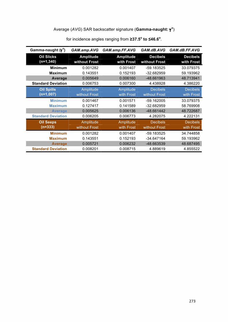
273
Average (AVG) SAR backscatter signature (Gamma-naught: γo)
for incidence angles ranging from ≥37.5o to ≤46.6o.
Gamma-naught (γo) GAM.amp.AVG GAM.amp.FF.AVG GAM.dB.AVG GAM.dB.FF.AVG
Amplitude Amplitude Decibels Decibels Oil Slicks (n=1,340) without Frost with Frost without Frost with Frost
Minimum 0.001282 0.001407 -59.183525 33.079375 Maximum 0.143551 0.152193 -32.682959 59.193962
Average 0.005649 0.006160 -48.661963 48.713941 Standard Deviation 0.006753 0.007300 4.438928 4.386220
Amplitude Amplitude Decibels Decibels Oil Spills (n=1,007) without Frost with Frost without Frost with Frost
Minimum 0.001467 0.001571 -59.162005 33.079375 Maximum 0.127417 0.141589 -32.682959 58.769908
Average 0.005625 0.006136 -48.661442 48.722687 Standard Deviation 0.006205 0.006773 4.282075 4.222131
Amplitude Amplitude Decibels Decibels Oil Seeps (n=333) without Frost with Frost without Frost with Frost
Minimum 0.001282 0.001407 -59.183525 34.744858 Maximum 0.143551 0.152193 -34.647164 59.193962
Average 0.005721 0.006232 -48.663539 48.687495 Standard Deviation 0.008201 0.008715 4.889619 4.855522

274
APPENDIX 4
ROOTED-TREE DENDROGRAMS BASED ON THE UPGMA (UNWEIGHTED
PAIR GROUP METHOD WITH ARITHMETIC MEAN) IMPLEMENTATION PER
DATA SUB-DIVISION
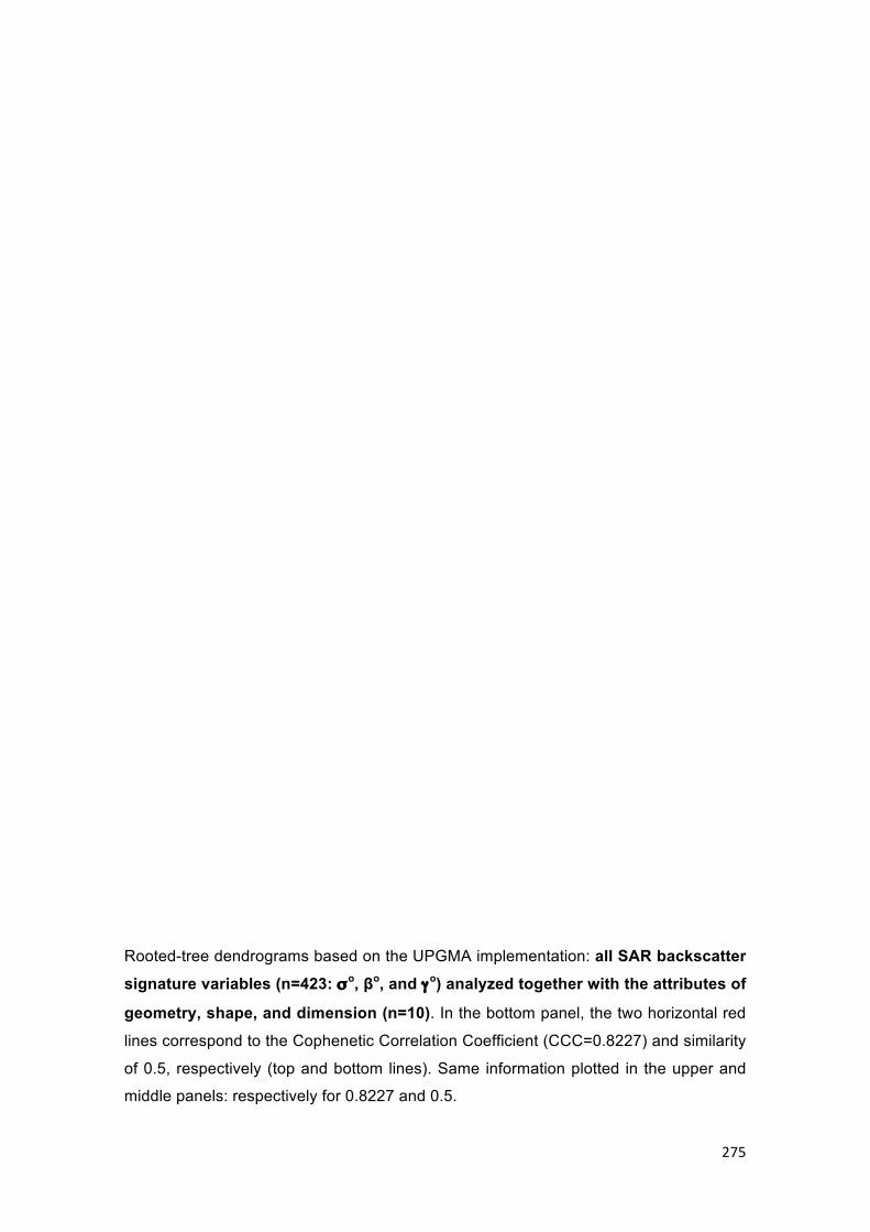
275
Rooted-tree dendrograms based on the UPGMA implementation: all SAR backscatter
signature variables (n=423: σo, βo, and γo) analyzed together with the attributes of
geometry, shape, and dimension (n=10). In the bottom panel, the two horizontal red
lines correspond to the Cophenetic Correlation Coefficient (CCC=0.8227) and similarity
of 0.5, respectively (top and bottom lines). Same information plotted in the upper and
middle panels: respectively for 0.8227 and 0.5.
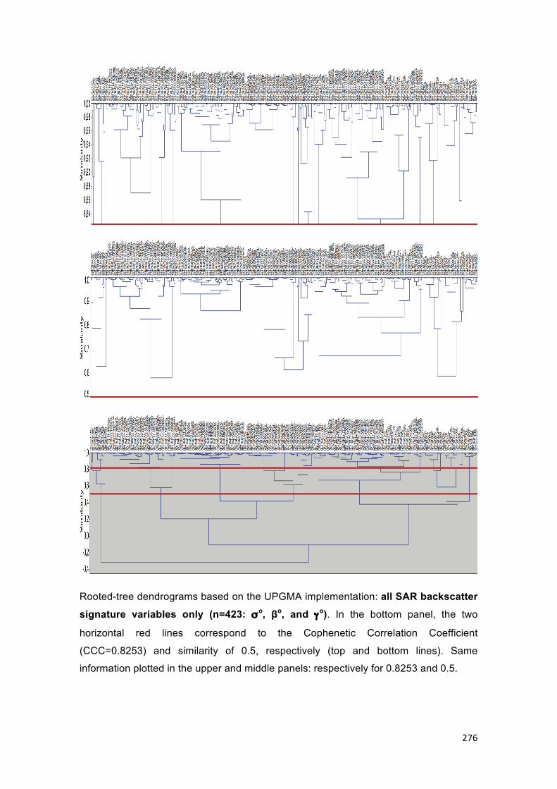
276
Rooted-tree dendrograms based on the UPGMA implementation: all SAR backscatter
signature variables only (n=423: σo, βo, and γo). In the bottom panel, the two
horizontal red lines correspond to the Cophenetic Correlation Coefficient
(CCC=0.8253) and similarity of 0.5, respectively (top and bottom lines). Same
information plotted in the upper and middle panels: respectively for 0.8253 and 0.5.

277
Rooted-tree dendrograms based on the UPGMA implementation: beta-naught (βo)
variables (n=141) together with the attributes of geometry, shape, and dimension
(n=10). In the lower panel, the two horizontal red lines correspond to the Cophenetic
Correlation Coefficient (CCC=0.8031) and similarity of 0.5, respectively (top and
bottom lines). Same information plotted in the upper and middle panels: respectively for
0.8031 and 0.5.
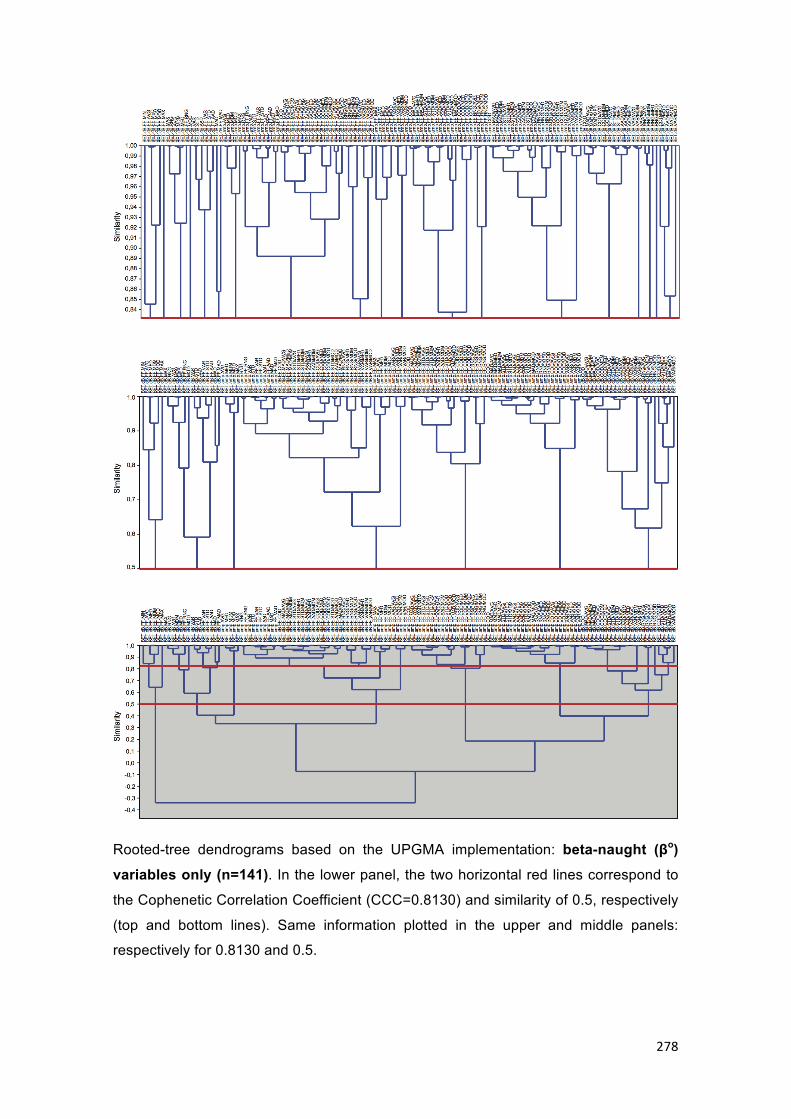
278
Rooted-tree dendrograms based on the UPGMA implementation: beta-naught (βo)
variables only (n=141). In the lower panel, the two horizontal red lines correspond to
the Cophenetic Correlation Coefficient (CCC=0.8130) and similarity of 0.5, respectively
(top and bottom lines). Same information plotted in the upper and middle panels:
respectively for 0.8130 and 0.5.

279
Rooted-tree dendrograms based on the UPGMA implementation: gamma-naught (γo)
variables (n=141) together with the attributes of geometry, shape, and dimension
(n=10). In the lower panel, the two horizontal red lines correspond to the Cophenetic
Correlation Coefficient (CCC=0.8240) and similarity of 0.5, respectively (top and
bottom lines). Same information plotted in the upper and middle panels: respectively for
0.8240 and 0.5.

280
Rooted-tree dendrograms based on the UPGMA implementation: gamma-naught (γo)
variables only (n=141). In the lower panel, the two horizontal red lines correspond to
the Cophenetic Correlation Coefficient (CCC=0.8260) and similarity of 0.5, respectively
(top and bottom lines). Same information plotted in the upper and middle panels:
respectively for 0.8260 and 0.5.

281
APPENDIX 5
CONSTANT OFFSETS (COFF) OF THE DISCRIMINANT FUNCTIONS

282
Constant offset (Coff) per data sub-divisions (Figure 5-3).
No PCA: See Table 6-31 for the number of variables.
Original Sets
UPGMA (CCC)
UPGMA (0.5) CFS
Complete Exploration of the CBOS-DScMod 20.70810 26.75160 22.38290 §
All SAR Backscatter Signature ¥ with Size* 4.73703 † † 5.89046
Only all SAR Backscatter Signature ¥ 5.94918 †† †† -0.97017
Size* and Sigma-naught (σo) 14.62320 16.69950 17.70760 4.34108
Size* and Beta-naught (βo) 9.60851 15.46650 17.28380 5.39505
Size* and Gamma-naught (γo) 13.70120 14.81050 16.47300 7.24409
Only Size* 3.85919 4.18807 3.96403 3.70246
Only Sigma-naught (σo) 17.54930 15.09050 8.16940 1.19049
Only Beta-naught (βo) 11.17600 14.15150 10.18060 1.68465
Only Gamma-naught (γo) 16.42570 14.23110 7.02485 -10.40370
Only Digital Numbers (DN’s) 2.87075 1.76280 1.26008 3.42718
With PCA: See Table 6-33 for the selected PC’s.
Original Set
UPGMA (CCC)
UPGMA (0.5) CFS
Complete Exploration of the CBOS-DScMod 1.2740100 6.6779200 7.0276700 §
All SAR Backscatter Signature ¥ with Size* 0.0795821 † † 0.0780176
Only all SAR Backscatter Signature ¥ 0.0447324 †† †† 0.0472360
Size* and Sigma-naught (σo) 0.0665499 0.0839193 0.0574982 0.0796083
Size* and Beta-naught (βo) 0.0678715 0.0821239 0.0576795 0.0826254
Size* and Gamma-naught (γo) 0.0644667 0.0833115 0.0562702 0.0768122
Only Size* 0.0772492 0.0795265 0.0811427 0.0811096
Only Sigma-naught (σo) 0.0443751 0.0440276 0.0334348 0.0478720
Only Beta-naught (βo) 0.0436300 0.0346945 0.0325406 0.0457521
Only Gamma-naught (γo) 0.0432606 0.0429225 0.0322825 0.0453125
Only Digital Numbers (DN’s) 0.0103062 0.0121737 0.0103375 0.0157960
§ Discriminant Function not performed (see Table 6-23).
* Attributes of geometry, shape, and dimension.
¥ See: Table 5-1 and Table 5-5.
σo SIG.amp, SIG.amp.FF, SIG.dB, and SIG.dB.FF.
βo BET.amp, BET.amp.FF, BET.dB, and BET.dB.FF.
γo GAM.amp, GAM.amp.FF, GAM.dB, and GAM.dB.FF.
† Same as Size* and Sigma-naught (σo).
†† Same as only Sigma-naught (σo).

283
APPENDIX 6
CONFIGURATION OF THE TWO DESIGNED CLASSIFICATION ALGORITHMS
PROPOSED ON PHASE 10 (SECTIONS 5.10 AND 6.10)
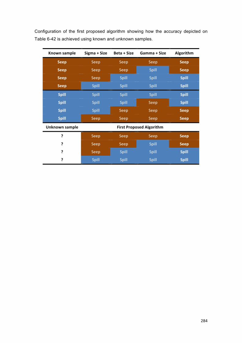
284
Configuration of the first proposed algorithm showing how the accuracy depicted on
Table 6-42 is achieved using known and unknown samples.
Knownsample Sigma+Size Beta+Size Gamma+Size Algorithm
Seep Seep Seep Seep Seep
Seep Seep Seep Spill Seep
Seep Seep Spill Spill Spill
Seep Spill Spill Spill Spill
Spill Spill Spill Spill Spill
Spill Spill Spill Seep Spill
Spill Spill Seep Seep Seep
Spill Seep Seep Seep Seep
Unknownsample FirstProposedAlgorithm
? Seep Seep Seep Seep
? Seep Seep Spill Seep
? Seep Spill Spill Spill
? Spill Spill Spill Spill

285
Configuration of the second proposed algorithm showing how the accuracy depicted on
Table 6-43 is achieved using known and unknown samples.
Knownsample Size Sigma Beta Gamma Algorithm
Seep Seep Seep Seep Seep Seep
Seep Seep Seep Seep Spill Seep
Seep Seep Seep Spill Spill Seep*
Seep Seep Spill Spill Spill Spill
Seep Spill Spill Spill Spill Spill
Spill Spill Spill Spill Spill Spill
Spill Spill Spill Spill Seep Spill
Spill Spill Spill Seep Seep Spill*
Spill Spill Seep Seep Seep Seep
Spill Seep Seep Seep Seep Seep
Unknownsample 1stModeoftheSecondProposedAlgorithm
? Seep Seep Seep Seep Seep
? Seep Seep Seep Spill Seep
? Seep Seep Spill Spill Spill
? Seep Spill Spill Spill Spill
? Spill Spill Spill Spill Spill
Unknownsample 2ndModeoftheSecondProposedAlgorithm
? Spill Spill Spill Spill Spill
? Spill Spill Spill Seep Spill
? Spill Spill Seep Seep ?*
? Spill Seep Seep Seep Seep
? Seep Seep Seep Seep Seep
Unknownsample 3rdModeoftheSecondProposedAlgorithm
? Spill Spill Spill Spill Spill
? Spill Spill Spill Seep Spill
? Spill Spill Seep Seep Seep
? Spill Seep Seep Seep Seep
? Seep Seep Seep Seep Seep
*Notconsideredonthe2ndMode.
Copyright © 2022 FDOKUMEN