Satellite-derived vegetation indices contribute significantly to the prediction of epiphyllous...

This article appeared in a journal published by Elsevier. The attachedcopy is furnished to the author for internal non-commercial researchand education use, including for instruction at the authors institution

and sharing with colleagues.

Other uses, including reproduction and distribution, or selling orlicensing copies, or posting to personal, institutional or third party

websites are prohibited.

In most cases authors are permitted to post their version of thearticle (e.g. in Word or Tex form) to their personal website orinstitutional repository. Authors requiring further information

regarding Elsevier’s archiving and manuscript policies areencouraged to visit:

http://www.elsevier.com/authorsrights

http://www.elsevier.com/authorsrights

Author's personal copy

Ecological Indicators 38 (2014) 72– 80

Contents lists available at ScienceDirect

Ecological Indicators

jou rn al hom epage: www.elsev ier .com/ locate /eco l ind

Satellite-derived vegetation indices contribute significantlyto the prediction of epiphyllous liverworts

Yanbin Jianga,b, Tiejun Wangc,∗, C.A.J.M. de Biec, A.K. Skidmorec, Xuehua Liud,Shanshan Songa, Li Zhange, Jian Wangf, Xiaoming Shaoa,∗∗

a College of Resources and Environmental Sciences, China Agricultural University, Beijing 100193, Chinab Key Laboratory of Ecosystem Network Observation and Modeling, Institute of Geographic Sciences and Natural Resources Research, Chinese Academy ofSciences, Beijing 100101, Chinac Faculty of Geo-Information Science and Earth Observation, University of Twente, 7500AE Enschede, The Netherlandsd School of Environment, Tsinghua University, Beijing 100084, Chinae Shenzhen Key Laboratory of Southern Subtropical Plant Diversity, Fairylake Botanical Garden, Shenzhen & Chinese Academy of Sciences, Shenzhen518004, Chinaf School of Life Sciences, East China Normal University, Shanghai 200062, China

a r t i c l e i n f o

Article history:Received 23 May 2013Received in revised form 16 August 2013Accepted 17 October 2013

Keywords:Species distribution modelMaxEntClimateVegetationMacro-habitatChina

a b s t r a c t

Epiphyllous liverworts form a special group of bryophytes that primarily grow on leaves of understoryvascular plants, occurring in constantly moist and warm evergreen forest in tropical and subtropicalregions. They are very sensitive to climate change and environmental pollution. Previous studies havefocused largely on microhabitat preferences of epiphyllous liverworts and demonstrated the importanceof climate factors such as humidity, temperature and light. However, little is known about the relationshipbetween distribution of epiphyllous liverworts and macro-habitat factors at broad spatial scales. Here,we predicated the distribution of epiphyllous liverworts in China based on topographic and bioclimaticvariables, as well as satellite-derived vegetation indices at a 1 km spatial resolution using presence-onlyecological niche models. We used the Area Under the receiver operating characteristic Curve (AUC) andTrue Skill Statistic (TSS) to validate the models, and then used the Wilcoxon paired test to comparemodel performances. Furthermore, we applied the jackknife test to identify the important factors affect-ing predictions. Our results showed that the highest accuracy (i.e., AUC = 0.98 and TSS = 0.93) in predictingepiphyllous liverworts was achieved by the model that combined climatic and remotely sensed vegeta-tion variables. The satellite-derived annual mean and minimum Normalized Difference Vegetation Index(NDVI) as well as the annual mean and minimum Normalized Difference Water Index (NDWI) emerged asthe most important predictors of distribution patterns of epiphyllous liverworts, while climatic variablessuch as precipitation in the wettest quarter and temperature of the coldest quarter were of ancillaryimportance. The significant contributions of NDVI and NDWI in defining the distribution range and spa-tial patterns of epiphyllous liverworts, and the strong relationship between this species and evergreenforest implies that epiphyllous liverworts may be a useful indicator for forest degradation or integrity atbroad spatial scales.

© 2013 Elsevier Ltd. All rights reserved.

1. Introduction

Bryophytes, represented by mosses, liverworts and hornworts,make a substantial contribution to terrestrial ecosystems in termsof nutrient cycling, water retention, water availability and modifi-cation of the global climate (Imada et al., 2011; Sim-Sim et al., 2011).

∗ Corresponding author. Tel.: +31 53 4874274.∗∗ Corresponding author. Tel.: +86 10 62734980.

E-mail addresses: [email protected] (T. Wang), [email protected] (X. Shao).

Being sensitive to moisture and temperature range, bryophytesform potential indicators for climate and climate change (Gignac,2001). Bryophytes have potential when testing predictions withrespect to plant population persistence in spatially structured land-scapes (Pharo and Zartman, 2007), as indicators of forest integrity(Frego, 2007) or metal accumulation (Pesch and Schroeder, 2006),and when monitoring hydrologic and micro-climate pressures onstream ecosystems (Vieira et al., 2012).

Epiphyllous liverworts form a special group of bryophytes thatprimarily grow on leaves of understory vascular plants. Sinceepiphyllous liverworts occur mainly in the tropical and sub-tropical moist broadleaf evergreen forests, they are particularly

1470-160X/$ – see front matter © 2013 Elsevier Ltd. All rights reserved.http://dx.doi.org/10.1016/j.ecolind.2013.10.024


Y. Jiang et al. / Ecological Indicators 38 (2014) 72– 80 73

sensitive to climate change and forest modification (Pócs, 1996;Zartman, 2003). The development of epiphyllous liverwort stud-ies dates back to the late 18th century (Massart, 1898). They area poorly collected and taxonomically complicated group, with anonly partly identified distribution pattern (Benavides and Sastre-De Jesus, 2011). According to Pócs (1996), the distribution ofepiphyllous liverworts extends into 21 floristic regions in Asia,Australia, Africa, Central and South America, and the Macarone-sian islands in Europe, with Asia having the highest diversity withmore than 500 known species. In China, due to its diverse topog-raphy and climate, about 200 species of epiphyllous liverwortshave been found with relatively high rates of endemism, leadingto a high conservation status (Zhu and So, 2001). They are dis-tributed throughout China’s rainforests and evergreen broadleavedforests, and found from the tropics to 30◦ N (Chen and Wu, 1964).More recently the distribution range has been extended to 31◦ N,including Guanxian County in Sichuan province (Luo, 1990) andHouhe Nature Reserve in Hubei province (Peng et al., 2002). How-ever, to date, apart from mapping species occurrences obtainedfrom field guide information, there has been no research con-ducted into understanding the distribution range of epiphyllousliverworts (Zhu and So, 2001). Moreover, constraints affectingbroader scales are little known, with only prime drivers of localdistribution patterns having been studied (Monge-Nájera, 1989;Olarinmoye, 1974; Wu et al., 1987). For example, forest fragmen-tation seems to be a threatening factor for epiphyllous liverwortson a continental scale (Alvarenga and Porto, 2007) as the invasionby exotics or the replacement of the original canopy by planta-tion trees usually means the total loss of epiphyllous liverworts(Pócs, 1996). Therefore, understanding their spatial distributionpatterns on a continental scale plus the environmental factorsaffecting them is important for regional conservation assessment,forest management, and when guiding future field surveys to detectunknown distribution areas and the impact of environmentalchange.

Species distribution models are becoming increasingly popularin ecology and have been used to address fundamental questions ofwhere a species is likely to be found when the conditions are right,what the most important factors are affecting distribution, and howa species is likely to respond to future climate change. Speciesdistribution models relate species occurrence data to environ-mental predictor variables, based on statistically or theoreticallyderived response surfaces (Guisan and Thuiller, 2005; Guisan andZimmermann, 2000). A variety of modeling methods are availableto predict potentially suitable habitat for a species, such as BIO-CLIM, DOMAIN, GARP, MaxEnt, GLM, GAM and BRT. These modelshave been employed to predict the distribution of many typesof organisms, such as fungi, lichens, herbs, shrubs, trees, insects,fish, reptiles, birds and mammals (Gillespie and Walter, 2001;Guisan et al., 1998; Judas et al., 2002; McKenzie and Halpern, 1999;Otte et al., 2005; Pearson et al., 2007; Riordan and Rundel, 2009;Rodriguez-Soto et al., 2011; Sundermeyer et al., 2006; Wisz et al.,2008; Wollan et al., 2008). However, species distribution mod-els have rarely been applied to epiphyllous liverworts, probablydue to insufficient taxonomic knowledge of epiphyllous liverwortsand lack of adequate data in many parts of the world. Samplingand collecting epiphyllous liverworts in the field is challenging,because correct identification of these small species commonlyrelies on microscopic examination and the expert knowledge ofbryologists.

The objectives of this study are: (1) to predict the distributionof epiphyllous liverworts in China based on topographic and bio-climatic variables, as well as satellite-derived vegetation indicesusing presence-only ecological niche models; (2) to identify macro-habitat factors affecting the spatial distribution of epiphyllousliverworts at a broad spatial scale.

2. Materials and methods

2.1. Study area and species data

The study area covers the entire China. Presence-only datafor epiphyllous liverworts were directly collected from the fieldbetween 2008 and 2010. The most comprehensive field campaignwas carried out from April to August 2010. The sampling schemeof this survey was designed based on a pre-selected NormalizedDifference Vegetation Index (NDVI) classes across the whole Chinain which occurrence of evergreen broadleaved forest, and thus epi-phyllous liverworts, was deemed possible. A total of 537 1-km2

plots were sampled within 19 blocks (100 km × 100 km) using arandom clustered representative sampling approach. Within eachsampled plot (1 km2), the fraction of evergreen broadleaved for-est was estimated for ten random locations, each with a radius ofabout 50 m. These locations were randomly picked along the pathof an exhaustive walk through the accessible areas of the 1-km2

sample. During that walk, we actively searched for epiphyllous liv-erworts. The coordinates of the sampled locations were recordedusing a GPS. As a result, the occurrence of epiphyllous liverwortshas been confirmed in 69 1-km2 plots. Detailed sample designabout this survey can be found in Jiang et al. (2013). In additionto this nationwide survey, we have also conducted another threethematic surveys at several regions (i.e. Hong Kong, Shenzhen, Tibetand Jiangxi provinces) in 2008 and 2009. These thematic surveysresulted in 14 occurrence records of epiphyllous liverworts. Tolessen the spatial auto-correlating effect, occurrences of epiphyl-lous liverworts at least 2 km apart from each other were retained.In total, 80 occurrence records were used in this study, as seen inFig. 1.

2.2. Environmental variables

2.2.1. Topographic dataTopography is a relatively static variable compared to other bio-

physical factors, including climate, which is seen as a key driverof biodiversity (Rosenzweig, 1995). Topographic variables werederived from a global 30′′ (about 1 km at the equator) elevationdataset, i.e., the USGS GTOPO30 (http://www1.gsi.go.jp/geowww/globalmap-gsi/gtopo30/gtopo30.html). Slope and aspect were cal-culated in ArcGIS 10.0 (ESRI, Inc., Redlands, CA, USA).

2.2.2. Bioclimatic dataBioclimatic variables were obtained from the WorldClim

database (http://www.worldclim.org/). A set of global climate lay-ers was derived from over 4000 weather stations between 1950and 2000, including annual time series with annual means, season-ality, and extreme or limiting temperature and precipitation data(Hijmans et al., 2005). This dataset represents biologically mean-ingful variables for characterizing species distribution at continentscale (Blach-Overgaard et al., 2010). In this study, 19 climatic layerswith a spatial resolution of 1 km were used (Table 1).

2.2.3. Satellite-derived vegetation indicesThe Normalized Difference Vegetation Index [NDVI, equal to

(�NIR − �RED)/(�NIR + �RED)] is often used as an indicator reflectingthe vigor of green land cover (Carlson and Ripley, 1997; Gamonet al., 1995). The temporal behavior of NDVI has proven to bevaluable for mapping different forest types, due to its ability tocapture seasonal differences in phenology and greenness by veg-etation type (Chen and Pan, 2002; Vancutsem et al., 2009; Xiaoet al., 2002). In this study, atmospherically corrected SPOT4 andSPOT5 Vegetation (VGT) Sensor 10-day composite NDVI-images ata 1 km resolution over the three year period from 2008 to 2010


74 Y. Jiang et al. / Ecological Indicators 38 (2014) 72– 80

Fig. 1. Study area and the 80 recorded locations of epiphyllous liverworts in China used in the species distribution models.

were obtained from www.vgt.vito.be (108 images, three images permonth). The upper-envelope method was used to smooth the timeseries (Jönsson and Eklundh, 2004). Then, a time series of 36 yearlyaveraged images was generated and used to calculate meaningfulNDVI indices: maximum NDVI, mean NDVI, minimum NDVI, NDVIamplitude (difference between maximum and minimum NDVI) andNDVI standard deviation.

The Normalized Difference Water Index [NDWI, equal to(�NIR − �SWIR)/(�NIR + �SWIR)] is proposed for remote sensing of liq-uid water content of vegetation canopies, using near-infrared andshort-wave infrared reflectance values (Gao, 1996). The NDWI indi-cates surface canopy moisture, and thus somehow reflects foresthumidity. The NDWI and NDVI time series complement each otherand provide an improved and comprehensive description of foresttypes and phenology (Xiao et al., 2002). The NDWI time series wasderived from MODIS/Terra vegetation indices 16-day products at a1 km resolution (https://wist.echo.nasa.gov/) over the three yearperiod from 2008 to 2010. The same procedure as used for theNDVI was applied to smooth and calculated the yearly maximumNDWI, mean NDWI, minimum NDWI, NDWI amplitude (differencebetween maximum and minimum NDWI) and NDWI standard devi-ation.

All these variables used in the modeling are shown in Table 1.We projected these environmental variables as GIS raster layers inGCS WGS 1984, and converted all layers to the ASCII format for usein the MaxEnt model.

2.3. Maximum entropy ecological niche model

Maximum Entropy (MaxEnt) algorithm in ecological niche mod-eling is a general-purpose machine-learning method that calculatesprobability distributions from incomplete information (Phillipset al., 2006). MaxEnt has been shown to perform well in comparisonwith alternative approaches and has a number of advantages over

other methods. These include high performance with both spatiallybiased data (Loiselle et al., 2008) and limited species occurrencerecords (Pearson et al., 2007), the ability to run with presence-only point occurrences, as well as a built-in jackknife test allowingthe estimation of the significance of individual environmental vari-ables in computing the species distribution (Elith et al., 2006).We implemented MaxEnt (version 3.3.3e) – a program devel-oped by Phillips et al. (2006) which is avaiable for free download,see http://www.cs.princeton.edu/∼schapire/MaxEnt/. The recom-mended default values were used for the convergence threshold(10−5) and maximum iterations (500), while 10,000 backgroundpoints were accepted. Suitable regularization values that includedto reduce over fitting, were selected automatically by the pro-gram. Selection of ‘features’ (environmental variables or functionsthereof) was also carried out automatically, following default rulesdependent on the number of presence records. The default logis-tic output of MaxEnt is a continuous variable ranging from 0 to 1,where high values indicate higher relative suitability.

2.4. Model scenarios, evaluation and statistical analysis

To address the study objectives, three model scenarios weredeveloped based on the same occurrence data set of epiphyllousliverworts to explore which environmental data sets (includingtopographic, bioclimatic and/or vegetation data) would producethe best predictive species distribution model, and to identify theenvironmental variables that constrain the geographical distribu-tion of epiphyllous liverworts at macro-habitat scale. The firstmodel was generated from the bioclimatic and topographic vari-ables (i.e., the clim-topo model), the second model was establishedwith the satellite-derived vegetation indices and topographicalvariables (i.e., the veg-topo model), and the third model was con-ducted using those predictors according to the jackknife test thatpotentially predicted species’ occurrence from the previous two



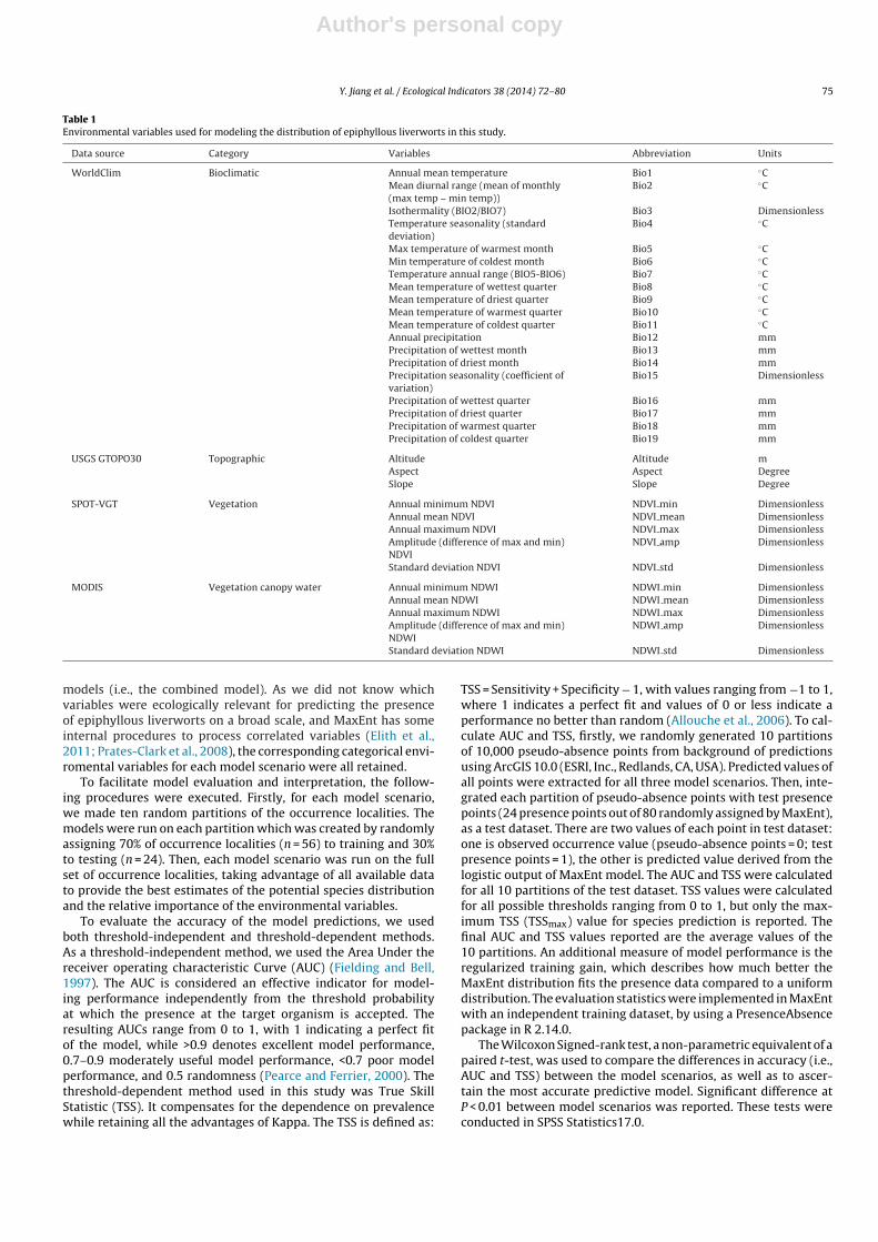
Table 1Environmental variables used for modeling the distribution of epiphyllous liverworts in this study.

Data source Category Variables Abbreviation Units

WorldClim Bioclimatic Annual mean temperature Bio1 ◦CMean diurnal range (mean of monthly(max temp – min temp))

Bio2 ◦C

Isothermality (BIO2/BIO7) Bio3 DimensionlessTemperature seasonality (standarddeviation)

Bio4 ◦C

Max temperature of warmest month Bio5 ◦CMin temperature of coldest month Bio6 ◦CTemperature annual range (BIO5-BIO6) Bio7 ◦CMean temperature of wettest quarter Bio8 ◦CMean temperature of driest quarter Bio9 ◦CMean temperature of warmest quarter Bio10 ◦CMean temperature of coldest quarter Bio11 ◦CAnnual precipitation Bio12 mmPrecipitation of wettest month Bio13 mmPrecipitation of driest month Bio14 mmPrecipitation seasonality (coefficient ofvariation)

Bio15 Dimensionless

Precipitation of wettest quarter Bio16 mmPrecipitation of driest quarter Bio17 mmPrecipitation of warmest quarter Bio18 mmPrecipitation of coldest quarter Bio19 mm

USGS GTOPO30 Topographic Altitude Altitude mAspect Aspect DegreeSlope Slope Degree

SPOT-VGT Vegetation Annual minimum NDVI NDVI min DimensionlessAnnual mean NDVI NDVI mean DimensionlessAnnual maximum NDVI NDVI max DimensionlessAmplitude (difference of max and min)NDVI

NDVI amp Dimensionless

Standard deviation NDVI NDVI std Dimensionless

MODIS Vegetation canopy water Annual minimum NDWI NDWI min DimensionlessAnnual mean NDWI NDWI mean DimensionlessAnnual maximum NDWI NDWI max DimensionlessAmplitude (difference of max and min)NDWI

NDWI amp Dimensionless

Standard deviation NDWI NDWI std Dimensionless

models (i.e., the combined model). As we did not know whichvariables were ecologically relevant for predicting the presenceof epiphyllous liverworts on a broad scale, and MaxEnt has someinternal procedures to process correlated variables (Elith et al.,2011; Prates-Clark et al., 2008), the corresponding categorical envi-romental variables for each model scenario were all retained.

To facilitate model evaluation and interpretation, the follow-ing procedures were executed. Firstly, for each model scenario,we made ten random partitions of the occurrence localities. Themodels were run on each partition which was created by randomlyassigning 70% of occurrence localities (n = 56) to training and 30%to testing (n = 24). Then, each model scenario was run on the fullset of occurrence localities, taking advantage of all available datato provide the best estimates of the potential species distributionand the relative importance of the environmental variables.

To evaluate the accuracy of the model predictions, we usedboth threshold-independent and threshold-dependent methods.As a threshold-independent method, we used the Area Under thereceiver operating characteristic Curve (AUC) (Fielding and Bell,1997). The AUC is considered an effective indicator for model-ing performance independently from the threshold probabilityat which the presence at the target organism is accepted. Theresulting AUCs range from 0 to 1, with 1 indicating a perfect fitof the model, while >0.9 denotes excellent model performance,0.7–0.9 moderately useful model performance, <0.7 poor modelperformance, and 0.5 randomness (Pearce and Ferrier, 2000). Thethreshold-dependent method used in this study was True SkillStatistic (TSS). It compensates for the dependence on prevalencewhile retaining all the advantages of Kappa. The TSS is defined as:

TSS = Sensitivity + Specificity − 1, with values ranging from −1 to 1,where 1 indicates a perfect fit and values of 0 or less indicate aperformance no better than random (Allouche et al., 2006). To cal-culate AUC and TSS, firstly, we randomly generated 10 partitionsof 10,000 pseudo-absence points from background of predictionsusing ArcGIS 10.0 (ESRI, Inc., Redlands, CA, USA). Predicted values ofall points were extracted for all three model scenarios. Then, inte-grated each partition of pseudo-absence points with test presencepoints (24 presence points out of 80 randomly assigned by MaxEnt),as a test dataset. There are two values of each point in test dataset:one is observed occurrence value (pseudo-absence points = 0; testpresence points = 1), the other is predicted value derived from thelogistic output of MaxEnt model. The AUC and TSS were calculatedfor all 10 partitions of the test dataset. TSS values were calculatedfor all possible thresholds ranging from 0 to 1, but only the max-imum TSS (TSSmax) value for species prediction is reported. Thefinal AUC and TSS values reported are the average values of the10 partitions. An additional measure of model performance is theregularized training gain, which describes how much better theMaxEnt distribution fits the presence data compared to a uniformdistribution. The evaluation statistics were implemented in MaxEntwith an independent training dataset, by using a PresenceAbsencepackage in R 2.14.0.

The Wilcoxon Signed-rank test, a non-parametric equivalent of apaired t-test, was used to compare the differences in accuracy (i.e.,AUC and TSS) between the model scenarios, as well as to ascer-tain the most accurate predictive model. Significant difference atP < 0.01 between model scenarios was reported. These tests wereconducted in SPSS Statistics17.0.



Table 2Performance of models predicting the distribution of epiphyllous liverworts usingthree different environmental data sets, showing threshold independent anddependent model evaluation results by the Area Under the receiver operating Curve(AUC) and the maximum True Skill Statistic (TSSmax).

Model AUC TSSmax

Mean SD Mean SD

Clim-topo 0.9607a 0.0006 0.8526a 0.0018Veg-topo 0.9796b 0.0006 0.9125b 0.0015Combined 0.9779c 0.0006 0.9304c 0.0014

For each model scenario, the AUC and TSSmax were given as the average values of tenpartitions. Superscript letters indicate significant differences among the means ofAUC and TSSmax. Means that share the same superscript letter are not significantlydifferent from one another; means with different superscript letters are significantdifferent at P < 0.01 (Wilcoxon paired test).

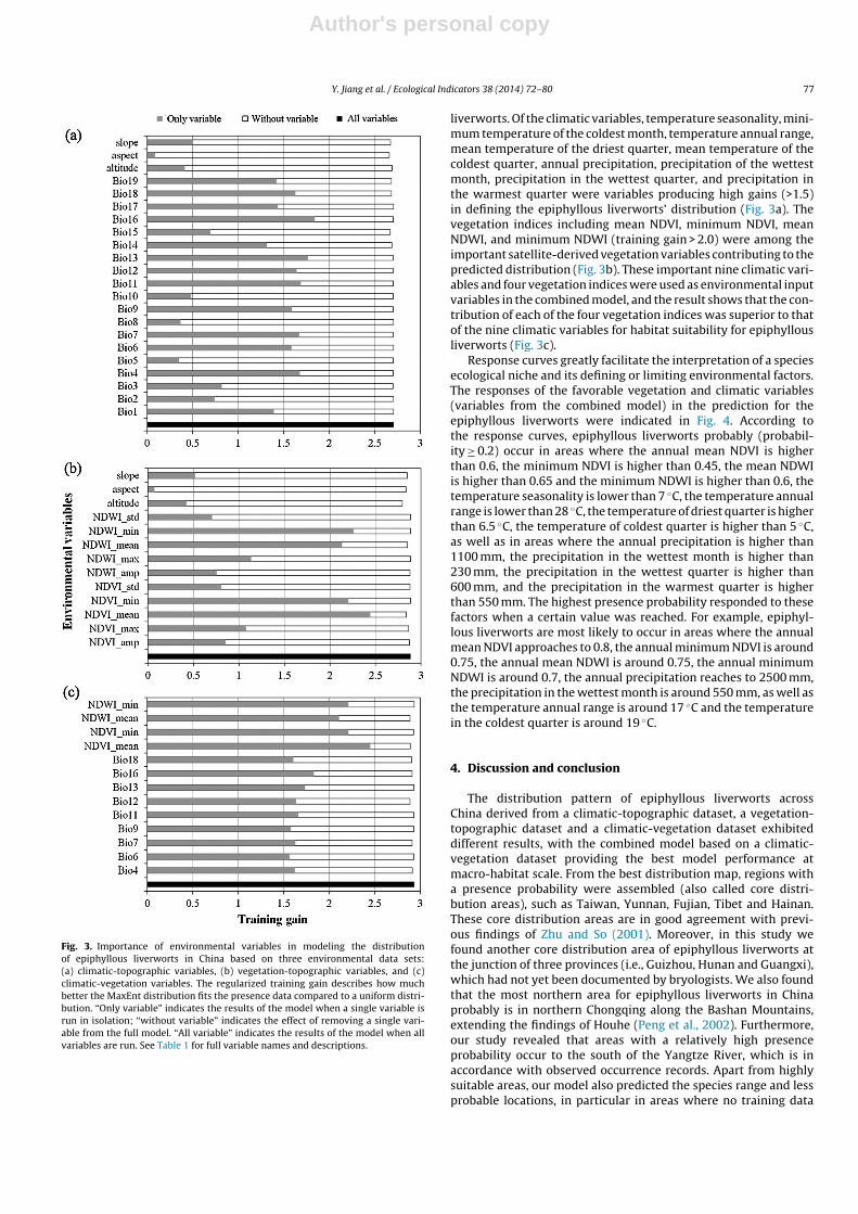
The jackknife test was applied to diagnose the relative impor-tance of environmental variables that may contribute to generatingthe species distribution models (Prates-Clark et al., 2008). The envi-ronmental variable with the highest training gain when used inisolation is considered to contain the most predictive ability ofany variables. Whilst, the environmental variable that decreasesthe gain the most when it is omitted, which therefore appears tohave the most information that is not present in the other vari-ables. The environmental variables used as input in the third model(i.e., the combined model) were determined based on the jackknifetest on the previous two models, retaining variables with traininggains of more than 1.5. The response curves were also plotted todemonstrate how variables affected the probability of epiphyllousliverworts being present. The response curves used all point local-ities and the respective environmental variable in isolation, and,thus, do not include interactions with other environmental vari-ables (Phillips et al., 2006). Both jackknife test and response curvesare available options in running MaxEnt.

3. Results

3.1. Distribution of epiphyllous liverworts in China

We derived three distribution maps of epiphyllous liverwortsover entire China (Fig. 2) based on the clim-topo, the veg-topo andthe combined model, respectively, depicting the logistic presenceprobability. The three models were all robust in capturing the varia-tion in environmental variables at presence localities of epiphyllousliverworts, with high values for AUC (all > 0.95), as well as TSSmax

(all > 0.85). As the environmental input datasets varied, the modelperformances differed significantly (P < 0.01, Wilcoxon paired test).The combined model performed best, with a relatively high TSSmax

(0.9304) compared to the TSSmax of the other two models (Table 2).The derived general potential distribution range of epiphyllous liv-erworts is similar for the three models, i.e., south to Hainan, northto Chongqing, west to Tibet and east to Zhejiang. However, it isnoticeable that the distribution map based on the clim-topo model(Fig. 2a) depicts a larger area than the other two models. The dis-tribution patches of epiphyllous liverworts are more fragmentedin the maps predicted by the veg-topo model (Fig. 2b) and thecombined model (Fig. 2c).

3.2. Environmental factors affecting the distribution ofepiphyllous liverworts at macro-habitat scale

The contribution of environmental variables to the epiphyllousliverwort distribution is shown in Fig. 3. Fig. 3a and b indicatesthat topographic variables (e.g. altitude, slope and aspect) resultin very little gain for the clim-topo and the veg-topo model, sug-gesting they barely contribute to the prediction of epiphyllous

Fig. 2. Maps showing the spatial distribution pattern (presence probability/habitatsuitability) of epiphyllous liverworts in China for three models: (a) using climatic andtopographic variables (the clim-topo model); (b) using vegetation and topographicvariables (the veg-topo model) and (c) using important variables of the previoustwo models (the combined model, which only retained climatic and vegetationvariables). All three models were executed based on full occurrence records.



Fig. 3. Importance of environmental variables in modeling the distributionof epiphyllous liverworts in China based on three environmental data sets:(a) climatic-topographic variables, (b) vegetation-topographic variables, and (c)climatic-vegetation variables. The regularized training gain describes how muchbetter the MaxEnt distribution fits the presence data compared to a uniform distri-bution. “Only variable” indicates the results of the model when a single variable isrun in isolation; “without variable” indicates the effect of removing a single vari-able from the full model. “All variable” indicates the results of the model when allvariables are run. See Table 1 for full variable names and descriptions.

liverworts. Of the climatic variables, temperature seasonality, mini-mum temperature of the coldest month, temperature annual range,mean temperature of the driest quarter, mean temperature of thecoldest quarter, annual precipitation, precipitation of the wettestmonth, precipitation in the wettest quarter, and precipitation inthe warmest quarter were variables producing high gains (>1.5)in defining the epiphyllous liverworts’ distribution (Fig. 3a). Thevegetation indices including mean NDVI, minimum NDVI, meanNDWI, and minimum NDWI (training gain > 2.0) were among theimportant satellite-derived vegetation variables contributing to thepredicted distribution (Fig. 3b). These important nine climatic vari-ables and four vegetation indices were used as environmental inputvariables in the combined model, and the result shows that the con-tribution of each of the four vegetation indices was superior to thatof the nine climatic variables for habitat suitability for epiphyllousliverworts (Fig. 3c).

Response curves greatly facilitate the interpretation of a speciesecological niche and its defining or limiting environmental factors.The responses of the favorable vegetation and climatic variables(variables from the combined model) in the prediction for theepiphyllous liverworts were indicated in Fig. 4. According tothe response curves, epiphyllous liverworts probably (probabil-ity ≥ 0.2) occur in areas where the annual mean NDVI is higherthan 0.6, the minimum NDVI is higher than 0.45, the mean NDWIis higher than 0.65 and the minimum NDWI is higher than 0.6, thetemperature seasonality is lower than 7 ◦C, the temperature annualrange is lower than 28 ◦C, the temperature of driest quarter is higherthan 6.5 ◦C, the temperature of coldest quarter is higher than 5 ◦C,as well as in areas where the annual precipitation is higher than1100 mm, the precipitation in the wettest month is higher than230 mm, the precipitation in the wettest quarter is higher than600 mm, and the precipitation in the warmest quarter is higherthan 550 mm. The highest presence probability responded to thesefactors when a certain value was reached. For example, epiphyl-lous liverworts are most likely to occur in areas where the annualmean NDVI approaches to 0.8, the annual minimum NDVI is around0.75, the annual mean NDWI is around 0.75, the annual minimumNDWI is around 0.7, the annual precipitation reaches to 2500 mm,the precipitation in the wettest month is around 550 mm, as well asthe temperature annual range is around 17 ◦C and the temperaturein the coldest quarter is around 19 ◦C.

4. Discussion and conclusion

The distribution pattern of epiphyllous liverworts acrossChina derived from a climatic-topographic dataset, a vegetation-topographic dataset and a climatic-vegetation dataset exhibiteddifferent results, with the combined model based on a climatic-vegetation dataset providing the best model performance atmacro-habitat scale. From the best distribution map, regions witha presence probability were assembled (also called core distri-bution areas), such as Taiwan, Yunnan, Fujian, Tibet and Hainan.These core distribution areas are in good agreement with previ-ous findings of Zhu and So (2001). Moreover, in this study wefound another core distribution area of epiphyllous liverworts atthe junction of three provinces (i.e., Guizhou, Hunan and Guangxi),which had not yet been documented by bryologists. We also foundthat the most northern area for epiphyllous liverworts in Chinaprobably is in northern Chongqing along the Bashan Mountains,extending the findings of Houhe (Peng et al., 2002). Furthermore,our study revealed that areas with a relatively high presenceprobability occur to the south of the Yangtze River, which is inaccordance with observed occurrence records. Apart from highlysuitable areas, our model also predicted the species range and lessprobable locations, in particular in areas where no training data



Fig. 4. Response curves illustrating the relationship between occurrence probability of epiphyllous liverworts and an environmental variable. These curves show how theresponse changes for a particular variable used in isolation. The response curves were derived from the combined model using climatic variables and vegetation indices,incorporated in MaxEnt.

were available. Probable areas predicted by this study have somefeatures in common, namely that they harbor continuous forest,especially evergreen forest, and a subtropical warm and humid cli-mate (Editorial Committee of Chinese Academy of Sciences, 2001),as indeed preferred by epiphyllous liverworts (Chen and Wu, 1964).

Climate is often thought to be the predominant range-determining mechanism at large spatial scales (Blach-Overgaardet al., 2010; Pearson and Dawson, 2003). In our study, climaticvariables were also found to contribute a lot when modelingthe distribution of epiphyllous liverworts, especially the temper-ature seasonality, the temperature of coldest quarter, and theprecipitation of wettest month and quarter. The low value of

temperature seasonality suggests that temperatures do not changesharply intra-annually, and that more stable temperatures as wellas temperatures higher than 10 ◦C are preferable to epiphyllous liv-erworts. The precipitation of the wettest month and quarter alsoneeds to be high for epiphyllous liverworts. These two precipi-tation variables reflect the precipitation in the wet season, anddirectly determine the annual precipitation. This implies that highannual precipitation is necessary for the occurrence of epiphyl-lous liverworts. The importance of these climatic factors may beexplained. Firstly, climate determines the geographical distributionof evergreen forest, which offers a probable habitat to epiphyllousliverworts. Evergreen forest occurs between 18–32◦ N and 98–123◦



E in China, in areas dominated by a tropical and subtropical cli-mate, with annual mean temperatures of between 14 and 26 ◦C, andannual precipitation ranging from 1000 to 5000 mm (Wu, 1980).Secondly, the precipitation is directly related to humidity, which isalways considered a major factor in the distribution of epiphyllousliverworts (Sonnleitner et al., 2009; Wu et al., 1987).

In the present study, we have achieved new insights in epi-phyllous liverwort distribution using vegetation indices. We foundthat satellite-derived vegetation indices, such as annual mean andminimum NDVI, and annual mean and minimum NDWI, providedmeaningful and significant contributions to defining the distri-bution range and spatial patterns of epiphyllous liverworts. This,however, is different from previous studies that showed microcli-mates to be the limiting factor at a local scale (Sonnleitner et al.,2009). Remote sensing data including NDVI and NDWI are mea-surements directly related to forest structure and overall health ofthe ecosystem that can collectively improve our understanding ofsuitable habitats for epiphyllous liverworts. The NDVI time seriesis very helpful for separating forests that are dominated by ever-green tree species from forests that are dominated by deciduoustree species. The NDWI time series provides additional and uniqueinformation on forest types and canopy water content, and leadsto the best performance when diagnosing forests humidity. TheNDVI and NDWI time series complement each other and providean improved and comprehensive description of forest types, forestconditions and phenology (Freitas et al., 2005; Xiao et al., 2002).The response curves of NDVI and NDWI further reveal that forestswith high biomass and water content throughout the year are pre-ferred, with the occurrence of epiphyllous liverworts increasingwith increasing vegetation cover and humidity. This infers and con-firms that evergreen broadleaved forest and rainforest play a keyrole in determining the occurrence of epiphyllous liverworts (Jianget al., 2013).

The significance, found in this study, of the contribution ofNDVI and NDWI in predicting epiphyllous liverwort distribution,as well as the strong correlation between the fraction of ever-green forest and the presence probability of epiphyllous liverwortsreported by Jiang et al. (2013), both imply that the presence ofepiphyllous liverworts can potentially be used to indicate natu-ral evergreen forest areas, and even to assess fragmentation ordegradation of that forest. Thus, using ecological indicators, eco-logical changes as, for example, habitat fragmentation, changesin ecological condition and escalating loss of biodiversity, can bemonitored, assessed and managed (Dale and Beyeler, 2001). Recentresearch has detected macrolichens and epiphytic bryophytes to beindicators of tropical lowland cloud forest distribution (Gradstein,2006; Normann et al., 2010). Our findings on present distribu-tion range and fragmentation patterns of epiphyllous liverwortssuggest large habitat fragmentation (e.g. evergreen forest frag-mentation). Regarding anthropogenic activity, during the period1949–1979 unsustainable timber harvesting in primary forest areasand afforestation of barren land were both undertaken in China(Wang et al., 2004). The demand for rubber and other tropical cashcrops has caused a great decrease in natural forest cover in Yunnanprovince over the past decades (Li et al., 2007; Zhang and Cao, 1995).Rainforests in Hainan have been degraded by logging, grazing andthe planting of eucalyptus and pines during the period from 1991 to2008 (Zhang et al., 2010). These anthropogenic disturbances as wellas poor forest management practices have fragmented the naturalforest distribution (Li et al., 2010).

In this study, the distribution of epiphyllous liverworts hasbeen accurately predicted on a broad scale for the first time. Thisresult is essential for efficient conservation planning – not onlyfor estimating the species distribution range of epiphyllous liv-erworts and its core distribution area, but also for determiningthe factors limiting their distribution. Ultimately this could be of

assistance in identifying forest degradation and even monitoringclimate change.

Acknowledgements

Financial support for this research at ITC was provided by theChina Scholarship Council. We would like to thank Prof. PengchengWu (Institute of Botany, Chinese Academy of Sciences) and Prof.Ruiliang Zhu (East China Normal University) for their valuable com-ments and suggestions in the earlier stage of the study.

Appendix A. Supplementary data

Supplementary data associated with this article can befound, in the online version, at http://dx.doi.org/10.1016/j.ecolind.2013.10.024. These data include Google maps of the most impor-tant areas described in this article.

References

Allouche, O., Tsoar, A., Kadmon, R., 2006. Assessing the accuracy of species distribu-tion models: prevalence, kappa and the true skill statistic (TSS). J. Appl. Ecol. 43,1223–1232.

Alvarenga, L.D.P., Porto, K.C., 2007. Patch size and isolation effects on epiphyticand epiphyllous bryophytes in the fragmented Brazilian Atlantic forest. Biol.Conserv. 134, 415–427.

Benavides, J.C., Sastre-De Jesus, I., 2011. Diversity and rarity of epiphyllousbryophytes in a superhumid tropical lowland forest of Choco-Colombia. Cryp-togamie Bryol. 32, 119–133.

Blach-Overgaard, A., Svenning, J.C., Dransfield, J., Greve, M., Balslev, H., 2010. Deter-minants of palm species distributions across Africa: the relative roles of climate,non-climatic environmental factors, and spatial constraints. Ecography 33,380–391.

Carlson, T.N., Ripley, D.A., 1997. On the relation between NDVI, fractional vegetationcover, and leaf area index. Remote Sens. Environ. 62, 241–252.

Chen, P.C., Wu, P.C., 1964. Study on epiphyllous liverworts of China (I). Acta Phyto-taxon. Sin. 9, 213–276.

Chen, X.Q., Pan, W.F., 2002. Relationships among phenological growing season, time-integrated normalized difference vegetation index and climate forcing in thetemperate region of eastern China. Int. J. Climatol. 22, 1781–1792.

Dale, V.H., Beyeler, S.C., 2001. Challenges in the development and use of ecologicalindicators. Ecol. Indicators 1, 3–10.

Editorial Committee of Chinese Academy of Sciences, 2001. Vegetation Map of China.Science Press, Bejing.

Elith, J., Graham, C.H., Anderson, R.P., Dudik, M., Ferrier, S., Guisan, A., Hijmans,R.J., Huettmann, F., Leathwick, J.R., Lehmann, A., Li, J., Lohmann, L.G., Loiselle,B.A., Manion, G., Moritz, C., Nakamura, M., Nakazawa, Y., Overton, J.M., Peterson,A.T., Phillips, S.J., Richardson, K., Scachetti-Pereira, R., Schapire, R.E., Soberon, J.,Williams, S., Wisz, M.S., Zimmermann, N.E., 2006. Novel methods improve pre-diction of species’ distributions from occurrence data. Ecography 29, 129–151.

Elith, J., Phillips, S.J., Hastie, T., Dudik, M., Chee, Y.E., Yates, C.J., 2011. A statisticalexplanation of MaxEnt for ecologists. Divers. Distrib. 17, 43–57.

Fielding, A.H., Bell, J.F., 1997. A review of methods for the assessment of predictionerrors in conservation presence/absence models. Environ. Conserv. 24, 38–49.

Frego, K.A., 2007. Bryophytes as potential indicators of forest integrity. Forest Ecol.Manage. 242, 65–75.

Freitas, S.R., Mello, M.C.S., Cruz, C.B.M., 2005. Relationships between forest structureand vegetation indices in Atlantic rainforest. Forest Ecol. Manage. 218, 353–362.

Gamon, J.A., Field, C.B., Goulden, M.L., Griffin, K.L., Hartley, A.E., Joel, G., Penue-las, J., Valentini, R., 1995. Relationships between NDVI, canopy structure, andphotosynthesis in 3 Californian vegetation types. Ecol. Appl. 5, 28–41.

Gao, B.-c., 1996. NDWI – a normalized difference water index for remote sensing ofvegetation liquid water from space. Remote Sens. Environ. 58, 257–266.

Gignac, L.D., 2001. Bryophytes as indicators of climate change. Bryologist 104,410–420.

Gillespie, T.W., Walter, H., 2001. Distribution of bird species richness at a regionalscale in tropical dry forest of Central America. J. Biogeogr. 28, 651–662.

Gradstein, S.R., 2006. The lowland cloud forest of French Guiana – a liverworthotspot. Cryptogamie Bryol. 27, 141–152.

Guisan, A., Theurillat, J.P., Kienast, F., 1998. Predicting the potential distribution ofplant species in an Alpine environment. J. Veg. Sci. 9, 65–74.

Guisan, A., Thuiller, W., 2005. Predicting species distribution: offering more thansimple habitat models. Ecol. Lett. 8, 993–1009.

Guisan, A., Zimmermann, N.E., 2000. Predictive habitat distribution models in ecol-ogy. Ecol. Model. 135, 147–186.

Hijmans, R.J., Cameron, S.E., Parra, J.L., Jones, P.G., Jarvis, A., 2005. Very high res-olution interpolated climate surfaces for global land areas. Int. J. Climatol. 25,1965–1978.



Imada, Y., Kawakita, A., Kato, M., 2011. Allopatric distribution and diversificationwithout niche shift in a bryophyte-feeding basal moth lineage (Lepidoptera:Micropterigidae). Proc. Roy. Soc. B: Biol. Sci. 278, 3026–3033.

Jönsson, P., Eklundh, L., 2004. TIMESAT – a program for analyzing time-series ofsatellite sensor data. Comput. Geosci. – UK 30, 833–845.

Jiang, Y.B., de Bie, C.A.J.M., Wang, T.J., Skidmore, A.K., Liu, X.H., Song, S.S., Shao, X.M.,2013. Hyper-temporal remote sensing helps in relating epiphyllous liverwortsand evergreen forests. J. Veg. Sci. 24, 214–226.

Judas, M., Dornieden, K., Strothmann, U., 2002. Distribution patterns of carabid beetlespecies at the landscape-level. J. Biogeogr. 29, 491–508.

Li, H.M., Aide, T.M., Ma, Y.X., Liu, W.J., Cao, M., 2007. Demand for rubber is causing theloss of high diversity rain forest in SW China. Biodivers. Conserv. 16, 1731–1745.

Li, M., Mao, L., Zhou, C., Vogelmann, J.E., Zhu, Z., 2010. Comparing forest fragmenta-tion and its drivers in China and the USA with Globcover v2.2. J. Environ. Manage.91, 2572–2580.

Loiselle, B.A., Jorgensen, P.M., Consiglio, T., Jimenez, I., Blake, J.G., Lohmann, L.G.,Montiel, O.M., 2008. Predicting species distributions from herbarium collec-tions: does climate bias in collection sampling influence model outcomes? J.Biogeogr. 35, 105–116.

Luo, J.S., 1990. A synopsis of Chinese epiphyllous liverworts. Trop. Bryol. 2, 161–166.Massart, J., 1898. Les végétaux épiphylles. Ann. Jard. Buitenzorg suppl. 2, 161–166.McKenzie, D., Halpern, C.B., 1999. Modeling the distributions of shrub species in

Pacific northwest forests. Forest Ecol. Manage. 114, 293–307.Monge-Nájera, J., 1989. The relationship of epiphyllous liverworts with leaf char-

acteristics and light in Monte-Verde, Costa-Rica. Cryptogamie Bryol. L. 10,345–352.

Normann, F., Weigelt, P., Gehrig-Downie, C., Gradstein, S.R., Sipman, H.J.M., Obregon,A., Bendix, J., 2010. Diversity and vertical distribution of epiphytic macrolichensin lowland rain forest and lowland cloud forest of French Guiana. Ecol. Indicators10, 1111–1118.

Olarinmoye, S.O., 1974. Ecology of epiphyllous liverworts – growth in 3 naturalhabitats in western Nigeria. J. Bryol. 8, 275–289.

Otte, V., Esslinger, T.L., Litterski, B., 2005. Global distribution of the European speciesof the lichen genus Melanelia Essl. J. Biogeogr. 32, 1221–1241.

Pócs, T., 1996. Epiphyllous liverworts diversity at worldwide level and its threat andconservation. Anales Inst. Biol. Univ. Nac. Autón. México. Ser. Bot. 67, 109–127.

Pearce, J., Ferrier, S., 2000. Evaluating the predictive performance of habitat modelsdeveloped using logistic regression. Ecol. Model. 133, 225–245.

Pearson, R.G., Dawson, T.P., 2003. Predicting the impacts of climate change on thedistribution of species: are bioclimate envelope models useful? Global Ecol.Biogeogr. 12, 361–371.

Pearson, R.G., Raxworthy, C.J., Nakamura, M., Peterson, A.T., 2007. Predicting speciesdistributions from small numbers of occurrence records: a test case using crypticgeckos in Madagascar. J. Biogeogr. 34, 102–117.

Peng, D., Liu, S.X., Wu, P.C., 2002. Studies on the epiphyllous liverworts of China VIII– the epiphyllous liverworts of Houhe national nature reserve. J. Wuhan. Bot.Res. 20, 199–201.

Pesch, R., Schroeder, W., 2006. Mosses as bioindicators for metal accumulation: sta-tistical aggregation of measurement data to exposure indices. Ecol. Indicators 6,137–152.

Pharo, E.J., Zartman, C.E., 2007. Bryophytes in a changing landscape: the hierarchicaleffects of habitat fragmentation on ecological and evolutionary processes. Biol.Conserv. 135, 315–325.

Phillips, S.J., Anderson, R.P., Schapire, R.E., 2006. Maximum entropy modeling ofspecies geographic distributions. Ecol. Model. 190, 231–259.

Prates-Clark, C.D., Saatchi, S.S., Agosti, D., 2008. Predicting geographical distributionmodels of high-value timber trees in the Amazon basin using remotely senseddata. Ecol. Model. 211, 309–323.

Riordan, E.C., Rundel, P.W., 2009. Modelling the distribution of a threatened habitat:the California sage scrub. J. Biogeogr. 36, 2176–2188.

Rodriguez-Soto, C., Monroy-Vilchis, O., Maiorano, L., Boitani, L., Faller, J.C., Briones,M.A., Nunez, R., Rosas-Rosas, O., Ceballos, G., Falcucci, A., 2011. Predicting poten-tial distribution of the jaguar (Panthera onca) in Mexico: identification of priorityareas for conservation. Divers. Distrib. 17, 350–361.

Rosenzweig, M.L., 1995. Species diversity in space and time. Cambridge UniversityPress, Cambridge and New York.

Sim-Sim, M., Bergamini, A., Luis, L., Fontinha, S., Martins, S., Lobo, C., Stech,M., 2011. Epiphytic bryophyte diversity on Madeira Island: effects of treespecies on bryophyte species richness and composition. Bryologist 114,142–154.

Sonnleitner, M., Dullinger, S., Wanek, W., Zechmeister, H., 2009. Microclimatic pat-terns correlate with the distribution of epiphyllous bryophytes in a tropicallowland rain forest in Costa Rica. J. Trop. Ecol. 25, 321–330.

Sundermeyer, M.A., Rothschild, B.J., Robinson, A.R., 2006. Assessment of environ-mental correlates with the distribution of fish stocks using a spatially explicitmodel. Ecol. Model. 197, 116–132.

Vancutsem, C., Pekel, J.-F., Evrard, C., Malaisse, F., Defourny, P., 2009. Mapping andcharacterizing the vegetation types of the Democratic Republic of Congo usingSPOT VEGETATION time series. Int. J. Appl. Earth Obser. Geoinf. 11, 62–76.

Vieira, C., Séneca, A., Sérgio, C., Ferreira, M.T., 2012. Bryophyte taxonomic and func-tional groups as indicators of fine scale ecological gradients in mountain streams.Ecol. Indicators 18, 98–107.

Wang, S., Cornelis van Kooten, G., Wilson, B., 2004. Mosaic of reform: forest policyin post-1978 China. Forest Policy Econ. 6, 71–83.

Wisz, M.S., Hijmans, R.J., Li, J., Peterson, A.T., Graham, C.H., Guisan, A., Distribut,N.P.S., 2008. Effects of sample size on the performance of species distributionmodels. Divers. Distrib. 14, 763–773.

Wollan, A.K., Bakkestuen, V., Kauserud, H., Gulden, G., Halvorsen, R., 2008. Modellingand predicting fungal distribution patterns using herbarium data. J. Biogeogr. 35,2298–2310.

Wu, P.C., Li, D.K., Gao, C.H., 1987. Preliminary measurement on some ecolog-ical factors of the epiphyllous liverworts in Mt. Wuyi. Acta Bot. Sin. 29,448–452.

Wu, Z.Y., 1980. Vegetation of China. Science Press, Beijing.Xiao, X., Boles, S., Liu, J., Zhuang, D., Liu, M., 2002. Characterization of forest types

in Northeastern China, using multi-temporal SPOT-4 VEGETATION sensor data.Remote Sens. Environ. 82, 335–348.

Zartman, C.E., 2003. Habitat fragmentation impacts on epiphyllous bryophyte com-munities in central Amazonia. Ecology 84, 948–954.

Zhang, J., Cao, M., 1995. Tropical forest vegetation of Xishuangbanna, SW China andits secondary changes, with special reference to some problems in local natureconservation. Biol. Conserv. 73, 229–238.

Zhang, M., Fellowes, J.R., Jiang, X., Wang, W., Chan, B.P.L., Ren, G., Zhu, J., 2010. Degra-dation of tropical forest in Hainan, China, 1991–2008: conservation implicationsfor Hainan Gibbon (Nomascus hainanus). Biol. Conserv. 143, 1397–1404.

Zhu, R.L., So, M.L., 2001. Epiphyllous liverworts of China. Nova Hedwig. 121, 1–418.

Satellite-derived vegetation indices contribute significantly to the prediction of epiphyllous...

Documents

Transcript of Satellite-derived vegetation indices contribute significantly to the prediction of epiphyllous...