Which investment (private or public) does contribute to ...
24
Munich Personal RePEc Archive Which investment (private or public) does contribute to economic growth more? a case study of South Africa Abbas, Aadil and Masih, Mansur INCEIF, Malaysia, Business School, Universiti Kuala Lumpur, Kuala Lumpur, Malaysia 28 February 2017 Online at https://mpra.ub.uni-muenchen.de/108919/ MPRA Paper No. 108919, posted 29 Jul 2021 09:56 UTC
-
Upload
khangminh22 -
Category
Documents
-
view
1 -
download
0
Transcript of Which investment (private or public) does contribute to ...
Munich Personal RePEc Archive
Which investment (private or public)does contribute to economic growthmore? a case study of South Africa
Abbas, Aadil and Masih, Mansur
INCEIF, Malaysia, Business School, Universiti Kuala Lumpur,
Kuala Lumpur, Malaysia
28 February 2017
Online at https://mpra.ub.uni-muenchen.de/108919/
MPRA Paper No. 108919, posted 29 Jul 2021 09:56 UTC
1 | P a g e
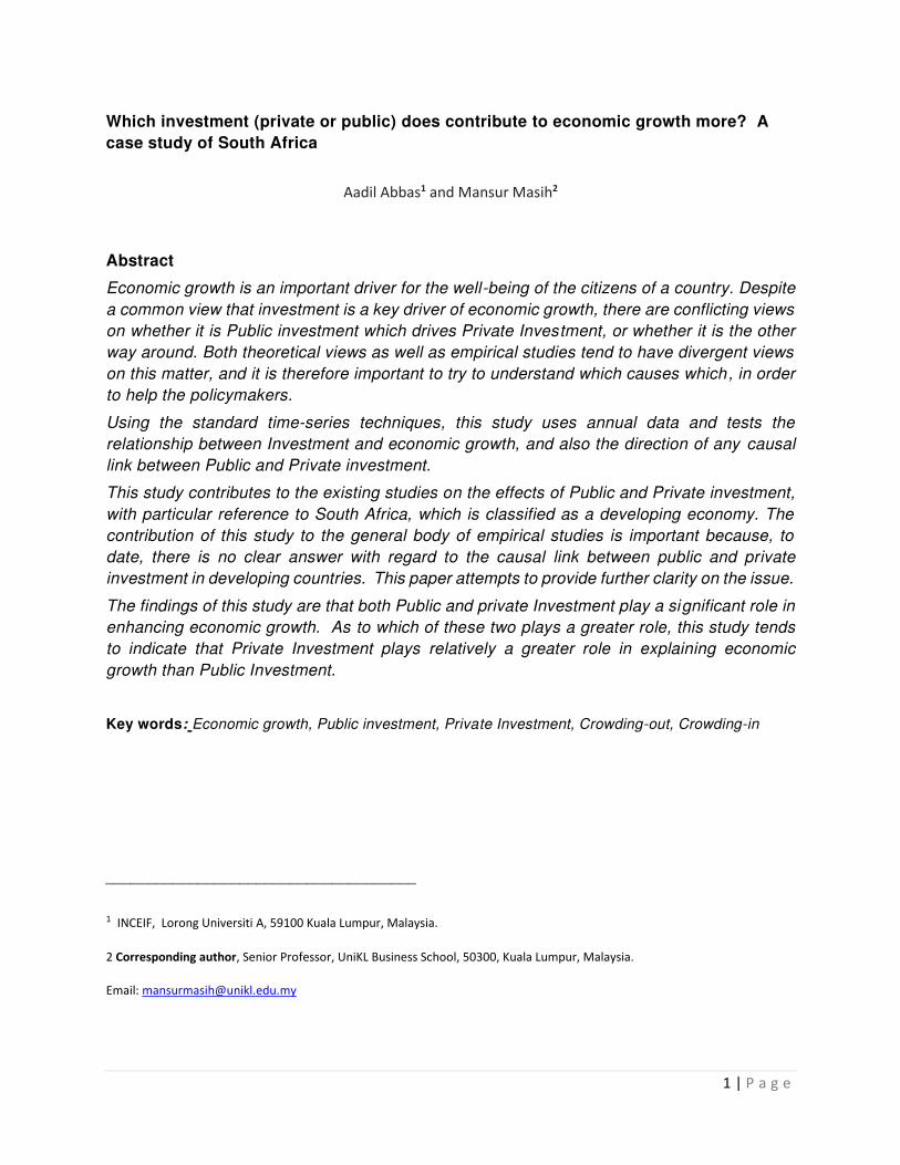
Which investment (private or public) does contribute to economic growth more? A
case study of South Africa
Aadil Abbas1 and Mansur Masih2
Abstract
Economic growth is an important driver for the well-being of the citizens of a country. Despite
a common view that investment is a key driver of economic growth, there are conflicting views
on whether it is Public investment which drives Private Investment, or whether it is the other
way around. Both theoretical views as well as empirical studies tend to have divergent views
on this matter, and it is therefore important to try to understand which causes which, in order
to help the policymakers.
Using the standard time-series techniques, this study uses annual data and tests the
relationship between Investment and economic growth, and also the direction of any causal
link between Public and Private investment.
This study contributes to the existing studies on the effects of Public and Private investment,
with particular reference to South Africa, which is classified as a developing economy. The
contribution of this study to the general body of empirical studies is important because, to
date, there is no clear answer with regard to the causal link between public and private
investment in developing countries. This paper attempts to provide further clarity on the issue.
The findings of this study are that both Public and private Investment play a significant role in
enhancing economic growth. As to which of these two plays a greater role, this study tends
to indicate that Private Investment plays relatively a greater role in explaining economic
growth than Public Investment.
Key words: Economic growth, Public investment, Private Investment, Crowding-out, Crowding-in
_____________________________________
1 INCEIF, Lorong Universiti A, 59100 Kuala Lumpur, Malaysia.
2 Corresponding author, Senior Professor, UniKL Business School, 50300, Kuala Lumpur, Malaysia.
Email: [email protected]

2 | P a g e
1. INTRODUCTION: ISSUE AND MOTIVATION
In order to have a sustained economic growth, Investment is important. It has been shown in
studies that the countries which have a high rate of Investment show a higher rate of growth
(Akomolafe, 2015). Therefore, it is important for Investment to take place to grow an
economy, and thereby to present the people with opportunities to better their lot in life.
Investment can take place in two forms: it is either done by the Private Sector (Private
Investment), or by the Public Sector (Public Investment).
a. Theoretical controversy:
There are two different views in explaining the relationship between government and private
sector investment:
a. The traditional view asserts that as government increases its expenditure, it will
lead to a lower level of private investment because there appears a competition
between public and private sectors in utilizing the limited resources in the factor
and financial markets.
b. the non-traditional view argues that if the government spending can increase the
marginal productivity of private investment - spending on human capital
development, airport, water system and transportation and communication system
- then, a significant positive relationship should be existing between these
variables.” (Choonga, 2015)
These divergent views are explained by Khan (Khan, 1997) as follows: “In general, some components of public investment may be complementary to private investment and so would
be beneficial for growth, while others may be substitutes and have a less positive, or even
negative, effect on growth. The complementarity may arise in the case of public investment in
infrastructure which increases the marginal product of private capital. This is most likely to be
true in those developing countries where the existing stock of infrastructure capital is
inadequate.” We see therefore, that Public investment plays many competing and offsetting roles in its
effect on the investment activities of the private sector, so the net effect of public investment
on private investment is an empirical question. (Hacettepe, 2006)
b. Empirical Controversy:
There has been a growing body of literature that investigates whether public investment
leads to an increase in output growth and/or the productivity of private capital. The
hypothesis has been tested either directly, using a neoclassical production function where
public capital enters as a separate input, or indirectly by looking at the productivity of private
capital and labor, and the rate of return to private capital derived from the production
function.
Overall, the empirical evidence from the US and from developing countries suggests that
private capital is more productive than public investment, and that although public investment
contributes to the productivity of private capital, it does not explain the major part of the
3 | P a g e
variation in output growth.
According to Mustefa Seraj (Seraj, 2014), there is no clear consensus on empirical evidence
from both developed and developing countries with regard to whether public or private
investment has a superior effect on economic growth. Most researchers claim that the
contribution of private investment to economic growth is larger than that of public investment,
based on the contention that the marginal productivity of the former is greater than that of the
latter (Khan and Reinhart, 1990; Serven and Solimano, 1992), although some studies have
shown a possibly larger contribution of public capital to economic growth (Ram, 1996).
c. Major questions or issues
Since it is uncertain from both the theoretical as well as the empirical literature whether
Public Investment plays a positive or a negative role in increasing economic growth, the
objective of this study is to determine whether Public investment or Private investment play a
greater role in enhancing economic growth. Such an analysis is of importance from both
theoretical as well as policy perspectives, because it will tell policymakers where to focus
their attention in stimulating growth in the economy. For example, Khan points out that
“Insofar as policy is concerned, if private investment does have a markedly stronger impact
on growth, it would further underscore the need to rationalize public investment.” (Khan,
1997).
d. Major contribution of this study:
Despite the fact that this study is similar to other studies on the issues raised, it is submitted
that this study will add to the existing literature on the issue by attempting to find further
clarity on the issue. In addition to this, because this study is conducted on South Africa,
which is a developing country, this study is of further importance because the empirical
studies to date find that developing countries tend to show conflicting effects of public
investment on private investment than developed countries.
e. Summary of findings:
In summary, the findings of this study are that both Public and private Investment play a
significant role in enhancing economic growth. As far as which of the two play a greater role,
this study tends to indicate that Private Investment plays relatively a greater role in economic
growth than Public Investment.
f. Structure of the paper:
This paper is structured as follows: section 1 deals with the introduction and motivation,
Section 2 provides a literature review, Section 3 deals with the methodology and data,
Section 4 will discuss the empirical findings, Section 5 and 6 will provide conclusions and
policy recommendations.
4 | P a g e
2. LITERATURE REVIEW
(i) Economic growth theory models:
According to Phetsavong: “Economic Growth Theory Growth models are fundamentally of two folds; the neoclassical growth model, also known as the exogenous growth model
developed primarily by Solow (1956) and the new growth theory, also known as the
endogenous growth model, pioneered by Romer (1986), Lucas (1988), Barro (1990), and
Rebelo (1991).
In neoclassical growth models government policy cannot have sustained effects on growth
rate of per capita income, although government can even influence the population growth
which is assumed to affect the growth rate. In these models, if incentives to save or to invest
in new capital are affected by fiscal policy, there will be a change in equilibrium capital output
ratio and therefore the output path will change, leaving the steady state growth rate
unchanged. The long-run growth rate is driven by exogenous factors of population growth
and technological progress while public policy can only influence the transition path of the
economy towards steady state growth rate.
According to the economists supporting ‘endogenous growth models’ (Barro 1990, King and Rebelo 1990, Lucas 1990, Mendoza et al. 1997, Stokey and Rebelo 1995, and Easterly and
Rebelo 1993), the share of public expenditure in output or the composition of expenditures
and taxation affects the steady state growth rate. This is in contrast to the neoclassical
growth theory where only investment in physical and human capital affects the steady state
growth rate.
Regarding to the endogenous growth model, the long-run growth rate depends on the stable
environment of business, specifically, government policies and actions on taxation, law and
order, provision of infrastructure services, protection of intellectual of property rights,
regulation of an international trade, financial markets, and other aspect of the economy.
Therefore, long-run growth rate has also guided by the government (Barro 1997).
In the endogenous growth model, investment is also treated as a significant factor. As noted,
neoclassic growth theory assumes that the investment has a limited role in boosting
economic growth. (Phetsavon, 2012)
(ii) Investment as a driver of economic growth:
According to Seraj Mustafa (Seraj, 2014), Coen and Eisher (1992), define investment as
follows:
“Investment is capital formation-the acquisition or creation of resources to be used in
production. In capitalist Economies much attention is focused on business investment in
physical capital building, equipment and inventories. But investment is also undertaken by
government, non-profit institutions and households, and it includes the acquisition of human
and intangible capital as well as physical capital (Coen and Eisher, 1992; 508).”
5 | P a g e
Investment is one of the most important bases for economic growth theoretically and
empirically (Levine and Renelt, 1992). Scott (1976) defines investment for proper growth
process understanding as ‘all expenditures which would not be made in a stationary state’. He further explained that such expenditures consist of new production capital such as new
machinery and vehicles, building and construction, research and development, expenditure
on marketing, planning et cetera.
We see therefore, that, Investment is an important component of aggregate demand and a
leading source of economic growth. Changes in investment not only affect aggregate
demand but also enhance the productive capacity of an economy. The investment plays an
essential and vital role in expanding the productive capacity of the economy and promoting
long term economic growth (Jongwanich and Kohpaiboon, 2008). Higher investment rate
triggers the fast economic growth. Levine and Renelt (1992) have argued that investment in
capital goods is the most robust and vital determinant of economic growth (Seraj, 2014).
(iii) The relationship between Public Investment, Private Investment and
Economic Growth:
There exists a divergence of opinion on the role that Public Investment plays in the growth
strategy of an economy. The debate really centres around what would be the optimal fiscal
policy to be adopted by a government if it wanted to stimulate economic growth. The issue in
question is whether Public Investment operates as a mechanism for achieving growth
(crowding-in) or whether it operates as a mechanism that inhibits economic growth
(crowding-out).
While most studies appear to find a relationship between Public Sector Investments and
Private Sector Investment, it is unclear whether the relationship is positive or negative.
Some argue that Public Investment inhibits (crowds-out) Private Sector Investment (Voss,
2002) (Biza, 2013), while other argue that Public Sector Investment actually stimulates
(crowds-in) Private Investment, arguing for the “Keynesian view that implies that an expansionary fiscal policy promotes Private Investment by raising the level of economic
activity” (Tugcu, 2015, p. 1). Still other studies suggest that the relationship is different in the short-run and the long-run (Belloc, 2002).
Previous literature suggests that public investment crowding out private investment more
often in developed economies. Voss (2002) studied on both data from US and Canada
concludes that there is no evidence to prove that public investment complements private
investment. In fact, innovations to public investment tend to crowd out private investment.
Meanwhile in developing economies public investment is seen tend to complement the
private investment. By examining a panel of developing economies from 1980 to 1997, Elden
and Holcombe (2005) find a 10 percent increase in public investment would increase private
investment by about 2 percent. On the other hand, Cavallo and Daude (2011) investigate that
in average for 116 developing countries the public investment crowd out private investment.
Ang (2009) analyzing the determinants of private investment in Malaysia suggest that public
investment have a complementary effect on private investment.
Neo-classical framework highlights the “crowding out” effect of private investment by public investment when the state decides to increase its investment contribution in the economy
6 | P a g e
through the issuance of debt or by raising the tax (Kustepeli, 2005). The empirical studies in
various country contexts have shown that public investment spending crowds out the amount
of private investment (Bairam and Ward, 1993; Voss, 2002; Bende-Nabende and Slater,
2003; Mitra 2006, Blejer and Khan (1984) and Gupta (1984)). It is because the government
spending that is financed either by taxes or debt (or both), competes with the private sector
in the use of scarce physical and financial resources (Belloc and Vertova, 2006). The
shortage of capital will inhibit private investment. This is worse when compounded by the
increase of cost of investment, thus make the investment disincentive. The decrease of cost
of capital influences positively the private investment (Ghura and Goodwin, 2000). However,
the negative impact can be mitigated in higher capital mobility. The inflow of international
capital will cause the interest rate to fall (Dehn, 2000). Ahmed and Miller (1999) suggest that
tax-financed government expenditure tends to crowd out private investment more often than
its debt-financed counterpart.
Credit constraint is seen as more binding than interest rate if its availability is limited in
developing countries, hence influences the level of private investment activities (Wai and
Wong (1982), Blejer and Khan (1984), Ramirez (1994), Ghura and Goodwin (2000), Erden
and Holcombe (2005), Ang (2009), Cavallo and Daude (2011). Credit availability was also
empirically shown to be a significant determinant of private investment (Vogel and Buser
(1976), Fry (1980), Wai and Wong (1982), Blejer and Khan (1984), Gupta (1984), Garcia
(1987), Leff and Sato (1988)), and Oshikoya (1994). Thus, the cost of funding investment
projects as well as the availability of credit can be expected to play important roles on private
investment in developing countries.
The relationship between public spending and private investment nowadays become more
complex (Kollamparambil and Nicolaou, 2010), different impacts might occur by the different
components of state spending. Numerous studies done on the impact of infrastructure
provision by public capital on private investment decision making have shown the ‘crowd in’ effect in the private sector (Easterly and Rebelo (1993), Ramirez (1994), Argimón et al.
(1997), Galbis (1979), Greene and Villanueva (1991), because it will reduce private costs of
production, thus raising profitability, which will stimulate private investment (Ndikumana,
(2005), Gjini and Kukeli (2012)). While the non-infrastructure gives the reverse impact
(Oshikoya (1994).
Moreover, the possibility of different effect of public investment also can be observed in
specific time span. Aschauer (1989b), Mitra (2006) and Serven (1996) investigate the effect
of public investment over the long run and the short run time period. They find that the public
investment crowding in the private investment in the short run. Meanwhile, in the long run the
public investment enhanced the private investment profitability.
Policy is regarded as a particularly important determinant of investment in African countries,
which are generally seen as more capital hostile than other regions (Collier, Hoeffler and
Pattillo (1999)). South Africa is an emerging market and it is recognized as the second
largest economy in Africa region, behind Nigeria. Numerous studies were done to examine
the causality relationship between public investment and private investment for this country.
P. Perkins and J. M. Luiz (2006) have studied the causality between investments in economic
infrastructure and the long run economic growth in South Africa suggest that electricity

7 | P a g e
generation consistently is shown to impact positively and directly on output. In fact, the public
investment which stimulate the aggregate demand of goods and services produced by the
private sector will positively effects the private investment in the country (Fielding, 1997).
3. DATA AND METHODOLOGY
This study proposes to test the causal relationship between Private Investment and Public
Investment. This will be done by doing a time-series based VAR study using South Africa as
the country of study. The study will focus on the period covering 35 years starting from 1980.
The variables to be used will be real GDP (GDPR), Public Investment (IG) and Private
Investment (IP).
a. Data:
Annual data for each of the variables. The Data for the study have been obtained from World
Bank Data (available on DataStream) and from the website of the South African Reserve Bank.
b. Methodology
In this study time series techniques are employed to achieve the stated research objectives,
which include the determination of whether there exists a long-run theoretical relationship
between the Economic growth and Investment, and between Public Investment and Private
Investment, as well as which has a greater impact on economic growth: private or public
investment. The study is conducted on a developing country, namely South Africa.
The standard time-series methodology is favored over traditional regression analysis for a
number of reasons, which will be discussed below.
In the first place, most economic time series variables tend to be non-stationary in their original
‘level’ form, thereby implying that any conventional statistical tests carried out on such variables
would be invalidated. However, if the variables are non-stationary but cointegrated, then the
ordinary regression without the error-correction term(s) derived from the cointegrating
equation would be mis-specified. If the variables are non-stationary and not cointegrated,
then an ordinary regression with ‘differenced’ variables (which will be
stationary) could be estimated. The difficulty with this, however, is that the conclusions drawn
from such an analysis will be valid only for the short run, and no conclusions can be made
about the long-run theoretical relationship among the variables. This is because the
‘differenced’ time-series variables have no information about the long-run relationship
between the trend components of the original series as these have, by definition, been
removed. The long run co-movement between the variables cannot be captured by
‘differenced’ variables (Masih et al, 2009).
8 | P a g e
We see therefore, that on the one hand, if the variables taken are ‘non-stationary’ in their original ‘level’ forms, the conventional statistical tests are not valid, since the variances of these
variables are changing and the relationship thus estimated will be ‘spurious’. On the other hand, if the variables taken are turned ‘stationary’ by ‘first-differencing’, the long-term
information contained in the trend element in each variable would have been, by definition,
removed and the relationship estimated would only give only the short-run relationship
between the variables. Thus, the regression analysis would only capture short-term, cyclical
or seasonal effects, and would not be testing any long-term theoretical relationships (Masih
et al, 2009).
In the second place, in traditional regression analysis, the endogenous and exogenous
nature of variables is pre-determined by the researcher, usually on the basis of prevailing
theories. Cointegration techniques have the advantage of not making any assumptions
regarding the endogeneity and exogeneity of variables. Instead, in the final
analysis, it is the data itself that will be allowed to determine which variables are in fact
exogenous, and which are exogenous. Put differently, in traditional regression analysis,
causality is assumed, whereas in Cointegration techniques, it is empirically proven by data.
This is achieved through the ‘Long-run Structural Modelling’ or ‘LRSM’ technique which
endeavors to estimate theoretically meaningful long-run (or cointegrating) relations by
imposing restrictions on those long-run relations (and then testing) both identifying and over-
identifying restrictions, based on theories and a priori information of the economies (Masih et
al, 2009).
In this study, therefore, the following methodology, as outlined by Masih et al
(2009) is employed:
(i) Conducting unit-root tests to test the stationarity of the variables,
(ii) determining the optimum order (or lags) of the vector autoregressive model or VAR.
(iii) Utilizing the lag order obtained in the previous step, to conduct Johansen
Cointegration tests. The test of Cointegration is designed to examine the long-run
theoretical or equilibrium relationship and to rule out any spurious relationship among
the variables.
(iv) The cointegrating estimated vectors will then be subjected to exactly identifying
and over-identifying restrictions based on theoretical and a priori information of the
economy. This ‘LRSM’ technique as outlined above would confirm whether a variable is
statistically significant, and also test the long-run coefficients of the variables against
theoretically expected values.
(v) Since the evidence of Cointegration does not necessarily mean causality, establishment
of causality is achieved through the Vector Error Correction Model (VECM), which is
able to indicate the direction of Granger causality both in the short- and long-run.
(vi) While the VECM enables a researcher say which variable is leading and which is
lagging, it does not tell which variable is relatively more exogenous or endogenous. To
know this, the Variance Decomposition technique is used to indicate the relative
9 | P a g e
exogeneity or endogeneity of a variable, and achieves this by decomposing (or
partitioning) the variance of the forecast error of a variable into proportions attributable
to shocks (or innovations) in each variable in the system, including its own. The
proportion of the variance explained by its own past shocks can help to determine the
relative exogeneity or endogeneity of a variable. The variable that is explained mostly
by its own shocks (and not by others) is deemed to be the most exogenous of all and
vice versa. After determining relative exogeneity/endogeneity, the Impulse Response
Function (IRF) is be applied to map out the dynamic response path of a variable due to
a one-period variable-specific shock to another variable. In essence, IRF is a graphical
way of expressing the relative exogeneity or endogeneity of a variable.
(vii) Lastly, the Persistence Profiles (PP) technique is applied. The results from the
application of this technique are also in graphical form, and are designed to estimate
the speed at which the variables would return to equilibrium in the event of a system-
wide shock, as opposed to the Impulse Response Function (IRF) which maps out the
effects of only a variable-specific shock on the long-run relationship (Masih et al, 2009).
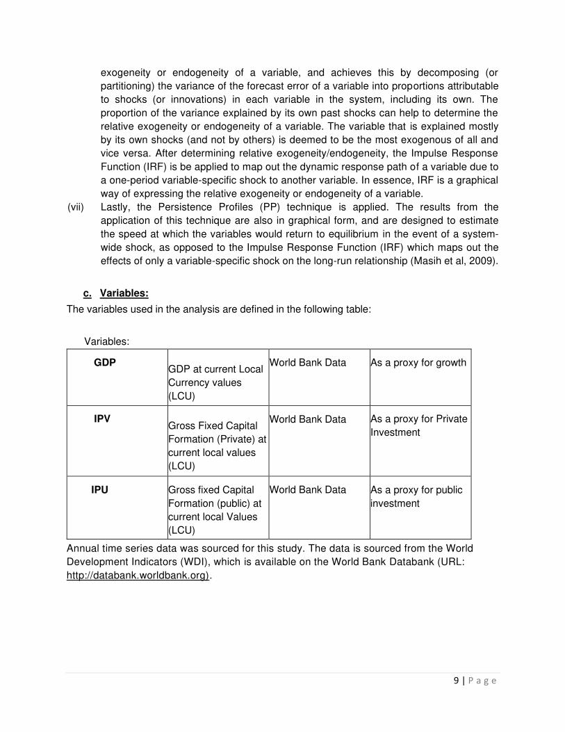
c. Variables:
The variables used in the analysis are defined in the following table:
Variables:
GDP
GDP at current Local
Currency values
(LCU)
World Bank Data As a proxy for growth
IPV
Gross Fixed Capital
Formation (Private) at
current local values
(LCU)
World Bank Data As a proxy for Private
Investment
IPU Gross fixed Capital
Formation (public) at
current local Values
(LCU)
World Bank Data As a proxy for public
investment
Annual time series data was sourced for this study. The data is sourced from the World
Development Indicators (WDI), which is available on the World Bank Databank (URL:
http://databank.worldbank.org).
10 | P a g e
4. EMPIRICAL RESULTS AND DISCUSSIONS
(i) Unit root tests
The empirical analysis is started by determining the stationarity of the variables utilized in the
study. To recap, a variable is stationary when its mean, variance and covariance are all
constant over time. In time series studies, it is critical to determine the stationarity of the
variables before proceeding to tests for Cointegration. Ideally, all variables should be I (1),
meaning that in their original ‘level’ form, they should be non-stationary, and in their ‘first differenced’ form, they should be stationary. The ‘differenced’ form of each variable is created by taking the difference of their logarithmic forms. For example, DGDP= LGDP - LGDPt-1.
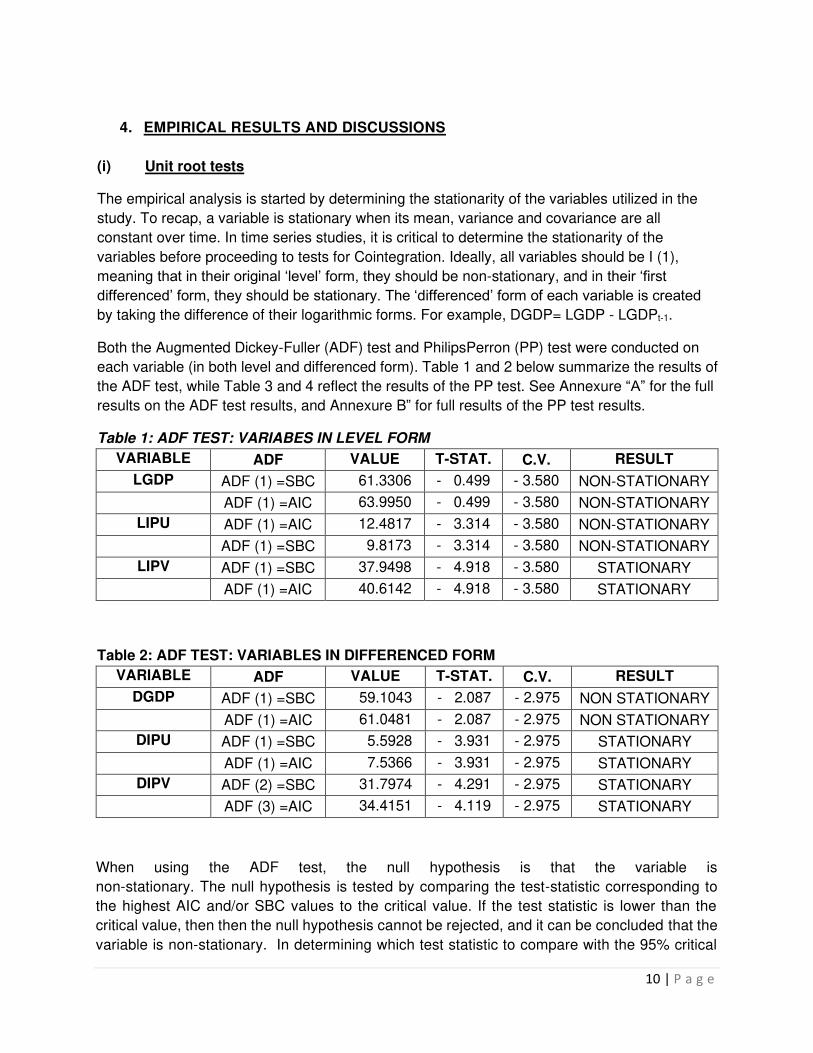
Both the Augmented Dickey-Fuller (ADF) test and PhilipsPerron (PP) test were conducted on
each variable (in both level and differenced form). Table 1 and 2 below summarize the results of
the ADF test, while Table 3 and 4 reflect the results of the PP test. See Annexure “A” for the full
results on the ADF test results, and Annexure B” for full results of the PP test results.
Table 1: ADF TEST: VARIABES IN LEVEL FORM
VARIABLE ADF VALUE T-STAT. C.V. RESULT
LGDP ADF (1) =SBC 61.3306 - 0.499 - 3.580 NON-STATIONARY
ADF (1) =AIC 63.9950 - 0.499 - 3.580 NON-STATIONARY
LIPU ADF (1) =AIC 12.4817 - 3.314 - 3.580 NON-STATIONARY
ADF (1) =SBC 9.8173 - 3.314 - 3.580 NON-STATIONARY
LIPV ADF (1) =SBC 37.9498 - 4.918 - 3.580 STATIONARY
ADF (1) =AIC 40.6142 - 4.918 - 3.580 STATIONARY
Table 2: ADF TEST: VARIABLES IN DIFFERENCED FORM
VARIABLE ADF VALUE T-STAT. C.V. RESULT
DGDP ADF (1) =SBC 59.1043 - 2.087 - 2.975 NON STATIONARY
ADF (1) =AIC 61.0481 - 2.087 - 2.975 NON STATIONARY
DIPU ADF (1) =SBC 5.5928 - 3.931 - 2.975 STATIONARY
ADF (1) =AIC 7.5366 - 3.931 - 2.975 STATIONARY
DIPV ADF (2) =SBC 31.7974 - 4.291 - 2.975 STATIONARY
ADF (3) =AIC 34.4151 - 4.119 - 2.975 STATIONARY
When using the ADF test, the null hypothesis is that the variable is
non-stationary. The null hypothesis is tested by comparing the test-statistic corresponding to
the highest AIC and/or SBC values to the critical value. If the test statistic is lower than the
critical value, then then the null hypothesis cannot be rejected, and it can be concluded that the
variable is non-stationary. In determining which test statistic to compare with the 95% critical

11 | P a g e
value for the ADF statistic, the ADF regression order based on the highest computed value for
AIC and SBC is used.
By applying this principle, as can be seen in table 1 above, the test-statistic for variables LGDP
and LIPU was lower than the critical value, and these variables were therefore being found to
be non-stationary, while the test statistic for variable LIPU was found to be higher than the
crucial value, making this variable stationary in the level form.
In the differenced form, the test statistic for variables DIPV and DIPU were found to be higher
than the critical value, meaning that these variables were stationary in the differenced form,
while the test-statistic for variable DGDP was found to be lower than the critical value making
the variable non-stationary in the differenced form.
Since the results based on the ADF test would not allow for proceeding with Cointegration
testing, the Philips Perron (PP) test results were also analysed to test for stationarity. It is noted
that the difference between the two tests is that while the ADF test is only able to resolve the
autocorrelation problem, the PP test takes care of both the autocorrelation and
heteroskedasticity issues.
The null hypothesis for the PP test once again is that the
variable is non-stationary, and the null hypothesis is tested based on the p-value of the test
statistic, which informs us of the percentage error we are making in rejecting the null.
As can be seen from table 3 and 4 below, in all cases of the variables in level form, the null
hypothesis cannot be rejected suggesting that all the variables are non-stationary. Also, in all
cases of the variable in differenced form, the null hypothesis was rejected and it could be
concluded that all the variables are stationary.
TABLE 3: PP TEST- VARIABLES IN LEVEL FORM
PP VARIABLE T-STAT. C.V. RESULT
LGDP - 1.071 - 3.649 non-stationary
LIPU - 2.006 - 3.649 non-stationary
LIPV - 1.889 - 3.649 non-stationary
TABLE 4: PP TEST- VARIABLES IN DIFFERENCED FORM
PP VARIABLE T-STAT. C.V. RESULT
DGDP - 3.126 - 2.927 stationary
DIPU - 8.916 - 2.927 stationary
DIPV - 3.584 - 2.927 stationary
Since the PP tests confirm that all the variables are non-stationary in the level form, and all the
variables are stationary in the differenced form, it is possible to proceed to the next step of the
12 | P a g e
study, namely testing of Cointegration.
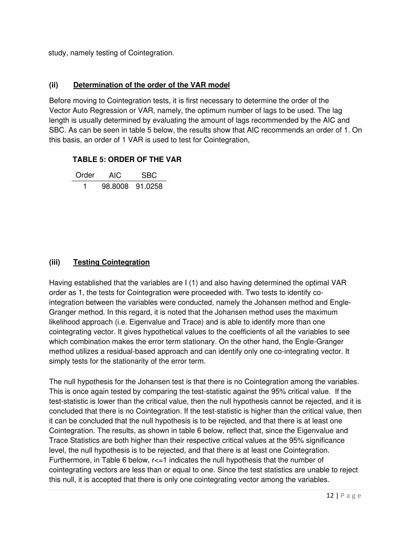
(ii) Determination of the order of the VAR model
Before moving to Cointegration tests, it is first necessary to determine the order of the
Vector Auto Regression or VAR, namely, the optimum number of lags to be used. The lag
length is usually determined by evaluating the amount of lags recommended by the AIC and
SBC. As can be seen in table 5 below, the results show that AIC recommends an order of 1. On
this basis, an order of 1 VAR is used to test for Cointegration,
TABLE 5: ORDER OF THE VAR
Order AIC SBC 1 98.8008 91.0258
(iii) Testing Cointegration
Having established that the variables are I (1) and also having determined the optimal VAR
order as 1, the tests for Cointegration were proceeded with. Two tests to identify co-
integration between the variables were conducted, namely the Johansen method and Engle-
Granger method. In this regard, it is noted that the Johansen method uses the maximum
likelihood approach (i.e. Eigenvalue and Trace) and is able to identify more than one
cointegrating vector. It gives hypothetical values to the coefficients of all the variables to see
which combination makes the error term stationary. On the other hand, the Engle-Granger
method utilizes a residual-based approach and can identify only one co-integrating vector. It
simply tests for the stationarity of the error term.
The null hypothesis for the Johansen test is that there is no Cointegration among the variables.
This is once again tested by comparing the test-statistic against the 95% critical value. If the
test-statistic is lower than the critical value, then the null hypothesis cannot be rejected, and it is
concluded that there is no Cointegration. If the test-statistic is higher than the critical value, then
it can be concluded that the null hypothesis is to be rejected, and that there is at least one
Cointegration. The results, as shown in table 6 below, reflect that, since the Eigenvalue and
Trace Statistics are both higher than their respective critical values at the 95% significance
level, the null hypothesis is to be rejected, and that there is at least one Cointegration.
Furthermore, in Table 6 below, r<=1 indicates the null hypothesis that the number of
cointegrating vectors are less than or equal to one. Since the test statistics are unable to reject
this null, it is accepted that there is only one cointegrating vector among the variables.
13 | P a g e
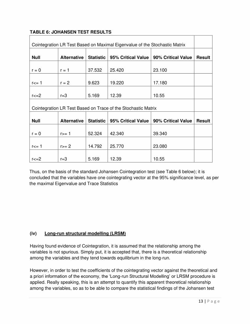
TABLE 6: JOHANSEN TEST RESULTS
Cointegration LR Test Based on Maximal Eigenvalue of the Stochastic Matrix
Null Alternative Statistic 95% Critical Value 90% Critical Value Result
r = 0 r = 1 37.532 25.420 23.100
r<= 1 r = 2 9.623 19.220 17.180
r<=2 r=3 5.169 12.39 10.55
Cointegration LR Test Based on Trace of the Stochastic Matrix
Null Alternative Statistic 95% Critical Value 90% Critical Value Result
r = 0 r>= 1 52.324 42.340 39.340
r<= 1 r>= 2 14.792 25.770 23.080
r<=2 r=3 5.169 12.39 10.55
Thus, on the basis of the standard Johansen Cointegration test (see Table 6 below); it is
concluded that the variables have one cointegrating vector at the 95% significance level, as per
the maximal Eigenvalue and Trace Statistics
(iv) Long-run structural modelling (LRSM)
Having found evidence of Cointegration, it is assumed that the relationship among the
variables is not spurious. Simply put, it is accepted that, there is a theoretical relationship
among the variables and they tend towards equilibrium in the long-run.
However, in order to test the coefficients of the cointegrating vector against the theoretical and
a priori information of the economy, the ‘Long-run Structural Modelling’ or LRSM procedure is
applied. Really speaking, this is an attempt to quantify this apparent theoretical relationship
among the variables, so as to be able to compare the statistical findings of the Johansen test
14 | P a g e
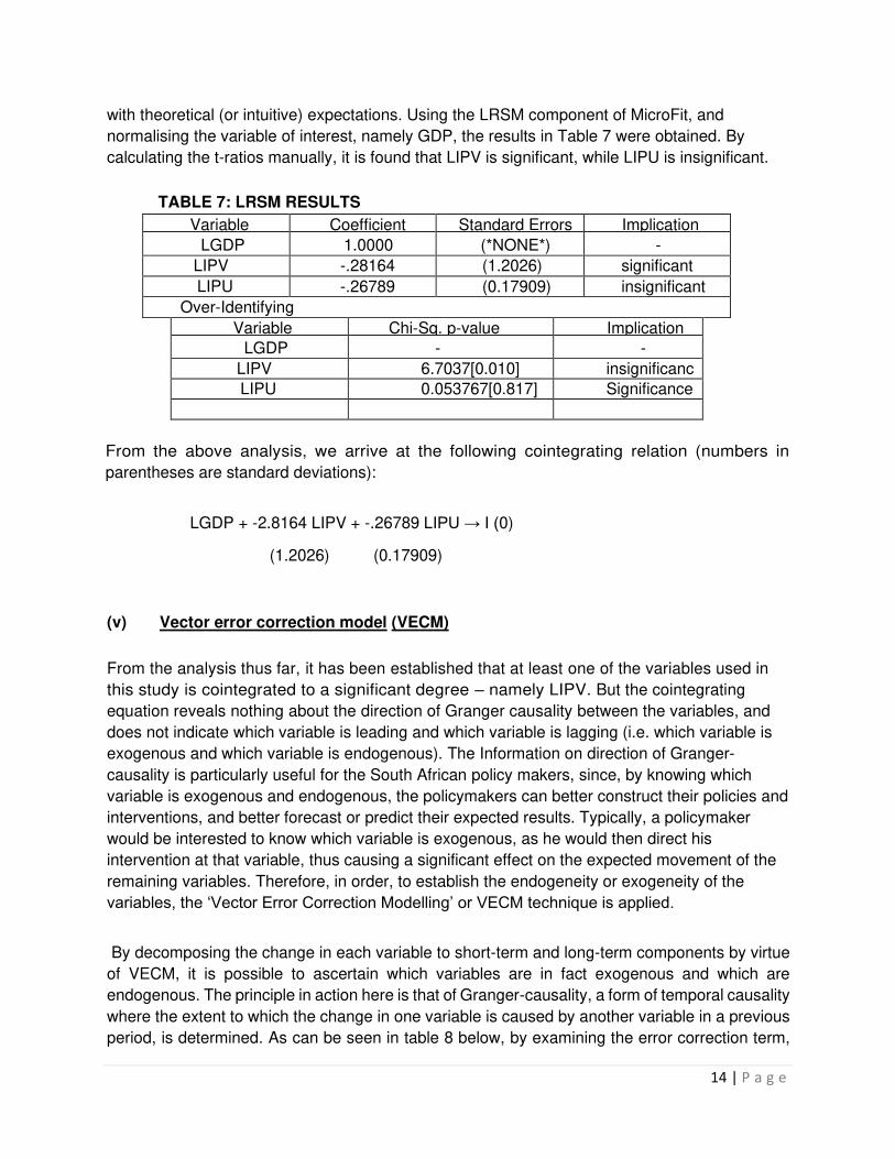
with theoretical (or intuitive) expectations. Using the LRSM component of MicroFit, and
normalising the variable of interest, namely GDP, the results in Table 7 were obtained. By
calculating the t-ratios manually, it is found that LIPV is significant, while LIPU is insignificant.
TABLE 7: LRSM RESULTS
Variable Coefficient Standard Errors Implication
LGDP 1.0000 (*NONE*) -
LIPV -.28164 (1.2026) significant
LIPU -.26789 (0.17909) insignificant
Over-Identifying
Variable Chi-Sq. p-value Implication
LGDP - -
LIPV 6.7037[0.010] insignificanc
e LIPU 0.053767[0.817] Significance
From the above analysis, we arrive at the following cointegrating relation (numbers in
parentheses are standard deviations):
LGDP + -2.8164 LIPV + -.26789 LIPU → I (0)
(1.2026) (0.17909)
(v) Vector error correction model (VECM)
From the analysis thus far, it has been established that at least one of the variables used in
this study is cointegrated to a significant degree – namely LIPV. But the cointegrating
equation reveals nothing about the direction of Granger causality between the variables, and
does not indicate which variable is leading and which variable is lagging (i.e. which variable is
exogenous and which variable is endogenous). The Information on direction of Granger-
causality is particularly useful for the South African policy makers, since, by knowing which
variable is exogenous and endogenous, the policymakers can better construct their policies and
interventions, and better forecast or predict their expected results. Typically, a policymaker
would be interested to know which variable is exogenous, as he would then direct his
intervention at that variable, thus causing a significant effect on the expected movement of the
remaining variables. Therefore, in order, to establish the endogeneity or exogeneity of the
variables, the ‘Vector Error Correction Modelling’ or VECM technique is applied.
By decomposing the change in each variable to short-term and long-term components by virtue
of VECM, it is possible to ascertain which variables are in fact exogenous and which are
endogenous. The principle in action here is that of Granger-causality, a form of temporal causality
where the extent to which the change in one variable is caused by another variable in a previous
period, is determined. As can be seen in table 8 below, by examining the error correction term,
15 | P a g e
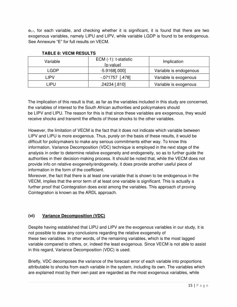
et-1, for each variable, and checking whether it is significant, it is found that there are two
exogenous variables, namely LIPU and LIPV, while variable LGDP is found to be endogenous.
See Annexure “E” for full results on VECM.
TABLE 8: VECM RESULTS
Variable ECM (-1): t-statistic
[p-value] Implication
LGDP -5.9168[.000] Variable is endogenous
LIPV -.071757 [.478] Variable is exogenous
LIPU .24234 [.810] Variable is exogenous
The implication of this result is that, as far as the variables included in this study are concerned,
the variables of interest to the South African authorities and policymakers should
be LIPV and LIPU. The reason for this is that since these variables are exogenous, they would
receive shocks and transmit the effects of those shocks to the other variables.
However, the limitation of VECM is the fact that it does not indicate which variable between
LIPV and LIPU is more exogenous. Thus, purely on the basis of these results, it would be
difficult for policymakers to make any serious commitments either way. To know this
information, Variance Decomposition (VDC) technique is employed in the next stage of the
analysis in order to determine relative exogeneity and endogeneity, so as to further guide the
authorities in their decision-making process. It should be noted that, while the VECM does not
provide info on relative exogeneity/endogeneity, it does provide another useful piece of
information in the form of the coefficient.
Moreover, the fact that there is at least one variable that is shown to be endogenous in the
VECM, implies that the error term of at least one variable is significant. This is actually a
further proof that Cointegration does exist among the variables. This approach of proving
Cointegration is known as the ARDL approach.
(vi) Variance Decomposition (VDC)
Despite having established that LIPU and LIPV are the exogenous variables in our study, it is
not possible to draw any conclusions regarding the relative exogeneity of
these two variables. In other words, of the remaining variables, which is the most lagged
variable compared to others, or, indeed the least exogenous. Since VECM is not able to assist
in this regard, Variance Decomposition (VDC) is used.
Briefly, VDC decomposes the variance of the forecast error of each variable into proportions
attributable to shocks from each variable in the system, including its own. The variables which
are explained most by their own past are regarded as the most exogenous variables, while
16 | P a g e
variables which least explain their own past are classified as the most endogenous.
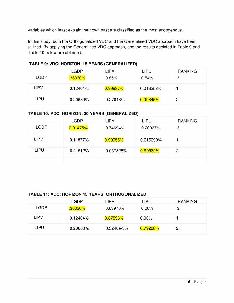
In this study, both the Orthogonalized VDC and the Generalised VDC approach have been
utilized. By applying the Generalized VDC approach, and the results depicted in Table 9 and
Table 10 below are obtained.
TABLE 9: VDC: HORIZON: 15 YEARS (GENERALIZED)
LGDP LIPV LIPU RANKING
LGDP .36030% 0.85% 0.54% 3
LIPV 0.12404% 0.99987% 0.016258% 1
LIPU 0.20680% 0.27648% 0.99845% 2
TABLE 10: VDC: HORIZON: 30 YEARS (GENERALIZED)
LGDP LIPV LIPU RANKING
LGDP 0.91475% 0.74694% 0.20927% 3
LIPV 0.11877% 0.99955% 0.015399% 1
LIPU 0.21512% 0.037326% 0.99539% 2
TABLE 11: VDC: HORIZON 15 YEARS: ORTHOGONALIZED
LGDP LIPV LIPU RANKING
LGDP .36030% 0.63970% 0.00% 3
LIPV 0.12404% 0.87596% 0.00% 1
LIPU 0.20680% 0.3246e-3% 0.79288% 2

17 | P a g e
TABLE 12: VDC: HORIZON 30 YEARS: ORTHOGONALIZED
LGDP LIPV LIPU RANKING
LGDP .091475% 0.90852% 0.00% 1
LIPV 0.11877% 0.88123% 0.00% 2
LIPU 0.21512% 0.0014517% 0.78343% 3
For the above two tables, rows read as the percentage of the variance of forecast error of each
variable into proportions attributable to shocks from other variables (in columns), including its
own. The columns read as the percentage in which that variable contributes to other variables
in explaining observed changes. The diagonal line of the matrix (highlighted)
represents the relative exogeneity.
According to these results, the ranking of the variables by
degree of exogeneity (extent to which variation is explained by its own past variations) is as
follows:
(1) LIPV~ (2) LIPU ~ (3) LGDP
The implications of the information provided by the VDC analysis provide valuable information to
the policymakers in South Africa.
By knowing which variable is exogenous and endogenous, the policymakers can better
construct their policies and interventions, and better forecast or predict their expected results.
Typically, a policymaker would be interested to know which variable is exogenous, as he would
then direct his intervention at that variable, thus causing a significant effect on the expected
movement of the remaining variables. The implication of this result is that, as far as the
variables included in this study are concerned, the primary variable of interest to the South
African authorities and policymakers should be LIPV or Private Investment. The reason for this
is that since this is the most exogenous variable, it would receive a shock and transmit the
effects of that shock to the other variables included in our study. Furthermore, as LIPU or Public
Investment displayed some relative exogeneity too, it should also feature in the policy decision-
making process of the authorities in South Africa.
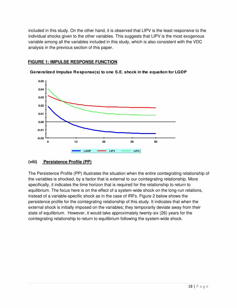
(vii) Impulse Response Functions (IRF)
Essentially, the impulse response functions (IRFs) map out the dynamic response path of a
variable owing to a one-period standard deviation shock to another variable. Thus, they
produce similar information to VDCs, except that they can be presented in graphical form.
In this study, both Orthogonalized and generalized IRFs for the all variables have been
conducted. For the sake of brevity, only the generalized IRFs are discussed here. It is found
that the results are consistent with those obtained in the VDC analysis. From figure 1, it is
observed that LGDP is the most responsive to the individual shocks given to the other
variables. This suggests that LGDP is the endogenous variable among all the variables
18 | P a g e
included in this study. On the other hand, it is observed that LIPV is the least responsive to the
individual shocks given to the other variables. This suggests that LIPV is the most exogenous
variable among all the variables included in this study, which is also consistent with the VDC
analysis in the previous section of this paper.
FIGURE 1: IMPULSE RESPONSE FUNCTION
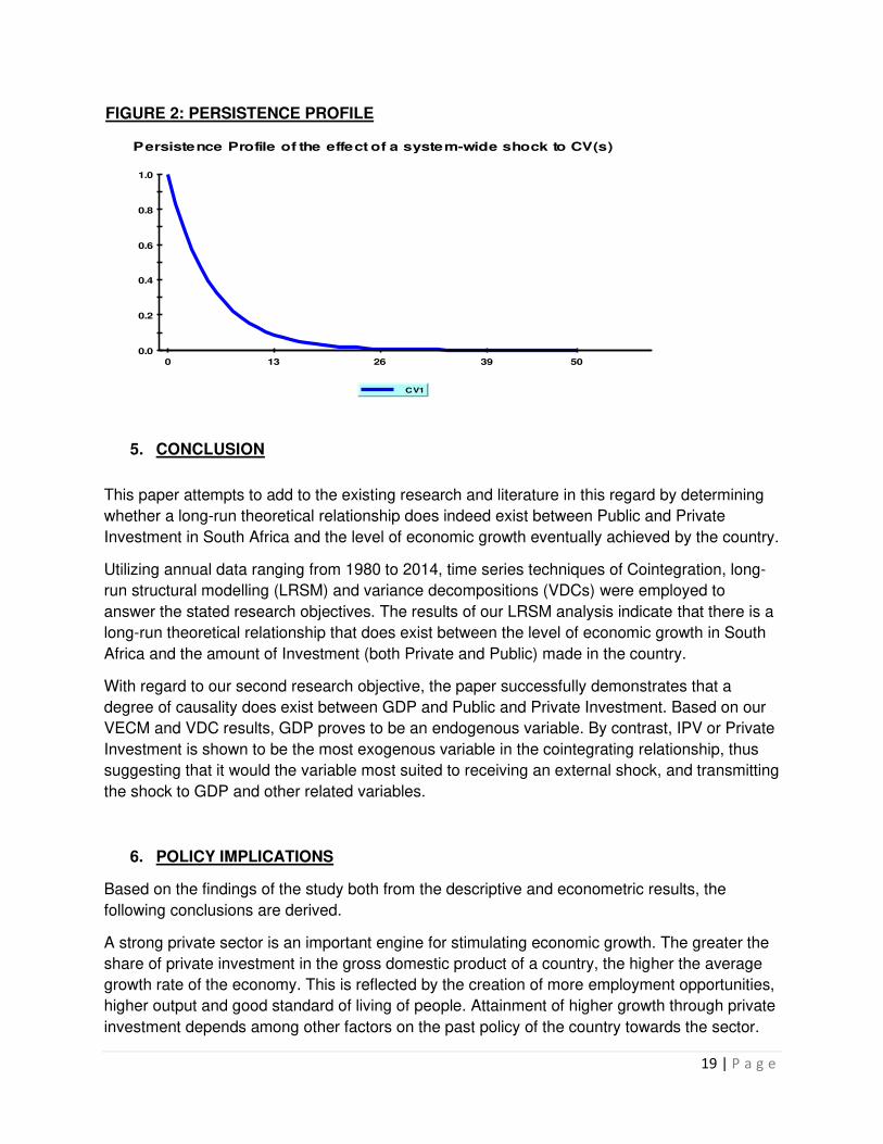
(viii) Persistence Profile (PP)
The Persistence Profile (PP) illustrates the situation when the entire cointegrating relationship of
the variables is shocked, by a factor that is external to our cointegrating relationship. More
specifically, it indicates the time horizon that is required for the relationship to return to
equilibrium. The focus here is on the effect of a system-wide shock on the long-run relations,
instead of a variable-specific shock as in the case of IRFs. Figure 2 below shows the
persistence profile for the cointegrating relationship of this study. It indicates that when the
external shock is initially imposed on the variables; they temporarily deviate away from their
state of equilibrium. However, it would take approximately twenty-six (26) years for the
cointegrating relationship to return to equilibrium following the system-wide shock.
-0.02
-0.01
0.00
0.01
0.02
0.03
0.04
0.05
0 13 26 39 50
Generalized Impulse Response(s) to one S.E. shock in the equation for LGDP
LGDP LIPV LIPU
19 | P a g e
FIGURE 2: PERSISTENCE PROFILE
5. CONCLUSION
This paper attempts to add to the existing research and literature in this regard by determining
whether a long-run theoretical relationship does indeed exist between Public and Private
Investment in South Africa and the level of economic growth eventually achieved by the country.
Utilizing annual data ranging from 1980 to 2014, time series techniques of Cointegration, long-
run structural modelling (LRSM) and variance decompositions (VDCs) were employed to
answer the stated research objectives. The results of our LRSM analysis indicate that there is a
long-run theoretical relationship that does exist between the level of economic growth in South
Africa and the amount of Investment (both Private and Public) made in the country.
With regard to our second research objective, the paper successfully demonstrates that a
degree of causality does exist between GDP and Public and Private Investment. Based on our
VECM and VDC results, GDP proves to be an endogenous variable. By contrast, IPV or Private
Investment is shown to be the most exogenous variable in the cointegrating relationship, thus
suggesting that it would the variable most suited to receiving an external shock, and transmitting
the shock to GDP and other related variables.
6. POLICY IMPLICATIONS
Based on the findings of the study both from the descriptive and econometric results, the
following conclusions are derived.
A strong private sector is an important engine for stimulating economic growth. The greater the
share of private investment in the gross domestic product of a country, the higher the average
growth rate of the economy. This is reflected by the creation of more employment opportunities,
higher output and good standard of living of people. Attainment of higher growth through private
investment depends among other factors on the past policy of the country towards the sector.
0.0
0.2
0.4
0.6
0.8
1.0
0 13 26 39 50
Persistence Profile of the effect of a system-wide shock to CV(s)
CV1
20 | P a g e
Given the relative significance and importance of the private sector investment in stimulating
economic growth, policies designed to attract private investment should be deep enough to
stimulate sustainable growth.
Considering the long run positive effect of real private investment the government of
should take supplementary reforms that promotes private sector development, in
supportive of entrepreneurial endeavor and with a bias towards expansion of business
activities. In particular, the government has roles to play at different levels of the economy to
encourage the private sector and to attain sustainable development. These include supply
of efficient infrastructure facilities such as electricity, telephone, water and road; improving the
tax administration system for example minimizing the random imposition of taxes and increasing
access to information and advisory services. In the absence of some or all of these
prerequisites, private investment expansion which is a means for accumulation of physical
capital and increment of national output may not result at the projected level.
Second, the long run positive effect of real public investment on growth calls the responsible
authority, first to identify which sectors of public investment are crowding in and which sectors
are crowding out private investment, before expansion of state participation. The guiding
principle for public investment should be complimentary rather than compete with private
investment.
The evidence suggests a clear need to improve the productivity of public sector investment by
identifying much more rigorously the types of investment that have positive net returns and are
likely to be complementary to the private sector. At the same time, policymakers should be
undertaking measures to stimulate private investment. This can be done in part by structural
reforms in the financial sector, which facilitate the mobilization of savings and help allocate
funds to productive private sector investment, and in part by ensuring a stable macroeconomic
environment.
7. LIMITATIONS AND SUGGESTIONS FOR FUTURE RESEARCH
It is noted that a relatively small dataset was employed in this study. Another major limitation of
this practice is that not too many variables can be included in such a model, due to its small
sample size. The reason for this is that the inclusion of too many variables in such a scenario
would lead to loss of degrees of freedom, and consequently, the resultant sample may not be
regarded as sufficient enough to make exceedingly accurate inferences. Thus, in future, the
usage quarterly data would be more appropriate and perhaps, provide the basis for more
precise estimations and inferences.
Furthermore, the number of variables utilized in the study are relatively few in number.
Consequently, the model has the ability to explain the variation in Economic Growth in light of
only a few variables, resulting in there being limited implications of the study in the area of
practice. This caveat can be taken care of in future, by increasing the number of variables
employed in the model, thereby enabling the model to explain the variation in GDP more
adequately. While this research focuses on only a few parameters with regards to Public and
21 | P a g e
Private Investment, there is a wide array of other factors, such as Interest rate and availability if
credit to the private sector, that have major influence on the rate of private investment. A better
understanding of most of these factors would enable policymakers to more effectively market
South Africa as an investment destination.
Finally, we have adopted basic time series techniques as the basis for our empirical
estimations. Even though these robust and advanced estimation techniques surpass ordinary
OLS regression analysis, they are still based on an assumption, namely the existence of a linear
relationship among the variables. To overcome this caveat, we recommend the application of
cutting-edge econometric techniques and dynamic modelling to a more extensive data set in
related future research.
REFERENCES:
Ahmed H and Miller SM (1999). Crowding-out and crowding-in effects of the components of
government expenditure. University of Connecticut, Working Paper, no. 1999-02.
Akomolafe K.J. (2015). Public debt and Private Investment in Nigeria. American Journal of
Economics, 5(5), 501-507.
Aschauer D.A (1989). Does public capital crowd out private capital? Journal of Monetary
Economics., 24: 171–188.
Bairam E and Ward B (1993). The externality effect of government expenditure on investment in
OECD countries. Applied. Economics., 25(6): 711-716.
Balcerzak, A. (2014), Crowding out and Crowding in within Keynesian Framework. Do we need
any new empirical research concerning them? Economics and Sociology, 7(2), 80-93.
Belloc, M. (2002). Public Investment and Economic Performance in Highly Indebted Poor
Countries: An empirical Assessment. International Review of Applied Economics, 20,151-170.
Belloc M and Vertova P (2006). Public investment and economic performance in highly indebted
poor countries: An empirical assessment. International Review of Applied Economics, 20(2),
151-170.
Blejer M.I. and Khan M.S. (1984). Private investment in developing countries. Finance and
Development, 21, 26-29.
Cavallo Eduardo and Daude Christian (2011). Public investment in developing countries: A
blessing or a curse? Journal of Comparative Economics 39: 65-81
Choonga, C. L. (2015). The Linkages between Private and Public Investments in Malaysia: The
Role of Foreign Direct Investment. International Journal of Economics and Management,
9(1),139-153.

22 | P a g e
Easterly W and Rebelo, S (1993). Fiscal policy and economic growth: An empirical
investigation. Journal of Monetary Economics., 32(3): 417-458.
Erden L and Holcombe R.G (2005). The effect of public investment on private investment in
developing economies. Public Finance Review, 33(5), 575-602.
Fedderke J.W, Perkins P and Luiz J. (2006). Infrastructural investment in long-run economic
growth: South Africa 1875-2001. World Development., 34(6): 1037-1059.
Fielding D (1997). Aggregate investment in South Africa: A model with implications for political
reform. Oxford Bulletin of Economics and Statistics, 59(3): 349-369.
Fry M.J. (1980). Saving, Investment, Growth and the Cost of Financial Repression. World
Development, 8, 317-327.
Galbis, V. (1979). Money, investment and growth in Latin America, 1961-73. Economic
Development and Cultural Change, 27, 423-443.
Ghura D and Goodwin B (2000). Determinants of private investment: A cross-regional empirical
investigation. Applied Economics, 32(14): 1819-1829.
Gilbert, N. A. ( 2015). Effects of Government spending on Private Investments and Economic
growth in Cameroon. International Journal of management and economics invention, 1(4),185-
209.
Greene J and D Villanueva (1991). Private investment in developing countries. IMF Staff Papers
38 (1), 33-58.
James B. Ang (2010). Determinants of private investment in Malaysia: what causes the post
crisis slumps? Contemporary Economic Policy, 28(3), 378 – 391
Kollamparambil U. and Nicolaou M. (2010). Nature and association of public and private
investment: Public policy implication for South Africa. Journal of Economics and International
Finance, 3(2), 98-108.
Leff, N.H and Sato, K. (1988). Estimating Investment and Savings Functions for Developing
Countries: With an Application to Latin America. International Economic Journal, 2(3),1-17.
Levine R and Renelt D. (1992). A sensitivity analysis of cross-country growth regressions.
American Economic Review 82 (4), 942-963.
Masih, M. and Algahtani, I. (2008). Estimation of long-run demand for money: An application
of long-run structural modelling to Saudi Arabia. Economia Internazionale (International
Economics): 61(1), 81 - 99.
Masih, M., Al-Elg, A. and Madani, H. (2009). Causality between financial development and
economic growth: an application of vector error correction and variance decomposition
methods to Saudi Arabia. Applied Economics, 41,1691 - 1699.
23 | P a g e
Masih, M., Al-Sahlawi, M. and De Mello, L. (2010). What drives carbon-dioxide emissions:
Income or electricity generation? Evidence from Saudi Arabia. Journal of Energy and
Developmen,: 33(2), 201 - 213.
Ndikumana, L. (2000). Financial determinants of domestic investment in sub-Saharan Africa:
Evidence from panel data. World Development, 28 (2): 381-400.
Oshikoya T.W (1994). Macroeconomic determinants of domestic private investment in Africa:
An empirical analysis. Economic Development and Cultural Change, 42, 573-596.
Ramirez, M (1994). Public and private investment in Mexico, 1950-90: An empirical analysis.
Retrieved from JSTOR General Science Collection database. Southern Economic Journal,
61(1): 1-17.
Scott, M.F.G. (1976). Investment and growth. Oxford Economic Papers, 28(3), 317–363.
Serven, L (1996). Does Public Capital Crowd Out Private Capital? World Bank Policy Research
Working Paper, no. 1613.
Tun Wai, U. and Chorng-huey Wong (1982). Determinants of private investment in developing
countries. Journal of Development Studies 19(1),19-36.
Voss, G.M. (2002). Public and private investment in the United States and Canada. Economic
Modelling., 19(4), 641-664.